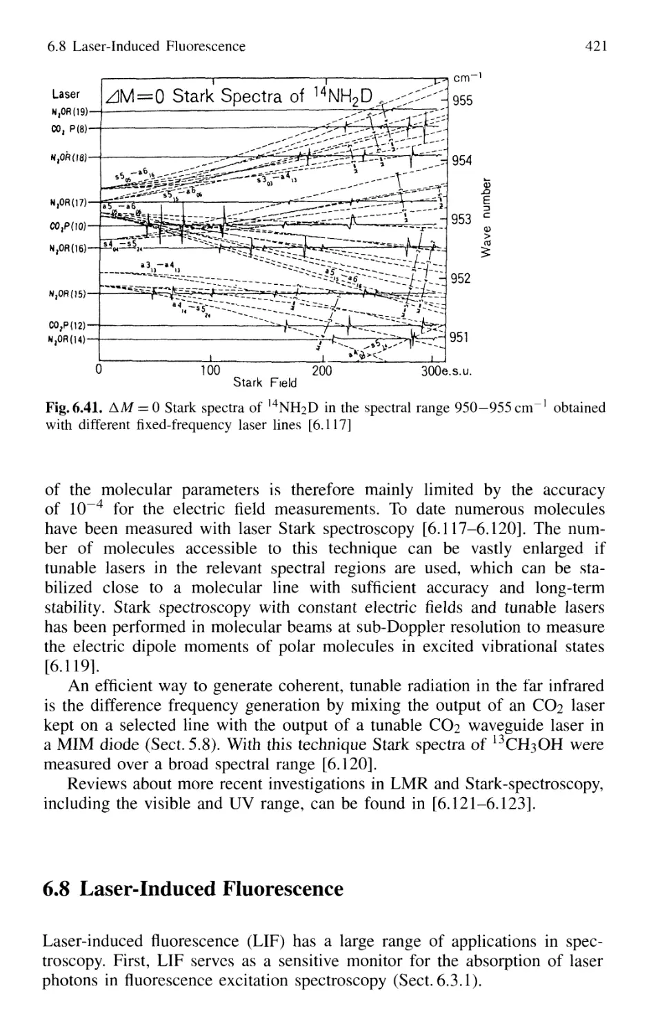
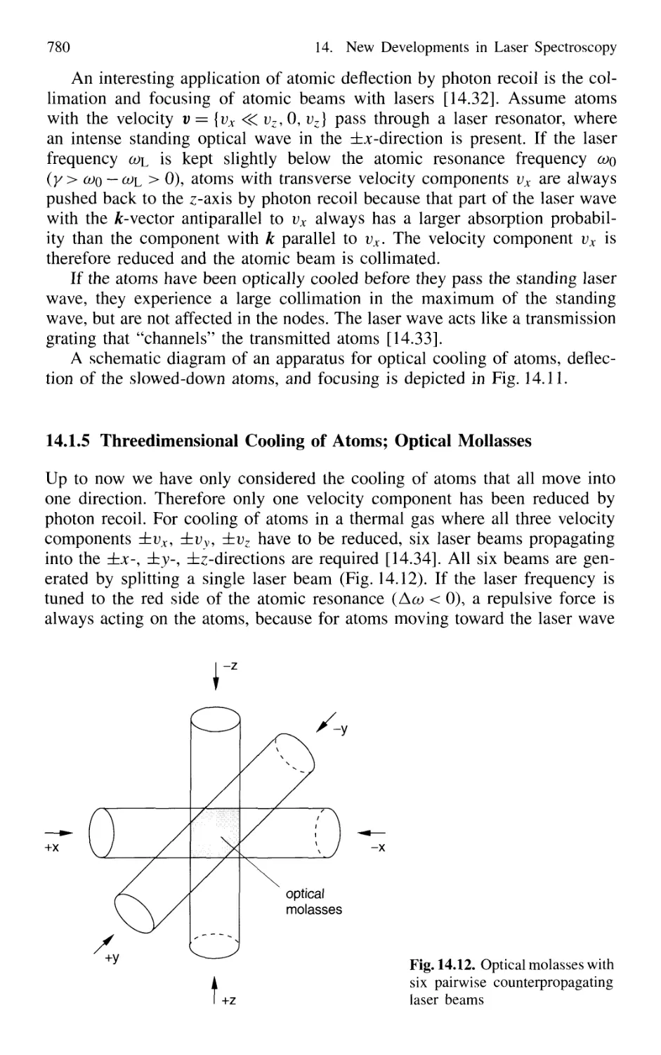
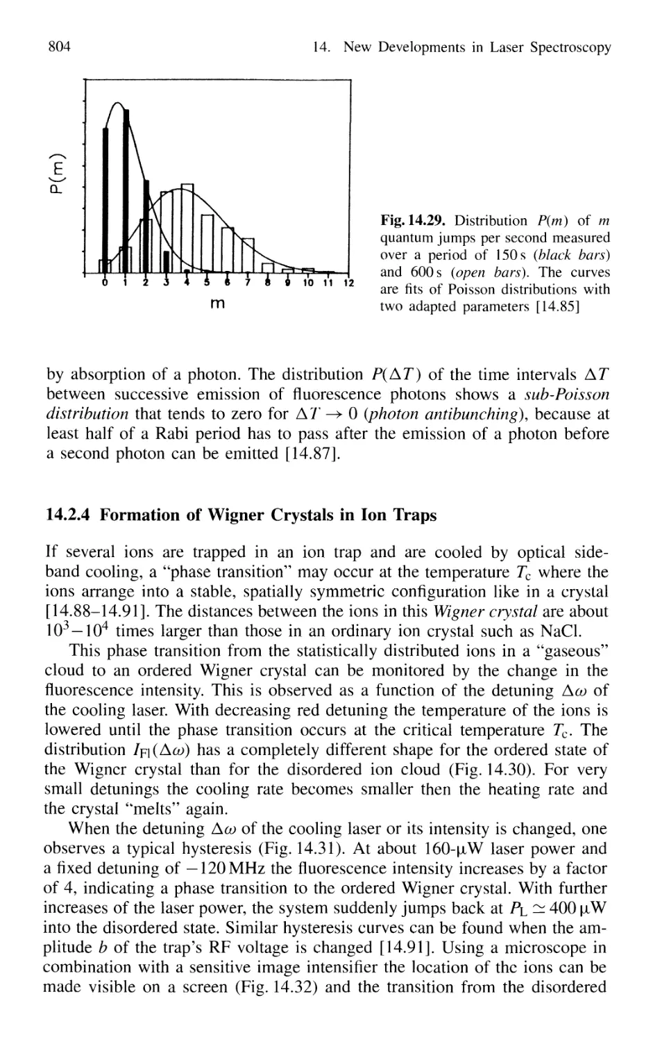
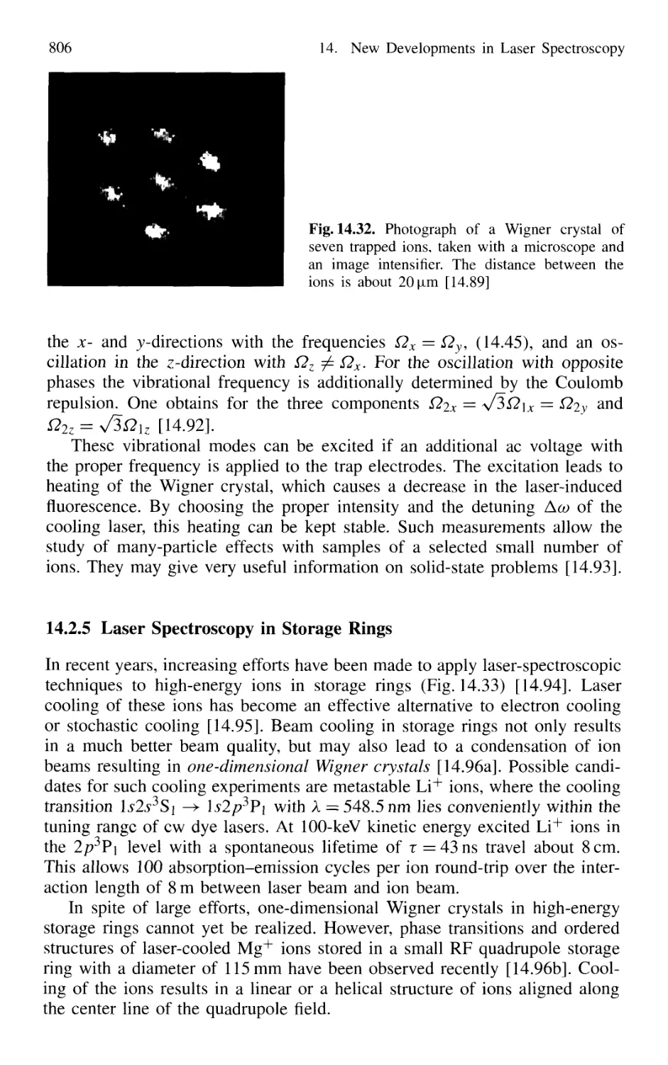
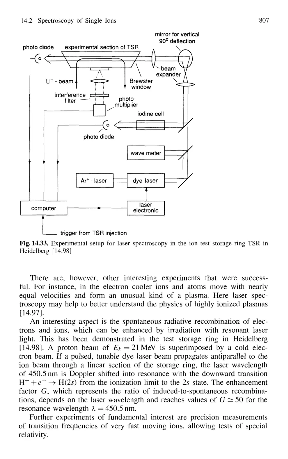
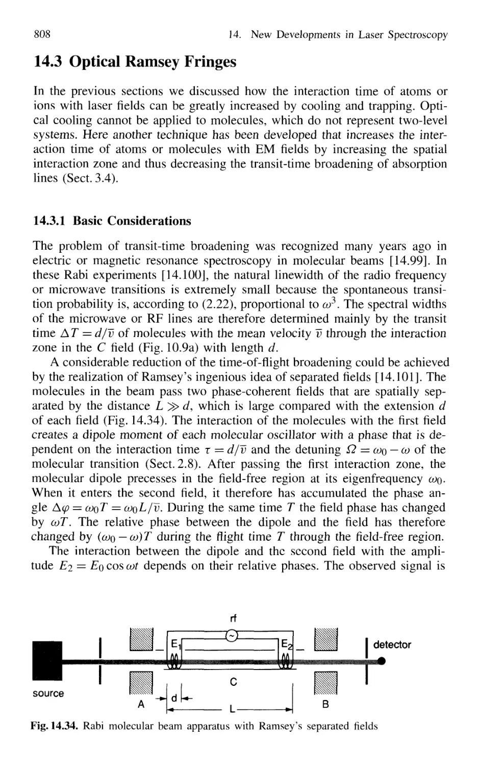
/


Автор: Demtröder W.
Теги: medicine springer edition practical medicine laser spectroscopy medical diagnostic
ISBN: 3540652256
Год: 2003


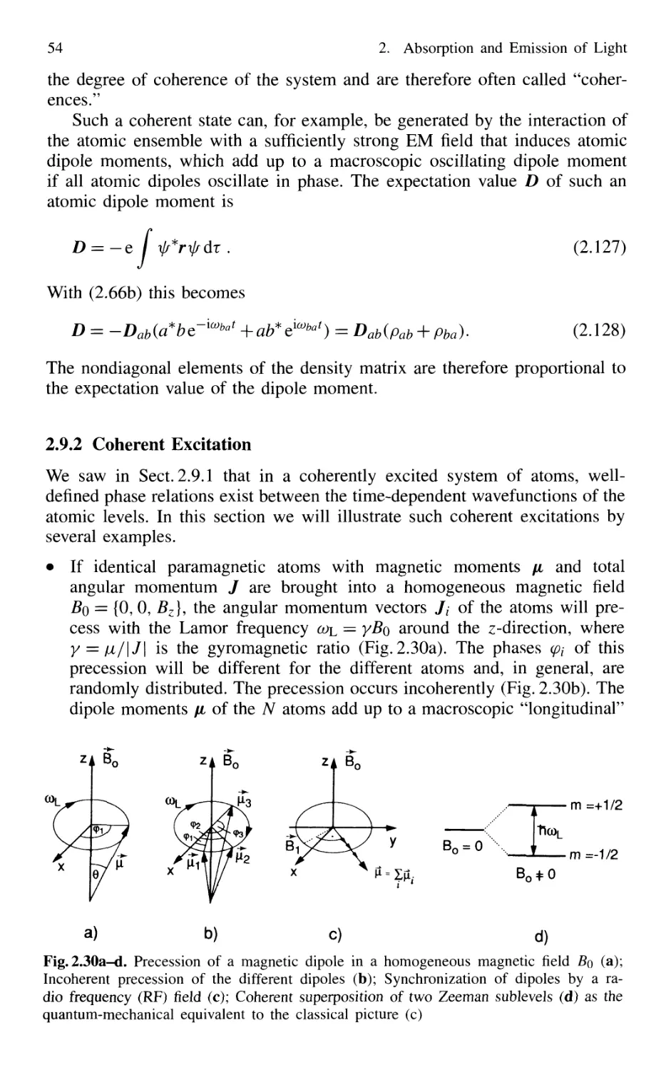
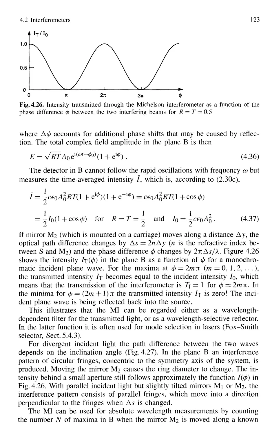
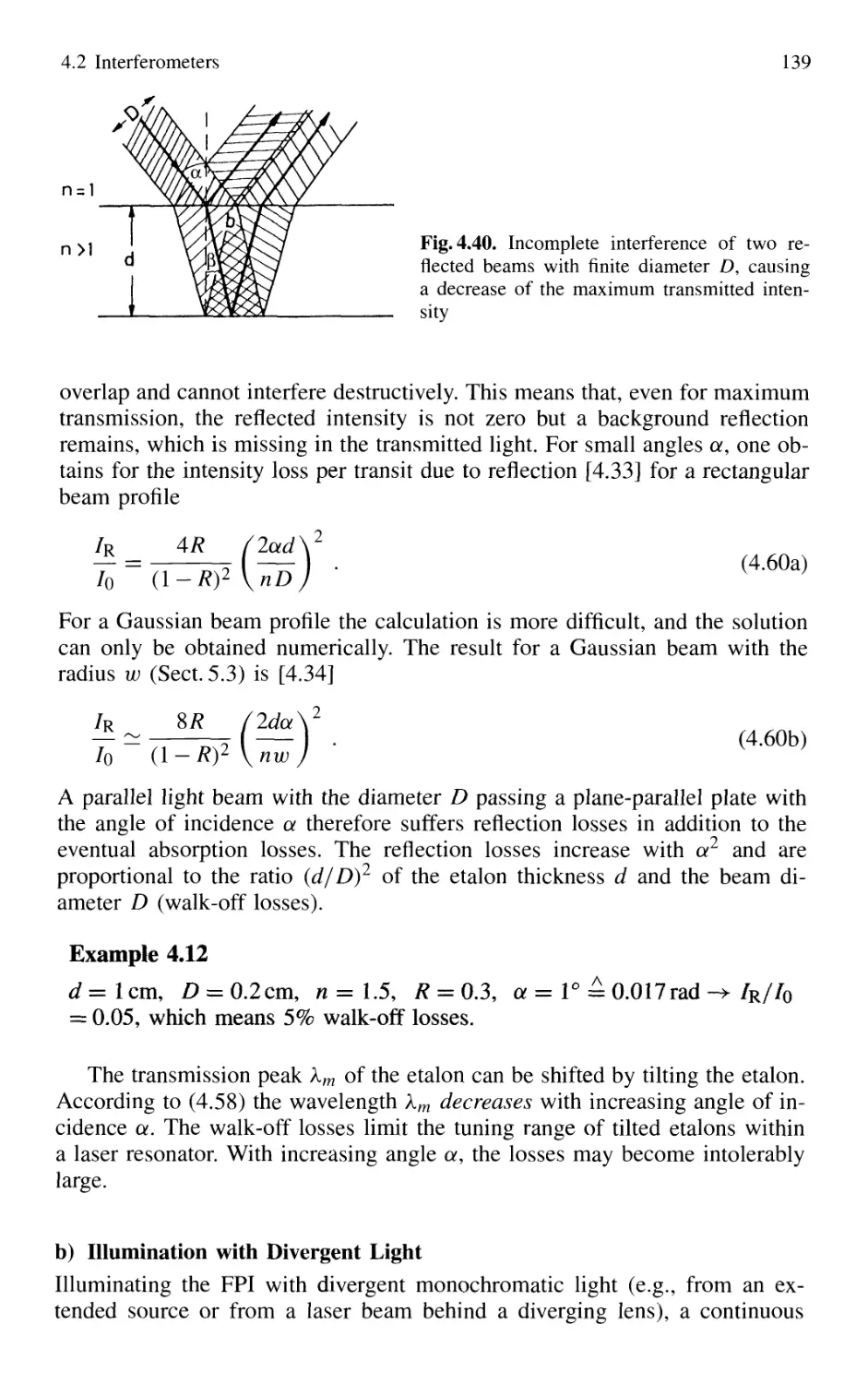
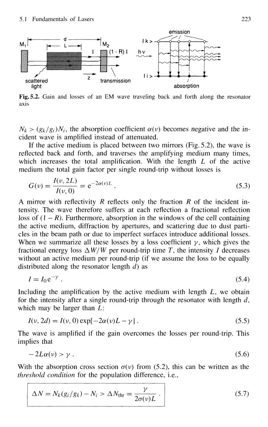
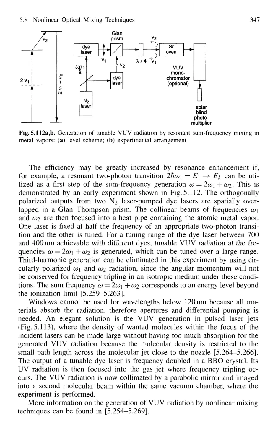
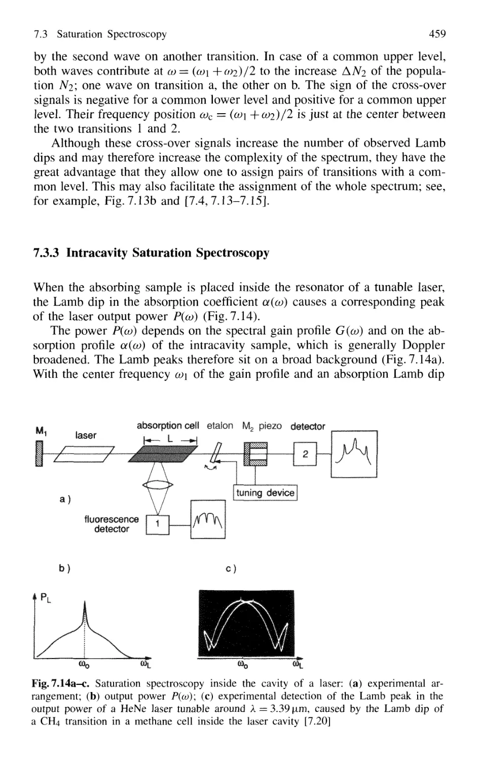
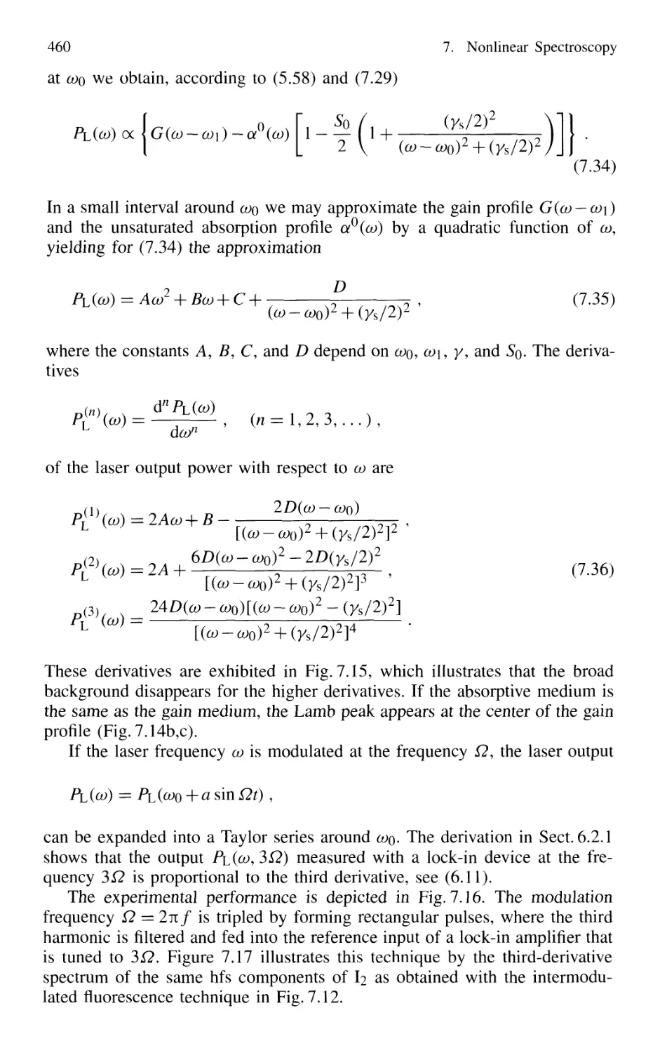
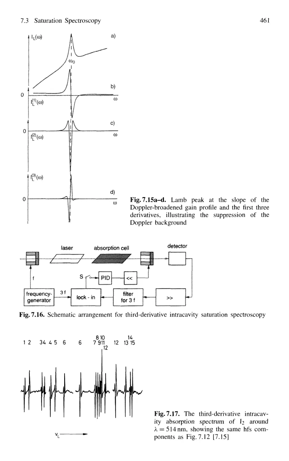
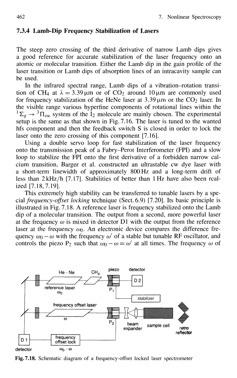
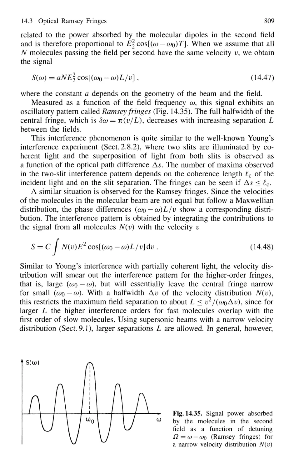
Текст
Advanced Texts in Physics
This program of advanced texts covers a broad spectrum of topics which are of
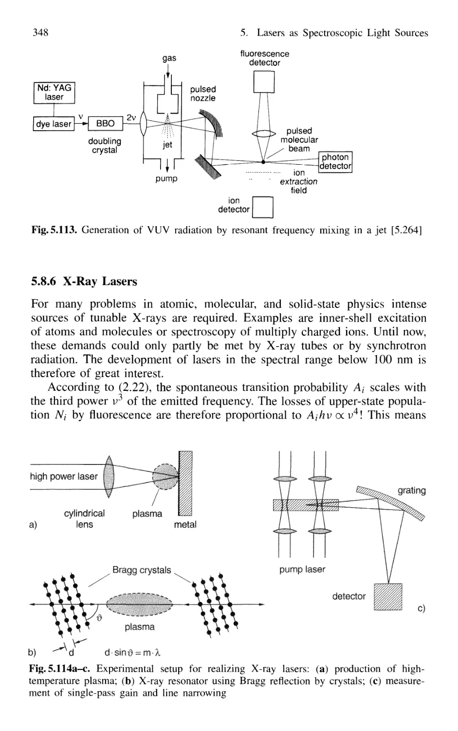
current and emerging interest in physics. Each book provides a comprehensive and
yet accessible introduction to a field at the forefront of modern research. As such,
these texts are intended for senior undergraduate and graduate students at the MS
and PhD level; however, research scientists seeking an introduction to particular
areas of physics will also benefit from the titles in this collection.
Springer
Berlin
Heidelberg
New York
Hong Kong
L^Hi °n ^t . i * ~i°NLINELIBRARY
Mllan Physics and Astronomy —
Paris 7 7 LJ
Tokyo http://www.springer.de/phys/
Wolfgang Demtröder
Laser Spectroscopy
Basic Concepts
and Instrumentation
Third Edition
With 710 Figures, 16 Tables
93 Problems and Hints for Solution
Springer
Professor Dr. Wolfgang Demtröder
Universität Kaiserslautern
Fachbereich Physik
Erwin-Schrödinger-Strasse
67663 Kaiserslautern, Germany
E-mail: demtroed@physik. uni-kl. de
Library of Congress Cataloging-in-Publication Data: Demtröder, W. Laser spectroscopy: basic concepts
and instrumentation/ Wolfgang Demtröder. - 3rd ed. p. cm. ISBN 3540652256 (alk. paper) 1. Laser
spectroscopy. I. Title. QC 454X3 D46 2002 62i.36'6-dc2i 2002029191
ISSN 1439-2674
ISBN 3-540-65225-6 3rd Edition Springer-Verlag Berlin Heidelberg New York
ISBN 3-540-57171-X 2nd Edition Springer-Verlag Berlin Heidelberg New York
This work is subject to copyright. All rights are reserved, whether the whole or part of the material
is concerned, specifically the rights of translation, reprinting, reuse of illustrations, recitation, broad-
broadcasting, reproduction on microfilm or in any other way, and storage in data banks. Duplication of
this publication or parts thereof is permitted only under the provisions of the German Copyright Law
of September 9, 1965, in its current version, and permission for use must always be obtained from
Springer-Verlag. Violations are liable for prosecution under the German Copyright Law.
Springer-Verlag Berlin Heidelberg New York
a member of BertelsmannSpringer Science+Business Media GmbH
http://www.springer.de
© Springer-Verlag Berlin Heidelberg 1981,1996, 2003
Printed in Germany
The use of general descriptive names, registered names, trademarks, etc. in this publication does not
imply, even in the absence of a specific statement, that such names are exempt from the relevant pro-
protective laws and regulations and therefore free for general use.
Typesetting: Data conversion by Fa. Le-TeX, Leipzig
Cover design: design & production GmbH, Heidelberg
Printed on acid-free paper SPIN 10673180 56/3141/ba 543210
Preface to the Third Edition
Laser Spectroscopy continues to develop and expand rapidly. Many new ideas
and recent realizations of new techniques based on old ideas have contributed
to the progress in this field since the last edition of this textbook appeared. In
order to keep up with these developments it was therefore necessary to include
at least some of these new techniques in the third edition.
There are, firstly, the improvement of frequency-doubling techniques in ex-
external cavities, the realization of more reliable cw-parametric oscillators with
large output power, and the development of tunable narrow-band UV sources,
which have expanded the possible applications of coherent light sources in
molecular spectroscopy. Furthermore, new sensitive detection techniques for
the analysis of small molecular concentrations or for the measurement of
weak transitions, such as overtone transitions in molecules, could be realized.
Examples are Cavity Ringdown Spectroscopy, which allows the measurement
of absolute absorption coefficients with great sensitivity or specific modula-
modulation techniques that push the minimum detectable absorption coefficient down
to lCT^cm!
The most impressive progress has been achieved in the development of
tunable femtosecond and subfemtosecond lasers, which can be amplified to
achieve sufficiently high output powers for the generation of high harmon-
harmonics with wavelengths down into the X-ray region and with pulsewidths in
the attosecond range. Controlled pulse shaping by liquid crystal arrays allows
coherent control of atomic and molecular excitations and in some favorable
cases chemical reactions can already be influenced and controlled using these
shaped pulses.
In the field of metrology a big step forward was the use of frequency
combs from cw mode-locked femtosecond lasers. It is now possible to directly
compare the microwave frequency of the cesium clock with optical frequen-
frequencies, and it turns out that the stability and the absolute accuracy of frequency
measurements in the optical range using frequency-stabilized lasers greatly
surpasses that of the cesium clock. Such frequency combs also allow the syn-
synchronization of two independent femtosecond lasers.
The increasing research on laser cooling of atoms and molecules and many
experiments with Bose-Einstein condensates have brought about some re-
remarkable results and have considerably increased our knowledge about the
interaction of light with matter on a microscopic scale and the interatomic in-
interactions at very low temperatures. Also the realization of coherent matter
waves (atom lasers) and investigations of interference effects between matter
waves have proved fundamental aspects of quantum mechanics.
VI Preface to the Third Edition
The largest expansion of laser spectroscopy can be seen in its possible and
already realized applications to chemical and biological problems and its use
in medicine as a diagnostic tool and for therapy. Also, for the solution of
technical problems, such as surface inspections, purity checks of samples or
the analysis of the chemical composition of samples, laser spectroscopy has
offered new techniques.
In spite of these many new developments the representation of established
fundamental aspects of laser spectroscopy and the explanation of the basic
techniques are not changed in this new edition. The new developments men-
mentioned above and also new references have been added. This, unfortunately,
increases the number of pages. Since this textbook addresses beginners in this
field as well as researchers who are familiar with special aspects of laser spec-
spectroscopy but want to have an overview on the whole field, the author did not
want to change the concept of the textbook.
Many readers have contributed to the elimination of errors in the former
edition or have made suggestions for improvements. I want to thank all of
them. The author would be grateful if he receives such suggestions also for
this new edition.
Many thanks go to all colleagues who gave their permission to use fig-
figures and results from their research. I thank Dr. H. Becker and T. Wilbourn
for critical reading of the manuscript, Dr. HJ. Kölsch and C.-D. Bachern of
Springer-Verlag for their valuable assistance during the editing process, and
LE-TeX Jelonek, Schmidt and Vöckler for the setting and layout. I appreci-
appreciate, that Dr. H. Lotsch, who has taken care for the foregoing editions, has
supplied his computer files for this new edition. Last, but not least, I would
like to thank my wife Harriet who made many efforts in order to give me the
necessary time for writing this new edition.
Kaiserslautern, Wolfgang Demtröder
April 2002
Preface to the Second Edition
During the past 14 years since the first edition of this book was published,
the field of laser spectroscopy has shown a remarkable expansion. Many
new spectroscopic techniques have been developed. The time resolution has
reached the femtosecond scale and the frequency stability of lasers is now in
the millihertz range.
In particular, the various applications of laser spectroscopy in physics,
chemistry, biology, and medicine, and its contributions to the solutions of
technical and environmental problems are remarkable. Therefore, a new edi-
edition of the book seemed necessary to account for at least part of these novel
developments. Although it adheres to the concept of the first edition, several
new spectroscopic techniques such as optothermal spectroscopy or velocity-
modulation spectroscopy are added.
A whole chapter is devoted to time-resolved spectroscopy including the
generation and detection of ultrashort light pulses. The principles of coherent
spectroscopy, which have found widespread applications, are covered in a sep-
separate chapter. The combination of laser spectroscopy and collision physics,
which has given new impetus to the study and control of chemical reactions,
has deserved an extra chapter. In addition, more space has been given to op-
optical cooling and trapping of atoms and ions.
I hope that the new edition will find a similar friendly acceptance as the
first one. Of course, a texbook never is perfect but can always be improved. I,
therefore, appreciate any hint to possible errors or comments concerning cor-
corrections and improvements. I will be happy if this book helps to support teach-
teaching courses on laser spectroscopy and to transfer some of the delight I have
experienced during my research in this fascinating field over the last 30 years.
Many people have helped to complete this new edition. I am grateful to
colleagues and friends, who have supplied figures and reprints of their work.
I thank the graduate students in my group, who provided many of the ex-
examples used to illustrate the different techniques. Mrs. Wollscheid who has
drawn many figures, and Mrs. Heider who typed part of the corrections. Par-
Particular thanks go to Helmut Lotsch of Springer-Verlag, who worked very hard
for this book and who showed much patience with me when I often did not
keep the deadlines.
Last but not least, I thank my wife Harriet who had much understand-
understanding for the many weekends lost for the family and who helped me to have
sufficient time to write this extensive book.
Kaiserslautern, Wolfgang Demtröder
June 1995
Preface to the First Edition
The impact of lasers on spectroscopy can hardly be overestimated. Lasers rep-
represent intense light sources with spectral energy densities which may exceed
those of incoherent sources by several orders of magnitude. Furthermore, be-
because of their extremely small bandwidth, single-mode lasers allow a spectral
resolution which far exceeds that of conventional spectrometers. Many exper-
experiments which could not be done before the application of lasers, because of
lack of intensity or insufficient resolution, are readily performed with lasers.
Now several thousands of laser lines are known which span the whole
spectral range from the vacuum-ultraviolet to the far-infrared region. Of
particular interst are the continuously tunable lasers which may in many
cases replace wavelength-selecting elements, such as spectrometers or inter-
interferometers. In combination with optical frequency-mixing techniques such
continuously tunable monochromatic coherent light sources are available at
nearly any desired wavelength above lOOnm.
The high intensity and spectral monochromasy of lasers have opened
a new class of spectroscopic techniques which allow investigation of the struc-
structure of atoms and molecules in much more detail. Stimulated by the variety
of new experimental possibilities that lasers give to spectroscopists, very lively
research activities have developed in this field, as manifested by an avalanche
of publications. A good survey about recent progress in laser spectroscopy
is given by the proceedings of various conferences on laser spectroscopy
(see "Springer Series in Optical Sciences"), on picosecond phenomena (see
"Springer Series in Chemical Physics"), and by several quasi-mongraphs on
laser spectroscopy published in "Topics in Applied Physics".
For nonspecialists, however, or for people who are just starting in this
field, it is often difficult to find from the many articles scattered over many
journals a coherent representation of the basic principles of laser spectroscopy.
This textbook intends to close this gap between the advanced research papers
and the representation of fundamental principles and experimental techniques.
It is addressed to physicists and chemists who want to study laser spec-
spectroscopy in more detail. Students who have some knowledge of atomic and
molecular physics, electrodynamics, and optics should be able to follow the
presentation.
The fundamental principles of lasers are covered only very briefly because
many excellent textbooks on lasers already exist.
On the other hand, those characteristics of the laser that are important for
its applications in spectroscopy are treated in more detail. Examples are the
frequency spectrum of different types of lasers, their linewidths, amplitude
and frequency stability, tunability, and tuning ranges. The optical compo-
X Preface to the First Edition
nents such as mirrors, prisms, and gratings, and the experimental equipment
of spectroscopy, for example, monochromators, interferometers, photon detec-
detectors, etc., are discussed extensively because detailed knowledge of modern
spectroscopic equipment may be crucial for the successful performance of an
experiment.
Each chapter gives several examples to illustrate the subject discussed.
Problems at the end of each chapter may serve as a test of the reader's un-
understanding. The literature cited for each chapter is, of course, not complete
but should inspire further studies. Many subjects that could be covered only
briefly in this book can be found in the references in a more detailed and of-
often more advanced treatment. The literature selection does not represent any
priority list but has didactical purposes and is intended to illustrate the subject
of each chapter more thoroughly.
The spectroscopic applications of lasers covered in this book are restricted
to the spectroscopy of free atoms, molecules, or ions. There exists, of course,
a wide range of applications in plasma physics, solid-state physics, or fluid
dynamics which are not discussed because they are beyond the scope of this
book. It is hoped that this book may be of help to students and researchers.
Although it is meant as an introduction to laser spectroscopy, it may also
facilitate the understanding of advanced papers on special subjects in laser
spectroscopy. Since laser spectroscopy is a very fascinating field of research,
I would be happy if this book can transfer to the reader some of my excite-
excitement and pleasure experienced in the laboratory while looking for new lines
or unexpected results.
I want to thank many people who have helped to complete this book.
In particular the students in my research group who by their experimental
work have contributed to many of the examples given for illustration and who
have spent their time reading the galley proofs. I am grateful to colleages
from many laboratories who have supplied me with figures from their pub-
publications. Special thanks go to Mrs. Keck and Mrs. Ofiiara who typed the
manuscript and to Mrs. Wollscheid and Mrs. Ullmer who made the draw-
drawings. Last but not least, I would like to thank Dr. U. Hebgen, Dr. H. Lotsch,
Mr. K.-H. Winter, and other coworkers of Springer-Verlag who showed much
patience with a dilatory author and who tried hard to complete the book in
a short time.
Kaiserslautern, Wolfgang Demtröder
March 1981
Contents
1. Introduction 1
2. Absorption and Emission of Light 7
2.1 Cavity Modes 7
2.2 Thermal Radiation and Planck's Law 10
2.3 Absorption, Induced, and Spontaneous Emission 12
2.4 Basic Photometric Quantities 16
2.4.1 Definitions 17
2.4.2 Illumination of Extended Areas 19
2.5 Polarization of Light 20
2.6 Absorption and Emission Spectra 22
2.7 Transition Probabilities 26
2.7.1 Lifetimes, Spontaneous
and Radiationless Transitions 26
2.7.2 Semiclassical Description: Basic Equations 28
2.7.3 Weak-Field Approximation 32
2.7.4 Transition Probabilities with Broad-Band Excitation 33
2.7.5 Phenomenological Inclusion of Decay Phenomena . 35
2.7.6 Interaction with Strong Fields 37
2.7.7 Relations Between Transition Probabilities,
Absorption Coefficient, and Line Strength 41
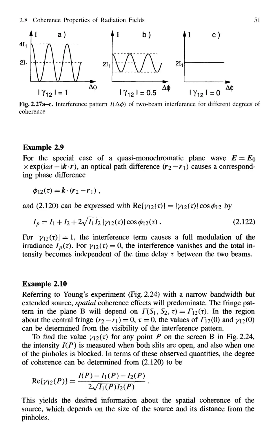
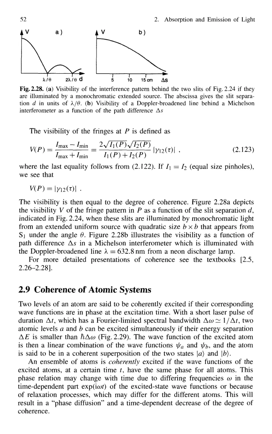
2.8 Coherence Properties of Radiation Fields 42
2.8.1 Temporal Coherence 42
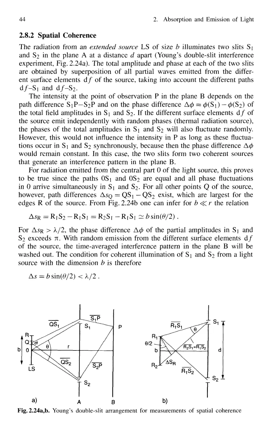
2.8.2 Spatial Coherence 44
2.8.3 Coherence Volume 45
2.8.4 The Coherence Function and the Degree
of Coherence 48
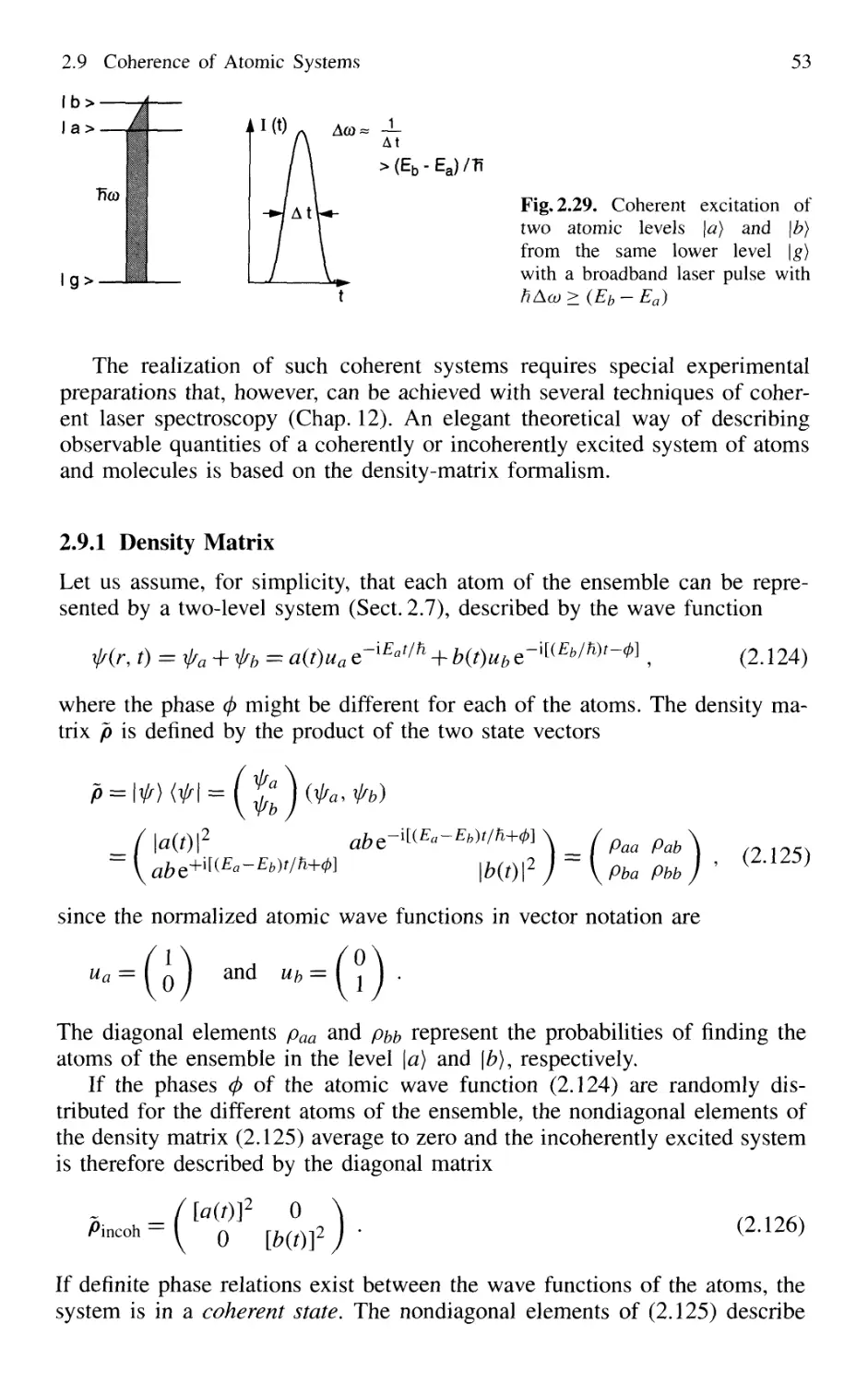
2.9 Coherence of Atomic Systems 52
2.9.1 Density Matrix 53
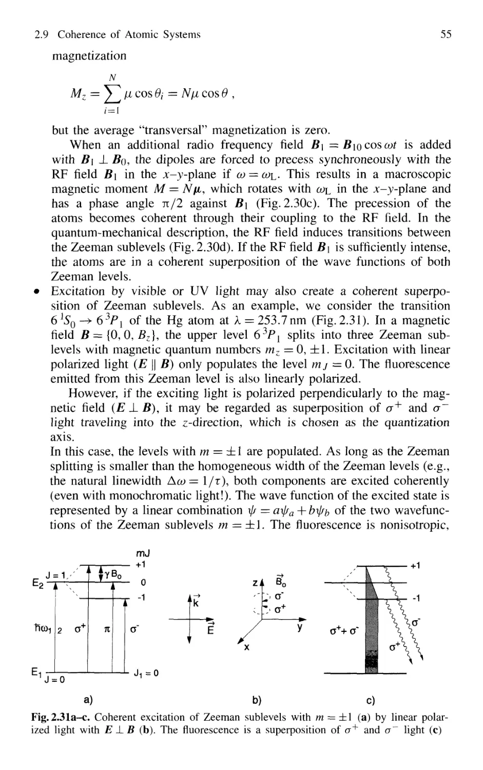
2.9.2 Coherent Excitation 54
2.9.3 Relaxation of Coherently Excited Systems 56
Problems 57
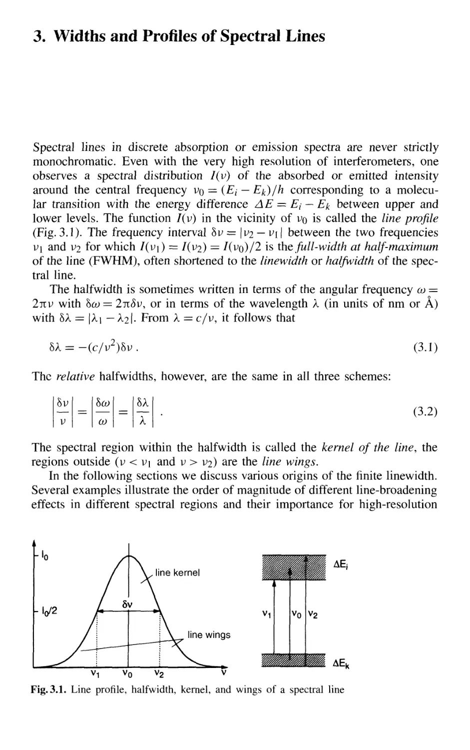
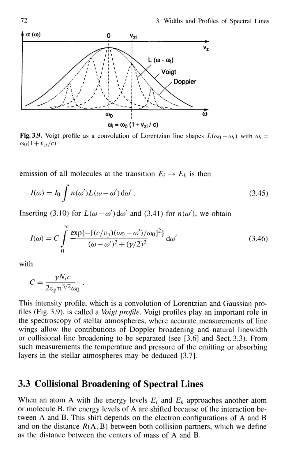
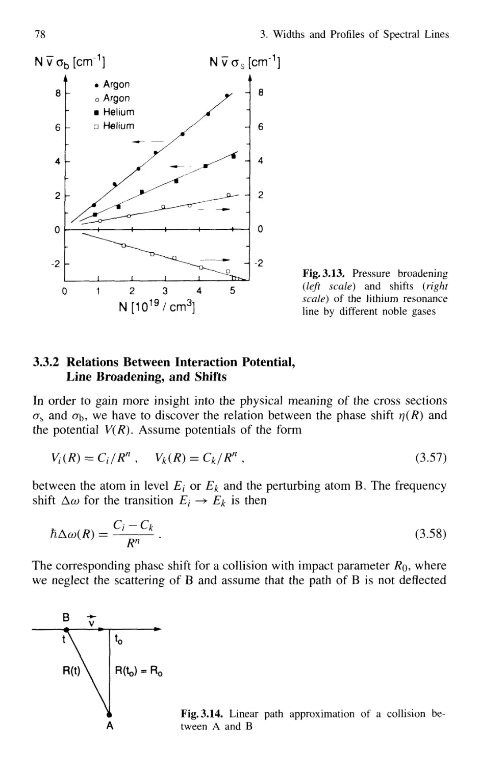
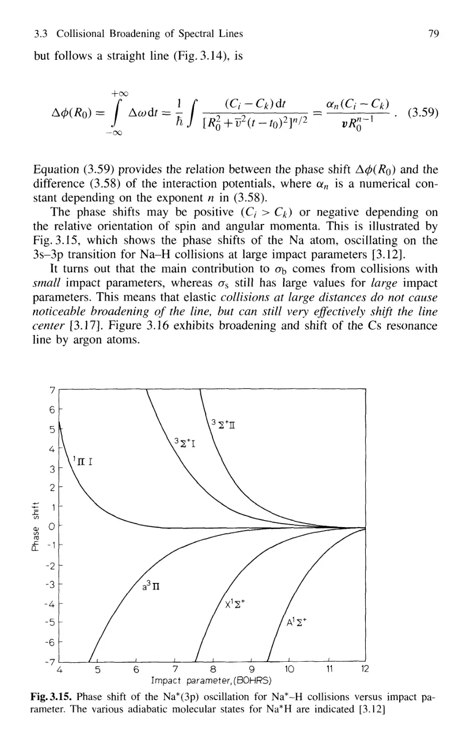
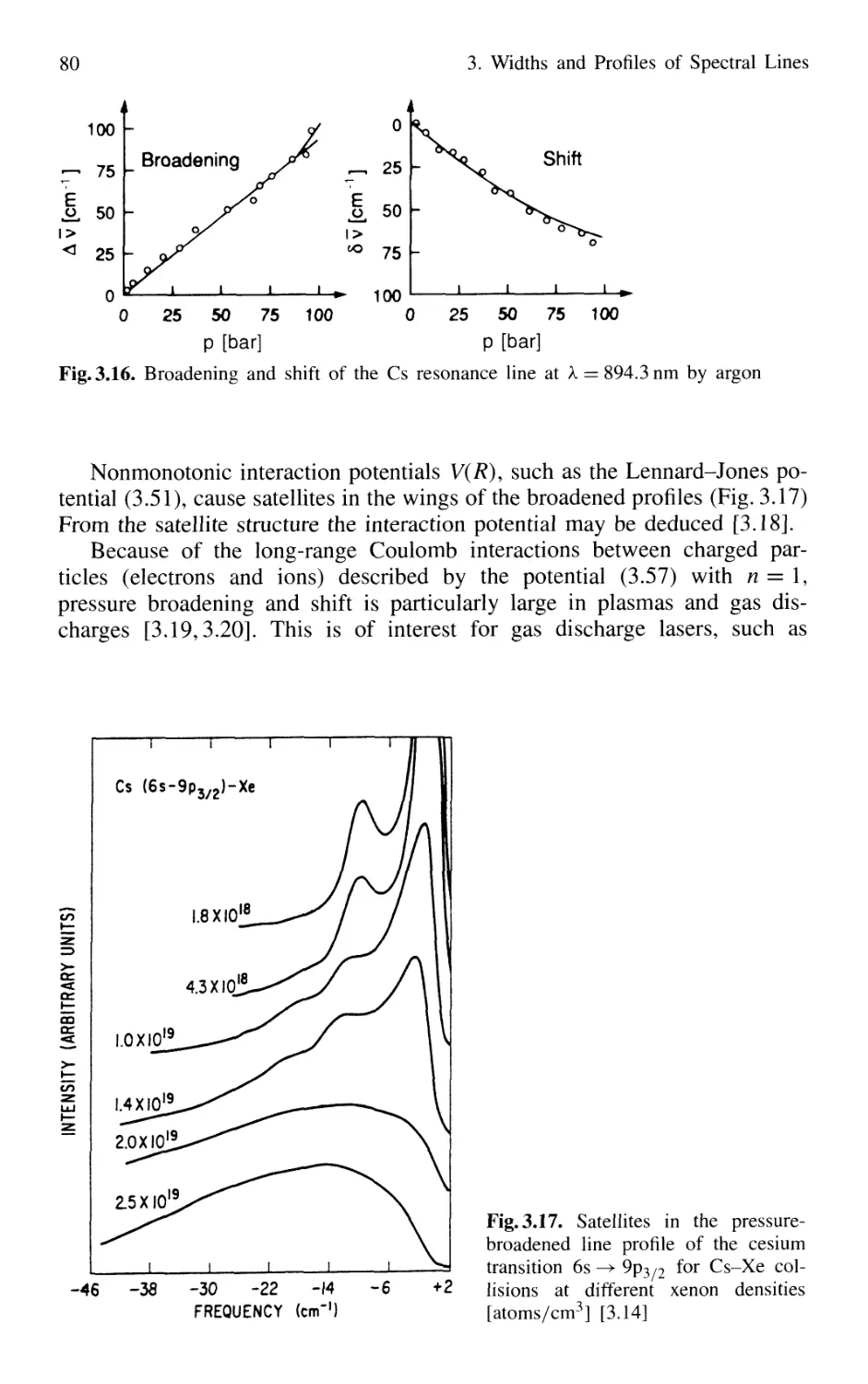
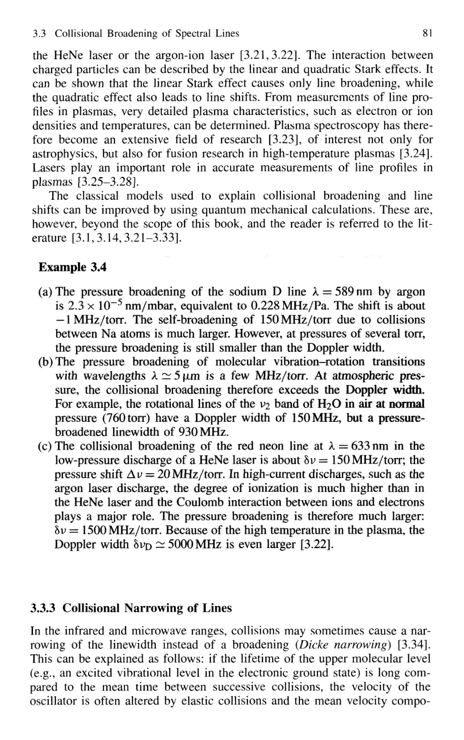
3. Widths and Profiles of Spectral Lines 59
3.1 Natural Linewidth 60
3.1.1 Lorentzian Line Profile of the Emitted Radiation .. 60
3.1.2 Relation Between Linewidth and Lifetime 62
3.1.3 Natural Linewidth of Absorbing Transitions 64
3.2 Doppler Width 68
XII Contents
3.3 Collisional Broadening of Spectral Lines 72
3.3.1 Phenomenological Description 73
3.3.2 Relations Between Interaction Potential,
Line Broadening, and Shifts 76
3.3.3 Collisional Narrowing of Lines 81
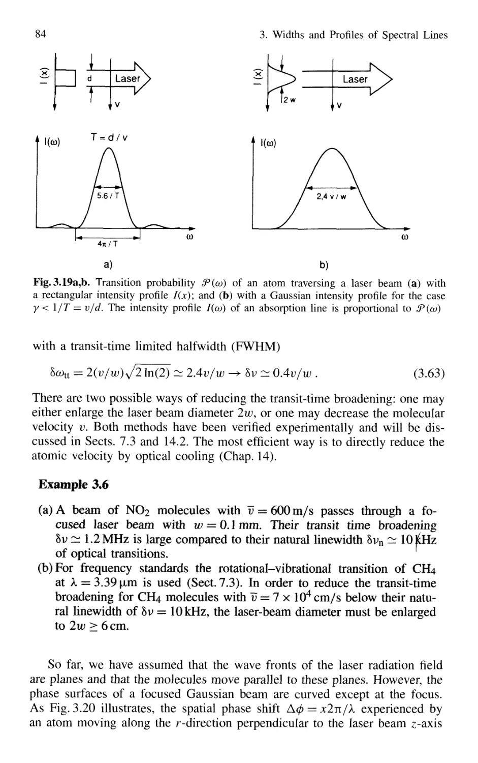
3.4 Transit-Time Broadening 82
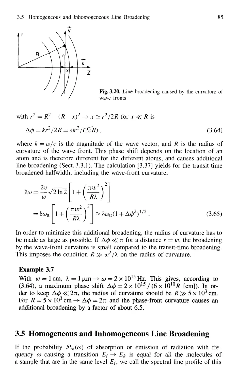
3.5 Homogeneous and Inhomogeneous Line Broadening 85
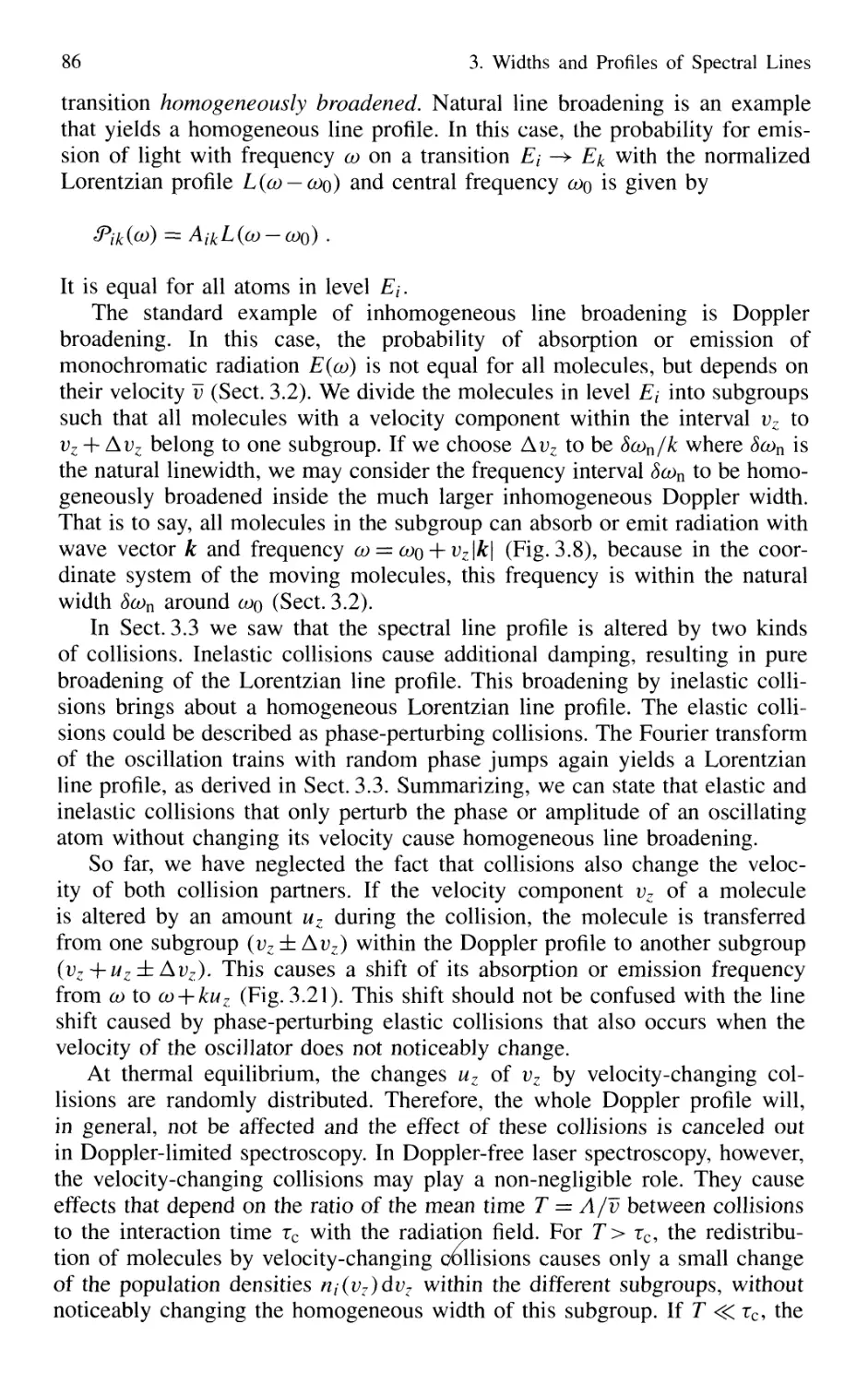
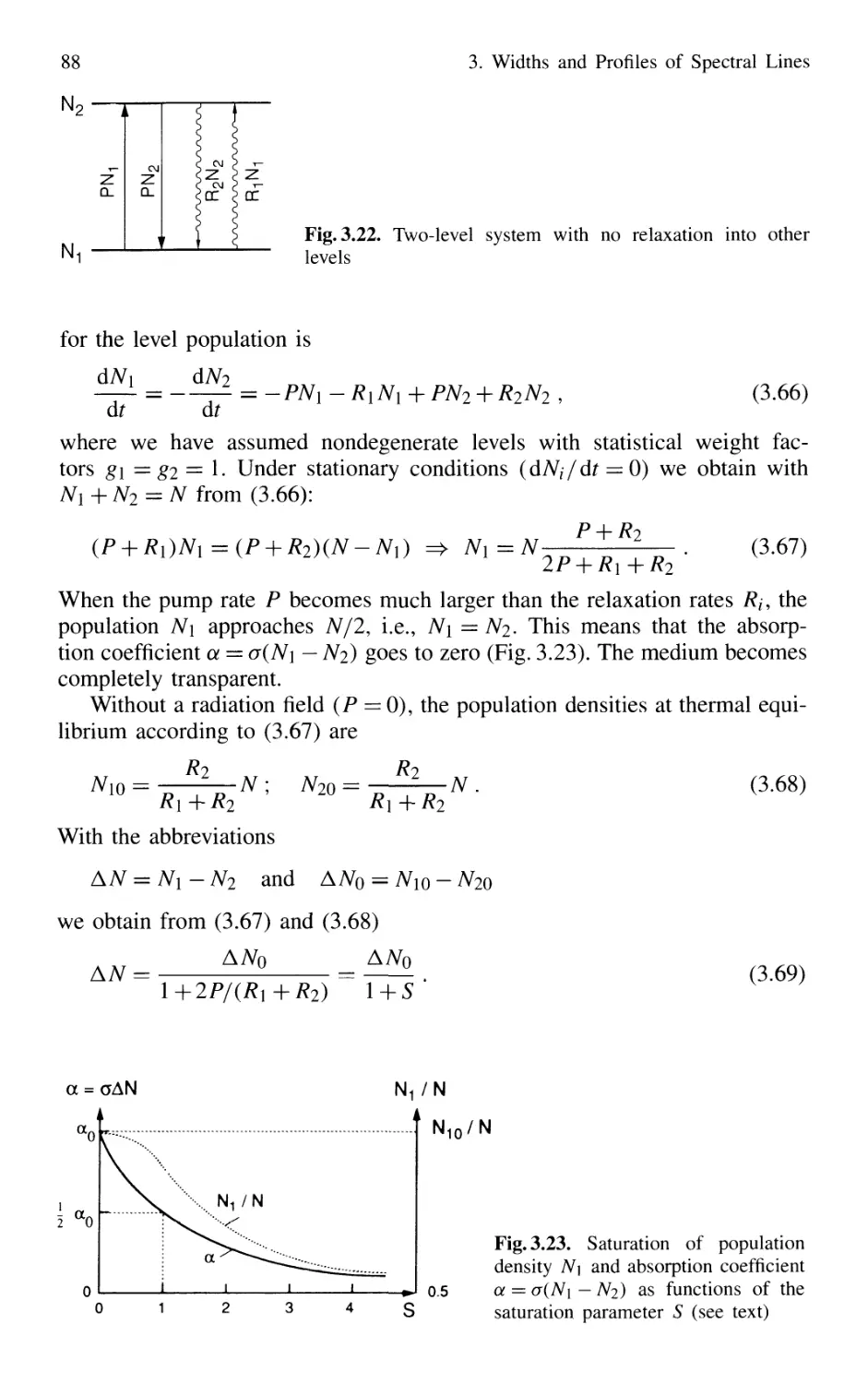
3.6 Saturation and Power Broadening 87
3.6.1 Saturation of Level Population by Optical Pumping 87
3.6.2 Saturation Broadening
of Homogeneous Line Profiles 89
3.6.3 Power Broadening 91
3.7 Spectral Line Profiles in Liquids and Solids 92
Problems 94
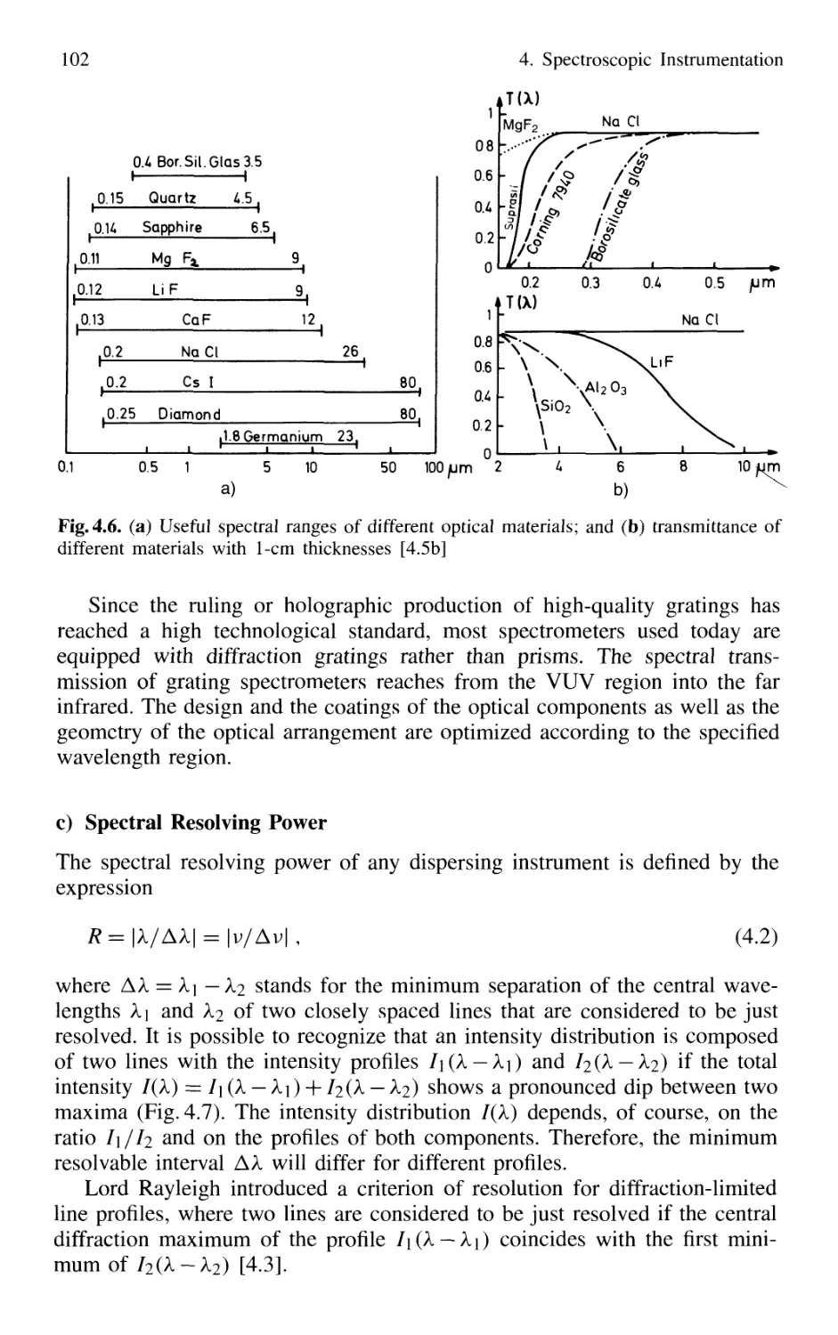
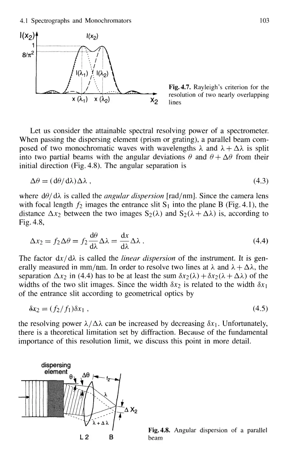
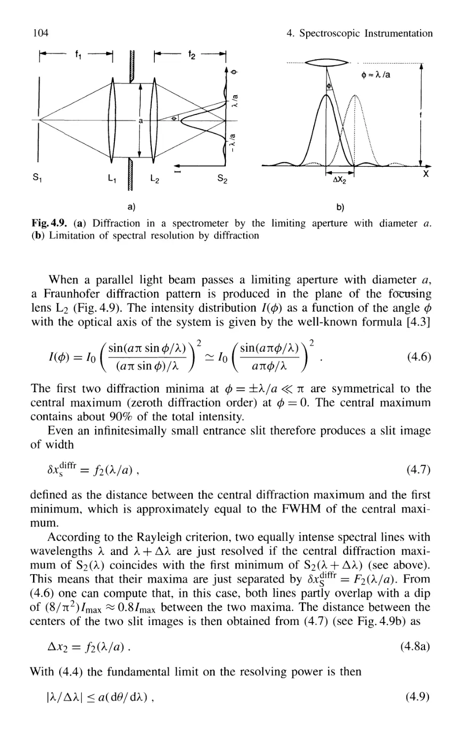
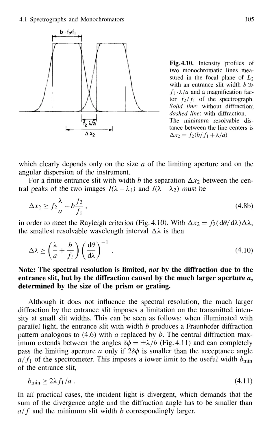
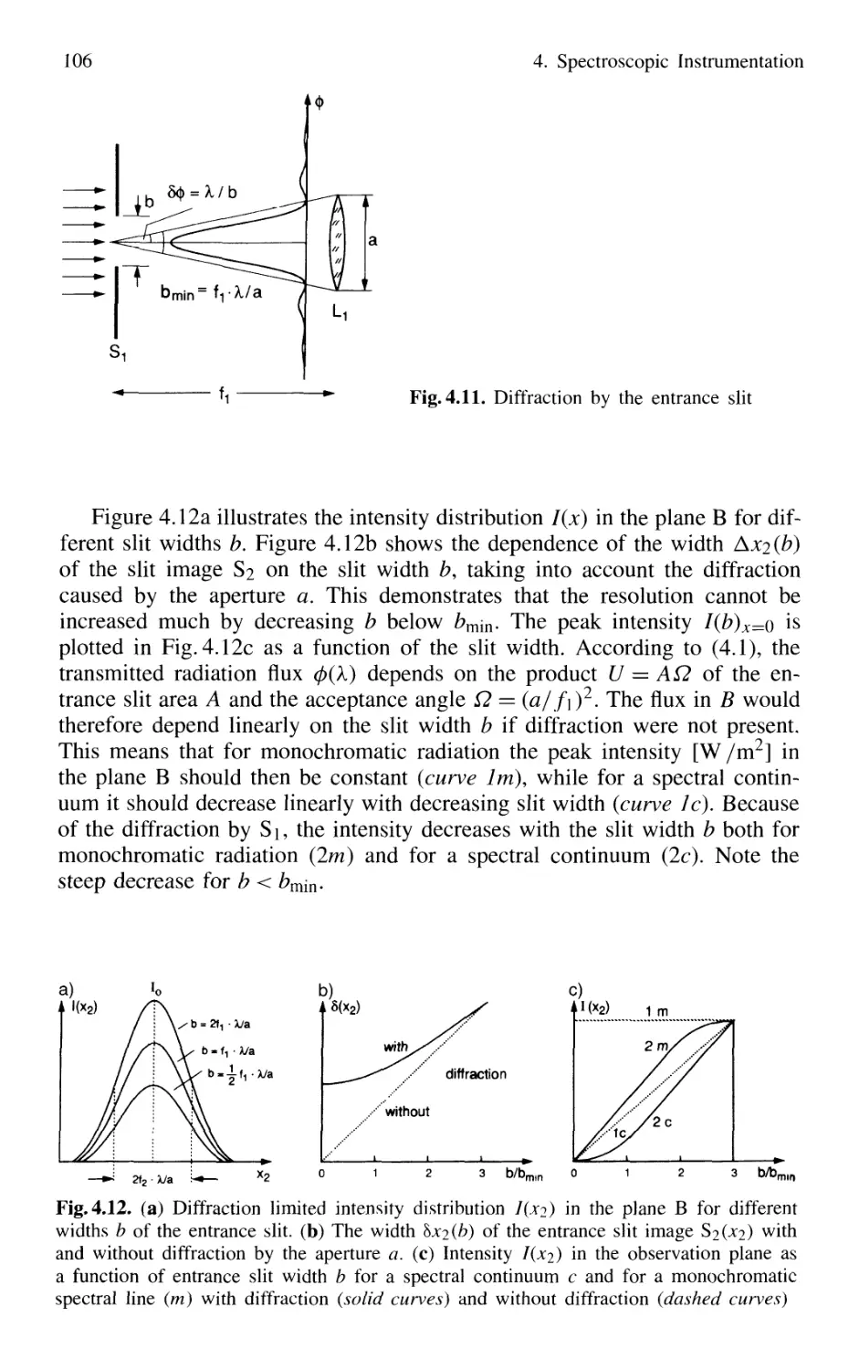
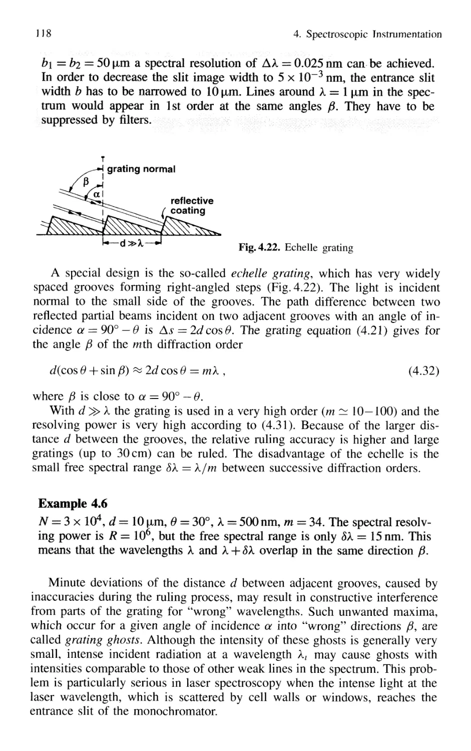
4. Spectroscopic Instrumentation 97
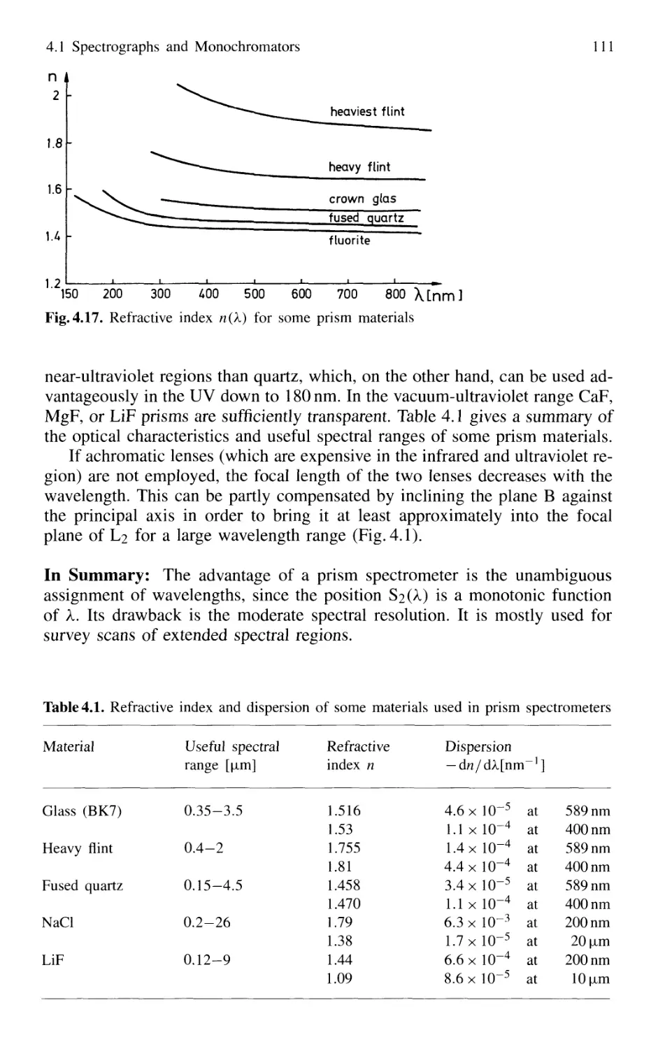
4.1 Spectrographs and Monochromators 97
4.1.1 Basic Properties 99
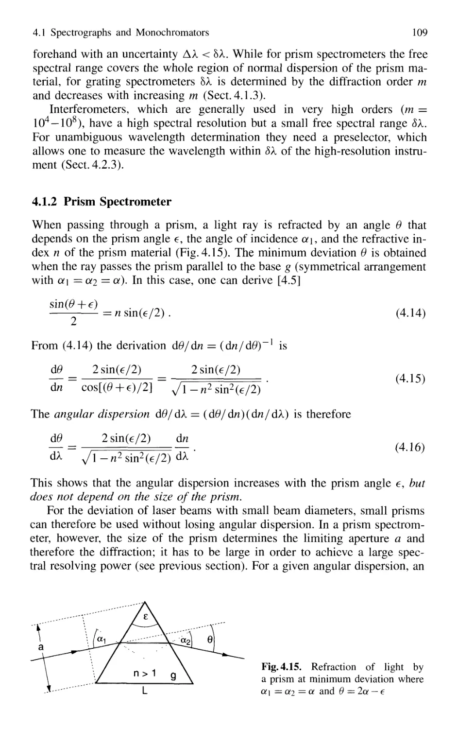
4.1.2 Prism Spectrometer 109
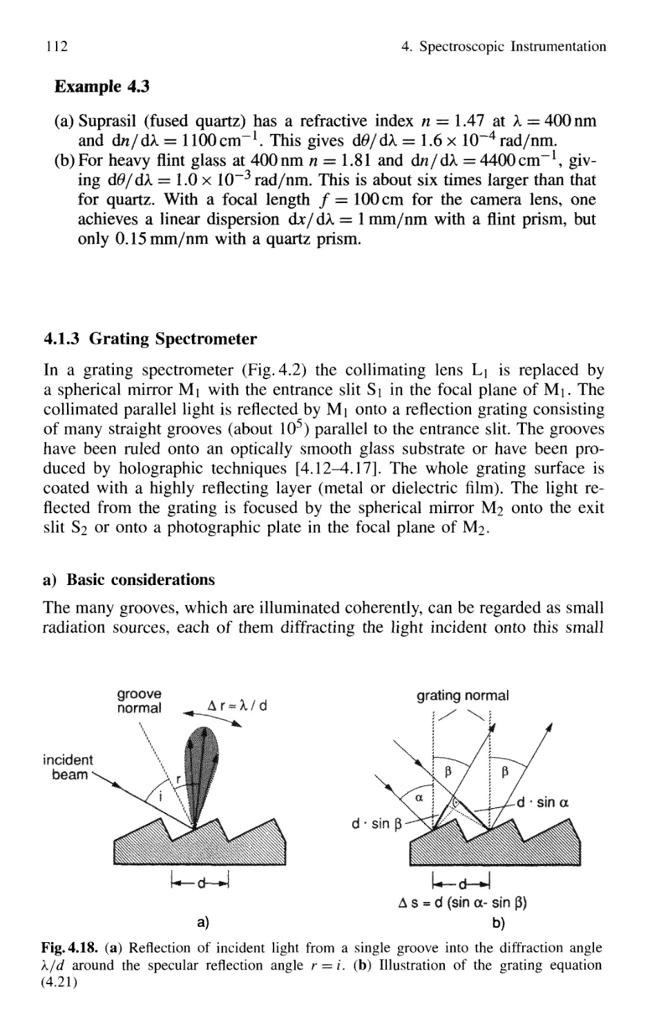
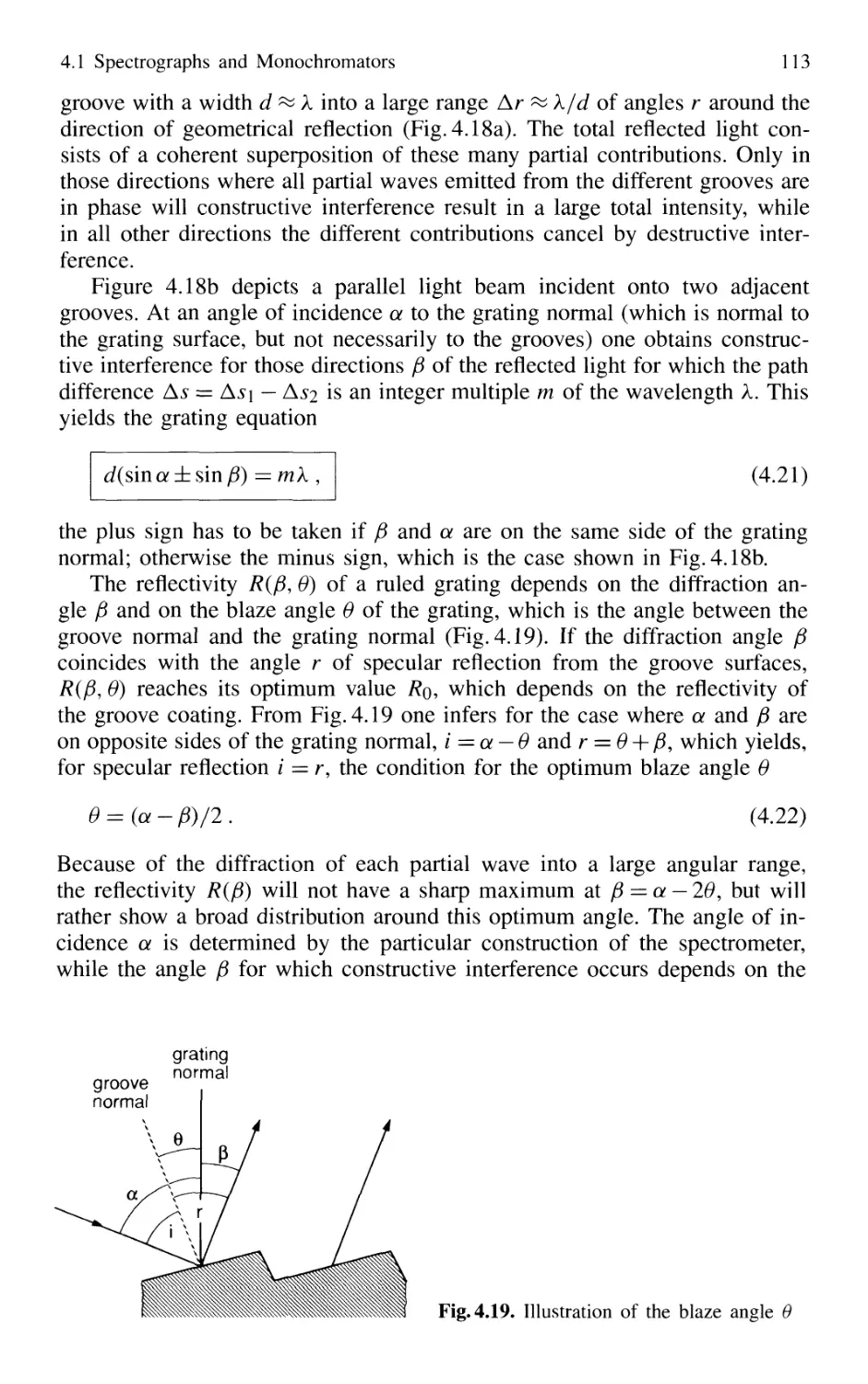
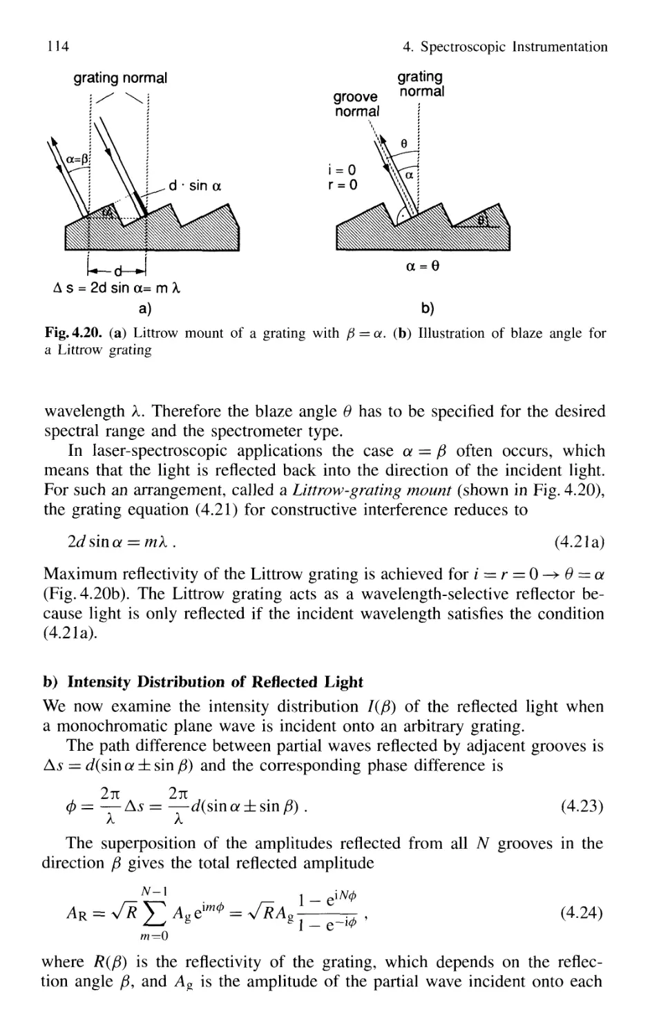
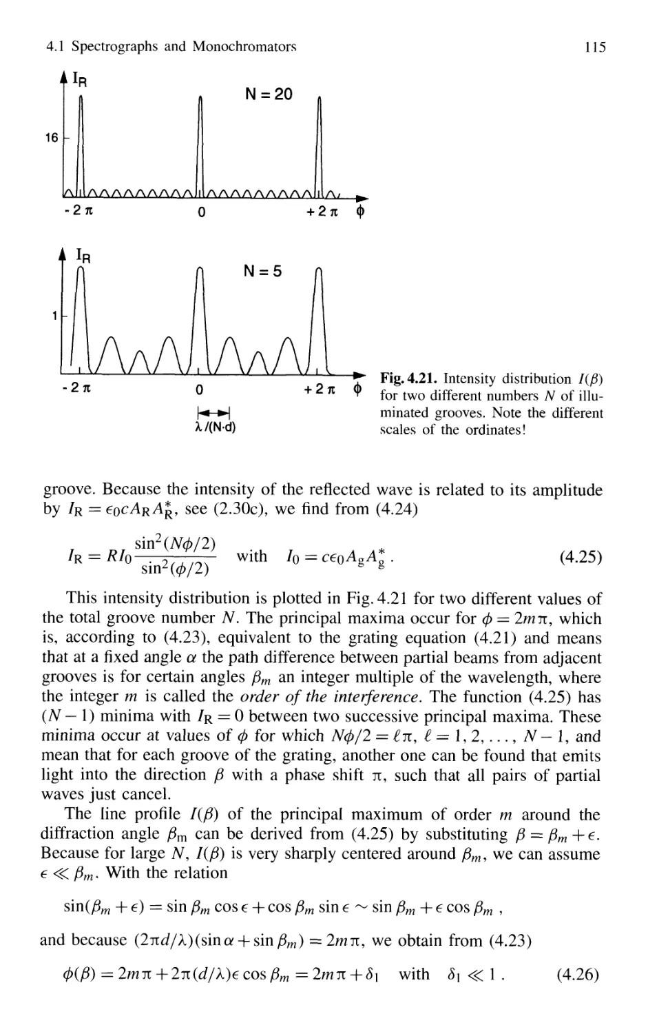
4.1.3 Grating Spectrometer 112
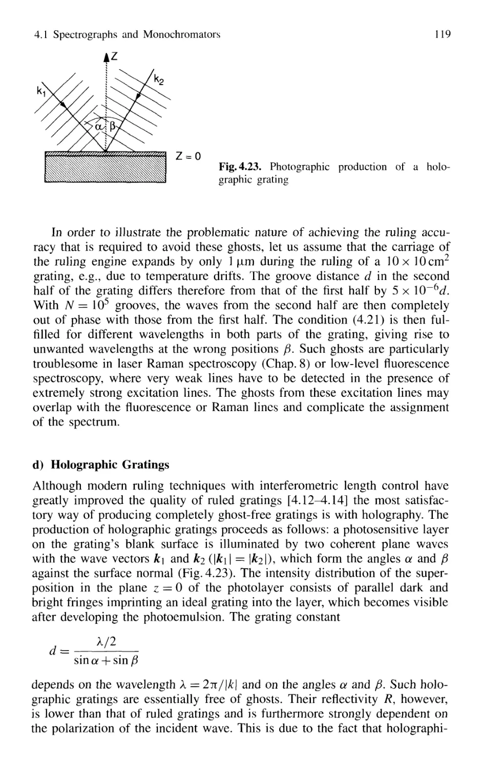
4.2 Interferometers 120
4.2.1 Basic Concepts 121
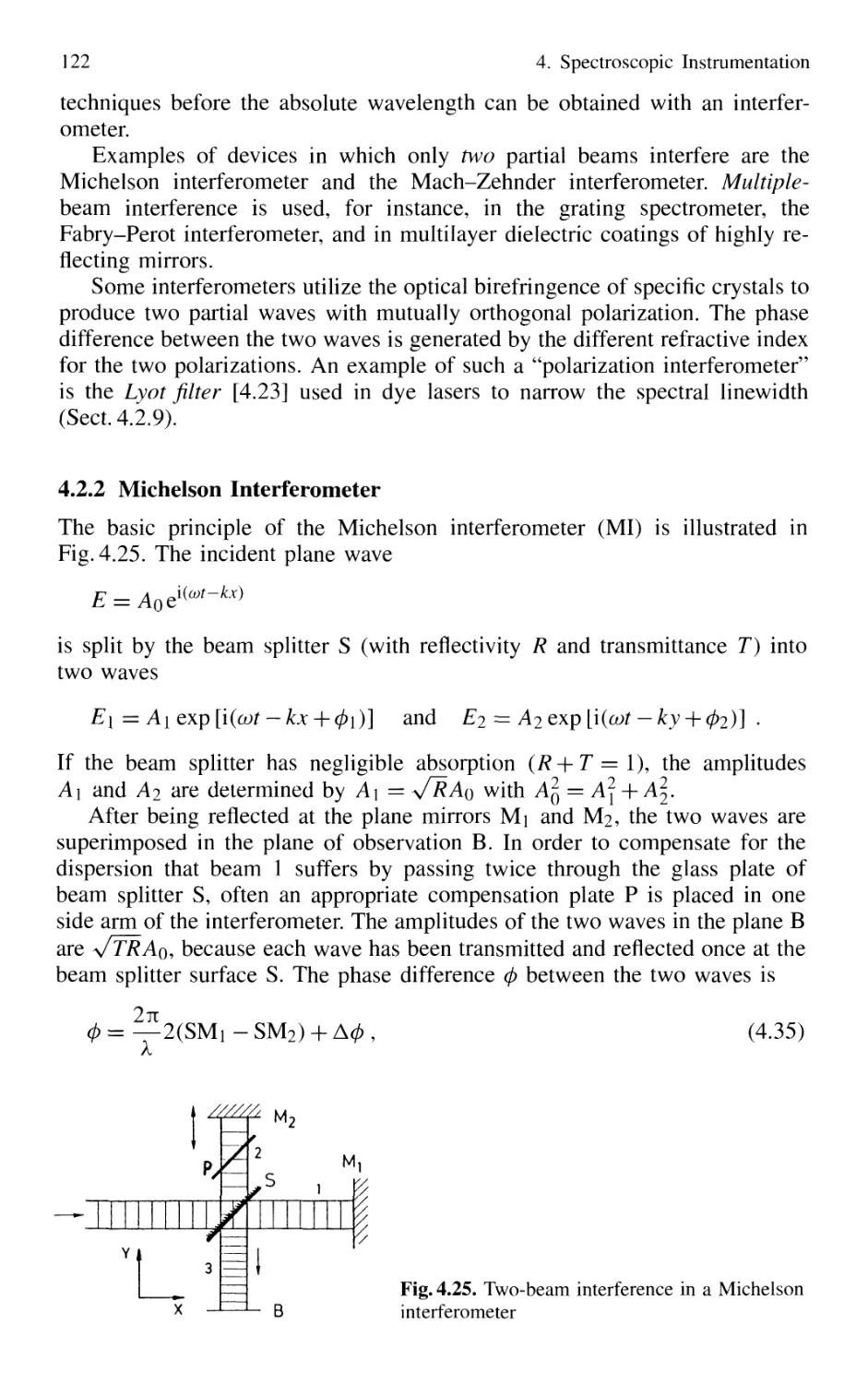
4.2.2 Michelson Interferometer 122
4.2.3 Mach-Zehnder Interferometer 127
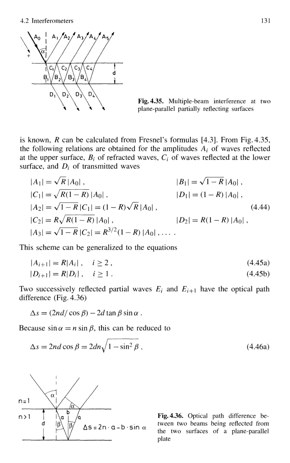
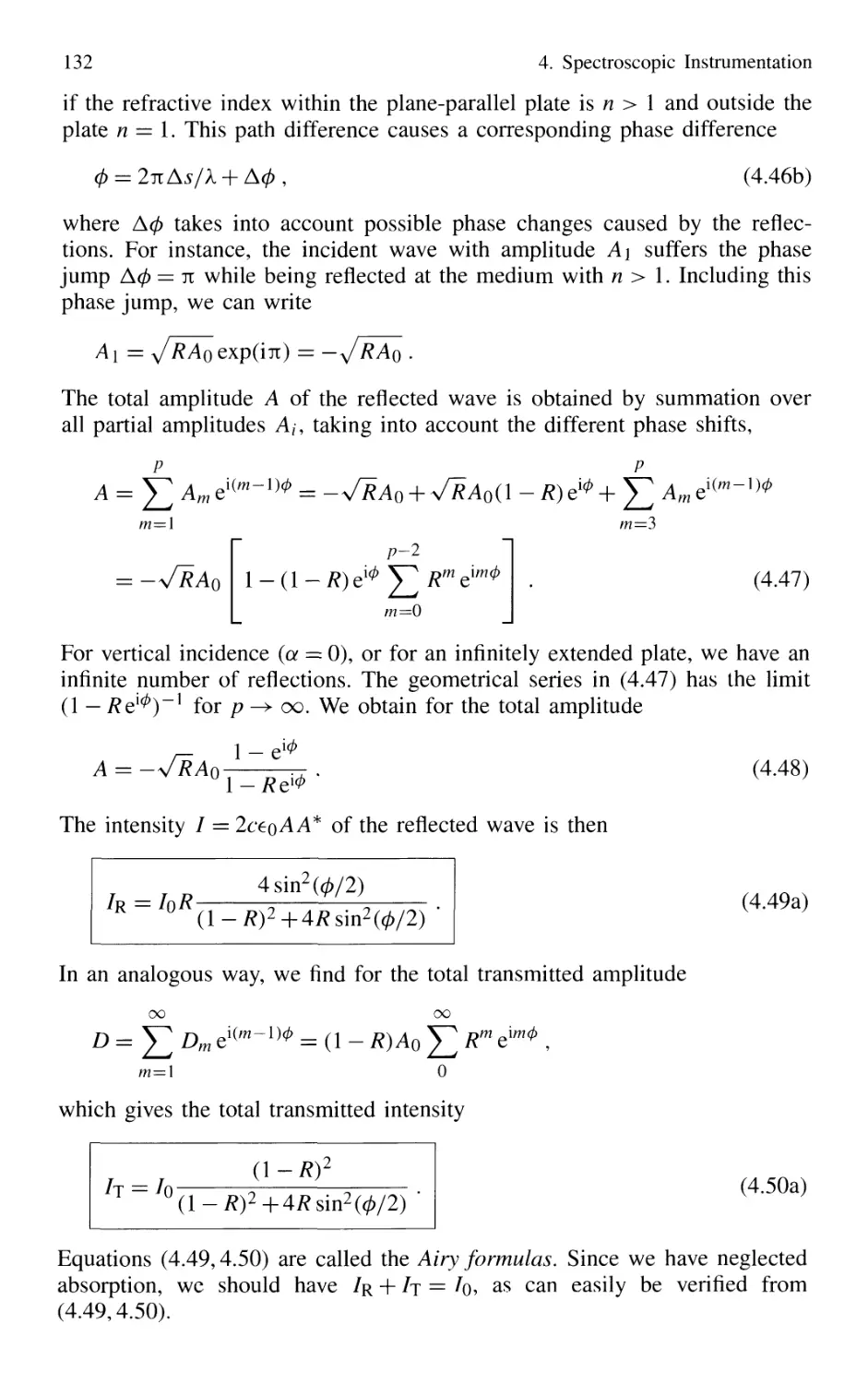
4.2.4 Multiple-Beam Interference 130
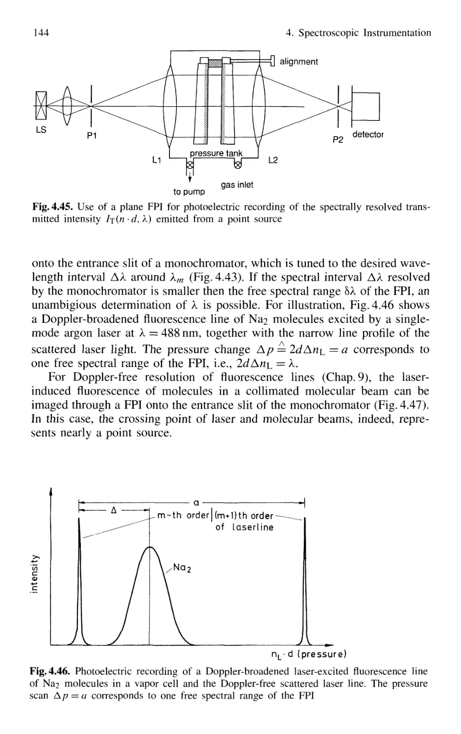
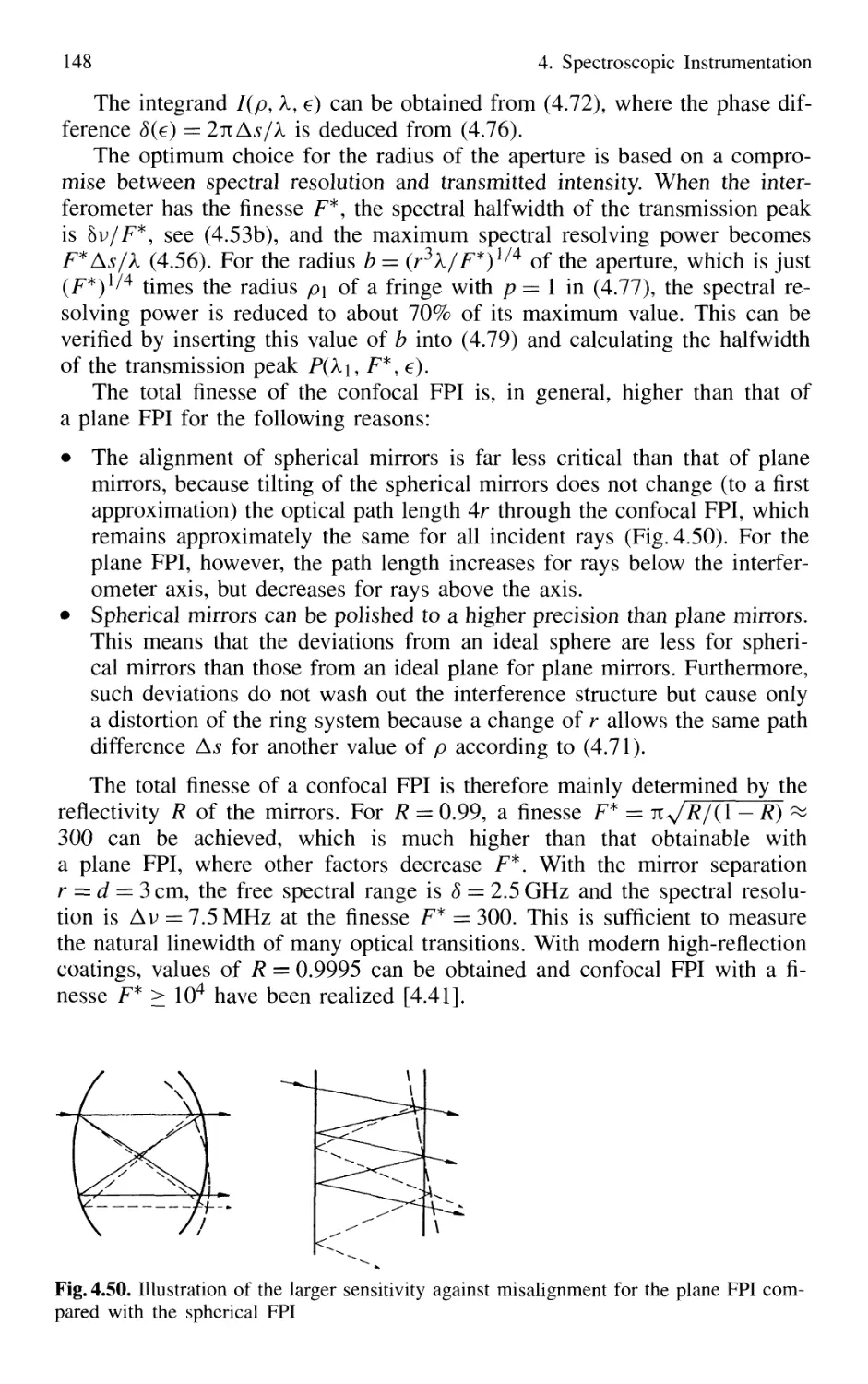
4.2.5 Plane Fabry-Perot Interferometer 137
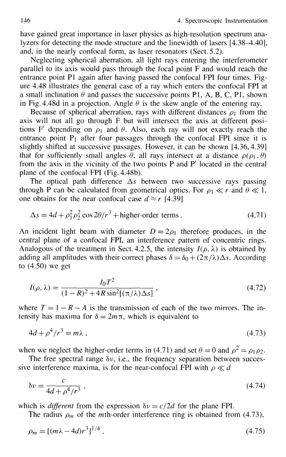
4.2.6 Confocal Fabry-Perot Interferometer 145
4.2.7 Multilayer Dielectric Coatings 150
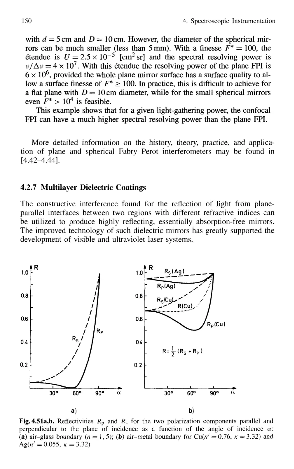
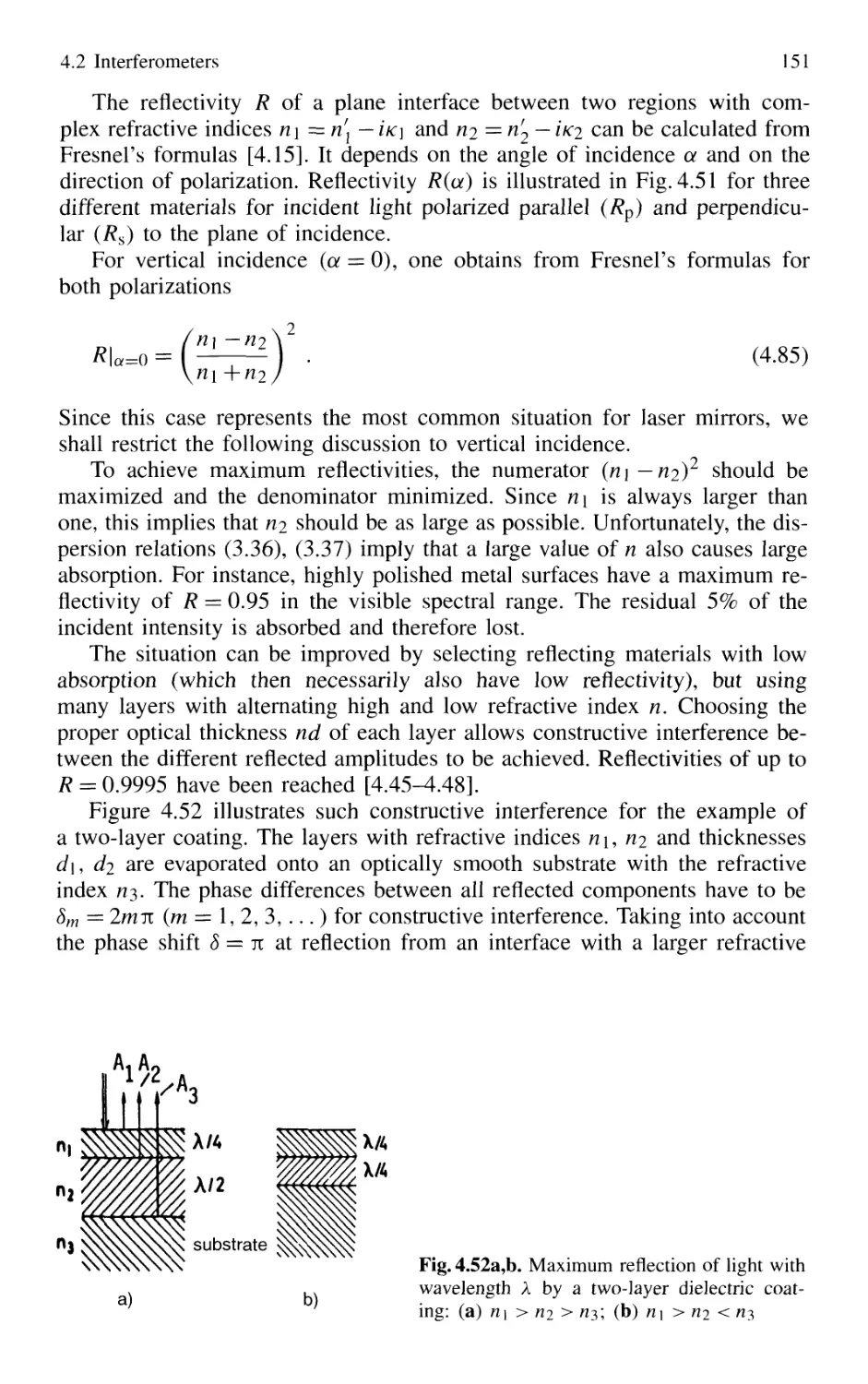
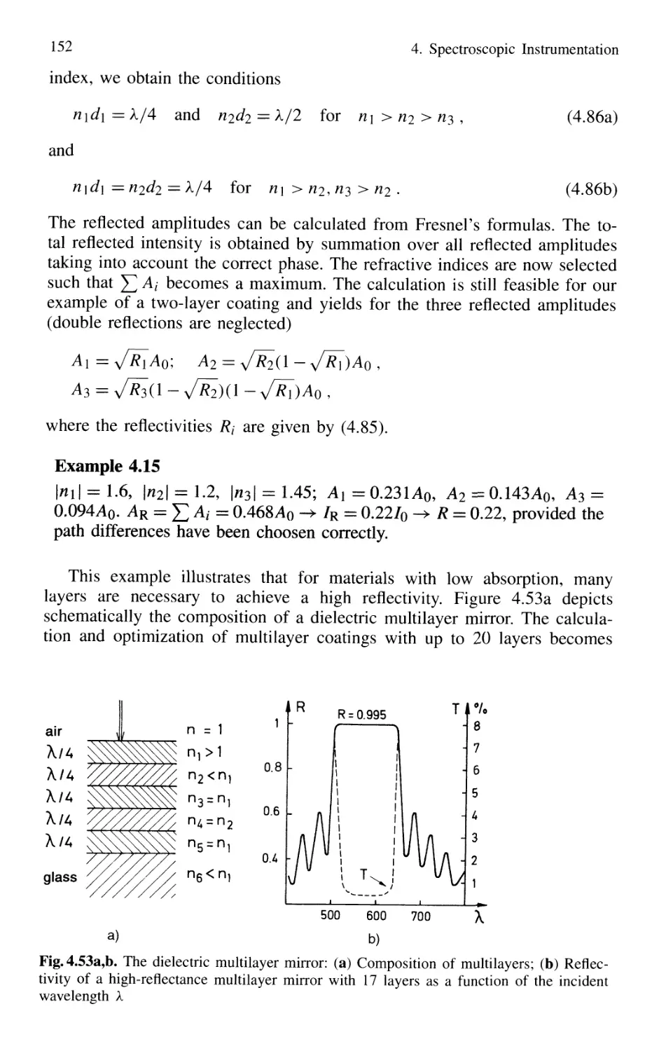
4.2.8 Interference Filters 154
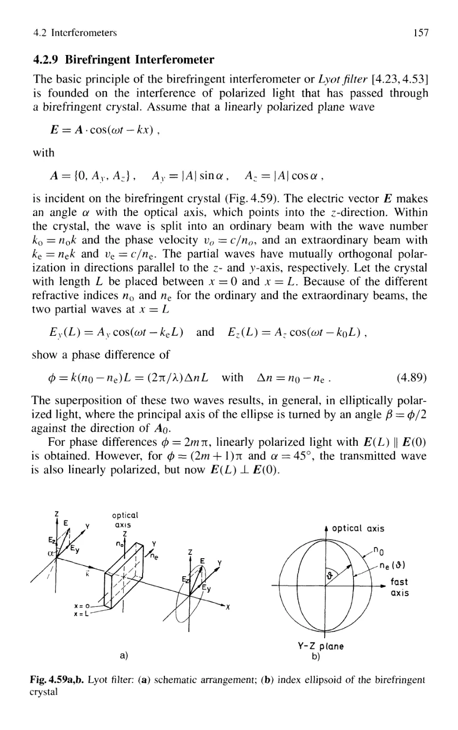
4.2.9 Birefringent Interferometer 157
4.2.10 Tunable Interferometers 161
4.3 Comparison Between Spectrometers and Interferometers .... 162
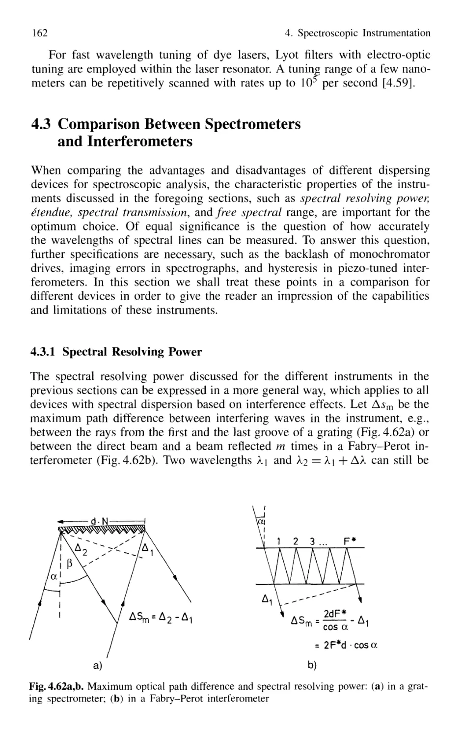
4.3.1 Spectral Resolving Power 162
4.3.2 Light-Gathering Power 164
4.4 Accurate Wavelength Measurements 166
4.4.1 Precision and Accuracy
of Wavelength Measurements 167
4.4.2 Today's Wavemeters 169
4.5 Detection of Light 179
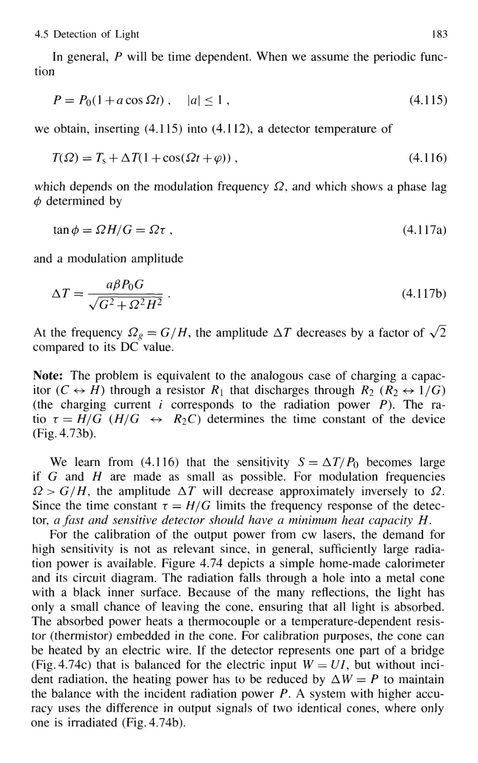
4.5.1 Thermal Detectors 182
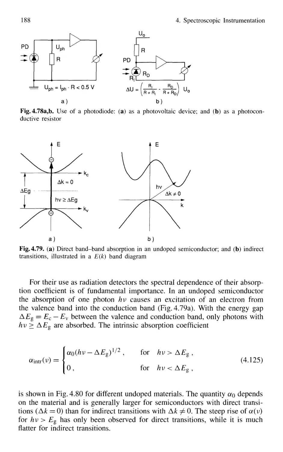
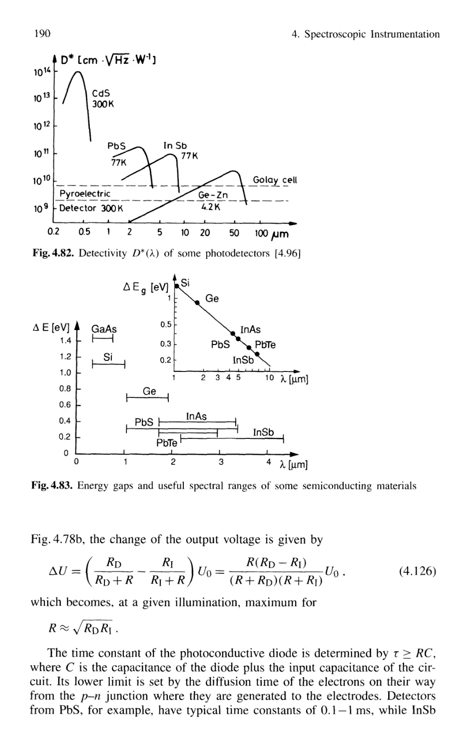
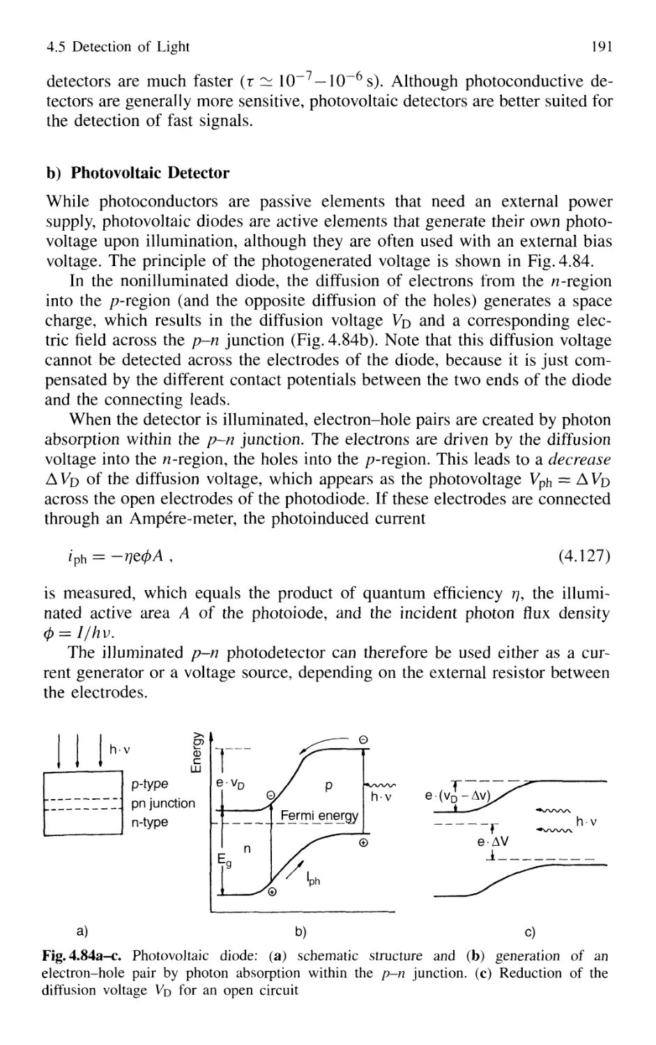
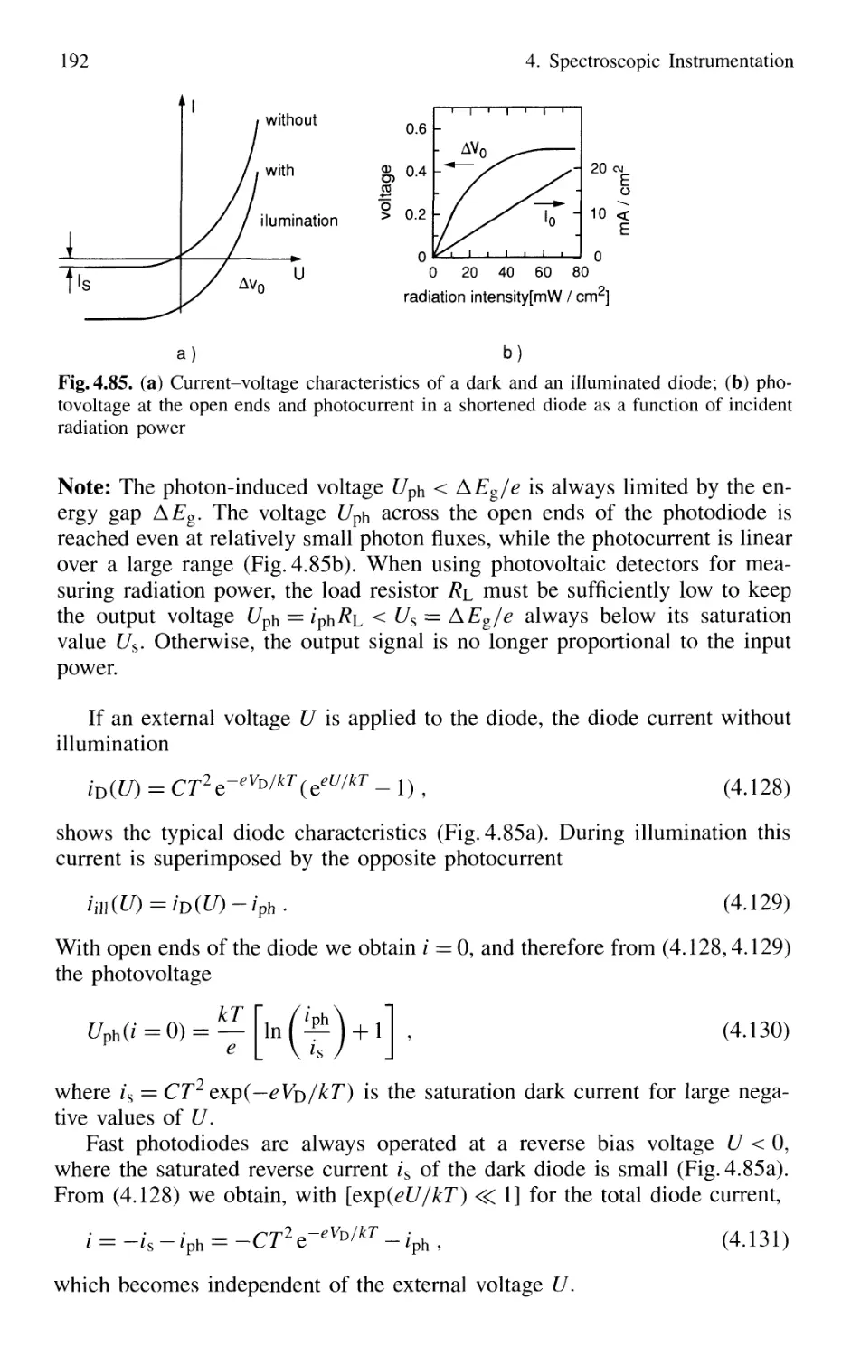
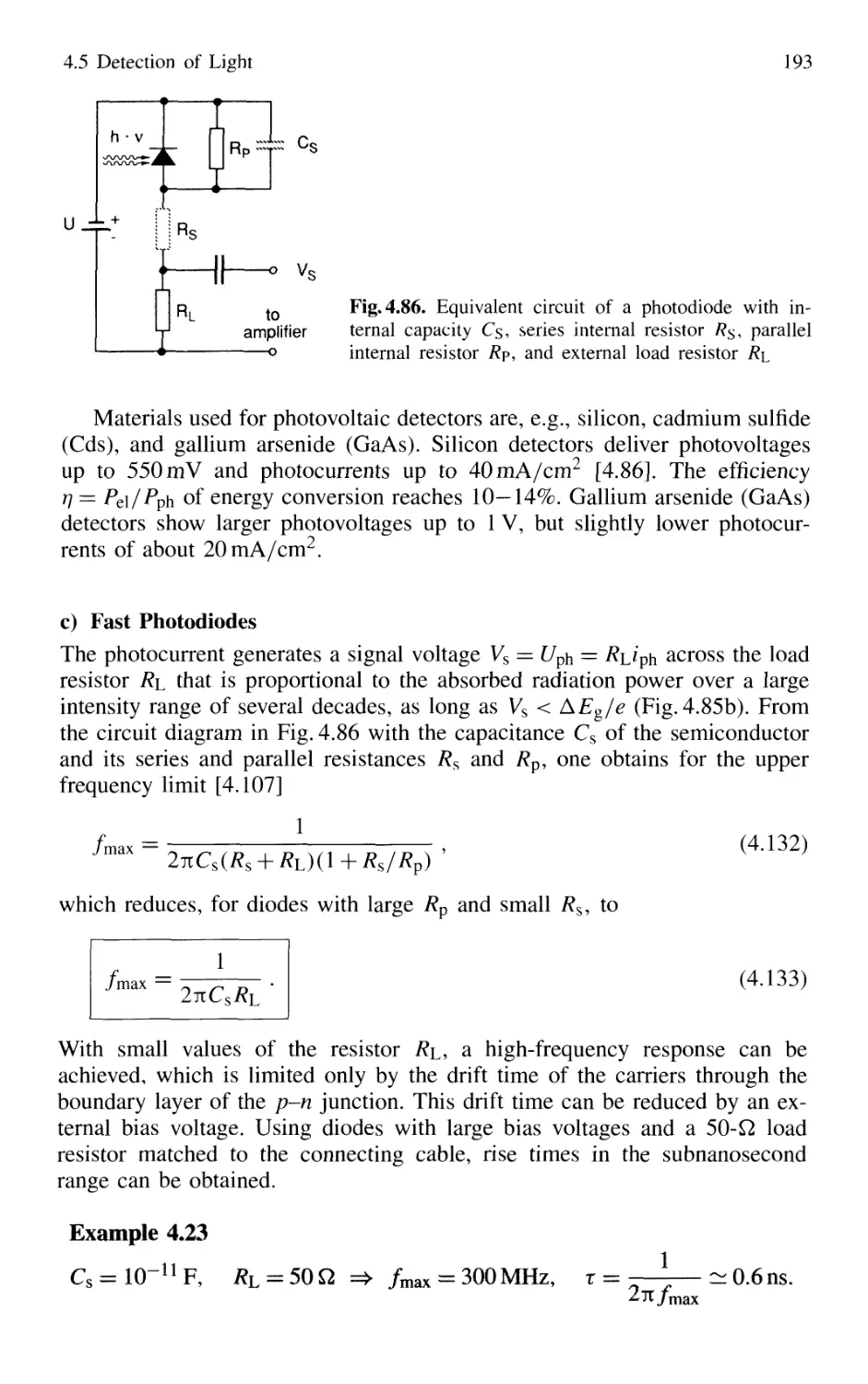
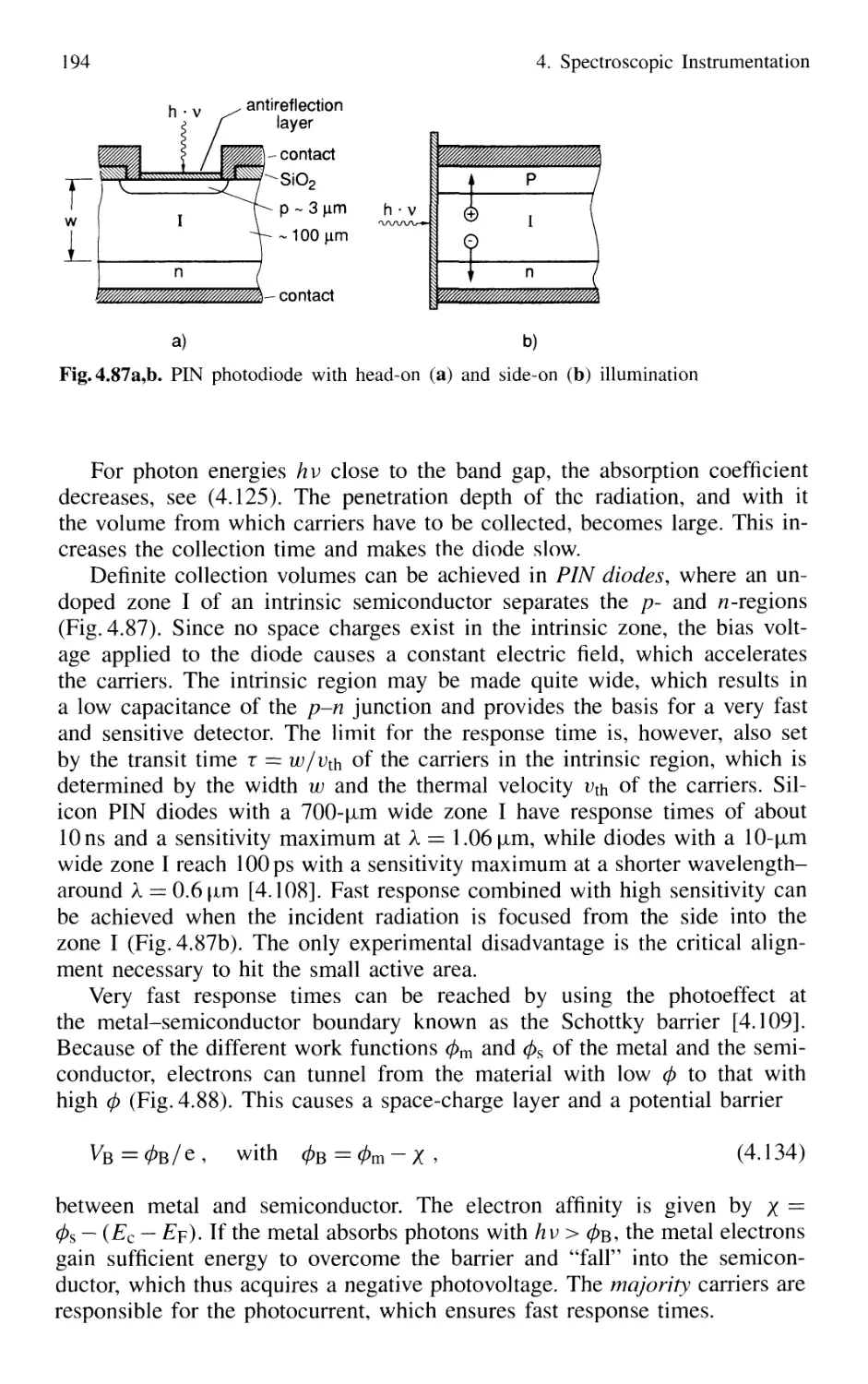
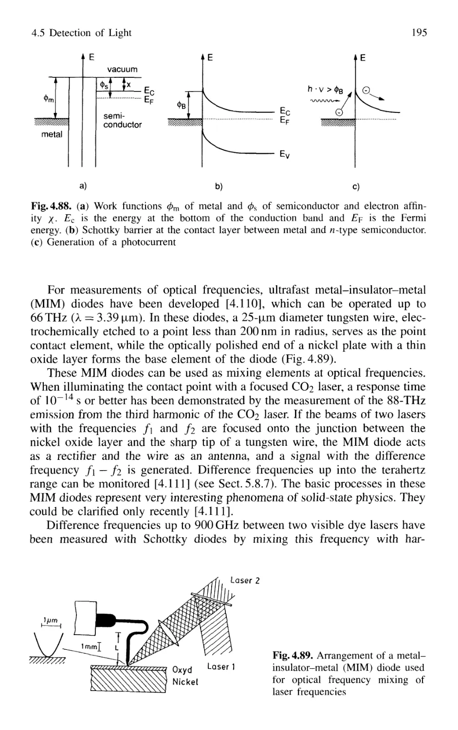
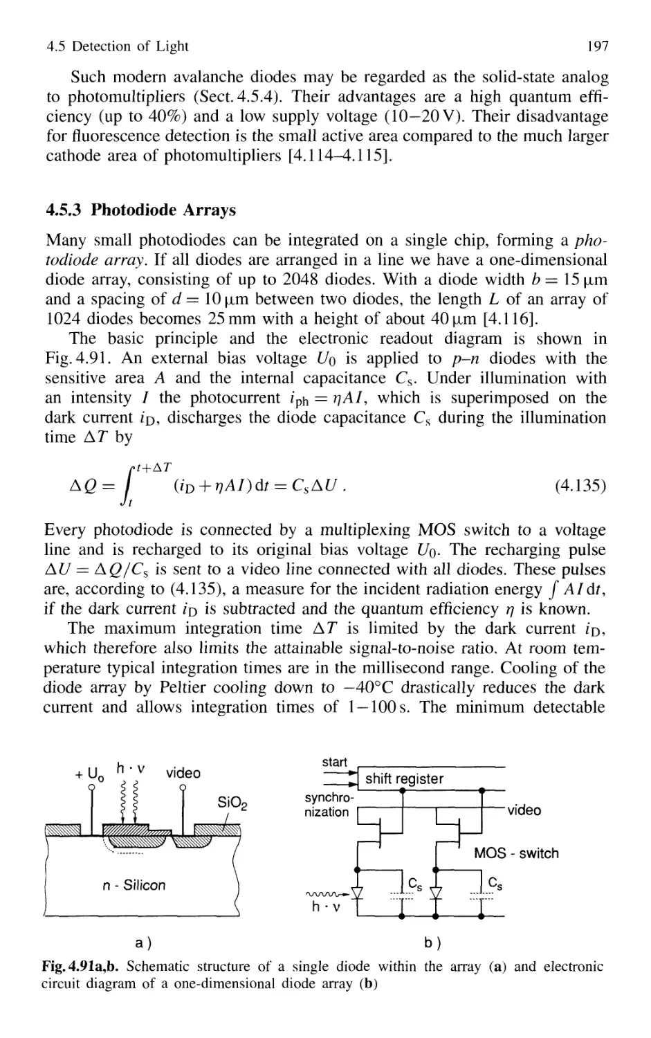
4.5.2 Photodiodes 187
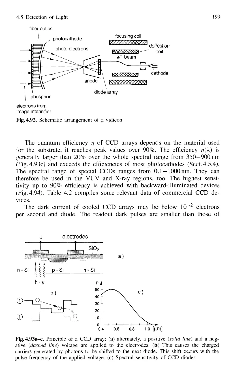
4.5.3 Photodiode Arrays 197
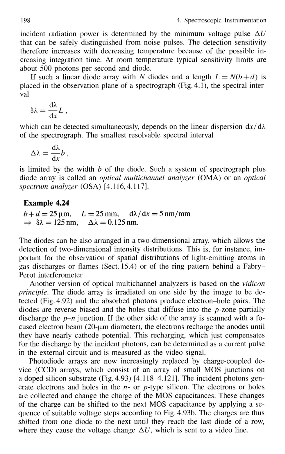
4.5.4 Photoemissive Detectors 200
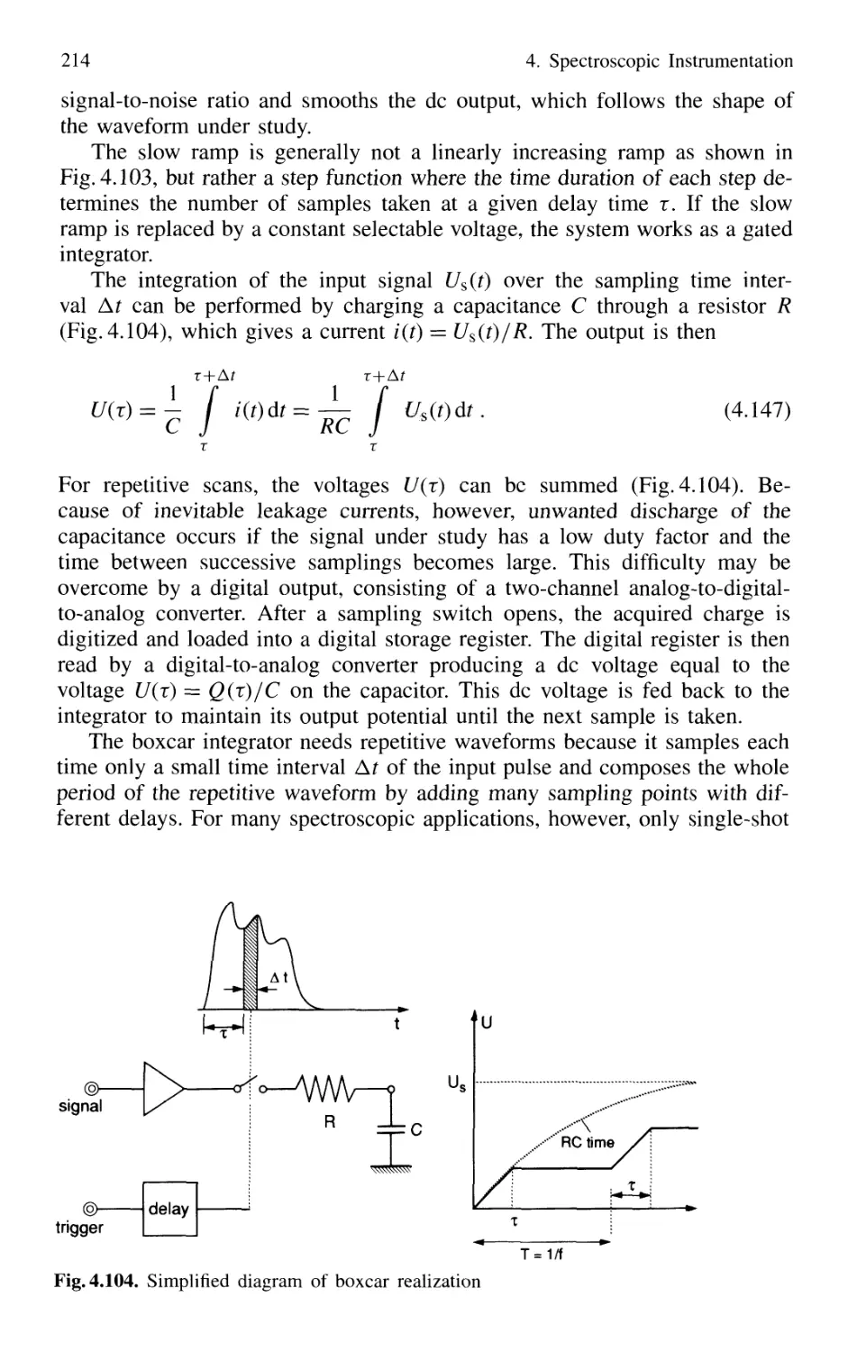
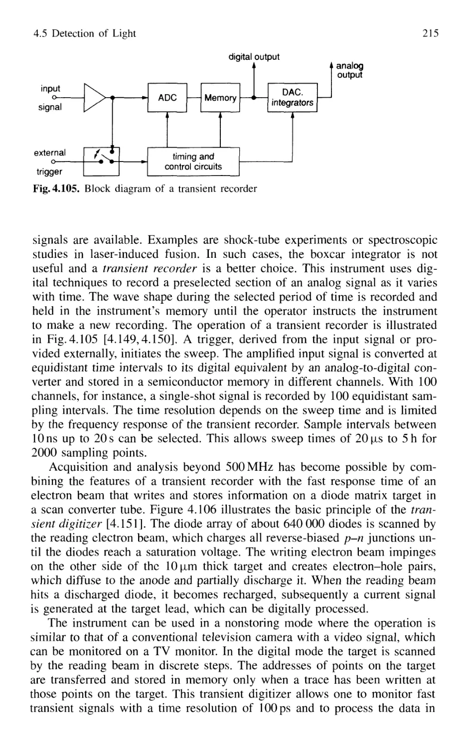
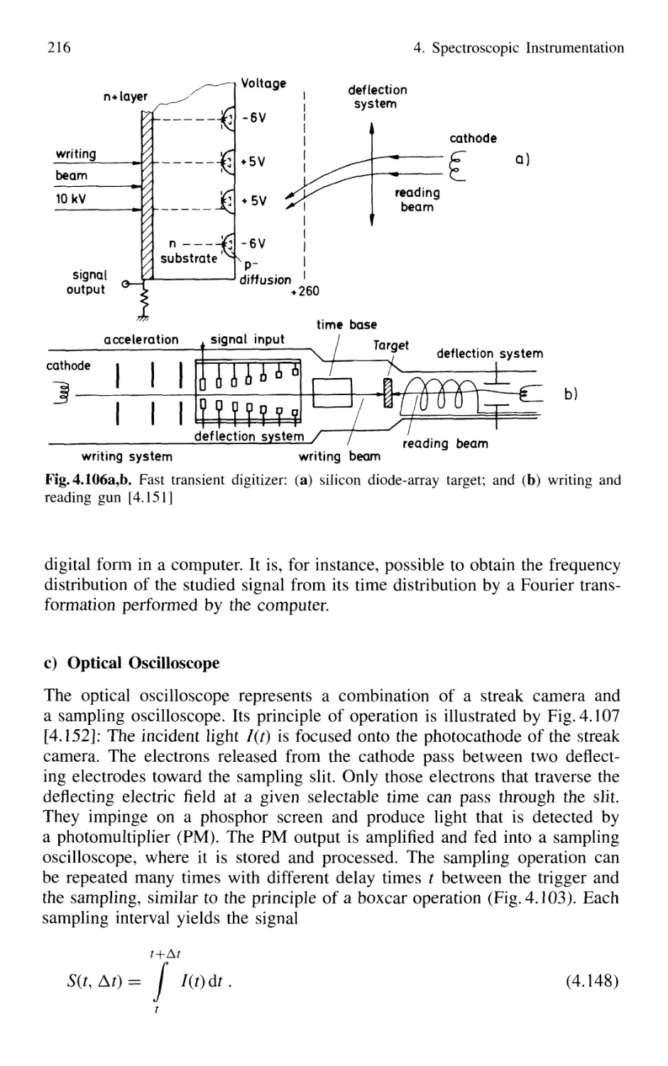
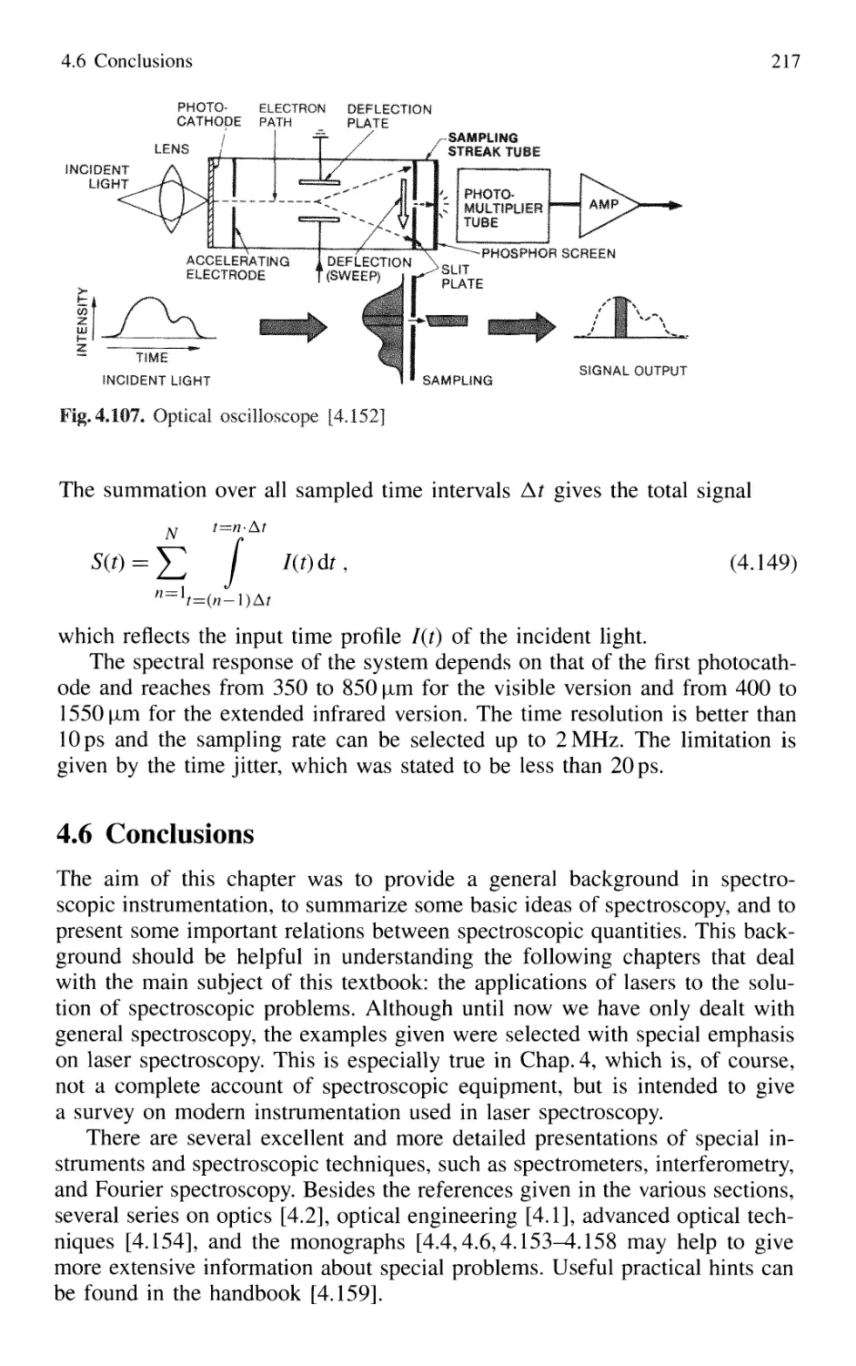
4.5.5 Detection Techniques and Electronic Equipment ... 211
4.6 Conclusions 217
Problems 218
Contents XIII
5. Lasers as Spectroscopic Light Sources 221
5.1 Fundamentals of Lasers 221
5.1.1 Basic Elements of a Laser 221
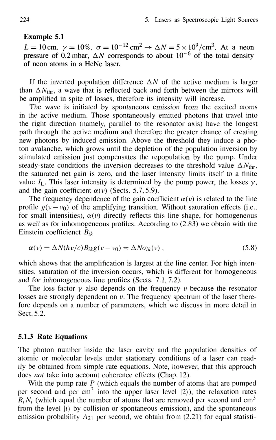
5.1.2 Threshold Condition 222
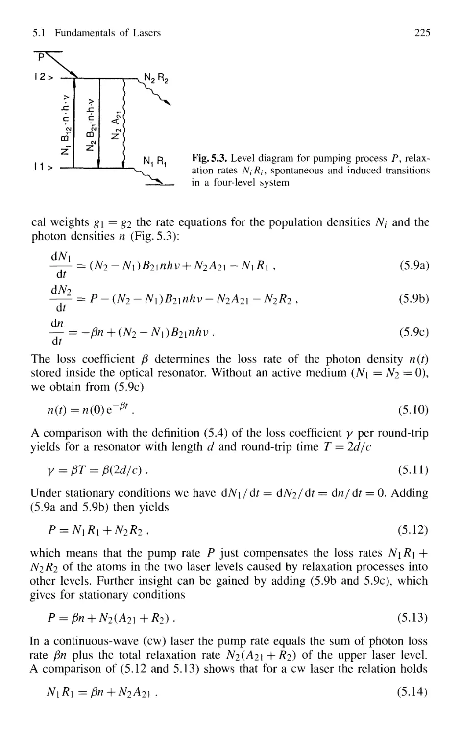
5.1.3 Rate Equations 224
5.2 Laser Resonators 226
5.2.1 Open Optical Resonators 228
5.2.2 Spatial Field Distributions in Open Resonators 231
5.2.3 Confocal Resonators 232
5.2.4 Genera] Spherical Resonators 236
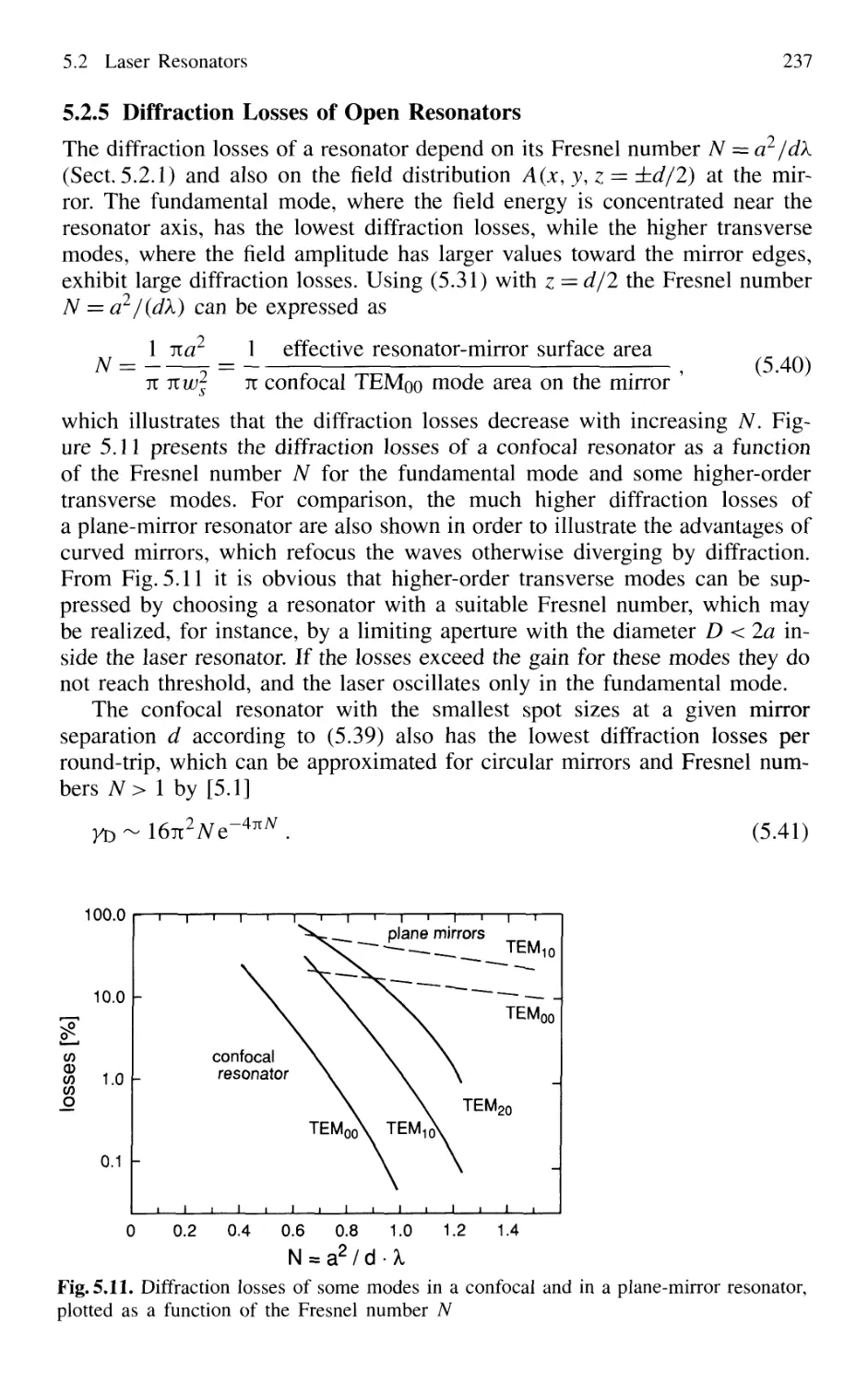
5.2.5 Diffraction Losses of Open Resonators 236
5.2.6 Stable and Unstable Resonators 238
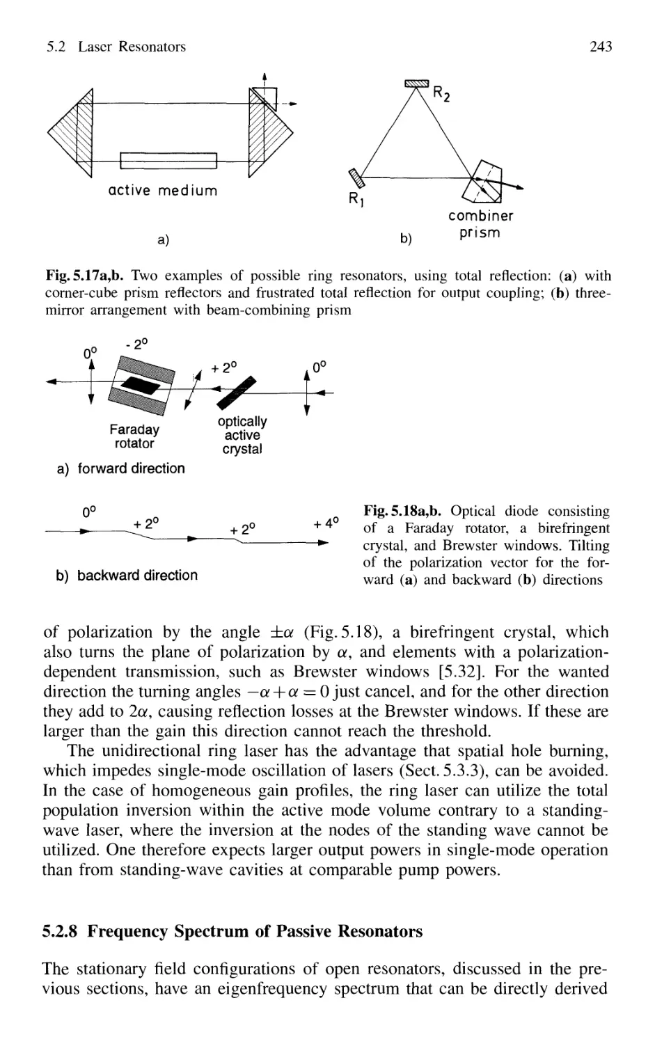
5.2.7 Ring Resonators 242
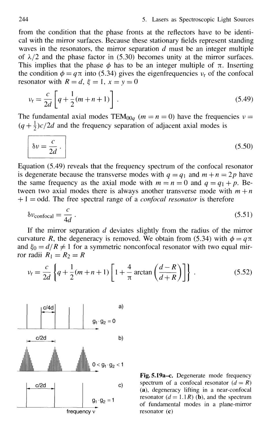
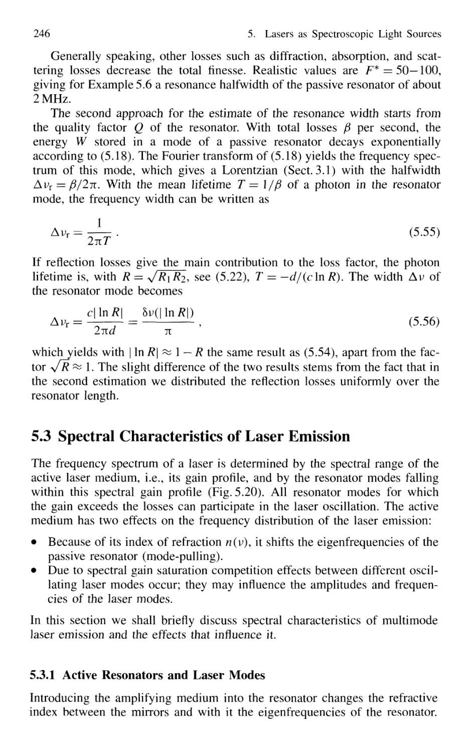
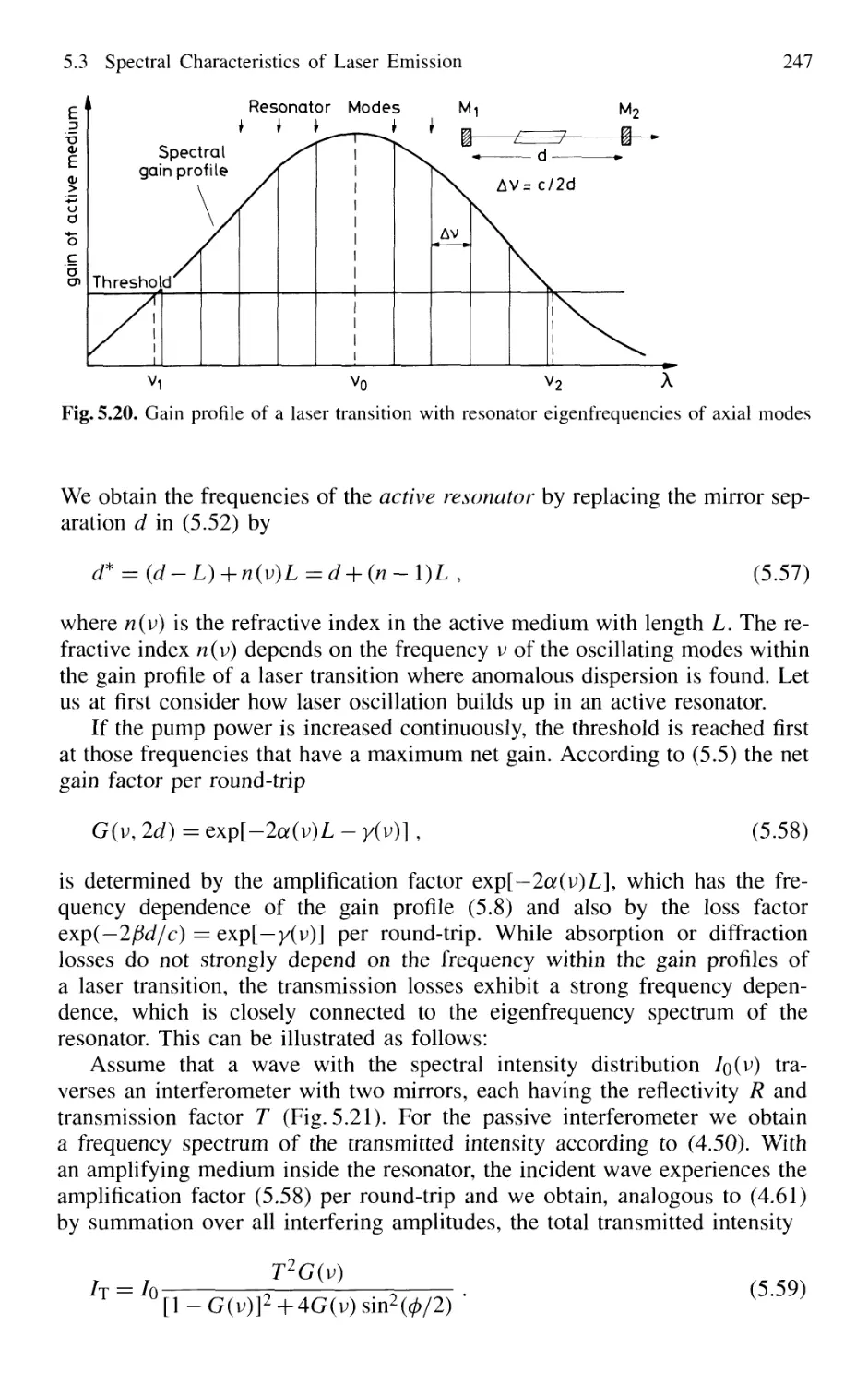
5.2.8 Frequency Spectrum of Passive Resonators 243
5.3 Spectral Characteristics of Laser Emission 246
5.3.1 Active Resonators and Laser Modes 246
5.3.2 Gain Saturation 249
5.3.3 Spatial Hole Burning 251
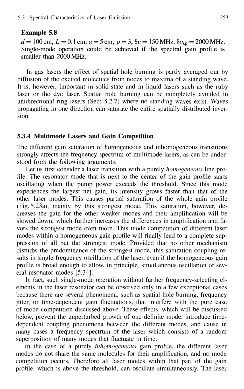
5.3.4 Multimode Lasers and Gain Competition 253
5.3.5 Mode Pulling 256
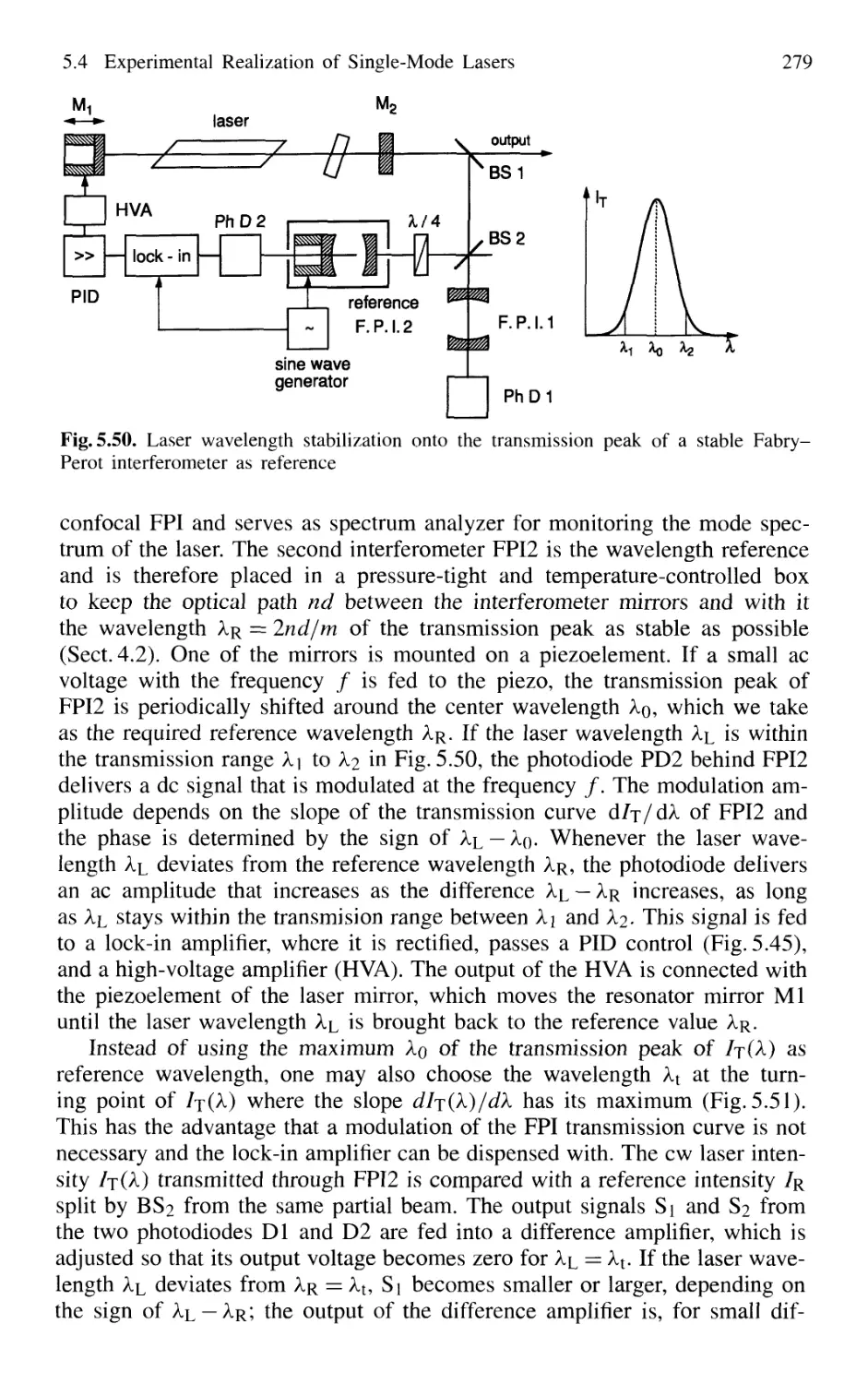
5.4 Experimental Realization of Single-Mode Lasers 258
5.4.1 Line Selection 258
5.4.2 Suppression of Transverse Modes 262
5.4.3 Selection of Single Longitudinal Modes 264
5.4.4 Intensity Stabilization 271
5.4.5 Wavelength Stabilization 274
5.5 Controlled Wavelength Tuning of Single-Mode Lasers 284
5.5.1 Continuous Tuning Techniques 285
5.5.2 Wavelength Calibration 288
5.6 Linewidths of Single-Mode Lasers 291
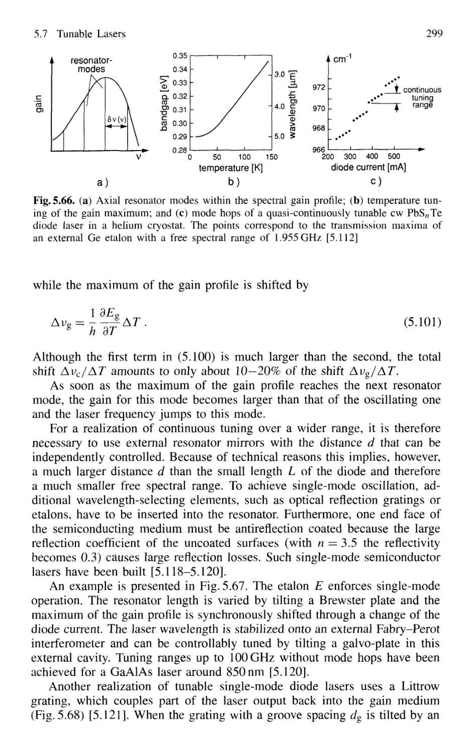
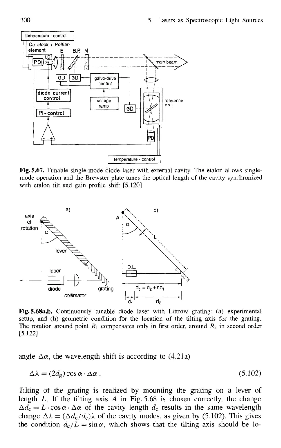
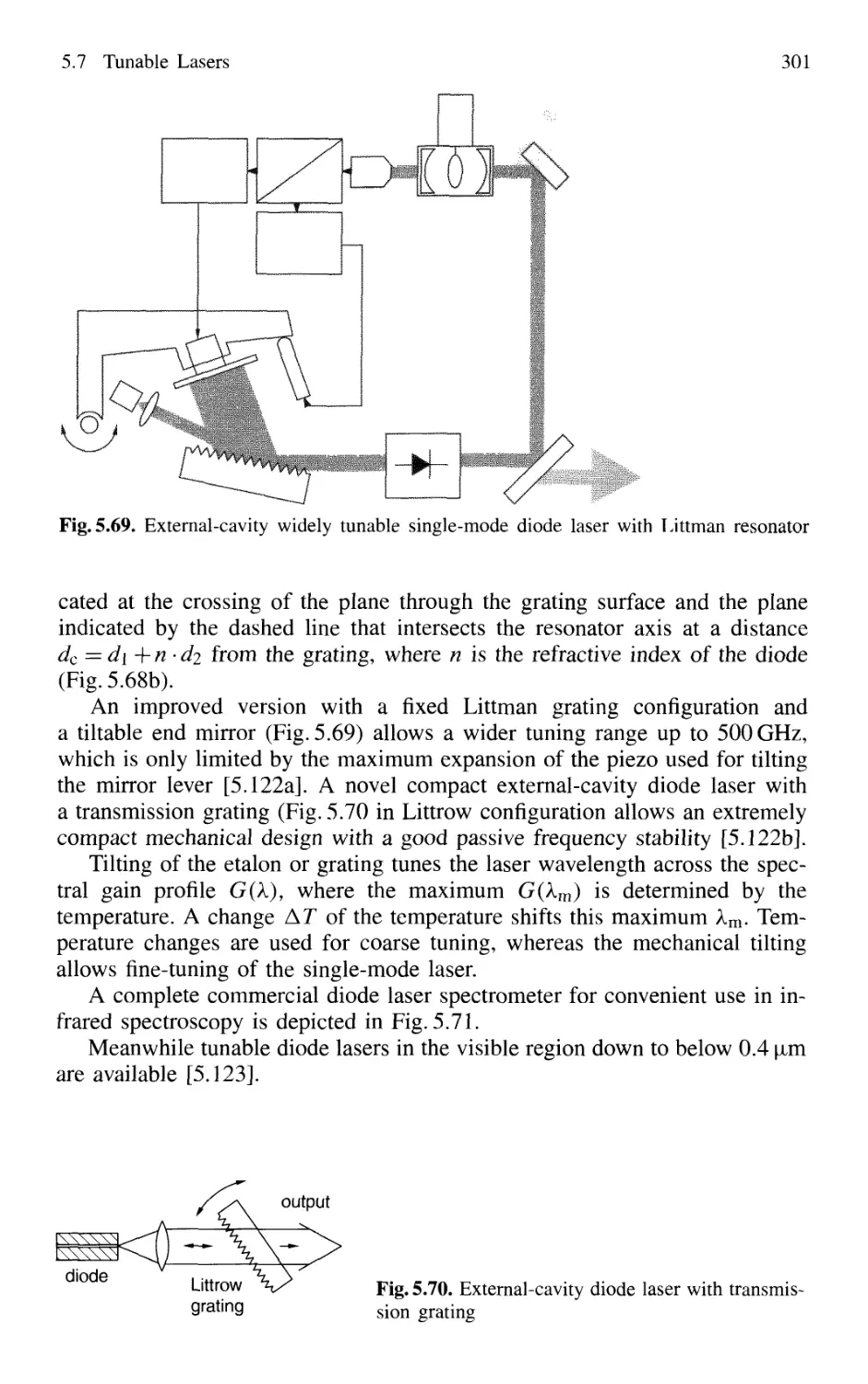
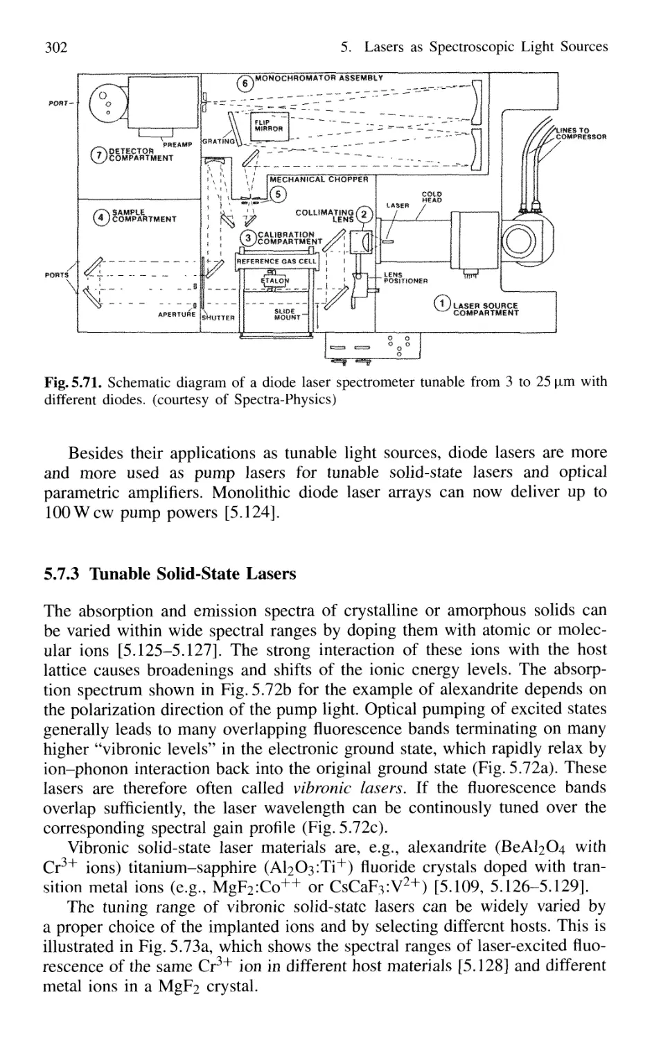
5.7 Tunable Lasers 294
5.7.1 Basic Concepts 295
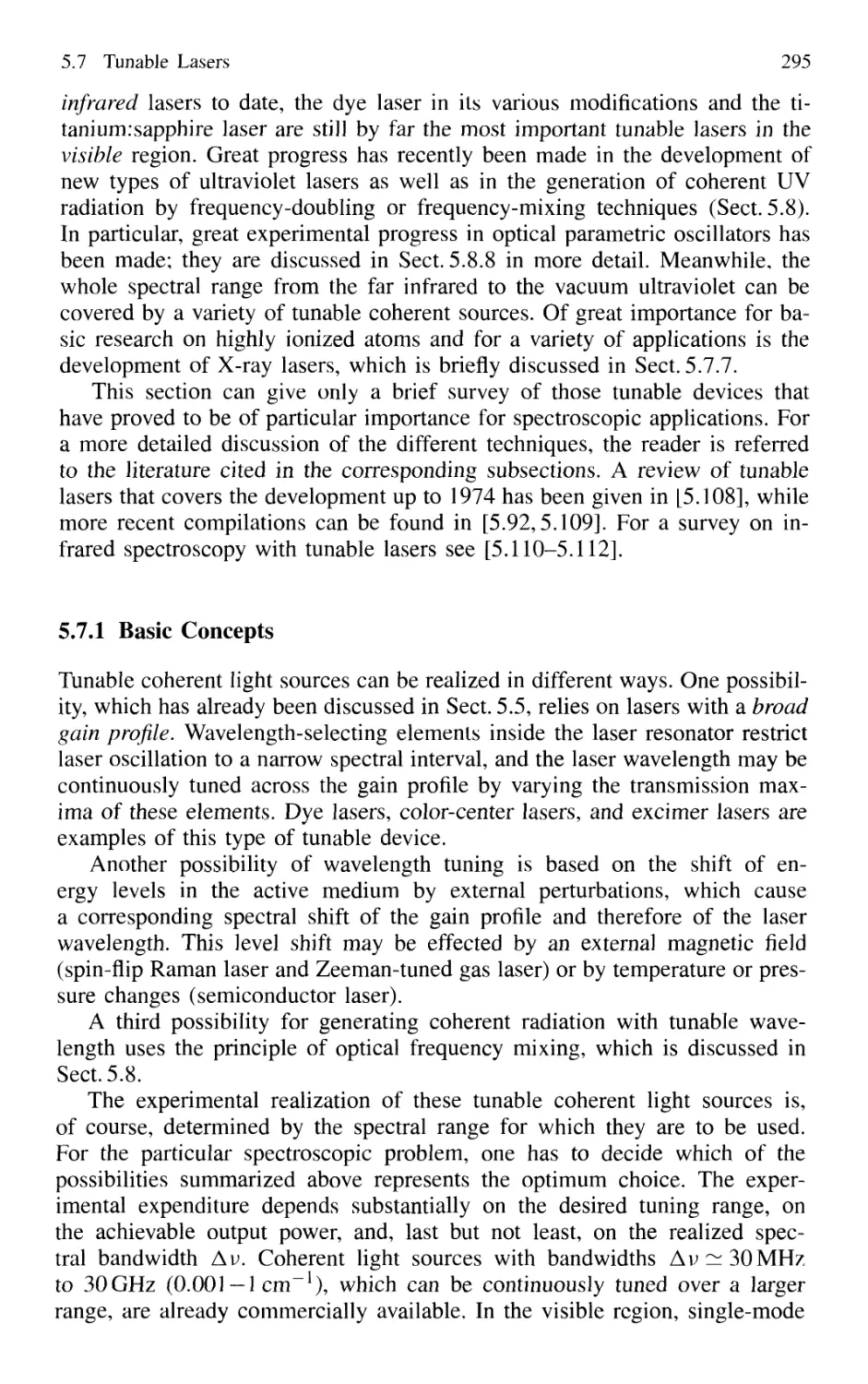
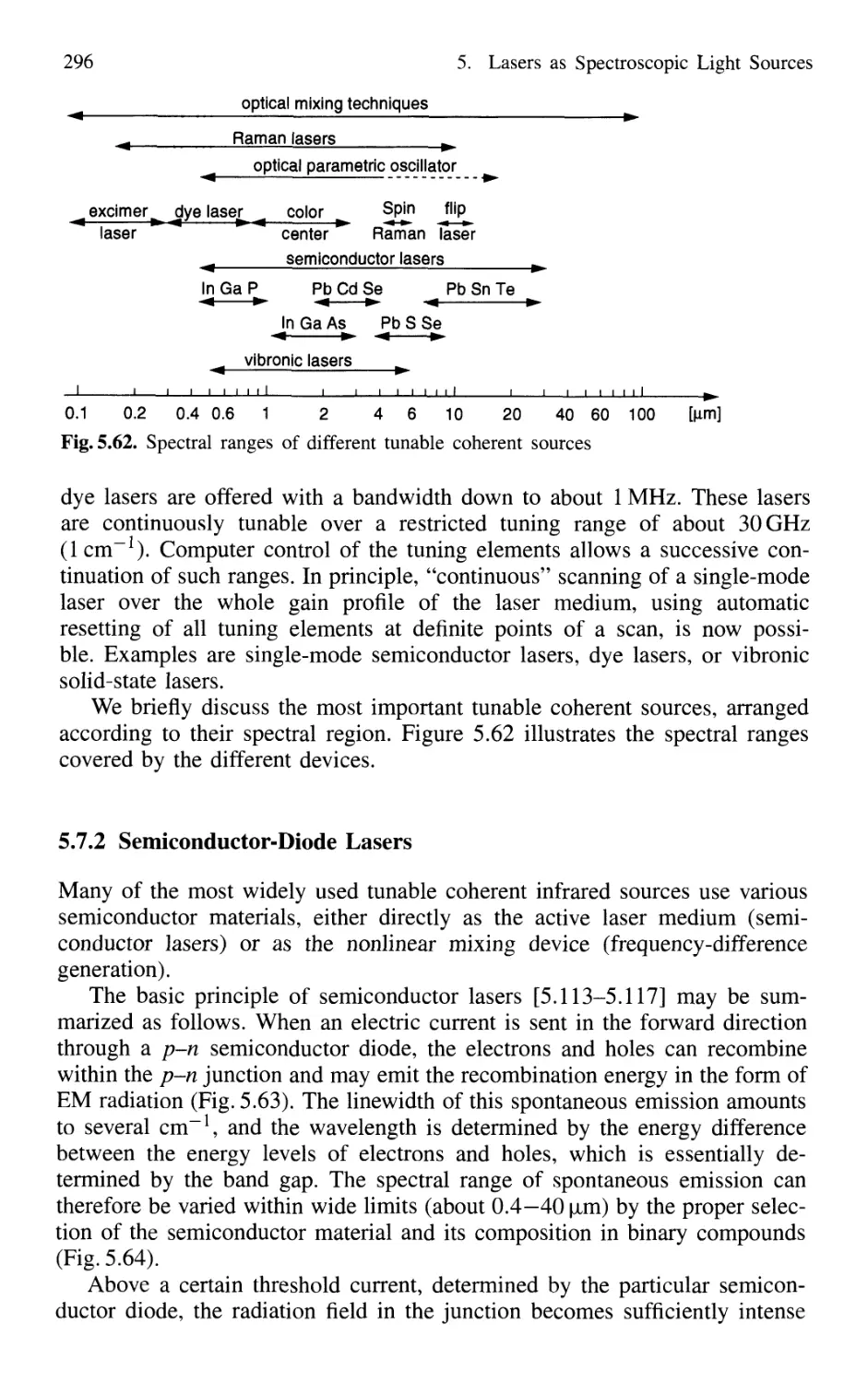
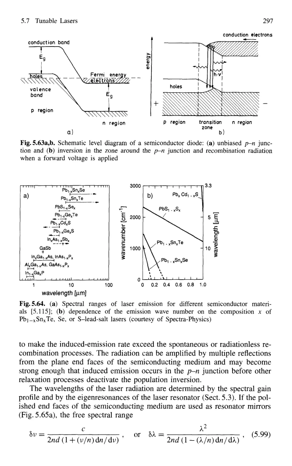
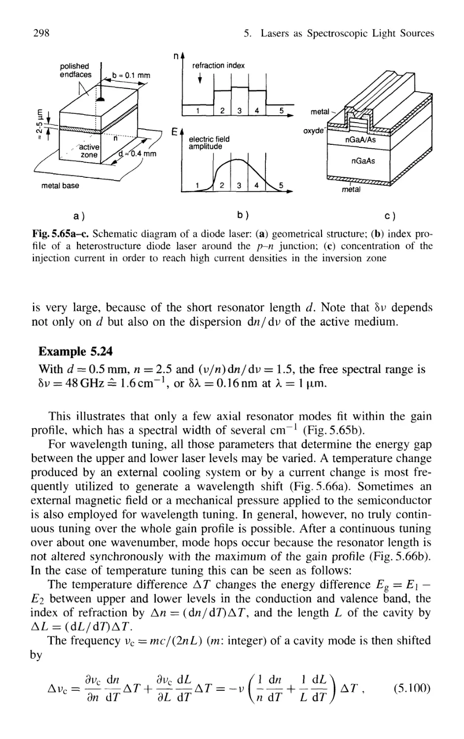
5.7.2 Semiconductor-Diode Lasers 296
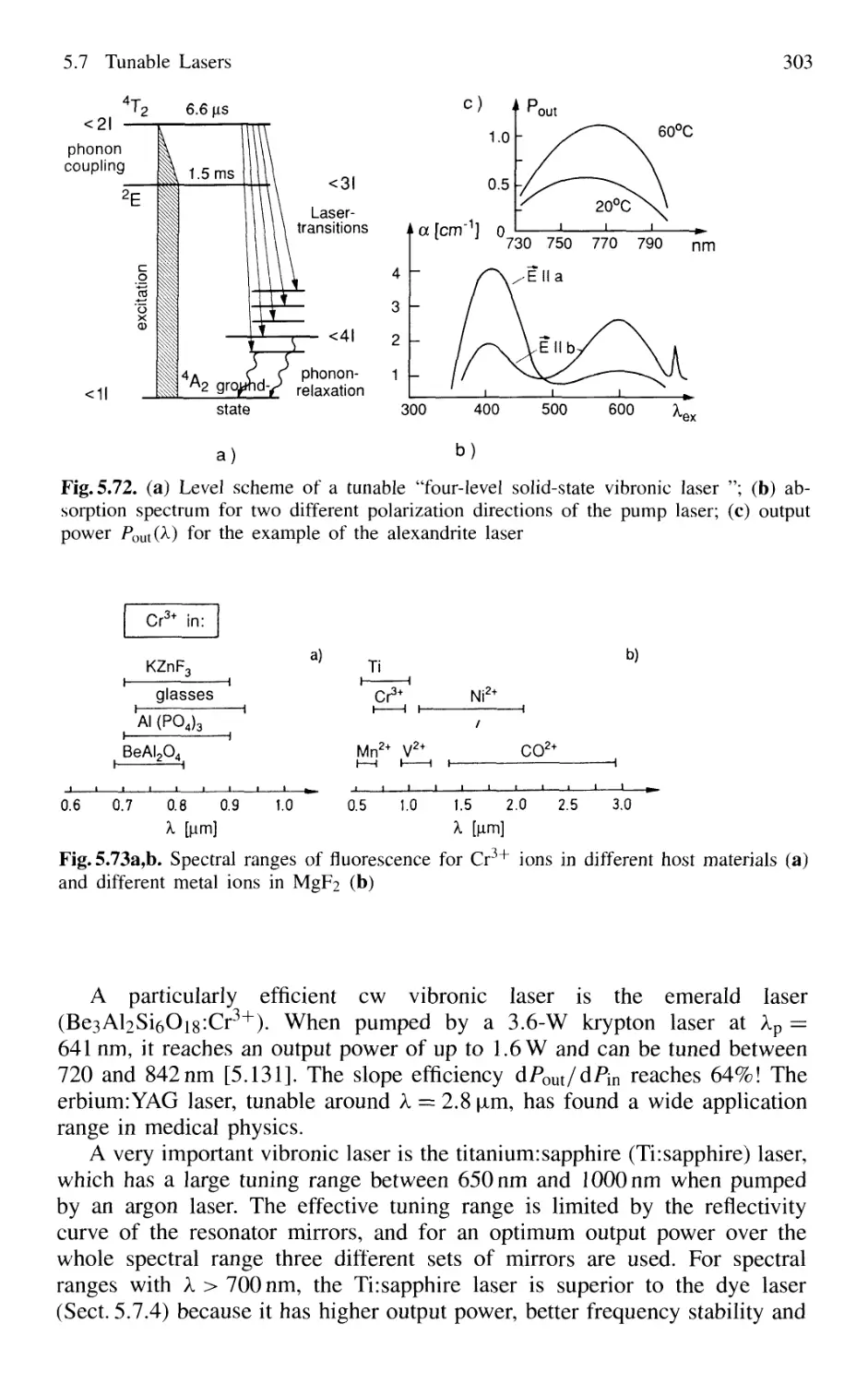
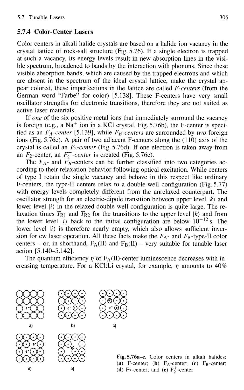
5.7.3 Tunable Solid-State Lasers 302
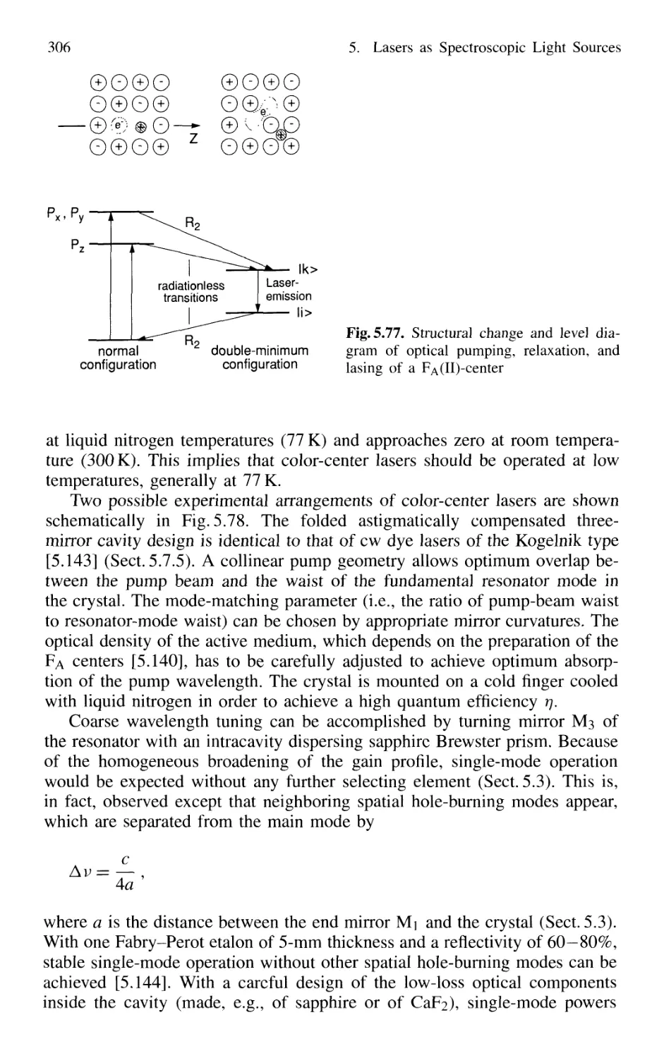
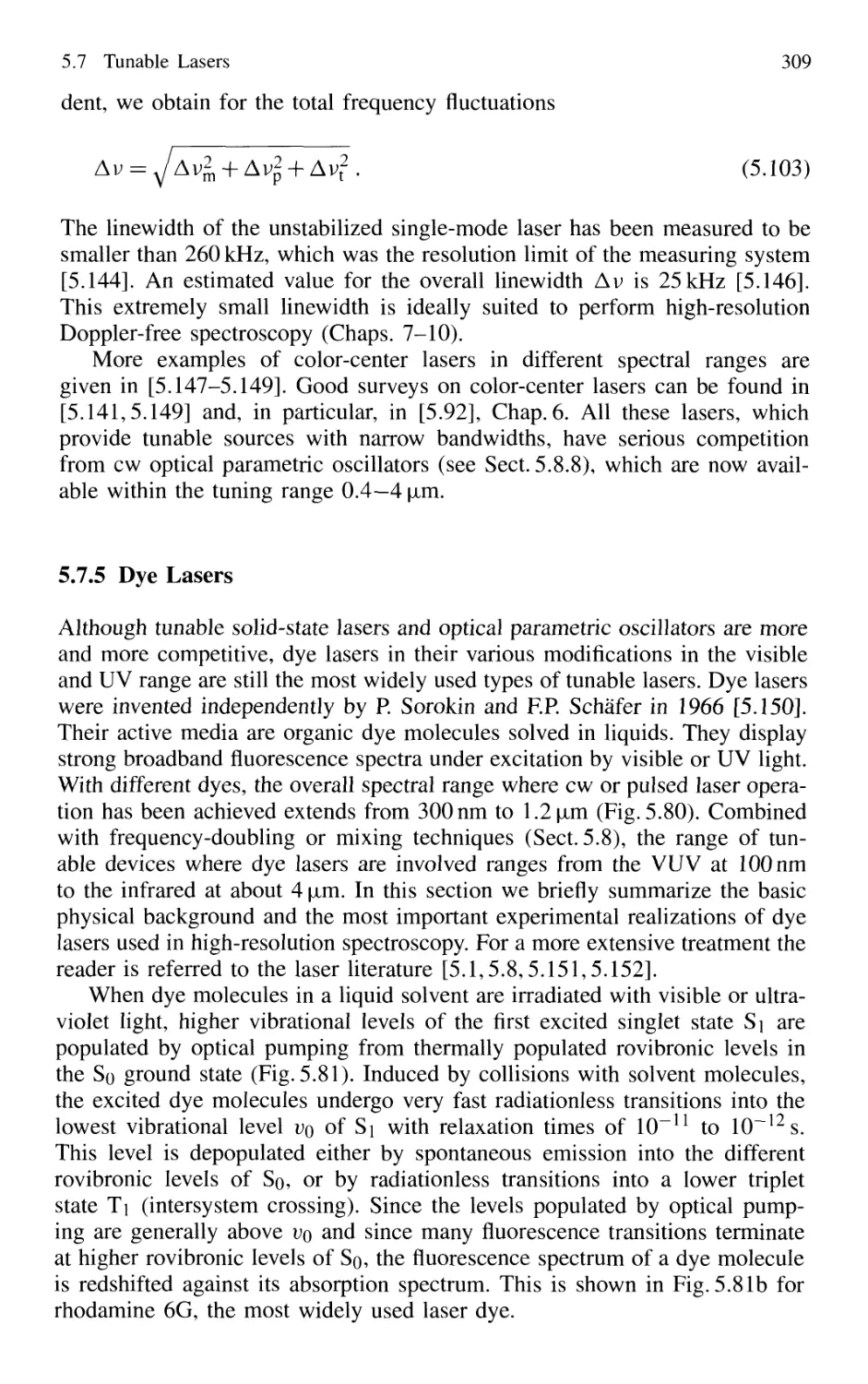
5.7.4 Color-Center Lasers 304
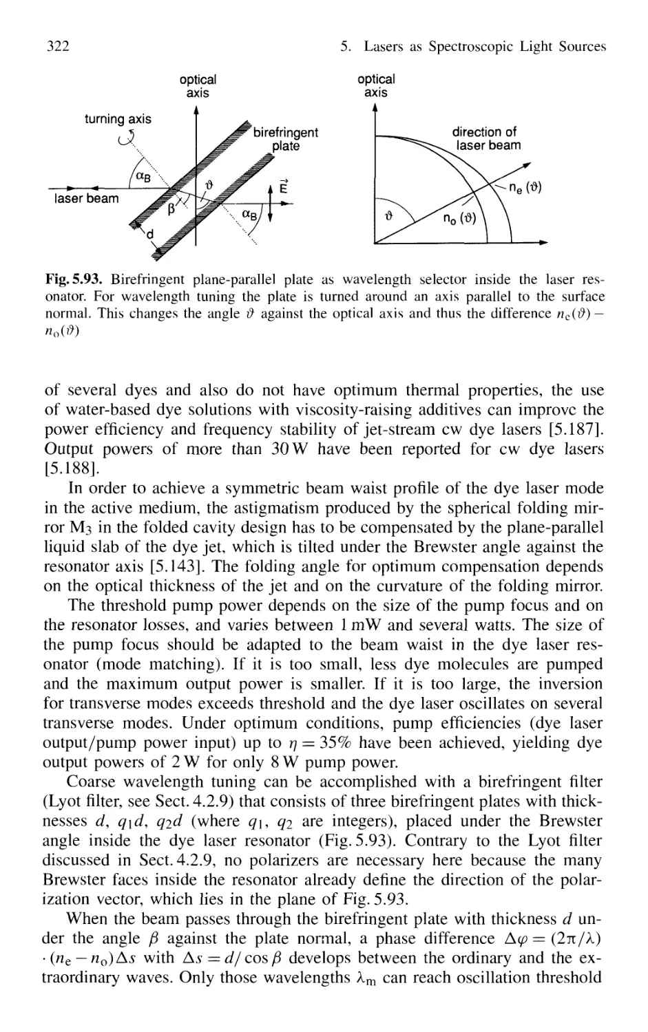
5.7.5 Dye Lasers 309
5.7.6 Excimer Lasers 325
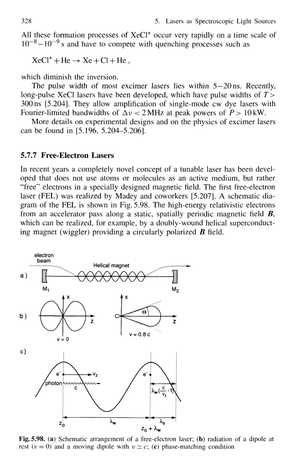
5.7.7 Free-Electron Lasers 328
5.8 Nonlinear Optical Mixing Techniques 331
5.8.1 Physical Background 331
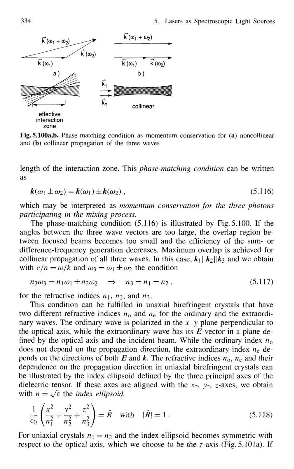
5.8.2 Phase Matching 333
5.8.3 Second-Harmonic Generation 335
5.8.4 Quasi Phase Matching 341
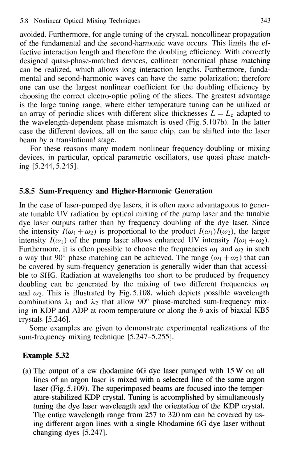
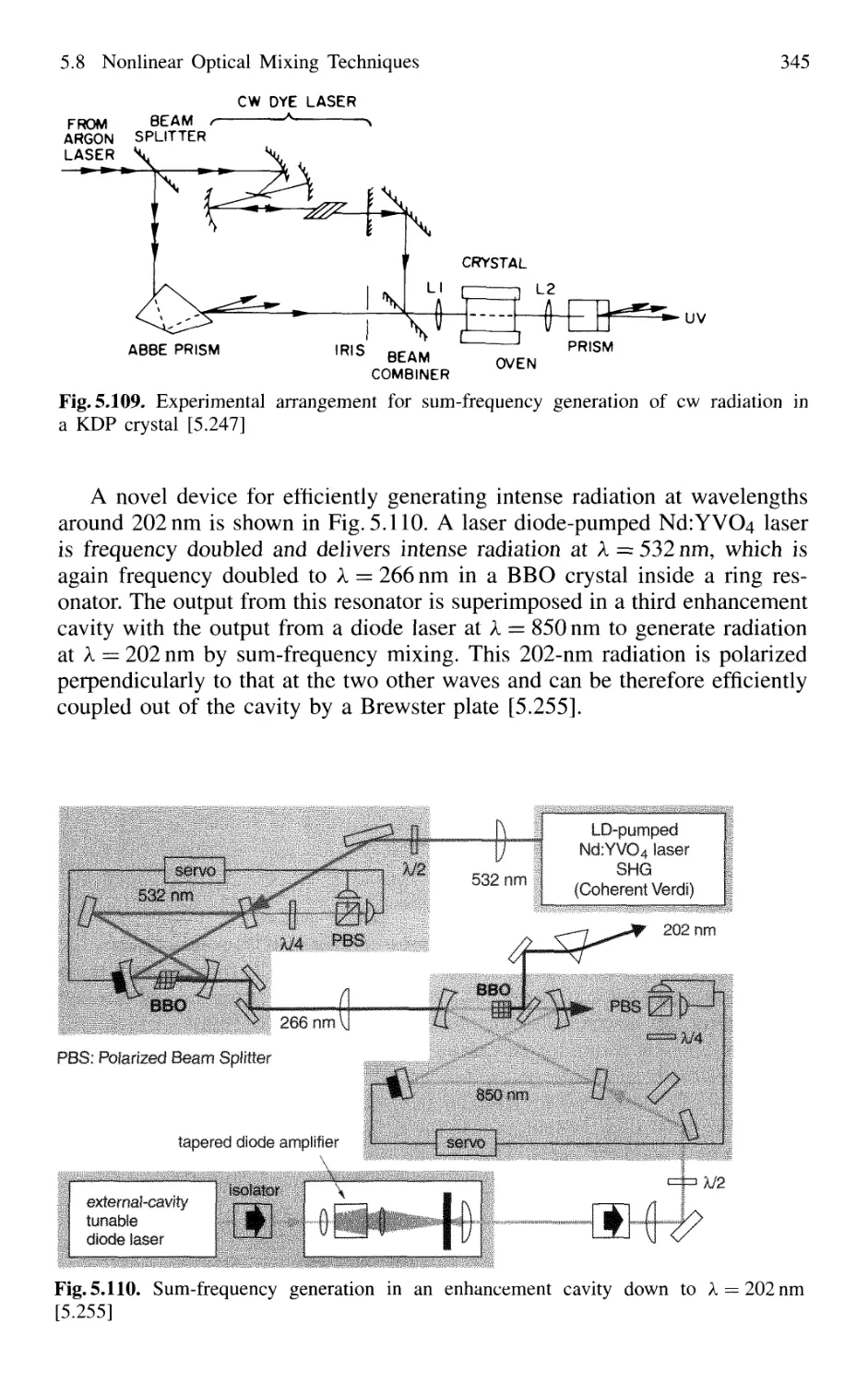
5.8.5 Sum-Frequency and Higher-Harmonic Generation . 343
5.8.6 X-Ray Lasers 348
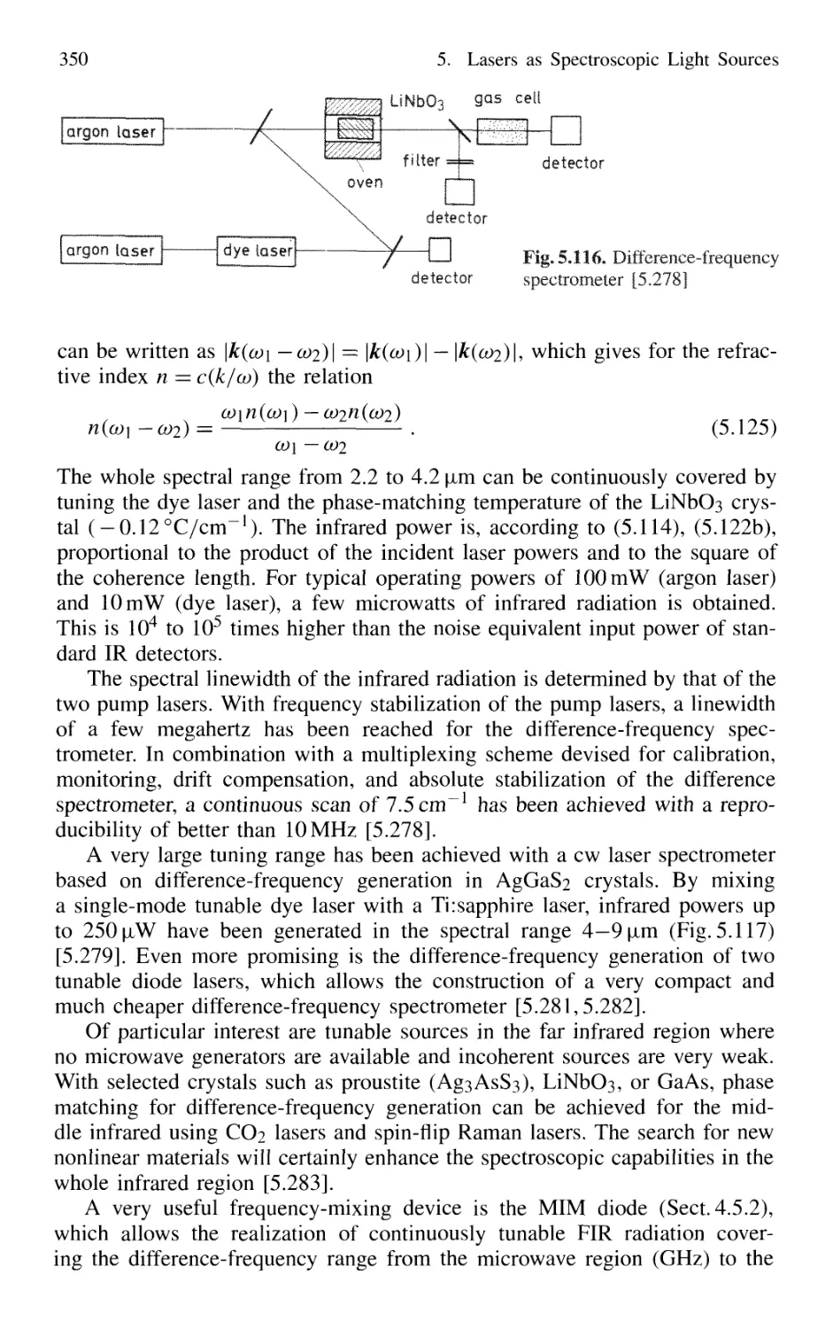
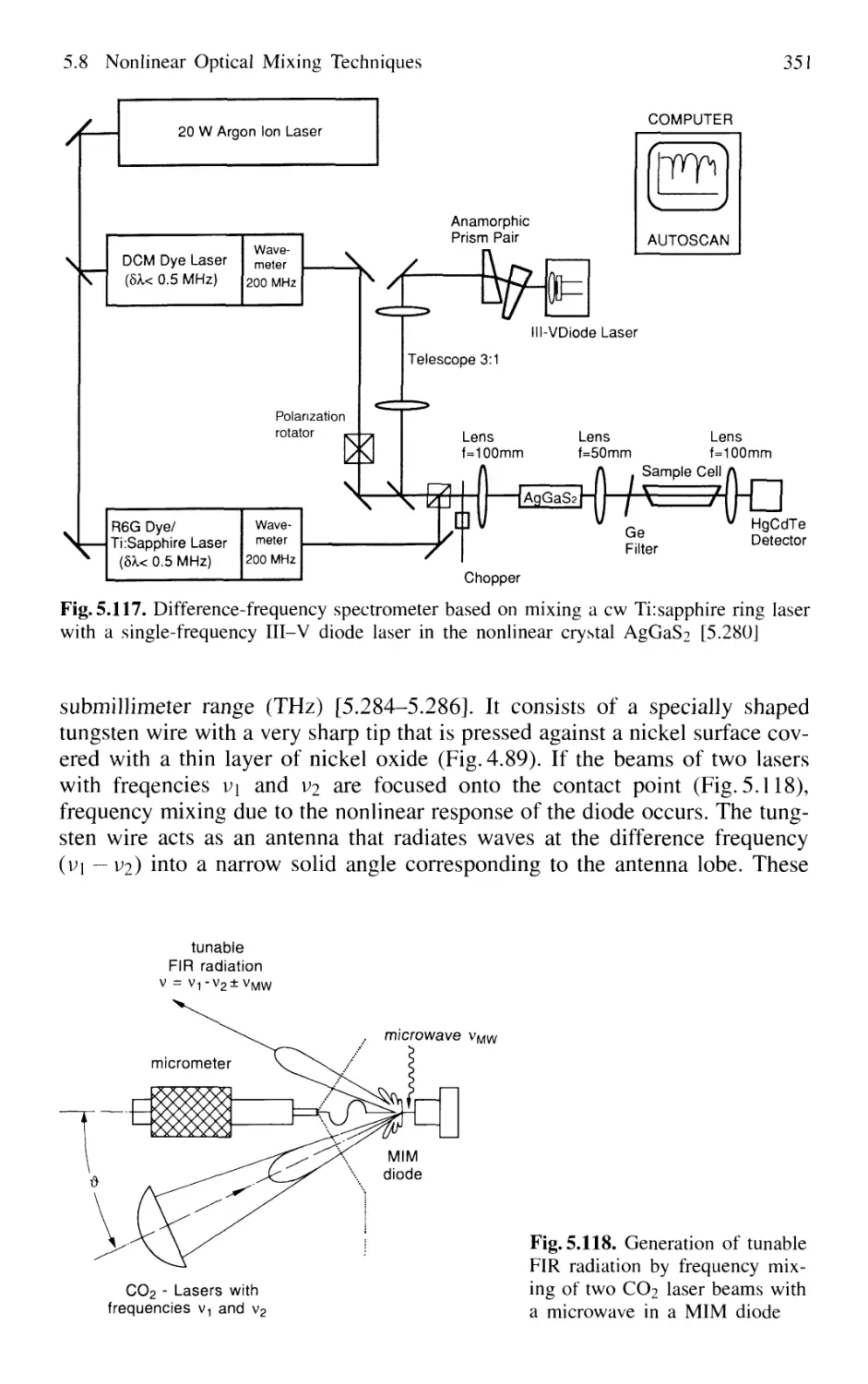
5.8.7 Difference-Frequency Spectrometer 349
XIV Contents
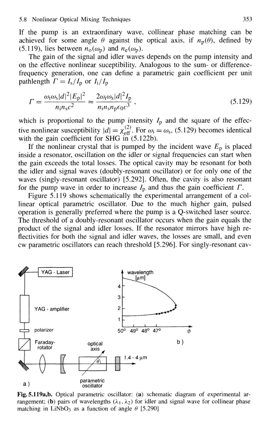
5.8.8 Optical Parametric Oscillator 352
5.8.9 Tunable Raman Lasers 356
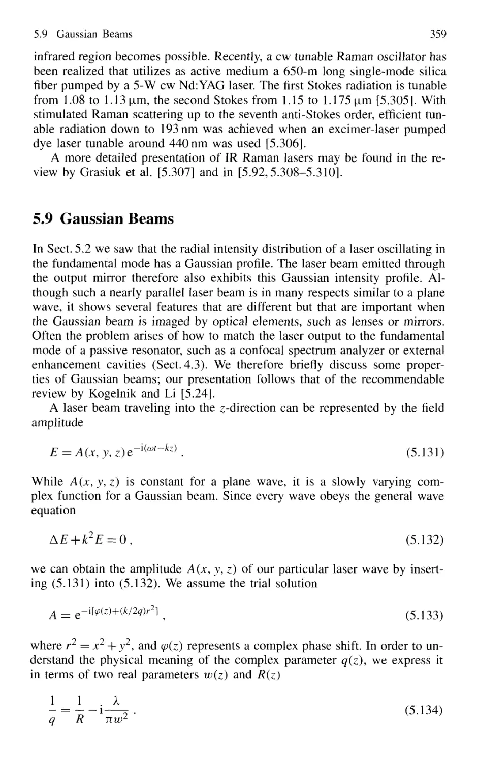
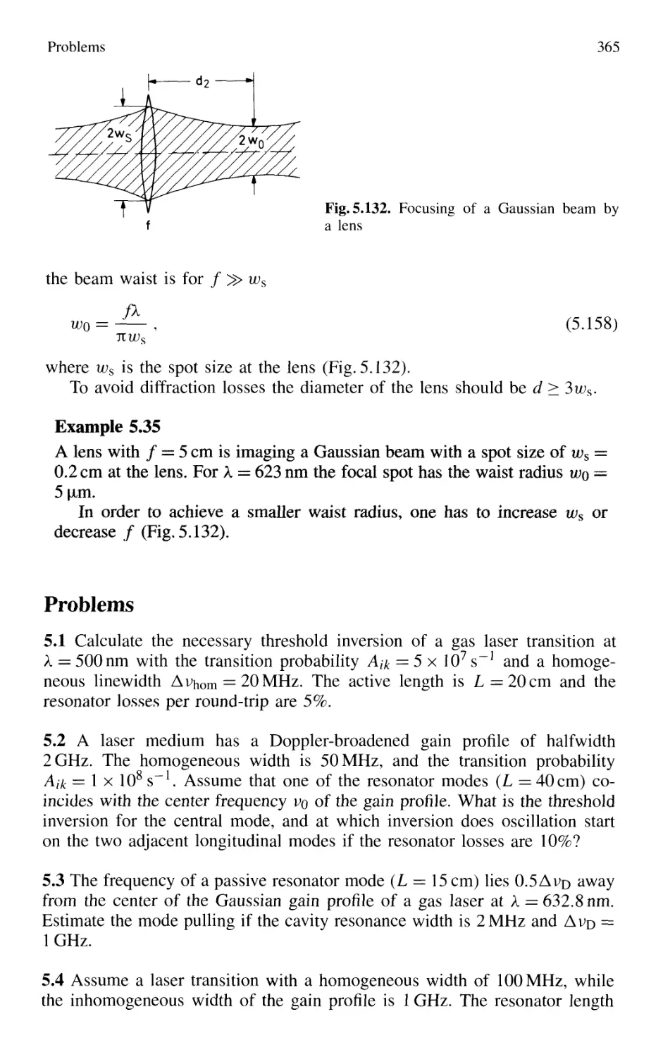
5.9 Gaussian Beams 359
Problems 365
6. Doppler-Limited Absorption and Fluorescence Spectroscopy
with Lasers 369
6.1 Advantages of Lasers in Spectroscopy 369
6.2 High-Sensitivity Methods of Absorption Spectroscopy 373
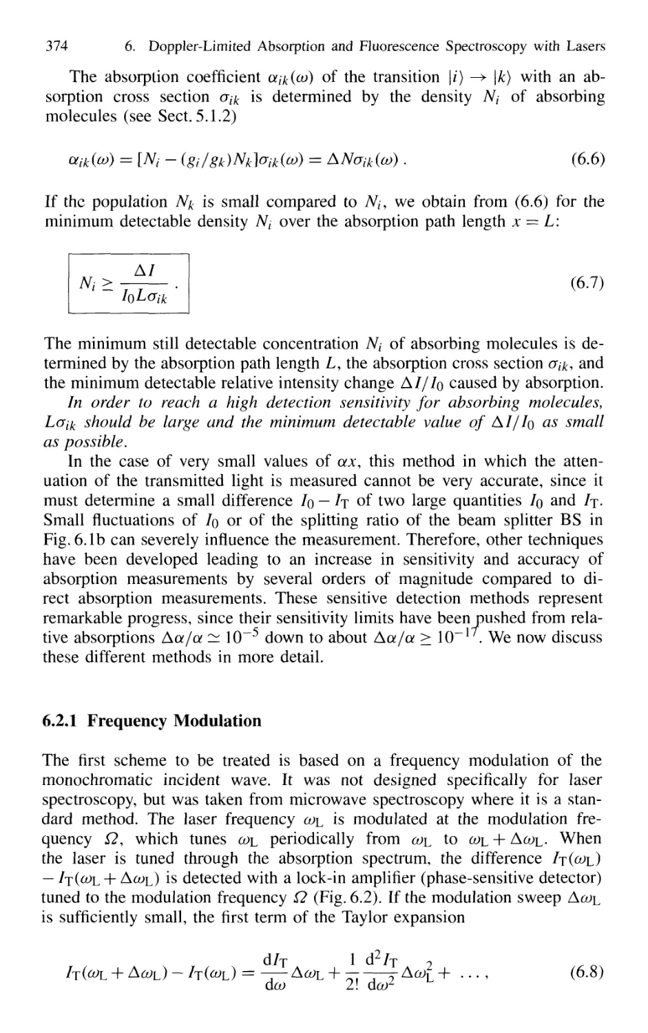
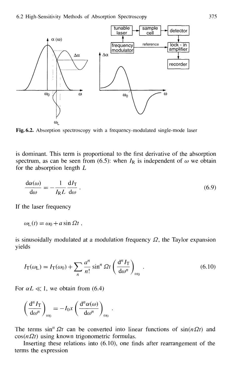
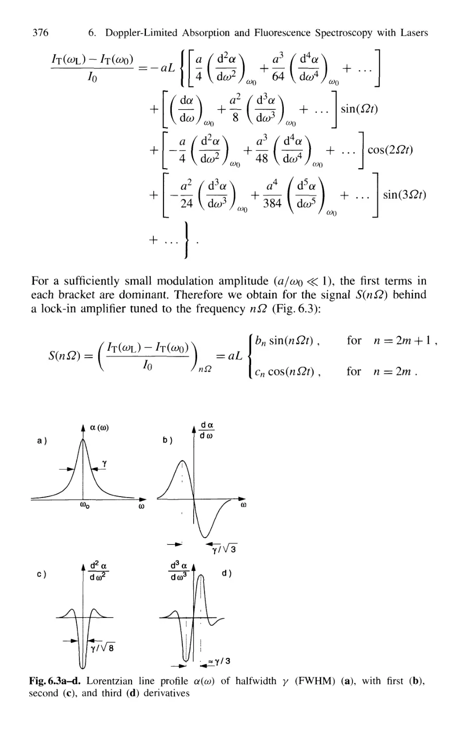
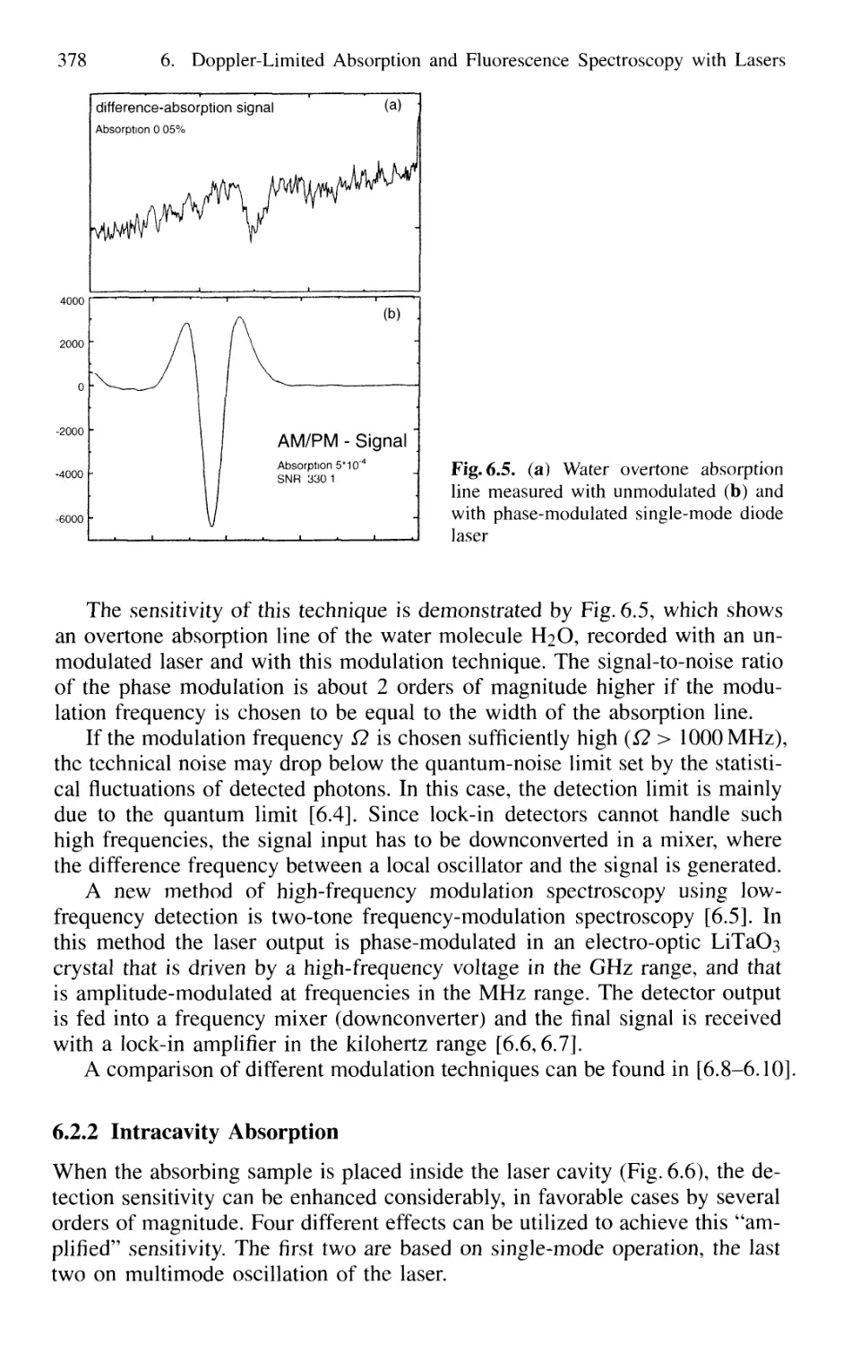
6.2.1 Frequency Modulation 374
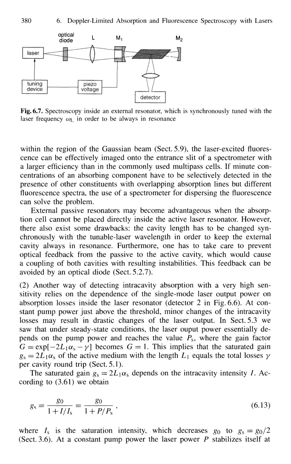
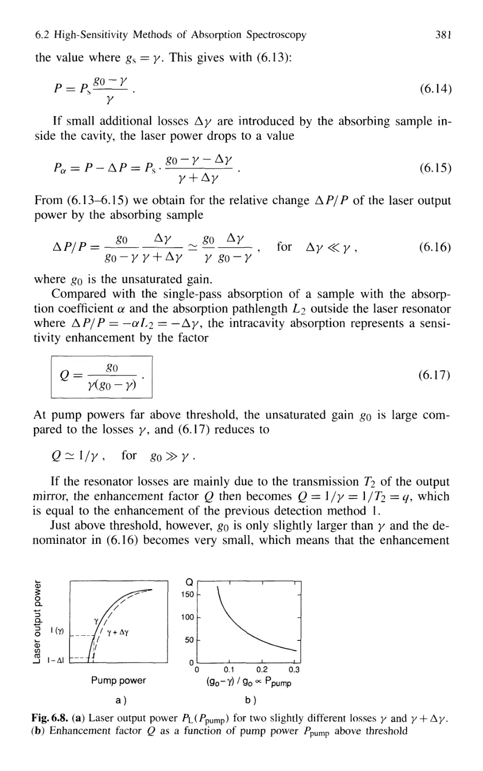
6.2.2 Intracavity Absorption 378
6.2.3 Cavity Ring-Down Spectroscopy (CRDS) 387
6.3 Direct Determination of Absorbed Photons 391
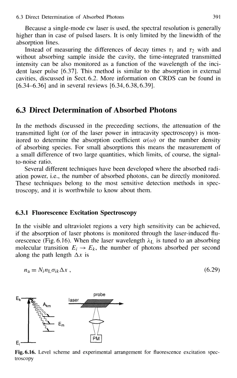
6.3.1 Fluorescence Excitation Spectroscopy 391
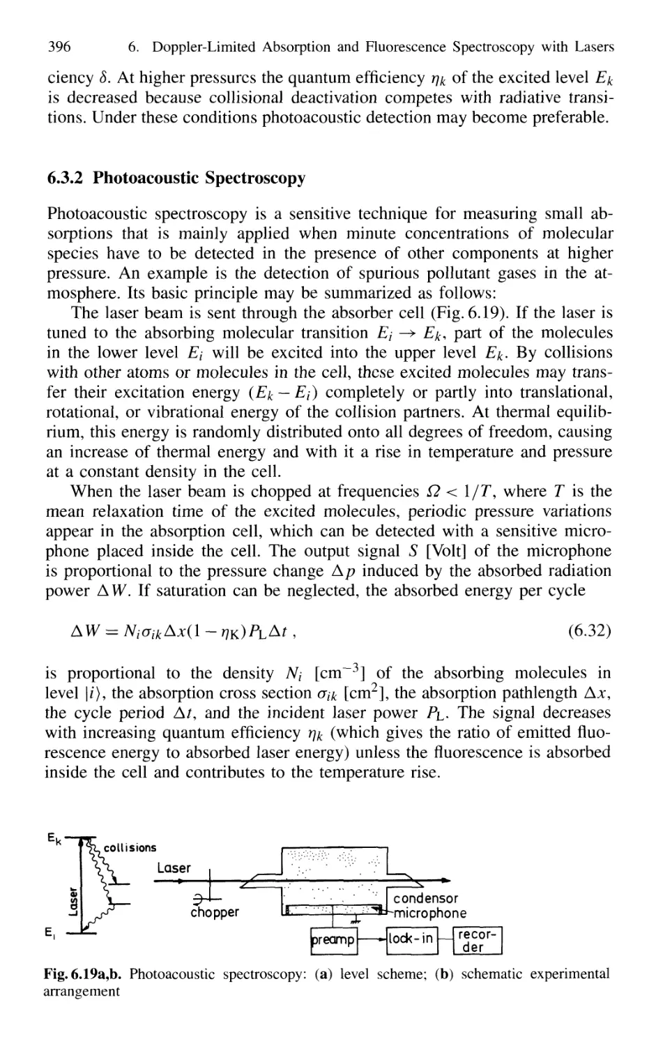
6.3.2 Photoacoustic Spectroscopy 396
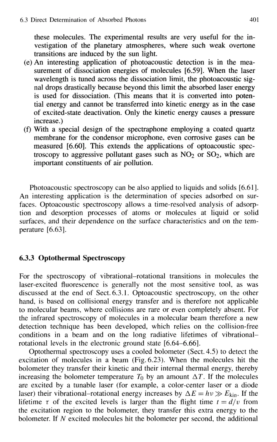
6.3.3 Optothermal Spectroscopy 401
6.4 Ionization Spectroscopy 405
6.4.1 Basic Techniques 405
6.4.2 Sensitivity of Ionization Spectroscopy 407
6.4.3 Pulsed Versus CW Lasers for Photoionization 408
6.4.4 Resonant Two-Photon Ionization Combined
with Mass Spectrometry 411
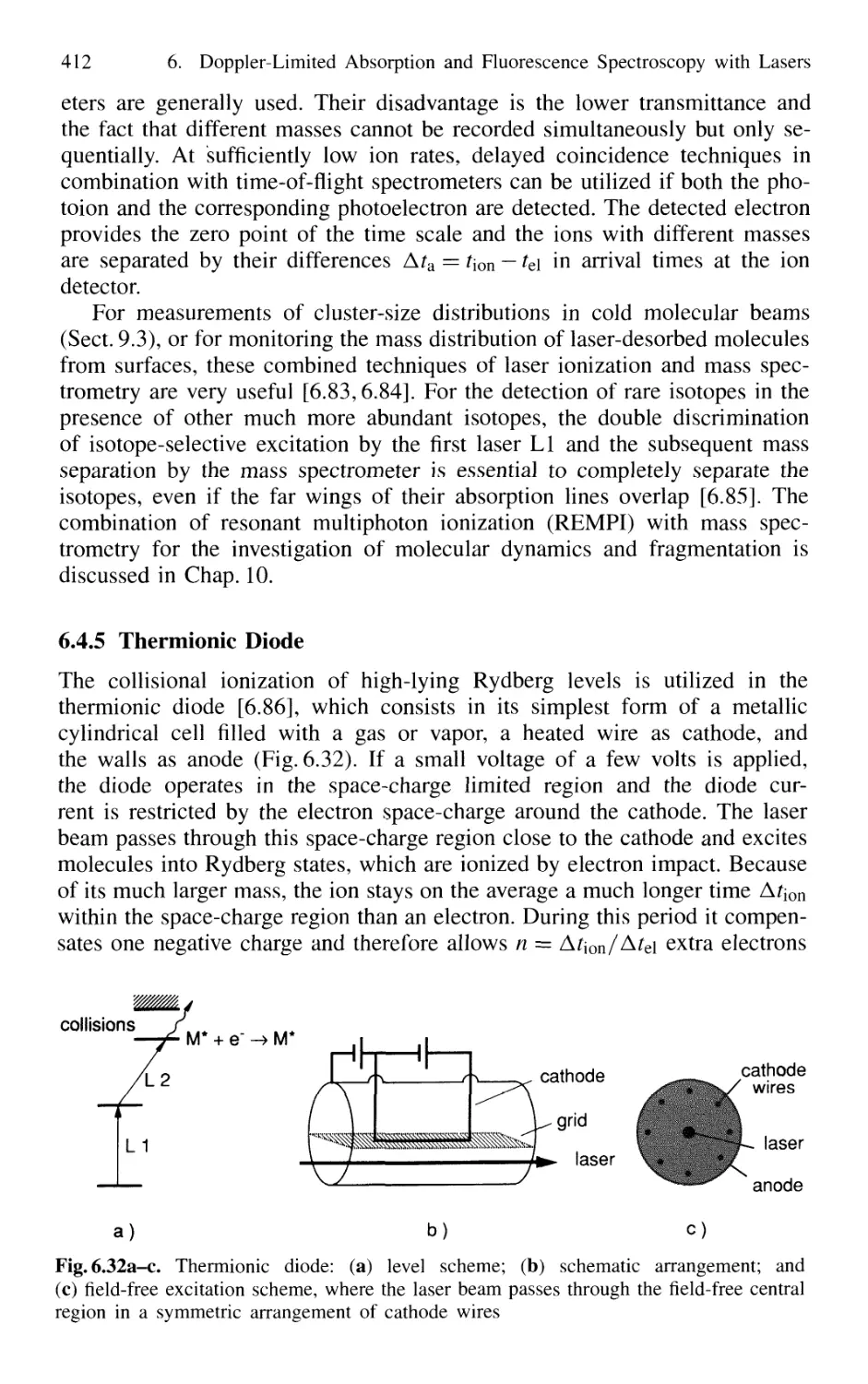
6.4.5 Thermionic Diode 412
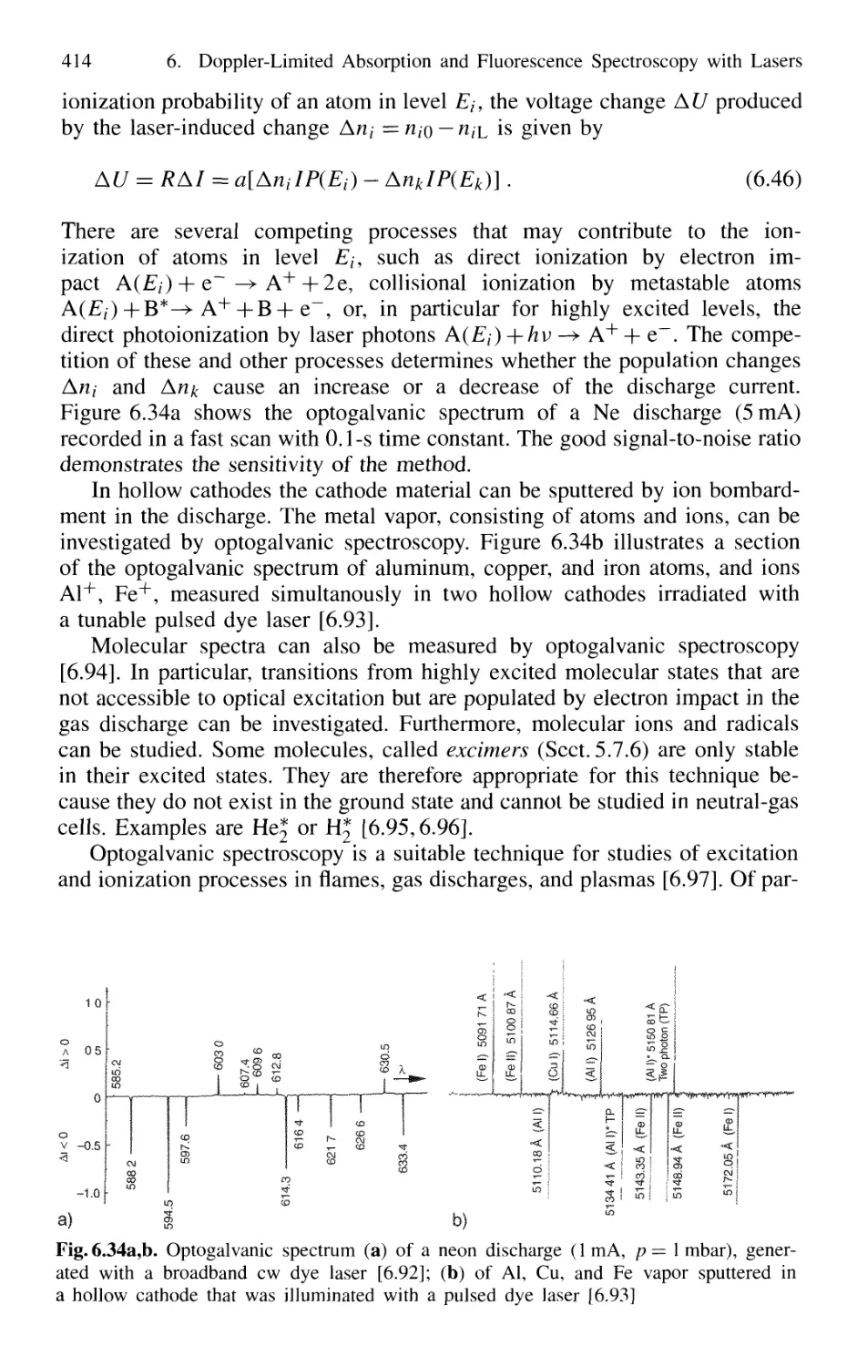
6.5 Optogalvanic Spectroscopy 413
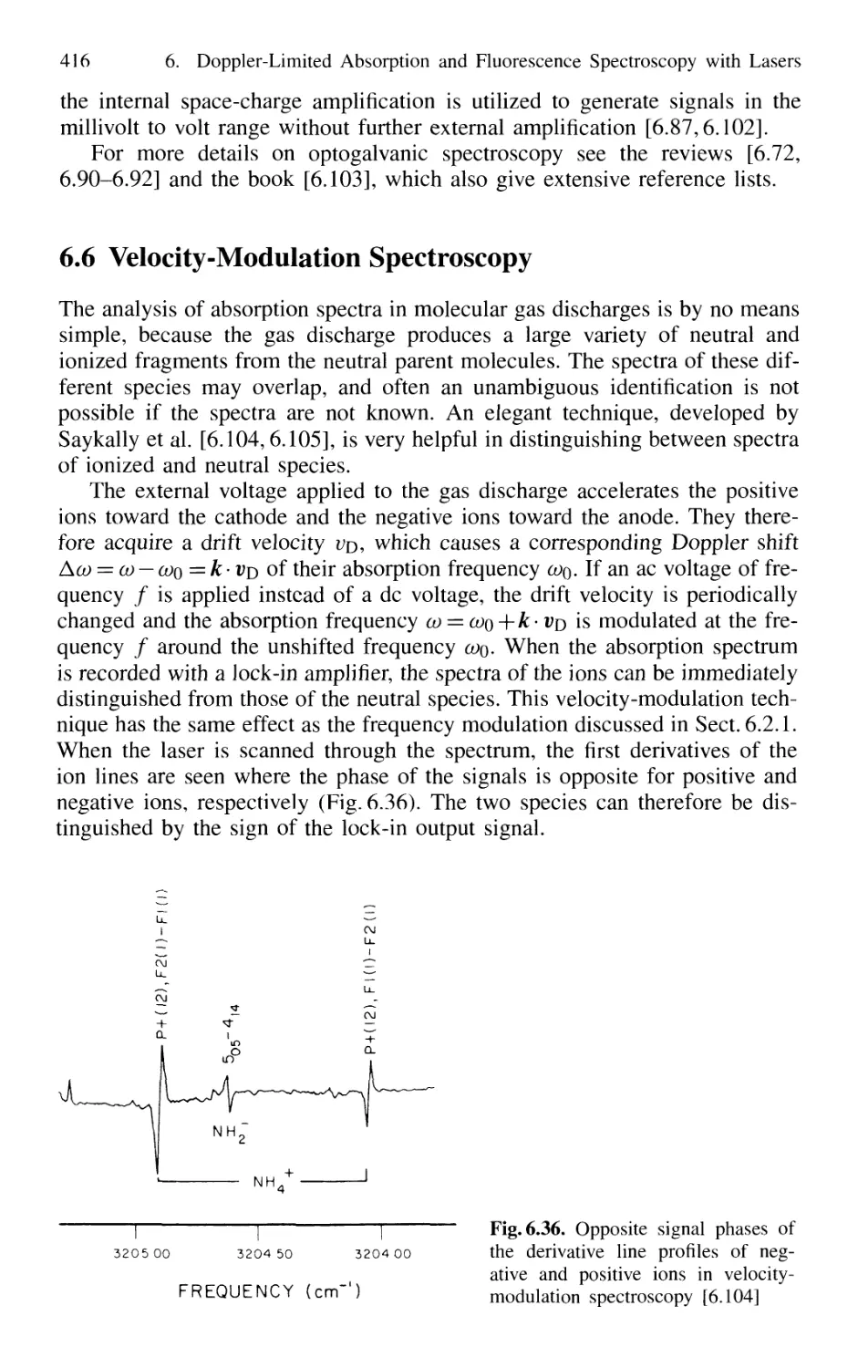
6.6 Velocity-Modulation Spectroscopy 416
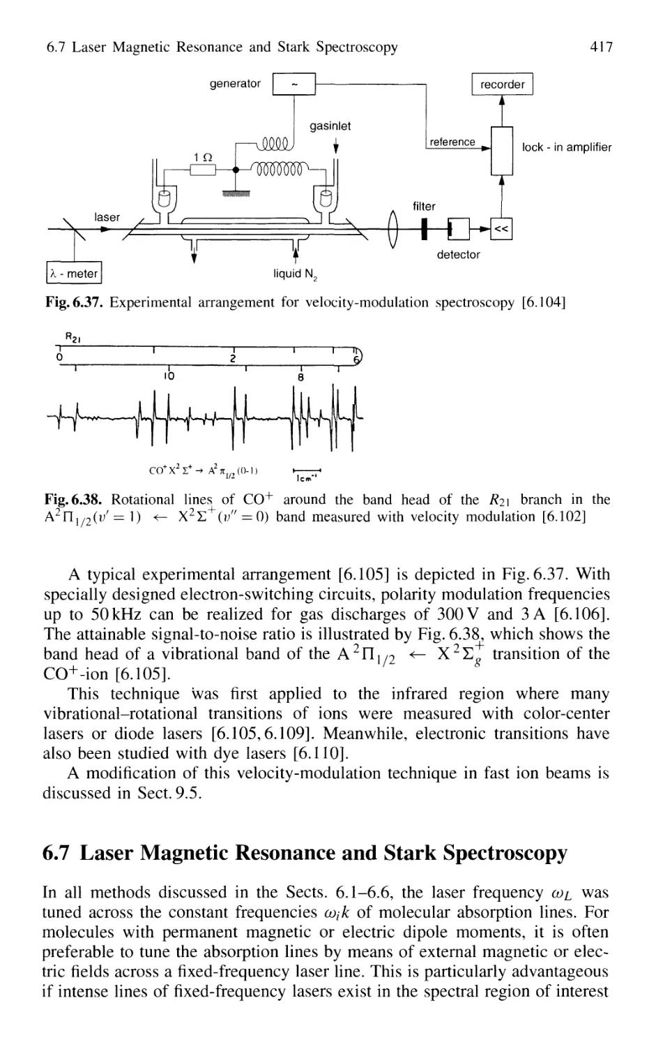
6.7 Laser Magnetic Resonance and Stark Spectroscopy 417
6.7.1 Laser Magnetic Resonance 418
6.7.2 Stark Spectroscopy 420
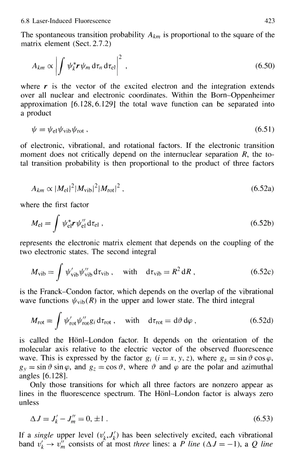
6.8 Laser-Induced Fluorescence 421
6.8.1 Molecular Spectroscopy
by Laser-Induced Fluorescence 422
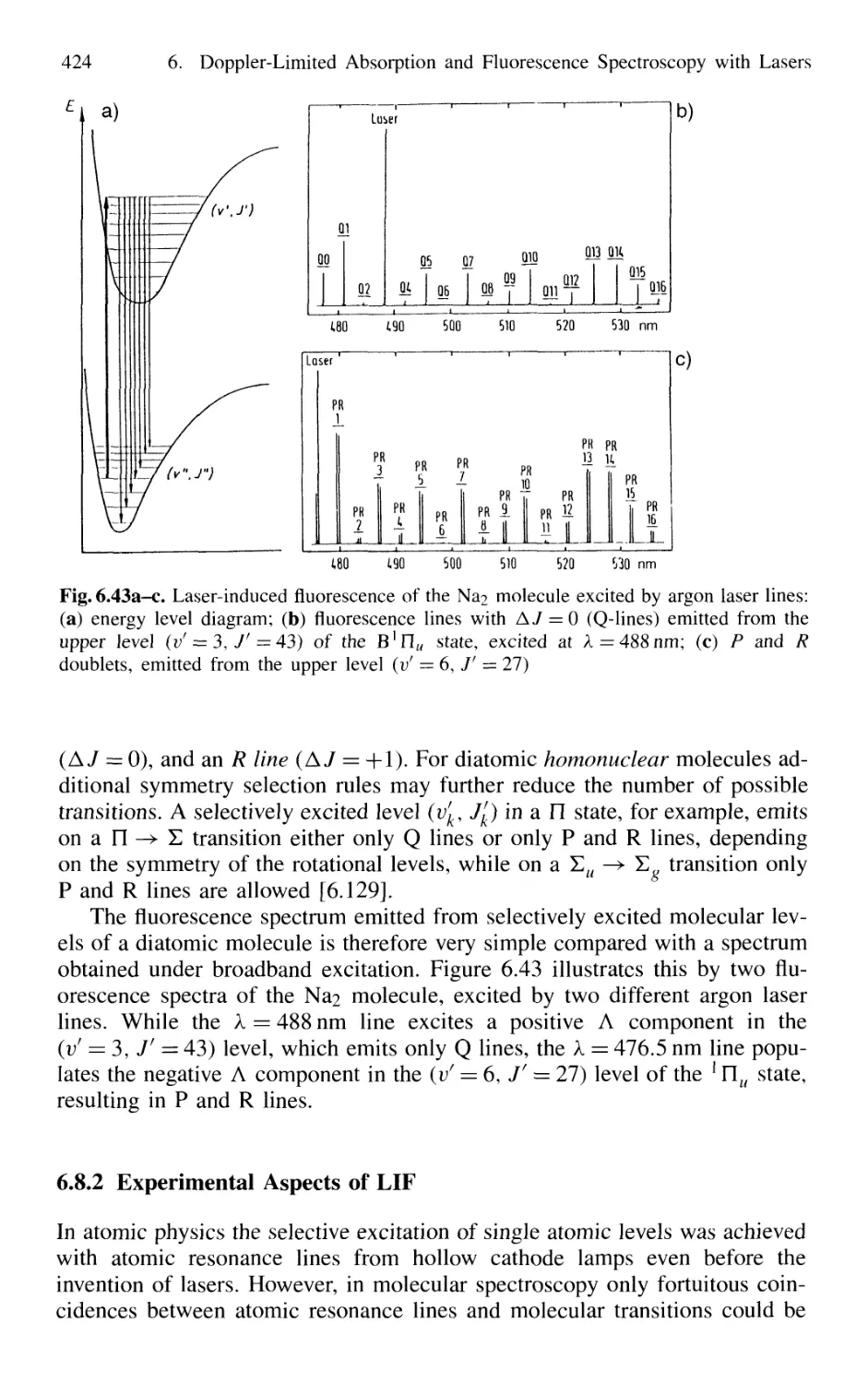
6.8.2 Experimental Aspects of LIF 424
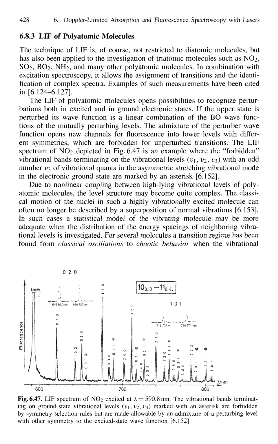
6.8.3 LIF of Polyatomic Molecules 428
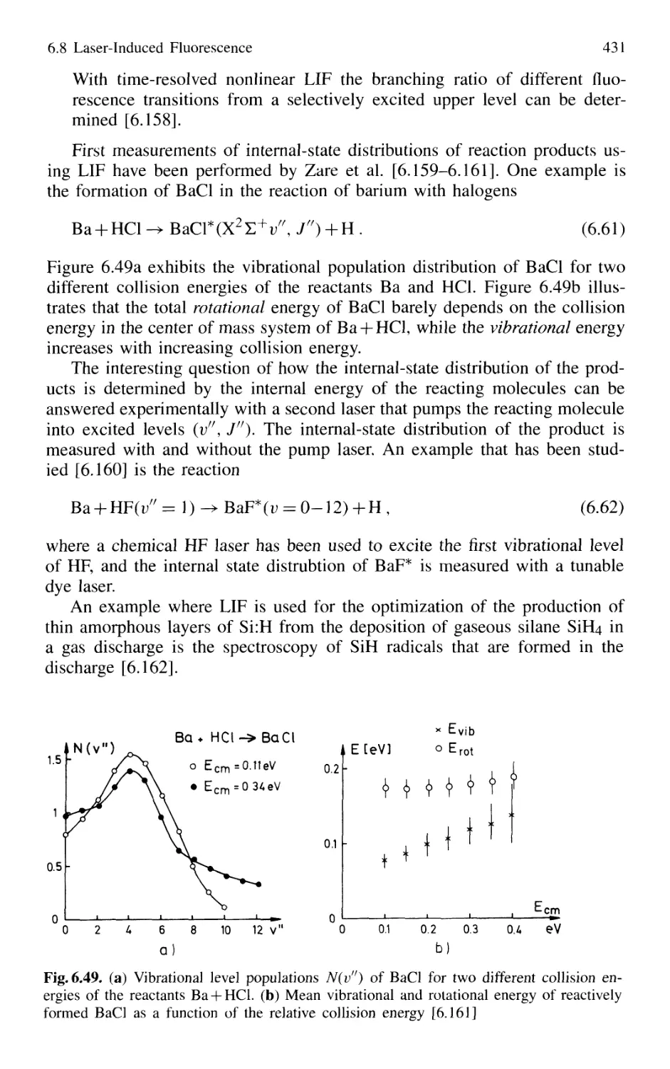
6.8.4 Determination of Population Distributions by LIF . 429
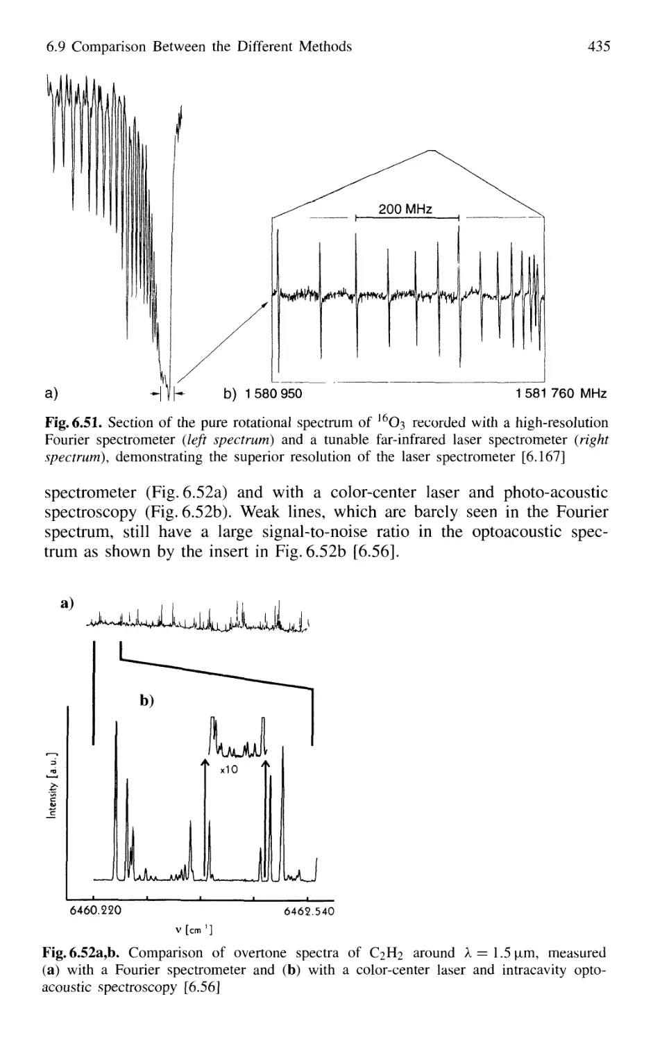
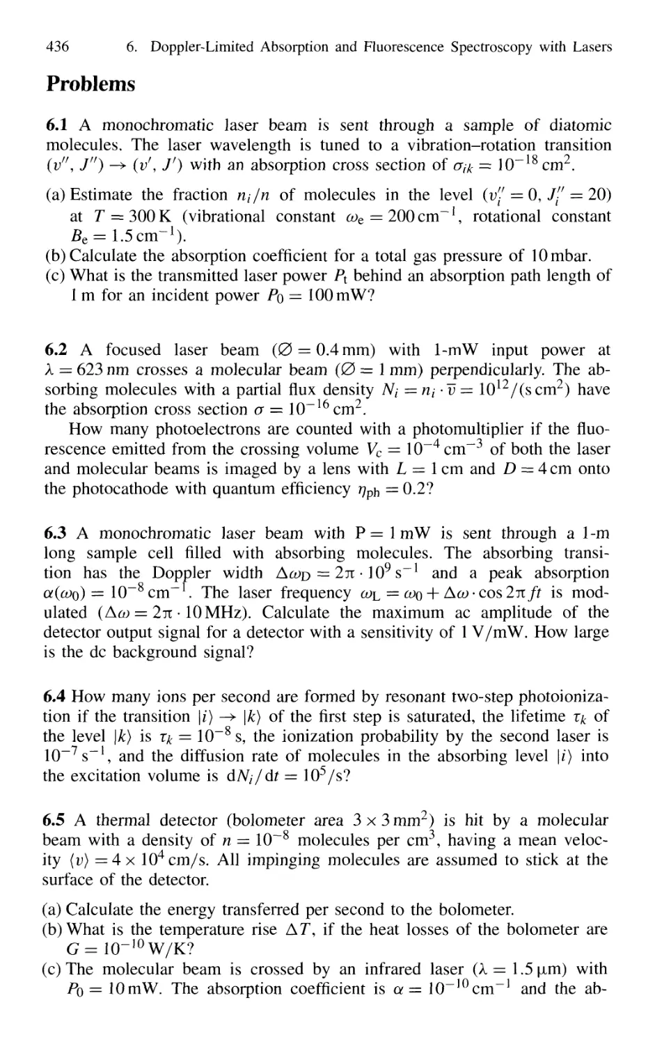
6.9 Comparison Between the Different Methods 432
Problems 436
7. Nonlinear Spectroscopy 439
7.1 Linear and Nonlinear Absorption 439
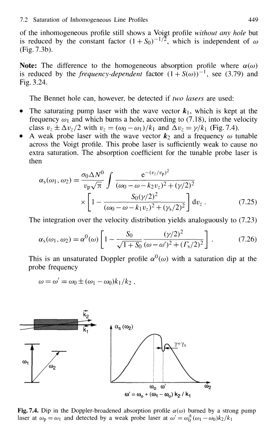
7.2 Saturation of Inhomogeneous Line Profiles 445
7.2.1 Hole Burning 446
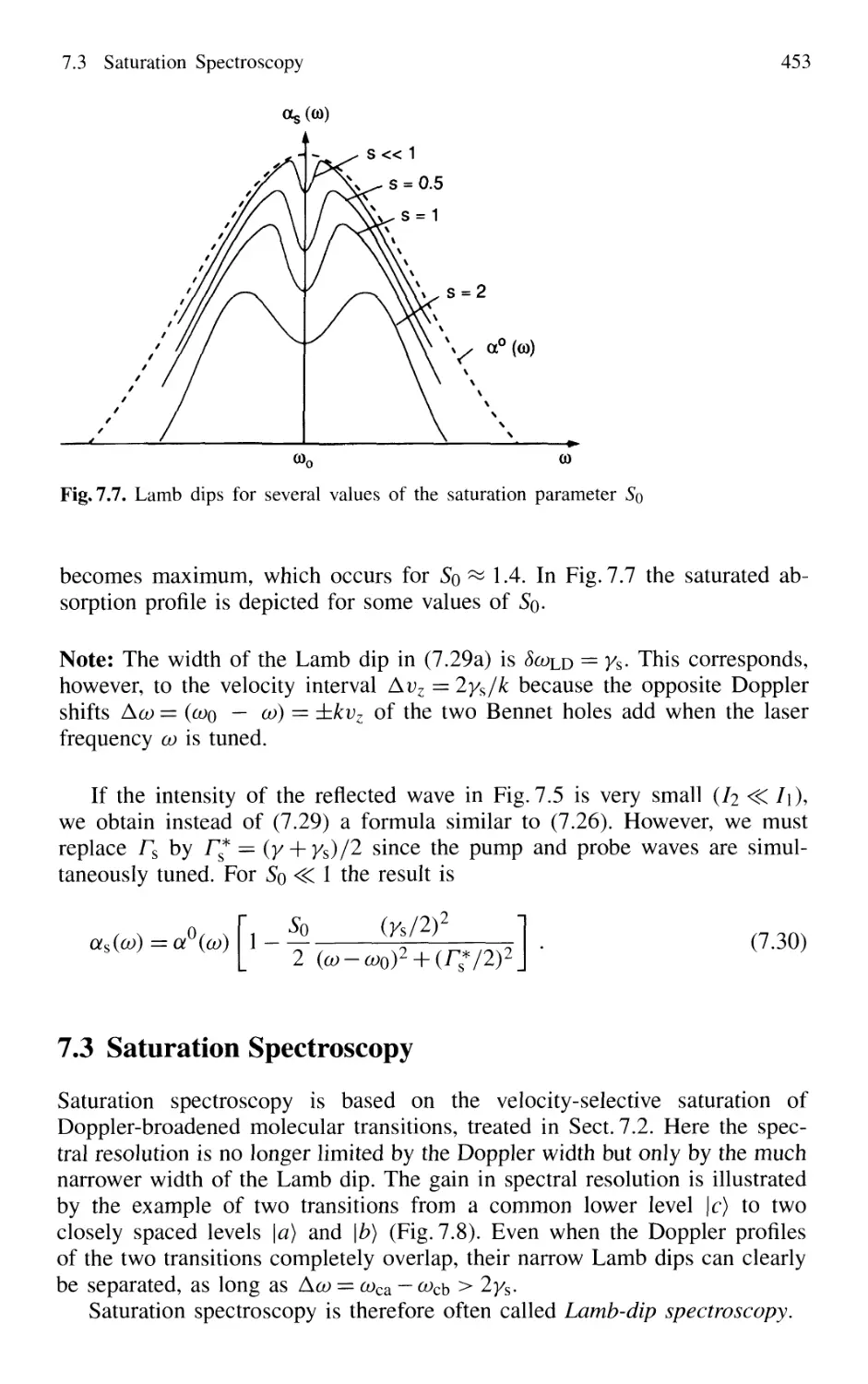
7.2.2 Lamb Dip v 450
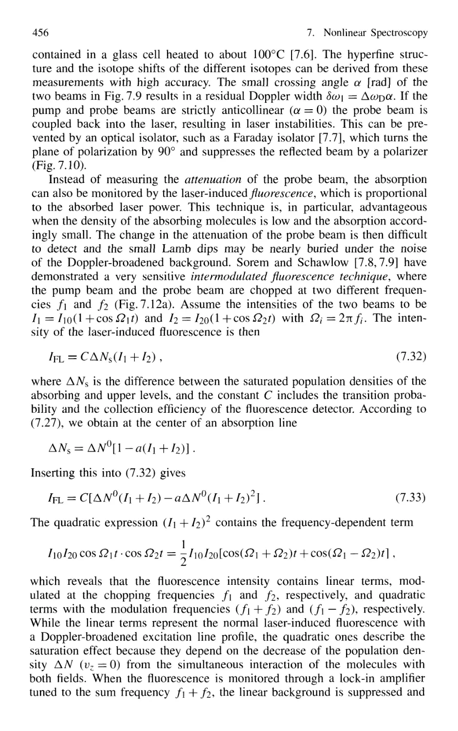
7.3 Saturation Spectroscopy 453
7.3.1 Experimental Schemes 454
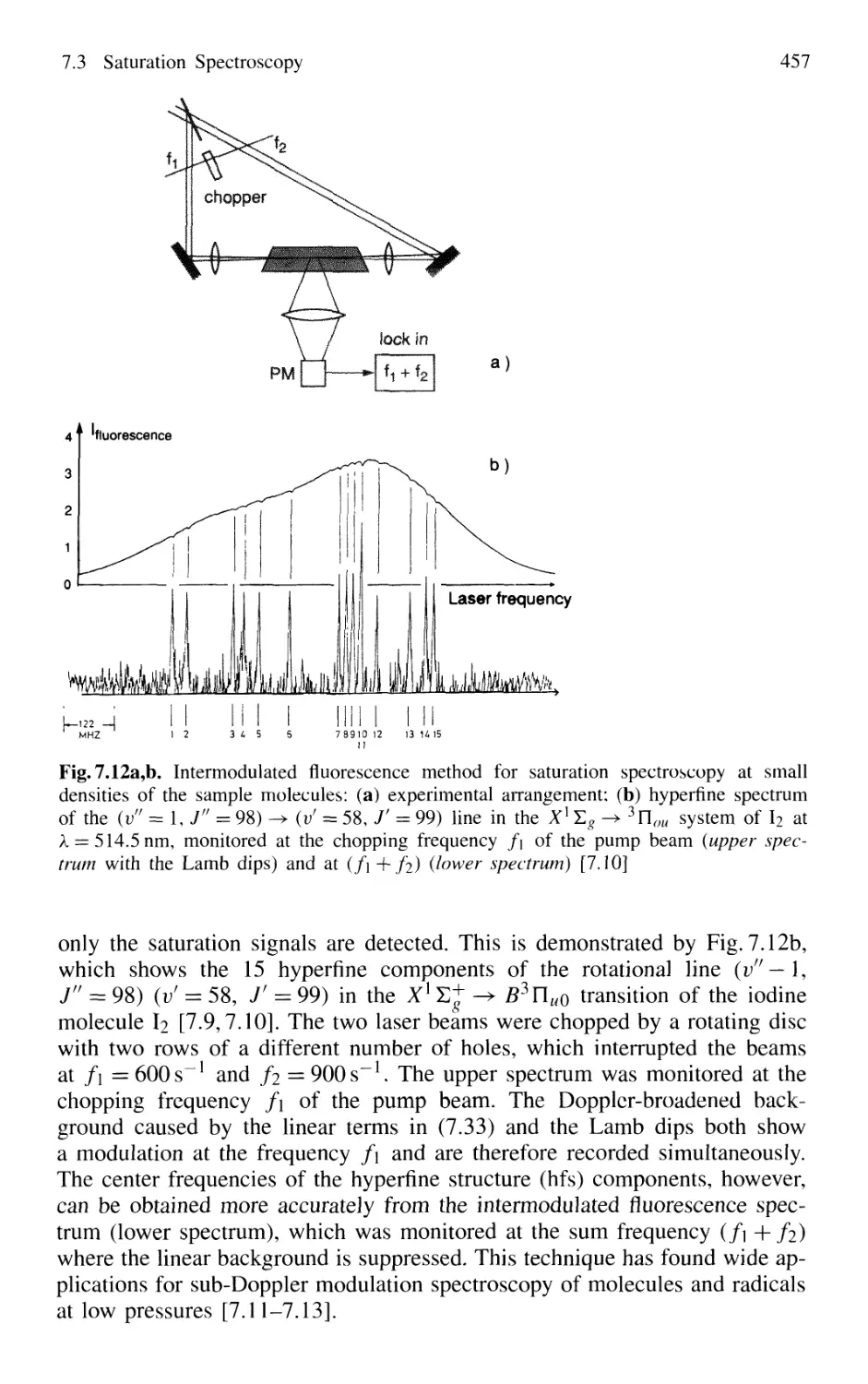
7.3.2 Cross-Over Signals 458
7.3.3 Intracavity Saturation Spectroscopy 459
7.3.4 Lamb-Dip Frequency Stabilization of Lasers 462
Contents XV
7.4 Polarization Spectroscopy 463
7.4.1 Basic Principle 464
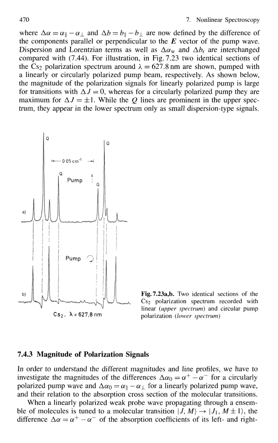
7.4.2 Line Profiles of Polarization Signals 465
7.4.3 Magnitude of Polarization Signals 470
7.4.4 Sensitivity of Polarization Spectroscopy 473
7.4.5 Advantages of Polarization Spectroscopy 476
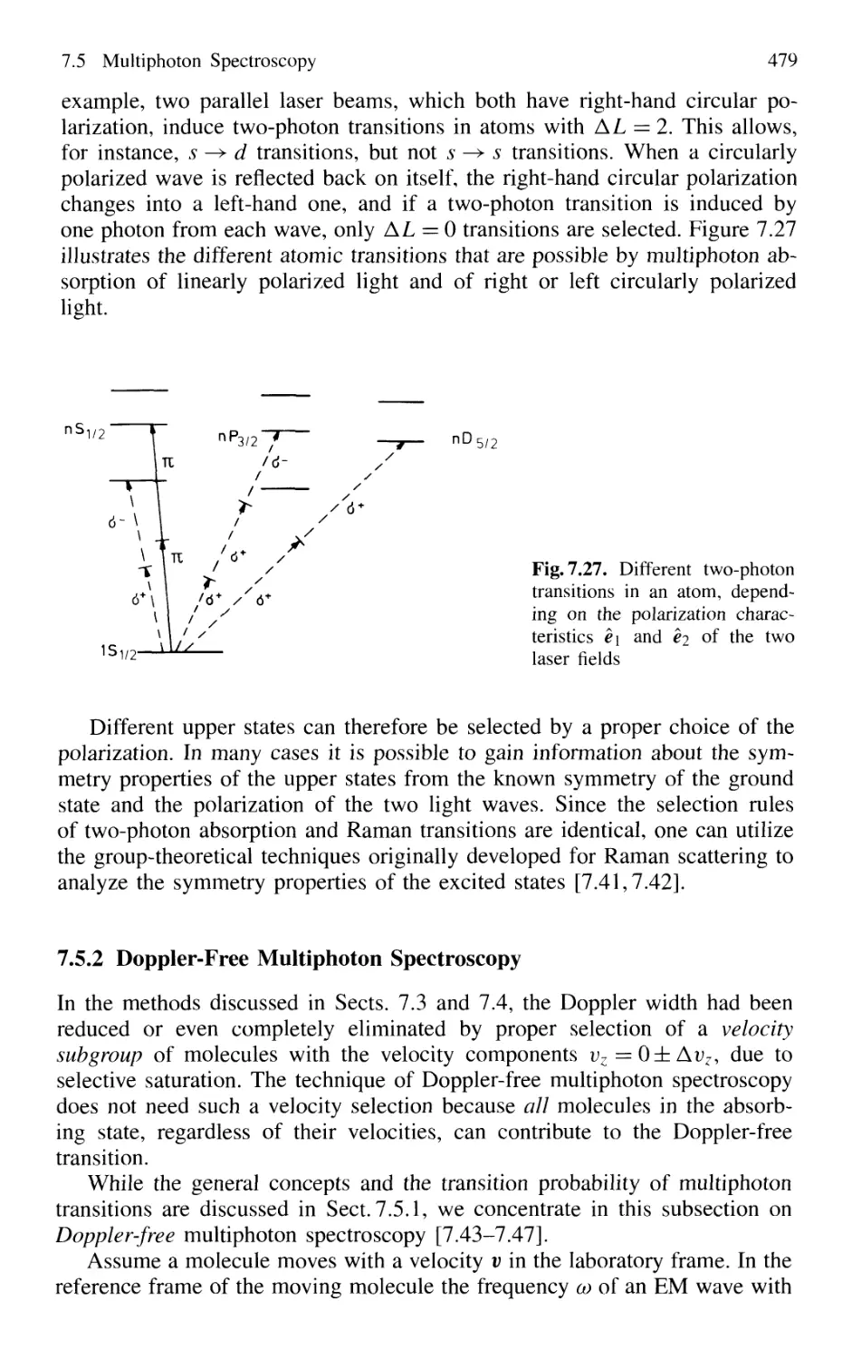
7.5 Multiphoton Spectroscopy 476
7.5.1 Two-Photon Absorption 476
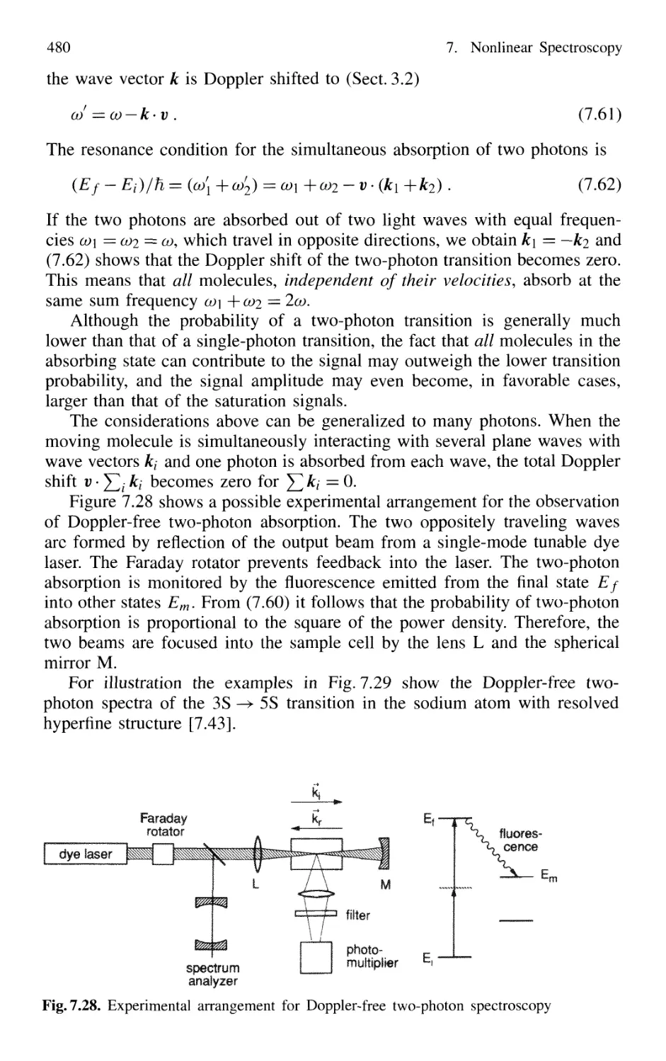
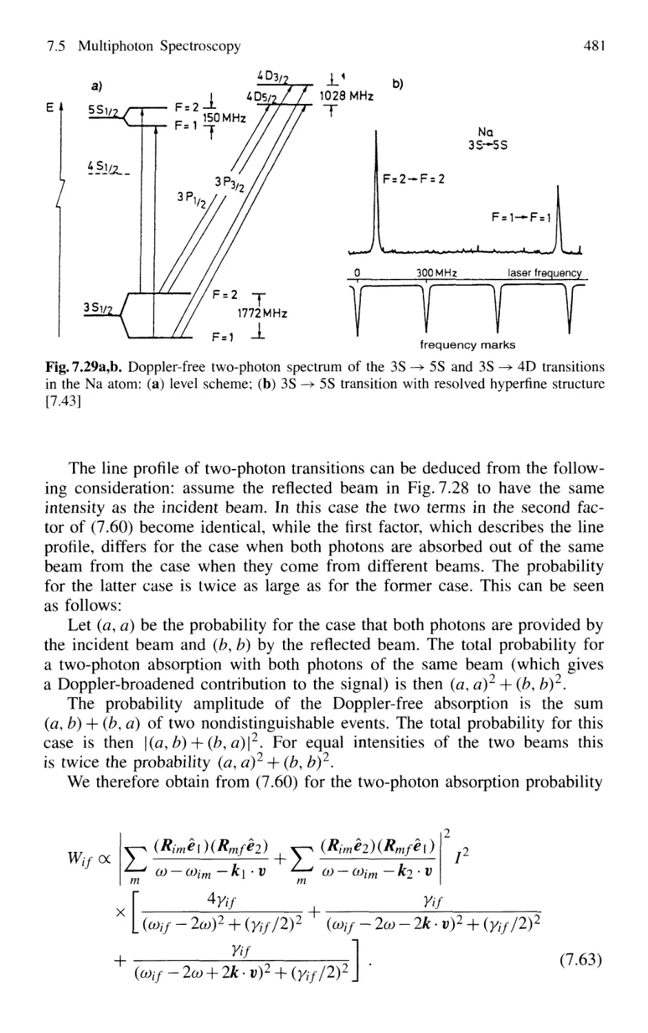
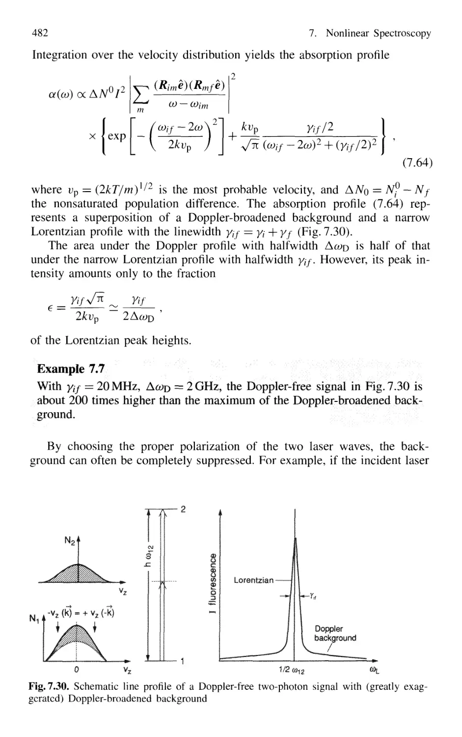
7.5.2 Doppler-Free Multiphoton Spectroscopy 479
7.5.3 Influence of Focusing on the Magnitude
of Two-Photon Signals 483
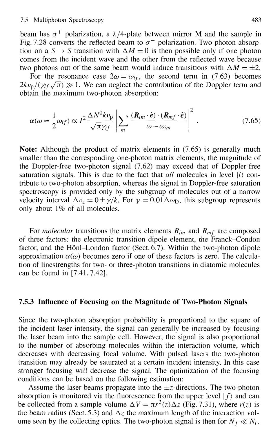
7.5.4 Examples of Doppler-Free Two-Photon
Spectroscopy 485
7.5.5 Multiphoton Spectroscopy 487
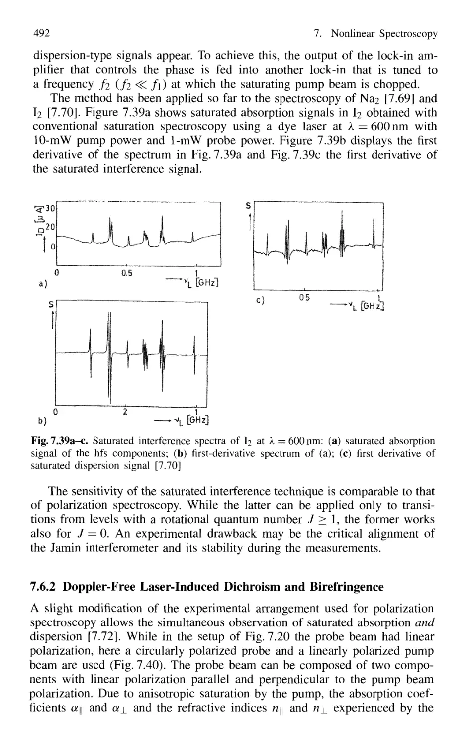
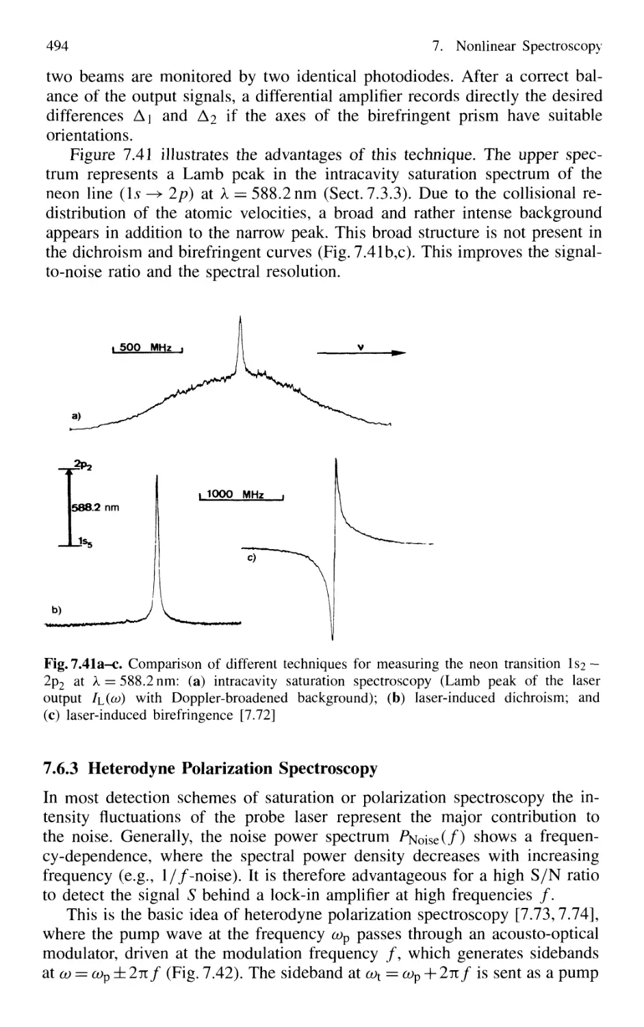
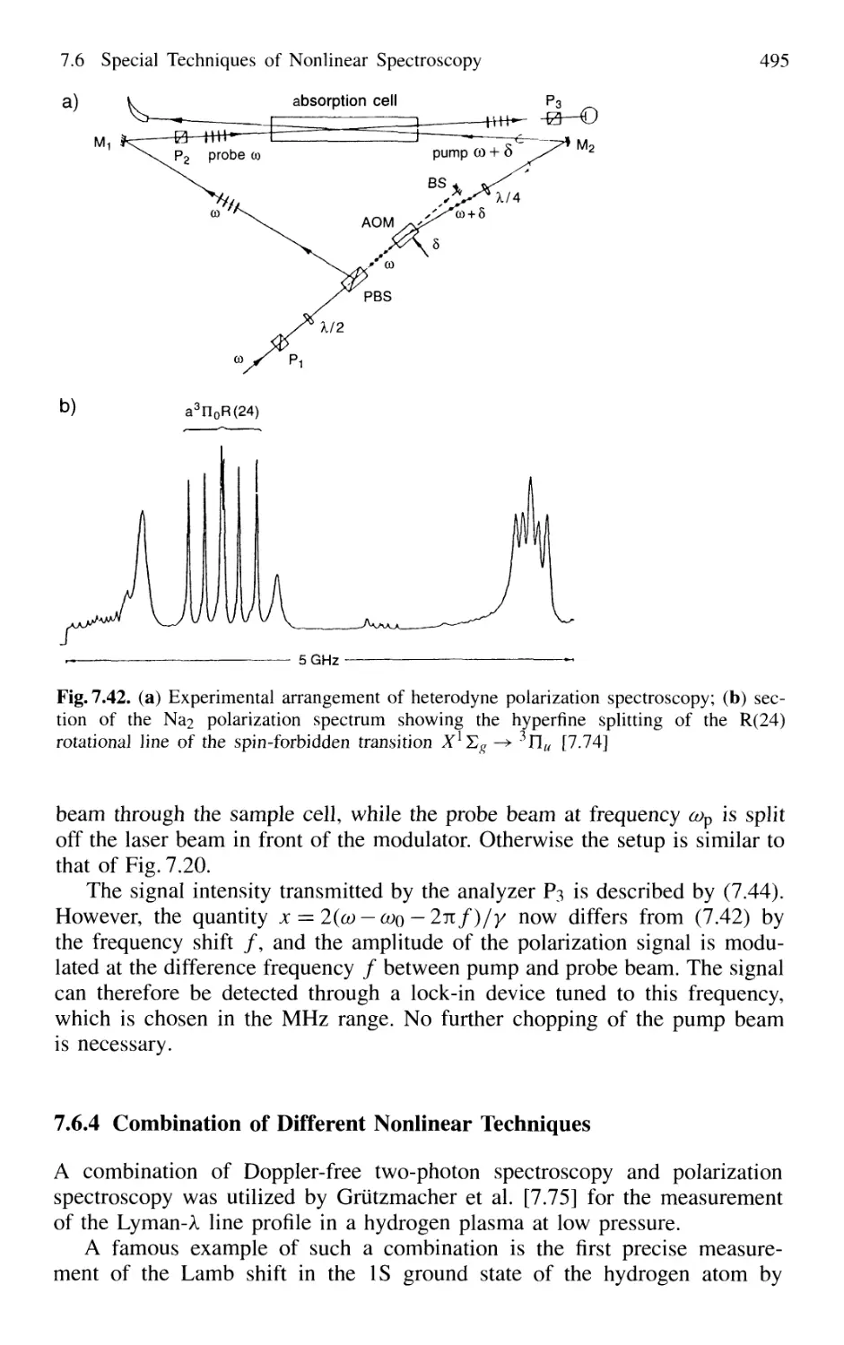
7.6 Special Techniques of Nonlinear Spectroscopy 490
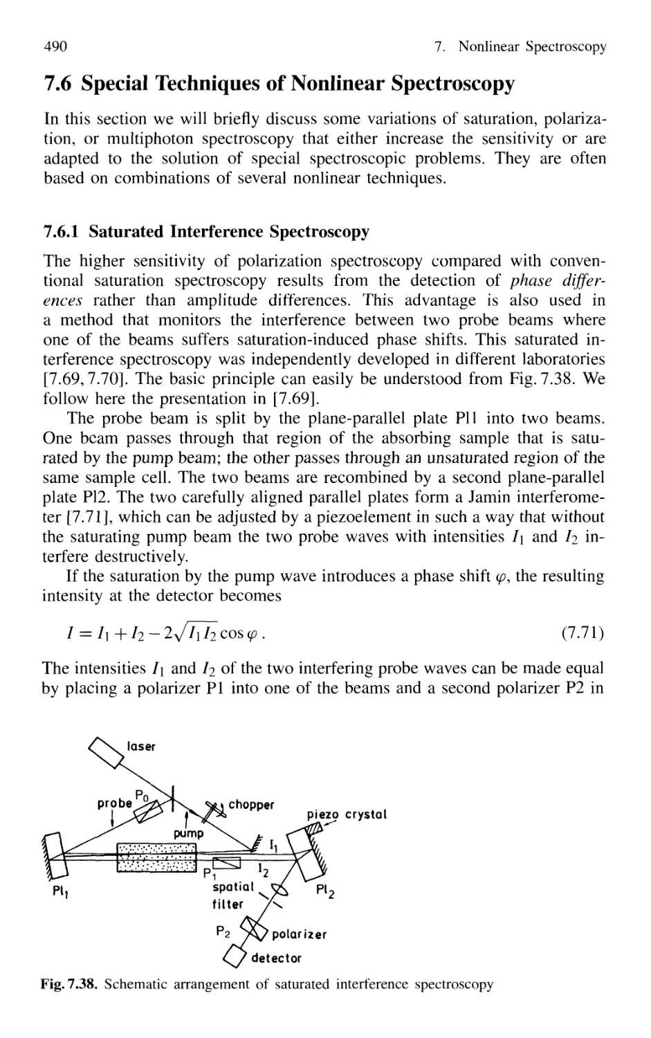
7.6.1 Saturated Interference Spectroscopy 490
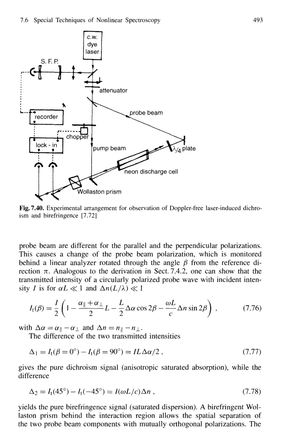
7.6.2 Doppler-Free Laser-Induced Dichroism
and Birefringence 492
7.6.3 Heterodyne Polarization Spectroscopy 494
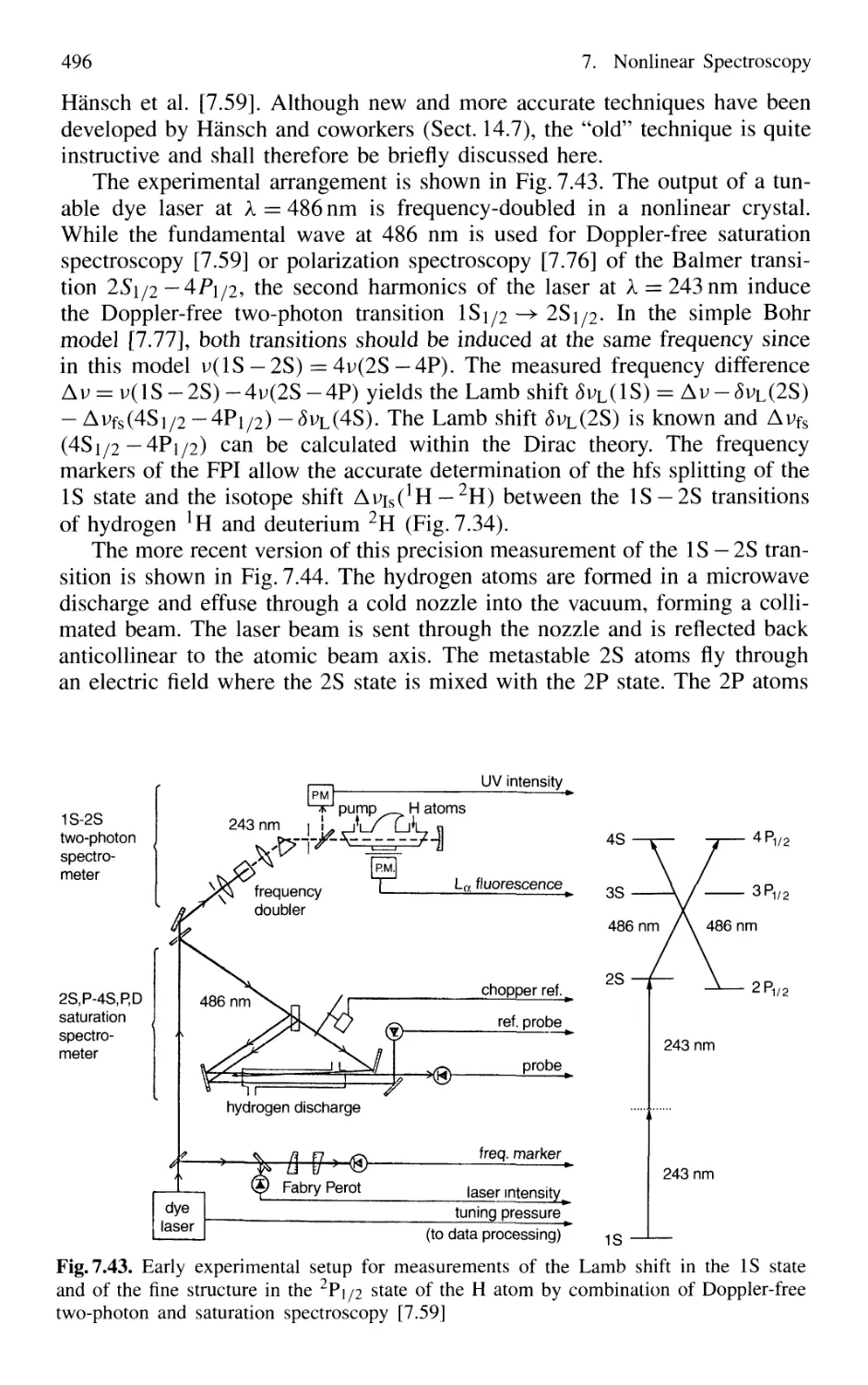
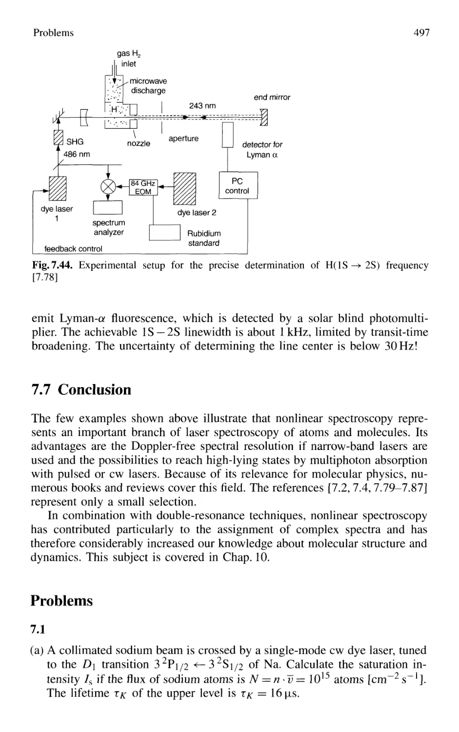
7.6.4 Combination of Different Nonlinear Techniques ... 495
7.7 Conclusion 497
Problems 497
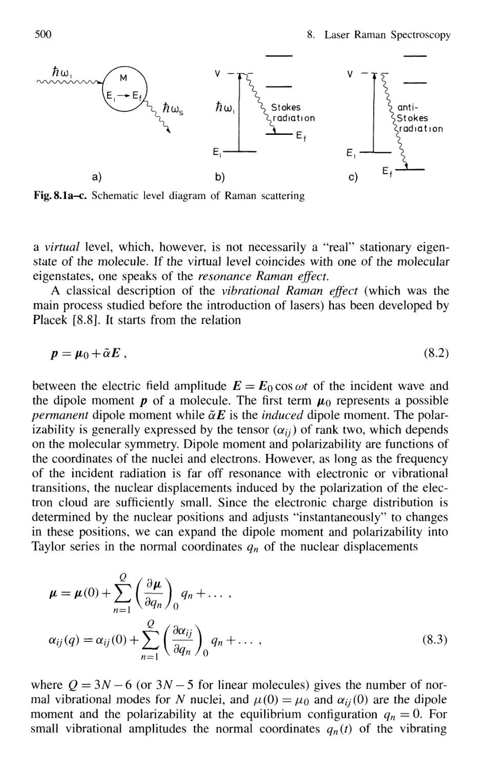
8. Laser Raman Spectroscopy 499
8.1 Basic Considerations 499
8.2 Experimental Techniques
of Linear Laser Raman Spectroscopy 504
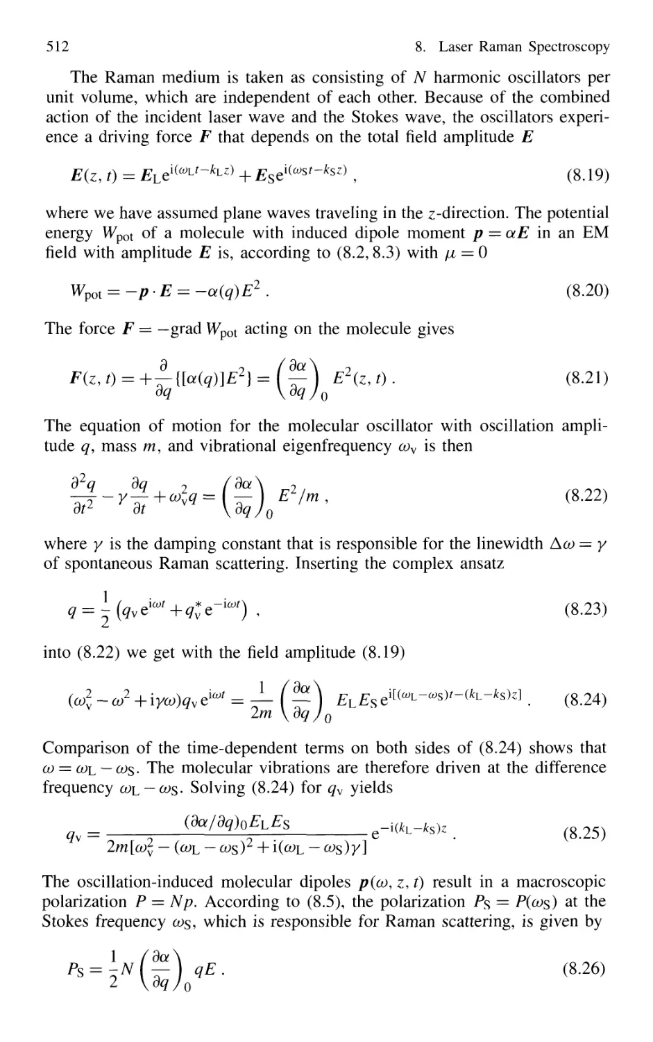
8.3 Nonlinear Raman Spectroscopy 511
8.3.1 Stimulated Raman Scattering 511
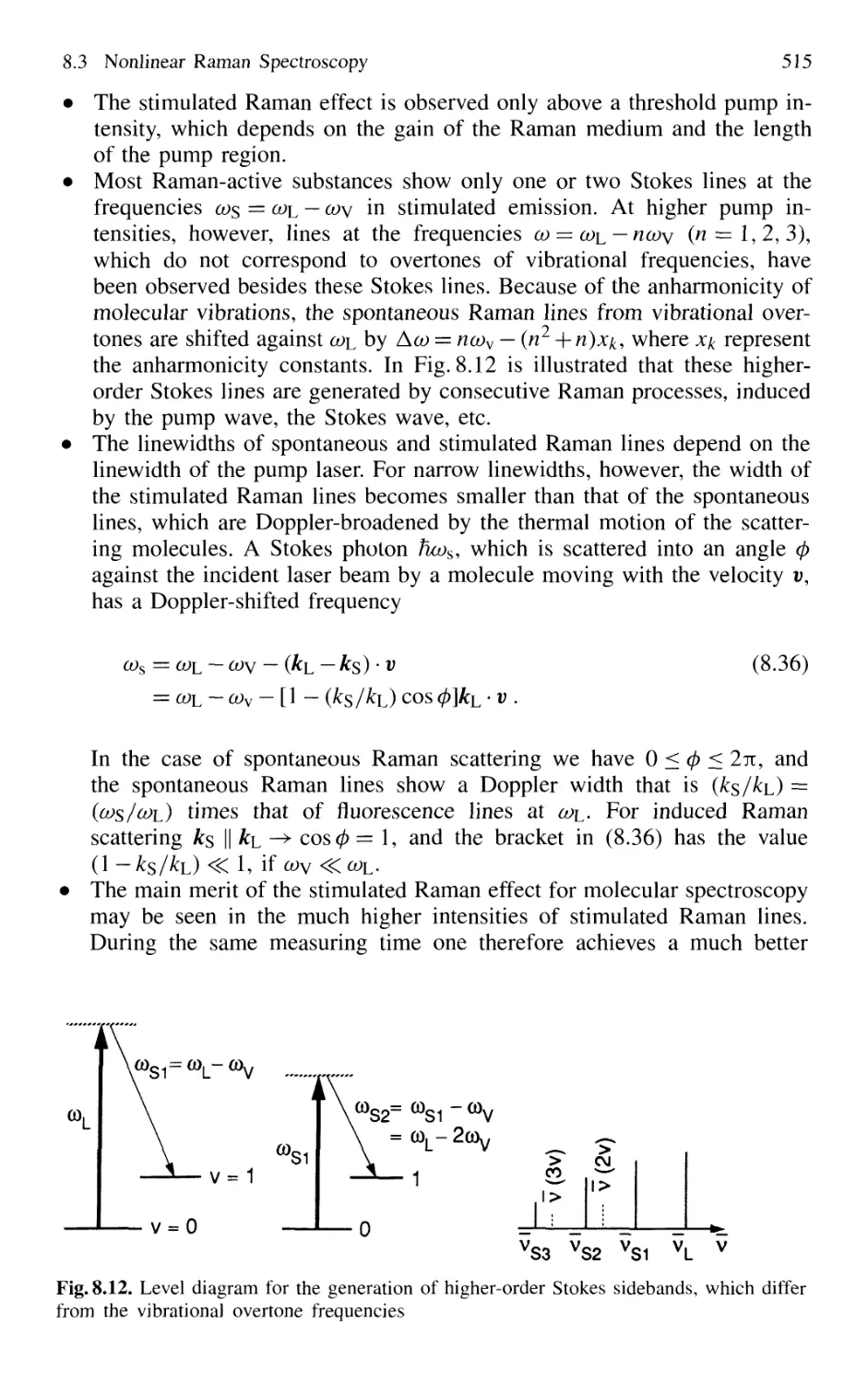
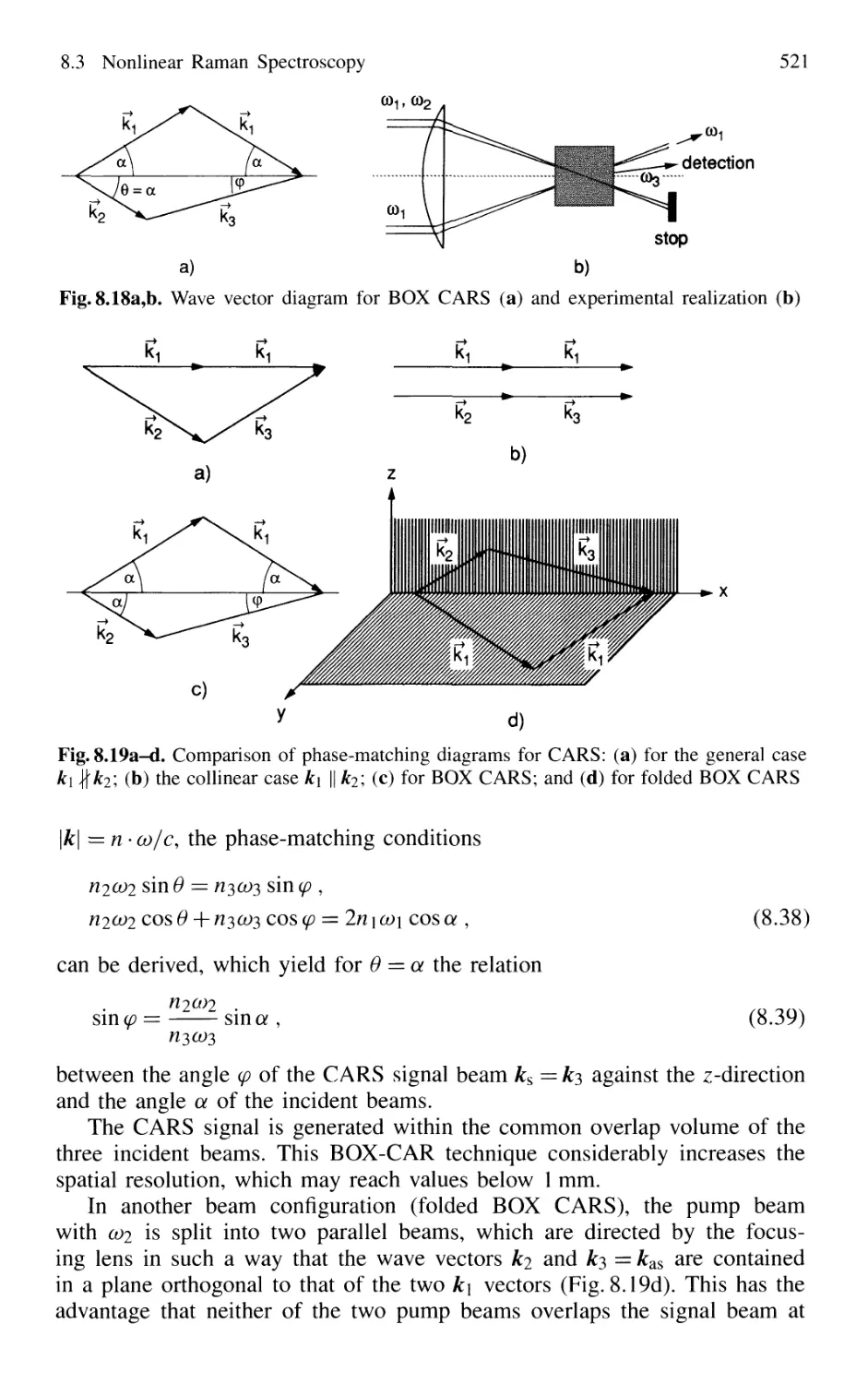
8.3.2 Coherent Anti-Stokes Raman Spectroscopy 517
8.3.3 Resonant CARS and BOX CARS 520
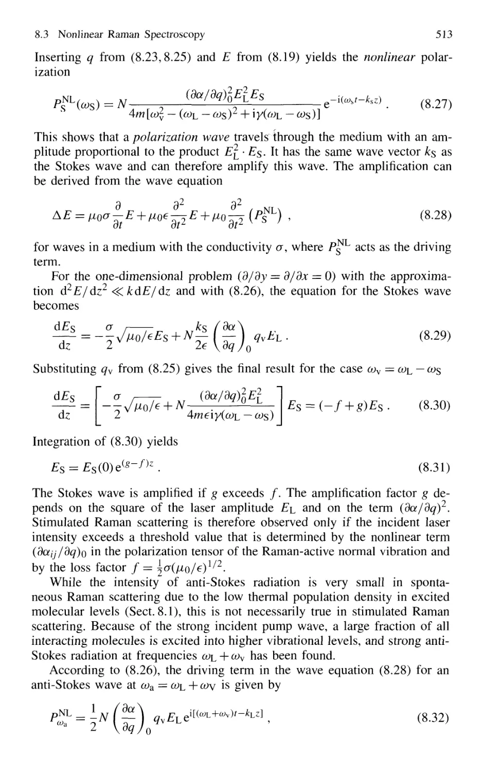
8.3.4 Hyper-Raman Effect 522
8.3.5 Summary of Nonlinear Raman Spectroscopy 523
8.4 Special Techniques 524
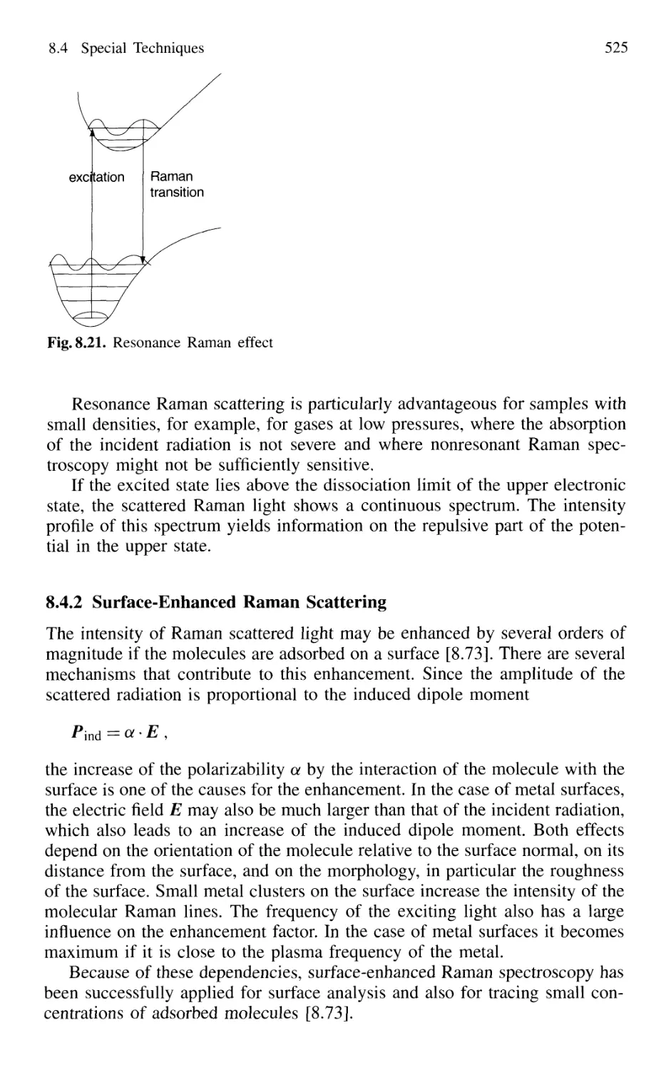
8.4.1 Resonance Raman Effect 524
8.4.2 Surface-Enhanced Raman Scattering 525
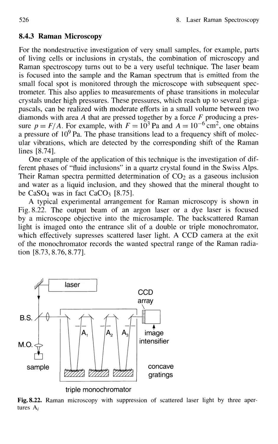
8.4.3 Raman Microscopy 526
8.4.4 Time-Resolved Raman Spectroscopy 527
8.5 Applications of Laser Raman Spectroscopy 527
Problems 529
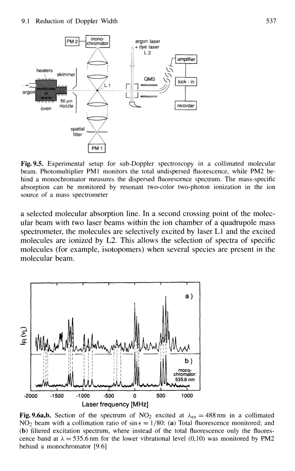
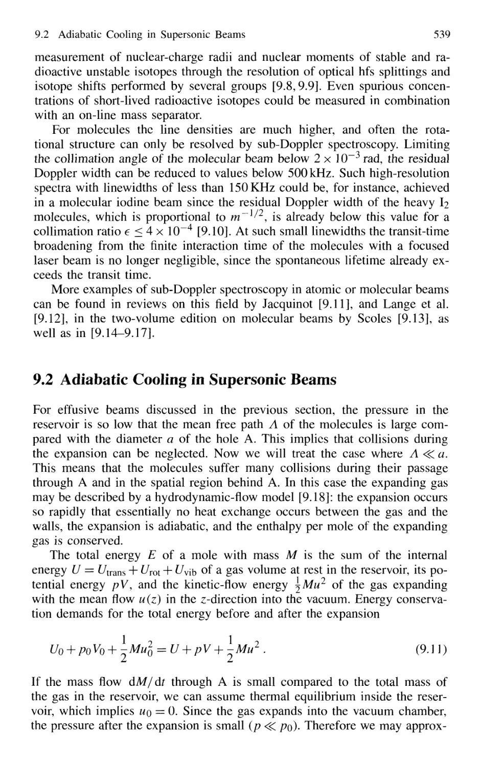
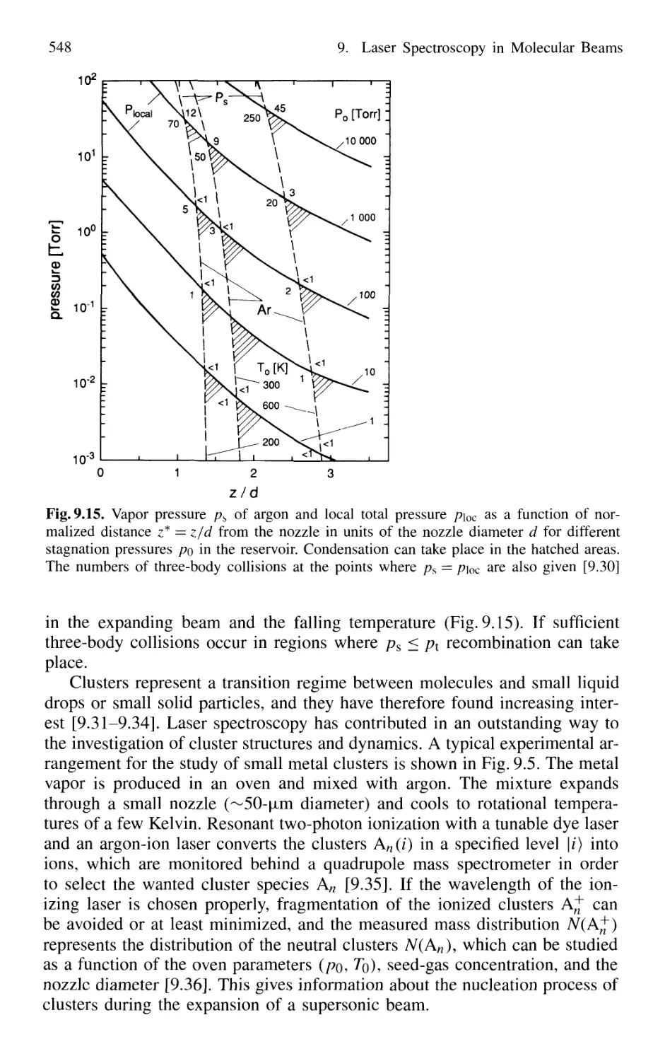
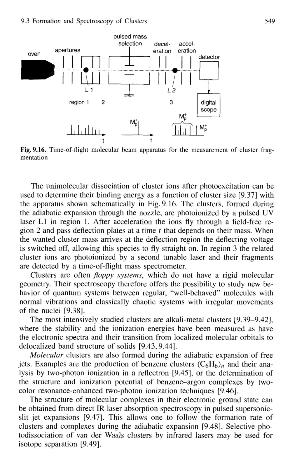
9. Laser Spectroscopy in Molecular Beams 531
9.1 Reduction of Doppler Width 531
9.2 Adiabatic Cooling in Supersonic Beams 539
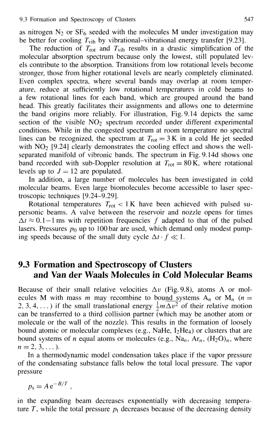
9.3 Formation and Spectroscopy of Clusters
and Van der Waals Molecules in Cold Molecular Beams .... 547
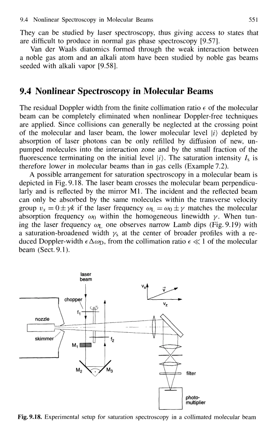
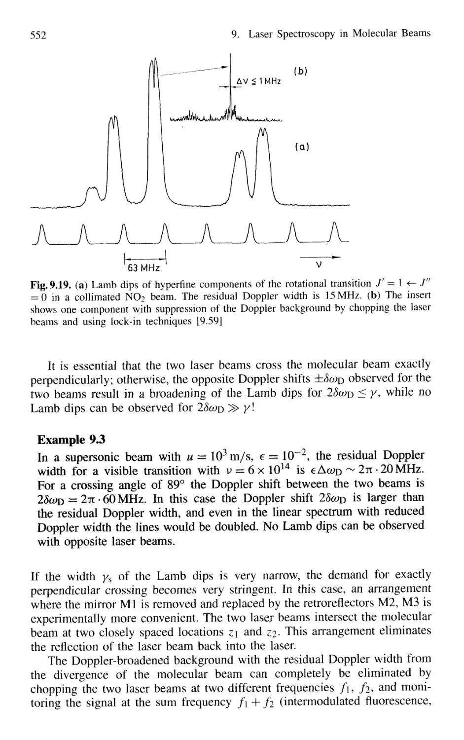
9.4 Nonlinear Spectroscopy in Molecular Beams 551
XVI Contents
9.5 Laser Spectroscopy in Fast Ion Beams 553
9.6 Applications of FIBLAS 556
9.6.1 Spectroscopy of Radioactive Elements 556
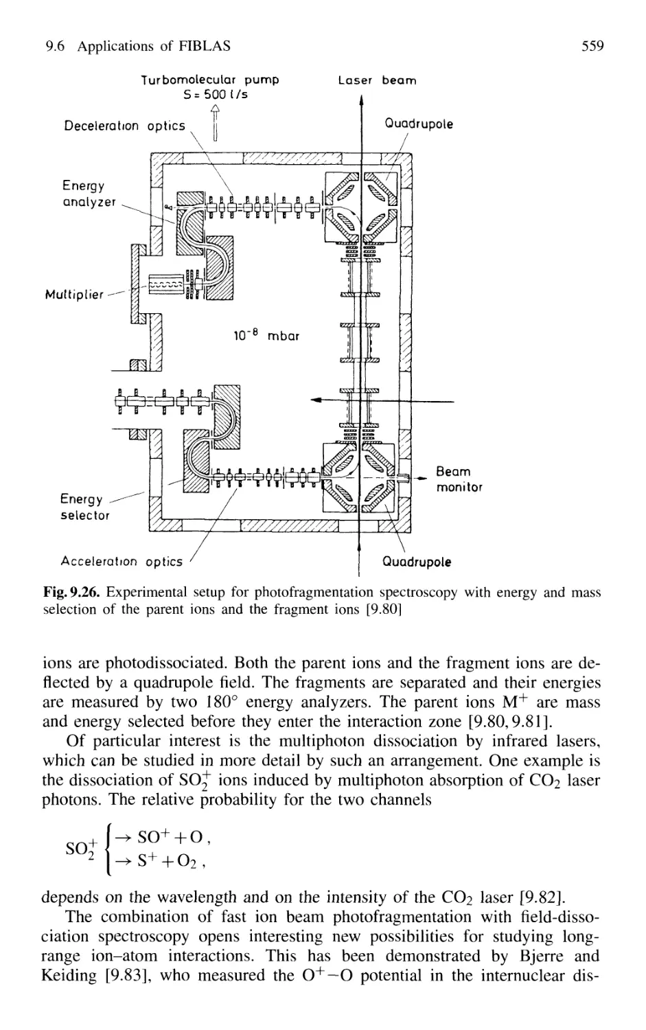
9.6.2 Photofragmentation Spectroscopy of Molecular Ions 557
9.6.3 Laser Photodetachment Spectroscopy 560
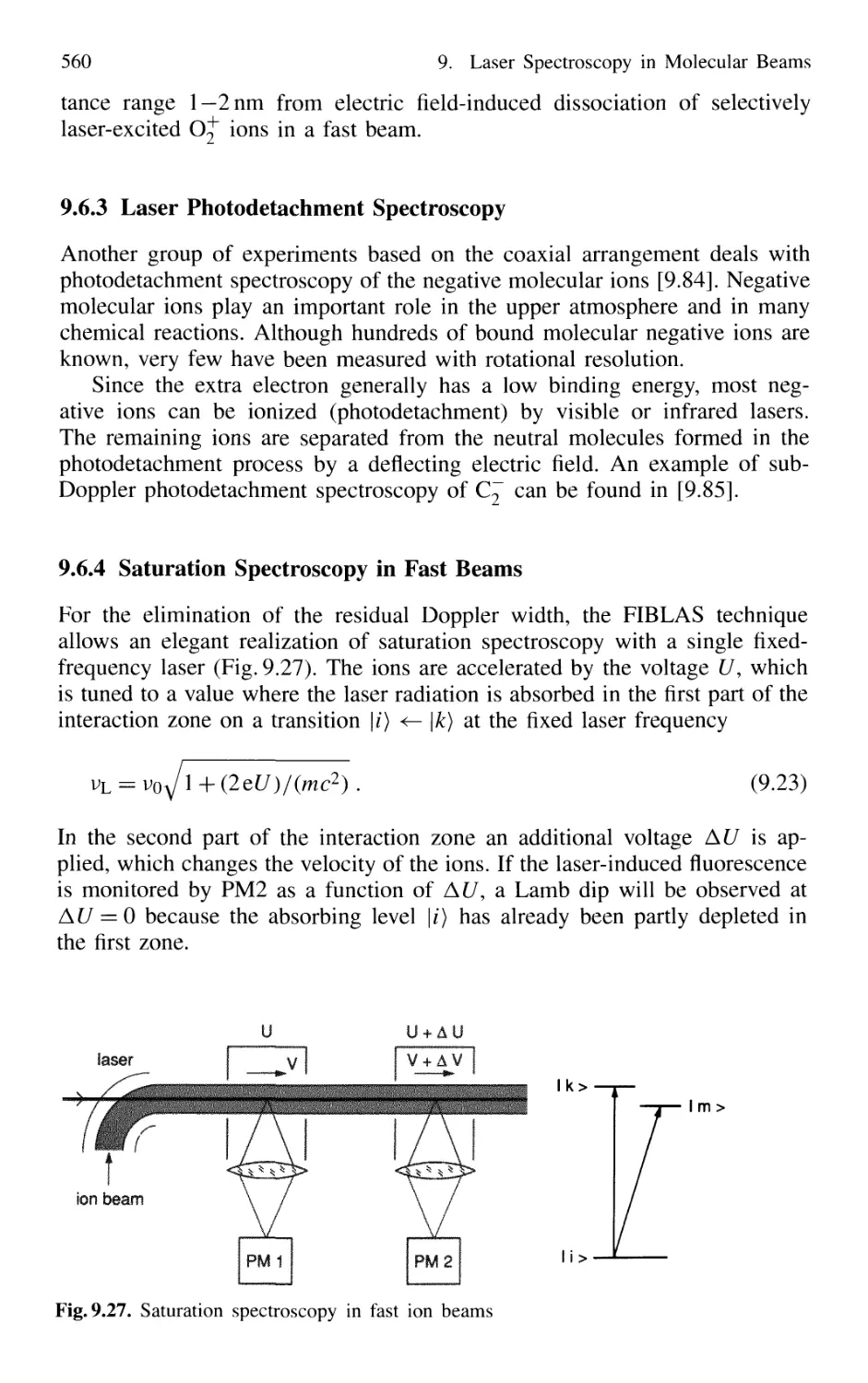
9.6.4 Saturation Spectroscopy in Fast Beams 560
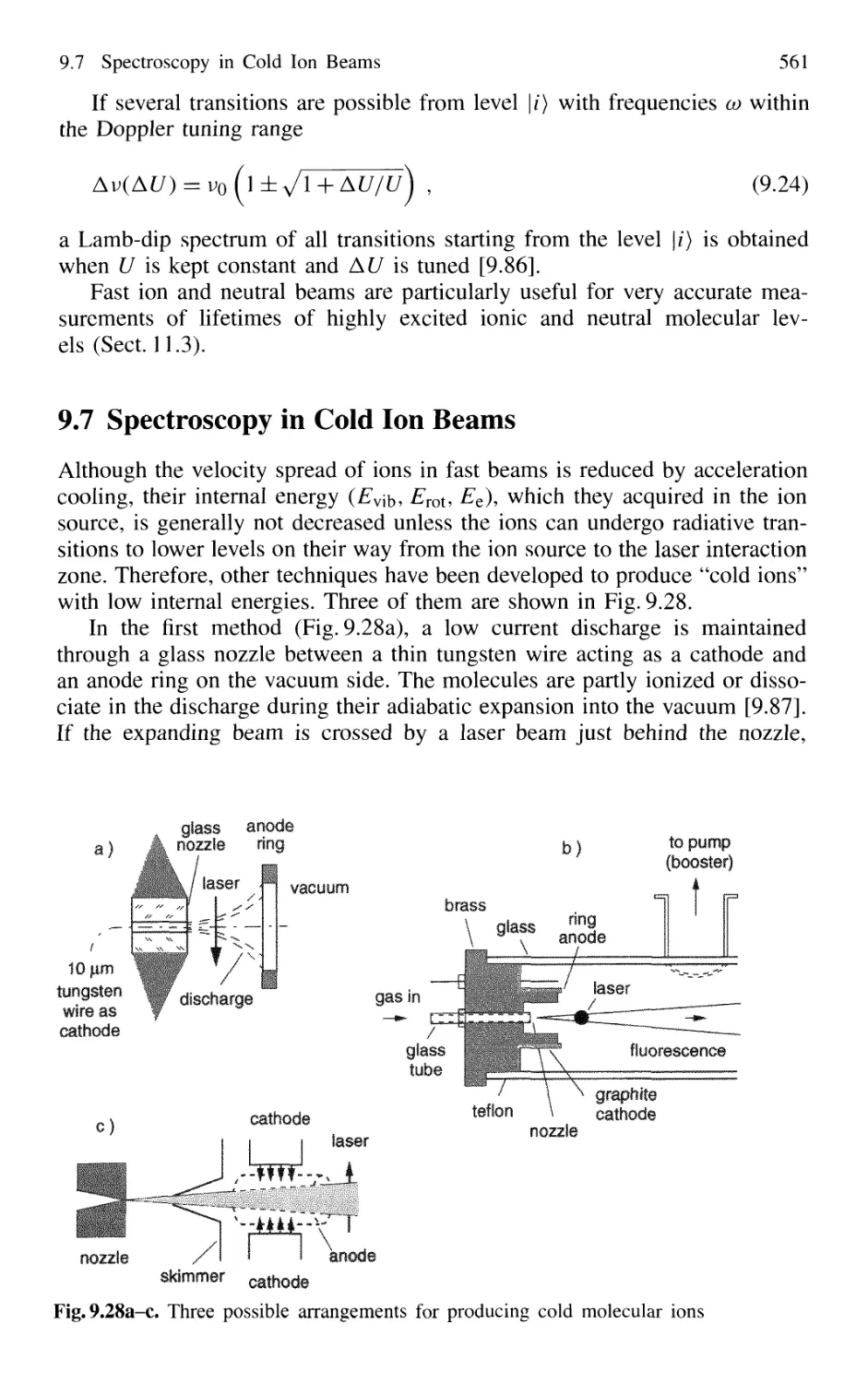
9.7 Spectroscopy in Cold Ion Beams 561
9.8 Combination of Molecular Beam Laser Spectroscopy
and Mass Spectrometry 562
Problems 564
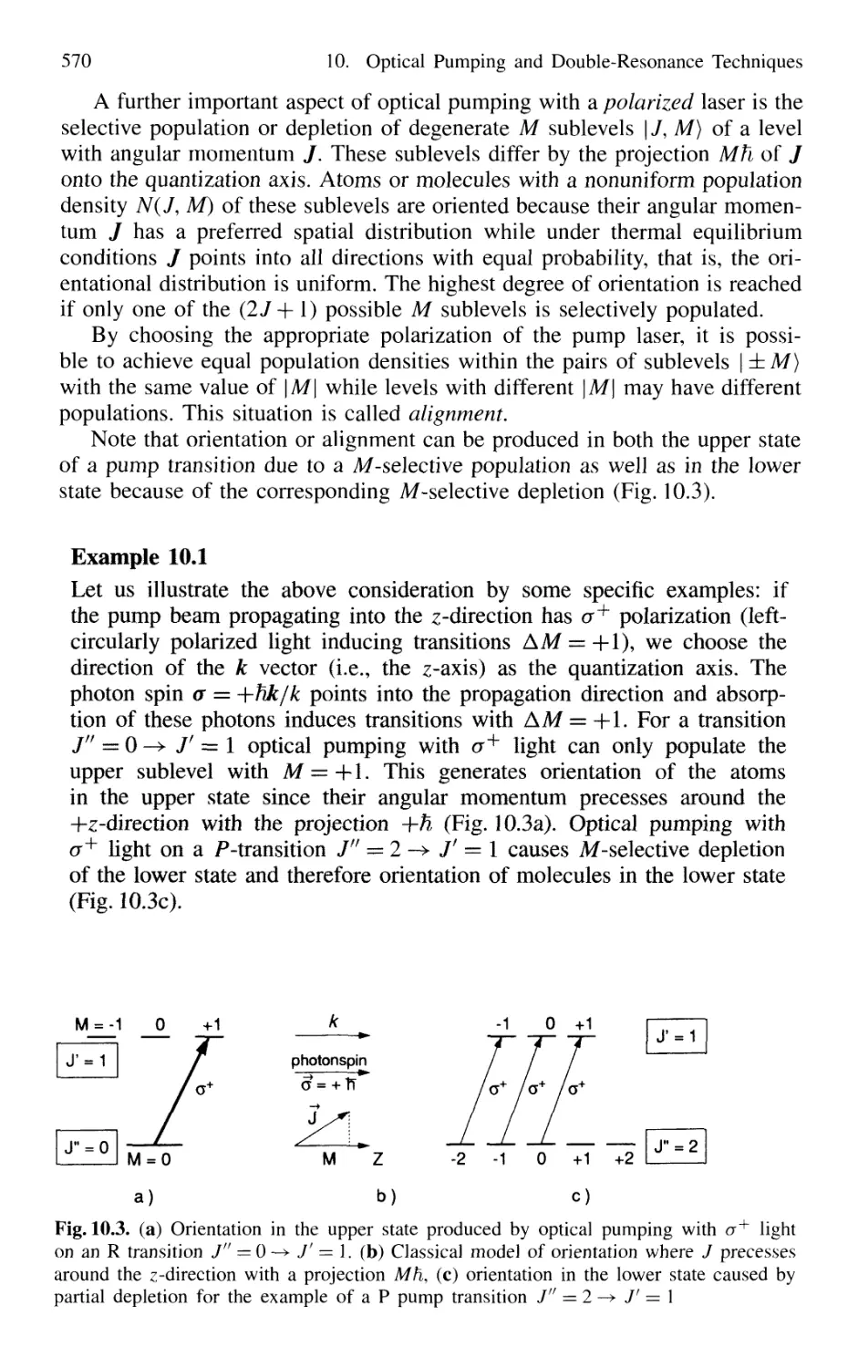
10. Optical Pumping and Double-Resonance Techniques 567
10.1 Optical Pumping 568
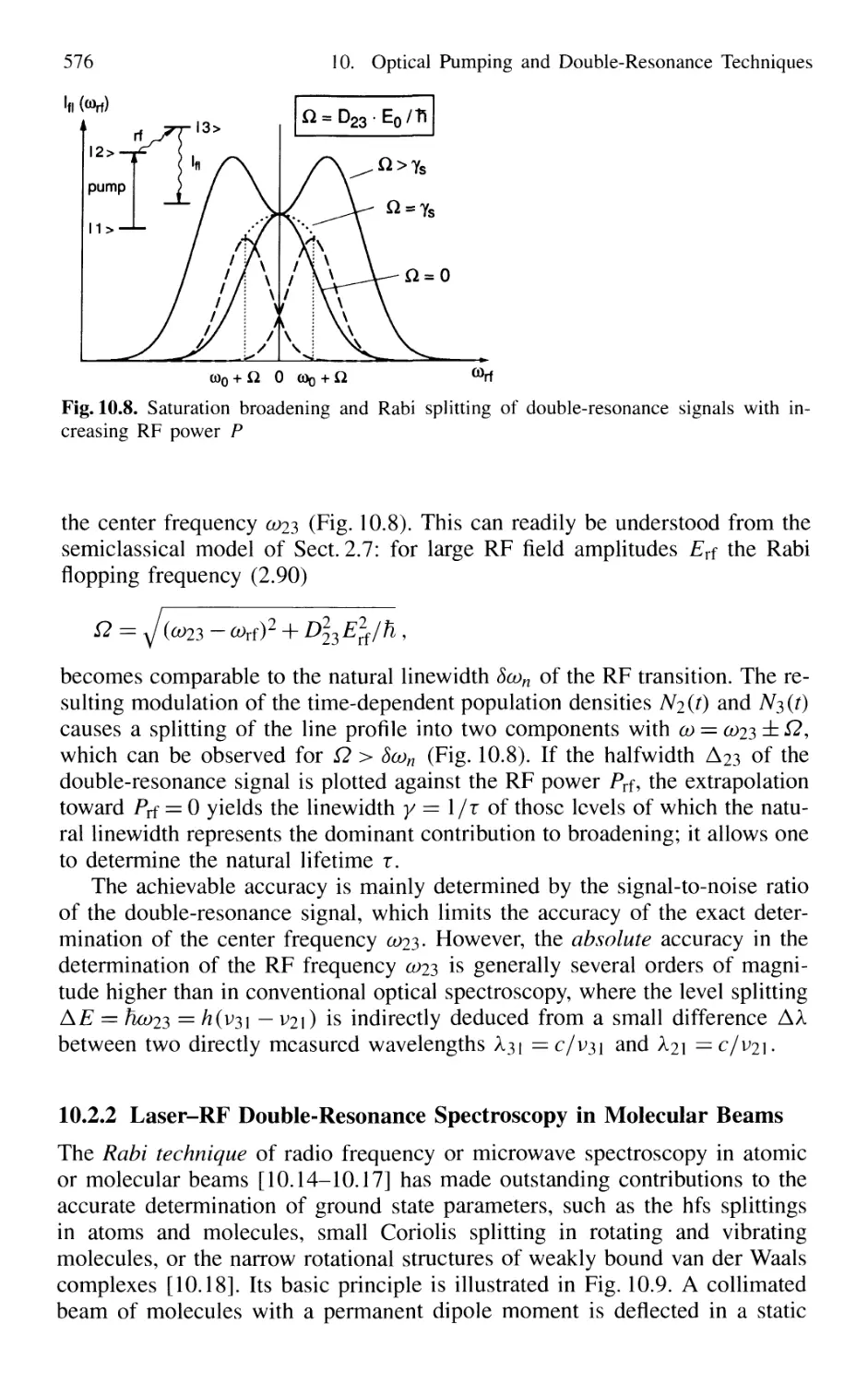
10.2 Optical-RF Double-Resonance Technique 573
10.2.1 Basic Considerations 573
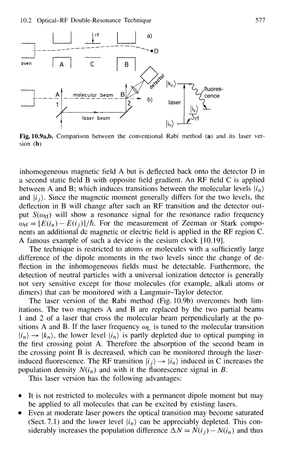
10.2.2 Laser-RF Double-Resonance Spectroscopy
in Molecular Beams 576
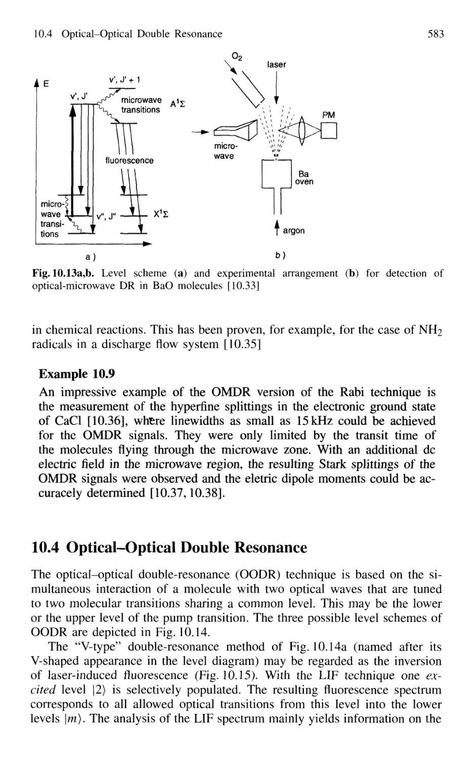
10.3 Optical-Microwave Double Resonance 579
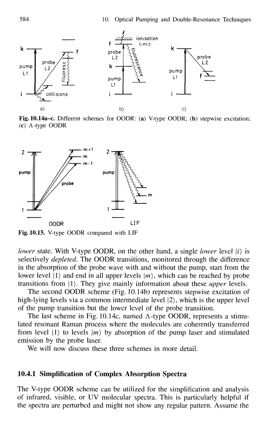
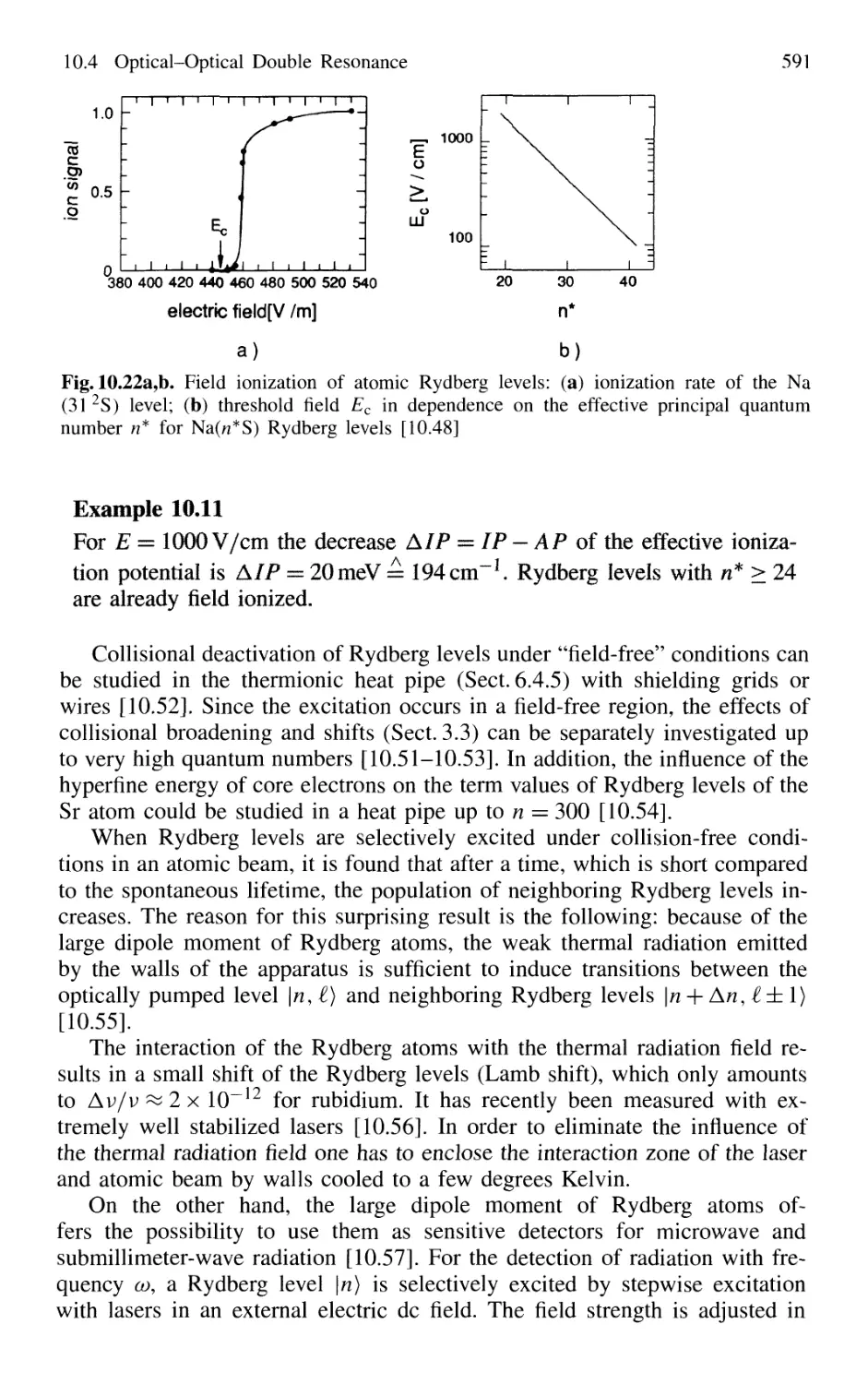
10.4 Optical-Optical Double Resonance 583
10.4.1 Simplification of Complex Absorption Spectra 584
10.4.2 Stepwise Excitation and Spectroscopy
of Rydberg States 588
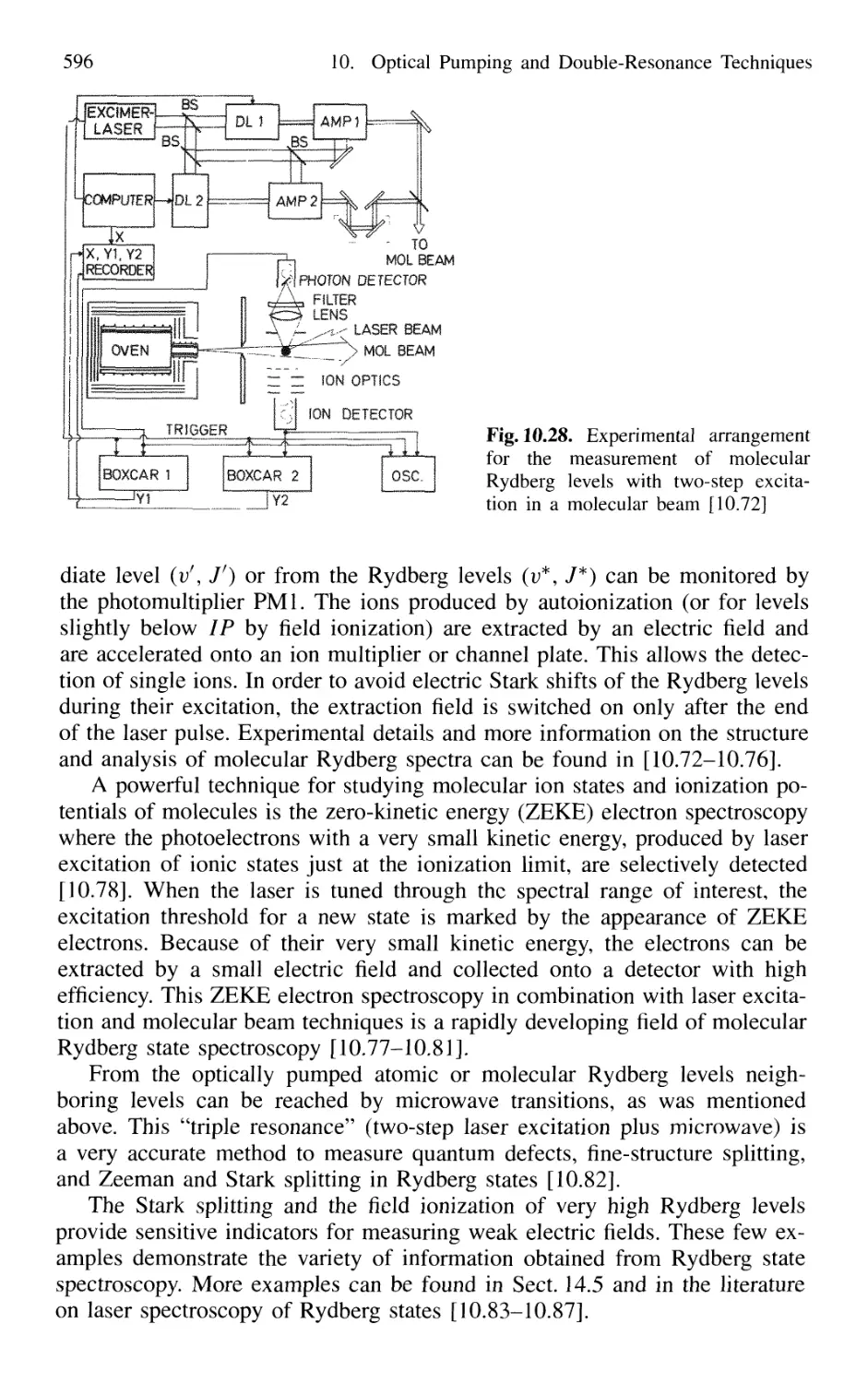
10.4.3 Stimulated Emission Pumping 597
10.5 Special Detection Schemes
of Double-Resonance Spectroscopy 600
10.5.1 OODR-Polarization Spectroscopy 600
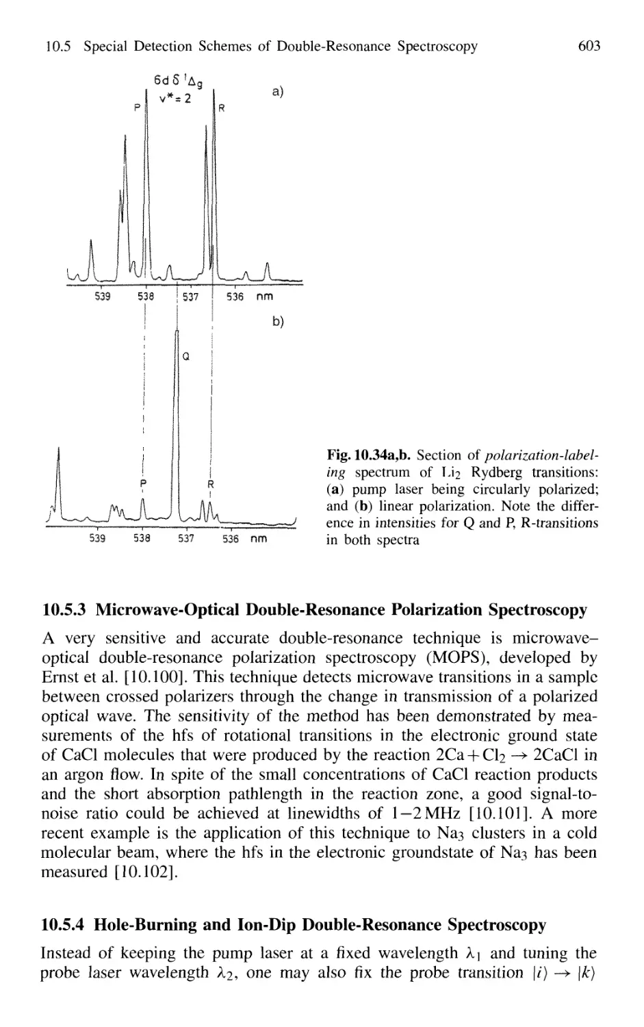
10.5.2 Polarization Labeling 601
10.5.3 Microwave-Optical Double-Resonance Polarization
Spectroscopy 603
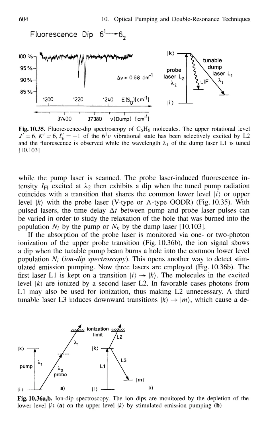
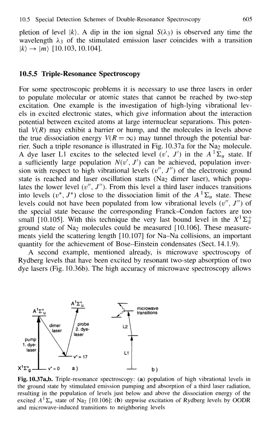
10.5.4 Hole-Burning and Ion-Dip Double-Resonance
Spectroscopy 603
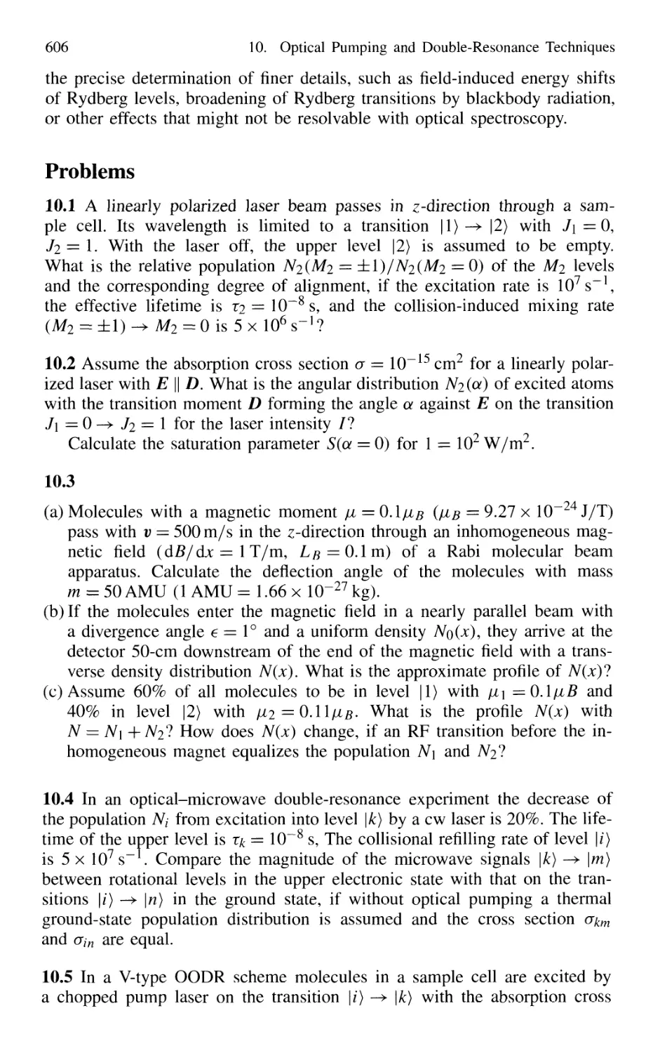
10.5.5 Triple-Resonance Spectroscopy 605
Problems 606
11. Time-Resolved Laser Spectroscopy 609
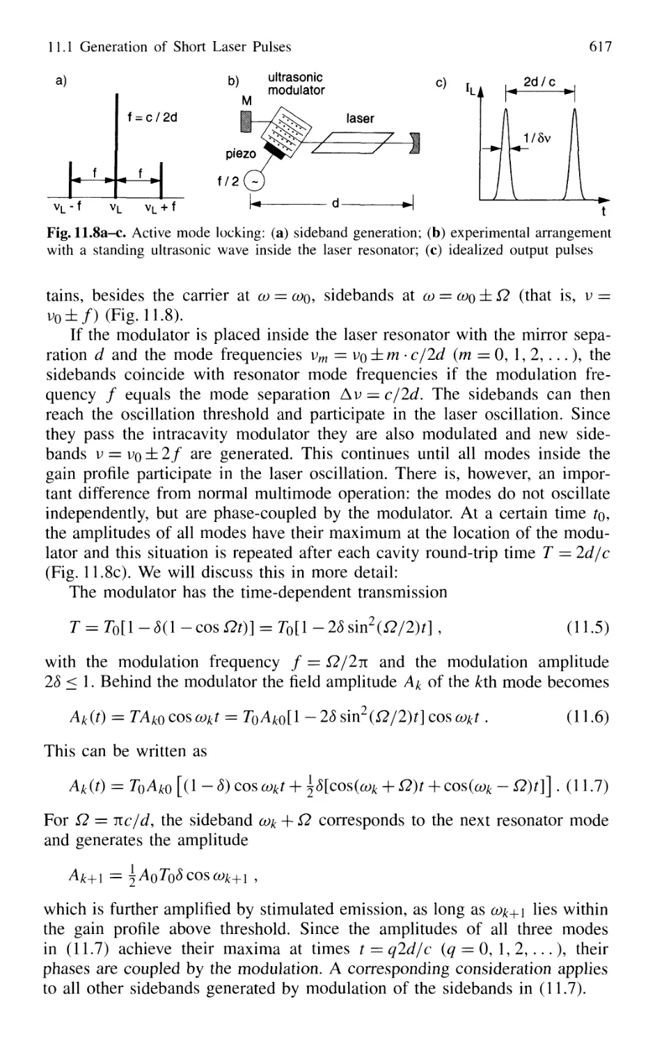
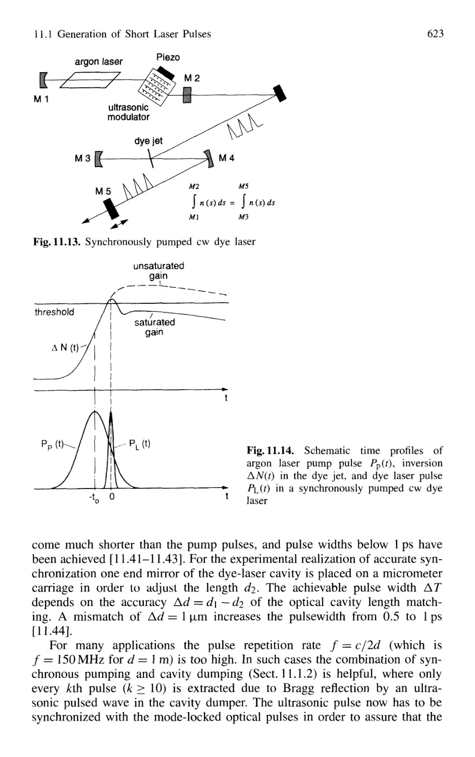
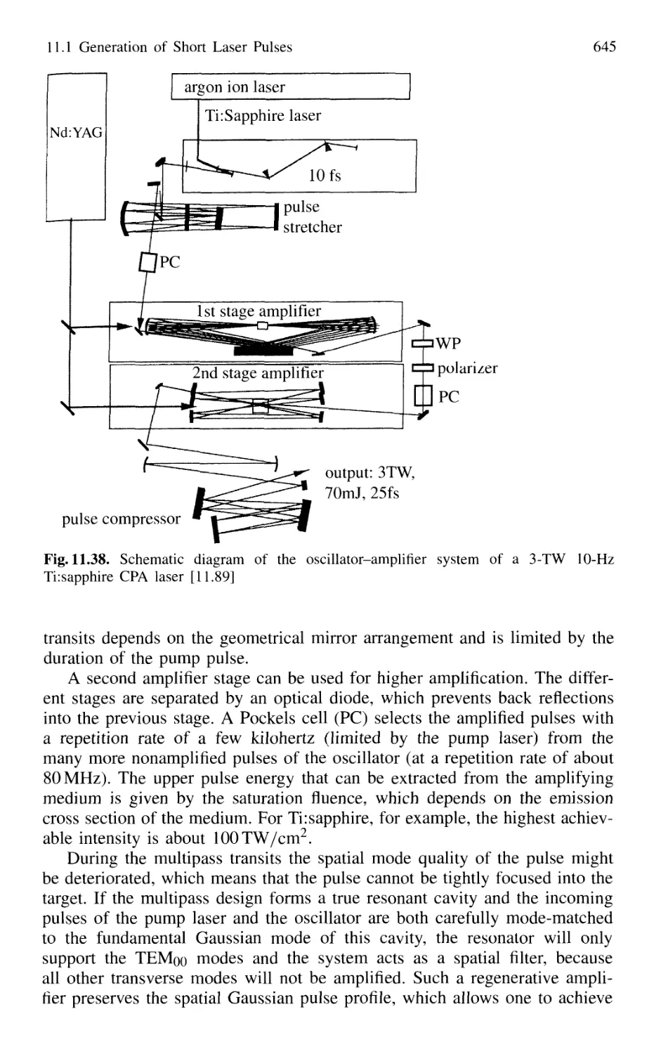
11.1 Generation of Short Laser Pulses 610
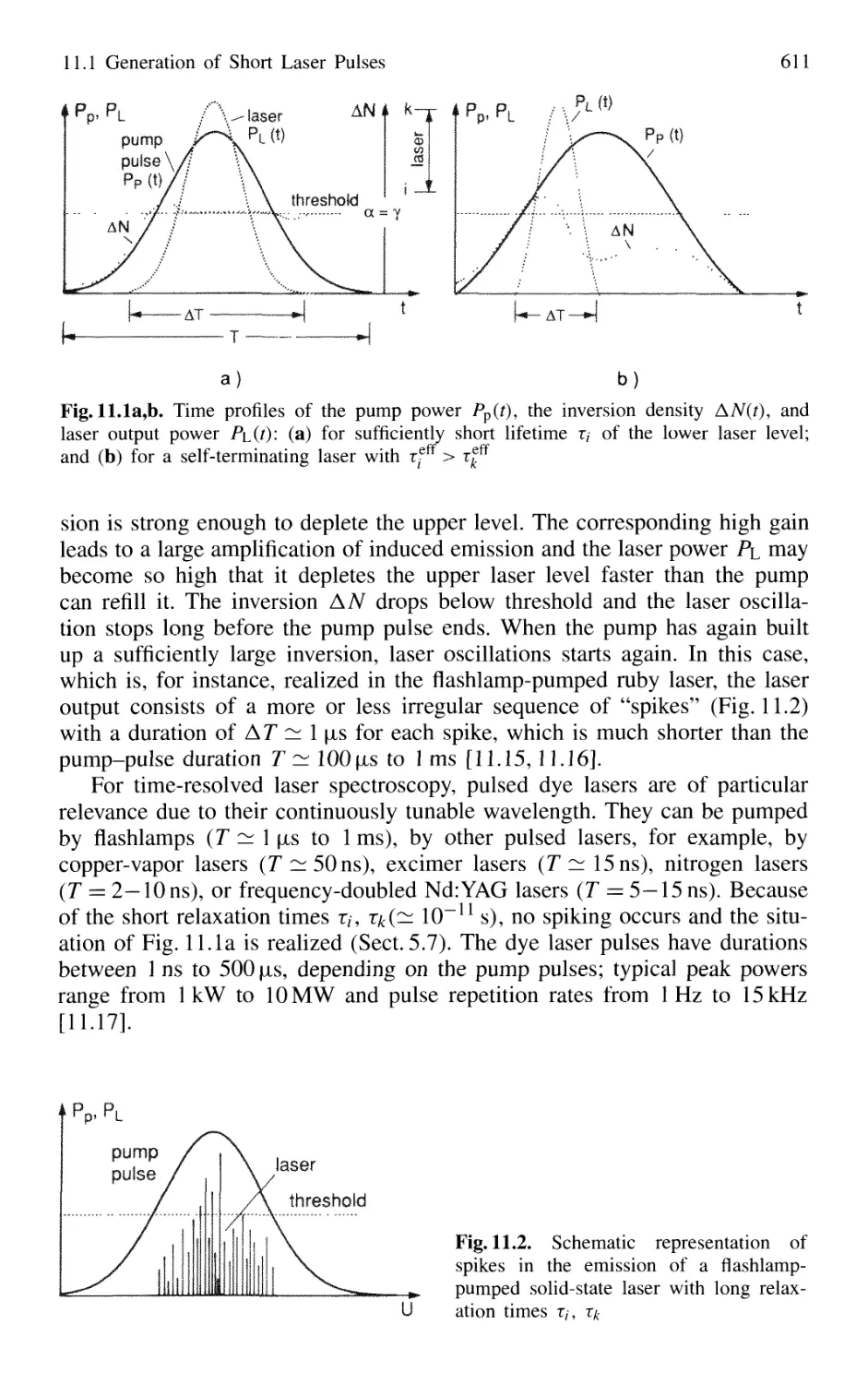
11.1.1 Time Profiles of Pulsed Lasers 610
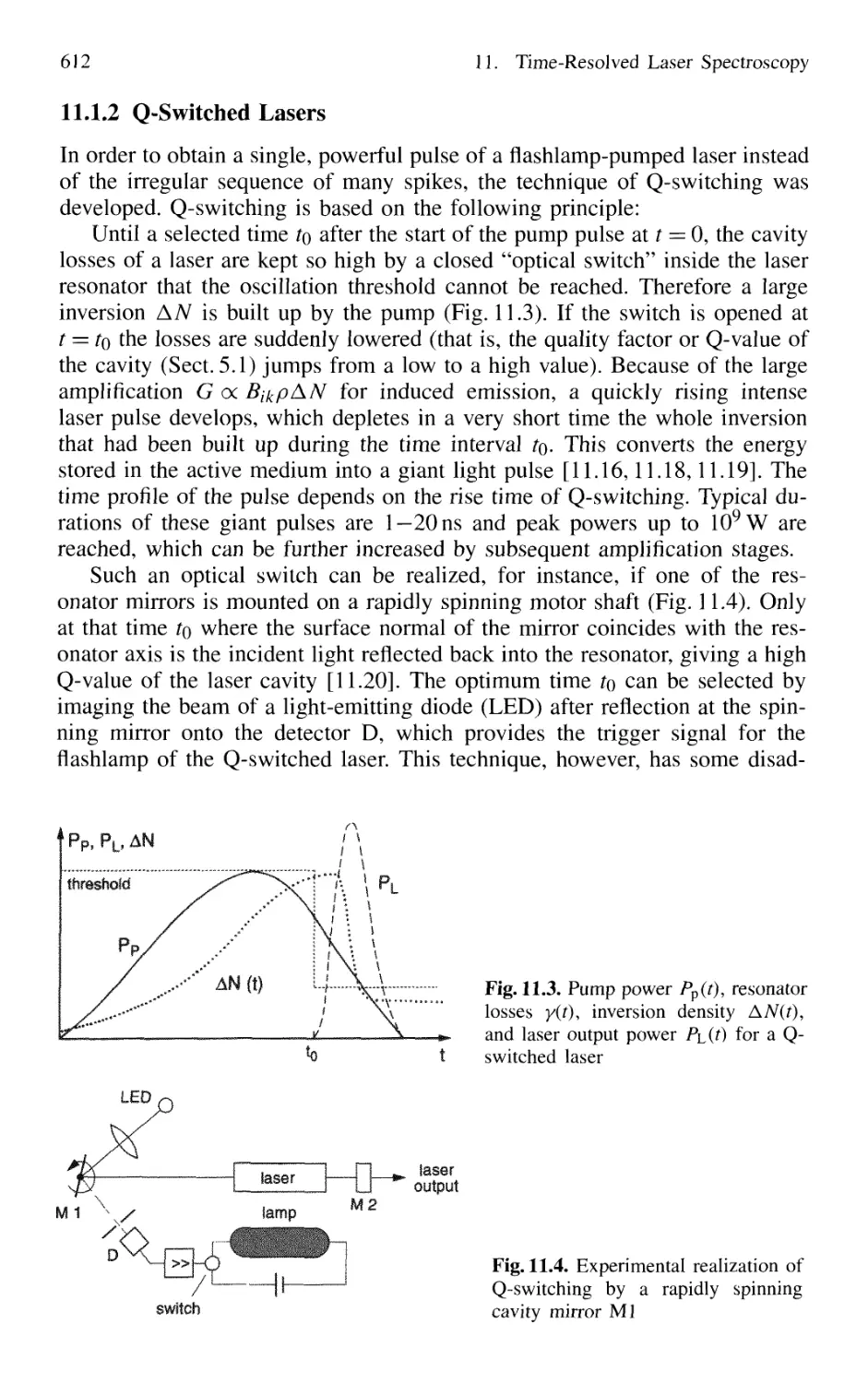
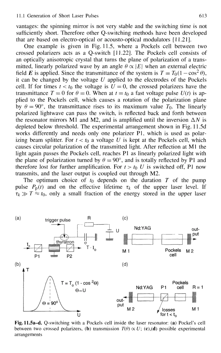
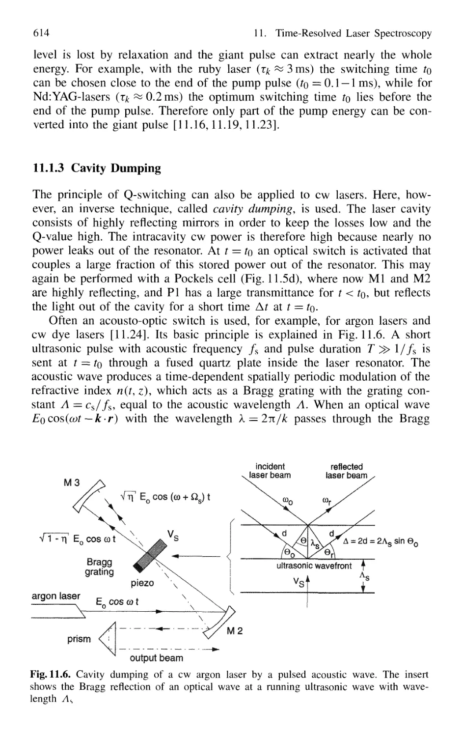
11.1.2 Q-Switched Lasers 612
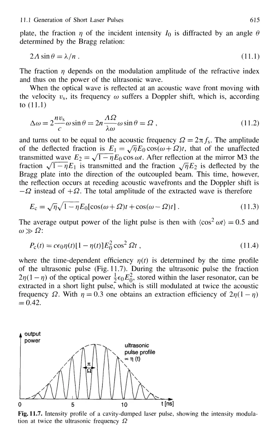
11.1.3 Cavity Dumping 614
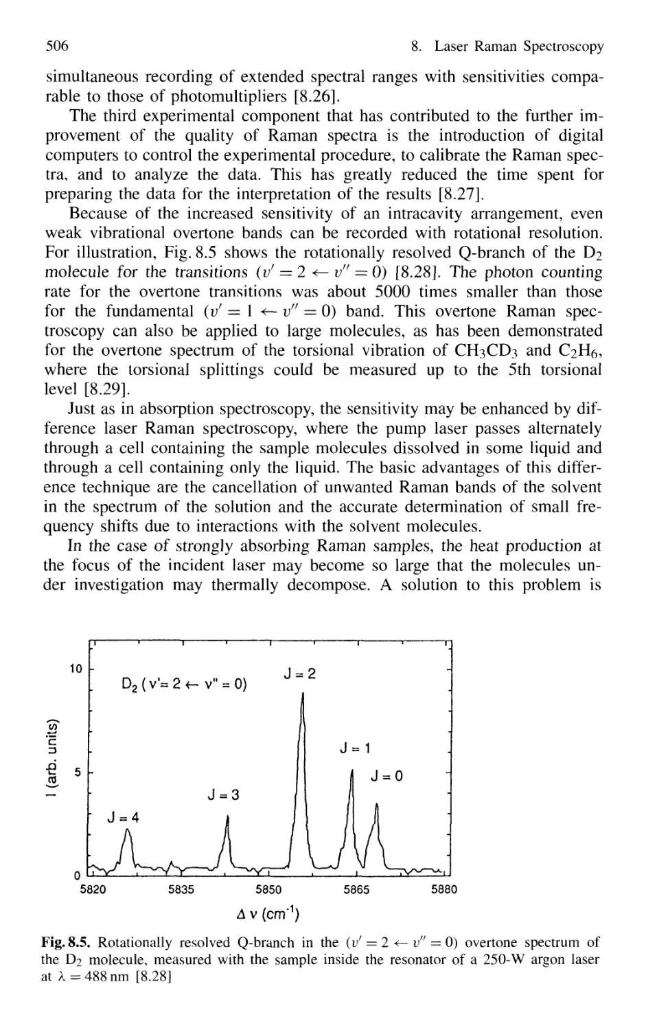
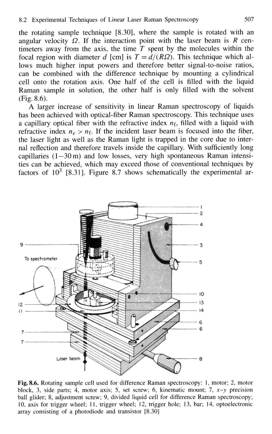
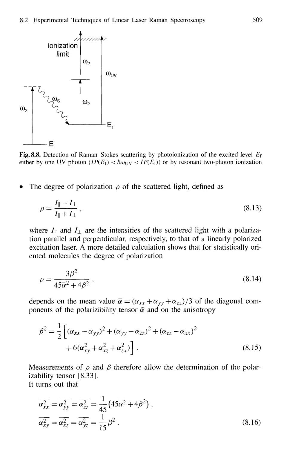
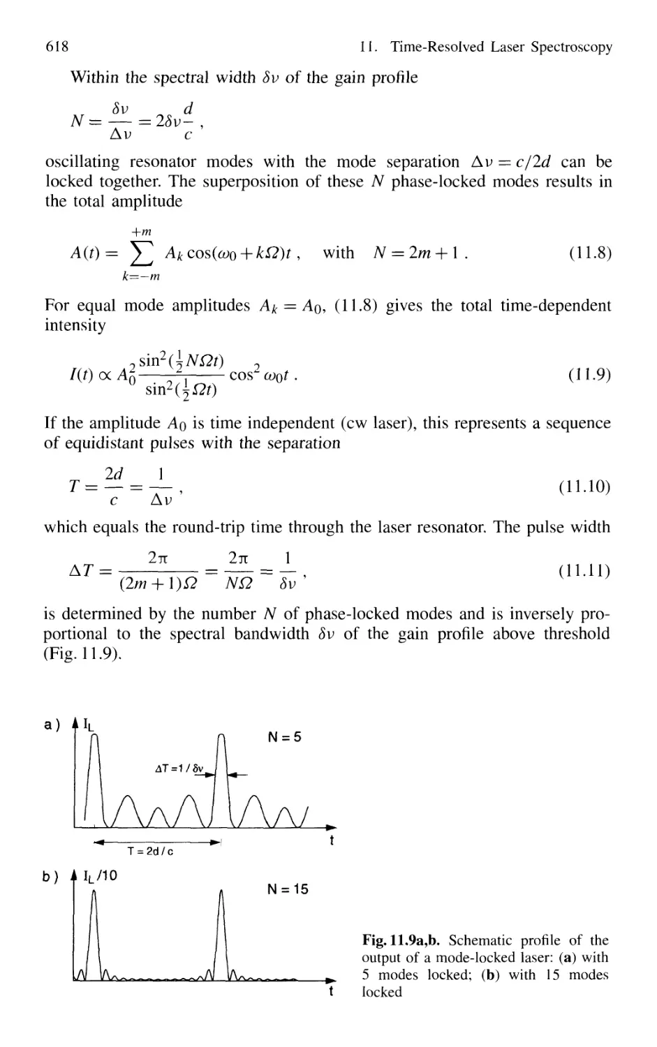
11.1.4 Mode Locking of Lasers 616
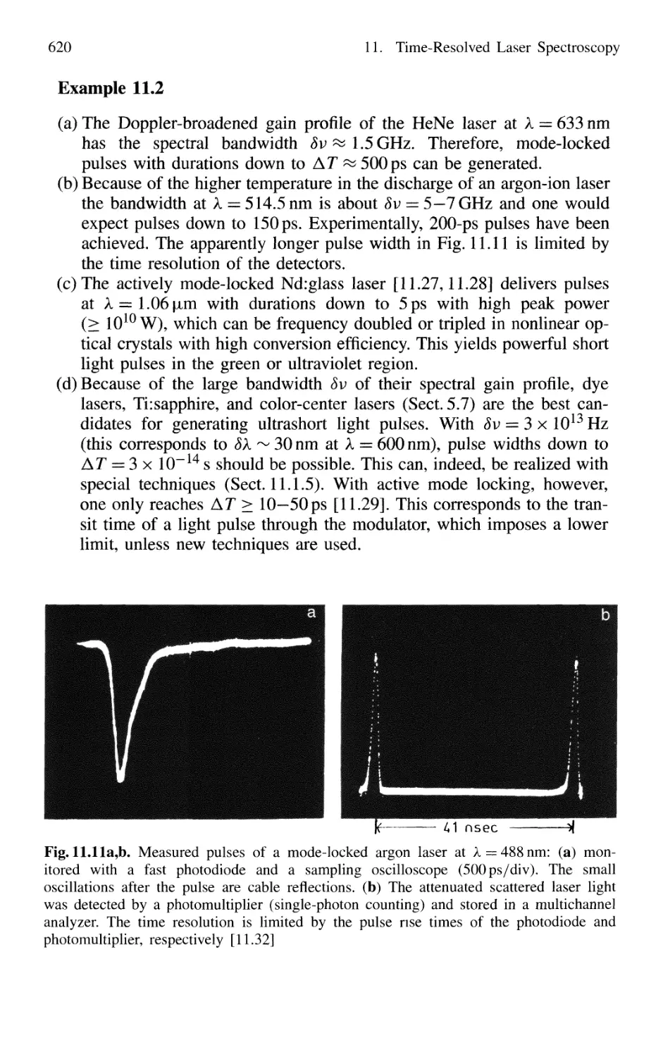
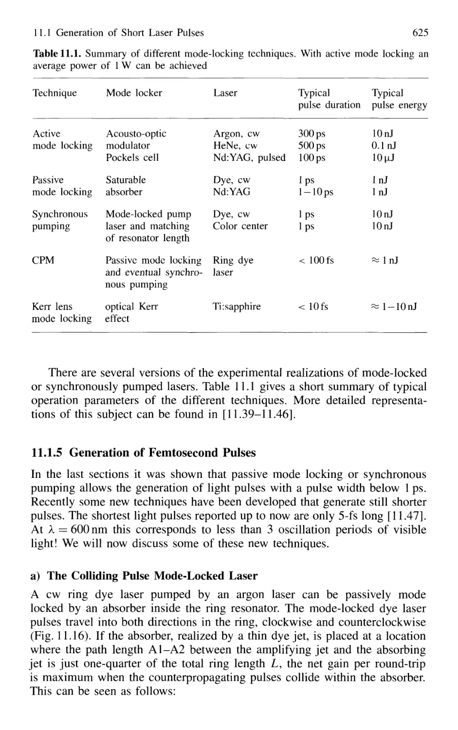
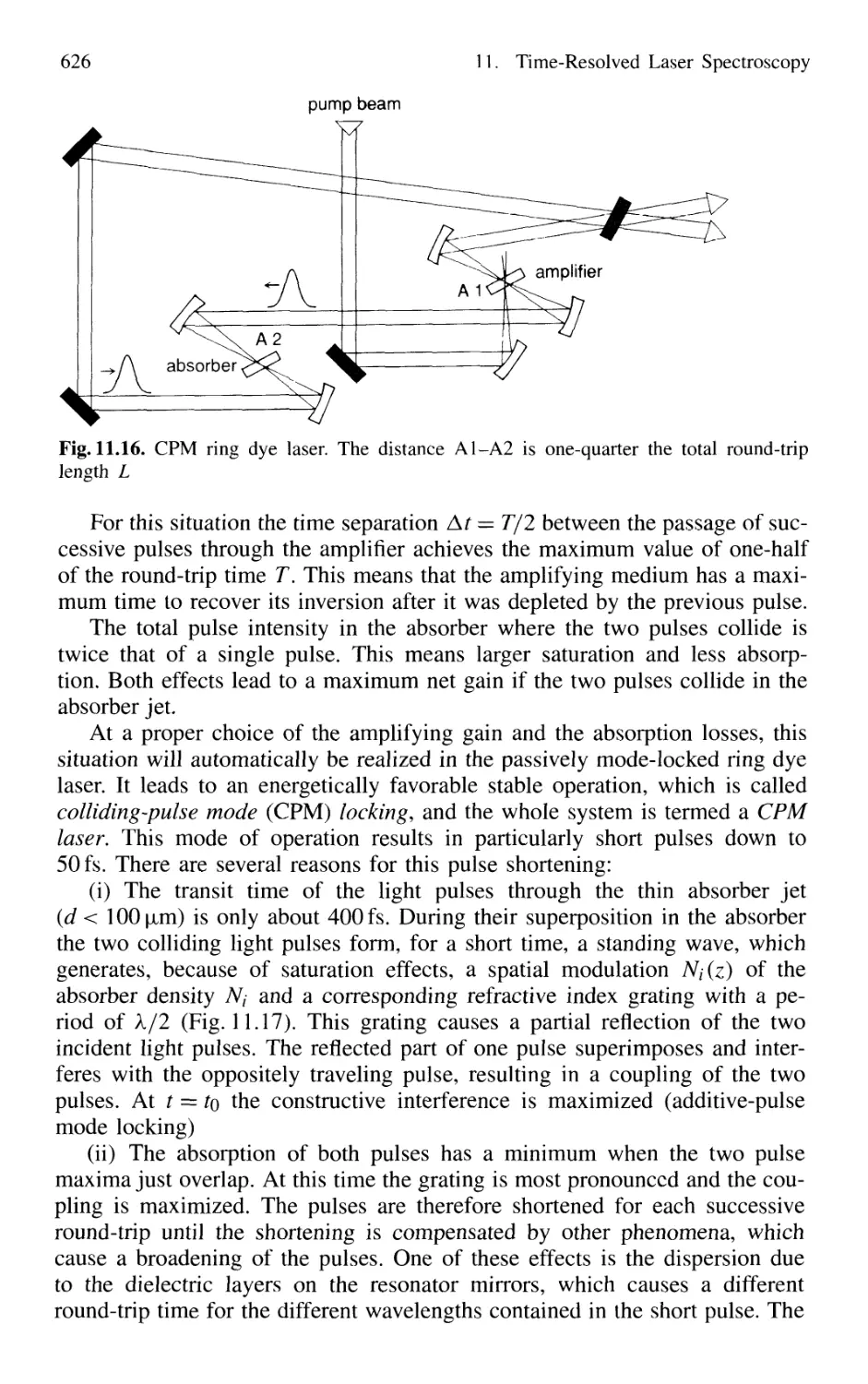
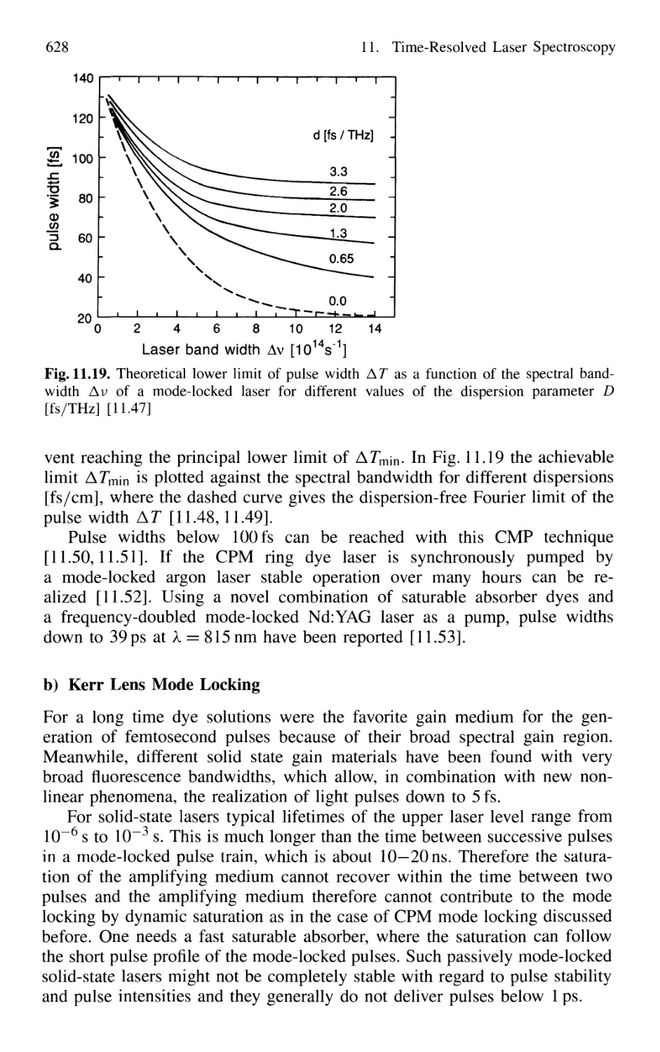
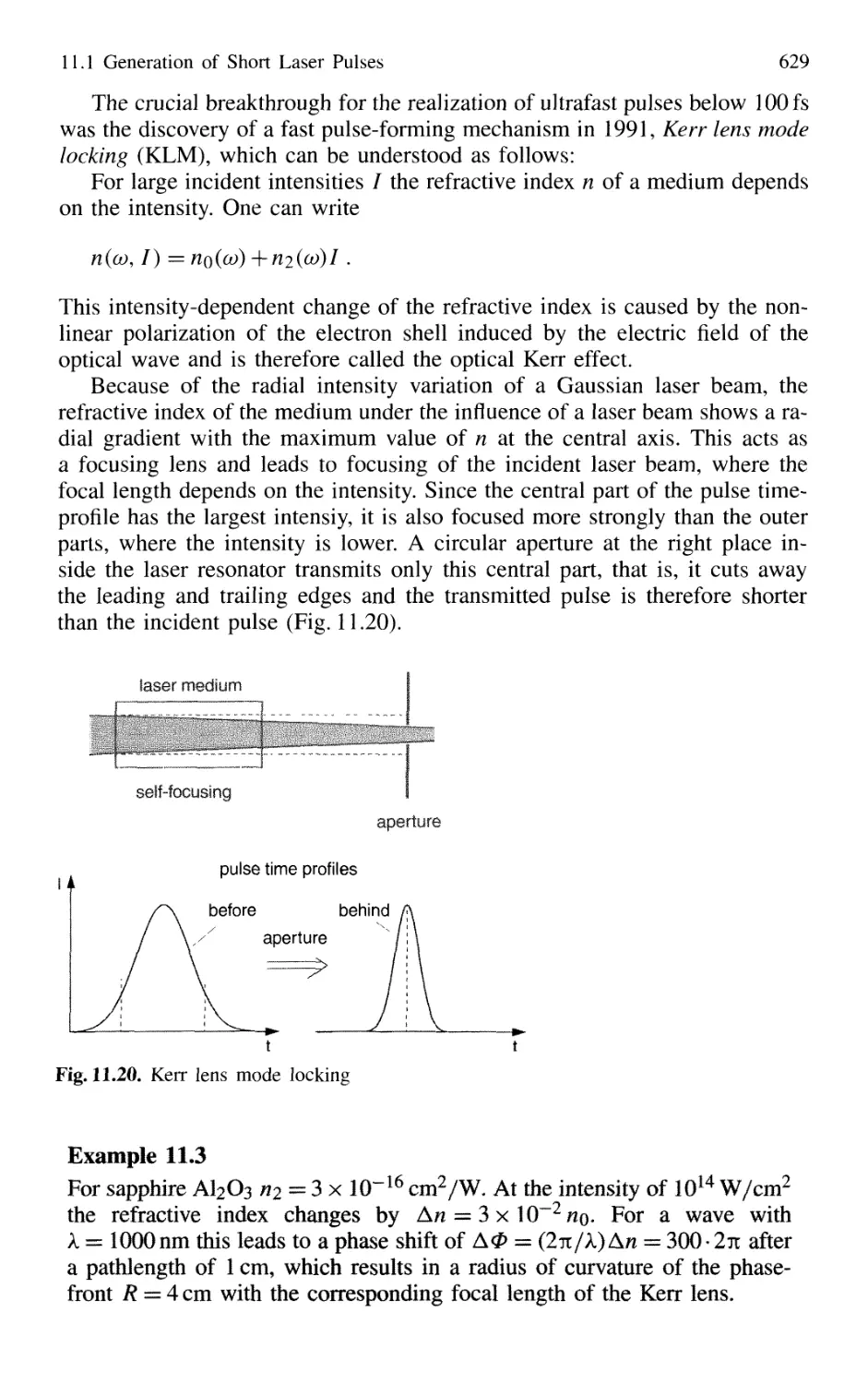
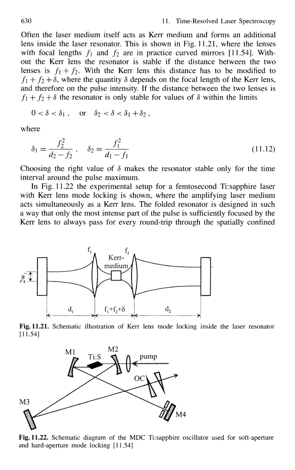
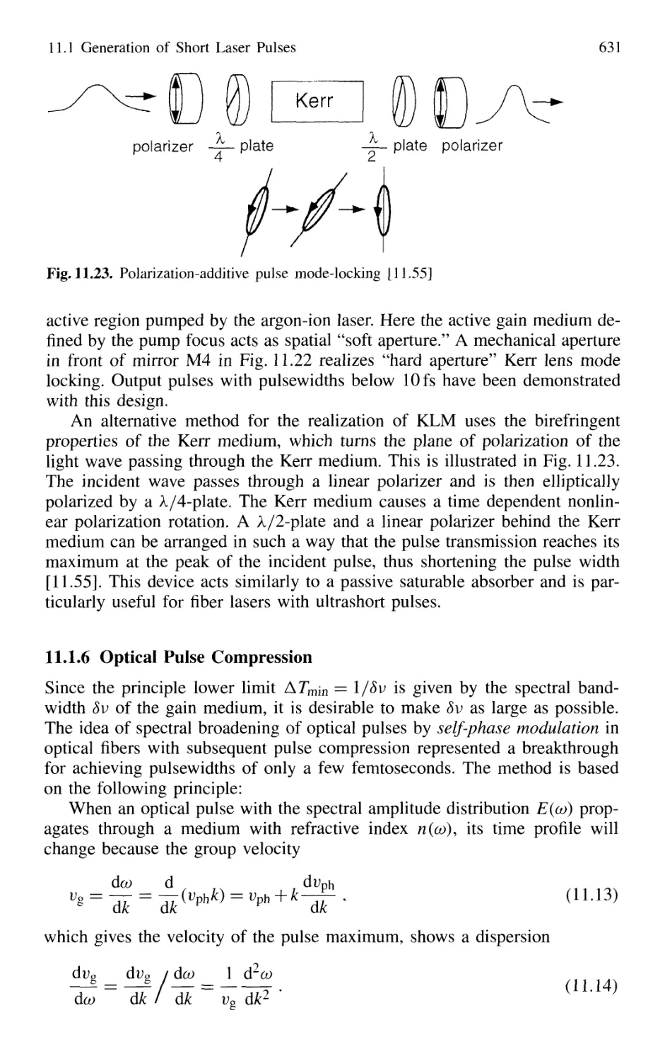
11.1.5 Generation of Femtosecond Pulses 625
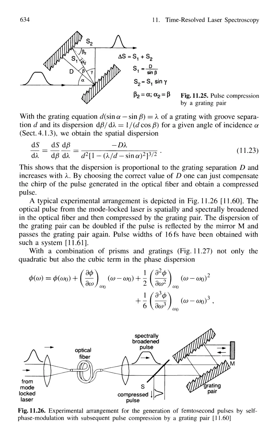
11.1.6 Optical Pulse Compression 631
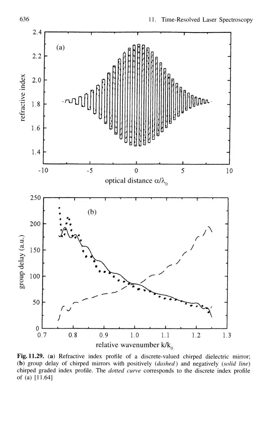
11.1.7 Sub 10-fs Pulses with Chirped Laser Mirrors 635
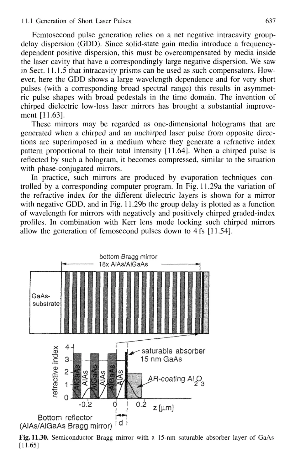
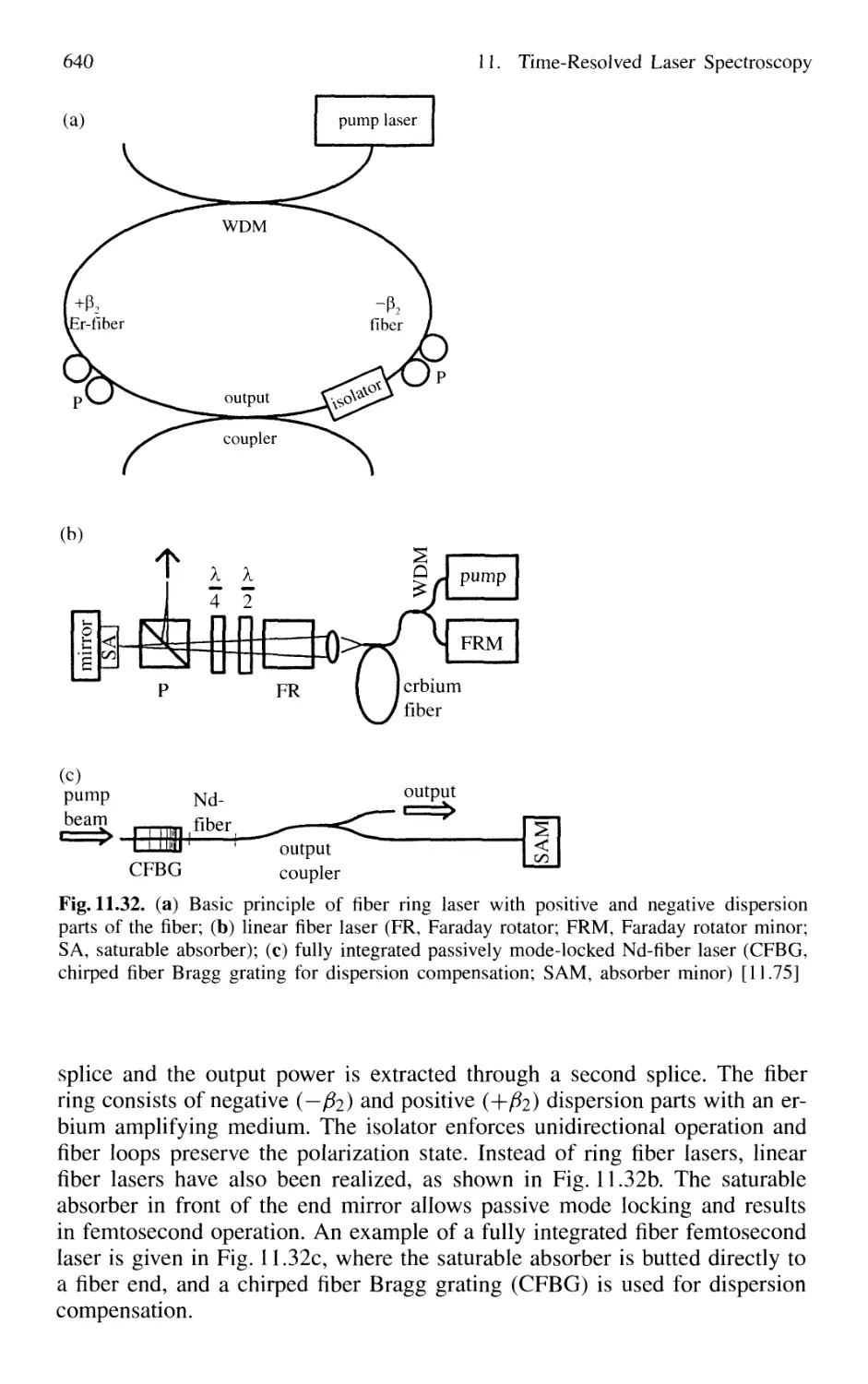
11.1.8 Fiber Lasers and Optical Solitons 638
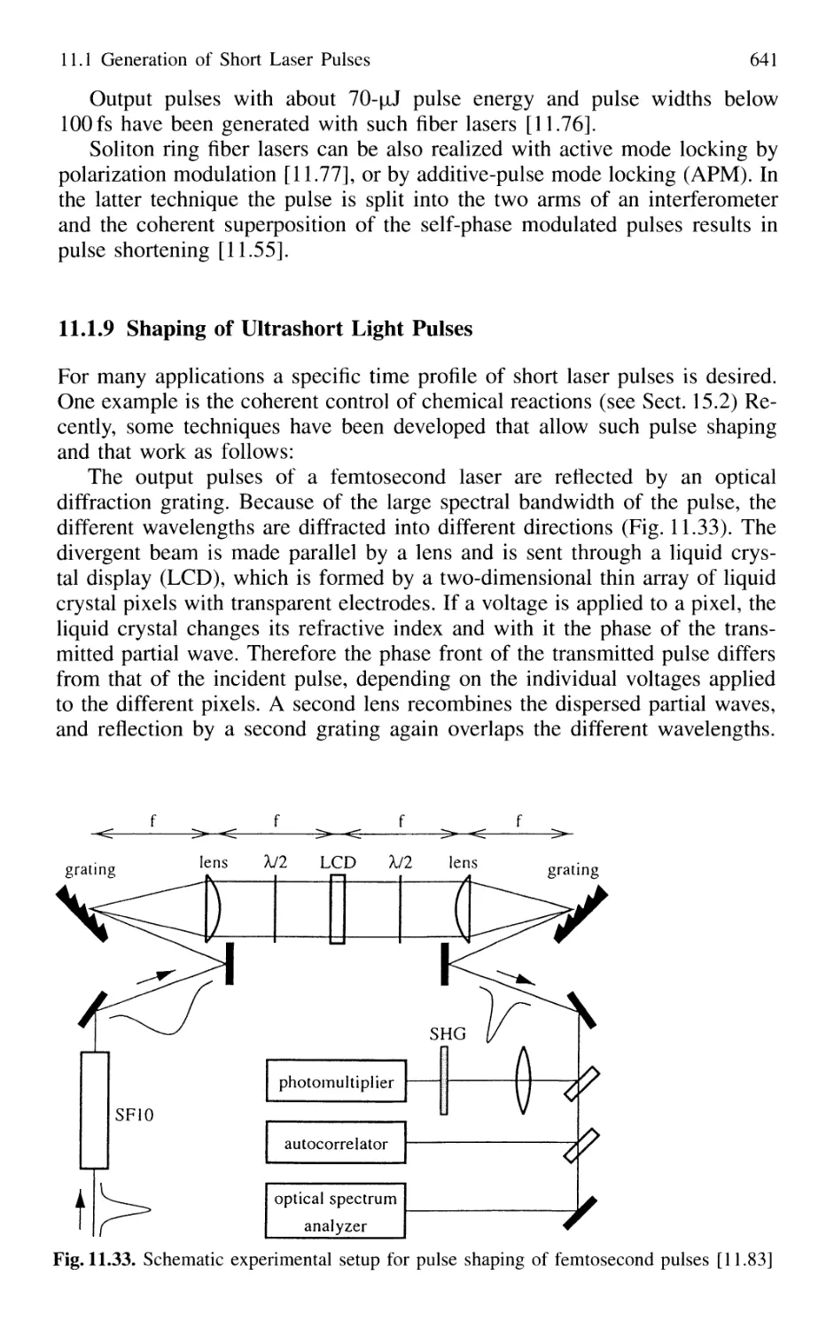
11.1.9 Shaping of Ultrashort Light Pulses 641
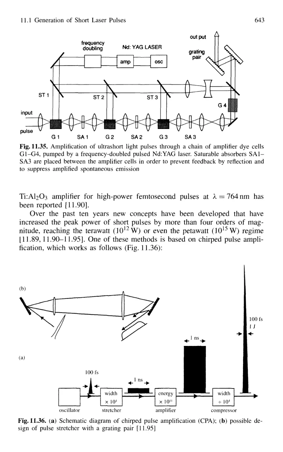
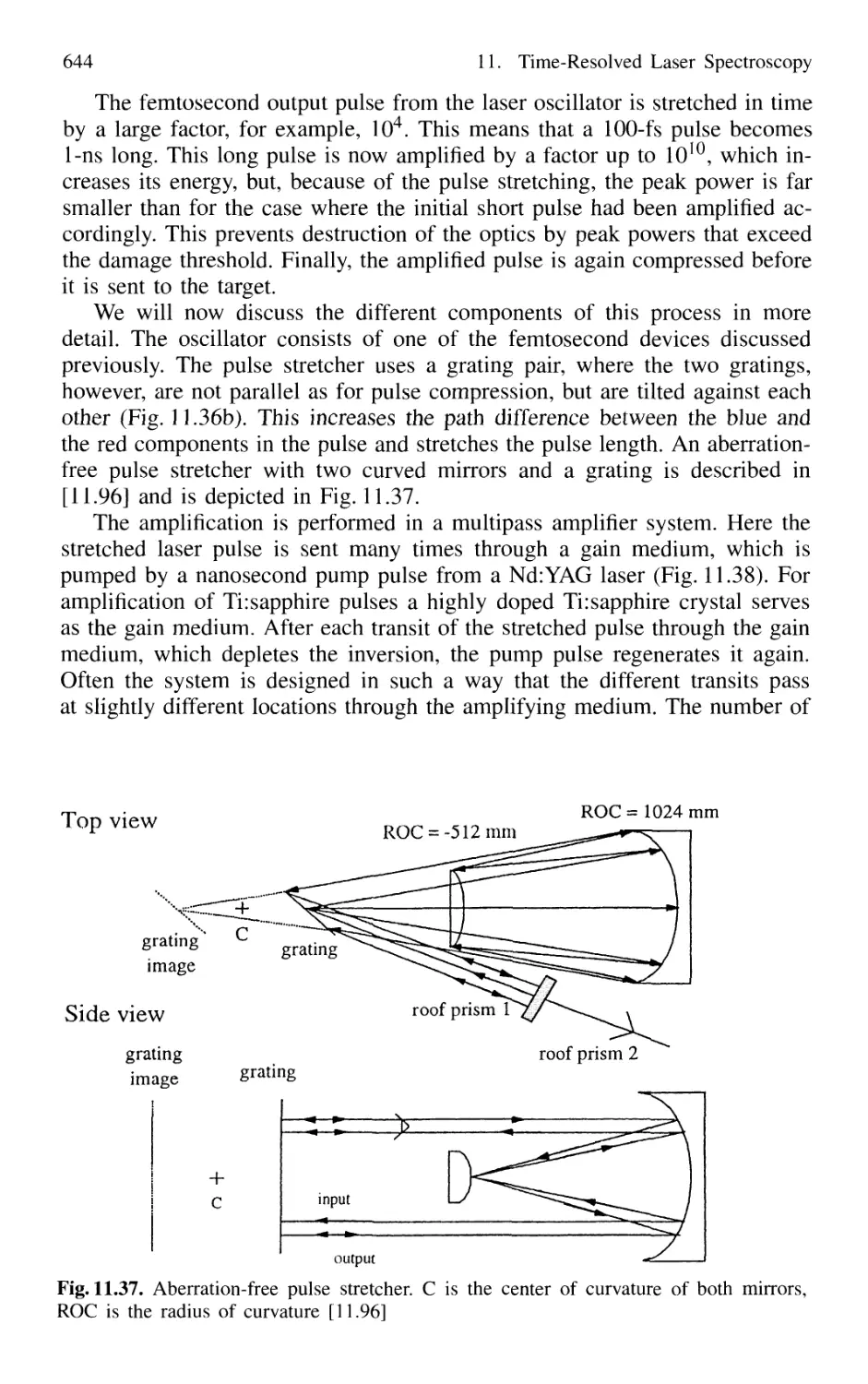
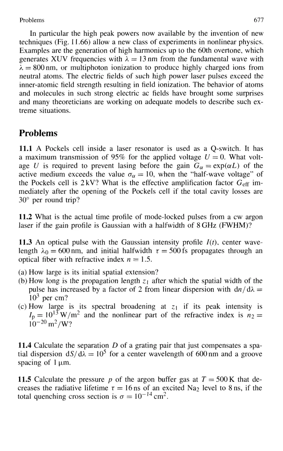
11.1.10 Generation of High-Power Ultrashort Pulses 7. 642
Contents XVII
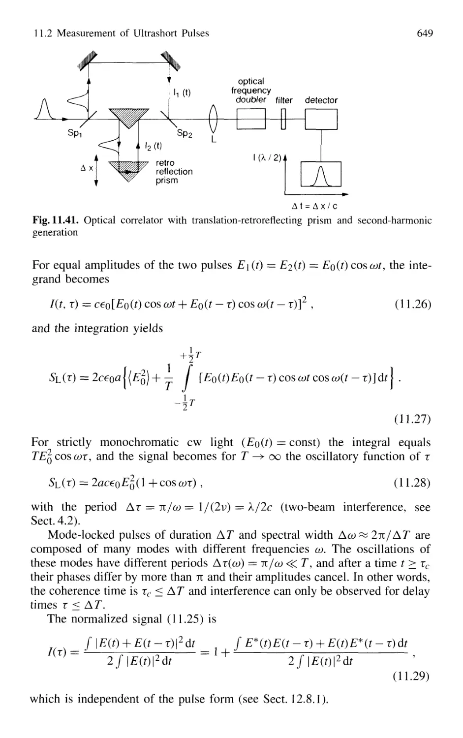
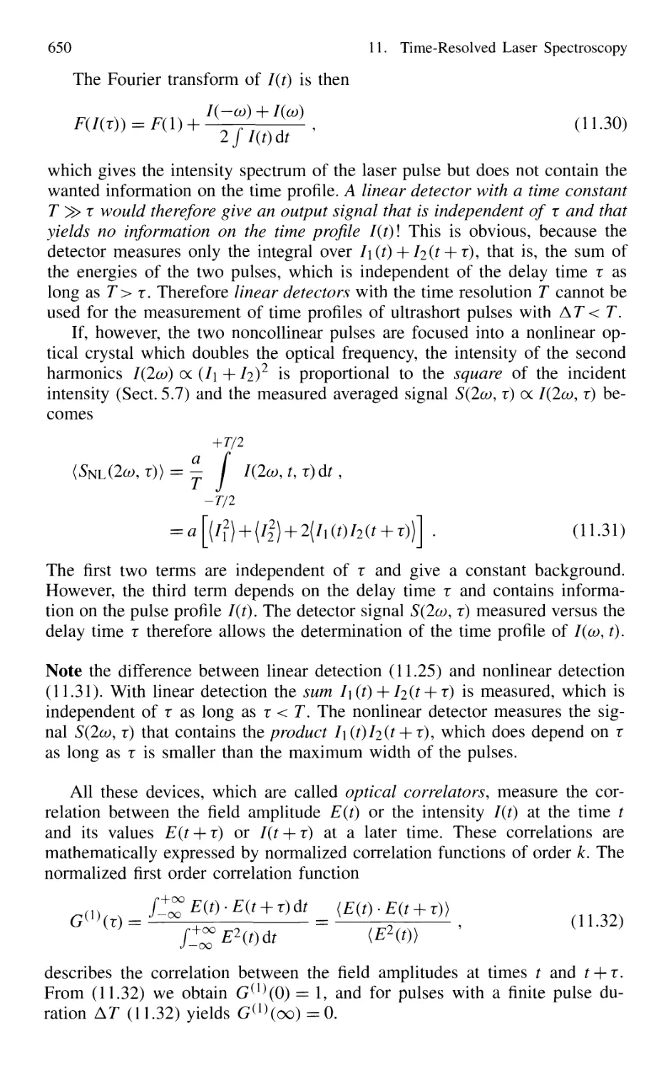
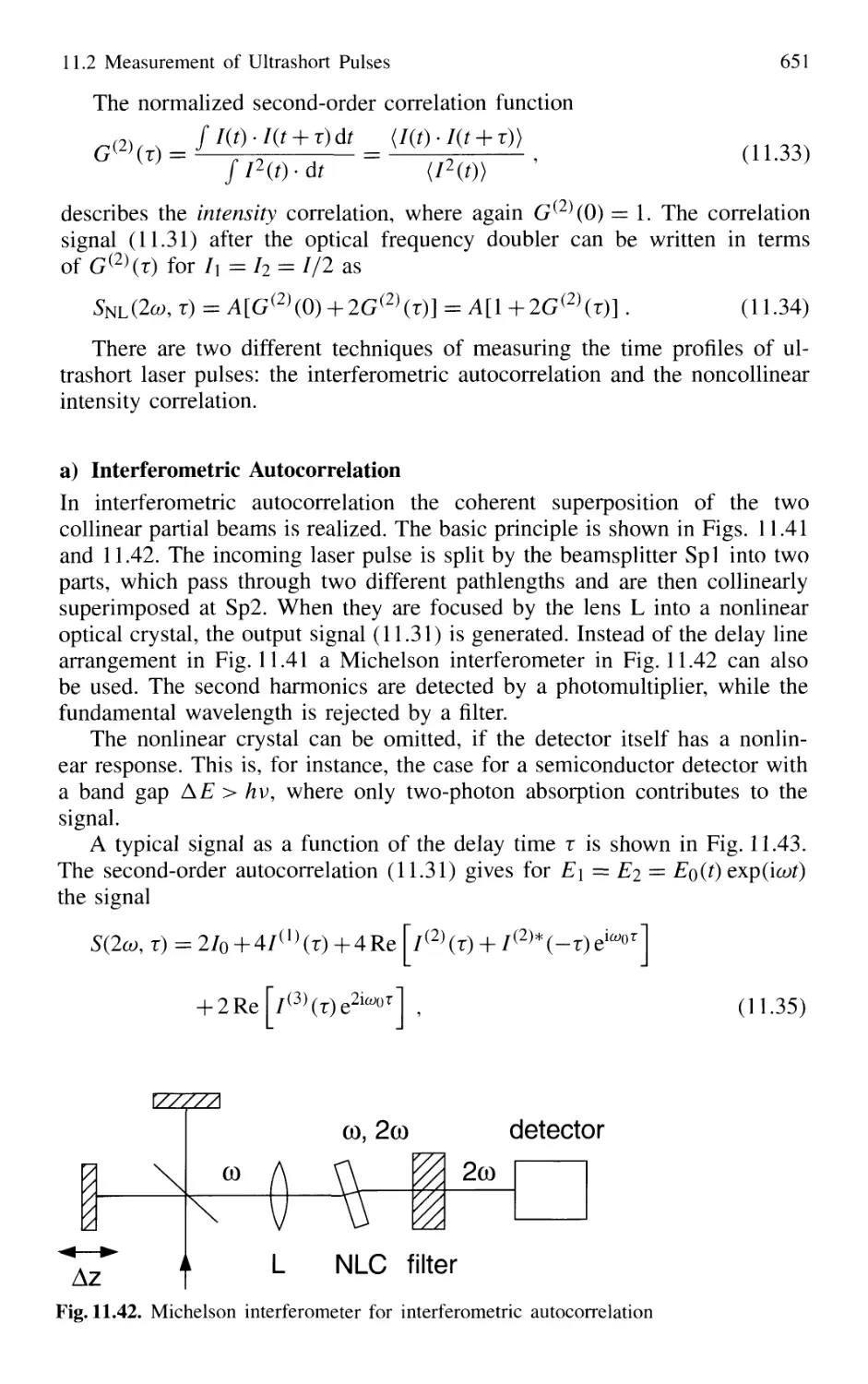
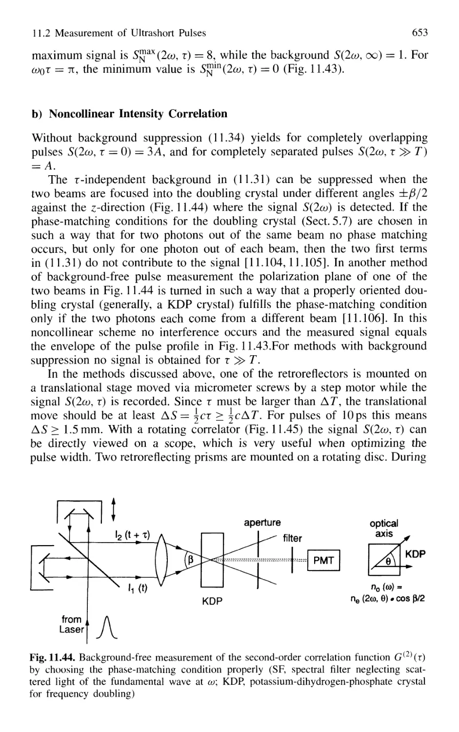
11.2 Measurement of Ultrashort Pulses 646
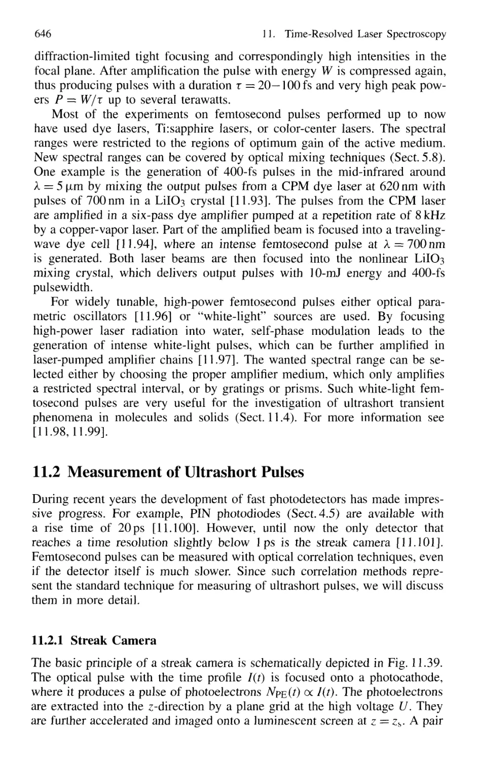
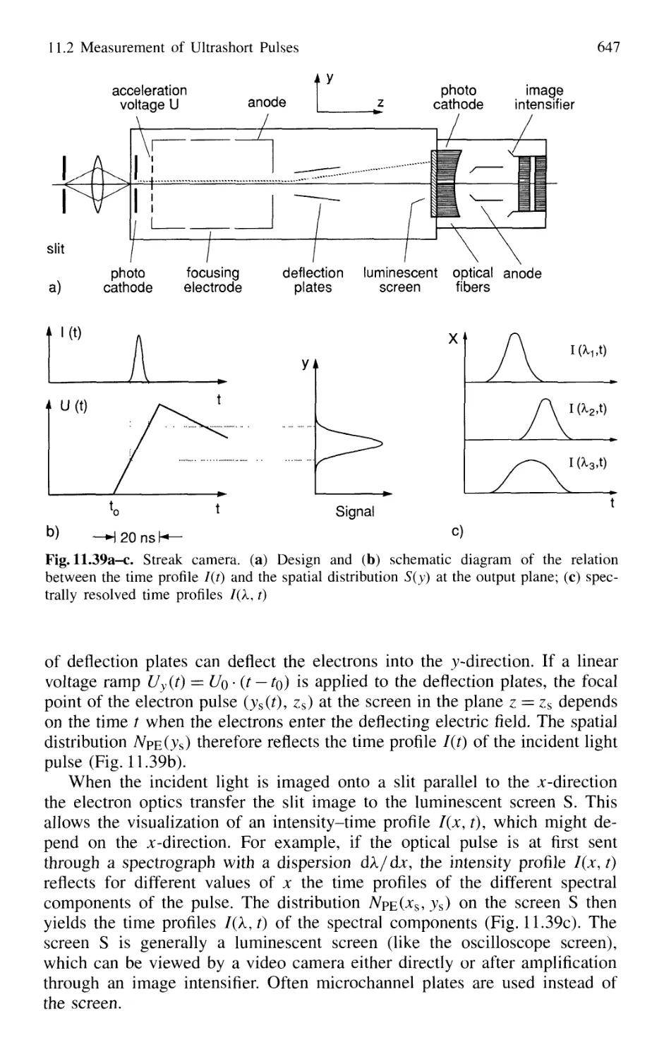
11.2.1 Streak Camera 646
11.2.2 Optical Correlator for Measuring Ultrashort Pulses 648
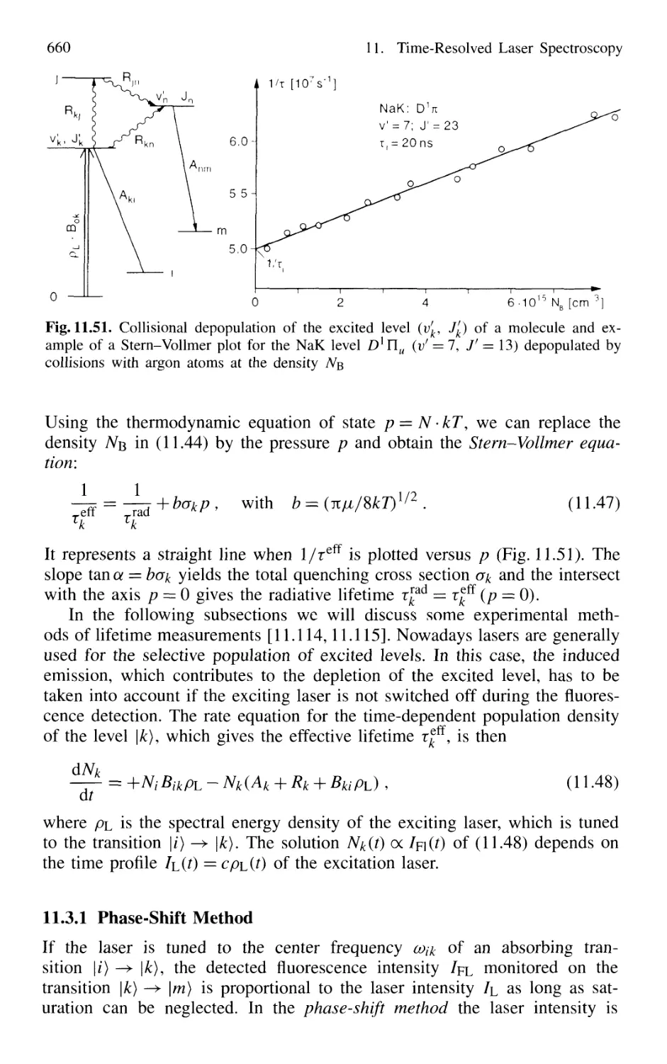
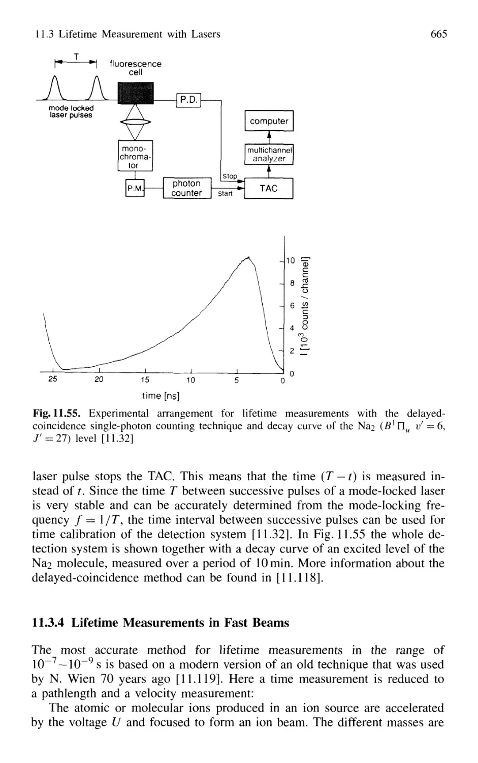
11.3 Lifetime Measurement with Lasers 658
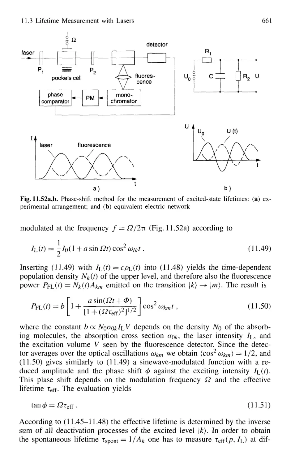
11.3.1 Phase-Shift Method 660
11.3.2 Single-Pulse Excitation 662
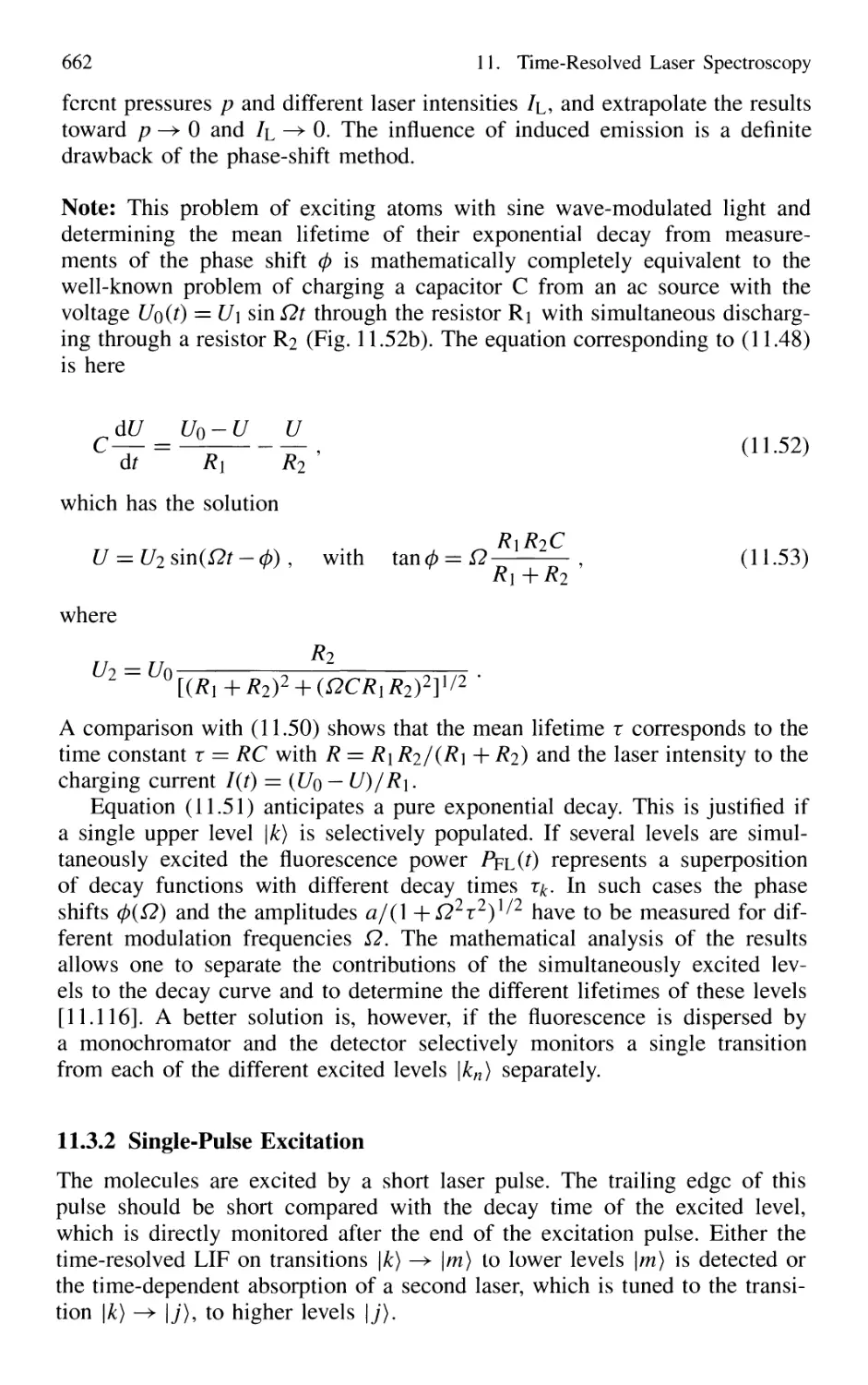
11.3.3 Delayed-Coincidence Technique 663
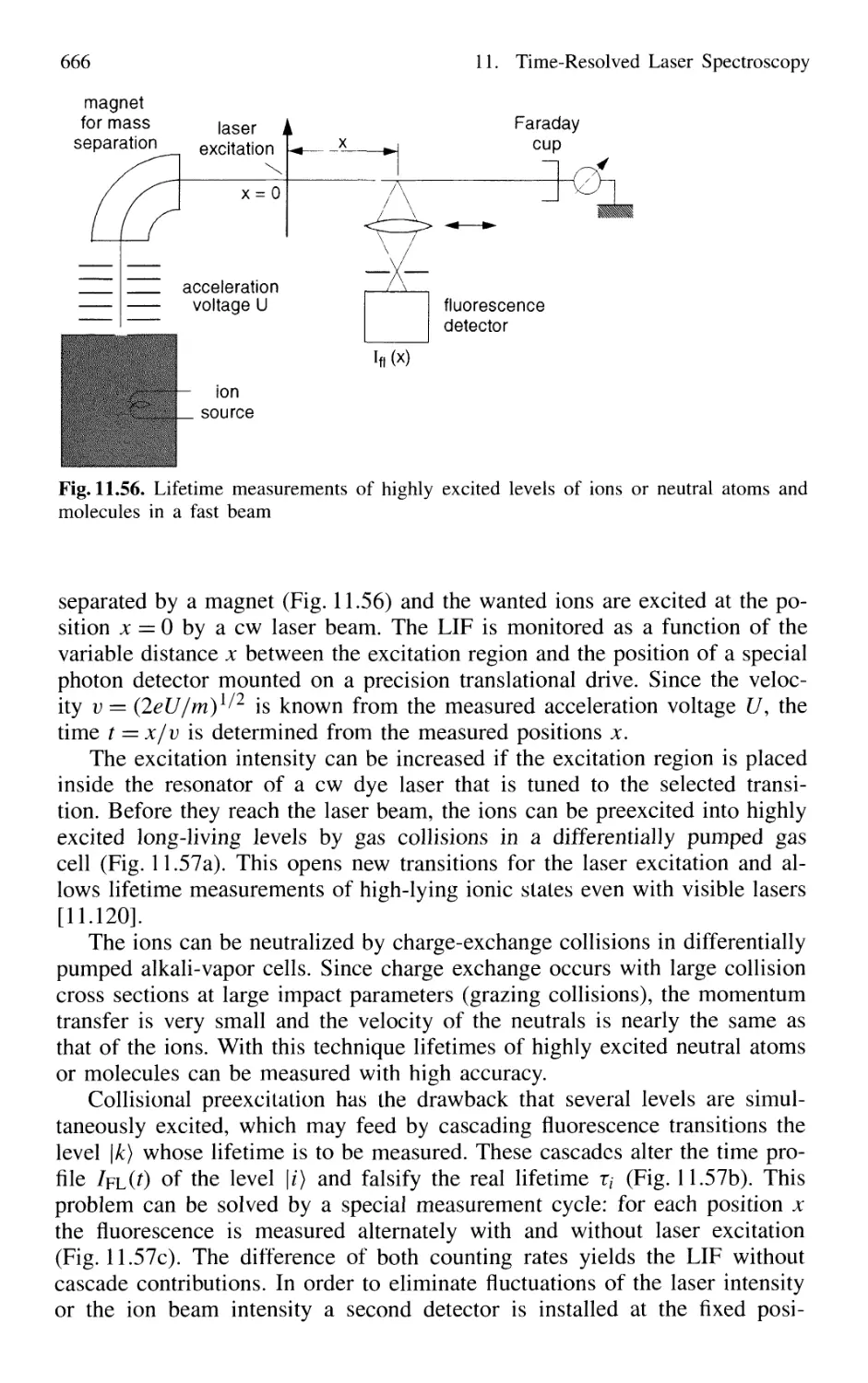
11.3.4 Lifetime Measurements in Fast Beams 665
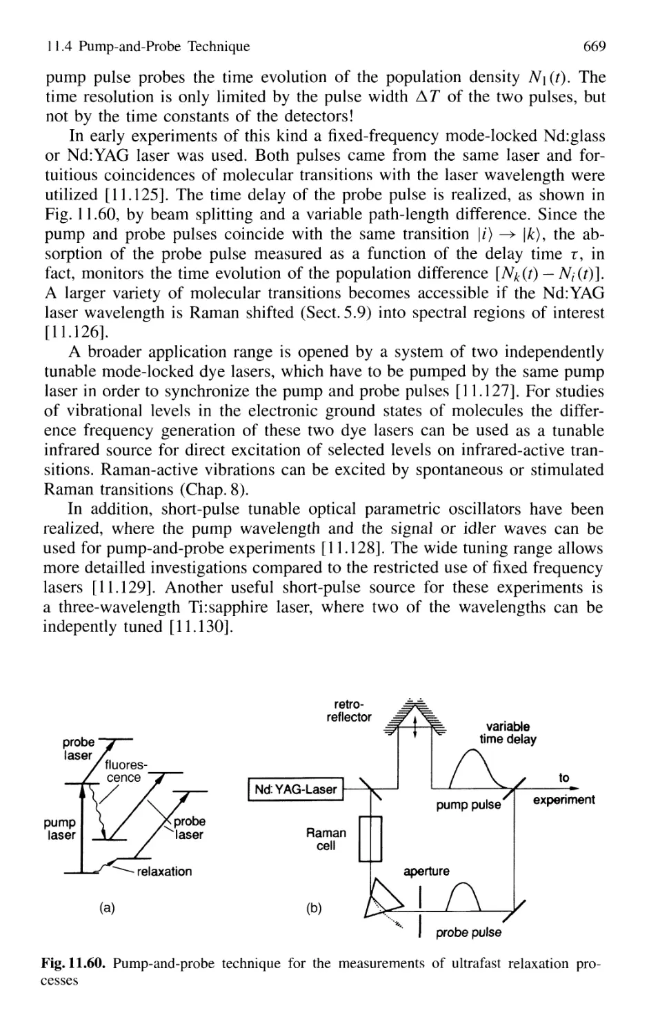
11.4 Pump-and-Probe Technique 668
11.4.1 Pump-and-Probe Spectroscopy
of Collisional Relaxation in Liquids 670
11.4.2 Electronic Relaxation in Semiconductors 671
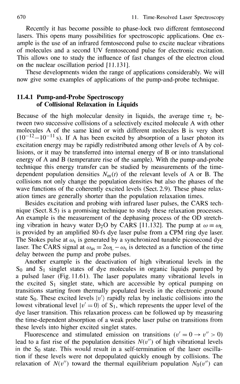
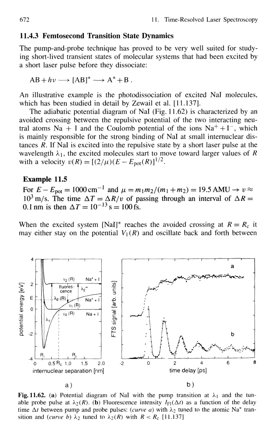
11.4.3 Femtosecond Transition State Dynamics 672
11.4.4 Real-Time Observations of Molecular Vibrations .. 673
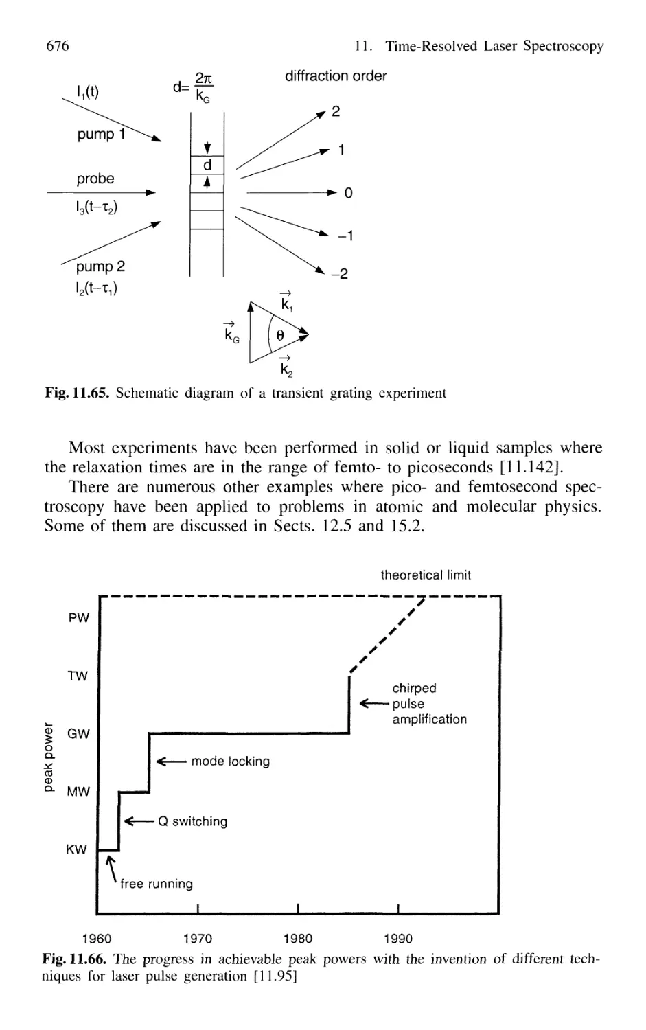
11.4.5 Transient Grating Techniques 675
Problems 677
12. Coherent Spectroscopy 679
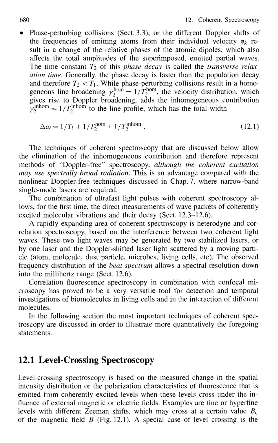
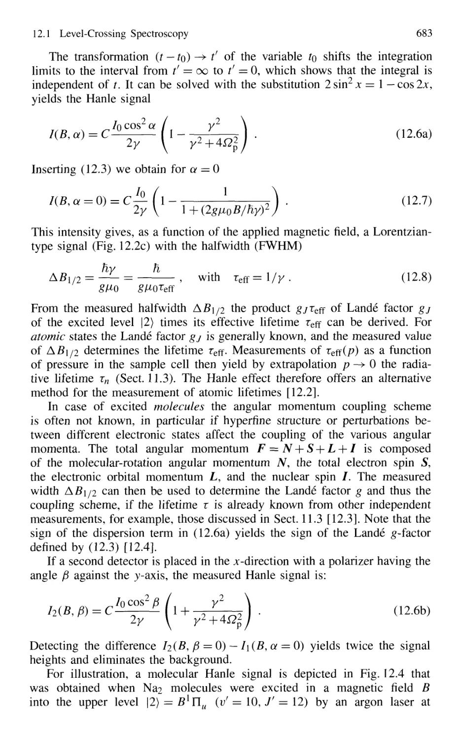
12.1 Level-Crossing Spectroscopy 680
12.1.1 Classical Model of the Hanle Effect 681
12.1.2 Quantum-Mechanical Models 684
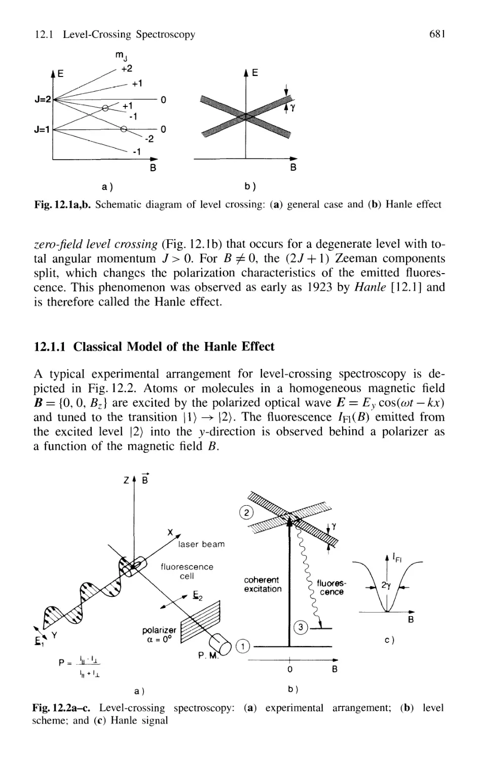
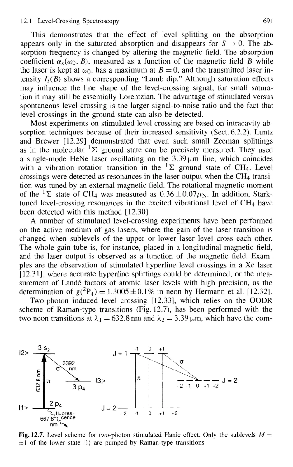
12.1.3 Experimental Arrangements 687
12.1.4 Examples 688
12.1.5 Stimulated Level-Crossing Spectroscopy 689
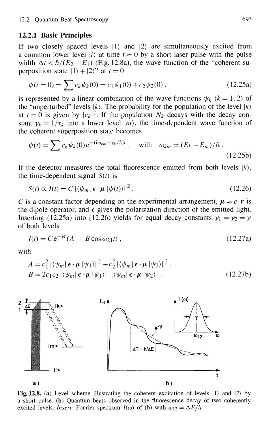
12.2 Quantum-Beat Spectroscopy 692
12.2.1 Basic Principles 693
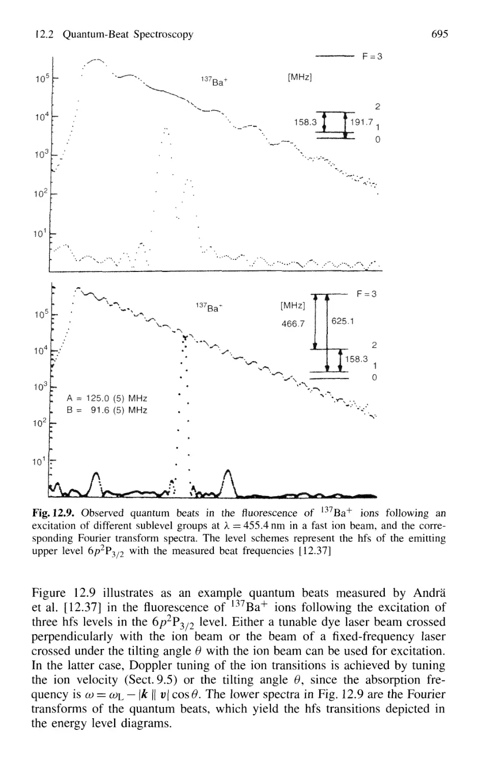
12.2.2 Experimental Techniques 694
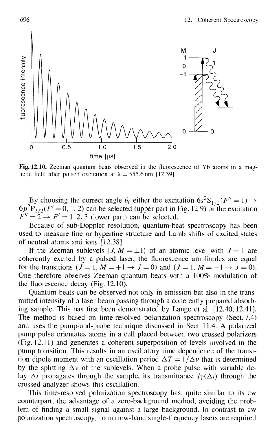
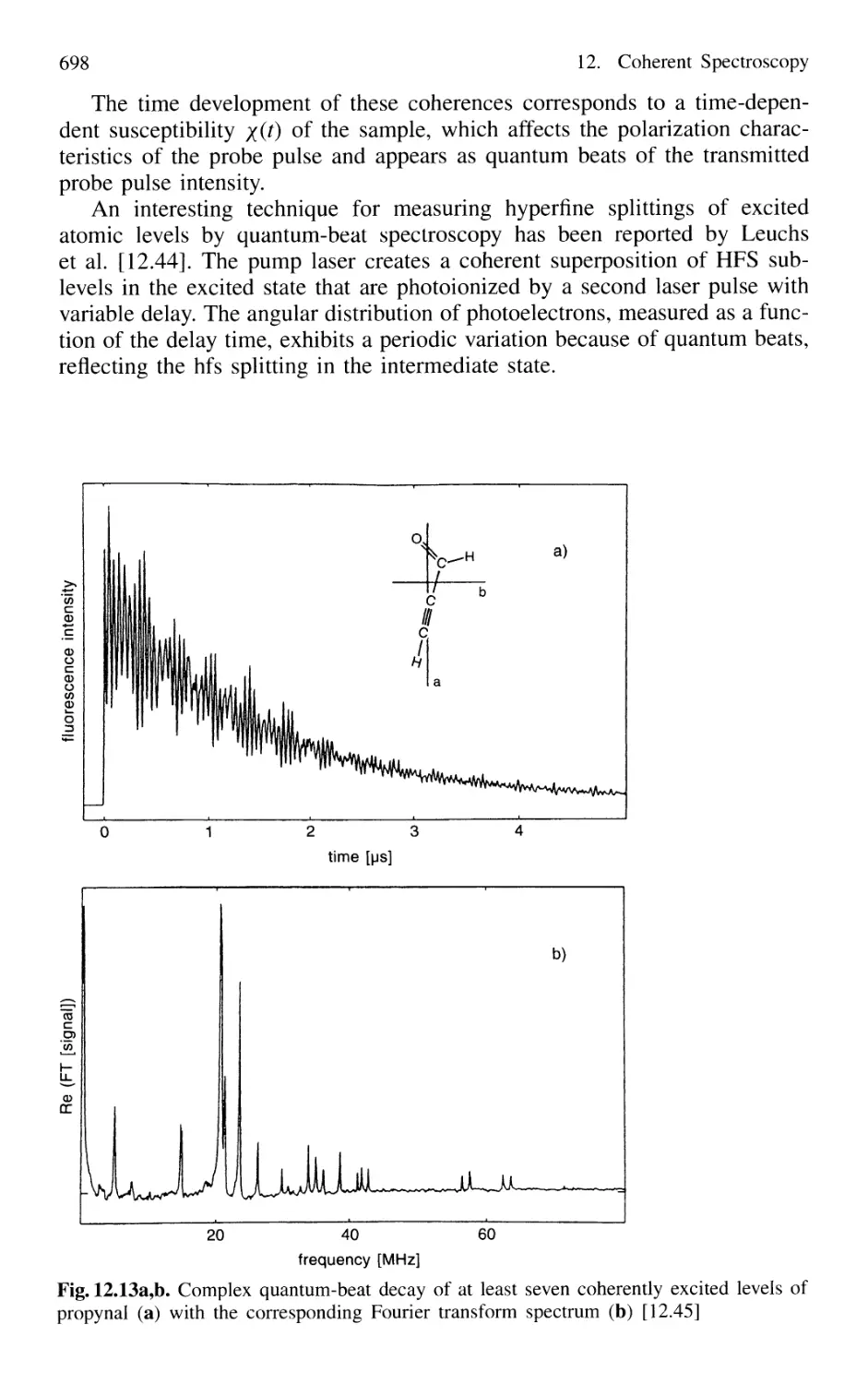
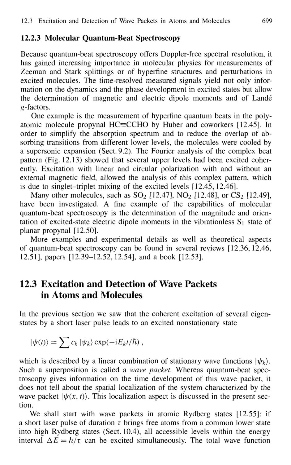
12.2.3 Molecular Quantum-Beat Spectroscopy 699
12.3 Excitation and Detection of Wave Packets
in Atoms and Molecules 699
12.4 Optical Pulse-Train Interference Spectroscopy 702
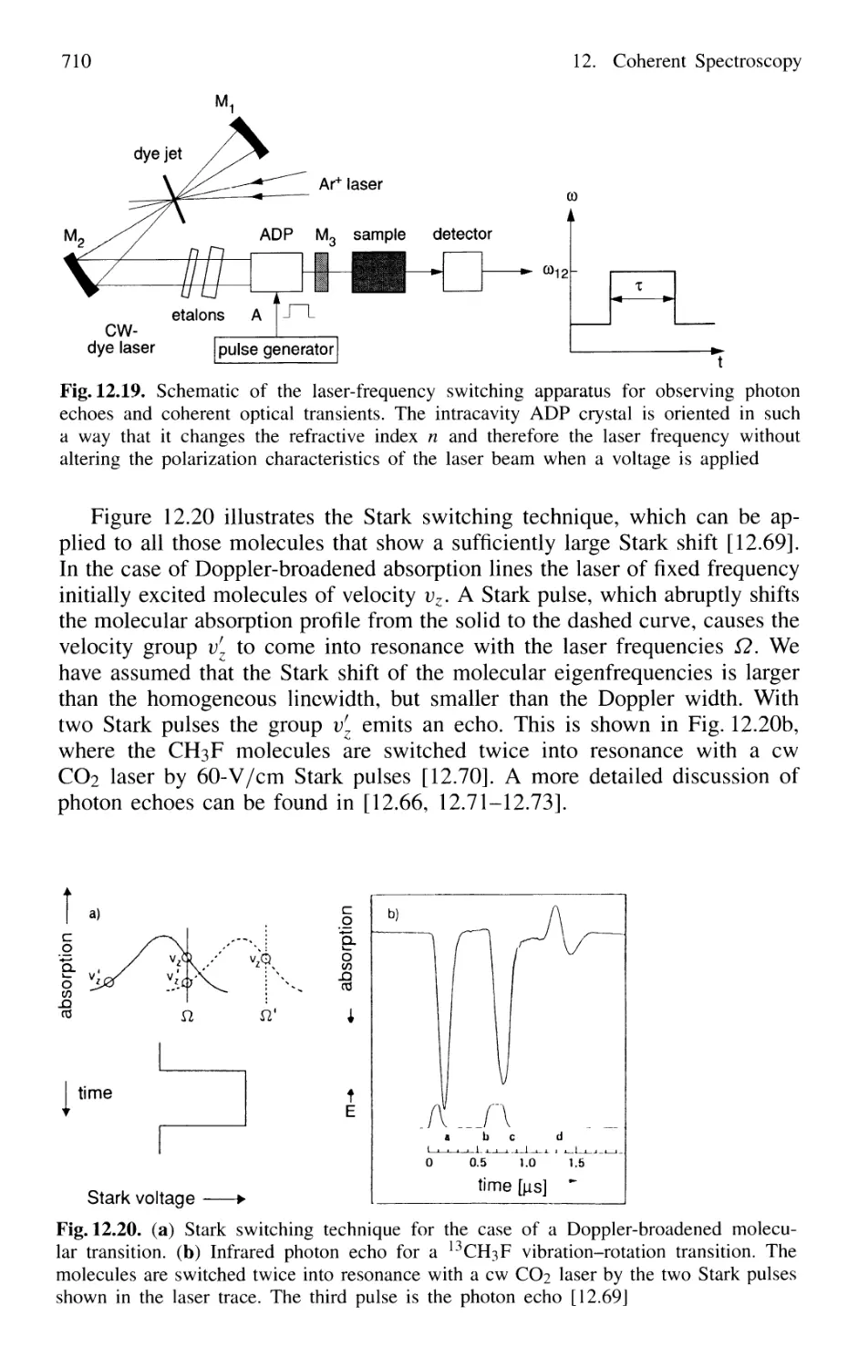
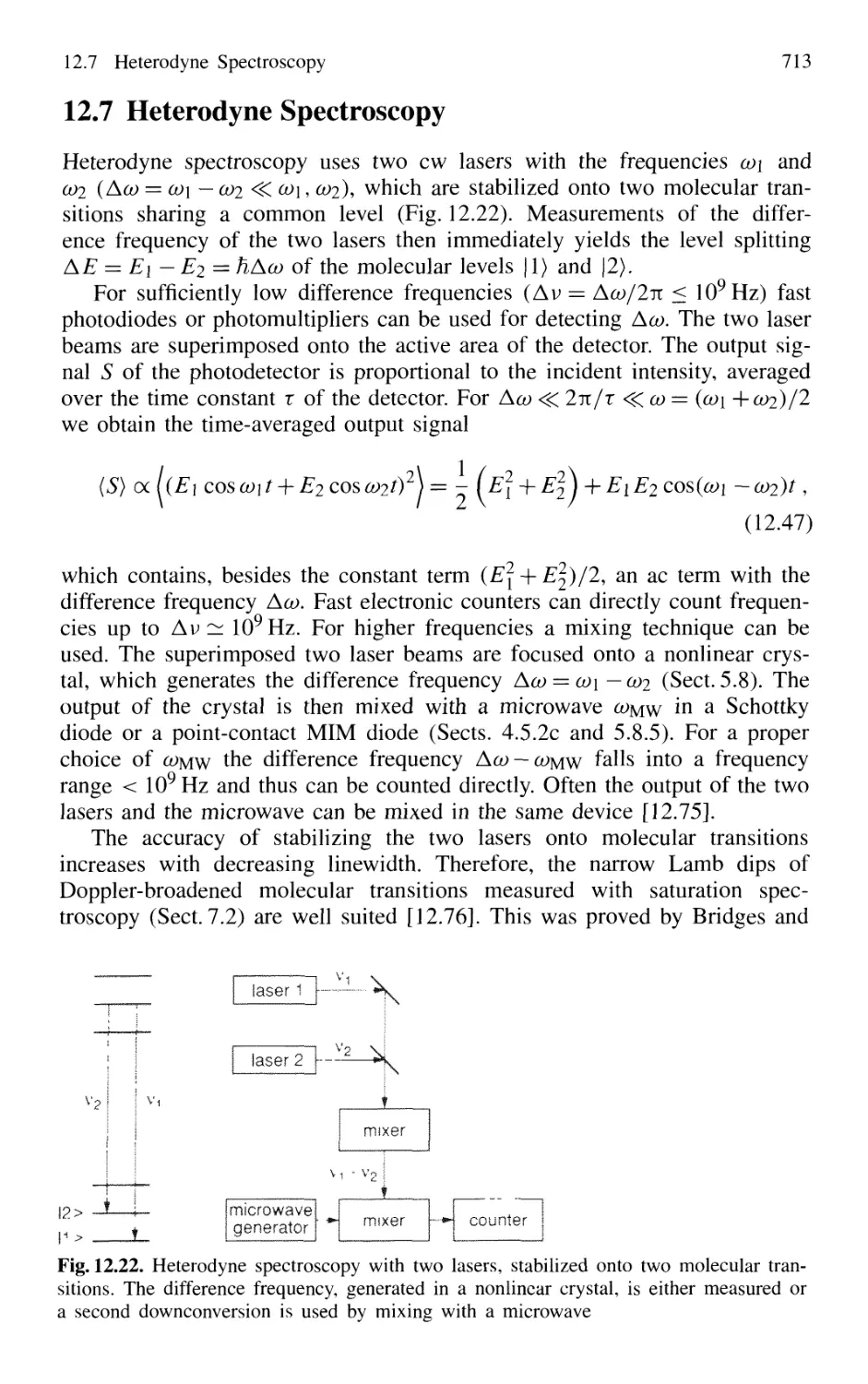
12.5 Photon Echoes 704
12.6 Optical Nutation and Free-Induction Decay 711
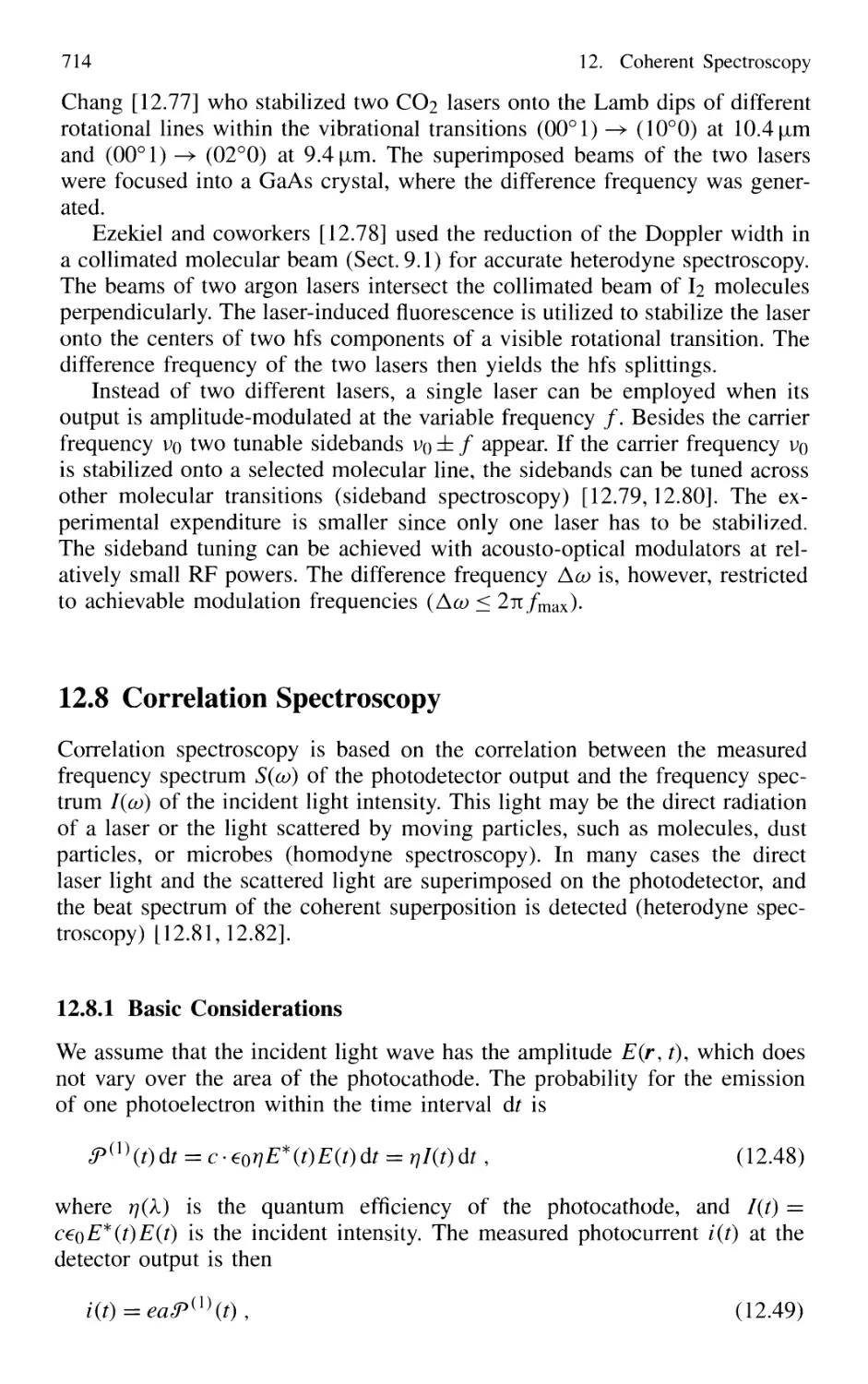
12.7 Heterodyne Spectroscopy 713
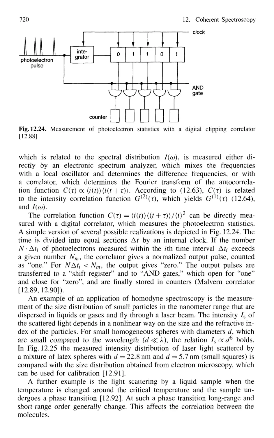
12.8 Correlation Spectroscopy 714
12.8.1 Basic Considerations 714
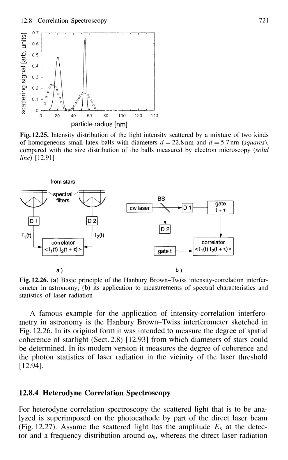
12.8.2 Correlation Spectroscopy of Light Scattered
by Microparticles 719
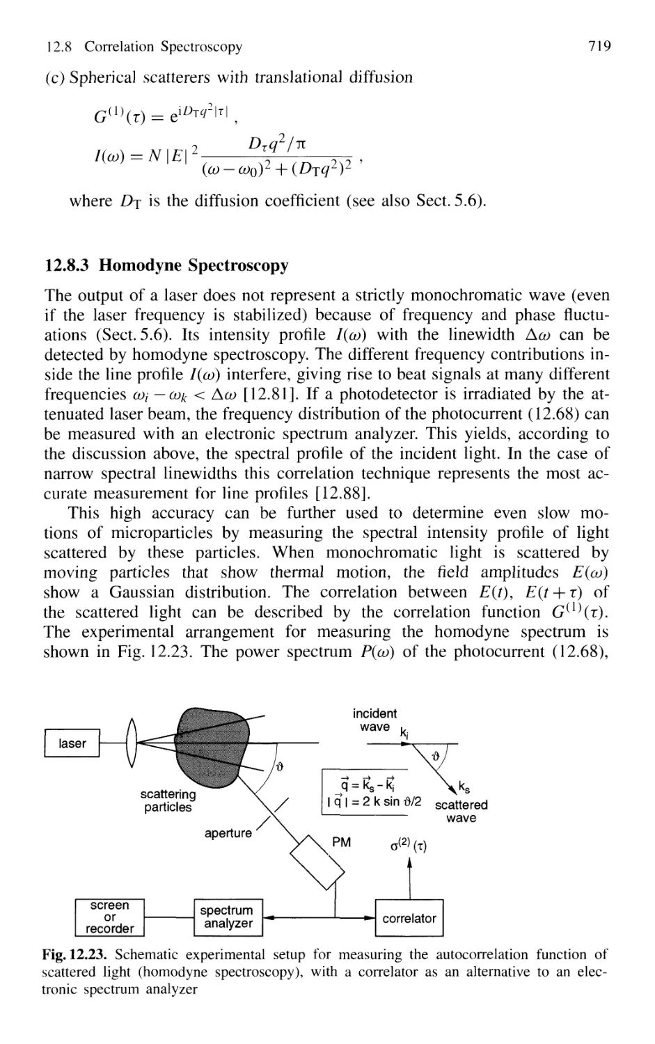
12.8.3 Homodyne Spectroscopy 720
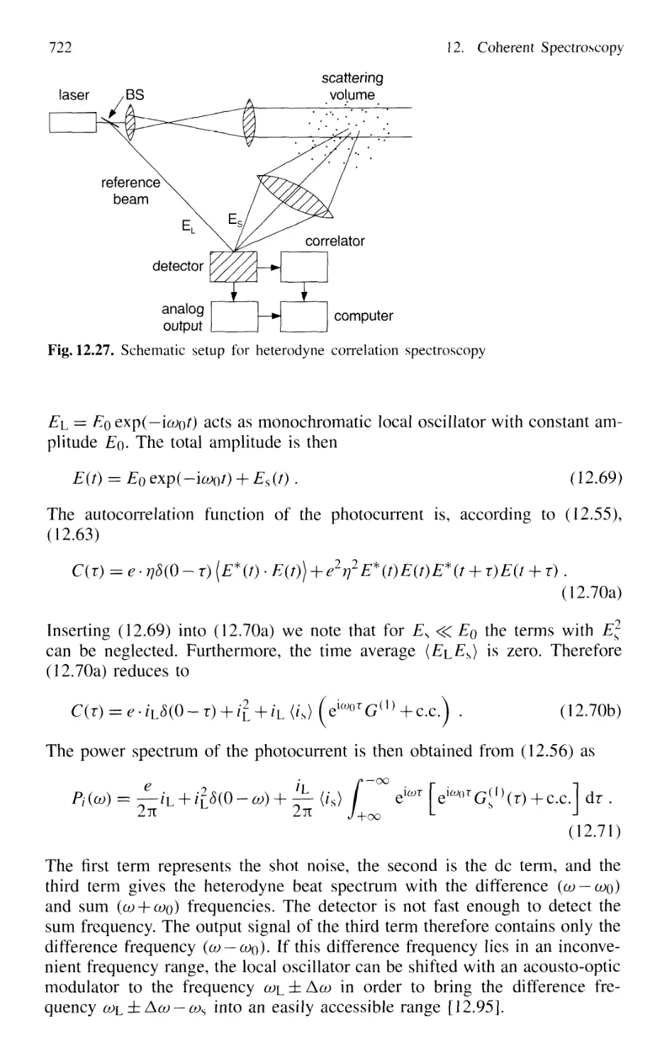
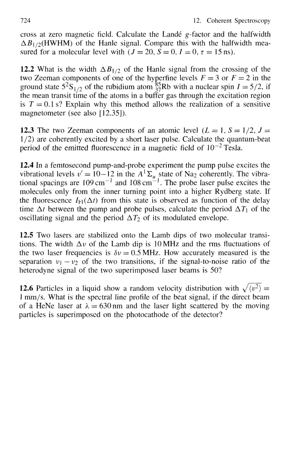
12.8.4 Heterodyne Correlation Spectroscopy 723
12.8.5 Fluorescence Correlation Spectroscopy
and Single Molecule Detection 724
Problems 724
XVIII Contents
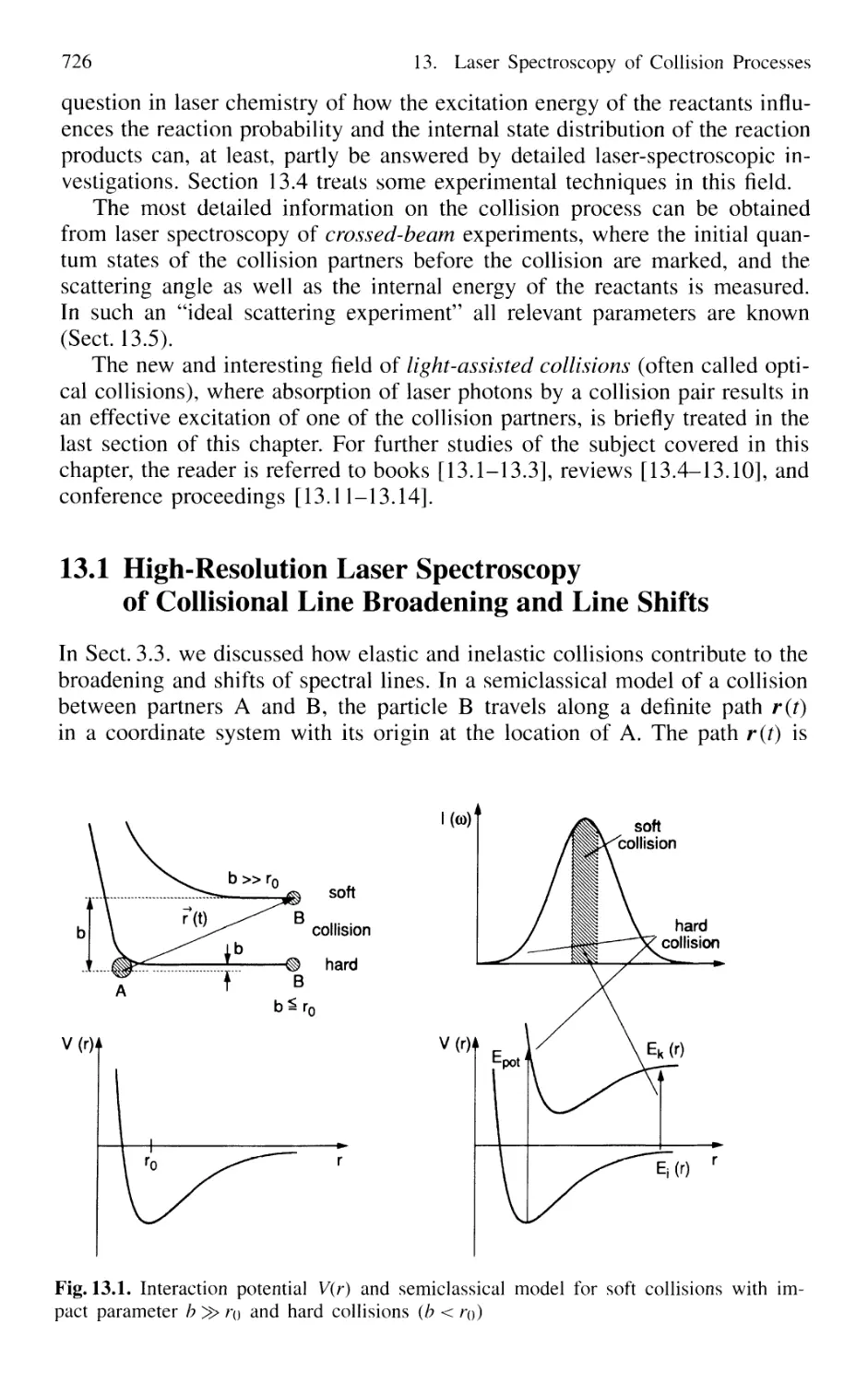
13. Laser Spectroscopy of Collision Processes 725
13.1 High-Resolution Laser Spectroscopy
of Collisional Line Broadening and Line Shifts 726
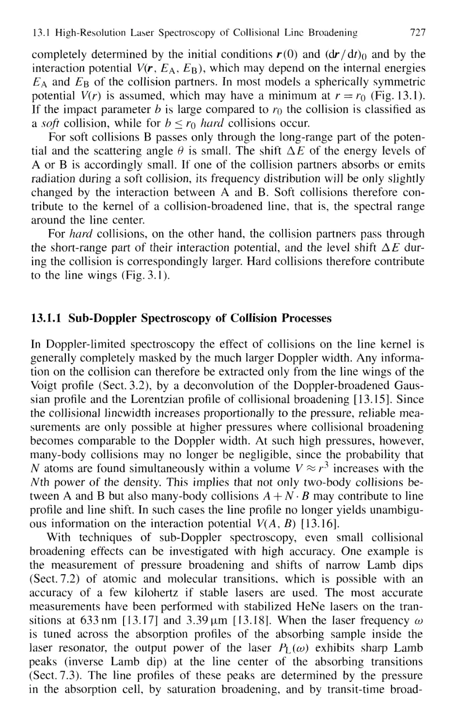
13.1.1 Sub-Doppler Spectroscopy of Collision Processes . 727
13.1.2 Combination of Different Techniques 729
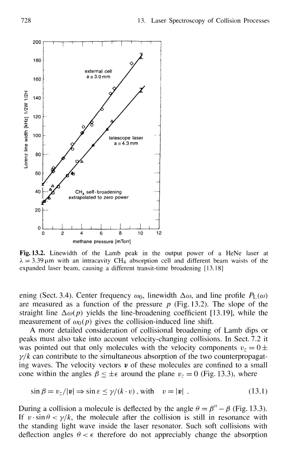
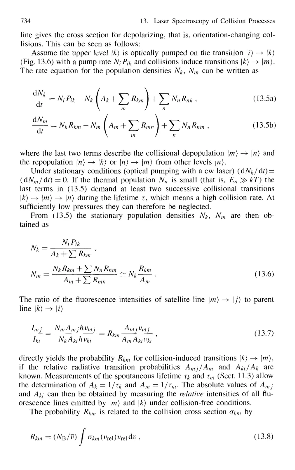
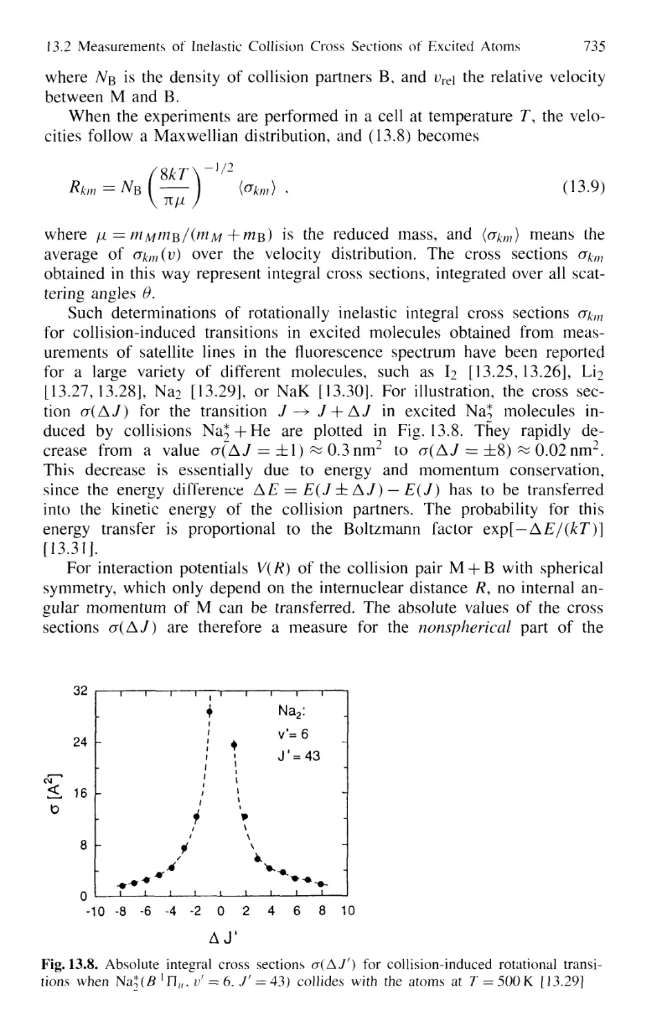
13.2 Measurements of Inelastic Collision Cross Sections
of Excited Atoms and Molecules 731
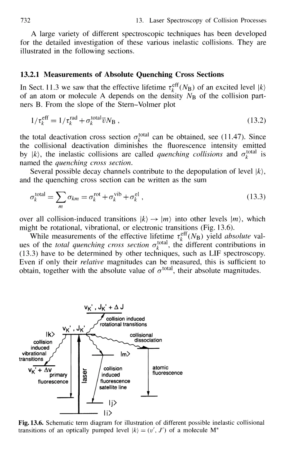
13.2.1 Measurements of Absolute Quenching
Cross Sections 732
13.2.2 Collision-Induced Rovibronic Transitions
in Excited States 733
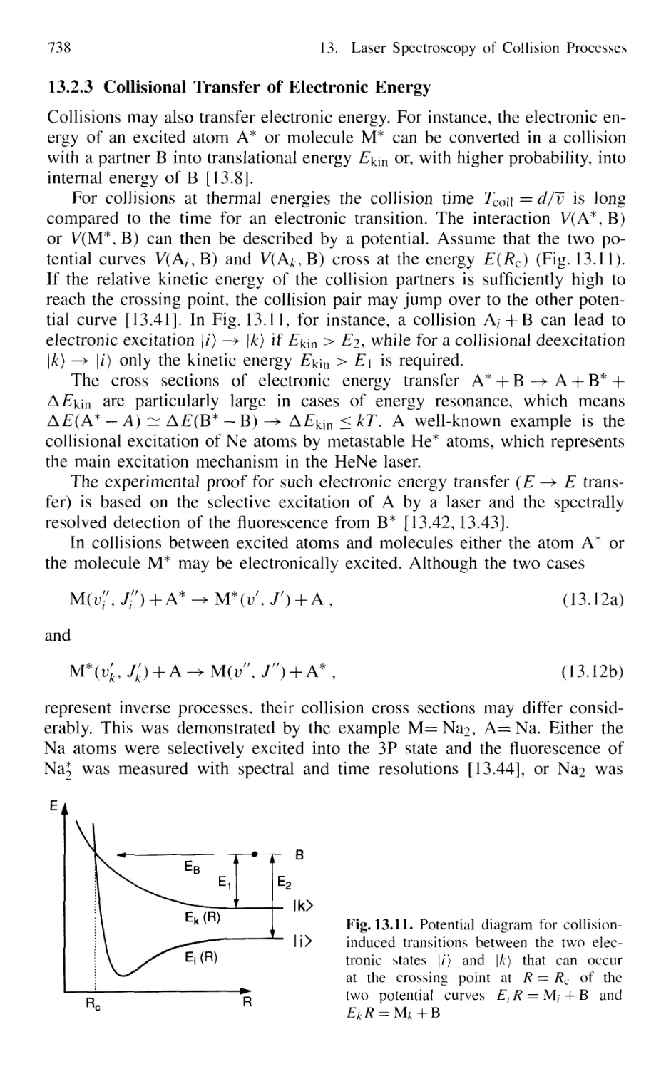
13.2.3 Collisional Transfer of Electronic Energy 738
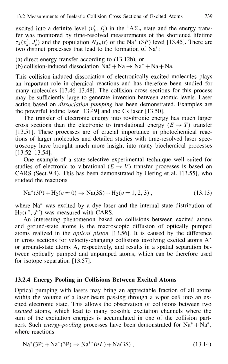
13.2.4 Energy Pooling in Collisions
Between Excited Atoms 739
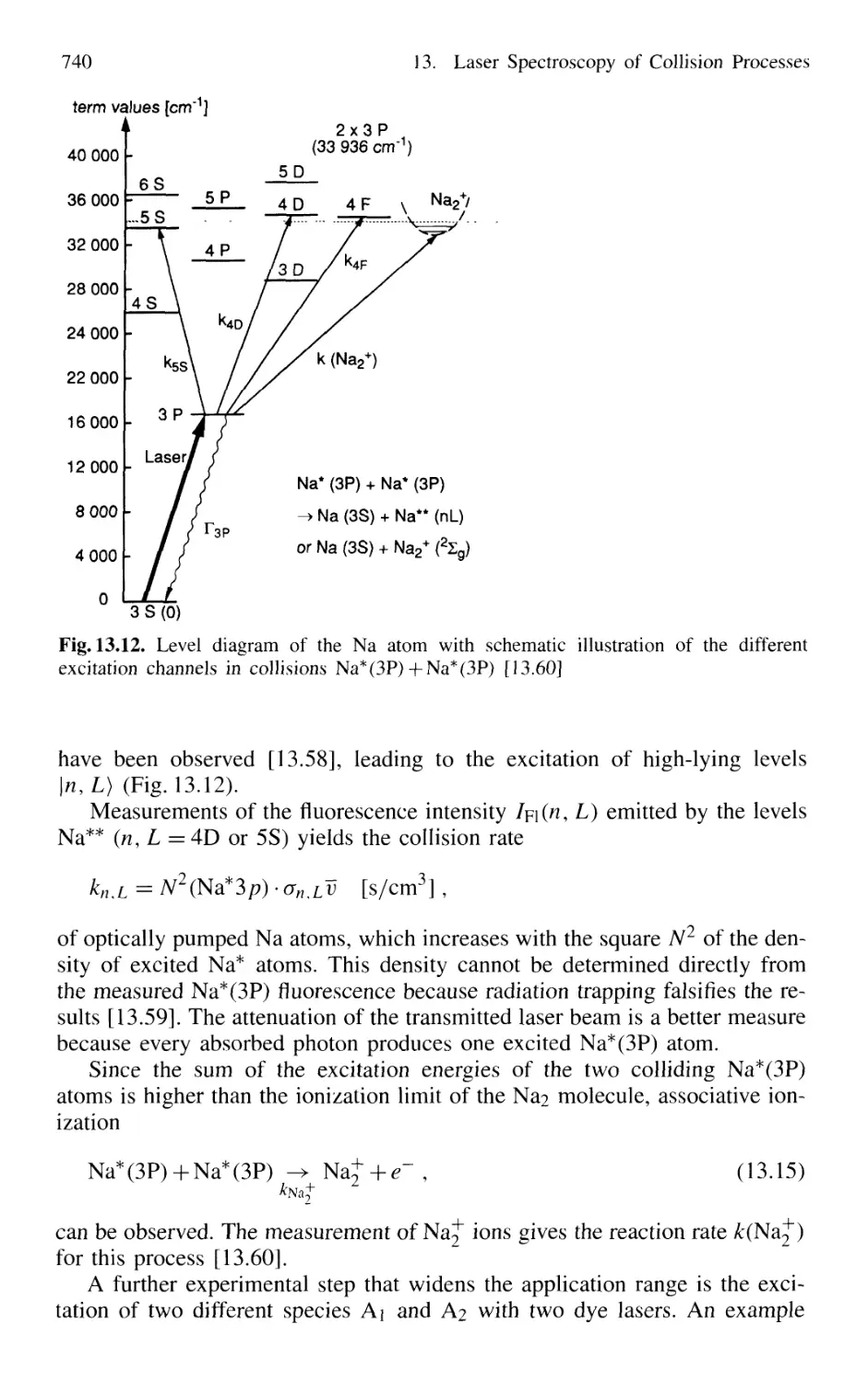
13.2.5 Spectroscopy of Spin-Flip Transitions 741
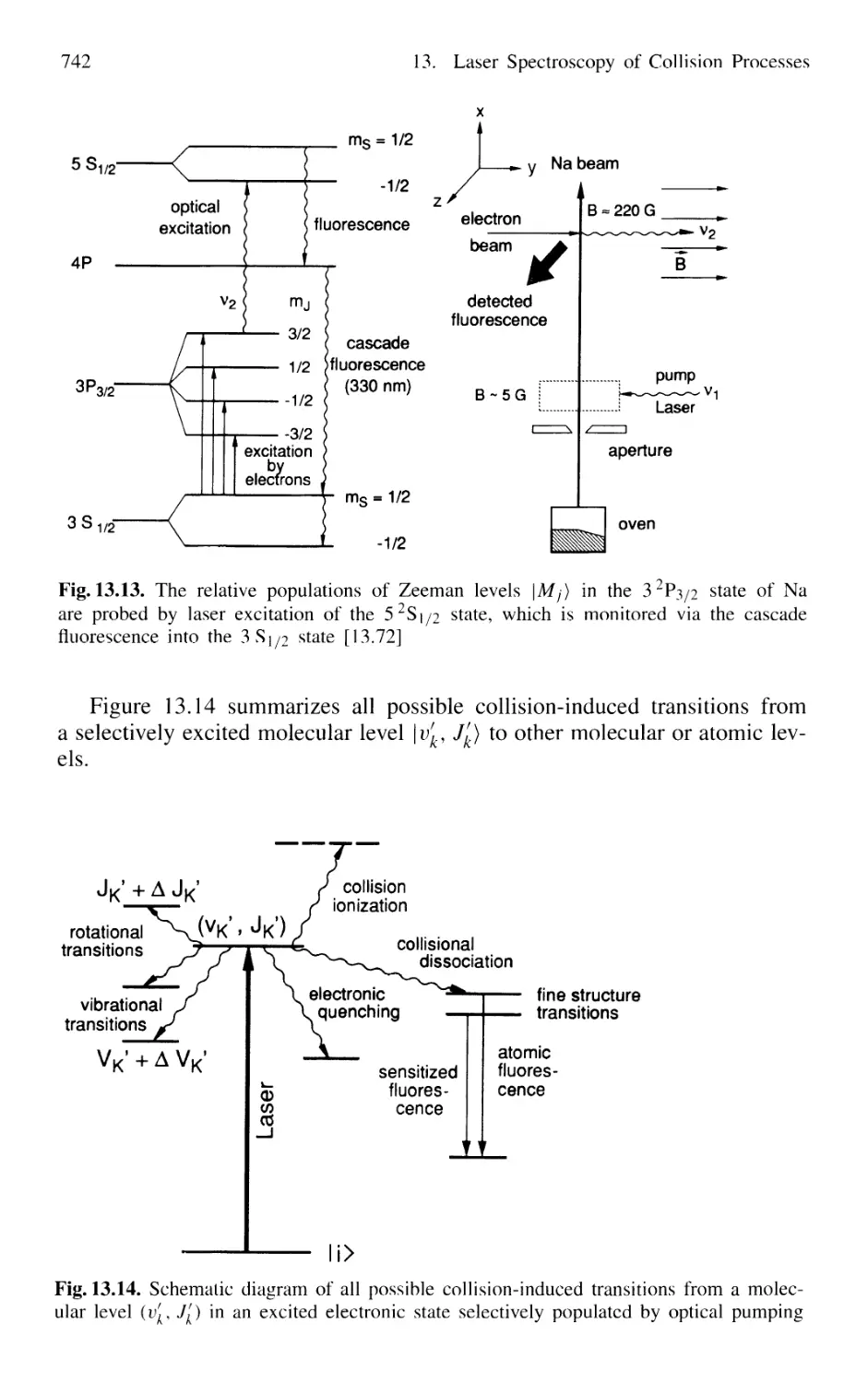
13.3 Spectroscopic Techniques
for Measuring Collision-Induced Transitions
in the Electronic Ground State of Molecules 743
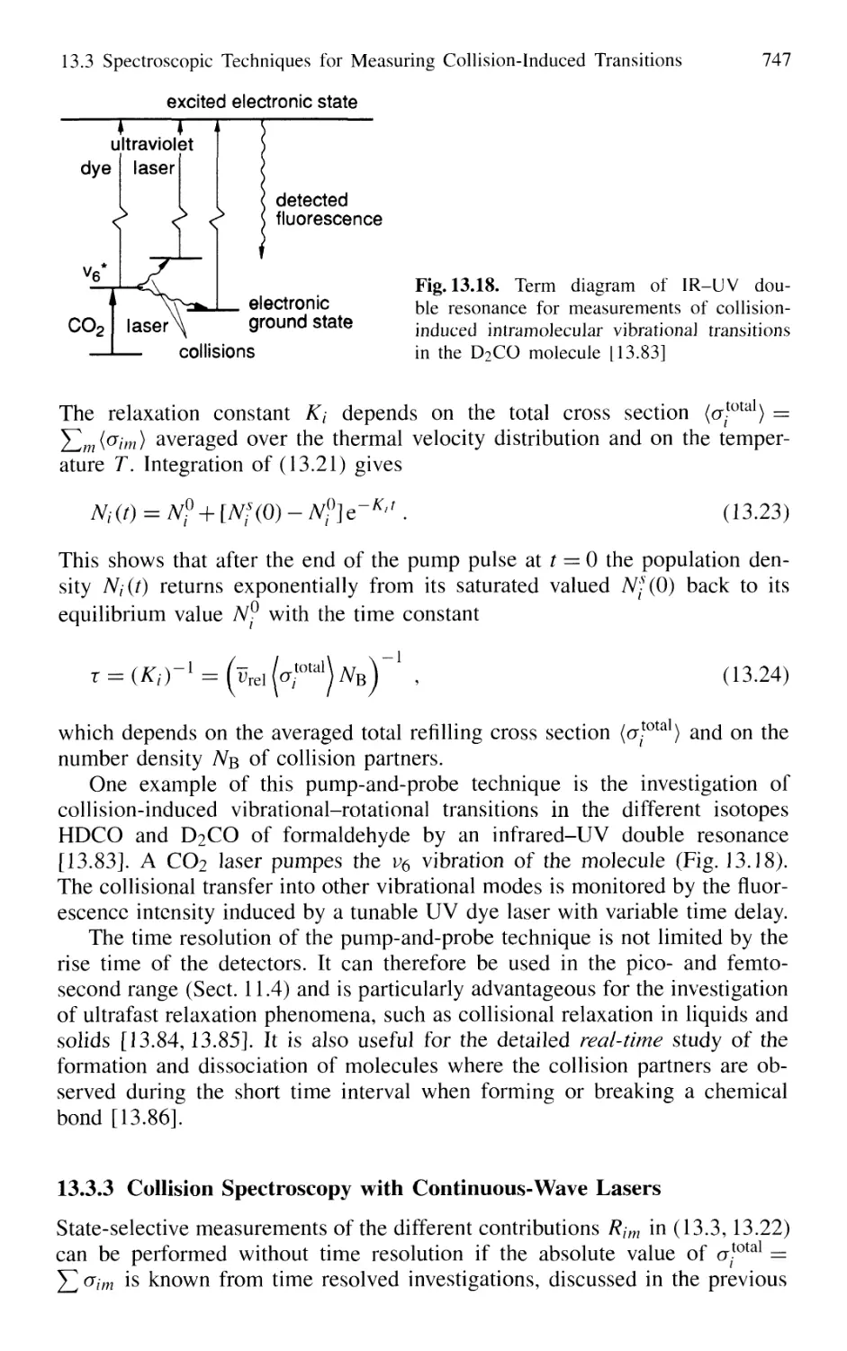
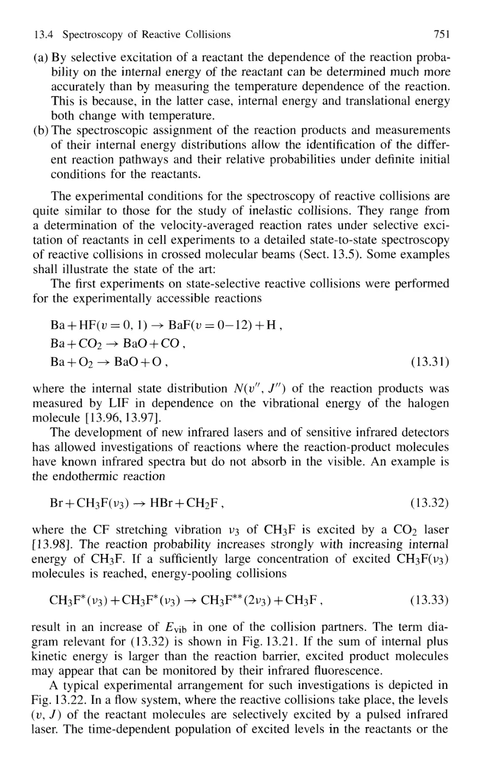
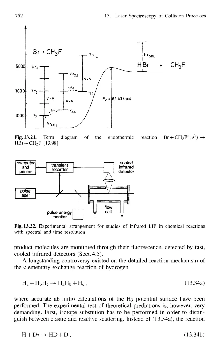
13.3.1 Time-Resolved Infrared Fluorescence Detection .... 744
13.3.2 Time-Resolved Absorption
and Double-Resonance Methods 745
13.3.3 Collision Spectroscopy
with Continuous-Wave Lasers 747
13.3.4 Collisions Involving Molecules
in High Vibrational States 749
13.4 Spectroscopy of Reactive Collisions 750
13.5 Spectroscopic Determination
of Differential Collision Cross Sections
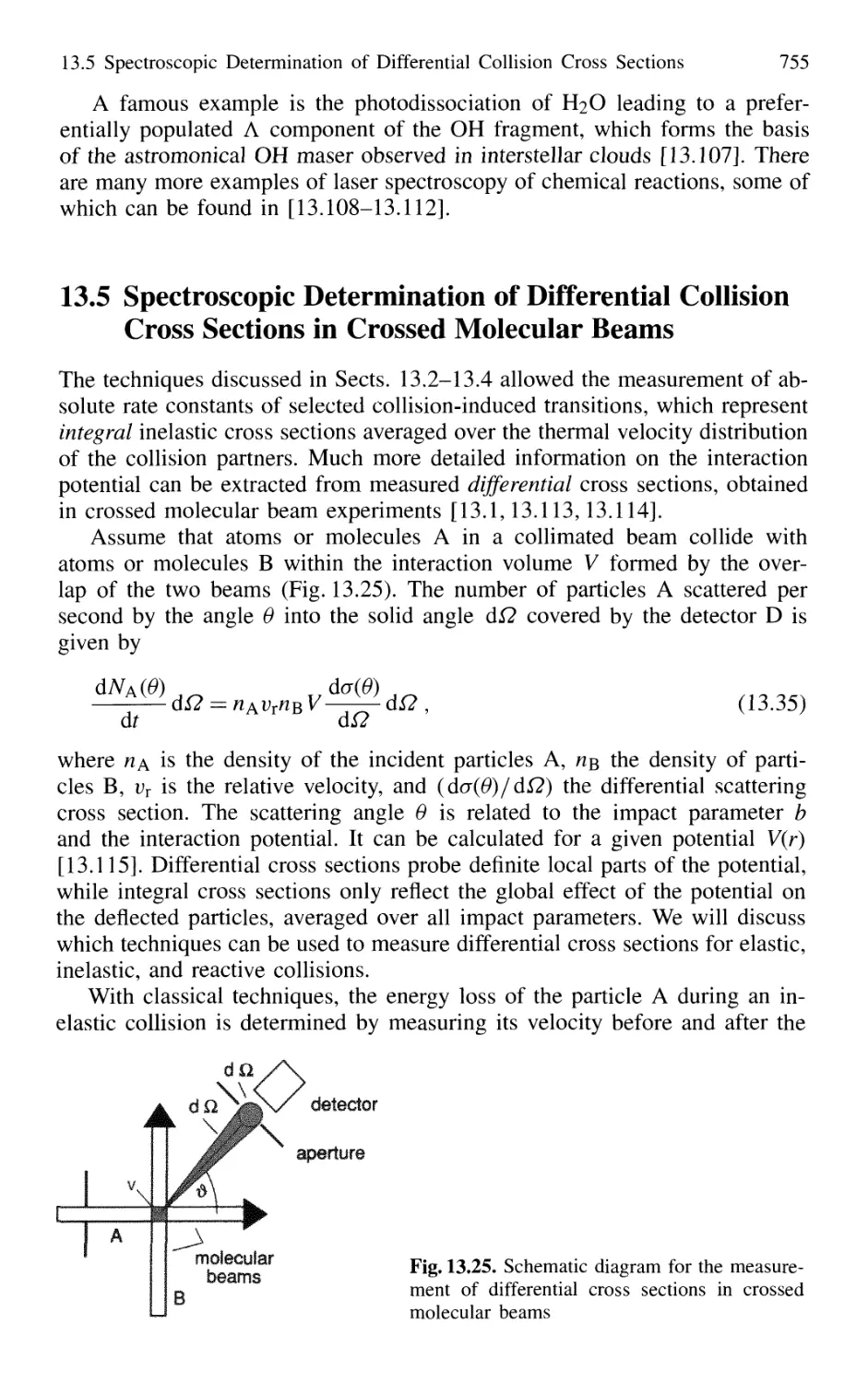
in Crossed Molecular Beams 755
13.6 Photon-Assisted Collisional Energy Transfer 760
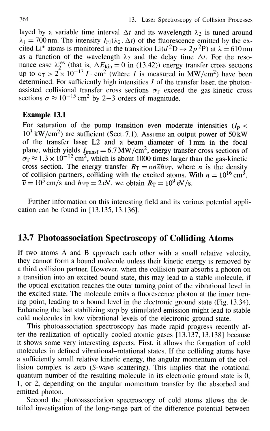
13.7 Photoassociation Spectroscopy of Colliding Atoms 764
Problems 765
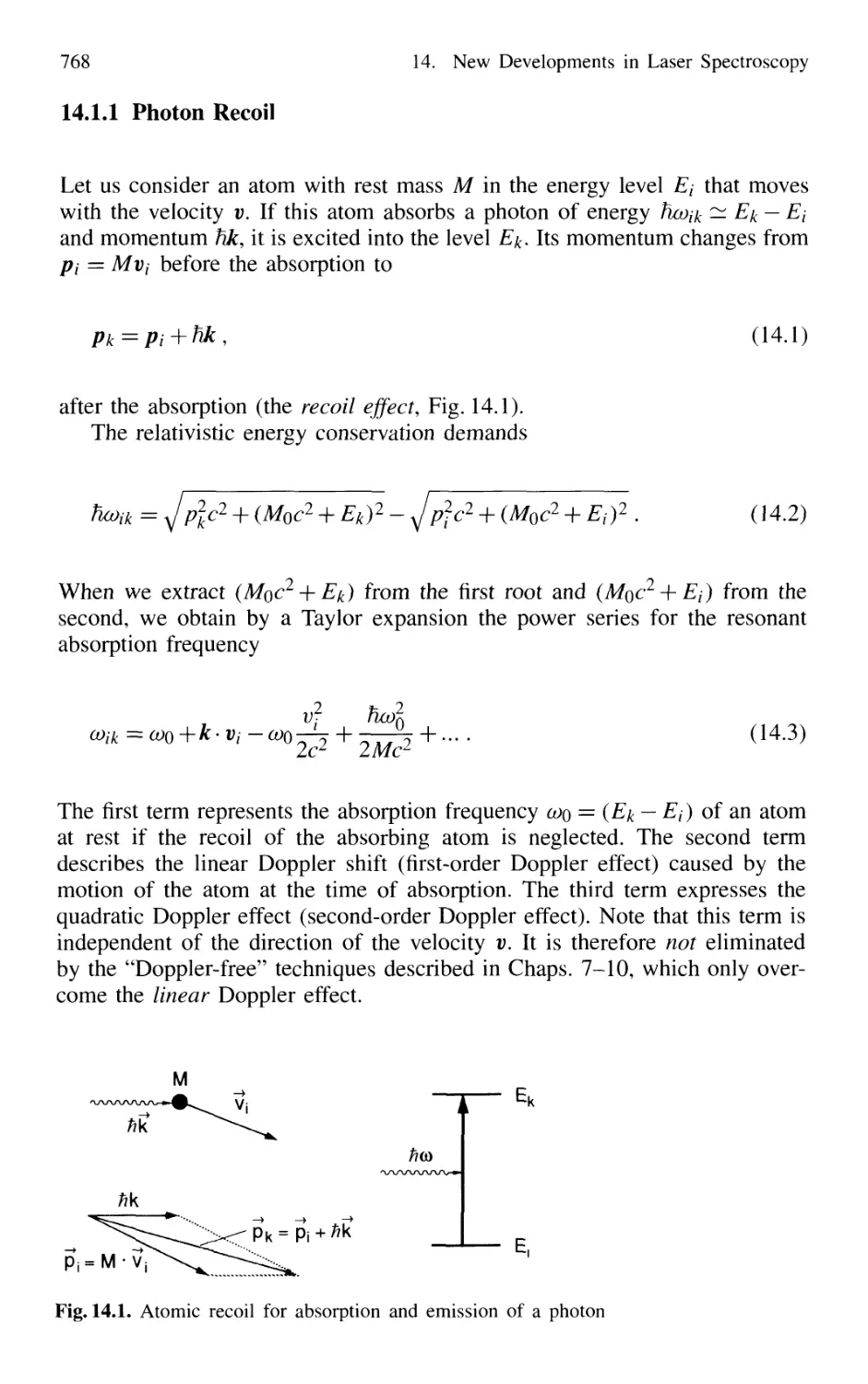
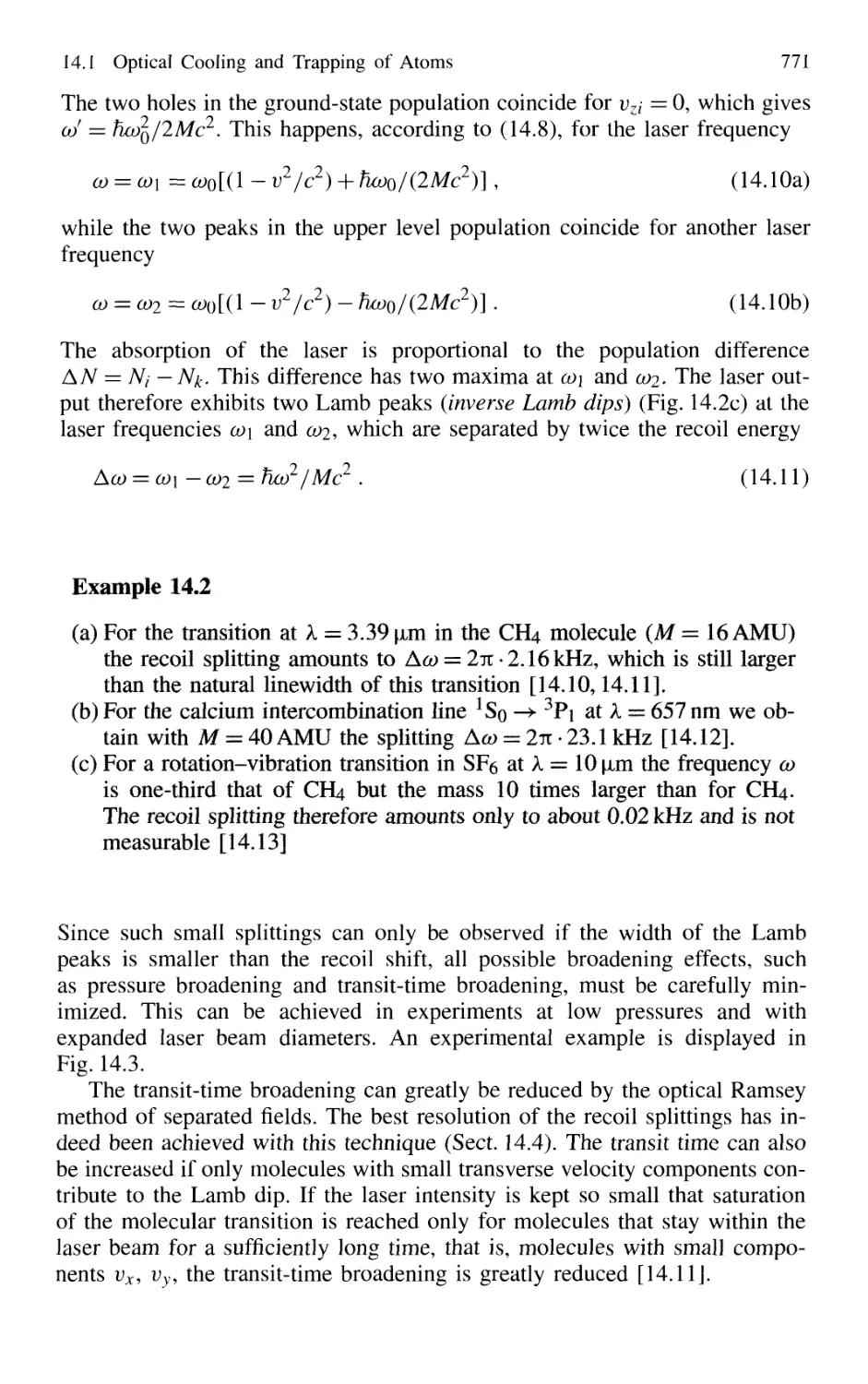
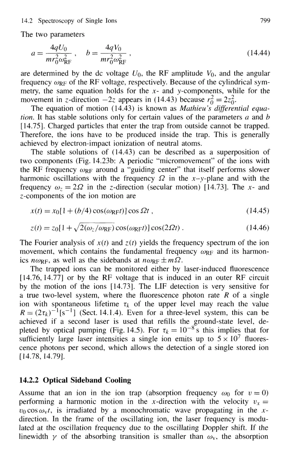
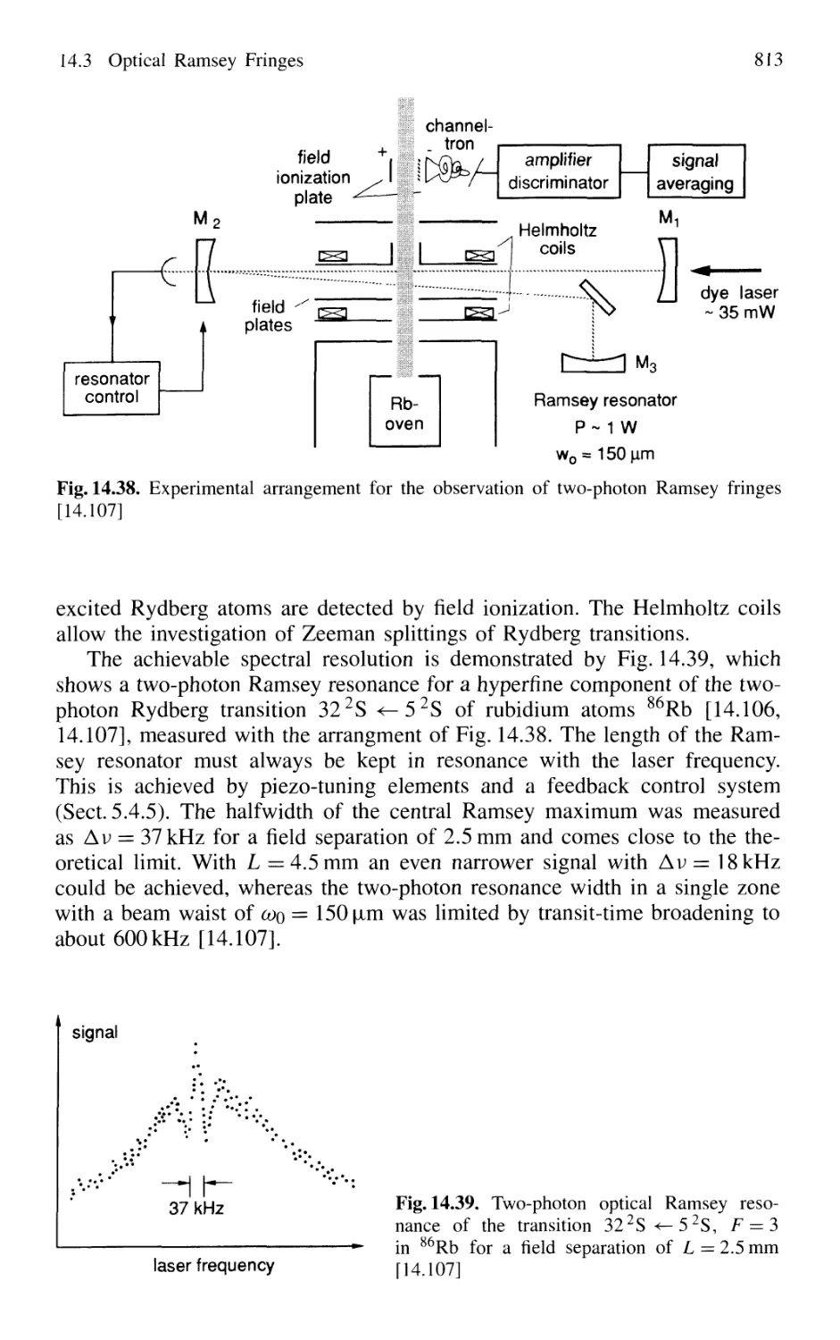
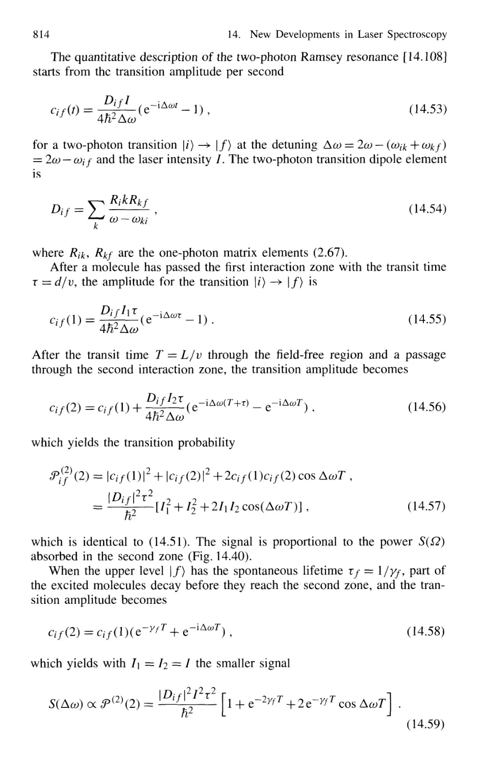
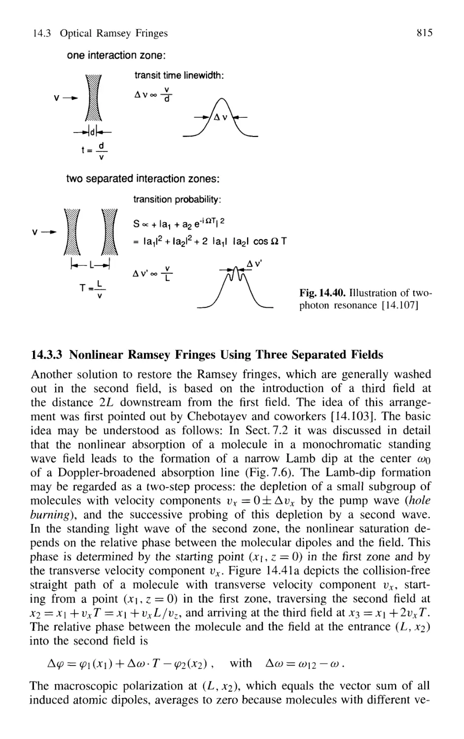
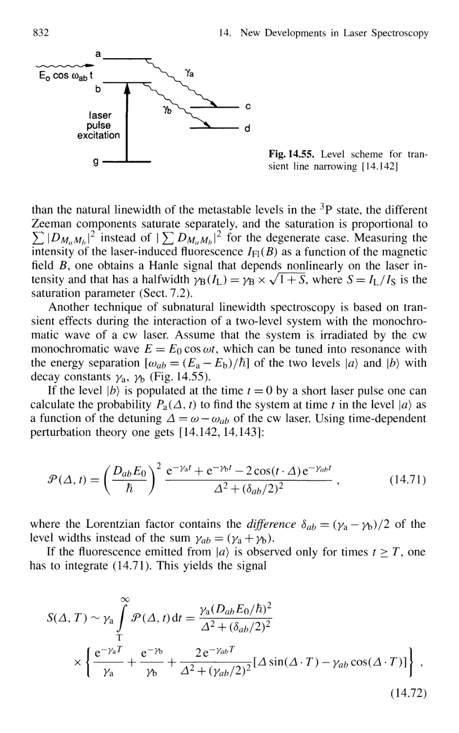
14. New Developments in Laser Spectroscopy 767
14.1 Optical Cooling and Trapping of Atoms 767
14.1.1 Photon Recoil 768
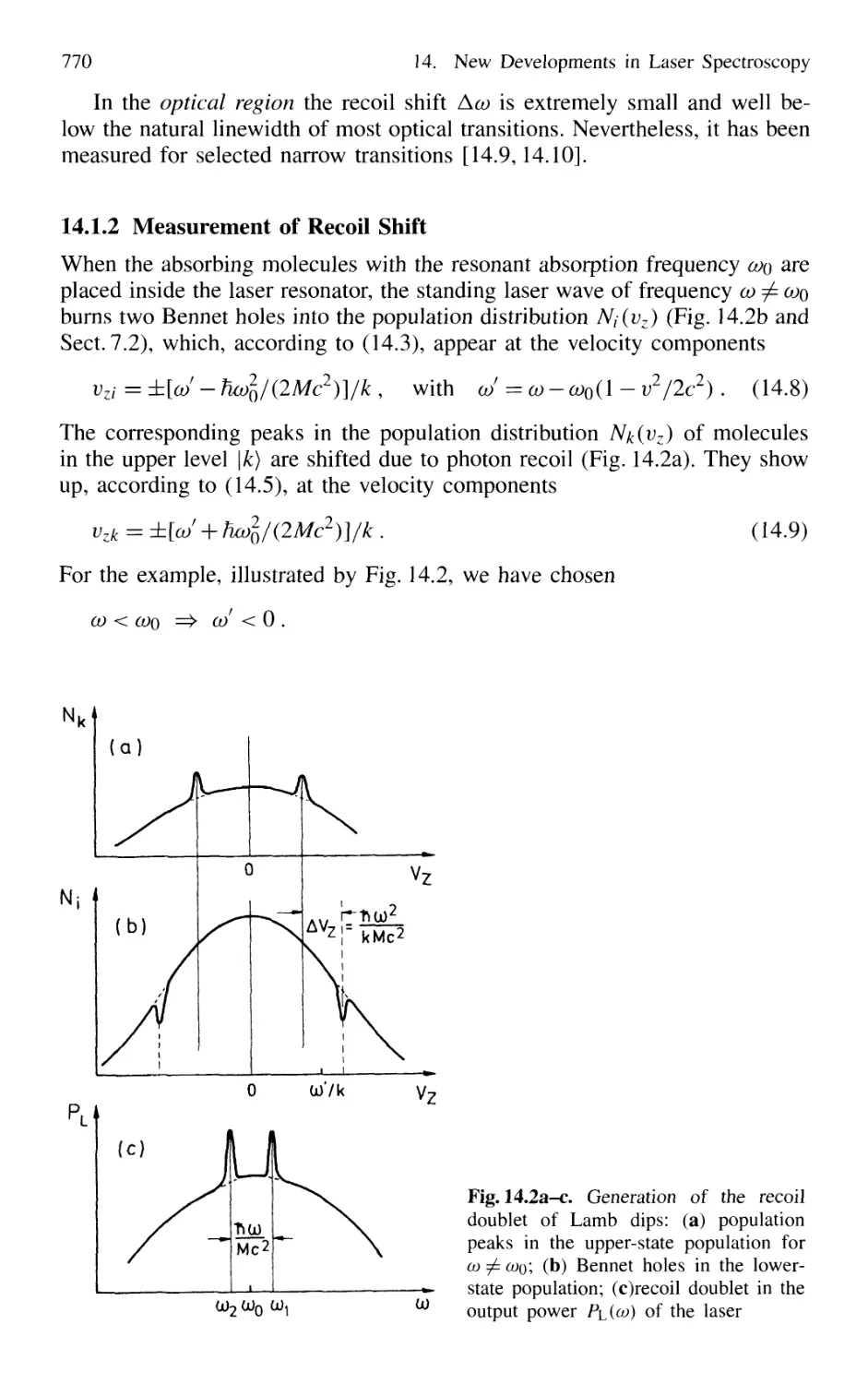
14.1.2 Measurement of Recoil Shift 770
14.1.3 Optical Cooling by Photon Recoil 772
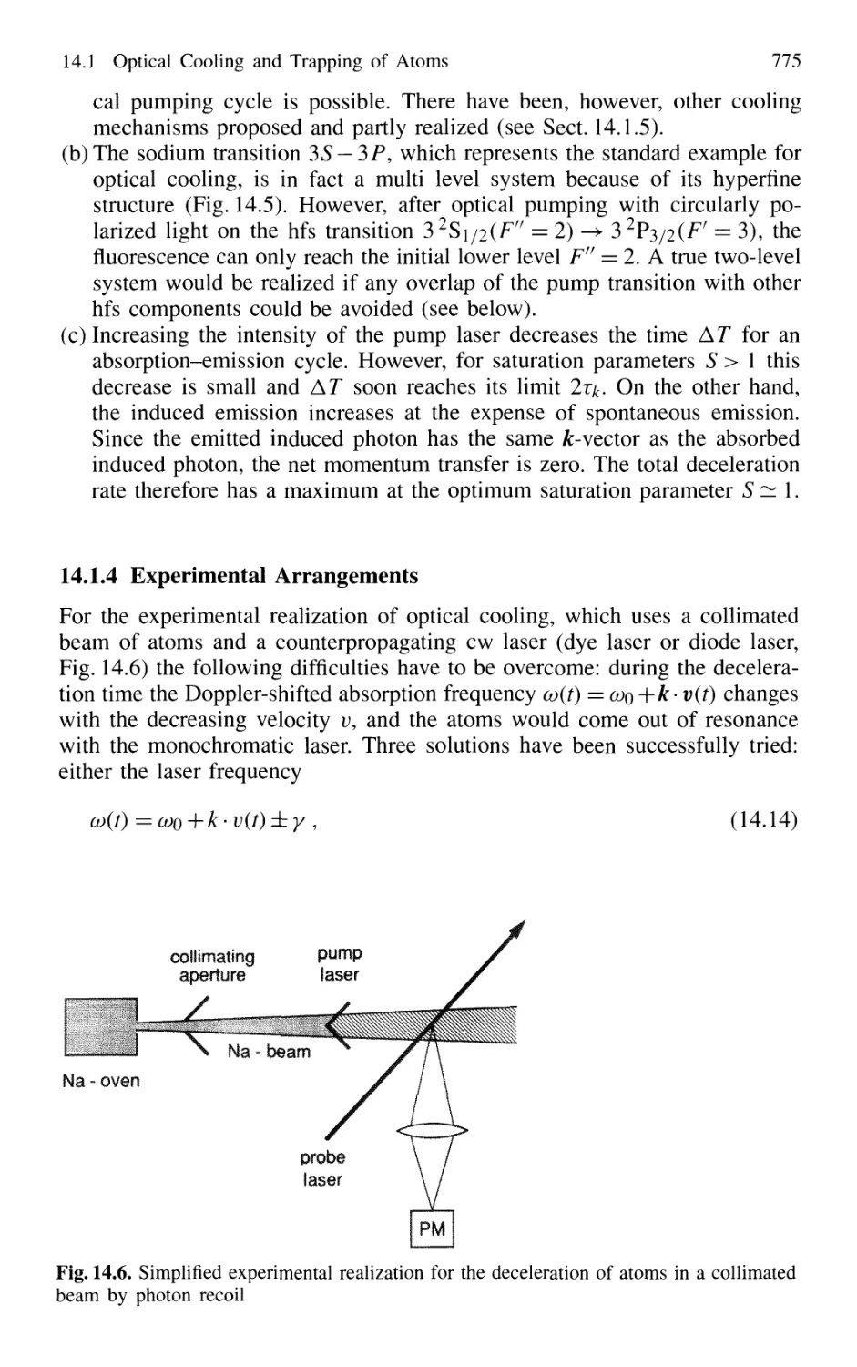
14.1.4 Experimental Arrangements 775
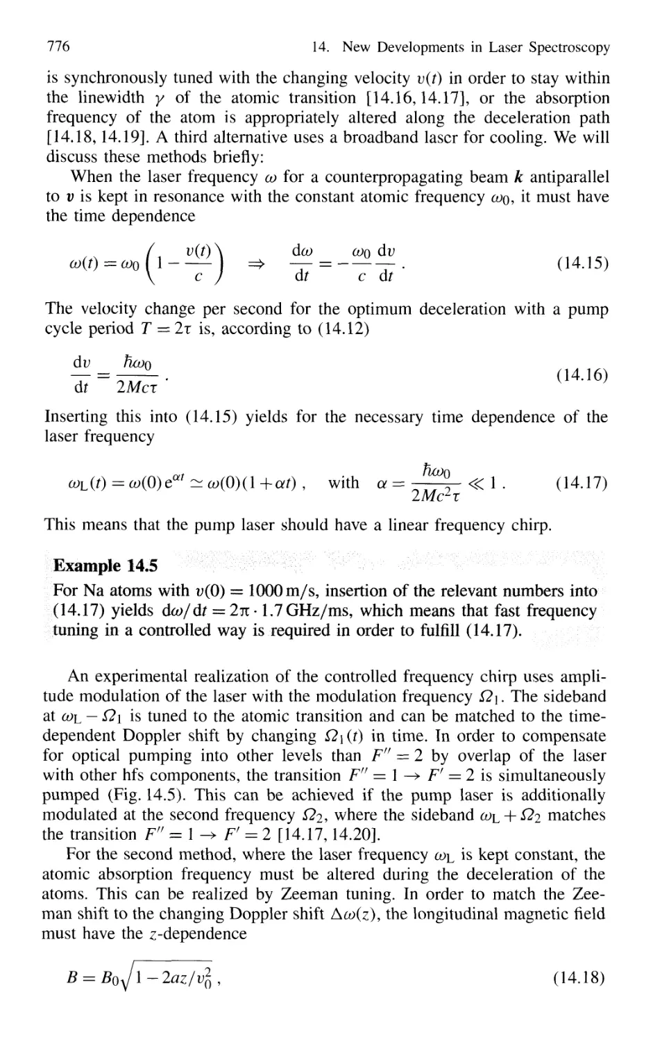
14.1.5 Threedimensional Cooling of Atoms;
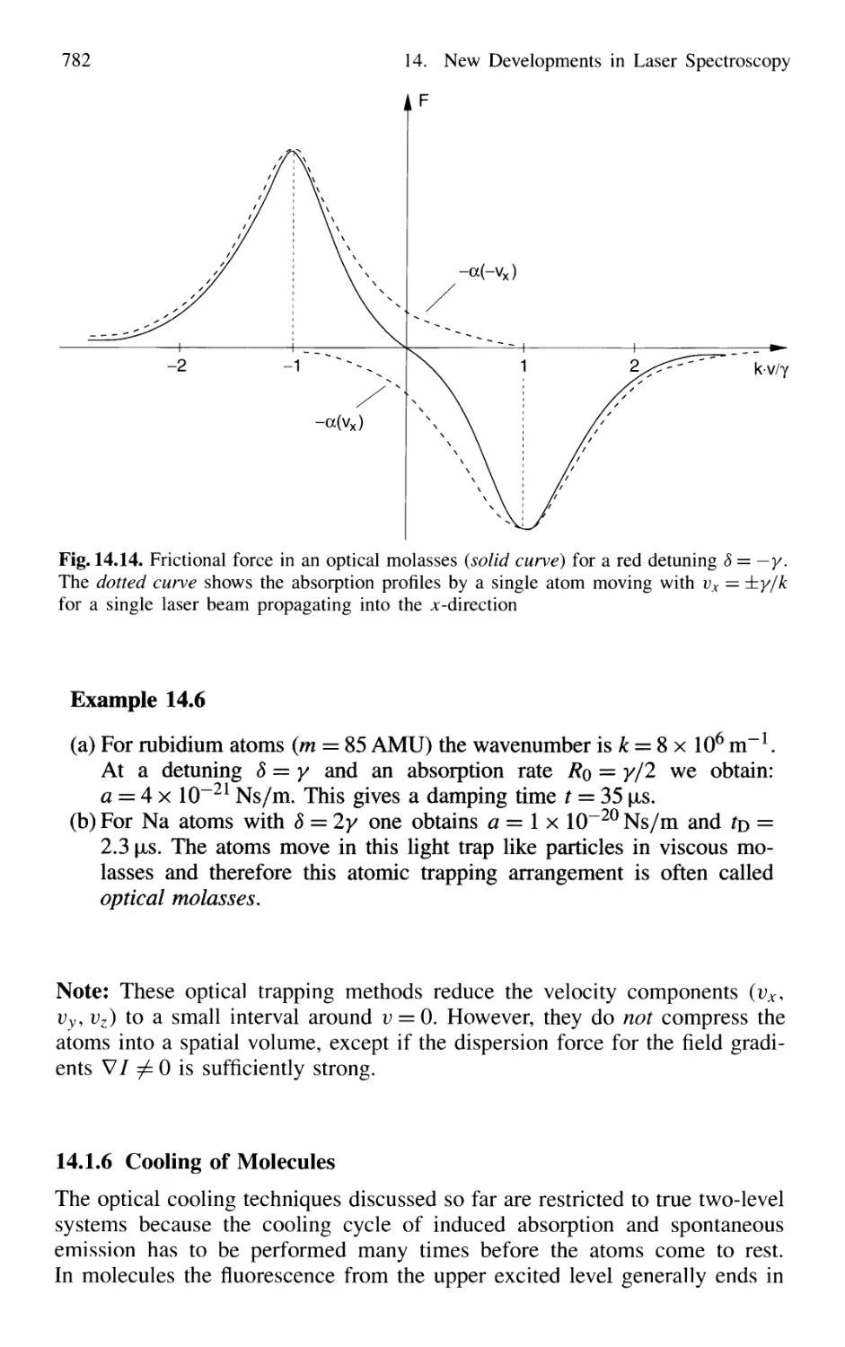
Optical Mollasses 780
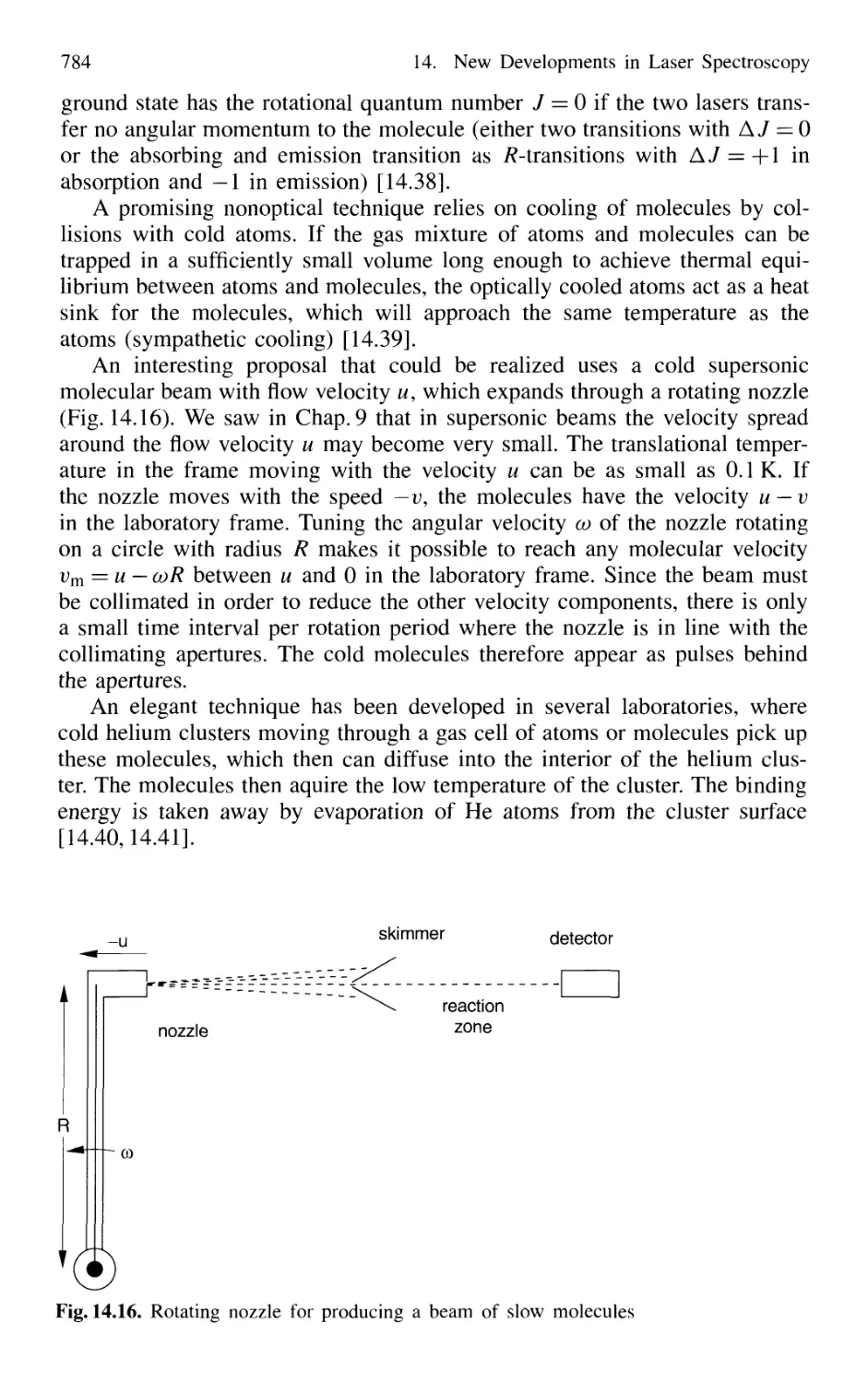
14.1.6 Cooling of Molecules 782
14.1.7 Optical Trapping of Atoms 785
14.1.8 Optical Cooling Limits 790
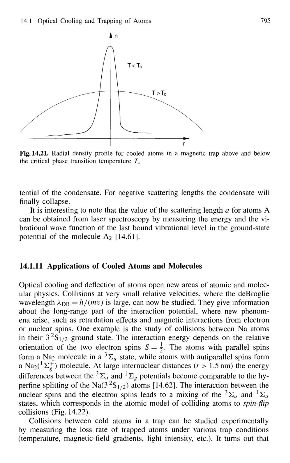
14.1.9 Bose-Einstein Condensation 793
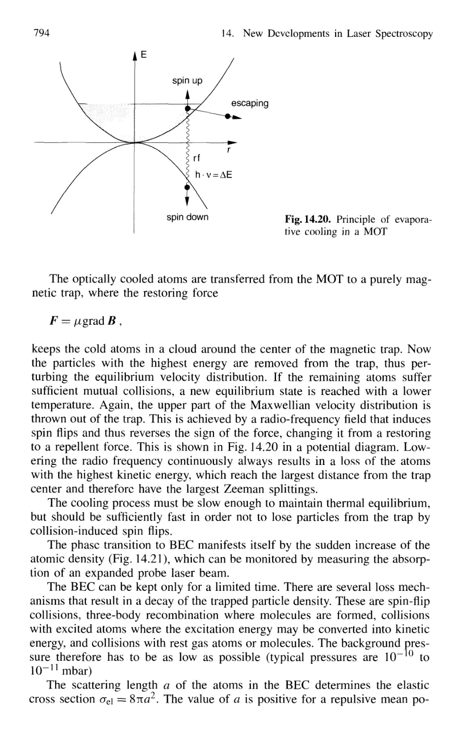
14.1.10 Evaporative Cooling 793
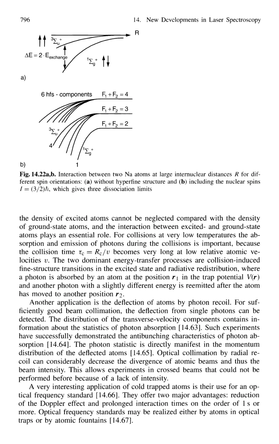
14.1.11 Applications of Cooled Atoms and Molecules 795
Contents XIX
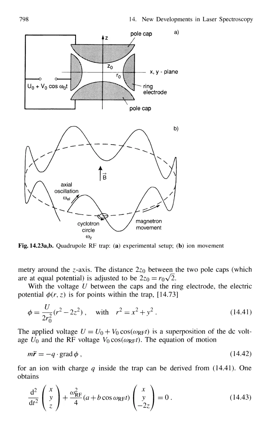
14.2 Spectroscopy of Single Ions 797
14.2.1 Trapping of Ions 797
14.2.2 Optical Sideband Cooling 799
14.2.3 Direct Observations of Quantum Jumps 802
14.2.4 Formation of Wigner Crystals in Ion Traps 804
14.2.5 Laser Spectroscopy in Storage Rings 806
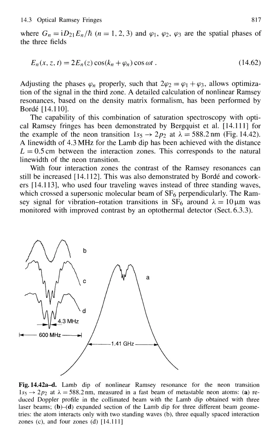
14.3 Optical Ramsey Fringes 808
14.3.1 Basic Considerations 808
14.3.2 Two-Photon Ramsey Resonance 811
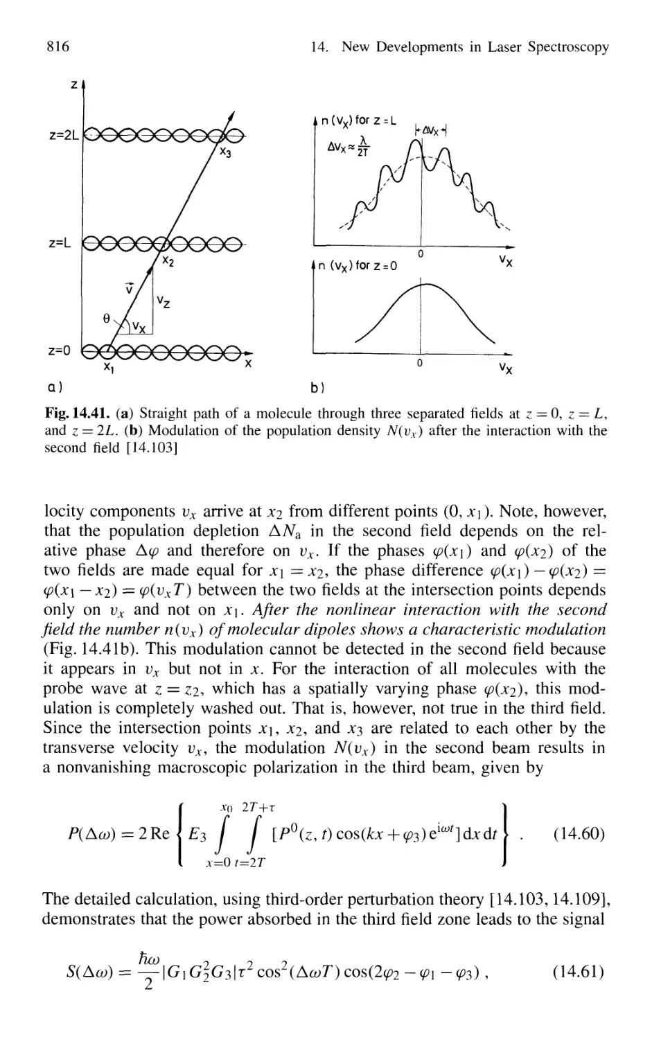
14.3.3 Nonlinear Ramsey Fringes
Using Three Separated Fields 815
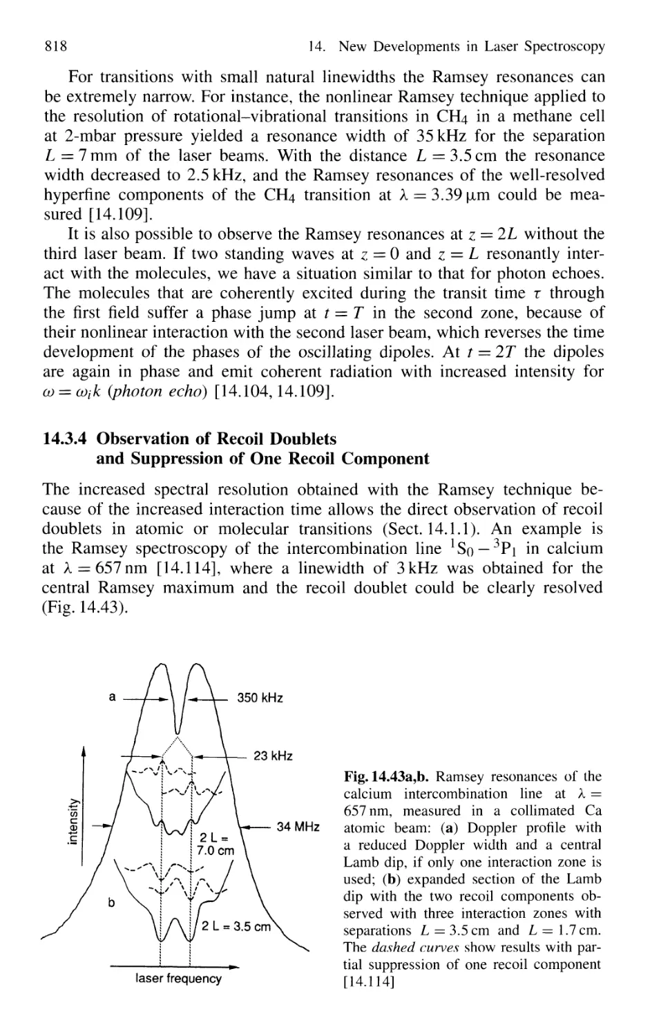
14.3.4 Observation of Recoil Doublets and Suppression
of One Recoil Component 818
14.4 Atom Interferometry 819
14.4.1 Mach-Zehnder Atom Interferometer 820
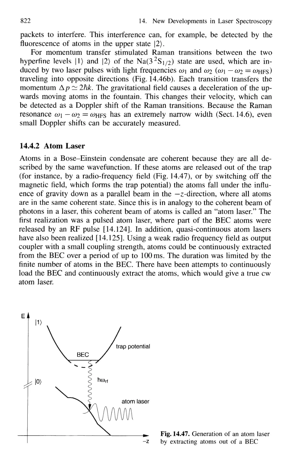
14.4.2 Atom Laser 822
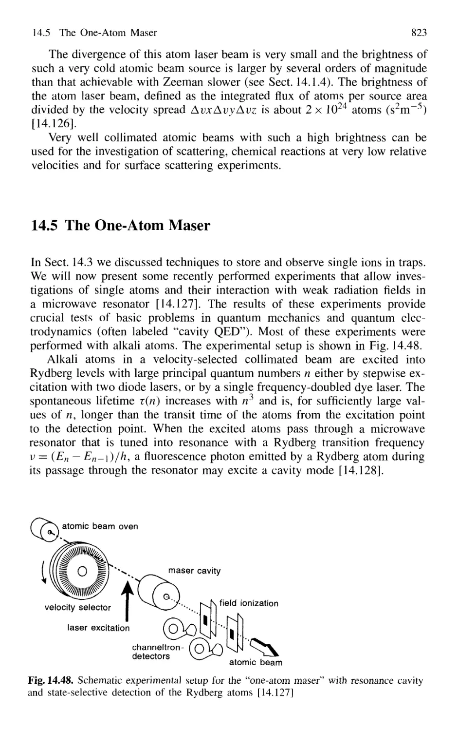
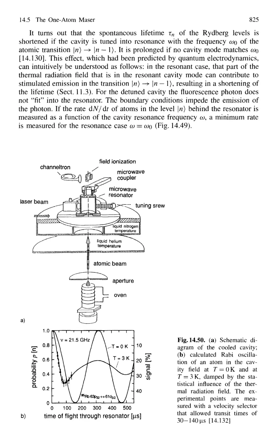
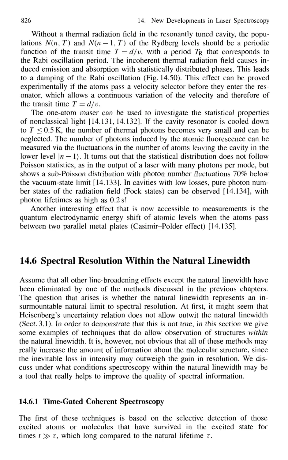
14.5 The One-Atom Maser 823
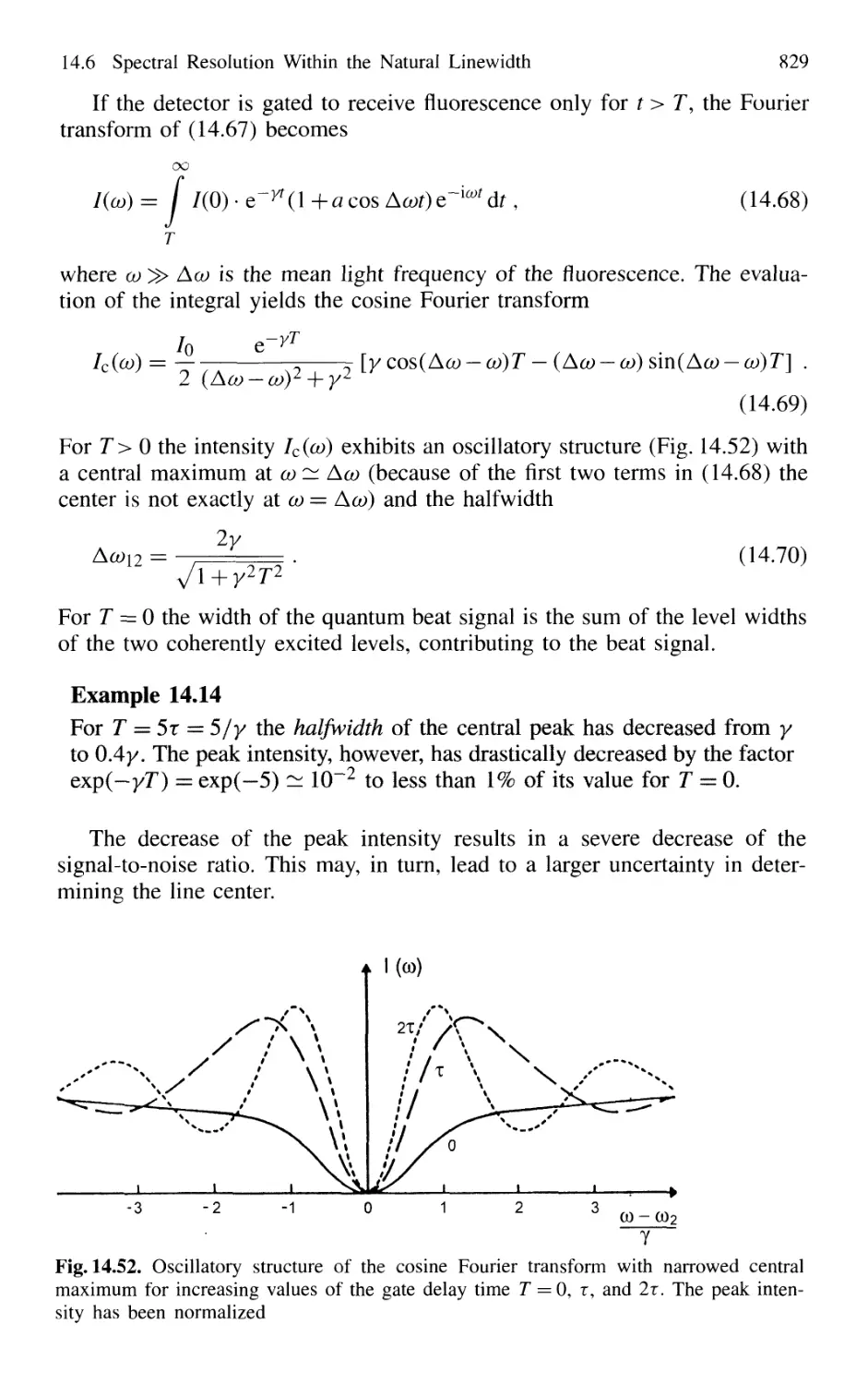
14.6 Spectral Resolution Within the Natural Linewidth 826
14.6.1 Time-Gated Coherent Spectroscopy 826
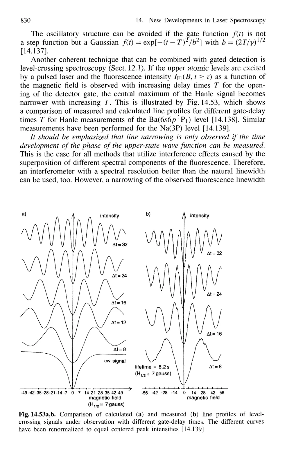
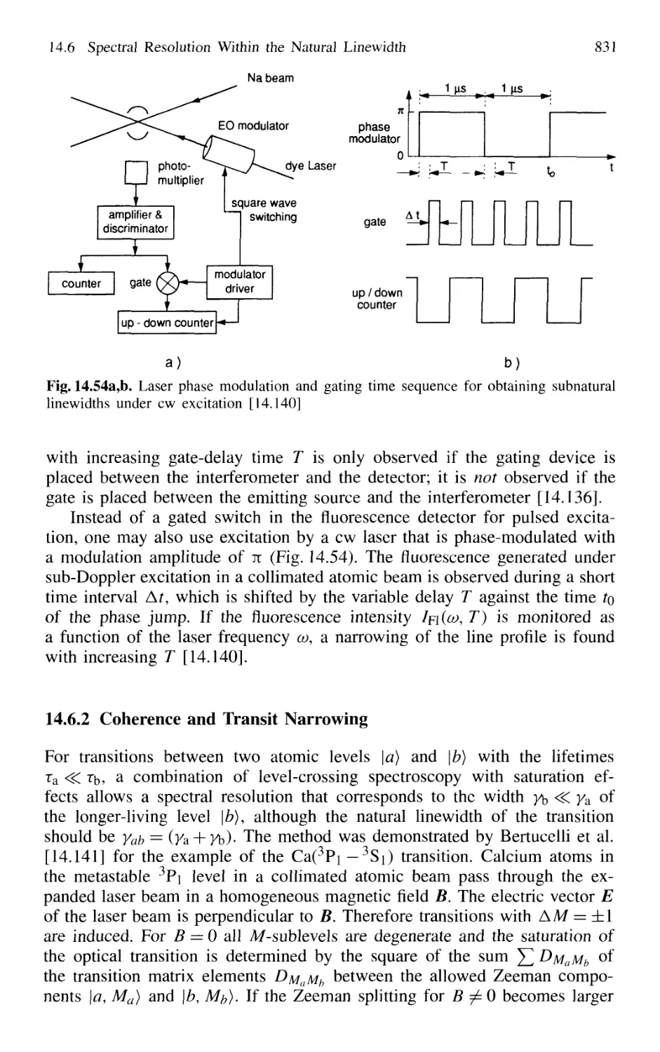
14.6.2 Coherence and Transit Narrowing 831
14.6.3 Raman Spectroscopy with Subnatural Linewidth ... 833
14.7 Absolute Optical Frequency Measurement
and Optical Frequency Standards 835
14.7.1 Microwave-Optical Frequency Chains 835
14.7.2 Frequency Comb from Femtosecond Laser Pulses . 838
14.8 Squeezing 840
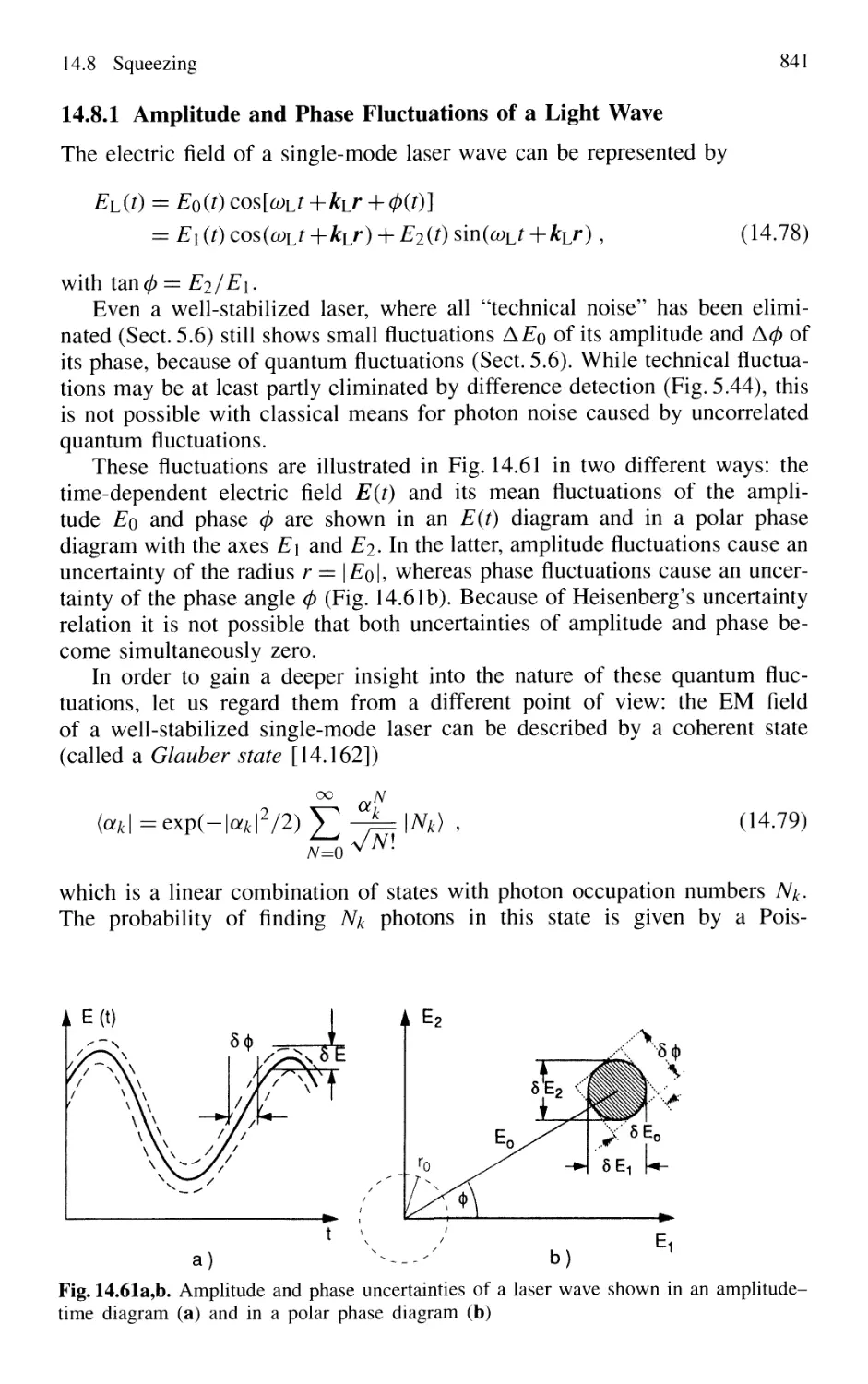
14.8.1 Amplitude and Phase Fluctuations of a Light Wave 841
14.8.2 Experimental Realization of Squeezing 844
14.8.3 Application of Squeezing
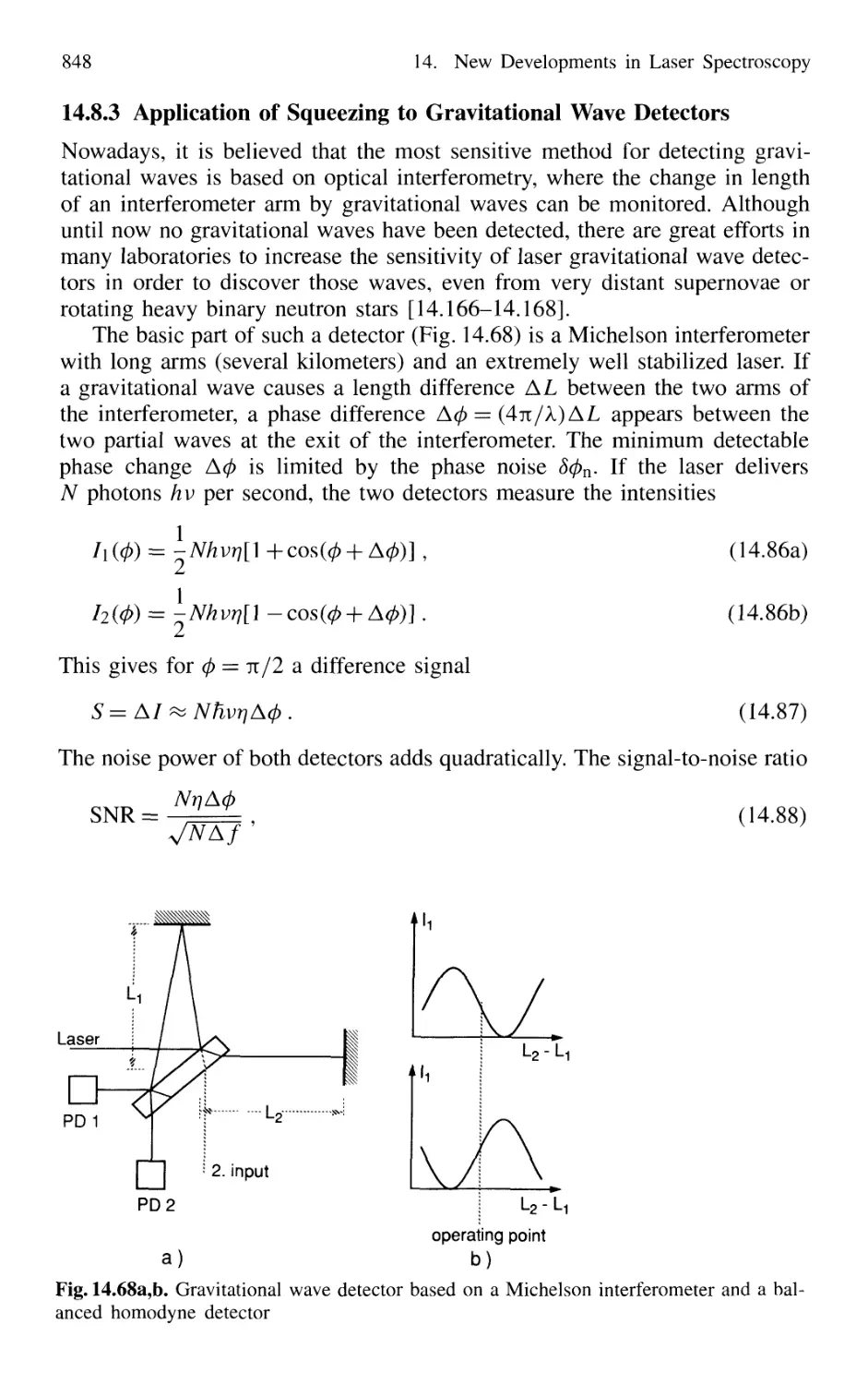
to Gravitational Wave Detectors 848
15. Applications of Laser Spectroscopy 851
15.1 Applications in Chemistry 851
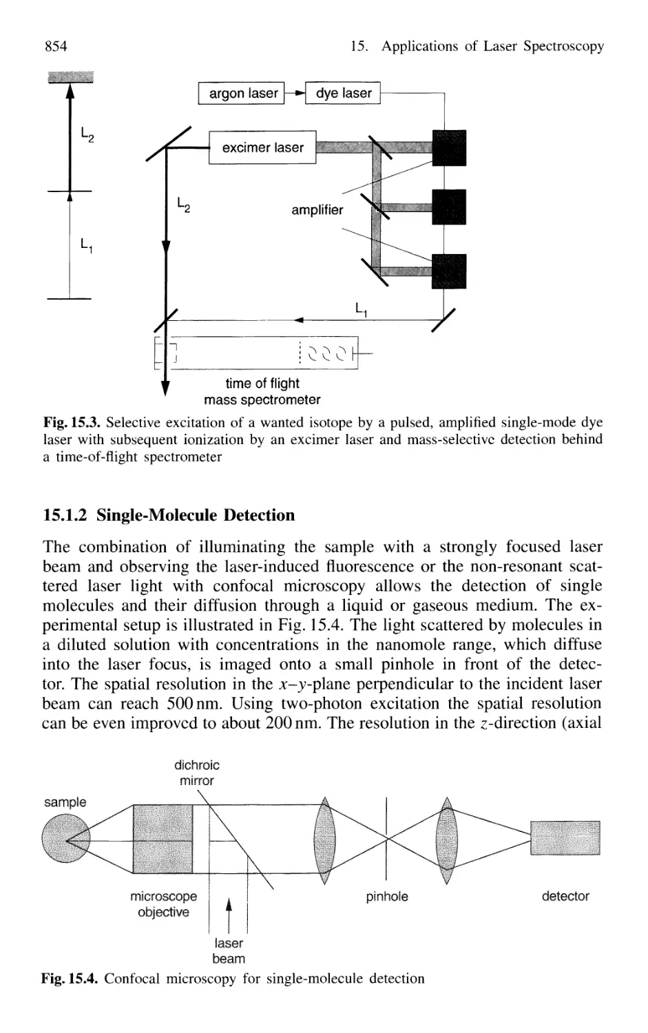
Laser Spectroscopy in Analytical Chemistry 851
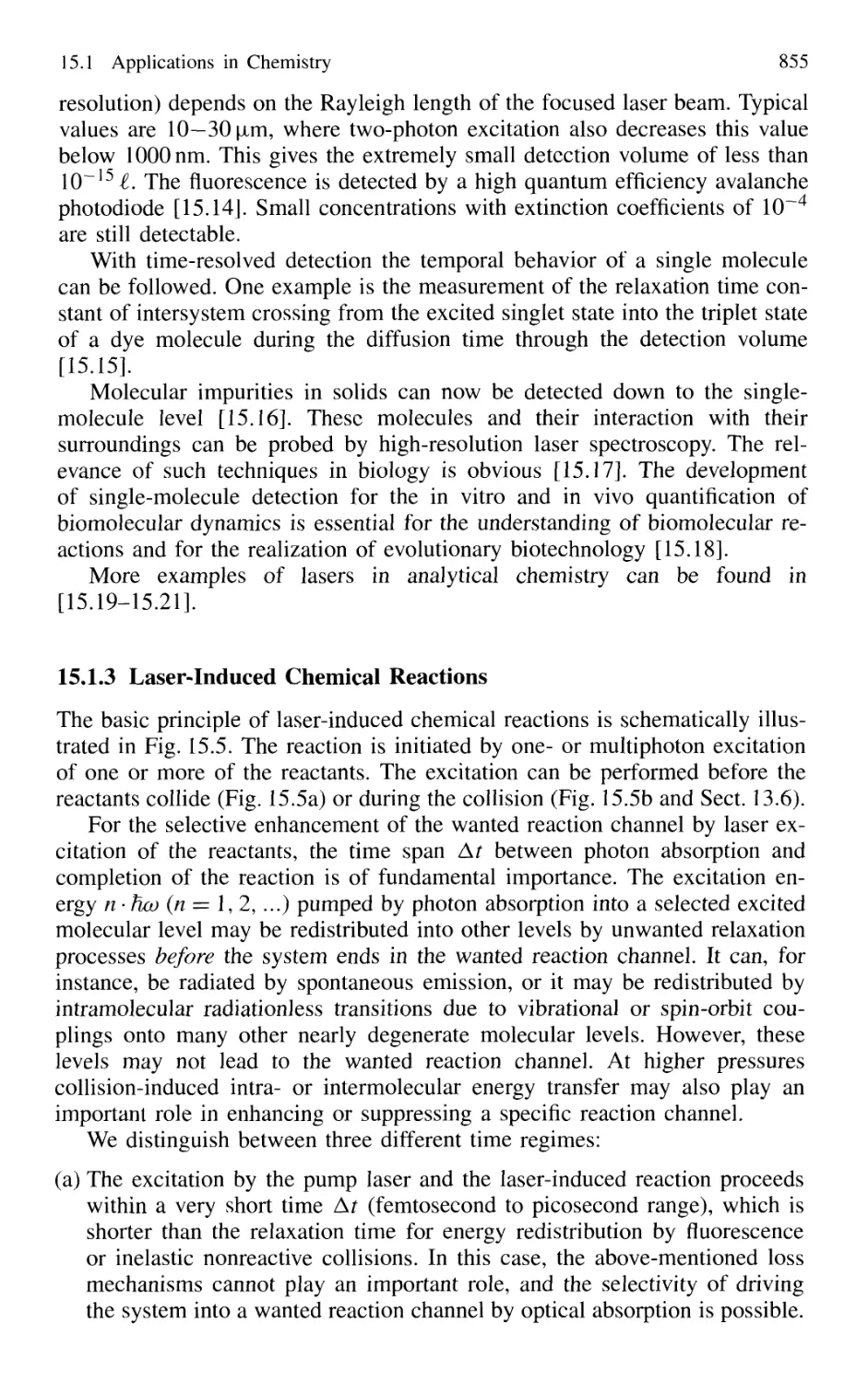
Single-Molecule Detection 854
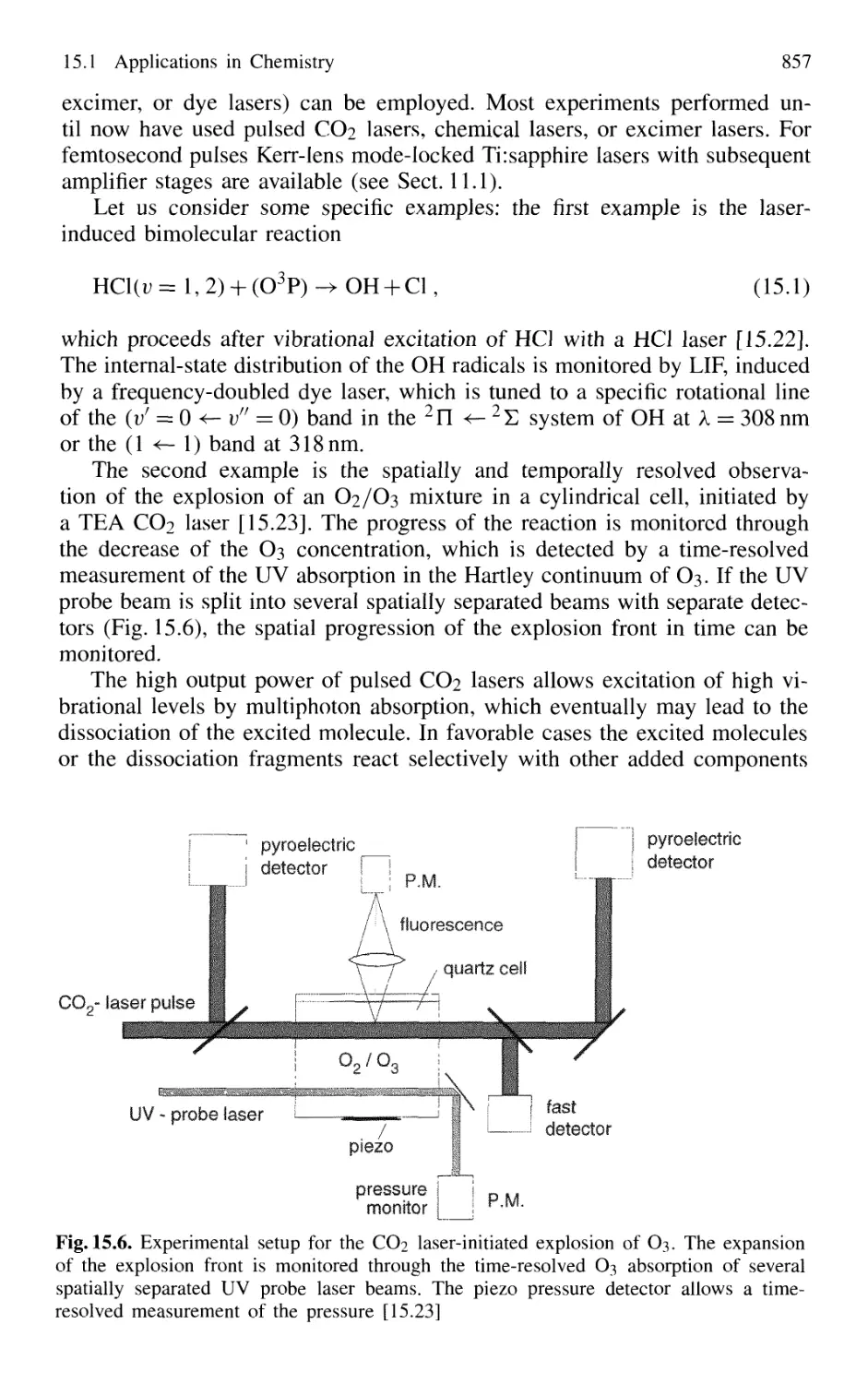
Laser-Induced Chemical Reactions 855
Coherent Control of Chemical Reactions 859
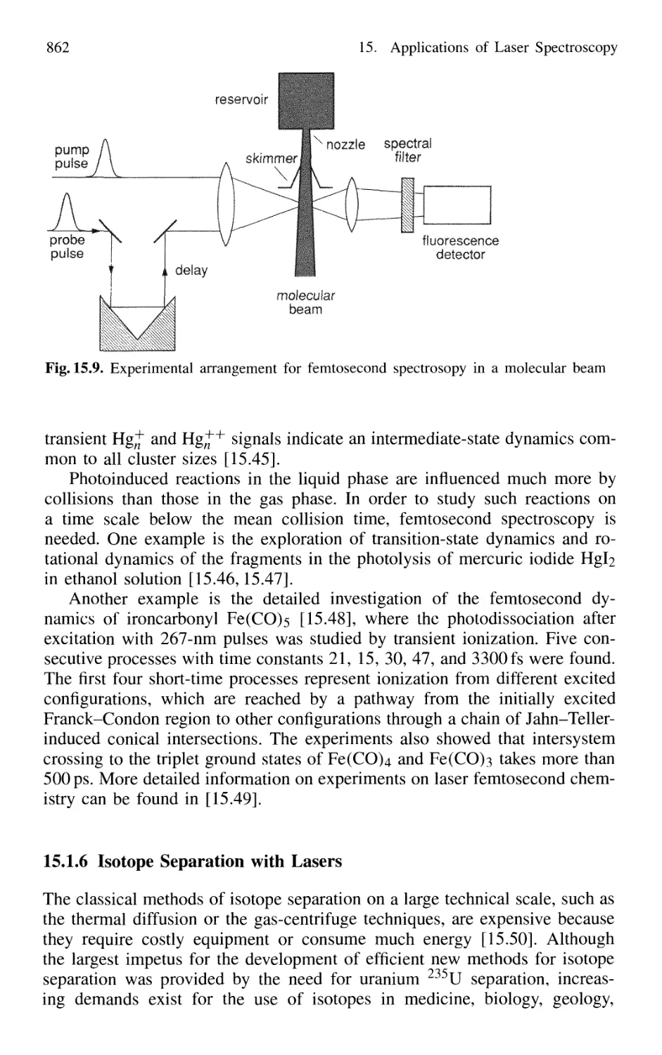
Laser Femtosecond Chemistry 860
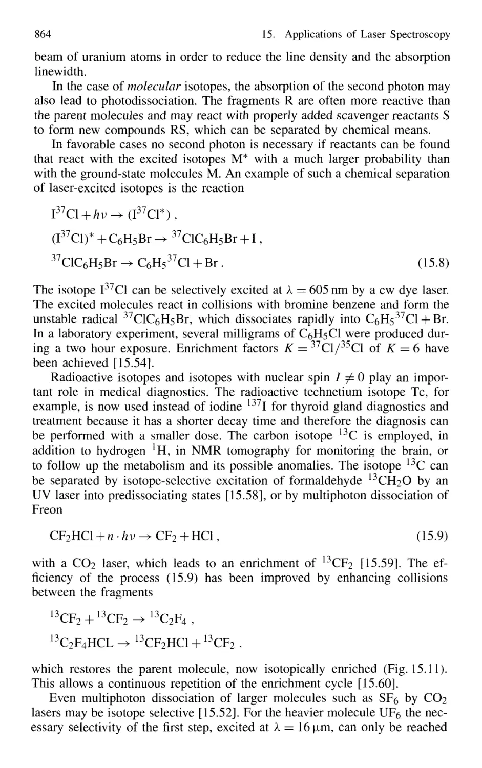
Isotope Separation with Lasers 862
15.1.7 Summary of Laser Chemistry 865
15.2 Environmental Research with Lasers 865
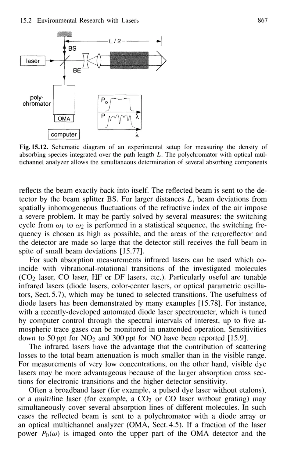
15.2.1 Absorption Measurements 866
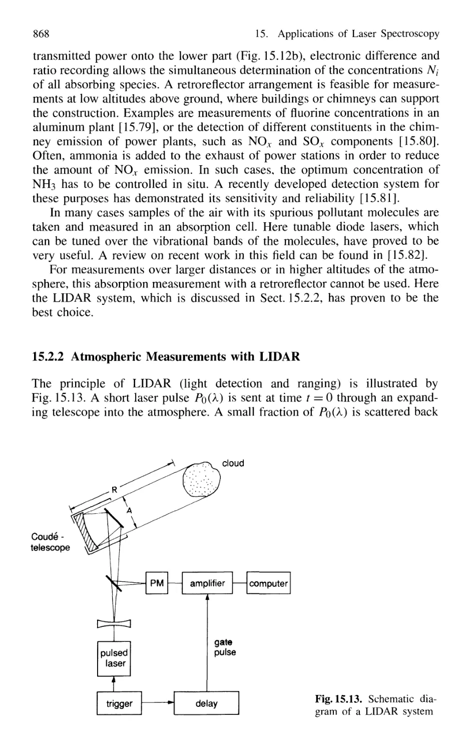
15.2.2 Atmospheric Measurements with LID AR 868
15.2.3 Spectroscopic Detection of Water Pollution 873
15.3 Applications to Technical Problems 874
15.3.1 Spectroscopy of Combustion Processes 874
15.1
15.1
15.1
15.1
15.1
15.1
l.l
1.2
1.3
1.4
.5
1.6
XX Contents
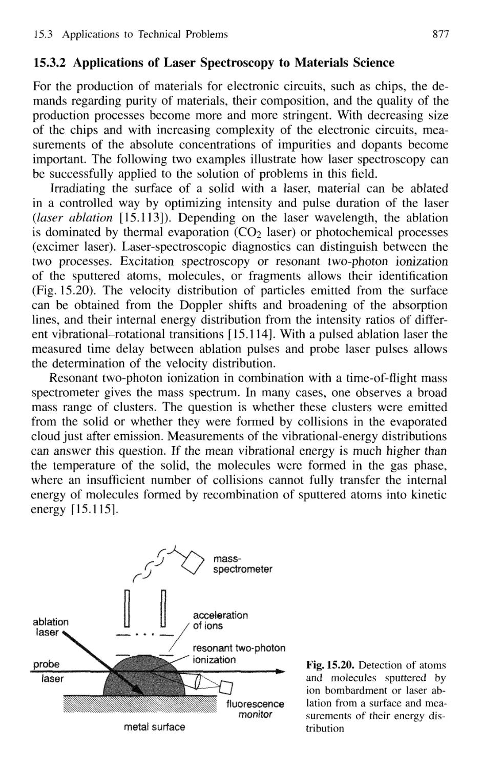
15.3.2 Applications of Laser Spectroscopy
to Materials Science 877
15.3.3 Measurements of Flow Velocities
in Gases and Liquids 878
15.4 Applications in Biology 879
15.4.1 Energy Transfer in DNA Complexes 879
15.4.2 Time-Resolved Measurements
of Biological Processes 881
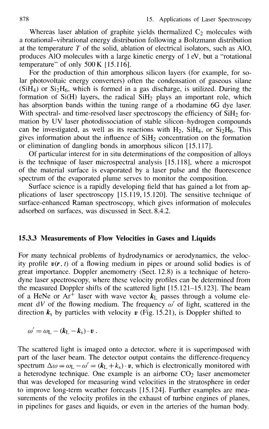
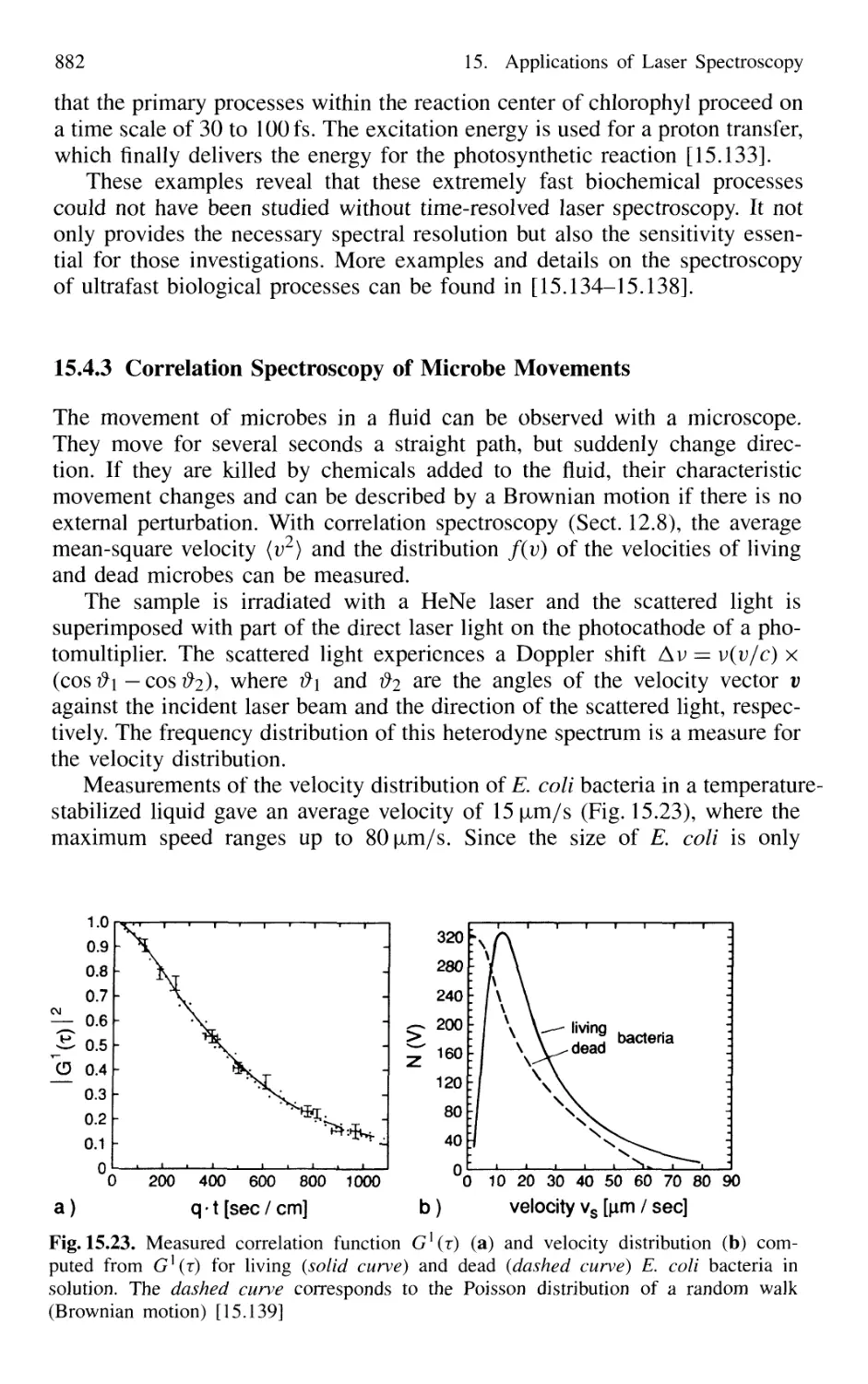
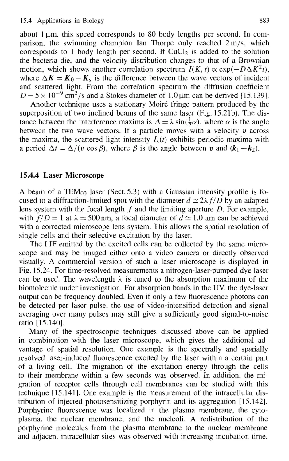
15.4.3 Correlation Spectroscopy of Microbe Movements .. 882
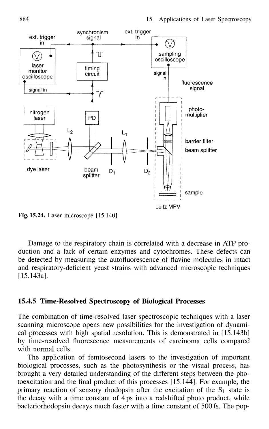
15.4.4 Laser Microscope 883
15.4.5 Time-Resolved Spectroscopy
of Biological Processes 884
15.5 Medical Applications of Laser Spectroscopy 885
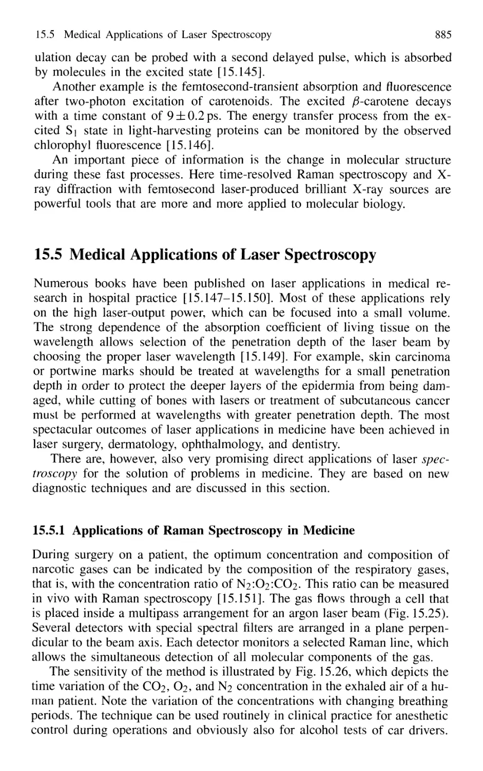
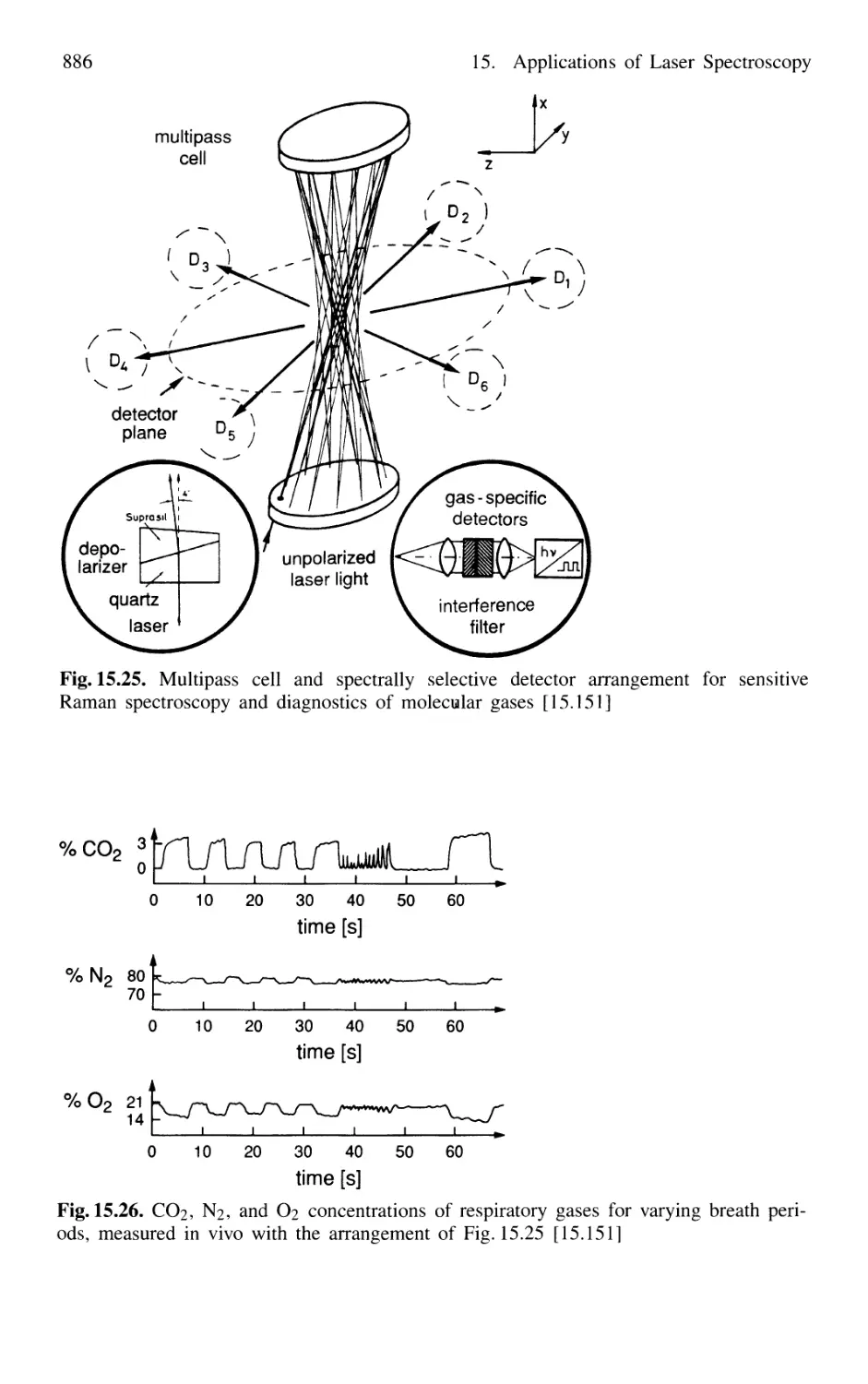
15.5.1 Applications of Raman Spectroscopy in Medicine . 885
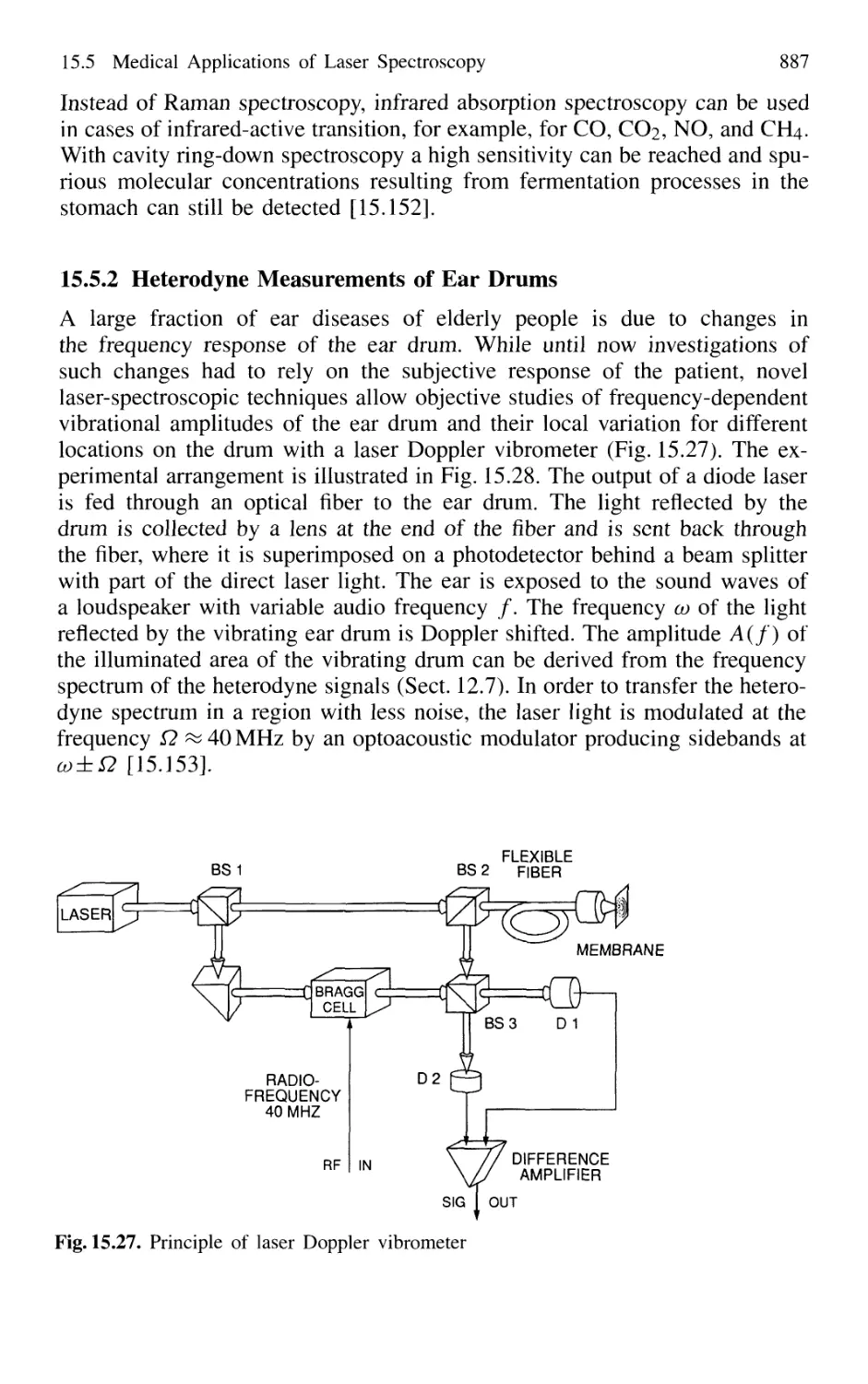
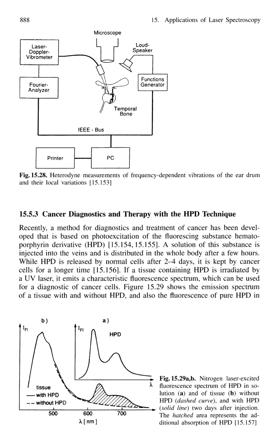
15.5.2 Heterodyne Measurements of Ear Drums 887
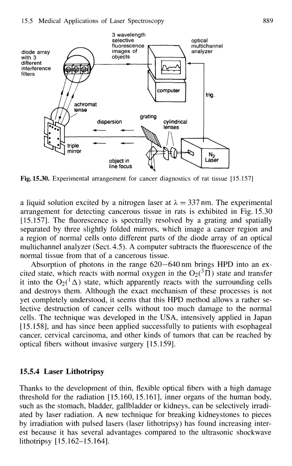
15.5.3 Cancer Diagnostics and Therapy
with the HPD Technique 888
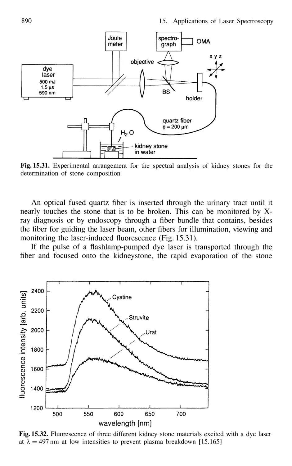
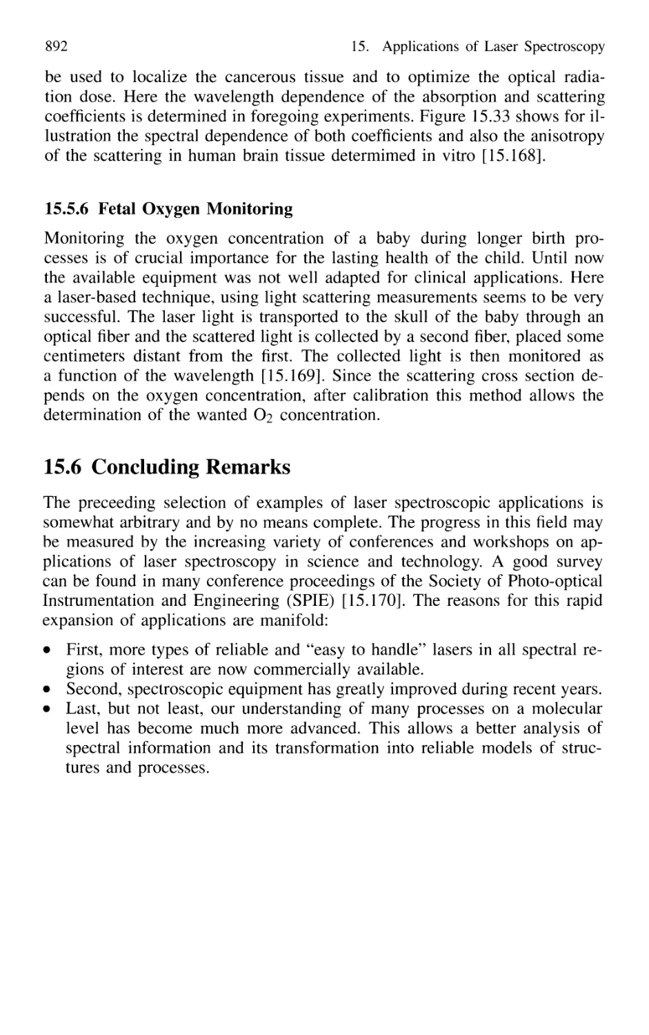
15.5.4 Laser Lithotripsy 889
15.5.5 Laser-Induced Thermotherapy of Brain Cancer 891
15.5.6 Fetal Oxygen Monitoring 892
15.6 Concluding Remarks 892
References 893
Subject Index 979
1. Introduction
Most of our knowledge about the structure of atoms and molecules is based
on spectroscopic investigations. Thus spectroscopy has made an outstanding
contribution to the present state of atomic and molecular physics, to chem-
chemistry, and to molecular biology. Information on molecular structure and on the
interaction of molecules with their surroundings may be derived in various
ways from the absorption or emission spectra generated when electromagnetic
radiation interacts with matter.
Wavelength measurements of spectral lines allow the determination of
energy levels of the atomic or molecular system. The line intensity is pro-
proportional to the transition probability, which measures how strongly the two
levels of a molecular transition are coupled. Since the transition probability
depends on the wave functions of both levels, intensity measurements are use-
useful to verify the spatial charge distribution of excited electrons, which can
only be roughly calculated from approximate solutions of the Schrödinger
equation. The natural linewidth of a spectral line may be resolved by spe-
special techniques, allowing mean lifetimes of excited molecular states to be
determined. Measurements of the Doppler width yield the velocity distri-
distribution of the emitting or absorbing molecules and with it the temperature
of the sample. From pressure broadening and pressure shifts of spectral
lines, information about collision processes and interatomic potentials can
be extracted. Zeemann and Stark splittings by external magnetic or elec-
electric fields are important means of measuring magnetic or electric moments
and elucidating the coupling of the different angular momenta in atoms or
molecules, even with complex electron configurations. The hyperfine struc-
structure of spectral lines yields information about the interaction between the
nuclei and the electron cloud and allows nuclear magnetic dipole moments or
electric quadrupole moments to be determined. Time-resolved measurements
allow the spectroscopist to follow up dynamical processes in ground-state
and excited-state molecules, to investigate collision processes and various en-
energy transfer mechanisms. Laser spectroscopic studies of the interaction of
single atoms with a radiation field provide stringent tests of quantum electro-
electrodynamics and the realization of high-precision frequency standards allows one
to check whether fundamental physical constants show small changes with
time.
These examples represent only a small selection of the many possible ways
by which spectroscopy provides tools to explore the microworld of atoms and
molecules. However, the amount of information that can be extracted from
a spectrum depends essentially on the attainable spectral or time resolution
and on the detection sensitivity that can be achieved.
2 1. Introduction
The application of new technologies to optical instrumentation (for in-
instance, the production of larger and better ruled gratings in spectrographs,
the use of highly reflecting dielectric coatings in interferometers, and the
development of optical multichannel analyzers and image intensifiers) has
certainly significantly extended the sensitivity limits. Considerable progress
was furthermore achieved through the introduction of new spectroscopic tech-
techniques, such as Fourier spectroscopy, optical pumping, level-crossing tech-
techniques, and various kinds of double-resonance methods and molecular beam
spectroscopy.
Although these new techniques have proved to be very fruitful, the really
stimulating impetus to the whole field of spectroscopy was given by the intro-
introduction of lasers. In many cases these new spectroscopic light sources may
increase spectral resolution and sensitivity by several orders of magnitude.
Combined with new spectroscopic techniques, lasers are able to surpass ba-
basic limitations of classical spectroscopy. Many experiments that could not be
performed with incoherent light sources are now feasible or have already been
successfully completed recently. This book deals with such new techniques of
laser spectroscopy and explains the necessary instrumentation.
The book begins with a discussion of the fundamental definitions and
concepts of classical spectroscopy, such as thermal radiation, induced and
spontaneous emission, radiation power and intensity, transition probabilities,
and the interaction of weak and strong electromagnetic (EM) fields with
atoms. Since the coherence properties of lasers are important for several spec-
spectroscopic techniques, the basic definitions of coherent radiation fields are
outlined and the description of coherently excited atomic levels is briefly dis-
discussed.
In order to understand the theoretical limitations of spectral resolution in
classical spectroscopy, Chap. 3 treats the different causes of the broadening
of spectral lines and the information drawn from measurements of line pro-
profiles. Numerical examples at the end of each section illustrate the order of
magnitude of the different effects.
The contents of Chap. 4, which covers spectroscopic instrumentation and
its application to wavelength and intensity measurements, are essential for
the experimental realization of laser spectroscopy. Although spectrographs
and monochromators, which played a major rule in classical spectroscopy,
may be abandoned for many experiments in laser spectroscopy, there are still
numerous applications where these instruments are indispensible. Of major
importance for laser spectroscopists are the different kinds of interferometers.
They are used not only in laser resonators to realize single-mode operation,
but also for line-profile measurements of spectral lines and for very precise
wavelength measurements. Since the determination of wavelength is a central
problem in spectroscopy, a whole section discusses some modern techniques
for precise wavelength measurements* and their accuracy.
Lack of intensity is one of the major limitations in many spectroscopic in-
investigations. It is therefore often vital for the experimentalist to choose the
proper light detector. Section 4.5 surveys several light detectors and sensi-
sensitive techniques such as photon counting, which is becoming more commonly
1. Introduction 3
used. This chapter concludes the first part of the book, which covers fun-
fundamental concepts and basic instrumentation of general spectroscopy. The
second part discusses in more detail subjects more specific to laser spec-
spectroscopy.
Chapter 5 treats the basic properties of lasers as spectroscopic radiation
sources. It starts with a short recapitulation of the fundamentals of lasers,
such as threshold conditions, optical resonators, and laser modes. Only those
laser characteristics that are important in laser spectroscopy are discussed
here. For a more detailed treatment the reader is referred to the extensive
laser literature cited in Chap. 5. Those properties and experimental tech-
niqes that make the laser such an attractive spectroscopic light source are
discussed more thoroughly. For instance, the important questions of wave-
wavelength stabilization and continuous wavelength tuning are treated, and ex-
experimental realizations of single-mode tunable lasers and limitations of laser
linewidths are presented. The last part of this chapter gives a survey of
the various types of tunable lasers that have been developed for different
spectral ranges. Advantages and limitations of these lasers are discussed.
The available spectral range could be greatly extended by optical frequency
doubling and mixing processes. This interesting field of nonlinear optics
is briefly presented at the end of Chap. 5 as far as it is relevant to spec-
spectroscopy.
The main part of the book presents various applications of lasers in
spectroscopy and discusses the different methods that have been developed
recently. Chapter 6 starts with Doppler-limited laser absorption spectroscopy
with its various high-sensitivity detection techniques such as frequency mod-
modulation and intracavity spectroscopy, cavity ring-down techniques, excitation-
fluorescence detection, ionization and optogalvanic spectroscopy, optoacoustic
and optothermal spectroscopy, or laser-induced fluorescence. A comparison
between the different techniques helps to critically judge their merits and lim-
limitations.
Really impressive progress toward higher spectral resolution has been
achieved by the development of various "Doppler-free" techniques. They rely
mainly on nonlinear spectroscopy, which is extensively discussed in Chap. 7.
Besides the fundamentals of nonlinear absorption, the techniques of satura-
saturation spectroscopy, polarization spectroscopy, and multiphoton absorption are
presented, together with various combinations of these methods.
Raman spectroscopy, a very important technique of classical spectroscopy,
has been revolutionized by the use of lasers. Not only spontaneous Raman
spectroscopy with greatly enhanced sensitivity, but also new techniques such
as induced Raman spectroscopy, surface-enhanced Raman spectroscopy, or
coherent anti-Stokes Raman spectroscopy (CARS) have contributed greatly
to the rapid development of sensitive, high-resolution detection of molecular
structure and dynamics, as is outlined in Chap. 8.
The combination of molecular beam methods with laser spectroscopic
techniques has brought about a large variety of new methods to study mo-
molecules, radicals, loosely bound van der Waals complexes, and clusters. This
is discussed extensively in Chap. 9.
4 1. Introduction
Of particular importance for the spectroscopy of highly excited states,
such as Rydberg levels of atoms and molecules, and for the assignment of
complex molecular spectra are various double-resonance techniques where
atoms and molecules are exposed simultaneously to two radiation fields res-
resonant with two transitions sharing a common level. In combination with
Doppler-free techniques, these double resonance methods are powerful tools
for spectroscopy. Some of these methods, representing modern versions of op-
optical pumping techniques of the prelaser era, are introduced in Chap. 10.
Impressive progress has been achieved in the development of short laser
pulses, with pulse durations in the femtosecond range. In 1999 the Nobel
Prize in Chemistry was awarded to A. H. Zewail for his work in femtosecond
spectroscopy. New techniques allow a time resolution hitherto out of reach.
Transient phenomena, such as fast isomerization of excited molecules, relax-
relaxation processes by collisional energy transfer, or fast dissociation processes of
optically excited molecules can now be investigated. Chapter 11 gives a sur-
survey on techniques in the nano-, pico-, and femto-second range to generate and
to detect ultrashort light pulses.
Coherent spectroscopy, which is based on the coherent excitation of
molecular levels and the detection of coherently scattered light, is treated
in Chap. 12, where techniques and applications of this interesting field are
illustrated by several examples.
Laser spectroscopy has contributed in an outstanding way to detailed stud-
studies of collision processes. Chapter 13 gives some examples of applications of
lasers in investigations of elastic, inelastic, and reactive collisions.
The rapid development of laser spectroscopy in recent years is demon-
demonstrated in Chap. 14, which compiles some recent fascinating ideas and their
methods to further increase spectral resolution and sensitivity. The goal of
studying single atoms and their interaction with radiation fields is no longer
a dream of theoreticians but can be realized experimentally. Interesting aspects
of cooling and trapping of atoms, the achievement of Bose-Einstein conden-
condensation for trapped atoms, phase transitions from ordered to chaotic systems,
and fundamental limits of detection-sensitivity are briefly outlined. The real-
realization of atom lasers and the fascinating aspects of atom interferometry are
also presented.
The last chapter illustrates by some examples the broad field of applica-
applications of laser spectroscopy to the solution of scientific, technical, and medical
problems.
This book is intended as an introduction to the basic methods and instru-
instrumentation of laser spectroscopy. The examples in each chapter illustrate the
text and may suggest other possible applications. They are mainly concerned
with the spectroscopy of free atoms and molecules and are, of course, not
complete, but have been selected from'the literature or from our own lab-
laboratory work for didactic purposes and may not represent the priorities of
publication dates. For a far more extensive survey of the latest publications
in the broad field of laser spectroscopy, the reader is referred to the proceed-
proceedings of various conferences on laser spectroscopy [1.1-1.10] and to textbooks
or collections of articles on modern aspects of laser spectroscopy [1.11-1.31].
1. Introduction 5
Since scientific achievements in laser physics have been pushed forward by
a few pioneers, it is interesting to look back to the historical development
and to the people who influenced it. Such a personal view can be found
in [1.32,1.33]. The reference list at the end of the book might be helpful
in finding more details of a special experiment or to dig deeper into theo-
theoretical and experimental aspects of each chapter. A useful "Encyclopedia of
spectroscopy" [1.34] gives a good survey on different aspects of laser spec-
troscopy.
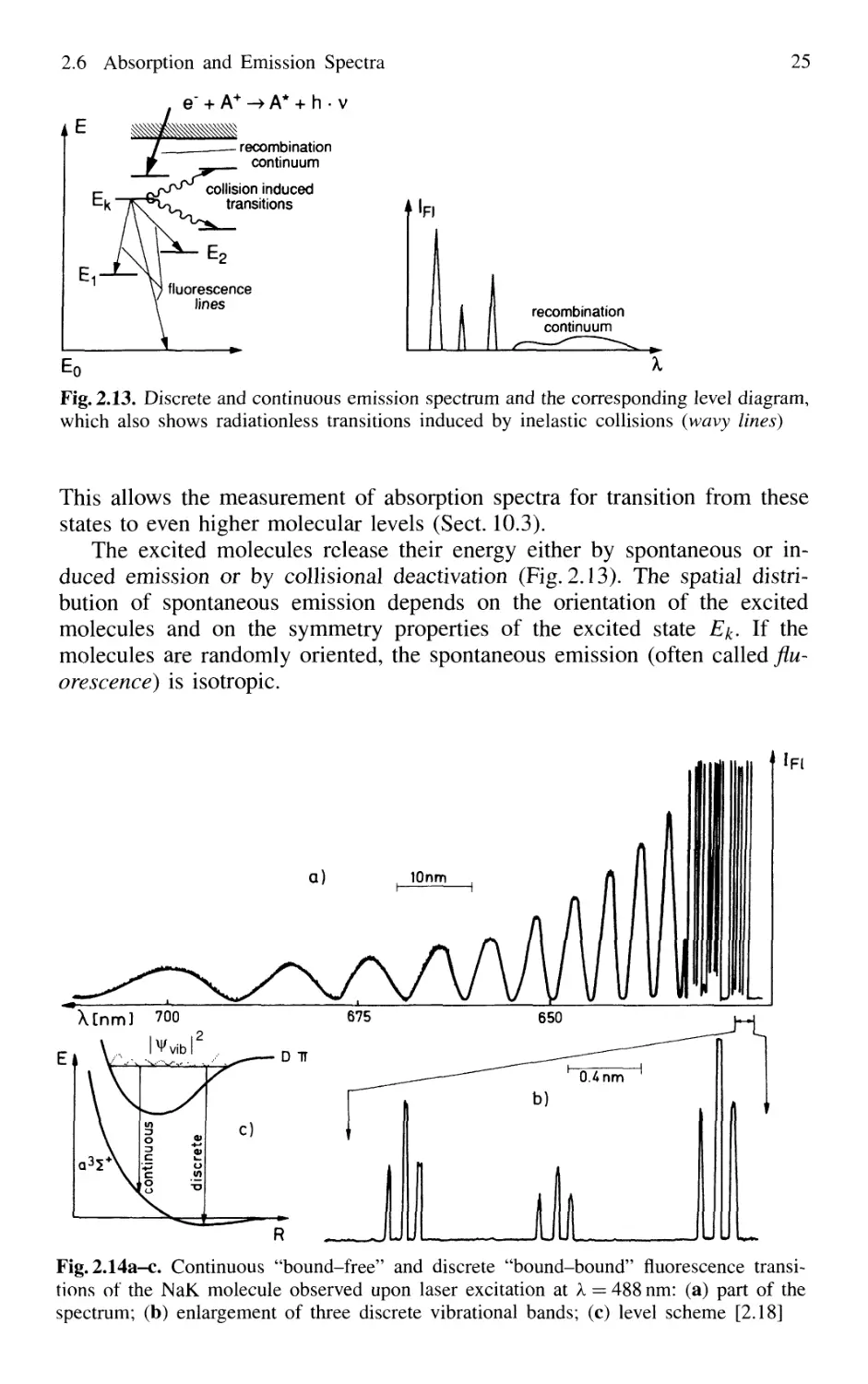
2. Absorption and Emission of Light
This chapter deals with basic considerations about absorption and emission
of electromagnetic waves interacting with matter. Especially emphasized are
those aspects that are important for the spectroscopy of gaseous media. The
discussion starts with thermal radiation fields and the concept of cavity modes
in order to elucidate differences and connections between spontaneous and in-
induced emission and absorption. This leads to the definition of the Einstein
coefficients and their mutual relations. The next section explains some defini-
definitions used in photometry such as radiation power, intensity, and spectral power
density.
It is possible to understand many phenomena in optics and spectroscopy in
terms of classical models based on concepts of classical electrodynamics. For
example, the absorption and emission of electromagnetic waves in matter can
be described using the model of damped oscillators for the atomic electrons.
In most cases, it is not too difficult to give a quantum-mechanical formulation
of the classical results. The semiclassical approach will be outlined briefly in
Sect. 2.7.
Many experiments in laser spectroscopy depend on the coherence prop-
properties of the radiation and on the coherent excitation of atomic or molecular
levels. Some basic ideas about temporal and spatial coherence of optical fields
and the density-matrix formalism for the description of coherence in atoms are
therefore discussed at the end of this chapter.
Throughout this text the term "light" is frequently used for electromagnetic
radiation in all spectral regions. Likewise, the term "molecule" in general
statements includes atoms as well. We shall, however, restrict the discussion
and most of the examples to gaseous media, which means essentially free
atoms or molecules.
For more detailed or more advanced presentations of the subjects sum-
summarized in this chapter, the reader is referred to the extensive literature on
spectroscopy [2.1-2.11]. Those interested in light scattering from solids are
directed to the sequence of Topics volumes edited by Cardona and coworkers
[2.12].
2.1 Cavity Modes
Consider a cubic cavity with the sides L at the temperature T. The walls of
the cavity absorb and emit electromagnetic radiation. At thermal equilibrium
the absorbed power Pa(co) has to be equal to the emitted power Pe(co) for all
8 2. Absorption and Emission of Light
frequencies co. Inside the cavity there is a stationary radiation field E, which
can be described at the point r by a superposition of plane waves with the
amplitudes Ap, the wave vectors kp, and the angular frequencies cov as
E =
— kp •/*)] + compl. conj.
B.1)
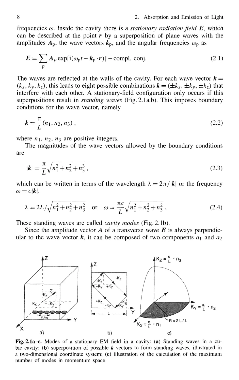
The waves are reflected at the walls of the cavity. For each wave vector k =
(kx, ky,kz), this leads to eight possible combinations k = (±kx, ±ky, ±kz) that
interfere with each other. A stationary-field configuration only occurs if this
superpositions result in standing waves (Fig. 2.1a,b). This imposes boundary
conditions for the wave vector, namely
7T
k =—(ni, H2, n^) , B.2)
where n\, n^, ft 3 are positive integers.
The magnitudes of the wave vectors allowed by the boundary conditions
are
B.3)
which can be written in terms of the wavelength k = 2tc/|/t| or the frequency
o) = c\k\.
or
= — Jn\ -j-n^+nl .
Lt
B.4)
These standing waves are called cavity modes (Fig. 2.1b).
Since the amplitude vector A of a transverse wave E is always perpendic-
perpendicular to the wave vector k, it can be composed of two components a\ and ai
21/ha
Fig.2.1a-c. Modes of a stationary EM field in a cavity: (a) Standing waves in a cu-
cubic cavity; (b) superposition of possible k vectors to form standing waves, illustrated in
a two-dimensional coordinate system; (c) illustration of the calculation of the maximum
number of modes in momentum space
2.1 Cavity Modes 9
with the unit vectors e\ and ej
B.5)
The complex numbers a\ and ai define the polarization of the standing wave.
Equation B.5) states that any arbitrary polarization can always be expressed
by a linear combination of two mutually orthogonal linear polarizations. To
each cavity mode defined by the* wave vector kp therefore belong two pos-
possible polarization states. This means that each triple of integers (n\, 122,113)
represents two cavity modes. Any arbitrary stationary field configuration can
be expressed as a linear combination of cavity modes.
We shall now investigate how many modes with frequencies co < com are
possible. Because of the boundary condition B.2), this number is equal to the
number of all integer triples (n\, n2, ^3) that fulfil the condition
c2k2=co2<0Jm .
In a system with the coordinates G1/L)(n\, n2, ^3), see Fig.2.1c, each
triple (n\,ri2, ^3) represents a point in a three-dimensional lattice with the
lattice constant tt/L. In this system, B.4) describes all possible frequencies
within a sphere of radius co/c. If this radius is large compared to tt/L, which
means that 2L ^> Xr}u the number of lattice points (n\, ^2, n^) with co2 < cojn
is roughly given by the volume of the octant of the sphere shown in Fig. 2.1c.
With the two possible polarization states of each mode, one therefore obtains
for the number of allowed modes with frequencies between co — 0 and co = com
in a cubic cavity of volume L3 with L ^> k
l^) f B.6)
N(ojm) 2l)
8 3 v nc ) 3 tt2c3
and N/L3 represents the number of modes per unit volume.
It is often interesting to know the number n(co)dco of modes per unit vol-
volume within a certain frequency interval dco, for instance, within the width
of a spectral line. The spectral mode density n(co) can be obtained directly
from B.6) by differentiating N(co)/L3 with respect to co. N(co) is assumed to
be a continuous function of co, which is, strictly speaking, only the case for
L —> 00. We get
co2
n(co) dco = n ~ dco . B.7a)
71ZC3
In spectroscopy the frequency v = co/2ti is often used instead of the angu-
angular frequency co. The number of modes per unit volume within the frequency
interval dv is then
87t v2
n(v)dv=—1-dv. B.7b)
c5
10 2. Absorption and Emission of Light
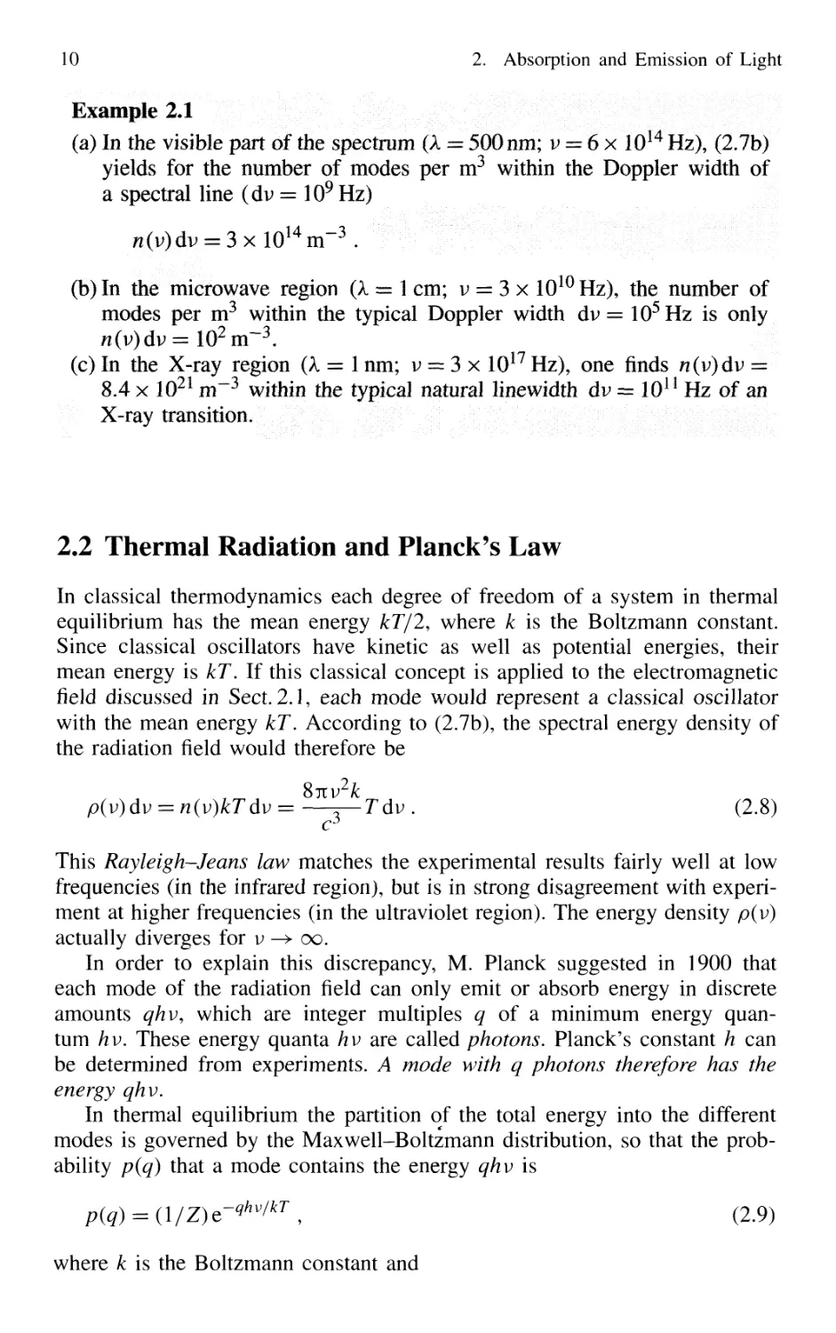
Example 2.1
(a) In the visible part of the spectrum (A = 500 nm; v = 6x 10¹⁴ Hz), B.7b)
yields for the number of modes per m3 within the Doppler width of
a spectral line (dv = 109 Hz)
(b)In the microwave region (A. = 1 cm; y = 3x 10¹⁰Hz), the number of
modes per m3 within the typical Doppler width dv = 105Hz is only
n(v)dv=102m~3.
(c) In the X-ray region (k = 1 nm; y = 3x 10¹⁷ Hz), one finds n(v)dv =
8.4 x 10²¹ m~3 within the typical natural linewidth dv = 1011 Hz of an
X-ray transition.
2.2 Thermal Radiation and Planck's Law
In classical thermodynamics each degree of freedom of a system in thermal
equilibrium has the mean energy kT/2, where k is the Boltzmann constant.
Since classical oscillators have kinetic as well as potential energies, their
mean energy is kT. If this classical concept is applied to the electromagnetic
field discussed in Sect. 2.1, each mode would represent a classical oscillator
with the mean energy kT. According to B.7b), the spectral energy density of
the radiation field would therefore be
Snvk
p(v)dv = n(v)kTdv = —^—Tdv . B.8)
This Rayleigh-Jeans law matches the experimental results fairly well at low
frequencies (in the infrared region), but is in strong disagreement with experi-
experiment at higher frequencies (in the ultraviolet region). The energy density p(v)
actually diverges for v -> oo.
In order to explain this discrepancy, M. Planck suggested in 1900 that
each mode of the radiation field can only emit or absorb energy in discrete
amounts qhv, which are integer multiples q of a minimum energy quan-
quantum hv. These energy quanta hv are called photons. Planck's constant h can
be determined from experiments. A mode with q photons therefore has the
energy qhv.
In thermal equilibrium the partition of the total energy into the different
modes is governed by the Maxwell-Boltzmann distribution, so that the prob-
probability p(q) that a mode contains the energy qhv is
hv'kT, B.9)
where k is the Boltzmann constant and
2.2 Thermal Radiation and Planck's Law
11
B.10)
is the partition function summed over all modes containing q photons h • v.
Z acts as a normalization factor which makes J\ /?(#) = 1, as can be seen im-
immediately by inserting B.10) into B.9). This means that a mode has to contain
with certainty (p = 1) some number (q = 0, 1, 2, ...) of photons.
The mean energy per mode is 'therefore
4=0
B.11)
The evaluation of the sum yields [2.6]
The thermal radiation field has the energy density p(v) dv within the frequency
interval v to v+dv , which is equal to the number n(v)dv of modes in the
interval dv times the mean energy W per mode. Using B.7b, 2.12) one obtains
B.13)
This is Planck's famous radiation law (Fig. 2.2), which predicts a spectral en-
energy density of the thermal radiation that is fully consistent with experiments.
The expression "thermal radiation" comes from the fact that the spectral en-
energy distribution B.13) is characteristic of a radiation field that is in thermal
equilibrium with its surroundings (in Sect. 2.1 the surroundings are deter-
determined by the cavity walls).
The thermal radiation field described by its energy density p(v) is
isotropic. This means that through any transparent surface element dA of
P(V)
6000K
10 000 20 000 30 000 40 000 v/c [cfn-ij
Fig. 2.2. Spectral distribution of the
energy density pv(v) for different
12 2. Absorption and Emission of Light
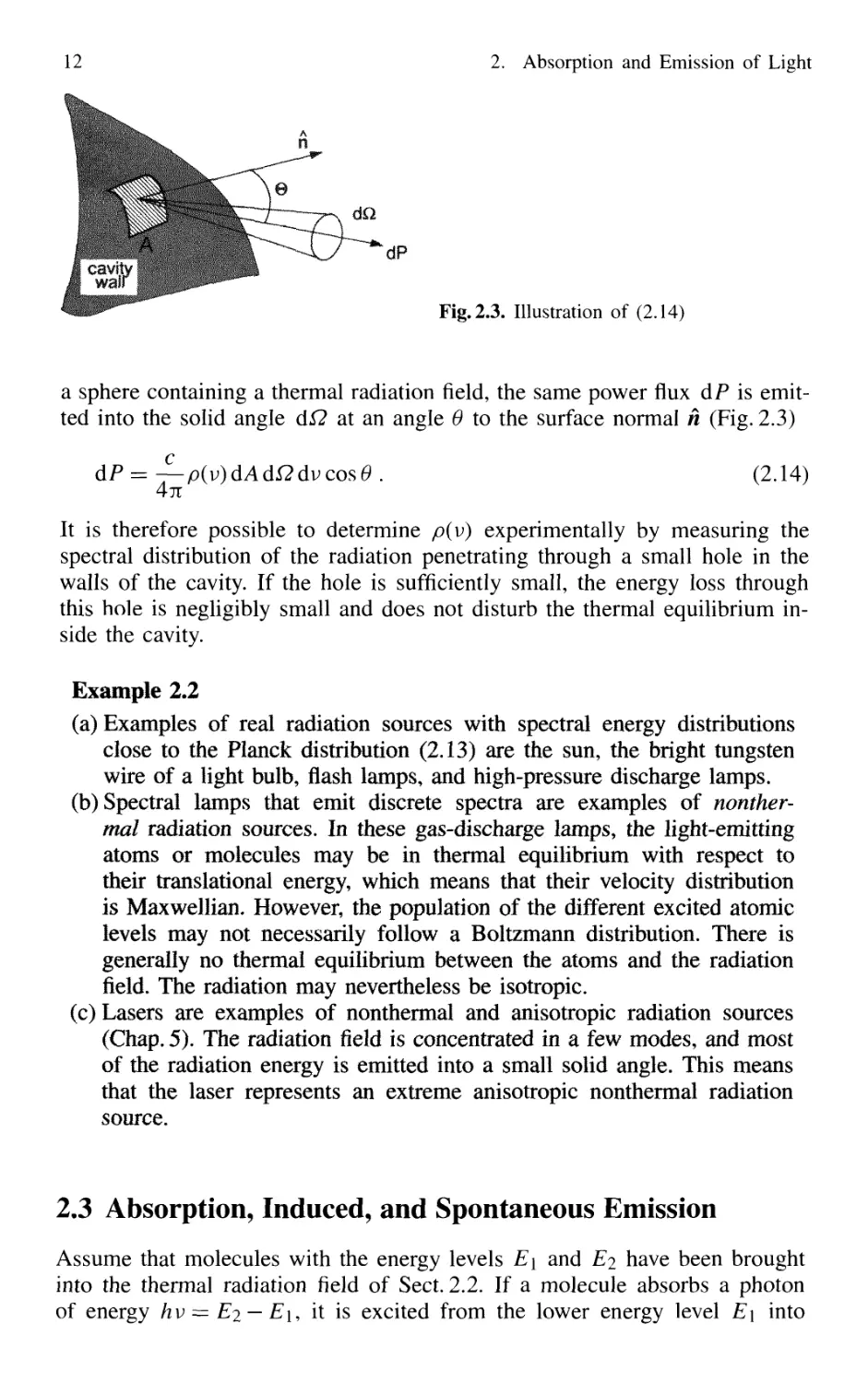
dP
Fig. 2.3. Illustration of B.14)
a sphere containing a thermal radiation field, the same power flux dP is emit-
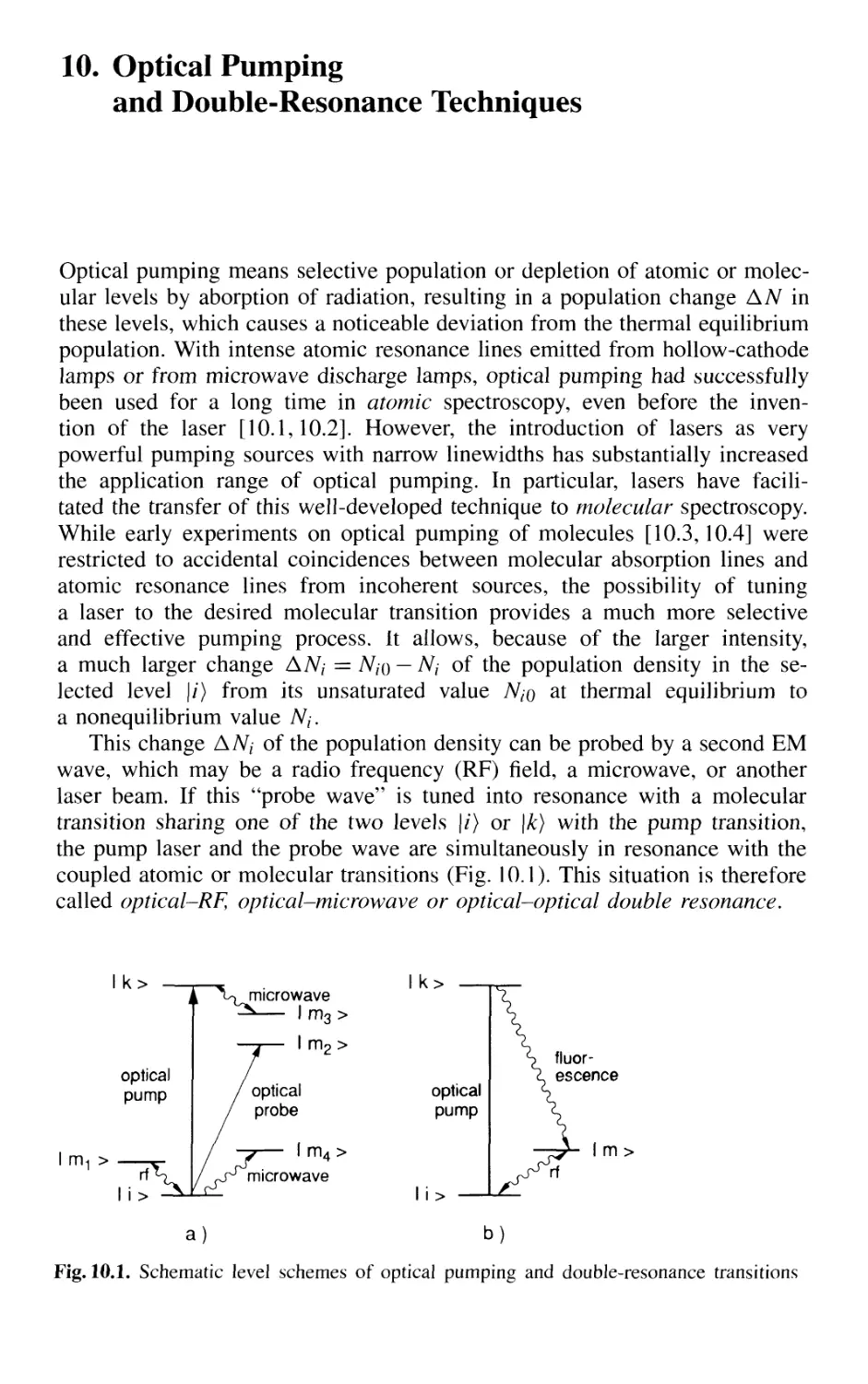
emitted into the solid angle df2 at an angle 6 to the surface normal h (Fig. 2.3)
dP = — p(v)dAdQdvcosO . B.14)
4tt
It is therefore possible to determine p(v) experimentally by measuring the
spectral distribution of the radiation penetrating through a small hole in the
walls of the cavity. If the hole is sufficiently small, the energy loss through
this hole is negligibly small and does not disturb the thermal equilibrium in-
inside the cavity.
Example 2.2
(a) Examples of real radiation sources with spectral energy distributions
close to the Planck distribution B.13) are the sun, the bright tungsten
wire of a light bulb, flash lamps, and high-pressure discharge lamps.
(b) Spectral lamps that emit discrete spectra are examples of nonther-
nonthermal radiation sources. In these gas-discharge lamps, the light-emitting
atoms or molecules may be in thermal equilibrium with respect to
their translational energy, which means that their velocity distribution
is Maxwellian. However, the population of the different excited atomic
levels may not necessarily follow a Boltzmann distribution. There is
generally no thermal equilibrium between the atoms and the radiation
field. The radiation may nevertheless be isotropic.
(c) Lasers are examples of nonthermal and anisotropic radiation sources
(Chap. 5). The radiation field is concentrated in a few modes, and most
of the radiation energy is emitted into a small solid angle. This means
that the laser represents an extreme anisotropic nonthermal radiation
source.
2.3 Absorption, Induced, and Spontaneous Emission
Assume that molecules with the energy levels E\ and Ei have been brought
into the thermal radiation field of Sect. 2.2. If a molecule absorbs a photon
of energy hv = E2 — E\, it is excited from the lower energy level E\ into
2.3 Absorption, Induced, and Spontaneous Emission
13
Fig. 2.4. Schematic diagram of the interaction
a two-level system with a radiation field
of
the higher level £2 (Fig- 2.4). This process is called induced absorption. The
probability per second that a molecule will absorb a photon, dPn/dt, is pro-
proportional to the number of photons of energy hv per unit volume and can be
expressed in terms of the spectral energy density pv(v) of the radiation field
as
d
—
B.15)
The constant factor B\2 is the Einstein coefficient of induced absorption. Each
absorbed photon of energy hv decreases the number of photons in one mode
of the radiation field by one.
The radiation field can also induce molecules in the excited state £2 to
make a transition to the lower state E\ with simultaneous emission of a pho-
photon of energy hv. This process is called induced (or stimulated) emission. The
induced photon of energy hv is emitted into the same mode that caused the
emission. This means that the number of photons in this mode is increased by
one. The probability d^2i/dr that one molecule emits one induced photon per
second is in analogy to B.15)
—
at
B.16)
The constant factor #21 is the Einstein coefficient of induced emission.
An excited molecule in the state £2 may also spontaneously convert its
excitation energy into an emitted photon hv. This spontaneous radiation can
be emitted in the arbitrary direction k and increases the number of photons in
the mode with frequency v and wave vector k by one. In the case of isotropic
emission, the probability of gaining a spontaneous photon is equal for all
modes with the same frequency v but different directions k.
The probability per second dtP^x°ni / dt that a photon hv = £2 — E\ is
spontaneously emitted by a molecule, depends on the structure of the
molecule and the selected transition |2) —> |1>, but it is independent of the
external radiation field,
B.17)
A21 is the Einstein coefficient of spontaneous emission and is often called the
spontaneous transition probability.
14 2. Absorption and Emission of Light
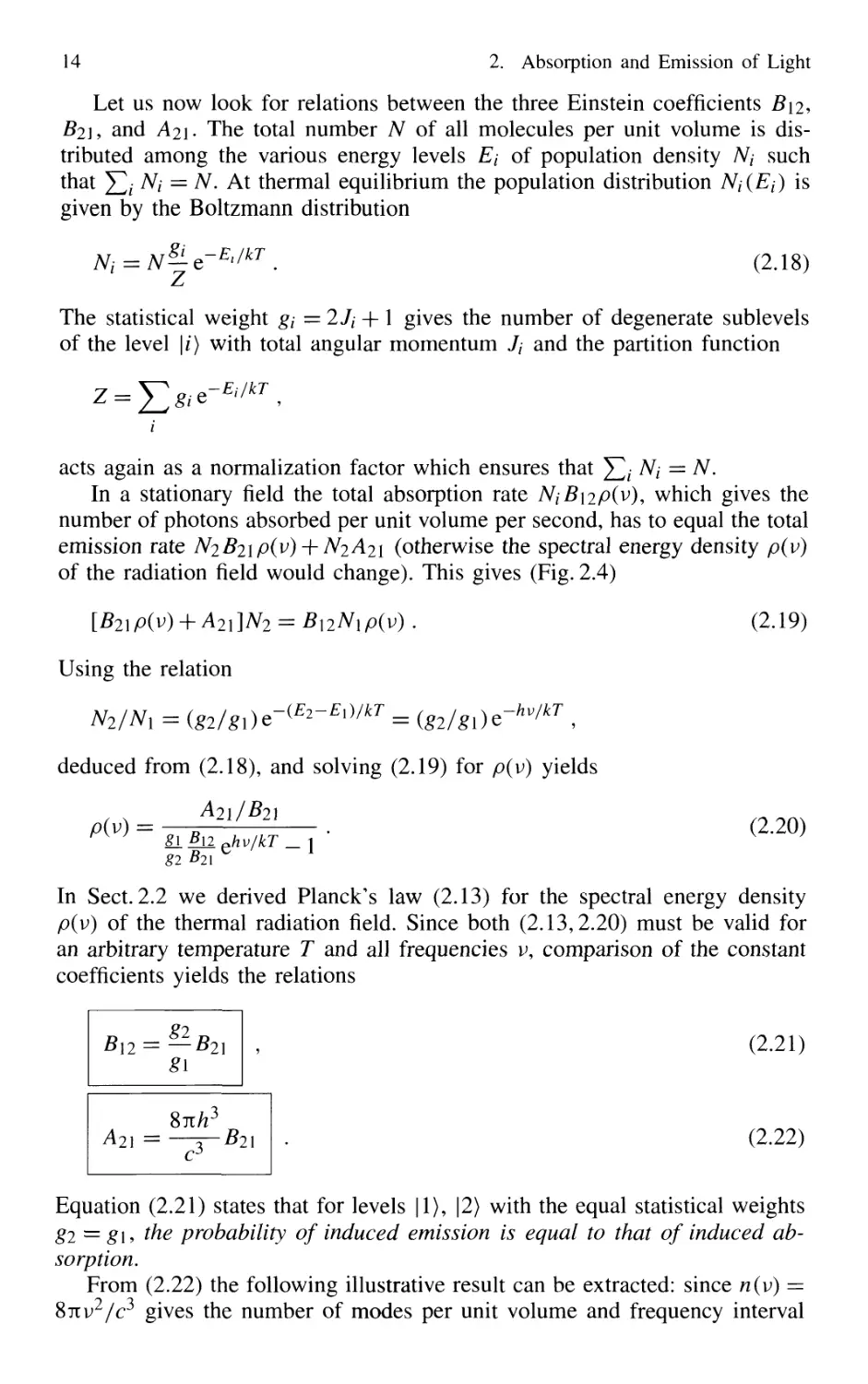
Let us now look for relations between the three Einstein coefficients B\2,
Z?2i, and A21. The total number TV of all molecules per unit volume is dis-
distributed among the various energy levels Et of population density Nf such
that Yli Ni = N. At thermal equilibrium the population distribution #/(£/) is
given by the Boltzmann distribution
Ni=N^c-Ei/kT . B.18)
The statistical weight gi = 27/ +1 gives the number of degenerate sublevels
of the level |/) with total angular momentum 7/ and the partition function
e-£//*r
acts again as a normalization factor which ensures that J^i Ni = N.
In a stationary field the total absorption rate N(B\2p(v), which gives the
number of photons absorbed per unit volume per second, has to equal the total
emission rate N2B2\p(v) -h N2A21 (otherwise the spectral energy density p(v)
of the radiation field would change). This gives (Fig. 2.4)
. B.19)
Using the relation
deduced from B.18), and solving B.19) for p(v) yields
gl #21
In Sect. 2.2 we derived Planck's law B.13) for the spectral energy density
p(v) of the thermal radiation field. Since both B.13,2.20) must be valid for
an arbitrary temperature T and all frequencies v, comparison of the constant
coefficients yields the relations
B.21)
B.22)
Equation B.21) states that for levels |1), |2) with the equal statistical weights
g2 = gi, the probability of induced emission is equal to that of induced ab-
absorption.
From B.22) the following illustrative result can be extracted: since n{v) =
87tv2/c3 gives the number of modes per unit volume and frequency interval
2.3 Absorption, Induced, and Spontaneous Emission
T[K]
15
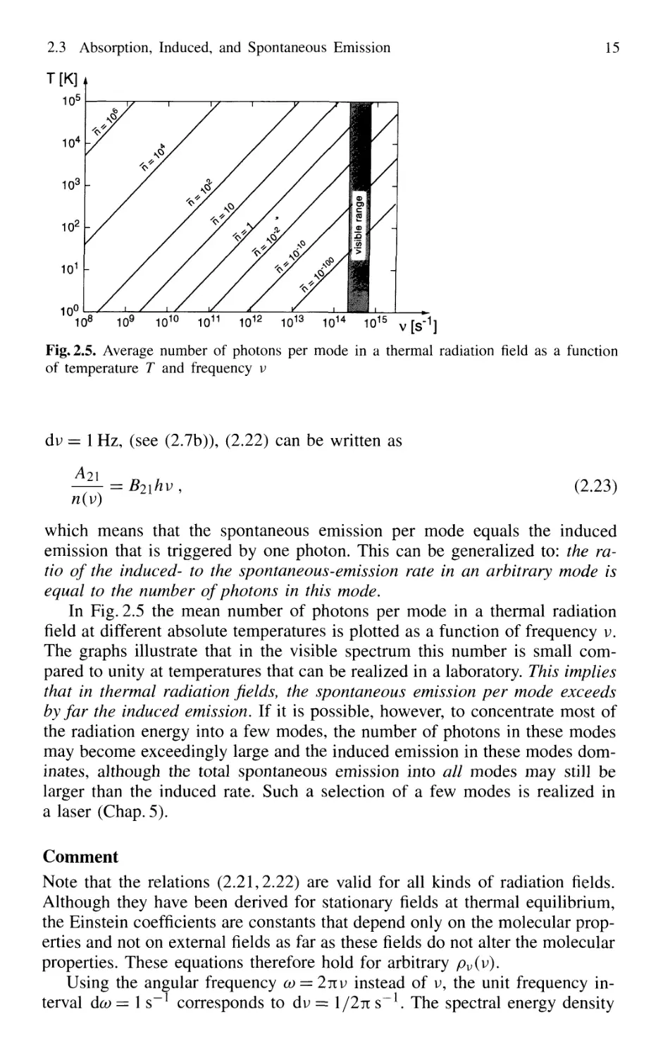
10'
Fig. 2.5. Average number of photons per mode in a thermal radiation field as a function
of temperature T and frequency v
dv = 1 Hz, (see B.7b)), B.22) can be written as
n(v)
B.23)
which means that the spontaneous emission per mode equals the induced
emission that is triggered by one photon. This can be generalized to: the ra-
ratio of the induced- to the spontaneous-emission rate in an arbitrary mode is
equal to the number of photons in this mode.
In Fig. 2.5 the mean number of photons per mode in a thermal radiation
field at different absolute temperatures is plotted as a function of frequency v.
The graphs illustrate that in the visible spectrum this number is small com-
compared to unity at temperatures that can be realized in a laboratory. This implies
that in thermal radiation fields, the spontaneous emission per mode exceeds
by far the induced emission. If it is possible, however, to concentrate most of
the radiation energy into a few modes, the number of photons in these modes
may become exceedingly large and the induced emission in these modes dom-
dominates, although the total spontaneous emission into all modes may still be
larger than the induced rate. Such a selection of a few modes is realized in
a laser (Chap. 5).
Comment
Note that the relations B.21,2.22) are valid for all kinds of radiation fields.
Although they have been derived for stationary fields at thermal equilibrium,
the Einstein coefficients are constants that depend only on the molecular prop-
properties and not on external fields as far as these fields do not alter the molecular
properties. These equations therefore hold for arbitrary pv(v).
Using the angular frequency co = luv instead of v, the unit frequency in-
interval dco = 1 s corresponds to dv = l/2n s. The spectral energy density
16 2. Absorption and Emission of Light
Paico) =n(<j))ha) is then, according to B.7a),
' ¦ ^ *" -r B-24)
where h is Planck's constant divided by 2ji. The ratio of the Einstein coeffi-
coefficients
ho?
Ä2\/B2\ = 3 , B.25)
now contains h instead of h, and is smaller by a factor of 2tt. However, the
ratio A2[/[B2\Pa)(co)], which gives the ratio of the spontaneous to the induced
transition probabilities, remains the same.
Example 2.3
(a) In the thermal radiation field of a 100 W light bulb, 10 cm away from
the tungsten wire, the number of photons per mode at X = 500 nm is
about 10"""**. If a molecular probe is placed in this field, the induced
emission is therefore completely negligible.
(b) In the center spot of a high-current mercury discharge lamp with very
high pressure, the number of photons per mode is about 10~2 at the
center frequency of the strongest emission line at X = 253.6mm. This
shows that, even in this very bright light source, the induced emission
only plays a minor role.
(c) Inside the cavity of a HeNe laser (output power 1 mW with mirror
transmittance T = 1%) that oscillates in a single mode, the number of
photons in this mode is about 107- In this example the spontaneous
emission into this mode is completely negligible. Note, however, that
the total spontaneous emission power at X = 632.2 nmt which is emit-
emitted into all directions, is much larger than the induced emission. This
spontaneous emission is more or less uniformly distributed among all
modes. Assuming a volume of 1 cm3 for the gas discharge, the number
of modes within the Doppler width of the neon transition is about 108,
which means that the total spontaneous rate is about 10 times the in-
induced rate.
2.4 Basic Photometric Quantities
In spectroscopic applications of light sources, it is very useful to define some
characteristic quantities of the emitted and absorbed radiation. This allows a
proper comparison of different light sources and detectors and enables one to
make an appropriate choice of apparatus for a particular experiment.
2.4 Basic Photometric Quantities 17
2.4.1 Definitions
The radiant energy W (measured in joules) refers to the total amount of en-
energy emitted by a light source, transferred through a surface, or collected by
a detector. The radiant power P (often called radiant flux 0) [W] is the ra-
radiant energy per second. The radiant energy density p [J/m3] is the radiant
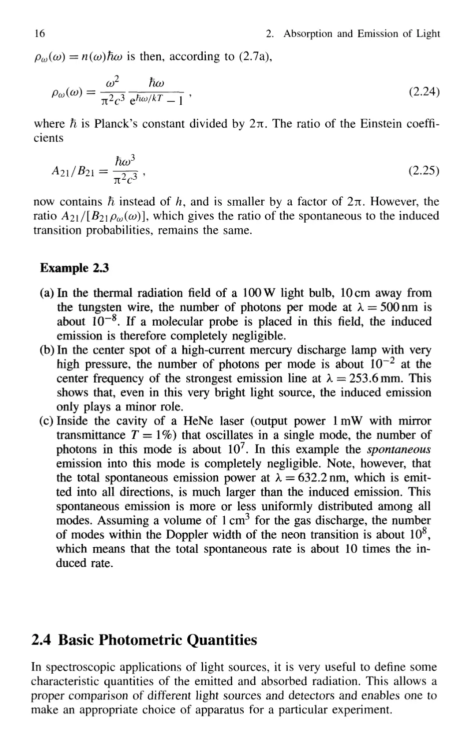
energy per unit volume of space. Consider a surface element dA of a light
source (Fig. 2.6). The radiant power emitted from dA into the solid angle dQ,
around the angle 0 against the surface normal h is
dP = LF)dAdn, B.26a)
where the radiance L [W/m2 sr] is the power emitted per unit surface ele-
element dA = 1 m2 into the unit solid angle d£2 = 1 sr.
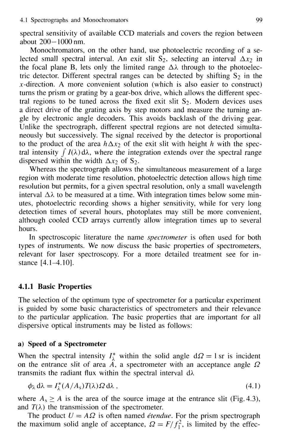
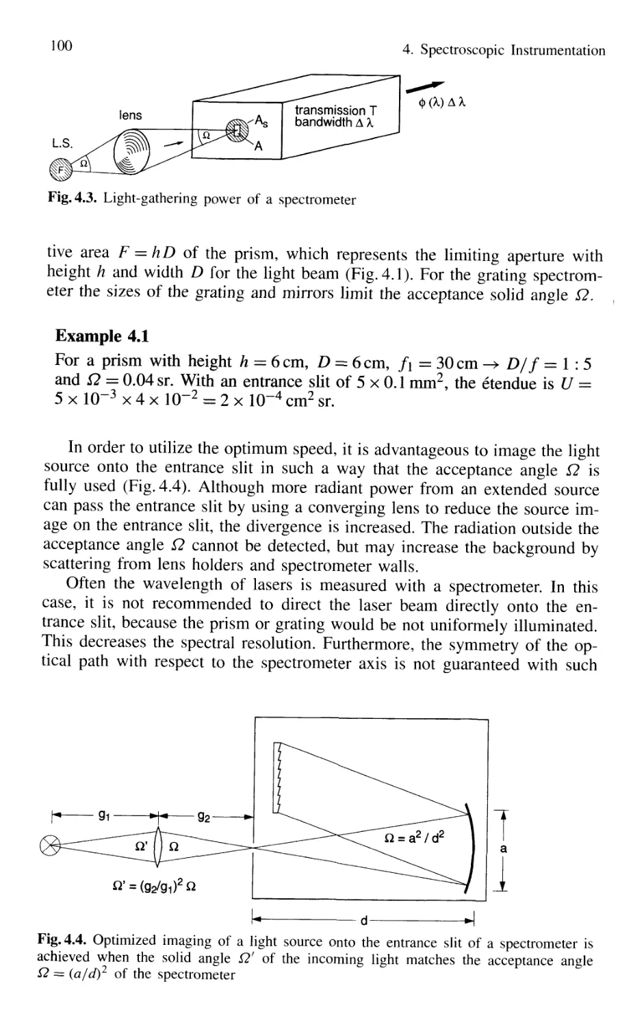
The total power emitted by the source is
P= / L(G)dAd£2 . B.26b)
Fig. 2.6. Basic radiant quantities of a light source
The above three quantities refer to the total radiation integrated over the
entire spectrum. Their spectral versions Wv(v), Pv(v)9 pv(v), and Lv(v) are
called the spectral densities, and are defined as the amounts of W, P, p, and L
within the unit frequency interval dv = 1 s around the frequency v:
00
w
0
OO OO 00 CO
= Wv(v)dv; P= /py(v)dv; p= pv(v)dv; L= Lv(v)dv.
B.27)
Example 2.4
For a spherical isotropic radiation source of radius R (e.g., a star) with
a spectral energy density pv, the spectral radiance Lv(v) is independent of 0
and can be expressed by
r s , , , t4 2hy l r,
Lv(v) = pv(v)c/4it = —= j-jpp—- -* Pv =
SnR2hv
3
C2 ehv/kT _ i y "" C2 ehv/kT _ | *
B.28)
18 2. Absorption and Emission of Light
/
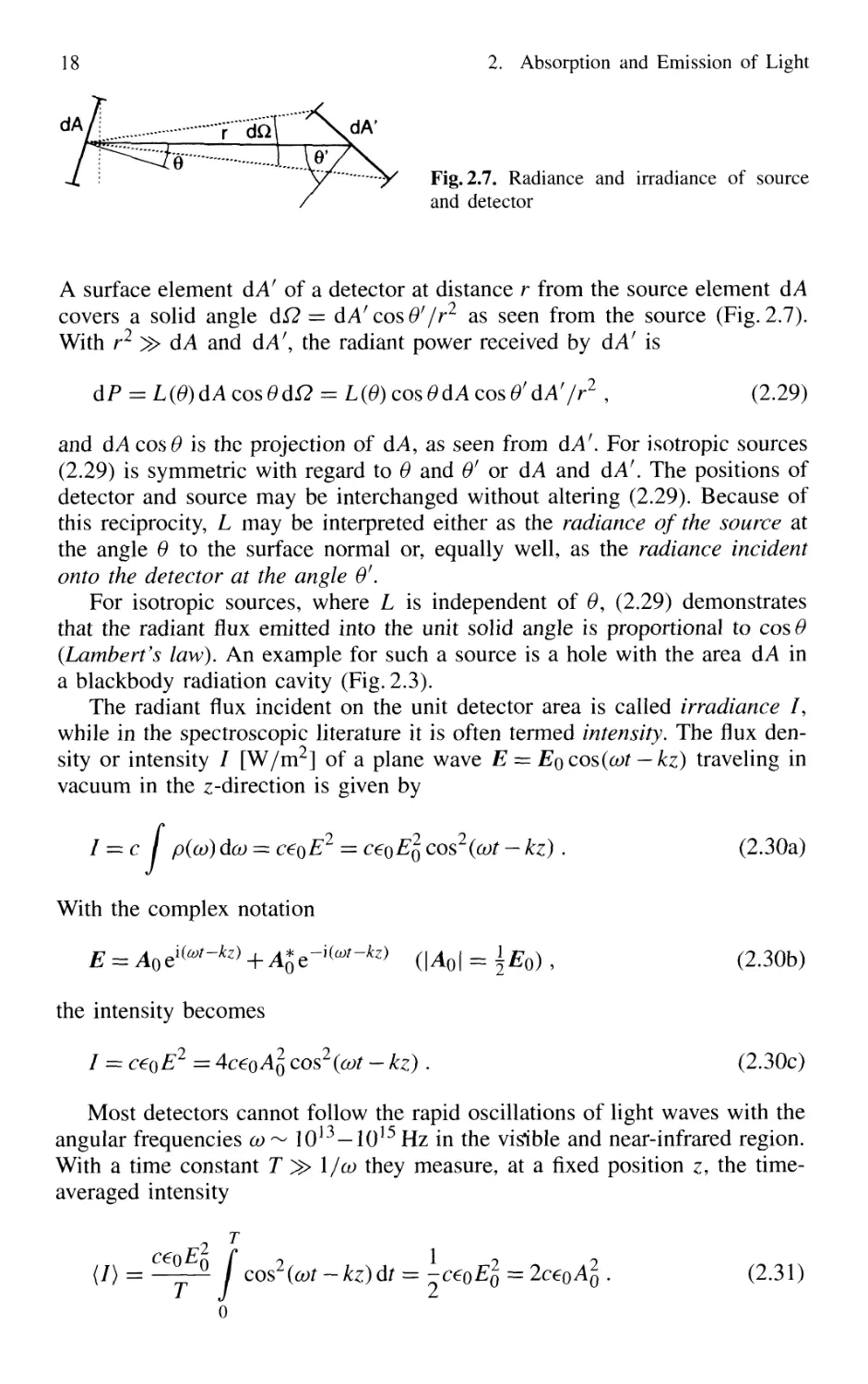
Fig. 2.7. Radiance and irradiance of source
and detector
A surface element dA' of a detector at distance r from the source element dA
covers a solid angle d£2 = dA'cos#'/r2 as seen from the source (Fig. 2.7).
With r2 ^> dA and dA', the radiant power received by dAf is
dP = L@)dAcos6dQ = L@) cos6>dA cos0'dAf/r2 , B.29)
and dA cos0 is the projection of dA, as seen from dA'. For isotropic sources
B.29) is symmetric with regard to 0 and 0f or dA and dA'. The positions of
detector and source may be interchanged without altering B.29). Because of
this reciprocity, L may be interpreted either as the radiance of the source at
the angle 0 to the surface normal or, equally well, as the radiance incident
onto the detector at the angle &'.
For isotropic sources, where L is independent of 0, B.29) demonstrates
that the radiant flux emitted into the unit solid angle is proportional to cos 0
(Lambert's law). An example for such a source is a hole with the area dA in
a blackbody radiation cavity (Fig. 2.3).
The radiant flux incident on the unit detector area is called irradiance /,
while in the spectroscopic literature it is often termed intensity. The flux den-
density or intensity / [W/m2] of a plane wave E = Eocos(cot — kz) traveling in
vacuum in the z-direction is given by
= c / p(co) dco = c^E2 = c€0El cos2(cot - kz).
l B.30a)
With the complex notation
E = Aoel(a*-kz) + A*oe-iia)t-kz) (\Aq\ = \Eq) , B.30b)
the intensity becomes
/ = c€0E2 = AceoAl cos2(cot - kz). B.30c)
Most detectors cannot follow the rapid oscillations of light waves with the
angular frequencies co ^ 1013-1015 Hz in the viable and near-infrared region.
With a time constant T ^> l/co they measure, at a fixed position z, the time-
averaged intensity
T
o 1 o O
2l 2 B.31)
C€f)Er{ To 1 o O
(/) = -JL-0 / cos2(cot ~kz)dt = -ceoEl = 2ce0A20 .
2.4 Basic Photometric Quantities
2.4.2 Illumination of Extended Areas
19
In the case of extended detector areas, the total power received by the detector
is obtained by integration over all detector elements dA' (Fig. 2.8). The detec-
detector receives all the radiation that is emitted from the source element dA within
the angles —u<0<+u. The same radiation passes an imaginary spherical
surface in front of the detector. We choose as elements of this spherical sur-
surface circular rings with dA' = 2icrdr = 2nR2 sinOcosOdO. From B.29) one
obtains for the total flux 0 impinging onto the detector with cos Q1 = 1
o
0= LdAcos027isin0d0.
-/
B.32)
If the source is isotropic, L does not depend on 6 and B.32) yields
B.33)
dr = Rd9
Fig. 2.8. Flux densities of detectors with
extended area
Comment
Note that it is impossible to increase the radiance of a source by any sophisti-
sophisticated imaging optics. This means that the image dA* of a radiation source dA
never has a larger radiance than the source itself. It is true that the flux density
can be increased by demagnification. The solid angle, however, into which ra-
radiation from the image dA* is emitted is also increased by the same factor.
Therefore, the radiance does not increase. In fact, because of inevitable reflec-
reflection, scattering, and absorption losses of the imaging optics, the radiance of
the image dA* is, in practice, always less than that of the source (Fig. 2.9).
A strictly parallel light beam would be emitted into the solid angle
dQ = 0. With a finite radiant power this would imply an infinite radiance L,
26Q
Fig. 2.9. The radiance of a source cannot be
increased by optical imaging
20 2. Absorption and Emission of Light
which is impossible. This illustrates that such a light beam cannot be real-
realized. The radiation source for a strictly parallel beam anyway has to be a point
source in the focal plane of a lens. Such a point source with zero surface
cannot emit any power.
For more extensive treatments of photometry see [2.13,2.14].
Example 2.5
(a) Radiance of the sun. An area equal to 1 m2 of the earth's surface re-
receives at normal incidence without reflection or absorption through the
atmosphere an incident radiant flux /e of about 1.35 kW/m2 (solar con-
constant). Because of the symmetry of B.32) we may regard AAf as emitter
and dA as receiver. The sun is seen from the earth under an angle
of 2w = 32 minutes of arc. This yields sin« =4.7x 10~3. Inserting
this number into B.33), one obtains Ls=2x 10⁷W/(m2sr) for the
radiance of the sun's surface. The total radiant power <P of the sun
can be obtained from B.32) or from the relation <P = 4nR2Ic, where
R = 1.5 x 10¹¹ m is the distance from the earth to the sun. These num-
numbers give <P = 4 x 1026 W.
(b) Radiance of a HeNe laser. We assume that the output power of 1 mW is
emitted from 1 mm2 of the mirror surface into an angle of 4 minutes of
arc, which is equivalent to a solid angle of 1 x 10" sr. The maximum
radiance in the direction of the laser beam is then L = 10~3/A0~6-
lCT6) = 109W/(m2sr). This is about 50 times larger than the radi-
radiance of the sun. For the spectral density of the radiance the comparison
is even more dramatic. Since the emission of a nonstabilized single-
mode laser is restricted to a spectral range of about 1 MHz, the laser
has a spectral radiance density Ly = lxl03W- s/(m2sr~1), whereas
the sun, which emits within a mean spectral range of «s 1015 Hz, only
reaches Lv = 2 x 10~8 W • s/(m2 sr'1).
(c) Looking directly into the sun, the retina receives a radiant flux of 1 mW
if the diameter of the iris is 1 mm. This is just the same flux the retina
receives staring into the laser beam of Example 2.5b. There is, however,
a big difference regarding the irradiance of the retina. The image of the
sun on the retina is about 100 times as large as the focal area of the
laser beam. This means that the power density incident on single retina
cells is about 100 times larger in the case of the laser radiation.
2.5 Polarization of Light
The complex amplitude vector Aq of the plane wave
E = Ao • ei(ätf-*z) B.34)
2.5 Polarization of Light
can be written in its component representation
21
B.35)
For unpolarized light the phases (j)x and </>y are uncorrelated and their
difference fluctuates statistically. For linearly polarized light with its electric
vector in x-direction Aoy = 0. When E points into a direction or against the
x axis, (px = 0y and tana = Aoy/Aox. For circular polarization Aqx = Aoy and
<j)x = <j)y ± tt/2. The different states of polarization can be characterized by
their Jones vectors, which are defined as follows:
ei(cot-kz)
B.36)
where the normalized vector {a, b} is the Jones vector. In Table 2.1 the Jones
vectors are listed for the different polarization states. For linearly polarized
light with a = 45°, for example, the amplitude Aq can be written as
B.37)
while for right circular polarization (a light), we obtain
B.38)
because exp(—ijr/2) = —i.
Table 2.1. Jones vectors for light traveling in the z-direction and Jones matrices for polar-
polarizers. The x-direction is horizontal, the v-direction vertical
Jones vectors
Jones matrices
Linear polarizers Circular polarizers
.v-direction (\
y-direction
t
c* = 45c
7!«
' V2V
Linear polarizers
Circular polarizers
Ü O
\
\ 0\ /0 0\ \ (I \\ \_ ( 1 -\\
0 0) [0 l) 2 V V 2 V 1 /
A./4 plate
1 /-i 0
22 2. Absorption and Emission of Light
The Jones representation shows its advantages when we consider the trans-
transmission of light through optical elements such as polarizers, X/4 plates, or
beamsplitters. These elements can be described by 2 x 2 matrices, which are
compiled for some elements in Table 2.1. The polarization state of the trans-
transmitted light is then obtained by multiplication of the Jones vector of the
incident wave by the Jones matrix of the optical element.
B.39)
For example, a linearly polarized incident light with a = 0° becomes, after
transmission through a circular polarizer,
a right circular polarized o~ wave. More examples can be found in [2.15-2.17].
2.6 Absorption and Emission Spectra
The spectral distribution of the radiant flux from a source is called its emis-
emission spectrum. The thermal radiation discussed in Sect. 2.2 has a continuous
spectral distribution described by its spectral energy density B.13). Discrete
emission spectra, where the radiant flux has distinct maxima at certain fre-
frequencies Vik, are generated by transitions of atoms or molecules between two
bound states, a higher energy state Ek and a lower state £/, with the relation
hvik = Ek-Ei. B.41)
In a spectrograph (see Sect. 4.1 for a detailed description) the entrance slit is
imaged into the focal plane of the camera lens. Because of dispersive elements
in the spectrograph, the position of this image depends on the wavelength of
the incident radiation. In a discrete spectrum each wavelength A.;* produces
a separate line in the imaging plane, provided the spectrograph has a suffi-
sufficiently high resolving power (Fig. 2.10). Discrete spectra are therefore also
called line spectra, as opposed to continuous spectra where the slit images
form a continuous band in the focal plane, even for spectrographs with infinite
resolving power.
If radiation with a continuous spectrum passes through a gaseous molecu-
molecular sample, molecules in the lower state E[ may absorb radiant power at the
eigenfrequencies v^ — (Ek — Ei)/h, which is thus missing in the transmitted
power. The difference in the spectral distributions of incident minus transmit-
transmitted power is the absorption spectrum of the sample. The absorbed energy hvik
brings a molecule into the higher energy level Ek- If these levels are bound
levels, the resulting spectrum is a discrete absorption spectrum. If Ek is above
the dissociation limit or above the ionization energy, the absorption spectrum
2.6 Absorption and Emission Spectra
23
Fig. 2.10. Spectral lines in a discrete spectrum as images of the entrance slit of a spec-
trograph
becomes continuous. In Fig. 2.11 both cases are schematically illustrated for
atoms (a) and molecules (b).
Examples of discrete absorption lines are the Fraunhofer lines in the spec-
spectrum of the sun, which appear as dark lines in the bright continuous spectrum
(Fig. 2.12). They are produced by atoms in the sun's atmosphere that absorb
at their specific eigenfrequencies the continuous blackbody radiation from the
sun's photosphere. A measure of the absorption strength is the absorption
lonization-
limit
recombination
continuum
Atom
Molecule
Fig.2.11a,b. Schematic diagram to illustrate the origin of discrete and continuous absorp-
absorption and emission spectra for atoms (a) and molecules (b)
24 2. Absorption and Emission of Light
O OH Na Fe H Fe Ca
Fig. 2.12. Prominent Fraunhofer absorption
761 687 656 589 527 486 431327 lines within the visible and near-UV spectral
**— A» [nm] range
cross section o^. Each photon passing through the circular area a^ — nrfk
around the atom is absorbed on the transition |/> -> \k).
The power
/ a- \
dPik(co)dco = Po Nt - —Nk aik(co)AAzdco = P0aik(co) AV dco , B.42)
V 8k J
absorbed within the spectral interval dco at the angular frequency co on the
transition \i) -> \k) within the volume AV = AAz is proportional to the
product of incident power Po, absorption cross section olk, the difference
(Nt — Nk) of the population densities of absorbing molecules in the upper and
lower levels, weighted with their statistical weights gi, gk, and the absorption
path length Az. A comparison with B.15) and B.21) yields the total power
absorbed per cm3 on the transition |/) -» \k):
Pik = Po I aik(co)dco = —PoBtk [Nt -—Nk) , B.43)
J c \ gk J
where the integration extends over the absorption profile. This gives the rela-
relation
B.44)
between the Einstein coefficient Bik and the absorption cross section o^.
At thermal equilibrium the population follows a Boltzmann distribution.
Inserting B.18) yields the power absorbed within the volume AV = AAz out
of an incident beam with the cross section A
pik = j
£/tr £/*rB.45)
for a monochromatic laser with Po(co) = PoS(co — coo).
The absorption lines are only measurable if the absorbed power is suffi-
sufficiently high, which means that the density N or the absorption path length Az
must be large enough. Furthermore, the difference in the two Boltzmann fac-
factors in B.45) should be sufficiently large, which means Ej should be not much
larger than kT, but Ek ^> kT. Absorption lines in gases at thermal equilib-
equilibrium are therefore only intense for transitions from low-lying levels Et that
are thermally populated.
It is, however, possible to pump molecules into higher energy states by var-
various excitation mechanisms such as optical pumping or electron excitation.
2.6 Absorption and Emission Spectra
e' + A+ -»A* + h ¦ v
25
Fig. 2.13. Discrete and continuous emission spectrum and the corresponding level diagram,
which also shows radiationless transitions induced by inelastic collisions (wavy lines)
This allows the measurement of absorption spectra for transition from these
states to even higher molecular levels (Sect. 10.3).
The excited molecules release their energy either by spontaneous or in-
induced emission or by collisional deactivation (Fig. 2.13). The spatial distri-
distribution of spontaneous emission depends on the orientation of the excited
molecules and on the symmetry properties of the excited state Ek. If the
molecules are randomly oriented, the spontaneous emission (often called flu-
fluorescence) is isotropic.
a)
Fig. 2.14a-c. Continuous "bound-free" and discrete "bound-bound" fluorescence transi-
transitions of the NaK molecule observed upon laser excitation at A. = 488 nm: (a) part of the
spectrum; (b) enlargement of three discrete vibrational bands; (c) level scheme [2.18]
26 2. Absorption and Emission of Light
The fluorescence spectrum (emission spectrum) emitted from a discrete
upper level Ek consists of discrete lines if the terminating lower levels Et
are bound states. A continuum is emitted if E\ belongs to a repulsive state of
a molecule that dissociates. As an example, the fluorescence spectrum of the
3n -> 3E transition of the NaK molecule is shown in Fig. 2.14. It is emitted
from a selectively excited level in a bound 3 FI state that has been populated
by optical pumping with an argon laser. The fluorescence terminates into a re-
repulsive 3E state, which has a shallow van der Waals minimum. Transitions
terminating to energies Ek above the dissociation energy form the continu-
continuous part of the spectrum, whereas transitions to lower bound levels in the van
der Waals potential well produce discrete lines. The modulation of the contin-
continuum reflects the modulation of the transmission probability due to the maxima
and nodes of the vibrational wave function \//vfo(R) in the upper bound level
[2.18].
2.7 Transition Probabilities
The intensities of spectral lines depend not only on the population density
of the molecules in the absorbing or emitting level but also on the transition
probabilities of the corresponding molecular transitions. If these probabilities
are known, the population density can be obtained from measurements of line
intensities. This is very important, for example, in astrophysics, where spec-
spectral lines represent the main source of information from the extraterrestrial
world. Intensity measurements of absorption and emission lines allow the con-
concentration of the elements in stellar atmospheres or in interstellar space to be
determined. Comparing the intensities of different lines of the same element
(e.g., on the transitions E\ —> Ek and Ee —» Ek from different upper levels
E(, Ee to the same lower level Ek) furthermore enables us to derive the tem-
temperature of the radiation source from the relative population densities Af;, Ne
in the levels E; and Ee at thermal equilibrium according to B.18). All these
experiments, however, demand a knowledge of the corresponding transition
probabilities.
There is another aspect that makes measurements of transition probabil-
probabilities very attractive with regard to a more detailed knowledge of molecular
structure. Transition probabilities derived from computed wave functions of
upper and lower states are much more sensitive to approximation errors in
these functions than are the energies of these states. Experimentally deter-
determined transition probabilities are therefore well suited to test the validity of
calculated approximate wave functions. A comparison with computed proba-
probabilities allows theoretical models of electronic charge distributions in excited
molecular states to be improved [2.19,2.20].
2.7.1 Lifetimes, Spontaneous and Radiationless Transitions
The probability Pik that an excited molecule in the level £/ makes a transi-
transition to a lower level Ek by spontaneous emission of a fluorescence quantum
2.7 Transition Probabilities
27
a) b)
Fig.2.15a,b. Radiative decay of the level |/>: (a) Level scheme; (b) decay curve N((t)
vik = E[ — Ek is, according to B.17), related to the Einstein coefficient
by
When several transition paths from Ei to different lower levels Ek are possible
(Fig. 2.15), the total transition probability is given by
4k • B.46)
The decrease dNi of the population density Ni during the time interval dt due
to radiative decay is then
B.47)
Integration of B.47) yields
v , B.48)
where Afo is the population density at t = 0.
After the time r/ = I/A/ the population density Ni has decreased to 1/e of
its initial value at t = 0. The time t; represents the mean spontaneous lifetime
of the level Ei as can be seen immediately from the definition of the mean
time
(X) OQ
ü= I tPi(t)dt = / tAit~Aitdt = — = T| ,
J J Ai
o o
B.49)
where ^ (i) dt is the probability that one atom in the level E[ makes a spon-
spontaneous transition within the time interval between t and t + dt.
The radiant power emitted from Ni molecules on the transition Et —>? Ek
is
Pik = NihvikAik .
B.50)
28
2. Absorption and Emission of Light
collision
induced
transitions
fluorescence
Fig. 2.16. Fluorescence- and collision-induced
decay channels of an excited level |/>
If several transitions E\ —> Ek from the same upper level E\ to different lower
levels Ek are possible, the radiant powers of the corresponding spectral lines
are proportional to the product of the Einstein coefficient Aik and the photon
energy hvik. The relative radiation intensities in a certain direction may also
depend on the spatial distribution of the fluorescence, which can be different
for the different transitions.
The level E[ of the molecule A can be depopulated not only by
spontaneous emission but also by collison-induced radiationless transitions
(Fig. 2.16). The probability d^oll/dr of such a transition depends on the den-
density N# of the collision partner B, on the mean relative velocity v between A
and B, and on the collision cross section o^°n for an inelastic collision that
induces the transition E[ -> Ek in the molecule A
mil
Jik
B.51)
When the excited molecule A(£;) is exposed to an intense radiation field, the
induced emission may become noticeable. It contributes to the depopulation
of level E[ in a transition |/) -> \k) with the probability
¦ = p(vik)Bik[Ni-(gi/gk)Nk].
B.52)
The total transition probability that determines the effective lifetime of a level
Et is then the sum of spontaneous, induced, and collisional contributions, and
the mean lifetime rfft becomes
B.53)
,-eff
Measuring the effective lifetime rf as a function of the exciting radiation
intensity and also its dependence on the density Nb of collision partners
(Stern-Vollmer plot) allows one to determine the three transition probabilities
separately (Sect. 11.3).
2.7 Transition Probabilities 29
2.7.2 Semiclassical Description: Basic Equations
In the semiclassical description, the radiation incident upon an atom is de-
described by a classical electromagnetic (EM) plane wave
E = Eo cos(cot - kz) . B.54a)
The atom, on the other hand, is treated quantum-mechanically. In order to
simplify the equations, we restrict ourselves to a two-level system with the
eigenstates Ea and Eh (Fig. 2.17).
Until now laser spectroscopy was performed in spectral regions where the
wavelength X was large compared to the diameter d of an atom (e.g., in the
visible spectrum A is 500 nm, but d is only about 0.5 nm). For X^>d, the
phase of the EM wave does not change much within the volume of an atom
because kz = Bn/k)z <^l for z < d. We can therefore neglect the spatial
derivatives of the field amplitude (dipole approximation). In a coordinate sys-
system with its origin in the center of the atom, we can assume kz — 0 within the
atomic volume, and write B.54a) in the form
E = E0 cos cot = A0(eia)t + e"iwr) with \A0\ = \Eq . B.54b)
The Hamiltonian operator
B.55)
of the atom interacting with the light field can be written as a sum of the un-
unperturbed Hamiltonian Mq of the free atom plus the perturbation operator V,
which reduces in the dipole approximation to
V = p • E = p • Eo cos cot, B.56)
where V is the scalar product of the dipole operator p — —er and the electric
field E.
The general solution \j/{r, t) of the time-dependent Schrödinger equation
dxlr
= ih— B.57)
at
LU
k
uff
CO
Ea-
¦~ a Fig. 2.17. Two-level system with open decay channels into other
levels interacting with an EM field
30 2. Absorption and Emission of Light
can be expressed as a linear superposition
VKr, 0 = J^cn(t)un(r)t~lE^h , B.58)
of the eigenfunctions of the unperturbed atom
i£"'//i. B.59)
The spatial parts un(r) of these eigenfunctions are solutions of the time-
independent Schrödinger equation
je0un(r) = Enun(r) , B.60)
and satisfy the orthogonality relations1
- Sfjc. B.61)
For our two-level system with the eigenstates \a) and \b) and the energies
Ea and Et,, B.58) reduces to a sum of two terms
B.62)
The coefficients aib) and b(t) are the time-dependent probability amplitudes
of the atomic states \a) and \b). This means that the value \a(t)\2 gives the
probability of finding the system in level \a) at time t. Obviously, the rela-
relation \a(t)\2 + 1^@12 = 1 must hold at all times t, if decay into other levels is
neglected.
Substituting B.62) and B.55) into B.57) gives
iM{t)ua t-lEat'h + ihb(t)ubQ~lE^h = aVuo t-xEat/h + bVuht-lEbt/h ,
B.63)
where the relation M§un = Enun has been used to cancel equal terms on both
sides. Multiplication with u*(n=a,b) and spatial integration results in the
following two equations
a(t) = -(i/h)[a(t)Vaa+b(t)Vabtl(E«-EMh] , B.64a)
bit) = -a//i)[/7@V^ + a@V^e-l(^-^)r^] , B.64b)
with the spatial integral
Vab = I u*aVubdx = -eE f u*arubdx . B.65a)
1 Note that in B.58-2.60) a nondegenerate system has been assumed.
2.7 Transition Probabilities 31
Since r has odd parity, the integrals Vaa and Vbb vanish when integrating over
all coordinates from —oo to +00. The quantity
= Dba = ~e
B.65b)
is called the atomic dipole matrix element. It depends on the stationary wave
functions ua and ub of the two states \a) and \b) and is determined by the
charge distribution in these states.
The expectation value D of the atomic dipole moment for our two-level
system, which should be distinguished from the dipole matrix element, is
—/¦
B.66a)
Using B.62) and the abbreviation coba = (Eh — Ea)/h = —coab, this can be ex-
expressed by the coefficients a(t) and b(t), and by the matrix element Dab as
D = -Dah(a*be~lc°hat +ab*e+1(Obat) = Do cos(cohat + <p) , B.66b)
with
A) = Dab |fl*fe| and tan <p = — -
Even without the external field, the expectation value of the atomic dipole mo-
moment oscillates with the eigenfrequency coba and the amplitude \a* -b\ if the
wavefunction of the atomic system can be represented by the superposition
B.65).
Using B.54b) for the EM field and the abbreviation
Si ab = DabEo/h = 2DahAo/h = Qba B.67)
for the Rabi frequency Qab, which depends on the field amplitude Eq and the
dipole matrix element Dab, B.64) reduces to
a(t) = -(i/2)nab{ei{ü)ab-co)t + e{tOab+(o)t)b{t) ,
b(f) = -(M2)Qab{e~KQ)ab~~Q))t + <Ti{(Oab+Q))t)a(t) .
B.68a)
B.68b)
These are the basic equations that must be solved to obtain the probability
amplitudes a(t) and b(t).
32 2. Absorption and Emission of Light
2.7.3 Weak-Field Approximation
Suppose that at time t = 0, the atoms are in the lower state Ea, which im-
implies that a@) = 1 and b@) = 0. We assume the field amplitude Ao to be
sufficiently small so that for times t < T the population of Eb remains small
compared with that of Ea, i.e., \b(t < 7)|2 <^ 1. Under this weak-field condi-
condition we can solve B.68) with an iterative procedure starting with a = 1 and
b = 0. Using thermal radiation sources, the field amplitude Aq is generally
small enough to make the first iteration step already sufficiently accurate.
With these assumptions the first approximation of B.68) gives
a(t) = 0 , B.69a)
b(t) = (i/2)ß^(ei(£ü^-w)r + ei(a)ab+a>)t) . B.69b)
With the initial conditions 0@) = 1 and b@) = 0, integration of B.69) yields
a(t) = 0@) = 1 , B.70a)
_ 1 e\{(Oba+CO)t _ 1 \
+ . B.70b)
Cuba + U> I
For Eb > Ea the term a>ba = (Eb - Ea)/h is positive. In the transition
Ea -» Eb, the atomic system absorbs energy from the radiation field. No-
Noticeable absorption occurs, however, only if the field frequency co is close
to the eigenfrequency coba- In the optical frequency range this implies that
\<*>ba—to\ <^coba- The second term in B.70b) is then small compared to the
first one and may be neglected. This is called the rotating-wave approxima-
approximation for only that term is kept in which the atomic wave functions and the
field waves with the phasors txp(—icoabt) = exp(+ia^r) and exp(—xcot) rotate
together.
In the rotating-wave approximation we obtain from B.70b) for the proba-
probability \b(t)\2 that the system is at time t in the upper level Eb
Since we had assumed that the atom was at / = 0 in the lower level Ea, B.71)
gives the transition probability for the atom to go from Ea to Eb during the
time t. Figure 2.18a illustrates this transition probability as a function of the
detuning Aco = coba -co. Equation B.71) shows that \b(t)\2 depends on the ab-
absolute value of the detuning Aco= \coba—co\ of the field frequency co from
the eigenfrequency coba- When tuning the frequency co into resonance with the
atomic system (co —? coba), the second factor in B.71) approaches the value t2
because limx_>o[(sin2 xt)/x2] = t2. The transition probability at resonance,
t2 , B.72)
2.7 Transition Probabilities
33
|b(t)|2/(QQb/2J
lb(t)l2
b)
c)
Fig. 2.18. (a) Normalized transition probability as a function of the detuning (co — cot,a)
in the rotating-wave approximation; (b) probability of a transition to the upper level as
a function of time for different detuning; (c) \b(i)\2 under broadband excitation and weak
fields
increases proportionally to t2. The approximation used in deriving B.71) has,
however, anticipated that \b(t)\2 <$C 1. According to B.72) and B.67), this as-
assumption for the resonance case is equivalent to
«
or t « T =
h
B.73)
Our small-signal approximation only holds if the maximum interaction time T
of the field (amplitude Eo) with the atom (matrix element Dab) is restricted to
t <&T. Because the spectral analysis of a wave with the finite detection time T
gives the spectral width Aco ~ \/T (see also Sect. 3.2), we cannot assume
monochromaticity, but have to take into account the frequency distribution of
the interaction term.
2.7.4 Transition Probabilities with Broad-Band Excitation
In general, thermal radiation sources have the bandwidth hco, which is much
larger than the Fourier limit Aco = l/T. Therefore, the finite interaction time
imposes no extra limitation. This may change, however, when lasers are con-
considered (Sects. 2.7.5 and 3.4).
Instead of the field amplitude Eo (which refers to a unit frequency inter-
interval), we introduce the spectral energy density p(co) within the frequency range
of the absorption line by the relation, see B.30),
p(co) dco =
We can now generalize B.71) to include the interaction of broadband radia-
radiation with our two-level system by integrating B.71) over all frequencies co of
the radiation field. This yields the total transition probability Pab^f) within the
time r, if Dab || Eo:
Pab{t)
f
= /
J
1
\b(t)\2 doj =
/ p(co)
J \
(coba-co)/2
dco. B.74)
34 2. Absorption and Emission of Light
For thermal light sources or broadband lasers, p(co) is slowly varying over
the absorption line profile. It is essentially constant over the frequency range
where the factor [sm2 (ojba — co)t/2]/[(coba ~ &>)/2]2 is large (Fig. 2.18a). We
can therefore replace p(co) by its resonance value p(coba)- The integration can
then be performed, which gives the value p(a)baJnt for the integral because
00 o
I-,
For broadband excitation, the transition probability for the time interval be-
between 0 and t
7t
—^Dflhp(ojha)t, B.75)
is linearly dependent on t (Fig. 2.18c). For broadband excitation the transition
probability per second
— Pab = ^D2abp(coba) , B.76)
becomes independent of time!
To compare this result with the Einstein coefficient Bab derived in
Sect. 2.3, we must take into account that the blackbody radiation was
isotropic, whereas the EM wave B.54) used in the derivation of B.76)
propagates into one direction. For randomly oriented atoms with the di-
pole moment p, the averaged component of p2 in the z-direction is (p2) =
p2(cos20) = p2/3.
In the case of isotropic radiation, the interaction term D2bp(a)ba) therefore
has to be divided by a factor of 3. A comparison of B.16) with the modified
equation B.76) yields
d 7i 9
-T^ab = ^ ^iP(u>ba)D2b = P(toba)Bab • B.77)
d£
With the definition B.65) for the dipole matrix element Z>^, the Einstein co-
coefficient Bft of induced absorption Et —? E^ finally becomes
and Bvlk = Bfk/2n . B.78)
Equation B.78) gives the Einstein coefficient for a one-electron sys-
system where r = (jc, y, z) is the vector from the nucleus to the electron, and
un(x,y,z) denotes the one-electron wave functions.2 From B.78) we learn
2 Note that when using the frequency v = (jü/2tz instead of co, the spectral energy den-
density p(v) per unit frequency interval is larger by a factor of 2tt than p(co) because a unit
frequency interval dv = 1 Hz corresponds to dco = 2n [Hz]. The right-hand side of B.78)
must then be divided by a factor of 2tt, since Bv-kp(v) ~ Bfkp(co).
2.7 Transition Probabilities 35
that the Einstein coefficient Bik is proportional to the squared transition dipole
moment.
So far we have assumed that the energy levels E\ and Ek are not degen-
degenerate, and therefore have the statistical weight factor g= 1. In the case of
a degenerate level \k), the total transition probability pBik of the transition
E[ -> Ek is the sum
over all transitions to the sublevels \kn) of \k). If level |/) is also degener-
degenerate, an additional summation over all sublevels \im) is necessary, taking into
account that the population of each sublevel \im) is only the fraction Ni/gi.
The Einstein coefficient Bik for the transition E[ -> Ek between the two
degenerate levels |/) and \k) is therefore
TT
The double sum is called the line strength Sik of the atomic transition
|/> +- \k).
2.7.5 Phenomenological Inclusion of Decay Phenomena
So far we have neglected the fact that the levels \a) and \b) are not only
coupled by transitions induced by the external field but may also decay
by spontaneous emission or by other relaxation processes such as collision-
induced transitions. We can include these decay phenomena in our formulas
by adding phenomenological decay terms to B.68), which can be expressed
by the decay constant ya and yt, (Fig. 2.17). A rigorous treatment requires
quantum electrodynamics [2.23].
In the rotating-wave approximation, for which the term with the frequency
is neglected, B.68) then becomes
a(t) - -^Yaa + ^ab^^-^Ht) , B.80a)
b{t) = —yhb+-£2abfyl{(Dba~ü)) a(t) . B.80b)
2 2
When the field amplitude Eo is sufficiently small, see B.73), we can use
the weak-signal approximation of Sect.2.7.3. This means that \a(t)\2 = l,
\b(t)\2 <<£ 1, and also aa* —bb* c^ 1. With this approximation, one obtains in
a similar way as in the derivation of B.71) the transition probability
9 f 1 °2
Pabico) = \b(t, co)\z= / Yabe~Yabt \b(t)\zdt = --
! —COJ ¦
B.80c)
This is a Lorentzian line profile (Fig. 2.19) with a full halfwidth yab = ya + Yb-
36
2. Absorption and Emission of Light
Fig. 2.19. Transition probability of a damped system under weak broadband excitation
After taking the second-time derivative of B.66b) and using B.80), the
equation of motion for the dipole moment D of the atom under the influence
of a radiation field, becomes
B.81a)
B.81b)
which describes the atomic dipoles without the driving field (Qab = 0), has
the solution for weak damping {yab <$C coba)
= (C2ab)[((Dba + 0)) COS Cut + (yabß) Sin Cut] .
The homogeneous equation
D + YabD + (co2ba + y^/4)D = 0 ,
COS CObat •
B.82)
The inhomogeneous equation B.81a) shows that the induced dipole moment
of the atom interacting with a monochromatic radiation field behaves like
a driven damped harmonic oscillator with coba — (Eb — Ea)/h for the eigenfre-
quency and yab = (ya -f- yb) f°r the damping constant oscillating at the driving
field frequency co.
Using the approximation (coba + co) — 2co and Yab^^ba^ which means
weak damping and a close-to-resonance situation, we obtain solutions of the
form
D= D\ cos cot -f- Z>2 sin cot,
where the factors D\ and D2 include the frequency dependence,
(coba - coI
(coab - coJ -
B.83)
B.84a)
B.84b)
2.7 Transition Probabilities 37
These two equations for D\ and D2 describe dispersion and absorption of the
EM wave. The former is caused by the phase lag between the radiation field
and the induced dipole oscillation, and the latter by the atomic transition from
the lower level Ea to the upper level E\, and the resultant conversion of the
field energy into the potential energy (Et, — Ea).
The macroscopic polarization P of a sample with N atoms/cm3 is related
to the induced dipole moment D by P = ND.
2.7.6 Interaction with Strong Fields
In the previous sections we assumed weak-field conditions where the proba-
probability of finding the atom in the initial state was not essentially changed by
the interaction with the field. This means that the population in the initial
state remains approximately constant during the interaction time. In the case
of broadband radiation, this approximation results in a time-independent tran-
transition probability. Also the inclusion of weak-damping terms with y^ <^ co^a
did not affect the assumption of a constant population in the initial state.
When intense laser beams are used for the excitation of atomic transitions,
the weak-field approximation is no longer valid. In this section, we there-
therefore consider the "strong-field case." The corresponding theory, developed by
Rabi, leads to a time-dependent probability of the atom being in either the
upper or lower level. The representation outlined below follows that of [2.21].
We consider a monochromatic field of frequency co and start from the basic
equations B.68) for the probability amplitudes in the rotating wave approxi-
approximation
a{t) = ~Qab^l{cOb^0))tb(t) , B.85a)
b(t) = -^ab^^'^ait) . B.85b)
Inserting the trial solution
a(t) = ei/xi =» ä(t) it
into B.85a) yields
Substituting this back into B.85b) gives the relation
^2
This is a quadratic equation for the unknown quantity \x with the two solu-
solutions
1 1 7 Z
.2 == (tyba — &)) ^- ~\J (&>ba — &0 H~ ^2^/, • B.86)
38 2. Absorption and Emission of Light
The general solutions for the amplitudes a and b are then
a(t) = Ci e^1' + C2 eiM2' , B.87a)
b(t) = B/nab)zi(^-(o)t(Clß{eifXit + C2ß2^l2t) • B.87b)
With the initial conditions a@) = 1 and b@) = 0, we find for the coefficients
C\ +C2 = 1 and C\ß\ = —C2/X2 ,
From B.86) we obtain ß\ß2 = ~^2/?/4- With the shorthand
we get the probability amplitude
b{t) = i(ß^/ß) ei(^-w)f/2 sin(ßr/2) . B.88)
The probability |b@l2 — b(t)b*(t) of finding the system in level £/> is then
\b(t)\ 2 = (ß^/ßJ sin2(^/2) , B.89)
where
ß = V^te ~^J + (D«^*^o/^J B.90)
is called the general Rabi "flopping frequency" for the nonresonant case
co 7^ coba- Equation B.89) reveals that the transition probability is a periodic
function of time. Since
\a(t)\ 2 = l- \b(t)\ 2 = \- {nab/QJ sin2(ßr/2) , B.91)
the system oscillates with the frequency Q between the levels Ea and £"/?,
where the level-flopping frequency Q depends on the detuning (coba — co), on
the field amplitude Eo, and the matrix element Dat> (Fig. 2.18b).
Note: In the literature the flopping frequency i?ab = DabEo/h for the resonant
case a) — coba is frequently called the Rabi frequency.
At resonance coba = 00, and B.89) and B.91) reduce to
\a(t) \2 = cos2(Dab • E0t/2h) , B.92a)
\b(t)\ 2 = sm2(Dab • E0t/2h) . B.92b)
After a time
T = nh/(Dab ¦ Eo) = n/Qab , B.93)
2.7 Transition Probabilities
undamped
39
Fig.2.20. Population probability \b(t)\2 of the
levels Eb altering with the Rabi flopping fre-
frequency due to the interaction with a strong
field. The resonant case is shown without
damping and with damping due to decay chan-
channels into other levels. The decaying curve rep-
represents the factor cxp[-(yab/2)?]
the probability \b(t)\2 of finding the system in level Et> becomes unity. This
means that the population probability \a@)\2 = 1 and \b@)\2 = 0 of the initial
system has been inverted to \a(T)\2 = 0 and \h(T)\2 = 1 (Fig.2.20).
Radiation with the amplitude Ao, which resonantly interacts with the
atomic system for exactly the time interval T = nh/{Dab • Eq), is called a tt-
pulse because it changes the phases of the probability amplitudes a(t), bit)
by 7t, see B.87,2.88).
We now include the damping terms ya and y^, and again insert the trial
solution
a{t) = e1"' ,
into B.80a, 2.80b). Similar to the procedure used for the undamped case, this
gives a quadratic equation for the parameter /x with the two complex solutions
1
,2 = ~2
¦<&
where
Yah = Ya + Yb and y = ya - yh .
From the general solution
B.94)
we obtain from B.80a) with the initial conditions |a@)|2 = 1 and |&@)|2 = 0
the transition probability
9
B.95)
6 ab
This is a damped oscillation (Fig. 2.20) with the damping constant \yab =
(Ya + Yb)/2, the Rabi flopping frequency
**
B.96)
40 2. Absorption and Emission of Light
and the envelope Qjbe-(y«h/2)t/[(coba -coJ+ (y/2J+ Q2b]. The spectral
profile of the transition probability is Lorentzian (Sect. 3.1), with a half-
width depending on y = ya — yb and on the strength of the interaction. Since
Q^h = (Dab • Eo/hJ is proportional to the intensity of the electromagnetic
wave, the linewidth increases with increasing intensity (saturation broadening,
Sect. 3.5). Note, that \a(t)\2 + \b(t)\2 < 1 for t > 0, because the levels a and b
can decay into other levels.
In some cases the two-level system may be regarded as isolated from its
environment. The relaxation processes then occur only between the levels \a)
and \b), but do not connect the system with other levels. This implies \a(t)\2 +
\b(t)\2 = 1. Equation B.80) then must be modified as
ä(t) = --yaa(t) + -ybb(t) + iß^e"^""^« , B.97a)
1 1 i
bit) = --ybb(t) + -yaa(t) + -QabZ ha a(t) . B.97b)
2 2 2
The trial solution a = exp(ifit) yields, for the resonance case co = coba, the two
solutions
_ 1 i _ 1
- ab ^ 2 2
and for the transition probability \b(t)\2, one obtains with |tf@)|2 = 1,
|2 = 0 a damped oscillation that approaches the steady-state value
=°°)i2=:°t.r,- B.98)
This is illustrated in Fig.2.21 for the special case ya — yb where \b(oo)\2 =
1/2, which means that the two levels become equally populated.
For a more detailed treatment see [2.21-2.24].
1
0.5
|b(t)|2
n
i \
undamped
Ah
^/damped \j \
Fig. 2.21. Population of level \b) for a closed
two-level system where the relaxation chan-
channels are open only for transitions between
\a) and \b)
2.7 Transition Probabilities 41
2.7.7 Relations Between Transition Probabilities, Absorption Coefficient,
and Line Strength
In this section we will summarize important relations between the different
quantities discussed so far.
The absorption coefficient a(co) for a transition between levels |/} and \k)
with population densities N; and Nk and statistical weights g/, gk is related to
the absorption cross section oik(co) by
a(co) = [Ni - (gi/gk)Nk]aik((o) . B.99)
The Einstein coefficient for absorption Bik is given by
oo
B* = TT f<rik(co)da). B.100)
0
And the transition probability per second according to B.15) is then
\
J
Pik = Bik • q = C \ q(co) . a^M doj , B.101)
Ak A& J
where A&> is the spectral linewidth of the transition.
The line strength Sfk of a transition is defined as the sum
Sik= J2 \Dml,mk\2 = \Dik\\ B.102)
over all dipole-allowed transitions between all subcomponents m/, m^ of lev-
levels |/>, \k). The oscillator strength //£ gives the ratio of the power absorbed
by a molecule on the transition |/> —^ |/c> to the power absorbed by a classical
oscillator on its eigenfrequency o>ik = (E^ — Ei)/h.
Some of these relations are compiled in Table 2.2.
Table 2.2. Relations between the transition matrix element Dtk and the Einstein coeffi-
coefficients Atk, B,k, the oscillator strength //£, the absorption cross section o^, and the line
strength Sik- The numerical values are obtained, when X is given in nm
1 16tt2i>3 9 (V\ 1 2tc
¦ID«I2 C = r^-=7lD«l
gk 3sohc3 gi 3soh2 gi
2
//Ä — 9~T l^//ci ^ik — i^iaci ^//c — ~ ^ ;
^- ^/z Av3sochgi
oo
= --1.5x 10~14A2A^ = B.37 x KT60gA) / ß^ = T~ I °ik(v) d»
gi hv J
0
42 2. Absorption and Emission of Light
2.8 Coherence Properties of Radiation Fields
The radiation emitted by an extended source S generates a total field ampli-
amplitude A at the point P that is a superposition of an infinite number of partial
waves with the amplitudes An and the phases 0W emitted from the different
surface elements dS (Fig. 2.22), i.e.,
n@)/^]ei(^+2Tr^/A) , B.103)
n n
where 0wo(O = cot + (j)n@) is the phase of the nth partial wave at the surface
element dS of the source. The phases (pn(rn,t) depend on the distances rn
from the source and on the angular frequency co.
If the phase differences A(f)n = 0n(P, t\) —<ßn(P, t^) at a given point P be-
between two different times t\, ti are nearly the same for all partial waves,
the radiation field at P is temporally coherent. The maximum time interval
At = t2 —1\ for which A(j)n for all partial waves differ by less than tu is termed
the coherence time of the radiation source. The path length Asc = cAt trav-
traveled by the wave during the coherence time At is the coherence length.
If a constant time-independent phase difference A(p = <t>(P\) —0(^2) exists
for the total amplitudes A = Aoe1(^ at two different points Pi, P2, the radi-
radiation field is spatially coherent. All points Pm, Pn that fulfill the condition
that for all times r, \<j>(Pm, t) — <j)(Pn, t)\ < tt have nearly the same optical path
difference from the source. They form the coherence volume.
The superposition of coherent waves results in interference phenomena
that, however, can be observed directly only within the coherence volume.
The dimensions of this coherence volume depend on the size of the radiation
source, on the spectral width of the radiation, and on the distance between the
source and observation point P.
The following examples illustrate these different expressions for the coher-
coherence properties of radiation fields.
2.8.1 Temporal Coherence
Consider a point source PS in the focal plane of a lens forming a parallel light
beam that is divided by a beam splitter S into two partial beams (Fig. 2.23).
They are superimposed in the plane of observation B after reflection from
Fig. 2.22. The field amplitudes An at a point P in
a radiation field as superposition of an infinite num-
number of waves from different surface elements dS[ of
Source " an extended source
2.8 Coherence Properties of Radiation Fields 43
M2 mm* J
PS
*
Fig. 2.23. Michelson interferometer for measure-
measurement of the temporal coherence of radiation from
the source S
the mirrors Mi, M2. This arrangement is called a Michelson interferometer
(Sect. 4.2). The two beams with wavelength X travel different optical path
lengths SMiSB and SM2SB, and their path difference in the plane B is
As = 2(SMi-SM2).
The mirror M2 is mounted on a carriage and can be moved, resulting in
a continuous change of As. In the plane B, one obtains maximum inten-
intensity when both amplitudes have the same phase, which means As = mX, and
minimum intensity if As = Bm + l)A./2. With increasing As, the contrast
(/max — /min)/(Anax + Anin) decreases and vanishes if As becomes larger than
the coherence length Asc (Sect. 2.8.4). Experiments show that Asc is related
to the spectral width Aco of the incident wave by
Asc ^ c/Aco = c/BnAv) . B.104)
This observation may be explained as follows. A wave emitted from a point
source with the spectral width Aco can be regarded as a superposition of
many quasi-monochromatic components with frequencies con within the inter-
interval Aco. The superposition results in wave trains of finite length Asc = cAt —
c/ Aco because the different components with slightly different frequencies con
come out of phase during the time interval At and interfere destructively,
causing the total amplitude to decrease (Sect. 3.1). If the path difference As
in the Michelson interferometer becomes larger than Asc, the split wave trains
no longer overlap in the plane B. The coherence length Asc of a light source
therefore becomes larger with decreasing spectral width Aco.
Example 2.6
(a) A low-pressure mercury spectral lamp with a spectral filter that only
transmits the green line X = 546 nm has, because of the Doppler width
Acojy = 4 x 10⁹ Hz, a coherence length of Asc — 8 cm.
(b) A single-mode HeNe laser with a bandwidth of Aco = 2tc • 1 MHz has
a coherence length of about 50 m.
44
2. Absorption and Emission of Light
2.8.2 Spatial Coherence
The radiation from an extended source LS of size b illuminates two slits S\
and S2 in the plane A at a distance d apart (Young's double-slit interference
experiment, Fig. 2.24a). The total amplitude and phase at each of the two slits
are obtained by superposition of all partial waves emitted from the differ-
different surface elements d/ of the source, taking into account the different paths
d/-Si and d/-S2.
The intensity at the point of observation P in the plane B depends on the
path difference S1P-S2P and on the phase difference A0 = 0(Si) -0(S2) of
the total field amplitudes in Si and S2. If the different surface elements d/ of
the source emit independently with random phases (thermal radiation source),
the phases of the total amplitudes in Si and S2 will also fluctuate randomly.
However, this would not influence the intensity in P as long as these fluctua-
fluctuations occur in Si and S2 synchronously, because then the phase difference A</>
would remain constant. In this case, the two slits form two coherent sources
that generate an interference pattern in the plane B.
For radiation emitted from the central part 0 of the light source, this proves
to be true since the paths OSi and OS2 are equal and all phase fluctuations
in 0 arrive simultaneously in Si and S2. For all other points Q of the source,
however, path differences Asq = QSi — QS2 exist, which are largest for the
edges R of the source. From Fig. 2.24b one can infer for b <$C r the relation
Ajr = RjS2-RiSi =R2S| -R1S1 — Z?sin(/9/2).
For Asr > A./2, the phase difference A</> of the partial amplitudes in Si and
S2 exceeds it. With random emission from the different surface elements d/
of the source, the time-averaged interference pattern in the plane B will be
washed out. The condition for coherent illumination of Si and S2 from a light
source with the dimension b is therefore
As = bsin@/2)
LS
1
a) A B b)
Fig. 2.24a,b. Young's double-slit arrangement for measurements of spatial coherence
2.8 Coherence Properties of Radiation Fields 45
With 2 sin@/2) = d/r, this condition can be written as
bd/r<X. B.105a)
Extension of this coherence condition to two dimensions yields, for
a source area As~ b2, the following condition for the maximum surface
Ac=d2 that can be illuminated coherently:
b2d2/r2 <X2 . B.105b)
Since AQ = d2/r2 is the solid angle accepted by the illuminated surface Ac =
d2, this can be formulated as
A,dQ<X2. B.105c)
The source surface As = b2 determines the maximum solid angle dQ < X2/As
inside which the radiation field shows spatial coherence. Equation B.105c) re-
reveals that radiation from a point source (spherical waves) is spatially coherent
within the whole solid angle dQ = 4tt. The coherence surfaces are spheres
with the source in the center. Likewise, a plane wave produced by a point
source in the focus of a lens shows spatial coherence over the whole aperture
confining the light beam. For given source dimensions, the coherence surface
Ac = d2 increases with the square of the distance from the source. Because
of the vast distances to stars, the starlight received by telescopes is spatially
coherent across the telescope aperture, in spite of the large diameter of the
radiation source.
The arguments above may be summarized as follows: the coherence sur-
surface 5C, i.e., that maximum area Ac that can be coherently illuminated at
a distance r from an extended quasi-monochromatic light source with the
area ^s emitting at a wavelength X is determined by
Sc = X2r2/As
B.106)
2.8.3 Coherence Volume
With the coherence length A.yc = c/Aco in the propagation direction of the ra-
radiation with the spectral width Aco and the coherence surface Sc = X2r2/As,
the coherence volume Vc = ScAsc becomes
^. B.107)
A unit surface element of a source with the spectral radiance LM
[W/(m2 sr)] emits L^/fico photons per second within the frequency interval
do) = 1 Hz into the unit solid angle 1 sr.
The mean number n of photons in the spectral range Aco within the co-
coherence volume defined by the solid angle AQ = X2/As and the coherence
46 2. Absorption and Emission of Light
length Asc = cAtc generated by a source with area As is therefore
n — (Lco/hco)AsAQAcoAtc .
With Aß = X2/As and Afc ~ 1/äö>, this gives
2 B.108)
Example 2.7
For a thermal radiation source, the spectral radiance for linearly polarized
light (given by B.28) divided by a factor 2) is for eos$ = 1 and Lvdv =
~v ehv/kT _ i '
The mean number of photons within the coherence volume is then with A =
c/v
I
n =
chv/kT _ j "
This is identical to the mean number of photons per mode of the thermal
radiation, as derived in Sect. 2.2. Figure 2.5 and Example 2.3 give values
of n for different conditions.
The mean number n of photons per mode is often called the degeneracy
parameter of the radiation field. This example shows that the coherence vol-
volume is related to the modes of the radiation field. This relation can be also
illustrated in the following way:
If we allow the radiation from all modes with the same direction of k to es-
escape through a hole in the cavity wall with the area As = b2, the wave emitted
from As will not be strictly parallel, but will have a diffraction-limited diver-
divergence angle 0 ~ k/b around the direction of k. This means that the radiation is
emitted into a solid angle &Q = X2/b2. This is the same solid angle B.105c)
that limits the spatial coherence.
The modes with the same direction of k (which we assume to be the z di-
direction) may still differ in \k\, i.e., they may have different frequencies co.
The coherence length is determined by the spectral width Aco of the radia-
radiation emitted from As. Since \k\ = co/c the spectral width Aco corresponds to
an interval Ak = Aco/c of the k values. This radiation illuminates a minimum
"diffraction surface"
Multiplication with the coherence length Asc = c/ Aco yields again the co-
coherence volume Vc = A^c/Aco = r2X2c/(AcoAs) of B.107). We shall now
2.8 Coherence Properties of Radiation Fields
47
Fig. 2.25. The uncertainty principle applied
to the diffraction of light by a slit
demonstrate that the coherence volume is identical with the spatial part of the
elementary cell in the general phase space.
As is well known from atomic physics, the diffraction of light can be ex-
explained by Heisenberg^ uncertainty relation. Photons passing through a slit of
width Ax have the uncertainty Apx of the x-component px of their momen-
momentum p, given by Apx Ax > H (Fig. 2.25).
Generalized to three dimensions, the uncertainty principle postulates that
the simultaneous measurements of momentum and location of a photon have
the minimum uncertainty
ApxApyApzAxAyAz > ft3 = Vph ,
B.109)
where Vph = h3 is the volume of one cell in phase space. Photons within the
same cell of the phase space are indistinguishable and can be therefore re-
regarded as identical.
Photons that are emitted from the hole As = b2 within the diffraction an-
angle 6 = X/b against the surface normal (Fig. 2.26), which may point into the
z-direction, have the minimum uncertainty
Apx = Apy = \p\ X/Bnb) = (tko/c)X/Bnb) = (hco/c)d/Bizr) , B.110)
of the momentum components px and py, where the last equality follows
from B.105b).
Az = c / A©
Fig. 2.26. Coherence volume and
phase space cell
48 2. Absorption and Emission of Light
The uncertainty Apz is mainly caused by the spectral width Aco. Since
p = hco/c, we find
Apz = (h/c) Ao). B.111)
Substituting B.110,2.111) into B.109), we obtain for the spatial part of the
phase space cell
X2r2c
AxAyAz = = Vc ,
AcoAs
which turns out to be identical with the coherence volume defined by B.107).
2.8.4 The Coherence Function and the Degree of Coherence
In the previous subsections we have described the coherence properties of
radiation fields in a more general way. We now briefly discuss a more quanti-
quantitative description which allows us to define partial coherence and to measure
the degree of coherence.
In the cases of both temporal and spatial coherence, we are concerned with
the correlation between optical fields either at the same point Po but at differ-
different times [E(Po, t\) and E(Pq, t2)], or at the same time t but at two different
points [E(P\, t) and E(P2, t)]. The subsequent description follows the repre-
representation in [2.3,2.25,2.26].
Suppose we have an extended source that generates a radiation field with
a narrow spectral bandwidth Aco, which we shall represent by the complex
notation of a plane wave, i.e.,
The field at two points in space Si and S2 (e.g., the two apertures in Young's
experiment) is then E(S],i) and E(S2,t). The two apertures serve as sec-
secondary sources (Fig. 2.24), and the resultant field at the point of observation P
at time t is
E(P, t) =k]E\(Sut-n/c)+k2E2(S2, t-r2/c) , B.112)
where the imaginary numbers k\ and k2 depend on the size of the apertures
and on the distances r\ =S\P and r2 = S2P.
The resulting time averaged irradiance at P measured over a time interval
which is long compared to the coherence time is
E*(P,t)) , B.113)
where the brackets (...) indicate the time average. Using B.112), this be-
becomes
BJ14)
2.8 Coherence Properties of Radiation Fields 49
If the field is stationary, the time-averaged values do not depend on time. We
can therefore shift the time origin without changing the irradiances B.113).
Accordingly, the first two time averages in B.114) can be transformed to
(E\(t)E*(t)) and {E2{t)El(i)). In the last two terms we shift the time origin
by an amount t2 and write them with r = t2 ~ t\
{( )} B.115)
The term
( |) B.116)
is called the mutual coherence function and describes the cross correlation of
the light field amplitudes at Si and S2. When the amplitudes and phases of E\
and E2 fluctuate within a time interval Ar < r, the time average r\2{x) will
be zero if these fluctuations of the two fields at two different points and at two
different times are completely uncorrelated. If the field at Si at time t + r was
perfectly correlated with the field at S2 at time t, the relative phase would be
unaltered despite individual fluctuations, and F\2 would become independent
of r.
Inserting B.116) into B.114) gives for the irradiance at P (note that k\
and k2 are pure imaginary numbers for which 2Re{k\ -k2] = 2\k\\ • \k2\)
Ip = €Oc [|*i I 2IS\ + \k2\ 2IS2 + 2 |*i I \k2\ Re{ri2(r)}] . B.117)
The first term I\ = €oc\k\ \2Is\ yields the irradiance at P when only the aper-
aperture Si is open (k2 = 0); the second term I2 = eoc\k2\2Is2 is that for k\ = 0.
Let us introduce the first-order correlation functions
T)EZ(t)) , B.118)
which correlate the field amplitude at the same point but at different times.
For t = 0 the self-coherence functions
T22@) =/2/F0c) ,
are proportional to the irradiance / at Si and S2, respectively.
With the definition of the normalized form of the mutual coherence func-
function,
B.117) can be written as
B.120)
50 2. Absorption and Emission of Light
This is the general interference law for partially coherent light; yni'c) is called
the complex degree of coherence. Tts meaning will be illustrated by the follow-
following: we express the complex quantity y\2(?) as
where the phase angle 0i2(r) = 0i(r) — 02 (r) is related to the phases of the
fields E\ and E2 in B.116).
For |yi2(t)| = 1, B.122) describes the interference of two completely co-
coherent waves out of phase at S\ or S2 by the amount 0i2(r). For |yi2(t)| =0,
the interference term vanishes. The two waves are said to be completely in-
incoherent. For 0 < |yi2(j)| < 1 we have partial coherence, ynit) is therefore
a measure of the degree of coherence. We illustrate the mutual coherence
function yni?) by applying it to the situations outlined in Sects. 2.8.1,2.8.2.
Example 2*8
In the Michelson interferometer, the incoming nearly parallel light beam is
split by S (Fig. 2.23) and recombined in the plane B. If both partial beams
have the same amplitude E = Eo^{t\ the degree of coherence becomes
For long averaging times T we obtain with A0 = <fc(t + r) — 0@,
T
1 f
yii(t)= lim — I (cosA0 + isinA0)df. B.121)
r->oo T J
0
For a strictly monochromatic wave with infinite coherence length Asc, the
phase function is 0@ —oyt — kr and A0 = -\-oor with r = As/c. This
yields
For a wave with spectral width Aco so large that r> Asc/c = 1/Aeo,
the phase differences A0 vary randomly between 0 and 2k and the
integral averages to zero, giving y\ \ (r) = 0. In Fig. 2.27 the interfer-
interference pattern /(A0) a \E\(t) -E2(t + T)\2 in the observation plane behind
a Michelson interferometer is illustrated as a function of the phase dif-
difference A0 == Bn/X)As for equal intensities I\ = h but different values
of |yi2(r)|. For completely coherent light {\yn{t)\ = 1) the intensity /(r)
changes between Al\ and zero, whereas for \y{t)\ = 0 the interference term
vanishes and the total intensity / = 21 \ does not depend on r.
2.8 Coherence Properties of Radiation Fields
¦ I a) fl b)
21-
51
C)
IY12 I = 0.5
IY12I=O
Fig.2.27a-c. Interference pattern /(A0) of two-beam interference for different degrees of
coherence
Example 2.9
For the special
Example 2.9
For the special case of a quasi-monochromatic plane
x exp(io>£ — ik-r), an optical path difference (r2 —ri) caus
ing phase difference
ep(£ k),
ing phase difference
p wave E = Eo
causes a correspond-
correspondand B.120) can be expressed with
by
B.122)
For Iki2(t)| = 1, the interference term causes a full modulation of the
irradiance Ip(t). For yni?) = 0, the interference vanishes and the total in-
intensity becomes independent of the time delay r between the two beams.
Example 2.10
Referring to Young's experiment (Fig. 2.24) with a narrow bandwidth but
extended source, spatial coherence effects will predominate. The fringe pat-
pattern in the plane B will depend on F(S\, S2, t) = /12CO- Iß the region
about the central fringe fo — n) = 0, r = 0, the values of F\2@) and yn@)
can be determined from the visibility of the interference pattern.
To find the value yu(?) for any point P on the screen B in Fig. 2.24,
the intensity I(P) is measured when both slits are open, and also when one
of the pinholes is blocked. In terms of these observed quantities, the degree
of coherence can be determined from B.120) to be
/(P)-
Re{yl2(P)} =
This yields the desired information about the spatial coherence of the
source, which depends on the size of the source and its distance from the
pinholes.
a)
2. Absorption and Emission of Light
X/0
2X/9 d
10 15cm
As
Fig. 2.28. (a) Visibility of the interference pattern behind the two slits of Fig. 2.24 if they
are illuminated by a monochromatic extended source. The abscissa gives the slit separa-
separation d in units of X/0. (b) Visibility of a Doppler-broadened line behind a Michelson
interferometer as a function of the path difference As
The visibility of the fringes at P is defined as
/max - /min 2^TI{P)Vh(P)
V(P) =
I\(P)+I2(P)
where the last equality follows from B.122). If I\ =
we see that
B.123)
(equal size pinholes),
The visibility is then equal to the degree of coherence. Figure 2.28a depicts
the visibility V of the fringe pattern in P as a function of the slit separation d,
indicated in Fig. 2.24, when these slits are illuminated by monochromatic light
from an extended uniform source with quadratic size bxb that appears from
Si under the angle 0. Figure 2.28b illustrates the visibility as a function of
path difference As in a Michelson interferometer which is illuminated with
the Doppler-broadened line A = 632.8 nm from a neon discharge lamp.
For more detailed presentations of coherence see the textbooks [2.5,
2.26-2.28].
2.9 Coherence of Atomic Systems
Two levels of an atom are said to be coherently excited if their corresponding
wave functions are in phase at the excitation time. With a short laser pulse of
duration At, which has a Fourier-limited spectral bandwidth Aco2^ 1 /At, two
atomic levels a and b can be excited simultaneously if their energy separation
AE is smaller than hAco (Fig. 2.29). The wave function of the excited atom
is then a linear combination of the wave functions \fra and i/^, and the atom
is said to be in a coherent superposition of the two states \a) and \b).
An ensemble of atoms is coherently excited if the wave functions of the
excited atoms, at a certain time t, have the same phase for all atoms. This
phase relation may change with time due to differing frequencies co in the
time-dependent part exp(i&>0 of the excited-state wave functions or because
of relaxation processes, which may differ for the different atoms. This will
result in a "phase diffusion" and a time-dependent decrease of the degree of
coherence.
2.9 Coherence of Atomic Systems
53
/
>(Eb-Ea)/?T
Fig. 2.29. Coherent excitation of
two atomic levels \a) and \b)
from the same lower level \g)
with a broadband laser pulse with
hAco > (Eh - Ea)
The realization of such coherent systems requires special experimental
preparations that, however, can be achieved with several techniques of coher-
coherent laser spectroscopy (Chap. 12). An elegant theoretical way of describing
observable quantities of a coherently or incoherently excited system of atoms
and molecules is based on the density-matrix formalism.
2.9.1 Density Matrix
Let us assume, for simplicity, that each atom of the ensemble can be repre-
represented by a two-level system (Sect. 2.7), described by the wave function
= a(i)ua Q
+ b(t)ub Q
B.124)
where the phase 0 might be different for each of the atoms. The density ma-
matrix p is defined by the product of the two state vectors
\a{t)\2
)¦(
Paa Pab \
Pba Pbb) '
B.125)
since the normalized atomic wave functions in vector notation are
'0
Ua =
and Uh =
The diagonal elements paa and pbb represent the probabilities of finding the
atoms of the ensemble in the level \a) and \b), respectively.
If the phases <f) of the atomic wave function B.124) are randomly dis-
distributed for the different atoms of the ensemble, the nondiagonal elements of
the density matrix B.125) average to zero and the incoherently excited system
is therefore described by the diagonal matrix
^incoh
[a(t)]2 0
0 [b(t)]2
B.126)
If definite phase relations exist between the wave functions of the atoms, the
system is in a coherent state. The nondiagonal elements of B.125) describe
54
2. Absorption and Emission of Light
the degree of coherence of the system and are therefore often called "coher-
"coherences."
Such a coherent state can, for example, be generated by the interaction of
the atomic ensemble with a sufficiently strong EM field that induces atomic
dipole moments, which add up to a macroscopic oscillating dipole moment
if all atomic dipoles oscillate in phase. The expectation value D of such an
atomic dipole moment is
B.127)
With B.66b) this becomes
D = -Dab(a*bel
= Dab(pab +pba).
B.128)
The nondiagonal elements of the density matrix are therefore proportional to
the expectation value of the dipole moment.
2.9.2 Coherent Excitation
We saw in Sect. 2.9.1 that in a coherently excited system of atoms, well-
defined phase relations exist between the time-dependent wavefunctions of the
atomic levels. In this section we will illustrate such coherent excitations by
several examples.
• If identical paramagnetic atoms with magnetic moments fi and total
angular momentum / are brought into a homogeneous magnetic field
#0 = {0, 0, Bz}, the angular momentum vectors Jt of the atoms will pre-
cess with the Lamor frequency &>l = y#o around the z-direction, where
y = ß/\j\ is the gyromagnetic ratio (Fig. 2.30a). The phases <pt of this
precession will be different for the different atoms and, in general, are
randomly distributed. The precession occurs incoherently (Fig. 2.30b). The
dipole moments ji of the N atoms add up to a macroscopic "longitudinal"
b)
c)
•m =+1/2
-m=-1/2
d)
Fig.2.30a-d. Precession of a magnetic dipole in a homogeneous magnetic field Bq (a);
Incoherent precession of the different dipoles (b); Synchronization of dipoles by a ra-
radio frequency (RF) field (c); Coherent superposition of two Zeeman sublevels (d) as the
quantum-mechanical equivalent to the classical picture (c)
2.9 Coherence of Atomic Systems
magnetization
N
Mz = ^^ ß cos $ — ^M cos ^
55
but the average "transversal" magnetization is zero.
When an additional radio frequency field B\ = B10 cos cot is added
with B\ ± Bq, the dipoles are forced to precess synchroneously with the
RF field B\ in the x-y-plane if co — coi^. This results in a macroscopic
magnetic moment M = Nfi, which rotates with &>l in the x-y-plane and
has a phase angle tt/2 against B\ (Fig. 2.30c). The precession of the
atoms becomes coherent through their coupling to the RF field. In the
quantum-mechanical description, the RF field induces transitions between
the Zeeman sublevels (Fig. 2.30d). If the RF field B\ is sufficiently intense,
the atoms are in a coherent superposition of the wave functions of both
Zeeman levels.
Excitation by visible or UV light may also create a coherent superpo-
superposition of Zeeman sublevels. As an example, we consider the transition
6 % -> 63P{ of the Hg atom at A. = 253.7nm (Fig. 2.31). In a magnetic
field B = {0,0, Bz}, the upper level 63P{ splits into three Zeeman sub-
sublevels with magnetic quantum numbers mz = 0, =bl. Excitation with linear
polarized light (E || B) only populates the level mj = 0. The fluorescence
emitted from this Zeeman level is also linearly polarized.
However, if the exciting light is polarized perpendicularly to the mag-
magnetic field (E _L B), it may be regarded as superposition of a+ and o~
light traveling into the z-direction, which is chosen as the quantization
axis.
In this case, the levels with ra = ±1 are populated. As long as the Zeeman
splitting is smaller than the homogeneous width of the Zeeman levels (e.g.,
the natural linewidth Aco= 1/r), both components are excited coherently
(even with monochromatic light!). The wave function of the excited state is
represented by a linear combination ij/ — a\{/a + bi/fb of the two wavefunc-
tions of the Zeeman sublevels m = ±1. The fluorescence is nonisotropic,
mJ
+1
o
-1
r J:
L2 i
fico-i
F,
2 G
L rYB0
n
I =0
a) b) c)
Fig. 2.31a-c. Coherent excitation of Zeeman sublevels with m = ± 1 (a) by linear polar-
polarized light with E LB (b). The fluorescence is a superposition of a+ and a" light (c)
56 2. Absorption and Emission of Light
but shows an angular distribution that depends on the coefficients a, b
(Sect. 12.1).
• A molecule with two closely lying levels \a) and \b) that can both be
reached by optical transitions from a common groundstate \g) can be co-
coherently excited by a light pulse with duration A77, if AT< h/(Ea — Et,),
even if the levels \a) and \b) are different vibrational levels of differ-
different electronic states and their separation is larger than their homogeneous
width.
The time-dependent fluorescence from these coherently excited states
shows, besides the exponential decay exp(—t/r), a beat period tqb =
h/(Ea — Eb) due to the different frequencies coa and cot, of the two fluo-
fluorescence components (quantum beats, Sect. 12.2).
2.9.3 Relaxation of Coherently Excited Systems
The time-dependent Schrödinger equation B.57) is written in the density-ma-
density-matrix formalism as
ihp = [X,p]. B.129)
In order to separate the different contributions of induced absorption or emis-
emission and of relaxation processes, we write the Hamiltonian 3i as the sum
\ {t) + MR , B.130)
of the "internal" Hamiltonian of the isolated two-level system
0 Eb
the interaction Hamiltonian of the system with an EM field E = Eq- cos cat
(_DbMt) l)B.131)
and a relaxation part
- <2-132)
which describes all relaxation processes, such as spontaneous emission or
collision-induced transitions. The population relaxation of level \b) with a de-
decay constant yb causing an effective lifetime Tb = \/yb is> f°r example,
described by
= [#fe, P\bb => Tb = -= 'Hpb* . B.133)
Yb L^R, P\bb
The decay of the off-diagonal elements pab, Pba describes the decay of the
coherence, i.e., of the phase relations between the atomic dipoles.
Problems 57
The dephasing rate is represented by the phase-relaxation constants y£, y^
and the decay of the nondiagonal elements is governed by
^ U, B.134)
where the "transverse" relaxation time T2 (dephasing time) is defined by
In general, the phase relaxation is faster than the population relaxation defined
by the relaxation time T\, which means that the nondiagonal elements decay
faster than the diagonal elements (Chap. 12).
For more information on coherent excitation of atomic and molecular sys-
systems see [2.29-2.31] and Chap. 12.
Problems
2.1 The angular divergence of the output from a 1-W argon laser is assumed
to be 4 x 10~3rad. Calculate the radiance L and the radiant intensity /* of
the laser beam and the irradiance / (intensity) at a surface 1 m away from the
output mirror, when the laser beam diameter at the mirror is 2 mm. What is
the spectral power density p(v) if the laser bandwidth is 1 MHz?
2.2 Unpolarized light of intensity Iq is transmitted through a dichroic polarizer
with thickness 1 mm. Calculate the transmitted intensity when the absorption
coefficients for the two polarizations are ct\\ — 100 cm and a± =5 cm.
2.3 Assume the isotropic emission of a pulsed flashlamp with spectral band-
bandwidth A A = lOOnm around A = 400 nm amounts to 100-W peak power out of
a volume of 1 cm3. Calculate the spectral power density p(v) and the spectral
intensity I(v) through a spherical surface 2 cm away from the center of the
emitting sphere. How many photons per mode are contained in the radiation
field?
2.4 The beam of a monochromatic laser passes through an absorbing atomic
vapor with path length L = 5 cm. If the laser frequency is tuned to the
center of an absorbing transition |/) -> \k) with absorption cross section
ao = 10~14 cm2, the attenuation of the transmitted intensity is 10%. Calculate
the atomic density Ni in the absorbing level |/>.
2.5 An excited molecular level E{ is connected with three lower levels En
by radiative transitions with spontaneous probabilities An=3xl07s~1,
A/2 = 1 x 10⁷ s, and A/3 =5x 10⁷ s. Calculate the spontaneous life-
lifetime X[ and the relative populations Nn/Nt under cw excitation of E(, when
n = 5 x 10~7 s, T2 = 6 x 10~9 s, and T3 = 10~8 s. Determine the Einstein co-
coefficient Bot for the excitation |0) -> \i) from a ground state |0) with ro = 00
58
2. Absorption and Emission of Light
at the wavelength X — 400 nm. How large is the absorption cross section ao,
when the absorption line profile has a bandwidth of Ao; = 9 x 10⁷ Hz?
2.6 Which pumping rates (molecules/second) are necessary on the transi-
transition \n) -> \i) of Exercise2.5 to achieve equal population densities Nt = Nn
for n = 1,2,3?
2.7 Expansion of a laser beam is accomplished by two lenses with different
focal lengths (Fig. 2.32). Why does an aperture in the focal plane improve the
quality of the wave fronts in the expanded beam by eliminating perturbations
due to diffraction effects by dust and other imperfections on the lens surfaces?
Fig. 2.32. Beam-expanding
telescope with an aperture
in the focal plane
2.8 Calculate the maximum slit separation in Young's interference experi-
experiments that still gives distinct interference fringes, if the two slits are illumi-
illuminated
(a) by incoherent light of X = 500 nm from a hole with 1 -mm diameter, 1 m
away from the slits;
(b)by a star with 106-km diameter, at a distance of 4 light-years;
(c) by the expanded beam from an HeNe laser with diffraction-limited diver-
divergence, emitted from a spot size of 1 mm at the output mirror.
2.9 A sodium atom is placed in a cavity with walls at the temperature T, pro-
producing a thermal radiation field with spectral energy density p(v). At what
temperature T are the spontaneous and induced transition probabilities equal
(a) for the transition 3P -> 3S (X = 589nm) with rCP) = 16ns;
(b) for the hyperfine transition 3S (F = 3 -» F = 2) with rCF) ^ 1 s and v =
1772 MHz?
2.10 An optically excited sodium atom NaCP) with a spontaneous lifetime
tCP) = 16 ns is placed in a cell filled with lOmbar nitrogen gas at a temper-
temperature of T = 400 K. Calculate the effective lifetime reft CP) if the quenching
cross section for NaCP)-N2 collisions is aq = 4 x 10~15 cm2.
3. Widths and Profiles of Spectral Lines
Spectral lines in discrete absorption or emission spectra are never strictly
monochromatic. Even with the very high resolution of interferometers, one
observes a spectral distribution I(v) of the absorbed or emitted intensity
around the central frequency vo = (Et — Ek)/h corresponding to a molecu-
molecular transition with the energy difference AE = E\ — Ek between upper and
lower levels. The function I(v) in the vicinity of vq is called the line profile
(Fig. 3.1). The frequency interval 8v = \v2 — v\ | between the two frequencies
vi and V2 for which I(v\) = /(v>2) = /(v>o)/2 is the full-width at half-maximum
of the line (FWHM), often shortened to the linewidth or halfwidth of the spec-
spectral line.
The halfwidth is sometimes written in terms of the angular frequency co =
2nv with hco = 2n8v, or in terms of the wavelength X (in units of nm or A)
with 8A = |Ai — A2I. From A = c/v, it follows that
The relative halfwidths, however, are the same in all three schemes:
C.1)
C.2)
The spectral region within the halfwidth is called the kernel of the line, the
regions outside (v < vi and v > V2) are the line wings.
In the following sections we discuss various origins of the finite linewidth.
Several examples illustrate the order of magnitude of different line-broadening
effects in different spectral regions and their importance for high-resolution
8v
V
=
ho)
CO
=
8A
k
line kernel
line wings
v2
i V0 V2 V
Fig. 3.1. Line profile, halfwidth, kernel, and wings of a spectral line
60 3. Widths and Profiles of Spectral Lines
spectroscopy [3.1-3.4]. Following the usual convention we shall often use the
angular frequency co = 2nv to avoid factors of 2tt in the equations.
3.1 Natural Line width
An excited atom can emit its excitation energy as spontaneous radiation
(Sect. 2.7). In order to investigate the spectral distribution of this spontaneous
emission on a transition E[ —> Ek, we shall describe the excited atomic elec-
electron by the classical model of a damped harmonic oscillator with frequency co,
mass ra, and restoring force constant k. The radiative energy loss results in
a damping of the oscillation described by the damping constant y. We shall
see, however, that for real atoms the damping is extremely small, which means
that y <^ co .
The amplitude x(t) of the oscillation can be obtained by solving the dif-
differential equation of motion
x + yx-\-co0x = 0 , C.3)
where co\ = k/m.
The real solution of C.3) with the initial values jc(O) = xq and i@) = 0 is
x{t) = xoe~{y/2)t[coscot+ (y/2co) sin cot] . C.4)
The frequency co = (cdq — y2/4I/2 of the damped oscillation is slightly lower
than the frequency coo of the undamped case. However, for small damping
(y <^ coo) we can set co ^ coo and also may neglect the second term in C.4).
With this approximation, which is still very accurate for real atoms, we obtain
the solution of C.3) as
x(t) = xoe~(y/2)t cos co0t. C.5)
The frequency coo = 2ttvo of the oscillator corresponds to the central fre-
frequency (Oik = (E[ ~ Ek)/h of an atomic transition E\ -> Ek-
3.1.1 Lorentzian Line Profile of the Emitted Radiation
Because the amplitude x(t) of the oscillation decreases gradually, the fre-
frequency of the emitted radiation is no longer monochromatic as it would be for
an oscillation with constant amplitude. Instead, it shows a frequency distribu-
distribution related to the function x(t) in C.5) by a Fourier transformation (Fig. 3.2).
The damped oscillation x{t) can be described as a superposition of
monochromatic oscillations exp(icot) with slightly different frequencies co and
amplitudes A(co)
(X)
f
J
x(t) = —^= f A(co)eicot dco . C.6)
2V2 J
3.1 Natural Linewidth
X
61
a)
0.5
ZT
|A(co)|2
b)
Fig.3.2. Damped oscillation: (a) the frequency distribution A(co) of the amplitudes ob-
obtained by the Fourier transform of x(t) yields the intensity profile I(co — coq) oc |A(&>)|2 (b)
The amplitudes A(co) are calculated from C.6) as the Fourier transform
+ 00 OO
= -^= f x(t) z-'iM dt = -L f x
A(<o) =
xoe
-(y/2)t
cos(co0t)e~l(Dtdt.
C.7)
The lower integration limit is taken to be zero because x(t) = 0 for t < 0.
Equation C.7) can readily be integrated to give the complex amplitudes
A(co) =
/8tt
1
1
y/2
C.8)
The real intensity I{co) a A(a))A*(co) contains terms with (co — coo) and {00 +
coo) in the denominator. In the vicinity of the central frequency coq of an
atomic transition where (co — cooJ ^^ me terms wim (^ + ^o) can be ne-
neglected and the intensity profile of the spectral line becomes
I(co ~ coo) =
C
C.9)
The constant C can be defined in two different ways:
(a) For comparison of different line profiles it is useful to define a normalized
intensity profile L(oo — coo) = I(co — coo)/Io with Iq = f I(co)dco such that
OO +OO
L(co — coo)dco= /
— coo)dco= / L(co — coo)d(co — coq) =
62 3. Widths and Profiles of Spectral Lines
With this normalization, the integration of C.9) yields C = /oy/2it.
C.10)
is called the normalized Lorentzian profile. Its full halfwidth at half-maximum
(FWHM) is
ho)n = y or hvn = y/2n . C.11)
Any intensity distribution with a Lorentzian profile is then
I(co-eoo) = k- V/^n, /o,2 - IoL(co-oH) , C.10a)
(J + (K/2J
with a peak intensity /(&>o) = 2/o/Gty).
(b) Often in the literature the normalization of C.9) is chosen in such a way
that I(coo) = h\ furthermore, the full halfwidth is denoted by IF. In this no-
notation the Lorentzian profile of a transition \k) <— \i) is
I(co) = IoL*(co - (oik) with /o = I (coo) ,
and
r2
L*(co-coik) = - ~? -2 with r = y/2. C.10b)
With x = (coik — (jo) / F this can be abbreviated as
L*()
with ^*(^-ik) = l. C.10c)
In this notation the area under the line profile becomes
(X) +OO
JI(co)dü)=r I I(x)dx = nlor . C.10d)
0
3.1.2 Relation Between Linewidth and Lifetime
The radiant power of the damped oscillator can be obtained from C.3) if both
sides of the equation are multiplied by mx, which yields after rearranging
mxx + mcoQXx = —ymx2 . C.12)
The left-hand side of C.12) is the time derivative of the total energy W (sum
of kinetic energy ^mx2 and potential energy Dx2/2 = mco^x2/2), and can
therefore be written as
m 2 2\ dW .2
) — = -ymX . C.13)
3.1 Natural Linewidth 63
Inserting x(t) from C.5) and neglecting terms with y2 yields
= —ymxQ(x^o~Yt sin2 coot. C.14)
Because the time average sin2 cot = 1/2, the time-averaged radiant power P =
dW/dt is
—- = --mxfale * . C.15)
dt 2
Equation C.15) shows that P and with it the intensity I(t) of the spectral line
decreases to 1/e of its initial value I(t = 0) after the decay time r — \/y.
In Sect. 2.8 we saw that the mean lifetime t/ of a molecular level £/, which
decays exponentially by spontaneous emission, is related to the Einstein co-
coefficient A/ by t/ = I/A/. Replacing the classical damping constant y by
the spontaneous transition probability A/, we can use the classical formulas
C.9-3.11) as a correct description of the frequency distribution of sponta-
spontaneous emission and its linewidth. The natural halfwidth of a spectral line
spontaneously emitted from the level Et is, according to C.11),
§vn = Ai/2n = Bnxi)~ or bcon = A/ = 1/r/ . C.16)
The radiant power emitted from Ni excited atoms on a transition Et -> Ek is
given by
dWik/dt — NiAikhcoik . C.17)
If the emission of a source with volume AV is isotropic, the radiation
power received by a detector of area A at a distance r through the solid angle
dQ = A/r2 is
Pik = (^] 7^ = NiAiktuoikAV-^ . C.18)
\ dt ) An 4nr2
This means that the density N; of emitters can be inferred from the measured
power, if A/£ is known (Sect. 11.3).
Note: Equation C.16) can also be derived from the uncertainty principle
(Fig. 3.3). With the mean lifetime t; of the excited level £/, its energy E[
can be determined only with an uncertainty Ais1; ~ h/x( [3.5]. The frequency
coik = (Ej ~ Ek)/h of a transition terminating in the stable ground state Ek has
therefore the uncertainty
hcD=AEi/h=l/Ti . C.19)
If the lower level Ek is not the ground state but also an excited state with the
lifetime t*, the uncertainties AE( and AEk of the two levels both contribute
to the linewidth. This yields for the total uncertainty
AE = AE( + AEk -+ h(on = (I/t/ + 1/r*) . C.20)
64
3. Widths and Profiles of Spectral Lines
mm
mm.
AEk
(AEi + AEk)/h
Fig. 3.3. Illustration of the uncertainty principle, which relates the natural linewidth to the
energy uncertainties of the upper and lower levels
3.1.3 Natural Linewidth of Absorbing Transitions
In a similar way, the spectral profile of an absorption line can be derived
for atoms at rest: the intensity / of a plane wave passing in the z-direction
through an absorbing sample decreases along the distance dz by
dl = -aldz. C.21)
The absorption coefficient atk [cm] for a transition |/> -> \k) depends on the
population densities Ni, N^ of the lower and upper levels, and on the optical
absorption cross section o^ [cm2] of each absorbing atom, see B.42):
C.22)
which reduces to oiik = oNi for Nk 4C N{ (Fig. 3.4). For sufficiently small in-
intensities /, the induced absorption rate is small compared to the refilling rate
of level |/) and the population density Nj does not depend on the intensity /
(linear absorption). Integration of C.21) then yields Beer's law
^—a(a))z
C.23)
The absorption profile a(a)) can be obtained from our classical model of
a damped oscillator with charge q under the influence of a driving force qE
F = 1 cm2
Kz)
]jla((£>)d(odz
CO
Fig. 3.4. Absorption of a parallel light beam passing through an optically thin absorbing
layer
3.1 Natural Linewidth 65
caused by the incident wave with amplitude E = Eoela)t. The corresponding
differential equation
rnx + bx + kx = qE0ew , C.24)
has the solution
x = T! T7~~, ' C*25)
with the abbreviations y = b/m, and (Oq = k/m. The forced oscillation of the
charge q generates an induced dipole moment
0.2«
In a sample with N oscillators per unit volume, the macroscopic polariza-
polarization P, which is the sum of all dipole moments per unit volume, is therefore
P = Nqx . C.27)
On the other hand, the polarization can be derived in classical electrodynamics
from Maxwell's equations using the dielectric constant eo or the susceptibil-
susceptibility x, i.e.,
C.28)
The relative dielectric constant € is related to the refractive index n by
n = ex/1 . C.29)
This can be easily verified from the relations
v = F6o/x/xo)~1/2 = cln and c = 1/2
for the velocity of light, which follows from Maxwell's equations in media
with the dielectric constant 6oe and the magnetic permeability ßoß. Except
for ferromagnetic materials, the relative permeability is/x^l^n = 61//2.
Combining C.25-3.29), the refractive index n can be written as
2
n2 = 1 + z^V- n ' C'30)
In gaseous media at sufficiently low pressures, the index of refraction is
close to unity (for example, in air at atmospheric pressure, n — 1.00028 for
X = 500 nm). In this case, the approximation
n2 - 1 = (n + \)(n - 1) ~ 2(n - 1) ,
66 3. Widths and Profiles of Spectral Lines
is sufficiently accurate for most purposes. Therefore C.30) can be reduced to
^C.31)
y — colJr iyco)
In order to make clear the physical implication of this complex index of re-
refraction, we separate the real and the imaginary parts and write
n = ri-\K. C.32)
An EM wave E = Eoexp[i(cot — kz)] passing in the z-direction through
a medium with the refractive index n has the same frequency con = coo as in
vacuum, but a different wave vector kn = kon. Inserting C.32) with \k\ — 2n/X
yields
E = Eoe~*0/fZe^t-kon'd = Eoz-2llKZ/x° eko(ct-n'z) ^ C j3)
Equation C.33) shows that the imaginary part k(co) of the complex refrac-
refractive index n describes the absorption of the EM wave. At a penetration depth
of Az = A.o/Btt/c), the amplitude Eq exp(—koKz) has decreased to 1/e of its
value at z = 0. The real part n'(co) represents the dispersion of the wave, i.e.,
the dependence of the phase velocity v(co) = c/n\co) on the frequency. The
intensity I <x EE* then decreases as
Comparison with C.23) yields the relation
a = 2Kk0 = 4-KK/ko . C.35)
The absorption coefficient a is proportional to the imaginary part k of the
complex refractive index n = n! — i/c.
The frequency dependence of a and nf can be obtained by inserting
C.32,3.35) into C.31). Separating the real and imaginary parts, we get
C.36a)
CM
Nq2
' 2eQm
ya)
'jo2J-\
a>l-
-co2)
-y2a>2 '
-co2
2 + y2co2 '
C.37a)
The equations C.36a) and C.37) are the Kramers—Kronig dispersion relations.
They relate absorption and dispersion through the complex refractive index
n = n — \k — n' — ia/Bko).
3.1 Natural Linewidth
67
CO
Fig. 3.5. Absorption coefficient a = 2kx{co)
and dispersion n'((o) in the vicinity of an
atomic transition with center frequency coo
co\
In the neighborhood of a molecular transition frequency coo where \coq —
<^ooq, the dispersion relations reduce with q = e to
a(co) =
y
4eotnc (coo ~<
Nt2
My/2)
i -co
2 '
(coo - toJ + (y/2)
2 *
C.36b)
C.37b)
The absorption profile a(co) is Lorentzian with a FWHM of Acon = y, which
equals the natural linewidth. The difference nf — no — n' — 1 between the re-
refractive indices in a gas and in vacuum yields a dispersion profile.
Figure 3.5 shows the frequency dependence of a(co) and n'(co) in the vicin-
vicinity of the eigenfrequency coo of an atomic transition.
Note: The relations derived in this section are only valid for oscillators at
rest in the observer's coordinate system. The thermal motion of real atoms
in a gas introduces an additional broadening of the line profile, the Doppler
broadening, which will be discussed in Sect. 3.2. The profiles C.36,3.37) can
therefore be observed only with Doppler-free techniques (Chaps. 7 and 9).
Example 3.1
(a) The natural linewidth of the sodium Dj line at A = 589.1 nm, which
corresponds to a transition between the 3P3y2 level (r = 16 ns) and the
35w2 ground state, is
109 _ j 7 _i
hVn ~~ 16 x 2* ~~ 10 S
68
3. Widths and Profiles of Spectral Lines
Note that with a central frequency vq = 5 x 10¹⁴Hz and a lifetime of
16 ns, the damping of the corresponding classical oscillator is extremely
small. Only after 8 x 10⁶ periods of oscillation has the amplitude de-
decreased to 1/e of its initial value.
(b) The natural linewidth of a molecular transition between two vibrational
levels of the electronic ground state with a wavelength in the infrared
region is very small because of the long spontaneous lifetimes of vibra-
vibrational levels. For a typical lifetime of r = 10~~3 s, the natural linewidth
becomes hvn = 160 Hz.
(c) Even in the visible or ultraviolet range, atomic or molecular electronic
transitions with very small transition probabilities exist. In a dipole
approximation these are "forbidden" transitions. One example is the
2s o Is transition for the hydrogen atom. The upper level 2s cannot
decay by electric dipole transition, but a two-photon transition to the
Is ground state is possible. The natural lifetime is r = 0.12 s and the
natural linewidth of such a two-photon line is therefore hvn = 1.3 Hz.
3.2 Doppler Width
Generally, the Lorentzian line profile with the natural linewidth 8vn, as dis-
discussed in Sect. 3.1, cannot be observed without special techniques, because it
is completely concealed by other broadening effects. One of the major con-
contributions to the spectral linewidth in gases at low pressures is the Doppler
width, which is due to the thermal motion of the absorbing or emitting
molecules.
Consider an excited molecule with a velocity v = {vx, vy, vz] relative to
the rest frame of the observer. The central frequency of a molecular emission
line that is coq in the coordinate system of the molecule is Doppler shifted to
coe =
C.38)
for an observer looking toward the emitting molecule (that is, against the
direction of the wave vector k of the emitted radiation; Fig. 3.6a). For the ob-
L*a>e = co0 + k ¦
coL
oI = o)L - k • v
a) b)
Fig. 3.6. (a) Doppler shift of a monochromatic emission line and (b) absorption line
3.2 Doppler Width 69
server, the apparent emission frequency cot is increased if the molecule moves
toward the observer (k - v > 0), and decreased if the molecule moves away
(k-v <0).
Similarly, one can see that the absorption frequency coo of a molecule mov-
moving with the velocity v across a plane EM wave E = Eoexp(icot — kr) is
shifted. The wave frequency co in the rest frame appears in the frame of the
moving molecule as
co = co — k • v .
The molecule can only absorb if co' coincides with its eigenfrequency too. The
absorption frequency co = coa is then
coa = too+k- v . C.39a)
As in the emission case, the absorption frequency coa is increased for k • v > 0
(Fig. 3.6b). This happens, for example, if the molecule moves parallel to the
wave propagation. It is decreased if k- v < 0, e.g., when the molecule moves
against the light propagation. If we choose the +z-direction to coincide with
the light propagation, with k = {0, 0, kz} and \k\ = 2tt/A, C.39a) becomes
coa = coo(\ + vz/c) . C.39b)
Note: Equations C.38) and C.39) describe the linear Doppler shift. For
higher accuracies, the quadratic Doppler effect must also be considered
(Sect. 14.1).
At thermal equilibrium, the molecules of a gas follow a Maxwellian ve-
velocity distribution. At the temperature 7\ the number of molecules nt(vz)dvz
in the level E[ per unit volume with a velocity component between vz and
vz + dvz is
ni(vz)dvz = l—G-(vz/vp) dvz , C.40)
where Nt•= fni(vz)dvz is the density of all molecules in level Et, Vp =
BkT/m){/2 is the most probable velocity, m is the mass of a molecule, and
k is Boltzmann's constant. Inserting the relation C.39b) between the veloc-
velocity component and the frequency shift with dvz — (c/coo) dco into C.40) gives
the number of molecules with absorption frequencies shifted from coo into the
interval from co to co + dco
rii(co)dco = Ni C—= exp _fc^aH)^\ dco C
/?) /IT I \ /)?) / I
Since the emitted or absorbed radiant power P(co)dco is proportional to the
density n\ (co) dco of molecules emitting or absorbing in the interval dco, the
intensity profile of a Doppler-broadened spectral line becomes
C.42)
70 3. Widths and Profiles of Spectral Lines
This is a Gaussian profile with a full halfwidth
hcoD = 2V\n2co0vp/c = (—} J%kTIn2/rn , C.43a)
which is called the Doppler width. Inserting C.43) into C.42) with 1/D In 2) =
0.36 yields
C.44)
Note that 8&>d increases linearly with the frequency a>o and is proportional to
(r/mI/2. The largest Doppler width is thus expected for hydrogen (M = 1)
at high temperatures and a large frequency co for the Lyman a line.
Equation C.43) can be written more conveniently in terms of the Avogadro
number N\ (the number of molecules per mole), the mass of a mole, M =
N\m, and the gas constant R = Npjz. Inserting these relations into C.43) for
the Doppler width gives
= BaH/c)/2RT\n2/M . C.43b)
or, in frequency units, using the values for c and R,
8vD = 7.16 x W^voy/f/M [Hz] . C.43c)
Example 3.2
(a) Vacuum ultraviolet: for the Lyman a line Bp-> Is transition in
the H atom) in a discharge with temperature T = 1000K, M = 1,
A = 121.6nm, v0 = 2.47 x 10¹⁵ s -> Svd = 5.6 x 10¹⁰ Hz, hkD =
2.8 x 10~3 nm.
(b) Visible spectral region: for the sodium D line Cp -» 3s transition of
the Na atom) in a sodium-vapor cell at T = 500K, A. = 589.1 nm,
v0 = 5.1xl014s~i -> 8vD = 1.7xl09Hz, SAD = 1 x 10~3nm.
(c) Infrared region: for a vibrational transition (Jf, v{) o {Ju, Vk) between
two rovibronic levels with the quantum numbers /, v of the CO2
molecule in a CO2 cell at room temperature (T = 300 K), A = 10 [xm,
l3! :5.6x 10⁷Hz, SAD = 1.9 x 10"-2nm.
These examples illustrate that in the visible and UV regions, the Doppler
width exceeds the natural linewidth by about two orders of magnitude. Note,
however, that the intensity / approaches zero for large arguments (v — vo)
much faster for a Gaussian line profile than for a Lorentzian profile (Fig. 3.7).
It is therefore possible to obtain information about the Lorentzian profile from
the extreme line wings, even if the Doppler width is much larger than the
natural linewidth (see below).
3.2 Doppler Width
71
0)
Fig. 3.7. Comparison between Lorentzian
(L) and Gaussian (G) line profiles of
equal halfwidths
More detailed consideration shows that a Doppler-broadened spectral line
cannot be strictly represented by a pure Gaussian profile as has been as-
assumed in the foregoing discussion, since not all molecules with a definite
velocity component vz emit or absorb radiation at the same frequency cot =
a>o(l +vz/c). Because of the finite lifetimes of the molecular energy levels,
the frequency response of these molecules is represented by a Lorentzian pro-
profile, see C.10)
with a central frequency oJ (Fig. 3.8). Let n(cof)dco/ = n(vz)dvz be the number
of molecules per unit volume with velocity components within the interval vz
to vz + dvz. The spectral intensity distribution I(cS) of the total absorption or
G)' = COq + k V
CO
vz = (©' - ©o) / k 0 vz
Fig. 3.8. Lorentzian profile centered at oJ ~ &>o+A> v = coo(\ + vz/c) for molecules with
a definite velocity component vz
72
3. Widths and Profiles of Spectral Lines
a (co)
co
Fig.3.9. Voigt profile as a convolution of Lorentzian line shapes L(ojq — &>/) with
COQ(\+Vzi/C)
emission of all molecules at the transition E{ -> E^ is then
I((jo) = Iq I n(a)f)L(o) — (jd)Aco'.
Inserting C.10) for L((o — co')dcof and C.41) for n(o/), we obtain
C.45)
I(co) =
dft/
C.46)
with
C =
yNtc
This intensity profile, which is a convolution of Lorentzian and Gaussian pro-
profiles (Fig. 3.9), is called a Voigt profile. Voigt profiles play an important role in
the spectroscopy of stellar atmospheres, where accurate measurements of line
wings allow the contributions of Doppler broadening and natural linewidth
or collisional line broadening to be separated (see [3.6] and Sect. 3.3). From
such measurements the temperature and pressure of the emitting or absorbing
layers in the stellar atmospheres may be deduced [3.7].
3.3 Collisional Broadening of Spectral Lines
When an atom A with the energy levels E[ and Ek approaches another atom
or molecule B, the energy levels of A are shifted because of the interaction be-
between A and B. This shift depends on the electron configurations of A and B
and on the distance R(A, B) between both collision partners, which we define
as the distance between the centers of mass of A and B.
3.3 Collisional Broadening of Spectral Lines
73
CO
Fig. 3.10. Illustration of collisional line broadening explained with the potential curves of
the collision pair AB
The energy shifts AE are, in general, different for the levels Et and Ek
and may be positive as well as negative. The energy shift AE is positive if
the interaction between A and B is repulsive, and negative if it is attractive.
When plotting the energy E(R) for the different energy levels as a function
of the interatomic distance R the potential curves of Fig. 3.10 are obtained.
This mutual interaction of both partners at distances R < Rc is called a col-
collision and 2RC is the collision diameter. If no internal energy of the collision
partners is transferred during the collision by nonradiative transitions, the
collision is termed elastic. Without additional stabilizing mechanisms (recom-
(recombination), the partners will separate again after the collision time rc ~ Rc/v,
which depends on the relative velocity v.
Example 3.3
At thermal velocities of v = 5 x 10²m/s and a typical collision radius of
Rc = 1 nm, we obtain the collision time rc = 2 x 10~!2 s. During this time
the electronic charge distribution generally follows the perturbation "adia-
batically", which justifies the potential curve model of Fig. 3.10.
3.3.1 Phenomenological Description
If atom A undergoes a radiative transition between levels Et and Ek during
the collision time, the frequency
jik = \El(R)-Ek(R)\/h
C.47)
74 3. Widths and Profiles of Spectral Lines
of absorbed or emitted radiation depends on the distance R(t) at the time of
the transition. We assume that the radiative transition takes place in a time
interval that is short compared to the collision time, so that the distance R
does not change during the transition. In Fig. 3.10 this assumption leads to
vertical radiative transitions.
In a gas mixture of atoms A and B, the mutual distance R(A, B) shows
random fluctuations with a distribution around a mean value R that depends
on pressure and temperature. According to C.47), the fluorescence yields
a corresponding frequency distribution around a most probable value coik(Rm),
which may be shifted against the frequency coq of the unperturbed atom A.
The shift Aco = coq — coik depends on how differently the two energy levels Et
and Ek are shifted at a distance Rm(A, B) where the emission probability has
a maximum. The intensity profile F(a)) of the collision-broadened and shifted
emission line can be obtained from
I((o) oc f Aik(R)PC0{(R)[Ei(R) - Ek(R)]dR , C.48)
where A[k(R) is the spontaneous transition probability, which depends on R
because the electronic wave functions of the collision pair (AB) depend on R,
and PCO\(R) is the probability per unit time that the distance between A and B
lies in the range from R to R+ dR.
From C.48) it can be seen that the intensity profile of the collision-
broadened line reflects the difference of the potential curves
Ei(R) - Ek(R) = V[A(Ei), B] - V[A(Ek), B] .
Let V(R) be the interaction potential between the ground-state atom A and
its collision partner B. The probability that B has a distance between R and
R+ dR is proportional to 4jzR2dR and (in thermal equilibrium) to the Boltz-
mann factor exp[— V(R)/kT]. The number N(R) of collision partners B with
distance R from A is therefore
N(R)dR = N04nR2Q-V(R)/kTdR , C.49)
where Nq is the average density of atoms B. Because the intensity of an ab-
absorption line is proportional to the density of absorbing atoms while they are
forming collision pairs, the intensity profile of the absorption line can be writ-
written as
f ~ / Vf(R)\ d
I(co)du = C*\R2exp(-^-±)--[Vi(R)-Vk(R)]
dR, C.50)
where hco(R) = [Vi(R) - Vk(R)] -+ hdco/dR = d[Vt(R) - Vk(R)]/dR has been
used. Measuring the line profile as a function of temperature yields
dI(co,T) Vi(h
and therefore the ground-state potential Vi(R) separately.
3.3 Collisional Broadening of Spectral Lines 75
Frequently, different spherical model potentials V(R) are substituted in
C.50), such as the Lennard-Jones potential
V(R)=a/R12-b/R6, C.51)
The coefficients a, b are adjusted for optimum agreement between theory and
experiment [3.8-3.16].
The line shift caused by elastic collisions corresponds to an energy shift
AE = hAa) between the excitation energy hcoo of the free atom A* and the
photon energy fko. It is supplied from the kinetic energy of the collision part-
partners. This means that in case of positive shifts (Aco > 0), the kinetic energy
is smaller after the collision than before.
Besides elastic collisions, inelastic collisions may also occur in which the
excitation energy Et of atom A is either partly or completely transferred into
internal energy of the collision partner B, or into translational energy of both
partners. Such inelastic collisions are often called quenching collisions be-
because they decrease the number of excited atoms in level E( and therefore
quench the fluorescence intensity. The total transition probabiltiy A; for the
depopulation of level Et is a sum of radiative and collision-induced probabil-
probabilities (Fig. 2.16)
Ai = A?* + Afl with Afx = NBcJiV. C.52)
Inserting the relations
MA-MB
between the mean relative velocity v, the responsible pressure pb> and the gas
temperature T into C.52) gives the total transition probability
At = — + ap* with a = 2aik I -^— . C.53)
It is evident from C.16) that this pressure-dependent transition probability
causes a corresponding pressure-dependent linewidth hco, which can be de-
described by a sum of two damping terms
h(t> = hcon + 8&>Col = Yn + Kcol = Yn + 0/>B • C.54)
The collision-induced additional line broadening ap& is therefore often called
pressure broadening.
From the derivation in Sect. 3.1, one obtains a Lorentzian profile C.9) with
a half width y — Yn + Yco\ f°r the line broadened by inelastic collisions:
C
C55)
X(t)
3. Widths and Profiles of Spectral Lines
b) A^ c)
t
Fig.3.11a-c. Phase perturbation of an oscillator by collisions: (a) classical path approx-
approximation of colliding particles; (b) frequency change of the oscillator A(t) during the
collision; (c) resulting phase shift
The elastic collisions do not change the amplitude, but the phase of the
damped oscillator is changed due to the frequency shift Aa)(R) during the
collisions. They are often termed phase-perturbing collisions (Fig. 3.11).
When taking into account line shifts Aco caused by elastic collisions, the
line profile for cases where it still can be described by a Lorentzian becomes
C*
C.56)
I(co) =
where the line shift Aco = Nß-v-as and the line broadening y = yn + N# • v
•ab are determined by the number density Nb of collision parameters B
and by the collision cross sections <js for line shifts and o\> for broaden-
broadening (Fig. 3.12). The constant C* = (Io/2n)(y + Nbvo\)) becomes Ioy/2tz for
7VB = 0, when C.56) becomes identical to C.10).
Note: The real collision-induced line profile depends on the interaction po-
potential between A and B. In most cases it is no longer Lorentzian, but has an
asymmetric profile because the transition probability depends on the internu-
clear distance and because the energy difference AE(R) = Ei(R) — Ek(R) is
generally not a uniformly rising or falling function but may have extrema.
Figure 3.13 depicts as examples pressure broadening and shifts in
[MHz/torr] of the lithium resonance line perturbed by different noble gas
atoms. Table 3.1 compiles pressure-broadening and line shift data for different
alkali resonance lines.
6co = 2N v ab
(Oq @ CO
Fig. 3.12. Shift and broadening of
a Lorentzian line profile by colli-
collisions
3.3 Collisional Broadening of Spectral Lines
77
$s
o £
X '5
c -5
I«
3 ^
C
00 X>
p r^
^ d
d
I
^'od^-H d ^ d —'<
I I I I I I III
vqin»ninincocN ^ —.
^ H -H H pH ^ -H O ^ CO
00 ^O I> O\ \D O OO
d do d d (N d
I I I I I I I
<n
r^ r^ t>; <n oo p oq
d do —< d cnj d
I I I I I I I
CN ^CN CO ^—' VO OOOO OcO
^ —IrJ ^.' J r'i r-HCOCN h ^f
CN CO Tt CN CO O
d do d d o d
I I I I I 1
^O ^O \& ^^ ^O 00 i/~)
d do odd d
00 O ^O ^ CO
O Op (N^ h
d do odd
o
I
in ^
d Tf
p vq in
r^ d ^
O On^h oO-^ON Opp OCN
~ ö ~* d ^ ^ ^ in in ^xt-
X
CO
O O O O
X X X X
CN rH OO ^t
i in t— r-- ^o in co o
O On (N i—1
oo \c q
O 00 00 _ . _ , ., . . . _
r***^" o^ o^ ^^^ ^^^ ^^ o^ o^ r™^ o^ ^")
^Oinin r-r^"^t r-^tcooo
aT ^r araT'ar aTa^o aTaT
_ co^h Ti-T+in in ^o -—' ^or--
a, i i 1 ] | ill II
3 Z
C/5
u
• Argon
o Argon
¦ Helium
? Helium
3. Widths and Profiles of Spectral Lines
Nvos [cm'1]
8
N[10Ty/cmJ]
Fig. 3.13. Pressure broadening
(left scale) and shifts (right
scale) of the lithium resonance
line by different noble gases
3.3.2 Relations Between Interaction Potential,
Line Broadening, and Shifts
In order to gain more insight into the physical meaning of the cross sections
a$ and ob, we have to discover the relation between the phase shift rj(R) and
the potential V(R). Assume potentials of the form
= Q/Rn , Vk(R) = Ck/Rn ,
C.57)
between the atom in level Et or £& and the perturbing atom B. The frequency
shift Aco for the transition Et -> Ek is then
hAco(R) =
Rn
C.58)
The corresponding phase shift for a collision with impact parameter Ro, where
we neglect the scattering of B and assume that the path of B is not deflected
Fig. 3.14. Linear path approximation of a collision be-
between A and B
3.3 Collisional Broadening of Spectral Lines
but follows a straight line (Fig. 3.14), is
79
+oo
vR"
,3.59)
Equation C.59) provides the relation between the phase shift A</>(Rq) and the
difference C.58) of the interaction potentials, where an is a numerical con-
constant depending on the exponent n in C.58).
The phase shifts may be positive (Q > Q) or negative depending on
the relative orientation of spin and angular momenta. This is illustrated by
Fig. 3.15, which shows the phase shifts of the Na atom, oscillating on the
3s-3p transition for Na-H collisions at large impact parameters [3.12].
It turns out that the main contribution to ab comes from collisions with
small impact parameters, whereas crs still has large values for large impact
parameters. This means that elastic collisions at large distances do not cause
noticeable broadening of the line, but can still very effectively shift the line
center [3.17]. Figure 3.16 exhibits broadening and shift of the Cs resonance
line by argon atoms.
10
11
12
7 8 9
Impact parameter, (BOHRS)
Fig. 3.15. Phase shift of the Na*Cp) oscillation for Na*-H collisions versus impact pa-
parameter. The various adiabatic molecular states for Na*H are indicated [3.12]
80
3. Widths and Profiles of Spectral Lines
Shift
25
100
50 75 100 0 25 50 75
p [bar] p [bar]
Fig. 3.16. Broadening and shift of the Cs resonance line at X = 894.3 nm by argon
Nonmonotonic interaction potentials V(R), such as the Lennard-Jones po-
potential C.51), cause satellites in the wings of the broadened profiles (Fig. 3.17)
From the satellite structure the interaction potential may be deduced [3.18].
Because of the long-range Coulomb interactions between charged par-
particles (electrons and ions) described by the potential C.57) with n = I,
pressure broadening and shift is particularly large in plasmas and gas dis-
discharges [3.19,3.20]. This is of interest for gas discharge lasers, such as
-46 -38 -30 -22 -14
FREQUENCY (cm)
Fig. 3.17. Satellites in the pressure-
broadened line profile of the cesium
transition 6s —»> 9p3/2 for Cs-Xe col-
collisions at different xenon densities
[atoms/cm3] [3.14]
3.3 Collisional Broadening of Spectral Lines 81
the HeNe laser or the argon-ion laser [3.21,3.22]. The interaction between
charged particles can be described by the linear and quadratic Stark effects. It
can be shown that the linear Stark effect causes only line broadening, while
the quadratic effect also leads to line shifts. From measurements of line pro-
profiles in plasmas, very detailed plasma characteristics, such as electron or ion
densities and temperatures, can be determined. Plasma spectroscopy has there-
therefore become an extensive field of research [3.23], of interest not only for
astrophysics, but also for fusion research in high-temperature plasmas [3.24].
Lasers play an important role in accurate measurements of line profiles in
plasmas [3.25-3.28].
The classical models used to explain collisional broadening and line
shifts can be improved by using quantum mechanical calculations. These are,
however, beyond the scope of this book, and the reader is referred to the lit-
literature [3.1,3.14,3.21-3.33].
Example 3,4
(a) The pressure broadening of the sodium D line A. = 589nm by argon
is 2.3 x 10~~5 nm/mbar, equivalent to 0.228 MHz/Pa, The shift is about
— IMHz/torr. The self-broadening of 150MHz/torr due to collisions
between Na atoms is much larger. However, at pressures of several torr,
the pressure broadening is still smaller than the Doppler width.
(b)The pressure broadening of molecular vibration-rotation transitions
with wavelengths A ^ 5 jxm is a few MHz/ton*. At atmospheric pres-
pressure, the collisional broadening therefore exceeds the Doppler width.
For example, the rotational lines of the V2 band of H2O in air at normal
pressure G60 torr) have a Doppler width of 150 MHz, but a pressure-
broadened linewidth of 930 MHz.
(c) The collisional broadening of the red neon line at k = 633 nm in the
low-pressure discharge of a HeNe laser is about 8v = 150MHz/torr; the
pressure shift A v = 20MHz/torr. In high-current discharges, such as the
argon laser discharge, the degree of ionization is much higher than in
the HeNe laser and the Coulomb interaction between ions and electrons
plays a major role. The pressure broadening is therefore much larger:
§v = 1500MHz/torr. Because of the high temperature in the plasma, the
Doppler width Svd ~ 5000 MHz is even larger [3.22].
3.3.3 Collisional Narrowing of Lines
In the infrared and microwave ranges, collisions may sometimes cause a nar-
narrowing of the linewidth instead of a broadening (Dicke narrowing) [3.34].
This can be explained as follows: if the lifetime of the upper molecular level
(e.g., an excited vibrational level in the electronic ground state) is long com-
compared to the mean time between successive collisions, the velocity of the
oscillator is often altered by elastic collisions and the mean velocity compo-
82
3. Widths and Profiles of Spectral Lines
300
200
X
tl 100 -
v = 2.0 Torr
o H2O-Ar
? H?O-Xe
0 100 200 300 400 500
partial pressure [Torr]
Fig. 3.18. Dicke narrowing and pressure broadening of a rotational transition in H2O at
1871 cm'1 (X — 5.3 |xm) as a function of Ar and Xe pressure [3.35]
nent is smaller than without these collisions, resulting in a smaller Doppler
shift. When the Doppler width is larger than the pressure-broadened width,
this effect causes a narrowing of the lines, if the mean-free path is smaller
than the wavelength of the molecular transition [3.35]. Figure 3.18 illus-
illustrates this Dicke narrowing for a rotational transition of the H2O molecule
at A = 5.34(xm. The linewidth decreases with increasing pressure up to
pressures of about 100-150 torr, depending on the collision partner, which
determines the mean-free path A. For higher pressures, the pressure broaden-
broadening overcompensates the Dicke narrowing, and the linewidth increases again.
There is a second effect that causes a collisional narrowing of spectral
lines. In the case of very long lifetimes of levels connected by an EM tran-
transition, the linewidth is determined by the diffusion time of the atoms out of
the laser beam (Sect. 3.4). Inserting a noble gas into the sample cell decreases
the diffusion rate and therefore increases the interaction time of the sample
atoms with the laser field, which results in a decrease of the linewidth with
pressure [3.36] until the pressure broadening overcompensates the narrowing
effect.
3.4 Transit-Time Broadening
In many experiments in laser spectroscopy, the interaction time of molecules
with the radiation field is small compared with the spontaneous lifetimes of
excited levels. Particularly for transitions between rotational-vibrational levels
of molecules with spontaneous lifetimes in the millisecond range, the transit
time T = d/\v\ of molecules with a mean thermal velocity v passing through
a laser beam of diameter d may be smaller than the spontaneous lifetime by
several orders of magnitude.
3.4 Transit-Time Broadening 83
Example 3.5
(a)Molecules in a molecular beam with thermal velocities |v| =5x 10⁴
cm/s passing through a laser beam of 0.1 -cm diameter have the mean
transit time T = 2 [xs.
(b)For a beam of fast ions with velocities v = 3 x 108 cm/s, the time re-
required to traverse a laser beam with d = 0.1 cm is already below 10~9 s,
which is shorter than the spontaneous lifetimes of most atomic levels.
In such cases, the linewidth of a Doppler-free molecular transition is no
longer limited by the spontaneous transition probabilities (Sect. 3.1), but by
the time of flight through the laser beam, which determines the interaction
time of the molecule with the radiation field. This can be seen as follows:
consider an undamped oscillator x = xo cos coot that oscillates with constant
amplitude during the time interval T and then suddenly stops oscillating. Its
frequency spectrum is obtained from the Fourier transform
T
1 f :nf
A(co) — . / xocos(coot)e at. C.60)
¦W Z7Z J
0
The spectral intensity profile I(co) = A*A is, for (co — coo) <^ coo,
I(co) = C -z , C.61)
(co-coor
according to the discussion in Sect. 3.1. This is a function with a full
halfwidth hcoj = 5.6/7 of its central maximum (Fig. 3.19a) and a full width
§cob =4tz/T 2^ 12.6/r between the zero points on both sides of the central
maximum.
This example can be applied to an atom that traverses a laser beam with
a rectangular intensity profile (Fig. 3.19a). The oscillator amplitude x(t) is
proportional to the field amplitude E = Eo(r) cos cot. If the interaction time
T = d/v is small compared to the damping time T = \/y, the oscillation am-
amplitude can be regarded as constant during the time T. The full halfwidth of
the absorption line is then hco = 5.6v/d —? 8v ~ v/d.
In reality, the field distribution across a laser beam that oscillates in the
fundamental mode is given by (Sect. 5.3)
E = E0Q~r2/w2 cos cot,
in which 2w gives the diameter of the Gaussian beam profile across the points
where E = Eo/e. Substituting the forced oscillator amplitude x = aE into
C.60), one obtains instead of C.61) a Gaussian line profile (Fig. 3.19b)
I(co) = /oexp (-(co-cooJ^) , C.62)
84
3. Widths and Profiles of Spectral Lines
Laser
Laser
2,4 v/w
4n/T
a) b)
Fig.3.19a,b. Transition probability tPiaS) of an atom traversing a laser beam (a) with
a rectangular intensity profile /(x); and (b) with a Gaussian intensity profile for the case
Y < 1/7 = i>/d. The intensity profile /(&>) of an absorption line is proportional to fp(co)
with a transit-time limited halfwidth (FWHM)
hcott = 2(v/w)y/2\nB) ^ 2Av/w -> 8v ~ 0.
C.63)
There are two possible ways of reducing the transit-time broadening: one may
either enlarge the laser beam diameter 2u>, or one may decrease the molecular
velocity v. Both methods have been verified experimentally and will be dis-
discussed in Sects. 7.3 and 14.2. The most efficient way is to directly reduce the
atomic velocity by optical cooling (Chap. 14).
Example 3*6
(a) A beam of NO2 molecules with v = 600 m/s passes through a fo-
focused laser beam with w = 0.1 mm. Their transit time broadening
8v 2^ 1.2 MHz is large compared to their natural linewidth Svn ~ 10 fez
of optical transitions.
(b)For frequency standards the rotational-vibrational transition of CH4
at A = 3.39 jxm is used (Sect. 7.3). In order to reduce the transit-time
broadening for CH4 molecules with v = 7 x 104 cm/s below their natu-
natural linewidth of hv = 10 kHz, the laser-beam diameter must be enlarged
to 2w > 6 cm.
So far, we have assumed that the wave fronts of the laser radiation field
are planes and that the molecules move parallel to these planes. However, the
phase surfaces of a focused Gaussian beam are curved except at the focus.
As Fig. 3.20 illustrates, the spatial phase shift A0 = x2n/X experienced by
an atom moving along the r-direction perpendicular to the laser beam z-axis
3.5 Homogeneous and Inhomogeneous Line Broadening
85
Fig. 3.20. Line broadening caused by the curvature of
wave fronts
with r2 = R2 - (R - xJ -? x ~ r2/2R forx<^R is
A0 = kr2/2R = cor2/(ZcR),
C.64)
where k = co/c is the magnitude of the wave vector, and R is the radius of
curvature of the wave front. This phase shift depends on the location of an
atom and is therefore different for the different atoms, and causes additional
line broadening (Sect. 3.3.1). The calculation [3.37] yields for the transit-time
broadened halfwidth, including the wave-front curvature,
C.65)
In order to minimize this additional broadening, the radius of curvature has to
be made as large as possible. If A</> <$C tt for a distance r = w, the broadening
by the wave-front curvature is small compared to the transit-time broadening.
This imposes the condition R^> w2/X on the radius of curvature.
Example 3.7
With w = 1 cm, X = 1 jim -> a> = 2x 10¹⁵ Hz. This gives, according to
C.64), a maximum phase shift A<f> = 2 x 10¹⁵ / F x \0l0R [cm]). In or-
order to keep A<p4C2ir, the radius of curvature should be i?>5x 103cm.
For R = 5 x 103 cm —> A$ = 2n and the phase-front curvature causes an
additional broadening by a factor of about 6.5.
3.5 Homogeneous and Inhomogeneous Line Broadening
If the probability !Pik(co) of absorption or emission of radiation with fre-
frequency (D causing a transition E{ —> E^ is equal for all the molecules of
a sample that are in the same level £"/, we call the spectral line profile of this
86 3. Widths and Profiles of Spectral Lines
transition homogeneously broadened. Natural line broadening is an example
that yields a homogeneous line profile. In this case, the probability for emis-
emission of light with frequency wona transition Et -> Ek with the normalized
Lorentzian profile L(co — coo) and central frequency coo is given by
3>ik(co) = AikL(co-coo) .
It is equal for all atoms in level Et.
The standard example of inhomogeneous line broadening is Doppler
broadening. In this case, the probability of absorption or emission of
monochromatic radiation E{co) is not equal for all molecules, but depends on
their velocity v (Sect. 3.2). We divide the molecules in level E[ into subgroups
such that all molecules with a velocity component within the interval vz to
vz + Avz belong to one subgroup. If we choose Avz to be 8con/k where 8con is
the natural linewidth, we may consider the frequency interval 8con to be homo-
homogeneously broadened inside the much larger inhomogeneous Doppler width.
That is to say, all molecules in the subgroup can absorb or emit radiation with
wave vector k and frequency co = coo + vz\k\ (Fig. 3.8), because in the coor-
coordinate system of the moving molecules, this frequency is within the natural
width 8con around coq (Sect. 3.2).
In Sect. 3.3 we saw that the spectral line profile is altered by two kinds
of collisions. Inelastic collisions cause additional damping, resulting in pure
broadening of the Lorentzian line profile. This broadening by inelastic colli-
collisions brings about a homogeneous Lorentzian line profile. The elastic colli-
collisions could be described as phase-perturbing collisions. The Fourier transform
of the oscillation trains with random phase jumps again yields a Lorentzian
line profile, as derived in Sect. 3.3. Summarizing, we can state that elastic and
inelastic collisions that only perturb the phase or amplitude of an oscillating
atom without changing its velocity cause homogeneous line broadening.
So far, we have neglected the fact that collisions also change the veloc-
velocity of both collision partners. If the velocity component vz of a molecule
is altered by an amount uz during the collision, the molecule is transferred
from one subgroup (vz ± Avz) within the Doppler profile to another subgroup
(vz+uz±Avz). This causes a shift of its absorption or emission frequency
from co to co + kuz (Fig. 3.21). This shift should not be confused with the line
shift caused by phase-perturbing elastic collisions that also occurs when the
velocity of the oscillator does not noticeably change.
At thermal equilibrium, the changes uz of vz by velocity-changing col-
collisions are randomly distributed. Therefore, the whole Doppler profile will,
in general, not be affected and the effect of these collisions is canceled out
in Doppler-limited spectroscopy. In Doppler-free laser spectroscopy, however,
the velocity-changing collisions may play a non-negligible role. They cause
effects that depend on the ratio of the mean time T = A/v between collisions
to the interaction time rc with the radiation field. For T> rc, the redistribu-
redistribution of molecules by velocity-changing collisions causes only a small change
of the population densities rii(v7)dvz within the different subgroups, without
noticeably changing the homogeneous width of this subgroup. If T <^ rc, the
3.6 Saturation and Power Broadening
co1 (o1 + k uz
87
Fig. 3.21. Effect of velocity-changing collisions on the frequency shift of homogeneous
subgroups within a Doppler-broadened lnae profile
different subgroups are uniformly mixed. This results in a broadening of the
homogeneous linewidth associated with each subgroup. The effective inter-
interaction time of the molecules with a monochromatic laser field is shortened
because the velocity-changing collisions move a molecule out of resonance
with the field. The resultant change of the line shape can be monitored using
saturation spectroscopy (Sect. 7.3).
Under certain conditions, if the mean free path A of the molecules is
smaller than the wavelength of the radiation field, velocity-changing collisions
may also result in a narrowing of a Doppler-broadening line profile (Dicke
narrowing, Sect. 3.3.3).
3.6 Saturation and Power Broadening
At sufficiently large laser intensities, the optical pumping rate on an absorbing
transition becomes larger than the relaxation rates. This results in a notice-
noticeable decrease of the population in the absorbing levels. This saturation of the
population densities also causes additional line broadening. The spectral line
profiles of such partially saturated transitions are different for homogeneously
and for inhomogeneously broadened lines [3.38]. Here we treat the homoge-
homogeneous case, while the saturation of inhomogeneous line profiles is discussed
in Chap. 7.
3.6.1 Saturation of Level Population by Optical Pumping
The effect of optical pumping on the saturation of population densities is il-
illustrated by a two-level system with population densities N\ and A/2. The two
levels are coupled to each other by absorption or emission and by relaxation
processes, but have no transitions to other levels (Fig. 3.22). Such a "true"
two-level system is realized by many atomic resonance transitions without hy-
perfine structure.
With the probability P = B\2p(co) for a transition |1> -> |2) by absorption
of photons hex) and the relaxation probability Rj for level \i), the rate equation
3. Widths and Profiles of Spectral Lines
No
Ü_
C\]
Q_
\
CM
CM
Fig. 3.22. Two-level system with no relaxation into other
levels
for the level population is
dN{ dN2
PN2 + R2N2 ,
C.66)
dt dt
where we have assumed nondegenerate levels with statistical weight fac-
factors g\ — g2 — 1. Under stationary conditions (dNi/dt = 0) we obtain with
Ni+N2 = N from C.66):
P + R2
Ni=N-,
C.67)
When the pump rate P becomes much larger than the relaxation rates /?/, the
population N\ approaches N/2, i.e., A^i = N2. This means that the absorp-
absorption coefficient a = a(N\ — N2) goes to zero (Fig. 3.23). The medium becomes
completely transparent.
Without a radiation field (P = 0), the population densities at thermal equi-
equilibrium according to C.67) are
R2
R\+R2
With the abbreviations
-N
= Ni- N2 and AA^0 = A^io - N20
we obtain from C.67) and C.68)
1+2P/(R\+R2)
C.68)
C.69)
NWN
N10/N
Fig. 3.23. Saturation of population
density N\ and absorption coefficient
a = a(N\ — N2) as functions of the
saturation parameter S (see text)
3.6 Saturation and Power Broadening 89
The saturation parameter
S = 2P/{RX + R2) = P/H = Bx2P(oo)/~R C.70)
represents the ratio of pumping rate P to the average relaxation rate R —
(R\ +/?2)/2. If the spontaneous emission of the upper level |2) is the only
relaxation mechanism, we have R\ = 0 and Ri = Ä21. Since the pump rate
due to a monochromatic wave with intensity I@0) is P = a\2(co)I(co)/tko, we
obtain for the saturation parameter
The saturated absorption coefficient a(co) =<r\2AN is, according to C.69),
C.72)
a =
1+5'
where o?o is the unsaturated absorption coefficient without pumping.
3.6.2 Saturation Broadening of Homogeneous Line Profiles
According to B.15) and C.69), the power absorbed per unit volume on the
transition |1) —? |2) by atoms with the population densities N\, N2 in a radi-
radiation field with a broad spectral profile and spectral energy density p is
dW]o AM)
= ?ia)Bi2p(o))AN = hcoBnp(co) . C.73)
at 1+5
With S= B\2p(co)/~R, see C.70), this can be written as
Since the absorption profile a(co) of a homogeneously broadened line is
Lorentzian, see C.36b), the induced absorption probability of a monochro-
monochromatic wave with frequency co follows a Lorentzian line profile B12p(co)
¦L(co — coo). We can therefore introduce a frequency-dependent spectral sat-
saturation parameter 5W for the transition E\ —> £2,
Bi2p(co)
L(o)(o) C.75)
We can assume that the mean relaxation rate (R) is independent of co within
the frequency range of the line profile. With the definition C.36b) of the
Lorentzian profile L(co — cdo), we obtain for the spectral saturation parame-
parameter So,
Sco = So- ,7 , , /on7 with 5o = Suicoo) . C.76)
(cocoJ + (y/2J
90 3. Widths and Profiles of Spectral Lines
Substituting C.76) into C.74) yields the frequency dependence of the ab-
absorbed radiation power per unit frequency interval dco — 1 s
— W tuoRANoSo(y/2J = C
dr (coJ + (/2J(l + S) (J + (j2J '
This a Lorentzian profile with the increased halfwidth
C.78)
The halfwidth ys = ho)s of the saturation-broadened line increases with the sat-
saturation parameter So at the line center coo- If the induced transition rate at coo
equals the total relaxation rate R, the saturation parameter So = [B[2p(coo)]/R
becomes So = 1, which increases the linewidth by a factor y/2, compared to
the unsaturated linewidth hcoo for weak radiation fields (/>—?()).
Since the power dW\2/dt absorbed per unit volume equals the intensity
decrease per centimeter, d/ = —asl, of an incident wave with intensity /,
we can derive the absorption coefficient a from C.77). With / = cp and
Sco = [BJP(co)]/R we obtain
as((o) = a0(co0)-
(
where the unsaturated absorption profile is
2fupBl2ANo (y/2J
oco{co) = t r- . C.80)
ncy (coV + (y/2)
This shows that the saturation decreases the absorption coefficient a(co) by the
factor A + So). At the line center, this factor has its maximum value A + So),
while it decreases for increasing (co — coo) to 1, see C.76). The saturation is
therefore strongest at the line center, and approaches zero for (co — coo) -* °°
(Fig. 3.24). Thislis the reason why the line broadens. For a more detailed dis-
discussion of saturation broadening, see Chap. 7 and [3.37-3.39].
CC(G)) ^
a (co) = A + S J as (co)
Fig. 3.24. Saturation broadening of
ö> a homogeneous line profile
3.6 Saturation and Power Broadening 91
3.6.3 Power Broadening
The broadening of homogeneous line profiles by intense laser fields can also
be regarded from another viewpoint compared to Sect. 3.6.2. When a two-
level system is exposed to a radiation field E = Eq cos cot, the population
probability of the upper level \b) is, according to B.89),
\b(co,t)\2=— ^
| ^yW ~ coJ + (DabEo/hJt ,
x sin2 | ^yW ~ coJ + (DabEo/hJt , C.81)
an oscillatory function of time, which oscillates at exact resonance co = coab
with the Rabi flopping frequency £?r = DabEo/h.
If the upper level \b) can decay by spontaneous processes with a relaxation
constant y, its mean population probability is
oo
= f
C.82)
o
Inserting C.81) and integrating yields
(,83)
with S= D2abE^/{h2y2). Since tPiioci) is proportional to the absorption line
profile, we obtain as in C.77) a power-broadened Lorentzian line profile with
the linewidth
Since the induced absorption rate within the spectral interval y is, according
to B.41) and B.77)
BnPY = Bnly/c - D22E2/h2 , C.84)
the quantity S in C.83) turns out to be identical with the saturation parame-
parameter S in C.70).
If both levels \a) and \b) decay with the relaxation constants ya and y&,
respectively, the line profile of the homogeneously broadened transition \a) ->
\b) is again described by C.83), where now (Sect. 7.1 and [3.39])
( ) and S = D2abEl/(h2yayh). C.85)
If a strong pump wave is tuned to the center coo = toab of the transition
and the absorption profile is probed by a tunable weak probe wave, the ab-
absorption profile looks different: due to the population modulation with the
92
3. Widths and Profiles of Spectral Lines
Fig. 3.25. Absorption profile of a homogeneous transition pumped by a strong pump wave
kept at coq and probed by a weak tunable probe wave for different values of the ratio
Q/ ys of the Rabi frequency Q to the linewidth ys
Rabi flopping frequency ß, sidebands are generated at ooo ±ß that have the
homogeneous linewidth ys- The superposition of these sidebands (Fig. 3.25)
gives a line profile that depends on the ratio ß/ys °f tne Rabi flopping fre-
frequency ß and the saturated linewidth ys- For a sufficiently strong pump wave
(ß > ys), the separation of the sidebands becomes larger than their width and
a dip appears at the center coq-
3.7 Spectral Line Profiles in Liquids and Solids
Many different types of lasers use liquids or solids as amplifying media. Since
the spectral characteristics of such lasers play a significant role in applica-
applications of laser spectroscopy, we briefly outline the spectral linewidths of optical
transitions in liquids and solids. Because of the large densities compared with
the gaseous state, the mean relative distances R(A, B7) between an atom or
molecule A and its surrounding partners B; are very small (typically a few
tenths of a millimeter), and the interaction between A and the adjacent part-
partners By is accordingly large.
In general, the atoms or molecules used for laser action are diluted to
small concentrations in liquids or solids. Examples are the dye laser, where
dye molecules are dissolved in organic solutions at concentrations of 10~4
to 10~3 moles/liter, or the ruby laser, where the concentration of the active
Cr3+ ions in AI3O3 is on the order of 10~3. The optically pumped laser
molecules A* interact with their surrounding host molecules B. The result-
resulting broadening of the excited levels of A* depends on the total electric field
produced at the location of A by all adjacent molecules B7, and on the
dipole moment or the polarizability of A*. The linewidth Acoik of a tran-
3.7 Spectral Line Profiles in Liquids and Solids
93
sition A*(Ej) —> A*(Ek) is determined by the difference in the level shifts
(AEi~AEk).
In liquids, the distances Rj(A*,Bj) show random fluctuations analogous
to the situation in a high-pressure gas. The linewidth Acotk is therefore deter-
determined by the probability distribution P(Rj) of the mutal distances Rj(A*, By)
and the correlation between the phase perturbations at A* caused by elastic
collisions during the lifetime of the levels £/, E^ (see the analogous discus-
discussion in Sect. 3.3).
Inelastic collisions of A* with molecules B of the liquid host may cause
radiationless transitions from the level E[ populated by optical pumping to
lower levels En. These radiationless transitions shorten the lifetime of Et and
cause collisional line broadening. In liquids the mean time between successive
inelastic collisions is of the order of 10~n to 103 s. Therefore the spectral
line E{ -> Ek is greatly broadened with a homogeneously broadened profile.
When the line broadening becomes larger than the separation of the differ-
different spectral lines, a broad continuum arises. In the case of molecular spectra
with their many closely spaced rotational-vibrational lines within an elec-
electronic transition, such a continuum inevitably appears since the broadening at
liquid densities is always much larger than the line separation.
Examples of such continuous absorption and emission line profiles are
the optical dye spectra in organic solvents, such as the spectrum of Rho-
damine 6G shown in Fig. 3.26, together with a schematic level diagram [3.40].
The optically pumped level Et is collisionally deactivated by radiationless
transitions to the lowest vibrational level Em of the excited electronic state.
The fluorescence starts therefore from Em instead of E[ and ends on vari-
various vibrational levels of the electronic ground state (Fig. 3.26a). The emission
spectrum is therefore shifted to larger wavelengths compared with the absorp-
absorption spectrum (Fig. 3.26b).
fast collisional
relaxation
2.0
1.5
1.0
0.5
n
a[10-16
cm2]
singlet-
r\ absorption
\/\ fluorescence
A\
1 1 ^V. 1 fc
quasicontinuus
manifold of
rot. vib. levels
0
460 500 540 580 620 660 nm
a) b)
Fig. 3.26. (a) Schematic level diagram illustrating radiative and radiationless transitions.
(b) Absorption and emission cross section of rhodamine 6G dissolved in ethanol
94 3. Widths and Profiles of Spectral Lines
In crystalline solids the electric field E(R) at the location R of the excited
molecule A* has a symmetry depending on that of the host lattice. Because
the lattice atoms perform vibrations with amplitudes depending on the tem-
peratur T, the electric field will vary in time and the time average (E(T, t, R)}
will depend on temperature and crystal structure [3.41-3.43]. Since the os-
oscillation period is short compared with the mean lifetime of A*(£;), these
vibrations cause homogeneous line broadening for the emission or absorption
of the atom A. If all atoms are placed at completely equivalent lattice points
of an ideal lattice, the total emission or absorption of all atoms on a transition
E[ -> Ek would be homogeneously broadened.
However, in reality it often happens that the different atoms A are placed at
nonequivalent lattice points with nonequal electric fields. This is particularly
true in amorphous solids or in supercooled liquids such as glass, which have
no regular lattice structure. For such cases, the line centers cooj of the homo-
homogeneously broadened lines for the different atoms Ay are placed at different
frequencies. The total emission or absorption forms an inhomogeneously
broadened line profile, which is composed of homogeneous subgroups. This
is completely analogous to the gaseous case of Doppler broadening, although
the resultant linewidth in solids may be larger by several orders of magni-
magnitude. An example of such inhomogeneous line broadening is the emission
of excited neodymium ions in glass, which is used in the Nd-glass laser.
At sufficiently low temperatures, the vibrational amplitudes decrease and the
linewidth becomes narrower. For T < 4 K it is possible to obtain, even in
solids under favorable conditions, linewidths below 10 MHz for optical tran-
transitions [3.44,3.45].
Problems
3.1 Determine the natural linewidth, the Doppler width, pressure broad-
broadening and shifts for the neon transition 3s2 -> 2p4 at A = 632.8nm in
a HeNe discharge at pue = 2mbar, p^Q = 0.2mbar at a gas temperature of
400 K. The relevant data are: rCs2) = 58 ns, rBp4) = 18 ns, o-ß(Ne-He) =
6x 10~14cm2, os(Ne-He)^ 1 x 104cm2, crß(Ne-Ne) = 1 x 10~13cm2,
142
3.2 What is the dominant broadening mechanism for absorption lines in the
following examples:
(a) The output from a CO2 laser with 50 W at X = 10 [xm is focused into an
absorbing probe of SF^ molecules. The beam waist has a 0.5-mm diameter,
T — 300 K, p = lOOmbar, o\> = 5 x 10~14cm2, absorption cross section
aa= 10~l2cm2.
(b) Radiation from a star passes through an absorbing atomic hydrogen cloud
with N = 100cm, T=10K, and a path length of 3xl09km. The
Einstein coefficient for the X = 21 cm line is A/* = 4x 10~15 s, that for
Problems 95
the Lyman-of line at X = 121.6nm is A^ = 1 x 10⁹ s~l. What is the atten-
attenuation of the light for the two transistions? Note that the cloud is optically
thick for the Lyman-a radiation.
(c) The expanded beam from a HeNe laser at X = 3.39 |xm with 10 mW power
is sent through a methane cell (T = 300 K, p = 0.1 mbar, beam diameter:
1 cm). The absorbing CH4 transition is from the vibrational ground state
(r cz 00) to an excited vibrational level with r ^ 20 ms. Give the ratios of
Doppler width to transit-time width to natural width to pressure-broadened
linewidth.
(d) Calculate the minimum beam diameter that is necessary to bring about
the transit-time broadening in Exercise 3.2c below the natural linewidth.
Is saturation broadening important, if the absorption coefficient is a =
104cm2?
3.3 The sodium D-line at k = 589 nm has a natural linewidth of 20 MHz.
(a) How far away from the line center do the wings of the Lorentzian line
profile exceed the Doppler profile at T = 500 K?
(b) Calculate the intensity I(co — coo) of the Lorentzian at this frequency coc
relative to the line center coo.
(c) Compare the intensities of both profiles normalized to 1 at co = coo at a dis-
distance \0(coo — coc) from the line center.
(d)At what laser intensity is the power broadening equal to half of the
Doppler width at T = 500 K, when the laser frequency is tuned to the line
center a>o?
3.4 Estimate the collision-broadened width of the Na D2 line at k = 589 |xm
due to
(a) Na - Ar collisions at p(Ar) = 1 mbar (Fig. 3.13);
(b) Na — Na collisions at /?(Na) = 1 mbar. This "resonance broadening" is
caused by the interaction potential V(r) oc r~3 and can be calculated as
yres = M'e2 fikl'(Aneomcoik), where the oscillator strength fa is 0.65.
3.5 An excited atom with spontaneous lifetime r suffers quenching collisions.
Show that the line profile stays Lorentzian and doubles its linewidth if the
mean time between two collisions is 7C = r. Calculate the pressure of N2
molecules at T = 400 K for which tc = r for collisions Na* + N2 with the
quenching cross section oa = 4 x 10~15 cm2.
3.6 A pulsed laser with a spectral bandwidth of 200 MHz and a pulse duration
of AT = 10ns excites K atoms at low potassium pressures in a cell with 1 bar
neon as a buffer gas. Estimate the different contributions to the total linewidth.
At what laser powers does the power broadening of the K resonance line at
404.7 nm exceed the pressure broadening or the Doppler width? Use the data
of Table 3.1.
4. Spectroscopic Instrumentation
This chapter is devoted to a discussion of instruments and techniques that
are of fundamental importance for the measurements of wavelengths and line
profiles, or for the sensitive detection of radiation. The optimum selection
of proper equipment or the application of a new technique is often decisive
for the success of an experimental investigation. Since the development of
spectroscopic instrumentation has shown great progress in recent years, it is
most important for any spectroscopist to be informed about the state-of-the-
art regarding sensitivity, spectral resolving power, and signal-to-noise ratios
attainable with modern equipment.
At first we discuss the basic properties of spectrographs and monochroma-
tors. Although for many experiments in laser spectroscopy these instruments
can be replaced by monochromatic tunable lasers (Chaps. 5-6), they are still
indispensible for the solution of quite a number of problems in spectroscopy.
Probably the most important instruments in laser spectroscopy are interfer-
interferometers, which are applicable in various modifications to numerous problems.
We therefore treat these devices in somewhat more detail. Recently, new
techniques of measuring laser wavelengths with high accuracy have been de-
developed; they are mainly based on interferometric devices. Because of their
relevance in laser spectroscopy they will be discussed in a separate section.
Great progress has also been achieved in the field of low-level signal de-
detection. Apart from new photomultipliers with an extended spectral sensivity
range and large quantum efficiencies, new detection instruments have been de-
developed such as image intensifiers, infrared detectors, or optical multichannel
analyzers, which could move from classified military research into the open
market. For many spectroscopic applications they prove to be extremely use-
useful.
4.1 Spectrographs and Monochromators
Spectrographs, the first instruments for measuring wavelengths, still hold
their position in spectroscopic laboratories, particularly when equipped with
modern accessories such as computerized microdensitometers or optical mul-
multichannel analyzers. Spectrographs are optical instruments that form im-
images S2(A) of the entrance slit Si; the images are laterally separated for
different wavelengths k of the incident radiation (Fig. 2.10). This lateral dis-
dispersion is due to either spectral dispersion in prisms or diffraction on plane
or concave reflection gratings.
98
4. Spectroscopic Instrumentation
Fig. 4.1. Prism spectrograph
Figure 4.1 depicts the schematic arrangement of optical components in
a prism spectrograph. The light source L illuminates the entrance slit Si,
which is placed in the focal plane of the collimator lens Li. Behind Li the
parallel light beam passes through the prism P, where it is diffracted by an
angle 6(k) depending on the wavelength k. The camera lens L2 forms an im-
image S2(A) of the entrance slit S\. The position x(k) of this image in the focal
plane of L2 is a function of the wavelength X. The linear dispersion dx/dk
of the spectrograph depends on the spectral dispersion dn/dk of the prism
material and on the focal length of L2.
When a reflecting diffraction grating is used to separate the spectral lines
S2(A), the two lenses Li and L2 are commonly replaced by two spherical mir-
mirrors Mi and M2, which image the entrance slit onto the plane of observation
(Fig. 4.2). Both systems can use either photographic or photoelectric record-
recording. According to the kind of detection, we distinguish between spectrographs
and monochromators.
In spectrographs a charge-coupled device (CCD) diode array is placed in
the focal plane of L2 or M2. The whole spectral range Ak = k\(x\) - A2O2)
covered by the lateral extension Ax = x\ — X2 of the diode array can be si-
simultaneously recorded. The cooled CCD array can accumulate the incident
radiant power over long periods (up to 20 h). CCD detection can be employed
for both pulsed and cw light sources. The spectral range is limited by the
Fig. 4.2.
Grating monochromator
4.1 Spectrographs and Monochromators 99
spectral sensitivity of available CCD materials and covers the region between
about 200-1000 nm.
Monochromators, on the other hand, use photoelectric recording of a se-
selected small spectral interval. An exit slit S2, selecting an interval Ax2 in
the focal plane B, lets only the limited range AX through to the photoelec-
photoelectric detector. Different spectral ranges can be detected by shifting S2 in the
jt-direction. A more convenient solution (which is also easier to construct)
turns the prism or grating by a gear-box drive, which allows the different spec-
spectral regions to be tuned across the fixed exit slit S2. Modern devices uses
a direct drive of the grating axis by step motors and measure the turning an-
angle by electronic angle decoders. This avoids backlash of the driving gear.
Unlike the spectrograph, different spectral regions are not detected simulta-
simultaneously but successively. The signal received by the detector is proportional
to the product of the area hAx2 of the exit slit with height h with the spec-
spectral intensity //(A)dA, where the integration extends over the spectral range
dispersed within the width A^2 of S2.
Whereas the spectrograph allows the simultaneous measurement of a large
region with moderate time resolution, photoelectric detection allows high time
resolution but permits, for a given spectral resolution, only a small wavelength
interval AA to be measured at a time. With integration times below some min-
minutes, photoelectric recording shows a higher sensitivity, while for very long
detection times of several hours, photoplates may still be more convenient,
although cooled CCD arrays currently allow integration times up to several
hours.
In spectroscopic literature the name spectrometer is often used for both
types of instruments. We now discuss the basic properties of spectrometers,
relevant for laser spectroscopy. For a more detailed treatment see for in-
instance [4.1-4.10].
4.1.1 Basic Properties
The selection of the optimum type of spectrometer for a particular experiment
is guided by some basic characteristics of spectrometers and their relevance
to the particular application. The basic properties that are important for all
dispersive optical instruments may be listed as follows:
a) Speed of a Spectrometer
When the spectral intensity /^ within the solid angle di? = 1 sr is incident
on the entrance slit of area A, a spectrometer with an acceptance angle Q
transmits the radiant flux within the spectral interval dX
D.1)
where As > A is the area of the source image at the entrance slit (Fig. 4.3),
and T(X) the transmission of the spectrometer.
The product U = AQ is often named etendue. For the prism spectrograph
the maximum solid angle of acceptance, Q = F/ff, is limited by the effec-
100
4. Spectroscopic Instrumentation
<|> (k) A X
LS.
Fig. 4.3. Light-gathering power of a spectrometer
tive area F = hD of the prism, which represents the limiting aperture with
height h and width D for the light beam (Fig. 4.1). For the grating spectrom-
spectrometer the sizes of the grating and mirrors limit the acceptance solid angle Q.
Example 4.1
For a prism with height h = 6cm, D = 6cm, f\ = 30cm —> D/f =1:5
and 42 = 0.04 sr. With an entrance slit of 5 x 0.1 mm2, the etendue is U =
5 x 10 x 4 x 10~2 = 2 x 10~4 cm2 sr.
In order to utilize the optimum speed, it is advantageous to image the light
source onto the entrance slit in such a way that the acceptance angle £2 is
fully used (Fig. 4.4). Although more radiant power from an extended source
can pass the entrance slit by using a converging lens to reduce the source im-
image on the entrance slit, the divergence is increased. The radiation outside the
acceptance angle Q cannot be detected, but may increase the background by
scattering from lens holders and spectrometer walls.
Often the wavelength of lasers is measured with a spectrometer. In this
case, it is not recommended to direct the laser beam directly onto the en-
entrance slit, because the prism or grating would be not uniformely illuminated.
This decreases the spectral resolution. Furthermore, the symmetry of the op-
optical path with respect to the spectrometer axis is not guaranteed with such
Fig. 4.4. Optimized imaging of a light source onto the entrance slit of a spectrometer is
achieved when the solid angle Q' of the incoming light matches the acceptance angle
i? = (a/dJ of the spectrometer
4.1 Spectrographs and Monochromators
101
b)
ground
glass
Fig. 4.5. (a) Imaging of an extended light source onto the entrance slit of a spectrometer
with £?* = Q. (b) Correct imaging optics for laser wavelength measurements with a spec-
spectrometer. The laser light, scattered by the ground glass, forms the source that is imaged
onto the entrance slit
an arrangement, resulting in systematic errors of wavelengths measurements.
It is better to illuminate a ground-glass plate with the laser and to use the in-
incoherently scattered laser light as a secondary source, which is imaged in the
usual way (Fig. 4.5).
b) Spectral Transmission
For prism spectrometers, the spectral transmission depends on the material of
the prism and the lenses. Using fused quartz, the accessible spectral range
spans from about 180 to 3000 nm. Below 180nm (vacuum-ultraviolet region),
the whole spectrograph must be evacuated, and lithium fluoride or calcium
fluoride must be used for the prism and the lenses, although most VUV spec-
spectrometers are equipped with reflection gratings and mirrors.
In the infrared region, several materials (for example, CaF2, NaCl, and
KBr crystals) are transparent up to 30 |xm (Fig. 4.6). However, because of the
high reflectivity of metallic coated mirrors and gratings in the infrared region,
grating spectrometers with mirrors are preferred over prism spectrographs.
Many vibrational-rotational transitions of molecules such as H2O or CO2
fall within the range 3—10|xm, causing selective absorption of the transmit-
transmitted radiation. Infrared spectrometers therefore have to be either evacuated or
filled with dry nitrogen. Because dispersion and absorption are closely related,
prism materials with low absorption losses also show low dispersion, resulting
in a limited resolving power (see below).
102
4. Spectroscopic Instrumentation
(U Bor. Sil. Glas 3.5
I 1
0.15 Quartz
.Q.U Sapphire
6.5,
,0.11
Mg
,0.12
Li F
,0.13
CaF
12,
,0.2
NaCl
26
0.2
Cs I
80,
0.25 Diamond
80.
1.8 Germanium 23.
1
0.1
0.5 1
10
1
0.8
0.6
(U
0.2
0
i'
0.8
0.6
(M
0.2
0
aT(X)
MgFp
; TV
w
1/ I
Na Cl
.-— ^—
/f
& ¦ ¦ .
0.2
T(X)
0.3
0.5
NaCl
/urn
a)
50 100/urn 2
6
b)
10
Fig. 4.6. (a) Useful spectral ranges of different optical materials; and (b) transmittance of
different materials with 1-cm thicknesses [4.5b]
Since the ruling or holographic production of high-quality gratings has
reached a high technological standard, most spectrometers used today are
equipped with diffraction gratings rather than prisms. The spectral trans-
transmission of grating spectrometers reaches from the VUV region into the far
infrared. The design and the coatings of the optical components as well as the
geometry of the optical arrangement are optimized according to the specified
wavelength region.
c) Spectral Resolving Power
The spectral resolving power of any dispersing instrument is defined by the
expression
R=\X/AX\ = \v/Av\ , D.2)
where AX = X] — X2 stands for the minimum separation of the central wave-
wavelengths X] and A.2 of two closely spaced lines that are considered to be just
resolved. It is possible to recognize that an intensity distribution is composed
of two lines with the intensity profiles I\(X — X\) and h{X — X2) if the total
intensity I(X) = 1\(X — X\) + h(X — X2) shows a pronounced dip between two
maxima (Fig. 4.7). The intensity distribution I(X) depends, of course, on the
ratio I\/h and on the profiles of both components. Therefore, the minimum
resolvable interval AX will differ for different profiles.
Lord Rayleigh introduced a criterion of resolution for diffraction-limited
line profiles, where two lines are considered to be just resolved if the central
diffraction maximum of the profile h(X — X\) coincides with the first mini-
minimum of h(X-X2) [4.3].
4.1 Spectrographs and Monochromators
l(X2)f
- m
103
Fig. 4.7. Rayleigh's criterion for the
resolution of two nearly overlapping
lines
Let us consider the attainable spectral resolving power of a spectrometer.
When passing the dispersing element (prism or grating), a parallel beam com-
composed of two monochromatic waves with wavelengths X and A, + AA. is split
into two partial beams with the angular deviations 9 and 9 + A9 from their
initial direction (Fig. 4.8). The angular separation is
= (d0/dX)AX,
D.3)
where d9/dX is called the angular dispersion [rad/nm]. Since the camera lens
with focal length /2 images the entrance slit Si into the plane B (Fig. 4.1), the
distance Ajt2 between the two images S2PO and S2(A.+ AA) is, according to
Fig. 4.8,
dO dx
Ax2 = f2A9 = f2 — AX = — AX .
dX dX
D.4)
The factor dx/dA. is called the linear dispersion of the instrument. It is gen-
generally measured in mm/nm. In order to resolve two lines at A. and A. + AA., the
separation Ajc2 in D.4) has to be at least the sum 8x2(X) +8x2(X -f- AX) of the
widths of the two slit images. Since the width 8x2 is related to the width 8x\
of the entrance slit according to geometrical optics by
Sx2 = (fil f\)&x\ > D.5)
the resolving power X/AX can be increased by decreasing 8x\. Unfortunately,
there is a theoretical limitation set by diffraction. Because of the fundamental
importance of this resolution limit, we discuss this point in more detail.
dispersing
element
L2
Fig. 4.8. Angular dispersion of a parallel
beam
104
4. Spectroscopic Instrumentation
a) b)
Fig. 4.9. (a) Diffraction in a spectrometer by the limiting aperture with diameter a.
(b) Limitation of spectral resolution by diffraction
When a parallel light beam passes a limiting aperture with diameter a,
a Fraunhofer diffraction pattern is produced in the plane of the focusing
lens L2 (Fig. 4.9). The intensity distribution 7@) as a function of the angle <p
with the optical axis of the system is given by the well-known formula [4.3]
D.6)
/0A
— . ,W1
\ (ansm(j))/X
aiuft/X
The first two diffraction minima at 0 = ±X/a < tt are symmetrical to the
central maximum (zeroth diffraction order) at 0 = 0. The central maximum
contains about 90% of the total intensity.
Even an infinitesimally small entrance slit therefore produces a slit image
of width
Sxf^ = fiCX/a) , D.7)
defined as the distance between the central diffraction maximum and the first
minimum, which is approximately equal to the FWHM of the central maxi-
maximum.
According to the Rayleigh criterion, two equally intense spectral lines with
wavelengths X and X -\- AX are just resolved if the central diffraction maxi-
maximum of S2(A.) coincides with the first minimum of S2(A + AA.) (see above).
This means that their maxima are just separated by 8xfffr = F2(Xld). From
D.6) one can compute that, in this case, both lines partly overlap with a dip
of (8/Tu2)/max ^0.8/max between the two maxima. The distance between the
centers of the two slit images is then obtained from D.7) (see Fig. 4.9b) as
D.8a)
D.9)
With D.4) the fundamental limit on the resolving power is then
|A/AA.| <a(dO/dl) ,
4.1 Spectrographs and Monochromators
105
Fig. 4.10. Intensity profiles of
two monochromatic lines mea-
measured in the focal plane of L^
with an entrance slit width b »
fi-k/a and a magnification fac-
factor /2//1 of the spectrograph.
Solid line: without diffraction;
dashed line: with diffraction.
The minimum resolvable dis-
distance between the line centers is
Ax2 = f2(b/fi+k/a)
which clearly depends only on the size a of the limiting aperture and on the
angular dispersion of the instrument.
For a finite entrance slit with width b the separation Ajc2 between the cen-
central peaks of the two images /(A — Ai) and /(A —A2) must be
D.8b)
in order to meet the Rayleigh criterion (Fig. 4.10). With Ax2 = /2(d#/dA)AA,
the smallest resolvable wavelength interval AA is then
~x
<410)
Note: The spectral resolution is limited, not by the diffraction due to the
entrance slit, but by the diffraction caused by the much larger aperture a,
determined by the size of the prism or grating.
Although it does not influence the spectral resolution, the much larger
diffraction by the entrance slit imposes a limitation on the transmitted inten-
intensity at small slit widths. This can be seen as follows: when illuminated with
parallel light, the entrance slit with width b produces a Fraunhofer diffraction
pattern analogous to D.6) with a replaced by b. The central diffraction max-
maximum extends between the angles 50 = ±k/b (Fig. 4.11) and can completely
pass the limiting aperture a only if 28(j) is smaller than the acceptance angle
a/f\ of the spectrometer. This imposes a lower limit to the useful width bm[n
of the entrance slit,
>2A/]/a.
D.11)
In all practical cases, the incident light is divergent, which demands that the
sum of the divergence angle and the diffraction angle has to be smaller than
a/f and the minimum slit width b correspondingly larger.
106
4. Spectroscopic Instrumentation
Fig. 4.11. Diffraction by the entrance slit
Figure 4.12a illustrates the intensity distribution I(x) in the plane B for dif-
different slit widths b. Figure 4.12b shows the dependence of the width Ax2(b)
of the slit image S2 on the slit width b, taking into account the diffraction
caused by the aperture a. This demonstrates that the resolution cannot be
increased much by decreasing b below bm[n. The peak intensity I(b)x=o is
plotted in Fig. 4.12c as a function of the slit width. According to D.1), the
transmitted radiation flux 0(A.) depends on the product U = AQ of the en-
entrance slit area A and the acceptance angle Q = (a/f\J. The flux in B would
therefore depend linearly on the slit width b if diffraction were not present.
This means that for monochromatic radiation the peak intensity [W/m2] in
the plane B should then be constant (curve lm), while for a spectral contin-
continuum it should decrease linearly with decreasing slit width (curve 1c). Because
of the diffraction by Si, the intensity decreases with the slit width b both for
monochromatic radiation Bm) and for a spectral continuum Bc). Note the
steep decrease for b < bm{n.
a)
2f2-X/a
Fig. 4.12. (a) Diffraction limited intensity distribution /fe) in the plane B for different
widths b of the entrance slit, (b) The width hx2(b) of the entrance slit image S2CX2) with
and without diffraction by the aperture a. (c) Intensity I(x2) in the observation plane as
a function of entrance slit width b for a spectral continuum c and for a monochromatic
spectral line (m) with diffraction (solid curves) and without diffraction (dashed curves)
4.1 Spectrographs and Monochromators
107
Substituting b — bm[n = Iß./a into D.10) yields the practical limit for AX
imposed by diffraction by Sj and by the limiting aperture with width a
= 3f(X/a)dX/dx .
D.12)
Instead of the theoretical limit D.9) given by the diffraction through the aper-
aperture a, a smaller practically attainable resolving power is obtained from D.12),
which takes into account a finite minimum entrance slit width bm\n imposed
by intensity considerations and which yields:
= (a/3)d0/dX.
D.13)
Example 4.2
For a = 10 cm, X = 5 x 10~5 cm, / = 100 cm, dX/dx = 1 nm/mm, with
b = 10 |xm, -? AA = 0.015 nm; with b = 5 |xm, -> AA = 0.01 nm. However,
from Fig. 4.12 one can see that the transmitted intensity with b — 5 fxm is
only 25% of that with b = 10|jim.
Note: For photographic detection of line spectra, it is actually better to re-
really use the lower limit bm[n for the width of the entrance slit, because the
density of the developed photographic layer depends only on the spectral ir-
radiance [W/m2] rather than on the radiation power [W]. Increasing the slit
width beyond the diffraction limit bm\n, in fact, does not significantly increase
the density contrast on the plate, but does decrease the spectral resolution.
Using photoelectric recording, the detected signal depends on the radiation
power (f)x dX transmitted through the spectrometer and therefore increases with
increasing slit width. In the case of completely resolved line spectra, this in-
increase is proportional to the slit width b since (j)\ oc b. For continuous spectra
it is even proportional to b2 because the transmitted spectral interval dX also
Fig. 4.13. Curvature of the image of a straight
entrance slit caused by astigmatic imaging
errors
108
4. Spectroscopic Instrumentation
Image of S-|
x2(t)
Fig. 4.14. Signal profile P(t) oc
P(xi(t)) at the exit slit of a mono-
chromator with b » bmm and /?2 <
(filf\)b\ for monochromatic in-
incident light with uniform turning
of the grating
increases proportional to b and therefore 4>\ dX oc b2. Using diode arrays as de-
detectors, the image Ajc2 = (fi/f\)b should have the same width as one diode
in order to obtain the optimum signal at maximum resolution.
The obvious idea of increasing the product of QA without loss of spectral
resolution by keeping the width b constant but increasing the height h of the
entrance slit is of limited value because imaging defects of the spectrometer
cause a curvature of the slit image, which again decreases the resolution. Rays
from the rim of the entrance slit pass the prism at a small inclination to the
principal axis. This causes a larger angle of incidence ai, which exceeds that
of miniumum deviation. These rays are therefore refracted by a larger angle 0,
and the image of a straight slit becomes curved toward shorter wavelengths
(Fig. 4.13). Since the deviation in the plane B is equal to /2Ö, the radius of
curvature is of the same order of magnitude as the focal length of the camera
lens and increases with increasing wavelength because of the decreasing spec-
spectral dispersion. In grating spectrometers, curved images of straight slits are
caused by astigmatism of the spherical mirrors. The astigmatism can be partly
compensated by using curved entrance slits [4.9]. Another solution is based
on astigmatism-corrected imaging by using an asymmetric optical setup where
the first mirror Mi in Fig. 4.2 is placed at a distance d\ < f\ from the entrance
slit and the exit slit at a distance ö?2 > H from M2. In this arrangement [4.11]
the grating is illuminated with slightly divergent light.
When the spectrometer is used as a monochromator with an entrance slit
width b\ and an exit slit width bi, the power P(t) recorded as a function
of time while the grating is uniformly turned has a trapezoidal shape for
b\ > £min (Fig. 4.14a) with a baseline (f2/f\)b\ +bi. Optimum resolution at
maximum transmitted power is achieved for bi = (fi/f\)b\. The line profile
P(t) = P(x2) then becomes a triangle.
d) Free Spectral Range
The free spectral range of a spectrometer is the wavelength interval 8X of the
incident radiation for which a one-valued relation exists between X and the
position x(X) of the entrance slit image. Two spectral lines with wavelengths
X\ and X2 = X\ ±8X cannot be distinguished without further information. This
means that the wavelength X measured by the instrument must be known be-
4.1 Spectrographs and Monochromators 109
forehand with an uncertainty A A. < SA. While for prism spectrometers the free
spectral range covers the whole region of normal dispersion of the prism ma-
material, for grating spectrometers 8A. is determined by the diffraction order m
and decreases with increasing m (Sect. 4.1.3).
Interferometers, which are generally used in very high orders (m =
104—108), have a high spectral resolution but a small free spectral range 8k.
For unambiguous wavelength determination they need a preselector, which
allows one to measure the wavelength within 8k of the high-resolution instru-
instrument (Sect. 4.2.3).
4.1.2 Prism Spectrometer
When passing through a prism, a light ray is refracted by an angle 6 that
depends on the prism angle e, the angle of incidence a\, and the refractive in-
index n of the prism material (Fig. 4.15). The minimum deviation 6 is obtained
when the ray passes the prism parallel to the base g (symmetrical arrangement
with a\ = oil — a). In this case, one can derive [4.5]
D.14)
2
From D.14) the derivation dO/dn = (dn/d9)~] is
dö = 2sin(€/2) = 2sinF/2)
dn
D.16)
The angular dispersion dß/dk = (dO/dn)(dn/dk) is therefore
d<9 _ 2 sinF/2) dn
dl~\/T-n2 sin2F/2)dl*
This shows that the angular dispersion increases with the prism angle 6, but
does not depend on the size of the prism.
For the deviation of laser beams with small beam diameters, small prisms
can therefore be used without losing angular dispersion. In a prism spectrom-
spectrometer, however, the size of the prism determines the limiting aperture a and
therefore the diffraction; it has to be large in order to achieve a large spec-
spectral resolving power (see previous section). For a given angular dispersion, an
Fig. 4.15. Refraction of light by
a prism at minimum deviation where
a\ =ioi2 = a and 6 = lot — e
110
d = g / Bsin e / 2)
4. Spectroscopic Instrumentation
Fig. 4.16. Limiting aperture in a prism spec-
spectrometer
equilateral prism with € = 60° uses the smallest quantity of possibly expensive
prism material. Because sin 30° = 1/2, D.16) then reduces to
jg= /^ D.17)
d^ y/l — (n/2J
The diffraction limit for the resolving power X/AX according to D.9) is
X/AX<a(dO/dX) .
The diameter a of the limiting aperture in a prism spectrometer is (Fig. 4.16)
gcosa
a = dcosai = . D.18)
2 sinF/2)
Substituting dO/dX from D.16) gives
dn
X/AX =
D.19)
At minimum deviation, D.14) gives n sin(e/2) = sin@-f-e)/2 = sinai and
therefore D.19) reduces to
X/AX — g{dn/dX) . D.20a)
According to D.20a), the theoretical maximum resolving power depends
solely on the base length g and on the spectral dispersion of the prism mate-
material. Because of the finite slit width b > bm[n, the resolution reached in practice
is somewhat lower. The corresponding resolving power can be derived from
D.11) to be at most
D.20b)
The spectral dispersion dn/dX is a function of prism material and wave-
wavelength X. Figure 4.17 shows dispersion curves n(X) for some materials com-
commonly used for prisms. Since the refractive index increases rapidly in the
vicinity of absorption lines, glass has a larger disperison in the visible and
R =
X
AX
1
< -Q
~ 3°
(dn\
— .
\dX
4.1 Spectrographs and Monochromators
111
n I
2
1.6
U
1.2
heaviest flint
crown glas
isssr
rtz
fluorite
150 200 300 400 500 600 700 800 \[nm]
Fig.4.17. Refractive index n(X) for some prism materials
near-ultraviolet regions than quartz, which, on the other hand, can be used ad-
advantageously in the UV down to 180nm. In the vacuum-ultraviolet range CaF,
MgF, or LiF prisms are sufficiently transparent. Table 4.1 gives a summary of
the optical characteristics and useful spectral ranges of some prism materials.
If achromatic lenses (which are expensive in the infrared and ultraviolet re-
region) are not employed, the focal length of the two lenses decreases with the
wavelength. This can be partly compensated by inclining the plane B against
the principal axis in order to bring it at least approximately into the focal
plane of L2 for a large wavelength range (Fig. 4.1).
In Summary: The advantage of a prism spectrometer is the unambiguous
assignment of wavelengths, since the position S2(A.) is a monotonic function
of X. Its drawback is the moderate spectral resolution. It is mostly used for
survey scans of extended spectral regions.
Table 4.1. Refractive index and dispersion of some materials used in prism spectrometers
Material
Glass (BK7)
Heavy flint
Fused quartz
NaCl
LiF
Useful spectral
range [|im]
0.35-3.5
0.4-2
0.15-4.5
0.2-26
0.12-9
Refractive
index n
1.516
1.53
1.755
1.81
1.458
1.470
1.79
1.38
1.44
1.09
Dispersion
— dn/dX[nm
4.6 x 10~5
1.1 xlO~4
1.4 x 10
4.4 x 10~4
3.4 xlO-5
1.1 xlO~4
6.3 x 10~3
1.7 x 10~5
6.6 x 10~4
8.6 x 10~5
~1]
at
at
at
at
at
at
at
at
at
at
589 nm
400 nm
589 nm
400 nm
589 nm
400 nm
200 nm
20 Jim
200 nm
10|im
112
Example 4.3
4. Spectroscopic Instrumentation
(a) Suprasil (fused quartz) has a refractive index n = 1.47 at X = 400 nm
and dn/dX = 1100 cm. This gives dÖ/dX = 1.6 x 10~4 rad/nm.
(b) For heavy flint glass at 400nm n = 1.81 and dn/dX = 4400cm, giv-
giving dO/dX = 1.0 x 10~3 rad/nm. This is about six times larger than that
for quartz. With a focal length /= 100 cm for the camera lens, one
achieves a linear dispersion djc/dX = 1 mm/nm with a flint prism, but
only 0.15 mm/nm with a quartz prism.
4.1.3 Grating Spectrometer
In a grating spectrometer (Fig. 4.2) the collimating lens Lj is replaced by
a spherical mirror Mi with the entrance slit S\ in the focal plane of Mi. The
collimated parallel light is reflected by Mi onto a reflection grating consisting
of many straight grooves (about 105) parallel to the entrance slit. The grooves
have been ruled onto an optically smooth glass substrate or have been pro-
produced by holographic techniques [4.12-4.17]. The whole grating surface is
coated with a highly reflecting layer (metal or dielectric film). The light re-
reflected from the grating is focused by the spherical mirror M2 onto the exit
slit S2 or onto a photographic plate in the focal plane of M2.
a) Basic considerations
The many grooves, which are illuminated coherently, can be regarded as small
radiation sources, each of them diffracting the light incident onto this small
groove
normal
incident
beam
Ar-X/d
grating normal
d • sin ß
A s = d (sin a- sin ß)
a)
Fig. 4.18. (a) Reflection of incident light from a single groove into the diffraction angle
X/d around the specular reflection angle r — i. (b) Illustration of the grating equation
D.21)
4.1 Spectrographs and Monochromators
[13
groove with a width d ^ X into a large range Ar % A/d of angles r around the
direction of geometrical reflection (Fig. 4.18a). The total reflected light con-
consists of a coherent superposition of these many partial contributions. Only in
those directions where all partial waves emitted from the different grooves are
in phase will constructive interference result in a large total intensity, while
in all other directions the different contributions cancel by destructive inter-
interference.
Figure 4.18b depicts a parallel light beam incident onto two adjacent
grooves. At an angle of incidence a to the grating normal (which is normal to
the grating surface, but not necessarily to the grooves) one obtains construc-
constructive interference for those directions ß of the reflected light for which the path
difference As = As\ — As2 is an integer multiple m of the wavelength X. This
yields the grating equation
d(sin a ± sin ß) = mX ,
D.21)
the plus sign has to be taken if ß and a are on the same side of the grating
normal; otherwise the minus sign, which is the case shown in Fig. 4.18b.
The reflectivity R(ß, 0) of a ruled grating depends on the diffraction an-
angle ß and on the blaze angle 6 of the grating, which is the angle between the
groove normal and the grating normal (Fig. 4.19). If the diffraction angle ß
coincides with the angle r of specular reflection from the groove surfaces,
R(ß, 0) reaches its optimum value Ro, which depends on the reflectivity of
the groove coating. From Fig. 4.19 one infers for the case where a and ß are
on opposite sides of the grating normal, i—a — Q and r = 0 + ß9 which yields,
for specular reflection / = r, the condition for the optimum blaze angle 0
= (a-ß)/2.
D.22)
Because of the diffraction of each partial wave into a large angular range,
the reflectivity R(ß) will not have a sharp maximum at ß = a - 20, but will
rather show a broad distribution around this optimum angle. The angle of in-
incidence a is determined by the particular construction of the spectrometer,
while the angle ß for which constructive interference occurs depends on the
groove
normal
grating
normal
Fig. 4.19. Illustration of the blaze angle 0
114
4. Spectroscopic Instrumentation
grating normal
groove
normal
\
grating
normal
A s
2d sin a= m A,
a)
b)
Fig. 4.20. (a) Littrow mount of a grating with ß = a. (b) Illustration of blaze angle for
a Littrow grating
wavelength a. Therefore the blaze angle 0 has to be specified for the desired
spectral range and the spectrometer type.
In Iaser-spectroscopic applications the case a = ß often occurs, which
means that the light is reflected back into the direction of the incident light.
For such an arrangement, called a Littrow-grating mount (shown in Fig. 4.20),
the grating equation D.21) for constructive interference reduces to
2ds'ma =
D.21a)
Maximum reflectivity of the Littrow grating is achieved for / = r = 0 —> 0 = a
(Fig. 4.20b). The Littrow grating acts as a wavelength-selective reflector be-
because light is only reflected if the incident wavelength satisfies the condition
D.21a).
b) Intensity Distribution of Reflected Light
We now examine the intensity distribution I(ß) of the reflected light when
a monochromatic plane wave is incident onto an arbitrary grating.
The path difference between partial waves reflected by adjacent grooves is
As = d(sin a ± sin ß) and the corresponding phase difference is
2tu 2tt
0 = — As = —d(sm a ± sin p) .
A A
D.23)
The superposition of the amplitudes reflected from all N grooves in the
direction ß gives the total reflected amplitude
N-\
D.24)
m=0
where R(ß) is the reflectivity of the grating, which depends on the reflec-
reflection angle ß, and Ag is the amplitude of the partial wave incident onto each
4.1 Spectrographs and Monochromators
115
16
N = 20
AHlAAAAAAAAA I A A AA A A AAAlllA/
-271
A If
N = 5
AaA
+ 2tc
Fig. 4.21. Intensity distribution I(ß)
for two different numbers N of illu-
illuminated grooves. Note the different
scales of the ordinates!
groove. Because the intensity of the reflected wave is related to its amplitude
by /R = 6OcARA^ see B.30c), we find from D.24)
= Rio
sin2(N<p/2)
sin2 @/2)
with /o =
D.25)
This intensity distribution is plotted in Fig. 4.21 for two different values of
the total groove number N. The principal maxima occur for <f> = 2m tt, which
is, according to D.23), equivalent to the grating equation D.21) and means
that at a fixed angle a the path difference between partial beams from adjacent
grooves is for certain angles ßm an integer multiple of the wavelength, where
the integer m is called the order of the interference. The function D.25) has
(N — 1) minima with /r = 0 between two successive principal maxima. These
minima occur at values of (p for which N(f>/2 = £n, £ = 1, 2, ..., TV — 1, and
mean that for each groove of the grating, another one can be found that emits
light into the direction ß with a phase shift tt, such that all pairs of partial
waves just cancel.
The line profile I(ß) of the principal maximum of order m around the
diffraction angle ßm can be derived from D.25) by substituting ß = ßm +6.
Because for large N, I(ß) is very sharply centered around ßm, we can assume
€ < ßm- With the relation
sin(ßm + 6) = sin ßm cos e + cos ßm sin 6 ~ sin ßm+€ cos ßm ,
and because Bnd/X)(sma + sinßm) = 2mn, we obtain from D.23)
+ 2'K(d/k)€cosßm =2nnz + 8i with 8} « 1 . D.26)
116 4. Spectroscopic Instrumentation
Furthermore, D.25) can be written as
sin(A^/2) ^
2(V2)
(N8]/2J
with 5i = 2:t(öf/AN cos yßm.
The first two minima on both sides of the central maximum at ßm are at
= ±2n => €1,2 = ^
Nd cos /3m
The central maximum of rath order therefore has a line profile D.27) with
a base halfwidth Aß = X/(Ndcos ßm). This corresponds to a diffraction pat-
pattern produced by an aperture with width b = Nd cos ßm, which is just the size
of the whole grating projected onto a plane, normal to the direction normal of
ßm (Fig. 4.18).
Example 4.4
For N-d= 10cm, A. = 5x 10cm, cosßm = \sfl =» ei/2 = 7x 10~6rad.
Note: According to D.28) the angular halfwidth Aß = 2e of the interfer-
interference maxima decreases as l/N, while according to D.27) the peak intensity
increases with the number N of illuminated grooves proportional to N2Iq,
where /o is the power incident onto a single groove. The area under the main
maxima is therefore proportional to NIq, which is due to the increasing con-
concentration of light into the directions ßm. Of course, the incident power per
groove decreases as l/N. The total reflected power is therefore independent
ofN.
The intensity of the TV — 2 small side maxima, which are caused by incom-
incomplete destructive interference, decreases proportional to l/N with increasing
groove number N. Figure 4.21 illustrates this point for N = 5 and N = 20.
For gratings used in practical spectroscopy with groove numbers of about 105,
the reflected intensity /r(A.) at a given wavelength A has very sharply de-
defined maxima only in those directions ßm, as defined by D.21). The small
side maxima are completely negligible at such large values of N, provided
the distance d between the grooves is exactly constant over the whole grating
area.
c) Spectral Resolving Power
Differentiating the grating equation D.21) with respect to A, we obtain at
a given angle a the angular dispersion
% ^ D-29a)
4.1 Spectrographs and Monochromators 117
Substituting m/d = (sin a ± sin/?)/A from D.21), we find
dß sin a ± sin ß
dX A cos ß
D.29b)
This illustrates that the angular dispersion is determined solely by the angles
a and ß and not by the number of grooves! For the Littrow mount with a = ß,
we obtain
dß 2 tan a
— = . D.29c)
dA X
The resolving power can be immediately derived from D.29a) and the
base halfwidth Aß = e — X/(Nd cos ß) of the principal diffraction maximum
D.28), if we apply the Rayleigh criterion (see above) that two lines X and
X + AX are just resolved when the maximum of I(X) falls into the adjacent
minimum for /(A-h AA). This is equivalent to the condition
dA
or
A
AA
which
R
Nd cos ß
Nd(sin a ± sin ß)
X
reduces with D.21) to
= — =mN .
AX
D.30)
D.31)
The theoretical spectral resolving power is the product of the diffraction
order m with the total number N of illuminated grooves. If the finite slit
width b\ and the diffraction at limiting aperatures are taken into account, the
practically achievable resolving power according to D.13) is about 2—3 times
lower.
Often it is advantageous to use the spectrometer in second order (m = 2),
which increases the spectral resolution by a factor of 2 without losing much
intensity, if the blaze angle 0 is correctly choosen to satisfy D.21) and D.22)
with m = 2.
Example 4.5
A grating with a ruled area of 10 x 10 cm2 and 103 grooves/mm allows
in second order (m = 2) a theoretical spectral resolution of R = 2 x 10⁵.
This means that at A = 500nm two lines that are separated by A A =
2.5 x 10~3 nm should be resolvable. Because of diffraction, the practical
limit is about 5 x 10~3 nm. The dispersion for a = ß = 30° and a fo-
focal length / = 1 m is dxf&X = fdß/dX — 2mm/nm. With a slit width
118 4. Spectroscopic Instrumentation
b\—b2— 50 |xm a spectral resolution of AX = 0.025 nm can be achieved.
In order to decrease the slit image width to 5 x 10~3 nm, the entrance slit
width b has to be narrowed to 10 |xm. Lines around A = 1 jxm in the spec-
spectrum would appear in 1st order at the same angles ß. They have to be
suppressed by filters.
T
I grating normal
reflective
coating
Fig. 4.22. Echelle grating
A special design is the so-called echelle grating, which has very widely
spaced grooves forming right-angled steps (Fig. 4.22). The light is incident
normal to the small side of the grooves. The path difference between two
reflected partial beams incident on two adjacent grooves with an angle of in-
incidence a = 90°-0 is As = 2dcosO. The grating equation D.21) gives for
the angle ß of the rath diffraction order
d(cos 0 + sin ß) % Id cos 0 = mk, D.32)
where ß is close to a = 90° — 0.
With d ^> k the grating is used in a very high order (ra ^ 10—100) and the
resolving power is very high according to D.31). Because of the larger dis-
distance d between the grooves, the relative ruling accuracy is higher and large
gratings (up to 30 cm) can be ruled. The disadvantage of the echelle is the
small free spectral range 8k = k/m between successive diffraction orders.
Example 4.6
N = 3 x 10⁴, d = 10 |xm, 0 = 30°, k = 500nm, m = 34. The spectral resolv-
resolving power is R = 106, but the free spectral range is only 8k = 15 nm. This
means that the wavelengths k and k + 8k overlap in the same direction ß.
Minute deviations of the distance d between adjacent grooves, caused by
inaccuracies during the ruling process, may result in constructive interference
from parts of the grating for "wrong" wavelengths. Such unwanted maxima,
which occur for a given angle of incidence a into "wrong" directions ß, are
called grating ghosts. Although the intensity of these ghosts is generally very
small, intense incident radiation at a wavelength kt may cause ghosts with
intensities comparable to those of other weak lines in the spectrum. This prob-
problem is particularly serious in laser spectroscopy when the intense light at the
laser wavelength, which is scattered by cell walls or windows, reaches the
entrance slit of the monochromator.
4.1 Spectrographs and Monochromators
119
Fig. 4.23. Photographic production of a
graphic grating
holo-
In order to illustrate the problematic nature of achieving the ruling accu-
accuracy that is required to avoid these ghosts, let us assume that the carriage of
the ruling engine expands by only 1 [im during the ruling of a 10 x 10 cm2
grating, e.g., due to temperature drifts. The groove distance d in the second
half of the grating differs therefore from that of the first half by 5 x \0~6d.
With N = 105 grooves, the waves from the second half are then completely
out of phase with those from the first half. The condition D.21) is then ful-
fulfilled for different wavelengths in both parts of the grating, giving rise to
unwanted wavelengths at the wrong positions ß. Such ghosts are particularly
troublesome in laser Raman spectroscopy (Chap. 8) or low-level fluorescence
spectroscopy, where very weak lines have to be detected in the presence of
extremely strong excitation lines. The ghosts from these excitation lines may
overlap with the fluorescence or Raman lines and complicate the assignment
of the spectrum.
d) Holographic Gratings
Although modern ruling techniques with interferometric length control have
greatly improved the quality of ruled gratings [4.12^.14] the most satisfac-
satisfactory way of producing completely ghost-free gratings is with holography. The
production of holographic gratings proceeds as follows: a photosensitive layer
on the grating's blank surface is illuminated by two coherent plane waves
with the wave vectors k\ and kj i\k\\ = fel), which form the angles a and ß
against the surface normal (Fig. 4.23). The intensity distribution of the super-
superposition in the plane z = 0 of the photolayer consists of parallel dark and
bright fringes imprinting an ideal grating into the layer, which becomes visible
after developing the photoemulsion. The grating constant
X/2
sin a + sin ß
depends on the wavelength A = 2n/\k\ and on the angles a and ß. Such holo-
holographic gratings are essentially free of ghosts. Their reflectivity R, however,
is lower than that of ruled gratings and is furthermore strongly dependent on
the polarization of the incident wave. This is due to the fact that holographi-
120 4. Spectroscopic Instrumentation
cally produced grooves are no longer planar, but have a sinusoidal surface and
the "blaze angle" 0 varies across each groove [4.16].
For Littrow gratings used as wavelength-selective reflectors, it is desir-
desirable to have a high reflectivity in a selected order m and low reflections
for all other orders. This can be achieved by selecting the width of the
grooves and the blaze angle correctly. Because of diffraction by each groove
with a width d, light can only reach angles ß within the interval ßo±X/d
(Fig. 4.18a).
Example 47
With a blaze angle 9 = a = ß — 30° and a step height h = X, the grating can
be used in second order, while the third order appears at ß = ßo + 3T, With
d = X/ tan 9 = 2A, the central diffraction lobe extends only to ßo ± 30°, the
intensity in the third order is very small.
Summarizing the considerations above, we find that the grating acts as
a wavelength-selective mirror, reflecting light of a given wavelength only into
definite directions ßm, called the mth diffraction orders, which are defined by
D.21). The intensity profile of a diffraction order corresponds to the diffrac-
diffraction profile of a slit with width b = Nd cos ßm representing the size of the
whole grating projection as seen in the direction ßm. The spectral resolution
X/AX = mN = Nd(sina-\-sinß)/X is therefore limited by the effective size of
the grating measured in units of the wavelength.
For a more detailed discussion of special designs of grating monochroma-
tors, such as the concave gratings used in VUV spectroscopy, the reader is
referred to the literature on this subject [4.12-4.17]. An excellent account of
the production and design of ruled gratings can be found in [4.12].
4.2 Interferometers
For the investigation of the various line profiles discussed in Chap. 3, interfer-
interferometers are preferentially used because, with respect to the spectral resolving
power, they are superior even to large spectrometers. In laser spectroscopy the
different types of interferometers not only serve to measure emission - or ab-
absorption - line profiles, but they are also essential devices for narrowing the
spectral width of lasers, monitoring the laser linewidth, and controlling and
stabilizing the wavelength of single-mode lasers (Chap. 5).
In this section we discuss some basic properties of interferometers with the
aid of some illustrating examples. The characteristics of the different types of
interferometers that are essential for spectroscopic applications are discussed
in more detail. Since laser technology is inconceivable without dielectric coat-
coatings for mirrors, interferometers, and filters, an extra section deals with such
dielectric multilayers. The extensive literature on interferometers [4.19-4.22]
informs about special designs and applications.
4.2 Interferometers
121
/
/
2
0s* 0
/
53
/
5?
\
\
\
\
\
\
A3(s3)J
Fig. 4.24. Schematic illustration of the basic principle for all interferometers
4.2.1 Basic Concepts
The basic principle of all interferometers may be summarized as follows
(Fig. 4.24). The indicent lightwave with intensity /o is divided into two or
more partial beams with amplitudes A&, which pass different optical path
lengths Sk = nxk (where n is the refractive index) before they are again super-
superimposed at the exit of the interferometer. Since all partial beams come from
the same source, they are coherent as long as the maximum path difference
does not exceed the coherence length (Sect. 2.8). The total amplitude of the
transmitted wave, which is the superposition of all partial waves, depends on
the amplitudes Ak and on the phases 0& = (j)^-\-2nsk/k of the partial waves.
It is therefore sensitively dependent on the wavelength k.
The maximum transmitted intensity is obtained when all partial waves in-
interfere constructively. This gives the condition for the optical path difference
Asjk — Sj — Sk, namely
Asik —mk , m — 1, 2, 3, .... D.33)
The condition D.33) for maximum transmission of the interferometer ap-
applies not only to a single wavelength k but to all km for which
km = As/m , m = 1, 2, 3, ... .
The wavelength interval
As As
As
2X
m
m + 1 mL-\-m 2m + 1
D.34a)
where X — \{Xm +km+\), is called the free spectral range of the interferom-
interferometer. It is more conveniently expressed in terms of frequency. With v = c/X,
D.33) yields As = mc/vm and the free spectral frequency range
Sv =
-vm =c/As ,
D.34b)
becomes independent of the order m.
It is important to realize that from one interferometric measurement alone
one can only determine X modulo m • Sk because all wavelengths k = Xq +
mSX are equivalent with respect to the transmission of the interferometer. One
therefore has at first to measure X within one free spectral range using other
122
4. Spectroscopic Instrumentation
techniques before the absolute wavelength can be obtained with an interfer-
interferometer.
Examples of devices in which only two partial beams interfere are the
Michelson interferometer and the Mach-Zehnder interferometer. Multiple-
beam interference is used, for instance, in the grating spectrometer, the
Fabry-Perot interferometer, and in multilayer dielectric coatings of highly re-
reflecting mirrors.
Some interferometers utilize the optical birefringence of specific crystals to
produce two partial waves with mutually orthogonal polarization. The phase
difference between the two waves is generated by the different refractive index
for the two polarizations. An example of such a "polarization interferometer"
is the Lyot filter [4.23] used in dye lasers to narrow the spectral linewidth
(Sect. 4.2.9).
4.2.2 Michelson Interferometer
The basic principle of the Michelson interferometer (MI) is illustrated in
Fig. 4.25. The incident plane wave
E = A0o[{a)t-kx)
is split by the beam splitter S (with reflectivity R and transmittance T) into
two waves
E\ = A\
and £2 =
[\(cot —
If the beam splitter has negligible absorption (R + T = 1), the amplitudes
A\ and A2 are determined by A\ = \Z~RAq with Aq = A\ + A\.
After being reflected at the plane mirrors Mi and M2, the two waves are
superimposed in the plane of observation B. In order to compensate for the
dispersion that beam 1 suffers by passing twice through the glass plate of
beam splitter S, often an appropriate compensation plate P is placed in one
side arm of the interferometer. The amplitudes of the two waves in the plane B
are VtRAo, because each wave has been transmitted and reflected once at the
beam splitter surface S. The phase difference 0 between the two waves is
0 = —2(SMi - SM2) + A0 ,
A
D.35)
7-
'L
V,
Fig. 4.25. Two-beam interference in a Michelson
interferometer
4.2 Interferometers 123
Fig. 4.26. Intensity transmitted through the Michelson interferometer as a function of the
phase difference 0 between the two interfering beams for R = T = 0.5
where A0 accounts for additional phase shifts that may be caused by reflec-
reflection. The total complex field amplitude in the plane B is then
E = ^RTA0 ei(^+0o) A + e1(/)) . D.36)
The detector in B cannot follow the rapid oscillations with frequency co but
measures the time-averaged intensity /, which is, according to B.30c),
/ = ~c€0A20RT(l + e^)(l + e*) = ce0 A20RT( 1 + cos 0)
= -/o(l+cos0) for R = T = - and /O = -c€0Al. D.37)
If mirror M2 (which is mounted on a carriage) moves along a distance Ay, the
optical path difference changes by As = 2nAy (n is the refractive index be-
between S and M2) and the phase difference 0 changes by 2nAs/\. Figure 4.26
shows the intensity /t@) in the plane B as a function of 0 for a monochro-
monochromatic incident plane wave. For the maxima at 0 = 2mtt (m = 0, 1, 2, ...),
the transmitted intensity Ij becomes equal to the incident intensity /o, which
means that the transmission of the interferometer is T\ = 1 for 0 = 2mit. In
the minima for 0 = Bm + 1)tt the transmitted intensity Ij is zero! The inci-
incident plane wave is being reflected back into the source.
This illustrates that the MI can be regarded either as a wavelength-
dependent filter for the transmitted light, or as a wavelength-selective reflector.
In the latter function it is often used for mode selection in lasers (Fox-Smith
selector, Sect. 5.4.3).
For divergent incident light the path difference between the two waves
depends on the inclination angle (Fig. 4.27). In the plane B an interference
pattern of circular fringes, concentric to the symmetry axis of the system, is
produced. Moving the mirror M2 causes the ring diameter to change. The in-
intensity behind a small aperture still follows approximately the function 7@) in
Fig. 4.26. With parallel incident light but slightly tilted mirrors Mi or M2, the
interference pattern consists of parallel fringes, which move into a direction
perpendicular to the fringes when As is changed.
The MI can be used for absolute wavelength measurements by counting
the number N of maxima in B when the mirror M2 is moved along a known
124
4. Spectroscopic Instrumentation
M2
Fig. 4.27. Circular fringe pattern produced by
the MI with divergent incident light
distance Ay. The wavelength X is then obtained from
X = 2nAy/N .
This technique has been applied to very precise determinations of laser wave-
wavelengths (Sect. 4.4).
The MI may be described in another equivalent way, which is quite in-
instructive. Assume that the mirror M2 in Fig. 4.25 moves with a constant
velocity v = Ay/At. A wave with frequency co and wave vector k incident
perpendicularly on the moving mirror suffers a Doppler shift
Aco — co — co—2k-v —
D.38)
on reflection.
Inserting the path difference As = Aso + 2vt and the corresponding phase
difference cp = Bn/X)As into D.37) gives, with D.38) and Aso = 0,
/= -/o(l +cos Acot) with Aco = 2cov/c . D.39)
2
We recognize D.39) as the time-averaged beat signal, obtained from the su-
superposition of two waves with frequencies co and co' = co— Aco, giving the
averaged intensity of
= /0(l + cos Acot)cos2[(co' + co)t/2]x = -
1 -
+ cos Acot) .
Note that the frequency co = (c/v)Aco/2 of the incoming wave can be mea-
measured from the beat frequency Aco, provided the velocity v of the moving
mirror is known. The MI with uniformly moving mirror M2 can be therefore
regarded as a device that transforms the high frequency co A014 —1015 s)
into an easily accessible audio range (v/c)co.
Example 4.8
v = 3 cm/s -> (v/c) = Kr10. The frequency co = 3 x 10¹⁵ Hz (X = 0.6 pm)
is transformed to Aco = 6 x 10⁵ Hz cz Av ^ 100kHz.
The maximum path difference As that still gives interference fringes
in the plane B is limited by the coherence length of the incident radia-
radiation (Sect. 2.8). Using spectral lamps, the coherence length is limited by the
4.2 Interferometers
M1
125
Fig.4.28a,b. Michelson interferometer with optical delay line allowing a large path dif-
difference between the two interfering beams: (a) schematic arrangement; (b) spot positions
of the reflected beams on mirror M3
Doppler width of the spectral lines and is typically a few centimeters. With
stabilized single-mode lasers, however, coherence lengths of several kilome-
kilometers can be achieved. In this case, the maximum path difference in the MI
is, in general, not restricted by the source but by technical limits imposed by
laboratory facilities.
The attainable path difference As can be considerably increased by an op-
optical delay line, placed in one arm of the interferometer (Fig. 4.28). It consists
of a pair of mirrors, M3, M4, which reflect the light back and forth many
times. In order to keep diffraction losses small, spherical mirrors, which com-
compensate by collimation the divergence of the beam caused by diffraction, are
preferable. With a stable mounting of the whole interferometer, optical path
differences up to 350 m could be realized [4.24], allowing a spectral resolu-
resolution of v/Av 2^ 10n. This was demonstrated by measuring the linewidth of
a HeNe laser oscillating at v = 5 x 10¹⁴ Hz as a function of discharge current.
The accuracy obtained was better than 5 kHz.
For gravitational-wave detection [4.25], a MI with side arms of about 1-km
length has been built where the optical path difference can be increased to
As > 100 km by using highly reflective spherical mirrors and an ultrastable
solid-state laser with a coherence length of Asc » As (see Sect. 14.8) [4.26].
When the incoming radiation is composed of several components with fre-
frequencies eok, the total amplitude in the plane B of the detector is the sum of
all interference amplitudes D.36),
D.40)
A detector with a large time constant compared with the maximum period
II^—q)^ does not follow the rapid oscillations of the amplitude at fre-
frequencies (Ok or at the difference frequencies (a)i—(Ok), but gives a signal
proportional to the sum of the intensities Ik in D.37). We therefore obtain for
the time-dependent total intensity
;r/*o(l
-/£o(l +cosA(Okt) ,
D.41a)
126
4. Spectroscopic Instrumentation
Fig. 4.29. Interference signal be-
behind the MI with uniformly mov-
moving mirror M2 when the incident
wave consists of two components
with frequencies co\ and C02 and
equal amplitudes
where the audio frequencies Aa>k = 2cokv/c are determined by the frequen-
frequencies cok of the components and by the velocity v of the moving mirror.
Measurements of these frequencies Aco^ allows one to reconstruct the spec-
spectral components of the incoming wave with frequencies (Ok (Fourier transform
spectroscopy [4.27,4.28]).
For example, when the incoming wave consists of two components with
frequencies co\ and &>2, the interference pattern varies with time according to
-I]o[l+cos2(o\(v/c)t] + -
Iq{\ +COS[(o>i —(O2)vt/c]COS[((O\ -\-(O2)Vt/c\\ ,
D.41b)
where we have assumed /10 = /20 = h> This is a beat signal, where the ampli-
amplitude of the interference signal at (co[ + (O2)(v/c) is modulated at the difference
frequency (oo\ —ol>2)v/c (Fig. 4.29).
The spectral resolution can roughly be estimated as follows: if Ay is the
path difference traveled by the moving mirror, the number of interference
maxima that are counted by the detector is N\ = 2Ay/X\ for an incident wave
with the wavelength X\, and N2 — 2Ay/X2 for X2 < A.i. The two wavelengths
can be clearly distinguished when N2>N\ + l. This yields with X\ — X2 + A A.
and AX <$C X for the spectral resolving power
X 2Av
— = —- = A^ with X = (X\ + X2)/2 and
AX X
N=-(N{+N2).
D.42a)
The equivalent consideration in the frequency domain follows. In order to de-
determine the two frequencies oo\ and @2, one has to measure at least over one
modulation period
2n
1
V (O\ — Cl>2 V V\ — V2
The frequency difference that can be resolved is then
c c c
Av= — = — = —
vT As NX
Av 1
= — or
c/X N
— = N .
Av
D.42b)
4.2 Interferometers
127
The spectral resolving power A,/AA. of the Michelson interferometer
equals the maximum path difference As/X measured in units of the wave-
wavelength A..
Example 4.9
(a) Ay = 5cm, k = lOjun -+ N = 104,
(b) Ay = 100 cm, A = 0.5 \xm -> N = 4 x 10⁶
where the latter example can be realized only with lasers that have
a sufficiently large coherence length (Sect. 4.4).
(cHi =10jxm, A2 = 9.8|xm-> (v2-v\) = 6x 10¹¹ Hz; with v— lcm/s->
r = 50ms.
4.2.3 Mach-Zehnder Interferometer
Analogous to the Michelson interferometer, the Mach-Zehnder interferometer
is based on the two-beam interference by amplitude splitting of the incom-
incoming wave. The two waves travel along different paths with a path difference
As = 2a cos a (Fig. 4.30b). Inserting a transparent object into one arm of the
interferometer alters the optical path difference between the two beams. This
results in a change of the interference pattern, which allows a very accurate
determination of the refractive index of the sample and its local variation. The
Mach-Zehnder interferometer may be regarded therefore as a sensitive refrac-
tometer.
If the beam splitters Bi, B2 and the mirrors Mi, M2 are all strictly par-
parallel, the path difference between the two split beams does not depend on
the angle of incidence a because the path difference between the beams 1
and 3 is exactly compensated by the same path length of beam 4 between
M2 and B2 (Fig. 4.30a). This means that the interfering waves in the symmet-
symmetric interferometer (without sample) experience the same path difference on the
solid path as on the dashed path in Fig. 4.30a. Without the sample, the total
path difference is therefore zero; it is As = (n~\)L with the sample having
the refractive index n in one arm of the interferometer.
As= 2a cos a
B1
a) b)
Fig. 4.30a,b. Mach-Zehnder interferometer: (a) schematic arrangement (b) path difference
between the two parallel beams
128
4. Spectroscopic Instrumentation
JÄL
Plane of
observation
Laser
rB,
Fig. 4.31. Laser interferometer for sensitive measurements of local variations of the index
of refraction in extended samples, for example, in air above a candle flame
Expanding the beam on path 3 gives an extended interference-fringe pat-
pattern, which reflects the local variation of the refractive index. Using a laser
as a light source with a large coherence length, the path lengths in the two
interferometer arms can be made different without losing the contrast of the
interference pattern (Fig. 4.31). With a beam expander (lenses Li and L2), the
laser beam can be expanded up to 10—20 cm and large objects can be tested.
The interference pattern can either be photographed or may be viewed directly
with the naked eye or with a television camera [4.29]. Such a laser inter-
interferometer has the advantage that the laser beam diameter can be kept small
everywhere in the interferometer, except between the two expanding lenses.
Since the illuminated part of the mirror surfaces should not deviate from an
ideal plane by more than A/10 in order to obtain good interferograms, smaller
beam diameters are advantageous.
The Mach-Zehnder interferometer has found a wide range of applications.
Density variations in laminar or turbulent gas flows can be seen with this tech-
technique and the optical quality of mirror substrates or interferometer plates can
be tested with high sensitivity [4.29,4.30].
In order to get quantitative information of the local variation of the optical
path through the sample, it is useful to generate a fringe pattern for calibra-
calibration purposes by slightly tilting the plates Bj, Mi and B2, M2 in Fig.4.31,
which makes the interferometer slightly asymmetric. Assume that Bi and Mi
are tilted clockwise around the z-direction by a small angle ß and the pair B2,
M2 is tilted counterclockwise by the same angle ß. The optical path between
Bj and Mi is then A\ = 2<zcos(a + jß), whereas B2M2 = A2 — 2acos(a — ß).
After being recombined, the two beams therefore have the path difference
A = A2 — A1 =
— ß) — cos(a + ß)] = 4a sin a sin ß ,
D.43)
which depends on the angle of incidence a. In the plane of observation, an
interference pattern of parallel fringes with path differences A = m • k is ob-
observed with an angular separation Ae between the fringes m and m + 1 given
by Ae = am — am+\ = k/Da sin ß cos a?).
4.2 Interferometers
129
Fig. 4.32. Interferogram of the den-
density profile in the convection zone
above a candle flame [4.29]
A sample in path 3 introduces an additional path difference
depending on the local refractive index n and the path length L through the
sample. The resulting phase difference shifts the interference pattern by an an-
angle y = (n — \){L/X)Ae. Using a lens with a focal length /, which images the
interference pattern onto the plane O, gives the spatial distance Av = f As
between neighboring fringes. The additional path difference caused by the
sample shifts the interference pattern by N — (n — \){L/X) fringes.
Figure 4.32 shows for illustration the interferogram of the convection zone
of hot air above a candle flame, placed below one arm of the laser interferom-
interferometer in Fig. 4.31. It can be seen that the optical path through this zone changes
by many wavelengths.
Fringes
Fig. 4.33. Combination of Mach-Zehnder interferometer and spectrograph used for the
hook method
130 4. Spectroscopic Instrumentation
32P1/2-42S1/2
3944.009 Ä 3961.523 Ä
Fig. 4.34. Position of fringes as a function of wavelength around the absorption line dou-
doublet of aluminum atoms, as observed behind the spectrograph [4.31]
The Mach-Zehnder interferometer has been used in spectroscopy to mea-
measure the refractive index of atomic vapors in the vicinity of spectral lines
(Sect. 3.1). The experimental arrangement (Fig. 4.33) consists of a combina-
combination of a spectrograph and an interferometer, where the plates Bi,Mi and
B2,M2 are tilted in such a direction that without the sample the parallel
interference fringes with the separation Ay(k) = f As are perpendicular to
the entrance slit. The spectrograph disperses the fringes with different wave-
wavelengths kt in the z-direction. Because of the wavelength-dependent refractive
index n(k) of the atomic vapor (Sect. 3.1.3), the fringe shift follows a disper-
dispersion curve in the vicinity of the spectral line (Fig. 4.34). The dispersed fringes
look like hooks around an absorption line, which gave this technique the name
hook method. To compensate for background shifts caused by the windows of
the absorption cell, a compensating plate is inserted into the second arm. For
more details of the Hook method, see [4.30,4.31].
4.2.4 Multiple-Beam Interference
In a grating spectrometer, the interfering partial waves emitted from the dif-
different grooves of the grating all have the same amplitude. In contrast, in
multiple-beam interferometers these partial waves are produced by multiple
reflection at plane or curved surfaces and their amplitude decreases with in-
increasing number of reflections. The resultant total intensity therefore differs
from D.25).
a) Transmitted and Reflected Intensity
Assume that a plane wave E = Aq exp[i(cot — kx)] is incident at the angle a
on a plane transparent plate with two parallel, partially reflecting surfaces
(Fig. 4.35). At each surface the amplitude A/ is split into a reflected com-
component Ar = A;^/7? and a refracted component At = A/>/l — R, neglecting
absorption. The reflectivity R = /r/// depends on the angle of incidence a
and on the polarization of the incident wave. Provided the refractive index n
4.2 Interferometers
131
Fig. 4.35. Multiple-beam interference at two
plane-parallel partially reflecting surfaces
is known, R can be calculated from Fresnel's formulas [4.3]. From Fig. 4.35,
the following relations are obtained for the amplitudes A; of waves reflected
at the upper surface, Bi of refracted waves, C, of waves reflected at the lower
surface, and £>/ of transmitted waves
D.44)
= A-ä)a/ä|A0|,
|A3| = Vl-Ä |C2| = R3/2(l - /?) |A0|
This scheme can be generalized to the equations
, i > 2 , D.45a)
, i > 1 . D.45b)
Two successively reflected partial waves E[ and E\+\ have the optical path
difference (Fig. 4.36)
As = BnJ/ cos )8) - 2d tan ^ sin a .
Because sin a = n sinß, this can be reduced to
As = 2nd cos ß — idnJ 1 — sin2 ß ,
D.46a)
n =
W As = 2n-a-b-si
sin a
Fig. 4.36. Optical path difference be-
between two beams being reflected from
the two surfaces of a plane-parallel
plate
132
4. Spectroscopic Instrumentation
if the refractive index within the plane-parallel plate is n > 1 and outside the
plate n = 1. This path difference causes a corresponding phase difference
0 = 2n As/X + A0 , D.46b)
where A0 takes into account possible phase changes caused by the reflec-
reflections. For instance, the incident wave with amplitude A] suffers the phase
jump A0 = 7t while being reflected at the medium with n > 1. Including this
phase jump, we can write
A\ = y/RAoexp(i:r) = — yjRA$ .
The total amplitude A of the reflected wave is obtained by summation over
all partial amplitudes A/, taking into account the different phase shifts,
=3
P-2
im ura0
Rmc
m=0
D.47)
For vertical incidence (a = 0), or for an infinitely extended plate, we have an
infinite number of reflections. The geometrical series in D.47) has the limit
A - Rel(f>)~] for p -> oo. We obtain for the total amplitude
A = -
The intensity / = 2c€qAA* of the reflected wave is then
4 sin2 @/2)
(l-RJ +4Rsin2@/2) '
In an analogous way, we find for the total transmitted amplitude
D.48)
D.49a)
D = J2 Dm el(m~1H = A - R)Ao
m = \ 0
which gives the total transmitted intensity
(l-RJ-\-4Rsin2((f)/2) '
D.50a)
Equations D.49,4.50) are called the Airy formulas. Since we have neglected
absorption, we should have /r + Ij = /o, as can easily be verified from
D.49,4.50).
4.2 Interferometers
1!
0.5
Bnd)
F*=1
133
2m 7C 2(m + ])'7c
Fig. 4.37. Transmittance of an absorption-free multiple-beam interferometer as a function
of the phase difference 0 for different values of the finesse F*
The abbreviation F = 4R/(] — RJ is often used, which allows the Airy
equations to be written in the form
F sin2 @/2)
+ Fsin2@/2) '
D.49b)
D.50b)
Figure 4.37 illustrates D.50) for different values of the reflectivity R. The
maximum transmittance is T = 1 for 0 = 2mit. At these maxima /j = /o,
therefore the reflected intensity /r is zero. The minimum transmittance is
'T-min
1
\-rV
l + F
b) Free Spectral Range and Finesse
The frequency range hv between two maxima is the free spectral range of the
interferometer. With cp = 2nAs/k and X — civ, we obtain from D.46a)
As 2d«Jn2 - sin2 a
For vertical incidence (a = 0), the free spectral range becomes
D.51a)
|Sv|a=0 =
2nd
D.51b)
134 4. Spectroscopic Instrumentation
The full halfwidth e = \<f>\ -021 with I(<f>\) = I((p2) = hß of the transmission
maxima in Fig. 4.37 expressed in phase differences is calculated from D.50)
as
/I T%\
6=4arcsin(—— ) , D.52a)
\2VrJ
which reduces for R % 1 => A -/?)«;/? to
20^) 4
In frequency units, the halfwidth becomes with D.51b)
D.52c)
The ratio Sv/Av of free spectral range hv to the halfwidth Ay of the trans-
transmission maxima is called the finesse F* of the interferometer. From D.51b)
and D.52c) we obtain for the finesse
D.53a)
The full halfwidth of the transmission peaks is then
Av = — . D.53b)
F*
The finesse is a measure for the effective number of interfering partial waves
in the interferometer. This means that the maximum path difference between
interfering waves is A5max = F*2nd.
Since we have assumed an ideal plane-parallel plate with a perfect sur-
surface quality, the finesse D.53a) is determined only by the reflectivity R of the
surfaces. In practice, however, deviations of the surfaces from an ideal plane
and slight inclinations of the two surfaces cause imperfect superposition of the
interfering waves. This results in a decrease and a broadening of the transmis-
transmission maxima, which decreases the total finesse. If, for instance, a reflecting
surface deviates by the amount X/q from an ideal plane, the finesse cannot
be larger than q. One can define the total finesse F* of an interferometer by
K ^ D.53c)
where the different terms F* give the contributions to the decrease of the fi-
finesse caused by the different imperfections of the interferometer.
4.2 Interferometers 135
Example 4.10
A plane, nearly parallel plate has a diameter D = 5 cm, a thickness
d = 1 cm, and a wedge angle of 0.2". The two reflecting surfaces have the
reflectivity R = 95%. The surfaces are flat to within 1/50, which means
that no point of the surface deviates from an ideal plane by more than k/50.
The different contributions to the finesse are:
• Reflectivity finesse: F£ = tc V#/(l - R) ^ 60;
• Surface finesse: F$ — 50;
• Wedge finesse: with a wedge angle of 0.2" the optical path between the
two reflecting surfaces changes by about O.lk(X = 0.5(xm) across the
diameter of the plate. For a monochromatic incident wave this causes
imperfect interference and broadens the maxima corresponding to a fi-
finesse of about 20.
The total finesse is then F*2 = l/(l/602 + 1/502 +1/202) -» F* ^ 17.7.
This illustrates that high-quality optical surfaces are necessary to obtain
a high total finesse [4.32]. It makes no sense to increase the reflectivity
without a corresponding increase of the surface finesse. In our example the
imperfect parallelism was the main cause for the low finesse. Decreasing
the wedge angle to 0.1" increases the wedge finesse to 40 and the total
finesse to 27.7.
A much larger finesse can be achieved using spherical mirrors, because
the demand for parallelism is dropped. With sufficiently accurate alignment
and high reflectivities, values of F* > 50 000 are possible (Sect 4.2.8).
c) Spectral Resolution
The spectral resolution, v/Av or A./AA., of an interferometer is determined by
the free spectral range 8v and by the finesse F*. Two incident waves with
frequencies v\ and V2 = v\ + Av can still be resolved if their frequency sepa-
separation Av is larger than Sv/F*, which means that their peak separation should
be larger than their full halfwidth.
Quantitatively this can be seen as follows: assume the incident radia-
radiation consists of two components with the intensity profiles I\(v — v\) and
hiy — vi) &nd equal peak intensities /i(vi) = h(vi) = h> For a peak sep-
separation V2 — v\ = Sv/F* = 2hv/n\/F, the total transmitted intensity /(v) =
/i(v) + /2(v) is obtained from D.50a) as
= /o ( 1 , g • 2
\1 +Fsin2
1 + F smz[iz(v -\-hv/ F*)/hv]
where the phase shift 0 = 2itAsv/c = 2nv/hv in D.50b) has been expressed
by the free spectral range 8v. The function I(v) is plotted in Fig. 4.38 around
the frequency v = (v\ + v?)/2. For v = v\ = me/2nd, the first term in D.54)
becomes 1 and the second term can be derived with sin[7t(vi +8v/F*)/Sv)
= sin tt/F* ~ n/F* and F(tt/F*J = 4 to become 0.2. Inserting this into
136
4. Spectroscopic Instrumentation
0.5
Fig. 4.38. Transmitted intensity Ij(v) for two
closely spaced spectral lines at the limit
of spectral resolution where the linespacing
equals the halfwidth of the lines
D.54) yields I(v = v{) = 1.2/0, I(v = (vi + v2)/2) ~ 70, and I(v = v2)
= 1.2/o. This just corresponds to the Rayleigh criterion for the resolution of
two spectral lines. The spectral resolving power of the interferometer is there-
therefore
v/Av = (v/8v)F* -> Av = 8v/F*
D.55)
This can be also expressed by the optical path differences As between two
successive partial waves
D.56)
The resolving power of an interferometer is the product of finesse F* and
optical path difference As/X in units of the wavelength X.
A comparison with the resolving power v/Av = mN = NAs/k of a grat-
grating spectrometer with TV grooves shows that the finesse F* can indeed be
regarded as the effective number of interfering partial waves and F*As can
be regarded as the maximum path difference between these waves.
Example 4.11
d = 1 cm, n = 1.5, R = 0.98, k = 500 nm. An interferometer with negligible
wedge and high-quality surfaces, where the finesse is mainly determined by
the reflectivity, achieves with F* = n+/R/{\ — Ä) = 155 a resolving power
of k/Ak = 107. This means that the instrument's linewidth is about AA ~
5 x 10~5 nm or, in frequency units, Av = 60 MHz.
4.2 Interferometers 137
d) Influence of Absorption Losses
Taking into account the absorption A = A — R~ T) of each reflective surface,
D.50) must be modified to
T2 1
h / D.57a)
u(A + rJ[l + Fsin2(<5/2)] '
where T2 = T\ T2 is the product of the transmittance of the two reflecting sur-
surfaces. The absorption causes three effects:
(a) The maximum transmittance is decreased by the factor
h T2 T2
/o (A + 7J (l-RJ
< 1 . D.57b)
Note that even a small absorption of each reflecting surface results in
a drastic reduction of the total transmittance. For A = 0.05, R = 0.9 ->
T = 0.05 and T2/{\ - RJ = 0.25.
(b) For a given transmission factor 7, the reflectivity R = 1 — A — T decreases
with increasing absorption. The quantity
^ 4(l-T-A) D.57c)
(\-RJ (T + A)
decreases with increasing A. For the example above we obtain F — 360.
This makes the transmission peaks broader because of the decreasing num-
number of interfering partial waves. The contrast
D.57d)
of the transmitted intensity also decreases.
(c) The absorption causes a phase shift A0 at each reflection, which depends
on the wavelength k, the polarization, and the angle of incidence a [4.3].
This effect causes a wavelength-dependent shift of the maxima.
4.2.5 Plane Fabry-Perot Interferometer
A practical realization of the multiple beam-interference discussed in this sec-
section may use either a solid plane-parallel glass or fused quartz plate with
two coated reflecting surfaces (Fabry-Perot etalon, Fig. 4.39a) or two sepa-
separate plates, where one surface of each plate is coated with a reflection layer.
The two reflecting surfaces are opposed and are aligned to be as parallel as
achievable (Fabry-Perot interferometer (FPI), Fig. 4.39b). The outer surfaces
are coated with antireflection layers in order to avoid reflections from these
surfaces that might overlap the interference pattern. Furthermore, they have
a slight angle against the inner surfaces (wedge).
138
4. Spectroscopic Instrumentation
reflection
coatings
Quartz
reflection
coatings
I
antireflection
coatings
Fig. 4.39a,b. Two realizations of
a Fabry-Perot interferometer: (a) so-
solid etalon; (b) air-spaced plane-paral-
plane-parallel reflecting surfaces
Both devices can be used for parallel as well as for divergent incident light.
We now discuss them in more detail, first considering their illumination with
parallel light.
a) The Plane FPI as a Transmission Filter
In laser spectroscopy, etalons are mainly used as wavelength-selective trans-
transmission filters within the laser resonator to narrow the laser bandwidth
(Sect. 5.4). The wavelength Xm or frequency vm for the transmission max-
maximum of mth order, where the optical path between successive beams is
As = mX, can be deduced from D.46a) and Fig. 4.36 to be
2d
2nd
Xm = —v n ~ sinz a =
m m
me
cosß ,
2nd cos ß
D.58a)
D.58b)
For all wavelengths X = Xm (m = 0, 1, 2, ...) in the incident light, the phase
difference between the transmitted partial waves becomes 8 = 2m ic and the
transmitted intensity is, according to D.57),
(\-RJ (A + TJ
oh,
D.59)
where A = 1 — T — R is the absorption of the etalon (substrate absorption plus
absorption of one reflecting surface). The reflected waves interfere destruc-
destructively for X — Xm and the reflected intensity becomes zero.
Note, however, that this is only true for A <^C 1 and infinitely extended
plane waves, where the different reflected partial waves completely overlap.
If the incident wave is a laser beam with the finite diameter Z), the different
reflected partial beams do not completely overlap because they are laterally
shifted by b = 2dtanßcosa (Fig. 4.40). For a rectangular intensity profile of
the laser beam, the fraction b/D of the reflected partial amplitudes does not
4.2 Interferometers 139
n>l J \^U&ST\?Y Fig.4.40. Incomplete interference of two re-
reflected beams with finite diameter £), causing
a decrease of the maximum transmitted inten-
sity
overlap and cannot interfere destructively. This means that, even for maximum
transmission, the reflected intensity is not zero but a background reflection
remains, which is missing in the transmitted light. For small angles a, one ob-
obtains for the intensity loss per transit due to reflection [4.33] for a rectangular
beam profile
For a Gaussian beam profile the calculation is more difficult, and the solution
can only be obtained numerically. The result for a Gaussian beam with the
radius w (Sect. 5.3) is [4.34]
/r SR /2da\2
7ö~o-*J Wz " D'60b)
A parallel light beam with the diameter D passing a plane-parallel plate with
the angle of incidence a therefore suffers reflection losses in addition to the
eventual absorption losses. The reflection losses increase with a2 and are
proportional to the ratio (d/DJ of the etalon thickness d and the beam di-
diameter D (walk-off losses).
Example 4.12
A
Z> = 0.2em, « = 1.5, # = 0.3, a = 1° = 0.017rad -* /R//o
= 0.05, which means 5% walk-off losses.
The transmission peak Xm of the etalon can be shifted by tilting the etalon.
According to D.58) the wavelength Xm decreases with increasing angle of in-
incidence a. The walk-off losses limit the tuning range of tilted etalons within
a laser resonator. With increasing angle a, the losses may become intolerably
large.
b) Illumination with Divergent Light
Illuminating the FPI with divergent monochromatic light (e.g., from an ex-
extended source or from a laser beam behind a diverging lens), a continuous
140
4. Spectroscopic Instrumentation
extended Li
source
F.P.I
Fig. 4.41. The interference ring system of the transmitted intensity may be regarded as
wavelength-selective imaging of corresponding ring areas of an extended light source
range of incident angles a is offered to the FPI, which transmits those di-
directions am that obey D.58a). We then observe an interference pattern of
bright rings in the transmitted light (Fig. 4.41). Since the reflected intensity
Ir = Io — h is complementary to the transmitted one, a corresponding system
of dark rings appears in the reflected light at the same angles of incidence am.
When ß is the angle of inclination to the interferometer axis inside the FPI,
the transmitted intensity is maximum, according to D.58), for
mX = 2nd cos ß ,
D.61)
where n is the refractive index between the reflecting planes. Let us number
the rings by the integer p, beginning with p = 0 for the central ring. With
m = mo — p, we can rewrite D.61) for small angles ßp as
(m0 - p)k = 2nd cos ßp - 2nd(l-ßl/2)
1
= 2nd \l-~
| 2
2 V n
D.62)
where no is the refractive index of air, and Snell's law sin a ^a — nß has
been used (Fig. 4.42).
When the interference pattern is imaged by a lens with the focal length /
into the plane of the photoplate, we obtain for the ring diameters Dp = 2fap
lens
D/2 =
Fig. 4.42. Illustration of D.63)
4.2 Interferometers 141
the relations
(m0 - p)k = 2nd[l - (no/nJD2p/(Zf2)] , D.63a)
(mo -p-l)k = 2nd[l - (no/nJD2p+l/(Sf2)l. D.63b)
Subtracting the second equation from the first one yields
For the smallest ring with /? = 0, D.62) becomes
m0k = 2nd(l-ß%/2), D.65)
which can be written as
D.66)
The "excess" e < 1, also called fractional interference order, can be obtained
from a comparison of D.65) and D.66) as
D.67)
Inserting e into D.63a) yields the relation
D.68)
A linear fit of the squares D^ of the measured ring diameters versus the ring
number p yields the excess € and therefore from D.66) the wavelength X,
provided the refractive index n and the value of d are known from a previ-
previous calibration of the interferometer. However, the wavelength is determined
by D.66) only modulo a free spectral range hk = X2/Bnd). This means that
all wavelengths km differing by m free spectral ranges produce the same ring
systems. For an absolute determination of A, the integer order mo must be
known.
The experimental scheme for the absolute determination of k utilizes
a combination of FPI and spectrograph in a so-called crossed arrangement
(Fig. 4.43), where the ring system of the FPI is imaged onto the entrance
slit of a spectrograph. The spectrograph disperses the slit images S(k) with
a medium dispersion in the x-direction (Sect. 4.1), the FPI provides high dis-
dispersion in the j-direction. The resolution of the spectrograph must only be
sufficiently high to separate the images of two wavelengths differing by one
free spectral range of the FPI. Figure 4.44 shows, for illustration, a section
of the Na2 fluorescence spectrum excited by an argon laser line. The ordi-
nate corresponds to the FPI dispersion and the abscissa to the spectrograph
dispersion [4.35].
142
4. Spectroscopic Instrumentation
image
intensifier
Fabry - Perot
Mono-
chromator
photomultiplier
-i i
fluorescence-
cell
calibration
lamp
to
pump
Laser
beam
Fabry - Perot-
plate
Fabry - Perot
ring system
Mono- imaging
chromator plane
s^trance invar-Ring
m -X = 2n • d cos 9
light
source
Fig. 4.43. Combination of FPI and spectrograph for the unambiguous determination of the
integral order mo
f .
Fig. 4.44. Section of the argon laser-excited fluorescence spectrum of Na2 obtained with
the arrangement of crossed FPI and spectrograph shown in Fig. 4.43 [4.35]
The angular dispersion dß/dA, of the FPI can be deduced from D.62)
-l
^7 = \ -JZ I = m/{2nd sin ß) = — with \m = 2nd/m .
dX \dßj Xmsmß
D.69)
4.2 Interferometers 143
Equation D.69) shows that the angular dispersion becomes infinite for ß -> 0.
The linear dispersion of the ring system on the photoplate is
™^ l D.70)
dX J dX Xm sin ß '
Example 4.13
/ = 50cm, ^ = 0.5|im. At a distance of 1mm from the ring center is
/? = 0.1/50 and we obtain a linear dispersion of dD/dX = 500mm/nm.
This is at least one order of magnitude larger than the dispersion of a large
spectrograph.
c) The Air-Spaced FPI
Different from the solid etalon, which is a plane-parallel plate coated on both
sides with reflecting layers, the plane FPI consists of two wedged plates,
each having one high-reflection and one antireflection coating (Fig. 4.39b).
The finesse of the FPI critically depends, apart from the reflectivity R and the
optical surface quality, on the parallel alignment of the two reflecting surfaces.
The advantage of the air-spaced FPI, that any desired free spectral range can
be realized by choosing the corresponding plate separation d, must be paid for
by the inconvenience of careful alignment. Instead of changing the angle of
incidence a, wavelength tuning can be also achieved for a = 0 by variation of
the optical path difference As = 2nd, either by changing d with piezoelectric
tuning of the plate separation, or by altering the refractive index by a pressure
change in the container enclosing the FPI.
The tunable FPI is used for high-resolution spectroscopy of line profiles.
The transmitted intensity hip) as a function of the optical path difference nd
is given by the convolution
/T(y) = I0(v)T(nd, X),
where T(nd, X) = 7@) can be obtained from D.50).
With photoelectric recording (Fig. 4.45), the large dispersion at the ring
center can be utilized. The light source LS is imaged onto a small pinhole
PI, which serves as a point source in the focal plane of LI. The parallel
light beam passes the FPI, and the transmitted intensity is imaged by L2 onto
another pinhole P2 in front of the detector. All light rays within the cone
cos ßo < moX/(nd), where ß is the angle against the interferometer axis, con-
contribute according to D.62) to the central fringe. If the optical path length nd
is tuned, the different transmission orders with m = mo, mo + 1, mo + 2, ...
are successively transmitted for a wavelength X according to mX = 2nd. Light
sources that come close to being a point source, can be realized when a fo-
focused laser beam crosses a sample cell and the laser-induced fluorescence
emitted from a small section of the beam length is imaged through the FPI
144
4. Spectroscopic Instrumentation
alignment
LS
P2
detector
L2
gas inlet
to pump
Fig. 4.45. Use of a plane FPI for photoelectric recording of the spectrally resolved trans-
transmitted intensity Ij(n-d,X) emitted from a point source
onto the entrance slit of a monochromator, which is tuned to the desired wave-
wavelength interval AX around Xm (Fig. 4.43). If the spectral interval AX resolved
by the monochromator is smaller then the free spectral range 8 A. of the FPI, an
unambigious determination of X is possible. For illustration, Fig. 4.46 shows
a Doppler-broadened fluorescence line of Na2 molecules excited by a single-
mode argon laser at A. = 488 nm, together with the narrow line profile of the
scattered laser light. The pressure change Ap = 2dAn^ = a corresponds to
one free spectral range of the FPI, i.e., idAn^ = X.
For Doppler-free resolution of fluorescence lines (Chap. 9), the laser-
induced fluorescence of molecules in a collimated molecular beam can be
imaged through a FPI onto the entrance slit of the monochromator (Fig. 4.47).
In this case, the crossing point of laser and molecular beams, indeed, repre-
represents nearly a point source.
m-th order|(m+1)th order-
of laserline
J \
nL- d (pressure)
Fig. 4.46. Photoelectric recording of a Doppler-broadened laser-excited fluorescence line
of Na2 molecules in a vapor cell and the Doppler-free scattered laser line. The pressure
scan Ap = a corresponds to one free spectral range of the FPI
4.2 Interferometers
145
detector
for total
fluorescence
FPI
L2
photo-
muWpfier
excitation
spectrum
fluorescence
spectrum
Fig. 4.47. Experimental arrangement for photoelectric recording of high-resolution fluores-
fluorescence lines excited by a single-mode laser in a collimated molecular beam and observed
through FPI plus monochromator
4.2.6 Confocal Fabry-Perot Interferometer
A confocal interferometer, sometimes called incorrectly a spherical FPI, con-
consists of two spherical mirrors Mi, M2 with equal curvatures (radius r) that
are opposed at a distance d = r (Fig. 4.48a) [4.36-4.40]. These interferometers
b)
c) d)
Fig.4.48a-d. Trajectories of rays in a confocal FPI: (a) incident beam parallel to the
FPI axis; (b) inclined incident beam; (c) perspective view for illustrating the skew angle;
(d) projection of the skewed rays onto the mirror surfaces
146 4. Spectroscopic Instrumentation
have gained great importance in laser physics as high-resolution spectrum ana-
analyzers for detecting the mode structure and the linewidth of lasers [4.38^4.40],
and, in the nearly confocal form, as laser resonators (Sect. 5.2).
Neglecting spherical aberration, all light rays entering the interferometer
parallel to its axis would pass through the focal point F and would reach the
entrance point PI again after having passed the confocal FPI four times. Fig-
Figure 4.48 illustrates the general case of a ray which enters the confocal FPI at
a small inclination 9 and passes the successive points PI, A, B, C, PI, shown
in Fig. 4.48d in a projection. Angle 9 is the skew angle of the entering ray.
Because of spherical aberration, rays with different distances p\ from the
axis will not all go through F but will intersect the axis at different posi-
positions Ff depending on p\ and 9. Also, each ray will not exactly reach the
entrance point Pi after four passages through the confocal FPI since it is
slightly shifted at successive passages. However, it can be shown [4.36,4.39]
that for sufficiently small angles 0, all rays intersect at a distance p(p\, 0)
from the axis in the vicinity of the two points P and P' located in the central
plane of the confocal FPI (Fig. 4.48b).
The optical path difference As between two successive rays passing
through P can be calculated from geometrical optics. For p\ < r and 9 < 1,
one obtains for the near confocal case d ^ r [4.39]
As = Ad + p\p\ cos 29/r3 + higher-order terms . D.71)
An incident light beam with diameter D = 2p\ therefore produces, in the
central plane of a confocal FPI, an interference pattern of concentric rings.
Analogous of the treatment in Sect. 4.2.5, the intensity I(p, X) is obtained by
adding all amplitudes with their correct phases 8 = 8o + Btc/A.) As. According
to D.50) we get
1{p'k)= {lR D72)
where T = 1 — R — A is the transmission of each of the two mirrors. The in-
intensity has maxima for 8 = 2m iz, which is equivalent to
4/r3
/r3 =mk, D.73)
when we neglect the higher-order terms in D.71) and set 9 = 0 and p2 = p\P2-
The free spectral range 8v, i.e., the frequency separation between succes-
successive interference maxima, is for the near-confocal FPI with p
hv = —A—- , D.74)
4d + p4/r3 ^
which is different from the expression Sv = c/2d for the plane FPI.
The radius pm of the mth-order interference ring is obtained from D.73),
pm = [(mk-4d)r3]]/4, D.75)
4.2 Interferometers
147
which reveals that pm depends critically on the separation d of the spherical
mirrors. Changing d by a small amount € from d = r to d = r + € changes the
path difference to
>3 . D.76)
For a given wavelength A, the value of € can be chosen such that 4i
mo A. In this case, the radius of the central ring becomes zero. We can number
the outer rings by the integer p and obtain with m = mo + p for the radius of
the pth ring the expression
~I/4. D.77)
D.78)
The radial dispersion deduced from D.75),
dp
dX
mr3/4
l(mk-4d)r3]3/4
becomes infinite for mX = 4d, which occurs according to D.75) at the center
with p = 0.
This large dispersion can be used for high-resolution spectroscopy of nar-
narrow line profiles with a scanning confocal FPI and photoelectric recording
(Fig. 4.49).
If the central plane of the near-confocal FPI is imaged by a lens onto
a circular aperture with sufficiently small radius b < (Ar3I//4 only the cen-
central interference order is transmitted to the detector while all other orders are
stopped. Because of the large radial dispersion for small p one obtains a high
spectral resolving power. With this arrangement not only spectral line pro-
profiles but also the instrumental bandwidth can be measured, when an incident
monochromatic wave (from a stabilized single-mode laser) is used. The mirror
separation d = r + 6 is varied by the small amount e and the power
P(X
,b,e) = 2iz / pl(p, A.,
p=0
D.79)
transmitted through the aperture is measured as a function of € at fixed values
of A and b.
nb2/r
f = r/2
Fig. 4.49. Photoelectric recording of the spectral light power transmitted of a scanning
confocal FPI
148
4. Spectroscopic Instrumentation
The integrand I(p, A,, e) can be obtained from D.72), where the phase dif-
difference 8(e) = 2n As/X is deduced from D.76).
The optimum choice for the radius of the aperture is based on a compro-
compromise between spectral resolution and transmitted intensity. When the inter-
interferometer has the finesse F*, the spectral halfwidth of the transmission peak
is 8v/F*, see D.53b), and the maximum spectral resolving power becomes
F*As/k D.56). For the radius b = (r^/F*I/4 of the aperture, which is just
(F*I/4 times the radius p\ of a fringe with p = 1 in D.77), the spectral re-
resolving power is reduced to about 70% of its maximum value. This can be
verified by inserting this value of b into D.79) and calculating the halfwidth
of the transmission peak P(X\, F*, e).
The total finesse of the confocal FPI is, in general, higher than that of
a plane FPI for the following reasons:
• The alignment of spherical mirrors is far less critical than that of plane
mirrors, because tilting of the spherical mirrors does not change (to a first
approximation) the optical path length Ar through the confocal FPI, which
remains approximately the same for all incident rays (Fig. 4.50). For the
plane FPI, however, the path length increases for rays below the interfer-
interferometer axis, but decreases for rays above the axis.
• Spherical mirrors can be polished to a higher precision than plane mirrors.
This means that the deviations from an ideal sphere are less for spheri-
spherical mirrors than those from an ideal plane for plane mirrors. Furthermore,
such deviations do not wash out the interference structure but cause only
a distortion of the ring system because a change of r allows the same path
difference As for another value of p according to D.71).
The total finesse of a confocal FPI is therefore mainly determined by the
reflectivity R of the mirrors. For R = 0.99, a finesse F* = iZy/R/(l-R) %
300 can be achieved, which is much higher than that obtainable with
a plane FPI, where other factors decrease F*. With the mirror separation
r = d = 3 cm, the free spectral range is 8 = 2.5 GHz and the spectral resolu-
resolution is Ay = 7.5 MHz at the finesse F* = 300. This is sufficient to measure
the natural linewidth of many optical transitions. With modern high-reflection
coatings, values of R = 0.9995 can be obtained and confocal FPI with a fi-
finesse F* > 104 have been realized [4.41].
Fig. 4.50. Illustration of the larger sensitivity against misalignment for the plane FPI com-
compared with the spherical FPI
4.2 Interferometers 149
From Fig. 4.49 we see that the solid angle accepted by the detector behind
the aperture with radius b is Q = nb2/r2. The light power transmitted to the
detector is proportional to the product of the solid angle Q and area A in the
central plane, which is imaged by the lens onto the aperture (often called the
etendue U). With the aperture radius b — (r3A/F*I//4 (see above) the etendue
becomes
U = A£2 = 7i2b4/r2 = ix2rk/F* . D.80)
For a given finesse F*, the etendue of the confocal FPI increases with the
mirror separation d = r. The spectral resolving power
— =4F*-, D.81)
Av A V
of the confocal FPI is proportional to the product of finesse F* and the ratio
of mirror separation r = d to the wavelength k. With a given etendue U =
7T2rA/F*, the spectra] resolving power is
v /2F*\2
— = — U, (confocal FPI). D.82)
Ay \7ik J
Let us compare this with the case of a plane FPI with the plate diame-
diameter D and the separation d, which is illuminated with nearly parallel light
(Fig. 4.45). According to D.62), the path difference between a ray parallel to
the axis and a ray with an inclination ß is, for small ß, given by As = ndß2.
To achieve a finesse F* with photoelectric recording, this variation of the path
length should not exceed k/F*9 which restricts the solid angle Q = ß2 accept-
acceptable by the detector to Q <k/(d- F*). The etendue is therefore
D.83)
Inserting the value of d given by this equation into the spectral resolving
power v/Av = 2dF*/X, we obtain
v jzD2
— - ~^j , (plane FPI). D.84)
While the spectral resolving power is proportional to U for the confocal FPI,
it is inversely proportional to U for the plane FPL This is because the eten-
etendue increases with the mirror separation d for the confocal FPI but decreases
proportional to 1 /d for the plane FPI. For a mirror radius r > D2/4d, the eten-
etendue of the confocal FPI is larger than that of a plane FPI with equal spectral
resolution.
Example 4.14
A confocal FPI with r = d = 5 cm has for k = 500 nm the etendue U =
B.47 x 10^3/F*)cm2/sr. This is the same etendue as that of a plane FPI
150
4. Spectroscopic Instrumentation
with d = 5 cm and D = 10 cm. However, the diameter of the spherical mir-
mirrors can be much smaller (less than 5 mm). With a finesse F* = 100, the
etendue is U = 2.5 x 10~5 [cm2 sr] and the spectral resolving power is
v/Av = 4 x 10⁷. With this etendue the resolving power of the plane FPI is
6 x 10⁶, provided the whole plane mirror surface has a surface quality to al-
allow a surface finesse of F* > 100. In practice, this is difficult to achieve for
a flat plane with D= 10 cm diameter, while for the small spherical mirrors
even F* > 104 is feasible.
This example shows that for a given light-gathering power, the confocal
FPI can have a much higher spectral resolving power than the plane FPI.
More detailed information on the history, theory, practice, and applica-
application of plane and spherical Fabry-Perot interferometers may be found in
[4.42-4.44].
4.2.7 Multilayer Dielectric Coatings
The constructive interference found for the reflection of light from plane-
parallel interfaces between two regions with different refractive indices can
be utilized to produce highly reflecting, essentially absorption-free mirrors.
The improved technology of such dielectric mirrors has greatly supported the
development of visible and ultraviolet laser systems.
1.0
0.8
0.6
0.4
0.2
R
y
/ j
/Rp
/
1.0
0.8
0.6
0M
0.2
30°
60°
90°
30°
60°
90°
a) b)
Fig. 4.51a,b. Reflectivities Rp and Rs for the two polarization components parallel and
perpendicular to the plane of incidence as a function of the angle of incidence a:
(a) air-glass boundary (n = 1, 5); (b) air-metal boundary for Cu(n' = 0.76, k = 3.32) and
Ag<y = 0.055, ä: = 3.32)
4.2 Interferometers
151
The reflectivity R of a plane interface between two regions with com-
complex refractive indices n\ ~ n\ — i\c\ and n2=nf2 — ik2 can be calculated from
Fresnel's formulas [4.15]. It depends on the angle of incidence a and on the
direction of polarization. Reflectivity R(a) is illustrated in Fig. 4.51 for three
different materials for incident light polarized parallel (Rp) and perpendicu-
perpendicular (Rs) to the plane of incidence.
For vertical incidence (a = 0), one obtains from Fresnel's formulas for
both polarizations
ni-n2Y
;
D.85)
Since this case represents the most common situation for laser mirrors, we
shall restrict the following discussion to vertical incidence.
To achieve maximum reflectivities, the numerator (n\ —ri2J should be
maximized and the denominator minimized. Since n\ is always larger than
one, this implies that n^ should be as large as possible. Unfortunately, the dis-
dispersion relations C.36), C.37) imply that a large value of n also causes large
absorption. For instance, highly polished metal surfaces have a maximum re-
reflectivity of R — 0.95 in the visible spectral range. The residual 5% of the
incident intensity is absorbed and therefore lost.
The situation can be improved by selecting reflecting materials with low
absorption (which then necessarily also have low reflectivity), but using
many layers with alternating high and low refractive index n. Choosing the
proper optical thickness nd of each layer allows constructive interference be-
between the different reflected amplitudes to be achieved. Reflectivities of up to
R = 0.9995 have been reached [4.45-4.48].
Figure 4.52 illustrates such constructive interference for the example of
a two-layer coating. The layers with refractive indices n\, ft 2 and thicknesses
d\, d2 are evaporated onto an optically smooth substrate with the refractive
index «3. The phase differences between all reflected components have to be
Sm=2mn (m = 1, 2, 3, ...) for constructive interference. Taking into account
the phase shift 8 = tt at reflection from an interface with a larger refractive
a)
Fig. 4.52a,b. Maximum reflection of light with
wavelength A by a two-layer dielectric coat-
coating: (a) n\ > 722 > ny, (b) n\ > «2 < ^3
152 4. Spectroscopic Instrumentation
index, we obtain the conditions
n\d\ = X/4 and «2^2 = V2 for n\ > ri2 > «3 , D.86a)
and
for n\
D.86b)
The reflected amplitudes can be calculated from Fresnel's formulas. The to-
total reflected intensity is obtained by summation over all reflected amplitudes
taking into account the correct phase. The refractive indices are now selected
such that J2 Ai becomes a maximum. The calculation is still feasible for our
example of a two-layer coating and yields for the three reflected amplitudes
(double reflections are neglected)
A\ =
A2 =
where the reflectivities Rj are given by D.85).
Example 4.15
(nil = 1.6, |/i2| = 1.2, |«3| = 1.45; Ai=0.231A0, A2 = 0.143A0, A3 =
0.094Ao. Ar = J^ At = O.468Ao -> /r = 0.22/0 -» R = 0.22, provided the
path differences have been choosen correctly.
This example illustrates that for materials with low absorption, many
layers are necessary to achieve a high reflectivity. Figure 4.53a depicts
schematically the composition of a dielectric multilayer mirror. The calcula-
calculation and optimization of multilayer coatings with up to 20 layers becomes
air
X/A
X/A
X/A
X/A
X/A
w
r i -
//Z// n2<
VA ^ =
1
1
ni
n2
a)
n6<rii
0.8 -
0.6 .
iR
-
¦ A
F
R = 0.995
i
1
1
i '
i 1
i ,
i
i i
i i
T
A
8
7
6
5
4
3
2
1
500
600
b)
700
Fig.4.53a,b. The dielectric multilayer mirror: (a) Composition of multilayers; (b) Reflec-
Reflectivity of a high-reflectance multilayer mirror with 17 layers as a function of the incident
wavelength X
4.2 Interferometers
153
very tedious and time consuming, and is therefore performed using computer
programs [4.46,4.48]. Figure 4.53b illustrates the reflectivity R(X) of a high-
reflectance mirror with 17 layers.
By proper selection of different layers with slightly different optical path
lengths, one can achieve a high reflectivity over an extended spectral range.
Currently, "broad-band" reflectors are available with reflectivity of R > 0.99
within the spectral range (A.o±O.2Ao), while the absorption losses are less
than 0.2% [4.45,4.47]. At such low absorption losses, the scattering of light
from imperfect mirror surfaces may become the major loss contribution.
When total losses of less than 0.5% are demanded, the mirror substrate must
be of high optical quality (better than A/20), the dielectric layers have to be
evaporated very uniformly, and the mirror surface must be clean and free of
dust or dirty films [4.48]. The best mirrors are produced by ion implantation
techniques.
Instead of maximizing the reflectivity of a dielectric multilayer coating
through constructive interference, it is, of course, also possible to minimize it
by destructive interference. Such antireflection coatings are commonly used
to minimize unwanted reflections from the many surfaces of multiple-lens
camera objectives, which would otherwise produce an annoying background
illumination of the photomaterial. In laser spectroscopy such coatings are im-
important for minimizing reflection losses of optical components inside the laser
resonator and for avoiding reflections from the back surface of output mir-
mirrors, which would introduce undesirable couplings, thereby causing frequency
instabilities of single-mode lasers.
Using a single layer (Fig. 4.54a), the reflectivity reaches a minimum only
for a selected wavelength X (Fig. 4.55). We obtain /r = 0 for 8 = Bm + 1)tt,
if the two amplitudes A\ and A 2 reflected by the interfaces (n\, nj) and («2,
n^) are equal. For vertical incidence this gives the condition
R\ =
n\ -H2
n\ +H2
1^3 Y
D.87)
which can be reduced to
n2 =
D.88)
air
antireflection
n2 > n3 > ni
a) b)
Fig. 4.54. Antireflection coating: (a) single layer; (b) multilayer coating
154
4. Spectroscopic Instrumentation
7oR
A 00
n= 1.5
uncoated
single layer
V \ double layer
600
%R
n =1.5
uncoated
/multilayer iralin
layer
700 X [nm] A 00
500
600
700 X [nm]
Fig.4.55a,b. Wavelength dependence of the reflectivity R(X) at normal incidence on
a substrate with n = l.5 at A=550nm: (a) for uncoated substrate, single and double,
antireflection coatings; (b) comparison of double and multilayer coatings
For a single layer on a glass substrate the values are n\ = 1 and n^ = 1.5. Ac-
According to D.88), ri2 should be ni — vT5 = 1.23. Durable coatings with such
low refractive indices are not available. One often uses MgF2 with ni = 1.38,
giving a reduction of reflection from 4% to 1.2% (Fig. 4.55).
With multilayer antireflection coatings the reflectivity can be decreased be-
below 0.2% for an extended spectral range [4.49]. For instance, with three X/4
layers (MgF2, SiO, and CeFs) the reflection drops to below 1% for the whole
range between 420nm and 840nm [4.45,4.50,4.51].
4.2.8 Interference Filters
Interference filters are used for selective transmission in a narrow spectral
range. Incident radiation of wavelengths outside this transmission range is ei-
either reflected or absorbed. One distinguishes between line filters and bandpass
filters.
A line filter is essentially a Fabry-Perot etalon with a very small optical
path nd between the two reflecting surfaces. The technical realization uses
two highly reflecting coatings (either silver coatings or dielectric multilayer
coatings) that are separated by a nonabsorbing layer with a low refractive
index (Fig. 4.56). For instance, for nd = 0.5 jxm the transmission maxima
for vertical incidence are obtained from D.58a) at k\ = 1 |xm, X2 = 0.5 |xm,
^3 = 0.33 |xm, etc. In the visible range this filter has therefore only one trans-
transmission peak at X = 500 nm, with a halfwidth that depends on the finesse
F* = tzVr/(\ - R) (Fig.4.37).
The interference filter is characterized by the following quantities:
• The wavelength Xm at peak transmission;
• The maximum transmission;
• The contrast factor, which gives the ratio of maximum to minimum trans-
transmission;
• The bandwidth at half-transmitted peak intensity.
4.2 Interferometers
155
separating _
layer
glass
substrate
V////////////;.
HP
silver
. layers
separating
layer
dielectric
layers
a) b)
Fig. 4.56a,b. Interference filters of the Fabry-Perot type: (a) with two single layers of
silver; (b) with dielectric multilayer coatings
The maximum transmission according to D.57) is 7^ax = T2/(l — RJ.
Using thin silver or aluminum coatings with R = 0.8, T = 0.1, and A = 0.1,
the transmission of the filter is only T* = 0.25 and the finesse F* = 15. For
our example this means a halfwidth of 660 cm at a free spectral range of
104cm~1. At A. = 500nm this corresponds to a halfwidth of about 16 nm.
For many applications in laser spectroscopy, the low peak transmission of in-
interference filters with absorbing metal coatings is not tolerable. One has to
use absorption-free dielectric multilayer coatings (Fig. 4.56b) with high re-
reflectivity, which allows a large finesse and therefore a smaller bandwidth and
a larger peak transmission (Fig. 4.57).
100
50
20
10
5
2
1
0.5
0.2
TV.
¦
¦/
¦I
1 T = 97%
IP
!
¦7
/
L-line
/ filter
! /
J
n .-bandpass
v<^ fitter
X
500 550 600 650 nm
Fig. 4.57. Spectral transmission of interference
filters. Solid curve: line filter. Dashed curve:
bandpass filter
156 4. Spectroscopic Instrumentation
Example 4.16
With R = 0.95, A = 0.01 and T = 0.04, according to D.57) we obtain
a peak transmission of 64%, which increases with A = 0.005, T = 0.045
to 81%. The contrast becomes y = I™x/lfn = A + F) = 1 + 4F*2/it2 =
1520. The free spectral range is 8y = 3 x 10¹² Hz = 4 jxm.
A higher finesse F* caused larger reflectivities of the reflecting films not
only decreases the bandwidth but also increases the contrast factor. With
R = 0.98 -> F = 4R/(l - RJ = 9.8 x 10³, which means that the intensity
at the transmission minimum is only about 10~4 of the peak transmission.
The bandwidth can be further decreased by using two interference filters
in series. However, it is preferable to construct a double filter that consists of
three highly-reflecting surfaces, separated by two nonabsorbing layers of the
same optical thickness. If the thickness of these two layers is made slightly
different, a bandpass filter that has a flat transmission curve but steep slopes
to both sides results. Commercial interference filters are currently available
with a peak transmission of at least 90% and a bandwidth of less than 2 nm
[4.46,4.52]. Special narrow-band filters even reach 0.3 nm, however, with re-
reduced peak transmission.
The wavelength Xm of the transmission peak can be shifted to lower values
by tilting the interference filter, which increases the angle of incidence a, see
D.58a). The tuning range is, however, restricted, because the reflectivity of the
multilayer coatings also depends on the angle a and is, in general, optimized
for a = 0. The transmission bandwidth increases for divergent incident light
with the divergence angle.
In the ultraviolet region, where the absorption of most materials used for
interference filters becomes large, the selective reflectance of interference fil-
filters can be utilized to achieve narrow-band filters with low losses (Fig. 4.58).
For more detailed treatment, see [4.45-4.52].
glass
dielectric
reflection
coatings
Fig. 4.58. Reflection interference filter
4.2 Interferometers
157
4.2.9 Birefringent Interferometer
The basic principle of the birefringent interferometer or Lyot filter [4.23,4.53]
is founded on the interference of polarized light that has passed through
a birefringent crystal. Assume that a linearly polarized plane wave
E = A - cos(ajt — kx) ,
with
A = {0, Av, Az}, Ar = \A\ sina , Az = \A\ cosa ,
is incident on the birefringent crystal (Fig. 4.59). The electric vector E makes
an angle a with the optical axis, which points into the z-direction. Within
the crystal, the wave is split into an ordinary beam with the wave number
kQ = nok and the phase velocity vo = c/nOi and an extraordinary beam with
&e = nck and i>e = c/ne. The partial waves have mutually orthogonal polar-
polarization in directions parallel to the z- and j-axis, respectively. Let the crystal
with length L be placed between x — 0 and x — L. Because of the different
refractive indices n0 and ne for the ordinary and the extraordinary beams, the
two partial waves at x = L
Ey(L) = Av cos(a)t - kQL) and EZ(L) = A- cos(cot -
show a phase difference of
(j) = k(no — ne)L = Bn/X)AnL with An = hq — ne .
D.89)
The superposition of these two waves results, in general, in elliptically polar-
polarized light, where the principal axis of the ellipse is turned by an angle ß = 0/2
against the direction of Aq.
For phase differences 0 = 2mtt, linearly polarized light with E(L) \\ E@)
is obtained. However, for <p = Bm + 1 )tc and a = 45°, the transmitted wave
is also linearly polarized, but now E(L) _L E@).
optical axis
a)
Fig. 4.59a,b. Lyot filter: (a) schematic arrangement; (b) index ellipsoid of the birefringent
crystal
158 4. Spectroscopic Instrumentation
The elementary Lyot filter consists of a birefringent crystal placed between
two linear polarizers (Fig. 4.59a). Assume that the two polarizers are both par-
parallel to the electric vector E@) of the incoming wave. The second polarizer
parallel to E@) transmits only the projection
E = Ey sin a + Ez cos a
= A[sin acos(cot — keL) + cos acos(cot — koL)] ,
of the amplitudes, which yields the transmitted time averaged intensity
/T = -c€oE = /o(sin4 a + cos4 a + 2 sin2 a cos2 a cos 0) . D.90)
Using the relations cos0 = 1 —2 sin2 ^0, and 2 sin a cos a = sin 2a, this re-
reduces to
/T = /0[l - sin2 ±0 sin2Ba)] , D.91)
which gives for a = 45°
/T = /0[i - sin2 i0] = /o cos2 \(j) . D.91a)
The transmission of the Lyot filter is therefore a function of the phase retar-
retardation, i.e.,
w(^V D.92)
Taking into account absorption and reflection losses, the maximum transmis-
transmission Ij/Io = To < 1 becomes less than 100%. Within a small wavelength
interval, the difference An = no— ne can be regarded as constant. Therefore
D.92) gives the wavelength-dependent transmission function, cos20, typical
of a two-beam interferometer (Fig. 4.26). For extended spectral ranges the
different dispersion of no(k) and ne(X) has to be considered, which causes
a wavelength dependence, Arc (A.).
The free spectral range 8v is obtained from D.92) as
AnL AnL
1
With v = c/A, this becomes
S C
(no-ne)L
D.93)
Note: According to D.91) the maximum modulation of the transmittance with
rmax = To and 7min = 0 is only achieved for a = 45°!
4.2 Interferometers
159
Example 4.17
For a crystal of potassium dihydrogen phosphate (KDP), ne = 1.51, «o =
1.47 -> An = 0.04 at A = 600 nm. A crystal with L = 2 cm then has a free
spectral range 8v == 3.75 x 10n Hz 4 5v = 12.5 cm -> AA = 0.45 nm at
A = 600nm.
If TV elementary Lyot filters with different lengths Lm are placed in series,
the total transmission T is the product of the different transmissions Tnu i.e.,
ty^ FT t 2f7lAnLm\
T(X) = | j TOm cos2 I 1 .
D.94)
Figure 4.60 illustrates a possible experimental arrangement and the corre-
corresponding transmission for a Lyot filter composed of three components with
the lengths L\ = L, L2 = 2L, and L3 = 4L. The free spectral range $v of this
filter equals that of the shortest component; the half width Ay of the transmis-
transmission peaks is, however, mainly determined by the longest component. When
we define, analogous to the Fabry-Perot interferometer, the finesse F* of the
Lyot filter as the ratio of the free spectral range $u to the halfwidth Av, we
transmission
ab
a- b- c
AAAAA
A
A
P KDP P KDP P
U 2L—»-I
b
"°
plane of polarization
KDP
\Z\
-4L
c
b)
no
P = polarizer
Fig. 4.60. (a) Transmitted intensity Ij(X) of a Lyot filter composed of three birefringent
crystals with lengths L, 2L, and 4L between polarizers, (b) Arrangement of the crystals
and the state of polarization of the transmitted wave
160 4. Spectroscopic Instrumentation
obtain, for a composite Lyot filter with TV elements of lengths Lm =2m~xL\,
a finesse that is approximately F* = 2N.
The wavelength of the transmission peak can be tuned by changing the
difference An = n0 — ne. This can be realized in two different ways:
• By changing the angle 0 between the optical axis and the wave vector k,
which alters the index ne. This can be illustrated with the index ellipsoid
(Fig. 4.59b), which gives both refractive indices for a given wavelength as
a function of 6. The difference An = no—nQ therefore depends on 0. The
two axes of the ellipsoid with minimum nQ @ = 90° for a negative bire-
fringent crystal) and maximum no @ = 0°) are often called the fast and
the slow axes. Turning the crystal around the j-axis in Fig. 4.59a, which is
perpendicular to the x-z-plane of Fig. 4.59b, results in a continuous change
of An and a corresponding tuning of the peak transmission wavelength X
(Sect. 5.7.4).
• By using the different dependence of the refractive indices n0 and ne on an
applied electric field [4.55]. This "induced birefringence" depends on the
orientation of the crystal axis in the electric field. A common arrangement
employs a potassium dihydrogen phosphate (KDP) crystal with an orien-
orientation where the electric field is parallel to the optical axis (z-axis) and
the wave vector k of the incident wave is perpendicular to the z-direction
(transverse electro-optic effect, Fig. 4.61). Two opposite sides of the rect-
rectangular crystal with the side length d are coated with gold electrodes and
the electric field E = U/d is controlled by the applied voltage.
In the external electric field the uniaxial crystal becomes biaxial. In ad-
addition to the natural birefringence of the uniaxial crystal, a field-induced
birefringence is generated, which is approximately proportional to the field
strength E [4.56]. The changes of no or ne by the electric field depend on
the symmetry of the crystal, the direction of the applied field, and on the
magnitude of the electro-optic coefficients. For the KDP crystal only one
electro-optic coefficient d^ = —10.7 x 10~12 [m/V] (see Sect. 5.8.1) is effec-
effective if the field is applied parallel to the optical axis.
The difference An = no — ne then becomes
An(Ez) = An(E = 0) + -n]d36Ez . D.95)
polarizer Laser M
KDP crystals
Fig. 4.61. Electro-optic tuning of a Lyot filter [4.54]
4.2 Interferometers 161
Maximum transmittance is obtained for
AnL=mX (m = 0, 1, 2...) ,
which gives the wavelength X at the maximum transmittance
X = (An(E = 0) + 0.5n{ 3d36Ez)L/m , D.96)
as a function of the applied field.
While this electro-optic tuning of the Lyot filter allows rapid switching of
the peak transmission, for many applications, where a high tuning speed is not
demanded, mechanical tuning is more convenient and easier to realize.
4.2.10 Tunable Interferometers
For many applications in laser spectroscopy it is advantageous to have a high-
resolution interferometer that is able to scan, in a given time interval At,
through a limited spectral range Av. The scanning speed Av/At depends on
the method used for tuning, while the spectral range Ay is limited by the free
spectral range Sv of the instrument. All techniques for tuning the wavelength
Xm = 2nd/m at the transmission peak of an interferometer are based on a con-
continuous change of the optical path difference between successive interfering
beams. This can be achieved in different ways:
(a) Change the refractive index n by altering the pressure between the reflect-
reflecting plates of a FPI (pressure-scanned FPI);
(b) Change the distance d with piezoelectric or magnetostrictive elements;
(c) Tilt the solid etalons with a given thickness d against the direction of the
incoming plane wave;
(d) Change the optical path difference As = AnL in birefringent crystals by
electro-optic tuning or by turning the optical axis of the crystal (Lyot fil-
filter).
While method (a) is often used for high-resolution fluorescence spectroscopy
with slow scan rates or for tuning pulsed dye lasers, method (b) is realized in
a scanning confocal FPI (used as an optical spectrum analyzer) for monitoring
the mode structure of lasers.
With a commercial spectrum analyzer, the transmitted wavelength A, can be
repetitively scanned over more than one free spectral range with a saw-tooth
voltage applied to the piezoelectric distance holder [4.38,4.57]. Scanning rates
up to several kilohertz are possible. Although the finesse of such devices may
exceed 103, the hysteresis of piezoelectric crystals limits the accuracy of abso-
absolute wavelength calibration. Here a pressure-tuned FPI may be advantageous.
The pressure change has to be sufficiently slow to avoid turbulence and tem-
temperature drifts. With a digitally pressure-scanned FPI, where the pressure of
the gas in the interferometer chamber is changed by small, discrete steps,
repetitive scans are reproduced within about 10~3 of the free spectral range
[4.58].
162 4. Spectroscopic Instrumentation
For fast wavelength tuning of dye lasers, Lyot filters with electro-optic
tuning are employed within the laser resonator. A tuning range of a few nano-
nanometers can be repetitively scanned with rates up to l(r per second [4.59].
4.3 Comparison Between Spectrometers
and Interferometers
When comparing the advantages and disadvantages of different dispersing
devices for spectroscopic analysis, the characteristic properties of the instru-
instruments discussed in the foregoing sections, such as spectral resolving power,
etendue, spectral transmission, and free spectral range, are important for the
optimum choice. Of equal significance is the question of how accurately
the wavelengths of spectral lines can be measured. To answer this question,
further specifications are necessary, such as the backlash of monochromator
drives, imaging errors in spectrographs, and hysteresis in piezo-tuned inter-
interferometers. In this section we shall treat these points in a comparison for
different devices in order to give the reader an impression of the capabilities
and limitations of these instruments.
4.3.1 Spectral Resolving Power
The spectral resolving power discussed for the different instruments in the
previous sections can be expressed in a more general way, which applies to all
devices with spectral dispersion based on interference effects. Let Asm be the
maximum path difference between interfering waves in the instrument, e.g.,
between the rays from the first and the last groove of a grating (Fig. 4.62a) or
between the direct beam and a beam reflected m times in a Fabry-Perot in-
interferometer (Fig. 4.62b). Two wavelengths X\ and A. 2 = X\ + AX can still be
-d-N
\
\ 1
V
A1\
1 2
v\
AS
3 ,
h
m =
=
b)
,.. F*
H
2dF*
cos a
2F*d-
\
\
-A,
cos a
a)
Fig. 4.62a,b. Maximum optical path difference and spectral resolving power: (a) in a grat-
grating spectrometer; (b) in a Fabry-Perot interferometer
4.3 Comparison Between Spectrometers and Interferometers 163
resolved if the number of wavelengths over this maximum path difference
Asm = 2raA<2 = Bm +l)Ai , m — integer ,
differs for the two wavelengths by at least one unit. In this case, an inter-
interference maximum for A] coincides with the first minimum for A2. From the
above equation we obtain the theoretical upper limit for the resolving power
A Asn
AA A
D.97)
which is equal to the maximum path difference measured in units of the wave-
wavelength A.
With the maximum time difference A!Tm = Asm/c for traversing the two
paths with the path difference Asm, we obtain with v = c/k from D.97) for
the minimum resolvable interval Av = — (c/k2)AA,
Av=l/ATm => Av-ATm = l. D.98)
The product of the minimum resolvable frequency interval Av and the maxi-
maximum difference in transit times through the spectral apparatus is equal to 1.
Example 4.18
(a) Grating Spectrometer: The maximum path difference is, according to
D30) and Fig. 4.62,
Asm = Nd(sin a — sin ß) — mNX .
The upper limit for the resolving power is therefore, according to D.97),
R = A/AA = mN (m : diffraction order,
N: number of illuminated grooves).
For m = 2 and N = 105 this gives R = 2 x 10⁵, or AA = 5 x 10~6A.
Because of diffraction, which depends on the size of the grating
(Sect 4.1.3), the realizable resolving power is 2—3 times lower. This
means that at A = 500 nm, two lines with AA > 10~2 nm can still be
resolved.
(b) Michelson Interferometer: The path difference As between the two
interfering beams is changed from As = 0 to As = Asm. The numbers
of interference maxima are counted for the two components k\ and A2
(Sect. 4.2.3). A distinction between k\ and A2 is possible if the number
m\ = As/k\ differs by at least 1 from m2 = A5/A2; this immediately
gives D.97). With a modern design, maximum path differences As up
to several meters have been realized for wavelength measurements of
stabilized lasers (Sect. 4.5.3). For A = 500 nm and As = 1 m, we obtain
164 4. Spectroscopic Instrumentation
k/ Ak = 2 x 10⁶, which is one order of magnitude better than for the
grating spectrometer.
(c) Fabry-Perot Interferometer: The path difference is determined by the
optical path difference 2nd between successive partial beams times the
effective number of reflections, which can be expressed by the reflectiv-
reflectivity finesse F* = izy/~R/(l — R). With ideal reflecting planes and perfect
alignment, the maximum path difference would be Asm = 2ndF* and
the spectral resolving power, according to D.97), would be
k/Ak = F*2nd/k .
Because of imperfections of the alignment and deviations from ideal
planes, the effective finesse is lower than the reflectivity finesse. With
a value of Fe*ff = 50, which can be achieved, we obtain for nd = 1 cm
k/Ak = 2x 10⁶,
which is comparable with the Michelson interferometer having Asm =
100 cm. However, with a confocal FPI, a finesse of Fe*ff = 1000 can be
achieved. With r = d = 4 cm we then obtain
k/Ak = F*4d/k ^ 5 x 10⁸ ,
which means that for k = 500nm, two lines with Ak = 1 x 10~6nm
(Av = 1 MHz at v = 5 x lO^s) are still resolvable, provided that
their linewidth is sufficiently small. With high-reflection mirror coatings
a finesse of F*g = 105 has been realized. With r = d =lm this yields
Sx\Q*1 [4.44].
4.3.2 Light-Gathering Power
The light-gathering power, or etendue, has been defined in Sect. 4.1.1 as the
product U — AQ of entrance area A and solid angle of acceptance Q of the
spectral apparatus. For most spectroscopic applications it is desirable to have
an etendue U as large as possible to gain intensity. An equally important
goal is to reach a maximum resolving power R. However, the two quantitites
U and R are not independent of each other but are related, as can be seen
from the following examples.
Example 4.19
(a) Spectrometer: The area of the entrance slit with width b and height h
is A = b- h. The acceptance angle Q = (a/fJ is determined by the fo-
4.3 Comparison Between Spectrometers and Interferometers
165
I a/2
Fig. 4.63a,b. Acceptance angle of a spectrometer (a); and a Fabry-Perot interferometer (b)
cal length / of the collimating lens or mirror and the diameter a of
the limiting aperture in the spectrometer (Fig. 4.63a). We can write the
etendue,
U = bha2/f2 ,
as the product of the area A = bh and the solid angle Q = (a//J.
Using typical figures for a medium-sized spectrometer (b = 10 }xm, h =
0.5 cm, a = 10cm, / = 100cm) we obtain Q = 0.01, A = 5 x 10 cm2
-> U = 5 x 10~6 cm2 sr. With the resolving power R = mN, the product
bha2
D.99a)
increases with the diffraction order m, the size a of the grating, the
number of illuminated grooves N, and the slit area bh (as long as imag-
imaging errors can be neglected). For m = 1, JV = 105, and the above figures
for h, b, a, and /, we obtain RU = 0.5 cm2 sr.
(b) Interferometer: For the Michelson and Fabry-Perot interferometers,
the allowable acceptance angle for photoelectric recording is limited
by the aperture in front of the detector, which selects the central
circular fringe. From Figs. 4.49 and 4.63b we see that the fringe
images at the center and at the edge of the limiting aperture with di-
diameter a are produced by incoming beams that are inclined by an
angle & against each other. With a/2 = /#, the solid angle accepted
by the FPI is Q — a2/D/2). For a plate diameter D the etendue
is then U = n(D2/4)ß. According to D.84) the spectral resolving
power R = v/Av of a plane FPI is correlated with the etendue U by
R = jtD2BU)~]. The product
= TtDl/2,
D.99b)
is, for a plane FPI, therefore solely determined by the plate diameter.
For D = 5 cm, RU is about 40 cm2 sr, and therefore two orders of mag-
magnitude larger than for a grating spectrometer.
166 4. Spectroscopic Instrumentation
In Sect. 4.2.10 we saw that for a given resolving power the spherical FPI
has a larger etendue for mirror separations r > D2/Ad. For Example 4.19 with
D = 5 cm, d~\ cm, the confocal FPI therefore gives the largest product RU
of all interferometers for r > 6 cm. Because of the higher total finesse, how-
however, the confocal FPI may be superior to all other instruments even for
smaller mirror separations.
In summary, we can say that at comparable resolving power interferome-
interferometers have a larger light-gathering power than spectrometers.
4.4 Accurate Wavelength Measurements
One of the major tasks for spectroscopists is the measurement of wavelengths
of spectral lines. This allows the determination of molecular energy levels and
of molecular structure. The attainable accuracy of wavelength measurements
depends not only on the spectral resolution of the measuring device but also
on the achievable signal-to-noise ratio and on the reproducibility of measured
absolute wavelength values.
With the ultrahigh resolution, which can, in principle, be achieved with
single-mode tunable lasers (Chaps. 6-10), the accuracy of absolute wave-
wavelength measurements attainable with conventional techniques may not be
satisfactory. New methods have been developed that are mainly based on
interferometric measurements of laser wavelengths. For applications in molec-
molecular spectroscopy, the laser can be stabilized on the center of a molecular
transition. Measuring the wavelength of such a stabilized laser yields simul-
simultaneously the wavelength of the molecular transition with a comparable accu-
accuracy. We shall briefly discuss some of these devices, often called wavemeters,
that measure the unknown laser wavelength by comparison with a reference
wavelength Ar of a stabilized reference laser. Most proposals use for reference
a HeNe laser, stabilized on a hyperflne component of a molecular iodine line,
which has been measured by direct comparison with the primary wavelength
standard to an accuracy of better than 100 [4.60].
Another method measures the absolute frequency v>l of a stabilized laser
and deduces the wavelength A,l from the relation Äl = c/vl using the best
average of experimental values for the speed of light [4.61-4.63], which has
been chosen to define the meter and thus the wavelength X by the definition:
1 m is the distance traveled by light in vacuum during the time At =
1/299 792 458 s. This defines the speed of light as
c = 299 792 458 m/s . D.100)
Such a scheme reduces the determination of lengths to the measurements
of times or frequencies, which can be measured much more accurately than
lengths [4.64]. Recently, the direct comparison of optical frequencies with the
Cs standard in the microwave region has become possible with broad fre-
frequency combs generated by visible femtosecond lasers. This method will be
discussed in Sect. 14.7.
4.4 Accurate Wavelength Measurements 167
4.4.1 Precision and Accuracy of Wavelength Measurements
Resolving power and light-gathering power are not the only criteria by
which a wavelength-dispersing instrument should be judged. A very impor-
important question is the attainable precision and accuracy of absolute wavelength
measurements.
To measure a physical quantity means to compare it with a reference stan-
standard. This comparison involves statistical and systematic errors. Measuring
the same quantity n times will yield values X; that scatter around the mean
value
The attainable precision for such a set of measurements is determined by
statistical errors and is mainly limited by the signal-to-noise ratio for a single
measurement and by the number n of measurements (i.e., by the total mea-
measuring time). The precision can be characterized by the standard deviation
[4.65^.66],
D.10!)
The adopted mean value X, averaged over many measured values X/, is
claimed to have a certain accuracy, which is a measure of the reliability of
this value, expressed by its probable deviation AX from the unknown "true"
value X. A stated accuracy of_X/AX means a certain confidence that the
true value X is within XdzAX. Since the accuracy is determined not only
by statistical errors but, particularly, by systematic errors of the apparatus and
measuring procedure, it is always lower than the precision. It is also influ-
influenced by the precision with which the reference standard can be measured
and by the accuracy of its comparison with the value X. Although the at-
attainable accuracy depends on the experimental efforts and expenditures, the
skill, imagination, and critical judgement of the experimentalist always have
a major influence on the ultimate achieved and stated accuracy.
We shall characterize precision and accuracy by the relative uncertainties
of the measured quantity X, expressed by the ratios
a AX
x or T'
respectively. A series of measurements with a standard deviation a = 10~8X
has a relative uncertainty of 10~8 or a precision of 108. Often one says that
the precision is 10~8, although this statement has the disadvantage that a high
precision is expressed by a small number.
Let us now briefly examine the attainable precision and accuracy of
wavelength measurements with the different instruments discussed above.
168 4. Spectroscopic Instrumentation
Although both quantities are correlated with the resolving power and the at-
attainable signal-to-noise ratio, they are furthermore influenced by many other
instrumental conditions, such as backlash of the monochromator drive, or
asymmetric line profiles caused by imaging errors, or shrinking of the pho-
photographic film during the developing process. Without such additional error
sources, the precision could be much higher than the resolving power, because
the center of a symmetric line profile can be measured to a small fraction e of
the halfwidth. The value of e depends on the attainable signal-to-noise ratio,
which is determined, apart from other factors, by the etendue of the spectrom-
spectrometer. We see that for the precision of wavelength measurements, the product
of resolving power R and etendue [/, RU, discussed in the previous section,
plays an important role.
For scanning monochromators with photoelectric recording, the main lim-
limitation for the attainable accuracy is the backlash of the grating-drive and
nonuniformities of the gears, which limits the reliability of linear extrapola-
extrapolation between two calibration lines. Carefully designed monochromators have
errors due to the drive that are less than 0.1 cm, allowing a relative uncer-
uncertainty of 10~~5 or an accuracy of about 105 in the visible range.
In absorption spectroscopy with a tunable laser, the accuracy of line po-
positions is also limited by the nonuniform scan speed dX/dt of the laser
(Sect. 5.6). One has to record reference wavelength marks simultaneously with
the spectrum in order to correct for the nonuniformities of dX/dt.
A serious source of error with scanning spectrometers or scanning lasers
is the distortion of the line profile and the shift of the line center caused by
the time constant of the recording device. If the time constant x is compara-
comparable with the time At = AX/vsc needed to scan through the halfwidth AX of
the line profile (which depends on the spectral resolution), the line becomes
broadened, the maximum decreases, and the center wavelength is shifted. The
line shift hX depends on the scanning speed vsc [nm/min] and is approxi-
approximately hX = vscz = (dX/dt)r [4.9].
Example 420
With a scanning speed t;sc = 10 nm/min and a time constant of the recorder
r = 1 s the line shift is already SX = 0.15 nm/min!
Because of the additional line broadening, the resolving power is re-
reduced. If this reduction is to be less than 10%, the scanning speed must be
below vsc < 0.24 AA/r. With AA = 0.02 nm, r = 1 s ~> vsc < 0.3 nm/min.
Photographic recording avoids these problems and therefore allows a more
accurate wavelength determination at the expense of an inconvenient devel-
developing process of the photoplate and the subsequent measuring procedure
to determine the line positions. A typical figure for the standard deviation
for a 3-m spectrograph is 0.01cm. Imaging errors causing curved lines,
asymmetric line profiles due to misalignment, and backlash of the microden-
sitometer used for measuring the line positions on the photoplate are the main
sources of errors.
4.4 Accurate Wavelength Measurements
169
Modern devices use photodiodes or CCD arrays (Sect. 4.5.2) instead of
photoplates. With a diode width of 25 |xm, the peak of a symmetric line pro-
profile extending over 3—5 diodes can be determined by a least-squares fit to
a model profile within 1— 5 |xm, depending on the S/N ratio. When the ar-
array is placed behind a spectrometer with a dispersion of 1 mm/nm, the center
of the line can be determined within 10~3 nm. Since the signals are read elec-
electronically, there are no moving parts in the device and any mechanical error
source (backlash) is eliminated.
The highest accuray (i.e., the lowest uncertainty) can be achieved with
modern wavemeters, which we shall discuss in Sect. 4.4.2.
4.4.2 Today's Wavemeters
The different types of wavemeters for very accurate measurements of laser
wavelengths are based on modifications of the Michelson interferome-
interferometer [4.67], the Fizeau interferometer [4.68], or on a combination of several
Fabry-Perot interferometers with different free spectral ranges [4.69-4.71].
The wavelength is measured either by monitoring the spatial distribution of
the interference pattern with photodiode arrays, or by using traveling devices
with electronic counting of the interference fringes.
a) The Michelson Wavemeter
Figure 4.64 illustrates the principle of a traveling-wave Michelson-type inter-
interferometer as used in our laboratory. Such a wavemeter was first demonstrated
in a slightly different version by Hall and Lee [4.67] and by Kowalski et
al. [4.72]. The beams #r of a reference laser and Bx of a laser with un-
unknown wavelength Xx traverse the interferometer on identical paths, but in
opposite directions. Both incoming beams are split into two partial beams by
spectrum
analyzer
synchron
motor
f2~stablffzed
He-Ne laser
BS3
beam expander
S1
PD3
PD2
A1—
pulied by
'S2
PD1
A3
SA2
Fig. 4.64. Traveling Michelson interferometer for accurate measurements of wavelengths
of single-mode cw lasers
170 4. Spectroscopic Instrumentation
the beam splitters BS1 and BS2, respectively. One of the partial beams trav-
travels the constant path BS1-P-T3-P-BS2 for the reference beam, and in the
opposite direction for the beam Bx- The second partial beam travels the vari-
variable path BS1-T1-M3-M4-T2-BS2 for £r, and in the opposite direction for
Bx. The moving corner-cube reflectors Tl and T2 are mounted on a carriage,
which either travels with wheels on rods or slides on an airtrack.
The corner-cube reflectors guarantee that the incoming light beam is al-
always reflected exactly parallel to its indicent direction, irrespective of slight
misalignments or movements of the traveling reflector. The two partial beams
(BS1-T1-M3-M4-T2-BS2 and BS1-P-T3-P-BS2) for the reference laser
interfere at the detector PD1, and the two beams BS2-T2-M4-M3-T1-BS1
and BS2-P-T3-P-BS1 from the unknown laser interfere at the detector PD2.
When the carriage is moving at a speed v = dx/dt the phase difference 8(t)
between the two interfering beams changes as
8(t) = 2tt— = 2ti • 4—- = 8tt- , D.102)
k dt k k
where the optical path difference As has been doubled by introducing two
corner-cube reflectors. The rates of interference maxima, which occur for
8 = ra27i, are counted by PD2 for the unknown wavelength kx and by PD1 for
the reference wavelength Ar. The unknown wavelength kx can be obtained
from the ratio of both counting rates if proper corrections are made for the
dispersion n(kR) — n(kx) of air.
The signal lines to both counters are simultaneously opened at the time to
when the detector PD2 just delivers a trigger signal. Both counters are simul-
simultaneously stopped at the time t\ when PD2 has reached the preset number Afo.
From
At = 11 -10 = N0kx/4v = (jVr + e)A.R/4i;,
we obtain for the vacuum wavelength k°x
N^ njkx1f^
x No Rn(kR,P,T) V
The unknown fractional number e < 2 takes into account that the trigger sig-
signals from PD1, which define the start and stop times to and t\ (Fig. 4.64), may
not exactly coincide with the pulse rise times in channel 2. The two worst
cases are shown in Fig. 4.65. For case a, the trigger pulse at to just misses
the rise of the signal pulse, but the trigger at t\ just coincides with the rise of
a signal pulse. This means that the signal channel counts one pulse less than
it should. In case b, the start pulse at to coincides with the rise time of a sig-
signal pulse, but the stop pulse just misses a signal pulse. In this case, the signal
channel counts one pulse more than it should.
For a maximum optical path difference As = 4 m, the number of counts
for k = 500 nm is 8 x 10⁶, which allows a precision of about 107, if the count-
counting error is not larger than 1. Provided the signal-to-noise ratio is sufficiently
4.4 Accurate Wavelength Measurements
171
reference
channel
stari
i
i
r
i ~-'
(- ¦,
T
1
C1
-— start 02
case a
t1 = stop C1
t
signal
channel 2
signal
fstopC2 channel
signal channel
with phase-locked
loop
Fig. 4.65. Signal sequences in the two detection channels of the traveling Michelson
wavemeter. The grey signal pulses are not counted
high, the attainable precision can, however, be enhanced by interpolations be-
between two successive counts using a phase-locked loop [4.73-4.74]. This is
an electronic device that multiplies the frequency of the incoming signal by
a factor M while always being locked to the phase of the incoming signal. As-
Assume that the counting rate /r = 4v/A.r in the reference channel is multiplied
by M. Then the unknown wavelength Xx is determined by
MNR-
MN0
U°m =
lnR
D.103b)
For M = 100 the limitation of the accuracy by the counting error due to the
unknown fractional number 6 is reduced by a factor of 100.
Instead of the phase-locked loop a coincidence curcuit may be employed.
Here the signal paths to both counters are opened and closed at selected
times Jo and t\, when both trigger signals from PD2 and PD1 coincide within
a small time interval, say 10~8 s. Both techniques reduce the counting uncer-
uncertainty to a value below 2 x 10~9.
In general, the attainable accuracy, however, is lower because it is in-
influenced by several sources of systematic errors. One is a misalignment of
the interferometer, which causes both beams to travel slightly different path
lengths. Another point that has to be considered is the curvature of the wave-
fronts in the diffraction-limited Gaussian beams (Sect. 5.3). This curvature can
be reduced by expanding the beams through telescopes (Fig. 4.64). The un-
uncertainty of the reference wavelength ^r and the accuracy of measuring the
refractive index n{X) of air are further error sources.
172
4. Spectroscopic Instrumentation
The maximum relative uncertainty of the absolute vacuum wavelength Xx
can be written as a sum of five terms:
AXX
Ax
<
AXR
AR
+
MNR
+
Ar
r
+
Is
As
+
hep
2nN0
D.104)
where r = n(Xx)/n(XR) is the ratio of the refractive indices, hs is the differ-
difference of the travel paths for reference and signal beams, and 8</> is the phase
front variation in the detector plane. Let us briefly estimate the magnitude of
the different terms in D.104):
• The wavelength Ar of the 12-stabilized HeNe laser is known within an un-
uncertainty |AAr/Ar| < 10~10 [4.64]. Its frequency stability is better than
100kHz, i.e., \Av/v\ < 2 x 100. This means that the first term in D.104)
contributes at most 3 x 10~10 to the uncertainty of Ax-
• With 6 = 1.5, M = 100, and iVR = 8x 10⁶, the second term is about
2x 10"9.
• The index of refraction, n(k,p,T), depends on the wavelength A, on
the total air pressure, on the partial pressures of H2O and CO2, and on
the temperature. If the total pressure is measured within 0.5mbar, the
temperature T within 0.1 K, and the relative humidity within 5%, the re-
refractive index can be calculated from formulas given by Edlen [4.75] and
Owens [4.76].
With the stated accuracies, the third term in D.104) becomes
\Ar/r\
D.105)
where no is the refractive index for dry air under standard conditions
Gb = 15°C, po = 1013 hPa). The contribution of the third term depends
on the wavelength difference AA = Ar-Ax- For AX = 1 nm one ob-
obtains \Ar/r\ < 10~n, while for AA = 200nm this term becomes, with
I Ar/r\ %5x 10~9, a serious limitation of the accuracy of | A Xx/Xx I.
The magnitude of the fourth term |8s/As| depends on the effort put into
the alignment of the two laser beams within the interferometer. If the two
beams are tilted against each other by a small angle a, the two path lengths
for Xx and Ar differ by
hs = As(Xr) — As(Xx) = AsrA —cosa) ^ (a /2)AsR .
With a = 10~4rad, the systematic relative error becomes
|8s/As|^5x 10~9 .
It is therefore necessary to align both beams very carefully.
With a surface quality of X/10 for all mirrors and beam splitters, the dis-
distortions of the wavefront are already visible in the interference pattern.
However, plane waves are focused onto the detector area and the phase
of the detector signal is due to an average over the cross section of the
4.4 Accurate Wavelength Measurements 173
enlarged beam (^ 1 cm2). This averaging minimizes the effect of wave-
front distortion on the accuracy of Ax- If the modulation of the interference
intensity D.37) exceeds 90%, this term may be neglected.
With careful alignment, good optical quality of all optical surfaces and
accurate recording of /?, T, and Ph2Oi the total uncertainty of A^ can be
pushed below 10~~8. This gives an absolute uncertainty Avx % 3 MHz of the
optical frequency vx = 5 x 10¹⁴ s for a wavelength separation between Ar
and Xx of A A ^ 120nm. This has been proved by a comparison of indepen-
independently measured wavelengths AA= 514.5 nm A2-stabilized argon laser) and
AR = 632.9 nm (I2-stabilized HeNe laser) [4.77].
When cw dye laser wavelengths are measured, another source of error
arises. Due to air bubbles in the dye jet or dust particles within the resonator
beam waist, the dye laser emission may be interrupted for a few microsec-
microseconds. If this happens while counting the wavelength a few counts are missing.
This can be avoided by using an additional phase-locked loop with a multi-
multiplication factor Mx = 1 in the counting channel of PDX. If the time constant
of the phase-locked loop is larger than 10|xs, it continues to oscillate at the
counting frequency during the few microseconds of dye laser beam interrup-
interruptions.
There are several different designs of Michel son wavemeters that are com-
commercially available and are described in [4.78-4.80].
b) Sigmameter
While the traveling Michelson is restricted to cw lasers, a motionless
Michelson interferometer was designed by Jacquinot, et al. [4.81], which in-
includes no moving parts and can be used for cw as well as for pulsed lasers.
Figure 4.66 illustrates its operation. The basic element is a Michelson interfer-
interferometer with a fixed path difference S. The laser beam enters the interferometer
polarized at 45° with respect to the plane of Fig. 4.66. When inserting a prism
into one arm of the interferometer, where the beam is totally reflected at the
prism base, a phase difference A<p is introduced between the two components
polarized parallel and perpendicular to the totally reflecting surface. The value
of Acp depends, according to Fresnel's formulas [4.15], on the incidence angle
a and can be made jt/2 for a = 55° 19' and n = 1.52. The interference signal
at the exit of the interferometer is recorded separately for the two polariza-
polarizations and one obtains, because of the phase shifts jr/2, I\\ = IqA +cos 2ixS/k)
and /j_ = 7o(l + sin2it5/A). From these signals it is possible to deduce the
wave number a = I/A modulo 1/5, since all wave numbers om =ao + m/8
(m = 1, 2, 3, ...) give the same interference signals. Using several interfer-
interferometers of the same type with a common mirror Ml but different positions
of M2, which have path differences in geometric ratios, such as 50 cm, 5 cm,
0.5 cm, and 0.05 cm, the wave number a can be deduced unambiguously with
an accuracy determined by the interferometer with the highest path differ-
difference. The actual path differences Si are calibrated with a reference line and
are servo-locked to this line. The precision obtained with this instrument is
174
4. Spectroscopic Instrumentation
ew single-mode
dye laser
55° 19'
totally
reflecting
prism
compensator
plate
INTERFEROMETER
Fig. 4.66. Sigmameter [4.81]
scope
screen
about 5 MHz, which is comparable with that of the traveling Michelson inter-
interferometer. The measuring time, however, is much less since the different 5/
can be determined simultaneously. This instrument is more difficult to build
but easier to handle. Since it measures wave numbers a = I/A, the inventors
called it a sigmameter.
c) Computer-Controlled Fabry-Perot Wavemeter
Another approach to accurate wavelength measurements of pulsed and
cw lasers, which can be also applied to incoherent sources, relies on
a combination of a small grating monochromator and three Fabry-Perot
etalons [4.69-4.71]. The incoming laser beam is sent simultaneously through
the monochromator and three temperature-stabilized Fabry-Perot interferom-
4.4 Accurate Wavelength Measurements
A?
175
\
Polarization StabHized
He - Ne - Laser
Temperature Stabilized Housing
Evacuated Housing
HB^
Intermediate
Image
02
Diode Array
1024 Diodes
25 ^m Distance
Fig. 4.67. Wavemeter for pulsed and cw lasers, based on a combination of a small poly-
chromator and three FPI with widely differing free spectral ranges [4.77]
eters with different free spectral ranges Sv/ (Fig. 4.67). In order to match the
laser beam profile to the sensitive area of the linear diode arrays B5 mm
x 50 |xm), focusing with cylindrical lenses Z; is utilized. The divergence of
the beams in the plane of Fig. 4.67 is optimized by the spherical lenses L/ in
such a way that the diode arrays detect 4—6 FPI fringes (Fig. 4.68). The lin-
linear arrays have to be properly aligned so that they coincide with a diameter
through the center of the ring system. According to D.68), the wavelength k
can be determined from the ring diameters Dp and the excess e, provided the
integer order mo is known, which means that k must already be known at least
within one-half of a free spectral range (Sect. 4.3).
The device is calibrated with different lines from a cw dye laser that are
simultaneously measured with the traveling Michelson wavemeter (see above).
This calibration allows:
Correctly aligned:
a)
Diode Array
Misaligned:
b)
Diode Array
Fig. 4.68a,b. Measuring interference ring diameters with a linear diode array: (a) correct
alignment; (b) misaligned diode array
176 4. Spectroscopic Instrumentation
• The unambiguous correlation between wavelength X and the position of
the illuminated diode of array 1 behind the monochromator with an accu-
accuracy of ±0.1 nm, which is sufficient to determine X within 0.5 of the free
spectral range of etalon 1;
• The accurate determination of nd for all three FPL
If the free spectral range lv\ of the thin FPI is at least twice as large as
the uncertainty Av of the monochromator measurement, the integer order mo
of FPI1 can be unambiguously determined. The measurement of the ring di-
diameters improves the accuracy by a factor of about 20. This is sufficient to
determine the larger integer order mo of FPI2; from its ring diameters, X can
be measured with an accuracy 20 times higher than that from FPI1. The fi-
final wavelength determination uses the ring diameters of the large FPI3. Its
accuracy reaches about 1% of the free spectral range of FPI3.
a)
POLYCHROMATOR
He-Ne LASER
b)
. 1 i
1000 GHz FSR
c)
jlJUULL
67 GHz FSR
I llh.
d)
3.3 GHz FSR
200 400 600
channel number
800
1000
Fig.4.69a-e. Output signals at the poly-
chromator and the three diode arrays of
the FPI wavemeter, which had been il-
illuminated by a cw HeNe laser oscil-
oscillating on two axial modes (a-d). The
lowest figure shows the ring intensity pat-
pattern of an excimer-pumped single-mode
dye laser measured behind a FPI with
3.3 GHz free spectral range [4.70]
4.4 Accurate Wavelength Measurements
177
The whole measuring cycle is controlled by a computer. For pulsed lasers,
one pulse (with an energy of > 5 |xJ) is sufficient to initiate the device, while
for cw lasers, a few microwatts input power are sufficient. The arrays are read
out by the computer and the signals can be displayed on a screen. Such signals
for the arrays D1-D4 are shown in Fig. 4.69 for a HeNe laser oscillating on
two longitudinal modes and for a pulsed dye laser.
Since the optical distances nidi of the FPI depend critically on temperature
and pressure, all FPI must be kept in a temperature-stabilized pressure-tight
box. Furthermore, a stabilized HeNe laser can be used to control long-term
drift of the FPI [4.77].
Example 421
With a free spectral range of §v = 1 GHz, the uncertainty of calibration and
of the determination of an unknown wavelength are both about 10 MHz.
This gives an absolute uncertainty of less than 20 MHz. For the optical fre-
frequency v = 6 x 10¹⁴ Hz, the relative accuracy is then Av/v < 3 x 10~8.
d) Fizeau Wavemeter
The Fizeau wavemeter constructed by Snyder [4.82] can be used for pulsed
and cw lasers. While its optical design is simpler than that of the sigmame-
ter and the FPI wavemeter, its accuracy is slightly lower. Its basic principle
is shown in Fig. 4.70b. The incident laser beam is focused by an achromatic
1 2
fused
c silica
\
d = z tg $ ; A = z2 -
As»2n-d(z) -cosß
from
laser
air wedge
Fig. 4,70a,b. Fizeau wavemeter: (a) interference at a wedge (the wedge angle 0 is greatly
exagerated); (b) schematic design; A, aperture as spatial filter; P, parabolic mirror; C,
distance holder of cerodur; D, diode array
178
4. Spectroscopic Instrumentation
microscope lens system onto a small pinhole, which represents a nearly point-
like light source. The divergent light is transformed by a parabolic mirror into
an enlarged parallel beam, which hits the Fizeau interferometer (FT) under an
incident angle a (Fig. 4.70a). The FI consists of two fused quartz plates with
a slightly wedged air gap @ % 1/20°). For small wedge angles 0, the opti-
optical path difference As between the constructively interfering beams 1 and Y
is approximately equal to that of a plane-parallel plate according to D.46a),
namely
As\ — 2nd(zi)cosß = mk .
The path difference between the beams 2 and 27, which belong to the next
interference order, is As2 = (m-\-\)k. The interference of the reflected light
produces a pattern of parallel fringes with the separation
d(z2)-d{z\)
tan0
k
2n tan 0 cos ß '
D.106)
which depends on the wavelength A, the wedge angle (f>, the angle of inci-
incidence a, and the refractive index n of air.
Changing the wavelength k causes a shift Az of the fringe pattern and
a slight change of the fringe separation A. For a change of k by one free
spectral range
k1
2nd cos ß
D.107)
and Az is equal to the fringe separation A. Therefore the two fringe pat-
patterns for k and A. + 8A. look identical, apart from the slight change of A. It
is therefore essential to know k at least within ±5A./2. This is possible from
a measurement of A. With a diode array of 1024 diodes, the fringe sepa-
separation A can be obtained from a least-squares fit to the measured intensity
distribution I(z) with a relative accuracy of 10, which yields an absolute
value of k within ±\0~4k [4.83].
Homosff
photodiode.
array
incident
light
Fig. 4.71. Compact design of a Fizeau waveme-
ter [4.84]
4.5 Detection of Light 179
With a value d = 1 mm of the air gap, the order of interference m is about
3000 at X = 500 nm. An accuracy of 10~4 is therefore sufficient for the un-
unambiguous determination of m. Since the position of the interference fringes
can be measured within 0.3% of the fringe separation, the wavelength X
can be obtained within 0.3% of a free spectral range, which gives the ac-
accuracy X/AX % 107. The preliminary value of k, deduced from the fringe
separation A, and the final value, determined from the fringe position, are
both obtained from the same FI after having calibrated the system with lines
of known wavelengths.
The advantage of the Fizeau wavemeter is its compact design and its
low price. A very elegant construction by Gardner [4.84,4.85] is sketched in
Fig. 4.71. The wedge air gap is fixed by a Zerodur spacer between the two
interferometer plates and forms a pressure tight volume. Variations of air pres-
pressure in the surroundings therefore do not cause changes of n within the air
gap. The reflected light is sent to the diode array by a totally reflecting prism.
The data are processed by a small computer.
4.5 Detection of Light
For many applications in spectroscopy the sensitive detection of light and the
accurate measurement of its intensity are of crucial importance for the suc-
successful performance of an experiment. The selection of the proper detector
for optimum sensitivity and accuracy for the detection of radiation must take
into account the following characteristic properties, which may differ for the
various detector types:
• The spectral relative response R(X) of the detector, which determines
the wavelength range in which the detector can be used. The knowledge
of R(X) is essential for the comparison of the true relative intensities
I(k\) and /(A2) at different wavelengths.
• The absolute sensitivity S(k) = Vs/P, which is defined as the ratio of out-
output signal Vs to incident radiation power P. If the output is a voltage, as
in photovoltaic devices or in thermocouples, the sensitivity is expressed in
units of volts per watt. In the case of photocurrent devices, such as pho-
tomultipliers, S(k) is given in amperes per watt. With the detector area A
the sensitivity S can be expressed in terms of the irradiance /:
S(X) = VS/(AI). D.108)
• The achievable signal-to-noise ratio Vs/Vn, which is, in principle, lim-
limited by the noise of the incident radiation. It may, in practice, be further
reduced by inherent noise of the detector. The detector noise is often
expressed by the noise equivalent input power (NEP), which means an
incident radiation power that generates the same output signal as the detec-
detector noise itself, thus yielding the signal-to-noise ratio S/N = 1. In infrared
180 4. Spectroscopic Instrumentation
physics a figure of merit for the infrared detector is the detectivity
P Vn NEP v
The detectivity D* [cms~1/2W~1] gives the obtainable signal-to-noise ra-
ratio Vs/Vn of a detector with the sensitive area A = 1 cm2 and the detector
bandwidth A/ = 1 Hz, at an incident radiation power of P=1W. Be-
Because the noise equivalent input power is NEP = P • Vn/Vs, the detectivity
of a detector with the area 1 cm2 and a bandwidth of 1 Hz is D* = 1/NEP.
The maximum intensity range in which the detector response is linear. It
means that the output signal Vs is proportional to the incident radiation
power P. This point is particularly important for applications where a wide
range of intensities is covered. Examples are output-power measurements
of pulsed lasers, Raman spectroscopy, and spectroscopic investigations of
line broadening, when the intensities in the line wings may be many orders
of magnitude smaller than at the center.
The time or frequency response of the detector, characterized by its time
constant r. Many detectors show a frequency response that can be de-
described by the model of a capacitor, which is charged through a resistor R\
and discharged through R2 (Fig. 4.72a). When a very short light pulse falls
onto the detector, its output pulse is smeared out. If the output is a cur-
current i(t) that is proportional to the incident radiation power P(t) (as, for
example, in photomultipliers), the output capacitance C is charged by this
current and shows a voltage rise and fall, determined by
If the current pulse i(t) lasts for the time T, the voltage V(t) at the capac-
capacitor increases up to t — T and for R^C ^> T reaches the peak voltage
T
-hi*
(t)dt,
0
which is determined by C and not by R2! After the time T the voltage de-
decays exponentially with the time constant r = CR2. Therefore, the value of
/?2 limits the repetition frequency / of pulses to /< (/^C).
The time constant r of the detector causes the output signal to rise slower
than the incident input pulse. It can be determined by modulating the
continuous input radiation at the frequency /. The output signal of such
a device is characterized by (see Exercise 4.12)
, D.111)
where r = CR\Ri/{R\ +Ri)- At the modulation frequency / = 1/Bttt),
the output signal has decreased to 1/V2 of its dc value. The knowledge
of the detector time constant r is essential for all applications where fast
4.5 Detection of Light
181
c)
Fig.4.72a-c. Typical detector: (a) schematic setup; (b) equivalent electrical circuit;
(c) frequency response Vs(/)
transient phenomena are to be monitored, such as atomic lifetimes or the
time dependence of fast laser pulses (Chap. 11).
• The price of a detector is another factor that cannot be ignored, since un-
unfortunately it often restricts the optimum choice.
In this section we briefly discuss some detectors that are commonly used
in laser spectroscopy. The different types can be divided into two categories,
thermal detectors and direct photodetectors. In thermal detectors, the en-
energy absorbed from the incident radiation raises the temperature and causes
changes in the temperature-dependent properties of the detector, which can
be monitored. Direct photodetectors are based either on the emission of
photoelectrons from photocathodes, or on changes of the conductivity of
semiconductors due to incident radiation, or on photovoltaic devices where
a voltage is generated by the internal photoeffect. Whereas thermal detectors
have a wavelength-independent sensitivity, photodetectors show a spectral re-
response that depends on the work function of the emitting surface or on the
band gap in semiconductors.
During recent years the development of image intensifiers, image convert-
converters, and vidicon detectors has made impressive progress. At first pushed by
military demands, these devices are now coming into use for light detec-
detection at low levels, e.g., in Raman spectroscopy, or for monitoring the faint
fluorescence of spurious molecular constituents. Because of their increasing
importance we give a short survey of the principles of these devices and their
application in laser spectroscopy. In time-resolved spectroscopy, subnanosec-
ond detection can now be performed with fast phototubes in connection with
transient digitizers, which resolve time intervals of less than 100 ps. Since
such time-resolved experiments in laser spectroscopy with streak cameras and
correlation techniques are discussed in Chap. 11, we confine ourselves here to
discussing only some of these modern devices from the point of view of spec-
troscopic instrumentation. A more extensive treatment of the characteristics
and the performance of various detectors can be found in special monographs
on detectors [4.86^.95]. For reviews on photodetection techniques relevant in
laser physics, see also [4.96-4.98].
182
4. Spectroscopic Instrumentation
4.5.1 Thermal Detectors
Because of their wavelength-independent sensitivity, thermal detectors are
useful for calibration purposes, e.g., for an absolute measurement of the ra-
radiation power of cw lasers, or of the output energy of pulsed lasers. In the
rugged form of medium-sensitivity calibrated calorimeters, they are conve-
convenient devices for any laser laboratory. With more sophisticated and delicate
design, they have been developed as sensitive detectors for the whole spectral
range, particularly for the infrared region, where other sensitive detectors are
less abundant than in the visible range.
For a simple estimate of the sensitivity and its dependence on the detector
parameters, such as the heat capacitance and thermal losses, we shall consider
the following model [4.99]. Assume that the fraction ß of the incident radia-
radiation power P is absorbed by a thermal detector with heat capacity H, which
is connected to a heat sink at constant temperature Ts (Fig. 4.73a). When G
is the thermal conductivity of the link between the detector and the heat sink,
the temperature T of the detector under illumination can be obtained from
at
D.112)
If the time-independent radiation power Po is switched on at t = 0, the
time-dependent solution of D.112) is
J — J _j_ & °A _ e~(G/H)t\ D.113)
s G
The temperature T rises from the initial value Ts at t — 0 to the temperature
r = Ts + AT for r = oo. The temperature rise
AT =
ßPo
G
D.114)
is inversely proportional to the thermal losses G and does not depend on the
heat capacity //, while the time constant of the rise r = H/G depends on the
ratio of both quantities. Small values of G make a thermal detector sensitive,
but slow!
ßl,
A - ß) lo t G
Fig. 4.73a-c. Model of a thermal detector: (a) schematic diagram; (b) equivalent electrical
circuit; (c) frequency response AT(Q)
4.5 Detection of Light 183
In general, P will be time dependent. When we assume the periodic func-
function
P = Po(\+a cos i2t) , \a\ < 1 , D.115)
we obtain, inserting D.115) into D.112), a detector temperature of
D.116)
which depends on the modulation frequency Q, and which shows a phase lag
</> determined by
tan0 = QH/G = Qx , D.117a)
and a modulation amplitude
D.117b)
At the frequency Qg = G/H, the amplitude AT decreases by a factor of y/2
compared to its DC value.
Note: The problem is equivalent to the analogous case of charging a capac-
capacitor (C *> H) through a resistor R\ that discharges through R2 (R2 *> 1/G)
(the charging current / corresponds to the radiation power P). The ra-
ratio r = H/G (H/G *> R2C) determines the time constant of the device
(Fig. 4.73b).
We learn from D.116) that the sensitivity S=AT/Pq becomes large
if G and H are made as small as possible. For modulation frequencies
Q > G/H, the amplitude AT will decrease approximately inversely to Q.
Since the time constant r — H/G limits the frequency response of the detec-
detector, a fast and sensitive detector should have a minimum heat capacity H.
For the calibration of the output power from cw lasers, the demand for
high sensitivity is not as relevant since, in general, sufficiently large radia-
radiation power is available. Figure 4.74 depicts a simple home-made calorimeter
and its circuit diagram. The radiation falls through a hole into a metal cone
with a black inner surface. Because of the many reflections, the light has
only a small chance of leaving the cone, ensuring that all light is absorbed.
The absorbed power heats a thermocouple or a temperature-dependent resis-
resistor (thermistor) embedded in the cone. For calibration purposes, the cone can
be heated by an electric wire. If the detector represents one part of a bridge
(Fig. 4.74c) that is balanced for the electric input W = UI, but without inci-
incident radiation, the heating power has to be reduced by AW = P to maintain
the balance with the incident radiation power P. A system with higher accu-
accuracy uses the difference in output signals of two identical cones, where only
one is irradiated (Fig. 4.74b).
184
4. Spectroscopic Instrumentation
thermal insulation
Ji thermo-
thermocouple
gas p
reference
thermistor
thermo
voltage
electric calibration
U input power
(a)
window
active
thermistor
Usignal
reference
active
thermal insulation
(b)
thermistor
(c)
Fig.4.74a-c. Calorimeter for measuring the output power of cw lasers or the output
energy of pulsed lasers: (a) experimental design; (b) calorimeter with active irradiated
thermistor and nonirradiated reference thermistor; (c) balanced bridge circuit
For the measurement of output energies from pulsed lasers, the calorime-
calorimeter should integrate the absorbed power at least over the pulse duration. From
D.112) we obtain
to
f
ßPdt = HAT + / G(T-Ts)dt.
'0
I
D.118)
When the detector is thermally isolated, the heat conductivity G is small,
therefore the second term may be completely neglected for sufficiently short
pulse durations to. The temperature rise
AT=- ßPdt
D.119)
is then directly proportional to the input energy. For calibration, a charged ca-
capacitor C is discharged through the heating coil (Fig. 4.74a). If the discharge
time is matched to the laser pulse time, the heat conduction is the same for
both cases and does not enter into calibration. If the temperature rise caused
by the discharge of the capacitor equals that caused by the laser pulse, the
pulse energy is \CU2.
For more sensitive detection of low incident powers, bolometers and Go-
lay cells are used. A bolometer consists of N thermocouples in series, where
one junction touches the backside of a thin electrically insulating foil that is
exposed to the incident radiation (Fig. 4.75a). The other junction is in contact
with a heat sink. The output voltage is
U = N
dT
where dU/ dT is the sensitivity of a single thermocouple.
4.5 Detection of Light
T
185
radiation
a)
b)
c)
Fig. 4.75a-c. Schematic circuit diagram of a bolometer: (a) thermopile; (b) thermistor;
and (c) bridge circuit with difference amplifier
Another version utilizes a thermistor that consists of a material with a large
temperature coefficient a = (dR/dT)/R of the resistance R. If a constant
current / is fed through R (Fig. 4.75b), the incident power P that causes a tem-
temperature increase AT produces the voltage output signal
AU = iAR =
VpR
R + Ri
aAT
D.120)
where AT is determined from D.116) as AT = ßP(G2 + Q2H2yV2. The re-
response AU/P of the detector is therefore proportional to /, R, and a, and
decreases with increasing H and G. At a constant supply voltage Vb» the cur-
current change Ai caused by the irradiation is, for AR <<C R + R[,
At = Vo
1
1
R\+R
Vo
aRAT
(Ri+RJ'
D.121)
and can be generally neglected.
Since the input impedance of the following amplifier has to be larger
than R, this puts an upper limit on R. Because any fluctuation of / causes
a noise signal, the current / through the bolometer has to be extremely con-
constant. This and the fact that the temperature rise due to Joule's heating should
be small limits the maximum current through the bolometer.
Equations D.120 and 4.116) demonstrate again that small values of
G and H are desirable. Even with perfect thermal isolation, heat radiation is
still present and limits the lower value of G. At the temperature difference AT
between a bolometer and its surroundings, the Stefan-Boltzmann law gives
for the net radiation flux AP to the surroundings from the detector with the
emitting area A* and the emissivity € < 1
AP=4AeaT3AT ,
D.122)
where a = 5.77 x 10~8 W/m2 K~4 is the Stefan-Boltzmann constant. The
minimum thermal conductivity is therefore
Gm =
D.123)
186
4. Spectroscopic Instrumentation
even for the ideal case where no other heat links to the surroundings exist.
This limits the detection sensitivity to a minimum input radiation of about
10~10 W for detectors operating at room temperatures and with a bandwidth
of 1 Hz. It is therefore advantageous to cool the bolometer, which furthermore
decreases the heat capacity.
This cooling has the additional advantage that the slope of the function
dR/dT becomes larger at low temperatures T. Two different materials can be
utilized, as discussed below.
In semiconductors the electrical conductivity is proportional to the electron
density nQ in the conduction band. With the band gap A£g this density is,
according to the Boltzmann relation
= exp -
AEGAT\
2kT2 )
D.124)
and is very sensitively dependent on temperature.
The quantity dR/dT becomes exceedingly large at the critical tempera-
temperature Tc of superconducting materials. If the bolometer is always kept at this
temperature Tc by a temperature control, the incident radiation power P can
be very sensitively measured by the magnitude of the feedback control signal
used to compensate for the absorbed radiation power [4.100-4.102].
Example 4.22
With / Pdt = 10~12 Ws, ß = 1, H = 101 Ws/K we obtain from D.119):
AT = 0.1 K. With a = 10/K and R = 10 fi, R{ = 10 fi, Vo = 1 V, the
current change is A/=2.5xlO~6A and the voltage change is AV =
RAi = 2.5 x 10~5 V, which is readily detected.
Another method of thermal detection of radiation used in a Golay cell is
the absorption of radiation in a closed capsule. According to the ideal gas law,
the temperature rise AT causes the pressure rise Ap = N(R/V)AT (where
N is the number of moles and R the gas constant), which expands a flexible
radiation
LED
chopper
Fig.4.76a,b. Golay cell: (a) using deflection of light by a flexible mirror; (b) monitoring
the capacitance change AC of a capacitor C with a flexible membrane (spectraphone)
4.5 Detection of Light 187
electrodes
pyroelectrical
material
° Fig. 4.77. Pyroelectric detector
membrane on which a mirror is mounted (Fig. 4.76a). The movement of the
mirror is monitored by observing the deflection of a light beam from a light-
emitting diode [4.103].
In modern devices the flexible membrane is part of a capacitor with the
other plate fixed. The pressure rise causes a corresponding change of the
capacitance, which can be converted to an AC voltage (Fig. 4.76b). This sensi-
sensitive detector, which is essentially a capacitor microphone, is now widely used
in photoacoustic spectroscopy (Sect. 6.3) to detect the absorption spectrum of
molecular gases by the pressure rise proportional to the absorption coefficient.
A recently developed thermal detector for infrared radiation is based on
the pyroelectric effect [4.104-4.106]. Pyroelectric materials are good electri-
electrical insulators that possess an internal macroscopic electric-dipole moment,
depending on the temperature. The crystal neutralizes the electric field of
this dielectric polarization by a corresponding surface-charge distribution.
A change of the internal polarization caused by a temperature rise will pro-
produce a measurable change in surface charge, which can be monitored by a pair
of electrodes applied to the sample (Fig. 4.77). Because of the capacitive
transfer of the change of the electric dipole moments, pyroelectric detectors
monitor only changes of input power. Any incident cw radiation therefore has
to be chopped.
While the sensitivity of good pyroelectric detectors is comparable to that
of Golay cells or high-sensitivity bolometers, they are more robust and there-
therefore less delicate to handle. They also have a much better time resolution
down into the nanosecond range [4.105].
4.5.2 Photodiodes
Photodiodes are doped semiconductors that can be used as photovoltaic or
photoconductive devices. When the p-n junction of the diode is irradiated,
the photovoltage Vph is generated at the open output of the diode (Fig. 4.78a);
within a restricted range it is proportional to the absorbed radiation power.
Diodes used as photoconductive elements change their internal resistance
upon irradiation and can therefore be used as photoresistors in combination
with an external voltage source (Fig. 4.78b).
188
4. Spectroscopic Instrumentation
Uph = lph
a)
Fig. 4.78a?b. Use of a photodiode: (a) as a photovoltaic device; and (b) as a photocon-
ductive resistor
4 E
a) b)
Fig. 4.79. (a) Direct band-band absorption in an undoped semiconductor; and (b) indirect
transitions, illustrated in a E(k) band diagram
For their use as radiation detectors the spectral dependence of their absorp-
absorption coefficient is of fundamental importance. In an undoped semiconductor
the absorption of one photon hv causes an excitation of an electron from
the valence band into the conduction band (Fig. 4.79a). With the energy gap
AEg = Ec — Ev between the valence and conduction band, only photons with
hv > AEg are absorbed. The intrinsic absorption coefficient
«intr(^) =
0,
for hv > AEg ,
for hv < AEg ,
D.125)
is shown in Fig. 4.80 for different undoped materials. The quantity c*o depends
on the material and is generally larger for semiconductors with direct transi-
transitions (Ak = 0) than for indirect transitions with Ak ^ 0. The steep rise of a(v)
for hv > Eg has only been observed for direct transitions, while it is much
flatter for indirect transitions.
4.5 Detection of Light
189
0.6 0.8 1.0 1.2 1.4 1.6 1
Fig. 4.80. Absorption coefficient a(v)
(a) for direct band-band transitions
in GaAs, (b) for indirect transi-
transitions in crystalline silicon, and (c)
in amorphous silicon
conduction band
h-v
t
E = 0
valence band
a)
donor levels
b)
acceptor levels
c)
Fig.4.81a-c. Photoabsorption in undoped semiconductors (a) and by donors (b) and ac-
acceptors (c) in n- or p-doped semiconductors
In doped semiconductors photon-induced electron transitions can occur
between the donor levels and the conduction band, or between the va-
valence band and the acceptor levels (Fig. 4.81). Since the energy gaps AEd =
Ec — Ed or AESi = Ev — Eä are much smaller than the gap Ec — Ew, doped
semiconductors absorb even at smaller photon energies hv and can therefore
be employed for the detection of longer wavelengths in the mid-infrared. In
order to minimize thermal excitation of electrons, these detectors must be op-
operated at low temperatures. For k < 10|xm generally liquid-nitrogen cooling
is sufficient, while for k > 10|xm liquid-helium temperatures around 4—10K
are required.
Figure 4.82 plots the detectivity of commonly used photodetector materials
with their spectral dependence, while Fig. 4.83 illustrates their useful spectral
ranges and their dependence on the energy gap A£g.
a) Photoconductive Diodes
When a photodiode is illuminated, its electrical resistance decreases from
a "dark value" /fo to a value R\ under illumination. In the circuit shown in
190
4. Spectroscopic Instrumentation
1OU
1013
1012
1011
10
'°
10
i D* Lern
Golay_ cell
0.2 0.5 1 2 5 10 20 50 100 yum
Fig. 4.82. Detectivity D*(k) of some photodetectors [4.96]
Si
\
[eV]'
1
0.5
0.3
0.2
: \- Ge
PbS
, InAs
^* PbTe
InSb\
A E [eV] 4 GaAs
1.4
1.2
1.0
0.8
0.6
0.4
0.2
0
01234 MM
Fig. 4.83. Energy gaps and useful spectral ranges of some semiconducting materials
Fig. 4.78b, the change of the output voltage is given by
Rd Ri \TT R(Rd-Ri)
which becomes, at a given illumination, maximum for
D.126)
The time constant of the photoconductive diode is determined by r > RC,
where C is the capacitance of the diode plus the input capacitance of the cir-
circuit. Its lower limit is set by the diffusion time of the electrons on their way
from the p-n junction where they are generated to the electrodes. Detectors
from PbS, for example, have typical time constants of 0.1 —1 ms, while InSb
4.5 Detection of Light
191
detectors are much faster (r ~ 10 7 —10 6s). Although photoconductive de-
detectors are generally more sensitive, photovoltaic detectors are better suited for
the detection of fast signals.
b) Photovoltaic Detector
While photoconductors are passive elements that need an external power
supply, photovoltaic diodes are active elements that generate their own photo-
voltage upon illumination, although they are often used with an external bias
voltage. The principle of the photogenerated voltage is shown in Fig. 4.84.
In the nonilluminated diode, the diffusion of electrons from the ^-region
into the /^-region (and the opposite diffusion of the holes) generates a space
charge, which results in the diffusion voltage Vd and a corresponding elec-
electric field across the p-n junction (Fig. 4.84b). Note that this diffusion voltage
cannot be detected across the electrodes of the diode, because it is just com-
compensated by the different contact potentials between the two ends of the diode
and the connecting leads.
When the detector is illuminated, electron-hole pairs are created by photon
absorption within the p~n junction. The electrons are driven by the diffusion
voltage into the rc-region, the holes into the p-region. This leads to a decrease
A Vd of the diffusion voltage, which appears as the photovoltage Vph = AVd
across the open electrodes of the photodiode. If these electrodes are connected
through an Ampere-meter, the photoinduced current
*ph =
D.127)
is measured, which equals the product of quantum efficiency rj, the illumi-
illuminated active area A of the photoiode, and the incident photon flux density
<p = I/hv.
The illuminated p-n photodetector can therefore be used either as a cur-
current generator or a voltage source, depending on the external resistor between
the electrodes.
1-
6
v fc
LLJ
p-type
pn junction
n-type
a)
b) c)
(a) schematic structure and (b) generation of an
Fig. 4.84a-c. Photovoltaic diode:
electron-hole pair by photon absorption within the p-n junction, (c) Reduction of the
diffusion voltage Vd for an open circuit
192
4. Spectroscopic Instrumentation
t's
AVn
. 20 40 60 80
radiation intensity[mW / cm2]
a) b)
Fig. 4.85. (a) Current-voltage characteristics of a dark and an illuminated diode; (b) pho-
tovoltage at the open ends and photocurrent in a shortened diode as a function of incident
radiation power
Note: The photon-induced voltage f/ph < AEg/e is always limited by the en-
energy gap A Eg. The voltage £/ph across the open ends of the photodiode is
reached even at relatively small photon fluxes, while the photocurrent is linear
over a large range (Fig. 4.85b). When using photovoltaic detectors for mea-
measuring radiation power, the load resistor R^ must be sufficiently low to keep
the output voltage C/ph = /ph^L < Us = AEg/e always below its saturation
value Us. Otherwise, the output signal is no longer proportional to the input
power.
If an external voltage U is applied to the diode, the diode current without
illumination
¦1), D.128)
shows the typical diode characteristics (Fig. 4.85a). During illumination this
current is superimposed by the opposite photocurrent
Un(U) = i:
¦'ph. D.129)
With open ends of the diode we obtain i = 0, and therefore from D.128,4.129)
the photovoltage
D.130)
where is = C7exp(—eVo/kT) is the saturation dark current for large nega-
negative values of U.
Fast photodiodes are always operated at a reverse bias voltage U < 0,
where the saturated reverse current /s of the dark diode is small (Fig. 4.85a).
From D.128) we obtain, with [exp(eU/kT) <£ 1] for the total diode current,
Mi, D.131)
which becomes independent of the external voltage U.
4.5 Detection of Light
193
U _±l
to
amplifier
o
Fig. 4.86. Equivalent circuit of a photodiode with in-
internal capacity Cs, series internal resistor /?$, parallel
internal resistor Rp, and external load resistor /?l
Materials used for photovoltaic detectors are, e.g., silicon, cadmium sulfide
(Cds), and gallium arsenide (GaAs). Silicon detectors deliver photovoltages
up to 550 mV and photocurrents up to 40mA/cm2 [4.86]. The efficiency
rj = Pe\/Pvh of energy conversion reaches 10—14%. Gallium arsenide (GaAs)
detectors show larger photovoltages up to 1 V, but slightly lower photocur-
photocurrents of about 20mA/cm2.
c) Fast Photodiodes
The photocurrent generates a signal voltage Vs = £/ph = Rhiph across the load
resistor R^ that is proportional to the absorbed radiation power over a large
intensity range of several decades, as long as Vs < AEg/e (Fig. 4.85b). From
the circuit diagram in Fig. 4.86 with the capacitance Cs of the semiconductor
and its series and parallel resistances Rs and Rp, one obtains for the upper
frequency limit [4.107]
1
/max —
which reduces, for diodes with large Rp and small Rs, to
D.132)
D.133)
With small values of the resistor 7?l, a high-frequency response can be
achieved, which is limited only by the drift time of the carriers through the
boundary layer of the p-n junction. This drift time can be reduced by an ex-
external bias voltage. Using diodes with large bias voltages and a 5O-£2 load
resistor matched to the connecting cable, rise times in the subnanosecond
range can be obtained.
Example 423
/max = 300MHZ, T =
¦cz 0.6 ns.
194
4. Spectroscopic Instrumentation
h -v
antireflection
a) b)
Fig.4.87a,b. PIN photodiode with head-on (a) and side-on (b) illumination
For photon energies hv close to the band gap, the absorption coefficient
decreases, see D.125). The penetration depth of the radiation, and with it
the volume from which carriers have to be collected, becomes large. This in-
increases the collection time and makes the diode slow.
Definite collection volumes can be achieved in PIN diodes, where an un-
doped zone I of an intrinsic semiconductor separates the p- and n-regions
(Fig. 4.87). Since no space charges exist in the intrinsic zone, the bias volt-
voltage applied to the diode causes a constant electric field, which accelerates
the carriers. The intrinsic region may be made quite wide, which results in
a low capacitance of the p—n junction and provides the basis for a very fast
and sensitive detector. The limit for the response time is, however, also set
by the transit time r = w/v± of the carriers in the intrinsic region, which is
determined by the width w and the thermal velocity uth of the carriers. Sil-
Silicon PIN diodes with a 700-|xm wide zone I have response times of about
10 ns and a sensitivity maximum at X = 1.06 |xm, while diodes with a 10-|xm
wide zone I reach lOOps with a sensitivity maximum at a shorter wavelength-
around X = 0.6 |xm [4.108]. Fast response combined with high sensitivity can
be achieved when the incident radiation is focused from the side into the
zone I (Fig. 4.87b). The only experimental disadvantage is the critical align-
alignment necessary to hit the small active area.
Very fast response times can be reached by using the photoeffect at
the metal-semiconductor boundary known as the Schottky barrier [4.109].
Because of the different work functions 0m and 0S of the metal and the semi-
semiconductor, electrons can tunnel from the material with low 0 to that with
high 0 (Fig. 4.88). This causes a space-charge layer and a potential barrier
, with 0B=0m-X,
D.134)
between metal and semiconductor. The electron affinity is given by x —
0s — (Ec — Ep). If the metal absorbs photons with hv > 0b, the metal electrons
gain sufficient energy to overcome the barrier and "fall" into the semicon-
semiconductor, which thus acquires a negative photovoltage. The majority carriers are
responsible for the photocurrent, which ensures fast response times.
4.5 Detection of Light
E
<t>m
195
semi-
semiconductor
<j>B .
a)
b)
c)
Fig. 4.88. (a) Work functions 4>m of metal and </>s of semiconductor and electron affin-
affinity X' Ec is the energy at the bottom of the conduction band and Ep is the Fermi
energy, (b) Schottky barrier at the contact layer between metal and ft-type semiconductor.
(c) Generation of a photocurrent
For measurements of optical frequencies, ultrafast metal-insulator-metal
(MIM) diodes have been developed [4.110], which can be operated up to
66THz (X = 3.39 |xm). In these diodes, a 25-|jim diameter tungsten wire, elec-
trochemically etched to a point less than 200 nm in radius, serves as the point
contact element, while the optically polished end of a nickel plate with a thin
oxide layer forms the base element of the diode (Fig. 4.89).
These MIM diodes can be used as mixing elements at optical frequencies.
When illuminating the contact point with a focused CO2 laser, a response time
of 10~14 s or better has been demonstrated by the measurement of the 88-THz
emission from the third harmonic of the CO2 laser. If the beams of two lasers
with the frequencies f\ and fj are focused onto the junction between the
nickel oxide layer and the sharp tip of a tungsten wire, the MIM diode acts
as a rectifier and the wire as an antenna, and a signal with the difference
frequency f\ — fi is generated. Difference frequencies up into the terahertz
range can be monitored [4.111] (see Sect. 5.8.7). The basic processes in these
MIM diodes represent very interesting phenomena of solid-state physics. They
could be clarified only recently [4.111].
Difference frequencies up to 900 GHz between two visible dye lasers have
been measured with Schottky diodes by mixing this frequency with har-
Jjum
Laser 2
Laser 1
Fig. 4.89. Arrangement of a metal-
insulator-metal (MIM) diode used
for optical frequency mixing of
laser frequencies
196
4. Spectroscopic Instrumentation
monies of 90-GHz microwave radiation which was also focused onto the
diode [4.112]. Meanwhile, Schottky-barrier mixer diodes have been developed
that cover the frequency range 1 —lOTHz [4.112].
d) Avalanche-Diodes
Internal amplification of the photocurrent can be achieved with avalanche
diodes, which are reverse-biased semiconductor diodes, where the free car-
carriers acquire sufficient energy in the accelerating field to produce additional
carriers on collisions with the lattice (Fig. 4.90). The multiplication factor M,
defined as the average number of electron-hole pairs after avalanche multipli-
multiplication initiated by a single photoproduced electron-hole pair, increases with
the reverse-bias voltage. Values of M up to 106 have been reported in silicon,
which allows sensitivities comparable with those of a photomultiplier. The ad-
advantage of these avalanche diodes is their fast response time, which decreases
with increasing bias voltage. In this device the product of gain times band-
bandwidth may exceed 1012 Hz if the breakdown voltage is sufficiently high [4.87].
In order to avoid electron avalanches induced by holes accelerated into
the opposite direction, which would result in additional background noise, the
amplification factor for holes must be kept considerably smaller than for elec-
electrons. This is achieved by a specially tailored layer structure, which yields
a sawtooth-like graded band-gap dependence AEg(x) in the field x-direction
(Fig. 4.90c,d). In an external field this structure results in an amplification fac-
factor M that is 50—100 times larger for electrons than for holes [4.113].
h -v
a)
c)
V
Multi-
plica-
tion-
zone
L \ -Mmm
p+ U J
0 ©
Ö©
<^>
r
conduction band
valence-band
d)
Fig.4.90a-d. Avalanche diode: (a) schematic illustration of avalanche formation (n+, p+
are heavily doped layers); (b) amplification factor M(V) as a function of the bias volt-
voltage V for a Si-avalanche diode; (c) spatial variation of band edges and bandgap without
external field; and (d) within an external electric field
4.5 Detection of Light
197
Such modern avalanche diodes may be regarded as the solid-state analog
to photomultipliers (Sect. 4.5.4). Their advantages are a high quantum effi-
efficiency (up to 40%) and a low supply voltage A0—20 V). Their disadvantage
for fluorescence detection is the small active area compared to the much larger
cathode area of photomultipliers [4.114—4.115].
4.5.3 Photodiode Arrays
Many small photodiodes can be integrated on a single chip, forming a pho-
todiode array. If all diodes are arranged in a line we have a one-dimensional
diode array, consisting of up to 2048 diodes. With a diode width b — 15 |xm
and a spacing of d = 10 |xm between two diodes, the length L of an array of
1024 diodes becomes 25 mm with a height of about 40|xm [4.116].
The basic principle and the electronic readout diagram is shown in
Fig. 4.91. An external bias voltage Uo is applied to p-n diodes with the
sensitive area A and the internal capacitance Cs. Under illumination with
an intensity / the photocurrent /ph = r)AI, which is superimposed on the
dark current i&, discharges the diode capacitance Cs during the illumination
time AT by
Aß =
t+AT
D.135)
Every photodiode is connected by a multiplexing MOS switch to a voltage
line and is recharged to its original bias voltage Uq. The recharging pulse
AU = AQ/CS is sent to a video line connected with all diodes. These pulses
are, according to D.135), a measure for the incident radiation energy / A/dr,
if the dark current /d is subtracted and the quantum efficiency y] is known.
The maximum integration time AT is limited by the dark current /p,
which therefore also limits the attainable signal-to-noise ratio. At room tem-
temperature typical integration times are in the millisecond range. Cooling of the
diode array by Peltier cooling down to —40°C drastically reduces the dark
current and allows integration times of 1 —100 s. The minimum detectable
U0 h"v video
SiOo
start
1
*
synchro-"
nization
shift register
"video
MOS - switch
•vT TI T
a) b)
Fig.4.91a,b. Schematic structure of a single diode within the array (a) and electronic
circuit diagram of a one-dimensional diode array (b)
198 4. Spectroscopic Instrumentation
incident radiation power is determined by the minimum voltage pulse AU
that can be safely distinguished from noise pulses. The detection sensitivity
therefore increases with decreasing temperature because of the possible in-
increasing integration time. At room temperature typical sensitivity limits are
about 500 photons per second and diode.
If such a linear diode array with N diodes and a length L = N(b + d) is
placed in the observation plane of a spectrograph (Fig. 4.1), the spectral inter-
interval
dX
hX = — L ,
dx
which can be detected simultaneously, depends on the linear dispersion dx/dA
of the spectrograph. The smallest resolvable spectral interval
dX
AX = —b,
dx
is limited by the width b of the diode. Such a system of spectrograph plus
diode array is called an optical multichannel analyzer (OMA) or an optical
spectrum analyzer (OSA) [4.116,4.117].
Example 4.24
& + rf = 25|xm, L = 25mm, dXfdx = 5nm/mm
=> SA = 125nm, AX = 0.125 nm.
The diodes can be also arranged in a two-dimensional array, which allows the
detection of two-dimensional intensity distributions. This is, for instance, im-
important for the observation of spatial distributions of light-emitting atoms in
gas discharges or flames (Sect. 15.4) or of the ring pattern behind a Fabry-
Perot interferometer.
Another version of optical multichannel analyzers is based on the vidicon
principle. The diode array is irradiated on one side by the image to be de-
detected (Fig. 4.92) and the absorbed photons produce electron-hole pairs. The
diodes are reverse biased and the holes that diffuse into the /7-zone partially
discharge the p—n junction. If the other side of the array is scanned with a fo-
focused electron beam B0-|xm diameter), the electrons recharge the anodes until
they have nearly cathode potential. This recharging, which just compensates
for the discharge by the incident photons, can be determined as a current pulse
in the external circuit and is measured as the video signal.
Photodiode arrays are now increasingly replaced by charge-coupled de-
device (CCD) arrays, which consist of an array of small MOS junctions on
a doped silicon substrate (Fig. 4.93) [4.118-4.121]. The incident photons gen-
generate electrons and holes in the n- or /?-type silicon. The electrons or holes
are collected and change the charge of the MOS capacitances. These changes
of the charge can be shifted to the next MOS capacitance by applying a se-
sequence of suitable voltage steps according to Fig. 4.93b. The charges are thus
shifted from one diode to the next until they reach the last diode of a row,
where they cause the voltage change AU, which is sent to a video line.
4.5 Detection of Light
fiber optics
photocathode
photo electrons
199
focusing coil
fy\XXXXXXXXXV
e" beam
deflection
-^ coil
i ^
cathode
3
diode array
| phosphor
electrons from
image intensifier
Fig. 4.92. Schematic arrangement of a vidicon
The quantum efficiency r\ of CCD arrays depends on the material used
for the substrate, it reaches peak values over 90%. The efficiency rj(X) is
generally larger than 20% over the whole spectral range from 350—900 nm
(Fig. 4.93c) and exceeds the efficiencies of most photocathodes (Sect. 4.5.4).
The spectral range of special CCDs ranges from 0.1 —1000 nm. They can
therefore be used in the VUV and X-ray regions, too. The highest sensi-
sensitivity up to 90% efficiency is achieved with backward-illuminated devices
(Fig. 4.94). Table 4.2 compiles some relevant data of commercial CCD de-
devices.
The dark current of cooled CCD arrays may be below 10~2 electrons
per second and diode. The readout dark pulses are smaller than those of
electrodes
n-Si
p-Si
n-Si
h-v
b)
©-
©-
1—L_
1 ,0
0.4
a)
c)
1.0 [u.m]
Fig.4.93a-c. Principle of a CCD array: (a) alternately, a positive (solid line) and a neg-
negative (dashed line) voltage are applied to the electrodes, (b) This causes the charged
carriers generated by photons to be shifted to the next diode. This shift occurs with the
pulse frequency of the applied voltage, (c) Spectral sensitivity of CCD diodes
200
4. Spectroscopic Instrumentation
70
60
50
40
30
20
10
200 300 400 500 600 700 800 900 1000
Fig. 4.94. Spectral dependence of the quantum efficiency rj(X) of front-illuminated (a) and
backward-illuminated CCD arrays with visible-AR coatings (b) and UV-AR coatings (c)
Table 4.2. Characteristic data of CCD arrays
Active area [mm2]
Pixel size [|xm]
Number of pixels
Dynamic range [bits]
Readout noise at 50 kHz [electron charges]
Dark charge [electrons/(h pixel)]
Hold time at -120°C [h]
Quantum efficiency peak
Front illuminated
Backward illuminated
24.6 x 24.6
7.5 x 15 up to 24x24
1024 x 1024 up to 2048 x 2048
16
4-6
< 1
> 10
45%
> 80%
photodiode arrays. Therefore, the sensitivity is high and may exceed that of
good photomultipliers. A particular advantage is their large dynamic range,
which covers about five orders of magnitude. More information about CCD
detectors, which are of increasing importance in spectroscopy, can be found
in [4.121,4.122].
4.5.4 Photoemissive Detectors
Photoemissive detectors, such as the photocell or the photomuliplier, are based
on the external photoeffect. The photocathode of such a detector is covered
with one or several layers of materials with a low work function 0 (e.g., al-
alkali metal compounds or semiconductor compounds). Under illumination with
monochromatic light of wavelength A = c/v, the emitted photoelectrons leave
the photocathode with a kinetic energy given by the Einstein relation
D.136)
201
(a)
/ \
glass cathode
(c)
Fig. 4.95a-c. Photoemissive detector: (a) principle arrangement of a photocell; (b) opaque
photocathode; and (c) semitransparent photocathode
They are further accelerated by the voltage Vq between the anode and cathode
and are collected at the anode. The resultant photocurrent is measured either
directly or by the voltage drop across a resistor (Fig. 4.95a).
a) Photocathodes
The quantum efficiency r] = /ieA*ph *s defined as the ratio of the rate of pho-
toelectrons nt to the rate of incident photons n^. It depends on the cathode
material, on the form and thickness of the photoemissive layer, and on the
wavelength X of the incident radiation. The quantum efficiency r\ = nant>nc
can be represented by the product of three factors. The first factor na gives
the probability that an incident photon is actually absorbed. For materials with
a large absorption coefficient, such as pure metals, the reflectivity R is high
(e.g., for metallic surfaces R > 0.8—0.9 in the visible region), and the fac-
factor na cannot be larger than A — R). For semitransparent photocathodes of
thickness d, on the other hand, the absorption must be large enough to ensure
that ad > L The second factor n^ gives the probability that the absorbed pho-
photon really produces a photoelectron instead of heating the cathode material.
Finally, the third factor nc stands for the probability that this photoelectron
reaches the surface and is emitted instead of being backscattered into the in-
interior of the cathode.
Two types of photoelectron emitters are manufactured: opaque layers,
where light is incident on the same side of the photocathode from which the
photoelectrons are emitted (Fig. 4.95b); and semitransparent layers (Fig. 4.95c),
where light enters at the opposite side to the photoelectron emission and is
absorbed throughout the thickness d of the layer. Because of the two factors
na and nc, the quantum efficiency of semitransparent cathodes and its spec-
spectral change are critically dependent on the thickness d, and reach that of the
reflection-mode cathode only if the value of d is optimized.
Figure 4.96 shows the spectral sensitivity S(l) of some typical photocath-
photocathodes, scaled in milliamperes of photocurrent per watt incident radiation. For
comparison, the quantum efficiency curves for r\ = 0.001, 0.01 and 0.1 are
202
4. Spectroscopic Instrumentation
200
400
600
1000 "\lnml
Fig. 4.96. Spectral sensitivity curves of some commercial cathode types. The solid lines
give S(X) [mA/W], whereas the dashed curves given quantum efficiencies r\ = ne/nph
also drawn (dashed curves). Both quantities are related by
s = — =
D.137)
For most emitters the threshold wavelength for photoemission is below
0.85 |xm, corresponding to a work function 0 > 1.4 eV. An example for such
a material with 0 - 1.4eV is a surface layer of NaKSb [4.123]. Only some
complex cathodes consisting of two or more separate layers have an extended
sensitivity up to about X < 1.2 |xm. The spectral response of the most com-
commonly fabricated photocathodes is designated by a standard nomenclature,
using the symbols SI to S20. Some newly developed types are labeled by
special numbers, which differ for the different manufacturers [4.124].
Recently, a new type of photocathode has been developed that is based on
photoconductive semiconductors whose surfaces have been treated to obtain
a state of negative electron affinity (NEA). In this state an electron at the bot-
bottom of the conduction band inside the semiconductor has a higher energy than
the zero energy of a free electron in vacuum [4.125]. When an electron is ex-
excited by absorption of a photon into such an energy level within the bulk, it
may travel to the surface and leave the photocathode. These NEA cathodes
have the advantage of a high sensitivity, which is fairly constant over an ex-
extended spectral range and even reaches into the infrared up to about 1.2 (xm.
Since these cathodes represent cold-electron emission devices, the dark cur-
current is very low. Until now, their main disadvantage has been the complicated
fabrication procedure and the resulting high price.
4.5 Detection of Light 203
Different devices of photoemissive detectors are of major importance in
modern spectroscopy. These are the the photomultiplier, the image intensifies
and the streak camera.
b) Photomultipliers
Photomultipliers are a good choice for the detection of low light levels. They
overcome some of the noise limitations by internal amplification of the pho-
tocurrent using secondary-electron emission from internal dynodes to mulitply
the number of photoelectrons (Fig. 4.97). The photoelectrons emitted from the
cathode are accelerated by a voltage of a few hundred volts and are focused
onto the metal surface (e.g., Cu-Be) of the first "dynode" where each imping-
impinging electron releases, on the average, q secondary electrons. These electrons
are further accelerated to a second dynode where each secondary electron
again produces about q tertiary electrons, and so on. The amplification fac-
factor q depends on the accelerating voltage U, on the incidence angle or, and
on the dynode material. Typical figures for U = 200 V are q = 3—5. A pho-
tomulitplier with ten dynodes therefore has a total current amplification of
G = # ~ 105 —107. Each photoelectron in a photomultiplier with /V dynodes
produces a charge avalanche at the anode of Q = qNe and a corresponding
voltage pulse of
c c c
where C is the capacitance of the anode (including connections).
Example 4.25
G = 2xlO6, C = 30pf =» V = 10mV.
For experiments demanding high time resolution, the rise time of this an-
anode pulse should be as small as possible. Let us consider which effects may
contribute to the anode pulse rise time, caused by the spread of transit times
Fig. 4.97. Photomultiplier with time-dependent output voltage pulse induced by an elec-
electron avalanche that was triggered by a delta-function light pulse
204 4. Spectroscopic Instrumentation
for the different electrons [4.126,4.127]. Assume that a single photoelectron
is emitted from the photocathode, and is accelerated to the first dynode. The
initial velocities of the secondary electrons vary because these electrons are
released at different depths of the dynode material and their initial energies,
when leaving the dynode surface, are between 0 and 5eV. The transit time
between two parallel electrodes with distance d and potential difference V is
D.139)
for electrons with mass m starting with zero initial energy. Electrons with the
initial energy £kin reach the next electrode earlier by the time difference
D.140)
Example 4.26
Skin = 0,5eV, d = lern, V = 250V =» A*i= 0.1ns.
The electrons travel slightly different path lengths through the tube, which
causes an additional time spread of
D.141)
which is of the same magnitude as At\. The rise time of an anode pulse
started by a single photoelectron therefore decreases with increasing voltage
proportional to V~1//2. It depends on the geometry and form of the dynode
structures.
When a short intense light pulse produces many photoelectrons simultane-
simultaneously, the time spread is further increased by two phenomena:
• The initial velocities of the emitted photoelectrons differ, e.g., for a cesium
antimonide S5 cathode between 0 and 2eV. This spread depends on the
wavelength of the incoming light [4.128a].
• The time of flight between the cathode and the first dynode strongly de-
depends on the locations of the spot on the cathode where the photoelectron
is emitted. The resulting time spread may be larger than that from the other
effects, but may be reduced by a focusing electrode between the cath-
cathode and the first dynode with careful optimization of its potential. Typical
anode rise times of photomultipliers range from 0.5—20 ns. For specially
designed tubes with optimized side-on geometry, where the curved opaque
cathode is illuminated from the side of the tube, rise times of 0.4 ns have
been achieved [4.128b]. Shorter rise times can be reached with channel
plates and channeltrons [4.128c].
4.5 Detection of Light 205
Example 4.27
Photomultiplier type 1P28: iV = 9, 4 = 5.1 at V = 1250 V =* G =
2.5 x 10⁶; anode capacitance and input capacitance of the amplifier Ca =
15 pF. A single photoelectron produces an anode pulse of 27 mV with a rise
time of 2 ns. With a resistor R = 105 Q at the PM exit, the trailing edge of
the output pulse is Ca = L5 x 10~6 s.
For low-level light detection, the question of noise mechanisms in pho-
tomultipliers is of fundamental importance [4.129]. There are three main
sources of noise:
• Photomultiplier dark current;
• Noise of the incoming radiation;
• Shot noise and Johnson noise caused by fluctuations of the amplification
and by noise of the load resistor.
We shall discuss these contributions separately:
• When a photomultiplier is operated in complete darkness, electrons are
still emitted from the cathode. This dark current is mainly due to
thermionic emission and is only partly caused by cosmic rays or by ra-
radioactive decay of spurious radioactive isotopes in the multiplier material.
According to Richardson's law, the thermionic emission current
i = C]T2Q-C2(f)/T, D.142)
strongly depends on the cathode temperature T and on its work function <fi.
If the spectral sensitvity extends into the infrared, the work function 0
must be small, which increases the dark current. In order to decrease the
dark current, the temperature T of the cathode must be reduced. For in-
instance, cooling a cesium-antimony cathode from 20° C to 0°C reduces the
dark current by a factor of about ten. The optimum operation tempera-
temperature depends on the cathode type (because of 0). For SI cathodes, e.g.,
those with a high infrared sensitivity and therefore a low work function 0,
it is advantageous to cool the cathode down to liquid nitrogen temper-
temperatures. For other types with maximum sensitivity in the green, cooling
below — 40°C gives no significant improvement because the thermionic
part of the dark current has already dropped below other contributions,
e.g., caused by high-energy ^-particles from disintegration of 40K nuclei
in the window material. Excessive cooling can even cause undesirable ef-
effects, such as a reduction of the signal photocurrent or voltage drops across
the cathode, because the resistance of the cathode film increases with de-
decreasing temperature [4.130].
For many spectroscopic applications only a small fraction of the cath-
cathode area is illuminated, e.g., for photomultipliers behind the exit slit of
a monochromator. In such cases, the dark current can be futher reduced
either by using photomulitpliers with a small effective cathode area or by
placing small magnets around an extended cathode. The magnetic field de-
206 4. Spectroscopic Instrumentation
focuses electrons from the outer parts of the cathode area. These electrons
cannot reach the first dynode and do not contribute to the dark current.
• The shot noise
D.143a)
of the photocurrent [4.129] is amplified in a photomultiplier by the gain
factor G. The root-mean-square (rms) noise voltage across the anode load
resistor R is therefore
(V)s = GRyj2zicAf , ic : cathode current,
= R^/2eGiaAf , /a : anode current. D.143b)
The gain factor G is not constant, but shows fluctuations due to random
variations of the secondary-emission coefficient q, which is a small inte-
integer. This contributes to the total noise and multiplies the rms shot noise
voltage by a factor a > 1, which depends on the mean value of q [4.131].
The Johnson noise of the load resistor R at the temperature T gives an
rms-noise current
D.144a)
• From D.143) we obtain with D.144a) for the sum of shot noise and John-
Johnson noise across the anode load resistor R at room temperature, where
{V)j+S = ^J tRAf{2RGa2i3L + 0A) [Volt] . D.144)
For GRiaa2 ^> 0.05 V, the Johnson noise can be neglected. With the gain
factor G = 106 and the load resistor of R = 105 £2, this implies that the
anode current /a should be larger than 5 x 10~13 A. Since the anode dark
current is already much larger than this limit, we see that the Johnson
noise does not contribute to the total noise of photomultipliers.
A significant improvement of the signal-to-noise ratio in detection of low
levels of radiation can be achieved with single-photon counting techniques,
which enable spectroscopic investigations to be performed at incident
radiation fluxes down to 10~17W. These techniques are discussed in
Sect. 4.5.5. More details about photomultipliers and optimum conditions
of performance can be found in excellent introductions issued by EMI or
RCA [4.131,4.132]. An extensive review of photoemissive detectors has
been given by Zwicker [4.123]; see also the monographs [4.133,4.134].
c) MicroChannel plates
Photomultipliers are now often replaced by microchannel plates. They consist
of a photocathode layer on a thin semiconductive glass plate @.5—1.5 mm)
that is perforated by millions of small holes with diameters in the range
4.5 Detection of Light
207
anode
(a) (c) CCD detector
Fig. 4.98a-c. MicroChannel plate (MCP): (a) schematic construction; (b) electron ava-
avalanche in one channel; (c) schematic arrangement of MCP detector with spatial resolution
10-25 (xm (Fig. 4.98). The total area of the holes covers about 60% of the
glass plate area. The inner surface of the holes (channels) has a high sec-
secondary emission coefficient for electrons that enter the channels from the
photocathode and are accelerated by a voltage applied between the two sides
of the glass plate. The amplification factor is about 103 at an electric field of
500 V/mm. Placing two microchannel plates in series allows an amplification
of 106, which is comparable to that of photomultipliers.
The advantage of the microchannel plates is the short rise time (< 1 ns) of
the electron avalanches generated by a single photon, the small size, and the
possibility of spatial resolution [4.135].
d) Photoelectric Image Intensifies
Image intensifies consist of a photocathode, an electro-optical imaging de-
device, and a fluorescence screen, where an intensified image of the irradiation
pattern at the photocathode is reproduced by the accelerated photoelectrons.
Either magnetic or electric fields can be used for imaging the cathode pattern
onto the fluorescent screen. Instead of the intensified image being viewed on
a phosphor screen, the electron image can be used in a camera tube to gener-
generate picture signals, which can be reproduced on the television screen and can
be stored either photographically or on a recording tape [4.136,4.137].
For applications in spectroscopy, the following characteristic properties of
image intensifiers are important:
• The intensity magnification factor M, which gives the ratio of output in-
intensity to input intensity;
• The dark current of the system, which limits the minimum detectable input
power;
• The spatial resolution of the device, which is generally given as the max-
maximum number of parallel lines per millimeter of a pattern at the cathode
which can still be resolved in the intensified output pattern;
• The time resolution of the system, which is essential for recording of fast
transient input signals.
208
4. Spectroscopic Instrumentation
light
sourco
/
transparent
cathode
^>
P
magnetic field coil
U^L :—^
P'
._ 11
photoplafe
or
diode array
Fig. 4.99. Single-stage image intensifier with magnetic focusing
Figure 4.99 illustrates a simple, single-stage image intensifier with a mag-
magnetic field parallel to the accelerating electric field. All photoelectrons starting
from the point P at the cathode follow helical paths around the magnetic field
lines and are focused into P' at the phosphor screen after a few revolutions.
The location of P' is, to a first approximation, independent of the direction ß
of the initial photoelectron velocities. To get a rough idea about the possi-
possible magnification factor M, let us assume a quantum efficiency of 20% for
the photocathode and an accelerating potential of 10 kV. With an efficiency
of 20% for the conversion of electron energy to light energy in the phosphor
screen, each electron produces about 1000 photons with hv = 2eV. The am-
amplification factor M giving the number of output photons per incoming photon
is then M = 200. However, light from the phosphor is emitted into all direc-
directions and only a small fraction of it can be collected by an optical system.
This reduces the total gain factor.
The collection efficiency can be enhanced when a thin mica window is
used to support the phosphor screen and photographic contact prints of the
image are made. Another way is the use of fiber-optic windows.
Larger gain factors can be achieved with cascade intensifier tubes
(Fig. 4.100), where two or more stages of simple image intensifies are
coupled in series [4.138]. The critical components of this design are the
phosphor-photocathode sandwich screens, which influence the sensitivity and
the spatial resolution. Since light emitted from a spot around P on the phos-
phosphor should release photelectrons from the opposite spot around P7 of the
photocathode, the distance between P and P' should be as small as possible in
order to preserve the spatial resolution. Therefore, a thin layer of phosphor (a
few microns) of very fine grain-size is deposited by electrophoresis on a mica
sheet with a few microns thickness. An aluminum foil reflects the light from
the phosphor back onto the photocathode (Fig. 4.100b) and prevents optical
feedback to the preceding cathode.
The spatial resolution depends on the imaging quality, which is influenced
by the thickness of the phosphor-screen-photocathode sandwiches, by the ho-
homogeneity of the magnetic field, and by the lateral velocity spread of the
photoelectrons. Red-sensitive photocathodes generally have a lower spatial
resolution since the initial velocities of the photoelectrons are larger. The res-
4.5 Detection of Light
209
+ - 30-50keV
VVyVWVYWWVAA^
aluminum
layer
mica
Phosphor cathode ring
screen electrodes
a)
photo-
cathode
Phosphor
Fig,4.100a,b. Cascade image intensifier: (a) schematic diagram with cathodes C,, fluo-
fluorescence screens P/, and ring electrodes providing the acceleration voltage; (b) detail of
phosphor-cathode sandwich structure
Table 4.3. Characteristic data of image intensifiers
Type
Useful diameter
[mm]
Resolution
[linepairs/mm]
Gain
RCA 4550
RCA C33085DP
EMI 9794
Multichannel plate
18
38
48
40
32
40
50
35
3x 10⁴
6xlO5
2x 10⁵
1 x 10⁷
olution is highest at the center of the screen and decreases toward the edges.
Table 4.3 compiles some typical data of commercial three-stage image intensi-
intensifiers [4.139]. In Fig. 4.101 a modern version of an image intensifier is shown.
It consists of a photocathode, two short proximity-focused image intensifiers,
and a fiber-optic coupler, which guides the intensified light generated at the
exit of the second stage onto a CCD array.
Image intensifiers can be advantageously employed behind a spectrograph
for the sensitive detection of extended spectral ranges [4.140]. Let us assume
a linear dispersion of 1 mm/nm of a medium-sized spectrograph. An image
intensifier with a useful cathode size of 30 mm and a spatial resolution of
30 lines/mm allows simultaneous detection of a spectral range of 30 nm with
a spectral resolution of 3 x 10~2 nm. This sensitivity exceeds that of a photo-
photographic plate by many orders of magnitude. With cooled photocathodes, the
thermal noise can be reduced to a level comparable with that of a photomul-
tiplier, therefore incident radiation powers of a few photons can be detected.
A combination of image intensifiers and vidicons or special diode arrays has
been developed (optical multichannel analyzers, OMA) that has proved to be
very useful for fast and sensitive measurements of extended spectral ranges,
in particular for low-level incident radiation (Sect. 4.5.3).
210
proximity focused
image intensifier potting
housing
incident
4. Spectroscopic Instrumentation
photo-
cathode
fiber optic
coupler
S CCD array
phosphor
screen
and
photocatode
Fig. 4.101. Modern version of a compact
image intensifier
Such intensified OMA systems are commercially available. Their advan-
advantages may be summarized as follows [4.141,4.142]:
• The vidicon targets store optical signals and allow integration over an ex-
extended period, whereas photomultipliers respond only while the radiation
falls on the cathode.
• All channels of the vidicon acquire optical signals simultaneously. Mounted
behind a spectrometer, the OMA can measure an extended spectral range
simultaneously, while the photomultiplier accepts only the radiation pass-
passing through the exit slit, which defines the resolution. With a spatial
resolution of 30 lines per mm and a linear dispersion of 0.5 nm/mm
of the spectrometer, the spectral resolution is 1.7xlO~2nm. A vidi-
vidicon target with a length of 16 mm can detect a spectral range of 8nm
simultaneously.
• The signal readout is performed electronically in digital form. This allows
computers to be used for signal processing and data analyzing. The dark
current of the OMA, for instance, can be automatically substracted, or the
program can correct for background radiation superimposed on the signal
radiation.
• Photomultipliers have an extended photocathode where the dark current
from all points of the cathode area is summed up and adds to the signal. In
the image intensifier in front of the vidicon, only a small spot of the pho-
photocathode is imaged onto a single diode. Thus the whole dark current from
the cathode is distributed over the spectral range covered by the OMA.
The image intensifier can be gated and allows detection of signals with
high time resolution [4.143]. If the time dependence of a spectral dis-
distribution is to be measured, the gate pulse can be applied with variable
delay and the whole system acts like a boxcar integrator with additional
spectral display. The two-dimensional diode arrays also allow the time de-
4.5 Detection of Light
211
pendence of single pulses and their spectral distribution to be displayed,
if the light entering the entrance slit of the spectrometer is swept (e.g., by
a rotating mirror) parallel to the slit. The OMA or OSA systems therefore
combine the advantages of high sensitivity, simultaneous detection of ex-
extended spectral ranges, and the capability of time resolution. These merits
have led to their increased popularity in spectroscopy [4.141,4.142].
4.5.5 Detection Techniques and Electronic Equipment
In addition to the radiation detectors, the detection technique and the opti-
optimum choice of electronic equipment are also essential factors for the success
and the accuracy of spectroscopic measurements. This subsection is devoted
to some modern detection techniques and electronic devices.
a) Photon Counting
At very low incident radiation powers it is advantageous to use the photo-
multiplier for counting single photoelectrons emitted at a rate n per second
rather than to measure the photocurrent i = neGAt/At averaged over a pe-
period At [4.144]. The electron avalanches with the charge Q = Ge generated
by a single photoelectron produce voltage pulses U = eG/C at the anode with
the capacitance C. With C = 1.5 x 101 F, G = 106 -> U = 10mV. These
pulses with rise times of about 1 ns trigger a fast discriminator, which delivers
a TTL-norm pulse of 5 V to a counter or to a digital-analog converter (DAC)
driving a rate meter with variable time constant (Fig. 4.102) [4.145].
Compared with the conventional analog measurement of the anode current,
the photon-counting technique has the following advantages:
• Fluctuations of the photomultiplier gain G, which contribute to the noise
in analog measurements, see D.144), are not significant here, since each
photoelectron induces the same normalized pulse from the discriminator
as long as the anode pulse exceeds the discriminator threshold.
• Dark curent generated by thermal electrons from the various dynodes
can be suppressed by setting the discriminator threshold correctly. This
discrimination is particularly effective in photomultipliers with a large con-
conversion efficiency q at the first dynode, covered with a GaAsP layer.
a n
—*
•-
hv
PM
Fast Dis-
Discriminator
1
H DAC
Counter
Computer
Rate meter
h
Recorder
Fig. 4.102. Schematic block-diagram of photon-counting electronics
212 4. Spectroscopic Instrumentation
• Leakage currents between the leads in the photomulitplier socket con-
contribute to the noise in current measurements, but are not counted by the
discriminator if it is correctly biased.
• High-energy jß-particles from the disintegration of radioactive isotopes in
the window material and cosmic ray particles cause a small, but nonnegli-
gible, rate of electron bursts from the cathode with a charge n-eof each
burst (ft ^> 1). The resulting large anode pulses cause additional noise of
the anode current. They can, however, be completely suppressed by a win-
window discriminator used in photon counting.
• The digital form of the signal facilitates its further processing. The dis-
discriminator pulses can be directly fed into a computer that analyzes the data
and may control the experiment [4.146].
The upper limit of the counting rate depends on the time resolution of the
discriminator, which may be below 10 ns. This allows counting of randomly
distributed pulse rates up to about 10 MHz without essential counting errors.
The lower limit is set by the dark pulse rate [4.144]. With selected low-
noise photomultipliers and cooled cathodes, the dark pulse rate may be below
1 per second. Assuming a quantum efficiency of r) — 0.2, it should therefore
be possible to achieve, within a measuring time of 1 s, a signal-to-noise ratio
of unity even at a photon flux of 5 photons/s. At these low photon fluxes, the
probability p(N) of N photoelectrons being detected within the time interval
At follows a Poisson distribution
p(N) = m , D.145)
where N is the average number of photoelectrons detected within At [4.147].
If the probability that at least one photoelectron will be detected within At is
99, then l-/?@)=0.99 and
p@) = e~^ = 0.01 , D.146)
which yields N > 4.6. This means that we can expect a pulse with 99% during
the observation time certainty only if at least 20 photons fall onto the pho-
tocathode with a quantum efficiency of rj = 0.2. For longer detection times,
however, the detectable photoelectron rate may be even lower than the dark
current rate if, for instance, lock-in detection is used. It is not the dark pulse
rate Afo itself that limits the signal-to-noise ratio, but rather its fluctuations,
which are proportional to ND .
b) Measurements of Fast Transient Events
Many spectroscopic investigations require the observation of fast transient
events. Examples are lifetime measurements of excited atomic or molecular
states, investigations of collisional relaxation, and studies of fast laser pulses
(Chap. 11). Another example is the transient response of molecules when the
4.5 Detection of Light
213
incident light frequency is switched into resonance with molecular eigenfre-
quencies (Chap. 12). Several techniques are used to observe and to analyze
such events and recently developed instruments help to optimize the measur-
measuring procedure. The combination of a CCD detector and a gated microchannel
plate, which acts as an image intensifier with nanosecond resolution, allows
the time-resolved sensitive detection of fast events. In addition, there are sev-
several devices that are particularly suited for the electronic handling of short
pulses. We briefly present three examples of such equipment: the boxcar in-
integrator with signal averaging, the transient recorder, and the fast transient
digitizer with subnanosecond resolution.
The boxcar integrator measures the amplitudes of signals with a constant
repetition rate integrated over a specific sampling interval At. It records these
signals repetitively over a selected number of pulses and computes the aver-
average value of those measurements. With a synchronized trigger signal it can
be assured that one looks each time at the identical time interval of each
sampled waveform. A delay circuit permits the sampled time interval Ar
(called aperture) to be shifted to any portion of the waveform under inves-
investigation. Figure 4.103 illustrates a possible way to perform this sampling and
averaging. The aperture delay is controlled by a ramp generator, which is syn-
synchronized to the signal repetition rate and which provides a sawtooth voltage
at the signal repetition frequency. A slow aperture-scan ramp shifts the gating
time interval Ar, where the signal is sampled between two successive signals
by an amount r, which depends on the slope of the ramp. This slope has to be
sufficiently slow in order to permit a sufficient number of samples to be taken
in each segment of the waveform. The output signal is then averaged over sev-
several scans of the time ramp by a signal averager [4.148]. This increases the
delay range time base
i /
/
/
\ /
/
/
/1
/
\*— AT —*j
trigger pulse aperture
iff xi n
/
x aperture
scan time
ramp
t
k
At
*03
t
Fig. 4.103. Principle of boxcar operation with synchronization of the repetitive signals.
The time base determines the opening times of the gate with width At. The slow scan-
time ramp shifts the delay times r,- continuously over the signal-pulse time profile
214
4. Spectroscopic Instrumentation
signal-to-noise ratio and smooths the dc output, which follows the shape of
the waveform under study.
The slow ramp is generally not a linearly increasing ramp as shown in
Fig. 4.103, but rather a step function where the time duration of each step de-
determines the number of samples taken at a given delay time r. If the slow
ramp is replaced by a constant selectable voltage, the system works as a gated
integrator.
The integration of the input signal Us(t) over the sampling time inter-
interval Ar can be performed by charging a capacitance C through a resistor R
(Fig.4.104), which gives a current /(£) = Us(t)/R. The output is then
r+Ar
r+At
D.147)
For repetitive scans, the voltages U(x) can be summed (Fig. 4.104). Be-
Because of inevitable leakage currents, however, unwanted discharge of the
capacitance occurs if the signal under study has a low duty factor and the
time between successive samplings becomes large. This difficulty may be
overcome by a digital output, consisting of a two-channel analog-to-digital-
to-analog converter. After a sampling switch opens, the acquired charge is
digitized and loaded into a digital storage register. The digital register is then
read by a digital-to-analog converter producing a dc voltage equal to the
voltage U(x) = Q{t)/C on the capacitor. This dc voltage is fed back to the
integrator to maintain its output potential until the next sample is taken.
The boxcar integrator needs repetitive waveforms because it samples each
time only a small time interval At of the input pulse and composes the whole
period of the repetitive waveform by adding many sampling points with dif-
different delays. For many spectroscopic applications, however, only single-shot
trigger
Fig. 4.104. Simplified diagram of boxcar realization
4.5 Detection of Light
215
input
signal
external
trigger
\
ADC
—
dig
Memory
timing and
control circuits
ital
output
D/
integi
\C.
'ators
analog
output
Fig. 4.105. Block diagram of a transient recorder
signals are available. Examples are shock-tube experiments or spectroscopic
studies in laser-induced fusion. In such cases, the boxcar integrator is not
useful and a transient recorder is a better choice. This instrument uses dig-
digital techniques to record a preselected section of an analog signal as it varies
with time. The wave shape during the selected period of time is recorded and
held in the instrument's memory until the operator instructs the instrument
to make a new recording. The operation of a transient recorder is illustrated
in Fig. 4.105 [4.149,4.150], A trigger, derived from the input signal or pro-
provided externally, initiates the sweep. The amplified input signal is converted at
equidistant time intervals to its digital equivalent by an analog-to-digital con-
converter and stored in a semiconductor memory in different channels. With 100
channels, for instance, a single-shot signal is recorded by 100 equidistant sam-
sampling intervals. The time resolution depends on the sweep time and is limited
by the frequency response of the transient recorder. Sample intervals between
10 ns up to 20 s can be selected. This allows sweep times of 20 [is to 5h for
2000 sampling points.
Acquisition and analysis beyond 500 MHz has become possible by com-
combining the features of a transient recorder with the fast response time of an
electron beam that writes and stores information on a diode matrix target in
a scan converter tube. Figure 4.106 illustrates the basic principle of the tran-
transient digitizer [4.151]. The diode array of about 640 000 diodes is scanned by
the reading electron beam, which charges all reverse-biased p-n junctions un-
until the diodes reach a saturation voltage. The writing electron beam impinges
on the other side of the 10|xm thick target and creates electron-hole pairs,
which diffuse to the anode and partially discharge it. When the reading beam
hits a discharged diode, it becomes recharged, subsequently a current signal
is generated at the target lead, which can be digitally processed.
The instrument can be used in a nonstoring mode where the operation is
similar to that of a conventional television camera with a video signal, which
can be monitored on a TV monitor. In the digital mode the target is scanned
by the reading beam in discrete steps. The addresses of points on the target
are transferred and stored in memory only when a trace has been written at
those points on the target. This transient digitizer allows one to monitor fast
transient signals with a time resolution of lOOps and to process the data in
216
4. Spectroscopic Instrumentation
deflection
system
cathode
b)
reading beam
writing system writing beam
Fig.4.106a,b. Fast transient digitizer: (a) silicon diode-array target; and (b) writing and
reading gun [4.151]
digital form in a computer. It is, for instance, possible to obtain the frequency
distribution of the studied signal from its time distribution by a Fourier trans-
transformation performed by the computer.
c) Optical Oscilloscope
The optical oscilloscope represents a combination of a streak camera and
a sampling oscilloscope. Its principle of operation is illustrated by Fig. 4.107
[4.152]: The incident light I{t) is focused onto the photocathode of the streak
camera. The electrons released from the cathode pass between two deflect-
deflecting electrodes toward the sampling slit. Only those electrons that traverse the
deflecting electric field at a given selectable time can pass through the slit.
They impinge on a phosphor screen and produce light that is detected by
a photomultiplier (PM). The PM output is amplified and fed into a sampling
oscilloscope, where it is stored and processed. The sampling operation can
be repeated many times with different delay times t between the trigger and
the sampling, similar to the principle of a boxcar operation (Fig. 4.103). Each
sampling interval yields the signal
t+At
S(t, At)
-I
7@ At
D.148)
4.6 Conclusions
217
PHOTO- ELECTRON
CATHODE PATH
DEFLECTION
PLATE
-SAMPLING
/ STREAK TUBE
TIME
INCIDENT LIGHT
SAMPLING
SIGNAL OUTPUT
Fig» 4107. Optical oscilloscope [4.152]
The summation over all sampled time intervals Ar gives the total signal
t=n-At
5@ =
f
D.149)
lt=(n-\)At
which reflects the input time profile I(t) of the incident light.
The spectral response of the system depends on that of the first photocath-
ode and reaches from 350 to 850 |xm for the visible version and from 400 to
1550 |xm for the extended infrared version. The time resolution is better than
lOps and the sampling rate can be selected up to 2 MHz. The limitation is
given by the time jitter, which was stated to be less than 20 ps.
4.6 Conclusions
The aim of this chapter was to provide a general background in spectro-
scopic instrumentation, to summarize some basic ideas of spectroscopy, and to
present some important relations between spectroscopic quantities. This back-
background should be helpful in understanding the following chapters that deal
with the main subject of this textbook: the applications of lasers to the solu-
solution of spectroscopic problems. Although until now we have only dealt with
general spectroscopy, the examples given were selected with special emphasis
on laser spectroscopy. This is especially true in Chap. 4, which is, of course,
not a complete account of spectroscopic equipment, but is intended to give
a survey on modern instrumentation used in laser spectroscopy.
There are several excellent and more detailed presentations of special in-
instruments and spectroscopic techniques, such as spectrometers, interferometry,
and Fourier spectroscopy. Besides the references given in the various sections,
several series on optics [4.2], optical engineering [4.1], advanced optical tech-
techniques [4.154], and the monographs [4.4,4.6,4.153-4.158 may help to give
more extensive information about special problems. Useful practical hints can
be found in the handbook [4.159].
218 4. Spectroscopic Instrumentation
Problems
4.1 Calculate the spectral resolution of a grating spectrometer with an
entrance slit width of 10|xm, focal lengths /j = /2 = 2 m of the mir-
mirrors Mi and M2, and a grating with 1800grooves/mm. What is the useful
minimum slit width if the size of grating is 100 x 100 mm2?
4.2 The spectrometer in Problem 4.1 shall be used in first order for a
wavelength range around 500 nm. What is the optimum blaze angle, if the
geometry of the spectrometer allows an angle of incidence a about 20°?
4.3 Calculate the number of grooves/mm for a Littrow grating for a 25° in-
incidence at k = 488nm (i.e., the first diffraction order is being reflected back
into the incident beam at an angle a = 25° to the grating normal).
4.4 A prism can be used for expansion of a laser beam if the incident beam
is nearly parallel to the prism surface. Calculate the angle of incidence a for
which a HeNe laser beam (k — 632.8 nm) transmitted through a 60° equilat-
equilateral flint glass prism is expanded tenfold.
4.5 Assume that a signal-to-noise ratio of 50 has been achieved in measur-
measuring the fringe pattern of a Michelson interferometer with one continuously
moving mirror. Estimate the minimum path length AL that the mirror has to
travel in order to reach an accuracy of 10~4 nm in the measurement of a laser
wavelength at A, = 600 nm.
4.6 The dielectric coatings of a Fabry-Perot interferometer have the following
specifications: # = 0.98, A = 0.3%. The flatness of the surfaces is k/100 at
X = 500 nm. Estimate the finesse, the maximum transmission, and the spectral
resolution of the FPI for a plate separation of 5 mm.
4.7 A fluorescence spectrum shall be measured with a spectral resolution of
10~2nm. The experimentor decides to use a crossed arrangement of grating
spectrometer (linear dispersion: 5 x 10~2nm/mm) and an FPI with coatings
of R = 0.98 and A — 03%. Estimate the optimum combination of spectrom-
spectrometer slit width and FPI plate separation.
4.8 An interference filter shall be designed with peak transmission at k =
550 nm and a bandwidth of 5nm. Estimate the reflectivity R of the dielectric
coatings and the thickness of the etalon, if no further transmission maximum
is allowed between 350 and 750 nm.
4.9 A confocal FPI shall be used as optical spectrum analyzer, with a free
spectral range of 3 GHz. Calculate the mirror separation d and the finesse that
is necessary to resolve spectral features in the laser output within 10 MHz.
What is the minimum reflectivity R of the mirrors, if the surface finesse is
500?
Problems 219
4.10 Calculate the transmission of a Lyot filter with two plates (d\ = 1 mm,
d2 — 4 mm) with n = 1.40 in the fast axis and n = 1.45 in the slow axis (a)
as a function of k for a = 45° in D.92); and (b) as a function of a for a fixed
wavelength X. What is the contrast of the transmitted intensity I (a) for arbi-
arbitrary values of A?
4.11 Derive D.111) for the equivalent electrical circuit of Fig. 4.73b.
4.12 A thermal detector has a heat capacity H ~ 10~8 J/K and a thermal con-
conductivity to a heat sink of G = 10~9 W/K. What is the temperature increase
AT for 107 W incident cw radiation if the efficiency ß = 0.8? If the radia-
radiation is switched on at a time t = 0, how long does it take before the detector
reaches a temperature increase AT(t) = 0.9A7Too? What is the time constant
of the detector and at which modulation frequency co of the incident radiation
has the response decreased to 0.5 of its dc value?
4.13 A bolometer is operated at the temperature T = 8 K between supercon-
superconducting and normal conducting states, where dR/dT is 103 Q/K. The heat
capacity is H = 10~8J/K and the dc electrical current 1mA. What is the
change A/ of the heating current in order to keep the temperature constant
when the bolometer is irradiated with 10~10 W?
4.14 The anode of a photomultiplier tube is connected by a resistor of
R = 1 k£2 to ground. The stray capacitance is lOpf, the current amplifica-
amplification 106, and the anode rise time 1.5 ns. What is the peak amplitude and the
halfwidth of the anode output pulse produced by a single photoelectron? What
is the dc output current produced by 10~12 W cw radiation at A = 500 nm, if
the quantum efficiency of the cathode is r\ = 0.2? Estimate the necessary volt-
voltage amplification of a preamplifier (a) to produce 1 V pulses for single-photon
counting; and (b) to read 1 V on a dc meter of the cw radiation?
4.15 A manufacturer of a two-stage optical image intensifier states that inci-
incident intensities of 10~17 W at X = 500 nm can still be "seen" on the phosphor
screen of the output state. Estimate the minimum intensity amplification, if the
quantum efficiency of the cathodes and the conversion efficiency of the phos-
phosphor screens are both 0.2 and the collection efficiency of light emitted by the
phosphor screens is 0.1. The human eye needs at least 20photons/s to observe
a signal.
4.16 Estimate the maximum output voltage of an open photovoltaic detector
at room temperature under 10|xW irradiation when the photocurrent of the
shortened output is 50|xA and the dark current is 50 nA.
5. Lasers as Spectroscopic Light Sources
In this chapter we summarize basic laser concepts with regard to their ap-
applications in spectroscopy. A sound knowledge of laser physics with regard
to passive and active optical cavities and their mode spectra, the realization
of single-mode lasers, or techniques for frequency stabilization will help the
reader to gain a deeper understanding of many subjects in laser spectroscopy
and to achieve optimum performance of an experimental setup. Of particu-
particular interest for spectroscopists are the various types of tunable lasers, which
are discussed in Sect. 5.7. Even in spectral ranges where no tunable lasers ex-
exist, optical frequency-doubling and mixing techniques may provide tunable
coherent radiation sources, as outlined in Sect. 5.8.
5.1 Fundamentals of Lasers
This section gives a short introduction to the basic physics of lasers in a more
intuitive than mathematical way. A more detailed treatment of laser physics
and an extensive discussion of various types of lasers can be found in text-
textbooks (see, for instance, [5.1-5.10]). For more advanced presentations based
on the quantum-mechanical description of lasers, the reader is referred to
[5.11-5.15].
5.1.1 Basic Elements of a Laser
A laser consists of essentially three components (Fig. 5.1a):
• The active medium, which amplifies an incident electromagnetic (EM)
wave;
• The energy pump, which selectively pumps energy into the active medium
to populate selected levels and to achieve population inversion;
• The optical resonator composed, for example, of two opposite mirrors,
which stores part of the induced emission that is concentrated within a few
resonator modes.
The energy pump (e.g., flashlamps, gas discharges, or even other lasers)
generates a population distribution N(E) in the laser medium, which strongly
deviates from the Boltzmann distribution B.18) that exists for thermal equi-
equilibrium. At sufficiently large pump powers the population density N(Ek) of
the specific level Ek may exceed that of the lower level E[ (Fig. 5.1b).
For such a population inversion, the induced emission rate NkBkiP(v) for
the transition Ek -> E\ exeeds the absorption rate N[B[kp(y). An EM wave
222
5. Lasers as Spectroscopic Light Sources
N(E)
M:
Pump
Fig. 5.1. (a) Schematic setup of a laser and (b) population inversion {dashed curve), com-
compared with a Boltzmann distribution at thermal equilibrium (solid curve)
passing through this active medium is amplified instead of being attenuated
according to C.22).
The function of the optical resonator is the selective feedback of radiation
emitted from the excited molecules of the active medium. Above a certain
pump threshold this feedback converts the laser amplifier into a laser oscil-
oscillator. When the resonator is able to store the EM energy of induced emission
within a few resonator modes, the spectral energy density p(v) may become
very large. This enhances the induced emission into these modes since, ac-
according to B.22), the induced emission rate already exceeds the spontaneous
rate for p(v) > hv. In Sect. 5.1.3 we shall see that this concentration of in-
induced emission into a small number of modes can be achieved with open
resonators, which act as spatially selective and frequency-selective optical fil-
filters.
5.1.2 Threshold Condition
When a monochromatic EM wave with the frequency v travels in the z-di-
rection through a medium of molecules with energy levels E\ and Ek and
(Ek — Et)/h = v, the intensity I(v, z) is, according to C.23), given by
Y(v)z , E.1)
E.2)
is determined by the absorption cross section cr(v) for the transition (£/ -> Ek)
and by the population densities Ni, Nk in the energy levels Et, Ek with
the statistical weights g,-, gk, see B.44). We infer from E.2) that for
where the frequency-dependent absorption coefficient
5.1 Fundamentals of Lasers
223
emission
\k>
1
A - R) I hv
scattered
light
transmission
M>
absorption
Fig. 5.2. Gain and losses of an EM wave traveling back and forth along the resonator
axis
Nk > (gk/gi)Ni, the absorption coefficient a(v) becomes negative and the in-
incident wave is amplified instead of attenuated.
If the active medium is placed between two mirrors (Fig. 5.2), the wave is
reflected back and forth, and traverses the amplifying medium many times,
which increases the total amplification. With the length L of the active
medium the total gain factor per single round-trip without losses is
I(v 2L)
G{v) = -j^- = ea(v)L . E.3)
A mirror with reflectivity R reflects only the fraction R of the incident in-
intensity. The wave therefore suffers at each reflection a fractional reflection
loss of A — /?). Furthermore, absorption in the windows of the cell containing
the active medium, diffraction by apertures, and scattering due to dust parti-
particles in the beam path or due to imperfect surfaces introduce additional losses.
When we summarize all these losses by a loss coefficient y, which gives the
fractional energy loss AW/W per round-trip time 7\ the intensity / decreases
without an active medium per round-trip (if we assume the loss to be equally
distributed along the resonator length d) as
I = Ioe~Y. E.4)
Including the amplification by the active medium with length L, we obtain
for the intensity after a single round-trip through the resonator with length d,
which may be larger than L:
(v, Id) = I(v, 0) exp[-2a(y)L - y\ .
E.5)
The wave is amplified if the gain overcomes the losses per round-trip. This
implies that
— 2La(v) > y .
E.6)
With the absorption cross section o(y) from E.2), this can be written as the
threshold condition for the population difference, i.e.,
E.7)
224 5. Lasers as Spectroscopic Light Sources
Example 5.1
L = 10cm, y = 10%, a = 102 cm2 -* AN = 5 x 10⁹/cm3. At a neon
pressure of 0.2mbar, AN corresponds to about 10~6 of the total density
of neon atoms in a HeNe laser.
If the inverted population difference AN of the active medium is larger
than A./Vthr, a wave that is reflected back and forth between the mirrors will
be amplified in spite of losses, therefore its intensity will increase.
The wave is initiated by spontaneous emission from the excited atoms
in the active medium. Those spontaneously emitted photons that travel into
the right direction (namely, parallel to the resonator axis) have the longest
path through the active medium and therefore the greater chance of creating
new photons by induced emission. Above the threshold they induce a pho-
photon avalanche, which grows until the depletion of the population inversion by
stimulated emission just compensates the repopulation by the pump. Under
steady-state conditions the inversion decreases to the threshold value AiVthr,
the saturated net gain is zero, and the laser intensity limits itself to a finite
value /l. This laser intensity is determined by the pump power, the losses y,
and the gain coefficient a(v) (Sects. 5.7,5.9).
The frequency dependence of the gain coefficient a(v) is related to the line
profile g(v — vo) of the amplifying transition. Without saturation effects (i.e.,
for small intensities), a(v) directly reflects this line shape, for homogeneous
as well as for inhomogeneous profiles. According to B.83) we obtain with the
Einstein coefficient Bik
a(v) = AN(hv/c)Bikg(v - v0) = ANoik(v) , E.8)
which shows that the amplification is largest at the line center. For high inten-
intensities, saturation of the inversion occurs, which is different for homogeneous
and for inhomogeneous line profiles (Sects. 7.1,7.2).
The loss factor y also depends on the frequency v because the resonator
losses are strongly dependent on v. The frequency spectrum of the laser there-
therefore depends on a number of parameters, which we discuss in more detail in
Sect. 5.2.
5.1.3 Rate Equations
The photon number inside the laser cavity and the population densities of
atomic or molecular levels under stationary conditions of a laser can read-
readily be obtained from simple rate equations. Note, however, that this approach
does not take into account coherence effects (Chap. 12).
With the pump rate P (which equals the number of atoms that are pumped
per second and per cm3 into the upper laser level |2}), the relaxation rates
RiNi (which equal the number of atoms that are removed per second and cm3
from the level |/) by collision or spontaneous emission), and the spontaneous
emission probability A21 per second, we obtain from B.21) for equal statisti-
5.1 Fundamentals of Lasers
225
11
h-v
c
CM
CQ
z~
sz
c
c\i
CD
CJ
Z
CJ
z
r ^1,2 ,x2
N,R,
Fig. 5.3. Level diagram for pumping process P, relax-
relaxation rates NjRt, spontaneous and induced transitions
in a four-level system
cal weights g\ = g2 the rate equations for the population densities Ni and the
photon densities n (Fig. 5.3):
dN{
dN2
dn
~dt~~
= P-(N2- N\)B2\nhv - N2A2{ - N2R2 ,
(N2-N\)B2\nhv .
E.9a)
E.9b)
E.9c)
The loss coefficient ß determines the loss rate of the photon density n(t)
stored inside the optical resonator. Without an active medium (N\ = N2 = 0),
we obtain from E.9c)
n(t)=n@)e~ßt.
E.10)
A comparison with the definition E.4) of the loss coefficient y per round-trip
yields for a resonator with length d and round-trip time T = 2d/c
= ßT = ßBd/c) .
E.11)
Under stationary conditions we have dN\/dt = dN2/dt = dn/ dt = 0. Adding
E.9a and 5.9b) then yields
= N]Ri+N2R2,
E.12)
which means that the pump rate P just compensates the loss rates N\R\ +
N2R2 of the atoms in the two laser levels caused by relaxation processes into
other levels. Further insight can be gained by adding E.9b and 5.9c), which
gives for stationary conditions
P = ßn + N2(A2\ + R2) . E.13)
In a continuous-wave (cw) laser the pump rate equals the sum of photon loss
rate ßn plus the total relaxation rate N2(A2\ -\-R2) of the upper laser level.
A comparison of E.12 and 5.13) shows that for a cw laser the relation holds
N\R\ =ßn + N2A2] .
E.14)
226 5. Lasers as Spectroscopic Light Sources
Under stationary laser operation the relaxation rate N\R\ of the lower laser
level must always be larger than its feeding rate from the upper laser level!
The stationary inversion AA^stat can be obtained from the rate equation
when multiplying E.9a) by R2, E.9b) by R\, and adding both equations. We
find
Bnnhv(R] +R2) + A2\R\ +R1R2
This shows that a stationary inversion A7Vstat > 0 can only be maintained for
R\ > A2\. The relaxation probability R\ of the lower laser level |1) must be
larger than its refilling probability A2\ by spontaneous transitions from the
upper laser level |2). In fact, during the laser operation the induced emis-
emission mainly contributes to the population N\ and therefore the more difficult
condition R\ > A2i + #2iP must be satisfied. Continuous-wave lasers can
therefore be realized on the transitions |2) —> [1> only if the effective lifetime
*eff= l/^i °f level |1) is smaller than (A2 + B2\p)~x.
When starting a laser, the photon density n increases until the inversion
density AN has decreased to the threshold density AAfthr- This can immedi-
immediately be concluded from E.9c), which gives for dn/dt = 0 and d = L
AN = 7TT- /
h
/h ,
2\hv/c
where the relation E.8) with
/ a(v)dv = AN(hv/c)Bi2 = AN<j]2 ,
has been used.
Example 5.2
With N2 = 1010/cm3 and (A2\ + R2) = 2 x 10⁷s~1, the total incoherent
loss rate is 2 x 10¹⁷/cm3 • s. In a HeNe laser discharge tube with L — 10cm
and lmm diameter, the active volume is about 0.075 cm3. The total loss
rate of the last two terms in E.9c) then becomes 1.5 x 10¹⁶ s.
For a laser output power of 3 mW at X = 633 nm, the rate of emit-
emitted photons is ßn = lO^s. In this example the total pump rate has to
be P = A.5 + 1) x 1016s~] =2.5 x 10¹⁶s~l, where the fluorescence rep-
represents a larger loss than the mirror transmission.
5.2 Laser Resonators
In Sect. 2.1 it was shown that in a closed cavity a radiation field exists with
a spectral energy density p(v) that is determined by the temperature T of the
cavity walls and by the eigenfrequencies of the cavity modes. In the optical
5.2 Laser Resonators 227
region, where the wavelength k is small compared with the dimension L of
the cavity, we obtained the Planck distribution B.13) at thermal equilibrium
for p(v). The number of modes per unit volume,
within the spectral interval dv of a molecular transition turns out to be very
large (Example2.la). When a radiation source is placed inside the cavity, its
radiation energy will be distributed among all modes; the system will, after
a short time, again reach thermal equilibrium at a correspondingly higher tem-
temperature. Because of the large number of modes in such a closed cavity, the
mean number of photons per mode (which gives the ratio of induced to spon-
spontaneous emission rate in a mode) is very small in the optical region (Fig. 2.5).
Closed cavities with L ^> k are therefore not suitable as laser resonators.
In order to achieve a concentration of the radiation energy into a small
number of modes, the resonator should exhibit a strong feedback for these
modes but large losses for all other modes. This would allow an intense radi-
radiation field to be built up in the modes with low losses but would prevent the
system from reaching the oscillation threshold in the modes with high losses.
Assume that the &th resonator mode with the loss factor ßk contains the
radiation energy W^. The energy loss per second in this mode is then
^T E.17)
at
Under stationary conditions the energy in this mode will build up to a sta-
stationary value where the losses equal the energy input. If the energy input is
switched off at t = 0, the energy Wk will decrease exponentially since inte-
integration of E.17) yields
Wlk(r) = Wlk@)e~A/. E.18)
When we define the quality factor Qk of the kth cavity mode as 2n times the
ratio of energy stored in the mode to the energy loss per oscillation period
T = \/v
we can relate the loss factor ßk and the qualtiy factor Qk by
Qk = -2nv/ßk . E.20)
After the time r = l/ßk, the energy stored in the mode has decreased to 1/e
of its value at t = 0. This time can be regarded as the mean lifetime of a pho-
photon in this mode. If the cavity has large loss factors for most modes but
a small ßk for a selected mode, the number of photons in this mode will be
larger than in the other modes, even if at t = 0 the radiation energy in all
228
5. Lasers as Spectroscopic Light Sources
modes was the same. If the unsaturated gain coefficient a{v)L of the active
medium is larger than the loss factor y^ = ßk{2d/c) per round-trip but smaller
than the losses of all other modes, the laser will oscillate only in this selected
mode.
5.2.1 Open Optical Resonators
A resonator that concentrates the radiation energy of the active medium into
a few modes can be realized with open cavities, which consist of two plane or
curved mirrors aligned in such a way that light traveling along the resonator
axis may be reflected back and forth between the mirrors. Such a ray tra-
traverses the active medium many times, resulting in a larger total gain. Other
rays may leave the resonator after a few reflections before the intensity has
reached a noticeable level (Fig. 5.4).
Besides these walk-off losses, reflection losses also cause a decrease of the
energy stored in the resonator modes. With the reflectivities R\ and R2 of the
resonator mirrors M\ and M2, the intensity of a wave in the passive resonator
has decreased after a single round-trip to
/ = R1R2I0 = /oe ^ , E.21)
with )/r = — \n(R\ R2). Since the round-trip time is T = 2d/c, the decay con-
constant ß in E.18) due to reflection losses is /?r = y^c/2d, therefore the mean
lifetime of a photon in the resonator becomes without any additional losses
1
Id
cln(R\R2)
E.22)
These open resonators are, in principle, the same as the Fabry-Perot inter-
interferometers discussed in Chap. 4; we shall see that several relations derived
in Sect. 4.2 apply here. However, there is an essential difference with regard
to the geometrical dimensions. While in a common FPI the distance between
both mirrors is small compared with their diameter, the relation is generally
reversed for laser resonators. The mirror diameter 2a is small compared with
the mirror separation d. This implies that diffraction losses of the wave, which
only a few round trips;
high walk-off losses
A)^ __ R
I
A - R) I
B) « y~^ round trips;
mainly reflection losses
Fig. 5.4. Walk-off losses of inclined rays
and reflection losses in an open resonator
5.2 Laser Resonators
a) b)
229
diffraction
losses
Fig.5.5a,b. Equivalence of diffraction at an aperture (a) and at a mirror of equal size (b).
The diffraction pattern of the transmitted light in (a) equals that of the reflected light
in (b). The case 0\d = a -^ N = 0.5 is shown
is reflected back and forth between the mirrrors, play a major role in laser
resonators, while they can be completely neglected in the conventional FPL
In order to estimate the magnitude of diffraction losses let us make use of
a simple example. A plane wave incident onto a mirror with diameter 2a ex-
exhibits, after being reflected, a spatial intensity distribution that is determined
by diffraction and that is completely equivalent to the intensity distribution
of a plane wave passing through an aperture with diameter 2a (Fig. 5.5). The
central diffraction maximum at 6 = 0 lies between the two first minima at
6\ = ±X/2a (for circular apertures a factor 1.2 has to be included, see, e.g.,
[5.16]). About 16% of the total intensity transmitted through the aperture is
diffracted into higher orders with \0\ > X/2a. Because of diffraction the outer
part of the reflected wave misses the second mirror M2 and is therefore lost.
This example demonstrates that the diffraction losses depend on the values
of a, d, A., and on the amplitude distribution A(x, y) of the incident wave
across the mirror surface. The influence of diffraction losses can be charac-
characterized by the Fresnel number
Xd
E.23)
where TV gives the number of Fresnel zones [5.16,5.17] across a resonator
mirror, as seen from the center A of the opposite mirror. For the mirror sepa-
separation d these zones have radii sm = \fmXd and the distances p = \{rn +q)\
(m = 0, 1, 2, ... « q) from A (Fig. 5.6).
If a photon makes n transits through the resonator, the maximum diffrac-
diffraction angle 26 should be smaller than a/(nd). With 26 = X/a we obtain the
condition
N>n,
E.24)
230
5. Lasers as Spectroscopic Light Sources
M
Fig.5.6. (a) Fresnel zones on mirror Mi, as seen from the center A of the other mirror
M2; (b) the three regions of d/a with the Fresnel number N > 1, N = 1, and N < I
which states that the Fresnel number of a plane mirror resonator with negli-
negligible diffraction losses should be larger than the number of transits through
the resonator.
Example 53
(a) A plane Fabry-Perot interferometer with d = 1 cm, a = 3 cm, X =
500 nm has a Fresnel number N = 1.8 x 10⁵.
(b) The resonator of a gas laser with plane mirrors at a distance d = 50 cm,
a = 0.1 cm, A. = 500 nm has a Fresnel number N = 4.
The fractional energy loss per transit due to diffraction of a plane wave
reflected back and forth between the two plane mirrors is approximately given
by
E.25)
For our first example the diffraction losses of the plane FPI are about 5 x 10 6
and therefore completely negligible, whereas for the second example they
reach 25% and may already exceed the gain for many laser transitions. This
means that a plane wave would not reach threshold in such a resonator. How-
However, these high diffraction losses cause nonnegligible distortions of a plane
wave and the amplitude A(x, y) is no longer constant across the mirror sur-
surface (Sect. 5.2.2), but decreases towards the mirror edges. This decreases the
diffraction losses, which become, for example, yoiftv < 0.01 for Af > 20.
It can be shown [5.18] that all resonators with plane mirrors that have the
same Fresnel number also have the same diffraction losses, independent of the
special choice of a, dy or X.
Resonators with curved mirrors may exhibit much lower diffraction losses
than the plane mirror resonator because they can refocus the divergent
diffracted waves of Fig. 5.5 (Sect. 5.2.5).
5.2 Laser Resonators
231
5.2.2 Spatial Field Distributions in Open Resonators
In Sect. 2.1 we have seen that any stationary field configuration in a closed
cavity (called a mode) can be composed of plane waves. Because of diffrac-
diffraction, plane waves cannot give stationary fields in open resonators, since the
diffraction losses depend on the coordinates (x, y) and increase from the axis
of the resonator towards its edges. This implies that the distribution A(x, y),
which is independent of x and y for a plane wave, will be altered with each
round-trip for a wave traveling back and forth between the mirrors of an open
resonator until it approaches a stationary distribution. Such a stationary field
configuration, called a mode of the open resonator, is reached when A(x, y)
no longer changes its form, although, of course, the losses result in a decrease
of the total amplitude if they are not compensated by the gain of the active
medium.
The mode configurations of open resonators can be obtained by an iterative
procedure using the Kirchhoff-Fresnel diffraction theory [5.17]. Concern-
Concerning the diffraction losses, the resonator with two plane square mirrors can
be replaced by the equivalent arrangement of apertures with size BaJ and
a distance d between successive apertures (Fig. 5.7). When an incident plane
wave is traveling into the z-direction, its amplitude distribution is successively
altered by diffraction, from a constant amplitude to the final stationary dis-
distribution An(x,y). The spatial distribution An(x,y) in the plane of the nth
aperture is determined by the distribution An-\(x, y) across the previous aper-
aperture.
From Kirchhoff s diffraction theory we obtain (Fig. 5.8)
iff , , 1 _i
An(x,y) = -- An-](x ,y)-e
^ JJ P
A stationary field distribution is reached if
An(x, y) = CAn-\ (jc, y) with C =
E.26)
E.27)
resonator [«- d »|« d -»| (n-2)-
d >a2/A
equivalent system of equidistant apertures
Fig. 5.7. The diffraction of an incident plane wave at successive apertures separated by d
is equivalent to the diffraction by successive reflections in a plane-mirror resonator with
mirror separation d
232
5. Lasers as Spectroscopic Light Sources
P (X1, Y1)
P (X, Y)
d»a
n-1
Fig. 5.8. Illustration of E.26),
showing the relations p2 = d2 +
(jc - x'J + (y~ y'J and cos & =
d/p
The amplitude attenuation factor \C\ does not depend on x and y. The quan-
quantity yd represents the diffraction losses and 0 the corresponding phase shift
caused by diffraction.
Inserting E.27) into E.26) gives the following integral equation for the
stationary field configuration
A
A^/J-e'^costfdjc'd/. E.28)
P
Because the arrangement of successive apertures is equivalent to the plane-mir-
plane-mirror resonator, the solutions of this integral equation also represent the station-
stationary modes of the open resonator. The diffraction-dependent phase shifts 0 for
the modes are determined by the condition of resonance, which requires that
the mirror separation d equals an integer multiple of k/2.
The general integral equation E.28) cannot be solved analytically, there-
therefore one has to look for approximate methods. For two identical plane mirrors
of quadratic shape BaJ, E.28) can be solved numerically by splitting it
into two one-dimensional equations, one for each coordinate x and y, if the
Fresnel number Af — a1 /(dk) is small compared with (d/aJ, which means if
a <£ (J3AI//4. Such numerical iterations for the "infinite strip" resonator have
been performed by Fox and Li [5.19]. They showed that stationary field con-
configurations do exist and computed the field distributions of these modes, their
phase shifts, and their diffraction losses.
5.2.3 Confocal Resonators
The analysis has been extended by Boyd, Gordon, and Kogelnik to resonators
with confocally-spaced spherical mirrors [5.20,5.21] and later by others to
general laser resonators [5.22-5.30]. For the symmetric confocal case (the two
foci of the two mirrors with equal radii R\ = R2 = R coincide, i.e., the mirror
5.2 Laser Resonators 233
separation d is equal to the radius of curvature R), the integral equation E.28)
can be solved with the acceptable approximation a <^d, which implies p % d
in the denominator and cos ü ^ 1. In the phase term exp(—ikp), the distance p
cannot be replaced by d, since the phase is sensitive even to small changes in
the exponent. One can, however, for x\ x, /, y <^ d expand p into a power
series
Inserting E.29) into E.28) allows the two-dimensional equation to be sepa-
separated into two one-dimensional homogeneous Fredholm equations that can be
solved analytically [5.20,5.24].
The stationary amplitude distribution is obtained from the solutions. For
the confocal resonator it can be represented by the product of Hermitian poly-
polynomials, a Gaussian function, and a phase factor:
Amn(x, y, z) = C*//m(x*)///lCy*)exp(-r2/u;2)exp[-i(/>(z, r, R)] . E.30)
Here, C* is a normalization factor. The function Hm is the Hermitian polyno-
polynomial of rath order. The last factor gives the phase (/>(zo, r) in the plane z = zo
at a distance r = (x2 + y2)x/2 from the resonator axis. The arguments x* and
v* depend on the mirror separation d and are related to the coordinates x, y
by x* = V2x/w and y* = *J2y/w, where
E.31)
is a measure of the radial intensity distribution.
From the definition of the Hermitian polynomials [5.31], one can see that
the indices m and n give the number of nodes for the amplitude A(x, y) in
the x- (or the y-) direction. Figures 5.9,5.10 illustrate some of these "trans-
"transverse electromagnetic standing waves," which are called TEMm?n modes.
The diffraction effects do not essentially influence the transverse character
of the waves. While Fig. 5.9a shows the one-dimensional amplitude distri-
distribution A(x) for some modes, Fig. 5.9b depicts the two-dimensional field
amplitude A(x, y) in Cartesian coordinates and A(r, &) in polar coordinates.
Modes with ra = n = 0 are called fundamental modes or axial modes (of-
(often zero-order transverse modes as well), while configurations with m > 0
or n > 0 are transverse modes of higher order. The intensity distribution
of the fundamental mode /oo oc AooA^o can be derived from E.30). With
H0(x*) = H0(y*) = 1 we obtain
/oo(x, y, z) = /oe~2r /w . E.32)
The fundamental modes have a Gaussian profile. For r — w(z) the intensity
decreases to 1/e2 of its maximum value Iq = C*2 on the axis (r = 0). The
234
5. Lasers as Spectroscopic Light Sources
? A(x)
TEM0
b)
? [?
? t »I* I ?
t i t
t ;?
t it
*
TEMqo TEM10 TEM20
? t ?
. I ?
«MM«
? MM»
Mt
tit-
TEMqo
TEMOi
TEM02
TEM01
TEMr
TEMP:
TEM10
TEMU
TEM12
coordinates: x, y
coordinates: r,
Fig. 5.9. (a) Stationary one-dimensional amplitude distributions Am(x) in a confo-
cal resonator; (b) two-dimensional presentation of linearly polarized resonator modes
TEMm,„(jc, y) for square and TEMm n(r, z>) for circular apertures
value r = w(z) is called the beam radius or mode radius. The smallest beam
radius wo within the confocal resonator is the beam waist, which is located at
the center z = 0. From E.31) we obtain with d = R
wo = (XR/2-k)
1/2
E.33)
At the mirrors (z = d/2) the beam radius ws = w(d/2) = y/2wo is increased
by a factor *J2.
Example 5.4
(a) For a HeNe laser with X = 633 nm, R = d = 30 cm, E.33) gives tu0 =
0.17 mm for the beam waist.
(b) For a CO2 laser with X = 10 |xm, R = d = 2 m is wo = 1.8 mm.
Note that wo and w do not depend on the mirror size. Increasing the mirror
width 2a reduces, however, the diffraction losses as long as no other limiting
aperture exists inside the resonator.
5.2 Laser Resonators
235
1—r
A ,
Z = d/2
Z=dM
\Z = 0
vx
Y/
/ w
-d/2 0 *d/2 'Z
Fig. 5.10. Phase fronts and intensity profiles of the fundamental TEMOo mode at several
locations z in a confocal resonator with the mirrors at z — ±d/2
For the phase 0(r, z) in the plane z — zo, one obtains with the abbreviation
[5.20]
2tt R
E.34)
-A+m+w)
Inside the resonator 0 < |£ol < 1, outside |£ol > 1.
The equations E.30) and E.34) show that the field distributions Amn(x, y)
and the form of the phase fronts depend on the location zo within the res-
resonator.
From E.34) we can deduce the phase fronts inside the confocal resonator,
i.e., all points (x, y, z) for which <p(r, z) is constant. For the fundamental mode
with m—n = 0 and for points close to the resonator axis, i.e., for r <^R, the
variation of the arctan term with z - zo along the phase front can be neglected.
We obtain as a condition for the curved phase front intersecting the resonator
axis at z = ^o that the first bracket in E.34) must be constant, i.e., independent
of x and y, which means: [... ]x,y^o - [> • • h,y=o — 0, or
+ y2
R l+§2 2
with the shorthand £ = 2z//?. This yields the equation
E.35)
ZQ Z —
R
E.36)
236 5. Lasers as Spectroscopic Light Sources
of a spherical surface with the radius of curvature
R'
E.37)
The phase fronts of the fundamental modes inside a confocal resonator close
to the resonator axis can be described as spherical surfaces with a z-dependent
radius of curvature. For zq = R/2 -> £o = 1 =>- Rr = R- This means that at the
mirror surfaces of the confocal resonator close to the resonator axis the wave-
fronts are identical with the mirror surfaces. Due to diffraction this is not quite
true at the mirror edges, (i.e., at larger distances r from the axis), where the
approximation E.35) is not correct.
At the center of the resonator z = 0 -» £o = 0 -> R' = oo. The radius R'
becomes infinite. At the beam waist the constant phase surface becomes
a plane z = 0. This is illustrated by Fig. 5.10, which depicts the phase fronts
and intensity profiles of the fundamental mode at different locations inside
a confocal resonator.
5.2.4 General Spherical Resonators
It can be shown [5.1,5.24] that in nonfocal resonators with large Fresnel num-
numbers N the field distribution of the fundamental mode can also be described
by the Gaussian profile E.32). The confocal resonator with d = R can be
replaced by other mirror configurations without changing the field configura-
configurations if the radius R( of each mirror at the position zo equals the radius Rr of
the wavefront in E.37) at this position. This means that any two surfaces of
constant phase can be replaced by reflectors, which have the same radius of
curvature as the wave front - in the approximation outlined above.
For symmetrical resonators with R\ = R2 = R* and the mirror separa-
separation d*, we find from E.37) with zo = d*/2 -> £0 = d*/R for the possible
mirror separations
= R* ±
' - R2 = R* |l ± y 1 - (R/R*2) 1 . E.38)
These resonators are equivalent, with respect to the field distribution, to the
confocal resonator with the mirror radii R and mirror separation d = R.
The beam radius ws of the TEMoo mode at the mirror surfaces (called the
spot size) is, according to E.31) and E.38), with zq = d/2 for a symmetric
resonator, mirror separation d, and the mirror radii R
Xd\i/2\ 2d (dY
-1/4
E.39)
The second factor is a function of d and becomes maximum for d = R. This
reveals that of all symmetrical resonators with a given mirror separation d
the confocal resonator with d = R has the smallest spot sizes at the mirrors.
5.2 Laser Resonators
237
5.2.5 Diffraction Losses of Open Resonators
The diffraction losses of a resonator depend on its Fresnel number TV = a2
(Sect, 5.2.1) and also on the field distribution A(x, y,z = ±d/2) at the mir-
mirror. The fundamental mode, where the field energy is concentrated near the
resonator axis, has the lowest diffraction losses, while the higher transverse
modes, where the field amplitude has larger values toward the mirror edges,
exhibit large diffraction losses. Using E.31) with z = d/2 the Fresnel number
N = a2/(dX) can be expressed as
7T 7ZW2
1 effective resonator-mirror surface area
tc confocal TEMoo mode area on the mirror
E.40)
which illustrates that the diffraction losses decrease with increasing N. Fig-
Figure 5.11 presents the diffraction losses of a confocal resonator as a function
of the Fresnel number N for the fundamental mode and some higher-order
transverse modes. For comparison, the much higher diffraction losses of
a plane-mirror resonator are also shown in order to illustrate the advantages of
curved mirrors, which refocus the waves otherwise diverging by diffraction.
From Fig. 5.11 it is obvious that higher-order transverse modes can be sup-
suppressed by choosing a resonator with a suitable Fresnel number, which may
be realized, for instance, by a limiting aperture with the diameter D < 2a in-
inside the laser resonator. If the losses exceed the gain for these modes they do
not reach threshold, and the laser oscillates only in the fundamental mode.
The confocal resonator with the smallest spot sizes at a given mirror
separation d according to E.39) also has the lowest diffraction losses per
round-trip, which can be approximated for circular mirrors and Fresnel num-
numbers N>\by [5.1]
E.41)
100.0
10.0
C/)
en
o
0.1
plane mirrors
TEMi,
TEMqo
confocal
resonator
\ \ TEM20
TEM00\ TEM10\
i i i i i i i
1.2 1.4
0 0.2 0.4 0.6 0.8 1.0
N = a2/d 'X
Fig. 5.11. Diffraction losses of some modes in a confocal and in a plane-mirror resonator,
plotted as a function of the Fresnel number N
238 5. Lasers as Spectroscopic Light Sources
5.2.6 Stable and Unstable Resonators
In a stable resonator the field amplitude A(x, y) reproduces itself after each
round-trip apart from a constant factor C, which represents the total diffrac-
diffraction losses but does not depend on x or y, see E.27).
The question is now how the field distribution A(x, y) and the diffrac-
diffraction losses change with varying mirror radii R\, R2 and mirror separation d
for a general resonator. We will investigate this problem for the fundamental
TEMoo mode, described by the Gaussian beam intensity profile. For a station-
stationary field distribution, where the Gaussian beam profile reproduces itself after
each round-trip, one obtains for a resonator consisting of two spherical mir-
mirrors with the radii R\, #2, separated by the distance d, the spot sizes ttw\ and
on the mirror surfaces [5.1,5.24]
1 , nw12=\d\ - 1 , E.42)
I82(l-8\82)j
with the parameters (/ = 1, 2)
E.43)
This reveals that for g\ = 0 or g2 = 0 and for g\g2 = l, the spot sizes become
infinite at one or at both mirror surfaces, which implies that the Gaussian
beam diverges: the resonator becomes unstable. An exception is the confocal
resonator with g\ — g2 = 0, which is "metastable", because it is only stable if
both parameters gi are exactly zero. For g\g2> 1 or g\g2 < 0, the right-hand
sides of E.42) become imaginary, which means that the resonator is unstable.
The condition for a stable resonator is therefore
E.44)
With the general stability parameter G = 2g\g2 — 1 we can distinguish
stable resonators: 0 < \G\ < 1, unstable resonators: \G\ > 1, metastable res-
Table 5.1. Some commonly used optical resonators with their stability parameters gi
1 — d/Ri, R] = 2d, R2 = 00 and the resonator parameters G = 2g\g2 — 1
Stability parameter
Type of resonator
Confocal
Concentric
Symmetric
Symmetric confocal
Symmetric concentric
Semiconfocal
Plane
Mirror radii
/v 1
R\
R\
R\
R\
R[
Ri
+ R2
+ R2
= R2
= R2
= R2
= 2d,
= ^2
= 2d
= d
= d
= l/2d
R2 =
= 00
£i£2=l G=l
g\ = g2 = 0 G = -
gi ~g2 = -1 G = 1
<gi =g2 = +1 G = 1
5.2 Laser Resonators
239
92"
2-
unstable
symmetric
confocal v
em
confoc
nfocal
pos. branch
unstable
plane - plane
table
table
s^ m metre
a ncentr c
unstable
I
\ confocal
\ neg. branch
I
j unstable
I
Fig. 5.12. Stability diagram of optical res-
resonators. The shaded areas represent sta-
stable resonators
onators: \G\ = 1. In Table 5.1 some resonators are compiled with their
corresponding parameters gt. Figure 5.12 displays the stability diagram in the
£i-#2-plane. According to E.44) the plane resonator (R\ = R2 = 00 => g\ =
g2 = l) is not stable, because the spot size of a Gaussian beam would in-
increase after each round-trip. As was shown above, there are, however, other
non-Gaussian field distributions, which form stable eigenmodes of a plane
resonator, although their diffraction losses are much higher than those of res-
resonators within the stability region. The symmetric confocal resonator with
g] = g2=0 might be called "metastable," since it is located between unsta-
unstable regions in the stability diagram and even a slight deviation of g[9 gi into
the direction g\g2 <0 makes the resonator unstable. For illustration, some
commonly used resonators are depicted in Fig. 5.13.
For some laser media, in particular those with large gain, unstable res-
resonators with g\g2 < 0 may be more advantageous than stable ones for the
following reason: in stable resonators the beam waist wo(z) of the fundamen-
fundamental mode is given by the mirror radii R\, R2 and the mirror separation d, see
E.33), and is generally small (Example 5.4). If the cross section of the active
volume is larger than it if2, only a fraction of all inverted atoms can contribute
to the laser emission into the TEMoo mode, while in unstable resonators the
beam fills the whole active medium. This allows extraction of the maximum
output power. One has, however, to pay for this advantage by a large beam
divergence.
Let us consider the simple example of a symmetric unstable resonator
depicted in Fig. 5.14 formed by two mirrors with radii Rf separated by the dis-
distance d. Assume that a spherical wave with its center at F\ is emerging from
mirror M\. The spherical wave geometrically reflected by M2 has its center
in F2. If this wave after ideal reflection at M\ is again a spherical wave with
its center at Fi, the field configuration is stationary and the mirrors image the
local point F\ into F2, and vice versa.
240
a) plane resonator
-d
Ri = R2 = «, 9i = g2 = "
c) concentric resonator
R2\
w0 ~~
5. Lasers as Spectroscopic Light Sources
b) confocal resonator
= R2 = d,
g2 = 0
d) semiconfocal resonator
gi = 0.5
:S^ g2 = i
R1==2d
Ri + R2 = d, g! • g2 = 1
e) general spherical resonator with TEM00- mode
Fig. 5.13a-e. Some examples of commonly used open resonators
For the magnification of the beam diameter on the way from mirror M\
to M2 or from M2 to M\9 we obtain from Fig. 5.14 the relations
R\
E.45)
a)
H,
\\
\\
ss
/ /
""¦>>
-i—
Ri
w
d
b)
Fig. 5.14. (a) Spherical waves in a symmetric unstable resonator emerging from the vir-
virtual focal points Fi and F2; (b) asymmetric unstable resonator with a real focal point
between the two mirrors
5.2 Laser Resonators
241
We define the magnification factor M = M12M21 per round-trip as the ratio of
the beam diameter after one round-trip to the initial one:
M = M12M21 =
d + R\ d + R2
E.46)
For Ri > 0 (/ = 1, 2) the virtual focal points are outside the resonator and the
magnification factor becomes M > 1 (Fig. 5.14a).
In the resonator of Fig. 5.14a the waves are coupled out of both sides
of the resonator. The resultant high resonator losses are generally not toler-
tolerable and for practical applications the resonator configurations of Fig. 5.14b
and Fig. 5.15 consisting of one large and one small mirror are better suited.
Two types of nonsymmetric spherical unstable resonators are possible with
gxg2 > 1 ==> G > 1 (Fig. 5.15a) with the virtual beam waist outside the res-
resonator and with g\g2 <0=^G < —1 (Fig.5.15b) where the focus lies inside
the resonator.
For these spherical resonators the magnification factor M can be expressed
by the resonator parameter G [5.25]:
E.47a)
where the + sign holds for g\g2 > 1 and the — sign for g\g2 < 0.
If the intensity profile I(x\, y\, zo) in the plane z = zo of the outcoupling
mirror does not change much over the mirror size, the fraction P2/P0 of the
power Po incident on M2 that is reflected back to M\ equals the ratio of the
areas
P2
Po
1
7TWT
The loss factor per round-trip is therefore
M2-l
P0-P2 1
y — — £ = 1 =
Po M2 M2
E.47b)
E.48)
For the two unstable resonators of Fig. 5.15 the near-field pattern of the
outcoupled wave is an annular ring (Fig. 5.16). The spatial far-field inten-
intensity distribution can be obtained as a numerical solution of the corresponding
2a-| 2a2
a) 9i • 92 > 1 M = a2 / ai b) 91 • 92 < °
Fig.5.15a,b. Two examples of unstable confocal resonators: (a) g\- g2> 1; (b) g\-g2 < 0,
with a definition of the magnification factor
242
5. Lasers as Spectroscopic Light Sources
-400 -200
200 400
Fig. 5.16a,b. Diffraction pattern of the output intensity of a laser with an unstable res-
resonator: (a) near field just at the output coupler and (b) far-field distribution for a resonator
with a = 0.66cm, g\ = 1.21, g2 = 0.85. The patterns obtained with a circular output mir-
mirror (solid curve) are compared with those of a circular aperture (dashed curves)
Kirchhoff-Fresnel integro-differential equation analog to E.26). For illustra-
illustration, the near-field and far-field patterns of an unstable resonator of the type
shown in Fig. 5.15a is compared with the diffraction pattern of a circular aper-
aperture.
Note that the angular divergence of the central diffraction order in the far
field is smaller for the annular-ring near-field distribution than that of a circu-
circular aperture with the same size as the small mirror of the unstable resonator.
However, the higher diffraction orders are more intense, which means that the
angular intensity distribution has broader wings.
In unstable resonators the laser beam is divergent and only a fraction of
the divergent beam area may be reflected by the mirrors. The losses are there-
therefore high and the effective number of round-trips is small. Unstable resonators
are therefore suited only for lasers with a sufficiently large gain per round-trip
[5.26-5.29].
In recent years, specially designed optics with slabs of cylindrical lenses
have been used to make the divergent output beam more parallel, which al-
allows one to focus the beam into a smaller spot size [5.30].
5.2.7 Ring Resonators
A ring resonator consists of at least three reflecting surfaces, which may be
provided by mirrors or prisms. Two possible arrangements are illustrated in
Fig. 5.17. Instead of the standing waves in a Fabry-Perot-type resonator, the
ring resonator allows traveling waves, which may run clockwise or counter-
counterclockwise through the resonator. With an "optical diode" inside the ring
resonator unidirectional traveling waves can be enforced. Such an "optical
diode" is a device that has low losses for light passing into one direction
but sufficiently high losses to prevent laser oscillation for light traveling into
the opposite direction. It consists of a Faraday rotator, which turns the plane
243
\
active medium
a)
b)
combiner
prism
Fig. 5.17a,b. Two examples of possible ring resonators, using total reflection: (a) with
corner-cube prism reflectors and frustrated total reflection for output coupling; (b) three-
mirror arrangement with beam-combining prism
0°
Faraday
rotator
a) forward direction
optically
active
crystal
0°
+ 2°
b) backward direction
+ 2°
+ 4°
Fig.5.18a,b. Optical diode consisting
of a Faraday rotator, a birefringent
crystal, and Brewster windows. Tilting
of the polarization vector for the for-
forward (a) and backward (b) directions
of polarization by the angle ±a (Fig. 5.18), a birefringent crystal, which
also turns the plane of polarization by a, and elements with a polarization-
dependent transmission, such as Brewster windows [5.32]. For the wanted
direction the turning angles — a + a = 0 just cancel, and for the other direction
they add to 2a, causing reflection losses at the Brewster windows. If these are
larger than the gain this direction cannot reach the threshold.
The unidirectional ring laser has the advantage that spatial hole burning,
which impedes single-mode oscillation of lasers (Sect. 5.3.3), can be avoided.
In the case of homogeneous gain profiles, the ring laser can utilize the total
population inversion within the active mode volume contrary to a standing-
wave laser, where the inversion at the nodes of the standing wave cannot be
utilized. One therefore expects larger output powers in single-mode operation
than from standing-wave cavities at comparable pump powers.
5.2.8 Frequency Spectrum of Passive Resonators
The stationary field configurations of open resonators, discussed in the pre-
previous sections, have an eigenfrequency spectrum that can be directly derived
244
5. Lasers as Spectroscopic Light Sources
from the condition that the phase fronts at the reflectors have to be identi-
identical with the mirror surfaces. Because these stationary fields represent standing
waves in the resonators, the mirror separation d must be an integer multiple
of X/2 and the phase factor in E.30) becomes unity at the mirror surfaces.
This implies that the phase 0 has to be an integer multiple of tc. Inserting
the condition cf) = qix into E.34) gives the eigenfrequencies vv of the confocal
resonator with R = d, § = 1, x = y = 0
E.49)
The fundamental axial modes TEMoo<? (m=n=0) have the frequencies v =
(q + ^)c/2d and the frequency separation of adjacent axial modes is
c
Yd
E.50)
Equation E.49) reveals that the frequency spectrum of the confocal resonator
is degenerate because the transverse modes with q = q\ and m-\-n~2p have
the same frequency as the axial mode with m =n = 0 and q = q\ + p. Be-
Between two axial modes there is always another transverse mode with m-\-n
-f 1 = odd. The free spectral range of a confocal resonator is therefore
0 ^confocal — ~7~j -
Ad
E.51)
If the mirror separation d deviates slightly from the radius of the mirror
curvature R, the degeneracy is removed. We obtain from E.34) with (/) = qn
and §0 = ^/^/1 for a symmetric nonconfocal resonator with two equal mir-
mirror radii Ri = R2 = R
c f 1
— \q-\--(m+n
2d \ 2
4 (d
— arctan
E.52)
c/4d
a)
91-92=0
c/2d
b)
c/2d
c)
91-92=1
frequency v
Fig. 5.19a-c. Degenerate mode frequency
spectrum of a confocal resonator (d = R)
(a), degeneracy lifting in a near-confocal
resonator (d = 1.1/?) (b), and the spectrum
of fundamental modes in a plane-mirror
resonator (c)
5.2 Laser Resonators 245
Now the higher-order transverse modes are no longer degenerate with axial
modes. The frequency separation depends on the ratio (d~ R)/(d + R). Fig-
Figure 5.19 illustrates the frequency spectrum of the plane-mirror resonator, the
confocal resonator (R = d), and of a nonconfocal resonator where d is slightly
larger than R. Due to higher diffraction losses the amplitudes of the higher
transverse modes decrease.
As has been shown in [5.21] the frequency spectrum of a general resonator
with unequal mirror curvatures R\ and R2 can be represented by
i / , i 1 \ —I / /£- CO\
vr = — <7 + -(ra+n-hl)arccos V£i£2 , E.53)
where g, = 1 —d/Ri (/ = 1, 2) are the resonator parameters. The eigenfrequen-
cies of the axial modes (m = n = 0) are no longer at (c/2d)(q + 5), but are
slightly shifted. The free spectral range, however, is again 8v = c/2d.
Example 5.5
(a) Consider a nonconfocal symmetric resonator: R\ = R2 = 75 cm, d =
100 cm. The free spectral range 8v, which is the frequency separation of
the adjacent axial modes q and #+ 1, is hv = (c/2d) = 150 MHz. The
frequency separation Av between the (#,0,0) mode and the (q, 1,0)
mode is Av = 87 MHz from E.52).
(b) Consider a confocal resonator: R = d— 100 cm. The frequency spec-
spectrum consists of equidistant frequencies with hv = 75 MHz. If, however,
the higher-order transverse modes are suppressed, only axial modes os-
oscillate with a frequency separation hv = 150 MHz.
Now we briefly discuss the spectral width Av of the resonator resonances.
The problem will be approached in two different ways.
Since the laser resonator is a Fabry-Perot interferometer, the spectral
distribution of the transmitted intensity follows the Airy formula D.57). Ac-
According to D.53b), the halfwidth Avr of the resonances, expressed in terms
of the free spectral range 8v, is Avr = &v/F*. If diffraction losses can be
neglected, the finesse F* is mainly determined by the reflectivity R of the
mirrors, therefore the halfwidth of the resonance becomes
hv c l-R
Example 5.6
With the reflectivity R = 0.98 =» F* = 150. A resonator with d = 1 m has
the free spectral range 8v = 150 MHz. The halfwidth of the resonator
modes then becomes Avr = 1 MHz if the mirrors are perfectly aligned and
have nonabsorptive ideal surfaces.
246 5. Lasers as Spectroscopic Light Sources
Generally speaking, other losses such as diffraction, absorption, and scat-
scattering losses decrease the total finesse. Realistic values are F* = 50—100,
giving for Example 5.6 a resonance halfwidth of the passive resonator of about
2 MHz.
The second approach for the estimate of the resonance width starts from
the quality factor Q of the resonator. With total losses ß per second, the
energy W stored in a mode of a passive resonator decays exponentially
according to E.18). The Fourier transform of E.18) yields the frequency spec-
spectrum of this mode, which gives a Lorentzian (Sect. 3.1) with the halfwidth
Avv = ß/2n. With the mean lifetime T = l/ß of a photon in the resonator
mode, the frequency width can be written as
Avr - —- . E.55)
ZTCi
If reflection losses give the main contribution to the loss factor, the photon
lifetime is, with R = J~RyRi, see E.22), T = -d/(c\n R). The width Av of
the resonator mode becomes
c\lnR\ hv(\\nR\)
Avr = o , = , E.56)
2nd it
which yields with | In R\ % 1 — R the same result as E.54), apart from the fac-
factor y/H % 1. The slight difference of the two results stems from the fact that in
the second estimation we distributed the reflection losses uniformly over the
resonator length.
5.3 Spectral Characteristics of Laser Emission
The frequency spectrum of a laser is determined by the spectral range of the
active laser medium, i.e., its gain profile, and by the resonator modes falling
within this spectral gain profile (Fig. 5.20). All resonator modes for which
the gain exceeds the losses can participate in the laser oscillation. The active
medium has two effects on the frequency distribution of the laser emission:
• Because of its index of refraction n(v), it shifts the eigenfrequencies of the
passive resonator (mode-pulling).
• Due to spectral gain saturation competition effects between different oscil-
oscillating laser modes occur; they may influence the amplitudes and frequen-
frequencies of the laser modes.
In this section we shall briefly discuss spectral characteristics of multimode
laser emission and the effects that influence it.
5.3.1 Active Resonators and Laser Modes
Introducing the amplifying medium into the resonator changes the refractive
index between the mirrors and with it the eigenfrequencies of the resonator.
5.3 Spectral Characteristics of Laser Emission
247
E1
E
of act
gain
Spectral
gain profile
\
Vi
Thresho
/ 1
/ 1
/ i
i
/
Resonator Modes M
i , * * p
/I
A
\
AV
1
r~
M2
—7 ^ -
AV= c/2d
f\
\
Vi v0 v2 A
Fig. 5.20. Gain profile of a laser transition with resonator eigenfrequencies of axial modes
We obtain the frequencies of the active resonator by replacing the mirror sep-
separation d in E.52) by
E.57)
= (d- L) +n(v)L =d + (n-\)L ,
where n(v) is the refractive index in the active medium with length L. The re-
refractive index n(v) depends on the frequency v of the oscillating modes within
the gain profile of a laser transition where anomalous dispersion is found. Let
us at first consider how laser oscillation builds up in an active resonator.
If the pump power is increased continuously, the threshold is reached first
at those frequencies that have a maximum net gain. According to E.5) the net
gain factor per round-trip
(v, Id) = exp[-2a(v)L - y(v)] ,
E.58)
is determined by the amplification factor exp[—2a(v)L], which has the fre-
frequency dependence of the gain profile E.8) and also by the loss factor
exp(—2ßd/c) = exp[—y(v)] per round-trip. While absorption or diffraction
losses do not strongly depend on the frequency within the gain profiles of
a laser transition, the transmission losses exhibit a strong frequency depen-
dependence, which is closely connected to the eigenfrequency spectrum of the
resonator. This can be illustrated as follows:
Assume that a wave with the spectral intensity distribution Io(v) tra-
traverses an interferometer with two mirrors, each having the reflectivity R and
transmission factor T (Fig. 5.21). For the passive interferometer we obtain
a frequency spectrum of the transmitted intensity according to D.50). With
an amplifying medium inside the resonator, the incident wave experiences the
amplification factor E.58) per round-trip and we obtain, analogous to D.61)
by summation over all interfering amplitudes, the total transmitted intensity
/t = /0:
T2G(v)
- G(v)]2
sin2@/2)
E.59)
248
5. Lasers as Spectroscopic Light Sources
•o
Fig. 5.21. Transmission of an incident wave through an active resonator
The total amplification Ij/Iq has maxima for 0 = 2qn, which corresponds to
the condition E.53) for the eigenfrequencies of the resonator with the mod-
modification E.57). For G(v) -> 1, the total amplification Ij/Io becomes infinite
for (p = 2qn. This means that even an infinitesimally small input signal re-
results in a finite output signal. Such an input is always provided, for instance,
by the spontaneous emission of the excited atoms in the active medium.
For G(v) = 1 the laser amplifier converts to a laser oscillator. This condi-
condition is equivalent to the threshold condition E.7). Because of gain saturation
(Sect. 5.3), the amplification remains finite and the total output power is de-
determined by the pump power rather than by the gain.
According to E.8) the gain factor Go(v) = exp[—2a(v)L] depends on the
line profile g(v — vo) of the molecular transition E\ —> E^. The threshold con-
condition can be illustrated graphically by subtracting the frequency-dependent
losses from the gain profile. Laser oscillation is possible at all frequencies vl
where this subtraction gives a positive net gain (Fig. 5.22).
Example 5,7
(a) In gas lasers, the gain profile is the Doppler-broadened profile of
a molecular transition (Sect 3.2) and therefore shows a Gaussian distri-
distribution with the Doppler width S&>d (see Sect. 3.2),
a(o)) = <x(coq) exp ( -
With aim) = -0.01 cm™1, L = 10cm, hcoo = 1.3 x 10⁹ Hz• 2tt, and
Y = 0.03, the gain profile extends over a frequency range of hco =
2rc • 3 GHz where —2a((o)L > 0.03. In a resonator with d — 50 cm, the
mode spacing is 300 MHz and ten axial modes can oscillate,
(b) Solid-state or liquid lasers generally exhibit broader gain profiles be-
because of additional broadening mechanisms (Sect. 3.7). A dye laser has,
for example, a gain profile with a width of about 1013 Hz. Therefore, in
a resonator with d — 50 cm about 3 x 10⁴ resonator modes fall within
the gain profile.
5.3 Spectral Characteristics of Laser Emission
249
-2ocL-y=O
-YT
Fig. 5.22. Reflection losses of a resonator (lower curve), gain curve a(v) (upper curve),
and net gain Aa(v) — —2La(v) ~ y(v) as difference between gain (a < 0) and losses (mid-
(middle curve). Only frequencies with Aa(v) > 0 reach the oscillation threshold
The preceding example illustrates that the passive resonance halfwidth of
typical resonators for gas lasers is very small compared with the linewidth
of a laser transition, which is generally determined by the Doppler width.
The active medium inside a resonator compensates the losses of the passive
resonator resonances resulting in an exceedingly high quality factor Q. The
linewidth of an oscillating laser mode should therefore be much smaller than
the passive resonance width.
From E.59) we obtain for the halfwidth Ay of the resonances for an active
resonator with a free spectral range hv the expression
Ava =
l-G(y)
E.60)
The finesse F* of the active resonator approaches infinity for G(v) -> 1. Al-
Although the laser linewidth Avl may become much smaller than the halfwidth
of the passive resonator, it does not approach zero. This will be discussed in
Sect. 5.6.
For frequencies between the resonator resonances, the losses are high and
the threshold will not be reached. In the case of a Lorentzian resonance pro-
profile, for instance, the loss factor has increased to about ten times /3(vo) at
frequencies that are 3Avr away from the resonance center vq.
5.3.2 Gain Saturation
When the pump power of a laser is increased beyond its threshold value, laser
oscillation will start at first at a frequency where the net gain, that is, the dif-
difference between total gain minus total losses, has a maximum. During the
250
5. Lasers as Spectroscopic Light Sources
buildup time of the laser oscillation, the gain is larger than the losses and
the stimulated wave inside the resonator is amplified during each round-trip
until the radiation energy is sufficiently large to deplete the population inver-
inversion AN down to the threshold value AiVthr- Under stationary conditions the
increase of AN due to pumping is just compensated by its decrease due to
stimulated emission. The gain factor of the active medium saturates from the
value Gq(I = 0) at small intensities to the threshold value
Gthr =
E.61)
where the gain just equals the total losses per round-trip. This gain satura-
saturation is different for homogeneous and for inhomogeneous line profiles of laser
transitions (Sect. 3.6).
In the case of a homogeneous profile g(v — vo), all molecules in the up-
upper level can contribute to stimulated emission at the laser frequency va
with the probability Bjkpgiv^ — vo), see E.8). Although the laser may os-
oscillate only with a single frequency v, the whole homogeneous gain profile
a(v) = AN<j(v) saturates until the inverted population difference AN has de-
decreased to the threshold value ANthr (Fig. 5.23a). The saturated amplification
coefficient asdi(v) at the intracavity laser intensity / is, according to Sect. 3.6,
horn/
ao(v) _ ao(v)
1+5 " l+///s '
E.62)
where / = /s is the intensity for which the saturation parameter 5=1, which
means that the induced transition rate equals the relaxation rate. For homoge-
AN
ANthr. / /
(a)
^ gain saturation
. by mode V|
v2 v, v3
G(v) L
(b)
vResonator modes'
Fig.5.23a,b. Saturation of gain
profiles: (a) for a homogeneous
profile; (b) for an inhomogeneous
profile
5.3 Spectral Characteristics of Laser Emission 251
neous gain profiles, the saturation caused by one laser mode also diminishes
the gain for adjacent modes (mode competition).
In the case of inhomogeneous laser transitions, the whole line profile
can be divided into homogeneously broadened subsections with the spec-
spectral width Avhom (for example, the natural linewidth or the pressure- or
power-broadened linewidth). Only those molecules in the upper laser level
that belong to the subgroup in the spectral interval vl± ^Avhom, centered at
the laser frequency vl, can contribute to the amplification of the laser wave.
A monochromatic wave therefore causes selective saturation of this subgroup
and burns a hole into the inhomogeneous distribution AN(v) (Fig. 5.23b). At
the bottom of the hole, the inversion AN(v]J has decreased to the threshold
value ANthr, but several homogeneous widths Avhom away from vl> AjV re-
remains unsaturated. According to C.78), the homogeneous width Avhom of this
hole increases with increasing saturating intensity as
Avs = AvoVl + S = AvoJl + I/h • E.63)
This implies that with increasing saturation more molecules from a larger
spectral interval Avs can contribute to the amplification. The gain factor de-
decreases by the factor 1/A + 5) because of a decrease of AN caused by
saturation. It increases by the factor A +5I/2 because of the increased ho-
homogeneous width. The combination of both phenomena gives (Sect. 7.2)
¦-(„=0,0,,:^ = ^=. E.64,
5.3.3 Spatial Hole Burning
A resonator mode represents a standing wave in the laser resonator with
a z-dependent field amplitude E(z), as illustrated in Fig. 5.24a. Since the sat-
saturation of the inversion AN, discussed in the previous section, depends on
the intensity / oc l^l2, the inversion saturated by a single laser mode exhibits
a spatial modulation AN(z), as sketched in Fig. 5.24c. Even for a completely
homogeneous gain profile, there are always spatial regions of unsaturated in-
inversion at the nodes of the standing wave E\(z). This may give sufficient
gain for another laser mode £2A) that is spatially shifted by X/4 against
E\ (z), or even for a third mode with a shift of A./3 of its amplitude maximum
(Fig. 5.24b).
If the mirror separation d changes by only one wavelength (e.g., caused by
acoustical vibrations of the mirrors), the maxima and nodes of the standing
waves are shifted and the gain competition, governed by spatial hole burn-
burning, is altered. Therefore, every fluctuation of the laser wavelength caused by
changes of the refractive index or the cavity length d results in a correspond-
corresponding fluctuation of the coupling strength between the modes and changes the
gain relations and the intensities of the simultaneously oscillating modes.
If the length L of the active medium is small compared to the resonator
length (e.g., in cw dye lasers), it is possible to minimize the spatial hole-
252
5. Lasers as Spectroscopic Light Sources
E2t X:
AN
ANthr
c)
active
medium
d)
Fig.5.24a-d. Spatial intensity distribution for two standing waves with slightly different
wavelengths k\ and X2 (a), (b), and their corresponding saturation of the inversion AN(z)
(c). Explanation of spatial hole-burning modes in the active medium (d) with a small
length L, close to a resonator mirror Ml (a<^b)
burning phenomenon by placing the active medium close to one cavity mirror
(Fig. 5.24d). Consider two standing waves with the wavelengths k\ and A.2.
Their maxima in the active medium, placed at a distance a from the end mir-
mirror, are shifted by k/p (p = 2, 3,...). Since all standing waves must have
nodes at the mirror surface, we obtain for two waves with the minimum pos-
possible wavelength difference AX = X\ — A. 2 the relation
E.65)
—a~ (m
or for their frequencies
v\~m-,
a
c
= -(m
a
c
l/p) =>> (Svsp = — .
ap
E.66)
In terms of the spacing hv — c/2d of the longitudinal resonator modes, the
spacing of the spatial hole-burning modes is
ap
E.67)
Even when the net gain is sufficiently large to allow oscillation of, e.g., up
to three spatially separated standing waves (p — 1, 2, 3), only one mode can
oscillate if the spectral width of the homogeneous gain profile is smaller than
B/3)(d/o)8v [5.33].
5.3 Spectral Characteristics of Laser Emission 253
Example 5.8
d = 100 cm, L — 0.1 cm, a = 5 cm, p = 3, 8v = 150 MHz, 8vsp = 2000 MHz.
Single-mode operation could be achieved if the spectral gain profile is
smaller than 2000 MHz.
In gas lasers the effect of spatial hole burning is partly averaged out by
diffusion of the excited molecules from nodes to maxima of a standing wave.
It is, however, important in solid-state and in liquid lasers such as the ruby
laser or the dye laser. Spatial hole burning can be completely avoided in
unidirectional ring lasers (Sect. 5.2.7) where no standing waves exist. Waves
propagating in one direction can saturate the entire spatially distributed inver-
inversion.
5.3.4 Multimode Lasers and Gain Competition
The different gain saturation of homogeneous and inhomogeneous transitions
strongly affects the frequency spectrum of multimode lasers, as can be under-
understood from the following arguments:
Let us first consider a laser transition with a purely homogeneous line pro-
profile. The resonator mode that is next to the center of the gain profile starts
oscillating when the pump power exceeds the threshold. Since this mode
experiences the largest net gain, its intensity grows faster than that of the
other laser modes. This causes partial saturation of the whole gain profile
(Fig. 5.23a), mainly by this strongest mode. This saturation, however, de-
decreases the gain for the other weaker modes and their amplification will be
slowed down, which further increases the differences in amplification and fa-
favors the strongest mode even more. This mode competition of different laser
modes within a homogeneous gain profile will finally lead to a complete sup-
suppression of all but the strongest mode. Provided that no other mechanism
disturbs the predominance of the strongest mode, this saturation coupling re-
results in single-frequency oscillation of the laser, even if the homogeneous gain
profile is broad enough to allow, in principle, simultaneous oscillation of sev-
several resonator modes [5.34].
In fact, such single-mode operation without further frequency-selecting el-
elements in the laser resonator can be observed only in a few exceptional cases
because there are several phenomena, such as spatial hole burning, frequency
jitter, or time-dependent gain fluctuations, that interfere with the pure case
of mode competition discussed above. These effects, which will be discussed
below, prevent the unperturbed growth of one definite mode, introduce time-
dependent coupling phenomena between the different modes, and cause in
many cases a frequency spectrum of the laser which consists of a random
superposition of many modes that fluctuate in time.
In the case of a purely inhomogeneous gain profile, the different laser
modes do not share the same molecules for their amplification, and no mode
competition occurs. Therefore all laser modes within that part of the gain
profile, which is above the threshold, can oscillate simultaneously. The laser
254 5. Lasers as Spectroscopic Light Sources
a)
Fig.5.25. (a) Stable multimode operation of a HeNe laser (exposure time: Is); (b) two
short-time exposures of the multimode spectrum of an argon laser superimposed on the
same film to demonstrate the randomly fluctuating mode distribution
output consists of all axial and transverse modes for which the total losses are
less than the gain (Fig. 5.25a).
Real lasers do not represent these pure cases, but exhibit a gain profile
that is a convolution of inhomogeneous and homogeneous broadening. It is
the ratio of mode spacing hv to the homogeneous width Avhom that gov-
governs the strength of mode competition and that is crucial for the resulting
single- or multi-mode operation. There is another reason why many lasers
oscillate on many modes: if the gain exceeds the losses for higher trans-
transverse modes, mode competition between the modes TEMmi?Wl and TEMW2>W2
with (rn\,n\) ^ (jn^.nj) is restricted because of their different spatial am-
amplitude distributions. They gain their amplification from different regions of
the active medium. This applies to laser types such as solid-state lasers
(ruby or Nd:YAG lasers), flash-lamp-pumped dye lasers, or excimer lasers. In
a nonconfocal resonator the frequencies of the transverse modes fill the gap
between the TEMoo frequencies va = (q-\- \)c/Bnd) (Fig. 5.19). These trans-
transverse modes lead to a larger divergence of the laser beam, which is no longer
a Gaussian-shaped beam.
The suppression of higher-order TEMm?w modes can be achieved by
a proper choice of the resonator geometry, which has to be adapted to the
cross section and the length L of the active medium (Sect. 5.4.2).
If only the axial modes TEMoo participate in the laser oscillation, the laser
beam transmitted through the output mirrors has a Gaussian intensity profile
E.32), E.42). It may still consist of many frequencies va = qc/Bnd) within
the spectral gain profile. The spectral bandwidth of a multimode laser oscillat-
oscillating on an atomic or molecular transition is comparable to that of an incoherent
source emitting on this transition!
We illustrate this discussion by some examples:
Example 5.9
HeNe Laser at X = 632.8 nm: The Doppler width of the Ne transition is
about 1500 MHz, and the width of the gain profile above the threshold, which
depends on the pump power, may be 1200 MHz. With a resonator length of
d = 100 cm, the spacing of the longitudinal modes is §v = c/2d = 150 MHz.
5.3 Spectral Characteristics of Laser Emission 255
If the higher transverse modes are suppressed by an aperture inside the
resonator, seven to eight longitudinal modes reach the threshold. The
homogeneous width Avhom is determined by several factors: the natu-
natural linewidth Avn = 20 MHz; a pressure broadening of about the same
magnitude; and a power broadening, which depends on the laser inten-
intensity in the different modes. With ///s = 10, for example, we obtain with
Avo = 30 MHz a power-broadened linewidth of about 100 MHz, which is
still smaller than the longitudinal modes spacing. The modes will there-
therefore not compete strongly, and simultaneous oscillation of all longitudinal
modes above threshold is possible. This is illustrated by Fig. 5.25a, which
exhibits the spectrum of a HeNe laser with d=lm, monitored with a spec-
spectrum analyzer and integrated over a time interval of 1 s.
Example 5.10
Argon Laser: Because of the high temperature in the high-current dis-
discharge (about 103 A/cm2), the Doppler width of the Ar+ transitions is very
large (about 8 to 10 GHz). The homogeneous width Avhom is also much
larger than for the HeNe laser for two reasons: the long-range Coulomb
interaction causes a large pressure broadening from electron-ion collisions
and the high laser intensity A0—100 W) in a mode results in apprecia-
appreciable power broadening. Both effects generate a homogeneous linewidth that
is large compared to the mode spacing hv = 125 MHz for a commonly
used resonator length of d = 120 cm. The resulting mode competition in
combination with the perturbations mentioned above cause the observed
randomly fluctuating mode spectrum of the multimode argon laser. Fig-
Figure 5.25b illustrates this by the superposition of two short-time exposures
of the oscilloscope display of a spectrum analyzer taken at two different
times.
Example 5.11
Dye Laser: The broad spectral gain profile of dye molecules in a liquid
are predominantly homogeneously broadened (Sect. 3.7). About 105 modes
of a laser resonator with L = 75 cm fall within a typical spectral width
of 20 nm (=2xl013Hz at A = 600nm). Without spectral hole burn-
burning and fluctuations of the optical length nd of the resonator, the laser
would oscillate in a single mode at the center of the gain profile, de-
despite the large number of possible modes. However, fluctuations of the
refractive index n in the dye liquid cause corresponding perturbations
of the frequencies and the coupling of the laser modes, which results
in a time-dependent multimode spectrum; the emission jumps in a ran-
random way between different mode frequencies. In the case of pulsed
lasers, the time-averaged spectrum of the dye laser emission fills more
or less uniformly a broader spectral interval (about 1 nm) around the
maximum of the gain profile. The spatial hole burning may result in oscil-
oscillation of several groups of lines centered around the spatial hole-burning
modes. In this case, the time-averaged frequency distribution generally
256 5. Lasers as Spectroscopic Light Sources
does not result in a uniformly smoothed intensity profile I{k). In order to
achieve tunable single-mode operation, extra wavelength-selective elements
have to be inserted into the laser resonator (Sect. 5.4).
For spectroscopic applications of multimode lasers one has to keep in mind
that the spectral interval Ay within the bandwidth of the laser is, in general,
not uniformly filled. This means that, contrary to an incoherent source, the in-
intensity I(v) is not a smooth function within the laser bandwidth but exhibits
holes. This is particularly true for multimode dye lasers with Fabry-Perot-
type resonators where standing waves are present and hole burning occurs
(Sect. 5.3.4).
The spectral intensity distribution of the laser output is the superposition
Il(co, t) =
k
E.68)
of the oscillating modes, where the phases <j>k(i) and the amplitudes Ak(i) may
randomly fluctuate in time because of mode competition and mode-pulling
effects.
The time average of the spectral distribution of the output intensity
dt, E.69)
reflects the gain profile of the laser transition. The necessary averaging time T
depends on the buildup time of the laser modes. It is determined by the un-
saturated gain and the strength of the mode competition. In the case of gas
lasers, the average spectral width (Ay) corresponds to the Doppler width of
the laser transition. The coherence length of such a multimode laser is com-
comparable to that of a conventional spectral lamp where a single line has been
filtered out.
If such a multimode laser is used for spectroscopy and is scanned, for in-
instance, with a grating or prism inside the laser resonator (Sect. 5.5), through
the spectral range of interest, this nonuniform spectral structure /l@) may
cause artificial structures in the measured spectrum. In order to avoid this
problem and to obtain a smooth intensity profile /l(v), the length d of the
laser resonator can be wobbled at the frequency /> 1/r, which should be
larger than the inverse scanning time r over a line in the investigated spec-
spectrum. This wobbling modulates all oscillating frequencies of the laser and
results in a smoother time average, particularly, if r > T.
5.3.5 Mode Pulling
We now briefly discuss the frequency shift (called mode pulling) of the pas-
passive resonator frequencies by the presence of an active medium [5.35]. The
5.3 Spectral Characteristics of Laser Emission
257
phase shift for a standing wave with frequency vp and round-trip time Tp
through a resonator with mirror separation d without an active medium is
0p = 2nvpTp = 2nvp2d/c = mn ,
E.70)
where the integer m determines the oscillating resonator mode. On insertion
of an active medium with refractive index n(v), the frequency vp changes to
ya in such a way that the phase shift per round-trip remains
0a = 27TVa7a = 2nv2in(v2iJd/c —
This gives the condition
90
— Oa - Vp) + [0a(va)
dv
= 0 .
E.71)
E.72)
The index of refraction n(v) is related to the absorption coefficient a(v) of
a homogeneous absorption profile by the dispersion relation
Vn — V C
AVrn 27TV
E.73)
where Avm is the linewidth of the amplifying transition in the active medium.
In case of inversion (A7V < 0), a(v) becomes negative and n(v) < 1 for v < vq,
while n(v) > 1 for v > vq (Fig. 5.26). Under stationary conditions, the to-
total gain per pass a(v)L saturates to the threshold value, which equals the
total losses y. These losses determine the resonance width Avr = ß/2n =
cy/Dnd) of the cavity, see E.54). We obtain from E.70,5.73) the final result
for the frequency va of a laser mode for laser transitions with homogeneous
line broadening
E.74)
n-1
AN = -0.6-AN0
passive
cavity
Fig.5.26. Dispersion curves for absorbing tran-
transitions (AN < 0) and amplifying transitions
(AN > 0) and phase shifts A0 per round-trip
in the passive and active cavity
258 5. Lasers as Spectroscopic Light Sources
The resonance width Avr of gas laser resonators is of the order of 1 MHz,
while the homogeneous width of the amplifying medium is about 100 MHz.
Therefore, when Avr <^ Avm, E.74) reduces to
AVr
Va = W + - (Vo-Vr). E.75)
Avm
This demonstrates that the mode-pulling effect increases proportionally to the
difference of cavity resonance frequency vr and central frequency vo of the
amplifying medium. At the slopes of the gain profile, the laser frequency is
pulled towards the center.
5.4 Experimental Realization of Single-Mode Lasers
In the previous sections we have seen that without specific manipulation
a laser generally oscillates in many modes, for which the gain exceeds the to-
total losses. In order to select a single wanted mode, one has to suppress all
others by increasing their losses to such an amount that they do not reach
the oscillation threshold. The suppression of higher-order transverse TEMm/7
modes demands actions other than the selection of a single longitudinal mode
out of many other TEMoo modes.
Many types of lasers, in particular, gaseous lasers, may reach oscilla-
oscillation threshold for several atomic or molecular transitions. The laser can then
simultaneously oscillate on these transitions [5.36]. In order to reach single-
mode operation, one has to first select a single transition.
5.4.1 Line Selection
In order to achieve single-line oscillation in laser media that exhibit gain
for several transitions, wavelength-selecting elements inside or outside the
laser resonator can be used. If the different lines are widely separated in the
spectrum, the selective reflectivity of the dielectric mirrors may already be
sufficient to select a single transition. In the case of broadband reflectors or
closely spaced lines, prisms, gratings, or Lyot filters are commonly utilized
for wavelength selection. Figure 5.27 illustrates line selection by a prism in
an argon laser. The different lines are refracted by the prism, and only the
line that is vertically incident upon the end mirror is reflected back into itself
and can reach the oscillation threshold, while all other lines are reflected out
of the resonator. Turning the end reflector M2 allows the desired line to be se-
selected. To avoid reflection losses at the prism surfaces, a Brewster prism with
tan0 = l/n is used, with the angle of incidence for both prism surfaces being
Brewster's angle. The prism and the end mirror can be combined by coating
the end face of a Brewster prism reflector (Fig. 5.27b). Such a device is called
a Litt row prism.
Because most prism materials such as glass or quartz absorb in the infrared
region, it is more convenient to use a Littrow grating (Sect. 4.1) as wavelength
selector in this wavelength range. Figure 5.28 illustrates the line selection in
5.4 Experimental Realization of Single-Mode Lasers
259
4p - levels
b)
Fig.5.27a-c. Line selection in an argon laser with a Brewster prism (a) or a Littrow
prism reflector (b). Term diagram of laser transition in Ar+ (c)
a CO2 laser, which can oscillate on many rotational lines of a vibrational tran-
transition. Often the laser beam is expanded by a proper mirror configuration in
order to cover a larger number of grating grooves, thus increasing the spectral
resolution (Sect. 4.1). This has the further advantage that the power density is
lower and damage of the grating is less likely.
If some of the simultaneously oscillating laser transitions share a common
upper or lower level, such as the lines 1, 2, and 3 in Fig. 5.27c and Fig. 5.29a,
gain competition diminishes the output of each line. In this case, it is advan-
advantageous to use intracavity line selection in order to suppress all but one of the
competing transitions. Sometimes, however, the laser may oscillate on cascade
transitions (Fig. 5.29b). In such a case, the laser transition 1 -> 2 increases the
population of level 2 and therefore enhances the gain for the transition 2-^3
Littrow
grating
Fig. 5.28. Selection of CO2
laser lines corresponding to
different rotational transitions
by a Littrow grating
b)
Fig.5.29a,b. Schematic level diagram for
a laser simultaneously oscillating on several
lines. While in (a) the transitions compete
with each other for gain, those in (b) en-
enhance the gain for the other line
260
5. Lasers as Spectroscopic Light Sources
[5.37]. Obviously, it is then more favorable to allow multiline oscillation and
to select a single line by an external prism or grating. Using a special mount-
mounting design, it can be arranged so that no deflection of the output beam occurs
when the multiline output is tuned from one line to the other [5.38].
For lasers with a broad continuous spectral gain profile, the preselecting el-
elements inside the laser resonator restrict laser oscillation to a spectral interval,
which is a fraction of the gain profile.
Some examples illustrate the situation (see also Sect. 5.7):
Example 5.12
HeNe Laser: The HeNe laser is probably the most thoroughly investigated
gas laser [5.39]. From the level scheme (Fig. 5.30), which uses the Paschen
notation [5.40], we see that two transitions around X = 3.39 jxm and the vis-
visible transitions at X = 0.6328 jxm share a common upper level. Suppression
of the 3.39 |xm lines therefore enhances the output power at 0.6328 |xm.
The 1.15 fxm and the 0.6328 jxm lines, on the other hand, share a com-
common lower level and also compete for gain, since both laser transitions
increase the lower-level population and therefore decrease the inversion. If
the 3.3903-|xm transition is suppressed, e.g., by placing an absorbing CH4
cell inside the resonator, the population of the upper 3s2 level increases,
and a new line at X = 3.3913 jxm reaches the threshold.
This laser transition populates the 3p4 level and produces gain for an-
another line at A, = 2.3951 |xm. This last line only oscillates together with the
3.3913-|xm one, which acts as pumping source. This is an example of cas-
cascade transitions in laser media [5.37], as depicted in Fig. 5.29b.
The homogeneous width of the laser transitions is mainly determined
by pressure and power broadening. At total pressures of above 5 mb and an
He
215
23S
Ne
Fig. 5.30. Level diagram of the HeNe laser
system in Paschen notation showing the most
intense laser transitions
5.4 Experimental Realization of Single-Mode Lasers 261
intracavity power of 200 mW, the homogeneous linewidth for the transition
A=632.8nm is about 200 MHz, which is still small compared with the
Doppler width Avd == 1500 MHz. In single-mode operation, one can ob-
obtain about 20% of the multimode power [5.41]. This roughly corresponds to
the ratio Avh/Avo of homogeneous to inhomogeneous linewidth above the
threshold. The mode spacing Sv = ^c/d equals the homogeneous linewidth
for d = d* = ^c/Avh. For d < d*, stable multimode oscillation is possible;
for d > öf*, mode competition occurs.
Example 5.13
Argon Laser: The discharge of a cw argon laser exhibits gain for more
than 15 different transitions. Figure 5.27c shows part of the energy level di-
diagram, illustrating the coupling of different laser transitions. Since the lines
at 514.5 run, 488.0 nm, and 465.8 nm share the same lower level, suppres-
suppression of the competing lines enhances the inversion and the output power
of the selected line. The mutual interaction of the various laser transitions
has therefore been studied extensively [5.42,5.43] in order to optimize the
ouput power. Line selection is generally achieved with an internal Brewster
prism (Fig. 5*27 and Fig. 5.39b), The homogeneous width Av& is mainly
caused by collision broadening due to electron-ion collisions and satura-
saturation broadening. Additional broadening and shifts of the ion lines result
from ion drifts in the field of the discharge. At intracavity intensities of
350 W/cm2, which correspond to about 1W output power, appreciable sat-
saturation broadening increases the homogeneous width, which may exceed
1000 MHz. This explains why the output at single-mode operation may
reach 30% of the multimode output on a single line [5.44].
Example 5.14
CO2 Laser: A section of the level diagram is illustrated in Fig. 531.
The vibrational levels (v\, vlv 13) are characterized by the number of
quanta in the three normal vibrational modes. The upper index of the
degenerate vibration vi gives the quantum number of the correspond-
corresponding vibrational angular momentum / [5.45], Laser oscillation is achieved
on many rotational lines within two vibrational transitions (vi, v!2, V3) ==
00°l -» 10°0 and 00°l -* 02°0 [5.46-5.48]. Without line selection, gen-
generally only the band around 961 cm™1 A0.6 |xm) appears because these
transitions exhibit larger gain. The laser oscillation depletes the popula-
population of the 00° 1 vibrational level and suppresses laser oscillation on the
second transition, because of to gain competition. With internal line se-
selection (Fig. 5.28), many more lines can successively be optimized by
turning the wavelength-selecting grating. The output power of each line
is then higher than that of the same line in multiline operation. Be-
Because of the small Doppler width F6 MHz), the free spectral range
8v = |c/J* is already larger than the width of the gain profile for
d* < 200 cm. For such resonators, the mirror separation d has to be ad-
262 5. Lasers as Spectroscopic Light Sources
2000
1000
co2
cm
Laser ^_.
transitions^^
1380.2 */
\
23A9.2
(J26S.U
02°0
"Ö^O
N2
2331
v = 1
Vr 0
V3
00° 0
a) b)
Fig.5.31a,b, Level diagram and laser transitions in the CO2 molecule (a) and normal
vibrations (v>i, V2, V3) (b)
justed to tune the resonator eigenfrequency vr = \qc/d* (where q is an
integer) to the center of the gain profile. If the resonator parameters are
properly chosen to suppress higher transverse modes, the CO2 laser then
oscillates on a single longitudinal mode.
5.4.2 Suppression of Transverse Modes
Let us first consider the selection of transverse modes. In Sect. 5.2.3 it was
shown that the higher transverse TEbAmnq modes have radial field distributions
that are less and less concentrated along the resonator axis with increasing
transverse order n or m. This means that their diffraction losses are much
higher than those of the fundamental modes TEMoo<? (Fig. 5.11). The field
distribution of the modes and therefore their diffraction losses depend on the
resonator parameters such as the radii of curvature of the mirrors Rt, the mir-
mirror separation d, and, of course, the Fresnel number N (Sect. 5.2.1). Only
those resonators that fulfill the stability condition [5.1,5.24]
0 < g\g2 < 1 or g\g2 = 0 with gt = A -d/Ri)
have finite spot sizes of the TEMoo field distributions inside the resonator
(Sect. 5.2.6). The choice of proper resonator parameters therefore establishes
the beam waist w of the fundamental TEMoo^ mode and the radial extension
of the higher-order TEMm„ modes. This, in turn, determines the diffraction
losses of the modes.
In Fig. 5.32, the ratio Xio/yoo of the diffraction losses for the TEM10 and
the TEMoo modes in a symmetric resonator with g\ = g2 = g is plotted for
different values of g as a function of the Fresnel number N. From this dia-
diagram one can obtain, for any given resonator, the diameter 2a of an aperture
5.4 Experimental Realization of Single-Mode Lasers
1 = 0
263
Y1O/YoO
0.5
0.9
0.99
0.1 0.2 0.5 1 2
N= a2/LA
5 10
Fig. 5.32. Ratio yio/Koo of diffraction losses for
the TEMio and TEMoo modes in symmetric res-
resonators as a function of the Fresnel number N
for different resonator parameters g=\—d/R
that suppresses the TEMio mode but still has sufficiently small losses for the
fundamental TEMoo mode with beam radius w. In gas lasers, the diameter 2a
of the discharge tube generally forms the limiting aperture. One has to choose
the resonator parameters in such a way that a ~ 3w/2 because this assures that
the fundamental mode nearly fills the whole active medium, but still suffers
less than 1% diffraction losses (Sect. 5.2.6).
Because the frequency separation of the transverse modes is small and
the TEMio^ mode frequency is separated from the TEMoo^ frequency by
less than the homogeneous width of the gain profile, the fundamental mode
can partly saturate the inversion at the distance rm from the axis, where the
TEM104 mode has its field maximum. The resulting transverse mode compe-
competition (Fig. 5.33) reduces the gain for the higher transverse modes and may
suppress their oscillation even if the unsaturated gain exceeds the losses. The
restriction for the maximum-allowed aperture diameter is therefore less strin-
stringent. The resonator geometry of many commercial lasers has already been
designed in such a way that "single-transverse-mode" operation is obtained.
The laser can, however, still oscillate on several longitudinal modes, and for
true single-mode operation, the next step is to suppress all but one of the
longitudinal modes.
f \
/ \tem10
0 rm r
Fig.5.33. Transverse gain competition between the TEMoo and TEMio modes
264
5. Lasers as Spectroscopic Light Sources
5.4.3 Selection of Single Longitudinal Modes
From the discussion in Sect. 5.3 it should have become clear that simultaneous
oscillation on several longitudinal modes is possible when the inhomogeneous
width Avg of the gain profile exceeds the mode spacing \c/d (Fig. 5.20).
A simple way to achieve single-mode operation is therefore the reduction of
the resonator length Id such that the width Avg of the gain profile above
threshold becomes smaller than the free spectral range §v = ^c/d [5.49].
If the resonator frequency can be tuned to the center of the gain pro-
profile, single-mode operation can be achieved even with the double length 2d,
because then the two neighboring modes just fail to reach the threshold
(Fig. 5.34). However, this solution for the achievement of single-mode oper-
operation has several drawbacks. Since the length L of the active medium cannot
be larger than d (L < d), the threshold can only be reached for transitions
with a high gain. The output power, which is proportional to the active mode
volume, is also small in most cases. For single-mode lasers with higher out-
output powers, other methods are therefore preferable. We distinguish between
external and internal mode selection.
When the output of a multimode laser passes through an external spec-
spectral filter, such as an interferometer or a spectrometer, a single mode can be
selected. For perfect selection, however, high suppression of the unwanted
modes and high transmission of the wanted mode by the filter are required.
This technique of external selection has the further disadvantage that only
part of the total laser output power can be used. Internal mode selection with
spectral filters inside the laser resonator completely suppresses the unwanted
modes even when the losses exceed the gain. Furthermore, the output power
of a single-mode laser is generally higher than the power in this mode at mul-
multimode oscillation because the total inversion V - AN in the active volume V
is no longer shared by many modes, as is the case for multimode operation
with gain competition.
In single-mode operation with internal mode selection, we can expect out-
output powers that reach the fraction Av\lom/ Avg of the multimode power, where
i gain
Fig. 5.34. Single longitudinal mode operation by reducing the cavity length d to a value
where the mode spacing exceeds half of the gain profile width above threshold
5.4 Experimental Realization of Single-Mode Lasers 265
is the homogeneous width within the inhomogeneous gain profile. This
width Avhom becomes even larger for single-mode operation because of power
broadening by the more intense mode. In an argon-ion laser, for example, one
can obtain up to 30% of the multimode power in a single mode with internal
mode selection.
This is the reason why virtually all single-mode lasers use internal mode
selection. We now discuss some experimental possibilities that allow stable
single-mode operation of lasers with internal mode selection. As pointed out
in the previous section, all methods for achieving single-mode operation are
based on mode suppression by increasing the losses beyond the gain for
all but the wanted mode. A possible realization of this idea is illustrated in
Fig. 5.35, which shows longitudinal mode selection by a tilted plane-parallel
etalon (thickness t and refractive index n) inside the laser resonator [5.50]. In
Sect. 4.2.5, it was shown that such an etalon has transmission maxima at those
wavelengths Xm for which
mkm = 2nt cos 0 , E.76)
for all other wavelengths the reflection losses should dominate the gain.
If the free spectral range of the etalon,
\m ra +1/
m + \
E.W)
is larger than the spectral width |Ai — A2I of the gain profile above the thresh-
threshold, only a single mode can oscillate (Fig. 5.36). Since the wavelength A is
also determined by the resonator length d, the tilting angle 6 has to be ad-
adjusted so that
2ntcos9/m = 2d/q (where q is an integer)
q n-t
E.78)
which means that the transmission peak of the etalon has to coincide with an
eigenresonance of the laser resonator.
z
Fig. 5.35. Single-mode operation by inserting a tilted etalon inside the laser resonator
266
5. Lasers as Spectroscopic Light Sources
c
o
transmission
of etalon
7\y\ s v?
/
i /
II /
o c /
Z-J /
¦B 2. ^ >/
\ wit
N
\
y
gain profile
\ /
\ I
j \
K
y
/ /
V
V
Fig. 5.36. Gain profile, resonator modes, and transmission peaks of the intracavity etalon
(dashed curve). Also shown are the threshold curves with and without etalon
Example 5.15
In the argon-ion laser the width of the gain profile is about 8 GHz. With
a free spectral range of Av = c/Bnt) = 10 GHz of the intracavity etalon,
single-mode operation can be achieved. This implies with n = 1.5 a thick-
thickness t = 1 cm.
The finesse F* of the etalon has to be sufficiently high to ensure for
the modes adjacent to the selected mode losses that overcome their gain
(Fig. 5.36). Fortunately, in many cases their gain is already reduced by the os-
oscillating mode due to gain competition. This allows the less stringent demand
that the losses of the etalon must only exceed the saturated gain at a distance
Av > Avhom away from the transmission peak.
Often a Michel son interferometer coupled by a beam splitter BS to the
laser resonator is used for mode selection (Fig. 5.37). The free spectral range
a)
BS,
13 n
M2
PE
I/F*
- 1
1.0 RBS
Fig. 5.37a,b. Mode selection with a Fox-Smith selector: (a) experimental setup; (b) max-
maximum reflectivity and inverted finesse 1/F* of the Michelson-type reflector as a function
of the reflectivity RBS of the beam splitter for R2 ~ R3 = 0.99 and ABs = 0.5%
5.4 Experimental Realization of Single-Mode Lasers 267
hv = ^c/(L2 + L3) of this Fox-Smith cavity [5.51] again has to be broader
than the width of the gain profile. With a piezoelement PE, the mirror M3 can
be translated by a few microns to achieve resonance between the two coupled
resonators. For the resonance condition
(L\ + L.2)/q = (L2 + L$)/m (wherem andq are integers) , E.79)
the partial wave Mi -> BS, reflected by BS, and the partial wave M3 -> BS,
transmitted through BS, interfere destructively. This means that for the res-
resonance condition E.79) the reflection losses by BS have a minimum (in the
ideal case they are zero). For all other wavelengths, however, these losses are
larger, and if they exceed the gain, single-mode oscillation is achieved [5.52].
In a more detailed discussion the absorption losses A^s of the beam split-
splitter BS cannot be neglected, since they cause the maximum reflectance R of
the Fox-Smith cavity to be less than 1. Similar to the derivation of D.76), the
reflectance of the Fox-Smith selector, which acts as a wavelength-selecting
laser reflector, can be calculated to be [5.53]
R. **M*»?_ . E.80)
1/?V%^+4/^^^i20/2
Figure 5.37b exhibits the reflectance Rm3Lx for 4> = 2m7i and the additional
losses of the laser resonator introduced by the Fox-Smith cavity as a function
of the beam splitter reflectance Rbs- The finesse F* of the selecting device is
also plotted for #2 = R3 = 0.99 and ABs = 0.5%. The spectral width Av of
the reflectivity maxima is determined by
Av = 8v/F* = c/[2F*(L2 + L3)] . E.81)
There are several other resonator-coupling schemes that can be utilized for
mode selection. Figure 5.38 compares some of them, together with their
frequency-selective losses [5.54].
In case of multiline lasers (e.g., argon or krypton lasers), line selection and
mode selection can be simultaneously achieved by a combination of prism
and Michelson interferometers. Figure 5.39 illustrates two possible realiza-
realizations. The first replaces mirror M2 in Fig. 5.37 by a Littrow prism reflector
(Fig. 5.39a). In Fig. 5.39b, the front surface of the prism acts as beam split-
splitter, and the two coated back surfaces replace the mirrors M2 and M3. The
incident wave is split into the partial beams 4 and 2. After being reflected
by M2, beam 2 is again split into 3 and 1. Destructive interference between
beams 4 and 3, after reflection from M3, occurs if the optical path differ-
difference As = 2n(S2 + S3) = mk. If both beams have equal amplitudes, no light
is emitted in the direction of beam 4. This means that all the light is reflected
back into the incident direction and the device acts as a wavelength-selective
reflector, analogous to the Fox-Smith cavity [5.55]. Since the wavelength X
depends on the optical path length n(L2 + L3), the prism has to be tem-
temperature stabilized to achieve wavelength-stable, single-mode operation. The
whole prism is therefore embedded in a temperature-stabilized oven.
268
5. Lasers as Spectroscopic Light Sources
\
Jd.2
Fig. 5.38. Some possible schemes of coupled resonators for longitudinal mode selection,
with their frequency-dependent losses. For comparison the eigenresonances of the long
laser cavity with a mode spacing Av = c/2d are indicated
M2
Fig. 5.39. (a) Simultaneous line selection and mode selection by a combination of prism
selector and Michelson-type interferometer; (b) compact arrangement
For lasers with a broad gain profile, one wavelength-selecting element
alone may not be sufficient to achieve single-mode operation, therefore one
has to use a proper combination of different dispersing elements. With pre-
preselectors, such as prisms, gratings, or Lyot filters, the spectral range of the
effective gain profile is narrowed down to a width that is comparable to that
of the Doppler width of fixed-frequency gas lasers. Figure 5.40 represents
a possible scheme that has been realized in practice. Two prisms are used as
preselector to narrow the spectral width of a cw dye laser [5.56]; two etalons
with different thicknesses t\ and t^ are used to achieve stable single-mode op-
operation. Figure 5.40b illustrates the mode selection, depicting schematically
the gain profile narrowed by the prisms and the spectral transmission curves
of the two etalons. In the case of the dye laser with its homogeneous gain
profile, not every resonator mode can oscillate, but only those that draw gain
from the spatial hole-burning effect (Sect. 5.3.3). The "suppressed modes" at
the bottom of Fig. 5.40 represent these spatial hole-burning modes that would
5.4 Experimental Realization of Single-Mode Lasers
output
269
b)
Fig. 5.40a,b. Mode selection in the case of broad gain profiles. The prisms narrow the net
gain profile and two etalons enforce single-mode operation: (a) experimental realization
for a jet stream cw dye laser; (b) schematic diagram of gain profile and transmission
curves of the two etalons
simultaneously oscillate without the etalons. The transmission maxima of the
two etalons have, of course, to be at the same wavelength ^l- This can be
achieved by choosing the correct tilting angles 6\ and 62 such that
nt\ cosr9i =
and nt2 cos O2 =
E.82)
Example 5.16
The two prisms narrow the spectral width of the gain profile above thresh-
threshold to about 100 GHz. If the free spectral range of the thin etalon 1 is
100 GHz (= AX ~ 1 nm at X = 600 nm) and that of the thick etalon 2 is
10 GHz, single-mode operation of the cw dye laser can be achieved. This
demands rx =0.1 cm and h = 1 cm for n = L5,
Commercial cw dye laser systems (Sect. 5.5) generally use a different re-
realization of single-mode operation (Fig. 5.41). The prisms are replaced by
a birefringent filter, which is based on the combination of three Lyot filters
(Sect. 4.2.9), and the thick etalon is substituted by a Fabry-Perot interferome-
270
5. Lasers as Spectroscopic Light Sources
Lyot filter
Fig. 5.41. Mode selection in the cw dye laser with a folded cavity using a birefringent fil-
filter, a tilted etalon, and a prism FPI (Coherent model 599). The folding angle # is chosen
for optimum compensation of astigmatism introduced by the dye jet
Reflection
layers
A
Piezo
Antireflection
/ layer
a) b)
Fig. 5.42a,b. Fabry-Perot interferometer tuned by a piezocylinder: (a) two plane-parallel
plates with inner reflecting surfaces; (b) two Brewster prisms with the outer coated sur-
surfaces forming the FPI reflecting planes
ter with the thickness t controllable by piezocylinders (Fig. 5.42). This is done
because the walk-off losses of an etalon increase according to D.60) with the
square of the tilting angle a and the etalon thickness t. They may become
intolerably high if a large, uninterrupted tuning range shall be achieved by
tilting of the etalon. Therefore the long intracavity FPI (Fig. 5.41) is kept at
a fixed, small tilting angle while its transmission peak is tuned by changing
the separation t between the reflecting surfaces.
In order to minimize the air gap between the reflecting surfaces of the FPI,
the prism construction of Fig. 5.42b is often used, in which the small air gap
is traversed by the laser beam at Brewster's angle to avoid reflection losses
[5.57]. This design minimizes the influence of air pressure variations on the
transmission peak wavelength Al.
Figure 5.43 depicts the experimental arrangement for narrow-band opera-
operation of an excimer laser-pumped dye laser; the beam is expanded to fill the
whole grating. Because of the higher spectral resolution of the grating (com-
(compared with a prism) and the wider mode spacing from the short cavity, a single
etalon inside or outside the laser resonator may be sufficient to select a single
mode [5.58].
5.4 Experimental Realization of Single-Mode Lasers
271
etalon
M
dyecell
external
mode
filter
Littrow
grating
Fig. 5.43. Short Hänsch-type dye laser cavity with Littrow grating and mode selection
either with an internal etalon or an external FPI as "mode filter" [5.58]
There are many more experimental possibilities for achieving single-mode
operation. For details, the reader is referred to the extensive literature on this
subject, which can be found, for instance, in the excellent reviews on mode
selection and single-mode lasers by Smith [5.54] or Goldsborough [5.59] and
in [5.60,5.61].
5.4.4 Intensity Stabilization
The intensity I{t) of a cw laser is not completely constant, but shows periodic
and random fluctuations and also, in general, long-term drifts. The reasons
for these fluctuations are manifold and may, for example, be due to an in-
insufficiently filtered power supply, which results in a ripple on the discharge
current of the gas laser and a corresponding intensity modulation. Other noise
sources are instabilities of the gas discharge, dust particles diffusing through
the laser beam inside the resonator, and vibrations of the resonator mirrors. In
multimode lasers, internal effects, such as mode competition, also contribute
to noise. In cw dye lasers, density fluctuations in the dye jet stream and air
bubbles are the main cause of intensity fluctuations.
Long-term drifts of the laser intensity may be caused by slow temper-
temperature or pressure changes in the gas discharge, by thermal detuning of the
resonator, or by increasing degradation of the optical quality of mirrors, win-
windows, and other optical components in the resonator. All these effects give rise
to a noise level that is well above the theoretical lower limit set by the photon
noise. Since these intensity fluctuations lower the signal-to-noise ratio, they
may become very troublesome in many spectroscopic applications, therefore
one should consider steps that reduce these fluctuations by stabilizing the laser
intensity.
Of the various possible methods, we shall discuss two that are often used
for intensity stabilization. They are schematically depicted in Fig. 5.44. In the
first method, a small fraction of the output power is split by the beam splitter
272
5. Lasers as Spectroscopic Light Sources
Pockels- . .
ceU polarizer
BS
detector
difference
amplifier
reference
voltage
^_| 1 reference
U difference
amplifier
b)
voltage
Fig.5.44a,b. Intensity stabilization of lasers (a) by controlling the power supply, and
(b) by controlling the transmission of a Pockels cell
BS to a detector (Fig. 5.44a). The detector output Vd is compared with a refer-
reference voltage Vr and the difference A V = Vd — Vr is amplified and fed to the
power supply of the laser, where it controls the discharge current. The servo
loop is effective in a range where the laser intensity increases with increasing
current.
The upper frequency limit of this stabilization loop is determined by the
capacitances and inductances in the power supply and by the time lag between
the current increase and the resulting increase of the laser intensity. The lower
limit for this time delay is given by the time required by the gas discharge to
reach a new equilibrium after the current has been changed. It is therefore not
possible with this method to stabilize the system against fluctuations of the
gas discharge. For most applications, however, this stabilization technique is
sufficient; it provides an intensity stability where the fluctuations are less than
05%.
To compensate fast intensity fluctuations, another technique, illustrated
in Fig. 5.44b, is more suitable. The output from the laser is sent through
a Pockels cell, which consists of an optically anisotropic crystal placed be-
between two linear polarizers. An external voltage applied to the electrodes of
the crystal causes optical birefringence, which rotates the polarization plane of
the transmitted light and therefore changes the transmittance through the sec-
second polarizer. If part of the transmitted light is detected, the amplified detector
signal can be used to control the voltage U at the Pockels cell. Any change
of the transmitted intensity can be compensated by an opposite transmission
change of the Pockels cell. This stabilization control works up to frequencies
in the megahertz range if the feedback-control electronics are sufficiently fast.
Its disadvantage is an intensity loss of 20% to 50% because one has to bias
the Pockels cell to work on the slope of the transmission curve (Fig. 5.44b).
Figure 5.45 sketches how the electronic system of a feedback control can
be designed to optimize the response over the whole frequency spectrum of
the input signals. In principle, three operational amplifiers with different fre-
frequency responses are put in parallel. The first is a common proportional
amplifier, with an upper frequency determined by the resonance frequency of
5.4 Experimental Realization of Single-Mode Lasers
Ci
273
-HI-—!
a)
non inverting
amplifier
differentiator
PID control
Ua
Fig.5.45a-d. Schematic diagram of PID feedback control: (a) noninverting proportional
amplifier; (b) integrator; (c) differentiating amplifier; (d) complete PID circuit that com-
combines the functions (a-c)
the mirror piezosystem. The second is an integral amplifier with the output
Uoul=— I Uin(t)dt.
This amplifier is necessary to bring the signal, which is proportional to the
wavelength deviation (U[n ^ AA), really back to zero. This cannot be per-
performed with a proportional amplifier. The third amplifier is a differentiating
device that takes care of fast peaks in the perturbations. All three functions
can be combined in a system called PID control [5.62,5.63], which is widely
used for intensity stabilization and wavelength stabilization of lasers.
argon laser
dye laser
BS
power supply
o 0.3
0)
«0.2
<u 0.1
unstabilized
\
570 580 600 620 640 nm
b)
Fig. 5.46a,b. Intensity stabilization of a cw dye laser by control of the argon laser power:
(a) experimental arrangement; (b) stabilized and unstabilized dye laser output P(k) when
the dye laser is tuned across its spectral gain profile
274 5. Lasers as Spectroscopic Light Sources
For spectroscopic applications of dye lasers, where the dye laser has to be
tuned through a large spectral range, the intensity change caused by the de-
decreasing gain at both ends of the gain profile may be inconvenient. An elegant
way to avoid this change of /l(A.) with X is to stabilize the dye laser output
by controlling the argon laser power (Fig. 5.46). Since the servo control must
not be too fast, the stabilization scheme of Fig. 5.46a can be employed. Fig-
Figure 5.46b demonstrates how effectively this method works if one compares
the stabilized with the unstabilized intensity profile I(X) of the dye laser.
5.4.5 Wavelength Stabilization
For many applications in high-resolution laser spectroscopy, it is essential that
the laser wavelength stays as stable as possible at a preselected value Xo. This
means that the fluctuations AX around Xo should be smaller than the molecu-
molecular linewidths that are to be resolved. For such experiments only single-mode
lasers can, in general, be used, because in most multimode lasers the mo-
momentary wavelengths fluctuate and only the time-averaged envelope of the
spectral output profile is defined, as has been discussed in the previous sec-
sections. This stability of the wavelength is important both for fixed-wavelength
lasers, where the laser wavelength has to be kept a time-independent value Xo,
as well as for tunable lasers, where the fluctuations AX = \X\^ — Ar(Y)| around
a controlled tunable wavelength X^(t) have to be smaller than the resolvable
spectral interval.
In this section we discuss some methods of wavelength stabilization with
their advantages and drawbacks. Since the laser frequency v = c/X is directly
related to the wavelength, one often speaks about frequency stabilization, al-
although for most methods in the visible spectral region, it is not the frequency
but the wavelength that is directly measured and compared with a reference
standard. There are, however, new stabilization methods that rely directly on
absolute frequency measurements (Sect. 14.7).
In Sect. 5.3 we saw that the wavelength X or the frequency v of a longitudi-
longitudinal mode in the active resonator is determined by the mirror separation d and
the refractive indices n^ of the active medium with length L and n\ outside
the amplifying region. The resonance condition is
qX = 2nx(d-L) + 2n2L . E.83)
For simplicity, we shall assume that the active medium fills the whole region
between the mirrors. Thus E.83) reduces, with L — d and ^2 = ^1 = n, to
qX = 2nd, or v = qc/Bnd). E.84)
Any fluctuation of n or d causes a corresponding change of X and v. We ob-
obtain from E.84)
AX Ad An Av Ad An c r
— = — + —, or = —+ —. E.85)
X d n v d n
5.4 Experimental Realization of Single-Mode Lasers
275
Example 5.17
To illustrate the demands of frequency stabilization, let us assume that
we want to keep the frequency v = 6 x 10¹⁴ Hz of an argon laser constant
within 1 MHz. This means a relative stability of Av/v = 1.6 x 10~9 and
implies that the mirror separation of d = 1 m has to be kept constant within
L6nm!
From this example it is evident that the requirements for such stabilization
are by no means trivial. Before we discuss possible experimental solutions,
let us consider the causes of fluctuations or drifts in the resonator length d
or the refractive index n. If we could reduce or even eliminate these causes,
we would already be well on the way to achieving a stable laser frequency.
We shall distinguish between long-term drifts of d and n, which are mainly
caused by temperature drifts or slow pressure changes, and short-term fluc-
fluctuations caused, for example, by acoustic vibrations of mirrors, by acoustic
pressure waves that modulate the refractive index, or by fluctuations of the
discharge in gas lasers or of the jet flow in dye lasers.
To illustrate the influence of long-term drifts, let us make the following es-
estimate. If a is the thermal expansion coefficient of the material (e.g., quartz or
invar rods), which defines the mirror separation d, the relative change Ad/d
for a possible temperature change AT is, under the assumption of linear ther-
thermal expansion,
Ad/d = a AT .
E.86)
Table 5,2 compiles the thermal expansion coefficients for some commonly
used materials.
Example 5.18
For invar, with a = 1 x 10~6 K, we obtain from E.86) for AT = 0,1 K
a relative distance change of Ad/d = 10~7, which gives for Example 5.17
a frequency drift of 60 MHz.
Table 5.2. Linear thermal expansion coefficient of some relevant materials at room tem-
temperature T = 20°C
Material
Aluminum
Brass
Steel
Titanium
Tungsten
A12O3
«PO-'K-']
23
19
11-15
8.6
4.5
5
Material
BeO
Invar
Soda-lime glass
Pyrex glass
Fused quartz
Cerodur
«[lO-'K-']
6
1.2
5-8
3
0.4-0.5
<0.1
276 5. Lasers as Spectroscopic Light Sources
If the laser wave inside the cavity travels a path length d — L through air at
atmospheric pressure, any change Ap of the air pressure results in the change
As = (d-L)(n-l)Ap/p, with Ap/p = An/(n - 1) , E.87)
of the optical path length between the resonator mirrors.
Example 5.19
With n = LÖ0Q27 and d—L = 0.2d, which is typical for gas lasers, we ob-
obtain from E.85) and E,87) for pressure changes of Ap = 3mbar (which
can readily occur during one hour, particularly in air-conditioned rooms)
Ak/X = -Av/v « (d-L)An/(nd) > 1.5 x 1(T7 .
For our example above, this means a frequency change of Av > 90 MHz.
In cw dye lasers, the length L of the active medium is negligible compared
with the resonator length d, therefore we can take d — Lczd. This implies
for the same pressure change a frequency drift that is five times larger than
estimated above.
To keep these long-term drifts as small as possible, one has to choose dis-
distance holders for the resonator mirrors with a minimum thermal expansion
coefficient a. A good choice is, for example, the recently developed cerodur-
quartz composition with a temperature-dependent a G) that can be made zero
at room temperature [5.64]. Often massive granite blocks are used as sup-
support for the optical components; these have a large heat capacity with a time
constant of several hours to smoothen temperature fluctuations. To minimize
pressure changes, the whole resonator must be enclosed by a pressure-tight
container, or the ratio (d — L)/d must be chosen as small as possible. How-
However, we shall see that such long-term drifts can be mostly compensated by
electronic servo control if the laser wavelength is locked to a constant refer-
reference wavelength standard.
A more serious problem arises from the short-term fluctuations, since these
may have a broad frequency spectrum, depending on their causes, and the
frequency response of the electronic stabilization control must be adapted
to this spectrum. The main contribution comes from acoustical vibrations
of the resonator mirrors. The whole setup of a wavelength-stabilized laser
should therefore be vibrationally isolated as much as possible. There are
commercial optical tables with pneumatic damping, in their more sophis-
sophisticated form even electronically controlled, which guarantee a stable setup
for frequency-stabilized lasers. A homemade setup is considerably cheaper:
Fig. 5.47 illustrates a possible table mount for the laser system as employed in
our laboratory. The optical components are mounted on a heavy granite plate,
which rests in a flat container filled with sand to damp the eigenresonances of
the granite block. Styrofoam blocks and acoustic damping elements prevent
room vibrations from being transferred to the system. The optical system is
protected against direct sound waves through the air, air turbulence, and dust
5.4 Experimental Realization of Single-Mode Lasers
Granite block
Sand
277
Styrofoam
acoustic
damping
Fig. 5.47. Experimental realiza-
realization of an acoustically isolated
table for a wavelength-stabilized
laser system
by a dust-free solid cover resting on the granite plate. A filtered laminar air
flow from a flow box above the laser table avoids dust and air turbulence and
increases the passive stability of the laser system considerably.
The high-frequency ^part of the noise spectrum is mainly caused by fast
fluctuations of the refractive index in the discharge region of gas lasers or
in the liquid jet of cw dye lasers. These perturbations can only be reduced
partly by choosing optimum discharge conditions in gas lasers. In jet-stream
dye lasers, density fluctuations in the free jet, caused by small air bubbles
or by pressure fluctuations of the jet pump and by surface waves along the
jet surfaces, are the main causes of fast laser frequency fluctuations. Careful
fabrication of the jet nozzle and filtering of the dye solution are essential to
minimize these fluctuations.
All the perturbations discussed above cause fluctuations of the optical path
length inside the resonator that are typically in the nanometer range. In order
to keep the laser wavelength stable, these fluctuations must be compensated
by corresponding changes of the resonator length d. For such controlled and
fast length changes in the nanometer range, piezoceramic elements are mainly
used [5.65,5.66]. They consist of a piezoelectric material whose length in an
external electric field changes proportionally to the field strength. Either cylin-
cylindrical plates are used, where the end faces are covered by silver coatings that
provide the electrodes or a hollow cylinder is used, where the coatings cover
the inner and outer wall surfaces (Fig. 5.48a). Typical parameters of such
piezoelements are a few nanometers of length change per volt. With stacks of
many thin piezodisks, one reaches length changes of 100nm/V. When a res-
resonator mirror is mounted on such a piezoelement (Fig. 5.48b,c), the resonator
length can be controlled within a few microns by the voltage applied to the
electrodes of the piezoelement.
The frequency response of this length control is limited by the inertial
mass of the moving system consisting of the mirror and the piezoelement,
and by the eigenresonances of this system. Using small mirror sizes and
carefully selected piezos, one may reach the 100kHz range [5.67]. For the
compensation of faster fluctuations, an optical anisotropic crystal, such as
potassium-dihydrogen-phosphate (KDP), can be utilized inside the laser res-
resonator. The optical axis of this crystal must be oriented in such a way that
a voltage applied to the crystal electrodes changes its refractive index along
the resonator axis without turning the plane of polarization. This allows the
278
5. Lasers as Spectroscopic Light Sources
a)
epoxy
M
laser mirror
"O"
laser
modulating
voltage
PZT drive
piezo ceramic
electrodes mjrror tj]tjng mecnanism
b) c)
Fig. 5.48. (a) Piezocylinders and their (exaggerated) change of length with applied
voltage; (b) laser mirror epoxide on a piezocylinder; (c) mirror plus piezomount on
a single-mode tunable argon laser
optical path length nd, and therefore the laser wavelength, to be controlled
with a frequency response up into the megahertz range.
The wavelength stabilization system consists essentially of three elements
(Fig. 5.49):
(a) The wavelength reference standard with which the laser wavelength is
compared. One may, for example, use the wavelength Ar at the maximum
or at the slope of the transmission peak of a Fabry-Perot interferometer
that is maintained in a controlled environment (temperature and pressure
stabilization). Alternately, the wavelength of an atomic or molecular tran-
transition may serve as reference. Sometimes another stabilized laser is used as
a standard and the laser wavelength is locked to this standard wavelength.
(b) The controlled system, which is in this case the resonator length nd defin-
defining the laser wavelength Al.
(c) The electronic control system with the servo loop, which measures the
deviation AA = Al — Ar of the laser wavelength Al from the reference
value Ar and which tries to bring AA to zero as quickly as possible
(Fig. 5.45).
A schematic diagram of a commonly used stabilization system is shown
in Fig. 5.50. A few percent of the laser output are sent from the two beam
splitters BSi and BS2 into two interferometers. The first FPI1 is a scanning
reference
standard
}
wavelength
comparator
laser
S(xR-?g
feedback
elect
con
sysi
ronic
troi
em
Fig. 5.49. Schematic of laser wave-
wavelength stabilization
5.4 Experimental Realization of Single-Mode Lasers
M1 M2
? laser
/ -7 n i
279
output
u
HVA
PhD 2
X/4
— lock - in
PID
reference
F.P.I. 2
sine wave
generator
,BS2
F. P. 1.1
PhD1
Fig. 5.50. Laser wavelength stabilization onto the transmission peak of a stable Fabry-
Perot interferometer as reference
confocal FPI and serves as spectrum analyzer for monitoring the mode spec-
spectrum of the laser. The second interferometer FPI2 is the wavelength reference
and is therefore placed in a pressure-tight and temperature-controlled box
to keep the optical path nd between the interferometer mirrors and with it
the wavelength Ar = 2nd/m of the transmission peak as stable as possible
(Sect. 4.2). One of the mirrors is mounted on a piezoelement. If a small ac
voltage with the frequency / is fed to the piezo, the transmission peak of
FPI2 is periodically shifted around the center wavelength Aq, which we take
as the required reference wavelength Ar. If the laser wavelength Al is within
the transmission range A] to A 2 in Fig. 5.50, the photodiode PD2 behind FPI2
delivers a dc signal that is modulated at the frequency /. The modulation am-
amplitude depends on the slope of the transmission curve d/x/dA of FPI2 and
the phase is determined by the sign of Al — A.n. Whenever the laser wave-
wavelength Al deviates from the reference wavelength Ar, the photodiode delivers
an ac amplitude that increases as the difference Al — Ar increases, as long
as Al stays within the transmision range between Ai and A2. This signal is fed
to a lock-in amplifier, where it is rectified, passes a PID control (Fig. 5.45),
and a high-voltage amplifier (HVA). The output of the HVA is connected with
the piezoelement of the laser mirror, which moves the resonator mirror Ml
until the laser wavelength Al is brought back to the reference value Ar.
Instead of using the maximum Xq of the transmission peak of /t(A) as
reference wavelength, one may also choose the wavelength At at the turn-
turning point of /t(A) where the slope dIj(X)/dX has its maximum (Fig. 5.51).
This has the advantage that a modulation of the FPI transmission curve is not
necessary and the lock-in amplifier can be dispensed with. The cw laser inten-
intensity /t(A) transmitted through FPI2 is compared with a reference intensity /r
split by BS2 from the same partial beam. The output signals Si and S2 from
the two photodiodes Dl and D2 are fed into a difference amplifier, which is
adjusted so that its output voltage becomes zero for Al = At. If the laser wave-
wavelength Al deviates from Ar = At, Si becomes smaller or larger, depending on
the sign of Al —Ar; the output of the difference amplifier is, for small dif-
280
5. Lasers as Spectroscopic Light Sources
difference
amplifier
reference
Fig. 5.51. Wavelength stabi-
stabilization onto the slope of
the transmission T(X) of
a stable reference FPI
ferences A — Ar, proportional to the deviation. The output signal again passes
a PID control and a high-voltage amplifier, and is fed into the piezoelement of
the resonator mirror. The advantages of this difference method are the larger
bandwidth of the difference amplifier (compared with a lock-in amplifier),
and the simpler and less expensive composition of the whole electronic con-
control system. Furthermore, the laser frequency does not need to be modulated
which represents a big advantage for many spectroscopic applications [5.68].
Its drawback lies in the fact that different dc voltage drifts in the two branches
of the difference amplifier result in a dc output, which shifts the zero ad-
adjustment and, with it, the reference wavelength Ar. Such dc drifts are much
more critical in dc amplifiers than in the ac-coupled devices used in the first
method.
The stability of the laser wavelength can, of course, never exceed that of
the reference wavelength. Generally it is worse because the control system
is not ideal. Deviations Ak(t) = Al@~^R cannot be compensated immedi-
immediately because the system has a finite frequency response and the inherent time
constants always cause a phase lag between deviation and response.
Most methods for wavelength stabilization use a stable FPI as reference
standard [5.69]. This has the advantage that the reference wavelength Ao or At
can be tuned by tuning the reference FPI. This means that the laser can be
stabilized onto any desired wavelength within its gain profile. Because the sig-
signals from the photodiodes Dl and D2 in Fig. 5.51 have a sufficiently large
amplitude, the signal-to-noise ratio is good, therefore the method is suitable
for correcting short-term fluctuations of the laser wavelength.
For long-term stabilization, however, stabilization onto an external FPI
has its drawbacks. In spite of temperature stabilization of the reference FPI,
small drifts of the transmission peak cannot be eliminated completely. With
a thermal expansion coefficient a = 10~6 of the distance holder for the FPI
mirrors, even a temperature drift of 0.01°C causes, according to E.86), a rel-
relative frequency drift of 10~8, which gives 6 MHz for a laser frequency
of vl = 6x 10¹⁴Hz. For this reason, an atomic or molecular laser transi-
transition is more suitable as a long-term frequency standard. A good reference
wavelength should be reproducible and essentially independent of external
perturbations, such as electric or magnetic fields and temperature or pres-
pressure changes. Therefore, transitions in atoms or molecules without permanent
dipole moments, such as CH4 or noble gas atoms, are best suited to serve as
reference wavelength standards (Chap. 14).
5.4 Experimental Realization of Single-Mode Lasers 281
reference- FPI 1
Piezo
fluorescence^^ >~ipiD
potentio-
detector digital step meter
voltmeter motor
Fig. 5.52. Long-term stabilization of the laser wavelength locked to a reference FPI that
in turn is locked by a digital servo loop to a molecular transition
The accuracy with which the laser wavelength can be stabilized onto the
center of such a transition depends on the linewidth of the transition and on
the attainable signal-to-noise ratio of the stabilization signal. Doppler-free line
profiles are therefore preferable. They can be obtained by some of the meth-
methods discussed in Chaps. 7 and 9. In the case of small line intensities, however,
the signal-to-noise ratio may be not good enough to achieve satisfactory sta-
stabilization. It is therefore advantageous to continue to lock the laser to the
reference FPI, but to lock the FPI itself to the molecular line. In this dou-
double servo control system, the short-term fluctuations of ^l are compensated
by the fast servo loop with the FPI as reference, while the slow drifts of the
FPI are stabilized by being locked to the molecular line.
Figure 5.52 illustrates a possible arrangement. The laser beam is crossed
perpendicularly with a collimated molecular beam. The Doppler width of
the absorption line is reduced by a factor depending on the collimation ra-
ratio (Sect. 9.1). The intensity /f(A.l) of the laser-excited fluorescence serves as
a monitor for the deviation k^ — Xc from the line center kc. The output sig-
signal of the fluorescence detector after amplification can be fed directly to the
piezoelement of the laser resonator or to the reference FPI.
To decide whether kt drifts to lower or to higher wavelengths, one must ei-
either modulate the laser frequency or use a digital servo control, which shifts
the laser frequency in small steps. A comparator compares whether the in-
intensity has increased or decreased by the last step and activates accordingly
a switch determining the direction of the next step. Since the drift of the
reference FPI is slow, the second servo control can also be slow, and the fluo-
fluorescence intensity can be integrated. This allows the laser to be stabilized for
a whole day, even onto faint molecular lines where the detected fluorescence
intensity is less than 100 photons per second [5.70].
Recently, cryogenic optical sapphire resonators with a very high finesse
operating at T = 4 K have proven to provide very stable reference standards
[5.71]. They reach a relative frequency stability of 3 x 10~15 at an integration
time of 20 s.
Since the accuracy of wavelength stabilization increases with decreasing
molecular linewidth, spectroscopists have looked for particularly narrow lines
that could be used for extremely well-stabilized lasers. It is very common to
stabilize onto a hyperfine component of a visible transition in the I2 molecule
282
5. Lasers as Spectroscopic Light Sources
using Doppler-free saturated absorption inside [5.72] or outside [5.73] the
laser resonator (Sect. 7.3). The stabilization record was held for a long time by
a HeNe laser at k = 3.39 |xm that was stabilized onto a Doppler-free infrared
transition in CH4 [5.74,5.75].
Using the dispersion profiles of Doppler-free molecular lines in polariza-
polarization spectroscopy (Sect. 7.4), it is possible to stabilize a laser to the line center
without frequency modulation. An interesting alternative for stabilizing a dye
laser on atomic or molecular transitions is based on Doppler-free two-photon
transitions (Sect. 7.5) [5.77]. This method has the additional advantage that
the lifetime of the upper state can be very long, and the natural linewidth
may become extremely small. The narrow Is —2s two-photon transition in the
hydrogen atom with a natural linewidth of 1.3 Hz provides the best known
optical frequency reference to date [5.76].
Often the narrow Lamb dip at the center of the gain profile of a gas laser
transition is utilized (Sect. 7.2) to stabilize the laser frequency [5.78,5.79].
However, due to collisional line shifts the frequency vo of the line center
slightly depends on the pressure in the laser tube and may therefore change
in time when the pressure is changing (for instance, by He diffusion out of
a HeNe laser tube).
A simple technique for wavelength stabilization uses the orthogonal po-
polarization of two adjacent axial modes in a HeNe laser [5.80]. The two-mode
output is split by a polarization beam splitter BS1 in the two orthogonally po-
polarized modes, which are monitored by the photodetectors PD1 and PD2. The
difference amplification delivers a signal that is used to heat the laser tube,
which expands until the two modes have equal intensities (Fig. 5.53). They are
then kept at the frequencies v± = vo± Av/2 = vo±c/Dnd). Only one of the
modes is transmitted to the experiment.
So far we have only considered the stability of the laser resonator itself. In
the previous section we saw that wavelength-selecting elements inside the res-
resonator are necessary for single-mode operation to be achieved, and that their
stability and the influence of their thermal drifts on the laser wavelength must
also be considered. We illustrate this with the example of single-mode selec-
G(v)
a)
He - Ne - Laser
H
heating
coil
power yv
amplifier / \
BS1
\
PD1
b)
BS2
v Single mode
^ output
^ orthogonal
polarization
PD2
v^1 y difference
\/ amplifier
Fig.5.53a,b. Schematic diagram of a polarization-stabilized HeNe laser: (a) symmetric
cavity modes v\ and V2 within the gain profile; (b) experimental setup
5.4 Experimental Realization of Single-Mode Lasers
283
tion by a tilted intracavity etalon. If the transmission peak of the etalon is
shifted by more than one-half of the cavity mode spacing, the total gain be-
becomes more favorable for the next cavity mode, and the laser wavelength will
jump to the next mode. This implies that the optical pathlength of the etalon
nt must be kept stable so that the peak transmission drifts by less than c/4d,
which is about 50 MHz for an argon laser. One can use either an air-spaced
etalon with distance holders with very small thermal expansion or a solid
etalon in a temperature-stabilized oven. The air-spaced etalon is simpler but
has the drawback that changes of the air pressure influence the transmission
peak wavelength.
The actual stability obtained for a single-mode laser depends on the laser
system, on the quality of the electronic servo loop, and on the design of the
resonator and mirror mounts. With moderate efforts, a frequency stability of
about 1 MHz can be achieved, while extreme precautions and sophisticated
equipment allow a stability of better than 1 Hz to be achieved for some laser
types [5.81].
A statement about the stability of the laser frequency depends on the av-
averaging time and on the kind of perturbations. For short time periods the
frequency stability is mainly determined by random fluctuations. The best way
to describe short-term frequency fluctuations is the statistical root Allan vari-
variance. For longer time periods (At ^> 1 s), the frequency stability is limited
by predictable and measurable fluctuations, such as thermal drifts and aging
of materials. The stability against short-term fluctuations, of course, becomes
better if the averaging time is increased, while long-term drifts increase with
the sampling time. Figure 5.54 illustrates the stability of a single-mode ar-
argon laser, stabilized with the arrangement of Fig. 5.50. With more expenditure,
a stability of better than 3 kHz has been achieved for this laser [5.82], with
novel techniques even better than 1 Hz (Sect. 14.7).
The residual frequency fluctuations of a stabilized laser can be represented
in an Allan plot. The Allan variance [5.81,5.83,5.84]
7\
E.88)
10
MHz
-2
- MHz
-MHz
10
20
time
s
30
+ 1
-1
VL
- MHz
-MHz
10
20
time
s
30
10 20 30
time s
a) b) c)
Fig.5.54a-c. Frequency stability of a single-mode argon laser: (a) unstabilized; (b) sta-
stabilized with the arrangement of Fig. 5.50; (c) additional long-term stabilization onto
a molecular transition. Note the different ordinate scales!
284
LOG SIGMAy(TAU)
-10
-11
5. Lasers as Spectroscopic Light Sources
FRACTIONAL FREQUENCY STABILITY OF
PRECISION FREQUENCY REFERENCES
\
N
PHM
\
\
(
\
\H-Mase
k
:H4 Laser
TB C
r
S1 vs
>. cs:
i
>
HPCs
—\
+rf Hg Ion
-13
-14
15
-16
-2-10 125 45G78
LOG TAU (Seconds)
Fig. 5.55. Allan variance obtained for different frequency-reference devices [5.83]
is comparable to the relative standard deviation. It is determined by measur-
measuring at N times t( =t$-\-iAt the frequency difference Av/ between two lasers
stabilized onto the same reference frequency vr averaged over equal time in-
intervals At. Figure 5.55 illustrates the Allan variance of the beat of two HeNe
lasers locked to the same laser cavity [5.85]. The relative frequency fluctua-
fluctuations go down to Av/vo < 106, which implies an absolute stability of about
0.05 Hz.
Such extremely stable lasers are of great importance in metrology since
they can provide high-quality wavelength or frequency standards with an ac-
accuracy approaching or even surpassing that of present-day standards [5.86].
For most applications in high-resolution laser spectroscopy, a frequency stabil-
stability of 100 kHz to 1 MHz is sufficiently good because most spectral linewidths
exceed that value by several orders of magnitude.
For a more complete survey of wavelength stabilization, the reader is re-
referred to the reviews by Baird and Hanes [5.87], Ikegami [5.88], Hall et al.
[5.89], Bergquist et al. [5.90] and Ohtsu [5.91].
5.5 Controlled Wavelength Tuning of Single-Mode Lasers
Although fixed-wavelength lasers have proved their importance for many
spectroscopic applications (Sect. 6.7 and Chaps. 8, 10, and 13), it was the de-
development of continuously tunable lasers that really revolutionized the whole
field of spectroscopy. This is demonstrated by the avalanche of publications
on tunable lasers and their applications (e.g., [5.92]). We shall therefore treat
5.5 Controlled Wavelength Tuning of Single-Mode Lasers 285
in this section some basic techniques for controlled tuning of single-mode
lasers, while Sect. 5.7 gives a survey on tunable coherent sources developed
in various spectral regions.
5.5.1 Continuous T\ining Techniques
Since the laser wavelength Al of a single-mode laser is determined by the
optical path length nd between the resonator mirrors,
qk = 2nd ,
either the mirror separation d or the refractive index n can be continuously
varied to obtain a corresponding tuning of A-l. This can be achieved, for ex-
example, by a linear voltage ramp U = Uo + at applied to the piezoelement on
which the resonator mirror is mounted, or by a continuous pressure varia-
variation in a tank containing the resonator or parts of it. However, as has been
discussed in Sect. 5.4.3, most lasers need additional wavelength-selecting el-
elements inside the laser resonator to ensure single-mode operation. When the
resonator length is varied, the frequency v of the oscillating mode is tuned
away from the transmission maximum of these elements (Fig. 5.36). During
this tuning the neighboring resonator mode (which is not yet oscillating) ap-
approaches this transmission maximum and its losses may now become smaller
than those of the oscillating mode. As soon as this mode reaches the thresh-
threshold, it will start to oscillate and will suppress the former mode because of
mode competition (Sect. 5.3). This means that the single-mode laser will jump
back from the selected resonator mode to that which is next to the trans-
transmission peak of the wavelength-selecting element. Therefore the continuous
tuning range is restricted to about half of the free spectral range hv = ^c/t
of the selecting interferometer with thickness r, if no additional measures are
taken. Similar but smaller mode hops occur when the wavelength-selecting
elements are continuously tuned but the resonator length is kept constant.
Such discontinuous tuning of the laser wavelength will be sufficient if
the mode hops §v = \c/d are small compared with the spectral linewidths
under investigation. As illustrated by Fig. 5.56a, which shows part of the
neon spectrum excited in a HeNe gas discharge with a discontinuously tuned
single-mode dye laser, the mode hops are barely seen and the spectral res-
resolution is limited by the Doppler width of the neon lines. In sub-Doppler
spectroscopy, however, the mode jumps appear as steps in the line profiles, as
is depicted in Fig. 5.56b, where a single-mode argon laser is tuned with mode
hops through some absorption lines of Na2 molecules in a slightly collimated
molecular beam where the Doppler width is reduced to about 200 MHz.
In order to enlarge the tuning range, the transmission maxima of the
wavelength selectors have to be tuned synchronously with the tuning of the
resonator length. When a tilted etalon with the thickness t and refractive in-
index n is employed, the transmission maximum Xm that, according to E.76),
is given by
mXm = 2ntcosO ,
286
5. Lasers as Spectroscopic Light Sources
b)
IGHz
tilting angle
Fig.5.56a,b. Discontinuous tuning of lasers: (a) part of the neon spectrum excited by
a single-mode dye laser in a gas discharge with Doppler-limited resolution, which con-
conceals the cavity mode hops of the laser; (b) excitation of Na2 lines in a weakly collimated
beam by a single-mode argon laser. In both cases the intracavity etalon was continuously
tilted but the cavity length was kept constant
can be continuously tuned by changing the tilting angle 9. In all practical
cases, 9 is very small, therefore we can use the approximation cos# % 1 - \ß2.
The wavelength shift AX = Xq — X is
2/1/
1
AA. = — A - cos 9) ^ -X00z , A.o = X@ = 0) .
m ?
E.89)
Equation E.89) reveals that the wavelength shift A^ is proportional to 02 but
is independent of the thickness t. Two etalons with different thicknesses t\
and /2 can be mounted on the same tilting device, which may simply be
a lever that is tilted by a micrometer screw driven by a small motor gearbox.
The motor simultaneously drives a potentiometer, which provides a voltage
proprotional to the tilting angle 9. This voltage is electronically squared,
amplified, and fed into the piezoelement of the resonator mirror. With prop-
properly adjusted amplification, one can achieve an exact sychronization of the
resonator wavelength shift AXL = X^Ad/d with the shift A A4 of the etalon
transmission maximum. This can be readily realized with computer control.
Unfortunately, the reflection losses of an etalon increase with increasing
tilting angle 9 (Sect. 4.2 and [5.50,5.93]). This is due to the finite beam ra-
radius w of the laser beam, which prevents a complete overlap of the partial
5.5 Controlled Wavelength Tuning of Single-Mode Lasers
287
beams reflected from the front and back surfaces of the etalon. These "walk-
off losses" increases with the square of the tilting angle 0, see D.60) and
Fig. 4.40.
Example 5,20
With w — 1 mm, t = 1 cm, n = 1.5, R = 0.4, we obtain for 0 = 0.01
(^0,6°) transmission losses of 13%. The frequency shift is, see E.89):
Av = jvq92 ^30GHz. For a dye laser with the gain factor G < 1.13 the
tuning range would therefore be smaller than 30 GHz.
For wider tuning ranges interferometers with a variable air gap can be used
at a fixed tilting angle 0 (Fig. 5.42a). The thickness t of the interferometer
and with it the transmitted wavelength Xm =2nt cos 0/m can be tuned with
a piezocylinder. This keeps the walk-off losses small. However, the extra two
surfaces have to be antireflection-coated in order to minimize the reflection
losses.
An elegant solution is shown in Fig. 5.42b, where the interferometer is
formed by two prisms with coated backsides and inner Brewster surfaces. The
air gap between these surfaces is very small in order to minimize shifts of the
transmission peaks due to changes of air pressure.
The continuous change of the resonator length d is limited to about
5 — 10|xm if small piezocylinders are used E—10nm/V). A further drawback
of piezoelectric tuning is the hysteresis of the expansion of the piezocylinder
when tuning back and forth. Larger tuning ranges can be obtained by tilting
a plane-parallel glass plate around the Brewster angle inside the laser res-
resonator (Fig. 5.57). The additional optical path length through the plate with
refractive index n at an incidence angle a is
s = (nAB — AC) = [n — cos(a — 6)] — d yn2 — sin2 a —cos a .
cos ß L J
E.90)
stainless steel
A = n • AB - AC
d/dT(nQa)-d/dT(nEb):
b)
Fig. 5.57. (a) Changing of resonator length by tilting of the Brewster plates inside the
resonator; (b) temperature-compensated reference cavity with tiltable Brewster plates for
wavelength tuning
288 5. Lasers as Spectroscopic Light Sources
If the plate is tilted by the angle Aa, the optical path length changes by
hs = — Aa = dsina A - COSa ) Aa . E.91)
da V V«2- sin2 a/
Example 5.21
A tilting of the plate with rf = 3mm, w =s 1.5 from a = 51° to a =
53° around the Brewster angle aß = 52° yields with Aa = 3 x 10~~2 rad
a change 8s = 35 jjim of the optical pathlength.
The reflection losses per surface from the deviation from Brewster's an-
angle are less than 0.01% and are therefore completely negligible.
If the free spectral range of the resonator is Sv, the frequency-tuning
range is
at A. = 600nm. E.92)
With a piezocylinder with ds/dV = 3nm/V only a change of Av = 55v
can be realized at V = 500 V.
The Brewster plate can be tilted in a controllable way by a galvo-drive
[5.94], where the tilting angle is determined by the strength of the magnetic
field. In order to avoid a translational shift of the laser beam when tilting the
plate, two plates with a = ±ctß can be used (Fig. 5.57b), which are tilted into
opposite directions. This gives twice the shift of E.91).
For many applications in high-resolution spectroscopy where the wave-
wavelength k(t) should be a linear function of the time t, it is desirable that
the fluctuations of the laser wavelength Al around the programmed tunable
value k(t) are kept as small as possible. This can be achieved by stabilizing Al
to the reference wavelength A,r of a stable external FPI (Sect. 5.4), while
this reference wavelength Ar is synchronously tuned with the wavelength-
selecting elements of the laser resonator. The synchronization utilizes an
electronic feedback system. A possible realization is shown in Fig. 5.58.
A digital voltage ramp provided by a computer through a digital-analog con-
converter (DAC) activates the galvo-drive and results in a controlled tilting of
the Brewster plates in a temperature-stabilized FPI. The laser wavelength is
locked via a PID feedback control (Sect. 5.4.4) to the slope of the transmis-
transmission peak of the reference FPI (Fig. 5.50). The output of the PID control is
split into two parts: the low-frequency part of the feedback is applied to the
galvo-plate in the laser resonator, while the high-frequency part is given to
a piezoelement, which translates one of the resonator mirrors.
5.5.2 Wavelength Calibration
An essential goal of laser spectroscopy is the accurate determination of en-
energy levels in atoms or molecules and their splittings due to external fields or
internal couplings. This goal demands the precise knowledge of wavelengths
and distances between spectral lines while the laser is scanned through the
5.5 Controlled Wavelength Tuning of Single-Mode Lasers 289
spectrum. There are several techniques for the solution of this problem: part
of the laser beam is sent through a long FPI with mirror separation d, which
is pressure-tight (or evacuated) and temperature stabilized. The equidistant
transmission peaks with distances 8v = \c/(nd) serve as frequency markers
and are monitored simultaneously with the spectral lines.
Most tunable lasers show an optical frequency v(V) that deviates to a vary-
varying degree from the linear relation v = aV + b between laser frequency v and
input voltage V to the scan electronics. For a visible dye laser the deviations
may reach 100 MHz over a 20-GHz scan. These deviations can be monitored
and corrected for by comparing the measured frequency markers with the lin-
linear expression v = vq + me/Bnd) (m = 0, 1, 2, ...).
For absolute wavelength measurements of spectral lines the laser is stabi-
stabilized onto the center of the line and its wavelength k is measured with one of
the wavemeters described in Sect. 4.4. For Doppler-free lines (Chaps. 7-11),
one may reach absolute wavelength determinations with an uncertainty of
smaller than 10 cm (= 20 pm at k = 500 |xm).
Often calibration spectra that are taken simultaneously with the unknown
spectra are used. Examples are the I2 spectrum, which has been published
in the iodine atlas by Gerstenkorn and Luc [5.95] in the range of 14 800 to
20 000 cm. For wavelengths below 500 nm, thorium lines [5.96] measured
in a hollow cathode by optogalvanic spectroscopy (Sect. 6.5) or uranium lines
[5.97] can be utilized.
If no wavemeter is available, two FPIs with slightly different mirror sep-
separations d\ and d2 can be used for wavelength determination (Fig. 5.58b).
Assume d\ /d2 = p/q equals the ratio of two rather large integers p and q with
no common divisor and both interferometers have a transmission peak at k\\
m\k\ = 2d\ 1 m\
11 J\ with —=p/q. E.93a)
m2k\=2d2\ m2
Let us assume that k\ is known from calibration with a spectral line. When
the laser wavelength is tuned, the next coincidence appears at k2 = k\ + Ak
where
(mi - p)X2 = 2d\ and (m2-q)k2 = 2d2 . E.93b)
From E.93a, 5.93b) we obtain
k\ m\-p m2-q m\-p m2-q
where p and q are known integers that can be counted by the number of
transmission maxima when A is tuned from k\ to k2.
Between these two wavelengths k\ and k2 the maximum of a spectral line
with the unknown wavelength kx may appear in a linear wavelength scan at
the distance 8X from the position of k\. Then we obtain from Fig. 5.59
E.93c)
290
a)
to
experiment *
FPI 2
5. Lasers as Spectroscopic Light Sources
[oil-
frequency marks
FPI 1
difference
amplifier
temperature stabilized
reference FPI
signals
monitor
b)
Xx
AX = X-2 — ^-1 =
Fig. 5.58. (a) Schematic diagram of computer-controlled laser spectrometer with fre-
frequency marks provided by two FPI with slightly different free spectral ranges and
a Iambdameter for absolute wavelength measurement, (b) Scheme for wavelength deter-
determination according to E.93c)
—I
dye laser
frequency
rcontrol
FPI
a)
\
\
Pockels cell
ah
I HR
/ generator
/
't
/ \\
I | \
/ Lf»K '
Vr vl v
vL=vR + f
b)
Fig.5.59a,b. Optical sideband technique for precise tuning of the laser wavelength A.:
(a) experimental setup; (b) stabilization of the sideband vr onto the transmission peak
of the FPI
With the inputs for k\, p, q, d\, and di a computer can readily calculate kx
from the measured value Sx,
For a very precise measurement of small spectral invervals between lines
a sideband technique is very useful. In this technique part of the laser beam is
sent through a Pockels cell (Fig. 5.59), which modulates the transmitted inten-
5.6 Linewidths of Single-Mode Lasers 291
sity and generates sidebands at the frequencies vr = vl ± /. When v^ = vl +
/ is stabilized onto an external FPI, the laser frequency vl = Vr — / can be
continuously tuned by varying the modulation frequency /. This method does
not need a tunable interferometer and its accuracy is only limited by the ac-
accuracy of measuring the modulation frequency / [5.98a].
This controllable shift of a laser frequency vl against a reference fre-
frequency vr can be also realized by electronic elements in the stabilization
feedback circuit. This omits the Pockels cell of the previous method. A tun-
tunable laser is "frequency-offset locked" to a stable reference laser in such
a way that the difference frequency / = vl — ^r can be controlled electroni-
electronically. This technique has been described by Hall [5.98b] and is used in many
laboratories.
5.6 Linewidths of Single-Mode Lasers
In the previous sections we have seen that the frequency fluctuations of single-
mode lasers caused by fluctuations of the product nd of the refractive index n
and the resonator length d can be greatly reduced by appropriate stabilization
techniques. The output beam of such a single-mode laser can be regarded for
most applications as a monochromatic wave with a radial Gaussian amplitude
profile, see E.32).
For some tasks in ultrahigh-resolution spectroscopy, the residual finite
linewidth Avl, which may be small but nonzero, still plays an important role
and must therefore be known. Furthermore, the question why there is an ulti-
ultimate lower limit for the linewidth of a laser is of fundamental interest, since
this leads to basic problems of the nature of electromagnetic waves. Any
fluctuation of amplitude, phase, or frequency of our "monochromatic" wave
results in a finite linewidth, as can be seen from a Fourier analysis of such
a wave (see the analogous discussion in Sects. 3.1,3.2). Besides the "techni-
"technical noise" caused by fluctuations of the product nd, there are essentially three
noise sources of a fundamental nature, which cannot be eliminated, even by
an ideal stabilization system. These noise sources are, to a different degree,
responsible for the residual linewidth of a single-mode laser.
The first contribution to the noise results from the spontaneous emission
of excited atoms in the upper laser level E[. The total power Psp of the
fluorescence spontaneously emitted on the transition E\ —» Ek is, according
to Sect. 2.3, proportional to the population density Afz, the active mode vol-
volume Vm, and the transition probability Az&, i.e.,
PsP = NiVmAik. E.94)
This fluorescence is emitted into all modes of the EM field within the spectral
width of the fluorescence line. According to Example 2.1 in Sect. 2.1, there
are about 3 x 10⁸ modes/cm3 within the Doppler-broadened linewidth Avd =
109 Hz at X = 500 nm. The mean number of fluorescence photons per mode is
therefore small.
292
5. Lasers as Spectroscopic Light Sources
n In I (co)
103
100
10
Laser
linewidth D
spontaneous
Doppler - broadend
background
co
Fig. 5.60. Linewidth of a single-
mode laser just above threshold
with Doppler-broadened back-
background due to spontaneous emis-
emission. Note the logarithmic scale!
Example 5.22
In a HeNe laser the stationary population density of the upper laser level
is Nf — 1010cm~~3. With A^ = l(r s, the number of fluorescence pho-
photons is 1018 s cm~3, which are emitted into 3 x 1Ö8 modes. Into each
mode a photon flux <f> == 3 x 10⁹ photons/s is emitted, which corresponds to
a mean photon density of (nvt) = 4>fc 5 10" m onQ niode. This has to be
compared with 107 photons per mode due to induced emission inside the
resonator at a laser output power of 1 mW through a mirror with R = 0.99.
When the laser reaches threshold, the number of photons in the laser mode
increases rapidly by stimulated emission and the narrow laser line grows from
the weak but Doppler-broadened background radiation (Fig. 5.60). Far above
the threshold, the laser intensity is larger than this background by many orders
of magnitude and we may therefore neglect the contribution of spontaneous
emission to the laser linewidth.
The second contribution to the noise resulting in line broadening is due
to amplitude fluctuations caused by the statistical distribution of the number
of photons in the oscillating mode. At the laser output power P, the average
number of photons that are transmitted per second through the output mir-
mirror is n = P/hv . With P = 1 mW and hv = 2 eV (= A. = 600nm), we obtain
n = &x 1015. If the laser operates far above threshold, the probability p{n)
that n photons are emitted per second is given by the Poisson distribution
[5.14,5.15]
P(n) =
n\
E.95)
The average number n is mainly determined by the pump power Pp
(Sect. 5.1.3). If at a given value of Pp the number of photons increases be-
because of an amplitude fluctuation of the induced emission, saturation of the
amplifying transition in the active medium reduces the gain and decreases the
field amplitude. Thus saturation provides a self-stabilizing mechanism for am-
amplitude fluctuations and keeps the laser field amplitude at a value Es 1/2
5.6 Linewidths of Single-Mode Lasers 293
The main contribution to the residual laser linewidth comes from phase
fluctuations. Each photon that is spontaneously emitted into the laser mode
can be amplified by induced emission; this amplified contribution is super-
superimposed on the oscillating wave. This does not essentially change the total
amplitude of the wave because these additional photons decrease the gain for
the other photons (by gain saturation) such that the average photon number n
remains constant. However, the phases of these spontaneously initiated pho-
photon avalanches show a random distribution, as does the phase of the total
wave. There is no such stabilizing mechanism for the total phase as there is
for the amplitude. In a polar diagram, the total field amplitude E = A el(p can
be described by a vector with the amplitude A, which is restricted to a nar-
narrow range 8A, and a phase angle <p that can vary from 0 to 2tc (Fig. 5.61).
In the course of time, a phase diffusion cp occurs that can be described in
a thermodynamic model by the diffusion coefficient D [5.99,5.100].
For the spectral distribution of the laser emission in the ideal case in which
all technical fluctuations of nd are totally eliminated, this model yields from
a Fourier transform of the statistically varying phase the Lorentzian line pro-
profile
with the center frequency i>o» which may be compared with the Lorentzian line
profile of a classical oscillator broadened by phase-perturbing collisions.
The full halfwidth Av = D of this intensity profile /(v) oc |£(v)|2 de-
decreases with increasing output power because the contributions of the sponta-
spontaneously initiated photon avalanches to the total amplitude and phase become
less and less significant with increasing total amplitude.
Furthermore, the halfwidth Avc of the resonator resonance must influence
the laser linewidth, because it determines the spectral interval where the gain
exceeds the losses. The smaller the value of Avc, the smaller is the fraction
of spontaneously emitted photons (which are emitted within the full Doppler
width) with frequencies within the interval Avc that find enough gain to build
up a photon avalanche. When all these factors are taken into account, one
6A
I8A| « |A|
0 < 5<p < 2 n
Fig. 5.61. Polar diagram of the amplitude vector A of
a single-mode laser, for illustration of phase diffusion
294 5. Lasers as Spectroscopic Light Sources
obtains for the theoretical lower limit Av^ = D for the laser linewidth the
relation [5.101]
where Nsp is the number of photons spontaneously emitted per second into the
oscillating laser mode, Afth is the number of photons in this mode due to the
thermal radiation field, and Pl is the laser output power. At room temperature
in the visible region, N± <3C 1 (Fig- 2.5). With Nsp = 1 (at least one sponta-
spontaneous photon starts the induced photon avalanche), we obtain from E.97) the
famous Schwalow-Townes relation [5.101]
E.98)
Example 5.23
(a) For a HeNe laser with vh = 5 x 10¹⁴ Hz, A vc = 1 MHz, P = 1 mW, we
obtain Av^ = 5 x 10~4 Hz.
(b) For an argon laser with vl = 6 x 10¹⁴ Hz, A vc = 3 MHz, P = 1W, the
theoretical lower limit of the linewidth is Avl = 3 x 10~~5 Hz.
However, even for lasers with a very sophisticated stabilization system,
the residual uncompensated fluctuations of nd cause frequency fluctuations
that are large compared with this theoretical lower limit. With moderate ef-
efforts, laser linewidths of Avl = 104—106Hz have been realized for gas and
dye lasers. With very great effort, laser linewidths of a few Hertz or even
below 1 Hz [5.81,5.102] can be achieved. However, several proposals have
been made how the theoretical lower limit may be approached more closely
[5.103,5.104].
This linewidth should not be confused with the attainable frequency sta-
stability, which means the stability of the center frequency of the line profile.
For dye lasers, stabilities of better than 1 Hz have been achieved, which
means a relative stability Av/v < 10~15 [5.81]. For gas lasers, such as the
stabilized HeNe laser or specially designed solid-state lasers, even values of
Av/v < 106 are possible [5.105,5.106].
5.7 Tunable Lasers
In this section we discuss experimental realizations of some tunable lasers,
which are of particular relevance for spectroscopic applications. A variety
of tuning methods have been developed for different spectral regions, which
will be illustrated by several examples. While semiconductor lasers, color-
center lasers, and vibronic solid-state lasers are the most widely used tunable
5.7 Tunable Lasers 295
infrared lasers to date, the dye laser in its various modifications and the ti-
taniumrsapphire laser are still by far the most important tunable lasers in the
visible region. Great progress has recently been made in the development of
new types of ultraviolet lasers as well as in the generation of coherent UV
radiation by frequency-doubling or frequency-mixing techniques (Sect. 5.8).
In particular, great experimental progress in optical parametric oscillators has
been made; they are discussed in Sect. 5.8.8 in more detail. Meanwhile, the
whole spectral range from the far infrared to the vacuum ultraviolet can be
covered by a variety of tunable coherent sources. Of great importance for ba-
basic research on highly ionized atoms and for a variety of applications is the
development of X-ray lasers, which is briefly discussed in Sect. 5.7.7.
This section can give only a brief survey of those tunable devices that
have proved to be of particular importance for spectroscopic applications. For
a more detailed discussion of the different techniques, the reader is referred
to the literature cited in the corresponding subsections. A review of tunable
lasers that covers the development up to 1974 has been given in [5.108], while
more recent compilations can be found in [5.92,5.109]. For a survey on in-
infrared spectroscopy with tunable lasers see [5.110-5.112].
5.7.1 Basic Concepts
Tunable coherent light sources can be realized in different ways. One possibil-
possibility, which has already been discussed in Sect. 5.5, relies on lasers with a broad
gain profile. Wavelength-selecting elements inside the laser resonator restrict
laser oscillation to a narrow spectral interval, and the laser wavelength may be
continuously tuned across the gain profile by varying the transmission max-
maxima of these elements. Dye lasers, color-center lasers, and excimer lasers are
examples of this type of tunable device.
Another possibility of wavelength tuning is based on the shift of en-
energy levels in the active medium by external perturbations, which cause
a corresponding spectral shift of the gain profile and therefore of the laser
wavelength. This level shift may be effected by an external magnetic field
(spin-flip Raman laser and Zeeman-tuned gas laser) or by temperature or pres-
pressure changes (semiconductor laser).
A third possibility for generating coherent radiation with tunable wave-
wavelength uses the principle of optical frequency mixing, which is discussed in
Sect. 5.8.
The experimental realization of these tunable coherent light sources is,
of course, determined by the spectral range for which they are to be used.
For the particular spectroscopic problem, one has to decide which of the
possibilities summarized above represents the optimum choice. The exper-
experimental expenditure depends substantially on the desired tuning range, on
the achievable output power, and, last but not least, on the realized spec-
spectral bandwidth Av. Coherent light sources with bandwidths Av~30MHz
to 30 GHz @.001—1 cm), which can be continuously tuned over a larger
range, are already commercially available. In the visible region, single-mode
296 5. Lasers as Spectroscopic Light Sources
optical mixing techniques
^ Raman lasers ^
optical parametric oscillator
excimer dye laser color Spin jlip^
laser center Raman laser
semiconductor lasers
InGaP Pb Cd Se Pb Sn Te
In Ga As Pb S Se
^ vibronic lasers
0.1 0.2 0.4 0.6 1 2 4 6 10 20 40 60 100 [|nm]
Fig. 5.62. Spectral ranges of different tunable coherent sources
dye lasers are offered with a bandwidth down to about 1 MHz. These lasers
are continuously tunable over a restricted tuning range of about 30 GHz
(lcm). Computer control of the tuning elements allows a successive con-
continuation of such ranges. In principle, "continuous" scanning of a single-mode
laser over the whole gain profile of the laser medium, using automatic
resetting of all tuning elements at definite points of a scan, is now possi-
possible. Examples are single-mode semiconductor lasers, dye lasers, or vibronic
solid-state lasers.
We briefly discuss the most important tunable coherent sources, arranged
according to their spectral region. Figure 5.62 illustrates the spectral ranges
covered by the different devices.
5.7.2 Semiconductor-Diode Lasers
Many of the most widely used tunable coherent infrared sources use various
semiconductor materials, either directly as the active laser medium (semi-
(semiconductor lasers) or as the nonlinear mixing device (frequency-difference
generation).
The basic principle of semiconductor lasers [5.113-5.117] may be sum-
summarized as follows. When an electric current is sent in the forward direction
through a p-n semiconductor diode, the electrons and holes can recombine
within the p-n junction and may emit the recombination energy in the form of
EM radiation (Fig. 5.63). The linewidth of this spontaneous emission amounts
to several cm, and the wavelength is determined by the energy difference
between the energy levels of electrons and holes, which is essentially de-
determined by the band gap. The spectral range of spontaneous emission can
therefore be varied within wide limits (about 0.4-40 |xm) by the proper selec-
selection of the semiconductor material and its composition in binary compounds
(Fig. 5.64).
Above a certain threshold current, determined by the particular semicon-
semiconductor diode, the radiation field in the junction becomes sufficiently intense
5.7 Tunable Lasers
conduction band
297
conduction electrons
\\\V
valence
band
p region
\\W\\\\\\\\
n region
p region
a)
transition
zone
b)
n region
Fig.5.63a,b. Schematic level diagram of a semiconductor diode: (a) unbiased p-n junc-
junction and (b) inversion in the zone around the p-n junction and recombination radiation
when a forward voltage is applied
a)
In
GaSb
AlxGa^As, C
i 11 HI . I ...
Pbi.xSnxTe
>—i
i i i i I i il 1 1—i lint.
3000
100
0.2 0.4 0.6 0.8 1.0
1 10
wavelength [jLim]
Fig. 5.64. (a) Spectral ranges of laser emission for different semiconductor materi-
materials [5.115]; (b) dependence of the emission wave number on the composition x of
Pbi_xSnxTe, Se, or S-lead-salt lasers (courtesy of Spectra-Physics)
to make the induced-emission rate exceed the spontaneous or radiationless re-
recombination processes. The radiation can be amplified by multiple reflections
from the plane end faces of the semiconducting medium and may become
strong enough that induced emission occurs in the p-n junction before other
relaxation processes deactivate the population inversion.
The wavelengths of the laser radiation are determined by the spectral gain
profile and by the eigenresonances of the laser resonator (Sect. 5.3). If the pol-
polished end faces of the semiconducting medium are used as resonator mirrors
(Fig. 5.65a), the free spectral range
+ (v/n)dn/dv) '
or hk =
2nd(l-(X/n)dn/dX) '
E.99)
298
5. Lasers as Spectroscopic Light Sources
polished
endfaces
0.1 mm
refraction index
1
2
3
4
5
metal base
electric field
amplitude
metal
a)
c)
Fig.5.65a-c. Schematic diagram of a diode laser: (a) geometrical structure; (b) index pro-
profile of a heterostructure diode laser around the p-n junction; (c) concentration of the
injection current in order to reach high current densities in the inversion zone
is very large, because of the short resonator length d. Note that hv depends
not only on d but also on the dispersion dn/dv of the active medium.
Example 5.24
With d = 0.5mm, n = 2.5 and (v/n)dn/dv = 1.5, the free spectral range is
8v = 48GHz= 1.6cm, or 8A = O.16nm at k = 1 jim.
This illustrates that only a few axial resonator modes fit within the gain
profile, which has a spectral width of several cm (Fig. 5.65b).
For wavelength tuning, all those parameters that determine the energy gap
between the upper and lower laser levels may be varied. A temperature change
produced by an external cooling system or by a current change is most fre-
frequently utilized to generate a wavelength shift (Fig. 5.66a). Sometimes an
external magnetic field or a mechanical pressure applied to the semiconductor
is also employed for wavelength tuning. In general, however, no truly contin-
continuous tuning over the whole gain profile is possible. After a continuous tuning
over about one wavenumber, mode hops occur because the resonator length is
not altered synchronously with the maximum of the gain profile (Fig. 5.66b).
In the case of temperature tuning this can be seen as follows:
The temperature difference AT changes the energy difference Eg = E\ —
Ei between upper and lower levels in the conduction and valence band, the
index of refraction by An = (dn/dT)AT, and the length L of the cavity by
AL = (dL/dT)AT.
The frequency vc = mc/BnL) (m: integer) of a cavity mode is then shifted
by
dvc dn
Avc = —- —
dn dT
dvc dL
—
8L dT
1 d, ^dL
I AT1 T AT *
, n dT L dT
5.7 Tunable Lasers
299
resonator-
modes
8v(v)
0 50 100 150
temperature [K]
b)
972
970
968
966
cm"
j continuous
tuning
j- range
200 300 400 500
diode current [mA]
c)
Fig. 5.66. (a) Axial resonator modes within the spectral gain profile; (b) temperature tun-
tuning of the gain maximum; and (c) mode hops of a quasi-continuously tunable cw PbS„Te
diode laser in a helium cryostat. The points correspond to the transmission maxima of
an external Ge etalon with a free spectral range of 1.955 GHz [5.112]
while the maximum of the gain profile is shifted by
1 dEg
E.101)
Although the first term in E.100) is much larger than the second, the total
shift Avc/AT amounts to only about 10—20% of the shift Avg/AT.
As soon as the maximum of the gain profile reaches the next resonator
mode, the gain for this mode becomes larger than that of the oscillating one
and the laser frequency jumps to this mode.
For a realization of continuous tuning over a wider range, it is therefore
necessary to use external resonator mirrors with the distance d that can be
independently controlled. Because of technical reasons this implies, however,
a much larger distance d than the small length L of the diode and therefore
a much smaller free spectral range. To achieve single-mode oscillation, ad-
additional wavelength-selecting elements, such as optical reflection gratings or
etalons, have to be inserted into the resonator. Furthermore, one end face of
the semiconducting medium must be antireflection coated because the large
reflection coefficient of the uncoated surfaces (with n = 3.5 the reflectivity
becomes 0.3) causes large reflection losses. Such single-mode semiconductor
lasers have been built [5.118-5.120].
An example is presented in Fig. 5.67. The etalon E enforces single-mode
operation. The resonator length is varied by tilting a Brewster plate and the
maximum of the gain profile is synchronously shifted through a change of the
diode current. The laser wavelength is stabilized onto an external Fabry-Perot
interferometer and can be controllably tuned by tilting a galvo-plate in this
external cavity. Tuning ranges up to 100 GHz without mode hops have been
achieved for a GaAlAs laser around 850nm [5.120].
Another realization of tunable single-mode diode lasers uses a Littrow
grating, which couples part of the laser output back into the gain medium
(Fig. 5.68) [5.121]. When the grating with a groove spacing dg is tilted by an
300
5. Lasers as Spectroscopic Light Sources
temperature - control
Cu- block + Peltier-
element e B.P M
Fig. 5.67. Tunable single-mode diode laser with external cavity. The etalon allows single-
mode operation and the Brewster plate tunes the optical length of the cavity synchronized
with etalon tilt and gain profile shift [5.120]
diode
collimator
Fig.5.68a,b. Continuously tunable diode laser with Littrow grating: (a) experimental
setup, and (b) geometric condition for the location of the tilting axis for the grating.
The rotation around point R\ compensates only in first order, around R2 in second order
[5.122]
angle Aa, the wavelength shift is according to D.21a)
AA = Bdg) cos a • Aa .
E.102)
Tilting of the grating is realized by mounting the grating on a lever of
length L. If the tilting axis A in Fig. 5.68 is chosen correctly, the change
Adc = L • cos a • Aa of the cavity length dc results in the same wavelength
change AA. = (Adc/dc)X of the cavity modes, as given by E.102). This gives
the condition dc/L = sin a, which shows that the tilting axis should be lo-
5.7 Tunable Lasers
301
Fig. 5.69. External-cavity widely tunable single-mode diode laser with Littman resonator
cated at the crossing of the plane through the grating surface and the plane
indicated by the dashed line that intersects the resonator axis at a distance
dc = d\ 4- n - d2 from the grating, where n is the refractive index of the diode
(Fig. 5.68b).
An improved version with a fixed Littman grating configuration and
a tiltable end mirror (Fig. 5.69) allows a wider tuning range up to 500 GHz,
which is only limited by the maximum expansion of the piezo used for tilting
the mirror lever [5.122a]. A novel compact external-cavity diode laser with
a transmission grating (Fig. 5.70 in Littrow configuration allows an extremely
compact mechanical design with a good passive frequency stability [5.122b].
Tilting of the etalon or grating tunes the laser wavelength across the spec-
spectral gain profile G(A), where the maximum G(Xm) is determined by the
temperature. A change AT of the temperature shifts this maximum km. Tem-
Temperature changes are used for coarse tuning, whereas the mechanical tilting
allows fine-tuning of the single-mode laser.
A complete commercial diode laser spectrometer for convenient use in in-
infrared spectroscopy is depicted in Fig. 5.71.
Meanwhile tunable diode lasers in the visible region down to below 0.4 |xm
are available [5.123].
output
~ VV>
diode
Littrow
grating
Fig. 5.70. External-cavity diode laser with transmis-
transmission grating
302
5. Lasers as Spectroscopic Light Sources
Fig. 5.71. Schematic diagram of a diode laser spectrometer tunable from 3 to 25 |xm with
different diodes, (courtesy of Spectra-Physics)
Besides their applications as tunable light sources, diode lasers are more
and more used as pump lasers for tunable solid-state lasers and optical
parametric amplifiers. Monolithic diode laser arrays can now deliver up to
lOOWcw pump powers [5.124].
5.7.3 Tunable Solid-State Lasers
The absorption and emission spectra of crystalline or amorphous solids can
be varied within wide spectral ranges by doping them with atomic or molec-
molecular ions [5.125-5.127]. The strong interaction of these ions with the host
lattice causes broadenings and shifts of the ionic energy levels. The absorp-
absorption spectrum shown in Fig. 5.72b for the example of alexandrite depends on
the polarization direction of the pump light. Optical pumping of excited states
generally leads to many overlapping fluorescence bands terminating on many
higher "vibronic levels" in the electronic ground state, which rapidly relax by
ion-phonon interaction back into the original ground state (Fig. 5.72a). These
lasers are therefore often called vibronic lasers. If the fluorescence bands
overlap sufficiently, the laser wavelength can be continously tuned over the
corresponding spectral gain profile (Fig. 5.72c).
Vibronic solid-state laser materials are, e.g., alexandrite (BeA^C^ with
Cr3+ ions) titanium-sapphire (Al2O3:Ti+) fluoride crystals doped with tran-
transition metal ions (e.g., MgF2:Co++ or CsCaF3:V2+) [5.109, 5.126-5.129].
The tuning range of vibronic solid-state lasers can be widely varied by
a proper choice of the implanted ions and by selecting different hosts. This is
illustrated in Fig. 5.73a, which shows the spectral ranges of laser-excited fluo-
fluorescence of the same Cr3+ ion in different host materials [5.128] and different
metal ions in a MgF2 crystal.
5.7 Tunable Lasers
303
phonon
coupling
60°C
Fig. 5.72. (a) Level scheme of a tunable "four-level solid-state vibronic laser "; (b) ab-
absorption spectrum for two different polarization directions of the pump laser; (c) output
power PoutM for the example of the alexandrite laser
Cr3+ in:
KZnF,
glasses
t AI (PQ4K
BeAI2O4
Ni2+
Mn2+ V2+
CO2+
0.6 0.7 0.8 0.9 1.0 0.5 1.0 1.5 2.0 2.5 3.0
X [urn] X [|im]
Fig.5.73a,b. Spectral ranges of fluorescence for Cr3+ ions in different host materials (a)
and different metal ions in MgF2 (b)
A particularly efficient cw vibronic laser is the emerald laser
(Be3Al2Si6Oig:Cr3+). When pumped by a 3.6-W krypton laser at Xp =
641 nm, it reaches an output power of up to 1.6 W and can be tuned between
720 and 842nm [5.131]. The slope efficiency dPom/dPin reaches 64%! The
erbium:YAG laser, tunable around X = 2.8 |im, has found a wide application
range in medical physics.
A very important vibronic laser is the titanium:sapphire (Tksapphire) laser,
which has a large tuning range between 650 nm and lOOOnm when pumped
by an argon laser. The effective tuning range is limited by the reflectivity
curve of the resonator mirrors, and for an optimum output power over the
whole spectral range three different sets of mirrors are used. For spectral
ranges with X > 700 nm, the Tksapphire laser is superior to the dye laser
(Sect. 5.7.4) because it has higher output power, better frequency stability and
304
5. Lasers as Spectroscopic Light Sources
OUTPUT
OPTICAL DIODE
PUMP BEAM
PUMP LENS
Tl .SAPPHIRE CRYSTAL
Fig. 5.74. Experimental setup of a Tksapphire laser, (courtesy of Schwartz Electro-Optics)
a smaller linewidth. The experimental setup of a titanium-sapphire laser is
depicted in Fig. 5.74.
The different vibronic solid-state lasers cover the red and near-infrared
spectral range from 0.65 to 2.5 (xm (Fig. 5.75). Most of them can run at room
temperature in a pulsed mode, some of them also run in cw operation.
The future importance of these lasers is derived from the fact that many
of them may be pumped by diode laser arrays. This has already been demon-
demonstrated for Nd:YAG and alexandrite lasers, where very high total energy
conversion efficiencies were achieved. For the diode laser-pumped Nd:YAG
laser, values of rj = 0.3 for the ratio of laser output power to electrical input
power have been reported C0% plug-in efficiency) [5.132].
Intracavity frequency doubling of these lasers (Sect. 5.8) covers the visible
and near-ultraviolet range [5.133]. Although dye lasers are still the most im-
important tunable lasers in the visible range, these compact and handy solid-state
devices present attractive alternatives and have started to replace dye lasers for
many applications.
For more details about tunable solid-state lasers and their pumping by
high-power diode lasers, the reader is referred to [5.109, 5.134-5.137].
Ni2+:MgO CO2+:KZnF3
Cr:BeAI2O4 CO2+: MgF2
Ti:AI2O3
0.5 0.6 0.7 0.8 0.9 1.0 2.0 3.0
Mum]
Fig. 5.75. Tuning ranges of some vibronic solid-state lasers
5.7 Tunable Lasers
305
5.7.4 Color-Center Lasers
Color centers in alkali halide crystals are based on a halide ion vacancy in the
crystal lattice of rock-salt structure (Fig. 5.76). If a single electron is trapped
at such a vacancy, its energy levels result in new absorption lines in the visi-
visible spectrum, broadened to bands by the interaction with phonons. Since these
visible absorption bands, which are caused by the trapped electrons and which
are absent in the spectrum of the ideal crystal lattice, make the crystal ap-
appear colored, these imperfections in the lattice are called F-centers (from the
German word "Farbe" for color) [5.138]. These F-centers have very small
oscillator strengths for electronic transitions, therefore they are not suited as
active laser materials.
If one of the six positive metal ions that immediately surround the vacancy
is foreign (e.g., a Na+ ion in a KC1 crystal, Fig. 5.76b), the F-center is speci-
specified as an F/^-center [5.139], while Fß-centers are surrounded by two foreign
ions (Fig. 5.76c). A pair of two adjacent F-centers along the A10) axis of the
crystal is called an ^-center (Fig. 5.76d). If one electron is taken away from
an F2-center, an F^-center is created (Fig. 5.76e).
The Fa- and Fb-centers can be further classified into two categories ac-
according to their relaxation behavior following optical excitation. While centers
of type I retain the single vacancy and behave in this respect like ordinary
F-centers, the type-II centers relax to a double-well configuration (Fig. 5.77)
with energy levels completely different from the unrelaxed counterpart. The
oscillator strength for an electric-dipole transition between upper level |ifc) and
lower level |/) in the relaxed double-well configuration is quite large. The re-
relaxation times 7ri and Tr2 for the transitions to the upper level \k) and from
the lower level |/> back to the initial configuration are below 10~12s. The
lower level |/) is therefore nearly empty, which also allows sufficient inver-
inversion for cw laser operation. All these facts make the Fa- and Fb-type-II color
centers - or, in shorthand, Fa (II) and Fb(II) - very suitable for tunable laser
action [5.140-5.142].
The quantum efficiency rj of FA(II)-center luminescence decreases with in-
increasing temperature. For a KCl:Li crystal, for example, rj amounts to 40%
b)
Fig. 5.76a-e. Color centers in alkali halides:
(a) F-center; (b) Fa-center; (c) Fb-center;
(d) F2-center; and (e) F^~-center
306
©0©O
O©O©
O©O©
©O©O
©O'
O©O1±)
5. Lasers as Spectroscopic Light Sources
normal
configuration
double-minimum
configuration
Fig. 5.77. Structural change and level dia-
diagram of optical pumping, relaxation, and
lasing of a FA(II)-center
at liquid nitrogen temperatures G7 K) and approaches zero at room tempera-
temperature C00 K). This implies that color-center lasers should be operated at low
temperatures, generally at 77 K.
Two possible experimental arrangements of color-center lasers are shown
schematically in Fig. 5.78. The folded astigmatically compensated three-
mirror cavity design is identical to that of cw dye lasers of the Kogelnik type
[5.143] (Sect. 5.7.5). A collinear pump geometry allows optimum overlap be-
between the pump beam and the waist of the fundamental resonator mode in
the crystal. The mode-matching parameter (i.e., the ratio of pump-beam waist
to resonator-mode waist) can be chosen by appropriate mirror curvatures. The
optical density of the active medium, which depends on the preparation of the
FA centers [5.140], has to be carefully adjusted to achieve optimum absorp-
absorption of the pump wavelength. The crystal is mounted on a cold finger cooled
with liquid nitrogen in order to achieve a high quantum efficiency r).
Coarse wavelength tuning can be accomplished by turning mirror M3 of
the resonator with an intracavity dispersing sapphire Brewster prism. Because
of the homogeneous broadening of the gain profile, single-mode operation
would be expected without any further selecting element (Sect. 5.3). This is,
in fact, observed except that neighboring spatial hole-burning modes appear,
which are separated from the main mode by
Av= — ,
4a
where a is the distance between the end mirror Mi and the crystal (Sect. 5.3).
With one Fabry-Perot etalon of 5-mm thickness and a reflectivity of 60—80%,
stable single-mode operation without other spatial hole-burning modes can be
achieved [5.144]. With a careful design of the low-loss optical components
inside the cavity (made, e.g., of sapphire or of CaF2), single-mode powers
5.7 Tunable Lasers
307
cold
finger
7J2 - plate
A.52 jim)
blrefringent
filter
ptezo
Fig. 5.78a,b. Two possible resonator designs for cw color-center lasers: (a) folded linear
resonator with astigmatic compensation; and (b) ring resonator with optical diode for en-
enforcing only one direction of the traveling laser wave and tuning elements (birefringent
filter and etalon) [5.145]
up to 75% of the multimode output can be reached, since the gain profile is
homogeneous.
Spatial hole burning can be avoided in the ring resonator (Fig. 5.78b). This
facilitates stable single-mode operation and yields higher output powers. For
example, a NaCl:OH color-center laser with a ring resonator yields 1.6W
output power at X = 1.55 |xm when pumped by 6 W of a cw YAG laser at
A. = 1.065 um [5.145].
When an Fa(II)- or F^~-color-center laser is pumped by a linearly polar-
ized cw YAG laser, the output power degrades within a few minutes to a few
percent of its initial value. The reason for this is as follows: many of the laser-
active color centers possess a symmetry axis, for example, the A10) direction.
Two-photon absorption of pump photons brings the system into an excited
state of another configuration. Fluorescence releases the excited centers back
into a ground state that, however, differs in its orientation from the absorbing
state and therefore does not absorb the linearly polarized pump wave. This op-
optical pumping process with changing orientation leads to a gradual bleaching
of the original ground-state population, which could absorb the pump light.
This orientation bleaching can be avoided when the crystal is irradiated dur-
during laser operation by the light of a mercury lamp or an argon laser, which
"repumps" the centers with "wrong" orientation back into the initial ground
state [5.141].
308
5. Lasers as Spectroscopic Light Sources
A
o
11«
Ü
Cd
0.6 1.0
U
1.8
2.2
2.6
3.0 3.4
pm
Fig. 5.79. Spectral ranges of
emission bands for different
color-center crystals
With different color-center crystals the total spectral range covered by ex-
existing color-center lasers extends from 0.65—3.4 |xm. The luminescence bands
of some color-center alkali halide crystals are exhibited in Fig. 5.79. Typical
characteristics of some commonly used color-center lasers are compiled in
Table 5.3 and are compared with some vibronic solid-state lasers. Recently
room-temperature color-center lasers have been realized which are pumped by
diode lasers [5.142].
The linewidth Ay of a single-mode color-center laser is mainly determined
by fluctuations of the optical path length in the cavity (Sect. 5.4). Besides the
contribution Avm caused by mechanical instabilities of the resonator, tem-
temperature fluctuations in the crystal, caused by pump power variations or by
temperature variations of the cooling system, further increase the linewidth by
adding contributions Avp and Avt. Since all three contributions are indepen-
Table5.3. Characteristic data of some tunable solid-state lasers
Laser
Ti: sapphire
Alexandrite
Emerald
Olivine
Flouride
laser
Magnesium
fluoride
F^~ F-center
Holmium laser
Erbium laser
Composition
Al2O3:Ti3+
BeAl2O4:Cr3+
Be3Al2(SiO3N:Cr3+
Mg2SiO4:Cr4+
SrAlF5:Cr3+
KZnF3:Cr3+
Ni:MgF2
NaCl/F+
Ho:YLF
Er.YAG
Tuning
range
[nm]
660-986
710-820
720-842
660-842
1160-1350
825-1010
1650-2070
1600-1740
1400-1750
2000-2100
2900-2950
Operation
temperature
[K]
300
300-600
300
300
300
300
77
77
77
300
300
Pump
Ar laser
Flashlamp
Kr laser
Kr+ laser
YAG laser
Kr laser
cw Nd:YAG laser
YAG laser
cw Nd:YAG laser
Flashlamp
Flashlamp
5.7 Tunable Lasers 309
dent, we obtain for the total frequency fluctuations
v^ + AVp-h Avt~ . E.103)
The linewidth of the unstabilized single-mode laser has been measured to be
smaller than 260 kHz, which was the resolution limit of the measuring system
[5.144]. An estimated value for the overall linewidth Av is 25 kHz [5.146].
This extremely small linewidth is ideally suited to perform high-resolution
Doppler-free spectroscopy (Chaps. 7-10).
More examples of color-center lasers in different spectral ranges are
given in [5.147-5.149]. Good surveys on color-center lasers can be found in
[5.141,5.149] and, in particular, in [5.92], Chap. 6. All these lasers, which
provide tunable sources with narrow bandwidths, have serious competition
from cw optical parametric oscillators (see Sect. 5.8.8), which are now avail-
available within the tuning range 0.4—4 |xm.
5.7.5 Dye Lasers
Although tunable solid-state lasers and optical parametric oscillators are more
and more competitive, dye lasers in their various modifications in the visible
and UV range are still the most widely used types of tunable lasers. Dye lasers
were invented independently by P. Sorokin and F.P. Schäfer in 1966 [5.150].
Their active media are organic dye molecules solved in liquids. They display
strong broadband fluorescence spectra under excitation by visible or UV light.
With different dyes, the overall spectral range where cw or pulsed laser opera-
operation has been achieved extends from 300 nm to 1.2 |xm (Fig. 5.80). Combined
with frequency-doubling or mixing techniques (Sect. 5.8), the range of tun-
tunable devices where dye lasers are involved ranges from the VUV at 100 nm
to the infrared at about 4 |xm. In this section we briefly summarize the basic
physical background and the most important experimental realizations of dye
lasers used in high-resolution spectroscopy. For a more extensive treatment the
reader is referred to the laser literature [5.1,5.8,5.151,5.152].
When dye molecules in a liquid solvent are irradiated with visible or ultra-
ultraviolet light, higher vibrational levels of the first excited singlet state S\ are
populated by optical pumping from thermally populated rovibronic levels in
the So ground state (Fig. 5.81). Induced by collisions with solvent molecules,
the excited dye molecules undergo very fast radiationless transitions into the
lowest vibrational level vo of S\ with relaxation times of 10~n to 10~12s.
This level is depopulated either by spontaneous emission into the different
rovibronic levels of So, or by radiationless transitions into a lower triplet
state Ti (intersystem crossing). Since the levels populated by optical pump-
pumping are generally above vo and since many fluorescence transitions terminate
at higher rovibronic levels of So, the fluorescence spectrum of a dye molecule
is redshifted against its absorption spectrum. This is shown in Fig. 5.81b for
rhodamine 6G, the most widely used laser dye.
310
5. Lasers as Spectroscopic Light Sources
a)
500
600
700
800
900
1000
b)
OXAZINE
750
400
600
700 800
WAVELENGTH (nm)
900
1000
Fig. 5.80a,b. Spectral gain profiles of different laser dyes, illustrated by the output power
of pulsed lasers (a) and cw dye lasers (b) (Lambda Physik and Spectra-Physics informa-
information sheets)
fast collisional
relaxation
fluorescence
quasicontinuous
manifold of
rot. vib. levels
a[1(r16cm2]
2.0
1.5
1.0
0.5
singlet-
absorption So ~~* S-(
fluorescence
460 500 540 580 620 660 nm
a) b)
Fig. 5.81. (a) Schematic energy level scheme and pumping cycle in dye molecules; (b) ab-
absorption and fluorescence spectrum of rhodamine 6G dissolved in ethanol
5.7 Tunable Lasers 311
Because of the strong interaction of dye molecules with the solvent, the
closely spaced rovibronic levels are collision broadened to such an extent
that the different fluorescence lines completely overlap. The absorption and
fluorescence spectra therefore consist of a broad continuum, which is homo-
homogeneously broadened (Sect. 3.3).
At sufficiently high pump intensity, population inversion may be achieved
between the level vq in Si and higher rovibronic levels vk in So, which have
a negligible population at room temperature, due to the small Boltzmann fac-
factor Qxp[-E(vk)/kT]. As soon as the gain on the transition uo(Si) -> Vjt(So)
exceeds the total losses, laser oscillation starts. The lower level i>&(So), which
now becomes populated by stimulated emission, is depleted very rapidly by
collisions with the solvent molecules. The whole pumping cycle can therefore
be described by a four-level system.
According to Sect. 5.2, the spectral gain profile G(v) is determined by the
population difference N(vo) — N(vk), the absorption cross section aok(v) at the
frequency v — E(vq) — E(vk)/h, and the length L of the active medium. The
net gain coefficient at the frequency v is therefore
-2a(v)L = +2L[N(v0) - N(vk)] f o0k(v - i/) dv' - y(v) ,
where y(v) is the total losses per round-trip, which may depend on the fre-
frequency v.
The spectral profile of a(v) is essentially determined by the Franck-
Condon factors for the different transitions (vq -> vk). The total losses are
determined by resonator losses (mirror transmission and absorption in optical
components) and by absorption losses in the active dye medium. The latter
are mainly caused by two effects:
(a) The intersystem crossing transitions Si -> Tj not only diminish the popu-
population N{vq) and therefore the attainable inversion, but they also lead to an
increased population N(T\) of the triplet state. The triplet absorption spec-
spectrum due to the transitions Ti -> Tm into higher triplet states Tm partly
overlaps with the singlet fluorescence spectrum. This results in additional
absorption losses N(T\)aj(v)L for the dye laser radiation. Because of the
long lifetimes of molecules in this lowest triplet state, which can only relax
into the So ground state by slow phosphorescence or by collisional deacti-
vation, the population density N(T\) may become undesirably large. One
therefore has to take care that these triplet molecules are removed from
the active zone as quickly as possible. This may be accomplished by mix-
mixing triplet-quenching additives to the dye solution. These arc molecules
that quench the triplet population effectively by spin-exchange collisions
enhancing the intersystem crossing rate Tj —> So. Examples are O2 or
cyclo-octotetraene (COT). Another solution of the triplet problem is me-
mechanical quenching, used in cw dye lasers. This means that the triplet
molecules are transported very rapidly through the active zone. The tran-
transit time should be much smaller than the triplet lifetime. This is achieved,
312 5. Lasers as Spectroscopic Light Sources
e.g., by fast-flowing free jets, where the molecules pass the active zone in
the focus of the pump laser in about 10~6 s.
(b)For many dye molecules the absorption spectra Si -> Sm, corresponding
to transitions from the optically pumped singlet state S\ to still higher
states Sm, partly overlap with the gain profile of the laser transition
Si -> So- These inevitable losses often restrict the spectral range where the
net gain is larger than the losses [5.151].
The essential characteristic of dye lasers is their broad homogeneous gain
profile. Under ideal experimental conditions, homogeneous broadening allows
all excited dye molecules to contribute to the gain at a single frequency.
This implies that under single-mode operation the output power should not be
much lower than the multimode power (Sect. 5.3), provided that the selecting
intracavity elements do not introduce large additional losses.
The experimental realizations of dye lasers employ either flashlamps,
pulsed lasers, or cw lasers as pumping sources. Recently, several experiments
on pumping of dye molecules in the gas phase by high-energy electrons have
been reported [5.153-5.155].
We now present the most important types of dye lasers in practical use for
high-resolution spectroscopy.
a) Flashlamp-Pumped Dye Lasers
Flashlamp-pumped dye lasers [5.156,5.157] have the advantage that they do
not need expensive pump lasers. Figure 5.82 displays two commonly used
pumping arrangements. The linear flashlamp, which is filled with xenon, is
placed along one of the focal lines of a cylindric reflector with elliptical cross
section. The liquid dye solution flowing through a glass tube in the second
focal line is pumped by the focused light of the flashlamp. The useful max-
maximum pumping time is again limited by the triplet conversion rate. By using
additives as triplet quenchers, the triplet absorption is greatly reduced and
long pulse emission has been obtained. Low-inductance pulsed power supplies
have been designed to achieve short flashlamp pulses below 1 |xs. A pulse-
forming network of several capacitors is superior to the single energy storage
capacitor because it matches the circuit impedance to that of the lamps, there-
therefore a constant flashlight intensity over a period of 60—70 |xs can be achieved
[5.158]. With two linear flashlamps in a double-elliptical reflector, a reliable
rhodamine 6G dye laser with 60-|xs pulse duration, and a repetition rate up
to 100 Hz, an average power of 4 W has been demonstrated. With the pump-
pumping geometry of Fig. 5.82b, which takes advantage of four linear flashlamps,
a very high collection efficiency for the pump light is achieved. The light rays
parallel to the plane of the figure are collected into an angle of about 85°
by the rear reflector, the aplanatic lens directly in front of the flashlamp, the
condenser lens, and the cylindrical mirrors. An average laser output power of
100 W is possible with this design [5.159].
Similar to the laser-pumped dye lasers, reduction of the linewidth and
wavelength tuning can be accomplished by prisms, gratings, interference fil-
filters [5.160], Lyot filters [5.161], and interferometers [5.162,5.163].
5.7 Tunable Lasers
313
cooling water
flashlamp
5)
Fig.5.82a,b. Two possible pumping designs for flashlamp-pumped dye lasers: (a) el-
elliptical reflector geometry for pumping of a flowing dye solution by one linear xenon
flashlamp; (b) arrangement of four flashlamps for higher pump powers [5.159]
One drawback of flashlamp-pumped dye lasers is the bad optical quality
of the dye solution during the pumping process. Local variations of the re-
refractive index due to schlieren in the flowing liquid, and temperature gradients
due to the nonuniform absorption of the pump light deteriorate the optical ho-
homogeneity. The frequency jitter of narrow-band flashlamp-pumped dye lasers
is therefore generally larger than the linewidth obtained in a single shot and
they are mainly used in multimode operation. However, with three FPI inside
the laser cavity, single-mode operation of a flashlamp-pumped dye laser has
been reported [5.164]. The linewidth achieved was 4 MHz, stable to within
12 MHz. A better and more reliable solution for achieving single-mode op-
operation is injection seeding. If a few milliwatts of narrow-band radiation from
a single-mode cw dye laser is injected into the resonator of the flashlamp-
pumped dye laser, the threshold is reached earlier for the injected wavelength
than for the others. Due to the homogeneous gain profile, most of the induced
emission power will then be concentrated at the injected wavelength [5.165].
314 5. Lasers as Spectroscopic Light Sources
A convenient tuning method of flashlamp-pumped dye lasers is based
on intracavity electro-optically tunable Lyot filters (Sect. 4.2), which have
the advantage that the laser wavelength can be tuned in a short time over
a large spectral range [5.166,5.167]. This is of particular importance for the
spectroscopy of fast transient species, such as radicals formed in intermedi-
intermediate stages of chemical reactions. A single-element electro-optical birefringent
filter can be used to tune a flashlamp-pumped dye laser across the entire
dye emission band. With an electro-optically tunable Lyot filter (Sect. 4.2.9)
in combination with a grating a spectral bandwidth of below 10~3nm was
achieved even without injection seeding [5.161].
b) Pulsed Laser-Pumped Dye Lasers
The first dye laser, developed independently by Schäfer [5.168] and Sorokin
[5.169] in 1966, was pumped by a ruby laser. In the early days of dye
laser development, giant-pulse ruby lasers, frequency-doubled Nd:glass lasers,
and nitrogen lasers were the main pumping sources. All these lasers have
sufficiently short pulse durations 7p, which are shorter than the intersystem
crossing time constant 7ic(S] -> Ti).
The short wavelength k = 337 nm of the nitrogen laser permits pumping
of dyes with fluorescence spectra from the near UV up to the near infrared.
The high pump power available from this laser source allows sufficient inver-
inversion, even in dyes with lower quantum efficiency [5.170-5.174]. At present
the most important dye laser pumps are the excimer laser [5.175,5.176],
the frequency-doubled or -tripled output of high-power Nd:YAG or Nd:glass
lasers [5.177,5.178], or copper-vapor lasers [5.179].
Various pumping geometries and resonator designs have been proposed or
demonstrated [5.151]. In transverse pumping (Fig. 5.83), the pump laser beam
is focused by a cylindrical lens into the dye cell. Since the absorption coeffi-
coefficient for the pump radiation is large, the pump beam is strongly attenuated
cylindrical ^ I 1 ' -^
lens Ml
N2- or
excimer
Laser
Fig. 5.83. Hansch-type dye laser with transverse pumping and beam expander [5.171].
The wavelength is tuned by turning the Littrow grating. Light with a different wavelength
ko + A A. is diffracted out of the resonator
5.7 Tunable Lasers
315
= 0% R(M = 100%
R(?vD) = 100% R(XD) = A-T)%
Fig. 5.84. Possible resonator designs for longitudinal pumping of dye lasers [5.151]
and the maximum inversion in the dye cell is reached in a thin layer di-
directly behind the entrance window along the focal line of the cylindrical lens.
This geometrical restriction to a small gain zone gives rise to large diffraction
losses and beam divergence. This divergent beam is converted by a telescope
of two lenses into a parallel beam with enlarged diameter and is then reflected
by a Littrow grating, which acts as wavelength selector (Hänsch-type arrange-
arrangement) [5.171].
In longitudinal pumping schemes (Fig. 5.84), the pump beam enters the
dye laser resonator through one of the mirrors, which are transparent for
the pump wavelength. This arrangement avoids the drawback of nonuniform
pumping, present in the transverse pumping scheme. However, it needs a good
beam quality of the pump laser and is therefore not suitable for excimer lasers
as pump sources, but is used more and more frequently for pumping with
frequency-doubled Nd:YAG lasers [5.177].
If wavelength selection is performed with a grating, it is preferable to ex-
expand the dye laser beam for two reasons.
(a) The resolving power of a grating is proportional to the product Nm of the
number of illuminated grooves TV times the diffraction order m (Sect. 4.1).
The more grooves that are hit by the laser beam, the better is the spectral
resolution and the smaller is the resulting laser linewidth.
(b) The power density without beam expansion might be high enough to dam-
damage the grating surface.
The enlargement of the beam can be accomplished either with a beam-
expanding telescope (Hänsch-type laser [5.171,5.172], Fig. 5.83) or by using
grazing incidence under an angle of a ~ 90° against the grating normal
(Littman-type laser, Fig. 5.85). The latter arrangement [5.180] allows very
316
5. Lasers as Spectroscopic Light Sources
excimer
Laser
grazing incidence
gretirg
output
beam
resonance
reflector
dye cell
mirror _.
Littrow grating
Fig. 5.85. Short dye laser cavity with grazing incidence grating. Wavelength tuning is
accomplished by turning the end mirror, which may also be replaced by a Littrow grating
short resonator lengths (below 10 cm). This has the advantage that even for
short pump pulses, the induced dye laser photons can make several transits
through the resonator during the pumping time. A further, very important
advantage is the large spacing hv = j c/d of the resonator modes, which
allows single-mode operation with only one etalon or even without any
etalon but with a fixed grating position and a turnable mirror M^ (Fig. 5.86)
[5.181,5.182]. At the wavelength k the first diffraction order is reflected from
the grazing incidence grating (a ^ 88—89°) into the direction ß determined by
the grating equation D.21)
k =
sin ß) ^ d{\ + sin ß) .
For d = 4 x 10~5 cm B500 lines/mm) and k = 400 nm -> ß = 0°, which
means that the first diffraction order is reflected normal to the grating surface
onto mirror M2. With the arrangement in Fig. 5.86, a single-shot linewidth
of less than 300 MHz and a time-averaged linewidth of 750 MHz have been
achieved. Wavelength tuning is accomplished by tilting the mirror M2.
For reliable single-mode operation of the Littman laser longitudinal pump-
pumping is better than transverse pumping, because the dye cell is shorter and
inhomogenities of the refractive index caused by the pump process are less
severe [5.183J.
The reflectivity of the grating is very low at grazing incidence and the
round-trip losses are therefore high. Using Brewster prisms for preexpansion
of the laser beam (Fig. 5.87), the angle of incidence a at the grazing incidence
M1
dye
ceil
rotation
axis
M2
A
f
p=
<?/ pump
grazing
incidence
grating
Fig. 5.86. Littman laser with grazing incidence
grating and Littrow grating using longitudinal
pumping
5.7 Tunable Lasers
317
dye cell
preexpanding
prism
output
coupler
d2 _ cos ß _ V n2 - sin2 a
d-i ~ cos a ~ n - cos a
a)
Pump
beam
b)
"grazing -
incidence"
grating
Fig. 5.87. (a) Beam expansion by a Brewster prism; (b) Littman laser with beam-expand-
beam-expanding prisms and grazing incidence grating
grating can be decreased from 89° to 85—80° achieving the same total expan-
expansion factor. This reduces the reflection losses considerably [5.184,5.185].
Example 5.25
Assume a reflectivity of R(a = 89°) = 0.05 into the wanted first order at
ß = 0°. The attenuation factor per round-trip is then @.05J ~ 2.5 x 10~3!
The gain factor per round-trip must be larger than 4 x 10² in order to reach
threshold. With preexpanding prisms and an angle a — 85°, the reflectivity
of the grating increases to R(a = 85°) = 0.25, which yields the attenuation
factor 0.06. Threshold is now reached if the gain factor exceeds 16.
In order to increase the laser power the output beam of the dye laser os-
oscillator is sent through one or more amplifying dye cells, which are pumped
by the same pump laser (Fig. 5.88).
etalon
Littrow
grating
oscillator +
1. amplifier 2. amplifier
cylindrical lens
beam \
expanding \
output
dye flow cells
Fig. 5.88. Excimer laser-pumped dye laser with oscillator and two amplifier stages. This
design suppresses effectively the ASE (Lambda Physik FL 3002)
318
5. Lasers as Spectroscopic Light Sources
A serious problem in all laser-pumped dye lasers is the spontaneous back-
background, emitted from the pumped volume of the oscillator and the amplifier
cells. This spontaneous emission is amplified when passing through the gain
medium. It represents a perturbing, spectrally broad background of the nar-
narrow laser emission. This amplified spontaneous emission (ASE) can partly be
suppressed by prisms and apertures between the different amplifying cells. An
elegant solution is illustrated in Fig. 5.88. The end face of a prism expander
serves as beam splitter. Part of the laser beam is refracted, expanded, and
spectrally narrowed by the Littrow grating and an etalon [5.175] before it is
sent back into the oscillator traversing the path 3-4-5^4-3. The spectral band-
bandwidth of the oscillator is thus narrowed and only a small fraction of the ASE
is coupled back into the oscillator. The partial beam 6 reflected at the prism
end face is sent to the same grating before it passes through another part of
the first dye cell, where it is further amplified (path: 3-6-7-8). Again only
a small fraction of the ASE can reach the narrow gain region along the focal
lines of the cylindrical lenses used for pumping the amplifiers. The newly de-
developed "super pure" design shown in Fig. 5.88 further decreases the ASE by
a factor of 10 compared to the former device [5.186].
For high-resolution spectroscopy the bandwidth of the dye laser should be
as small as possible. With two etalons having different free spectral ranges,
single-mode operation of the Hänsch-type laser (Fig. 5.83) can be achieved.
For continuous tuning both etalons and the optical length of the laser res-
resonator must be tuned synchronously. This can be realized with computer
control (Sect. 5.4.5)
A simple mechanical solution for wavelength tuning of the dye laser in
Fig. 5.85 without mode hops has been realized by Littman [5.182] for a short
pump beam
tuning
mirror
grating
Fig. 5.89. Continuous mechanical tuning of the dye laser wavelength without mode hops
by tilting mirror M2 around an axis through the intersection of two planes through the
grating surface and the surface of mirror M2
5.7 Tunable Lasers
319
laser cavity (Fig. 5.89). If the turning axis of mirror M2 coincides with the
intersection of the two planes through mirror M2 and the grating surface, the
two conditions for the resonance wavelength (cavity length 1\+12 = N -X/2
and the diffracted light must always have vertical incidence on mirror M2) can
be simultaneously fulfilled. In this case we obtain from Fig. 5.89 the relations:
NX = 2L (sin a + sin ß) , and
nß) =» L = Nd/2 .
E.104)
With such a system single-mode operation without etalons has been achieved.
The wave number could be tuned over a range of 100 cm without mode
hops.
The spectral bandwidth of a single-mode pulsed laser with pulse dura-
duration AT is, in principle, limited by the Fourier limit, that is,
Av = a/AT ,
E.105)
where the constant a 2^ 1 depends on the time profile I(t) of the laser pulse.
This limit is, however, generally not reached because the center frequency v0
of the laser pulse shows a jitter from pulse to pulse, due to fluctuations
and thermal instabilities. This is demonstrated by Fig. 5.90 where the spec-
spectral profile of a Littman-type single-mode pulsed laser was measured with
a Fabry-Perot wavemeter for a single shot and compared with the average
a)
Etalon
Diode
Array
A J
1
Comput
9r
EMG102E
} Trigger
Array
Control
Unit
ttt
Signal-
Averager
b)
1 Pulse
132 MHz
LU
500 Pulses
Fig. 5.90a-c. Linewidth of a single-mode pulsed laser measured with a Fabry-Perot
wavemeter: (a) experimental setup; (b) single shot; and (c) signal averaged over 500
pulses
320
5. Lasers as Spectroscopic Light Sources
dye
solution
Fig. 5.91. Transversely pumped pris-
prismatic amplifier cell (Berthune cell)
for more uniform isotropic pumping.
The laser beam should have a diam-
diameter about four times larger than the
bore for the dye. The partial beam 1
traverses the bore from above, beam 2
from behind, beam 4 from below, and
beam 3 from the front
over 500 shots. A very stable resonator design and, in particular, tempera-
temperature stabilization of the dye liquid, which is heated by absorption of the pump
laser, decreases both the jitter and the drift of the laser wavelength.
A more reliable technique for achieving really Fourier-limited pulses is
based on the amplification of a cw single-mode laser in several pulsed am-
amplifier cells. The expenditure for this setup is, however, much larger because
one needs a cw dye laser with a pump laser and a pulsed pump laser for the
amplifier cells. Since the Fourier limit Av = \/AT decreases with increas-
increasing pulse width A7\ copper-vapor lasers with AT = 50ns are optimum for
achieving spectrally narrow and frequency-stable pulses. A further advantage
of copper-vapor lasers is their high repetition frequency up to / = 20 kHz.
In order to maintain the good beam quality of the cw dye laser during its
amplification by transversely pumped amplifier cells, the spatial distribution
of the inversion density in these cells should be as uniform as possible. Spe-
Special designs (Fig. 5.91) of prismatic cells, where the pump beam traverses the
dye several times after being reflected from the prism end faces, considerably
improves the quality of the amplified laser beam profile.
Example 5.26
When the output of a stable cw dye laser (Av 2^ 1 MHz) is amplified
in three amplifier cells, pumped by a copper-vapor laser with a Gaus-
Gaussian time profile /(/) with the halfwidth A/, Fourier-limited pulses with
Av 2^ 40 MHz and peak powers of 500kW can be generated. These pulses
are wavelength tunable with the wavelength of the cw dye laser.
c) Continuous-Wave Dye Lasers
For sub-Doppler spectroscopy, single-mode cw dye lasers represent the most
important laser types besides cw tunable solid-state lasers. Great efforts have
therefore been undertaken in many laboratories to increase the output power,
tuning range, and frequency stability. Various resonator configurations, pump
geometries, and designs of the dye flow system have been successfully tried
5.7 Tunable Lasers
pump
321
prism
beam
b)
Fig. 5.92a-c. Three possible standing-wave resonator configurations used for cw dye
lasers: (a) collinear pumping geometry; (b) folded astigmatically compensated resonator
of the Kogelnik type [5.143] with a Brewster prism for separation of pump beam and
dye-laser beam; and (c) the pump beam is focused by an extra pump mirror into the dye
jet and is tilted against the resonator axis
to realize optimum dye-laser performance. In this section we can only present
some examples of the numerous arrangements used in high-resolution spec-
troscopy.
Figure 5.92 illustrates three possible resonator configurations. The pump
beam from an argon or krypton laser enters the resonator either collinearly
through the semi transparent mirror Ml and is focused by LI into the dye
(Fig. 5.92a), or the pump beam and dye laser beam are separated by a prism
(Fig. 5.92b). In both arrangements the dye laser wavelength can be tuned
by tilting the flat end mirror M2. In another commonly used arrangement
(Fig. 5.92c), the pump beam is focused by the spherical mirror Mp and crosses
the dye medium under a small angle against the resonator axis.
In all these configurations the active zone consists of the focal spot of the
pump laser within the dye solution streaming in a laminar free jet of about
0.5-1-mm thickness, which is formed through a carefully designed polished
nozzle. At flow velocities of 10 m/s the time of flight for the dye molecules
through the focus of the pump laser (about 10|xm) is about 10~6s. During
this short period the intersystem crossing rate cannot build up a large triplet
concentration, and the triplet losses are therefore small.
For free-running dye jets the viscosity of the liquid solvent must be suf-
sufficiently large to ensure the laminar flow necessary for high optical quality
of the gain zone. Most jet-stream dye lasers use ethylene glycol or propy-
lene glycol as solvents. Since these alcohols decrease the quantum efficiency
322
5. Lasers as Spectroscopic Light Sources
turning
L
laser beam
axis
X
optical
axis
r
^birefringent
^plate
t *
optical
axis
1>
direction of
^^^laser beam
Fig. 5.93. Birefringent plane-parallel plate as wavelength selector inside the laser res-
resonator. For wavelength tuning the plate is turned around an axis parallel to the surface
normal. This changes the angle ft against the optical axis and thus the difference nc(ft) —
of several dyes and also do not have optimum thermal properties, the use
of water-based dye solutions with viscosity-raising additives can improve the
power efficiency and frequency stability of jet-stream cw dye lasers [5.187].
Output powers of more than 30 W have been reported for cw dye lasers
[5.188].
In order to achieve a symmetric beam waist profile of the dye laser mode
in the active medium, the astigmatism produced by the spherical folding mir-
mirror M3 in the folded cavity design has to be compensated by the plane-parallel
liquid slab of the dye jet, which is tilted under the Brewster angle against the
resonator axis [5.143]. The folding angle for optimum compensation depends
on the optical thickness of the jet and on the curvature of the folding mirror.
The threshold pump power depends on the size of the pump focus and on
the resonator losses, and varies between 1 mW and several watts. The size of
the pump focus should be adapted to the beam waist in the dye laser res-
resonator (mode matching). If it is too small, less dye molecules are pumped
and the maximum output power is smaller. If it is too large, the inversion
for transverse modes exceeds threshold and the dye laser oscillates on several
transverse modes. Under optimum conditions, pump efficiencies (dye laser
output/pump power input) up to rj = 35% have been achieved, yielding dye
output powers of 2 W for only 8 W pump power.
Coarse wavelength tuning can be accomplished with a birefringent filter
(Lyot filter, see Sect. 4.2.9) that consists of three birefringent plates with thick-
thicknesses d, q\d, q^d (where q\, qi are integers), placed under the Brewster
angle inside the dye laser resonator (Fig. 5.93). Contrary to the Lyot filter
discussed in Sect. 4.2.9, no polarizers are necessary here because the many
Brewster faces inside the resonator already define the direction of the polar-
polarization vector, which lies in the plane of Fig. 5.93.
When the beam passes through the birefringent plate with thickness d un-
under the angle ß against the plate normal, a phase difference Acp = Bn/X)
- (ne—n0)As with As = d/ cosß develops between the ordinary and the ex-
extraordinary waves. Only those wavelengths Xm can reach oscillation threshold
5.7 Tunable Lasers
T
080
0.60
0.40
0.20
0 Ji 5,,
323
III
-
lili
If ¦¦ '¦
1
|j
ii^JiiliiL
1 i
HI
r ' i
547
583
XCnml
Fig. 5.94. Transmission T(k) of a birefringent filter with three Brewster plates of KDP,
with plate thickness d\ = 0.34mm, d2 =4d\, d3 = \6d\ [5.189]
for which this phase difference is 2mn (m = 1, 2, 3, ...). In this case, the plane
of polarization of the incident wave has been turned by mn and the trans-
transmitted wave is again linearly polarized in the same direction as the incident
wave. For all other wavelengths the transmitted wave is elliptically polar-
polarized and suffers reflection losses at the Brewster end faces. The transmission
curve T(k) of a three-stage birefringent filter is depicted in Fig. 5.94. The laser
will oscillate on the transmission maximum that is closest to the gain maxi-
maximum of the dye medium [5.189,5.190]. Turning the Lyot filter around the axis
in Fig. 5.93 will shift all these maxima.
For single-mode operation additional wavelength-selecting elements have
to be inserted into the resonator (Sect. 5.4.3). In most designs two FPI etalons
with different free spectral ranges are employed [5.191,5.192]. Continuous
tuning of the single-mode laser demands synchronous control of the cavity
length and the transmission maxima of the selecting elements (Sect. 5.5). Fig-
Figure 5.95 shows a commercial version of a single-mode cw dye laser. The
optical path length of the cavity can be conveniently tuned by turning a tilted
plane-parallel glass plate inside the resonator (galvo-plate). If the tilting range
is restricted to a small interval around the Brewster angle, the reflection losses
remain negligible (see Sect. 5.5.1).
The scanning etalon can be realized by the piezo-tuned prism FPI etalon
in Fig. 5.42 with a free spectral range of about 10 GHz. It can be locked
to the oscillating cavity eigenfrequency by a servo loop: if the transmission
maximum vj of the FPI is slightly modulated by an ac voltage fed to the
piezoelement, the laser intensity will show this modulation with a phase de-
depending on the difference vc — vj between the cavity resonance vc and the
transmission peak vy. This phase-sensitive error signal can be used to keep the
difference vc — vj always zero. If only the prism FPI is tuned synchronously
with the cavity length, tuning ranges of about 30 GHz (= 1 cm~l) can be cov-
covered without mode hops. For larger tuning ranges the second thin etalon and
324
5. Lasers as Spectroscopic Light Sources
ION LASER BEAM PUMP
M PUMP
SCANNING BIREFRINGENT
ETALON FILTER
t UM4
L-COLLI MATED ARM
Fig. 5.95. Commercial version of a single-mode cw ring dye laser (Spectra-Physics)
the Lyot filter must also be tuned synchronously. This demands a more sophis-
sophisticated servo system, which can, however, be provided by computer control.
A disadvantage of cw dye lasers with standing-wave cavities is spatial hole
burning (Sect. 5.3.3), which impedes single-mode operation and prevents all
of the molecules within the pump region from contributing to laser emission.
This effect can be avoided in ring resonators, where the laser wave propagates
in only one direction (Sect. 5.2.7). Ring lasers therefore show, in principle,
higher output powers and more stable single-mode operation [5.193]. How-
However, their design and their alignment are more critical than for standing-wave
resonators.
In order to avoid laser waves propagating in both directions through the
ring resonator, losses must be higher for one direction than for the other. This
can be achieved with an optical diode [5.32]. This diode essentially consists
of a birefringent crystal and a Faraday rotator (Fig. 5.18), which turns the
bifringent rotation back to the input polarization for the wave incident in one
direction but increases the rotation for the other direction.
Pp [W]
Fig. 5.96. Comparison of out-
output powers of ring lasers
(full circles and squares)
and standing wave lasers
(open circles and crosses)
for two different laser dyes
5.7 Tunable Lasers 325
Table 5.4. Characteristic parameters of some dye lasers pumped by different sources
Pump
Excimer laser
N2 laser
Flashlamp
Ar+ laser
Kr+ laser
Nd:YAG laser
X/2\ 530 nm
A/3: 355 nm
Copper-vapor
laser
Tuning
range
[nm]
370-985
370-1020
300-800
350-900
400-1100
400-920
530-890
Pulse
width
[ns]
10-200
1-10
300-104
cw
cw
10-20
30-50
Peak
power
[W]
< 107
< 105
102-4
CW
cw
105-107
~104-105
Pulse
energy
[mJ]
<300
< 1
<5000
—
-
10-100
~ 1
Repetition
rate
[s-1]
20-200
< 103
1-100
CW
10-30
~104
Average
output
[W]
0.1-10
0.01-0.1
0.1-200
0.1-5
0.1-3
0.1-1
< 10
The specific characteristics of a cw ring dye laser regarding output power
and linewidth have been studied in [5.193]. A theoretical treatment of mode
selection in Fabry-Perot-type and in ring resonators can be found in [5.194].
Because of the many optical elements in the ring resonator, the losses are gen-
generally slightly higher than in standing-wave resonators. This causes a higher
threshold. Since more molecules contribute to the gain, the slope efficiency
r/ai = d/out/d/m is, however, higher. At higher input powers well above
threshold, the output power of ring lasers is therefore higher (Fig. 5.96).
The characteristic data of different dye laser types are compiled in Ta-
Table 5.4 for "typical" operation conditions in order to give a survey on typical
orders of magnitude for these figures. The tuning ranges depend not only on
the dyes but also on the pump lasers. They are slightly different for pulsed
lasers pumped by excimer lasers from that of cw lasers pumped by argon or
krypton lasers. Meanwhile, frequency-doubled Nd:YAG lasers are used more
and more frequently as pump sources for dye lasers. Many data on dye laser
wavelengths, tuning ranges and possible pump lasers can be found in [5.6].
5.7.6 Excimer Lasers
Excimers (that is, excited dimers) are molecules that are bound in excited
states but are unstable in their electronic ground states. Examples are diatomic
molecules composed of closed-shell atoms with ^0 ground states, such as the
rare gases, which form stable excited dimers He^, Ar^, etc., but have a mainly
repulsive potential in the ground state with a very shallow van der Waals min-
minimum (Fig. 5.97). The well depth 6 of this minimum is small compared to
the thermal energy kT at room temperature, which prevents the stable for-
formation of ground-state molecules. Mixed excimers such as KF or XeNa can
be formed from combinations of closed-shell/open-shell atoms (for example,
combination of atomic states 1S+2S, 1S+2P, ]S+3P, etc.), which lead to
repulsive ground-state potentials [5.195,5.196].
326
5. Lasers as Spectroscopic Light Sources
inelastic collisions
continuous *
fluorescence
? Fig. 5.97. Schematic potential energy dia-
diagram of an excimer molecule
These excimers are ideal candidates for forming the active medium of tun-
tunable lasers since inversion between the upper bound state and the dissociating
lower state is automatically maintained. This inversion is maintained because
the lower state dissociates very rapidly (^ 10~12 —10~13 s) and the frequently
occurring bottleneck caused by a small depletion rate of the lower laser level
is prevented. The output power of excimer lasers mainly depends on the ex-
excitation rate of the upper state.
The tunability range depends on the slope of the repulsive potential and
on the internuclear distances R\ and R2 of the classical turning points in
the excited vibrational levels. The spectral gain profile is determined by the
Franck-Condon factors for bound-free transitions. The corresponding inten-
intensity distribution I(co) of the fluorescence from the upper vibrational levels
shows a modulatory structure (see Fig. 2.14) reflecting the R dependence
\^\ib(R)\2 of the vibrational wave function in these levels [5.197].
The gain of the active medium at the frequency co — (Ek — Ei)/h is, ac-
according to E.2), given by
E.106)
where the absorption cross section 0@0) is related to the spontaneous transi-
transition probability A& = 1/r* [5.195] by
<x>2
/
cr(a))dcD= (X/2JAki =
(A/2J
E.107)
Because of the broad spectral range Aco = a)\ — o>2, the cross section <j(cd)
may be very small in spite of the large overall transition probability indicated
by the short upper-state lifetime r#. Consequently, a high population den-
density Nk is necessary to achieve sufficient gain. Since the pumping rate Rp has
to compete with the spontaneous transition rate, which is proportional to the
5.7 Tunable Lasers 327
third power of the transition frequency cd, the pumping power Rpfko at laser
threshold scales at least as the fourth power of the lasing frequency. Short-
wavelength lasers therefore require high pumping powers [5.198,5.199].
Pumping sources are provided by high-voltage, high-current electron beam
sources, such as the FEBETRON [5.200] or by fast transverse discharges
[5.201]. The primary step is the excitation of atoms by electron impact. Since
the excitation of the upper excimer states needs collisions between these ex-
excited atoms and ground-state atoms (remember that there are no ground-state
excimer molecules), high atom densities are required to form a sufficient num-
number TV* of excimers in the upper state. These high pressures impede a uniform
discharge along the whole active zone in the channel. Preionization by fast
electrons or by ultraviolet radiation is required to achieve a large and uni-
uniform density of excimers, and specially formed electrodes are used [5.202].
Fast switches, such as magnetically confined thyratrons have been developed,
and the inductances of the discharge circuits must be matched to the discharge
time [5.203].
Up to now the rare-gas halide excimers, such as KrF, ArF, or XeCl, form
the active medium of the most advanced UV excimer lasers. Similar to the
nitrogen laser, these rare-gas halide lasers can be pumped by fast transverse
discharges, and lasers of this type are the most common commercial excimer
lasers (Table 5.5).
Inversion is reached by a sufficiently fast and large population increase of
the upper laser level. This is achieved through a chain of different collision
processes that are still not been completely understood for all excimer lasers.
As an example of the complexity of these processes, some possible paths to
inversion in XeCl excimer lasers, which use a mixture of Xe, HC1, and He or
Ne as gas filling, are given by
Xe*+Cl2-»XeCl*
Xe*+HCl^XeCl*+H,
Xe+ + Cl~ + M -* XeCl* + M. E.108)
Table 5.5. Characteristic data of some excimer lasers. (Pulse width: 10—200|uls; repetition
frequency: 1—200 s, depending on the model; output beam divergence: 2 x 4mrad; jitter
of the pulse energy: 3—10; time jitter: 1 —10|is, depending on the model)
Laser medium F2 ArF KrCl KrF XeCl XeF
Wavelength
[nm]
Pulse energy
[mJ]
157
15
193
<500
222
<60
248
< 1000
308
<500
357
200
328
5. Lasers as Spectroscopic Light Sources
All these formation processes of XeCl* occur very rapidly on a time scale of
10~8 — 10~9s and have to compete with quenching processes such as
which diminish the inversion.
The pulse width of most excimer lasers lies within 5—20 ns. Recently,
long-pulse XeCl lasers have been developed, which have pulse widths of T >
300ns [5.204]. They allow amplification of single-mode cw dye lasers with
Fourier-limited bandwidths of Av < 2MHz at peak powers of P> 10kW.
More details on experimental designs and on the physics of excimer lasers
can be found in [5.196, 5.204-5.206].
5.7.7 Free-Electron Lasers
In recent years a completely novel concept of a tunable laser has been devel-
developed that does not use atoms or molecules as an active medium, but rather
"free" electrons in a specially designed magnetic field. The first free-electron
laser (FEL) was realized by Madey and coworkers [5.207]. A schematic dia-
diagram of the FEL is shown in Fig. 5.98. The high-energy relativistic electrons
from an accelerator pass along a static, spatially periodic magnetic field B,
which can be realized, for example, by a doubly-wound helical superconduct-
superconducting magnet (wiggler) providing a circularly polarized B field.
electron
beam
Helical magnet
¦¦'oooooooo-"
v = 0
v = 0.8c
c)
Fig. 5.98. (a) Schematic arrangement of a free-electron laser; (b) radiation of a dipole at
rest (v = 0) and a moving dipole with v — c\ (c) phase-matching condition
5.7 Tunable Lasers 329
The basic physics of the FEL and the process in which FEL radiation orig-
originates can be understood in a classical model, following the representation in
[5.208]. Because of the Lorentz force, the electrons passing through the wig-
gler undergo periodic oscillations, resulting in the emission of radiation. For
an electron oscillating in the ^-direction around a point at rest, the angular dis-
distribution of such a dipole radiation is 1@) = /o • sin2 9 (Fig. 5.98b). In contrast,
for the relativistic electron with the velocity i; ~ c, it is sharply peaked in the
forward direction (Fig. 5.98b) within a cone of solid angle 0 ~ A — v2/c2I^2.
For electrons of energy E = lOOMeV, for instance, 0 is about 2mrad. This
relativistic dipole radiation is the analog to the spontaneous emission in con-
conventional lasers and can be used to initiate induced emission in the FEL.
The wavelength k of the emitted light is determined by the wiggler pe-
period Aw and the following phase-matching condition: assume the oscillating
electron at the position zo in the wiggler emits radiation of all wavelengths.
However, the light moves faster than the electron (velocity vz) in the z-direc-
tion. After one wiggler period at z,\ = zo + ^w, there will be a time lag
1 1
vz c
between the electron and the light emitted at zo- The light emitted by the elec-
electron in z\ will therefore not be in phase with the light emitted in zo unless
the time difference At = m-T = m - k/c is an integer multiple of the light
period T. Phase matching can be therefore only be achieved for certain wave-
wavelengths
(m = 1,2,3,...). E.109)
m \vz
Only for these wavelengths km are the contributions emitted by the electron at
different locations in phase and therefore interfere constructively. The lowest
harmonic k\ (m = 1) of the emitted light has therefore the wavelength k\ =
Aw(c/vz — 1) and can be tuned with the velocity vz of the electron.
Example 5.27
With Ay, = 3 cm, EQ\ = lOMeV -> vz ^ 0.999c, we obtain k = 40|xm for
m = 1 and k = 13 |im for m = 3, which lies in the mid-infrared. For £ei =
100 MeV =» vz = A — 1.25) x 10~5c and the phase-matching wavelength has
decreased to k\ = 1.25 x 10~5yiw = 375 nm, which is in the UV range.
When the field amplitude of the radiation emitted by a single electron is £"/,
the total intensity radiated by N independent electrons is
/tot=
E.110a)
330 5. Lasers as Spectroscopic Light Sources
where the phases cpj of the different contributions may be randomly dis-
distributed.
If somehow all electrons emit with the same phase, the total intensity for
the case of equal amplitudes Ej = Eq becomes
rcoherent
E^-e"
2
\2(xN2
oc\NE0\2(xN2Ieu E.110b)
when 7ej oc E^ is the intensity emitted by a single electron. This coherent
emission with equal phases therefore yields N times the intensity of the in-
incoherent emission with random phases. It is realized in the FEL.
In order to understand how this can be achieved, we first consider a laser
beam with the correct wavelength A.m that passes along the axis of the wig-
gler. Electrons that move at the critical velocity vc = cAw/(Aw-\-mXm) are in
phase with the laser wave and can be induced to emit a photon that amplifies
the laser wave (stimulated Compton scattering). The electron loses the emitted
radiation energy and becomes slower. All electrons that are a little bit faster
than vc can lose energy by adding radiation to the laser wave without coming
out of phase as long as they are not slower than vc. On the other hand, elec-
electrons that are slower than vc can absorb photons, which makes them faster
until they reach the velocity vc.
This means that the faster electrons contribute to the amplification of the
incident laser wave, whereas the slower electrons attenuate it. This stimulated
emission of the faster electrons and the absorption of photons by the slower
electrons leads to a velocity bunching of the electrons toward the critical ve-
velocity vc and enhances the coherent superposition of their contributions to the
radiation field. The energy pumped by the electrons into the radiation field
comes from their kinetic energy and has to be replaced by acceleration in
RF cavities, if the same electrons in storage rings are to be used for multiple
traversions through the wiggler.
This free-electron radiation amplifier can be converted into a laser by
providing reflecting mirrors for optical feedback. Such FELs are now in op-
operation at several places in the world. Their advantages are their tunability
over a large spectral range from millimeter waves into the VUV region by
changing the electron energy. Their potential high output power represents
a further plus for FELs. Their definitive disadvantage is the large experimental
expenditure that demands, besides a delicate wiggler structure, a high-energy
accelerator or a storage ring.
At present FELs with output powers of several kilowatts in the infrared
and several watts in the visible have been realized. The Stanford FEL reaches,
for example, 130kW at 3.4 |xm, whereas from a cooperation between TRW
and Stanford University, peak powers of 1.2 MW at A, = 500 mm were re-
reported. There are plans to build FELs that cover all wavelengths in the UV
down to lOnm. The spectral brilliance of these sources will be three to four
orders of magnitude higher than the advanced third-generation synchrotron
radiation sources. More details can be found in the literature [5.208-5.211].
5.8 Nonlinear Optical Mixing Techniques 331
5.8 Nonlinear Optical Mixing Techniques
Besides the various types of tunable lasers discussed in the foregoing sections,
sources of tunable coherent radiation have been developed that are based on
the nonlinear interaction of intense radiation with atoms or molecules in crys-
crystals or in liquid and gaseous phases. Second-harmonic generation, sum- or
difference-frequency generation, parametric processes, or stimulated Raman
scattering are examples of such nonlinear optical mixing techniques. These
techniques cover the whole spectral range from the vacuum ultraviolet (VUV)
up to the far infrared (FIR) with sufficiently intense tunable coherent sources.
After a brief summary of the basic physics of these devices, we exem-
exemplify their applications by presenting some experimentally realized systems
[5.212-5.220].
5.8.1 Physical Background
The dielectric polarization P of a medium with nonlinear susceptibility x>
subject to an electric field E, can be written as an expansion in powers of
the applied field
)E2 + xC)E3 + ...), E.111)
where x^ is the &th-order susceptibility tensor of rank k+\.
Example 5.28
Consider, for example, the EM wave
E.112)
composed of two components incident on the nonlinear medium. The in-
induced polarization at a fixed position (say, z = 0) in the crystal is generated
by the combined action of both components. The linear time describes the
Rayleigh scattering. The quadratic term xB)E2 in E.111) gives the contri-
contributions
COS2 COlt + E2 COS2 OJt + 2E\E2 COS <O\t • COS0>2t\
1 9
H—E2
E.113)
which represents dc polarization, ac components at the second harmonics
i, 2ö>2, and components at the sum or difference frequencies (o\
332
5. Lasers as Spectroscopic Light Sources
Taking into account that the field amplitudes E\, E2 are vectors and that
the second-order susceptibility x^2) is a tensor of rank 3 with components Xijk
depending on the symmetry properties of the nonlinear crystal [5.217], we can
write the second-order term in the explicit form
E.114)
j,k=\
where P; (/ = jc, y, z) gives the /th component of the dielectric polarization
Note: The direction of the polarization vector P may be different from those
of E\ and E2. The components xtjk are generally complex and the phase of
the polarization differs from that of the driving fields.
Equation E.114) demonstrates that the components of the induced polar-
polarization P are determined by the tensor components Xijk and the components
of the incident fields. Since the sequence EjEk produces the same polariza-
polarization as EkEj, we obtain
Xijk — Xikj ¦
This reduces the 27 components of the susceptibility tensor x^ to 18 inde-
independent components.
In isotropic media the reflection of all vectors at the origin should not
change the nonlinear susceptibility. This yields Xijk = —Xijk> which could be
only fulfilled by Xijk = 0. In all media with an inversion center the second-
order susceptibility tensor vanishes! This means, for instance, that optical
frequency doubling in gases is not possible.
In order to reduce the number of indices in the formulas, the com-
components Xijk are often written in the reduced Voigt notation. For the first
index the convention jc = 1, y = 2, z = 3 is used, whereas the second and
third indices are combined as follows: xx = \, yy = 2, zz = 3, yz = zy = 4,
xz = zx = 5, xy = yx = 6. The coefficients in this Voigt notation are named
dim. Equation E.114) can then be written as:
= So I ^21 ^22 ^23 ^24 ^25
31 ^32 ^33 ^34 ^35
2E2E3
2EXE3
E.115)
5.8 Nonlinear Optical Mixing Techniques
optical axis
333
k = (kx, ky, 0)
Fig. 5.99. Coordinate system for
the description of nonlinear optics
in a uniaxial birefringent crystal.
An incident wave with wavevector
kk and k=(kXi ky, 0) electric field
vector E — {Ex, Ey, 0} generates
in a KDP crystal the polarization
P = {0,0, PzBco)}
Example 5.29
In potassium dihydrogen phosphate (KDP) the only nonvanishing compo-
components of the susceptibility tensor are
Xg = </i4 = xg=*5 and x©=*6.
The components of the induced polarization are therefore with ^25 =d\4
Px = 2€OduEyEz , Py =
Pz =
Suppose there is only one incident wave traveling in a direction k with the
polarization vector E normal to the optical axis of a uniaxial birefringent
crystal, which we choose to be the z-axis (Fig, 5.99). In this case, Ez = 0
and the only nonvanishing component of PBw),
PzBa>) = 2€od36EAü>)Ey(co),
is perpendicular to the polarization plane of the incident wave.
5.8.2 Phase Matching
The nonlinear polarization induced in an atom or molecule acts as a source of
new waves at frequencies (i>~co\ ±co2, which propagate through the nonlinear
medium with the phase velocity uph = co/k = c/n(co). However, the micro-
microscopic contributions generated by atoms at different positions (x, y, z) in the
nonlinear medium can only add up to a macroscopic wave with appreciable
intensity if the vectors of the phase velocities of incident inducing waves and
the polarization waves are properly matched. This means that the phases of
the contributions Pi(co\±co2,ri) to the polarization wave generated by all
atoms at different locations rz within the pump beam must be equal at a given
point within the pump beam. In this case, the amplitudes Ei(co\ ±&>2) add up
in phase in the direction of the pump beam and the intensity increases with the
5. Lasers as Spectroscopic Light Sources
k (co-| + 0J)
collinear
effective
interaction
zone
Fig. 5.100a,b. Phase-matching condition as momentum conservation for (a) noncollinear
and (b) collinear propagation of the three waves
length of the interaction zone. This phase-matching condition can be written
as
k(o)i ±co2) = k(a)i)±k(co2) , E.116)
which may be interpreted as momentum conservation for the three photons
participating in the mixing process.
The phase-matching condition E.116) is illustrated by Fig. 5.100. If the
angles between the three wave vectors are too large, the overlap region be-
between focused beams becomes too small and the efficiency of the sum- or
difference-frequency generation decreases. Maximum overlap is achieved for
collinear propagation of all three waves. Tn this case, k\ \\k2\\kz and we obtain
with c/n = co/k and 0K = co\ ± 002 the condition
n^co?, = n\(i>\ ±ft2&>2 => ns=n{=n2, E.117)
for the refractive indices n\, /?2> and /13.
This condition can be fulfilled in unaxial birefringent crystals that have
two different refractive indices no and ne for the ordinary and the extraordi-
extraordinary waves. The ordinary wave is polarized in the x-j-plane perpendicular to
the optical axis, while the extraordinary wave has its /^-vector in a plane de-
defined by the optical axis and the incident beam. While the ordinary index n0
does not depend on the propagation direction, the extraordinary index nQ de-
depends on the directions of both E and k. The refractive indices n0, ne and their
dependence on the propagation direction in uniaxial birefringent crystals can
be illustrated by the index ellipsoid defined by the three principal axes of the
dielectric tensor. If these axes are aligned with the x-, y-7 z-axes, we obtain
with n = */s the index ellipsoid.
2\
-y =/? with \R\ = 1. E.118)
For uniaxial crystals n\ =n2 and the index ellipsoid becomes symmetric with
respect to the optical axis, which we choose to be the z-axis (Fig. 5.101a). If
5.8 Nonlinear Optical Mixing Techniques
optical axis optical axis
ne(9)
b)
335
Fig. 5.101. (a) Index ellipsoid and re-
refractive indices no and ne for two di-
directions of the electric vector of the
wave in a plane perpendicular to the
wave propagation k. (b) Dependence
of n0 and ne on the angle 0 between
the wave vector k and the optical
axis of a uniaxial positive birefringent
crystal
we specify a propagation direction k, we can illustrate the refractive indices n0
and ne experienced by the EM wave E = Eo x cos(cot — k - r) in the follow-
following way: consider a plane through the center of the index ellipsoid with its
normal in the direction of k. The intersection of this plane with the ellipsoid
forms an ellipse. The principal axes of this ellipse give the ordinary and ex-
extraordinary indices of refraction n0 and ne, respectively. These principal axes
are plotted in Fig. 5.101b as a function of the angle 0 between the optical axis
and the wave vector k. If the angle 0 between k and the optical axis (which
is assumed to coincide with the z-axis) is varied, no remains constant, while
the extraordinary index ne@) changes according to
1 cos2 0 sin2 6
+ -^-„
n\(ß)
ni
E.119)
The uniaxial crystal is called positively birefringent if nQ > n0 and negatively
birefringent if ne < n0. It is possible to find nonlinear birefringent crystals
where the phase-matching condition E.117) for collinear phase matching can
be fulfilled if one of the three waves at co\, AJ, and co\ ±co2 propagates as
an extraordinary wave and the others as ordinary waves through the crystal in
a direction 0 specified by E.119) [5.218].
One distinguishes between type-I and type-II phase-matching depending
on which of the three waves with a>\, @2, C03 = co\ ±002 propagates as an or-
ordinary or as an extraordinary wave. Type I corresponds to A —? e, 2 —> e,
3^o) in positive uniaxial crystals and to A —? o, 2 —> o, 3 —>? e) in neg-
negative uniaxial crystals, whereas type II is characterized by A —? o, 2 -> e,
3^o) for positive and A -> e, 2 -> o, 3 —? e) for negative uniaxial crystals
[5.220]. Let us now illustrate these general considerations with some specific
examples.
5.8.3 Second-Harmonic Generation
For the case co\ = aJ=co, the phase-matching condition E.116) for second-
harmonic generation (SHG) becomes
kBco) = 2k(co)
E.120)
336
5. Lasers as Spectroscopic Light Sources
Fig. 5.102. Index matching for SHG in a uniaxial neg-
negatively birefringent crystal
which implies that the phase velocities of the incident and SH wave must
be equal. This can be achieved in a negative birefringent uniaxial crystal
(Fig. 5.102) in a certain direction 0p against the optical axis if in this direction
the extraordinary refractive index ntBo)) for the SH wave equals the ordinary
index no(co) for the fundamental wave. When the incident wave propagates as
an ordinary wave in this direction 0v through the crystal, the local contribu-
contributions of PBco, r) can all add up in phase and a macroscopic SH wave at the
frequency 2co will develop as an extraordinary wave. The polarization direc-
direction of this SH wave is orthogonal to that of the fundamental wave. In uniaxial
positive birefringent crystals, the phase-matching condition can be fulfilled for
type-I phase matching when the fundamental wave at co travels as an extraor-
extraordinary wave through the crystal and the second harmonic at 2a> travels as an
ordinary wave.
In favorable cases phase-matching is achieved for 6 = 90°. This has the ad-
advantage that both the fundamental and the SH beams travel collinearly through
the crystal, whereas for 0 ^ 90° the power flow direction of the extraordinary
wave differs from the propagation direction kQ. This results in a decrease of
the overlap region between both beams.
Let us estimate how a possible slight phase mismatch An — n(co) —nBco)
affects the intensity of the SH wave. The nonlinear polarization PBco) gener-
generated at the position r by the driving field Eo cos[cot — k(co) -r] can be deduced
from E.113) as
PBco) = -eoxiff eI(oo)[1 +cosB<wf)] • E.121)
2
This nonlinear polarization generates a wave
PBco, r) = EqBco) • cosBcot - kBco) -r) ,
with amplitude EBco), which travels with the phase velocity vBco) =
2ü)/kBoü) through the crystal. The effective nonlinear coefficient x^ depends
on the nonlinear crystal and on the propagation direction.
Assume that the pump wave propagates in the z-direction. Over the path
length z a phase difference
Acp = Ak • z = [2k(o)) - kBco)] • z ,
5.8 Nonlinear Optical Mixing Techniques 337
between the fundamental wave at co and the second-harmonic wave at 2a>
has developed. If the field amplitude EBco) always remains small com-
compared to E((jo) (low conversion efficiency), we may neglect the decrease
of E(co) with increasing z. Therefore we obtain the total amplitude of the
SH wave summed over the path length z = 0 to z = L through the nonlinear
crystal by integration over the microscopic contribution dEBco, z) gener-
generated by PBco,z)- From E.121), one obtains with Ak = \2k(co) -kBco)\ and
dEBco)/dz = [2a)/€0nc]PBü)) [5.220]
L
EBoo,L)= / xift(v/nc)El(co)cos(Akz)dz
J
z=0
n\ o sin AkL
= x^(co/nc)El(co) M . E.122a)
The intensity / = («ceo/2«) |£B<w)|2 of the SH wave is then
E.122b)
If the length L exceeds the coherence length
^ ^ , E.123)
the fundamental wave (A.) and the SH wave (A,/2) have a phase difference
A<p > 7t/2, and destructive interference begins, which diminishes the ampli-
amplitude of the SH wave. The difference n2(j0 — nCD should therefore be sufficiently
small to provide a coherence length larger than the crystal length L.
According to the definition at the end of Sect. 5.8.1, type-I phase match-
matching is achieved in uniaxial negatively birefringent crystals when fteB&>, 0) =
no(oj). The polarizations of the fundamental wave and the SH wave are then
orthogonal. From E.119) and the condition nQBa), 0) = no(co), we obtain the
phase-matching angle 0 as
vIBco,ji/2)-v2oBcd)
E.124a)
For type-II phase matching the polarization of the fundamental wave does not
fall into the plane defined by the optical axis and the A:-vector. It therefore has
one component in the plane, which travels with v = c/no, and another compo-
component with v = c/ne perpendicular to the plane. The phase-matching condition
now becomes
neBco,0) = -[ne(coi0) + no(u))]. E.124b)
The choice of the nonlinear medium depends on the wavelength of the
pump laser and on its tuning range (Table 5.6). For SHG of lasers around
338
5. Lasers as Spectroscopic Light Sources
Table 5.6. Characteristic data of nonlinear crystals used for frequency doubling or sum-
frequency generation
Material
ADP
KDP
Urea
BBO
LiJO3
KTP
LiNbO3
L1B3O5
CdGeAs2
Te
Table 5.7.
Transparency
range [nm]
220-2000
200-2500
210-1400
197-3500
300-5500
350-4500
400-5000
160-2600
1 -20 |xm
3.8-32 |xm
Abbreviations
Spectral range
of phase matching
of type I or II
500-1100
517-1500 (I)
732-1500 (II)
473-1400 (I)
410-3500 (I)
750-1500 (II)
570-5500 (I)
1000-2500 (II)
800-5000 (II)
550-2600
2—15 Jim
for some commonly
Damage
threshold
[GW/cm2]
0.5
8.4
1.5
9.9
0.06
1.0
0.05
18.9
0.04
0.045
Relative
doubling
efficiency
1.2
1.0
8.4
6.1
26.0
50.0
215.0
105.0
3
9
270
used nonlinear crystals
Reference
[5.5]
[5.239]
[5.249]
[5.224-5.229]
[5.250,5.233]
[5.248]
[5.239]
[5.240]
[5.253]
[5.239]
ADP = Ammonium dihydrogen phosphate
KDP = Potassium dihydrogen phosphate
KD*P = Potassium dideuterium phosphate
KTP = Potassium titanyl phosphate
KNbO3 = Potassium niobate
LBO = Lithium triborate
LÜO3 = Lithium iodate
LiNbO3= Lithium niobate
BBO = Beta-barium borate
NH4H2PO4
KH2PO4
KD2PO4
KTiOPO4
L1B3O5
k = 1 |xm, 90° phase matching can be achieved with LiNbO3 crystals, while
for SHG of dye lasers around k = 0.5-0.6 |xm, KDP crystals or ADA can
be used. Figure 5.103 illustrates the dispersion curves no(k) and nQ(k) of or-
ordinary and extraordinary waves in KDP and LiNbO3, which show that 90°
phase matching can be achieved in LiNbC>3 for Ap = 1.06 jum and in KDP for
Ap^515nm [5.218].
Since the intensity IBco) of the SH wave is proportional to the square of
the pump intensity I(cd), most of the work on SHG has been performed with
pulsed lasers, which offer high peak powers.
Focusing of the pump wave into the nonlinear medium increases the power
density and therefore enhances the SHG efficiency. However, the resulting
divergence of the focused beam decreases the coherence length because the
wave vectors kv are spread out over an interval AA:p, which depends on the di-
divergence angle. The partial compensation of both effects leads to an optimum
focal length of the focusing lens, which depends on the angular dispersion
5.8 Nonlinear Optical Mixing Techniques
339
KDP
1.46
500 600 700 800 900 1000 200 300 400 500 600 700 800
X [nm] X [nm]
Fig.5.103a,b. Refractive indices no(k) and ne(k): (a) for 0 = 90° in LiNbO3 [5.220]
and (b) for 0 = 50° and 90° KDP [5.217]. Collinear phase matching can be achieved in
LiNbO3 for 0 = 90° and k = 1.06 |im (Nd+ laser) and in KDP for 6 = 50° at k = 694 nm
(ruby laser) or for 6 = 90° at k — 515 nm (argon laser)
dnQ/d0 of the refractive index ne and on the spectral bandwidth Acop of the
pump radiation [5.223].
If the wavelength Ap of the pump laser is tuned, phase matching can
be maintained either by turning the crystal orientation 9 against the pump
beam propagation kp (angle tuning) or by temperature control (temperature
tuning), which relies on the temperature dependence An(T, X) = no(T, X)
— ne(T,k/2). The tuning range 2a)±A2(o of the SU wave depends on that
of the pump wave (co± A\a)) and on the range where phase matching can be
maintained. Generally, A2C0 <2A\co because of the limited phase-matching
range. With frequency-doubled pulsed dye lasers and different dyes the whole
tuning range between X = 195—500nm can be completely covered. The strong
optical absorption of most nonlinear crystals below 220 nm causes a low dam-
damage threshold, and the shortest wavelength achieved by SHG is, at present,
[5.221-5.226].
Example 5.30
The refractive indices no(X) and ne(X) of ADP (ammonium dihydrogen
phosphate) for 9 = 90° are plotted in Fig. 5.104, together with the phase-
matching curve: A(F, X) = no(T, X)-ne(T, A/2) = 0. This plot shows that
at T = -11°C, the phase-matching condition A(T, A.) = 0 is fulfilled for
X = 514.5 mm, and thus 90° phase matching for SHG of the powerful green
argon laser line at X = 514.5nm is possible.
Limitations of the SH output power generated by pulsed lasers are mainly
set by the damage threshold of available nonlinear crystals. Very promising
new crystals are the negative uniaxial BBO (beta-barium borate) yö-BaB2Ü4
[5.225-5.228] and lithium borate LiBO, which have high damage thresholds
and which allow SHG from 205 nm to above 3000 nm.
5. Lasers as Spectroscopic Light Sources
600
Fig. 5.104. Wavelength dependence for n0 and ne in ADP at 6 = 90° and temperature
dependence of the phase-matching condition An(T, X) = no(T, X) —ne(T, A/2) = 0
Example 531
The five nonvanishing nonlinear coefficients of BBO are d\\, dii, ^31, ^13,
Ji4, where the largest coefficient d\\ is about 6 times larger than c/36 of
KDP. The transmission range of BBO is 195-3500nm. It has a low tem-
temperature dependence of its birefringence and a high optical homogeneity.
Its damage threshold is about 10GW/cm2.
Type-I phase matching is possible in the range 410-3500 nm, type-II
phase-matching in the range 750—1500 nm.
The effective nonlinear coefficient for type-I phase-matching is
deff = ^31 sin 0 + (d\ 1 cos 3(/> — ^22 sin 30) cos </>,
where 9 and 4> are the polar angles between the k-vector of the incident
wave and the z(= c)-axis and the jc(= a)-axis of the crystal, respectively.
For <p = 0 deff becomes maximum.
With cw dye lasers in the visible (output power < 1 W), generally UV
powers of only a few milliwatts are achieved by frequency doubling. The dou-
doubling efficiency r\ — IBco)/I(co) can be greatly enhanced when the doubling
crystal is placed inside the laser cavity where the power of the fundamental
wave is much higher [5.231-5.235]. The auxiliary beam waist in a ring laser
resonator is the best location for placing the crystal (Fig. 5.95). With an intra-
cavity L1IO3 crystal, for example, UV powers in the range 20—50 mW have
been achieved at A/2 = 300nm [5.233].
If the dye laser must be used for visible as well as for UV spectroscopy,
a daily change of the configuration is troublesome, therefore it is advan-
advantageous to apply an extra external ring resonator for frequency doubling
[5.236-5.238]. This resonator must, of course, always be kept in resonance
with the dye laser wavelength Al and therefore must be stabilized by a feed-
feedback control to the wavelength Al when the dye laser is tuned.
5.8 Nonlinear Optical Mixing Techniques
341
input
beam
waist
piezo
Fig. 5.105. External ring resonator for ef-
efficient optical frequency doubling. The
mirrors M2 and M4 are highly reflective,
while mirror Mj transmits the fundamen-
fundamental wave and mirror M3 transmits the
second-harmonic wave
PZT
input
M2
output
Fig. 5.106. Low-loss ring resonator with wide tuning range for optical frequency doubling
with astigmatic compensation [5.221]
One example is illustrated in Fig. 5.105. In order to avoid feedback into
the laser, ring resonators are used and the crystal is placed under the Brewster
angle in the beam waist of the resonator. Since the enhancement factor for
I((d) depends on the resonator lasers, the mirrors should be highly reflec-
reflective for the fundamental wave, but the output mirror should have a high
transmission for the second-harmonic wave. An elegant solution is shown in
Fig. 5.106, where only two mirrors and a Brewster prism form the ring res-
resonator. The resonator length can be conveniently tuned by shifting the prism
with a piezo-translating device in the ^-direction.
Many more examples of external and intracavity frequency doubling
with different nonlinear crystals [5.239] can be found in the literature
[5.241-5.243]. Table 5.6 compiles some optical properties of commonly uti-
utilized nonlinear crystals.
5.8.4 Quasi Phase Matching
Recently, optical frequency doubling devices have been developed that con-
consist of many thin slices of crystal with periodically varying directions of their
optical axes. This can be achieved by producing many thin electrodes with
lithographic techniques on the two side faces of the crystal and then plac-
placing the crystal at higher temperatures in a spatially periodic electric field.
This results in a corresponding anisotropy of the charge distribution (induced
342
a)
1111111111111111
5. Lasers as Spectroscopic Light Sources
PBco)
b) - Lc3 ' C) lc 2IC 3IC 4IC 6IC
Fig.5.107a-c. Quasi phase matching: (a) periodic poling of crystal orientation; (b) array
of crystals with different period lengths for choosing the optimum doubling efficiency
for a given wavelength; (c) second-harmonic output power as a function of total length
L = n-Lc for one crystal with slight phase mismatch (curve a), for a periodically poled
crystal (curve b), and for a single crystal with ideal phase matching
electric dipole moments), which determines the optical axis of the crystal
(Fig. 5.107a). If there is a phase mismatch
Ak=—[nBco-n((o))] ,
A
the phases of fundamental and second-harmonic waves differ by it after the
coherence length
Lc =
kBco) - 2k(to) 4[nBco) - n(
A nonlinear crystal with a length L^> Lc shows the output power PBco) of
the second-harmonic wave as a function of the propagation length z depicted
by curve a in Fig. 5.107c. After one coherence length the power decreases
again because of destructive interference between the second-harmonic and
the out-of-phase fundamental wave.
If, however, the crystal has length L = Lc followed by a second crystal
with L = 2LC but opposite orientation of its optical axis, then the phase mis-
mismatch is reversed and the phase difference decreases from tu to — ji. Now the
next layer follows with the orientation of the first one and the phase difference
again increases from — n to +tc, and so on. This yields the output power of
the second harmonic as shown in Fig. 5.107c, curve b.
For comparison, the curve c of a perfectly phase-matched long crystal is
shown in Fig. 5.107c. This demonstrates that the quasi-phase-matching device
gives a lower output power than the perfectly matched crystal, but a much
larger power than for a single crystal in the case of slight phase mismatches.
For frequency doubling of tunable lasers, it is difficult to maintain perfect
phase matching for all wavelengths; therefore phase mismatches cannot be
5.8 Nonlinear Optical Mixing Techniques 343
avoided. Furthermore, for angle tuning of the crystal, noncollinear propagation
of the fundamental and the second-harmonic wave occurs. This limits the ef-
effective interaction length and therefore the doubling efficiency. With correctly
designed quasi-phase-matched devices, collinear noncritical phase matching
can be realized, which allows long interaction lengths. Furthermore, funda-
fundamental and second-harmonic waves can have the same polarization; therefore
one can use the largest nonlinear coefficient for the doubling efficiency by
choosing the correct electro-optic poling of the slices. The greatest advantage
is the large tuning range, where either temperature tuning can be utilized or
an array of periodic slices with different slice thicknesses L = Lc adapted to
the wavelength-dependent phase mismatch is used (Fig. 5.107b). In the latter
case the different devices, all on the same chip, can be shifted into the laser
beam by a translational stage.
For these reasons many modern nonlinear frequency-doubling or mixing
devices, in particular, optical parametric oscillators, use quasi phase match-
matching [5.244,5.245].
5.8.5 Sum-Frequency and Higher-Harmonic Generation
In the case of laser-pumped dye lasers, it is often more advantageous to gener-
generate tunable UV radiation by optical mixing of the pump laser and the tunable
dye laser outputs rather than by frequency doubling of the dye laser. Since
the intensity I(co\ -\-c02) is proportional to the product I(co\)/(&>2), the larger
intensity I(co\) of the pump laser allows enhanced UV intensity I(co\ +0J).
Furthermore, it is often possible to choose the frequencies co\ and a>2 in such
a way that 90° phase matching can be achieved. The range (co\ +0J) that can
be covered by sum-frequency generation is generally wider than that accessi-
accessible to SHG. Radiation at wavelengths too short to be produced by frequency
doubling can be generated by the mixing of two different frequencies co\
and C02. This is illustrated by Fig. 5.108, which depicts possible wavelength
combinations k\ and A. 2 that allow 90° phase-matched sum-frequency mix-
mixing in KDP and ADP at room temperature or along the Z?-axis of biaxial KB5
crystals [5.246].
Some examples are given to demonstrate experimental realizations of the
sum-frequency mixing technique [5.247-5.255].
Example 532
(a) The output of a cw rhodamine 6G dye laser pumped with 15 W on all
lines of an argon laser is mixed with a selected line of the same argon
laser (Fig. 5.109). The superimposed beams are focused into the temper-
temperature-stabilized KDP crystal. Tuning is accomplished by simultaneously
tuning the dye laser wavelength and the orientation of the KDP crystal.
The entire wavelength range from 257 to 320 nm can be covered by us-
using different argon lines with a single Rhodamine 6G dye laser without
changing dyes [5.247].
344
5. Lasers as Spectroscopic Light Sources
260-
200
400 600
INPUT WAVELENGTHS
800
[nmj
1000
Fig. 5.108. Possible combinations of wavelength pairs (A. 1,^.2) that allow 90° phase-
matched sum-frequency generation in ADP, KDP, and KB5 [5.247,5.252]
(b) The generation of intense tunable radiation in the range 240—250 nm
has been demonstrated by mixing in a temperature-tuned 90° phase-
matched ADP crystal the second harmonic of a ruby laser with the
output of an infrared dye laser pumped by the ruby laser's fundamental
output [5.246].
(c) UV radiation tunable between 208 and 259 nm has been generated ef-
efficiently by mixing the fundamental output of a Nd:YAG laser and the
output of a frequency-doubled dye laser. Wavelengths down to 202 nm
can be obtained with a refrigerated ADP crystal because ADP is partic-
particularly sensitive to temperature tuning [5.253].
(d) In lithium borate (LBO) noncritical phase-matched sum-frequency gen-
generation at 0 = 90° can be achieved over a wide wavelength range.
Starting with X\ < 220nm and X2 > 1064nm, sum-frequency radiation
down to wavelengths of A3 = A/Ai + l/^) = 160nm can be gener-
generated. The lower limit is set by the transmission cutoff of LBO [5.254].
5.8 Nonlinear Optical Mixing Techniques
CW DYE LASER
345
FROM BEAM
AflGON SPLITTER
LASER V
COMBINER
Fig.5J09, Experimental arrangement for sum-frequency generation of cw radiation in
a KDP crystal [5.247]
A novel device for efficiently generating intense radiation at wavelengths
around 202 nm is shown in Fig. 5.110. A laser diode-pumped Nd:YVC>4 laser
is frequency doubled and delivers intense radiation at A = 532 nm, which is
again frequency doubled to X = 266 nm in a BBO crystal inside a ring res-
resonator. The output from this resonator is superimposed in a third enhancement
cavity with the output from a diode laser at k — 850 nm to generate radiation
at X = 202 nm by sum-frequency mixing. This 202-nm radiation is polarized
perpendicularly to that at the two other waves and can be therefore efficiently
coupled out of the cavity by a Brewster plate [5.255].
LD-pumped
Nd:YVO4 iaser
SHG
PBS: Polarized Beam Splitter
tapered diode amplifier l^4f#I^
external-cavity
tunable
diode laser
-0
«4
1 ^
1 u
Ä/2
Fig. 5.110. Sum-frequency generation in an enhancement cavity down to A. = 202nm
[5.255]
346 5. Lasers as Spectroscopic Light Sources
The lower-wavelength limit for nonlinear processes in crystals (SHG or
sum-frequency mixing) is generally given by the absorption (transmission cut-
cutoff) of the crystals.
For shorter wavelengths sum-frequency mixing or higher-harmonic genera-
generation in homogeneous mixtures of rare gases and metal vapors can be achieved.
Because in centro-symmetric media the second-order susceptibility must van-
vanish, SHG is not posssible, but all third-order processes can be utilized for
the generation of tunable ultraviolet radiation. Phase matching is achieved by
a proper density ratio of raregas atoms to metal atoms. Several examples il-
illustrate the method.
Example 5.33
(a) Third-harmonic generation of Nd:YAG laser lines around X = 1.05 (jtm
can be achieved in mixtures of xenon and rubidium vapor in a heat pipe.
Figure 5.111 is a schematic diagram for the refractive indices n(X) for
Xe and rubidium vapor. Choosing the proper density ratio JV(Xe)/Af(Rb),
phase matching is obtained for n(co) —nCco), where the refractive in-
index n = tt(Xe) + «(Rb) is determined by the rubidium and Xe densities.
Figure 5.111 illustrates that this method utilizes the compensation of
the normal dispersion in Xe by the anomalous dispersion for rubidium
[5.256].
(b)A second example is the generation of tunable VUV ratiation be-
between 110 and 130nm by phase-matched sum-frequency generation in
a xenon-krypton mixture [5.257]. This range covers the Lyman-a line
of hydrogen and is therefore particularly important for many experi-
experiments in plasma diagnostics and in fundamental physics. A frequency-
doubled dye laser at wtjv = 2ö>i and a second tunable dye laser
at a>2 are focused into a cell that contains a proper mixture of
Kr/Xe. The sum frequency 0K = 2&>uv + <*>i can be tuned by syn-
synchronous tuning of art and the variation of the Kr/Xe mixture.
Because of the lower densities of gases compared with solid crystals, the
efficiency ICü))/I(co) is much smaller than in crystals. However, there is no
short-wavelength limit as in crystals, and the spectral range accessible by op-
optical mixing can be extended far into the VUV range [5.258].
100 200 300 £00 500 600
1000 A[nm]
Fig. 5.111. Schematic diagram of
the refractive indices n(X) for
rubidium vapor and xenon, illus-
illustrating phase matching for third-
harmonic generation
5.8 Nonlinear Optical Mixing Techniques
347
dye
laser
3371
X
A
f
V1
Glan
prism
v2
v2
X/4 %
dye
laser
N2
(aser
Sr
oven
VUV
mono-
chromator
(optional)
solar
blind
photo-
multiplier
Fig. 5.112a,b. Generation of tunable VUV radiation by resonant sum-frequency mixing in
metal vapors: (a) level scheme; (b) experimental arrangement
The efficiency may be greatly increased by resonance enhancement if,
for example, a resonant two-photon transition 2Hco\ = E\ -> £# can be uti-
utilized as a first step of the sum-frequency generation co = 2co\ + 0J. This is
demonstrated by an early experiment shown in Fig. 5.112. The orthogonally
polarized outputs from two N2 laser-pumped dye lasers are spatially over-
overlapped in a Glan-Thompson prism. The collinear beams of frequencies co\
and C02 are then focused into a heat pipe containing the atomic metal vapor.
One laser is fixed at half the frequency of an appropriate two-photon transi-
transition and the other is tuned. For a tuning range of the dye laser between 700
and 400 nm achievable with different dyes, tunable VUV radiation at the fre-
frequencies co = 2co\ +C02 is generated, which can be tuned over a large range.
Third-harmonic generation can be eliminated in this experiment by using cir-
circularly polarized co\ and 0J radiation, since the angular momentum will not
be conserved for frequency tripling in an isotropic medium under these condi-
conditions. The sum frequency co = 2co\ -\-c02 corresponds to an energy level beyond
the ionization limit [5.259-5.263].
Windows cannot be used for wavelengths below 120nm because all ma-
materials absorb the radiation, therefore apertures and differential pumping is
needed. An elegant solution is the VUV generation in pulsed laser jets
(Fig. 5.113), where the density of wanted molecules within the focus of the
incident lasers can be made large without having too much absorption for the
generated VUV radiation because the molecular density is restricted to the
small path length across the molecular jet close to the nozzle [5.264-5.266].
The output of a tunable dye laser is frequency doubled in a BBO crystal. Its
UV radiation is then focused into the gas jet where frequency tripling oc-
occurs. The VUV radiation is now collimated by a parabolic mirror and imaged
into a second molecular beam within the same vacuum chamber, where the
experiment is performed.
More information on the generation of VUV radiation by nonlinear mixing
techniques can be found in [5.254-5.269].
348
5. Lasers as Spectroscopic Light Sources
fluorescence
detector
Nd: YAG
laser
Fig.5.113. Generation of VUV radiation by resonant frequency mixing in a jet [5.264]
5.8.6 X-Ray Lasers
For many problems in atomic, molecular, and solid-state physics intense
sources of tunable X-rays are required. Examples are inner-shell excitation
of atoms and molecules or spectroscopy of multiply charged ions. Until now,
these demands could only partly be met by X-ray tubes or by synchrotron
radiation. The development of lasers in the spectral range below 100 nm is
therefore of great interest.
According to B.22), the spontaneous transition probability A-t scales with
the third power v3 of the emitted frequency. The losses of upper-state popula-
population N( by fluorescence are therefore proportional to A[hv oc v4! This means
grating
Fig.5.114a-c. Experimental setup for realizing X-ray lasers: (a) production of high-
temperature plasma; (b) X-ray resonator using Bragg reflection by crystals; (c) measure-
measurement of single-pass gain and line narrowing
5.8 Nonlinear Optical Mixing Techniques 349
Ax(q-1).
Fig. 5.115. Level scheme for inversion by ion-electron recombi-
recombination
that high pumping powers are required to achieve inversion. Therefore only
pulsed operation has a chance to be realized where ultrashort laser pulses
with high peak powers are used as pumping sources. Possible candidates
that can serve as active media for X-ray lasers are highly excited multi-
multiply charged ions. They can be produced in a laser-induced high-temperature
plasma (Fig. 5.114). If the pump laser beam is focused by a cylindrical lens
onto the target, a high-temperature plasma is produced along the focal line.
The g-fold ionized species with nuclear charge z-e in the plasma plume re-
combine with electrons to form Rydberg states of ions with electron charge
<2ei = ~(£~#+l)- In favorable cases these high Rydberg levels are more
strongly populated than lower states of this ion and inversion is achieved
(Fig. 5.115). The conditions for achieving inversion and thus amplification of
X-ray radiation can only be maintained for very short times (on the order of
picoseconds).
Such soft X-ray lasers have also been realized [5.265-5.272]. The shortest
wavelength reported to date is 6nm [5.271]. Resonators for X-ray lasers can
be composed of Bragg reflectors, which consist of suitable crystals that can
be tilted to fulfill the Bragg condition 2d • sin ft = m • A, for constructive inter-
interference between the partial waves reflected by the crystal planes with distance
d (Fig. 5.114b). More detailed information on this interesting subject can be
found in [5.270-5.276].
5.8.7 Difference-Frequency Spectrometer
While generation of sum frequencies yields tunable ultraviolet radiation by
mixing the output from two lasers in the visible range, the phase-matched
generation of difference frequencies allows one to construct tunable coherent
infrared sources. One early example is the difference-frequency spectrome-
spectrometer of Pine [5.277], which has proved to be very useful for high-resolution
infrared spectroscopy.
Two collinear cw beams from a stable single-mode argon laser and a tun-
tunable single-mode dye laser are mixed in a LiNbO3 crystal (Fig. 5.116). For
90° phase matching of collinear beams, the phase-matching condition
k(co\ — (jl>2) = k(co\) —
350
5. Lasers as Spectroscopic Light Sources
-—veHU
detector
detector
1
/ I—J Fig. 5.116. Difference-frequency
detector spectrometer [5.278]
can be written as \k(oo\ —oJ)\ = l&
tive index n = c(k/co) the relation
n{üL>\ —C02) =
coyn(a)\) -
O)\ —0J
— \k{oJ)\, which gives for the refrac-
refracE.125)
The whole spectral range from 2.2 to 4.2 |xm can be continuously covered by
tuning the dye laser and the phase-matching temperature of the LiNbÜ3 crys-
crystal (-QA2°C/cm-]). The infrared power is, according to E.114), E.122b),
proportional to the product of the incident laser powers and to the square of
the coherence length. For typical operating powers of lOOmW (argon laser)
and 10 mW (dye laser), a few microwatts of infrared radiation is obtained.
This is 104 to 105 times higher than the noise equivalent input power of stan-
standard IR detectors.
The spectral linewidth of the infrared radiation is determined by that of the
two pump lasers. With frequency stabilization of the pump lasers, a linewidth
of a few megahertz has been reached for the difference-frequency spec-
spectrometer. In combination with a multiplexing scheme devised for calibration,
monitoring, drift compensation, and absolute stabilization of the difference
spectrometer, a continuous scan of 7.5cm-1 has been achieved with a repro-
ducibility of better than 10MHz [5.278].
A very large tuning range has been achieved with a cw laser spectrometer
based on difference-frequency generation in AgGaS2 crystals. By mixing
a single-mode tunable dye laser with a Ti:sapphire laser, infrared powers up
to 250 |xW have been generated in the spectral range 4—9|im (Fig. 5.117)
[5.279]. Even more promising is the difference-frequency generation of two
tunable diode lasers, which allows the construction of a very compact and
much cheaper difference-frequency spectrometer [5.281,5.282].
Of particular interest are tunable sources in the far infrared region where
no microwave generators are available and incoherent sources are very weak.
With selected crystals such as proustite (Ag3AsS3), LiNbC>3, or GaAs, phase
matching for difference-frequency generation can be achieved for the mid-
middle infrared using CO2 lasers and spin-flip Raman lasers. The search for new
nonlinear materials will certainly enhance the spectroscopic capabilities in the
whole infrared region [5.283].
A very useful frequency-mixing device is the MIM diode (Sect. 4.5.2),
which allows the realization of continuously tunable FIR radiation cover-
covering the difference-frequency range from the microwave region (GHz) to the
5.8 Nonlinear Optical Mixing Techniques
351
20 W Argon Ion Laser
COMPUTER
DCM Dye Laser
Ek< 0.5 MHz)
Wave
Anamorphic
Prism Pair
Polarization
rotator
ll-VDiode Laser
Telescope 3:1
R6G Dye/
Ti:Sapphire Laser
{h\< 0.5 MHz)
Filter
HgCdTe
Detector
Chopper
Fig. 5.117. Difference-frequency spectrometer based on mixing a cw Ti:sapphire ring laser
with a single-frequency III-V diode laser in the nonlinear crystal AgGaS2 [5.280J
submillimeter range (THz) [5.284-5.286]. It consists of a specially shaped
tungsten wire with a very sharp tip that is pressed against a nickel surface cov-
covered with a thin layer of nickel oxide (Fig. 4.89). If the beams of two lasers
with freqencies v\ and V2 are focused onto the contact point (Fig. 5.118),
frequency mixing due to the nonlinear response of the diode occurs. The tung-
tungsten wire acts as an antenna that radiates waves at the difference frequency
(vi —1>2) into a narrow solid angle corresponding to the antenna lobe. These
tunable
FIR radiation
v = v1-v2±vMW
CO2 - Lasers with
frequencies v1 and v2
microwave vMW
Fig. 5.118. Generation of tunable
FIR radiation by frequency mix-
mixing of two CO2 laser beams with
a microwave in a MIM diode
352 5. Lasers as Spectroscopic Light Sources
waves are collimated by a parabolic mirror with a focus at the position of the
diode.
Using CO2 lasers with different isotope mixtures, laser oscillation on sev-
several hundred lines within the spectral range between 9 and 10|xm can be
achieved. This laser oscillation can be fine-tuned over the pressure-broadened
gain profiles. Therefore their difference frequencies cover the whole FIR re-
region with only small gaps. These gaps can be closed when the radiation of
a tunable microwave generator is additionally focused onto the MIM mixing
diode. The waves at frequencies
V = vi -
represent continuous tunable collimated coherent radiation, which can be used
for absorption spectroscopy in the far infrared [5.286,5.287].
5.8.8 Optical Parametric Oscillator
The optical parametric oscillator (OPO) [5.288-5.295] is based on the para-
parametric interaction of a strong pump wave Ep cos(copt — kv -r) with molecules
in a crystal that have a sufficiently large nonlinear susceptibility. This inter-
interaction can be described as an inelastic scattering of a pump photon hcov by
a molecule where the pump photon is absorbed and two new photons hcos and
hco[ are generated. Because of energy conservation, the frequencies co\ and cos
are related to the pump frequency cov by
cov = o)\ + <jos . E.126)
Analogous to the sum-frequency generation, the parametrically generated pho-
photons co[ and cos can add up to a macroscopic wave if the phase-matching
condition
jfcp=Jfci+Jfcs E.127)
is fulfilled, which may be regarded as the conservation of momentum for the
three photons involved in the parametric process. Simply stated, parametric
generation splits a pump photon into two photons that satisfy conservation
of energy and momentum at every point in the nonlinear crystal. For a given
wave vector kp of the pump wave, the phase-matching condition E.127) se-
selects, out of the infinite number of possible combinations co\ -\-c02 allowed by
E.126), a single pair (co[,k\) and (a)s,ks) that is determined by the orienta-
orientation of the nonlinear crystal with respect to kp. The two resulting macroscopic
waves Escos(o)st —ks- r) and E{ cos(oj[t — k{ - r) are called the signal wave
and idler wave. The most efficient generation is achieved for collinear phase
matching where fcp||fci||fcs. For this case, the relation E.117) between the re-
refractive indices gives
nscos+ni(Oi . E.128)
5.8 Nonlinear Optical Mixing Techniques
353
If the pump is an extraordinary wave, collinear phase matching can be
achieved for some angle 0 against the optical axis, if np@), defined by
E.119), lies between n0((jop) and nt{cop).
The gain of the signal and idler waves depends on the pump intensity and
on the effective nonlinear suceptibility. Analogous to the sum- or difference-
frequency generation, one can define a parametric gain coefficient per unit
pathlength F = /s//p or I\/Ip
r =
2co[cos\d\2
E.129)
which is proportional to the pump intensity 7p and the square of the effec-
effective nonlinear susceptibility \d\ = x^f- For co\ = cos, E.129) becomes identical
with the gain coefficient for SHG in E.122b).
If the nonlinear crystal that is pumped by the incident wave Ep is placed
inside a resonator, oscillation on the idler or signal frequencies can start when
the gain exceeds the total losses. The optical cavity may be resonant for both
the idler and signal waves (doubly-resonant oscillator) or for only one of the
waves (singly-resonant oscillator) [5.292]. Often, the cavity is also resonant
for the pump wave in order to increase 7p and thus the gain coefficient 7".
Figure 5.119 shows schematically the experimental arrangement of a col-
collinear optical parametric oscillator. Due to the much higher gain, pulsed
operation is generally preferred where the pump is a Q-switched laser source.
The threshold of a doubly-resonant oscillator occurs when the gain equals the
product of the signal and idler losses. If the resonator mirrors have high re-
reflectivities for both the signal and idler waves, the losses are small, and even
cw parametric oscillators can reach threshold [5.296]. For singly-resonant cav-
r
YAG - Laser
5
YAG - amplifier
polarizer
Faraday-
rotator
optical
axis
wavelength
50° 49° 48° 47°
^ 1.4-4 jim
b)
v parametric
a / oscillator
Fig.5.119a,b. Optical parametric oscillator: (a) schematic diagram of experimental ar-
arrangement; (b) pairs of wavelengths (A.i, X2) for idler and signal wave for collinear phase
matching in LiNbO3 as a function of angle 0 [5.290]
354
5. Lasers as Spectroscopic Light Sources
ities, however, the losses for the nonresonant waves are high and the threshold
increases.
phase-matched LiNbOß crystal pumped at A,p =
Example 534
For a 5-cm long 90(
0.532 |xm, threshold is at 38-mW pump power for the doubly-resonant cav-
cavity with 2% losses at coi and cos. For the singly-resonant cavity, threshold
increases by a factor of 100 to 3.8 W [5.293].
Tuning of the OPO can be accomplished either by crystal rotation or
by controlling the crystal temperature. The tuning range of a LiNbO^ OPO,
pumped by various frequency-doubled wavelengths of a Q-switched Nd:YAG
laser, extends from 0.55 to about 4 \im. Turning the crystal orientation by only
4° covers a tuning range between 1.4 and 4.4|jim (Fig. 5.119b). Figure 5.120
shows temperature tuning curves for idler and signal waves generated in
20,000 -
SIGNAL
5000
4000
3000
600
550
500
200
400
450
250 300 350
TEMPERATURE [°C]
Fig. 5.120. Temperature tuning curves of signal and idler wavelengths for a LiNbO3 op-
optical parametric oscillator pumped by different pump wavelengths [5.292]
5.8 Nonlinear Optical Mixing Techniques
355
£
C
c
0
>
CO
2800
2400
2000
1600
1200
800
400
-
-
-
-
-
BBO-OPO
Wavelength Tuning
20
3 nm ~
30 40 50 60
Phase-matching angle $ [deg]
Fig. 5.121. Wavelengths of signal and idler waves in BBO as a function of the phase-
matching angle & for different pump wavelengths Ap [5.295]
LiNbC>3 by different pump wavelengths. Angle tuning has the advantage of
faster tuning rates than in the case of temperature tuning.
Previously, one of the drawbacks of the OPO was the relatively low
damage threshold of available nonlinear crystals. The growth of advanced ma-
materials with high damage thresholds, large nonlinear coefficients, and broad
transparency spectral ranges has greatly aided the development of widely tun-
tunable and stable OPOs [5.294]. Examples are BBO (ß-barium borate) and
lithium borate (LBO) [5.295]. For illustration of the wide tuning range,
Fig. 5.121 displays wavelength tuning of the BBO OPO for different pump
wavelengths.
The bandwidth of the OPO depends on the parameters of the resonator,
on the linewidth of the pump laser, on the pump power, and, because of the
different slopes of the tuning curves in Figs. 5.120,5.121, also on the wave-
wavelength. Typical bandwidths are 0.1-5 cm. Detailed spectral properties de-
depend on the longitudinal mode structure of the pump and on the resonator
mode spacing Av = (c/2L) for the idler and signal standing waves. For the
singly-resonant oscillator the cavity has to be adjusted to only one frequency,
while the nonresonant frequency can be adjusted so that cdp = co\ + co$ is sat-
satisfied. There are several ways to narrow the bandwidths of the OPO. With
a tilted etalon inside the resonator of a singly-resonant cavity, single-mode
operation can be achieved. Frequency stability of a few MHz has been demon-
demonstrated [5.297]. Another possibility is injection seeding. Stable single-mode
operation was, for example, obtained by injecting the beam of a single-mode
Nd:YAG pump-laser into the OPO cavity [5.298]. Using a single mode cw
dye laser as the injection seeding source, tunable pulsed OPO-radiation with
linewidths below 500 MHz have been achieved. A seed power of 0.3 mW(!)
was sufficient for stable single-mode OPO operation. The pump threshold can
be lowered with a doubly-resonant resonator. However, the simple cavity of
Fig. 5.119 cannot be kept in resonance for two different wavelengths, if these
wavelengths are tuned. Here the three-mirror cavity of Fig. 5.122 solves this
problem. Since the polarizations of the pump wave and the idler wave are gen-
356
5. Lasers as Spcctroscopic Light Sources
M2
Fig. 5.122. Three-mirror resonator for tunable cw OPO, resonant for pump and idler
with polarization beam splitter and separately controlled cavity lengths M\Mi and M3M2
[5.3001
Mo
single
frequency
idler V^
M2
PPLN
oven
^\ pump
\J7 A
Fig. 5.123. High-power cw OPO with periodically poled LiNbO^ crystal with temperature
control in a ring cavity [5.302]
erally orthogonal, a polarization beam splitter PBS splits both waves, which
now experience resonant enhancement in the resonator M1M2 or M3M2.
When the pump wavelength Xp (a dye laser is used as pump source) is tuned,
both cavities can be controlled by piezos to keep in resonance [5.300]. Fre-
Frequency stabilities of below the 1-kHz level can be achieved [5.301]. The
tuning range for collinear phase matching can be greatly extended by quasi
phase matching in periodically poled LiNbC>3 (PPLN) (Fig. 5.123). Mean-
Meanwhile, cw OPOs are commercially available [5.302].
A good survey on different aspects of OPOs can be found in [5.299].
5.8.9 Tunable Raman Lasers
The tunable "Raman laser" may be regarded as a parametric oscillator based
on stimulated Raman scattering. Since stimulated Raman scattering is dis-
discussed in more detail in Sect. 8.3, we here summarize only very briefly the
basic concept of these devices.
The ordinary Raman effect can be described as an inelastic scattering of
pump photons /kop by molecules in the energy level £/. The energy loss
h(cov— a>s) of the scattered Stokes photons hcos is converted into excitation
5.8 Nonlinear Optical Mixing Techniques
357
a)
C/)
v = 2
v=1
v = 0
VS2
Vp VaSi VaS2
Fig. 5.124. (a) Term diagram of Raman processes with several Stokes and anti-Stokes
lines at frequencies v = vp±myv; (b) spectral distribution of Raman lines and their over-
overtones
energy (vibrational, rotational, or electronic energy) of the molecules
M(Ei) -> M*(Ef) + Heu* , E.130)
where Ef — Ei = h((Op — a>s). For the vibrational Raman effect this process
can be interpreted as parametric splitting of the pump photon hcop into
a Stokes photon ?icos and an optical phonon hcov representing the molecular
vibrations (Fig. 5.124a). The contributions hcos from all molecules in the in-
interaction region can add up to macroscopic waves when the phase-matching
condition
is fulfilled for the pump wave, the Stokes wave, and the phonon wave. In this
case, a strong Stokes wave Escos(a)st — ks -r) develops with a gain that de-
depends on the pump intensity and on the Raman scattering cross section. If
the active medium is placed in a resonator, oscillation arises on the Stokes
component as soon as the gain exceeds the total losses. Such a device is
called a Raman oscillator or Raman laser, although, strictly speaking, it is
not a laser but a parametric oscillator.
Those molecules that are initially in excited vibrational levels can give rise
to superelastic scattering of anti-Stokes radiation, which has gained energy
(hojs — ho)p) = (Ei — Ef) from the deactivation of vibrational energy.
The Stokes and the anti-Stokes radiation have a constant frequency shift
against the pump radiation, which depends on the vibrational eigenfrequen-
cies cov of the molecules in the active medium.
cos = (Op — COy , &)as — &*p ~\~ &*n • • • •
If the Stokes or anti-Stokes wave becomes sufficiently strong, it can again
— o)v = cov — 2cov
produce another Stokes or anti-Stokes wave at co^ =
>
and &>as = ojp-\-2cov. Therefore, several Stokes and anti-Stokes waves are
generated at frequencies co^ = cop — na\:co^ = cop + ncov (n = 1, 2, 3,...)
358
5. Lasers as Spectroscopic Light Sources
inverse
beam
expander BS
pump
532 nm
waveguide
with high pressure H2
Fig. 5.125. Infrared Raman waveguide laser in compressed hydrogen gas H2, pumped by
a tunable dye laser. The frequency-doubled output beam of a Nd:YAG laser is split by BS
in order to pump a dye laser oscillator and amplifier. The dye laser oscillator is composed
of mirror M, grating G, and beam-expanding prism BEP. The different Stokes lines are
separated by the prism P (ODC: oscillator dye cell) [5.304]
(Fig. 5.124b). Tunable lasers as pumping sources therefore allow one to trans-
transfer the tunability range (cop ± Aco) into the other spectral regions (cop ± Aco
Stimulated Raman scattering (SRS) of dye laser radiation in hydrogen gas
can cover the whole spectrum between 185 and 880 nm without any gaps, us-
using three different laser dyes and frequency doubling the dye laser radiation
[5.303]. A broadly tunable IR waveguide Raman laser pumped by a dye laser
can cover the infrared region from 0.7 to 7 |xm without gaps, using SRS up
to the third Stokes order (cos = cop — 3cow) in compressed hydrogen gas. En-
Energy conversion efficiencies of several percent are possible and output powers
in excess of 80 kW for the third Stokes component (cop — 3cov) have been
achieved [5.304]. Figure 5.125 depicts part of the experimental arrangement
of an IR waveguide Raman laser.
For infrared spectroscopy, Raman lasers pumped by the numerous intense
lines of CO2, CO, HF, or DF lasers may be advantageous. Besides the vibra-
tional Raman scattering, the rotational Raman effect can be utilized, although
the gain is much lower than for vibrational Raman scattering, due to the
smaller scattering cross section. For instance, H2 and D2 Raman lasers ex-
excited with a CO2 laser can produce many Raman lines in the spectral range
from 900 to 400 cm, while liquid N2 and O2 Raman lasers pumped with an
HF laser cover a quasi-continuous tuning range between 1000 and 2000 cm"l.
With high-pressure gas lasers as pumping sources, the small gaps between
the many rotational-vibrational lines can be closed by pressure broadening
(Sect. 3.3) and a true continuous tuning range of IR Raman lasers in the far
5.9 Gaussian Beams 359
infrared region becomes possible. Recently, a cw tunable Raman oscillator has
been realized that utilizes as active medium a 650-m long single-mode silica
fiber pumped by a 5-W cw Nd: YAG laser. The first Stokes radiation is tunable
from 1.08 to 1.13 |xm, the second Stokes from 1.15 to 1.175 |jim [5.305]. With
stimulated Raman scattering up to the seventh anti-Stokes order, efficient tun-
tunable radiation down to 193nm was achieved when an excimer-laser pumped
dye laser tunable around 440nm was used [5.306].
A more detailed presentation of IR Raman lasers may be found in the re-
review by Grasiuk et al. [5.307] and in [5.92,5.308-5.310].
5.9 Gaussian Beams
In Sect. 5.2 we saw that the radial intensity distribution of a laser oscillating in
the fundamental mode has a Gaussian profile. The laser beam emitted through
the output mirror therefore also exhibits this Gaussian intensity profile. Al-
Although such a nearly parallel laser beam is in many respects similar to a plane
wave, it shows several features that are different but that are important when
the Gaussian beam is imaged by optical elements, such as lenses or mirrors.
Often the problem arises of how to match the laser output to the fundamental
mode of a passive resonator, such as a confocal spectrum analyzer or external
enhancement cavities (Sect. 4.3). We therefore briefly discuss some proper-
properties of Gaussian beams; our presentation follows that of the recommendable
review by Kogelnik and Li [5.24].
A laser beam traveling into the z-direction can be represented by the field
amplitude
E = A(x, y, z)e~iFrf-*z) . E.131)
While A(x,y,z) is constant for a plane wave, it is a slowly varying com-
complex function for a Gaussian beam. Since every wave obeys the general wave
equation
AE + k2E = 0, E.132)
we can obtain the amplitude A(x, y, z) of our particular laser wave by insert-
inserting E.131) into E.132). We assume the trial solution
A = e-iMz)+(*/2*)r2i ^ E;133)
where r2 = x2 + y2, and cp(z) represents a complex phase shift. In order to un-
understand the physical meaning of the complex parameter q(z), we express it
in terms of two real parameters w(z) and R(z)
- = ~-i~2- E134)
q R 7iwz
360
5. Lasers as Spectroscopic Light Sources
With E.134) we obtain from E.133) the amplitude A(x, v, z) in terms of R,
w, and (p
E.135)
This illustrates that R(z) represents the radius of curvature of the wavefronts
intersecting the axis at z, and w(z) gives the distance r = (x2 -\-y2I^2 from
the axis where the amplitude has decreased to 1/e and thus the intensity has
decreased to 1/e2 of its value on the axis (Sect.5.2.3 and Fig. 5.10). Insert-
Inserting E.135) into E.132) and comparing terms of equal power in r yields the
relations
dq . dcp
- = 1. and ^ = -./*,
which can be integrated and gives, with R(z = 0) = oo
E.136)
\-Z ,
E.137)
where n>o = w(z — 0) (Fig. 5.126). When we measure z from the beam waist
at z = 0, we obtain
w (z) = w0
R(z)=z
Integration of the phase relation E.136)
E.138)
E.139)
Fig. 5.126. Gaussian beam with beam waist wo
and phase-front curvature R(z) [5.24]
5.9 Gaussian Beams
yields the z-dependent phase factor
i<p(z) = \nJl +
Vq) — i arcta.n(Xz/iiw2)) .
361
E.140)
Having found the relations between <p, R, and w, we can finally express the
Gaussian beam E.131) by the real beam parameters R and w. From E.140)
and E.135), we get
E.141)
The first exponential factor gives the radial Gaussian distribution, the second
the phase, which depends on z and r. We have used the abbreviation
(p = arctan(Az/7Tu;Q) .
The factor C\ is a normalization factor. When we compare E.141) with the
field distribution E.30) of the fundamental mode in a laser resonator, we see
that both formulas are identical for m = n — 0.
The radial intensity distribution (Fig. 5.127) is
E.142)
i
The
C60
(r,z) = —\E
normalization
00
2
factor
2—¦
c2
UxpT-
, exp^
allows
2r2
w2
2nrl(r)dr =
E.143)
r=0
to be normalized, which yields C2 = B/-kwq)Po, where Po is the total power
in the beam. This yields
I(r, z) -
Ttur
exp -
E.144)
Fig. 5.127. Radial intensity profile of a Gaussian beam
362
5. Lasers as Spectroscopic Light Sources
0.5w
1.5w
2w a
Fig. 5.128. Fraction Px/Px of
the incident power P\ of
a Gaussian beam transmit-
transmitted through an aperture with
radius a
Phase fronts
-d2
A
V
w2
Fig. 5.129. Imaging of a Gaussian beam by a thin lens
When the Gaussian beam is sent through an aperture with diameter 2a, the
fraction
a
f
2 J
r=0
= 1 -
E.145)
of the incident power is transmitted through the aperture. Figure 5.128 illus-
illustrates this fraction as a function of a/w. For a = C/2)tu 99% of the incident
power is transmitted, and for a = 2w more than 99.9% of the incident power
is transmitted. In this case diffraction losses are therefore negligible.
A Gaussian beam can be imaged by lenses or mirrors, and the imaging
equations are similar to those of spherical waves. When a Gaussian beam
passes through a focusing thin lens with focal length /, the spot size ws is
the same on both sides of the lens (Fig. 5.129). The radius of curvature R of
the phase fronts changes from R\ to R2 in the same way as for a spherical
wave, so that
1
1 1
E.146)
5.9 Gaussian Beams 363
The beam parameter q therefore satisfies the imaging equation
*—L-L E.147)
qi q\ f
If q\ and q2 are measured at the distances d\ and d2 from the lens, we obtain
from E.147) and E.137) the relation
{\dlf)qlf
which allows the spot size w and radius of curvature R at any distance d2
behind the lens to be calculated.
If, for instance, the laser beam is focused into the interaction region with
absorbing molecules, the beam waist of the laser resonator has to be trans-
transformed into a beam waist located in this region. The beam parameters in the
waists are purely imaginary, that is,
#1 = iTtWi/A., q2=:\nw\/X . E.149)
The beam diameters in the waists are 1w\ and 1vo2, and the radius of curva-
curvature is infinite. Inserting E.149) into E.148) and equating the imaginary and
the real parts yields the two equations
d] — f W7
4 4 E-150)
d2-f w\
(d]-f)(d2-f) = f2-f£, with fo = nwiw2/X. E.151)
Since d\ > f and d2 > /, this shows that any lens with / > /o can be used.
For a given /, the position of the lens is determined by solving the two equa-
equations for d\ and d2,
E.152)
E.153)
From E.150) we obtain the beam waist radius w2 in the collimated region
^y) • E-154)
When the Gaussian beam is mode matched to another resonator, the beam pa-
parameter q2 at the mirrors of this resonator must match the curvature R and the
spot size w E.39). From E.148), the correct values of /, d\, and d2 can be
calculated.
We define the collimated or waist region as the range |z| < zr around the
beam waist at z — 0, where at z = ±zr the spot size w(z) has increased by
364
5. Lasers as Spectroscopic Light Sources
Fig. 5.130. Beam waist region and Rayleigh length
zr of a Gaussian beam
0.01
Fig. 5.131. Full Rayleigh lengths 2zr as a func-
tion of the beam waist wq for two different
wavelengths k\ = 632.8nm (HeNe laser) and
i2 = io.6 [Jim (CO2 laser)
a factor of V5 compared with the value wo at the waist. Using E.138) we
obtain
w{z) =
1/2
E.155)
which yields for the waist length or Rayleigh length
zr = nwo/k .
E.156)
The waist region extends about one Rayleigh distance on either side of the
waist (Fig. 5.130). The length of the Rayleigh distance depends on the spot
size and therefore on the focal length of the focusing lens. Figure 5.131 de-
depicts the dependence on wo of the full Rayleigh length 2zr for two different
wavelengths.
At large distances z ^> zr from the waist, the Gaussian beam wavefront
is essentially a spherical wave emitted from a point source at the waist. This
region is called the far field. The divergence angle 0 (far-field half angle) of
the beam can be obtained from E.138) and Fig. 5.126 with z ^> zr as
w(z)
k
E.157)
Note, however, that in the near-field region the center of curvature does not
coincide with the center of the beam waist (Fig. 5.126). When a Gaussian
beam is focused by a lens or a mirror with focal length /, the spot size in
Problems
365
Fig. 5.132. Focusing of a Gaussian beam by
a lens
the beam waist is for f ^> ws
WQ =
TIW*
E.158)
where ws is the spot size at the lens (Fig. 5.132).
To avoid diffraction losses the diameter of the lens should be d > 3ws.
Example 5.35
A lens with / = 5 cm is imaging a Gaussian beam with a spot size of ws =
0.2 cm at the lens. For X = 623 nm the focal spot has the waist radius wq =
5|xm.
In order to achieve a smaller waist radius, one has to increase ws or
decrease / (Fig. 5.132).
Problems
5.1 Calculate the necessary threshold inversion of a gas laser transition at
X = 500 nm with the transition probability A(k = 5 x 10⁷ s and a homoge-
homogeneous linewidth Avhom = 20 MHz. The active length is L = 20cm and the
resonator losses per round-trip are 5%.
5.2 A laser medium has a Doppler-broadened gain profile of halfwidth
2 GHz. The homogeneous width is 50 MHz, and the transition probability
Aik — 1 x 10⁸ s. Assume that one of the resonator modes (L = 40 cm) co-
coincides with the center frequency vq of the gain profile. What is the threshold
inversion for the central mode, and at which inversion does oscillation start
on the two adjacent longitudinal modes if the resonator losses are 10%?
5.3 The frequency of a passive resonator mode (L = 15 cm) lies 0.5Avq away
from the center of the Gaussian gain profile of a gas laser at X = 632.8 nm.
Estimate the mode pulling if the cavity resonance width is 2 MHz and Avd =
lGHz.
5.4 Assume a laser transition with a homogeneous width of 100 MHz, while
the inhomogeneous width of the gain profile is 1 GHz. The resonator length
366 5. Lasers as Spectroscopic Light Sources
is d = 200 cm and the active medium with length L <^C d is placed 20 cm from
one end mirror. Estimate the spacing of the spatial hole-burning modes. How
many modes can oscillate simultaneously if the unsaturated gain at the line
center exceeds the losses by a factor of 10%?
5.5 Estimate the optimum transmission of the laser output mirror if the unsat-
unsaturated gain is 2 and the internal resonator losses are 10.
5.6 The output beam from an HeNe laser with a confocal resonator (R = L =
30 cm) is focused by a lens of / = 30 cm, 50 cm away from the output mirror.
Calculate the location of the focus, the Rayleigh length, and the beam waist
in the focal plane.
5.7 A nearly parallel Gaussian beam is expanded by a telescope with two
lenses of focal lengths f\ = 1 cm and /2 = 10 cm. The spot size at the en-
entrance lens is w = 1 mm. An aperture in the common focal plane of the two
lenses acts as a spatial filter to improve the quality of the wavefront in the
expanded beam (why?). What is the diameter of this aperture, if 95% of the
intensity is transmitted?
5.8 A HeNe laser with an unsaturated gain of Go(vo) = 1.3 at the center of
the Gaussian gain profile has a resonator length of d = 50 cm and total losses
of 4%. Single-mode operation at vq is achieved with a coated tilted etalon in-
inside the resonator. Design the optimum combination of etalon thickness and
finesse.
5.9 An argon laser with resonator length d = 100 cm and two mirrors with
radius r\ = oo and r^ =400 cm has an intracavity circular aperture close to
the spherical mirror to prevent oscillation on transversal modes. Estimate
the maximum diameter of the aperture that introduces losses ydiffr < 1% for
the TEMoo mode, but prevents oscillation of higher transverse modes, which
without the aperture have a net gain of 10%.
5.10 A single-mode HeNe laser with resonator length L = 15 cm is tuned by
moving a resonator mirror mounted on a piezo. Estimate the maximum tuning
range before a mode hop will occur, assuming an unsaturated gain of 10% at
the line center and resonator losses of 3%. What voltage has to be applied to
the piezo (expansion 1 nm/V) for this tuning range?
5.11 Estimate the frequency drift of a laser oscillating at X = 500 nm because
of thermal expansion of the resonator at a temperature drift of l°C/h, when
the resonator mirrors are mounted on distance-holder rods (a) made of invar
and (b) made of fused quartz.
5.12 Mode selection in an argon laser is often accomplished with an intra-
intracavity etalon. What is the frequency drift of the transmission maximum
Problems 367
(a) for a solid fused quartz etalon with thickness d = 1 cm due to a tempera-
temperature change of 2°C?
(b) For an air-space etalon due to an air pressure change of 4 mb?
(c) Estimate the average time between two mode hopes (cavity length L =
100 cm) for a temperature drift of l°C/h or a pressure drift of 2mbar/h.
5.13 Assume that the output power of a laser shows random fluctuations of
about 5%. Intensity stabilization is accomplished by a Pockels cell with a half-
wave voltage of 600 V. Estimate the ac output voltage of the amplifier driving
the Pockels cell that is necessary to stabilize the transmitted intensity if the
Pockels cell is operated around the maximum slope of the transmission curve.
5.14 A single-mode laser is frequency stabilized onto the slope of the trans-
transmission maximum of an external reference Fabry-Perot interferometer made
of invar with a free spectral range of 8 GHz. Estimate the frequency stability
of the laser
(a) against temperature drifts, if the FPI is temperature stabilized within
0.01°C,
(b) against acoustic vibrations of the mirror distance d in the FPI with ampli-
amplitudes of 1 nm.
(c) Assume that the intensity fluctuations are compensated to 1% by a dif-
difference amplifier. Which frequency fluctuations are still caused by the
residual intensity fluctuations, if a FPI with a free spectral range of 10 GHz
and a finesse of 50 is used for frequency stabilization at the slope of the
FPI transmission peak?
6. Doppler-Limited Absorption
and Fluorescence Spectroscopy with Lasers
In the previous chapter we presented the different realizations of tunable
lasers; we now discuss their applications in absorption and fluorescence
spectroscopy. First we discuss those methods where the spectral resolution
is limited by the Doppler width of the molecular absorption lines. This
limit can in fact be reached if the laser linewidth is small compared with
the Doppler width. In several examples, such as optical pumping or laser-
induced fluorescence spectroscopy, multimode lasers may be employed, al-
although in most cases single-mode lasers are superior. In general, however,
these lasers may not necessarily be frequency stabilized as long as the fre-
frequency jitter is small compared with the absorption linewidth. We compare
several detection techniques of molecular absorption with regard to their
sensitivity and their feasibility in the different spectral regions. Some exam-
examples illustrate the methods to give the reader a feeling of what has been
achieved. After the discussion of Doppler-limited spectroscopy, Chaps. 7-10
give an extensive treatment of various techniques which allow sub-Doppler
spectroscopy.
6.1 Advantages of Lasers in Spectroscopy
In order to illustrate the advantages of absorption spectroscopy with tunable
lasers, we first compare it with conventional absorption spectroscopy, which
uses incoherent radiation sources. Figure 6.1 presents schematic diagrams for
both methods.
In classical absorption spectroscopy, radiation sources with a broad emis-
emission continuum are preferred (e.g., high-pressure Hg arcs, Xe flash lamps,
etc.). The radiation is collimated by the lens Li and passes through the
absorption cell. Behind a dispersing instrument for wavelength selection
(spectrometer or interferometer) the intensity Ij(k) of the transmitted light
is measured as a function of the wavelength A (Fig. 6.1a). By comparison
with the reference beam /r(A), which can be realized, for instance, by shift-
shifting the absorption cell alternatively out of the light beam, the absorption
spectrum
IA(k) = a[I0(k) - IT(k)] = a[bIR(k) - IT(k)] ,
can be obtained, where the constants a and b take into account wavelength-
independent losses of /r and Ij (e.g., reflections of the cell walls).
370 6. Doppier-Limited Absorption and Fluorescence Spectroscopy with Lasers
a) 11 12
continuum
light source
absorption cell
recorder
tunable
laser
photo-
diodes
recorder
long Fabry - Perot Int.
frequency
markers
Fig. 6,la,b. Comparison between absorption spectroscopy with a broadband incoherent
source (a) and with a tunable single-mode laser (b)
The spectral resolution is generally limited by the resolving power of
the dispersing spectrometer. Only with large and expensive instruments (e.g.,
Fourier spectrometers) may the Doppler limit be reached [6.1].
The detection sensitivity of the experimental arrangement is defined by
the minimum absorbed power that can still be detected. In most cases it is
limited by the detector noise and by intensity fluctuations of the radiation
source. Generally, the limit of the detectable absorption is reached at relative
absorptions AI/I > 10~4—1CT5. This limit can be pushed further down only
in favorable cases by using special sources and lock-in detection or signal-
averaging techniques.
Contrary to radiation sources with broad emission continua used in con-
conventional spectroscopy, tunable lasers offer radiation sources in the spectral
range from the UV to the IR with extremely narrow bandwidths and with
spectral power densities that may exceed those of incoherent light sources by
many orders of magnitude (Sects. 5.7,5.8).
In several regards laser absorption spectroscopy corresponds to microwave
spectroscopy, where klystrons or carcinotrons instead of lasers represent tun-
tunable coherent radiation sources. Laser spectroscopy transfers many of the
techniques and advantages of microwave spectroscopy to the infrared, visible,
and ultraviolet spectral ranges.
The advantages of absorption spectroscopy with tunable lasers may be
summarized as follows:
• No monochromator is needed, since the absorption coefficient a(co) and
its frequency dependence can be directly measured from the difference
AI(co) = a[I^(co) — It((jl>)] between the intensities of the reference beam
with lR = h and transmitted beam with h = I\ (Fig. 6.1b). The spec-
spectral resolution is higher than in conventional spectroscopy. With tunable
6.1 Advantages of Lasers in Spectroscopy 371
single-mode lasers it is only limited by the linewidths of the absorbing
molecular transitions. Using Doppler-free techniques (Chaps. 7-10), even
sub-Doppler resolution can be achieved.
• Because of the high spectral power density of many lasers, the detector
noise is generally negligible. Intensity fluctuations of the laser, which limit
the detection sensitivity, may essentially be suppressed by intensity stabi-
stabilization (Sect. 5.4). This furthermore increases the signal-to-noise ratio and
therefore enhances the sensitivity.
• The detection sensitivity increases with increasing spectral resolution
co/Aco as long as Aco is still larger than the Hnewidth Sco of the absorp-
absorption line. This can be seen as follows:
The relative intensity attenuation per absorption path length x = 1 cm on
the transition with center frequency coo is, for small absorption ax <^ 1,
^ Aco (O(^^
AI/I = / a(oo)I(co)dco/ / I(co)dco. F.1)
1 A U
If I(co) does not change much within the interval Aco, we can write
coo+2&ti>
I I{co)dco—I Aco and I a(co)I(co)dco = I I a(co)dco.
coo— ~
This yields
If _ Sco
AI/1 = / a(co) dco 2^ a for Aco > Sco . F.2)
Aco J Aco
coq— 7y 8co
The measured relative intensity attenuation per centimeter absorption path-
length is therefore the product of absorption coefficient a and the ratio of
absorption linewidth Sco and spectral resolution bandwidth Aco, as long as
Sco < Acol
For Aco < Sco, the line profile a(co) of the absorption line can be measured,
although the ratio AI/1 does not exceed a(co) • L.
Example 6.1
The spectra] resolution of a 1-m spectrograph is about 0,01 nm, which
corresponds at X = 500 nm to Aco = 2% • 12 GHz. The Doppler width of
gas molecules with M = 30 at T = 300K is, according to C.43) Sco a
2it • 1 GHz. With a single-mode laser the value of Sco becomes smaller than
Aco and the observable signal A/// becomes 12 times larger than in con-
conventional spectroscopy with the same absorption cell.
372 6. Doppler-Limited Absorption and Fluorescence Spectroscopy with Lasers
• Because of the good collimation of a laser beam, long absorption paths
can be realized by multiple reflection back and forth through the multi-
multiple-path absorption cell. Disturbing reflections from cell walls or windows,
which may influence the measurements, can essentially be avoided (for
example, by using Brewster end windows). Such long absorption paths en-
enable measurements of transitions even with small absorption coefficients.
Furthermore, pressure broadening can be reduced by using low gas pres-
pressure. This is especially important in the infrared region, where the Doppler
width is small and pressure broadening may become the limiting factor for
the spectral resolution (Sect. 3.3).
Example 6.2
With an intensity-stabilized light source and lock-in detection the mini-
minimum relative absorption that may be safely detected is about A/// > 10~6,
which yields the minimum measurable absorption coefficient am[n for an
absorption pathlength L,
lOAco *
«min = —7 r~ [cm k].
With conventional spectroscopy for a pathlength L = 10cm and Sco =
IOAoj we obtain c^n = 10"~6cm~1, With single-mode lasers one may
reach Aco < Sco and a long absorption path with L = 10 m, which yields
a minimum detectable absorption coefficient of am{n = 10~9 cm~\ i.e., an
improvement of a factor of 1000 !
If a small fraction of the laser output is sent through a long Fabry-Perot
interferometer with a separation d of the mirrors (Fig. 6.1b), the photode-
tector PD3 receives intensity peaks each time the laser frequency vi is
tuned to a transmission maximum at v = ^mc/d (Sects. 4.2-4.4). These
peaks serve as accurate wavelength markers, which allow one to cali-
calibrate the separation of adjacent absorption lines (Fig. 6.1). With d =^m
the frequency separation Avp between successive transmission peaks is
Avp = c/2d = 150MHz, corresponding to a wavelength separation of
10nm at X = 550 nm. With a semiconfocal FPI the free spectral range
is c/Sd, which gives Avp = 75 MHz for d = 0.5 m.
The laser frequency may be stabilized onto the center of an absorption
line. With the methods discussed in Sect. 4.4 it is possible to measure the
wavelength Xi of the laser with an absolute accuracy of 10~8 or better.
This allows determination of the molecular absorption lines with the same
accuracy.
It is possible to tune the laser wavelength very rapidly over a spec-
spectral region where molecular absorption lines have to be detected. With
electro-optical components, for instance, pulsed dye lasers can be tuned
over several wave numbers within a microsecond. This opens new
perspectives for spectroscopic investigations of short-lived intermediate
6.2 High-Sensitivity Methods of Absorption Spectroscopy 373
radicals in chemical reactions. The capabilities of classical flash pho-
photolysis may be considerably extended using such rapidly tunable laser
sources.
• An important advantage of absorption spectroscopy with tunable single-
mode lasers stems from their capabilites to measure line profiles of ab-
absorbing molecular transitions with high accuracy. In case of pressure
broadening, the determination of line profiles allows one to derive infor-
information about the interaction potential of the collision partners (Sects. 3.3
and 13.1). In plasma physics this technique is widely used to determine
electron and ion densities and temperatures.
• In fluorescence spectroscopy and optical pumping experiments, the high
intensity of lasers allows an appreciable population in selectively excited
states to be achieved that may be comparable to that of the absorbing
ground states. The small laser linewidth favors the selectivity of optical
excitation and results in favorable cases in the exclusive population of
single molecular levels. These advantageous conditions allow one to per-
perform absorption and fluorescence spectroscopy of excited states and to
transform spectroscopic methods, such as microwave or RF spectroscopy,
which has until now been restricted to electronic ground states, also to
excited states.
This brief overview of some of the advantages of lasers in spectroscopy
will be outlined in more detail in the following chapters and several examples
will illustrate their relevance.
6.2 High-Sensitivity Methods of Absorption Spectroscopy
The general method for measuring absorption spectra is based on the deter-
determination of the absorption coefficient a((o) from the spectral intensity
It(co) = /o exp[-a(co)x] , F.3)
which is transmitted through an absorbing path length x. For small absorption
ax <$C 1, we can use the approximation exp(—ax) d 1 ~ax, and F.3) can be
reduced to
IT(co)^Io[l-a(co)x]. F.4)
With the reference intensity /r = /q, as produced, for example, by a 50% beam
splitter with the reflectivity R = 0.5 (Fig. 6.1b), one can measure the absorp-
absorption coefficient
a(co) = , F.5)
IRx
from the difference A/ = /r - I?(<o).
374 6. Doppler-Limited Absorption and Fluorescence Spectroscopy with Lasers
The absorption coefficient aikico) of the transition \i) -> \k) with an ab-
absorption cross section a^ is determined by the density Nt of absorbing
molecules (see Sect. 5.1.2)
<Xik(o>) = W - (gi/gk)Nk]0ik(o>) = ANaaico) . F.6)
If the population Nk is small compared to Af,-, we obtain from F.6) for the
minimum detectable density N[ over the absorption path length x = L:
F-7)
The minimum still detectable concentration Ni of absorbing molecules is de-
determined by the absorption path length L, the absorption cross section a/&, and
the minimum detectable relative intensity change A///o caused by absorption.
In order to reach a high detection sensitivity for absorbing molecules,
hoik should be large and the minimum detectable value of A///o as small
as possible.
In the case of very small values of ax, this method in which the atten-
attenuation of the transmitted light is measured cannot be very accurate, since it
must determine a small difference /o — h of two large quantities Iq and Ij.
Small fluctuations of /o or of the splitting ratio of the beam splitter BS in
Fig. 6.1b can severely influence the measurement. Therefore, other techniques
have been developed leading to an increase in sensitivity and accuracy of
absorption measurements by several orders of magnitude compared to di-
direct absorption measurements. These sensitive detection methods represent
remarkable progress, since their sensitivity limits have been pushed from rela-
relative absorptions Aa/a 2^ 10~5 down to about Aa/a > 10 . We now discuss
these different methods in more detail.
6.2.1 Frequency Modulation
The first scheme to be treated is based on a frequency modulation of the
monochromatic incident wave. It was not designed specifically for laser
spectroscopy, but was taken from microwave spectroscopy where it is a stan-
standard method. The laser frequency &>l is modulated at the modulation fre-
frequency Q, which tunes &>l periodically from o>l to &>l + A&>l- When
the laser is tuned through the absoiption spectrum, the difference /t(&>l)
— /t(&>l + A&>l) is detected with a lock-in amplifier (phase-sensitive detector)
tuned to the modulation frequency Q (Fig. 6.2). If the modulation sweep A&>l
is sufficiently small, the first term of the Taylor expansion
d/T 1 d2/T ?
A + --7^A<+ ..., F.8)
2! dcoz
6.2 High-Sensitivity Methods of Absorption Spectroscopy
375
a (co)
tunable
laser
t
frequency
modulator
—
sample
cell
reference
—-*>
detector
\
lock - in
amplifier
A
recorder
Fig. 6.2. Absorption spectroscopy with a frequency-modulated single-mode laser
is dominant. This term is proportional to the first derivative of the absorption
spectrum, as can be seen from F.5): when /r is independent of co we obtain
for the absorption length L
da (co)
dco
dir
dco
F.9)
If the laser frequency
co^(t) =coo + a sin Qt,
is sinusoidalJy modulated at a modulation frequency Q, the Taylor expansion
yields
IT(ajL) = IT(coo) + V °-- sin" Qt
F.10)
For aL <$C I, we obtain from F.4)
dna(co)\
COQ
The terms sin'1 Qt can be converted into linear functions of sin(/i£?0 and
cos(nfit) using known trigonometric formulas.
Inserting these relations into F.10), one finds after rearrangement of the
terms the expression
376 6. Doppler-Limited Absorption and Fluorescence Spectroscopy with Lasers
i-/TOo) _ I |<
sin(ßr)
da \ a2 / d3a \
4
^ + 384 ydoo5j
sinCßr)
For a sufficiently small modulation amplitude (a/coo <^ 1), the first terms in
each bracket are dominant. Therefore we obtain for the signal S(nQ) behind
a lock-in amplifier tuned to the frequency nQ (Fig. 6.3):
bnsin(n£2t), for n = 2m + l
cn cos(n£2t) , for n = 2m .
c)
y/3
Fig.6.3a-d. Lorentzian line profile a{co) of halfwidth y (FWHM) (a), with first (b),
second (c), and third (d) derivatives
6.2 High-Sensitivity Methods of Absorption Spectroscopy 377
In particular, the signals for the first three derivatives of the absorption coef-
coefficient a(co), shown in Fig. 6.3, are
da
S(ß) = -ah— sin(^) ,
dco
a2L d2a
SBß) = +—-—TcosBß0, F.11)
4 daI
a3L d3a
SCß) = + ——3SinCßf).
The advantage of this "derivative spectroscopy" [6.2] with a frequency-
modulated laser is the possibility for phase-sensitive detection, which restricts
the frequency response of the detection system to a narrow frequency interval
centered at the modulation frequency Q. Frequency-independent background
absorption from cell windows and background noise from fluctuations of
the laser intensity or of the density of absorbing molecules are essentially
reduced. Regarding the signal-to-noise ratio and achievable sensitivity, the fre-
frequency modulation technique is superior to an intensity modulation of the
incident radiation. The frequency of a single-mode laser can readily be modu-
modulated when an ac voltage is applied to the piezo onto which a resonator mirror
is mounted (Sect. 5.5).
The technical noise, which represents the major limitation, decreases with
increasing frequency. It is therefore advantageous to choose the modulation
frequency as high as possible. For diode lasers this can be achieved by mod-
modulation of the diode current. For other lasers, often electro-optical modulators
outside the laser resonator are used as phase modulators, resulting in a fre-
frequency modulation of the transmitted laser beam [6.3].
The phase modulation has an additional advantage: the first two sidebands
at frequencies co + Q and co — Q have equal amplitudes but opposite phases
(Fig. 6.4). A lock-in detector tuned to the modulation frequency Q therefore
receives the superposition of two beat signals between the carrier and the two
sidebands, which cancel to zero if no absorption is present. Any fluctuation of
the laser intensity appears equally on both signals and is therefore also can-
cancelled. If the laser wavelength is tuned over an absorption line, one sideband
is absorbed, if oo + Q or co-Q coincides with the absorption frequency &>o-
This perturbs the balance and gives raise to a signal with a profile that is
similar to the profile of the second derivative in Fig. 6.3c.
absorption-profile b)
CO CO + O-j % I CO CO-lUi
Fig. 6.4a,b. Principle of phase-modulated absorption spectroscopy
378
6. Doppler-Limited Absorption and Fluorescence Spectroscopy with Lasers
difference-absorption signal
Absorption 0.05%
¦Aj\
\
V
AM/PM
Absorption 5
SNR 330:1
(a)
(b)
- Signal
MO
-
Fig. 6.5. (a) Water overtone absorption
line measured with unmodulated (b) and
with phase-modulated single-mode diode
laser
The sensitivity of this technique is demonstrated by Fig. 6.5, which shows
an overtone absorption line of the water molecule H2O, recorded with an un-
unmodulated laser and with this modulation technique. The signal-to-noise ratio
of the phase modulation is about 2 orders of magnitude higher if the modu-
modulation frequency is chosen to be equal to the width of the absorption line.
If the modulation frequency Q is chosen sufficiently high (Q > 1000 MHz),
the technical noise may drop below the quantum-noise limit set by the statisti-
statistical fluctuations of detected photons. In this case, the detection limit is mainly
due to the quantum limit [6.4]. Since lock-in detectors cannot handle such
high frequencies, the signal input has to be downconverted in a mixer, where
the difference frequency between a local oscillator and the signal is generated.
A new method of high-frequency modulation spectroscopy using low-
frequency detection is two-tone frequency-modulation spectroscopy [6.5]. In
this method the laser output is phase-modulated in an electro-optic LiTaO3
crystal that is driven by a high-frequency voltage in the GHz range, and that
is amplitude-modulated at frequencies in the MHz range. The detector output
is fed into a frequency mixer (downconverter) and the final signal is received
with a lock-in amplifier in the kilohertz range [6.6,6.7].
A comparison of different modulation techniques can be found in [6.8-6.10].
6.2.2 Intracavity Absorption
When the absorbing sample is placed inside the laser cavity (Fig. 6.6), the de-
detection sensitivity can be enhanced considerably, in favorable cases by several
orders of magnitude. Four different effects can be utilized to achieve this "am-
"amplified" sensitivity. The first two are based on single-mode operation, the last
two on multimode oscillation of the laser.
6.2 High-Sensitivity Methods of Absorption Spectroscopy
379
laser
absorption cell
_/ 7^ //
detector
fluorescence
detector
A
tuning device
I—JUi
Fig. 6.6. Intracavity absorption detected either by monitoring the laser output P(col) with
detector 2 or the laser-induced fluorescence /fi(&>l) with detector 1
A) Assume that the reflectivities of the two resonator mirrors are R\ — 1 and
R2 = I — 72 (mirror absorption is neglected). At the laser output power Pout,
the power inside the cavity is Pmt = qPout with q = 1/72. For aL <$C 1, the
power AP(co) absorbed at the frequency co in the absorption cell (length L) is
AP(co) =
= qa(oj)LPoui.
F.12)
If the absorbed power can be measured directly, for example, through the
resulting pressure increase in the absorption cell (Sect. 6.3.3) or through the
laser-induced fluorescence (Sect. 6.3.1), the signal will be q times larger than
for the case of single-pass absorption outside the cavity.
Example 6.3
With a resonator transmission Ti = 0.02 (a figure that can be readily re-
realized in practice) the enhancement factor becomes q = 50, as long as
saturation effects can be neglected and provided the absorption is suffi-
sufficiently small that it does not noticeably change the laser intensity.
This g-fold amplification of the sensitivity can be also understood from the
simple fact that a laser photon travels on the average q times back and forth
between the resonator mirrors before it leaves the resonator. It therefore has
a g-fold chance to be absorbed in the sample.
This sensitivity enhancement in detecting small absorptions has no direct
correlation with the gain medium and can be also realized in external passive
resonators. If the laser output is mode matched (Sect. 5.2.3) by lenses or mir-
mirrors into the fundamental mode of the passive cavity containing the absorbing
sample (Fig. 6.7), the radiation power inside this cavity is q times larger. The
enhancement factor q may become larger if the internal losses of the cavity
can be kept low.
Intracavity absorption cells are particularly advantageous if the absorption
is monitored via the laser-induced fluorescence. Since the radiation field inside
the active resonator or inside the mode-matched passive cavity is concentrated
380
6. Doppler-Limited Absorption and Fluorescence Spectroscopy with Lasers
optical - M ..
diode L M1 M2
laser
tuning
device
piezo
voltage
detector
Fig. 6.7. Spectroscopy inside an external resonator, which is synchronously tuned with the
laser frequency &>l in order to be always in resonance
within the region of the Gaussian beam (Sect. 5.9), the laser-excited fluores-
fluorescence can be effectively imaged onto the entrance slit of a spectrometer with
a larger efficiency than in the commonly used multipass cells. If minute con-
concentrations of an absorbing component have to be selectively detected in the
presence of other constituents with overlapping absorption lines but different
fluorescence spectra, the use of a spectrometer for dispersing the fluorescence
can solve the problem.
External passive resonators may become advantageous when the absorp-
absorption cell cannot be placed directly inside the active laser resonator. However,
there also exist some drawbacks: the cavity length has to be changed syn-
synchronously with the tunable-laser wavelength in order to keep the external
cavity always in resonance. Furthermore, one has to take care to prevent
optical feedback from the passive to the active cavity, which would cause
a coupling of both cavities with resulting instabilities. This feedback can be
avoided by an optical diode (Sect. 5.2.7).
B) Another way of detecting intracavity absorption with a very high sen-
sensitivity relies on the dependence of the single-mode laser output power on
absorption losses inside the laser resonator (detector 2 in Fig. 6.6). At con-
constant pump power just above the threshold, minor changes of the intracavity
losses may result in drastic changes of the laser output. In Sect. 5.3 we
saw that under steady-state conditions, the laser ouput power essentially de-
depends on the pump power and reaches the value Ps, where the gain factor
G = exp[—2L\as — y] becomes G = 1. This implies that the saturated gain
gs = 2Lias of the active medium with the length L\ equals the total losses y
per cavity round trip (Sect. 5.1).
The saturated gain gs = 2L\as depends on the intracavity intensity /. Ac-
According to C.61) we obtain
l+I/Is
F.13)
where Is is the saturation intensity, which decreases go to gs = go/2
(Sect. 3.6). At a constant pump power the laser power P stabilizes itself at
6.2 High-Sensitivity Methods of Absorption Spectroscopy
the value where gs = y. This gives with F.13):
P = Psg0~V
y
381
F.14)
If small additional losses Ay are introduced by the absorbing sample in-
inside the cavity, the laser power drops to a value
Pa = P-AP = Ps-
go-y-Ay
y + Ay
F.15)
From F.13-6.15) we obtain for the relative change AP/P of the laser output
power by the absorbing sample
AP/P =
go
Ay
go
go-y y-\-&y y go-y
for Ay < y
F.16)
where go is the unsaturated gain.
Compared with the single-pass absorption of a sample with the absorp-
absorption coefficient a and the absorption pathlength Li outside the laser resonator
where AP/P = —aLi = —Ay, the intracavity absorption represents a sensi-
sensitivity enhancement by the factor
go
y(go - y)
F.17)
At pump powers far above threshold, the unsaturated gain go is large com-
compared to the losses y, and F.17) reduces to
ß^l/y, for go»y.
If the resonator losses are mainly due to the transmission T2 of the output
mirror, the enhancement factor Q then becomes Q = \/y = I/T2 = q, which
is equal to the enhancement of the previous detection method 1.
Just above threshold, however, go is only slightly larger than y and the de-
denominator in F.16) becomes very small, which means that the enhancement
1G)
-AI
y/
-//
y+ Ay
Pump power
a)
b)
Fig. 6.8. (a) Laser output power PL(PpUmp) f°r two slightly different losses y and y + Ay.
(b) Enhancement factor Q as a function of pump power PpUmp above threshold
382 6. Doppler-Limited Absorption and Fluorescence Spectroscopy with Lasers
factor Q may reach very large values (Fig. 6.8). At first, it might appear that
the sensitivity could be made arbitrarily large for 2aoL —> y. However, there
are experimental as well as fundamental limitations that restrict the maximum
achievable value of Q. The increasing instability of the laser output, for in-
instance, limits the detection sensitivity when the threshold is approached. Just
above threshold, the spontaneous radiation that is emitted into the solid angle
accepted by the detector cannot be neglected. It represents a constant back-
background intensity, nearly independent of y, which puts a principal upper limit
to the relative change AI/1 and thus to the sensitivity.
Note: If the gain medium is inhomogeneously broadened, the saturated
gain gs becomes
(Sect. 3.6 and 7.2). The derivation analogue to F.13—6.16) yields
AP ^ g2ByAy + Ay2) ^ g2 Ay
p (gl-y2)(y-hAyJ ~ y2 go~Y '
instead of F.16).
F.18a)
C) In the preceding discussion of the sensitivity enhancement by intracavity
absorption, we have implicitly assumed that the laser oscillates in a single
mode. Even larger enhancement factors Q can be achieved, however, with
lasers oscillating simultaneously in several competing modes. Pulsed or cw
dye lasers without additional mode selection are examples of lasers with mode
competition. As discussed in Sect. 5.3, the active dye medium exhibits a broad
homogeneous spectral gain profile, which allows the same dye molecules to
simultaneously contribute to the gain of all modes with frequencies within the
homogeneous linewidth (see the discussion in Sects. 5.3,5.8). This means that
the different oscillating laser modes may share the same molecules to achieve
their gains. This leads to mode competition and bring about the following
mode-coupling phenomena:
Assume that the laser oscillates simultaneously on TV modes, which may
have equal gain and equal losses, and therefore equal intensities. When the
laser wavelength is tuned across the absorption spectrum of an absorbing sam-
sample inside the laser resonator, one of the oscillating modes may be tuned into
resonance with an absorption line (frequency cok) of the sample molecules.
This mode now suffers additional losses Ay = a{a)jc)L, which cause the de-
decrease A/ of its intensity. Because of this decreased intensity the inversion of
the active medium is less depleted by this mode, and the gain at ook increases.
Since the other (N ~ 1) modes can participate in the gain at a>k, their inten-
intensity will increase. This, however, again depletes the gain at cok and decreases
the intensity of the mode oscillating at co^. With sufficiently strong coupling
between the modes, this mutual interaction may finally result in a total sup-
suppression of the absorbing mode.
6.2 High-Sensitivity Methods of Absorption Spectroscopy 383
Frequency fluctuations of the modes caused by external perturbations
(Sect. 5.4) limit the mode coupling. Furthermore, in dye lasers with standing-
wave resonators, the spatial hole-burning effect (Sect. 5.8) weakens the cou-
coupling between modes. Because of their slightly different wavelengths, the
maxima and nodes of the field distributions in the different modes are lo-
located at different positions in the active medium. This has the effect that the
volumes of the active dye from which the different modes extract their gain
overlap only partly. With sufficiently high pump power, the absorbing mode
has an adequate gain volume on its own and is not completely suppressed but
suffers a large intensity loss.
A more detailed calculation [6.11,6.12] yields for the relative power
change of the absorbing mode
AP_ = go Ay ,l+KN) F 18b)
P V(go ~ V)
where A^@ < K < 1) is a measure of the coupling strength.
Without mode coupling (K = 0), F.18) gives the same result as F.16) for
a single-mode laser. In the case of strong coupling (K = 1) and a large num-
number of modes (N » 1), the relative intensity change of the absorbing mode
increases proportionally to the number of simultaneously oscillating modes.
If several modes are simultaneously absorbed, the factor TV in F.18) stands
for the ratio of all coupled modes to those absorbed. If all modes have equal
frequency spacing, their number TV gives the ratio of the spectral width of the
homogeneous gain profile to the width of the absorption profile.
In order to detect the intensity change of one mode in the presence of
many others, the laser output has to be dispersed by a monochromator or
an interferometer. The absorbing molecules may have many absorption lines
within the broadband gain profile of a multimode dye laser. Those laser
modes that overlap with absorption lines are attenuated or are even com-
completely quenched. This results in "spectral holes" in the output spectrum
of the laser and allows the sensitive simultaneous recording of the whole
absorption spectrum within the laser bandwidth, if the laser output is pho-
photographically recorded behind a spectrograph or if an optical multichannel
analyzer (Sect. 4.5) is used.
D) The discussion in item 3 has assumed that the mode coupling and mode
frequencies were time independent. In real laser systems this is not true. Fluc-
Fluctuations of mode frequencies due to density fluctuations of the dye liquid or
caused by external perturbations prevent stationary conditions in a multimode
laser. We can define a mean "mode lifetime" fm, which represents the aver-
average time a specific mode exists in a multimode laser. If the measuring time
for intracavity absorption exceeds the mode lifetime rm, no quantitatively re-
reliable information on the magnitude of the absorption coefficient a(co) of the
intracavity sample can be obtained.
It is therefore better to pump the "intracavity laser" with a step-function
pump laser, which starts pumping at t = 0 and then remains constant. The
intracavity absorption is then measured at times t with 0 < t < tm, which are
384 6. Doppier-Limited Absorption and Fluorescence Spectroscopy with Lasers
AOM 1
argon iaser
pump beam
ÄOM2
spectro-
graph
sample cell
jet
diode
array
computer
I
pump
Fig. 6.9. Experimental arrangement for intracavity laser spectroscopy using a step-function
pump intensity and a definite delay for the detection [6.13]
shorter than the mean mode lifetime tm. The experimental arrangement is
depicted in Fig. 6.9 [6.13]. The cw broadband dye laser is pumped by an
argon laser. The pump beam can be switched on by the acousto-optic modu-
modulator AOM1 at t = 0. The dye laser output passes a second modulator A0M2,
which transmits the dye laser beam for the time interval Ar at the selectable
time t to the entrance slit of a high-resolution spectrograph. A photodiode
array with a length D allows simultaneous recording of the spectral interval
A A. = (dx/dk)D. The repetition rate / of the pump cycles must be smaller
than the inverse delay time t between A0M1 and A0M2, i.e., f< 1/f.
A detailed consideration [6.11—6.17] shows that the time evolution of the
laser intensity in a specific mode q(co) with frequency co after the start of
the pump pulse depends on the gain profile of the laser medium, the absorp-
absorption a (co) of the intracavity sample, and the mean mode lifetime tm. If the
broad gain profile with the spectral width Acog and the center frequency coo
can be approximated by the parabolic function
g(co) = go
1-
co -cop
the time evolution of the output power Pq = P(coa) in the qth mode for a con-
constant pumping rate and times t < tm is, after saturation of the gain medium
Pq(t) = Pq@)
exp -
co—
t/tm
F.19)
The first exponential factor describes the spectral narrowing of the gain profile
with increasing time / from laser mode competition, and the second factor can
be recognized as the Beer-Lambert absorption law for the transmitted laser
power in the qth mode with the effective absorption length Leff = ct. In prac-
practice, effective absorption lengths up to 70 000 km have been realized [6.15].
The spectral width of the laser output becomes narrower with increasing time,
but the absorption dips become more pronounced (Fig. 6.10).
6.2 High-Sensitivity Methods of Absorption Spectroscopy
tg=90jjs
385
Wavenumber (cm )
Fig. 6.10. Time evolution of the spectral profile of the laser output measured with time-
resolved intracavity absorption spectroscopy [6.13]
Example 6.4
With typical delay times / = 10~~4 s, the effective absorption pathlength be-
becomes Leff = 3 x 108 x 10~4 m = 30 km! If dips of 1% can still be detected,
this gives a sensitivity limit of a > 3 x 10~9 cm~l for the absorption co-
coefficient a(co). For Leff = 7xl07m, even a limit amjn = 10~12cm~l is
possible.
In ring lasers (Sect. 5.6) the spatial hole-burning effect does not occur if
the laser is oscillating in unidirectional traveling-wave modes. If no optical
diode is inserted into the ring resonator, the unsaturated gain is generally
equal for clockwise and counterclockwise running waves. In such a bistable
operational mode, slight changes of the net gain, which might be different
for both waves because of their opposite Doppler shifts, may switch the laser
from clockwise to counterclockwise operation, and vice versa. Such a bistable
multimode ring laser with strong gain competition between the modes there-
therefore represents an extremely sensitive detector for small absorptions inside the
resonator [6.18].
The enhanced sensitivity of intracavity absorption may be utilized either
to detect minute concentrations of absorbing components or to measure very
weak forbidden transitions in atoms or molecules at sufficently low pressures
to study the unperturbed absorption line profiles. With intracavity absorption
cells of less than 1 m, absorbing transitions have been measured that would
demand a path length of several kilometers with conventional single-pass ab-
absorption at a comparable pressure [6.15,6.19].
Some examples illustrate the various applications of the intracavity absorp-
absorption technique.
• With an iodine cell inside the resonator of a cw multimode dye laser,
an enhancement factor of Q = 105 could be achieved, allowing the de-
detection of I2 molecules at concentrations down to n < 108 /cm3 [6.20].
386 6. Doppler-Limited Absorption and Fluorescence Spectroscopy with Lasers
This corresponds to a sensitivity limit of aL < 10~7. Instead of the laser
output power, the laser-induced fluorescence from a second iodine cell out-
outside the laser resonator was monitored as a function of wavelength. This
experimental arrangement (Fig. 6.11) allows demonstration of the isotope-
specific absorption. When the laser beam passes through two external
iodine cells filled with the isotopes 127I2 and 129I2, tiny traces of 127I2 in-
inside the laser cavity are sufficient to completely quench the laser-induced
fluorescence from the external 127I2 cell, while the 129I2 fluorescence is
not affected [6.21]. This demonstrates that those modes of the broadband
dye laser that are absorbed by the internal l27l2 are completely suppressed.
• Detection of absorbing transitions with very small oscillator strength
(Sect. 2.7.2) has been demonstrated by Bray et al. [6.22], who mea-
measured the extremely weak (i/ = 2, v!f = 0) infrared overtone absorption
band of the red-atmospheric system of molecular oxygen and also the
(vf = 6 «— v" = 0) overtone band of HC1, with a cw rhodamine B dye
laser @.3-nm bandwidth) using a 97-cm-long intracavity absorption cell.
Sensitivity tests indicated that even transitions with oscillator strengths
down to / < 10~12 could be readily detected. An example is the P(ll) line
in the B <- 0) band of the b15^ «- x 3E~ system of O2 with the oscil-
oscillator strength / = 8.4 x 1(T13 [6.23]!
• The overtone spectrum Au = 6 of SiFLj. was measured with the effective
absorption pathlength Leff = 5.25km [6.13]. The spectrum shows well-
resolved rotational structure, and local Fermi resonances were observed.
Although most experiments have so far been performed with dye lasers,
the color-center lasers or the newly developed vibronic solid-state lasers with
broad spectral-gain profiles (Sect. 5.7.3) are equally well suited for intracavity
spectroscopy in the near infrared. An example is the spectroscopy of rovi-
bronic transitions between higher electronic states of the H3 molecule with
a color-center laser [6.24].
Instead of absorption, weak emission lines can also be detected with the
intracavity techniques [6.25]. If this light is injected into specific modes of
the multimode laser, the intensity of these modes will increase for observation
times t < tm before they can share their intensity by mode-coupling with other
modes.
127,
I 1 \
temperature | |\
control fluorescence
detectors
Fig. 6.11. Isotope-selective intracavity absorption spectroscopy. The frequencies co^ ab-
absorbed by the 127i2 isotope inside the laser cavity are missing in the laser output, which
therefore does not excite any fluorescence in the same isotope outside the laser res-
resonator [6.20]
6.2 High-Sensitivity Methods of Absorption Spectroscopy 387
A detailed discussion of intracavity absorption, its dynamics, and its limi-
limitations can be found in the articles of Baev et al. [6.15,6.26], in the thesis of
Atmanspacher [6.23], and in several review articles [6.13,6.27-6.30].
6.2.3 Cavity Ring-Down Spectroscopy (CRDS)
During the last ten years a new, very sensitive detection technique for mea-
measuring small absorptions, cavity ring-down spectroscopy (CRDS), has been
developed and gradually improved. It is based on measurements of the decay
times of optical resonators filled with the absorbing species [6.31]. We can
understand its general principle as follows:
Assume a short laser pulse with input power Pq is sent through an opti-
optical resonator with two highly reflecting mirrors (reflectivities R\ — R2 = R,
and transmission T = 1 — R — A <^ 1, where A includes all losses of the cav-
cavity from absorption, scattering, and diffraction, except those losses introduced
by the absorbing sample). The pulse will be reflected back and forth between
the mirrors (Fig. 6.12), while for each round-trip a small fraction will be trans-
transmitted through the end mirror and reach the detector. The transmitted power
of the first output pulse is
Px = T2t~aL • Po , F.20)
where a is the absorption coefficient of the gas sample inside the resonator
with length L. For each round-trip the pulse power decreases by an additional
factor Fr -exp(—2aL). After n round-trips the power of the transmitted pulse
has decreased to
/>„ = [*. e-*L]2" PX = [A - T - A) e~aLJn P{ , F.21)
which can be written as
Pn = PA .e-2/i(ln/?-a-L) % pj m^-\2n{T+A+a-L)\ ^ F.22)
The time delay between successive transmitted pulses equals the cavity
round-trip time 7r = 2L/c. The nth pulse therefore is detected at the time
t = 2nL/c. If the time constant of the detector is large compared to Tr, the
detector averages over subsequent pulses and the detected signals give the ex-
exponential function
Pi't~t/Tl , F.23)
computer
1 1
Fig. 6.12. Principle of cavity ring-down spectroscopy with pulsed lasers
388 6. Doppler-Limited Absorption and Fluorescence Spectroscopy with Lasers
with the decay time
L/c
t
T + A+a-L
F.24)
Without an absorbing sample inside the resonator (a = 0), the decay time of
the resonator will be lengthened to
From the difference V2 ~ x\
a-L/c a-L2/c
F.26)
A+aL) A - R)(l - R + aL)
the product
F.27)
of absorption coefficient a and cavity length L can be determined as a func-
function of the laser wavelength k. The minimum detectable absorption a • L is
limited by the reflection R of the cavity mirrors and the accuracy of the decay
time measurements, which in turn depends on the achievable signal-to-noise
ratio. Similar to intracavity absorption, this technique takes advantage of the
increased effective absorption length Leff = L/{\ — R), because the laser pulse
traverses the absorbing sample 1/A — R) times.
Example 6*5
R = 99.99%, Ar/r = 10~4 =» {a • L)min = 10~8. This implies for a cavity
length L = 1 m the possibility to measure absorption coefficients as small
asa = 10"0cm.
The experimental setup is shown in Fig. 6.13. The laser pulses are cou-
coupled into the resonator by carefully designed mode-matching optics, which
ensure that only the TEMoo modes of the cavity are excited. Diffraction losses
are minimized by spherical mirrors, which also form the end windows of the
absorption cell. If the absorbing species are in a molecular beam inside the
cavity, the mirrors form the windows of the vacuum chamber. For a suffi-
sufficiently short input pulse (Tp < 7r), the output consists of a sequence of pulses
with a time separation of Tr and with exponentially decreasing intensities,
which are detected with a boxcar integrator. For longer pulses (Tp > 7r), these
pulses overlap in time and one observes a quasi-continuous exponential decay
of the transmitted intensity. Instead of input pulses, the resonator can also be
illuminated with cw radiation, which is suddenly switched off at t = 0.
If several resonator modes within the bandwidth of the laser pulse are ex-
excited, beat signals are superimposed onto the exponential decay curve. These
6.2 High-Sensitivity Methods of Absorption Spectroscopy
mode matching
389
4i2 ringdown-
Resonator
Fig. 6.13. Experimental setup with mode-matching optics
beats are due to interference between the different modes with differing fre-
frequencies. They depend on the relative phases between the excited resonator
modes. Since these phase differences vary from pulse to pulse when the cav-
cavity is excited by a train of input pulses, averaging over many excitation pulses
smears out the interference pattern, and again a pure exponential decay curve
is obtained.
When the laser wavelength A is tuned over the absorption range of the
molecules inside the resonator, the measured differences Az(X) of the decay
times yield the absorption spectrum [6.32]. For illustration, the rotationally re-
resolved vibrational overtone band B, 0, 5) «— @, 0, 0) of the HCN molecule,
obtained with cavity ring-down spectroscopy, is shown in Fig. 6.14.
The possible high sensitivity of cavity ring-down spectroscopy can be
achieved only if several conditions are met:
(a) the bandwidth 8cor of all excited cavity modes should be smaller than the
width 80)% of the absorption lines. This implies that the laser pulsewidth
(b) The relaxation time of the cavity must be longer than that of the excited
molecules, which means 8cor = 1/Tr < Sco^ = l/Texc.
0.4-
0.2-
0.0-
k I
t$hf^J^^S^/^^AftJ
mJ
J
J
mJ
J
J
V
hi
J
J
-0.2-
19440 19460 19480 19500 19520/cm'
Fig. 6.14. Section of the rotational lines on the overtone band B, 0, 5) «- @, 0, 0) of the
HCN molecule, measured with CRDS [6.32]
390 6. Doppler-Limited Absorption and Fluorescence Spectroscopy with Lasers
Example 6.6
The resonator length is L = 0.5 m, the mirror reflectivity is R = 0.995;
=* TR = 3.3 x 10 *s, ti = 3.3 x 10~5s, &R = 3x 10⁴s. With a laser
pulse duration of 10"8s, the laser bandwidth is 5&>l = 108s~1 -> Sv =
1.5 x 10⁷ s. This is smaller than the Doppler width of absorption lines.
The major source of noise in single-shot decay is the technical noise in-
introduced by the detection electronics and by fluctuations of the cavity length.
Here an optical heterodyne detection technique can greatly enhance the signal-
to-noise ratio. The experimental arrangement [6.33] is illustrated by Fig. 6.15.
The output of a cw tunable single mode diode laser is split into two parts.
One part is directly sent into the cavity ring-down ring resonator and one of
the TEMoo modes of the cavity is locked to the laser frequency. This part
serves as the local oscillator. The other part is frequency shifted in an AOM
(acousto-optic modulator) by one free spectral range of the cavity. It is there-
therefore resonant with the adjacent TEMoo mode. It is chopped by the AOM at
40 kHz. Both parts are superimposed, pass through the ring-down cavity, and
the total transmitted intensity
+ 2ES • ELO • cosBn8vt + 0) , F.28)
is measured by the detector. Since the signal enters the cavity as pulses of
12.5-|xs duration at a repetition rate of 40 kHz, the transmitted signal intensity
decays exponentially after the end of each pulse, while the local oscillator has
constant intensity.
The interference term in F.28) contains the product of the large amplitude
£lo (its transmission through the ring-down cavity is T ^ \) and the small
amplitude Es(t) and is, therefore, much larger than (Es(t)J. Measuring the
decay time of the interference amplitude at the frequency Sv (= free spectral
range of the cavity), therefore, gives a larger signal (which decays with 2r)
and thus a larger signal-to-noise ratio.
birefringent
plate
Fig. 6.15. Apparatus for heterodyne-detected cavity ring-down spectroscopy
6.3 Direct Determination of Absorbed Photons 391
Because a single-mode cw laser is used, the spectral resolution is generally
higher than in case of pulsed lasers. It is only limited by the linewidth of the
absorption lines.
Instead of measuring the differences of decay times x\ and 12 with and
without absorbing sample inside the cavity, the time-integrated transmitted
intensity can be also monitored as a function of the wavelength of the inci-
incident laser pulse [6.37]. This method is similar to the absorption in external
cavities, discussed in Sect. 6.2. More information on CRDS can be found in
[6.34-6.36] and in several reviews [6.34,6.38,6.39].
6.3 Direct Determination of Absorbed Photons
In the methods discussed in the preceeding sections, the attenuation of the
transmitted light (or of the laser power in intracavity spectroscopy) is mon-
monitored to determine the absorption coefficient a(co) or the number density
of absorbing species. For small absorptions this means the measurement of
a small difference of two large quantities, which limits, of course, the signal-
to-noise ratio.
Several different techniques have been developed where the absorbed radi-
radiation power, i.e., the number of absorbed photons, can be directly monitored.
These techniques belong to the most sensitive detection methods in spec-
spectroscopy, and it is worthwhile to know about them.
6.3.1 Fluorescence Excitation Spectroscopy
In the visible and ultraviolet regions a very high sensitivity can be achieved,
if the absorption of laser photons is monitored through the laser-induced flu-
fluorescence (Fig. 6.16). When the laser wavelength Al is tuned to an absorbing
molecular transition Ef —> Ek, the number of photons absorbed per second
along the path length Ax is
F.29)
probe
laser
Fig. 6.16. Level scheme and experimental arrangement for fluorescence excitation spec-
spectroscopy
392 6. Doppler-Limited Absorption and Fluorescence Spectroscopy with Lasers
where n^ is the number of incident laser photons per second, && the ab-
absorption cross section per molecule, and Ni the density of molecules in the
absorbing state |/>.
The number of fluorescence photons emitted per second from the excited
level Ek is
wfi = NkAk = n.drjk , F.30)
where Ak = 5ZOT Akm stands for the total spontaneous transition probability
(Sect. 2.8) to all levels with Em < £*. The quantum efficiency of the excited
state r)k — Ak/(Ak + Rk) gives the ratio of the spontaneous transition rate to
the total deactivation rate, which may also include the radiationless transi-
transition rate Rk (e.g., collision-induced transitions). For ^ = 1, the number n?\
of fluorescence photons emitted per second equals the number na of photons
absorbed per second under stationary conditions.
Unfortunately, only the fraction 8 of the fluorescence photons emitted into
all directions can be collected on the photomultiplier cathode, where again
only the fraction ^ph = npe/nph of these photons produces on the average npQ
photoelectrons. The quantity ?7ph is called the quantum efficiency of the pho-
tocathode (Sect. 4.5.2). The number npe of photoelectrons counted per second
is then
& - F.31)
Example 6.7
Modern photomultipliers reach quantum efficiencies of ??ph = 0.2. With
carefully designed optics it is possible to achieve a collection factor 8 = 0.1,
which implies that the collecting optics cover a solid angle dß = 0.4 it.
Using photon-counting techniques and cooled multipliers (dark pulse rate
< 10counts/s), counting rates of npe = 100counts/s are sufficient to obtain
a signal-to-noise ratio S/R^S at integration times of 1 s.
Inserting this figure for hpe into F.31) illustrates that with rjk = 1 ab-
absorption rates of rca = 5 x 10³ /s can be measured quantitatively. Assuming
a laser power of 1W at the wavelength k = 500 nm, which corresponds to
a photon flux of «l = 3 x 10¹⁸ /s, this implies that it is possible to detect
a relative absorption of AI/1 < 10~14. When placing the absorbing probe
inside the cavity where the laser power is q times larger {q ~ 10 to 100,
Sect. 6.2.2), this impressive sensitivity may be even further enhanced.
Since the attainable signal is proportional to the fluorescence collection ef-
efficiency 5, it is important to design collection optics with optimum values of 8.
Two possible designs are shown in Fig. 6.17 that are particularly useful if the
excitation volume is small (e.g., the crossing volume of a laser beam with
a collimated molecular beam). One of these collection optics uses a parabolic
mirror, which collects the light from a solid angle of nearly 2tt. A lens images
the light source onto the photomultiplier cathode. The design of Fig. 6.17b
6.3 Direct Determination of Absorbed Photons
393
parabolic
reflector
elliptical
reflector
molecular ho|es
beam for
molecular
beam
a)
to entrance slit
of monochromator
c)
Fig. 6.17. (a) Parabolic optical system and (b) elliptical/spherical mirror system with high
collection efficiency of fluorescence light, (c) Imaging of the fluorescence onto the en-
entrance slit of a monochromator with a properly adjusted shape of the fiber bundle
uses an elliptical mirror where the light source is placed in one focal point A
and the polished end of a multifiber bundle into the other B. A half-sphere re-
reflector with its center in A reflects light, which is emitted into the lower half
space back into the source A, which is then further reflected by the elliptical
mirror and focused into B.
The exit end of the fiber bundle can be arranged to have a rectangular
shape in order to match it to the entrance slit of a spectrograph (Fig. 6.17c).
When the laser wavelength A.l is tuned across the spectral range of the
absorption lines, the total fluorescence intensity /fi(Al) ocn^atkNi monitored
as a function of laser wavelength Al represents an image of the absorption
spectrum called the excitation spectrum. According to F.31) the photoelectron
rate ^pe is directly proportional to the absorption coefficient Af/or;*, where the
proportionality factor depends on the quantum efficiency r]^ of the photomul-
tiplier cathode and on the collection efficiency 8 of the fluorescence photons.
Although the excitation spectrum directly reflects the absorption spectrum
with respect to the line positions, the relative intensities of different lines I(X)
are identical in both spectra only if the following conditions are guaranteed:
• The quantum efficiency rj^ must be the same for all excited states £*. Un-
Under collision-free conditions, i.e., at sufficiently low pressures, the excited
molecules radiate before they can collide, and we obtain rjk = 1 for all
levels Ek.
• The quantum efficiency r}ph of the detector should be constant over the
whole spectral range of the emitted fluorescence. Otherwise, the spec-
spectral distribution of the fluorescence, which may be different for different
394 6. Doppler-Limited Absorption and Fluorescence Spectroscopy with Lasers
excited levels £&> will influence the signal rate. Some modern photomul-
tipliers can meet this requirement.
• The geometrical collection efficiency 8 of the detection system should be
identical for the fluorescence from different excited levels. This demand
excludes, for example, excited levels with very long lifetimes, where the
excited molecules may diffuse out of the observation region before they
emit the fluorescence photon. Furthermore, the fluorescence may not be
isotropic, depending on the symmetry of the excited state. In this case 8
will vary for different upper levels.
However, even if these requirements are not strictly fulfilled, excita-
excitation spectroscopy is still very useful to measure absorption lines with ex-
extremely high sensitivity, although their relative intensities may not be recorded
accurately.
The technique of excitation spectroscopy has been widely used to mea-
measure very small absorptions. One example is the determination of absorption
lines in molecular beams where both the pathlength Ax and the density Nt of
absorbing molecules are small.
The LIF method is illustrated by Fig. 6.18, which shows a section of the
excitation spectrum of Ag2, taken in a collimated molecular beam under con-
conditions comparable to that of Example 6.8.
Example 6*8
With Ax = 0.1 cm, 8 = 0.5, r\ = 1, a density N( = 107 /cm3 of absorbing
molecules yields for an absorption cross section 07* = 10~17 cm2 and an in-
incident flux of nL = 1016photons/s (= 3mW at A = 500 nm) about 5 x 10⁴
fluorescence photons imaged onto the photomultiplier cathode, which emits
about 1 x l(r photoelectrons per second.
The extremely high sensitivity of this technique has been demonstrated
impressively by Fairbanks et al. [6.40], who performed absolute density
measurements of sodium vapor in the density range N = 102 — 10u cm"
using laser-excited fluorescence as a monitor. The lower detection limit of
N = 102cm~3 was imposed by background stray light scattered out of the
incident laser beam by windows and cell walls.
Because of the high sensitivity of excitation spectroscopy, it can be suc-
successfully used to monitor minute concentrations of radicals and short-lived
intermediate products in chemical reactions [6.42]. Besides measurements of
small concentrations, detailed information on the internal state distribution
Ni(v", J") of reaction products can be extracted, since the fluorescence signal
is, according to F.31), proportional to the number N( of absorbing molecules
in the level \i) (Sect. 6.8.4).
If in atoms a transition \i) -? \k) can be selected, which represents
a true two level system (i.e., the fluorescence from \k) terminates only in
|/)), the atom may be excited many times while it flies through the laser
beam. At a spontaneous lifetime r and a travel time T, a maximum of
n = 77Br) excitation-fluorescence cycles can be achieved (photon burst).
6.3 Direct Determination of Absorbed Photons
395
v ^
0?
23,130.45
v [cm]
23,130.85
,109/
Fig. 6.18. Section of the fluorescence excitation spectrum of the 107AgluyAg isotope,
showing the band head of the v' = 1 <- v" — 0 band in the A j EM <— X l X system,
superimposed by some lines of the 107Ag107Ag isotope [6.41]
With 7 = 10 5 s and r = 10 8 s we can expect w = 500 fluorescence photons
per atom! This allows single atom detection.
If molecules are diluted in solutions or in solids, single molecules can be
excited if the focused laser beam diameter is smaller than the average distance
between the molecules. Although the fluorescence from the upper state termi-
terminates in many rovibrational levels of the electronic ground state, these levels
are rapidly quenched by collisions with the solvent molecules, which brings
them back into the initial level, from where they can again be excited by the
laser. This allows the detection of many photons per second from a single
molecule and gives sufficient sensitivity to follow the diffusion of molecules
into and out of the laser spot. This technique of "single-molecule detection"
has developed into a very useful and sensitive method in chemistry and biol-
biology [6.43-6.45].
Excitation spectroscopy has its highest sensitivity in the visible, ultraviolet,
and near-infrared regions. With increasing wavelength X the sensitivity de-
decreases for the following reasons: F.31) shows that the detected photoelectron
rate hpe decreases with rjk, ??ph, and 8. All these numbers generally decrease
with increasing wavelength. The quantum efficiency ^Ph and the attainable
signal-to-noise ratio are much lower for infrared than for visible photode-
tectors (Sect. 4.5). By absorption of infrared photons, vibrational-rotational
levels of the electronic ground state are excited with radiative lifetimes that
are generally several orders of magnitude larger than those of excited elec-
electronic states. At sufficiently low pressures the molecules diffuse out of the
observation region before they radiate. This diminishes the collection effi-
396 6. Doppler-Limited Absorption and Fluorescence Spectroscopy with Lasers
ciency 8. At higher pressures the quantum efficiency rjk of the excited level Ek
is decreased because collisional deactivation competes with radiative transi-
transitions. Under these conditions photoacoustic detection may become preferable.
6.3.2 Photoacoustic Spectroscopy
Photoacoustic spectroscopy is a sensitive technique for measuring small ab-
absorptions that is mainly applied when minute concentrations of molecular
species have to be detected in the presence of other components at higher
pressure. An example is the detection of spurious pollutant gases in the at-
atmosphere. Its basic principle may be summarized as follows:
The laser beam is sent through the absorber cell (Fig. 6.19). If the laser is
tuned to the absorbing molecular transition £/ —> Ek, part of the molecules
in the lower level E{ will be excited into the upper level Ek. By collisions
with other atoms or molecules in the cell, these excited molecules may trans-
transfer their excitation energy (Ek — £/) completely or partly into translational,
rotational, or vibrational energy of the collision partners. At thermal equilib-
equilibrium, this energy is randomly distributed onto all degrees of freedom, causing
an increase of thermal energy and with it a rise in temperature and pressure
at a constant density in the cell.
When the laser beam is chopped at frequencies Q < 1/T, where T is the
mean relaxation time of the excited molecules, periodic pressure variations
appear in the absorption cell, which can be detected with a sensitive micro-
microphone placed inside the cell. The output signal S [Volt] of the microphone
is proportional to the pressure change Ap induced by the absorbed radiation
power AW. If saturation can be neglected, the absorbed energy per cycle
AW - NicrikAx(l - r]K)PLAt, F.32)
is proportional to the density N( [cm~3] of the absorbing molecules in
level |/>, the absorption cross section atk [cm2], the absorption pathlength Ax,
the cycle period A/, and the incident laser power /^. The signal decreases
with increasing quantum efficiency r)k (which gives the ratio of emitted fluo-
fluorescence energy to absorbed laser energy) unless the fluorescence is absorbed
inside the cell and contributes to the temperature rise.
collisions
Laser
it-H
chopper
m
Dreamp
condensor
-microphone
lock-in
recor-
recorder
Fig.6.19a,b. Photoacoustic spectroscopy: (a) level scheme; (b) schematic experimental
arrangement
arrangement
6.3 Direct Determination of Absorbed Photons 397
Since the absorbed energy AW is transferred into kinetic or internal en-
energy of all TV molecules per cm3 in the photoacoustic cell with the volume V,
the temperature rise AT is obtained from
AW =\fVNkAT , F.33)
where / is the number of degrees of freedom that are accessible for each of
the N molecules at the temperature T [K]. If the chopping frequency of the
laser is sufficiently high, the heat transfer to the walls of the cell during the
pressure rise time can be neglected. From the equation of state pV = NVkT,
we finally obtain
Ap = MA T = ^-^ . F.34)
The output signal S from the microphone is then
S = ApSm = —~ A*(l - T]k)PL^tSm , F.35)
where the sensitivity Sm [Volt/Pascal] of the microphone not only depends on
the characteristics of the microphone but also on the geometry of the photo-
acoustic cell.
With infrared lasers the molecules are generally excited into higher vi-
brational levels of the electronic ground state. Assuming cross sections of
10~18 — 10~i9cm2 for the collisional deactivation of the vibrationally excited
molecules, the equipartition of energy takes only about 10~5 s at pressures
around 1 mbar. Since the spontaneous lifetimes of these excited vibrational
levels are typically around 10~2—10~5 s, it follows that at pressures above
1 mbar, the excitation energy absorbed from the laser beam will be almost
completely transferred into thermal energy, which implies that rjk — 0.
The idea of the spectraphone is very old and was demonstrated by Bell
and Tyndal [6.46] in 1881. However, the impressive detection sensitivity ob-
obtained today could only be achieved with the development of lasers, sensitive
capacitance microphones, low-noise amplifiers, and lock-in techniques. Con-
Concentrations down to the parts per billion range (ppb, or 10~9) at total pressures
of 1 mbar up to several atmospheres are readily detectable with a modern
spectraphone (Fig. 6.20).
Modern condensor microphones with a low-noise FET preamplifier and
phase-sensitive detection achieve signals of larger than 1 V/mbar (= 10 mV/Pa)
with a background noise of 3 x 10~8 V at integration times of 1 s. This sen-
sensitivity allows detection of pressure amplitudes below 10~7 mbar and is, in
general, not limited by the electronic noise but by another disturbing effect:
laser light reflected from the cell windows or scattered by aerosols in the cell
may partly be absorbed by the walls and contributes to a temperature increase.
The resulting pressure rise is, of course, modulated at the chopping frequency
and is therefore detected as background signal. There are several ways to re-
reduce this phenomenon. Antireflection coatings of the cell windows or, in case
398 6. Doppler-Limited Absorption and Fluorescence Spectroscopy with Lasers
microphone
Laser
'////////X
sSl Y/
window with y longitudinal radial
antireflection gas resonances
coatings inlet
a) b)
Fig. 6.20. (a) Spectrophone with capacitance microphone; (b) longitudinal and radial
acoustic resonance modes
of linearly polarized laser light, the use of Brewster windows minimize the
reflections. An elegant solution chooses the chopping frequency to coincide
with an acoustic resonance of the cell. This results in a resonant amplification
of the pressure amplitude, which may be as large as 1000-fold. This experi-
experimental trick has the additional advantage that those acoustic resonances can
be selected that couple most efficiently to the beam profile but are less ef-
effectively excited by heat conduction from the walls. The background signal
caused by wall absorption can thus be reduced and the true signal is enhanced.
Figure 6.20b shows longitudinal and radial acoustic resonances in a cylindri-
cylindrical cell.
Example 6.9
With iVi=2.5xl011cm-3 (=10"8barX aik = 10~16cm2, Ax = 10cm,
F = 50cm3, rjk = O, / = 6, we obtain the pressure change Ap = 1.5 Pa
(= 0.015 mbar) for the incident laser power Pl = 100 mW, With a micro-
microphone sensitivity of Sm = 10 V/Pa the output signal becomes S = 15 mV.
The sensitivity can be further enhanced by frequency modulation of the
laser (Sect. 6.2.1) and by intracavity absorption techniques. With the spectra-
phone inside the laser cavity, the photoacoustic signal due to nonsaturating
transitions is increased by a factor ^ asa result of a g-fold increase of the
laser intensity inside the resonator (Sect. 6.2.2). The optoacoustic cell can be
placed inside a multipath optical cell (Fig. 6.21) where an absorption path-
length of about 50m can be readily realized [6.56].
According to F.35) the optoacoustic signal decreases with increasing
quantum efficiency because the fluorescence carries energy away without
heating the gas, as long as the fluorescence light is not absorbed within the
cell. Since the quantum efficiency is determined by the ratio of spontaneous
to collision-induced deactivation of the excited level, it decreases with increas-
increasing spontaneous lifetime and gas pressure. Therefore, the optoacoustic method
is particularly favorable to monitor vibrational spectra of molecules in the in-
infrared region (because of the long lifetimes of excited vibrational levels) and
to detect small concentrations of molecules in the presence of other gases
6.3 Direct Determination of Absorbed Photons 399
gasiniet
optical-
multipass
ceii
-950
Fig. 6.21. Acoustic resonance cell inside an optical multipass cell. Dimensions are in
millimeters
at higher pressures (because of the large collisional deactivation rate). It is
even possible to use this technique for measuring rotational spectra in the
microwave region as well as electronic molecular spectra in the visible or ul-
ultraviolet range, where electronic states with short spontaneous lifetimes are
excited. However, the sensitivity in these spectral regions is not quite as high
and there are other methods that are superior.
Some examples illustrate this very useful spectroscopic technique. For
a more detailed discussion of optoacoustic spectroscopy, its experimental
tricks, and its various applications [6.50], the reader is referred to re-
recently published monographs [6.47-6.49,6.62] and to conference proceed-
proceedings [6.51-6.53].
Example 6*10
(a) The sensitivity of the spectraphone has been demonstrated by Kreutzer
et al. [6.54]. At a total air pressure of 660mbar in the absorption
cell these researchers could detect concentrations of ethylene down to
0.2 ppb, of NH3 down to 0.4 ppb, and of NO pollutants down to lOppb.
The feasibility of determining certain important isotope abundances or
ratios by simple and rapid infrared spectroscopy with the spectraphone
and also the ready control of small leaks of polluting or poison gases
have been demonstrated [6.55]*
(b) The optoacoustic method has been applied with great success to high-
resolution spectroscopy of rotational-vibrational bands of numerous
molecules [6.56]. Figure 6.22 illustrates as an example a section of the
visible overtone absorption spectrum of the C2H2 molecule where, in
spite of the small absorption coefficient, a good signal-to-noise ratio
could be achieved.
(c) A general technique for the optoacoustic spectroscopy of excited molec-
molecular vibrational states has been demonstrated by Patel [6.57]. This
technique involves the use of vibrational energy transfer between two
dissimilar molecules A and B. When A is excited to its first vibrational
level by absorption of a laser photon h v\, it can transfer its excitation
400
6. Doppler-Limited Absorption and Fluorescence Spectroscopy with Lasers
P-branch
R-branch
15560
15580
15600
15620
[cm]
Fig. 6.22. Optoacoustic overtone absorption spectrum of acetylene around v = 15 600 cm
corresponding to the excitation of a local mode by five quantum vibrations [6.56]
energy by a near-resonant collision to molecule B. Because of the
large cross section for such collisions, a high density of vibrationally
excited molecules B can be achieved also for those molecules that can-
cannot be pumped directly by existing powerful laser lines. The excited
molecule B can absorb a photon hv2 from a second, weak tunable laser,
which allows spectroscopy of all accessible transitions (v = 1 -> v = 2).
The technique has been proved for the NO molecule, where the fre-
frequency of the four transitions in the 2Yl\/2 and 2Fl3/2 subbands of l5NO
and the A doubling for the v = 1 —? 2 transition have been accurately
measured. The following scheme illustrates the method:
14
NO-r-/*vi(CO2 laser)
14
NO*(v=l),
14
NO*(v = 1) + 15NO(v = 0) —* i4NO(i/ = 0) + 15NO*(v = 1)
+ A£C5cnr1),
15NO*(t; = 1) + Äy2(spin-flip laser) —? 15NO*(u = 2).
The last process is detected by optoacoustic spectroscopy.
(d) The application of photoacoustic detection to the visible region has been
reported by Stella et al. [6.58], They placed the spectraphone inside the
cavity of a cw dye laser and scanned the laser across the absorption
bands of the CH4 and NH3 molecules. The high-quality spectra with re-
resolving power of over 2 x 10⁵ proved to be adequate to resolve single
rotational features of the very weak vibrational overtone transitions in
6.3 Direct Determination of Absorbed Photons 401
these molecules. The experimental results are very useful for the in-
investigation of the planetary atmospheres, where such weak overtone
transitions are induced by the sun light.
(e) An interesting application of photoacoustic detection is in the mea-
measurement of dissociation energies of molecules [6.59]. When the laser
wavelength is tuned across the dissociation limit, the photoacoustic sig-
signal drops drastically because beyond this limit the absorbed laser energy
is used for dissociation. (This means that it is converted into poten-
potential energy and cannot be transferred into kinetic energy as in the case
of excited-state deactivation. Only the kinetic energy causes a pressure
increase.)
(f) With a special design of the spectraphone employing a coated quartz
membrane for the condensor microphone, even corrosive gases can be
measured [6.60]. This extends the applications of optoacoustic spec-
troscopy to aggressive pollutant gases such as NO2 or SO2, which are
important constituents of air pollution.
Photoacoustic spectroscopy can be also applied to liquids and solids [6.61].
An interesting application is the determination of species adsorbed on sur-
surfaces. Optoacoustic spectroscopy allows a time-resolved analysis of adsorp-
adsorption and desorption processes of atoms or molecules at liquid or solid
surfaces, and their dependence on the surface characteristics and on the tem-
temperature [6.63].
6.3.3 Optothermal Spectroscopy
For the spectroscopy of vibrational-rotational transitions in molecules the
laser-excited fluorescence is generally not the most sensitive tool, as was
discussed at the end of Sect. 6.3.1. Optoacoustic spectroscopy, on the other
hand, is based on collisional energy transfer and is therefore not applicable
to molecular beams, where collisions are rare or even completely absent. For
the infrared spectroscopy of molecules in a molecular beam therefore a new
detection technique has been developed, which relies on the collision-free
conditions in a beam and on the long radiative lifetimes of vibrational-
rotational levels in the electronic ground state [6.64-6.66].
Optothermal spectroscopy uses a cooled bolometer (Sect. 4.5) to detect the
excitation of molecules in a beam (Fig. 6.23). When the molecules hit the
bolometer they transfer their kinetic and their internal thermal energy, thereby
increasing the bolometer temperature 7o by an amount AT. If the molecules
are excited by a tunable laser (for example, a color-center laser or a diode
laser) their vibrational-rotational energy increases by AE — hv ^> E^n. If the
lifetime r of the excited levels is larger than the flight time t = d/v from
the excitation region to the bolometer, they transfer this extra energy to the
bolometer. If N excited molecules hit the bolometer per second, the additional
402 6. Doppler-Limited Absorption and Fluorescence Spectroscopy with Lasers
de war
laser
molecular
beam
He
Bolometer
multiplex. y^ref lection
arrangement
molecular
90° , mirror
from
laser
detector
Fig. 6.23. Optothermal spectroscopy in a molecular beam with a helium-cooled bolometer
as detector and two optical systems, which increase the absorption path length
rate of heat transfer is
= Nhv.
dt
F.36)
With the heat capacity C of the bolometer and a heat conduction G(T~ Tq)
the temperature T is determined by
dT
= c— + G(t~t0).
at
Under stationary conditions (d7yd/ =
ture rise
AT = T-T0 =
Nhv
F.37)
), we obtain from F.37) the tempera-
F.38)
In general, the exciting laser beam is chopped in order to increase the
signal-to-noise ratio by lock-in detection. The time constant r = C/G of the
bolometer (Sect. 4.5) should be smaller than the chopping period. Therefore
the bolometer must be constructed in such a way that both C and G are as
small as possible.
The bolometer consists of a small @.25 x 0.25 x 0.25 mm3) doped silicon
semiconductor crystal (Fig. 6.24), which has a low heat capacity at T = 1.5 K.
If a small electric current / is sent through the crystal with resistance R,
a voltage U = Ri is generated across the bolometer. The resistance decreases
6.3 Direct Determination of Absorbed Photons
.v.;' 5;.:". v'.\';•"..:' heatsink
403
L,f
->u 3mm
. 1
1
1
1 -
}:-->"vi i?y:.!",t"'-> ~VV'r4';: .""::
diamond plate
doped silicon crystal
constantan wire
copper block as
heatsink
Fig. 6.24. Central part of the bolometer. The diamond plate increases the sensitivity area
without contributing much to the heat capacity
with increasing temperature. The temperature change AT can be measured by
the resulting resistance change
which is a function of the temperature dependence dR/dT of the bolometer
material. Large values of dR/dT are achieved with doped semiconductor ma-
materials at low temperatures (a few Kelvin!). Even larger values can be realized
with materials around their critical temperature Tc for the transition from the
superconducting to the normal conducting state. In this case, however, one al-
always has to keep the temperature at Tc. This can be achieved by a temperature
feedback control, where the feedback signal is a measure for the rate dQ/dt
of energy transfer to the bolometer by the excited molecules.
With such a detector at T = 1.5 K, energy transfer rates dQ/dt > 10~14 W
are still detectable [6.65]. This means that an absorbed laser power of
AP > 10~14 W is measurable. In order to maximize the absorbed power, the
absorption path length can be increased by an optical device consisting of two
90° reflectors, which reflect the laser beam many times back and forth through
the molecular beam (Fig. 6.23). An even higher sensitivity is achieved with
an optical enhancement cavity with spherical mirrors, where the optical beam
waist has to be matched to the molecular beam diameter (Fig. 6.25).
The sensitivity of the optothermal technique is illustrated by the com-
comparison of the same sections of the overtone spectrum of C2H4 molecules,
optical
, fiber
molecular
beam
—g,^. ^V
/ piezo
V \
modematching highly reflecting
lens mirrors
Fig. 6.25. Excitation of molecules in a collimated beam inside an optical enhancement
cavity
404
c
I
<
% 6150,75
6. Doppler-Limited Absorption and Fluorescence Spectroscopy with Lasers
Fourier-spectrum (a)
6150,80 6150,85 6150,90
v /cm1
optoacoustic spectrum
6150,95
(b)
375 MHz frequency markers
L
opto thermal spectrum
(SNR> 1000)
O v
Fig.6.26a-c. Section of the overtone band O5 + V9) of C2H4, comparison of (a) Fourier
spectrum; (b) optoacoustic spectrum; (c) Doppler-free optothermal spectrum
measured with Fourier, optoacoustic, and optothermal spectroscopy, respec-
respectively (Fig. 6.26). Note the increase of spectral resolution and signal-to-noise
ratio in the optothermal spectrum compared to the two other Doppler-limited
techniques [6.67]. More examples can be found in [6.68].
The term photothermal spectroscopy is also used in the literature for the
generation of thermal-wave phenomena in samples that are illuminated with
a time-dependent light intensity [6.69]. In many aspects this is equivalent to
photoacoustic spectroscopy. An interesting modification of this technique for
He-Ne
laser
pulsed
laser
a)
detector
array
thermal
wave at
t>0
surface temperature
AT'1
He-Ne
laser
t>0
t = 0
IDx
100 200 300 400
time [us]
Fig.6.27a-c. Optothermal spectroscopy of solids and of molecules adsorbed at surfaces:
(a) propagation of thermal wave induced by a pulsed laser; (b) deformation of a surface
detected by the deflection of a HeNe laser beam; (c) time profile of surface temperature
change following pulsed illumination [6.70]
6.4 Ionization Spectroscopy
405
the study of molecules adsorbed at surfaces is illustrated in Fig. 6.27. A small
spot of a surface is irradiated by a pulsed laser beam. The absorbed power re-
results in a temperature rise of the illuminated spot. This temperature travels as
a thermal shock wave through the solid. It leads to a slight time-dependent de-
deformation of the surface from thermal expansion. This deformation is probed
by the time-dependent deflection of a low-power HeNe laser. In the case of
adsorbed molecules, the absorbed power varies when the laser wavelength
is tuned over the absorption spectrum of the molecules. Time-resolved mea-
measurements of the probe-beam deflection allow one to determine the kind and
amount of adsorbed molecules and to follow their desorption, caused by the
irradiating light, with time [6.70].
6.4 Ionization Spectroscopy
6.4.1 Basic Techniques
Ionization spectroscopy monitors the absorption of photons on the molecular
transition E-x —> Ek by detecting the ions or electrons produced by ionization
of the excited state Ek. The necessary ionization of the excited molecule may
be performed by photons, by collisions, or by an external electric field.
a) Photoionization
The excited molecules are ionized by absorption of a second photon, i.e.,
+ hv2
M
F.39a)
The ionizing photon may come either from the same laser that has excited the
level Ek or from a separate light source, which can be another laser or even
an incoherent source (Fig. 6.28a).
auto-
ionization
hv2
h vi
+
ion
optics
ion
multiplier
anode
_i_
T
7-J
laser 1 + 2
^innolecularjii^^
beam ^
discriminator
H counter I
a) b) c) d)
Fig.6.28a-d. Level schemes of ionization spectroscopy: (a) photoionization; (b) exci-
excitation of autoionizing Rydberg levels; (c) two-photon ionization of excited molecules;
(d) experimental arrangement for photoionization spectroscopy in a molecular beam
406
6. Doppler-Limited Absorption and Fluorescence Spectroscopy with Lasers
A very efficient photionization process is the excitation of high-lying
Rydberg levels above the ionization limit (Fig. 6.28b), which decay by au-
toionization into lower levels of the ion M+
M+
F.39b)
The absorption cross section for this process is generally much larger than that
of the bound-free transition described by F.39a) (Sect. 10.4.2).
The excited molecule may also be ionized by a nonresonant two-photon
process (Fig. 6.28c)
—>? M+ + e~ + £kin . F.39c)
b) Collision-Induced Ionization
Ionizing collisions between excited atoms or molecules and electrons repre-
represent the main ionization process in gas
M++2e"
F.40a)
If the excited level Ek is not too far from the ionization limit, the molecule
may also be ionized by thermal collisions with other atoms or molecules. If
Ek lies above the ionization limit of the collision partners A, Penning ioniza-
ionization [6.71] becomes an efficient process and proceeds as
M*(Ek)+A —? M +A+ + e
F.40b)
c) Field Ionization
If the excited level Ek lies closely below the ionization limit, the molecule
M*(Efc) can be ionized by an external electric dc field (Fig. 6.29a). This
V(x)
external
field
\
y
s
/
/'
// a)
coulomb
\
\^
..--• I .... -^
field-
ionized level
" X
e'
laser t i
PM
filter
electric field
plate
molecular-
beam
electron-
multiplier
b)
Fig. 6.29a,b. Field ionization of highly excited levels closely below the ionization limit:
(a) Potential diagram and (b) experimental arrangement for field ionization in a molecu-
molecular beam. The photomultiplier monitors the L1F from the intermediate level populated in
a two-step excitation process
6.4 Ionization Spectroscopy 407
method is particularly efficient if the excited level is a long-lived, highly
excited Rydberg state with principal quantum number n, quantum defect 8,
and ionization energy Ry//?*2, which can be expressed by the Rydberg con-
constant Ry and the effective quantum number n* — n — 8. The required minimum
electric field can readily be estimated from Bohr's atomic model, which gives
a good approximation for atomic levels with large principal quantum num-
number n. Without an external field the ionization energy for the outer electron
at the mean radius r from the nucleus is determined by the Coulomb field of
the nucleus shielded by the inner electron core.
m f z^e A zeffe2 Ry Ry
IP = I y dr = = y = y
J 4tt6o' 4n€or {n — 8I n*1
r
where eZeff is the effective nuclear charge, i.e., the nuclear charge eZ partly
screened by the electron cloud. If an external field £ext = — Eqx is applied,
the effective ionization potential is lowered to the value (see Problem 6.9)
If the energy E of the excited level is above /Peff> it will be field-ionized.
Techniques where the laser excites the atoms but the ionizing step is per-
performed by field ionization have found increasing applications in the detection
of Rydberg atoms in molecular beams (Sect. 14.6), in analytical chemistry for
trace elements, or for small concentrations of pollutants [6.72].
Example 6.11
For levels lOmeV below the ionization limit, F.41) gives Eq>\.1
x 104 V/m for the ionizing external field. However, because of the
quantum-mechanical tunnel effect the fields required for complete ioniza-
ionization are even lower.
6.4.2 Sensitivity of Ionization Spectroscopy
The following estimation illustrates the possible sensitivity of ionization spec-
spectroscopy (Fig. 6.28a). Let Nk be the density of excited molecules in level Ek,
Pk\ the probability per second that a molecule in level Ek is ionized, and na
the number of photons absorbed per second on the transition E\ —> £*. If Rk
is the total relaxation rate of level £#, besides the ionization rate (spontaneous
transitions plus collision-induced deactivation) the signal rate in counts per
second for the absorption path length Ax and for n^ incident laser photons
per second under steady state conditions is:
Si = NkPkI8 • n = n» Pl* 8 • r/ = NinLaikAx—^—S • r\. F.42)
Pki + Rk pk\ + Rk
408 6. Doppler-Limited Absorption and Fluorescence Spectroscopy with Lasers
With a proper design the collection efficiency 8 for the ionized electrons
or ions can reach 8 = 1. If the electrons or ions are accelerated to several keV
and detected by electron multipliers or channeltrons, a detection efficiency of
r] = 1 can also be achieved. If the ionization probability P&i can be made large
compared to the relaxation rate Rk of the level \k)9 the signal S\ then becomes
with 8 — T) = 1:
This means that every laser photon absorbed in the transition E[ —>? Ek gives
rise to a detected ion or electron. It implies that single absorbed photons can
be detected with an overall efficiency close to unity (or 100%). In experi-
experimental practice there are, of course, additional losses and sources of noise,
which limit the detection efficiency to a somewhat lower level. However, for
all absorbing transitions Ei -+ Ek where the upper level Ek can readily be ion-
ionized, ionization spectroscopy is the most sensitive detection technique and is
superior to all other methods discussed so far [6.73,6.74].
6.4.3 Pulsed Versus CW Lasers for Photoionization
In case of photoionization of the excited level \k), the ionization probability
per second
equals the product of the ionization cross section o>i [cm2] and the photon flux
density n^2 [cm~2 • s] of the ionizing laser. We can then write F.42) as
-rj 1
lnL2)]
Ax . F.43)
The maximum ion rate S™x, which is achieved if
^i^l2 > Rk , and 8 = n] = 1 ,
becomes equal to the rate na of photons absorbed in the transition |/) —? \k):
S™x = NiaiknLlAx = na. F.44)
The following estimation illustrates under which conditions this maximum ion
rate can be realized:
Typical cross sections for photoionization are Ok\ ~ 10~17cm2. If radiative
decay is the only deactivation mechanism of the excited level \k), we have
Rk = Ak^ 108 s. In order to achieve n^2aki > A#, we need a photon flux
ftL2 > 1025cm~2s~1 of the ionizing laser. With pulsed lasers this condition
can be met readily.
6.4 Ionization Spectroscopy 409
Example 6.12
Excimer laser: lOOmJ/pulse, AT = 10ns, the cross section of the laser
beam may be 1 cm2 -» «l2 = 2 x 1025cm~2s~1. With the numbers above
we can reach an ionization probability of P/& = 2x 10⁸s~1 for all mol-
molecules within the laser beam. This gives an ion rate S\ that is 2/3 of the
maximum rate Si = na.
The advantage of pulsed lasers is the large photon flux during the pulse
time AT, which allows the ionization of the excited molecules before they de-
decay by relaxation into lower levels where they are lost for further ionization.
Their disadvantages are their large spectral bandwidth, which is generally
larger than the Fourier-limited bandwidth Av > 1/A7\ and their low duty
cycle. At typical repetition rates of /l = 10 to 100 s and a pulse duration
of AT = 10~8 s, the duty cycle is only 10-10!
If the diffusion time fo of molecules out of the excitation-ionization region
is smaller than 1//l, at most the fraction /l*d of molecules can be ionized,
even if the ionization probability during the laser pulse AT approaches 100.
Example 6.13
Assume that the two laser beams LI and L2 for excitation and ion-
ionization have the diameter D = 1 cm and traverse a collimated molecular
beam with 1-cm2 cross section perpendicularly. During the pulse time
AT = 10~8s the distance traveled by the molecules at the mean veloc-
velocity v = 500m/s is d = A7U ~ 5 x 10~4 cm. This means that all molecules
in the excitation volume of lcm3 can be ionized during the time AT.
During the "dark" time F=1//l, however, the molecules travel the
distance d = vT ~ 500 cm at /L = 102s~1. Therefore, only the fraction
1/500 = 2x 10 of all molecules in the absorbing level |/) are ionized in
a continuous molecular beam.
There are two solutions:
(a) If pulsed molecular beams can be employed having the pulse time
A7ß < D/v and the repetition rate j% = /l, an optimum detection prob-
probability can be achieved.
(b) In continuous molecular beams the two laser beams may propagate an-
tiparallel to the molecular beam axis. If lasers with a high-repetition
frequency /l are used (for example, copper-laser-pumped dye lasers
with /l< 104s~3), then the distance traveled by the molecules during
the dark time is only d = v/f > 5 cm. They can therefore still be de-
detected by the next pulse [6.76,6.77].
With cw lasers the duty cycle is 100% and the spectral resolution is not
limited by the laser bandwidth. However, their intensity is smaller and the
laser beam must be focused in order to meet the requirement Pk\ > Rk-
410
6. Doppler-Limited Absorption and Fluorescence Spectroscopy with Lasers
Example 6.14
If a cw argon laser with 10 W at X = 488 nm(= 2.5 x 1029photon/s) is
used for the ionizing step, it has to be focused down to an area of
2.5 x 10~6cm2, i.e., a diameter of 17|xm, in order to reach a photon flux
density of n^2 = 1025 cm~2s~1.
Here the following problem arises: the molecules excited by laser LI into
level \k) travel during their spontaneous lifetime of r = 10 ns at around ther-
thermal velocities of about v = 5 x 10⁴ m/s only a distance of d = 5 |xm before
they decay into lower levels. The second laser L2 must therefore be focused
in a similar way as LI and its focus must overlap that of LI within a few
microns.
A technical solution of this problem is depicted in Fig. 6.30. The dye
laser LI is guided through a single-mode optical fiber. The divergent light
emitted out of the fiber end is made parallel by a spherical lens, superimposed
with the beam of the argon laser L2 by a dichroic mirror M. Both beams are
then focused by a cylindrical lens into the molecular beam, forming a rect-
rectangular "sheet of light" with a thickness of about 5 — 10|jim and a height of
about 1 mm, adapted to the dimensions of the molecular beam [6.78]. All
molecules in the beam have to pass through the two laser beams. Since the
transition probability for the first step |/> -> \k) is generally larger by some or-
orders of magnitude than that of the ionizing transition, the first transition can be
readily saturated (Sect. 7.1). It is therefore advantageous to adjust the relative
positions of the two beams in such a way that the maximum intensity of L2
coincides spatially with the slope of the Gaussian intensity profile of LI (see
insert of Fig. 6.30).
Often it is possible to tune the ionizing laser L2 to transitions from \k) into
autoionizing Rydberg levels (Sect. 10.4). For such transitions the probability
may be from two to three orders of magnitude larger than for bound-free tran-
cylindrical
lens
dichraic
beamsplitter
argon
laser L2
single
mode
fiber
Fig. 6.30. Experimental arrangement for resonant two-photon two-color ionization with
two cw lasers. The insert shows the optimum overlap of the Gaussian intensity profiles
in the focal plane
6.4 Ionization Spectroscopy
411
sitions into the ionization continuum. In these cases the requirement F.44)
can be met even at much lower intensities of L2.
Resonant two-step ionization with two laser photons from pulsed or cw
lasers represents the most versatile and sensitive detection technique. If
laser LI excites all atoms or molecules that fly through the laser beam, single
atoms or molecules can be detected [6.73,6.79,6.80] if the condition F.44)
can be fulfilled.
6.4.4 Resonant Two-Photon Ionization Combined
with Mass Spectrometry
In combination with mass spectrometry mass- and wavelength-selective spec-
spectroscopy becomes possible, even if the spectral lines of the different species
overlap. This is particularly important for molecular isotopes with dense spec-
spectra, which overlap for the different isotopes (Fig. 6.31). Such isotope-selective
spectra give detailed information on isotope shifts of vibrational and rotational
levels and facilitate the correct assignment of the spectral lines considerably.
Furthermore, they yield the relative isotopic abundances.
Time-of-flight mass spectrometers with pulsed lasers are convenient since
they allow the simultaneous but separate recording of the spectra of different
isotopes [6.81,6.82]. For ionization by cw lasers, quadrupole mass spectrom-
Aj^j^JJ^^
lJjuXxXJJL
14573.5
14574.0
14574.5
14575.0
wavenumber (cm1)
Fig.6.31a-c. Excitation spectra of Li3-clusters detected with photoionization of the ex-
excited states: (a) no mass selection; (b) spectrum of the 21Li3 isotopomer; (c) spectrum
of 2OLi3, recorded with doubled sensitivity [6.75]
412
6. Doppler-Limited Absorption and Fluorescence Spectroscopy with Lasers
eters are generally used. Their disadvantage is the lower transmittance and
the fact that different masses cannot be recorded simultaneously but only se-
sequentially. At sufficiently low ion rates, delayed coincidence techniques in
combination with time-of-flight spectrometers can be utilized if both the pho-
toion and the corresponding photoelectron are detected. The detected electron
provides the zero point of the time scale and the ions with different masses
are separated by their differences Ata = t\on — te\ in arrival times at the ion
detector.
For measurements of cluster-size distributions in cold molecular beams
(Sect. 9.3), or for monitoring the mass distribution of laser-desorbed molecules
from surfaces, these combined techniques of laser ionization and mass spec-
trometry are very useful [6.83,6.84]. For the detection of rare isotopes in the
presence of other much more abundant isotopes, the double discrimination
of isotope-selective excitation by the first laser LI and the subsequent mass
separation by the mass spectrometer is essential to completely separate the
isotopes, even if the far wings of their absorption lines overlap [6.85]. The
combination of resonant multiphoton ionization (REMPI) with mass spec-
trometry for the investigation of molecular dynamics and fragmentation is
discussed in Chap. 10.
6.4.5 Thermionic Diode
The collisional ionization of high-lying Rydberg levels is utilized in the
thermionic diode [6.86], which consists in its simplest form of a metallic
cylindrical cell filled with a gas or vapor, a heated wire as cathode, and
the walls as anode (Fig. 6.32). If a small voltage of a few volts is applied,
the diode operates in the space-charge limited region and the diode cur-
current is restricted by the electron space-charge around the cathode. The laser
beam passes through this space-charge region close to the cathode and excites
molecules into Rydberg states, which are ionized by electron impact. Because
of its much larger mass, the ion stays on the average a much longer time Afion
within the space-charge region than an electron. During this period it compen-
compensates one negative charge and therefore allows n = ArjOn/Afei extra electrons
collisions
a)
b)
c)
Fig.6.32a-c. Thermionic diode: (a) level scheme; (b) schematic arrangement; and
(c) field-free excitation scheme, where the laser beam passes through the field-free central
region in a symmetric arrangement of cathode wires
6.5 Optogalvanic Spectroscopy
413
to leave the space-charge region. If TV ions are formed per second, the diode
current therefore increases by
A/ =
= eMiV .
F.45)
The current magnification factor M can reach values of up to M — 105.
Sensitive and accurate measurements of atomic and molecular Rydberg
levels have been performed [6.87-6.89] with thermionic diodes. With a spe-
special arrangement of the electrodes, a nearly field-free excitation zone can be
realized that allows the measurement of Rydberg states up to the principal
quantum numbers n = 300 [6.89] without noticeable Stark shifts.
A more detailed representation of ionization spectroscopy and its vari-
various applications to sensitive detection of atoms and molecules can be found
in [6.72-6.74, 6.79-6.81].
6.5 Optogalvanic Spectroscopy
Optogalvanic spectroscopy is an excellent and simple technique to perform
laser spectroscopy in gas discharges. Assume that the laser beam passes
through part of the discharge volume. When the laser frequency is tuned
to the transition E\ —> Ek between two levels of atoms or ions in the dis-
discharge, the population densities nt(Ei) and rik(Ek) are changed by optical
pumping. Because of the different ionization probabilities from the two lev-
levels, this population change will result in a change A/ of the discharge
current that is detected as a voltage change AU = RAI across the resis-
resistor R at a constant supply voltage Uo (Fig- 6.33). When the laser intensity is
chopped, an ac voltage is obtained, which can be directly fed into a lock-in
amplifier.
Even with moderate laser powers (a few milliwatts) large signals (|xV to
mV) can be achieved in gas discharges of several milliamperes. Since the ab-
absorbed laser photons are detectd by the optically induced current change, this
very sensitive technique is called optogalvanic spectroscopy [6.90-6.92].
Both positive and negative signals are observed, depending on the levels
£"/, Ek involved in the laser-induced transition Et —> Ek. If IP(E() is the total
beam
\ splitter
Fig. 6.33. Experimental arrangement of optogalvanic spectroscopy in a hollow cathode
lamp
414
6. Doppler-Limited Absorption and Fluorescence Spectroscopy with Lasers
ionization probability of an atom in level Ej, the voltage change AU produced
by the laser-induced change An/ = n;o — w;l *s giyen by
AU = RAI = a[AriiIP(Ei) - AnkIP(Ek)] .
F.46)
There are several competing processes that may contribute to the ion-
ionization of atoms in level £/, such as direct ionization by electron im-
impact A(Et) + e~ -> A+ + 2e, collisional ionization by metastable atoms
A(£7)+B*—? A++B + e~, or, in particular for highly excited levels, the
direct photoionization by laser photons A(E() + hv —? A+ + e~. The compe-
competition of these and other processes determines whether the population changes
Ant and An^ cause an increase or a decrease of the discharge current.
Figure 6.34a shows the optogalvanic spectrum of a Ne discharge E mA)
recorded in a fast scan with 0.1-s time constant. The good signal-to-noise ratio
demonstrates the sensitivity of the method.
In hollow cathodes the cathode material can be sputtered by ion bombard-
bombardment in the discharge. The metal vapor, consisting of atoms and ions, can be
investigated by optogalvanic spectroscopy. Figure 6.34b illustrates a section
of the optogalvanic spectrum of aluminum, copper, and iron atoms, and ions
Al+, Fe+, measured simultanously in two hollow cathodes irradiated with
a tunable pulsed dye laser [6.93].
Molecular spectra can also be measured by optogalvanic spectroscopy
[6.94]. In particular, transitions from highly excited molecular states that are
not accessible to optical excitation but are populated by electron impact in the
gas discharge can be investigated. Furthermore, molecular ions and radicals
can be studied. Some molecules, called excimers (Sect. 5.7.6) are only stable
in their excited states. They are therefore appropriate for this technique be-
because they do not exist in the ground state and cannot be studied in neutral-gas
cells. Examples are He* or H* [6.95,6.96].
Optogalvanic spectroscopy is a suitable technique for studies of excitation
and ionization processes in flames, gas discharges, and plasmas [6.97]. Of par-
a)
Fig. 6.34a,b. Optogalvanic spectrum (a) of a neon discharge A mA, p— 1 mbar), gener-
generated with a broadband cw dye laser [6.92]; (b) of Al, Cu, and Fe vapor sputtered in
a hollow cathode that was illuminated with a pulsed dye laser [6.93]
6.5 Optogalvanic Spectroscopy
415
a)
5834
5860
5882
5889
5929
5943
5972
{?u}
5987
5999
6014
-5
5927
5940
5949
5968 596
5988
6006 *[-
6018( + u)
5844
5870
Ar
5917
4
5982
5995
—
«=
u—-I
\
—~~~$
5915
5934
5997
5998-
en
a
Q)
CD
0-5 0
Optogalvanic signal [V]
Fig. 6.35a,b. Optogalvanic spectrum of a uranium hollow-cathode lamp filled with argon
buffer gas. In the upper spectrum (a) taken at 7 mA discharge current, most of the lines
are argon transitions, while in the lower spectrum (b) at 20 mA many more uranium lines
appear, because of sputtering of uranium from the hollow cathode walls [6.98]
ticular interest is the investigation of radicals and unstable reaction products
that are formed by electron-impact fragmentation in gas discharges. These
species play an important role in the extremely rarefied plasma in molecular
clouds in the interstellar medium.
Besides its applications to studies of collision processes and ionization
probabilities in gas discharges and combustion processes, this technique
has the very useful aspect of simple wavelength calibration in laser spec-
spectroscopy [6.98]. A small fraction of the output from a tunable laser is split
into a hollow-cathode spectral lamp and the optogalvanic spectrum of the
discharge is recorded simultaneously with the unknown spectrum under in-
investigation. The numerous lines of thorium or uranium are nearly equally
distributed throughout the visible and ultraviolet spectral regions (Fig. 6.35).
They are recommended as secondary wavelength standards since they have
been measured interferometrically to a high precision [6.99,6.100]. They can
therefore serve as convenient absolute wavelength markers, accurate to about
0.001cm-1.
If the discharge cell has windows of optical quality, it can be placed inside
the laser resonator to take advantage of the g-fold laser intensity (Sect. 6.2.2).
With such an intracavity arrangement, Doppler-free saturation spectroscopy
can also be performed with the optogalvanic technique (Sect. 7.2 and [6.101]).
An increased sensitivity can be achieved by optogalvanic spectroscopy in
thermionic diodes under space-charge-limited conditions (Sect. 6.4.5). Here
416 6. Doppler-Limited Absorption and Fluorescence Spectroscopy with Lasers
the internal space-charge amplification is utilized to generate signals in the
millivolt to volt range without further external amplification [6.87,6.102].
For more details on optogalvanic spectroscopy see the reviews [6.72,
6.90-6.92] and the book [6.103], which also give extensive reference lists.
6.6 Velocity-Modulation Spectroscopy
The analysis of absorption spectra in molecular gas discharges is by no means
simple, because the gas discharge produces a large variety of neutral and
ionized fragments from the neutral parent molecules. The spectra of these dif-
different species may overlap, and often an unambiguous identification is not
possible if the spectra are not known. An elegant technique, developed by
Saykally et al. [6.104,6.105], is very helpful in distinguishing between spectra
of ionized and neutral species.
The external voltage applied to the gas discharge accelerates the positive
ions toward the cathode and the negative ions toward the anode. They there-
therefore acquire a drift velocity v&, which causes a corresponding Doppler shift
Aw = a) — coo = k - vd of their absorption frequency &>o. If an ac voltage of fre-
frequency / is applied instead of a dc voltage, the drift velocity is periodically
changed and the absorption frequency co = coo +k> vd is modulated at the fre-
frequency / around the unshifted frequency cdq. When the absorption spectrum
is recorded with a lock-in amplifier, the spectra of the ions can be immediately
distinguished from those of the neutral species. This velocity-modulation tech-
technique has the same effect as the frequency modulation discussed in Sect. 6.2.1.
When the laser is scanned through the spectrum, the first derivatives of the
ion lines are seen where the phase of the signals is opposite for positive and
negative ions, respectively (Fig. 6.36). The two species can therefore be dis-
distinguished by the sign of the lock-in output signal.
I I I Fig. 6.36. Opposite signal phases of
320500 3204 50 320400 the derivative line profiles of neg-
negative and positive ions in velocity-
FREQUENCY (cm"') modulation spectroscopy [6.104]
6.7 Laser Magnetic Resonance and Stark Spectroscopy
generator
417
?J lock - in amplifier
r •
detector
\X - meter liquid N2
Fig. 6.37. Experimental arrangement for velocity-modulation spectroscopy [6.104]
CO+ X2 Z+ -» A2 jr @-1) i ?
1/2 I cm"
Fig. 6.38. Rotational lines of CO+ around the band head of the #21 branch in the
A2n1/2(y = 1) «- X2L+(?/' = 0) band measured with velocity modulation [6.102]
A typical experimental arrangement [6.105] is depicted in Fig. 6.37. With
specially designed electron-switching circuits, polarity modulation frequencies
up to 50 kHz can be realized for gas discharges of 300 V and 3 A [6.106].
The attainable signal-to-noise ratio is illustrated by Fig. 6.38, which shows the
band head of a vibrational band of the A2F1
1/2
X2XL transition of the
CO+-ion [6.105].
This technique was first applied to the infrared region where many
vibrational-rotational transitions of ions were measured with color-center
lasers or diode lasers [6.105,6.109]. Meanwhile, electronic transitions have
also been studied with dye lasers [6.110].
A modification of this velocity-modulation technique in fast ion beams is
discussed in Sect. 9.5.
6.7 Laser Magnetic Resonance and Stark Spectroscopy
In all methods discussed in the Sects. 6.1-6.6, the laser frequency col was
tuned across the constant frequencies cojk of molecular absorption lines. For
molecules with permanent magnetic or electric dipole moments, it is often
preferable to tune the absorption lines by means of external magnetic or elec-
electric fields across a fixed-frequency laser line. This is particularly advantageous
if intense lines of fixed-frequency lasers exist in the spectral region of interest
418 6. Doppler-Limited Absorption and Fluorescence Spectroscopy with Lasers
but no tunable source with sufficient intensity is available. Such spectral re-
regions of interest are, for example, the 3—5 [xm and the 10|xm ranges, where
numerous intense lines of HF, DF, CO, N2O, and CO2 lasers can be utilized.
Since many of the vibrational bands fall into this spectral range, it is often
called the fingerprint region of molecules.
Another spectral range of interest is the far infrared, where the rota-
rotational lines of polar molecules are found. Here a large number of lines from
H2O or D2O lasers A25 |xm) and from HCN lasers C30 \ira) provide intense
sources. The successful development of numerous optically pumped molecular
lasers [6.111] has considerably increased the number of FIR lines.
6.7.1 Laser Magnetic Resonance
The molecular level Eq with the total angular momentum J splits in an ex-
external magnetic field B into B7 + 1) Zeeman components. The sublevel with
the magnetic quantum number M shifts from the energy Eo at zero field to
E = E0-gfi0BM, F.47)
where /zo is the Bohr magneton, and g is the Lande factor, which depends on
the coupling scheme of the different angular momenta (electronic angular mo-
momentum, electron spin, molecular rotation, and nuclear spin). The frequency co
of a transition A/', /", M") —> (t/, J\ Mr) is therefore tuned by the magnetic
field from its unperturbed position coo to
co = coo- ßo(g'M' - gf/M")B/h , F.48)
and we obtain on the transition (t/\ J'', M") -» A/, J', M') three groups of
lines with AM = M" — M1 = 0, ±1, which degenerate to three single lines
if g" — g' (normal Zeeman effect). The tuning range depends on the mag-
magnitude of g" - g' and is larger for molecules with a large permanent dipole
moment. These are, in particular, radicals with an unpaired electron, which
have a large spin moment. In favorable cases a tuning range of up to 2 cm
can be reached in magnetic fields of 2T (= 20 kG).
Figure 6.39a explains schematically the appearance of resonances be-
between the fixed frequency coi and the different Zeeman components when
the magnetic field B is tuned. The experimental arrangement is illustrated in
Fig. 6.39b. The sample is placed inside the laser cavity and the laser output is
monitored as a function of the magnetic field. The cell is part of a flow sys-
system in which radicals are generated either directly in a microwave discharge
or by adding reactants to the discharge close to the laser cavity. A polyethy-
polyethylene membrane beam splitter separates the laser medium from the sample.
The beam splitter polarizes the radiation and transitions with either AM = 0
or ±1, which can be selected by rotation of the tube about the laser axis.
For illustration, Fig. 6.39c shows the laser magnetic resonance (LMR) spec-
spectrum of the CH radical with some OH lines overlapping. Concentrations of
2 x 10⁸ molecules/cm3 could be still detected with reasonable signal-to-noise
ratio for the detector time constant of 1 s [6.112,6.113].
6.7 Laser Magnetic Resonance and Stark Spectroscopy
419
TT
-I
a)
magnetic field
0 10 20
magnetic field
c)
b)
Fig.6.39a-c. Laser magnetic resonance spectroscopy: (a) level diagram; (b) experimental
set-up with an intracavity sample; and (c) LMR spectrum of CH radicals, superimposed
by some OH-lines, measured in a low-pressure oxygen-acetylene flame with an H2O
laser [6.113]
The sensitivity of this intracavity technique (Sect. 6.2.2) can even be en-
enhanced by modulating the magnetic field, which yields the first derivative of
the spectrum (Sect. 6.2.1). When a tunable laser is used it can be tuned to
the center vo of a molecular line at zero field B = 0. If the magnetic field is
now modulated around zero, the phase of the zero-field LMR resonances for
AM = +1 transitions is opposite to that for AM = -1 transitions. The ad-
advantages of this zero-field LMR spectroscopy have been proved for the NO
molecule by Urban et al. [6.114] using a spin-flip Raman laser.
Because of its high sensitivity LMR spectroscopy is an excellent method
to detect radicals in very low concentrations and to measure their spectra with
high precision. If a sufficient number of resonances with laser lines can be
found, the rotational constant, the fine structure parameters, and the magnetic
moments can be determined very accurately. The identification of the spec-
spectra and the assignment of the lines are often possible even if the molecular
constant was not known before [6.115]. All radicals observed in interstellar
space by radio astronomy have been found and measured in the laboratory
with LMR spectroscopy.
Often, a combination of LMR spectroscopy with a fixed-frequency laser
and absorption spectroscopy at zero magnetic field with a tunable laser is
helpful for the identification of spectra.
Instead of inside the laser cavity, the sample can also be placed outside
between two crossed polarizers (Fig. 6.40). In a longitudinal magnetic field
the plane of polarization of the transmitted light is turned due to the Faraday
420
6. Doppler-Limited Absorption and Fluorescence Spectroscopy with Lasers
iaser
a)
Iaser
P 1
Pt
Will.Ml
absorption ceü
-g
P2
detector
P 2 defector
Fig. 6.40a,b. Schematic arrangement for LMR spectroscopy using the Faraday effect in
a longitudinal magnetic field (a), or the Voigt effect in a transverse magnetic field
(b) [6.116]
effect if its frequency co coincides with one of the allowed Zeeman transi-
transitions. The detector receives a signal only for these resonance cases, while
the nonresonant background is blocked by the crossed polarizers [6.116]. This
technique is similar to polarization spectroscopy (Sect. 7.4). Modulation of
the magnetic field and lock-in detection further enhances the sensitivity. In
a transverse magnetic field, the plane of polarization of the incident beam is
chosen 45° inclined against B. Due to the Voigt effect, the plane of polariza-
polarization is turned if &>l coincides with a Zeeman transition [6.116].
6.7.2 Stark Spectroscopy
Analogously to the LMR technique, Stark spectroscopy utilizes the Stark
shift of molecular levels in electric fields to tune molecular absorption lines
into resonance with lines of fixed-frequency lasers. A number of small
molecules with permanent electric dipole moments and sufficiently large Stark
shifts have been investigated, in particular, those molecules that have rota-
rotational spectra outside spectral regions accessible to conventional microwave
spectroscopy [6.117].
To achieve large electric fields, the separation of the Stark electrodes is
made as small as possible (typically about 1 mm). This generally excludes an
intracavity arrangement because the diffraction by this narrow aperture would
introduce intolerably large losses. The Stark cell is therefore placed outside
the resonator, and for enhanced sensitivity the electric field is modulated while
the dc field is tuned. This modulation technique is also common in microwave
spectroscopy. The accuracy of 10~4 for the Stark field measurements allows
a precise determination of the absolute value for the electric dipole moment.
Figure 6.41 illustrates the obtainable sensitivity by a AM = 0 Stark spec-
spectrum of the ammonia isotope 14NH2D composed of measurements with
several laser lines [6.117]. Since the absolute frequency of many laser lines
was measured accurately within 20—40 kHz (Sect. 14.7), the absolute fre-
frequency of the Stark components at resonance with the laser line can be
measured with the same accuracy. The total accuracy in the determination
6.8 Laser-Induced Fluorescence
421
Laser
N,0RA9)-
C02 P(8)-
N,0RA7)-
CO,P{12)-
N,0R(M)-
ZlM=0 Stark Spectra of 14NH2D^
o
955
954
I
953 =
>
952
951
100 200
Stark Field
300e.s.u.
Fig. 6.41. AM = 0 Stark spectra of 14NH2D in the spectral range 950-955 cm obtained
with different fixed-frequency laser lines [6.117]
of the molecular parameters is therefore mainly limited by the accuracy
of 10~4 for the electric field measurements. To date numerous molecules
have been measured with laser Stark spectroscopy [6.117-6.120]. The num-
number of molecules accessible to this technique can be vastly enlarged if
tunable lasers in the relevant spectral regions are used, which can be sta-
stabilized close to a molecular line with sufficient accuracy and long-term
stability. Stark spectroscopy with constant electric fields and tunable lasers
has been performed in molecular beams at sub-Doppler resolution to measure
the electric dipole moments of polar molecules in excited vibrational states
[6.119].
An efficient way to generate coherent, tunable radiation in the far infrared
is the difference frequency generation by mixing the output of an CO2 laser
kept on a selected line with the output of a tunable CO2 waveguide laser in
a MIM diode (Sect. 5.8). With this technique Stark spectra of 13CH3OH were
measured over a broad spectral range [6.120].
Reviews about more recent investigations in LMR and Stark-spectroscopy,
including the visible and UV range, can be found in [6.121-6.123].
6.8 Laser-Induced Fluorescence
Laser-induced fluorescence (LIF) has a large range of applications in spec-
spectroscopy. First, LIF serves as a sensitive monitor for the absorption of laser
photons in fluorescence excitation spectroscopy (Sect. 6.3.1).
6. Doppler-Limited Absorption and Fluorescence Spectroscopy with Lasers
collisions
laser
fluores-
fluorescence
calibration
lamp
monochro-
mator
PM
fluores-
fluorescence
f cell
Fig.6.42a,b. Laser-induced fluorescence: (a) level scheme and (b) experimental arrange-
arrangement for measuring LIF spectra
Second, it is well suited to gain information on molecular states if the flu-
fluorescence spectrum excited by a laser on a selected absorption transition is
dispersed by a monochromator. The fluorescence spectrum emitted from a se-
selectively populated rovibronic level (v'k,Jfk) consists of all allowed transitions
to lower levels {v"mJ'^) (Fig. 6.42). The wavenumber differences of the flu-
fluorescence lines immediately yield the term differences of these terminating
levels (v'^C).
A third aspect of LIF is the spcctroscopic study of collision processes. If
the excited molecule is transferred by inelastic collisions from the level (v'k,J'k)
into other rovibronic levels, the fluorescence spectrum emitted from these col-
lisionally populated levels gives quantitative information on the collision cross
sections (Sect. 13.4).
Another aspect of LIF concerns its application to the determination of
the internal-state distribution in molecular reaction products of chemical re-
reactions (Sects. 6.8.4 and 13.6). Under certain conditions the intensity /pi of
LIF excited on the transition |/) —? \k) is a direct measure of the population
density Nt in the absorbing level |/).
Let us now consider some basic facts of LIF in molecules. Extensive in-
information on LIF can be found in [6.124-6.127].
6.8.1 Molecular Spectroscopy by Laser-Induced Fluorescence
Assume a rovibronic level (vfk,Jk) in an excited electronic state of a di-
diatomic molecule has been selectively populated by optical pumping. With
a mean lifetime Tk = \/^mAkm, the excited molecules undergo sponta-
spontaneous transitions to lower levels Em(y"m, J^) (Fig.6.42). At a population
density Nk(vfk,Jk) the radiation power of a fluorescence line with frequency
vkm = (Ek - Em)/h is given by (Sect. 2.7.1)
Pkm ocNkAkmvkm .
F.49)
6.8 Laser-Induced Fluorescence 423
The spontaneous transition probability Akm is proportional to the square of the
matrix element (Sect. 2.7.2)
F,50)
where r is the vector of the excited electron and the integration extends
over all nuclear and electronic coordinates. Within the Born-Oppenheimer
approximation [6.128,6.129] the total wave function can be separated into
a product
i it — i If i i If • i i If (r\ ^ 1 i
\y Y'cl 'r V1D 'r TOt i I U» J 1 /
of electronic, vibrational, and rotational factors. If the electronic transition
moment does not critically depend on the internuclear separation R, the to-
total transition probability is then proportional to the product of three factors
Akm oc \Me]\2\Mvib\2\Mrot\2 , F.52a)
where the first factor
F.52b)
= /
represents the electronic matrix element that depends on the coupling of the
two electronic states. The second integral
Mvlb
= f V<ibKb drvib , with drvlb = R2 dR , F.52c)
is the Franck-Condon factor, which depends on the overlap of the vibrational
wave functions T^vibC^) in the upper and lower state. The third integral
f f n
— I i/r iff q •
i ' rot i rot 61
J
Mrot = / V4tVW£; drrot, with drrot = dftd<p , F.52d)
is called the Hönl-London factor. It depends on the orientation of the
molecular axis relative to the electric vector of the observed fluorescence
wave. This is expressed by the factor gi (i = x, y, z), where gx = sin ft cos cp,
gy = sin ft sirup, and gz = cos ft, where ft and cp are the polar and azimuthal
angles [6.128].
Only those transitions for which all three factors are nonzero appear as
lines in the fluorescence spectrum. The Hönl-London factor is always zero
unless
AJ = 4-J^=0,±l . F.53)
If a single upper level (v'k,Jfk) has been selectively excited, each vibrational
band v'k —? v^ consists of at most three lines: a P line (A7 = — 1), a Q line
424
E a)
6. Doppler-Limited Absorption and Fluorescence Spectroscopy with Lasers
b)
30 nm
Fig. 6.43a-c. Laser-induced fluorescence of the Nao molecule excited by argon laser lines:
(a) energy level diagram; (b) fluorescence lines with AJ = 0 (Q-lines) emitted from the
upper level (v' = 3, J' = 43) of the B]UU state, excited at A=488nm; (c) P and R
doublets, emitted from the upper level (i/ = 6, J' = 27)
(A/ = 0), and an R line (AJ = + 1). For diatomic homonuclear molecules ad-
additional symmetry selection rules may further reduce the number of possible
transitions. A selectively excited level (v'k, J'k) in a IT state, for example, emits
on a n ^ S transition either only Q lines or only P and R lines, depending
on the symmetry of the rotational levels, while on a Ew -> D transition only
P and R lines are allowed [6.129].
The fluorescence spectrum emitted from selectively excited molecular lev-
levels of a diatomic molecule is therefore very simple compared with a spectrum
obtained under broadband excitation. Figure 6.43 illustrates this by two flu-
fluorescence spectra of the Na2 molecule, excited by two different argon laser
lines. While the k = 488 nm line excites a positive A component in the
(vf = 3, J' = 43) level, which emits only Q lines, the k — 476.5 nm line popu-
populates the negative A component in the (i/ = 6, J' = 27) level of the l Uu state,
resulting in P and R lines.
6.8.2 Experimental Aspects of LIF
In atomic physics the selective excitation of single atomic levels was achieved
with atomic resonance lines from hollow cathode lamps even before the
invention of lasers. However, in molecular spectroscopy only fortuitous coin-
coincidences between atomic resonance lines and molecular transitions could be
6.8 Laser-Induced Fluorescence
425
b)
axial
laser
modes
spectral profile
of multimode-
laser v
A
Doppler profiles
of molecular
absorption lines
absorption
coefficient
1.5 GHz
frequency v
Fig. 6.44a,b. Doppler-broadened absorption lines overlapping with the spectral line profile
of a laser: (a) level scheme and (b) line profiles
used in some cases.Molecular lamps generally emit on many lines and are
therefore not useful for the selective excitation of molecular levels.
Tunable narrow-band lasers can be tuned to every wanted molecular tran-
transition \i) —? \k) within the tuning range of the laser. However, selective
excitation of a single upper level can only be achieved if neighboring absorp-
absorption lines do not overlap within their Doppler width (Fig. 6.44). In the case
of atoms this can generally be achieved, whereas for molecules with com-
complex absorption spectra, many absorption lines often overlap. In this latter case
the laser simultaneously excites several upper levels, which are not necessar-
necessarily energetically close to each other (Fig. 6.44a). In many cases, however, the
fluorescence spectra of these levels can readily be separated by a spectrometer
of medium size [6.130].
In order to achieve selective excitation of single levels even in com-
complex molecular spectra, one may use collimated cold molecular beams where
the Doppler width is greatly decreased and the number of absorbing levels
is drastically reduced due to the low internal temperature of the molecules
(Sect. 9.2).
A very elegant technique combines selective laser excitation with high-
resolution Fourier transform spectroscopy of the LIF spectrum. This combi-
combination takes advantage of the simultaneous recording of all fluorescence lines
and has therefore, at the same total recording time, a higher signal-to-noise
ratio. It has also been applied to the spectroscopy of visible and infrared
fluorescence spectra of a large variety of molecules [6.131-6.133].
When the beam of a single-mode laser passes in the z-direction through
a molecular absorption cell, only molecules with velocity components vz =
0±y are excited if the laser is tuned to the center frequency of an absorption
line with the homogeneous width y. The fluorescence collected within a nar-
narrow cone around the z-axis then shows sub-Doppler linewidths, which may be
resolved with Fourier transform spectroscopy (Fig. 6.45) [6.133].
The advantages of LIF spectroscopy for the determination of molecular
parameters may be summarized as follows:
(a) The relatively simple structure of the fluorescence spectra allows ready
assignment. The fluorescence lines can be resolved with medium-sized
426 6. Doppler-Limited Absorption and Fluorescence Spectroscopy with Lasers
mirror
laser
absorption / ^fluorescence
cell
detector
Fourier-
spectrometer
Fig. 6.45. Measurement of LIF spectrum with reduced Doppler width, excited by a single-
mode laser
spectrometers. The demands of experimental equipment are much less
stringent than those necessary for complete resolution and analysis of ab-
absorption spectra of the same molecule. This advantage still remains if
a few upper levels are simultaneously populated under Doppler-limited ex-
excitation [6.130].
(b) The large intensities of many laser lines allow achievement of large popu-
population densities Nk in the excited level. This yields, according to F.49),
correspondingly high intensities of the fluorescence lines and enables
detection even of transitions with small Franck-Condon factors (FCF).
A fluorescence progression v'k —> v'^ may therefore be measured with
sufficiently good signal-to-noise ratio up to very high vibrational quan-
quantum numbers v"rr The potential curve of a diatomic molecule can be
determined very accurately from the measured term energies E(v"n, J^)
using the Rydberg-Klein-Rees (RKR) method, which is based on a mod-
modified WKB procedure [6.134-6.137]. Since the term values E(y"m, j£) can
be immediately determined from the wave numbers of the fluorescence
lines, the RKR potential can be constructed up to the highest measured
level Vmax* In some cases fluorescence progressions are found up to lev-
levels v" just below the dissociation limit [6.138,6.139]. This allows the
spectroscopic determination of the dissociation energy by an extrapola-
extrapolation of the decreasing vibrational spacings A£vib = E(v^+{) ~ E(vf^) to
A£vib = 0 (Birge-Sponer plot) [6.140-6.143].
(c) The relative intensities of the fluorescence lines (vfk, J'k -> v"m, J^) are
proportional to the Franck-Condon factors. The comparison between cal-
calculated FCF obtained with the RKR potential from the Schrödinger equa-
equation and the measured relative intensities allows a very sensitive test
for the accuracy of the potential. In combination with lifetime measure-
measurements, these intensity measurements yield absolute values of the elec-
electronic transition moment Me\(R) and its dependence on the internuclear
distance R [6.144].
(d)In several cases discrete molecular levels have been excited that emit
continuous fluorescence spectra terminating on repulsive potentials of
dissociating states [6.145]. The overlap integral between the vibrational
6.S Laser-Induced Fluorescence
427
eigenfunctions i//ib of the upper discrete level and the continuous func-
function ifcont(R) of the dissociating lower state often shows an intensity
modulation of the continuous fluorescence spectrum that reflects the square
\\lffvib(R)\2 of the upper-state wave function (Fig. 2.14). If the upper poten-
potential is known, the repulsive part of the lower potential can be accurately
determined [6.146,6.147]. This is of particular relevance for excimer spec-
troscopy (Sect. 5.7) [6.148].
(e) For transitions between high vibrational levels of two bound states, the
main contribution to the transition probability comes from the internu-
clear distances R close to the classical turning points Rm[n and Rmax
of the vibrating oscillator. There is, however, a nonvanishing contribu-
contribution from the internuclear distance R between Rmm and /?max, where
the vibrating molecule has kinetic energy E^\n = E(v, J) — V(R). Dur-
During a radiative transition this kinetic energy has to be preserved. If
the total energy E" = E(vf, J') -hv= V"(R) + £kin = U(R) in the lower
state is below the dissociation limit of the potential V"(R), the fluores-
fluorescence terminates in bound levels and the fluorescence spectrum consists
of discrete lines. If it is above this limit, the fluorescence transitions
end in the dissociation continuum (Fig. 6.46). The intensity distribution
of these Condon internal-diffraction bands [6.149,6.150] is very sensi-
sensitive to the difference potential V"(R) - Vf(R), and therefore allows an
accurate determination of one of the potential curves if the other is
known [6.151].
630
0,1 0,2 0,3 0,4 0,5 0,6 0,7 0,8 R / nm
a)
Fig. 6.46. (a) Schematic potential energy curve diagram illustrating bound-bound tran-
transitions between the discrete levels and bound-free transitions from an upper discrete
level into the lower continuum above the dissociation energy of the electronic ground
state, (b) Two sections of the NaK fluorescence spectrum showing both kinds of transi-
transitions [6.149]
428
6. Doppler-Limited Absorption and Fluorescence Spectroscopy with Lasers
6.8.3 LIF of Polyatomic Molecules
The technique of LIF is, of course, not restricted to diatomic molecules, but
has also been applied to the investigation of triatomic molecules such as NO2,
SO2, BO2, NH2, and many other polyatomic molecules. In combination with
excitation spectroscopy, it allows the assignment of transitions and the identi-
identification of complex spectra. Examples of such measurements have been cited
in [6.124-6.127].
The LIF of polyatomic molecules opens possibilities to recognize pertur-
perturbations both in excited and in ground electronic states. If the upper state is
perturbed its wave function is a linear combination of the BO wave func-
functions of the mutually perturbing levels. The admixture of the perturber wave
function opens new channels for fluorescence into lower levels with differ-
different symmetries, which are forbidden for unperturbed transitions. The LIF
spectrum of NO2 depicted in Fig. 6.47 is an example where the "forbidden"
vibrational bands terminating on the vibrational levels (v\, V2, V3) with an odd
number V3 of vibrational quanta in the asymmetric stretching vibrational mode
in the electronic ground state are marked by an asterisk [6.152].
Due to nonlinear coupling between high-lying vibrational levels of poly-
polyatomic molecules, the level structure may become quite complex. The classi-
classical motion of the nuclei in such a highly vibrationally excited molecule can
often no longer be described by a superposition of normal vibrations [6.153].
In such cases a statistical model of the vibrating molecule may be more
adequate when the distribution of the energy spacings of neighboring vibra-
vibrational levels is investigated. For several molecules a transition regime has been
found from classical oscillations to chaotic behavior when the vibrational
020
lOo.lO ""
1 0 1
X/nm
600
700
800
Fig. 6.47. LIF spectrum of NO2 excited at X = 590.8 nm. The vibrational bands terminat-
terminating on ground-state vibrational levels (v\, V2, V3) marked with an asterisk are forbidden
by symmetry selection rules but are made allowable by an admixture of a perturbing level
with other symmetry to the excited-state wave function [6.152]
6.8 Laser-Induced Fluorescence 429
energy is increasing. The chaotic region corresponds to a Wigner distribu-
distribution of the energy separations of neighboring vibrational levels, while the
classical nonchaotic regime leads to a Poisson distribution of the vibrational
energy spacings. With LIF spectroscopy such high-lying levels in the elec-
electronic ground state can be reached. The analysis of such LIF spectra therefore
yields information on the dynamics of molecules in vibronically coupled
levels [6.154-6.156].
6.8.4 Determination of Population Distributions by LIF
An interesting application of LIF is the measurement of relative popula-
population densities N(v", J") and their distribution over the different vibrational-
rotational levels (y'{, J") under situations that differ from thermal equilibrium.
Examples are chemical reactions of the type AB + C -> AC* +B, where a re-
reaction product AC* with internal energy is formed in a reactive collision
between the partners AB and C. The measurement of the internal state dis-
distribution N\c(v", J") can often provide useful information on the reaction
paths and on the potential surfaces of the collision complex (ABC)*. The ini-
initial internal state distribution N&c{v, J) is often far away from a Boltzmann
distribution. There even exist reactions that produce population inversions
allowing the realization of chemical lasers [6.157]. Investigations of these
population distributions may finally allow the optimization and better control
of these reactions.
The population density NkO>k, Jk) in the excited state \k) can be deter-
determined from the measurement of the fluorescence rate
nF\ = NKAKVR, F.54)
which represents the number of fluorescence photons nF\ emitted per second
from the reaction volume Vr.
In order to obtain the population densities Ni(vi, //) in the electronic
ground state, the laser is tuned to the absorbing transitions |/) -> \k) starting
from levels (v", J") of the reaction products under investigation, and the to-
total fluorescence rate F.54) is measured for different upper levels \k). Under
stationary conditions these rates are obtained from the rate equation
F.55a)
at
which gives, according to F.54) with Blk —
= NkAkVR = NiAkVR *ikp , F.55b)
B + A + 7?
where /?k is the total nonradiative deactivation rate of the level \k) (Fig. 6.48).
If the collisional deactivation of level \k) is negligible compared with its ra-
radiative depopulation by fluorescence, F.55) reduces to
at a 1/ B*P NiVrBucP „„,
nF] = Nt • Ak • VR • = —— — . F.56)
A + B \+Bikp/Ak
430
6. Doppler-Limited Absorption and Fluorescence Spectroscopy with Lasers
Fig. 6.48. Level scheme for measurements of population distributions in rotational-
vibrational levels of molecular reaction products in their electronic ground state
We distinguish two limiting cases:
(a) The laser intensity is sufficiently low to ensure BikP <<C Ak- Then the ratio
nF\(k) / nF\(m) of fluorescence rates observed under excitation on the two
transitions |1) -» \k) and |2) -> |ra), respectively, with the same laser in-
intensity /l = cp becomes (Fig. 6.48)
nF](k) = Ni Bik
nF\(m) N2
F.57)
where a is the optical absorption cross section and a = No the absorption
coefficient. Therefore the ratio Nx/Ni of the lower-level population can
be obtained from the measured ratio of fluorescence rates or of absorption
coefficients if the absorption cross sections are known,
(b) If the laser intensity is sufficiently high to saturate the absorbing transition
we have the case Btkp » A^. Then F.56) yields
Under stationary conditions the population densities Ni are determined by
the rate equations
~~ 'mRmi, F.59)
where A/ is the feeding rate of the level |/) by the reaction, or by diffu-
diffusion of molecules in the level |/) into the detection volume. The rate Ni
(Ri + B(kp) is the total deactivation rate of the level |/>, whereas J] NmRmi
is the sum of all transition rates from other levels \m) into the level |/).
If At y>> ^ NmRmi and the main depletion rate of N( is due to laser absorp-
absorption (B(kP ^ Ri), the stationary level population becomes Ni = Ai/Bikp
and the ratio F.58) of LIF rates becomes
ny\(k)
A2BxkA
F.60)
6.8 Laser-Induced Fluorescence
431
With time-resolved nonlinear LIF the branching ratio of different fluo-
fluorescence transitions from a selectively excited upper level can be deter-
determined [6.158].
First measurements of internal-state distributions of reaction products us-
using LIF have been performed by Zare et al. [6.159-6.161]. One example is
the formation of BaCl in the reaction of barium with halogens
Ba + HCl -* BaCl*(X^E"V, J") + H .
F.61)
Figure 6.49a exhibits the vibrational population distribution of BaCl for two
different collision energies of the reactants Ba and HCl. Figure 6.49b illus-
illustrates that the total rotational energy of BaCl barely depends on the collision
energy in the center of mass system of Ba + HCl, while the vibrational energy
increases with increasing collision energy.
The interesting question of how the internal-state distribution of the prod-
products is determined by the internal energy of the reacting molecules can be
answered experimentally with a second laser that pumps the reacting molecule
into excited levels (i/', J"). The internal-state distribution of the product is
measured with and without the pump laser. An example that has been stud-
studied [6.160] is the reaction
Ba + HF(i>" = 1) -> BaF*O = 0-12)+H , F.62)
where a chemical HF laser has been used to excite the first vibrational level
of HF, and the internal state distrubtion of BaF* is measured with a tunable
dye laser.
An example where LIF is used for the optimization of the production of
thin amorphous layers of Si:H from the deposition of gaseous silane S1H4 in
a gas discharge is the spectroscopy of SiH radicals that are formed in the
discharge [6.162].
12 v"
0.2
0.1
EEeVl
EVib
Erot
0.1
0.2 0.3
b)
0.4 eV
Fig. 6.49. (a) Vibrational level populations N(v") of BaCl for two different collision en-
energies of the reactants Ba + HCl. (b) Mean vibrational and rotational energy of reactively
formed Bad as a function of the relative collision energy [6.161]
432 6. Doppler-Limited Absorption and Fluorescence Spectroscopy with Lasers
Another example is the determination of vibrational-rotational population
distributions in supersonic molecular beams [6.163], where molecules are
cooled down to rotational temperatures of a few Kelvin (Sect. 9.2).
The method is not restricted to neutral molecules but can also be applied
to ionic species. This is of importance when LIF is used for diagnostics of
combustion processes [6.164,6.165] or plasmas [6.166].
6.9 Comparison Between the Different Methods
The different sensitive techniques of Doppler-limited laser spectroscopy dis-
discussed in the previous sections supplement each other in an ideal way. In the
visible and ultraviolet range, where electronic states of atoms or molecules are
excited by absorption of laser photons, excitation spectroscopy is generally the
most suitable technique, particularly at low molecular densities. Because of
the short spontaneous lifetimes of most excited electronic states E#, the quan-
quantum efficiency rjk reaches 100% in many cases. For the detection of the laser-
excited fluorescence, sensitive photomultipliers or intensified CCD cameras
are available that allow, together with photon-counting electronics (Sect. 4.5),
the detection of single fluorescence photons with an overall efficiency of
10~3 —10 including the collection efficiency S% 0.01-0.3 (Sect. 6.3.1).
Excitation of very high-lying states close below the ionization limit, e.g.,
by ultraviolet lasers or by two-photon absorption, enables the detection of ab-
absorbed laser photons by monitoring the ions. Because of the high collection
efficiency of these ions, ionization spectroscopy represents the most sensitive
detection method, superior to all other techniques in all cases where it can be
applied.
In the infrared region, excitation spectroscopy is less sensitive because of
the lower sensitivity of infrared photodetectors and because of the longer life-
lifetimes of excited vibrational levels. These long lifetimes bring about either
at low pressures a diffusion of the excited molecules out of the observation
region, or at high pressures a collision-induced radiationless deactivation of
the excited states. Here photoacoustic spectroscopy becomes superior, since
this technique utilizes this collision-induced transfer of excitation energy into
thermal energy. A specific application of this technique is the quantitative
determination of small concentrations of molecular components in gases at
higher pressures. Examples are measurements of air pollution or of poi-
poisonous constituents in auto engine exhausts, where sensitivities in the ppb
range have been successfully demonstrated. For pure gases at lower pressures,
where collisions are less significant, absorption spectroscopy with wavelength-
modulation may be even superior to optoacoustic spectroscopy, Fig. 6.50.
For infrared spectroscopy in molecular beams optothermal spectroscopy is
a very good choice (Sect. 6.3.3).
For the spectroscopy of atoms or ions in gas discharges, optogalvanic
spectroscopy (Sect. 6.5) is a very convenient and experimentally simple al-
alternative to fluorescence detection. In favorable cases it may even reach the
6.9 Comparison Between the Different Methods
433
a)
LLJ
<:
b)
CO
CO
-6000
100mbarCS2
optoacoustic spectrum
with color center laser
atlOOmW
P branch
6445 6450 6455
wave number [ cm
6460
6465
40 mbar CS2
WMS at 0.5 mW
6445 6450 6455
wave number [ cm ]
6460
6465
Fig.6.50a,b. Section of CS2-overtone spectrum. Comparison of optoacoustic detection (a)
and absorption spectroscopy with wavelength modulation (b) [G.H. Wenz, Thesis, K.L.]
434 6. Doppler-Limited Absorption and Fluorescence Spectroscopy with Lasers
sensitivity of excitation spectroscopy. For the distinction between spectra of
ions and neutral species velocity-modulation spectroscopy (Sect. 6.6) offers an
elegant solution.
Regarding detection sensitivity, LMR and Stark spectroscopy can compete
with the other methods. However, their applications are restricted to molecules
with sufficiently large permanent dipole moments to achieve the necessary
tuning range. They are therefore mainly applied to the spectroscopy of free
radicals with an unpaired electron. The magnetic moment of these radicals
is predominantly determined by the electron spin and is therefore several or-
orders of magnitude larger than that of stable molecules in l Y ground states.
The advantage of LMR or Stark spectroscopy is the direct determination of
Zeeman or Stark splittings from which the Lande factors and therefore the
coupling schemes of the different angular momenta can be deduced. A fur-
further merit is the higher accuracy of the absolute frequency of molecular
absorption lines because the frequencies of fixed-frequency laser lines can
be absolutely measured with a higher accuracy than is possible with tunable
lasers.
All these methods represent modifications of absorption spectroscopy,
whereas LIF spectroscopy is based on emission of fluorescence from selec-
selectively populated upper levels. The absorption spectra depend on both the
upper and lower levels. The absorption transitions start from thermally pop-
populated lower levels. If their properties are known (e.g., from microwave
spectroscopy) the absorption spectra yield information on the upper levels. On
the other hand, the LIF spectra start from one or a few upper levels and ter-
terminate on many rotational-vibrational levels of a lower electronic state. They
give information about this lower state.
All these techniques may be combined with intracavity absorption when
the sample molecules are placed inside the laser resonator to enhance the
sensitivity. Cavity ring-down spectroscopy yields absorption spectra with
a detection sensitivity that is comparable to the most advanced modulation
techniques in multipass absorption spectroscopy.
A serious competitor of laser absorption spectroscopy is Fourier spec-
spectroscopy [6.1,6.167], which offers the advantage of simultaneous recording
of a large spectral interval and with it a short measuring time. In contrast,
in laser absorption spectroscopy the whole spectrum must be measured se-
sequentially, which takes much more time. However, laser techniques offer
the two advantages, namely, higher spectral resolution and higher sensitiv-
sensitivity. This is demonstrated by examples in two different spectral regimes.
Figure 6.51 exhibits part of the submillimeter, purely rotational spectrum of
16O3 taken with a high-resolution @.003 cm) Fourier spectrometer
(Fig. 6.51a) and a small section of Fig. 6.51a in an expanded scale, recorded
with the tunable far-infrared laser spectrometer shown in Fig. 5.118. Al-
Although the resolution is still limited by the Doppler width of the absorp-
absorption lines, this imposes no real limitation because at v= 1.5 x 10¹²Hz the
Doppler width of ozone is only Avd ^2 MHz, compared with a resolution
of 90 MHz of the Fourier spectrometer. Another example illustrates the over-
overtone spectrum of acethylene C2H2 around k = 1.5 |xm, recorded with a Fourier
6.9 Comparison Between the Different Methods
435
1 581 760 MHz
Fig. 6.51. Section of the pure rotational spectrum of J6C>3 recorded with a high-resolution
Fourier spectrometer (left spectrum) and a tunable far-infrared laser spectrometer (right
spectrum), demonstrating the superior resolution of the laser spectrometer [6.167]
spectrometer (Fig. 6.52a) and with a color-center laser and photo-acoustic
spectroscopy (Fig. 6.52b). Weak lines, which are barely seen in the Fourier
spectrum, still have a large signal-to-noise ratio in the optoacoustic spec-
spectrum as shown by the insert in Fig. 6.52b [6.56].
a)
J^
6460.220
6462.540
v [cm1]
Fig.6.52a,b. Comparison of overtone spectra of C2H2 around A = 1.5|xm, measured
(a) with a Fourier spectrometer and (b) with a color-center laser and intracavity opto-
optoacoustic spectroscopy [6.56]
436 6. Doppler-Limited Absorption and Fluorescence Spectroscopy with Lasers
Problems
6.1 A monochromatic laser beam is sent through a sample of diatomic
molecules. The laser wavelength is tuned to a vibration-rotation transition
(vff, J") -» (V, Jf) with an absorption cross section of oik = 108cm2.
(a) Estimate the fraction ni/n of molecules in the level (v'( = 0, J" = 20)
at 7 = 300 K (vibrational constant coe = 200 cm~l, rotational constant
BQ = 1.5 cm).
(b) Calculate the absorption coefficient for a total gas pressure of lOmbar.
(c) What is the transmitted laser power Pt behind an absorption path length of
1 m for an incident power Po = 100 mW?
6.2 A focused laser beam @ = 0.4 mm) with 1-mW input power at
X = 623 nm crosses a molecular beam @ = 1 mm) perpendicularly. The ab-
absorbing molecules with a partial flux density Ni = nl• • v = 1012/(scm2) have
the absorption cross section a = 10~16cm2.
How many photoelectrons are counted with a photomultiplier if the fluo-
fluorescence emitted from the crossing volume Vc = 10~4cm~3 of both the laser
and molecular beams is imaged by a lens with L = 1 cm and D = 4 cm onto
the photocathode with quantum efficiency ??ph = 0.2?
6.3 A monochromatic laser beam with P= 1 mW is sent through a 1-m
long sample cell filled with absorbing molecules. The absorbing transi-
transition has the Doppler width Acou = 2tt • 109 s and a peak absorption
a(coo) = 10~8cm~1. The laser frequency col = coq +Aco-cos 2n ft is mod-
modulated (Aci) — 2tt • 10 MHz). Calculate the maximum ac amplitude of the
detector output signal for a detector with a sensitivity of 1 V/mW. How large
is the dc background signal?
6.4 How many ions per second are formed by resonant two-step photoioniza-
tion if the transition |/) —? \k) of the first step is saturated, the lifetime Xk of
the level \k) is Xk = 10~8s, the ionization probability by the second laser is
10~7s-1, and the diffusion rate of molecules in the absorbing level \i) into
the excitation volume is dNj/dt = 105/s?
6.5 A thermal detector (bolometer area 3x3 mm2) is hit by a molecular
beam with a density of n = 10~8 molecules per cm3, having a mean veloc-
velocity (d)=4x 104cm/s. All impinging molecules are assumed to stick at the
surface of the detector.
(a) Calculate the energy transferred per second to the bolometer.
(b) What is the temperature rise AT, if the heat losses of the bolometer are
G= 10-]0W/K?
(c) The molecular beam is crossed by an infrared laser (X = 1.5 |im) with
Pq= 10mW. The absorption coefficient is a = lO'^cm and the ab-
Problems 437
Sorption path length L= 10 cm (by the multiple-reflection techniques).
Calculate the additional temperature rise of the bolometer.
6.6 The frequency vq of a molecular transition to an upper level \k) is
108 Hz away from the frequency vl of a fixed laser line. Assume that the
molecules have no magnetic moment in the ground state, but \i — 0.5/xb
(^B = 9.27 x 1CT24 J/T) in the upper state. What magnetic field B is neces-
necessary to tune the absorption line into resonance with the laser line? How many
Zeeman components are observed, if the lower level has the rotational quan-
quantum number J = 1 and the upper 7 = 2, and the laser is (a) linearly and (b)
circularly polarized?
6.7 For velocity-modulation spectroscopy an ac voltage of 2 kV peak-to-peak
and / = 1kHz is applied along a discharge tube with 1-m length in the z-
direction.
(a) How large is the mean electric field strength?
(b) Estimate the value of Aut for the ion velocity v = i>o + Avz sin2jr/if for
ions with the mass m = 40amu A amu = 1.66 x 10~27 kg) if their mean
free path length is A = 10~3m and the density of neutral species in the
discharge tube is n = 1017/cm3.
(c)How large is the maximum modulation Av of the absorption frequency
v(üt) = vo + Av(üt) for vo= lO^s-1?
(d) How large is the ac signal for an absorbing transition with a(vo) =
10~6 cm if the incident laser power is 10 mW and the detector sensitivity
1 V/mW?
6.8 An absorbing sample in a cell with L — 10 cm is placed within the laser
resonator with a total resonator loss of 1% per round trip and a transmission
T = 0.5% of the output coupler.
(a) Calculate the relative decrease of the laser output power of 10 mW when
the laser is tuned from a frequency v where a = 0 to a frequency vo where
the sample has an absorption coefficient a = 5 x 10~4 cm, while the gain
of the active laser medium stays constant.
(b) How many fluorescence photons are emitted if the fluorescence yield of
the sample is 0.5 and the laser wavelength is 500 nm?
(c) Could you design the optimum collection optics that image a maximum ra-
ratio of the fluorescence light onto the photomultiplier cathode of 40-mm 0 ?
How many photon counts are observed if the quantum yield of the cathode
is 77 = 0.15?
(d) Compare the detection sensitivity of (c) (dark current of the PM is 10~9 A)
with that of method (a) if the laser output is monitored by a photodiode
with a sensitivity of 10V/W and a noise level of 10~9 V.
6.9 Derive F.41).
7. Nonlinear Spectroscopy
One of the essential advantages that single-mode lasers can offer for high-
resolution spectroscopy is the possibility of overcoming the limitation set by
Doppler broadening. Several techniques have been developed that are based
on selective saturation of atomic or molecular transitions by sufficiently in-
intense lasers.
The population density of molecules in the absorbing level is decreased
by optical pumping. This results in a nonlinear dependence of the absorbed
radiation power on the incident power. Such techniques are therefore summa-
summarized as nonlinear spectroscopy, which also includes methods that are based
on the simultaneous absorption of two or more photons during an atomic or
molecular transition. In the following sections the basic physics and the ex-
experimental realization of some important methods of nonlinear spectroscopy
are discussed. At first we shall, however, treat the saturation of population
densities by intense incident radiation.
7.1 Linear and Nonlinear Absorption
Assume that a monochromatic plane lightwave
E = Eo cos(cvt — kz) ,
with the mean intensity
ll [W/m2],
passes through a sample of molecules, which absorb on the transition £7 ->
Ek {Ek — E[ — hco). The power dP absorbed in the volume dV = Adz is then
dP = AloikANdz [W] , G.1a)
where AN = [N( — (gi/gk)Nk] is the difference of the population densities,
and <Jik(v) is the absorption cross section per molecule at the light frequency
v = co/2n, see E.2).
If the incident plane wave with the spectral energy density pv(v) = Iv(v)/c
[W s2/m3] has the spectral width Avl> which is large compared to the
halfwidth Svl of the absorption profile, the total intensity becomes
'= f Iv(v
1= Iv(v)dv*Iv(vo)'
440
7. Nonlinear Spectroscopy
The absorbed power is then
f
AN-dV-I-aik(v0)-
lv(v)-oik(v)dv ,
8v
G.1b)
This absorbed power corresponds to nph = 8P/hv absorbed photons. From
B.15) we can deduce
iV. G.1c)
G.2)
The comparison of G.1b) and G.1c) yields the relation
Bik
oo
= — / crik(v
hv J
v=0
)dv.
BikPv gives the net probability for absorbing a photon per molecule and per
second within the unit volume dV = 1 m3, see B.15,2.78).
The absorption of the incident wave causes population changes of the
levels involved in the absorbing transition. This can be described by the rate
equations for the population densities N\, N2 of the nondegenerate levels 11)
and |2> with gi=g2 = 1 (Fig. 7.1):
G.3a)
G.3b)
dt
dN2
~dT
- N2) - R2N2 + C2 ,
where R(Ni represents the total relaxation rate (including spontaneous emis-
emission) that depopulates the level |/) and
~~ >/ , G.3c)
takes care of all relaxation paths from the other levels \k) that contribute to
the repopulation of the level |/> and also of the diffusion rate A of molecules
c)
dz
Fig.7.1a-c. Level diagram of an open two-level system with open relaxation channels
into other levels and population paths from outside the system (a), a closed system (b),
and schematic illustration of absorption (c)
7.1 Linear and Nonlinear Absorption 441
in level \i) into the excitation volume dV. We call the system described by
G.3a, 7.3b) an open two-level system because optical pumping occurs only
between the two levels |1) and |2), which, however, may decay into other lev-
levels. That is, channels are open for transitions out of the system and for the
population of the system from outside.
If the quantities C; are not noticeably changed by the radiation field, we
obtain from G.3) under stationary conditions (diV/df = 0) the unsaturated
population difference for p = 0
A/V° = AN(p = 0) = yV2° - N° = C2Jgl"ClJg2 , G.4)
R\R2
and for the saturated population difference (p / 0):
AN0 AN0
AN = = , G.5)
l + Bp(l/R + l/R) l + S
where the saturation parameter
Bnp1=BnbL = _R}R2_
/?*/?*. C R1+R2
gives the ratio of the induced transition probability Bup to the "mean" relax-
relaxation probability /?*.
The power decrease of the incident light wave from absorption along the
length dz of the path is, according to G.1 and 7.5)
1+5
The intensity / = /s at which the saturation parameter 5 becomes S = 1
is called the saturation intensity. From G.5) we derive that for 5=1 the
population-density difference AN decreases to one half of its unsaturated
value AN0. The saturation power Ps is Ps = /SA, where A is the cross section
of the laser beam at the absorbing molecular sample.
In case of incoherent light sources, such as spectral lamps, the intensity Iv
is so small that 5 <3C 1. We can then approximate G.7) by
0dz, G.8)
AvL
where the unsaturated population difference as given by G.4) is independent
of the intensity /, and the absorbed power is proportional to the incident
power (linear absorption), i.e., the relative absorbed power dP/P is constant.
Integration of G.8) gives
P = Poexp(-ori2AAf0z) = Pot~az . G.9)
This is the Lambert-Beer law of linear absorption.
442
7. Nonlinear Spectroscopy
With lasers incident intensities Iv are achievable, where S <^C 1 may be no
longer valid and G.7) instead of G.8) has to be used. Because of the decreas-
decreasing population difference the absorbed power increases less than linearly with
increasing incident intensity. The decreasing relative absorption dP/P with
increasing intensity / can readily be demonstrated when the absorbed power
as a function of the incident intensity is measured via the laser-induced fluo-
fluorescence. If the depopulation of the absorbing level 11} by absorption of laser
photons becomes a noticeable fraction of the repopulation rate (Fig. 7.2), the
population A^i decreases and the laser-induced fluorescence intensity increases
less than linearly with the incident laser intensity /l.
Using the relations B.30,2.78 and 2.90) with the homogeneous spectral
width 8a).d = 2n8va = y = y± + y2 = R\ + R2 (see Sect. 3.1.2) and the Rabi fre-
frequency ßi2 we obtain from G.6)
S =
'12
R*y yxy2
for R\ = y\ , R2 — yi .
G.10)
This demonstrates that the saturation parameter can also be expressed as
the square of the ratio £2/y/Y\Y2 °f ^e Rabi frequency Qn at resonance
(cd~cx)\2) and the geometric mean of the relaxation rates of |1) and |2>. In
other words, when the atoms are exposed to light with intensity / = /s, their
Rabi frequency is Q\2 = y/y\ -yi- The saturation parameter defined by G.6)
for the open two-level system is more general than that defined in C.69) for
a closed two-level system. The difference lies in the definition of the mean
relaxation probability, which is R = (R\ + R2)/2 in the closed system but
R* = R\R2/(R\ + R2) in the open system. We can close our open system
defined by the rate equations G.3) by setting C\ = R2N2, C2 = R\N[, and
N\ + N2 = N = const, (see Fig. 7.1b). The rate equations then become iden-
identical to C.66) and R* converts to R.
Regarding the saturation of the absorbing-level population N\, there ex-
exists an important difference between a closed and an open two-level system.
For the closed two-level system the stationary population density N\ of
the absorbing level |1) is, according to G.3) and C.67) with C\ — R2N2,
>—relaxation
Fig. 7.2. Laser-induced fluorescence power and population difference AN as a function
of laser intensity /l
7.1 Linear and Nonlinear Absorption 443
C2 = R\N\, N\+N2 = N = const.:
BnI/c + R2 A^ = Ar1+^v2. G.11a)
2Bl2Iv/c + R+R
A/"i can never drop below AT/2 because
#1 > lim A^j = N/2 -+ N\>N2.
For our open system, however, we obtain from G.3)
A, ^(C1 + C2)g12/v/c + /?2C1
1 (Rl + R2)Bi2Iv/c+RlR2 '
For large intensities lv (S^> 1), the population density N\(I) approaches the
limit
G.11c)
K\ + K2
If the repopulation rates d, C2 are small compared to the depopulation
rates R\, R2 the saturated population density A^i may become quite small.
This case applies, for instance, to the saturation of molecular transitions
in a molecular beam, where collisions are generally negligible. The excited
level 12} decays by spontaneous emission at the rate N2A2 into many other
rotational-vibrational levels \m) #11), and only a small fraction N2A2\ comes
back to the level |1). The only repopulation mechanisms of level |1) are
the diffusion of molecules into the excitation volume and the radiative decay
rate N2A2\. For E2 ;» kT, the upper level |2> can be populated only by op-
optical pumping. If 11) is the ground state, its "lifetime" is given by the transit
time T = d/v through the excitation region of length d. We therefore have to
replace in G.3): C\ = Di+N2A2x, D2=0, Ri = 1/7, R2 = A2 + 1/T, and
find
Nl Bl2p(A2~A2l+2/T)
Without the laser excitation (p = 0, A2 = A2\ = 0), we obtain N^ = D\ T. This
is the stationary population due to the diffusion of molecules into the excita-
excitation region. For large laser intensities, G.12a) yields
lim Nx = ] . G.12b)
/-*oo A2-A2X+2/T
444 7. Nonlinear Spectroscopy
Example 7.1
For rf=lmm, v = 5 x 104cm/s -* T = 2x 10~6s. With £>i = 1014s
• cm we have the stationary population density Nf = 2 x 108 cm". With
typical figures of A2 = 108s~\ A21 = 107s we obtain for the com-
completely saturated population density N\ & 106cm~3. The saturated popula-
population N\ has therefore decreased to 0.5% of its unsaturated value NJ\
We shall now briefly illustrate for two different situations at which intensities
the saturation becomes noticeable:
(a) The bandwidth Avl of the cw laser is larger than the spectral width 8v.d of
the absorbing transition. In this case, we get the same results both for ho-
homogeneous and inhomogeneous line broadening. The saturation intensity
/s = cps(v)Aul is then according to G.6)
^AvL [W/m2]. G.13a)
Example 7.2
Saturation of a molecular transition in a molecular beam by a broadband
cw laser with Avl = 3 x 10⁹ s" (= 0.1 cm):
With R\ = l/7\ #2 = A2 + I/T, we obtain with Bxl = (c3ßnhv3)A2i
the saturation intensity
With the values of our previous example A2 = 108 s, T — 2 x 10~6 s,
v = 5 x 10¹⁴ s, A21 = 107 s, and Avl = 3 x 10⁹ s, which gives
/s ^ 3 x 10³ W/m2 .
If the laser beam is focused to a cross section of A = 1 mm2, a laser power
of 3 mW is sufficient for our example to reach the value S = 1 of the sat-
saturation parameter.
If the laser bandwidth Avl matches the homogeneous width y/2% of
the absorption line, we find with y = A2 + 2/T from G.13b) the saturation
intensity
/s = J£ü_(A2 + l/r) ** 100 W/m2 . G.13c)
TA2\c2
7.2 Saturation of Inhomogeneous Line Profiles 445
(b)The second case deals with a cw single-mode laser with frequency
v = vq tuned to the center frequency vq of a homogeneously broad-
broadened atomic resonance transition. If spontaneous emission into the ground
state is the only relaxation process of the upper level, the relaxation
rate is 7?* = A21/2 for 5=1, the saturation-broadened linewidth is
8v.d = V2A2i/27t, and the saturation intensity is, according to G.6) and
B.22)
h = cPsSv, = = -^ . G.14)
2 *
The same result could have been obtained from C.71) /s =
with
/ andv - a(vo)Ava = (hv/c)Bn = (c2/8ttv2)A2i , G.15a)
which yields without saturation broadening
a(vo) ~ c2/4v2 = (a/2J , and /s = ^- . G.15b)
A
For A21 = 108 s the relaxation due to diffusion out of the excitation vol-
volume can be neglected. At sufficiently low pressures the collision-induced
transition probability is small compared to A21.
Example 7.3
a = 500nm -> v = 6 x 10¹⁴ s™1, A2i = 108 s -* /s & 380 W/m2. Focus-
Focusing the beam to a focal area of 1 mm2 means a saturation power of only
265 jxW! With the value A21 = 107s~1 of Example 7.2, the saturation in-
intensity drops to 38 W/m2.
If collision broadening is essential, the linewidth increases and the satura-
saturation intensity increases roughly proportionally to the homogeneous linewidth.
If pulsed lasers are used, the saturation peak powers are much higher because
the system does generally not reach the stationary conditions. For the optical
pumping time the laser pulse duration 7l often is the limiting time interval.
Only for long laser pulses (e.g., copper-vapor laser-pumped dye lasers) the
transit time of the molecules through the laser beam may be shorter than 7l.
7.2 Saturation of Inhomogeneous Line Profiles
In Sect. 3.6 we saw that the saturation of homogeneously broadened transi-
transitions with Lorentzian line profiles results again in a Lorentzian profile with
the half width
Acos = AcoQ^/l + So , Sq = S((i>o) , G.16)
446 7. Nonlinear Spectroscopy
which is increased by the factor A+SoI^2 compared to the unsaturated
halfwidth Acoq. The saturation broadening is due to the fact that the absorp-
absorption coefficient
( , <x0(co)
a(co) =
l+S(eo)
decreases by the factor [1 +S(co)]~\ whereas the saturation parameter S(co)
itself has a Lorentzian line profile and the saturation is stronger at the line
center than in the line wings (Fig. 3.24).
We will now discuss saturation of inhomogeneous line profiles. As an
example we treat Doppler-broadened transitions, which represent the most im-
important case in saturation spectroscopy.
7.2.1 Hole Burning
When a monochromatic light wave
E = Eo cos(cot — kz) , with k = kz ,
passes through a gaseous sample of molecules with a Maxwell-Boltzmann
velocity distribution, only those molecules that move with such veloci-
velocities i; that the Doppler-shifted laser frequency in the frame of the mov-
moving molecule co' — co — k • v with kv — kvz falls within the homogeneous
linewidth y around the center absorption frequency coo of a molecule at rest,
i.e., co' = coo ± y, can significantly contribute to the absorption. The absorption
cross section for a molecule with the velocity component vz on a transition
(y/2J
crl2(co, vz) = cro- 7 ' n.2 , G-17)
(co-coo- kvzJ + iyßr
where <ro = <j(co = coo + kvz) is the maximum absorption cross section at the
line center of the molecular transition.
Due to saturation, the population density N\(vz)Avz decreases within the
velocity interval dvz = y/k, while the population density N2(vz)dvz of the up-
upper level |2> increases correspondingly (Fig. 7.3a). From G.5) and C.76) we
obtain
AN0
y2r
So(r/2J
S°W2) G.18b)
_(co-co0-kvzJ-\-(ys/2J_
G.18a)
where y = y\ + y2 denotes the homogeneous width of the transition. The
quantity
z = — + — = —^—, G.18c)
Y\ 72 Y\ • K2
7.2 Saturation of Inhomogeneous Line Profiles
447
a)
b)
Fig.7.3a,b. Velocity-selective saturation of a Doppler-broadened transition: (a) the Bennet
hole in the lower- and the Bennet peak in the upper-state population distribution Ni(vz).
(b) Saturated absorption profile when the saturating laser is tuned across the Doppler-
proflle of a molecular transition (dashed curve)
is called the longitudinal relaxation time, while
1 _]_
y
T =
is the transverse relaxation time.
According to G.6) the saturation intensity can also be written as
G.18d)
G.18e)
Note that for y\ ^ X2 the depth of the hole in N\(vz) and the heights of the
peak in N2(vz) are different. Subtracting G.18b) from G.18a) yields for the
saturated population difference
;, vz) = A^V°(uz) \l -
So(y/2J
G.18f)
The velocity-selective minimum in the velocity distribution AN(vz) at
Dz = (a) — ct>o)/k, which is often called a Bennet hole [7.1], has the homoge-
homogeneous width (according to Sect. 3.6)
448 7. Nonlinear Spectroscopy
and a depth at the hole center at co = coo + kvz of
AN°(vz) ~ AN(vz) = AN°(vz)—— . G.19)
1 + So
For So — 1 the hole depth amounts to 50% of the unsaturated population dif-
difference. Molecules with velocity components in the interval vz to vz + dvz
give the contribution
da(co, v7)
— dvz = AN(vz)a(co, vz) dvz , G.20)
dvz
to the absorption coefficient a(co, vz). The total absorption coefficient caused
by all molecules in the absorbing level is then
a(co)= / AN(vz)an(cD, vz)dvz . G.21)
j
Inserting AN{vz) from G.18), a(co, vz) from G.17) and AN°(vz) from C.40)
yields
AN°cro f e~(vz/vp.
Vny/K J (tO — ti>0 — kvz)
«(«) = ^ / , o.; ,.o - G-22)
with the most probable velocity vp — Bk^T/m)l/2 and the total unsaturated
population difference AN0 = f AN°(vz)dvz. Despite the saturation, one ob-
obtains again a Voigt profile for a(co), similarly to C.46). The only difference is
the saturation-broadened homogeneous linewidth ys in G.22) instead of y in
C.46).
Since for So < 1 the Doppler width is generally large compared to the ho-
homogeneous width ys, the nominator in G.22) at a given frequency co does
not vary much within the interval Avz = y^/k, where the integrand contributes
significantly to a(co). We therefore can take the factor exp[—(vz/vpJ] outside
the integral. The residual integrals can be solved analytically and one obtains
with vz = (co~coo)/k and C.44) the saturated absorption coefficient
«,(aO = ^exp(-fe*Tl, G-23)
with the unsaturated absorption coefficient
0/ x ooycJii , , ^ ^o SkT In 2
a (coo) = A No , and the Doppler width dcon = —J ,
Vpcoo c V m
Equation G.23) illustrates a remarkable result: Although at each fre-
frequency co the monochromatic laser burns a Bennet hole into the velocity
distribution Nj(vz), this hole cannot be detected just by tuning the laser
through the absorption profile. The absorption coefficient
G-24)
7.2 Saturation of Inhomogeneous Line Profiles
449
of the inhomogeneous profile still shows a Voigt profile without any hole but
is reduced by the constant factor A +5o)-1^ , which is independent of co
(Fig. 7.3b).
Note: The difference to the homogeneous absorption profile where a(co)
is reduced by the frequency-dependent factor A + S(co))~\ see C.79) and
Fig. 3.24.
The Bennet hole can, however, be detected if two lasers are used:
• The saturating pump laser with the wave vector k\, which is kept at the
frequency co\ and which burns a hole, according to G.18), into the velocity
class vz ± Auz/2 with vz = (coo — co\)/k\ and Avz = y/k\ (Fig. 7.4).
• A weak probe laser with the wave vector k2 and a frequency co tunable
across the Voigt profile. This probe laser is sufficiently weak to cause no
extra saturation. The absorption coefficient for the tunable probe laser is
then
\n" r
G.25)
z
The integration over the velocity distribution yields analoguously to G.23)
(y/2J
as(co\,co2)=a°(co) I 1-
G.26)
This is an unsaturated Doppler profile a°(co) with a saturation dip at the
probe frequency
co = co = coo =t (co\ — coo)k\ /k2 ,
T+Ys
co' = co0 + (©! - co0) k2 / k)
Fig. 7.4. Dip in the Doppler-broadened absorption profile a(co) burned by a strong pump
laser at a)p = oo\ and detected by a weak probe laser at oJ — o)^(o)\ —coo)k2/k]
450 7. Nonlinear Spectroscopy
where the + sign holds for collinear and the — sign for anticollinear prop-
propagation of the pump and probe waves.
The halfwidth rs = y + ys = y[\ + A + 50I/2] of the absorption dip at
cd = co' equals the sum of the saturated dip (due to the strong pump) and the
unsaturated homogeneous absorption width y of the weak probe wave. The
depth of the dip at co = cof is
J) = a°(co')-as(co') = a°(cof)- °
% —a°(co'), for So « 1 . G.26a)
Note: In the derivation of G.26) we have only regarded population changes
due to saturation effects. We have neglected coherence phenomena that may,
for instance, result from interference between the two waves. These ef-
effects, which differ for copropagating waves from those of counterpropagating
waves, have been treated in detail in [1.2-7A].
For sufficiently small laser intensities (S 4C 1) they do not strongly affect the
results derived above, but add finer details to the spectral structures obtained.
7.2.2 Lamb Dip
Pump and probe waves may also be generated by a single laser when the
incident beam is reflected back into the absorption cell (Fig. 7.5).
The saturated population difference in such a case of equal intensities
/i = /2 = / of the two counterpropagating waves with wavevectors k\ = ~k2
is then
AN(vz) = AN°(vz)
S0(y/2JSo(y/2J
(^
G.27)
where So = So(I) is the saturation parameter due to one of the running waves.
Because of the opposite Doppler shifts the two waves with frequency co burn
two Bennet holes at the velocity components vz = ±(a)Q — co)/k into the pop-
population distribution AN(vz) (Fig. 7.5b).
The saturated absorption coefficient then becomes
as(co)= / AN(vz)[cr(coo-(o-kvz)+cr((oo-(o + kvz)]dvz. G.28)
Inserting G.27 and 7.17) into G.28) yields in the weak-field approximation
(Sq <$C 1) after some elaborate calculations [7.2] the saturated-absorption co-
7.2 Saturation of Inhomogeneous Line Profiles
451
Fig.7.5a-c. Saturation of an inhomogeneous line profile: (a) Bennet hole and dip pro-
produced by a monochromatic running wave with cd^cdq', (b) Bennet holes caused by the
two counterpropagating waves for co^coq and for cd — coq (dashed curve)', (c) Lamb dip
in the absorption profile as(&>)
efficient for a sample in a standing-wave field
G.29a)
with
and
= 5o(/, coo) •
This represents the Doppler-broadened absorption profile a°(co) with a dip at
the line center co = coo, which is called a Lamb d//? after W.E. Lamb, who first
explained it theoretically [7.5]. The depth of the Lamb dip is So = Bikl/(cys),
/ = /, = I2 being the intensity of one of the counterpropagating waves that
form the standing wave. For coo-co^> ys the saturated absorption coefficient
becomes as=ao(\— So/'2), which corresponds to the saturation by one of the
two waves.
The Lamb dip can be understood in a simple, conspicuous way: for
co ^ coo the incident wave is absorbed by molecules with the velocity com-
components vz = +(co-cooTYs/2)/k, the reflected wave by other molecules with
vz = —(co — coo)±Ys/2. For co = coo both waves are absorbed by the same
molecules with vz = @±ys/s)/k, which essentially move perpendicularly to
the laser beams. The intensity per molecule absorbed is now twice as large,
and the saturation accordingly higher.
452
7. Nonlinear Spectroscopy
In Fig. 7.6 the differences in the saturation behavior of a homogeneous and
an inhomogeneous line profile are illustrated. For the inhomogeneous case two
situations are illustrated:
(a) The absorbing sample is placed in a standing-wave field (I\ = h — I) and
the frequency co is tuned over the line profiles (Fig. 7.6b).
(b) A pump laser (/ = I\) is kept at the line center at coo and a weak probe
laser is tuned over the saturated line profiles (Fig. 7.6c).
a(co)
ao(co)
a (co)
1
/
//
/
1 K
11
' /
1
\
a0 (co)
\\
CO Gty CO ^ CO
a) b) c)
Fig.7.6a-c. Comparison of the saturation of a homogeneous absorption line profile
(a) and an inhomogeneous profile (b) in a standing-wave field, (c) The saturating wave
is kept at cd = coq and a weak probe wave is tuned across the line profile
In the first case (Fig. 7.6b), the saturation of the inhomogeneous line
profile is So = B(kl/(cys) at the center of the Lamb dip and So/2 for
(co —coo) > Ks- In the second case (Fig. 7.6b), the depth of the Bennet hole
is S0/2 = BikI]/(cys).
For strong laser fields the approximation So <$C 1 no longer holds. Instead
of G.29) one obtains, neglecting coherent effects [7.2]:
as(co) =or(co)-
y/2
B 1-
A + B
1/2
G.29b)
with
and B = [(co-cooJ+ {y/2J{\ +25)]
1/2
This yields ot^ooo) = oP(coo)I\T^r2S at the line center co = coo, and as(co) =
ot°((o)/y/\ +S for (co-coo) > Y- The maximum depth of the Lamb dip is
achieved when
a(co ~
- ot(coo)
1
1
a (coo)
7.3 Saturation Spectroscopy
453
CO
Fig. 7.7. Lamb dips for several values of the saturation parameter So
becomes maximum, which occurs for So ^ 1.4. In Fig. 7.7 the saturated ab-
absorption profile is depicted for some values of Sq.
Note: The width of the Lamb dip in G.29a) is <5&>ld = Xs- This corresponds,
however, to the velocity interval Avz = 2ys/k because the opposite Doppler
shifts Aco — (coo — (o) = ±kvz of the two Bennet holes add when the laser
frequency co is tuned.
If the intensity of the reflected wave in Fig. 7.5 is very small {h <?C /i),
we obtain instead of G.29) a formula similar to G.26). However, we must
replace Fs by 7"s* = (y + ys)/2 since the pump and probe waves are simul-
simultaneously tuned. For So <3C 1 the result is
G.30)
7.3 Saturation Spectroscopy
Saturation spectroscopy is based on the velocity-selective saturation of
Doppler-broadened molecular transitions, treated in Sect. 7.2. Here the spec-
spectral resolution is no longer limited by the Doppler width but only by the much
narrower width of the Lamb dip. The gain in spectral resolution is illustrated
by the example of two transitions from a common lower level \c) to two
closely spaced levels \a) and \b) (Fig. 7.8). Even when the Doppler profiles
of the two transitions completely overlap, their narrow Lamb dips can clearly
be separated, as long as Aco = cocä — coCb > 2ys.
Saturation spectroscopy is therefore often called Lamb-dip spectroscopy.
7. Nonlinear Spectroscopy
Fig.7.8a,b. Spectral resolution of the Lamb dips of two transitions with overlapping
Doppler profiles
7.3.1 Experimental Schemes
A possible experimental realization of saturation spectroscopy is illustrated in
Fig. 7.9. The output beam from a tunable laser is split by the beam splitter
BS into a strong pump beam with the intensity 1\ and a weak probe beam
with intensity h<^h, which pass through the absorbing sample in oppo-
opposite directions. When the transmitted probe-beam intensity laicS) is measured
as a function of the laser frequency &>, the detection signal DS(co) oc h — hi
shows the Doppler-broadened absorption profiles with Lamb dips at their
centers.
The Doppler-broadened background can be eliminated if the pump beam
is chopped and the transmitted probe intensity is monitored through a lock-in
amplifier that is tuned to the chopping frequency. According to G.30), we ob-
fromX BS
laser \ f chopper
"t2 detector
Fig. 7.9. Experimental setup for saturation spectroscopy where the transmitted probe in-
intensity hico) is monitored
7.3 Saturation Spectroscopy 455
tain for a sufficiently weak probe intensity the Doppler-free absorption profile
a°"° Gs/^r^. G31)
To enhance the sensitivity, the probe beam can again be split into two parts.
One beam passes the region of the sample that is saturated by the pump beam,
and the other passes the sample cell at an unsaturated region (Fig. 7.10). The
difference between the two probe-beam outputs monitored with the detec-
detectors Dl and D2 yields the saturation signal if this difference has been set
to zero with the pump beam off. The pump-beam intensity measured by D3
can be used for normalization of the saturation signal. Figure 7.11 shows as
an example the saturation spectrum of a mixture of different cesium isotopes
isolator
from
laser
sample cell
Fig. 7.10. Sensitive version of saturation spectroscopy. The probe is split by BS2 into
two parallel beams, which pass through a pumped and an unpumped region, respectively.
Pump and probe beams are strictly antiparallel. A Faraday isolator prevents feedback of
the probe beam into the laser
200MHz
Fig.7.11. Saturation spectrum of all hyperfine components of the 62Si/2 —> 72P transition
at A = 459.3nm in a mixture of isotopes 133Cs, 135Cs, and 137Cs [7.6]
456 7. Nonlinear Spectroscopy
contained in a glass cell heated to about 100°C [7.6]. The hyperfine struc-
structure and the isotope shifts of the different isotopes can be derived from these
measurements with high accuracy. The small crossing angle a [rad] of the
two beams in Fig. 7.9 results in a residual Doppler width 8co\ = Aco^a. If the
pump and probe beams are strictly anticollinear (a = 0) the probe beam is
coupled back into the laser, resulting in laser instabilities. This can be pre-
prevented by an optical isolator, such as a Faraday isolator [7.7], which turns the
plane of polarization by 90° and suppresses the reflected beam by a polarizer
(Fig. 7.10).
Instead of measuring the attenuation of the probe beam, the absorption
can also be monitored by the laser-induced fluorescence, which is proportional
to the absorbed laser power. This technique is, in particular, advantageous
when the density of the absorbing molecules is low and the absorption accord-
accordingly small. The change in the attenuation of the probe beam is then difficult
to detect and the small Lamb dips may be nearly buried under the noise
of the Doppler-broadened background. Sorem and Schawlow [7.8,7.9] have
demonstrated a very sensitive intermodulated fluorescence technique, where
the pump beam and the probe beam are chopped at two different frequen-
frequencies /i and /2 (Fig. 7.12a). Assume the intensities of the two beams to be
lx = /10(l + cos £2\t) and /2 = /2o(l +cos^0 with Q[ = In ft. The inten-
intensity of the laser-induced fluorescence is then
/fl = CAWs(/i+/2), G.32)
where AAfs is the difference between the saturated population densities of the
absorbing and upper levels, and the constant C includes the transition proba-
probability and the collection efficiency of the fluorescence detector. According to
G.27), we obtain at the center of an absorption line
Inserting this into G.32) gives
/fl = C[AN°(h + h) - aAN°(h + /2J]. G.33)
The quadratic expression (I\ + hJ contains the frequency-dependent term
/10/20COS J2i£-cos£?2^
which reveals that the fluorescence intensity contains linear terms, mod-
modulated at the chopping frequencies f\ and /2, respectively, and quadratic
terms with the modulation frequencies (/1 + /2) and (f\ — /2), respectively.
While the linear terms represent the normal laser-induced fluorescence with
a Doppler-broadened excitation line profile, the quadratic ones describe the
saturation effect because they depend on the decrease of the population den-
density A7V (vz = 0) from the simultaneous interaction of the molecules with
both fields. When the fluorescence is monitored through a lock-in amplifier
tuned to the sum frequency f\ +/2, the linear background is suppressed and
7.3 Saturation Spectroscopy
457
a)
Laser frequency
Fig. 7.12a,b. Intermodulated fluorescence method for saturation spectroscopy at small
densities of the sample molecules: (a) experimental arrangement; (b) hyperfine spectrum
of the (v" = 1,7" = 98) -^ (i/ = 58, 7' = 99) line in the X1 Eg -> 3I~U system of I2 at
A. = 514.5 nm, monitored at the chopping frequency f\ of the pump beam (upper spec-
spectrum with the Lamb dips) and at (f\ -f/2) (lower spectrum) [7.10]
only the saturation signals are detected. This is demonstrated by Fig. 7.12b,
which shows the 15 hyperfine components of the rotational line (v" — l,
j" = 98) A/ = 58, f = 99) in the X1 £+ -> £3nw0 transition of the iodine
molecule I2 [7.9,7.10]. The two laser beams were chopped by a rotating disc
with two rows of a different number of holes, which interrupted the beams
at /1 = 600 s-1 and j\ = 900 s. The upper spectrum was monitored at the
chopping frequency j\ of the pump beam. The Doppler-broadened back-
background caused by the linear terms in G.33) and the Lamb dips both show
a modulation at the frequency f\ and are therefore recorded simultaneously.
The center frequencies of the hyperfine structure (hfs) components, however,
can be obtained more accurately from the intermodulated fluorescence spec-
spectrum (lower spectrum), which was monitored at the sum frequency (/1 + /2)
where the linear background is suppressed. This technique has found wide ap-
applications for sub-Doppler modulation spectroscopy of molecules and radicals
at low pressures [7.11-7.13].
458
7.3.2 Cross-Over Signals
7. Nonlinear Spectroscopy
If two molecular transitions with a common lower or upper level overlap
within their Doppler width, extra resonances, called cross-over signals, occur
in the Lamb-dip spectrum. Their generation is explained in Fig. 7.13a.
Assume that for the center frequencies co\ and C02 of the two transitions
\co\ — a>2\ < Acjod holds. At the laser frequency a>= (co\ -\-(O2)/2, the inci-
incident wave saturates the velocity class (vz ± dvz) = (a>2 — cv\)/2k±yk on the
transition 1 with center frequency co\, while the reflected wave saturates the
same velocity class on the transition 2 with the center frequency &>2- One
therefore observes, besides the saturation signals at co\ and C02 (where the ve-
velocity class vz — 0 is saturated), an additional saturation signal (cross-over)
at cd— (co\ -\-(jc>2)/2 because one of the two waves causes a decrease — AA^
of the population density N\ in the common lower level, which is probed
Fig. 7.13. (a) Generation of cross-over saturation signals; (b) illustration of cross-overs
in the helium transition 33D «- 23P. The cross-over signals are marked by 0 above the
lines [7.14]
7.3 Saturation Spectroscopy
459
by the second wave on another transition. In case of a common upper level,
both waves contribute at co = (co\ +o)i)/2 to the increase AN2 of the popula-
population N2', one wave on transition a, the other on b. The sign of the cross-over
signals is negative for a common lower level and positive for a common upper
level. Their frequency position coc = (co\ +@2)/2 is just at the center between
the two transitions 1 and 2.
Although these cross-over signals increase the number of observed Lamb
dips and may therefore increase the complexity of the spectrum, they have the
great advantage that they allow one to assign pairs of transitions with a com-
common level. This may also facilitate the assignment of the whole spectrum; see,
for example, Fig. 7.13b and [7.4,7.13-7.15].
7.3.3 Intracavity Saturation Spectroscopy
When the absorbing sample is placed inside the resonator of a tunable laser,
the Lamb dip in the absorption coefficient a(co) causes a corresponding peak
of the laser output power P(co) (Fig. 7.14).
The power P(co) depends on the spectral gain profile G(co) and on the ab-
absorption profile a(co) of the intracavity sample, which is generally Doppler
broadened. The Lamb peaks therefore sit on a broad background (Fig. 7.14a).
With the center frequency co\ of the gain profile and an absorption Lamb dip
mm absorption cell etaion IVL piezo detector
M" laser ^ L
b)
c)
Fig. 7.14a-c. Saturation spectroscopy inside the cavity of a laser: (a) experimental ar-
arrangement; (b) output power P(co); (c) experimental detection of the Lamb peak in the
output power of a HeNe laser tunable around A = 3.39 \±m, caused by the Lamb dip of
a CH4 transition in a methane cell inside the laser cavity [7.20]
460 7. Nonlinear Spectroscopy
at o)q we obtain, according to E.58) and G.29)
PL(co) oc \G(co-co\)-ct\ci
\ L z V {co~coor-^KYs/^r/_\
G.34)
In a small interval around coo we may approximate the gain profile G(co — co\)
and the unsaturated absorption profile a°(co) by a quadratic function of co,
yielding for G.34) the approximation
G.35)
(co-co0J-\-(Ys/2J
where the constants A, B, C, and D depend on coo, co\, Y, and So- The deriva-
derivatives
L
of the laser output power with respect to co are
P/ (<y) = 2Att) +5
L
6P(<o-a>oJ-2£>(ys/2J
2J]3 ' GJ6)
24£>(a>-a>o)[(a>-ffloJ-()/s/2J]
These derivatives are exhibited in Fig. 7.15, which illustrates that the broad
background disappears for the higher derivatives. If the absorptive medium is
the same as the gain medium, the Lamb peak appears at the center of the gain
profile (Fig. 7.14b,c).
If the laser frequency co is modulated at the frequency Q, the laser output
PL(co) = Pl(coo + a sin fit) ,
can be expanded into a Taylor series around coo- The derivation in Sect. 6.2.1
shows that the output Pl(co, 3fi) measured with a lock-in device at the fre-
frequency 3fi is proportional to the third derivative, see F.11).
The experimental performance is depicted in Fig. 7.16. The modulation
frequency fi = 2nf is tripled by forming rectangular pulses, where the third
harmonic is filtered and fed into the reference input of a lock-in amplifier that
is tuned to 3fi. Figure 7.17 illustrates this technique by the third-derivative
spectrum of the same hfs components of h as obtained with the intermodu-
lated fluorescence technique in Fig. 7.12.
7.3 Saturation Spectroscopy
461
Fig.7.15a-d. Lamb peak at the slope of the
Doppler-broadened gain profile and the first three
derivatives, illustrating the suppression of the
Doppler background
fre<|uency-
generator
laser
absorption cell
detector
3f
3> cfo-
lock - in
PID
i
«
filter
for3f
>>
—
Fig. 7.16. Schematic arrangement for third-derivative intracavity saturation spectroscopy
12 34 4 5 6 6 7 911 12 13 15
Fig. 7.17. The third-derivative intracav-
intracavity absorption spectrum of I2 around
A = 514nm, showing the same hfs com-
components as Fig.7.12 [7.15]
462
7. Nonlinear Spectroscopy
7.3.4 Lamb-Dip Frequency Stabilization of Lasers
The steep zero crossing of the third derivative of narrow Lamb dips gives
a good reference for accurate stabilization of the laser frequency onto an
atomic or molecular transition. Either the Lamb dip in the gain profile of the
laser transition or Lamb dips of absorption lines of an intracavity sample can
be used.
In the infrared spectral range, Lamb dips of a vibration-rotation transi-
transition of CH4 at k = 3.39 |xm or of CO2 around 10|xm are commonly used
for frequency stabilization of the HeNe laser at 3.39 |Jim or the CO2 laser. In
the visible range various hyperfine components of rotational lines within the
1 T,g -> 3Yl0U system of the I2 molecule are mainly chosen. The experimental
setup is the same as that shown in Fig. 7.16. The laser is tuned to the wanted
hfs component and then the feedback switch S is closed in order to lock the
laser onto the zero crossing of this component [7.16].
Using a double servo loop for fast stabilization of the laser frequency
onto the transmission peak of a Fabry-Perot Interferometer (FPI) and a slow
loop to stabilize the FPI onto the first derivative of a forbidden narrow cal-
calcium transition, Barger et al. constructed an ultrastable cw dye laser with
a short-term linewidth of approximately 800 Hz and a long-term drift of
less than 2kHz/h [7.17]. Stabilities of better than 1 Hz have also been real-
realized [7.18,7.19].
This extremely high stability can be transferred to tunable lasers by a spe-
special frequency-offset locking technique (Sect. 6.9) [7.20]. Its basic principle is
illustrated in Fig. 7.18. A reference laser is frequency stabilized onto the Lamb
dip of a molecular transition. The output from a second, more powerful laser
at the frequency co is mixed in detector Dl with the output from the reference
laser at the frequency cl>q. An electronic device compares the difference fre-
frequency coo — <*> with the frequency co' of a stable but tunable RF oscillator, and
controls the piezo P2 such that coq — co — cd at all times. The frequency co of
D1
He~Ne
detector
frequency
offset lock
expander SampleCe" retro
reftedsr
detector «o ~ m
Fig. 7.18. Schematic diagram of a frequency-offset locked laser spectrometer
7.4 Polarization Spectroscopy
463
the powerful laser is therefore always locked to the offset frequency coo — co\
which can be controlled by tuning the RF frequency co'.
The output beam of the powerful laser is expanded before it is sent through
the sample cell in order to minimize transit-time broadening (Sect. 3.4).
A retroreflector provides the counterpropagating probe wave for Lamb-dip
spectroscopy. The real experimental setup is somewhat more complicated.
A third laser is used to eliminate the troublesome region near the zero-offset
frequency. Furthermore, optical decoupling elements have to be inserted to
avoid optical feedback between the three lasers. A detailed description of the
whole system can be found in [7.21].
An outstanding example of the amount of information on interactions
in a large molecule that can be extracted from a high-resolution spectrum
is represented by the work of Borde et al. on saturation spectroscopy of
SFö [7.22]. Many details of the various interactions, such as spin-rotation
coupling, Coriolis coupling, and hyperfine structure, which are completely
masked at lower resolution, can be unravelled when sufficiently high resolu-
resolution is achieved. For illustration Fig. 7.19 depicts a section of the saturation
spectrum of SF6 taken by this group.
Meanwhile, many complex molecular spectra have been resolved by satu-
saturation spectroscopy. One example are the ultranarrow overtone transitions of
the acetylene isotopomer 13C2H2 [7.23].
R29 FK2)
R29 F2(l)
100 kHz
b)
Fig.7.19a,b. Hyperfine and super-hyperfine structures of a rotational-vibrational transi-
transition in SF6, showing the molecular transitions and cross-over signals: (a) experimental
spectrum; (b) calculated spectrum [7.22]
7.4 Polarization Spectroscopy
While saturation spectroscopy monitors the decrease of absorption of a probe
beam caused by a pump wave that has selectively depleted the absorbing
level, the signals in polarization spectroscopy come mainly from the change of
the polarization state of the probe wave induced by a polarized pump wave.
Because of optical pumping, the pump wave causes a change of refractive
index n and absorption coefficient a.
464
7. Nonlinear Spectroscopy
This very sensitive Doppler-free spectroscopic technique has many ad-
advantages over conventional saturation spectroscopy and will certainly gain
increasing attention [7.24,7.25]. We therefore discuss the basic principle and
some of its experimental modifications in more detail.
7.4.1 Basic Principle
The basic idea of polarization spectroscopy can be understood in a simple
way (Fig. 7.20). The output from a monochromatic tunable laser is split into
a weak probe beam with the intensity I\ and a stronger pump beam with the
intensity h- The probe beam passes through a linear polarizer Pi, the sam-
sample cell, and a second linear polarizer P2, which is crossed with Pj. Without
the pump laser, the sample is isotropic and the detector D behind P2 receives
only a very small signal caused by the residual transmission of the crossed
polarizer, which might be as small as 10~8/i.
After having passed through a A/4-plate, which produces a circular po-
polarization, the pump beam travels in the opposite direction through the
sample cell. When the laser frequency co is tuned to a molecular transi-
transition (/", M") -> (/', M'\ molecules in the lower level (J", M") can ab-
absorb the pump wave. The quantum number M that describes the projec-
projection of / onto the direction of light propagation follows the selection rule
AM = +1 for the transitions M" -> M' induced by a+ circularly polarized
laser
J-2
polariser sample
analyser
molecular sample
probe wave
Fig.7.20a-c. Polarization spectroscopy: (a) level scheme for a P transition J — 2—^
J = 1; (b) experimental setup; (c) linearly polarized probe wave as superposition of o^
(angular momentum +5 in z-direction) and o~ components
7.4 Polarization Spectroscopy 465
light (M" -> Mr = M" + 1). The degenerate Af" sublevels of the rotational
level J" become partially or completely depleted because of saturation.
The degree of depletion depends on the pump intensity I2, the absorption
cross section cr(J", Mn -> Jf, Mf), and on possible relaxation processes that
may repopulate the level (J", M"). The cross section o depends on J",
Af", J\ and M'. From Fig. 7.20a it can be seen that in the case of P or
R transitions AJ = — 1 or +1, not all of the M sublevels are pumped. For
example, from levels with M" = -\-J" no P transitions with AM = ~\-\ are
possible, while for R transitions the levels M' = —J' are not populated.
This implies that the pumping process produces an unequal saturation and
with it a nonuniform population of the M sublevels, which is equivalent
to an anisotropic distribution for the orientations of the angular momentum
vector J.
Such an anisotropic sample becomes birefringent for the incident linearly
polarized probe beam. Its plane of polarization is slightly rotated after having
passed the anisotropic sample. This effect is quite analogous to the Fara-
Faraday effect, where the nonisotropic orientation of / is caused by an external
magnetic field. For polarization spectroscopy no mangetic field is needed.
Contrary to the Faraday effect where all molecuels are oriented, here only
those molecules that interact with the monochromatic pump wave show this
nonisotropic orientation. As has already been discussed in Sect. 7.2, this is the
subgroup of molecules with the velocity components
vz ± Avz = (coo ~ o))/k ± y/k ,
where Avz is determined by the homogeneous linewidth S(o = y.
For co ^ coo the probe wave that passes in the opposite direction through
the sample interacts with a different group of molecules in the velocity inter-
interval vz± Avz = — (coo — co±8co)/k, and will therefore not be influenced by the
pump wave. If, however, the laser frequency co coincides with the center fre-
frequency coo of the molecular transition within its homogeneous linewidth Sco
(i.e., cd = coq ±8@ —> vz = 0± Avz), both waves can be absorbed by the same
molecules and the probe wave experiences a birefringence from the non-
nonisotropic M distribution of the molecules in the absorbing lower rotational
level J" or in the upper level J'.
Only in this case will the plane of polarization of the probe wave be
slightly rotated by AÖ, and the detector D will receive a Doppler-free sig-
signal every time the laser frequency co is tuned across the center of a molecular
absorption line.
7.4.2 Line Profiles of Polarization Signals
Let us now discuss the generation of this signal in a more quantitative way.
The linearly polarized probe wave
E = Eo^cot-kzK E0 = {£0, 0, 0} ,
466 7. Nonlinear Spectroscopy
can always be composed of a a+ and a o~ circularly polarized component
(Fig. 7.20c)
E+ = £+ei(a"-*+z) , E+ = ^£0(x + ij) , G.37a)
E- = ^ jbx-k-z) ^ E- = 1 £o(Ä _ ^ ? G37b)
where x and j are unit vectors in the x- and y-direction, respectively. While
passing through the sample the two components experience different absorp-
absorption coefficients a+ and oT and different refractive indices n+ and n~ from
the nonisotropic saturation caused by the a+-polarized pump wave. After
a path length L through the pumped region of the sample, the two components
are
£ — £<o e
E~ = E~ Q{/] ^ G38)
Because of the differences An =n+ —n~ and Aa = a+ — a~ caused by the
nonisotropic saturation, a phase difference
A0 = (k+ -k~)L = (coL/c)(n+ -n~) ,
has developed between the two components, as has a small amplitude differ-
difference
AE = ^0[ j
The windows of the absorption cell with thickness d also show a small ab-
absorption and a pressure-induced birefringence from the atmospheric pressure
on one side and vacuum on the other side. Their index of refraction nw and
their absorption aw can be expressed by the complex quantity
n^ =bf+ ibf , with nw = bx, and aw = 2k • b{ • Id .
Behind the exit window the superposition of the a+ and a~ components of
the linearly polarized probe wave traveling into the z-direction yields the el-
liptically polarized wave
E(z = L) = E+ + E- G.39)
where aw = Ba)/c)b\ is the window absorption and
n = -{n+ +n~)\ a = -(a+ +a~) ; b = ~{
7.4 Polarization Spectroscopy 467
are the average quantities. The phase factor
A = co(LAn + Abr)/2c - i(LAa/4 + Aaw/2) ,
depends on the differences
An=n+—n~, Aa = a+— a~~ , Ab = b+— b~ .
If the transmission axis of the analyzer P2 is tilted by the small angle 0 <^C 1
against the j-axis (Fig. 7.21) the transmitted amplitude becomes
Et = Ex sin 6 + Ey cos 0 .
For most practical cases, the differences Aa and An caused by the pump
wave are very small. Also, the birefringence of the cell windows can be
minimized (for example, by compensating the air pressure by a mechanical
pressure onto the edges of the windows). With
LAa«[l, LAJfc<£l, and Ab < 1 ,
we can expand exp(iA) in G.39). We then obtain for small angles 9 <^\
(cos# ^ 1, sin# ^ 6) the transmitted amplitude
Ex = Eotl0)texpIMrcL + br)/c-Ua-L+ aw)](ö + A) . G.40)
The detector signal S(co) is proportional to the transmitted intensity
S(o)) oc
Even for 0 = 0 the crossed polarizers have a small residual transmission
/t = §/o (§ ^ 10~6 to 10"8). Taking this into account, we obtain with the
incident probe intensity Iq and the abbreviation 0f = 0 + co/Bc) • A/?r, the
Trans-
Transmission
axis of P2
Fig. 7.21. Transmission of the elliptically polarized probe
wave through the analyzer, uncrossed by the angle 6
468 7. Nonlinear Spectroscopy
transmitted intensity
G.41)
The change of absorption Aa is caused by those molecules within the velocity
interval At^ =0±ys/k that simultaneously interact with the pump and probe
waves. The line profile of Aa(co) is therefore, analogous to the situation in
saturation spectroscopy (Sect. 7.2) with a Lorentzian profile
Aao ojq — co
Aa(co) = z- , with x = , and ao = ot(coo) , G.42)
\+x2 ys/2
having the halfwidth ys, which corresponds to the homogeneous width of the
molecular transition saturated by the pump wave.
The absorption coefficient a(co) and the refractive index n(co) are related
by the Kramers-Kronig dispersion relation, see C.36b, 3.37b) in Sect. 3.1.
We therefore obtain for An(co) the dispersion profile
*„(*>) = ^Ü*. G.43)
coo 1+x2
Inserting G.42 and 7.43) into G.41) gives for the circularly polarized pump
beam the line profile of the detector signal
G.44)
The signal contains a constant background term % + 6'2 -f- Aa^/4 that is inde-
independent of the frequency co. The quantity § = h/h (ß = 0> Aaw = Abx = 0,
Aa = A«o = 0) gives the residual transmission of the completely crossed ana-
analyzer Pi. With normal Glan-Thomson polarizers § < 10~6 can be realized,
with selected samples even £ < 10~8 can be obtained. The third term is due
to the absorption part of the window birefringence. All these three terms are
approximately independent of the frequency co.
The next three terms contribute to the line profile of the polarization signal.
The first frequency-dependent term in G.44) gives the additional transmitted
intensity when the angle 0' = 0-\-(co/2c)Abr is not zero. It has a dispersion-
type profile. For 0f = 0 the dispersion term vanishes. The two Lorentzian
7.4 Polarization Spectroscopy
469
terms depend on the product of Aaw and Aao • L and on (Aao^J. By
squeezing the windows their dichroism (that is, Aaw) can be increased and
the amplitude of the first Lorentzian term can be enlarged. Of course, the
background term A^ also increases and one has to find the optimum signal-
to-noise ratio. Since in most cases AaoL <$C 1, the last term in G.44), which is
proportional to Ac^L2, is generally negligible. Nearly pure dispersion signals
can be obtained if Aaw is minimized and 0' is increased until the optimum
signal-to-noise ratio is achieved. Therefore by controlling the birefringence
of the window either dispersion-shaped or Lorentzian line profilescan be ob-
obtained for the signals.
The sensitivity of polarization spectroscopy compared with saturation
spectroscopy is illustrated by Fig. 7.22a, which shows the same hfs transitions
of I2 as in Fig. 7.12 taken under comparable experimental conditions. A sec-
section of the same spectrum is depicted in Fig. 7.22b with 0' 7^ 0, optimized for
dispersion-line profiles.
If the pump wave is linearly polarized with the electric field vector
45° against the x-axis, one obtains in an analogous derivation for the polar-
polarization signal instead of G.44) the expression
G.45)
100 MHz
a)
Fig. 7.22a,b. Polarization spectrum of the same hyperfine components of I2 as shown in
Fig. 7.12 with circularly polarized pump: (a) with 9' = 0; (b) with 9' / 0
470
7. Nonlinear Spectroscopy
where Aa = a\\ —a± and Ab — b\\ — b±_ are now defined by the difference of
the components parallel or perpendicular to the E vector of the pump wave.
Dispersion and Lorentzian terms as well as Aaw and Abv are interchanged
compared with G.44). For illustration, in Fig. 7.23 two identical sections of
the Cs2 polarization spectrum around X = 627.8 nm are shown, pumped with
a linearly or circularly polarized pump beam, respectively. As shown below,
the magnitude of the polarization signals for linearly polarized pump is large
for transitions with A J = 0, whereas for a circularly polarized pump they are
maximum for A/ = ±1. While the Q lines are prominent in the upper spec-
spectrum, they appear in the lower spectrum only as small dispersion-type signals.
Cs2, X = 627,8 nm
Fig.7.23a,b. Two identical sections of the
Cs2 polarization spectrum recorded with
linear (upper spectrum) and circular pump
polarization (lower spectrum)
7A3 Magnitude of Polarization Signals
In order to understand the different magnitudes and line profiles, we have to
investigate the magnitudes of the differences Aao = a+ — a~ for a circularly
polarized pump wave and Aao = oi\\ —a± for a linearly polarized pump wave,
and their relation to the absorption cross section of the molecular transitions.
When a linearly polarized weak probe wave propagating through a ensem-
ensemble of molecules is tuned to a molecular transition \J, M) -» \J\, M± 1), the
difference Aa = cx+ — a~ of the absorption coefficients of its left- and right-
7.4 Polarization Spectroscopy 471
hand circularly polarized components is
Aa(M) = NM (a+y, M - aJJx M) , G.46)
where Nm = Nj/BJ +1) represents the population density of one of the
B/4-1) degenerate sublevels |/, M) of a rotational level |/> in the lower
state, and ojj M the absorption cross section for transitions starting from the
level \J, M) and ending on |/i, M± 1).
Because of the saturation by the pump beam, the population Nm decreases
from its unsaturated value N°M to
where the saturation parameters So = S(coo) at the line center
S
ys/
G-47)
depends on the absorption cross section for the pump transition, the saturated
homogeneous linewidth ys, the mean relaxation rate /?*, which refills the sat-
saturated level population (for example, by collisions) and the number of pump
photons h/hco per cm2 and second.
The absorption cross section
ojj,m=°jjxCU,JuM,Mx) G.48)
can be separated into a product of two factors: the first factor is indepen-
independent of the molecular orientation, but depends solely on the internal transition
probability of the molecular transitions, which differs for P, g, and R lines
[7.26,7.27]. The second factor in G.48) is the Clebsch-Gordan coefficient,
which depends on the rotational quantum numbers /, J\ of the lower and
upper levels, and on the orientation of the molecule with respect to the
quantization axis. In the case of a a+ pump wave, this is the propagation di-
direction kp; in the case of a jt pump wave, it is the direction of the electric
vector E, see Fig. 7.24.
The total change Aa (J -> J\) on a rotational transition J —? J\ is due to
the saturation of all allowed transitions (Mj —? Mj\ with AM = ±1 for a cir-
circular pump polarization or AM = 0 for a linearly polarized pump) between
the B/+1) degenerate sublevels M in the lower level / and the BJ\ + 1)
sublevels in the upper level J\.
Aa(J, ¦/,) = £ NM (a+, M - a~h M) . G.49)
M
From G.4.3-7.49) we finally obtain for the quantity A«o in G.44,7.45)
Aa0 = ao-SbACj^ , G.50)
472
7. Nonlinear Spectroscopy
J-J+1
G
Jj c
/
Y
-J o m = O
\
LJ c
0
6'
J—J
C f
-I c
V G
-J c
'X
.1
I
-j o m=*'j
/
-J c
J—J-1
1 /
-J o m = *'j
-J f
0 /
> m=tj
R-lines
Q-lines
P-lines
AM =
AM =
AM =
Fig. 7.24. Dependence of ojj{ m
on the orientational quantum
number M for transitions with
AM = 0, ±1
Table7.1. Values of 2/3AC}j72 for linear pump polarization (a) and circular pump po-
polarization (b). For the two-level system J\ = Ji and r = (yj — yj2)/(yj + Yj2)- F°r tne
three-level system J is the rotational quantum number of the common level and r = — 1
(a)
7i-
(b)
ii-
7 + 1
7-1
7 + 1
7 1
72 = 7 + 1
Linear pump polarization
5G + l)B7 + 3)
-B7-1)
5G + 1)
1
5
Circular pump polarization
B7 + 3)G + l)
-1
7 + 1
72 = 7
-B7-1)
5G + 1)
B7-3)B7-l)
57G + 1)
27+ 3
27+57
-1
7 + 1
1
7G+1)
1
7
1
5
27 + 3
57
272-5r7 + 3
57B7-1)
i
1
7
272-r7-l
7B7-1)
7.4 Polarization Spectroscopy
473
o
1.5
1.0
0.5
n
/ (o-
A
\ Q - transitions
1 - + 1
pump)
p
R
- transitions
-
- transitions
-
-
0 2 4 6
10 12 14 16 18 20
J
1.5
1.0
P - transitions
Q - transitions
0 2 4 6 8 1012141618 20
Fig. 7.25. Relative magnitude of polarization signals expressed by the factor ACJy as
a function of rotational quantum number J for circular and linear pump polarization
where ao = Nj<jjjx is the unsaturated absorption coefficient of the probe wave
at the line center, and AC}y is a numerical factor that is proportional to the
sum J2 A<JjJymC(JJ\MM\) with A<r = <r+— cr~. The numerical values of
are compiled in Table 7.1 for P, Q, and R transitions. Their dependence
on the rotational quantum number / is illustrated by Fig. 7.25.
7.4.4 Sensitivity of Polarization Spectroscopy
In the following we briefly discuss the sensitivity and the signal-to-noise
ratio achievable with polarization spectroscopy. The amplitude of the dis-
dispersion signal in G.44) is approximately the difference A/t = h(x = +1) —
IT(x = — 1) between the maximum and the minimum of the dispersion curve.
From G.44) we obtain
A5max = Io&~a ~aw0;AotoL , G.51a)
while for the Lorentzian profiles (/t(* = 0) — Ij(x = oo), 0f = 0) we derive
from G.44)
ASmax = -
Aaw + -
G.51b)
474 7. Nonlinear Spectroscopy
Under general laboratory conditions the main contribution to the noise comes
from fluctuations of the probe-laser intensity, while the principal limit set by
shot noise (Chap. 4) is seldom reached. The noise level is therefore essentially
proportional to the transmitted intensity, which is given by the background
term in G.44).
Because the crossed polarizers greatly reduce the background level, we can
expect a better signal-to-noise ratio than in saturation spectroscopy, where the
full intensity of the probe beam is detected.
In the absence of window birefringence (that is, Abr = AZ?/ = 0, 6'= 0) the
signal-to-noise (S/N) ratio, which is, besides a constant factor a, equal to the
signal-to-background ratio, becomes with G.50) and G.51a) for the dispersion
signals
G.52)
where a is a measure of the intensity stability of the probe laser, i.e., J\/a is
the mean noise of the incident probe wave, and 5b is the saturation parameter
at a) = coo-
This ratio is a function of the uncrossing angle 6 of the two polarizers
(Fig. 7.21) and has a maximum for d(S/N)/d0 = 0, which yields 62 = § and
4Vf
In this case of ideal windows (bT = b[ — 0) the quality of the two polarizers,
given by the residual transmission § of the completely crossed polarizations
@ = 0), limits the achievable S/N ratio. In saturation spectroscopy the S/N
ratio is, according to G.31), given by
^ = ]-aaQLSo . G.54)
Polarization spectroscopy therefore increases the S/N ratio by the factor
AC}7 /2v/f for optimized dispersion-type signals.
Example 7.4
For AC}j =0.5, £ = 10~6, the S/N ratio in polarization spectroscopy with
ideal cell windows becomes 500 times better than saturation spectroscopy.
For windows with birefringence the situation is more complex: for br = 0 we
obtain for the dispersion signals the optimum uncrossing angle
G.55)
7.4 Polarization Spectroscopy 475
This yields the maximum obtainable signal-to-noise ratio for dispersion
signals
' S \ disp 1
-J =a-ao-LSo-AC*jjl - , G.56)
which converts to G.52) for aw = 0.
Example 7,5
For £ = 10~6 and Aaw = 10~3, the S/N ratio is smaller than in Exam-
Example 7.4 by a factor of 0.89. For £ = 10~8 one reaches S/N = 5000 with
Aaw = 0, but only S/N = 980 for Aaw = 10~3.
For the Lorentzian line profiles with 6' — 0 in G.44) we obtain
'S\ = a Aa0L(Aaw + AapL/4) ^^
Here we have to optimize Aaw to achieve the maximum S/N ratio. The dif-
differentiation of G.57) with respect to Aaw gives for ^ « AaL the optimum
window birefringence
G.58)
- L
which yields for the maximum S/N ratio for Lorentzian signals
G.59)
Example 7.6
With a = 102, § = 10~6, AC)jx = 0.5, a0L = 10~2, and So = 0.1, we ob-
obtain a signal-to-noise ratio of 5ao-L = 5x 10~2 without lock-in detection
for the saturation spectroscopy signal measured with the arrangement in
Fig. 7.9, but S/N= 1.25 x 10³<xq- L for the dispersion signal in polariza-
polarization spectroscopy and for the optimized Lorentzian profiles. In practice,
these figures are somewhat lower because Aaw ^ 0. One also has to take
into account that the length L of the interaction zone is smaller in the
arrangement of Fig. 7.20 (because of the finite angle between pump and
probe beams) than for saturation spectroscopy with completely overlap-
overlapping pump and probe beams (Fig. 9.10). For cxqL = 10~~2 and £ = 10~6,
one still achieves S/N^ 12.5 for dispersion and for Lorentzian signals.
For £ = 10~8 and Aaw = 10~3, the improvement factor over saturation
spectroscopy is 2 x 10³ for dispersion signals and 2 x 10⁴ for Lorentzian
signals.
476 7. Nonlinear Spectroscopy
7.4.5 Advantages of Polarization Spectroscopy
Let us briefly summarize the advantages of polarization spectroscopy, dis-
discussed in the previous sections:
• Along with the other sub-Doppler techniques, it has the advantage of high
spectral resolution, which is mainly limited by the residual Doppler width
due to the finite angle between the pump beam and the probe beam. This
limitation corresponds to that imposed to linear spectroscopy in collimated
molecular beams by the divergence angle of the molecular beam. The tran-
transit-time broadening can be reduced if the pump and probe beams are less
tightly focused.
• The sensitivity is 2—3 orders of magnitude larger than that of saturation
spectroscopy. It is surpassed only by that of the intermodulated fluores-
fluorescence technique at very low sample pressures (Sect. 7.3.1).
• The possibility of distinguishing between P, R, and Q lines is a particular
advantage for the assignment of complex molecular spectra.
• The dispersion profile of the polarization signals allows a stabilization of
the laser frequency to the line center without any frequency modulation.
The large achievable signal-to-noise ratio assures an excellent frequency
stability.
Meanwhile polarization spectroscopy has been applied to the measure-
measurement of many high-resolution atomic and molecular spectra. Examples can be
found in [7.3,7.28-7.34].
7.5 Multiphoton Spectroscopy
In this section we consider the simultaneous absorption of two or more pho-
photons by a molecule that undergoes a transition E[ —? Ef with (Ef — Ei) =
hj^i^i- The photons may either come from a single laser beam passing
through the absorbing sample or they may be provided by two or more beams
emitted from one or several lasers.
The first detailed theoretical treatment of two-photon processes was given
in 1929 by Göppert-Mayer [7.35], but the experimental realization had to wait
for the development of sufficiently intense light sources, now provided by
lasers [7.36,7.37].
7.5.1 Two-Photon Absorption
Two-photon absorption can be formally described by a two-step process from
the initial level |/> via a "virtual level" \v) to the final level |/> (Fig.7.26b).
This fictitious virtual level is represented by a linear combination of the wave
functions of all real molecular levels \kn) that combine with |/) by allowed
one-photon transitions. The excitation of \v) is equivalent to the off-resonance
excitation of all these real levels \kn). The probability amplitude for a transi-
transition |/> -> \v) is then represented by the sum of the amplitudes of all allowed
7.5 Multiphoton Spectroscopy
477
If >-
I k> —
tl co
I i
Ik9>
a)
b)
c)
d)
Fig. 7.26a-d. Level schemes of different two-photon transitions: (a) resonant two-photon
absorption with a real intermediate level \k); (b) nonresonant two-photon absorption;
(c) Raman transition; (d) resonant anti-Stokes Raman scattering
transitions |/> -> \k) with off-resonance detuning (co — coik). The same argu-
arguments hold for the second step \v) —^ \f).
For a molecule moving with a velocity v, the probability A// for a two-
photon transition between the ground state E\ and an excited state Ef induced
by the photons fuo\ and haJ from two light waves with the wave vectors k\,
k2, the polarization unit vectors e\, h, and the intensities I\, I2 can be written
as
oc
Yifhh
[coif -oo\-(D2-V' (k\ +k2)]2 + (Yif/2J
ik-e\-Rkfh RhR
— CO\ — V • k\
ki — CO2 —
G.60)
The first factor gives the spectral line profile of the two-photon transi-
transition of a single molecule. It corresponds exactly to that of a single-photon
transition of a moving molecule at the center frequency cojf = co\ +0J+
v-(k\~\-k2) with a homogeneous linewidth ytf (Sects. 3.1,3.6). Integration
over all molecular velocities v gives a Voigt profile with a halfwidth that de-
depends on the relative orientations of k\ and k2. If both light waves are parallel,
the Doppler width, which is proportional to \k\ +&2L becomes maximum and
is, in general, large compared to the homogeneous width )///. For k\ — —^2
the Doppler broadening vanishes and we obtain a pure Lorentzian line profile
with a homogeneous linewidth yif provided that the laser linewidth is small
compared to y/y. This Doppler-free two-photon spectroscopy is discussed in
Sect. 7.5.2.
Because the transition probability G.60) is proportional to the product of
the intensities I\h (which has to be replaced by I2 in the case of a single
laser beam), pulsed lasers, which deliver sufficiently large peak powers, are
generally used. The spectral linewidth of these lasers is often comparable to or
even larger than the Doppler width. For nonresonant transitions \cokt —£Oi\y>
478 7. Nonlinear Spectroscopy
vki, and the denominators (com — co — k-v) in the sum in G.60) can then be
approximated by (com — cot).
The second factor in G.60) describes the transition probability for the two-
photon transition. It can be derived quantum mechanically by second-order
perturbation theory (see, for example, [7.38,7.39]). This factor contains a sum
of products of matrix elements RtkRkf for the transitions between the ini-
initial level / and intermediate molecular levels k or between these levels k
and the final state /, see B.110). The summation extends over all molecular
levels k that are accessible by allowed one-photon transitions from the initial
state |/). The denominator shows, however, that only those levels k that are
not too far off resonance with one of the Doppler-shifted laser frequencies
(jofn—con — V'kn (n = 1, 2) will mainly contribute.
Often the frequencies a)\ and a>2 can be selected in such a way that the
virtual level is close to a real molecular eigenstate, which greatly enhances the
transition probability. It is therefore generally advantageous to excite the final
level Ef by two different photons with co\ +&>2 = (Ef — E()/h rather than by
two photons out of the same laser with 2co = (Ef — E[)/h.
The second factor in G.60) describes quite generally the transition prob-
probability for all possible two-photon transitions such as Raman scattering or
two-photon absorption and emission. Figure 7.26 illustrates schematically
three different two-photon processes. The important point is that the same
selection rules are valid for all these two-photon processes. Equation G.60)
reveals that both matrix elements Rfk and Rkf must be nonzero to give a non-
vanishing transition probability A//. This means that two-photon transitions
can only be observed between two states \i) and |/> that are both con-
connected to intermediate levels \k) by allowed single-photon optical transitions.
Because the selection rule for single-photon transitions demands that the lev-
levels |/) and \k) or \k) and |/> have opposite parity, the two levels \i) and \f)
connected by a two-photon transition must have the same parity. In atomic
two-photon spectroscopy s —? s or s —> d transitions are allowed, and in di-
diatomic homonuclear molecules £« -> S« transitions are allowed.
6 <S
It is therefore possible to reach molecular states that cannot be pop-
populated by single-photon transitions from the ground state. In this regard
two-photon absorption spectroscopy is complementary to one-photon absorp-
absorption spectroscopy, and its results are of particular interest because they yield
information about states, which often had not been found before [7.40].
Although excited molecular states are often perturbed by nearby states of op-
opposite parity, it is generally difficult to deduce the structure of these perturbing
states from the degree of perturbations, while two-photon spectroscopy allows
direct access to such states.
Since the matrix elements R^ -e\ and Rkf-e^ depend on the polarization
characteristics of the incident radiation, it is possible to select the accessible
upper states by a proper choice of the polarization. While for single-photon
transitions the total transition probability (summed over all M sublevels) is
independent of the polarization of the incident radiation, there is a distinct
polarization effect in multiphoton transitions, which can be understood by
applying known selection rules to the two matrix elements in G.60). For
7.5 Multiphoton Spectroscopy 479
example, two parallel laser beams, which both have right-hand circular po-
polarization, induce two-photon transitions in atoms with AL = 2. This allows,
for instance, s -> d transitions, but not s -> 5" transitions. When a circularly
polarized wave is reflected back on itself, the right-hand circular polarization
changes into a left-hand one, and if a two-photon transition is induced by
one photon from each wave, only AL = 0 transitions are selected. Figure 7.27
illustrates the different atomic transitions that are possible by multiphoton ab-
absorption of linearly polarized light and of right or left circularly polarized
light.
nD5/2
Fig. 7.27. Different two-photon
transitions in an atom, depend-
depending on the polarization charac-
characteristics e\ and £2 of the two
laser fields
Different upper states can therefore be selected by a proper choice of the
polarization. In many cases it is possible to gain information about the sym-
symmetry properties of the upper states from the known symmetry of the ground
state and the polarization of the two light waves. Since the selection rules
of two-photon absorption and Raman transitions are identical, one can utilize
the group-theoretical techniques originally developed for Raman scattering to
analyze the symmetry properties of the excited states [7.41,7.42].
7.5.2 Doppler-Free Multiphoton Spectroscopy
In the methods discussed in Sects. 7.3 and 7.4, the Doppler width had been
reduced or even completely eliminated by proper selection of a velocity
subgroup of molecules with the velocity components vz = 0=t Auz, due to
selective saturation. The technique of Doppler-free multiphoton spectroscopy
does not need such a velocity selection because all molecules in the absorb-
absorbing state, regardless of their velocities, can contribute to the Doppler-free
transition.
While the general concepts and the transition probability of multiphoton
transitions are discussed in Sect. 7.5.1, we concentrate in this subsection on
Doppler-free multiphoton spectroscopy [7.43-7.47].
Assume a molecule moves with a velocity v in the laboratory frame. In the
reference frame of the moving molecule the frequency co of an EM wave with
480
the wave vector k is Doppler shifted to (Sect. 3.2)
co — co — k • v .
7. Nonlinear Spectroscopy
G.61)
The resonance condition for the simultaneous absorption of two photons is
(Ef - Ei)/h = (co[ + cof2)=cox+co2-v- (k{ +k2) . G.62)
If the two photons are absorbed out of two light waves with equal frequen-
frequencies co] — cl>2 = co, which travel in opposite directions, we obtain k\ = ~k2 and
G.62) shows that the Doppler shift of the two-photon transition becomes zero.
This means that all molecules, independent of their velocities, absorb at the
same sum frequency co\ +C02 = 2co.
Although the probability of a two-photon transition is generally much
lower than that of a single-photon transition, the fact that all molecules in the
absorbing state can contribute to the signal may outweigh the lower transition
probability, and the signal amplitude may even become, in favorable cases,
larger than that of the saturation signals.
The considerations above can be generalized to many photons. When the
moving molecule is simultaneously interacting with several plane waves with
wave vectors k; and one photon is absorbed from each wave, the total Doppler
shift v - J^i ki becomes zero for J2 k = 0-
Figure 7.28 shows a possible experimental arrangement for the observation
of Doppler-free two-photon absorption. The two oppositely traveling waves
arc formed by reflection of the output beam from a single-mode tunable dye
laser. The Faraday rotator prevents feedback into the laser. The two-photon
absorption is monitored by the fluorescence emitted from the final state Ef
into other states Em. From G.60) it follows that the probability of two-photon
absorption is proportional to the square of the power density. Therefore, the
two beams are focused into the sample cell by the lens L and the spherical
mirror M.
For illustration the examples in Fig. 7.29 show the Doppler-free two-
photon spectra of the 3S -> 5S transition in the sodium atom with resolved
hyperfine structure [7.43].
Faraday
rotator
spectrum
analyzer
photo-
multiplier ci
Fig. 7.28. Experimental arrangement for Doppler-free two-photon spectroscopy
7.5 Multiphoton Spectroscopy
481
frequency marks
Fig.7.29a,b. Doppler-free two-photon spectrum of the 3S -> 5S and 3S -> 4D transitions
in the Na atom: (a) level scheme; (b) 3S -> 5S transition with resolved hyperfine structure
[7.43]
The line profile of two-photon transitions can be deduced from the follow-
following consideration: assume the reflected beam in Fig. 7.28 to have the same
intensity as the incident beam. In this case the two terms in the second fac-
factor of G.60) become identical, while the first factor, which describes the line
profile, differs for the case when both photons are absorbed out of the same
beam from the case when they come from different beams. The probability
for the latter case is twice as large as for the former case. This can be seen
as follows:
Let (a, a) be the probability for the case that both photons are provided by
the incident beam and (b, b) by the reflected beam. The total probability for
a two-photon absorption with both photons of the same beam (which gives
a Doppler-broadened contribution to the signal) is then {a, aJ + (b, bJ.
The probability amplitude of the Doppler-free absorption is the sum
(a, b) + (b, a) of two nondistinguishable events. The total probability for this
case is then \(a9 b) + (&, a)\2. For equal intensities of the two beams this
is twice the probability (a, aJ + (b, bJ.
We therefore obtain from G.60) for the two-photon absorption probability
T
(Rime\)(Rmfe2)
Ayif
)
co-a)im-k2'V
¦ + ¦
Yif
(coif - 2coJ + (Yif/2J (coif -2co-2k- vJ + (yif/2J
m1 G63)
482 7. Nonlinear Spectroscopy
Integration over the velocity distribution yields the absorption profile
¦0,2
a(co)ocANöI
x < exp
Yifß
G.64)
where vp = BkT/m)^2 is the most probable velocity, and ANo = Nf — Nf
the nonsaturated population difference. The absorption profile G.64) rep-
represents a superposition of a Doppler-broadened background and a narrow
Lorentzian profile with the linewidth y(f = yi + yf (Fig. 7.30).
The area under the Doppler profile with halfwidth Acoo is half of that
under the narrow Lorentzian profile with halfwidth yif. However, its peak in-
intensity amounts only to the fraction
Yif
of the Lorentzian peak heights.
Example 7.7
With Yif = 20 MHz, A&>d = 2 GHz, the Doppler-free signal in Fig. 7.30 is
about 200 times higher than the maximum of the Doppler-broadened back-
background.
By choosing the proper polarization of the two laser waves, the back-
background can often be completely suppressed. For example, if the incident laser
s
JZ
1/2 ©t 2
Fig. 7.30. Schematic line profile of a Doppler-free two-photon signal with (greatly exag-
exaggerated) Doppler-broadened background
7.5 Multiphoton Spectroscopy 483
beam has a+ polarization, a A./4-plate between mirror M and the sample in
Fig. 7.28 converts the reflected beam to a~ polarization. Two-photon absorp-
absorption on a S -> S transition with AM = 0 is then possible only if one photon
comes from the incident wave and the other from the reflected wave because
two photons out of the same beam would induce transitions with AM = ±2.
For the resonance case 2co — coif, the second term in G.63) becomes
2kvp/(yify/7i) ^> 1. We can neglect the contribution of the Doppler term and
obtain the maximum two-photon absorption:
a(co = —<*>if
CO ~ COin
{Rim-e)-(Rmre)
G.65)
Note: Although the product of matrix elements in G.65) is generally much
smaller than the corresponding one-photon matrix elements, the magnitude of
the Doppler-free two-photon signal G.62) may exceed that of Doppler-free
saturation signals. This is due to the fact that all molecules in level |/> con-
contribute to two-photon absorption, whereas the signal in Doppler-free saturation
spectroscopy is provided only by the subgroup of molecules out of a narrow
velocity interval Avz = 0±y/k. For y = 0.01A&>d, this subgroup represents
only about 1% of all molecules.
For molecular transitions the matrix elements Rim and Rmf are composed
of three factors: the electronic transition dipole element, the Franck-Condon
factor, and the Hönl-London factor (Sect. 6.7). Within the two-photon dipole
approximation ot(co) becomes zero if one of these factors is zero. The calcula-
calculation of linestrengths for two- or three-photon transitions in diatomic molecules
can be found in [7.41,7.42].
7,5.3 Influence of Focusing on the Magnitude of Two-Photon Signals
Since the two-photon absorption probability is proportional to the square of
the incident laser intensity, the signal can generally be increased by focusing
the laser beam into the sample cell. However, the signal is also proportional
to the number of absorbing molecules within the interaction volume, which
decreases with decreasing focal volume. With pulsed lasers the two-photon
transition may already be saturated at a certain incident intensity. In this case
stronger focusing will decrease the signal. The optimization of the focusing
conditions can be based on the following estimation:
Assume the laser beams propagate into the indirections. The two-photon
absorption is monitored via the fluorescence from the upper level | /) and can
be collected from a sample volume AV = nr2(z)Az (Fig. 7.31), where r(z) is
the beam radius (Sect. 5.3) and Az the maximum length of the interaction vol-
volume seen by the collecting optics. The two-photon signal is then for Nf <^ N(,
484
7. Nonlinear Spectroscopy
Fig. 7.31. Beam waist wq and Rayleigh length L for optimum focusing in two-photon
spectroscopy
that is, AN ^ Af/, according to G.65)
(-coif
oc
(Rime) ¦ (Rmfe)
CO - COi„
II
I2(r,z
G.66)
where Af/ is the density of the molecules in the absorbing level |/) and
TCttT
G.67)
gives the radial intensity distribution of the laser beam with power Pq in the
TEMoo mode with a Gaussian intensity profile. The beam waist
w(z) =
G.68)
gives the radius of the Gaussian beam in the vicinity of the focus at z = 0
(Sect. 5.4). The Rayleigh length L = nwl/X gives that distance from the fo-
focus at z = 0 where the beam cross section txw2(L) = 2nw\ has increased by
a factor of two compared to the area hwq at z — 0.
Inserting G.67,7.68) into G.66) shows that the signal 5//- becomes maxi-
maximum if
+Az/2
-Az/2
1 +
= 2L arctan[Az/BL)]
G.69)
has a maximum value. Equation G.69) shows that the signal cannot be in-
increased any longer by stronger focusing when the Rayleigh length L becomes
smaller than the interval Az from which the fluorescence can be collected.
The two-photon signal can be greatly enhanced if the sample is placed ei-
either inside the laser resonator or in an external resonator, which has to be
tuned synchroneously with the laser wavelength (Sect. 6.4).
7.5 Multiphoton Spectroscopy 485
7.5.4 Examples of Doppler-Free Two-Photon Spectroscopy
The first experiments on Doppler-free two-photon spectroscopy were per-
performed on the alkali atoms [7.43-7.47] because their two-photon transitions
can be induced by cw dye lasers or diode lasers in convenient spectral ranges.
Furthermore, the first excited P state is not too far away from the virtual level
in Fig. 7.26b. This enlarges the two-photon transition probabilities for such
"near-resonant" transitions. Meanwhile, there are numerous further applica-
applications of this sub-Doppler technique in atomic and molecular physics. We shall
illustrate them by a few examples only.
The isotope shift between different stable lead isotopes shown in Fig. 7.32
has been determined by Doppler-free two-photon absorption of a cw dye laser
beam at A=450.4nm on the transition 6p2 3Po -> 7/?3Po [7.48] using the
experimental arrangement of Fig. 7.28.
Doppler-free two-photon transitions to atomic Rydberg levels [7.49] allow
the accurate determination of quantum defects and of level shifts in exter-
external fields. Hyperfine structures in Rydberg states of two-electron atoms, such
as calcium and singlet-triplet mixing of the valence state 4s and *D and
3D Rydberg levels have been thoroughly studied by Doppler-free two-photon
spectroscopy [7.50].
The application of two-photon spectroscopy to molecules has brought
a wealth of new insight to excited molecular states. One example is the
two-photon excitation of CO in the fourth positive system A l Yl +- X]j£g
and of N2 in the Lyman-Birge-Hopfield system with a narrow-band pulsed
frequency-doubled dye laser. Doppler-free spectra of states with excitation en-
energies between 8—12eV can be measured with this technique [7.51J.
6p2 3P0 -7p3P0 B25.2 nm) I Pb 208
Pb 206
0 500 MHz laser frequency v
Fig. 7.32. Measurement of the isotope shift of the stable lead isotopes measured with
Doppler-free two-photon spectroscopy at Xexc=450nm and monitored via fluorescence
[7.48]
486
7. Nonlinear Spectroscopy
il
-150
-140
-130
[GHz]-120
Fig. 7.33. Section of the Doppler-free two-photon excitation spectrum of the 14q Qq band
of C6H6 [7.53]
For larger molecules, rotationally resolved absorption spectra could, for the
first time, be measured, as has been demonstrated for the UV spectra of ben-
benzene CßHfr. Spectral features, which had been regarded as true continua in
former times, could now be completely resolved (Fig. 7.33) and turned out
to be dense but discrete rotational-line spectra [7.52,7.53]. The lifetimes of
these upper levels could be determined from the natural linewidths of these
transitions [7.54]. It was proven that these lifetimes strongly decrease with in-
increasing vibrational-rotational energy in the excited electronic state because
of the increasing rate of radiationless transitions [7.55].
Molecular two-photon spectroscopy can also be applied in the infrared
region to induce transitions between rotational-vibrational levels within the
electronic ground state. One example is the Doppler-free spectroscopy of rota-
rotational lines in the V2 vibrational bands of NH3 [7.56]. This allows the study of
the collisional properties of the V2 vibrational manifold from pressure broad-
broadening and shifts (Sect. 3.3) and Stark shifts.
Near-resonant two-photon spectroscopy of NH3 has been reported by
Winnewisser et al. [7.57], where a diode laser was tuned to a frequency v\
and a two-photon excitation v\ + V2 of the 2u2 A,1) level of NH3 is observed
with the second photon hv2 coming from a fixed-frequency CO2 laser.
The possibilities of Doppler-free two-photon spectroscopy for metrology
and fundamental physics has been impressively demonstrated by precision
measurements of the IS — 2S transition in atomic hydrogen [7.58-7.61].
Precise measurements of this one-photon forbidden transition with a very
narrow natural linewidth of 1.3 Hz yield accurate values of fundamental
constants and can provide stringent tests of quantum electrodynamic the-
theory (Sect. 14.7). A comparison of the IS —2S transition frequency with the
2S — 3P frequency allows the precise determination of the Lamb shift of
the IS ground state [7.59], whereas the 2S Lamb shift was already mea-
measured long ago by the famous Lamb-Rutherford experiments where the RF
transition between 2Sj/2 and 2P1/2 were observed. Because of the isotope
shift the IS -2S transitions of ]H and 2H = \D differ by 670.99433464 GHz
(Fig. 7.34). From this measurement a value r^ — r^ = 3.8212 fm2 for the
difference of the mean square charge radii of proton and deuteron is derived.
The Rydberg constant has been determined within a relative uncertainty of
KT10 [7.60-7.62].
7.5 Multiphoton Spectroscopy
487
ate
count r
o
JZ
Q.
O
I
Lyman
AH
hydrogen 1S-2S
F-=1
F=0
I , , , , 1 , h>
deuterium 1S-2S
F-1/2
(-1I I I I
0 500 336000 MHz
frequency detuning B43 nm)
Fig. 7.34. Doppler-free two-photon transitions of hydrogen 1S-2S and deuterium IS —2S
[7.58]
7.5.5 Multiphoton Spectroscopy
If the incident intensity is sufficiently large, a molecule may absorb several
photons simultaneously. The probability for absorption of a photon Kcok on the
transition |/> —> \f) with Ef — E[ = ^ hcok can be obtained from a general-
generalization of G.60). The first factor in G.60) now contains the product f]^ 4 of
the intensities 4 of the different beams. In the case of rc-photon absorption of
a single laser beam this product becomes In. The second factor in the gener-
generalized formula G.60) includes the sum over products of n one-photon matrix
elements.
In the case of Doppler-free multiphoton absorption, momentum conserva-
conservation
G.70)
has to be fulfilled in addition to energy conservation ^ hcok — Ef — Et. Each
of the absorbed photons transfers the momentum hkk to the molecule. If
G.70) holds, the total transfer of momentum is zero, which implies that the
velocity of the absorbing molecule has not changed. This means that the
photon energy hj^^k is completely converted into excitation energy of the
molecule without changing its kinetic energy. This is independent of the initial
velocity of the molecule, that is, the transition is Doppler-free.
A possible experimental arrangement for Doppler-free three-photon ab-
absorption spectroscopy is depicted in Fig. 7.35. The three laser beams generated
by beam splitting of a single dye laser beam cross each other under 120° in
the absorbing sample.
The three-photon absorption can be used for the excitation of high-lying
molecular levels with the same parity as accessible to one-photon transi-
transitions. However, for a one-photon absorption, lasers with a wavelength X/3
488
7. Nonlinear Spectroscopy
Ik: =0
Fig. 7.35. Possible arrangements for Doppler-free three-photon spectroscopy
have to be available in order to reach the same excitation energy. An ex-
example of Doppler-limited collinear three-photon spectroscopy is the excita-
excitation of high-lying levels of xenon and CO with a narrow-band pulsed dye
laser at A = 440nm (Fig. 7.36). For one-photon transitions light sources at
X = 146.7 nm in the VUV would have been necessary.
The absorption probability increases if a two-photon resonance can be
found. One example is illustrated in Fig. 7.37a, where the AD level of the Na
atom is excited by two-photons of a dye laser at A = 578.7 nm and further ex-
excitation by a third photon reaching high-lying Rydberg levels nP or nF with
the electronic orbital momentum I = 1 or £ = 3. For Doppler-free excitation
the wave-vector diagram of Fig. 7.35 has been used [7.64].
LASER WAVELENGTH {nm]
Fig. 7.36. Three-photon excited resonance fluorescence in Xe at A = 147nm, excited with
a pulsed dye laser at X = 441 nm with 80-kW peak power. The Xe pressure was 8mtorr
[7.63]
7.5 Multiphoton Spectroscopy
489
a)
Fig. 7.37a,b. Level schemes for Doppler-free three-photon spectroscopy of the Na atom:
(a) stepwise excitation of Rydberg states; (b) Raman-type process shown for the example
of the 3S3P excitation of the Na atom. Laser 1 is tuned while L2 is kept 30 GHz below
the Na D\ line [7.64]
Three-photon excitation may also be used for a Raman-type process, de-
depicted in Fig. 7.37b, which proceeds via two virtual levels. This Doppler-free
technique was demonstrated for the 32Si/2 -» 32Pi/2 transition of the Na
atom, where the photons with the momentum h k\ and fik\ are absorbed while
the photon with the momentum Hk2 is emitted. The hyperfine structure of the
upper and lower states could readily be resolved [7.64].
Multiphoton absorption of visible photons may result in ionization of
atoms or molecules. At a given laser intensity the ion rate A^on(^L) recorded
as a function of the laser intensity shows narrow maxima if one-, two-, or
three-photon resonances occur. If, for instance, the ionization potential (IP) is
smaller than 3ho), resonances in the ionization yield are observed, either when
the laser frequency co is in resonance with a two-photon transition between the
levels |/) and |/>, i.e. (Ef — Ei ~2hco), or when autoionizing Rydberg states
can be reached by three-photon transitions [7.65].
Multiphoton absorption has also been observed on transitions within the
electronic ground states of molecules, induced by infrared photons of a CO2
laser [7.66,7.67]. At sufficient intensities this multiphoton excitation of high
vibrational-rotational states may lead to the dissociation of the molecule
[7.68].
If the first step of the multiphoton excitation can be chosen isotope se-
selectively so that a wanted isotopomer has a larger absorption probability than
the other isotopomers of the molecular species, selective dissociation may be
achieved [7.68], which can be used for isotope separation by chemical reac-
reactions with the isotope-selective dissociation products (Sect. 15.2).
490 7. Nonlinear Spectroscopy
7.6 Special Techniques of Nonlinear Spectroscopy
In this section we will briefly discuss some variations of saturation, polariza-
polarization, or multiphoton spectroscopy that either increase the sensitivity or are
adapted to the solution of special spectroscopic problems. They are often
based on combinations of several nonlinear techniques.
7.6.1 Saturated Interference Spectroscopy
The higher sensitivity of polarization spectroscopy compared with conven-
conventional saturation spectroscopy results from the detection of phase differ-
differences rather than amplitude differences. This advantage is also used in
a method that monitors the interference between two probe beams where
one of the beams suffers saturation-induced phase shifts. This saturated in-
interference spectroscopy was independently developed in different laboratories
[7.69,7.70]. The basic principle can easily be understood from Fig. 7.38. We
follow here the presentation in [7.69].
The probe beam is split by the plane-parallel plate Pll into two beams.
One beam passes through that region of the absorbing sample that is satu-
saturated by the pump beam; the other passes through an unsaturated region of the
same sample cell. The two beams are recombined by a second plane-parallel
plate P12. The two carefully aligned parallel plates form a Jamin interferome-
interferometer [7.71], which can be adjusted by a piezoelement in such a way that without
the saturating pump beam the two probe waves with intensities I\ and h in-
interfere destructively.
If the saturation by the pump wave introduces a phase shift cp, the resulting
intensity at the detector becomes
/ = /, + /2 - 2/lJ^cos (p . G.71)
The intensities I\ and li of the two interfering probe waves can be made equal
by placing a polarizer PI into one of the beams and a second polarizer P2 in
loser
chopper
piezo crystal
Pi
p2 /v polarizer
f detector
Fig. 7.38. Schematic arrangement of saturated interference spectroscopy
7.6 Special Techniques of Nonlinear Spectroscopy 491
front of the detector. Due to a slight difference 8 in the absorptions of the two
beams by the sample molecules, their intensities at the detector are related by
Ix=I2(l+S) with <5«;l.
For small phase shifts cp(cp <^ 1 -> coscp % 1 — \<p2), we can approximate
G.71) by
^2 2\, G.72)
when we neglect the higher-order terms 8<p2 and 82(p2. The amplitude differ-
difference 8 and the phase shift <p are both caused by selective saturation of the
sample through the monochromatic pump wave, which travels in the opposite
direction. Analogous to the situation in polarization spectroscopy, we there-
therefore obtain Lorentzian and dispersion profiles for the frequency dependence
of both quantities
8(co) = -^-2 , <P(o>) = ^o-^ , G.73)
\+xl 2 l+xz
where 8q = 8(coo), x — 2(co — coo)/y, and y is the homogeneous linewidth
(FWHM).
Inserting G.73) into G.12) yields, for the total intensity / at the minimum
of the interference patterns, the Lorentzian profile,
1 I282
I = ±o G.14)
4 \+x2
According to G.73), the phase differences <p(co) depends on the laser fre-
frequency co. However, it can always be adjusted to zero while the laser fre-
frequency is scanned. This can be accomplished by a sine-wave voltage at the
piezoelement, which causes a modulation
cp(co) = <po((o)+asmB7zf\t) .
When the detector signal is fed to a lock-in amplifier that is tuned to the mod-
modulation frequency f\, the lock-in output can drive a servo loop to bring the
phase difference cpo back to zero. For cp(co) = 0, we obtain from G.72,7.73)
1 9 1 8ll2
* £. «7.75,
The halfwidth of this signal is reduced from y to (V2— \)l^2y ^ 0.64y.
Contrary to the situation in polarization spectroscopy, where for slightly
uncrossed polarizers the line shape of the polarization signal is a superposition
of Lorentzian and dispersion profiles, with saturated interference spectroscopy
pure Lorentzian profiles are obtained because the phase shift is compensated
by the feedback control. Measuring the first derivative of the profiles, pure
492
7. Nonlinear Spectroscopy
dispersion-type signals appear. To achieve this, the output of the lock-in am-
amplifier that controls the phase is fed into another lock-in that is tuned to
a frequency fa (fi <^ f\) at which the saturating pump beam is chopped.
The method has been applied so far to the spectroscopy of Na2 [7.69] and
I2 [7.70]. Figure 7.39a shows saturated absorption signals in I2 obtained with
conventional saturation spectroscopy using a dye laser at X — 600 nm with
10-mW pump power and 1-mW probe power. Figure 7.39b displays the first
derivative of the spectrum in Fig. 7.39a and Fig. 7.39c the first derivative of
the saturated interference signal.
^30
0,5
a)
[GHz]
c)
Fig. 7.39a-c. Saturated interference spectra of I2 at X = 600 nm: (a) saturated absorption
signal of the hfs components; (b) first-derivative spectrum of (a); (c) first derivative of
saturated dispersion signal [7.70]
The sensitivity of the saturated interference technique is comparable to that
of polarization spectroscopy. While the latter can be applied only to transi-
transitions from levels with a rotational quantum number / > 1, the former works
also for J = 0. An experimental drawback may be the critical alignment of
the Jamin interferometer and its stability during the measurements.
7.6.2 Doppler-Free Laser-Induced Dichroism and Birefringence
A slight modification of the experimental arrangement used for polarization
spectroscopy allows the simultaneous observation of saturated absorption and
dispersion [7.72]. While in the setup of Fig. 7.20 the probe beam had linear
polarization, here a circularly polarized probe and a linearly polarized pump
beam are used (Fig. 7.40). The probe beam can be composed of two compo-
components with linear polarization parallel and perpendicular to the pump beam
polarization. Due to anisotropic saturation by the pump, the absorption coef-
coefficients a\\ and a± and the refractive indices n\\ and n± experienced by the
7.6 Special Techniques of Nonlinear Spectroscopy
493
S. F. R
c.w.
dye
laser
<•!] I,
pump beam ^*^^%V4 plate
"neon discharge cell
^Wollaston prism
Fig. 7.40. Experimental arrangement for observation of Doppler-free laser-induced dichro-
ism and birefringence [7.72]
probe beam are different for the parallel and the perpendicular polarizations.
This causes a change of the probe beam polarization, which is monitored
behind a linear analyzer rotated through the angle ß from the reference di-
direction jr. Analogous to the derivation in Sect. 7.4.2, one can show that the
transmitted intensity of a circularly polarized probe wave with incident inten-
intensity / is for otL <£C 1 and An(L/k) <$C 1
G.76)
G.77)
with Aa = a\\ —a± and An = n\\ — n±.
The difference of the two transmitted intensities
A} = It(ß = 0°) - hiß = 90°) = ILAotß ,
gives the pure dichroism signal (anisotropic saturated absorption), while the
difference
A2 = /tD5°) - /t(-45°) = I(o)L/c)An ,
G.78)
yields the pure birefringence signal (saturated dispersion). A birefringent Wol-
laston prism behind the interaction region allows the spatial separation of
the two probe beam components with mutually orthogonal polarizations. The
494
7. Nonlinear Spectroscopy
two beams are monitored by two identical photodiodes. After a correct bal-
balance of the output signals, a differential amplifier records directly the desired
differences Aj and A2 if the axes of the birefringent prism have suitable
orientations.
Figure 7.41 illustrates the advantages of this technique. The upper spec-
spectrum represents a Lamb peak in the intracavity saturation spectrum of the
neon line (Is —> 2p) at X = 588.2 nm (Sect. 7.3.3). Due to the collisional re-
redistribution of the atomic velocities, a broad and rather intense background
appears in addition to the narrow peak. This broad structure is not present in
the dichroism and birefringent curves (Fig. 7.41b,c). This improves the signal-
to-noise ratio and the spectral resolution.
1 500 MHz
588.2 nm
1 1000 MHz ¦
b)
Fig.7.41a-c. Comparison of different techniques for measuring the neon transition IS2 —
2p2 at A = 588.2nm: (a) intracavity saturation spectroscopy (Lamb peak of the laser
output /l(&>) with Doppler-broadened background); (b) laser-induced dichroism; and
(c) laser-induced birefringence [7.72]
7.6.3 Heterodyne Polarization Spectroscopy
In most detection schemes of saturation or polarization spectroscopy the in-
intensity fluctuations of the probe laser represent the major contribution to
the noise. Generally, the noise power spectrum fWse(/) shows a frequen-
frequency-dependence, where the spectral power density decreases with increasing
frequency (e.g., 1//-noise). It is therefore advantageous for a high S/N ratio
to detect the signal S behind a lock-in amplifier at high frequencies /.
This is the basic idea of heterodyne polarization spectroscopy [7.73,7.74],
where the pump wave at the frequency cov passes through an acousto-optical
modulator, driven at the modulation frequency /, which generates sidebands
at co = cop ± 2nf (Fig. 7.42). The sideband at cot = cop + 2nf is sent as a pump
7.6 Special Techniques of Nonlinear Spectroscopy
a) k absorption cell
pump co + 8
495
b)
a3n0RB4)
1/1/ 1/1/
5 GHz -
Fig. 7.42. (a) Experimental arrangement of heterodyne polarization spectroscopy; (b) sec-
section of the Na2 polarization spectrum showing the hyperfine splitting of the RB4)
rotational line of the spin-forbidden transition XlyZg -> 3flw [7.74]
beam through the sample cell, while the probe beam at frequency a)v is split
off the laser beam in front of the modulator. Otherwise the setup is similar to
that of Fig. 7.20.
The signal intensity transmitted by the analyzer P3 is described by G.44).
However, the quantity x = 2(co — a)o — 27if)/y now differs from G.42) by
the frequency shift /, and the amplitude of the polarization signal is modu-
modulated at the difference frequency / between pump and probe beam. The signal
can therefore be detected through a lock-in device tuned to this frequency,
which is chosen in the MHz range. No further chopping of the pump beam
is necessary.
7.6.4 Combination of Different Nonlinear Techniques
A combination of Doppler-free two-photon spectroscopy and polarization
spectroscopy was utilized by Grützmacher et al. [7.751 for the measurement
of the Lyman-A line profile in a hydrogen plasma at low pressure.
A famous example of such a combination is the first precise measure-
measurement of the Lamb shift in the IS ground state of the hydrogen atom by
496
7. Nonlinear Spectroscopy
Hänsch et al. [7.59]. Although new and more accurate techniques have been
developed by Hänsch and coworkers (Sect. 14.7), the "old" technique is quite
instructive and shall therefore be briefly discussed here.
The experimental arrangement is shown in Fig. 7.43. The output of a tun-
tunable dye laser at A = 486nm is frequency-doubled in a nonlinear crystal.
While the fundamental wave at 486 nm is used for Doppler-free saturation
spectroscopy [7.59] or polarization spectroscopy [7.76] of the Balmer transi-
transition 25i/2 -4Pi/2, the second harmonics of the laser at A. = 243 nm induce
the Doppler-free two-photon transition IS1/2 -+ 2S1/2. In the simple Bohr
model [7.77], both transitions should be induced at the same frequency since
in this model v(lS -2S) = 4vBS -4P). The measured frequency difference
Av = v(lS-2S) -4vBS-4P) yields the Lamb shift <5vlAS) = Av-SvLBS)
- AvfsDSi/2 -4Pi/2) -<5vlDS). The Lamb shift <5vLBS) is known and Avfs
DSi/2-4Pi/2) can be calculated within the Dirac theory. The frequency
markers of the FPI allow the accurate determination of the hfs splitting of the
IS state and the isotope shift Avis(lU-2H) between the 1S-2S transitions
of hydrogen 2H and deuterium 2H (Fig. 7.34).
The more recent version of this precision measurement of the IS - 2S tran-
transition is shown in Fig. 7.44. The hydrogen atoms are formed in a microwave
discharge and effuse through a cold nozzle into the vacuum, forming a colli-
mated beam. The laser beam is sent through the nozzle and is reflected back
anticollinear to the atomic beam axis. The metastable 2S atoms fly through
an electric field where the 2S state is mixed with the 2P state. The 2P atoms
UV intensity
1S-2S
two-photon
spectro-
spectrometer
2S,P-4S,RD
saturation
spectro-
spectrometer
4 Pi/
Fig.7.43. Early experimental setup for measurements of the Lamb shift in the IS state
and of the fine structure in the 2P\/2 state of the H atom by combination of Doppler-free
two-photon and saturation spectroscopy [7.59]
Problems
497
gas H2
JlClet
- microwave
discharge
end mirror
detector for
Lyman a
Fig. 7.44. Experimental setup for the precise determination of HAS —> 2S) frequency
[7.78]
emit Lyman-a fluorescence, which is detected by a solar blind photomulti-
plier. The achievable IS — 2S linewidth is about 1 kHz, limited by transit-time
broadening. The uncertainty of determining the line center is below 30Hz!
7.7 Conclusion
The few examples shown above illustrate that nonlinear spectroscopy repre-
represents an important branch of laser spectroscopy of atoms and molecules. Its
advantages are the Doppler-free spectral resolution if narrow-band lasers are
used and the possibilities to reach high-lying states by multiphoton absorption
with pulsed or cw lasers. Because of its relevance for molecular physics, nu-
numerous books and reviews cover this field. The references [7.2,7.4,7.79-7.87]
represent only a small selection.
In combination with double-resonance techniques, nonlinear spectroscopy
has contributed particularly to the assignment of complex spectra and has
therefore considerably increased our knowledge about molecular structure and
dynamics. This subject is covered in Chap. 10.
Problems
7.1
(a) A collimated sodium beam is crossed by a single-mode cw dye laser, tuned
to the D\ transition 32Pi/2 <— 3 2Si/2 of Na. Calculate the saturation in-
intensity 7S if the flux of sodium atoms is N = n *v= 1015 atoms [cm~2s~1].
The lifetime xk of the upper level is tk = 16 |jls.
498 7. Nonlinear Spectroscopy
(b)How large is /s in a sodium cell at PNa = 10mbar with PAn = lOmbar
additional argon pressure? The pressure broadening is 25 MHz/mbar for
Na —Ar collisions.
7.2 A pulsed dye laser with the pulse length AT = 10~8 s and with a peak
power of P = 1 kW illuminates a molecular sample in a cell at p = 1 mbar
and T = 300 K. A rectangular intensity profile is assumed with a laser-beam
cross section of 1 cm2. Which fraction of all molecules Ni in the absorbing
lower level \i) is excited when the laser is tuned to a weak absorbing tran-
transition \i) —? \k) with the absorption cross section a^ = 10~18cm2? The laser
bandwidth is assumed to be 3 times the Doppler width.
7.3 In an experiment on polarization spectroscopy the circularly polarized
pump laser causes a change Aa = a+ — a~ = lO~2ao of the absorption
coefficient. By which angle is the plane of polarization of the linearly polar-
polarized probe laser beam at A = 600 |xm tuned after passing through the pumped
region with length L, if the absorption without pump laser oiqL = 5 x 10?
7.4 Estimate the fluorescence rate (number of fluorescence photons/s) on the
Na transition 55 —> 3/7, obtained in the Doppler-free free-photon experiment
of Fig. 7.28, when a single-mode dye laser is timed to v/2 of the transi-
transition 3s -± 5s in a cell with a Na density of n = 1012 crrT3. The laser power
is P = 100 mW, the beam is focused to the beam waist wo = 10~2cm and
a length L = 1 cm around the focus is imaged with a collection efficiency of
5% onto the fluorescence detector.
7.5 The saturation spectrum of the Na D\ transition 32Si/2 -> 32Pi/2 shows
the resolved hyperfine components. Estimate the relative magnitude of the
cross-over signal between the two transitions 3 2S\/2{F = 1) -> 3 P1/2 (F = 1
and F = 2) sharing the same laser level, if the laser intensity is 2 times the
saturation intensity /s.
7.6 Estimate from the known matrix elements of an atomic-hydrogen transi-
transition the fraction of H atoms in the 1 2Sj/2 ground state that can be excited
by a Dopplcr-free two-photon transition into the 22S]/2 state in a colli-
mated H atomic beam with v = 103 m/s, when a laser with / = 103 W/cm2
and a rectangular beam cross section of 1 x 1 mm2 crosses the atomic beam
perpendicularly.
8. Laser Raman Spectroscopy
For many years Raman spectroscopy has been a powerful tool for the inves-
investigation of molecular vibrations and rotations. In the pre-laser era, however,
its main drawback was a lack of sufficiently intense radiation sources. The
introduction of lasers, therefore, has indeed revolutionized this classical field
of spectroscopy. Lasers have not only greatly enhanced the sensitivity of
spontaneous Raman spectroscopy but they have furthermore initiated new
spectroscopic techniques, based on the stimulated Raman effect, such as co-
coherent anti-Stokes Raman scattering (CARS) or hyper-Raman spectroscopy.
The research activities in laser Raman spectroscopy have recently shown an
impressive expansion and a vast literature on this field is available. In this
chapter we summarize only briefly the basic background of the Raman ef-
effect and present some experimental techniques that have been developed for
Raman spectroscopy of gaseous media. For more thorough studies of this
interesting field the textbooks and reviews given in [8.1-8.12] and the confer-
conference proceedings [8.13,8.14] are recommended. More information on Raman
spectroscopy of liquids and solids can be found in [8.11,8.15-8.18].
8.1 Basic Considerations
Raman scattering may be regarded as an inelastic collision of an incident pho-
photon ha)[ with a molecule in the initial energy level Ex (Fig. 8.1a). Following
the collision, a photon hcos with lower energy is detected and the molecule is
found in a higher-energy level Ef
hco[ + M(Ei)-^ M*(Ef)-\-hcos , with h{a){ -cos) = Ef- Ex > 0 . (8.1a)
The energy difference AE = Ef — E\ may appear as vibrational, rotational, or
electronic energy of the molecule.
If the photon hco\ is scattered by a vibrationally excited molecule, it may
gain energy and the scattered photon has a higher frequency coas (Fig. 8.1c),
where
hcoas — hct)[ + E\ — Ef, with E[> Ef. (8. lb)
This "superelastic" photon scattering is called anti-Stokes radiation.
In the energy level scheme (Fig. 8.lb), the intermediate state Ev = E[ + hco\
of the system "during" the scattering process is often formally described as
500
8. Laser Raman Spectroscopy
V -r,-
Stokes
radiation
a) b)
Fig. 8.1a-c. Schematic level diagram of Raman scattering
V -x
anti-
Stokes
radiation
a virtual level, which, however, is not necessarily a "real" stationary eigen-
state of the molecule. If the virtual level coincides with one of the molecular
eigenstates, one speaks of the resonance Raman effect.
A classical description of the vibrational Raman effect (which was the
main process studied before the introduction of lasers) has been developed by
Placek [8.8]. It starts from the relation
P =
(8.2)
between the electric field amplitude E = E$ cos cot of the incident wave and
the dipole moment p of a molecule. The first term ilq represents a possible
permanent dipole moment while äE is the induced dipole moment. The polar-
izability is generally expressed by the tensor (o^) of rank two, which depends
on the molecular symmetry. Dipole moment and polarizability are functions of
the coordinates of the nuclei and electrons. However, as long as the frequency
of the incident radiation is far off resonance with electronic or vibrational
transitions, the nuclear displacements induced by the polarization of the elec-
electron cloud are sufficiently small. Since the electronic charge distribution is
determined by the nuclear positions and adjusts "instantaneously" to changes
in these positions, we can expand the dipole moment and polarizability into
Taylor series in the normal coordinates qn of the nuclear displacements
(8.3)
where Q = 3N — 6 (or 3N — 5 for linear molecules) gives the number of nor-
normal vibrational modes for TV nuclei, and /x@) = jjlq and %@) are the dipole
moment and the polarizability at the equilibrium configuration qn = 0. For
small vibrational amplitudes the normal coordinates qn(f) of the vibrating
8.1 Basic Considerations
molecule can be approximated by
qn{t) = qnocos(cont) ,
501
(8.4)
where qno gives the amplitude, and con the vibrational frequency of the nth
normal vibration. Inserting (8.4 and 8.3) into (8.2) yields the total dipole
moment
Q
(8.5)
^l-^—) qnocos(ü)nt)+aij @) £0 cos (cot)
n=[ \°<ln/o
der
The second term describes the infrared spectrum, the third term the Rayleigh
scattering, and the last term represents the Raman scattering. In Fig. 8.2 the
dependence of dfi/dq and da/dq is shown for the three normal vibrations of
the CO2 molecule. This illustrates that dji/dq ^ 0 for the bending vibration V2
and for the asymmetric stretch V3. These two vibrational modes are called "in-
"infrared active." The polarizability change is da/dq ^ 0 only for the symmetric
stretch v\, which is therefore called "Raman active."
Since an oscillating dipole moment is a source of new waves gener-
generated at each molecule, (8.5) shows that an elastically scattered wave at the
frequency co is produced (Rayleigh scattering) as are inelastically scattered
components with the frequencies (o — (on (Stokes waves) and superelastically
scattered waves with the frequencies o)-\-o)n (anti-Stokes components). The
microscopic contributions from each molecule add up to macroscopic waves
£=°
A«
da
da „
— = 0
Fig. 8.2. Dependence d/i/dq of dipole moment and da/dq of polarizability on the normal
vibrations of the CO2 molecule
502 8. Laser Raman Spectroscopy
with intensities that depend on the population N(E[) of the molecules in the
initial level E{, on the intensity of the incident radiation, and on the expression
(daij/dqn)qn, which describes the dependence of the polarizability compo-
components on the nuclear displacements.
Although the classical theory correctly describes the frequencies co ± con of
the Raman lines, it fails to give the correct intensities and a quantum mechan-
mechanical treatment is demanded. The expectation value of the component ciy of the
polarizability tensor is given by
{<Xij)ab = / ul(q)
(8.6)
where the functions u{q) represent the molecular eigenfunctions in the initial
level a and the final level b. The integration extends over all nuclear co-
coordinates. This shows that a computation of the intensities of Raman lines
is based on the knowledge of the molecular wave functions of the ini-
initial and final states. In the case of vibrational-rotational Raman scattering
these are the rotational-vibrational eigenfunctions of the electronic ground
state.
For small displacements qn, the molecular potential can be approximated
by a harmonic potential, where the coupling between the different normal vi-
brational modes can be neglected. The functions u(q) are then separable into
a product
wn(qn,vn), (8.7)
n=\
of vibrational eigenfunction of the nth normal mode with vn vibrational
quanta. Using the orthogonality relation
/ wn
(8.8)
of the functions wn(qn), one obtains from (8.6 and 8.3)
ij) ab =
~~ ) / wn (qn, Va)qn wn (qn, vb) dqn . (8.9)
vqn /qJ
The first term is a constant and is responsible for the Rayleigh scattering.
For nondegenerate vibrations the integrals in the second term vanish unless
va — Vb±l. In these cases it has the value [^(i;a +1)]1/2 [8.18]. The ba-
basic intensity parameter of vibrational Raman spectroscopy is the derivative
(daij/dq), which can be determined from the Raman spectra.
The intensity of a Raman line at the Stokes or anti-Stokes frequency
a)s = co±ü)n is determined by the population density Ni(E{) in the initial
level E[(v, J), by the intensity /l of the incident pump laser, and by the
8.1 Basic Considerations 503
Raman scattering cross section or(/ -> /) for the Raman transition Ex -> Ef.
h = Ni(Ei)aR(i-+f)IL. (8.10)
At thermal equilibrium the population density Ni(E[) follows the Boltzmann
distribution
Ni(Ei, v, J) = ~gie~Ei/kT , with W = J^ ty . (8.11a)
The statistical weight factors gi depend on the vibrational state v = (n\v\,
ri2V2,...), the rotational state with the rotational quantum number 7, the
projection K onto the symmetry axis in the case of a symmetric top, and
furthermore on the nuclear spins / of the TV nuclei. The partition function
Z = £g,e-£i/*7\ (8.11b)
is a normalization factor, which makes ^ N[(v, J) = N, as can be verified by
inserting (8.11b) into (8.11a).
In case of Stokes radiation the initial state of the molecules may be
the vibrational ground state, while for the emission of anti-Stokes lines the
molecules must have initial excitation energy. Because of the lower population
density in these excited levels, the intensity of the anti-Stokes lines is lower
by a factor exp(—hcov/kT).
Example 8.1
hcov = 1000 cm", T = 300 K -+ kT - 250 cm -> exp(-Ei/kT) % e~4 %
0.018, With comparable cross sections <tr the intensity of anti-Stokes lines
is therefore lower by two orders of magnitude compared with those of
Stokes lines.
The scattering cross section depends on the matrix element (8.9) of the
polarizability tensor and furthermore contains the coA frequency dependence
derived from the classical theory of light scattering. One obtains [8.19] anal-
analogously to the two-photon cross section (Sect. 7.5)
<trA -? /) =
9hc4
E(aij)eL(ajf)e&
con -col ~\Y\
j j j
(8.12)
where £y, and e$ are unit vectors representing the polarization of the incident
laser beam and the scattered light. The sum extends over all molecular levels j
with homogeneous width y; accessible by single-photon transitions from the
initial state /. We see from (8.12) that the initial and final states are connected
by two-photon transitions, which implies that both states have the same parity.
For example, the vibrational transitions in homonuclear diatomic molecules,
which are forbidden for single-photon infrared transitions, are accessible to
Raman transitions.
504 8. Laser Raman Spectroscopy
The matrix elements (o^) depend on the symmetry characteristics of
the molecular states. While the theoretical evaluation of the magnitude of
(aij) demands a knowledge of the corresponding wave functions, the ques-
question whether (atj) is zero or not depends on the symmetry properties of
the molecular wave functions for the states |/> and \f) and can therefore
be answered by group theory without explicitly calculating the matrix ele-
elements (8.9).
According to (8.12), the Raman scattering cross section increases consid-
considerably if the laser frequency &>l matches a transition frequency cotj of the
molecule (resonance Raman effect) [8.20,8.21]. With tunable dye lasers and
optical frequency doubling this resonance condition can often be realized. The
enhanced sensitivity of resonant Raman scattering can be utilized for mea-
measurements of micro-samples or of very small concentrations of molecules in
solutions, where the absorption of the pump wave is small in spite of reso-
resonance with a molecular transition.
If the frequency difference a>^ — <ws corresponds to an electronic transition
of the molecule, we speak of electronic Raman scattering [8.22,8.23], which
gives complementary information to electronic-absorption spectroscopy. This
is because the initial and final states must have the same parity, and therefore
a direct dipole-allowed electronic transition |/> —? \f) is not possible.
In paramagnetic molecules Raman transitions between different fine-
structure components (spin-flip Raman transitions) can occur [8.9]. If the
molecules are placed in a longitudinal magnetic field parallel to the laser
beam, the Raman light is circularly polarized and is measured as cr+ light for
AM = +1 and as o~ for AM = — 1 transitions.
8.2 Experimental Techniques
of Linear Laser Raman Spectroscopy
The scattering cross sections in spontaneous Raman spectroscopy are very
small, typically on the order of 10~~30cm2. The experimental problems of de-
detecting weak signals in the presence of intense background radiation are by no
means trivial. The achievable signal-to-noise ratio depends both on the pump
intensity and on the sensitivity of the detector. Recent years have brought re-
remarkable progress on the source as well as on the detector side [8.24]. The
incident light intensity can be greatly enhanced by using multiple reflection
cells, intracavity techniques (Sect. 6.2.2), or a combination of both. Figure 8.3
depicts as an example of such advanced equipment a Raman spectrometer
with a multiple-reflection Raman cell inside the resonator of an argon laser.
The laser can be tuned by the prism LP to the different laser lines [8.25].
A sophisticated system of mirrors CM collects the scattered light, which is
further imaged by the lens Li onto the entrance slit of the spectrometer.
A Dove prism [8.26] turns the image of the line source by 90° to make it par-
parallel to the entrance slit. Figure 8.4, which shows the pure rotational Raman
1.2 Experimental Techniques of Linear Laser Raman Spectroscopy
-**- S
505
Li
DP
argon laser
LP + M
Fig. 8.3. Experimental arrangement for intracavity Raman spectroscopy with an argon
laser: CM, multiple reflection four-mirror system for efficient collection of scattered light;
LM, laser-resonator mirror; DP, Dove prism, which turns the image of the horizontal
interaction plane by 90° in order to match it to the vertical entrance slit S of the spec-
trograph; FPE, Fabry-Perot etalon to enforce single-mode operation of the argon laser;
LP, Littrow prism for line selection [8.25]
spectrum of C2N2, illustrates the sensivity that can be obtained with this setup
[8.25].
In earlier days of Raman spectroscopy the photographic plate was the only
detector used to record the Raman spectra. The introduction of sensitive pho-
tomultipliers and, in particular, the development of image intensifiers and opti-
optical multichannel analyzers with cooled photocathodes (Sect. 4.5) have greatly
enhanced the detection sensitivity. Image intensifiers and instrumentation such
as optical multichannel analyzers (OMAs) or CCD arrays (Sect. 4.5.3) allow
Anti-Stokes
55 50 45 40 35 30 25 20 15
A488nm
Stokes
15 20 25 30 35 40 45 50 55 60
(cm1) 40
40 (cm)
Raman shift
Fig. 8.4. Rotational Raman spectrum of C2N2 excited with the 488-nm line of the ar-
argon laser in the experimental setup of Fig. 8.3 and recorded on a photographic plate with
10-min exposure time [8.25]
506
8. Laser Raman Spectroscopy
simultaneous recording of extended spectral ranges with sensitivities compa-
comparable to those of photomultipliers [8.26].
The third experimental component that has contributed to the further im-
improvement of the quality of Raman spectra is the introduction of digital
computers to control the experimental procedure, to calibrate the Raman spec-
spectra, and to analyze the data. This has greatly reduced the time spent for
preparing the data for the interpretation of the results [8.27].
Because of the increased sensitivity of an intracavity arrangement, even
weak vibrational overtone bands can be recorded with rotational resolution.
For illustration, Fig. 8.5 shows the rotationally resolved Q-branch of the D2
molecule for the transitions A/ = 2 <— v" = 0) [8.28]. The photon counting
rate for the overtone transitions was about 5000 times smaller than those
for the fundamental A/ = 1 <~ v" = 0) band. This overtone Raman spec-
spectroscopy can also be applied to large molecules, as has been demonstrated
for the overtone spectrum of the torsional vibration of CH3CD3 and C2H6,
where the torsional splittings could be measured up to the 5th torsional
level [8.29].
Just as in absorption spectroscopy, the sensitivity may be enhanced by dif-
difference laser Raman spectroscopy, where the pump laser passes alternately
through a cell containing the sample molecules dissolved in some liquid and
through a cell containing only the liquid. The basic advantages of this differ-
difference technique are the cancellation of unwanted Raman bands of the solvent
in the spectrum of the solution and the accurate determination of small fre-
frequency shifts due to interactions with the solvent molecules.
In the case of strongly absorbing Raman samples, the heat production at
the focus of the incident laser may become so large that the molecules un-
under investigation may thermally decompose. A solution to this problem is
5820
5880
Fig. 8.5. Rotationally resolved Q-branch in the A/ = 2 <- v" = 0) overtone spectrum of
the D2 molecule, measured with the sample inside the resonator of a 250-W argon laser
at A = 488nm [8.28]
8.2 Experimental Techniques of Linear Laser Raman Spectroscopy
507
the rotating sample technique [8.30], where the sample is rotated with an
angular velocity Q. If the interaction point with the laser beam is R cen-
centimeters away from the axis, the time T spent by the molecules within the
focal region with diameter d [cm] is T = d/(R£2). This technique which al-
allows much higher input powers and therefore better signal-to-noise ratios,
can be combined with the difference technique by mounting a cylindrical
cell onto the rotation axis. One half of the cell is filled with the liquid
Raman sample in solution, the other half is only filled with the solvent
(Fig. 8.6).
A larger increase of sensitivity in linear Raman spectroscopy of liquids
has been achieved with optical-fiber Raman spectroscopy. This technique uses
a capillary optical fiber with the refractive index nf, filled with a liquid with
refractive index ne > rif. If the incident laser beam is focused into the fiber,
the laser light as well as the Raman light is trapped in the core due to inter-
internal reflection and therefore travels inside the capillary. With sufficiently long
capillaries A—30 m) and low losses, very high spontaneous Raman intensi-
intensities can be achieved, which may exceed those of conventional techniques by
factors of 103 [8.31]. Figure 8.7 shows schematically the experimental ar-
Fig. 8.6. Rotating sample cell used for difference Raman spectroscopy: 1, motor; 2, motor
block, 3, side parts; 4, motor axis; 5, set screw; 6, kinematic mount; 7, x-y precision
ball glider; 8, adjustment screw; 9, divided liquid cell for difference Raman spectroscopy;
10, axis for trigger wheel; 11, trigger wheel; 12, trigger hole; 13, bar; 14, optoelectronic
array consisting of a photodiode and transistor [8.30]
508
8. Laser Raman Spectroscopy
rangement where the fiber is wound on a drum. Because of the increased
sensitivity, this fiber technique also allows one to record second- and third-
order Raman bands, which facilitates complete assignments of vibrational
spectra [8.32].
The sensitivity of Raman spectroscopy in the gas phase can be greatly
enhanced by combination with one of the detection techniques discussed
in Chap. 6. For example, the vibrationally excited molecules produced by
Raman-Stokes scattering can be selectively detected by resonant two-photon
ionization with two visible lasers or by UV ionization with a laser fre-
frequency a)\j\, which can ionize molecules in level £> but not in Ex (Fig. 8.8).
The information obtained from linear Raman spectroscopy is derived from
the following experimental data:
• The linewidth of the scattered radiation, which represents for gaseous sam-
samples a convolution of the Doppler width, collisional broadening, spectral
profile of the exciting laser, and natural linewidth, depending on the life-
lifetimes of molecular levels involved in the Raman transition.
a)
oxy-hydrogen
torch
fiber
b)
argon ion
laser beam
objective
fiber on drum
C)
v
window
htluld
entrance and exit device
fiber filled
with liquid
Fig. 8.7a-c. Raman spectroscopy of liquid samples in a thin capillary fiber: (a) production
of the fiber; (b) incoupling of an argon laser beam with a microscope objective into the
fiber and imaging of the outcoupled radiation into a spectrometer; (c) fiber with liquid
[8.30]
8.2 Experimental Techniques of Linear Laser Raman Spectroscopy
509
ionization
limit
co2
co2
@2
couv
Fig. 8.8. Detection of Raman-Stokes scattering by photoionization of the excited level E\
either by one UV photon (IP(Ef) < hco\jy < IP{E\)) or by resonant two-photon ionization
The degree of polarization p of the scattered light, defined as
P =
(8.13)
where I\\ and I± are the intensities of the scattered light with a polariza-
polarization parallel and perpendicular, respectively, to that of a linearly polarized
excitation laser. A more detailed calculation shows that for statistically ori-
oriented molecules the degree of polarization
(8.14)
depends on the mean value a = (axx-\-ayy-\-azz)/3 of the diagonal com-
components of the polarizibility tensor ä and on the anisotropy
(8.15)
Measurements of p and ß therefore allow the determination of the polar-
izability tensor [8.33].
It turns out that
(8.16)
510
8. Laser Raman Spectroscopy
scattering
volume
laser
Fig. 8.9. Possible scattering geometry for mea-
measurements of the components axx and azx of the
polarizability tensor
With the experimental arrangement of Fig. 8.9, where the exciting laser
is polarized in the jc-direction and the Raman light is observed in the y-
direction without polarizer (ßx + ßz)> the measured intensity becomes
167i2e
/ 2 2 \
(8.17)
0c
• The intensity of the Raman lines is proportional to the product of the
Raman scattering cross section <tr, which depends according to (8.12) on
the matrix elements («y) of the polarizability tensor and the density Ni of
molecules in the initial state. If the cross sections <tr have been determined
elsewhere, the intensity of the Raman lines can be used for measurements
of the population densities N(v, J). Assuming a Boltzmann distribution
(8.11a), the temperature T of the sample can be derived from measured
values of N(v, J). This is frequently used for the determination of un-
unknown temperature profiles in flames [8.34] or of unknown density profiles
in liquid or gaseous flows [8.35] at a known temperature (Sect. 8.5).
One example is intracavity Raman spectroscopy of molecules in a super-
supersonic jet, demonstrated by van Helvoort et al. [8.36]. If the intracavity
beam waist of an argon-ion laser is shifted to different locations of the
molecular jet (Fig. 8.10), the vibrational and rotational temperatures of the
molecules (Sect. 9.2) and their local variations can be derived from the
Raman spectra. More details of recent techniques in linear laser Raman
spectroscopy can be found in [8.11,8.37].
Fig. 8.10. Intracavity Raman spectroscopy
of molecules in a cold jet with spatial res-
resolution
8.3 Nonlinear Raman Spectroscopy 511
8.3 Nonlinear Raman Spectroscopy
When the intensity of the incident light wave becomes sufficiently large, the
induced oscillation of the electron cloud surpasses the linear range assumed
in Sect. 8.1. This implies that the induced dipole moments p of the molecules
are no longer proportional to the electric field E and we have to general-
generalize (8.2). The function p(E) can be expanded into a power series of En
(n = 0, 1,2,...), which is generally written as
p(E) = p + üE+~ßE-E + yE-E-E, (8.18a)
where a is the polarizability tensor, ß is named hyper-polarizability, and y is
called the second hyper-polarizability. The quantities a, ß7 and y are tensors
of rank two, three, and four, respectively.
In component notation (/ = jc, y, z) (8.18a) can be written as
Pi (E) = pi + Y2 aik Ek
k
HJJi' (8-18b)
k j I
This gives for the polarization P = Np of a medium with oriented dipoles
(8-18c)
which corresponds to E.114) discussed in the section on nonlinear op-
optics and frequency conversion, if we define the susceptibilities Xi = N/x;/€o,
Xik = Naik/eo, and so on.
For sufficiently small electric field amplitudes E the nonlinear terms in
(8.18a) can be neglected, and we then obtain (8.2) for the linear Raman
spectroscopy.
8.3.1 Stimulated Raman Scattering
If the incident laser intensity /l becomes very large, an appreciable fraction of
the molecules in the initial state E\ is excited into the final state Ef and the
intensity of the Raman-scattered light is correspondingly large. Under these
conditions we have to consider the simultaneous interaction of the molecules
with two EM waves: the laser wave at the frequency &>l and the Stokes wave
at the frequency cos — (*>l ~ Mv or the anti-Stokes wave at co-d = &>l + &>v- Both
waves are coupled by the molecules vibrating with the frequencies coy. This
parametric interaction leads to an energy exchange between the pump wave
and the Stokes or anti-Stokes waves. This phenomenon of stimulated Raman
scattering, which was first observed by Woodbury et al. [8.38] and then ex-
explained by Woodbury and Eckhardt [8.39], can be described in classical terms
[8.40,8.41].
512 8. Laser Raman Spectroscopy
The Raman medium is taken as consisting of N harmonic oscillators per
unit volume, which are independent of each other. Because of the combined
action of the incident laser wave and the Stokes wave, the oscillators experi-
experience a driving force F that depends on the total field amplitude E
E(z, t) = ELcl(a)Lt-kLZ) + ESGl(a}st'ksz) , (8.19)
where we have assumed plane waves traveling in the z-direction. The potential
energy Wpot of a molecule with induced dipole moment p = otE in an EM
field with amplitude E is, according to (8.2, 8.3) with /x = 0
WpOt = -p E = -a(q)E2 . (8.20)
The force F = —grad Wpot acting on the molecule gives
F(z,t) = +— {Mq)]E2} = ( ^) E2(z,t). (8.21)
dq \dq/0
The equation of motion for the molecular oscillator with oscillation ampli-
amplitude q, mass m, and vibrational eigenfrequency cov is then
£2/m' (8-22)
where y is the damping constant that is responsible for the linewidth Aco = y
of spontaneous Raman scattering. Inserting the complex ansatz
(8.23)
into (8.22) we get with the field amplitude (8.19)
(£Ü2 __W2 +j } iorf = J_ (te\ E^jKatL-casK-ikL-ksM (8>24)
2m \dqjo
Comparison of the time-dependent terms on both sides of (8.24) shows that
00 = 0)^ — cos. The molecular vibrations are therefore driven at the difference
frequency col — cos. Solving (8.24) for qy yields
(da/dqHELEs
iv —
2m[oo% - (col - cosJ + K<^L - cos)y]
The oscillation-induced molecular dipoles p(co, z, t) result in a macroscopic
polarization P = Np. According to (8.5), the polarization Ps = P(o>s) at the
Stokes frequency cos, which is responsible for Raman scattering, is given by
Ps=~N[-) qE. (8.26)
2 \9<7/o
8.3 Nonlinear Raman Spectroscopy 513
Inserting q from (8.23,8.25) and E from (8.19) yields the nonlinear polar-
polarization
= N , (ida/d9)^\ e-«-^) . (8.27)
This shows that a polarization wave travels through the medium with an am-
amplitude proportional to the product E^- Es- It has the same wave vector k$ as
the Stokes wave and can therefore amplify this wave. The amplification can
be derived from the wave equation
3 d2 d2 , NLs
for waves in a medium with the conductivity a, where P^L acts as the driving
term.
For the one-dimensional problem (d/dy = d/dx = 0) with the approxima-
approximation d2E/dz2 <^kdE/dz and with (8.26), the equation for the Stokes wave
becomes
(8.29)
dz
Substituting qv from (8.25) gives the final result for the case cov = co^ — cos
E}
(da/dq)nE}
} 1
L ES = (-f + g)Es . (8.30)
) I
d£s
Integration of (8.30) yields
)z . (8.31)
The Stokes wave is amplified if g exceeds /. The amplification factor g de-
depends on the square of the laser amplitude £l and on the term (da/dqJ.
Stimulated Raman scattering is therefore observed only if the incident laser
intensity exceeds a threshold value that is determined by the nonlinear term
(daij/dq)o in the polarization tensor of the Raman-active normal vibration and
by the loss factor / = ^a()ü6o/eI//2.
While the intensity of anti-Stokes radiation is very small in sponta-
spontaneous Raman scattering due to the low thermal population density in excited
molecular levels (Sect. 8.1), this is not necessarily true in stimulated Raman
scattering. Because of the strong incident pump wave, a large fraction of all
interacting molecules is excited into higher vibrational levels, and strong anti-
Stokes radiation at frequencies &>l + &V has been found.
According to (8.26), the driving term in the wave equation (8.28) for an
anti-Stokes wave at coa = &>l + co\ is given by
\ 4v£Le , (8.32)
dq )
514
8. Laser Raman Spectroscopy
For small amplitudes Ed <<£ £L of the anti-Stokes waves, we can assume that
the molecular vibrations are independent of Ed and can replace qv by its
solution (8.25). This yields an equation for the amplification of Ea that is
analogous to (8.29) for Es
L
COd
kL-ks-ka)z
8m
(8.33)
where Nv is the density of vibrationally excited molecules. This shows that,
analogously to sum- or difference-frequency generation (Sect. 5.8), a macro-
macroscopic wave can build up only if the phase-matching condition
hd = 2kL -
(8.34)
can be satisfied. In a medium with normal dispersion this condition cannot
be met for collinear waves. From a three-dimensional analysis, however, one
obtains the vector equation
2kL=ks+kd
(8.35)
which reveals that the anti-Stokes radiation is emitted into a cone whose axis
is parallel to the beam-propagation direction (Fig. 8.11). This is exactly what
has been observed [8.38,8.41].
Let us briefly summarized the differences between the linear (spontaneous)
and the nonlinear (induced) Raman effect:
• While the intensity of spontaneous Raman lines is proportional to the in-
incident pump intensity, but lower by several orders of magnitude compared
with the pump intensity, the stimulated Stokes or anti-Stokes radiation de-
depend in a nonlinear way on /p but have intensities comparable to that of
the pump wave.
a) b) c)
Fig.8.11a-c. Generation of stimulated anti-Stokes radiation: (a) term diagram illustrating
energy conservation; (b) vector diagram of momentum conservation for the collinear and
noncollincar case; (c) radiation cone for different values of ks showing red, yellow, and
green rings of anti-Stokes radiation excited by a ruby laser at 694 nm
!.3 Nonlinear Raman Spectroscopy
515
The stimulated Raman effect is observed only above a threshold pump in-
intensity, which depends on the gain of the Raman medium and the length
of the pump region.
Most Raman-active substances show only one or two Stokes lines at the
frequencies cos = col — <^v in stimulated emission. At higher pump in-
intensities, however, lines at the frequencies co = co^ — nco\ (n = 1,2,3),
which do not correspond to overtones of vibrational frequencies, have
been observed besides these Stokes lines. Because of the anharmonicity of
molecular vibrations, the spontaneous Raman lines from vibrational over-
overtones are shifted against col by Aco = ncov — (n2 + n)xk, where Xk represent
the anharmonicity constants. In Fig. 8.12 is illustrated that these higher-
order Stokes lines are generated by consecutive Raman processes, induced
by the pump wave, the Stokes wave, etc.
The linewidths of spontaneous and stimulated Raman lines depend on the
linewidth of the pump laser. For narrow linewidths, however, the width of
the stimulated Raman lines becomes smaller than that of the spontaneous
lines, which are Doppler-broadened by the thermal motion of the scatter-
scattering molecules. A Stokes photon lico^, which is scattered into an angle <p
against the incident laser beam by a molecule moving with the velocity u,
has a Doppler-shifted frequency
cos = col ~ coy - (kL -
= coL~cov-[\ -
(8.36)
cos
In the case of spontaneous Raman scattering we have 0 < 0 < 2tt, and
the spontaneous Raman lines show a Doppler width that is (&s/&l) =
(cos/col) times that of fluorescence lines at col- For induced Raman
scattering ks || &l —> cos0 = 1, and the bracket in (8.36) has the value
A -ks/kL) « 1, if coy « col.
The main merit of the stimulated Raman effect for molecular spectroscopy
may be seen in the much higher intensities of stimulated Raman lines.
During the same measuring time one therefore achieves a much better
«
v = 1
S1
v = 0
CO
2v)
VS3 VS2
VS^
vL v
Fig. 8.12. Level diagram for the generation of higher-order Stokes sidebands, which differ
from the vibrational overtone frequencies
516 8. Laser Raman Spectroscopy
signal-to-noise ratio than in linear Raman spectroscopy. The experimen-
experimental realization of stimulated Raman spectroscopy is based on two different
techniques:
(a) Stimulated Raman gain spectroscopy (SRGS), where a strong pump laser
at co\ is used to produce sufficient gain for the Stokes radiation at a>2 ac-
according to (8.31). This gain can be measured with a weak tunable probe
laser tuned to the Stokes wavelengths [8.42].
(b) Inverse Raman spectroscopy (IRS), where the attenuation of the weak
probe laser at co\ is measured when the strong pump laser at C02 is tuned
through Stokes or anti-Stokes transitions [8.43].
Several high-resolution stimulated Raman spectrometers have been built
[8.42-8.44] that are used for measurements of linewidths and Raman line
positions in order to gain information on molecular structure and dynamics.
A good compromise for obtaining a high resolution and a large signal-to-
noise ratio is to use a pulsed pump laser and a single-mode cw probe laser
(quasi-cw spectrometer [8.44]). The narrow-band pulsed laser can be realized
by pulsed amplification of a single-mode cw laser (Sect. 5.7). For illustration
Fig. 8.13 shows a typical quasi-cw stimulated Raman spectrometer, where the
wavelengths of the tunable dye laser are measured with a traveling Michelson
wavemeter (Sect. 4.4)
There is another important application of stimulated Raman scattering in
the field of Raman lasers. With a tunable pump laser at the frequency &>l,
intense coherent radiation sources at frequencies &>l ±ncoy (n = 1, 2, 3, ...)
can be realized that cover the UV and infrared spectral range if visible pump
lasers are used (Sect. 5.8).
More details on the stimulated Raman effect and reference to experiments
in this field can be found in [8.11,8.45-8.51].
wavemeter
reference
Ar+ laser
single mode
dye laser
i/
4 stages
amplifier
i
A
. i
Nd : YAG -
laser
Raman
signal
single mode
stabilized Ar+ laser
EO gate
50 u.s
Fig. 8.13. Schematic diagram of a stimulated Raman spectrometer with pulsed, amplified
cw pump laser and a single-mode cw probe laser [8.46]
8.3 Nonlinear Raman Spectroscopy
517
8.3.2 Coherent Anti-Stokes Raman Spectroscopy
In Sect. 8.3.1 we discussed the observation that a sufficiently strong inci-
incident pump wave at the frequency a)^ can generate an intense Stokes wave at
cos = (jo^ — coy. Under the combined action of both waves, the nonlinear po-
polarization Pnl of the medium is generated that contains contributions at the
frequencies ct>\ = &>l — <^s> &>s = col~ &>v> and &>a = &>l ~f coy. These contribu-
contributions act as driving forces for the generation of new waves. Provided that the
phase-matching conditions 2&l = &s +^a can be satisfied, a strong anti-Stokes
wave Eacos(o).dt — kd -r) is observed in the direction of/ra.
Despite the enormous intensities of stimulated Stokes and anti-Stokes
waves, stimulated Raman spectroscopy has been of little use in molecular
spectroscopy. The high threshold, which, according to (8.30), depends on the
molecular density N, the incident intensity / a E^, and the square of the
small polarizability term (daij/dq) in (8.27), limits stimulated emission to
only the strongest Raman lines in materials of high densities N.
The recently developed technique of coherent anti-Stokes Raman spec-
spectroscopy (CARS), however, combines the advantages of signal strength ob-
obtained in stimulated Raman spectroscopy with the general applicability of
spontaneous Raman spectroscopy [8.45-8.56]. In this technique two lasers
are needed. The frequencies co\ and 002 of the two incident laser waves are
chosen such that their difference co\ ~ 002 = coy coincides with a Raman-ac-
Raman-active vibration of the molecules under investigation. These two incident waves
correspond to the pump wave (co\ = col) and the Stokes wave @02 = cos) in
stimulated Raman scattering. The advantage is that the Stokes wave at @2 is
already present and does not need to be generated in the medium. These two
waves are considered in (8.29).
Because of the nonlinear interaction discussed in Sect. 8.3.1, new Stokes
and anti-Stokes waves are generated (Fig. 8.14). The waves co\ and 0J gener-
generate a large population density of vibrationally excited molecules by stimulated
Raman scattering. These excited molecules act as the nonlinear medium for
b)
c)
Fig. 8.14. (a) Level diagram of CARS; (b) vector diagrams for phase matching in gases
with negligible dispersion and (c) in liquids or solids with noticeable dispersion
518
8. Laser Raman Spectroscopy
the generation of anti-Stokes radiation at coa ~ 2co\ — a>2 by the incident
wave with frequency wi. In a similar way, a Stokes wave with frequency
cos = 2(i>2 — co\ is generated by the incident waves at co\ and &>2- Since four
waves are involved in the generation of the anti-Stokes wave, CARS is called
a. four-wave parametric mixing process.
It can be derived that from (8.33) the power S of the CARS signal (which
is proportional to the square of the amplitude E.d)
S oc Nz It I2,
(8.37)
increases with the square TV2 of the molecular density N and is proportional
to the product I ](co\J12@02) of the pump laser intensities. It is therefore ne-
necessary to use either high densities N or large intensities /. If the two pump
beams are focused into the sample, most of the CARS signal is generated
within the local volume where the intensities are maximum. CARS spec-
spectroscopy therefore offers high spatial resolution.
If the incident waves are at optical frequencies, the difference frequency
con = co] — 0J is small compared with co\ in the case of rotational-vibrational
frequencies cor. In gaseous Raman samples the dispersion is generally neg-
negligible over small ranges Aco = co\ —co2 and satisfactory phase matching is
obtained for collinear beams. The Stokes wave at cos — 2co2—co\ and the anti-
Stokes wave at coa = 2co\ - C02 are then generated in the same direction as
the incoming beams (Fig. 8.14b). In liquids, dispersion effects are more se-
severe and the phase-matching condition can be satisfied over a sufficiently long
coherence length only, if the two incoming beams are crossed at the phase-
matching angle (Fig. 8.14c).
In the collinear arrangement the anti-Stokes wave at coa — 2co\ — C02
(&>a > co\!) is detected through filters that reject both incident laser beams as
well as the fluorescence that may be generated in the sample. Figure 8.15
illustrates an early experimental setup used for rotational-vibrational spec-
spectroscopy of gases by CARS [8.57]. The two incident laser beams are provided
Q switch ruby etalons rub.y
amplifier
etalons dye cell R = 50% telescope
Fig. 8.15. Experimental setup of an early CARS experiment in gases using a ruby laser
and a dye laser pumped by the ruby laser [8.57]
8.3 Nonlinear Raman Spectroscopy
519
by a Q-switched ruby laser and a tunable dye laser that pumped by this ruby
laser. Because the gain of the anti-Stokes wave depends quadratically on the
molecular density TV (see (8.37)), megawatt-range power levels of the incident
beams are required for gaseous samples, while kilowatt powers are sufficient
for liquid samples [8.58].
The most common pump system for pulsed CARS experiments are two
dye lasers pumped by the same pump laser (N2 laser, excimer laser, or
frequency-doubled Nd:YAG laser). This system is very flexible because both
frequencies co\ and C02 can be varied over large spectral ranges. Since both the
frequency and intensity fluctuations of the dye lasers result in strong intensity
fluctuations of the CARS signal, the stability of the dye lasers needs particu-
particular attention. With compact and stable systems the signal fluctuations can be
reduced below 10% [8.59].
In addition, many CARS experiments have been performed with cw dye
lasers with liquid samples as well as with gaseous ones. An experimental
setup for cw CARS of liquid nitrogen is shown in Fig. 8.16, where the two
incident collinear pump waves are provided by the 514.5-nm argon laser
line (co\) and a cw dye laser @J) pumped by the same argon laser [8.58].
The advantage of cw CARS is its higher spectral resolution because the
bandwidth Av of single-mode cw lasers is several orders of magnitude below
that of pulsed lasers. In order to obtain sufficiently high intensities, intracav-
ity excitation has been used. A possible experimental realization (Fig. 8.17)
places the sample cell inside the ring resonator of an argon ion laser, where
the cw dye laser is coupled into the resonator by means of a prism [8.43].
The CARS signal generated in the sample cell at the beam waist of the res-
resonator is transmitted through the dichroic mirror M2 and is spectrally purified
by a filter or a prism and a monochromator before it reaches a photomultiplier.
High-resolution CARS can be also performed with injection-seeded pulsed
dye lasers [8.43,8.60]. If the radiation of a single-mode cw dye laser with
frequency co is injected into the cavity of a pulsed dye laser that has been
mode matched to the Gaussian beam of the cw laser (Sect. 5.8), the ampli-
amplification of the gain medium is enhanced considerably at the frequency co and
Ar+ laser
recorder
X
laser
l
/ A
\ W2^
PM
liquid N
monochromator
TFTt
A
CO
459.5 nm
hzn filter
/
/
HRW
Fig. 8.16. Experimental setup for cw CARS in liquids [8.58]
520
8. Laser Raman Spectroscopy
stabilized single mode
argon laser
CARS
signal
cw ring-
dye laser
D
l2 - ceil
Fig. 8.17. Schematic arrangement of a cw CARS spectrometer with intracavity excitation
of the sample [8.43]
the pulsed laser oscillates on a single cavity mode at the frequency co. Only
some milliwatts of the cw laser are needed for injection, while the output of
the single-mode pulsed laser reaches several kilowatts, which may be further
amplified (Sect. 5.5).
8.3.3 Resonant CARS and BOX CARS
If the frequencies co\ and oJ of the two incident laser waves are chosen to
match a molecular transition, one or even two of the virtual levels in Fig. 8.14
coincide with a real molecular level. In this case of resonant CARS, the sensi-
sensitivity may be increased by several orders of magnitude. Because of the larger
absorption of the incident waves, the absorption path length must be suffi-
sufficiently short or the density of absorbing molecules must be correspondingly
small [8.61,8.62].
A certain disadvantage of collinear CARS in gases is the spatial overlap
of the two parallel incident beams with the signal beam. This overlap must be
separated by spectral filters. This disadvantage can be overcome by the BOX
CARS technique [8.63], where the pump beam of laser LI (k\,a){) is split
into two parallel beams that are focused by a lens into the sample (Fig. 8.18b),
where the directions of the three incoming beams match the vector diagram
of Fig. 8.18a. The CARS signal beam can now be separated by geometri-
geometrical means (beam stop and apertures). For comparison the vector diagrams of
the phase-matching condition (8.35) are shown in Fig. 8.19 for the general
case (k\ ^ £2), the collinear CARS arrangement, and for BOX CARS, where
the vector diagram has the form of a box. From Fig. 8.18a with the relation
8.3 Nonlinear Raman Spectroscopy
521
stop
a) b)
Fig. 8.18a,b. Wave vector diagram for BOX CARS (a) and experimental realization (b)
»»x
Fig. 8.19a-d. Comparison of phase-matching diagrams for CARS: (a) for the general case
k{ p2; (b) the collinear case kx \\ k2; (c) for BOX CARS; and (d) for folded BOX CARS
|A:| = n • co/c, the phase-matching conditions
H2OO2 sin 6 — H3CO3 sin cp ,
cos 0 + «30K cos cp = 2n i co\ cos a ,
can be derived, which yield for 0 = a the relation
ri2O>2
sin (p = sin a ,
(8.38)
(8.39)
between the angle cp of the CARwS signal beam &s = fe against the z-direction
and the angle a of the incident beams.
The CARS signal is generated within the common overlap volume of the
three incident beams. This BOX-CAR technique considerably increases the
spatial resolution, which may reach values below 1 mm.
In another beam configuration (folded BOX CARS), the pump beam
with cl>2 is split into two parallel beams, which are directed by the focus-
focusing lens in such a way that the wave vectors &2 and k^ = kas are contained
in a plane orthogonal to that of the two k\ vectors (Fig. 8.19d). This has the
advantage that neither of the two pump beams overlaps the signal beam at
522 8. Laser Raman Spectroscopy
the detector [8.64]. If the Raman shifts are small, spectral filtering becomes
difficult and the advantage of this folded BOX CAR technique is obvious.
The advantages of CARS may be summarized as follows:
• The signal levels in CARS may exceed those obtained in spontaneous
Raman spectroscopy by a factor of 104 —105.
• The higher frequency cos > co\, @2 of the anti-Stokes waves allows one to
use filters that reject the incident light as well as fluorescence light.
• The small beam divergence allows one to place the detector far away
from the sample, which yields excellent spatial discrimination against
fluorescence or thermal luminous background such as occurs in flames,
discharges, or chemiluminescent samples.
• The main contribution to the anti-Stokes generation comes from a small
volume around the focus of the two incident beams. Therefore very small
sample quantities (microliters for liquid samples or millibar pressures for
gaseous samples) are required. Furthermore, a high spatial resolution is
possible, which allows one to probe the spatial distribution of molecules in
definite rotational-vibrational levels. The measurements of local tempera-
temperature variations in flames from the intensity of anti-Stokes lines in CARS
is an example where this advantage is utilized.
• A high spectral resolution can be achieved without using a monochro-
mator. The Doppler width A&>d, which represents a principal limitation
in 90° spontaneous Raman scattering, is reduced to [(co2 —co\)/co\]A(dd
for the collinear arrangement used in CARS. While a resolution of 0.3 to
0.03 cm is readily obtained in CARS with pulsed lasers, even linewidths
down to 0.001 cm have been achieved with single-mode lasers.
The main disadvantages of CARS are the expensive equipment and strong
fluctuations of the signals caused by instabilities of intensities and alignments
of the incident laser beams. The sensitivity of detecting low relative concen-
concentrations of specified sample molecules is mainly limited by interference with
the nonresonant background from the other molecules in the sample. This lim-
limitation can be overcome, however, by resonant CARS.
8.3.4 Hyper-Raman Effect
The higher-order terms ßEE, yEEE in the expansion (8.18a) of p{E) repre-
represent the hyper-Raman effect. Analogous to (8.3), we can expand ß in a Taylor
series in the normal coordinates qn — qnocos(cont)
2Q
Assume that two laser waves E\ = Eoi cos (co\ t ~ k\ z) and E2 =
£02 cos(co2^ — &2O are incident on the Raman sample. From the third term in
(8.18a) we then obtain with (8.40) contributions to p(E) due to ßo
cosBcüiO , and ß0El2cosBco2t) , (8.41)
8.3 Nonlinear Raman Spectroscopy
523
(a) (b) (c)
Fig.8.20a-c. Hyper-Rayleigh scattering (a), Stokes hyper-Raman (b), and anti-Stokes
hyper-Raman scattering (c)
which give rise to hyper-Rayleigh scattering (Fig. 8.20a). The term (dß/dqn)
qnQ cos(cont) of (8.40) inserted into (8.18a) yields contributions
HR
pnK oc — qn0[cosB(jo\
(8.42)
which are responsible for hyper-Raman scattering (Fig. 8.20b,c) [8.65].
Since the coefficients (dß/dq)o are very small, one needs large incident
intensities to observe hyper-Raman scattering. Similar to second-harmonic
generation (Sect. 5.8), hyper-Rayleigh scattering is forbidden for molecules
with a center of inversion. The hyper-Raman effect obeys selection rules that
differ from those of the linear Raman effect. It is therefore very attractive
to molecular spectroscopists since molecular vibrations can be observed in
the hyper-Raman spectrum that are forbidden for infrared as well as for lin-
linear Raman transitions. For example, spherical molecules such as CH4 have
no pure rotational Raman spectrum but a hyper-Raman spectrum, which
was found by Maker [8.66]. A general theory for rotational and rotational-
vibrational hyper-Raman scattering has been worked out by Altmann and
Strey [8.67].
The intensity of hyper-Raman lines can be considerably enhanced when
the molecules under investigation are adsorbed at a surface [8.68], because the
surface lowers the symmetry and increases the induced dipole moments.
Similar to the induced Raman effect, the hyper-Raman effect can also be
used to generate coherent radiation in spectral ranges where no intense lasers
exist. One example is the generation of tunable radiation around 16 |xm by the
stimulated hyper-Raman effect in strontium vapor [8.69].
8.3.5 Summary of Nonlinear Raman Spectroscopy
In the previous subsections we briefly introduced some nonlinear techniques
of Raman spectroscopy. Besides stimulated Raman spectroscopy, Raman gain
spectroscopy, inverse Raman spectroscopy, and CARS, several other special
techniques such as the Raman-induced Kerr effect [8.70] or coherent Raman
524 8. Laser Raman Spectroscopy
ellipsometry [8.71] also offer attractive alternatives to conventional Raman
spectroscopy.
All these nonlinear techniques represent coherent third-order processes
analogous to saturation spectroscopy, polarization spectroscopy, or two-photon
absorption (Chap. 7), because the magnitude of the nonlinear signal is propor-
proportional to the third power of the involved field amplitudes (8.18).
The advantages of these nonlinear Raman techniques are the greatly in-
increased signal-to-noise ratio and thus the enhanced sensitivity, the higher
spectral and spatial resolution, and in the case of the hyper-Raman spec-
spectroscopy, the possibility of measuring higher-order contributions of molecules
in the gaseous, liquid, or solid state to the susceptibility.
Additionally, there are several good books and reviews on nonlinear
Raman spectroscopy. For more thorough information the reader is therefore
referred to [8.11,8.37,8.43,8.47,8.48,8.54,8.56,8.72].
8.4 Special Techniques
In this section we briefly discuss some special techniques of linear and
nonlinear Raman spectroscopy that have special advantages for different ap-
applications. These are the resonance Raman effect, surface-enhanced Raman
signals, Raman microscopy, and time-resolved Raman spectroscopy.
8.4.1 Resonance Raman Effect
The Raman scattering cross section can be increased by several orders of
magnitude if the excitation wavelength matches an electronic transition of the
molecule, that is, when it coincides with or comes close to a line in an elec-
electronic absorption band. In this case, the denominator in (8.12) becomes very
small for the neighboring lines in this band, and several terms in the sum
(8.12) give large contributions to the signal.
The Raman lines appear predominantly at those downward transitions that
have the largest Franck-Condon factors, that is, the largest overlap of the vi-
brational wavefunctions in the upper and lower state (Fig. 8.21). Unlike the
nonresonant case, in spontaneous resonance Raman scattering a larger num-
number of Raman lines may appear that are shifted against the excitation line by
several vibrational quanta. They correspond to Raman transitions terminating
on higher vibrational levels of the ground electronic state. This is quite similar
to laser-excited fluorescence and opens the possibility to determine the anhar-
monicity constants of the molecular potential curve or potential surface of the
lower electronic state.
In stimulated Raman scattering the strongest Raman transition will have
the largest gain and reaches threshold before the other transitions can develop.
Just above threshold we therefore expect only a single Raman line in the stim-
stimulated Raman spectum, while at higher pump powers more lines will appear.
8.4 Special Techniques
525
excitation
Raman
transition
Fig. 8.21. Resonance Raman effect
Resonance Raman scattering is particularly advantageous for samples with
small densities, for example, for gases at low pressures, where the absorption
of the incident radiation is not severe and where nonresonant Raman spec-
troscopy might not be sufficiently sensitive.
If the excited state lies above the dissociation limit of the upper electronic
state, the scattered Raman light shows a continuous spectrum. The intensity
profile of this spectrum yields information on the repulsive part of the poten-
potential in the upper state.
8.4.2 Surface-Enhanced Raman Scattering
The intensity of Raman scattered light may be enhanced by several orders of
magnitude if the molecules are adsorbed on a surface [8.73]. There are several
mechanisms that contribute to this enhancement. Since the amplitude of the
scattered radiation is proportional to the induced dipole moment
the increase of the polarizability a by the interaction of the molecule with the
surface is one of the causes for the enhancement. In the case of metal surfaces,
the electric field E may also be much larger than that of the incident radiation,
which also leads to an increase of the induced dipole moment. Both effects
depend on the orientation of the molecule relative to the surface normal, on its
distance from the surface, and on the morphology, in particular the roughness
of the surface. Small metal clusters on the surface increase the intensity of the
molecular Raman lines. The frequency of the exciting light also has a large
influence on the enhancement factor. In the case of metal surfaces it becomes
maximum if it is close to the plasma frequency of the metal.
Because of these dependencies, surface-enhanced Raman spectroscopy has
been successfully applied for surface analysis and also for tracing small con-
concentrations of adsorbed molecules [8.73].
526
8. Laser Raman Spectroscopy
8.4.3 Raman Microscopy
For the nondestructive investigation of very small samples, for example, parts
of living cells or inclusions in crystals, the combination of microscopy and
Raman spectroscopy turns out to be a very useful technique. The laser beam
is focused into the sample and the Raman spectrum that is emitted from the
small focal spot is monitored through the microscope with subsequent spec-
spectrometer. This also applies to measurements of phase transitions in molecular
crystals under high pressures. These pressures, which reach up to several giga-
pascals, can be realized with moderate efforts in a small volume between two
diamonds with area A that are pressed together by a force F producing a pres-
pressure p = F/A. For example, with F = 103 Pa and A = 10~6 cm2, one obtains
a pressure of 109 Pa. The phase transitions lead to a frequency shift of molec-
molecular vibrations, which are detected by the corresponding shift of the Raman
lines [8.74].
One example of the application of this technique is the investigation of dif-
different phases of "fluid inclusions" in a quartz crystal found in the Swiss Alps.
Their Raman spectra permitted determination of CO2 as a gaseous inclusion
and water as a liquid inclusion, and they showed that the mineral thought to
be CaSO4 was in fact CaCO3 [8.75].
A typical experimental arrangement for Raman microscopy is shown in
Fig. 8.22. The output beam of an argon laser or a dye laser is focused
by a microscope objective into the microsample. The backscattered Raman
light is imaged onto the entrance slit of a double or triple monochromator,
which effectively supresses scattered laser light. A CCD camera at the exit
of the monochromator records the wanted spectral range of the Raman radia-
radiation [8.73,8.76,8.77].
B.S.
M.O.
CCD
sample
4
image
intenslfier
concave
gratings
triple monochromator
Fig. 8.22. Raman microscopy with suppression of scattered laser light by three aper-
apertures A/
8.5 Applications of Laser Raman Spectroscopy 527
8.4.4 Time-Resolved Raman Spectroscopy
Both linear and nonlinear Raman spectroscopy can be combined with time-
resolved detection techniques when pumping with short laser pulses [8.781.
Since Raman spectroscopy allows the determination of molecular parame-
parameters from measurements of frequencies and populations of vibrational and
rotational energy levels, time-resolved techniques give information on en-
energy transfer between vibrational levels or on structural changes of short-lived
intermediate species in chemical reactions. One example is the vibrational
excitation of molecules in liquids and the collisional energy transfer from
the excited vibrational modes into other levels or into translational energy of
the collision partners. These processes proceed on picosecond to femtosecond
time scales [8.77,8.79].
Time-resolved Raman spectroscopy has proved to be a very useful tool
to elucidate fast processes in biological molecules, for instance, to follow
the fast structural changes during the visual process where, after photoex-
citation of rhodopsin molecules, a sequence of energy transfer processes
involving isomerization and proton transfer takes place. This subject is treated
in more detail in Chap. 11 in comparison with other time-resolved tech-
techniques.
8.5 Applications of Laser Raman Spectroscopy
The primary object of Raman spectroscopy is the determination of molecular
energy levels and transition probabilities connected with molecular transi-
transitions that are not accessible to infrared spectroscopy. Linear laser Raman
spectroscopy, CARS, and hyper-Raman scattering have very successfully
collected many spectroscopic data that could not have been obtained with
other techniques. Besides these basic applications to molecular spectroscopy
there are, however, a number of scientific and technical applications of
Raman spectroscopy to other fields, which have become feasible with the
new methods discussed in the previous sections. We can give only a few
examples.
Since the intensity of spontaneous Raman lines is proportional to the den-
density N(vi, Ji) of molecules in the initial state (t>;, //), Raman spectroscopy can
provide information on the population distribution N(vi, Ji), its local varia-
variation, and on concentrations of molecular constituents in samples. This allows
one, for instance, to probe the temperature in flames or hot gases from the
rotational Raman spectra [8.80-8.83] and to detect deviations from thermal
equilibrium.
With CARS the spatial resolution is greatly increased, in particular if BOX
CARS is used. The focal volume from which the signal radiation is gener-
generated can be made smaller than 0.1mm3 [8.53]. The local density profiles of
reaction products formed in flames or discharges can therefore be accurately
probed without disturbing the sample conditions. The intensity of the stimu-
528
8. Laser Raman Spectroscopy
a)
1 -
0.1cm"
-l
!Jo8
— 1300
A w
Fig. 8.23a,b. Determination of density profiles of H2 molecules in a flame. R is the dis-
distance from the burner axis, z the distance along this axis. The profiles in (a) have been
obtained from the spatial variations of the Q line intensities shown in (b). The rela-
relative intensities of Q(J) furthermore allow the determinations of the temperature profiles
[8.57]
lated anti-Stokes radiation is proportional to TV2 (8.31). Figure 8.23 shows
for illustration the H2 distribution in a horizontal Bunsen flame, measured
from the CARS spectrum of the Q branch in H2. The H2 molecules are
formed by the pyrolysis of hydrocarbon molecules [8.57]. Another example
is the measurement of CARS spectra of water vapor in flames, which allowed
one to probe the temperature in the postflame region of a premixed CH4 air
flame [8.81].
With a detection sensitivity of 10 to lOOppm, CARS is not as good as
some other techniques in monitoring pollutant gases at low concentrations
Problems 529
(Sect. 6.2), but its advantage is the capability to examine a large number
of species quickly by tuning the dye lasers. The good background rejection
allows the use of this technique under conditions of bright background ra-
radiation where other methods may fail [8.82]. Examples are temperature and
concentration measurements of molecular nitrogen, oxygen, and methane in
a high-temperature furnace up to 2000 K [8.83], where the thermal radiation
is much stronger than laser-induced fluorescence. Therefore CARS is the best
choice.
A further example of the scientific application of CARS is the investiga-
investigation of cluster formation in supersonic beams (Sect. 9.3), where the decrease
in the rotational and vibrational temperatures during the adiabatic expansion
(Sect. 9.2) and the degree of cluster formation in dependence on the distance
from the nozzle can be determined [8.84].
CARS has been successfully used for the spectroscopy of chemical re-
reactions (Sect. 13.4). The BOX CARS technique with pulsed lasers offers
spectral, spatial, and time-resolved investigations of collision processes and
reactions, not only in laboratory experiments but also in the tougher surround-
surroundings of factories, in the reaction zone of car engines, and in atmospheric
research (Sect. 15.2 and [8.85,8.86]).
The detection sensitivity of CARS ranges from 0.1-lOOppm (= 10~7-
10 relative concentrations) depending on the Raman cross sections. Al-
Although other spectroscopic techniques such as laser-induced fluorescence or
resonant two-photon ionization (Sect. 6.2) may reach higher sensitivities, there
are enough examples where CARS is the best or even the only choice, for in-
instance, when the molecules under investigation are not infrared active or have
no electronic transitions within the spectral range of available lasers.
Problems
8.1 What is the minimum detectable concentration Ni of molecules with
a Raman scattering cross section o = 10~30cm2, if the incident cw laser has
10W output power at A = 500nm that is focused into a scattering volume
of 5 mm x 1 mm2, which can be imaged with 10% collection efficiency onto
a photomultiplier with the quantum efficiency r] — 25%? The multiplier dark
current is 10 photoelectrons per second and a signal-to-noise ratio of 3:1
should be achieved.
8.2 The linear acetylene molecule C2H2 has seven normal vibrations. Which
of these are Raman active and which are infrared active? Are there also vi-
vibrations that are both infrared as well as Raman active?
8.3 A small molecular sample of 1021 molecules in a volume of 5mmx
lmm is illuminated by 10 W of argon laser radiation. The Raman cross
section is a = 10~29cm2 and the Stokes radiation is shifted by 1000 cm.
Calculate the heat energy dWn/dt generated per second in the sample, if the
molecules do not absorb the laser radiation or the the Stokes radiation. How
530 8. Laser Raman Spectroscopy
much is dWn/df increased if the laser wavelength is close to resonance of an
absorbing transition, causing an absorption coefficient a = 10"] cm?
8.4 Estimate the intensity of Raman radiation emerging out of the endface of
an optical fiber of 100-m length and 0.1 —mm 0, filled with a Raman-active
medium with a molecular density N( = 1021 cm and a Raman scattering
cross section of 0r = 100cm2, if the laser radiation A W) and the Raman
light are both kept inside the fiber by total internal reflection.
8.5 The two parallel incident laser beams with a Gaussian intensity profile
are focused by a lens with / = 5 cm in a BOX CARS arrangement into the
sample. Estimate the spatial resolution, defined by the halfwidth Sa(z) of the
CARS signal, when the beam diameter of each beam at the lens is 3 mm and
their separation is 20 mm.
9. Laser Spectroscopy in Molecular Beams
For many years molecular beams were mainly employed for scattering experi-
experiments. The combination of new spectroscopic methods with molecular beam
techniques has brought about a wealth of new information on the structure of
atoms and molecules, on details of collision processes, and on fundamentals
of quantum optics and the interaction of light with matter.
There are several aspects of laser spectroscopy performed with molecu-
molecular beams that have contributed to the success of these combined techniques.
First, the spectral resolution of absorption and fluorescence spectra can be in-
increased by using collimated molecular beams with reduced transverse velocity
components (Sect. 9.1). Second, the internal cooling of molecules during the
adiabatic expansion of supersonic beams compresses their population distri-
distribution into the lowest vibrational-rotational levels. This greatly reduces the
number of absorbing levels and results in a drastic simplification of the ab-
absorption spectrum (Sect. 9.2).
The low translational temperature achieved in supersonic beams allows
the generation and observation of loosely bound van der Waals complexes
and clusters (Sect. 9.3). The collision-free conditions in molecular beams after
their expansion into a vacuum chamber facilitates saturation of absorbing lev-
levels, since no collisions refill a level depleted by optical pumping. This makes
Doppler-free saturation spectroscopy feasible even at low cw laser intensities
(Sect. 9.4).
New techniques of high-resolution laser spectroscopy in beams of posi-
positive or negative ions have been developed. These techniques are discussed in
Sects. 9.5 and 9.6.
Several examples illustrate the advantages of molecular beams for spec-
spectroscopic investigation. The wide, new field of laser spectroscopy of collision
processes in crossed molecular beams is discussed in Chap. 13.
9.1 Reduction of Doppler Width
Let us assume molecules effusing into a vacuum tank from a small hole A
in an oven that is filled with a gas or vapor at pressure p (Fig. 9.1). The mo-
molecular density behind A and the background pressure in the vacuum tank are
sufficiently low to assure a large mean free path of the effusing molecules,
such that collisions can be neglected. The number N@) of molecules that
travel into the cone 0 ± dO around the direction 0 against the symmetry axis
(which we choose to be the z-axis) is proportional to cos#. A slit B with
width b, at a distance d from the point source A, selects a small angular in-
532
9. Laser Spectroscopy in Molecular Beams
b) _>
n(x)
x-i 0 x2 x
Fig. 9.1a,b. Laser excitation spectroscopy with reduced Doppler width in a collimated
molecular beam: (a) schematic experimental arrangement; (b) collimation ratio and den-
density profile n(x) in a collimated beam effusing from a point source A
terval — e < 0 < -f-e around 0 = 0 (Fig. 9.1). The molecules passing through
the slit B, which is parallel to the y-axis, form a molecular beam in the
z-direction, collimated with respect to the x-direction. The collimation ratio
is defined by (Fig. 9.1b)
vx b
— = tan € = —- .
v7 Id
(9.1)
If the source diameter is small compared with the slit width b and if b <$C d
(which means e <^ 1), the flux density behind the slit B is approximately con-
constant across the beam diameter, since cos0 ^ 1 for 0 <$C 1. For this case, the
density profile of the molecular beam is illustrated in Fig. 9.1b.
The density n(v)dv of molecules with velocities v = \v\ inside the inter-
interval v to v + dv in a molecular beam at thermal equilibrium, which effuses
with the most probable velocity vp = BkT/m)l//2 into the z-direction, can be
described at the distance r — (z2 + jc2I/2 from the source A as
n(v,r,0)dv =
COS0
du,
(9.2)
where the normalization factor C = D/v^t)vp3 assures that the total den-
density n of the molecules is n = f n(v)dv.
Note: The mean flux density is N — nv = j vn(v)dv.
If the collimated molecular beam is crossed perpendicularly with a mono-
monochromatic laser beam with frequency co propagating into the x-direction, the
absorption probability for each molecule depends on its velocity compo-
component vx. In Sect. 3.2 it was shown that the center frequency of a molecular
transition, which is coq in the rest frame of the moving molecule, is Doppler
shifted to a frequency cof0 according to
oq = coo — k • v = coq — kvx , k=\k\ .
(9.3)
Only those molecules with velocity components vx in the interval dvx =
8con/k around vx = (co — coo)/k essentially contribute to the absorption of the
9.1 Reduction of Doppler Width
533
monochromatic laser wave, because these molecules are shifted into resonance
with the laser frequency co within the natural linewidth 8con of the absorbing
transition.
When the laser beam in the x-z-plane (y — 0) travels along the x-direction
through the molecular beam, its power decreases as
P(aS) = p0 exp
x2
— I a(co, x)dx
(9.4)
The absorption within the distance &x=-X2—x\ inside the molecular beam is
generally extremely small. Typical figures for AP(co) = Po~ P(x2, co) range
from 10~4 to 10~15 of the incident power. We can therefore use the approx-
approximation e~* 2^ 1 — x and obtain with the absorption coefficient
a(co, x) =
n(vx,x)a(co,vx)dvx ,
(9.5)
the spectral profile of the absorbed power
+00
AP(oo)
-*/ I
n(vx,x)a(co, vx)dx
_X[
dvx .
(9.6)
With vx = (x/r)v -> dvx = (x/r)dv and cosO = z/r, we derive from (9.2) for
the molecular density
n(vx, x)dvx = Cn — v\ exp — (rvx/xvpJ dvx .
X L -I
(9.7)
The absorption cross section <j(co, vx) describes the absorption of a mono-
monochromatic wave of frequency co by a molecule with a velocity component vx.
Its spectral profile is represented by a Lorentzian (Sect. 3.6), namely
(K/2J
<J(CO, Vx) =CTO- 2
(co — coo — kvxy
Inserting (9.7) and (9.8) into (9.6) yields the absorption profile
(9.8)
-i-oo x2
/c
/
(co-co0-kvxJ
dx
with a\ = Ponaoyc3z/(y/nv^col), and Ao^o = cüq — coo = vxa>o/c, where cof0 =
coo + kvx is the Doppler-shifted eigenfrequency coo. The integration over Acoo
extends from — oo to +oo since the velocities v are spread from 0 to oo.
534 9. Laser Spectroscopy in Molecular Beams
The integration over x is analytically possible and yields with x\ =
—r sin e, X2 = +r sin e
AP(co) = a2 I L ,V ' -f1 dcon , with a2 = a\ ( -^-
\ 2zct>o
(9.9)
This represents a Vb/gf profile, that is, a convolution product of a Lorentzian
function with halfwidth y and a Doppler function. A comparison with
C.33) shows, however, that the Doppler width is reduced by the factor
sin 6 = vx/v = b/2d, which equals the collimation ratio of the beam. The col-
collimation of the molecular beam therefore reduces the Doppler width Acoo of
the absorption lines to the width
^ = Acoj) sin e ,
with AwD = 2oH(vp/c)V\n2 , (9.10)
where Acod is the corresponding Doppler width in a gas at thermal equilib-
equilibrium.
Example 9.1
Typical figures of b = 1 mm and d = 5 cm yield a collimation ratio
b/Bd) = 1/100. This brings the Doppler width Av0 = A(o0/2n «
1500 MHz down to Av£ = Aco^ßn & 15 MHz, which is of the same order
of magnitude as the natural linewidth y of many molecular transitions.
Note: For larger diameters of the oven hole A, the density profile n(x) of the
molecular beam is no longer rectangular but decreases gradually beyond the
limiting angles 9 = ±6. For Aco^ > y, the absorption profile is then altered
compared to that in (9.9), while for A&>^ <<C y the difference is negligible be-
because the Lorentzian profile is dominant in the latter case [9.1].
The technique of reducing the Doppler width by the collimation of mo-
molecular beams was employed before the invention of lasers to produce light
sources with narrow emission lines [9.2]. Atoms in a collimated beam were
excited by electron impact. The fluorescence lines emitted by the excited
atoms showed a reduced Doppler width if observed in a direction perpen-
perpendicular to the atomic beam. However, the intensity of these atomic beam
light sources was very weak and only the application of intense monochro-
monochromatic, tunable lasers has allowed one to take full advantage of this method of
Doppler-free spectroscopy.
A typical laser spectrometer for sub-Doppler excitation spectroscopy in
a collimated molecular beam is shown in Fig. 9.2. The laser wavelength Al
is controlled by a computer, which also records the laser-induced fluorescence
)- Spectral regions in the UV can be covered by frequency-doubling the
9.1 Reduction of Doppler Width
Top View :
535
Side View:
? S02. Argon +
Diffusion Pump
Diffusion Pump
Fig. 9.2. Laser spectrometer for sub-Doppler excitation spectroscopy in a collimated
molecular beam
visible laser frequency in a nonlinear optical crystal, such as L1IO3. For ef-
effective collection of the fluorescence, the optical system of Fig. 6.17 can be
utilized. The transmission peaks of a long FPI give frequency marks separated
by the free spectral range Sv = c/2d of the FPI (Sect. 4.3). The absolute laser
wavelength is measured by a wavemeter described in Sect. 4.4.
. !L_y
X [nm] 625.690
A,-1) A,0) A,1)
C,3)
625.665
Fig. 9.3. (a) Hyperflne structure of rotational lines in the A ] Tu <- X ] Z+ system of Na2,
caused by spin-orbit coupling between the A l EM and a3nustate [9.31; and (b) enlarged
scan of the HF multiplet of the RB3) line
536
9. Laser Spectroscopy in Molecular Beams
The achievable spectral resolution is demonstrated by Fig. 9.3, which
shows a small section of the Na2 spectrum of the A l EM «— X l E system.
Because of spin-orbit coupling with a 3UU state, some rotational levels of
the A lHu state are mixed with levels of the 3FIM state and therefore show
hyperfine splittings [9.3].
Particularly for polyatomic molecules with their complex visible absorp-
absorption spectra, the reduction of the Doppler width is essential for the resolution
of single lines [9.5]. This is illustrated by a section from the excitation spec-
spectrum of the SO2 molecule, excited with a single-mode frequency-doubled dye
laser tunable around k = 304 nm (Fig. 9.4b). For comparison the same section
of the spectrum as obtained with Doppler-limited laser spectroscopy in an SO2
cell is shown in Fig. 9.4a [9.4].
absorption
cell
T=190K
a)
pure S02 beam
Trot * 100 K
32 868.400
32 868.500
32 868.600
32 868,700 vCcrTT1)
Fig.9.4a,b. Section of the excitation spectrum of SO2: (a) taken in a SO2 cell at 0.1 mbar
with Doppler-limited resolution; (b) taken in a collimated SO2 beam [9.4]
The possibilities of molecular beam spectroscopy can be enhanced by al-
allowing for spectrally resolved fluorescence detection or for resonant two-pho-
two-photon ionization in combination with a mass spectrometer. Such a molecular
beam apparatus is shown in Fig. 9.5. The photomultiplier PM1 monitors the
total fluorescence /fi(^l) as a function of the laser wavelength Al (excitation
spectrum, Sect. 6.3). Photomultiplier PM2 records the dispersed fluorescence
spectrum excited at a fixed laser wavelength, where the laser is stabilized onto
9.1 Reduction of Doppler Width
537
Fig. 9.5. Experimental setup for sub-Doppler spectroscopy in a collimated molecular
beam. Photomultiplier PM1 monitors the total undispersed fluorescence, while PM2 be-
behind a monochromator measures the dispersed fluorescence spectrum. The mass-specific
absorption can be monitored by resonant two-color two-photon ionization in the ion
source of a mass spectrometer
a selected molecular absorption line. In a second crossing point of the molec-
molecular beam with two laser beams within the ion chamber of a quadrupole mass
spectrometer, the molecules are selectively excited by laser LI and the excited
molecules are ionized by L2. This allows the selection of spectra of specific
molecules (for example, isotopomers) when several species are present in the
molecular beam.
-2000
-1500
1000
-1000 -500 0 500
Laser frequency [MHz]
Fig. 9.6a,b. Section of the spectrum of NO2 excited at Aex = 488 nm in a collimated
NO2 beam with a collimation ratio of sin € ~ 1/80: (a) Total fluorescence monitored; and
(b) filtered excitation spectrum, where instead of the total fluorescence only the fluores-
fluorescence band at X = 535.6 nm for the lower vibrational level @,10) was monitored by PM2
behind a monochromator [9.6]
538
9. Laser Spectroscopy in Molecular Beams
The excitation spectrum can be further simplified and its analysis facili-
facilitated by recording a filtered excitation spectrum (Fig. 9.6b). The monochroma-
tor is set to a selected vibrational band of the fluorescence spectrum while the
laser is tuned through the absorption spectrum. Then only transitions to those
upper levels appear in the excitation spectrum that emit fluorescence into the
selected band. These are levels with a certain symmetry, determined by the
selected fluorescence band.
The selective excitation of single upper levels, which is possible in mo-
molecular beams with sufficiently good collimation, results even in polyatomic
molecules in astonishingly simple fluorescence spectra. This is, for example,
demonstrated in Fig. 6.47 for the NO2 molecule, which is excited at a fixed
wavelength A,l = 592 nm. The fluorescence spectrum consists of readily as-
assigned vibrational bands that are composed of three rotational lines (strong
P and R lines, and weak Q lines).
Instead of measuring the fluorescence intensity /fi(Al), the excitation
spectrum can also be monitored via resonant two-photon ionization (RTPI).
This is illustrated by Fig. 9.7, which shows a RTPI spectrum of a band head
of the Cs2 molecule, excited by a tunable cw dye laser and ionized by a cw
argon laser [9.7] using the arrangement of Fig. 9.5.
Besides these three examples, a large number of atoms and molecules have
been studied in molecular beams with high spectral resolution. For atoms
mainly hyperfine structure splittings, isotope shifts, and Zeeman splittings
have been investigated by this technique, because these splittings are generally
so small that they may be completely masked in Doppler-limited spectroscopy
[9.6,9.7]. An impressive illustration of the sensitivity of this technique is the
627.75
627.73
X [nm]
Fig. 9.7. Absorption spectrum of the @-0) band head of the ClUu
system
of Cs2, monitored by resonant two-photon ionization spectroscopy in a cold collimated
Ar beam seeded with cesium
9.2 Adiabatic Cooling in Supersonic Beams 539
measurement of nuclear-charge radii and nuclear moments of stable and ra-
radioactive unstable isotopes through the resolution of optical hfs splittings and
isotope shifts performed by several groups [9.8,9.9]. Even spurious concen-
concentrations of short-lived radioactive isotopes could be measured in combination
with an on-line mass separator.
For molecules the line densities are much higher, and often the rota-
rotational structure can only be resolved by sub-Doppler spectroscopy. Limiting
the collimation angle of the molecular beam below 2 x 10~3rad, the residual
Doppler width can be reduced to values below 500 kHz. Such high-resolution
spectra with linewidths of less than 150 KHz could be, for instance, achieved
in a molecular iodine beam since the residual Doppler width of the heavy I2
molecules, which is proportional to ra~1//2, is already below this value for a
collimation ratio e < 4 x 10~4 [9.10]. At such small linewidths the transit-time
broadening from the finite interaction time of the molecules with a focused
laser beam is no longer negligible, since the spontaneous lifetime already ex-
exceeds the transit time.
More examples of sub-Doppler spectroscopy in atomic or molecular beams
can be found in reviews on this field by Jacquinot [9.11], and Lange et al.
[9.12], in the two-volume edition on molecular beams by Scoles [9.13], as
well as in [9.14-9.17].
9.2 Adiabatic Cooling in Supersonic Beams
For effusive beams discussed in the previous section, the pressure in the
reservoir is so low that the mean free path A of the molecules is large com-
compared with the diameter a of the hole A. This implies that collisions during
the expansion can be neglected. Now we will treat the case where A <^a.
This means that the molecules suffer many collisions during their passage
through A and in the spatial region behind A. In this case the expanding gas
may be described by a hydrodynamic-flow model [9.18]: the expansion occurs
so rapidly that essentially no heat exchange occurs between the gas and the
walls, the expansion is adiabatic, and the enthalpy per mole of the expanding
gas is conserved.
The total energy E of a mole with mass M is the sum of the internal
energy U = Utmm + Uvot + f/vib of a gas volume at rest in the reservoir, its po-
potential energy pV, and the kinetic-flow energy ^Mu2 of the gas expanding
with the mean flow u(z) in the z-direction into the vacuum. Energy conserva-
conservation demands for the total energy before and after the expansion
Uo + PoVq + -Mu20 = U + pV + -Mu2 . (9.11)
If the mass flow dM/dt through A is small compared to the total mass of
the gas in the reservoir, we can assume thermal equilibrium inside the reser-
reservoir, which implies uq = 0. Since the gas expands into the vacuum chamber,
the pressure after the expansion is small (p <^C po)- Therefore we may approx-
540
9. Laser Spectroscopy in Molecular Beams
imate (9.11) by setting p = 0, which yields
~Mu2 .
(9.12)
This equation illustrates that a "cold beam" with small internal energy U is
obtained, if most of the initial energy Uq + po Vq is converted into kinetic-flow
energy jMu2. The flow velocity u may exceed the local velocity of sound
c(p, T). In this case a supersonic beam is produced. In the limiting case of
total conversion we would expect U = 0, which means T = 0. We will later
discuss several reasons why this ideal case cannot be reached in reality.
The decrease of the internal energy means also a decrease of the relative
velocities of the molecules. In a microscopic model this may be understood
as follows (Fig. 9.8): during the expansion the faster molecules collide with
slower ones flying ahead and transfer kinetic energy.
The energy transfer rate decreases with decreasing relative velocity and de-
decreasing density and is therefore important only during the first stage of the
expansion. Head-on collisions with impact parameter zero narrow the velocity
distribution n(v\\) of velocity components v\\ — vz parallel to the flow veloc-
velocity u in the z-direction. This results in a modified Maxwellian distribution
n(vz) = C\ exp -
m(vz -uJ
2*7||
(9.13)
around the flow velocity u. This distribution may be characterized by the
translational temperature T\\, which is a measure of the width of the distri-
distribution (9.13).
Fig. 9.8. Molecular model of adiabatic cooling by collisions during the expansion from
a reservoir with a Maxwellian velocity distribution into the directed molecular flow with
a narrow distribution around the flow velocity u [9.20]
9.2 Adiabatic Cooling in Supersonic Beams
541
For collisions with nonzero impact parameter both collision partners are
deflected. If the deflection angle is larger than the collimation angle £, these
molecules can no longer pass the collimating aperture B in Fig. 9.1. The aper-
aperture causes for effusive as well as for supersonic beams a reduction of the
transverse velocity components. Along the beam axis z the width of the distri-
distribution n(vx) measured within a fixed spatial interval Ajc, which can be set by
the optics for LIF detection, decreases proportionally to Ax/z. This is often
named geometrical cooling because the reduction of the width of n(vz) is not
caused by collision but by a pure geometrical effect. The transverse velocity
distribution
n(vx) = C2 exp —
2kTL)
= C2 exp —
wir snr e
2kT±
(9.14)
is often characterized by a transverse temperature T±, which is determined by
the velocity distribution n(v), the collimation ratio e = vx/vz = b/2d, and the
distance z from the nozzle.
The reduction of the velocity distribution can be measured with different
spectroscopic techniques. The first method is based on measurements of the
Doppler profiles of absorption lines (Fig. 9.9). The beam of a single-mode dye
laser is split into one beam that crosses the molecular beam perpendicularly,
and another that is directed anticollinearly to the molecular beam. The max-
maximum com of the Doppler-shifted absorption profile yields the most probable
velocity vp — (coo — com)/k, while the absorption profiles of the two arrange-
arrangements give the distribution n(v\\) and n(v±) [9.19,9.20].
Dye-Laser
^A/Ayvs/ w*w/
-1GHz
Fig.9.9. Determination of the velocity distributions n(v\\) and n(v±) by measuring the
Doppler profile of absorption lines in a thermal, effusive NO2 beam [9.20]
542
9. Laser Spectroscopy in Molecular Beams
Fig.9.10. Quantum-state-specific determination of the velocity distribution n(i,v\\) of
molecules in an absorbing level |/> = (v", J") by time-of-flight measurements
The second method is based on a time-of-flight measurement. The laser
beam is again split, but now both partial beams cross the molecular beam
perpendicularly at different positions z\ and zi (Fig- 9.10). When the laser is
tuned to a molecular transition |/) —> \k) the lower level |/> = (v", J") is partly
depleted due to optical pumping. The second laser beam therefore experiences
a smaller absorption and produces a smaller fluorescence signal. In the case
of molecules even small intensities are sufficient to saturate a transition and
to completely deplete the lower level (Sect. 7.1).
If the first laser beam is interrupted at the time to for a time interval Ar
that is short compared to the transit time T = A2 — z\)/v (this can be real-
realized by a Pockels cell or a fast mechanical chopper), a pulse of molecules
in level |/> can pass the pump region without being depleted. Because of
their velocity distribution, the different molecules reach Z2 at different times
t = to + T. The time-resolved detection of the fluorescence intensity /fi@
induced by the second, noninterrupted laser beam yields the distribution
0 100 200 300 400 500
flight time [jis]
Fig. 9.11. Time-of-flight distribution of Na atoms
and Na2 molecules in two different vibrational-
rotational levels (v" = 3, J" = 43) and (v" = 0,
7;/ = 28) [9.21]
9.2 Adiabatic Cooling in Supersonic Beams
543
n(T) = w(Az/u), which can be converted by a Fourier transformation into
the velocity distribution n(v). Figure 9.11 shows as an example the velocity
distribution of Na atoms and Na2 molecules in a sodium beam in the inter-
intermediate range between effusive and supersonic conditions. If the molecules
Na2 had been formed in the reservoir before the expansion, one would expect
the relation up(Na) = V2i;p(Na2). The result of Fig. 9.11 proves that the Na2
molecules have a larger most probable velocity t>p. This implies that most of
the dimers are formed during the adiabatic expansion [9.21].
The laser spectroscopic techniques provide much more detailed informa-
information about the state-dependent velocity distribution than measurements with
mechanical velocity selectors. Note that in Fig. 9.11 not only vp(Na2) >
Up(Na) but the velocity distribution of the Na2 molecules differs for different
vibration-rotation levels (v, /). This is due to the fact that molecules are be-
being formed by stabilizing collisions during the adiabatic expansion. Molecules
in lower states have suffered more collisions with atoms of the "cold bath."
Their distribution n(v) becomes narrower and their most probable velocity vp
more closely approaches the flow velocity u.
The main advantage of cold molecular beams for molecular spectroscopy
is the decrease of rotational energy [/rot and vibrational energy £/vib> which
results in a compression of the population distribution n(v, J) into the lowest
vibrational and rotational levels. This energy transfer proceeds via collisions
during the adiabatic expansion (Fig. 9.12). Since the cross sections for col-
lisional energy transfer Urot -> [/trans are generally smaller than for elastic
collisions ([/trans -> [/transX the rotational energy of the molecules before
the expansion cannot be completely transferred into flow energy during the
short time interval of the expansion, where collisions are important. This im-
implies that after the expansion [7rot > [/trans, which means that the translational
energy of the relative velocities (internal kinetic energy) has cooled faster
than the rotational energy. The rotational degrees of freedom are not com-
completely in thermal equilibrium with the translation. However, for molecules
with sufficiently small rotational constants, the cross sections crrüt_rot for col-
lisional redistribution within the manifold of rotational levels may be larger
than Orot-trans- In these cases it is often possible to describe the rotational
population n(J) approximately by a Boltzmann distribution
= C2B/+l)exp(-
kTx
rot
(9.15)
Urot=ffOt-1/2kTrot
Uvib=fvib ' k Tvib
collisions
a (V -> T)
Utrans
1/2kTtrans
collisions
a(T->T) te
flow energy
1/2 m u2
Fig. 9.12. Energy transfer diagram for adiabatic cooling in supersonic molecular beams
544 9. Laser Spectroscopy in Molecular Beams
where C2 = nv/Z is a constant, depending on the partition function Z and the
total population density nY in a vibrational level. This defines a rotational tem-
temperature TTOt, which is higher than the translational temperature T\\ defined by
(9.13).
The rotational temperature can be determined experimentally by measuring
relative intensities of the absorption lines
4bs = C\rii(vi, Ji)B±pL , (9.16a)
for different rotational lines in the same vibrational band, starting from dif-
different rotational levels \J() in the lower state. If the laser intensity /l = plc
is sufficiently low, saturation can be neglected and the line intensities (moni-
(monitored, for instance, by laser-induced fluorescence, LIF) are proportional to the
unsaturated population densities n\(viJi).
For unperturbed transitions the relative transition propabilities of different
rotational lines in the same vibrational bands are given by the corresponding
Hönl-London factors [9.22] and can thus be readily calculated. In case of per-
perturbed spectra this may be no longer true. Here the following alternatives can
be used:
• If the laser intensity is sufficiently large the molecular transitions are satu-
saturated. In the case of complete saturation (S ^> 1, Sect. 7.1) every molecule
in the absorbing level |/> passing through the laser beam will absorb
a photon. The intensity of the absorption line is then independent of
the transition probability B& but only depends on the molecular flux
N(vi, Jj) = u(vi, Ji) x n(vi, Ji). We then obtain instead of (9.16a)
hbs = C2u(vi,Ji)n(vi,Ji). (9.16b)
• Another possibility for the determination of rrot in the case of perturbed
spectra is based on the following procedure: at first the relative intensi-
intensities Ith(v, J) are measured in an effusive thermal beam with a sufficiently
low pressure po in the reservoir. Here the population distribution n(v, J)
can still be described by a Boltzmann distribution
n±(vi, Ji) = gt txp(-Ei/kTo) ,
with the reservoir temperature 7b since cooling is negligible. Then the
changes in the relative intensities are observed while the pressure po
is increased and adiabatic cooling starts. This yields the dependence
TTot(P0i To) of rotational temperatures in the supersonic beam on the reser-
reservoir parameters po and 7b.
If the intensities in the supersonic beam are named 7s(i>, /), we obtain
h(vi, Ji)/h(vk, Jk) _ ns(Vj, Jj)/ns(vk, Jk)
(9 1
Vi, Ji)/nth(vk, Jk) '
Since the relative Boltzmann distribution in the thermal beam is
Jk) gk
9.2 Adiabatic Cooling in Supersonic Beams
545
we can determine the rotational and vibrational temperatures Troi and
with (9.15M9.18) from the equation
(9.19)
where g/ = gvibgrot is the statistical weight factor.
The cross sections <7vib-trans or ^vib-rot are generally much smaller than
^rot-trans- This implies that the cooling of vibrational energy is less effective
than that of Erot. Although the population distribution n(v) deviates more or
less from a Boltzmann distribution, it is often described by the vibrational
temperature 7Vib- From the discussion above we can deduce the relation
Ttrans
*r
rot
-*vib •
(9.20)
The lowest translational temperatures T\\ < 1 K can be reached with supersonic
beams of noble gas atoms. The reason for this fact is the following:
If two atoms A recombine during the expansion to form a dimer A2, the
binding energy is transferred to a third collision partner. This results in heating
of the cold beam and prevents the translational temperature from reaching its
lowest possible value. Since the binding energy of noble gas atoms is very
small, this heating effect is generally negligible in beams of noble gas atoms.
In order to reach low values of TYOt for molecules, it is advantageous to use
noble gas atomic beams that are "seeded" with a few percent of the wanted
molecules. The cold bath of the atoms acts as a heat sink for the transfer
of rotational energy of the molecules to translational energy of the atoms.
This effect is demonstrated by Fig. 9.13, which shows the rotational tempera-
temperature rrot as a function of the pressure po in the reservoir for a pure NO2 beam
and an argon beam seeded with 5% NO2 molecules.
300
0.4
0.6 0.8
1.0
Po [bar]
Fig. 9.13. Rotational temperature rrot of NO2 molecules in a pure NO2 beam (a) and in
an argon beam seeded with 5% NO2 (b) as a function of the pressure po in the reservoir
546
9. Laser Spectroscopy in Molecular Beams
Example 9.2
In a molecular beam of 3% NO2 diluted in argon one measures at a total
pressure of pq = 1 bar in the reservoir and a nozzle diameter a = lOOjxm
'trans
1 K, Trot * 5-10K, rvib « 50-100 K .
Because of the small cross sections ovib-trans» vibrational cooling in seeded
noble gas beams is not as effective. Here a beam of cold inert molecules such
300 K
a)
Fig.9.14a-d. Section of the excitation spectrum of NO2 obtained under different experi-
experimental conditions: (a) in a vapor cell at T = 300K, p(NC>2) =0.05mbar; (b) in a pure
NO2 beam at Trol = 30K; (c) in a supersonic argon beam seeded with 5% NO2 at
Tmt = 3 K, where (a-c) were excited with a dye laser with 0.05-nm bandwidth [9.241;
(d) 0.01-nm section of (b) recorded with a single-mode dye laser A-MHz bandwidth)
[9.25]
9.3 Formation and Spectroscopy of Clusters 547
as nitrogen N2 or SFö seeded with the molecules M under investigation may
be better for cooling 7vib by vibrational-vibrational energy transfer [9.23].
The reduction of TYOt and Tvib results in a drastic simplification of the
molecular absorption spectrum because only the lowest, still populated lev-
levels contribute to the absorption. Transitions from low rotational levels become
stronger, those from higher rotational levels are nearly completely eliminated.
Even complex spectra, where several bands may overlap at room temper-
temperature, reduce at sufficiently low rotational temperatures in cold beams to
a few rotational lines for each band, which are grouped around the band
head. This greatly facilitates their assignments and allows one to determine
the band origins more reliably. For illustration, Fig. 9.14 depicts the same
section of the visible NO2 spectrum recorded under different experimental
conditions. While in the congested spectrum at room temperature no spectral
lines can be recognized, the spectrum at TTOt = 3 K in a cold He jet seeded
with NO2 [9.24] clearly demonstrates the cooling effect and shows the well-
separated manifold of vibronic bands. The spectrum in Fig.9.14d shows one
band recorded with sub-Doppler resolution at Trot = 80 K, where rotational
levels up to / — 12 are populated.
In addition, a large number of molecules has been investigated in cold
molecular beams. Even large biomolecules become accessible to laser spec-
troscopic techniques [9.24-9.29].
Rotational temperatures rrot < 1 K have been achieved with pulsed su-
supersonic beams. A valve between the reservoir and nozzle opens for times
Ar ~ 0.1 —lms with repetition frequencies / adapted to that of the pulsed
lasers. Pressures po up to 100 bar are used, which demand only modest pump-
pumping speeds because of the small duty cycle At • / <£ 1.
9.3 Formation and Spectroscopy of Clusters
and Van der Waals Molecules in Cold Molecular Beams
Because of their small relative velocities Av (Fig. 9.8), atoms A or mol-
molecules M with mass m may recombine to bound systems An or Mn (n =
2, 3, 4,...) if the small translational energy \rnAv1 of their relative motion
can be transferred to a third collision partner (which may be another atom or
molecule or the wall of the nozzle). This results in the formation of loosely
bound atomic or molecular complexes (e.g., NaHe, ^He^O or clusters that are
bound systems of n equal atoms or molecules (e.g., Na/T, Arw, (H2O)W, where
w = 2,3,...).
In a thermodynamic model condensation takes place if the vapor pressure
of the condensating substance falls below the total local pressure. The vapor
pressure
in the expanding beam decreases exponentially with decreasing tempera-
temperature 7\ while the total pressure pt decreases because of the decreasing density
548
9. Laser Spectroscopy in Molecular Beams
Fig. 9.15. Vapor pressure ps of argon and local total pressure pioc as a function of nor-
normalized distance z* =z/d from the nozzle in units of the nozzle diameter d for different
stagnation pressures po in the reservoir. Condensation can take place in the hatched areas.
The numbers of three-body collisions at the points where ps = p\oc are also given [9.30]
in the expanding beam and the falling temperature (Fig. 9.15). If sufficient
three-body collisions occur in regions where ps < pt recombination can take
place.
Clusters represent a transition regime between molecules and small liquid
drops or small solid particles, and they have therefore found increasing inter-
interest [9.31-9.34]. Laser spectroscopy has contributed in an outstanding way to
the investigation of cluster structures and dynamics. A typical experimental ar-
arrangement for the study of small metal clusters is shown in Fig. 9.5. The metal
vapor is produced in an oven and mixed with argon. The mixture expands
through a small nozzle (—50-|xm diameter) and cools to rotational tempera-
temperatures of a few Kelvin. Resonant two-photon ionization with a tunable dye laser
and an argon-ion laser converts the clusters An(i) in a specified level |/> into
ions, which are monitored behind a quadrupole mass spectrometer in order
to select the wanted cluster species An [9.35]. If the wavelength of the ion-
ionizing laser is chosen properly, fragmentation of the ionized clusters A+ can
be avoided or at least minimized, and the measured mass distribution N(A^)
represents the distribution of the neutral clusters N(An), which can be studied
as a function of the oven parameters (/?o, 7b). seed-gas concentration, and the
nozzle diameter [9.36]. This gives information about the nucleation process of
clusters during the expansion of a supersonic beam.
9.3 Formation and Spectroscopy of Clusters
549
oven
apertures
pulsed mass
selection decel- accel-
acceleration eration
detector
L1
region 1 2
iLilii
^^csx
Mp+
t t
Fig. 9.16. Time-of-flight molecular beam apparatus for the measurement of cluster frag-
fragmentation
The unimolecular dissociation of cluster ions after photoexcitation can be
used to determine their binding energy as a function of cluster size [9.37] with
the apparatus shown schematically in Fig. 9.16. The clusters, formed during
the adiabatic expansion through the nozzle, are photoionized by a pulsed UV
laser LI in region 1. After acceleration the ions fly through a field-free re-
region 2 and pass deflection plates at a time t that depends on their mass. When
the wanted cluster mass arrives at the deflection region the deflecting voltage
is switched off, allowing this species to fly straight on. In region 3 the related
cluster ions are photoionized by a second tunable laser and their fragments
are detected by a time-of-flight mass spectrometer.
Clusters are often floppy systems, which do not have a rigid molecular
geometry. Their spectroscopy therefore offers the possibility to study new be-
behavior of quantum systems between regular, "well-behaved" molecules with
normal vibrations and classically chaotic systems with irregular movements
of the nuclei [9.38].
The most intensively studied clusters are alkali-metal clusters [9.39-9.42],
where the stability and the ionization energies have been measured as have
the electronic spectra and their transition from localized molecular orbitals to
delocalized band structure of solids [9.43,9.44].
Molecular clusters are also formed during the adiabatic expansion of free
jets. Examples are the production of benzene clusters (CöHö)« and their ana-
analysis by two-photon ionization in a reflectron [9.45], or the determination of
the structure and ionization potential of benzene-argon complexes by two-
color resonance-enhanced two-photon ionization techniques [9.46].
The structure of molecular complexes in their electronic ground state can
be obtained from direct IR laser absorption spectroscopy in pulsed supersonic-
slit jet expansions [9.47]. This allows one to follow the formation rate of
clusters and complexes during the adiabatic expansion [9.48]. Selective pho-
todissociation of van der Waals clusters by infrared lasers may be used for
isotope separation [9.49].
550
9. Laser Spectroscopy in Molecular Beams
Nd: YÄG
laser
Ar-
rotating
metal rod
pump pump
Fig. 9.17. Production of cold metal clusters by laser evaporation of metal vapors
An interesting technique for the production of metal clusters has been de-
developed by Smalley et al. [9.50]. A slowly rotating metal rod is irradiated by
pulses from a Nd.YAG laser (Fig. 9.17). The metal vapor produced by evap-
evaporation of material in the focal spot on the rod surface is mixed with a noble
gas, which is let into the evaporation chamber through a pulsed nozzle syn-
synchronized with the laser pulses. The resulting mixture of noble gas and metal
vapor expands through a narrow nozzle. In the resulting supersonic pulsed jet,
metal clusters are formed, which can be analyzed by their fluorescence in-
induced by laser LI or by two-photon ionization with L2. The mass distribution
can be measured with a time-of-flight spectrometer.
With this technique metal clusters of materials with high melting points
could be produced, which are more difficult to realize by evaporation in hot
furnaces. A famous example of carbon clusters formed by this technique for
the first time were the fullerenes Cöo, C70, etc. [9.51].
An elegant technique for studying van der Waals complexes at low tem-
temperatures was developed by Toennies and coworkers [9.52]. A beam of large
He clusters A04 —105 He atoms) passes through a region with a suffient vapor
pressure of molecules. The He droplets pick up a molecule, which then dif-
diffuses into the central part of the droplet, where it is cooled down to the low
temperature of a few Kelvin. Since the interaction with the four He atoms is
very small, the spectrum of this trapped molecule does not differ much from
that of a free cold molecule. However, in this case Trot = Tvl\y [9.53-9.55],
A similar technique, where alkali molecules and clusters in high spin
states are formed, was invented by Scoles and coworkers [9.56]. Here the
He-clusters pass through a region with high alkali vapor pressure. The al-
alkali atoms condense at the surface of the He clusters. Alkali atoms meet and
recombine by migration along the surface. Since the singlet states of alkali
dimers have a large binding energy, which is transferred to the He cluster, this
leads to the evaporation of many He atoms and may completely destroy the
cluster. However, the formation of triplet states with a much smaller binding
energy will evaporate only a few He atoms. The alkali dimers and multimers
in high spin states rapidly adjust this temperature to that of the He cluster.
9.4 Nonlinear Spectroscopy in Molecular Beams
551
They can be studied by laser spectroscopy, thus giving access to states that
are difficult to produce in normal gas phase spectroscopy [9.57].
Van der Waals diatomics formed through the weak interaction between
a noble gas atom and an alkali atom have been studied by noble gas beams
seeded with alkali vapor [9.58].
9.4 Nonlinear Spectroscopy in Molecular Beams
The residual Doppler width from the finite collimation ratio 6 of the molecular
beam can be completely eliminated when nonlinear Doppler-free techniques
are applied. Since collisions can generally be neglected at the crossing point
of the molecular and laser beam, the lower molecular level |/) depleted by
absorption of laser photons can be only refilled by diffusion of new, un-
pumped molecules into the interaction zone and by the small fraction of the
fluorescence terminating on the initial level |/). The saturation intensity /s is
therefore lower in molecular beams than in gas cells (Example 7.2).
A possible arrangement for saturation spectroscopy in a molecular beam is
depicted in Fig. 9.18. The laser beam crosses the molecular beam perpendicu-
perpendicularly and is reflected by the mirror Ml. The incident and the reflected beam
can only be absorbed by the same molecules within the transverse velocity
group vx = 0 ± yk if the laser frequency &>l = coo ± y matches the molecular
absorption frequency coo within the homogeneous linewidth y. When tun-
tuning the laser frequency col one observes narrow Lamb dips (Fig. 9.19) with
a saturation-broadened width ys at the center of broader profiles with a re-
reduced Doppler-width e Ao>d> from the collimation ratio e <£ 1 of the molecular
beam (Sect. 9.1).
filter
photo-
multiplier
Fig. 9.18. Experimental setup for saturation spectroscopy in a collimated molecular beam
552
9. Laser Spectroscopy in Molecular Beams
\J
JW < 1MHz
(b)
(a)
63 MHz
Fig. 9.19. (a) Lamb dips of hyperfine components of the rotational transition J' = 1 <— J"
= 0 in a collimated NO2 beam. The residual Doppler width is 15 MHz. (b) The insert
shows one component with suppression of the Doppler background by chopping the laser
beams and using lock-in techniques [9.59]
It is essential that the two laser beams cross the molecular beam exactly
perpendicularly; otherwise, the opposite Doppler shifts ±8a>v observed for the
two beams result in a broadening of the Lamb dips for 28cov < y, while no
Lamb dips can be observed for 28a>v ^> y!
Example 9.3
In a supersonic beam with u = 103m/s, e = 10~~2, the residual Doppler
width for a visible transition with v = 6x 10¹⁴ is eA&>D ^2n • 20MHz.
For a crossing angle of 89° the Doppler shift between the two beams is
2&*>d = 2:n;-60 MHz. In this case the Doppler shift ISoo® is larger than
the residual Doppler width, and even in the linear spectrum with reduced
Doppler width the lines would be doubled. No Lamb dips can be observed
with opposite laser beams.
If the width ys of the Lamb dips is very narrow, the demand for exactly
perpendicular crossing becomes very stringent. In this case, an arrangement
where the mirror Ml is removed and replaced by the retroreflectors M2, M3 is
experimentally more convenient. The two laser beams intersect the molecular
beam at two closely spaced locations z\ and zi> This arrangement eliminates
the reflection of the laser beam back into the laser.
The Doppler-broadened background with the residual Doppler width from
the divergence of the molecular beam can completely be eliminated by
chopping the two laser beams at two different frequencies f\, fi, and moni-
monitoring the signal at the sum frequency f\ + fa (intermodulated fluorescence,
9.5 Laser Spectroscopy in Fast Ion Beams 553
Sect. 7.3.1). This is demonstrated by the insert in Fig. 9.19. The linewidth of
the Lamb dips in Fig. 9.19 is below 1 MHz and is mainly limited by frequency
fluctuations of the cw single-mode dye laser [9.59].
Additionally, several experiments on saturation spectroscopy of molecules
and radicals in molecular beams have been reported [9.60-9.61] where finer
details of congested molecular spectra, such as hyperfine structure or yl-
doubling can be resolved. Another alternative is Doppler-free two-photon
spectroscopy in molecular beams, where high-lying molecular levels with the
same purity as the absorbing ground state levels are accessible [9.62].
The improvements in the sensitivity of CARS (Sect. 8.3) have made this
nonlinear technique an attractive method for the investigation of molecu-
molecular beams. Its spectral and spatial resolution allow the determination of the
internal-state distributions of molecules in effusive or in supersonic beams,
and their dependence on the location with respect to the nozzle (Sect. 8.5).
An analysis of rotationally-resolved CARS spectra and their variation with
increasing distance z from the nozzle allows the determination of rotational
and vibrational temperatures TTOt(z), TvibOO* from which the cooling rates can
be obtained [9.63]. With cw CARS realized with focused cw laser beams the
main contribution to the signal comes from the small focal volume, and a spa-
spatial resolution below 1 mm3 can be achieved [9.64].
Another example of the application of CARS is the investigation of cluster
formation in a supersonic beam. The formation rate of clusters can be inferred
from the increasing intensity I(z) of characteristic cluster bands in the CARS
spectra.
The advantage of CARS compared to infrared absorption ion spectroscopy
is the higher sensitivity and the fact that nonpolar molecules, such as N2,
can also be studied [9.65]. With pulsed CARS short-lived transient species
produced by photo dissociation in molecular beams can also be investi-
investigated [9.66,9.67].
9.5 Laser Spectroscopy in Fast Ion Beams
In the examples considered so far, the laser beam was crossed perpendicu-
perpendicularly with the molecular beam, and the reduction of the Doppler width was
achieved through the limitation of the maximum transverse velocity compo-
components vx by geometrical apertures. One therefore often calls this reduction
of the transverse velocity components geometrical cooling. Kaufmann [9.68]
and Wing et al. [9.69] have independently proposed another arrangement,
where the laser beam travels collinearly with a fast ion or atom beam and
the narrowing of the longitudinal velocity distribution is achieved by an accel-
acceleration voltage {acceleration cooling). This fast-ion-beam laser spectroscopy
(FIBLAS) can be understood as follows:
Assume that two ions start from the ion source (Fig. 9.20) with different
thermal velocities v\@) and i>2@). After being accelerated by the voltage U
554
9. Laser Spectroscopy in Molecular Beams
Fig. 9.20. Acceleration cooling
their kinetic energies are
1
= —v\ = -
eU ,
E2 vl mvj(O) + eU.
Subtracting the first equation from the second yields
o o o o ^0
v\v\ — i;5@)^@)
*^0
Av = v\ -V2 = ~
with
and i>o = ~
Since £th = (w/2)i;q and f = Bef//mI/2, we obtain for the final velocity
spread
Au =
(9.21)
For
Ai;
Example 9.4
AEth = 0.1 eV, cU = lOkeV -> At; = 3 x 1OAi;o. This means that the
Doppler width of the ions in the ion source has been decreased by acceler-
acceleration cooling by a factor of 300! If the laser crosses the ion beam perpen-
perpendicularly, the transverse velocity components for ions with v = 3x 10⁵ m/s
at a coliimation ratio € = 10~2 are vx = vy < 3 x 10³ m/s. This would re-
result in a residual Doppler width of Ay ~ 3 GHz, which illustrates that for
fast beams the longitudinal arrangement is superior to the transverse one.
This reduction of the velocity spread results from the fact that ener-
energies rather than velocities are added (Fig. 9.20). If the energy tU 2> £th> the
velocity change is mainly determined by (/, but is hardly affected by the
9.5 Laser Spectroscopy in Fast Ion Beams 555
fluctuations of the initial thermal velocity. This implies, however, that the ac-
acceleration voltage has to be extremely well stabilized to take advantage of this
acceleration cooling.
A voltage change At/ results, according to (9.21) and v = i>o(l + v/c), in
the frequency change
Av = —Av = v0J-—ö—- . (9.22)
c V 2mcz U
Example 9.5
At the acceleration voltage t/=10kV? which is stable within ±1V,
an absorption line of neon ions (m = 21 AMU) at vo = 5 x 10¹⁴ suffers
Doppler broadening from the voltage instability according to (9.22) of
Av ^25 MHz.
A definite advantage of this coaxial arrangement of laser beam and ion beam
in Fig. 9.21 is the longer interaction zone between the two beams because the
laser-induced fluorescence can be collected by a lens from the path length Az
of several centimeters, compared to a few millimeters in the perpendicular
arrangement. This increases the sensitivity because of the longer absorp-
absorption path. Furthermore, transit-time broadening for an interaction length L of
10 cm becomes 8vtr ^ 0.4 v/L ^ 2 MHz, while for the perpendicular intersec-
intersection of a laser beam with diameter 2w—\ mm, the transit time broadening
8vtr = 400 MHz gives a nonnegligible contribution.
laser
<r
Fig. 9.21. Collinear laser spectroscopy in ion beams
A further advantage of collinear laser spectroscopy is the possibility of
"electric Doppler tuning". The absorption spectrum of the ions can be scanned
across a fixed laser frequency vo simply by tuning the acceleration voltage U.
This allows one to use high-intensity, fixed-frequency lasers, such as the
argon-ion laser. Because of their high gain the interaction zone may even be
placed inside the laser cavity. Instead of tuning the acceleration voltage U
(which influences the beam collimation), the velocity of the ions in the inter-
interaction zone with the laser beam is tuned by retarding or accelerating potentials
f/i and U2 (Fig. 9.22).
556
voltage tuning
laser
9. Laser Spectroscopy in Molecular Beams
charge
exchange
ion neutral
excitation spectra
Fig. 9.22. Arrangement for "electric Doppler tuning" applied to the spectroscopy of fast
ionized or neutral species
Example 9,6
A voltage shift of At/ = 100 V at U = lOkV causes for Hj ions a relative
frequency shift of Av/v & 1.5 x 10~5. At an absorption frequency of v =
6 x 10¹⁴ s" this gives an absolute shift of Av & lOGHz.
If the ion beam passes through a differentially pumped alkali-vapor cell the
ions can suffer charge-exchange collisions, where an electron is transferred
from an alkali atom to the ion. Because such charge-exchange collisions show
very large cross sections they occur mainly at large impact parameters, and
the transfer of energy and momentum is small. This means that the fast beam
of neutralized atoms has nearly the same narrow velocity distribution as the
ions before the collisions. The charge exchange produces neutral atoms or
molecules in highly excited states. This offers the possibility to investigate
electronically excited atoms or neutral molecules and to study their structure
and dynamics.
With this technique it is, for instance, possible to investigate excimers
(molecular dimers that are stable in excited states but are unstable in their
electronic ground state, see Sect. 5.7) in more detail. Examples are high-
resolution studies of fine structure and barrier tunneling in excited triplet
states of He2 [9.70,9.71].
9.6 Applications of FIBLAS
Some special techniques and possible applications of fast-ion-beam laser spec-
spectroscopy (FIBLAS) are illustrated by four different groups of experiments.
9.6.1 Spectroscopy of Radioactive Elements
The first group comprises high-resolution laser spectroscopy of short-lived
radioactive isotopes with lifetimes in the millisecond range. The ions are
9.6 Applications of FIBLAS 557
22 k
Ä A aJ\ 23
K
Fig. 9.23. Hyperfine structure and isotope shift of the D lines of radioactive Na isotopes
[9.74]
produced by nuclear reactions induced by bombardment of a thin foil with
neutrons, protons, y-quanta, or other particles inside the ion source of a mass
spectrometer. They are evaporated and enter after mass selection the interac-
interaction zone of the collinear laser [9.72].
Precision measurements of hyperfine structure and isotope shifts yield in-
information on nuclear spins, quadrupole moments, and nuclear deformations.
The results of these experiments allow tests of nuclear models of the spa-
spatial distribution of protons and neutrons in highly deformed nuclei [9.73]. In
Fig. 9.23 the hyperfine spectra of different Na isotopes are depicted, which
had been produced by spallation of aluminum nuclei by proton bombardment
according to the reaction 27Al(p,3p,;tn) 25~*Na [9.74]. Such precision mea-
measurements have been performed in several laboratories for different families
of isotopes [9.72-9.75].
9.6.2 Photofragmentation Spectroscopy of Molecular Ions
Besides excitation spectroscopy of bound-bound transitions, photofragmenta-
photofragmentation spectroscopy has gained increasing interest. Here predissociating upper
levels of parent molecular ions M+, which decay into neutral and ionized
fragments, are excited. The ionized fragments can be detected with a mass
spectrometer, while the neutral fragments need to be ionized by laser photons
or by electron impact.
For illustration, Fig. 9.24 shows the number of O+ ions formed in the pho-
todissociation reaction
O^O
as a function of the absorption wavelength X [9.76].
558
9. Laser Spcctroscopy in Molecular Beams
-i—i—i—i—i—i—i—i—i—i—i—i—i—i—i—i—i—i—i—i—i-
02+ (a) + hv -> O2+ (b, f) -> O+ + O
0.02 nm
Q- 583.0 582.5 582.0 581.5 581.0
Absorption wavelength [nm]
Fig. 9.24. Dependance of the O+ photofragment signal on the absorption wavelength of
Oj, obtained by Doppler tuning at a fixed laser wavelength [9.76]
With a properly selected polarization of the laser, the photofragments are
ejected into a direction perpendicular to the ion beam direction. Their trans-
transverse energy distribution can be measured with a position-sensitive detector,
because their impact position x, y at the ion detector centered around the pos-
position x = y = 0 of the parent ion beam is given by x — (vx/vz)z, where z is
the distance between the excitation zone and the detector [9.77,9.78].
A special version of ion spectroscopy is the Coulomb-explosion technique
(Fig. 9.25). A collimated beam of molecular ions with several MeV kinetic
energy pass through a thin foil where all valence electrons are stripped. By
Coulomb explosion the fragments are ejected and are detected by a position-
sensitive detector. The geometry and structure of the original parent ion M+
in its electronic ground state can be inferred from the measured pattern. Ex-
Excitation of the ions M+ by a laser just before they enter the foil allows the
determination of the molecular structure in excited states [9.79].
If the kinetic energy distribution of fragments produced by direct photodis-
sociation of molecular ions is measured, the form of the repulsive potential
may be deduced. This can be realized with the apparatus shown in Fig. 9.26.
In the long interaction zone with the collinear laser beam, part of the parent
laser
aperture
high
energy
parent
ions
target
fragment
ions
I
detector
array
Fig. 9.25. Schematic illustration of Coulomb-explosion technique [9.79]
9.6 Applications of FIBLAS
559
Turbomolecular pump
S=500(/s
Laser beam
Deceleration optics
Energy
analyzer
Multiplier
Quadrupole
Beam
monitor
Energy
selector
Acceleration optics
Fig. 9.26. Experimental setup for photofragmentation spectroscopy with energy and mass
selection of the parent ions and the fragment ions [9.80]
ions are photodissociated. Both the parent ions and the fragment ions are de-
deflected by a quadrupole field. The fragments are separated and their energies
are measured by two 180° energy analyzers. The parent ions M+ are mass
and energy selected before they enter the interaction zone [9.80,9.81].
Of particular interest is the multiphoton dissociation by infrared lasers,
which can be studied in more detail by such an arrangement. One example is
the dissociation of SO^~ ions induced by multiphoton absorption of CO2 laser
photons. The relative probability for the two channels
SO+
SO+ + O,
S++O2,
depends on the wavelength and on the intensity of the CO2 laser [9.82].
The combination of fast ion beam photofragmentation with field-disso-
field-dissociation spectroscopy opens interesting new possibilities for studying long-
range ion-atom interactions. This has been demonstrated by Bjerre and
Keiding [9.83], who measured the O+-O potential in the internuclear dis-
560
9. Laser Spectroscopy in Molecular Beams
tance range 1—2nm from electric field-induced dissociation of selectively
laser-excited O^ ions in a fast beam.
9.6.3 Laser Photodetachment Spectroscopy
Another group of experiments based on the coaxial arrangement deals with
photodetachment spectroscopy of the negative molecular ions [9.84]. Negative
molecular ions play an important role in the upper atmosphere and in many
chemical reactions. Although hundreds of bound molecular negative ions are
known, very few have been measured with rotational resolution.
Since the extra electron generally has a low binding energy, most neg-
negative ions can be ionized (photodetachment) by visible or infrared lasers.
The remaining ions are separated from the neutral molecules formed in the
photodetachment process by a deflecting electric field. An example of sub-
Doppler photodetachment spectroscopy of C^ can be found in [9.85].
9.6.4 Saturation Spectroscopy in Fast Beams
For the elimination of the residual Doppler width, the FIBLAS technique
allows an elegant realization of saturation spectroscopy with a single fixed-
frequency laser (Fig. 9.27). The ions are accelerated by the voltage U, which
is tuned to a value where the laser radiation is absorbed in the first part of the
interaction zone on a transition |/> «— \k) at the fixed laser frequency
(9.23)
In the second part of the interaction zone an additional voltage AU is ap-
applied, which changes the velocity of the ions. If the laser-induced fluorescence
is monitored by PM2 as a function of AU, a Lamb dip will be observed at
AU = 0 because the absorbing level |/> has already been partly depleted in
the first zone.
laser
ion beam
Fig. 9.27. Saturation spectroscopy in fast ion beams
9.7 Spectroscopy in Cold Ion Beams
561
If several transitions are possible from level |/) with frequencies 00 within
the Doppler tuning range
Av(AU) = vo(\±/l + AU/u) ,
(9.24)
a Lamb-dip spectrum of all transitions starting from the level |/) is obtained
when U is kept constant and AU is tuned [9.86].
Fast ion and neutral beams are particularly useful for very accurate mea-
measurements of lifetimes of highly excited ionic and neutral molecular lev-
levels (Sect. 11.3).
9.7 Spectroscopy in Cold Ion Beams
Although the velocity spread of ions in fast beams is reduced by acceleration
cooling, their internal energy (£Vib> Eroi, Et), which they acquired in the ion
source, is generally not decreased unless the ions can undergo radiative tran-
transitions to lower levels on their way from the ion source to the laser interaction
zone. Therefore, other techniques have been developed to produce "cold ions"
with low internal energies. Three of them are shown in Fig. 9.28.
In the first method (Fig. 9.28a), a low current discharge is maintained
through a glass nozzle between a thin tungsten wire acting as a cathode and
an anode ring on the vacuum side. The molecules are partly ionized or disso-
dissociate in the discharge during their adiabatic expansion into the vacuum [9.87].
If the expanding beam is crossed by a laser beam just behind the nozzle,
a)
glass anode
nozzle ring
b)
ss.ser
10 jim
ungsten
wire as
cathode
" // " fs "
la»
V
to pump
(booster)
vacuum
brass
\ *» <Z%
\
tungsten Wdischarge
wire as w
a
¦T = jj^=' -'aser
glass " f-vnt fluorescence
tube
c)
cathode
laser
^ graphite
teflon \ cathode
nozzle
aWHHHHI
nozzle / ' * • anode
skimmer cathocl©
Fig. 9.28a-c. Three possible arrangements for producing cold molecular ions
562 9. Laser Spectroscopy in Molecular Beams
excitation spectroscopy of cold molecular ions or short-lived radicals can be
performed [9.88]. Erman et al. [9.89] developed a simple hollow-cathode su-
supersonic beam arrangement, which allows sub-Doppler spectroscopy of cold
ions (Fig. 9.28b).
Instead of gas discharges, electrons emitted from hot cathodes can be
used for ionization (Fig. 9.28c). With several cathodes arranged cylindrically
around a cylindrical grid acting as an anode, a large electron current can be
focused into the cold molecular beam. Because of the low electron mass, elec-
electron impact ionization at electron energies closely above ionization threshold
does not much increase the rotational energy of the ionized molecules, and
rotationally cold molecular ions can be formed from cold neutral molecules.
Rotational temperatures of about 20 K have been reached, for instance, when
supersonically cooled neutral triacetylene molecules were ionized by 200-eV
electrons in a seeded free jet of helium [9.90]. The vibrational energy depends
on the Franck-Condon factors of the ionizing transitions. If the electron beam
is modulated, lock-in detection allows separation of the spectra of neutral and
ionized species [9.91]. When pulsed lasers are used, the electron gun can also
be pulsed in order to reach high peak currents.
Cold ions can also be formed by two-photon ionization directly behind the
nozzle of a supersonic neutral molecular beam [9.92]. These cold ions can
then be further investigated by one of the laser spectroscopic techniques dis-
discussed above. The combination of pulsed lasers and pulsed nozzles with time-
of-flight spectrometers gives sufficiently large signals to study not only molec-
molecular excitation but also the different fragmentation processes [9.93-9.95].
9.8 Combination of Molecular Beam Laser Spectroscopy
and Mass Spectrometry
The combination of pulsed lasers, pulsed molecular beams, and time-of-flight
mass spectrometry represents a powerful technique for studying the selective
excitation, ionization, and fragmentation of wanted molecules out of a large
variety of different molecules or species in a molecular beam [9.93-9.99].
The technique, developed by Boesl et al. [9.93] is illustrated by Fig. 9.29:
rotationally and vibrationally cold neutral parent molecules M in a super-
supersonic molecular beam pass through the ion source of a time-of-flight mass
spectrometer. A pulsed laser LI forms molecular ions M+ by resonant en-
enhanced multiphoton ionization. By selecting special intermediate states of M,
the molecular ion M+ can often be preferentially prepared in a selected vibra-
vibrational level.
In the second step, after a time delay At that is long compared with typical
lifetimes of excited states of M+ but shorter than the time of flight out of the
excitation region, a pulsed tunable dye laser L2 excites the molecular ions M+
from their electronic ground state into selected electronic states of interest.
The detection of spectroscopic excitation is performed by photofragmen-
tation of (M+)* with a pulsed laser L3. For discrimination of the resulting
9.8 Combination of Molecular Beam Laser Spectroscopy and Mass Spectrometry 563
a) MOLECULAR BEAM
' I LASER , SPACE FOCUS
^ DETECTOR
JON REFLECTOR
LASER 2
LASER 3
X,
Xi
J—
— molecule
%%fp% ~>~~~ fragment ion F*
Jij FRAGMENTATION
i.e. j[x3
SPECTROSCOPIC
molecular ion M*
MULTIPHOTON
IONIZATION
STEP
STEP
u
transition
B-—X transition
I WV '
, IL Mml M^MONOFWORO-
^^J^^JVW BENZENE CATION
20000 21000 22 000
C) LASER 2 FREQUENCY [cm'1]
b)
Fig. 9.29a-c. Spectroscopy of fragmentation products produced by photoionization and
excitation of large molecules: (a) experimental setup; (b) level scheme; and (c) spectrum
of the fragment ion [9.93]
secondary fragment ions F+ from unwanted molecular ions and other frag-
fragment ions produced by laser LI, the laser L3 crosses the time-of-flight
spectrometer (reflectron [9.97]) at the space focus in the field-free drift re-
region, where ions of the same mass (in the example of Fig. 9.29b this is M^)
are compressed to ion bunches, while ion clouds of different masses are al-
already separated by several microseconds due to their different flight times.
This allows mass-selective excitation of MJ~ at the space focus by choosing
the correct delay time of laser pulse 3.
If the wavelength A.3 of laser L3 is chosen properly, the ions M^ cannot
be excited by L3 if they are in their electronic ground state. Therefore, the
excitation by L2 can be monitored by L3.
Behind the space focus, the whole assembly of molecular primary and sec-
secondary ions passes a field-free drift region and enters the ion mirror of the
reflectron. This mirror has two functions: by setting the potential of the mirror
end plate lower than the potential in the ion source where all primary ions are
formed, these primary ions hit the end plate and are eliminated. All secondary
fragment ions F+ formed at the space focus have considerably less kintic en-
energy (with the neutral fragments carrying away the residual kinetic energy).
They are reflected in the ion mirror and reach the ion detector. By choos-
choosing the right reflecting field strength, secondary fragment ions F+ (within
the mass range of interest) are focused in time and appear in a narrow time
window (for example, A^ = 10 ns) at the detector. This allows an excellent
discrimination against most sources of noise, which may produce signals at
different times or in very wide time ranges.
564 9. Laser Spectroscopy in Molecular Beams
The spectroscopic technique described above is applicable to most ionic
states, but is particularly useful for nonfluorescing or nonpredissociating
molecular ion states, such as those of many radical cations. Because of the
considerably lower energies of their first excited electronic states in compar-
comparison to their neutral parent molecules, internal conversion is enhanced, thus
suppressing fluorescence. Typical examples are the cations of all mono- and
of many di- and trihalogenated benzenes as well as of the benzene cation it-
itself. For illustration, the UV/VIS spectrum of the monofluorobenzene cation
shown in Fig. 9.29c was measured by the method described above and re-
revealed for the first time vibrational resolution for this molecular cation.
The whole experimental arrangement is very flexible due to an uncompli-
uncomplicated mechanical setup; it allows some more ion optical variations as well
as laser excitation schemes as presented above and thus several additional
possibilities to perform spectroscopy and analysis of ionized and of neutral
molecules [9.93].
Further information on molecular multiphoton ionization and ion fragmen-
fragmentation spectroscopy can be found in [9.99].
Problems
9.1 A collimated effusive molecular beam with a rectangular density pro-
profile behind the collimating aperture has a thermal velocity distribution at
T = 500 K. Calculate the intensity profile a(co) of an absorption line, centered
at coo for molecules at rest, if the beam of a weak tunable monochromatic
laser crosses the molecular beam under 45° against the molecular beam axis
(a) for negligible divergence of the molecular beam, and
(b) for a collimation angle of e = 5°.
9.2 A monochromatic laser beam in the x-direction crosses a supersonic di-
divergent atomic beam perpendicularly to the beam axis at a distance d = 10 cm
away from the nozzle. Calculate the halfwidth Ax of the spatial fluorescence
distribution /(x), if the laser frequency is tuned to the center of an atomic
transition with a homogeneous linewidth of Av>h = 10 MHz (saturation effects
shall be negligible).
9.3 A laser beam from a tunable monochromatic laser is directed along
the z-axis against a collimated thermal molecular beam with a Maxwell-
Boltzmann velocity distribution. Calculate the spectral profiles of the absorp-
absorption a(co)
(a) for a weak laser (no saturation);
(b)for a strong laser (complete saturation s » 1), where the saturated homo-
homogeneous linewidth is still small compared to the Doppler width.
Problems 565
9.4 The beam of a monochromatic cw laser is split into two beams that inter-
intersect an atomic beam perpendicularly at the positions z\ and zi = z\ +d. The
laser frequency is tuned to the center of the absorption transition \k) <— \i)
where the laser depletes the level |/>. Calculate the time profile I(z2, t) of the
LIF signal measured at zi, if the first beam at z\ is interrupted for a time in-
interval At = 10~7 s, which is short compared to the mean transit time 1 = d/v
with d — OAm
(a) for a supersonic beam with the approximate velocity distribution N(v) =
a(u-lO\u-v\), u = v= 103m/s, 0.9u <v< 1.1m;
(b) for a thermal beam with a translational temperature of T = 600 K and v =
103m/s.
9.5 Calculate the population distribution N(v") and N(J") of vibrational and
rotational levels of Na2 molecules in a supersonic beam with 7Vib = 100 K and
rrot = 10K. Which fraction of all molecules is in the levels (v" = 0, J" = 20)
and {y" = 1, 7// = 20)? At which value of J" is the maximum of N(Jff)l
The rotational constant is BQ — 0A5cm~l, and the vibrational constant is
coq = 150 cm.
10. Optical Pumping
and Double-Resonance Techniques
Optical pumping means selective population or depletion of atomic or molec-
molecular levels by aborption of radiation, resulting in a population change AN in
these levels, which causes a noticeable deviation from the thermal equilibrium
population. With intense atomic resonance lines emitted from hollow-cathode
lamps or from microwave discharge lamps, optical pumping had successfully
been used for a long time in atomic spectroscopy, even before the inven-
invention of the laser [10.1,10.2]. However, the introduction of lasers as very
powerful pumping sources with narrow linewidths has substantially increased
the application range of optical pumping. In particular, lasers have facili-
facilitated the transfer of this well-developed technique to molecular spectroscopy.
While early experiments on optical pumping of molecules [10.3,10.4] were
restricted to accidental coincidences between molecular absorption lines and
atomic resonance lines from incoherent sources, the possibility of tuning
a laser to the desired molecular transition provides a much more selective
and effective pumping process. It allows, because of the larger intensity,
a much larger change AiV, = N(q — N( of the population density in the se-
selected level |/) from its unsaturated value TV/o at thermal equilibrium to
a nonequilibrium value Nj.
This change ANi of the population density can be probed by a second EM
wave, which may be a radio frequency (RF) field, a microwave, or another
laser beam. If this "probe wave" is tuned into resonance with a molecular
transition sharing one of the two levels \i) or \k} with the pump transition,
the pump laser and the probe wave are simultaneously in resonance with the
coupled atomic or molecular transitions (Fig. 10.1). This situation is therefore
called optical-RF, optical-microwave or optical-optical double resonance.
I m1 >
Ik:
I rru
4>
microwave
optical
pump
fluor-
fluorescence
I m >
a) b)
Fig. 10.1. Schematic level schemes of optical pumping and double-resonance transitions
568 10. Optical Pumping and Double-Resonance Techniques
Even this double-resonance spectroscopy has already been applied to the
study of atomic transitions before lasers were available. In these pre-laser ex-
experiments incoherent atomic resonance lamps served as pump sources and
a radio frequency field provided probe transitions between Zeeman levels of
optically excited atomic states [10.5]. However, with tunable lasers as pump
sources, these techniques are no longer restricted to some special favorable
cases, and the achievable signal-to-noise ratio of the double-resonance signals
may be increased by several orders of magnitude [10.6].
In this chapter we shall treat the most important laser double-resonance
techniques by illustration with several examples. While the pump transition
is always induced by a pulsed or cw laser, the probe field may be provided
by any coherent source in the spectral range between the RF region and the
-65 mmUV.
10.1 Optical Pumping
The effect of optical pumping on a molecular system depends on the char-
characteristics of the pump laser, such as intensity, spectral bandwidth, and
polarization, and on the linewidth and the transition probability of the ab-
absorbing transition. If the bandwidth Aco^ of the pump laser is larger than
the linewidth Aco of the molecular transition, all molecules in the absorb-
absorbing level |/) can be pumped. In case of dominant Doppler broadening this
means that molecules within the total velocity range can simultaneously
be pumped into a higher level \k). If the laser bandwidth is small com-
compared to the inhomogeneous width of a molecular transition, only a subgroup
of molecules with a matching absorption frequency to = coo — k- v = co^ is
pumped (Sect. 7.2).
There are several different aspects of optical pumping that are related to
a number of spectroscopic techniques based on optical pumping. The first as-
aspect concerns the increase or decrease of the population in selected levels.
At sufficiently high laser intensities the molecular transition can be saturated.
This means that a maximum change AN = Nis — Nio of the population densi-
densities can be achieved, where AN is negative for the lower level and positive for
the upper level of the transition (Sect. 7.1). In case of molecular transitions,
where only a small fraction of all excited molecules returns back into the ini-
initial level |/) by fluorescence, this level may be depleted rather completely.
Since the fluorescent transitions must obey certain selection rules, it is
often possible to populate a selected level \m) by fluorescence from the laser-
pumped upper level (Fig. 10.1b). Even with a weak pumping intensity large
population densities in the level \m) may be achieved. In the pre-laser era,
the term "optical pumping" was used for this special case because this scheme
was the only way to achieve an appreciable population change with incoherent
pumping sources.
Excited molecular levels \k) with Ek ^> kT are barely populated at thermal
equilibrium. With lasers as pumping sources large population densities Nk can
10.1 Optical Pumping
569
be achieved, which may become comparable to those of the absorbing ground
states. This opens several possibilities for new experimental techniques:
• The selectively excited molecular levels emit fluorescence spectra that are
much simpler than those emitted in gas discharges, where many upper
levels are populated. These laser-induced fluorescence spectra are there-
therefore more readily assignable and allow the determination of molecular
constants for all levels in lower states into which fluorescence transitions
terminate (Sect. 6.8).
• A sufficiently large population of the upper state furthermore allows
the measurement of absorption spectra for transitions from this state to
still higher-lying levels (excited-state spectroscopy, stepwise excitation)
(Sect. 10.4). Since all absorbing transitions start from this selectively pop-
populated level, the absorption spectrum is again much simpler than in gas
discharges.
The selectivity of optical pumping depends on the laser bandwidth and on
the line density of the absorption spectrum. If several absorption lines overlap
within their Doppler width with the spectral profile of the laser, more than one
transition is simultaneously pumped, which means that more than one upper
level is populated (Fig. 10.2). In such cases of dense absorption spectra, opti-
optical pumping with narrow-band lasers in collimated cold molecular beams can
be utilized to achieve the wanted selectivity for populating a single upper level
(Sects. 9.3,10.5).
The situation is different when narrow-band lasers are used as pumping
sources:
If the beam of a single-mode laser with the frequency co is sent in the
z-direction through an absorption cell, only molecules within the velocity
group vz = (co — coo±y)/k can absorb the laser photons tko (Sect. 7.2) on
the transition |/) -> \k) with Ek — E-t = tuoQ. Therefore only molecules within
this velocity group arc excited. This implies that the absorption of a tun-
tunable narrow-band probe laser by these excited molecules yields a Doppler-free
double-resonance signal.
axial
laser
1 modes
spectral profile
of multimode- A
laser y/\
A
\
Doppler profiles
of molecular
absorption lines
absorption
coefficient
1.5 GHz
frequency v
Fig. 10.2. Overlap of several Doppler-broadened absorption lines with the laser line profile
leads to simultaneous optical pumping of several levels
570
10. Optical Pumping and Double-Resonance Techniques
A further important aspect of optical pumping with a polarized laser is the
selective population or depletion of degenerate M sublevels \J, M) of a level
with angular momentum /. These sublevels differ by the projection Mtl of J
onto the quantization axis. Atoms or molecules with a nonuniform population
density N(J, M) of these sublevels are oriented because their angular momen-
momentum / has a preferred spatial distribution while under thermal equilibrium
conditions / points into all directions with equal probability, that is, the ori-
entational distribution is uniform. The highest degree of orientation is reached
if only one of the BJ+ 1) possible M sublevels is selectively populated.
By choosing the appropriate polarization of the pump laser, it is possi-
possible to achieve equal population densities within the pairs of sublevels | ±M)
with the same value of \M\ while levels with different \M\ may have different
populations. This situation is called alignment.
Note that orientation or alignment can be produced in both the upper state
of a pump transition due to a M-selective population as well as in the lower
state because of the corresponding M-selective depletion (Fig. 10.3).
Example 10.1
Let us illustrate the above consideration by some specific examples: if
the pump beam propagating into the z-direction has o+ polarization (left-
circularly polarized light inducing transitions AM = +1), we choose the
direction of the k vector (i.e., the z-axis) as the quantization axis. The
photon spin a = -\-hk/k points into the propagation direction and absorp-
absorption of these photons induces transitions with AM = +1. For a transition
J" = 0 -» Jf = 1 optical pumping with a+ light can only populate the
upper sublevel with M = +l. This generates orientation of the atoms
in the upper state since their angular momentum precesses around the
-fz-direction with the projection +h (Fig. 10.3a). Optical pumping with
a+ light on a P-transition J" — 2 -> Jf = 1 causes M-selective depletion
of the lower state and therefore orientation of molecules in the lower state
(Fig. 10.3c).
M = -1 0 +1
-1 0 +1
photonspin
M = 0
J' =
-2 -1 0 +1 +2
J" =
a) b) c)
Fig. 10.3. (a) Orientation in the upper state produced by optical pumping with a+ light
on an R transition J" = 0 -> J' = 1. (b) Classical model of orientation where J precesses
around the z-direction with a projection Mh, (c) orientation in the lower state caused by
partial depletion for the example of a P pump transition /" = 2 —> /; = 1
10.1 Optical Pumping 571
Example 10.2
Optical pumping with linearly polarized light (jt-polarization) propagating
into the z-direction can be regarded as a superposition of <t+ and a~ light
(Sect. 7.4). This means that AM = il transitions can simultaneously be
pumped with equal probability. The upper state becomes aligned because
both sublevels M = ±1 are equally populated (Fig. 10.4).
Note: If the direction of the E vector of the linearly polarized light is
selected as the quantization axis (which we chose as the x-axis), the
two sublevels with Mz = ±1 now transform into the sublevel Mx = 0
(Fig. 10.4). The linearly polarized pump induces transitions with AM* = 0
and again produces alignment since only the component Mx = 0 is popu-
populated. Of course, the selection of the quantization axis cannot change the
physical situation but only its description.
For a quantitative treatment of optical pumping we consider a pump transi-
transition between the levels |7iMi) —? \J2M2). Without an external magnetic field
all B7+1) sublevels \M) are degenerate and their population densities at
thermal equilibrium are, without the pump laser
N°(J) +7
N°(J,M) = — , with N°(J)= J2 N°(M,J). A0.1)
M=—J
The decrease of ^G, M) by optical pumping PX2 = P(\J\M\) -> \JiM2))
can be described by the rate equation
^ J2 A0.2)
t M2 k
Included are the optical pumping (induced absorption and emission) and
all relaxation processes that refill level |1) from other levels \k) or that
-1 0 +1
a)
MY = 0
Fig. 10.4a-c. Alignment in the upper level of a R transition J" = 0 -> J' — 1 by a linearly
polarized pump wave: (a) direction of E and k\ (b) level scheme with with z-quantization
axis; and (c) with x-quantization axis
572 10. Optical Pumping and Double-Resonance Techniques
deplete |1>. The optical pumping probability
Pu oc | (J\Mi| D • E\J2M2) I2 , A0.3)
is proportional to the square of the transition matrix element (Sect. 2.7) and
depends on the scalar product DE, of transition dipole moment Z>, and elec-
electric field vector E, that is, on the polarization of the pump laser. Molecules
that are oriented with their transition dipole moment parallel to the electric
field vector have the highest optical pumping probability.
When the laser intensity is sufficiently high, the population differ-
difference AN® decreases according to G.5) to its saturated value
AAf°
1+5'
Since the transition probability and therefore also the saturation parameter S
have a maximum value for molecules with D || E, the population density N
will decrease with increasing laser intensity for molecules with D \\ E more
than for those with D J_ E. This means that the degree of orientation decreases
with increasing saturation (Fig. 10.5).
The pump rate
Pn(N2-N])=a]2Nph(N2-N]),
A0.4)
is proportional to the optical absorption cross section a\2 and the photon flux
rate Afph [number of photons/cm2 s]. The absorption cross section can be writ-
written as a product
J2M2) ,
A0.5)
\/
small | high
intensity
-90°
-90°
a 1
— collisions
p =
III-
I II 4-
...•¦¦'
Il
I,
Fig. 10.5. (a) Decrease of molecular orientation with increasing pump intensity from sat-
saturation in the lower and upper state; (b) schematic level scheme monitored through the
polarization Pq of laser-induced fluorescence(c)
10.2 Optical-RF Double-Resonance Technique 573
of two factors. The cross section ojxj2 is independent of the molecular ori-
orientation and is essentially equal to the product of the electronic transition
probability times the Franck-Condon factor times the Hönl-London factor.
The second factor is the Clebsch-Gordan coefficient C(J\M\J2Mi), which
depends on the rotational quantum numbers and on the molecular orienta-
orientation in both levels of the pump transition [10.7]. In the case of molecules
the orientation is partly canceled by rotation. The maximum achievable de-
degree of orientation obtained with optical pumping depends on the orientation
of the transition-dipole vector with respect to the molecular rotation axis and
is different for P, Q, or R transitions [10.8]. For molecules the maximum
orientation is therefore generally smaller than in case of atoms.
The coupling of the molecular angular momentum / with a possible nu-
nuclear spin / leads to a precession of J around the total angular momentum
F = J + I, which further reduces the molecular orientation [10.9]. A careful
analysis of experiments on optical pumping of molecules gives detailed in-
information on the various coupling mechanisms between the different angular
momenta in selected molecular levels [10.10].
Another aspect of optical pumping is related to the coherent excitation of
two or more molecular levels. This means that the optical excitation produces
definite phase relations between the wave functions of these levels. This leads
to interference effects, which influence the spatial distribution and the time
dependence of the laser-induced fluorescence. This subject of coherent spec-
troscopy is covered in Chap. 12.
A thorough theoretical treatment of optical pumping can be found in
the review of Happer [10.11]. Specific aspects of optical pumping by lasers
with particular attention to problems arising from the spectral intensity dis-
distribution of the pump laser and from saturation effects were treated in
[10.12,10.13]. Applications of optical pumping methods to the investigation
of small molecules were discussed in [10.4].
10.2 Optical-RF Double-Resonance Technique
The combination of laser-spectroscopic techniques with molecular beams and
RF spectroscopy has considerably enlarged the application range of optical-
RF double-resonance schemes. This optical-RF double-resonance method has
now become a very powerful technique for high-precision measurements of
electric or magnetic dipole moments, of Lande factors, and of fine or hyper-
fine splitting in atoms and molecules. It is therefore used in many laboratories.
10.2.1 Basic Considerations
Two different levels \i) and \k) that are connected by an optical transition may
be split into closely spaced sublevels \in) and \km). A narrow-band laser that
is tuned to the transition \in) -> \km) between specific sublevels selectively de-
depletes the level \in) and increases the population of the level \km). Examples
574
10. Optical Pumping and Double-Resonance Techniques
I km>
rf-transitions
fluorescence
«kmj
V
Fig. 10.6. Optical-radio frequency double resonance for lower and upper level of the
optical transition
of this situation are hyperfine components of two rotational-vibrational levels
in two different electronic states of a molecule or Zeeman sublevels of atomic
electronic states (Fig. 10.6).
If the optically pumped sample is placed inside an RF field with the fre-
frequency &>rf tuned into resonance with the transition \ij) -» \in) between two
sublevels of the lower state, the level population N(in) that was depleted by
optical pumping will increase again. This leads to an increased absorption of
the optical pump beam, which may be monitored by the corresponding in-
increase of the laser-induced fluorescence intensity. Measuring /Fi(^rf) while
corf is tuned yields a double-resonance signal at corf = co{nj = [E(in) — E(ij)]/h
(Fig. 10.6).
Each absorbed RF photon leads to an extra absorbed optical photon of the
pump beam. This optical-RF double resonance therefore yields an internal en-
energy amplification factor V = o)Opt/^>rf for the detection of an RF transition.
With a)opi = 3 x 10¹⁵ Hz and corf = 107 Hz, we obtain V = 3 x 10⁸! Since op-
optical photons can be detected with a much higher efficiency than RF quanta,
this inherent energy amplification results in a corresponding increase in the
detection sensitivity.
RF transitions between sublevels of the upper state result in a change of
the polarization and the spatial distribution of the laser-induced fluorescence.
They can therefore be monitored through polarizers in front of the photomul-
tiplier. Since the RF transitions deplete the optically pumped upper level, the
RF double-resonance signal at C02 = cokmj — [E(kj) — E(km)]/h has an oppo-
opposite sign to that of the lower state at oo\ = coinj (Fig. 10.6).
In case of Zeeman sublevels or hfs levels, the allowed RF transitions are
magnetic dipole transitions. Optimum conditions are then achieved if the sam-
sample is placed at the maximum of the magnetic field amplitude of the RF.
This can be realized, for instance, inside a coil that is fed by an RF cur-
current. For electric dipole transitions (for example, between Stark components
in an external dc electric field) the electric amplitude of the RF field should
be maximum in the optical pumping region.
A typical experimental arrangement for measuring RF transitions between
Zeeman levels in the upper state of the optical transition is shown in Fig. 10.7.
10.2 Optical-RF Double-Resonance Technique
575
photo-
multiplier
b)
c)
co23
Fig. 10.7a-c. Experimental arrangement for optical-RF double-resonance spectroscopy
(a), level scheme (b) and double-resonance signal monitored through the LIF (c)
A coil around the sample cell provides the RF field, while the dc magnetic
field is produced by a pair of Helmholtz coils. The fluorescence induced by
a polarized dye laser beam is monitored by a photomultiplier through a po-
polarizer as a function of the radio frequency corf [10.10].
Instead of tuning coYf one may also vary the dc magnetic or electric field at
a fixed value of corf thus tuning the Zeeman or Stark splittings into resonance
with the fixed radio frequency (Sect. 6.7). This has the experimental advantage
that the RF coil can be better impedance-matched to the RF generator.
The fundamental advantage of the optical-RF double-resonance technique
is its high spectral resolution, which is not limited by the optical Doppler
width. Although the optical excitation may occur on a Doppler-broadened
transition, the optical-RF double-resonance signal /Fi(&>rf) is measured at
a low radio frequency &>rf, and the Doppler width, which is according to C.43)
porportional to the frequency, is reduced by the factor (corf/^opt)- This makes
the residual Doppler width of the double-resonance signal completely negli-
negligible compared with other broadening effects such as collisional or saturation
broadening. In the absence of these additional line-broadening effects, the
halfwidth of the double-resonance signal for the RF transition |2) —? |3)
A0.6)
is essentially determined by the energy level widths AEi of the correspond-
corresponding levels 12) and |3>, which are related to their spontaneous lifetime t/ by
AEi = h/xi. For transitions between sublevels in the ground state, the radia-
radiative lifetimes may be extremely long and the linewidth is only limited by the
transit time of the molecules through the RF field.
With increasing RF intensity, however, saturation broadening is observed
(Sect. 3.6) and the double-resonance signal may even exhibit a minimum at
10. Optical Pumping and Double-Resonance Techniques
QH + Q 0 (Dq + 1] <%
Fig. 10.8. Saturation broadening and Rabi splitting of double-resonance signals with in-
increasing RF power P
the center frequency @23 (Fig. 10.8). This can readily be understood from the
semiclassical model of Sect. 2.7: for large RF field amplitudes Erf the Rabi
flopping frequency B.90)
=/
+ D2^
becomes comparable to the natural linewidth Scon of the RF transition. The re-
resulting modulation of the time-dependent population densities A^@ and
causes a splitting of the line profile into two components with co = 0023
which can be observed for Q > 8cün (Fig. 10.8). If the halfwidth A23 of the
double-resonance signal is plotted against the RF power Prf, the extrapolation
toward Prf = 0 yields the linewidth y = 1/r of those levels of which the natu-
natural linewidth represents the dominant contribution to broadening; it allows one
to determine the natural lifetime r.
The achievable accuracy is mainly determined by the signal-to-noise ratio
of the double-resonance signal, which limits the accuracy of the exact deter-
determination of the center frequency 0J3- However, the absolute accuracy in the
determination of the RF frequency 0023 is generally several orders of magni-
magnitude higher than in conventional optical spectroscopy, where the level splitting
AE = hci>23 = h(v3\ — V21) is indirectly deduced from a small difference A A.
between two directly measured wavelengths A31 = c/vn and A.21 = c/v2\.
10.2.2 Laser-RF Double-Resonance Spectroscopy in Molecular Beams
The Rabi technique of radio frequency or microwave spectroscopy in atomic
or molecular beams [10.14-10.17] has made outstanding contributions to the
accurate determination of ground state parameters, such as the hfs splittings
in atoms and molecules, small Coriolis splitting in rotating and vibrating
molecules, or the narrow rotational structures of weakly bound van der Waals
complexes [10.18]. Its basic principle is illustrated in Fig. 10.9. A collimated
beam of molecules with a permanent dipole moment is deflected in a static
10.2 Optical-RF Double-Resonance Technique
577
m
molecular beam B
laser beam
Fig. 10.9a,b. Comparison between the conventional Rabi method (a) and its laser ver-
version (b)
inhomogeneous magnetic field A but is deflected back onto the detector D in
a second static field B with opposite field gradient. An RF field C is applied
between A and B; which induces transitions between the molecular levels \in)
and \ij). Since the magnetic moment generally differs for the two levels, the
deflection in B will change after such an RF transition and the detector out-
output 5((Wrf) will show a resonance signal for the resonance radio frequency
corf = [E(in) — E(ij)]/h. For the measurement of Zeeman or Stark compo-
components an additional dc magnetic or electric field is applied in the RF region C.
A famous example of such a device is the cesium clock [10.19].
The technique is restricted to atoms or molecules with a sufficiently large
difference of the dipole moments in the two levels since the change of de-
deflection in the inhomogeneous fields must be detectable. Furthermore, the
detection of neutral particles with a universal ionization detector is generally
not very sensitive except for those molecules (for example, alkali atoms or
dimers) that can be monitored with a Langmuir-Taylor detector.
The laser version of the Rabi method (Fig. 10.9b) overcomes both lim-
limitations. The two magnets A and B are replaced by the two partial beams
1 and 2 of a laser that cross the molecular beam perpendicularly at the po-
positions A and B. If the laser frequency &>l is tuned to the molecular transition
\in) —? \kn), me lower level |/„) is partly depleted due to optical pumping in
the first crossing point A. Therefore the absorption of the second beam in
the crossing point B is decreased, which can be monitored through the laser-
induced fluorescence. The RF transition \ij) —> \in) induced in C increases the
population density N(in) and with it the fluorescence signal in B.
This laser version has the following advantages:
• It is not restricted to molecules with a permanent dipole moment but may
be applied to all molecules that can be excited by existing lasers.
• Even at moderate laser powers the optical transition may become saturated
(Sect. 7.1) and the lower level \in) can be appreciably depleted. This con-
considerably increases the population difference AN = N(ij) — N(in) and thus
578 10. Optical Pumping and Double-Resonance Techniques
the absorption of the RF field on the transition \ij) -* \in), which is pro-
proportional to AN. In the conventional Rabi technique the population N(E)
follows a Boltzmann distribution, and for AE <<£ kT the difference A TV
becomes very small.
• The detection of the RF transitions through the change in the LIF inten-
intensity is much more sensitive than the universal ionization detector. Using
resonant two-photon ionization (Sect. 6.3), the sensitivity may further be
enhanced.
• In addition, the signal-to-noise ratio is higher because only molecules in
the level \in) contribute to the RF-double-resonance signal, while for the
conventional Rabi technique the difference in deflection is generally so
small that molecules in other levels also reach the detector and the signal
represents a small difference of two large background currents.
These advantages allow the extension of the laser Rabi technique to a large
variety of different problems [10.20], which shall be illustrated by three
examples:
Example 10.3, Measurements of the hfs in the 1 Hf state of
The small magnetic hfs in the * £ state of a homonuclear diatomic molecule
is caused by the interaction of the nuclear spins / with the weak mag-
magnetic field produced by the rotation of the molecule. For the Na2 molecular
ground state the hyperfine splittings are smaller than the natural linewidth
of the optical transitions. They could nevertheless be measured by the laser
version of the Rabi technique [10.21]. A polarized argon laser beam at
A = 476.5 nm crosses the sodium beam and excites the Na2 molecules on
the transition X l £+(i/' = 0, J" = 28) -> B l Uu(vf = 3, f = 27). The hfs
splittings are much smaller than the laser linewidth. Therefore all hfs com-
components are pumped by the laser. However, the optical transition probability
depends on the hfs components of the lower and upper states. Therefore
the depletion of the lower levels \in) differs for the different hfs compo-
components. The RF transitions change the population distribution and affect the
monitored LIF signal. The hfs constant for the level (vn = 0, J" = 28) was
determined to be 0.17 ±0.03 kHz, while the quadrupole coupling constant
was found to be eQq =463.7 ±0.9 kHz.
With a tunable single-mode cw dye laser any wanted transition can
be selected and the hfs constants can be obtained for arbitrary rotational
levels [10.22]. The hyperfine splittings are very small compared to the nat-
natural linewidth of the optical transition X{lEg ~> B]Tlu, which is about
20 MHz because of the short lifetime r = 7 ns of the upper levels. At larger
laser intensities optical pumping of the overlapping hfs components gen-
generates a coherent superposition of the lower-state hfs components. This
results in a drastic change of line profiles and center frequencies of the RF
double-resonance signals with increasing laser intensity. One therefore has
to measure at different laser intensities /l and to extrapolate to /l ~> 0.
10.3 Optical-Microwave Double Resonance
579
• electrons
1J\
beam of i
metastable i
atoms •
photomultiplier
_£
PM 2 / PM 1
PM1
collimator
probe
laser
Fig. 10.10. Atomic beam resonance apparatus with combined electron-impact and laser
pumping for the sensitive detection of optical-RF double resonance in highly excited
states [10.23]
Example 10.4. Hyperfine structure of highly excited atomic levels
The combination of electron-impact excitation with the laser version of
the Rabi technique allows measurements of hfs splittings in higher excited
states. Penselin and coworkers [10.23,10.24] have developed the atomic
beam RF resonance apparatus shown in Fig. 10.10. Metals with a high con-
condensation temperature are evaporated from a source heated by an electron
gun and are further excited by electron impact into metastable states. Be-
Behind a collimating aperture optical pumping with a single-mode dye laser
in a multiple-path arrangement results in a selective depletion of single
hfs sublevels of the metastable states, which are refilled by RF transitions.
In order to enhance the sensitivity, the laser beam is reflected by a prism
arrangement back and forth and crosses the atomic beam several times.
With difference and ratio recording the influence of fluctuations of the laser
intensity or of the atomic-beam intensity could be minimized. The high
sensitivity allowed a good signal-to-noise ratio even in cases where the
population density of the metastable levels was less than 1% of the ground-
state population.
10.3 Optical-Microwave Double Resonance
Microwave spectroscopy has contributed in an outstanding way to the pre-
precise determination of molecular parameters, such as bond lengths and bond
angles, nuclear equilibrium configurations of polyatomic molecules, fine and
580 10. Optical Pumping and Double-Resonance Techniques
hyperfine splittings, or Coriolis interactions in rotating molecules. Its applica-
application was, however, restricted to transitions between thermally populated levels,
which generally means transitions within electronic ground states [10.26].
At room temperatures (T = 300K -> kT ~ 250cm) the ratio hv/kT is
very small for typical microwave frequencies v ~ 1010Hz (=0.3 cm). For
the thermal population distribution
the power of a microwave absorbed along the path length Ax through the
sample is
AP = -P0aik[Ni - (gi/gk)Nk]Ax * ~PoNiaikAxhvlk/kT . A0.7)
Since hv/kT <<C 1, the absorbed power is small, because induced absorption
and emission nearly balance one another. Furthermore, the absorption coeffi-
coefficient 0%, which scales with v3, is many orders of magnitude smaller than in
the optical region.
Optical-microwave double resonance (OMDR) can considerably improve
the situation and extends the advantages of microwave spectroscopy to excited
vibrational or electronic states, because selected levels in these states can be
populated by optical pumping. Generally dye lasers or tunable diode lasers
are used for optical pumping. However, even fixed frequency lasers can often
be used. Many lines of intense infrared lasers (for example, CO2, N2O, CO,
HF, and DF lasers) coincide with rotational-vibrational transitions of poly-
polyatomic molecules. Even for lines that are only close to molecular transitions
the molecular lines may be tuned into resonance by external magnetic or elec-
electric fields (Sect. 6.6). The advantages of this OMDR may be summarized as
follows:
• Optical pumping of a level \i) increases the population difference AN =
N( — Nk for a microwave transition by several orders of magnitude com-
compared to the value Nthv/kT of A0.7).
• The selective population or depletion of a single level simplifies the mi-
microwave spectrum considerably. The difference of the microwave spectra
with and without optical pumping yields directly those microwave tran-
transitions that start from one of the two levels connected by the pump
transition.
• The detection of the microwave transition does not rely on the small ab-
absorption of the microwave but can use the higher sensitivity of optical or
infrared detectors.
Some examples illustrate these advantages.
Example 10.5. Laser version of the cesium clock
The cesium clock provides our present time or frequency standard that
is based on the hfs transition 72Si/2 (F = 3 -» F = 4) in the electronic
ground state of Cs. The accuracy of the frequency standard depends
10.3 Optical-Microwave Double Resonance 581
on the achievable signal-to-noise ratio and on the symmetry of the line pro-
profile of the microwave transition. With optical pumping and probing, the
signal-to-noise ratio can be increased by more than one order of magnitude.
A further advantage is the absence of the two inhomogeneous magnetic
fields, which may cause stray fields in the RF zone [10.25],
Example 10.6
Figure 10.11 illustrates the enhancement of microwave signals on transi-
transitions between the inversion doublets of NH3 in rotational levels of the
vibrational ground state and of the excited state vf2 = 1 from to infrared
pumping with an N2O-laser line. This pumping causes selective deple-
depletion of the upper inversion component of the (/" = 8, Kt! = 7) level and
an increased population of the lower inversion component into the upper
vibrational level. The selective change AN of the populations is partly
transferred by collisions to neighboring levels (Sect. 13.2), resulting in sec-
secondary collision-induced double-resonance signals [10.27].
Example 10.7
Figure 10.12 gives an example of microwave spectroscopy in an excited
vibrational state, where the (A^Ka,Kc = 2i,2> rotational level in the excited
vibrational state v-i — 1 of DCCCHO has been selectively populated by in-
infrared pumping with a HeXe laser [10.28], The solid arrows represent the
direct microwave transitions from the pumped level, while the wavy ar-
arrows correspond to "triple-resonance" transitions starting from levels that
have been populated either by the first microwave quantum or by collision-
induced transitions from the laser-pumped level.
Further examples and experimental details on infrared-microwave double-
resonance spectroscopy can be found in [10.29-10.32].
The electronically excited states of most molecules are far less thoroughly
investigated than their ground states. On the other hand, their level structure
is generally more complex because of interactions between electron and nu-
nuclear motions, which are more pronounced in excited states (breakdown of
the Born-Oppenheimer approximation, perturbations). It is therefore most de-
desirable to apply spectroscopic techniques that are sensitive and selective and
that facilitate assignment. This is just what the optical-microwave double-
resonance technique can provide.
Example 10.8
One example of this technique is the excited-state spectroscopy of the
molecule BaO [10.33]. In the volume that is crossed by an atomic barium
beam and a molecular O2 beam, BaO molecules are formed in various vi-
bronic levels (v", Jtf) of their electronic X l Eg ground state by the reaction
> BaO-hO (Fig. 10.13). With a dye laser tuned to the transitions
582
10. Optical Pumping and Double-Resonance Techniques
14NH,
v2= 1, J = 8, K = 7
N20 PA3)
8, K = 7
J=7, K=7
Fig. 10.11. Infrared-microwave double
resonance in NH3. The microwave tran-
transitions between the inversion doublets
can start from the laser-pumped level
(signal S) or from levels where the
depletion has been transferred by col-
collisions (secondary DR signals S', S")
[10.27]
V2 =
He-Xe laser
2850.726
Fig. 10.12. Infrared-microwave double reso-
resonance in the vibrationally excited V2 = 1 state
of DCCCOH. The solid arrows indicate the
microwave transitions, the wavy arrows sec-
secondary MW transitions [10.28]
Aly£(v\ /') «- X ^(v", /") different levels (v\ /') in the excited A state
are selectively populated. Their quantum numbers A/, Jf) can be deter-
determined from the LIF spectrum (Sect. 6.7).
When the crossing volume is irradiated with a microwave produced by
a tunable clystron, transitions /" -> /" ± 1 or Jf -> /' db 1 between adja-
adjacent rotational levels in the X or the A state can be induced by tuning the
microwave to the corresponding frequencies.
Since optical pumping by the laser has decreased the population
N(vf/, Jff) below its thermal equilibrium value, microwave transitions
Jff —> /"db 1 increase N(yn\ /"), which result in a corresponding increase
of the total fluorescence intensity. The transitions /' -> /'± 1, on the other
hand, decrease the population N(v\ Jf) in the optically excited levels.
Therefore they decrease the fluorescence intensity emitted from (t/, /'), but
generate new lines in the fluorescence spectrum originating from the lev-
levels (/'± 1). They can be separated by a monochromator or by interference
filters.
The use of OMDR spectroscopy allows very accurate measurements of ro-
rotational spacings in both the ground state and in electronically exited states
[10.34]. The sensitivity is sufficiently high to measure even very small con-
concentrations of molecules or radicals that are formed as intermediate products
10.4 Optical-Optical Double Resonance
583
laser
1 E
v', J1 + 1
y' J pp^ microwave
^ \ transitions
i
fluorescence
v", J"
argon
a) b)
Fig. 10.13a,b. Level scheme (a) and experimental arrangement (b) for detection of
optical-microwave DR in BaO molecules [10.33]
in chemical reactions. This has been proven, for example, for the case of NH2
radicals in a discharge flow system [10.35]
Example 10.9
An impressive example of the OMDR version of the Rabi technique is
the measurement of the hyperfine splittings in the electronic ground state
of CaCl [10.36], whfcre linewidths as small as 15 kHz could be achieved
for the OMDR signals. They were only limited by the transit time of
the molecules flying through the microwave zone. With an additional dc
electric field in the microwave region, the resulting Stark splittings of the
OMDR signals were observed and the eletric dipole moments could be ac-
curacely determined [10.37,10.38].
10.4 Optical-Optical Double Resonance
The optical-optical double-resonance (OODR) technique is based on the si-
simultaneous interaction of a molecule with two optical waves that are tuned
to two molecular transitions sharing a common level. This may be the lower
or the upper level of the pump transition. The three possible level schemes of
OODR are depicted in Fig. 10.14.
The "V-type" double-resonance method of Fig. 10.14a (named after its
V-shaped appearance in the level diagram) may be regarded as the inversion
of laser-induced fluorescence (Fig. 10.15). With the LIF technique one ex-
excited level 12} is selectively populated. The resulting fluorescence spectrum
corresponds to all allowed optical transitions from this level into the lower
levels \m). The analysis of the LIF spectrum mainly yields information on the
584
10. Optical Pumping and Double-Resonance Techniques
pump
L1
a)
b)
c)
Fig. 10.14a-c. Different schemes for OODR: (a) V-type OODR; (b) stepwise excitation;
(c) A-type OODR
m-1
pump
pump
probe
OODR LI F
Fig. 10.15. V-type OODR compared with LIF
lower state. With V-type OODR, on the other hand, a single lower level [/) is
selectively depleted. The OODR transitions, monitored through the difference
in the absorption of the probe wave with and without the pump, start from the
lower level 11) and end in all upper levels \m), which can be reached by probe
transitions from |1). They give mainly information about these upper levels.
The second OODR scheme (Fig. 10.14b) represents stepwise excitation of
high-lying levels via a common intermediate level |2), which is the upper level
of the pump transition but the lower level of the probe transition.
The last scheme in Fig. 10.14c, named A-type OODR, represents a stimu-
stimulated resonant Raman process where the molecules are coherently transferred
from level 11) to levels \m) by absorption of the pump laser and stimulated
emission by the probe laser.
We will now discuss these three schemes in more detail.
10.4.1 Simplification of Complex Absorption Spectra
The V-type OODR scheme can be utilized for the simplification and analysis
of infrared, visible, or UV molecular spectra. This is particularly helpful if
the spectra are perturbed and might not show any regular pattern. Assume the
10.4 Optical-Optical Double Resonance
585
pump laser LI, with intensity I\, which has been tuned to the transition |1) —?
12} is chopped at the frequency f\. The population densities N\, N2 then show
a corresponding modulation
Ni(t) =
N2(t) =
+cosBjt/iO]}
A0.8)
which has an opposite phase for the two levels. The modulation amplitudes a
and b depend on the transition probability of the pump transition and on possi-
possible relaxation processes such as spontaneous emission, collisional relaxation,
or diffusion of molecules into or out of the pump region (Sect. 7.1).
The LIF intensity /fi(^2) induced by the tunable probe laser L2 will be
modulated at the frequency f\ if the wavelength A 2 coincides with an ab-
absorbing transition |1> —> \m) from the optically pumped lower level |1) to an
upper level \m) or with a downward transition |2) -> \m) from the upper pump
level |2) to a lower level \m). If the probe laser-induced fluorescence /fi(^2)
is monitored through a lock-in amplifier at the frequency f\, one obtains neg-
negative OODR signals for all transitions |1) —> \m) and positive signals for the
transitions |2> -» \m) (Fig. 10.16). From the phase of the lock-in signal it is
therefore, in principle, possible to decide which of the two possible types of
probe transitions is detected. Since this double-resonance technique selectively
detects transitions that start from or terminate at levels labeled by the pump
lever, it is often called labeling spectroscopy.
In reality, the situation is generally more complex. If the OODR exper-
experiments are performed on molecules in a cell that have a thermal velocity
distribution and that may suffer collisions, double-resonance signals are also
observed for probe transitions starting from other levels than |1) or |2). This
is due to the following facts:
selectively
detected
fluorescence
Fl
£
t
V
e e
I t
1/
E
t
ft
fl
l\
£
f
A
^probe
Fig. 10.16. OODR signals with opposite phase for probe transitions starting from the
lower or the upper pump level, respectively
586
10. Optical Pumping and Double-Resonance Techniques
pump
primary
/ OODR
collisions
Fig. 10.17. Secondary OODR signals in-
induced by collisions or by fluorescence
from the optically pumped levels
(a) Even with a narrow-band pump laser several absorbing transitions may
simultaneously be pumped if the absorption profiles overlap within their
Doppler width (Fig. 10.2).
(b) Collisions may transfer the modulation of the population density N\ to
neighboring levels if the collisional time is shorter than the chopping
period l//i of the pump laser (Sect. 13.3). This causes additional double-
resonance signals, which may impede the analysis (Fig. 10.17). On the
other hand, they also can give much information on cross sections for col-
collisional population and energy transfer (Chap. 13).
(c)The fluorescence from the level |2) into all accessible lower levels \m)
is also modulated at f\ and leads to a corresponding modulation of the
population densities Nm.
~*\ lock[-'m
Fig. 10.18. OODR spectroscopy in a molecular beam with spatially separated pump and
probe beams. The probe transition L2 can be monitored by ionizing the excited levels m
with L3
10.4 Optical-Optical Double Resonance
587
In order to avoid such secondary OODR signals, sub-Doppler excitation
under collision-free conditions has to be realized. This can be achieved in
a collimated molecular beam that is intersected by the two lasers LI and L2
either at two different positions z\ and zi (Fig. 10.18) or with two overlap-
overlapping laser beams (Fig. 10.19). In the first arrangement the probe laser-induced
fluorescence h\(\i) can be imaged separately onto the detector, and chop-
chopping of the pump laser LI with phase-sensitive detection of /fi(A.2) yields
the wanted OODR spectrum. In the second arrangement with superimposed
pump and probe beams, the detected fluorescence /pi = /fi(L1) + /fi(L2) is
the sum of pump and probe laser-induced fluorescence intensities, which are
both modulated at the chopping frequency f\. In order to eliminate the large
background of /fi(L1) one can use a double-modulation technique, where LI
is modulated at /i, L2 at /2, and the fluorescence is monitored at the sum fre-
frequency f\ +/2- This selects the OODR signals from the background, as can
be seen from the following consideration.
The fluorescence intensity /fi(^2) induced by the probe laser with intensity
h = ^20A +cos2tt/20 on a transition starting from the lower level |/) of the
pump transition is
2) oc Nth = Ni0{\ -
+cosBtt/i0]}/20[1 +cosBtt/20] . A0.9)
The nonlinear term
/10J20 cosBtt/iO cosBtt/20
= -/io/2o[cos27t(/i +/2
-f2)t]
A0.10)
Laser 1
Laser 2
r
—
•f Lock-In 3l
ref.
sign.
, Lock-In 2
ref.
sign.
ref Lock-In 1
Fig. 10.19. OODR spectroscopy in a collimated molecular beam with overlapping pump
and probe beams and detection at the sum frequency
588
10. Optical Pumping and Double-Resonance Techniques
3" = 10.5
v( laser 2) v (laser 2)
Fig. 10.20. Section of the linear excitation spectrum of NO2 around X = 488 nm (lower
spectrum) and OODR signals obtained with the pump laser kept on transition 1 or 4,
respectively [10.39]
which represents the OODR signal, is modulated at the frequencies (f\ +/2)
and (/1 — fi) whereas the linear terms, representing the pump laser-induced
fluorescence or the fluorescence induced by the probe laser on transitions from
nonmodulated levels only contain the frequencies f\ or /2.
The application of OODR in molecular beams to the analysis of com-
complex perturbed spectra is illustrated by Fig. 10.20, which shows a section of
the visible NO2 spectrum around X = 488 nm. In spite of the small residual
Doppler width of 15 MHz, not all lines are fully resolved and the analysis of
the spectrum turns out to be very difficult, because the upper state is heavily
perturbed. If in the OODR experiment the pump laser LI is kept on line 1, one
obtains the two OODR signals as shown in the upper left part of Fig. 10.20,
which proves that lines 1 and 4 in the lower spectrum share a common lower
level. The right part of Fig. 10.20 also shows that the lines 2 and 5 start from
a common lower level. The whole lower spectrum consists of two rovibronic
transitions J", K" = 10, 5) -> (/', K') = A1, 5) (each with three hfs compo-
components), which end in two closely spaced rotational levels with equal quantum
numbers (V7, K') that belong to two different vibronic states coupled by a mu-
mutual interaction [10.39].
This V-type OODR has been used in many laboratories. Further examples
can be found in [10.40-10.44].
10.4.2 Step wise Excitation and Spectroscopy of Rydberg States
When the excited state |2) has been selectively populated by optical pumping
with laser LI, transitions to still higher levels \m) can be induced by a sec-
second tunable laser L2 (Fig. 10.14b). This two-step excitation may be regarded
10.4 Optical-Optical Double Resonance
589
as the special resonance case of the more general two-photon excitation with
two different photons Twl>2 (Sect. 7.5). Because the upper levels \m) must have
the same parity as the initial level |1), they cannot be reached by an allowed
one-photon transition. The one-step excitation by a frequency-doubled laser
with the photon energy 2fkv = h(ci>\ +002) therefore excites, in the same en-
energy range, levels of opposite symmetry compared to those levels reached by
the two-step excitation.
With two visible lasers, levels \m) with excitation energies up to 6eV can
be reached. Optical frequency doubling of both lasers allows even the popula-
population of levels up to 12 eV. This makes the Rydberg levels of most atoms and
molecules accessible to detailed investigations. The population of Rydberg
levels of species M can be monitored either by their fluorescence or by de-
detecting the ions M+ or the electrons e~ that are produced by photoionization,
field ionization, collisional ionization, or autoionization of the Rydberg levels.
Rydberg states have some remarkable characteristics (Table 10.1). Their
spectroscopic investigation allows one to study fundamental problems of
quantum optics (Sect. 14.5), nonlinear dynamics, and chaotic behavior of
quantum systems (see below). Therefore detailed studies of atomic and molec-
molecular Rydberg states have found increasing interest [10.45-10.57].
The term value Tn of a Rydberg level with principal quantum number n is
given by the Rydberg formula
Tn=IP , with n*=n-8,
n*2
A0.11)
where IP is the ionization potential, R the Rydberg constant, and 8(n, I) the
quantum defect that depends on n and on the angular momentum lh of the
Rydberg electron. The quantum defect describes the deviation of the real po-
Table 10.1. Characteristic properties of Rydberg atoms
Property
Binding energy
E(n + l)-En
Mean radius
Geometrical
cross section
Spontaneous
lifetime
Critical field
Orbital period
Polarizability
n-dependence
-Rn~2
n2 (n+\J n3
aon2
2 4
na^n
oc n3
Ec = ^R2z-\-
Tn (X n3
a oc n1
H (n = 2)
4eV
4üq ~ 0.2 nm
%1.2x 10~16
5x 10~9s
4 5x 10⁹V/m
10~15s
10-6s-'V-2n
Numerical values for
H(n = 50)
5.4 meV
0.2meV = 2cm
132nm
cm25x 10-i0cm2
1.5xlO-4s
5x 10³V/m
2x 10-ns
i2 104s-]V-2m2
Na (lOd)
0.14eV
« 1.5 meV
7nm
^ 10~12cm2
^10-^s
3 x 10⁶ V/m
2xlO-|3s
20s-'V-2m^
590
10. Optical Pumping and Double-Resonance Techniques
Na 32P«
3D
T3
n2D-
n2S-
30 35 40
f n2S
I n2D
50 70 90
30
35 Ü0 50
a)
411 410
wavelength [nm]
b)
409
Fig. 10.21. Level scheme for two-step excitation of Rydberg levels of alkali atoms (a)
2 2 2
and Rydberg series Na 32P3/2
states (b) [10.48]
2S, n2D measured by field ionization of the Rydberg
tential (from the nucleus, including its shielding by the core electrons) from
a pure Coulomb potential V = Zeffe2/DTC€or).
The investigation of atomic Rydberg states started with alkali atoms since
they can be readily prepared in cells or atomic beams. Because of their rela-
relatively low ionization energy, their Rydberg states can be reached by stepwise
excitation with two dye lasers in the visible spectral region. The first step
generally uses the resonance transitions nS -> nP to the first excited state,
which has a large transition probability and therefore can be already saturated
at laser intensities of /(LI) < 0.1W/cm2! The second step requires higher in-
intensities /(L2) & 1 — 100W/cm2 (because the transition probability decreases
with n~3 [10.50]), which, however, can be readily realized with cw dye lasers.
For illustration, Fig. 10.21 exhibits the term diagram and measured Rydberg
series 3p2P -> nS, and 3p2P —> nD of Na atoms excited via the 3p2P3/2
state.
Example 10*10
From A0.11) one can calculate that the term energy of Na*(rc = 40) is only
about 0.005 eV below the ionization limit, and Fig. 10.22 shows that an ex-
external field with E = 100 V/cm is sufficient to ionize this state.
The external field E [V/m] decreases the ionization threshold of a Rydberg
state down to the "appearance potential" AP of the ions:
A0.12)
which can be readily derived from the maximum energy of the superposition
of Coulomb potential and external potential Vext = Ex of the electric field in
the x-direction.
10.4 Optical-Optical Double Resonance
591
CO
§>
c
9
1.0
0.5
n
i i i i i i i
-
-
: .U
1 ' 1 ' 1 ' 1 '
f
l 1 1 1 1 1 l
r/cm]
1000
100
;\ i
¦ \;
- 1 1 1 -
380 400 420 440 460 480 500 520 540
electric field[V /m]
20
30
n*
40
a) b)
Fig. 10.22a?b. Field ionization of atomic Rydberg levels: (a) ionization rate of the Na
C1 2S) level; (b) threshold field Ec in dependence on the effective principal quantum
number n* for Na(w*S) Rydberg levels [10.48]
Example 10.11
For E = 1000V/cm the decrease AIP = IP-AP of the effective ioniza-
ionization potential is AIP = 20meV = 194 cm. Rydberg levels with n* > 24
are already field ionized.
Collisional deactivation of Rydberg levels under "field-free" conditions can
be studied in the thermionic heat pipe (Sect. 6.4.5) with shielding grids or
wires [10.52]. Since the excitation occurs in a field-free region, the effects of
collisional broadening and shifts (Sect. 3.3) can be separately investigated up
to very high quantum numbers [10.51-10.53]. In addition, the influence of the
hyperfine energy of core electrons on the term values of Rydberg levels of the
Sr atom could be studied in a heat pipe up to n = 300 [10.54].
When Rydberg levels are selectively excited under collision-free condi-
conditions in an atomic beam, it is found that after a time, which is short compared
to the spontaneous lifetime, the population of neighboring Rydberg levels in-
increases. The reason for this surprising result is the following: because of the
large dipole moment of Rydberg atoms, the weak thermal radiation emitted
by the walls of the apparatus is sufficient to induce transitions between the
optically pumped level \n,£) and neighboring Rydberg levels \n + An, I ± 1)
[10.55].
The interaction of the Rydberg atoms with the thermal radiation field re-
results in a small shift of the Rydberg levels (Lamb shift), which only amounts
to Av/v^2x 10~12 for rubidium. It has recently been measured with ex-
extremely well stabilized lasers [10.56]. In order to eliminate the influence of
the thermal radiation field one has to enclose the interaction zone of the laser
and atomic beam by walls cooled to a few degrees Kelvin.
On the other hand, the large dipole moment of Rydberg atoms of-
offers the possibility to use them as sensitive detectors for microwave and
submillimeter-wave radiation [10.57]. For the detection of radiation with fre-
frequency co, a Rydberg level \ri) is selectively excited by stepwise excitation
with lasers in an external electric dc field. The field strength is adjusted in
592
10. Optical Pumping and Double-Resonance Techniques
microwaves
laser
L1 +L2
tonization limit
field ionization
M.W
fn>
LI
resonator
a)
electron
multiplier
b)
Fig. 10.23a,b. Sensitive detection of microwave radiation by microwave-photon ionization
of Rydberg levels
such a way that the energy En of the Rydberg level \n) is just below the
critical value Ec for field ionization, but En+ha> is just above. Every ab-
absorbed microwave photon fko then produces an ion that can be detected with
100% efficiency (Fig. 10.23).
There is another interesting aspect of Rydberg levels: the Coulomb energy
of a Rydberg electron in level \n) from the electric field of the core decreases
with 1/n*2. For sufficiently large principle quantum numbers n* the Zeeman
energy in an external magnetic field B may become larger than the Coulomb
energy.
The Lorentz force F = q(v x B) causes the electron to precess around the
magnetic field direction B, and even if the total energy of the electron lies
above the field-free ionization limit, the electron cannot escape except into
the direction of B. This leads to relatively long lifetimes of such autoionizing
states. The corresponding classical trajectories of the electron in such states
are complicated and may even be chaotic. At present, investigations in several
laboratories are attempting to determine how the chaotic behavior of the clas-
classical model is related to the term structure of the quantum states [10.58]. The
question whether "quantum chaos" really exists is still matter of controversy
[10.60-10.63].
Example 10.12
For n = 100 the Coulomb binding energy of the electron to the pro-
proton in a hydrogen Rydberg atom is Ecm\ = Ry/«2 = 1.3 x 10~3eV. The
magnetic energy of the electron with an average orbital angular momen-
momentum of 50H in a field of B = 1 T is £mag = 1/ab = 2.8 x 10~3eV, where
/xb = 5.6 x 10~5 eV/T is the Bohr magneton.
10.4 Optical-Optical Double Resonance
593
Until now detailed experiments on Rydberg atoms in crossed electric and
magnetic fields have been performed on alkali atoms [10.59] and on Rydberg
states of the H atom [10.64], which are excited either by direct two-photon
transitions or by stepwise excitation via the 22p state. Since the ionization en-
energy of H is 13.6eV, one needs photon energies above 6.7 eV (k < 190nm),
which can be produced by frequency doubling of UV lasers in gases or metal
vapors [10.65].
In the examples given so far only one single Rydberg electron was ex-
excited. Special laser excitation techniques allow the simultaneous excitation
of two electrons into high-lying Rydberg states [10.66]. The total energy of
this doubly excited system is far above the ionization energy. The correlation
between the two electrons causes an exchange of energy and results in auto-
ionization (Fig. 10.24). The population of the doubly-excited Rydberg state is
achieved by two two-photon transitions: at first a one-electron Rydberg state
is excited by a two-photon transition induced by a visible laser. A succes-
successive two-photon transition with UV photons excites a second electron from the
core into a Rydberg state [10.67,10.68]. Such doubly excited Rydberg atoms,
which are named planetary atoms [10.69], offer the unique possibility to study
the correlations between two electrons that are both in defined Rydberg orbits
(n\, £\, S\) and (ri2,I2, S2) by measuring the autoionization time for different
sets of quantum numbers.
Molecular Rydberg series are by far more complex than those of atoms.
The reason is that many more electronic states exist in molecules, where fur-
furthermore each of these states has a manifold of vibrational-rotational levels.
Often vibronic levels of different electronic Rydberg states are coupled by
several interactions (vibronic, spin-orbit, Coriolis interaction, etc.). This inter-
9dn'd
6snd
M IPII
LJ
channel plate
detector
time of flight
spectrometer
laser 1 + 2
Fig. 10.24a,b. Double excited planetary atoms: (a) level diagram for two-step excitation
of two electrons in the Ba atom with subsequent autoionization to Ba++; (b) experimental
arrangement [10.65]
594 10. Optical Pumping and Double-Resonance Techniques
P-,Q-,R- transition
p. 1S+ in+ 1A+
:=+i
Fig. 10.25. Molecular Rydberg states of homonuclear alkali dimers, accessibly by one-
photon transitions from the intermediate B J Ylu state
action shifts their energy, and such perturbed Rydberg series often show an
irregular structure that is not easy to analyze [10.70].
Here, the stepwise excitation is, in particular, very helpful since only those
Rydberg levels are excited that are connected by allowed electric dipole tran-
transitions to the known intermediate level, populated by the pump. This shall be
illustrated by the example of a relatively simple molecule, the lithium dimer
L12 [10.71,10.72]. When the pump laser selectively populates a level (vfk, J'k)
in the Bl I\u state, all levels (u*, 7* = J'k ± 1 or 7* = J'k) in the Rydberg states
ns1?: with I = 0 and nd xDelta, ndlU, or ndlH with I = 2 and A = 2, 1,
0 are accessible by probe laser transitions with A J = +1 (R-lines), A 7 = 0
(Q-lines), or AJ = — 1 (P-lines). This is shown in (Fig. 10.25), where all pos-
possible transitions from the two A components of the BlUu state with parity
— 1 and +1 into the different Rydberg states are compiled.
The excitation of Rydberg levels below the ionization potential IP can be
monitored via the probe laser-induced fluorescence. There are, however, also
many Rydberg levels above IP where higher vibrational or rotational levels
are excited (Fig. 10.26). If the Rydberg electron can gain enough energy from
the vibration or rotation of the molecular core it can leave the core. This au-
toionization demands a coupling between the kinetic energy of the nuclei and
the energy of the Rydberg electron, which implies a breakdown of the adi-
abatic Born-Oppenheimer approximation [10.70]. This coupling is generally
weak and the autoionization is therefore much slower than that in doubly ex-
excited atoms caused by electron-electron correlation. The autoionizing states
are therefore "long-living" states and the corresponding transitions remark-
remarkably narrow. Since the spontaneous lifetimes increase proportionally to rc3,
the autoionization may still be faster than the radiative decay of the levels.
The ions produced by autoionization can therefore be used for sensitive detec-
detection of transitions to Rydberg levels above the ionization limit of molecules.
10.4 Optical-Optical Double Resonance
595
autoionization
DL 1
X fluorescence
2s 2S 1s21S
v =0, J =0
adiabatic
ion izat ion-potential
Fig. 10.26. Autoionization of molecular Rydberg levels (n*, v*, /*) above the energy of
the lowest level of the molecular ion M+
When the wavelength X (L2) of the second laser is tuned, one observes sharp
intense resonances in the ion yield N\on(k2) superimposed on a continuous
background of direct photoionization (Fig. 10.27). The analysis of such spec-
spectra demands the application of quantum defect theory [10.73-10.75].
A common experimental arrangement for the study of molecular Rydberg
states is depicted in Fig. 10.28. The output beams of two pulsed narrow-band
dye lasers, pumped by the same excimer laser, are superimposed and cross the
molecular beam perpendicularly. The fluorescence emitted from the interme-
1 ll
RAT!
IUN
L2
ik>-
LI
X1 =490.315 nm
^(v'^O, J"=7)^1tt;(v'=0. J'=7)
auto-ionizing
^ / level
/
I i
j
II
x(b)
(a)
475.100
475.000
474.900
\2 (nm)
474.800
474.700
Fig. 10.27a,b. Direct ionization and autoionization resonances just above the ionization
threshold observed through the ion yield A^iOn(^2) m Lh when the first laser excites the
level \k) = (i/ = 2, J' = 1) in the B ] Uu state: (a) with LI off; (b) with LI on
596
10. Optical Pumping and Double-Resonance Techniques
J TO
MOL. BEAM
PHOTON DETECTOR
FILTER
LENS
LASER BEAM
MOL. BEAM
Fig. 10.28. Experimental arrangement
for the measurement of molecular
Rydberg levels with two-step excita-
excitation in a molecular beam [10.72]
diate level (i/, Jf) or from the Rydberg levels (u*, 7*) can be monitored by
the photomultiplier PM1. The ions produced by autoionization (or for levels
slightly below IP by field ionization) are extracted by an electric field and
are accelerated onto an ion multiplier or channel plate. This allows the detec-
detection of single ions. In order to avoid electric Stark shifts of the Rydberg levels
during their excitation, the extraction field is switched on only after the end
of the laser pulse. Experimental details and more information on the structure
and analysis of molecular Rydberg spectra can be found in [10.72-10.76].
A powerful technique for studying molecular ion states and ionization po-
potentials of molecules is the zero-kinetic energy (ZEKE) electron spectroscopy
where the photoelectrons with a very small kinetic energy, produced by laser
excitation of ionic states just at the ionization limit, are selectively detected
[10.78]. When the laser is tuned through the spectral range of interest, the
excitation threshold for a new state is marked by the appearance of ZEKE
electrons. Because of their very small kinetic energy, the electrons can be
extracted by a small electric field and collected onto a detector with high
efficiency. This ZEKE electron spectroscopy in combination with laser excita-
excitation and molecular beam techniques is a rapidly developing field of molecular
Rydberg state spectroscopy [10.77-10.81].
From the optically pumped atomic or molecular Rydberg levels neigh-
neighboring levels can be reached by microwave transitions, as was mentioned
above. This "triple resonance" (two-step laser excitation plus microwave) is
a very accurate method to measure quantum defects, fine-structure splitting,
and Zeeman and Stark splitting in Rydberg states [10.82].
The Stark splitting and the field ionization of very high Rydberg levels
provide sensitive indicators for measuring weak electric fields. These few ex-
examples demonstrate the variety of information obtained from Rydberg state
spectroscopy. More examples can be found in Sect. 14.5 and in the literature
on laser spectroscopy of Rydberg states [10.83-10.87].
10.4 Optical-Optical Double Resonance 597
10.4.3 Stimulated Emission Pumping
In the A-type OODR scheme (Fig. 10.29) the probe laser induces downward
transitions from the upper level k = |2> of the pump transition to lower lev-
levels f =\m). This process, which is called stimulated emission pumping (SEP),
may be regarded as a resonantly induced Raman-type transition. In case of
monochromatic pump and probe lasers tuned to the frequencies co\ and a>2,
respectively, the resonance condition for a molecule moving with velocity v is
-k\ -v-(aJ-k2'V) = (Em~E\)/h±rm\ ,
A0.13)
where &>/, k{ are frequency and wave vectors of laser /, and Fm\ =y\+ym is
the sum of the homogeneous widths of initial and final levels of the Raman
transition. The probe laser is in resonance if its frequency is
• v - (Em - E\)/h±rm\ .
A0.14)
For a collinear arrangement of the two laser beams k\ \\ k2 the Doppler shift
becomes very small for \k\ \ ~ \k2\ <$C \k\ |, and the width of the OODR sig-
signal S(ct>2) is only determined by the sum of the level widths of the initial and
final levels, while the width of the upper level |2) does not enter into the cal-
calculations. If the two levels |1> and \m) are, for example, vibrational-rotational
levels in the electronic ground state of a molecule, their spontaneous lifetimes
are very long (even infinite for homonuclear diatomics!) and the level widths
are only determined by the transit time of the molecule through the laser
beams. In such cases, the linewidth of the OODR signal may become smaller
than the natural linewidth of the optical transitions |1) —>? |2) (Sect. 14.4).
A more thorough consideration starts similar to the discussion of saturation
spectroscopy in Sect. 7.2 from the absorption coefficient of the probe wave
+ 0O
a(co) = / cr(vz,a))AN(vz)dvz ,
-oo
A0.15)
with AN = (Nm — N2). The population density N2(vz) in the common upper
level 12) is altered through optical pumping with the laser LI from its thermal
m
1)
Fig. 10.29. Stimulated emission spectroscopy
598 10. Optical Pumping and Double-Resonance Techniques
equilibrium value N2(vz) to
2 (co - con - *i vzJ + (ri2/2J(l + 5)
where S is the saturation parameter of the pump transition, see G.2). Insert-
Inserting A0.16) into A0.15) and integrating over all velocity components vz yields
[10.88]
a(co)=a to) A l
a \ 2
A0.17)
with i2i=co\— 0J, &2 — u>2m-> and Af = F2m + (&2AOA2VI + S.
This represents a Doppler profile ao(co) with a narrow dip at the frequency
0J = {k2/k\){0)\ -tO\2)+tO2m .
If the second term in the bracket of A0.17) becomes larger than 1, a(co) be-
becomes negative, that is, the probe wave is amplified instead of attenuated
(Raman gain, see Sect. 5.7).
Chopping of the pump laser and detection of the probe laser Raman signal
behind a lock-in amplifier yields a narrow OODR signal with a linewidth
Ar = ym + [(k2/ki)Y\ + (lTk2/ki)Y2\VT+S , A0.18)
where the — sign in the bracket of A0A 8) stands for collinear, and the + sign
for anticollinear propagation of the two laser beams. This shows that for the
collinear arrangement the level width 3/2 of the common upper level only en-
enters with the fraction A — &2A1X which becomes very small for k2lk\ ~ 1
L10.89J.
This A-type OODR can be used to probe high-lying vibrational-rotational
levels close to the dissociaton limit of the electronic ground state. As an
example, Fig. 10.30 shows the term diagram of the Cs2 molecule where
a high-lying vibrational level A/ = 50, J! = 48) in the D l Yu state is optically
pumped at the inner turning point of the vibrating molecule and the probe
laser induces downward transition with large Franck-Condon factors from the
outer turning point into levels (t>3, J3) closely below the dissociation energy of
the X1 S J ground state. These levels show perturbations by hyperfine mixing
with triplet levels induced by indirect nuclear spin-nuclear spin interactions,
which are mediated by the electron spin. This OODR spectroscopic technique
therefore can give very detailed information of atoms at large internuclear
distances, which are gained increasing interest after the realization of Bose-
Einstein condensation of alkali atoms, where such interactions cause spin-flips
resulting in a loss of atoms from the condensate (see Sect. 14.1.9).
10.4 Optical-Optical Double Resonance
599
19
17
x -
1 4
LU
z
LU
2
0
a
pump
\
\
probe
/
b)
probe
A - type
double resonance
FWHM 230MHz
FWHM 35MHz
coUinear
63MHz
JUÜUJUJUUUÜÜUJUÜUÜUÜir
R[A]
Fig. 10.30a,b. A-type OODR spectroscopy illustrated for the example of the Cs2 mol-
molecule: (a) term diagram; (b) two OODR signals of the same transition measured with
collinear and anticollinear propagation of pump and probe beams. For this example the
homogeneous width of the upper (predissociating) level is yi ^ 100 MHz [10.95]
The linewidth of the OODR signal is much smaller than the level width of
the predissociating upper level.
The downward transitions can be probed by the change in transmission
of the probe wave by OODR-polarization spectroscopy or by ion-dip spec-
spectroscopy (Sect. 10.5.1).
Often the super-high spectral resolution of the induced resonant Raman
transitions obtained with single-mode lasers is not neccessary if the levels \m)
are separated by more than one Doppler width. Then pulsed lasers can be used
for stimulated emission pumping [10.90]. Many experiments on high vibra-
tional levels in the electronic ground state of polyatomic molecules have been
performed so far by SEP with pulsed lasers. Compilations may be found in
[10.91-10.94].
The stimulated emission pumping technique allows one to selectively pop-
populate high vibrational levels of molecules that are going to collide with other
atoms or molecules. The investigation of the cross section for reactive colli-
collisions as a function of the excitation energy gives very valuable information
on the reaction mechanism and the intermolecular potential (Chap. 13). There-
Therefore, the SEP technique is a useful method for the selective population transfer
into high-lying levels that are not accessible by direct absorption from the
ground state.
An even more efficient scheme for population transfer is provided by the
coherent stimulated rapid adiabatic passage (STIRAP) method, explained in
Chap. 12.
600 10. Optical Pumping and Double-Resonance Techniques
10.5 Special Detection Schemes
of Double-Resonance Spectroscopy
Because of their great advantages for the analysis of molecular spectra, a large
variety of different detection schemes for double-resonance spectroscopy have
been developed. In this section we present four examples.
10.5.1 OODR-Polarization Spectroscopy
Similar to polarization spectroscopy with a single tunable laser (Sect. 7.4),
in OODR-polarization spectroscopy the sample cell is placed between two
crossed polarizers and the transmitted probe laser intensity /t(A-2) is measured
as a function of the probe laser wavelength A.2.
The optical pumping of the molecules is now performed with a separate
laser beam, which is sent through the sample cell anticollinearly to the probe
beam for V-type OODR, but collinearly for A-type OODR (Fig. 10.31). In
order to keep the pump transition on the wanted selected transition, at first
an ordinary Doppler-free polarization spectrum of the pump laser must be
recorded. Therefore, the pump laser beam is split into a pump and a probe
beam, and the spectrum is recorded while laser L2 is switched off. Now the
pump laser is stabilized onto the wanted transition and the second (weak)
probe laser L2 is simultaneously sent through the cell.
There are several experimental tricks to separate the two probe beams of
LI and L2: for A-type OODR these two probe beams travel into opposite di-
directions and can therefore be detected by two different detectors. In case of
V-type OODR the pump beam LI and the probe beam L2 are anticollinear,
which means that the two probe beams are collinear. If their wavelengths dif-
differ sufficiently they can be separated by a prism behind the analyzer. Although
this is efficient for separating both probe beams, it has the disadvantage that
the refraction angle of the prism changes with wavelength and the detector
must be realigned when the probe wavelength is scanned over a larger spec-
to wavemeter to wavemeter
PM 1
?^
heafpipe
PM2 P2
DM M3
Fig. 10.31. Experimental arrangement for OODR A-type double resonance
M1 M2
10.5 Special Detection Schemes of Double-Resonance Spectroscopy
601
tral range. If the wavelengths X\, A, 2 of the two probe beams differ sufficiently,
the two probe beams can be separated by a dichroic mirror (Fig. 10.31).
The sum-frequency method is easier with respect to the optical arrange-
arrangement but with more electronics involved. The pump beam LI and the probe
beam L2 are chopped at two different frequencies with the same chopper
(Fig. 10.19). Both probe beams are detected by the same detector. The out-
output signals are fed parallel into two lock-in detectors tuned to f\ and f\ +/2,
respectively. While the lock-in at f\ records the polarization spectrum of LI
if X\ is tuned, the lock-in at (f\ + fi) records the OODR spectrum induced
by both lasers LI and L2 at a fixed wavelength X\ while X2 is tuned.
For illustration, Fig. 10.32 displays a section of the polarization spectrum
of Cs2 with V-type and A-type OODR signals of CS2 transitions with a com-
common upper or lower level, respectively [10.95,10.96].
PI76)
Fig. 10.32. Section of the polarization spectrum of CS2 and OODR signals. The small
lines marked by crosses are collision-induced signals
10.5.2 Polarization Labeling
Often it is advantageous to gain an overlook over a wider range of the
OODR spectra with lower resolution before Doppler-free scans over selected
sections of this range are performed. Here, the polarization labeling tech-
technique, first introduced by Schawlow and his group [10.97,10.98], turns out
to be very useful. A polarized pump laser LI orients molecules in a se-
selected lower level |/) or an upper level \k) and therefore labels those levels.
Instead of a single-mode probe laser, a linearly polarized spectral contin-
continuum is now sent through the sample between two crossed polarizers. Only
those wavelengths A./m or Xkm are affected in their polarization characteris-
characteristics that correspond to molecular transitions starting from the labeled levels \i)
or I k) .These wavelengths are transmitted through the crossed analyzer, are
602
10. Optical Pumping and Double-Resonance Techniques
beam
a) b)
Fig. 10.33a,b. Polarization labeling method: (a) term diagram; and (b) experimental ar-
arrangement
separated by a spectrograph, and are simultaneously recorded by an optical
multichannel analyzer or a CCD camera (Sect. 4.5). The spectral resolution is
limited by the spectrograph and the spectral range by its dispersion and by the
length of the diode array of the OMA.
A typical experimental arrangement used in our lab for studying molecu-
molecular Rydberg states is exhibited in Fig. 10.33. The pump laser is a single-mode
cw dye laser, which is amplified in two pulsed amplifier cells pumped by
a nitrogen or excimer laser. The spectral continuum is provided by the broad
fluorescence excited in a dye cell by part of the excimer laser beam. Since
this spectral continuum is only formed within the small pump region in the
dye cell, it can be transformed into a parallel beam by a lens and is sent an-
tiparallel to the pump beam through a heat pipe containing lithium vapor. The
OMA system behind the spectrograph is gated in order to make the detector
sensitive only for the short time of the probe pulse.
Figure 10.34 illustrates a section of the polarization labeling spec-
spectrum of Rydberg transitions in Li2 starting from the intermediate level
B]TIU (v'=l, f = 27), which is labeled by the pump laser [10.99]. In the
upper spectrum the pump laser was circularly polarized, enhancing P and R
transitions, while in the lower spectrum the pump laser was linearly polarized
with an angle of 45° between the electric vectors of pump and probe. The
Q-lines are now pronounced, while the P and R lines are weakened (Sect. 7.4).
This demonstrates the advantage of polarization labelling for the analysis of
the spectra.
10.5 Special Detection Scheines of Double-Resonance Spectroscopy
603
539 538 j 537 538 nm
b)
539
538
53?
536 nm
Fig. 10.34a,b. Section of polarization-label-
polarization-labeling spectrum of Li2 Rydberg transitions:
(a) pump laser being circularly polarized;
and (b) linear polarization. Note the differ-
difference in intensities for Q and P, R-transitions
in both spectra
10.5.3 Microwave-Optical Double-Resonance Polarization Spectroscopy
A very sensitive and accurate double-resonance technique is microwave-
optical double-resonance polarization spectroscopy (MOPS), developed by
Ernst et al. [10.100]. This technique detects microwave transitions in a sample
between crossed polarizers through the change in transmission of a polarized
optical wave. The sensitivity of the method has been demonstrated by mea-
measurements of the hfs of rotational transitions in the electronic ground state
of CaCl molecules that were produced by the reaction 2Ca + Ci2 -> 2CaCl in
an argon flow. In spite of the small concentrations of CaCl reaction products
and the short absorption pathlength in the reaction zone, a good signal-to-
noise ratio could be achieved at linewidths of 1—2MHz [10.101]. A more
recent example is the application of this technique to Na3 clusters in a cold
molecular beam, where the hfs in the electronic groundstate of Na3 has been
measured [10.102].
10.5.4 Hole-Burning and Ion-Dip Double-Resonance Spectroscopy
Instead of keeping the pump laser at a fixed wavelength X\ and tuning the
probe laser wavelength A.2, one may also üx the probe transition |/) —? \k)
604 10. Optical Pumping and Double-Resonance Techniques
Fluorescence Dip 61—^69
100 %-.
95%-
90%-
85%-
1200
1220
probe
Av = 0.68 cm laser L2
E(S0)[cm-1]
37400 37380 v(Dump) [cm]
Fig. 10.35. Fluorescence-dip spectroscopy of C^Ue molecules. The upper rotational level
Jr = 6, K' = 6, f6 = — 1 of the 6]v vibrational state has been selectively excited by L2
and the fluorescence is observed while the wavelength Aj of the dump laser LI is tuned
[10.103]
while the pump laser is scanned. The probe laser-induced fluorescence in-
intensity /pi excited at A 2 then exhibits a dip when the tuned pump radiation
coincides with a transition that shares the common lower level \i) or upper
level |it> with the probe laser (V-type or A-type OODR) (Fig. 10.35). With
pulsed lasers, the time delay At between pump and probe laser pulses can
be varied in order to study the relaxation of the hole that was burned into the
population Nt by the pump or Nk by the dump laser [10.103].
If the absorption of the probe laser is monitored via one- or two-photon
ionization of the upper probe transition (Fig. 10.36b), the ion signal shows
a dip when the tunable pump beam burns a hole into the common lower level
population Nt (ion-dip spectroscopy). This opens another way to detect stim-
stimulated emission pumping. Now three lasers are employed (Fig. 10.36b). The
first laser LI is kept on a transition |/> -> \k). The molecules in the excited
level I it) are ionized by a second laser L2. In favorable cases photons from
LI may also be used for ionization, thus making L2 unnecessary. A third
tunable laser L3 induces downward transitions \k) -> |ra), which cause a de-
b)
Fig. 10.36a,b. Ion-dip spectroscopy. The ion dips are monitored by the depletion of the
lower level |/) (a) on the upper level \k) by stimulated emission pumping (b)
10.5 Special Detection Schemes of Double-Resonance Spectroscopy
605
pletion of level \k). A dip in the ion signal S(Xi,) is observed any time the
wavelength A.3 of the stimulated emission laser coincides with a transition
\k) -+ \m) [10.103,10.104].
10.5.5 Triple-Resonance Spectroscopy
For some spectroscopic problems it is necessary to use three lasers in order
to populate molecular or atomic states that cannot be reached by two-step
excitation. One example is the investigation of high-lying vibrational lev-
levels in excited electronic states, which give information about the interaction
potential between excited atoms at large internuclear separations. This poten-
potential V(R) may exhibit a barrier or hump, and the molecules in levels above
the true dissociation energy V(R = 00) may tunnel through the potential bar-
barrier. Such a triple resonance is illustrated in Fig. 10.37a for the Na2 molecule.
A dye laser LI excites to the selected level A/, J') in the A{YU state. If
a sufficiently large population N(yr, Jf) can be achieved, population inver-
inversion with respect to high vibrational levels (v", J") of the electronic ground
state is reached and laser oscillation starts (Na2 dimer laser), which popu-
populates the lower level (i>", J"). From this level a third laser induces transitions
into levels (v*, /*) close to the dissociation limit of the A XT,U state. These
levels could not have been populated from low vibrational levels (i>", J") of
the special state because the corresponding Franck-Condon factors are too
small [10.105]. With this technique the very last bound level in the XlH^
ground state of Na2 molecules could be measured [10.106]. These measure-
measurements yield the scattering length [10.107] for Na-Na collisions, an important
quantity for the achievement of Bose-Einstein condensates (Sect. 14.1.9).
A second example, mentioned already, is microwave spectroscopy of
Rydberg levels that have been excited by resonant two-step absorption of two
dye lasers (Fig. 10.36b). The high accuracy of microwave spectroscopy allows
microwave
transitions
L1
-J- b)
Fig. 10.37a,b. Triple-resonance spectroscopy: (a) population of high vibrational levels in
the ground state by stimulated emission pumping and absorption of a third laser radiation,
resulting in the population of levels just below and above the dissociation energy of the
excited A]52U state of Na2 [10.106]: (b) step wise excitation of Rydberg levels by OODR
and microwave-induced transitions to neighboring levels
606 10. Optical Pumping and Double-Resonance Techniques
the precise determination of finer details, such as field-induced energy shifts
of Rydberg levels, broadening of Rydberg transitions by blackbody radiation,
or other effects that might not be resolvable with optical spectroscopy.
Problems
10.1 A linearly polarized laser beam passes in ^-direction through a sam-
sample cell. Its wavelength is limited to a transition |1) -> |2) with J\ = 0,
J2 = 1. With the laser off, the upper level |2> is assumed to be empty.
What is the relative population N2(M2 = ±l)/N2(M2 = 0) of the M2 levels
and the corresponding degree of alignment, if the excitation rate is 107s,
the effective lifetime is x2 = 10~8 s, and the collision-induced mixing rate
(M2 = ±1) -> M2 = 0 is 5 x 10⁶ s~] ?
10.2 Assume the absorption cross section a — 105 cm2 for a linearly polar-
polarized laser with E \\ D. What is the angular distribution N2(a) of excited atoms
with the transition moment D forming the angle a against E on the transition
J\ = 0 -> J2 = 1 for the laser intensity II
Calculate the saturation parameter S(a = 0) for 1 = 102 W/m2.
10.3
(a) Molecules with a magnetic moment jx = 0.1/x# (/z# = 9.27 x 10~24 J/T)
pass with v = 500 m/s in the z-direction through an inhomogeneous mag-
magnetic field (dB/dx = 1 T/m, Lß=0.1m) of a Rabi molecular beam
apparatus. Calculate the deflection angle of the molecules with mass
m = 50 AMU A AMU = 1.66 x 10~27 kg).
(b) If the molecules enter the magnetic field in a nearly parallel beam with
a divergence angle 6 = 1° and a uniform density iVoW, they arrive at the
detector 50-cm downstream of the end of the magnetic field with a trans-
transverse density distribution N(x). What is the approximate profile of N(x)l
(c) Assume 60% of all molecules to be in level |1) with \x\ =O.lfiB and
40% in level |2) with //2 = 0.11/Z£. What is the profile N(x) with
N = N[-\- N21 How does N(x) change, if an RF transition before the in-
homogeneous magnet equalizes the population N\ and AV?
10.4 In an optical-microwave double-resonance experiment the decrease of
the population N( from excitation into level \k) by a cw laser is 20%. The life-
lifetime of the upper level is tk = 10~8 s, The collisional refilling rate of level |/>
is 5 x 10⁷ s . Compare the magnitude of the microwave signals \k) -^ \m)
between rotational levels in the upper electronic state with that on the tran-
transitions |/} —? \n) in the ground state, if without optical pumping a thermal
ground-state population distribution is assumed and the cross section o£m
and ain are equal.
10.5 In a V-type OODR scheme molecules in a sample cell are excited by
a chopped pump laser on the transition |/) —> \k) with the absorption cross
Problems 607
section 0% = 10~17cm2. What pump intensity is required in order to achieve
a modulation of 50% of the lower-level population N,, if the relaxation rate
into the level \i) is 107s~!?
10.6 A potassium atom is excited into a Rydeberg level (n = 50, I = 0) with
the quantum defect 8 = 2.18.
(a) Calculate the ionization energy of this level.
(b) What is the minimum electric field required for field ionization (the tunnel
effect is neglected)?
(c) What frequency corf is required for resonant RF transitions between levels
0z = 50,£ = 0)^ (n = 50,S= 1.71)?
10.7 In a A-type OODR scheme a transition is induced between the ground-
state levels |1) and |3> of the CS2 molecule. The radiative lifetime of these
levels is x\ = T3 = 00. The upper level |2) has a lifetime of X2 = 1 ns. Calcu-
Calculate the linewidth of the OODR signal
(a) for collinear, and
(b) for anticollinear propagation of pump and probe beams,
if the laser linewidth is <5vl < 1 MHz, the transit time of the molecules through
the focused laser beam is 30 ns, and the wavelengths are Apump =
= 680 nm.
11. Time-Resolved Laser Spectroscopy
The investigation of fast processes, such as radiative or collision-induced decays
of excited levels, isomerization of excited molecules, or the relaxation of an
optically pumped system toward thermal equilibrium, opens the way to study
in detail the dynamic properties of excited atoms and molecules. A thorough
knowledge of dynamical processes is of fundamental importance for many
branches of physics, chemistry, or biology. Examples are predissociation rates
of excited molecules, femtosecond chemistry, or the understanding of the visual
process and its different steps from the photoexcitation of rhodopsin molecules
in the retina cells to the arrival of electrical nerve pulses in the brain.
In order to study these processes experimentally, one needs a sufficiently
good time resolution, which means that the resolvable minimum time in-
interval At must still be shorter than the time scale T of the process under
investigation. While the previous chapters emphasized the high spectral res-
resolution, this chapter concentrates on experimental techniques that allow high
time resolution.
The development of ultrashort laser pulses and of new detection techniques
that allow a very high time resolution has brought about impressive progress
in the study of fast processes. The achievable time resolution has been pushed
recently into the femtosecond range A fs = 10~15 s). Spectroscopists can now
quantitatively follow up ultrafast processes, which could not be resolved ten
years ago.
The spectral resolution Av of most time-resolved techniques is, in prin-
principle, confined by the Fourier limit Av = a/AT7 where AT is the duration
of the short light pulse and the factor a ~ 1 depends on the profile I(t) of
the pulse. The spectral bandwidth Ay of such Fourier-limited pulses is still
much narrower than that of light pulses from incoherent light sources, such
as flashlamps or sparks. Some time-resolved coherent methods based on reg-
regular trains of short pulses even circumvent the Fourier limit Av of a single
pulse and simultaneously reach extremely high spectral and time resolutions
(Sect. 12.3).
We will at first discuss techniques for the generation and detection of
short laser pulses before their importance for different applications is demon-
demonstrated by some examples. Methods for measuring lifetimes of excited atoms
or molecules and of fast relaxation phenomena are presented. These appli-
applications illustrate the relevance of pico- and femtosecond molecular physics
and chemistry for our understanding of fundamental dynamical processes in
molecules.
The special aspects of time-resolved coherent spectroscopy are covered
in Sects. 12.2,12.3. For a more extensive representation of the fascinat-
610 11. Time-Resolved Laser Spectroscopy
ing field of time-resolved spectroscopy some monographs [11.1-11.4], re-
reviews [11.5-11.8], and conference proceedings [11.9-11.11] should be men-
mentioned.
11.1 Generation of Short Laser Pulses
For incoherent, pulsed light sources (for example, flashlamps or spark dis-
discharges) the duration of the light pulse is essentially determined by that of the
electric discharge. For a long time, microsecond pulses represented the short-
shortest available pulses. Only recently could the nanosecond range be reached by
using special discharge circuits with low inductance and with pulse-forming
networks [11.12,11.13].
For laser pulses, on the other hand, the time duration of the pulse is not
necessarily limited by the duration of the pump pulse, but may be much
shorter. Before we present different techniques to achieve ultrashort laser
pulses, we will discuss the relations between the relevant parameters of a laser
that determine the time profile of a laser pulse.
11.1.1 Time Profiles of Pulsed Lasers
In active laser media pumped by pulsed sources (for example, flashlamps,
electron pulses, or pulsed lasers), the population inversion necessary for oscil-
oscillation threshold can be maintained only over a time interval AT that depends
on the duration and power of the pump pulse. A schematic time diagram
of a pump pulse, the population inversion, and the laser output is shown in
Fig. 11.1. As soon as threshold is reached, laser emission starts. If the pump
power is still increasing, the gain becomes high and the laser power rises
faster than the inversion, until the increasingly induced emission reduces the
inversion to the threshold value.
The time profile of the laser pulse is not only determined by the amplifi-
amplification per round trip G(t) (Sect. 5.2) but also by the relaxation times r/, tk of
the upper and lower laser levels. If these times are short compared to the rise
time of the pump pulse, quasi-stationary laser emission is reached, where the
inversion AN(t) and the output power P^(t) have a smooth time profile, deter-
determined by the balance between pump power Pp@, which creates the inversion,
and laser output power Pl@> which decreases it. Such a time behavior, which
is depicted in Fig. 11.1a, can be found, for instance, in many pulsed gas lasers
such as the excimer lasers (Sect. 5.7).
In some pulsed lasers (for example, the N2 laser) the lower laser level has
a longer effective lifetime than the upper level [11.14]. The increasing laser
power Pl@ decreases the population inversion by stimulated emission. Since
the lower level is not sufficiently quickly depopulated, it forms a bottleneck
for maintaining threshold inversion. The laser pulse itself limits its duration
and it ends before the pump pulse ceases (self-terminating laser, Fig. 11.1b).
If the relaxation times t/, r^ are long compared to the rise time of the
pump pulse, a large inversion AN may build up before the induced emis-
11.1 Generation of Short Laser Pulses
611
pump y^
pulse \ yf
PP (t)//
AH // /
U -AT —
--laser
\\
\\
\ X
threshold
Y
f
\ f\ / L {t}
"/ l \ \ AN
/ / \\ \..
PP
\
(t)
\
V
—»|
a)
b)
Fig. ll.la,b. Time profiles of the pump power PpG), the inversion density AN(t), and
laser output power Pl@- (a) for sufficiently short lifetime x\ of the lower laser level;
and (b) for a self-terminating laser with xf* > r^ff
sion is strong enough to deplete the upper level. The corresponding high gain
leads to a large amplification of induced emission and the laser power P^ may
become so high that it depletes the upper laser level faster than the pump
can refill it. The inversion AN drops below threshold and the laser oscilla-
oscillation stops long before the pump pulse ends. When the pump has again built
up a sufficiently large inversion, laser oscillations starts again. In this case,
which is, for instance, realized in the flashlamp-pumped ruby laser, the laser
output consists of a more or less irregular sequence of "spikes" (Fig. 11.2)
with a duration of AT ~ 1 |xs for each spike, which is much shorter than the
pump-pulse duration T ^ 100 |xs to 1 ms [11.15, II .16].
For time-resolved laser spectroscopy, pulsed dye lasers are of particular
relevance due to their continuously tunable wavelength. They can be pumped
by flashlamps (T ~ 1 |xs to 1 ms), by other pulsed lasers, for example, by
copper-vapor lasers (T^:50ns), excimer lasers (T ~ 15 ns), nitrogen lasers
(T = 2—10 ns), or frequency-doubled Nd:YAG lasers (T = 5—15 ns). Because
of the short relaxation times t/, Tk(—lO~lls), no spiking occurs and the situ-
situation of Fig. 11.1a is realized (Sect. 5.7). The dye laser pulses have durations
between 1 ns to 500 jus, depending on the pump pulses; typical peak powers
range from 1 kW to 10 MW and pulse repetition rates from 1 Hz to 15 kHz
[11.17].
Fig. 11.2. Schematic representation of
spikes in the emission of a flashlamp-
pumped solid-state laser with long relax-
relaxation times t/, Tk
612
11. Time-Resolved Laser Spectroscopy
11.1.2 Q-Switched Lasers
In order to obtain a single, powerful pulse of a flashlamp-pumped laser instead
of the irregular sequence of many spikes, the technique of Q-switching was
developed. Q-switching is based on the following principle:
Until a selected time to after the start of the pump pulse at t — 0, the cavity
losses of a laser are kept so high by a closed "optical switch" inside the laser
resonator that the oscillation threshold cannot be reached. Therefore a large
inversion AN is built up by the pump (Fig. 11.3). If the switch is opened at
t = to the losses are suddenly lowered (that is, the quality factor or Q-value of
the cavity (Sect. 5.1) jumps from a low to a high value). Because of the large
amplification G a B^pAN for induced emission, a quickly rising intense
laser pulse develops, which depletes in a very short time the whole inversion
that had been built up during the time interval to. This converts the energy
stored in the active medium into a giant light pulse [11.16,11.18,11.19]. The
time profile of the pulse depends on the rise time of Q-switching. Typical du-
durations of these giant pulses are 1—20 ns and peak powers up to 109 W are
reached, which can be further increased by subsequent amplification stages.
Such an optical switch can be realized, for instance, if one of the res-
resonator mirrors is mounted on a rapidly spinning motor shaft (Fig. 11.4). Only
at that time to where the surface normal of the mirror coincides with the res-
resonator axis is the incident light reflected back into the resonator, giving a high
Q-value of the laser cavity [11.20]. The optimum time to can be selected by
imaging the beam of a light-emitting diode (LED) after reflection at the spin-
spinning mirror onto the detector D, which provides the trigger signal for the
flashlamp of the Q-switched laser. This technique, however, has some disad-
'PP>PL,AN
threshofd X4"^1'
/ / ^
'"i
I '
\
f \
!
s
I
\
\
\
\
\
: \
- \
V
pL
•v
LED
laser
output
Fig. 11.3. Pump power Pp(t), resonator
losses y{t), inversion density AN(t),
and laser output power Pl@ for a Q-
switched laser
switch
Fig. 11.4. Experimental realization of
Q-switching by a rapidly spinning
cavity mirror Ml
11.1 Generation of Short Laser Pulses
613
vantages: the spinning mirror is not very stable and the switching time is not
sufficiently short. Therefore other Q-switching methods have been developed
that are based on electro-optical or acousto-optical modulators [11.21].
One example is given in Fig. 11.5, where a Pockels cell between two
crossed polarizers acts as a Q-switch [11.22]. The Pockels cell consists of
an optically anisotropic crystal that turns the plane of polarization of a trans-
transmitted, linearly polarized wave by an angle 6 oc \E\ when an external electric
field E is applied. Since the transmittance of the system is T = 7bA —cos2 0),
it can be changed by the voltage U applied to the electrodes of the Pockels
cell. If for times t < to the voltage is G = 0, the crossed polarizers have the
transmittance T = 0 for 0 = 0. When at t = to a fast voltage pulse U(t) is ap-
applied to the Pockels cell, which causes a rotation of the polarization plane
by 0 = 90°, the transmittance rises to its maximum value 7b. The linearly
polarized lightwave can pass the switch, is reflected back and forth between
the resonator mirrors Ml and M2, and is amplified until the inversion AN is
depleted below threshold. The experimental arrangement shown in Fig. 11.5d
works differently and needs only one polarizer PI, which is used as polar-
polarizing beam splitter. For t < to a voltage U is kept at the Pockels cell, which
causes circular polarization of the transmitted light. After reflection at Ml the
light again passes the Pockels cell, reaches PI as linearly polarized light with
the plane of polarization turned by 0 — 90°, and is totally reflected by PI and
therefore lost for further amplification. For / > to U is switched off, PI now
transmits, and the laser output is coupled out through M2.
The optimum choice of to depends on the duration T of the pump
pulse Pp(t) and on the effective lifetime t* of the upper laser level. If
tk ^> T ^ to, only a small fraction of the energy stored in the upper laser
(c)
Pockefs
Nd:YAG P1 ceil R=1
Fig. 11.5a-d. Q-switching with a Pockels cell inside the laser resonator: (a) Pockel's cell
between two crossed polarizers, (b) transmission TF) oc U; (c),(d) possible experimental
arrangements
614
11. Time-Resolved Laser Spectroscopy
level is lost by relaxation and the giant pulse can extract nearly the whole
energy. For example, with the ruby laser (t# & 3 ms) the switching time to
can be chosen close to the end of the pump pulse (r0 = 0.1 — 1 ms), while for
Nd:YAG-lasers (t* ^ 0.2 ms) the optimum switching time to lies before the
end of the pump pulse. Therefore only part of the pump energy can be con-
converted into the giant pulse [11.16,11.19,11.23].
11.1.3 Cavity Dumping
The principle of Q-switching can also be applied to cw lasers. Here, how-
however, an inverse technique, called cavity dumping, is used. The laser cavity
consists of highly reflecting mirrors in order to keep the losses low and the
Q-value high. The intracavity cw power is therefore high because nearly no
power leaks out of the resonator. At t = to an optical switch is activated that
couples a large fraction of this stored power out of the resonator. This may
again be performed with a Pockels cell (Fig. 11.5d), where now Ml and M2
are highly reflecting, and PI has a large transmittance for t < to, but reflects
the light out of the cavity for a short time At at t = to-
Often an acousto-optic switch is used, for example, for argon lasers and
cw dye lasers [11.24]. Its basic principle is explained in Fig. 11.6. A short
ultrasonic pulse with acoustic frequency /s and pulse duration T ^> l//s is
sent at t = to through a fused quartz plate inside the laser resonator. The
acoustic wave produces a time-dependent spatially periodic modulation of the
refractive index n(t, z), which acts as a Bragg grating with the grating con-
constant A = cs//s, equal to the acoustic wavelength A. When an optical wave
Eocos(cot— kr) with the wavelength X — 2n/k passes through the Bragg
reflected
laser beam
output beam
Fig. 11.6. Cavity dumping of a cw argon laser by a pulsed acoustic wave. The insert
shows the Bragg reflection of an optical wave at a running ultrasonic wave with wave-
wavelength yis
11.1 Generation of Short Laser Pulses
615
plate, the fraction y\ of the incident intensity
determined by the Bragg relation:
2^1sin# = A/rc •
is diffracted by an angle 0
A1.1)
The fraction r\ depends on the modulation amplitude of the refractive index
and thus on the power of the ultrasonic wave.
When the optical wave is reflected at an acoustic wave front moving with
the velocity us, its frequency co suffers a Doppler shift, which is, according
to A1.1)
nv$ AQ
Ao) = 2—-cosmO = 2n cosinO =
c Xco
A1.2)
and turns out to be equal to the acoustic frequency Q = 2ti/s. The amplitude
of the deflected fraction is E\ = ^/rjEocos(co + £2)t, that of the unaffected
transmitted wave £2 = VI ~~ ^Eo cos cot. After reflection at the mirror M3 the
fraction ^/\ —r]E\ is transmitted and the fraction y/rjE2 is deflected by the
Bragg plate into the direction of the outcoupled beam. This time, however,
the reflection occurs at receding acoustic wavefronts and the Doppler shift is
—ß instead of +ß. The total amplitude of the extracted wave is therefore
Ec = y/rjy/l-riEo[cos(co + n)t + cos(co-n)t] . A1.3)
The average output power of the light pulse is then with (cos2 cot) = 0.5 and
Pc(t) =
cos2
A1.4)
where the time-dependent efficiency r\(i) is determined by the time profile
of the ultrasonic pulse (Fig. 11.7). During the ultrasonic pulse the fraction
2*7A — rj) of the optical power \coEq, stored within the laser resonator, can be
extracted in a short light pulse, which is still modulated at twice the acoustic
frequency Q. With rj = 0.3 one obtains an extraction efficiency of 2*7A — rj)
= 0.42.
output
power
ultrasonic
pulse profile
0 5 10 t[ns]
Fig. 11.7. Intensity profile of a cavity-dumped laser pulse, showing the intensity modula-
modulation at twice the ultrasonic frequency Q
616 11. Time-Resolved Laser Spectroscopy
The repetition rate / of the extracted pulses can be varied within wide lim-
limits by choosing the appropriate repetition rate of the ultrasonic pulses. Above
a critical frequency /c, which varies for the different laser types, the peak
power of the extracted pulses decreases if the time between two successive
pulses is not sufficiently long to recover the inversion and to reach sufficient
intracavity power.
The technique of cavity dumping is mainly applied to gas lasers and cw
dye lasers. One achieves pulse durations AT = 10—100ns, pulse-repetition
rates of 0—4 MHz, and peak powers that may be 10—100 times higher than
for normal cw operation with optimized transmission of the output cou-
coupler. The average power depends on the repetition rate /. Typical values for
/ = 104-4 x 10⁶ Hz are 0.1-40% of the cw output power. The disadvantage
of the acoustic cavity dumper compared to the Pockels cell of Fig. 11.5 is the
intensity modulation of the pulse at the frequency 2Q.
Example 11.1
With an argon laser, which delivers 3-W cw power at X = 514.5nm, the
cavity dumping yields a pulse duration AT = 10ns. At a repetition rate
/ = 1 MHz peak powers of 60 W are possible. The on/off ratio is then
fAT — 10~^ and the average power P & 0.6 W is 20% of the cw power.
11.1.4 Mode Locking of Lasers
Without frequency-selective elements inside the laser resonator, the laser gen-
generally oscillates simultaneously on many resonator modes within the spectral
gain profile of the active medium (Sect. 5.3). In this "multimode operation"
no definite phase relations exist between the different oscillating modes, and
the laser output equals the sum J^k ^ °f me intensities /& of all oscillating
modes, which are more or less randomly fluctuating in time (Sect. 6.2).
If coupling between the phases of these simultaneously oscillating modes
can be established, a coherent superposition of the mode amplitudes may be
reached, which leads to the generation of short output pulses in the picosec-
picosecond range. This mode coupling or mode locking has been realized by optical
modulators inside the laser resonator (active mode locking) or by saturable
absorbers (passive mode locking) or by a combined action of both locking
techniques [11.16, 11.25-11.29].
a) Active Mode Locking
When the intensity of a monochromatic lightwave
E = Ao cos(o)ot — kx) ,
is modulated at the frequency / = Q/2n (for example, by a Pockels cell or
an acousto-optic modulator), the frequency spectrum of the optical wave con-
11.1 Generation of Short Laser Pulses
a) b)
f = c / 2d
- f J
617
ultrasonic
modulator
c)
laser
2d/c
1/öv
V|_-f VL Vl + f
Fig. 11.8a-c. Active mode locking: (a) sideband generation; (b) experimental arrangement
with a standing ultrasonic wave inside the laser resonator; (c) idealized output pulses
tains, besides the carrier at co = coo, sidebands at co = coo ± Q (that is, v —
vo±f) (Fig. 11.8).
If the modulator is placed inside the laser resonator with the mirror sepa-
separation d and the mode frequencies vm = vq ±m • c/2d (m = 0, 1,2,...), the
sidebands coincide with resonator mode frequencies if the modulation fre-
frequency / equals the mode separation Av = c/2d. The sidebands can then
reach the oscillation threshold and participate in the laser oscillation. Since
they pass the intracavity modulator they are also modulated and new side-
sidebands v = v>o ± 2/ are generated. This continues until all modes inside the
gain profile participate in the laser oscillation. There is, however, an impor-
important difference from normal multimode operation: the modes do not oscillate
independently, but are phase-coupled by the modulator. At a certain time to,
the amplitudes of all modes have their maximum at the location of the modu-
modulator and this situation is repeated after each cavity round-trip time T = 2d/c
(Fig. 11.8c). We will discuss this in more detail:
The modulator has the time-dependent transmission
T = 7b[l -5A -cosßr)] = Ml-28 sin2(£2/2)t] ,
A1.5)
with the modulation frequency / = ß/2jr and the modulation amplitude
28 < 1. Behind the modulator the field amplitude Ak of the kin mode becomes
Ak(t) = TAk0 cos cokt =
This can be written as
-28 sin2(£2/2)t] coscokt.
A1.6)
Ak(t) = ToAko [A-8) cos cokt + ±8[cos(cok + S2)t + cos(cok - f2)t]]. A1.7)
For £2 = izc/d, the sideband ook + Q corresponds to the next resonator mode
and generates the amplitude
Ak+\ = jAoT08coscok+i ,
which is further amplified by stimulated emission, as long as Q)k+\ lies within
the gain profile above threshold. Since the amplitudes of all three modes
in A1.7) achieve their maxima at times t — q2d/c (q = 0, 1, 2, ...), their
phases are coupled by the modulation. A corresponding consideration applies
to all other sidebands generated by modulation of the sidebands in A1.7).
618 11. Time-Resolved Laser Spectroscopy
Within the spectral width Sv of the gain profile
8v d
N =— =28v-,
Av c
oscillating resonator modes with the mode separation Av = c/2d can be
locked together. The superposition of these TV phase-locked modes results in
the total amplitude
+m
A(t) = ^ Ak cos(&>o + k£2)t, with N = 2m
k=—m
A1.8)
For equal mode amplitudes A^ = Ao, A1.8) gives the total time-dependent
intensity
osin
I(t) a A5-T
si
sin2(Aßr)
1
os- co0t.
A1.9)
If the amplitude Ao is time independent (cw laser), this represents a sequence
of equidistant pulses with the separation
T = — = — , A1.10)
c Av
which equals the round-trip time through the laser resonator. The pulse width
2tt 2jt 1
AT =
NQ
A1.11)
is determined by the number Af of phase-locked modes and is inversely pro-
proportional to the spectral bandwidth 8v of the gain profile above threshold
(Fig-11.9).
a)
N = 5
T = 2d/c
N = 15
Fig. 11.9a,b. Schematic profile of the
output of a mode-locked laser: (a) with
^ 5 modes locked; (b) with 15 modes
t locked
11.1 Generation of Short Laser Pulses 619
The peak power of the pulses, which can be derived from the intensity
maxima in A1.9) at times t = 2nq/Q = qBd/c) (q = 0, 1, 2,...), is propor-
proportional to N2. The pulse energy is therefore proportional to N2AT ocN. In
between the main pulses (N — 2) small maxima appear, which decrease in
intensity as N increases.
Note: For equal amplitudes A& = Ao the time-dependent intensity I(t) in
A1.9) corresponds exactly to the spatial intensity distribution I(x) of light
diffracted by a grating with N grooves that are illuminated by a plane wave.
One has to replace Qt by the phase difference 0 between neighboring inter-
interfering partial waves, see D.28) in Sect. 4.1.3 and compare Figs. 4.21 and 11.9.
In real mode-locked lasers the amplitudes A& are generally not equal. Their
amplitude distribution Ak depends on the form of the spectral gain profile.
This modifies A1.9) and gives slightly different time profiles of the mode-
locked pulses, but does not change the principle considerations.
For pulsed mode-locked lasers the envelope of the pulse heights follows
the time profile AN(t) of the inversion, which is determined by the pump
power Pp(t). Instead of a continuous sequence of equal pulses one obtains
a finite train of pulses (Fig. 11.10).
For many applications a single laser pulse instead of a train of pulses is
required. This can be realized with a synchronously triggered Pockels cell out-
outside the laser resonator, which transmits only one selected pulse out of the
pulse train. It is triggered by a mode-locked pulse just before the maximum
of the train envelope, then it opens for a time At < 2d/c and transmits only
the next pulse following the trigger pulse [11.30]. Another method of single-
pulse selection is cavity dumping of a mode-locked laser [11.31]. Here the
trigger signal for the intracavity Pockels cell (Fig. 11.5) is synchronized by the
mode-locked pulses and couples just one mode-locked pulse out of the cavity
(Fig. 11.10b).
Fig. 11.10. (a) Pulse train of a mode-locked pulsed NdiYAG laser; and (b) single pulse
selected by a Pockel's cell. Note the different time scales in (a) and (b) [11.30]
620
Example 11.2
11. Time-Resolved Laser Spectroscopy
(a) The Doppler-broadened gain profile of the HeNe laser at k = 633 nm
has the spectral bandwidth Sv ^ 1.5 GHz. Therefore, mode-locked
pulses with durations down to AT ^ 500ps can be generated.
(b) Because of the higher temperature in the discharge of an argon-ion laser
the bandwidth at k = 514.5 nm is about 8v = 5—7 GHz and one would
expect pulses down to 150 ps. Experimentally, 200-ps pulses have been
achieved. The apparently longer pulse width in Fig. 11.11 is limited by
the time resolution of the detectors,
(c)The actively mode-locked Ndrglass laser [11.27,11.28] delivers pulses
at k = 1.06 |xm with durations down to 5ps with high peak power
(> 1010 W), which can be frequency doubled or tripled in nonlinear op-
optical crystals with high conversion efficiency. This yields powerful short
light pulses in the green or ultraviolet region.
(d) Because of the large bandwidth Sv of their spectral gain profile, dye
lasers, Ti:sapphire, and color-center lasers (Sect. 5.7) are the best can-
candidates for generating ultrashort light pulses. With 5v = 3xl013Hz
(this corresponds to 8k ~ 30 nm at k = 600 nm), pulse widths down to
AT = 3 x 10~14s should be possible. This can, indeed, be realized with
special techniques (Sect. 11.1.5). With active mode locking, however,
one only reaches AT > 10—50ps [11.29]. This corresponds to the tran-
transit time of a light pulse through the modulator, which imposes a lower
limit, unless new techniques are used.
Fig. 11.1 la,b. Measured pulses of a mode-locked argon laser at A. = 488nm: (a) mon-
monitored with a fast photodiode and a sampling oscilloscope E00ps/div). The small
oscillations after the pulse are cable reflections, (b) The attenuated scattered laser light
was detected by a photomultiplier (single-photon counting) and stored in a multichannel
analyzer. The time resolution is limited by the pulse rise times of the photodiode and
photomultiplier, respectively [11.32]
11.1 Generation of Short Laser Pulses
b) Passive Mode Locking
621
Passive mode locking is a technique that demands less experimental effort
than active mode-locking; it can be applied to pulsed as well as to cw lasers.
Pulse widths below 1 ps have been realized. Its basic principles can be under-
understood as follows:
Instead of the active modulator, a saturable absorber is put inside the laser
resonator, close to one of the end mirrors (Fig. 11.12). The absorbing transi-
transition \k) <r-\i) takes place between the levels |/} and \k) with short relaxation
times t|, T*. In order to reach oscillation threshold in spite of the absorption
losses the gain of the active medium must be correspondingly high. In the
case of a pulsed pump source, the emission of the active laser medium at
a time shortly before threshold is reached consists of fluorescence photons,
which are amplified by induced emission. The peak power of the result-
resulting photon avalanches (Sect. 5.2) fluctuates more or less randomly. Because
of nonlinear saturation in the absorber (Sect. 7.1), the most intense photon
avalanche suffers the lowest absorption losses and thus experiences the largest
net gain. It therefore grows faster than other competing weaker avalanches,
saturates the absorber more, and increases its net gain even more. After a few
resonator round trips this photon pulse has become so powerful that it depletes
the inversion of the active laser medium nearly completely and therefore sup-
suppresses all other avalanches.
This nonlinear interaction of photons with the absorbing and the ampli-
amplifying media leads under favorable conditions to mode-locked laser operation
1.0 nm
end-
mirror
Fig. 11.12a-d. Passive mode locking of a cw dye laser: (a) experimental arrangement;
(b) level scheme of absorber; (c) time profile; and (d) spectral profile of a mode-locked
pulse [11.281
622 11. Time-Resolved Laser Spectroscopy
starting from a statistically fluctuating, unstable threshold situation. After this
short unstable transient state the laser emission consists of a stable, regular
train of short pulses with the time separation T = 2d/c, as long as the pump
power remains above threshold (which is now lower than at the beginning
because the absorption is saturated).
This more qualitative representation illustrates that the time profile and the
width AI of the pulses is determined by the relaxation times of absorber
and amplifier. In order to suppress the weaker photon avalanches reliably, the
relaxation times of the absorber must be short compared with the resonator
round-trip time. Otherwise, weak pulses, which pass the absorber shortly
after the stronger saturating pulse, would take advantage of the saturation
and would experience smaller losses. The recovery time of the amplifying
transition in the active laser medium, on the other hand, should be compa-
comparable to the round-trip time in order to give maximum amplification of the
strongest pulse, but minimum gain for pulses in between. A more thorough
analysis of the conditions for stable passive mode locking can be found in
[11.16,11.33,11.34].
The Fourier analysis of the regular pulse train yields again the mode spec-
spectrum of all resonator modes participating in the laser oscillation. The coupling
of the modes is achieved at the fixed times t = to + qld/c when the saturat-
saturating pulse passes the absorber. This explains the term passive mode locking.
Different dyes can be employed as saturable absorbers. The optimum choice
depends on the wavelength. Examples are methylene blue, diethyloxadicarbo-
cyanine iodide DODCI, or polymethinpyrylin [11.35], which have relaxation
times of 10~9 —10~n s.
Passive mode locking can also be realized in cw lasers. However, the
smaller amplification restricts stable operation to a smaller range of values for
the ratio of absorption to amplification, and the optimum conditions are more
critical than in pulsed operation [11.36,11.37]. With passively mode-locked
cw dye lasers pulse widths down to 0.5 ps have been achieved [11.38].
More detailed representations of active and passive mode locking can be
found in [11.16,11.39,11.40].
c) Synchronous Pumping with Mode-Locked Lasers
For synchronous pumping the mode-locked pump laser LI, which delivers
short pulses with the time separation T = 2d\ /c, is employed to pump another
laser L2 (for example, a cw dye laser or a color-center laser). This laser L2
then operates in a pulsed mode with the repetition frequency /= 1/T. An
example, illustrated by Fig. 11.13, is a cw dye laser pumped by an acousto-
optically mode-locked argon laser.
The optimum gain for the dye-laser pulses is achieved if they arrive in the
active medium (dye jet) at the time of maximum inversion AN(t) (Fig. 11.14).
If the optical cavity length J2 of the dye laser is properly matched to the
length d\ of the pump laser, the round-trip times of the pulses in both lasers
become equal and the arrival times of the two pulses in the amplifying dye
jet are synchronized. Because of saturation effects, the dye-laser pulses be-
11.1 Generation of Short Laser Pulses
argon laser Piezo
623
M2 A/5
J n (s) ds = ] n (s) ds
Ml M3
Fig. 11.13. Synchronously pumped cw dye laser
unsatu rated
gam
threshold
Fig. 11.14. Schematic time profiles of
argon laser pump pulse Pp@, inversion
AN(t) in the dye jet, and dye laser pulse
Pt(t) in a synchronously pumped cw dye
laser
come much shorter than the pump pulses, and pulse widths below 1 ps have
been achieved [11.41-11.43]. For the experimental realization of accurate syn-
synchronization one end mirror of the dye-laser cavity is placed on a micrometer
carriage in order to adjust the length d2. The achievable pulse width AT
depends on the accuracy Ad = d\ - d2 of the optical cavity length match-
matching. A mismatch of Ad — 1 |xm increases the pulsewidth from 0.5 to 1 ps
[11.44].
For many applications the pulse repetition rate / = c/2d (which is
/ = 150 MHz for d = 1 m) is too high. In such cases the combination of syn-
synchronous pumping and cavity dumping (Sect. 11.1.2) is helpful, where only
every &th pulse (k > 10) is extracted due to Bragg reflection by an ultra-
ultrasonic pulsed wave in the cavity dumper. The ultrasonic pulse now has to be
synchronized with the mode-locked optical pulses in order to assure that the
624
11. Time-Resolved Laser Spectroscopy
oscillator
v = c / 4 L
argon ion laser
birefringent filter
b)
time
Fig. 11.15a,b. Cavity-dumped synchronously pumped dye laser system with synchroniza-
synchronization electronics [Courtesy Spectra-Physics]: (a) experimental setup; (b) correct synchro-
synchronization time of a mode-locked pulse with the time of maximum output coupling of the
cavity dumping pulse
ultrasonic pulse is applied just at the time when the mode-locked pulse passes
the cavity dumper (Fig. 11.15b).
The technical realization of this synchronized system is shown in
Fig. 11.15a. The frequency vs = £?/2tt of the ultrasonic wave is chosen as an
integer multiple vs = q • c/2d of the mode-locking frequency. A fast photodi-
ode, which detects the mode-locked optical pulses, provides the trigger signal
for the RF generator. This allows the adjustment of the phase of the ultra-
ultrasonic wave in such a way that the arrival time of the mode-locked pulse in
the cavity dumper coincides with its maximum extraction efficiency. During
the ultrasonic pulse only one mode-locked pulse is extracted. The extraction
repetition frequency ve = (c/2d)/k can be chosen between 1 Hz to 4 MHz by
selecting the repetition rate of the ultrasonic pulses [11.45].
11.1 Generation of Short Laser Pulses
625
Table 11.1. Summary of different mode-locking techniques. With active mode locking an
average power of 1 W can be achieved
Technique
Active
mode locking
Passive
mode locking
Synchronous
pumping
CPM
Kerr lens
mode locking
Mode locker
Acousto-optic
modulator
Pockels cell
Saturable
absorber
Mode-locked pump
laser and matching
of resonator length
Passive mode locking
and eventual synchro-
synchronous pumping
optical Ken-
effect
Laser
Argon, cw
HeNe, cw
Nd:YAG, pulsed
Dye, cw
Nd:YAG
Dye, cw
Color center
Ring dye
laser
Ti: sapphire
Typical
pulse duration
300 ps
500 ps
100 ps
1 ps
l-10ps
1 ps
1 ps
< 100 fs
< lOfs
Typical
pulse energy
10 nJ
0.1 nJ
10|jlJ
lnJ
lnJ
lOnJ
10 nJ
%lnJ
%l-10nJ
There are several versions of the experimental realizations of mode-locked
or synchronously pumped lasers. Table 11.1 gives a short summary of typical
operation parameters of the different techniques. More detailed representa-
representations of this subject can be found in [11.39-11.46].
11.1.5 Generation of Femtosecond Pulses
In the last sections it was shown that passive mode locking or synchronous
pumping allows the generation of light pulses with a pulse width below 1 ps.
Recently some new techniques have been developed that generate still shorter
pulses. The shortest light pulses reported up to now are only 5-fs long [11.47].
At A. = 600 nm this corresponds to less than 3 oscillation periods of visible
light! We will now discuss some of these new techniques.
a) The Colliding Pulse Mode-Locked Laser
A cw ring dye laser pumped by an argon laser can be passively mode
locked by an absorber inside the ring resonator. The mode-locked dye laser
pulses travel into both directions in the ring, clockwise and counterclockwise
(Fig. 11.16). If the absorber, realized by a thin dye jet, is placed at a location
where the path length A1-A2 between the amplifying jet and the absorbing
jet is just one-quarter of the total ring length L, the net gain per round-trip
is maximum when the counterpropagating pulses collide within the absorber.
This can be seen as follows:
626
11. Time-Resolved Laser Spectroscopy
pump beam
Fig. 11.16. CPM ring dye laser. The distance A1-A2 is one-quarter the total round-trip
length L
For this situation the time separation At = T/2 between the passage of suc-
successive pulses through the amplifier achieves the maximum value of one-half
of the round-trip time T. This means that the amplifying medium has a maxi-
maximum time to recover its inversion after it was depleted by the previous pulse.
The total pulse intensity in the absorber where the two pulses collide is
twice that of a single pulse. This means larger saturation and less absorp-
absorption. Both effects lead to a maximum net gain if the two pulses collide in the
absorber jet.
At a proper choice of the amplifying gain and the absorption losses, this
situation will automatically be realized in the passively mode-locked ring dye
laser. It leads to an energetically favorable stable operation, which is called
colliding-pulse mode (CPM) locking, and the whole system is termed a CPM
laser. This mode of operation results in particularly short pulses down to
50 fs. There are several reasons for this pulse shortening:
(i) The transit time of the light pulses through the thin absorber jet
(d < 100|xm) is only about 400 fs. During their superposition in the absorber
the two colliding light pulses form, for a short time, a standing wave, which
generates, because of saturation effects, a spatial modulation Nt(z) of the
absorber density N{ and a corresponding refractive index grating with a pe-
period of k/2 (Fig. 11.17). This grating causes a partial reflection of the two
incident light pulses. The reflected part of one pulse superimposes and inter-
interferes with the oppositely traveling pulse, resulting in a coupling of the two
pulses. At t = to the constructive interference is maximized (additive-pulse
mode locking)
(ii) The absorption of both pulses has a minimum when the two pulse
maxima just overlap. At this time the grating is most pronounced and the cou-
coupling is maximized. The pulses are therefore shortened for each successive
round-trip until the shortening is compensated by other phenomena, which
cause a broadening of the pulses. One of these effects is the dispersion due
to the dielectric layers on the resonator mirrors, which causes a different
round-trip time for the different wavelengths contained in the short pulse. The
11.1 Generation of Short Laser Pulses
627
Fig. 11.17a,b. Density grating generated in the absorber jet by the colliding optical pulses
at two different times: (a) partial overlap at time to — Ar; (b) complete overlap at t = to
shorter the pulses the broader their spectral profile /(A,) becomes and the more
serious are dispersion effects.
The mirror dispersion can be compensated up to the first order by inserting
into the ring resonator (Fig. 11.18) dispersive prisms, which introduce dif-
different optical path lengths dpn(X) [11.48]. This dispersion compensation can
be optimized by shifting the prisms perpendicularly to the pulse propagation,
thus adjusting the optical path length dvn(X) of the pulses through the prisms.
In principle, the lower limit Armjn of the pulse width is given by the
Fourier limit ATmin — a/8v, where a ~ 1 is a constant that depends on the
time profile of the pulse (Sect. 11.2.2). The larger the spectral width 8v of the
gain profile is, the smaller Armjn becomes. In reality, however, the dispersion
effects, which increase with <Sv, become more and more important and pre-
M3
M1
P1
Fig. 11.18. Compensation of mirror dis-
dispersion by prisms within the cavity
628
11. Time-Resolved Laser Spectroscopy
140
10 12
Laser band width Av [101V1]
14
Fig. 11.19. Theoretical lower limit of pulse width AT as a function of the spectral band-
bandwidth Ay of a mode-locked laser for different values of the dispersion parameter D
[fs/THz] [11.47]
vent reaching the principal lower limit of Armjn. In Fig. 11.19 the achievable
limit Armin is plotted against the spectral bandwidth for different dispersions
[fs/cm], where the dashed curve gives the dispersion-free Fourier limit of the
pulse width AT [11.48,11.49].
Pulse widths below lOOfs can be reached with this CMP technique
[11.50,11.51]. If the CPM ring dye laser is synchronously pumped by
a mode-locked argon laser stable operation over many hours can be re-
realized [11.52]. Using a novel combination of saturable absorber dyes and
a frequency-doubled mode-locked Nd:YAG laser as a pump, pulse widths
down to 39ps at A. = 815nm have been reported [11.53].
b) Kerr Lens Mode Locking
For a long time dye solutions were the favorite gain medium for the gen-
generation of femtosecond pulses because of their broad spectral gain region.
Meanwhile, different solid state gain materials have been found with very
broad fluorescence bandwidths, which allow, in combination with new non-
nonlinear phenomena, the realization of light pulses down to 5 fs.
For solid-state lasers typical lifetimes of the upper laser level range from
10~6 s to 10~3 s. This is much longer than the time between successive pulses
in a mode-locked pulse train, which is about 10—20 ns. Therefore the satura-
saturation of the amplifying medium cannot recover within the time between two
pulses and the amplifying medium therefore cannot contribute to the mode
locking by dynamic saturation as in the case of CPM mode locking discussed
before. One needs a fast saturable absorber, where the saturation can follow
the short pulse profile of the mode-locked pulses. Such passively mode-locked
solid-state lasers might not be completely stable with regard to pulse stability
and pulse intensities and they generally do not deliver pulses below 1 ps.
11.1 Generation of Short Laser Pulses
629
The crucial breakthrough for the realization of ultrafast pulses below lOOfs
was the discovery of a fast pulse-forming mechanism in 1991, Kerr lens mode
locking (KLM), which can be understood as follows:
For large incident intensities / the refractive index n of a medium depends
on the intensity. One can write
n(co, I) =
This intensity-dependent change of the refractive index is caused by the non-
nonlinear polarization of the electron shell induced by the electric field of the
optical wave and is therefore called the optical Kerr effect.
Because of the radial intensity variation of a Gaussian laser beam, the
refractive index of the medium under the influence of a laser beam shows a ra-
radial gradient with the maximum value of n at the central axis. This acts as
a focusing lens and leads to focusing of the incident laser beam, where the
focal length depends on the intensity. Since the central part of the pulse time-
profile has the largest intensiy, it is also focused more strongly than the outer
parts, where the intensity is lower. A circular aperture at the right place in-
inside the laser resonator transmits only this central part, that is, it cuts away
the leading and trailing edges and the transmitted pulse is therefore shorter
than the incident pulse (Fig. 11.20).
laser medium
self-focustng
aperture
! n
pulse time profiles
before behind
aperture
Fig. 11.20. Keir lens mode locking
Example 11.3
For sapphire A12O3 n2~3x 10~16 cm2/W. At the intensity of 1014 W/cm2
the refractive index changes by An = 3 x \Q~~2 no. For a wave with
X = 1000 nm this leads to a phase shift of A<£ = Bn/k) An = 300 • 2tc after
a pathlength of 1 cm, which results in a radius of curvature of the phase-
front R = 4 cm with the corresponding focal length of the Kerr lens.
630
11. Time-Resolved Laser Spectroscopy
Often the laser medium itself acts as Kerr medium and forms an additional
lens inside the laser resonator. This is shown in Fig. 11.21, where the lenses
with focal lengths f\ and f2 are in practice curved mirrors [11.54]. With-
Without the Kerr lens the resonator is stable if the distance between the two
lenses is /1+/2. With the Kerr lens this distance has to be modified to
f\ + fi + 8, where the quantity 8 depends on the focal length of the Kerr lens,
and therefore on the pulse intensity. If the distance between the two lenses is
f\ + fi + 8 the resonator is only stable for values of 8 within the limits
0 < 8 < 8\ , or 82 < 8 < S\ + 82 ,
where
fl
82 =
f2
J\
di-fi
A1.12)
Choosing the right value of 8 makes the resonator stable only for the time
interval around the pulse maximum.
In Fig. 11.22 the experimental setup for a femtosecond Tksapphire laser
with Kerr lens mode locking is shown, where the amplifying laser medium
acts simultaneously as a Kerr lens. The folded resonator is designed in such
a way that only the most intense part of the pulse is sufficiently focused by the
Kerr lens to always pass for every round-trip through the spatially confined
Kerr-
mediurrr
f,+f2+5
Fig. 11.21. Schematic illustration of Kerr lens mode locking inside the laser resonator
[11.54]
M4
Fig. 11.22. Schematic diagram of the MDC Tiisapphire oscillator used for soft-aperture
and hard-aperture mode locking [11.54]
11.1 Generation of Short Laser Pulses
631
Kerr
polarizer —— plate
plate polarizer
Fig. 11.23. Polarization-additive pulse mode-locking [11.55]
active region pumped by the argon-ion laser. Here the active gain medium de-
defined by the pump focus acts as spatial "soft aperture." A mechanical aperture
in front of mirror M4 in Fig. 11.22 realizes "hard aperture" Kerr lens mode
locking. Output pulses with pulsewidths below lOfs have been demonstrated
with this design.
An alternative method for the realization of KLM uses the birefringent
properties of the Kerr medium, which turns the plane of polarization of the
light wave passing through the Kerr medium. This is illustrated in Fig. 11.23.
The incident wave passes through a linear polarizer and is then elliptically
polarized by a A/4-plate. The Kerr medium causes a time dependent nonlin-
nonlinear polarization rotation. A A/2-plate and a linear polarizer behind the Kerr
medium can be arranged in such a way that the pulse transmission reaches its
maximum at the peak of the incident pulse, thus shortening the pulse width
[11.55]. This device acts similarly to a passive saturable absorber and is par-
particularly useful for fiber lasers with ultrashort pulses.
11.1.6 Optical Pulse Compression
Since the principle lower limit AImin = l/Sv is given by the spectral band-
bandwidth Sv of the gain medium, it is desirable to make 8v as large as possible.
The idea of spectral broadening of optical pulses by self-phase modulation in
optical fibers with subsequent pulse compression represented a breakthrough
for achieving pulsewidths of only a few femtoseconds. The method is based
on the following principle:
When an optical pulse with the spectral amplitude distribution E(co) prop-
propagates through a medium with refractive index n(co), its time profile will
change because the group velocity
dco
which gives the velocity of the pulse maximum, shows a dispersion
' dco 1 d2co
vg
di;g dfg / dco 1 d co
dco dk I dk Vp dk2
A1.13)
A1.14)
632
11. Time-Resolved Laser Spectroscopy
For d2co/ dk2 ^ 0, the velocity differs for the different frequency components
of the pulse, which means that the shape of the pulse will change during
its propagation through the medium (Fig. 11.24a). For negative dispersion
(dn/dk < 0), for example, the red wavelengths have a larger velocity than the
blue ones, that is, the pulse becomes spatially broader.
If the optical pulse of a mode-locked laser is focused into an optical fiber,
the intensity / becomes very high. The amplitude of the forced oscillations
that the electrons in the fiber material perform under the influence of the Op-
Optical field increases with the field amplitude and the refractive index becomes
intensity dependent:
n(co, I) = no(co)+ri2l(t) ,
A1.15)
where no(co) describes the linear dispersion (see Sect. 11.1.5). The phase <j> =
cot — kz of the optical wave E = Eo cos(cot — kz)
0 = cot — con -= co it — no-) — A I(t) ,
c V c'
now depends on the intensity
with A =
\E(co, t)\2 cos2(cot — kz)dco .
A1.16)
A1.17)
Since the momentary optical frequency
d</> d/
co= —- =coo-A—- ,
dt dt
is a function of the time derivative dZ/dr, A1.18) illustrates that the frequency
decreases at the leading edge of the pulse {dl/dt > 0), while at the trailing
A1.18)
a)
CO
initial pulse
spatially broadened chirped pulse
blue
red
ox.
I ((«))
spectral broadening
I
@
Fig. 11.24a,b. Spatial and spectral broadening of a pulse in a medium with normal lin-
linear (a) and nonlinear (b) refractive index
11.1 Generation of Short Laser Pulses 633
edge (dl/dt < 0) cd increases (self-phase modulation). The leading edge is red
shifted, the trailing edge blue shifted (chirp). The spectral profile of the pulse
becomes broader (Fig. 11.24b).
The linear dispersion wo(A-) causes a spatial broadening, the intensity-
dependent refractive index nil(f) a spectral broadening. The spatial broad-
broadening of the pulse (which corresponds to a broadening of its time profile) is
proportional to the length of the fiber and depends on the spectral width Aco
of the pulse and on its intensity.
A quantitative description starts from the wave equation for the pulse en-
envelope [11.56,11.57]
dE 1 dE i dvgd2E
+fo <9)
which can be derived from the general wave equation with the slowly varying
envelope approximation (kd2E/dz2 <^C dE/dz) (.11.16].
For a pulse of initial width r, which propagates with the group velocity vg
through a medium of length L, the solution of A1.19) yields the pulse width
[11.58]
+ (tc/tL , with rc = 25/4 • ^ (L/vgJ(dvg/dco) . A1.20)
For r = rC9 the initial pulse width r increases by a factor y/2. Pulses that are
shorter than the critical pulse width rc become broader. After the length
the pulse width has doubled. The relative pulse broadening sharply increases
with decreasing width r of the incident pulse.
The compression of this spectrally and spatially broadened pulse can now
be achieved by a grating pair with the separation D that has a larger path-
length for red wavelengths than for blue ones and therefore delays the leading
red edge of the pulse compared to its blue trailing edge. This can be seen
as follows [11.59]: the optical pathlength S(k) between two phase-fronts of
a plane wave before and after the grating is, according to Fig. 11.25
A+siny), with y = 90° - (a + ß). A1.22)
cos/3
This transforms with cos(a + ß) = cos a cos ß — sin a sin ß into
S(X)
= D (- cos a — sin a tan ß\ .
[cosyö J
634
11. Time-Resolved Laser Spectroscopy
A
AS = S1 + S2
sinß
= S1 sin y
ß2 = a; (X2 = ß Fig. 11.25. Pulse compression
bv a eratinp nair
by a grating pair
With the grating equation d(sin a — sin ß) = k of a grating with groove separa-
separation d and its dispersion dß/dk = l/(dcos ß) for a given angle of incidence a
(Sect. 4.1.3), we obtain the spatial dispersion
dS
~dk
dS dß
d/Jdl
-Dk
d2[\ - (k/d - sin aJ
A1.23)
This shows that the dispersion is proportional to the grating separation D and
increases with k. By choosing the correct value of D one can just compensate
the chirp of the pulse generated in the optical fiber and obtain a compressed
pulse.
A typical experimental arrangement is depicted in Fig. 11.26 [11.60]. The
optical pulse from the mode-locked laser is spatially and spectrally broadened
in the optical fiber and then compressed by the grating pair. The dispersion of
the grating pair can be doubled if the pulse is reflected by the mirror M and
passes the grating pair again. Pulse widths of 16fs have been obtained with
such a system [11.61].
With a combination of prisms and gratings (Fig. 11.27) not only the
quadratic but also the cubic term in the phase dispersion
/90
</>((*))= <I>(<do) + I —
1 /30\ 9
= 7—j) (co-coo)
COQ
da?)
(DQ
A A
from W
mode v
ocked
laser
optical
fiber
spectrally
broadened
pulse >f
V /
compressed |
pulse
>
i
llttiF !
«grating
v^ pair
M
Fig. 11.26. Experimental arrangement for the generation of femtosecond pulses by self-
phase-modulation with subsequent pulse compression by a grating pair [11.60]
11.1 Generation of Short Laser Pulses
L
635
L' M'
Fig. 11.27. Sequence of grating pairs and prism pairs for the compensation of quadratic
and cubic phase dispersion. LL' and MM' are two phase-fronts. The solid line represents
a reference path and the dashed line illustrates the paths for the wave of wavelength X,
which is diffracted by an angle ß at the first grating and refracted by an angle a against
the reference path in a prism [11.62]
10-1
10'"
12
10
CD
£ 103
Q.
IQ
10
,-15
i I I I I I r
Nd glass - Laser
pulsed dye Laser
cw - dye Laser
CPM - Laser
i pulse compression
3rd order phase -
^compensation
~ ^KLM and chirped
p laser mirrors
1965 1970 1975 1980 1985 1990 1995
year
Fig. 11.28. Historical development of the progress in generating ultrashort pulses
can be compensated [11.62]. This allows one to reach pulsewidths of 6fs.
Figure 11.28, which illustrates the historical development on the way to the
Fourier limit of ultrashort pulses, shows the progress achieved during the last
20 years.
Note: Extrapolation into the future might be erroneous [11.47].
11.1.7 Sub 10-fs Pulses with Chirped Laser Mirrors
The development of broadband saturable semiconductor absorber mirrors and
of dispersion-engineered chirped multilayer dielectric mirrors has allowed the
realization of self-starting ultrashort laser pulses, which routinely reach sub-
10-fs pulsewidths and peak powers above the megawatt level.
636
11. Time-Resolved Laser Spectroscopy
-5 0 5
optical distance alX{)
10
Z,JU
200
150
100
50
r>
*
-
J
(b)
1
1 ' 1 ' 1 '
r
/
i.i.i.
0.7
0.8
0.9
1.0
1.1
relative wavenumber
1.2
1.3
Fig. 11.29. (a) Refractive index profile of a discrete-valued chirped dielectric mirror;
(b) group delay of chirped mirrors with positively {dashed) and negatively (solid line)
chirped graded index profile. The dotted curve corresponds to the discrete index profile
of (a) [11.64]
11.1 Generation of Short Laser Pulses
637
Femtosecond pulse generation relies on a net negative intracavity group-
delay dispersion (GDD). Since solid-state gain media introduce a frequency-
dependent positive dispersion, this must be overcompensated by media inside
the laser cavity that have a correspondingly large negative dispersion. We saw
in Sect. 11.1.5 that intracavity prisms can be used as such compensators. How-
However, here the GDD shows a large wavelength dependence and for very short
pulses (with a corresponding broad spectral range) this results in asymmet-
asymmetric pulse shapes with broad pedestals in the time domain. The invention of
chirped dielectric low-loss laser mirrors has brought a substantial improve-
improvement [11.63].
These mirrors may be regarded as one-dimensional holograms that are
generated when a chirped and an unchirped laser pulse from opposite direc-
directions are superimposed in a medium where they generate a refractive index
pattern proportional to their total intensity [11.64]. When a chirped pulse is
reflected by such a hologram, it becomes compressed, similar to the situation
with phase-conjugated mirrors.
In practice, such mirrors are produced by evaporation techniques con-
controlled by a corresponding computer program. In Fig. 11.29a the variation of
the refractive index for the different dielectric layers is shown for a mirror
with negative GDD, and in Fig. 11.29b the group delay is plotted as a function
of wavelength for mirrors with negatively and positively chirped graded-index
profiles. In combination with Kerr lens mode locking such chirped mirrors
allow the generation of femosecond pulses down to 4fs [11.54].
bottom Bragg mirror
18xA!As/AiGaAs
safurable absorber
15 nm GaAs
^R-coafing A! O.
0
-0.2
0 « 0.2 z{m]
Bottom reflector r®p
(AlAs/AIGaAs Bragg mirror) l ö f
Fig. 11.30. Semiconductor Bragg mirror with a 15-nm saturable absorber layer of GaAs
[11.65]
638 11. Time-Resolved Laser Spectroscopy
Another alternative for the generation of ultrafast pulses is the passive
mode locking by fast semiconductor saturable absorbers in front of chirped
mirrors in combination with Kerr lens mode locking [11.65]. The recovery
time of the saturable absorber must be generally faster then the laser pulse
width. This is provided by KLM, which may be regarded as artificial sat-
saturable absorber that is as fast as the Kerr nonlinearity following the laser
intensity. Since the recovery time in a semiconductor material is given by the
relaxation of the excited electrons into the initial state in the valence band,
they represent fast saturable absorbers in the sub-picosecond range, but do not
reach the 10-fs limit. Nevertheless, soliton-like pulses down to 13 fs have been
achieved.
A combination of saturable semiconductor media in front of a chirped
mirror and KLM techniques can be used for reliable operation of sub-10-fs
pulses. In Fig. 11.30 such a multilayer saturable absorber is illustrated.
11.1.8 Fiber Lasers and Optical Solitons
In the Sect. 11.1.7 we discussed the self-phase modulation of an optical pulse
in a fiber because of the intensity-dependent refractive index n = no + ri2l(t).
While the resultant spectral broadening of the pulse leads in a medium with
normal negative dispersion (dno/dX < 0) to a spatial broadening of the pulse,
an anomalous linear dispersion (dno/dk > 0) would result in a pulse com-
compression. Such anomalous dispersion can be found in fused quartz fibers for
k > 1.3 |xm [11.66,11.67]. For a suitable choice of the pulse intensity the dis-
dispersion effects caused by no(k) and by ri2l(t) may cancel, which means that
the pulse propagates through the medium without changing its time profile.
Such a pulse is named a fundamental soliton [11.68,11.69].
Introducing the refractive index n = no + ri2l into the wave equation
A1.19) yields stable solutions that are called solitons of order N. While the
fundamental soliton (N — 1) has a constant time profile I(t), the higher-order
solitons show an oscillatory change of their time profile I(t): the pulsewidth
decreases at first and then increases again. After a path length zo, which de-
depends on the refractive index of the fiber and on the pulse intensity, the soliton
recovers its initial form I(t) [11.70,11.71].
Optical solitons in fused quartz fibers can be utilized to achieve stable fem-
femtosecond pulses in broadband infrared lasers, such as the color-center laser or
the Ti:sapphire laser. Such a system is called a soliton laser [11.72-11.79]. Its
experimental realization is shown in Fig. 11.31.
A KC1:T1° color-center laser is synchronously pumped by a mode-locked
Nd:YAG laser. The output pulses of the color-center laser at k = 1.5 nm pass
the beam splitter S. A fraction of the intensity is reflected by S and is focused
into an optical fiber where the pulses propagate as solitons, because the dis-
dispersion of the fiber at 1.5 |xm is dn/dk > 0. The pulses are compressed, are
reflected by M5, pass the fiber again, and are coupled back into the laser res-
resonator. If the length of the fiber is adjusted properly, the transit time along
the path M°-S-M5-S-Mq just equals the round-trip time T = 2d/c through
11.1 Generation of Short Laser Pulses
639
M2
piezo
Fig. 11.31. Soliton laser [11.79]
reference
the laser resonator Mo-Mi-Mo- In this case compressed pulses are always in-
injected into the laser resonator at the proper times t = t$ + q2d/c (q = 1, 2, ...)
to superimpose the pulses circulating inside the laser cavity. This injection of
shortened pulses leads to a decrease of the laser pulse width until other broad-
broadening mechanisms, which increase with decreasing pulse width, compensate
the pulse shortening.
In order to match the phase of the reflected fiber light pulse to that of the
cavity internal pulse, the two resonator path lengths have to be equal within
a small fraction of a wavelength. The output power, transmitted through S to
the detector, critically depends on the proper matching of both cavity lengths
and can therefore be used as feedback control for stabilizing the length of the
laser resonator, which is controlled by the position of M4 mounted on a piezo
cylinder. It turns out that the best stabilization can be achieved with solitons
of order N>2 [11.73].
With such a KC1:T1° color-center soliton laser, stable operation with pulse
widths of 19fs was demonstrated [11.78]. This corresponds at X = 1.5 jjim to
only four oscillation periods of the infrared wave. More about soliton lasers
can be found in [11.72-11.80].
The fabrication of rare-earth-doped optical fibers with a wide bandwidth
gain have pushed the development of optical fiber amplifiers. This large
bandwidth together with the low pump power requirements facilitated the re-
realization of passively mode-locked femtosecond fiber lasers. The advantages
of such fiber lasers are their compact setup with highly integrated optical
components, their reliability, and their prealignment, which makes their daily
operation more convenient [11.75].
The basic principle of a fiber ring laser is schematically shown in
Fig. 11.32. The pump laser is coupled into the fiber ring laser through a fiber
11. Time-Resolved Laser Spectroscopy
output
CFBG
output |gj|
coupler
Fig. 11.32. (a) Basic principle of fiber ring laser with positive and negative dispersion
parts of the fiber; (b) linear fiber laser (FR, Faraday rotator; FRM, Faraday rotator minor;
SA, saturable absorber); (c) fully integrated passively mode-locked Nd-fiber laser (CFBG,
chirped fiber Bragg grating for dispersion compensation; SAM, absorber minor) [11.75]
splice and the output power is extracted through a second splice. The fiber
ring consists of negative (—ßi) and positive (+#>) dispersion parts with an er-
erbium amplifying medium. The isolator enforces unidirectional operation and
fiber loops preserve the polarization state. Instead of ring fiber lasers, linear
fiber lasers have also been realized, as shown in Fig. 11.32b. The saturable
absorber in front of the end mirror allows passive mode locking and results
in femtosecond operation. An example of a fully integrated fiber femtosecond
laser is given in Fig. 11.32c, where the saturable absorber is butted directly to
a fiber end, and a chirped fiber Bragg grating (CFBG) is used for dispersion
compensation.
11.1 Generation of Short Laser Pulses
641
Output pulses with about 70-|xJ pulse energy and pulse widths below
100fs have been generated with such fiber lasers [11.76].
Soliton ring fiber lasers can be also realized with active mode locking by
polarization modulation [11.77], or by additive-pulse mode locking (APM). In
the latter technique the pulse is split into the two arms of an interferometer
and the coherent superposition of the self-phase modulated pulses results in
pulse shortening [11.55].
11.1.9 Shaping of Ultrashort Light Pulses
For many applications a specific time profile of short laser pulses is desired.
One example is the coherent control of chemical reactions (see Sect. 15.2) Re-
Recently, some techniques have been developed that allow such pulse shaping
and that work as follows:
The output pulses of a femtosecond laser are reflected by an optical
diffraction grating. Because of the large spectral bandwidth of the pulse, the
different wavelengths are diffracted into different directions (Fig. 11.33). The
divergent beam is made parallel by a lens and is sent through a liquid crys-
crystal display (LCD), which is formed by a two-dimensional thin array of liquid
crystal pixels with transparent electrodes. If a voltage is applied to a pixel, the
liquid crystal changes its refractive index and with it the phase of the trans-
transmitted partial wave. Therefore the phase front of the transmitted pulse differs
from that of the incident pulse, depending on the individual voltages applied
to the different pixels. A second lens recombines the dispersed partial waves,
and reflection by a second grating again overlaps the different wavelengths.
grating
lens X/2 LCD A/2
lens
optical spectrum
analyzer
grating
Fig. 11.33. Schematic experimental setup for pulse shaping of femtosecond pulses [11.83]
642
11. Time-Resolved Laser Spectroscopy
laser pulse E'(t)
i
laser-pulse
shaper
target
r
detector
varied
E(t)
optimization
algorithm
result
1
wanted
result
Fig. 11.34. Optimization control loop of laser
pulse shaping by a learning algorithm with
feedback [11.83]
This results in a light pulse with a time profile that depends on the phase dif-
differences between its spectral components, which in turn can be controlled by
the LCD, driven by a special computer program (Fig. 11.34) [11.81,11.82].
A self-learning algorithm can be incorporated into the closed loop, which
compares the output pulse form with the wanted one and tries to vary the
voltage at the different pixels in such a way that the wanted pulse form is
approximated [11.83]. More details can be found in [11.84]
11.1.10 Generation of High-Power Ultrashort Pulses
The peak powers of ultrashort light pulses, which are generated by the tech-
techniques discussed in the previous section, are for many applications not high
enough. Examples where higher powers are required are nonlinear optics and
the generation of VUV ultrashort pulses, multiphoton ionization and exci-
excitation of multiply charged ions, the generation of high-temperature plasmas
for optical pumping of X-ray lasers, or industrial applications in short-time
material processing. Therefore, methods must be developed that increase the
energy and peak power of ultrashort pulses. One solution of this problem is
the amplification of the pulses in dye cells that are pumped by pulsed, pow-
powerful lasers, such as excimer, Nd:YAG, or Nd:glass lasers (Fig. 11.35). The
dispersion of the amplifying cells leads to a broadening of the pulse, which
can, however, be compensated by pulse compression with a grating pair. In
order to suppress optical feedback by reflection from cell windows and ampli-
amplification of spontaneous emission, saturable absorber cells are placed between
the amplifying states, which are saturated by the wanted high-power pulses
but suppress the weaker fluorescence [11.85-11.89].
A serious limitation is the low repetition rate of most pump lasers used
for the amplifier chain. Although the input pulse rate of the pico- or fem-
femtosecond pulses from mode-locked lasers may be many megahertz, most
solid-state lasers used for pumping only allow repetition rates below 1 kHz.
Copper-vapor lasers can be operated up to 20 kHz. Recently, a multi-kilohertz
11.1 Generation of Short Laser Pulses
643
fdouWingy
input
pulse
G1
SA1
SA 2
G3
SA 3
Fig. 11.35. Amplification of ultrashort light pulses through a chain of amplifier dye cells
G1-G4, pumped by a frequency-doubled pulsed Nd:YAG laser. Saturable absorbers SA1-
SA3 are placed between the amplifier cells in order to prevent feedback by reflection and
to suppress amplified spontaneous emission
Ti:Al2O3 amplifier for high-power femtosecond pulses at A = 764nm has
been reported [11.90].
Over the past ten years new concepts have been developed that have
increased the peak power of short pulses by more than four orders of mag-
magnitude, reaching the terawatt A012W) or even the petawatt A015 W) regime
[11.89,11.90-11.95]. One of these methods is based on chirped pulse ampli-
amplification, which works as follows (Fig. 11.36):
(b)
oscillator
stretcher
amplifier
compressor
Fig. 11.36. (a) Schematic diagram of chirped pulse amplification (CPA); (b) possible de-
design of pulse stretcher with a grating pair [11.95]
644
11. Time-Resolved Laser Spectroscopy
The femtosecond output pulse from the laser oscillator is stretched in time
by a large factor, for example, 104. This means that a 100-fs pulse becomes
1-ns long. This long pulse is now amplified by a factor up to 1010, which in-
increases its energy, but, because of the pulse stretching, the peak power is far
smaller than for the case where the initial short pulse had been amplified ac-
accordingly. This prevents destruction of the optics by peak powers that exceed
the damage threshold. Finally, the amplified pulse is again compressed before
it is sent to the target.
We will now discuss the different components of this process in more
detail. The oscillator consists of one of the femtosecond devices discussed
previously. The pulse stretcher uses a grating pair, where the two gratings,
however, are not parallel as for pulse compression, but are tilted against each
other (Fig. 11.36b). This increases the path difference between the blue and
the red components in the pulse and stretches the pulse length. An aberration-
free pulse stretcher with two curved mirrors and a grating is described in
[11.96] and is depicted in Fig. 11.37.
The amplification is performed in a multipass amplifier system. Here the
stretched laser pulse is sent many times through a gain medium, which is
pumped by a nanosecond pump pulse from a Nd:YAG laser (Fig. 11.38). For
amplification of Ti:sapphire pulses a highly doped Tksapphire crystal serves
as the gain medium. After each transit of the stretched pulse through the gain
medium, which depletes the inversion, the pump pulse regenerates it again.
Often the system is designed in such a way that the different transits pass
at slightly different locations through the amplifying medium. The number of
Top view
grating
image
Side view
grating
image
ROC= 1024 mm
ROC = -512 mm
roof prism
grating
roof prism 2
input
output -*?——
Fig. 11.37. Aberration-free pulse stretcher. C is the center of curvature of both mirrors,
ROC is the radius of curvature [11.96]
11.1 Generation of Short Laser Pulses
645
Nd:YAG
argon ion laser
Ti:Sapphire laser
output: 3TW,
70mJ, 25fs
pulse compressor
Fig. 11.38. Schematic diagram of the oscillator-amplifier system of a 3-TW 10-Hz
Ti:sapphire CPA laser [11.89]
transits depends on the geometrical mirror arrangement and is limited by the
duration of the pump pulse.
A second amplifier stage can be used for higher amplification. The differ-
different stages are separated by an optical diode, which prevents back reflections
into the previous stage. A Pockels cell (PC) selects the amplified pulses with
a repetition rate of a few kilohertz (limited by the pump laser) from the
many more nonamplified pulses of the oscillator (at a repetition rate of about
80 MHz). The upper pulse energy that can be extracted from the amplifying
medium is given by the saturation fluence, which depends on the emission
cross section of the medium. For Ti:sapphire, for example, the highest achiev-
achievable intensity is about 100TW/cm2.
During the multipass transits the spatial mode quality of the pulse might
be deteriorated, which means that the pulse cannot be tightly focused into the
target. If the multipass design forms a true resonant cavity and the incoming
pulses of the pump laser and the oscillator are both carefully mode-matched
to the fundamental Gaussian mode of this cavity, the resonator will only
support the TEMoo modes and the system acts as a spatial filter, because
all other transverse modes will not be amplified. Such a regenerative ampli-
amplifier preserves the spatial Gaussian pulse profile, which allows one to achieve
646 11. Time-Resolved Laser Spectroscopy
diffraction-limited tight focusing and correspondingly high intensities in the
focal plane. After amplification the pulse with energy W is compressed again,
thus producing pulses with a duration r = 20—lOOfs and very high peak pow-
powers P = W/x up to several terawatts.
Most of the experiments on femtosecond pulses performed up to now
have used dye lasers, Ti:sapphire lasers, or color-center lasers. The spectral
ranges were restricted to the regions of optimum gain of the active medium.
New spectral ranges can be covered by optical mixing techniques (Sect. 5.8).
One example is the generation of 400-fs pulses in the mid-infrared around
A = 5 jxm by mixing the output pulses from a CPM dye laser at 620 nm with
pulses of 700 nm in a LÜO3 crystal [11.93]. The pulses from the CPM laser
are amplified in a six-pass dye amplifier pumped at a repetition rate of 8 kHz
by a copper-vapor laser. Part of the amplified beam is focused into a traveling-
wave dye cell [11.94], where an intense femtosecond pulse at A = 700nm
is generated. Both laser beams are then focused into the nonlinear LÜO3
mixing crystal, which delivers output pulses with 10-mJ energy and 400-fs
pulsewidth.
For widely tunable, high-power femtosecond pulses either optical para-
parametric oscillators [11.96] or "white-light" sources are used. By focusing
high-power laser radiation into water, self-phase modulation leads to the
generation of intense white-light pulses, which can be further amplified in
laser-pumped amplifier chains [11.97]. The wanted spectral range can be se-
selected either by choosing the proper amplifier medium, which only amplifies
a restricted spectral interval, or by gratings or prisms. Such white-light fem-
femtosecond pulses are very useful for the investigation of ultrashort transient
phenomena in molecules and solids (Sect. 11.4). For more information see
[11.98,11.99].
11.2 Measurement of Ultrashort Pulses
During recent years the development of fast photodetectors has made impres-
impressive progress. For example, PIN photodiodes (Sect. 4.5) are available with
a rise time of 20 ps [11.100]. However, until now the only detector that
reaches a time resolution slightly below 1 ps is the streak camera [11.101].
Femtosecond pulses can be measured with optical correlation techniques, even
if the detector itself is much slower. Since such correlation methods repre-
represent the standard technique for measuring of ultrashort pulses, we will discuss
them in more detail.
11.2.1 Streak Camera
The basic principle of a streak camera is schematically depicted in Fig. 11.39.
The optical pulse with the time profile I(t) is focused onto a photocathode,
where it produces a pulse of photoelectrons M>e@ oc K0- The photoelectrons
are extracted into the z -direction by a plane grid at the high voltage U. They
are further accelerated and imaged onto a luminescent screen at z = zs. A pair
11.2 Measurement of Ultrashort Pulses
647
acceleration
voltage U
\
anode
I
photo
cathode
image
intensifier
slit
photo focusing deflection luminescent optical anode
a) cathode electrode plates screen fibers
? l(t)
U(t)
b)
l(X2,\)
ipt3>t)
Signal
I 20 ns H—
c)
Fig. 11.39a-c. Streak camera, (a) Design and (b) schematic diagram of the relation
between the time profile I(t) and the spatial distribution S(y) at the output plane; (c) spec-
spectrally resolved time profiles I(X, t)
of deflection plates can deflect the electrons into the y-direction. If a linear
voltage ramp Uy(f) = Uq ¦ (t — to) is applied to the deflection plates, the focal
point of the electron pulse (ys(t), zs) at the screen in the plane z — zs depends
on the time / when the electrons enter the deflecting electric field. The spatial
distribution A^peCJs) therefore reflects the time profile I(t) of the incident light
pulse (Fig. 11.39b).
When the incident light is imaged onto a slit parallel to the ^-direction
the electron optics transfer the slit image to the luminescent screen S. This
allows the visualization of an intensity-time profile I(x, r), which might de-
depend on the ^-direction. For example, if the optical pulse is at first sent
through a spectrograph with a dispersion dA/clt, the intensity profile I(x, i)
reflects for different values of x the time profiles of the different spectral
components of the pulse. The distribution Nve(Xs, y$) on the screen S then
yields the time profiles I(k, t) of the spectral components (Fig. 11.39c). The
screen S is generally a luminescent screen (like the oscilloscope screen),
which can be viewed by a video camera either directly or after amplification
through an image intensifier. Often microchannel plates are used instead of
the screen.
648 11. Time-Resolved Laser Spectroscopy
4 ps
466 fs
392 fs
Fig. 11.40. Streak image of two subpicosecond
pulses separately by 4ps, measured with the
15.4 ps H femtosecond streak camera [11.101]
The start time to for the voltage ramp Uy = (t — to)Uo is triggered by the
optical pulse. Since the electronic device that generates the ramp has a fi-
finite start and rise time, the optical pulse must be delayed before it reaches
the cathode of the streak camera. This assures that the photoelectrons pass
the deflecting field during the linear part of the voltage ramp. The optical de-
delay can be realized by an extra optical path length such as a spectrograph
(Sect. 11.4.1).
In commercial streak cameras the deflection speed can be selected be-
between lcm/100ps to 1 cm/10ns. With a spatial resolution of 0.1 nm, a time
resolution of 1 ps is achieved. A femtosecond streak camera has been devel-
developed [11.101] that has a time resolution selectable between 400 fs to 8ps
over a spectral range 200—850 nm. Figure 11.40 illustrates this impressive
resolution by showing the streak camera screen picture of two femtosec-
femtosecond pulses which are separated by 4ps. More details can be found in
[11.100-11.103].
11.2.2 Optical Correlator for Measuring Ultrashort Pulses
For measurements of optical pulse widths below 1 ps the best choice is a cor-
correlation technique that is based on the following principle: the optical pulse
with the intensity profile I(t) =ceo\E(f)\2 and the halfwidth AT is split into
two pulses I] (t) and h(t), which travel different path lengths s\ and 5-2 before
they are again superimposed (Fig. 11.41). For a path difference As = s\—S2
the pulses are separated by the time interval r = As/c and their coherent su-
superposition yields the total intensity
I(t, r) = c€0[Ei(t) + E2(t - r)]2 . A1.24)
A linear detector has the output signal 5l@ =al(f). If the time constant T
of the detector is large compared to the pulse length AT, the output signal is
+772
/(f,r)df. A1.25)
-T/2
11.2 Measurement of Ultrashort Pulses
649
retro
reflection
prism
optical
frequency
doubler filter detector
At=AX/C
Fig. 11.41. Optical correlator with translation-retroreflecting prism and second-harmonic
generation
For equal amplitudes of the two pulses E\ (t) = £2@ = £o(O cos cot, the inte-
integrand becomes
I{t, r) = c€o[Eo(t) cos cot + Eo(t — r) cos co(t — r)]2 ,
and the integration yields
A1.26)
SL(r) = 2c
)-\-
1
[E0(t) E0(t-r) cos cot cos co(t-r)]dt
A1.27)
For strictly monochromatic cw light (£b@ = const) the integral equals
TEq cos ^r, and the signal becomes for T —? 00 the oscillatory function of r
+ cos cot) ,
A1.28)
with the period Ar = n/co — l/By) = X/2c (two-beam interference, see
Sect. 4.2).
Mode-locked pulses of duration AT and spectral width Aco^ 2n/AT are
composed of many modes with different frequencies co. The oscillations of
these modes have different periods Ax(co) = n/co^T, and after a time t > rc
their phases differ by more than tt and their amplitudes cancel. In other words,
the coherence time is rc < AT and interference can only be observed for delay
times t < AT.
The normalized signal A1.25) is
(t-r)\2dt _ f E*(t)E(t-r) + E(t)E*(t-T)dt
2f\E(t)\2dt
2/|£(f)|2dr
A1.29)
which is independent of the pulse form (see Sect. 12.8.1).
650 11. Time-Resolved Laser Spectroscopy
The Fourier transform of I(t) is then
which gives the intensity spectrum of the laser pulse but does not contain the
wanted information on the time profile. A linear detector with a time constant
T ^> x would therefore give an output signal that is independent of x and that
yields no information on the time profile I(t)\ This is obvious, because the
detector measures only the integral over I\(t) + hit + r), that is, the sum of
the energies of the two pulses, which is independent of the delay time r as
long as T> r. Therefore linear detectors with the time resolution T cannot be
used for the measurement of time profiles of ultrashort pulses with AT< T.
If, however, the two noncollinear pulses are focused into a nonlinear op-
optical crystal which doubles the optical frequency, the intensity of the second
harmonics IBco) oc (I\ +12J is proportional to the square of the incident
intensity (Sect. 5.7) and the measured averaged signal SBco, x) oc /B&>, r) be-
becomes
+ T/2
,r)) = ^ [
-T/2
B) ()] A1.31)
The first two terms are independent of r and give a constant background.
However, the third term depends on the delay time r and contains informa-
information on the pulse profile I(t). The detector signal S{2co, x) measured versus the
delay time r therefore allows the determination of the time profile of I(co, t).
Note the difference between linear detection A1.25) and nonlinear detection
A1.31). With linear detection the sum I\(t)-\-l2(t + x) is measured, which is
independent of r as long as r < T. The nonlinear detector measures the sig-
signal SBo), x) that contains the product I\(t)l2(t + x), which does depend on r
as long as r is smaller than the maximum width of the pulses.
All these devices, which are called optical correlators, measure the cor-
correlation between the field amplitude E(t) or the intensity I if) at the time t
and its values E(t + x) or I{t + x) at a later time. These correlations are
mathematically expressed by normalized correlation functions of order k. The
normalized first order correlation function
_ f^E(t)-E(t + r)dt _ (E(t).E(t
f™E2()d ~ (EHt)
describes the correlation between the field amplitudes at times t and t + x.
From A1.32) we obtain G^@) = 1, and for pulses with a finite pulse du-
duration AT A1.32) yields GA)(oo) = 0.
11.2 Measurement of Ultrashort Pulses
The normalized second-order correlation function
651
describes the intensity correlation, where again GB)@) = 1. The correlation
signal A1.31) after the optical frequency doubler can be written in terms
of GB)(r) for/i =/2 = 7/2 as
SnlBö>, r) - A[GB)@) + 2GB)(r)] = A[l +2GB)(r)] . A1.34)
There are two different techniques of measuring the time profiles of ul-
trashort laser pulses: the interferometric autocorrelation and the noncollinear
intensity correlation.
a) Interferometric Autocorrelation
In interferometric autocorrelation the coherent superposition of the two
collinear partial beams is realized. The basic principle is shown in Figs. 11.41
and 11.42. The incoming laser pulse is split by the beamsplitter Spl into two
parts, which pass through two different pathlengths and are then collinearly
superimposed at Sp2. When they are focused by the lens L into a nonlinear
optical crystal, the output signal A1.31) is generated. Instead of the delay line
arrangement in Fig. 11.41 a Michelson interferometer in Fig. 11.42 can also
be used. The second harmonics are detected by a photomultiplier, while the
fundamental wavelength is rejected by a filter.
The nonlinear crystal can be omitted, if the detector itself has a nonlin-
nonlinear response. This is, for instance, the case for a semiconductor detector with
a band gap AE > hv, where only two-photon absorption contributes to the
signal.
A typical signal as a function of the delay time r is shown in Fig. 11.43.
The second-order autocorrelation A1.31) gives for E\ = E2 = Eo(t) exp(icot)
the signal
., t) = 2/o + 4/A)(t) + 4Re \lm(T) + /B)*(-T)eia)°rl
+ 2Re[/C)(r)e2i'yorl ,
A1.35)
Az
CO
co, 2co
detector
\y
2co
NLC filter
Fig. 11.42. Michelson interferometer for interferometric autocorrelation
652
11. Time-Resolved Laser Spectroscopy
SNBco, x)
V
z = 7.5 fs
-20 -10 0 10 20
Time delay [fs]
Fig. 11.43. Measured femtosecond pulse with upper and lower envelopes [11.99]
where the different terms are
I0 = j \E0(t)\4dt,
= j \E0(t)E0(t -
dt
f
= f \E0(t)\ 2E0(t)E*(t-r)dt,
Often the normalized interferometric autocorrelation function
7B)
is introduced, which yields the measured second-harmonic signal
_LT2/(
,, r) =
Re
A1.36)
A1.37)
Note: SnBo>, t) is symmetric, that is, 5n(t) = 5n(—t). A possible asymmetry
of the pulse does not show up in the signal Sn-
For t = oo the normalized signal becomes SBco, oo) = 1, while for r = 0 all
terms in A1.37) are equal:
= h= I |£o(OI4df.
The upper envelope of this interference pattern is obtained if the phase
is replaced by the constant phase 2tt, the lower envelope for coot = n. The
11.2 Measurement of Ultrashort Pulses
653
maximum signal is S™xBa>, r) = 8, while the background 3B0;, oo) = 1. For
= 7t, the minimum value is S™mBco, r) = 0 (Fig. 11.43).
b) Noncollinear Intensity Correlation
Without background suppression A1.34) yields for completely overlapping
pulses SBco, x — 0) = 3 A, and for completely separated pulses SBa>, x^>T)
= A.
The r-independent background in A1.31) can be suppressed when the
two beams are focused into the doubling crystal under different angles ±N/2
against the z-direction (Fig. 11.44) where the signal SBco) is detected. If the
phase-matching conditions for the doubling crystal (Sect. 5.7) are chosen in
such a way that for two photons out of the same beam no phase matching
occurs, but only for one photon out of each beam, then the two first terms
in A1.31) do not contribute to the signal [11.104,11.105]. In another method
of background-free pulse measurement the polarization plane of one of the
two beams in Fig. 11.44 is turned in such a way that a properly oriented dou-
doubling crystal (generally, a KDP crystal) fulfills the phase-matching condition
only if the two photons each come from a different beam [11.106]. In this
noncollinear scheme no interference occurs and the measured signal equals
the envelope of the pulse profile in Fig. 11.43.For methods with background
suppression no signal is obtained for r ^> T.
In the methods discussed above, one of the retroreflectors is mounted on
a translational stage moved via micrometer screws by a step motor while the
signal SBco, r) is recorded. Since r must be larger than A7\ the translational
move should be at least AS = \cz > ^cAT. For pulses of lOps this means
AS > 1.5 mm. With a rotating correlator (Fig. 11.45) the signal SBco, r) can
be directly viewed on a scope, which is very useful when optimizing the
pulse width. Two retroreflecting prisms are mounted on a rotating disc. During
aperture
filter
optical
axis
PMT
ne B(ö, 9) • cos ß/2
from
Laser
Fig. 11.44. Background-free measurement of the second-order correlation function G^2)(t)
by choosing the phase-matching condition properly (SF, spectral filter neglecting scat-
scattered light of the fundamental wave at co; KDP, potassium-dihydrogen-phosphate crystal
for frequency doubling)
654
11. Time-Resolved Laser Spectroscopy
M1
LED
P H.
Fig. 11.45. Rotating autocorrela-
tor, allowing the direct obser-
vation of the correlation signal
SBco, t) on a scope that is trig-
triggered by the output signal of the
photodiode PD
a certain fraction A TTOi of the rotation period Troi the reflected beams reach
the mirrors Ml and M2 and are focused into the KDP crystal. The viewing
oscilloscope is triggered by a pulse obtained by reflecting the light of a LED
onto the photodetector PD.
Instead of using optical frequency doubling other nonlinear effects can also
be used, such as two-photon absorption in liquids or solids, which can be
monitored by the emitted fluorescence. If the optical pulse is again split into
two pulses traveling in the opposite indirections through the sample cell
(Fig. 11.46), the spatial intensity profile I^l(z) oc I2(cd, r) can be imaged by
magnifying optics onto a vidicon or an image intensifier. Since a pulse width
film or
CCD - camera
Fig. 11.46. Measurement of short pulses
via two-photon induced fluorescence
11.2 Measurement of Ultrashort Pulses 655
Table 11.2. Ratios Ar/AT of the width Ar of the autocorrelation profile and AT of
the pulse I(t), and products Av- AT of spectral widths and duration AT of pulses with
different profiles I(t)
Pulse profile
Rectangular
Gaussian
Sech2
Lorentzian
Mathematical
expression for I(t)
il0for0<t<AT,
1 0 elsewhere
/0exp[-rV@.36Ar2)]
sech2(V0.57A7)
[l + Br/AD2]-1
at/at
l
V2
1.55
2
Av-AT
0.886
0.441
0.315
0.221
AT = 1 ps corresponds to a path length of 0.3 mm, this technique, which is
based on the spatial resolution of the fluorescence intensity, is limited to pulse
widths AT > 0.3 ps. For shorter pulses the delay time r between the pulses
has to be varied and the total fluorescence
/fl(t)= £ I(z,r)dz, A1.38)
has to be measured as a function of r [11.107, IIAOS].
It is important to note that the profile S(x) of the correlation signal de-
depends on the time profile 7@ of the light pulse. It gives the correct pulse
width AT only if an assumption is made about the pulse profile. For il-
illustration, Fig. 11.47a depicts the signal SBco, x) of Fourier-limited pulses
with the Gaussian profile I(t) = 7oexp(—t2/036AT2) with and without back-
background suppression. From the halfwidth Ar of the signal the halfwidth AT
of the pulses can only be derived if the pulse profile I(t) is known. In Ta-
Table 11.2 the ratio Ax/AT and the products AT • Av are compiled for different
pulse profiles 7@, while Fig. 11.47a-c illustrates the corresponding profiles
and contrasts of GB^(r). Even noise pulses and continuous random noise re-
result in a maximum of the correlation function G^2\x) at r = 0 (Fig. 11.47d),
and the contrast becomes GB)@)/GA)(oo) = 2 [11.104,11.109]. For the de-
determination of the real pulse profile one has to measure the function G^2\x)
over a wider range of delay times r. Generally, a model profile is assumed
and the calculated functions GB)(r) and even GC)(r) are compared with the
measured ones [11.110].
In Fig. 11.48 a chirped hyperbolic secant pulse
E(t) = [sech(r/A7)]A^) ,
is shown for ß = 2. Chirped pulses result in a more complex autocorrelation
signal.
Si
3
2
1
-
0
0
s,
2
1
r\
-
s
3
2
1
X °
S
2
1
11. Time-Resolved Laser Spectroscopy
S
3
a) b) c) d)
Fig. 11.47a-d. Autocorrelation signal ScxGB)(r) for different pulse profiles without
background suppression (upper part) and with background suppression (lower part):
(a) Fourier-limited Gaussian pulse; (b) rectangular pulse; (c) single noise pulse; and
(d) continuous noise
Fig. 11.48. Interferometric autocor-
relation of a pulse with AT = lOfs
and a chirp of ß = 2
The drawback of the techniques discussed so far is their lack of phase
measurements. This can be overcome by the frequency-resolved optical gating
technique (FROG) [11.111].
c) FROG Technique
We have seen that the second-order autocorrelations are symmetric and there-
therefore do not provide any information on possible pulse asymmetries. Here the
FROG technique is useful, since it allows measurements of the third-order
11.2 Measurement of Ultrashort Pulses
lP^ probe beam
657
Fig. 11.49. Schematic experimental setup for FROG
autocorrelation. Its basic features are depicted in Fig. 11.49: as in the other
autocorrelation techniques the incoming pulse is split by a polarizing beam-
beamsplitter into two partial beams with amplitudes E\ and E2. The probe pulse
with amplitude E\(t) passes through a shutter (Kerr cell), which is opened by
the delayed fraction E^it - x) of the same pulse. The signal transmitted by the
Kerr gate is then
Es(t,x)otE(t)-g(t-x),
A1.39)
where g is the gate function g(t — x) oc I2O — x) oc E\(t — r).
If the transmitted pulse is sent through a spectrometer, where it is spec-
spectrally dispersed, a CCD camera will record the time dependence of the
spectral components, which gives the two-dimensional function
* (ß, r) =
+00
/
E(t)-g(t-x)t
\Qt
A1.40)
In Fig. 11.50 this two-dimensional function is illustrated for a Gaussian pulse
profile without frequency chirp and for a chirped pulse.
The integration of A1.39) over the delay time, which can be experimen-
experimentally achieved by opening the gate for a time larger than all relevant delay
times, yields the time profile of the pulse
+00
E(t)= f Es(t,r)dr.
A1.41)
The two functions Es(t, Q) and Es(t, r) form a Fourier pair, related to each
other by
Es(t
+00
, S2T) =-^ I
Es(t, r)e lßrTdr .
A1.42)
658
11. Time-Resolved Laser Spectroscopy
vAT
20--
b)
spectrum
-20--
-30
I
-15
-1.0 0 +1.0
time delay t/AT
0
vAT
I
15
30
c)
AvAT
t/AT
The measured spectrogram
+00 +00
/ / Es(t9
Fig. 11.50a~c. Information drawn from FROG:
(a) plot of measured light frequencies versus
delay time r in units of pulse length AT;
(b) frequency spectrum of (a); (c) frequency
chirp [11.112]
, r) can be expressed by
2
A1.43)
The unknown signal E(t, Q) can be extracted by a two-dimensional (the
two dimensions are t and r) phase retrieval. The reconstruction of the pulse
E(t, Q) yields the instantaneous frequency as a function of time and the pulse
spectrum, shown in Fig. 11.50b [11.2].
11.3 Lifetime Measurement with Lasers
Measurements of lifetimes of excited atomic or molecular levels are of great
interest for many problems in atomic, molecular, or astrophysics, as can be
seen from the following three examples:
11.3 Lifetime Measurement with Lasers 659
(i) From the measured lifetimes r* = 1/ Ak of levels \k), which may decay
by fluorescence into the lower levels \m), the absolute transition probabil-
probability Ak = X!m Akm can be determined (Sect. 2.7). From the measurements of
relative intensities l^m of transitions \k) -> \m) the absolute transition prob-
probabilities Akm can then be obtained. This yields the transition dipole matrix
elements (k\r\m) (Sect. 2.7.4). The values of these matrix elements are sensi-
sensitively dependent on the wave functions of the upper and lower states. Lifetime
measurements therefore represent crucial tests for the quality of computed
wave functions and can be used to optimize models of the electron distribution
in complex atoms or molecules.
(ii) The intensity decrease I(co, z) = Ioe~a^z of light passing through ab-
absorbing samples depends on the product a(co)z = NiOik((o)z of the absorber
density N( and the absorption cross section a^. Since 07& is proportional to
the transition probability A;# B.22,2.44), it can be determined from lifetime
measurements, see item (i). Together with measurements of the absorption
coefficient a(co) the density N[ of the absorbers can be determined. This prob-
problem is very important for testing of models of stellar atmospheres [11.113].
A well-known example is the measurement of absorption profiles of Fraun-
Fraunhofer lines in the solar spectrum. They yield density and temperature profiles
and the abundance of the elements in the sun's atmosphere (photosphere and
chromosphere). The knowledge of transition probabilities allows absolute val-
values of these quantities to be determined.
(iii) Lifetime measurements are not only important to gain information on the
dynamics of excited states but also for the determination of absolute cross
sections for quenching collisions. The probability Rkn per second for the
collision-induced transition \k) -> \n) in an excited atom or molecule A
00
Rkn = f NB(v)akn(v)vdv = NB(ock°u ¦ v) «s NB(ackf)-v, A1.44)
depends on the density N& of the collision partners B, the collision cross
section o^11, and the mean relative velocity v. The total deactivation prob-
probability Pk of an excited level \k) is the sum of radiative probability Ak =
^mAkm — 1/Trad and the collisional deactivation probability R^. Since the
measured effective lifetime is r^ff = l//\, we obtain the equation
iff = -Sd+**' with Rk
In a gas cell at the temperature T the mean relative velocity between collision
partners A and B with masses Ma, Mb is
with M = #^£-. 01.46)
M + M
660
1. Time-Resolved Laser Spectroscopy
6.0-
5.5-1
1/t [107s]
NaK: D1k
v' = 7; J' = 23
i, = 20ns
0 2 4 6-1015 NB [cm'3]
Fig. 11.51. Collisional depopulation of the excited level (vk, J'k) of a molecule and ex-
example of a Stern-Vollmer plot for the NaK level D1 riM (i/ = 1, J' — 13) depopulated by
collisions with argon atoms at the density Aß
Using the thermodynamic equation of state p = N • kT, we can replace the
density TVß in A1.44) by the pressure p and obtain the Stern—Vollmer equa-
equation:
1
1
with /? = Gi/x/8£7I/2.
A1.47)
It represents a straight line when l/reff is plotted versus p (Fig. 11.51). The
slope tan a — bak yields the total quenching cross section ak and the intersect
with the axis p = 0 gives the radiative lifetime r£ad = r^ff (p = 0).
In the following subsections we will discuss some experimental meth-
methods of lifetime measurements [11.114,11.115]. Nowadays lasers are generally
used for the selective population of excited levels. In this case, the induced
emission, which contributes to the depletion of the excited level, has to be
taken into account if the exciting laser is not switched off during the fluores-
fluorescence detection. The rate equation for the time-dependent population density
of the level \k), which gives the effective lifetime r^ff, is then
dt
= +NiBikPL - Nk(Ak + Rk + BkipL)
A1.48)
where pl is the spectral energy density of the exciting laser, which is tuned
to the transition |/> —? \k). The solution Nk(t) a 7fi@ of A1.48) depends on
the time profile I^(t) = cp^it) of the excitation laser.
11.3.1 Phase-Shift Method
If the laser is tuned to the center frequency a>ik of an absorbing tran-
transition \i) -> \k)9 the detected fluorescence intensity /fl monitored on the
transition \k) —> \m) is proportional to the laser intensity /l as long as sat-
saturation can be neglected. In the phase-shift method the laser intensity is
11.3 Lifetime Measurement with Lasers
661
laser
_L
detector
pockels cell
fluores-
fluorescence
phase
comparator
PM
mono-
chromator
IA
laser
fluorescence
u i
la, u
Uo U (t)
V /
a) b)
Fig. 11.52a,b. Phase-shift method for the measurement of excited-state lifetimes: (a) ex-
experimental arrangement; and (b) equivalent electric network
modulated at the frequency / = 42/2tt (Fig. 11.52a) according to
IL(t) = -IoO+a sin 42/) cos2 coikt.
A1.49)
Inserting A1.49) with Il@ = cPl(O into A1.48) yields the time-dependent
population density Nk(t) of the upper level, and therefore also the fluorescence
power /VlW = ^k@^km emitted on the transition \k) —> \m). The result is
= b\l
COS" (Okmt
A1.50)
where the constant b oc NoooklhV depends on the density No of the absorb-
absorbing molecules, the absorption cross section croib tne la^er intensity /l, and
the excitation volume V seen by the fluorescence detector. Since the detec-
detector averages over the optical oscillations cokm we obtain (cos2 cokm) = 1/2, and
A1.50) gives similarly to A1.49) a sinewave-modulated function with a re-
reduced amplitude and the phase shift 4> against the exciting intensity /l@-
This plase shift depends on the modulation frequency 42 and the effective
lifetime reft. The evaluation yields
tan (f) = 42 reff.
A1.51)
According to A1.45-11.48) the effective lifetime is determined by the inverse
sum of all deactivation processes of the excited level \k). In order to obtain
the spontaneous lifetime TspOnt = 1/Afc one has to measure reff(/?, /l) at dif-
662 11. Time-Resolved Laser Spectroscopy
fcrcnt pressures p and different laser intensities /l, and extrapolate the results
toward /?—?() and /l -> 0. The influence of induced emission is a definite
drawback of the phase-shift method.
Note: This problem of exciting atoms with sine wave-modulated light and
determining the mean lifetime of their exponential decay from measure-
measurements of the phase shift 0 is mathematically completely equivalent to the
well-known problem of charging a capacitor C from an ac source with the
voltage Uo(t) = U\ sin£?r through the resistor Ri with simultaneous discharg-
discharging through a resistor R2 (Fig. 11.52b). The equation corresponding to A1.48)
is here
c
dt Ri R2
which has the solution
f? /? f~*
U = U2 sin(£2t - 6) , with tan0 = i?—1 2 , A1.53)
R\ +R2
where
A comparison with A1.50) shows that the mean lifetime r corresponds to the
time constant r = RC with R = R\R2/(R] + R2) and the laser intensity to the
charging current I(t) = (Uq-U)/R\.
Equation A1.51) anticipates a pure exponential decay. This is justified if
a single upper level \k) is selectively populated. If several levels are simul-
simultaneously excited the fluorescence power /^l@ represents a superposition
of decay functions with different decay times r^. In such cases the phase
shifts 0(ß) and the amplitudes a/(I +£?2r2I/2 have to be measured for dif-
different modulation frequencies Q. The mathematical analysis of the results
allows one to separate the contributions of the simultaneously excited lev-
levels to the decay curve and to determine the different lifetimes of these levels
[11.116]. A better solution is, however, if the fluorescence is dispersed by
a monochromator and the detector selectively monitors a single transition
from each of the different excited levels \kn) separately.
11.3.2 Single-Pulse Excitation
The molecules are excited by a short laser pulse. The trailing edge of this
pulse should be short compared with the decay time of the excited level,
which is directly monitored after the end of the excitation pulse. Either the
time-resolved LIF on transitions \k) -> \m) to lower levels \m) is detected or
the time-dependent absorption of a second laser, which is tuned to the transi-
transition \k) —? jj), to higher levels \j).
11.3 Lifetime Measurement with Lasers
663
delay
range
/
AH T .
time
base %
71
/
7
y
-*\ AT3
/
--\
gate-
delay
function
t
-trigger pulse
gate
t03
At
Fig. 11.53. Lifetime measurements with a gated boxcar system with successively increas-
increasing gate delay time
The time-dependent fluorescence can be viewed either with an oscilloscope
or may be recorded by a transient recorder. Another method is based on a box-
boxcar integrator, which transmits the signal through a gate that opens only during
a selected time interval Ar (Sect. 4.5.5). After each successive excitation pulse
the delay AT of the gate is increased by T/m. After m excitation cycles the
whole time window T has been covered (Fig. 11.53). The direct observation of
the decay curve on an oscilloscope has the advantage that nonexponential de-
decays can be recognized immediately. For sufficiently intense fluorescence one
needs only a single excitation pulse, although generally averaging over many
excitation cycles will improve the signal-to noise ratio.
This technique of single-pulse excitation is useful for low repetition rates.
Examples are the excitation with pulsed dye lasers pumped by Nd:YAG or
excimer lasers [11.114,11.117].
11.3.3 Delayed-Coincidence Technique
As in the previous method the delayed-coincidence technique also uses short
laser pulses for the excitation of selected levels. However, here the pulse en-
energy is kept so low that the detection probability Prj of a fluorescence photon
per laser excitation pulse remains small (Pu < 0.1). If Po(t)dt is the proba-
probability of detecting a fluorescence photon in the time interval t to t + d/ after
the excitation then the mean number n?\(t) of fluorescence photons detected
664 11. Time-Resolved Laser Spectroscopy
within this time interval for TV excitation cycles (A^ ^> 1) is
A1.54)
The experimental realization is shown schematically in Fig. 11.54. Part of the
laser pulse is send to a fast photodiode. The output pulse of this diode at
t = to starts a time-amplitude converter (TAC), which generates a fast-rising
voltage ramp U(t) — (t — to)Uo. A photomultiplier with a large amplification
factor generates for each detected fluorescence photon an output pulse that
triggers a fast discriminator. The normalized output pulse of the discrimina-
discriminator stops the TAC at time t. The amplitude 17@ of the TAC output pulse is
proportional to the delay time t - to between the excitation pulse and the fluo-
fluorescence photon emission. These pulses are stored in a multichannel analyzer.
The number of events per channel gives the number of fluorescence photons
emitted at the corresponding delay time.
The repetition rate / of the excitation pulses is chosen as high as possible
since the measuring time for a given signal-to-noise-ratio is proportional to
1//. An upper limit for / is determined by the fact that the time T between
two successive laser pulses should be at least three times the lifetime Xk of
the measured level \k). This technique is therefore ideally suited for excitation
with mode-locked or cavity-dumped lasers. There is, however, an electronic
bottleneck: the input pulse rate of a TAC is limited by its dead time td and
should be smaller than 1/td. It is therefore advantageous to invert the func-
functions of the start and stop pulses. The fluorescence pulses (which have a much
smaller rate than the excitation pulses) now act as start pulses and the next
P.M.
discriminator
stop
TAC
start
P.D.
laser
pulse
u = uo(t-g
,, pulse rate
channel number
fluorescence
photons
Fig. 11.54. Basic principle of lifetime measurements with the delayed-coincidence single-
photon counting technique
11.3 Lifetime Measurement with Lasers
T
665
A A
mode locked
laser pulses
fluorescence
cell
time [ns]
Fig. 11.55. Experimental arrangement for lifetime measurements with the delayed-
coincidence single-photon counting technique and decay curve of the Na2 (BlTlu v' = 6,
7' = 27) level [11.32]
laser pulse stops the TAC. This means that the time (T — t) is measured in-
instead of t. Since the time T between successive pulses of a mode-locked laser
is very stable and can be accurately determined from the mode-locking fre-
frequency / = 1/7, the time interval between successive pulses can be used for
time calibration of the detection system [11.32]. In Fig. 11.55 the whole de-
detection system is shown together with a decay curve of an excited level of the
Na2 molecule, measured over a period of 10 min. More information about the
delayed-coincidence method can be found in [11.118].
11.3.4 Lifetime Measurements in Fast Beams
The most accurate method for lifetime measurements in the range of
10~7 —10~9 s is based on a modern version of an old technique that was used
by N. Wien 70 years ago [11.119]. Here a time measurement is reduced to
a pathlength and a velocity measurement:
The atomic or molecular ions produced in an ion source are accelerated
by the voltage U and focused to form an ion beam. The different masses are
666
11. Time-Resolved Laser Spectroscopy
magnet
for mass iaser
separation excitation
Faraday
cup
acceleration
voltage U
fluorescence
detector
Ifi M
Fig. 11.56. Lifetime measurements of highly excited levels of ions or neutral atoms and
molecules in a fast beam
separated by a magnet (Fig. 11.56) and the wanted ions are excited at the po-
position x = 0 by a cw laser beam. The LIF is monitored as a function of the
variable distance x between the excitation region and the position of a special
photon detector mounted on a precision translational drive. Since the veloc-
velocity v = BeU/mI/2 is known from the measured acceleration voltage U, the
time t = x/v is determined from the measured positions x.
The excitation intensity can be increased if the excitation region is placed
inside the resonator of a cw dye laser that is tuned to the selected transi-
transition. Before they reach the laser beam, the ions can be preexcited into highly
excited long-living levels by gas collisions in a differentially pumped gas
cell (Fig. 11.57a). This opens new transitions for the laser excitation and al-
allows lifetime measurements of high-lying ionic states even with visible lasers
[11.120].
The ions can be neutralized by charge-exchange collisions in differentially
pumped alkali-vapor cells. Since charge exchange occurs with large collision
cross sections at large impact parameters (grazing collisions), the momentum
transfer is very small and the velocity of the neutrals is nearly the same as
that of the ions. With this technique lifetimes of highly excited neutral atoms
or molecules can be measured with high accuracy.
Collisional preexcitation has the drawback that several levels are simul-
simultaneously excited, which may feed by cascading fluorescence transitions the
level \k) whose lifetime is to be measured. These cascades alter the time pro-
profile /flW of the level |/> and falsify the real lifetime n (Fig. 11.57b). This
problem can be solved by a special measurement cycle: for each position x
the fluorescence is measured alternately with and without laser excitation
(Fig. 11.57c). The difference of both counting rates yields the LIF without
cascade contributions. In order to eliminate fluctuations of the laser intensity
or the ion beam intensity a second detector is installed at the fixed posi-
11.3 Lifetime Measurement with Lasers
667
laser
^cascades
fluorescence
b) t =0 c)
Fig. 11.57a-c. Cascade-free lifetime measurements despie the simultaneous excitation of
many levels: (a) preexcitation by collisions in a gas cell with subsequent laser excita-
excitation; (b) decay of level \i) without cascading (curve a), its feeding by cascades (curve
b), and resulting population Nj(t) with cascading and decaying (curve c). (c) The fluo-
fluorescence I(x, X) is measured alternately with and without selective laser excitation
tion xo (Fig. 11.58). The normalized ratios S(jc)/S(jco), which are independent
of these fluctuations, are then fed into a computer that fits them to a theoret-
theoretical decay curve [11.121].
gas inleU aperture fixed light
y N, \ c^p collector
ion beam . |[—i
movable light
collector
t
ion
beam
differentially flight trap
pumped
gas cell ^_
""" laser
chopper
energy
analyzer
computer
Fig. 11.58. Experimental arrangement for cascade-free lifetime measurements in fast
beams of ions or neutrals with fluorescence collection by conically shaped optical-fiber
bundles
668
11. Time-Resolved Laser Spectroscopy
The time resolution Ar of the detectors is determined by their spatial reso-
resolution Ax and the velocity v of the ions or neutrals. In order to reach a good
time resolution, which is independent of the position x of the detector, one
has to take care that the detector collects the fluorescence only from a small
path interval Ax, but still sees the whole cross section of the slightly divergent
ion beam. This can be realized by specially designed bundles of optical fibers,
which are arranged in a conical circle around the beam axis (Fig. 11.58),
while the outcoupling end of the fiber bundle has a rectangular form which
is matched to the entrance slit of a spectrograph.
Lifetimes of atoms and ions have been measured very accurately with this
technique. More experimental details and different versions of this laser beam
method can be found in the extensive literature [11.120—11.124].
Example 1L4
Ne ions B3 atomic mass units, AMU) accelerated by U = 150kV have
a velocity v = 106 m/s. In order to reach a time resolution of 1 ns the spa-
spatial resolution of the detector must be Ax = 1 mm.
11.4 Pump-and-Probe Technique
For measurements of very fast relaxation processes that demand a time res-
resolution below 10~10s most detectors (except the streak camera) are not fast
enough. Here the pump-and-probe technique is the best choice. It is based on
the following principle shown in Fig. 11.59.
The molecules under investigation are excited by a fast laser pulse on the
transition |0) -> |1>. A probe pulse with a variable time delay r against the
pump pulse
probe pulse
Ni(t)
Fig. 11.59. Pump-and-probe technique
11.4 Pump-and-Probe Technique
669
pump pulse probes the time evolution of the population density N\(t). The
time resolution is only limited by the pulse width AT of the two pulses, but
not by the time constants of the detectors!
In early experiments of this kind a fixed-frequency mode-locked Nd:glass
or Nd:YAG laser was used. Both pulses came from the same laser and for-
tuitious coincidences of molecular transitions with the laser wavelength were
utilized [11.125]. The time delay of the probe pulse is realized, as shown in
Fig. 11.60, by beam splitting and a variable path-length difference. Since the
pump and probe pulses coincide with the same transition |/) —> \k), the ab-
absorption of the probe pulse measured as a function of the delay time r, in
fact, monitors the time evolution of the population difference [A^@ — Nj(t)].
A larger variety of molecular transitions becomes accessible if the Nd:YAG
laser wavelength is Raman shifted (Sect. 5.9) into spectral regions of interest
[11.126].
A broader application range is opened by a system of two independently
tunable mode-locked dye lasers, which have to be pumped by the same pump
laser in order to synchronize the pump and probe pulses [11.127]. For studies
of vibrational levels in the electronic ground states of molecules the differ-
difference frequency generation of these two dye lasers can be used as a tunable
infrared source for direct excitation of selected levels on infrared-active tran-
transitions. Raman-active vibrations can be excited by spontaneous or stimulated
Raman transitions (Chap. 8).
In addition, short-pulse tunable optical parametric oscillators have been
realized, where the pump wavelength and the signal or idler waves can be
used for pump-and-probe experiments [11.128]. The wide tuning range allows
more detailled investigations compared to the restricted use of fixed frequency
lasers [11.129]. Another useful short-pulse source for these experiments is
a three-wavelength Ti:sapphire laser, where two of the wavelengths can be
indepently tuned [11.130].
probe
laser
pump
laser
| NdYAG-Laser
probe
laser
Raman
cell
relaxation
(a)
variable
time delay
to
pump pulse
aperture
A
experiment
probe pulse
Fig. 11.60. Pump-and-probe technique for the measurements of ultrafast relaxation pro-
processes
670 11. Time-Resolved Laser Spectroscopy
Recently it has become possible to phase-lock two different femtosecond
lasers. This opens many possibilities for spectroscopic applications. One ex-
example is the use of an infrared femtosecond pulse to excite nuclear vibrations
of molecules and a second UV femtosecond pulse for electronic excitation.
This allows one to study the influence of fast changes of the electron cloud
on the nuclear oscillation period [11.131].
These developments widen the range of applications considerably. We will
now give some examples of applications of the pump-and-probe technique.
11.4.1 Pump-and-Probe Spectroscopy
of Collisional Relaxation in Liquids
Because of the high molecular density in liquids, the average time rc be-
between two successive collisions of a selectively excited molecule A with other
molecules A of the same kind or with different molecules B is very short
A0~12 — 10~n s). If A has been excited by absorption of a laser photon its
excitation energy may be rapidly redistributed among other levels of A by col-
collisions, or it may be transferred into internal energy of B or into translational
energy of A and B (temperature rise of the sample). With the pump-and-probe
technique this energy transfer can be studied by measurements of the time-
dependent population densities Nm(t) of the relevant levels of A or B. The
collisions not only change the population densities but also the phases of the
wave functions of the coherently excited levels (Sect. 2.9). These phase relax-
relaxation times are generally shorter than the population relaxation times.
Besides excitation and probing with infrared laser pulses, the CARS tech-
technique (Sect. 8.5) is a promising technique to study these relaxation processes.
An example is the measurement of the dephasing process of the OD stretch-
stretching vibration in heavy water D2O by CARS [11.132]. The pump at 00 = 0)^
is provided by an amplified 80-fs dye laser pulse from a CPM ring dye laser.
The Stokes pulse at cos is generated by a synchronized tunable picosecond dye
laser. The CARS signal at o>as = 2&>l - <^s is detected as a function of the time
delay between the pump and probe pulses.
Another example is the deactivation of high vibrational levels in the
So and Si singlet states of dye molecules in organic liquids pumped by
a pulsed laser (Fig. 11.61). The laser populates many vibrational levels in
the excited Si singlet state, which are accessible by optical pumping on
transitions starting from thermally populated levels in the electronic ground
state So- These excited levels |i/) rapidly relax by inelastic collisions into the
lowest vibrational level \v' — 0) of Si, which represents the upper level of the
dye laser transition. This relaxation process can be followed up by measuring
the time-dependent absorption of a weak probe laser pulse on transitions from
these levels into higher excited singlet states.
Fluorescence and stimulated emission on transitions A/ = 0 -> v" > 0)
lead to a fast rise of the population densities N(v") of high vibrational levels
in the So state. This would result in a self-termination of the laser oscilla-
oscillation if these levels were not depopulated quickly enough by collisions. The
relaxation of N(v/f) toward the thermal equilibrium population Nq(v") can
11.4 Pump-and-Probe Technique
671
vibrational
relaxation
pump
laser
probe
laser
phosphor-
phosphorescence
Fig. 11.61. Measurements of fast relax-
relaxation processes in excited and ground
states
again be probed by a weak visible probe laser. Polarization spectroscopy
(Sect. 7.4) with femtosecond pulses allows one to separately determine the
decay times rvib of population redistribution and the dephasing times [11.133].
Of particular importance for dye laser physics is the intersystem crossing
of dye molecules from the excited Si state into levels of the triplet state Ti.
Because the population of these long-living triplet levels represents a severe
loss for the dye laser radiation because of absorption on electronic transitions
to higher triplet states, the time-dependent triplet concentration and possible
quenching processes by triplet-quenching additives have been investigated in
detail [11.134]. Furthermore, spin-exchange and transitions by collisions be-
between excited Si dye molecules and triplet O2 molecules or between Ti dye
molecules and excited O2 (] A) molecules play a crucial role in photodynam-
ical processes in cancer cells (Sect. 15.5).
11.4.2 Electronic Relaxation in Semiconductors
A very interesting problem is concerned with the physical limitations of the
ultimate speed of electronic computers. Since any bit corresponds to a transi-
transition from a nonconducting to a conducting state of a semiconductor, or vice
versa, the relaxation time of electrons in the conduction band and the recom-
recombination time certainly impose a lower limit for the minimum switching time.
This electronic relaxation can be measured with the pump-and-probe tech-
technique. The electrons are excited by a femtosecond laser pulse from the upper
edge of the valence band into levels with energies E — fwo — AE (AE: band
gap) in the conduction band, from where they relax into the lower edge of the
conduction band before they recombine with holes in the valence band. Since
the optical reflectivity of the semiconductor sample depends on the energy dis-
distribution N(E) of the free conduction electrons, the reflection of a weak probe
laser pulse can be used to monitor the distribution N(E) [11.135]. Because
of their fast relaxaton semiconductors can be used as saturable absorbers for
passive mode locking in femtosecond lasers [11.65]. In this case, a thin semi-
semiconductor sheet is placed in front of a resonator mirror (see Sect. 11.1.10. The
characteristic time scales for interband and intraband electron relaxation are
again measured with the pump-and probe technique [11.136].
672
11. Time-Resolved Laser Spectroscopy
11.4.3 Femtosecond Transition State Dynamics
The pump-and-probe technique has proved to be very well suited for study-
studying short-lived transient states of molecular systems that had been excited by
a short laser pulse before they dissociate:
AB + hv
[AB]*
A* + B.
An illustrative example is the photodissociation of excited Nal molecules,
which has been studied in detail by Zewail et al. [11.137].
The adiabatic potential diagram of Nal (Fig. 11.62) is characterized by an
avoided crossing between the repulsive potential of the two interacting neu-
neutral atoms Na + I and the Coulomb potential of the ions Na+H-I~, which
is mainly responsible for the strong binding of Nal at small internuclear dis-
distances R. If Nal is excited into the repulsive state by a short laser pulse at the
wavelength X\, the excited molecules start to move toward larger values of R
with a velocity v(R) = [B/ß)(E - Epot(R)]^2.
Example 11.5
For E- Evot = 1000cm" and \x =m\m2/(m\ -\-rni) = 19.5 AMU -* v ^
103m/s. The time AT = AR/v of passing through an interval of AR =
0.1 nm is then AT = 10~13s= 100fs.
When the excited system [Nal]* reaches the avoided crossing at R = Rc it
may either stay on the potential V\ (R) and oscillate back and forth between
c
0)
c
CD
O
Q.
4
2
E
o
2
4
R
1 v2 (R)
r
fluores- '
cence
I
1 i
vo(R)
1 ' h^-
Na*+ 1
)
Na+ 1
-
i
0.5 Rc 1.0 1.5
2.0
internuclear separation [nm]
a)
time delay [ps]
Fig. 11.62. (a) Potential diagram of Nal with the pump transition at \\ and the tun-
tunable probe pulse at X2(R). (b) Fluorescence intensity lr\(At) as a function of the delay
time At between pump and probe pulses: (curve a) with Xj tuned to the atomic Na* tran-
transition and (curve b) X2 tuned to X2(R) with R < Rc [11.137]
11.4 Pump-and-Probe Technique 673
R\ and R2, or it may tunnel to the potential curve Vq(R), where it separates
into Na + I.
The time behavior of the system can be probed by a probe pulse with the
wavelength A, 2 tuned to the transition from V\(R) into the excited state V2(R)
that dissociates into Na* +1. At the fixed wavelength X2 = 2tic/co2 the disso-
dissociating system absorbs the probe pulse only at that distance R where V\ (R) —
V2(R) — hco2' If X2 is tuned to the sodium resonance line 3s -> 3p, absorption
occurs for R = 00.
Since the dissociation time is very short compared to the lifetime of the
excited sodium atom Na*C/?), the dissociating (Nal)* emits nearly exclu-
exclusively at the atomic resonance fluorescence. The atomic fluorescence intensity
/pi(Na*, AO, monitored in dependence on the delay time At between the
pump-and-probe pulse, gives the probability for finding the excited system
[Nal]* at a certain internuclear separation R, where V\(R) — V2(R) = hco2
(Fig. 11.62b).
The experimental results [11.138J shown in Fig. 11.62b reflect the oscilla-
oscillatory movement of Na*I(/?) on the potential V\(R) between R\ and /?2, which
had been excited at the inner turning point R\ by the pump pulse at t = 0.
This corresponds to a periodic change between the covalent and ionic poten-
potential. The damping is due to the leakage into the lower-state potential around
the avoided crossing at R = Rc. If X2 is tuned to the atomic resonance line,
the accumulation of Na*C/?) atoms can be measured when the delay between
the pump-and-probe pulse is increased.
11.4.4 Real-Time Observations of Molecular Vibrations
The time scale of molecular vibrations is on the order of 10~13 —10~15 s.
The vibrational frequency of the H2 molecule, for example, is vvib =
1.3 x lO^s -> rvib = 7.6x 10⁵s, that of the Na2 molecule is vvib =
4.5 x 10¹² s~] -> 7Vib = 2 x 10~13 s, and even the heavy I2 molecule still has
rvib = 5x 10~13 s. With conventional techniques one always measures a time
average over many vibrational periods.
With femtosecond pump-and-probe experiments "fast motion pictures" of
a vibrating molecule may be obtained, and the time behavior of the wave
packets of coherently excited and superimposed molecular vibrations can be
mapped. This is illustrated by the following examples dealing with the dy-
dynamics of molecular multiphoton ionization and fragmentation of Na2, and
its dependence on the phase of the vibrational wave packet in the inter-
intermediate state [11.139]. There are two pathways for photoionization of cold
Na2 molecules in a supersonic beam (Fig. 11.63):
(i) One-photon absorption of a femtosecond pulse (X = 672nm, AT = 50fs,
/ = 50GW/cm2) leads to simultaneous coherent excitation of vibrational
levels v1 = 10-14 in the A]EW state of Na2 at the inner part of the po-
potential Vi(R). This generates a vibrational wave packet, which oscillates at
a frequency of 3 x 10¹² s back and forth between the inner and outer turn-
turning point. Resonant enhanced two-photon ionization of the excited molecules
674
11. Time-Resolved Laser Spectroscopy
o
o
o -
o
in
o
CD
o -
o
m
o
o
o -
o
energy [cm
(b)
vMl-18
Xpump
Xpump
^probe
Na Cs) +Na Cp)
v' = 11-15
^pump
Na Cs) +Na Cs)
x 'i;
.3
.5
.7
.9
.3
.5
.7
.9R [nm]
Fig. 11.63a,b. Femtosecond spectroscopy of Na2-' (a) potential curve diagram illustrating
the preparation of a vibrational wave packet in the 21 Fl? state of Na2 due to coherent si-
simultaneous two-photon excitation of vibrational levels (i/ = 11 — 18). Further excitation by
a third photon results in production of Na^* -? Na+ +Na* from the outer turning point of
the wave packet, (b) One-photon excitation of a vibrational wave packet in the Al EM state
with subsequent two-photon ionization from the inner turning point [1 J.I40]
by the probe pulse has a larger probability at the inner turning point than
at the outer turning point, because of favorable Franck-Condon factors for
transitions from the AlHu state to the near-resonant intermediate state 21n^,,
which enhances ionizing two-photon transitions at small values of the internu-
clear distance R (Fig. 11.63b). The ionization rate A^(Na^", At) monitored as
a function of the delay time At between the weak pump pulse and the stronger
probe pulse, yields the upper oscillatory function of Fig. 11.64 with a period
that matches the vibrational wave-packet period in the A1^ state,
(ii) The second possible competing process is the two-photon excitation of
wavepackets of the i/ = 11 —18 vibrational levels in the 21 n^ state of Na2 by
the pump pulse, with subsequent one-photon excitation into a doubly excited
state of NaS*, which autoionizes according to
Na**
Na+
Na++Na*
11.4 Pump-and-Probe Technique
675
fragment ions-Na*
-2
0
2 4
pump-probe delay [ps]
Fig. 11.64. Observed ion rates TV(NaJ) (upper trace) and Af(Na+) (lower trace) as a func-
function of the delay time At between the pump and probe pulses [11.140]
and results in the generation of Na+ ions. The number Af(Na+, At) of atomic
ions Na+, measured as a function of the delay time At between pump and
probe pulses, shows again an oscillatory structure (Fig. 11.64, lower trace), but
with a time shift of half a vibrational period against the upper trace. In this
case, the ionization starts from the outer turning point of the 21 n levels and
the oscillatory structure shows a 180° shift and slightly different oscillation
period, which corresponds to the vibrational period in the 21 n^ state.
The photoelectrons and ions and their kinetic energies can be measured
with two time-of-flight mass spectrometers arranged into opposite directions
perpendicular to the molecular and the laser beams [11.141,11.142].
11.4.5 Transient Grating Techniques
If two light pulses of different propagation directions overlap in an absorb-
absorbing sample, they produce an interference pattern because of the intensity-
dependent saturation of the population density (Fig. 11.65). When a probe
pulse is sent through the overlap region in the sample, this interference pattern
shows up as periodic change of the sample transmission and therefore acts as
a grating that produces diffraction orders of the probe beam. The grating vec-
vector is Jcq = &2 — &i, and the grating period depends on the angle 0 between
the two pump beams. The grating amplitude can be inferred from the relative
intensity of the different diffraction orders. This gives information on the sat-
saturation intensities. The grating will fade away if the delay times x\ and X2 are
larger than the relaxation time of the sample molecules. Therefore this tech-
technique of transient gratings gives information on the dynamics of the sample
[11.143].
676
11. Time-Resolved Laser Spectroscopy
diffraction order
Fig. 11.65. Schematic diagram of a transient grating experiment
Most experiments have been performed in solid or liquid samples where
the relaxation times are in the range of femto- to picoseconds [11.142].
There are numerous other examples where pico- and femtosecond spec-
spectroscopy have been applied to problems in atomic and molecular physics.
Some of them are discussed in Sects. 12.5 and 15.2.
theoretical limit
PW
TW
% GW
o
Q_
X.
CO
CD
°
J
|
Mree
<— mode locking
- Q switching
running
I I
7
•
s
s
chirped
<— pulse
amplification
MW
KW
1960 1970 1980 1990
Fig. 11.66. The progress in achievable peak powers with the invention of different tech-
techniques for laser pulse generation [11.95]
Problems 677
In particular the high peak powers now available by the invention of new
techniques (Fig. 11.66) allow a new class of experiments in nonlinear physics.
Examples are the generation of high harmonics up to the 60th overtone, which
generates XUV frequencies with k = 13 nm from the fundamental wave with
a = 800 nm, or multiphoton ionization to produce highly charged ions from
neutral atoms. The electric fields of such high power laser pulses exceed the
inner-atomic field strength resulting in field ionization. The behavior of atoms
and molecules in such strong electric ac fields have brought some surprises
and many theoreticians are working on adequate models to describe such ex-
extreme situations.
Problems
11.1 A Pockels cell inside a laser resonator is used as a Q-switch. It has
a maximum transmission of 95% for the applied voltage U = 0. What volt-
voltage U is required to prevent lasing before the gain Ga = exp(aL) of the
active medium exceeds the value oa — 10, when the "half-wave voltage" of
the Pockels cell is 2kV? What is the effective amplification factor Geff im-
immediately after the opening of the Pockels cell if the total cavity losses are
30° per round trip?
11.2 What is the actual time profile of mode-locked pulses from a cw argon
laser if the gain profile is Gaussian with a halfwidth of 8 GHz (FWHM)?
11.3 An optical pulse with the Gaussian intensity profile l(t), center wave-
wavelength ao = 600 nm, and initial halfwidth r = 500 fs propagates through an
optical fiber with refractive index n = 1.5.
(a) How large is its initial spatial extension?
(b)How long is the propagation length z\ after which the spatial width of the
pulse has increased by a factor of 2 from linear dispersion with dn/dk =
103 per cm?
(c)How large is its spectral broadening at z\ if its peak intensity is
/p = 1013 W/m2 and the nonlinear part of the refractive index is ri2 =
10-20rn2/W?
11.4 Calculate the separation D of a grating pair that just compensates a spa-
spatial dispersion dSJ dk = 105 for a center wavelength of 600 nm and a groove
spacing of 1 |xm.
11.5 Calculate the pressure p of the argon buffer gas at T = 500 K that de-
decreases the radiative lifetime r = 16 ns of an excited Na2 level to 8 ns, if the
total quenching cross section is a = 10~J4cm2.
12. Coherent Spectroscopy
This chapter provides an introduction to different spectroscopic techniques
that are based either on the coherent excitation of atoms and molecules or on
the coherent superposition of light scattered by molecules and small particles.
The coherent excitation establishes definite phase relations between the am-
amplitudes of the atomic or molecular wave functions; this, in turn, determines
the total amplitudes of the emitted, scattered, or absorbed radiation.
Either two or more molecular levels of a molecule are excited coherently
by a spectrally broad, short laser pulse (level-crossing and quantum-beat spec-
spectroscopy) or a whole ensemble of many atoms or molecules is coherently
excited simultaneously into identical levels (photon-echo spectroscopy). This
coherent excitation alters the spatial distribution or the time dependence of the
total, emitted, or absorbed radiation amplitude, when compared with incoher-
incoherent excitation. Whereas methods of incoherent spectroscopy measure only the
total intensity, which is proportional to the population density and therefore to
the square \\j/\2 of the wave function \fr, the coherent techniques, on the other
hand, yield additional information on the amplitudes and phases of \/f.
Within the density-matrix formalism (Sect. 2.9) the coherent techniques
measure the off-diagonal elements pab of the density matrix, called the co-
coherences, while incoherent spectroscopy only yields information about the
diagonal elements, representing the time-dependent population densities. The
off-diagonal elements describe the atomic dipoles induced by the radiation
field, which oscillate at the field frequency co and which represent radia-
radiation sources with the field amplitude Ak(r, t). Under coherent excitation the
dipoles oscillate with definite phase relations, and the phase-sensitive super-
superposition of the radiation amplitudes A^ results in measurable interference
phenomena (quantum beats, photon echoes, free induction decay, etc.).
After switching off the excitation sources, the phase relations between the
different oscillating atomic dipoles are altered by different relaxation pro-
processes, which perturb the atomic dipoles. We may classify these processes
into two categories:
• Population-changing processes: the decay of the population density in the
excited level |2)
by spontaneous emission or by inelastic collisions decreases the intensity
of the radiation with the time constant T\ = reff, often called the longitu-
longitudinal relaxation time.
680 12. Coherent Spectroscopy
• Phase-perturbing collisions (Sect. 33), or the different Doppler shifts of
the frequencies of emitting atoms from their individual velocity v^ re-
result in a change of the relative phases of the atomic dipoles, which also
affects the total amplitudes of the superimposed, emitted partial waves.
The time constant T2 of this phase decay is called the transverse relax-
relaxation time. Generally, the phase decay is faster than the population decay
and therefore T2 < T\. While phase-perturbing collisions result in a homo-
homogeneous line broadening yJ?0111 — l/Toom, the velocity distribution, which
gives rise to Doppler broadening, adds the inhomogeneous contribution
h = ]/rmhom tQ
Aco = l/Tx + l/72hom + l/rjnhom . A2.1)
72 + l/rj
The techniques of coherent spectroscopy that are discussed below allow
the elimination of the inhomogeneous contribution and therefore represent
methods of "Doppler-free" spectroscopy, although the coherent excitation
may use spectrally broad radiation. This is an advantage compared with the
nonlinear Doppler-free techniques discussed in Chap. 7, where narrow-band
single-mode lasers are required.
The combination of ultrafast light pulses with coherent spectroscopy al-
allows, for the first time, the direct measurements of wave packets of coherently
excited molecular vibrations and their decay (Sect. 12.3-12.6).
A rapidly expanding area of coherent spectroscopy is heterodyne and cor-
correlation spectroscopy, based on the interference between two coherent light
waves. These two light waves may be generated by two stabilized lasers, or
by one laser and the Doppler-shifted laser light scattered by a moving parti-
particle (atom, molecule, dust particle, microbes, living cells, etc). The observed
frequency distribution of the beat spectrum allows a spectral resolution down
into the millihertz range (Sect. 12.6).
Correlation fluorescence spectroscopy in combination with confocal mi-
microscopy has proved to be a very versatile tool for detection and temporal
investigations of biomolecules in living cells and in the interaction of different
molecules.
In the following section the most important techniques of coherent spec-
spectroscopy are discussed in order to illustrate more quantitatively the foregoing
statements.
12.1 Level-Crossing Spectroscopy
Level-crossing spectroscopy is based on the measured change in the spatial
intensity distribution or the polarization characteristics of fluorescence that is
emitted from coherently excited levels when these levels cross under the in-
influence of external magnetic or electric fields. Examples are fine or hyperfine
levels with different Zeeman shifts, which may cross at a certain value Bc
of the magnetic field B (Fig. 12.1). A special case of level crossing is the
12.1 Level-Crossing Spectroscopy
681
a)
b)
Fig. 12.1a,b. Schematic diagram of level crossing: (a) general case and (b) Hanle effect
zero-field level crossing (Fig. 12.1b) that occurs for a degenerate level with to-
total angular momentum J> 0. For 5^0, the B/+1) Zeeman components
split, which changes the polarization characteristics of the emitted fluores-
fluorescence. This phenomenon was observed as early as 1923 by Hanle [12.1] and
is therefore called the Hanle effect.
12.1.1 Classical Model of the Hanle Effect
A typical experimental arrangement for level-crossing spectroscopy is de-
depicted in Fig. 12.2. Atoms or molecules in a homogeneous magnetic field
B = {0, 0, Bz] are excited by the polarized optical wave E = Ey cos(cot — kx)
and tuned to the transition |1) -> |2). The fluorescence h\{B) emitted from
the excited level |2) into the y-direction is observed behind a polarizer as
a function of the magnetic field B.
zf B
Fig. 12.2a-c. Level-crossing spectroscopy: (a) experimental arrangement; (b) level
scheme; and (c) Hanle signal
682
12. Coherent Spectroscopy
a) b)
Fig. 12.3a,b. Spatial intensity distribution of the radiation emitted by a classical oscillating
dipole: (a) stationary case for B = 0; and (b) time sequence of intensity distributions of
a dipole with decay constant y, precessing in a magnetic field B = {0,0, Bz]
In a classical, vivid description, the excited atom is represented by
a damped oscillator that oscillates in the y-direction with a spatial emission
charactistics I (ft) oc sin2 ft, depending on the angle ft between observation di-
direction and dipole axis (Fig. 12.3a). If the atom with an excited-state lifetime
r2 = 1/Y2 is excited at t = to by a short laser pulse, the amplitude of the emit-
emitted radiation is for B = 0:
_ p^-(ico-hy/2)(t~t0)
A2.2)
With the angular momentum / in level |2>, the atomic dipole with the mag-
magnetic dipole moment \i — gjßo (gj'- Lande factor; ßo'- Bohr's magneton) will
precess for B ^ 0 around the z-axis with the precession frequency
£?p = gjßoB/h . A2.3)
Together with the dipole axis the direction of maximum emission, which is
perpendicular to the dipole axis, also precesses with £?p around the z-axis
while the amplitude of the dipole oscillation decreases as exp[—(y/2)t]
(Fig. 12.3b). If the fluorescence is observed behind a polarizer with the
transmission axis tilted by the angle a against the jc-axis, the measured in-
intensity Ip\(t) becomes
^\n2[Qp(t~t0)]cos2i
A2.4)
This intensity can either be monitored in a time-resolved fashion after pulsed
excitation in the constant magnetic field B (quantum beats, Sect. 12.2), or the
time-integrated fluorescence intensity is measured as a function of B (level
crossing), where the excitation may be pulsed or cw.
In the case of cw excitation the fluorescence intensity I(t) at any time t is
the result of all atoms excited within the time interval between to = — oo and
to = t. It can therefore be written as
I(B, a) = C/o cos
Jtn=-c
A2.5)
12.1 Level-Crossing Spectroscopy 683
The transformation (t — to) ^ tf of the variable to shifts the integration
limits to the interval from tr — oo to t! = 0, which shows that the integral is
independent of t. It can be solved with the substitution 2sin2* = 1 — cos2x,
yields the Hanle signal
( / \ A2.6a)
Inserting A2.3) we obtain for a = 0
/(£, a = 0) = C— ( 1 —-^ ) . A2.7)
2y\ \ + Bg/i0B/hyJJ
This intensity gives, as a function of the applied magnetic field, a Lorentzian-
type signal (Fig. 12.2c) with the halfwidth (FWHM)
AB[/2 = — = , with teff = 1/y . A2.8)
gßO gßOtff
From the measured halfwidth AB\/2 the product gyteff of Lande factor gj
of the excited level |2) times its effective lifetime reff can be derived. For
atomic states the Lande factor gj is generally known, and the measured value
of AB\/2 determines the lifetime reff. Measurements of reff(/?) as a function
of pressure in the sample cell then yield by extrapolation p —> 0 the radia-
radiative lifetime zn (Sect. 11.3). The Hanle effect therefore offers an alternative
method for the measurement of atomic lifetimes [12.2].
In case of excited molecules the angular momentum coupling scheme
is often not known, in particular if hyperfine structure or perturbations be-
between different electronic states affect the coupling of the various angular
momenta. The total angular momentum F = N + S + L + I is composed
of the molecular-rotation angular momentum A^, the total electron spin 5,
the electronic orbital momentum L, and the nuclear spin /. The measured
width AZ?i/2 can then be used to determine the Lande factor g and thus the
coupling scheme, if the lifetime r is already known from other independent
measurements, for example, those discussed in Sect. 11.3 [12.3]. Note that the
sign of the dispersion term in A2.6a) yields the sign of the Lande g-factor
defined by A2.3) [12.4]
If a second detector is placed in the x-direction with a polarizer having the
angle ß against the y-axis, the measured Hanle signal is:
Detecting the difference h(B, ß — 0) — I\(B, a = 0) yields twice the signal
heights and eliminates the background.
For illustration, a molecular Hanle signal is depicted in Fig. 12.4 that
was obtained when Na2 molecules were excited in a magnetic field B
into the upper level |2) = BlTlu (i/ = 10, J' — 12) by an argon laser at
684
12. Coherent Spectroscopy
MB)
analyzer
for I
-10 -8 -6 -4 -2 0 2 4 6 8 10
magnetic field [Kilogauss]
Fig. 12.4a,b. Hanle signal of the fluorescence If\(B) from laser-excited Na^ß1!!^,
vf = 10, J' = 12) molecules: (a) schematic experimental setup for difference and ratio
recording; and (b) measured polarization P(B) [12.5]
A. = 475nm [12.5]. For this Na2 level with
applies, and the Lande factor
gF =
= 0 Hund's coupling case aa
A2.9)
decreases strongly with increasing rotational quantum number 7 [12.6]. For
larger values of 7 one therefore needs much larger magnetic fields than for
atomic-level crossings.
12.1,2 Quantum-Mechanical Models
The quantum-mechanical treatment of level-crossing spectroscopy [12.4,12.7]
starts with the Breit formula
3) = C \(l
\2)\2 \B\
E2\3)\2 ,
A2.10)
for the fluorescence intensity excited on the transition 11) —^ |2) by a polar-
polarized light wave with the electric field vector E\ and observed on the transition
|2) -> |3) behind a polarizer with its axis parallel to E2 [12.8]. The spatial
intensity distribution and the polarization characteristics of the fluorescence
depend on the orientation of the molecular transition dipoles ii\2 and ^23
relative to the electric vectors E\ and E2 of absorbed and emitted radiation.
The level |2) with the total angular momentum J has B7+1) Zeeman
components with the magnetic quantum number M, which are degenerate at
B = 0. The wave function of |2)
*-ic»kt
A2.11)
12.1 Level-Crossing Spectroscopy
685
is a linear combination of the wave functions ^ exp(—ki^f) of all coherently
excited Zeeman components. The products of matrix elements in A2.10) con-
contain the interference terms CM(%^^exp[i(^ — cofit].
For B = 0 all frequencies cok are equal. The interference terms become
time independent and describe together with the other constant terms in
A2.10) the spatial distribution of /pi. However, for B ^ 0 the phase factors
exp[i(&>£ — ct>i)t] are time dependent. Even when all levels (/, M) for a given J
have been excited coherently at time t = 0 and their wave functions x//k(t = 0)
all have the same phase ^@) = 0, the phases of ^ develop differently in time
because of the different frequencies &>&. The magnitudes and the signs of the
interference terms change in time, and for (coi —cok) ^> 1/t (which is equiva-
equivalent to gjßoB/h ^> y) the interference terms average to zero and the observed
time-averaged intensity distribution becomes isotropic.
Note: Although the magnetic field alters the spatial distribution and the po-
polarization characteristics of the fluorescence, it does not change the total
fluorescence intensity!
Example 12.1
The quantum-mechanical description may be illustrated by a specific exam-
example, taken from [12.9], where optical pumping on the transition (/, M) ->
(/', Mf) is achieved by linearly polarized light with a polarization vec-
vector in the Jt-y-plane, perpendicular to the field direction along the z-axis
(Fig. 12.5). The linearly polarized light may be regarded as a superposi-
superposition of left- and right-hand circularly polarized components <r+ and a~.
The excited-state wave function for the excitation by light polarized in the
jc-direction is
\M+
-i |Af -
A2.12)
Fig. 12.5. Level scheme for optical pumping of Zeeman levels by light linearly polarized
in the j-direction. Each of the two excited Zeeman levels can decay in three final-state
sublevels. Superposition of the two different routes (J", M") -> Gy, Mf) generates in-
interference effects [12.9]
686 12. Coherent Spectroscopy
and for excitation with y-polarization
\2)y = (-iV5)faif+1 \M+ 1> -aM^ \M- 1» . A2.13)
The coefficients um are proportional to the matrix element of the transition
(/, M) -? (/', MO- The optical pumping process generates a coherent su-
superposition of the eigenstates {Mf = M± 1) as long as the spectral width
of the pump radiation is broader than the level splitting.
The time development of the excited-state wave function is described by
the time-dependent Schrödinger equation
-T~7~=^2, A2.14)
l dt
where the operator 3i has the eigenvalues Em = Eq + ßogMB. Including
the spontaneous emission in a semiclassical way by the decay constant y
(Sect. 2.7.5), we may write the solution of A2.14)
A2.15)
where the operator exp(—\Mi) is defined by its power-series expansion.
From A2.12)—A2.15) we find for excitation with y-polarization
\M+ l)-aM~x |Af- 1>],
V2
\M +1} -flM-i e(i^ß)r/a |M- 1)]
\f2) y cos(ßogBt/K)] . A2.16)
This shows that the excited wave function under the influence of the mag-
magnetic field B changes continuously from 1^2)* to |^2>v> and back. If the
fluorescence is detected through a polarizer with the transmission axis par-
parallel to the x axis, only light from the |^h)x component is detected. The
intensity of this light is
I(EX, t) = C W2x(t)\2 = Ce-y* sin2(ßOgBt/h), A2.17)
which gives, after integration over all time intervals from t = —oo to the
time ?o of observation, the Lorentzian intensity profile A2.7) with y = 1/r
observed in the y-direction behind a polarizer in the x-direction (Fig. 12.2)
12.1 Level-Crossing Spectroscopy 687
7/_ Cr/o Bß0gvB/hJ ^ A218)
which turns out to be identical with the classical result A2.7).
12.1.3 Experimental Arrangements
Level-crossing spectroscopy was used in atomic physics even before the in-
invention of lasers [12.1,12.10-12.12]. These investigations were, however,
restricted to atomic resonance transitions that could be excited with in-
intense hollow-cathode or microwave atomic-resonance lamps. Only a very few
molecules have been studied, where accidental coincidences between atomic
resonance lines and molecular transitions were utilized [12.6].
Optical pumping with tunable lasers or even with one of the various lines
of fixed-frequency lasers has largely increased the application possibilities
of level-crossing spectroscopy to the investigation of molecules and complex
atoms. Because of the higher laser intensity the population density in the ex-
excited state is much larger, and therefore the signal-to-noise ratio is higher. In
combination with two-step excitation (Sect. 10.4), Lande factors and lifetimes
of high-lying Rydberg levels can be studied with this technique. Furthermore,
lasers have introduced new versions of this technique such as stimulated level-
crossing spectroscopy [12.13].
Level-crossing spectroscopy with lasers has some definite experimental
advantages. Compared with other Doppler-free techniques it demands a rel-
relatively simple experimental arrangement. Neither single-mode lasers and
frequency-stabilization techniques nor collimated molecular beams are re-
required. The experiments can be performed in simple vapor cells, and the
experimental expenditure is modest. In many cases no monochromator is
needed since sufficient selectivity in the excitation process can be achieved
to avoid simultaneous excitation of different molecular levels with a resulting
overlap of several level-crossing signals.
There are, of course, also some disadvantages. One major problem is the
change of the absorption profile with the magnetic field. The laser bandwidth
must be sufficiently large in order to assure that all Zeeman components can
absorb the radiation independent of the field strength B. On the other hand,
the laser bandwidth should not be too large, to avoid simultaneous excita-
excitation of different, closely-spaced transitions. This problem arises particularly
in molecular level-crossing spectroscopy, where several molecular lines of-
often overlap within their Doppler widths. In such cases a compromise has to
be found for an intermediate laser bandwidth, and the fluorescence may have
to be monitored through a monochromator in order to discriminate against
other transitions. Because of the high magnetic fields required for Hanle sig-
signals from short-lived molecular levels with high rotational quantum numbers
and therefore with small Lande factors, careful magnetic shielding of the pho-
688 12. Coherent Spectroscopy
tomultiplier is essential to avoid a variation of the muliplier gain factor with
the magnetic field strength.
The level-crossing signal may only be a few percent of the field-
independent background intensity. In order to improve the signal-to-noise
ratio, either the field is modulated or the polarizer in front of the detector is
made to rotate and the signal is recovered by lock-in detection.
Since the total fluorescence intensity is independent of the magnetic field,
ratio recording can be used to eliminate possible field-dependent absorption
effects. If the signals of the two detectors Dj and D2 in Fig. 12.4 are S\ =
/„(£) - f(B); S2 = I±(B) - f(B)9 the ratio
R = S\ - S2 _ I\\ - I±
S\ + S2 I\\ +1± '
no longer depends on the field-dependent absorption f(B) [12.5].
12.1.4 Examples
A large number of atoms and molecules have been investigated by level-
crossing spectroscopy using laser excitation. A compilation of the measure-
measurements up to 1975 can be found in the review of Walther [12.14], up to 1990
in [12.15], and up to 1997 in [12.16].
The iodine molecule has been very thoroughly studied with electric and
magnetic level-crossing spectroscopy. The hyperfine structure of the rotational
levels affects the profile of the level-crossing curves [12.17]. A computer fit
to the non-Lorentzian superposition of all Hanle curves from the different
hfs levels allows simultaneous determination of the Lande factor g and the
lifetime x [12.18]. Because of different predissociation rates the effective life-
lifetimes of different hfs levels differ considerably.
In larger molecules the phase-coherence time of excited levels may be
shorter than the population lifetime because of perturbations between closely
spaced levels of different electronic states, which cause a dephasing of the
excited-level wave functions. One example is the NO2 molecule, where the
width of the Hanle signal turns out to be more than one order of magnitude
larger than expected from independent measurements of population lifetime
and Lande factors [12.19,12.20]. This discrepancy is explained by a short
intramolecular decay time (dephasing time), but a much larger radiative life-
lifetime [12.21].
The energy levels Ek(B), split by a magnetic field, can be made to recross
again at B ^ 0 by an additional electric field. Such Zeeman-Stark recross-
ings allow the determination of magnetic and electric moments of selectively
excited rotational levels. In the case of perturbed levels these moments are
altered, and the g-values may vary strongly from level to level even if the
level-energy separation is small [12.22].
An external electric field may also prevent level crossings caused by the
magnetic field. Such anti-crossing effects in Rydberg states of Li atoms in the
12.1 Level-Crossing Spectroscopy 689
presence of parallel magnetic and electric fields have been studied in the re-
region where the Stark and Zeeman components of adjacent principal quantum
numbers n overlap. The experimental results give information on core effects
and interelectronic coupling [12.23,12.24].
By stepwise excitation with two or three lasers, highly excited states and
Rydberg levels of atoms and molecules can be investigated. These techniques
allow measurement of the natural linewidth, the fine structure, and hfs param-
parameters of high-lying Rydberg states. Most experiments have been performed
on alkali atoms. For example, Li atoms in an atomic beam were excited by
a frequency-doubled pulsed dye laser and level-crossing signals of the excited
Rydberg atoms were detected by field ionization [12.25].
An example of a more recent experiment is the study of hyperfine structure
of highly excited levels of neutral copper atoms, which yielded the magnetic-
dipole and electric-quadrupole interaction constants. The experimental results
allowed a comparison with theoretical calculations based on multiconfigura-
tion Hartree-Fock methods [12.26]. Measurements of lifetimes [12.27] and of
state multipoles using level-crossing techniques can be found in [12.28].
12.1.5 Stimulated Level-Crossing Spectroscopy
So far we have considered level crossing monitored through spontaneous
emission. A level-crossing resonance can also manifest itself as a change in
absorption of an intense monochromatic wave tuned to the molecular transi-
transition when the absorbing levels cross under the influence of external fields.
The physical origin of this stimulated level-crossing spectroscopy is based on
saturation effects and may be illustrated by a simple example [12.13].
Consider a molecular transition between the two levels \a) and \b) with
the angular momenta / = 0 and Jf=\ (Fig. 12.6). We denote the cen-
center frequencies of the AM = +1, 0, —1 transitions by oo+, coo, and co- and
the corresponding matrix elements by //+, /zo, and /x_, respectively. With-
Without an external field the M sublevels are degenerate and co+ = co- = coo.
The monochromatic wave E = Eocos(cot — kx), linearly polarized in the
y-direction, induces transitions with AM — 0 without an external field. The
saturated absorption of the laser beam is then, according to G.24),
where c*o = (Na — Nb)\fi\2co/(hy2) is the unsaturated absorption coefficient,
and So = £q|/x|2/Gi2)/s) is the saturation parameter at the line center
(Sect. 3.6). If an external electric or magnetic field is applied in the z-direction,
the degenerate levels split and the laser beam, polarized in the y-direction,
induces transitions AM = ±1 because it can be composed of a++a~ con-
contributions (see previous section). If the level splitting (co+ — co-) ^> y, the
690
12. Coherent Spectroscopy
B=0 B*0
a)
+1
0
-1
Zeeman -shift
Lamb - dips
0).
coo
Fig. 12.6a,b. Stimulated level-crossing spectroscopy with a common lower level: (a) level
scheme; and (b) saturation holes in the Doppler-broadened population distribution with
and without magnetic field
absorption coefficient is now the sum of two contributions:
S 0 ^I/2 0I/2
A2.20)
For a7=1^0 transition |/z+|2 = |/x_|2 — ^|/xol2. Neglecting the difference
in the absorption coefficients a((jo+) and a(a>-) for co+ -co- <^ Acod. w^ may
approximate A2.20) for K(co+ —coJ) > y by
vV2
A2.21)
with Sq ^ Sq = - So , and a® = ajj" + a0 ,
which differs from A2.19) by the factor | in the denominator. The difference
of the absorption coefficient with and without a field (that is, for co+ = cor
and o;+ — co~ > y) is
Aa(co) = a^
For S <^ 1, this becomes
1
1
A2.22)
A2.23)
where the saturation parameter S(o)) has a Lorentzian profile and width y (sec
Sect. 3.6).
12.1 Level-Crossing Spectroscopy
691
This demonstrates that the effect of level splitting on the absorption
appears only in the saturated absorption and disappears for S —> 0. The ab-
absorption frequency is changed by altering the magnetic field. The absorption
coefficient as(coo, BO measured as a function of the magnetic field B while
the laser is kept at coo, has a maximum at B — 0, and the transmitted laser in-
intensity It{B) shows a corresponding "Lamb dip." Although saturation effects
may influence the line shape of the level-crossing signal, for small satura-
saturation it may still be essentially Lorentzian. The advantage of stimulated versus
spontaneous level crossing is the larger signal-to-noise ratio and the fact that
level crossings in the ground state can also be detected.
Most experiments on stimulated level crossing are based on intracavity ab-
absorption techniques because of their increased sensitivity (Sect. 6.2.2). Luntz
and Brewer [12.29] demonstrated that even such small Zeeman splittings
as in the molecular ] E ground state can be precisely measured. They used
a single-mode HeNe laser oscillating on the 3.39 |xm line, which coincides
with a vibration-rotation transition in the ]2 ground state of CH4. Level
crossings were detected as resonances in the laser output when the CH4 transi-
transition was tuned by an external magnetic field. The rotational magnetic moment
of the lH state of CH4 was measured as 0.36±0.07/zn. In addition, Stark-
tuned level-crossing resonances in the excited vibrational level of CH4 have
been detected with this method [12.30].
A number of stimulated level-crossing experiments have been performed
on the active medium of gas lasers, where the gain of the laser transition is
changed when sublevels of the upper or lower laser level cross each other.
The whole gain tube is, for instance, placed in a longitudinal magnetic field,
and the laser output is observed as a function of the magnetic field. Exam-
Examples are the observation of stimulated hyperfine level crossings in a Xe laser
[12.31], where accurate hyperfine splittings could be determined, or the mea-
measurement of Lande factors of atomic laser levels with high precision, as the
determination of gBP4) = 1.3005 ±0.1% in neon by Hermann et al. [12.32].
Two-photon induced level crossing [12.33], which relies on the OODR
scheme of Raman-type transitions (Fig. 12.7), has been performed with the
two neon transitions at k\ = 632.8 nm and A 2 = 3.39 |xm, which have the com-
-1 0 +1
Fig. 12.7. Level scheme for two-photon stimulated Hanle effect. Only the sublevels M —
±1 of the lower state |1> are pumped by Raman-type transitions
692 12. Coherent Spectroscopy
mon upper 3s2 level. Here the Paschen notation of neon levels is used [12.34].
A HeNe laser in an external magnetic field B is simultaneously oscillating on
both transitions. Each level splits into B7+1) Zeeman components, where
J is the quantum number of the total angular momentum, which is the sum
of the angular momenta of the core and the excited electron. The Hanle sig-
signal S(B) is monitored via the fluorescence from the 3p4 level at k = 661.8 nm.
There is one important point to note. The width AB\/2 of the level-
crossing signal reflects the average width y = \{y\ +^2) of the two crossing
levels. If these levels have a smaller width than the other level of the optical
transition, level-crossing spectroscopy allows a higher spectral resolution than,
for example, saturation spectroscopy, where the limiting linewidth y = ya -f
yb is given by the sum of upper and lower level widths. Examples are all
cw laser transitions, where the upper level always has a longer spontaneous
lifetime than the lower level (otherwise inversion could not be maintained).
Level-crossing spectroscopy of the upper level then yields a higher spectral
resolution than the natural linewidth of the fluorescence between both levels.
This is, in particular, true for level-crossing spectroscopy in electronic ground
states, where the spontaneous lifetimes are infinite and other broadening ef-
effects, such as transit-time broadening or the finite linewidth of the laser, limit
the resolution [12.35].
12.2 Quantum-Beat Spectroscopy
Quantum-beat spectroscopy represents not only a beautiful demonstration
of the fundamental principles of quantum mechanics, but this Doppler-free
technique has also gained increasing importance in atomic and molecular
spectroscopy. Whereas commonly used spectroscopy in the frequency domain
yields information on the stationary states \k) of atoms and molecules, which
are eigenstates of the total Hamiltonian
X1rk = Ek1rk, A2.24a)
time-resolved spectroscopy with sufficiently short laser pulses characterizes
nonstationary states
iE/h A2.24b)
which can be described as a coherent time-dependent superposition of sta-
stationary eigenstates. Because of the different energies E^ this superposition
is no longer independent of time. With time-resolved spectroscopy the time-
dependence of |^@) can be measured in the form of a signal S(t). The
Fourier transformation of this time-dependent signal S(t) yields the spectral
information on the spectral components c^lV^) anc* their energies Ek- This is
illustrated by the following subsections.
12.2 Quantum-Beat Spectroscopy
693
12.2.1 Basic Principles
If two closely spaced levels |1) and |2> are simultaneously excited from
a common lower level |/> at time t = 0 by a short laser pulse with the pulse
width Ar < h/{Ei — E\) (Fig. 12.8a), the wave function of the "coherent su-
superposition state 11) + 12)" at t = 0
@)
A2.25a)
is represented by a linear combination of the wave functions fa (k = 1, 2) of
the "unperturbed" levels \k). The probability for the population of the level \k)
at t = 6 is given by |q|2. If the population Nk decays with the decay con-
constant yk = \/xk mt0 a lower level m), the time-dependent wave function of
the coherent superposition state becomes
m = (Ek~Em)/h.
with (
A2.25b)
If the detector measures the total fluorescence emitted from both levels \k),
the time-dependent signal 5@ is
S(t) (X
= C \
A2.26)
C is a constant factor depending on the experimental arrangement, \i~er is
the dipole operator, and 6 gives the polarization direction of the emitted light.
Inserting A2.25a) into A2.26) yields for equal decay constants yi = y2 = V
of both levels
+BcosoJit)
with
A2.27a)
A2.27b)
A I (co)
a)
b)
Fig. 12.8. (a) Level scheme illustrating the coherent excitation of levels |1) and |2> by
a short pulse, (b) Quantum beats observed in the fluorescence decay of two coherently
excited levels. Insert: Fourier spectrum I(co) of (b) with con —
694 12. Coherent Spectroscopy
This represents an exponential decay exp(—yt) superimposed by a modulation
with the frequency co2\ = (E2 — E\)/h, which depends on the energy separa-
separation A£21 of the two coherently excited levels (Fig. 12.8b). This modulation
is called quantum beats, because it is caused by the interference of the time-
dependent wave functions of the two coherently excited levels.
The physical interpretation of the quantum beats is based on the following
fact. When the molecule has reemitted a photon, there is no way to distinguish
between the transitions 1 -> m or 2 -> m if the total fluorescence is monitored.
As a general rule, in quantum mechanics the total probability amplitude of
two indistinguishable processes is the sum of the two corresponding ampli-
amplitudes and the observed signal is the square of this sum. This quantum-beat
interference effect is analogous to Young's double-slit interference experi-
experiment. The quantum beats disappear if the fluorescence from only one of the
upper levels is selectively detected.
The Fourier analysis of the time-dependent signal A2.27) yields a Doppler-
free spectrum /(&>), from which the energy spacing AE as well as the width y
of the two levels \k) can be determined, even if AE is smaller than the
Doppler width of the detected fluorescence (Fig. 12.8c). Quantum-beat spec-
spectroscopy therefore allows Doppler-free resolution [12.36].
12.2.2 Experimental Techniques
The experimental realization uses either short-pulse lasers, such as pulsed
dye lasers (Sect. 5.7), or mode-locked lasers (Sect. 11.1). The time response
of the detection system has to be fast enough to resolve the time inter-
intervals At < h/(E2 — E\). Fast transient digitizers or boxcar detection systems
(Sect. 4.5) meet this requirement.
When atoms, ions, or molecules in a fast beam are excited and the fluores-
fluorescence intensity is monitored as a function of the distance z downstream of the
excitation point, the time resolution Ar = Az/v is determined by the particle
velocity v and the resolvable spatial interval Az from which the fluorescence
is collected [12.37]. In this case, detection systems can be used that integrate
over the intensity and measure the quantity
z= I /(r,z)dH
The excitation can even be performed with cw lasers since the bandwidth
necessary for coherent excitation of the two levels is assured by the short in-
interaction time At = d/v of a molecule with velocity v passing through a laser
beam with the diameter d.
Example 12.2
With d = 0.1 cm and v = 108crn/s -> f —> 10~~9s, This allows coherent
excitation of two levels with a separation up to 1000 MHz.
12.2 Quantum-Beat Spectroscopy
695
icr
101r
'Ba+
[MHz]
158,3
191.7
1OV-
10* r
7
I A =
> B =
•
125
91
r-
.0E)
.6 E)
MHz
MHz
137Ba^
[MHz]
466.7
J
625.1
1158.3
•s
3
2
1
0
¦v-
Fig. 12.9. Observed quantum beats in the fluorescence of 137Ba+ ions following an
excitation of different sublevel groups at X = 455.4 nm in a fast ion beam, and the corre-
corresponding Fourier transform spectra. The level schemes represent the hfs of the emitting
upper level 6p2P3/2 with the measured beat frequencies [12.37]
Figure 12.9 illustrates as an example quantum beats measured by Andrä
et al. [12.37] in the fluorescence of 137Ba+ ions following the excitation of
three hfs levels in the 6/?2P3/2 level. Either a tunable dye laser beam crossed
perpendicularly with the ion beam or the beam of a fixed-frequency laser
crossed under the tilting angle 0 with the ion beam can be used for excitation.
In the latter case, Doppler tuning of the ion transitions is achieved by tuning
the ion velocity (Sect. 9.5) or the tilting angle 0, since the absorption fre-
frequency is co = col — \k || v\ cos 0. The lower spectra in Fig. 12.9 are the Fourier
transforms of the quantum beats, which yield the hfs transitions depicted in
the energy level diagrams.
696
12. Coherent Spectroscopy
1.0
time [ps]
Fig. 12.10. Zeeman quantum beats observed in the fluorescence of Yb atoms in a mag-
magnetic field after pulsed excitation at A = 555.6nm [12.39]
By choosing the correct angle 0/ either the excitation 6s2S}ß(F" = 1) ->
6/?2P3/2(F/ = 0, 1,2) can be selected (upper part in Fig. 12.9) or the excitation
F" = 2 -> F' = 1, 2, 3 (lower part) can be selected.
Because of sub-Doppler resolution, quantum-beat spectroscopy has been
used to measure fine or hyperfine structure and Lamb shifts of excited states
of neutral atoms and ions [12.38].
If the Zeeman sublevels \J, M = ±1) of an atomic level with J —\ are
coherently excited by a pulsed laser, the fluorescence amplitudes are equal
for the transitions (J = 1, M = +1 -> J = 0) and (J = 1, M = -1 -> J = 0).
One therefore observes Zeeman quantum beats with a 100% modulation of
the fluorescence decay (Fig. 12.10).
Quantum beats can be observed not only in emission but also in the trans-
transmitted intensity of a laser beam passing through a coherently prepared absorb-
absorbing sample. This has first been demonstrated by Lange et al. [12.40,12.41].
The method is based on time-resolved polarization spectroscopy (Sect. 7.4)
and uses the pump-and-probe technique discussed in Sect. 11.4. A polarized
pump pulse orientates atoms in a cell placed between two crossed polarizers
(Fig. 12.11) and generates a coherent superposition of levels involved in the
pump transition. This results in an oscillatory time dependence of the transi-
transition dipole moment with an oscillation period AT = 1/Av that is determined
by the splitting Ay of the sublevels. When a probe pulse with variable de-
delay Ar propagates through the sample, its transmittance h(At) through the
crossed analyzer shows this oscillation.
This time-resolved polarization spectroscopy has, quite similar to its cw
counterpart, the advantage of a zero-background method, avoiding the prob-
problem of finding a small signal against a large background. In contrast to cw
polarization spectroscopy, no narrow-band single-frequency lasers are required
12.2 Quantum-Beat Spectroscopy
697
^ M
detector
P2 sample
b)
G
XI4 plate
pulsed
laser
Fig. 12.1 la,b. Quantum-beat spectroscopy of atomic or molecular ground states measured
by time-resolved polarization spectroscopy: (a) experimental arrangement; and (b) Zee-
man quantum beat signal of the Na 32S1/2 ground state recorded by a transient digitizer
with a time resolution of 100 ns. (Single pump pulse, time scale 1 jis/div, magnetic field
B = 1.63xlO~4T) [12.40]
and a broadband laser source can be utilized, which facilitates the experimen-
experimental setup considerably. The time resolution of the pump-and-probe technique
is not limited by that of the detector (Sect. 11.4). With a mode-locked cw dye
laser a time resolution in the picosecond range can be achieved [12.42].
The spectral resolution of the Fourier-transformed spectrum is not lim-
limited by the bandwidth of the lasers or the Doppler width of the absorbing
transition, but only by the homogeneous width of the levels involved. The am-
amplitude of the quantum-beat signal is damped by collisions and by diffusion of
the oriented atoms out of the interaction zone. If the diffusion time represents
the limiting factor, the damping may be decreased by adding a noble gas,
which slows down the diffusion. This decreases the spectral linewidth in the
Fourier spectrum until collisional broadening becomes dominant. The decay
time of the quantum-beat signal yields the phase relaxation time T2 [12.43].
The basic difference of stimulated quantum beats in emission or absorption
is illustrated by Fig. 12.12. The V-type scheme of Fig. 12.12a creates coher-
coherences in the excited state that can be observed by stimulated emission. The
A-type scheme of Fig. 12.12b, on the other hand, describes coherence in the
ground state, which can be monitored by absorption [12.41].
Fig. 12.12a,b. Preparation of coherences: (a) in
the excited state; and (b) in the ground state of
an atomic system
698
12. Coherent Spectroscopy
The time development of these coherences corresponds to a time-depen-
time-dependent susceptibility x@ °f the sample, which affects the polarization charac-
characteristics of the probe pulse and appears as quantum beats of the transmitted
probe pulse intensity.
An interesting technique for measuring hyperfine splittings of excited
atomic levels by quantum-beat spectroscopy has been reported by Leuchs
et al. [12.44]. The pump laser creates a coherent superposition of HFS sub-
levels in the excited state that are photoionized by a second laser pulse with
variable delay. The angular distribution of photoelectrons, measured as a func-
function of the delay time, exhibits a periodic variation because of quantum beats,
reflecting the hfs splitting in the intermediate state.
JjJlUJJ iX^M
60
40
frequency [MHz]
Fig. 12.13a,b. Complex quantum-beat decay of at least seven coherently excited levels of
propynal (a) with the corresponding Fourier transform spectrum (b) [12.45]
12.3 Excitation and Detection of Wave Packets in Atoms and Molecules 699
12.2.3 Molecular Quantum-Beat Spectroscopy
Because quantum-beat spectroscopy offers Doppler-free spectral resolution, it
has gained increasing importance in molecular physics for measurements of
Zeeman and Stark splittings or of hyperfine structures and perturbations in
excited molecules. The time-resolved measured signals yield not only infor-
information on the dynamics and the phase development in excited states but allow
the determination of magnetic and electric dipole moments and of Lande
g-factors.
One example is the measurement of hyperfine quantum beats in the poly-
polyatomic molecule propynal HC=CCHO by Huber and coworkers [12.45]. In
order to simplify the absorption spectrum and to reduce the overlap of ab-
absorbing transitions from different lower levels, the molecules were cooled by
a supersonic expansion (Sect. 9.2). The Fourier analysis of the complex beat
pattern (Fig. 12.13) showed that several upper levels had been excited coher-
coherently. Excitation with linear and circular polarization with and without an
external magnetic field, allowed the analysis of this complex pattern, which
is due to singlet-triplet mixing of the excited levels [12.45,12.46].
Many other molecules, such as SO2 [12.47], NO2 [12.48], or CS2 [12.49],
have been investigated. A fine example of the capabilities of molecular
quantum-beat spectroscopy is the determination of the magnitude and orien-
orientation of excited-state electric dipole moments in the vibrationless S\ state of
planar propynal [12.50].
More examples and experimental details as well as theoretical aspects
of quantum-beat spectroscopy can be found in several reviews [12.36,12.46,
12.51], papers [12.39-12.52,12.54], and a book [12.53].
12.3 Excitation and Detection of Wave Packets
in Atoms and Molecules
In the previous section we saw that the coherent excitation of several eigen-
states by a short laser pulse leads to an excited nonstationary state
which is described by a linear combination of stationary wave functions
Such a superposition is called a wave packet. Whereas quantum-beat spec-
spectroscopy gives information on the time development of this wave packet, it
does not tell about the spatial localization of the system characterized by the
wave packet \ir(x, t)). This localization aspect is discussed in the present sec-
section.
We shall start with wave packets in atomic Rydberg states [12.55]: if
a short laser pulse of duration r brings free atoms from a common lower state
into high Rydberg states (Sect. 10.4), all accessible levels within the energy
interval AE = h/x can be excited simultaneously. The total wave function
700
12. Coherent Spectroscopy
describing the coherent superposition of excited Rydberg levels is the linear
combination
A2.28)
n,i,m
of stationary Rydberg state hydrogen-like functions with the principal quan-
quantum number n, angular momentum quantum number I, and magnetic quantum
number m. This superposition A2.28) represents a localized, nonstationary
wave packet.
Depending on the kind of preparation, different types of Rydberg wave
packets can be formed:
Radial wave packets are localized only with respect to the radial electronic
coordinate r. They consist of a superposition, A2.28), with several different
values of n but only a few values of I or m.
Angular Rydberg wave packets, on the other hand, are formed by a superpo-
superposition, A2.28), with many different values of I and m but only a single fixed
value of n.
When the Rydberg levels \nlm) are excited by a short laser pulse with the
duration r from the ground state |/), where the electron is localized within
a few Bohr radii around the nucleus, the excitation process is fast com-
compared to the oscillation period of a radial Rydberg wave packet, provided that
r <^C (En — En-\)/h. This fast excitation corresponds to a vertical transition
in the potential diagram of Fig. 12.14a. A delayed probe pulse transfers the
Rydberg electron into the ionization continuum (Fig. 12.14b). The probability
of photoionization depends strongly on the radial coordinate r. Only in the
near-core region (small r) can the Rydberg electron absorb a photon because
a) b)
Fig. 12.14. (a) Excitation of a radial Rydberg wave packet by a short pump pulse from
the ground state |/) into a Rydberg state at its inner turning point; and (b) its detection
by a delayed photoionizing probe pulse [12.55]
12.3 Excitation and Detection of Wave Packets in Atoms and Molecules
701
the coupling to the nucleus can take the recoil and helps to satisfy energy
and angular momentum conservation. For large values of r the electron moves
like a free particle, which has a very small probability of absorbing a visible
photon. Therefore the number of photoelectrons detected as a function of the
delay time Ar between the pump and probe pulses will exhibit maxima each
time the Rydberg electron is close to the nucleus, that is, if At is a multiple
of the mean classical orbit time. Experiments performed on sodium Rydberg
atoms confirm this oscillatory photoionization yield Npt(At) [12.56].
A second example, which is discussed in Sect. 11.4.4, concerns wave
packets of molecular vibrations studied with femtosecond time resolution
[11.140]. While stationary spectroscopy with narrow-band lasers excites the
molecule into vibrational eigenstates corresponding to a time average over
many vibrational periods, the excitation by short pulses produces nonstation-
ary wave packets composed of all vibrational eigenfunctions within the energy
range AE = h/r. For high vibrational levels these wave packets represent
the classical motion of the vibrating nuclei. As outlined in Sect 11.4.4, the
pump-and-probe technique with femtosecond resolution allows the real-time
observation of the motion of vibrational wave packets. This is illustrated by
Fig. 12.15, which shows schematically the level diagram of the I2 molecule.
A short pump pulse (AT ^ 70fs) at k = 620nm excites at least two vibra-
vibrational levels 1/ in the B3Tlou state simultaneously (coherently) from the v" = 0
concept of FTS
experimental - molecular iodine
theoretical - two vibrational motions
' 3.3 THz
— 0.1 THz
¦
JlL
j
J
3.3 THz
— 0.1 THz-
a) b) time delay [fs] c) frequency [THz]
Fig. 12.15a-c. Vibrational motion of the I2 molecule: (a) potential curve of the ground
state, the excited 3n,,M state reached by the pump laser, and a higher excited state of I2
populated by the probe laser. The probe laser-induced fluorescence is used to monitor the
vibrational motion of the I2 molecule in the B3T\OU state depicted by the probability P(R)
in a superpositional vibrational level 1/. (b) Probe-laser induced fluorescence intensity as
a function of the delay time between probe pulse and pump pulse, showing the oscillation
of the wave packet. The short period gives the mean vibrational period in the two states,
the long one represents the recurrence time, (c) Fourier spectrum of (b) [12.59]
702 12. Coherent Spectroscopy
vibrational level of the X-ground state. The probe pulse at X = 310 nm excites
the molecules further into a higher Rydberg state, where the excitation prob-
probability has a maximum at the inner turning point, since the Franck-Condon
factor has here its maximum. The fluorescence from this state is monitored
as a function of the delay time At between pump and probe pulse. The mea-
measured signal /fi(A0 shows fast oscillations with a frequency v = (v\ + v>2)/2,
which equals the mean vibrational frequency of the coherently excited vibra-
vibrational levels in the 3U0U state. Due to anharmonicity of the 3UOU potential,
the two vibrational frequencies v\ and V2 differ. The slowly varying envelope
of the signal in Fig. 12.15 reflects the difference v\ —V2- After the recurrence
time AT = l/(v\ — V2), the two coherently excited vibrations are again "in
phase." The Fourier transform of this beat signal gives the absolute vibrational
energy £vib and the separation AEvib °f the two coherently excited levels
(Fig. 12.15c). This demonstrates that the "real time" vibrational motion of the
molecule can be viewed with such a "stroboscopic" method. More examples
can be found in [12.57-12.61].
12.4 Optical Pulse-Train Interference Spectroscopy
Let us consider atoms with optical transitions between a single level |/} and
a state \k) that is split into two sublevels \k\) and |fe) (Fig-12.8). If the atoms
are irradiated by a short laser pulse of duration r < h/ AE = h/(Ek\ — E]a)
and mean optical frequency co = (E[ — E^/fi, an induced dipole moment is
produced, which oscillates at the frequency 00. The envelope of the damped
oscillation shows a modulation with the beat frequency Aco = AE/h (quan-
(quantum beats, Sect. 12.2).
If the sample is now exposed not to a single pulse but to a regular train
of pulses with the repetition frequency / such that Aco — q-lnf (q e N),
the laser pulses always arrive "in phase" with the oscillating dipole moments.
With this synchronization the contributions of subsequent pulses in the regu-
regular pulse train add up coherently in phase and a macroscopic oscillating dipole
moment is produced in the sample, where the damping between successive
pulses is always compensated by the next pulse [12.62].
The regular pulse train of a mode-locked laser with the pulse-repetition
frequency / corresponds in the frequency domain to a spectrum consist-
consisting of the carrier frequency vq = co/ln and sidebands at vo±q ¦ f (q e N)
(Sect. 11.2). If a molecular sample with a level scheme depicted in Fig. 12.12b
and a sublevel splitting Av = 2qf is irradiated by such a pulse train, where
the frequeny vo is chosen as vo = (vi +V2)/2, the two frequencies VQ±qf are
absorbed on the two molecular transitions yj, vi. This may be regarded as the
superposition of two Raman processes (|1> -> |2> —? |3>: Stokes process) and
(|3) —? 12) —> |1): anti-Stokes process), where the population of the two sub-
levels |1) and |3> oscillates periodically with the frequency Av = AE/h. The
level splitting AE can be obtained much more accurately from this oscillation
frequency than from the difference of the two optical frequencies vi, V2-
12.4 Optical Pulse-Train Interference Spectroscopy
a)
703
cavity J synchronously pumped
dumper ; mode-locked dye-Laser
b)
32 Hz
83569666 67 68
pulse repetition rate [Hz]
9192663260 370 480
splitting freq. [Hz]
1021405.497 .557 .624
pulse repetition rate [kHz]
9192649.473
50.013 50.616
splitting freq. [kHz]
At [ns]
Fig. 12.16a-d. Measurements of the hfs splittings in the 72S1/2 ground state of Cs atoms
with the pulse-train interference method. Excitation occurs on the D2 line at X = 852.1 nm
with a repetition rate f = qAv with q = 110. (a) Experimental arrangement; (b) transmis-
transmission of the probe pulse as a function of /; (c) fluorescene intensity /fi(/) as a function
of / with a modulated small external magnetic field; and (d) as a function of the delay
time Ar at a fixed repetition frequency / [12.63]
704 12. Coherent Spectroscopy
The experimental arrangement, which is similar to that of time-resolved
polarization spectroscopy (Fig. 12.11), is depicted in Fig. 12.16. The pulse
train is provided by a synchronously pumped, mode-locked cw dye laser.
A fraction of each pulse is split hy the beam splitter BS and passes through
an optical delay line. Pump and probe pulses propagate either in the same
direction or in opposite ones through the sample cell, which is placed be-
between two crossed polarizers. Either the transmitted probe-pulse intensity or
the laser-induced fluorescence is monitored as a function of pulse-repetition
frequency / and delay time At. For the resonance case / = Av/q, the
signal S(f) becomes maximum (Fig. 12.16b). The halfwidth of S(f) is de-
determined by the homogeneous level widths of the levels |1) and |3) in
Fig. 12.12b. If these are, for example, hfs levels in the electronic ground
state, their spontaneous lifetime is very long (Problem 3.2b) and the halfwidth
of S(f) is mainly limited by collisional broadening and by the interaction
time of the atoms with the laser. The latter can be increased by adding
noble gases as buffer gas, which increases the time for diffusion of the
pumped atoms out of the laser beam. As can be seen from Fig. 12.16d,
linewidths down to a few hertz can be achieved. The center frequency of
these signals 5(/) can be measured within uncertainties below 1 Hz, because
the repetition frequency can be determined very precisely by digital coun-
counters [12.63]. The accuracy is mainly limited by the achievable signal-to-noise
ratio and by asymmetries of the line profile S(f).
This method allows the measurement of atomic level splittings by elec-
electronic counting of the pulse-repetition frequency! If the delay time Ar of the
probe pulse is continuously varied at a fixed repetition frequency /, the os-
oscillating atomic dipole moment becomes apparent through the time-dependent
probe-pulse transmission Ij(At), as shown in Fig. 12.16c for the Cs atom.
The fast oscillation corresponds to the hfs splitting of the 72S1/2 ground state,
the slowly damped oscillation to that of the excited state (quantum beats in
transmission, Sect. 12.2.2). The Fourier transform of the quantum-beat signal
yields the Doppler-free absorption spectrum of the D2 line with the hfs split-
splittings in the upper and lower states, and the decay time of the 2P3,2 state.
12.5 Photon Echoes
Assume that TV atoms have simultaneously been excited by a short laser pulse
from a lower level |1) into an upper level |2>. The total fluorescence intensity
emitted on the transition |2) -» |1) is given by (Sect. 2.7.4)
A2.29)
g\
gl
N
L>2\)
where D21 is the dipole matrix element of the transition |2) -> |1), and gy, g2
are the weight factors of levels |1), |2), respectively, see B.50) and Table 2.2.
The sum extends over all TV atoms.
12.5 Photon Echoes 705
If the atoms are excited incoherently, no definite phase relations exist be-
between the wave functions of the N excited atoms. The cross terms in the
square of the sum A2.29) average to zero, and we obtain in the case of iden-
identical atoms
£
A2.30)
N
The situation is drastically changed, however, under coherent excitation,
where definite phase relations are established between the N excited atoms
at the time t = 0 of excitation. If all N excited atomic states are in phase we
obtain
\2 + T$h = N2
= \N(Dn)\2 -+ T$h = N2 \(Dn)\2 = N• I$coh . A2.31)
This implies that the fluorescence intensity /pi(f) at times t < Tc, where all
excited atoms oscillate still in phase, is TV times larger than in the incoherent
case (Dicke super-radiance) [12.64].
This phenomenon of super-radiance is used in the photon-echo tech-
technique for high-resolution spectroscopy to measure population and phase de-
decay times, expressed by the longitudinal and transverse relaxation times T\
and 72, see A2.1). This technique is analogous to the spin-echo method in
nuclear magnetic resonance (NMR) [12.65]. Its basic principle may be under-
understood in a simple model, transferred from NMR to the optical region [12.66].
Corresponding to the magnetization vector M = {Mx, My, Mz} in NMR
spectroscopy, we introduce for our optical two-level system the pseudopolar-
ization vector
P = {Px,Py,P3} , with P3 = DnAN, A2.32)
with the two components Px, Py of the atomic polarization, but a third compo-
component P3 representing the product of the transition dipole moment D\2 and the
population density difference AN = N\ — N2. Instead of the Bloch equation
in NMR
— =Mxß, A2.33a)
dt
for the time variation of the magnetization M under the influence of a mag-
magnetic RF field with frequency Q, one obtains from B.80-2.85) the optical
Bloch equation
dP
— = P x ß - {Px/T2; Py/T2\ P3/Ti} , A2.33b)
at
706
12. Coherent Spectroscopy
for the pseudopolarization vector under the influence of the optical field. The
bracket contains the damping terms from phase relaxation and population re-
relaxation that were neglected in A2.33a). The vector
Q = {(DU/2H), Ao, Aco}
A2.34)
is named the optical nutation. Its components represent the transition dipole
D12, the amplitude Ao of the optical wave, and the frequency difference
Aco = co\2—co between the atomic resonance frequency co\2 = (£2 ~~ E\/K)
and the optical field frequency co. The time development of P describes
the time-dependent polarization of the atomic system. This is illustrated by
Fig. 12.17, which shows P in a {x, y, 3} coordinate system, where the axis 3
represents the population difference AN = N\ — N2. For times t < — r all
atoms are in their ground state where they are randomly oriented. This im-
implies Px = Py = 0 and AN = N\. At t — —x an optical pulse is applied that
excites the atoms into level |2). For a proper choice of pulse intensity and
pulse duration r it is possible to achieve, at the end of the pump pulse (t = 0),
equal populations N\ = N2 -> AN(t = 0) = 0. This means the probabilities
\ai\2 to find the system in level |/} change from \a\ |2 = 1, \a2\2 = 0 before the
pulse to \a\ |2 = \ci212 = 1/2 after the pulse. This implies P-$(t = 0) = 0, which
means that the pseudopolarization vector now lies in the x-y-plane. Since
such a pulse changes the phase of the probability amplitudes ai(t) by tt/2,
it is called a 71/2-pulse (Sect. 2.7.6). At t = 0 all induced atomic dipoles os-
oscillate in phase, resulting in the macroscopic polarization P, which we have
assumed to point into the j-direction (Fig. 12.17b).
Because of the finite linewidth Aco of the transition |1) —? |2) (for ex-
example, the Doppler width in a gaseous sample), the frequencies con =
(E\ — E2)/h of the atomic transitions of our TV dipoles are distributed within
t<T
t>T?
t4=2T
71 - pulse
Fig. 12.17a-f. Time development of the pseudopolarization vector and generation of
a photon echo observed at t = 2r after applying a tt /2-pulse at / = 0 and a 71-pulse at
/ = r (see text)
12.5 Photon Echoes 707
the interval Aco. This causes the phases of the TV oscillating dipoles to develop
in time at different rates after the end of the 7i/2-pulse at t = 0. After a time
t > 72, which is large compared to the phase relaxation time 72, the phases
are again randomly distributed (Fig. 12.17c).
If a second laser pulse that has the proper intensity and duration to in-
invert the phase of the induced polarization (Tt-pulse) is applied to the sample
at a time t^ = T < T\, it causes a reversal of the phase development for each
dipole (Fig. 12.17d-f). This means that after a time ?4 = TT all dipoles are
again in phase (Fig. 12.17f). As discussed above, while these excited atoms
are in phase they emit a superradiant signal at the time t = 2T that is called
photon echo (Fig. 12.18).
In the ideal case the magnitude of the photon echo is N2BT) times larger
than the incoherent fluorescence (which is emitted at all times t > 0), where
N2BT) is the number density of excited atoms at t = 2T.
There are, however, two relaxation processes that prevent the original state,
as prepared just after the first Tt/2-pulse at t = 0, from being completely
reestablished at the echo time t = 27. Because of spontaneous or collision-
induced decay, the population of the upper state decreases to
N2BT) = N2@)e~2T/T[ . A2.35)
This means that the echo amplitude decreases because of population decay
with the longitudinal relaxation constant T\.
A second, generally more rapid relaxation is caused by phase-perturbing
collisions (Sect. 3.3), which change the phase development of the atoms and
therefore prevent all atoms from being again in phase at t = 27. Because
such phase-perturbing collisions give rise to homogeneous line broadening
(Sect. 3.5), the phase relaxation time due to these collisions is called r2hom in
contrast to the inhomogeneous phase relaxation caused, for instance, by the
different Doppler shifts of moving atoms in a gas (Doppler broadening).
The important point is that the inhomogeneous phase relaxation, which
occurs between t = 0 and t = 2T because of the random Doppler-shifted
frequencies of atoms with different velocities, does not prevent a complete
restoration of the initial phases by the n-pulse. If the velocity of a single atom
does not change within the time 27\ the different phase development of each
Fig. 12.18. Oscilloscope trace of
tt/2- and Ti-pulses and a photon
echo observed from SF6 molecules
that were excited by two CO2 laser
pulses [12.68]
708 12. Coherent Spectroscopy
atom between t = 0 and t = T is exactly reversed by the n-pulse. This means
that even in the presence of inhomogeneous line broadening, the homoge-
homogeneous relaxation processes (that is, the homogeneous part of the broadening)
can be measured with the photon-echo method. This technique therefore al-
allows Doppler-free spectroscopy.
The production of the coherent state by the first pulse must, of course, be
faster than these homogeneous relaxation processes. This implies that the laser
pulse has to be sufficiently intense. From B.93) we obtain the condition
DnE0 > nh (l/7i + l/r2hom) , A2.36)
for the product of laser field amplitude Eo and transition matrix element D\2-
With typical relaxation times of 10~6 to 10~9 s the condition A2.36) requires
power densities in the range kW/cm2 to MW/cm2, which can be readily
achieved with pulsed or mode-locked lasers. With increasing delay time T
between the first Tt/2-pulse and the second n-pulse the echo intensity /e de-
decreases exponentially as
7eB7) = /e@) exp (-2rhom) , with l/rhom = (\/Tx + l/r2hom) .
A2.37)
From the slope of a logarithmic plot of IeBT) versus the delay time T the
homogeneous relaxation times can be obtained.
The qualitative presentation of photon echoes, discussed above, may be
put on a more quantitative base by using time-dependent perturbation theory.
We outline briefly the basic considerations, which can be understood from the
treatment in Sect. 2.9. For a more detailed discussion see [12.66].
A two-level system can be represented by the time-dependent wave func-
function B.58)
an(f)un*-Entlh- A2.38)
n = \
Before the first light pulse is applied, the system is in the lower level |1),
which means \a\ \ = 1 and 1^21 = 0. The harmonic perturbation B.46)
V = -DnEocos(ot, with hco, = E2-E\ A2.39)
produces a linear superposition
m=cos (^t) «i/e-^^ + sin (^t) W2e-^ . A2.40)
V 2h ) \ 2h J
If this perturbation consists of a short intense light pulse of duration r such
that
= Tz/29 A2.41)
12.5 Photon Echoes 709
the total wave function becomes, with cos(ti/4) = sinGt/4) =
VKO = 4- f«i z~iE]t/h+u2t-iE2t/h) . A2.42)
V2 ^ '
After the time 7\ the phases have developed to EnT/h. If now a second tt-
pulse with \(Di2Eo/h)\z = tt is applied, the wave functions of the upper and
lower states are just interchanged, so that for time t = T
The total wave function therefore becomes
if(t, T) = ~ (W2e-^(?-2r)/2-Wie+i^(/-2r)/2) , A2.44)
and the dipole moment for each atom is
D12 = (if* I er| i/r) = - [u*2 | er| u{) t-'^(t-2T) A2.45)
If the different atoms have slightly different absorption frequencies co = (E2 —
E\)/h (for example, because of the different velocities in a gas), the phase
factors for different atoms are different for t ^ 27\ and the macroscopic flu-
fluorescence intensity is the incoherent superposition A2.30) from all atomic
contributions. However, for t = 2T the phase factor is zero for all atoms,
which implies that all atomic dipole moments are in phase, and super-radiance
is observed.
Photon echoes were first observed in ruby crystals using two ruby laser
pulses with variable delay [12.67]. The application of this technique to gases
started with CO2 laser pulses incident on a SFo sample. The collision-induced
homogeneous relaxation time 79hom has been measured from the time decay
of the echo amplitude. Figure 12.18 is an oscilloscope trace of the tt/2- and
7r-pulses, which shows the echo obtained from a SF^ cell at the pressure of
0.01 mb [12.68] as the small third pulse.
For sufficiently large transition-dipole matrix elements D\2, photon echoes
can be also observed with cw lasers if the molecules are tuned for a short
time interval into resonance with the laser frequency. There are two possible
experimental realizations: the first uses an electro-optical pulsed modulator in-
inside the laser cavity, which shifts the laser frequency co ^ co[2 for short time
intervals r into resonance (&> = &>]2) with the molecules. The second method
shifts the absorption frequency a>\2 of the molecules by a pulsed electric field
(Stark shifting) into resonance with the fixed laser frequency eo^. Figure 12.19
shows an example of an experimental arrangement [12.69] where a stable,
tunable cw dye laser is used, and frequency switching is achieved with an
ammonium dihydrogen phosphate (ADP) crystal driven by a sequence of low-
voltage pulses. It produces a variation of the refractive index n and therefore
a shift of the laser wavelength A. = c/Bnd) in a resonator with mirror sepa-
separation d.
710
12. Coherent Spectroscopy
ADP Mo sample detector
CW-
dye laser
| pulse generator |
t
Fig. 12.19. Schematic of the laser-frequency switching apparatus for observing photon
echoes and coherent optical transients. The intracavity ADP crystal is oriented in such
a way that it changes the refractive index n and therefore the laser frequency without
altering the polarization characteristics of the laser beam when a voltage is applied
Figure 12.20 illustrates the Stark switching technique, which can be ap-
applied to all those molecules that show a sufficiently large Stark shift [12.69].
In the case of Doppler-broadened absorption lines the laser of fixed frequency
initially excited molecules of velocity vz. A Stark pulse, which abruptly shifts
the molecular absorption profile from the solid to the dashed curve, causes the
velocity group v'z to come into resonance with the laser frequencies Q. We
have assumed that the Stark shift of the molecular eigenfrequencies is larger
than the homogeneous linewidth, but smaller than the Doppler width. With
two Stark pulses the group vz emits an echo. This is shown in Fig. 12.20b,
where the CH3F molecules are switched twice into resonance with a cw
CO2 laser by 60-V/cm Stark pulses [12.70]. A more detailed discussion of
photon echoes can be found in [12.66, 12.71-12.73].
1 a)
"¦ä . / r
o VJJ2T ^
CO "^
n
1 time
Stark voltage ?
ion
*• i 9-
t
E
b)
0
n
i
r
a b
A
1
{
c d
time [us] "*"
Fig. 12.20. (a) Stark switching technique for the case of a Doppler-broadened molecu-
molecular transition, (b) Infrared photon echo for a 13CH3F vibration-rotation transition. The
molecules are switched twice into resonance with a cw CO2 laser by the two Stark pulses
shown in the laser trace. The third pulse is the photon echo [12.69]
12.6 Optical Nutation and Free-Induction Decay 711
12.6 Optical Nutation and Free-Induction Decay
If the laser pulse applied to the sample molecules is sufficiently long and
intense, a molecule (represented by a two-level system) will be driven back
and forth between the two levels at the Rabi flopping frequency B.96). The
time-dependent probability amplitudes a\(t) and a2(t) are now periodic func-
functions of time and we have the situation depicted in Fig. 2.21. Since the laser
beam is alternately absorbed (induced absorption E\ -> Ei) and amplified (in-
(induced emission £2 —? E\), the intensity of the transmitted beam displays an
oscillation. Because of relaxation effects this oscillation is damped and the
transmitted intensity reaches a steady state determined by the ratio of induced
to relaxation transitions. According to B.96) the flopping frequency depends
on the laser intensity and on the detuning (co\2 -co) of the molecular eigen-
frequency con from the laser frequency cd. This detuning can be performed
either by tuning of the laser frequency co (Fig. 12.19) or by Stark tuning of
the molecular eigenfrequencies a>\2 (Fig. 12.20).
We consider the case of a gaseous sample with Doppler-broadened tran-
transitions [12.73], where the molecular levels are shifted by a pulsed electric
field. The Stark shift of the molecular eigenfrequencies is larger than the
homogeneous linewidth but smaller than the Doppler width (Fig. 12.20a). Dur-
During the steady-state absorption preceding the Stark pulse, the single-mode cw
laser excites only a narrow velocity group of molecules around v\ within the
Doppler line shape. Sudden application of a Stark field shifts the transition
frequency oo\2 of this subgroup out of resonance with the laser field and an-
another velocity subgroup around vZ2 is shifted into resonance. At the end of the
Stark pulse the first group of molecules is again switched into resonance. We
can now realize two different situations:
(a) The two Stark pulses act for the optical excitation as tt/2 and Tt-pulses.
This generates a photon echo (Fig. 12.20b).
(b) The pulses are longer than the Rabi oscillation period. Then the molecules
of each subgroup start their damped oscillation with the Rabi frequency
Q — DnEo/h at the beginning of the excitation, giving the optical nuta-
nutation patterns in Fig. 12.21. When the Stark pulse terminates at t = r, the
initial velocity group is switched back into resonance and generates the
second nutation pattern in Fig. 12.21a.
The amplitude A(t) of this delayed nutation depends on the population of
the first subgroup vz\ at the time r where the Stark pulse ends. This popula-
population had partially been saturated before t = 0, but collisions during the time r
try to refill it. Berman et al. [12.74] have shown that
A(r) oc Ni(r) - N2(r) = AN0-h[AN0 - AN@)]e~T/T] , A2.46)
where AAfy is the unsaturated population difference in the absence of radia-
radiation, and AAf(O), AN(r) are the saturated population difference at t = 0 or the
partially refilled difference at t = r. The dependence of A{x) on the length r
of the Stark pulse therefore allows measurement of the relaxation time T\ for
refilling the lower level and depopulating the upper one.
712
12. Coherent Spectroscopy
a)
h
/W—
0 2.5 5
time [|js]
M {modulating voltage —•- absorption ——
V
A
f
\ V
b)
1
b—'
200 r ,
[ns]
Fig. 12.21. (a) Optical nutation in ]3CH3F observed with CO2 laser excitation at X =
9.7 |xm. The Rabi oscillations appear because the Stark pulse (lower trace) is longer than
in Fig. 12.20. (b) Optical free-induction decay in I2 vapor following resonant excitation
with a cw dye laser at X = 589.6nm. At the time t — 0 the laser is frequency-shifted
with the arrangement depicted in Fig. 12.19 by Aco = 54 MHz out of resonance with the
I2 transition. The slowly varying envelope is caused by a superposition with the optical
nutation of molecules in the velocity group vz = (co-coo)/k, which are now in resonance
with the laser frequency co. Note the difference in time scales of (a) and (b) [11.71]
After the end of the laser pulse the induced dipole moment of the co-
coherently prepared molecular system performs a damped oscillation at the
frequency con, where the damping is determined by the sum of all relaxation
processes (spontaneous emission, collisions, etc.) that affect the phase of the
oscillating dipole.
This optical induction free decay can be measured with a beat tech-
technique: at time t — 0 the frequency co of a cw laser is switched from co — co 12
to cof ^ co\2 out of resonance with the molecules. The superposition of the
damped wave at co\2 emitted by the coherently prepared molecules with the
wave at co' gives a beat signal at the difference frequency Aco = co\2 — (*>',
which is detected [12.70]. If Aco is smaller than the Doppler width, the laser
at cd interacts with another velocity subgroup of molecules and produces
optical nutation, which superimposes the free-induction decay and which is
responsible for the slowly varying envelope in Fig. 12.21b.
These experiments give information on the polarizability of excited
molecules (from the amplitude of the oscillation), on the transverse phase re-
relaxation times 72 (which depend on the cross sections of phase-perturbing
collisions, Sect. 3.3), and on the population decay time T\. For more details
see [12.72,12.74].
12.7 Heterodyne Spectroscopy
713
12.7 Heterodyne Spectroscopy
Heterodyne spectroscopy uses two cw lasers with the frequencies co\ and
0J (A<w = co\ — 0J <^ co\, C02), which are stabilized onto two molecular tran-
transitions sharing a common level (Fig. 12.22). Measurements of the differ-
difference frequency of the two lasers then immediately yields the level splitting
AE = E\ — E2 = hAco of the molecular levels |1> and |2).
For sufficiently low difference frequencies (Ay = Aco/2n < 109Hz) fast
photodiodes or photomultipliers can be used for detecting Aco. The two laser
beams are superimposed onto the active area of the detector. The output sig-
signal S of the photodetector is proportional to the incident intensity, averaged
over the time constant r of the detector. For Aco <^ 2n/x <^co = (co\ -\-co2)/2
we obtain the time-averaged output signal
(S) CX l(E] COS O)\t + E2 COS (O2tJ) = - ( E\ H-^2/
COS(CO{ ~(£>2)t ,
A2.47)
which contains, besides the constant term (E\-}-E\)/2, an ac term with the
difference frequency Aco. Fast electronic counters can directly count frequen-
frequencies up to Av ^ 109Hz. For higher frequencies a mixing technique can be
used. The superimposed two laser beams are focused onto a nonlinear crys-
crystal, which generates the difference frequency Aco = co\ —C02 (Sect. 5.8). The
output of the crystal is then mixed with a microwave &>mw in a Schottky
diode or a point-contact MIM diode (Sects. 4.5.2c and 5.8.5). For a proper
choice of &>mw the difference frequency Aco~comw falls into a frequency
range < 109 Hz and thus can be counted directly. Often the output of the two
lasers and the microwave can be mixed in the same device [12.75].
The accuracy of stabilizing the two lasers onto molecular transitions
increases with decreasing linewidth. Therefore, the narrow Lamb dips of
Doppler-broadened molecular transitions measured with saturation spec-
spectroscopy (Sect. 7.2) are well suited [12.76]. This was proved by Bridges and
laser 1
11 >
V
microwave
generator
mixer
i
- v2j
f
mixer
counter
Fig. 12.22. Heterodyne spectroscopy with two lasers, stabilized onto two molecular tran-
transitions. The difference frequency, generated in a nonlinear crystal, is either measured or
a second downconversion is used by mixing with a microwave
714 12. Coherent Spectroscopy
Chang [12.77] who stabilized two CO2 lasers onto the Lamb dips of different
rotational lines within the vibrational transitions @0° 1) —? A0°0) at 10.4 |xm
and @0° 1) —? @2°0) at 9.4 |xm. The superimposed beams of the two lasers
were focused into a GaAs crystal, where the difference frequency was gener-
generated.
Ezekiel and coworkers [12.78] used the reduction of the Doppler width in
a collimated molecular beam (Sect. 9.1) for accurate heterodyne spectroscopy.
The beams of two argon lasers intersect the collimated beam of I2 molecules
perpendicularly. The laser-induced fluorescence is utilized to stabilize the laser
onto the centers of two hfs components of a visible rotational transition. The
difference frequency of the two lasers then yields the hfs splittings.
Instead of two different lasers, a single laser can be employed when its
output is amplitude-modulated at the variable frequency /. Besides the carrier
frequency vq two tunable sidebands vq =b / appear. If the carrier frequency vo
is stabilized onto a selected molecular line, the sidebands can be tuned across
other molecular transitions (sideband spectroscopy) [12.79,12.80]. The ex-
experimental expenditure is smaller since only one laser has to be stabilized.
The sideband tuning can be achieved with acousto-optical modulators at rel-
relatively small RF powers. The difference frequency Aco is, however, restricted
to achievable modulation frequencies (Aco < 2itfmax).
12.8 Correlation Spectroscopy
Correlation spectroscopy is based on the correlation between the measured
frequency spectrum S(co) of the photodetector output and the frequency spec-
spectrum I(co) of the incident light intensity. This light may be the direct radiation
of a laser or the light scattered by moving particles, such as molecules, dust
particles, or microbes (homodyne spectroscopy). In many cases the direct
laser light and the scattered light are superimposed on the photodetector, and
the beat spectrum of the coherent superposition is detected (heterodyne spec-
spectroscopy) [12.81,12.82].
12.8.1 Basic Considerations
We assume that the incident light wave has the amplitude E(r,t), which does
not vary over the area of the photocathode. The probability for the emission
of one photoelectron within the time interval dt is
P(l)(t)dt = c€OriE*(t)E(f)dt = rjl(t)dt, A2.48)
where rj(k) is the quantum efficiency of the photocathode, and I(t) =
c€oE*(t)E(t) is the incident intensity. The measured photocurrent i(t) at the
detector output is then
i{t) = eaP{X)(t) , A2.49)
12.8 Correlation Spectroscopy 715
where a is the amplification factor of the detector, which is a = 1 for a vac-
vacuum photocell, but a — 106—108 for a photomultiplier.
The joint probability per unit time that one photoelectron is emitted at
time t and also another electron at time t-\-z is described by the product
. A2.50)
Most experimental arrangements generally detect the time-averaged photocur-
rent. For the description of the measured signals, therefore, the normalized
correlation functions
T-^oo (I) T J
B) =
=
[(E*(t).E(t))]2 " (IJ
l l rT
W f Jo
= Hm —2- / I(t)-I(t + T)dt, A2.52)
r^oo (/)z T J
of first and second order are introduced to describe the correlation between the
field amplitudes and the intensities, respectively, at the times t and t + x. The
first-order correlation function G^(t) is identical to the normalized mutual
coherence function, defined by B.119).
The Fourier transform of ^
-f
T'Jo
-r
F(a>)= Hm — / G{l){x)tia)Xdz , A2.53)
can be calculated by inserting A2.51) into A2.53). This yields, as was first
shown by Wiener [12.83J
A2'54)
Fourier transform of the first-order correlation function G^(r) repre-
represents the normalized frequency spectrum of the incident light-wave intensity
I((o) (Wiener-Khintchine theorem) [12.82,12.83].
Example 12.3
For completely uncorrelated light we have G^\r) = 3@ —r), where 8 is
the Kronnecker symbol, that is, S(x) = 1 for x = 0, and 0 elsewhere. For
a strictly monochromatic light wave E = Eo cos cot, the first-order corre-
correlation function G^(r) =cos(cot) becomes a periodic function of time r
oscillating with the period Ar = 2it/co between the values +1 and —1
(Sect. 2.8.4).
The second-order correlation function is a constant G^2\f) = 1 for cases
of both completely uncorrelated light and strictly monochromatic light.
716 12. Coherent Spectroscopy
Inserting G(l)(r) = 8@- t) into A2.53) yields a constant intensity
I(co) = (I) (white noise) for completely uncorrelated light, while ^
cos(o)t) gives F(o>) = cos2 cot + %, and therefore I(co) = {/)(cos2
We must now discuss how the measured frequency spectrum i(co) of the
photocurrent is related to the wanted frequency spectrum I(co) of the incident
light wave.
Similar to A2.51) we define the correlation function
A255)
of the time-resolved photocurrent i(t). The Fourier transform of A2.55) yields,
analogously to A2.53), the power spectrum P(co) of the measured photocur-
photocurrent
PCX)
P(co)= C(t)tXC0T dr. A2.56)
Jo
The correlation function A2.55) of the photocurrent is determined by the two
contributions
(a) The statistical process of emission of photoelectrons from the photocath-
ode, resulting in a statistical fluctuation of the photocurrent, even when the
incident light wave would consist of a completely regular and noise-free
photon flux.
(b) The amplitude fluctuations of the incident light wave that are caused by
the characteristics of the photon source or by the objects that scatter light
onto the detector.
Let us consider these contributions for two different cases: for a constant
light intensity / described by the probability function
^(/) = «(/-(/», A2.57)
the mean photoelectron number within the time interval dt shall be (n). Then
the probability !P(n, dt) of detecting n photoelectrons within dt is given by
the Poisson distribution
<P(n, dt) = -{n)n e~{n) dt, A2.58)
n\
with the mean square fluctuation
j(AnJ) = (n) , A2.59)
of the rate n = i^/e of the photoelectron emission [12.84,12.85].
The light intensity scattered by statistically fluctuating particles can gener-
generally be described by a Gaussian intensity distribution [12.86]
— Q~I/{I)dI . A2.60)
12.8 Correlation Spectroscopy 717
If a quasi-monochromatic light wave I(co) with a statistically fluctuating in-
intensity distribution A2.60) falls onto the photocathode, the probability of
detecting n photoelectrons within the time interval dt is not described by
A2.58) but by the Bose-Einstein distribution
<126I)
which leads to a mean-square deviation of the photoelectron rate of ((AnJ) =
(nJ instead of A2.59).
Including both contributions a) and b), the mean-square deviation be-
becomes [12.81]
W + W2, A2.62)
and the correlation function
JGB)(r). A2.63)
This shows that the autocorrelation function C(r) of the photoelectron current
is directly related to the second-order correlation function G^2\x) of the light
field.
As proved by Siegert [12.87] for optical fields with a Gaussian intensity
distribution A2.60), the second-order correlation function GB)(r) is related to
GA)(tt) by the Siegert relation
GB)(t) = [GB>@)]2-
A2.64)
The procedure to obtain information on the spectral distribution of the light
incident onto the detector is then as follows: from the time-resolved measured
photocurrent i(t) the correlation function C(t) can be derived A2.63), which
yields GB)(r) and with A2.64) GA)(r). The Fourier transform of G{l\r) then
gives the wanted intensity spectrum I(co) according to A2.53) and A2.54).
Example 12.4
A time-dependent optical field with the amplitude
A(t) = AQ^imt-(r/2)t\ A2.65)
has, according to A2.51), the first-order autocorrelation function
A2.66)
718 12. Coherent Spectroscopy
The Fourier transformation A2.53), A2.54) yields the spectral distribution
I(co) = {J1 r e^oK-(x/2)rdr = (I)Y/2n
2% J_oo (cooJ + (y/2J
of the Lorentzian line profile (Sect. 3.1). Inserting A2.66) into A2.63)
yields the correlation function C(r) of the photoelectron current which is,
according to A2.56), related to the power spectrum Pi(oo) of the photocur-
rent
2 2 ^* A2.68)
Pi(co>0) = (i}+2(i)8(a>) + 2{i) 2^ .
n o/- + (y/2J
Equation A2.68) reveals that the power spectrum has a peak at &> = 0
[3(a>^=0) == 1], giving the dc part 2(/}2. The first term (e/it){i) represents
the shot-noise term, and the third term describes a Lorentzian frequency
distribution peaked at &> = 0 with the total power B/iiy){iJ. This repre-
represents the light-beating spectrum, which gives information on the intensity
profile I((o) of the incident light wave.
For more examples see [12.81,12.82].
12.8.2 Correlation Spectroscopy of Light Scattered by Microparticles
The light scattered elastically by small particles contains information on the
size, structure, and movement of the particles. The most simple case that can
be treated theoretically is the model of homogeneous spherical particles.
We will distinguish three different situations:
(a) Randomly distributed static scatterers. In this case the correlation func-
function is time independent, and one obtains for the normalized correlation
function
,n (E(t)E(t + r)) ,
" \E(t)\2 -"
The intensity spectrum of the elastically scattered radiation from TV scat-
scatterers is
(b) Spherical scatterers with constant velocity v
where q = ko — ks is the wave vector difference between incident and scat-
scattered light. The intensity of the scattered light is
I(co) = N \E\ 2S(oj -coo+q-v).
12.8 Correlation Spectroscopy
(c) Spherical scatterers with translational diffusion
719
DTq2/n
I(co) = N\E\2
where Dj is the diffusion coefficient (see also Sect. 5.6).
12.8.3 Homodyne Spectroscopy
The output of a laser does not represent a strictly monochromatic wave (even
if the laser frequency is stabilized) because of frequency and phase fluctu-
fluctuations (Sect. 5.6). Its intensity profile I(co) with the linewidth Aco can be
detected by homodyne spectroscopy. The different frequency contributions in-
inside the line profile I(co) interfere, giving rise to beat signals at many different
frequencies to\ — cok< Aco [12.81]. If a photodetector is irradiated by the at-
attenuated laser beam, the frequency distribution of the photocurrent A2.68) can
be measured with an electronic spectrum analyzer. This yields, according to
the discussion above, the spectral profile of the incident light. In the case of
narrow spectral linewidths this correlation technique represents the most ac-
accurate measurement for line profiles [12.88].
This high accuracy can be further used to determine even slow mo-
motions of microparticles by measuring the spectral intensity profile of light
scattered by these particles. When monochromatic light is scattered by
moving particles that show thermal motion, the field amplitudes E(co)
show a Gaussian distribution. The correlation between E(t), E(t + x) of
the scattered light can be described by the correlation function GA)(r).
The experimental arrangement for measuring the homodyne spectrum is
shown in Fig. 12.23. The power spectrum P(co) of the photocurrent A2.68),
incident
wave i
\
I q I = 2 k sin 0/2 scattered
wave
c<2>(t)
correlator
Fig. 12.23. Schematic experimental setup for measuring the autocorrelation function of
scattered light (homodyne spectroscopy), with a correlator as an alternative to an elec-
electronic spectrum analyzer
720
12. Coherent Spectroscopy
clock
counter
Fig. 12.24. Measurement of photoelectron statistics with a digital clipping correlator
[12.88]
which is related to the spectral distribution /(&>), is measured either di-
directly by an electronic spectrum analyzer, which mixes the frequencies
with a local oscillator and determines the difference frequencies, or with
a correlator, which determines the Fourier transform of the autocorrela-
autocorrelation function C(r) oc {i(t)){i(t + r)). According to A2.63), C(r) is related
to the intensity correlation function GB^(r), which yields G^]\t) A2.64),
and I{co).
The correlation function C(r) = {i(t))((t-\-r))/(iJ can be directly mea-
measured with a digital correlator, which measures the photoelectron statistics.
A simple version of several possible realizations is depicted in Fig. 12.24. The
time is divided into equal sections At by an internal clock. If the number
N • At[ of photoelectrons measured within the /th time interval Atj exceeds
a given number Nm, the correlator gives a normalized output pulse, counted
as "one." For NAu < Nm, the output gives "zero." The output pulses are
transferred to a "shift register" and to "AND gates," which open for "one"
and close for "zero", and are finally stored in counters (Malvern correlator
[12.89,12.90]).
An example of an application of homodyne spectroscopy is the measure-
measurement of the size distribution of small particles in the nanometer range that are
dispersed in liquids or gases and fly through a laser beam. The intensity /s of
the scattered light depends in a nonlinear way on the size and the refractive in-
index of the particles. For small homogeneous spheres with diameters d, which
are small compared to the wavelength (d <^C A), the relation 7S a d6 holds.
In Fig. 12.25 the measured intensity distribution of laser light scattered by
a mixture of latex spheres with d = 22.8 nm and d = 5.7 nm (small squares) is
compared with the size distribution obtained from electron microscopy, which
can be used for calibration [12.91].
A further example is the light scattering by a liquid sample when the
temperature is changed around the critical temperature and the sample un-
undergoes a phase transition [12.92]. At such a phase transition long-range and
short-range order generally change. This affects the correlation between the
molecules.
12.8 Correlation Spectroscopy
721
particle radius [nm]
Fig. 12.25. Intensity distribution of the light intensity scattered by a mixture of two kinds
of homogeneous small latex balls with diameters d = 22.8nm and d = 5.1nm (squares),
compared with the size distribution of the balls measured by electron microscopy (solid
line) [12.911
from stars
BS
D2
I2(t)
gate
t + T
correlator
a) b)
Fig. 12.26. (a) Basic principle of the Hanbury Brown-Twiss intensity-correlation interfer-
interferometer in astronomy; (b) its application to measurements of spectral characteristics and
statistics of laser radiation
A famous example for the application of intensity-correlation interfero-
metry in astronomy is the Hanbury Brown-Twiss interferometer sketched in
Fig. 12.26. In its original form it was intended to measure the degree of spatial
coherence of starlight (Sect. 2.8) [12.93] from which diameters of stars could
be determined. In its modern version it measures the degree of coherence and
the photon statistics of laser radiation in the vicinity of the laser threshold
[12.94].
12.8.4 Heterodyne Correlation Spectroscopy
For heterodyne correlation spectroscopy the scattered light that is to be ana-
analyzed is superimposed on the photocathode by part of the direct laser beam
(Fig. 12.27). Assume the scattered light has the amplitude Es at the detec-
detector and a frequency distribution around a>s, whereas the direct laser radiation
722
12. Coherent Spectroscopy
analog
output
scattering
volume
correlator
v////
\
1
computer
Fig. 12.27. Schematic setup for heterodyne correlation spectroscopy
£L — Eq exp(-icoQt) acts as monochromatic local oscillator with constant am-
amplitude Eq. The total amplitude is then
E(i) = Eq exp(-icoQt) + Es(t) .
A2.69)
The autocorrelation function of the photocurrent is, according to A2.55),
A2.63)
i
A2.70a)
Inserting A2.69) into A2.70a) we note that for Es < Eo the terms with E%
can be neglected. Furthermore, the time average (£l£s) is zero. Therefore
A2.70a) reduces to
A2.70b)
The power spectrum of the photocurrent is then obtained from A2.56) as
pt(co) = ^-i
2tt J+oo
.c] dr .
J
A2.71)
The first term represents the shot noise, the second is the dc term, and the
third term gives the heterodyne beat spectrum with the difference (co — coq)
and sum (co + coq) frequencies. The detector is not fast enough to detect the
sum frequency. The output signal of the third term therefore contains only the
difference frequency (co — coq). If this difference frequency lies in an inconve-
inconvenient frequency range, the local oscillator can be shifted with an acousto-optic
modulator to the frequency co^ ± Aco in order to bring the difference fre-
frequency ^l±^-^s into an easily accessible range [12.95].
Problems 723
Example 12.5
When we assume the correlation function
for the scattered light, the power spectrum of A2.71) becomes
. A2.72)
The heterodyne spectrum is a Lorentzian like the homodyne spectrum
A2.67), but its maximum is shifted from co^ to co = (&>s —col)-
12.8.5 Fluorescence Correlation Spectroscopy
and Single Molecule Detection
The combination of confocal microscopy, laser excitation, and time-resolved
fluorescence measurements allows the detection of single molecules or mi-
croparticles and the investigation of their movements in gases or liquids
[12.96] (see Sect. 15.1.2). The exciting laser is focused by a microscope into
the sample. If the focal diameter is smaller than the average distance be-
between the molecules diluted in a liquid or a gas, a single molecule is excited
(see Fig. 15.5). The laser-induced fluorescence or the light scattered by the
microparticle is collected by the same microscope and imaged onto a small
aperture in front of the detector. This aperture defines the volume from which
light can be detected. The lifetime of the excited state is generally much
smaller than the diffusion time of the molecule through the laser focus. In the
case of microparticles the scattered light has no time delay against the excita-
excitation light. In this case the number of scattered photons depends on the transit
time of the particle through the laser focus. Each particle moving through
the excitation region gives a small burst pulse of scattered light. The random
time sequence of these pulses yields information on the diffusion time, the
transport coefficients, and the correlation between the movement of different
particles. Measuring the fluorescence intensity signal F(f) and F(t + r) allows
the determination of the first-order correlation function.
This chapter can only give a brief survey of some aspects of coherent
spectroscopy. For more details, the reader is referred to the literature. Good
representations of the fundamentals of coherent spectroscopy and its various
applications can be found in several textbooks [12.82,12.97-12.99] and con-
conference proceedings [12.100].
Problems
12.1 The Zeeman components of an excited atomic level with the quan-
quantum numbers (J = 1, S = 0, L = 1, / = 0) and a radiative lifetime r = 15 ns
724 12. Coherent Spectroscopy
cross at zero magnetic field. Calculate the Lande g-factor and the halfwidth
A2?i/2(HWHM) of the Hanle signal. Compare this with the halfwidth mea-
measured for a molecular level with (J = 20, S = 0, / — 0, r = 15 ns).
12.2 What is the width AB\/2 of the Hanle signal from the crossing of the
two Zeeman components of one of the hyperfine levels F — 3 or F = 2 in the
ground state 52Sj ,2 of the rubidium atom j^Rb with a nuclear spin / = 5/2, if
the mean transit time of the atoms in a buffer gas through the excitation region
is r = 0.1s? Explain why this method allows the realization of a sensitive
magnetometer (see also [12.35]).
12.3 The two Zeeman components of an atomic level (L = 1, S = 1/2, J =
1/2) are coherently excited by a short laser pulse. Calculate the quantum-beat
period of the emitted fluorescence in a magnetic field of 10~~2Tesla.
12.4 In a femtosecond pump-and-probe experiment the pump pulse excites the
vibrational levels i/ = 10—12 in the A1 Hu state of Na2 coherently. The vibra-
tional spacings are 109 cm" and 108 cm. The probe laser pulse excites the
molecules only from the inner turning point into a higher Rydberg state. If
the fluorescence /fi(A0 from this state is observed as function of the delay
time At between the pump and probe pulses, calculate the period AT\ of the
oscillating signal and the period A 72 of its modulated envelope.
12.5 Two lasers are stabilized onto the Lamb dips of two molecular transi-
transitions. The width Av of the Lamb dip is 10 MHz and the rms fluctuations of
the two laser frequencies is Sv = 0.5 MHz. How accurately measured is the
separation v\ — V2 of the two transitions, if the signal-to-noise ratio of the
heterodyne signal of the two superimposed laser beams is 50?
12.6 Particles in a liquid show a random velocity distribution with y/{v2) =
1 mm/s. What is the spectral line profile of the beat signal, if the direct beam
of a HeNe laser at k = 630 nm and the laser light scattered by the moving
particles is superimposed on the photocathode of the detector?
13. Laser Spectroscopy of Collision Processes
The two main sources of information about atomic and molecular structure
and interatomic interactions are provided by spectroscopic measurements and
by the investigation of elastic, inelastic, or reactive collision processes. For
a long time these two branches of experimental research developed along
separate lines without a strong mutual interaction. The main contributions
of classical spectroscopy to the study of collision processes have been the
investigations of collision-induced spectral line broadening and line shifts
(Sect. 3.3).
The situation has changed considerably since lasers were introduced to
this field. In fact, laser spectroscopy has already become a powerful tool for
studying various kinds of collision processes in more detail. The different
spectroscopic techniques presented in this chapter illustrate the wide range
of laser applications in collision physics. They provide a better knowledge of
the interaction potentials and of the different channels for energy transfer in
atomic and molecular collisions, and they give information that often cannot
be adequately obtained from classical scattering experiments without lasers.
The high spectral resolution of various Doppler-free techniques discussed
in Chaps. 7-9 has opened a new dimension in the measurement of collisional
line broadening. While in Doppler-limited spectroscopy small line-broadening
effects at low pressures are completely masked by the much larger Doppler
width, Doppler-free spectroscopy is well suited to measure line-broadening
effects and line shifts in the kilohertz range. This allows detection of soft
collisions at large impact parameters of the collision partners that probe the
interaction potential at large internuclear separations and that contribute only
a small line broadening.
Some techniques of laser spectroscopy, such as the method of separated
fields {optical Ramsey fringes, Sect. 14.4), coherent transient spectroscopy
(Sect. 12.4), or polarization spectroscopy (Sect. 7.4) allow one to distinguish
between phase-changing, velocity-changing, or orientation-changing colli-
collisions.
The high time resolution that is achievable with pulsed or mode-locked
lasers (Chap. 11) opens the possibility for studying the dynamics of collision
processes and relaxation phenomena. The interesting questions of how and
how fast the excitation energy that is selectively pumped into a polyatomic
molecule by absorption of laser photons, is redistributed among the various
degrees of freedom by intermolecular or intramolecular energy transfer can
be addressed by femtosecond laser spectroscopy.
One of the attractive goals of laser spectroscopy of reactive collision pro-
processes is the basic understanding of chemical reactions. The fundamental
726
13. Laser Spectroscopy of Collision Processes
question in laser chemistry of how the excitation energy of the reactants influ-
influences the reaction probability and the internal state distribution of the reaction
products can, at least, partly be answered by detailed laser-spectroscopic in-
investigations. Section 13.4 treats some experimental techniques in this field.
The most detailed information on the collision process can be obtained
from laser spectroscopy of crossed-beam experiments, where the initial quan-
quantum states of the collision partners before the collision are marked, and the
scattering angle as well as the internal energy of the reactants is measured.
In such an "ideal scattering experiment" all relevant parameters are known
(Sect. 13.5).
The new and interesting field of light-assisted collisions (often called opti-
optical collisions), where absorption of laser photons by a collision pair results in
an effective excitation of one of the collision partners, is briefly treated in the
last section of this chapter. For further studies of the subject covered in this
chapter, the reader is referred to books [13.1-13.3], reviews [13.4-13.10], and
conference proceedings [13.11-13.14].
13.1 High-Resolution Laser Spectroscopy
of Collisional Line Broadening and Line Shifts
In Sect. 3.3. we discussed how elastic and inelastic collisions contribute to the
broadening and shifts of spectral lines. In a semiclassical model of a collision
between partners A and B, the particle B travels along a definite path r(i)
in a coordinate system with its origin at the location of A. The path r(t) is
soft
soft
collision
V(r)f
Ej(r)
Fig. 13.1. Interaction potential V(r) and semiclassical model for soft collisions with im-
impact parameter b ^> rn and hard collisions (b < ry)
13.1 High-Resolution Laser Spectroscopy of Collisional Line Broadening 727
completely determined by the initial conditions r@) and (dr/dOo and by the
interaction potential V(r, Ej\, £b), which may depend on the internal energies
£a and Eb of the collision partners. In most models a spherically symmetric
potential V(r) is assumed, which may have a minimum at r = tq (Fig. 13.1).
If the impact parameter b is large compared to ro the collision is classified as
a soft collision, while for b < ro hard collisions occur.
For soft collisions B passes only through the long-range part of the poten-
potential and the scattering angle 6 is small. The shift AE of the energy levels of
A or B is accordingly small. If one of the collision partners absorbs or emits
radiation during a soft collision, its frequency distribution will be only slightly
changed by the interaction between A and B. Soft collisions therefore con-
contribute to the kernel of a collision-broadened line, that is, the spectral range
around the line center.
For hard collisions, on the other hand, the collision partners pass through
the short-range part of their interaction potential, and the level shift AE dur-
during the collision is correspondingly larger. Hard collisions therefore contribute
to the line wings (Fig. 3.1).
13.1.1 Sub-Doppler Spectroscopy of Collision Processes
In Doppler-limited spectroscopy the effect of collisions on the line kernel is
generally completely masked by the much larger Doppler width. Any informa-
information on the collision can therefore be extracted only from the line wings of the
Voigt profile (Sect. 3.2), by a deconvolution of the Doppler-broadened Gaus-
Gaussian profile and the Lorentzian profile of collisional broadening [13.15]. Since
the collisional lincwidth increases proportionally to the pressure, reliable mea-
measurements are only possible at higher pressures where collisional broadening
becomes comparable to the Doppler width. At such high pressures, however,
many-body collisions may no longer be negligible, since the probability that
N atoms are found simultaneously within a volume V ^ r3 increases with the
Nth power of the density. This implies that not only two-body collisions be-
between A and B but also many-body collisions A + N ¦ B may contribute to line
profile and line shift. In such cases the line profile no longer yields unambigu-
unambiguous information on the interaction potential V(A, B) [13.16].
With techniques of sub-Doppler spectroscopy, even small collisional
broadening effects can be investigated with high accuracy. One example is
the measurement of pressure broadening and shifts of narrow Lamb dips
(Sect. 7.2) of atomic and molecular transitions, which is possible with an
accuracy of a few kilohertz if stable lasers are used. The most accurate
measurements have been performed with stabilized HeNe lasers on the tran-
transitions at 633 nm [13.17] and 3.39 |xm [13.18]. When the laser frequency co
is tuned across the absorption profiles of the absorbing sample inside the
laser resonator, the output power of the laser Pl(co) exhibits sharp Lamb
peaks (inverse Lamb dip) at the line center of the absorbing transitions
(Sect. 7.3). The line profiles of these peaks are determined by the pressure
in the absorption cell, by saturation broadening, and by transit-time broad-
728
13. Laser Spectroscopy of Collision Processes
200
180
telescope laser
a = 4.3 mm
CH4 self-broadening
extrapolated to zero power
4 6 8 10
methane pressure [mTorr]
12
Fig. 13.2. Linewidth of the Lamb peak in the output power of a HeNe laser at
A = 3.39|xm with an intracavity CH4 absorption cell and different beam waists of the
expanded laser beam, causing a different transit-time broadening [13.18]
ening (Sect. 3.4). Center frequency oüq, linewidth A&>, and line profile
are measured as a function of the pressure p (Fig. 13.2). The slope of the
straight line Aco(p) yields the line-broadening coefficient [13.19], while the
measurement of coo(p) gives the collision-induced line shift.
A more detailed consideration of collisional broadening of Lamb dips or
peaks must also take into account velocity-changing collisions. In Sect. 7.2 it
was pointed out that only molecules with the velocity components vz=0±
y/k can contribute to the simultaneous absorption of the two counterpropagat-
ing waves. The velocity vectors v of these molecules are confined to a small
cone within the angles ß < ±e around the plane vz = 0 (Fig. 13.3), where
sinß = vz/\v\ =>> sins < y/(k- v), with v = \v\
A3.1)
During a collision a molecule is deflected by the angle 6 = ß" - ß (Fig. 13.3).
Tf v • sin 0 < y/k, the molecule after the collision is still in resonance with
the standing light wave inside the laser resonator. Such soft collisions with
deflection angles 0 < 6 therefore do not appreciably change the absorption
13.1 High-Resolution Laser Spectroscopy of Collisional Line Broadening
729
Laser
ß1
<y/k
Fig. 13.3. Only molecules with velocity vectors within the angular range ß < e around the
plane z = 0 contribute to the line profile of the Lamb dip. Velocity-changing collisions
that increase ß to values ß > € push the molecules out of resonance with the laser field
1.05
1
Or
1.02
[MHz]
-4 -2
0
(a)
0 3 6
(b)
-30
3
(c)
Fig. 13.4a-c. Line profiles of Lamb peaks of a HeNe laser at A. = 3.39|xm with intra-
cavity CH4 absorption cell: (a) pure CH4 at 1.4mbar; (b) addition of 30mbar He; and
(c) 79mbar He [13.20]
probability of a molecule. Because of their statistical phase jumps (Sect. 3.3)
they do, however, contribute to the linewidth. The line profile of the Lamb dip
broadened by soft collisions remains Lorentzian.
Collisions with 6 > e may shift the absorption frequency of the molecule
out of resonance with the laser field. After a hard collision the molecule,
therefore, can only contribute to the absorption in the line wings.
The combined effect of both kinds of collisions gives a line profile with
a kernel that can be described by a Lorentzian profile slightly broadened
by soft collisions. The wings, however, form a broad background caused by
velocity-changing collisions. The whole profile cannot be described by a sin-
single Lorentzian function. In Fig. 13.4 such a line profile is shown for the Lamb
peak in the laser output P^{co) at X = 3.39 |xm with a methane cell inside the
laser resonator for different pressures of CH4 and He [13.20].
13.1.2 Combination of Different Techniques
Often the collisional broadening of the Lamb dip and of the Doppler profile
can be measured simultaneously. A comparison of both broadenings allows
730 13. Laser Spectroscopy of Collision Processes
the separate determination of the different contributions to line broadening.
For phase-changing collisions there is no difference between the broadenings
of the two different line profiles. However, velocity-changing collisions do af-
affect the Lamb-dip profile (see above), but barely affect the Doppler profile
because they mainly cause a redistribution of the velocities but do not change
the temperature.
Since the homogeneous width y of the Lamb-dip profile increases with
pressure /?, the maximum allowed deflection angle 6 in A3.1) also increases
with p. A comparison of pressure-induced effects on the kernel and on the
background profile of the Lamb dips and on the Doppler profile therefore
yields more detailed information on the collision processes. Velocity-selective
optical pumping allows the measurement of the shape of velocity-changing
collisional line kernels over the full thermal range of velocity changes [13.21].
Collisions may also change the orientation of atoms and molecules
(Sect. 10.1), which means that the orientational quantum number M of an
optically pumped molecule is altered. This can be monitored by polariza-
polarization spectroscopy (Sect. 7.4). The orientation of molecules within the velocity
interval Avz = (cov±y)/k induced by the polarized pump radiation with fre-
frequency cop determines the polarization characteristics of the transmitted probe
laser wave at frequency co and therefore the detected signal S(co). Any col-
collision that alters the orientation, the population density Nj of molecules in
the absorbing level |/), or the velocity v of absorbing molecules affects the
line profile S(co) of the polarization signal. The velocity-changing collisions
have the same effect on S(a>) as on the Lamb-dip profiles in saturation
spectroscopy. The orientation-changing collisions decrease the magnitude of
the signal S(co), while inelastic collisions result in the appearance of new
satellite polarization signals in neighboring molecular transitions (Sect. 13.2).
Orientation-changing collisions may also be detected with OODR saturation
spectroscopy (Sect. 10.4) if the Lamb-dip profile is measured in dependence
on the pressure for different angles a between the polarization planes of the
linearly polarized pump and probe waves.
A commonly used technique for the investigation of depolarizing collisions
in excited states is based on the orientation of atoms or molecules by optical
pumping with a polarized laser and the measurement of the degree of polar-
polarization P — (/|| — /_l)/(/|| + /j_) of the fluorescence emitted from the optically
pumped or the collisionally populated levels (Sect. 13.2).
Because of the large mean radius (rn) oc n2 of the Rydberg electron, Ryd-
berg atoms or molecules have very large collision cross sections. Therefore
optical transitions to Rydberg states show large collisional broadening, which
can be studied with Doppler-free two-photon spectroscopy or with two-step
excitation (Sect. 10.4). For illustration, Fig. 13.5 illustrates pressure broaden-
broadening and shifts of a rotational transition to a Rydberg level of the Li2 molecule
measured with Doppler-free OODR polarization spectroscopy (Sect. 10.5) in
a lithium/argon heat pipe [13.22], where the intermediate level B(v\ J') was
pumped optically by a circularly polarized pump laser. For the chosen tem-
temperature and pressure conditions the argon is confined to the cooled outer
parts of the heat pipe, and the center of the heat pipe contains pure lithium
13.2 Measurements of Inelastic Collision Cross Sections of Excited Atoms
300
731
0.2
0.4 0.6 0.8
PAr [Torr]
1.0
1.2
Fig. 13.5. Pressure broadening (left scale) and shift (right scale) of a Doppler-free rota-
rotational line in the Rydberg system B ] Hu -> 6d8 ] Ag of the Li2 molecule in a heat pipe for
L12 +Li collisions at p < 0.4mbar and for Li^ -f Ar collisions for p > 0.4mbar [13.23]
vapor (98% Li atoms and 2% L12 molecules) with a total vapor pressure
p(L{) = p(Ar) up to argon pressures of 0.7mbar. The observed pressure
broadening and shift in this range p < 0.7 mbar are therefore caused by Li^ +
Li collisions.
For p(Ar) > 0.7 mbar the argon begins to diffuse into the central part,
if the temperature and thus the lithium vapor pressure remains constant
while p(Ar) increases. The slope of the curve Aco(p) yields for p > 0.7 mbar
the cross section for Li^ + Ar collisions. For the example depicted in
Fig. 13.5 the cross sections for line broadening are o^Li^ +Li) = 60nm2 and
a(Li^ + Ar) = 41 nm2, whereas the line shifts are dv/dp = — 26MHz/mbar for
L12 +Ar collisions [13.23]. Similar measurements have been performed on Sr
Rydberg atoms [13.24], where the pressure shift and broadenings of Rydberg
levels R(n) for the principle quantum numbers n in the range 8 < n < 35 were
observed.
13.2 Measurements of Inelastic Collision Cross Sections
of Excited Atoms and Molecules
Inelastic collisions transfer the internal energy of an atom or molecule A ei-
either into internal energy of the collision partner B or into relative kinetic
energy of both partners. In the case of atoms, either electronic internal en-
energy can be transferred to the collision partner or the magnetic energy of
spin-orbit interaction. In the first case this leads to collision-induced transi-
transitions between different electronic states, and in the second case to transitions
between atomic fine-structure components [13.24]. For molecules many more
possibilities for energy transfer by inelastic collisions exist, such as rotational-
vibrational or electronic energy transfer, and collision-induced dissociation.
732
13. Laser Spectroscopy of Collision Processes
A large variety of different spectroscopic techniques has been developed
for the detailed investigation of these various inelastic collisions. They are
illustrated in the following sections.
13.2.1 Measurements of Absolute Quenching Cross Sections
In Sect. 11.3 we saw that the effective lifetime Tff(Nß) of an excited level \k)
of an atom or molecule A depends on the density Nb of the collision part-
partners B. From the slope of the Stern-Vblmer plot
1 / T"/ — 1 / x"/ "T" ex i uTVr A «3.2*)
the total deactivation cross section a^otal can be obtained, see A1.47). Since
the collisional deactivation diminishes the fluorescence intensity emitted
l°tii]
is
by \k), the inelastic collisions are called quenching collisions and al
named the quenching cross section.
Several possible decay channels contribute to the depopulation of level \k),
and the quenching cross section can be written as the sum
—total \ A _ _rot , _vib , _el
ak =2^ °km = °* + Gk +Gk
A3.3)
over all collision-induced transitions \k) —? \m) into other levels \m), which
might be rotational, vibrational, or electronic transitions (Fig. 13.6).
While measurements of the effective lifetime r^ff(A^ß) yield absolute val-
values of the total quenching cross section a^otal, the different contributions in
A3.3) have to be determined by other techniques, such as LIF spectroscopy.
Even if only their relative magnitudes can be measured, this is sufficient to
obtain, together with the absolute value of atotal, their absolute magnitudes.
<+AJ
vKf ,jk' y
1K/ ~^~
collision f
induced /
vibrational f
transitions /
Vi/ + Av
primary
fluorescence
läse
1
J collision induced
' rotational transitions
^-^_^ collisional
^N_^_^ dissociation
k ^
/ collision
/induced
1 fluorescence
satellite line
— lj>
atomic
fluorescence
Fig. 13.6. Schematic term diagram for illustration of different possible inelastic collisional
transitions of an optically pumped level \k) = (i/, J') of a molecule M*
13.2 Measurements of Inelastic Collision Cross Sections of Excited Atoms
13.2.2 Collision-Induced Rovibronic Transitions in Excited States
733
When the level |jt> = |i/, J'k) of an excited molecule M* has been selectively
populated by optical pumping, inelastic collisions M* +B, which occur during
the lifetime r*, will transfer M*(k) into other levels \m) = Wk + Av, Jk + AJ)
of the same or of another electronic state:
M*(v'k,
M*(v'k + Av, Jk + AJ) + B* + AEki]
A3.4)
The difference AE = E^ — Em of the internal energies before and after the
inelastic collision is transferred either into internal energy of B or into trans-
translation energy of the collisions partners.
Molecules in the collisionally populated levels \m) can decay by the emis-
emission of fluorescence or by further collisions. In the LIF spectrum new lines
then appear besides the parent lines, which are emitted from the optically
pumped level (Fig. 13.7). These new lines, called collision-induced satellites
contain the complete information on the collision process that has gener-
generated them. Their wavelength X allows the assignment of the upper level
\m) — (v'k + Av, J'k + A7), their intensities yield the collisional cross sec-
sections <7fcw, and their degree of polarization compared with that of the parent
parent
line
54 52 50 48 46 44 42 40 38 36
1 I I I I I I I I 1
Av = 0
Fig. 13.7. Collision-induced satellite lines Q(AJf), R(AJ'), and P(A/') in the LIF spec-
spectrum of Na2 under excitation of the rotational level BlUu(vf = 6, J' = 43). The parent
line is recorded with one-twentieth the sensitivity. The high satellite lines are related to
Au = 0 transitions and partly superimpose the weaker satellites from Au = ±l collision-
induced transitions [13.29]
734 13. Laser Spectroscopy of Collision Processes
line gives the cross section for depolarizing, that is, orientation-changing col-
collisions. This can be seen as follows:
Assume the upper level \k) is optically pumped on the transition |/) —? \k)
(Fig. 13.6) with a pump rate NjPik and collisions induce transitions \k) -» \m).
The rate equation for the population densities Nk, Nm can be written as
dNk=NiPik-Nk[Ak + y*Rkm] + y *NnR„k, A3.5a)
N" R»'« '
where the last two terms describe the collisional depopulation \m) -+ \n) and
the repopulation \n) -> \k) or \n) —> \m) from other levels |rc).
Under stationary conditions (optical pumping with a cw laser) (dNk/di) =
(dNm/dt) — 0. If the thermal population Nn is small (that is, En ^> kT) the
last terms in A3.5) demand at least two successive collisional transitions
\k) -> \m) —> |w> during the lifetime r, which means a high collision rate. At
sufficiently low pressures they can therefore be neglected.
From A3.5) the stationary population densities Nk, Nm are then ob-
obtained as
Nk = - v^ „ ,
NkRkm + E Nn Rnm AT Rkm /t Q ,,
Nm = A +YR * NkT~ ' A3)
The ratio of the fluorescence intensities of satellite line \m) -> \j) to parent
line \k) -> \i)
'mj NmAmjh,Vmj AmjVmj ,n_.
== = Kk:U O
hi NkAkihvki AmAkivki
directly yields the probability Rkm for collision-induced transitions \k) -> |m),
if the relative radiative transition probabilities Amj/Am and Aki/Ak are
known. Measurements of the spontaneous lifetime xk and xm (Sect. 11.3) allow
the determination of Ak — \/rk and Am = 1/rm. The absolute values of Amj
and A/:/ can then be obtained by measuring the relative intensities of all flu-
fluorescence lines emitted by \m) and \k) under collision-free conditions.
The probability Rkm is related to the collision cross section akm by
¦/
Rkm = (Nb/v) / Cfkm(VreOVreidv , A3.8)
13.2 Measurements of Inelastic Collision Cross Sections of Excited Atoms
735
%kT\
(crkm) ,
where N& is the density of collision partners B, and vve\ the relative velocity
between M and B.
When the experiments are performed in a cell at temperature 7\ the velo-
velocities follow a Maxwellian distribution, and A3.8) becomes
A3.9)
where \i — niMm^/irriM -fraß) is the reduced mass, and {akm) means the
average of crkm(v) over the velocity distribution. The cross sections o>/77
obtained in this way represent integral cross sections, integrated over all scat-
scattering angles 0.
Such determinations of rotationally inelastic integral cross sections Okm
for collision-induced transitions in excited molecules obtained from meas-
measurements of satellite lines in the fluorescence spectrum have been reported
for a large variety of different molecules, such as I2 [13.25,13.26], Li2
[13.27,13.28], Na2 [13.29], or NaK [13.30]. For illustration, the cross sec-
section cr(AJ) for the transition 7-> J + AJ in excited Na? molecules in-
induced by collisions Na* + He are plotted in Fig. 13.8. They rapidly de-
decrease from a value a(AJ = ±1) % 0.3nm2 to cr(AJ = ±8) ^ 0.02nm2.
This decrease is essentially due to energy and momentum conservation,
since the energy difference AE = E(J ± AJ) - E(J) has to be transferred
into the kinetic energy of the collision partners. The probability for this
energy transfer is proportional to the Boltzmann factor exp[—AE/(kT)]
[13.31].
For interaction potentials V(R) of the collision pair M + B with spherical
symmetry, which only depend on the internuclear distance /?, no internal an-
angular momentum of M can be transferred. The absolute values of the cross
sections cr(AJ) are therefore a measure for the nonspherical part of the
-10 -8
Fig. 13.8. Absolute integral cross sections ct(AJ') for collision-induced rotational transi-
transitions when Na?(Ä'nM, y; = 6, y'=43) collides with the atoms at T = 500K [13.29]
736
13. Laser Spectroscopy of Collision Processes
a)
b)
Fig. 13.9. (a) Illustration of the variables R, 0, and <p in the interaction potential
V(R, 0, (p). (b) Schematic electron cloud distribution for excited homonuclear diatomic
molecules in a n state. Also shown are the two directions of <p for a E-type and a Fl-type
interaction potential
potential V(M, B). This potential can be represented by the expansion
A3.10)
where the Y™ denote the spherical surface functions. A homonuclear diatomic
molecule M in a £ state has a cylindrically symmetric electron cloud. Its in-
interaction potential must be independent of 0 and furthermore has a symmetry
plane perpendicular to the internuclear axis. For such symmetric states A3.10)
reduces to
V(R, 0) = a0Vo(R)+a2P2(cosO)
A3.11)
where the coefficient a2 of the Legendre polynomical P2 (cos 0) can be deter-
determined from cr(A7), while ao is related to the value of the elastic cross section
[13.32,13.33].
In a n state, however, the electron cloud possesses an electronic angu-
angular momentum and the charge distribution no longer has cylindrical symmetry
(Fig. 13.9). The interaction potential V(R, 0, 0) depends on all three variables.
Since the two A components of a rotational level in a n state (/i = 1) cor-
correspond to different charge distributions, different magnitudes of the cross
sections a(J, ±A7) for collision-induced rotational transitions are expected
for the two A components of the same rotational level \J) [13.34,13.35].
Such an asymmetry, which can be recognized in Fig. 13.7 (transitions with
A / = even reach other A components than those with A 7 = odd), has indeed
been observed [13.28,13.34,13.36].
In addition to LIF resonant two-photon ionization (Sect. 6.4) can also be
used for the sensitive detection of collision-induced rotational transitions. This
method represents an efficient alternative to LIF for those electronic states
that do not emit detectable fluorescence because there are no allowed optical
transitions into lower states. An illustrative example is the detailed inves-
investigation of inelastic collisions between excited N2 molecules and different
collision partners [13.37]. A vibration-rotation level (v',Jf) in the a {Ylg
13.2 Measurements of Inelastic Collision Cross Sections of Excited Atoms
737
a)
18
16
14
12
E
(D
S
4
2 \-
272.6 272.8
[nm]
Fig. 13.10. Term diagram for selective excitation of the level (vf — 2,Jf = 7) in the a1 Ug
state of N2 with the detection of collisional transitions by resonant two-photon ionization
[13.37]
state of N2 is selectively populated by two-photon absorption (Fig. 13.10).
The collision-induced transitions to other levels (t/ + Ai>, / + A7) are moni-
monitored by resonant two-photon ionization (REMPI, Sect. 6.2) with a pulsed dye
laser. The achievable good signal-to-noise ratio is demonstrated by the colli-
collisional satellite spectrum in Fig. 13.10b, where the optically pumped level was
(V = 2, J' = 7). This level is ionized by the P(l) parent line in the spectrum,
which has the signal height 7.2 on the scale of Fig. 13.10b.
If the parent level \k) = (u*, 7&) of the optically pumped molecule has been
oriented by polarized light, this orientation is partly transferred by collisions
to the levels (v^ + Av, Jk~\- A7). This can be monitored by measuring the po-
polarization ratio Rp = (I\\ — I±)/(I\\ + 7j_) of the collisional satellite lines in the
fluorescence [13.38].
The cross sections for collision-induced vibrational transitions are gener-
generally much smaller than those for rotational transitions. This is due to energy
conservation (if A£vib ^> kT) and also to dynamical reasons (the collision has
to be sufficiently nonadiabatic, that is, the collision time should be compara-
comparable or shorter than the vibrational period) [13.33]. The spectroscopic detection
is completely analogous to that for rotational transitions. In the LIF spectrum
new collision-induced bands (u^ + A*) —? (vm) appear (Fig. 13.7), with a rota-
rotational distribution that reflects the probabilities of collision-induced transitions
(I/*, Jk) -> (Vk + Av, h + A/) [13.27, 13.29,13.39,13.40].
Vibrational transitions within the electronic ground state can be studied by
time-resolved infrared spectroscopy (Sect. 13.3.1).
738
13. Laser Spectroscopy of Collision Processes
13.2.3 Collisional Transfer of Electronic Energy
Collisions may also transfer electronic energy. For instance, the electronic en-
energy of an excited atom A* or molecule M* can be converted in a collision
with a partner B into translational energy E^\n or, with higher probability, into
internal energy of B [13.81.
For collisions at thermal energies the collision time Tco\\ = d/v is long
compared to the time for an electronic transition. The interaction V(A*, B)
or V(M*, B) can then be described by a potential. Assume that the two po-
potential curves V(A/, B) and V(A*,B) cross at the energy E(RC) (Fig. 13.11).
If the relative kinetic energy of the collision partners is sufficiently high to
reach the crossing point, the collision pair may jump over to the other poten-
potential curve [13.41]. In Fig. 13.11, for instance, a collision A/+B can lead to
electronic excitation |/) -> \k) if E^[n > Ei, while for a collisional deexcitation
\k) -> |/> only the kinetic energy E\^n > E\ is required.
The cross sections of electronic energy transfer A* + B^A + B* +
A£kin are particularly large in cases of energy resonance, which means
A£(A* - A) ~ A£(B* -B) -> A£kin < kT. A well-known example is the
collisional excitation of Ne atoms by metastable He* atoms, which represents
the main excitation mechanism in the HeNe laser.
The experimental proof for such electronic energy transfer (E —? E trans-
transfer) is based on the selective excitation of A by a laser and the spectrally
resolved detection of the fluorescence from B* [13.42,13.43],
In collisions between excited atoms and molecules either the atom A* or
the molecule M* may be electronically excited. Although the two cases
and
M*(v'k,
M(i/
+ A*
A3.12a)
A3.12b)
represent inverse processes, their collision cross sections may differ consid-
considerably. This was demonstrated by the example M= Na2, A= Na. Either the
Na atoms were selectively excited into the 3P state and the fluorescence of
Na*, was measured with spectral and time resolutions [13.44], or Na2 was
Fig. 13.11. Potential diagram for collision-
induced transitions between the two elec-
electronic states |/> and \k) that can occur
at the crossing point at R = Rc of the
two potential curves E\ /? = M; -f B and
EkR = Mk + B
13.2 Measurements of Inelastic Collision Cross Sections of Excited Atoms 739
excited into a definite level (v'k, Jk) in the [AEU state and the energy trans-
transfer was monitored by time-resolved measurements of the shortened lifetime
rk(v'k, Jfk) and the population N3p(t) of the Na* CP) level [13.45]. There are
two distinct processes that lead to the formation of Na*:
(a) direct energy transfer according to A3.12b), or
(b) collision-induced dissociation Na*, + Na -> Na* + Na + Na.
This collision-induced dissociation of electronically excited molecules plays
an important role in chemical reactions and has therefore been studied for
many molecules [13.46-13.48]. The collision cross sections for this process
may be sufficiently large to generate inversion between atomic levels. Laser
action based on dissociation pumping has been demonstrated. Examples are
the powerful iodine laser [13.49] and the Cs laser [13.50].
The transfer of electronic energy into rovibronic energy has much larger
cross sections than the electronic to translational energy (E —> T) transfer
[13.51]. These processes are of crucial importance in photochemical reac-
reactions of larger molecules and detailed studies with time-resolved laser spec-
troscopy have brought much more insight into many biochemical processes
[13.52-13.54].
One example of a state-selective experimental technique well suited for
studies of electronic to vibrational (E -+ V) transfer processes is based on
CARS (Sect. 9.4). This has been demonstrated by Hering et al. [13.55], who
studied the reactions
Na*CP) +H2(i; = 0) -> NaCS) + H2(u = 1, 2, 3) , A3.13)
where Na* was excited by a dye laser and the internal state distribution of
H2(u//, J") was measured with CARS.
An interesting phenomenon based on collisions between excited atoms
and ground-state atoms is the macroscopic diffusion of optically pumped
atoms realized in the optical piston [13.56]. It is caused by the difference
in cross sections for velocity-changing collisions involving excited atoms A*
or ground-state atoms A, respectively, and results in a spatial separation be-
between optically pumped and unpumped atoms, which can be therefore used
for isotope separation [13.57].
13.2.4 Energy Pooling in Collisions Between Excited Atoms
Optical pumping with lasers may bring an appreciable fraction of all atoms
within the volume of a laser beam passing through a vapor cell into an ex-
excited electronic state. This allows the observation of collisions between two
excited atoms, which lead to many possible excitation channels where the
sum of the excitation energies is accumulated in one of the collision part-
partners. Such energy-pooling processes have been demonstrated for Na*+Na*,
where reactions
Na*CP)+Na*CP) -> Na**(nL) + NaCS) , A3.14)
2x3P
C3 936cnT1)
13. Laser Spectroscopy of Collision Processes
Na* CP) + Na* CP)
-> Na CS) + Na** (nL)
or Na CS) + Na2+ (%)
3S@)
Fig. 13.12. Level diagram of the Na atom with schematic illustration of the different
excitation channels in collisions Na*CP) + Na*CP) [13.60]
have been observed [13.58], leading to the excitation of high-lying levels
|n,L) (Fig. 13.12).
Measurements of the fluorescence intensity Ir\(n, L) emitted by the levels
Na** (n, L = 4D or 5S) yields the collision rate
kn,L = N2Qiz*3p)-an,Lv [s/cm3] ,
of optically pumped Na atoms, which increases with the square N2 of the den-
density of excited Na* atoms. This density cannot be determined directly from
the measured Na*CP) fluorescence because radiation trapping falsifies the re-
results [13.59]. The attenuation of the transmitted laser beam is a better measure
because every absorbed photon produces one excited Na*CP) atom.
Since the sum of the excitation energies of the two colliding Na*CP)
atoms is higher than the ionization limit of the Na2 molecule, associative ion-
ization
Na*CP)+Na*CP)
A3.15)
can be observed. The measurement of Na^~ ions gives the reaction rate
for this process [13.60].
A further experimental step that widens the application range is the exci-
excitation of two different species A\ and A 2 with two dye lasers. An example
13.2 Measurements of Inelastic Collision Cross Sections of Excited Atoms 741
is the simultaneous excitation of Na*CP) and K*DP) in a cell containing
a mixture of sodium and potassium vapors. Energy pooling can lead to the
excitation of high-lying Na** or K** states, which can be monitored by their
fluorescence [13.61]. When both lasers are chopped at two different frequen-
frequencies f\ and j\ (where 1// is long compared to the collisional transfer time),
lock-in detection of the fluorescence emitted from the highly excited levels
at /i, J2 or f\ +/2 allows the distinction between the energy pooling pro-
processes Na* + Na*, K* + K*, and Na*+K* leading to the excitation of the
levels \n, L) of Na** or K**. For further examples see [13.62,13.63].
13.2.5 Spectroscopy of Spin-Flip Transitions
Collision-induced transitions between fine-structure components where the
relative orientation of the electron spin with respect to the orbital angular
momentum is changed have been studied in detail by laser-spectroscopic tech-
techniques [13.64]. One of the methods often used is sensitized fluorescence,
where one of the fine-structure components is selectively excited and the fluo-
fluorescence of the other component is observed as a function of pressure [13.65].
Either pulsed excitation and time-resolved detection is used [13.66] or the
intensity ratio of the two fine-structure components is measured under cw ex-
excitation [13.67].
Of particular interest is the question into which of the fine-structure com-
components of the atoms a diatomic molecule dissociates after excitation into
predissociating states. The investigation of this question gives information on
the recoupling of angular momenta in molecules at large intermolecular dis-
distances and about crossings of potential curves [13.68]. Early measurements of
these processes in cells often gave wrong answers because collision-induced
fine-structure transitions and also radiation trapping had changed the origi-
original fine-structure population generated by the dissociation process. Therefore,
laser excitation in molecular beams has to be used to measure the initial pop-
population of a certain fine-structure component [13.69].
Collision-induced spin-flip transitions in molecules transfer the optically
excited molecule from a singlet into a triplet state, which may drastically
change its chemical reactivity [13.70]. Such processes are important in dye
lasers and have therefore been intensively studied [13.71]. Because of the long
lifetime of the lowest triplet state 7b, its population N(t) can be determined
by time-resolved measurements of the absorption of a dye laser tuned to the
transition 7b -> T\.
A laser-spectroscopic technique for investigations of spin-flip transitions
under electron impact excitation of Na atoms [13.72] is shown in Fig. 13.13.
Optical pumping with a+ light on the 3Si/2 -> 3Pi/2 transition in an external
weak magnetic field orients the Na atoms into the 3Si/2(ras = +1/2) level.
Starting from this level the Zeeman components 3P3/2(M/) are populated by
electron impact. The population Nm is probed by a cw dye laser tuned to
the transitions 32P3/2(M/) -> 52Si/2(Ms = ±1/2), which can be monitored
by the cascade fluorescence 5Sj/2 -> 4P —> 3Sj/2.
742
13. Laser Spectroscopy of Collision Processes
Fig. 13.13. The relative populations of Zeeman levels \Mj) in the 32P3/2 state of Na
are probed by laser excitation of the 52Sj/2 state, which is monitored via the cascade
fluorescence into the 3Si/2 state [13.72]
Figure 13.14 summarizes all possible collision-induced transitions from
a selectively excited molecular level \v'k, J'k) to other molecular or atomic lev-
levels.
< + A Ji/
rotational
transitions
vibrational
transitions
/ collision
r ionization
electronic
quenching
colhsionaj
dissociation
sensitized
fluores-
fluorescence
fine structure
transitions
atomic
fluores-
fluorescence
Fig. 13.14. Schematic diagram of all possible collision-induced transitions from a molec-
molecular level (i>£, J'k) in an excited electronic state selectively populated by optical pumping
13.3 Spectroscopic Techniques for Measuring Collision-Induced Transitions 743
13.3 Spectroscopic Techniques for Measuring
Collision-Induced Transitions
in the Electronic Ground State of Molecules
In the electronic ground states of molecules collision-induced transitions rep-
represent, for most experimental situations, the dominant mechanism for the
redistribution of energy, because the radiative processes are generally too
slow. In cases where a nonequilibrium distribution has been produced (for ex-
example, by chemical reactions or by optical pumping), these collisions try to
restore thermal equilibrium. The relaxation time of the system is determined
by the absolute values of collision cross sections.
For most infrared molecular lasers, such as the CO2 and the CO laser, or
for chemical lasers, such as the HF or HC1 lasers, collisional energy transfer
between vibrational-rotational levels of the lasing molecules plays a crucial
role for the generation and maintenance of inversion and gain. These lasers are
therefore called energy-transfer lasers [13.73]. Also in many visible molec-
molecular lasers, which oscillate on transitions between optically pumped levels
A/, J') of the excited electronic state and high vibrational levels of the elec-
electronic ground state, collisional deactivation of the lower laser level is essential
because the radiative decay is generally too slow. Examples are dye lasers
[13.74] or dimer lasers, such as the Na2 laser or the I2 laser [13.75],
The internal energy E\ — £Vib + £Vot of a molecule M(t>/, /,•) in its elec-
electronic ground state may be transferred during a collision with another
molecule AB
M(£i) + AB(£OT)-^M(£/-A£i) + AB*(£m + A£:2) + A£kin, A3.16)
into vibrational energy of AB* (V -> V transfer), rotational energy (V —> R
transfer), electronic energy (V -+ E transfer), or translational energy (V —> T
transfer). In collisions of M with an atom A only the last two processes are
possible.
The experiments show that the cross sections are much larger for V —> V
or V —> R transfer than for V -> T transfer. This is particularly true when
the vibrational energies of the two collision partners are near resonant.
A well-known example of such a near-resonant V -+ V transfer is the col-
collisional excitation of CO2 molecules by N2 molecules
CO2@,0,0)+N2(i; = l)-»CO2@,0, l)+N2(i; = 0) , A3.17)
which represents the main excitation mechanism of the upper laser level in
the CO2 laser (Fig. 13.15) [13.76].
The experimental techniques for the investigation of inelastic collisions in-
involving molecules in their electronic ground state generally differ from those
discussed in Sect. 13.2. The reasons are the long spontaneous lifetimes of
ground-state levels and the lower detection sensitivity for infrared radiation
compared to those for the visible or UV spectrum. Although infrared fluores-
fluorescence detection has been used, most of the methods are based on absorption
measurements and double-resonance techniques.
744
1.0 ?0
13. Laser Spectroscopy of Collision Processes
N2
2331 cm-1
oi1o-
0,0,0
02°0
v=0
Fig. 13.15. Vibrational energy transfer
from N2 (v — 1) to the upper vibrational
level (i>i = 0, v2 = 0, /Vlb = 0, v3 = 1) of
the CO2 laser transitions
13.3.1 Time-Resolved Infrared Fluorescence Detection
The energy transfer described by A3.16) can be monitored if M* is excited
by a short infrared laser pulse and the fluorescence of AB* is detected by
a fast cooled infrared detector (Sect. 4.5) with sufficient time resolution. Such
measurements have been performed in many laboratories [13.6]. For illustra-
illustration, an experiment carried out by Green and Hancock [13.77] is explained by
Fig. 13.16a: a pulsed HF laser excites hydrogen fluoride molecules into the
vibrational level v = 1. Collisions with other molecules AB (AB = CO, N2)
transfer the energy to excited vibrational levels of AB*. The infrared fluores-
fluorescence emitted by AB* and HF* has to be separated by spectral filters. If two
detectors are used, the decrease of the density 7V(HF*) of vibrationally ex-
excited HF molecules and the build-up and decay of iV(AB*) can be monitored
simultaneously.
For larger molecules M two different collisional relaxation processes have
to be distinguished: collisions M*+AB may transfer the internal energy
of M* to AB* (mtermolecular energy transfer), or may redistribute the en-
energy among the different vibrational modes of M* (m^ramolecular transfer)
CH4 (v3)
Fig. 13.16a,b. Fluorescence detection of vibrational energy transfer from an optically
pumped molecular level: (a) intermolecular transfer HF* -> CO, N2. The mean numbers
of collisions are given for the different collision-induced transitions, (b) Intramolecular
transfer CH*(v3) -> CH*(v2) + A£kin [13.77]
13.3 Spectroscopic Techniques for Measuring Collision-Induced Transitions
745
(Fig. 13.16b). One example is the molecule M = C2H4O, which can be ex-
excited on the C-H stretching vibration by a pulsed parametric oscillator at
3000cm [13.78]. The fluorescence emitted from other vibrational levels
which are populated by collision-induced transitions is detected through spec-
spectral filters. Further examples can be found in several reviews [13.79-13.81].
13.3.2 Time-Resolved Absorption and Double-Resonance Methods
While collision-induced transitions in excited electronic states can be mon-
monitored through the satellite lines in the fluorescence spectrum (Sect. 13.2.2),
inelastic collisional transfer in electronic ground states of molecules can be
studied by changes in the absorption spectrum. This technique is particu-
particularly advantageous if the radiative lifetimes of the investigated rotational-
vibrational levels are so long that fluorescence detection fails because of
intensity problems.
A successful technique for studying collision-induced transitions in elec-
electronic ground states is based on time-resolved double resonance [13.82]. The
method is explained by Fig. 13.17. A pulsed laser LI tuned to an infrared or
(vk\Jk')
pump
m>
|i> = (v,",Jf)
a)
I,
'pump
Ifl.
I
1 //
I /
I
t
b)
Fig. 13.17. (a) Level diagram for the
determination of the refilling rate of
a lower level (y", J") depleted by
a pump laser pulse via measurements
of the time-dependent probe laser ab-
absorption; (b) time dependence of pump
pulses and level population Nj(t) mon-
monitored via the probe laser-induced fluo-
fluorescence
746 13. Laser Spectroscopy of Collision Processes
optical transition \i) -> \k) depletes the lower level |1) = (u", //')• The de-
depleted level is refilled by collisional transitions from other levels. A second
weak probe laser L2 is tuned to another transition |1) -> |3> = A/•, J') starting
from the depleted lower level |/). If the pump and probe laser beams over-
overlap within a path length Az in the absorbing sample, the absorption of the
probe laser radiation can be measured by monitoring the transmitted probe
laser intensity
/(Az, 0 = /oe-aAc % /otl - Ni(t)a^Az] . A3.18)
The time-resolved measurement of /(Az, t) yields the time dependence of
the population density N((t). Using a cw probe laser the absorption can
be measured by the transmitted intensity /(Az, r), or by the time-dependent
fluorescence induced by the probe laser, which is proportional to Nj(t) ex
Nj(t) - P(L2). If a pulsed probe laser is used, the time delay At between pump
and probe is varied and the measured values of a(At) yield the refilling time
of the level 11).
Without optical pumping the population densities are time independent at
thermal equilibrium. From the rate equation
L = 0 = -W? £ Rim+J2KRnu , A3.19)
m m
we obtain the condition of detailed balance
im=YlNmR'ni> A3'20)
where Run are the relaxation probabilities for transitions |/) -> \m). If the
population A^} is depleted to the saturated value Nf < N^ by optical pump-
pumping at t = 0, the right side of A3.20) becomes larger than the left side
and collision-induced transitions \m) —> |/) from neighboring levels \m) re-
refill Ni(f). At a density A^b of collision partners the time dependence Nt(t)
after the end of the pump pulse is obtained from
~ = Y, NmRmi - Nt(t) J2 R»n • A3.21a)
m m
If we assume that optical pumping of level |/> does not essentially affect the
population densities Nm (m ^ /), we obtain from A3.20), A3.21a)
^± = [Nf-Ni(t)\Kj, A3.21b)
with the relaxation constant
13.3 Spectroscopic Techniques for Measuring Collision-Induced Transitions
excited electronic state
detected
fluorescence
747
CO,
vr^^ 1 electronic
laser\ ground state
— collisions
Fig. 13.18. Term diagram of IR-UV dou-
double resonance for measurements of collision-
induced intramolecular vibrational transitions
in the D2CO molecule [13.83]
The relaxation constant Kt depends on the total cross section (a*otal) =
]Tm(o7m) averaged over the thermal velocity distribution and on the temper-
temperature T. Integration of A3.21) gives
*-Kit
A3.23)
This shows that after the end of the pump pulse at t = 0 the population den-
density Nj(t) returns exponentially from its saturated valued N?@) back to its
equilibrium value Nf with the time constant
-l
A3.24)
which depends on the averaged total refilling cross section (cr*otal) and on the
number density N# of collision partners.
One example of this pump-and-probe technique is the investigation of
collision-induced vibrational-rotational transitions in the different isotopes
HDCO and D2CO of formaldehyde by an infrared-UV double resonance
[13.83]. A CO2 laser pumpes the v^ vibration of the molecule (Fig. 13.18).
The collisional transfer into other vibrational modes is monitored by the fluor-
fluorescence intensity induced by a tunable UV dye laser with variable time delay.
The time resolution of the pump-and-probe technique is not limited by the
rise time of the detectors. It can therefore be used in the pico- and femto-
femtosecond range (Sect. 11.4) and is particularly advantageous for the investigation
of ultrafast relaxation phenomena, such as collisional relaxation in liquids and
solids [13.84,13.85]. It is also useful for the detailed real-time study of the
formation and dissociation of molecules where the collision partners are ob-
observed during the short time interval when forming or breaking a chemical
bond [13.86].
13.3.3 Collision Spectroscopy with Continuous-Wave Lasers
State-selective measurements of the different contributions /?z-m in A3.3,13.22)
can be performed without time resolution if the absolute value of <j?otal =
Y^ Gim is known from time resolved investigations, discussed in the previous
748
probe laser
chopper
13. Laser Spectroscopy of Collision Processes
k
f Ni
Nm
J
*T » ^relax
probe laser
frecluency ' recorder
or computer
Fig. 13.19. Experimental arrangement and term diagram for measurements of individual
collision-induced transitions in molecular electronic ground states with cw lasers
section. The pump laser may be a cw dye laser that is tuned to the wanted
transition \i) —? \k) (Fig. 13.19) and is chopped at a frequency / <*C 1/t; = K{.
This always guarantees quasi-stationary population densities N- during the on
phase and Nf during the off phase of the pump laser.
In this case the deviation N? — Nf from thermal equilibrium during the on
phase does affect via collisional transfer the population densities Nm of neigh-
neighboring levels \m) A3.21a). Under stationary conditions we obtain in analogy
to A3.19,13.21)
At
= 0 = Y(NjRjm - NmRmj) = (Nm - A^)
A3.25)
where the right side of A3.25) represents the relaxation of Nm toward
the equilibrium population N^. Inserting the deviations AN = N — N° into
A3.25) yields with A3.19)
0=Y(ANfRim-ANmRmi)
A3.26)
This equation relates the population change ANm with that of all other lev-
levels \j), where the sum over j also includes the optically pumped level |/). For
j ^ / the quantities ANj and Rjm are proportional to the density N& of the
collision partners. At sufficiently low pressures we can neglect all terms ANj
13.3 Spectroscopic Techniques for Measuring Collision-Induced Transitions 749
for j 7^ / in A3.26) and obtain for the limiting case p -> 0 the relation
ANm _ Rjm _ Rjm
The relaxation constant Km can be obtained from a time-resolved measure-
measurement (Sect. 13.3.2). The signals from the chopped cw laser experiments give
the following information: the ratio ANm/ ANt is directly related to the ac
absorption signals of the probe laser tuned to the transition |/} -> \p) and
\m) -> |/?}, respectively, when the lock-in detector is tuned to the chopping
frequency / of the pump laser. The ratio
S£ BmpANm
of the ac signals is proportional to the ratio of the population changes and
depends furthermore on the Einstein coefficients Bmp and Bip.
If the time-averaged dc part of the probe laser signal
for a square-wave modulation of the pump laser is also monitored, the relative
changes ANm/Nm of the population densities Nm can be obtained from the
relations
ANm/NJ _ S£ S*
ANi/Nf S* S? ' { ^
With N9/N% = (gi/gm)exp(-AE/kT), the absolute values of ANm can be
determined from A3.30).
13.3.4 Collisions Involving Molecules in High Vibrational States
Molecules in high vibrational levels |i>) of the electronic ground state gen-
generally show much larger collision cross sections. If the kinetic energy E^m
of the collision partners exceeds the energy difference (Ed — Ew) between
the dissociation energy Ed and the vibrational energy Ew, dissociation can
take place (Fig. 13.20a). Since the resulting fragments often have a larger
reactivity than the molecules, the probability for the initiation of chemical
reactions generally increases with increasing vibrational energy. The investi-
investigation of collisions involving vibrationally excited molecules is therefore of
fundamental interest. Several spectroscopic methods have been developed for
achieving a sufficient population of high vibrational levels: optical pumping
with infrared lasers with one- or multiple-photon absorption is a possibility
for infrared-active vibrational transitions [13.87]. For homonuclear diatomics
or for infrared-inactive modes, this method is not applicable.
Here, stimulated emission pumping is a powerful technique to achieve
a large population in selected vibrational levels [13.88,13.89]. While the
750
13. Laser Spectroscopy of Collision Processes
AB + n • h v => (AB)*vib
(AB)*vib
a)
b)
Fig. 13.20. Collision-induced dissociation of high vibrational levels populated either by
multiple IR-photon absorption (a) or by stimulated emission pumping (b)
pump laser is kept on the transition \i) —> \k), the probe laser is tuned to
the downward transition \k) -> \v) (Fig. 13.20b). Proper selection of the upper
level \k) allows one to reach sufficiently large Franck-Condon factors for the
transition \k) -> \v). With pulsed lasers a considerable fraction of the initial
population Nt in the level |/> can be transferred into the final level \v).
With a coherent stimulated Raman process (STIRAP), nearly the whole
initial population Nt may be transferred into the final level \v) [13.90]. Here
no exact resonance with the intermediate excited level \k) is wanted in order
to avoid transfer losses by spontaneous emission from level \k). The popula-
population transfer can be explained by an adiabatic passage between dressed states
(that is, states of the molecule plus the radiation field) [13.91,13.92].
Investigations of collision processes with molecules in these selectively
populated levels \v) yields the dependence of collision cross sections on the
vibrational energy for collision-induced dissociation as well as for energy
transfer into other bound levels of the molecule. Since the knowledge of this
dependence is essential for a detailed understanding of the collision dynam-
dynamics, a large number of theoretical and experimental papers on this subject have
been published. For more information the reader is referred to some review
articles and the literature given therein [13.81,13.87,13.93-13.95].
13.4 Spectroscopy of Reactive Collisions
A detailed understanding of reactive collisions is the basis for optimization of
chemical reactions that is not dependent on "trial-and-error methods." Laser-
spectroscopic techniques have opened a large variety of possible strategies to
reach this goal. Two aspects of spectroscopic investigations for reactive colli-
collisions shall be emphasized:
13.4 Spectroscopy of Reactive Collisions 751
(a) By selective excitation of a reactant the dependence of the reaction proba-
probability on the internal energy of the reactant can be determined much more
accurately than by measuring the temperature dependence of the reaction.
This is because, in the latter case, internal energy and translational energy
both change with temperature.
(b) The spectroscopic assignment of the reaction products and measurements
of their internal energy distributions allow the identification of the differ-
different reaction pathways and their relative probabilities under definite initial
conditions for the reactants.
The experimental conditions for the spectroscopy of reactive collisions are
quite similar to those for the study of inelastic collisions. They range from
a determination of the velocity-averaged reaction rates under selective exci-
excitation of reactants in cell experiments to a detailed state-to-state spectroscopy
of reactive collisions in crossed molecular beams (Sect. 13.5). Some examples
shall illustrate the state of the art:
The first experiments on state-selective reactive collisions were performed
for the experimentally accessible reactions
+ BaO + CO,
Ba + O2 -> BaO + O , A3.31)
where the internal state distribution N(v/f, Jf/) of the reaction products was
measured by LIF in dependence on the vibrational energy of the halogen
molecule [13.96,13.97].
The development of new infrared lasers and of sensitive infrared detectors
has allowed investigations of reactions where the reaction-product molecules
have known infrared spectra but do not absorb in the visible. An example is
the endothermic reaction
Br + CH3F(v3) -> HBr + CH2F , A3.32)
where the CF stretching vibration V3 of CH3F is excited by a CO2 laser
[13.98]. The reaction probability increases strongly with increasing internal
energy of CH3F. If a sufficiently large concentration of excited CH3F(v3)
molecules is reached, energy-pooling collisions
CH3F*(V3)+CH3F*(V3) -+ CH3F**Bv3) + CH3F, A3.33)
result in an increase of £vib in one of the collision partners. The term dia-
diagram relevant for A3.32) is shown in Fig. 13.21. If the sum of internal plus
kinetic energy is larger than the reaction barrier, excited product molecules
may appear that can be monitored by their infrared fluorescence.
A typical experimental arrangement for such investigations is depicted in
Fig. 13.22. In a flow system, where the reactive collisions take place, the levels
(v, J) of the reactant molecules are selectively excited by a pulsed infrared
laser. The time-dependent population of excited levels in the reactants or the
752
13. Laser Spectroscopy of Collision Processes
5000
3000
1000
Br*CH3F
SDL
CH,F
Fig. 13.21. Term diagram of the endothermic reaction Br + CH3F*(v3)
HBr + CH2F [13.98]
computer
and
printer
pulse
laser
transient
recorder
/
\
pulse energy
monitor
I
^ 1
*
't
flow
cell
cooled
infrared
detector
1r
Fig. 13.22. Experimental arrangement for studies of infrared LIF in chemical reactions
with spectral and time resolution
product molecules are monitored through their fluorescence, detected by fast,
cooled infrared detectors (Sect. 4.5).
A longstanding controversy existed on the detailed reaction mechanism of
the elementary exchange reaction of hydrogen
A3.34a)
where accurate ab initio calculations of the H3 potential surface have been
performed. The experimental test of theoretical predictions is, however, very
demanding. First, isotope substution has to be performed in order to distin-
distinguish between elastic and reactive scattering. Instead of A3.34a), the reaction
A3.34b)
13.4 Spectroscopy of Reactive Collisions
753
is investigated. Second, all electronic transitions fall into the VUV range. The
excitation of H or D2 and the detection of HD or D require VUV lasers. Third,
hydrogen atoms have to be produced since they are not available in bottles.
The first experiments were carried out in 1983 [13.99,13.100]. The
H atoms were produced by photodissociation of HJ molecules in an effusive
beam using the fourth harmonics of Nd:YAG lasers. Since the dissociated io-
iodine atom is found in the two fine-structure levels /(P1/2) and /(P3/2), two
groups of H atoms with translational energies E\^n = 0.55 eV or 1.3 eV in the
center-of-mass system H + D2 are produced. If the slower H atoms collide
with D2 they can reach vibrational-rotational excitation energies in the prod-
product molecule up to (v = 1, / = 3), while the faster group of H atoms can
populate levels of HD up to (v = 3, J = 8). The internal-state distribution of
the HD molecules can be monitored either by CARS (Sect. 8.3) or by reso-
resonant multiphoton ionization [13.99]. Because of their fundamental importance,
these measurements have been repeated by several groups with other spectro-
scopic techniques that have improved signal-to-noise ratios [13.101].
Ion-molecule reactions, which play an important role in interstellar clouds
and in many chemical and biological processes, have increasing caught the
attention of spectroscopists. As a recently investigated example, the charge-
exchange reaction
N+ + CO->CO++N,
2 0 K"
A,0) band
To R21 branch
4 2 0 k" A,1 ) band
R2i branch
20 k" A,2) band
nrr R2ibranch
454.0 454.5
504.0 504.6 565.3
wavelength [nm]
Fig. 13.23. LIF spectrum of the R2i
566.1
g p
charge-exchange reaction N+ + CO
band heads of CO+
N + CO+
= 0, 1,2) formed by the
754 13. Laser Spectroscopy of Collision Processes
is mentioned, where the rotational distribution N(v, J) of CO+ for different
vibrational levels v has been measured by infrared fluorescence (Fig. 13.23) in
dependence on the kinetic energy of the N+ ions [13.102].
Photochemical reactions are often initiated by direct photodissociation or
by collision-induced dissociation of a laser-excited molecule, where radicals
are formed as intermediate products, which further react by collisions. The dy-
dynamics of photodissociation after excitation of the parent molecule by a UV
laser has therefore been studied thoroughly [13.103]. While the first experi-
experiments were restricted to measurements of the internal-state distribution of the
dissociation products, later more refined arrangements also allowed the de-
determination of the angular distribution and of the orientation of the products
for different polarizations of the photodissociating laser [13.104,13.105]. The
technique is illustrated by the example
ICN
248 nm
CN + I
which was investigated with the apparatus depicted in Fig. 13.24. The ICN
molecules are dissociated by the circularly polarized radiation of a KrF laser
at Ä = 248nm. The orientation of the CN fragments is monitored through
the fluorescence induced by a polarized dye laser. The dye laser is tuned
through the B 2£ <- X 2E+ systen of CN. This circular polarization is period-
periodically switched between a+ and o~ by a photoelastic polarization modulator
(PEM). The corresponding change in the fluorescence intensity is a measure
of the orientation of the CN fragments [13.106].
trigger signal
to laser
trigger
dye
laser beam
polarizer
polarizer
Fresne!
rhombus
photoelastic
modulator
Fig. 13.24. Schematic experimental arrangement for measurements of the fragment orien-
orientation after photodissociation of the parent molecule [13.106]
13.5 Spectroscopic Determination of Differential Collision Cross Sections
755
A famous example is the photodissociation of H2O leading to a prefer-
preferentially populated A component of the OH fragment, which forms the basis
of the astromonical OH maser observed in interstellar clouds [13.107]. There
are many more examples of laser spectroscopy of chemical reactions, some of
which can be found in [13.108-13.112].
13.5 Spectroscopic Determination of Differential Collision
Cross Sections in Crossed Molecular Beams
The techniques discussed in Sects. 13.2-13.4 allowed the measurement of ab-
absolute rate constants of selected collision-induced transitions, which represent
integral inelastic cross sections averaged over the thermal velocity distribution
of the collision partners. Much more detailed information on the interaction
potential can be extracted from measured differential cross sections, obtained
in crossed molecular beam experiments [13.1,13.113,13.114].
Assume that atoms or molecules A in a collimated beam collide with
atoms or molecules B within the interaction volume V formed by the over-
overlap of the two beams (Fig. 13.25). The number of particles A scattered per
second by the angle 0 into the solid angle dfi covered by the detector D is
given by
dJVA(g))
dt
A3.35)
where ha is the density of the incident particles A, n^ the density of parti-
particles B, vT is the relative velocity, and (doF) / dQ) the differential scattering
cross section. The scattering angle 6 is related to the impact parameter b
and the interaction potential. It can be calculated for a given potential V(r)
[13.115]. Differential cross sections probe definite local parts of the potential,
while integral cross sections only reflect the global effect of the potential on
the deflected particles, averaged over all impact parameters. We will discuss
which techniques can be used to measure differential cross sections for elastic,
inelastic, and reactive collisions.
With classical techniques, the energy loss of the particle A during an in-
inelastic collision is determined by measuring its velocity before and after the
dßA
Äv datector
aperture
Fig. 13.25. Schematic diagram for the measure-
measurement of differential cross sections in crossed
molecular beams
molecular
beams
756
13. Laser Spectroscopy of Collision Processes
collision with velocity selectors or by time-of-flight measurements [13.33].
Since the velocity resolution Av/v and therefore the minimum detectable
energy loss AE^m is restricted by technical limitations, this method can be
applied to only a limited number of real problems.
For polar molecules with an electric dipole moment, Rabi spectrometers
with electrostatic quadrupole deflection fields offer the possibility to detect ro-
tationally inelastic collisions since the focusing and deflecting properties of
the quadrupole field depend on the quantum state 17, M) of a polar molecule.
This technique is, however, restricted to small values of the rotational quan-
quantum number J [13.115].
Applications of laser-spectroscopic techniques can overcome many of the
above-mentioned limitations. The energy resolution is higher by several or-
orders of magnitude than that for time-of-flight measurements. In principle,
molecules in arbitrary levels \v, J) can be investigated, as long as they have
absorption transitions within the spectral range of available lasers. The essen-
essential progress of laser spectroscopy is, however, due to the fact that besides the
scattering angle 0, the initial and final quantum states of the scattered parti-
particle A can also be determined. In this respect, laser spectroscopy of collisions
in crossed beams represents the ideal scattering experiment in which all the
relevant parameters are measured.
The technique is illustrated by Fig. 13.26. A collimated supersonic beam
of argon, which contains Na atoms and Na2 molecules, is crossed perpendic-
perpendicularly with a noble gas beam [13.116]. Molecules of Na2 in the level W^J^)
that have been scattered by the angle 6 are monitored by a quantum-state-
specific detector. It consists of a cw dye laser focused into a spot behind
the aperture A and tuned to the transition \v/jn, J^} -> |t/-, /'•), and an optical
system of a mirror and lens, which collects the LIF through an optical fiber
bundle onto a photomultiplier. The entire detector can be turned around the
scattering center.
optical fiber bundle
collision induced
transitions
b)
Fig. 13.26. (a) Experimental arrangement for the spectroscopic determination of state-to-
state differential cross sections [13.117]. (b) Level scheme for pump-probe experiment
13.5 Spectroscopic Determination of Differential Collision Cross Sections
757
probe
laser
(a)
27 'B
31 1A
27
pump
laser
-34
32
30 X
28
26
@.28)
R32
/
(b)
modul.
P28
/
JL
X = 605.7 nm
Fig. 13.27. (a) Level diagram of Na2 for optical depletion of the levels {v"', J") = @, 28)
and optical probing of collisionally populated levels (i/\ J" + A/), (b) The measured
spectrum in the right part gives the experimental proof that a level (v", J") can be
completely depleted by optical pumping. The lower spectrum shows the pump laser-
induced fluorescence /fi (LI) when the laser LI is tuned, the upper trace the probe
laser-induced fluorescence, where the probe laser was stabilized onto the transition
X(v" = 0, J" = 28) -* B(v' = 6, J' = 27). When the pump laser is tuned over the transi-
transition starting from X(v" = 0, J" = 28) the probe laser-induced fluorescence drops nearly
to zero. The lower spectrum has been shifted by 2 mm to the right [13.118]
The detected intensity of the LIF is a measure of the scattering rate
vf^, J^,0)/dt]d£2 which has two contributions:
(a) The elastically scattered molecules (v£, j£) -> (u^, j£, 0), and
(b)the sum of all inelastically scattered molecules which have suffered
collision-induced transitions ^n[(v%, J%) —? (t>^, 7^)].
In order to select molecules with definite initial and final states, an OODR
method is used (Sect. 10.4). Shortly before they reach the scattering volume,
the molecules pass through the beam of a pump laser that induces transitions
(i/', 7/0 —? (v'k, Jfk) and depletes the lower level (v", J") by optical pumping
(Fig. 13.27). If the scattering rate is measured by the detector alternately with
the pump laser on and off, the difference of the two signals just gives the
contribution of those molecules with initial state (t/', /"), final state (u^, j£),
and scattering angle 8 [13.117].
Since the scattering angle 8 is related to the impact parameter b, the
experiment indicates which impact parameters contribute preferentially to
collision-induced vibrational or rotational transitions, and how the transferred
angular momentum A 7 depends on impact parameters, initial state (i/', 7"),
758
13. Laser Spectroscopy of Collision Processes
•
f:
II
0
-o
i* 20
* 0
•
7; so
• •
• •
i . i
50 i*\ ]
-• •
i \
i •
i •
i i
^ '.
60 f\
' • •
• * > i
!
-
-
10° 20°
30° 10°
°LAB
20° 30° 40°
Fig. 13.28. Differential cross sections for col-
collision-induced rotational transitions [7j = 5 —>¦
J{. = 7j + A7] in Na2 +Ne collisions for dif-
different values of 7f versus the scattering an-
angle 0 in the laboratory system [13.118]
and collision partner B [13.118].. In Fig. 13.28 some differential cross sec-
sections aF) for inelastic Na2 + Ne collisions are plotted versus the scattering
angle 0. The analysis of the measured data yields very accurate interaction
potentials.
Of particular interest is the dependence of collision cross sections on the
vibrational state, since the probability of inelastic and reactive collisions in-
increases with increasing vibrational excitation L13.119J. Stimulated emission
pumping before the scattering center allows a large population transfer into
selected, high vibrational levels of the electronic ground state. For some
molecules, such as Na2 or I2, an elegant realization of this technique is based
on a molecular beam dimer laser [13.120], which uses the molecules in the
primary beam as an active medium pumped by an argon laser or a dye
laser (Fig. 13.29). Threshold pump powers below 1 mW (!) could indeed be
achieved.
Optical pumping also allows measurements of differential cross sections
for collisions where one of the partners is electronically excited. The interac-
interaction potential V(A*, B) could be determined in this way for alkali-noble gas
partners, which represent exciplexes since they are bound in an excited state
but dissociate in the unstable ground state. One example is the investigation
of K +Ar collision partners [13.121]. In the crossing volume of a potassium
beam and an argon beam, the potassium atoms are excited by a cw dye laser
into the 4 P3/2 state. The scattering rate for K atoms is measured versus the
scattering angle 6 with the pump laser on and off. The signal difference yields
the contribution of the excited atoms to the elastic scattering if the fraction of
excited atoms can be determined, which demands a consideration of the hy-
perfine structure. In order to reach the maximum concentration of excited K
13.5 Spectroscopic Determination of Differential Collision Cross Sections
759
probe
laser
0.2 0.3 0.4 0.5 0.6
R[nm]
Fig. 13.29a,b. Selective pumping of a high vibrational level (v, J) by stimulated emission
pumping in Na2 with a Na2 dimer laser: (a) level scheme; (b) experimental realization
[13.120]
atoms, either a single-mode circularly polarized dye laser must be used, which
is tuned to the transition F" = 2 —? Ff = 3 between selected hfs components,
or a broad-band laser, which pumps all allowed hfs transitions simultaneously.
An example of measurements of inelastic collisions between excited
atoms A* and molecules M in crossed beams is the experiment by Hertel et
al. [13.122], where laser-excited Na*CP) atoms collide with molecules such
as N2 or CO and the energy transfer
A*M(i/' = 0) -> A + M(v" > 0) + A£ki]
A3.36)
is studied. If the scattering angle 0 and the velocity of the scattered Na
atoms are measured, kinematic considerations (energy and momentum con-
conservation) allow the determination of the fraction of the excitation energy
that is converted into internal energy of M and that is transferred into ki-
kinetic energy A£kin- The experimental results represent a crucial test of
ab initio potential surfaces V(r, G, 0) for the interaction potential Na* — N2
(u=l,2,3, ...) [13.123].
Scattering of electrons, fast atoms, or ions with laser-excited atoms A* can
result in elastic, inelastic, or superelastic collisions. In the latter case, the ex-
excitation energy of A* is partly converted into kinetic energy of the scattered
particles. Orientation of the excited atoms by optical pumping with polarized
lasers allows investigations of the influence of the atomic orientation on the
differential cross sections for A*+B collisions, which differs for collisions
with electrons or ions from the case of neutral atoms [13.124]. An exam-
example of the measurement of differential cross sections of the reactive collisions
Na* + HF is given in [13.125].
^ A*+M.
This reaction can be regarded as the three step process:
A + M-> (AM),
(AM)-*Av-> (AM)*,
A*+M.
760 13. Laser Spectroscopy of Collision Processes
13.6 Photon-Assisted Collisional Energy Transfer
If two collision partners A and M absorb a photon hv at a relative distance Rc,
one of the partners may remain in an excited state after the collision:
A3.37)
A3.38)
A3.39)
A3.40)
The two particles form a collision complex that is excited by absorption
of the photon hv at a relative distance Rc, where the energy difference
AE = £(AM)* — is (AM) between the two potential curves just equals the
photon energy h • v (Fig. 13.30a) and the Franck-Condon factor has a maxi-
maximum value [13.126].
If the potential is not monotonic, there are generally two trajectories with
different impact parameters that lead to the same deflection angle 0 in the
center of mass system (Fig. 13.30b).
In a similar way collisions with excited atoms can be studied. The energy
transfer by inelastic collisions between excited atoms A* and ground-state
atoms B
A*+B^B*+A + A£kin , A3.41)
is governed by the conservation of energy and momentum. The energy dif-
difference Aisint = E(A*) — E(B*) is transferred into kinetic energy A£kin of
Fig. 13.30a,b. Schematic diagram of "optical collisions": (a) potential curves of ground
and excited state of the collision complex; (b) classical trajectories in the center-of-mass
system for two different impact parameters b\, &2
13.6 Photon-Assisted Collisional Energy Transfer
761
the collision partners. For A£"kjn ^> AT, the cross section a for the reac-
reaction A3.41) becomes very small, while for near-resonant collisions (A£kin <^C
KT), a may exceed the gas kinetic cross section by several orders of magni-
magnitude.
If such a reaction A3.41) proceeds inside the intense radiation field of
a laser, a photon may be absorbed or emitted during the collision, which may
help to satisfy energy conservation for small AE^m even if AEint is large.
Instead of A3.41), the reaction is now
B* + A + A£kin .
A3.42)
For a suitable choice of the photon energy kco, the cross section for a nonres-
onant reaction A3.41) can be increased by many orders of magnitude through
the help of the photon, which makes the process near resonant. Such photon-
assisted collisions will are in this section.
In the molecular model of Fig. 13.31a the potential curves V(R) are con-
considered for the collision pairs A*+B and A + B*. At the critical distance Rc
the energy difference AE = V(AB*) — V(A*B) may be equal to Two. Resonant
absorption of a photon by the collision pair A* + B at the distance Rc results
in a transition into the upper potential curve V(AB*), which separates into
A + B*. The whole process A3.42) then leads to an energy transfer from A*
to B*, where the initial and final kinetic energy of the collision partners de-
depends on the slope dV/dR of the potential curves and the distance Rc of
photon absorption.
If we start with A + B* the inverse process of stimulating photon emission
will result in a transition from the upper into the lower potential, which means
an energy transfer from B* to A* for the separated atoms.
For the experimental realization of such photon-assisted collisional energy
transfer one needs two lasers: the pump laser LI excites the atoms A into the
A+B*
virtual
state
transfer
laser
excitation
laser
fit
collision
0
A*
A
lission
a)
b)
Fig. 13.31a,b. Photon-assisted collisional energy transfer: (a) molecular model; (b) dressed-
atom model
762
13. Laser Spectroscopy of Collision Processes
excited state A* and the transfer laser L2 induces the transition between the
two potential curves V(A*B) -> V(AB*).
In the atomic model (Fig. 13.31b, often called the dressed-atom model)
[13.127] the excited atom A* absorbes a photon hco of the transfer laser,
which excites A* further into a virtual state A* + hco that is near resonant with
the excited state of B*. The collisional energy transfer A* + hco -> B* + A£kin
with A£kin <^ f^co then proceeds with a much higher probability than the off-
resonance process without photon absorption [13.128],
The first experimental demonstration of photon-assisted collisional energy
transfer was reported by Harris and coworkers [13.129], who studied the
process
^SrE1S)+CaD/?21S).
The corresponding term diagram is depicted in Fig. 13.32. The strontium
atoms are excited by a pulsed pump laser at X = 460.7 nm into the level
5s5plP°{. During the collision with a Ca atom in its ground state the col-
collision pair SrE 1P^)-CaD1S) absorbs a photon hco of the transfer laser at
X = 497.9 nm. After the collision the excited Ca*D/?2 lS) atoms are monitored
through their fluorescence at X = 551.3 nm.
It is remarkable that the transitions As1 {S\ -> 4p2 lS and 4s21S->
4p2 [D of the Ca atom do not represent allowed dipole transitions and are
therefore forbidden for the isolated atom. Regarding the photon-absorption
probability, the absorption by a collision pair with subsequent energy transfer
to the atom is therefore called collision-induced absorption or collision-aided
transfer
4977 Ä
Tj 5s5p1P°
I
pump
4607 Ä
5s2 1S
AC195
-4p21S
\
\ö513Ä
4s2 1S
Sr
Ca
Fig. 13.32. Term diagram for photon-assisted collisional energy transfer from Sr*AP°) to
CaD/?21S) [13.129]
13.6 Photon-Assisted Collisional Energy Transfer
763
radiative excitation [13.130], where a dipole-allowed transition of the molec-
molecular collision pair A*B or AB* takes place. The molecular transition has
a dipole transition moment fi(R) that depends on the internuclear separation
/?(A*B) and that approaches zero for R -> oo [13.131]. It is caused by the
induced dipole-dipole interaction from the polarizability of the collision part-
partners.
Such collision-induced absorption of radiation is important not only for the
initiation of chemical reactions (Sect. 15.2), but also plays an important role
in the absorption of infrared radiation in planetary atmospheres and interstel-
interstellar molecular clouds. By the formation of H2-H2 collision pairs, for instance,
vibration-rotational transitions within the electronic ground state of H2 be-
become allowed although they are forbidden in the isolated homonuclear H2
molecule [13.132,13.133].
An interesting aspect of collision-aided radiative excitation is its potential
for optical cooling of vapors. Since the change in kinetic energy of the colli-
collision partners per absorbed photon can be much larger than that transferred by
photon recoil (Sect. 14.1), only a few collisions are necessary for cooling to
low temperatures compared with a few thousand for recoil cooling [13.130].
Detailed investigations of the transfer cross section and its dependence on
the wavelength A.2 of the transfer laser L2 have been performed by Toschek
and coworkers [13.134], who studied the reaction SvEs5p) +L\Bs) + hco -+
SrEs2)+LiDd). The experimental setup is shown in Fig. 13.33. A mix-
mixture of strontium and lithium vapors is produced in a heat pipe [13.22].
The beams of two dye lasers pumped by the same N2 laser are superim-
superimposed and focused into the center of the heat pipe. The first laser LI at
A4 =407nm excites the Sr atoms. The pulse of the second laser L2 is de-
Fig. 13.33. Experimental setup for studies of photon-assisted collisional energy trans-
transfer [13.134]
764 13. Laser Spectroscopy of Collision Processes
layed by a variable time interval At and its wavelength A 2 is tuned around
X] = 700 nm. The intensity /fi(^2, Ar) of the fluorescence emitted by the ex-
excited Li* atoms is monitored in the transition Li(d 2D —> 2p 2P) at X = 610 nm
as a function of the wavelength A.2 and the delay time At. For the reso-
resonance case A,!-,es (that is, AE\än =0 in A3.42)) energy transfer cross sections
up to gj > 2 x 10~13 / • cm2 (where / is measured in MW/cm2) have been
determined. For sufficiently high intensities / of the transfer laser, the photon-
assisted collisional transfer cross sections crj exceed the gas-kinetic cross
sections a ^ 10~15 cm2 by 2-3 orders of magnitude.
Example 13.1
For saturation of the pump transition even moderate intensities (Ip <
103kW/cm2) are sufficient (Sect. 7.1). Assume an output power of 50 kW
of the transfer laser L2 and a beam diameter of lmm in the focal
plane, which yields /transf = 6.7 MW/cm2, energy transfer cross sections of
ax ^ 1.3 x 10~12 cm2, which is about 1000 times larger than the gas-kinetic
cross section. The energy transfer Rj = anvhvT, where n is the density
of collision partners, colliding with the excited atoms. With n = 1016cm3,
v = 105 cm/s and hvj = 2eV, we obtain Rj — 109eV/s.
Further information on this interesting field and its various potential appli-
application can be found in [13.135,13.136].
13.7 Photoassociation Spectroscopy of Colliding Atoms
If two atoms A and B approach each other with a small relative velocity,
they cannot form a bound molecule unless their kinetic energy is removed by
a third collision partner. However, when the collision pair absorbs a photon on
a transition into an excited bound state, this may lead to a stable molecule, if
the optical excitation reaches the outer turning point of the vibrational level in
the excited state. The molecule emits a fluorescence photon at the inner turn-
turning point, leading to a bound level in the electronic ground state (Fig. 13.34).
Enhancing the last stabilizing step by stimulated emission might lead to stable
cold molecules in low vibrational levels of the electronic ground state.
This photoassociation spectroscopy has made rapid progress recently af-
after the realization of optically cooled atomic gases [13.137,13.138] because
it shows some very interesting aspects. First, it allows the formation of cold
molecules in defined vibrational-rotational states. If the colliding atoms have
a sufficiently small relative kinetic energy, the angular momentum of the col-
collision complex is zero (S-wave scattering). This implies that the rotational
quantum number of the resulting molecule in its electronic ground state is 0,
1, or 2, depending on the angular momentum transfer by the absorbed and
emitted photon.
Second the photoassociation spectroscopy of cold atoms allows the de-
detailed investigation of the long-range part of the difference potential between
Problems
765
R(AB)
Fig. 13.34. Level scheme of photoassociation spectroscopy
the excited and ground state of the collision pair. Often the ground-state
potential can be accurately calculated. Then the difference potential yields
the potential of the excited state up to large internuclear distances. Here the
potential energy is the sum of different contributions, such as induced and per-
permanent dipole forces, and electron and nuclear spin contributions. Retardation
effects may also play a role. The potential curve in excited states therefore
has a more complicated /^-dependence and may exhibit a hump or a shallow
minimum at large internuclear separations.
Third, the spectroscopy of cold collisions may open the way to a new
chemistry at ultralow temperatures, which allows more detailed insights into
the mechanisms of molecular reactions and their dependence on the relative
kinetic energy of the reactants [13.139].
A historical overview on the development of our understanding of the
dynamics of molecular processes during the last 50 years can be found in
[13.140].
Problems
13.1 Assume an inelastic cross section of ainel = 10~17cm2 for collisions be-
between excited atoms A* and partners B, and a velocity-changing cross section
av(Av) = ao exp(—Av2/(v2)) for velocity changes Av of atom A. Discuss for
a0 = 10~16cm2 the line profile of the Lamb dip in the transition A -> A* if
the radiative lifetime is rrad = 10~8 s, the pressure of partners B is 1 mbar, the
766 13. Laser Spectroscopy of Collision Processes
temperature T = 300 K, the saturation parameter 5=1, and the reduced mass
/z(AB)=40AMU.
13.2 The effective lifetime of an excited molecular level is reff(/? = 5 mbar) =
8 x 10~9 s and reff(/? = 1 mbar) = 12 x 10~9 s for molecules with the mass
M = 43 AMU in a gas cell with argon buffer gas at T = 500 K. Calculate the
radiative lifetime, the collision-quenching cross section, and the homogeneous
linewidth Av(p).
13.3 A single-mode laser beam with a Gaussian profile (w — 3 mm) and
a power of 10 mW, tuned to the center coq of the sodium line C2Si/2 —?
32Pi/2) passes through a cell containing sodium vapor at p = 10~3mbar.
The absorption cross section is aabs = 5x 10~ncm2, the natural linewidth
is 8vn = 10 MHz, and the Doppler width <5vd = 1 GHz. Calculate the satura-
saturation parameter 5, the absorption coefficient as(coo)9 and the mean density of
ground-state and excited atoms that collide in an energy-pooling collision with
aep = 3x 10~14cm2. Which Rydberg levels are accessible by energy-pooling
collisions Na* C P) + Na* C P) if the relative kinetic energy is £kin < 0.1 eV?
13.4 A square-wave chopped cw laser depopulates the level (v", J") in the
electronic ground state of the molecule M. What is the minimum chopping
period T to guarantee quasi-stationary conditions for level |/) and its neigh-
neighboring levels |//±A7), if the total refilling cross section of level |/> is
a = 10~14cm2 and the individual cross sections a^ — 3 x 10~16 per A/ for
transitions between neighboring levels \J) and \J± AJ) of the same vibra-
tional level at a pressure of 1 mbar?
14. New Developments in Laser Spectroscopy
During the last few years several new ideas have been born and new spec-
troscopic techniques have been developed that not only improve the spectral
resolution and increase the sensitivity for investigating single atoms but that
also allow several interesting experiments for testing fundamental concepts of
physics. In the historical development of science, experimental progress in the
accuracy of measurements has often brought about a refinement of theoreti-
theoretical models or even the introduction of new concepts [14.1]. Examples include
A. Einstein's theory of special relativity based on the interferometric experi-
experiments of Michelson and Morley [14.2], M. Planck's introduction of quantum
physics for the correct explanation of the measured spectral distribution of
blackbody radiation, the introduction of the concept of electron spin after the
spectroscopic discovery of the fine structure in atomic spectra [14.3], or the
test of quantum electrodynamics by precision measurements of the Lamb shift
[14.4]. In this chapter some of these new and exciting developments are pre-
presented.
14.1 Optical Cooling and Trapping of Atoms
In order to improve the accuracy of spectroscopic measurements of atomic
energy levels, all perturbing effects leading to broadening or shifts of these
levels must be either eliminated or should be sufficiently well understood to
introduce appropriate corrections. One of the largest perturbing effects is the
thermal motion of atoms. In Chap. 9 we saw that in collimated atomic beams
the velocity components vx and vy, which are perpendicular to the beam
axes, can be drastically reduced by collimating apertures (geometrical cool-
cooling). The component vz can be compressed by adiabatic cooling into a small
interval vz = u± Avz around the flow velocity u. If this reduction of the ve-
velocity distribution is described by a translational temperature rtrans, values
of rtrans < 1 K can be reached. However, the molecules still have a nearly
uniform but large velocity m, and broadening effects such as transit-time
broadening or shifts caused by the second-order Doppler effect (see below)
are not eliminated.
In this section we discuss the new technique of optical cooling, which de-
decreases the velocity of atoms to a small interval around v = 0. Optical cooling
down to "temperatures" of a few microKelvin has been achieved; by combin-
combining optical and evaporative cooling even the nanoKelvin range was reached.
This brought the discovery of quite new phenomena, such as Bose-Einstein
condensation or atom-lasers, and atomic fountains. [14.5-14.7].
768
14.1.1 Photon Recoil
14. New Developments in Laser Spectroscopy
Let us consider an atom with rest mass M in the energy level £/ that moves
with the velocity v. If this atom absorbs a photon of energy hcotk — Ek — Et
and momentum We, it is excited into the level E^ Its momentum changes from
before the absorption to
A4.1)
after the absorption (the recoil effect, Fig. 14.1).
The relativistic energy conservation demands
= ^p\c2 + (M0c2 + EkJ
c2 + (M0c2 + E(J .
A4.2)
When we extract (Mqc2-\- Ek) from the first root and (Mqc1 -\- Et) from the
second, we obtain by a Taylor expansion the power series for the resonant
absorption frequency
v2
2c1
kcol
2Mcz
A4.3)
The first term represents the absorption frequency coo = (Ek — £/) of an atom
at rest if the recoil of the absorbing atom is neglected. The second term
describes the linear Doppler shift (first-order Doppler effect) caused by the
motion of the atom at the time of absorption. The third term expresses the
quadratic Doppler effect (second-order Doppler effect). Note that this term is
independent of the direction of the velocity v. It is therefore not eliminated
by the "Doppler-free" techniques described in Chaps. 7-10, which only over-
overcome the linear Doppler effect.
/zco
Fig. 14.1. Atomic recoil for absorption and emission of a photon
14.1 Optical Cooling and Trapping of Atoms 769
Example 14.1
A parallel beam of Ne ions accelerated by lOkeV moves with the velocity
vz = 3 x 10⁵ m/s. When the beam is crossed perpendicularly by a single-
mode laser beam tuned to a transition with X = 500 nm, even ions with
vx = vy = 0 show a quadratic relativistic Doppler shift of A v/v = 5 x 10~7,
which yields an absolute shift of Ay = 250MHz. This should be compared
with the linear Doppler shift of 600 GHz, which appears when the laser
beam is parallel to the ion beam (Example 9.6).
The last term in A4.3) represents the recoil energy of the atom from mo-
momentum conservation. The energy hco of the absorbed photon has to be larger
than that for recoil-free absorption by the amount
h2a& AE 1 hco
When the excited atom in the state Ek with the momentum pjc = Mvk emits
a photon, its momentum changes to
Pi =pk-ftk
after the emission. The emission frequency becomes analogous to A4.3)
fc 2
ncoi
A4.5)
2cz 2Mcz
The difference between the resonant absorption and emission frequencies is
since the second term can be written as (coo/Me2) - (Efn - E^n) and A£kin <
hco. It can be therefore neglected for atoms with thermal velocities.
The relative frequency shift between absorbed and emitted photons be-
because of recoil
5t 04.7)
co McA
equals the ratio of photon energy to rest-mass energy of the atom.
For y-quanta in the MeV range this ratio may be sufficiently large that Aco
becomes larger than the linewidth of the absorbing transition. This means
that a y-photon emitted from a free nucleus cannot be absorbed by another
identical nucleus at rest. The recoil can be greatly reduced if the atoms are
embedded in a rigid crystal structure below the Debye temperature. This
recoil-free absorption and emission of y-quanta is called the Mössbauer effect
[14.81.
770 14. New Developments in Laser Spectroscopy
In the optical region the recoil shift Aco is extremely small and well be-
below the natural linewidth of most optical transitions. Nevertheless, it has been
measured for selected narrow transitions [14.9,14.10].
14.1.2 Measurement of Recoil Shift
When the absorbing molecules with the resonant absorption frequency ooq are
placed inside the laser resonator, the standing laser wave of frequency co ^ coo
burns two Bennet holes into the population distribution Nj(vz) (Fig. 14.2b and
Sect. 7.2), which, according to A4.3), appear at the velocity components
vzi = ±[a/ - Ho)l/BMc2)]/k , with co = co - ^0(l - v2/2c2) . A4.8)
The corresponding peaks in the population distribution Nk(vz) of molecules
in the upper level \k) are shifted due to photon recoil (Fig. 14.2a). They show
up, according to A4.5), at the velocity components
vzk = ±[cof + hool/BMc2)]/k .
For the example, illustrated by Fig. 14.2, we have chosen
A4.9)
CO < COQ
co'
ix)
Fig. 14.2a-c. Generation of the recoil
doublet of Lamb dips: (a) population
peaks in the upper-state population for
ö)/wo; (b) Bennet holes in the lower-
state population; (c)recoil doublet in the
output power P^(co) of the laser
14.1 Optical Cooling and Trapping of Atoms 771
The two holes in the ground-state population coincide for vzt = 0, which gives
oj — ?uoq/2Mc2. This happens, according to A4.8), for the laser frequency
222)], A4.10a)
while the two peaks in the upper level population coincide for another laser
frequency
co = oJ = coq[A - v2/c2) - kco0/BMc2)] . A4.10b)
The absorption of the laser is proportional to the population difference
A TV = Ni — Nk- This difference has two maxima at co\ and C02. The laser out-
output therefore exhibits two Lamb peaks (inverse Lamb dips) (Fig. 14.2c) at the
laser frequencies co\ and a>2, which are separated by twice the recoil energy
= co\ —cl>2 = ha>2/Me2 . A4.11)
Example 14.2
(a) For the transition at X = 3.39 |xm in the CH4 molecule (M = 16 AMU)
the recoil splitting amounts to A&> = 2ir-2.16kHz, which is still larger
than the natural linewidth of this transition [14.10,14.11].
(b) For the calcium intercombination line 1Sq —>¦ 3Pi at A = 657 nm we ob-
obtain with M = 40 AMU the splitting Am = 2n ? 23.1 kHz [14.12].
(c) For a rotation-vibration transition in SF6 at A. = 10 |xm the frequency co
is one-third that of CH4 but the mass 10 times larger than for CH4.
The recoil splitting therefore amounts only to about 0.02 kHz and is not
measurable [14.13]
Since such small splittings can only be observed if the width of the Lamb
peaks is smaller than the recoil shift, all possible broadening effects, such
as pressure broadening and transit-time broadening, must be carefully min-
minimized. This can be achieved in experiments at low pressures and with
expanded laser beam diameters. An experimental example is displayed in
Fig.14.3.
The transit-time broadening can greatly be reduced by the optical Ramsey
method of separated fields. The best resolution of the recoil splittings has in-
indeed been achieved with this technique (Sect. 14.4). The transit time can also
be increased if only molecules with small transverse velocity components con-
contribute to the Lamb dip. If the laser intensity is kept so small that saturation
of the molecular transition is reached only for molecules that stay within the
laser beam for a sufficiently long time, that is, molecules with small compo-
components vx, vy, the transit-time broadening is greatly reduced [14.11J.
14. New Developments in Laser Spectroscopy
end mirror
-4
-h
0 +4 kHz
Fig. 14.3. Schematic experimental arrangement for measuring the recoil splitting and the
measured signal of the recoil doublet of the hyperfine component 8 -> 7 of the (PG), V3)
transition at A = 3.39|xm in methane [14.11]
14.1.3 Optical Cooling by Photon Recoil
Although the recoil effect is very small when a single photon is absorbed, it
can be used effectively for optical cooling of atoms by the cumulative effect
of many absorbed photons. This can be seen as follows:
When atom A stays for the time T in a laser field that is in resonance with
the transition |/) -> \k), the atom may absorb and emit a photon tko many
times, provided the optical pumping cycle is short compared to T and the
atom behaves like a true two-level system. This means that the emission of
fluorescence photons hco by the excited atom in level \k) brings the atom back
only to the initial state |/), but never to other levels. With the saturation pa-
parameter S = Bikp{ooik)/Aik, the fraction of excited atoms becomes
Nk = S
N ~ 1+25 '
The fluorescence rate is NkAk — Nk/r^. Since Nk can never exceed the sat-
saturated value Nk = (Ni + A^)/2 = N/2, the minimum recycling time for the
saturation parameter S —> 00 (Sect. 3.6) is AT = 2r^.
Example 14.3
When an atom passes with a thermal velocity v = 500 m/s through a laser
beam with 2-mm diameter, the transit time is T = 4 |xs. For a spontaneous
lifetime r* = 10~8 s the atom can undergo q < {T/2)/xk = 400 absorption-
emission cycles during its transit time.
When a laser beam is sent through a sample of absorbing atoms, the LIF
is generally isotropic, that is, the spontaneously emitted photons are randomly
14.1 Optical Cooling and Trapping of Atoms 773
Fig. 14.4. Recoil momentum of an atom for a fixed direction of the absorbed photons but
different directions of the emitted fluorescence photons
distributed over all spatial directions. Although each emitted photon transfers
the momentum lik to the emitting atoms, the time-averaged momentum trans-
transfer tends to zero for sufficiently large values of q = T/lxk-
The absorbed photons, however, all come from the same direction. There-
Therefore, the momentum transfer for q absorptions adds up to a total recoil
momentum p ~ qhk (Fig. 14.4). This changes the velocity v of an atom which
flies against the beam propagation by the amount Av = hk/M per absorption.
For q absorption-emission cycles we get
hk Ha)
Av = q-=q-. A4.12a)
Atoms in a collimated atomic beam can therefore be slowed down by a laser
beam propagating anticollinearly to the atomic beam [14.14]. This can be ex-
expressed by the "cooling force"
£*S A4.12b)
AT tk \+2S
Note that the recoil energy transferred to the atom
^ A4.13)
is still very small.
Example 14.4
(a) For Na atoms with M = 23 AMU, which absorb photons fko~2dV
on the transition 32Si/2 —? 32P3/2, A4.12) gives Ai; = 3cm/s per
photon absorption. In order to reduce the initial thermal velocity
of t/ = 600m/s at T = 500K to 20 m/s (this would correspond to
a temperature F = 0.6K for a thermal distribution with TJ = 20m/s),
774
14. New Developments in Laser Spectroscopy
this demands q == 2 x 10⁴ absorption-emission cycles. At the sponta-
spontaneous lifetime i£ = 16 ns a minimum cooling time of T — 2 x 10⁴ • 2 •
16 x 10~9 s ~ 600 |xs is required. This gives a negative acceleration of
a = —106m/s2, which is 105 times the gravity acceleration on earth
g = 9.81 m/s2! During the time T the atom has traveled the distance
Az = voT — \aT2 ~ 18 cm. During this deceleration path length it al-
always has to remain within the laser beam. The total energy transferred
by recoil to the atom is only —2x 10~2 eV. It corresponds to the kinetic
energy jMv2 of the atom and is very small compared to ha) = 2€V.
(b) For M g atoms with M = 24 AMU, which absorb on the singlet res-
resonance transition at X = 285.2 nm, the situation is more favorable
because of the higher photon energy hco^3J€V and the shorter life-
lifetime T£ = 2ns of the upper level. One obtains: Av = — 6cm/s per
absorbed photon; q = 1.3 x 10⁴. The minimum cooling time becomes
T = 3 x 10~5 s and the deceleration path length Az—l cm.
(c)In [14.15] a list of other atoms can be found that were regarded as
possible candidates for optical cooling. Some of them have since been
successfully tried.
The following remarks may be useful:
(a) Without additional tricks, this optical-cooling method is restricted to true
two-level systems. Therefore, molecules cannot be cooled with this tech-
technique, because after their excitation into level \k) they return by emission
of fluorescence into many lower vibrational-rotational levels and only
a small fraction goes back into the initial level |/>. Thus, only one opti-
Fig. 14.5. Level diagram of the Na 32Si/2 —> 32P.3/2 transition with hyperfine splittings.
Optical pumping on the hfs component F" = 2 —> F' = 3 represents a true two-level sys-
system, provided any overlap between the hfs components can be avoided. The additional
pump laser L2 is necessary in order to pump atoms tranferred into level F" — 1 by
spectral overlap between the components 2 —? 3 and 2 —? 2 back into level F" = 2
14.1 Optical Cooling and Trapping of Atoms 775
cal pumping cycle is possible. There have been, however, other cooling
mechanisms proposed and partly realized (see Sect. 14.1.5).
(b)The sodium transition 3S — 3P, which represents the standard example for
optical cooling, is in fact a multi level system because of its hyperfine
structure (Fig. 14.5). However, after optical pumping with circularly po-
polarized light on the hfs transition 32Si/2(F" = 2) -? 32P3/2(/r/ = 3), the
fluorescence can only reach the initial lower level F" = 2. A true two-level
system would be realized if any overlap of the pump transition with other
hfs components could be avoided (see below).
(c) Increasing the intensity of the pump laser decreases the time AT for an
absorption-emission cycle. However, for saturation parameters 5 > 1 this
decrease is small and AT soon reaches its limit 2t>. On the other hand,
the induced emission increases at the expense of spontaneous emission.
Since the emitted induced photon has the same ^-vector as the absorbed
induced photon, the net momentum transfer is zero. The total deceleration
rate therefore has a maximum at the optimum saturation parameter 5 ~ 1.
14.1.4 Experimental Arrangements
For the experimental realization of optical cooling, which uses a collimated
beam of atoms and a counterpropagating cw laser (dye laser or diode laser,
Fig. 14.6) the following difficulties have to be overcome: during the decelera-
deceleration time the Doppler-shifted absorption frequency oo(i) = a>o +k-v(t) changes
with the decreasing velocity v, and the atoms would come out of resonance
with the monochromatic laser. Three solutions have been successfully tried:
either the laser frequency
co(i)=coo+k'V(t)±y, A4.14)
collirnating
aperture
Ha - oven
pump
laser
beam x^~jj
/
/ <
probe
laser
X
5
i——i
V
PM
Fig. 14.6. Simplified experimental realization for the deceleration of atoms in a collimated
beam by photon recoil
776 14. New Developments in Laser Spectroscopy
is synchronously tuned with the changing velocity v(t) in order to stay within
the linewidth y of the atomic transition [14.16,14.17], or the absorption
frequency of the atom is appropriately altered along the deceleration path
[14.18,14.19]. A third alternative uses a broadband laser for cooling. We will
discuss these methods briefly:
When the laser frequency co for a counterpropagating beam k antiparallel
to v is kept in resonance with the constant atomic frequency coo, it must have
the time dependence
co(t)=coo[l => — = — . A4.15)
\ c ) dt c dt
The velocity change per second for the optimum deceleration with a pump
cycle period T = 2t is, according to A4.12)
dt
Inserting this into A4.15) yields for the necessary time dependence of the
laser frequency
coL(i)=co@)eat^co@)(l+af) , with a = 5- « I . A4.17)
2Mczt
This means that the pump laser should have a linear frequency chirp.
Example 14.5
For Na atoms with v@) = 1000 m/s, insertion of the relevant numbers into
A4.17) yields dco/dt = 2tc • L7GHz/ms, which means that fast frequency
tuning in a controlled way is required in order to fulfill C4.17).
An experimental realization of the controlled frequency chirp uses ampli-
amplitude modulation of the laser with the modulation frequency ßj. The sideband
at &>l — Q\ is tuned to the atomic transition and can be matched to the time-
dependent Doppler shift by changing Q\(t) in time. In order to compensate
for optical pumping into other levels than F" = 2 by overlap of the laser
with other hfs components, the transition F" = 1 —» Ff = 2 is simultaneously
pumped (Fig. 14.5). This can be achieved if the pump laser is additionally
modulated at the second frequency i?2, where the sideband <x>l + ^2 matches
the transition F" = 1 -> F1 = 2 [14.17,14.20].
For the second method, where the laser frequency ö>l is kept constant, the
atomic absorption frequency must be altered during the deceleration of the
atoms. This can be realized by Zeeman tuning. In order to match the Zee-
man shift to the changing Doppler shift Aa)(z), the longitudinal magnetic field
must have the z-dependence
A4.18)
14.1 Optical Cooling and Trapping of Atoms
~O, Mic'-l
FSi=2? rt^5 =
777
fluorescence
detection
pump
Laser
Fig. 14.7. Laser cooling of atoms in a collimated beam with a fixed laser frequency and
Zeeman tuning of the atomic absorption frequency [14.19]
for atoms that enter the field at z = 0 with the velocity vo and experience
the negative acceleration a [m/s2] by photon recoil [14.19]. This field depen-
dependence B(z) can be realized by a proper choice of the windings jVw(z) per
centimeters of the magnetic field coil (Fig. 14.7)
Most optical cooling experiments have been performed up to now on
alkali atoms, such as Na or Rb, using a single-mode cw dye laser. The ve-
velocity decrease of the atoms is monitored with the tunable probe laser L2,
which is sufficiently weak that it does not affect the velocity distribution.
The probe-laser-induced fluorescence /F1O2) is measured as a function of the
Doppler shift. Experiments have shown that the atoms could be completely
stopped and their velocity could even be reversed [14.16]. An example of the
compression of the thermal velocity distribution into a narrow range around
v = 200 m/s is illustrated in Fig. 14.8 for Na atoms.
A favorable alternative to dye lasers is a GaAs diode laser, which can cool
rubidium or cesium atoms [14.21-14.23] and also metastable noble gas atoms,
such as He* or Ar* [14.24]. The experimental expenditures are greatly re-
reduced since the GaAs laser is much less expensive than an argon laser plus
dye-laser combination. Furthermore, the frequency modulation is more readily
realized with a diode laser than with a dye laser.
A very interesting alternative laser for optical cooling of atoms in a colli-
collimated beam is the modeless laser [14.25], which has a broad spectral emission
(without mode structure, when averaged over a time of T > 10 ns, with an ad-
adjustable bandwidth and a tunable center frequency). Such a laser can cool all
atoms regardless of their velocity if its spectral width Aco^ is larger than the
Doppler shift Acov = v$k [14.26].
With the following experimental trick it is possible to compress the veloc-
velocity distribution N(vz) of atoms in a beam into a small interval Avz around
a wanted final velocity vf. The beam from the modeless laser propagates an-
778
14. New Developments in Laser Spectroscopy
1400 1000 600 200 0 velocity [ms]
Fig. 14.8. (a) Compression of the thermal velocity distribution of Na atoms by optical
cooling into a narrow velocity range around v = 200 m/s. (b) The sharp resonance at
v = 0 is caused by the probe laser perpendicular to the atomic beam. The arrow k gives
the tuning range of the cooling laser, the arrow (xs gives that of the upper sideband, which
pumps the transition F" = 1 -> F' = 2 [14.16]
laser L2
atomic
beam
mode less
laser L1
= o>o ± A coD
N(v)A
@
o>2 = co0 + k vf cos a
Fig. 14.9. Cooling of all atoms with
a counterpropagating modeless laser.
A cooling stop at a selectable veloc-
velocity Vf can be realized with a sec-
second copropagating single-mode laser
[14.27]
ticollinearly to the atomic beam and cools the atoms (Fig. 14.9). A second
single-mode laser intersects the atomic beam under a small angle a against
the beam axis. If it is tuned to the frequency
CO2 — coo + kvf cos a ,
it accelerates the atoms as soon as they have reached the velocity Vf. This
second laser therefore acts as a barrier for the lower velocity limit of cooled
atoms [14.27].
The photon recoil can be used not only for the deceleration of collimated
atomic beams but also for the deflection of the atoms, if the laser beam
14.1 Optical Cooling and Trapping of Atoms
779
\
molecular
beam
a)
A
molecular
beam
b)
Fig. 14.10. Deflection of atoms in a col-
limated atomic beam using a multiple-
path geometry. The molecular beam
travels into the z-direction: (a) view
into the z-direction; (b) view into the
^-direction. On the dashed return paths
the laser beam does not intersect the
atomic beam
crosses the atomic beam perpendicularly [14.28-14.30]. In order to increase
the transferred photon momentum, and with it the deflection angle, an ex-
experimental arrangement is chosen where the laser beam crosses the atomic
beam many times in the same direction (Fig. 14.10). The deflection angle 8 per
absorbed photon, which is given by tan 8 — hk/(mvz), increases with decreas-
decreasing atomic velocity vz. Optically cooled atoms can therefore be deflected by
large angles. Since the atomic absorption frequency differs for different iso-
isotopes, this deflection can be used for spatial isotope separation [14.31] if other
methods cannot be applied (Sect. 15.1.6).
Na oven
dye-
laser
feedback
control of
beat
frequency
dye
laser
fiber
<i
deflected
and
compressed
atomic beam
atomic beam cooling laser
EOM,
AOM
Fig. 14.11. Cooling, deflection and compression of atoms by photon recoil. The electro-
optic modulators (EOM) and the acousto-optic modulator (AOM) serve for sideband
generation and frequency tuning of the cooling laser sideband [14.30]
780
14. New Developments in Laser Spectroscopy
An interesting application of atomic deflection by photon recoil is the col-
limation and focusing of atomic beams with lasers [14.32]. Assume atoms
with the velocity v = {vx <$C vz, 0, vz} pass through a laser resonator, where
an intense standing optical wave in the ±x-direction is present. If the laser
frequency &>l is kept slightly below the atomic resonance frequency coo
(y> cdq — col > 0), atoms with transverse velocity components vx are always
pushed back to the z-axis by photon recoil because that part of the laser wave
with the A:-vector antiparallel to vx always has a larger absorption probabil-
probability than the component with k parallel to i^. The velocity component vx is
therefore reduced and the atomic beam is collimated.
If the atoms have been optically cooled before they pass the standing laser
wave, they experience a large collimation in the maximum of the standing
wave, but are not affected in the nodes. The laser wave acts like a transmission
grating that "channels" the transmitted atoms [14.33].
A schematic diagram of an apparatus for optical cooling of atoms, deflec-
deflection of the slowed-down atoms, and focusing is depicted in Fig. 14.11.
14.1.5 Threedimensional Cooling of Atoms; Optical Mollasses
Up to now we have only considered the cooling of atoms that all move into
one direction. Therefore only one velocity component has been reduced by
photon recoil. For cooling of atoms in a thermal gas where all three velocity
components ±1^, ±t>v, ±vz have to be reduced, six laser beams propagating
into the ±jc-, ±;y-, indirections are required [14.34]. All six beams are gen-
generated by splitting a single laser beam (Fig. 14.12). If the laser frequency is
tuned to the red side of the atomic resonance (Aco < 0), a repulsive force is
always acting on the atoms, because for atoms moving toward the laser wave
-z
/-v
optical
molasses
Fig. 14.12. Optical molasses with
six pairwise counterpropagating
laser beams
14.1 Optical Cooling and Trapping of Atoms
781
<7(G))
g(co) for
kv<0
s
fork
k v
/
__ —?
v<0
<0 /
/ /
/ /
/ /
/
—ii^l 1
kv
X
_kv=.
\ ^
\
\
\
\
\
!
I
\ k
v<0
^- ¦¦••-••.
0)< 0H 0H 0)
Fig. 14.13. For co < ooq, the absorption probability is larger for k- v < 0 than for k v > 0
(k • v < 0) the Doppler-shifted absorption frequency is shifted toward the res-
resonance frequency coo, whereas for the counterpropagating wave (k v > 0) it
is shifted away from resonance (Fig. 14.13). For a quantitative description we
denote the absorption rate of an atom with k- v > 0 by R+(v), and for k- v < 0
by R~(v). The net recoil force component F/ (/ — x, y, z) is then
Fi = [R+(vi)-R~(vi)]-hk . A4.19)
For a Lorentzian absorption profile with FHWM y, the frequency dependence
of the absorption rate is (Fig. 14.13)
R±(v) =
1 +
y/2
A4.20)
Inserting A4.20) into A4.19) yields for k- v <£ co^ — coo = 8 the net force
(Fig. 14.14)
F/ = —a ? vt , with a =
\68hk2
2 '
A4.21)
An atom moving within the overlap region of the six running laser waves
therefore experiences a force F;(u;) = —avi (i = jc, y, z) that damps its ve-
velocity. From the relation du/dr = F/m =>? dv/v = —a/mdt we obtain the
time-dependent velocity
A4.22)
The velocity decreases exponentially with a damping time fo = m/a.
782
14. New Developments in Laser Spectroscopy
kv/y
Fig. 14.14. Frictional force in an optical molasses (solid curve) for a red detuning 8 = — y.
The dotted curve shows the absorption profiles by a single atom moving with vx — ±y/k
for a single laser beam propagating into the jc-direction
Example 14.6
(a) For rubidium atoms (m = 85 AMU) the wavenumber is k = 8 x 10⁶ m.
At a detuning S = y and an absorption rate Rq = y/2 we obtain:
a = 4 x 10~21 Ns/m. This gives a damping time t = 35 |jts.
(b) For Na atoms with 8 = 2y one obtains a = I x 10~20 Ns/m and tjy =
2.3 jxs. The atoms move in this light trap like particles in viscous mo-
molasses and therefore this atomic trapping arrangement is often called
optical molasses.
Note: These optical trapping methods reduce the velocity components (vx,
vy,vz) to a small interval around v = 0. However, they do not compress the
atoms into a spatial volume, except if the dispersion force for the field gradi-
gradients V/ t^ 0 is sufficiently strong.
14.1.6 Cooling of Molecules
The optical cooling techniques discussed so far are restricted to true two-level
systems because the cooling cycle of induced absorption and spontaneous
emission has to be performed many times before the atoms come to rest.
In molecules the fluorescence from the upper excited level generally ends in
14.1 Optical Cooling and Trapping of Atoms
783
many rotational-vibrational levels in the electronic ground state that differ
from the initial level. Therefore most of the molecules cannot be excited again
with the same laser. They are lost for further cooling cycles.
Cold molecules are very interesting for several scientific and technical
applications. One example is chemical reactions initiated by collisions be-
between cold molecules where the collision time is very long and the reaction
probability might become larger by several orders of magnitude. In addition
interactions of cold molecules with surfaces where the sticking coefficient
will be 100% open new insights into molecule-surface interactions and re-
reactions between cold adsorbed molecules. Finally, the possibility to reach
Bose-Einstein condensation of molecular gases opens new fascinating aspects
of collective molecular quantum phenomena.
There have been several proposals how molecules might be cooled in spite
of the above-mentioned difficulties [14.35-14.37]. An optical version of these
proposals is based on a frequency comb laser, which oscillates on many fre-
frequencies, matching the relevant frequencies of the transitions from the upper
to the lower levels with the highest transition probabilities [14.37]. In this
case, the molecules can be repumped into the upper level from many lower
levels, thus allowing at least several pumping cycles.
A very interesting optical cooling technique starts with the selective excita-
excitation of a collision pair of cold atoms into a bound level in an upper electronic
state (Fig. 14.15). While this excitation occurs at the outer turning point of the
upper-state potential, a second laser dumps the excited molecule down into
a low vibrational level of the electronic ground state by stimulated emission
pumping (photo-induced association). In favorable cases the level v = 0 can
be reached. If the colliding atoms are sufficiently cold, the angular momen-
momentum of their relative movement is zero E-wave scattering). Therefore the final
Fig. 14.15. Formation of cold
molecules by photoassociation
of a collision pair A+B
784 14. New Developments in Laser Spectroscopy
ground state has the rotational quantum number / = 0 if the two lasers trans-
transfer no angular momentum to the molecule (either two transitions with A/ = 0
or the absorbing and emission transition as R-transitions with A/ = +l in
absorption and -1 in emission) [14.38].
A promising nonoptical technique relies on cooling of molecules by col-
collisions with cold atoms. If the gas mixture of atoms and molecules can be
trapped in a sufficiently small volume long enough to achieve thermal equi-
equilibrium between atoms and molecules, the optically cooled atoms act as a heat
sink for the molecules, which will approach the same temperature as the
atoms (sympathetic cooling) [14.39].
An interesting proposal that could be realized uses a cold supersonic
molecular beam with flow velocity u, which expands through a rotating nozzle
(Fig. 14.16). We saw in Chap. 9 that in supersonic beams the velocity spread
around the flow velocity u may become very small. The translational temper-
temperature in the frame moving with the velocity u can be as small as 0.1 K. If
the nozzle moves with the speed —v, the molecules have the velocity u-v
in the laboratory frame. Tuning the angular velocity co of the nozzle rotating
on a circle with radius R makes it possible to reach any molecular velocity
vm = u— coR between u and 0 in the laboratory frame. Since the beam must
be collimated in order to reduce the other velocity components, there is only
a small time interval per rotation period where the nozzle is in line with the
collimating apertures. The cold molecules therefore appear as pulses behind
the apertures.
An elegant technique has been developed in several laboratories, where
cold helium clusters moving through a gas cell of atoms or molecules pick up
these molecules, which then can diffuse into the interior of the helium clus-
cluster. The molecules then aquire the low temperature of the cluster. The binding
energy is taken away by evaporation of He atoms from the cluster surface
[14.40,14.41].
skimmer detector
Fig. 14.16. Rotating nozzle for producing a beam of slow molecules
14.1 Optical Cooling and Trapping of Atoms 785
14.1.7 Optical Trapping of Atoms
The effectiveness of the optical molasses for cooling atoms anticipates that
the atoms are trapped within the overlap region of the six laser beams for
a sufficiently long time. This demands that the potential energy of the atoms
shows a sufficiently deep minimum at the center of the trapping volume, that
is, restoring forces must be present that will bring escaping atoms back to the
center of the trapping volume.
We will briefly discuss the two most commonly used trapping arrange-
arrangements. The first is based on induced electric dipole forces in inhomoge-
neous electric fields and the second on magnetic dipole forces in magnetic
quadrupole fields. Letokhov proposed [14.42,14.43] to use the potential min-
minima of a three-dimensional standing optical field composed by the superpo-
superposition of three perpendicular standing waves for spatial trapping of cooled
atoms, whereas Ashkin and Gordon calculated [14.441 that the dispersion
forces in focused Gaussian beams could be employed for trapping atoms.
a) Induced Dipole Forces in a Radiation Field
When an atom with the polarizability a is brought into an inhomogeneous
electric field E, a dipole moment p = otE is induced and the force
F=-(p grad)£ = -a(E• V)E = -a[{S/\E2) - E x (V x E)] , A4.23)
acts onto the induced dipole. The same relation holds for an atom in an optical
field. However, when averaging over a cycle of the optical oscillation the last
term in A4.23) vanishes, and we obtain for the mean dipole force [14.45]
(FD) = --aV(E2). A4.24)
The polarizability a(co) depends on the frequency co of the optical field. It
is related to the refractive index n(co) of a gas with the atomic density N
(Sect. 3.1.3) by a ^ eo(€ - \)/N. With F - 1) = n2 - 1 ^ 2{n - 1) we obtain
2€0[n(co)-\]
a(co) = . A4.25)
Inserting C.37b) for n(co), the polarizability a(co) becomes
e Aco
a(io) = , A4.26)
2 Acoz + (y/2)z
where me is the electron mass, Aco = a)— (coo+k- v) is the detuning of the
field frequency co against the Doppler-shifted eigenfrequency coo+kv of the
atom, and ys = Scony/l + S is the saturation-broadened linewidth characterized
by the saturation parameter S (Sect. 3.6).
For Aco <^ys the polarizability a(co) increases nearly linearly with the de-
detuning Aco. From A4.24) and A4.26) it follows that in an intense laser beam
786
(S^> 1) with the intensity / = eocE2 the force
dipole is
14. New Developments in Laser Spectroscopy
on an induced atomic
= —aAoNI, with a =
A4.27)
This reveals that in a homogeneous field (for example, an extended plane
wave) V/ = 0 and the dipole force becomes zero. For a Gaussian beam with
the beam waist w propagating in the z-direction, the intensity I{r) in the x~
y-plane is, according to E.32)
I(r) = I0Q-2r2^\ with r2=x2 + y2.
The intensity gradient V/ = — Dr/w2)I(r)r points into the radial direction and
the dipole force Frj is then directed toward the axis r = 0 for Aco < 0 and
radially outwards for Aco > 0.
For Aco < 0 the z-axis of an intense Gaussian laser beam with l(r = 0) =
Tq represents a minimum of the potential energy
— -\~aAcoIo
A4.28)
where atoms with sufficiently low radial kinetic energy may be trapped. In the
focus of a Gaussian beam we have an intensity gradient in the r-direction as
well as in the z-direction. If the two forces are sufficiently strong, atoms can
be trapped in the focal region.
Besides this dipole force in the r- and z-directions the recoil force in
the +z-direction acts onto the atom (Fig. 14.17). In a standing wave in ±z-
direction the radial force and the recoil force may be sufficiently strong to trap
atoms in all directions. For more details see [14.46-14.48].
Example 14.7
In the focal plane of a Gaussian laser beam with /t = 200mW fo-
focused down to a beam waist of w = lOjxm (Iq =1.2x 10⁹ W/m2), the
radial intensity gradient is dl/dr = 2r/w2loe~2r ^w , which gives for
r = w : C//3r)r=lü = 2Iq/w- e2. With the number above one obtains:
Fig. 14.17. Longitudinal and transverse forces
on an atom in the focus of a Gaussian beam
14.1 Optical Cooling and Trapping of Atoms 787
(dl/dr)r=w = 2.4 x 10¹³ W/m3 and the radial dipole force acting on a Na
atom is for Aco = — \y\ = — 2it • 107 s~*, S = 0, and r = w
~16
FD = +aAco^Ior0 = 1.5 x 10~16N ,
The axial intensity gradient is for a focusing lens with / = 5 cm and
a beam diameter dl/dz = 4.5 x 10⁵ W/m3, This gives an axial dipole force
of Fn(z) = 3 x 10~24N, while the recoil force is about
In the axial direction the recoil force is many orders of magnitude larger
than the axial dipole force. The potential minimum with respect to the ra-
radial dipole force is £pot ~ —5 x 10~~7 eV. In order to trap atoms in this
minimum their radial kinetic energy must be smaller than 5 x 10~7 eV,
which corresponds to the "temperature" T ~ 5 x 10~3 K.
Example 14.8
Assume a standing laser wave with X = 600nm, an average intensity
/ = 10 W/cm2, and a detuning of Aa> = y = 60MHz. The maximum force
acting on an atom because of the intensity gradient V/ = 6 x 10¹¹ W/m3
between maxima and nodes of the field becomes, according to A4.27), with
a saturation parameter S = 10: F& = 10~17N. The trapping energy is then
1.5 xlO~5eVÄT = 0.15 K.
Example 14.8 demonstrates that the negative potential energy in the poten-
potential minima (the nodes of the standing wave for Aco > 0) is very small. The
atoms must be cooled to temperatures below 1 K before they can be trapped.
Another method of trapping cooled atoms is based on the net recoil force
in a three-dimensional light trap, which can be realized in the overlap region
of six laser beams propagating into the six directions ±x, ±j, ±z.
b) Magneto-Optical Trap
A very elegant experimental realization for cooling and trapping of atoms is
the magneto-optical trap (MOT), which is based on a combination of opti-
optical molasses and an inhomogeneous magnetic quadrupole field (Fig. 14.18).
Its principle can be understood as follows:
In a magnetic field the atomic energy levels £/ experience Zeeman shifts
AEt = -fti -B = -fiB.gF>mF-B, A4.29)
which depend on the Lande g-factor gp, Bohr's magneton /xb, the quantum
number mp of the projection of the total angular momentum F onto the field
direction, and on the magnetic field B.
788
14. New Developments in Laser Spectroscopy
to
photodiode
(c)
to
photodiode
Fig. 14.18a-c. Realization of optical molasses [14.50a]: (a) laser beam arrangement;
(b) Zeeman detuning of the AM = +1 transition; and (c) schematic experimental setup
In the MOT the inhomogeneous field is produced by two equal electric
currents flowing into opposite directions through two coils with radius R and
distance D = R (anti-Helmholtz arrangement). If we choose the z-direction as
the symmetry axis through the center of the coils, the magnetic field around
z = 0 in the middle of the arrangement can be described by the linear depen-
dependence
B = bz. A4.30)
where the constant b depends on the size of the anti-Helmholtz coils. The Zee-
Zeeman splittings of the transition from F — 0 to F = 1 are shown in Fig. 14.18c.
Atoms in the center of this MOT are exposed to the six red-tuned laserbeams
of the optical molasses. Let us at first only consider the two beams in the
±z-direction, where the laserbeam in +z-direction is a+ polarized. Then the
reflected beam in the —z direction is <r~ polarized. For an atom at z = 0
where the magnetic field is zero, the absorption rates are equal for both laser
beams, which means that the average momentum transferred to the atom is
zero. For an atom at z > 0, however, the a "-beam is preferentially absorbed
because here the frequency difference &>l — &>o is smaller than for the a+-
beam. This means that the atom experiences a net momentum transfer into
the —z-direction, back to the center.
In a similar way an atom at z < 0 shows a preferential absorption of a+-
light and gets a net momentum in the +z-direction. This shows that the atoms
in the MOT are compressed toward the trap center.
We will now discuss this spatially dependent restoring force more quanti-
quantitatively.
14.1 Optical Cooling and Trapping of Atoms 789
From the above discussion the net force
F(z) = Ra+(z)hka+ + Ra-(z)hkG- , A4.31)
is determined by the difference of the absorption rates Ra+, RG~ (note that
the wave vectors are antiparallel). For a Lorentzian absorption profile with
half width y, the absorption rates become
[coL - cop ±fibz/hi '
L Y/2 J
A4-32)
Around z = 0 (jubz <^C ^5) this expression can be expanded as a power series
of ßbz/hy.
Taking only the linear term into account yields with 8 = col — coo:
16k-8
Fz = -Dz, with D = ROßb ?. A4.33)
2( 2)
We therefore obtain a restoring force that increases linearly increasing with z.
The potential around the center of the MOT can be then described (because
of Fz = — dV/dz) as the harmonic potential
V{z)=X-Dz2 . A4.34)
The atoms oscillate like harmonic oscillators around z = 0 and are spatially
stabilized.
Note: There is a second force
which acts on atoms with a magnetic moment in an inhomogeneous magnetic
üeld.
Inserting the numbers for sodium atoms, it turns out that this force is negli-
negligibly small compared to the recoil force at laser powers in the milliwatt range.
At very low temperatures, however, this force is essential to trap the atoms
after the laser beams have been shut off (see Sect. 14.1.9)
In the discussion above we have neglected the velocity-dependent force in the
optical molasses (Sect. 14.1.5).
The total force acting on an atom in the MOT
Fz = -Dz~av ,
results in a damped oscillation around the center with an oscillation frequency
^o-T^M, A4.35)
790 14. New Developments in Laser Spectroscopy
and a damping constant
ß = a/m .
So far we have only considered the movement in the z-direction. The anti-
Helmholtz coils produce a magnetic quadrupole field with three components.
From Maxwell's equation div B = 0 and the condition dBx/dx = dBy/dy,
which follows from the rotational symmetry of the arrangement, we obtain the
relations
8BX _ dBy _ 1 3BZ
dx dy 2 dz
The restoring forces in the x- and y-directions are therefore half of the forces
in z-directions. The trapped thermal cloud of atoms fills an ellipsoidal volume.
Example 14.9
With a magnetic field gradient of 0.04 T/m a sodium atom at z = 0 in
a light trap with two counter-propagating <r+-polarized laser beams L+, L~
in the ±z-direction with /+ =0,8/sat, co+ = coo — y/2 and /- = 0.15/sat,
co- = coq + y/10, the negative acceleration of a Na atom moving away from
z = 0 reaches a value of a = — 3 x 10⁴ m/s2 (= 3 x 10³g!), driving the atom
back to z = 0.
Generally, the MOT is filled by slowing down atoms in an atomic beam
(see Sect. 14.1.3). Spin-polarized cold atoms can also be produced by optical
pumping in a normal vapor cell and trapped in a magneto-optic trap. This was
demonstrated by Wieman and coworkers [14.50b], who captured and cooled
107 Cs atoms in a low-pressure vapor cell by six orthogonal intersecting laser
beams. A weak magnetic field gradient regulates the light pressure in conjunc-
conjunction with the detuned laser frequency to produce a damped harmonic motion
of the atoms around the potential minimum. This arrangement is far sim-
simpler than an atomic beam. Effective kinetic temperatures of 1 |xK have been
achieved for Cs atoms. For more details on MOT and their experimental re-
realizations see [14.6,14.7] and [14.51].
14.1.8 Optical Cooling Limits
The lowest achievable temperatures of the trapped atoms can be estimated as
follows: because of the recoil effect during the absorption and emission of
photons, each atom performs a statistical movement comparable to the Brown-
ian motion. If the laser frequency &>l is tuned to the resonance frequency coo
of the atomic transition, the net damping force becomes zero. Although the
time average (v) of the atomic velocity approaches zero, the mean value of
(v2) increases, analogous to the random-walk problem [14.52,14.53]. The op-
optical cooling for co — coo < 0 must compensate this "statistical heating" caused
by the statistical photon scattering. If the velocity of the atoms has decreased
14.1 Optical Cooling and Trapping of Atoms 791
to v < y/k, the detuning to — coo of the laser frequency must be smaller than
the homogeneous linewidth of the atomic transition y in order to stay in res-
resonance. This yields a lower limit of hAco < &B7min> or with Aco = y/2
Tmin = hy/2kB (Doppler limit) , A4.36)
if the recoil energy EY = Hco2BMc2)~l is smaller than the uncertainty hy of
the homogeneous linewidth.
Example 14.10
(a) For Mg+ ions with r = 2 ns -> y - 80 MHz A4.36) yields Tmm =2mK.
(b) For Na atoms with y = 10 MHz -> 7min = 240 |xK.
(c) For Rb atoms with y = 5.6 MHz =*? rmin = 140 jxK.
(d) For Ca atoms cooled on the narrow intercombination line at X = 657 nm
with y = 20 kHz the minimum temperature of Tm\n = 240 nK is calcu-
calculated from A4.36).
Meanwhile, experiments have shown that, in fact, temperatures lower than this
calculated Doppler limit can be reached [14.54-14.56]. How is this possible?
The experimental results can be explained by the following model of po-
polarization gradient cooling [14.55-14.57]. If two orthogonally polarized light
waves travel anticollinearly in indirections through the atoms of the optical
molasses in a magnetic field, the total field amplitude acting on the atoms is
E(z,t) = Eiexcos(cot-kz.) + E2eycos(cot + kz) . A4.37)
This field shows a z-dependent elliptical polarization: for z = 0 it has lin-
linear polarization along the direction e\ = (ex-\-ey) (assuming E\ = E2), for
z = A./8 it has elliptical o~ polarization, for z = Ä./4 again linear polarization
along £2 = (^jc —%y), f°r z = 3A./8 elliptical a+ polarization, etc. (Fig. 14.19a).
For an atom at rest with the level scheme of Fig. 14.19b, the energies and
the populations of the two ground-state sublevels g-1/2, 8+1/2 depend on the
location z- For example, for z = A./8 the atom rests in a o~ light field and is
therefore optically pumped into the g-1/2 level, giving the stationary popula-
population probabilities |(g-i/2)|2 = 1 and |(g+i/2)|2 =0, while for z = C/8)A. the
atom is pumped by a+ light into the g+i/2-level.
The electric field E(z, i) of the standing light wave causes a shift and
broadening of the atomic Zeeman levels (ac Stark shift) that depends on the
saturation parameter, which in turn depends on the transition probability, the
polarization of E, and the frequency detuning co^ — coo- It differs for the dif-
different Zeeman transitions. Since the a~ transition starting from g-1/2 is three
times as intense as that from g+1/2 (Fig. 14.19b), the light shift A- of g-1/2
is three times the shift A+ of 8+1/2- If the atom is moved to z — C/8)A, the
situation is reversed, since now pumping occurs on a a+ transition.
The z-dependent energy shift of the ground-state sublevel therefore follows
the curve of Fig. 14.19c. For those z values where a linearly polarized light
792
14. New Developments in Laser Spectroscopy
1/8 1/4 3/8 1/2 X
9+1/2
energy
A./8
X/4
3A./8
A./2
5X/8
Fig. 14.19a-c. Schematic diagram of polarization gradient (Sisyphus) cooling: (a) two
counterpropagating linearly polarized waves with orthogonal polarization create a stand-
standing wave with z-dependent polarization, (b) Atomic level scheme and Clebsch-Gordan
coefficients for a Jg — 1/2 *> Je = 3/2 transition, (c) Atomic Sisyphus effect in the lin
J_ lin configuration [14.55]
field is present, the transition probabilities and light shifts are equal for the
two sublevels.
The cooling now proceeds as follows: the important point is that the opti-
optical pumping between the sublevels takes a certain time rp, depending on the
absorption probability and the spontaneous lifetime of the upper level. Sup-
Suppose the atom starts at z = A/8 and moves to the right with such a velocity
that it travels a distance of A./4 during the time rp. Then it always climbs up
the potential E~oi(g_\/2). When the optical pumping takes place at t = 3A/8
(which is the maximum transition probability for cr+-light!), it is transferred
to the minimum E^oi{g+\/2) of the g+1/2 potential and can again climb up
the potential. During the optical pumping cycle it absorbs less photon energy
than it emits, and the energy difference must be supplied by its kinetic en-
energy. This means that its velocity decreases. The process is reminiscent of the
Greek myth of Sisyphus, the king of Corinth, who was punished by the gods
to roll a heavy rock uphill. Just before he reached the top, the rock slipped
from his grasp and he had to begin again. Sisyphus was condemned to re-
repeat this exhausting task for eternity. Therefore polarization gradient cooling
is also called Sisyphus cooling [14.58].
Because the population density (indicated by the magnitude of the dots in
Fig. 14.19c) is larger in the minimum than in the maxima of the potentials
Epot(z), on the average the atom climbs uphill more than downhill. It transfers
part of its kinetic energy to photon energy and is therefore cooled.
Depending on the polarization of the two counterpropagating laser beams
the lin_Llin configuration can be used with two orthogonal linear polarizations
or the g+-g~ configuration with a circularly polarized a+ wave, superim-
superimposed by the reflected o~ wave. With Sisyphus cooling temperatures as low
as 5—10|xK can be achieved.
14.1 Optical Cooling and Trapping of Atoms 793
14.1.9 Bose-Einstein Condensation
At sufficiently low temperatures where the de Broglie wavelength
A4.38)
m • v
becomes larger than the mean distance d = n~]^3 between the atoms in the
cold gas, a phase transition takes place for bosonic particles with integer to-
total spin. More and more particles occupy the lowest possible energy state in
the trap potential and are then indistinguishable, which means that all these
atoms in the same energy state are described by the same wave function (note
that for bosons the Pauli exclusion principle does not apply). Such a situation
of a macroscopic state occupied by many indistinguishable particles is called
a Bose-Einstein condensate (BEC, Nobel prize in physics 2001 for E. Cornell,
W. Ketterle, and C. Wiemann).
More detailed calculations show that BEC is reached if
n-X3DB > 2.612. A4.39)
With v2 = 3kBT/m we obtain the de Broglie wavelength
kDB= f, A4.40)
and the condition A4.40) for the critical density becomes
n> 13.57(m-kBTK/2/h3 .
The minimum density for BEC depends on the temperature and decreases
with 73/2 [14.6,14.59].
Example 14.12
For Na atoms at a temperature of 10 jxK the critical density would be n =
6 x 10¹⁴ /cm3, which at present not achievable. For experimentally realized
densities of l012cm~3 the atoms have to be cooled below lOOnK in order
to reach BEC,
For rubidium atoms BEC was observed at T = 170 nK and a density of
3xl012cm-3.
14.1.10 Evaporative Cooling
The temperatures reached with the optical cooling methods discussed so far
are not sufficiently low to obtain Bose-Einstein condensation. Here the very
old and well-known technique of evaporation cooling leads to the desired
goal. The principle of this method is as follows [14.60]:
794
14. New Developments in Laser Spectroscopy
escaping
spin down
Fig. 14.20. Principle of evapora-
evaporative cooling in a MOT
The optically cooled atoms are transferred from the MOT to a purely mag-
magnetic trap, where the restoring force
F = /xgrad B ,
keeps the cold atoms in a cloud around the center of the magnetic trap. Now
the particles with the highest energy are removed from the trap, thus per-
perturbing the equilibrium velocity distribution. If the remaining atoms suffer
sufficient mutual collisions, a new equilibrium state is reached with a lower
temperature. Again, the upper part of the Maxwellian velocity distribution is
thrown out of the trap. This is achieved by a radio-frequency field that induces
spin flips and thus reverses the sign of the force, changing it from a restoring
to a repellent force. This is shown in Fig. 14.20 in a potential diagram. Low-
Lowering the radio frequency continuously always results in a loss of the atoms
with the highest kinetic energy, which reach the largest distance from the trap
center and therefore have the largest Zeeman splittings.
The cooling process must be slow enough to maintain thermal equilibrium,
but should be sufficiently fast in order not to lose particles from the trap by
collision-induced spin flips.
The phase transition to BEC manifests itself by the sudden increase of the
atomic density (Fig. 14.21), which can be monitored by measuring the absorp-
absorption of an expanded probe laser beam.
The BEC can be kept only for a limited time. There are several loss mech-
mechanisms that result in a decay of the trapped particle density. These are spin-flip
collisions, three-body recombination where molecules are formed, collisions
with excited atoms where the excitation energy may be converted into kinetic
energy, and collisions with rest gas atoms or molecules. The background pres-
pressure therefore has to be as low as possible (typical pressures are 10~l() to
10-nmbar)
The scattering length a of the atoms in the BEC determines the elastic
cross section cre\ = Una2. The value of a is positive for a repulsive mean po-
14.1 Optical Cooling and Trapping of Atoms
795
Fig. 14.21. Radial density profile for cooled atoms in a magnetic trap above and below
the critical phase transition temperature Tc
tential of the condensate. For negative scattering lengths the condensate will
finally collapse.
It is interesting to note that the value of the scattering length a for atoms A
can be obtained from laser spectroscopy by measuring the energy and the vi-
brational wave function of the last bound vibrational level in the ground-state
potential of the molecule A2 [14.61].
14.1.11 Applications of Cooled Atoms and Molecules
Optical cooling and deflection of atoms open new areas of atomic and molec-
molecular physics. Collisions at very small relative velocities, where the deBroglie
wavelength A.db —h/(mv) is large, can now be studied. They give information
about the long-range part of the interaction potential, where new phenom-
phenomena arise, such as retardation effects and magnetic interactions from electron
or nuclear spins. One example is the study of collisions between Na atoms
in their 32Si/2 ground state. The interaction energy depends on the relative
orientation of the two electron spins S = \. The atoms with parallel spins
form a Na2 molecule in a 3 Hu state, while atoms with antiparallel spins form
a Na2(] S^") molecule. At large internuclear distances (r > 1.5 nm) the energy
differences between the 32M and ] Eg potentials become comparable to the hy-
perfine splitting of the NaC 2Si/2) atoms [14.62]. The interaction between the
nuclear spins and the electron spins leads to a mixing of the 3HM and ]y£u
states, which corresponds in the atomic model of colliding atoms to spin-flip
collisions (Fig. 14.22).
Collisions between cold atoms in a trap can be studied experimentally
by measuring the loss rate of trapped atoms under various trap conditions
(temperature, magnetic-field gradients, light intensity, etc.). It turns out that
796
14. New Developments in Laser Spectroscopy
= 2Ee:
a)
6 hfs - components F, + F2 = 4
F1+F2=3
b) 1
Fig. 14.22a,b. Interaction between two Na atoms at large internuclear distances R for dif-
different spin orientations: (a) without hyperfine structure and (b) including the nuclear spins
/ = C/2)ft, which gives three dissociation limits
the density of excited atoms cannot be neglected compared with the density
of ground-state atoms, and the interaction between excited- and ground-state
atoms plays an essential role. For collisions at very low temperatures the ab-
absorption and emission of photons during the collisions is important, because
the collision time rc = Rc/v becomes very long at low relative atomic ve-
velocities v. The two dominant energy-transfer processes are collision-induced
fine-structure transitions in the excited state and radiative redistribution, where
a photon is absorbed by an atom at the position r\ in the trap potential V(r)
and another photon with a slightly different energy is reemitted after the atom
has moved to another position r2.
Another application is the deflection of atoms by photon recoil. For suf-
sufficiently good beam collimation, the deflection from single photons can be
detected. The distribution of the transverse-velocity components contains in-
information about the statistics of photon absorption [14.63]. Such experiments
have successfully demonstrated the antibunching characteristics of photon ab-
absorption [14.64]. The photon statistic is directly manifest in the momentum
distribution of the deflected atoms [14.65]. Optical collimation by radial re-
recoil can considerably decrease the divergence of atomic beams and thus the
beam intensity. This allows experiments in crossed beams that could not be
performed before because of a lack of intensity.
A very interesting application of cold trapped atoms is their use for an op-
optical frequency standard [14.66]. They offer two major advantages: reduction
of the Doppler effect and prolonged interaction times on the order of 1 s or
more. Optical frequency standards may be realized either by atoms in optical
traps or by atomic fountains [14.67].
14.2 Spectroscopy of Single Ions 797
For the realization of an atomic fountain, cold atoms are released in the
vertical direction out of an atomic trap. They are decelerated by the gravi-
gravitational field and return back after having passed the culmination point with
vz=0.
Example 14.12
Assume the atoms start with vqz = 5 m/s. Their upward flight time is then
t = voz/g = 0.5 s, their path length is z = v$t - gt2/2 = 1.25 m, and their
total flight time is 1 s. Their transit time through a laser beam with the
diameter d— lcm close to the culmination point is Ttr = 90 ms, and the
maximum transverse velocity is v < 0.45 m/s. The transit-time broadening
is then less than 10 Hz.
There are many possible applications of cold trapped molecules.
One example is the spectroscopy of highly forbidden transitions, which be-
becomes possible because of the long interaction time. Another aspect is a closer
look at the chemistry of cold trapped molecules, where the reaction rates and
the molecular dynamics are dominated by tunneling and a manipulation of
molecular trajectories seems possible. Experiments on testing time-reversal
symmetry via a search for a possible electric dipole moment of the pro-
proton or the electron [14.68] are more sensitive when cold molecules are used
[14.69,14.70].
14.2 Spectroscopy of Single Ions
During recent years it has become possible to perform detailed spectroscopic
investigations of single ions that are stored in electromagnetic (EM) traps
and cooled by special laser arrangements. This allows tests of fundamental
problems of quantum mechanics and electrodynamics and, furthermore, opens
possibilities for precise frequency standards.
14.2.1 Trapping of Ions
Since ions show stronger interactions with EM fields than neutral atoms,
which experience only a weak force because of their polarizability, they
can be stored more effectively in EM traps. Therefore trapping of ions was
achieved long before neutral particles were trapped [14.71,14.72]. Two dif-
different techniques have been developed to store ions within a small volume:
in the radio frequency (RF) quadrupole trap [14.72,14.73] the ions are con-
confined within a hyperbolic electric dc field superimposed by a RF field, while
in the Penning trap [14.74] a dc magnetic field with a superimposed electric
field of hyperbolic geometry is used to trap the ions.
The EM quadrupole trap (Paul trap) is formed by a ring electrode with
a hyperbolic surface and a ring radius of ro as one pole, and two hyperbolic
caps as the second pole (Fig. 14.23). The whole system has cylindrical sym-
798
14. New Developments in Laser Spectroscopy
x, y - plane
ring
electrode
V
pole cap
cyclotron
circle
@z
Fig. 14.23a,b. Quadrupole RF trap: (a) experimental setup; (b) ion movement
metry around the z-axis. The distance 2zo between the two pole caps (which
are at equal potential) is adjusted to be 2zo = roV2.
With the voltage U between the caps and the ring electrode, the electric
potential (p(r, z) is for points within the trap, [14.73]
(f)=—2<>2-2z2), with r2=x2
2ro
A4.41)
The applied voltage U = Uq + Vq cos(<t/.)rfO is a superposition of the dc volt-
voltage Uq and the RF voltage Vqcos^rfO- The equation of motion
mr = —q -grad0 ,
A4.42)
for an ion with charge q inside the trap can be derived from A4.41). One
obtains
y =o.
A4.43)
14.2 Spectroscopy of Single Ions 799
The two parameters
J*%_ IUM)
are determined by the dc voltage Uo, the RF amplitude Vb> and the angular
frequency &>rf of the RF voltage, respectively. Because of the cylindrical sym-
symmetry, the same equation holds for the x- and y-components, while for the
movement in z-direction — 2z appears in A4.43) because r^ = 2z,q.
The equation of motion A4.43) is known as Mathieu's differential equa-
equation. It has stable solutions only for certain values of the parameters a and b
[14.75]. Charged particles that enter the trap from outside cannot be trapped.
Therefore, the ions have to be produced inside the trap. This is generally
achieved by electron-impact ionization of neutral atoms.
The stable solutions of A4.43) can be described as a superposition of
two components (Fig. 14.23b: A periodic "micromovement" of the ions with
the RF frequency &>rf around a "guiding center" that itself performs slower
harmonic oscillations with the frequency Q in the x-y-plane and with the
frequency coz = 2Q in the z-direction (secular motion) [14.73]. The x- and
z-components of the ion motion are
x{t) = xo[l + (b/4) cos(coRFt)] cos Qt, A4.45)
z(t) = zoll + y/2(a>z/coRFJcos(coRFt)] cosBüt). A4.46)
The Fourier analysis of x(t) and z(t) yields the frequency spectrum of the ion
movement, which contains the fundamental frequency corf and its harmon-
harmonics hcorf, as well as the sidebands at hcorf ±m.£2.
The trapped ions can be monitored either by laser-induced fluorescence
[14.76,14.77] or by the RF voltage that is induced in an outer RF circuit
by the motion of the ions [14.73]. The LIF detection is very sensitive for
a true two-level system, where the fluorescence photon rate R of a single
ion with spontaneous lifetime tk of the upper level may reach the value
R = Br^)~1[s~1] (Sect. 14.1.4). Even for a three-level system, this can be
achieved if a second laser is used that refills the ground-state level, de-
depleted by optical pumping (Fig. 14.5). For r^ = 10~8s this implies that for
sufficiently large laser intensities a single ion emits up to 5 x 10⁷ fluores-
fluorescence photons per second, which allows the detection of a single stored ion
[14.78,14.79].
14.2.2 Optical Sideband Cooling
Assume that an ion in the ion trap (absorption frequency coq for v = 0)
performing a harmonic motion in the jc-direction with the velocity vx =
vq cos cowt, is irradiated by a monochromatic wave propagating in the x-
direction. In the frame of the oscillating ion, the laser frequency is modu-
modulated at the oscillation frequency due to the oscillating Doppler shift. If the
linewidth y of the absorbing transition is smaller than &>v, the absorption
800
. . I 1 I , . I . i . . i i
1
, 1
1. 1.
. 1
1
.1
¦¦III.
1.
14. New Developments in Laser Spectroscopy
i ili K'x°
10
-30 -20 -10 0 10 20 30 mo)v
Fig. 14.24. Sideband spectrum of an oscillating ion as a function of the oscillating am-
amplitude
spectrum of the oscillating ion consists of discrete lines at the frequencies
com = coo±m<jOy. The relative line intensities are given by the rath-order Bessel
function Jm(vocoo / ccom) [14.80,14.81], which depend on the velocity ampli-
amplitude vo of the ion (Fig. 14.24).
If the laser is tuned to the frequency col — ^>o — ^&>v of a lower sideband,
the atom can only absorb during that phase of the oscillation when the atom
moves toward the laser wave (kv< 0). If its spontaneous lifetime is large
compared to the oscillation period T = 2n/cov, the fluorescence is uniformly
averaged over all phases of the oscillation and its frequency distribution is
symmetric to coo- On the average, the atom therefore loses more energy by
emission than it gains by absorption. This energy difference is taken from its
kinetic energy, resulting in an average decrease in its oscillation energy by
mhcoy per absorption-emission cycle. As depicted in Fig. 14.24, the absorp-
absorption spectrum narrows down to an interval around coo. This has the unwanted
effect that the efficiency of sideband cooling at ax^ = coo~ m^>\ decreases with
decreasing oscillation energy.
In a quantum-mechanical model, the ion confined to the trap can be
described by a nearly harmonic oscillator with vibrational energy levels de-
14.2 Spectroscopy of Single Ions
801
fluorescence
649.7 nm
repump laser
5d2D3/2
to
microscope
b)
Fig. 14.25. (a) The Ba+ ion as a three-level system. The second laser at X = 649.7 nm
pumps the 5d2D3/2 atoms back into the 6p2P]/2 level, (b) Experimental arrangement
for trapping and cooling of Ba+ ions in a Paul trap [14.771
termined by the trap potential. Optical cooling corresponds to a compression
of the population probability into the lowest levels.
Optical sideband cooling is quite analogous to the Doppler cooling by pho-
photon recoil discussed in Sect. 14.1. The only difference is that the confinement
of the ion within the trap leads to discrete energy levels of the oscillating ion,
whereas the translational energy of a free atom corresponds to a continuous
absorption spectrum within the Doppler width.
Optical sideband cooling was demonstrated for Mg+ ions in a Penning
trap [14.80,14.81] and for Ba+ ions in an RF quadrupole trap (Paul trap,
Nobel Prize in physics in 1989) [14.82]. The Mg+ ions were cooled below
0.5 K on the 3s2S\/2 — 3/?2P3/2 transition by a frequency-doubled dye laser at
X = 560.2 nm. The vibrational amplitude of the oscillating ions decreased to
a few microns. With decreasing temperature the ions are therefore confined to
a smaller and smaller volume around the trap center.
The cooling can be monitored with a weak probe laser that is tuned over
the absorption profile. Its intensity must be sufficiently small to avoid heating
of the ions for frequencies coVrobe > ^o-
Recently, single Ba+ ions could be trapped in a Paul trap, cooled down
to the milliKelvin range, and observed with a microscope by their LIE Since
Ba+ represents a three-level system (Fig. 14.25), two lasers have to be used
that are tuned to the transitions 6p2S\/2 —> 6p2P\/2 (pump transition for
cooling) and 5J2D3/2 -> 6p2P\/2 (repumping to avoid optical pumping in-
into the 5d2D3/2 level).
802
14. New Developments in Laser Spectroscopy
number of
trapped ions
4
Fig. 14.26. Steps in the fluorescence intensity of a few trapped ions when the number
of ions changes by 1. When the red repumping laser is switched off, the ions are trans-
transferred by optical pumping into the metastable 5D3/2 level and the pump laser-induced
fluorescence vanishes [14.78]
Any change in the number N of trapped ions (from a change in electron
impact ionization, or from collisions with residual gas molecules, which may
throw an ion out of the trap) appears as a step in the LIF signal (Fig. 14.26).
Imaging of the spatial distribution of the LIF source by a microscope in
combination with an image intensifier (Sect. 4.5) allows the measurement of
the average spatial probability of a single ion as a function of its "tempera-
"temperature" [14.77].
14.2.3 Direct Observations of Quantum Jumps
In quantum mechanics the probability 5>\ (t) of finding an atomic system at the
time t in the quantum state |1) is described by time-dependent wave functions.
If one wants to find out whether a system is with certainty [^i@ = 1] in
a well-defined quantum state 11) one has to perform a measurement that, how-
however, changes this state of the system. Many controversial opinions have been
published on whether it is possible to perform experiments with a single atom
in such a way that its initial state and a possible transition to a well-defined
final state can be unambiguously determined.
Laser-spectroscopic experiments with single ions confined in a trap have
proved that such information can be obtained. The original idea was pro-
proposed by Dehmelt [14.83] and has since been realized by several groups
[14.84-14.86]. It is based on the coupling of an intense allowed transition
with a weak dipole-forbidden transition via a common level. For the example
of the Ba+ ion (Fig. 14.27) the metastable 52D5/2 level with a spontaneous
lifetime of r = C2±5) s can serve as a "shelf state." Assume that the Ba+
ion is cooled by the pump laser at A. = 493.4 nm and the population leaking by
fluorescence into the 52Ü3/2 level is pumped back into the 62Pi/2 level by the
second laser at X = 649.7 nm. If the pump transition is saturated, the fluores-
fluorescence rate is about 108 photons per second with the lifetime rF2Pi/2) = 8 ns.
14.2 Spectroscopy of Single Tons
803
62P
weak
pump light
455.4 nm
cooling laser
493.4 nm
Raman-
transition
fluorescence
649.7 nm
52D5/2
5 2D3/2
Fig. 14.27. More detailed level scheme of
Ba+ including the fine-structure splitting.
The "dark level" 52D5/2 can be popu-
populated by off-resonance Raman transitions
62Si/2 -+ 62P3/2 -» 52P5/2 induced by
the cooling laser
If the metastable 52D5/2 level is populated (this can be reached, for example,
by exciting the 62P3/2 level with a weak laser at A. = 455 nm, which decays
by fluorescence into the 52D5/2 level, or even without any further laser by
a nonresonant Raman transition induced by the cooling laser), the ion is, on
the average, for rE2D5/2) = 32 s not in its ground state 62Si/2 and therefore
cannot absorb the pump radiation at A = 493nm. The fluorescence rate be-
becomes zero but jumps to its value of 108 photons/s as soon as the 52D5/2 level
returns by emission of a photon at X = 1.762 |jim back into the 62Si/2 level.
The allowed transition 62Si/2 — 62Pi/2 serves as an amplifying detector for
a single quantum jump on the dipole-forbidden transition 52D5/2 -> 62Si/2
[14.85]. In Fig. 14.28 the statistically occurring quantum jumps can be seen
by the in-and-out phases of the fluorescence. The effective lifetime of the
52D5/2 level can be shortened by irradiating the Ba+ ion with a third laser at
X = 614.2 nm, which induces the transitions 52Ü5/2 —? 62P3/2 where the upper
level decays into the 62Si/2 ground state.
Similar observations of quantum jumps have been made for Hg+ ions con-
confined in a Penning trap [14.86].
Of fundamental interest are measurements of the photon statistics in
a three-level system, which can be performed by observing the statistics of
quantum jumps. While the durations Ati of the "on-phases" or the "off-
phases" show an exponential distribution, the probability P(m) of m quantum
jumps per second exhibits a Poisson distribution (Fig. 14.29). In a two-level
system the situation is different. Here, a second fluorescence photon can be
emitted after a first emission only, when the upper state has been reexcited
S JT 6
8 s.
3
0
0
100
J^| pr^H****** M^MMu*^ M^^A-M^^St^-^f;
400
200 300
time [s]
Fig. 14.28. Experimental demonstration of quantum jumps of a single ion [14.85J
804
14. New Developments in Laser Spectroscopy
m
Fig. 14.29. Distribution P(m) of m
quantum jumps per second measured
over a period of 150 s (black bars)
and 600 s (open bars). The curves
are fits of Poisson distributions with
two adapted parameters [14.85]
by absorption of a photon. The distribution P(AT) of the time intervals AT
between successive emission of fluorescence photons shows a sub-Poisson
distribution that tends to zero for A 7' —? 0 (photon antibunching), because at
least half of a Rabi period has to pass after the emission of a photon before
a second photon can be emitted [14.87].
14.2.4 Formation of Wigner Crystals in Ion Traps
If several ions are trapped in an ion trap and are cooled by optical side-
sideband cooling, a "phase transition" may occur at the temperature Tc where the
ions arrange into a stable, spatially symmetric configuration like in a crystal
[14.88-14.91]. The distances between the ions in this Wigner crystal are about
103 —104 times larger than those in an ordinary ion crystal such as NaCl.
This phase transition from the statistically distributed ions in a "gaseous"
cloud to an ordered Wigner crystal can be monitored by the change in the
fluorescence intensity. This is observed as a function of the detuning Aco of
the cooling laser. With decreasing red detuning the temperature of the ions is
lowered until the phase transition occurs at the critical temperature Tc. The
distribution I^(Aco) has a completely different shape for the ordered state of
the Wigner crystal than for the disordered ion cloud (Fig. 14.30). For very
small detunings the cooling rate becomes smaller then the heating rate and
the crystal "melts" again.
When the detuning Aco of the cooling laser or its intensity is changed, one
observes a typical hysteresis (Fig. 14.31). At about 160-|jlW laser power and
a fixed detuning of —120 MHz the fluorescence intensity increases by a factor
of 4, indicating a phase transition to the ordered Wigner crystal. With further
increases of the laser power, the system suddenly jumps back at P^ — 400 |JiW
into the disordered state. Similar hysteresis curves can be found when the am-
amplitude b of the trap's RF voltage is changed [14.91]. Using a microscope in
combination with a sensitive image intensifier the location of the ions can be
made visible on a screen (Fig. 14.32) and the transition from the disordered
14.2 Spectroscopy of Single Ions
805
~ 150
1100
o
jg 50
Uo » 460 V
P = 500^W
-800 -400 0
laser detuning (MHz)
Fig. 14.30. Fluorescence intensity /fi(A&>) of five Mg+ ions as a function of laser detun-
detuning for a disordered ion cloud and for an ion crystal (between the arrows) [14.88]
200 400
laser power [^W]
600
Fig. 14.31. Hysteresis curve for a
phase transition. The laser-induced
fluorescence rate is plotted as a func-
function of laser power at a fixed de-
detuning (Av = -120 MHz). At about
170-|xW laser power the phase tran-
transition occurs from the disordered ion
cloud to the ordered Wigner crystal,
and at 400|xW the opposite phase
transition is observed [14.90]
state of the ion cloud to the ordered Wigner crystal can be directly observed
[14.88,14.90].
Similar to the situation for a coupled pendulum, normal vibrations can be
excited in a Wigner crystal. For example, the two-ion crystal has two nor-
normal vibrations where the two ions oscillate in the ion trap potential either
in phase or with opposite phases. For the in-phase oscillations, the Coulomb
repulsion between the ions does not influence the oscillation frequency be-
because the distance between the ions does not change. The restoring force is
solely due to the trap potential. One obtains two degenerate oscillations in
806 14. New Developments in Laser Spectroscopy
Fig. 14.32. Photograph of a Wigner crystal of
seven trapped ions, taken with a microscope and
an image intensifier. The distance between the
ions is about 20^m [14.89]
the jc- and y-directions with the frequencies Qx = Qy, A4.45), and an os-
oscillation in the z-direction with Qz i^Qx- For the oscillation with opposite
phases the vibrational frequency is additionally determined by the Coulomb
repulsion. One obtains for the three components Q2% = V3&\x = &2y and
Q2z = V5ßu [14.92].
These vibrational modes can be excited if an additional ac voltage with
the proper frequency is applied to the trap electrodes. The excitation leads to
heating of the Wigner crystal, which causes a decrease in the laser-induced
fluorescence. By choosing the proper intensity and the detuning Aco of the
cooling laser, this heating can be kept stable. Such measurements allow the
study of many-particle effects with samples of a selected small number of
ions. They may give very useful information on solid-state problems [14.93].
14.2.5 Laser Spectroscopy in Storage Rings
In recent years, increasing efforts have been made to apply laser-spectroscopic
techniques to high-energy ions in storage rings (Fig. 14.33) [14.94]. Laser
cooling of these ions has become an effective alternative to electron cooling
or stochastic cooling [14.95]. Beam cooling in storage rings not only results
in a much better beam quality, but may also lead to a condensation of ion
beams resulting in one-dimensional Wigner crystals [14.96a]. Possible candi-
candidates for such cooling experiments are metastable Li+ ions, where the cooling
transition ls2s3S\ -> \s2p3P\ with A = 548.5 nm lies conveniently within the
tuning range of cw dye lasers. At 100-keV kinetic energy excited Li+ ions in
the 2/?3Pi level with a spontaneous lifetime of r =43ns travel about 8 cm.
This allows 100 absorption-emission cycles per ion round-trip over the inter-
interaction length of 8 m between laser beam and ion beam.
In spite of large efforts, one-dimensional Wigner crystals in high-energy
storage rings cannot yet be realized. However, phase transitions and ordered
structures of laser-cooled Mg+ ions stored in a small RF quadrupole storage
ring with a diameter of 115 mm have been observed recently [14.96b]. Cool-
Cooling of the ions results in a linear or a helical structure of ions aligned along
the center line of the quadrupole field.
14.2 Spectroscopy of Single Ions
807
mirror for vertical
90° deflection
photo diode experimental section of TSR A \
rC°<—^
V
Li+ - beam -
interference cd=
filter — i
J\
beam
\ expander
Brewster \
window
photo
^multiplier
iodine cell
photo diode
wave meter
Ar+ - laser
dye laser
computer
laser
electronic
trigger from TSR injection
Fig. 14.33. Experimental setup for laser spectroscopy in the ion test storage ring TSR in
Heidelberg [14.98]
There are, however, other interesting experiments that were success-
successful. For instance, in the electron cooler ions and atoms move with nearly
equal velocities and form an unusual kind of a plasma. Here laser spec-
spectroscopy may help to better understand the physics of highly ionized plasmas
[14.97].
An interesting aspect is the spontaneous radiative recombination of elec-
electrons and ions, which can be enhanced by irradiation with resonant laser
light. This has been demonstrated in the test storage ring in Heidelberg
[14.98]. A proton beam of £'fc = 21MeV is superimposed by a cold elec-
electron beam. If a pulsed, tunable dye laser beam propagates antiparallel to the
ion beam through a linear section of the storage ring, the laser wavelength
of 450.5 nm is Doppler shifted into resonance with the downward transition
H+ + e~ -> HBs) from the ionization limit to the 2s state. The enhancement
factor G, which represents the ratio of induced-to-spontaneous recombina-
recombinations, depends on the laser wavelength and reaches values of G — 50 for the
resonance wavelength A, = 450.5 nm.
Further experiments of fundamental interest are precision measurements
of transition frequencies of very fast moving ions, allowing tests of special
relativity.
808
14. New Developments in Laser Spectroscopy
14.3 Optical Ramsey Fringes
In the previous sections we discussed how the interaction time of atoms or
ions with laser fields can be greatly increased by cooling and trapping. Opti-
Optical cooling cannot be applied to molecules, which do not represent two-level
systems. Here another technique has been developed that increases the inter-
interaction time of atoms or molecules with EM fields by increasing the spatial
interaction zone and thus decreasing the transit-time broadening of absorption
lines (Sect. 3.4).
14.3.1 Basic Considerations
The problem of transit-time broadening was recognized many years ago in
electric or magnetic resonance spectroscopy in molecular beams [14.99]. In
these Rabi experiments [14.100J, the natural linewidth of the radio frequency
or microwave transitions is extremely small because the spontaneous transi-
transition probability is, according to B.22), proportional to a?. The spectral widths
of the microwave or RF lines are therefore determined mainly by the transit
time AT =d/v of molecules with the mean velocity v through the interaction
zone in the C field (Fig. 10.9a) with length d.
A considerable reduction of the time-of-flight broadening could be achieved
by the realization of Ramsey's ingenious idea of separated fields [14.101]. The
molecules in the beam pass two phase-coherent fields that are spatially sep-
separated by the distance L 2> d, which is large compared with the extension d
of each field (Fig. 14.34). The interaction of the molecules with the first field
creates a dipole moment of each molecular oscillator with a phase that is de-
dependent on the interaction time r = d/v and the detuning Q = coo — co of the
molecular transition (Sect. 2.8). After passing the first interaction zone, the
molecular dipole precesses in the field-free region at its eigenfrequency coo-
When it enters the second field, it therefore has accumulated the phase an-
angle A<p = cooT = cooL/v. During the same time T the field phase has changed
by coT. The relative phase between the dipole and the field has therefore
changed by (coo-co)T during the flight time T through the field-free region.
The interaction between the dipole and the second field with the ampli-
amplitude E2 = Eq cos cot depends on their relative phases. The observed signal is
source
I
detector
B
Fig. 14.34. Rabi molecular beam apparatus with Ramsey's separated fields
14.3 Optical Ramsey Fringes
809
related to the power absorbed by the molecular dipoles in the second field
and is therefore proportional to E\ cos[(co — coo)T]. When we assume that all
N molecules passing the field per second have the same velocity v, we obtain
the signal
S(co) = aNEJ cos[Oo - co)L/v] ,
A4.47)
where the constant a depends on the geometry of the beam and the field.
Measured as a function of the field frequency a>, this signal exhibits an
oscillatory pattern called Ramsey fringes (Fig. 14.35). The full halfwidth of the
central fringe, which is Sco = it(v/L)9 decreases with increasing separation L
between the fields.
This interference phenomenon is quite similar to the well-known Young's
interference experiment (Sect. 2.8.2), where two slits are illuminated by co-
coherent light and the superposition of light from both slits is observed as
a function of the optical path difference As. The number of maxima observed
in the two-slit interference pattern depends on the coherence length £c of the
incident light and on the slit separation. The fringes can be seen if As <lc.
A similar situation is observed for the Ramsey fringes. Since the velocities
of the molecules in the molecular beam are not equal but follow a Maxwellian
distribution, the phase differences (coq — co)L/v show a corresponding distri-
distribution. The interference pattern is obtained by integrating the contributions to
the signal from all molecules N(v) with the velocity v
N(v)E
A4.48)
Similar to Young's interference with partially coherent light, the velocity dis-
distribution will smear out the interference pattern for the higher-order fringes,
that is, large (coo — <o), but will essentially leave the central fringe narrow
for small (coo — co). With a halfwidth At» of the velocity distribution N(v),
this restricts the maximum field separation to about L < v2/(a>oAv), since for
larger L the higher interference orders for fast molecules overlap with the
first order of slow molecules. Using supersonic beams with a narrow velocity
distribution (Sect. 9.1), larger separations L are allowed. In general, however,
Fig. 14.35. Signal power absorbed
by the molecules in the second
field as a function of detuning
Q = (o — (oq (Ramsey fringes) for
a narrow velocity distribution N(v)
810 14. New Developments in Laser Spectroscopy
only the zeroth order of the Ramsey interference is utilized in high-resolution
spectroscopy and the "velocity averaging" of the higher orders has the ad-
advantage that it avoids the overlap of different orders for two closely spaced
molecular lines.
The extension of Ramsey's idea to the optical region seems quite obvious
if the RF fields in Fig. 14.34 are replaced by two phase-coherent laser fields.
However, the transfer from the RF region, where the wavelength X is larger
than the field extension d, to the optical range where X<^d, causes some dif-
difficulties [14.102]. Molecules with slightly inclined path directions traverse the
optical fields at different phases (Fig. 14.36). Consider molecules starting from
a point x = 0, z = 0 at the beginning of the first field. Only those molecules
with flight directions within a narrow angular cone 80 < X/2d around the z-
axis experience phases at the end of the first field differing by less than it.
These molecules, however, traverse the second field at a distance L down-
downstream within the extension Ax = L80 < LX/2d, where the phase cp of the
optical field has a spatial variation up to Acp < Ln/d. If the method of sepa-
separated fields is to increase the spectral resolution, L has to be large compared
to d, which implies that Acp > tt. Although these molecules have experienced
nearly the same phase in the first field, they do not generate observable Ram-
Ramsey fringes when interacting with the second field because their interaction
phases are all different, and the total signal is obtained by summing over all
molecules present at the time t in the second field. This implies averaging over
their different phases, which means that the Ramsey fringes are washed out.
The same is true for molecules starting from different points (x\, z = 0) in
the first interaction zone that arrive at the same point (*2, z — L) in the sec-
second zone (Fig. 14.36b). The phases of these molecules may differ by Acp ^> jt,
and for all molecules starting at different x\ they are randomly distributed and
therefore no macroscopic polarization is observed at (*2, L).
-Hdh
Fig. 14.36a,b. Molecules starting from the same point with different values of vx (a) or
from different points x\, x2 in the first zone (b) experience different phase differences in
the second field
14.3 Optical Ramsey Fringes
811
Z,=d
a)
b)
Fig. 14.37a,b. Relative phase Acp(vx) between the oscillating dipole molecule and the EM
field: (a) at the end of the first zone z = d; (b) in the second zone at z = L^> d
Note: The requirement So < k/2d for molecules that experience nearly the
same phase in the first zone is equivalent to the condition that the residual
Doppler width 8ct>v of the absorption profile for a laser transverse to the beam
axis does not exceed the transit-time broadening 8cot = nv/d. This can be
seen immediately from the relations vx = vz80 and 5o>d = covx/c = co80vz/c =
80vz2n/X. For
80 < X/2d
< nvz/d = Scot •
A4.49)
The phase difference Acp(vx) of a molecular dipole starting from the point
(x\,0) in the first zone can be plotted as a function of the transverse ve-
velocity vx, as indicated in Fig. 14.37. Although Acp(vx,z\ =d) shows a flat
distribution at the end of the first laser beam, it exhibits a modulation with the
period Avx = X/2T = Xvz/2L in the second zone. However, this modulation
cannot be detected because it is washed out by integrating over all contri-
contributions from molecules with different starting points x\ arriving at the point
(jC2, L) with different transverse velocities vx.
Fortunately, several methods have been developed that overcome these dif-
difficulties and that allow ultranarrow Ramsey resonances to be obtained. One of
these methods is based on Doppler-free two-photon spectroscopy, while an-
another technique uses saturation spectroscopy but introduces a third interaction
zone at the distance z — 2L downstream from the first zone to recover the
Ramsey fringes [14.103-14.105]. We briefly discuss both methods.
14.3.2 Two-Photon Ramsey Resonance
In Sect. 7.4 we saw that the first-order Doppler effect can be exactly canceled
for a two-photon transition if the two photons hco\ = ha>2 have opposite wave
vectors, i.e., k\ = —k^. A combination of Doppler-free two-photon absorp-
812 14. New Developments in Laser Spectroscopy
tion and the Ramsey method therefore avoids the phase dependence <p(vx) on
the transverse velocity component. In the first interaction zone the molecu-
molecular dipoles are excited with the transition amplitude a\ and precess with their
eigenfrequency co\2 — (£2 — E[)/h. If the two photons come from oppositely
traveling waves with frequency co, the detuning
Q = <jo~\-kvx -\~co — kvx —co\2 = 2co — ü)\2 , A4.50)
of the molecular eigenfrequency co\2 from 2co is independent of vx. The phase
factor cos(^?r), which appears after the transit time T = L/vz at the entrance
of the molecular dipoles into the second field, can be composed as cosO^-j-
V2 ~W\ ~{P\}-> where each cp comes from one of the four fields (two oppo-
oppositely traveling waves in each zone). If we denote the two-photon transition
amplitudes in the first and second field zone by c\ and c2, respectively, we
obtain the total transition probability as
^12 = |ci|2 + |c2|2 + 2|ci||c2|cos^r. A4.51)
The first two terms describe the conventional two-photon transitions in the
first and second zones, while the third term represents the interference leading
to the Ramsey resonance. Due to the longitudinal thermal velocity distribu-
distribution f(vz), only the central maximum of the Ramsey resonance is observed
with a theoretical halfwidth (for negligible natural width) of
A£2 = B/3Ot/r = 2nv/3L A4.52)
=> Av= — , with T = L/v .
The higher interference orders are washed out.
Example 14.13
With a field separation of L = 2.5 mm and a mean velocity U = 270 m/s
at 400K, we obtain a halfwidth (FWHM) of Av = IßT = 36kHz for the
central Ramsey fringe if the other contributions to the linewidth are negli-
negligible.
The experimental arrangement is depicted in Fig. 14.38. Rubidium atoms are
collimated in an atomic beam that traverses the two laser beams. The two
counterpropagating waves in both fields are generated from a single laser
beam by reflection from the resonator mirrors Ml, M2, M3. The radiative
lifetimes of the excited atomic levels must be longer than the transit time
T ~ L/v. Otherwise, the phase information obtained in the first zone would be
lost at the second zone. Therefore the method is applied to long-living states,
such as Rydberg states or vibrational levels of the electronic ground state. The
14.3 Optical Ramsey Fringes
813
channel-
tron
Ramsey resonator
P~1 W
w0 = 150 n-m
dye laser
~35mW
Fig. 14.38. Experimental arrangement for the observation of two-photon Ramsey fringes
[14.107]
excited Rydberg atoms are detected by field ionization. The Helmholtz coils
allow the investigation of Zeeman splittings of Rydberg transitions.
The achievable spectral resolution is demonstrated by Fig. 14.39, which
shows a two-photon Ramsey resonance for a hyperfine component of the two-
photon Rydberg transition 32 2S ^52S of rubidium atoms 86Rb [14.106,
14.107], measured with the arrangment of Fig. 14.38. The length of the Ram-
Ramsey resonator must always be kept in resonance with the laser frequency.
This is achieved by piezo-tuning elements and a feedback control system
(Sect. 5.4.5). The halfwidth of the central Ramsey maximum was measured
as Av = 37 kHz for a field separation of 2.5 mm and comes close to the the-
theoretical limit. With L =4.5 mm an even narrower signal with Av = 18 kHz
could be achieved, whereas the two-photon resonance width in a single zone
with a beam waist of coo = 150 |xm was limited by transit-time broadening to
about 600kHz [14.107].
Signal
: •* *
vj" * ** •..
37 kHz
laser frequency
Fig. 14.39, Two-photon optical Ramsey reso-
resonance of the transition 322S«^52S, F = 3
in 86Rb for a field separation of L = 2.5 mm
[14.107]
814 14. New Developments in Laser Spectroscopy
The quantitative description of the two-photon Ramsey resonance [14.108]
starts from the transition amplitude per second
for a two-photon transition \i) -> \f) at the detuning A(o = 2a)-(a)i]c
= 2co — CL>if and the laser intensity /. The two-photon transition dipole element
is
^ co~coki
where /fo, R^f are the one-photon matrix elements B.67).
After a molecule has passed the first interaction zone with the transit time
r = d/v, the amplitude for the transition |/) -> |/> is
-i^-l). A4.55)
After the transit time T = L/v through the field-free region and a passage
through the second interaction zone, the transition amplitude becomes
= c,f{\)
which yields the transition probability
\2T2 ~ n
— Ui +1\ + 2/i h cos(Aö>D] , A4.57)
which is identical to A4.51). The signal is proportional to the power S(Q)
absorbed in the second zone (Fig. 14.40).
When the upper level \f) has the spontaneous lifetime r/ = 1/y/, part of
the excited molecules decay before they reach the second zone, and the tran-
transition amplitude becomes
cifB) = cif(l)(e-yfT + e"iAwr) , A4.58)
which yields with I\ = I2 = / the smaller signal
S(Aco) a P{2){2) = |D//I/ T [l + e~2yfT +2z~YfT cos
A4.59)
14.3 Optical Ramsey Fringes 815
one interaction zone:
transit time linewidth:
1
v
two separated interaction zones:
transition probability:
la,! la2l cosßT
Fig. 14.40. Illustration of two-
photon resonance [14.107]
14.3.3 Nonlinear Ramsey Fringes Using Three Separated Fields
Another solution to restore the Ramsey fringes, which are generally washed
out in the second field, is based on the introduction of a third field at
the distance 2L downstream from the first field. The idea of this arrange-
arrangement was first pointed out by Chebotayev and coworkers [14.103]. The basic
idea may be understood as follows: In Sect. 7.2 it was discussed in detail
that the nonlinear absorption of a molecule in a monochromatic standing
wave field leads to the formation of a narrow Lamb dip at the center coo
of a Doppler-broadened absorption line (Fig. 7.6). The Lamb-dip formation
may be regarded as a two-step process: the depletion of a small subgroup of
molecules with velocity components vx =0± Avx by the pump wave (hole
burning), and the successive probing of this depletion by a second wave.
In the standing light wave of the second zone, the nonlinear saturation de-
depends on the relative phase between the molecular dipoles and the field. This
phase is determined by the starting point (x\, z = 0) in the first zone and by
the transverse velocity component vx. Figure 14.41a depicts the collision-free
straight path of a molecule with transverse velocity component vx, start-
starting from a point (x\, z = 0) in the first zone, traversing the second field at
X2 = x\ + vxT = x\ + vxL/vz, and arriving at the third field at x?> — x\ + 2vxT.
The relative phase between the molecule and the field at the entrance (L, xi)
into the second field is
Acp = (pi(x\) + Aco- T — (P2(xi) , with Aco = a)\2 — &>.
The macroscopic polarization at (L,X2), which equals the vector sum of all
induced atomic dipoles, averages to zero because molecules with different ve-
816
14. New Developments in Laser Spectroscopy
z=2L
z=L
Fig. 14.41. (a) Straight path of a molecule through three separated fields at z = 0, z — L,
and z = 2L. (b) Modulation of the population density N(vx) after the interaction with the
second field [14.103]
locity components vx arrive at X2 from different points @, x\). Note, however,
that the population depletion ANa in the second field depends on the rel-
relative phase A(p and therefore on vx. If the phases <p(x\) and yfa) of the
two fields are made equal for x\ = X2, the phase difference (p(x\)-(p(x2) =
<p(Xl _X2) = cp(vxT) between the two fields at the intersection points depends
only on vx and not on x\. After the nonlinear interaction with the second
field the number n(vx) of molecular dipoles shows a characteristic modulation
(Fig. 14.41b). This modulation cannot be detected in the second field because
it appears in i;* but not in x. For the interaction of all molecules with the
probe wave at z = zi, which has a spatially varying phase ^fe), this mod-
modulation is completely washed out. That is, however, not true in the third field.
Since the intersection points jq, JC2, and xi, are related to each other by the
transverse velocity vx, the modulation N(vx) in the second beam results in
a nonvanishing macroscopic polarization in the third beam, given by
E3
x=0 t=2T
A4.60)
The detailed calculation, using third-order perturbation theory [14.103,14.109],
demonstrates that the power absorbed in the third field zone leads to the signal
S(Aco) = —\G\GJG3\r2 cos2(Aa)T) cosB(p2 - <p\ -cpi)
A4.61)
14.3 Optical Ramsey Fringes
817
where Gn = \D2\En/h (n = 1, 2, 3) and cp\, cp2, (P3 are the spatial phases of
the three fields
En (x, z, t) = 2En (z) cos(£„ + (pn) cos cot.
A4.62)
Adjusting the phases cpn properly, such that 2<p2 = (pi + <^3, allows optimiza-
optimization of the signal in the third zone. A detailed calculation of nonlinear Ramsey
resonances, based on the density matrix formalism, has been performed by
Borde [14.110].
The capability of this combination of saturation spectroscopy with opti-
optical Ramsey fringes has been demonstrated by Bergquist et al. [14.111] for
the example of the neon transition 1^5 -> 2p2 at k = 588.2 nm (Fig. 14.42).
A linewidth of 4.3 MHz for the Lamb dip has been achieved with the distance
L = 0.5 cm between the interaction zones. This corresponds to the natural
linewidth of the neon transition.
With four interaction zones the contrast of the Ramsey resonances can
still be increased [14.112]. This was also demonstrated by Borde and cowork-
ers [14.113], who used four traveling waves instead of three standing waves,
which crossed a supersonic molecular beam of SFö perpendicularly. The Ram-
Ramsey signal for vibration-rotation transitions in SFe around k= 10|xm was
monitored with improved contrast by an optothermal detector (Sect. 6.3.3).
Fig. 14.42a-d. Lamb dip of nonlinear Ramsey resonance for the neon transition
1^5 -> 2p2 at k = 588.2 nm, measured in a fast beam of metastable neon atoms: (a) re-
reduced Doppler profile in the collimated beam with the Lamb dip obtained with three
laser beams; (b)-(d) expanded section of the Lamb dip for three different beam geome-
geometries: the atom interacts only with two standing waves (b), three equally spaced interaction
zones (c), and four zones (d) [14.111]
818
14. New Developments in Laser Spectroscopy
For transitions with small natural linewidths the Ramsey resonances can
be extremely narrow. For instance, the nonlinear Ramsey technique applied to
the resolution of rotational-vibrational transitions in CH4 in a methane cell
at 2-mbar pressure yielded a resonance width of 35 kHz for the separation
L = 7 mm of the laser beams. With the distance L = 3.5 cm the resonance
width decreased to 2.5 kHz, and the Ramsey resonances of the well-resolved
hyperfine components of the CH4 transition at A. = 3.39|xm could be mea-
measured [14.109].
It is also possible to observe the Ramsey resonances at z = 2L without the
third laser beam. If two standing waves at z = 0 and z = L resonantly inter-
interact with the molecules, we have a situation similar to that for photon echoes.
The molecules that are coherently excited during the transit time r through
the first field suffer a phase jump at t = T in the second zone, because of
their nonlinear interaction with the second laser beam, which reverses the time
development of the phases of the oscillating dipoles. At t = 2T the dipoles
are again in phase and emit coherent radiation with increased intensity for
co = (L>ik (photon echo) [14.104,14.109].
14.3.4 Observation of Recoil Doublets
and Suppression of One Recoil Component
The increased spectral resolution obtained with the Ramsey technique be-
because of the increased interaction time allows the direct observation of recoil
doublets in atomic or molecular transitions (Sect. 14.1.1). An example is
the Ramsey spectroscopy of the intercombination line ^0 —3Pi in calcium
at A, = 657nm [14.114], where a linewidth of 3 kHz was obtained for the
central Ramsey maximum and the recoil doublet could be clearly resolved
(Fig. 14.43).
350 kHz
23 kHz
34 MHz
laser frequency
Fig. 14.43a,b. Ramsey resonances of the
calcium intercombination line at A =
657 nm, measured in a collimated Ca
atomic beam: (a) Doppler profile with
a reduced Doppler width and a central
Lamb dip, if only one interaction zone is
used; (b) expanded section of the Lamb
dip with the two recoil components ob-
observed with three interaction zones with
separations L = 3.5 cm and L = 1.7 cm.
The dashed curves show results with par-
partial suppression of one recoil component
[14.114]
14.4 Atom Interferometry
819
0 50 100 150
difference frequency [kHz]
Fig. 14.44a-c. Suppression of one recoil component by optical pumping with a second
laser: (a) experimental setup; (b) level scheme; and (c) Ramsey resonance of the remain-
remaining recoil component [14.115]
Although transit-time broadening is greatly reduced by the Ramsey tech-
technique, the quadratic Doppler effect is still present and may prevent the
complete resolution of the recoil components. This may cause asymmetric line
profiles where the central frequency cannot be determined with the desired ac-
accuracy. As was shown by Helmcke et al. [14.115,14.116], one of the recoil
components can be eliminated if the upper level 3Pi of the Ca transition is
depopulated by optical pumping with a second laser. In Fig. 14.44 the rele-
relevant level scheme, the experimental setup, and the measured central Ramsey
maximum of the remaining recoil component is shown.
14.4 Atom Interferometry
Atomic particles moving with the momentum p can be characterized by their
de Broglie wavelength A. = h/p. If beams of such particles can be split into
coherent partial beams, which are recombined after traveling different path
820
14. New Developments in Laser Spectroscopy
lengths, matter-wave interferometry becomes possible. This has been demon-
demonstrated extensively for electrons and neutrons, and recently also for neutral
atoms [14.117,14.1181.
14.4.1 Mach-Zehnder Atom Interferometer
A beam of neutral atoms may be split into coherent partial beams by diffrac-
diffraction from two slits [14.119] or from microfabricated gratings [14.120], but
also by photon recoil in laser beams. While the two former methods are anal-
analogous to the optical phenomena (Young's two-slit experiment) although with
a much smaller wavelength A., the latter technique has no counterpart in opti-
optical interferometers. Therefore, we will briefly discuss this method, which uses
a four-zone Ramsey excitation as an atomic interferometer. It was proposed by
Borde [14.121], and experimentally realized by several groups. The explana-
explanation, which follows that of Helmcke and coworkers [14.122], is as follows:
atoms in a collimated beam pass through the four interaction zones of the
Ramsey arrangement, exhibited in Figs. 14.44 and 14.45. Atoms in state \a)
that absorb a laser photon in the interaction zone 1 are excited into state \b)
and suffer a recoil momentum hk, which deflects them from their straight
path. If these excited atoms undergo an induced emission in the second zone,
they return to the state \a) and fly parallel to the atoms that have not absorbed
a photon in both zones 1 and 2. In Fig. 14.45 the atoms in the different zones
are characterized by their internal state, \a) or \b), and their transverse mo-
momentum mftk. The figure illustrates that in the fourth zone there are two pairs
of exit ports where the two components of each pair pass through the same lo-
, mb>
la, ma>
L<
0> ...
la,2>
/ s
la,0>
la, 0> c
1
Fig. 14.45. Optical Ramsey scheme of an atomic beam passing through four traveling
laser fields, interpreted as matter-wave interferometer. Solid lines represent the high-
frequency recoil components, dotted lines the low-frequency components (only those
traces leading to Ramsey resonances in the fourth zone are drawn) [14.122]
14.4 Atom Interferometry
821
cation and can therefore interfere. The phase difference of the corresponding
matter waves depends on the path difference and on the internal state of the
atoms. The excited atoms in state \b) arriving at the fourth zone can be de-
detected through their fluorescence. These atoms differ in the two interference
ports by their transverse momentum ±hk, and their transition frequencies are
therefore split by recoil splitting (Sect. 4.1.1). The signals in the exit ports in
zone 4 depend critically on the difference ß = &>l — coo between the laser fre-
frequency o>l and the atomic resonance frequency coo- The two trapezoidal areas
in Fig. 14.45, which are each enclosed by the two interfering paths, may be re-
regarded as two separate Mach-Zehnder interferometers (Sect. 4.2) for the two
recoil components.
Matter-wave interferometry has found wide applications for testing basic
laws of physics. One advantage of interferometry with massive particles, for
instance, is the possibility of studying gravitational effects. Compared to the
neutron interferometer, atomic interferometry can provide atomic fluxes that
are many orders of magnitude higher than thermalized neutron fluxes from
reactors. The sensitivity is therefore higher and the costs are much lower.
One example of an application is the measurement of the gravitational ac-
acceleration g on earth with an accuracy of 3 x 10~8g with a light-pulse atomic
interferometer [14.123]. Laser-cooled wave packets of sodium atoms in an
atomic fountain (Sect. 14.1.8) are irradiated by a sequence of three light pulses
with properly chosen intensities. The first pulse is chosen as Tt/2-pulse, which
creates a superposition of two atomic states |1> and |2> and results in a split-
splitting of the atomic fountain beam at position 1 in Fig. 14.46 into two beams
because of photon recoil. The second pulse is a ti-pulse, which deflects the
two partial beams into opposite directions; the third pulse finally is again
a 7r/2-pulse, which recombines the two partial beams and causes the wave
a)
b)
ll>
c)
Fig. 14.46. (a) Paths of the atom in a Mach-Zehnder-type atomic interferometer; (b) mo-
momentum transfer by stimulated Raman transitions applied to rubidium atoms in an atomic
fountain where the atoms move parallel to the laser beams [14.123]; (c) level scheme for
Raman transitions
822 14. New Developments in Laser Spectroscopy
packets to interfere. This interference can, for example, be detected by the
fluorescence of atoms in the upper state |2>.
For momentum transfer stimulated Raman transitions between the two
hyperfine levels |1> and |2) of the NaC2Si/2) state are used, which are in-
induced by two laser pulses with light frequencies co\ and 002 (co\ —0J= &>hfs)
traveling into opposite directions (Fig. 14.46b). Each transition transfers the
momentum Ap ~ 2hk. The gravitational field causes a deceleration of the up-
upwards moving atoms in the fountain. This changes their velocity, which can
be detected as a Doppler shift of the Raman transitions. Because the Raman
resonance 0I—0J = &>hfs has an extremely narrow width (Sect. 14.6), even
small Doppler shifts can be accurately measured.
14.4.2 Atom Laser
Atoms in a Bose-Einstein condensate are coherent because they are all de-
described by the same wavefunction. If these atoms are released out of the trap
(for instance, by a radio-frequency field (Fig. 14.47), or by switching off the
magnetic field, which forms the trap potential) the atoms fall under the influ-
influence of gravity down as a parallel beam in the -z-direction, where all atoms
are in the same coherent state. Since this is in analogy to the coherent beam of
photons in a laser, this coherent beam of atoms is called an "atom laser." The
first realization was a pulsed atom laser, where part of the BEC atoms were
released by an RF pulse [14.124]. In addition, quasi-continuous atom lasers
have also been realized [14.125]. Using a weak radio frequency field as output
coupler with a small coupling strength, atoms could be continuously extracted
from the BEC over a period of up to 100 ms. The duration was limited by the
finite number of atoms in the BEC. There have been attempts to continuously
load the BEC and continuously extract the atoms, which would give a true cw
atom laser.
trap potential
BEC
Fig. 14.47. Generation of an atom laser
-z by extracting atoms out of a BEC
14.5 The One-Atom Maser
823
The divergence of this atom laser beam is very small and the brightness of
such a very cold atomic beam source is larger by several orders of magnitude
than that achievable with Zeeman slower (see Sect. 14.1.4). The brightness of
the atom laser beam, defined as the integrated flux of atoms per source area
divided by the velocity spread AvxAvyAvz is about 2 x 1024 atoms (s2m~5)
[14.126].
Very well collimated atomic beams with such a high brightness can be
used for the investigation of scattering, chemical reactions at very low relative
velocities and for surface scattering experiments.
14.5 The One-Atom Maser
In Sect. 14.3 we discussed techniques to store and observe single ions in traps.
We will now present some recently performed experiments that allow inves-
investigations of single atoms and their interaction with weak radiation fields in
a microwave resonator [14.127]. The results of these experiments provide
crucial tests of basic problems in quantum mechanics and quantum elec-
electrodynamics (often labeled "cavity QED"). Most of these experiments were
performed with alkali atoms. The experimental setup is shown in Fig. 14.48.
Alkali atoms in a velocity-selected collimated beam are excited into
Rydberg levels with large principal quantum numbers n either by stepwise ex-
excitation with two diode lasers, or by a single frequency-doubled dye laser. The
spontaneous lifetime r(n) increases with rv* and is, for sufficiently large val-
values of n, longer than the transit time of the atoms from the excitation point
to the detection point. When the excited atoms pass through a microwave
resonator that is tuned into resonance with a Rydberg transition frequency
v = (En — En-\)/h, a fluorescence photon emitted by a Rydberg atom during
its passage through the resonator may excite a cavity mode [14.128].
C (\ atomic beam oven
maser cavity
velocity selector
laser excitation
field ionization
channeltron- (Q
detectors
atomic beam
Fig. 14.48. Schematic experimental setup for the "one-atom maser" with resonance cavity
and state-selective detection of the Rydberg atoms [14.127]
824
14. New Developments in Laser Spcctroscopy
If the cavity resonator is cooled down to temperatures of a few Kelvin,
the cavity walls become superconducting and its losses decrease drastically.
Cavity Q-values of larger than 5 x 10¹⁰ can be achieved, which corresponds
to a decay time of an excited mode of Tr > 1 s at a resonance frequency of
v = 21 GHz. This decay time is much longer than the transit time of the atom
through the cavity. If the density of atoms in the beam is decreased, one can
reach the condition that only a single atom is present in the cavity resonator
during the transit time T = d/c ~ 100 |xs. This allows investigations of the in-
interaction of a single atom with the EM field in the cavity (Fig. 14.49). The
resonance frequency of the cavity can be tuned continuously within certain
limits by mechanical deformation of the cavity walls [14.129].
Because of its large transition dipole moment Az,«-i oc/i2 (!) the atom
that emitted a fluorescence photon exciting the cavity mode may again absorb
a photon from the EM field of the cavity and return to its initial state \ri). This
can be detected when the Rydberg atom passes behind the cavity through two
static electric fields (Fig. 14.48). The field strength in the first field is adjusted
to field-ionize Rydberg atoms in level \n) but not in |n — 1>, while the second,
slightly stronger field also ionizes atoms in level \n-\). This allows one to
decide in which of the two levels the Rydberg atoms have left the microwave
resonator.
a)
CD
8
.*¦.***¦>¦•,*
.%'
85Rb
V. ;
T = 0.5K
• . . j'..
61d3/2
N = 1750/s
N = 5000/s
N = 18000/s
N = 28000/s
-300 kHz • +280 kHz
21.506577800 GHz
b) cavity frequency
Fig. 14.49. (a) Level diagram of the maser transition in rubidium. The transition frequen-
frequencies are given in MHz. (b) Measured ion signal, which is proportional to the number of
Rydberg atoms in level \n), as a function of the cavity resonance frequency. Maser op-
operation of the one-atom maser manifests itself in a decrease in the number of atoms in
level \n) [14.130]
14.5 The One-Atom Maser
825
It turns out that the spontaneous lifetime xn of the Rydberg levels is
shortened if the cavity is tuned into resonance with the frequency coo of the
atomic transition \n) —^ |/2 — 1>. It is prolonged if no cavity mode matches coo
[14.130]. This effect, which had been predicted by quantum electrodynamics,
can intuitively be understood as follows: in the resonant case, that part of the
thermal radiation field that is in the resonant cavity mode can contribute to
stimulated emission in the transition \n) —? \n — \), resulting in a shortening of
the lifetime (Sect. 11.3). For the detuned cavity the fluorescence photon does
not "fit" into the resonator. The boundary conditions impede the emission of
the photon. If the rate dN/dt of atoms in the level \ri) behind the resonator is
measured as a function of the cavity resonance frequency co, a minimum rate
is measured for the resonance case to — coo (Fig. 14.49).
field \on\zat\on
microwave
coupler
laser beam
a)
tuning srew
b)
0 100 200 300 400 500
time of flight through resonator [u,s]
Fig. 14.50. (a) Schematic di-
diagram of the cooled cavity;
(b) calculated Rabi oscilla-
oscillation of an atom in the cav-
cavity field at T = 0K and at
T = 3 K, damped by the sta-
statistical influence of the ther-
thermal radiation field. The ex-
experimental points are mea-
measured with a velocity selector
that allowed transit times of
30—140|xs [14.132]
826 14. New Developments in Laser Spectroscopy
Without a thermal radiation field in the resonantly tuned cavity, the popu-
populations N(n, T) and N(n — \,T) of the Rydberg levels should be a periodic
function of the transit time T — d/v, with a period 7r that corresponds to
the Rabi oscillation period. The incoherent thermal radiation field causes in-
induced emission and absorption with statistically distributed phases. This leads
to a damping of the Rabi oscillation (Fig. 14.50). This effect can be proved
experimentally if the atoms pass a velocity selector before they enter the res-
resonator, which allows a continuous variation of the velocity and therefore of
the transit time T = d/v.
The one-atom maser can be used to investigate the statistical properties
of nonclassical light [14.131,14.132]. Tf the cavity resonator is cooled down
to T < 0.5 K, the number of thermal photons becomes very small and can be
neglected. The number of photons induced by the atomic fluorescence can be
measured via the fluctuations in the number of atoms leaving the cavity in the
lower level \n — l). It turns out that the statistical distribution does not follow
Poisson statistics, as in the output of a laser with many photons per mode, but
shows a sub-Poisson distribution with photon number fluctuations 70% below
the vacuum-state limit [14.133]. In cavities with low losses, pure photon num-
number states of the radiation field (Fock states) can be observed [14.134], with
photon lifetimes as high as 0.2 s!
Another interesting effect that is now accessible to measurements is the
quantum electrodynamic energy shift of atomic levels when the atoms pass
between two parallel metal plates (Casimir-Polder effect) [14.135].
14*6 Spectral Resolution Within the Natural Linewidth
Assume that all other line-broadening effects except the natural linewidth have
been eliminated by one of the methods discussed in the previous chapters.
The question that arises is whether the natural linewidth represents an in-
insurmountable natural limit to spectral resolution. At first, it might seem that
Heisenberg^ uncertainty relation does not allow outwit the natural linewidth
(Sect. 3.1). In order to demonstrate that this is not true, in this section we give
some examples of techniques that do allow observation of structures within
the natural linewidth. It is, however, not obvious that all of these methods may
really increase the amount of information about the molecular structure, since
the inevitable loss in intensity may outweigh the gain in resolution. We dis-
discuss under what conditions spectroscopy within the natural linewidth may be
a tool that really helps to improve the quality of spectral information.
14.6,1 Time-Gated Coherent Spectroscopy
The first of these techniques is based on the selective detection of those
excited atoms or molecules that have survived in the excited state for
times t ^> r, which long compared to the natural lifetime r.
14.6 Spectral Resolution Within the Natural Linewidth
827
If molecules are excited into an upper level with the spontaneous lifetime
r = 1/y by a light pulse ending at t — 0, the time-resolved fluorescence am-
amplitude is given by
A(t) = A@)e
-(r/2)t
cos coot.
A4.63)
If the observation time extends from t = 0 to t = oo, a Fourier transforma-
transformation of the measured intensity I(t) oc A2 it) yields, for the line profile of the
fluorescence emitted by atoms at rest, the Lorentzian profile (Sect. 3.1)
I(co) =
/o
with
= — I I(ü))dü).
2tt
A4.64)
If the detection probability for I(f) is not constant, but follows the time depen-
dependence /(r), the detected intensity 7g(/) is determined by the gate function fit)
hit) = lit)fit) .
The Fourier transform of I git) now depends on the form of fit) and may no
longer be a Lorentzian. Assume the detection is gated by a step function
0 forr<r
1 forr>r
a)
not
detected
Gaussian
gate function
\ step function
pulsed
Laser
detector
Pockels- photo-
photocell multiplier
gate-
pulse
signaj
analysis
delay
b)
Fig. 14.51a,b. Gated detection of exponentional fluorescence decay with a gate func-
function f(t): (a) schematic scheme; (b) experimental realization
828 14. New Developments in Laser Spectroscopy
which may simply be realized by a shutter in front of the detector that opens
only for times t > T (Fig. 14.51).
The Fourier transform of the amplitude A(t) in A4.63) is now
oo
= f
~y/2t
A(co)= f A@)e~y/2t cos(aHt)e~iajtdt,
T
which yields in the approximation f2 = \co — coo\ <^ a>o, with exp(—icot) =
cos(cot) —ism(cot), the cosine and sine Fourier transforms:
vy
(}/) [f <**W) - B
An e(^2)r ry 1
|f sin(ßr) + :r?cos(^r)J A4*65)
As(£ü) = 2 f?2 + ( /2J |_f
If only the incoherent fluorescence intensity is observed without obtaining any
information on the phases of the wave function of the excited state, we ob-
observe the intensity
oc \Ac(co)-\As(co)\2 = 2 2 ^ \\
This is again a Lorentzian with a halfwidth (FWHM) of y = 1/r, which is in-
independent of the gate time T\ Because of the delayed detection one loses the
factor exp(—T/x) in intensity, since all fluorescence events occurring for times
t < T are missing. This shows that with incoherent techniques no narrowing of
the natural linewidth can be achieved, even if only fluorescence photons from
selected long-living atoms with t > T ^> r are selected [14.136].
The situation changes, however, if instead of the intensity A4.66), the
amplitude A4.63) or an intensity representing a coherent superposition of am-
amplitudes can be measured, where the phase information and its development in
time is preserved. Such measurements are possible with one of the coherent
techniques discussed in Chap. 12.
One example is the quantum-beat technique. According to A2.27a) the flu-
fluorescence signal at the time t after the coherent excitation at t = 0 of two
closely spaced levels separated by Aco, with equal decay times r = l/y, is
I(t) = /(COe-^Ol +acosAcot) . A4.67)
The term cos(Acot) contains the wanted information on the phase difference
Acp(t) = Acot = (Ei - Ek)t/h ,
between the wave functions V>?@ = i//n@)t~lEn^h (n = /, k) of the two lev-
levels |/> and \k).
14.6 Spectral Resolution Within the Natural Linewidth
829
If the detector is gated to receive fluorescence only for t > T, the Fourier
transform of A4.67) becomes
-/
A4.68)
where co ^> Aco is the mean light frequency of the fluorescence. The evalua-
evaluation of the integral yields the cosine Fourier transform
[y cos( Aco —co)T— (Aco —co)sin(Aco — co)T] .
2 (Aco-toJ + y2
A4.69)
For T> 0 the intensity Ic(co) exhibits an oscillatory structure (Fig. 14.52) with
a central maximum at co — Aco (because of the first two terms in A4.68) the
center is not exactly at co — Aco) and the halfwidth
Acon =
2y
A4.70)
For T = 0 the width of the quantum beat signal is the sum of the level widths
of the two coherently excited levels, contributing to the beat signal.
Example 14.14
For T = 5r = 5/y the halfwidth of the central peak has decreased from y
to 0.4j/. The peak intensity, however, has drastically decreased by the factor
exp(-yr) = exp(-5) ^ 10~2 to less than 1% of its value for T = 0.
The decrease of the peak intensity results in a severe decrease of the
signal-to-noise ratio. This may, in turn, lead to a larger uncertainty in deter-
determining the line center.
Fig. 14.52. Oscillatory structure of the cosine Fourier transform with narrowed central
maximum for increasing values of the gate delay time T — 0, r, and 2r. The peak inten-
intensity has been normalized
830
14. New Developments in Laser Spectroscopy
The oscillatory structure can be avoided if the gate function f(t) is not
a step function but a Gaussian f(t) = exp[-(f- TJ/b2] with b = BT/y)l/2
[14.137].
Another coherent technique that can be combined with gated detection is
level-crossing spectroscopy (Sect 12.1). If the upper atomic levels are excited
by a pulsed laser and the fluorescence intensity /fi(#, t > r) as a function of
the magnetic field is observed with increasing delay times T for the open-
opening of the detector gate, the central maximum of the Hanle signal becomes
narrower with increasing T. This is illustrated by Fig. 14.53, which shows
a comparison of measured and calculated line profiles for different gate-delay
times T for Hanle measurements of the BaFs6/? ]Pi) level [14.138]. Similar
measurements have been performed for the NaCP) level [14.139].
It should be emphasized that line narrowing is only observed if the time
development of the phase of the upper-state wave function can be measured.
This is the case for all methods that utilize interference effects caused by the
superposition of different spectral components of the fluorescence. Therefore,
an interferometer with a spectral resolution better than the natural linewidth
can be used, too. However, a narrowing of the observed fluorescence linewidth
\ intensity
-49-42-35-28-21-14-7 0 7 14 2128 35 42 49 -56 -42 -28 -14 0 14 28 42 56
magnetic field magnetic field
(H1/2= 7 gauss)
Fig. 14.53a,b. Comparison of calculated (a) and measured (b) line profiles of level-
crossing signals under observation with different gate-delay times. The different curves
have been rcnormalizcd to equal centered peak intensities [14.139]
14.6 Spectral Resolution Within the Natural Linewidth
Na beam
phase
modulator
831
1 )is m m 1 us
gate
up / down
counter
a) b)
Fig. 14.54a,b. Laser phase modulation and gating time sequence for obtaining subnatural
linewidths under cw excitation [14.140]
with increasing gate-delay time T is only observed if the gating device is
placed between the interferometer and the detector; it is not observed if the
gate is placed between the emitting source and the interferometer [14.136].
Instead of a gated switch in the fluorescence detector for pulsed excita-
excitation, one may also use excitation by a cw laser that is phase-modulated with
a modulation amplitude of tc (Fig. 14.54). The fluorescence generated under
sub-Doppler excitation in a collimated atomic beam is observed during a short
time interval At, which is shifted by the variable delay T against the time to
of the phase jump. If the fluorescence intensity Ifi(co, T) is monitored as
a function of the laser frequency oo, a narrowing of the line profile is found
with increasing T [14.140].
14.6.2 Coherence and Transit Narrowing
For transitions between two atomic levels \a) and \b) with the lifetimes
^a <*C tb, a combination of level-crossing spectroscopy with saturation ef-
effects allows a spectral resolution that corresponds to the width /b <$C ya of
the longer-living level \b), although the natural linewidth of the transition
should be ya\j — (ya + Kb)- The method was demonstrated by Bertucelli et al.
[14.141] for the example of the CaCPi — 3Si) transition. Calcium atoms in
the metastable 3Pj level in a collimated atomic beam pass through the ex-
expanded laser beam in a homogeneous magnetic field B. The electric vector E
of the laser beam is perpendicular to B. Therefore transitions with AM — ±1
are induced. For B = 0 all M-sublevels are degenerate and the saturation of
the optical transition is determined by the square of the sum Yl ^MaMh of
the transition matrix elements ÜMaMh between the allowed Zeeman compo-
components \a, Ma) and \b, Mb). If the Zeeman splitting for B ^ 0 becomes larger
14. New Developments in Laser Spectroscopy
Fig. 14.55. Level scheme for tran-
transient line narrowing [14.142]
than the natural linewidth of the metastable levels in the 3P state, the different
Zeeman components saturate separately, and the saturation is proportional to
J2 \DMaMh\2 instead of | ^ZE>MaMh\2 for the degenerate case. Measuring the
intensity of the laser-induced fluorescence If\(B) as a function of the magnetic
field B, one obtains a Hanle signal that depends nonlinearly on the laser in-
intensity and that has a halfwidth kb(/l) = Kb x VT+S, where S = Il/Is is the
saturation parameter (Sect. 7.2).
Another technique of subnatural linewidth spectroscopy is based on tran-
transient effects during the interaction of a two-level system with the monochro-
monochromatic wave of a cw laser. Assume that the system is irradiated by the cw
monochromatic wave E = Eq cos cot, which can be tuned into resonance with
the energy separation [coab = (Ea - E\>)/K\ of the two levels \a) and \b) with
decay constants ya, Yb (Fig-14.55).
If the level \b) is populated at the time t = 0 by a short laser pulse one can
calculate the probability Pa(A, t) to find the system at time t in the level \a) as
a function of the detuning A-co — coat> of the cw laser. Using time-dependent
perturbation theory one gets [14.142,14.143]:
where the Lorentzian factor contains the difference 8at> = (ya — Kb)/2 of the
level widths instead of the sum yab — (Ka + Kb).
If the fluorescence emitted from \a) is observed only for times t > T, one
has to integrate A4.71). This yields the signal
00
S(A, r)~ya f
" A2 + (W2J
T
x \ 1 1 r T[Z\ sin(Z\ • T) - y^ cos(Z\ •
ya yb Z\2 + (Yab/2J
A4.72)
14.6 Spectral Resolution Within the Natural Linewidth
833
which represents an oscillatory structure with a narrowed central peak. For
T —? 0 this again becomes a Lorentzian
Yah
A4.73)
14.6.3 Raman Spectroscopy with Subnatural Linewidth
A very interesting method for achieving subnatural linewidths of optical tran-
transitions is based on induced resonant Raman spectroscopy, which may be
regarded as a special case of optical-optical double resonance (Sect. 10.4).
The pump laser LI is kept on the molecular transition |1) -> |2) (Fig. 14.56),
while the tunable probe laser L2 induces downward transitions. A double-
resonance signal is obtained if the frequency &>s of the probe laser matches
the transition |2> —? |3). This signal can be detected by monitoring the change
in absorption or polarization of the transmitted probe laser.
When both laser waves with the wave vectors kp and ks are sent collinearly
through the sample, energy conservation for the absorption of a photon hcop
and emission of a photon tkos by a molecule moving with the velocity v de-
demands
(cop -kp - v) - (ws-ts • v) = (con ~ CO23) ± (n +
A4.74)
where yt is the homogeneous width of level |/). The quadratic Doppler effect
and the photon recoil have been neglected in A4.74). Their inclusion would,
however, not change the argument.
Integration over the velocity distribution N(vz) of the absorbing molecules
yields with A4.74) the width ys of the double-resonance signal [14.144]
= 73 + Y\
A4.75)
where the minus sign holds for copropagating, the plus sign for counter-
propagating laser beams. If |1> and |3) denote vibrational-rotational levels
(Op
a) b)
Fig. 14.56a,b. Stimulated resonant Raman transition spectroscopy with subnatural linewidth
resolution: (a) level scheme; (b) experimental arrangement
834
14. New Developments in Laser Spectroscopy
in the electronic ground state of homonuclear diatomic molecules, their ra-
radiative lifetimes are very small and y\, /2 are mainly limited at higher
pressures by collision broadening and at low pressures by transit-time broad-
broadening (Sect. 3.4). For cos — cop the contribution of the level width yi to ys
becomes very small for copropagating beams and the halfwidth ys of the sig-
signal may become much smaller than the natural linewidths of the transitions
|l)-H2)or|2)-H3).
Of course, one cannot get accurate information on the level width y2 from
A4.75) unless all other contributions to ys are sufficiently well known. The
width ys is comparable to the width of the direct transition |1> -> |3). How-
However, if |1) -> |2) and |2) -> |3) are allowed electric dipole transitions, the
direct transition |1) —? |3) is dipole-forbidden.
Figure 14.56 exhibits the experimental arrangement used by Ezekiel et al.
[14.145] to measure subnatural linewidths in I2 vapor. An intensity-modulated
pump beam and a continuous dye laser probe pass the iodine cell three times.
The transmitted probe beam yields the forward scattering signal (detector Dl)
and the reflected beam the backward scattering (detector D2). A lock-in am-
amplifier monitors the change in transmission from the pump beam, which yields
the probe signal with width ys. Ezekiel et al. achieved a linewidth as narrow as
80 kHz on a transition with the natural linewidth yn = 141 kHz. The theoreti-
theoretical limit of ys = 16.5 kHz could not be reached because of dye laser frequency
jitter. This extremely high resolution can be used to measure collision broad-
o
's
•— 3
or
a)
A - type
double resonance
FWHM 35MHz
FWHM 230MHz
collinear
JUÜÜUUÜUUÜÜUUUUJUJU111
63MHz
5 7
RCÄ1
b)
Fig. 14.57. (a) Potential diagram of the CS2 molecule with the stimulated resonance
Raman transitions to high-lying vibration-rotation levels of the X] Z+ ground state,
(b) Comparison of linewidths of a Doppler-free transition |1) -> |2) to a predissociating
upper level |2> with an effective lifetime reff — 800 ps and the much narrower linewidths
of the Raman signal 5(ws) [14.146]
14.7 Absolute Optical Frequency Measurement and Optical Frequency Standards 835
ening at low pressures caused by long-distance collisions (Sect. 13.1) and to
determine the collisional relaxation rates of the levels involved.
The small signal width of the OODR signal ys becomes essential if
the levels |3) are high-lying rotation-vibration levels of heavy molecules
just below the dissociation limit, where the level density may become very
high. As an example, Fig. 14.57 shows such an OODR signal of a rotation-
vibration transition D ] £M(i/ = 50, f = 48) -> X2Yg(v" = 125, J" = 49) in
the Cs2 molecule. A comparison with a Doppler-free polarization signal on
a transition |1) -> |2) to the upper predissociating level |2) = DXyLu(vr = 50,
J' — 48), which has an effective lifetime of reff — 800 ps because of predisso-
ciation, shows that the OODR signal is not influenced by y2 [14.146].
14.7 Absolute Optical Frequency Measurement
and Optical Frequency Standards
In general, frequencies can be measured more accurately than wavelengths
because of the deviation of light waves from the ideal plane wave caused
by diffraction and local inhomogenities of the refractive index. This leads
to local deviations of the phase fronts from ideal planes and therefore to
uncertainties in measurements of the wavelength X, which is defined as the
distance between two phase fronts differing by 2tt. While the wavelength
X = c/v = co/(nv) of an EM wave depends on the refractive index n, the fre-
frequency v is independent of n.
In order to achieve the utmost accuracy for the determination of physi-
physical quantities that are related to the wavelength X or frequency v of atomic
transitions, it is desirable to measure the optical frequency v instead of the
wavelength X. From the relation Xo = cq/v the vacuum wavelength Xo can
then be derived, since the speed of light in vacuum
co = 229 792 458 m/s,
Def
is now defined as a fixed value, taken from a weighted average of the most
accurate measurements [14.147,14.148]. In this section we will learn about
some experimental techniques to measure frequencies of EM waves in the
infrared and visible range.
14.7.1 Microwave-Optical Frequency Chains
With fast electronic counters, frequencies up to a few gigahertz can be mea-
measured directly and compared with a calibrated frequency standard, derived
from the cesium clock, which is still the primary frequency standard [14.149].
For higher frequencies a heterodyne technique is used, where the unknown
frequency vx is mixed with an appropriate multiple wvr of the reference fre-
836
14. New Developments in Laser Spectroscopy
v10 = 520.206 837
1.15 ^m
X2
260.103 264
e B0Ne)
v9 = v8 -
v"Co2 + v9 B
VQ=196.78o372
He - Ne A.52 urn)
v8 = v7 + vco + v8 B
v7= 147.915 857
Xe B.03 jim)
v7 = v6 ¦
v6
,+V7B
v6 = 88.376 181 627
He- Ne A.52 urn) CH4PG)
: 3 v5 + 0.049 + v6 b fSÄ>—(gH—§¦
v5 = 29.442 483 315
CO2vR[30] A0.2 jim)
- 0.
3.020 + v5 b rsÄl^-^T-^i
v4 = 3 v3 - 0.020 + v4 B
v4 = 32.134 266 891
vR[10] (9.3 ^m)
v3= 10.718 068 6
H2O B8 (im)
v3 = 12 v2 + 0.029 + v3 B rsÄ>—J^>—WM
v2 = 0.890 760 550
HCN C37 urn)
V10
A27I2)
13C16O29jimRB0)
9 \im RB2)
v = 48.862 064
CO F.1 \im)
] v6i j CO2 9 ^im PC6) |
|v6 7" CO2 10 |im P(8) I
Laser
frequency
chain
(all frequencies
in THz)
v2 =
V2B
Vt = 0.074 232 545 83
Klystron
V1=7v0+V1B rSÄ>* fo
I—-
1—'
diode
Klystron
spectrum
analyzer
= 0.010 600 363 69
Klystron
Cs frequency
standard
Fig. 14.58. Optical frequency chain that connects the frequency of stabilized optical lasers
with the Cs frequency standard [14.150]
quency vr (m — 1, 2, 3,...). The integer m is chosen such that the difference
frequency Av = vx — mvR at the output of the mixer lies in a frequency range
that can be directly counted.
This frequency mixing in suitable nonlinear mixing elements is the basis
for building up a frequency chain from the Cs atomic beam frequency stan-
standard to the optical frequency of visible lasers. The optimum choice for the
mixer depends on the spectral range covered by the mixed frequencies. When
14.7 Absolute Optical Frequency Measurement and Optical Frequency Standards 837
the output beams of two infrared lasers with known frequencies v\ and V2
are focused together with the superimposed radiation from the unknown fre-
frequency vx of another laser, the frequency spectrum of the detector output
contains the frequencies
v = ±vx ±mv\ ±nv2 (m,n : integers), A4.76)
which can be measured with an electronic spectrum analyser if they are within
its frequency range.
In the National Institute of Standards and Technology, NIST (the former
National Bureau of Standards, NBS) the frequency chain, shown in Fig. 14.58,
has been built [14.150], which starts at the frequency of the hyperfine tran-
transition in cesium at v = 9.192 631 7700 GHz, currently accepted now as the
primary frequency standard. A klystron is frequency-offset locked (Sect. 7.3.4)
to the Cs clock and stabilized with the accuracy of this clock at the fre-
frequency vo = 10.600 363 690 GHz. The seventh harmonic of v>o is mixed with
the frequency v\ of another clystron in a nonlinear diode, and v\ is again
frequency-offset locked to the frequency v\ =1vq-\-v\b, where v\b is pro-
provided by a RF generator and can be directly counted. The 12th harmonic of v\
is then mixed with the radiation of a HCN laser at v = 890 GHz (X = 337 |xm).
The 12th overtone of this radiation is mixed with the radiation of the H2O
laser at 10.7 THz (A. = 28 |xm), etc. The frequency chain goes up to the fre-
frequencies of visible HeNe lasers stabilized to HFS components of a visible
transition in the I2 molecule (Chap. 5). MIM (metal-insulator-metal) mixing
diodes (Fig. 5.118) consisting of a thin tungsten wire with a sharp-edged tip,
which contacts a nickel surface coated by a thin oxyde layer [14.151], al-
allow the mixing of frequencies above 1 THz [14.152]. Also, Schottky diodes
have successfully been used for mixing optical frequencies with difference
frequencies up to 900GHz [14.153]. The physical processes relevant in such
fast Schottky diodes have been understood only recently [14.154].
In addition, other frequency chains have been developed that start from sta-
stabilized CO2 lasers locked to the cesium frequency standard in a similar way,
but then use infrared color-center lasers to bridge the gap to the ^-stabilized
HeNe laser [14.155a].
A very interesting proposal for a frequency chain based on transition fre-
frequencies of the hydrogen atom has been made by Hänsch [14.155b]. The
basic idea is illustrated in Fig. 14.59. Two lasers are stabilized onto two tran-
transitions of the hydrogen atoms at the frequencies f\ and /2. Their output
beams are superimposed and focused into a nonlinear crystal, forming the
sum frequency f\ +/2- The second harmonics of a laser oscillating at the
frequency f$ are phase-locked to the frequency /1+/2. This stabilizes the
frequency f$ by a servo loop to the value (/2 + /O/2. The original frequency
difference f\ — J2 is therefore halved to f\—f$ = (f\ — fi)ß. By connect-
connecting several such stages in cascade until the frequency difference becomes
measurable by a counter, the difference f\ — fi can be directly connected to
the cesium clock. If a laser frequency / and its second harmonic are used
as the starting frequencies, the beat signal at f/2n can be observed after n
838
14. New Developments in Laser Spectroscopy
fBS-4S)/2
486 nm fBS-4S),
f(iS-2S)/4
divide by 2n,
get microwave
beat signal
Fig. 14.59. Optical difference frequency-division and synthesizer based on hydrogen tran-
transition frequencies [14.155b]
stages. In order to link the 2s -4s hydrogen transition at k = 486 nm to the 9-
GHz cesium frequency standard by this method, 16 stages would be required
[14.155c].
14.7.2 Frequency Comb from Femtosecond Laser Pulses
Recently, a new technique has been developed [14.156] that allows the direct
comparison of widely different reference frequencies and thus considerably
simplifies the frequency chain from the cesium clock to optical frequencies by
reducing it to a single step. Its basic principle can be understood as follows
(Fig. 14.60):
The frequency spectrum of a mode-locked continuous laser emitting a reg-
regular train of short pulses consists of a comb of equally spaced frequency
components (the modes of the laser resonator). The spectral width of this
comb spectrum depends on the temporal width of the laser pulses (Fourier
theorem). With femtosecond pulses the comb spectrum extends over more
than 30 THz. The spectral width can be further increased by focusing the laser
pulses into an optical fiber, where by self-phase modulation the spectrum is
considerably broadened and extends over one decade (e.g., from 1064 nm to
532 nm). This corresponds to a frequency span of 300 THz [14.157]!
It turns out that the spectral modes of the comb are precisely equidis-
equidistant, even in the far wings of the comb. This is also true when the spectrum
is broadened by self-phase modulation. One example of frequency compar-
comparison over a broad spectral range is provided by the experimental setup in
Fig. 14.60.
14.7 Absolute Optical Frequency Measurement and Optical Frequency Standards 839
hydrogen 1S-2S
interval: 28/-8A/
( hydrogen
[spectrometer
14/-4A/
(
4/-A/
848 nm 851 nm
[counter fcl ||counter/t.2|
973 nm
l laser diodej
Fig. 14.60. Novel frequency chain for the measurement of the hydrogen 15-25 inter-
interval. The frequency comb of a mode-locked laser is used to measure two large optical
frequency differences [14.157]
The mode spacing Avm is locked to the cesium clock frequency vcs in
such a way that v>cs = m • Avm. Therefore the frequency difference N- Avm
between N comb modes is precisely known. The fourth harmonics of a sta-
stabilized HeNe laser at A. = 3.39|xm is now compared with the frequency of
a mode of the frequency comb. The beat frequency fc\ between 4/HeNe and
the mode frequency f\ is measured by a frequency counter. A dye laser at
486 nm is frequency doubled and excites the two-photon transition 15-25
of the hydrogen atom. Its frequency is locked to the doubled frequency of
a diode laser, which is in turn locked to a mode of the frequency comb. The
dye laser frequency is not exactly 7 times the HeNe laser frequency /, but
differs from If by —2A/. A frequency divider chain (see Fig. 14.59) gen-
generates from / and 7/ —2A/ the frequency 4/ —A/, which is just half of
the sum / + 7/ —2A/. This frequency, which corresponds to a wavelength
of 851 nm, is compared with that of a mode of the frequency comb. The dif-
difference frequency fC2 is measured by a counter.
The final frequency of the hydrogen transition at 28/ —8A/ can now be
determined by the two radiofrequencies fc\, fa and the number of modes be-
840 14. New Developments in Laser Spectroscopy
tween the two selected modes onto which the HeNe laser and the diode laser
are stabilized. This yields the relation
fis-2S = -8/ci -64/c2 +2466.06384THz ,
where the last term gives the frequency difference between the two selected
modes.
With this technique a relative uncertainty of the absolute frequency deter-
determination of less than 10~13 is possible. This means an accuracy of the 15—5
transition frequency at 2.4 x 10¹⁵ s of better than 300Hz!
14.8 Squeezing
For very low light intensities the quantum structure of light becomes evi-
evident by statistical fluctuations of the number of detected photons, which lead
to corresponding fluctuations of the measured photoelectron rate (Sect. 12.6).
This photon noise, which is proportional to *JN at a measured rate of N pho-
toelectrons per second, imposes a principal detection limit for experiments
with low-level light detection [14.158]. Additionally, the frequency stabiliza-
stabilization of lasers on the millihertz scale is limited by photon noise of the detector
that activates the electronic feedback loop [14.159].
It is therefore desirable to further decrease the photon-noise limit. At
first, this seems to be impossible because the limit is of principal nature.
However, it has been shown that under certain conditions the photon-noise
limit can be overcome without violating general physical laws. We will dis-
discuss this in some more detail, partly following the representation given in
[14.160,14.161].
Example 14.15
The shot-noise limit of an optical detector with the quantum efficiency
r] < 1 irradiated by N photons per second leads to a minimum relative
fluctuation AS/S of the detector signal 5, which is for a detection band-
bandwidth A/ given by
A4.77)
For a radiation power of 100 mW at X = 600 |xm -» iV = 3 x 10¹⁷ s. With
a bandwidth of A/ = 100 Hz (time constant 2^ 10 ms) and r\ = 0.2, the min-
minimum fluctuation is AS/5 > 4 x 10"8.
14.8 Squeezing
841
14.8.1 Amplitude and Phase Fluctuations of a Light Wave
The electric field of a single-mode laser wave can be represented by
EL(t) = E0(t) cos[coLt+kLr
A4.78)
with tan0 = E2I'E\.
Even a well-stabilized laser, where all "technical noise" has been elimi-
eliminated (Sect. 5.6) still shows small fluctuations A£o of its amplitude and A0 of
its phase, because of quantum fluctuations (Sect. 5.6). While technical fluctua-
fluctuations may be at least partly eliminated by difference detection (Fig. 5.44), this
is not possible with classical means for photon noise caused by uncorrelated
quantum fluctuations.
These fluctuations are illustrated in Fig. 14.61 in two different ways: the
time-dependent electric field E(t) and its mean fluctuations of the ampli-
amplitude Eo and phase 0 are shown in an E(t) diagram and in a polar phase
diagram with the axes E\ and £2- In the latter, amplitude fluctuations cause an
uncertainty of the radius r = \Eq\, whereas phase fluctuations cause an uncer-
uncertainty of the phase angle 0 (Fig. 14.61b). Because of Heisenberg^ uncertainty
relation it is not possible that both uncertainties of amplitude and phase be-
become simultaneously zero.
In order to gain a deeper insight into the nature of these quantum fluc-
fluctuations, let us regard them from a different point of view: the EM field
of a well-stabilized single-mode laser can be described by a coherent state
(called a Glauber state [14.162])
(ak\ =exp(-|<**l2/2)
/v=o
\Nk)
A4.79)
which is a linear combination of states with photon occupation numbers A^.
The probability of finding N^ photons in this state is given by a Pois-
Fig. 14.61a,b. Amplitude and phase uncertainties of a laser wave shown in an amplitude-
time diagram (a) and in a polar phase diagram (b)
842 14. New Developments in Laser Spectroscopy
son distribution around the mean value N = (Nk) = a| with the width
) y/(j\\
Although the laser field is concentrated into a single mode, all other modes
of the vacuum with different frequencies co and wave vectors k still have
an average occupation number of N = 1/2, corresponding to the zero-point
energy hco/2 of a harmonic oscillator. When the laser radiation falls onto
a photodetector, all these other modes are also present (vacuum zero-field fluc-
fluctuations) and beat signals are generated at the difference frequencies. The
magnitudes of these beat signals are proportional to the product of the ampli-
amplitudes of the two interfering waves. Since the amplitude of the laser mode is
proportional to y/~N, and that of the vacuum modes to <s/T/2, the magnitude of
the beat signals is proportional to ^/N/2. Adding up all beat signals in the fre-
frequency interval A/ of the detector bandwidth gives the shot noise treated in
Example 14.14. In this model the shot noise is regarded as the beat signal be-
between the occupied laser mode and all other vacuum modes. This view will be
important for the understanding of interferometric devices used for squeezing
experiments.
If the field amplitude E in A4.78) is normalized in such a way that
where V is the mode volume, and eo the dielectric constant, the uncertainty
relation can be written as [14.158,14.162]
AE\ AE2> 1 . A4.81)
For coherent states A4.15) of the radiation field, and also for a thermal-
equilibrium radiation field one obtains the symmetric relations
A Ei = AE2 = 1 , A4.82)
and therefore the minimum possible value of the product AE\ • AE2. In the
phase diagram displayed in Fig. 14.61b the relation A4.82) yields a circle as
the uncertainty area.
Coherent light shows phase-independent noise. This can be demonstrated
by a two-beam interferometer, such as the Mach-Zehnder interferometer
shown in Fig. 14.62. The monochromatic laser beam with the mean inten-
intensity /o is split by the beam splitter BSi into two partial beams bi and b2 with
amplitudes E\ and E2, which are superimposed again by BS2. The beam b2
passes a movable optical wedge, causing a variable phase shift 0 between the
two partial beams. The detectors PD1 and PD2 receive the intensities
averaged over many cycles of the optical field with frequency co. For equal
amplitudes E\ = E2, the detected intensities are
[ft) + ft) ± 2E[ El C0S 0
= </o> cos2 0/2, (I2) = (/o). sin2 0/2^ </i> + (/2) = </0> .
14.8 Squeezing
843
wedge
vacuum-
Pn
Po
< I > (<|>f f = 0)
0 n 2n <(>
b)
Fig. 14.62, (a) Mach-Zehnder interferometer with variable phase delay </> realized by an
optical wedge, (b) Detected mean intensity (/> measured at / = 0, and phase-independent
photon noise power density, measured at / = 10 MHz with and without input intensity Iq
A variation of the phase 0 by the wedge in one arm of the interferometer cor-
corresponds to a rotation of the vector E in the phase diagram of Fig. 14.61b.
The two detectors in Fig. 14.62a measure the two projections of E onto the
axes, E\ and E^. The arrangement of Fig. 14.62a therefore allows the sepa-
separate determination of the fluctuations (8E\) and (8E2) by a proper choice of
the phase 0.
If the frequency spectrum /(/) of the detector signals is measured with
a spectrum analyzer at sufficiently high frequencies /, where the technical
noise is negligible, one obtains a noise power spectrum pn(/), which is es-
essentially independent of the phase 0 (Fig. 14.62b), but depends only on the
number of photons entering the interferometer. It is proportional to y/~N. It is
surprising that the noise power density pn(f) of each detector is independent
of the phase 0. This can be understood as follows: the intensity fluctuations,
because of the statistical emission of photons, are uncorrelated in the two par-
partial beams. Although the mean intensities (/]) and (I2) depend on 0, their
fluctuations do not! The detected noise power pn oc \fN shows the same noise
level pn c< VÄ) for the minimum of /@) as for the maximum (Fig. 14.62b).
If the incident laser beam in Fig. 14.62a is blocked, the mean intensity {/)
becomes zero. However, the measured noise power density pn(f) does not
go to zero but approaches a lower limit po that is attributed to the zero-
point fluctuations of the vacuum field, which is also present in a dark room.
The interferometer in Fig. 14.62a has two inputs: the coherent light field and
a second field, which, for a dark input part, is the vacuum field. Because the
fluctuations of these two inputs are uncorrelated, their noise powers add. In-
Increasing the input intensity Iq will increase the signal-to-noise-ratio
s
— ex
Pn
N
where the fundamental limitation is set by the quantum noise
14. New Developments in Laser Spectroscopy
Fig. 14.63a-c. Uncertainty areas for different squeezing conditions: (a) {E\) = 0, A£2 is
squeezed but A(f> is larger than in the nonsqueezed case; (b) general case of squeezing
of AE at the expense of increasing A </>; (c) uncertainty area of zero-point fluctuations with
= (E2)=0
In the phase diagram of Fig. 14.63 the radius r = ^/pö of the circular
uncertainty area around E\ — E2 = 0 corresponds to the vacuum fluctuation
noise power density p$.
The preparation of squeezed states tries to minimize the uncertainty of one
of the two quantities AE or A<p at the expense of the uncertainty of the other.
Although the uncertainty area in Fig. 14.63, which is squeezed into an ellipse,
does increase compared to the symmetric case A4.82), one may still gain in
signal-to-noise ratio if the minimized quantity determines the noise level of
the detected signal. This will be illustrated by some examples.
14.8.2 Experimental Realization of Squeezing
A typical layout of a squeezing experiment based on a Mach-Zehnder inter-
interferometer (Sect. 4.2.3) is shown in Fig. 14.64. The output of a well-stabilized
laser is split into two beams, a pump beam bi and a reference beam b2- The
pump beam with the frequency col generates by nonlinear interaction with
a medium (e.g., four-wave mixing or parametric interaction) new waves at
frequencies &>l ± /• After superposition with the reference beam, which acts
as a local oscillator, the resulting beat spectrum is detected by the photode-
tectors Dl and D2 as a function of the phase difference A0, which can be
controlled by a wedge in one of the interferometer arms. The difference be-
between the two detector output signals is monitored as a function of the phase
difference A0. Contrary to the situation in Fig. 14.62, the spectral noise power
density p(f, <p) (= Pnep per frequency interval d/ = 1 s-1) shows a periodic
variation with (p. This is due to the nonlinear interaction of one of the beams
with the nonlinear medium, which preserves phase relations. At certain val-
values of (j) the noise power density pn(f, 0) drops below the photon noise limit
14.8 Squeezing
845
Di
homodyne
detector
nonlinear |_
BS1 medium BS2
. \ bi_ —
coL±f
D2
a)
wedge
quantum
noise limit
Fig. 14.64a,b. Schematic diagram of squeezing experiments with a nonlinear medium
in a Mach-Zehnder interferometer: (a) experimental arrangement; (b) noise power den-
density p@) and quantum-noise limit po, which is independent of the phase <f>
po = (n-hv/rjAf)l//2 that is measured without squeezing, when n photons fall
onto the detector with bandwidth A/ and quantum efficienty rj. This yields
a signal-to-noise ratio
—
A4.83)
which is larger than that without squeezing SNRq.
3P
1/2"
coL
3S
1/2"
ü)L+ö
Na - beam
oven
Laser
s'9nal
wave
Fig. 14.65. Generation of squeezed states by four-wave mixing in an atomic Na beam.
Both the pumped wave and signal and idler waves are resonantly enhanced by two optical
resonators [14.163]
846 14. New Developments in Laser Spectroscopy
iegree of squee
A) —Anin(/)
6 14. New E
The degree of squeezing Vsq is defined as
.
PO
The first successful experimental realization of squeezing was reported by
Slusher and coworkers [14.163], who used the four-wave mixing in a Na-
atomic beam as nonlinear process (Fig. 14.65). The Na atoms are pumped by
a dye laser at the frequency wl=wo + 8, which is slightly detuned from the
resonance frequency coo. In order to increase the pump power, the Na beam is
placed inside an optical resonator tuned to the pump frequency co^. Because
of parametric processes (Sect. 5.8.8) of the two pump waves (co^, ±&l) inside
the resonator, new waves at &>l ± 8 are generated at this four-wave mixing pro-
process (signal and idler wave). Conservation of energy and momentum demands
2coL -» coL + 8 + coL -8 , A4.85a)
JfcL+Jfcs. A4.85b)
A second resonator with a properly chosen length, such that the mode spacing
is Av = 8, enhances the signal as well as the idler wave.
The essential point is that there are definite phase relations between pump,
signal and idler waves, and this fact establishes a correlation between ampli-
amplitude and phase of the signal wave. This correlation is illustrated in Fig. 14.66:
The four-wave mixing generates new sidebands. If the input contains the
frequencies &>l and a)^-\-8, the output has the additional sideband co^ — 8.
Thus, the amplitude of one sideband is increased at the cost of the other
sideband until both sidebands have equal amplitudes. This maximizes the am-
amplitude modulation of the output. Since the phases of the two sidebands are
opposite, this transfer minimizes the phase modulation. As was shown in de-
detail in [14.161], this correlation results in a phase-dependent noise that is, for
certain phase ranges, below the quantum noise power po- In these experiments
a squeezing degree of 0.1 was obtained, which means that pm\n = 0.9po-
The best squeezing results with a noise suppression of 60% (^ —4 dB)
below the quantum noise limit po were obtained by Kimbel and coworkers
[14.164] with an optical parametric oscillator, where the parametric interac-
interaction in a MgO:LiNbO3 crystal was used for squeezing.
Another example, where a beam of squeezed light was realized with
3.2mW and 52% noise reduction, is the second-harmonic generation with
a cw Nd:YAG laser in a monolithic resonator [14.165]. The experimental
setup is shown in Fig. 14.67a.
The output of the cw Nd: YAG laser is frequency doubled in a MgO:LiNbO3
nonlinear crystal. The endfaces of the crystal form the resonator mirrors and
by a special modulation technique the resonator is kept in resonance both for
the fundamental and for the second harmonic wave. A balanced homodyne
interferometric detection of the fundamental wave yields the intensity noise
of the light beam (/+ detected by Dl) and the shot-noise level (/_ detected
by D2) as a reference (Fig. 14.67b).
847
amplitude
b)
d)
j
'•':'.'"M
>E2
•}.vyV
input
I ?-
E
j
iE2
output
col-8 ;
c)
03|_ +5
Fig. 14.66. (a) Schematic diagram of four-wave mixing; (b) amplitude transfer increasing
amplitude modulation; (c) phase transfer decreasing phase modulation; (d) phase diagram
lock-in 1
IrI
laser
lock-in 2
a)
Fig. 14.67. (a) Experimental setup for the generation of bright squeezed light by second-
harmonic generation in a monolithic resonator; (b) spectral power density of photocurrent
fluctuations for squeezed light input to a balanced homodyne detector. The upper
curve (j)- gives the shot-noise level [14.165]
848
14. New Developments in Laser Spectroscopy
14.8.3 Application of Squeezing to Gravitational Wave Detectors
Nowadays, it is believed that the most sensitive method for detecting gravi-
gravitational waves is based on optical interferometry, where the change in length
of an interferometer arm by gravitational waves can be monitored. Although
until now no gravitational waves have been detected, there are great efforts in
many laboratories to increase the sensitivity of laser gravitational wave detec-
detectors in order to discover those waves, even from very distant Supernovae or
rotating heavy binary neutron stars [14.166-14.168].
The basic part of such a detector (Fig. 14.68) is a Michelson interferometer
with long arms (several kilometers) and an extremely well stabilized laser. If
a gravitational wave causes a length difference AL between the two arms of
the interferometer, a phase difference A0 = Dn/k)AL appears between the
two partial waves at the exit of the interferometer. The minimum detectable
phase change A0 is limited by the phase noise <50n. If the laser delivers
N photons hv per second, the two detectors measure the intensities
= -Nhvrj[\ +cos@ + A0)] ,
A4.86a)
/2@) = -Nhvr][\ -cos@+- A0)].
A4.86b)
This gives for 0 = tt/2 a difference signal
S = A/ % NhvrjAcf). A4.87)
The noise power of both detectors adds quadratically. The signal-to-noise ratio
NrjA<f>
SNR =
A4.88)
Laser
PD 1
2. input
PD2
operating point
a) b)
Fig. 14.68a,b. Gravitational wave detector based on a Michelson interferometer and a bal-
balanced homodyne detector
14.8 Squeezing 849
becomes larger than unity for A0 > yfKf/{rJ • N). The minimum detectable
phase change is therefore limited by the maximum available photon flux N.
In Sect. 14.8.1 it was shown that the noise limit without squeezing is
caused by the zero-point field coupled into the second input part of the in-
interferometer. If a beam of squeezed light is fed into this input part, the noise
level can be decreased and the detectable length change AL can be further
decreased [14.166].
For a more detailed representation of squeezing, the most recent exper-
experiments on the realization of squeezing, and for further applications of this
interesting technique, the reader is referred to the literature [14.169-14.175].
15. Applications of Laser Spectroscopy
The relevance of laser spectroscopy for numerous applications in physics,
chemistry, biology, and medicine, or to environmental studies and technical
problems has rapidly gained enormous significance. This is manifested by
an increasing number of books and reviews. This chapter can only discuss
some examples that are selected in order to demonstrate how many fascinat-
fascinating applications already exist and how much research and development is still
needed. For a detailed representation of more examples, the reader is referred
to the references given in the sections that follow as well as to some mono-
monographs and reviews [15.1-15.4].
15.1 Applications in Chemistry
For many fields of chemistry, lasers have become indispensable tools
[15.5-15.8]. They are employed in analytical chemistry for the ultrasensitive
detection of small concentrations of pollutants, trace elements, or short-lived
intermediate species in chemical reactions. Important analytical applications
are represented by measurements of the internal-state distribution of reaction
products with LIF (Sect. 6.3) and spectroscopic investigations of collision-
induced energy-transfer processes (Sects. 13.3-13.6). These techniques allow
a deeper insight into reaction paths of inelastic or reactive collisions, and their
dependence on the interaction potential and the initial energy of the reactants.
Time-resolved spectroscopy with ultrashort laser pulses gives, for the first
time, access to a direct view of the short time interval in which molecules
are formed or fall apart during a collision. This femtosecond chemistry is dis-
discussed in Sect. 15.1.3.
The possibility of controlling chemical reactions by selective excitation of
the reactands and by coherent control of the excited state wavefunction may
open a new fascinating field of laser-induced chemistry.
15.1.1 Laser Spectroscopy in Analytical Chemistry
The first aspect of laser applications in analytical chemistry is the sensitive
detection of small concentrations of impurity atoms or molecules. With the
laser-spectroscopic techniques discussed in Chap. 6, detection limits down into
the parts-per-billion (ppb) range can be achieved for molecules, which corre-
corresponds to a relative concentration of 10~9. Atomic species and some favorable
molecules can even be traced in concentrations within the parts-per-trillion
852
entrance and
outlet hole
15. Applications of Laser Spectroscopy
to vacuum systems electret /
\ microphone / acoustic
/ resonator
pattern of
reflected beams
Fig. 15.1. Multipass cell of an optoacoustic spectrometer. All laser beams pass through
regions in the acoustic resonator where the radial acoustic resonance has maximum am-
amplitude. Measurementss are in millimeter
(ppt) (= 10 12) range. Recently "single molecule detection" in solids, solu-
solutions, and gases has become possible.
A very sensitive detection scheme is the photoacoustic method in com-
combination with a multipass optical resonator, illustrated in Fig. 15.1. With this
apparatus absorption coefficients down to a = lO'^cm can be measured.
Example 15.1
With a diode laser spectrometer and a multipass absorption cell (Fig. 15.1)
NO2 concentrations down to the 50-ppt level in air were detected on
a vibrational-rotational transition at 1900 cm, NO concentrations down
to 300 ppt, while for SO2 at 1335 cm a sensitivity limit of lppb was
reached [15.9].
If the spectroscopic detection of atoms can be performed on transitions
that represent a true two-level system (Sect. 14.1.5), atoms with the radia-
radiative lifetime r may undergo up to T/2r absorption-emission cycles during
their transit time T through through the laser beam (photon burst). If the
atoms are detected in carrier gases at higher pressures, the mean free path A
becomes small (A <$C d) and T is only limited by the diffusion time. Al-
Although quenching collisions may decrease the fluorescence (Sect. 11.3), the
ratio T/2t becomes larger and the magnitude of the photon bursts may still
increase inspite the decreasing quantum yield.
Example 15.2
For gases at low pressures where the mean free path A is larger than the
diameter d of the laser beam, we obtain the typical value T = d/v = 10 jxs
15J Applications in Chemistry
853
for d = 5 mm and v = 5 x 10² m/s. For an upper-state lifetime of r = 10 ns
the atom emits 500 fluorescence photons (photon burst), allowing the de-
detection of single atoms. With noble gas pressures of 1 mbar the mean-free
path is ^ 0.03 mm and the diffusion time through the laser beam may be-
become 100 times longer. Although the lifetime is quenched to 5 ns, which
means a fluorescence quantum yield of 0.5, this increases the photon burst
to 5 x 10⁴ photons.
Another very sensitive detection scheme is based on resonant two- or
three-photon ionization of atoms and molecules in the gas phase (Sect. 6.3).
With this technique even liquid or solid samples can be monitored if they can
be vaporized in a furnace or on a hot wire. If, for instance, a heated wire or
plate in a vacuum system is covered by the sample, the atoms or molecules
are evaporated during the pulsed heating period and fly through the superim-
superimposed laser beams L1+L2 (+L3) in front of the heated surface (Fig. 15.2).
The laser LI is tuned to the resonance transition |/> —> |A:> of the wanted atom
or molecule while L2 further excites the transition \k) —H/). I°ns are formed
if E{ is above the ionization potential IP. The ions are accelerated toward an
ion multiplier. If L2 has sufficient intensity, all excited particles in the level \k)
can be ionized and all atoms in the level |/) flying through the laser beam dur-
during the laser pulse can be detected (single-atom detection) [15.10-15.12]. If
Ef < IP a third photon provided by LI and L2 can ionize the species since
there is no resonance condition for the ionizing step.
The selective detection sensitivity for spurious species with absorption
spectra overlapping those of more abundant molecules or atoms can be
enhanced further by a combination of mass spectrometer and resonant two-
photon ionization (Fig. 15.3). This is, for instance, important for the detection
of rare isotopic components in the presence of other more abundant isotopes
[15.12,15.13].
h V-| or
i
h v2
h vi
flange
I. P.
h Vo
heated
surface
L1 +12
Fig. 15.2. Resonant multiphoton ionization (REMPI) as a sensitive detection technique for
small quantities of atoms or molecules evaporated from a heated surface
854
15. Applications of Laser Spectroscopy
argon laser]—»-[dye läse
time of flight
mass spectrometer
Fig. 15.3. Selective excitation of a wanted isotope by a pulsed, amplified single-mode dye
laser with subsequent ionization by an excimer laser and mass-selective detection behind
a time-of-flight spectrometer
15.1.2 Single-Molecule Detection
The combination of illuminating the sample with a strongly focused laser
beam and observing the laser-induced fluorescence or the non-resonant scat-
scattered laser light with confocal microscopy allows the detection of single
molecules and their diffusion through a liquid or gaseous medium. The ex-
experimental setup is illustrated in Fig. 15.4. The light scattered by molecules in
a diluted solution with concentrations in the nanomole range, which diffuse
into the laser focus, is imaged onto a small pinhole in front of the detec-
detector. The spatial resolution in the jc-y-plane perpendicular to the incident laser
beam can reach 500 nm. Using two-photon excitation the spatial resolution
can be even improved to about 200 nm. The resolution in the z-direction (axial
sample
dichroic
mirror
\
microscope
objective
r\
pinhole
detector
laser
beam
Fig. 15.4. Confocal microscopy for single-molecule detection
15.1 Applications in Chemistry 855
resolution) depends on the Rayleigh length of the focused laser beam. Typical
values are 10—30 ^m, where two-photon excitation also decreases this value
below lOOOnm. This gives the extremely small detection volume of less than
\0~]5 I. The fluorescence is detected by a high quantum efficiency avalanche
photodiode [15.14]. Small concentrations with extinction coefficients of 10~4
are still detectable.
With time-resolved detection the temporal behavior of a single molecule
can be followed. One example is the measurement of the relaxation time con-
constant of intersystem crossing from the excited singlet state into the triplet state
of a dye molecule during the diffusion time through the detection volume
[15.15].
Molecular impurities in solids can now be detected down to the single-
molecule level [15.16]. These molecules and their interaction with their
surroundings can be probed by high-resolution laser spectroscopy. The rel-
relevance of such techniques in biology is obvious [15.17]. The development
of single-molecule detection for the in vitro and in vivo quantification of
biomolecular dynamics is essential for the understanding of biomolecular re-
reactions and for the realization of evolutionary biotechnology [15.18].
More examples of lasers in analytical chemistry can be found in
[15.19-15.21].
15.1.3 Laser-Induced Chemical Reactions
The basic principle of laser-induced chemical reactions is schematically illus-
illustrated in Fig. 15.5. The reaction is initiated by one- or multiphoton excitation
of one or more of the reactants. The excitation can be performed before the
reactants collide (Fig. 15.5a) or during the collision (Fig. 15.5b and Sect. 13.6).
For the selective enhancement of the wanted reaction channel by laser ex-
excitation of the reactants, the time span Ar between photon absorption and
completion of the reaction is of fundamental importance. The excitation en-
energy n - hco (n — 1, 2, ...) pumped by photon absorption into a selected excited
molecular level may be redistributed into other levels by unwanted relaxation
processes before the system ends in the wanted reaction channel. It can, for
instance, be radiated by spontaneous emission, or it may be redistributed by
intramolecular radiationless transitions due to vibrational or spin-orbit cou-
couplings onto many other nearly degenerate molecular levels. However, these
levels may not lead to the wanted reaction channel. At higher pressures
collision-induced intra- or intermolecular energy transfer may also play an
important role in enhancing or suppressing a specific reaction channel.
We distinguish between three different time regimes:
(a) The excitation by the pump laser and the laser-induced reaction proceeds
within a very short time Ar (femtosecond to picosecond range), which is
shorter than the relaxation time for energy redistribution by fluorescence
or inelastic nonreactive collisions. In this case, the above-mentioned loss
mechanisms cannot play an important role, and the selectivity of driving
the system into a wanted reaction channel by optical absorption is possible.
856 15. Applications of Laser Spectroscopy
probe laser
fluorescence
b)
A + BC - I LICET I +¦ AB + C
fluorescence
Fig. 15.5a,b. Schematic diagram of laser-induced chemical reactions with state-selective
detection of the reaction products: (a) by excitation of the reactants; (b) by excitation of
the collision pair (ABC)
(b) Within an intermediate time range (nanosecond to microsecond range),
depending on the pressure in the reaction cell, the reaction may happen be-
before the initial excitation energy is completely redistributed by collisions.
If the excited reagent is a large molecule, the intramolecular energy trans-
transfer within the many accessible degrees of freedom is, however, fast enough
to redistribute the excitation energy onto many excited levels. The excited
molecule may still react with a larger probability than in the ground state,
but the selectivity of reaction control is partly lost.
(c) For still longer time scales (microsecond to continuous wave excitation)
the excitation energy is distributed by collisions statistically over all ac-
accessible levels and is finally converted into translational, vibrational, and
rotational energy at thermal equilibrium. This raises the temperature of the
sample, and the effect of laser excitation with respect to the wanted re-
reaction channel does not differ much from that for thermal heating of the
sample.
(d) Recently, the new technique of coherent control of chemical reactions has
been developed, where definitely shaped femtosecond pulses are used (see
Sect. 11.1) to prepare a coherent wavefunction in the excited state of a re-
actant molecule. The phase and amplitude of this wavefunction are chosen
in a way that favors the decay of the molecule into the wanted reaction
channel.
For the first time range ultrashort laser pulses, generated by mode-locked
lasers (Chap. 11), are needed, whereas for the second class of experiments in
the nanosecond to microsecond range pulsed lasers (Q-switched CO2 lasers,
15.1 Applications in Chemistry
857
excimer, or dye lasers) can be employed. Most experiments performed un-
until now have used pulsed CO2 lasers, chemical lasers, or excimer lasers. For
femtosecond pulses Kerr-lens mode-locked Ti:sapphire lasers with subsequent
amplifier stages are available (see Sect. 11.1).
Let us consider some specific examples: the first example is the laser-
induced bimolecular reaction
HCl(i; =1,2) + (O3P) -> OH + Cl,
A5.1)
which proceeds after vibrational excitation of HC1 with a HC1 laser [15.22].
The internal-state distribution of the OH radicals is monitored by LIF, induced
by a frequency-doubled dye laser, which is tuned to a specific rotational line
of the A/ = 0 «- v" = 0) band in the 2IT «- 2E system of OH at A = 308 nm
or the A «- 1) band at 318 nm.
The second example is the spatially and temporally resolved observa-
observation of the explosion of an O2/O3 mixture in a cylindrical cell, initiated by
a TEA CO2 laser [15.23]. The progress of the reaction is monitored through
the decrease of the O3 concentration, which is detected by a time-resolved
measurement of the UV absorption in the Hartley continuum of O3. If the UV
probe beam is split into several spatially separated beams with separate detec-
detectors (Fig. 15.6), the spatial progression of the explosion front in time can be
monitored.
The high output power of pulsed CO2 lasers allows excitation of high vi-
vibrational levels by multiphoton absorption, which eventually may lead to the
dissociation of the excited molecule. In favorable cases the excited molecules
or the dissociation fragments react selectively with other added components
pyroelectric
detector f
CO2~ laser pulse
UV - probe laser
I P.M.
\ fluorescence
z quartz cell
I pyroelectric
I detector
fast
detector
pressure
monitor
P.M.
Fig. 15.6. Experimental setup for the CO2 laser-initiated explosion of O3. The expansion
of the explosion front is monitored through the time-resolved O3 absorption of several
spatially separated UV probe laser beams. The piezo pressure detector allows a time-
resolved measurement of the pressure [15.23]
858 15. Applications of Laser Spectroscopy
[15.24]. Such selectively initiated chemical reactions induced by CCb lasers
are particularly advantageous due to the large efficiency of these lasers, which
makes the CO2 photons cheap. As an example, let us consider the synthesis
of SF5NF2 by multiphoton absorption of CO2 photons in a mixture of S2F10
and N2F4, which proceeds according to the following scheme:
—> 2SF5 ,
N2F4 + nhv-> 2NF2 ,
SF5+NF2-+SF5NF2. A5.2)
While the conventional synthesis without laser takes about 10—20 at a tem-
temperature of 425 K and demands high pressures of S2F10, the laser-driven
reaction proceeds much more quickly, even at the lower temperature of 350 K
[15.25,15.26].
Another example of CO2 laser-initiated reactions is the gas-phase telom-
erization of methyl-iodide CF3I with C2F4, which represents an exothermic
radical chain reaction
(CF3I)*+ttC2F4 -? CF3(C2F4)J , (n = 1, 2, 3) , A5.3)
producing CF3(C2F4)„I with low values of n. The CO2 laser is in near res-
resonance with the V2 + V3 band of CF3I. The quantum yield for the reaction
A5.3) increases with increasing pressure in the irradiated reaction cell [15.27].
In many cases, electronic excitation by UV lasers is necessary for laser-
initiated reactions. An example is the photolysis of vinyl chloride
-> C2H3 +C1, A5.4a)
-»C2H2 + HCI, A5.4b)
induced by a XeCl excimer laser (Sect. 5.7). Tn spite of the small absorption
cross section (a = 10~24cm2 at k = 308 nm) the yield ratio of the two re-
reaction branches A5.4a, 15.4b) and its dependence on temperature could be
accurately measured [15.28].
As another example, let us mention the chain reaction of organic bromides
with olefins induced by a KrF excimer laser [15.29], which proceeds as fol-
follows:
RBr + hv -+ R + Br (initiation) ,
Rfi + C2H4 -> R„+2 (propagation) ,
Rn + RBr -> R„Br + R (chain transfer) ,
Br + Br -+ Br2 (termination) , A5.5)
where R^ denotes any radical with n carbon atoms.
Many chemical reactions can be enhanced by catalytic effects at solid sur-
surfaces. The prospect of increasing these catalytic enhancements further by laser
15.1 Applications in Chemistry
859
irradiation of the surface has initiated intense research activity [15.30,15.31].
The laser may either excite atoms or molecules adsorbed at the surface, or
it may excite desorbed molecules just above the surface. In both cases the
desorption or adsorption process is altered because excited molecules have
a different interaction potential between the molecule M* and the surface than
the ground-state molecules. Furthermore, the laser may evaporate surface ma-
material, which can react with the molecules.
15.1.4 Coherent Control of Chemical Reactions
Coherent control is based on interference effects, which become essential
when an excited state can be populated on two ore more excitation paths. The
population rates then depend on the phase relations between the optical waves
that are inducing these excitations. Coherent control has to be performed on
a very short time scale in order to win over dephasing processes. Therefore
femtosecond lasers are generally demanded [15.32].
Two different schemes have been proposed [15.33,15.34]. In the first
scheme (Fig. 15.7) two coupled levels \a) and \b) are simultaneously pop-
populated on two different excitation paths. Depending on the relative phase
between the field amplitudes of the optical waves, there can be constructive
interference, leading to maximum population of the mixed state \a) + \b), or
destructive interference, minimizing the population. An instructive example is
the optical excitation of autoionizing states above the ionization limit, which
interact with the ionization continuum (Fig. 15.7b). While the phase of the
wavefunction of the discrete level changes rapidly when the optical frequency
is tuned over the absorption profile, that of the continuum is only slightly af-
affected. Therefore the phase difference of the two excitation paths depends on
the optical frequency and changes in such a way that constructive interfer-
interference occurs (maximum absorption) or destructive interference occurs, where
the absorption is nearly zero. The resulting asymmetric absorption profile is
a)
b)
L2
j
L1
L1
L2
in)
Fig. 15.7. (a) Coherent control of the population of the coupled levels \a) and \b) by
interference between two different excitation paths; (b) excitation of autoionizing level;
(c) Fano profile of absorption line
860 15. Applications of Laser Spectroscopy
called the Fano profile. The produced ion rate can be therefore controlled by
slight changes of the excitation frequency.
The second scheme of coherent control utilizes the time difference be-
between two femtosecond laser pulses interacting with a molecule on two differ-
different transitions sharing a common level, which was illustrated in Sect. 11.4.4
by the example of the Na2 molecule. Here the phase of the wave packet
produced by the first pulse in the excited state develops in time, and the con-
controlled time lag between the first and the second pulse selects a favorable
phase for further excitation or deexcitation of the molecule by the second
pulse.
In the first scheme it is not necessary to use two different lasers if a fem-
femtosecond pulse with a broad spectral range is used for excitation. The different
spectral components in the pulse give rise to many different excitation paths.
In order to achieve optimum population in the excited state, the relative
phases of these different spectral components have to be optimized. This can
be realized by the pulse-shaping techniques discussed in Sect. 11.1.9 where
a feedback loop with a learning algorithm is used to maximize or minimize
the wanted decay channel of the excited state [15.35,15.36].
One example is the dissociation of laser-excited iron pentacarbonyl
Fe(COM, where the ratio Fe(COM/Fe can be varied between 0.06 to 4.8
by coherent control [15.37]. Another example is the photodissociation of
C5H5Fe(COJCl into selected fragments. Optimum shaped femtosecond pulses
can alter the ratio C5H5COCl/FeCl from 1 to 5 [15.38], or the selected bond
dissociation of acetone (CH3JCO or acetophenone C6H5COCH3 [15.39].
More examples and a detailed description of the technique can be found in
[15.40] and [15.41].
15.1.5 Laser Femtosecond Chemistry
Chemical reactions are based on atomic or molecular collisions. These col-
collisions, which may bring about chemical-bond formation or bond breaking,
occur on a time scale of 10~n to 10~13s. In the past, the events that hap-
happened in the transition state between reagents and reaction products could not
be time resolved. Only the stages "before" or "after" the reaction could be
investigated [15.42].
The study of chemical dynamics concerned with the ultrashort time in-
interval when a chemical bond is formed or broken may be called real-time
femtochemistry [15.43]. It relies on ultrafast laser techniques with femtosec-
femtosecond time resolution [15.44].
Example 15.3
Assume a dissociating molecule with a fragment velocity of 103m/s.
Within 0.1 ps the fragment separation changes by
A* = A03.103 = 10~10)m = 0.1 nm .
15.1 Applications in Chemistry
861
ABC + h v. -> ABC*
ABC*-»[A... BC1*-»A
o
o
60
¦8
b)
O
interatomic distance
c)
delay time
Fig. 15.8. (a) Potential energy curves for a bound molecule (Vb) and the first and second
dissociative curves V\, V^\ (b) the expected femtosecond transient signals Sfa, 0 versus
the delay time t for X2(R = oo) and (c) for X2(R*) [15.43]
Let us regard the photodissociation process
ABC + hv^ [ABC]*-> A + BC,
A5.6)
of
which represents an unimolecular reaction. The real-time spectroscopy
bond breaking is explained by the potential diagram of Fig. 15.8.
The molecule ABC is excited by a pump photon hv\ into the dissociating
state with a potential curve V\(R). A second probe laser pulse with a tunable
wavelength A.2 is applied with the time delay At. If A 2 is tuned to a value
that matches the potential energy difference hv = V2(R) ~ V\ (R) at a selected
distance R between A and the center of BC, the probe radiation absorption a
(A.2, At) shows a time dependence, as schematically depicted in Fig. 15.8b.
When A.2 is tuned to the transition BC -> (BC)* = V2(R = oo)-V\(R = 00)
of the completely separated fragment BC, the curve in Fig. 15.19c is expected.
These signals yield the velocity v(R) of the dissociation products from which
the energy difference V2(R) - V\(R) can be derived.
The experimental arrangement for such femtosecond experiments is ex-
exhibited in Fig. 15.9. The output pulses from a femtosecond pulse laser
(Sect. 11.1.5) are focused by the same lens into the molecular beam. The
probe pulses are sent through a variable optical-delay line and the absorp-
absorption a(At) of the probe pulse as a function of the delay time At is monitored
via the laser-induced fluorescence. Cutoff filters suppress scattered laser light.
Another example is the real-time observation of ultrafast ionization and
fragmentation of mercury clusters (Hg)w (n < 110) with femtosecond laser
pulses. In pump-probe experiments short-time oscillatory modulations of the
862
15. Applications of Laser Spectroscopy
pump
pulse
fluorescence
detector
Fig. 15.9. Experimental arrangement for femtosecond spectrosopy in a molecular beam
transient Hg+ and Hg++ signals indicate an intermediate-state dynamics com-
common to all cluster sizes [15.45].
Photoinduced reactions in the liquid phase are influenced much more by
collisions than those in the gas phase. In order to study such reactions on
a time scale below the mean collision time, femtosecond spectroscopy is
needed. One example is the exploration of transition-state dynamics and ro-
rotational dynamics of the fragments in the photolysis of mercuric iodide Hgl2
in ethanol solution [15.46,15.47].
Another example is the detailed investigation of the femtosecond dy-
dynamics of ironcarbonyl Fe(COM [15.48], where the photodissociation after
excitation with 267-nm pulses was studied by transient ionization. Five con-
consecutive processes with time constants 21, 15, 30, 47, and 3300 fs were found.
The first four short-time processes represent ionization from different excited
configurations, which are reached by a pathway from the initially excited
Franck-Condon region to other configurations through a chain of Jahn-Teller-
induced conical intersections. The experiments also showed that intersystem
crossing to the triplet ground states of Fe(COL and Fe(COK takes more than
500 ps. More detailed information on experiments on laser femtosecond chem-
chemistry can be found in [15.49].
15.1.6 Isotope Separation with Lasers
The classical methods of isotope separation on a large technical scale, such as
the thermal diffusion or the gas-centrifuge techniques, are expensive because
they require costly equipment or consume much energy [15.50]. Although
the largest impetus for the development of efficient new methods for isotope
separation was provided by the need for uranium 235U separation, increas-
increasing demands exist for the use of isotopes in medicine, biology, geology,
15.1 Applications in Chemistry
863
and hydrology. Independent of the future of nuclear reactors, it is therefore
worthwhile to think about new, efficient techniques of isotope separation on
a medium scale. Some of the novel techniques, which are based on a combi-
combination of isotope-selective excitation by lasers with subsequent photochemical
reactions, represent low-cost processes that have already been proved feasi-
feasible in laboratory experiments. Their extension to an industrial scale, however,
demands still more efforts and improvements [15.51 — 15.56].
Most methods of laser isotope separation are based on the selective ex-
excitation of the desired atomic or molecular isotope in the gas phase. Some
possible ways for separating the excited species are depicted schematically in
Fig. 15.10, where A and B may be atoms or molecules, such as radicals. If the
selectively excited isotope Ai is irradiated by a second photon during the life-
lifetime of the excited state, photoionization or photodissociation may take place
if
or
A5.7)
The ions can be separated from the neutrals by electric fields, which collect
them into a Faraday cup. This technique has been used, for example, for the
separation of 235U atoms in the gas phase by resonant two-photon ioniza-
tion with copper-vapor laser-pumped dye lasers at high repetition frequencies
[15.57], Since the line density in the visible absorption spectrum of 235U
is very high, the lasers are crossed perpendicularly with a cold collimated
V
photo-
photoionization
+ B->A1B
chemical
reaction
Tiv-,
ground state
of isotope A1, A2
V
photodissociation
C ->AtB
chemical
reaction
b)
Fig. 15.10a,b. Different possible ways of isotope separation following selective excitation
of the wanted isotope: (a) photoionization; and (b) dissociation or excitation of predisso-
ciating molecular states
864 15. Applications of Laser Spectroscopy
beam of uranium atoms in order to reduce the line density and the absorption
linewidth.
In the case of molecular isotopes, the absorption of the second photon may
also lead to photodissociation. The fragments R are often more reactive than
the parent molecules and may react with properly added scavenger reactants S
to form new compounds RS, which can be separated by chemical means.
In favorable cases no second photon is necessary if reactants can be found
that react with the excited isotopes M* with a much larger probability than
with the ground-state molecules M. An example of such a chemical separation
of laser-excited isotopes is the reaction
(I37C1)* + C6H5Br -> 37ClC6H5Br +1,
37ClC6H5Br -> C6H537C1 + Br. A5.8)
The isotope I37C1 can be selectively excited at X = 605 nm by a cw dye laser.
The excited molecules react in collisions with bromine benzene and form the
unstable radical 37ClC6H5Br, which dissociates rapidly into C6H537C1 + Br.
In a laboratory experiment, several milligrams of C6H5CI were produced dur-
during a two hour exposure. Enrichment factors K = 37C1/35C1 of K = 6 have
been achieved [15.54].
Radioactive isotopes and isotopes with nuclear spin / 7^ 0 play an impor-
important role in medical diagnostics. The radioactive technetium isotope Tc, for
example, is now used instead of iodine 137I for thyroid gland diagnostics and
treatment because it has a shorter decay time and therefore the diagnosis can
be performed with a smaller dose. The carbon isotope 13C is employed, in
addition to hydrogen 1H, in NMR tomography for monitoring the brain, or
to follow up the metabolism and its possible anomalies. The isotope 13C can
be separated by isotope-selective excitation of formaldehyde 13CH2O by an
UV laser into predissociating states [15.58], or by multiphoton dissociation of
Freon
CF2HC\ + nhv -> CF2 +HC1, A5.9)
with a CO2 laser, which leads to an enrichment of 13CF2 [15.59]. The ef-
efficiency of the process A5.9) has been improved by enhancing collisions
between the fragments
13CF2 + 13CF2 -> 13C2F4 ,
13C2F4HCL -> 13CF2HC1 + 13CF2 ,
which restores the parent molecule, now isotopically enriched (Fig. 15.11).
This allows a continuous repetition of the enrichment cycle [15.60].
Even multiphoton dissociation of larger molecules such as SFö by CO2
lasers may be isotope selective [15.52]. For the heavier molecule VFß the nec-
necessary selectivity of the first step, excited at X = 16 |xm, can only be reached
15.2 Environmental Research with Lasers 865
12CF2HCI
CF2HC!
CF2HCI ->13CF2 + HCI
213CF2->13C2F4
C2F4 + 2HCI
-»2CF2HCI
12'13C?HCI
CF2HCI->13CF2
213CF?->13C?F(
'2r4
photolysis I recombination photolysis II
X = 9.5|im A. = 9.5 um
feedback
Fig. 15.11. Isotope enrichment of 13CF2 by a cyclic process following isotope-enhanced
multiphoton dissociation of Freon CF2HCI [15.60]
in a collimated cold UF6 beam. The vibrationally excited UFö isotope can
then be ionized by a XeCl excimer laser at X = 308 nm [15.55a]. The absolute
amount of isotopes separated in this way is, however, very small [15.55b].
The last examples illustrate that the most effective method of isotope sepa-
separation is a combination of isotope-selective excitation with selective chemical
reactions. The laser plays the role of an isotope-selective initiator of the chem-
chemical reactions [15.61].
15.1.7 Summary of Laser Chemistry
The main advantages of laser applications in chemistry may be summarized
as follows:
• Laser spectroscopy offers different techniques of increased sensitivity for
the detection of tiny concentrations of impurities, pollutant gases, or rare
isotopes down to the ultimate level of single-molecule detection.
• The combination of spectral and time resolutions allows detailed investiga-
investigations of transition states and intermediate reaction transients. Femtosecond
spectroscopy gives direct "real-time" information on the formation or
breaking of chemical bonds during the collision process.
• Selective excitation of reaction products results (in favorable cases) in an
enhancement of wanted reaction channels. It often turns out to be supe-
superior to temperature-enhanced nonselective reaction rates, particularly when
coherent control techniques are used [15.61].
• The preparation of reagents in selected states and the study of the internal-
state distribution of the reaction products by LIF or REMPI brings com-
complete information on the "state-to-state" molecular dynamics [15.42].
More aspects of laser chemistry and many more examples of applications
of laser spectroscopy in chemistry can be found in [15.1-15.6,15.61-15.74].
15.2 Environmental Research with Lasers
A detailed understanding of our environment, such as the earth's atmosphere,
the water resources, and the soil, is of fundamental importance for mankind.
866 15. Applications of Laser Spectroscopy
Since in densely populated industrial areas air and water pollution has become
a serious problem, the study of pollutants and their reactions with natural
components of our environment is urgently needed [15.75]. Various tech-
techniques of laser spectroscopy have been successfully employed in atmospheric
and environmental research: direct absorption measurements, laser-induced
fluorescence techniques, photoacoustic detection, spontaneous Raman scatter-
scattering and CARS (Chap. 8), resonant two-photon ionization, and many more of
the sensitive detection techniques discussed in Chap. 6 can be applied to var-
various environmental problems. This section illustrates the potential of laser
spectroscopy in this field by some examples.
15.2.1 Absorption Measurements
The concentration N( of atomic or molecular pollutants in the lower part of
our atmosphere just above the ground can be determined by measurements of
the direct absorption of a laser beam propagating through the atmosphere. The
detector receives, at a distance L from the source, the fraction
A5.10)
of the emitted laser power Po- The attenuation coefficient
frofat, A5.11)
is represented by the sum of the absorption coefficient a(co) = Af/cr?bs (which
equals the product of density N( of absorbing molecules in level |/> and the
absorption cross section a?abs) and the scattering coefficient S = J2 Nkcrjj,0*1
(which is due to light scattering by all particles present in the atmosphere).
The dominant contribution to scattering is the Mie scattering [15.76] by small
particles (dust, water droplets), and only a minor part is due to Rayleigh scat-
scattering by atoms and molecules.
The absorption coefficient a(co) assumes nonnegligible values only within
the small spectral ranges Aco of absorption lines (a few gigahertz around the
center frequencies coo). On the other hand, the scattering cross section, which
is proportional to co4 for Rayleigh scattering, does not vary appreciably over
these small ranges Aco. Therefore, measurements of the laser beam attenu-
attenuation at the two different frequencies co\ and 002 inside and just outside an
absorption profile yields the ratio
L) ' '
of two transmitted laser powers, from which the wanted concentration Ni of
the absorbers can be derived if the absorption cross sections 07 are known.
A possible experimental realization is illustrated in Fig. 15.12. The laser beam,
enlarged by a telescope, reaches a cats-eye reflector at the distance L/2, which
15.2 Environmental Research with Lasers
867
L/2 —
Pol
J
?
Fig. 15.12. Schematic diagram of an experimental setup for measuring the density of
absorbing species integrated over the path length L. The polychromator with optical mul-
multichannel analyzer allows the simultaneous determination of several absorbing components
reflects the beam exactly back into itself. The reflected beam is sent to the de-
detector by the beam splitter BS. For larger distances L, beam deviations from
spatially inhomogeneous fluctuations of the refractive index of the air impose
a severe problem. It may be partly solved by several measures: the switching
cycle from co\ to C02 is performed in a statistical sequence, the switching fre-
frequency is chosen as high as possible, and the areas of the retroreflector and
the detector are made so large that the detector still receives the full beam in
spite of small beam deviations [15.77].
For such absorption measurements infrared lasers can be used which co-
coincide with vibrational-rotational transitions of the investigated molecules
(CO2 laser, CO laser, HF or DF lasers, etc.). Particularly useful are tunable
infrared lasers (diode lasers, color-center lasers, or optical parametric oscilla-
oscillators, Sect. 5.7), which may be tuned to selected transitions. The usefulness of
diode lasers has been demonstrated by many examples [15.78]. For instance,
with a recently-developed automated diode laser spectrometer, which is tuned
by computer control through the spectral intervals of interest, up to five at-
atmospheric trace gases can be monitored in unattended operation. Sensitivities
down to 5Oppt for NO2 and 300ppt for NO have been reported [15.9].
The infrared lasers have the advantage that the contribution of scattering
losses to the total beam attenuation is much smaller than in the visible range.
For measurements of very low concentrations, on the other hand, visible dye
lasers may be more advantageous because of the larger absorption cross sec-
sections for electronic transitions and the higher detector sensitivity.
Often a broadband laser (for example, a pulsed dye laser without etalons),
or a multiline laser (for example, a CO2 or CO laser without grating) may
simultaneously cover several absorption lines of different molecules. In such
cases the reflected beam is sent to a polychromator with a diode array or
an optical multichannel analyzer (OMA, Sect. 4.5). If a fraction of the laser
power Po(co) is imaged onto the upper part of the OMA detector and the
868
15. Applications of Laser Spectroscopy
transmitted power onto the lower part (Fig. 15.12b), electronic difference and
ratio recording allows the simultaneous determination of the concentrations Nj
of all absorbing species. A retroreflector arrangement is feasible for measure-
measurements at low altitudes above ground, where buildings or chimneys can support
the construction. Examples are measurements of fluorine concentrations in an
aluminum plant [15.79], or the detection of different constituents in the chim-
chimney emission of power plants, such as NOX and SOX components [15.80].
Often, ammonia is added to the exhaust of power stations in order to reduce
the amount of NOY emission. In such cases, the optimum concentration of
NH3 has to be controlled in situ. A recently developed detection system for
these purposes has demonstrated its sensitivity and reliability [15.81].
In many cases samples of the air with its spurious pollutant molecules are
taken and measured in an absorption cell. Here tunable diode lasers, which
can be tuned over the vibrational bands of the molecules, have proved to be
very useful. A review on recent work in this field can be found in [15.82].
For measurements over larger distances or in higher altitudes of the atmo-
atmosphere, this absorption measurement with a retroreflector cannot be used. Here
the LIDAR system, which is discussed in Sect. 15.2.2, has proven to be the
best choice.
15.2.2 Atmospheric Measurements with LIDAR
The principle of LIDAR (light detection and ranging) is illustrated by
Fig. 15.13. A short laser pulse Po(X) is sent at time t — 0 through an expand-
expanding telescope into the atmosphere. A small fraction of Pq(X) is scattered back
Coude -
telescope
cloud
1
1 »——1
u—
—-j
pulsed
laser
==-
¦ PM
amplifier
t
trigger
»>
computer
gate
pulse
delay
Fig. 15.13. Schematic dia-
diagram of a LIDAR system
15.2 Environmental Research with Lasers 869
into the telescope due to Mie scattering by droplets and dust particles, and
Rayleigh scattering by the atmosopheric molecules. This backscattered light
yields a photomultiplier signal S(k, t), which is measured with spectral and
time resolution. The signal at time t\ = 2R/c depends on the scattering by
particles at the distance R. If the detector is gated during the time interval
t\ ± \ At, the time-integrated measured signal
/l -H A//2
S(kJi)= / S(k,t)dt,
fi-Ar/2
is proportional to the light power scattered by particles within a distance R ±
^ AR = jc(t\ ± jAt). The magnitude of the received signal S(k, t) depends
on the attenuation of the emitted power Po(k) on its way back and forth, on
the solid angle dß = D2/R2 covered by the telescope with the diameter D,
and on the concentration N and the backscattering cross section <jscatt of the
scattering particles:
S(k, t) = Po(k)e'2a{x)RNascm(k)Dz/Rz . A5.13)
The quantity of interest is the factor exp[—2a(k)R], where a is the sum of
absorption and scattering coefficients, which gives with A5.11) the necessary
information on the concentration of absorbing species. Similar to the method
described in the previous section, the laser wavelength k is tuned alternately
to an absorption line at k\ and to a wavelength A 2 where absorption by the
wanted molecules is negligible. For sufficiently small values of A A = k\ — A2
the variation of the scattering cross section can be neglected. The ratio
R
Ni(R)cr(ki)dR\ , A5.14)
yields the concentration N((R) integrated over the total absorption path length.
The dependence Nt(R) on the distance R can be measured with a differential
technique: the sequence of the quantities S(k\,t), S(k2,t) S(k\,t + At), and
S(k2, t-\~ At) is measured alternately. The ratio
yields the absorption within the spatial interval (R + A R)~ R = cAt/2. If the
absorption coefficient under the atmospheric conditions (pressure, tempera-
temperature) within the detection volume AV = AR- A (A is the area of the laser
870 15. Applications of Laser Spectroscopy
beam at the distance R) is known, the concentration Ni = at/oi of the wanted
species can be determined. The lower limit AR = cAt/2 is given by the time
resolution At of the LIDAR system and by the attainable signal-to-noise ratio.
This differential-absorption LIDAR (DIAL) method represents a very sensitive
technique for atmospheric research.
In this way a complete air-pollution map of industrial and urban areas can
be recorded and pollution sources can be localized. With pulsed dye lasers
NO2 concentrations in the parts-per-million (ppm) range at distances up to
5 km can be monitored [15.83]. Recent developments of improved LIDAR
systems with frequency-doubled lasers have greatly increased the sensitivity
as well as the spatial and spectral ranges that can be covered [15.84-15.86].
A further example of the application of the LIDAR technique is the mea-
measurement of the atmospheric ozone concentration, and its daily and annual
variations as a function of altitude and latitude [15.87]. In order to reach
reliable and stable laser operation, with reproducible wavelength switching
even under unfavorable conditions (in an aircraft or on a ship), a XeCl ex-
cimer laser at k\ = 308nm was used instead of a dye laser, and the second
wavelength A 2 = 353 nm was produced by Raman shifting in a hydrogen high-
pressure cell. While radiation at k\ is strongly absorbed by O3 the absorption
of 353 nm is negligible [15.88,15.89a]. However, one has to be sure that the
absorption by other gaseous components is zero for both wavelengths, or at
least equal. Otherwise, serious errors can arise [15.89b]. Besides the ozone
layer at altitudes in the range 30—60 km, the ozone concentration just above
ground is of vital interest. Here LIDAR measurements are able to provide
a complete map of ozone concentrations in urban and rural areas and to find
the different reactions that lead to ozone production and destruction as well
as the sources of the reactants [15.90].
A third example of the usefulness of differential LIDAR is given by the
spectroscopic determination of daily and annual variations of the temperature
profile T(h) of the atmosphere as a function of the height h above ground. The
everywhere-present Na atoms can be used as tracer atoms since the Doppler
width of the Na-D line, which is measured with a pulsed, narrow-band tunable
dye laser, is a measure of the temperature [15.91,15.92].
In the higher atmosphere, the aerosol concentration decreases rapidly
with increasing altitudes. Mie scattering therefore becomes less effective and
other techniques have to be used for the measurements of concentration pro-
profiles N(h). Either the fluorescence induced by UV lasers or Raman scattering
can provide the wanted signals. Fluorescence detection is sufficiently sensi-
sensitive only if quenching collisions are not the dominant deactivation process
for the excited levels. This means that either the radiative lifetime rrad of
the excited levels must be sufficiently short or the pressure p(h) should be
low, that is, the altitude h high. If quenching collisions are not negligible,
the effective lifetimes and the quenching cross sections have to be known in
order to derive quantitative values of the concentration profiles Ni(h) from
measured fluorescence intensities. This difficulty may be overcome by Raman
spectroscopy, which, however, has the disadvantage of smaller scattering cross
sections [15.93-15.95].
15.2 Environmental Research with Lasers
871
a)
pump laser
in
1
lUZZZ
1
1
p atomic
1 1 vapor cell
detector
Fig. 15.14. (a) Principal setup for cross-correlation LIDAR with time-dependent signals
and spectral distribution as detected by Dl and D2 [15.96]; (b) optically active atomic
filter [15.971
For daytime measurements the bright, continuous background of sunlight
scattered in the atmosphere limits the attainable signal-to-noise ratio. With
a narrow spectral filter, which is matched to the detected fluorescence wave-
wavelength, or in the case of LIDAR to the laser wavelength, the background can
be substantially suppressed. An elegant technical trick of LIDAR measure-
measurements is based on a cross-correlation method (Fig. 15.14). The back-scattered
light is split into two parts: one part is reflected by the beam splitter BS onto
a detector Dl, while the transmitted part is sent through an absorption cell of
length £, which contains the investigated molecular components under compa-
comparable conditions of total pressure and temperature as in the atmosphere. Their
partial density Nj is, however, chosen so high that at the center of an absorp-
absorption line a(coo)l ^> 1. The laser bandwidth is set to be slightly larger than the
linewidth of the absorbing transition. The amplification of the two amplifiers
following Dl and D2 is adjusted to obtain the difference signal S\— S2 = 0 for
a wanted concentration Nj. Any deviation of Nj(R) from this balanced value
is monitored behind the difference amplifier as the signal AS(Nj), which is
essentially independent of fluctuations in laser intensity and frequency, since
they affect both arms of the difference detection [15.96].
The cross-correlation technique represents a special case of a more general
method, where the absorption lines of atomic vapors are used as narrow opti-
872
15. Applications of Laser Spectroscopy
cal filters, matched to the special problem [15.97]. This method is illustrated
in Fig. 15.14b. The backscattered laser light, with wavelength Al, collected by
the telescope is sent through a narrow spectral filter Fi with a transmission
peak at Al and then through an absorption cell with atomic or molecular va-
vapor that absorbs at Al- The atoms or molecules excited by absorption of the
photons Kcol emit fluorescence with the wavelengths Api > A.l. This radiation
is detected behind a cutoff filter, which suppresses the wavelengths X < Xpi.
In this way the background radiation can essentially be eliminated. These pas-
passive atomic filters are restricted to those wavelengths Al that match atomic or
molecular resonance transitions starting from the thermally populated ground
state. The number of possible coincidences can be greatly enlarged if transi-
transitions between excited states of the filter atoms or molecules can be utilized.
This can be achieved with a tunable pump laser that generates a sufficiently
large population density of absorbing atoms or molecules in selectively ex-
excited states {active atomic filters, Fig. 15.14b). A further advantage of these
active filters is the fact that the fluorescence induced by the signal wave may
be shifted into the shorter wavelength range. This allows the detection of in-
infrared radiation via visible or UV fluorescence.
A new interesting technique of air-pollution measurements is based on
high-power terawatt femtosecond laser pulses that sent into the atmosphere.
High intensities are reached in the focal area due to self-focusing, which
leads to air breakdown and the production of a high-temperature plasma. This
plasma represents a white-light source with a continuous spectrum extending
Fig. 15.15. Setup of fs-LIDAR: laser source and sending telescope are shown on the left
side, receiving telescope and time resolved detection apparatus from the UV to the IR
are depicted on the right side [15.98].
15.2 Environmental Research with Lasers
873
from the UV into the near infrared. In the plasma the laser beam is again de-
focused. This restricts the plasma to a narrow range along the beam axis. The
beam is then refocused again in air and generates a new plasma spot, which
results in a series of bright white-light spots along the beam propagation axis
like sausages on a straight cord. These white-light spots can be used as spec-
troscopic light sources, where the continuum radiation propagates through the
atmosphere to the detector (Fig. 15.15), which monitors the absorption spec-
spectrum of the air constituents between sources and detector. Because of these
many bright spots, the laser beam can be seen by the naked eye at distances
up to some kilometers [15.98].
A detailed representation of the various laser-spectroscopic techniques for
atmospheric research can be found in [15.94,15.99]. Many examples were
given in [15.99-15.103]. The basic physics of laser beam propagation through
the atmosphere was discussed in [15.104,15.105].
15.2.3 Spectroscopic Detection of Water Pollution
Unfortunately, the pollution of water by oil, gasoline, or other pollutants is
increasing. Several spectroscopic techniques have been developed to measure
the concentrations of specific pollutants. These techniques are not only helpful
in tracing the polluting source but they can also be used to initiate measures
against the pollution.
Often the absorption spectra of several pollutants overlap. It is therefore
not possible to determine the specific concentrations of different pollutants
from a single absorption measurement at a given wavelength X. Either sev-
several well-selected excitation wavelengths A., have to be chosen (which is time
consuming for in situ measurements) or time-resolved fluorescence excitation
spectroscopy can be used. If the excited states of the different components
have sufficiently different effective lifetimes, time-gated fluorescence detec-
¦Fl
ti t2 t3
Fig. 15.16. Fluorescence decay curves of different oil species
874 15. Applications of Laser Spectroscopy
tion at two or three time delays A^ after the excitation pulse allows a clear
distinction between different components.
This was demonstrated by Schade [15.106], who measured laser-induced
fluorescence spectra of diesel oil and gasoline, excited by a nitrogen laser
at X = 331A nm. Time-resolved spectroscopy exhibits two different lifetimes
that are determined by measuring the intensity ratio of the LIF in two dif-
different time windows (Fig. 15.16). This time-resolved spectroscopy increases
the detection sensitivity for field measurements. Mineral-oil pollutions of
0.5 mg/1 in water or 0.5mg/kg in polluted soil can be detected [15.106].
Using photoacoustic spectroscopy with a dye laser, concentrations down to
10~6—10~9mol/l of transuranium elements could be detected in the ground
water. Such techniques are important for safety control around military test
grounds and plutonium recycling factories [15.107].
15.3 Applications to Technical Problems
Although the main application range of laser spectroscopy is related to basic
research in various fields of physics, chemistry, biology, and medicine, there
are quite a few interesting technical problems where laser spectroscopy offers
elegant solutions. Examples include investigations and optimization of flames
and combustion processes in fossile power stations, in car engines, or in steel
plants; analytical spectroscopy of surfaces or liquid alloys for the production
of high-purity solids; or measurements of flow velocities and turbulences in
aerodynamics and hydrodynamic problems.
15.3.1 Spectroscopy of Combustion Processes
A detailed knowledge of the chemical reactions and gas-dynamical processes
occurring during the combustion process is indispensible for the optimization
of the thermodynamic efficiency and the minimization of pollutants. Spatially
and time-resolved spectroscopy allow measurements of the concentrations of
different reaction products during the combustion, which can lead to a detailed
understanding of the different stages during its development and their depen-
dependence on temperature, pressure, and geometry of the combustion chamber.
The technical realization uses a one-, two-, or even three-dimensional grid
of laser beams that pass through the combustion chamber. If the laser wave-
wavelength is tuned to absorption lines of atoms, molecules, or radicals, the spatial
distribution of the LIF can be monitored with a video camera. With pulsed
lasers and appropriately chosen gates in the electronic detection system, time-
resolved spectroscopy is possible. The spatial distribution of the investigated
reaction products during selected time intervals after the ignition can then be
observed on a monitor. This gives direct information of the flame-front devel-
development, which can be followed on the screen in slow motion mode.
15.3 Applications to Technical Problems
monitor computer
875
XeCI-excimer-laser
light sheet B5 mm x 150 urn)
interference filter
(CWL308nm: FWHM 10nm)
gated image intensified
CCD camera
(gate time: 25ns)
UV-imaging optics
pressure sensor
quartz side
windows
combined
inlet and quartz-top
outlet valve windows
pneumatic cylinder
square piston
Fig. 15.17. Experimental setup for a two-dimensional analysis of combustion processes by
measuring the spatial distribution of OH radicals by LIF [15.108]
In many combustion processes OH radicals are produced as an interme-
intermediate product. These radicals can be excited by a XeCl laser at 308 nm. The
UV fluorescence of OH can be discriminated against the bright background of
the flame by interference filters. A possible experimental setup is depicted in
Fig. 15.17. The beam of the XeCl laser is imaged into the combustion cham-
chamber in such a way that it forms a cross section of 0.15 x 25 mm2. A CCD
camera (Sect. 4.5) with UV optics and a gate time of 25 ns monitors the OH
fluorescence with spatial and time resolution [15.108].
For quantitative measurements of molecular concentrations by LIF the
ratio Ai/Ri of radiative and radiationless deactivation probabilities of the ex-
excited level \i) must be known. At high pressures the collisional quenching
of |/> becomes important, which may change the ratio Ai/R( considerably
during the combustion process. However, if the laser excites predissociating
levels with very short effective lifetimes (Fig. 15.18) the predissociation rate
generally far exceeds the collisional quenching rate. Although the fluores-
fluorescence rate is weakened, since most molecules predissociate before they emit
a fluorescence photon, the fluorescence efficiency is not much influenced by
collisions [15.109a]. With tunable excimer lasers such predissociating levels
can be excited for most radicals that are relevant in combustion processes.
The high intensity of excimer lasers has the additional advantage that the
absorbing transition can be saturated. The LIF intensity is then independent
of the absorption probability, but depends only on the concentration of the
absorbing species [15.109b]. The experimental setup for measuring the con-
concentrations of OH, NO, CO, DH, etc. radicals during the combustion in a car
engine (Otto motor) is illustrated in Fig. 15.19, where the LIF is reflected by
a mirror on the moving piston through an exit window onto the CCD camera
[15.110].
15. Applications of Laser Spectroscopy
R
Fig. 15.18. LIF spectroscopy of predisso-
ciating levels, where the predissociating
rate is fast compared to the collisional
quenching rates (Api, fluorescence rate
per molecule; kp, predissociating rate;
kc, collisional quenching rate)
^ cylinder head
laser sheet
upper tuning point
quartz window
in bottom
of piston
lower turning point
piston
_ fixed 45°
mirror
Fig. 15.19. Measurements of radical concentrations during combustion in a slightly mod-
modified car engine with windows for laser entrance and fluorescence exit [15.110]
With picosecond or femtosecond lasers the excitation efficiency and the
saturation of the absorbing level is nearly independent of collisions. At
a pressure of lbar the mean time between inelastic collisions is about
10~9 — 10~10s, which is long compared to the laser pulse width.
The spatial temperature variation in flames and combustions can also be
determined by CARS (Sect. 8.3), which yields the population distribution
of rotational-vibrational levels over the combustion region [15.111,15.112].
A computer transforms the spatially resolved CARS signal into a colorful
temperature profile on the screen.
15.3 Applications to Technical Problems
877
15.3,2 Applications of Laser Spectroscopy to Materials Science
For the production of materials for electronic circuits, such as chips, the de-
demands regarding purity of materials, their composition, and the quality of the
production processes become more and more stringent. With decreasing size
of the chips and with increasing complexity of the electronic circuits, mea-
measurements of the absolute concentrations of impurities and dopants become
important. The following two examples illustrate how laser spectroscopy can
be successfully applied to the solution of problems in this field.
Irradiating the surface of a solid with a laser, material can be ablated
in a controlled way by optimizing intensity and pulse duration of the laser
(laser ablation [15.113]). Depending on the laser wavelength, the ablation
is dominated by thermal evaporation (CO2 laser) or photochemical processes
(excimer laser). Laser-spectroscopic diagnostics can distinguish between the
two processes. Excitation spectroscopy or resonant two-photon ionization
of the sputtered atoms, molecules, or fragments allows their identification
(Fig. 15.20). The velocity distribution of particles emitted from the surface
can be obtained from the Doppler shifts and broadening of the absorption
lines, and their internal energy distribution from the intensity ratios of differ-
different vibrational-rotational transitions [15.114]. With a pulsed ablation laser the
measured time delay between ablation pulses and probe laser pulses allows
the determination of the velocity distribution.
Resonant two-photon ionization in combination with a time-of-flight mass
spectrometer gives the mass spectrum. In many cases, one observes a broad
mass range of clusters. The question is whether these clusters were emitted
from the solid or whether they were formed by collisions in the evaporated
cloud just after emission. Measurements of the vibrational-energy distributions
can answer this question. If the mean vibrational energy is much higher than
the temperature of the solid, the molecules were formed in the gas phase,
where an insufficient number of collisions cannot fully transfer the internal
energy of molecules formed by recombination of sputtered atoms into kinetic
energy [15.115].
ablation
laser
mass-
spectrometer
acceleration
' of ions
resonant two-photon
ionization
fluorescence
monitor
metal surface
Fig. 15.20. Detection of atoms
and molecules sputtered by
ion bombardment or laser ab-
ablation from a surface and mea-
measurements of their energy dis-
distribution
878 15. Applications of Laser Spectroscopy
Whereas laser ablation of graphite yields thermalized C2 molecules with
a rotational-vibrational energy distribution following a Boltzmann distribution
at the temperature T of the solid, ablation of electrical isolators, such as A1O,
produces A1O molecules with a large kinetic energy of 1 eV, but a "rotational
temperature" of only 500 K [15.116].
For the production of thin amorphous silicon layers (for example, for so-
solar photovoltaic energy converters) often the condensation of gaseous silane
(S1H4) or Si2Hö, which is formed in a gas discharge, is utilized. During the
formation of Si(H) layers, the radical SiH2 plays an important role, which
has absorption bands within the tuning range of a rhodamine 6G dye laser.
With spectral- and time-resolved laser spectroscopy the efficiency of SiH2 for-
formation by UV laser photodissociation of stable silicon-hydrogen compounds
can be investigated, as well as its reactions with H2, SfflU, or Si2H6. This
gives information about the influence of SiH2 concentration on the formation
or elimination of dangling bonds in amorphous silicon [15.117].
Of particular interest for in situ determinations of the composition of alloys
is the technique of laser microspectral analysis [15.118], where a microspot
of the material surface is evaporated by a laser pulse and the fluorescence
spectrum of the evaporated plume serves to monitor the composition.
Surface science is a rapidly developing field that has gained a lot from ap-
applications of laser spectroscopy [15.119,15.120]. The sensitive technique of
surface-enhanced Raman spectroscopy, which gives information of molecules
adsorbed on surfaces, was discussed in Sect. 8.4.2.
15.3.3 Measurements of Flow Velocities in Gases and Liquids
For many technical problems of hydrodynamics or aerodynamics, the veloc-
velocity profile v(r, t) of a flowing medium in pipes or around solid bodies is of
great importance. Doppler anemometry (Sect. 12.8) is a technique of hetero-
heterodyne laser spectroscopy, where these velocity profiles can be determined from
the measured Doppler shifts of the scattered light [15.121-15.123]. The beam
of a HeNe or Ar+ laser with wave vector &l passes through a volume ele-
element dV of the flowing medium. The frequency a/ of light, scattered in the
direction A:s by particles with velocity v (Fig. 15.21), is Doppler shifted to
The scattered light is imaged onto a detector, where it is superimposed with
part of the laser beam. The detector output contains the difference-frequency
spectrum Aco = &>l — <or = (&l + ^s) • v, which is electronically monitored with
a heterodyne technique. One example is an airborne CO2 laser anemometer
that was developed for measuring wind velocities in the stratosphere in order
to improve long-term weather forecasts [15.124]. Further examples are mea-
measurements of the velocity profiles in the exhaust of turbine engines of planes,
in pipelines for gases and liquids, or even in the arteries of the human body.
15.4 Applications in Biology
879
laser
Bragg I
eel! \
frequency
shifter
local
oscillator
mixer 1"
±
scattering
volume
amplifier
PM
| spectrum analyzer
moire - pattern
b)
PM
Fig. 15.21. Laser Doppler anemometry
15.4 Applications in Biology
Three aspects of laser spectroscopy are particularly relevant for biological
applications. These are the high spectral resolution combined with high tem-
temporal resolution, and the high detection sensitivity. Laser light, focused into
cells, also offers a high spatial resolution. The combination of LIF and Raman
spectroscopy has proven very helpful in the determination of the structure of
biological molecules, whereas time-resolved spectroscopy plays an essential
role in the study of fast dynamical processes, such as the isomerization dur-
during photosynthesis or the formation of antenna molecules during the first steps
of the visual process. Many of these spectroscopy techniques are based on the
absorption of laser photons by a biological system, which brings the system
into a nonequilibrium state. The time evolution of the relaxation processes that
try to bring the system back to thermal equilibrium can be followed by laser
spectroscopy [15.125].
We will give several examples to illustrate the many possible applications
of laser spectroscopy in the investigation of problems in molecular biology.
15.4.1 Energy Transfer in DNA Complexes
DNA molecules, with their double-helix structure, provide the basis of the ge-
genetic code. The four different bases (adenine, guanine, cytosine, and thymine),
880
15. Applications of Laser Spectroscopy
which are the building blocks of DNA, absorb light in the near UV at slightly
different wavelengths, but overlapping absorption ranges. By inserting dye
molecules between the bases, the absorption can be increased and shifted into
the visible range. The absorption spectrum and fluorescence quantum yield of
a dye molecule depend on the specific place within the DNA molecule where
the dye molecule has been built in. After absorption of a photon, the excitation
energy of the absorbing dye molecule may be transferred to the neighboring
bases, which then emit their characteristic fluorescence spectrum (Fig. 15.22).
On the other hand, excitation of the DNA by UV radiation may invert the
direction of the energy transfer from the DNA bases to the dye molecule.
The efficiency of the energy transfer depends on the coupling between the
dye molecule and its surroundings. Measurements of this energy transfer for
different base sequences allow the investigation of the coupling strength and
its variation with the base sequence [15.126]. For example, the base guanine
within a DNA-dye complex can be selectively excited at X = 300nm with-
without affecting the other bases. The energy transfer rate is determined from the
ratio of quantum efficiencies under excitation with visible light (excitation of
the acridine dye molecule) and UV light (direct excitation of guanine), respec-
respectively [15.127].
Since the use of dye molecules in cells plays an important role in the diag-
diagnosis and therapy of cancer (Sect. 15.5) a detailed knowledge of the relevant
energy transfer processes and the photoactivity of different dyes is of vital
interest.
DNA-
strand
energy
transfer^.
fluorescence
DNA
DNA-
strand
Fig. 15.22. Example of energy transfer within a DNA-dye complex with acridine dye
molecules inserted between the bases adenine and guanine after laser excitation [15.127]
15.4 Applications in Biology 881
15.4.2 Time-Resolved Measurements of Biological Processes
The detailed knowledge of the different steps of biological processes on
a molecular level is one of the ambitious goals of molecular biology. The
importance of this field was underlined by the award of the Nobel Prize
in chemistry in 1988 to J. Deisenhofer, R. Huber, and H. Michel for the
elucidation of the primary steps in photosynthesis and the visual process
[15.128]. This subsection illustrates the importance of time-resolved Raman
spectroscopy in combination with pump-and-probe techniques (Sect. 11.4) for
the investigation of fast biological processes.
Hemoglobine (Hb) is a protein that is used in the body of mammals for the
transportation of O2 and CO2 through blood circulation. Although its structure
has been uncovered by X-ray diffraction, not much is known about the struc-
structural change of Hb when it absorbs O2 and becomes oxyhemoglobin HbC>2,
or when it releases O2 again. With laser Raman spectroscopy (Chap. 8) its vi-
brational structure can be studied, giving information on the force constants
and the molecular dynamics. Based on high-resolution Raman spectroscopy
with cw lasers, empirical rules have been obtained about the relationship be-
between vibrational spectra and the geometrical structure of large molecules.
The change in the Raman spectra of Hb before and after the attachment of
O2 therefore gives hints about the corresponding structural change. If HbC>2
is photodissociated by a short laser pulse, the Hb molecule is left in a nonsta-
tionary state. The relaxation of this nonequilibrium state back into the ground
state of Hb can be followed by time-resolved Raman or LIF spectroscopy
[15.129].
Excitation with polarized light creates a partial orientation of selectively
excited molecules. The relaxation rate of these excited molecules and its
dependence on the degree of orientation can be studied either by the time-
resolved absorption of polarized light by the excited molecules, or by mea-
measuring the polarization of the fluorescence and its time dependence [15.130].
Of particular interest is the investigation of the primary processes of vi-
vision. The light-sensitive layer in the retina of our eye contains the protein
rhodopsin with the photoactive molecule retinal. Rhodopsin is a membrane
protein whose structure is not yet fully investigated. The polyene molecule
retinal exists in several isomeric forms. Since the vibrational spectra of these
isomers are clearly distinct, at present Raman spectroscopy provides the most
precise information on the structure and dynamical changes of the different
retinal configurations. In particular, it has allowed the assignment of the dif-
different retinal configurations present in the isomers rhodopsin and isorhodopsin
before photoabsorption, and batho-rhodopsin after photoexcitation. With pico-
and femtosecond Raman spectroscopy it was proved that the isomer batho-
rhodopsin is formed within 1 ps after the photoabsorption. It transfers its
excitation energy within 50 ns to transducin, which triggers an enzyme cas-
cascade that finally results, after several slower processes, in the signal transport
by nerve conduction to the brain [15.131,15.132].
Probably the most important biochemical process on earth is the photosyn-
photosynthesis within the chlorophyl cells in green plants. Recently, it was discovered
882
15. Applications of Laser Spectroscopy
that the primary processes within the reaction center of chlorophyl proceed on
a time scale of 30 to 100 Is. The excitation energy is used for a proton transfer,
which finally delivers the energy for the photosynthetic reaction [15.133].
These examples reveal that these extremely fast biochemical processes
could not have been studied without time-resolved laser spectroscopy. It not
only provides the necessary spectral resolution but also the sensitivity essen-
essential for those investigations. More examples and details on the spectroscopy
of ultrafast biological processes can be found in [15.134-15.138].
15.4.3 Correlation Spectroscopy of Microbe Movements
The movement of microbes in a fluid can be observed with a microscope.
They move for several seconds a straight path, but suddenly change direc-
direction. If they are killed by chemicals added to the fluid, their characteristic
movement changes and can be described by a Brownian motion if there is no
external perturbation. With correlation spectroscopy (Sect. 12.8), the average
mean-square velocity (v2) and the distribution f(v) of the velocities of living
and dead microbes can be measured.
The sample is irradiated with a HeNe laser and the scattered light is
superimposed with part of the direct laser light on the photocathode of a pho-
tomultiplier. The scattered light experiences a Doppler shift Av = v(v/c) x
(cos#i —cos#2)» where #i and #2 are the angles of the velocity vector v
against the incident laser beam and the direction of the scattered light, respec-
respectively. The frequency distribution of this heterodyne spectrum is a measure for
the velocity distribution.
Measurements of the velocity distribution of E. coli bacteria in a temperature-
stabilized liquid gave an average velocity of 15 |xm/s (Fig. 15.23), where the
maximum speed ranges up to 80|xm/s. Since the size of E. coli is only
200 400 600 800
a) q • t [sec / cm]
1000
10 20 30 40 50 60 70 80 90
b) velocity vs [|xm / sec]
Fig. 15.23. Measured correlation function Gx(r) (a) and velocity distribution (b) com-
computed from G](t) for living {solid curve) and dead (dashed curve) E. coli bacteria in
solution. The dashed cun>e corresponds to the Poisson distribution of a random walk
(Brownian motion) [15.139]
15.4 Applications in Biology 883
about 1 |xm, this speed corresponds to 80 body lengths per second. In com-
comparison, the swimming champion Ian Thorpe only reached 2 m/s, which
corresponds to 1 body length per second. If C11CI2 is added to the solution
the bacteria die, and the velocity distribution changes to that of a Brownian
motion, which shows another correlation spectrum I{K,t) ocexp(—DAK2t),
where AK ~ Kq — Ks is the difference between the wave vectors of incident
and scattered light. From the correlation spectrum the diffusion coefficient
D = 5x 10~9 cm2/s and a Stokes diameter of 1.0 |xm can be derived [15.139].
Another technique uses a stationary Moire fringe pattern produced by the
superposition of two inclined beams of the same laser (Fig. 15.21b). The dis-
distance between the interference maxima is A = k sin(^a), where a is the angle
between the two wave vectors. If a particle moves with a velocity v across
the maxima, the scattered light intensity /s@ exhibits periodic maxima with
a period At = A/(v cosß), where ß is the angle between v and (k\
15.4.4 Laser Microscope
A beam of a TEMoo laser (Sect. 5.3) with a Gaussian intensity profile is fo-
focused to a diffraction-limited spot with the diameter d~2kf/D by an adapted
lens system with the focal length / and the limiting aperture D. For example,
with f/D = 1 at k = 500 nm, a focal diameter of d ^ 1.0 |xm can be achieved
with a corrected microscope lens system. This allows the spatial resolution of
single cells and their selective excitation by the laser.
The LIF emitted by the excited cells can be collected by the same micro-
microscope and may be imaged either onto a video camera or directly observed
visually. A commercial version of such a laser microscope is displayed in
Fig. 15.24. For time-resolved measurements a nitrogen-laser-pumped dye laser
can be used. The wavelength A is tuned to the absorption maximum of the
biomolecule under investigation. For absorption bands in the UV, the dye-laser
output can be frequency doubled. Even if only a few fluorescence photons can
be detected per laser pulse, the use of video-intensified detection and signal
averaging over many pulses may still give a sufficiently good signal-to-noise
ratio [15.140].
Many of the spectroscopic techniques discussed above can be applied
in combination with the laser microscope, which gives the additional ad-
advantage of spatial resolution. One example is the spectrally and spatially
resolved laser-induced fluorescence excited by the laser within a certain part
of a living cell. The migration of the excitation energy through the cells
to their membrane within a few seconds was observed. In addition, the mi-
migration of receptor cells through cell membranes can be studied with this
technique [15.141]. One example is the measurement of the intracellular dis-
distribution of injected photosensitizing porphyrin and its aggregation [15.142].
Porphyrine fluorescence was localized in the plasma membrane, the cyto-
plasma, the nuclear membrane, and the nucleoli. A redistribution of the
porphyrine molecules from the plasma membrane to the nuclear membrane
and adjacent intracellular sites was observed with increasing incubation time.
15. Applications of Laser Spectroscopy
ext. trigger
in
dye laser
synchronism ext. trigger
signal in
fluorescence
signal
photo-
multiplier
barrier filter
beam splitter
sample
Leitz MPV
Fig. 15.24. Laser microscope [15.140J
Damage to the respiratory chain is correlated with a decrease in ATP pro-
production and a lack of certain enzymes and cytochromes. These defects can
be detected by measuring the autofluorescence of flavine molecules in intact
and respiratory-deficient yeast strains with advanced microscopic techniques
[15.143a].
15.4.5 Time-Resolved Spectroscopy of Biological Processes
The combination of time-resolved laser spectroscopic techniques with a laser
scanning microscope opens new possibilities for the investigation of dynami-
dynamical processes with high spatial resolution. This is demonstrated in [15.143b]
by time-resolved fluorescence measurements of carcinoma cells compared
with normal cells.
The application of femtosecond lasers to the investigation of important
biological processes, such as the photosynthesis or the visual process, has
brought a very detailed understanding of the different steps between the pho-
toexcitation and the final product of this processes [15.144]. For example, the
primary reaction of sensory rhodopsin after the excitation of the Si state is
the decay with a time constant of 4ps into a redshifted photo product, while
bacteriorhodopsin decays much faster with a time constant of 500 fs. The pop-
15.5 Medical Applications of Laser Spectroscopy 885
illation decay can be probed with a second delayed pulse, which is absorbed
by molecules in the excited state [15.145].
Another example is the femtosecond-transient absorption and fluorescence
after two-photon excitation of carotenoids. The excited /3-carotene decays
with a time constant of 9±0.2ps. The energy transfer process from the ex-
excited Si state in light-harvesting proteins can be monitored by the observed
chlorophyl fluorescence [15.146].
An important piece of information is the change in molecular structure
during these fast processes. Here time-resolved Raman spectroscopy and X-
ray diffraction with femtosecond laser-produced brilliant X-ray sources are
powerful tools that are more and more applied to molecular biology.
15.5 Medical Applications of Laser Spectroscopy
Numerous books have been published on laser applications in medical re-
research in hospital practice [15.147-15.150]. Most of these applications rely
on the high laser-output power, which can be focused into a small volume.
The strong dependence of the absorption coefficient of living tissue on the
wavelength allows selection of the penetration depth of the laser beam by
choosing the proper laser wavelength [15.149]. For example, skin carcinoma
or portwine marks should be treated at wavelengths for a small penetration
depth in order to protect the deeper layers of the epidermia from being dam-
damaged, while cutting of bones with lasers or treatment of subcutaneous cancer
must be performed at wavelengths with greater penetration depth. The most
spectacular outcomes of laser applications in medicine have been achieved in
laser surgery, dermatology, ophthalmology, and dentistry.
There are, however, also very promising direct applications of laser spec-
spectroscopy for the solution of problems in medicine. They are based on new
diagnostic techniques and are discussed in this section.
15.5.1 Applications of Raman Spectroscopy in Medicine
During surgery on a patient, the optimum concentration and composition of
narcotic gases can be indicated by the composition of the respiratory gases,
that is, with the concentration ratio of N2:O2:CO2. This ratio can be measured
in vivo with Raman spectroscopy [15.151]. The gas flows through a cell that
is placed inside a multipass arrangement for an argon laser beam (Fig. 15.25).
Several detectors with special spectral filters are arranged in a plane perpen-
perpendicular to the beam axis. Each detector monitors a selected Raman line, which
allows the simultaneous detection of all molecular components of the gas.
The sensitivity of the method is illustrated by Fig. 15.26, which depicts the
time variation of the CCb, O2, and N2 concentration in the exhaled air of a hu-
human patient. Note the variation of the concentrations with changing breathing
periods. The technique can be used routinely in clinical practice for anesthetic
control during operations and obviously also for alcohol tests of car drivers.
multipass
cell
15. Applications of Laser Spectroscopy
x
Fig. 15.25. Multipass cell and spectrally selective detector arrangement for sensitive
Raman spectroscopy and diagnostics of molecular gases [15.151]
0
No 80 k_
70L
0
D2 21 t
141
10
y \_ /
10
-TV-/
1
20
20
i
30
time
-f—v '
30
time
i
40
[s]
40
[s]
1
50
50
<*/*-*—¦
i
60
i ^
60
0 10 20 30 40 50 60
time [s]
Fig. 15.26. CO2, N2, and O2 concentrations of respiratory gases for varying breath peri-
periods, measured in vivo with the arrangement of Fig. 15.25 [15.151]
15.5 Medical Applications of Laser Spectroscopy
887
Instead of Raman spectroscopy, infrared absorption spectroscopy can be used
in cases of infrared-active transition, for example, for CO, CO2, NO, and CH4.
With cavity ring-down spectroscopy a high sensitivity can be reached and spu-
spurious molecular concentrations resulting from fermentation processes in the
stomach can still be detected [15.152].
15.5.2 Heterodyne Measurements of Ear Drums
A large fraction of ear diseases of elderly people is due to changes in
the frequency response of the ear drum. While until now investigations of
such changes had to rely on the subjective response of the patient, novel
laser-spectroscopic techniques allow objective studies of frequency-dependent
vibrational amplitudes of the ear drum and their local variation for different
locations on the drum with a laser Doppler vibrometer (Fig. 15.27). The ex-
experimental arrangement is illustrated in Fig. 15.28. The output of a diode laser
is fed through an optical fiber to the ear drum. The light reflected by the
drum is collected by a lens at the end of the fiber and is sent back through
the fiber, where it is superimposed on a photodetector behind a beam splitter
with part of the direct laser light. The ear is exposed to the sound waves of
a loudspeaker with variable audio frequency /. The frequency co of the light
reflected by the vibrating ear drum is Doppler shifted. The amplitude A(f) of
the illuminated area of the vibrating drum can be derived from the frequency
spectrum of the heterodyne signals (Sect. 12.7). In order to transfer the hetero-
heterodyne spectrum in a region with less noise, the laser light is modulated at the
frequency Q ~ 40 MHz by an optoacoustic modulator producing sidebands at
co±S2 [15.153].
BS1
FLEXIBLE
BS 2 FIBER
MEMBRANE
RF
DIFFERENCE
AMPLIFIER
SIG I OUT
Fig. 15.27. Principle of laser Doppler vibrometer
15. Applications of Laser Spectroscopy
Laser-
Doppler-
Vibrometer
Fol
Ana
rier-
lyzer
Printer
Microscope
L J Loud-
1 Speaker
I
Functions
Generator
j Temporal
Bone
IEEE - Bus
PC
Fig. 15.28. Heterodyne measurements of frequency-dependent vibrations of the ear drum
and their local variations [15.153]
15.5.3 Cancer Diagnostics and Therapy with the HPD Technique
Recently, a method for diagnostics and treatment of cancer has been devel-
developed that is based on photoexcitation of the fluorescing substance hemato-
porphyrin derivative (HPD) [15.154,15.155]. A solution of this substance is
injected into the veins and is distributed in the whole body after a few hours.
While HPD is released by normal cells after 2-4 days, it is kept by cancer
cells for a longer time [15.156]. If a tissue containing HPD is irradiated by
a UV laser, it emits a characteristic fluorescence spectrum, which can be used
for a diagnostic of cancer cells. Figure 15.29 shows the emission spectrum
of a tissue with and without HPD, and also the fluorescence of pure HPD in
b)
tissue
-with HPD
- without HPD
500
600
Mnm]
700
Fig. 15.29a,b. Nitrogen laser-excited
fluorescence spectrum of HPD in so-
solution (a) and of tissue (b) without
HPD (dashed curve), and with HPD
(solid line) two days after injection.
The hatched area represents the ad-
additional absorption of HPD [15.157]
15.5 Medical Applications of Laser Spectroscopy
889
diode array
with 3
different
interference
filters
3 wavelength
selective
fluorescence
images of
objects
\
optical
multichannel
analyzer
s
\
achromat
iense
computer
dispersion
grating
cylindrical
lenses
trig.
triple
mirror
object in
line focus
Fig. 15.30. Experimental arrangement for cancer diagnostics of rat tissue [15.157]
a liquid solution excited by a nitrogen laser at A, = 337 nm. The experimental
arrangement for detecting cancerous tissue in rats is exhibited in Fig. 15.30
[15.157]. The fluorescence is spectrally resolved by a grating and spatially
separated by three slightly folded mirrors, which image a cancer region and
a region of normal cells onto different parts of the diode array of an optical
multichannel analyzer (Sect. 4.5). A computer subtracts the fluorescence of the
normal tissue from that of a cancerous tissue.
Absorption of photons in the range 620—640 nm brings HPD into an ex-
excited state, which reacts with normal oxygen in the O2Cn) state and transfer
it into the C^A) state, which apparently reacts with the surrounding cells
and destroys them. Although the exact mechanism of these processes is not
yet completely understood, it seems that this HPD method allows a rather se-
selective destruction of cancer cells without too much damage to the normal
cells. The technique was developed in the USA, intensively applied in Japan
[15.158], and has since been applied successfully to patients with esophageal
cancer, cervical carcinoma, and other kinds of tumors that can be reached by
optical fibers without invasive surgery [15.159].
15.5.4 Laser Lithotripsy
Thanks to the development of thin, flexible optical fibers with a high damage
threshold for the radiation [15.160,15.161], inner organs of the human body,
such as the stomach, bladder, gallbladder or kidneys, can be selectively irradi-
irradiated by laser radiation. A new technique for breaking kidneystones to pieces
by irradiation with pulsed lasers (laser lithotripsy) has found increasing inter-
interest because it has several advantages compared to the ultrasonic Shockwave
lithotripsy [15.162-15.164].
890
15. Applications of Laser Spectroscopy
OMA
Fig. 15.31. Experimental arrangement for the spectral analysis of kidney stones for the
determination of stone composition
An optical fused quartz fiber is inserted through the urinary tract until it
nearly touches the stone that is to be broken. This can be monitored by X-
ray diagnosis or by endoscopy through a fiber bundle that contains, besides
the fiber for guiding the laser beam, other fibers for illumination, viewing and
monitoring the laser-induced fluorescence (Fig. 15.31).
If the pulse of a flashlamp-pumped dye laser is transported through the
fiber and focused onto the kidneystone, the rapid evaporation of the stone
— 2400 -
1200
500
700
550 600 650
wavelength [nm]
Fig. 15.32. Fluorescence of three different kidney stone materials excited with a dye laser
= 497nm at low intensities to prevent plasma breakdown [15.165]
at
15.5 Medical Applications of Laser Spectroscopy
891
material results in a shock wave in the surrounding liquid, which leads to de-
destruction of the stone after several laser shots [15.163]. The necessary laser
power and the optimum wavelength depend on the chemical composition of
the stone, which generally varies for different patients. It is therefore advan-
advantageous to know the stone composition before distruction in order to choose
optimum laser conditions. This information can be obtained by collecting the
fluorescence of the evaporated stone material at low laser powers through an
optical fiber (Fig. 15.31). The fluorescence spectrum is monitored with an op-
optical multichannel analyzer and a computer gives, within seconds, the wanted
information about the stone composition [15.165].
First demonstrations of the capability of spectral analysis of kidney stones
in vitro are illustrated in Fig. 15.32, where the fluorescence spectra of differ-
different kidney stones that had been irradiated in a water surrounding outside the
body, and that were detected with the arrangement of Fig. 15.30 are shown
[15.165]. Further information on laser lithotripsy and spectroscopic control of
this technique can be found in [15.166,15.167].
15.5.5 Laser-Induced Thermotherapy of Brain Cancer
Laser-induced interstitial thermotherapy represents a minimally invasive ther-
therapy, where the cancerous tissue is irradiated by laser light guided through an
optical fiber. Planning the operation anticipates the knowledge of the absorp-
absorption and scattering properties of cancerous tissue compared to healthy tissue.
Several optical and computational techniques have been developed that can
100
Q)
0,01
S:
2
-0,8
0,7
300 400
500
600
700 800
Wavelength/nm
900 1000 1100 1200
Anisotropy
standard error
—¦— Absoption coefficient
—•— Scattering coefficient Bars
Fig. 15.33. Optical properties of human gray matter determined in vitro with an
integrating-sphere setup and an inverse Monte Carlo technique [15.168]
892 15. Applications of Laser Spectroscopy
be used to localize the cancerous tissue and to optimize the optical radia-
radiation dose. Here the wavelength dependence of the absorption and scattering
coefficients is determined in foregoing experiments. Figure 15.33 shows for il-
illustration the spectral dependence of both coefficients and also the anisotropy
of the scattering in human brain tissue determimed in vitro [15.168].
15.5.6 Fetal Oxygen Monitoring
Monitoring the oxygen concentration of a baby during longer birth pro-
processes is of crucial importance for the lasting health of the child. Until now
the available equipment was not well adapted for clinical applications. Here
a laser-based technique, using light scattering measurements seems to be very
successful. The laser light is transported to the skull of the baby through an
optical fiber and the scattered light is collected by a second fiber, placed some
centimeters distant from the first. The collected light is then monitored as
a function of the wavelength [15.169]. Since the scattering cross section de-
depends on the oxygen concentration, after calibration this method allows the
determination of the wanted O? concentration.
15.6 Concluding Remarks
The preceeding selection of examples of laser spectroscopic applications is
somewhat arbitrary and by no means complete. The progress in this field may
be measured by the increasing variety of conferences and workshops on ap-
applications of laser spectroscopy in science and technology. A good survey
can be found in many conference proceedings of the Society of Photo-optical
Instrumentation and Engineering (SPIE) [15.170]. The reasons for this rapid
expansion of applications are manifold:
• First, more types of reliable and "easy to handle" lasers in all spectral re-
regions of interest are now commercially available.
• Second, spectroscopic equipment has greatly improved during recent years.
• Last, but not least, our understanding of many processes on a molecular
level has become much more advanced. This allows a better analysis of
spectral information and its transformation into reliable models of struc-
structures and processes.
References
Chapter 1
1.1 Laser Spectmscopy I-XV, Proc. Int. Confs. 1973-2001,
I, Vale 1973, ed. by R.G. Brewer, A. Mooradian (Plenum, New York 1974);
II, Megeve 1975, ed. by S. Haroche, J.C. Pebay-Peyroula, T.W. Hänsch,
S.E. Harris, Lecture Notes Phys., Vol.43 (Springer, Berlin, Heidelberg 1975);
III, Jackson Lake Lodge 1977, ed. by J.L. Hall, J.L. Carlsten, Springer Ser. Opt.
Sei., Vol.7 (Springer, Berlin, Heidelberg 1977);
IV, Rottach-Egern 1979, ed. by H. Walther, K.W. Rothe, Springer Ser. Opt. Sei.,
Vol.21 (Springer, Berlin, Heidelberg 1979);
V, Jaspers 1981, ed. by A.R.W. McKellar, T. Oka, B.P. Stoichef, Springer Ser.
Opt. Sei., Vol.30 (Springer, Berlin, Heidelberg 1981);
VI, Interlaken 1983, ed. by H.P. Weber, W. Liithy, Springer Ser. Opt. Sei.,
Vol.40 (Springer, Berlin, Heidelberg 1983);
VII, Maui 1985, ed. by T.W. Hänsch, Y.R. Shen, Springer Ser. Opt. Sei., Vol.49
(Springer, Berlin, Heidelberg 1985);
VIII, Are 1987, ed. by W. Persson, S. Svanberg, Springer Ser. Opt. Sei., Vol.55
(Springer, Berlin, Heidelberg 1987);
IX, Bretton Woods 1989, ed. by M.S. Feld, J.E. Thomas, A. Mooradian (Aca-
(Academic, New York 1989);
X, Font Romeau 1991, ed. by M. Ducloy, E. Giacobino, G. Camy (World Sci-
Scientific, Singapore 1992);
XI, Hot Springs, VA 1993, ed. by L. Bloomfield, T. Gallagher, D. Larson, AIP
Conf. Proc. 290 (AIP, New York 1993);
XII, Capri, Italy 1995, ed. by M. Inguscio, M. Allegrini, A. Sasso (World Sci-
Scientific, Singapore 1995);
XIII, Hangzhou, P.R. China 1997, ed. by YZ. Wang, YZ. Wang, Z.M. Zhang
(World Scientific, Singapore 1997);
XIV Innsbruck, Austria 1999, ed. by R. Blatt, J. Eschner, D. Leihfried,
F. Schmidt-Kaler (World Scientific, Singapore 1999)
XV, Snowbird, USA 2001, ed. by St. Chu (World Scientific, Singapore 2002)
1.2 Advances in Laser Sciences I-IV, Int. Conf. 1985-1989,
I, Dallas 1985, ed. by W.C. Stwally, M. Lapp (Am. Inst. Phys., New York 1986)
II, Seattle 1986, ed. by W.C. Stwalley, M. Lapp, G.A. Kennedy-Wallace (AIP,
New York 1987);
III, Atlantic City 1987, ed. by A.C. Tarn, J.L. Gale, W.C. Stwalley (AIP, New
York 1988);
IV, Atlanta 1988, ed. by J.L. Gole et al. (AIP, New York 1989);
1.3 M. Feld, A. Javan, N. Kurnit (Eds.): Fundamental and Applied Laser Physics,
Proc. Esfahan Symposium 1971 (Wiley, London 1973)
1.4 A. Mooradian, T. Jaeger, P. Stokseth (Eds.): Tunable Lasers and Applications,
Springer Ser. Opt. Sei., Vol.3 (Springer, Berlin, Heidelberg 1976)
894 References
1.5 R.A. Smith (Ed.): Very High Resolution Spectroscopy (Wiley Interscience, New
York 1970)
1.6 Int. Colloq. on Doppler-Free Spectroscopic Methods for Simple Molecular Sys-
Systems, Aussois, May 1973 (CNRS, Paris 1974)
1.7 S. Martellucci, A.N. Chester (Eds.): Analytical Laser Spectroscopy, Proc. NATO
ASI (Plenum, New York 1985)
1.8 Y. Prior, A. Ben-Reuven, M. Rosenbluth (Eds.): Methods of Laser Spectroscopy
(Plenum, New York 1986)
1.9 A.C.P. Alves, J.M. Brown, J.M. Hollas (Eds.): Frontiers of Laser Spectroscopy
of Gases, NATO ASI Series, Vol.234 (Kluwer, Dordrecht 1988)
T.W. Hänsch, M. Inguscio (Eds.): Frontiers in Laserspectroscopy (North Hol-
Holland, Amsterdam 1994)
1.10 W. Demtröder, M. Inguscio (Eds.): Applied Laser Spectroscopy, NATO ASI Se-
Series, Vol.241 (Plenum, New York 1991)
1.11 H. Walther (Ed.): Laser Spectroscopy of Atoms and Molecules, Topics Appl.
Phys., Vol.2 (Springer, Berlin, Heidelberg 1976)
1.12 K. Shimoda (Ed.): High-Resolution Laser Spectroscopy, Topics Appl. Phys.,
Vol.13 (Springer, Berlin, Heidelberg 1976)
1.13 A. Corney: Atomic and Laser Spectroscopy (Clarendon, Oxford 1977)
1.14 V.S. Letokhov: Laserspektroskopie (Vieweg, Braunschweig 1977);
VS. Letokhov (Ed.): Laser Spectroscopy of Highly Vibrationally Excited
Molecules (Hilger, Bristol 1989)
1.15 J.M. Weinberg, T. Hirschfeld (Eds.): Unconventional Spectroscopy, SPIE Proc.
82 A976)
1.16 S. Jacobs, M. Sargent III, J. Scott, M.O. Scully (Eds.): Laser Applications to
Optics and Spectroscopy (Addison-Wesley, Reading, MA 1975)
1.17 D.C. Hanna, M.A. Yuratich, D. Cotter: Nonlinear Optics of Free Atoms and
Molecules, Springer Ser. Opt. Sei., Vol. 17 (Springer, Berlin, Heidelberg 1979)
1.18 M.S. Feld, V.S. Letokhov (Eds.): Coherent Nonlinear Optics, Topics Curr. Phys.,
Vol.21 (Springer, Berlin, Heidelberg 1980)
1.19 S. Stenholm: Foundations of Laser Spectroscopy (Wiley, New York 1984)
1.20 J.I. Steinfeld: Laser and Coherence Spectroscopy (Plenum, New York 1978)
1.21 W.M. Yen, M.D. Levenson (Eds.): Lasers, Spectroscopy and New Ideas, Springer
Ser. Opt. Sei., Vol.54 (Springer, Berlin, Heidelberg 1987)
1.22 D.S. Kliger (Ed.): Ultrasensitive Laser Spectroscopy (Academic, New York
1983)
1.23 B.A. Garetz, J.R. Lombardi (Eds.): Advances in Laser Spectroscopy, Vols.I and
II (Heyden, London 1982, 1983)
1.24 S. Svanberg: Atomic and Molecular Spectroscopy, 2nd edn., Springer Ser. Atoms
Plasmas, Vol.6 (Springer, Berlin, Heidelberg 1992)
1.25 D.L. Andrews, A.A. Demidov: An Introduction to Laser Spectroscopy (Plenum,
New York 1989)
D.I.. Andrews (Ed.): Applied Laser Spectroscopy (VCH-Wiley, Weinheim 1992)
1.26 L.J. Radziemski, R.W. Solarz, J. Paissner: Laser Spectroscopy and its Applica-
Applications (Dekker, New York 1987)
1.27 V.S. Letokhov (Ed.): Lasers in Atomic, Molecular and Nuclear Physics (World
Scientific, Singapore 1989)
1.28 E.R. Menzel: Laser Spectroscopy (Dekker, New York 1994)
1.29 Z.-G. Wang, H.-R. Xia: Molecular and Laser Spectroscopy, Springer Ser. Chem.
Phys., Vol.50 (Springer, Berlin, Heidelberg 1991);
R. Blatt, W. Neuhauser (Eds.): High Resolution Laser Spectroscopy. Appl. Phys.
B 59 A994)
1.30 J. Sneddon (Ed.): Lasers in Analytical Atomic Spectroscopy (Wiley, New York
1997)
References 895
1.31 R. Menzel: Photonics: Linear and Nonlinear Interaction of Laser Light and
Matter (Springer, Heidelberg 2001)
1.32 J. Hecht: Laser Pioneers (Academic, Boston 1992)
1.33 Ch.H. Townes: How the Laser Happened. Adventures of a Scientist (Oxford
Univ. Press, Oxford 1999)
1.34 J.C. Lindon, G.E. Trauter, J.L. Holmes: Encyclopedia of Spectroscopy and Spec-
trometry, Vols. I-1II (Academic, London 2000)
Chapter 2
2.1 A. Corney: Atomic and Laser Spectroscopy (Clarendon, Oxford 1977)
2.2 A.P. Thome, U. Litzen, S. Johansson: Spectrophysics (Springer, Heidelberg
1999)
2.3 I.I. Sobelman: Atomic Spectra and Radiative Transitions, 2nd edn., Springer Ser.
Atoms Plasmas, Vol. 12 (Springer, Berlin, Heidelberg 1992)
2.4 H.G. Kuhn: Atomic Spectra (Longmans, London 1969)
2.5 M. Born, E. Wolf: Principles of Optics, 5th edn. (Pergamon, Oxford 1999)
2.6 R. Loudon: The Quantum Theory of Light, 3rd edn. (Clarendon, Oxford 2000)
2.7 W. Schleich: Quantum Optics in Phase Space (Wiley-VCH, Weinheim 2001)
2.8 S. Suter: The Physics of Laser-Atom Interaction (Cambridge Studies in Modern
Optics, Cambridge 1997)
2.9 J.W. Robinson (Ed.): Handbook of Spectroscopy, Vols. I-III (CRC, Cleveland,
Ohio 1974-81)
Atomic Spectroscopy (Dekker, New York 1996)
2.10 L. May (Ed.): Spectroscopic Tricks, Vols. I-III (Plenum, New York 1965-73)
2.11 J.O. Hirschfelder, R. Wyatt, R.D. Coulson (Eds.): Lasers, Molecules and Meth-
Methods, Adv. Chem. Phys., Vol.78 (Wiley, New York 1986)
2.12 M. Cardona, G. Giintherodt (Eds.): Light Scattering in Solids I-VI, Topics Appl.
Phys., Vols. 8, 50, 51, 54, 66, 68 (Springer, Berlin, Heidelberg 1983-91)
2.13 A. Stimson: Photometry and Radiometry for Engineers (Wiley-Interscience, New
York 1974)
2.14 W.L. Wolfe: 'Radiometry'. In: Appl. Optics and Optical Engineering, Vol.8, ed.
by J.C. Wyant, R.R. Shannon (Academic, New York 1980)
W.L. Wolfe: Introduction to Radiometry (SPIE, Bellingham, WA 1998)
2.15 D.S. Klinger, J.W. Lewis, C.E. Randull: Polarized Light in Optics and Spec-
Spectroscopy (Academic, Boston 1997)
2.16 S. Huard, G. Vacca: Polarization of Light (Wiley, Chichester 1997)
2.17 E. Collet: Polarized Light: Fundamentals and Applications (Dekker, New York
1993)
2.18 D. Eisel, D. Zevgolis, W. Demtröder: Sub-Doppler laser spectroscopy of the
NaK-molecule. J. Chem. Phys. 71, 2005 A979)
2.19 W.L. Wiese: Transition probabilities'. In: Methods of Experimental Physics,
Vol. 7a, ed. by B. Bederson, W.L. Fite (Academic, New York 1968) p. 117;
W.L. Wiese, M.W. Smith, B.M. Glennon: Atomic Transition Probabilities. Nat'l
Standard Reference Data Series NBS4 and NSRDS-NBS22 A966-1969), see
Data Center on Atomic Transition Probabilities and Lineshapes, NIST Home-
Homepage (www.nist.org);
PL. Smith, W.L. Wiese: Atomic and Molecular Data for Space Astronomy
(Springer, Berlin 1992)
2.20 C.J.H. Schutte: The Wave Mechanics of Atoms, Molecules and Ions (Arnold,
London 1968);
R.E. Christoffersen: Basic Principles and Techniques of Molecular Quantum Me-
Mechanics (Springer, Heidelberg 1989)
896 References
2.21 M.O. Scully, W.E. Lamb Jr., M. Sargent III: Laser Physics (Addison Wesley,
Reading, MA 1974)
2.22 P. Meystre, M. Sargent III: Elements of Quantum Optics, 2nd edn. (Springer,
Berlin, Heidelberg 1991)
2.23 G. Källen: Quantum Electrodynamics (Springer, Berlin, Heidelberg 1972)
2.24 C. Cohen-Tannoudji, B. Diu, F. Laloe: Quantum Mechanics, Vols. I, II (Wiley-
International, New York 1977)
C. Cohen-Tannoudji, J. Dupont-Roche, G. Grynberg: Atom-Photon Interaction
(Wiley, New York 1992)
2.25 L. Mandel, E. Wolf: Coherence properties of optical fields. Rev. Mod. Phys. 37,
231 A965);
L. Mandel, E. Wolf: Optical Coherence and Quantum Optics (Cambridge Uni-
University Press, Cambridge 1995)
2.26 G.W. Stroke: An Introduction to Coherent Optics and Holography (Academic,
New York 1969)
2.27 J.R. Klauder, E.C.G. Sudarshan: Fundamentals of Quantum Optics (Benjamin,
New York 1968)
2.28 A.F. Harvey: Coherent Light (Wiley Interscience, London 1970)
2.29 H. Kleinpoppen: 'Coherence and correlation in atomic collisions'. In: Adv.
Atomic and Molecular Phys., Vol. 15, ed. by D.R. Bates, B. Bederson (Aca-
(Academic, New York 1979) p. 423;
H.J. Beyer, K. Blum, R. Hippler: Coherence in Atomic Collision Physics
(Plenum, New York 1988)
2.30 R.G. Brewer: 'Coherent optical spectroscopy'. In: Frontiers in Laser Spec-
troscopy, Vol. 1, ed. by R. Balian, S. Haroche, S. Liberman (North-Holland,
Amsterdam 1977) p. 342
2.31 B.W. Shore: The Theory of Coherent Excitation (Wiley, New York 1990)
Chapter 3
3.1 I.I. Sobelman, L.A. Vainstein, E.A. Yukov: Excitation of Atoms and Broaden-
Broadening of Spectral Lines, 2nd edn., Springer Ser. Atoms Plasmas, Vol. 15 (Springer,
Berlin, Heidelberg 1995)
3.2 R.G. Breene: Theories of Spectral Line Shapes (Wiley, New York 1981)
3.3 K. Burnett: Lineshapes Laser Spectroscopy (Cambridge University Press, Cam-
Cambridge 2000)
3.4 See, for instance, Proc. Int. Conf on Spectral Line Shapes,
Vol. 1, ed. by B. Wende (De Gruyter, Berlin 1981);
Vol.2, 5th Int. Conf., Boulder 1980, ed. by K. Burnett (De Gruyter, Berlin
1983);
Vol.3, 7th Int. Conf., Aussois 1984, ed. by F. Rostas (De Gruyter, Berlin 1985);
Vol.4, 8th Int. Conf., Williamsburg 1986, ed. by R.J. Exton (Deepak Publ.,
Hampton, VA 1987);
Vol.5, 9th Int. Conf., Torun, Poland 1988, ed. by J. Szudy (Ossolineum, Wro-
Wroclaw 1989);
Vol.6, Austin 1990, ed. by L. Frommhold, J.W. Keto (AIP Conf. Proc. No.216,
1990);
Vol.7, Carry Le Rovet 1992, ed. by R. Stamm, B. Talin (Nova Science, Paris
1994);
Vol.8, Toronto 1994, ed. by A.D. May, J.R. Drummond (AIP, New York 1995);
Vol.9, Florence 1996, ed. by M. Zoppi, L. Olivi (AIP, New York 1997);
Vol. JO, State College, PA, USA, ed. by R.M. Herrmann (AIP, New York 1999);
Vol. 11, Berlin 2000, ed. by J. Seidel (AIP, New York 2001)
References 897
3.5 C. Cohen-Tannoudji: Quantum Mechanics (Wiley, New York 1977)
3.6 S.N. Dobryakov, Y.S. Lebedev: Analysis of spectral lines whose profile is de-
described by a composition of Gaussian and Lorentz profiles. Sov. Phys. Dokl. 13,
9 A969)
3.7 A. Unsold: Physik der Sternatmosphären (Springer, Berlin, Heidelberg 1955)
A. Unsold, B. Baschek: The New Cosmos, 5th edn. (Springer, Berlin, Heidelberg
2001)
3.8 E. Lindholm: Pressure broadening of spectral lines. Ark. Mat. Astron. Fys. 32A,
17 A945)
3.9 A. Ben Reuven: The meaning of collisional broadening of spectral lines. The
classical oscillation model. Adv. Atom. Mol. Phys. 5, 201 A969)
3.10 F. Schuler, W. Behmenburg: Perturbation of spectral lines by atomic interactions.
Phys. Rep. C 12, 274 A974)
3.11 D. Ter Haar: Elements of Statistical Mechanics (Pergamon, New York 1977)
3.12 A. Gallagher: 'The spectra of colliding atoms'. In: Atomic Physics, Vol. 4, ed.
by G. zu Putlitz, E.W. Weber, A. Winnaker (Plenum, New York 1975)
3.13 K. Niemax. G. Pichler: Determination of van der Waals constants from the red
wings of self-broadened Cs principal series lines. J. Phys. B 8, 2718 A975)
3.14 N. Allard, J. Kielkopf: The effect of neutral nonresonant collisions on atomic
spectral lines. Rev. Mod. Phys. 54, 1103 A982)
3.15 U. Fano, A.R.P. Rau: Atomic Collisions and Spectra (Academic, New York 1986)
3.16 K. Sando, Shi-L: Pressure broadening and laser-induced spectral line shapes.
Advanc. At. Mol. Phys. 25, 133 A988)
3.17 J.N. Murrel: Introduction to the Theory of Atomic and Molecular Collisions
(Wiley, Chichester 1989)
3.18 R.J. Exton, W.L. Snow: Line shapes for satellites and inversion of the data to
obtain interaction potentials. J. Quant. Spectrosc. Radiat. Transfer. 20, 1 A978)
3.19 H. Griem: Principles of Plasma Spectroscopy (Cambridge University Press,
Cambridge 1997)
3.20 A. Sasso, G.M. Tino, M. Inguscio, N. Beverini, M. Francesconi: Investigations
of collisional line shapes of neon transitions in noble gas mixtures. Nuov. Ci-
mento D 10, 941 A988)
3.21 C.C. Davis, I.A. King: 'Gaseous ion lasers'. In: Adv. Quantum Electronics,
Vol.3, ed. by D.W. Godwin (Academic, New York 1975)
3.22 W.R. Bennett: The Physics of Gas Lasers (Gordon and Breach, New York 1977)
3.23 R. Moore: 'Atoms in dense plasmas'. In: Atoms in Unusual Situations, ed. by
J.P Briand, Nato ASI, Ser. B, Vol. 143 (Plenum, New York 1986)
3.24 H. Motz: The Physics of Laser Fusion (Academic, London 1979)
3.25 T.P. Hughes: Plasmas and Laser Light (Hilger, Bristol 1975)
3.26 A.S. Katzantsev, J.C. Henoux: Polarization Spectroscopy of Ionized Gases
(Kluwer Academ., Dordrecht 1995)
3.27 I.R. Senitzky: 'Semiclassical radiation theory within a quantum mechanical
framework'. In: Progress in Optics 16 (North-Holland, Amsterdam 1978) p. 413
3.28 W.R. Hindmarsh, J.M. Fair: 'Collision broadening of spectral lines by neutral
atoms'. In: Progr. Quantum Electronics, Vol.2, Part 4, ed. by J.H. Sanders,
S. Stenholm (Pergamon, Oxford 1973)
3.29 N. Anderson, K. Bartschat: Polarization, Alignment and Orientation in Atomic
Collisions (Springer, Heidelberg 2001)
3.30 R.G. Breen: 'Line width'. In: Handbuch der Physik, Vol.27, ed. by S. Flügge
(Springer, Berlin 1964) p. 1
3.31 J. Hirschfelder, Ch.F. Curtiss, R.B. Bird: Molecular Theory of Gases and Liquids
(Wiley, New York 1954)
3.32 S. Yi Chen, M. Takeo: Broadening and shift of spectral lines due to the presence
of foreign gases. Rev. Mod. Phys. 29, 20 A957)
898 References
3.33 K.M. Sando, Shih-I. Chu: Pressure broadening and laser-induced spectral line
shapes. Adv. At. Mol. Phys. 25, 133 A988)
3.34 R.H. Dicke: The effect of collisions upon the Doppler width of spectral lines.
Phys. Rev. 89, 472 A953)
3.35 R.S. Eng, A.R. Calawa, T.C. Harman, PL. Kelley: Collisional narrowing of in-
infrared water vapor transitions. Appl. Phys. Lett. 21, 303 A972)
3.36 A.T. Ramsey, L.W. Anderson: Pressure Shifts in the 23Na Hyperfine Frequency.
J. Chem. Phys. 43, 191 A965)
3.37 K. Shimoda: 'Line broadening and narrowing effects'. In: High-Resolution Spec-
troscopy, Topics Appl. Phys., Vol. 13, ed. by K. Shimoda (Springer, Berlin,
Heidelberg 1976) p. 11
3.38 J. Hall: 'The line shape problem in laser saturated molecular absorptions'. In:
Lecture Notes in Theor. Phys., Vol. 12 A, ed. by K. Mahanthappa, W. Brittin (Gor-
(Gordon and Breach, New York 1971)
3.39 V.S. Letokhov, V.R Chebotayev: Nonlinear Laser Spectroscopy, Springer Ser.
Opt. Sei., Vol.4 (Springer, Berlin, Heidelberg 1977)
3.40 K.H. Drexhage: 'Structure and properties of laser dyes'. In: Dye Lasers, 3rd
edn., Topics Appl. Phys., Vol. 1, ed. by F.P Schäfer (Springer, Berlin, Heidelberg
1990)
3.41 D.S. McClure: 'Electronic spectra of molecules and ions in crystals'. In: Solid
State Phys., Vols. 8 and 9 (Academic, New York 1959)
3.42 W.M. Yen, P.M. Selzer (Eds.): Laser Spectroscopy of Solids, Springer Ser. Opt.
Sei., Vol. 14 (Springer, Berlin, Heidelberg 1981)
3.43 A.A. Kaminskii: Laser Crystals, 2nd edn., Springer Ser. Opt. Sei., Vol. 14
(Springer, Berlin, Heidelberg 1991)
3.44 C.H. Wei, K. Holliday, A.J. Meixner, M. Croci, U.P. Wild: Spectral hole-burning
study of BaFClBrSmB+). J. Lumin. 50, 89 A991)
3.45 W.E. Moerner: Persistent Spectral Hole-Burning: Science and Applications, Top-
Topics Curr. Phys., Vol.44 (Springer, Berlin, Heidelberg 1988)
Chapter 4
4.1 R. Kingslake, B.J. Thompson (Eds.): Applied Optics and Optical Engineering,
Vols. 1-10 (Academic, New York 1969-1985);
M. Bass, E. van Skryland, D. Williams, W. Wolfe (Eds.): Handbook of Optics,
Vols. I and 11 (McGraw-Hill, New York 1995)
4.2 E. Wolf (Ed.): Progress in Optics, Vols. 1-42 (North-Holland, Amsterdam 1961-
2001)
4.3 M. Born, E. Wolf: Principles of Optics, 4th edn. (Pergamon, Oxford 1970)
4.4 A.P. Thorne, U. Litzen, S. Johansson: Spectrophysics, 2nd edn. (Springer, Berlin
1999);
G.L. Clark (Ed.): The Encyclopedia of Spectroscopy (Reinhold, New York 1960)
4.5 (a) L. Levi: Applied Optics (Wiley, London 1980);
(b) D.F. Gray (Ed.): Am. lnst. Phys. Handbook (McGraw-Hill, New York 1980)
4.6 R.D. Guenther: Modern Optics (Wiley, New York 1990)
4.7 F. Graham-Smith, T.A. King: Optics and Photonics (Wiley, London 2000)
4.8 H. Lipson: Optical Physics, 3rd edn. (Cambridge University Press, Cambridge
1995)
4.9 K.I. Tarasov: The Spectroscope (Hilger, London 1974)
4.10 S.P. Davis: Diffraction Grating Spectrographs (Holt, Rinehard & Winston, New
York 1970)
4.11 A.B. Schäfer, L.R. Megil, L. Dropleman: Optimization of the Czerny-Turner
spectrometer. J. Opt. Soc. Am. 54, 879 A964)
References 899
4.12 Handbook of Diffraction Gratings, Ruled and Holographic (Jobin Yvon Optical
Systems, Metuchen, NJ 1970)
Bausch and Lomb Diffraction Grating Handbook (Bausch & Lomb, Rochester,
NY 1970)
4.13 G.W. Stroke: 'Diffraction gratings'. In: Handbuch der Physik, Vol. 29, ed. by
S. Flügge (Springer, Berlin, Heidelberg 1967)
4.14 M.C. Hutley: Diffraction Gratings (Academic, London 1982);
E. Popov, E.G. Loewen: Diffraction Gratings and Applications (Dekker, New
York 1997)
4.15 See, for example, E. Hecht: Optics, 4th edn. (Addison-Wesley, London 2002)
4.16 G. Schmahl, D. Rudolph: 'Holographic diffraction gratings'. In: Progress in Op-
Optics 14, 195 (North-Holland, Amsterdam 1977)
4.17 E. Loewen: 'Diffraction gratings: ruled and holographic'. In: Applied Optics and
Optical Engineering, Vol. 9 (Academic, New York 1980)
4.18 M.D. Perry, et al.: High-efficiency multilayer dielectric diffraction gratings. Opt.
Lett. 20, 940 A995)
4.19 Basic treatments of interferometers may be found in general textbooks on op-
optics. A more detailed discussion has, for instance, been given in S. Tolansky:
An Introduction to Interferometry (Longman, London 1973);
W.H. Steel: Interferometry (Cambridge Univ. Press, Cambridge 1967);
J. Dyson: Interferometry (Machinery Publ., Brighton 1970);
M. Francon: Optical Interferometry (Academic, New York 1966)
4.20 H. Polster, J. Pastor, R.M. Scott, R. Crane, P.H. Langenbeck, R. Pilston,
G. Steingerg: New developments in interferometry. Appl. Opt. 8, 521 A969)
4.21 K.M. Baird, G.R. Hanes: 'Interferometers'. In: [4.1], Vol.4, pp.309-362
4.22 P. Hariharan: Optical Interferometry (Academic, New York 1986)
W.S. Gornall: The world of Fabry-Perots. Laser Appl. 2, 47 A983)
4.23 M. Francon, J. Mallick: Polarisation Interferometers (Wiley, London 1971)
4.24 H. Welling, B. Wellingehausen: High resolution Michelson interferometer for
spectral investigations of lasers. Appl. Opt. 11, 1986 A972)
4.25 PR. Saulson: Fundamentals of Interferometric Gravitational Wave Detectors
(World Scientific, Singapore 1994)
4.26 R.W.P. Drever, J.L. Hall, F.V. Kowalski, J. Hough, G.M. Ford, A.J. Munley,
H. Ward: Laser phase and frequency stabilization using an optical resonator.
Appl. Phys. B 31, 97 A983)
A. Wicht, K. Danzmann, M. Fleischhauer, M. Scully, G. Müller, R.-H. Rinkleff:
White-light cavities, atomic phase coherence and gravitational wave detectors.
Opt. Commun. 134, 431 A997)
4.27 RJ. Bell: Introductory Fourier Transform Spectroscopy (Academic, New York
1972)
4.28 P. Griffiths, J.A. de Haseth: Fourier-Transform Infrared Spectroscopy (Wiley,
New York 1986)
4.29 V. Grigull, H. Rottenkolber: Two beam interferometer using a laser. J. Opt. Soc.
Am. 57, 149 A967);
W. Schumann, M. Dubas: Holographic Interferometry, Springer Ser. Opt. Sei.,
Vol. 16 (Springer, Berlin, Heidelberg 1979);
W. Schumann, J.-P. Zürcher, D. Cuche: Holography and Deformation Analysis,
Springer Ser. Opt. Sei., Vol.46 (Springer, Berlin, Heidelberg 1986);
4.30 W. Marlow: Hakenmethode. Appl. Opt. 6, 1715 A967)
4.31 I. Meroz (Ed.): Optical Transition Probabilities. A Representative Collection of
Russian Articles (Israel Program for Scientific Translations, Jerusalem 1962)
4.32 J.P. Marioge, B. Bonino: Fabry-Perot interferometer surfacing. Opt. Laser Tech-
nol. 4, 228 A972)
4.33 M. Hercher: Tilted etalons in laser resonators. Appl. Opt. 8, 1103 A969)
900 References
4.34 W.R. Leeb: Losses introduced by tilting intracavity etalons. Appl. Phys. 6, 267
A975)
4.35 W. Demtröder, M. Stock: Molecular constants and potential curves of Na2 from
laser-induced fluorescence. J. Mol. Spectrosc. 55, 476 A975)
4.36 P. Connes: L'etalon de Fabry-Perot spherique. Phys. Radium 19, 262 A958);
P. Connes: Quantum Electronics and Coherent Light, ed. by P.H. Miles (Aca-
(Academic, New York 1964) p. 198
4.37 D.A. Jackson: The spherical Fabry-Perot interferometer as an instrument of high
resolving power for use with external or with internal atomic beams. Proc. Roy.
Soc. (London) A 263, 289 A961)
4.38 J.R. Johnson: A high resolution scanning confocal interferometer. Appl. Opt. 7,
1061 A968)
4.39 M. Hercher: The spherical mirror Fabry-Perot interferometer. Appl. Opt. 7, 951
A968)
4.40 R.L. Fork, D.R. Herriot, H. Kogelnik: A scanning spherical mirror interferometer
for spectral analysis of laser radiation. Appl. Opt. 3, 1471 A964)
4.41 F. Schmidt-Kaler, D. Leibfried, M. Weitz, T.W. Hänsch: Precision measurements
of the isotope shift of the \s-2s transition of atomic hydrogen and deuterium.
Phys. Rev. Lett. 70, 2261 A993)
4.42 J.R. Johnson: A method for producing precisely confocal resonators for scanning
interferometers. Appl. Opt. 6, 1930 A967)
4.43 P. Hariharan: Optical Interferometry (Academic, New York 1985);
G.W. Hopkins (Ed.): Interferometry. SPIE Proc. 192 A979);
R.J. Pryputniewicz (Ed.): Industrial Interferometry. SPIE Proc. 746 A987);
R.J. Pryputniewicz (Ed.): Laser Interferometry. SPIE Proc. 1553 A991);
J.D. Briers: Interferometric testing of optical systems and components. Opt.
Laser Techn. (February 1972) p. 28
4.44 J.M. Vaughan: The Fabry-Perot Interferometer (Hilger, Bristol 1989);
Z. Jaroscewicz, M. Pluta (Eds.): Interferometry 89: 100 Years after Michelson:
State of the Art and Applications. SPIE Proc. 1121 A989)
4.45 J. McDonald: Metal Dielectric Multilayer (Hilger, London 1971)
4.46 A. Thelen: Design of Optical Interference Coatings (McGraw-Hill, New York
1988)
Z. Knittl: Optics of Thin Films (Wiley, New York 1976)
4.47 V.R. Costich: 'Multilayer dielectric coatings'. In: Handbook of Lasers, ed. by
R.J. Pressley (CRC, Cleveland, Ohio 1972)
4.48 H.A. MacLeod (Ed.): Optical interference coatings. Appl. Opt. 28, 2697-2974
A989);
R.E. Hummel, K.H. Guenther (Eds.): Optical Properties, Vol.1: Thin Films for
Optical Coatings (CRC, Cleveland, Ohio 1995)
4.49 A. Müsset, A. Thelen: 'Multilayer antireflection coatings'. In: Progress in Optics
3, 203 (North-Holland, Amsterdam 1970)
4.50 J.T. Cox, G. Hass: In: Physics of Thin Films, Vol. 2, ed. by G. Hass (Academic,
New York 1964)
4.51 E. Delano, R.J. Pegis: 'Methods of synthesis for dielectric multilayer filters'. In:
Progress in Optics, Vol. 7, 69 (North-Holland, Amsterdam 1969)
4.52 H.A. Macleod: Thin Film Optical Filter, 3rd edn. (Inst. of Physics Publ., London
2001)
4.53 J. Evans: The birefringent filter. J. Opt. Soc. Am. 39, 229 A949)
4.54 H. Walther, J.L. Hall: Tunable dye laser with narrow spectral output. Appl. Phys.
Lett. 17, 239 A970)
4.55 M. Okada, S. Iliri: Electronic tuning of dye lasers by an electro-optic birefrin-
birefringent Fabry-Perot ctalon. Opt. Commun. 14, 4 A975)
References 901
4.56 B.H. Billings: The electro-optic effect in uniaxial crystals of the type XH2PO4.
J. Opt. Soc. Am. 39, 797 A949)
4.57 R.L. Fork, D.R. Herriot, H. Kogelnik: A scanning spherical mirror interferometer
for spectral analysis of laser radiation. Appl. Opt. 3, 1471 A964)
4.58 V.G. Cooper, B.K. Gupta, A.D. May: Digitally pressure scanned Fabry-Perot
interferometer for studying weak spectral lines. Appl. Opt. 11, 2265 A972)
4.59 J.M. Teile, C.L. Tang: Direct absorption spectroscopy, using a rapidly tunable
cw-dye laser. Opt. Commun. 11, 251 A974)
4.60 P. Cerez, S.J. Bennet: New developments in iodine-stabilized HeNe lasers. IEEE
Trans. IM-27, 396 A978)
4.61 K.M. Evenson, J.S. Wells, F.R. Petersen, B.L. Danielson, G.W. Day, R.L. Barger,
J.L. Hall: Speed of light from direct frequency and wavelength measurements of
the methane-stabilized laser. Phys. Rev. Lett. 29, 1346 A972)
4.62 K.M. Evenson, D.A. Jennings, F.R. Petersen, J.S. Wells: 'Laser frequency
measurements: a review, limitations and extension to 197 THz'. In: Laser Spec-
Spectroscopy III, ed. by J.L. Hall, J.L. Carlsten, Springer Ser. Opt. Sei., Vol.7
(Springer, Berlin, Heidelberg 1977)
4.63 K.M. Evenson, J.S. Wells, F.R. Petersen, B.L. Davidson, G.W. Day, R.L. Barger,
J.L. Hall: The speed of light. Phys. Rev. Lett. 29, 1346 A972)
4.64 A. DeMarchi (Ed.): Frequency Standards and Metrology (Springer, Berlin, Hei-
Heidelberg 1989)
4.65 PR. Bevington: Data Reduction and Error Analysis for the Physical Sciences
(McGraw-Hill, New York 1969)
4.66 J.R. Taylor: An Introduction to Error Analysis (Univ. Science Books, Mill Valley
1982)
4.67 J.L. Hall, S.A. Lee: Interferometric real time display of CW dye laser wave-
wavelength with sub-Doppler accuracy. Appl. Phys. Lett. 29, 367 A976)
4.68 J.J. Snyder: 'Fizeau wavelength meter'. In: Laser Spectroscopy III, ed. by
J.L. Hall, J.L. Carlsten, Springer Ser. Opt. Sei., Vol.7 (Springer, Berlin, Hei-
Heidelberg 1977) p. 419
4.69 R.L. Byer, J. Paul, M.D. Duncan: 'A wavelength meter'. In: Laser Spectroscopy
III, ed. by J.L. Hall, J.L. Carlsten, Springer Ser. Opt. Sei., Vol.7 (Springer,
Berlin, Heidelberg 1977) p. 414
4.70 A. Fischer, H. Kullmer, W. Demtröder: Computer-controlled Fabry-Perot-
wavemeter. Opt. Commun. 39, 277 A981)
4.71 N. Konishi, T. Suzuki, Y. Taira, H. Kato, T. Kasuya: High precision wavelength
meter with Fabry-Perot optics. Appl. Phys. 25, 311 A981)
4.72 F.V. Kowalski, R.E. Teets, W. Demtröder, A.L. Schawlow: An improved
wavemeter for CW lasers. J. Opt. Soc. Am. 68, 1611 A978)
4.73 R. Best: Theorie und Anwendung des Phase-Locked Loops (AT Fachverlag,
Stuttgart 1976)
4.74 F.M. Gardner: Phase Loch Techniques (Wiley, New York 1966);
Phase-Locked Loop Data Book (Motorola Semiconductor Prod., Inc. 1973)
4.75 B. Edlen: Dispersion of standard air. J. Opt. Soc. Am. 43, 339 A953)
4.76 J.C. Owens: Optical refractive index of air: Dependence on pressure, temperature
and composition. Appl. Opt. 6, 51 A967)
4.77 R. Castell, W. Demtröder, A. Fischer, R. Kullmer, K. Wickert: The accuracy of
laser wavelength meters. Appl. Phys. B 38, 1 A985)
4.78 J. Cachenaut, C. Man, P. Cerez, A. Brillet, F. Stoeckel, A. Jourdan, F. Hartmann:
Description and accuracy tests of an improved lambdameter. Rev. Phys. Appl.
14, 685 A979)
4.79 J. Vique, B. Girard: A systematic error of Michelson's type lambdameter. Rev.
Phys. Appl. 21, 463 A986)
902 References
4.80 J.J. Snyder: 'An ultrahigh resolution frequency meter'. Proc. 35th Ann. Freq.
Control USAERADCOM May 1981. Appl. Opt. 19, 1223 A980)
4.81 P. Juncar, J. Pinard: Instrument to measure wavenumbers of CW and pulsed laser
lines: The sigma meter. Rev. Sei. Instrum. 53, 939 A982);
P. Jacquinot, P. Juncar, J. Pinard: 'Motionless Michelson for high precision laser
frequency measurements'. In: Laser Spectroscopy III, ed. by J.L. Hall, J.L. Carl-
sten, Springer Ser. Opt. Sei., Vol.7 (Springer, Berlin, Heidelberg 1977) p.417
4.82 J.J. Snyder: Fizeau wavemeter. SPIE Proc. 288, 258 A981)
4.83 M.B. Morris, T.J. Mclllrath, J. Snyder: Fizeau wavemeter for pulsed laser wave-
wavelength measurement. Appl. Opt. 23, 3862 A984)
4.84 J.L. Gardner: Compact Fizeau wavemeter. Appl. Opt. 24, 3570 A985)
4.85 J.L. Gardner: Wavefront curvature in a Fizeau wavemeter. Opt. Lett. 8, 91
A983)
4.86 J.J. Keyes (Ed.): Optical and Infrared Detectors, 2nd edn., Topics Appl. Phys.,
Vol. 19 (Springer, Berlin, Heidelberg 1980)
4.87 P.N. Dennis: Photodetectors (Plenum, New York 1986)
4.88 M. Bleicher: Halbleiter-Optoelektronik (Hüthig, Heidelberg 1976)
4.89 E.L. Dereniak, G.D. Boreman: Infrared Detectors and Systems (Wiley, New
York 1996)
4.90 G.H. Rieke: Detection of Light: From the Ultraviolet to the Submillimeter (Cam-
(Cambridge University Press, Cambridge 1994)
4.91 J. Wilson, J.F.B. Hawkes: Optoelectronics (Prentice Hall, London 1983)
4.92 R. Paul: Optoelektronische Halbleiterbauelemente (Teubner, Stuttgart 1985)
4.93 T.S. Moss, G.J. Burell, B. Ellis: Semiconductor Opto-Electronics (Butterworth,
London 1973)
4.94 R.W. Boyd: Radiometery and the Detection of Optical Radiation (Wiley, New
York 1983)
4.95 E.L. Dereniak, D.G. Crowe: Optical Radiation Detectors (Wiley, New York
1984)
4.96 F. Stöckmann: Photodetectors, their performance and limitations. Appl. Phys. 7,
1 A975)
4.97 F. Grum, R.L. Becher: Optical Radiation Measurements, Vols. 1 and 2 (Aca-
(Academic, New York 1979 and 1980)
4.98 R.H. Kingston: Detection of Optical and Infrared Radiation, Springer Ser. Opt.
Sei., Vol. 10 (Springer, Berlin, Heidelberg 1978)
4.99 E.H. Putley: 'Thermal detectors'. In: [4.86], p. 71
4.100 T.E. Gough, R.E. Miller, G. Scoles: Infrared laser spectroscopy of molecular
beams. Appl. Phys. Lett. 30, 338 A977)
M. Zen: Cryogenic bolometers, in Atomic and Molecular Beam Methods, ed. by
G. Scoles (Oxford Univ. Press, New York 1988) Vol. 1
4.101 D. Bassi, A. Boschetti, M. Scotoni, M. Zen: Molecular beam diagnostics by
means of fast superconducting bolometer. Appl. Phys. B 26, 99 A981)
4.102 J. Clarke, P.L. Richards, N.H. Yeh: Composite superconducting transition edge
bolometer. Appl. Phys. Lett. B 30, 664 A977)
4.103 M.J.E. Golay: A Pneumatic Infra-Red Detector. Rev. Scient. Instrum. 18, 357
A947)
4.104 B. Tiffany: Introduction and review of pyroelectric detectors. SPIE Proc. 62, 153
A975)
4.105 C.B. Boundy, R.L. Byer: Subnanosecond pyroelectric detector. Appl. Phys. Lett.
21, 10 A972)
4.106 L.E. Ravich: Pyroelectric detectors and imaging. Laser Focus 22, 104 A986)
4.107 H. Melchior: 'Demodulation and photodetection techniqes'. In: Laser Handbook,
Voll, ed. by ET. Arrecchi, E.O. Schulz-Dubois (North-Holland, Amsterdam
1972) p. 725
References 903
4.108 H. Melchior: Sensitive high speed photodetectors for the demodulation of visible
and near infrared light. J. Lumin. 7, 390 A973)
4.109 D. Long: 'Photovoltaic and photoconductive infrared detectors'. In: [4.86], p. 101
4.110 E. Sakuma, K.M. Evenson: Characteristics of tungsten nickel point contact
diodes used as a laser harmonic generation mixers. IEEE J. QE-10, 599 A974)
4.111 K.M. Evenson, M. Ingussio, D.A. Jennings: Point contact diode at laser frequen-
frequencies. J. Appl. Phys. 57, 956 A985);
H.D. Riccius, K.D. Siemsen: Point-contact diodes. Appl. Phys. A 35, 67 A984);
H. Rösser: Heterodyne spectroscopy for submillimeter and far-infrared wave-
wavelengths. Infrared Phys. 32, 385 A991)
4.112 H.-U. Daniel, B. Maurer, M. Steiner: A broad band Schottky point contact mixer
for visible light and microwave harmonics. Appl. Phys. B 30, 189 A983);
T.W. Crowe: GaAs Schottky barrier mixer diodes for the frequency range from
1-lOTHz. Int. J. IR and Millimeter Waves 10, 765 A989);
H.P. Roser, R.V. Titz, G.W. Schwab, M.F. Kimmitt: Current-frequency character-
characteristics of submicron GaAs Schottky barrier diodes with femtofarad capacitances.
J. Appl. Phys. 72, 3194 A992)
4.113 F. Capasso: Band-gap engineering via graded-gap structure: Applications to
novel photodetectors. J. Vac. Sei. Techn. B12, 457 A983)
4.114 F. Capasso (Ed.): Physics of Quantum Electron Devices, Springer Ser. Electron.
Photon., Vol. 28 (Springer, Berlin, Heidelberg 1990)
4.115 F. Capasso: Multilayer avalanche photodiodes and solid state photomultipliers.
Laser Focus 20, 84 (July 1984)
4.116 G.A. Walter, E.L. Dereniak: Photodetectors for focal plane arrays. Laser Focus
22, 108 (March 1986)
4.117 A. Tebo: IR detector technology. Arrays. Laser Focus 20, 68 (July 1984);
E.L. Dereniak, R.T. Sampson (Eds.): Infrared Detectors, Focal Plane Arrays and
Imaging Sensors, SPIE Proc. 1107 A989);
E.L. Dereniak (Ed.): Infrared Detectors and Arrays. SPIE Proc. 930 A988)
4.118 D.F. Barbe (Ed.): Charge-Coupled Devices, Topics Appl. Phys., Vol. 38 (Springer,
Berlin, Heidelberg 1980)
4.119 see special issue on CCDs of Berkeley Lab 23, 3 (Fall 2000) and G.C. Hoist:
CCD Arrays, Cameras and Display (Sofitware, ISBN 09640000024, 2000)
K.P. Proll, J.M. Nivet, C. Voland: Enhancement of the dynamic range of the de-
detected intensity in an optical measurement system by a three channel technique.
Appl. Opt. 41, 130 B002)
4.120 H. Zimmermann: Integrated Silicon Optoelectronics (Springer, Berlin, Heidel-
Heidelberg 2000)
4.121 R.B. Bilborn, J.V. Sweedler, P.M. Epperson, M.B. Denton: Charge transfer de-
device detectors for optical spectroscopy. Appl. Spectrosc. 41, 1114 A987)
4.122 I. Nin, Y. Talmi: CCD detectors record multiple spectra simultaneously. Laser
Focus 27, 111 (August 1991)
4.123 H.R. Zwicker: Photoemissive detectors. In Optical and Infrared Detectors, 2nd
edn., ed. by J. Keyes, Topics Appl. Phys., Vol. 19 (Springer, Berlin, Heidelberg
1980)
4.124 C. Gosh: Photoemissive materials. SPIE Proc. 346, 62 A982)
4.125 R.L. Bell: Negative Electron Affinity Devices (Clarendon, Oxford 1973)
4.126 L.E. Wood, T.K. Gray, M.C. Thompson: Technique for the measurement of pho-
tomultiplier transit time variation. AppJ. Opt. 8, 2143 A969)
4.127 J.D. Rees, M.P. Givens: Variation of time of flight of electrons through a pho-
tomultiplier. J. Opt. Soc. Am. 56, 93 A966)
4.128 (a) B. Sipp. J.A. Miehe, R. Lopes Delgado: Wavelength dependence of the time
resolution of high speed photomultipliers used in single-photon timing experi-
experiments. Opt. Commun. 16, 202 A976)
904 References
(b) G. Beck: Operation of a 1P28 photomultipier with subnanosecond response
time. Rev. Sei. Instrum. 47, 539 A976)
(c) B.C. Mongan (Ed.): Adv. Electronics and Electron Physics, Vol. 74 (Aca-
(Academic, London 1988)
4.129 A. van der Ziel: Noise in Measurements (Wiley, New York 1976)
4.130 A.T. Young: Undesirable effects of cooling photomultipliers. Rev. Sei. Instrum.
38, 1336 A967)
4.131 J. Sharpe, C. Eng: Dark Current in Photomultiplier Tubes (EMI Ltd. information
document, ref. R-P021470)
4.132 Phototubes and Photocells. In: An Introduction to the Photomultiplier (RCA
Manual, EMI Ltd. information sheet, 1966)
4.133 E.L. Dereniak, D.G. Crowe: Optical Radiation Detectors (Wiley, New York
1984)
4.134 R.W. Boyd: Radiometry and the Detection of Optical Radiation (Wiley, New
York 1983)
4.135 G. Pietri: Towards picosecond resolution. Contribution of microchannel electron
multipiers to vacuum tube design. IEEE Trans. NS-22, 2084 A975);
J.L. Wiza: MicroChannel plate detectors (Galileo information sheet, Sturbridge,
MA, 1978)
4.136 L.M. Bieberman, S. Nudelman (Eds.): Photoelectronic Imaging Devices (Plenum,
New York 1971);
I.P. Csonba (Ed.): Image Intensification, SPIE Proc. 1072 A989)
4.137 Proc. Topical Meeting on Quantum-Limited Imaging and Image Processing (Opt.
Soc. Am., Washington, DC 1986)
4.138 T.P. McLean, P. Schagen (Eds.): Electronic Imaging (Academic, London 1979)
4.139 H.K. Pollehn: 'Image intensifies'. In: [4.1], Vol.6 A980) p. 393
4.140 S. Jeffers, W. Weller: 'Image intensifier optical multichannel analyser for astro-
astronomical spectroscopy'. In: Adv. Electronics and Electron Phys. B 40 (Academic,
New York 1976) p. 887
4.141 L. Perko, J. Haas, D. Osten: Cooled and intensified array detectors for optical
spectroscopy. SPIE Proc. 116, 64 A977)
4.142 J.L. Hall: 'Arrays and charge coupled devices'. In: [4.1], Vol.8 A980) p.349
4.143 J.L. Weber: Gated optical multichannel analyzer for time resolved spectroscopy.
SPIE Proc. 82, 60 A976)
4.144 R.G. Tull: A comparison of photon-counting and current measuring techniques
in spectrometry of faint sources. Appl. Opt. 7, 2023 A968)
4.145 J.F. James: On the use of a photomultiplier as a photon counter. Monthly Notes
R. Astron. Soc. 137, 15 A967)
4.146 D.V. O'Connor, D. Phillips: Time-Correlated Photon-Counting (Academic, Lon-
London 1984);
G.F. Knoll: Radiation Detectors and Measurement (Wiley, New York 1979)
4.147 P.W. Kruse: The photon detection process'. In: Optical and Infrared Detec-
Detectors, 2nd edn., ed. by JJ. Keyes, Topics Appl. Phys., Vol. 19 (Springer, Berlin,
Heidelberg 1980)
4.148 Signal Averagers. (Information sheet, issued by Princeton Appl. Res., Princeton,
NJ, 1978)
4.149 Information sheet on transient recorders, Biomation, Palo Alto, CA
4.150 C. Morgan: Digital signal processing. Laser Focus 13, 52 (Nov. 1977)
4.151 Handshake: Information sheet on waveform digitizing instruments (Tektronic,
Beaverton, OR 1979)
4.152 Hamamatsu photonics information sheet (February 1989)
4.153 H. Mark: Principles and Practice of Spectroscopic Calibration (Wiley, New
York 1991)
References 905
4.154 A.C.S. van Heel (Ed.): Advanced Optical Techniques (North-Holland, Amster-
Amsterdam 1967)
4.155 W. Göpel, J. Hesse, J.N. Zemel (Eds.): Sensors, A Comprehensive Survey
(Wiley-VCH, Weinheim 1992)
4.156 D. Dragoman, M. Dragoman: Advanced Optical Devices (Springer, Heidelberg
1999)
4.157 F. Grum, R.L. Becherer (Eds.): Optical Radiation Measurements, Vols. I, II (Aca-
(Academic; New York 1979, 1980)
4.158 C.H. Lee: Picosecond Optoelectronics Devices (Academic, New York 1984)
4.159 The Photonics and Application Handbook (Laurin, Pittsficld, MA 1990)
Chapter 5
5.1 A.E. Siegman: An Introduction to Lasers and Masers (McGraw-Hill, New York
1971);
A.E. Siegman: Lasers (Oxford Univ. Press, Oxford 1986)
5.2 I. Hecht: The Laser Guidebook, 2nd edn. (McGraw-Hill, New York 1992)
5.3 Lasers, Vols. 1^1, ed. by A. Levine (Dekker, New York 1966-76)
5.4 A. Yariv: Quantum Electrons (Wiley, New York 1975);
A. Yariv: Optical Electronics, 3rd edn. (Holt, Rinehart, Winston, New York
1985)
5.5 O. Svelto: Principles of Lasers, 4th edn. (Plenum, New York 1998)
5.6 Laser Handbook, Vols. I-V (North-Holland, Amsterdam 1972-1985)
M.J. Weber: Handbook of Lasers (CRC, New York 2001)
M.J. Weber: Handbook of Laser Wavelengths (CRC, New York 1999)
5.7 A. Maitland, M.H. Dunn: Laser Physics (North-Holland, Amsterdam 1969);
P.W. Milona, J.H. Eberly: Lasers (Wiley, New York 1988)
5.8 F.K. Kneubühl, M.W. Sigrist: Laser, 5th edn. (Teubner, Stuttgart 1999)
5.9 I.T. Verdeyen: Laser Electronics, 2nd edn. (Prentice Hall, Englewood Cliffs,
NJ 1989)
5.10 C.C. Davis: Lasers and Electro-Optic (Cambridge University Press, Cambridge
1996)
5.11 M.O. Scully, W.E. Lamb Jr., M. Sargent III: Laser Physics (Addison Wesley,
Reading, MA 1974);
P. Meystre, M. Sargent III: Elements of Quantum Optics, 2nd edn. (Springer,
Berlin, Heidelberg 1991)
5.12 H. Haken: Laser Theory (Springer, Berlin, Heidelberg 1984)
5.13 D. Eastham: Atomic Physics of Lasers (Taylor & Francis, London 1986)
5.14 R. Loudon: The Quantum Theory of Light (Clarendon, Oxford 1973)
5.15 A.F. Harvey: Coherent Light (Wiley, London 1970)
5.16 E. Hecht: Optics, 3rd edn. (Addison Wesley, Reading, MA 1997)
5.17 M. Born, E. Wolf: Principles of Optics, 7th edn. (Cambridge University Press,
Cambridge 1999)
5.18 G. Koppelmann: Multiple beam interference and natural modes in open res-
resonators. Progress in Optics 7 (North-Holland, Amsterdam 1969) pp. 1-66
5.19 A.G. Fox, T. Li: Resonant modes in a maser interferometer. Bell System Techn.
J. 40, 453 A961)
5.20 G.D. Boyd, J.P. Gordon: Confocal multimode resonator for millimeter through
optical wavelength masers. Bell Syst. Techn. J. 40, 489 A961)
5.21 G.D. Boyd, H, Kogelnik: Generalized confocal resonator theory. Bell Syst.
Techn. J. 41, 1347 A962)
5.22 A.G. Fox, T. Li: Modes in maser interferometers with curved and tilted mirrors.
Proc. IEEE 51, 80 A963)
906 References
5.23 H.K.V. Lotsch: The Fabry-Perot resonator. Optik 28, 65, 328, 555 A968);
H.K.V. Lotsch: Optik 29, 130, 622 A969)
H.K.V. Lotsch: The confocal resonator system. Optik 30, 1, 181, 217, 563
A969/70)
5.24 H. Kogelnik, T. Li: Laser beams and resonators. Proc. IEEE 54, 1312 A966)
5.25 N. Hodgson, H. Weber: Optical Resonators (Springer, Berlin, Heidelberg, New
York 1997)
5.26 A.E. Siegman: Unstable optical resonators. Appl. Opt. 13, 353 A974)
5.27 W.H. Steier: 'Unstable resonators'. In: Laser Handbook III, ed. by M.L. Stitch
(North-Holland, Amsterdam 1979)
5.28 R.L. Byer, R.L. Herbst: The unstable-resonator YAG laser. Laser Focus 14, 48
(July 1978)
5.29 Y.A. Anan'ev: Laser Resonators and the Beam Divergence Problem (Hilger,
Bristol 1992)
5.30 N. Hodgson, H. Weber: Unstable resonators with excited converging wave. IEEE
J. QE-26, 731 A990);
N. Hodgson, H. Weber: High-power solid state lasers with unstable resonators.
Opt. Quant. Electron. 22, 39 A990)
5.31 W. Magnus, F. Oberhettinger, R.P. Soni: Formulas and Theories for the Special
Functions of Mathematical Physics (Springer, Berlin, Heidelberg 1966)
5.32 T.F. Johnston: Design and performance of broadband optical diode to enforce
one direction travelling wave operation of a ring laser. IEEE J. QE-16, 483
A980);
T.F. Johnson: Focus on Science 3, No. 1, A980) (Coherent Radiation, Palo Alto,
Calif.);
G. Marowsky: A tunable flash lamp pumped dye ring laser of extremely narrow
bandwidth. IEEE J. QE-9, 245 A973)
5.33 I.V. Hertel, A. Stamatovic: Spatial hole burning and oligo-mode distance control
in CW dye lasers. IEEE J. QE-11, 210 A975)
5.34 D. Kühlke, W. Diehl: Mode selection in cw-laser with homogeneously broad-
broadened gain. Opt. Quant. Electron. 9, 305 A977)
5.35 W.R. Bennet Jr.: The Physics of Gas Lasers (Gordon and Breach, New York
1977)
5.36 R. Beck, W. Englisch, K. Gürs: Table of Laser Lines in Gases and Vapors, 2nd
edn., Springer Ser. Opt. Sei., Vol. 2 (Springer, Berlin, Heidelberg 1978);
M.J. Weber: Handbook of Laser Wavelengths (CRC, New York 1999)
5.37 K. Bergmann, W. Demtröder: A new cascade laser transition in a He-Ne mix-
mixture. Phys. Lett. 29 A, 94 A969)
5.38 B.J. Orr: A constant deviation laser tuning device. J. Phys. E 6, 426 A973)
5.39 L. Allen, D.G.C. Jones: The helium-neon laser. Adv. Phys. 14, 479 A965)
5.40 C.E. Moore: Atomic Energy Levels, Nat. Stand. Ref. Ser. 35, NBS Circular 467
(U.S. Dept. Commerce, Washington, DC 1971)
5.41 PW. Smith: On the optimum geometry of a 6328 A laser oscillator. IEEE J. QE-
2, 77 A966)
5.42 W.B. Bridges, A.N. Chester, A.S. Halsted, J.V. Parker: Ion laser plasmas. IEEE
Proc. 59, 724 A971)
5.43 A. Ferrario, A. Sirone, A. Sona: Interaction mechanisms of laser transitions in
argon and krypton ion-lasers. Appl. Phys. Lett. 14, 174 A969)
5.44 C.C. Davis, T.A. King: 'Gaseous ion lasers'. In: Adv. Quantum Electronics,
Vol. 3, ed. by D.W. Goodwin (Academic, London 1975)
5.45 G. Herzberg: Molecular Spectra and Molecular Structure, Vol. II (Van Nostrand
Reinhold, New York 1945)
5.46 D.C. Tyle: 'Carbon dioxyde lasers". In: Adv. Quantum Electronics, Vol. I, ed. by
D.W. Goodwin (Academic, London 1970)
References 907
5.47 w.J. Witteman: The CO2 Laser, Springer Ser. Opt. Sei., Vol.53 (Springer,
Berlin, Heidelberg 1987)
5.48 H.W. Mocker: Rotational level competition in CO2-lasers. IEEE J. QE-4, 769
A968)
5.49 J. Haisma: Construction and properties of short stable gas lasers. Phillips Res.
Rpt., Suppl. No. 1 A967) and Phys. Lett. 2, 340 A962)
5.50 M. Hercher: Tunable single mode operation of gas lasers using intra-cavity tilted
etalons. Appl. Opt. 8, 1103 A969)
5.51 P.W. Smith: Stabilized single frequency output from a long laser cavity. IEEE
J. QE-1, 343 A965)
5.52 P. Zory: Single frequency operation of argon ion lasers. IEEE J. QE-3, 390
A967)
5.53 V.P. Belayev, V.A. Burmakin, A.N. Evtyunin, F.A. Korolyov, V.V. Lebedeva,
A.I. Odintzov: High power single-frequency argon ion laser. IEEE J. QE-5, 589
A969)
5.54 P.W. Smith: Mode selection in lasers. Proc. IEEE 60, 422 A972)
5.55 W.W. Rigrod, A.M. Johnson: Resonant prism mode selector for gas lasers. IEEE
J. QE-3, 644 A967)
5.56 R.E. Grove, E.Y. Wu, L.A. Hackel, D.G. Youmans, S. Ezekiel: Jet stream CW-
dye laser for high resolution spectroscopy. Appl. Phys. Lett. 23,. 442 A973)
5.57 H.W. Schröder, H. Dux, H. Welling: Single mode operation of CW dye lasers.
Appl. Phys. 1, 347 A973)
5.58 T.W. Hänsch: Repetitively pulsed tunable dye laser for high resolution spec-
spectroscopy. Appl. Opt. 11, 895 A972)
5.59 J.P. Goldsborough: 'Design of gas lasers'. In: Laser Handbook /, ed. by F.T. Ar-
recchi, E.O. Schulz-Dubois (North-Holland, Amsterdam 1972) p. 597
5.60 B. Peuse: 'New developments in CW dye lasers'. In: Physics of New Laser
Sources, ed. by N.B. Abraham, F.T. Annecchi, A. Mooradian, A. Suna (Plenum,
New York 1985)
5.61 M. Pinard, M. Leduc, G. Trenec, CG. Aminoff, F. Laloc: Efficient single mode
operation of a standing wave dye laser. Appl. Phys. 19, 399 A978)
5.62 E. Samal, W. Becker: Grundriß der praktischen Regelungstechnik (Oldenbourg,
München 1996)
5.63 P. Horrowitz, W. Hill: The Art of Electronics, 2nd edn. (Cambridge Univ. Press,
Cambridge 1989)
5.64 Schott Information Sheet (Jenaer Glaswerk Schott & Gen., Mainz 1972)
5.65 R.W. Cahn, P. Haasen, E.J. Kramer (Eds.): Materials Science and Technology,
Vol. 11 (Wiley-VCH, Weinheim 1994)
5.66 J.J. Gagnepain: Piezoelectricity (Gordon & Breach, New York 1982)
5.67 W Jitschin, G. Meisel: Fast frequency control of a CW dye jet laser. Appl. Phys.
19, 181 A979)
5.68 D.P. Blair: Frequency offset of a stabilized laser due to modulation distortion.
Appl. Phys. Lett. 25, 71 A974)
5.69 J. Hough, D. Hills, M.D. Rayman, L.-S. Ma, L. Holbing, J.L. Hall: Dye-laser
frequency stabilization using optical resonators. Appl. Phys. B 33, 179 A984)
5.70 F. Paech, R. Schmiedl, W. Demtröder: Collision-free lifetimes of excited NO2
under very high resolution. J. Chem. Phys. 63, 4369 A975)
5.71 S. Seel, R. Storz, G. Ruosa, J. Mlynek, S. Schiller: Cryogenic optical resonators:
a new tool for laser frequency stabilization at the 1 kHz lLevel. Phys. Rev. Lett.
78 4741 A997)
5.72 G. Camy, B. Decomps, J.-L. Gardissat, C.J. Borde: Frequency stabilization of
argon lasers at 582.49 THz using saturated absorption in 127I2- Metrologia 13,
145 A977)
908 References
5.73 F. Spieweck: Frequency stabilization of Ar+ lasers at 582 THz using expanded
beams in external 127I2 cells. IEEE Trans. IM-29, 361 A980)
5.74 S.N. Bagayev, V.P. Chebotajev: Frequency stability and reproducibility at the
3.39 nm He-Ne laser stabilized on the methane line. Appl. Phys. 7, 71 A975)
5.75 J.L. Hall: 'Stabilized lasers and the speed of light'. In: Atomic Masses and Fun-
Fundamental Constants, Vol. 5, ed. by J.H. Sanders, A.H. Wapstra (Plenum, New
York 1976) p. 322
5.76 M. Niering et al.: Measurement of the hydrogen 1S-2S transition frequency by
phase coherent comparison with a microwave cesium fountain clock. Phys. Rev.
Lett. 84, 5496 B000)
5.77 T.W. Hänsch: 'High resolution spectroscopy of hydrogen'. In: The Hydrogen
Atom, ed. by G.F. Bassani, M. Inguscio, T.W. Hänsch (Springer, Berlin, Hei-
Heidelberg 1989)
5.78 PH. Lee, M.L. Skolnik: Saturated neon absorption inside a 6328 Ä laser. Appl.
Phys. Lett. 10, 303 A967)
5.79 H. Greenstein: Theory of a gas laser with internal absorption cell. J. Appl. Phys.
43, 1732 A972)
5.80 T.N. Niebauer, J.E. Faller, H.M. Godwin, J.L. Hall, R.L. Barger: Frequency sta-
stability measurements on polarization-stabilized HeNe lasers. Appl. Opt 27, 1285
A988)
5.81 C. Salomon, D. Hils, J.L. Hall: Laser stabilization at the millihertz level. J. Opt.
Soc. Am. B 5, 1576 A988)
5.82 D.G. Youmans, L.A. Hackel, S. Ezekiel: High-resolution spectroscopy of h us-
using laser-molecular-beam techniques. J. Appl. Phys. 44, 2319 A973)
5.83 D.W. Allan: 'Tn search of the best clock: An update'. In: Frequency Standards
and Metrology (Springer, Berlin, Heidelberg 1989)
5.84 E.A. Gerber, A. Ballato (Eds.): Precision Frequency Control (Academic, New
York 1985)
5.85 D. Hils, J.L. Hall: 'Ultrastable cavity-stabilized laser with subhertz linewidth'.
In: [5.86], p. 162
5.86 Frequency Standards and Metrology, ed. by A. De Marchi (Springer, Berlin,
Heidelberg 1989);
M. Zhu, J.L. Hall: Short and long term stability of optical oscillators. J. Opt.
Soc. Am. B 10, 802 A993)
5.87 K.M. Baird, G.R. Hanes: Stabilisation of wavelengths from gas lasers. Rep.
Prog. Phys. 37, 927 A974)
5.88 T. Ikegami, S. Sudo, Y. Sakai: Frequency Stabilization of Semiconductor Laser
Diodes. (Artech House, Boston 1995)
5.89 J. Hough, D. Hils, M.D. Rayman, L.S. Ma, L. Hollberg, J.L. Hall: Dye-laser
frequency stabilization using optical resonators. Appl. Phys. B 33, 179 A984)
5.90 J.C. Bergquist (Ed.): Proc. 5th Symposium on Frequency Standards and Metrol-
Metrology (World Scientific, Singapore 1996)
5.91 M. Ohtsu (Ed.): Frequency Control of Semiconductor Lasers. (Wiley, New York
1991)
5.92 L.F. Mollenauer, J.C. White, C.R. Pollock (Eds.): Tunable Lasers, 2nd. edn.,
Topics Appl. Phys., Vol.59 (Springer, Berlin, Heidelberg 1992)
5.93 H.G. Danielmeyer: Stabilized efficient single-frequency Nd:YAG laser. IEEE
J. QE-6 101 A970)
5.94 J.P Goldsborough: Scanning single frequency CW dye laser techniques for high-
resolution spectroscopy. Opt. Eng. 13, 523 A974)
5.95 S. Gerstenkorn, P. Luc: Atlas du spectre d'absorption de la molecule d'iode
(Edition du CNRS, Paris 1978) with corrections in Rev. Phys. Appl. 14, 791
A979)
References 909
5.96 A Giachetti, R.W. Stanley, R. Zalibas: Proposed secondary standard wavelengths
in the spectrum of thorium. J. Opt. Soc. Am. 60, 474 A970)
5.97 B.A. Palmer, R.A. Keller, F.V. Kovalski, J.L. Hall: Accurate wave-number mea-
measurements of uranium spectral lines. J. Opt. Soc. Am. 71, 948 A981)
5.98 (a) W. Jitschin, G. Meisel: 'Precise frequency tuning of a single mode dye laser'.
In: Laser'77, Opto-Electronics, ed. by W. Waidelich (IPC Science and Technol-
Technology, Guildford, Surrey 1977)
(b) J.L. Hall: 'Saturated absorption spectroscopy'. In: Atomic Physics, Vol. 3, ed.
by S. Smith, G.K. Walters (Plenum, New York 1973)
5.99 H.M. Nussenzweig: Introduction to Quantum Optics (Gordon & Breach, New
York 1973)
5.100 W. Brunner, W. Radioff, K. Junge: Quantenelektronik (VEB Deutscher Verlag
der Wissenschaften, Berlin 1975) p.212
5.101 A.L. Schawlow, C.H. Townes: Infrared and optical masers. Phys. Rev. 112, 1940
A958)
5.102 C.J. Borde, J.L. Hall: 'Ultrahigh resolution saturated absorption spectroscopy'.
In: Laser Spectroscopy, ed. by R.G. Brewer, H. Mooradian (Plenum, New York
1974) pp. 125-142
5.103 J.L. Hall, M. Zhu, P. Buch: Prospects focussing laser-prepared atomic fountains
for optical frequency standards applications. J. Opt. Soc. Am. B 6, 2194 A989)
5.104 R.W.R Drever, J.L. Hall, F.V. Kowalski, J. Hough, G.M. Ford, A.J. Munley,
H.W. Ward: Laser phase and frequency stabilization using an optical resonator.
Appl. Phys. B 31, 97 A983)
5.105 S.N. Bagayev, A.E. Baklarov, V.P. Chebotayev, A.S. Dychkov, P.V. Pokasov:
'Super high resolution laser spectroscopy with cold particles'. In: Laser Spec-
Spectroscopy VIII, ed. by W. Persson, J. Svanbcrg, Springer Ser. Opt. Sei., Vol.55
(Springer, Berlin, Heidelberg 1987);
V.P. Chebotayev: 'High resolution laser spectroscopy'. In: Frontier of Laser
Spectroscopy, ed. by T.W. Hänsch, M. Inguscio (North-Holland, Amsterdam
1994)
5.106 K. Ueda, N. Uehara: Laser diode pumped solid state lasers for gravitational
wave antenna. Proc. SPIE 1837, 337 A992)
5.107 G. Ruoso, R. Storz, S. Seel, S. Schiller, J. Mlynek: Nd:YAG laser frequency
stabilization to a supercavity at the 0.1 Hz instability level. Opt. Comm. 133,
259 A997)
5.108 MJ. Colles, C.R. Pidgeon: Tunable lasers. Rep. Prog. Phys. 38, 329 A975)
5.109 P.F. Moulton: 'Tunable paramagnetic-ion lasers'. In: Laser Handbook, Vol. 5, ed.
by M. Bass, M.L. Stitch (North-Holland, Amsterdam 1985) p. 203
5.110 R.S. McDowell: 'High resolution infrared spectroscopy with tunable lasers'.
In: Advances in Infrared and Raman Spectroscopy, Vol. 5, ed. by RJ.H. Clark,
R.E. Hester (Heyden, London 1978)
5.111 K.W. Nill: Spectroscopy with tunable diode lasers. Laser Focus 13, 32 (February
1977)
5.112 E.D. Hinkley, K.W. Nill, F.A. Blum: 'Infrared spectroscopy with tunable lasers'.
In: Laser Spectroscopy of Atoms and Molecules, ed. by H. Walther, Topics Appl.
Phys. Vol.2 (Springer, Berlin, Heidelberg 1976)
5.113 G.P. Agraval (Ed.): Semiconductor Lasers (AIP, Woodbury 1995)
5.114 G.P. Agrawal, N.K. Dutta: Long Wavelength Semiconductor Lasers (Van Nos-
trand, Reinhold, New York 1986)
5.115 A. Mooradian: 'High resolution tunable infrared lasers'. In: Very High Resolu-
Resolution Spectroscopy, ed. by R.A. Smith (Academic, London 1976)
5.116 I. Melgailis, A. Mooradian: 'Tunable semiconductor diode lasers and applica-
applications'. In: Laser Applications in Optics and Spectroscopy ed. by S. Jacobs,
M. Sargent, M. Scully, J. Scott (Addison Wesley, Reading, MA 1975) p. 1
910 References
5.117 H.C. Casey, M.B. Panish: Heterostructure Lasers (Academic, New York 1978)
5.118 C. Vourmard: External-cavity controlled 32MHz narrow band CW GaAs-diode
laser. Opt. Lett. 1, 61 A977)
5.119 W. Fleming, A. Mooradian: Spectral characteristics of external cavity controlled
semiconductor lasers. IEEE J. QE-17, 44 A971)
5.120 W. Fuhrmann, W. Demtröder: A widely tunable single-mode GaAs-diode laser
with external cavity. Appl. Phys. B 49, 29 A988)
5.121 H. Tabuchi, H. Ishikawa: External grating tunable MQW laser with wide tuning
range at 240 nm. Electron. Lett. 26, 742 A990);
M. de Labachelerie, G. Passedat: Mode-hop suppression of Littrow grating-tuned
lasers. Appl. Opt. 32, 269 A993)
5.122 H. Wenz, R. Großkloß, W. Demtröder: Kontinuierlich durchstimmbare Halb-
leiterlaser. Laser & Optoelektronik 28, 58 (Febr. 1996)
CJ. Hawthorne, K.P. Weber, R.E. Schulten: Littrow configuration tunable exter-
external cavity diode laser with fixed direction output beam. Rev. Sei. Instrum. 72,
4477 B001)
5.123 Sh. Nakamura, Sh.F. Chichibu: Introduction to Nitride Semiconductor Blue
Lasers (Taylor and Francis, London 2000)
5.124 N.W. Carlson: Monolythic Diode Laser Arrays (Springer, Berlin, Heidelberg,
New York 1994)
R. Diehl (Ed.): High Power Diode Lasers (Springer, Berlin, Heidelberg, New
York 2000)
5.125 R.C. Powell: Physics of Solid-State Laser Materials (Springer, Berlin, Heidel-
Heidelberg, New York 1998)
5.126 A.A. Kaminskii: Laser Crystals, 2nd edn., Springer Ser. Opt. Sei., Vol.14
(Springer, Berlin, Heidelberg 1990); A.A. Kaminsky: Crystalline Lasers (CRC,
New York 1996)
5.127 M. Inguscio, R. Wallenstein (Eds.): Solid State Lasers; New Developments and
Applications (Plenum, New York 1993)
5.128 U. Dürr: Vibronische Festkörperlaser: Der Übergangsmetallionen-Laser. Laser
Optoelectr. 15, 31 A983)
5.129 A. Miller, D.M. Finlayson (Eds.): Laser Sources and Applications (Institute of
Physics, Bristol 1996)
5.130 F. Gan: Laser Materials (World Scientific, Singapore 1995)
5.131 ST. Lai: Highly efficient emerald laser. J. Opt. Soc. Am. B 4, 1286 A987)
5.132 G.T. Forrest: Diode-pumped solid state lasers have become a mainstream tech-
technology. Laser Focus 23, 62 A987)
5.133 W.P. Risk, W. Lenth: Room temperature continuous wave 946 nm Nd:YAG laser
pumped by laser diode arrays and intracavity frequency doubling to 473 nm.
Opt. Lett. 12, 993 A987)
5.134 P. Hammerling, A.B. Budgor, A. Pinto (Eds.): Tunable Solid State Lasers /,
Springer Ser. Opt. Sei., Vol.47 (Springer, Berlin, Heidelberg 1984)
5.135 A.B. Budgor, L. Esterowitz, L.G. DeShazer (Eds.): Tunable Solid State Lasers
//, Springer Ser. Opt. Sei., Vol.52 (Springer, Berlin, Heidelberg 1986)
5.136 W. Koechner: Solid-State Laser Enginering, 4th edn., Springer Ser. Opt. Sei.,
Vol. 1 (Springer, Berlin, Heidelberg 1996)
5.137 N.P. Barnes: 'Transition Metal Solid State Lasers'. In: Tunable Laser Handbook,
ed. by F.J. Duarte (Academic, San Diego 1995)
5.138 W.B. Fowler (Ed.): Physics of Color Centers (Academic, New York 1968)
5.139 F. Liity: 'F^-Centers in Alkali Halide Crystals'. In: Physics of Color Centers,
ed. by W.B. Fowler (Academic, New York 1968)
5.140 L.F. Mollenauer, D.H. Olsen: Broadly tunable lasers using color centers. J. Appl.
Phys. 46, 3109 A975)
References 911
5.141 L.R Mollenauer: 'Color center lasers'. In: Laser Handbook IV, ed. by M. Bass,
M.L. Stitch (North-Holland, Amsterdam 1985) p. 143
5.142 V. Ter-Mikirtychev: Diode pumped tunable room-temparature LiF:F^ color cen-
center laser. Appl. Opt. 37, 6442 A998)
5.143 H.W. Kogelnik, E.P. Ippen, A. Dienes, C.V. Shank: Astigmatically compensated
cavities for CW dye lasers. IEEE J. QE-8, 373 A972)
5.144 R. Beigang, G. Litfin, H. Welling: Frequency behavior and linewidth of CW
single mode color center lasers. Opt. Commun. 22, 269 A977)
5.145 G. Phillips, P. Hinske, W. Demtröder, K. Möllmann, R. Beigang: NaCl-color
center laser with birefringent tuning. Appl. Phys. B 47, 127 A988)
5.146 G. Litfin: Color center lasers. J. Phys. E 11, 984 A978)
5.147 L.F. Mollenauer, D.M. Bloom, A.M. Del Gaudio: Broadly tunable CW lasers
using F2+-centers for the 1.26-1.48 |xm and 0.82-1.07 |xm bands. Opt. Lett. 3,
48 A978)
5.148 L.F. Mollenauer: Room-temperature stable F^-like center yields CW laser tun-
tunable over the 0.99-1.22 |xm range. Opt. Lett. 5, 188 A980)
5.149 W. Gellermann, K.P. Koch, F. Liity: Recent progess in color center lasers. Laser
Focus 18, 71 A982)
5.150 M. Stuke (Ed.): 25 Years Dye Laser, Topics Appl. Phys., Vol.70 (Springer,
Berlin, Heidelberg 1992)
5.151 EP. Schäfer (Ed.): Dye Lasers, 3rd edn., Topics Appl. Phys., Vol. 1 (Springer,
Berlin, Heidelberg 1990)
5.152 F.J. Duarte, L.W. Hillman: Dye Laser Principles (Academic, Boston 1996);
FJ. Duarte: Tunable Lasers Handbook (Academic, New York 1996)
5.153 G. Marowsky, R. Cordray, FK. Tittel, W.L. Wilson, J.W. Keto: Energy transfer
processes in electron beam excited mixtures of laser dye vapors with rare gases.
J. Chem. Phys. 67, 4845 A977)
5.154 B. Steyer, F.P. Schäfer: Stimulated and spontaneous emission from laser dyes in
the vapor phase. Appl. Phys. 7, 113 A975)
5.155 F.J. Duarte (Ed.): High-Power Dye Lasers, Springer Ser. Opt. Sei., Vol.65
(Springer, Berlin, Heidelberg 1991)
5.156 W. Schmidt: Farbstoff laser. Laser 2, 47 A970)
5.157 G.H. Atkinson, M.W. Schuyler: A simple pulsed laser system, tunable in the
ultraviolet. Appl. Phys. Lett. 27, 285 A975)
5.158 A. Hirth, H. Fagot: High average power from long pulse dye laser. Opt. Com-
Commun. 21, 318 A977)
5.159 J. Jethwa, F.P. Schäfer, J. Jasny: A reliable high average power dye laser. IEEE
J. QE-14, 119 A978)
5.160 J. Kühl, G. Marowsky, P. Kunstmann, W. Schmidt: A simple and reliable dye
laser system for spectroscopic investigations. Z. Naturforsch. 27a, 601 A972)
5.161 H. Walther, J.L. Hall: Tunable dye laser with narrow spectral output. Appl. Phys.
Lett. 6, 239 A970)
5.162 PJ. Bradley, W.G.I. Caugbey, J.I. Vukusic: High efficiency interferometric tuning
of flashlamp-pumped dye lasers. Opt. Commun. 4, 150 A971)
5.163 M. Okada, K. Takizawa, S. Ieieri: Tilted birefringent Fabry-Perot etalon for
tuning of dye lasers. Appl. Opt. 15 472 A976)
5.164 G.M. Gale: A single-mode flashlamp-pumped dye laser. Opt. Commun. 7, 86
A973)
5.165 J.J. Turner, E.I. Moses, C.L. Tang: Spectral narrowing and electro-optical tuning
of a pulsed dye-laser by injection-locking to a CW dye laser. Appl. Phys. Lett.
27. 441 A975)
5.166 M. Okada, S. Ieiri: Electronic tuning of dye-lasers by an electro-optical birefrin-
birefringent Fabry-Perot etalon. Opt. Commun. 14, 4 A975)
912 References
5.167 J. Kopainsky: Laser scattering with a rapidly tuned dye laser. Appl. Phys. 8, 229
A975)
5.168 KP. Schäfer, W. Schmidt, J. Volze: Appl. Phys. Lett. 9 306 A966)
5.169 P.P. Sorokin, J.R. Lankard: IBM J. Res. Develop. 10, 162 A966);
P.P. Sorokin: Organic lasers. Sei. Am. 220, 30 (February 1969)
5.170 F.B. Dunning, R.F. Stebbings: The efficient generation of tunable near UV ra-
radiation using a N2-pumped dye laser. Opt. Commun. 11, 112 A974)
5.171 T.W. Hansen: Repetitively pulsed tunable dye laser for high resolution spec-
troscopy. Appl. Opt. 11, 895 A972)
5.172 R. Wallenstein: Pulsed narrow band dye lasers. Opt. Acta 23, 887 A976)
5.173 I. Soshan, N.N. Danon, V.P. Oppenheim: Narrowband operation of a pulsed dye
laser without intracavity beam expansion. J. Appl. Phys. 48, 4495 A977)
5.174 S. Saikan: Nitrogen-laser-pumped single-mode dye laser. Appl. Phys. 17, 41
A978)
5.175 K.L. Hohla: Excimer-pumped dye lasers - the new generation. Laser Focus 18,
67 A982)
5.176 O. Uchino, T. Mizumami, M. Maeda, Y. Miyazoe: Efficient dye lasers pumped
by a XeCl excimer laser. Appl. Phys. 19, 35 A979)
5.177 R. Wallenstein: 'Pulsed dye lasers'. In: Laser Handbook Vol. 3, ed. by
M.L. Stitch (North-Holland, Amsterdam 1979) pp. 289-360
5.178 W. Hartig: A high power dye laser pumped by the second harmonics of
a Nd:YAG laser. Opt. Commun. 27, 447 A978)
5.179 F.J. Duarte, J.A. Piper: Narrow linewidths, high pulse repetition frequency
copper-laser-pumped dye-laser oscillators. Appl. Opt. 23, 1991 A984)
5.180 M.G. Littman: Single-mode operation of grazing-incidence pulsed dye laser. Opt.
Lett. 3, 138 A978)
5.181 K. Liu, M.G. Littmann: Novel geometry for single-mode scanning of tunable
lasers. Opt. Lett. 6, 117 A981)
5.182 M. Littmann, J. Montgomery: Grazing incidence designs improve pulsed dye
lasers: Laser Focus 24, 70 (February 1988)
5.183 F.J. Duarte, R.W. Conrad: Diffraction-limited single-longitudinal-mode multiple-
prism flashlamp-pumped dye laser oscillator. Apl. Opt. 26, 2567 A987);
F.J. Duarte, R.W. Conrad: Multiple-prism Littrow and grazing incidence pulsed
CO2 lasers. Appl.Opt. 24, 1244 A985)
5.184 F.J. Duarte, J.A. Piper: Prism precxpanded gracing incidence grating cavity for
pulsed dye lasers. Appl. Opt. 20. 2113 A981)
5.185 F.J. Duarte: Multipass dispersion theory of prismatic pulsed dye lasers. Opt.
Acta 31, 331 A984)
5.186 Lambda Physik information sheet, Gottingen 2000
and http://www.lambdaphysik.com
5.187 S. Leutwyler, E. Schumacher, L. Wöste: Extending the solvent palette for CW
jet-stream dye lasers. Opt. Commun. 19, 197 A976)
5.188 P. Anliker, H.R. Liithi, W. Seelig, J. Steinger, H.R Weber: 33 watt CW dye laser.
IEEE J. QE-13, 548 A977)
5.189 P. Hinske: Untersuchung der Prädissoziation von Cs2-Molekülen. Diploma The-
Thesis, F.B. Physik, University of Kaiserslautern A988)
5.190 A. Bloom: Modes of a laser resonator, containing tilted birefringent plates.
J. Opt. Soc. Am. 64, 447 A974)
5.191 H.W. Schröder, H. Dux, H. Welling: Single-mode operation of CW dye lasers.
Appl. Phys. 7, 21 A975)
5.192 H. Gerhardt, A. Timmermann: High resolution dye-laser spectrometer for meas-
measurements of isotope and isomer shifts and hyperfine structure. Opt. Commun.
21, 343 A977)
References 913
5.193 H.W. Schröder, L. Stein, D. Fröhlich, F. Fugger, H. Welling: A high power
single-mode CW dye ring laser. Appl. Phys. 14, 377 A978)
5.194 D. Kiihlke, W. Diehl: Mode selection in CW laser with homogeneously broad-
broadened gain. Opt. Quantum Electron. 9, 305 A977)
5.195 J.D. Birks: Excimers. Rep. Prog. Phys. 38, 903 A977)
5.196 C.K. Rhodes (Ed.): Excimer Lasers, 2nd edn., Topics Appl. Phys., Vol.30
(Springer, Berlin, Heidelberg 1984)
5.197 H. Scheingraber, C.R. Vidal: Discrete and continuous Franck-Condon factors of
the Mg2A {^-X ]E+ system. J. Chem. Phys. 66, 3694 A977)
5.198 DJ. Bradley: 'Coherent radiation generation at short wavelengths'. In: High-
Power Lasers and Applications, ed. by K.L. Kompa, H. Walther, Springer Ser.
Opt. Sei., Vol.9 (Springer, Berlin, Heidelberg 1978) pp.9-18
5.199 R.C. Elton: X-Ray Lasers (Academic, New York 1990)
5.200 H.H. Fleischmann: High current electron beams. Phys. Today 28, 34 (May 1975)
5.201 C.P. Wang: Performance of XeF/KrF lasers pumped by fast discharges. Appl.
Phys. Lett. 29, 103 A976)
5.202 H. Pummer, U. Sowada, P. Oesterlin, U. Rebban, D. Basting: Kommerzielle
Excimerlaser. Laser u. Optoelektronik 17, 141 A985)
5.203 S.S. Merz: Switch developments could enhance pulsed laser performance. Laser
Focus 24, 70 (May 1988)
5.204 P. Klopotek, V. Brinkmann, D. Basting, W. Mückenheim: A new excimer laser
producing long pulses at 308 nm. Lambda-Physik Mitteilung (Göttingen 1987)
5.205 D. Basting: Excimer lasers - new perspectives in the UV. Laser and Elektro-
Optic 11, 141 A979)
5.206 K. Miyazak: T. Fukatsu, I. Yamashita, T. Hasama, K. Yamade, T. Sato: Out-
Output and picosecond amplifcation characteristics of an efficient and high-power
discharge excimer laser. Appl. Phys. B 52, 1 A991)
5.207 J.MJ. Madey: Stimulated emission of Bremsstrahlung in a periodic magnetic
field. J. Appl. Phys. 42, 1906 A971)
5.208 E.L. Saldin, E. Schneidmiller, M. Yurkow: The Physics of Free Electron Lasers
(Springer, Berlin, Heidelberg, New York 2000)
5.209 T.C. Marshall: Free-Electron Lasers (MacMillan, New York 1985)
5.210 .P. Freund, T.M. Antonsen: Principles of Free-electron Lasers (Chapmand Hall,
London 1992)
5.211 Report of the Committee of the National Academy of Science on Free Elec-
Electron Lasers and Other Advanced Sources of Light (National Academy Press,
Washington 1994);
5.212 A. Yariv, P. Yeh: Optical waves in crystals (Wiley, New York 1984)
C.R. Vidal: Coherent VUV sources for high resolution spectroscopy. Appl. Opt.
19, 3897 A980)
5.213 J.R. Reintjes: 'Coherent ultraviolet and VUV-sources'. In: Laser Handbook V,
ed. by M. Bass, M.L. Stitch (North-Holland, Amsterdam 1985)
5.214 N. Bloembergen: Nonlinear Optics, 4th edn. (World Scientific, Singapore 1996)
5.215 A. Newell, J.V. Moloney: Nonlinear Optics (Addison-Wesley, Reding, MA 1992)
5.216 D.L. Mills: Nonlinear Optics, 2nd edn. (Springer, Berlin, Heidelberg 1998)
5.217 G.C. Baldwin: An Introduction to Nonlinear Optics (Plenum, New York 1969)
5.218 F. Zernike, J.E. Midwinter: Applied Nonlinear Optics (Academic, New York
1973)
5.219 A.C. Newell, J.V. Moloney: Nonlinear Optics (Addison Wesley, Redwood City
1992);
Y.P. Svirko, N.I. Zheluder: Polarization of Light in Nonlinear Optics (Wiley,
Chichester 1998)
5.220 P.G. Harper, B.S. Wherrett (Eds.) Nonlinear Optics (Academic, London 1977)
914 References
5.221 Laser Analytical Systems GmbH, Berlin, now available at Spectra Physics, Palo
Alto, USA
5.222 P. Günther (Ed.): Nonlinear Optical Effects and Materials (Springer, Berlin, Hei-
Heidelberg, New York 2000)
5.223 D.A. Kleinman, A. Ashkin, G.D. Boyd: Second harmonic generation of light by
focussed laser beams. Phys. Rev. 145, 338 A966)
5.224 P. Lokai, B. Burghardt, S.D. Basting: W. Mückenheim: Typ-I Frequenzver-
Frequenzverdopplung und Frequenzmischung in ß-BaB2O4. Laser Optoelektr. 19, 296 A987)
5.225 R.S. Adhav, S.R. Adhav, J.M. Pelaprat: BBO's nonlinear optical phase-matching
properties. Laser Focus 23, 88 A987)
5.226 G.G. Gurzadian et al.: Handbook of Nonlinear Optical Crystals (Springer,
Berlin, Heidelberg, New York 1999)
5.227 H. Schmidt, R. Wallenstein: Beta-Bariumbort: Ein neues optisch-nichtlineares
Material. Laser Optoelektr. 19, 302 A987)
5.228 Ch. Chuangtian, W. Bochang, J. Aidong, Y. Giuming: A new-type ultraviolet
SHG crystal: ß-BaB2O4. Scientia Sinica B 28, 235 A985)
5.229 I. Shogi, H. Nakamura, K. Obdaira, T. Kondo, R. Ito: Absolute measurement of
second order nonlinear-optical cefficient of beta-BaB2O4 for visible and ultravi-
ultraviolet second harmonic wavelengths. J. Opt. Soc. Am. B 16, 620 A999)
5.230 H. Kouta, Y. Kuwano: Attaining 186 nm light generation in cooled beta BaB2O4
crystal. Opt Lett. 24, 1230 A999)
5.231 J.C. Baumert, J. Hoffnagle, P. Günter: High efficiency intracavity frequency dou-
doubling of a styril-9 dye laser with KNbO3 crystals. Appl. Opt. 24, 1299 A985)
5.232 TJ. Johnston Jr.: 'Tunable dye lasers'. In: The Encyclopedia of Physical Science
and Technology, Vol. 14 (Academic, San Diego 1987)
5.233 W.A. Majewski: A tunable single frequency UV source for high resolution spec-
troscopy. Opt. Commun. 45, 201 A983)
5.234 S.J. Bastow, M.H. Dunn: The generation of tunable UV radiation from 238-
249 nm by intracavity frequency doubling of a coumarin 102 dye laser. Opt.
Commun. 35, 259 A980)
5.235 D. Fröhlich, L. Stein, H.W. Schröder, H. Welling: Efficient frequency doubling
of CW dye laser radiation. Appl. Phys. 11, 97 A976)
5.236 A. Renn, A. Hese, H. Busener: Externer Ringresonator zu Erzeugung kontinuier-
kontinuierliche UV-Strahlung. Laser Optoelektr. 3, 11 A982)
5.237 F.V. Moers, T. Hebert, A. Hese: Theory and experiment of CW dye laser injec-
injection locking and its application to second harmonic generation. Appl. Phys. B
40, 67 A986)
5.238 N. Wang, V. Gaubatz: Optical frequency doubling of a single-mode dye laser in
an external resonator Appl. Phys. B 40, 43 A986)
5.239 J.T. Lin, C. Chen: Chosing a nonlinear crystal. Laser and Optronics 6, 59
(November 1987)
5.240 Castech-Phoenix Inc. Fujian, China, information sheets
5.241 L. Wöste: 'UV-generation in CW dye lasers'. In: Advances in Laser Spec-
troscopy ed. by F.T. Arrechi, F. Strumia, H. Walther (Plenum, New York 1983)
5.242 HJ. Müschenborn, W. Theiss, W. Demtröder: A tunable UV-light source for
laser spectroscopy using second harmonic generation in ß-BaB2O4. Appl. Phys.
B 50, 365 A990)
5.243 H. Dewey: Second harmonic generation in KB4OH-4H20 from 217 to 315 nm.
IEEE J. QE-12, 303 A976)
5.244 M. Feger, G.M. Magel, D.H. Hundt, R.L. Byer: Quasi-phasc-matched second
harmonic generation: tuning and tolerances. IEEE J. Quant. Electr. 28, 2631
A992)
References 915
5.245 M. Pierrou, F. Laurell, H. Karlsson, T. Kellner, C. Czeranowsky, G. Huber: Gen-
Generation of 740 mW of blue light by intracavity frequency doubling with a first
order quasi-phase-matched KTiOPO4 crystal. Opt. Lett. 24, 205 A999)
5.246 F.B. Dunnings: Tunable ultraviolet generation by sum-frequency mixing. Laser
Focus 14, 72 A978)
5.247 S. Blit, E.G. Weaver, F.B. Dunnings, F.K. Tittel: Generation of tunable contin-
continuous wave ultraviolet radiation from 257 to 329 nm. Opt. Lett. 1, 58 A977)
5.248 R.F. Belt, G. Gashunov, Y.S. Liu: KTP as an harmonic generator for Nd:YAG
lasers. Laser Focus 21, 110 A985)
5.249 J. Halbout, S. Blit, W. Donaldson, Ch.L. Tang: Efficient phase-matched second
harmonic generation and sum-frequency mixing in urea. IEEE J. QE-15, 1176
A979)
5.250 G. Nath, S. Haussiihl: Large nonlinear optical coefficient and phase-matched
second harmonic generation in L1IO3. Appl. Phys. Lett. 14, 154 A969)
5.251 F.B. Dunnings, F.K. Tittle, R.F. Stebbings: The generation of tunable coherent
radiation in the wavelength range 230 to 300 nm using lithium formate mono-
hydride. Opt. Commun. 7, 181 A973)
5.252 F.B. Dunnings: Tunable ultraviolet generation by sum-frequency mixing. Laser
Focus 14, 72 (May 1978)
5.253 G.A. Massey, J.C. Johnson: Wavelength tunable optical mixing experiments be-
between 208 and 259 nm. IEEE J. QE-12, 721 A976)
5.254 A. Borsutzky, R. Briinger, Ch. Huang, R. Wallenstein: Harmonic and sum-
frequency generation of pulsed laser radiation in BBO, LBO and KD+P. Appl.
Phys. B 52, 55 A991)
5.255 K. Matsubara, U. Tanaka, H. Imago, M. Watanabe: All-solid state light source
for generation of continious-wave coherent radiation near 202 nm. J. Opt. Soc.
Am. B 16, 1668 A999)
5.256 C.R. Vidal: Third harmonic generation of mode-locked Nd:glass laser pulses in
phase-matched Rb-Xe-mixtures. Phys. Rev. A 14, 2240 A976)
5.257 R. Hilbig, R. Wallenstein: Narrow band tunable VUV-radiation generated by
nonresonant sum- and difference-frequency mixing in xenon and krypton. Appl.
Opt. 21, 913 A982)
5.258 C.R. Vidal: 'Four-wave frequency mixing in gases'. In: Tunable Lasers, 2nd
edn., ed. by I.F. Mollenauer, J.C. White, C.R. Pollock, Topics Appl. Phys.,
Vol.59 (Springer, Berlin, Heidelberg 1992)
5.259 G. Hilber, A. Lago, R. Wallenstein: Broadly tunable VUV/XUV-adiation gener-
generated by resonant third-order frequency conversion in Kr. J. Opt. Soc. Am. B 4,
1753 A987);
A. Lago, G. Hilber, R. Wallenstein: Optical frequency conversion in gaseous
media. Phys. Rev. A 36, 3827 A987)
5.260 S.E. Harris, J.F. Young, A.H. Kung, D.M. Bloom, G.C. Bjorklund: 'Generation
of ultraviolet and VUV-radiation'. In: Laser Spectroscopy /, ed. by R.G. Brewer,
A. Mooradian (Plenum, New York 1974)
5.261 A.H. Kung, J.F. Young, G.C. Bjorklund, S.E. Harris: Generation of Vacuum Ul-
Ultraviolet Radiation in Phase-matched Cd Vapor. Phys. Rev. Lett. 29, 985 A972)
5.262 W. Jamroz, B.P. Stoicheff: 'Generation of tunable coherent vacuum-ultraviolet
radiation'. In: Progress in Optics 20, 324 (North-Holland, Amsterdam 1983)
5.263 A. Timmermann, R. Wallenstein: Generation of tunable single-frequency CW
coherent vacuum-ultraviolet radiation. Opt. Lett. 8, 517 A983)
5.264 T.P. Softley, W.E. Ernst, L.M. Tashiro, R.Z. Zare: A general purpose XUV laser
spectrometer: Some applications to N2, O2 and CO2. Chem. Phys. 116, 299
A987)
5.265 J. Bokon, P.H. Bucksbaum, R.R. Freeman: Generation of 35.5 nm coherent ra-
radiation. Opt. Lett. 8, 217 A983)
916 References
5.266 P.F. Levelt, W. Ubachs: XUV-laser spectroscopy in the Cu]E+, v = 0 and
c3 lUu, v = 0 Rydberg states of N2. Chem. Phys. 163, 263 A992)
5.267 H. Palm, F. Merkt: Generation of tunable coherent XUV radiation beyond 19 eV
by resonant four wave mixing in argon. Appl. Phys. Lett. 73, 157 A998)
5.268 U. Hollenstein, H. Palm, F. Merkt: A broadly tunable XUV laser source with a
0.008 cm bandwidth. Rev. Sei. Instrum. 71, 4023 B000)
5.269 D.L. Matthews, R.R. Freeman (Eds.): The generation of coherent XUV and soft
X-Ray radiation. J. Opt. Soc. Am. B 4, 533 A987)
5.270 C. Yamanaka (Ed.): Short-Wavelength Lasers, Springer Proc. Phys., Vol.30
(Springer, Berlin, Heidelberg 1988)
5.271 D.L. Matthews, M.D. Rosen: Soft X-ray lasers. Sei. Am. 259, 60 A988)
5.272 TJ. Mcllrath (Ed.): Laser Techniques for Extreme UV Spectroscopy, AIP Conf.
Proc. 90 A986)
5.273 B. Wellegehausen, M. Hube, F. Jim: Investigation on laser plasma soft X-ray
sources generated with low-energy laser systems. Appl. Phys. B 49, 173 A989)
5.274 E. Fill (Guest Ed.): X-ray lasers. Appl. Phys. B 50, 145-226 A990);
E. Fill: Appl. Phys. B 58, 1-56 A994)
5.275 A.L. Robinson: Soft X-ray laser at Lawrence Livermore Lab. Science 226, 821
A984)
5.276 E.E. Fill (Guest Ed.): X-ray lasers. Appl. Phys. B 50 A990);
E.E. Fill (Ed.): X-Ray Lasers (Institute of Physics, Bristol 1992)
5.277 A.S. Pine: TR-spectroscopy via difference-frequency generation'. In: Laser
Spectroscopy III, ed. by J.L. Hall, J.L. Carlsten, Springer Ser. Opt. Sei., Vol.21
(Springer, Berlin, Heidelberg 1977) p. 376
5.278 A.S. Pine: High-resolution methane V3-band spectra using a stabilized tunable
difference-frequency laser system. J. Opt. Soc. Am. 66, 97 A976);
A.S. Pine: J. Opt. Soc. Am. 64, 1683 A974)
5.279 U. Simon, S. Waltman, I. Loa, L. Holberg, T.K. Tittel: External cavity differ-
difference frequency source near 3.2 |im based on mixing a tunable diode laser with
a diode-pumped Nd.YAG-laser in AgGaS2. J. Opt. Soc. Am. B 12, 322 A995)
5.280 A.H. Hilscher, C.E. Miller, D.C. Bayard, U. Simon, K.P. Smolka, R.F Curl,
F.K. Tittel: Optimization of a midinfrared high-resolution difference frequency
laser spectrometer. J. Opt. Soc. Am. B 9, 1962 A992)
5.281 M. Seiter, D. Keller, M.W. Sigrist: Broadly tunable difference-frequency spec-
trometry for trace gas detection with noncollinear critical phase-matching in
LiNbO3. Appl. Phys. B 67, 351 A998)
5.282 W. Chen, J. Buric, D. Boucher: A widely tunable cw laser difference frequency
source for high resolution infrared spectroscopy. Laser Physics 10, 521 B000)
5.283 R.Y. Shen (Ed.): Nonlinear Infrared Generation, Topics Appl. Phys., Vol. 16
(Springer, Berlin, Heidelberg 1977)
5.284 K.M. Evenson, D.A. Jennings, K.R. Leopold, L.R. Zink: 'Tunable far infrared
spectroscopy'. In: Laser Spectroscopy VII, ed. by T.W. Hänsch, Y.R. Shen,
Springer Ser. Opt. Sei., Vol.49 (Springer, Berlin, Heidelberg 1985) p.366
5.285 M. Inguscio: Coherent atomic and molecular spectroscopy in the far-infrared.
Physica Scripta 37, 699 A988)
5.286 L.R. Zink, M. Prevedelti, K.M. Evenson, M. Inguscio: 'High resolution far-
infrared spectroscopy'. In: Applied Laser Spectroscopy X, ed. by W. Demtröder,
M. Inguscio (Plenum, New York 1990)
5.287 M. Inguscio, PR. Zink, K.M. Evenson, D.A. Jennings: Sub-Doppler tunable far-
infrared spectroscopy. Opt. Lett. 12, 867 A987)
5.288 S.E. Harris: Tunable optical parametric oscillators. Proc. IEEE 57, 2096 A969)
5.289 R.L. Byer: 'Parametric oscillators and nonlinear materials'. In: Nonlinear Optics,
ed. by P.G. Harper, B.S. Wherret (Academic, London 1977)
References 917
5.290 R.L. Byer, R.L. Herbet, R.N. Fleming: 'Broadly tunable IR-source'. In: Laser
Spectroscopy II, ed. by S. Haroche, J.C. Pebay-Peyroula, T.W. Hänsch, S.E. Har-
Harris, Lect. Notes Phys., Vol. 43 (Springer, Berlin, Heidelberg 1974) p. 207
5.291 C.L. Tang, L.K. Cheng: Fundamentals of Optical Parametric Processes and Os-
Oscillators (Harwood, Amsterdam 1995)
5.292 A. Yariv: 'Parametric processes'. In: Progress in Quantum Electronics Vol. I,
Part /, ed. by J.H. Sanders, S. Stenholm (Pergamon, Oxford 1969)
5.293 R. Fischer: Vergleich der Eigenschaften doppelt-resonanter optischer parametri-
parametrischer Oszillatoren. Exp. Technik der Physik 21, 21 A973)
5.294 C.L. Tang, W.R. Rosenberg, T. Ukachi, RJ. Lane, L.K. Cheng: Advanced ma-
materials aid parametric oscillator development. Laser Focus 26, 107 A990)
5.295 A. Fix, T. Schröder, R. Wallenstein: New sources of powerful tunable laser ra-
radiation in the ultraviolet, visible and near infrared. Laser und Optoelektronik 23,
106 A991)
5.296 R.L. Byer, M.K. Oshamn, J.F. Young, S.E. Harris: Visible CW parametric os-
oscillator. Appl. Phys. Lett. 13, 109 A968)
5.297 J. Pinnard, J.F. Young: Interferometric stabilization of an optical parametric os-
oscillator. Opt. Commun. 4, 425 A972)
5.298 J.G. Haub, M.J. Johnson, B.J. Orr, R. Wallenstein: Continuously tunable,
injection-seeded ß-barium boratc optical parametric oscillator. Appl. Phys. Lett.
58, 1718 A991)
5.299 S. Schiller, J. Mlynek (Eds.): Special issue on cw optical parametric oscillators.
Appl. Phys. B 25 (June 1998) and J. Opt. Soc. Am. B 12, A1) A995)
5.300 M.E. Klein, M. Scheidt, K.J. Boiler, R. Wallenstein: Dye laser pumped,
continous-wave KTP optical parametric oscillators. Appl. Phys. B 25, 727
A998)
5.301 R. Al-Tahtamouni, K. Bencheik, R. Sturz, K. Schneider, M. Lang, J. Mlynek,
S. Schiller: Long-term stable operation and absolute frequency stability of a dou-
doubly resonant parametric oscillator. Appl. Phys. B 25, 733 A998)
5.302 Information leaflet Coherent Laser Group, Palo Alto, Calif.; and Linos Photonics
GmbH, Göttingen, Germany
5.303 V. Wilke, W. Schmidt: Tunable coherent radiation source covering a spectral
range from 185 to 880 nm. Appl. Phys. 18, 177 A979)
5.304 W. Hartig, W. Schmidt: A broadly tunable IR waveguide Raman laser pumped
by a dye laser. Appl. Phys. 18, 235 A979)
5.305 C. Lin, R.H. Stolen, W.G. French, T.G. Malone: A CW tunable near-infrared
A.085-1.175 |im) Raman oscillator. Opt. Lett. 1, 96 A977)
5.306 D.J. Brink, D. Proch: Efficient tunable ultraviolet source based on stimulated
Raman scattering of an excimer-pumped dye laser. Opt. Lett. 7, 494 A982)
5.307 A.Z. Grasiuk, I.G. Zubarev: High power tunable IR Raman lasers. Appl. Phys.
17, 211 A978)
5.308 K. Suto: Semiconductor Raman Lasers (Boston Artech House, Boston 1994)
5.309 B. Wellegehausen, K. Ludewigt, H. Welling: Anti-Stokes Raman lasers. SPIE
Proc. 492, 10 A985)
5.310 A. Weber (Ed.): Raman Spectroscopy of Gases and Liquids, Topics Curr. Phys.,
Vol.11 (Springer, Berlin, Heidelberg 1979)
Chapter 6
6.1 R.J. Bell: Introductory Fourier Transform Spectroscopy (Academic, New York
1972);
P. Griffiths, J.A. de Haset: Fourier Transform Infrared Spectroscopy (Wiley, New
York 1986);
918 References
J. Kauppinen, J. Partanen: Fourier Transforms in Spectroscopy (Wiley, New York
2001)
6.2 D.G. Cameron, DJ. Moffat: A generalized approach to derivative spectroscopy.
Appl. Spectrosc. 41, 539 A987);
G. Talsky: Derivative Spectrophotometers (VCH, Weinheim 1994)
6.3 G.C. Bjorklund: Frequency-modulation spectroscopy: A new method for mea-
measuring weak absorptions and dispersions. Opt. Lett. 5, 15 A980)
6.4 M. Gehrtz, G.C. Bjorklund, E. Whittaker: Quantum-limited laser frequency-
modulation spectroscopy. J. Opt. Soc. Am. B 2, 1510 A985)
6.5 G.R. Janik, C.B. Carlisle, T.F. Gallagher: Two-tone frequency-modulation spec-
spectroscopy. J. Opt. Soc. Am. B 3, 1070 A986)
6.6 F.S. Pavone, M. Inguscio: Frequency- and wavelength-modulation spectroscopy:
Comparison of experimental methods, using an AlGaAs diode laser. Appl. Phys.
B 56, 118 A993)
6.7 R. Grosskloss, P. Kersten, W. Demtroder: Sensitive amplitude and phase-
modulated absorption spectroscopy with a continuously tunable diode laser.
Appl. Phys. B 58, 137 A994)
6.8 P.C.D. Hobbs: Ultrasensitive laser measurements without tears. Appl. Opt. 36,
903 A997)
6.9 P. Wehrle: A review of recent advances in semiconductor laser gas monitors.
Spectrochim. Acta, Part A 54, 197 A998)
6.10 J.A. Silver: Frequency modulation spectroscopy for trace species detection.
Appl. Opt. 31, 707 A992)
6.11 W. Brunner, H. Paul: On the theory of intracavity absorption. Opt. Commun. 12,
252 A974)
6.12 K. Tohama: A simple model for intracavity absorption. Opt. Commun. 15, 17
A975)
6.13 A. Campargue, F. Stoeckel, M. Chenevier: High sensitivity intracavity laser
spectroscopy: applications to the study of overtone transitions in the visible
range. Spectrochimica Acta Rev. 13, 69 A990)
6.14 A.A. Kaschanov, A. Charvat, F. Stoeckel: Intracavity laser spectroscopy with
vibronic solid state lasers. J. Opt. Soc. Am. B 11, 2412 A994)
6.15 V.M. Baev, T. Latz, P.E. Toschek: Laser intracavity absorption spectroscopy.
Appl. Phys. B 69, 172 A999);
V.M. Baev: Intracavity spectroscopy with diode lasers. Appl. Phys. B 55, 463
A992)
6.16 V.R. Mironenko, V.l. Yudson: Quantum noise in intracavity laser spectroscopy.
Opt. Commun. 34, 397 A980);
V.R. Mironenko, V.l. Yudson: Sov. Phys. JETP 52, 594 A980)
6.17 P.E. Toschek, V.M. Baev: '"One is not enough": Intracavity laser spectroscopy
with a multimode laser'. In: Laser Spectroscopy and New Ideas, ed. by
WM. Yen, M.D. Levenson, Springer Ser. Opt. Sei., Vol.54 (Springer, Berlin,
Heidelberg 1987)
6.18 E.M. Belenov, M.V. Danileiko, V.R. Kozuborskii, A.P. Nedavnii, M.T. Shpak:
Ultrahigh resolution spectroscopy based on wave competition in a ring laser.
Sov. Phys. JETP 44, 40 A976)
6.19 E.A. Sviridenko, M.P. Frolov: Possible investigations of absorption line profiles
by intracavity laser spectroscopy. Sov. J. Quant. Electron. 7, 576 A977)
6.20 T.W. Hänsch, A.L. Schawlow, P. Toschek: Ultrasensitive response of a CW dye
laser to selective extinction. IEEE J. Quantum Electron. 8, 802 A972)
6.21 R.N. Zare: Laser separation of isotopes. Sei. Am. 236, 86 (February 1977)
6.22 R.G. Bray, W. Henke, S.K. Liu, R.V Reddy, M.J. Berry: Measurement of highly
forbidden optical transitions by intracavity dye laser spectroscopy. Chem. Phys.
Lett. 47, 213 A977)
References 919
6.23 H. Atmanspacher, B. Baldus, C.C. Harb, T.G. Spence, B. Wilke, J. Xie, J.S. Har-
Harris, R.N. Zane: Cavity-locked ring-down spectroscopy. J. Appl. Phys. 83, 3991
A998)
6.24 W. Schrepp, H. Figger, H. Walther: Intracavity spectroscopy with a color-center
laser. Lasers and Applications 77 (July 1984)
6.25 V.M. Baev, K.J. Boiler, A. Weiler, P.E. Toschek: Detection of spectrally narrow
light emission by laser intracavity spectroscopy. Opt. Commun. 62, 380 A987)
6.26 V.M. Baev, A. Weiler, P.E. Toschek: Ultrasensitive intracavity spectroscopy with
multimode lasers. J. Phys. (Paris) 48, C7, 701 A987)
6.27 T.D. Harris: 'Laser intracavity-enhanced spectroscopy'. In: Ultrasensitive Laser
Spectroscopy, ed. by D.S. Kliger (Academic, New York 1983)
6.28 E.H. Piepmeier (Ed.): Analytical Applications of Lasers (Wiley, New York 1986)
6.29 H. Atmanspacher, H. Scheingraber, C.R. Vidal: Dynamics of laser intracavity
absorption. Phys. Rev. A 32, 254 A985);
H. Atmanspacher, H. Scheingraber, C.R. Vidal: Mode-correlation times and dy-
dynamical instabilities in a multimode CW dye laser. Phys. Rev. A 33, 1052 A986)
6.30 H. Atmanspacher, H. Scheingraber, V.M. Baev: Stimulated Brillouin scattering
and dynamical instabilities in a multimode laser. Phys. Rev. A 35, 142 A987)
6.31 P. Zalicki, R.N. Zare: Cavity ringdown spectroscopy for quantitative absorption
measurements. J. Chem. Phys. 102, 2708 A995)
6.32 D. Romanini, K.K. Lehmann: Ring-down cavity absorption spectroscopy of the
very weak HCN overtone bands with six, seven and eight stretching quanta. J.
Chem. Phys. 99, 6287 A993)
6.33 M.D. Levenson, B.A. Paldus, T.G. Spence, C.C. Harb, J.S. Harris, R.N. Zare:
Optical heterodyne detection in cavity ring-down spectroscopy. Chem. Phys.
Lett. 290, 335 A998)
6.34 B.A. Baldus, R.N. Zare, et al.: Cavity-locked ringdown spectroscopy. J. Appl.
Phys. 83, 3991 A998)
6.35 J.J. Scherer, J.B. Paul, C.P. Collier, A. O'Keefe, RJ. Saykally: Cavity-ringdown
laser absorption spectroscopy and time-of-flight mass spectroscopy of jet-cooled
gold suicides. J. Chem. Phys. 103, 9187 A995)
6.36 K.H. Becker, D. Haaks, T. Tartarczyk: Measurements of C2-radicals in flames
with a tunable dye lasers. Z. Naturforsch. 29a, 829 A974)
6.37 A.O'Keefe: Integrated cavity output analysis of ultraweak absorption. Chem.
Phys. Lett. 293, 331 A998)
6.38 J.J. Scherer, J.B. Paul, C.P. Collier, A.O'Keefe, RJ. Saykally: Cavity ringdown
laser absorption spectroscopy history, development and application to pulsed
molecular beams. Chem. Rev. 97, 25 A997)
6.39 G. Berden, R. Peeters, G. Meijer: Cavity ringdown spectroscopy: experimental
schemes and applications. Int. Rev. Phys. Chemistry 19, 565 B000)
6.40 W.M. Fairbanks, T.W. Hänsch, A.L. Schawlow: Absolute measurement of very
low sodium-vapor densities using laser resonance fluorescence. J. Opt. Soc. Am.
65, 199 A975)
6.41 H.G. Krämer, V. Beutel, K. Weyers, W. Demtröder: Sub-Doppler laser spec-
spectroscopy of silver dimers Ag2 in a supersonic beam. Chem. Phys. Lett. 193,
331 A992)
6.42 P.J. Dagdigian, H.W. Cruse, R.N. Zare: Laser fluorescence study of A1O, formed
in the reaction AI + O2: Product state distribution, dissociation energy and radia-
radiative lifetime. J. Chem. Phys. 62, 1824 A975)
6.43 W.E. Moerner, L. Kador: Finding a single molecule in a haystack. Anal. Chem.
61, 1217A A989);
W.E. Moerner: Examining nanoenvironments in solids on the scale of a single,
isolated impurity molecule. Science 265, 46 A994)
920 References
6.44 K. Kneipp, S.R. Emory, S. Nie: Single-molecule Raman-spectroscopy: Fact or
fiction?. Chimica 53, 35 A999)
6.45 T. Plakbotnik, E.A. Donley, U.R Wild: Single molecule spectroscopy. Ann. Rev.
Phys. Chem. 48, 181 A997)
6.46 References to the historical development can be found in HJ. Bauer: Son et
lumiere or the optoacoustic effect in multilevel systems. J. Chem. Phys. 57, 3130
A972)
6.47 Yoh-Han Pao (Ed.): Optoacoustic Spectroscopy and Detection (Academic, New
York 1977)
6.48 A. Rosencwaig: Photoacoustic and Photoacoustic Spectroscopy (Wiley, New
York 1980)
6.49 V.P. Zharov, V.S. Letokhov: Laser Optoacoustic Spectroscopy, Springer Ser. Opt.
Sei., Vol. 37 (Springer, Berlin, Heidelberg 1986)
6.50 M.W. Sigrist (Ed.): Air Monitoring by Spectroscopic Techniques. (Wiley, New
York 1994);
J. Xiu, R. Stroud: Acousto-Optic Devices: Principles, Design and Applications.
(Wiley, New York 1992)
6.51 P. Hess, J. Pelzl (Eds.): Photoacoustic and Photothermal Phenomena, Springer
Ser. Opt. Sei., Vol.58 (Springer, Berlin, Heidelberg 1988)
6.52 P. Hess (Ed.): Photoacoustic, Photothermal and Photochemical Processes in
Gases, Topics Curr. Phys., Vol.46 (Springer, Berlin, Heidelberg 1989)
6.53 J.C. Murphy, J.W. Maclachlan Spicer, L.C. Aamodt, B.S.H. Royce (Eds.): Pho-
Photoacoustic and Photothermal Phenomena II, Springer Ser. Opt. Sei., Vol. 62
(Springer, Berlin, Heidelberg 1990)
6.54 L.B. Kreutzer: Laser optoacoustic spectroscopy: A new technique of gas analy-
analysis. Anal. Chem. 46, 239A A974)
6.55 W Schnell, G. Fischer: Spectraphone measurements of isotopes of water vapor
and nitricoxyde and of phosgene at selected wavelengths in the CO- and CO2-
laser region. Opt. Lett. 2, 67 A978)
6.56 C. Hornberger, W. Demtröder: Photoacoustic overtone spectroscopy of acetylene
in the visible and near infrared. Chem. Phys. Lett. 190, 171 A994)
6.57 C.K.N. Patel: Use of vibrational energy transfer for excited-state opto-acoustic
spectroscopy of molecules. Phys. Rev. Lett. 40, 535 A978)
6.58 G. Stella, J. Gelfand, W.H. Smith: Photoacoustic detection spectroscopy with
dye laser excitation. The 6190Ä CH4 and the 6450 NH3-bands. Chem. Phys.
Lett. 39, 146 A976)
6.59 A.M. Angus, E.E. Marinero, M.J. Colles: Opto-acoustic spectroscopy with a vis-
visible CW dye laser. Opt. Commun. 14, 223 A975)
6.60 E.E. Marinero, M. Stuke: Quartz optoacoustic apparatus for highly corrosive
gases. Rev. Sei. Instrum. 50, 31 A979)
6.61 A.C. Tarn: 'Photoacoustic spectroscopy and other applications'. In: Ultrasen-
Ultrasensitive Laser Spectroscopy, ed. by D.S. Kliger (Academic, New York 1983)
pp.1-108
6.62 V.Z. Gusev, A.A. Karabutov: Laser Optoacoustics. (Springer, Berlin, Heidelberg,
New York 1997)
6.63 A.C. Tarn, C.K.N. Patel: High-resolution optoacoustic spectroscopy of rare-earth
oxide powders. Appl. Phys. Lett. 35, 843 A979)
6.64 T.E. Gough, G. Scoles: Optothermal infrared spectroscopy. In: Laser Spec-
Spectroscopy V, ed. by A.R.W McKeller, T. Oka, B.P. Stoicheff, Springer Ser. Opt.
Sei., Vol.30 (Springer, Berlin, Heidelberg 1981) p.337
T.E. Gough, R.E. Miller, G. Scoles: Sub-Doppler resolution infrared molecular
beam spectroscopy. Faraday Disc. 71, 6 A981)
6.65 M. Zen: 'Cyrogenic bolometers'. In: Atomic and Molecular Beams Methods,
Vol. 1 (Oxford Univ. Press, London 1988) Vol. 1
References 921
6.66 R.E. Miller: Infrared laser spectroscopy. In: Atomic and Molecular Beam Meth-
Methods, ed. by G. Scoles, (Oxford Univ. Press, London 1992) pp. 192 ff.;
D. Bassi: Detection principles. In: Atomic and Molecular Beam Methods, ed. by
G. Scoles (Oxford Univ. Press, London 1992) pp. 153 ff.
6.67 T.B. Platz, W. Demtröder: Sub-Doppler optothermal overtone spectroscopy of
ethylene. Chem. Phys. Lett. 294, 397 A998)
6.68 K.K. Lehmann, G. Scoles: Intramolecular dynamics from Eigenstate-resolved in-
infrared spectra. Ann. Rev. Phys. Chem. 45, 241 A994)
6.69 H. Coufal: Photothermal spectroscopy and its analytical application. Fresenius
Z. Anal. Chem. 337, 835 A990)
6.70 F. Träger: Surface analysis by laser-induced thermal waves. Laser u. Optoelek-
Optoelektronik 18, 216 Sept. A986);
H. Coufal, F. Träger, T.J. Chuang, A.C. Tarn: High sensitivity photothermal sur-
surface spectroscopy with polarization modulation. Surf. Sei. 145, L504 A984)
6.71 P.E. Siska: Molecular-beam studies of Penning ionization. Rev. Mod. Phys. 65,
337 A993)
6.72 Y.Y. Kuzyakov, N.B. Zorov: Atomic ionization spectrometry. CRC Critical Rev.
Anal. Chem. 20, 221 A988)
6.73 G.S. Hurst, M.G. Payne, S.P. Kramer, J.P. Young: Resonance ionization spec-
spectroscopy and single atom detection. Rev. Mod. Phys. 51, 767 A979)
6.74 G.S. Hurst, M.P. Payne, S.P. Kramer, C.H. Cheng: Counting the atoms. Physics
Today 33, 24 (September 1980)
6.75 M. Keil, H.G. Krämer, A. Kudell, M.A. Baig, J. Zhu, W. Demtröder, W. Meyer:
Rovibrational structures of the pseudo-rotating lithium trimer Li3. J. Chem.
Phys. 113, 7414 B000)
6.76 L. Wöste: Zweiphotonen-Ionisation. Laser u. Optoelektronik 15, 9 (February
1983)
6.77 G. Delacretaz, J.D. Garniere, R. Monot, L. Wöste: Photoionization and fragmen-
fragmentation of alkali metal clusters in supersonic molecular beams. Appl. Phys. B 29,
55 A982)
6.78 H.J. Foth, J.M. Gress, C. Hertzler, W. Demtröder: Sub-Doppler laser spec-
spectroscopy of Na3. Z. Physik D 18, 257 A991)
6.79 V.S. Letokhov: Laser Photoionization Spectroscopy (Academic, Orlando 1987)
6.80 G. Hurst, M.G. Payne: Principles and Applications of Resonance Ionization
Spectroscopy, ed. by D.S. Kliger (Academic, New York 1983)
6.81 D.H. Parker: 'Laser ionization spectroscopy and mass spectrometry'. In: Ultra-
Ultrasensitive Laser Spectroscopy, ed. by D.S. Kliger (Academic, New York 1983)
6.82 V. Beutel, G.L. Bhale, M. Kuhn, W. Demtröder: The ionization potential of Ag2.
Chem. Phys. Lett. 185, 313 A991)
6.83 H.J. Neusser, U. Boesl, R. Weinkauf, E.W. Schlag: High-resolution laser mass
spectrometer. Int. J. Mass Spectrom. 60, 147 A984)
6.84 J.E. Parks, N. Omeneto (Eds.): Resonance Ionization Spectroscopy. Inst. Phys.
Conf. Ser. 114 A990)
D.M. Lübman (Ed.): Lasers and Mass Spectrometry (Oxford Univ. Press, Lon-
London 1990)
6.85 P. Peuser, G. Herrmann, H. Rimke, P. Sattelberger, N. Trautmann, W. Rüster,
F. Ames, J. Bonn, HJ. Kluge, V. Krönert, E.W. Otten: Trace detection of plu-
tonium by three-step photoionization with a laser system pumped by a copper
vapor laser. Appl. Phys. B 38, 249 A985)
6.86 D. Popescu, M.L. Pascu, C.B. Collins, B.W. Johnson, I. Popescu: Use of space
charge amplification techniques in the absorption spectroscopy of Cs and Cs2.
Phys. Rev. A 8, 1666 A973)
6.87 K. Niemax: Spectroscopy using thermionic diode detectors. Appl. Phys. B 38,
1 A985)
922 References
6.88 R. Beigang, W. Makat, A. Timmermann: A thermionic ring diode for high res-
resolution spectroscopy. Opt. Commun. 49, 253 A984)
6.89 R. Beigang, A. Timmermann: The thermionic annular diode: a sensitive detector
for highly excited atoms and molecules. Laser u. Optoelektronik 4, 252 A984)
6.90 D.S. King, P.K. Schenck: Optogalvanic spectroscopy. Laser Focus 14, 50 (March
1978)
6.91 J.E.M. Goldsmith, J.E. Lawler: Optogalvanic spectroscopy. Contemp. Phys. 22,
235 A981)
6.92 B. Barbieri, N. Beverini, A. Sasso: Optogalvanic spectroscopy. Rev. Mod. Phys.
62, 603 A990)
6.93 K. Narayanan, G. Ullas, S.B. Rai: A two step optical double resonance study of
a Fe-Ne hollow cathode discharge using optogalvanic detection. Opt. Commun.
184, 102 A991)
6.94 C.R. Webster, C.T. Rettner: Laser optogalvanic spectroscopy of molecules. Laser
Focus 19, 41 (February 1983)
D. Feldmann: Optogalvanic spectroscopy of some molecules in discharges: NH2,
NO2, A2 and N2. Opt. Commun. 29, 67 A979)
6.95 K. Kawakita, K. Fukada, K. Adachi, S. Maeda, C. Hirose: Doppler-free opto-
optogalvanic spectrum of He?(b3Tlg — /3AM) transitions. J. Chem. Phys. 82, 653
A985)
6.96 K. Myazaki, H. Scheingraber, C.R. Vidal: 'Optogalvanic double-resonance spec-
spectroscopy of atomic and molecular discharge'. In: Laser Spectroscopy VI, ed. by
H.P Weber, W. Lüthy, Springer Ser. Opt. Sei., Vol.40 (Springer, Berlin, Heidel-
Heidelberg 1983) p. 93
6.97 J.C. Travis: 'Analytical optogalvanic spectroscopy in flames'. In: Analytical
Laser Spectroscopy, ed. by S. Martellucci, A.N. Chester (Plenum, New York
1985) p. 213
6.98 D. King, P. Schenck, K. Smyth, J. Travis: Direct calibration of laser wavelength
and bandwidth using the optogalvanic effect in hollow cathode lamps. Appl. Opt.
16, 2617 A977)
6.99 V. Kaufman, B. Edlen: Reference wavelength from atomic spectra in the range
15 A to 25 000 Ä. J. Phys. Chem. Ref. Data 3, 825 A974)
6.100 A. Giacchetti, R.W. Stanley, R. Zalubas: Proposed secondary standard wave-
wavelengths in the spectrum of thorium. J. Opt. Soc. Am. 60, 474 A969)
6.101 J.E. Lawler, A.I. Ferguson, J.E.M. Goldsmith, D.J. Jackson, A.L. Schawlow:
'Doppler-free optogalvanic spectroscopy'. In: Laser Spectroscopy IV, ed. by
H. Walther, K.W. Rothe, Springer Ser. Opt. Sei., Vol.21 (Springer, Berlin, Hei-
Heidelberg 1979) p. 188
6.102 W. Bridges: Characteristics of an optogalvanic effect in cesium and other gas
discharge plasmas. J. Opt. Soc. Am. 68, 352 A978)
6.103 R.S. Stewart, J.E. Lawler (Eds.): Optogalvanic Spectroscopy (Hilger, London 1991)
6.104 R.J. Saykally, R.C. Woods: High resolution spectroscopy of molecular ions. Ann.
Rev. Phys. Chem. 32, 403 A981)
6.105 C.S. Gudeman, R.J. Saykally: Velocity modulation infrared laser spectroscopy
of molecular ions. Am. Rev. Phys. Chem. 35, 387 A984)
6.106 C.E. Blom, K. Müller, R.R. Filgueira: Gas discharge modulation using fast elec-
electronic switches. Chem. Phys. Lett. 140, 489 A987)
6.107 M. Gruebele, M. Polak, R. Saykally: Velocity modulation laser spectroscopy of
negative ions: The infrared spectrum of SH~. J. Chem. Phys. 86, 1698 A987)
6.108 J.W. Farley: Theory of the resonance lineshape in velocity-modulation spec-
spectroscopy J. Chem. Phys. 95, 5590 A991)
6.109 G. Lan, H.D. Tholl, J.W. Farley: Double-modulation spectroscopy of molecular
ions: Eliminating the background in velocity-modulation spectroscopy. Rev. Sei.
Instrum. 62, 944 A991)
References 923
6.110 M.B. Radunsky, RJ. Saykally: Electronic absorption spectroscopy of molecular
ions in plasmas by dye laser velocity modulation spectroscopy. J. Chem. Phys.
87, 898 A987)
6.111 K.J. Button (Ed.): Infrared and Submillimeter Waves (Academic, New York
1979)
6.112 K.M. Evenson, R.J. Saykally, D.A. Jennings, R.E. Curl, J.M. Brown: 'Far in-
infrared laser magnetic resonance'. In: Chemical and Biochemical Applications of
Lasers, ed. by C.B. Moore (Academic, New York 1980) Chapt.V
6.113 RB. Davies, K.M. Evenson: 'Laser magnetic resonance (LMR) spectroscopy of
gaseous free radicals'. In: Laser Spectroscopy II, ed. by S. Haroche, J.C. Pebay-
Peyroula, T.W. Hänsch, S.E. Harris, Lect. Notes Phys., Vol.43 (Springer, Berlin,
Heidelberg 1975)
6.114 W. Urban, W. Herrmann: Zeeman modulation spectroscopy with spin-flip Raman
laser. Appl. Phys. 17, 325 A978)
6.115 K.M. Evenson, C.J. Howard: 'Laser Magnetic Resonance Spectroscopy'. In:
Laser Spectroscopy. R.G. Brewer, ed. by A. Mooradian (Plenum, New York
1974)
6.116 A. Hinz, J. Pfeiffer, W. Bohle, W. Urban: Mid-infrared laser magnetic resonance
using the Faraday and Voigt effects for sensitive detection. Mol. Phys. 45, 1131
A982)
6.117 Y. Ueda, K. Shimoda: 'Infrared laser Stark spectroscopy'. In: Laser Spectroscopy
II, ed. by S. Haroche, J.C. Pebay-Peyroula, T.W. Hänsch, Lecture Notes Phys.,
Vol.43 (Springer, Berlin, Heidelberg 1975) p. 186
6.118 K. Uehara, T. Shimiza, K. Shimoda: High resolution Stark spectroscopy of
molecules by infrared and far infrared masers. IEEE J. Quantum Electron. 4,
728 A968)
6.119 K. Uehara, K. Takagi, T. Kasuya: Stark Modulation Spectrometer, Using a Wide-
Wideband Zeeman-Tuned He-Xe Laser. Appl. Phys. 24 A981)
6.120 L.R. Zink, D.A. Jennings, K.M. Evenson, A. Sasso, M. Inguscio: New tech-
techniques in laser Stark spectroscopy. J. Opt. Soc. Am. B 4, 1173 A987)
6.121 K.M. Evenson, R.J. Saykally, D.A. Jennings, R.F. Curl, J.M. Brown: 'Far in-
infrared laser magnetic resonance'. In: Chemical and Biochemical Applications of
Lasers, Vol. V, ed. by C.B. Moore (Academic, New York 1980)
6.122 M. Inguscio: Coherent atomic and molecular spectroscopy in the far infrared.
Phys. Scripta 37, 699 A989)
6.123 W.H. Weber, K. Tanaka, T. Kanaka (Eds.): Stark and Zeeman techniques in laser
spectroscopy. J. Opt. Soc. Am. B 4, 1141 A987)
6.124 J.L. Kinsey: Laser-induced fluorescence. Ann. Rev. Phys. Chem. 28, 349 A977)
6.125 A. Delon, R. Jost: Laser-induced dispersed fluorescence spectroscopy of 107 vi-
bronic levels of NO2 ranging from 12 000 to 17 600 cm. J. Chem. Phys. 114,
331 B001)
6.126 M.A. Clyne, I.S. McDermid: Laser-induced fluorescence: electronically excited
states of small molecules. Adv. Chem. Phys. 50, 1 A982)
6.127 J.R. Lakowicz: Topics in Fluorescence Spectroscopy (Plenum, New York 1991);
J.N. Miller: Fluorescence Spectroscopy (Ellis Harwood, Singapore 1991);
O.S. Wolflich (Ed.): Fluorescence Spectroscopy (Springer, Berlin, Heidelberg
1992)
6.128 C. Schütte: The Theory of Molecular Spectroscopy (North-Holland, Amsterdam
1976)
6.129 G. Herzberg: Molecular Spectra and Molecular Structure, Vol.1 (Van Nostrand,
New York 1950)
6.130 G. Honing, M. Cjajkowski, M. Stock, W. Demtröder: High resolution laser spec-
spectroscopy of Cs2. J. Chem. Phys. 71, 2138 A979)
924 References
6.131 C. Amiot, W. Demtröder, C.R. Vidal: High resolution Fourier-spectroscopy and
laser spectroscopy of Cs2. J. Chem. Phys. 88, 5265 A988)
6.132 C. Amiot: Laser-induced fluorescence of Rb2. J. Chem. Phys. 93, 8591 A990)
6.133 R. Bacis, S. Chunassy, R.W. Fields, J.B. Koffend, J. Verges: High resolution and
sub-Doppler Fourier transform spectroscopy. J. Chem. Phys. 72, 34 A980)
6.134 R. Rydberg: Graphische Darstellung einiger bandenspektroskopischer Ergeb-
Ergebnisse. Z. Physik 73, 376 A932)
6.135 O. Klein: Zur Berechnung von Potentialkurven zweiatomiger Moleküle mit Hilfe
von Spekraltermen. Z. Physik 76, 226 A938)
6.136 A.L.G. Rees: The calculation of potential-energy curves from band spectroscopic
data. Proc. Phys. Soc. London, Sect. A 59, 998 A947)
6.137 R.N. Zare, A.L. Schmeltekopf, W.J. Harrop, D.L. Albritton: J. Mol. Spectrosc.
46, 37 A973)
6.138 G. Ennen, C. Ottinger: Laser fluorescence measurements of the 7LiD(X ] E+)-
potential up to high vibrational quantum numbers. Chem. Phys. Lett. 36, 16
A975)
6.139 M. Raab, H. Weickenmeier, W. Demtröder: The dissociation energy of the ce-
cesium dimer. Chem. Phys. Lett. 88, 377 A982)
6.140 C.E. Fellows: The NaLi 1 'X + (X) electronic ground state dissociation limit. J.
Chem. Phys. 94, 5855 A991)
6.141 A.G. Gaydon: Dissociation Energies and Spectra of Diatomic Molecules (Chap-
(Chapman and Hall, London 1968)
6.142 H. Atmanspacher, H. Scheingraber, C.R. Vidal: Laser-induced fluorescence of
the MgCa molecule. J. Chem. Phys. 82, 3491 A985)
6.143 R.J. LeRoy: Molecular Spectroscopy, Specialist Periodical Reports, Vol. 1
(Chem. Soc, Burlington Hall, London 1973) p. 113
6.144 W. Demtröder, W. Stetzenbach, M. Stock, J. Witt: Lifetimes and Franck-Condon
factors for the B ] Y\u -> X ] £+-system of Na2. J. Mol. Spectrosc. 61, 382
A976)
6.145 E.J. Breford, F. Engelke: Laser-induced fluorescence in supersonic nozzle beams:
applications to the NaK DlU -> X !E and D 1 Fl ^ X3£ systems. Chem. Phys.
Lett. 53, 282 A978);
E.J. Breford, F. Engelke: J. Chem. Phys. 71, 1949 A979)
6.146 J. Tellinghuisen, G. Pichler, W.L. Snow, M.E. Hillard, R.J. Exton: Analaysis of
the diffuse bands near 6100 Ä in the fluorescence spectrum of Cs2. Chem. Phys.
50, 313 A980)
6.147 H. Scheingraber, C.R. Vidal: Discrete and continuous Franck-Condon factors of
the Mg2 A]yZu - X lls system and their J dependence. J. Chem. Phys. 66, 3694
A977)
6.148 CA. Brau, J.J. Ewing: 'Spectroscopy, kinetics and performance of rare-gas
halide lasers'. In: Electronic Transition Lasers, ed. by J.I. Steinfeld (MIT Press,
Cambridge, Mass. 1976)
6.149 D. Eisel, D. Zevgolis, W. Demtröder: Sub-Doppler laser spectroscopy of the
NaK-molecule. J. Chem. Phys. 71, 2005 A979)
6.150 E.V. Condon: Nuclear motions associated with electronic transitions in diatomic
molecules. Phys. Rev. 32, 858 A928)
6.151 J. Tellinghuisen: The McLennan bands of I2: A highly structured continuum.
Chem. Phys. Lett. 29, 359 A974)
6.152 H.J. Vedder, M. Schwarz, HJ. Foth, W. Demtröder: Analysis of the perturbed
NO2 2B2 -> 2A\ system in the 591.4—592.9 nm region based on sub-Doppler
laser spectroscopy. J. Mol. Spectrosc. 97, 92 A983)
6.153 A. Delon, R. Jost: Laser-induced dispersed fluorescence spectra of jet-cooled
NO2. J. Chem. Phys. 95, 5686 A991)
References 925
6.154 Th. Zimmermann, HJ. Koppel, L.S. Cederbaum, G. Persch, W. Demtröder: Con-
Confirmation of random-matrix fluctuations in molecular spectra. Phys. Rev. Lett.
61, 3 A988)
6.155 K.K. Lehmann, St.L. Coy: The optical spectrum of NO2: Is it or isn't it chaotic?
Ber. Bunsenges. Phys. Chem. 92, 306 A988)
6.156 J.M. Gomez-Llorentl, H. Taylor: Spectra in the chaotic region: A classical anal-
analysis for the sodium trimer. J. Chem. Phys. 91, 953 A989)
6.157 K.L. Kompa: Chemical Lasers, Topics Curr. Chem., Vol.37 (Springer, Berlin,
Heidelberg 1975)
6.158 R. Schnabel, M. Kock: Time-Resolved nonlinear LIF-techniques for a combined
lifetime and branching fraction measurements. Phys. Rev. A 63, 125 B001)
6.159 P.J. Dagdigian, H.W. Cruse, A. Schultz, R.N. Zare: Product state analysis of
BaO from the reactions Ba + CO2 and Ba + O2. J. Chem. Phys. 61, 4450 A974)
6.160 J.G. Pruett, R.N. Zare: State-to-state reaction rates: Ba + HF(u = 0) -> BaF(u =
0- 12) + //". J. Chem. Phys. 64, 1774 A976)
6.161 H.W. Cruse, P.J. Dagdigian, R.N. Zare: Crossed beam reactions of barium with
hydrogen halides. Faraday Discuss. Chem. Soc. 55, 277 A973)
6.162 Y. Nozaki, et al.: Identification of Si and SiH. J. Appl. Phys. 88, 5437 B000)
6.163 V. Hefter, K. Bergmann: 'Spectroscopic detection methods'. In: Atomic and
Molecular Beam Methods, Vol. I, ed. by G. Scoles (Oxford Univ. Press, New
York 1988) p. 193
6.164 J.E.M. Goldsmith: 'Recent advances in flame diagnostics using fluorescence and
ionisation techniques'. In: Laser Spectroscopy VIII, ed. by S. Svanberg, W. Pers-
son, Springer Ser. Opt. Sei., Vol.55 (Springer, Berlin, Heidelberg 1987) p. 337
6.165 J. Wolfrum (Ed.): Laser diagnostics in combustion. Appl. Phys. B 50, 439
A990)
6.166 T.P. Hughes: Plasma and Laser Light (Hilger, Bristol 1975)
6.167 M. Bellini, P. DeNatale, G. DiLonardo, L. Fusina, M. Inguscio, M. Prevedelli:
Tunable far infrared spectroscopy of i6O3 ozone. J. Mol. Spectrosc. 152, 256
A992)
Chapter 7
7.1 W.R. Bennet, Jr.: Hole-burning effects in a He-Ne-optical maser. Phys. Rev. 126,
580 A962)
7.2 VS. Letokhov, V.P. Chebotayev: Nonlinear Laser Spectroscopy, Springer Ser.
Opt. Sei., Vol.4 (Springer, Berlin, Heidelberg 1977)
7.3 S. Mukamel: Principles of nonlinear optical spectroscopy (Oxford Univ. Press,
Oxford 1999)
7.4 M.D. Levenson: Introduction to Nonlinear Spectroscopy (Academic, New York
1982)
7.5 W.E. Lamb: Theory of an optical maser. Phys. Rev. A 134, 1429 A964)
7.6 H. Gerhardt, E. Matthias, F. Schneider, A. Timmermann: Isotope shifts and hy-
perfine structure of the 6s — 7/?-transitions in the cesium isotopes 133, 135 and
137. Z. Phys. A 288, 327 A978)
7.7 See, for instance: S.L. Chin: Fundamentals of Laser Optoelectronics (World Sci-
Scientific, Singapore 1989) pp.281 ff.
7.8 M.S. Sorem, A.L. Schawlow: Saturation spectroscopy in molecular iodine by
intermodulated fluorescence. Opt. Commun. 5, 148 A972)
7.9 M.D. Levenson, A.L. Shawlow: Hyperfine interactions in molecular iodine.
Phys. Rev. A 6, 10 A972)
7.10 HJ. Foth: Sättigungsspektroskopie an Molekülen. Diplom thesis, University of
Kaiserslautern, Germany A976)
926 References
7.11 R.S. Lowe, H. Gerhardt, W. Dillenschneider, R.F. Curl, Jr., RK. Tittel: Intermod-
ulated fluorescence spectroscopy of BO2 using a stabilized dye laser. J. Chem.
Phys. 70, 42 A979)
7.12 A.S. Cheung, R.C. Hansen, A.J. Nerer: Laser spectroscopy of VO: analysis of
the rotational and hyperfine structure. J. Mol. Spectrosc. 91, 165 A982)
7.13 L.A. Bloomficld, B. Couillard, Ph. Dabkiewicz, H. Gerhardt, T.W. Hänsch: Hy-
Hyperfine structure of the 23S — 53P transition in 3He by high resolution UV laser
spectroscopy. Opt. Commun. 42, 247 A982)
7.14 Ch. Hertzler, H.J. Foth: Sub-Doppler polarization spectra of He, N2 and Ar+
recorded in discharges. Chem. Phys. Lett. 166, 551 A990)
7.15 HJ. Foth, F. Spieweck. Hyperfine structure of the R(98), E8-l)-line of I2 at
A = 514.5nm. Chem. Phys. Lett. 65, 347 A979)
7.16 W.G. Schweitzer, E.G. Kessler, R.D. Deslattes, H.P. Layer, J.R. Whetstone: De-
Description, performance and wavelength of iodine stabilised lasers. Appl. Opt. 12,
2927 A973)
7.17 R.L. Barger, J.B. West, T.C. English: Frequency stabilization of a CW dye laser.
Appl. Phys. Lett. 27, 31 A975)
7.18 C. Salomon, D. Hills, J.L. Hall: Laser stabilization at the millihertz level. J. Opt.
Soc. B 5, 1576 A988)
7.19 V. Bernard, et al.: CO2-Laser stabilization to 0.1 Hz using external electro-optic
modulation. IEEE J. Quantum Electron. 33, 1288 A997)
7.20 J.C. Hall, J.A. Magyar: 'High resolution saturation absorption studies of methane
and some methyl-halides'. In: High-Resolution Laser Spectroscopy, ed. by
K. Shimoda, Topics Appl. Phys., Vol.13 (Springer, Berlin, Heidelberg 1976)
p. 137
7.21 J.L. Hall: 'Sub-Doppler spectroscopy, methane hyperfine spectroscopy and the
ultimate resolution limit'. In: Colloq. Int. due CNRS, No. 217 (Edit, due CNRS,
15 quai Anatole France, Paris 1974) p. 105
7.22 B. Bobin, C.J. Borde, J. Borde, C. Breant: Vibration-rotation molecular constants
for the ground and (V3 = 1) states of SFö from saturated absorption spectroscopy.
J. Mol. Spectrosc. 121, 91 A987)
7.23 M. de Labachelerie, K. Nakagawa, M. Ohtsu: Ultranarrow 13C2H2 saturated ab-
absorption lines at 1.5 [xm. Opt. Lett. 19, 840 A994)
7.24 C. Wieman, T.W. Hänsch: Doppler-free laser polarization spectroscopy. Phys.
Rev. Lett. 36, 1170 A976)
7.25 R.E. Teets, F.V. Kowalski, W.T. Hill, N. Carlson, T.W. Hänsch: 'Laser polar-
polarization spectroscopy'. In: Advances in Laser Spectroscopy, SPIE Proc. 113, 80
A977)
7.26 M.E. Rose: Elementary Theory of Angular Momentum (Wiley, New York 1957)
7.27 R.N. Zare: Angular Momentum: Understanding Spatial Aspects in Chemistry
and Physics (Wiley, New York 1988)
7.28 V. Stert, R. Fischer: Doppler-free polarization spectroscopy using linear polar-
polarized light. Appl. Phys. 17, 151 A978)
7.29 H. Gerhardt, T. Huhle, J. Neukammer, PJ. West: High resolution polarization
spectroscopy of the 557 nm transition of KrI. Opt. Commun. 26, 58 A978)
7.30 M. Raab, G. Honing, R. Castell, W. Demtröder: Doppler-free polarization spec-
spectroscopy of the Cs2 molecule at ^ = 6270Ä. Chem. Phys. Lett. 66, 307 A979)
7.31 M. Raab, G. Höning, W. Demtröder, C.R. Vidal: High resolution laser spec-
spectroscopy of Cs2. J. Chem. Phys. 76, 4370 A982)
7.32 W. Ernst: Doppler-free polarization spectroscopy of diatomic molecules in flame
reactions. Opt. Commun. 44, 159 A983)
7.33 M. Francesconi, L. Gianfrani, M. Inguscio, P. Minutolo, A. Sasso: A new ap-
approach to impedance atomic spectroscopy. Appl. Phys. B 51, 87 A990)
References 927
7.34 L. Gianfrani, A. Sasso, G.M. Tino, F. Marin: Polarization spectroscopy of atomic
oxygen by dye and semiconductor diode lasers. 11 Nuovo Cimento D10, 941
A988)
7.35 M. Göppert-Mayer: Über Elementarakte mit zwei Quantensprüngen. Ann. Physik
9, 273 A931)
7.36 W. Kaiser, CG. Garret: Two-photon excitation in LLCA F2: E^+. Phys. Rev.
Lett. 7, 229 A961)
7.37 JJ. Hopfield, J.M. Worlock, K. Park: Two-quantum absorption spectrum of KI.
Phys. Rev. Lett. 11, 414 A963)
7.38 P. Bräunlich: 'Multiphoton spectroscopy'. In: Progress in Atomic Spectroscopy,
ed. by W. Hanle, H. Kleinpoppen (Plenum, New York 1978)
7.39 J.M. Worlock: Two-photon spectroscopy'. In: Laser Handbook, ed. by F.T. Ar-
recchi, E.O. Schulz-Dubois (North-Holland, Amsterdam 1972)
7.40 B. Dick, G. Hohlneicher: Two-photon spectroscopy of dipole-forbidden transi-
transitions. Theor. Chim. Acta 53, 221 A979);
B. Dick, G. Hohlneicher: J. Chem. Phys. 70, 5427 A979)
7.41 J.B. Halpern, H. Zacharias, R. Wallenstein: Rotational line strengths in two- and
three-photon transitions in diatomic molecules. J. Mol. Spectrosc. 79, 1 A980)
7.42 K.D. Bonin, T.J. Mcllrath: Two-photon electric dipole selection rules. J. Opt.
Soc. Am. B 1, 52 A984)
7.43 G. Grynberg, B. Cagnac: Doppler-free multiphoton spectroscopy. Rep. Progr.
Phys. 40, 791 A977)
7.44 F. Biraben, B. Cagnac, G. Grynberg: Experimental evidence of two- photon tran-
transition without Doppler broadening. Phys. Rev. Lett. 32, 643 A974)
7.45 G. Grynberg, B. Cagnbac, F. Biraben: 'Multiphoton resonant processes in
atoms'. In: Coherent Nonlinear Optics, ed. by M.S. Feld, VS. Letokhov, Topics
Curr. Phys., Vol.21 (Springer, Berlin, Heidelberg 1980)
7.46 T.W. Hänsch, K. Harvey, G. Meisel, A.L. Shawlow: Two-photon spectroscopy of
Na 3s-4d without Doppler-broadening using CW dye laser. Opt. Commun. 11,
50 A974)
7.47 M.D. Levenson, N. Bloembergen: Observation of two-photon absorption without
Doppler-broadening on the 3s — 5s transition in sodium vapor. Phys. Rev. Lett.
32, 645 A974)
7.48 A. Timmermann: High resolution two-photon spectroscopy of the 6/?23Po —
7/?3Po transition in stable lead isotopes. Z. Physik A 286, 93 A980)
7.49 S.A. Lee, J. Helmcke, J.L. Hall, P. Stoicheff: Doppler-free two-photon transitions
to Rydberg levels. Opt. Lett. 3, 141 A978)
7.50 R. Beigang, K. Lücke, A. Timmermann: Singlet-Triplet mixing in 4s and
Rydberg states of Ca. Phys. Rev. A 27, 587 A983)
7.51 S.V. Filseth, R. Wallenstein, H. Zacharias: Two-photon excitation of CO (A]U)
and N2 (alY\g). Opt. Commun. 23, 231 A977)
7.52 E. Riedle, H.J. Neusser, E.W. Schlag: Electronic spectra of polyatomic
molecules with resolved individual rotational transitions: benzene. J. Chem.
Phys. 75, 4231 A981)
7.53 H. Sieber, E. Riedle, J.H. Neusser: Intensity distribution in rotational line spec-
spectra 1: Experimental results for Doppler-free Si ^ So transitions in benzene. J.
Chem. Phys. 89, 4620 A988);
E. Riedle: Doppler-freie Zweiphotonen-Spektroskopic an Benzol. Habilitation
thesis, Inst. Physikalische Chemie, TU München, Germany A990)
7.54 E. Riedle, H.J. Neusser: Homogeneous linewidths of single rotational lines in
the "channel three" region of C6H6. J. Chem. Phys. 80, 4686 A984)
7.55 U. Schubert, E. Riedle, J.H. Neusser: Time evolution of individual rotational
states after pulsed Doppler-free two-photon excitation. J. Chem. Phys. 84, 5326
and 84, 6182 A986)
928 References
7.56 W. Bischel, PJ. Kelley, Ch.K. Rhodes: High-resolution Doppler-free two-photon
spectroscopic studies of molecules. Phys. Rev. A 13, 1817 and 13, 1829 A976)
7.57 R. Guccione-Gush, H.P. Gush, R. Schieder, K. Yamada, C. Winnewisser:
Doppler-free two-photon absorption of NH3 using a CO2 and a diode laser.
Phys. Rev. A 23, 2740 A981)
7.58 G.F. Bassani, M. Inguscio, T.W. Hänsch (Eds.): The Hydrogen Atom (Springer,
Berlin, Heidelberg 1989)
7.59 M. Weitz, F. Schmidt-Kaler, T.W. Hänsch: Precise optical Lamb-shift measure-
measurements in atomic hydrogen. Phys. Rev. Lett. 68, 1120 A992);
S.A. Lee, R. Wallenstein, T.W. Hänsch: Hydrogen lS-2S-isotope shift and IS
Lamb shift measured by laser spectroscopy. Phys. Rev. Lett. 35, 1262 A975)
7.60 J.R.M. Barr, J.M. Girkin, J.M. Tolchard, A.I. Ferguson: Interferometric measure-
measurement of the IS1/2 — 2S1/2 transition frequency in atomic hydrogen. Phys. Rev.
Lett. 56, 580 A986)
7.61 M. Niering, et al.: Measurement of the hydrogen 1S-2S transition frequency
by phase coherent comparison with a microwave cesium fountain clock. Phys.
Rev. Lett. 84, 5496 B000)
7.62 F. Biraben, J.C. Garreau, L. Julien: Determination of the Rydberg constant by
Doppler-free two-photon spectroscopy of hydrogen Rydberg states. Europhys.
Lett. 2, 925 A986)
7.63 F.H.M. Faisal, R. Wallenstein, H. Zacharias: Three-photon excitation of xenon
and carbon monoxide. Phys. Rev. Lett. 39, 1138 A977)
7.64 B. Cagnac: 'Multiphoton high resolution spectroscopy'. In: Atomic Physics 5,
ed. by R. Marrus, M. Prior, H. Shugart (Plenum, New York 1977) p. 147
7.65 V.l. Lengyel, M.I. Haylak: Role of autoionizing states in multiphoton ionization
of complex atoms. Adv. At. Mol. Phys. 27, 245 A990)
7.66 E.M. Alonso, A.L. Peuriot, V.B. Slezak: CO2-laser-induced multiphoton absorp-
absorption of CF2C12. Appl. Phys. B 40, 39 A986)
7.67 V.S. Lethokov: Multiphoton and multistep vibrational laser spectroscopy of
molecules. Commen. At. Mol. Phys. 8, 39 A978)
7.68 W. Fuss, J. Hartmann: IR absorption of SF6 excited up to the dissociation limit.
J. Chem. Phys. 70, 5468 A979)
7.69 F.V. Kowalski, W.T. Hill, A.L. Schawlow: Saturated-interference spectroscopy.
Opt. Lett. 2, 112 A978)
7.70 R. Schieder: Interferometric nonlinear spectroscopy. Opt. Commun. 26, 113
A978)
7.71 S. Tolanski: An Introduction to Interferometry (Longman, London 1973)
7.72 C. Delsart, J.C. Keller: 'Doppler-free laser induced dichroism and birefringence'.
In: Laser Spectroscopy of Atoms and Molecules, ed. by H. Walther, Topics Appl.
Phys., Vol.2, (Springer, Berlin, Heidelberg 1976) p. 154
7.73 M.D. Levenson, G.L. Eesley: Polarization selective optical heterodyne detection
for dramatically improved sensitivity in laser spectroscopy. Appl. Phys. 19, 1
A979)
7.74 M. Raab, A. Weber: Amplitude-modulated heterodyne polarization spectroscopy.
J. Opt. Soc. Am. B 2, 1476 A985)
7.75 K. Danzmann, K. Grützmacher, B. Wende: Doppler-free two-photon polarization
spectroscopy measurement of the Stark-broadened profile of the hydrogen Ha
line in a dense plasma. Phys. Rev. Lett. 57, 2151 A986)
7.76 T.W. Hänsch, A.L. Schawlow, C.W. Series: The spectrum of atomic hydrogen.
Sei. Am. 240, 72 A979)
7.77 R.S. Berry: How good is Niels Bohrs atomic model? Contemp. Phys. 30, 1
A989)
References 929
7.78 F. Schmidt-Kaien, D. Leibfried, M. Weitz, T.W. Hänsch: Precision measurement
of the isotope shift of the 1S-2S transition of atomic hydrogen and deuterium.
Phys. Rev. Lett. 70, 2261 A993)
7.79 VS. Butylkin, A.E. Kaplan, Y.G. Khronopulo: Resonant Nonlinear Interaction
of Light with Matter (Springer, Berlin, Heidelberg 1987)
7.80 J.J.H. Clark, R.E. Hester (Eds.): Advances in Nonlinear Spectroscopy (Wiley,
New York 1988)
7.81 S.S. Kano: Introduction to Nonlinear Laser Spectroscopy (Academic, New York
1988)
7.82 T.W. Hänsch: 'Nonlinear high-resolution spectroscopy of atoms and molecules'.
In: Nonlinear Spectroscopy, Proc. Int. School of Physics "Enrico Fermi" Course
LXIV (North-Holland, Amsterdam 1977) p. 17
7.83 D.C. Hanna, M.Y Yunatich, D. Cotter: Nonlinear Optics of Free Atoms and
Molecules, Springer Ser. Opt. Sei., Vol. 17 (Springer, Berlin, Heidelberg 1979)
7.84 St. Stenholm: Foundations of Laser Spectroscopy (Wiley, New York 1984)
7.85 R. Altkorn, R.Z. Zare: Effects of saturation on laser-induced fluorescence mea-
measurements. Ann. Rev. Phys. Chem. 35, 265 A984)
7.86 B. Cagnac: 'Laser Doppler-free techniques in spectroscopy'. In: Frontiers of
Laser Spectroscopy of Gases, ed. by A.C.P. Alves, J.M. Brown, J.H. Hollas,
Nato ASO Series C, Vol.234, (Kluwer, Dondrost 1988)
7.87 S.H. Lin (Ed.): Advances in Multiphoton Processes and Spectroscopy (World
Scientific, Singapore 1985-1992)
Chapter 8
8.1 A. Anderson: The Raman Effect, Vols. I 2 (Dekker, New York 1971, 1973)
8.2 D.A. Long: Raman Spectroscopy (McGraw-Hill, New York 1977)
8.3 B. Schrader: Infrared and Raman Spectroscopy (Wiley VCH, Weinheim 1993);
M.J. Pelletier (Ed.): Analytical Applications of Raman Spectroscopy (Blackwell
Science, Oxford 1999)
8.4 J.R. Ferraro, K. Nakamato: Introductory Raman Spectroscopy (Academic, New
York 1994)
8.5 I.R. Lewis, H.G.M. Edwards (Eds.): Handbook of Raman Spectroscopy (Dekker,
New York 2001)
8.6 M.C. Tobin: Laser Raman Spectroscopy (Wiley Interscience, New York 1971)
8.7 A. Weber (Ed.): Raman Spectroscopy of Gases and Liquids, Topics Curr. Phys.,
Vol.11 (Springer, Berlin, Heidelberg 1979)
8.8 G. Placzek: 'Rayleigh-Streuung und Raman Effekt'. In: Handbuch der Radiolo-
Radiologie, Vol. VI, ed. by E. Marx (Akademische Verlagsgesellschaft, Leipzig 1934)
8.9 L.D. Barron: 'Laser Raman spectroscopy, in Frontiers of Laser Spectroscopy
of Gases, ed. by A.C.P. Alves, J.M. Brown, J.M. Hollas, NATO ASI Series,
Vol.234 (Kluwer, Dordrecht 1988)
8.10 N.B. Colthup, L.H. Daly, S.E. Wiberley: Introduction to Infrared and Raman
Spectroscopy, 3rd edn. (Academic, New York 1990)
8.11 R.J.H. Clark, R.E. Hester (Eds.): Advances in Infrared and Raman Spectroscopy,
Vols. 1-17 (Heyden, London 1975-1990)
8.12 J. Popp, W. Kiefer: 'Fundamentals of Raman spectroscopy'. In: Encyclopedia of
Analytical Chemistry (Wiley, New York 2001)
8.13 P.P. Pashinin (Ed.): Laser-Induced Raman Spectroscopy in Crystals and Gases
(Nova Science, Commack 1988)
8.14 J.R. Durig, J.F. Sullivan (Eds.): XII Int. Conf. on Raman Spectroscopy (Wiley,
Chichester 1990)
930 References
8.15 H. Kuzmany: Festkörperspektroskopie (Springer, Berlin, Heidelberg 1989)
8.16 M. Cardona (Ed.): Light Scattering in Solids, 2nd edn., Topics Appl. Phys. Vol. 8
(Springer, Berlin, Heidelberg 1983);
M. Cardona, G. Güntherodt (Eds.): Light Scattering in Solids II-VF, Topics Appl.
Phys., Vols.50, 51, 54, 66, 68 (Springer, Berlin, Heidelberg 1982, 1984, 1989,
1991)
8.17 K.W. Szymanski: Raman Spectroscopy I & II (Plenum, New York 1970)
8.18 G. Herzberg: Molecular Spectra and Molecular Structure, Vol.11, Infrared and
Raman Spectra of Polyatomic Molecules (van Nostrand Reinhold, New York
1945)
8.19 H.W. Schrötter, H.W. Klöckner: 'Raman scattering cross sections in gases and
liquids'. In: Raman Spectroscopy of Gases and Liquids, ed. by A. Weber, Topics
Curr. Phys., Vol.11 (Springer, Berlin, Heidelberg 1979) pp.123 ff.
8.20 D.L. Rousseau: 'The resonance Raman effect'. In: Raman Spectroscopy of Gases
and Liquids, ed. by A. Weber, Topics Curr. Phys., Vol. II (Springer, Berlin, Hei-
Heidelberg 1979) pp.203 ff.
8.21 S.A. Achcr: UV resonance Raman studies of molecular structures and dynamics.
Ann. Rev. Phys. Chem. 39, 537 A988)
8.22 R.J.H. Clark, T.J. Dinev: 'Electronic Raman spectroscopy'. In: Advances in
Infrared and Raman Spectroscopy, Vol. 9, ed. by R.J.H. Clark, R.E. Hester (Hey-
den, London 1982) p. 282
8.23 J.A. Koningstein: Introduction to the theory of the Raman effect (Reidel, Dor-
Dordrecht 1972)
8.24 D.J. Gardner: Practical Raman Spectroscopy (Springer, Berlin, Heidelberg, New
York 1989)
8.25 A. Weber: 'High-resolution rotational Raman spectra of gases'. In: Advances
in Infrared and Raman Spectroscopy, Vol. 9, ed. by R.J.H. Clark, R.E. Hester
(Heyden, London 1982) Chapt. 3
8.26 E.B. Brown: Modern Optics (Krieger, New York 1974) p. 251
8.27 J.R. Downey, G.J. Janz: 'Digital methods in Raman spectroscopy'. In: XII Int.
Conf. on Raman Spectroscopy, ed. by J.R. Durig, J.F. Sullivan (Wiley, chichester
1990) pp.1-34
8.28 W Knippers, K. van Helvoort, S. Stolte: Vibrational overtones of the homonu-
clear diatomics N2, O2, D2. Chem. Phys. Lett. 121, 279 A985)
8.29 K. van Helvoort, R. Fantoni, W.L. Meerts, J. Reuss: Internal rotation in
CH3CD3: Raman spectroscopy of torsional overtones. Chem. Phys. Lett. 128,
494 A986);
K. van Helvoort, R. Fantoni, W.L. Meerts, J. Reuss: Chem. Phys. 110, 1 A986);
8.30 W. Kiefer: 'Recent techniques in Raman spectroscopy'. In: Adv. Infrared and
Raman Spectroscopy, Vol. 3, ed. by R.J.H. Clark, R.E. Hester (Heyden, London
1977)
8.31 G.W. Walrafen, J. Stone: Intensification of spontaneous Raman spectra by use
of liquid core optical fibers. Appl. Spectrosc. 26, 585 A972)
8.32 H.W. Schrötter, J. Bofilias: On the assignment of the second-order lines in the
Raman spectrum of benzene. J. Mol. Struct. 3, 242 A969)
8.33 D.A. Long: 'The polarisability and hyperpolarisability tensors'. In: Nonlin-
Nonlinear Raman Spectroscopy and its Chemical Applications, ed. by W. Kiefer,
D.A. Long (Reidel, Dordrecht 1982)
8.34 L. Beardmore, H.G.M. Edwards, D.A. Long, T.K. Tan: 'Raman spectroscopic
measurements of temperature in a natural gas laser flame'. In: Lasers in Chem-
Chemistry, ed. by M.A. West (Elsevier, Amsterdam 1977)
8.35 A. Leipert: Laser Raman-Spectroskopie in der Wärme- und Strömungstechnik.
Physik in unserer Zeit 12, 107 A981)
References 931
8.36 K. van Helvoort, W. Knippers, R. Fantoni, S. Stolte: The Raman spectrum of
ethane from 600 to 6500 cm Stokes shifts. Chem. Phys. Ill, 445 A987)
8.37 J. Lascombe, P.V. Huong, (Eds.): Raman Spectroscopy: Linear and Nonlinear
(Wiley, New York 1982)
8.38 E.J. Woodbury, W.K. Ny: IRE Proc. 50, 2367 A962)
8.39 G. Eckardt: Selection of Raman laser materials. IEEE J. Quantum Electron. 2,
1 A966)
8.40 A. Yariv: Quantum Electronics, 3rd edn. (Wiley, New York 1989)
8.41 W. Kaiser, M. Maier: 'Stimulated Rayleigh, Brillouin and Raman spectroscopy'.
In: Laser Handbook, ed. by F.T. Arrecchi, E.O. Schulz-Dubois (North-Holland,
Amsterdam 1972) pp. 1077 ff.
8.42 E. Esherik, A. Owyoung: 'High resolution stimulated Raman spectroscopy'. In:
Adv. Infrared and Raman Spectroscopy Vol. 9 (Heyden, London 1982)
8.43 H.W. Schrötter, H. Frunder, H. Berger, J.P. Boquillon, B. Lavorel, G. Millet:
'High Resolution CARS and Inverse Raman spectroscopy'. In: Adv. Nonlinear
Spectroscopy 3, 97 (Wiley, New York 1987)
8.44 R.S. McDowell, C.W. Patterson, A. Owyoung: Quasi-CW inverse Raman spec-
spectroscopy of the o)\ fundamental of 13CH4. J. Chem. Phys. 72, 1071 A980)
8.45 E.K. Gustafson, J.C. McDaniel, R.L. Byer: CARS measurement of velocity in
a supersonic jet. IEEE. J. Quantum Electron. 17, 2258 A981)
8.46 A. Owyoung: 'High resolution CARS of gases'. In: Laser Spectroscopy IV, ed.
by H. Walther, K.W. Roth, Springer, Ser. Opt. Sei., Vol. 21 (Springer, Berlin,
Heidelberg, 1979) p. 175
8.47 N. Bloembergen: Nonlinear Optics, 3rd ptg. (Benjamin, New York 1977);
D.L. Mills: Nonlinear Optics (Springer, Berlin, Heidelberg 1991)
8.48 C.S. Wang: 'The stimulated Raman process'. In: Quantum Electronics: A Trea-
Treatise, Vol. 1, ed. by H. Rabin, C.L. Tang (Academic, New York 1975) Chapt.7
8.49 M. Mayer: Applications of stimulated Raman scattering. Appl. Phys. 11, 209
A976)
8.50 G. Marowski, V.V. Smirnov (Eds.): Coherent Raman Spectroscopy, Springer
Proc. Phys., Vol.63 (Springer, Berlin, Heidelberg 1992)
8.51 W. Kiefer: 'Nonlinear Raman Spectroscopy: Applications'. In: Encyclopedia of
Spectroscopy and Spectrometry (Academic, New York 2000) p. 1609
8.52 J.W. Nibler, G.V. Knighten: 'Coherent anti-Stokes Raman spectroscopy'. In:
Raman Spectroscopy of Gases and Liquids, ed. by A. Weber, Topics Curr. Phys.,
Vol.11 (Springer, Berlin, Heidelberg 1979) Chapt.7
8.53 J.W. Nibler: 'Coherent Raman spectroscopy: Techniques and recent applica-
applications'. In: Applied Laser Spectroscopy, ed. by W. Demtröder, M. Inguscio,
NATO ASI, Vol.241 (Plenum, London 1990) p. 313
8.54 S.A.J. Druet, J.P.E. Taran: CARS spectroscopy. Progr. Quantum Electron. 7, 1
A981)
8.55 I.P.E. Taran: 'CARS spectroscopy and applications'. In: Appl. Laser Spec-
Spectroscopy, ed. by W. Demtröder, M. Inguscio (Plenum, London 1990) pp.313-
328
8.56 W. Kiefer, D.A. Long (Eds.): Nonlinear Raman Spectroscopy and its Chemical
Applications (Reidel, Dordrecht 1982)
8.57 F. Moya, S.A.J. Druet, J.P.E. Taran: 'Rotation-vibration spectroscopy of gases
by CARS'. In: Laser Spectroscopy II, ed. by S. Haroche, J.C. Pebay-Peyroula,
T.W Hänsch, S.E. Harris, Springer Notes Phys., Vol. 34 (Springer, Berlin, Hei-
Heidelberg 1975) p. 66
8.58 S.A. Akhmanov, A.F. Bunkin, S.G. Ivanov, N.I. Koroteev, A.I. Kourigin,
I.L. Shumay: 'Development of CARS for measurement of molecular param-
parameters'. In: Tunable Lasers and Applications, ed. by A. Mooradian, T. Jaeger,
P. Stokseth, Springer Ser. Opt. Sei., Vol.3 (Springer, Berlin, Heidelberg 1976)
932 References
8.59 J.RE. Taran: 'Coherent anti-Stokes spectroscopy'. In: Tunable Lasers and Ap-
Applications, ed. by A. Mooradian, T. Jaeger, P. Stokseth, Springer Ser. Opt. Sei.,
Vol.3 (Springer, Berlin, Heidelberg 1976) p.315
8.60 Q.H.F. Vremen, A.J. Breiner: Spectral properties of a pulsed dye laser with
monochromatic injection. Opt. Commun. 4, 416 A972)
8.61 T.J. Vickers: Quantitative resonance Raman spectroscopy. Appl. Spectrosc. Rev.
26, 341 A991)
8.62 B. Attal, Debarre, K. Müller-Dethlets, J.P.E. Taran: Resonant coherent anti-
Stokes Raman spectroscopy of C2. Appl. Phys. B 28, 221 A982)
8.63 A.C. Eckbreth: BOX CARS: Crossed-beam phase matched CARS generation.
Appl. Phys. Lett. 32, 421 A978)
8.64 Y. Prior: Three-dimensional phase matching in four-wave mixing. Appl. Opt. 19,
1741 A980)
8.65 S.J. Cyvin, J.E. Rauch, J.C. Decius: Theory of hyper-Raman effects. J. Chem.
Phys. 43, 4083 A965)
8.66 P.D. Maker: 'Nonlinear light scattering in methane'. In: Physics of Quantum
Electronics, ed. by PL. Kelley, B. Lax, P.E. Tannenwaldt (McGraw-Hill, New
York 1960) p. 60
8.67 K. Altmann, G. Strey: Enhancement of the scattering intensity for the hyper-
Raman effect. Z. Naturforsch. 32a, 307 A977)
8.68 S. Nie, L.A. Lipscomb, N.T. Yu: Surface-enhanced hyper-Raman spectroscopy.
Appl. Spectrosc. Rev. 26, 203 A991)
8.69 J. Reif, H. Walther: Generation of Tunable 16|im radiation by stimulated hyper-
Raman effect in strontium vapour. Appl. Phys. 15, 361 A978)
8.70 M.D. Levenson, JJ. Song: Raman-induced Kerr effect with elliptical polariza-
polarization. J. Opt. Soc. Am. 66, 641 A976)
8.71 S.A. Akhmanov, A.F. Bunkin, S.G. Ivanov, N.I. Koroteev: Polarization active
Raman spectroscopy and coherent Raman ellipsometry. Sov. Phys. JETP 47, 667
A978)
8.72 J.W. Nibler, J.J. Young: Nonlinear Raman spectroscopy of gases. Ann. Rev.
Phys. Chem. 38, 349 A987)
8.73 Z.Q. Tian, B. Ren (Eds.): Progress in Surface Raman Spectroscopy (Xiaman
Univ. Press, Xiaman, China 2000)
8.74 B. Eckert, H.D. Albert, H.J. Jodl: Raman studies of sulphur at high pressures
and low temperatures. J. Phys. Chem. 100, 8212 A996)
8.75 P. Dhamelincourt: 'Laser molecular microprobe'. In: Lasers in Chemistry, ed. by
M.A. West (Elsevier, Amsterdam 1977) p. 48
8.76 G. Mariotto, F. Ziglio, F.L. Freire, Jr.: Light-emitting porous silicon: a structural
investigation by high spatial resolution Raman spectroscopy J. Non-Crystalline
Solids 192, 253 A995)
8.77 L. Quin, Z.X. Shen, S.H. Tang, M.H. Kuck: The modification of a spex spec-
spectrometer into a micro-Raman spectrometer Asian J. Spectrosc. 1, 121 A997)
8.78 W. Kiefer: Femtosecond coherent Raman spectroscopy. J. Raman Spectrosc. 31,
3 B000)
8.79 M. Danfus, G. Roberts: Femtosecond transition state spectroscopy and chemical
reaction dynamics. Commen. At. Mol. Phys. 26, 131 A991)
8.80 L. Beardmore, H.G.M. Edwards, D.A. Long, T.K. Tan: 'Raman spectroscopic
measurements of temperature in a natural gas/air-flame'. In: Lasers in Chem-
Chemistry, ed. by M.A. West (Elsevier, Amsterdam 1977) p. 79
8.81 M.A. Lapp, CM. Penney: 'Raman measurements on flames'. In: Advances in
Infrared and Raman Specroscopy, Vol. 3, ed. by R.S.H. Clark, R.E. Hester (Hey-
den, London 1977) p. 204
References 933
8.82 J.R Taran: 'CARS: Techniques and applications'. In: Tunable Lasers and Ap-
Applications, ed. by A. Mooradian, P. Jaeger, T. Stokseth, Springer Ser. Opt. Sei.,
Vol.3 (Springer, Berlin, Heidelberg 1976) p. 378
8.83 T. Dreier, B. Lange, J. Wolfrum, M. Zahn: Determination of temperature and
concentration of molecular nitrogen, oxygen and methane with CARS. Appl.
Phys. B 45, 183 A988)
8.84 H.D. Barth, C. Jackschath, T. Persch, F. Huisken: CARS spectroscopy of
molecules and clusters in supersonic jets. Appl. Phys. B 45, 205 A988)
8.85 F. Adar, J.E. Griffith (Eds.): Raman and luminescent spectroscopy in technology.
SPIE Proc. 1336 A990)
8.86 A.C. Eckbreth: 'Laser diagnostics for combustion temperature and species'. In:
Energy and Engineering Science, ed. by A.K. Gupta, D.G. Lilley (Abacus Press,
Cambridge 1988)
Chapter 9
9.1 R. Abjean, M. Leriche: On the shapes of absorption lines in a divergent atomic
beam. Opt. Commun. 15, 121 A975)
9.2 R.W. Stanley: Gaseous atomic beam light source. J. Opt. Soc. Am. 56, 350
A966)
9.3 J.B. Atkinson, J. Becker, W. Demtröder: Hyperfine structure of the 625 nm band
in the a3nM <- XlHg transition for Na2. Chem. Phys. Lett. 87, 128 A982);
J.B. Atkinson, J. Becker, W. Demtröder: Chem. Phys. Lett. 87, 92 A982)
9.4 R. Kullmer, W. Demtröder: Sub-Doppler laser spectroscopy of SO2 in a super-
supersonic beam. J. Chem. Phys. 81, 2919 A984)
9.5 W. Demtröder, F. Paech, R. Schmiedle: Hyperfine-structure in the visible spec-
spectrum of NO2. Chem. Phys. Lett. 26, 381 A974)
9.6 R. Schmiedel, I.R. Bonilla, F. Paech, W. Demtröder: Laser spectroscopy of NO2
under very high resolution. J. Mol. Spectrosc. 8, 236 A977)
9.7 U. Diemer: Dissertation, Universität Kaiserslautern, Germany A990);
U. Diemer, H.M. Greß, W. Demtröder: The 23Ug <r- X3EM-triplet system of
Cs2. Chem. Phys. Lett. 178, 330 A991);
H. Bovensmann, H. Knöchel, E. Tiemann: Hyperfine structural investigations of
the excited AO+ state of TU. Mol. Phys. 73, 813 A991)
9.8 C. Duke, H. Fischer, HJ. Kluge, H. Kremling, T. Kühl, E.W. Otten: Determi-
Determination of the isotope shift of 190Hg by on line laser spectroscopy. Phys. Lett.
A 60, 303 A977)
9.9 G. Nowicki, K. Bekk, J. Goring, A. Hansen, H. Rebel, G. Schatz: Nuclear
charge radii and nuclear moments of neutrons deficient Ba-isotopes from high
resolution laser spectroscopy. Phys. Rev. C 18, 2369 A978)
9.10 L.A. Hackel, K.H. Casleton, S.G. Kukolich, S. Ezekiel: Observation of magnetic
octople and scalar spin-spin interaction in I2 using laser spectroscopy. Phys. Rev.
Lett. 35, 568 A975);
L.A. Hackel, K.H. Casleton, S.G. Kukolich, S. Ezekiel: J. Opt. Soc. Am. 64,
1387 A974)
9.11 P. Jacquinot: 'Atomic beam spectroscopy'. In: High-Resolution Laser Spec-
Spectroscopy, ed. by K. Shimoda, Topics Appl. Phys., Vol. 13 (Springer, Berlin,
Heidelberg 1976) p. 51
9.12 W. Lange, J. Luther, A. Steudel: Dye lasers in atomic spectroscopy. In: Adv.
Atomic and Molecular Phys., Vol. 10 (Academic, New York 1974)
9.13 G. Scoles (Ed.): Atomic and Molecular Beam Methods, Vols. I and 11 (Oxford
Univ. Press, New York 1988, 1992)
934 References
C. Whitehead: Molecular beam spectroscopy. Europ. Spectrosc. News 57, 10
A984)
9.14 J.R Bekooij: High resolution molecular beam spectroscopy at microwave and op-
optical frequencies. Dissertation, University of Nijmwegen, The Netherlands A983)
9.15 W. Demtröder: 'Visible and ultraviolet spectroscopy'. Tn: Atomic and Molecular
Beam Methods II, ed. by G. Scoles (Oxford Univ. Press, New York 1992);
W. Demtröder, HJ. Foth: Molekülspektroskopie in kalten Düsenstrahlen. Phys.
Blätter 43, 7 A987)
9.16 S.A. Abmad, et al. (Eds.): Atomic, Molecular and Cluster Physics (Narosa Publ.
House, New Delhi 1997)
9.17 R. Campargue (Ed.): Atomic and Molecular Beams - The State of the Art 2000
(Springer, Berlin, Heidelberg, New York 2001)
9.18 P.W. Wegner (Ed.): Molecular Beams and Low Density Gas Dynamics (Dekker,
New York 1974)
9.19 K. Bergmann, W. Demtröder, P. Hering: Laser diagnostics in molecular beams.
Appl. Phys. 8, 65 A975)
9.20 H.-J. Foth: Hochauflösende Methoden der Laserspektroskopie zur Interpretation
des NO2-Moleküls. Dissertation, F.B. Physik, Universität Kaiserslautern, Ger-
Germany A981)
9.21 K. Bergmann, U. Hefter, P. Hering: Molecular beam diagnostics with internal
state selection. Chem. Phys. 32, 329 A978);
K. Bergmann, U. Hefter, P. Hering: J. Chem. Phys. 65, 488 A976)
9.22 G. Herzberg: Molecular Spectra and Molecular Structure (van Nostrand, New
York 1950)
9.23 N. Ochi, H. Watanabe, S. Tsuchiya: Rotationally resolved laser-induced fluores-
fluorescence and Zeeman quantum beat spectroscopy of the VlB state of jet-cooled
CS2. Chem. Phys. 113, 271 A987)
9.24 D.H. Levy, L. Wharton, R.E. Smalley: 'Laser spectroscopy in supersonic jets'.
In: Chemical and Biochenical Applications of Lasers, Vol. II, ed. by C.B. Moore
(Academic, New York 1977)
9.25 HJ. Foth, HJ. Vedder, W. Demtröder: Sub-Doppler laser spectroscopy of NO2
in the 1 = 592-5 nm region. J. Mol. Spectrosc. 88, 109 A981)
9.26 D.H. Levy: The spectroscopy of supercooled gases. Sei. Am. 251, 86 A984)
9.27 E. Pebay-Peyroula, R. Jost: Si-So laser excitation spectra of glyoxal in a super-
supersonic jet. J. Mol. Spectr. 121, 167 A987)
B. Soep, R. Campargue: 'Laser spectroscopy of biacetyl in a supersonic jet and
beam'. In: Rarefied Gas Dynamics, Vol. II, ed. by R. Campargue (Commissariat
A L'Energie Atomique, Paris 1979)
9.28 M. Ito: 'Electronic spectra in a supersonic jet'. In: Vibrational Spectra and
Structure, Vol. 15, ed. by J.R. Durig (Elsevier, Amsterdam 1986);
M. Ito, T. Ebata, N. Mikami: Laser spectroscopy of large polyatomic molecules
in supersonic jets. Ann. Rev. Phys. Chem. 39, 123 A988)
9.29 W.R. Gentry: 'Low-energy pulsed beam sources'. Tn: Atomic and Molecular
Beam Methods I, ed. by G. Scoles (Oxford Univ. Press, New York 1988) p. 54
9.30 S.B. Ryali, J.B. Fenn: Clustering in free jets. Ber. Bunsenges. Phys. Chem. 88,
245 A984)
9.31 P. Jena, B.K. Rao, S.N. Khanna (Eds.): Physics and Chemistry of Small Clusters
(Plenum, New York 1987)
9.32 P.J. Sarre: Large gas phase clusters. Faraday Transactions 13, 2343 A990)
9.33 G. Benedek, T.P. Martin, G. Paccioni (Eds.): Elemental and Molecular Clusters,
Springer Ser. Mater. Sei., Vol.6 (Springer, Berlin, Heidelberg 1987);
U. Kreibig, M. Vollmer: Optical Properties of Metal Clusters, Springer Ser.
Mater. Sei., Vol.25 (Springer, Berlin, Heidelberg 1995)
References 935
9.34 M. Kappes, S. Leutwyler: 'Molecular beams of clusters'. In: Atomic and Molec-
Molecular Beam Methods, Vol. 7, ed. by G. Scoles (Oxford Univ. Press, New York
1988) p. 380
9.35 HJ. Foth, J.M. Greß, C. Hertzler, W. Demtröder: Sub-Doppler spectroscopy of
Na3. Z. Physik D 18, 257 A991)
9.36 M.M. Kappes, M. Schär, U. Röthlisberger, C. Yeretzian, E. Schumacher: Sodium
cluster ionization potentials revisited. Chem. Phys. Lett. 143, 251 A988)
9.37 C. Brechnignac, P. Cahuzac, J.P. Roux, D. Davolini, F. Spiegelmann: Adiabatic
decomposition of mass-selected alkali clusters. J. Chem. Phys. 87, 3694 A987)
9.38 J.M. Gomes Llorente, H.S. Tylor: Spectra in the chaotic region: A classical
analysis for the sodium trimer. J. Chem. Phys. 91, 953 A989)
9.39 M.M. Kappes: Experimental studies of gas-phase main-group metal clusters.
Chem. Rev. 88, 369 A988)
9.40 M. Broyer, G. Delecretaz, P. Labastie, R.L. Whetten, J.P. Wolf, L. Wöste: Spec-
Spectroscopy of Na3. Z. Physik D 3, 131 A986)
9.41 C. Brechignac, P. Cahuzac, F. Carlier, M. de Frutos, J. Leygnier: Alkali-metal
clusters as prototype of metal clusters. J. Chem. Soc. Faraday Trans. 86, 2525
A990)
9.42 J. Blanc, V. Boncic-Koutecky, M. Broyer, J. Chevaleyre, P. Dugourd, J. Koutecki,
C. Scheuch, J.P. Wolf, L. Wöste: Evolution of the electronic structure of lithium
clusters between four and eight atoms. J. Chem. Phys. 96, 1793 A992)
9.43 W.D. Knight, W.A. deHeer, W.A. Saunders, K. Clemenger, M.Y. Chou,
M.L. Cohen: Alkali metal clusters and the jellium model. Chem. Phys. Lett. 134,
1 A987)
9.44 V. Bonacic-Koutecky, P. Fantucci, J. Koutecky: Systemic ab-initio configuration-
interaction studies of alkali-metal clusters. Phys. Rev. B 37, 4369 A988)
9.45 A. Kiermeier, B. Ernstberger, HJ. Neusser, E.W. Schlag: Benzene clusters in
a supersonic beam. Z. Physik D 10, 311 A988)
9.46 K.H. Fung, W.E. Henke, T.R. Hays, H.L. Selzle, E.W. Schlag: Ionization poten-
potential of the benzene-argon complex in a jet. J. Phys. Chem. 85, 3560 A981)
9.47 CM. Lovejoy, M.D. Schuder, DJ. Nesbitt: Direct IR laser absorption spec-
spectroscopy of jet-cooled CO2HF complexes. J. Chem. Phys. 86, 5337 A987)
9.48 E.L. Knuth: Dimer-formation rate coefficients from measurements of terminal
dimer concentrations in free-jet expansions. J. Chem. Phys. 66, 3515 A977)
9.49 J.M. Philippos, J.M. Hellweger, H. van den Bergh: Infrared vibrational predis-
sociation of van der Waals clusters. J. Phys. Chem. 88, 3936 A984)
9.50 J.B. Hopkins, PR. Langridge-Smith, M.D. Morse, R.E. Smalley: Supersonic
metal cluster beams of refractory metals: Spectral investigations of ultracold
Mo2. J. Chem. Phys. 78, 1627 A983);
J.M. Hutson: Intermolecular forces and the spectroscopy of van der Waals
molecules. Ann. Rev. Phys. Chem. 41, 123 A990)
9.51 H.W. Kroto, J.R. Heath, S.C. O'Brian, R.E Curl, R.E. Smalley: C6o' Buckmin-
sterfullerene. Nature 318, 162 A985)
9.52 S. Grebenev, M. Hartmann, M. Havenith, B. Sartakov, J.P. Toennies, A.F. Vilesov:
The rotational spectrum of single OCS molecules in liquid 4He droplets. J.
Chem. Phys. 112, 4485 B000)
9.53 S. Grebenev, et al.: Spectroscopy of molecules in helium droplets. Physica B
280, 65 B000)
9.54 S. Grebenev, et al.: Spectroscopy of OCS-hydrogen clusters in He-droplets. Proc.
Nobel Symposium 117 (World Scientific, Singapore 2001) pp.123 ff.
9.55 S. Grebenev, et al.: The structure of OCS-H2 van der Waals complexes embed-
embedded in 4He/3He-droplets. J. Chem. Phys. 114, 617 B001)
936 References
9.56 F. Stienkemeyer, W.E. Ernst, J. Higgins, G. Scoles: On the use of liquid He-
cluster beams for the preparation and spectroscopy of alkali dimers and often
weakly bound complexes. J. Chem. Phys. 102, 615 A995)
9.57 J. Higgins, et al.: Photo-induced chemical dynamics of high spin alkali trimers.
Science 273, 629 A996)
9.58 R. Michalak, D. Zimmermann: Laser-spectroscopic investigation of higher ex-
excited electronic states of the KAr molecules. J. Mol. Spectrosc. 193, 260 A999)
9.59 F. Bylicki, G. Persch, E. Mehdizadeh, W. Demtröder: Saturation spectroscopy
and OODR of NO2 in a collimated molecular beam. Chem. Phys. 135, 255
A989)
9.60 T. Kröckertskothen, H. Knöckel, E. Tiemann: Molecular beam spectroscopy on
FcO. Chem. Phys. 103, 335 A986)
9.61 G. Meijer, B. Janswen, J.J. ter Meulen, A. Dynamus: High resolution Lamb-dip
spectroscopy on OD and SiCl in a molecular beam. Chem. Phys. Let. 136, 519
A987)
9.62 G. Meijer: Structure and dynamics of small molecules studied by UV laser spec-
spectroscopy. Dissertation, Katholicke Universiteit te Nijmegen, Holland A988)
9.63 H.D. Barth, C. Jackschatz, T. Peitsch, F. Huisken: CARS spectroscopy of
molecules and clusters in supersonic jets. Appl. Phys. B 45, 205 A988)
9.64 E.K. Gustavson, R.L. Byer: 'High resolution CW CARS spectroscopy in a su-
supersonic expansion'. In: Laser Spectroscopy VI, ed. by H.R Weber, W. Liithy,
Springer Sen Opt. Sei., Vol.40 (Springer, Berlin, Heidelberg 1983) p. 326
9.65 J.W. Nibler, J. Yang: Nonlinear Raman spectroscopy of gases. Ann. Rev. Phys.
Chem. 38, 349 A987)
9.66 J.W. Nibler: 'Coherent Raman spectroscopy: techniques and recent applications'.
In: Applied Laser Spectroscopy, ed. by W. Demtröder, M. Inguscio, NATO ASI
Series B, Vol.241 (Plenum, New York 1991) p. 313
9.67 J.W. Nibler, G.A. Puhanz: Adv. Nonlinear Spectroscopy 15, 1 (Wiley, New York
1988)
9.68 S.L. Kaufman: High resolution laser spectroscopy in fast beams. Opt. Commun.
17, 309 A976)
9.69 W.H. Wing, G.A. Ruff, WE. Lamb, J.J. Spezeski: Observation of the infrared
spectrum of the hydrogen molecular ion HD+. Phys. Rev. Lett. 36, 1488 A976)
9.70 M. Kristensen, N. Bjerre: Fine structure of the lowest triplet states in He2- J.
Chem. Phys. 93, 983 A990)
9.71 D.C. Lorents, S. Keiding, N. Bjerre: Barrier tunneling in the He2 c3£+ state.
J. Chem. Phys. 90, 3096 A989)
9.72 HJ. Kluge: 'Nuclear ground state properties from laser and mass spectroscopy'.
In: Applied Laser Spectroscopy, ed. by W. Demtröder, M. Inguscio, NATO ASI
Series B, Vol.241 (Plenum, New York 1991)
9.73 E.W Otten: 'Nuclei far from stability'. In: Treatise on Heavy Ion Science, Vol.8
(Plenum, New York 1989) p. 515
9.74 R. Jacquinot, R. Klapisch: Hyperfine spectroscopy of radioactive atoms. Rept.
Progr. Phys. 42, 773 A979)
9.75 J. Eberz, et al.: Collinear laser spectroscopy of 108g108mln using an ion source
with bunched beam release. Z. Physik A 328, 119 A986)
9.76 B.A. Huber, T.M. Miller, P.C. Cosby, H.D. Zeman, R.L. Leon, J.T. Moseley,
J.R. Peterson: Laser-ion coaxial beam spectroscopy. Rev. Sei. Instrum. 48, 1306
A977)
9.77 M. Dufay, M.L. Gaillard: 'High-resolution studies in fast ion beams', In: Laser
Spectroscopy HI, ed. by J.L. Hall, J.L. Carlsten, Springer Ser. Opt. Sei., Vol.7
(Springer, Berlin, Heidelberg 1977) p. 231
References 937
9.78 S. Abed, M. Broyer, M. Carre, M.L. Gaillard, M Larzilliere: High resolution
spectroscopy of N2O+ in the near ultraviolet, using FIBLAS (Fast-Ion-Beam
Laser Spectroscopy). Chem. Phys. 74, 97 A983)
9.79 D. Zajfman, Z. Vager, R. Naaman, et al.: The structure of C2H+ and C2H+ as
measured by Coulomb explosion. J. Chem. Phys. 94, 6379 A991)
9.80 L. Andric, H. Bissantz, E. Solarte, F. Linder: Photogragment spectroscopy of
molecular ions: design and performance of a new apparatus using coaxial beams.
Z. Phys. D 8, 371 A988)
9.81 J. Lerme, S. Abed, R.A. Hold, M. Larzilliere, M. Carre: Measurement of the
fragment kinetic energy distribution in laser photopredissociation of N2O+.
Chem. Phys. Lett. 96, 403 A983)
9.82 H. Stein, M. Erben, K.L. Kompa: Infrared photodissociation of sulfur dioxide
ions in a fast ion beam. J. Chem. Phys. 78, 3774 A983)
9.83 N.J. Bjerre, S.R. Keiding: Long-range ion-atom interactions studied by field dis-
dissociation spectroscopy of molecular ions. Phys. Rev. Lett. 56, 1458 A986)
9.84 D. Neumark: 'High resolution photodetachment studies of molecular negative
ions'. In: Ion and Cluster Ion Spectroscopy and Structure, ed. by J.P. Maier
(Elsevier, Amsterdam 1989) pp.155 ff.
9.85 R.D. Mead, V. Hefter, P.A. Schulz, W.C. Lineberger: Ultrahigh resolution spec-
spectroscopy of C^. J. Chem. Phys. 82, 1723 A985)
9.86 O. Poulsen: 'Resonant fast-beam interactions: saturated absorption and two-
photon absorption'. In: Atomic Physics 8, ed. by I. Lindgren, S. Svanberg,
A. Rosen (Plenum, New York 1983) p. 485
9.87 D. Klapstein, S. Leutwyler, J.P. Maier, C. Cossart-Magos, D. Cossart, S. Leach:
The B2A'{^ X2¥" transition of 1,3,5-C6F3H+ and 1,3,5-C6F3D+ in discharge
and supersonic free jet emission sources. Mol. Phys. 51, 413 A984)
9.88 S.C. Foster, R.A. Kennedy, T.A. Miller: 'Laser spectroscopy of chemical inter-
intermediates in supersonic free jet expansions'. In: Frontiers of Laser Spectroscopy,
ed. by A.C.P. Alves, J.M. Brown, J.M. Hollas, NATO ASI Series C, Vol.234
(Kluwer, Dordrecht 1988)
9.89 P. Erman, O. Gustafssosn, P. Lindblom: A simple supersonic jet discharge source
for sub-Doppler spectroscopy. Phys. Scripta 38, 789 A988)
9.90 D. Pflüger, W.E. Sinclair, A. Linnartz, J.P. Maier: Rotationally resolved elec-
electronic absorption spectra of triacethylen cation in a supersonic jet
9.91 M.A. Johnson, R.N. Zare, J. Rostas, L. Leach: Resolution of the A photoion-
ization branching ratio paradox for the 12CC>2 state. J. Chem. Phys. 80, 2407
A984)
9.92 A. Kiermeyer, H. Kühlewind, HJ. Neusser, E.W. Schlag: Production and uni-
molecular decay of rotationally selected polyatomic molecular ions. J. Chem.
Phys. 88, 6182 A988)
9.93 U. Boesl: Multiphoton excitation and mass-selective ion detection for neutral and
ion spectroscopy. J. Phys. Chem. 95, 2949 A991)
9.94 K. Walter, R. Weinkauf, U. Boesl, E.W. Schlag: Molecular ion spectroscopy:
mass-selected resonant two-photon dissociation spectra of CH3I+ and CÖ3i+. J.
Chem. Phys. 89, 1914 A988)
9.95 J.P. Maier: 'Mass spectrometry and spectroscopy of ions and radicals'. In: En-
Encyclopedia of Spectroscopy and Spectrometry, ed. by J.C. Lindon, G.E. Trauter,
J.L. Holm (Academic, New York 1999) p. 2181
9.96 E.J. Bieske, M.W. Rainbird, A.E.W. Knight: Suppression of fragment contribu-
contribution to mass-selected resonance enhanced multiphoton ionization spectra of van
der Waals clusters. J. Chem. Phys. 90, 2086 A989);
E.J. Bieske, M.W. Rainbird, A.E.W. Knight: ibid. 94, 7019 A991)
9.97 U. Boesl, J. Grotemeyer, K. Walter, E.W. Schlag: Resonance ionization and
time-of-flight mass spectroscopy. Anal. Instrum. 16, 151 A987)
938 References
9.98 C.W.S. Conover, YJ. Twu, Y.A. Yang, L.A. Blomfield: A time-of-flight mass
spectrometer for large molecular clusters produced in supersonic expansions.
Rev. Scient. Instrum. 60, 1065 A989)
9.99 J.A. Syage, J.E. Wessel: 'Molecular multiphoton ionization and ion fragmenta-
fragmentation spectroscopy'. In: Appl. Spectrosc. Rev. 24, 1 (Dekker, New York 1988)
Chapter 10
10.1 R.A. Bernheim: Optical Pumping, an Introduction (Benjamin, New York 1965)
10.2 B. Budick: 'Optical pumping methods in atomic spectroscopy'. In: Adv. At. Mol.
Phys. 3, 73 (Academic, New York 1967)
10.3 R.N. Zare: 'Optical pumping of molecules'. In: Int'l Colloquium on Doppler-
Free Spectroscopic Methods for Simple Molecular Systems (CNRS, Paris 1974)
p. 29
10.4 M. Broyer, G. Gouedard, J.C. Lehmann, J. Vigue: 'Optical pumping of
molecules'. In: Adv. At. Mol. Phys. 12, 164 (Academic, New York 1976)
10.5 G. zu Putlitz: 'Determination of nuclear moments with optical double reso-
resonance'. Springer Tracts Mod. Phys. 37, 105 (Springer, Berlin, Heidelberg 1965)
10.6 C. Cohen-Tannoudji: 'Optical pumping with lasers.' In: Atomic Physics IV, ed.
by G. zu Putlitz, E.W. Weber, A. Winnacker (Plenum, New York 1975) p. 589
10.7 R.N. Zare: Angular Momentum (Wiley, New York 1988)
10.8 R.E. Drullinger, R.N. Zare: Optical pumping of molecules. J. Chem. Phys. 51,
5532 A969)
10.9 K. Bergmann: 'State selection via optical methods'. In: Atomic and Molecular
Beam Methods, ed. by G. Scoles (Oxford Univ. Press, Oxford 1988) p. 293
10.10 H.G. Weber, P. Brucat, W. Dcmtröder, R.N. Zare: Measurement of NO2 2B2 state
g-values by optical radio frequency double-resonance. J. Mol. Spectrosc. 75, 58
A979)
10.11 W. Happer: Optical pumping. Rev. Mod. Phys. 44, 168 A972)
10.12 B. Decomps, M. Dumont, M. Ducloy: 'Linear and nonlinear phenomena in
laser optical pumping'. In: Laser Spectroscopy of Atoms and Molecules, ed. by
H. Walther, Topics Appl. Phys., Vol.2 (Springer, Berlin, Heidelberg 1976) p.284
10.13 G.W. Series: Thirty years of optical pumping. Contemp. Phys. 22, 487 A981)
10.14 I.I. Rabi: Zur Methode der Ablenkung von Molekularstrahlen. Z. Physik 54, 190
A929)
10.15 H. Kopfermann: Kernmomente (Akad. Verlagsanstalt, Frankfurt 1956)
10.16 N.F. Ramsay: Molecular Beams, 2nd edn. (Clarendon, Oxford 1989)
10.17 J.C. Zorn, T.C. English: 'Molecular beam electric resonance spectroscopy'. In:
Adv. At. Mol Phys. 9, 243 (Academic, New York 1973)
10.18 D.D. Nelson, G.T. Fräser, K.I. Peterson, K. Zhao, W. Klemperer: The microwave
spectrum of K = O states of Ar-NH3. J. Chem. Phys. 85, 5512 A986)
10.19 A.E. DeMarchi (Ed.): Frequency Standards and Metrology (Springer, Berlin,
Heidelberg 1989) pp.46 ff.
10.20 W.J. Childs: Use of atomic beam laser RF double resonance for interpretation
of complex spectra. J. Opt. Soc. Am. B 9, 191 A992)
10.21 S.D. Rosner, R.A. Holt, T.D. Gaily: Measurement of the zero-field hyperfine
structure of a single vibration-rotation level of Na2 by a laser-fluorescence
molecular-beam resonance. Phys. Rev. Lett. 35, 785 A975)
10.22 A.G. Adam: Laser-fluorescence molecular-beam-resonance studies of Na2 line-
shape due to HFS. PhD. thesis, Univ. of Western Ontario, London, Ontario
A981);
A.G. Adam, S.D. Rosner, T.D. Gaily, R.A. Holt: Coherence effects in laser-
fluorescence molecular beam magnetic resonance. Phys. Rev. A 26, 315 A982)
References 939
10.23 W. Ertmer, B. Hofer: Zerofield hyperfine structure measurements of the
metastable states 3d24s4F^ß^ß of *SC using laser-fluorescence-atomic beam
magnetic resonance technique. Z. Physik A 276, 9 A976)
10.24 1 Pembczynski, W Ertmer, V. Johann, S. Penselin, P. Stinner: Measurement of
the hyperfine structure of metastable atomic states of 55Mm, using the ABMR-
LIRF-method. Z. Physik A 291, 207 A979);
J. Pembczynski, W. Ertmer, V. Johann, S. Penselin, P. Stinner: Z. Physik A 294,
313 A980)
10.25 N. Dimarca, V. Giordano, G. Theobald, P. Cerez: Comparison of pumping a ce-
cesium beam tube with Di and D2 lines. J. Appl. Phys. 69, 1159 A991)
10.26 G.W. Chantry (Ed.): Modern Aspects of Microwave Spectroscopy (Academic,
London 1979)
10.27 K. Shimoda: 'Double resonance spectroscopy by means of a laser'. In: Laser
Spectroscopy of Atoms and Molecules, ed. by H. Walther, Topics Appl. Phys.,
Vol.2 (Springer, Berlin, Heidelberg 1976) p. 197
10.28 K. Shimoda: 'Infrared-microwave double resonance'. In: Laser Spectroscopy HI,
ed. by J.L. Hall, H.L. Carlsten, Springer Ser. Opt. Sei., Vol. 7 (Springer, Berlin,
Heidelberg 1975) p. 279
10.29 H. Jones: Laser microwave-double-resonance and two-photon spectroscopy.
Commen. At. Mol. Phys. 8, 51 A978)
10.30 F. Tang, A. Olafson, J.O. Henningsen: A study of the methanol laser with a
500 MHz tunable CO2 laser. Appl. Phys. B 47, 47 A988)
10.31 R. Neumann, F. Träger, G. zu Putlitz: 'Laser microwave spectroscopy'. In:
Progress in Atomic Spectroscopy, ed. by HJ. Byer, H. Kleinpoppen (Plenum,
New York 1987)
10.32 J.C. Petersen, T. Amano, D.A. Ramsay: Microwave-optical double resonance of
DND in the A ]A"@00) state. J. Chem. Phys. 81, 5449 A984)
10.33 R.W. Field, A.D. English, T. Tanaka, D.O. Harris, P.A. Jennings: Microwave-
optical double resonance with a CW dye laser, BaO X {jE and Al*Z. J. Chem.
Phys. 59, 2191 A973)
10.34 R.A. Gottscho, J. Brooke-Koffend, R.W. Field, J.R. Lombardi: OODR spec-
spectroscopy of BaO. J. Chem. Phys. 68, 4110 A978); R.A. Gottscho, J. Brooke-
Koffend, R.W. Field, J.R. Lombardi: J. Mol. Spectrosc. 82, 283 A980)
10.35 J.M. Cook, G.W. Hills, R.F. Curl: Microwave-optical double resonance spectrum
of NH2. J. Chem. Phys. 67, 1450 A977)
10.36 W.E. Ernst, S. Kindt: A molecular beam laser-microwave double resonance spec-
spectrometer for precise measurements of high temperature molecules. Appl. Phys.
B 31, 79 A983)
10.37 W.J. Childs: The hyperfine structure of alkaline-earth monohalide radicals: New
methods and new results 1980-82. Comments At. Mol. Phys. 13, 37 A983)
10.38 W.E. Ernst, S. Kindt, T. Toning: Precise Stark-effect measurements in the
Vground state of CaCl. Phys. Rev. Phys. Lett. 51, 979 A983); W.E. Ernst,
S. Kindt, T. Törring: Phys. Rev. A 29, 1158 A984)
10.39 W. Demtröder, D. Eisel, HJ. Foth, G. Höning, M. Raab, H.J. Vedder, D. Zev-
golis: Sub-Doppler laser spectroscopy of small molecules. J. Mol. Structure 59,
291 A980)
10.40 F. Bylicki, G. Persch, E. Mehdizadeh, W. Demtröder: Saturation spectroscopy
and OODR of NO2 in a collimated molecular beam. Chem. Phys. 135, 255
A989)
10.41 M.A. Johnson, C.R. Webster, R.N. Zare: Rotational analysis of congested spec-
spectra: Application of population labelling to the Bal C-X system. J. Chem. Phys.
75, 5575 A981)
940 References
10.42 M.A. Kaminsky, R.T. Hawkins, F.V. Kowalski, A.L. Schawlow: Identifiction of
absorption lines by modulated lower-level population: Spectrum of Na2. Phys.
Rev. Lett. 36, 671 A976)
10.43 A.L. Schawlow: Simplifying spectra by laser labelling. Phys. Scripta 25, 333
A982)
10.44 D.P. O'Brien, S. Swain: Theory of bandwidth induced asymmetry in optical
double resonances. J. Phys. B 16, 2499 A983)
10.45 S.A. Edelstein, T.F. Gallagher: 'Rydberg atoms'. In: Adv. At. Mol. Phys. 14, 365
(Academic, New York 1978)
10.46 T.I. Sobelman: Atomic Spectra and Radiative Transitions, 2nd edn., Springer Ser.
Atoms and Plasmas, Vol. 12 (Springer, Berlin, Heidelberg 1992)
10.47 R.F. Stebbings, F.B. Dunnings (Eds.): Rydberg States of Atoms and Molecules
(Cambridge Univ. Press, Cambridge 1983)
10.48 H. Figger: Experimente an Rydberg-Atomen und Molekülen. Phys. in unserer
Zeit 15, 2 A984)
10.49 J.A.C. Gallas, H. Walther, E. Werner: Simple formula for the ionization rate of
Rydberg states in static electric fields. Phys. Rev. Lett. 49, 867 A982)
10.50 C.E. Theodosiou: Lifetimes of alkali-metal-atom Rydberg states. Phys. Rev. A
30, 2881 A984)
10.51 J. Neukammer, H. Rinneberg, K. Vietzke, A. König, H. Hyronymus, M. Kohl,
H.J. Grabka: Spectroscopy of Rydberg atoms at n = 500. Phys. Rev. Lett. 59,
2847 A987)
10.52 K.H. Weber, K. Niemax: Impact broadening of very high Rb Rydberg levels
by Xe. Z. Physik A 312, 339 A983)
10.53 K. Heber, P.J. West, E. Matthias: Pressure shift and broadening of SnI Rydberg
states in noble gases. Phys. Rev. A 37, 1438 A988)
10.54 R. Beigang, W. Makat, A. Timmermann, P.J. West: Hyperflne-induced rc-mixing
in high Rydberg states of 87Sr. Phys. Rev. Lett. 51, 771 A983)
10.55 T.F. Gallagher, W.E. Cooke: Interaction of blackbody radiation with atoms. Phys.
Rev. Lett. 42, 835 A979)
10.56 L. Holberg, J.L. Hall: Measurements of the shift of Rydberg energy levels in-
induced by blackbody radiation. Phys. Rev. Lett. 53, 230 A984)
10.57 H. Figger, G. Leuchs, R. Strauchinger, H. Walther: A photon detector for sub-
millimeter wavelengths using Rydberg atoms. Opt. Commun. 33, 37 A980)
10.58 D. Wintgen, H. Friedrich: Classical and quantum mechanical transition between
regularity and irregularity. Phys. Rev. A 35 1464 A987)
10.59 G. Raithel, M. Fauth, H. Walther: Quasi-Landau resonances in the spectra of
rubidium Rydberg atoms in crossed electric and magnetic fields. Phys. Rev. A
44, 1898 A991)
10.60 G. Wunner: Gibt es Chaos in der Quantenmechanik? Phys. Blätter 45, 139 (Mai
1989);
M. Gutzwiller: Chaos in Classical and Quantum Mechanics (Springer, Berlin,
Heidelberg 1990)
10.61 A. Holle, J. Main, G. Wiebusch, H. Rottke, K.H. Welge: 'Laser spectroscopy
of the diamagnetic hydrogen atom in the chaotic region'. In: Atomic Spectra
and Collisions in External Fields, ed. by K.T. Taylor, M.H. Nayfeh, C.W. Clark
(Plenum, New York 1988)
10.62 P. Meystre, M. Sargent III: Elements of Quantum Optics, 2nd edn. (Springer,
Berlin, Heidelberg 1991)
10.63 H. Held, J. Schlichter, H. Walther: Quantum chaos in Rydberg atoms. Lecture
Notes in Physics 503, 1 A998)
10.64 A. Holle, G. Wiebusch, J. Main, K.H. Welge, G. Zeller, G. Wunner, T. Ertl,
H. Ruder: Hydrogenic Rydberg atoms in strong magnetic fields. Z. Physik D 5,
271 A987)
References 941
10.65 H. Rottke, K.H. Welge: Photoionization of the hydrogen atom near the ioniza-
tion limit in strong electric field. Phys. Rev. A 33, 301 A986)
10.66 C. Fahre, S. Haroche: 'Spectroscopy of one- and two-electron Rydberg atoms'.
In: Rydberg States of Atoms and Molecules, ed. by R.F. Stebbings, F.B. Dun-
nings (Cambridge Univ. Press, Cambridge 1983)
10.67 J. Boulmer, P. Camus, P. Pillet: Autoionizing Double Rydberg States in Barium,
ed. by H.B. Gilbody, W.R. Newell, F.H. Read, A.C. Smith (Elsevier, Amsterdam
1988)
10.68 J. Boulmer, P. Camus, P. Pillet: Double Rydberg spectroscopy of the barium
atom. J. Opt. Soc. Am. B 4, 805 A987)
10.69 I.C. Percival: Planetary atoms. Proc. Roy. Soc. London A 353, 289 A977)
10.70 R.S. Freund: 'High Rydberg molecules'. In: Rydberg States of Atoms and
Molecules, ed. by R.F. Stebbing, F.B. Dunning (Cambridge Univ. Press, Cam-
Cambridge 1983);
G. Herzberg: Rydberg molecules. Ann. Rev. Phys. Chem. 38, 27 A987)
10.71 R.A. Bernheim, L.P. Gold, T. Tipton: Rydberg states of 7Li2 by pulsed optical-
optical double resonance spectroscopy. J. Chem. Phys. 78, 3635 A983);
D. Eisel, W. Demtröder, W. Müller, P. Botschwina: Autoionization spectra of Li2
and the X2Z+ ground state of Li+. Chem. Phys. 80, 329 A983)
10.72 M. Schwarz, R. Duchowicz, W. Demtröder, C. Jungen: Autoionizing Rydberg
states of Li2: analysis of electronic-rotational interactions. J. Chem. Phys. 89,
5460 A988)
10.73 C.H. Greene, C. Jungen: 'Molecular applications of quantum defect theory'. In:
Adv. At. Mol. Phys. 21, 51 (Academic, New York 1985)
10.74 F. Merkt: Molecules in high Rydberg states. Ann. Rev. Phys. Chemistry 48, 675
A997);
F. Merkt: Chimica 54, 89 B000)
10.75 A. Osterwalder, F. Merkt: High resolution spectroscopy of high Rydberg states.
Chimica 54, 89 B000)
10.76 S. Fredin, D. Gauyacq, M. Horani, C. Jungen, G. Lefevre, F. Masnou-Seeuws: S
and d Rydberg series of NO probed by double resonance multiphoton ionization.
Mol. Phys. 60, 825 A987)
10.77 U. Aigner, L.Y. Baranov, H.L. Selzle, E.W. Schlag: Lifetime enhancement of
ZEKE-states in molecular clusters and cluster fragmentation. J. Electron. Spec-
trosc. Rel. Phenom. 112, 175 B000)
10.78 M. Sander, L.A. Chewter, K. Müller-Dethlefs, E.W. Schlag: High-resolution
zero-kinetic-energy photoelectron spectroscopy of NO. Phys. Rev. A 36, 4543
A987)
10.79 K. Müller-Dethlefs, E.W. Schlag: High-resolution ZEKE photoelectron spec-
spectroscopy of molecular systems. Ann. Rev. Phys. Chem. 42, 109 A991);
E.R. Grant, M.G. White: ZEKE threshold photoelectron spectroscopy. Nature
354, 249 A991)
10.80 C.E.H. Descent, K. Müller-Dethlefs: Hydrogen-bonding and van der Waals Com-
Complexes Studies by ZEKE and REMP Spectroscopy. Chem. Rev. 100, 3999 B000)
10.81 R. Signorelli, U. Hollenstein, F. Merkt: PFI-ZEKE photo electron spectroscopy
study of the first electronic states of Kr+. J. Chem. Phys. 114, 9840 B001)
10.82 P. Goy, M. Bordas, M. Broyer, P. Labastie, B. Tribellet: Microwave transitions
between molecular Rydberg states. Chem. Phys. Lett. 120, 1 A985)
10.83 P. Filipovicz, P. Meystere, G. Rempe, H. Walther: Rydberg atoms, a testing
ground for quantum electrodynamics. Opt. Acta 32, 1105 A985)
10.84 C.J. Latimer: Recent experiments involving highly excited atoms. Contemp.
Phys. 20, 631 A979)
10.85 J.C. Gallas, G. Leuchs, H. Walther, H. Figger: 'Rydberg atoms: High resolution
spectroscopy'. In: Adv. At. Mol. Phys. 20, 414 (Academic, New York 1985)
942 References
10.86 G. Alber, R Zoller: Laser-induced excitation of electronic Rydberg wave packets.
Contemp. Phys. 32, 185 A991)
10.87 K. Harth, M. Raab, H. Hotop: Odd Rydberg spectrum of 20Ne: High resolution
laser spectroscopy and MQDT analysis. Z. Physik D 7, 219 A987)
10.88 V.S. Letokhov, V.P. Chebotayev: Nonlinear Laser Spectroscopy, Springer Ser.
Opt. Sei., Vol.4 (Springer, Berlin, Heidelberg 1977) Chap.5
10.89 T. Hansen, P. Toschek: Theory of a three-level gas laser amplifier. Z. Physik
236, 213 A970)
10.90 C. KitrelL E. Abramson, J.L. Kimsey, S.A. McDonald, D.E. Reisner, R.W. Field,
D.H. Katayama: Selective vibrational excitation by stimulated emission pump-
pumping. J. Chem. Phys. 75, 2056 A981)
10.91 Hai-Lung Da (Guest Ed.): Molecular spectroscopy and dynamics by stimulated-
emission pumpings. J. Opt. Soc. Am. B 7, 1802 A990)
10.92 G. Zhong He, A. Kuhn, S. Schiemann, K. Bergmann: Population transfer by
stimulated Raman scattering with delayed pulses and by the stimulated-emission
pumping method: A comperative study. J. Opt. Soc. Am. B 7, 1960 A990)
10.93 K. Yamanouchi, H. Yamada, S. Tsuciya: Vibrational levels structure of highly
excited SO2 in the electronic ground state as studied by stimulated emission
pumping spectroscopy. J. Chem. Phys. 88, 4664 A988)
10.94 U. Brinkmann: Higher sensitivity and extended frequency range via stimulated
emission pumping SEP. Lamda Physik Highlights (June 1990) p. 1
10.95 H. Weickenmeier, V. Diemer, M. Wahl, M. Raab, W. Demtröder, W. Müller: Ac-
Accurate ground state potential of CS2 up to the dissociation limit. J. Chem. Phys.
82, 5354 A985)
10.96 H. Weickemeier, U. Diemer, W. Demtröder, M. Broyer: Hyperfine interaction
between the singlet and triplet ground states of Cs2- Chem. Phys. Lett. 124, 470
A986)
10.97 R. Teets, R. Feinberg, T.W. Hänsch, A.L. Schawlow: Simplification of spectra
by polarization labelling. Phys. Rev. Lett. 37, 683 A976)
10.98 N.W. Carlson, A.J. Taylor, K.M. Jones, A.L. Schawlow: Two step polarization-
labelling spectroscopy of excited states of Na2- Phys. Rev. A 24, 822 A981)
10.99 B. Hcmmerling, R. Bombach, W. Demtröder, N. Spies: Polarization labelling
spectroscopy of molecular L12 Rydberg states. Z. Physik D 5, 165 A987)
10.100 W.E. Ernst: Microwave optical polarization spectroscopy of the X S state
of SrR Appl. Phys. B 30, 2378 A983)
10.101 W.E. Ernst, T. Törring: Hyperfine Structure in the X2S state of CaCl, measured
with microwave optical polarization spectroscopy. Phys. Rev. A 27, 875 A983)
10.102 WE. Ernst, O. Golonska: Microwave transitions in the Na3 cluster. Phys. Rev.
Lett., submitted B002)
10.103 Th. Weber, E. Riedle, H.J. Neusser: Rotationally resolved fluorescence dip and
ion-dip spectra of single rovibronic states of benzene. J. Opt. Soc. Am. B 7,
1875 A990)
10.104 M. Takayanagi, I. Hanazaki: Fluorescence dip and stimulated emission-pumping
laser-induced-fluorescence spectra of van der Waals molecules. J. Opt. Soc.
Am. B 7, 1878 A990)
10.105 H.S. Schweda, G.K. Chawla, R.W. Field: Highly excited, normally inaccessible
vibrational levels by sub-Doppler modulated gain spectroscopy. Opt. Commun.
42, 165 A982)
10.106 M. Elbs, H. Knöckel, T. Laue, C. Samuelis, E. Tiemann: Observation of the last
bound levels near the Na2 ground state asymptote. Phys. Rev. A 59, 3665 A999)
10.107 A. Crubellier, O. Dulieu, F. Masnou-Seeuws, M. Elbs, H. Knöckel, E. Tiemann:
Simple determination of Na2 scattering lengths using observed bound levels of
the ground state asymptote. Eur. Phys. J. D 6, 211 A999)
References 943
Chapter 11
11.1 J. Herrmann, B. Wilhelmi: Lasers for Ultrashort Light Impulses (North Holland,
Amsterdam 1987)
11.2 J.C. Diels, W. Rudolph: Ultrashort Laser Pulse Phenomena (Academic Press,
San Diego 1996);
C. Rulliere (Ed.): Femtosecond Laser Pulses (Springer, Berlin, Heidelberg, New
York 1998)
11.3 S.A. Akhmanov, V.A. Vysloukhy, A.S. Chirikin: Optics of Femtosecond Laser
Pulses (AIR New York 1992)
11.4 V. Brückner, K.H. Felle, V.W. Grummt: Application of Time-Resolved Optical
Spectroscopy (Elsevier, Amsterdam 1990)
11.5 J.G. Fujimoto (Ed.): Special issue on ultrafast phenomena. IEEE J. QE-25, 2415
A989)
11.6 G.R. Fleming: Sub-picosecond spectroscopy. Ann. Rev. Phys. Chem. 37, 81
A986)
11.7 W.H. Lowdermilk: Technology of bandwidth-limited ultrashort pulse genera-
generation'. In: Laser Handbook, ed. by M.L. Stitch (North Holland, Amsterdam 1979)
Vol.3, Chapt.Bl, pp. 361-420
11.8 L.P Christov: 'Generation and propagation of ultrashort optical pulses'. In:
Progress in Optics 24, 201 (North Holland, Amsterdam 1991)
11.9 W. Kaiser (Ed.): Ultrashort Laser Pulses, 2nd edn., Topics Appl. Phys., Vol.60
(Springer, Berlin, Heidelberg 1993)
S.L. Shapiro (Ed.): Ultrashort Light Pulses. Topics Appl. Phys., Vol. 18
(Springer, Berlin, Heidelberg 1977)
11.10 Picosecond /Ultrashort Phenomena l-IX, Proc. Int'l Confs. 1978-1994:
Picosecond Phenomena I, ed. by K.V. Shank, E.P. Ippen, S.L. Shapiro, Springer
Ser. Chem. Phys., Vol. 4 (Springer, Berlin, Heidelberg 1978);
Picosecond Phenomena II, ed. by R.M. Hochstrasser, W. Kaiser, C.V. Shank,
Springer Ser. Chem. Phys., Vol. 14 (Springer, Berlin, Heidelberg 1980);
Picosecond Phenomena III, ed. by K.B. Eisenthal, R.M. Hochstrasser, W. Kaiser,
A. Laubereau, Springer Ser. Chem. Phys., Vol. 38 (Springer, Berlin, Heidelberg
1982);
Ultrashort Phenomena IV, ed. by D.H. Auston, K.B. Eisenthal, Springer Ser.
Chem. Phys., Vol.38 (Springer, Berlin, Heidelberg 1984);
Ultrashort Phenomena V, ed. by G.R. Fleming, A.E. Siegman, Springer Ser.
Chem. Phys., Vol.46 (Springer, Berlin, Heidelberg 1986);
Ultrashort Phenomena VI, ed. by T. Yajima, K. Yoshihara, C.B. Harris, S. Sh-
ionoya, Springer Ser. Chem. Phys., Vol.48 (Springer, Berlin, Heidelberg 1988);
Ultrashort Phenomena VII, ed. by E. Ippen, C.B. Harris, A. Zewail, Springer
Ser. Chem. Phys., Vol.53 (Springer, Berlin, Heidelberg 1990);
Ultrafast Phenomena VIII, ed. by J.-L. Martin, A. Migus, G.A. Mourou,
A.H. Zewail, Springer Ser. Chem. Phys., Vol.55 (Springer, Berlin, Heidelberg
1993);
Ultrafast Phenomena IX, ed. by P.F. Barbara, W.H. Knox, G.A. Mourou,
A.H. Zewail, Springer Ser. Chem. Phys., Vol.60 (Springer, Berlin, Heidelberg
1994);
Ultrafast Phenomena X, ed. by P.F. Barbard, J.G. Fujimoto Springer Ser. Chem.
Phys! (Springer, Berlin, Heidelberg 1996);
Ultrafast Phenomena XI, ed. by T. Elsaesser, J.G. Fujimoto, D.A. Wiersma,
W. Zinth Springer Ser. Chem. Phys. (Springer, Berlin, Heidelberg 1998);
Ultrafast Phenomena XII, ed. by T. Elsaesser, S. Mukamel, M.M. Murnane
Springer Ser. Chem. Phys. (Springer, Berlin, Heidelberg 2000)
944 References
11.11 T.R. Gosnel, AJ. Taylor (Eds.): Ultrafast Laser Technology. SPIE Proc. 44
A991)
11.12 E. Niemann, M. Klenert: A fast high-intensity-pulse light source for flash-
photolysis. Appl. Opt. 7, 295 A968)
11.13 L.S. Marshak: Pulsed Light Sources (Consultants Bureau, New York 1984)
11.14 P. Richter, J.D. Kimel, G.C. Moulton: Pulsed nitrogen laser: dynamical UV be-
behaviour. Appl. Opt. 15, 756 A976)
11.15 D. Röss: Lasers, Light Amplifiers and Oscillators (Academic, London 1969)
11.16 A.E. Siegman: Lasers (University Science Books, Mill Valey, CA 1986)
11.17 F.P. Schäfer (Ed.): Dye Lasers, 3rd edn., Topics Appl. Phys., Vol.1 (Springer,
Berlin, Heidelberg 1990);
F.J. Duarte (Ed.): High Power Dye Lasers, Springer Ser. Opt. Sei., Vol.65
(Springer Berlin, Heidelberg 1991)
11.18 F.J. McClung, R.W. Hellwarth: Characteristics of giant optical pulsation from
ruby. IEEE Proc. 51, 46 A963)
11.19 R.B. Kay, G.S. Waldman: Complete solutions to the rate equations describing
Q-spoiled and PTM laser operation. J. Appl. Phys. 36, 1319 A965)
11.20 O. Kafri, S. Speiser, S. Kimel: Doppler effect mechanism for laser Q-switching
with a rotating mirror. IEEE J. QE-7, 122 A971)
11.21 G.H.C. New: The generation of ultrashort light pulses. Rpt. Progr. Phys. 46, 877
A983)
11.22 E. Hartfield, BJ. Thompson: 'Optical modulators'. In: Handbook of Optics, ed.
by W. Driscal, W. Vaughan (McGraw Hill, New York 1974)
11.23 W.E. Schmidt: Pulse stretching in a Q-switched Nd:YAG laser. IEEE J. QE-16,
790 A980)
11.24 Spectra Physics: Instruction Manual on Model 344S Cavity Dumper
11.25 A. Yariv: Quantum Electronics (Wiley, New York 1975)
11.26 P.W. Smith, M.A. Duguay, E.P. Ippen: 'Mode-locking of lasers'. In: Progr.
Quantum Electron., Vol.3 (Pergamon, Oxford 1974)
11.27 M.S. Demokan: Mode-Locking in Solid State and Semiconductor-Lasers (Wiley,
New York 1982)
11.28 W. Koechner: Solid-State Laser Engineering, 4th edn, Springer Ser. Opti. Sei,
Vol. 1 (Springer, Berlin, Heidelberg 1996)
11.29 C.V Shank, E.P. Ippen: 'Mode-locking of dye lasers'. In: Dye Lasers, 3rd edn.,
ed. by F.P. Schäfer (Springer, Berlin, Heidelberg 1990) Chap. 4
11.30 W. Rudolf: Die zeitliche Entwicklung von Mode-Locking-Pulsen aus dem
Rauschen. Dissertation, Fachbereich Physik, Universität Kaiserslautern A980)
11.31 P. Heinz, M. Fickenscher, A. Lauberau: Electro-optic gain control and cavity
dumping of a Nd:glass laser with active passive mode-locking. Opt. Commun.
62, 343 A987)
11.32 W. Demtröder, W. Stetzenbach, M. Stock, J. Witt: Lifetimes and Franck-
Condon-factors for the BOX system of Na2. J. Mol. Spectrosc. 61, 382 A976)
11.33 H.A. Haus: Waves and Fields in Optoelectronics (Prentice Hall, New York 1982)
11.34 R. Wilbrandt, H. Weber: Fluctuations in mode-locking threshold due to statistics
of spontaneous emission. IEEE J. QE-11, 186 A975)
11.35 B. Kopnarsky, W. Kaiser, K.H. Drexhage: New ultrafast saturable absorbers for
Nd:lasers. Opt. Commun. 32, 451 A980)
11.36 E.P. Ippen, C.V Shank, A. Dienes: Passive mode-locking of the cw dye laser.
Appl. Phys. Lett. 21, 348 A972)
11.37 G.R. Flemming, G.S. Beddard: CW mode-locked dye lasers for ultrashort spec-
troscopic studies. Opt. Laser Technol. 10, 257 A978)
11.38 D.J. Bradley: 'Methods of generations'. In: Ultrashort Light Pulses, ed. by
S.L. Shapiro, Topics Appl. Phys., Vol.18 (Springer, Berlin, Heidelberg 1977)
Chap. 2
References 945
11.39 RW. Smith: Mode-locking of lasers. Proc. IEEE 58, 1342 A970)
11.40 L. Allen, D.G.C. Jones: 'Mode-locking of gas lasers'. In: Progress in Optics 9,
179 (North-Holland, Amsterdam 1971)
11.41 C.K. Chan: Synchronously pumped dye lasers. Laser Techn. Bulletin 8, Spectra
Physics (June 1978)
11.42 J. Kühl, H. Klingenberg, D. von der Linde: Picosecond and subpicosecond pulse
generation in synchroneously pumped mode-locked CW dye lasers. Appl. Phys.
18, 279 A979)
11.43 G.W. Fehrenbach, K.J. Gruntz, R.G. Ulbrich: Subpicosecond light pulses from
synchronously pumped mode-locked dye lasers with composite gain and ab-
absorber medium. Appl. Phys. Lett. 33, 159 A978)
11.44 D. Kiihlke, V. Herpers, D. von der Linde: Characteristics of a hybridly mode-
locked CW dye lasers. Appl. Phys. B 38, 159 A978)
11.45 R.H. Johnson: Characteristics of acousto-optic cavity dumping in a mode-locked
laser. IEEE J. QE-9, 255 A973)
11.46 B. Couillaud, V. Fossati-Bellani: Mode locked lasers and ultrashort pulses I and
II. Laser and Applications 4, 79 (January 1985) and 91 (February 1985)
11.47 W.H. Knox, R.S. Knox, J.F. Hoose, R.N. Zare: Observation of the O-fs pulse.
Opt. & Photon. News 1, 44 (April 1990)
11.48 R.L. Fork, O.E. Martinez, J.P. Gordon: Negative dispersion using pairs of
prisms. Opt. Lett. 9, 150 A984);
D. Kiihlke: Calculation of the colliding pulse mode locking in CW dye ring
lasers. IEEE J. QE-19, 526 A983)
11.49 S. DeSilvestri, P. Laporta, V. Magni: Generation and applications of femtosecond
laser-pulses. Europhys. News 17, 105 (Sept. 1986)
11.50 R.L. Fork, B.T. Greene, V.C. Shank: Generation of optical pulses shorter than
0.1 ps by colliding pulse mode locking. Appl. Phys. Lett. 38, 671 A981)
11.51 K. Naganuma, K. Mogi: 50 fs pulse generation directly from a colliding-pulse
mode-locked Ti:sapphire laser using an antiresonant ring mirror. Opt. Lett. 16,
738 A991)
11.52 M.C. Nuss, R. Leonhardt, W. Zinth: Stable operation of a synchronously
pumped colliding pulse mode-locking ring dye laser. Opt. Lett. 10, 16 A985)
11.53 P.K. Benicewicz, J.P. Roberts, A.J. Taylor: Generation of 39 fs pulses and
815 nm with a synchronously pumped mode-locked dye laser. Opt. Lett. 16, 925
A991)
11.54 L. Xu, G. Tempea, A. Poppe, M. Lenzner, C. Spielmann, F. Krausz, A. Stingl,
K. Ferencz: High-power sub-10-fs TkSapphire oscillators. Appl. Phys. B 65, 151
A997)
A. Poppe, A. Führbach, C. Spielmann, F. Krausz: 'Electronics on the time scale
of the light oscillation period'. In: OSA Trends in Optics and Photonics, Vol.28
(Opt. Soc. Am., Washington 1999)
11.55 L.E. Nelson, D.J. Jones, K. Tamura, H.A. Haus, E.P. Ippen: Ultrashort-pulse
fiber ring lasers. Appl. Phys. B 65, 277 A997)
11.56 G.P. Agrawal: Nonlinear Fiber Optics (Academic, London 1989)
11.57 S.A. Akhmanov, A.P. Sukhonukov, A.S. Chirkin: Nonstationary nonlinear optical
effects and ultrashort light pulse formation. IEEE J. QE-4, 578 A968);
W.J. Tomlinson, R.H. Stollen, C.V. Shank: Compression of optical pulses
chirped by self-phase modulation in fibers. J. Opt. Soc. Am. B 1, 139 A984)
11.58 D. Marcuse: Pulse duration in single-mode fibers. Appl. Opt. 19, 1653 A980)
11.59 E.B. Treacy: Optical pulse compression with diffraction gratings. IEEE J. QE-5,
454 A969)
11.60 C.V. Shank, R.L. Fork, R. Yen, R.H. Stolen, WJ. Tomlinson: Compression of
femtosecond optical pulses. Appl. Phys. Lett. 40, 761 A982)
946 References
11.61 J.G. Fujiimoto, A.M. Weiners, E.P. Ippen: Generation and measurement of op-
optical pulses as short as 16 fs. Appl. Phys. Lett. 44, 832 A984)
11.62 R.L. Fork, C.H. BritoCruz, P.C. Becker, C.V. Shank: Compression of optical
pulses to six femtoseconds by using cubic phase compensation. Opt. Lett. 12,
483 A987)
11.63 R. Szipöcs, K. Ferencz, C. Spielmann, F. Krausz: Chirped mutilayer coatings for
broadband dispersion control in femtosecond lasers. Opt. Lett. 19, 201 A994)
11.64 R. Szipöcz, A. Köbäzi-Kis: Theory and designs of chirped dielectric laser mir-
mirrors. Appl. Phys. B 65, 115 A997)
11.65 I.D. Jung, F.X. Kärtner, N. Matuschek, D.H. Sutter, F. Morier-Genoud, Z. Shi,
V. Scheuer, M. Milsch, T. Tschudi, U. Keller: Semiconductor saturable absorber
mirrors supporting sub JO-fs pulses. Appl. Phys. B 65, 137 A997)
11.66 J.E. Midwinter: Optical Fibers for Transmission (Wiley, New York 1979)
11.67 E.G. Neumann: Single-Mode Fibers, Springer Ser. Opt. Sei., Vol.57 (Springer,
Berlin, Heidelberg 1988)
11.68 V.E. Zakharov, A.B. Shabat: Exact theory of two-dimensional self-focussing and
one-dimensional self-modulation of waves in nonlinear media. Sov. Phys. JETP
37, 823 A973)
11.69 A. Hasegawa: Optical Solitons in Fibers, 2nd edn. (Springer, Berlin, Heidelberg
1990)
11.70 J.R. Taylor: Optical Solitons - Theory and Experiment (Cambridge Univ. Press,
Cambridge 1992)
11.71 G.P. Agrawal: Nonlinear Fiber Optics (Academic Press, San Diego 1989)
11.72 L.F. Mollenauer, R.H. Stolen: The soliton laser. Opt. Lett. 9, 13 A984)
11.73 F.M. Mitschke, L.F. Mollenauer: Stabilizing the soliton laser. IEEE J. QE-22,
2242 A986)
11.74 E. Dusuvire: Erbium-doped Fiber Amplifiers (Wiley, New York 1994)
11.75 M.E. Fermann, A. Galvanauskas, G. Sucha, D. Harter: Fiber-lasers for ultrafast
optics. Appl. Phys. B 65, 259 A997);
U. Keller: Ultrafast all solid-state laser technology. Appl. Phys. B 58, 349 A994)
11.76 K. Tamura, H.A. Haus, E.P. Ippen: Self-starting additive pulse mode-locked er-
erbium fiber ring laser. Electron. Lett. 28, 2226 A992)
11.77 E.R Ippen, DJ. Jones, L.R Nelson, H.A. Haus: 'Ultrafast fiber lasers'. In: T. El-
saesser et al. (Ed.): Ultrafast Phenomena XI, (Springer, Berlin, Heidelberg 1998)
p. 30
11.78 F.M. Mitschke, L.F. Mollenauer: Ultrashort pulses from the soliton laser. Opt.
Lett. 12, 407 A987)
11.79 F.M. Mitschke: Solitonen in Glasfasern. Laser und Optoelektronik 4, 393 A987)
11.80 B. Wilhelmi, W. Rudolph (Eds.): Light Pulse Compression (Harwood Academic,
Chur 1989)
11.81 T. Brixner, M. Strehle, G. Gerber: Feedback-controlled optimization of amplified
femtosecond laser pulses. Appl. Phys. B 68, 281 A999)
11.82 T. Hornung, R. Meier, M. Motzkus: Optimal control of molecular states in
a learning loop with a parametrization in frequency and time domain. Chem.
Phys. Lett. 326, 445 B000)
11.83 T. Baumert, T. Brixner, V. Seyfried, M. Strehle, G. Gerber: Femtosecond pulse
shaping by an evolutionary algorithm with feedback. Appl. Phys. B 65, 779
A997)
11.84 A. Pierce, M.A. Dahleh, H. Rubitz: Optimal control of quantum-mechanical sys-
systems. Phys. Rev. A 37, 4950 A988)
11.85 R.W. Schoenlein, J.Y. Gigot, M.T. Portella, C.V. Shank: Generation of blue-
green 10 fs pulses using an excimer pumped dye amplifier. Appl. Phys. Lett.
58, 801 A991)
References 947
11.86 C.V. Shank, E.P. Ippen: Subpicosecond kilowatt pulses from a mode-locked CW
dye laser. Sov. Phys. JETP 34, 62 A972)
11.87 R.L. Fork, C.V. Shank, R.T. Yen: Amplification of 70-fs optical pulses to gi-
gawatt powers. Appl. Phys. Lett. 41, 233 A982)
11.88 S.R. Rotman, C. Roxlo, D. Bebelaar, T.K. Yee, M.M. Salour: Generation, sta-
stabilization and amplification of subpicosecond pulses. Appl. Phys. B 28, 319
A982)
] 1.89 A. Rundquist, et al.: Ultrafast laser and amplifier sources. Appl. Phys. B 65, 161
A997)
11.90 E. Salin, J. Squier, G. Mourov, G. Vaillancourt: Multi-kilohertz Ti:AJ203 ampli-
amplifier for high power femtosecond pulses: Opt. Lett. 16, 1964 A991)
11.91 G. Sucha, D.S. Chenla: Kilohertz-rate continuum generation by amplification of
femtosecond pulses near 1.5|jim. Opt. Lett. 16, 1177 A991)
11.92 A. Sullivan, H. Hamster, H.C. Kapteyn, S. Gordon, W. White, H. Nathel,
R.J. Blair, R.W. Falcow: Multiterawatt, 100 fs laser. Opt. Lett. 16, 1406 A991)
11.93 T. Elsasser, M.C. Nuss: Femtosecond pulses in the mid-infrared generated by
downconversion of a travelling-wave dye laser. Opt. Lett. 16, 411 A991)
11.94 J. Heling, J. Kuhl: Generation of femtosecond pulses by travelling-wave ampli-
amplified spontaneous emission. Opt. Lett. 14, 278 A991)
11.95 G.A. Mourou, C.P.J. Barty, M.D. Pery: Ultrahigh-intensity lasers: physics of the
extreme on a tabletop. Physics Today, Jan. 1998, p. 22
11.96 T. Wilhelm, J. Piel, E. Riedle: Sub-20fs pulses, tunable across the visible from
a blue-pumped single pass noncollinear parameter oscillator. Opt. Lett. 22, 1494
A997)
11.97 S. Svanberg, et al.: 'Applications of terrawatt lasers'. In: Laser Spectroscopy XI,
ed. by L. Bloomfield, T. Gallagher, D. Lanson (AIP, New York 1993)
11.98 R.R. Alfano (Ed.): The Supercontinuum Laser Source (Springer, New York 1989);
J.D. Kmetec, J.I. MacKlin, J.F. Young: 0.5 TW, 125 fs Ti.sapphire laser. Opt.
Lett. 16, 1001 A991)
11.99 T. Brabec, F. Krausz: Intense few cycle laser fields: frontiers of nonlinear optics.
Rev. Mod. Phys. 77, 545 B000)
11.100 C.H. Lee: Picosecond Optoelectronic Devices (Academic, New York 1984)
11.101 Hamamatsu: FESCA (Femtosecond Streak camera 2908, information sheet,
August 1988) and actual information under http://usa.hamamatsu.com/
sys-streak/guide.htm
11.102 F.J. Leonberger, C.H. Lee, F. Capasso. H. Morkoc (Eds.): Picosecond Electron-
Electronics and Optoelectronics II, Springer Ser. Electron. Photon., Vol. 28 (Springer,
Berlin, Heidelberg 1987)
11.103 D.J. Bradley: 'Methods of generation'. In: Ultrashort Light Pulses, ed. by
S.L. Shapiro, Topics Appl. Phys., Vol.18 (Springer, Berlin, Heidelberg 1977)
Chap. 2
11.104 D.J. Bowley: Measuring ultrafast pulses. Laser and Optoelectronics 6, 81 A987)
11.105 H.E. Rowe, T. Li: Theory of two-photon measurement of laser output. IEEE
J. QE-6, 49 A970)
11.106 H.P. Weber: Method for pulsewidth measurement of ultrashort light pulses, using
nonlinear optics. J. Appl. Phys. 38, 2231 A967)
11.107 J.A. Giordmaine, P.M. Rentze, S.L. Shapiro, K.W. Wecht: Two-photon Exci-
Excitation of fluorescence by picosecond light pulses. Appl. Phys. Lett. 11, 216
A967); sec also [11.26]
11.108 W.H. Glenn: Theory of the two-photon absorption-fluorescence method of
pulsewidth measurement. IEEE J. QE-6, 510 A970)
11.109 E.P. Ippen, C.V. Shank: 'Techniques for measurement'. In: Ultrashort Light
Pulses, ed. by S.L. Shapiro, Topics Appl. Phys., Vol. 18 (Springer, Berlin, Hei-
Heidelberg 1977) Chap. 3
948 References
11.110 D.H. Auston: Higher order intensity correlation of optical pulses. IEEE J. QE-7,
465 A971)
11.111 R. Trebino, DJ. Kane: Using phase retrieval to measure the intensity and phase
of ultrashort pulses: frequency resolved optical gating. J. Opt. Soc. Am. A 11,
2429 A993);
11.112 DJ. Kane, R. Trebino: Single-shot measurement of the intensity and phase of
an arbitrary ultrashort pulse using frequency-resolved optical gating. Opt. Lett.
18, 823 A993)
11.113 A. Unsold, B. Baschek: The New Cosmos, 5th edn. (Springer, Berlin, Heidelberg
1991)
11.114 R.E. Imhoff, F.H. Read: Measurements of lifetimes of atoms, molecules. Rep.
Progr. Phys. 40, 1 A977)
11.115 M.C.E. Huber, RJ. Sandeman: The measurement of oscillator strengths. Rpt.
Progr. Phys. 49, 397 A986)
11.116 J.R. Lakowvicz, B.P. Malivatt: Construction and performance of a variable-
frequency phase-modulation fluorometer. Biophys. Chemistry 19, 13 A984) and
Biophys. J. 46, 397 A986)
11.117 J. Carlson: Accurate time resolved laser spectroscopy on sodium and bismuth
atoms. Z. Physik D 9, 147 A988)
11.118 D.V. O'Connor, D. Phillips: Time Correlated Single Photon Counting (Aca-
(Academic, New York 1984)
11.119 W. Wien: Über Messungen der Leuchtdauer der Atome und der Dämpfung der
Spektrallinien. Ann. Physik 60, 597 A919)
11.120 P. Hartmetz, H. Schmoranzer: Lifetime and absolute transition probabilities of
the 2Pjo CSi) level of Nel by beam-gas-dye laser spectroscopy. Z. Physik A
317, 1 A984)
11.121 D. Schulze-Hagenest, H. Harde, W. Brandt, W. Demtröder: Fast beam-
spectroscopy by combined gas-cell laser excitation for cascade free measure-
measurements of highly excited states. Z. Physik A 282, 149 A977)
11.122 L. Ward, O. Vogel, A. Arnesen, R. Hallin, A. Wännström: Accurate experimen-
experimental lifetimes of excited levels in Nail, Sdll. Phys. Scripta 31, 149 A985)
11.123 H. Schmoranzer, P. Hartmetz, D. Marger, J. Dudda: Lifetime measurement of
the #2S+ (v = 0) state of 14N+ by the beam-dye-laser method. J. Phys. B 22,
1761 A989)
11.124 A. Arnesen, A. Wännström, R. Hallin, C. Nordling, O. Vogel: Lifetime in KII
with the beam-laser method. J. Opt. Soc. Am. B 5, 2204 A988)
11.125 A. Lauberau, W. Kaiser: 'Picosecond investigations of dynamic processes in
polyatomic molecules and liquids'. In: Chemical and Biochemical Applications
of Lasers II, ed. by C.B. Moore (Academic, New York 1977)
11.126 W. Zinth, M.C. Nuss, W. Kaiser: 'A picosecond Raman technique with reso-
resolution four times better than obtained by spontaneous Raman spectroscopy'. In:
Picosecond Phenomena III, ed. by K.B. Eisenthal, R.M. Hochstrasser, W. Kaiser,
A. Laubereau, Springer Ser. Chem. Phys., Vol. 38 (Springer, Berlin, Heidelberg
1982) p. 279
11.127 A. Seilmeier, W. Kaiser: 'Ultrashort intramolecular and intermolecular vibra-
tional energy transfer of polyatomic molecules in liquids1. In: Picosecond Phe-
Phenomena III, ed. by K.B. Eisenthal, R.M. Hochstrasser, W. Kaiser, A. Laubereau,
Springer Ser. Chem. Phys., Vol.38 (Springer, Berlin, Heidelberg 1982) p.279
11.128 M. Nisoli, et al.: Highly efficient parametric conversion of femtosecond
Ti:Sapphire laser pulses at 1 kHz. Opt. Lett. 19, 1973 A994)
11.129 E. Riedle, M. Beutter, S. Lochbrunner, J. Piel, S. Schenkl, S. Spörlein, W. Zinth:
Generation of 10 to 50 fs pulses, tunable through all of the visible and the NIR.
Appl. Phys. B 71, 457 B000)
References 949
11.130 W. Shuicai, H. Junfang, X. Dong, Z. Changjun, H. Xun: A three-wavelength
Ti:sapphire femtosecond laser for use with the multi-excited photosystem II.
Appl. Phys. B 72, 819 B001)
11.131 Long-Sheng Ma, et al.: Synchronization and phase-locking of two independent
femtosecond lasers. Conference Proceedings of ICOLS 2001 (Snowbird, Utah
2001) p. 2-26
11.132 W. Zinth, W. Holzapfel, R. Leonhardt: Femtosecond dephasing processes of
molecular vibrations, in [Ref. 11.10, VI, p. 401 A988)]
11.133 G. Angel, R. Gagel, A. Lauberau: Vibrational dynamics in the S\ and So states
of dye molecules studied separately by femtosecond polarization spectroscopy,
in [Ref. 11.10, VI, p. 467 A988)]
11.134 F.J. Duarte (Ed.): High-Power Dye Lasers, Springer Ser. Opt. Sei., Vol. 65
(Springer, Berlin, Heidelberg 1991)
11.135 W. Kütt, K. Seibert, H. Kurz: High density femtosecond excitation of hot carrier
distributions in InP and InGaAs, in [Ref. 11.10, VI, p. 233 A988)]
11.136 W.Z. Lin, R.W. Schoenlein, M.J. LaGasse, B. Zysset, E.P. Ippen, J.G. Fujimoto:
Ultrafast scattering and energy relaxation of optically excited carriers in GaAs
and AlGaAs, in [Ref. 11.10, VI, p. 210 A988)]
11.137 L.R. Khundkar, A.H. Zewail: Ultrafast molecular reaction dynamics in real-time.
Ann. Rev. Phys. Chem. 41, 15 A990);
A.H. Zewail (Ed.): Femtochemistry: Ultrafast Dynamics of the Chemical Bond,
I and II (World Scientific, Singapore 1994)
11.138 A.H. Zewail: Femtosecond transition-state dynamics. Faraday Discuss. Chem.
Soc. 91, 207 A991)
11.139 T. Baumert, M. Grosser, R. Thalveiser, G. Gerber: Femtosecond time- resolved
molecular multiphoton ionisation: The Na2 system. Phys. Rev. Lett. 67, 3753
A991)
11.140 T. Baumert, B. Bühler, M. Grosser, R. Thalweiser, V Weiss, E. Wiedemann,
R. Gerber: Femtosecond time-resolved wave packet motion in molecular multi-
photon ionization and fragmentation. J. Phys. Chem. 95, 8103 A991)
11.141 E. Schreiber: Femtosecond Real Time Spectroscopy of Small Molecules and
Clusters (Springer, Berlin, Heidelberg, New York 1998)
11.142 O. Svelto, S. DeSilvestry, G. Denardo (Eds.): Ultrafast Processes in Spec-
Spectroscopy (Plenum, New York 1997)
11.143 HJ. Eichler, P. Günther, D.W. Pohl: Laser-Induced Dynamic Gratings. Springer
Series in Optical Sciences Vol.50 (Springer 1986)
Chapter 12
12.1 W. Hanle: Über magnetische Beeinflussung der Polarisation der Resonanzfluo-
Resonanzfluoreszenz. Z. Physik 30, 93 A924)
12.2 M. Norton, A. Gallagher: Measurements of lowest-S-state lifetimes of gallium,
indium and thallium. Phys. Rev. A 3, 915 A971)
12.3 F. Bylicki, H.G. Weber, H. Zscheeg, M. Arnold: On NO2 excited state lifetime
and g-factors in the 593 nm band. J. Chem. Phys. 80, 1791 A984)
12.4 H.H. Stroke, G. Fulop, S. Klepner: Level crossing signal line shapes and order-
ordering of energy levels. Phys. Rev. Lett. 21, 61 A968)
12.5 M. McClintock, W. Demtröder, R.N. Zare: Level crossing studies of Na2, using
laser-induced fluorescence. J. Chem. Phys. 51, 5509 A969)
12.6 R.N. Zare: Molecular level crossing spectroscopy. J. Chem. Phys. 45, 4510
A966)
12.7 P. Franken: Interference effects in the resonance fluorescence of "crossed" ex-
excited states. Phys. Rev. 121, 508 A961)
950 References
12.8 G. Breit: Quantum theory of dispersion. Rev. Mod. Phys. 5, 91 A933)
12.9 R.N. Zare: Interference effects in molecular fluorescence. Accounts Chem. Res.
4, 361 (November 1971)
12.10 G.W. Series: 'Coherence effects in the interaction of radiation with atoms'. In:
Physics of the One- and Two-Electron Atoms, ed. by F. Bopp, H. Kleinpoppen
(North-Holland, Amsterdam 1969) p. 268
12.11 W. Happer: Optical pumping. Rev. Mod. Phys. 44, 168 A972)
12.12 J.N. Dodd, R.D. Kaul, D.M. Warrington: The modulation of resonance fluores-
fluorescence excited by pulsed light. Proc. Phys. Soc. 84, 176 A964)
12.13 M.S. Feld. A. Sanchez, A. Javan: Theory of stimulated level crossing'. In: lnt'l
Colloq. on Doppler-Free Spectroscopic Methods for Single Molecular Systems,
ed. by J.C. Lehmann, J.C. Pebay-Peyroula (Ed. du Centre National Res. Scient.,
Paris 1974) p. 87
12.14 H. Walther (Ed.): Laser Spectroscopy of Atoms and Molecules, Topics Appl.
Phys., Vol.2 (Springer, Berlin, Heidelberg 1976)
12.15 G. Moruzzi, F. Strumia (Eds.): The Hanle Effect and Level Crossing Spec-
Spectroscopy (Plenum, New York 1992)
12.16 P. Hannaford: Oriented atoms in weak magnetic fields. Physica Scripta T 70,
117 A997)
12.17 J.C. Lehmann: 'Probing small molecules with lasers'. In: Frontiers of Laser
Spectroscopy, Vol. 1, ed. by R. Balian, S. Haroche, S. Liberman (North-Holland,
Amsterdam 1977)
12.18 M. Broyer, J.C. Lehmann, J. Vigue: G-factors and lifetimes in the 5-state of
molecular iodine. J. Phys. 36, 235 A975)
12.19 H. Figger, D.L. Monts, R.N. Zare: Anomalous magnetic depolarization of fluo-
fluorescence from the NO2 2B2-state. J. Mol. Spectrosc. 68, 388 A977)
12.20 J.R. Bonilla, W. Demtröder: Level crossing spectroscopy of NO2 using Doppler-
reduced laser excitation in molecular beams. Chem. Phys. Lett. 53, 223 A978)
12.21 H.G. Weber, F. Bylicki: NO2 lifetimes by Hanle effect measurements. Chem.
Phys. 116, 133 A987)
12.22 F. Bylicki, H.G. Weber, G. Persch, W. Demtröder: On g factors and hyperfine
structure in electronically excited states of NO2. J. Chem. Phys. 88, 3532 A988)
12.23 H.J. Beyer, H. Kleinpoppen: 'Anticrossing spectroscopy'. In: Progr. Atomic
Spectroscopy, ed. by W. Hanle, H. Kleinpoppen (Plenum, New York 1978)
p. 607
12.24 P. Cacciani, S. Liberman, E. Luc-Koenig, J. Pinard, C. Thomas: Anticrossing
effects in Rydberg states of lithium in the presence of parallel magnetic and
electric fields. Phys. Rev. A 40, 3026 A989)
12.25 G. Raithel, M. Fauth, H. Walther: Quasi-Landau resonances in the spectra of
rubidium Rydberg atoms in crossed electric and magnetic fields. Phys. Rev. A
44, 1898 A991)
12.26 J. Bengtsson, J. Larsson, S. Svanberg, CG. Wahlström: Hyperfine-structure
study of the 3dI0/?2P3/2 level of neutral copper using pulsed level crossing spec-
spectroscopy at short laser wavelengths. Phys. Rev. A 41, 233 A990)
12.27 G. Hermann, G. Lasnitschka, J. Richter, A. Scharmann: Determination of life-
lifetimes and hyperfine splittings of Tl states nV^/2 by level crossing spectroscopy
with two-photon excitation. Z. Physik D 10, 27 A988)
12.28 G. von Oppen: Measurements of state multipoles using level crossing tech-
techniques. Commen. At. Mol. Phys. 15, 87 A984)
12.29 A.C. Luntz, R.G. Brewer: Zeeman-tuned level crossing in !S CH4. J. Chem.
Phys. 53, 3380 A970)
12.30 A.C. Luntz, R.G. Brewer, K.L. Foster, J.D. Swalen: Level crossing in CH4 ob-
observed by nonlinear absorption. Phys. Rev. Lett. 23, 951 A969)
References 951
12.31 J.S. Levine, P. Boncyk, A. Javan: Observation of hyperfine level crossing in
stimulated emission. Phys. Rev. Lett. 22, 267 A969)
12.32 G. Hermann, A. Scharmann: Untersuchungen zur Zeeman-Spektroskopie mit
Hilfe nichtlinearer Resonanzen eines Multimoden Lasers. Z. Physik 254, 46
A972)
12.33 W. Jastrzebski, M. Kolwas: Two-photon Hanle effect. J. Phys. B 17, L855
A984)
12.34 L. Allen, D.G. Jones: The helium-neon laser. Adv. Phys. 14, 479 A965)
12.35 C. Cohen-Tannoudji: Level-crossing resonances in atomic ground states. Corn-
men. At. Mol. Phys. 1, 150 A970)
12.36 S. Haroche: 'Quantum beats and time resolved spectroscopy'. In: High Res-
Resolution Laser Spectroscopy, ed. by K. Shimoda, Topics Appl. Phys., Vol.13
(Springer, Berlin, Heidelberg 1976) p. 253
12.37 HJ. Andrä: Quantum beats and laser excitation in fast beam spectroscopy, in
Atomic Physics 4, ed. by G. zu Putlitz, E.W. Weber, A. Winnacker (Plenum,
New York 1975) p. 635
12.38 H.J. Andrä: Fine structure, hyperfine structure and Lamb-shift measurements by
the beam foil technique. Phys. Scripta 9, 257 A974)
12.39 R.M. Lowe, P. Hannaford: Observation of quantum beats in sputtered metal
vapours. 19th EGAS Conference, Dublin A987)
12.40 W. Lange, J. Mlynek: Quantum beats in transmission by time resolved polariza-
polarization spectroscopy. Phys. Rev. Lett. 40, 1373 A978)
12.41 J. Mlynek, W. Lange: A simple method of observing coherent ground-state tran-
transients. Opt. Commun. 30, 337 A979)
12.42 H. Harde, H. Burggraf, J. Mlynek, W. Lange: Quantum beats in forward scat-
scattering: subnanosecond studies with a mode-locked dye laser. Opt. Lett. 6, 290
A981)
12.43 J. Mlynek, K.H. Drake, W. Lange: 'Observation of transient and stationary
Zeeman coherence by polarization spectroscopy'. In: Laser Spectroscopy IV, ed.
by A.R.W. McKellar, T. Oka, B.R Stoicheff, Springer Ser. Opt. Sei., Vol.30
(Springer, Berlin, Heidelberg 1981) p. 616
12.44 G. Leuchs, SJ. Smith, E. Khawaja, H. Walther: Quantum beats observed in
photoionization. Opt. Commun. 31, 313 A979)
12.45 M. Dubs, J. Mühlbach, H. Bitto, P. Schmidt, J.R. Huber: Hyperfine quantum
beats and Zeeman spectroscopy in the polyatomic molecule propynol CHOC-
CHO. J. Chem. Phys. 83, 3755 A985)
12.46 H. Bitto, J.R. Huber: Molecular quantum beat spectroscopy. Opt. Commun. 80,
184 A990)
12.47 W. Scharfin, M. Ivanco, St. Wallace: Quantum beat phenomena in the fluores-
fluorescence decay of the C(]B2) State of SO2. J. Chem. Phys. 76, 2095 A982)
12.48 P.J. Brucat, R.N. Zare: NO2 A2B2 state properties from Zeeman quantum beats.
J. Chem. Phys. 78, 100 A983); J. Chem. Phys. 81, 2562 A984)
12.49 N. Ochi, H. Watanabe, S. Tsuchiya, S. Koda: Rotationally resolved laser-induced
fluorescence and Zeeman quantum beat spectroscopy of the V*B2 state of jet
cooled CS2. Chem. Phys. 113, 271 A987)
12.50 P. Schmidt, H. Bitto, J.R. Huber: Excited state dipole moments in a polyatomic
molecule determined by Stark quantum beat spectroscopy. J. Chem. Phys. 88,
696 A988)
12.51 J.N. Dodd, G.W. Series: 'Time-resolved fluorescence spectroscopy'. In: Progress
in Atomic Spectroscopy, ed. by W. Hanle, H. Kleinpoppen (Plenum, New York
1978)
12.52 J. Mlynek: Neue optische Methoden der hochauflösenden Kohärenzspektroskopie
an Atomen. Phys. Blätter 43, 196 A987)
12.53 A. Corney: Atomic and Laser Spectroscopy (Oxford Univ. Press, London 1977)
952 References
12.54 BJ. Dalton: Cascade Zeeman quantum beats produced by stepwise excitation
using broad-line laser pulses. J. Phys. B 20, 251, 267 A987)
12.55 G. Alber, P. Zoller: Laser-induced excitation of electronic Rydberg wave packets.
Contemp. Phys. 32, 185 A991)
12.56 A. Wolde, I.D. Noordam, H.G. Müller, A. Lagendijk, H.B. van Linden: Obser-
Observation of radially localized atomic electron wave packets. Phys. Rev. Lett. 61,
2099 A988)
12.57 T. Baumert, V. Engel, C. Röttgermann, W.T. Strunz, G. Gerber: Femtosecond
pump-probe study of the spreading and recurrance of a vibrational wave packet
in Na2. Chem. Phys. Lett. 191, 639 A992)
12.58 M. Gruebele, A.H. Zewail: Ultrashort reaction dynamics. Phys. Today 43, 24
(May 1990)
12.59 M. Gruebele, G. Roberts, M. Dautus, R. M Bowman, A.H. Zewail: Femtosec-
Femtosecond temporal spectroscopy and direct inversion to the potentials: application to
iodine. Chem. Phys. Lett. 166, 459 A990)
12.60 FC. deSchryver, S.E. Fyter, G. Schweitzer: Femtochemistry (Wiley & Sons, New
York 2001)
12.61 E. Schreiber: Femtosecond Real-Time Spectroscopy of Small Molecules and
Clusters, Springer Tracts in Modern Physics Vol. 143 (Springer, Berlin, Heidel-
Heidelberg, New York 1999)
12.62 J. Mlyneck, W. Lange, H. Harde, H. Burggraf: High resolution coherence spec-
spectroscopy using pulse trains. Phys. Rev. A 24, 1099 A989)
12.63 H. Lehmitz, W. Kattav, H. Harde: 'Modulated pumping in Cs with picosecond
pulse trains'. In: Methods of Laser Spectroscopy, ed. by Y. Prior, A. Ben-
Reuven, M. Rosenbluth (Plenum, New York 1986) p. 97
12.64 R.H. Dicke: Coherence in spontaneous radiation processes. Phys. Rev. 93, 99
A954)
12.65 E.L. Hahn: Spin echoes. Phys. Rev. 80, 580 A950);
C.P. Süchten Principles of Magnetic Resonance, 3rd edn., Springer Ser. Solid-
State Sei., Vol.1 (Springer, Berlin, Heidelberg 1990)
12.66 I.D. Abella: 'Echoes at optical frequencies'. In: Progress in Optics 7, 140
(North-Holland, Amsterdam 1969)
12.67 S.R. Hartmann: 'Photon echoes'. In: Lasers and Light, Readings from Scientific
American (Freeman, San Francisco 1969) p. 303
12.68 C.K.N. Patel, R.E. Slusher: Photon echoes in gases. Phys. Rev. Lett. 20, 1087
A968)
12.69 R.G. Brewer: Coherent optical transients. Phys. Today 30, 50 (May 1977)
12.70 R.G. Brewer: A.Z. Genack: Optical coherent transients by laser frequency
switching. Phys. Rev. Lett. 36, 959 A976)
12.71 R.G. Brewer: 'Coherent optical spectroscopy'. In: Frontiers in Laser Spec-
Spectroscopy, cd. by R. Balian, S. Haroche, S. Lieberman (North-Holland, Amster-
Amsterdam 1977)
12.72 L.S. Vasilenko, N.Y. Rubtsova: Coherent spectroscopy of gaseous media: ways
of increasing spectral resolution. Bull. Acad. Sei. USSR Phys. Ser. 53, No. 12,
54 A989)
12.73 R.G. Brewer, R.L. Shoemaker: Photon echo and optical nutation in molecules.
Phys. Rev. Lett. 27, 631 A971)
12.74 PR. Berman, J.M. Levy, R.G. Brewer: Coherent optical transient study of molec-
molecular collisions. Phys. Rev. A 11, 1668 A975)
12.75 C. Freed, D.C. Spears, R.G. O'Donnell: 'Precision heterodyne calibration'. In:
Laser Spectroscopy, ed. by R.G. Brewer, A. Mooradian (Plenum, New York
1974) p. 17
12.76 F.R. Petersen, D.G. McDonald, F.D. Cupp, B.L. Danielson: Rotational constants
of 12C,°2 from beats between Lamb-dip stabilized laser lines. Phys. Rev. Lett.
References 953
31, 573 A973); also in Laser Spectroscopy, ed. by R.G. Brewer, A. Mooradian
(Plenum, New York 1974) p. 555
12.77 T.J. Bridge, T.K. Chang: Accurate rotational constants of CO2 from measure-
measurements of CW beats in bulk GaAs between COi vibrational-rotational laser lines.
Phys. Rev. Lett. 22, 811 A969)
12.78 L.A. Hackel, K.H. Casleton, S.G. Kukolich, S. Ezekiel: Observation of magnetic
octupole and scalar spin-spin interaction in I2 using laser spectroscopy. Phys.
Rev. Lett. 35, 568 A975)
12.79 W.A. Kreiner, G. Magerl, E. Bonek, W. Schupita, L. Weber: Spectroscopy with
a tunable sideband laser. Physica Scripta 25, 360 A982)
12.80 J.L. Hall, L. Hollberg, T. Baer, H.G. Robinson: Optical heterodyne saturation
spectroscopy. Appl. Phys. Lett. 39, 680 A981)
12.81 H.Z. Cummins, H.L. Swinney: Light beating spectroscopy. Progress in Optics
8, 134 (North-Holland, Amsterdam 1970)
12.82 E.O. DuBois (Ed.): Photon Correlation Techniques, Springer Ser. Opt. Sei., Vol.
38 (Springer, Berlin, Heidelberg 1983)
12.83 N. Wiener: Generalized harmonic analysis. Acta Math. 55, 117 A930)
12.84 C.L. Mehta: 'Theory of photoelectron counting'. In: Progress in Optics 7, 373
(North Holland, Amsterdam 1970)
12.85 B. Saleh: Photoelectron Statistics, Springer Ser. Opt. Sei., Vol.6 (Springer,
Berlin, Heidelberg 1978)
12.86 L. Mandel: 'Fluctuation of light beams'. In: Progress in Optics 2, 181 (North-
Holland, Amsterdam 1963)
12.87 AJ. Siegert: MIT Rad. Lab. Rpt. No. 465 A943)
12.88 E.O. Schulz-DuBois: High-resolution intensity interferometry by photon correla-
correlation, in [Ref. 12.82, p. 6]
12.89 P.P.L. Regtien (Ed.): Modern Electronic Measuring Systems (Delft Univ. Press,
Delft 1978)
P. Horrowitz, W. Hill: The Art of Electronics (Cambridge Univ. Press, Cam-
Cambridge 1980)
12.90 H.Z. Cummins, E.R. Pike (Eds.): Photon Correlation and Light Spectroscopy
(Plenum, New York 1974)
12.91 E. Stelzer, H. Ruf, E. Grell: Analysis and resolution of polydispersive systems,
in [Ref. 12.82, p. 329]
12.92 N.C. Ford, G.B. Bennedek: Observation of the spectrum of light scattered from
a pure fluid near its critical point. Phys. Rev. Lett. 15, 649 A965)
12.93 R. Hanbury Brown: The Intensity Interferometer (Taylor and Francis, London
1974)
12.94 F.T. Arecchi, A. Berne, P. Bulamacchi: High-order fluctuations in a single mode
laser field. Phys. Rev. Lett. 88, 32 A966)
12.95 M. Adam, A. Hamelin, P. Berge: Mise au point et etude d'une technique de
spectrographie par battements de photons heterodyne. Opt. Acta 16, 337 A969)
12.96 R. Riegler: Fluorescence Correlation Spectroscopy (Springer, Berlin, Heidelberg,
New York 2001)
12.97 A.F. Harvey: Coherent Light (Wiley, London 1970)
12.98 J.I. Steinfeld (Ed.): Laser and Coherence Spectroscopy (Plenum, New York
1978)
12.99 B.W. Shore: The Theory of Coherent Atomic Excitation, Vols. /, 2 (Wiley, New
York 1990)
12.100 L. Mandel, E. Wolf: Coherence and Quantum Optics I-V, Proc. Rochester Con-
Conferences (Plenum, New York 1961, 1967, 1973, 1978, 1984)
954 References
Chapter 13
13.1 R.B. Bernstein: Chemical Dynamics via Molecular Beam and Laser Techniques
(Clarendon, Oxford 1982)
13.2 J.T. Yardle: Molecular Energy Transfer (Academic, New York 1980)
13.3 W.H. Miller (Ed.): Dynamics of Molecular Collisions (Plenum, New York 1976)
13.4 P.R. Berman: Studies of collisions by laser spectroscopy. Adv. At. Mol. Phys.
13, 57 A977)
13.5 G.W. Flynn, E. Weitz: Vibrational energy flow in the ground electronic states of
polyatomic molecules. Adv. Chem. Phys. 47, 185 A981)
13.6 V.E. Bondeby: Relaxation and vibrational energy redistribution processes in
polyatomic molecules. Ann. Rev. Phys. Chem. 35, 591 A984)
13.7 S.A. Rice: Collision-induced intramolecular energy transfer in electronically ex-
excited polyatomic molecules. Adv. Chem. Phys. 47, 237 A981)
13.8 P.J. Dagdigian: State-resolved collision-induced electronic transitions. Ann. Rev.
Phys. Chem. 48, 95 A997)
13.9 J.J. Valentini: State-to-State chemical reaction dynamics in polyatomic systems.
Ann. Rev. Phys. Chem. 52, 15 B001)
13.10 CA. Taatjes, J.F. Herschberger: Recent progress in infrared absorption tech-
techniques for elementary gas phase reaction kinetics. Ann. Rev. Phys. Chem. 52,
41 B001)
13.11 See for instance: Proc. inVl Conf on the Physics of Electronic and Atomic
Collisions, ICPEAC I - XVII (North-Holland, Amsterdam)
13.12 Proc. Int'l Conf on Spectral Line Shapes: Vols. I-XI, Library of Congress Cat-
Catalog
13.13 J. Hinze (Ed.): Energy Storage and Redistribution in Molecules (Plenum, New
York 1983)
13.14 F. Aumeyer, H. Winter (Eds.): Photonic, Electronic and Atomic Collisions
(World Scientific, Singapore 1998)
13.15 J. Ward, J. Cooper: Correlation effects in the theory of combined Doppler and
pressure broadening. J. Quant. Spectr. Rad. Transf. 14, 555 A974)
13.16 J.O. Hirschfelder, Ch.F. Curtiss, R.B. Bird: Molecular Theory of Gases and Liq-
Liquids (Wiley, New York 1954)
13.17 Th.W. Hänsch, P. Toschek: On pressure broadening in a He-Ne laser. IEEE
J. QE-6, 61 A969)
13.18 J.L. Hall: 'Saturated absorption spectroscopy'. In: Atomic Physics, Vol. 3, ed. by
S.J. Smith, G.K. Walthers (Plenum, New York 1973) pp.615 ff.
13.19 J.L. Hall: The Line Shape Problem in Laser-Saturated Molecular Absorption
(Gordon & Breach, New York 1969)
13.20 S.N. Bagayev: 'Spectroscopic studies into elastic scattering of excited particles'.
In: Laser Spectroscopy IV, ed. by H. Walther, K.W. Rothe, Springer Ser. Opt.
Sei., Vol.21 (Springer, Berlin, Heidelberg 1979) p. 222
13.21 K.E. Gibble, A. Gallagher: Measurements of velocity-changing collision kernels.
Phys. Rev. A 43, 1366 A991)
13.22 C.R. Vidal, F.B. Hallen Heat pipe oven applications: production of metal vapor-
gas mixtures. Rev. Sei. Instrum. 42, 1779 A971)
13.23 R. Bombach, B. Hemmerling, W. Demtröder: Measurement of broadening rates,
shifts and effective lifetiems of Li2 Rydberg levels by optical double-resonance
spectroscopy. Chem. Phys. 121, 439 A988)
13.24 K.D. Heber, P.J. West, E. Matthias: Collisions between Sr-Rydberg atoms and
intermediate and high principal quantum number and noble gases. J. Phys. D
21, 563 A988)
References 955
13.25 R.B. Kürzel, J.L Steinfeld, D.A. Hazenbuhler, G.E. LcRoi: Energy transfer pro-
processes in monochromatically excited iodine molecules. J. Chem. Phys. 55, 4822
A971)
13.26 J.L Steinfeld: 'Energy transfer processes'. In: Chemical Kinetics Phys. Chem.
Ser. One, Vol. 9, ed. by J.C. Polany (Butterworth, London 1972)
13.27 G. Ennen, C. Ottinger: Rotation-vibration-translation energy transfer in laser ex-
excited Li2 (B lY\u). Chem. Phys. 3, 404 A974)
13.28 Ch. Ottinger, M. Schröder: Collision-induced rotational transitions of dye laser
excited Li2 molecules. J. Phys. B 13, 4163 A980)
13.29 K. Bergmann, W. Demtröder: Inelastic cross sections of excited molecules. J.
Phys. B 5, 1386, 2098 A972)
13.30 D. Zevgolis: Untersuchung inelastischer Stoßprozesse in Alkalidämpfen mit
Hilfe spektral- und zeitaufgelöster Laserspektroskopie. Dissertation, Faculty of
Physics, Kaiserslautern A980)
13.31 T.A. Brunner, R.D. Driver, N. Smith, D.E. Pritchard: Rotational energy transfer
in Na2-Xe collisions. J. Chem. Phys. 70, 4155 A979);
T.A. Brunner, et al.: Simple scaling law for rotational energy transfer in Na^-Xe
collisions. Phys. Rev. Lett. 41, 856 A978)
13.32 R. Schinke: Theory of Rotational Transitions in Molecules, fnt'l Conf. Phys. El.
At. Collisions XIII (North-Holland, Amsterdam 1984) p. 429
13.33 M. Faubel: Vibrational and rotational excitation in molecular collisions. Adv. At.
Mol. Phys. 19, 345 A983)
13.34 K. Bergmann, H. Klar, W. Schlecht: Asymmetries in collision-induced rotational
transitions. Chem. Phys. Lett. 12, 522 A974)
13.35 H. Klar: Theory of collision-induced rotational energy transfer in the !4-state of
diatomic molecule. J. Phys. B 6, 2139 A973)
13.36 AJ. McCaffery, MJ. Proctor, BJ. Whitaker: Rotational energy transfer: polar-
polarization and scaling. Annu. Rev. Phys. Chem. 37, 223 A986)
13.37 G. Sha, P. Proch, K.L. Kompa: Rotational transitions of N2 (a lTlg) induced by
collisions with Ar/He studied by laser REMPI spectroscopy. J. Chem. Phys. 87,
5251 A987)
13.38 C.R. Vidal: Collisional depolarization and rotational energy transfer of the Li2
(B 'nM)-LiBSi/2) system from laser-induced fluorescence. Chem. Phys. 35, 215
A978)
13.39 W.B. Gao, Y.Q. Shen, H. Hager, W. Krieger: Vibrational relaxation of ethylene
oxide and ethylene oxide-rare-gas mixtures. Chem. Phys. 84, 369 A984)
13.40 M.H. Alexander, A. Benning: Theoretical studies of collision-induced energy
transfer in electronically excited states. Ber. Bunsengesell. Phys. Chem. 14, 1253
A990)
13.41 E. Nikitin, L. Zulicke: Theorie Chemischer Elementarprozesse (Vieweg, Braun-
Braunschweig 1985)
13.42 E.K. Kraulinya, E.K. Kopeikana, M.L. Janson: Excitation energy transfer in
atom-molecule interactions of sodium and potassium vapors. Chem. Phys. Lett.
39, 565 A976); Opt. Spectrosc. 41, 217 A976)
13.43 W. Kamke, B. Kamke, I. Hertel, A. Gallagher: Fluorescence of the Na* + N2
collision complex. J. Chem. Phys. 80, 4879 A984)
13.44 L.K. Lam, T. Fujiimoto, A.C. Gallagher, M. Hessel: Collisional excitation tranfer
between Na und Na2. J. Chem. Phys. 68, 3553 A978)
13.45 H. Hulsman, P. Willems: Transfer of electronic excitation in sodium vapour.
Chem. Phys. 119, 377 A988)
13.46 G. Ennen, Ch. Ottinger: Collision-induced dissociation of laser excited Li2
BlUß. J. Chem. Phys. 40, 127 A979); ibid. 41, 415 A979)
13.47 J.E. Smedley, H.K. Haugen, St.R. Leone: Collision-induced dissociation of laser-
excited Br2 [£3n(O+); i/, J']. J. Chem. Phys. 86, 6801 A987)
956 References
13.48 E.W. Rothe, U. Krause, R. Dünen: Photodissociation of Na2 and Rb2: analysis
of atomic fine structure of 2P products. J. Chem. Phys. 72, 5145 A980)
13.49 G. Brederlow, R. Brodmann, M. Nippus, R. Petsch, S. Witkowski, R. Volk,
K.J. Witte: Performance of the Asterix IV high power iodine laser. IEEE J. QE-
16, 122 A980)
13.50 V. Diemer, W. Demtröder: Infrared atomic Cs laser based on optical pumping
of Cs2 molecules. Chem. Phys. Lett. 176, 135 A991)
13.51 St. Lemont, G.W Flynn: Vibrational state analysis of electronic-to-vibrational
energy transfer processes. Annu. Rev. Phys. Chem. 28, 261 A977)
13.52 A. Tramer, A. Nitzan: Collisional effects in electronic relaxation. Adv. Chem.
Phys. 47 B), 337 A981)
13.53 S.A. Rice: Collision-induced intramolecular energy transfer in electronically ex-
excited polyatomic molecules. Adv. Chem. Phys. 47 B), 237 A981)
13.54 K.B. Eisenthal: 'Ultrafast chemical reactions in the liquid state'. In: Ultrashort
Laser Pulses, 2nd edn., ed. by W. Kaiser, Topics Appl. Phys., Vol. 60 (Springer,
Berlin, Heidelberg, New York 1993)
13.55 P. Hering, S.L. Cunba, K.L. Kompa: Coherent anti-Stokes Raman spectroscopy
study of the energy paritioning in the NaCP)-H2 collision pair with red wing
excitation. J. Phys. Chem. 91, 5459 A987)
13.56 H.G.C. Werij, J.F.M. Haverkort, J.P. Woerdman: Study of the optical piston.
Phys. Rev. A 33, 3270 A986)
13.57 A.D. Streater, J. Mooibroek, J.P. Woerdman: Light-induced drift in rubidium:
spectral dependence and isotope separation. Opt. Commun. 64, 1 A987)
13.58 M. Allegrini, P. Bicchi, L. Moi: Cross-section measurements for the energy
transfer collisions NaCP) + NaCP) -> NaE5, 4D) + NaCSr). Phys. Rev. A 28,
1338 A983)
13.59 J. Huenneckens, A. Gallagher: Radiation diffusion and saturation in optically
thick Na vapor. Phys. Rev. A 28, 238 A983)
13.60 J. Huenneckens, A. Gallagher: Associative ionization in collisions between two
NaC/>) atoms. Phys. Rev. A 28, 1276 A983)
13.61 S.A. Abdullah, M. Allegrini, S. Gozzini, L. Moi: Three-body collisions between
laser excited Na and K-atoms in the presence of buffer gas. Nuov. Cimento D
9, 1467 A987)
13.62 H.G.C. Werij, M. Harris, J. Cooper, A. Gallagher: Collisional energy transfer
between excited Sr atoms. Phys. Rev. A 43, 2237 A991)
13.63 S.G. Leslie, J.T. Verdeyen, W.S. Millar: Excitation of highly excited states by
collisions between two excited cesium atoms. J. Appl. Phys. 48, 4444 A977)
13.64 A. Ermers, T. Woschnik, W. Behmenburg: Depolarization and fine structure ef-
effects in halfcollisions of sodium-noble gas systems. Z. Physik D 5, 113 A987)
13.65 P.W. Arcuni, M.L. Troyen, A. Gallagher: Differential cross section for Na fine
structure transfer induced by Na and K collisions. Phys. Rev. A 41, 2398 A990)
13.66 G.C. Schatz, L.J. Kowalenko, S.R. Leone: A coupled channel quantum scatter-
scattering study of alignment effects in NaBP3/2) + He -> NaBPi/2) + He collisions.
J. Chem. Phys. 91, 6961 A989)
13.67 T.R. Mallory, W. Kedzierski, J.B. Atkinson, L. Krause: 92D fine structure mix-
mixing in rubidium by collisions with ground-state Rb and noble-gas atoms. Phys.
Rev. A 38, 5917 A988)
13.68 A. Sasso, W. Demtröder, T. Colbert, C. Wang, W. Ehrlacher, J. Huennekens:
Radiative lifetimes, collisional mixing and quenching of the cesium 5 Dy levels.
Phys. Rev. A 45, 1670 A992)
13.69 D.L. Feldman, R.N. Zare: Evidence for predissociation of Rb* (C ' nu) into Rb*
BP3/2) and Rb BSi/2). Chem. Phys. 15, 415 A976);
References 957
E.J. Breford, F. Engelke: Laser induced fluorescence in supersonic nozzle beams:
predissociation in the Rb2 C ] Tlu and DlYlu states. Chem. Phys. Lett. 75, 132
A980)
13.70 K.F. Freed: Collision-induced intersystem crossing. Adv. Chem. Phys. 47, 211
A981)
13.71 J.P Webb, W.C. McColgin, O.G. Peterson, D. Stockman, J.H. Eberly: Intersys-
Intersystem crossing rate and triplet state lifetime for a lasing dye. J. Chem. Phys. 53,
4227 A970)
13.72 X.L. Han, G.W. Schinn, A. Gallagher: Spin-exchange cross sections for electron
excitation of Na 3S-3P determined by a novel spectroscopic technique. Phys.
Rev. A 38, 535 A988)
13.73 T.A. Cool: 'Transfer chemical laser'. In: Handbook of Chemical Lasers, ed. by
R.W.F. Gross, J.F. Bott (Wiley, New York 1976)
13.74 S.A. Ahmed, J.S. Gergely, D. Infaute: Energy transfer organic dye mixture
lasers. J. Chem. Phys. 61, 1584 A974)
13.75 B. Wellegehausen: Optically pumped CW dimer lasers. IEEE J. QE-15, 1108
A979)
13.76 W.J. Witteman: The CO2 Laser, Springer Ser. Opt. Sei., Vol.53 (Springer,
Berlin, Heidelberg, New York 1987)
13.77 W.H. Green, J.K. Hancock: Laser excited vibrational energy exchange studies of
HF, CO and NO. IEEE J. QE-9, 50 A973)
13.78 W.B. Gao, Y.Q. Shen, J. Hager, W. Krieger: Vibrational relaxation of ethylene
oxide and ethylene oxide-rare gas mixtures. Chem. Phys. 84, 369 A984)
13.79 S.R. Leone: State-resolved molecular reaction dynamics. Annu. Rev. Phys.
Chem. 35, 109 A984)
13.80 J.O. Hirschfelder, R.E. Wyatt, R.D. Coalson (Eds.): Lasers, Molecules and Meth-
Methods (Wiley, New York 1989)
13.81 E. Hirota, K. Kawaguchi: High resolution infrared studies of molecular dynam-
dynamics. Annu. Rev. Phys. Chem. 36, 53 A985)
13.82 R. Feinberg, R.E. Teets, J. Rubbmark, A.L. Schawlow: Ground-state relaxation
measurements by laser-induced depopulation. J. Chem. Phys. 66, 4330 A977)
13.83 J.G. Haub, B.J. Orr: Coriolis-assisted vibrational energy transfer in D2CO/D2CO
and HDCO/HDCO-collisions. J. Chem. Phys. 86, 3380 A987)
13.84 A. Lauberau, W. Kaiser: Vibrational dynamics of liquids and solids investigated
by picosecond light pulses. Rev. Mod. Phys. 50, 607 A978)
13.85 T. Elsaesser, W. Kaiser: Vibrational and vibronic relaxation of large polyatomic
molecules in liquids. Annu. Rev. Phys. Chem. 43, 83 A991)
13.86 L.R. Khunkar, A.H. Zewail: Ultrafast molecular reaction dynamics in real-time.
Annu. Rev. Phys. Chem. 41, 15 A990)
13.87 R.T. Bailey, FR. Cruickshank: Spectroscopic studies of vibrational energy trans-
transfer. Adv. Infr. Raman Spectrosc. 8, 52 A981)
13.88 Ch.E. Hamilton, J.L. Kinsey, R.W. Field: Stimulated emission pumping: new
methods in spectroscopy and molecular dynamics. Annu. Rev. Phys. Chem. 37,
A986)
13.89 A. Geers, J. Kappert, F. Temps, J.W Wiebrecht: Preparation of single rotation-
vibration states of CH3O(C( 2E) above the H-CH2O dissociation threshold by
stimulated emission pumping. Ber. Bunsenges. Phys. Chem. 94, 1219 A990)
13.90 M. Becker, U. Gaubatz, K. Bergmann, PL. Jones: Efficient and selective popu-
population of high vibrational levels by stimulated near resonance Raman scattering.
J. Chem. Phys. 87, 5064 A987)
13.91 N.V Vitanov, T. Halfmann, B.W. Shore, K. Bergmann: Laser-induced population
transfer by adiabatic passage techniques. Ann. Rev. Phys. Chem. 52, 763 B001)
13.92 G.W. Coulston, K. Bergmann: Population transfer by stimulated Raman scatter-
scattering with delayed pulses. J. Chem. Phys. 96, 3467 A992)
958 References
13.93 W.R. Gentry: 'State-to-state energy transfer in collisions of neutral molecules'.
In: ICPEAC XIV A985) (North-Holland, Amsterdam 1986) p. 13
13.94 See the special issue on "Molecular Spectroscopy and Dynamics by Stimulated
Emission Pumping", H.L. Dai (Guest Ed.) J. Opt. Soc. Am. B 7, 1802 A990)
13.95 P.J. Dagdigian: 'Inelastic scattering: optical methods'. In: Atomic and Molecular
Methods, ed. by G. Scoles (Oxford Univ. Press, Oxford 1988) p. 569
13.96 J.B. Pruett, R.N. Zare: State-to-state reaction rates: Ba + HF(v = 0.1) -> BaF(u =
0-12)+H. J. Chem. Phys. 64, 1774 A976)
13.97 P.J. Dagdigian, H.W. Cruse, A. Schultz, R. N Zare: Product state analysis of
BaO from the reactions Ba + CO2 and Ba + O2. J. Chem. Phys. 61, 4450 A974)
13.98 K. Kleinermanns, J. Wolfrum: Laser stimulation and observation of elementary
chemical reactions in the gas phase. Laser Chem. 2, 339 A983)
13.99 K.D. Rinnen, D.A.V. Kliner, R.N. Zare: The H + D2 reaction: prompt HD dis-
distribution at high collision energies. J. Chem. Phys. 91, 7514 A989)
13.100 D.P. Gerrity, J.J. Valentini: Experimental determination of product quantum state
distributions in the H + D2 -> HD + D reaction. J. Chem. Phys. 79, 5202 A983)
13.101 H. Buchenau, J.P. Toennies, J. Arnold, J. Wolfrum: H + H2: the current status.
Ber. Bunsenges. Phys. Chem. 94, 1231 A990)
13.102 V.M. Bierbaum, S.R. Leone: 'Optical studies of product state distribution in
thermal energy ion-molecule reactions'. In: Structure, Reactivity and Thermo-
Thermochemistry of Ions, ed. by P. Ausloos, S.G. Lias (Reidel, New York 1987) p. 23
13.103 M.N.R. Ashfold, J.E. Baggott (Eds.): Molecular Photodissociation Dynamics,
Adv. in Gas-Phase Photochemistry (Roy. Soc. Chemistry, London 1987)
13.104 E. Hasselbrink, J.R. Waldeck, R.N. Zare: Orientation of the CN X2S+ frag-
fragment, following photolysis by circularly polarized light. Chem. Phys. 126, 191
A988)
13.105 F.J. Comes: Molecular reaction dynamics: Sub-Doppler and polarization spec-
spectroscopy. Ber. Bunsenges. Phys. Chem. 94, 1268 A990)
13.106 J.F. Black, J.R. Waldeck, R.N. Zare: Evidence for three interacting potential en-
energy surfaces in the photodissociation of ICN at 249 nm. J. Chem. Phys. 92,
3519 A990)
13.107 P. Andresen, G.S. Ondrey, B. Titze, E.W. Rothe: Nuclear and electronic dynam-
dynamics in the photodissociation of water. J. Chem. Phys. 80, 2548 A984)
13.108 St.R. Leone: Infrared fluorescence: A versatile probe of state selected chemical
dynamics. Ace. Chem. Res. 16, 88 A983)
13.109 See, for instance, many contributions in: Laser Chemistry, an International Jour-
Journal (Harwood, Chur)
13.110 G.E. Hall. PL. Houston: Vector correlations in photodissociation dynamics.
Annu. Rev. Phys. Chem. 40, 375 A989)
13.111 See special issue on "Dynamics of Molecular Photofragmentation", R.N. Dixon,
G.G. Balint-Kurti, M.S. Child, R. Donovun, J.P. Simmons (Guest Eds.) Faraday
Discuss. Chem. Soc. 82 A986)
13.112 A. Gonzales Urena: Influence of translational energy upon reactive scattering
cross sections of neutral-neutral collisions. Adv. Chem. Phys. 66, 213 A987)
13.113 M.A.D. Fluendy, K.P. Lawley: Chemical Applications of Molecular Beam Scat-
Scattering (Chapman and Hall, London 1973)
13.114 K. Liu: Crossed-beam studies of neutral reactions: state specific differential cross
sections. Ann. Rev. Phys. Chem. 52, 139 B001)
13.115 V. Borkenhagen, M. Halthau, J.P. Toennies: Molecular beam measurements of
inelastic cross sections for transition between defiend rotational staes of CsF.
J. Chem. Phys. 71, 1722 A979)
13.116 K. Bergmann, R. Engelhardt, U. Hefter, J. Witt: State-resolved differential cross
sections for rotational transition in Na2 + Ne collisions. Phys. Rev. Lett. 40, 1446
A978)
References 959
13.117 K. Bergmann: 'State selection via optical methods'. In: Atomic and Molecular
Beam Methods, Vol. 12, ed. by G. Coles (Oxford Univ. Press, Oxford 1989)
13.118 K. Bergmann, U. Hefter, J. Witt: State-to-state differential cross sections for
rotational transitions in Na2 + He-collisions. J. Chem. Phys. 71, 2726 A979);
K. Bergmann, U. Hefter, J. Witt: J. Chem. Phys. 72, 4777 A980)
13.119 H.G. Rubahn, K. Bergmann: The effect of laser-induced vibrational band stretch-
stretching in atom-molecule collisions. Annu. Rev. Phys. Chem. 41, 735 A990)
13.120 V. Gaubatz, H. Bissantz, V. Hefter, I. Colomb de Daunant, K. Bergmann: Opti-
Optically pumped supersonic beam lasers. J. Opt. Soc. Am. B 6, 1386 A989)
13.121 R. Düren, H. Tischer: Experimental determination of the KD2P3/3-Ar) potential.
Chem. Phys. Lett. 79, 481 A981)
13.122 I.V. Hertel, H. Hofmann, K.A. Rost: Electronic to vibrational-rotational energy
transfer in collisions of NaC 2P) with simple molecules. Chem. Phys. Lett. 47,
163 A977)
13.123 P. Botschwina, W. Meyer, I.V. Hertel, W. Reiland: Collisions of excited Na
atoms with H2-molecules: ab initio potential energy surfaces. J. Chem. Phys.
75, 5438 A981)
13.124 E.E.B. Campbell, H. Schmidt, I.V. Hertel: Symmetry and angular momentum in
collisions with laser excited polarized atoms. Adv. Chem. Phys. 72, 37 A988)
13.125 R. Düren, V. Lackschewitz, S. Milosevic, H. Panknin, N. Schirawski: Differen-
Differential cross sections for reactive and nonreactive scattering of electronically excited
Na from HF molecules. Chem. Phys. Lett. 143, 45 A988)
13.126 J. Grosser, O. Hoffmann, S. Klose, F. Rebentrost: Optical excitation of collision
pairs in crossed beams: determination of the NaKr Z?2S-potential. Europhys.
Lett. 39, 147 A997)
13.127 C. Cohen-Tannoudji, S. Reynaud: Dressed-atom description of absorption spectra
of a multilevel atom in an intense laser beam. J. Phys. B 10, 345 A977)
13.128 S. Keynaud, C. Cohen-Tannoudji: 'Collisional effects in resonance fluorescence'.
In: Laser Spectroscopy V, ed. by A.R.W. McKellar, T. Oka, B.P. Stoicheff,
Springer Ser. Opt. Sei., Vol.30 (Springer, Berlin, Heidelberg 1981) p. 166
13.129 S.E. Harris, R.W. Falcone, W.R. Green, P.B. Lidow, J.C. White, J.F. Young:
'Laser-induced collisions'. In: Tunable Lasers and Applications, ed. by A. Moora-
dian, T. Jaeger, P. Stockseth, Springer Ser. Opt. Sei., Vol. 3 (Springer, Berlin,
Heidelberg 1976) p. 193
13.130 S.E. Harris, J.F. Young, W.R. Green, R.W. Falcone, J. Lukasik, J.C. White,
J.R. Willison, M.D. Wright, G.A. Zdasiuk: 'Laser-induced collisional and radia-
radiative energy transfer'. In: Laser Spectroscopy IV, ed. by H. Walther, K.W. Rothe,
Springer Ser. Opt. Sei., Vol. 21 (Springer, Berlin, Heidelberg 1979) p. 349
13.131 E. Giacobino, PR. Berman: Cooling of vapors using collisionally aided radiative
excitation. NBD special publication No. 653 (US Dept. Commerce, Washington,
DC 1983)
13.132 A. Gallagher, T. Holstein: Collision-induced absorption in atomic electronic tran-
transitions. Phys. Rev. A 16, 2413 A977)
13.133 A. Birnbaum, L. Frommhold, G.C. Tabisz: 'Collision-induced spectroscopy: ab-
absorption and light scattering'. In: Spectral Line Shapes 5, ed. by J. Szudy
(Ossolineum, Wroclaw 1989) p. 623;
A. Bonysow, L. Frommhold: Collision-induced light scattering. Adv. Chem.
Phys. 35, 439 A989)
13.134 F. Dorsch, S. Geltman, P.E. Toschek: Laser-induced collisional and energy in
thermal collisions of lithium and stontium. Phys. Rev. A 37, 2441 A988)
13.135 K. Burnett: 'Spectroscopy of collision complexes'. In: Electronic and Atomic
Collisions, ed. by J. Eichler, I.V. Hertel, N. Stoltenfoth (Elsevier, Amsterdam
1984) p. 649
960 References
13.136 N.K. Rahman, C. Guidotti (Eds.): Photon-Associated Collisions and Related
Topics (Harwood, Chur 1982)
13.137 J. Weiner: Advances in ultracold collisions. Adv. At. Mol. Opt. Phys. 35, 332
A995)
13.138 W.C. Stwalley, He Wang: Photoassociation of ultracold atoms: a new spectro-
scopic technique. J. Mol. Spectrosc. 194, 228 A999)
13.139 T. Walker, P. Feng: Measurements of collisions between laser-cooled atoms.
Adv. At. Mol. Opt. Phys. 34, 125 A994)
13.140 G. Boato, G.G. Volpi: Experiments on the dynamics of molecular processes:
a chronicle of fifty years. Ann. Rev. Phys. Chem. 50, 23 A999)
Chapter 14
14.1 J.L. Hall: 'Some remarks on the interaction between precision physical mea-
measurements and fundamental physical theories'. In: Quantum Optics, Experimental
Gravity and Measurement Theory, ed. by P. Meystre, M.V. Scully (Plenum, New
York 1983)
14.2 A.I. Miller: Albert Einstein's Special Theory of Relativity (Addison-Wesley,
Reading, MA 1981);
J.L. Heilbron: Max Planck (Hirzel, Stuttgart 1988)
14.3 H.G. Kuhn: Atomic Spectra, 2nd edn. (Longman, London 1971);
I.I. Sobelman: Atomic Spectra and Radiative Transitions, 2nd edn., Springer Ser.
Atoms Plasmas, Vol. 12 (Springer, Berlin, Heidelberg, New York 1992)
14.4 W.E. Lamb Jr., R.C. Retherford: Fine-structure of the hydrogen atom by a mi-
microwave method. Phys. Rev. 72, 241 A947); Phys. Rev. 79, 549 A959)
14.5 C. Salomon, J. Dalibard, W.D. Phillips, A. Clairon, S. Guellati: Laser cooling
of cesium atoms below 3 \xK. Europhys. Lett. 12, 683 A990)
14.6 H.J. Metcalf, P. van der Straaten: Laser Cooling and Trapping (Springer, Berlin,
Heidelberg, New York 1999)
14.7 K. Sengstock, W. Ertmer: Laser manipulation of atoms. Adv. At. Mol. Opt.
Phys. 35, 1 A995)
14.8 H. Frauenfelder: The Mössbauer Effect (Benjamin, New York 1963);
U. Gonser (Ed.): Mössbauer Spectroscopy, Topics Appl. Phys., Vol. 5 (Springer,
Berlin, Heidelberg 1975)
14.9 J.L. Hall: 'Sub-Doppler spectroscopy: methane hyperfine spectroscopy and
the ultimate resolution limit'. In: Laser Spectroscopy II, ed. by S. Haroche,
J.C. Pebay-Peyroula, T.W. Hänsch, S.E. Harris, Lecture Notes Phys., Vol.43
(Springer, Berlin, Heidelberg 1975) p. 105
14.10 C.H. Borde: 'Progress in understanding sub-Doppler-line shapes'. In: Laser
Spectroscopy III, ed. by J.L. Hall, J.L. Carlsten, Springer Ser. Opt. Sei., Vol. 7
(Springer, Berlin, Heidelberg 1977) p. 121
14.11 S.N. Bagayev, A.E. Baklanov, V.P. Chebotayev, A.S. Dychkov, P.V Pokuson:
'Superhigh resolution laser spectroscopy with cold particles'. In: Laser Spec-
Spectroscopy VIII, ed. by W. Pearson, S. Svanberg, Springer Ser. Opt. Sei., Vol.55
(Springer, Berlin, Heidelberg, New York 1987) p. 95
14.12 J.C. Berquist, R.L. Barger, D.L. Glaze: 'High resolution spectroscopy of calcium
atoms'. In: Laser Spectroscopy IV, ed. by H. Walther, K.W. Rothe, Springer Ser.
Opt. Sei., Vol.21 (Springer, Berlin, Heidelberg 1979) p. 120
14.13 B. Bobin, C. Borde, C. Breaut: Vibration-rotation molecular constants for the
ground state of SFß from saturated absorption spectroscopy. J. Mol. Spectrosc.
121, 91 A987)
14.14 T.W. Hänsch, A.L. Schawlow: Cooling of gases by laser radiation. Opt. Com-
mun. 13, 68 A975)
References 961
14.15 W. Ertmer, R. Blatt, J.L. Hall: Some candidate atoms and ions for frequency
standards research using laser radiative cooling techniques. Progr. Quantum
Electron. 8, 249 A984)
14.16 W. Ertmer, R. Blatt, J.L. Hall, M. Zhu: Laser manipulation of atomic beam ve-
velocities: demonstration of stopped atoms and velocity reversal. Phys. Rev. Lett.
54 996 A985)
14.17 R. Blatt, W. Ertmer, J.L. Hall: Cooling of an atomic beam with frequency-sweep
techniques. Progr. Quantum Electron. 8, 237 A984)
14.18 W.O. Phillips, J.V. Prodan, HJ. Metcalf: 'Neutral atomic beam cooling, experi-
experiments at NBS'. In: NBS Special Publication No. 653 (US Dept. of Commerce,
June 1983); Phys. Lett. 49, 1149 A982)
14.19 H. Metcalf: 'Laser cooling and magnetic trapping of neutral atoms'. In: Methods
of Laser Spectroscopy, ed. by Y. Prior, A. Ben-Reuven, M. Rosenbluth (Plenum,
New York 1986) p. 33
14.20 J.V. Prodan, W.O. Phillips: 'Chirping the light-fantastic?' In: Laser Cooled and
Trapped Atoms, NBS Special Publication No. 653 (US Dept. Commerce, June
1983)
14.21 D. Sesko, CG. Farn, C.E. Wieman: Production of a cold atomic vapor using
diode-laser cooling. J. Opt. Soc. Am. B 5, 1225 A988)
14.22 R.N. Watts, C.E. Wieman: Manipulating atomic velocities using diode lasers.
Opt. Lett. 11, 291 A986)
14.23 B. Sheeby, S.Q. Shang, R. Watts, S. Hatamian, H. Metcalf: Diode laser de-
deceleration and collimation of a rubidium beam. J. Opt. Soc. Am. B 6, 2165
A989)
14.24 H. Metcalf: Magneto-optical trapping and its application to helium metastables.
J. Opt. Soc. Am. B 6, 2206 A989)
14.25 I.C.M. Littler, St. Balle, K. Bergmann: The CW modeless laser: spectral control,
performance data and build-up dynamics. Opt. Commun. 88, 514 A992)
14.26 J. Hoffnagle: Proposal for continuous white-light cooling of an atomic beam.
Opt. Lett. 13, 307 A991)
14.27 I.C.M. Littler, H.M. Keller, U. Gaubatz, K. Bergmann: Velocity control and
cooling of an atomic beam using a modeless laser. Z. Physik D 18, 307 A991)
14.28 R. Schieder, H. Walther, L. Wöste: Atomic beam deflection by the light of a tun-
tunable dye laser. Opt. Commun. 5, 337 A972)
14.29 I. Nebenzahl, A. Szöke: Deflection of atomic beams by resonance radiation us-
using stimulated emission. Appl. Phys. Lett. 25, 327 A974)
14.30 J. Nellesen, J.M. Müller, K. Sengstock, W. Ertmer: Large-angle beam deflection
of a laser cooled sodium beam. J. Opt. Soc. Am. B 6, 2149 A989)
14.31 S. Villani (Ed.): Uranium Enrichment, Topics Appl. Phys., Vol.35 (Springer,
Berlin, Heidelberg 1979)
14.32 C.E. Tanner, B.P. Masterson, C.E. Wieman: Atomic beam collimation using
a laser diode with a self-locking power buildup-cavity. Opt. Lett. 13, 357 A988)
14.33 J. Dalibard, C. Salomon, A. Aspect, H. Metcalf, A. Heidmann, C. Cohen-
Tannoudji: 'Atomic motion in a standing wave'. In: Laser Spectroscopy VIII, ed.
by S. Svanberg, W. Persson, Springer Ser. Opt. Sei., Vol.55 (Springer, Berlin,
Heidelberg, New York 1987) p. 81
14.34 St. Chu, J.E. Bjorkholm, A. Ashkin, L. Holberg, A. Cable: 'Cooling and trap-
trapping of atoms with laser light'. In: Methods of Laser Spectroscopy, ed. by
Y. Prior, A. Ben-Reuven, M. Rosenbluth (Plenum, New York 1986) p. 41
14.35 T. Baba, I. Waki: Cooling and mass analysis of molecules using laser-cooled
atoms. Jpn. J. Appl. Phys. 35, 1134 A996)
14.36 J.T. Bahns, PL. Gould, W.C. Stwalley: Formation of Cold (T < 1 K) Molecules.
Adv. At. Mol. Opt. Phys. 42, 171 B000)
962 References
14.37 W.C. Stwalley: 'Making Molecules at Microkelvin'. In: R. Campargue (Ed.):
Atomic and Molecular Beams (Springer, Berlin, Heidelberg, New York 2001)
p. 105
14.38 P. Pillet, F. Masnou-Seeuws, A. Crubelier: 'Molecular photoassociation and
ultracold molecules'. In: R. Campargue (Ed.): Atomic and Molecular Beams
(Springer, Berlin, Heidelberg, New York 2001) p. 113
14.39 J.M. Doyle, B. Friedrich, J. Kim, D. Patterson: Buffer-gas loading of atoms and
molecules into a magnetic trap. Phys. Rev. A 52, R2515 A995)
14.40 E. Lusovoj, J.P Toennies, S. Grebenev, et al: 'Spectroscopy of molecules and
unique clusters in superfluid He-droplets'. In: R. Campargue (Ed.): Atomic and
Molecular Beams (Springer, Berlin, Heidelberg, New York 2001) p. 775
14.41 S. Grebenev, M. Hartmann, M. Havenith, B. Sartakov, J.P. Toennies, A.F. Vilesov:
The rotational spectrum of single OCS molecules in liquid 4He droplets.
J. Chem. Phys. 112, 4485 B000)
14.42 V.S. Lctokhov, V.G. Minogin, B.D. Pavlik: Cooling and capture of atoms and
molecules by a resonant light field. Sov. Phys. JETP 45, 698 A977); Opt. Com-
mun. 19, 72 A976)
14.43 V.S. Letokhov, B.D. Pavlik: Spectral line narrowing in a gas by atoms trapped
in a standing light wave. Appl. Phys. 9, 229 A976)
14.44 A. Ashkin, J.P. Gordon: Cooling and trapping of atoms by resonance radiation
pressure. Opt. Lett. 4, 161 A979)
14.45 J.P. Gordon: Radiation forces and momenta in dielectric media. Phys. Rev. A 8,
14 A973)
14.46 M.H. Mittelman: Introduction to the Theory of Laser-Atom Interaction (Plenum,
New York 1982)
14.47 J.E. Bjorkholm, R.R. Freeman, A. Ashkin, D.B. Pearson: 'Transverse resonance
radiation pressure on atomic beams and the influence of fluctuations'. In: Laser
Spectroscopy IV, ed. by H. Walther, K.W. Rothe, Springer Ser. Opt. Sei., Vol.
21 (Springer, Berlin, Heidelberg 1979) p. 49
14.48 R. Grimm, M. Weidemüller, Y.B. Ovchinnikov: Optical Dipole Traps for Neutral
Atoms. Adv. At. Mol. Opt. Phys. 42, 95 B000)
14.49 D.E. Pritchard, E.L. Raab, V. Bagnato, C.E. Wieman, R.N. Watts: Light traps
using spontaneous forces. Phys. Rev. Lett. 57, 310 A986);
H. Metcalf: Magneto-optical trapping and its application to helium metastables.
J. Opt. Soc. Am. B 6, 2206 A989)
14.50 (a) J. Nellessen, J. Werner, W. Ertmer: Magneto-optical compression of a mo-
noenergetic sodium atomic beam. Opt. Commun. 78, 300 A990);
(b) C. Monroe, W. Swann, H. Robinson, C. Wieman: Very cold trapped atoms
in a vapor cell. Phys. Rev. Lett. 65, 1571 A990)
14.51 A.M. Steane, M. Chowdhury, C.J. Foot: Radiation force in the magneto-optical
trap. J. Opt. Soc. Am. B 9, 2142 A992)
14.52 See, for instance, Feynman Lectures on Physics I (Addison-Wesley, Reading,
MA 1965)
14.53 S. Stenholm: The semiclassical theory of laser cooling. Rev. Mod. Phys. 58, 699
A986)
14.54 A. Aspect, E. Arimondo, R. Kaiser, N. Vansteenkiste, C. Cohen-Tannoudji:
Laser cooling below the one-photon recoil energy by velocity-selective coherent
population trapping. J. Opt. Soc. Am. B 6, 2112 A989)
14.55 J. Dalibard, C. Cohen-Tannoudji: Laser cooling below the Doppler limit by
polarization gradients: simple theoretical model. J. Opt. Soc. Am. B 6, 2023
A989);
C. Cohen-Tannoudji: 'New laser cooling mechanisms'. In: Laser Manipulation
of Atoms and Ions, ed. by A. Arimondo, WD. Phillips, F. Strumia (North-
Holland, Amsterdam 1992) p. 99
References 963
14.56 D.S. Weiss, E. Riis, Y. Shery, P. Jeffrey Ungar, St. Chu: Optical molasses and
multilevel atoms: experiment. J. Opt. Soc. Am. B 6, 2072 A989)
14.57 P.J. Ungar, D.S. Weiss, E. Riis, St. Chu: Optical molasses and multilevel atoms:
theory. J. Opt. Soc. Am. B 6, 2058 A989)
14.58 C. Cohen-Tannoudji, W.D. Phillips: New mechanisms for laser cooling. Physics
Today 43, 33 (October 1990)
14.59 S. Martelucci (Ed.): Bose-Einstein Condensates and Atom Laser (Kluwer Aca-
Academic, New York 2000);
A. Griffin, D.W. Snoke, S. Stringari (Eds.): Bose-Einstein Condensation (Cam-
(Cambridge Univ. Press, Cambridge 1995)
14.60 W. Ketterle, N.J. van Druten: Evaporative cooling of trapped atoms. Adv. At.
Mol. Opt. Phys. 37, 181 A996)
14.61 A. Crubellier, O. Dulieu, F. Masnou-Seeuws, H. Knöckel, E. Tiemann: Simple
determination of scattering length using observed bound levels at the ground
state asymptote. Europhys. J. D 6, 211 A999)
14.62 H. Weickenmeier, U. Diemer, W Demtröder, M. Broyer: Hyperfine-interaction
between the singlet and triplet ground states and Cs2<. Chem. Phys. Lett. 124,
470 A986)
14.63 K. Rubin, M.S. Lubell: 'A proposed study of photon statistics in fluorescence
through high resolution measurements of the transverse deflection of an atomic
beam'. In: Laser Cooled and Trapped Atoms, NBS Special Publ. No. 653 (June
1983) p. 119
14.64 YZ. Wang, W.G. Huang, YD. Cheng, L. Liu: 'Test of photon statistics by
atomic beam deflection'. In: Laser Spectroscopy VII, ed. by T.W. Hänsch,
YR. Shen, Springer Ser. Opt. Sei., Vol.49 (Springer, Berlin, Heidelberg, New
York 1985) p. 238
14.65 V.M. Akulin, F.L. Kien, W.P. Schleich: Deflection of atoms by a quantum field.
Phys. Rev. A 44, R1462 A991)
14.66 W. Ertmer, S. Penselin: Cooled atomic beams for frequency standards. Metrolo-
gia 22, 195 A986);
C. Salomon: 'Laser cooling of atoms and ion trapping for frequency standards'.
In: Metrology at the Frontiers of Physics and Technology, ed. by L. Crovini,
T.J. Quinn (North-Holland, Amsterdam 1992) p. 405
14.67 J.L. Hall, M. Zhu, P. Buch: Prospects for using laser prepared atomic fountains
for optical frequency standards applications. J. Opt. Soc. Am. B 6, 2194 A989)
14.68 E.D. Commins: Electric dipole moments of leptons. Adv. At. Mol. Opt. Phys.
40, 1 A999)
14.69 F.M.H. Crompfoets, H.L. Bethlem, R.T. Jongma, G. Meyer: A prototype storage
ring for neutral molecules. Nature 411, 174 B001)
14.70 B. Friedrich: Slowing of supersonically cooled atoms and molecules by time-
varying nonresonant dipole forces. Phys. Rev. A 61, 025403 B000)
14.71 W. Paul, M. Raether: Das elektrische Massenfilter. Z. Physik 140, 262 A955);
W. Paul: Elektromagnetische Käfige für geladene und neutrale Teilchen. Phys.
Blätter 46, 227 A990)
14.72 E. Fischer: Die dreidimensionale Stabilisierung von Ladungsträgern in einem
Vierpolfeld. Z. Physik 156, 1 A959)
14.73 G.H. Dehmelt: Radiofrequency spectroscopy of stored ions. Adv. At. Mol. Phys.
3, 53 A967); Adv. At. Mol. Phys. 5, 109 A969)
14.74 R.E. Drullinger, D.J. Wineland: Laser cooling of ions bound to a penning trap.
Phys. Rev. Lett. 40, 1639 A978)
14.75 See, for instance, E.T. Whittacker, S.N. Watson: A Course of Modern Analysis
(Cambridge Univ. Press, Cambridge 1963);
J. Meixner, F.W. Schaefke: Mathieusche Funktionen und Sphäroidfunktionen
(Springer, Berlin, Göttingen, Heidelberg 1954)
964 References
14.76 P.E. Toschek, W. Neuhauser: 'Spectroscopy on localized and cooled ions'. In:
Atomic Physics Vol. 7, ed. by D. Kleppner, KM. Pipkin (Plenum, New York
1981)
14.77 W. Neuhauser, M. Hohenstatt, P.E. Toschek, H.G. Dehmelt: Visual observation
and optical cooling of electrodynamically contained ions. Appl. Phys. 17, 123
A978)
14.78 P.E. Toschek, W. Neuhauser: Einzelne Ionen für die Doppler-freie Spektroskopie.
Phys. Blätter 36, 1798 A980)
14.79 T. Sauter, H. Gilhaus, W. Neuhauser, R. Blatt, P.E. Toschek: Kinetics of a single
trapped ion. Europhys. Lett. 7, 317 A988)
14.80 R.E. Drullinger, DJ. Wineland: 'Laser cooling of ions bound to a Penning trap'.
In: Laser Spectroscopy IV, ed. by H. Walther, K.W. Rother, Springer Ser. Opt.
Sei., Vol.21 (Springer, Berlin, Heidelberg 1979) p.66; Phys. Rev. Lett. 40, 1639
A978)
14.81 DJ. Wineland, WM. Itano: Laser cooling of atoms. Phys. Rev. A 20, 1521
A979)
14.82 W. Neuhauser, M. Hohenstatt, P.E. Toschek, H. Dehmelt: Optical sideband cool-
cooling of visible atom cloud confined in a parabolic well. Phys. Rev. Lett. 41, 233
A978)
14.83 H.G. Dehmelt: Proposed 1014Ai> < v laser fluorescence spectroscopy on a Tl +
mono-ion oscillator. Bull. Am. Phys. 20, 60 A975)
14.84 P.E. Toschek: Absorption by the numbers: recent experiments with single
trapped and cooled ions. Phys. Scripta T 23, 170 A988)
14.85 T. Sauter, R. Blatt, W. Neuhauser, P.E. Toschek: Quantum jumps in a single ion.
Phys. Scripta 22, 128 A988); Opt. Commun. 60, 287 A986)
14.86 W.M. Itano, J.C. Bergquist, R.G. Hulet, DJ. Wineland: 'The observation of
quantum jumps in Hg+\ In: Laser Spectroscopy VIII, ed. by S. Svanberg,
W. Persson, Springer Ser. Opt. Sei., Vol.55 (Springer, Berlin, Heidelberg, New
York 1987) p. 117
14.87 F. Diedrich, H. Walther: Nonclassical radiation of a single stored ion. Phys. Rev.
Lett. 58, 203 A987)
14.88 R. Bliimel, J.M. Chen, E. Peik, W. Quint, W. Schleich, Y.R. Chen, H. Walther:
Phase transitions of stored laser-cooled ions. Nature 334, 309 A988)
14.89 F. Diedrich, E. Peik, J.M. Chen, W. Quint, H. Walther: Ionenkristalle und
Phasenübergänge in einer lonenfalle. Phys. Blätter 44, 12 A988)
14.90 F. Diedrich, E. Peik, J.M. Chen, W. Quint, H. Walther: Observation of a phase
transition of stored laser-cooled ions. Phys. Rev. Lett. 59, 2931 A987)
14.91 R. Blümel, C. Kappler, W. Quint, H. Walther: Chaos and order of laser-cooled
ions in a Paul trap. Phys. Rev. A 40, 808 A989)
14.92 J. Javamainen: Laser cooling of trapped ion-clusters. J. Opt. Soc. Am. B 5, 73
A988)
14.93 DJ. Wineland, J.C. Bergquist, W.M. Itano, JJ. Bollinger, C.H. Manney: Atomic-
ion Coulomb clusters in an ion trap. Phys. Rev. Lett. 59, 2935 A987);
W. Quint: Chaos und Ordnung von lasergekühlten Ionen in einer Paulfalle. Dis-
Dissertation, MPQ-Berichte 150, MPQ für Quantenoptik, Garching A990)
14.94 Th.V. Kühl: Storage ring laser spectroscopy. Adv. At. Mol. Opt. Phys. 40, 113
A999)
14.95 H. Poth: Applications of electron cooling in atomic, nuclear and high energy
physics. Nature 345, 399 A990)
14.96 (a) J.P. Schiffer: Layered structure in condensed cold one-component plasma
confined in external fields. Phys. Rev. Lett. 61, 1843 A988)
(b) I. Waki, S. Kassner, G. Birkl, H. Walther: Observation of ordered struc-
structures of laser-cooled ions in a quadrupole storage ring. Phys. Rev. Lett. 68, 2007
A992)
References 965
14.97 J.S. Hängst, M. Kristensen, J.S. Nielsen, O. Poulsen, J.R Schiffer, R Shi: Laser
cooling of a stored ion beam to 1 mK. Phys. Rev. Lett. 67, 1238 A991)
14.98 II Schramm, et aL: Observation of laser-induced recombination in merged elec-
electron and proton beams. Phys. Rev. Lett. 67, 22 A991)
14.99 T.C. English, J.C. Zorn: 'Molecular beam spectroscopy'. In: Methods of Exper-
Experimental Physics, Vol. 3, ed. by D. Williams (Academic, New York 1974)
14.100 I.I. Rabi: Zur Methode der Ablenkung von Molekularstrahlen. Z. Physik 54, 190
A929)
14.101 N.F. Ramsey: Molecular Beams, 2nd edn. (Clarendon, Oxford 1989)
14.102 J.C. Bergquist, S.A. Lee, J.L. Hall: 'Ramsey fringes in saturation spectroscopy'.
In: Laser Spectroscopy III, ed. by J.L. Hall, J.L. Carlsten (Springer, Berlin, Hei-
Heidelberg 1977)
14.103 Y.V. Baklanov, B.Y. Dubetsky, V.P. Chebotayev: Nonlinear Ramsey resonance in
the optical region. Appl. Phys. 9, 171 A976)
14.104 V.P. Chebotayev: The method of separated optical fields for two level atoms.
Appl. Phys. 15, 219 A978)
14.105 C. Borde: Sur les franges de Ramsey en spectroscopie sans elargissement
Doppier. C.R. Acad. Sc. (Paris) Serie B 282, 101 A977)
14.106 S.A. Lee, J. Helmcke, J.L. Hall, P. Stoicheff: Doppler-free two-photon transitions
to Rydberg levels. Opt. Lett. 3, 141 A978)
14.107 S.A. Lee, J. Helmcke, J.L. Hall: 'High-resolution two-photon spectroscopy of
Rb Rydberg levels'. In: Laser Spectroscopy IV, ed. by H. Walther, K.W. Rothe,
Springer Ser. Opt. Sei., Vol.21 (Springer, Berlin, Heidelberg 1979) p. 130
14.108 Y.V. Baklanov, V.P. Chebotayev, B.Y. Dubetsky: The resonance of two-photon
absorption in separated optical fields. Appl. Phys. 11, 201 A976)
14.109 S.N. Bagayev, V.P. Chebotayev, A.S. Dychkov: Continuous coherent radiation in
methane at A = 3.39 ^m in spatially separated fields. Appl. Phys. 15, 209 A978)
14.110 C.J. Borde: 'Density matrix equations and diagrams for high resolution nonlin-
nonlinear laser spectroscopy: application to Ramsey fringes in the optical domain'. In:
Advances in Laser Spectroscopy, ed. by F.T. Arrecchi, F. Strumia, H. Walther
(Plenum, New York 1983) p. 1
14.111 J.C. Bergquist, S.A. Lee, J.L. Hall: Saturated absorption with spatially separated
laser fields. Phys. Rev. Lett. 38, 159 A977)
14.112 J. Helmcke, D. Zevgolis, B.U. Yen: Observation of high contrast ultra narrow
optical Ramsey fringes in saturated absorption utilizing four interaction zones of
travelling waves. Appl. Phys. B 28, 83 A982)
14.113 C.J. Borde, C. Salomon, S.A. Avrillier, A. Van Lerberghe, C. Breant, D. Bassi,
G. Scoles: Optical Ramsey fringes with travelling waves. Phys. Rev. A 30, 1836
A984)
14.114 J.C. Bergquist, R.L. Barger, P.J. Glaze: 'High resolution spectroscopy of calcium
atoms'. In: Laser Spectroscopy IV, ed. by H. Walther, K.W. Rothe, Springer Ser.
Opt. Sei., Vol.21 (Springer, Berlin, Heidelberg 1979) p. 120
14.115 J. Helmcke, J. Ishikawa, F. Riehle: 'High contrast high resolution single com-
component Ramsey fringes in Ca'. In: Frequency Standards and Metrology, ed. by
A. De Marchi (Springer, Berlin, Heidelberg, New York 1989) p. 270
14.116 F. Riehle, J. Ishikawa, J. Helmcke: Suppression of recoil component in nonlinear
Doppler-free spectroscopy. Phys. Rev. Lett. 61, 2092 A988)
14.117 See, for instance, J. Mlynek, V. Balykin, P. Meystere (Guest Eds.): Atom inter-
ferometry. Appl. Phys. B 54, 319-368 A992);
C.S. Adams, M. Siegel, J. Mlynek: Atom optics. Phys. Rpt. 240, 144 A994)
14.118 P. Bermann (Ed.): Atom Interferometry (Academic, San Diego 1997)
14.119 O. Carnal, J. Mlynek: Young's double slit experiment with atoms: a simple atom
interferometer. Phys. Rev. Lett. 66, 2689 A991)
966 References
14.120 D.W. Keith, C.R. Ekstrom, Q.A. Turchette, D.E. Pritchard: An interferometer for
atoms. Phys. Rev. Lett. 66, 2693 A991)
14.121 C.J. Borde: Atomic interferometry with internal state labelling. Phys. Lett. A
140, 10 A989)
14.122 F. Riehie, A. Witte, T. Kisters, J. Helmcke: Interferometry with Ca atoms. Appl.
Phys. B 54, 333 A992)
14.123 M. Kasevich, S. Chu: Measurement of the gravitational acceleration of an atom
with a light-pulse atom interferometer. Appl. Phys. B 54, 321 A992)
14.124 M.R. Andrews, CG. Townsend, HJ. Miesner, D.S. Durfee, D.M. Kurn, W. Ket-
terle: Observation of interference between two Bose condensates. Science 275,
637 A997)
14.125 I. Block, T.W. Hänsch, T. Esslinger: Atom laser with a cw output coupler. Phys.
Rev. Lett. 82, 3008 A999)
14.126 S. Martellucci, A.N. Chester, A. Aspect, M. Inguscio (Eds.): Bose-Einstein Con-
Condensates and Atom Lasers (Kluwer/Plenum, New York 2000)
14.127 F. Diedrich, J. Krause, G. Rempe. M.O. Scully, H. Walther: Laser experiments
on single atoms and the test of basic physics. Physica B 151, 247 A988); IEEE
J. QE-24, 1314 A988)
14.128 S. Haroche, J.M. Raimond: Radiative properties of Rydberg states in resonant
cavities. Adv. At. Mol. Phys. 20, 347 A985)
14.129 G. Rempe, H. Walther: 'The one-atom maser and cavity quantum electrody-
electrodynamics'. In: Methods of Laser Spectroscopy, ed. by Y. Prior, A. Ben-Reuven,
M. Rosenbluth (Plenum, New York 1986)
14.130 H. Walther: Single-atom oscillators. Europhys. News 19, 105 A988)
14.131 G. Rempe, M.O. Scully, H. Walther: 'The one-atom maser and the generation
of nonclassical light'. In: Proc. ICAP 12, Ann Arbor A990)
14.132 P. Meystre, G. Rempe, H. Walther: Very low temperature behaviour of a micro-
maser. Opt. Lett. 13, 1078 A988)
14.133 G. Rempe, H. Walther: Sub-Poissonian atomic statistics in a micromaser. Phys.
Rev. A 42, 1650 A990)
14.134 B.T. Varcoe, S. Brattke, M. Weidinger, H. Walther: Preparing pure photon num-
number states of the radiatium field. Nature 403, 743 B000)
14.135 M. Marrocco, M. Weidinger, R.T. Sang, H. Walther: Quantum electrodynamic
shifts of Rydberg energy levels between two parallel plates. Phys. Rev. Lett. 81,
5784 A998)
14.136 H. Metcalf, W. Phillips: Time resolved subnatural width spectroscopy. Opt. Lett.
5, 540 A980)
14.137 J.N. Dodd, G.W. Series: 'Time-resolved fluorescence spectroscopy'. In: Progr.
Atomic Spectroscopy A, ed. by W. Hanle, H. Kleinpoppen (Plenum, New York
1978)
14.138 S. Schenk, R.C. Hilburn, H. Metcalf: Time resolved fluorescence from Ba and
Ca, excited by a pulsed tunable dye laser. Phys. Rev. Lett. 31, 189 A973)
14.139 H. Figger, H. Walther: Optical resolution beyond the natural linewidth: a level
crossing experiment on the 32P3/2 level of sodium using a tunable dye laser.
Z. Physik 267, 1 A974)
14.140 F. Shimizu, K. Umezu, H. Takuma: Observation of subnatural linewidth in Na
D2-lines. Phys. Rev. Lett. 47, 825 A981)
14.141 G. Bertuccelli, N. Beverini, M. Galli, M. Inguscio, F. Strumia: Subnatural co-
coherence effects in saturation spectroscopy using a single travelling wave. Opt.
Lett. 10, 270 A985)
14.142 P. Meystre, M.O. Scully, H. Walther: Transient line narrowing: a laser spectro-
scopic technique yielding resolution beyond the natural linewidth. Opt. Com-
mun. 33, 153 A980)
References 967
14.143 A. Guzman, P. Meystre, M.O. Scully: 'Subnatural spectroscopy'. In: Adv. Laser
Spectroscopy, ed. by FT. Arecchi, F. Strumia, H. Walther (Plenum, New York
1983) p. 465
14.144 V.S. Letokhov, V.P. Chebotayev: Nonlinear Laser Spectroscopy, Springer Ser.
Opt. Sei., Vol.4 (Springer, Berlin, Heidelberg 1977)
14.145 R.R Hackel, S. Ezekiel: Observation of subnatural linewidths by two-step reso-
resonant scattering in I2-vapor. Phys. Rev. Lett. 42, 1736 A979); and in [Ref. 1.11b,
p. 88]
14.146 H. Weickenmeier, U. Diemer, W. Demtröder, M. Broyer: Hyperfine interaction
between the singlet and triplet ground states of Cs2. Chem. Phys. Lett. 124, 470
A986)
14.147 E.R. Cohen, B.N. Taylor: The 1986 CODATA recommended values of the fun-
fundamental physical constants. J. Phys. Chem. Ref. Data 17, 1795 A988)
14.148 F. Bayer-Helms: Neudefinition der Basiseinheit Meter im Jahr 1983. Phys.
Blätter 39, 307 A983);
Documents concerning the new definition of the metre. Metrologia 19, 163
A984)
14.149 K.M. Baird: Frequency measurements of optical radiation. Phys. Today 36, 1
(January 1983)
14.150 K.M. Evenson, D.A. Jennings, F.R. Peterson, J. S Wells: 'Laser frequency mea-
measurements: A. Review, limitations, extension to 197THz A.5 |xm)\ In: Laser
Spectroscopy III, ed. by J.L. Hall, J.L. Carlsten, Springer Ser. Opt. Sei., Vol. 7
(Springer, Berlin, Heidelberg 1977);
D.A. Jennings, F.R. Peterson, K.M. Evenson: 'Direct frequency measurement of
the 260THz A.15 |xm) 20Ne laser: And beyond'. In: Laser Spectroscopy IV, ed.
by H. Walther, K.W. Rothe, Springer Ser. Opt. Sei., Vol.21 (Springer, Berlin,
Heidelberg 1979) p. 39
14.151 K.M. Evenson, M. Inguscio, D.A. Jennings: Point contact diode at laser frequen-
frequencies. J. Appl. Phys. 57, 956 A985)
14.152 L.R. Zink, M. Prevedelli, K.M. Evenson, M. Inguscio: 'High resolution far
infrared spectroscopy'. In: Applied Laser Spectroscopy, ed. by M. Inguscio,
W. Demtröder (Plenum, New York 1991) p. 141
14.153 H.V. Daniel, B. Maurer, M. Steiner: A broadband Schottky point contact mixer
for visible laser light and microwave harmonics. J. Appl. Phys. B 30, 189 A983)
14.154 H.P. Roeser, R.V. Titz, G.W. Schwaab, M.F Kimmit: Current-frequency char-
characteristics of submicron GaAs Schottky barrier diodes with femtofarad capaci-
capacitances. J. Appl. Phys. 72, 3194 A992)
14.155 (a) B.G. Whitford: 'Phase-locked frequency chains to 130 THz at NRC. In:
Frequency Standards and Metrology, ed. by A. De Marchi (Springer, Berlin,
Heidelberg, New York 1989);
(b) T.W. Hänsch: 'High resolution spectroscopy of hydrogen'. In: The Hydro-
Hydrogen Atom, ed. by G.F. Bussani, M. Inguscio, T.W. Hänsch (Springer, Berlin,
Heidelberg, New York 1989);
(c) S.G. Karshenboim, FS. Pavone, G.F Bussani, M. Inguscio, T.W. Hänsch
(Eds.): The Hydrogen Atom (Springer, Berlin, Heidelberg, New York 2001)
14.156 J. Reichert, M. Niering, R. Holzwarth, M. Weitz, T. Udem, T.W. Hänsch: Phase
coherent vacuum ultraviolet to radiofrequency comparison with a mode-locked
laser. Phys. Rev. Lett. 84, 3232 B000)
14.157 S.A. Diddams, T.W. Hänsch, et al.: Direct link between microwave and optical
frequencies with a 300 THz femtosecond pulse. Phys. Rev. Lett. 84, 5102 B000)
14.158 R. Loudon: The Quantum Theory of Light (Clarendon, Oxford 1973)
14.159 H. Gerhardt, H. Welling, A. Gtittner: Measurements of laser linewidth due
to quantum phase and quantum amplitude noise above and below threshold.
Z. Physik 253, 113 A972);
968 References
M. Zhu, J.L. Hall: Stabilization of optical phase/frequency of a laser system. J.
Opt. Soc. Am. B 10, 802 A993)
14.160 H.A. Bachor, P.J. Manson: Practical implications of quantum noise. J. Mod. Opt.
37, 1727 A990);
H.A. Bachor, P.T. Fisk: Quantum noise - a limit in photodetection. Appl. Phys.
B 49, 291 A989)
14.161 H.A. Bachor: A Guide to Experiments in Quantum Optics (Wiley VCH, Wein-
heim 1998)
14.162 R.J. Glauber: 'Optical coherence and photon statistics'. In: Quantum Optics
and Electronics, ed. by C. DeWitt, A. Blandia, C. Cohen-Tannoudji (Gordon &
Breach, New York 1965) p. 65;
J.D. Cresser: Theory of the spectrum of the quantized light field. Phys. Rpt. 94,
48 A983);
H. Paul: Squeezed states - nichtklassische Zustände des Strahlungsfeldes. Laser
und Optoelektronik 19, 45 (März 1987)
14.163 R.E. Slusher, L.W. Holberg, B. Yorke, J.C. Mertz, J.F. Valley: Observation of
squeezed states generated by four wave mixing in an optical cavity. Phys. Rev.
Lett. 55, 2409 A985)
14.164 M. Xiao, L.A. Wi, H.J. Kimble: Precision measurements beyond the shot noise
limit. Phys. Rev. Lett. 59, 278 A987)
14.165 H.J. Kimble, D.F. Walls (Guest ceds.): Feature issue on squeezed states of the
electromagnetic field. J. Opt. Soc. Am. B 4, 1449 A987);
P. Kurz, R. Paschotta, K. Fiedler, J. Mlynek: Bright squeezed light by second
harmonic generation and monolytic resonator. Europhys. Lett. 24, 449 A993)
14.166 T.M. Niebaum, A. Rüdiger, R. Schilling, L. Schnupp, W Winkler, K. Danz-
mann: Pulsar search using data compression with the Garching gravitational
wave detector. Phys. Rev. D 47, 3106 A993)
14.167 P.G. Blair (Ed.): The Detection of Gravitational Waves (Cambridge Univ. Press,
Cambridge 1991)
14.168 P.S. Saul son: Fundamentals of Interferometric Gravitational Wave Detectors
(World Scientific, Singapore 1994)
14.169 K. Zaheen, M.S. Zubairy: Squeezed states of the radiation field. Adv. At. Mol.
Phys. 28, 143 A991)
14.170 H.J. Kimble: Squeezed states of light. Adv. Chem. Phys. 38, 859 A989)
14.171 P. Tombesi, E.R. Pikes (Eds.): Squeezed and Nonclassical Light (Plenum, New
York 1989)
14.172 E. Giacobino, C. Fabry (Guest Eds.): Quantum noise reduction in optical sys-
systems. Appl. Phys. B 55, 187-297 A992)
14.173 D.F. Walls, G.J. Milburn: Quantum Optics, study edn. (Springer, Berlin, Heidel-
Heidelberg, New York 1995)
14.174 H.A. Haus: Electromagnetic Noise and Quantum Optical Measurements (Sprin-
(Springer, Berlin, Heidelberg, New York 2000)
14.175 H.J. Carmichael, R.J. Glauber, M.O. Scully (Eds.): Directions in Quantum Op-
Optics (Springer, Berlin, Heidelberg, New York 2001)
Chapter 15
15.1 A. Mooradian, T. Jaeger, P. Stokseth (Eds.): Tunable Lasers and Applications,
Springer Ser. Opt. Sei., Vol.3 (Springer, Berlin, Heidelberg 1976)
15.2 C.T. Lin, A. Mooradian (Eds.): Lasers and Applications, Springer Ser. Opt. Sei.,
Vol.26 (Springer, Berlin, Heidelberg 1981)
15.3 J.F. Ready, R.K. Erf (Eds.): Lasers and Applications, Vols. 1-5 (Academic, New
York 1974-1984)
References 969
15.4 S. Svanberg: Atomic and Molecular Spectroscopy, 2nd edn., Springer Ser. Atoms
Plasmas, Vol.6 (Springer, Berlin, Heidelberg, New York 1991)
15.5 C.B. Moore: Chemical and Biochemical Applications of Lasers, Vols. 1-5 (Aca-
(Academic, New York 1974-1984)
15.6 D.K. Evans: Laser Applications in Physical Chemistry (Dekkcr, New York
1989);
D.L. Andrews: Lasers in Chemistry (Springer, Berlin, Heidelberg, New York
1986);
A.H. Zewail (Ed.): Advances in Laser Chemistry, Springer Ser. Chem. Phys.,
Vol. 3 (Springer, Berlin, Heidelberg, New York 1978)
15.7 G.R. van Hecke, K.K. Karukstis: A Guide to Lasers in Chemistry (Jones &
Bartlett PubL, Boston 1997)
15.8 R.T. Rizzo, A.B. Myers: Laser Techniques in Chemistry (Wiley, New York 1995)
15.9 G. Schmidtke, W. Kohn, U. Klocke, M. Knothe, W.J. Riedel, H. Wolf: Diode
laser spectrometer for monitoring up to five atmospheric trace gases in unat-
unattended operation. Appl. Opt. 28, 3665 A989)
15.10 G.S. Hurst, M.P. Payne, S.R Kramer, C.H. Cheng: Counting the atoms. Phys.
Today 33, 24 (Sept. 1980)
15.11 VS. Letokhov: Laser Photoionization Spectroscopy (Academic, Orlando, FL
1987)
15.12 P. Peuser, G. Herrmann, H. Rimke, P. Sattelberger, N. Trautmann: Trace detec-
detection of plutonium by three-step photoionization with a laser system pumped by
a copper vapor laser. Appl. Phys. B 38, 249 A985)
15.13 T. Whitaker: Isotopically selective laser measurements. Lasers Appl. 5, 67 (Aug.
1986)
15.14 H. Kano, H.T.M. van der Voort, M. Schrader, G.M.P. van Kampen, S.W. Hell:
Avalanche photodiode detection with object scanning and image restoration
provides 2—4 fold resolution increase in two-photon fluorescence microscopy.
Bioimaging 4, 187 A996)
15.15 J. Widengren, Ü. Mets, R. Rigler: Fluorescence correlation spectroscopy of
triplet states in solution. J. Chem. Phys. 99, 13368 A995)
15.16 W.E. Moerner, R.M. Dickson, D.J. Norris: Single-molecule spectroscopy and
quantum optics in solids. Adv. At. Mol. Opt. Phys. 38, pp. 193 ff. A997)
15.17 G. Jung, J. Wiehler, B. Steipe, C. Brauchte, A. Zumbusch: Single-molecule
microscopy of the green fluorescent protein using two-color excitation. Chem.
Phys. Chem. 2, 392 B001)
15.18 P. Schwüle, U. Haupts, S. Maiti, W.W. Web: Molecular dynamics in living cells
observed by fluorescence correlation spectroscopy. Biophys. J. 77, 2251 A999)
15.19 E.H. Piepmeier (Ed.): Analytical Applicability of Lasers (Wiley, New York 1986)
15.20 J. Sneddon, T.L. Thiem, Y. Lee (Eds.): Lasers in Analytical Atomic Spectroscopy
(Wiley VCH, Weinheim 1997)
15.21 K. Niemax: Analytical Aspects of Atomic Laser Spectrochemistry (Harwood
Acad. PubL, Philadelphia 1989)
15.22 A. Baronarski, J.W. Butler, J.W Hudgens, M.C. Lin, J.R. McDonald, M.E. Um-
stead: 'Chemical Applications of Lasers'. In: A.H. Zewail (Ed.): Advances in
Laser Chemistry, Springer Ser. Chem. Phys., Vol. 3 (Springer, Berlin, Heidelberg
New York 1986) p. 62
15.23 B. Raffel, J. Wolfrum: Spatial and time resolved observation of CO2-laser in-
induced explosions of O2-O3-mixtures in a cylindrical cell. Z. Phys. Chem. (NF)
161, 43 A989)
15.24 R.L. Woodin, A. Kaldor: Enhancement of chemical reactions by infrared lasers.
Adv. Chem. Phys. 47, 3 A981)
M. Quack: Infrared laser chemistry and the dynamics of molecular multiphoton
excitation. Infrared Phys. 29, 441 A989)
970 References
15.25 CD. Cantrell (Ed.): Multiple-Photon Excitation and Dissociation of Polyatomic
Molecules, Springer Topics. Curr. Phys., Vol. 35 (Springer, Berlin, Heidelberg,
New York 1986);
V.N. Bagratashvili, V.S. Letokhov, A.D. Makarov, E.A. Ryabov: Multiple Photon
Infrared Laser Photophysics and Photochemistry (Harwood, Chur 1985)
15.26 J.H. Clark, K.M. Leary, T.R. Loree, L.B. Harding: 'Laser synthesis chemistry
and laser photogeneration of catalysis'. In: D.K. Evans: Laser Applications in
Physical Chemistry (Dekker, New York 1989) p. 74
15.27 Gong Mengxiong, W. Fuss, K.L. Kompa: CO2 laser induced chain reaction of
C2F4 + CF3I. J. Phys. Chem. 94, 6332 A990)
15.28 M. Schneider, J. Wolfrum: Mechanisms of by-product formation in the dehydro-
chlorination of dichlorethane. Ber. Bunsenges. Phys. Chem. 90, 1058 A986)
15.29 Zhang Linyang, W. Fuss, K.L. Kompa: KrF laser induced telomerization of bro-
bromides with olefins. Ber. Bunsenges. Phys. Chem. 94, 867 A990)
15.30 K.L. Kompa: Laser photochemistry at surfaces. Angew. Chem. 27, 1314 A988)
15.31 M.S. Djidjoev, R.V. Khokhlov, A.V. Kieselev, V.l. Lygin, V.A. Namiot, A.I. Os-
ipov, V.l. Panchenko, YB.I. Provottorov: 'Laser chemistry at surfaces'. In:
D.K. Evans: Laser Applications in Physical Chemistry (Dekker, New York 1989)
p. 7
15.32 de Vivie-Riedle, H. Rabitz, K.L. Kompa (Eds.): Laser Control of Quantum Dy-
Dynamics. Special Issue of Chemical Physics 267 B001)
15.33 P. Brumer, M. Shapiro: Control of unimolecular reactions using coherent light.
Chem. Phys. Lett. 126, 541 A986);
M. Shapiro, P. Brumer: Coherent control of atomic, molecular and electronic
processes. Adv. At. Mol. Opt. Phys. 42, 287 B000)
15.34 DJ. Tannor, R. Kosloff, S.A. Rice: Coherent pulse sequence induced control of
selectivity reactions. J. Chem. Phys. 85, 5805 A986)
15.35 M. Shapiro: Association, dissociation and the acceleration and suppression of
reactions by laser pulses. Adv. Chem. Phys. 114, 123-192 A999);
A. Assion, T. Baumert, M. Bergt, T. Brixner, B. Kiefer, V. Seyfried, M. Strehle,
G. Gerber: Control of chemical reactions by feedback-optimized phase-shaped
femtosecond laser pulses. Science 282, 919 A998)
15.36 D. Zeidler, S. Frey, K.L. Kompa, M. Motzkus: Evolutionary algorithms and their
applications to optimal control studies. Phys. Rev. A 64, 023420 B001)
15.37 M. Bergt, T. Brixner, B. Kiefer, M. Strehle, G. Gerber: Controlling the femto-
chemistry of Fe(COM. J. Phys. Chem. 103, 10381 A999)
15.38 T. Brixner, B. Kiefer, G. Gerber: Problem complexity in femtosecond quantum
control. Chem. Phys. 267, 241 B001)
15.39 R.J. Levis, G.M. Menkir, H. Rabitz: Selective bond dissociation and rearrange-
rearrangement with optimally tailored, strong field laser pulses. Science 292, 709 B001)
15.40 A. Rice, M. Zhao: Optical Control of Molecular Dynamics (Wiley, New York
2000)
15.41 P. Gaspard, I. Burghardt (Eds.): Chemical reactions and their control on the
femtosecond time scale. Adv. Chem. Phys. 101, A997)
15.42 R.N. Zare, R.B. Bernstein: State to state reaction dynamics. Phys. Today 3, 43
(Nov. 1980)
15.43 A.H. Zewail: Laser femtochemistry. Science 242, 1645 A988);
A.H. Zewail: The birth of molecules. Sei. Am. 262, 76 (Dec. 1990);
J. Manz, L. Wöste (Eds.): Femtosecond Chemistry, Vols. I and II (VCH, Wein-
heim 1995)
15.44 A.H. Zewail: Femtochemistry (World Scientific, Singapore 1994)
15.45 B. Bescos, B. Lang, J: Weiner, V. Weiss, E. Wiedemann, G. Gerber: Real-time
observation of ultrafast ionization and fragmentation of mercury clusters. Eur.
Phys. J. D 9, 399 A999)
References 971
15.46 H. Bürsing, P. Vöhringer: Transition state probing and fragment rotational dy-
dynamics of Hgl2. Phys. Chem. Chem. Phys. 2, 73 B000)
15.47 St. Hess, H. Bürsing, P. Vöhringer: Dynamics of fragment recoil in the fem-
femtosecond photodissociation of triiodide ions. J. Chem. Phys. Ill, 5461 A999)
15.48 S.A. Trushin, W. Fuss, K.L. Kompa, W.E. Schmid: Femtosecond dynamics of
Fe(COM photodissociation at 267 nm studied by transient ionization. J. Phys.
Chem. A 104, 1997 B000)
15.49 A.H. Zewail: Femtosecond transition-state dynamics. Faraday Discuss. Chem.
Soc. 91, 1 A991)
15.50 S. Villani: Isotope Separation (Am. Nucl. Soc, Hinsdale, 111. 1976);
S. Villani: Uranium Enrichment, Topics Appl. Phys., Vol. 35 (Springer, Berlin,
Heidelberg 1979);
W. Ehrfeld: Elements of Flow and Diffusion Processes in Separation Nozzles,
Springer Tracts Mod. Phys., Vol.97 (Springer, Berlin, Heidelberg 1983)
15.51 CD. Cantrell, S.M. Freund, J.L. Lyman: 'Laser induced chemical reactions and
isotope separation'. In: Laser Handbook, Vol.3, ed. by M.L. Stitch (North-
Holland, Amsterdam 1979);
R.N. Zare: Laser separation of isotopes. Sei. Am. 236, 86 (Feb. 1977);
F.S. Becker, K.L. Kompa: Laser isotope separation. Europhys. News 12, 2 (July
1981);
R.D. Alpine, D.K. Evans: Laser isotope separation by the selective multiphoton
decomposition process. Adv. Chem. Phys. 60, 31 A985)
15.52 J.P. Aldridge, J.H. Birley, CD. Cantrell, D.C Cartwright: 'Experimental and
studies of laser isotope separation'. In: Laser Photochemistry, Tunable Lasers,
ed. by S.E. Jacobs, S.M. Sargent, M.O. Scully, C.T. Walker (Addison-Wesley,
Reading, MA 1976)
15.53 J.I. Davies, J.Z. Holtz, M.L. Spaeth: Status and prospects for lasers in isotope
separation. Laser Focus 18, 49 (Sept. 1982)
15.54 M. Stuke: Isotopentrennung mit Laserlicht. Spektrum Wissenschaft. 4, 76 A982)
15.55 (a) F.S. Becker, K.L. Kompa: The practical and physical aspects of uranium
isotope separation with lasers. Nuc. Technol. 58, 329 A982);
(b) C.P. Robinson, R.J. Jensen: 'Laser methods of uranium isotope separa-
separation'. In: S. Villani: Uranium Enrichment, Topics Appl. Phys., Vol.35 (Springer,
Berlin, Heidelberg 1979) p. 269
15.56 L. Mannik, S.K. Brown: Laser enrichment of carbon 14. Appl. Phys. B 37, 79
A985)
15.57 A. von Allmen: Laser-Beam Interaction with Materials, 2nd edn., Springer Ser.
Mater. Sei., Vol.2 (Springer, Berlin, Heidelberg, New York 1995);
P.N. Bajaj, K.G. Manohar, B.M. Suri, K. Dasgupta, R. Talukdar, P.K. Chakraborti,
P.R.K. Rao: Two colour multiphoton ionization spectroscopy of uranium from
a metastable state. Appl. Phys. B47, 55 A988)
15.58 A. Outhouse, P. Lawrence, M. Gauthier, P.A. Hacker: Laboratory scale-up of
two stage laser chemistry separation of 13C from CF2HCL. Appl. Phys. B 36,
63 A985);
I. Deac, V. Cosma, D. Silipas, L. Muresan, V. Tosa: Parametric study of the
IRMPD of CF2HC1 molecules with the 9P22 CO2 laser time. Appl. Phys. B
51, 211 A990)
15.59 C. D'Ambrosio, W Fuss, K.L. Kompa, W.E. Schmid, S. Trushin: 13C separation
by a continuous discharge CO2 laser Q-switched at 10 kHz. Infrared Phys. 29,
479 A989); Appl. Phys. B 47, 19 A988)
15.60 K. Kleinermanns, J. Wolfrum: Laser in der Chemie - Wo stehen wir heute?
Angew. Chemie 99, 38 A987);
J. Wolfrum: Laser spectroscopy for studying chemical processes. Appl. Phys. B
46, 221 A988)
972 References
15.61 DJ. Neshitt, St.R. Leone: Laser-initiated chemical chain reactions. J. Chem.
Phys. 72, 1722 A980)
15.62 D. Bäuerle: Chemical Processing with Lasers, Springer Ser. Mater. Sei., Vol. 1
(Springer, Berlin, Heidelberg, New York 1986)
15.63 V.S. Letokhov (Ed.): Laser Analytical Spectrochemistry (Hilger, Bristol 1985)
15.64 K. Peters: Picosecond organic photochemistry. Annu. Rev. Phys. Chem. 38, 253
A987)
15.65 M. Gruehele, A.H. Zewail: Ultrafast reaction dynamics. Phys. Today, 13, 24
(May 1990)
15.66 J. Wolfrum: Laser spectroscopy for studying chemical processes. Appl. Phys. B
46, 221 A988);
J. Wolfrum: Laser stimulation and observation of simple gas phase radical reac-
reactions. Laser Chem. 9, 171 A988)
15.67 E. Hirota: From high resolution spectroscopy to chemical reactions. Ann. Rev.
Phys. Chem. 42, 1 A991)
15.68 J.I. Steinfeld: Laser-Induced Chemical Processes (Plenum, New York 1981)
15.69 L.J. Kovalenko, S.L. Leone: Innovative laser techniques in chemical kinetics.
J. Chem. Educ. 65, 681 A988)
15.70 A. Ben-Shaul, Y. Haas, K.L. Kompa, R.D. Levine: Lasers and Chemical
Change, Springer Ser. Chem. Phys., Vol. 10 (Springer, Berlin, Heidelberg 1981)
15.71 K.L. Kompa, S.D. Smith (Eds.): Laser-Induced Processes in Molecules, Springer
Ser. Chem. Phys., Vol.6 (Springer, Berlin, Heidelberg 1979)
15.72 K.L. Kompa, J. Warner: Laser Applications in Chemistry (Plenum, New York
1984)
15.73 A.H. Zewail: Femtosecond transition state dynamics. Faraday Discuss. Chem.
Soc. 91, 1 A991)
15.74 L.R. Khundar, A.H. Zewail: Ultrafast reaction dynamics in real times. Annu.
Rev. Phys. Chem. 41, 15 A990)
15.75 J. Steinfeld: Air Pollution (Wiley, New York 1986)
15.76 C.F. Bohren, D.R. Huffman: Absorption and Scattering of Light by Small Par-
Particles (Wiley, New York 1983)
15.77 R. Zellner, J. Hagele: A double-beam UV-laser differential absorption method
for monitoring tropospheric trace gases. Opt. Laser Technol. 17, 79 (April 1985)
15.78 E.D. Hinkley (Ed.): Laser Monitoring of the Atmosphere, Topics Appl. Phys.,
Vol.14 (Springer, Berlin, Heidelberg 1976);
B. Stumpf, D. Göring, R. Haseloff, K. Herrmann: Detection of carbon monox-
monoxide, carbon dioxide with pulsed tunable Pbi_xSex diode lasers. Collect. Czech.
Chem. Commun. 54, 284 A989)
15.79 A. Tönnissen, J. Wanner, K.W. Rothe, H. Walther: Application of a CW chem-
chemical laser for remote pollution monitoring and process control. Appl. Phys. 18,
297 A979)
15.80 W. Meinburg, H. Neckel, J. Wolfrum: Lasermeßtechnik und mathematische Sim-
Simulation von Sekundärmaßnahmen zur NOX-Minderung in Kraftwerken. Appl.
Phys. B 51, 94 A990);
A. Arnold, H. Becker, W. Ketterle, J. Wolfrum: Combustion diagnostics by two
dimensional laser-induced fluorescence using tunable excimer lasers. SPIE Proc.
1602, 70 A991)
15.81 W. Meienburg, H. Neckel, J. Wolfrum: In situ measurement of ammonia with a
13CO2-waveguide laser system. Appl. Phys. B 51, 94 A990)
15.82 P. Wehrle: A review of recent advances in semiconductor laser based gas mon-
monitors. Spectrochim. Acta, Part A 54, 197 A998)
15.83 K.W. Rothe, U. Brinkmann, H. Walther: Remote measurement of NO2-emission
from a chemical factory by the differential absorption technique. Appl. Phys. 4,
181 A974)
References 973
15.84 HJ. Kölsch, R Rairoux, J.P. Wolf, L. Wöste: Simultaneous NO and NO2 DIAL
measurements using BBO crystals. Appl. Opt. 28, 2052 A989)
15.85 J.P. Wolf, HJ. Kölsch, P. Rairoux, L. Wöste: 'Remote detection of atmospheric
pollutants using differential absorption LIDAR techniques'. In: Applied Laser
Spectroscopy, ed. by W. Demtröder, M. Inguscio (Plenum, New York 1991)
p. 435
15.86 A.L. Egeback, K.A. Fredrikson, H.M. Hertz: DIAL techniques for the control
of sulfur dioxide emissions. Appl. Opt. 23, 722 A984)
15.87 J. Werner, K.W. Rothe, H. Walther: Monitoring of the stratospheric ozone layer
by laser radar. Appl. Phys. B 32, 113 A983)
15.88 W. Steinbrecht, K.W. Rothe, H. Walther: Lidar setup for daytime and night-
nighttime probing of stratospheric ozone and measurements in polar and equitorial
regimes. Appl. Opt. 28, 3616 A988)
15.89 (a) J. Shibuta, T. Fukuda, T. Narikiyo, M. Maeda: Evaluation of the solarblind
effect in ultraviolet ozone lidar with Raman lasers. Appl. Opt. 26, 2604 A984);
(b) C. Weitkamp, O. Thomsen, P. Bisling: Signal and reference wavelengths for
the elimination of SO2 cross sensitivity in remote measurements of tropospheric
ozone with lidar. Laser Optoelectr. 24, 246 (April 1992)
15.90 A. Asmann, R. Neuber, P. Rairoux (Eds.): Advances in Atmospheric Remote
Sensing with LIDAR (Springer, Berlin, Heidelberg, New York 1997)
15.91 U. v. Zahn, P. von der Gathen, G. Hansen: Forced release of sodium from upper
atmospheric dust particles. Geophys. Res. Lett. 14, 76 A987)
15.92 F.J. Lehmann, S.A. Lee, C.Y. She: Laboratory measurements of atmospheric
temperature and backscatter ratio using a high-spectral-resolution lidar tech-
technique. Opt. Lett. 11, 563 A986)
15.93 M.M. Sokolski (Ed.): Laser Applications in Meterology and Earth- and Atmo-
Atmospheric Remote Sensing. SPIE Proc. 1062 A989)
15.94 R.M. Measure: Laser Remote Sensing: Fundamentals and Applications (Wiley,
Toronto 1984)
15.95 J. Looney, K. Petri, A. Salik: Measurements of high resolution atmospheric wa-
water vapor profiles by use of a solarblind Raman lidar. Appl. Opt. 24, 104 A985)
15.96 H. Edner, S. Svanberg, L. Uneus, W. Wendt: Gas-correlation LIDAR. Opt. Lett.
9, 493 A984)
15.97 J.A. Gelbwachs: Atomic resonance filters. IEEE J. QE-24, 1266 A988)
15.98 P. Rairoux, H. Schillinger, S. Niedermeier, M. Rodriguez, F. Ronneberger,
R. Sauerbrey, B. Stein, D. Waite, C. Wedekind, H. Wille, L. Wöste: Remote
sensing of the atmosphere, using ultrashort laser pulses. Appl. Phys. B 71, 573
B000)
15.99 S. Svanberg: 'Fundamentals of atmospheric spectroscopy'. In: Surveillance of
Environmental Pollution and Resources by El. Mag. Waves, ed. by I. Lund (Rei-
del, Dordrecht 1978)
Ph.N. Slater: Remote Sensing (Addison-Wesley, London 1980)
15.100 R.M. Measures: Laser Remote Chemical Analysis (Wiley, New York 1988)
15.101 D.K. Killinger, A. Mooradian (Eds.): Optical and Laser Remote Sensing,
Springer Ser. Opt. Sei., Vol. 39 (Springer, Berlin, Heidelberg 1983)
15.102 R.N. Dubinsky: Lidar moves towards the 21st century. Laser Optron. 7, 93
(April 1988);
S. Svanberg: 'Environmental monitoring using optical techniques'. In: Applied
Laser Spectroscopy, ed. by W. Demtröder, M. Inguscio (Plenum, New York
1991) p.417
15.103 H. Walther: Laser investigations in the atmosphere. Festkörperprobleme 20, 327
(Vieweg, Braunschweig 1980)
15.104 E.J. McCartney: Optics of the Atmosphere (Wiley, New York 1976)
974 References
15.105 J.W. Strohbehn (Ed.): Laser Beam Propagation in the Atmosphere, Topics Appl.
Phys., Vol.25 (Springer, Berlin, Heidelberg 1978)
15.106 W. Schade: Experimentelle Untersuchungen zur zeitaufgelösten Fluoreszenzspek-
Fluoreszenzspektroskopie mit kurzen Laserpulsen. Habilitation-Thesis, Math.-Naturw. Fakultät,
Univ. Kiel, Germany A992)
15.107 J. Ilkin, R. Stumpe, R. Klenze: Laser-induced photoacoustic spectroscopy for
the speciation of transuranium elements in natural aquatic systems. Topics Curr.
Chem. 157, 129 (Springer, Berlin, Heidelberg, New York 1990)
15.108 R. Suntz, H. Becker, P. Monkhouse, J. Wolfrum: Two-dimensional visualization
of the flame front in an internal combustion engine by laser-induced fluorescence
of OH radicals. Appl. Phys. B 47, 287 A988)
15.109 (a) A.M. Wodtke, L. Hüwel, H. Schlüter, H. Voges, G. Meijer, P. Andresen:
High sensitivity detection of NO in a flame using a tunable Ar-F-laser. Opt. Lett.
13, 910 A988);
(b) M. Schäfer, W. Ketterle, J. Wolfrum: Saturated 2D-LIF of OH and 2D deter-
determination of effective collisional lifetimes in atmospheric pressure flames. Appl.
Phys. B 52, 341 A991)
15.110 P. Andresen, G. Meijer, H. Schlüter, H. Voges, A. Koch, W Hentschel,
W. Oppermann: Zweidimensionale Konzentrationsmessungen im Brennraum des
Transparentmotors mit Hilfe von Laser-Fluoreszenzverfahren. Bericht 11/1989,
MPI für Strömungsforschung Göttingen A989);
Combustion optimization pushed forward by excimer LIF-methods. Lambda-
Physic Highlights No. 14 (December 1988)
15.111 M. Alden, K. Fredrikson, S. Wallin: Application of a two-colour dye laser in
CARS experiments for fast determination of temperatures. Appl. Opt. 23, 2053
A984)
15.112 J.P Taran: 'CARS spectroscopy and applications'. In: Applied Laser Spec-
Spectroscopy, ed. by W. Demtröder, M. Inguscio (Plenum, New York 1991) p. 365;
A. D'Allescio, A. Cavaliere: 'Laser spectroscopy applied to combustion'. In: Ap-
Applied Laser Spectroscopy, ed. by W. Demtröder, M. Inguscio (Plenum, New York
1991) p. 393
15.113 R.W. Dreyfus: 'Useful macroscopic phenomena due to laser ablation'. In: Des-
orption Induced by Electronic Transitions DIET IV, Springer Ser. Surf. Sei.,
Vol. 19 (Springer, Berlin, Heidelberg, New York 1990) p. 348;
J.C. Miller, R.F. Haglund (Eds.): Laser Ablation: Mechanisms and Applications,
Lecture Notes Phys., Vol.389 (Springer, Berlin, Heidelberg 1991);
J.C. Miller (Ed.): Laser Ablation, Springer Ser. Mater. Sei., Vol.28 (Springer,
Berlin, Heidelberg, New York 1994)
15.114 R. DeJonge: Internal energy of sputtered molecules. Comm. At. Mol. Phys. 22,
1 A988)
15.115 H.L. Bay: Laser induced fluorescence as a technique for investigations of sput-
sputtering phenomena. Nucl. Instrum. Meth. B 18, 430 A987)
15.116 R.W. Dreyfus, J.M. Jasinski, R.E. Walkup, G. Selwyn: Laser spectroscopy in
electronic materials processing research. Laser Focus 22, 62 (Dec. 1986);
R.W. Dreyfus, R.W Walkup, R. Kelly: Laser-induced fluorescence studies of
excimer laser ablation of A12O3. J. Appl. Phys. 49, 1478 A986)
15.117 J.M. Jasinski, E.A. Whittaker, G.C. Bjorklund, R.W. Dreyfus, R.D. Estes,
R.E. Walkup: Detection of SiH2 in silane and disilane glow discharge by fre-
frequency modulated absorption spectroscopy. Appl. Phys. Lett. 44, 1155 A984)
15.118 H. Moenke, L. Moenke-Blankenburg: Einführung in die Laser MikroSpektral-
MikroSpektralanalyse (Geest und Portig, Leipzig 1968)
15.119 D. Bäuerle: Laser Processing and Chemistry, 3rd edn. (Springer, Berlin, Heidel-
Heidelberg, New York 2000)
References 975
15.120 Hai-Lung, H. Wilson (Eds.): Laser Spectroscopy and Photochemistry on Metal
Surfaces (World Scientific, Singapore 1995)
15.121 F. Durst, A. Melling, J.H. Whitelaw: Principles and Practice of Laser-Doppler
Anemometry, 2nd edn (Academic, New York 1981)
15.122 T.S. Durrani, C.A. Greated: Laser Systems in Flow Measurement (Plenum, New
York 1977)
15.123 L.E. Drain: The Laser Doppler Technique (Wiley, New York 1980)
15.124 F. Durst, G. Richter: 'Laser Doppler measurements of wind velocities using vis-
visible radiation'. In: Photon Correlation Techniques in Fluid Mechanics, ed. by
E.O. Schulz-Dubois, Springer Ser. Opt. Sei., Vol. 38 (Springer, Berlin, Heidel-
Heidelberg 1983) p. 136
15.125 R.M. Hochstrasser, C.K. Johnson: Lasers in biology. Laser Focus 21, 100 (May
1985)
15.126 A. Anders: Dye-laser spectroscopy of bio-molecules. Laser Focus 13, 38 (Feb.
1977);
A. Anders: Selective laser excitation of bases in nucleic acids. Appl. Phys. 20,
257 A979)
15.127 A. Anders: Models of DNA-dye-complexes: energy transfer and molecular struc-
structure. Appl. Phys. 18, 373 A979);
M.E. Michel-Beyerle (Ed.): Antennas and Reaction Centers of Photo synthetic
Bacteria, Springer Ser. Chem. Phys., Vol.42 (Springer, Berlin, Heidelberg 1983)
15.128 R.R. Birge, B.M. Pierce: 'The nature of the primary photochemical events in
bacteriorhodopsin and rhodopsin'. In: Photochemistry and Photobiology, ed. by
A.H. Zewail (Harwood, Chur 1983) p. 841
15.129 P. Cornelius, R.M. Hochstrasser: 'Picosecond processes involving CO, O2
and NO derivatives of hemoproteins'. In: Picosecond Phenomena III, ed. by
K.B. Eisenthal, R.M. Hochstrasser, W. Kaiser, A. Lauberau, Springer Ser. Chem.
Phys., Vol.23 (Springer, Berlin, Heidelberg 1982)
15.130 D.P. Millar, R.J. Robbins, A.H. Zewail: Torsion and bending of nucleic acids,
studied by subnanosecond time resolved depolarization of intercalated dyes.
J. Chem. Phys. 76, 2080 A982)
15.131 L. Stryer: The molecules of visual excitation. Sei. Am. 157, 32 (July 1987)
15.132 R.A. Mathies, S.W. Lin, J.B. Ames, W.T. Pollard: From femtoseconds to biol-
biology: mechanisms of bacterion rhodopsin's light driven proton pump. Annu. Rev.
Biophysics Biophys. Chem. 20, 1000 A991)
15.133 D.C. Youvan, B.L. Marrs: Molecular mechanisms of photosynthesis. Sei. Am.
256, 42 (June 1987)
15.134 A.H. Zewail (Ed.): Photochemistry and Photobiology (Harwood, London 1983)
VS. Letokhov: Laser Picosecond Spectroscopy and Photochemistry of Biomol-
ecules (Hilger, London 1987);
R.R. Alfano (Ed.): Biological Events Probed by Ultrafast Laser Spectroscopy
(Academic, New York 1982)
15.135 W. Kaiser (Ed.): Ultrashort Laser Pulses, 2nd edn., Topics Appl. Phys., Vol.60
(Springer, Berlin, Heidelberg, New York 1993)
15.136 E. Klose, B. Wilhelmi (Eds.): Ultrafast Phenomena in Spectroscopy, Springer
Proc. Phys., Vol.49 (Springer, Berlin, Heidelberg, New York 1990)
15.137 J.R. Lakowicz (Ed.): Time-Resolved Laser Spectroscopy in Biochemistry. SP1E
Proc. 909 A988)
15.138 R.R. Birge, L.A. Nufie (Eds.): Biomolecular Spectroscopy. SPIE Proc. 1432
A991)
15.139 R. Nossal, S.H. Chen: Light scattering from mobile bacteria. J. Physique Suppl.
33, Cl-171 A972)
15.140 A. Andreoni, A. Longoni, C.A. Sacchi, O. Svelto: 'Laser-induced fluorescence
of biological molecules'. In: A. Mooradian, T. Jaeger, P. Stokseth (Eds.): Tun-
976 References
able Lasers and Applications, Springer Scr. Opt. Sei., Vol. 3 (Springer, Berlin,
Heidelberg 1976) p. 303
15.141 G.N. McGregor, H.G. Kaputza, K.A. Jacobsen: Laser-based fluorescence mi-
microscopy of living cells. Laser Focus 20, 85 (Nov. 1984)
15.142 H. Schneckenburger, A. Rück, B. Baros, R. Steiner: Intracellular distribution
of photosensitizing porphyrins measured by video-enhanced fluorescence mi-
microscopy. J. Photochem. Photobiol. B 2, 355 A988)
15.143 (a) H. Schneckenburger, A. Rück, O. Haferkamp: Energy transfer microscopy
for probing mitochondrial deficiencies. Analyt. Chimica Acta 227, 227 A988);
(b) P. Fischer: Time-resolved methods in laser scanning microscopy. Laser Opt.
Elektr. 24, 36 (Febr. 1992)
15.144 H. Scheer: 'Chemistry and spectroscopy of chlorophylls'. In: CRC Handbook
of Organic Photochemistry and Photobiology, ed. by W.M. Horspool, P.S. Song
(CRC, New York 1995) p. 1402;
P. Mathis: 'Photosynthetic reaction centers', ibid. p. 1412
15.145 I. Lutz, W. Zinth, et al.: 'Primary reactions of sensory rhodopsins'. In: Ultrafast
Phenomena XII, ed. by T. Eisäser, et al., Springer Series in Chem. Phys., Vol. 66
(Springer, Berlin, Heidelberg, New York 2000) p. 677+680;
W. Zinth, et al.: 'Femtosecond spectroscopy and model calculations for an un-
understanding of the primary reactions in bacterio-rhodopson'. ibid. p. 680
15.146 P.J. Walla, P.A. Linden, G.R. Fleming: 'Fs-transient absorption and fluorescence
upconversion after two-photon excitation of carotenoids in solution and in LHC
IF. ibid. p.671
15.147 L. Goldstein (Ed.): Laser Non-Surgical Medicine. New Challenges for an Old
Application (Lancaster, Basel 1991)
15.148 G. Biamino, G. Müller (Eds.): Advances in Laser Medicine I (Ecomed. Verlags-
gesell., Berlin 1988)
15.149 S.L. Jacques (Ed.): Proc. Laser Tissue Interaction II. SPIE Proc. 1425 A991);
A. Anders, I. Lamprecht, H. Schacter, H. Zacharias: The use of dye lasers for
spectroscopic investigations and photodynamics therapy of human skin. Arch.
Dermat. Res. 255, 211 A976)
15.150 H.P. Berlien, G. Müller (Eds.): Angewandte Lasermedizin (Ecomed, Landsberg
1989)
15.151 H. Albrecht, G. Müller, M. Schaldach: Entwicklung eines Raman- spektroskopis-
spektroskopisches Gasanalysesystems. Biomed. Tech. 22, 361 A977);
Proc. VII Int'l Summer School on Quantum Optics, Wiezyca, Poland A979)
15.152 M. Mürtz, T. Kayser, D. Kleine, S. Stry, P. Hering, W. Urban: Recent de-
developments on cavity ringdown spectroscopy with tunable cw lasers in the
mid-infrared. Proc. SPIE 3758, 7 A999)
15.153 HJ. Foth, N. Stasche, K. Hörmann: Measuring the motion of the human tym-
tympanic membrane by laser Doppler vibrometry. SPIE Proc. 2083, 250 A994)
15.154 TJ. Dougherty, J.E. Kaulmann, A. Goldfarbe, K.R. Weishaupt, D. Boyle,
A. Mittleman: Photoradiation therapy for the treatment of malignant tumors.
Cancer Res. 38, 2628 A978);
D. Kessel: Components of hematoporphyrin derivates and their tumor-localizing
capacity. Cancer Res. 42, 1703 A982)
15.155 G. Jori: 'Photodynamic therapy: basic and preclinical aspects'. In: CRC Hand-
Handbook of Organic Photochemistry and Photobiology, ed. by W.M. Horspool,
P.S. Song (CRC, New York 1995) p. 1379;
T.J. Dougherty: 'Clinical applications of photodynamic therapy', ibid. p. 1384
15.156 P.J. Bugelski, CW. Porter, T.J. Dougherty: Autoradiographic distribution of HPD
in normal and tumor tissue in the mouse. Cancer Res. 41, 4606 A981)
15.157 A.S. Svanberg: Laser spectroscopy applied to energy, environmental and medical
research. Phys. Scr. 23, 281 A988)
References 977
15.158 Y. Hayata, H. Kato, Ch. Konaka, J. Ono, N. Takizawa: Hematoporphyrin deriva-
derivative and laser photoradiation in the treatment of lung cancer. Chest 81, 269
A982)
15.159 A. Katzir: Optical Fibers in Medicine IV. SPIE Proc. 1067 A989); ibid. 906
A988)
15.160 L. Prause, P. Hering: Lichtleiter für gepulste Laser: Transmissionsverhalten,
Dämpfung und Zerstörungsschwellen. Laser Optoelektron. 19, 25 (January
1987); ibid. 20, 48 (May 1988)
15.161 A. Katzir: Optical fibers in medicine. Sei. Am. 260, 86 (May 1989)
15.162 H. Schmidt-Kloiber, E. Reichel: 'Laser lithotripsy'. In: H.P. Berlien, G. Müller
(Eds.): Angewandte Lasermedizin (Ecomed, Landsberg 1989) VI, Sect. 2.12.1
15.163 R. Steiner (Ed.): Laser Lithotripsy (Springer, Berlin, Heidelberg, New York
1988);
R. Pratesi, CA. Sacchi (Eds.): Lasers in Photomedicine and Photobiology,
Springer Ser. Opt. Sei., Vol. 31 (Springer, Berlin, Heidelberg 1982);
L. Goldmann (Ed.): The Biomedical Laser (Springer, Berlin, Heidelberg York
1981)
15.164 W. Simon, P. Hering: Laser-induzierte Stoßwellenlithotripsie an Nieren- und Gal-
Gallensteinen. Laser Optoelektron. 19, 33 (January 1987)
15.165 D. Beaucamp, R. Engelhardt, P Hering, W. Meyer: 'Stone identification dur-
during laser-induced Shockwave lithotripsy'. In: Proc. 9th Congress Laser 89, ed.by
W. Waidelich (Springer, Berlin, Heidelberg, New York 1990)
15.166 R. Engelhardt, W. Meyer, S. Thomas, P. Oehlert: Laser-induzierte Schockwellen-
Lithotripsie mit Mikrosekunden Laserpulsen. Laser Optoelektr. 20, 36 (April
1988)
15.167 S.P. Dretler: Techniques of laser lithotripsy. J. Endourology 2, 123 A988);
B.C. Ihler: Laser lithotripsy: system and fragmentation processes closely exam-
examined. Laser Optoelektron. 24, 76 (April 1992)
15.168 S. Willmann, A. Terenji, I.V. Yaroslavsky, T. Kahn, P. Hering: Determination of
the optical properties of a human brain tumor using a new microspectrophoto-
metric technique. Proc. SPIE 3598, 233 A999)
15.169 A.N. Yaroslavsky, I.V. Yaroslavsky, T. Goldbach, HJ. Schwarzmaier: Influence
of the scattering phase function approximation on the optical properties of blood.
J. Biomedical Optics 4, 47 A999)
15.170 Check-Yin Ng (Ed.): Optical Methods for Time- and State Resolved Chemistry,
SPIE Proc. 1638 A992)
B.L. Feary (Ed.): Optical Methods for Ultrasensitive Dilution and Analysis.
SPIE Proc. 1435 A991);
J.L. McElroy, R.J. McNeal: Remote Sensing of the Atmosphere. SPIE Proc. 1491
A991);
S.A. Akhmanov, M. Poroshina (Eds.): Laser Applications in Life Sciences. SPIE
Proc. 1403 A991);
L.O. Jvassand (Ed.): Future Trends in Biomedical Applications of Lasers. SPIE
Proc. 1535 A991);
J.R. Lakowicz (Ed.): Time-Resolved Laser Spectroscopy in Biochemistry. SPIE
Proc. 1204 A991);
R.R. Birge, L.A. Nafie: Biomolecular Spectroscopy. SPIE Proc. 1432 A991)
Subject Index
ablation 877
absolute wavelength measurements 289
absorption
- cross section 24, 470, 533
- nonlinear 439
- spectra 22
- spectroscopy 370
absorption coefficient 41, 222, 448
- saturated 448
- unsaturated 448
absorption profile 64
acceleration cooling 553
accuracy 167
acoustic isolation 277
acousto-optic switch 614
active mode locking 616
active resonators 246
additive-pulse mode locking 626
adiabatic cooling 539, 543
Airy formulas 132
alexandrite laser 304
alignment 570
Allan plot 283
Allan variance 283, 284
amplitude fluctuations 292, 841
angular dispersion 103, 109
antireflection coatings 153
anti-Stokes components 501
approximation
- rotating-wave 32
- weak-field 32
argon laser 259, 261
ASE 317, 318
associative ionization 740
atomic beam resonance spectroscopy 579
atomic filters 872
atomic fountains 796
atom interferometry 819
atom laser 822
autocorrelation signals 656
autocorrelator 654
autoionization 594
avalanche diode 196
beam, collimation 532
beam expansion 317
beam waist 234, 236, 364
Bennet hole 447, 448, 450
Berthune cell 320
biology applications 879
birefringent filter 323
- finesse 159
- free spectral range 159
birefringent interferometer 157
blaze angle 113
Bloch equation 705
bolometer 184, 402
Boltzmann constant 10
Boltzmann distribution 14, 543
Born-Oppenheimer approximation 423
Bose-Einstein condensate 793
boxcar integrator 213
BOX CARS 520
Bragg reflection 614
Breit formula 684
Brewster plates 287
calorimeter 184
cancer diagnostics 889
capacitor microphone 187
CARS 553, 753
cascade-free lifetime measurements 667
cascade image intensifier 209
cavity dumping 614
cavity modes 7, 8
cavity ring-down spectroscopy 887
CCD (charge-coupled device) 198
CCD array 199
chirp 633
Clebsch-Gordan coefficient 471, 573
closed cavities 226
CO2 laser 259, 261
coherence 42, 679
- function 48
- length 42, 337
- partial 50
- time 42
- volume 45
980
Subject Index
coherence of atomic systems 52
coherent excitation 54, 705
coherent tunable sources 295
coincidence technique 663
cold ion beam 561
colliding-pulse mode locking 626
collimation ratio 532
collinear laser spectroscopy 555
collision, elastic 73
collisional broadening 72
collisional energy transfer 738
collisional narrowing 81
collisional relaxation 670
collision diameter 73
collision-induced absorption 762
- satellites 733
collision-induced absorption
dissociation 750
collision-induced Ionization 406
collision pair 74
collisions 72
- elastic 75
- inelastic 75
- quenching 75
collision spectroscopy 747
color-center laser 305
combustion spectroscopy 874
complex refractive index 66
computer-controlled tuning 288
confocal FPI 146
- alignment 148
- comparison with plane FPI 149
- finesse 148
- free spectral range 146
- radial dispersion 147
- scanning 147
confocal resonators 232
continuous spectra 22
continuous tuning 286, 318
contrast of fringes 137
cooling force 773
cooling limits 790
corner-cube reflectors 170
correlation function 49, 650, 715, 882
correlation spectroscopy 714, 882
correlator 719
Coulomb explosion 558
CPM laser 626
critical pulse width 633
cross-correlation LIDAR 871
cross-over signals 458
cryogenic resonator 281
cubic phase dispersion 634
cw CARS 519
cw dye laser 320
damped oscillation 61
dark current 205
decay phenomena 35
deflection of atoms 779
degeneracy parameter 46
degree of coherence 50
delayed coincidence 663
density grating 627
density matrix 53
dephasing 57
derivative spectroscopy 375, 377
detailed balance 746
detection of light 179
detection sensitivity 371, 374
detectivity 189
detectors 179
- frequency response of 180
- heat capacity of 182
- noise equivalent input power
(NEP) 179
- photoemissive 200
- photovoltaic 187, 191
- sensitivity 179
- thermal 182
Dicke narrowing 81
dielectric coatings 150
dielectric polarization 331
difference amplifier 279
difference-frequency generation 331
difference-frequency spectrometer 349
differential cross section 755
diffraction 104, 106
diffraction losses 229, 237, 262
dimer laser 758, 759
diode characteristics 192
dipole approximation 29
dipole matrix element 31
discontinuous tuning 285
discrete spectra 22
dispersion 66, 110
- compensation 627
dissociation pumping 739
DNA complexes 879
Doppler anemometry 878
Doppler-free
- spectroscopy 477, 534, 694, 708
- technique 687, 694, 708
Doppler-free multiphoton spectroscopy
- two-photon spectroscopy 479
Doppler limit 791
Doppler tuning 555
Doppler width 68
double-resonance 567
double resonance, optical-microwave 579
double servo control 281
Subject Index
981
dressed-atom model 762
dressed states 750
dye amplifier 317
dye laser 309
- multimode, frequency spectrum 255
echelle grating 118
effective lifetime 659
eigenfrequency 243
Einstein coefficient 13, 41
elastic collisions 75
electronic Raman scattering 504
electronic relaxation 671
emerald laser 303
emission spectra 22
energy pooling collisions 739
energy-transfer lasers 743
enhancement factor 381
Environmental Research 865
equivalent resonators 236
etalon 137, 154
etendue 149, 164
excess 141
excimer laser 325
excitation of levels 693
excitation spectroscopy 391, 532, 546
excitation spectrum 393
Fabry-Perot 137
- air-spaced 143
- computer-controlled 174
- confocal 145
- interferometer 164, 270
- pressure-tunable 143
- scanning 147
Fano profile 860
Faraday effect 420
Faraday rotator 242, 324
far field 364
feedback control 272
FEL 328
femtosecond
- chemistry 860
- resolution 701
- spectroscopy 674, 862
- streak camera 648
fetal oxygen monitoring 892
fiber bundle 393
FIBLAS 556
field-dissociation spectroscopy 559
field ionization 406, 591
filtered excitation spectrum 538
finesse 134
Fizeau wavemeter 177
flashlamp pumping 314
flow velocity 540, 878
fluorescence 25
- background 291
- excitation spectroscopy 391
folded cavity 270
Fourier limit 609, 628
Fourier transform 695
four-level laser 225
four-wave mixing 845
Fox-Smith cavity 267
Fox-Smith selector 266
fractional interference order 141
fragment orientation 754
Franck-Condon factor 702
Free-Electron Laser 328
free spectral range 108, 244
- of interferometer 133
- of spectrometer 121
frequency
- chain 836
- drift 276
- fluctuation 276
- modulation 374
- response 272
- spectrum 243
- stabilization 274, 462
frequency-offset locking 291, 462
Fresnel number 229
fringe dispersion 130
fundamental modes 233
fundamental soliton 638
FWHM 59
gain 223
- coefficient 224
- competition 253, 263
- profile 250, 266
- saturation 249, 250
gated boxcar 663
Gaussian beams 359
geometrical cooling 541
giant pulses 612
Glauber state 841
Golay cell 184
grating 118
- equation 112, 113
- ghosts 118
- holographic 119
- monochromator 98
- pair 634
- spectrometer 112
gravitational wave detectors 848
group velocity 631
982
Subject Index
Hänsch-type dye laser 271, 315
halfwidth of modes 246
Hanbury Brown-Twiss intensity 721
Hanbury Brown-Twiss interferometer 721
Hanle effect 681, 683
HematoPorphyrin Derivate (HPD) 888
HeNe laser 260
HeNe laser, radiance 20
Hermitian polynomials 233
heterodyne measurements 887
heterodyne spectroscopy 713
high-finesse FPI 148
hole burning 446
holographic gratings 119
homodyne spectroscopy 719
homogeneous gain profile 250
homogeneous line broadening 85
homogeneous relaxation time 708
hook method 129, 130
HPD technique 888
hyperfine quantum beats 699
hyperfine structure 535, 553, 557, 695
hyper-polarizability 511
hyper-Raman effect 522
hyper-Rayleigh scattering 523
hysteresis 804
ideal scattering experiment 756
image curvature 108
image intensifier 207
index ellipsoid 335
induced absorption 13
induced birefringence 160
induced dipole forces 785
induced emission 13
inelastic collisions 75, 86
infrared-microwave double resonance 582
inhomogeneous line broadening 85
integral cross section 735, 755
intensity 18
- correlation 721
- stabilization 271
interaction potential 726, 736
interference
- filters 154
- multiple-beam 130
- order 141
- plane-parallel plate 131
- rings 140
- signal 126
- two-beam 122
interferogram 129
interferometer 120
- birefringent 157
- Fizeau 177
- Mach-Zehnder 127
- Michelson 122
- resolving power 136
- transmittance 133
- tunable 161
intersystem crossing 309
intracavity etalon 266
intracavity saturation 459
intracavity spectroscopy 377
intra-molecular transfer 744
inversion of population 221
iodine atlas 288
ion-dip spectroscopy 603
ionization spectroscopy 405
ion trap 797, 804
irradiance 18
isotope enrichment 865
isotope-selective spectroscopy 386, 411
isotope separation 862
Jones vector 21
KDP 159, 277, 333
Kerr lens mode locking 628
Kirchhoff's diffraction theory 231
Kramers-Kronig relations 66
labeling spectroscopy 585
A-type OODR 597
Lamb dip 450, 452, 817
Lamb-dip spectroscopy 453
Lamb-dip stabilization 282, 462
Lambert's law 18
Lambert-Beer absorption law 441
Lamb peak 728
Lamb-shift measurements 496
laser
- Argon 255
- color center 305
- cooling 777
- Doppler anemometry 879
- dye 255, 309
- excimer 325
- flashlamp-pumped 312
- HeNe 254
—induced birefringence 492
- -induced chemical reactions 855
—induced dichroism 492
- -induced fluorescence 421, 422
—induced thermotherapy 891
- laser-pumped 314
- linewidth 292
Subject Index
983
- lithotripsy 889
- magnetic resonance 417, 418
- mass spectroscopy 562
- microscope 883
- mode-locked 622
- operation condition 226
- pulses 610
- resonators 226
- Ti: sapphire 302
- tunable 294, 302
- vibronic 303
laser ablation 877
LBO 344
Lennard-Jones potential 75, 80
level crossing 680
- stimulated 689
level-crossing spectroscopy 830
level excitation 693
LIDAR 868
LIF 752, 875
- applications of 877
lifetime measurements 658
lifetimes 26, 63
- spontaneous 26
light collection efficiency 393
light detection 179
light-gathering power 100, 164
limiting aperture 110
line
- kernel 59
- profiles 468, 469
- selection 258, 259
- spectra 22
- strength 35, 41
- wing 59
linear dispersion 103
linear Doppler effect 768
linear Doppler shift 69
line broadening
- collisional 72
- homogeneous 85
- inhomogeneous 86
- transit-times 82
linewidth 62, 291
- of color-center lasers 308
Littman laser 315, 316
Littrow grating 114, 299
Littrow prism 258
LMR spectroscopy 418
longitudinal modes 264
longitudinal pumping 315
longitudinal relaxation 705
longitudinal relaxation time 447, 679
long-term stability 280
Lorentzian profile 60, 62
loss factor
Lyot filter
241
122, 157
Mach-Zehnder interferometer 127, 843
magneto-optical trap 787
Malvern correlator 720
mass-selective RTPI 412
Mathieu's differential equation 799
matter-wave interferometer 820
maximum path difference 163
mechanical quenching 311
medical applications 885
metal clusters 550
Michelson interferometer 43, 122, 163
- spectral resolving power 127
Michelson wavemeter 169
microbe movements 882
MIM diode 195
mixing frequencies 331
mode competition 263
modeless laser 777
mode-locked argon laser 622
mode locking 616
- additive 626
mode pulling 256
mode radius 234
mode selection 261
mode suppression 268
modulation spectroscopy 375
molecular beam scattering 755
molecular clusters 549
molecular ion 557
molecular quantum beats 699
molecular spectroscopy 422
monochromator 97
MOPS 603
Mössbauer effect 769
multilayer coatings 154
multilayer mirror 152
multimode lasers 253
multipass cell 852, 886
multiple-beam interference 130
multiple-photon spectroscopy 476
narrowing, collisional 81
natural linewidth 60, 64
NEA 202
negative electron affinity 202
NEP 179
net gain 224
net gain coefficient 311
nonlinear coefficients 340
nonlinear Raman spectroscopy 511
nonlinear Ramsey fringes 815
nonlinear spectroscopy 439, 551
normalized line profile 62
984
Subject Index
OMA 198
OMDR 580
one-atom maser 823
OODR 583, 757
- V-type 584
OODR-polarization spectroscopy 599
OODR spectroscopy 835
open optical resonators 228
optical axis 160, 334
optical cooling 767
optical correlator 648, 650
optical delay line 125
optical diode 242, 324
optical frequency chain 836
optical frequency standards 835
optical induction decay 712
optical materials 102
optical-microwave double resonance 579
optical molasses 782, 788
optical multichannel analyzer 198
optical nutation 706, 711
optical-optical double resonance 583
optical oscilloscope 216
optical parametric oscillator 352
optical path difference 162
optical piston 739
optical pulse-train 702
optical pumping 567, 685
optical Ramsey fringes 808
Optical-RF, Fabry-Perot 573
optical sideband technique 290
optoacoustic 398
optogalvanic spectroscopy 413
optothermal spectroscopy 401, 404
order of interference 115
orientation 570
orientational quantum number 472
orientation bleaching 307
OSA 198
oscillator-amplifier design 317
oscillator strength 41
overlap of line profiles 569
overtone spectra 403
overtone spectroscopy 400, 435
parent lines 733
partial coherence 50
partition function 11
passive mode locking 621
Paul trap 801
Penning ionization 406
Penning trap 797
phase
- diffusion 293
- fluctuations 841
- -front curvature 360
- front of resonator modes 236
- locked loop 171
- matching 329, 334
—matching angle 355
- mismatch 336
—perturbing collisions 76
- -shift method 660
- space cell 47
photoacoustic spectroscopy 396
photocathodes 201
photocells, photoconductive 189
photoconductive detector 189
photodetachment spectroscopy 560
photodiode 187, 193
- array 197
- frequency response 193
photoemissive detectors 200
photofragmentation 557
photoionization 405
photometric quantities 16
photomultiplier 203
photon 10
- antibunching 804
- -assisted collisions 761
- burst 394, 852, 853
- counting 211
- echo 704
- recoil 768
photovoltaic detectors 191
PID control 273
PID feedback control 273
piezocylinders 278
piezoelements 277
PIN diode 194
it pulse 39
Planck's radiation law 11
Planck distribution 227
plane FPI 138
planetary atoms 593
Pockels cell 613
polarizability 500, 785
polarization 500
- interferometer 122
- labeling 601
- line profiles 463
- signals 465
- signals, magnitude 470
- stabilization 282
polarization spectroscopy 463
- advantages 476
- magnitude of signals 470
- OODR 600
- sensitivity 473
polarization wave 513
Subject Index
985
polarized light
- circularly 21
- linearly 21
population distribution 429
population inversion 221, 222
positively birefringece 335
power broadening 91
precision 167
pressure broadening 75, 731
pressure changes 276
pressure tuning 161
prism refraction 109
prism spectrograph 98
prism spectrometer 109
probability amplitudes 30
pseudopolarization vector 705
pulse compression 631
pulse train 619
pump-and-probe technique 668, 669
pumping geometries 314
ß-factor 227
Q-switch 612
quadratic Doppler effect 69
quadrupole trap 797
quality factor 227
quantum
—beat spectroscopy 692
- efficiency 199, 392
- jumps 802
—noise limit 845
—state-specific detector 756
quasi phase matching 341
quenching collisions 75
quenching cross section 732
Rabi frequency 31
Rabi oscillation 825
Rabi technique 576
Rabi "flopping frequency" 38
radial wave packet 700
radiance 17, 20
radiant energy 17
radiant power 27
radiation field 8
radiationless transitions 26
radio frequency (RF) spectroscopy 575
Raleigh criterion 136
Raman cross section 504
Raman lasers 356, 516
Raman microscopy 526
Raman scattering, surface-enhanced 525
Raman spectroscopy 499, 833, 885
- applications 527
- intracavity 505, 510
- linear 507
- of liquid 508
- overtone 507
- rotational 505
- stimulated 511
- time-resolved 527
Raman spectrum, overtone 506
Ramsey fringes 809
rate equations 224, 440
Rayleigh 501
Rayleigh's criterion 103
Rayleigh-Jeans law 10
Rayleigh length 364
reactive collisions 750
recoil
- doublets 818
- energy 773
- momentum 773
- shift 770
reflection losses 228, 249
reflectivity 150
reflection 563
refractive index 65, 111
relaxation 56
relaxation times 611
REMPI-technique 853
resolving power 102, 117, 136
resonance Raman effect 504, 524
resonant CARS 520
resonant multiphoton ionization 853
resonator
- concentric 239
- designs 320
- equivalent 236
- losses 228
- modes 234, 246
- spherical 236
- stable 238
- symmetric 239
- unstable 239
rhodamine 6G 310
rhodopsin spectroscopy 881
ring dye laser 325
ring resonators 242
rotational Raman spectroscopy 505
rotational temperature 544
rotational transitions 736
round-trip gain 223
RTPI 411, 538
Rydberg atoms 589, 823
Rydberg levels 823
- autoionization 595
- collisional 591
- field ionization 591
- microwave ionization 592
986
Subject Index
- molecular 593
Rydberg molecules 593
sampling system 213
Satellites 80
saturated interference spectroscopy 490
saturation 250
- broadening, Rabi splitting 576
- of homogeneous profile 444, 452
- of inhomogeneous profile 445
- parameter 88, 441
- spectroscopy 453
saturation intensity 441
Schottky diode 195, 837
Schwalow-Townes relation 294
secondary OODR signals 586
second-harmonic generation 335
selective pumping 759
self-phase modulation 631
semiconductor 189
semiconductor laser 296
- free spectral range 297
- mode hops 298
- temperature tuning 298
sensitized fluorescence 741
separated fields 808, 815
servo loop 278
shot noise 206
sideband cooling 799
Siegelt relation 717
sigmameter 173
single-atom detection 853
single-mode lasers 258
single-mode operation 265
single-mode selection 264
single-motecute detection 395
single-pulse excitation 662
Sisyphus cooling 792
soft collisions 726
soliton laser 638
spatial coherence 44
spatial field distributions 231
spatial hole burning 251
spectra 22
- continuous 22, 23
- discrete 22, 23
- line 22
spectral density 17
spectral energy density 13
spectral gain profiles 310
spectral lines 59
spectral mode density 9
spectral resolving power
102, 126, 149, 162
spectral sensitivity 201, 202
spectral transmission 101
spectraphone 398
spectrograph 97
spectrometer 99
spectroscopy
- collinear 555
- excitation 391
- fluorescence 421
- heterodyne 494
- in beams 551, 560
- intracavity 380, 459
- ionization 405
- laser-induced fluorescence 421
- nonlinear 439
- optogalvanic 413
- optothermal 499
- photodetachment 560
- polarization 469, 494
- saturated interference 490
- three-photon 488
- two photon 477
- velocity-modulation 416
spectrum analyzer 161
speed of light 166
spherical resonators 236
spikes 611
spin-flip collisions 795
spin-flip transitions 741
spontaneous emission 13
spontaneous lifetimes 26
spot size 236
squeezing 840
SRS 358
stable resonator 238
standard deviation 167
standing-wave resonator 321
Stark effect 81
Stark spectroscopy 420
Stark switching 710
step wise excitation 588
Stern-Vollmer plot 28, 660
stimulated emission 13
stimulated-emission pumping
597, 758, 759
stimulated level crossing 689
stimulated Raman scattering 358
STIRAP 599
Stokes photon 356
Stokes radiation 499
storage rings 806
streak camera 646
stroboscopic method 702
sum-frequency generation 331, 343
supersonic beams 539
suppressed modes 268
Subject Index
suppression of recoil component 819
surface investigations 878
susceptibility 331
synchronous pumping 622
TEMm,„ modes 233
temporally coherent 42
thermal detectors 182
thermal radiation 10, 11, 15
thermionic diode 412
thermocouple 183
thermotherapy 891
third-harmonic generation 346
three-photon spectroscopy 488
threshold condition 222, 223
tilted etalon 265
time-gated spectroscopy 826
time-of-flight measurement 542, 549
time-resolved detection 744
time-resolved spectroscopy 874, 881
titaniunr.sapphire laser 302
transient recorder 215
transition matrix element 423
transition probability 13, 26, 33, 37,
41, 659
transitions
- collison-induced 28
- radiationless 26, 28
transition-state dynamics 672
transit narrowing 831
transit-time broadening 82
translational temperature 540
transmission filter 138
transmission maxima 134
trans mittance 102
transverse modes 262
transverse relaxation 705
transverse relaxation time 447, 680
transverse temperature 541
triple-resonance spectroscopy 605
triplet quenching 311
tunable diode laser 300
tunable lasers 294
tuning by Brewster plates 288
tuning of interferometers 161
two-level system 440
two-photon absorption 476
two-photon induced fluorescence 654
987
two-photon level crossing 691
two-photon Ramsey resonance 811
two-photon spectroscopy
- transition probability 477
two-step excitation 590
ultrashort pulses 635
uncertainty principle 64
velocity compression 778
velocity distribution 542
velocity-modulation spectroscopy 416
vibrational isolation 276
vibrational Raman effect 500
vibrational temperature 545
vibronic laser 302
vidicon 198
visibility 52
Voigt effect 420
Voigt notation 332
Voigt profile 72, 477, 534, 727
voltage ramp 647
V-type OODR 584
VUV radiation 347
waist region 363
walk-off losses 139, 228, 287
wave-front curvature 85
wavelength
- calibration 288
- measurement 166
- stabilization 274, 278, 282
- tuning 284
wavemeters 169
wave packet 674, 699
white-light pulses 646
Wiener-Khintchine theorem 715
Wigner crystals 804
window birefringence 466
X-ray lasers 348
Young's double-slit 44
Zeeman levels 685
Zeeman quantum beats 696
ZEKE spectroscopy 596
zero-field level crossing 681