/


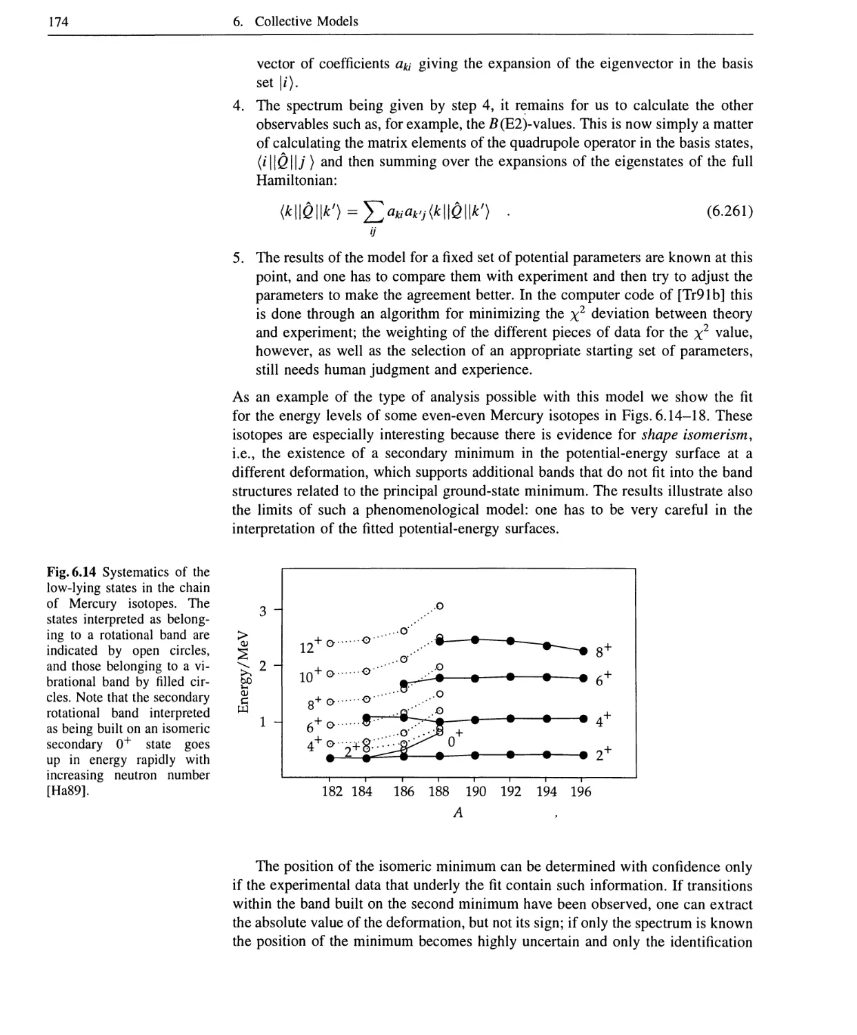


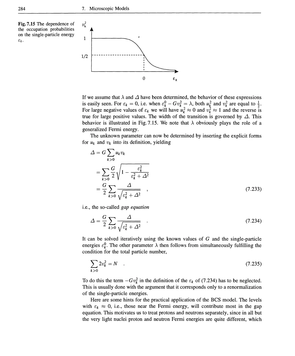


Текст
Greiner Maruhn
NUCLEAR
MODELS
W. Greiner • J. A.Maruhn
NUCLEAR MODELS
Springer
Berlin
Heidelberg
New York
Barcelona
Budapest
Hong Kong
London
Milan
Paris
Santa Clara
Singapore
Tokyo
Greiner
Quantum Mechanics
An Introduction 3rd Edition
Greiner
Quantum Mechanics
Special Chapters
Greiner • Miiller
Quantum Mechanics
Symmetries 2nd Edition
Greiner
Relativistic Quantum Mechanics
Wave Equations
Greiner • Reinhardt
Field Quantization
Greiner • Reinhardt
Quantum Electrodynamics
2nd Edition
Greiner • Schafer
Quantum Chromodynamics
Greiner • Maruhn
Nuclear Models
Greiner • Miiller
Gauge Theory of Weak Interactions
2nd Edition
Greiner
Mechanics I
(in preparation)
Greiner
Mechanics II
(in preparation)
Greiner
Electrodynamics
(in preparation)
Greiner • Neise • Stocker
Thermodynamics
and Statistical Mechanics
Walter Greiner • Joachim A. Maruhn
NUCLEAR MODELS
With a Foreword by
D. A. Bromley
With 50 Figures,
and 39 Worked Examples and Problems
Springer
Professor Dr. Walter Greiner
Professor Dr. Joachim A. Maruhn
Institut fur Theoretische Physik der
Johann Wolfgang Goethe-Universitat Frankfurt
Postfach 111932
D-60054 Frankfurt am Main
Germany
Street address:
Robert-Mayer-Strasse 8-10
D-60325 Frankfurt am Main
Germany
email:
greiner@th.physik.uni-frankfurt.de (W. Greiner)
maruhn@th.physik.uni-frankfurt.de (J. A. Maruhn)
Title of the original German edition: Theoretische Physik, Ein Lehr- und Ubungsbuch,
Band 11: Kernmodelle © Verlag Harri Deutsch, Thun 1995
Die Deutsche Bibliothek - CIP-Einheitsaufnahme
Greiner, Walter:
Nuclear models : with 39 worked examples and problems /Walter Greiner ; Joachim A. Maruhn. With a foreword by
D. A. Bromley. - Berlin ; Heidelberg ; New York ; Barcelona ; Budapest ; Hong Kong ; London ; Milan ; Paris ;
Santa Clara ; Singapore ; Tokyo : Springer, 1996
Einheitssacht.: Kernmodelle <engl.>
ISBN 3-540-59180-X
NE: Maruhn, Joachim:
ISBN 3-540-59180-X Springer-Verlag Berlin Heidelberg New York
This work is subject to copyright. All rights are reserved, whether the whole or part of the material is concerned,
specifically the rights of translation, reprinting, reuse of illustrations, recitation, broadcasting, reproduction on
microfilm or in any other way, and storage in databanks. Duplication of this publication or parts thereof is permitted
only under the provisions of the German Copyright Law of September 9,1965, in its current version, and permission
for use must always be obtained from Springer-Verlag. Violations are liable for prosecution under the German
Copyright Law.
© Springer-Verlag Berlin Heidelberg 1996
Printed in Germany
The use of general descriptive names, registered names, trademarks, etc. in this publication does not imply, even in
the absence of a specific statement, that such names are exempt from the relevant protective laws and regulations
and therefore free for general use.
Typesetting: Camera ready copy from the authors using a Springer T^X macro package
Cover design; Design Concept, Emil Smejkal, Heidelberg
Copy Editor: V Wicks
Production Editor: P. Treiber
SPIN 10469337 56/3144 - 5 4 3 2 1 0 - Printed on acid-free paper
Foreword to Earlier Series Editions
More than a generation of German-speaking students around the world have worked
their way to an understanding and appreciation of the power and beauty of modern
theoretical physics - with mathematics, the most fundamental of sciences - using
Walter Greiner's textbooks as their guide.
The idea of developing a coherent, complete presentation of an entire field
of science in a series of closely related textbooks is not a new one. Many older
physicists remember with real pleasure their sense of adventure and discovery
as they worked their ways through the classic series by Sommerfeld, by Planck
and by Landau and Lifshitz. From the students' viewpoint, there are a great many
obvious advantages to be gained through use of consistent notation, logical ordering
of topics and coherence of presentation; beyond this, the complete coverage of
the science provides a unique opportunity for the author to convey his personal
enthusiasm and love for his subject.
The present five-volume set, Theoretical Physics, is in fact only that part of
the complete set of textbooks developed by Greiner and his students that presents
the quantum theory. I have long urged him to make the remaining volumes on
classical mechanics and dynamics, on electromagnetism, on nuclear and particle
physics, and on special topics available to an English-speaking audience as well,
and we can hope for these companion volumes covering all of theoretical physics
some time in the future.
What makes Greiner's volumes of particular value to the student and professor
alike is their completeness. Greiner avoids the all too common "it follows that..."
which conceals several pages of mathematical manipulation and confounds the
student. He does not hesitate to include experimental data to illuminate or illustrate
a theoretical point and these data, like the theoretical content, have been kept up to
date and topical through frequent revision and expansion of the lecture notes upon
which these volumes are based.
Moreover, Greiner greatly increases the value of his presentation by including
something like one hundred completely worked examples in each volume. Nothing
is of greater importance to the student than seeing, in detail, how the theoretical
concepts and tools under study are applied to actual problems of interest to a
working physicist. And, finally, Greiner adds brief biographical sketches to each
chapter covering the people responsible for the development of the theoretical ideas
and/or the experimental data presented. It was Auguste Comte A798-1857) in his
Positive Philosophy who noted, "To understand a science it is necessary to know
its history". This is all too often forgotten in modern physics teaching and the
VI Foreword to Earlier Series Editions
bridges that Greiner builds to the pioneering figures of our science upon whose
work we build are welcome ones.
Greiner's lectures, which underlie these volumes, are internationally noted for
their clarity, their completeness and for the effort that he has devoted to making
physics an integral whole; his enthusiasm for his science is contagious and shines
through almost every page.
These volumes represent only a part of a unique and Herculean effort to make
all of theoretical physics accessible to the interested student. Beyond that, they
are of enormous value to the professional physicist and to all others working with
quantum phenomena. Again and again the reader will find that, after dipping into a
particular volume to review a specific topic, he will end up browsing, caught up by
often fascinating new insights and developments with which he had not previously
been familiar.
Having used a number of Greiner's volumes in their original German in my
teaching and research at Yale, I welcome these new and revised English translations
and would recommend them enthusiastically to anyone searching for a coherent
overview of physics.
Yale University D. Allan Bromley
New Haven, CT, USA Henry Ford II Professor of Physics
1989
Preface
Theoretical physics has become a many-faceted science. For the young student it is
difficult enough to cope with the overwhelming amount of new scientific material
that has to be learned, let alone to obtain an overview of the entire field, which
ranges from mechanics through electrodynamics, quantum mechanics, field theory,
nuclear and heavy-ion science, statistical mechanics, thermodynamics, and solid-
state theory to elementary-particle physics. And this knowledge should be acquired
in just 8-10 semesters during which, in addition, a Diploma or Master's thesis has
to be worked on or examinations prepared for. All this can be achieved only if the
university teachers help to introduce the student to the new disciplines as early on
as possible, in order to create interest and excitement that in turn set free essential
new energy. Naturally, all inessential material must simply be eliminated.
At the Johann Wolfgang Goethe University in Frankfurt we therefore confront
the student with theoretical physics immediately in the first semester. Theoretical
Mechanics I and II, Electrodynamics, and Quantum Mechanics I - an Introduction
are the basic courses during the first two years. These lectures are supplemented
with many mathematical explanations and much support material. After the fourth
semester of studies, graduate work begins and Quantum Mechanics II - Symme-
Symmetries, Statistical Mechanics and Thermodynamics, Relativistic Quantum Mechanics,
Quantum Electrodynamics, the Gauge Theory of Weak Interactions, and Quantum
Chromodynamics are obligatory. Apart from these, a number of supplementary
courses on special topics are offered, such as Hydrodynamics, Classical Field The-
Theory, Special and General Relativity, Many-Body Theories, Nuclear Models, Models
of Elementary Particles, and Solid-State Theory. Some of them, for example the
two-semester courses on Theoretical Nuclear Physics and Theoretical Solid-State
Physics, are obligatory.
This volume is devoted to the Theory of Nuclear Models, which forms a two-
semester cycle together with a course on Nuclear Reactions. For this field it ap-
appeared to be especially important to present a relatively short textbook actually
suitable for accompanying a lecture, since while there are excellent and compre-
comprehensive treatises on nuclear models, the wealth of material presented in those tends
to overwhelm the students initially. In this connection we mention preferentially
the three-volume work by Eisenberg and Greiner,1 on which the present treatment
1 J. M. Eisenberg and W. Greiner, Nuclear Theory, 3 Volumes, Third Edition (North Holland,
Amsterdam 1973-1987).
VIII Preface
is based in many respects, and the textbook by Ring and Schuck,2 which puts more
emphasis on many-body approaches.
A textbook for direct use with a lecture has to concentrate on the most essential
points, emphasize the explanation of ideas and methods, and forego the presentation
of a wealth of individual results, which cannot be shown in a lecture anyway if it
is not to degenerate into a slide show. Another characteristic that makes the theory
of nuclear models different from the classical fields of theoretical physics is the
scarcity of examples that can be calculated from start to finish without the use of
computers.
For all of these reasons the focus is on the discussion of the most important types
of models and the requisite mathematical methods. Since experience shows that
most students have not really mastered the crucial methods of angular-momentum
coupling and second quantization, we have not relegated these topics to an appendix
but treated them at the start of the book. Of course these chapters can be ignored
if desired. Even in these chapters the material was carefully restricted to what is
actually used in the rest of the book. Following this there is a short discussion of
group-theoretical methods, which are essential, for example, for the IBA model.
The fifth chapter treats the theory of the radiation field up to the definition of
multipole transition probabilities. Again with a view to brevity the magnetic transi-
transitions are only dicussed in general terms. The sixth chapter presents the classical col-
collective models, which because of their didactic value and their fundamental impor-
importance for introducing concepts form the centerpiece of the book. A short overview
of the phenomenological properties of nuclear matter is followed by a treatment of
the geometric collective model (surface vibrations, the rotation-vibration model,
etc.) in the various limiting cases, the IBA model, and the collective theory of giant
resonances.
Only a little less space is devoted to microscopic models in Chapter 7. The
most important concepts, from Hartree-Fock theory via phenomenological single-
particle models to the relativistic mean-field model, are introduced successively.
The next chapter treats the coupling of single-particle and collective motion both
with respect to the particle-plus-core model and to the microscopic description of
collective vibrations.
The final chapter presents large-amplitude collective motion, concentrating
on ways to describe nuclear fission and similar processes. This includes two-
center models, the general problem of collective mass parameters, time-dependent
Hartree-Fock, the generator-coordinate method, and an elementary overview of
high-spin states.
In addition to the classical syllabus of nuclear models that still form the basic
equipment of the nuclear theorist, short discussions of topics of present-day interest
are interspersed in many places - such as superheavy elements, high-spin states, and
the relativistic mean-field model. These should give young physicists an impression
of the continuing vitality of this science. The reader will also note in various places
that the book is based on repeated practical experience with such a course and offers
many explanations and illustrations motivated by typical student questions.
2 P. Ring and P. Schuck, The Nuclear Many-Body Problem (Springer-Verlag, New York
1980).
Preface IX
We express our sincere thanks to Dr. Dirk Troltenier, Michael Bender, Christian
Spieles, and Klemens Rutz for their efficient help in the formulation, formatting,
and editing of the text as well as to Ms. Astrid Steidl for support in producing
some of the graphics.
Finally we wish to thank Springer-Verag; in particular Dr. H. J. Kolsch for his
encouragement and patience, and Petra Treiber for the production and Dr. Victoria
Wicks for expertly copy-editing the English edition.
Frankfurt am Main, Walter Greiner
November 1995 Joachim Maruhn
Contents
1. Introduction 1
1.1 Nuclear Structure Physics 1
1.2 The Basic Equation 2
1.3 Microscopic versus Collective Models 3
1.4 The Role of Symmetries 5
2. Symmetries 7
2.1 General Remarks 7
2.2 Translation 8
2.2.1 The Operator for Translation 8
2.2.2 Translational Invariance 9
2.2.3 Many-Particle Systems 10
2.3 Rotation 11
2.3.1 The Angular Momentum Operators 11
2.3.2 Representations of the Rotation Group 16
2.3.3 The Rotation Matrices 20
2.3.4 SUB) and Spin 21
2.3.5 Coupling of Angular Momenta 25
2.3.6 Intrinsic Angular Momentum 27
2.3.7 Tensor Operators 30
2.3.8 The Wigner-Eckart Theorem 35
2.3.9 6/ and 9/ Symbols 37
2.4 Isospin 39
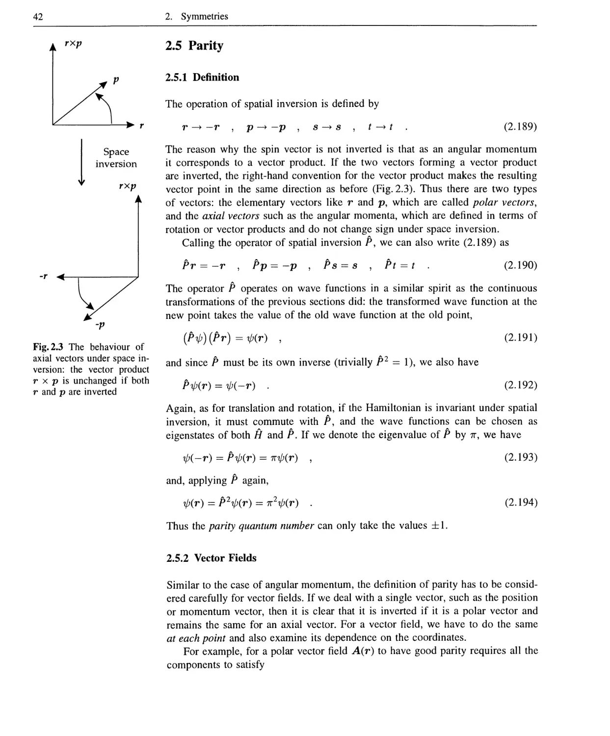
2.5 Parity 42
2.5.1 Definition 42
2.5.2 Vector Fields 42
2.6 Time Reversal 43
3. Second Quantization 47
3.1 General Formalism 47
3.1.1 Motivation 47
3.1.2 Second Quantization for Bosons 50
3.1.3 Second Quantization for Fermions 52
3.2 Representation of Operators 53
3.2.1 One-Particle Operators 53
3.2.2 Two-Particle Operators 56
3.3 Evaluation of Matrix Elements for Fermions 58
3.4 The Particle-Hole Picture 60
XII Contents
4. Group Theory in Nuclear Physics 65
4.1 Lie Groups and Lie Algebras 65
4.2 Group Chains 72
4.3 Lie Algebras in Second Quantization 73
5. Electromagnetic Moments and Transitions 75
5.1 Introduction 75
5.2 The Quantized Electromagnetic Field 75
5.3 Radiation Fields of Good Angular Momentum 77
5.3.1 Solutions of the Scalar Helmholtz Equation 77
5.3.2 Solutions of the Vector Helmholtz Equation 78
5.3.3 Properties of the Multipole Fields 81
5.3.4 Multipole Expansion of Plane Waves 82
5.4 Coupling of Radiation and Matter 85
5.4.1 Basic Matrix Elements 85
5.4.2 Multipole Expansion of the Matrix Elements
and Selection Rules 88
5.4.3 Siegert's Theorem 90
5.4.4 Matrix Elements for Emission
in the Long-Wavelength Limit 91
5.4.5 Relative Importance of Transitions
and Weisskopf Estimates 95
5.4.6 Electric Multipole Moments 97
5.4.7 Effective Charges 97
6. Collective Models 99
6.1 Nuclear Matter 99
6.1.1 Mass Formulas 99
6.1.2 The Fermi-Gas Model 101
6.1.3 Density-Functional Models 103
6.2 Nuclear Surface Deformations 106
6.2.1 General Parametrization 106
6.2.2 Types of Multipole Deformations 108
6.2.3 Quadrupole Deformations 110
6.2.4 Symmetries in Collective Space 115
6.3 Surface Vibrations 117
6.3.1 Vibrations of a Classical Liquid Drop 117
6.3.2 The Harmonic Quadrupole Oscillator 124
6.3.3 The Collective Angular-Momentum Operator 128
6.3.4 The Collective Quadrupole Operator 130
6.3.5 The Quadrupole Vibrational Spectrum 132
6.4 Rotating Nuclei 138
6.4.1 The Rigid Rotor 138
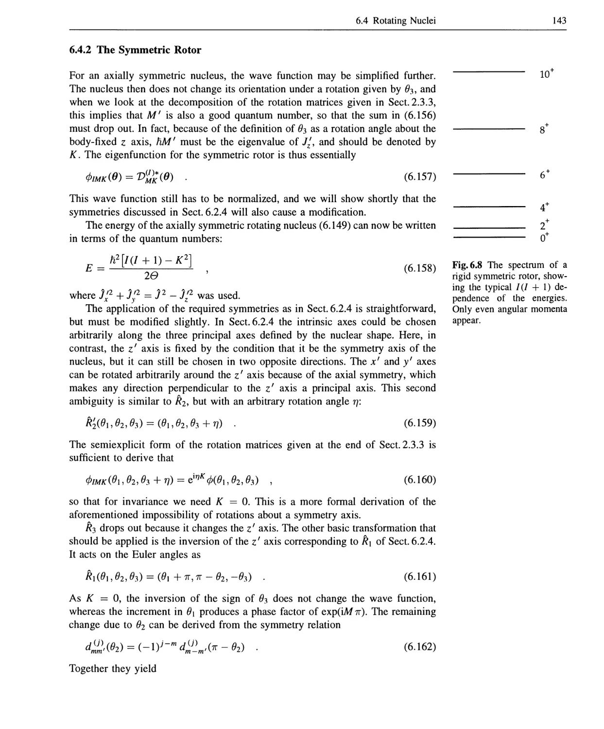
6.4.2 The Symmetric Rotor 143
6.4.3 The Asymmetric Rotor 145
Contents XIII
6.5 The Rotation-Vibration Model 147
6.5.1 Classical Energy 147
6.5.2 Quantal Hamiltonian 151
6.5.3 Spectrum and Eigenfunctions 155
6.5.4 Moments and Transition Probabilities 159
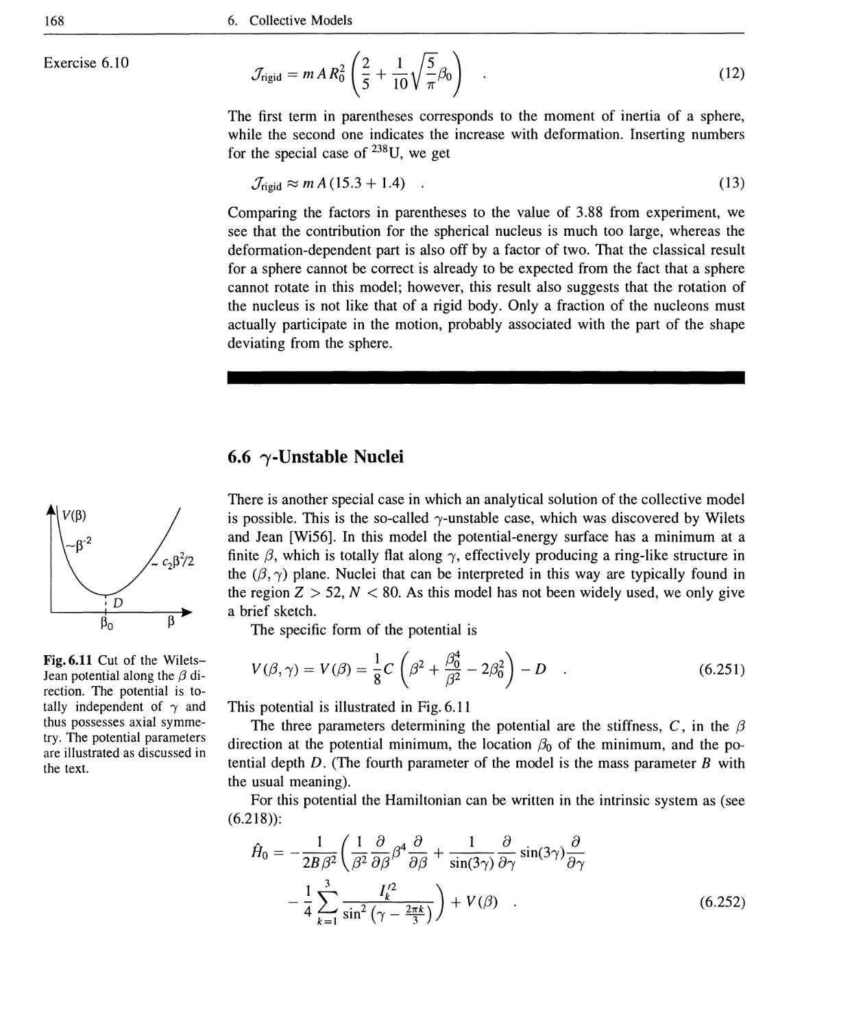
6.6 7-Unstable Nuclei 168
6.7 More General Collective Models for Surface Vibrations 170
6.7.1 The Generalized Collective Model 170
6.7.2 Proton-Neutron Vibrations 177
6.7.3 Higher Multipoles 177
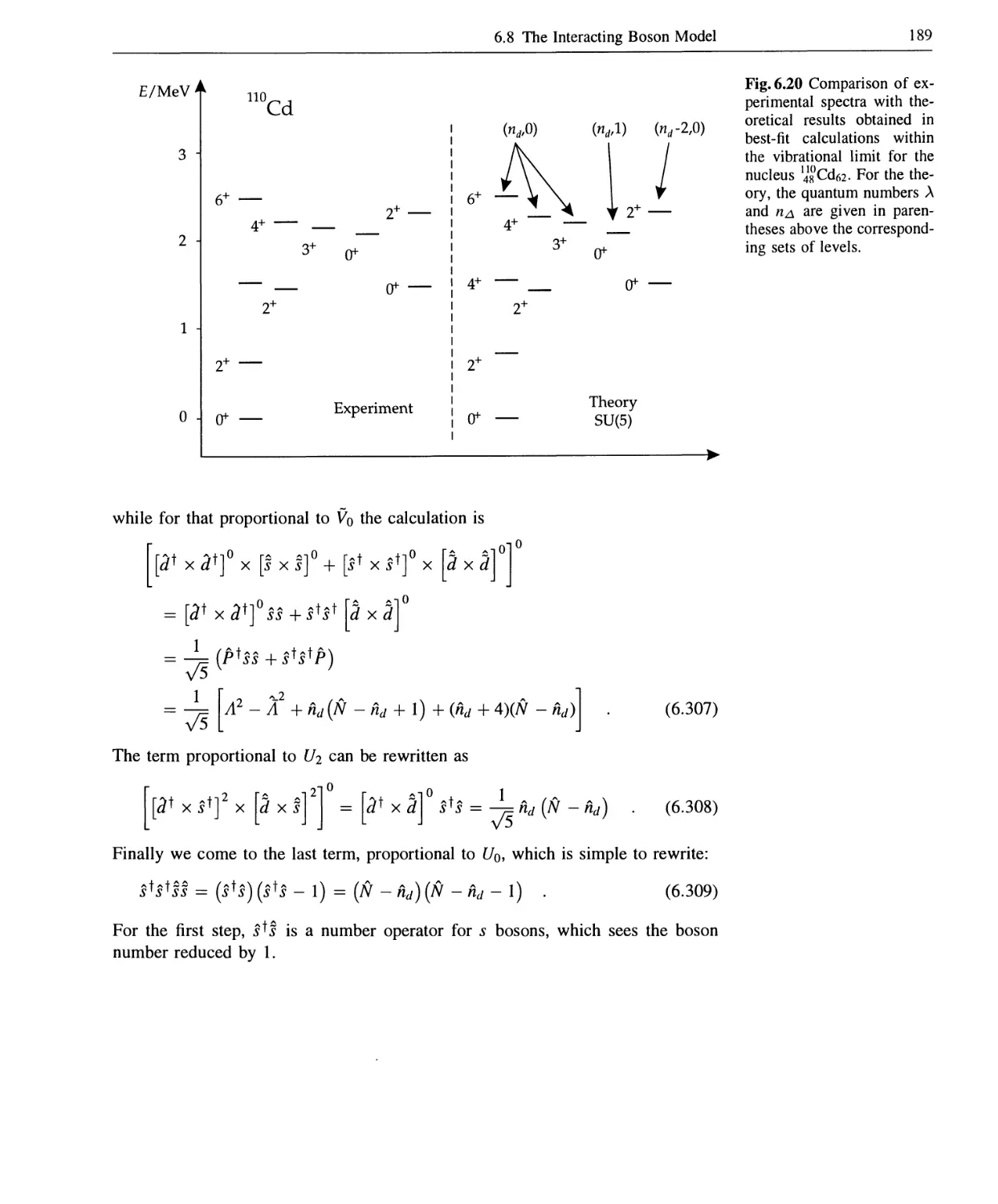
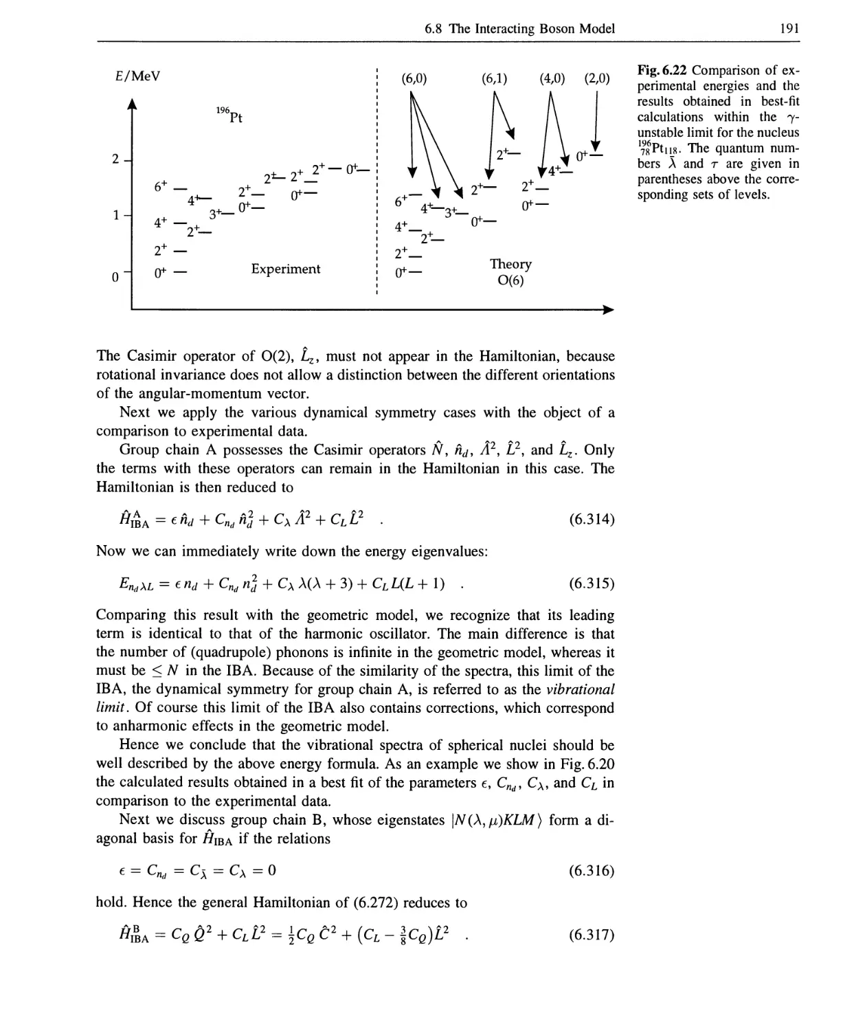
6.8 The Interacting Boson Model 178
6.8.1 Introduction 178
6.8.2 The Hamiltonian 180
6.8.3 Group Chains 182
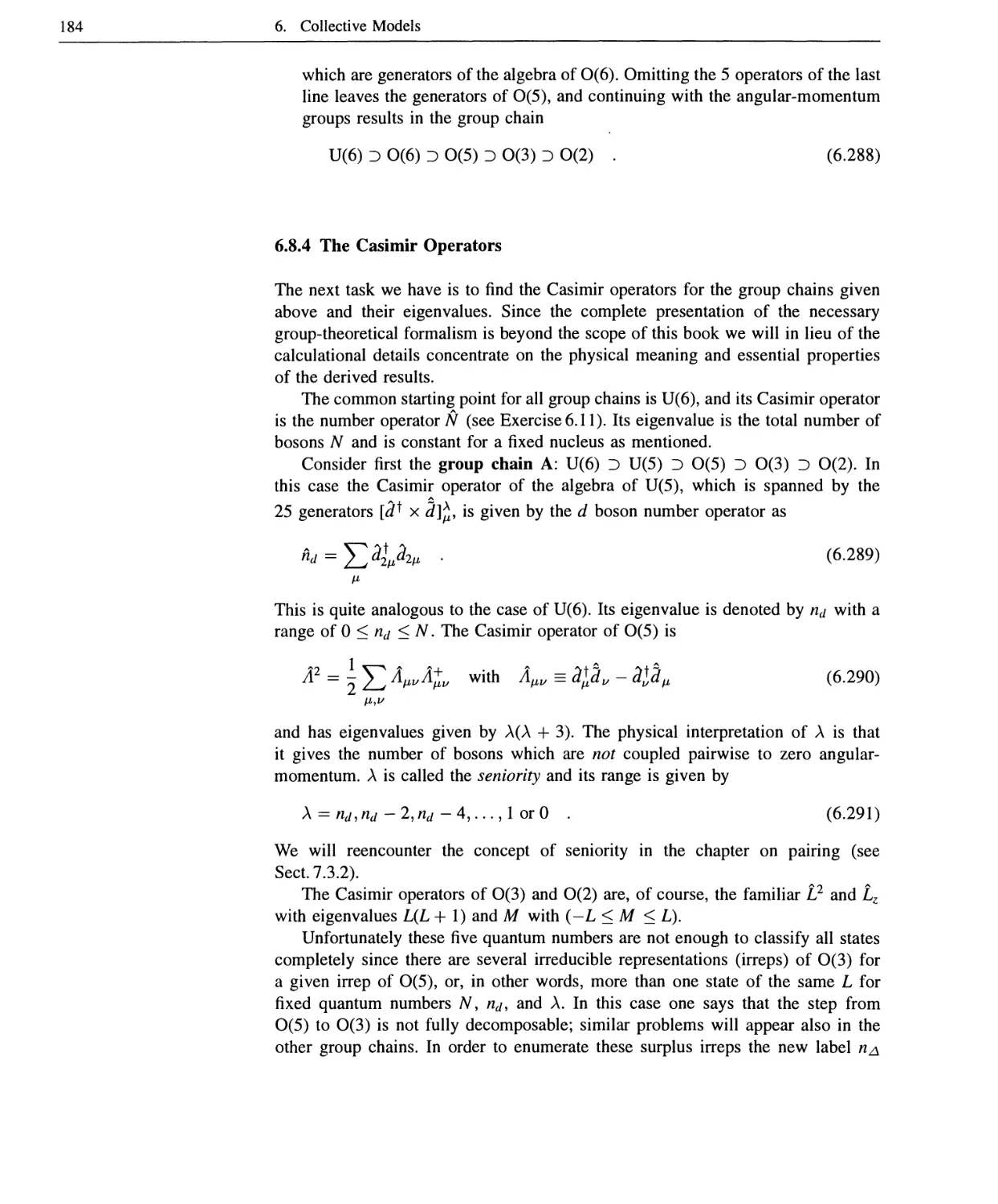
6.8.4 The Casimir Operators 184
6.8.5 The Dynamical Symmetries 187
6.8.6 Transition Operators 192
6.8.7 Extended Versions of the IBA 193
6.8.8 Comparison to the Geometric Model 196
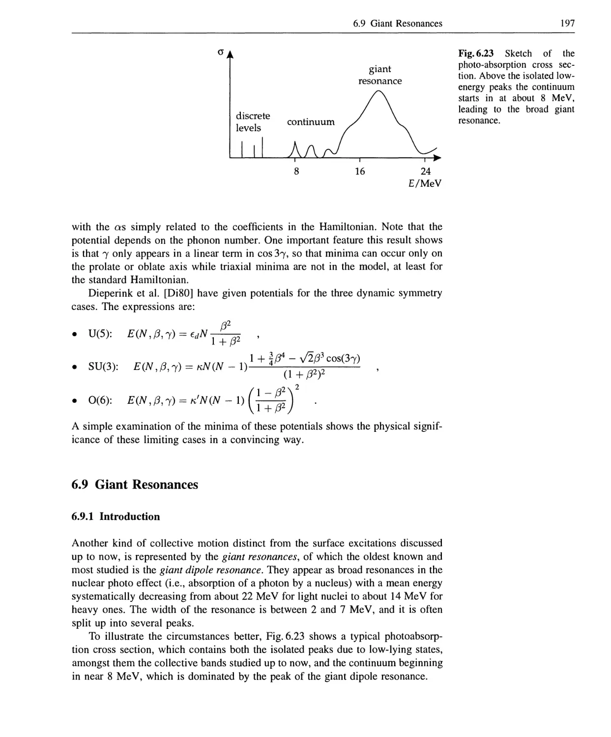
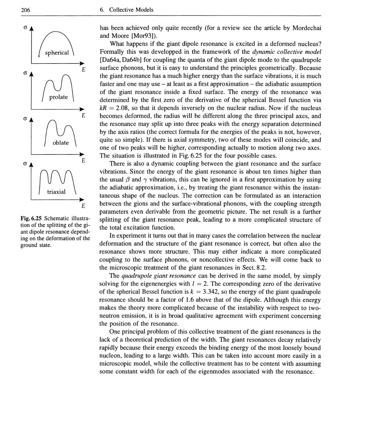
6.9 Giant Resonances 197
6.9.1 Introduction 197
6.9.2 The Goldhaber-Teller Model 200
6.9.3 The Steinwedel-Jensen Model 202
6.9.4 Applications 205
7. Microscopic Models 207
7.1 The Nucleon-Nucleon Interaction 207
7.1.1 General Properties 207
7.1.2 Functional Form 210
7.1.3 Interactions from Nucleon-Nucleon Scattering 211
7.1.4 Effective Interactions 214
7.2 The Hartree-Fock Approximation 217
7.2.1 Introduction 217
7.2.2 The Variational Principle 218
7.2.3 The Slater-Determinant Approximation 219
7.2.4 The Hartree-Fock Equations 220
7.2.5 Applications 225
7.2.6 The Density Matrix Formulation 227
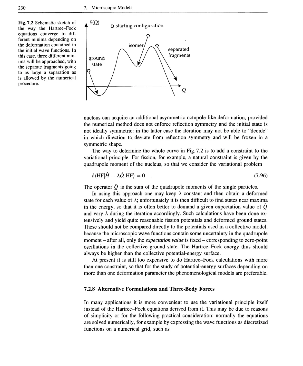
7.2.7 Constrained Hartree-Fock 229
7.2.8 Alternative Formulations and Three-Body Forces 230
7.2.9 Hartree-Fock with Skyrme Forces 231
7.3 Phenomenological Single-Particle Models 237
7.3.1 The Spherical-Shell Model 237
7.3.2 The Deformed-Shell Model 248
7.4 The Relativistic Mean-Field Model 261
7.4.1 Introduction 261
7.4.2 Formulation of the Model 261
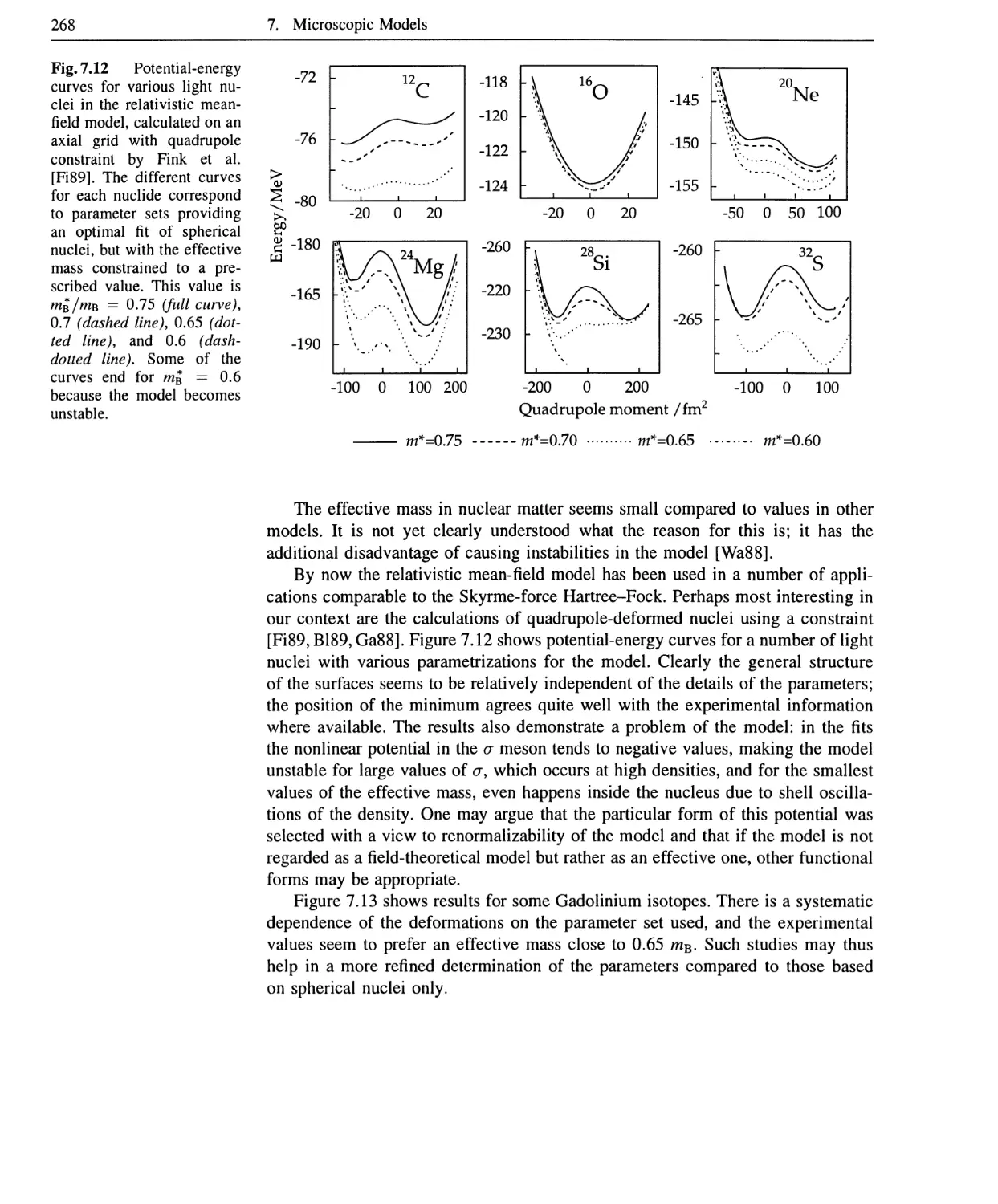
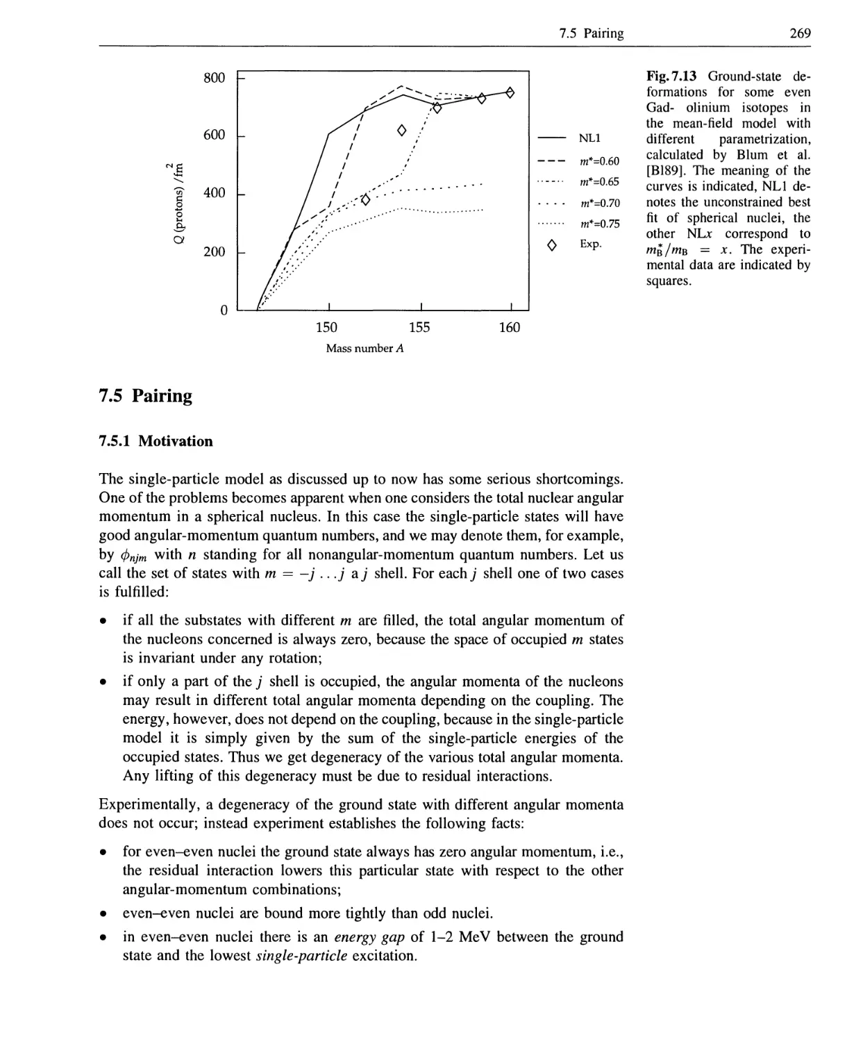
7.4.3 Applications 266
XIV Contents
7.5 Pairing 269
7.5.1 Motivation 269
7.5.2 The Seniority Model 272
7.5.3 The Quasispin Model 278
7.5.4 The BCS Model 280
7.5.5 The Bogolyubov Transformation 285
7.5.6 Generalized Density Matrices 290
8. Interplay of Collective and Single-Particle Motion 293
8.1 The Core-plus-Particle Models 293
8.1.1 Basic Considerations 293
8.1.2 The Weak-Coupling Limit 294
8.1.3 The Strong-Coupling Approximation 296
8.1.4 The Interacting Boson-Fermion Model 302
8.2 Collective Vibrations in Microscopic Models 303
8.2.1 The Tamm-Dancoff Approximation 303
8.2.2 The Random-Phase Approximation (RPA) 309
8.2.3 Time-Dependent Hartree-Fock and Linear Response 312
9. Large-Amplitude Collective Motion 317
9.1 Introduction 317
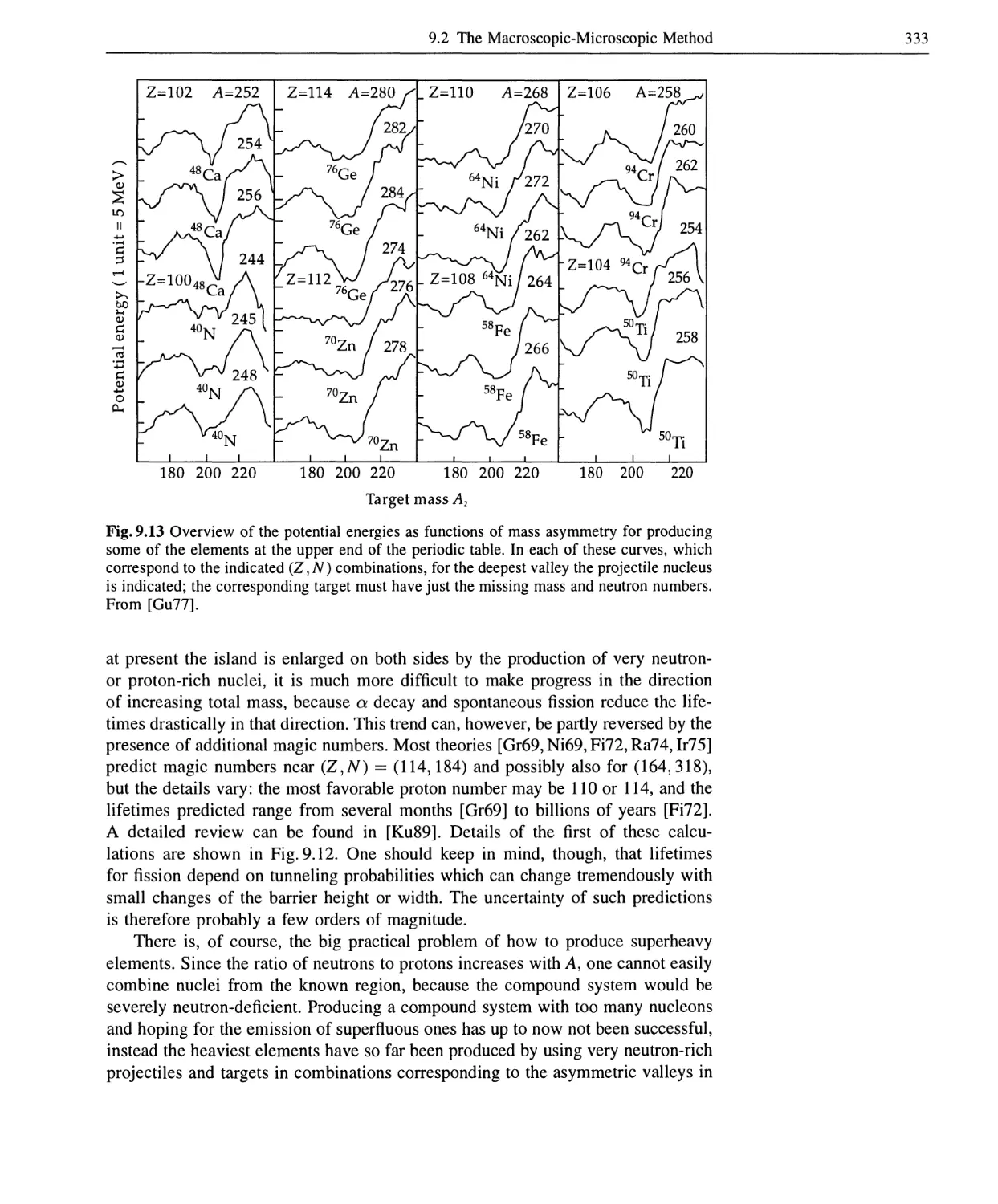
9.2 The Macroscopic-Microscopic Method 318
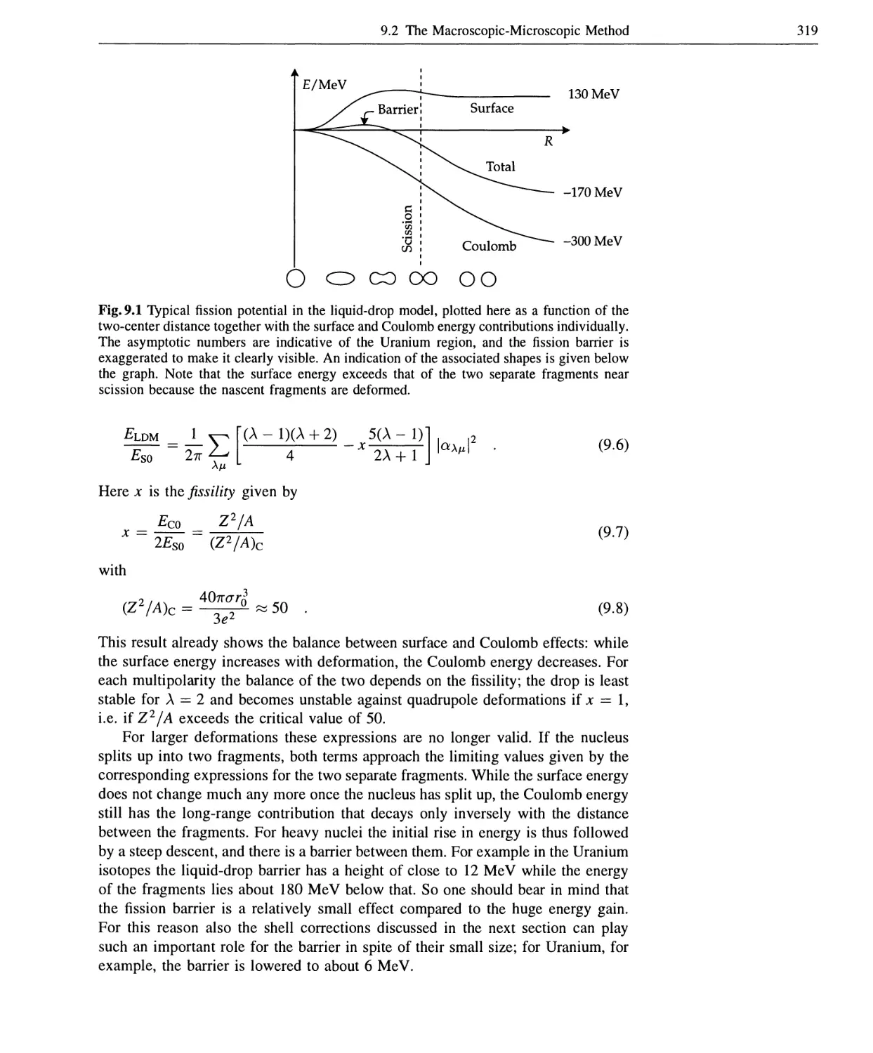
9.2.1 The Liquid-Drop Model 318
9.2.2 The Shell-Correction Method 320
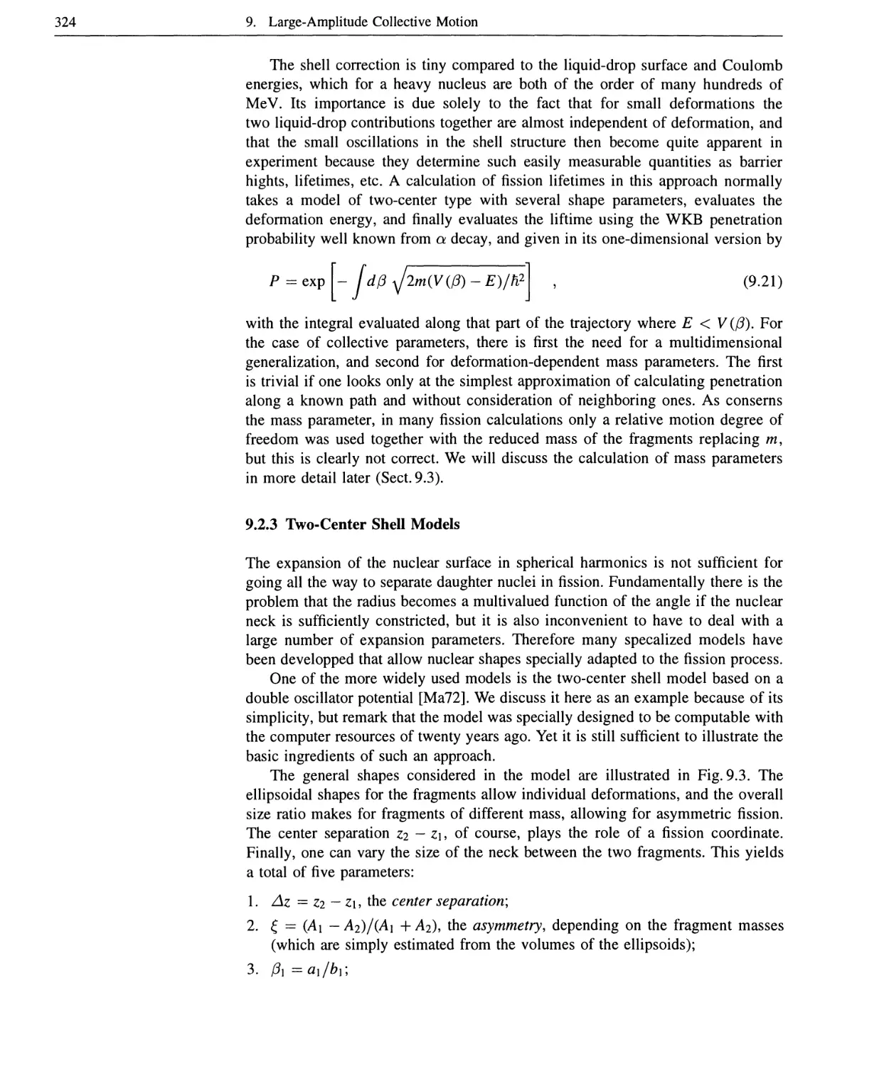
9.2.3 Two-Center Shell Models 324
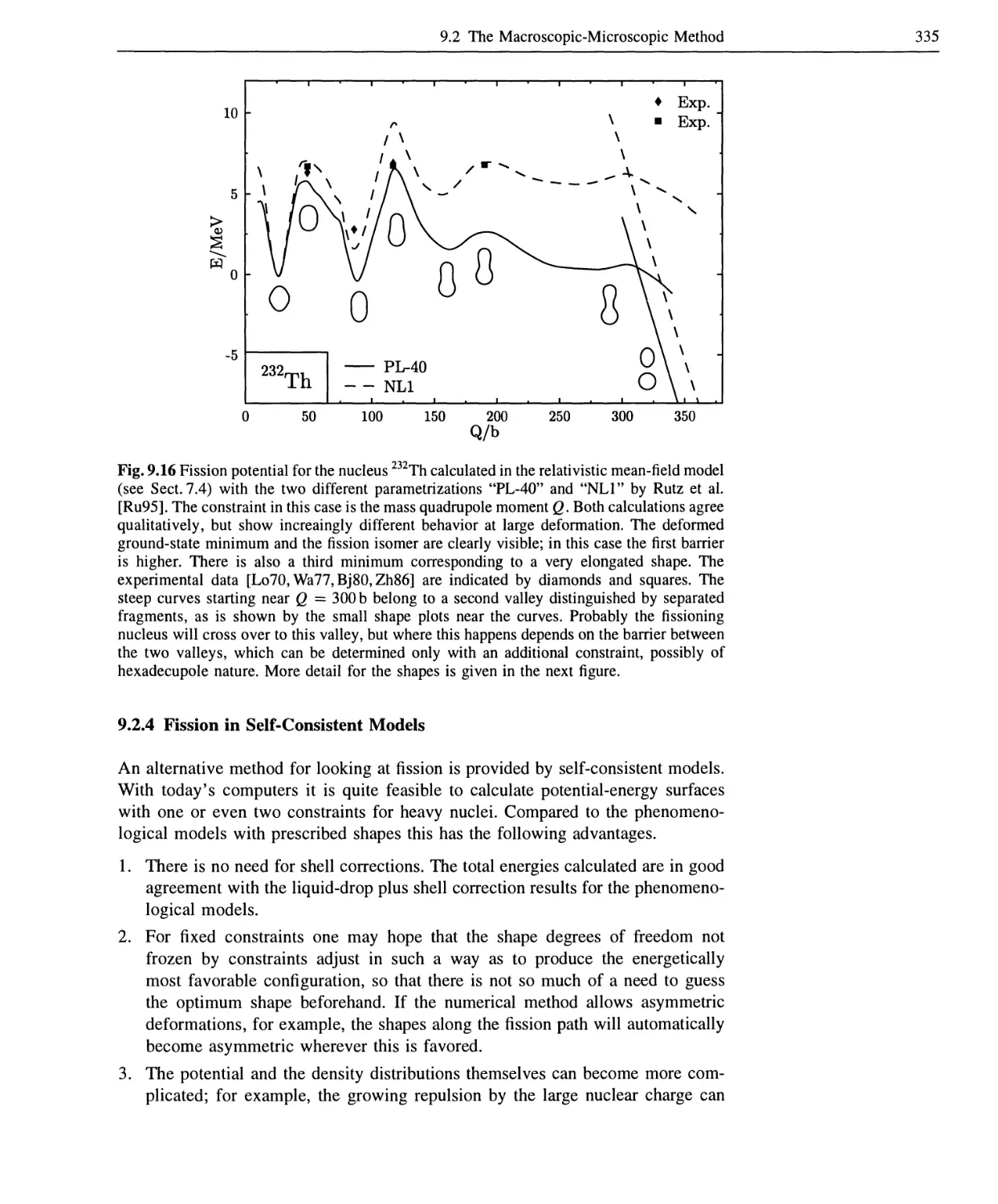
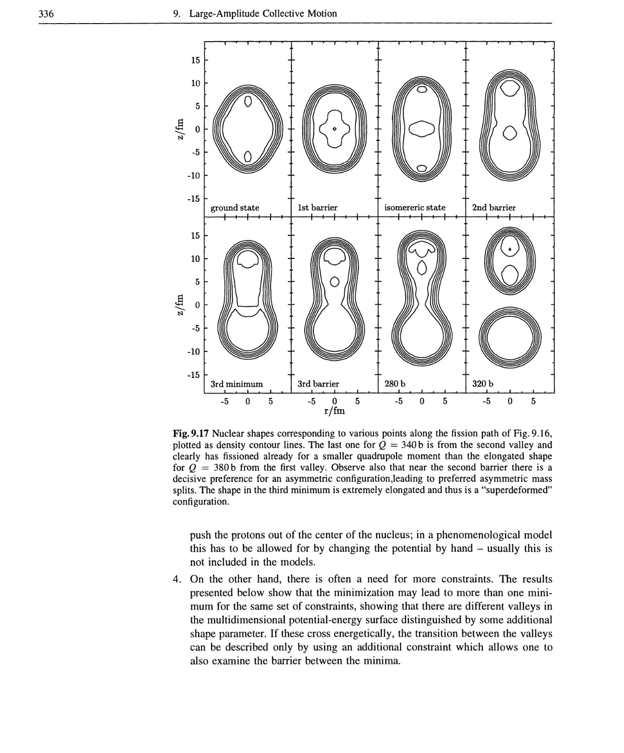
9.2.4 Fission in Self-Consistent Models 335
9.3 Mass Parameters and the Cranking Model 337
9.3.1 Overview 337
9.3.2 The Irrotational-Flow Model 337
9.3.3 The Cranking Formula 338
9.3.4 Applications of the Cranking Formula 340
9.4 Time-Dependent Hartree-Fock 344
9.5 The Generator-Coordinate Method 346
9.6 High-Spin States 353
9.6.1 Overview 353
9.6.2 The Cranked Nilsson Model 355
Appendix: Some Formulas from Angular-Momentum Theory 359
References 363
Subject Index 369
Contents of Examples and Exercises
2.1 Cartesian Form of the Angular-Momentum Operator Jz 12
2.2 Cayley-Klein Representation of the Rotation Matrix 24
2.3 Coupling of Two Vectors to Good Angular Momentum 31
2.4 The Position Operator as an Irreducible Spherical Tensor 33
2.5 Commutation Relations of the Position Operator 34
2.6 The Two-Nucleon System 41
2.7 The Time-Reversal Operator for Spinors with Spin \ 46
3.1 Two-Body Operators in Second Quantization 57
4.1 The Lie Algebra of Angular-Momentum Operators 68
4.2 The Casimir Operator of the Angular-Momentum Algebra 69
4.3 The Lie Algebra of SO(n) 70
5.1 The Vector Spherical Harmonics 79
5.2 The Weisskopf Estimates for Electric Transitions 96
6.1 Volume and Center-of-Mass Vector for a Deformed Nucleus .... 109
6.2 Quadrupole Deformations 113
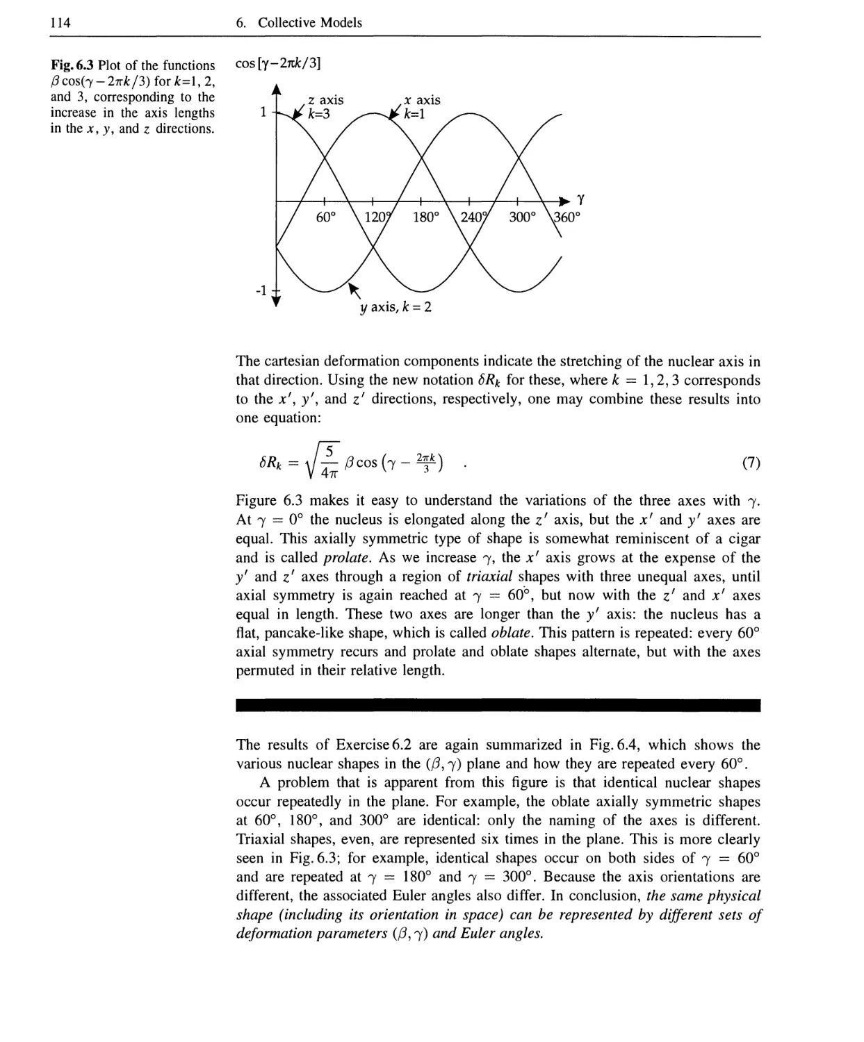
6.3 Angular-Momentum Operator for Quadrupole Phonons
in Second Quantization 129
6.4 114Cd as a Spherical Vibrator 136
6.5 Angular-Momentum Operators in the Intrinsic System 139
6.6 States with Angular Momentum 2
in the Asymmetric Rotor Model 146
6.7 The Time Derivatives of the a2fl 150
6.8 Transformation of the Quadrupole Operator 162
6.9 Quadrupole Moments and Transition Probabilities 162
6.10 238U in the Rotation-Vibration Model 166
6.11 Casimir Operators of U(N) 187
6.12 Contributions to the Thomas-Reiche-Kuhn Sum Rule 199
7.1 The Angular Average of the Tensor Force 210
7.2 Matrix Elements in the Variational Equation 224
7.3 The Skyrme Energy Functional 234
7.4 The Eigenfunctions of the Harmonic Oscillator 240
7.5 The Quadrupole Moment of a Nucleus 246
7.6 Single-Particle Energies in the Deformed Oscillator 254
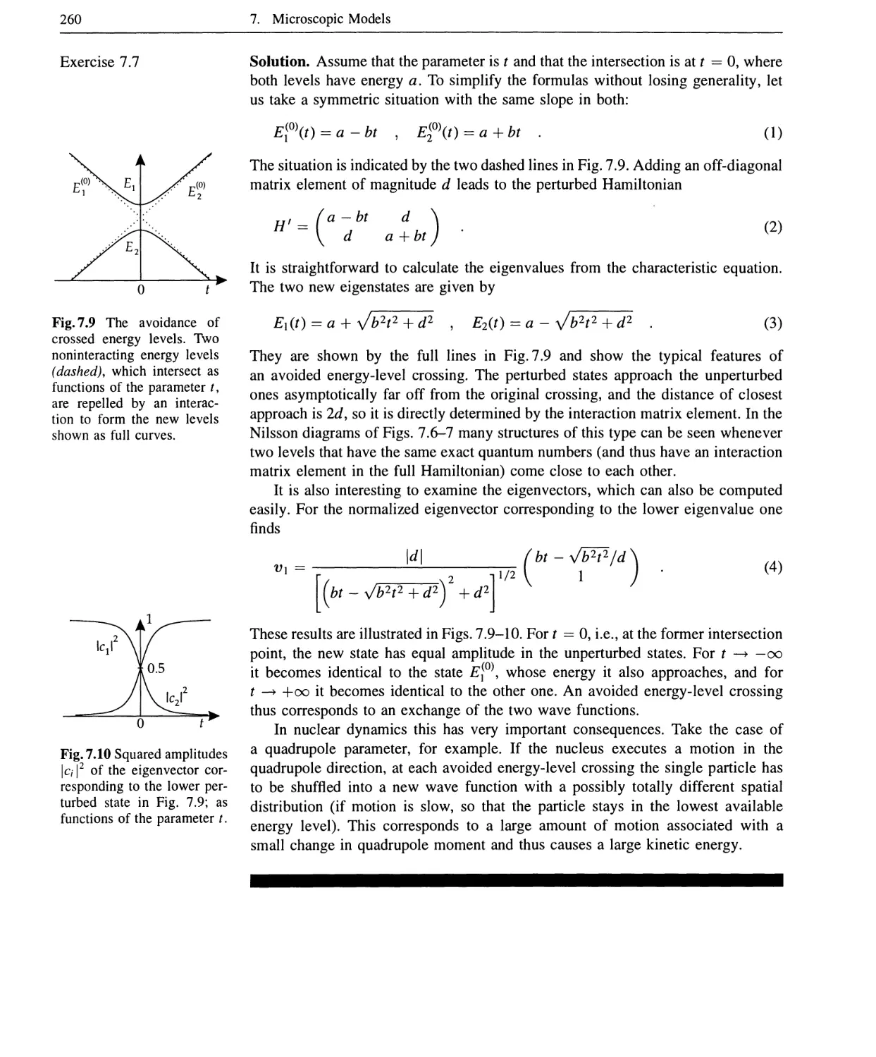
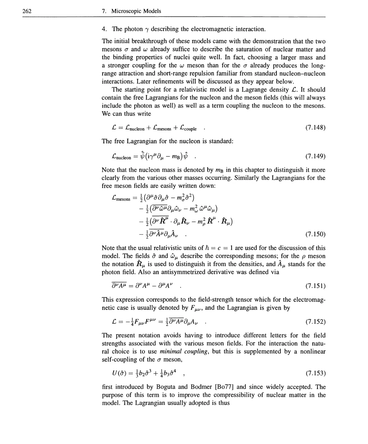
7.7 The Crossing of Energy Levels 259
7.8 Pairing in a j = \ Shell 278
XVI Contents of Examples and Exercises
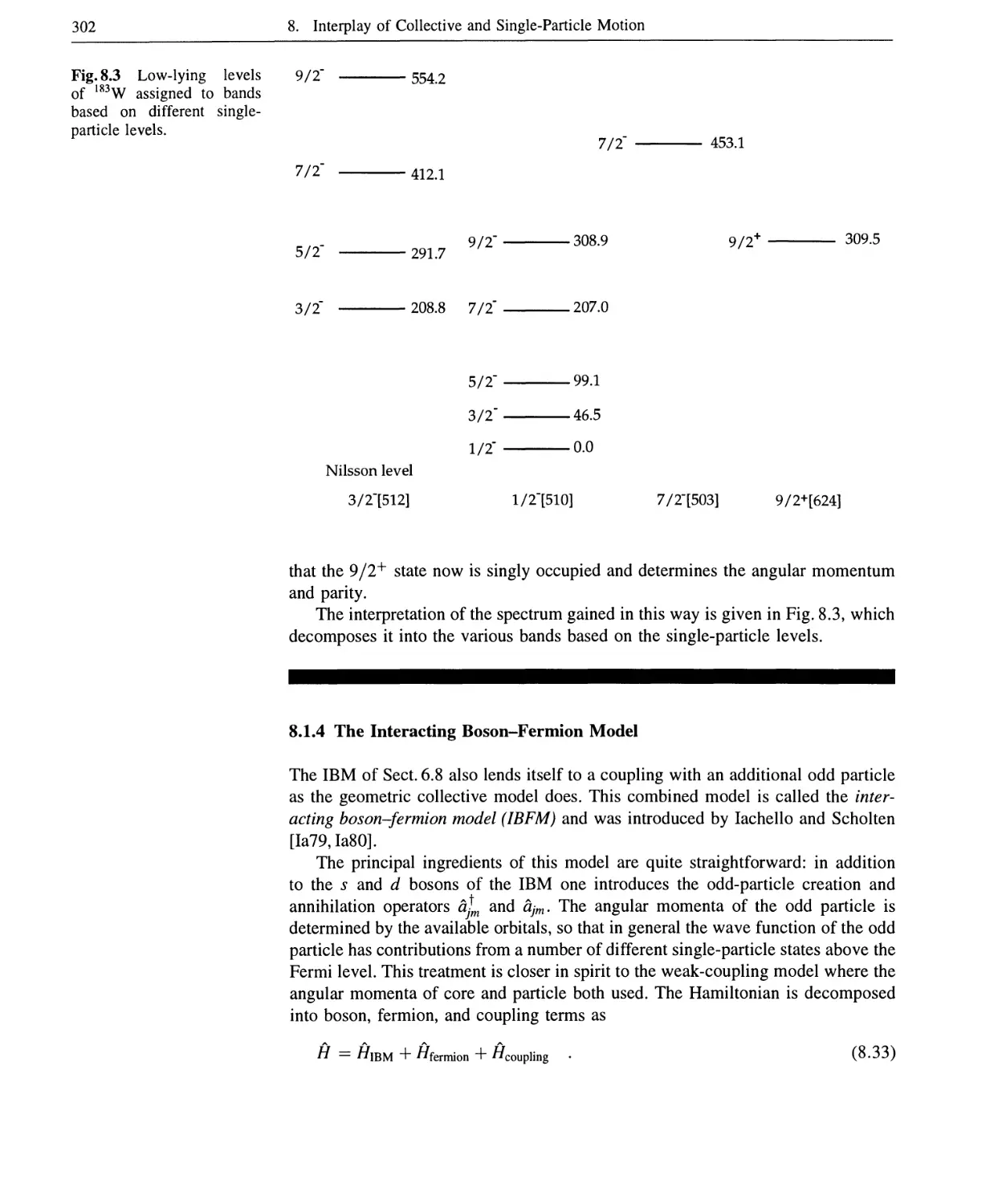
8.1 The Spectrum of 183W in the Strong-Coupling Model 301
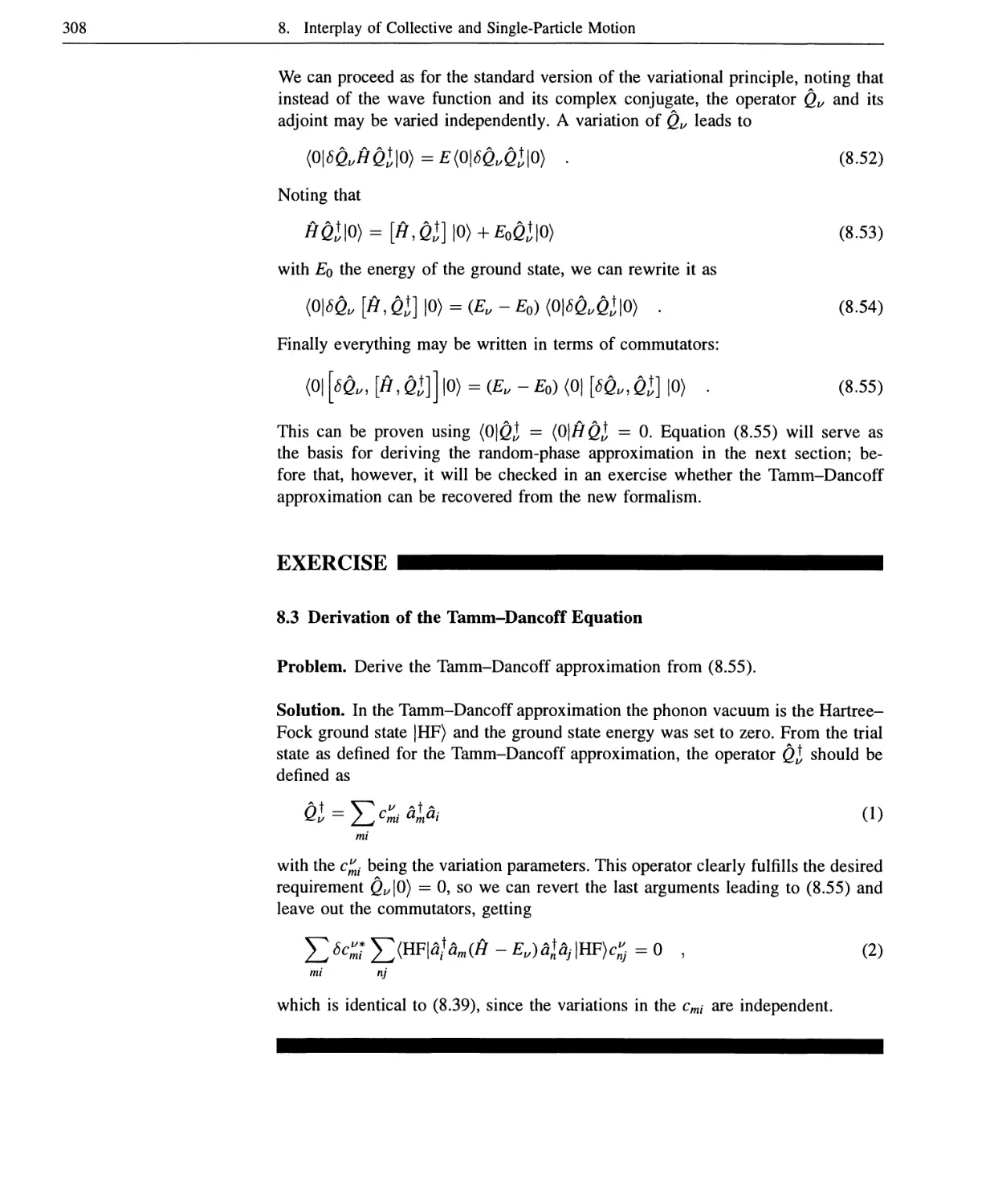
8.2 Tamm-Dancoff Calculation for 16O 306
8.3 Derivation of the Tamm-Dancoff Equation 308
8.4 The Extended Schematic Model 311
9.1 The Cranking Formula for the BCS Model 341
9.2 The Harmonic Oscillator in the Generator-Coordinate Method . .. 348
1. Introduction
1.1 Nuclear Structure Physics
The nuclear models discussed in this book belong to the realm of nuclear structure
theory. In present usage, nuclear structure physics is devoted to the study of the
properties of nuclei at low excitation energies, where individual energy levels can
be resolved. This means that typically quantum effects are predominant and the
states of the nucleus have a very complicated structure that depends on the intricate
interrelations of all the many nucleons involved.
In contrast, at higher energies and especially for heavy-ion reactions, quantum
mechanics becomes less important and the preeminent place is instead given to
methods of statistical mechanics. Theories then typically employ bulk properties
of nuclear matter such as the equation of state or the dissipation coefficients, or
are even based on purely classical many-body physics like the cascade models.
Of course it is impossible to give an exact energy boundary between these
types of theories. The theories presented here, however, are typically employed for
excitation energies up to 2-3 MeV. Usually only the lowest few energy levels can
be described well by a theoretical model, and the number of levels increases so
rapidly above that energy range that it becomes impossible to make any sensible
comparison with experiment (for nuclei with an odd number of neutrons or protons
or both this is even more dramatic - most nuclear models prefer even-even nuclei
with their relatively simple spectra). Also one should remember that in experimental
spectra only a relatively small number of states can be identified as to spin and
parity, and that to really test a model transitions, i.e., essentially overlaps between
the wave functions, are needed, which again are often not known even for the most
interesting states.
It is thus not surprising that the models presented in this book usually explain a
relatively small number of low-lying states and to a modest accuracy, and even this
is a considerable achievement. To esteem that, remember that we are dealing with
a system of particles whose number is neither small enough to allow direct solution
nor large enough to make statistical methods highly accurate, and which interact
through an interaction that has still not been pinned down to any definite form.
It is this extraordinary difficulty and the freedom with which methods and ideas
from many other branches are applied here that make nuclear structure physics so
fascinating and so much alive.
1. Introduction
1.2 The Basic Equation
To find the proper theoretical starting point some more ballpark estimates of the
relevent physical quantitities have to be introduced. Let us first recall a few numbers
from elementary experimental nuclear physics.
The elements known at the time of this writing have nuclei consisting of (at
present) Z = 1,..., 111 protons and N = 0,..., 161 neutrons, giving a total
number of A nucleons. The radii of nuclei follow the empirical law
R(A) = r0Al/3 A.1)
with r0 w 1.2fm. Nuclear radii thus range up to about 7.5 fm. The formula also
implies that the nuclear volume is proportional to the number of particles in the
nucleus, indicating the near incompressibility of nuclear matter (the true density
profile observed by electron scattering is a bit more complicated). The least-bound
nucleon has a binding energy of the order of 8 MeV and a kinetic energy close to
40 MeV.
This information is already sufficient to form some rough ideas about what is
essential in the theories. Since a nucleon has a mass of me2 « 938 MeV, the kinetic
energy is quite negligible by comparison, so that a nonrelativistic approach appears
quite sufficient, and this assumption is made in the vast majority of nuclear structure
models. More recently, however, relativistic approaches have become important -
this theme is taken up in Sect. 7.4 in connection with the relativistic mean-field
model, and we also explain there why relativistic effects can be important in spite
of the simple estimate given above.
The velocity of a nucleon with a kinetic energy of T = 40 MeV is given by
, A.2)
and the associated de Broglie wavelength by
mv (mcl)(v/c)
Here the useful constant he « 197.32 MeVfm was used. The result shows that
quantum effects are certainly not negligible, as Л is by no means small compared
to the nuclear radii. This is even more pronounced for the more tightly bound
nucleons, which have a smaller kinetic energy.
Taking these considerations into account, the starting point for a theory of
nuclear eigenstates should be a stationary Schrodinger equation very generally
given by
Hip = Eip . A.4)
The rest of this book is about what to write for H and which degrees of freedom
to use in the wave functions.
1.3 Microscopic versus Collective Models
1.3 Microscopic versus Collective Models
The most natural selection for the degrees of freedom is, of course, to use the
nucleonic ones, i.e., the A sets of positions r,, spins s/, and isospins r,. The wave
function then takes the general form
ЬТ1,Г2,в2,Г2,...,Гл,вд,Гд) , A.5)
while for the Hamiltonian we would try the natural expression
This is the principal starting point for microscopic models, in which the degrees
of freedom are those of the constituent particles of the nucleus. Here v(ij) is the
nucleon-nucleon interaction, which may depend on all the degrees of freedom of
a pair of nucleons. Clearly it is impractical even with modern computers to solve
the many-particle Schrodinger equation directly for A larger than three or four, so
that the search for suitable approximations is the overriding concern in this type
of model.
It is one of the important features of nuclear theory that there is no a priori the-
theory for v(ij). Instead, various parametrizations are employed which are good for
different purposes - one may be adapted for describing nucleon-nucleon scatter-
scattering while another may be suitable for Hartree-Fock calculations of heavy nuclei.
It is not even clear how important three-body forces not included in the above
Hamiltonian might be. Until the nucleon-nucleon interaction can be derived from
a more fundamental theory such as quantum chromodynamics, we will have to
live with this situation. Contrast this with the situation in atomic physics, where
the fundamental interaction theory - QED - is very well known and it is "only" a
matter of approximation methods to find solutions to the problem.
A typical microscopic model thus depends on a nucleon-nucleon interaction
which necessarily contains parameters fitted to reproduce some experimental data.
This justifies the name "model" even for the microscopic approaches: the lacking
knowledge about the fundamental interaction is replaced by the proposal of a
reasonable functional form with a limited number of parameters, which cannot be
determined from an underlying theory.
The proposal of suitable functional forms for the nucleon-nucleon interaction
depends to a large extent on symmetry arguments. These considerations and an
overview of some interactions used in practice will be given in Sect. 7.1.
A complementary and important role is also played by collective models. These
are based on degrees of freedom that do not refer to individual nucleons, but instead
indicate some bulk property of the nucleus as a whole. Simple but trivial examples
for collective coordinates are the center-of-mass vector for the nucleus and the
quadrupole moment,
1. Introduction
Note that in these cases it is possible to express the collective coordinates in terms
of the microscopic ones, so that at least theoretically one should be able to go back
and forth between both descriptions. In practice, however, one often introduces
coordinates defined without any reference to microscopic physics, for example,
by expanding the surface of the nucleus in spherical harmonics and using the
coefficients as coordinates; let us just give an impression of the issues involved
and refer the reader to Chap. 6 for details.
In a special case of the geometric model the nuclear surface is given in spherical
coordinates by
R(f2) = R0(l + a(t)Y2O(f2)) . A.8)
This will be seen to describe shapes close to ellipsoids a deformation a that is not
too large. A time-dependent a(t) then describes oscillations in the shape of the
nucleus, and if the nucleus is a sphere in its equilibrium state, it appears natural to
assume harmonic vibrations around a = 0, leading to a classical Lagrangian
L=\Ba2-\Ca2 A.9)
with a mass parameter В and a stiffness parameter С, which are as yet undeter-
undetermined. To develop this into, and exploit it as, a full-fledged model the following
steps may be taken.
1. Quantize the Lagrangian. For the harmonic oscillator this is easy, but if the
collective coordinate is defined in a more complicated way, quantization may
be a problem. An example is given by the rotation-vibration model discussed
in Sect. 6.4.
2. Determine the eigenstates. This is mostly a matter of mathematical prowess.
3. Set up expressions for other observables. It is not sufficient to determine the en-
energy spectrum; calculating transition probabilities also requires operators such
as the quadrupole operator, which has to be given in terms of the collective
coordinates. Again, a physical model has to be employed to find such expres-
expressions.
4. Compare with experiment. Since the models always involve some undetermined
parameters, one should concentrate on the characteristic structure. For the har-
harmonic oscillator, for example, we would expect a spectrum with equally spaced
levels (in the realistic case, one does indeed find an equidistant spectrum, but a
rich angular-momentum structure is superimposed). If an experimental spectrum
comes close to this, the spacing between the levels determines the oscillator
frequency uj = y/C/B, and it turns out that a single transition probability is
sufficient to determine В and С independently. This defines this simple model
completely, and any additional quantity in experiment agreeing well with the
model supports the model as a reasonable interpretation of the data. At this
stage one might claim to have "gained an understanding" of the structure of a
certain nucleus.
5. Finally, if possible, check whether the parameters В and С can be understood
from a slightly deeper description of the physics; for example, the mass pa-
parameter В might be calculated from a model about the movement of the matter
inside the nucleus during a surface vibration.
1.4 The Role of Symmetries
The final goal in this context is to unify microscopic and collective models by
explaining the latter in terms of the former: collective models would be used to
classify spectra and explain their structure whereas microscopic models should
explain why collective coordinates of a certain type should lead to a viable model.
1.4 The Role of Symmetries
As was discussed in this chapter, many of the foundations of nuclear structure the-
theory are still unclear. In this situation is is very important to use symmetry arguments
to restrict the freedom inherent in setting up new models for the nucleon-nucleon
interaction, the collective Hamiltonian, etc. A deep understanding of symmetry
arguments in quantum physics is therefore essential for anyone interested in nu-
nuclear structure. The most important parts of this subject are repeated in the next
chapter, where we give only as much detail as is actually needed for this book.
Active work in nuclear structure theory requires much more than can be presented
in the available space and suitable works on angular-momentum theory should be
consulted.
2. Symmetries
2.1 General Remarks
In this chapter the principal symmetries of interest to nuclear physics and their
mathematical treatment will be introduced. The importance of a good understanding
of these mathematical developments cannot be overestimated; many very useful
concepts, such as isospin, become quite obscure if one does not see the formal
analogies, in this case to angular momentum.
Symmetry operations generally correspond to a mathematical group, i.e., they
fulfil the following four properties.
1. If S and Sf are two symmetry operations one can always define a product
t = S • Sf such that t is also a symmetry operation of the same type (belongs
to the same group). Generally one defines the product as the application of
first Sf and then S to the physical system. For example, for rotations the group
property means that the result of carrying out two rotations one after the other
should be representable by a single rotation.
2. Multiplication is associative, i.e., for all S, Sf, and S" we have
$•(§'•§") = (§.§').§" . B.1)
3. There is an identity operation 11 which has the property that
П • 5 =S , S 1 = S . B.2)
Generally the identity is realized by the operation of "doing nothing", for ex-
example, the rotation about an angle of zero.
4. For each S there is an inverse S~] such that
$-§~l = l , 5"I-5 = I . B.3)
For example, the inverse of a rotation about some axis through an angle ф is a
rotation about the same axis through an angle -ф.
The groups of interest to us can be divided into two quite different types: groups
whose elements depend on continuous parameters such as the translation and rota-
rotation groups, which are parametrized in terms of rotation angles and the translation
vector, respectively, and groups consisting of discrete operations, for example,
space or time inversion.
2. Symmetries
2.2 Translation
2.2.1 The Operator for Translation
Translational invariance provides a symmetry which is not too useful in nuclear
physics, but which serves as a very simple case for illustrating many of the methods
that will be used for the much more complicated case of rotation. Translational
invariance can normally be taken into account quite simply, but there are cases in
nuclear physics where it plays a more subtle role; for example, a phenomenological
single-particle model with a prescribed potential violates translational invariance,
because the potential has to be located at a fixed position in space, and special
considerations have to be made to correct for this.
The translation of a point particle located at r with momentum p and spin s
is defined by the operation
r —> r' — r + a , p —> pr = p , s —> sf = s . B.4)
(Here, as in the following, the transformation of the spin s is included for complete-
completeness, although spin will be defined formally only in the later sections on angular
momentum.) The vector a is the constant vector by which the particle is moved.
This is the active view of the transformation; the passive view can be achieved by
moving the coordinate system instead, which corresponds to moving the particle
by -a. These two formulations of transformations are equivalent but may lead to
different signs in the formulas. In this book the active view will be used throughout.
If the particle is described by a wave function ф(г,р,в), the translated wave
function may be defined simply by letting the value be carried along with the
particle, i.e., its value at the new position r' is the same as that of the original
wave function at r:
ф\г') = ф'(г + а) = ф(г) . B.5)
Its value at the point r is then given by moving both points by —a:
ф\г) = ф(г - a) . B.6)
In quantum mechanics the action of transforming ф(г) into ф'(г) has to be ex-
expressed as an operator U{a). This can be done by expanding B.6) in a Taylor
series:
ф\г) = ф(г) - a • V^(r) + ~(-a • V)V(r) - ...
Formally the sum can be written as an exponential function and the operator V
may be expressed through the momentum operator p — —iftV, so that
^/(г) = ехр(-о-УЖг) = ехр(-^о.р)^(г) . B.8)
Thus the momentum operator is directly connected with translations; in fact, an
expansion for small displacements a yields
2.2 Translation
, B.9)
so that one may call p the operator or, alternatively, the generator for infinitesimal
translations.
We have thus obtained the operator for translations
#(a) = exp(-ia-0) , B.10)
transforming wave functions according to
<ф'(г) = ф(г-а)=0 (а) ф(г) . B.11)
To find out how position-dependent operators A(r) have to be transformed, just
keep in mind that А(г)ф(г) must transform like a wave function, so that
А'(г)ф'(г) = A{r - а) ф(г - а)
= 0(а)(А(г)ф(г))
= и(а)А(г)и-](аH(а)ф(г) . B.12)
So operators are transformed according to
A' = UAU-] , B.13)
and obviously this is a general result holding analogously for any transformation
group.
If we use the power series expansion it is seen immediately that for the expo-
exponential of an operator
exp(f)f=exp(ft) , exp(f)-1=exp(-f) . B.14)
Since p is a Hermitian operator, its product with an imaginary number changes
sign under Hermitian conjugation and we have
U\a) = U-\a) = U{-a) . B.15)
The operator U{a) thus is unitary, so that it conserves the norm of wave functions
as well as the matrix elements between them. That the inverse translation is the
same as the translation by -a just states formally what is intuitively obvious.
2.2.2 Translational Invariance
These arguments are still applicable to arbitrary one-particle systems; the formulas
derived simply express the action of translation on wave functions without assum-
assuming any invariance property. A physical system is translationally invariant if the
Hamiltonian does not change under translations (note that all other arguments of
H such as spin and momentum are omitted for brevity). For arbitrary a it must be
true that
. B.16)
10 2. Symmetries
This implies
H(r) = 0(a) H(r) U~\a) B.17)
or, by multiplying with U(a) from the right,
H(r)U(a) = U(a)H(r) , B.18)
i.e.,
[A(r),#(a)]=0 , B.19)
so that the Hamiltonian commutes with the operator of translation for arbitrary a. At
this point it becomes advantageous to use B.10): clearly U(a) will commute with
H independent of the specific displacement a, provided the momentum operator
does. This leads to the simpler condition
[Й,р]=0 . B.20)
Summarizing the above considerations we may conclude that the properties of a
physical system with respect to translation can all be expressed in terms of the
momentum operator.
2.2.3 Many-Particle Systems
Translation of a many-particle system leads naturally to the concept of total mo-
momentum, again giving a simple introduction to what will be more complex for
angular momentum. Translating a system of N particles by the displacement a is
expressed as
(rbr2,...,r;v)-*(ri + a,r2 + a,...,rN + а) B.21)
(the momenta and spins are not affected, as before). For the many-body wave
function the transformation is given by
ф\гиг2,..-,гм) = ф(г1 -a,r2-a,...,rN -a) B.22)
and one may apply the translational operators separately for each coordinate. Since
they refer to different degrees of freedom, these operators commute and one may
choose any ordering.
Ф'(гиг2, . • • ,rN) = й\(а)й2(а) • • • и„(а)ф(гиг2,... ,rN) . B.23)
Here Ui(a) acts on coordinate number /:
Ui{a) = exp(-a • V/) = exp (-{a • p() . B.24)
Again because of the commutation of the p, the arguments of the exponentials
may be combined to yield
(^) 2,... ,rN) , B.25)
where P is the total momentum operator
2.3 Rotation
11
B.26)
So the total momentum operator appears as the operator for simultaneous infinites-
infinitesimal translation of all particles.
This also makes it easy to understand what translational invariance of a many-
particle system implies in practice: the Hamiltonian should be invariant under
simultaneous translation of all the particles. For example, for two-body interactions
a Hamiltonian of standard form like
B.27)
will be invariant if the potential depends only on the relative positions n - r7.
The canonically conjugate coordinate to the total momentum is the center-of-
mass vector
R =
B.28)
This can be proved easily by checking that the cartesian components kk and Pk>
fulfil
B.29)
2.3 Rotation
2.3.1 The Angular Momentum Operators
For the case of rotation we will proceed along the same lines as for translation,
as far as is possible for this more complicated case. Let us make a few general
remarks first, though. In this book only the fundamental definitions and meth-
methods will be discussed. Active research in nuclear theory requires a much deeper
knowledge of angular-momentum theory, for which a number of textbooks can
be recommended [Ro57,Ed60,Br68c]. These should also be consulted for possi-
possible differences in definitions, which can affect signs, notation, and even additional
factors, for example, in the Wigner-Eckart theorem. The textbooks cited all use
the set of definitions that seems to be almost universally accepted in nuclear the-
theory nowadays, but the reader should carefully check which conventions are used,
especially when consulting older papers. A comprehensive modern collection of
angular-momentum formulas is given in the book by Varshalovich et al. [Va88].
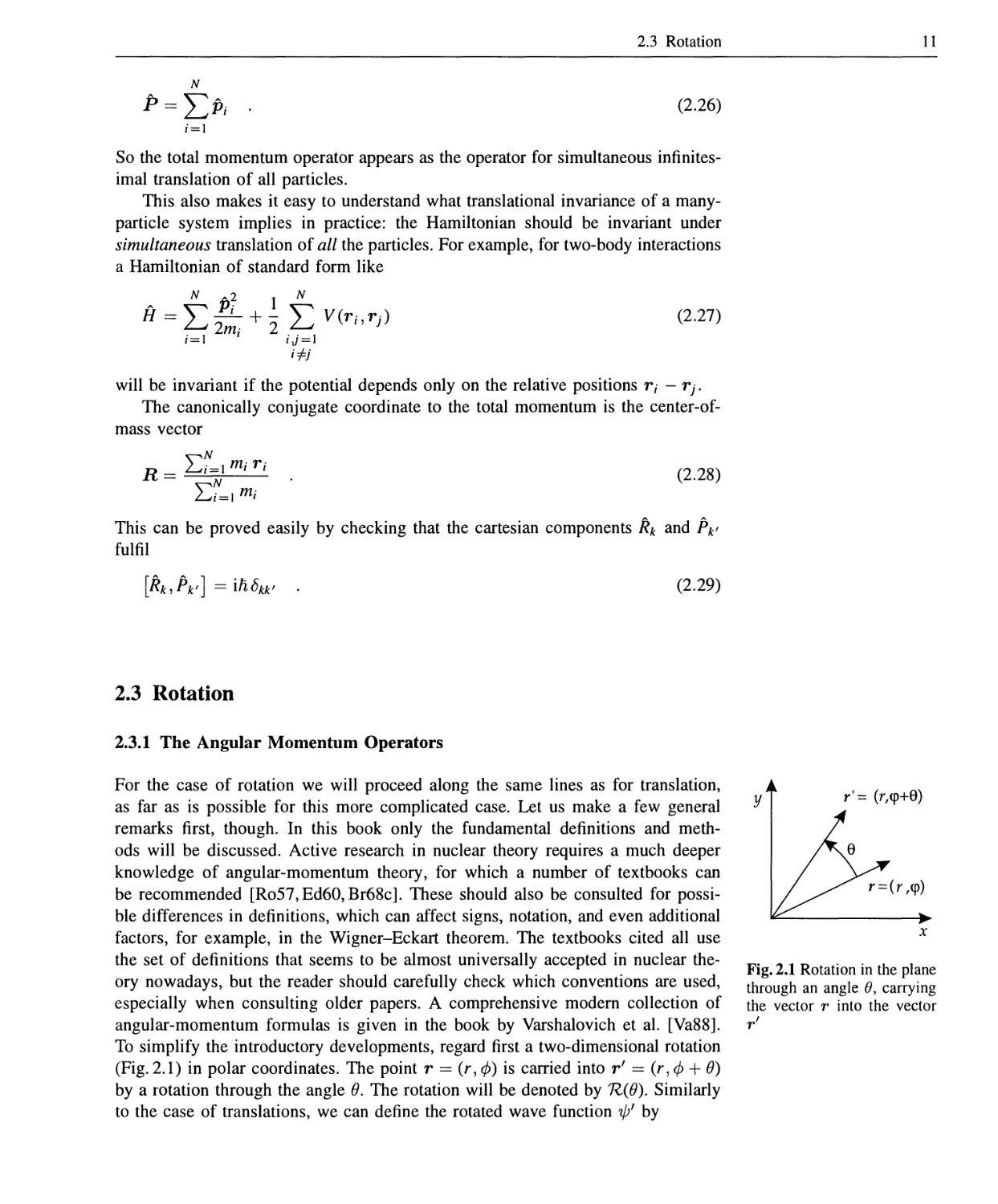
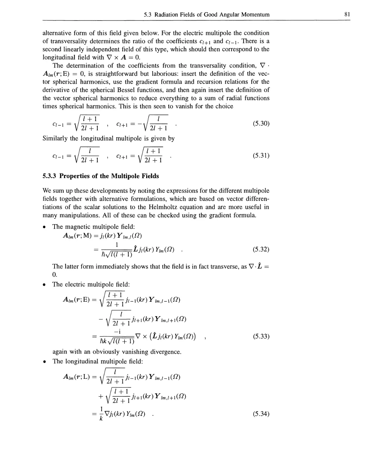
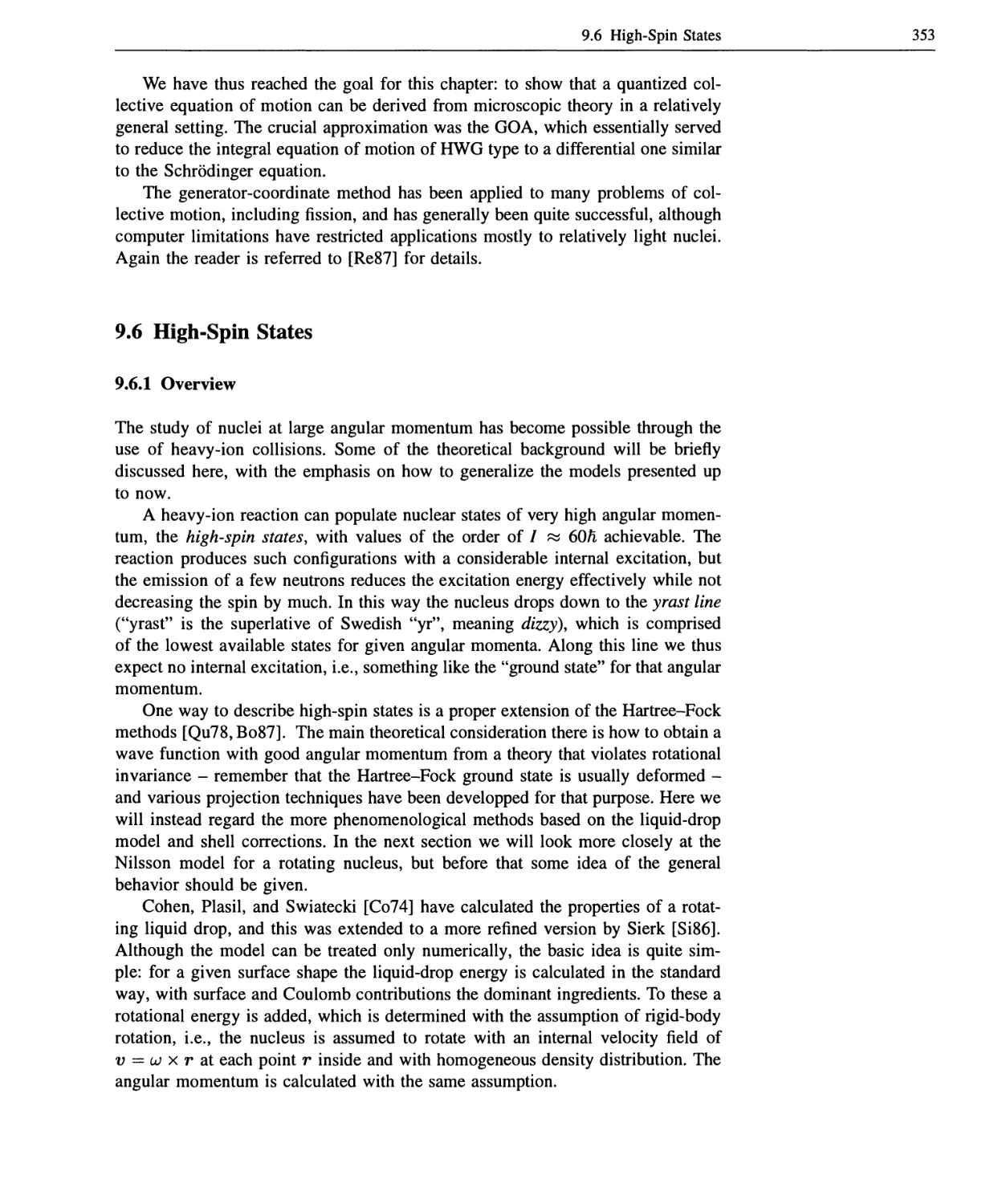
To simplify the introductory developments, regard first a two-dimensional rotation
(Fig. 2.1) in polar coordinates. The point r = (г, ф) is carried into r' = (г,ф + 6)
by a rotation through the angle в. The rotation will be denoted by Щ6). Similarly
to the case of translations, we can define the rotated wave function ф' by
Fig. 2.1 Rotation in the plane
through an angle в, carrying
the vector r into the vector
r'
12 2. Symmetries
ф'(г') = ф(г) , B.30)
and its value at r is determined by the value of ф at that point which is carried
into r by the rotation:
(г,ф) = ф'(г,ф) = ф(г,ф-в) . B.31)
The shift in ф can also be expressed by a Taylor series expansion
00 (~6)n Bn
n=0 '
= ехр(-у)г)ф(г,ф) . B.32)
The operator Jz for infinitesimal rotations can also be written in cartesian coordi-
coordinates,
• B-зз)
and thus is identical with the angular-momentum operator.
EXERCISE
2.1 Cartesian Form of the Angular-Momentum Operator Jz
Problem. Derive the cartesian form of the angular-momentum operator Jz.
Solution. One way is to simply transform the expression in cylindrical coordinates
to cartesian ones. It is more instructive, however, to go back to the definition
of the rotated wave function. A rotation through an angle —в is given by x —»
x cos в + у sin в and у —» у cos в - x sin #, so that
Щ6)ф(х,у) = ф(хсоьв +ysine,ycos6 -xsinO) , A)
which for small в reduces to
ЩО)ф(х,у)аф(х+уО,у-хО)
Comparison with the corresponding small-angle result
Щ6) = exp Н^Л) * A - \0Jz) C)
immediately yields the above result for Jz.
2.3 Rotation 13
The rotation of the vector r itself in cartesian coordinates may be written in matrix
form as
{sine oose){y
If the rotation matrix is expanded to first order for small #, we also get a matrix
representation for Jz:
)<)(;)=[•-•(-. Ж) •
so that
' 0 1
_! О ' • B'36)
We now show that the finite rotation can be recovered from this matrix. This
evaluation of the exponential function of a matrix is quite instructive in itself,
because the trick used always recurs in such cases: it can be applied if some power
of the matrix in the exponent is proportional to the identity matrix. In the present
case we have
~ (-#)" ( 0
n=0 П' ^
{-efn / о \\2n ^ (-0Jn+1 / о i^2n+l
Bл)! \-l OJ ^Bл + 1)! V-l 0
^о Bn)!
1 0\
where we have made use of
) '
so that in general for even powers
1
i 1)
and for odd powers
This allowed the matrices to be taken out of the sums and the sums to be replaced
by trigonometric functions.
14 2. Symmetries
The representation of finite transformations through the exponential function of
the operator for infinitesimal transformations, which can in turn be expressed either
as a differential operator or as a matrix, is called the exponential representation.
An alternative way of deriving the angular-momentum operator rotations is in
terms of derivatives of finite rotations. For both the matrix and the differential
operator versions we can write
' -дЩв) , B.41)
0=0
дв
which simply results from its definition as the first-order coefficient in the Taylor
series.
In the case of three dimensions there are three degrees of freedom for rotations.
Examining rotations around the three cartesian axes leads to a simple generalization
of the results for two dimensions. For rotations about the z axis
у') = I sm9z cosfl/ О] [у } , B.42)
„/
V 0 0
so that according to B.41) the matrix for the angular momentum is
B.43)
Similarly for rotations about the у axis
0 sin^ \ /jc\
0 1 0 b I • B.44)
- sin Qy 0 cos 9y / \ z /
The signs in the matrix keep account of the fact that a positive rotation about
the у axis turns the x axis into the negative z direction. The associated angular-
momentum matrix is
B.45)
Finally for a rotation about the x axis
0 cos0x -sin(9, b I B.46)
0 sinfl, , J
and
/0 0 0\
Jx = -\k 0 0 11 . B.47)
VO -1 0/
The angular-momentum matrices fulfil the familiar commutation relations for an-
angular momentum
2.3 Rotation 15
[jx,jy]=ituz , [jy,jz]=ihJx , [jz,jx]=ihJy . B.48)
The same commutation relations hold for the representation of the angular momenta
as differential operators
Jx = -Щу- z^~
V dz dy
Jz
Jz = -mix- y —
dy ox
The angular-momentum operators form a Lie algebra, whose properties are deter-
determined by the commutation relations. We will see that these commutation relations
by themselves determine the properties of finite rotations to a large extent, and
usually it is much simpler mathematically to study the Lie algebra instead of the
rotation group itself. Formally a Lie algebra is a set of operators which is closed
under linear combination and under the commutation relations: a commutator of
two elements of the Lie algebra must be expressible as a linear combination of ele-
elements of the algebra. The commutation relations of the angular-momentum algebra
clearly have this property.
Finite rotations about any of these axes may be written in the exponential
representation as
Щек) = ехр(-±Ок]к) , ke{x,y,z} . B.50)
There is a problem, however, in expressing arbitrary rotations, because rotations
about the different axes do not commute. If one has a composite rotation denoted
formally by в = Fx,9y,6z), one should specify precisely in which order the
rotations about the three coordinate axes should be performed. Furthermore, it
is not clear whether a given finite rotation can be parametrized uniquely by а в
and how such a parametrization could be determined in practice. We will later see
that for this purpose it is better to use the Euler angles and not the rotations about
the three axes, and for the formal developments in this chapter we merely assume
that finite rotations Щ6) can somehow be defined uniquely.
A final remark concerning the group terminology: rotations in three dimensions
are represented by real 3x3 matrices and conserve the scalar product between
vectors. The condition that
a • b = a! • b1 = (Щ0) a) • (Щв) b) B.51)
can be rewritten in matrix notation as
aTb = (П(в)а)ТП(в)Ь = атПт@)П(в)Ь , B.52)
so that the matrix for 7ZF) must fulfil the orthogonality condition
Пт@)Щв)= 11 . B.53)
16 2. Symmetries
Since
detftT@) = detft@) B.54)
orthogonal matrices can have a determinant of either +1 or — 1. Those with a
negative determinant should not be included, because they change the handedness
of the coordinate system and are thus not true rotations (they are rotations combined
with a space inversion).
Thus we may conclude that rotations in three dimensions are represented by
matrices belonging to the special orthogonal group SOC), i.e., the group consisting
of all 3 x 3 matrices 11 fulfilling
Т I . B.55)
2.3.2 Representations of the Rotation Group
We have seen that the angular-momentum operators may be represented by matri-
matrices. In the same way, any abstract rotation 7ZF) acting on a wave function can be
represented by matrices via a basis expansion. Expanding
ф\г) = Щв) ф(г) B.56)
in a complete orthonormal basis ф{{г) and taking the overlap with фг on both sides
yields
^(ф]\ф) . B.57)
j
So the abstract rotation Щв) is "represented" by the matrix with elements
RijV) = (ф(\Щ0)\фЛ , B.58)
and clearly the representation must reproduce the group structure in the sense that
products and inverses in the group are represented by products and inverses of
matrices:
") = Щв)Щв') -> fy@") ^^
* B.59)
The set of matrices is called a representation of the rotation group. It need not be
faithful, i.e., different rotations may be represented by the same matrix - a simple
example is a scalar wave function, for which all rotations correspond to the identity
transformation. The number of basic functions </>;, which is also the dimension of
the matrices, is called the dimension of the representation.
In many cases representations can be reduced to simpler ones. For example, the
total space of wave functions may be decomposable into two invariant subspaces,
with the wave functions of each subspace mixing among themselves only under
2.3 Rotation 17
rotations. With a suitable choice of basis the matrices of the representation then all
take the form
B.60)
0
where both R^\0) and Rf\0) are representations of smaller dimension. Of special
interest are the irreducible representations, which cannot be decomposed in this
sense. For the rotation group it can be shown that all representations can be built
up from finite-dimensional irreducible representations.
In practice it is usually much easier to construct the representations of the
Lie algebra, in the sense of constructing matrices with the correct commutation
properties, and then to obtain those of the group by the exponential formula. For the
rotation group this means that we need to determine only the matrices representing
the three operators Jx, Jy, and Jz. Because all of these operators commute with 72,
the eigenvalue of J2 cannot be changed by any rotation and it must be the same
within one irreducible representation. As the components of the angular momentum
vector do not commute amongst themselves, only one of them can be chosen to
be diagonal in addition to J2.
Let us try then to use a basis diagonal in both J2 and /z,
J2\jm) = h2Aj\jm) , Jz\jm) = Hm\jm) , B.61)
withy constant and m varying in a range still to be determined (elementary quantum
mechanics suggests that although the eigenvalue of Jz will turn out to be km, that
of J2 will not be as simple, so that we tentatively write Aj). Because Jx and Jy
do not commute with /z, they cannot simultaneously be chosen to be diagonal.
Instead of studying the action of Jx and Jy on these wave functions, it is simpler
to replace them by shift operators
У+ — Jx + \Jy , J - = Jx — iJy . B.62)
The meaning of the term "shift operator" becomes clear through the commutation
relations
[Зг,3±]=±ПЗ± , B.63)
which allows us to compute the eigenvalue corresponding to J±\jm):
Jz(h\jm))=j±jz\jm)[j±jz}\jm)
= him ± \)\jm) . B.64)
This shows that J± shifts the eigenvalue of Jz by ±h, or the value of m by ±1.
The underlying idea, which will be used several times in this book, is that if
two operators A and В have a commutation relation of the form
[A,B] =0B B.65)
with /3 some number, then the same calculation as above shows that В shifts the
eigenvalue of A by C.
18 2. Symmetries
Given a particular basis state \jm), by using the operators J± we can suc-
successively construct the states \jm ± 1), \jm ± 2), etc. Since we are looking for
representations of finite dimension, this process must end somewhere (in fact it can
be shown that "all irreducible unitary representations of a connected simple com-
compact group" are finite-dimensional - details may be found in textbooks on group
theory . Let us only remark that this theorem applies to the rotation group). Use /i
for the largest value attainable by m. Then we must have
У+|;»=0 , B.66)
because anything else would imply the existence of a vector with eigenvalue /i+ 1.
Now compute the action of J2 on |y/i) using
This may be rewritten using the commutation relation
[J+J-] =2tiz B.68)
to yield
P=j-j++jz2 + hjz , B.69)
and the first term on the right produces zero on |y/i), while Jz has the eigenvalue
ft/i, so that we get the eigenvalue of J2:
B.70)
as
2 B.71)
Up to now the variable j had no direct physical meaning; it only enumerated the
eigenvalues of J2. The preceding equation suggests we use the maximal eigenvalue
of Jz instead. Thus we identify j with /i and keep the letter j. Then the states of
the representation fulfil
J2\jm) = h2j(j + l)\jm) , Jz\jm) = hm\jm) , B.72)
and the one with the largest eigenvalue of Jz is \jj).
Now the same arguments can be applied to the lowest possible value of m.
Assume that for some positive number n we have
3-\j,j-n)=Q B.73)
to stop the generation of states on the lower end. The angular momentum squared
of B.67) can also be expressed as
J2=J+J.+J2-JZ , B.74)
and again the first term will yield zero, so that
P\jJ-n) = h2[{j-nJ-j+n]\jJ-n) . B.75)
2.3 Rotation 19
Since the eigenvalue of J2 must still be the same, it must be true that
Л7 + 1) = G-лJ-G-л) , B.76)
which is a quadratic equation for n with the only positive solution n — 2y. This
makes the lowest projection equal to -j.
The representation we have constructed thus has the basis states
| у/и) , m = -y,-y 4- l,...,y , B.77)
which are 2y + 1 in number and are eigenstates of the angular momentum squared
and of the z projection according to
J2\jm) = k2j{j + \)\jm) > 3z\jm) = hm\jm) . B.78)
The construction of the basis with the shift operators did not explicitly normalize
the states, but this can be done easily if we note that J+ is just the Hermitian
conjugate of/_, so that the norm of the state J±\jm) is given by
(jm\J4:J±\jm) = {jm\J2-J2^Jz\jm)
= H2(j ± /и 4- l)(y =F m) . B.79)
The reciprocal square root of this expression will be the normalizing factor for the
state |y,ra ± 1), and the matrix elements of the shift operators also result as
(у,/и ± l\J±\Jm) = hy/U±m + 1)(у T т) . B.80)
These matrix elements define the matrix representations of the shift operators and
hence of the operators Jx and Jy via
/ I (J \ I \ T — i (J J \ n on
Jx — 2 \J4- ' ** —) ? •'V — —? V + — J VZ.olJ
as
(j,m'\Jx\jm) = %(y/(j +m + l)(y - m)
.w'l^lyw) - -y f \/0
lH'+w)«w/fW.
J
B.82)
1H -
- л/О - W + 1H + m) bm',m-\ j ,
where for completeness the matrix elements of Jz are also given. Thus we have
represented the full Lie algebra by By -f 1) x By +1) matrices. There is a freedom of
choice in the phases of the matrix elements, since multiplying them by an arbitrary
phase would not change the normalization argument. The phase chosen here is the
Condon and Shortley phase and is the usual choice. Another choice of phase will
be used in the BCS model for pairing (Chap. 7.5).
20 2. Symmetries
2.3.3 The Rotation Matrices
Finite rotations are quite a bit more complicated. It is important to find a unique
parametrization of these rotations in terms of rotations performed about certain axes
in a prescribed order. The order is important because rotations about different axes
do not in general commute. The most familiar set of angles are the Euler angles в —
(#i, 02» 0з)» which are defined as follows (all rotations performed counterclockwise).
1. Rotate the system through an angle 9\ about the z axis, yielding new axes x',
y\ and zf.
2. The second rotation is through an angle 92 about the new axis yf. This yields
(*",/', z").
3. Finally, rotate through 03 about the new axis z" produced in the first two steps.
What is the advantage of using the Euler angles compared with the rotations about
the three Cartesian axes that we have considered with up to now? It is much easier
to determine the Euler angles needed to orient a body uniquely in space by using
the first two angles to orient its body-fixed z axis correctly and then to turn it about
that axis into the correct position. Also, for the Euler angles two of the rotations
involve a diagonal Jz. On the other hand, for the infinitesimal rotations the Euler
angles are useless because for 92 ~ 0, Q\ and 03 rotate about the same axis and do
not lead to independent angular-momentum operators.
To write these rotations in terms of angular-momentum operators, we have to
define Jyi as the operator for infinitesimal rotations about the rotated y' axis needed
for 92, and Jz>> as that for the final zn axis needed for 03. The rotation operator is
then given by
Щв) = exp (-?0зЛ") ехр (-\02Зу) ехр (-{в}3г) . B.83)
This is very difficult to use as it stands, but can fortunately be transformed into
a form with rotations about fixed axes. Instead of rotating the system about y\
we can clearly first go back to the original axes, rotate about the original у axis,
and then rotate back to the primed coordinate system. Expressing this by operators
replaces this part of the rotation operator by
exp H02-V) = exP Н^Л) ехр Н^Л) ехР (ЙЛ) - B-84)
and a similar argument for 03 yields
exp Н0зЛ") = exp (-ffily) ехр (-^Л)
x exp (-^0зЛ) ехр (\вх3г) exp ({в2Зу) B.85)
with the two other rotations reversed and then reapplied. Inserting this result into
B.83), cancelling the operators as far as possible, and then using the formula B.84)
for the remaining Jyf term finally yields
Щв) = exp (-^01Л) ехр (-{в2Зу) ехр (-?0зЛ) , B.86)
i.e., the interesting fact that one produces the same rotation by rotating about the
fixed original axes with the order of the Euler angles reversed.
2.3 Rotation 21
The matrices for these rotations in the irreducible representation with angular
momentum j are defined by
^« , B.87)
which implies that a state \jm) transforms into
\M)'= ^2\jm'}V^m(e) . B.88)
We will not need many explicit properties of the matrices T^jJm(O)\ special forms
will be given when needed. It is useful, however, to reduce the matrix to simpler
form by noting that in B.86) the first and last operator is diagonal in the basis
\jm), so that one may simplify the matrix to
- i«W + 63m)] dU)n@2) • B.89)
In this way the dependence on two of the angles has become trivial, and the only
complicated function is the reduced rotation matrix d^)m(92).
2.3.4 SUB) and Spin
Let us return to the question of which values of j are actually possible. The con-
construction of the representations of the angular-momentum algebra led to the condi-
condition that 2/ should be integer, a consequence of B.76). So the somewhat surprising
result is that j may be integer or half-integer, leading to the natural appearance
of spin in the latter case. The representations with half-integer angular momen-
momentum cannot correspond to normal rotations of classical objects. To see this, simply
examine a rotation for an angle of 2тг. For the z axis, for example, this is given by
П(вг = 2тг) - exp (-2tt±/z) , B-90)
and for a state with angular-momentum projection ^, for example, it will be mul-
multiplied by a factor of ехр(-тп) = — 1. For wave functions there is nothing wrong
with this, as all measurable quantities lead to matrix elements containing the square
of this factor. But if a classical object such as a vector is rotated by 2тг, it should
always be transformed into itself. Certainly the group SOC) that we started with
has the property that all rotations about an angle of 2тг revert to the identity matrix,
so how can it be that its representations do not have this property in general? The
answer is that the half-integer representations are not representations of SOC).
Remember that we constructed the representations from the angular-momentum
operators. These operators together with their commutation relations form the Lie
algebra associated with the Lie group of the rotations, for which they determine the
infinitesimal rotations. Now it turns out that the Lie algebra does not completely
determine the associated Lie group, and in this special case the groups SOC)
and SUB) have the same Lie algebra. Because an understanding of SUB) and its
relation to spin is very important for more general applications such as isospin, it
is worth explaining SUB) in some more detail.
The group SUB) is the special unitary group of all 2 x 2 unitary matrices with
determinant 1, i.e., matrices U fulfilling
22 2. Symmetries
i , det t/ = 1 . B.91)
Its relation to rotations has already been used in classical mechanics in connection
with the Cayley-Klein parameters, and here we sketch the derivation. Examine a
general 2x2 complex matrix
Requiring the determinant to be 1 yields the condition
ad -be = I , B.93)
whereas the unitarity condition reads
* c*\ fa b\ (\ 0
* d*)\c d)-\0 1
or, explicitly,
я*я+с*с = 1 , B.95a)
b*b+d*d = l , B.95b)
a*b+c*d = 0 , B.95c)
b*a+d*c = 0 . B.95d)
The last equation is simply the complex conjugate of the preceding one and can
thus be omitted. These conditions allow one to reduce the number of degrees of
freedom in the matrices. From B.95c) we have
a*b
d = ~— , B.96)
and inserting this into B.93) yields
l = _al±_cb = ^a + c*c)t L
c* c* c*
B.97)
where the content of the parentheses is equal to 1 because of B.95a). So we must
have b = —c* and, inserting this again into B.96), also d = a*. Then B.95b) is
automatically fulfilled and the matrix can be written in the more specific form
«-D- *¦
with the subsidiary condition
a*a + b*b = \ . B.99)
Of the four complex numbers only two are left and because of the subsidiary
condition three real degrees of freedom remain, identical in number to the three
degrees of freedom of rotations in three dimensions.
To see the relation to these rotations, associate with a vector r — (x,y,z) a
matrix
2.3 Rotation 23
¦ BЛ00)
This matrix is hermitian and has trace zero. Conversely, any 2x2 hermitian matrix
with trace zero defines a vector in three dimensions, which can be obtained simply
by reading the components from the real and imaginary parts of the matrix elements.
Now investigate transformations of the form
P' = UPU] , B.101)
where U is any matrix in SUB). Does this describe a rotation of the associated
vector? The matrix P' is also hermitian because
p't = {UPU])] = UP]U] = UPU] = P' B.102)
and it also has trace zero. To see the latter, we write the trace of a product of
matrices in component form and check that the matrices in the product can be
permuted cyclically without changing the trace:
ЩАВС ...Z}= Y^ AvBjkCki' • • Zm
ijkl-n
jkl-ni
= Tr{BC-ZA} . B.103)
Applying this to our transformation formula yields
Tr{P'} =Tr {UPU^} =Tv{PUj[U} =Tr{P} = 0 B.104)
since UW = 1. So P' also defines a vector r', and to prove that r' is obtained
from r by a rotation, we only have to check its length, which is given by the
determinant:
detP = -z2 -(x -iy)(x +iy) = - (x2 + y2 + z2) = -r2 . B.105)
The determinant of a product of matrices is equal to the product of the determinants,
so that
detP' = det (UPU]) = detU detP det?/f = detP B.106)
and ra = r2. Now a linear transformation which preserves the lengths of all vectors
must be a rotation, possibly combined with reflections.
To complete the construction, the rotations about the three coordinate axes have
to be constructed in this representation (see Exercise 2.2). The result for rotations
about the z axis is
-i0z/2 rv \
о Д ' B107)
and for those about the x axis
cos(9x/2) ) > BЛ08)
24 2. Symmetries
and finally for the у axis
/ cos@y/2)
cos(V2)/ • BЛ°9)
The form of these expressions allows two important conclusions. First, the angles
are halved in the arguments of the trigonometric functions, and all of these matrices
reduce to minus the unit matrix for an angle of 2тг. This does not cause problems
in this case, because in the rotation law B.101) U appears twice and the signs
cancel. Second, expanding the rotation matrices for small angles yields the angular
momentum operators
' 3y = \(°i ~o) ' *z = i(o -°i) 'B110)
which can also be expressed in terms of the Pauli matrices as
J = \cr B.111)
with
-(! J) • *-(?«') • *-(i
i -
and fulfil the usual angular momentum commutation relations. This shows that
SUB) and SOC) have the same Lie algebras.
Although the Cayley-Klein formulation as described above will not be used
further in this book, this discussion should have made the intimate connection be-
between rotations and the group SUB) clear. Since SUB) describes arbitrary unitary
transformations with determinant 1 in a two-dimensional space of wave functions,
angular-momentum methods can be used by mathematical analogy whenever one
is dealing with symmetries in such a space. Isospin will be the principal application
of this idea.
EXERCISE
2.2 Cayley-Klein Representation of the Rotation Matrix
Problem. Derive the transformation matrix in the Cayley-Klein representation for
rotations about the z axis.
Solution. We have to compare the usual transformation
x' — x cos# — у sin# , y' = x sinO 4- у cosO , z' — z A)
with the one given by B.101). With the matrix set in the form of B.98), this leads
to the matrix equation
z1 x'-'\y'\_( a b\( z x-iy\(a* -b
4i/ -z' j~\-b* a*)[x + iy -z Mb* a
2.3 Rotation 25
Carrying through the matrix multiplications and inserting the expressions for the Exercise 2.2
primed coordinates yields four complex equations, in which the coefficients of x,
y, and z can be compared separately. In the diagonal, the coefficients of x and у
must be zero and that of z must be 1 or — 1, leading to
ab*=a*b = 0 , a*a-b*b = l . C)
In the off-diagonal terms the coefficient of z must vanish, requiring ab = 0.
Now split the lower off-diagonal equation into real and imaginary parts; defining
a = ar 4- Ш{ and b = br 4- ife/ one obtains
cos в = -of 4- a] 4- bf - b2r - sin в = 2а{аг 4- 2b(br ,
D)
cos в = -a? 4- яг2 4- bf - fe? sin (9 = -2а(аг 4- 2fe/fer ,
from which Ьг = br = 0, i.e., ^ = 0, and
Idjdr = - sin в , ^ - af = cos ^ E)
follow, which can be solved yielding
ar = -cos(§) , a,- = -sin(f) , a=exp(-i§) . F)
This completes the construction of the matrix.
2.3.5 Coupling of Angular Momenta
In a system of two particles, there is for each of the particles an angular-momentum
operator that infinitesimally rotates that particle about the origin of the coordinate
system. Let us designate these operators by J\ and Ji- If the particles interact, the
energy of the system will not be invariant if only one of the particles is rotated, but
if both are rotated simultaneously, their relative position, relative spin orientation,
etc., will not be changed and the physics should remain the same. Thus it makes
sense to study the operator for a common infinitesimal rotation of both particles,
which is the total angular-momentum operator
J = J}+J2 , B.113)
(cf. the construction of the total momentum in Sect. 2.2.3) and for the two-particle
system the eigenfunctions of J 2 and Jz must be sought. Normally these are obtained
by angular-momentum coupling from the products of eigenfunctions of the separate
angular momenta.
Let two sets of eigenfunctions \j\tn\) and I72AW2) be given such that
0172^2) , h\h ^\J)
A basis for the system of two particles may then be built out of the products of
these states, forming the so-called uncoupled basis
26 2. Symmetries
\j\m\j2m2) = \j\mi)\j2m2) • B.115)
One sees immediately that such a state is an eigenstate of the z component of the
total angular momentum with eigenvalue m\ -V mi, since
3z\j\m\j2m2) = (Jh + J2z) \j\m\j2m2) = h(m{ + m2)\jxmxj2m2) . B.116)
However, it cannot be an eigenstate of У2, and to see this we have to examine the
commutation relations of the different angular momenta.
First note that all components of J\ will commute with all components of J2,
since they refer to different particles. Thus we get immediately
%щ = [лл2] = [лtf] = [з\т=о , B.П7)
as well as
[JzJlz] = [JzJ2z] = 0 , B.118)
while the square of the total angular momentum does not commute with the z
projections of the individual angular momenta; for example,
[J2Jn] = [J?Jn] + [JiJn] + [2J, • JiJn] ¦ B.119)
Although the first two commutators on the right-hand side vanish, the third one
does not and the result becomes
[J2J]Z] = 2ih{j2yJXx-J2xJXy) . B.120)
A fully commuting set of operators is thus given by 72, Jz, Jf, and У22> апC angular-
momentum coupling essentially consists in replacing the quantum numbers m\ and
m2 by j and m. The new basis vectors may be denoted by
\jmj\h) , B.121)
and the unitary matrix leading to this basis is simply defined by
\M\j2) = ^2 \j\m^2m2){jxmxj2m2\jmjxj2) . B.122)
Obviously for practical notation the repetition of/! and 72 on both sides of the matrix
element is superfluous, so that the transformation coefficient is more succinctly
defined as
) • B.123)
This is the Clebsch-Gordan coefficient. The transformation is now written as
\JmJ\h) = ^2 \hm\hmi)U\J'2J\m\m2m) . B.124)
/W1/W2
The following properties of the Clebsch-Gordan coefficients are used in this book
(for a derivation see the literature on angular momentum).
2.3 Rotation
27
1. Selection rules: the coefficient is zero unless the quantum numbers fulfil the
two conditions
m\ + mi = m
and
l/i -h\ <j <
B.125)
B.126)
The first one merely repeats what we said above about the eigenvalue of Jz,
while the latter is known as the "triangular condition": the size of the total
angular momentum is restricted to those values that are allowed by the rules
of vector addition, where the vectors J\, J2, and J form a triangle.
2. The coefficients are real. This is not a general condition, because the phases of
the basis states are arbitrary in principle, but is assured for the standard choice of
basis states due to Condon and Shortley. Note that a real transformation matrix
is orthogonal so that the inverse transform corresponds to the transposed matrix:
(j\mxj2m2\jmj\j2) = (jmjJ2\ j\m\j2m2) = U\JzJ\m\m2>n)
B.127)
and the transformation back to the uncoupled basis uses the same coefficients
but the summation is over different indices:
\j\mxj2m2) =
B.128)
jm
3. In the language of group representations, angular-momentum coupling corre-
corresponds to the reduction of the product of two representations:
?)O"l) x J)(J2) — pO'l+/2) _j_ ?)O"l+72-l) _j_ . . . _j_ p(l/l-/2|) ^ B.129)
The dimensions of the bases involved on both sides coincide, i.e.,
71 +72
B/, + l)B/2 + 1) = Yl B->' + 1) ' BЛ30)
j = 1/1 -h I
which may be checked easily by direct calculation.
4. Special formulas for the Clebsch-Gordan coefficients are to be found in angular
momentum textbooks and special tables; the few that are needed in this book
will always be quoted explicitly.
2.3.6 Intrinsic Angular Momentum
Up to now the rotational invariance of wave functions has been investigated in
terms of their dependence on the space coordinates, leading to orbital angular
momentum. There are also fields that have an intrinsic angular momentum, for
example, vector fields. Figure 2.2 shows the situation for this case. A rotation not
only moves the field to a different point r1 in space, but also rotates the vector
itself. So we must have
= (r,(p+9)
= TlA(r)
B.131)
Fig. 2.2 Rotation of a vector
field. In addition to the trans-
transformation of the base point
the field vector itself is also
rotated
28 2. Symmetries
where 1Z is the appropriate rotation matrix for a vector in three dimensions, for
example, for a rotation about the z axis
(cos0z - sin0z 0 \
sin<9z cosOz 0 . B.132)
0 0 1/
The rotated field at r is then given by
г) . B.133)
The infinitesimal rotation is easy to derive from this expression: for the dependence
on the coordinates we get the usual angular-momentum operator and for the rotation
of the vector itself the matrix 11 has to be expanded in the angles. For a rotation
about the z axis this is
/1 -Oz 0\
Щвг) ~ \°z i 0=1- \ezsz , B.134)
\0 0 0/
where Sz is the matrix
/0 -i 0\
B.135)
This is one component of the operator of intrinsic angular momentum, which is
usually called spin, even if it does not refer to half-integral angular momentum. In
this case, for a vector field, the angular momentum is unity, corresponding to the
three-dimensional representation withy = 1. An example of this type of field is a
photon.
The other angular-momentum components, obtained in the same way, are
Sx = h 0 0 -i . B.136)
These matrices fulfil, as indeed they must, the commutation relations for angular
momentum.
For the field A(r) the infinitesimal rotation is given by
A\r) = [1 - {6Z (Lz 4- Sz)] A{r) • B.137)
Here the orbital angular momentum is denoted by L, to reserve the letter / for the
total angular momentum J given by
J = L + S . B.138)
Obviously J generates rotations for the vector field, and eigenstates of J2 and Jz
have to be constructed by angular-momentum coupling.
For this coupling, however, the coordinate system used for the vector is not
adequate. As is clear from the form of the matrix Sz> it is not diagonal in carte-
cartesian coordinates and one has to go over to spherical coordinates to obtain spin
2.3 Rotation 29
eigenstates. Formally we need to construct vectors fulfilling Sze^ = h/ле^ or, if
we assume components a,b,c for the unknown eigenvector,
B.139)
This equation can have solutions only if the determinant det (Sz — h/л) vanishes,
which leads to the condition
/х(/х2-1)=0 B.140)
with solutions /j, = -1,0,1 as should be expected for the three projections of
unit angular momentum. Inserting these eigenvalues into the equation, finding the
required relations between a, b, and c, and normalizing the resulting vectors leads
to
eo = ez , B.141)
These complex vectors could in principle be multiplied by an arbitrary phase with-
without affecting their eigenvector properties, and the special choice made here is partly
conventional and also made such that the general property
e* =(-1)"е_м B.142)
is fulfilled. This is analogous to spherical harmonics and corresponds to the
Condon-Shortley choice of phases of the-angular momentum eigenstates.
Let us list a few properties of spherical coordinates. The basis vectors of B.141)
are orthogonal in the generalized version for complex vectors:
e*eM,=V , B.143)
and if spherical components ад, /x = —1,0,1, of a vector a are defined via
J>*eM=a , B.144)
д
they are related to the cartesian components by
± шу) , a0 = az . B.145)
To understand the physical meaning of spherical components, regard the case of
a plane-wave electromagnetic field with a polarization vector given by one of the
spherical basis vectors:
, t) = e\ exp (\fe • r — \u;t)
= —-j=[ex cos(fc • r — ut) — ey sin(fc • r — cot)]
- -Tjtejt sin(fc • r - ut) 4- ey cos(k • r - ut)] . B.146)
30 2. Symmetries
The real part of this, corresponding to the physical field, and evaluated for simplicity
at v = 0, is
Re {A@,0} = -75 К cosM) 4- ey sinM)] , B.147)
which describes a field rotating in the mathematically positive sense about the z
axis and thus nicely conforming to the idea of positive intrinsic angular momentum
about that axis.
A second important case of internal angular momentum is that of spin fields.
In this case the wave function has two components at each point in space that
transform under rotations according to the representation of the rotation group
with angular momentum j = \. There are no classical analogies and in this case
we do not have to worry about the choice of the basis: since there is no predefined
physical set of basis states, we can immediately use the eigenstates of angular
The two basic states may be called |^) and | - \) with
, B.148)
and the spin operator is denoted by the small letter s to distinguish it from the
case of intrinsic angular momentum of unity, where capital S is commonly used.
Its components are determined by
s = \h& , B.149)
where & are the Pauli matrices as defined above in B.112). For both operators
S and s this agrees with the representation constructed in Sect. 2.3.2, as may be
checked by calculating the matrix elements for Jz and J± given there for these
special cases and then obtaining Jx and Jy from them.
2.3.7 Tensor Operators
Up to now only the transformation of wavefunctions under rotations has been ex-
examined. Before considering operators in more detail, we first introduce the various
types of transformation properties. A scalar is a quantity that does not change
under rotations, whereas a vector or tensor of rank 1 is an object with three com-
components that transforms like the position vector r; as discussed in the last section
this corresponds to unit angular momentum.
Higher-rank tensors can be constructed in two ways, reminiscent of the al-
alternative of angular-momentum coupled or uncoupled bases. A cartesian tensor
of rank n has components with n indices, each of them running from -1 to 4-1
(i.e., spherical components are assumed, but cartesian ones can be used as well),
and with each index transforming according to the representation for unit angular
momentum:
amxm2...mn ~ /—/ a>
1 2 »
For the simplest case of a rank-2 tensor this reads
i'j'
2.3 Rotation 31
and is essentially the same formula as that giving the rotations for an uncoupled
basis built from two angular momenta of magnitude 1. Such a cartesian tensor has
3n components.
Equivalently, and usually much more usefully in nuclear structure, one may
employ spherical tensors (more precisely, irreducible spherical tensors), which
are objects transforming under rotations like a wave function of good angular
momentum. Thus an irreducible tensor with angular momentum tk consists of
components tk, q = —?,...,+&, which under rotations transform according to
t'k = J2 Ц'^цФ) ' B.152)
The most useful application, of course, is the coupling of such tensors, for which
all the considerations for wave functions are still applicable. Two tensors Rk and
Sk of angular momenta к and k\ respectively, may be coupled to total angular
momentum К using
qq'
This type of angular-momentum coupling is so important that we introduce a more
concise notation,
f$ = [tf* x Ǥ*'] or tK = \Rk x Sk>] . B.154)
^ L \q L J
The latter version is useful when one is not interested in the projections.
EXERCISE
2.3 Coupling of Two Vectors to Good Angular Momentum
Problem. What are the possible couplings of two vectors a and b to good total
angular momentum?
Solution. According to the triangular rule, the coupling of the vectors is that of two
tensors of unit angular momentum to a resulting angular momentum К = 0,1,2.
The general formula is
*fi =EA1*l*G-*GK*fi-* ' (D
ч
involving the spherical components of the vectors. For К = 0 we can use A \0\q —
/ toget
bo - аф-i - a-\b\)
= —^ [azbz 4- \{ax 4- iay)(bx - \by) 4- \(ax - \ay)(bx 4- \by)]
$ + ayby + azbz) =—^=a • Ъ , B)
32 2. Symmetries
Exercise 2.3 i.e., the not very surprising result that the scalar built up from the two vectors is
just the scalar product, aside from a constant factor.
For К — 1 let us do only one component explicitly: Q = I. Here we have
A11| 101) = -(lll|011) = \/y/2 and
T\ = ±(-aobx + аф0)
= \[az{bx +iby)- bz(ax 4- iay)]
= -%[(aybz - azby) 4- i(azbx - axbz)]
= ^(a x b)+1 , C)
the spherical component of the vector product. The other components work out
similarly and in general we can write
[a xb]]Q = -^(ax b)Q . D)
v2
Again this result is intuitively clear. Finally, for К = 2, we write down the first
three components explicitly:
Г22 = аф\ = \{axbx - ayby 4- 2iaxby) ,
7? = ^(«i*o + aob\) = ~{[axbz 4- azbx 4- i(ay^z 4- azby)] , ^5j
Г02 = ^(aife_i 4- a-ifei) 4- yjaobo = -^(ax^x 4- ay^y) 4- \J\azb
zbz
The negative Q-components can be obtained from the rule T^Q = (-\)qT*q.
One may also view these results in terms of a decomposition of the cartesian
tensor product
/axbx axby axbz\
I aybx ayby aybz J F)
\azbx azby azbz /
into a scalar a • 6, a vector a x 6, and a symmetric tensor 7^ with components
like tfjc^y 4- fltyfejc.
An irreducible spherical-tensor operator is now simply an irreducible spherical
tensor whose components are operators. This introduces a new condition, because
an operator Г* can be transformed either by using B.152) or via the general formula
t'qk =V{6)tkqV-\0) , B.155)
where VF) is the appropriate operator for rotating the wave functions (which,
for wave functions of good angular momentum, may again be a rotation matrix,
though possibly for angular momentum other than k). What do these two different
transformation laws imply? Although B.155) holds for any operator and essentially
says that one may apply the rotated operator by first rotating the wave function
back, then applying the original operator, and finally rotating the result forward to
2.3 Rotation 33
the desired position, B.152) is valid only for irreducible spherical-tensor operators.
It requires that a set of operators corresponding to the components of the spherical-
tensor operator transform under rotations like a set of spherical components in the
way prescribed by B.152).
EXAMPLE
2.4 The Position Operator as an Irreducible Spherical Tensor
The three operators jc, y, and z, which multiply the wave function by the value of
the corresponding coordinate, can be combined into an irreducible spherical-tensor
operator rq of unit angular momentum and with components following the usual
definition of spherical components:
ssion of vector fie
according to B.152) with к = 1.
From the discussion of vector fields it should be clear that rq indeed transforms
Comparing the two ways of transforming an irreducible spherical-tensor operator,
one would expect that, if infinitesimal rotations are considered, some condition on
the commutation of tk with the angular momentum operator should follow. If we
assume an infinitesimal rotation about the a axis, B.155) may be written up to
second order as
tlk ^ (\ - {ва3а)тк{\ + \eaja)
ъТк-{ва[За,Тк] . B.156)
On the other hand, the rotation matrix element in B.152) may also be simplified
for infinitesimal rotations:
ч% (kq'\l - j,eja\kq) = <V - {еа{кд'\}а\кд) , B.157)
so that comparing the two ways of rotation yields
[tk}J2^U • B-158)
Using the matrix elements of the angular- momentum operators given at the end
of Sect. 2.3.2 we obtain
[jz,tk]=qtk , [J±Jk4] = hy/(k ±q + l)(k T q) fkq±x . B.159)
Note that this result essentially means that the angular-momentum operators act on
the components of an irreducible spherical-tensor operator in the same way as they
act on a wave function; for an operator the product merely has to be replaced by a
commutator, because the J also needs to be "passed through" to act on the wave
function.
34 2. Symmetries
EXAMPLE
2.5 Commutation Relations of the Position Operator
The position vector operator r should fulfil
[Л,ЯО]=О , [Jz,r±i]=±hr±i ,
[3±,Po]=y/2hf±l , [J+,r+i]=0 , [У_,г_,]=О , A)
which can be checked easily using the definition of J in terms of differential
operators. The angular-momentum operator itself is also a spherical tensor with
unit angular momentum, but it is important to realize that the components are not
identical to the shift operators. The spherical components are denoted by subscripts
4-1 and -1 and are given by
Jo = Л
J+i=-^(^+^) = -75J+ B)
In general, any vector operator can be written as a spherical-tensor operator with
unit angular momentum by using spherical components.
The applications of tensor operators are mostly concerned with the possibility of
coupling them
• with wave functions: a new wave function with good angular momentum can
be constructed through
^ , B.160)
qm
where a and C refer to any other quantum numbers affected by the operator.
The resulting angular momenta are determined by the selection rules implicit
in the Clebsch-Gordan coefficients.
• with other operators: this is similar to B.154) above. Of course for operators
one has to keep track of the ordering because of their possible noncommutation.
In this way the scalar and vector products of operators can be defined as above
as the coupling to zero or unit angular momentum.
The distinction between operators and fields is crucial for some considerations and
the "same" mathematical expression may have to be treated differently depending
on how it is used. We illustrate this point for the position vector.
Acting on wave functions, r is really composed of the three operators jc, y9
and z, which may be combined into the irreducible spherical-tensor operator r^,
2.3 Rotation 35
ji = —1,0,1, as described above. Its application to a wave function produces three
new functions r^ip(r), each of which may be rotated using the rotation operator:
= P@)(v/>(r)) . B.161)
Because r is a spherical-tensor operator, we can alternatively write
E V^'m) V>(Z>-'@)r) • B-162)
/x' '
This last way of writing the rotation makes it clear how this works: the spherical
operator r is rotated at a fixed point and thus multiplies the wave function with
the values that pertain to the location V~x{0)r.
The situation is different if r is regarded as a vector field with an intrinsic
angular momentum of 1. Now we have a vector function r(x,y,z) which under
rotations will have both its dependence on the coordinates and its direction at a
fixed point affected. In fact, it can be written as
r = -y/b ^A10|ц-/Ю)гме_м B.163)
/x=-l
and so appears explicitly as a scalar. This agrees with intuition since the field r is
obviously spherically symmetric. Formally, the position-independent basic vectors
eM carry the intrinsic angular momentum and the coefficients rM carry the orbital
angular momentum, which in this case just couple to zero total angular momentum.
2.3.8 The Wigner-Eckart Theorem
Since the states of different projection belonging to a multiplet of fixed angular
momentum are in some sense trivially related to each other by application of
the operators J+ or У_, one would expect that matrix elements should also in
some sense depend "trivially" on the projections involved, i.e., simply through
manipulations having to do with the rotation group and its representations. In fact,
this is the contents of the Wigner-Eckart theorem which will now be derived.
Take a matrix element of an irreducible spherical-tensor operator 7* between
angular-momentum states of the form \ajm). As the operator may also change the
nonrotational quantum numbers, they are explicitly represented by a and C. The
matrix element we are interested in is
(pj'm'lt'lajm) . B.164)
The idea will now be to couple the right-hand state with the tensor operator to
good angular momentum and then to exploit orthogonality with the left-hand state.
36 2. Symmetries
The coupling yields intermediate states
\lj"m") = Y, Ш"\тЯт") Ц \ajm) , B.165)
mq
with7" and m" taking all allowed values. This coupling can be inverted according
to Sect. 2.3.5, yielding
?$\<*jm) = ^ (jkj"\mqm") \<yj"m") . B.166)
j"m"
Taking the overlap with \Cj'mf) produces
(Cj'm'\tkq\ajm) = ? (jkj"\mqm") @j'mbj"m")
j"m"
= (jkj'\mqm')(Cj'mfbj'm') . B.167)
The second matrix element on the right-hand side does not depend on m', which
can be seen by examining
J-J+ \0jm)(>yjm \J-h\lJm)
= (Pjm\-yjm) , B.168)
in which the operator combination У_У+ is diagonal and its eigenvalue is inde-
independent of any additional quantum numbers - in fact, this expression was used in
Sect. 2.3.2 to derive the matrix element of J+. The same argument can be used for
lowering the projection, of course.
The result is thus that the matrix element can be split up into a Clebsch-Gordan
coefficient, which contains all the information about the projection dependence, and
an as yet unknown matrix element (Pjffnf\^yjfmf), which describes the physics of
the operator Г*. To make this fact clear, we define a reduced matrix element by
writing
(Pi'm'\tk4\ajm)=(-\Jk{f3j'\\tk\\aj)(jkj'\mqm') . B.169)
The reduced matrix element {Cjr\\tk\\aj) is determined implicitly: to calculate its
value simply calculate the left-hand side of B.169) for any convenient combination
of projections m, m;, and q, for which it does not vanish, and then use the equation
to obtain the reduced matrix element itself. The advantage is then that all other
combinations of projections can be calculated easily, and that the reduced matrix
element as defined does not explicitly contain any reference to the projections,
thus providing a more general characterization of the operator's action. The factor
(— \Jk is a conventional phase factor and different authors have employed different
definitions for the reduced matrix element.
2.3 Rotation 37
2.3.9 6j and 9/ Symbols
The coupling of three or four angular momenta leads to the definition of 6/ and
9/ symbols. Their most important application is for the decomposition of reduced
matrix elements; since they are used rarely in this book we give only a brief
discussion and refer the reader to the books on angular momentum theory for their
properties and evaluation.
Assume an uncoupled basis given by the individual angular momentum quan-
quantum numbers as \j\iriiJ2fn2J3m3). The total angular momentum is given by
J = 3\ + h +3з anc* both its square and the z component will yield good quantum
numbers. Additional quantum numbers are provided by the squares of the individ-
individual angular momenta, and all these operators also commute with the squares of
the sum of two angular momenta such as J?2 = (jj + j2) . But clearly we have
[/Лг, Лз] ф 0, so that at most one of these intermediate coupling operators will be
diagonal. If У^ is chosen to be diagonal, the construction proceeds by first coupling
jj and j2 with the standard method,
\j\j2J\2M\2) = ^U\hJn\m\rn2Mn)\j\m\)\hm2) , B.170)
and then performing the additional coupling
\jM, G172)^1273) = / G12/3^1^12^3^I7172^12^12I73^3) • B.171)
M12W3
An alternative is to first couple j2 and j3, leading to the following construction:
1727*3^23^23) == / (J2J3J23|^2^з^2з)|72^2I7*з^з) 5
Tl B-172)
Thus we have two alternative sets of basis states for the system of three coupled
angular momenta, which must be related by a transformation. Conventionally two
definitions are used. One is the Racah coefficient W given by
+ l)B/23 + 1) (J, U\J2)Ji7J3\J,71G27зУ2з) • B.173)
Note that M was omitted in the wave functions since it turns out that W is inde-
independent of M. The normalization factor is useful for making W more symmetric.
The transformation reads
\jM,(jlJ2)Jl2J3) = J2 \/BУ12 + 1)BУ23 + 1)
X WUd2JJ3\Jl2J23)\jMJiU2J3)J23) • B.174)
An even higher degree of symmetry is possessed by the 67 symbol defined as
' BЛ75)
38 2. Symmetries
In the case of four angular momenta the ideas are developed quite similarly. One
may for example couple j\ and j2 to J\2 as well as73 and74 to У34, and then combine
these to the total У, or obtain У from a coupling of У13 and У24. The transformation
is given by the 9/ symbol defined through
{ h h Jn)
= х/BУ,2 + 1)BУ34 + 1)BУ13 + 1)BУ24 + 1) < h h J34 > • B.176)
v У13 У24 У )
Note that each column or row describes an angular-momentum coupling. The 9/
symbol is also known by the name of Fano X coefficient which is denoted by
X OWl 2, J3J4J34, J\ 3 ^24^ ) •
As mentioned above, these symbols are very useful for the decomposition of
matrix elements of tensor operators, which will briefly be discussed now.
One often has to deal with wave functions and tensor operators referring to
different subsystems. For example, the wave function may be built up from an
orbital and a spin part, and the operator is also a coupling of a spin and an orbital
contribution. Another example is that of two particles combining their angular
momenta and an operator consisting of a product of two operators each acting on
one of the particles only. We are then forced to consider matrix elements of the
iy^{JxJ2J\\fk\\j[j{J'), where
tk = [Rkl x Sk*]k , B.177)
and R acts on particle 1 characterized by j\ and j[, whereas S acts only on particle
2 with j2 and}'г- The following general formula allows the expression of the total
matrix element in terms of a product of matrix elements of the subsystems:
1X2/1
(h\\kk'\\j{)(j2\\Sb\\Jl) . B.178)
In the special case where one of the operators is the identity, so that, for example,
t = S, the matrix element must be diagonal for particle 2, but the result still
depends on the angular-momentum coupling present in the wave functions. The
formula is
(hJ2J\\Rk\W) = (-l
([)jx\\Rk\\j[)8jlj{ . B.179)
2.4 Isospin 39
2.4 Isospin
As has been shown in Sect. 2.3.4, the spin operators are intimately related to the
generators of the group SUB), which describes unitary transformations (with unit
determinant) in a two-dimensional space of wave functions. Thus it should not
come as a surprise that whenever one considers such a space - no matter what its
physical interpretation - the group SUB) and the spin representations will play a
role.
In nuclear physics the interesting application is that of isospin. The proton and
neutron appear to be two states of the same particle, which are indistinguishable
under the strong interactions. If the Coulomb force is neglected in a first approx-
approximation, the physics of nuclei should therefore be invariant under transformations
which transform proton and neutron states into each other. Mathematically, if we
assign the basis states "proton", |p), and "neutron", |n), as the unit basis in a
two-dimensional space,
(?) B180)
A transformation in SUB) will then mix proton and neutron states and we can take
over all the results from angular momentum theory because of the identical group
structure. The name "isospin" is chosen such as to show both the mathematical
similarity and the different physical meaning (the term is derived from "isotopic"
spin).
The generators of the group are the isospin operators i = ^r, where f is a
vector of matrices that is identical to the Pauli vector & and just has a different
notation to make clear that it refers to a different physical degree of freedom. The
proton and neutron must be the eigenstates of iz in the two-dimensional represen-
representation corresponding to isospin ^; whether one chooses the positive eigenvalue for
the proton or the neutron is a matter of choice. In this book - and in most nuclear
physics publications - the proton gets the positive isospin projection, so that
Ш = 5|Р> , ?» = -i|n> • B.181)
The operator t2 has the eigenvalue ^ Q + l) = f > and tx and ty transform protons
into neutrons and vice versa; for example
w ¦
A Hamiltonian is isospin invariant if it commutes with the operators i. This is
actually slightly more general than the starting consideration: the Hamiltonian will
be invariant under any finite rotation in isospin, i.e., any mixture of proton and
neutron state, whereas in nature only the eigenstates of iz, the proton and neutron,
are realized. However, requiring this more general invariance is quite successful
and there is no need to consider special transformations exchanging proton and
neutron only. Because isospin is not an angular momentum, the dimensional factor
h is not necessary and is dropped from all the formulas.
40 2. Symmetries
Of course the formalism of isospin would be pretty useless if only this single
representation for isospin \ were considered. There is, however, a useful extension
of the concept of angular-momentum coupling to isospin. Mathematically, this
works exactly the same, using the same Clebsch-Gordan coefficients. If a system
consists of A nucleons, its total isospin is defined by
B.183)
Isospin invariance of the Hamiltonian implies that it commutes with T so that its
eigenstates can also be classified in terms of representations analogous to T>] with
j being replaced by t. Representing all other quantum numbers of the nucleus by
Л, the eigenstates will fulfil
T2\ttz\) = t(t + l)\ttz\) , fz\ttz\) = tz\ttz\) . B.184)
As for angular momentum, the eigenvalue of the projection is simply the sum of
the projections for the individual nucleons; since each of these contributes +^ for
protons and — ^ for neutrons, it is given by
tz={(Z-N) . B.185)
The eigenstates for different tz thus correspond to nuclei with the same number
of nucleons, but different proton-to-neutron ratios. If the Hamiltonian is isospin
invariant, these must all have the same energy, since the isospin shift operators
commute with #, and we get the prediction that there should exist analog states
in a chain of isobaric nuclei that have the same internal structure. Such states are
in fact found in light nuclei where Coulomb effects are negligible. These are the
well-known isobaric analog states.
Of what kind of multiplet such a state may be a member depends on the Z
and N of the nucleus. A symmetric nucleus, for example, has an isospin projection
of zero and may thus be a member of any isospin multiplet, the simplest one
being the singlet with zero isospin, for which case there are no analogue states in
neighbouring isobars. In general a state in a nucleus (Z,N) requires an isospin
t>tz={{Z-N) . B.186)
Another advantage of isospin is that all nucleons can be treated in the same way. If
proton and neutron were kept distinct, one would have to antisymmetrize the wave
functions separately for each type of particle, no antisymmetry being imposed upon
exchanges of protons with neutrons because they are different particles. Isospin
allows us to regard them as the same particle if the requirement is added that the
wave function including isospin dependence is antisymmetric.
2.4 Isospin 41
EXAMPLE
2.6 The Two-Nucleon System
For the isospin part of the wave functions we have the uncoupled basis consisting
of the four states (the indices 1 and 2 refer to the two particles)
|Pl>|P2> , |Pl)|n2) , |n,)|P2> , |П,)|П2) . A)
Applying angular momentum results in the coupled basis
= 1,?г =0) = -=(|p,)|n2}
V2
\t = \,tz = 1) = |P|>|P2> ,
The states with total isospin t = 1 are obviously symmetric under exchange of the
two particles, whereas the state with isospin 0 is antisymmetric, and consequently
the spin and orbital parts of the wave function must have the opposite symmetry
in order to make the total wave function antisymmetric. Isospin invariance of the
strong interaction implies that it should not depend on the isospin projection, so
that the systems p-p and n-n should have similar scattering behavior. For the p-n
system only the symmetric component with isospin 1 should act the same, whereas
the antisymmetric component with isospin 0 may have totally different scattering
properties. Thus isospin invariance does not predict identical behavior of the p-
n system to p-p and n-n (modifications due to Coulomb effects are in any case
neglected in this discussion).
Finally we should mention the useful formula expressing the charges of nucleons
or nuclei in terms of isospin. Since the proton has a charge of +e and the neutron
has no charge, this can be achieved simply by adding ^ to the eigenvalue of isospin
and multiplying by e, so that the charge operator is
q = e(tz + \) B.187)
for one nucleon and analogously
Q =e{Tz + \A) B.188)
for a nucleus.
42
2. Symmetries
rxp
-> r
Space
inversion
rxp
-r
-v
Fig. 2.3 The behaviour of
axial vectors under space in-
inversion: the vector product
r x p is unchanged if both
r and p are inverted
2.5 Parity
2.5.1 Definition
The operation of spatial inversion is defined by
—r
P-+-P
B.189)
The reason why the spin vector is not inverted is that as an angular momentum
it corresponds to a vector product. If the two vectors forming a vector product
are inverted, the right-hand convention for the vector product makes the resulting
vector point in the same direction as before (Fig. 2.3). Thus there are two types
of vectors: the elementary vectors like r and p, which are called polar vectors,
and the axial vectors such as the angular momenta, which are defined in terms of
rotation or vector products and do not change sign under space inversion.
Calling the operator of spatial inversion P, we can also write B.189) as
Pr = -i
Pp=-p , Ps =
Pt =
B.190)
The operator P operates on wave functions in a similar spirit as the continuous
transformations of the previous sections did: the transformed wave function at the
new point takes the value of the old wave function at the old point,
(Рф)(Рг)=ф(г) , B.191)
and since P must be its own inverse (trivially P2 = 1), we also have
Рф(г) = ф(~г) . B.192)
Again, as for translation and rotation, if the Hamiltonian is invariant under spatial
inversion, it must commute with P, and the wave functions can be chosen as
eigenstates of both H and P. If we denote the eigenvalue of P by тг, we have
ф(-Г) = Рф(Г) = 7Тф(г) ,
and, applying P again,
Ф(Г) = Р2Ф(Г) = 7Т2ф(г) .
Thus the parity quantum number can only take the values ± 1.
B.193)
B.194)
2.5.2 Vector Fields
Similar to the case of angular momentum, the definition of parity has to be consid-
considered carefully for vector fields. If we deal with a single vector, such as the position
or momentum vector, then it is clear that it is inverted if it is a polar vector and
remains the same for an axial vector. For a vector field, we have to do the same
at each point and also examine its dependence on the coordinates.
For example, for a polar vector field A(r) to have good parity requires all the
components to satisfy
2.6 Time Reversal 43
Ax(r) = 7i> Ax(-r) ,
Ay(r) = тгг A/-r) , B.195)
4z(r) = 7i> Az(-r) ,
where тгг is the orbital parity, while the total parity also contains an additional
factor of -1 describing the intrinsic parity of the polar vector field. Its total parity
7Г is then given by — тгг, whereas that for an axial vector field is given by ti>, so
that it may be defined by the conditions
-A = A(-r) B.196)
for polar fields and
A = A(-r) B.197)
for axial vector fields. As an example, consider the position vector field r. Its
components jc(r), y(r), and z(r) have negative orbital parity, so that, because of
the additional negative parity due to the polar character of the vector r, the total
parity is +1. This agrees with the reflection-invariant character of the field when
plotted. The example also shows clearly that the distinction between single vectors
and vector fields is very important: the vector r by itself has only the intrinsic parity
of — 1. Remember the analogous discussion concerning the angular momentum of
the field r in Sect. 2.3.7.
Note that some authors use тгг as the total parity, which of course leads to the
same final results in physical calculations if used consistently. Usually the parity
of scalar products is needed, and if the vector fields are of the same type their
intrinsic parities will cancel, so that the parity of the product is in fact determined
by only the orbital parity.
2.6 Time Reversal
Although both Coulomb and strong interactions are invariant under time reversal,
this symmetry plays only a minor role in nuclear structure physics (it is much more
important for reactions, where time-reversed processes are of natural interest). Time
reversal is defined by
r->r , p->-p , s -> -s , t -> -t . B.198)
One application is to restrict functional forms of Hamiltonians; for example, a term
such as r • p cannot be allowed. In this book, however, the principal application
will be in the theory of pairing (Sect. 7.3), so that the reader may skip this section
until the need arises.
Time reversal has unusual properties compared with the other symmetries dis-
discussed. Using the defining properties, the commutator of position and momentum
should be transformed according to
ih=[x,px] -> [x,-Px]=-ih . B.199)
44 2. Symmetries
This implies that the constant \h changes sign under time reversal! The only way
to achieve this is to assume that time reversal includes complex conjugation. This
also appears reasonable if we consider the time-dependent Schrodinger equation
ih%-iKr,t) = H1>(r,t) • B.200)
ot
As H should not change under time reversal, this equation retains its form if a
change in sign in t is balanced by a sign change in ift.
The consequence is that the operator for time reversal, 7", cannot be unitary, be-
because it is not even a linear operator. A linear operator commutes with an arbitrary
с number, so that one should have
f ihf-] = \ht t -1 = ift , B.201)
which would not allow the complex conjugation that is needed. Operators that have
the property Та = a*T are called antilinear operators.
One has to be very careful when constructing the eigenstates of 7\ because
many of the usual operator properties do not hold. Assume that \A) is an eigenstate
of 7~ with eigenvalue A. Applying T1 then yields
f 2\A) = tA\A) = A*f\A) = \A\2\A) , B.202)
and because the definition of time reversal shows that it still satisfies 7~2 = 1, we
must have
A = ёфл B.203)
with some angle фА. The angle depends on the choice of phase for the eigenstate.
If \A) is replaced by a new state
\А')=&1фл\А) , B.204)
the eigenvalue also changes:
f \A') = ff№**\A) = e~№Af\A) = e-J^e^lA) - |A;) . B.205)
It is thus possible to make the eigenvalue of T equal to 1 by a change of phase, and
the reader should keep in mind that the properties of time reversal are intimately
linked with the phases of wave functions.
For nuclear physics the interplay between angular momentum and time reversal
is interesting. Since 7~ inverts the sign of J, it commutes with j2 but not with Jz.
If it is combined with a rotation 1Z that inverts the direction of the z axis, it should
commute with both:
[Jlf,J2]=0 , [RfJz]=0 , B.206)
and TIT can be diagonalized in the usual angular-momentum basis. The possible
eigenvalues, by the same argument as for T, must have the form exp(i0^) and can
again be made equal to 1 by a change of phase of the wave function. Denoting any
additional quantum numbers by a, we can thus assume a system of eigenfunctions
\aJM) such that
2.6 Time Reversal 45
Uf\aJM) = \aJM) B.207)
in addition to the usual angular momentum eigenvalue relations. This requires a
special choice of phase for the basic functions.
The rotation 71 is arbitrary except for the condition of inverting the z axis. It
is customary to choose a rotation by an angle тг about the у axis, 71 = RyGr).
The action of Ry (тг) on the wave functions can be evaluated from the rotation
matrices:
(aJM'\Ry(ir)\a'JM) = 4'mWU' = {-\)J~M 5М-м>5аа, , B.208)
so that
R-l(ir)\oJM) =(-\)J-M\aJ -M) , B.209)
and because 7ZT has an eigenvalue of 1 this implies
f\aJM) =R-lGT)Glf \aJM)) ={-\)J~M\aJ - M) . B.210)
Let us now examine the action of GZTJ. On the one hand, since its eigenvalue is
1, we have
(ntf \aJM) = \aJM) . B.211)
On the other hand, 71 commutes with T, because the finite rotation Ry(ir) is given
by ехр^ттУу) and T inverts the signs of both Jy and the imaginary factor m. Thus
we can also write
(TITJ \aJM) = 7Z2f2\aJM) = RyBir)f 2\aJM) . B.212)
Now RyB7r) is +1 for integral spin particles and -1 for fractional spin. We must
thus have
f2 = / +1 for mteSral sPin> B 213)
\ -1 for fractional spin
On the other hand, T2 can only have eigenvalues of +1, because from the eigen-
eigenvalues of t it follows that if f\A) = exp(i0A) |Л) then
f 2\A) = ТёфА\А) = е-'1флТ\А) = \А) . B.214)
So for integral spin there is no problem: both arguments show that for eigenvectors
of T the eigenvalues of T2 are +1. For fractional spin on the other hand there is a
conflict in sign. The resolution is that in this case there are no eigenvectors of 7~,
or, in other words, T\A) is always linearly independent of |Л). As the Hamiltonian
is invariant under time reversal and thus commutes with 7\ |Л) and ^lA) are two
linearly independent but degenerate eigenstates of the Hamiltonian.
This general result can be restated as follows. If the Hamiltonian for a system
consisting of an odd number of fermions (and thus having a fractional spin) is
invariant under time reversal, its eigenstates will always show twofold degeneracy
with the two states being time-reversed with respect to each other. This is called
Kramers degeneracy. A typical application is in microscopic nuclear models, where
single-particle wave functions with opposite values of the angular-momentum pro-
projection are always degenerate.
46 2. Symmetries
EXERCISE
2.7 The Time-Reversal Operator for Spinors with Spin \
Problem. Give an explicit form for the time-reversal operator for spinors with spin
2*
Solution. From B.210) time reversal acts on a spinor \<j) with a = ±\ according
to
t|<7)=(-l)(b")|-<7) , A)
or
t|I) = |-i> , t\-\) = -\\) . B)
This can easily be reformulated as a matrix operator
In view of the definition of the phases using rotations about the у axis, it is not
surprising that the Pauli matrix ay appears in this result.
3. Second Quantization
3.1 General Formalism
3.1.1 Motivation
The mathematical apparatus of second quantization is extremely useful for dealing
with many-body systems. Although in nuclear physics the total number of particles
is fixed in most problems (the principal particles that can be created and destroyed
in low-energy nuclear physics are photons and - taking the concept of "particle" in
a broader sense - phonons), the formalism takes the required symmetry properties
into account more elegantly and allows the formulation of the extremely useful
particle-hole picture of nuclear excitations.
Here we will first motivate the mathematical structures by examining what
kinds of operators are needed to create and destroy particles, derive the most
appropriate commutation relations, and then develop the formalism on the basis of
these commutations as far as is necessary for later needs.
The simplest starting point is a system of noninteracting particles. "Noninter-
acting" means that the Hamiltonian of the total system is simply the sum of the
Hamiltonians for each individual particle: there are no interaction terms depending
on the coordinates of more than one particle. For such a Hamiltonian,
,ft) , C.1)
a solution can be found easily in terms of a product of single particle states. If we
have a set of one-particle wave functions фк(т) fulfilling h{r,p) фк(г) — ek Фк(т\
a product state like
^itl(rA) C.2)
will be an eigenstate of H with
ek . C.3)
k = \
This is not yet the correct solution, though, because the wave function must still
be symmetrized for bosons and antisymmetrized for fermions in order to fulfil the
requirement that the wave function take the same value (bosons) or change its sign
(fermions) under the exchange of two particles. Thus we end up with an expression
like the Slater determinant
48 3. Second Quantization
(rJkir) , C.4)
for the case of Л fermions, where тг is a permutation of the indices / = 1,..., A and
(— IO1" is its sign, i.e., +1 for even and —1 for odd permutations. The permutation
changes the index i into i^. For bosons this sign is left out. The sum is over all
A! permutations of the A indices and the normalization factor is obtained simply
from this number of terms, each of which is normalized. Clearly dealing with such
wave functions directly is cumbersome, to say the least.
However, it is also clear that there is a lot of superfluous information in these
expressions. Quantum mechanics insists that the information about which particle
occupies which wave function is meaningless because of the indistinguishability
of the particles: therefore, a better formalism should not explicitly contain this
information. The only meaningful information is how many particles populate each
state i>i(r). Calling this the occupation number щ, we can define the many-particle
state as an abstract (normalized) vector in the occupation-number representation.
\V) = \nun2,...,nA) . C.5)
The space of these abstract vectors characterized by varying particle numbers is
called Fock space. Each of the occupation numbers щ can take on values of 0 or
1 for fermions, and 0,..., oo for bosons.
To simplify matters, look at the simple case that only one single-particle wave
function is available for occupation. When we leave out the index к the many-
particle states will be characterized by only the occupation number n of this wave
function, and we can simply denote it by \n). We need an operator that changes
the number n; let us try the definition
\n-l)=c\n) . C.6)
Normalization of the states then requires
1 = (n - l\n - 1) - (n\c]c\n) , C.7)
and this is the only nonvanishing matrix element of the operator c^c, so that this
operator must be diagonal in the states \n) with an eigenvalue of 1. Unfortunately
this causes trouble for n = 0: applying с to |0) we then get a normalized state
| - 1) with a negative occupation number, which is clearly useless physically. One
should rather require c|0) = 0, so that the construction of states with lower particle
numbers is stopped at n = 0. But then c^c must have an eigenvalue of 0 for the
state |0), and our tentative definition of the operator с does not work.
A natural way out is to assume that the eigenvalue of c^c is not 1 but n, so that
this difficulty does not appear (and we also obtain a simple operator determining the
number of particles in the wave function). The state c\n) cannot then be normalized
to unity and instead we have for its norm
(n\c4\n)=n . C.8)
So we try the new definition
c\n) = фг\п - 1) , C.9)
3.1 General Formalism 49
or, written as a matrix element,
(n - \\c\n) = y/n ; C.10)
all other matrix elements of this operator being assumed to vanish. Taking the
hermitian conjugate of this matrix element yields
and it is clear that while с lowers the number of particles by 1, c^ raises it by 1.
To complete this development it only remains for us to examine the commutation
relation between с and с*. For any n we must have
= 1 , C.12)
so that the commutation relations must read
[c,c^] = 1 , [c,c] =0 , [c\c^] = 0 . C.13)
The latter two are, of course, trivial.
Leaving the simple case of one single-particle state, let us return to a set of
single-particle wave functions фк(г). The operators must then also receive this
index, so that c* lowers the number of particles in wave function фк(г) by 1. For
bosons the order in which the particles are inserted into the state is unimportant,
so that operators with different indices should commute and we get
[eiidj]=sij , [di9ej]=o , [г/,г/]=о . C.i4)
These developments make it appear that the commutation relations could be used in
the same way for bosons and fermions, at least for the case of one single-particle
wave function. This is not true, because as set up the operator c^ would allow
the construction of states with an arbitrarily large number of particles in the same
single-particle wave function. Instead, the Pauli principle requires that n should
take only the values 0 and 1, and the construction must be cut off for increasing
particle number in the same way as at |0) is:
0 = cf|l) =с^|0) . C.15)
Clearly, any power of c* higher than 1 must vanish, which can be fulfilled by
requiring c^2 = 0. Since there can be at most one particle in any state, it must also
be true that c2 = 0. Also for particles in different single-particle wave functions
the wave function should change sign under interchange of the particles, so that we
expect that a product of two operators changes sign if they are interchanged: cjcj =
—cjc;. All of these conditions can be formulated in terms of anticommutation
relations (the usual notation for the anticommutator {A,B} = AB 4- В A is used):
{di,dJ}=Sij , {chCj}=0 , {c/,c/}=0 . C.16)
The first of these relations still has to be checked for its validity. For / = j the
only matrix elements are
50 3. Second Quantization
@|cct + cfc|0) - @|сс+|0) = 1 C.17)
and
ff f 1 C.18)
because c|0) =0 and сЦ\) = 0, so that the anticommutation relation is reasonable
also for this combination.
This completes the motivation for the commutation and anticommutation rela-
relations in second quantization; we will now use these as a starting point for devel-
opping the formalism of second quantization in the next section.
3.1.2 Second Quantization for Bosons
As motivated in the preceding section, two operators are defined which are Hermi-
tian adjoints of each other and which will now be designated by their customary
name and notation: the annihilation operator a and the creation operator a\ de-
describing the annihilation and creation of particles, respectively, in a given single-
particle state. For bosons they are required to fulfil the commutation relations
[a,a] = 0 , [at,at] =0 , [a,**] = 1 • C.19)
Now define the particle-number operator h as
ft =a]a , C.20)
and study its commutation rules with a and a^\
[a,n] = [a,a*a] = aa^a -a^aa = [a,a*]a = a , C.21)
and
[a\h] = [a^tfa] =a]a]a -a]aa] =a][a\a] = -a] . C.22)
These are commutation relations of the shift-operator type as discussed for the
angular-momentum operators in Sect. 2.3.2. Thus we may immediately conclude
that a and a* lower and raise, respectively, the eigenvalues of h by 1. Assuming
eigenstates of n in the form
Л|лг> = лг|лг> , C.23)
we get as in the preceding section
a\n) = y/n\n - I) , a*\n) = Vn + \\n + 1) . C.24)
What values can n have? Since
n = (n\n\n) = {n\a]a\n) C.25)
corresponds to the square of the norm of the state a\n), it must be a positive
number. If we repeatedly apply a to such a state, the eigenvalue must eventually
become negative, which would be inconsistent, or the construction must break off
at some place. This happens for the case n = 0, the vacuum state, where
3.1 General Formalism 51
a|0)=0 . C.26)
Equation C.26) may be taken as defining the vacuum state.
The states n may also be generated from the vacuum by repeated application
of я*. With the normalization factors from C.24) taken into account this yields
yn\
C.27)
For the case of many single particle states with index / that are to be occupied by
bosons, the operators are indexed by / to denote which state they affect, and the
commutation relations become
[ahaj}=0 , [a/,fl/]=O , [aha]]^6ij . C.28)
There is now also a particle-number operator for each single-particle state,
щ = а}щ C.29)
as well as one counting the total number of particles,
= I>,4 • C-30)
The states of the system are characterized by all the occupation numbers:
щ \n\, /i2,..., /i/ ,...)= /i/ \n\, /i2,..., /i/,...) C.31)
and may be written in terms of the vacuum state as
(л t \ n>
?^) , C.32)
where usually |0) is written instead of the more correct but lengthy |0,0,..., 0,...)
with one zero for each quantum number. Note that the ordering of the operators
is unimportant because they can be commuted freely; this will be different for
fermions. The application of the operators я, and a) is simply given by
flf-|/ll,/l2,...,/lf-,...) = у/щ |/Ii,/12,...,/1/ - 1,...) ,
fl/|/ll,/l2,...,/l/,...> = y/rii + 1 |/Ii,/12,...,/1/ + 1,...) •
In this book the applications of second quantization for bosons include the photons
of the radiation field and the various phonons present in the collective models.
52 3. Second Quantization
3.1.3 Second Quantization for Fermions
In the fermion case the basic and commutation relations are - again first quoted
for the case of a single level -
{a,a}= 0 , {**,**}= 0 , {fl,flt} = l . C.34)
Many of the developments are now formally similar to the boson case, but the
small differences in mathematical detail cause tremendous differences in physics.
The particle-number operator is defined in the same way,
n=a*a , C.35)
and the shift operator properties can be derived analogously, for example
[fl,w] = [а,а*а] = aa^a — a^aa = aa^a -f cfiaa
= {a,a*}a =a . C.36)
The sign change leading to the last equality in the first line is due to the anticommu-
tation of the two as (in fact, this product is zero, so that a vanishing term is being
manipulated). Thus we can again use eigenstates of я, with the eigenvalue raised
and lowered by cfi and a, respectively. That only two values of n are possible can
be inferred from the fact that eft eft = aa = 0, leading to
h2 = cftacfta = eft ({a,eft) -a]a\a = cfta - cftcftaa
= a]a=h , C.37)
so that h can have eigenvalues of 0 and 1 only. There are thus only two eigenstates,
the vacuum state |0) and the one-particle state |1), and the action of the operators
is given by
n|0)=0 , at|O> = |1> , a|0)=0 ,
й|1) = |1) , at|l)=0 , а|1> = |0> .
The matrix elements of the operators have been calculated exactly in the same way
as for bosons, but reduce to trivial factors of 1 in this case. These equations can
be brought into the same form for both states as follows:
n\n)=n\n) , аЦп) = (l-n)\n + l) , a\n)=n\n-l) . C.39)
For systems with many single-particle levels the procedure starts off similarly as
for bosons. We now have many operators щ and aj f and anticommutation relations
{ai,aj}=0 , {a/,a/}=0 , {ai,aj}=6ij , C.40)
and again the states are characterized by the eigenvalues of the particle-number
operators,
щ=а}щ , nf-|/ii,/i2,...,/i/,...) =/i/|/ii,/i2,...,/i/,...) , C.41)
albeit with all щ restricted to values of 0 or 1. There is one new problem, however,
in that the order of the operators is important for the overall sign of the wave
3.2 Representation of Operators 53
function when it is expressed as a product of creation operators acting on the
vacuum state. We use the convention
\n
n2,...,nh...) = (a/)»-(alf ¦ ¦ ¦ («/)"' • • • io> , C.42)
i.e., order the operators in the same way as the quantum numbers in the ket. There
is no normalization factor, because 1! and 0! both reduce to unity.
Applying the operator щ or a} onto a state similar to that in C.42) will yield
a sign that depends on the exact ordering of the creation operators. Regard the
operator ah for example. If the state has щ = 0, then application of щ must yield
zero. But if щ — 1, then the expression C.42) contains a] once at a certain position.
To evaluate the sign, we anticommute я, with all operators preceding a) in the
product:
b {&T ¦ ¦ ¦ («/-,)""«/ • • • |0> = <* (af)-' ... (а/_,)"-'а,«/ • ¦ • |0> . C.43)
e sign factor cr, is determined by
in the product and is thus given by
The sign factor cr, is determined by the number of operator factors preceding a]
Gi =(_i)?]=N . C.44)
The product ща) can now be commuted with all other operators between its present
position and the state |0); this is possible because all these operators anticommute
with both a\ and a] and so commute with their product because of the double sign
change. Finally, from C.39) one has
a,A-|o> = |o> , C.45)
so that
= Gi \щ, л2,..., m-u 0> Л/+1, •. •) . C-46)
We may summarize the results of doing the same derivations for aj as
а/|ль...,л/,...) =G,-(l -л/)|ль...,л/ - 1,...) ,
t. . v C-4?)
fl/lfl!,...,/!/,...) = <7/f!/|/Zi,...,/Z/ + 1,...) •
3.2 Representation of Operators
3.2.1 One-Particle Operators
Up to now we have seen how the wave functions of a noninteracting many-body
system can be represented in the occupation-number representation. To complete
this description, we also have to translate operators into this representation. The
types of operators that will be needed are one-body operators that depend only
on the coordinates of one particle, for example the kinetic energy or an external
54 3. Second Quantization
potential, and two-body operators involving coordinates of two particles, such as
an interaction potential. Matrix elements of such operators have to be evaluated
between Slater determinants and then an operator in second quantization has to
be constructed that yields the same matrix elements in the equivalent occupation-
number states. This provides a good illustration of how cumbersome it would be
to work with the original representation.
As our use of Slater determinants has already hinted at, we will only consider
the case of Fermions. For bosons the developments are quite similar, but only
trivial instances will be needed in this book.
A one-particle operator has the general form/(r^), where the coordinate г* of
the kth particle also represents the momentum, spin, and any other needed degrees
of freedom. Now in a system of nondistinguishable particles it makes no sense
to ask for the properties of a certain particle; instead only quantities should be
evaluated that are invariant under an arbitrary permutation of the particles. The
reasonable definition of a one-particle operator is thus
What are its matrix elements? Take one of the terms in the sum between two
determinantal wave functions
j 5^ П (Ti) C-49)
and
!р'(г1,...,гл) = JLyvir'n #,(»-.•') • C-5O)
Note that the indices /' and / are taken from sets of indices О' and О, which refer to
different choices of A single-particle wave functions from a complete orthonormal
set ipk(r)> к = 1, •. •, oo. The matrix element becomes
Г+7Г'(ПC(r-))M) ( П ^.(Ti')) ¦ C-51)
iO 'O'
i'eo'
The products can be split up into A single-particle matrix elements. One of these
involves the operator/(r^),
13Г? ^l^(Tk)f{rk) Фк^(гк) — fknkn, ? C.52)
whereas the others can be reduced because of orthonormality of the wave functions,
C.53)
and the total matrix element may now be written as
3.2 Representation of Operators 55
A
A: ' тгтг' /GO,/'GO'
Before proceeding further it is worthwhile to state a few consequences of this
formula.
1. The Kronecker symbols require that for a nonvanishing matrix element the
same states must be occupied in Ф as in Ф1 with a single exception. Thus a
single-particle operator changes the state of a single particle only.
2. To obtain a nonvanishing matrix element, for a fixed permutation тг there is
one and only one permutation тг' which correctly pairs the single-particle wave
functions in \P' with those in Ф\ Instead of a double sum over permutations,
a single sum then suffices; we only have to keep track of the sign. As тг and
тг' are the permutations needed to bring the states numbered by / and i' from
their original ordering into the same order (with the indices kn and kn> also
in the same position), the factor a = (—1OГ+7Г tells whether an even or odd
permutation is needed to transform these original orderings into each other and
it does not depend on тг or тг'.
3. The sum over permutations тг then effectively runs only over the various ways
to number the A - 1 states occupied in both & and Ф'.
The matrix element thus is totally independent of the permutation. It only contains
the factor a and the matrix element fkvkn> always obtains the same indices: those
of the two single-particle states which differ between \P and \P'\ let us simply call
them j and j'. The matrix element is now
^ Aj_CT у, 1-±аЛ
к = \ irj fixed
What should the equivalent operator in second quantization look like? It must
remove one particle from state 7' and put it into the state 7 while not doing anything
to the other states; the resulting matrix element is^y/. It seems natural to try
>a/a,v • C-56)
jj'
The sum is included because it should work for all possible states j and 7'. It only
remains for us to check whether the sign comes out alright. In second quantization
the states are
\Ф)=й1---й1\о) , \*') = a\---a},\o) , C.57)
and the matrix element is
<0|а,л • ¦¦а^ауа], ¦ ¦ -й\ |0> . C.58)
jj'
It is clear that again the indices i must denote the same states as the /', except that
j replaces j'. Permute the /' in such a way that they are in the same order as the i
56 3. Second Quantization
(and withy' at the same place as j), and this will yield the same sign factor a as
defined above. Permuting the operator combination ajcij' in front of aj, does not
change the sign, and we get
) = EMWb ¦ ~a'A --•&&'&}'
In this expression the operator combinations а\а{> yield factors of 1, so that we
end up with
l$r\&\V) = о fo , C.60)
and this agrees with the previous result.
The rule for transcribing a single-particle operator into second-quantized form
is thus
*=i ii'
with the single-particle matrix elements^/ given by C.52).
3.2.2 Two-Particle Operators
The analogous result for two-particle operators such as the potential energy
V) C.62)
can be derived similarly, but naturally more laboriously. We prefer to give only
the result, providing a check in Exercise 3.1 for a simple special case.
The second quantized operator is
j , C.63)
ijkl
with the two-particle matrix element defined by
Vijki = fd3r /dV ^(r)^(rV(r,r'LW*(r') . C.64)
Note that the operator can, as expected, change two single-particle states simulta-
simultaneously, and that the index order in the operator products has the last two indices
interchanged relative to the ordering in the matrix element.
In many calculations the evaluation of the matrix elements leads to an antisym-
antisymmetric combination, which is therefore given a special abbreviation:
Щи = Щы ~ Щ1к • C.65)
Note also the symmetry of the matrix element under the interchange of the two
pairs of single-particle wave functions:
Vijki = v/dij • C.66)
3.2 Representation of Operators 57
EXERCISE
3.1 Two-Body Operators in Second Quantization
Problem. Derive the transcription of two-body operators into second quantization
for the special case of two-particle wave functions.
Solution. Written as Slater determinants, the two-particle wave functions are
fy(ry)=^(il>i(r)il>i(r')-tl>i(r')tl>j(r)) A)
and
**/(г,г') = ^(^(г)Мг') - Ыт')Ф1<Г)) , B)
so that the matrix element becomes
-ljd3rjd3r' tl>;(r)tf(r')i)(ry
+ \ fd3r fd3r' ^{г')ф;{г)у{гУ
. C)
Using the definition C.64) and the symmetry of v(r,r') = v(r',r) this may be
rewritten as
= Vfjki - Vijik
= vtjki • D)
Now comes the same calculation in second quantization. The two states are
№j)=ujaJ\O) E)
and
№ы>=Ф/|0> , F)
and the matrix element becomes
i'j'k'l'
Evaluating it with the methods presented in Sect. 3.3 leads to
58 3. Second Quantization
Exercise 3.1
- 6/// <5//y 6jfe// 6//л 4- 6i
= {(Viju - Vjm - Vijik 4-
= %/ . (8)
In the last steps the symmetry of the matrix elements was exploited.
This derivation makes it quite apparent what causes the difference in the order
of indices in the matrix element and the operator product: it has to make up for
the interchange of operators when changing the wave function from a ket to a bra
vector.
3.3 Evaluation of Matrix Elements for Fermions
The most frequent type of calculation required for microscopic nuclear models is
that of matrix elements of a product of fermion creation and annihilation operators.
The simplest case is an expectation value of such an operator in the vacuum, and
we will illustrate the general procedure for the example
M = {O\aiajalaialal\O) . C.67)
Any nonvanishing matrix element must have equal numbers of creation and anni-
annihilation operators, because applying the operator product to the vacuum state on
the right must lead back to the vacuum: all created particles must be destroyed
again. If there is a surplus of annihilation operators, their action on the vacuum
produces zero in any case.
Note that if there were an annihilation operator to the right of the product, or
a creation operator to the left, the matrix element would vanish because of
af-|0)=0 , @|a/=0 . C.68)
The strategy will now be to exploit this very fact and to commute the annihilation
operators to the right, which, of course, also commutes the creation operators to
the left.
For this purpose, the anticommutation rules can be stated as the following two
simple rules.
1. The commutation of two operators of the same type (both creation or both
annihilation operators) only inverts the sign.
2. Two operators of opposite type yield an additional term with a Kronecker
symbol replacing both operators:
ajuj = -uj-aj 4- 6tj , ща] = -а]щ 4- Ц . C.69)
3.3 Evaluation of Matrix Elements for Fermions 59
Thus in our procedure each commutation either only changes the sign or adds
a term with a Kronecker symbol replacing the two operators. If the process is
continued finally only terms consisting entirely of Kronecker symbols will remain,
because the operators have been commuted far enough to yield zero.
Let us apply this to the example matrix element. One possibility for starting is
to commute щ to the right. After the first step, commuting with al, this yields
M = -Ща^а^щаЩ + б^офа^й^О) . C.70)
In the first matrix element on the right-hand side, the process has to be continued by
commuting with а„, whereas in the second matrix element we can start commuting
cij to the right. The result is
Ч! ^1т^к@\а{а1\0) . C.71)
The first matrix element on the right vanishes, because щ acts directly on the
vacuum. In the second and third matrix elements commutation of а-} to the right
continues, whereas the last one needs one final commutation. This leaves
M = SmiOlaialajallO) - My*@1^410)
- бипб^О^а^О) + SlmSjkSin . C.72)
It is worth while to memorize as a shortcut that
@\aiaJ\0) = Sij . C.73)
This means that creating a particle from the vacuum and annihilating it immediately
just provides a factor of 1. This fact already makes two of the three remaining
matrix elements trivial, and in the other one we continue commuting:
M = 6in6jm{0\aiul\0) - SinSjkSim - SimSjnSik + 6im6jk6tn
= blnbjmbik - ^In^jk^im ~ ^Im^jn^ik + ^Im^jk^in • C.74)
Future calculations of this type can be done much more rapidly by noting the shape
of this final result while keeping in mind how it was reached.
• The matrix element is reduced to combinations of Kronecker symbols with
different signs taking care of the antisymmetry.
• The index combinations in the Kronecker symbols show all possible combi-
combinations of one annihilation and one creation operator, where the annihilation
operator preceded the creation operator in the original matrix element. These
are exactly the cases where the commutation process will leave a Kronecker
symbol.
• The sign of a term in this final result can be obtained from the following
consideration: reorder the operators in the original matrix element such as to
produce the combinations appearing in the Kronecker symbols with annihilator
preceding creator. For this reordering only the sign changes are considered, not
the commutation remainders, and the resulting sign is the desired one. It does
not matter whether the other operators are in front of or behind the pair, as
60 3. Second Quantization
the sign of the matrix element does not depend on this (commuting with a pair
always produces a plus sign).
Going back to the example original matrix element, we can generate the final result
more simply by noting that the indices to be combined into Kronecker symbols are
/ and j with к, m, and n, respectively, while / combines only with m and n, because
&i is to the right of ak. This yields the combinations <5/п<5//и<5,ь <5/л <5/* <5/m > 8imfyn8ik>
and 6im6jk6in> exactly as seen in the matrix element. To understand the sign, for
example, of the second term note that getting from a[a^akaiaman to ajaka\ainCL\a\
requires three commutations, so that the sign must be negative.
Actually the method derived here constitutes a simple case of Wick's Theorem,
which also deals with more general matrix elements. However, for the purposes of
this book the present results are quite sufficient.
The method only needs to be modified slightly if the expectation value is taken
in a more complicated state; this is the subject of the following section.
3.4 The Particle-Hole Picture
Expectation values of operators in the vacuum do not really occur very often in
theoretical nuclear physics. The more frequent case will be matrix elements in the
nuclear ground state, which in the single-particle model is given by A nucleons
occupying the lowest-available single-particle states. If we arrange the indices in
order of increasing single-particle energy,
ex <e2 < -"SA <eA+l < ••• , C.75)
the lowest state of the A-nucleon system is
A
i = \
with an energy
• C.77)
i = \
The highest occupied state with energy eA is the Fermi level. The expectation value
of an operator О in the ground state may then be written as
(%\д\Ф0) = @\аА---а1да1---а1\0) , C.78)
and this is just the vacuum expectation of the much more complicated operator
contained in the matrix element on the right, so that in this sense such expectation
values can always be rewritten as vacuum expectation values. They could in prin-
principle be evaluated with the method discussed above, but they of course involve an
impractically large number of operators. Some simplification is possible, however,
if we remember that mathematically the ground state has a similar property to the
vacuum. While for the latter we have
3.4 The Particle-Hole Picture 61
a/|0) = 0 for all/ , C.79)
the ground state fulfills
a,-io) = o , i >a
C.80)
л/|0)=0 , i<A .
This implies that similar methods may be used if indices above and below A are
treated differently. There are two ways of handling this formally:
• keep the present notation and explicitly note in the formulas which index in
. which term takes what range of values, or,
• redefine the operators such that the ground state takes over the role of the
vacuum.
Let us exemplify this by looking at matrix elements and at the excited states of the
system in both notations.
The simplest excited states will have one particle lifted from an occupied state
into an unoccupied one. They can be written as
\^mi) = а1а(\%) , m>A , i<A , C.81)
and the associated excitation energy is
Emi -E0 = em- Si . C.82)
The state \&mi) has an unoccupied level /, a hole below the Fermi energy, and
a particle in state m above the Fermi energy. For that reason it is called a one-
particle/one-hole state or lplh state. The next more complicated type of excitation
is a two-particle/two-hole Bp2h) state like
\&mnij) =4^fo) C-83)
with excitation energy
Emnij = em + en - e{ - Sj . C.84)
Looking at the expectation value of a one-particle operator like
tij (%\ajuj\%) , C.85)
V=l '7 = 1
it is clear that for j > A the contributions will vanish. For j < A the operators can
be commuted to yield
(%\&jaj\v0) = su - (!P0|a,-a/|*b> , C.86)
and the second term on the right-hand side now vanishes. A convenient notation
for this result is
{%\aJaJ\9o)=SijeiA . C.87)
The symbol 6ki is an adapted analog to the в function and is defined by
62 3. Second Quantization
Г
1 if / < A ,
0 if/>A . C-88)
Its function is to restrict summations over the index / to the range 1,..., A. The
full matrix element now becomes
oo oo A
ij=\ ij=\ i=\
i.e., simply a sum of the diagonal matrix elements over all occupied states.
In this book this method of treating the ground state will usually be used. An
alternative method consists in redefining the operators in the following way. We
introduce new creation and annihilation operators $] and Д related to the usual
ones via
К i>A А (% 1>Л ' C.90)
], i<A .
For these operators the nuclear ground state is the vacuum state:
$i\%)=0 for all/ , C.91)
and the operators /3/, i < Л, describe the creation of holes through the destruction
of the particles in the corresponding states.
In this framework the lplh states are given by
№w>=AL#l*b> , m>A , i<A , C.92)
and the 2p2h states are
, m,n>A , iJ<A . C.93)
The matrix element discussed above can now also be calculated in this notation
after rewriting the operators:
oo A A oo Л
ч т
ij=\ i=\ 7=1 /=Л+1y=l
oo
j j / ^ / ^ j i j
Л oo oo oo
E
Remembering that for these operators \%) is the vacuum, we see immediately that
the second through last terms will yield a zero expectation value, whereas the first
one gives the result calculated above.
It is clear that this second method has no particular advantage for the type
of problem discussed here; in both cases the index range has to be divided up
into occupied and unoccupied states. Its true power becomes apparent in situations
where holes can be treated analogously to particles; for example, a hole inside a
closed shell can be treated quite similarly to a single particle in the empty shell
(for examples see the section on pairing, Sect. 7.5.5).
Let us just briefly mention how the quantum numbers of holes should be re-
related to those of a particle in the same state. Since a hole is created by destroying
3.4 The Particle-Hole Picture 63
a particle, all its additive quantum numbers are opposite in sign to those of the
particle destroyed. This requires a modification of C.90) in the case of such quan-
quantum numbers. For example, if the states have good angular momentum there are
multiplets of operators ajm, m = —7,... ,7. In this case the hole-creation operator
should be defined as
/3/m = (-l)"Vm , C.95)
with the phase factor added to fulfil the Condon-Shortley phase convention (see
Sect. 2.3.2).
4. Group Theory in Nuclear Physics
4.1 Lie Groups and Lie Algebras
In Sect. 2.1 we discussed the concept of groups, which was then applied principally
to the study of rotations. In this chapter the treatment of group theory will be
expanded sufficiently to understand the mathematics, for example, of the interacting
boson model.
A continous group is a group whose elements д depend continously on r param-
parameters a,- (i = 1,2,..., r), so that they can be written as functions g(a\, a2,..., ar).
To shorten the notation we also denote the r tuplet of numbers a,- by the vector
a, so that group elements are written as g(a) (to avoid confusion, we will always
use Greek letters for group parameters), r is the order of the continous group G.
If the parameter range spanned by (a 1,0:2,... , av) in an r-dimensional space is
bounded and closed (i.e., compact), we call G a compact group.
A Lie group is a continuous group fulfilling continuity requirements for all
group operations; since this is usually fulfilled for the applications in physics,
we will always deal with Lie groups and assume that all mathematical functions
describing the group are arbitrarily differentiable.
Usually one considers continous groups with elements that act as transfor-
transformations on a multi-dimensional vector space. Consider, for example, the three-
dimensional rotation group SOC) whose elements rotate the vectors of the usual
three-dimensional space. Another example is the group of unitary transformations
in two dimensions, SUB), which mixes the two isospin projections in a wavefunc-
tion.
The application of a group element g(a) on a vector x = (x\ ,jc2, • • •»xn) in an
N -dimensional space can be written as
x' = g(pt)x = /(ж, а) D.1)
with a vector function /(ж, a) still to be determined. Within this formalism we
write for the group multiplication
[g(a).g(C)]x = f(f(x,C),a)=f(xn) , D.2)
if 7 is such that g(a) • g(C) = GG) holds. This expresses the law of multiplication
in the group in terms of the parameters and can be quite complicated; it is often
not expressible analytically.
Now consider as an example the two-dimensional translation group T2 acting
on two-dimensional space according to
66 4. Group Theory in Nuclear Physics
)(х1у) = (х+а,у+13) , D.3)
where a and /?, the displacements, are real numbers. Note that T^ is a noncompact
group since the parameter range of (a, /?) is noncompact (both have infinite range)
and that both the order and the dimension of this group equal 2. In the following
we check the four fundamental group relations.
• Closure:
[$(<*,/?) • 0G, «)](*,У) = 9(ot,/3)(x + 7,У + S)
= (x+a + j,y +/3 + <5)
= 0(a + 7,/J + tf)(*,)O , D.4)
which shows that the multiplication rule in this group is expressed by addition
of the parameters.
• Associativity:
= [(д(а,/3)-д(ч,6))-д(е,О](х,у) . D.5)
• Neutral element: this is clearly given by #@,0).
• Inverse element:
D.6)
Generalizing the discussion in Sect. 2.2.1, we now introduce the generators of a
continous group, which are determined by the group elements near the identity
element, which is conventionally assumed to correspond to parameter values of
zero, a = 0. Consider the transformation
x -> x' = /(ж, а) D.7)
and expand /(ж, a) in a Taylor series for small values of a:
/(ж, a) = /(ж, 0) + a • Va/(a;, a)
+ ¦•¦ D.8)
a=0
with Va the gradient operator in the r-dimensional parameter space. Setting
x' = x + dж , D.9)
we obtain for small values of a, i.e., a —¦> da,
dж = da • \7а/(ж,а)
a=0
д
Г^
D.10)
a=0
In terms of components we can write
4.1 Lie Groups and Lie Algebras 67
with the definition
Utk = —fk(x,a) . D.12)
In the following we consider the change of an arbitrary scalar function F(x) if
an infinitesimal group transformation, i.e., a group element close to the identity
element, is applied to its argument x. The total differential of F(x) reads
dF(a:)=x ^F(*b...,*„).
d<XiGiF(x) , D.13)
*=i ~"K i=\ i=\
with the definition
The quantities G/ are called the generators of the group G, since they induce the
infinitesimal changes of an arbitrary function F(x) due to the transformation.
As an example we discuss the SOB), the group of orthogonal transformations
in two dimensions, i.e.,
*' =fx(x,y) =xcos(j)-ysin(j)
y' =fy(x,y) = x sin ф -f у cosф
' f() i ф f ф
Obviously SOB) is of order 1, since it has only one parameter, the rotation angle
ф. For the functions Uf- when we substitute the notation i = </>, к = x, у we get
dfy
0=0
= +x , D.16)
(>=0
and for the generator 6ф,
«•-"¦•| + <«|-»s-^ • D17)
which equals the z component of the angular-momentum operator.
A Lie algebra is a vector space with an additional antisymmetric multiplication
given by the commutator. The generators of a Lie group form a Lie algebra, because
they can be added and multiplied by scalars, and it can be shown that they also
form a closed set under commutation, i.e.,
Сйа„Са , D.18)
A=l
where the C^v are the structure constants. The properties fulfilled by the commu-
commutator are as follows.
68 4. Group Theory in Nuclear Physics
• Definition:
[<5М, 6„] = G^GV - GVG^ . D.19)
• Antisymmetry:
[G^GU]=-[G^G^ . D.20)
• Jacobi identity:
] [[6]X] [[66]6] • D.21)
As a direct consequence of these conditions for the generators of a Lie algebra the
structure constants must themselves be antisymmetric, СД, = — С^д, and fulfil the
Jacobi identity,
С-7 + с&с?. + С°аС$р) = 0 . D.22)
Conversely it can be shown that if the structure constants have these two properties,
the corresponding generators form a Lie algebra with the properties given.
EXERCISE ШШШШШШШШШШШШШШШШШШШШ^ШШШЛ
4.1 The Lie Algebra of Angular-Momentum Operators
Problem. Show that the angular-momentum operators form a Lie algebra.
Solution. In Chap. 2 the angular-momentum operators L, were constructed as gen-
generators for rotations about the three coordinate axes (note that the parametrization
in terms of Euler angles cannot be used for this purpose, as they are not indepen-
independent for small rotations: in fact, both 6\ and 0-$ have Lz as generator). They obey
the commutation relations
[LhLk] =iheiJkLk . A)
Hence the structure constants of the algebra associated with 50C) are given by the
antisymmetric tensor e^. The antisymmetry is obviously fulfilled since ?jik = -?/,*,
and the Jacobi identity can be seen from
/
о
— / jS-OL^o^^jpa i ё/З'усгёарсг г
= 0 . B)
4.1 Lie Groups and Lie Algebras 69
Of central importance for the application of Lie groups to physics are the Casimir
operators C\, which are defined as operators which commute with all generators
Gi of the algebra:
[Cx,6,]=0 . D.23)
For a given group there exist in general several Casimir operators and their explicit
form is not unique: if C\ and Ca are Casimir operators, any combination of them
is, too; e.g., C\ - Ca, C\ -f Ca, C\Ca, and so on.
In general it is very difficult to determine all the Casimir operators for a given
algebra, but there is a simple rule for obtaining at least one nontrivial Casimir
operator from the generators, namely
wGnG» . D.24)
The tensor <7М„ is called the metric of the algebra and is defined as
C?tCZp ¦ D-25)
EXERCISE
4.2 The Casimir Operator of the Angular-Momentum Algebra
Problem. Construct the Casimir operator for the angular-momentum algebra using
D.24).
Solution. Using the structure constants Cf- = ?,#, one obtains for the metric
[ir^vp — /_^ ец.тр?ирт
тр
/ J ?flTp?l/Tp ?иц,и 5 A)
and the Casimir operator becomes
.vL\X>v = -2
= -2J2. B)
This simply reproduces the well-known fact that the J operator is the Casimir
operator of the angular-momentum algebra, commuting with all angular-momentum
operators У,. It is also the only Casimir operator for this algebra.
70 4. Group Theory in Nuclear Physics
Finally we want to make the concept of representations more precise. Consider a
group G with elements gm. If a mapping from the elements gm to matrices D (gm)
exists, so that D(g\) • D(g2) = D(g?) holds whenever g\ • дг — 9з, we call the
matrices D(gm) a representation of the group G. An example is provided by the
rotation matrices given in Sect. 2.3.3.
In the general case we obtain a representation of a group by considering the
л-dimensional vector space the group elements are applied to. If \ф() (i = 1,..., n)
is a basis for this vector space, the effect of a group element on a basic vector can
be expanded as
j J2j?\<l>i) > D-26)
/=i
with
D(gm)j, = ШдпШ ¦ D.27)
The с numbers D(gm)jj are to be interpreted as the matrix elements of the represen-
representation matrix D(gm). The D(g) form a matrix group with the required representation
property, which may be seen by calculating
D(g2)).k = ]T ?(<?,),, D(g2)jk
= (i\gig2\k) = D(gig2)ik . D.28)
Thus it is easy to obtain a special representation; usually the important and much
more difficult task is to systematically determine all possible representation by
constructing all irreducible representations as building blocks, as was done for the
rotation group in Sect. 2.3.2.
EXERCISE
4.3 The Lie Algebra of SO(n)
Problem. Derive the Lie algebra for the group SO(n), i.e., the group of orthog-
orthogonal transformations of dimension n with determinant 1, starting from its matrix
representation.
Solution. It has already been mentioned, that the algebra of a Lie group is com-
completely determined by the properties of the group elements near the identity, where
all group parameters are infinitesimally small. We thus need the elements of SO(n)
in matrix form differring infinitesimally from the unit matrix. The defining property
of orthogonal transformations in n dimensions is that they leave the vector norm
4.1 Lie Groups and Lie Algebras 71
invariant. This means that if the transformed vector is defined as xf = Ax with Exercise 4.3
A e SO(n), the equation
(cc')V = xTx A)
must hold. Next we consider infinitesimal transformations of the form
x' = (l + 6A)x , B)
where fl stands for the identity matrix. To first order in SA this implies
(cc')V = (х)т (Д + SAT) (Д + 6A)x
&(x)T (H + SA + SAT)x , C)
so that the matrices A must be antisymmetric:
6AT = -SA . D)
As parameters of the group one may thus choose the independent matrix elements
of an antisymmetric matrix. Their number for dimension n is n (n - l)/2 (this is
the number of matrix elements above the diagonal, or one half of the total number
excluding the diagonal, n2 — n), so the order of the group SO(n) is n(n — l)/2.
Each of these can be labelled by an index pair (ij) with i <j and we may call
the group parameters r,y. An arbitrary infinitesimal transformation is then given by
6А(П]) = nj (EW - EW) , E)
where E^ij) is a matrix with a 1 in the ith row and the 7 th column and all other
elements equal to zero. The matrix form of the generators can be read off simply
as
F)
We can now easily derive a realization for the generators Gtj of SO(n) using the
definitions in D1-2):
definitions in D.1-2):
.„ д
о
kl °Xk
1 dxj J dxi
72 4. Group Theory in Nuclear Physics
Exercise 4.3 The commutation relations for the generators, i.e., the Lie algebra of SO(n), now
follow as
x — -x— ^ (x — -x —
1 dxj 3 dxi ) \ дхт т dx/c
— -x — ^ (x — -x —
' dxm Xmdxk) \ldxj Xj dxi
In the case of n = 3 these equations reduce to the angular-momentum commutation
relations if one identifies
Lx = iG23 , Ly = 1G31 , Lz = \Gu • (9)
4.2 Group Chains
A method that is often used for constructing the representations of the more com-
complicated groups is based on chains of subgroups and their Casimir operators. It will
be employed extensively in the IBA model (Sect. 6.8), but the simplest example is
the derivation of the representations of the rotation group as given in Sect. 2.3.2,
and we will use this example for an explanation of the ideas involved.
The operators employed in Sect. 2.3.2 were J2, J±, and Jz. Of these the group-
theoretic role is clear only for J2, which is simply the Casimir operator of the group
SUB) (or SOC)) and thus distinguishes the different irreducible representations
according to Schur's lemma. What is the significance of Jzl It is the generator of
the group of rotations about the z axis, which is obviously a subgroup of the full
rotation group.
The two-dimensional rotation group SOB) consists of matrices of the type
costf j ' D<2У)
which are in one-to-one correspondence with complex phases factors e1<9, so that
the group SOB) is isomorphic to the group U(l). Since there is only one group
parameter в, there is only one generator Jz, which is also trivially a Casimir operator
of the group. The irreducible repesentations are thus all one-dimensional and are
labelled by the eigenvalue hm of Jz.
What happened in Sect. 2.3.2 now becomes clear on a more general level: the
representations of SUB) or SOC) were decomposed into representations of the
subgroup U(l) or SOB). The subspaces of fixed projection m are invariant only
under SOB), not under the full rotation group, while the additional generators J±
or Jx and 7V link the different projections. Formally we write the relation of groups,
Casimir operators, and eigenvalues as
4.3 Lie Algebras in Second Quantization 73
SOC) D SOB)
J2 Jz D.30)
+1) hm
Of course this is an extremely simple example. In the IBA the group chain will
be, for example,
UF) D UE) D 0E) D 0C) D 0B) . D.31)
It is always desirable to have a chain that concludes with 0C) and 0B), because
then the angular-momentum quantum numbers will appear and the representations
become more useful for physics.
Each representation is characterized by the eigenvalue of the Casimir operator(s)
of the first group in the chain, and the representation space is then decomposed into
subspaces invariant under the next group and characterized in turn by its Casimir
operator(s), and so on. This yields a set of quantum numbers and a full solution of
the problem if the Hamiltonian can be expressed in terms of the Casimir operators.
If the Hamiltonian is invariant under the group, it must commute with all gen-
generators of the group and is itself a Casimir operator. An example is provided by the
Hamiltonian of a spherically symmetric system in ordinary space, whose depen-
dependence on the rotation angles is contained purely in the centrifugal term proportional
to J 2. In this case the angular dependence of the wave functions and the associated
quantum numbers can be obtained purely by group-theoretical methods; the radial
dependence requires a more complicated treatment and it is often the case that a
more general symmetry group encompassing all degress of freedom of the system
can be found and the full solution be constructed group-theoretically.
4.3 Lie Algebras in Second Quantization
The generators of Lie algebras often appear in the guise of second quantization. The
mathematical reason for this is quite simple: if a particle is created in a space of n
single-particle wave functions, it can be described by some linear combination of
these wave functions. A transformation that changes its wave function to another
such linear combination corresponds to an element of the group U(n). Alterna-
Alternatively, this redistribution may be achieved by some combination djdk of creation
and annihilation operators, which remove the particle from the original states and
put it into the new ones, instead. The simplest example is again provided by the
ubiquitous rotation group, in this case in its incarnation as SUB).
Regard a fermion that can exist in two different states. Thinking of isospin as
the simplest example, call them |p) and |n); they will be created using the operators
up and al, so that
|P> = a+|o> , |n> = al|o> . D.32)
A change in the state of the particle can then be mediated by the operators alap and
<3р<яп, respectively. These might thus correspond to the shift operators of angular-
momentum theory. If we assign a projection of ^ to the state |p) and -^ to |n),
we may define "angular-momentum operators"
74 4. Group Theory in Nuclear Physics
J+ = &lan , /_ = a+fip . D.33)
In addition the z component of the angular-momentum operator may be conjectured
to be
Л = \ (ярЧ " Фп) , D.34)
which clearly the yields desired eigenvalues ±^ for the two states.
Whether this indeed yields the Lie algebra can be checked by evaluating the
commutation relations. Since the operator an can be anticommuted to the back, we
have
[а+Яр,а+ап] = [я*ар,я*]ап = а*ап D.35)
(the latter commutator is one of the "shift-operator" relations of Sect. 3.1.2), and
using the similar result for the alan operator, we get
= ЙрЧ D.36)
or
[JZJ+] =J+ , D.37)
exactly as it should be for the angular-momentum shift operators. Similarly all the
other angular-momentum commutation rules can be confirmed. Thus we have the
full Lie algebra of the group SUB) realized in terms of the second-quantization
operators.
Similarly the generators of SO(n) can be seen simply from the matrix repre-
representation of F) in Exercise 4.3. Each matrix E®) corresponds to an operator pair
aj&j, so that the second-quantization form becomes
Gtj = ajuj - ajat . D.38)
This methodology will be applied to the much more complicated case of a six-
dimensional space in the context of the IBA (Sect. 6.8). There is, however, also
an example of an application of the angular-momentum algebra in a situation that
is not so trivially connected with the group SUB): this is the quasispin model
explained in Sect. 7.5.3.
5. Electromagnetic Moments and Transitions
5.1 Introduction
The measurement of the interaction of the electromagnetic field with the nucleus
provides the most important source of experimental information. Gamma radiation
can be both absorbed and emitted by the nucleus, and carries information in its
angular momentum and energy as well as the associated transition probabilities.
These allow direct conclusions about the angular momentum, parity, excitation
energies, and transition matrix elements of the stationary states of the nucleus. In
some cases the information may be summarized simply in terms of the electromag-
electromagnetic multipole moments such as the quadrupole moment, which is more directly
related to the shape of the nuclear charge distribution.
The purpose of this chapter is to derive the necessary formulas allowing the
calculation of the electromagnetic transition probabilities and moments from nu-
nuclear models. The electromagnetic field first has to be quantized and decomposed
into fields of definite parity and multipolarity. Then the interaction of these fields
with the charge and current distributions within the nucleus must be formulated in
such a way that nuclear model distributions can be inserted. These steps will be
the subject matter of the following sections.
5.2 The Quantized Electromagnetic Field
The quantization of the electromagnetic field will be shown here only in its final
form, without many of the subtleties associated with field theory, because we
are essentially only interested in it as a tool for studying nuclei. Regard the vector
potential A(r, t) as the principal dynamic field and use the Coulomb (or transverse)
gauge. The field then fulfils the gauge condition
V-A = 0 E.1)
and, in the absence of charges or currents, the wave equation
The electromagnetic fields are given in terms of A by
E = --?-A , H = VxA , E.3)
с ot
76 5. Electromagnetic Moments and Transitions
and the energy density of the field is
eem = ^(\E\2 + \H\2) . E.4)
With a plane wave for the vector potential,
Ak(r,t) = A0cos(k-r -u)t) , E.5)
these expressions become (using и = ck = c|fe|, a direct consequence of the wave
equation)
Ek = -kA0 s'm(k • r - ut) , Hk — -k x Ao sin(fc • r - ut) , E.6)
and the energy density will be
?ет = ^-*2Ио|2 • E.7)
О7Г
For a field corresponding to one photon, this should be equal to ftw/V, with V the
system volume, so that the appropriate amplitude becomes
The corresponding complex expression yielding the same average energy density
is
, t) - e^(e/"-ta + ао*е-^+-') , E.9)
where ao is a complex number with unit modulus, which determines the phase
of the wave, and e is the unit vector indicating the polarization. Because of the
transverse nature of electromagnetic waves, there are two independent polarization
directions S/, / = 1,2, both fulfilling s/ • к — 0.
We will now give the motive for the quantized form of this vector potential.
The interaction Hamiltonian density with matter will be the quantized version of
the classical
1
em = —j(r) • A(r) , E.10)
с
with j the current distribution. This should describe the emission and absorption
of photons, and the typical transition matrix element between nuclear states Ф/ and
)Pf should be something like
d3r (?fy,one photon| - ? j • A|l?,-,no photon) E.11)
for the emission of a photon, and the Hermitian conjugate for the absorption of
a photon. The field operator should thus contain two Hermitian conjugate parts
involving creation and annihilation operators for photons, and it appears natural to
just replace the amplitudes ao and uq by Д and Д the creation and annihilation
operators for photons. It only remains for us to settle which of the operators to use
5.3 Radiation Fields of Good Angular Momentum 77
for which of the two terms, but this is clear from the energy balance. In the above
matrix element for emission the total time-dependent phase is
\(Ef -Ei)t + \ф E.12)
with ф the unknown phase accompanying the creation operator in the radiation field.
Total energy conservation implies Ef = ?, — hu), so that we must have ф — ut.
It is also consistent that the creation and annihilation operators are associated with
plane waves having momenta in opposite directions, since momentum conservation
requires the appropriate change in total momentum for creation or destruction of a
photon. The normalization factor ensures that the energy of the field will be given
correctly in terms of the photon number; to see this just compute the field energy
as above and remove the zero point energy as for the harmonic oscillator.
For the final form of the radiation field the operators need to acquire indices
indicating which mode in the field (determined by wave vector к and polarization
index /i) they act on. In the following the symbol и will always stand for ck. Thus
the resultant field operator summed up over all modes (fc,/i) is
A(r Л - У^ 27Thc2 /* ifc.r-iw* , Af -ifc-r+iwA /с Пч
^ V CJV \ ^ /
fc/z
(The choice of ?M or its complex conjugate took into account that the spherical basis
vector ?д with angular momentum projection \i should accompany the creation
operator for that projection.)
The operator for the total energy of the field, integrated over the volume V, is
5)
fc/z
and the total momentum is given by
ДД • E-15)
The photon states treated here are eigenstates of the momentum operator. For
their interaction with nuclei, however, it is much more convenient to use angular-
momentum eigenstates. Their construction is carried out in the next section.
5.3 Radiation Fields of Good Angular Momentum
5.3.1 Solutions of the Scalar Helmholtz Equation
As was shown in Sect. 2.3.6, the vector field A describing the photon has an
intrinsic angular momentum of 1 with basis states given by the spherical unit
vectors eM, /2 = -1,0,1. To construct states of good total angular momentum
these have to be coupled with scalar functions Ф\^(г) of good orbital angular
momentum, and this is completed by the usual harmonic time dependence:
78 5. Electromagnetic Moments and Transitions
E.16)
Note that Л remains a good quantum number also for the coupled field. With
u) = ck, the wave equation reduces to the Helmholtz equation for the Фдд:
(Л + к2) Флд(г) = 0 . E.17)
The boundary condition is that the function vanish at infinity. Solutions to this
problem are familiar from elementary scattering theory:
where j\(kr) denotes the spherical Bessel function.
At this place it is helpful to summarize a few properties of the spherical Bessel
functions, which will be needed in this chapter.
1. Definition in terms of Bessel functions of the first kind:
i—
7Г
Jl+x/2{x) , /=0,±l,±2,... E.19)
2. Approximation for small argument values:
E-20)
3. Approximation for large argument values:
ji(x) ~ - sin (jc - \ln) for*—>oo . E.21)
4. Differential equation:
1'+1-!Ц!1)т.О . ,5.22,
x dx x2 )
The solutions Ф\^(г) obviously have angular momentum Л and projection \i. Their
parity is determined by that of the spherical harmonics as (—1)л.
5.3.2 Solutions of the Vector Helmholtz Equation
Vector solutions of the Helmholtz equation with good angular momentum can now
be constructed by angular-momentum coupling as outlined. They are
^ . E.23)
The basic vectors eM are customarily chosen such that the wave propagates in the
positive z direction, i.e., the directions of eo and к agree.
For the angular-momentum coupling the radial function appears only as a trivial
factor, so that it is useful to define the vector spherical harmonics as the angular
and vector part of this expression:
5.3 Radiation Fields of Good Angular Momentum 79
E.24)
Y/m?A keeps the index Л because Л remains a good quantum number in the coupled
basis. The other angular momentum involved is the constant 1, so that there is no
need to keep it in the notation (although in other notations it is used as an index to
distinguish these functions, for example, from spin spherical harmonics, in which
the Удд are coupled with spinors)
Two useful properties of the vector spherical harmonics are given here
1. Complex conjugation:
"V* (O\ ( i \^-Ь/-ьА-}-1 л/" ( O\ (^ 0^\
2. Orthonormality:
fdf2 У*Л,|Л,(Я) • y/WiA(«) = Siv 6X\> bmm' • E.26)
Note that this involves both the scalar product in the function space (the integration
over i?) as well as a scalar product of the two vectors.
EXERCISE
5.1 The Vector Spherical Harmonics
Problem. Calculate the vector spherical harmonic Yqo^(?2). Does it show the
symmetry associated with its total angular momentum of zero?
Solution. According to the definition,
^-M • 0)
м
Inserting the Clebsch-Gordan coefficient yields
YaaAO) = ^^-1I~M}V/?)e-M , B)
and a further reduction can only be made through explicit use of the spherical
harmonics:
= --4=(cos# ez + sin в cos ф ех -bsin#sin0 e^)
" C)
80 5. Electromagnetic Moments and Transitions
Exercise 5.1 So the result is the spherically symmetric vector field proportional to the unit vector
in the radial direction at each point. It can be combined with an arbitrary function
of r without destroying its scalar character; for example, we have
r = -r>/47rlroofi(«) • D)
It is also interesting to note its parity. The components (x,y, z) of the vector change
their sign under a spatial inversion, but regarded as a vector field the vector has
in addition to be inverted at each point, so that the total parity is positive. This
accords with the geometric picture.
An important application of the vector spherical harmonics is the gradient formula,
which we will state here without proof. It allows the expression of the gradient of
a product of a spherical harmonic and a radial function in terms of vector spherical
harmonics:
. E.27)
Now it is time to go back to the construction of the vector solutions of the Helmholtz
equation. They are obtained by coupling the scalar solution Ф\^(П) with the polar-
polarization vectors ед. For a given total angular momentum / the different choices for
the angular-momentum coupling, i.e., Л = /,/ ± 1, yield three independent vector
fields
Mkr)YlmJ(fi) , ji-X(kr)YlmJ.x(Q) , and jl+](kr)YlmJ+](f2) . E.28)
This corresponds to the three-dimensional basis of the ед. But eo does not describe
a physical solution, because the field must be transverse, i.e., V • A = 0 or for
plane waves к • A = 0. This condition leaves two independent solutions, and one
may further narrow down their choice by requiring good parity.
Keeping in mind the discussion of the parity of vector fields given in Sect. 2.5.2
and using the special definition presented there, we find that the parity of the vector
spherical harmonic У/т,л is a product of the orbital parity, which results from the
spherical harmonic Удд and is consequently (—1)л, and a —1 for the polar vectors
eM, so that the total parity is (-1)A+1. The fields of good parity must be constructed
like
A/w(r;M)=7/(*r)y/Wf/(«) ,
Parity: (-1)/+1 ,
E.29)
A/w(r;E) = c/_17/_1(/:r)y/W)/_1(i7) + c/+17/+i(/:r)y/w,/+1(i7) ,
Parity: (-1)' .
The variables M and E indicate the magnetic and electric multipole fields.
Since A/w(r;M) is the only field for that parity, it should automatically be
transverse; this can be confirmed by direct calculation or seen directly from the
5.3 Radiation Fields of Good Angular Momentum
81
alternative form of this field given below. For the electric multipole the condition
of transversality determines the ratio of the coefficients c/+i and q_i. There is a
second linearly independent field of this type, which should then correspond to the
longitudinal field with V x A = 0.
The determination of the coefficients from the transversality condition, V •
A/w(r;E) = 0, is straightforward but laborious: insert the definition of the vec-
vector spherical harmonics, use the gradient formula and recursion relations for the
derivative of the spherical Bessel functions, and then again insert the definition of
the vector spherical harmonics to reduce everything to a sum of radial functions
times spherical harmonics. This is then seen to vanish for the choice
Q+i = -
2/ + 1 ' l"ri V2/
Similarly the longitudinal multipole is given by
ci-\ =
ci+\ =
E.30)
E.31)
5.3.3 Properties of the Multipole Fields
We sum up these developments by noting the expressions for the different multipole
fields together with alternative formulations, which are based on vector differen-
differentiations of the scalar solutions to the Helmholtz equation and are more useful in
many manipulations. All of these can be checked using the gradient formula.
• The magnetic multipole field:
Alm(r;M)=Mkr)YlmJ(f2)
1
--LMkr)Ylm(f2)
E.32)
hy/i(i + iy
The latter form immediately shows that the field is in fact transverse, as V-l/ =
0.
The electric multipole field:
A,m(r;E)= // + 1
E.33)
hky/l(l
again with an obviously vanishing divergence.
The longitudinal multipole field:
A/w(r;L) =
= -VMkr)Ylm(f2)
E.34)
82 5. Electromagnetic Moments and Transitions
The last formula makes it immediately apparent that V x A/w(r;L) = 0.
Some additional properties of these fields may also be summarized here.
1. All of them are solutions of the Helmholtz equation:
r;R) = 0 for /?=E,M,L . E.35)
2. Transversality and longitudinality properties:
V-A/w(r;E) = V-A/w(r;M) = 0 , VxA/w(r;L) = 0 . E.36)
3. The parity is (-1)' for E and L, (-1)/+1 for M multipole fields.
4. Interrelation: direct manipulation of the definitions shows that
V x A/w(r;E) = -ikAlm(r;M) ,
VxA/w(r;M) = i*A/w(r;E) .
5. Name: the terminology is obvious for the longitudinal multipole. The other
names refer to the properties of the radiation field near the radiating source.
Using the above relations between the fields, we see that the electric and mag-
magnetic multipole fields themselves are given by
B(r;E) = -~A(r\E) = i*A(r;E) ,
с ot
E(r;M) = --^-A(r;M) = i*A(r;M) , E.38)
с ot v y
H(r\ E) = V x A(r\ E) = -\kA(r\ M) ,
if(r; M) = V x A(r\ M) = \kA(r\ E) .
Near the source, where kr <^C 1, the spherical Bessel functions 7/(kr) can be
approximated by (krI /B1 + 1)!!, so that the field A(r;E), which contains a
spherical Bessel function with an index lower by 1, will dominate over the
magnetic multipole field. The above relations then show that in this region
|JS(r;E)| » |H(r;E)| , |H(r;M)| » |JS(r;M)| E.39)
and justify the nomenclature.
5.3.4 Multipole Expansion of Plane Waves
In experiments the incoming or outgoing photon is usually in a plane-wave state
with fixed momentum. The connection to the states of good angular momentum
must thus be found by expanding the plane wave in this basis. Because the mathe-
mathematics is simplest in this case, we will usually deal with waves having their wave
vector к into the z direction. In this case the polarization vectors can be chosen to
be the spherical unit vectors eM, \i = ±1.
5.3 Radiation Fields of Good Angular Momentum 83
Define the expansion coefficients for a plane wave of unit amplitude propagating
into the z direction via
e^cikz = ^2 (cimA/W(r; E) 4- dimAim(r\ M)) . E.40)
lm
To evaluate the coefficients, first take the curl on both sides. On the left we get
V x eMelfe = \k eo x eM clkz — fik eM clkz , E.41)
for which e0 x eM = -i//eM (easily checked using the definition of the spherical
basis vectors) was used. On the right-hand side properties D) of the multipole
fields may be employed to yield
Vx^ (c/wA/w(r;E) 4- rf/wA/w(r;M))
lm
= J2(~ ucimAlm(r; M) 4- ikdimAbnir; E)) , E.42)
lm
and a comparison of the two expressions leads to c/w = i//d/w. The expansion now
reads
//i i A i (t*' АЛЛ -4- \ 11 A i (т*' pn rS4^^
lm
Finding the remaining coefficients dim requires a lengthier calculation. Probably
the easiest way is to use the expansion of the scalar plane wave
E.44)
Here в denotes the polar angle in spherical coordinates. The vector field of E.43)
can be turned into a scalar field by letting the angular momentum operator act on
it with a scalar product (the simpler divergence operator cannot be used because
of the transversality). We first rewrite the left-hand side of E.43), then insert the
expansion of E.44) and the definition of the magnetic multipole field of E.32) to
get
L • e^ikz = уД^ Y^ hVW + 1)B/ 4- 1) i; eM • A/0(r; M) . E.45)
On the right-hand side of E.43) the magnetic multipole is again replaced by its
definition, so that the two L operators combine into an L2, while in the second
term the electric multipole is expressed in terms of the curl of the magnetic one:
E.46)
84 5. Electromagnetic Moments and Transitions
In the second term on the right the vector products can be manipulated as follows:
L • (V x A/w(r;M)) = -\h(r x V) • (V x A/w(r;M))
= -\hr • [V x (V x A/w(r;M))]
= -iftr • [V(V • A/w(r;M)) - V2A/w(r;M)]
= -\hk2r- A/w(r;M) . E.47)
In the next-to-last step the transversality of the field and the Helmholtz equation
were used. The final result is zero, however, as can be seen from the definition in
E.32).
Combining the two intermediate results now yields
A;o(r;M)
, E.48)
and determines the coefficients фт still requires expressing the sums on both sides
in the same orthonormal set of functions. On the left the magnetic multipole may
be expressed in terms of the spherical harmonics:
eM • A/0(r;M) =j/(*r)^(ZH|^/ - //0)
. E.49)
Since for the transverse fields only ji — ±1 appears, the properties of the spherical
basis vectors (see Sect. 2.3.6) lead to
eM • e_M/ = -eM • e*, = -8^ for // = ±1 , E.50)
which was used above. Comparing coefficients on both sides of E.48) after replac-
replacing L by its eigenvalue h2l(l + 1) shows that
-V4nhy/l(l + 1X2/ + 1) i' (/l/|//-//0)<5w/i = dbnhy/Щ + 1) , E.51)
so that
4* = -У4тгB/ + 1) i; (Hl\fi - ii0Nmll , E.52)
and inserting the Clebsch-Gordan coefficient from the Appendix:1
dlm = -iiy/2irBl + 1) i; SmfjL . E.53)
This completes the final result for the multipole expansion of the plane wave:
; M) + i/M/M(r; E)) . E.54)
1 Note that the expressions there can, for the special case M = 0, be combined into
(l\l\m -wO) = -m/y/2
5.4 Coupling of Radiation and Matter 85
This formula can be generalized to an arbitrary direction of the wave vector к by
the application of the appropriate rotation matrix, but this will be needed later only
for an intermediate manipulation, so we skip the details.
5.4 Coupling of Radiation and Matter
5.4.1 Basic Matrix Elements
The rate for transitions between the initial state \i) and the final state \f) under the
influence of a perturbation Hamiltonian Hmt is given by Fermi's golden rule
f ^\\f , E.55)
where pf is the density of final states. In this chapter we will have to supply
detailed expressions for all the terms in this expression in the special case of a
nucleus interacting with the electromagnetic field.
The initial and final states in our case are made up of nuclear states coupled to
states of the radiation field. The nuclear states will be denoted in the following by
la@)» 1/3@) * where details have to be supplied by the nuclear model, while the
radiation field will be either in the vacuum, |0), or the one-phonon state determined
by the wave vector and polarization, |fc/z). Note that for the radiation field we have
assumed the Heisenberg picture with the time dependence in the operators, whereas
the nucleus is treated in the Schrodinger picture and has time-dependent wave
functions. This was indicated by writing a(t) in the state vectors. For emission of
radiation we will thus have
|i> = |a@,0> = |a@>|0> , |f> = |/?@,fc^> = l/?@>M , E-56)
and for absorption the roles of the initial and final states are reversed.
For the Hamiltonian of interaction between radiation and matter we will take
the usual expression
#im = -~c fd3rj(r) • A(r,0 . E.57)
The field operator A is the Fock-space operator as constructed in Sect. 5.2. The
matrix elements of the operators ^ and Д^ between the one-photon and vacuum
states are equal to 1, so that the combined matrix element becomes
,0) = Jd3r ^2^e*Me-ifc'r+iw' • </?@l3(r)|a@> E.58)
for the emission of photons, and
0> E-59)
for absorption. Note that the two expressions differ only by the signs in the expo-
exponential function; it therefore suffices to do the following manipulations for the case
86 5. Electromagnetic Moments and Transitions
of emission only and then obtain the corresponding absorption result by simple
sign changes.
The matrix element of the operator j(r), which describes the current density in
the nucleus, obtains its time dependence through that of the wave functions. Since
these are stationary states, we have
|a@> = |a> exp (-iEat/h) , \C(t)) = Щ exp (-iEpt/h) , E.60)
and
\а) exp (i(E0 - Ea)t/h) . E.61)
As usual for Fermi's golden rule, the time-dependent phase of the matrix element
has to vanish to ensure energy conservation; combining the phases of the nuclear
states with that of the photon operator yields the condition Ep = Ea + ftw for
absorption and Ep — Ea — huo for emission.
In special cases to be treated later the operator j(r) can be replaced by the
charge-density operator p(r) in a simple way: the continuity equation must be
valid also for the operators in the Heisenberg picture,
!"/3(r,0 + V.j(r,0 = 0 . E.62)
ot
Taking matrix elements of this equation yields
^ t)\a)=0 , E.63)
because the wave functions in \a) and \/3) depend neither on r, the fixed position
in space where the density and current density are being evaluated, nor on time.
But this may be transformed easily into the Schrodinger picture:
^(P(t)\p(r)\a(t)) + V • (P(t)\j(r)\a(t)) = 0 , E.64)
and now the explicit time dependence of the states can be inserted,
{ \a)=O . E.65)
Thus all matrix elements involving the divergence of j(r) can be simplified to
matrix elements of the density operator, which is usually much more easily handled,
as is already plausible because of the scalar nature of the density.
The remaining ingredient in the formula for the transition rate is the density of
states. Again we have to distinguish the cases of emission and absorption.
• Absorption: the cases of interest to this book are the transition to an isolated
energy level or a narrow resonance of the nucleus, where in both cases one is
interested only in the total transition rate integrated over the extent of the line
or resonance and may assume that the matrix element varies little as a function
of the energy within the resonance. In both cases
A"? P(E) , E.66)
/ AE ^\(f\Hm\i)\2p(E) « ^|</|An,|;>L A
./line ^ д J
5.4 Coupling of Radiation and Matter 87
and the remaining integral over the width of the line is unity. The absorption
cross section is defined as the absorption rate divided by the incoming photon
flux, which in our case must correspond to the flux due to the one-photon field.
This can be calculated from the Poynting vector of the field, but may also be
obtained more easily by observing that we have assumed that there is only one
photon in the volume V, i.e., a photon density of 1/V, and this produces a
photon-number flux density of c/V. The cross section is thus
^absorption — ^ |\/|"int|O| ' (j.O/)
and inserting the expression of E.58) we have
^absorption —
LJ
(p\%r)\a)
2
ikr
E.68)
Emission: in this case the final state will be a discrete state or narrow resonance
of the nucleus combined with a photon state of given energy but arbitrary direc-
direction, so that the density of available states is determined by the photon. To count
the number of photon states take the volume V as a cube with side length L.
Imposing periodic boundary conditions on the photon field along each cartesian
direction in the cube restricts the wave number in each direction to multiples of
2?r/L, so that, conversely, the number of photon states is given by L/2tt times
the range of wave numbers. Translating this into spherical coordinates implies
that
d3n = (^\ d3k = (^Л k2dkdf2k , E.69)
where J?* is the solid angle of emission. The density of states can now be
written as
(hKdn EJ0)
where E — hw — hck was used. The transition rate is then
and after insertion of E.59)
2
<Ш* . E.72)
88 5. Electromagnetic Moments and Transitions
5.4.2 Multipole Expansion of the Matrix Elements and Selection Rules
The crucial matrix element containing the nuclear model for both absorption and
emission has the form
= Jd3r (C\j(r)\a) • e^lkr , E.73)
where to utilize the results of Sect. 5.3.4 it was assumed that the wave runs into the
z direction and its polarization is given by one of the spherical unit vectors e±\.
Inserting the expansion of the plane wave into fields of good angular momentum
we get
J
d3r (P\%r)\a) • (A/M(r; M) + ijxA/M(r; E)) . E.74)
This result is sufficient already for discussing the selection rules for angular mo-
momentum and parity.
• Angular momentum: the integral in E.74) is nonzero only if the various terms
can be coupled to a total angular momentum of zero (see this by inserting the
constant function Koo(J7), which is orthogonal to any function with nonzero
angular momentum). The vector character of the operator j and the fields is
unimportant for the integration and they are anyway coupled to zero by the
scalar product. This requires that Ja, Jp, and / obey the triangular rule:
\J*-l\<Jf3<Ja + l • E.75)
• Parity: the total parity of the fields contained in the integral must be positive,
as otherwise the contributions from r and — r would cancel. The multipole
field has a parity of (—1)' and (—1)/+1 for the electric and magnetic cases,
respectively, while the vector field (/3\j(r)\a) has a parity given by the two
nuclear states involved: тгатг^. So the selection rule is
_ f (— 1)' for electric transitions , .- -^
a P \(-l)/+1 for magnetic transitions
Why does the vector character of j not contribute an additional minus sign to
the total parity of the matrix element? Actually the parity of the nuclear matrix
element is a bit more involved, as is usual for questions about vector field parity.
To understand the result given, take as a simple example the probability current of
one particle, which is given by j(r) = Н[ф*(г)\/ф(г) - ф(г)Уф*(г)]/2т\. This
can be translated into an operator as
where r' is the variable to be integrated over in (ф\з(г)\ф). This expression works
because
5.4 Coupling of Radiation and Matter 89
(ф\%г)\ф) =
= ^т |dV (фЧг')б(г' - г)
') - Vip*(r')8(r' - г)ф(г'))
)Vt/;(r)-VV*(r)V(r)) • E.78)
Substituting r —» — r yields
{ф\з(-г)\ф) = -^т( - тг'тгф*(
E-79)
with 7Г and тг' the parities of the wave functions. The minus sign comes from
df(x)
dx
_
— — 7Г
df(x)
— 7Г
d(-jc) dx dx
and is clearly associated with the orbital parity of the operator. Then an additional
sign is added by the vector character of the operator V. Compare the scalar field
^r2, which has positive parity, and whose derivative V^r2 = r is a vector field
of positive parity also.
Clearly the different selection rules for electric and magnetic multipoles make
it advantageous to separate their contributions and to assign an appropriate nomen-
nomenclature:
• E/ transitions: electric multipole transitions with angular momentum /. Parity
selection rule: тг^тг^ = (—I)'. Matrix element:
fd
. E.81)
M/ transitions: magnetic multipole transitions with angular momentum /. Parity
selection rule: тг^тг^ = (—1)/+1. Matrix element:
iV2/ + 1 /d3r {C\%r)\a) • А/д(г;М) . E.82)
The angular momentum selection rule is the triangle rule for (Ja,J/3,l) in both
cases.
For two given nuclear states the parity selection rules allow transitions of both
types but with alternating angular momenta. For example, transitions between a
4+ and a 6+ state can be of type E2, M3, E4, M5, E6, M7, E8, M9, E10. The
upper and lower cutoffs in angular momenta are caused by the triangle rule. For
a transition between a 4~ and a 6+ the same series with M and E interchanged
is allowed. We will see later that the lowest possible angular momenta dominate
in each case. The upper cutoff restricts the available transitions severely if one of
the angular momenta is small; for example a 0+ —> J+ transition allows only E/
transitions for J even and M/ for J odd.
90
5. Electromagnetic Moments and Transitions
5.4.3 Siegert's Theorem
The general matrix elements derived above have somewhat simpler forms in the
low-energy limit, the most important of which is the application of Siegert's the-
theorem for the case of electric radiation. "Low energy" refers to the energy of the
radiation, i.e., the wave length is assumed to be small compared to the typical
length scale in the nucleus, the nuclear radius R:
?Д < 1 .
As the nuclear radii are smaller than 10 fm, this corresponds to energies
2QQMeVfm
E =
B00 MeVfm)к
10 fm
= 2o MeV
E.83)
E.84)
which is practically fulfilled for all transitions of interest in this book with the
exception of the giant resonances.
As the current distribution is restricted to the nuclear volume, the assumption
implies that in the integrals always /:r < 1, and this may be used to simplify the
radiation fields. Recalling the definitions of the electric and longitudinal multipole
fields,
A/w(r;E) =
A/w(r;L) =
E.85)
one notes that aside from a trivial factor they are identical if the second term could
be neglected in each case. This is in fact the case in the low-energy limit, because
Thus we can write
. E.87)
The advantage gained is that we can express this field as the gradient of a scalar,
which enables us to perform a partial integration:
М0а(кц\
B/
Jd3r (p\j(r)\a)
к
х /d3rV
B1
Jd
E.88)
5.4 Coupling of Radiation and Matter 91
The surface terms vanish because of the finite extent of the nuclear current distri-
distribution.
Now the continuity equation for the current can be applied according to E.65),
К
x
B/
Jd3r i(?e - E0){E\p(r)\a)j,(kr) Yllx
, E.89)
where the difference in energy was replaced by the photon energy
**!;. f°re™n ' E.90)
-nek for absorption
So the upper sign in E.89) is correct for emission and the lower one for absorption.
Siegert's theorem essentially consists in the replacement of j(r) by p(r) in the
matrix element. The density is usually much easier to calculate and less sensitive
to dynamic currents such as pion exchanges in the nucleus.
5.4.4 Matrix Elements for Emission in the Long-Wavelength Limit
For the emission of photons we collect here the results obtained up to now and
then separate the complicated phase space and angular momentum factors from the
basic nuclear matrix elements. The transition rate calculated in Sect. 5.4.1 was
wf<-i =
2ттПс2
tfr ф\%т)\а)
2
<\Qk . E.91)
Inserting the multipole expansion developed in Sect. 5.4.2 and renaming the tran-
transition rate for a given mode Tpa(lii\R) for type Rl, where R is either E or M
depending on the electric or magnetic character of the radiation, we can rewrite
the rate as
0l)\2dQk E.92)
with the matrix elements
/ i' /d3r (p\p(r)\a) • А/д(г;Е) E.93)
and
i; Jd3r (p\j(r)\a) • A/M(r;M) . E.94)
Now for the limit of long wavelengths we will approximate the spherical Bessel
function in both cases with the by now familiar formula ji(kr) « (krI /B1 + 1)!!.
92 5. Electromagnetic Moments and Transitions
For electric transitions we may use Siegert's theorem in addition, yielding
@\3(r)\a)B^т?11м(П) , E.95)
and inserting this into the transition rate leads to
fun • E.96)
The relatively simple part, dependent on the nuclear model, has been defined as
E.97)
For magnetic transitions, the expansion of the multipole field is
Л/д(г;М) =
1 . (kr\l
E.98)
After inserting this into the transition rate, we separate off the same factors as for
the electric case to get
with
Jd3r (/3\%r)\a) • L(rlYlfx(f2)) . E.100)
These results already show a separation into the crucial nuclear matrix elements,
which contain the nuclear model information, and the kinematic and radiation field
factors. Experimentally, however, one is often interested only in averaged transition
rates. For example, the direction of the outgoing photon is often unimportant. In
the formulas obtained we have assumed the photon is emitted in the z direction
exclusively. Other directions can be calculated by rotating the expansion of the
plane wave, which in turn corresponds to rotating the multipole fields. Since these
are spherical tensors, it can be achieved through the rotation matrices, with #3 = 0
since two Euler angles suffice for selecting a direction:
(г;Я) . E.101)
There is no need to worry about what direction this actually corresponds to, since
we will sum over those directions in a moment anyway. Note, however, that the
Euler angle в\ corresponds to an azimuthal angle, as it rotates about the z axis,
while #2 takes over the polar rotation role.
5.4 Coupling of Radiation and Matter 93
The rotation does not interfere with any of the manipulations carried out, so
that we may simply rotate the final result for the matrix elements,
@\fil/A(R)\a) -> J2v^,e,O)@\^(R)\a) , E.102)
but we have to sum the transition rates and not the matrix elements. This requires
forming the absolute value squared and then integrating over the Euler angles.
Since only the rotation matrices participate in this, it boils down to evaluating the
factor
<W<W , (
which is an orthogonality relation for the rotation matrices.
Summing also over the two polarization states of the photon produces an ad-
additional factor of 2, and we get
]2 , E.104)
where, as before, R stands for either E or M in formulas like these that have the
same form for electric and magnetic radiation.
Finally the projections Mp and Ma of the nuclear angular momenta are not
needed unless experiments with polarized beams and/or targets are considered.
The transition rate in this case has to be averaged over the initial projection Ma
and summed over the final one, Mp. This can be done in closed form by using the
reduced matrix element. The reduced transition probability is defined as
.E.105)
Evaluating the sum over Clebsch-Gordan coefficients is not too difficult. The fact
that the uncoupled basis \JaMaJpMp) and the coupled basis \lfjJaJp) both form
orthonormal sets requires that
= 6n>6^> . E.106)
For the diagonal case this reads
J2 (JaJpl\MaMpfiJ = 1 , E.107)
MaMp
and one may convert it into the desired result by using the symmetry property of
the Clebsch-Gordan coefficients
94
5. Electromagnetic Moments and Transitions
- m - m2)
reaching
21
E.108)
E.109)
Note that there is one crucial difference between what we needed and this deriva-
derivation. The desired sum runs over all possible values of Ma and Mp with \i varying
as necessary to fulfil the selection rule Ma + ц = Mp for the projections. In the
Clebsch-Gordan sum, however, /x is implicitly assumed to be fixed, so that only
one of the projections can vary freely. We have to make up for this by summing
over the values of \x also, which adds a factor of 2/ -f 1, so that the denominator
drops out and the result for the reduced transition probability becomes
E.110)
which is the final version.
To sum up the principal results of these lengthy manipulations we repeat the
three crucial formulas, replacing the letters a and C by i and / to make it obvious
which is the initial and which the final state of the nucleus.
The transition rate for the emission of a photon:
where R stands for E or M.
The reduced transition probability for electric multipole radiation:
E.111)
B(El,Ji
Jd3r (f\\p(r)rlY,(Q)\\i)
27,-+ 1
The reduced transition probability for magnetic multipole radiation:
27/+ 1 1
E.112)
B(Ml,Ji ->Jf) =
27,- + 1 c2(l + IJ
E.113)
These values are usually referred to simply as B(El) or B(Ml) values, respectively.
5.4 Coupling of Radiation and Matter 95
5.4.5 Relative Importance of Transitions and Weisskopf Estimates
Even if we take into account the selection rules, often several transition types will
be allowed between two nuclear states, and it is important to find some guidance
as to which of the allowed transitions will be strongest. First examine the relative
magnitude of two electric transitions. The В (El) value scales roughly as /?2/, where
R is the nuclear radius, so that the transition rate will depend on / as (kRI1. Since
it was assumed that l:r « 1, this means that the lowest multipole will be dominant.
The same argument applies to magnetic transitions.
Estimating the relative strength of electric and magnetic transitions is somewhat
more involved, because one has to specify in detail how the currents inside the
nucleus are generated. Instead of doing this, we just cite the results of the simple
Weisskopf estimates, which are useful in their own right and give an indication of
the relative strengths; this is also applicable in the general case.
The Weisskopf estimates are based on electromagnetic transitions due to a
single nucleon, which is described by a schematic wave function that has a constant
radial wave function within r < R as well as an angular-momentum part given
by a spherical harmonic and a spinor, but carries angular-momentum properties.
Assuming a transition between the state with / = 0 and a general value of / with
the same spin state produces the transition probabilities
г(*;в)= ,„„; ,,1)П]2( —) -(*№ с5-114)
and
The factor h/mcR arises from the nuclear magneton present in the magnetic mo-
moments of the nucleons.
Comparing the two formulas, it is apparent that the ratio between magnetic and
electric transitions of the same angular momentum is
^0.3Л/3 , E.116)
where for the last estimate standard values for the nucleon mass me2 w 938 MeV
and for the nuclear radius R « 1.2 A1/3 were used. Thus at the same angular
momentum the electric transitions are somewhat stronger. This is, however, not
usually a meaningful comparison, since the parity selection rule forbids us from
having both transitions between the same levels. The case of practical interest is
that of an E(/ + 1) transition mixing with an M/ transition. For this case we get
(l(l + 2)(
T(l;M) 10 \mcRj Щ + l){Bl+ 3)(l + Щ+4)
The factors containing the angular momentum produce something close to unity;
inserting numerical values in the rest with к corresponding to a 1 MeV transition
yields
96 5. Electromagnetic Moments and Transitions
E.118)
For masses in, for example, the rare-earth region (A « 150) the factor is about
0.1, showing that magnetic transitions should dominate appreciably under these
conditions.
Of course it should be borne in mind that all of these estimates ignore nuclear
structure effects, which may change the matrix elements very strongly; also they
are strictly valid only in the long wavelength limit.
There is an additional value in knowing the Weisskopf estimates: since they
assume that only one nucleon takes part in the transition, experimental values much
larger than these estimates point to a collective transition, in which a large fraction
of the nucleons in the nucleus participate in the excitation. Such experimental
observations gave one of the crucial hints for collective motion in nuclei.
EXERCISE
5.2 The Weisskopf Estimates for Electric Transitions
Problem. Derive the Weisskopf estimates for the electric transitions.
Solution. As mentioned in the text, the wave functions assumed for the Weisskopf
estimates consist of a constant radial part for r < /?, a spherical harmonic, and a
spinor:
• A)
The constant N can be determined from the normalization condition
l=N2 fdrr2 = N2^- B)
о
to be N = y/3/R\
Now for a single point particle with charge e the electric density operator is
p(r) = eS(r - r1) , C)
where r' is the particle coordinate. The integration over r in the В (El) thus drops
out and the integration inherent in the matrix element is left. For a transition from
/ = 0 to / it can be split into an r integral and a reduced matrix element according
to
R
(l\\prlYl\\0)=e2^Jdrrl+2x(l\\Yl\\0) . D)
о
Using the general formula for reduced matrix elements of spherical harmonics from
the Appendix, we get
5.4 Coupling of Radiation and Matter 97
(/||У/||0) - ^@//|000) = тЬ ' E) Exercise 5.2
while the radial integral is
0
and the full В (El) becomes
Inserting all of these results into the formula for the transition rate yields the
final result given in the text, except for an additional factor of 2/ -f 1, which is
missing there because the Weisskopf estimates pertain to specific polarization of
the radiation.
5.4.6 Electric Multipole Moments
The operator appearing in the electric transition rate of E.112) is also used for
determining electric multipole moments. We define the electric multipole operator
as
Qlm = J^rrlYlm(Q)p(r) . E.119)
Its diagonal matrix elements then yield the multipole moments, but are modified by
conventional factors, which can be traced back to original definitions in cartesian
coordinates. So, for example, the quadrupole moment is defined as
E.120)
and customarily this matrix element is evaluated for the substate with the highest
angular momentum projection, i.e., m =j.
5.4.7 Effective Charges
Naively one would expect that in the description of electromagnetic transitions
only the protons should appear, since they alone carry charge inside the nucleus.
This is, however, not quite the full story. On the one hand, the interactions between
the nucleons may exchange charge and thus contribute to the current, and on the
other hand, neutrons and protons are coupled by center-of-mass conservation. The
former effect is beyond the scope of this book, but the latter will be discussed now.
98 5. Electromagnetic Moments and Transitions
Assume, for example, that a neutron is excited in its orbital motion. By itself
it carries no charge, but because the total center of mass must be stationary, the
rest of the nucleus will move to balance that and produce a displacement of charge
also. The formal application is simple in the case of the dipole moment, which is
given by the vector
where qx is the charge of the ith nucleon and JJ is the center-of-mass vector. Now
focus attention on one particular nucleon, for example, that with i — 1, which is
excited in a single-particle mode, and assume that the remaining A - 1 particles
are correspondingly shifted as a group to a position Rf. We then have
R) • E.122)
The center of mass is
and insertion into E.122) yields
D = qfr[ , E.124)
where r\ = r\ - R! is the relative separation between the single particle and the
remainder, and
is the effective charge of the nucleon. Often this expression is simplified by setting
A - 1 « A and Ze - q w Ze, so that
q& = ^ _ Z± (
is used for the effective charge. Note that this implies a reduced charge for the
protons while the neutrons acquire a negative charge. For Z — A the charges of
the nucleons are ±\e, showing that the correction can be quite essential.
For higher angular momenta the formulas are not as simple and the corrections
become much smaller, so that usually this effect is ignored. In this book the effective
charges will be used explicitly during the discussion of giant dipole resonances,
see Sect. 6.9.
6. Collective Models
6.1 Nuclear Matter
6.1.1 Mass Formulas
In many nuclear models the properties of nuclear matter enter as limiting condi-
conditions. Nuclear matter is a fictitious concept: it should be thought of as the extrap-
extrapolation of the almost homogeneous conditions in the center of heavy nuclei to an
infinite geometry. "Fictitious" means that it is unrealistic for the following reasons.
• A fixed ratio of protons to neutrons close to 1 is assumed; this would imply
an infinite Coulomb energy, so that the Coulomb interaction is disregarded. In
reality beta decay would produce an equilibrium ratio. Note that in the related
case of neutron star matter the number of protons is very small, and the study
of nuclear matter is certainly of interest to the theory of neutron stars.
• For the same reason the density inside heavy nuclei is actually depressed, so
that an extrapolation has to eliminate the effects of the Coulomb interaction.
• A homogeneous system of protons and neutrons is not always the lowest state.
At lower densities it will break up into smaller fragments, whereas at a very
high density the nucleons may dissolve and form a quark-gluon plasma instead.
Although nuclear matter is therefore not a physically measurable system, it is
extremely useful in providing a simple theoretical limiting case for which theories
may be tested and interesting parameters be defined.
The reader should be warned that for reasons of space we do omit the very
important and interesting field of nuclear matter theory, which tries to derive the
properties of nuclear matter from the nucleon-nucleon interaction. This theory is
treated in many of the larger treatises on theoretical nuclear physics, such as, [Ei72].
Basic information about nuclear matter comes from semiempirical mass for-
formulas, which determine the binding energies of nuclei in terms of a nuclear-matter
contribution and various corrections for finite nuclei. The oldest, most well-known,
and still useful one of these is the Bethe-Weizsdcker formula [We35, Be36]
B(A) = a,
flvol '
flcoul
/olA + flSurfA2/3
« -16 MeV
^0.751 MeV
' + ucoulZ2
, flsurf «
5 ^sym
20 MeV ,
«21.4 MeV
F'
Here the first term is the volume term, which indicates the constant binding energy
per nucleon at equal density of protons and neutrons and so provides one of the
100 6. Collective Models
important parameters of nuclear matter. The second term is proportional to the
square of the nuclear radius, so that it describes the reduction of binding due to the
nucleons on the surface - the surface energy. The third term describes the Coulomb
energy, which for a homogeneously charged sphere is proportional to Z2/R and so
to Z2/A]/3. Finally the last term is the symmetry energy showing the decrease in
binding for unequal numbers of protons and neutrons.
The surface and Coulomb energies will be used for developing the dependence
of the energy on surface shape, while the volume and symmetry energies are directly
related to the properties of nuclear matter.
A more modern version of the mass formula was given by Seeger [Se68]. It is
defined by
B(A) = W0A-jA2/3
- 0.86r Z2A~1^ (l - 0.76361 Z/3 - 2.543 r~2A/3)
N -ZJ + <5Д-1/2(О,±1)
+ 1g-6\n-z\/a + 14 33 x 10-6z239 . F.2)
Here the first term again describes the volume contribution and the second one the
surface energy, while the third one corrects the Coulomb energy by an exchange and
a surface difuseness correction (second and third term in parentheses). The fourth
term is the symmetry energy now with an A dependence due to surface effects.
In addition there is a pairing term (proportional to <5), for which the expression in
parentheses is zero for odd-even, positive for even-even, and negative for odd-
odd nuclei. This term represents the fact that pairs of nucleons are more tightly
bound; see Sect. 7.5 for details. The final two terms have a less obvious physical
significance but increase the accuracy of the mass predictions. The standard values
for the coefficients not explicitly given are Wq = 15.645 MeV, 7 = 19.655 MeV,
/? - 30.586 MeV, 77 - 53.767 MeV, S = 10.609 MeV, and r0 - 1.2025 fm.
This type of mass formula is sufficent to describe the bulk properties of nuclei
throughout the periodic table to within about ±10 MeV in the binding energies,
including the position of the valley ofC stability. In addition, because of the physical
motivation of the major terms, it is useful for deriving deformation properties up
to and including the fission barrier. Although for the quantitative analysis of fission
and for the description of deformed ground states shell effects (see Sect. 9.2) are
necessary, it should be kept in mind that these are small perturbations on a large
binding energy which is described quite well by such a simple formula.
There are more recent enhanced mass formulas, amongst which the droplet
model [My76] is probably the most important one. It contains a larger number
of terms to describe the surface dependence of all the physical contributions in
more detail - similar in spirit to the density-dependent formulas such as given in
Sect. 6.1.3.
6.1 Nuclear Matter 101
6.1.2 The Fermi-Gas Model
Another model that is very simple yet gives insight into a number of important
properties of nuclear matter is the Fermi-gas model. In contrast to the liquid-drop
simile underlying the previous chapter, it focuses on single-particle properties by
treating the nucleus as a gas of noninteracting fermions with prescribed densities
of protons and neutrons.
Free particles in an infinite volume are described by wave functions and
eigenenergies given by
h2k2
Фк(г) = sin(k • r) , ek = —— . F.3)
Am
To discretize the continuum of states we restrict the wave functions to a cube with
side length a; x, y, z = 0,... ,a. The requirement that the wave functions vanish
at both ends of the interval immediately leads to
7Г 7Г 7Г
К = ~nx , ky = -ny , kz = -nz ,
a a a F.4)
nx, ny, nz = 1,2,...
and the eigenenergies are then
h2 -к2
enxnynz = ^-^(n2 + n2 + n2) . F.5)
The next argument is quite similar to that given for photons at the end of Sect. 6.4.1:
in the limit of large a the number N of triples (nx,ny,nz) can be determined by
going over to spherical coordinates (n, Q) in the differential:
dN = dnx dny dnz = n2dn dQ . F.6)
Using spherical symmetry we can replace the integration over Q by a factor of
4тг/8 (the 8 because only positive values of the n are allowed, corresponding to
one eighth of angle space), and n is then the only independent quantity. On the
other hand, because of F.4) we have
which can be used to replace n on the right of F.6)
?« • F-8)
In the derivation is was assumed that all states in the spherical region corresponding
to an energy e < en are filled. The density of states has to be integrated up to the
Fermi energy ?p, and dividing by the volume a3 yields the density of particles g:
N 1 / m \ -V2 /
a* 7r2v2 ^h1; J
102 6. Collective Models
The trivial calculation of the integral produces the desired result
F.10)
Before applying this result, we have to add one crucial ingredient: degeneracy.
All the states constructed can actually be filled twice, so that the same number
of states and the same Fermi energy correspond to twice the number of protons
or neutrons. One might also deal with protons and neutrons together, so that an
additional occupancy factor of 2 comes in; in general, therefore, a degeneracy
factor д is needed. It is easy to insert this factor into the derivation; we only note
that in the final result the density has to be divided by that factor, so that we get
2m \д/д)
A related and important additional quantity is the Fermi momentum, which is often
given in nuclear theory instead of the density,
F.12)
The total kinetic energy density is the sum of the single-particle energies over
occupied states,
4/2 . F.i3)
It was called kinetic energy density, because it does not include the binding poten-
potentials in any way. In this model the nucleons move like free particles, but should
actually be bound in a very large homogeneous potential well that contributes a
negative potential energy, which is not considered. The average energy per particle
is given by the simple relation
s=^ = lsF . F.14)
Q
It increases with ?2/3 and thus is a density-dependent term in the nuclear matter
energy formula.
Note that the situation considered was the lowest state of the Fermi gas only,
corresponding to nuclear matter in the ground state or, in the statistical limit, at
zero temperature. The energy arises only from the Pauli exclusion principle, which
forced us to occupy higher and higher levels with increasing density. This is the
case of a degenerate gas.
One important consequence of the Fermi-gas model is an explanation of the
origin of the nuclear symmetry energy. For different proton number Z and neutron
number N, Z + N = A, in the volume considered, the densities of protons and
neutrons, qv and gn can be different but should still add up to the total density,
6.1 Nuclear Matter 103
Qv + Qn = Qo • F.15)
Consequently the Fermi energies will differ, and all the formulas above have to
be adapted to such a mixture. Comparing the integrals for total kinetic energy and
particle number yields the proper averaging for the average kinetic energy,
F16)
The Fermi energies are given in terms of the densities according to F.11), so
that only the densities need to be expressed in terms of Z, N, Л, and the total
density. Remembering the dependence of the symmetry energy on the expression
(Z - N)/A, we can write
Inserting this into the Fermi energies, then into the average kinetic energy, and
finally expanding the powers yields to lowest order in (Z - N)/A
where the constant coefficient is given by
з h2 'i-2- ч2/3
I I
5 2m V 2 )
21MeV . F.19)
This result shows the correct behavior and thus explains at least one simple mech-
mechanism that can lead to a symmetry energy. A quantitative comparison shows that it
is too small by a factor of 2. Some arguments for correcting it by potential-energy
contributions can be found in [Ei87].
6.1.3 Density-Functional Models
A natural generalization of the Fermi-gas model is provided by Thomas-Fermi
theory, in which the true single-particle wave functions are replaced by plane
waves locally, so that at each point there is a density of nucleons in proper relation
to the local Fermi momentum. Fixing both the momentum and the position clearly
violates quantum mechanics, but this method, which is also called local density
approximation (LDA) still is quite succesful, for example, in atomic physics. For
modern applications in nuclei, many corrections and higher-order terms have to be
added, leading to the so-called energy density formalism. It can be summarized in
a variational principle
8 fd3r (E[Q(r)] - А д(г)) = 0 . F.20)
104
6. Collective Models
Fig. 6.1 Schematic plot of
the "nuclear equation of
state" W(q). Note the small
positive region above zero
density due to the Fermi-
gas limit. Above equilibrium
density little experimental
information is available and
exotic effects may be conjec-
conjectured; here two equations of
state with different stiffness
and one with an isomeric
minimum are shown.
W(p)
stiff
soft
Po
density isomer
Here g(r) is the density inside the nucleus, which is varied until a minimum of the
integral is found, and E[g] is the energy functional, which expresses the energy of
the nucleus in terms of the local density. The second term in the integral expresses
the subsidiary condition that the total number of nucleons must be constant.
The main problem in this approach is, of course, to find a suitable functional
E(g). In nuclear physics the development began in connection with the Bethe-
Weizsacker formula [We35,Be36], was increasingly developed in parallel with
the growing understanding of the nuclear interaction [Sk56, Sk59, Wi58], and fi-
finally lead to a fully developed energy density formalism [Br68a, Be73,Lo73]. In
the succeeding years many refinements were added and the method has been ap-
applied successfully to many aspects of nuclear structure and collective excitations.
In this book practical examples of density functionals will appear in connection
with giant resonances (Sect. 6.9) and with the Skyrme-force Hartree-Fock approach
(Sect. 7.2.9). In this section we do not go into further detail (see, e.g., the review
by M. Brack [Br85] and the other articles in that volume); instead we only discuss
a few elementary definitions in a schematic model along the lines of [Sc68].
This density functional contains only the most basic ingredients but is already
sufficient to describe the density distributions in nuclei quite well. It is given by
E[Q] =
g W(g) + €-
Qp(r)gP(r')
Ir-r'l
sym
Jd3r
F.21)
Most of the terms are easily understood in the context of mass formulas. The first
term is a volume energy contribution with the new twist that a density dependence
for the volume energy per nucleon W(g) is allowed. In this form, it is often called
the equation of state of nuclear matter, although strictly speaking the equation of
state should also describe the thermal properties.
In normal nuclei, most of the matter is close to equilibrium density g0 ~
0.17fm~3 with a binding energy of Wq = W(g0) « -16MeV. Little is known
6.1 Nuclear Matter 105
about its behavior away from equilibrium. Fig. 6.1 gives an indication of what
this function might look like. There is a minimum at (g0, Wo) and a parabolic
rise on both sides. At zero density the proper limit of zero energy should be
reached, and for very small densities, where the nucleons do not yet feel sufficient
attraction, the energy must be positive because of the Fermi-gas kinetic energy. In
principle the behavior between these two points should be felt in the structure of
the nuclear surface, but in this region of rapidly changing density such a simple
energy functional is certainly not good enough for us to draw firm conclusions.
In recent years the question of what happens at higher densities has become
the focus of attention, because in the collision of nuclei at high energies it may
be possible to create nuclear matter at high density and temperature. Many exotic
effects such as a secondary metastable state of nuclear matter, a density isomer, or
the phase transition to a quark-gluon plasma have been discussed, but at present
the situation is still open. Since this topic is outside the subject matter of this book,
we refer the reader to reviews such as [Ma85] or the excellent articles in [Cs91]
for an introduction.
An important quantity for nuclear models is the incompressibility of nuclear
matter, which is related to the curvature of W (g) at the minimum and is conven-
conventionally defined as
F.22)
Q=Qo
К cannot be measured directly but must be deduced from density vibrations, the
so-called giant monopole resonances, which unfortunately require a detailed model
of the behavior of the surface. Thus there is still no unanimous consent about
the proper value of K, but К и 210MeV [B180] seems to be widely accepted. A
simple equation of state with the correct incompressibility is given by a parabolic
expansion
v
- goJ , F.23)
but note that although it should be valid for small oscillations around equilibrium
density, it does not correctly produce the vacuum limit and it is quite unclear
how far the parabolic behavior may be extrapolated to higher densities. Various
parametrizations of the equation of state of similar simplicity are being employed
in simulations of high-energy heavy-ion reactions.
We now return to a discussion of F.21). The second term is the familiar
Coulomb energy of a charge distribution egp(r) produced by the protons. Note
that this implies that the proton and neutron densities are different and have to
be varied independently to determine the nuclear density distribution. The third
term is an approximation to the Coulomb exchange energy [Di30]. Such exchange
effects will be discussed in connection with the Hartree-Fock method (Sect. 7.2).
The next term is the symmetry energy, now written as an integral over local
deviations between neutron and proton densities. This is quite in the spirit of the
local-density aprroximation, which produces a local Fermi-gas model at each point
and thus a simple generalization of F.18). The power v of the additional density
factor is not well known. The Fermi-gas model would suggest v — — ^, but as
106 6. Collective Models
we saw it is not quantitatively reliable, so we try to fit it to experimental data; in
practice values between —1 and | work well.
The last term is the density-functional version of the surface energy. It is ba-
basically the energy due to a Yukawa interaction, but the energy for a homogeneous
distribution has been subtracted (that is why g(r') - g(r) appears), so that it con-
contributes only on the surface.
6.2 Nuclear Surface Deformations
6.2.1 General Parametrization
The excitation spectra of even-even nuclei in the energy range of up to 2 MeV
show characteristic band structures that are interpreted as vibrations and rota-
rotations of the nuclear surface in the geometric collective model first proposed by
Bohr and Mottelson [Bo52, Bo53a, Bo54] and elaborated by Faessler and Greiner
[Fa62a,b, Fa64a,b,Fa65a-c]. The underlying physical picture is that of a nucleus
modeled by a classical charged liquid drop, generalizing the concept that led to
the Bethe-Weizsacker mass formula to dynamic excitation of the nucleus. For
low-energy excitations the compression of nuclear matter is unimportant, and the
thickness of the nuclear surface layer will also be neglected, so that we start with
the model of a liquid drop of constant density and with a sharp surface. The in-
interior structure, i.e., the existence of individual nucleons, is neglected in favor of
the picture of homogeneous fluid-like nuclear matter.
The comparison of the results with experiment will show to what extent these
approximations may be justified. However, it is already clear that the model of a
liquid drop will be applicable only if the size of the nucleon can be neglected with
respect to the size of the nucleus as a whole. This, as well as the neglect of the
surface layer thickness, should work best in the case of heavy nuclei.
With these assumptions, the moving nuclear surface may be described quite
generally by an expansion in spherical harmonics with time-dependent shape pa-
parameters as coefficients:
R@, ф, t) = Ro ( 1 + Yl J2 aV') 1%*@, Ф)) , F-24)
\ A=0/x=-A '
where RF,(j),t) denotes the nuclear radius in the direction (#, ф) at time /, and Rq
is the radius of the spherical nucleus, which is realized when all the a\^ vanish.
In all the following formulas the ranges of summation Л = 0,..., oo and
ji = — Л,..., Л will be implied if not otherwise indicated.
The time-dependent amplitudes a\^(t) describe the vibrations of the nucleus
and thus serve as collective coordinates.
To complete the formulation of the collective model a Hamiltonian depending
on the a\^ and their suitably defined conjugate momenta has to be set up. Before
doing that, however, let us examine the physical meaning of the a\^ in more detail.
6.2 Nuclear Surface Deformations 107
From F.24) one may easily derive some properties of the coefficients
1. Complex conjugation: the nuclear radius must be real, i.e., R(9,(j),t) =
/?*(#,</>, t). Applying this to F.24) and using the property of the spherical
harmonics that
^ ^в,ф) , F.25)
it is clear that the a\^ have to fulfil
алм = (-Пм«л-м • F-26)
2. Spherical tensor character: the behavior of the a\^ under rotations follows
from the invariance of the function R@, ф\ which must be a scalar under
rotations. At first this statement may seem surprising, because the nuclear shape
described obviously does not show rotational symmetry. To explain this point,
therefore, let us carefully reexamine what happens as we rotate the system.
The original nuclear shape is described by the function RF, ф). A rotation
carries the direction (в,ф) into (в1\ф')> and we have to describe the shape by
a new function R'@', ф1), which fulfills (cf. the discussion at the beginning of
Sect. 2.2.1)
R'@',<l>') = R@,<l>) . F.27)
The idea now is to demand that the definition of the nuclear surface be ro-
tationally invariant in the sense that the rotated surface R'(9, ф) has the same
functional form, but with rotated parameters a'Xfl. These can then be determined
from
аАмУ^0>*) , F.28)
Xfi Xfi
where Yl is obtained from Y\^ through application of the usual rotation matri-
matrices. It is easy to see from here how the a\^ have to transform: because of F.26)
the sum over ji can be expressed as a coupling to zero angular momentum:
F-29)
Thus the desired invariance of the definition in F.24) is attained if the set of
parameters a\^, ц = -Л,..., Л transforms like a spherical tensor with angular
momentum A; more precisely,
м>^' ¦ F-30)
3. Parity: the same arguments hold for the parity transformation. If the spherical
harmonics are reflected, the tensor а\^ must undergo the same sign change to
108
6. Collective Models
Fig. 6.2 Illustration of the
multipole deformations for
Л = 1,..., 4. In each case
the shapes are plotted for
ало = na\, with n =
0,...,3 and fli = 0.15,
a2 = 0.25, аъ = a4 = 0.15.
The figures are not scaled
correctly with respect to each
other and the volume is also
not kept constant with in-
increasing deformation. Note
the complicated shape con-
constant with increasing defor-
deformation. Note the compli-
complicated shapes for larger de-
deformation.
preserve the invariance of the surface definition. As the spherical harmonics
have a parity of (—1)л, so must a\^.
6.2.2 Types of Multipole Deformations
The general expansion of the nuclear surface in F.24) allows for arbitrary distor-
distortions. In this section the physical meaning of the various multipole orders and their
application will be examined for increasing values of Л.
1. The monopole mode, A = 0. The spherical harmonic Yqq(Q) is constant, so
that a nonvanishing value of адо corresponds to a change of the radius of
the sphere. The associated excitation is the so-called breathing mode of the
nucleus. Because of the large amount of energy needed for compression of
nuclear matter, however, this mode is far too high in energy to be important
for the low-energy spectra discussed here.1 The deformation parameter aoo
can be used to cancel the overall density change present as a side effect in the
other multipole deformations. Calculating the nuclear volume (see Exercise 6.1)
shows that this requires
F.31)
to second order.
2. Dipole deformations, A = 1 to lowest order, really do not correspond to a
deformation of the nucleus but rather to a shift of the center of mass (see
Exercise 6.1). Thus to lowest order A = 1 corresponds only to a translation of
the nucleus, and should be disregarded for nuclear excitations.
3. Quadrupole deformations: the modes with A = 2 turn out to be the most
important collective excitations of the nucleus. Most of the coming discussion
of collective models will be devoted to this case, so a more detailed treatment
is given in the next section.
3. The octupole deformations, A = 3, are the principal asymmetric modes of the
nucleus associated with negative-parity bands. An octupole-deformed shape
looks somewhat like a pear.
4. Hexadecupole deformations, A = 4: this is the highest angular momentum that
has been of any importance in nuclear theory. While there is no evidence for
pure hexadecupole excitation in spectra, it seems to play an important role as
an admixture to quadrupole excitations and for the ground-state shape of heavy
nuclei.
5. Modes with higher angular momentum are of no practical importance. It should
be mentioned, though, that there is also a fundamental limitation in A, be-
because the range of the individual "bumps" on the nuclear surface described by
The compression is seen experimentally and is quite important for determining the com-
compression properties of nuclear matter. The assumption of a sharp surface, though, is not
good enough for a quantitative description as its energy depends sensitively on how the
density profile on the surface changes during the vibration.
6.2 Nuclear Surface Deformations 109
, Ф) decreases with increasing Л, but it should obviously not be smaller
than a nucleon diameter. For a crude estimate it suffices to notice that the
number of extrema of Y\^{Q) is roughly given by A2 (the number of zeros
of the associated Legendre function in в times that of sin ф or cos ф). As the
number of nucleons on the surface is A2//3, we get a limiting value of Л < Л1/3.
This shows that even the hexadecupole deformations become marginal below
A = 64.
An illustration of the multipole deformations for the lowest four angular momenta
is given in Fig. 6.2.
EXERCISE
6.1 Volume and Center-of-Mass Vector for a Deformed Nucleus
Problem. Calculate the volume (to second order in the a2fl) and the center-of-mass
vector (to first order) for a deformed nucleus with the surface given by F.24).
Solution. The volume of the nucleus is given by
R(f2)
V = /dJ? f drr2 . A)
о
Integrating over r and inserting F.24) yields
з
Ад
J
Xfi Xfj, X'fi'
„ л
B)
where terms up to second order in the deformation parameters were kept and then
the orthogonality of the spherical harmonics was used. Note that the integral over
such a single function can be evaluated using
[&
= V4^ f
C)
The first term in the parentheses in B) is just the volume of the undeformed nucleus.
Thus the volume will be unaffected by the deformation if
|aAM|2=0 . D)
ПО 6. Collective Models
Exercise 6.1 For the center-of-mass vector we have to evaluate
_ ftfrrgjr)
which, for the case of constant density within the volume given by F.25) and in
spherical notation, where гд = J^f г У1/х, reduces to
1 /4тг Г f л 2 v
Rcm^ = y]jY JdQ I drr rY^ ' (^
0
Proceeding in the same way as for the volume we get
G)
6.2.3 Quadrupole Deformations
As mentioned above, these deformations are the most important vibrational degrees
of freedom of the nucleus and many of the coming developments will be devoted
to this case. In this section we will therefore take a closer look at the significance
of the various parameters hidden in the quadrupole deformation tensor a^u.
For the case of pure quadrupole deformation the nuclear surface is given by
F.32)
Note that the volume-conserving term in aoo is of second order in a2fl and thus can
be safely omitted. The parameters a^ are not independent, because F.26) implies
а2м = (-\Уа\_^ so that a2o is real and we are left with five independent real
degrees of freedom: aoo and the real and imaginary parts of a2\ and a22-
To investigate the actual form of the nucleus, it is best to express this in
cartesian coordinates by rewriting the spherical harmonics in terms of the cartesian
components of the unit vector in the direction (в, ф),
? = sin в cos ф , г] = sin 9 sin ф , ( = cos в , F.33)
6.2 Nuclear Surface Deformations
111
which fulfil the subsidiary condition ?2 + r\2 + ?2 = 1:
[\5 _l-^ /~15~
sin2
- r/2 ±
Inserting these into F.32) yields an expression of the form
, г/, С) =
F.34)
F.35)
where the cartesian components of the deformation are related to the spherical ones
by
у
/8тг~ 1 .
i5 7i' cc
F.36)
There appear to be six independent cartesian components (all real), compared to
the five degrees of freedom contained in the spherical components. However, the
function Я@, ф) fulfills
F.37)
because the integral over the Y2fl(f2) vanishes. Doing the same integral in the
cartesian form is easy: for symmetry reasons the mixed components contribute
nothing, while the diagonal ones, from symmetry, should yield
f 2 f 2 f 2
(no need to evaluate a), and we have
R{Q)dQ = 4тг/?о + я(
so that the cartesian components must fulfil the subsidiary condition
aa + a^ + acc = 0 .
F.38)
F.39)
F.40)
112 6. Collective Models
As the cartesian deformations are directly related to the stretching (or contraction)
of the nucleus in the appropriate direction, we can read off that
• a2o describes a stretching of the z axis with respect to the у and x axes,
• a2±2 describes the relative length of the x axis compared to the у axis (real
part), as well as an oblique deformation in the x-y plane, and
• OL2±\ indicate an oblique deformation of the z axis.
One problem with these parameters is that the symmetry axes of the nucleus (if
there are any) can still have an arbitrary orientation in space, so that the shape
of the nucleus and its orientation are somehow mixed in the a2fl. The geometry
of the situation becomes clearer if this orientation is separated by going into the
principal axis system. If we denote this new coordinate frame by primed quantities,
the cartesian deformation tensor must then be diagonal, so that
*(?', т/, О = *o(l + ot'^e + o^r/2 + a'a('2) , F.41)
and the condition a^ = a^ = a^ = 0 implies for the spherical components that
. /8тг 1 , , , _
20 = V Is V5 cc " a" ~a^) =
= «2
F>42)
There are still five independent real parameters, but now with an even clearer
geometrical significance:
• «o> indicating the stretching of the z' axis with respect to the x' and y1 axes;
• «2> which determines the difference in length between the x' and yf axes; and
• three Euler angles в = @\, 02,0$), which determine the orientation of the prin-
principal axis system (x',y',zf) with respect to the laboratory-fixed frame (x,y,z).
The advantage of the principal axis system is that rotation and shape vibration
are clearly separated; a change in the Euler angles denotes a pure rotation of the
nucleus without any change in its shape, which is only determined by a0 and a2.2
Note also that #2 = 0 describes a shape with equal axis lengths in the x and у
directions, i.e., one with axial symmetry around the z axis.
There is also another set of parameters introduced by A. Bohr [Bo52, Bo54].
It corresponds to something like polar coordinates in the space of («0,^2) and is
defined via
a0 = C cos 7, a2 = -7=psmj . F.43)
The factor 4^ was chosen such that
2 It is interesting to note that this is is exclusively possible for the quadrupole deformation,
which contains just the right number of parameters to fix three axis directions and their
relative lengths. In comparison, the dipole deformation determines only one axis direction
and length, while the octupole fixes too many.
6.2 Nuclear Surface Deformations 113
= Е1а2д|2=«о+2а22 = /?2 • F.44)
This particular sum over the components of oli^ is rotationally invariant since
- V5 ]ГB20|/х//0) a^ = л/5[а2 * а2]0 , F.45)
and so has the same value in the laboratory and the principal axes systems, as
already indicated in F.44).
EXERCISE
6.2 Quadrupole Deformations
Problem. Describe the nuclear shapes in the principal axes system as a function
of 7 for fixed E.
Solution. To see the shape of the nucleus, calculate the cartesian components in
terms of E and 7. First the condition F.32) for the primed components yields
which when inserted into the definition of a0 in F.42), with the use of F.43) leads
to:
Again from F.40) we have
and this may be used in the definition of a2 from F.42) to yield
The terms in parentheses can be combined using the addition theorem for cosines:
In a similar way
F)
114
6. Collective Models
Fig. 6.3 Plot of the functions
j0cosG-27rifc/3)forA:=l,2,
and 3, corresponding to the
increase in the axis lengths
in the x, y, and z directions.
cos[y-2tc/c/3]
, z axis
,x axis
y axis, к = 2
The cartesian deformation components indicate the stretching of the nuclear axis in
that direction. Using the new notation 6Rk for these, where к = 1,2,3 corresponds
to the jc', y\ and z' directions, respectively, one may combine these results into
one equation:
G)
Figure 6.3 makes it easy to understand the variations of the three axes with 7.
At 7 = 0° the nucleus is elongated along the z' axis, but the x' and y' axes are
equal. This axially symmetric type of shape is somewhat reminiscent of a cigar
and is called prolate. As we increase 7, the x' axis grows at the expense of the
yf and zf axes through a region of triaxial shapes with three unequal axes, until
axial symmetry is again reached at 7 = 60°, but now with the z' and x' axes
equal in length. These two axes are longer than the y' axis: the nucleus has a
flat, pancake-like shape, which is called oblate. This pattern is repeated: every 60°
axial symmetry recurs and prolate and oblate shapes alternate, but with the axes
permuted in their relative length.
The results of Exercise 6.2 are again summarized in Fig. 6.4, which shows the
various nuclear shapes in the (/3,7) plane and how they are repeated every 60°.
A problem that is apparent from this figure is that identical nuclear shapes
occur repeatedly in the plane. For example, the oblate axially symmetric shapes
at 60°, 180°, and 300° are identical: only the naming of the axes is different.
Triaxial shapes, even, are represented six times in the plane. This is more clearly
seen in Fig. 6.3; for example, identical shapes occur on both sides of 7 = 60°
and are repeated at 7 = 180° and 7 — 300°. Because the axis orientations are
different, the associated Euler angles also differ. In conclusion, the same physical
shape (including its orientation in space) can be represented by different sets of
deformation parameters (/3,7) and Euler angles.
6.2 Nuclear Surface Deformations
115
у = 120
y=180c
y=0°
Fig. 6.4 The @tj) plane is
divided into six equivalent
parts by the symmetries; the
sector between 0° and 60°
contains all shapes uniquely
and may be taken as the rep-
representative one. The types of
shapes encountered along the
axes are indicated verbally;
e.g., prolate x=y implies pro-
prolate shapes with the z' axis
as the long axis and the two
other axes equal.
у =240
= 300°
6.2.4 Symmetries in Collective Space
In the previous section two alternative approaches to developing a collective
model were suggested: the quadrupole deformation may be described either in
a laboratory-fixed reference frame through the spherical tensor a2pb, or, alterna-
alternatively, by giving the deformation of the nucleus with respect to the principal axes
frame using the parameters (ao,a2) or (Д7) and the Euler angles (#ь#2>#з) indi-
indicating the instantaneous orientation of that body-fixed frame. Both cases require
different treatments of rotational symmetry.
In the laboratory frame the kinetic and potential energies of the nucleus must be
a function of the a\^ and the velocities a\^. They should be rotationally invariant,
and this can be fulfilled by constructing them in a manifestly invariant way. For
example, a deformation-dependent potential may contain powers of a\^ coupled
to zero total angular momentum,
= С [а2х а2]0 + D [а2 х [а2 х а2]2]° + ...
but also more complicated functions of scalars, such as
x a2f ~ p
F.46)
F.47)
The kinetic energy should be constructed in a similar way. The wave functions
then also have to be built up as functions with good angular momentum фш^Хц)-
As will be shown later in the section about the harmonic quadrupole vibrator, this
is done most easily in second quantization.
In the principal-axes frame, which is often called the intrinsic system, on the
other hand, rotational invariance is even easier to ensure: the energy must be
independent of the Euler angles. The time derivatives of these angles of course
can and should appear in the rotational kinetic energy. The deformation energy
depends on /3 and 7 exclusively. We thus expect an energy expression of the form
,7) •
F.48)
116 6. Collective Models
For the wave functions, however, there are problems because of the nonuniqueness
of the coordinate values as shown in the preceding section. There are in general
six different points in the (/3,7) plane describing the same physical shape of the
nucleus, plus an additional ambiguity in the Euler angles. It is thus necessary to
examine the problem more closely.
Consider how many ways there are to choose an intrinsic coordinate system
(again denoted by primed coordinates) that has its axes along the principal axes of
the nucleus. Three steps are necessary to select such a system.
1. Choose the z' axis along any of the three principal axes, pointing in a positive
or negative direction along that axis; there are six possibilities.
2. Now fix the y' axis by selecting one of the two remaining axes and again
positive or negative orientation; four choices are possible.
3. The x' axis now is completely determined by the requirement of having a
right-handed coordinate system.
The total number of different coordinate systems thus is 24.Mathematically they can
be enumerated systematically by taking one of them as the "standard" system and
constructing the others through transformations that perform a suitable permutation
of the axes and the associated transformation of the collective coordinates. It is
easy to convince oneself that all 24 of these transformations can be built up out of
three basic ones /?*, к — 1,2,3, which are usually chosen as follows.
R\\ R\(x',y',z') = (¦*', — y', — zr). This corresponds to a rotation about the x' axis
for an angle of тг. It does not change /3 and 7, because the stretching of the
nucleus along each axis is not changed by reflecting that axis. The Euler angles,
however, are affected: к\(в\, 02,0з) = @i + тг, тг - 02, -0з). Note that ?? = 1.
R^Riix'^y'^z1) — (y'i—x'iz')\ a rotation of |тг about the z' axis. Therefore,
k\ = 1. Examining the corresponding interchange of axes xf <-> y' in Fig. 6.3
shows that the effect on the deformation parameters is /?2(/3,7) = (/?, -7). The
Euler angles obviously show only the rotation about the z' axis: кг@\, 02»03) —
@1, 02,03 + f )•
Ry.R${x',y',z') — (y',z',xf), i.e., a cyclic permutation of the axes, which implies
Щ = 1. In Fig. 6.3 this corresponds to #з(/3,7) = (Pn + ^f)- Again, as for
R\, it is not so trivial to derive the change in the Euler angles: /?з@1,02, 0з) =
@i,02+ f,0з+ f).
The existence of these transformations, which describe ambiguities in the choice
of the intrinsic system, now has an important consequence for collective wave
functions: a collective wave function must have the same value at all 24 points that
are related by the 24 choices of the coordinate system. Phrased in terms of the basic
transformations, a collective wave function must fulfil:
(R2): Ф@,ъ9ивг,9з) = Ф{0,-ъОивг,0з + %) , F-49)
It is important to understand that this has nothing to do with a physical symmetry
like, for example, parity. In that case, there are two physically distinct points in
6.3 Surface Vibrations 117
space, r and —r, and if the Hamiltonian is parity invariant, we can choose wave
functions fulfilling ip(r) = 7n/>(—r) with a parity quantum number тт.
In contrast here, even for R\, which is very similar to parity in that it also
fulfills #,2 = 1, there is no parity-like quantum number. The difference is that
the 24 different sets of coordinates do not describe physically related but distinct
situations as r and — r do, but describe one and the same physical configuration.
The different points in collective coordinate space correspond to only one physical
situation and there is only one unique value of the wave function associated with
all of them. So the term "symmetry" is used in a different sense here: there is no
physical symmetry in the sense of that used in Chap. 2 but rather a degeneracy of
the coordinates.
6.3 Surface Vibrations
6.3.1 Vibrations of a Classical Liquid Drop
It is instructive to examine the vibrations of a charged liquid drop in classical
physics, because it gives particular insight into the origin of the important forces
and their balance. The total energy of a charged drop with a sharp surface can be
split up into kinetic energy, Coulomb energy, and surface energy:
E - T + Ec + Es , F.50)
where each term will depend on the deformation parameters a\^ and the kinetic
energy should also contain the collective velocities ol\^. Calculating these terms
to reasonable complexity is possible in the limit of small a\^. Expecting harmonic
vibrations as the crudest approximation, we will keep terms up to second order.
Let us now evaluate the contributions to the energy one by one.
The Coulomb energy of a proton charge distribution with density g(r) is in
general given by
EC = I /dV /dV °рЩ1 . F.51)
2 7 J \r-r'\
For a nucleus with constant charge density equal to zero outside the nucleus and
to Qq inside, this can be rewritten as
V-—- , F.52)
or, in spherical coordinates,
/?(Я) R(Q')
Ec = -g2q jdQ jdQ1 I drr2 I dr'r'1-——r . F.53)
о о
The upper bounds for the radial integrations depend on the angle and are given by
R(fi) according to F.53).
118 6. Collective Models
It is useful to split up the integrals into the energy of the unperturbed sphere,
given by integration up to a constant radius of Ro, and the varying parts. Formally
this can be achieved by writing
R(f2) R{Qf) /?„ R{Q) /?o R{Q')
/dr /*--(/*+/*)(/<"'+/<"") . ()
0 0 0 /?o
and this can be recast into
^o ^o ^o R\S2 ) R\S2)
/*•/*'+/*• /dr'+ /<"¦/<"'+ h' /*¦
0 0 0 R{) Ro 0 R{) /?o
= /dr /dr' + 2 / dr /dr' + f dr f dr' , F.55)
0 0
where the last step utilized the interchangeability of the dummy variables r and r'.
Inserting this into F.53) yields
+ ^
'' / drr2 dr'r'2- -
+ X-Q4jdQJdQl I drr2 j dr'r12-^—- . F.56)
2 / / / / г — г
j j j j ii
Ro R{)
The Coulomb energy of the undistorted sphere was abbreviated as
о о
-Itt • <«7>
Z is the charge number of the nucleus and is related to gq via
^л _ n 3 / /^ с о \
L,e = Qq——t\Q . \p.J(S)
To proceed further, the addition theorem for spherical harmonics is applied:
F-59)
The expressions r< and r> stand for the smaller and larger of the two radii r and
r', respectively. Now the first four-fold integral in F.56) becomes
') IdQYyJQ) I drr1 I dr'r'1— .
J J J Г>
Y^ ~t—Г / di7' y^(^) / di7 Y?u(f2) I dr rz / dr' r'1 — . F.60)
Ад
6.3 Surface Vibrations 119
The integration over Q' can be done using
Jdf2' YXfl(f2') = V^Jdf2fY^ Yx^(f2f) = V^ вЛ|о«М|о , F.61)
because of Уоо(^) — 1/\Дтг and the orthonormalization of the spherical harmonics.
Thus the sum over Л and \i collapses to the term with Л = 0, /j, — 0 and the
remaining function Yqq(Q) yields only a factor 1/\/4тг, reducing the integral to
47TQ2q jdQ fdrr2 fdr'r'2 — . F.62)
/?o 0
To perform the integration over r' we have to split up the integral into two parts
because of the definition of r>:
/?o r R()
/drV2— = /drV2-+ fdr'r12-
J r> J r J rr
_ 1 „2 i 1 n2 I „2 1
- 3Г + 2^0 ~ 2Г ~ 2
The integration over r has also become simple now:
dr r2\ (r2 - \r2) = I (r2R\Q) -Rl- \R\Q) - \Rt) . F.64)
When we expand the difference between /?0 and R(f2) to second order in а\^, the
full integral now becomes
R(f2) R{)
4тг?2 jdQ I dr r2 /dr' ra —
E E
<^oo ¦
F-65)
Here the upper limit of the integration was inserted from F.32), and then again
the orthonormalization of the spherical harmonics was used. Finally the relation
л/4тгаоо + Х^Лд laA/J2 — 0 derived in Exercise 6.1 was inserted.
The second integral in F.56) can be evaluated quite similarly. Keeping only
terms up to second order in a\^ leads to
120
6. Collective Models
F.66)
Combining all of these terms we get the Coulomb energy to second order:
4тг
2Л
F.67)
Thus any small deformation from a sphere lowers the electrostatic energy of the
nucleus (disregard the trivial case A = 1, which in this order corresponds to trans-
translation and does not therefore affect the potential energy).
The surface energy of the nucleus E$ is given by
J»
dS
F.68)
surface
with a the surface tension and dS the surface element, in spherical coordinates
equal to
dS
х + тЛ-дё
dR
F.69)
If the multipole order is not too large, the derivatives should be small also and one
may expand to first order to get
F.70)
Here again the definition of the nuclear surface according to F.25) has to be
inserted. To abbreviate the resulting formulas we use the notation
F.71)
Ад
and with this the surface element becomes
2
dS
1 + 2r] + г]2
дв) - sin2
~дф
.F.72)
In analogy to the Coulomb energy we separate the surface energy of the unperturbed
sphere
F.73)
6.3 Surface Vibrations
121
to rewrite the surface energy as
dr)Y
дв
If (
Es =E^0) + -a sinOdOd</>< -Ir? + R% (
X-a /sin 0 d<9 dф |-2ry2 + R% E E
^ L \i, \/„/
sin2
dr)
в Ш
= ? <0)
Ад А'д'
дф дф
F.74)
where the argument Q of the spherical harmonics was suppressed for conciseness.
The aim now is to rewrite the derivatives of the spherical harmonics in such
a way as to exploit some well-known simplifying relation. In fact this can be
achieved by partial integration. For example, the в integration in the first term may
be rewritten
7Г
ae
F.75)
Similar manipulations with the term including the ф derivatives finally lead to
ES =
\'ц'
x [-
Ухи]}- F.76)
The differential operator appearing in this form is almost identical to the angular-
momentum operator (a factor — h2 is missing), so we can utilize the eigenvalue
equation
F.77)
to get the final result for the surface energy:
1
2L
ES = ?f + \crRl
+ l)-2]}
Ад А'д
1
F.78)
Thus the surface energy shows a quadratic rise with deformation, which increases
strongly with rising angular momentum, which is natural because more numerous
122 6. Collective Models
smaller structures on the surface for higher angular momentum should lead to a
stronger increase in the surface area. Again for Л = 1 the restriction to a pure
translation leads to no change in the surface.
Finally the kinetic energy needs to be determined. This requires some additional
assumption about what motion of the nuclear material is associated with a motion
of the surface. Keeping to the spirit of the fluid model, we assume that there will
be a local velocity field of the matter v(r, 0 and that the kinetic energy of the flow
is given by
T= [<Pr±Qmv2(r,t) . F.79)
Here gm is the mass density inside the nucleus. The velocity field has to obey the
boundary condition that at the nuclear surface it should agree with the velocity
of the surface. Unfortunately this is not sufficient to fix the field; an additional
assumption about the dynamics is necessary. In fluid mechanics the simplest natural
case is that of an ideal, i.e., nonviscous, fluid for which the flow is irrotational,
V x 17 = 0 . F.80)
This irrotational flow model is often used in nuclear physics; although it is certainly
not justified quantitatively (the viscosity of nuclear matter should be quite large
at low excitation energies and the shell effects should also distort the dynamical
behavior quite drastically), it provides a convenient limiting case to which more
detailed pictures of nuclear dynamics can be compared.
For irrotational flow the velocity field can be expressed in terms of a potential,
, F.81)
and the assumed incompressibility of nuclear matter also demands
V-t7(r,0 = 0 . F.82)
Combining these two conditions we find a Laplace equation for the potential:
2\<P(r,0 = 0 . F.83)
In spherical coordinates the general solution, regular at the origin, is given by
лм(ОглУлм(е,0) . F.84)
The coefficients A\^{t) have to be determined from the boundary condition
—R(9,<t>,t) = vr
г=Я(в,ф,1)
¦Ц-Ф(г,0,ф)
F.85)
r=R(O,<f>,t)
which expresses the equality of the radial component of the velocity on the surface
to the velocity of the time-dependent surface itself (in principle the components
should be evaluated along the surface normal; for small vibrations though, this
deviates only slightly from the radial direction). Inserting the definition of the
surface from F.25) and the expansion of F.84) leads to
6.3 Surface Vibrations 123
A/x A/x
For small oscillations we can replace RF, ф, t) by /?o on the right-hand side and
then solve for the coefficients:
Ла/х = jRo~Xa*\» • F-87)
These can now be inserted into the kinetic energy, which in spherical coordinates
is given by
T = \qm fd3r |V<Z>|2
2У J [\drj r2\d0j г2вт2в\дф]
to yield
A/x \'ц'
^А'УаДа',
4
Again because of the smallness of the oscillations the upper boundary of the integral
is set equal to /?o; then, like in the case of the surface energy, partial integration
is used to exploit the eigenvalue relation for the angular-momentum operator. The
final result is
A/x
This can be written in the familiar form
A/x
if the collective mass parameters B\ are defined as
Bx = QmRll\ . F.91)
If we define stiffness coefficientsfor the potential through
, F.92)
124 6. Collective Models
the kinetic and potential energy of the vibrating nucleus take the form
2^a|c*A/z| = ) -
A/z
F.93)
This result shows that each single mode (characterized by Л and ц) behaves like
a harmonic oscillator with both the mass parameters and the stiffness coefficients
depending on the angular momentum. The second form given in each case shows
their scalar character explicitly and can be seen immediately form (\\0\/j, — /j,0) —
For the description of nuclear spectra, only quantization has to be added, which
will be done in the next section.
The preceding discussion completes the first construction of a nuclear model
and illustrates this crucial concept quite well. We have used physical ideas from
another field of physics, which need not be exactly applicable but can give insight
into the physics of the nucleus via its successes and shortcomings. In this case,
the assumption of hydrodynamic behavior of the nuclear matter may or may not
be adequate and this can be judged by looking at the predictions gained. All
the parameters of the model are known from the liquid-drop mass formula. As
happens often with such model ideas, we will find that the structures predicted,
such as the excitation spectra constructed in the next section, are found in nature,
but the detailed values of the parameters are not correct. In this case one may still
employ the model, but determine the mass parameters and stiffness coefficients
from experiments, hoping to still find the model useful for predicting additional
pieces of data and for understanding the underlying physics. Eventually, however,
each model has to be justified through a derivation within a more fundamental
description of the nucleus.
6.3.2 The Harmonic Quadrupole Oscillator
The next step in the formulation of the surface vibration model is quantization.
This can be done in strict analogy to the familiar harmonic oscillator. The method
is outlined by: the definition of coordinates and canonically conjugate momenta,
replacement of these by operators and postulation of canonical commutation re-
relations, introduction of creation and annihilation operators. The last step is not
strictly part of quantization, but rather an elegant solution method.
Restricting the discussion again to quadrupole deformations, we start off with
a Lagrangian of the form
L = T - V = \y/5 B2 [a2 x a2f - \y/5 C2 [a2 x a2f . F.94)
Following the outline given, we first derive the conjugate momentum to
Y, (-1У'м'О2-д' = В2(-1Га2^ . F.95)
6.3 Surface Vibrations 125
From this expression one may already deduce the principal properties of the con-
conjugate momenta: тг2/х does not form a spherical tensor, because although it is
defined in terms of the spherical tensor a2/x, the components are exchanged;
тг2/х = (—1)дтг2_м = Oiiy,, however, is a spherical tensor. Since 7Г2М must then
transform under the complex conjugate representation,
the usual angular-momentum coupling, etc., can be transferred to the momenta, but
if one wants to construct terms involving both momenta and coordinates, тг| , then
7Г2М should not be coupled with a.2pb. The kinetic energy can be rewritten in terms
of the momenta as
/5 1 2
T = ^" [7Г X 7Г]0 = — ? ()^2^2-^ • F.97)
2B2 2B2 ^_2
Quantization is now easy, a2^ and 7Г2М are replaced by operators a2/x and тг2м.
These operators must have the generalized property
й;м = (-1Га2_м , *2*м = -(-1)м*2-м , F.98)
where a2fx and тг| are spherical tensors.
Note that there is an additional minus sign for тг|м associated with the time re-
reversal properties of the momentum operator: this is a purely quantum-mechanical
property that has no analog in classical mechanics; compare the analogous differ-
difference between the classical momentum, which is a real quantity, and the quantum
operator — iftV. This additional sign does not affect the transformation properties
under rotation.
Quantization can now be done by imposing the commutation relations
-О , F.99)
Analogously to the standard case of cartesian coordinates, the commutation rela-
relations can be fulfilled by setting
, F.100)
and creation and annihilation operators Eг and $2^ may be introduced:
F.101)
&д = ^|^(-1)^2-^ + 4
The pseudoparticles that are created and annihilated by these operators are called
phonons in analogy to the quanta of vibrations in solids.
126 6. Collective Models
The precise form of these definitions still requires some explanations. The
factors are exactly identical to the cartesian case if, as usual, the frequency is defined
as U2 — у/Сг/Вг. What is new is the particular combination of azimuthal quantum
numbers and the factors of (—1)M; these are necessary to make the operators into
spherical tensor operators, so that, for example, 0.2^ and 7Г2-Д can only be combined
in the way shown, and just this combination must appear in the creation operator
for it to also become a spherical tensor and to have the desired property that /3^
creates a phonon with projection +//. 02^ on the other hand transforms like 7Г2М,
and its form follows from that of /3^ through Hermitian conjugation.
The commutation relations between the operators take the usual form for
bosons:
and the Hamiltonian becomes
Note that the operators in the sum are effectively coupled to zero angular momen-
momentum.
The results of Chap. 3 can now be applied directly. The operators fi\ create
quadrupole phonons with magnetic quantum number //, and we can immediately
enumerate the lowest states of the nucleus in this model. All the states will have
positive parity because of the parity of the 0.2^,-
If we introduce the phonon number operator
2
/z=-2
with eigenvalue N, the energies of the states will be given by
(N + $) , F.105)
as we are effectively dealing with five oscillators, corresponding to the different
magnetic quantum numbers, which can be excited independently and have a zero-
point energy of \huJ each. N counts the total number of quanta present.
Other quantum numbers that will appear are the angular momentum A and
its projection /i, so that the states can be labelled provisionally by \NXfi). The
lowest-lying states are as follows.
1. The nuclear ground state is the phonon vacuum \N — 0, A = 0, /i = 0). Its
energy is the zero-point energy:
§ . F.106)
2. The first excited state is the multiplet (one-phonon state)
|JV = l,A = 2,/i)=/%J0), p=-2,...,+2 , F.107)
6.3 Surface Vibrations 127
with angular momentum 2. The excitation energy above the ground state is
3. The second set of excited states is given by the two-phonon states with an
excitation energy of 2huj2. It is not sufficient, of course, to just construct them
using $2и^2^': шеУ have t0 ^e coupled to good total angular momentum. Thus
these states are
\N = 2, ЛМ) = ? B2А|дУ» 4V4" 1°) • <6-108>
Angular-momentum selection rules allow values of Л = 0,1,2,3,4. However,
it turns out that not all of these values are possible. Exchanging \J and //' in
the Clebsch-Gordan coefficient and using a symmetry property of the Clebsch-
Gordan coefficients
(Ш\тхт2М) = (-\Г+]1-\Ш\тгт\М) F.109)
to symmetrize the expression we get
\N = 2, A/x) = i Y, i1 + (- >)A] B2A|/xVV) 4V'4V' 1°) - <бл10>
because the operators commute. Consequently the wave functions for odd val-
values of Л vanish: such states do not exist. The two-phonon states are thus
restricted to angular momenta 0, 2, and 4, forming the two-phonon triplet. This
effect is an example of the interplay of angular-momentum coupling and sym-
metrization (or, for fermions, antisymmetrization), which for more complex
applications can be formalized in the coefficients of fractional parentage. They
will not be needed in this book.
In general, the higher states of the spherical vibrator are not of interest for analyzing
experimental spectra; for real nuclei one rarely finds states above the triplet which
might be interpreted in this model. However, they are useful as mathematical basis
states for expanding the wave functions of more complex models. A full analytic
construction of the eigenstates was given by Chacon and Moshinsky [Ch76a],
who also introduced the required additional quantum numbers. The first systematic
application of the model as discussed here was given by Scharff-Goldhaber and
Weneser [Sc55].
The spectrum and the properties of vibrational nuclei will be examined in more
detail in Sect. 6.3.5, after a derivation of the other important observables calculable
in this model.
It is interesting to note the symmetry group of the harmonic oscillator model;
this will not be exploited directly but is mainly useful for a comparison to the IBA
model of Sect. 6.8. When we write the Hamiltonian as
/z=-2 /z=-2
both terms appear as absolute squares of five-dimensional complex vectors, and
such a quantity is invariant under unitary transformations in п\с dimensions, i.e.,
128 6. Collective Models
under the group UE). This same group will appear in the vibrational limit of the
IBA model.
6.3.3 The Collective Angular-Momentum Operator
The collective coordinates a\^ have been defined in a highly abstract way. To con-
construct proper eigenstates of total angular momentum we will also need a collective
angular-momentum operator, which acts on these coordinates. It has to fulfil the
following crucial properties, which are all apparent from the general discussion of
angular momentum in Chap. 2.
1. It should be a spherical tensor operator LM, ц — -1,0,1, of rank 1, constructed
out of &2ii and 7Г2М-
2. It must fulfil the usual angular-momentum commutation rules.
3. More specifically, it must act on the collective coordinate operators in the
correct way for an infinitesimal rotation; as was seen in Sect. 2.3.7 this requires
[Lz,tk] = hqt\ , [L±Jk4]=h^/(k±q + \)(k^q)tk4±x F.112)
for any tensor operator f* constructed out of the collective coordinate a\^
and the momentum operator тгд/х- Note that if this property holds when sub-
substituting both a\^ and тгдм for 7^, it must be true also for all spherical ten-
tensors constructed from these by angular-momentum coupling, so that, e.g., the
angular-momentum commutation rules for the LM follow automatically.
We will discuss for the motivation the general form for such an operator and check
the last property for the special case T\^ = a\^, which is sufficient to fix an overall
normalizing factor of the operator. The calculation for тгд^ is quite analogous.
For the familiar case of cartesian coordinates the angular-momentum operator is
given by L = r x p, which can also be written in terms of the angular-momentum
coupling of the two tensor operators to a resulting angular momentum of one.
Assuming the same form for the present case leads to a conjectured expression
4 = С
with an as yet unspecified constant factor C. Note that we have used тг* because
of the mentioned transformation properties of the conjugate momenta.
Inserting
*V = (О*А-м" = ift(l)
OOL\ — jj,"
into F.133) we get for the z component (fi = 0) of the angular momentum
F.114)
, F.115)
so that we should require
6.3 Surface Vibrations 129
— . F.116)
To make sense, of course, С must turn out to be independent of fi. The value of
the special Clebsch-Gordan coefficient appearing here is
(АА1|/г—/jff) — v3 (— 1)л~м . = , F.117)
so that
С = -i ±—~- y/BX + 1)(A + 1)A . F.118)
v3
Specifically for quadrupole coordinates we find С = —i\/T0 and the angular-
momentum operator becomes
Ip =-iy/lO [a x 7t*]\ . F.119)
It is straightforward but laborious to check that the operator fulfills the remaining
requirements, needing essentially the extensive manipulation of Clebsch-Gordan
coefficients and their special expressions.
It remains for us to write this operator in second-quantized form, which is done
in the following exercise.
EXERCISE
6.3 Angular-Momentum Operator for Quadrupole Phonons
in Second Quantization
Problem. Write the angular-momentum operator for quadrupole phonons in second-
quantized form.
Solution. From the definition of the creation and annihilation operators given in
the preceding section, we can in turn solve for the coordinates and momenta (let
us stick to the special case A = 2):
• A)
The expression for the angular-momentum operator now becomes
B)
130 6. Collective Models
Exercise 6.3 The first two terms in the parentheses each vanish when summed up over the
Clebsch-Gordan coefficients because the symmetry relation F.109) leads to a sign
change when interchanging the summation indices (the operators commute). The
last two terms, on the other hand, can be combined using the Boson commutation
relations to yield
\ ?
The last term again vanishes because of F.109), while in the other two the dummy
summation indices ц' and \i" can be interchanged using this same relation:
('М)(-1)д'4!д"^' • D)
An interesting special case is for \i — 0. The sum can then be evaluated using
F.117) in the form
B2 WO) = (-l/-^= E)
to give the result
1$ F)
This formula simply counts the number of phonons in each of the oscillator states
with projection fi and sums up their contributions to the total projection. Clearly
the formalism is consistent in that /3^ creates a phonon with angular momentum
projection fi.
6.3.4 The Collective Quadrupole Operator
Another important ingredient for the model is the electric quadrupole operator
expressed in the coordinates a2fl. On the one hand, it allows one to calculate
predictions for the transition rates and static moments, but, on the other hand, it
also makes the physical significance of the а2д more precise. The Hamiltonian and
its model are largely determined by symmetry arguments and would look similar
if a2/x were any other nuclear excitation degree of freedom of quadrupole type that
could be approximated by harmonic oscillations. In fact, the Hamiltonian could
be constructed using only symmetry arguments without any reference to the exact
nature of the deformations considered.
Setting up the quadrupole operator, however, requires a specification of the
nuclear shape and charge distribution. We first derive the classical quadrupole
tensor and then replace the a2/i@ by operators. We will naturally use the simplest
6.3 Surface Vibrations 131
assumption about the charge distribution, namely that the charge density is uniform
within the time-dependent nuclear shape given by the a^CO- The quadrupole tensor
is then given by using the methods developped in Exercise 6.1:
nuclear volume
J drr4
Я(й)
J
= ^R50 jdQ У21М{
+ 10^ а2й-а2^У2;,(/?)У2>(Г2)| . F.120)
What was done here was to insert the definition of the deformed surface (including
aoo to correct the volume of the nucleus according to Exercise 6.1), and then to
expand the fifth power of the nuclear radius up to second order in the deformations.
According to Exercise 6.1, aoo itself is of second order in the ос-ц^ and this was
taken into account in the omission of the higher-order terms. Now it remains to
evaluate the integrals over one to three spherical harmonics. The integral over a
single spherical harmonic was determined in F.61). The integral over two spherical
harmonics is directly given by the orthonormality relation, so that F.120) can be
rewritten as
10 J2 <*W<*2W, jdQ У2Д/2)У2;,(/2)У2;,,(/2I . F.121)
= jRo
To go further we need the formula for an integral over three spherical harmonics,
which is easily obtained from the reduced matrix element given in the Appendix,
= (h\\Yh\\l\)(hhh\mxmitm)
= \/ 'Ло?B!2.Т ° (М2/з|«1«2«э)(Шз|000) . F.122)
у 4тгB/з + 1)
Since the right-hand side is a real number, we can also apply the complex conjugate
of this equation
сШ Y2^{Q) Y^,{Q) У2;„(Л) = У|- B22|/iVV) B22|000) . F.123)
The /г-dependent Clebsch-Gordan coefficient can be used to couple the a2fl to total
angular momentum 2, while the constant one is given by
B22|000) = -yjlj . F.124)
132 6. Collective Models
In this way the quadrupole tensor becomes
B2/* = QoRo (<*г* - -^= [a x all) ' F-125>
and it may be quantized simply by substituting the operator a^ for the classical
deformation.
Express the charge density g0 in terms of the proton number and the nuclear
volume as the quadrupole operator may finally be written as
¦ F-126)
Note that if the second quantized version of this operator is inserted, it shows that
the operator allows a change in the phonon number by 1 (to first order in a2fl) or 2
(to second order), so that typically E2 transitions will strongly link states differring
by one phonon, but also cause two-phonon transitions with less probability.
6.3.5 The Quadrupole Vibrational Spectrum
The angular momenta and energies of the first few excited states have already
been given in Sect. 6.3.2 and are illustrated in Exercise 6.4. Here we will derive
a few more properties of these states and then discuss their realization in nature.
Remember that the states are denoted by \NX/j) with phonon number N and angular
momentum quantum numbers Л and fi (this classification is unique only for the
lowest few states).
As already mentioned, the energy spectrum by itself is not very specific, in
the sense that any harmonic motion of quadrupole type would show the same
structures. It is thus very important to investigate also the predictions for transition
rates, but even before this the parameters of the model have to be fixed. These are
two: the stiffness C2 and the mass parameter (also called the collective inertia) B2.
Their combination huJ = hy/CipBi can be read off immediately from the energy
spectrum as the spacing between the ground state and the first excited state, which
should be a 2+ state and should have equal separation from the 0+ - 2+ - 4+
triplet above it. The remainder of the spectrum is also completely determined by
this one parameter - one may find agreement with experiment or not, but one has
no handle to adjust things further. To determine the second independent parameter,
however, already requires some other measurable quantity. In the electromagnetic
properties the nuclear radius appears as an additional quantity; this should not be
fitted but assumed to be given by the standard experimental result Ro = r0A1/3.
Some easily derivable quantities are given here.
1. The mean deformation:
(a2fl) = (N\'ii'\&Xp\N\'ii') = 0 . F.127)
That this quantity must vanish is clear mathematically from the fact that the op-
operator a\^ changes the phonon number by ±1 and thus cannot have a nonzero
expectation value in a state of good phonon number. Intuitively this is a con-
consequence of the fact that dynamically the nuclear surface spends as much time
6.3 Surface Vibrations 133
in positive deformations as in negative ones - similar to the vanishing of the
average (jc) for the one-dimensional oscillator.
2. It is more useful to regard the mean square deformation
. F.128)
It can be evaluated using the standard methods of second quantization, but there
is a much faster way using the virial theorem, which for the harmonic oscillator
in both classical and quantum mechanics states that the average values of the
kinetic and potential energies are equal to each other. In our case this should
also apply, since each /i component acts like a harmonic oscillator, so that for
an yV-phonon state
EN =2(V)=hLj2(N + §
§)
22 , F.129)
which yields
2 ^N + ^ • FЛЗО)
The quantity (/32) indicates the softening of the nuclear surface caused by the
vibrations. Although we used the assumption of a homogeneous charge distri-
distribution for setting up the quadrupole operator, these oscillations will effectively
produce a diffuse surface, even though this effect should not be taken too se-
seriously as an "explanation" of the surface diffuseness. The associated mean
square deviation in the radius is (AR2) = Rq(C2). We will look at numbers
in an exercise. The mean square deformation of the ground state is a useful
parameter, so we assign to it the notation
5ft
"u 2B2u2 '
3. A related and directly measurable quantity is the mean square charge radius,
defined as the average of r2 over the charge distribution, i.e., in this model
with its homogeneous charge distribution but time-dependent surface,
3R2 f / \
^jdB(\+Y№) + ^Yl(Q)) F.132)
Using the same methods as for the quadrupole tensor, the integral may be
reduced to
(г2) = !д2 + ^Д2(/?2) , F.133)
47Г
134 6. Collective Models
and one may now, for example, investigate its dependence on the phonon
number N. An excitation of the nucleus leads to a change in the Coulomb field
felt by the electrons, so that these show a slight but measurable energy shift.
4. The B(E2) values are relatively easily obtained if the quadratic term in the
quadrupole operator is neglected. In this case
) , F.134)
so that only one-phonon transitions are allowed. The matrix element of the
operator is trivial in the case of transitions between the ground state and the
first excited state \2fm) = \N = 1,2m) = Д,|0):
<2+m|62/4|0) = ^^1^<о|ДД|0) = ео*оУ~ <W • FЛ35)
The Wigner-Eckart theorem states that
?бтм , F.136)
so that in this simple case the reduced matrix element just differs from the
standard one by the Kronecker symbol. Using 7,- = 0 and Jf = 2, the B(E2)
value reduces to
5ft
2$ . F.137)
This В (Е2)-value therefore directly determines the mean square deformation,
and together with the excitation energy suffices to fix all the parameters of the
model.
5. The quadrupole moment of an excited state is given by
!^(yvA/i = X\Q2o\N\fi = X) F.138)
(see Sect. 5.4.6), and in this case the linear term does not contribute because
the phonon number is the same on both sides of the matrix element. Of the
quadratic term only the combinations with one creation and one annihilation
operator need to be considered, so that we can substitute
10 n5 ft
?20-> R
F.139)
The operators may be commuted according to
+mi=щь+1 >
6.3 Surface Vibrations 135
and the constant term herein does not contribute because of
/i0) = 0 F.141)
(to show this once again use the symmetry relation F.109)). So we are left
with
x (N\i_i = \\$l$p\N\iJ. = A) . F.142)
The sum can be evaluated only for specific cases. In the ground state the matrix
element is zero, but for the first excited state we get
B+m = 2|^M|2+m = 2) = «M2 , F-143)
and because B22|2-20) = л/f the final result is
^2l . F.144)
In the exercise we suggest applying this model to a specific nucleus. The quality
of the description obtained is typical also for other nuclei and we can summarize
the experimental situation in the following way.
Spectra like that predicted by the spherical vibrator model are approximated
for a small number of nuclei near closed shells, which are generally believed to be
spherical in their ground states. Usually one finds the predicted triplet of 0+, 2+,
and 4+ states at about twice the energy of the first excited 2+ state, but the triplet
is not degenerate. The quadrupole moments and B(E2) values are not described
well by the model, and this is easily understood. The nondegeneracy of the triplet
already indicates that there are deviations from harmonic motion, and this implies
that the true states of the nucleus do not possess good phonon number. But then
for the quadrupole moment, for example, the linear term contributes even in the
diagonal matrix element, and even if the admixture of different phonon numbers is
small, it may still yield contributions comparable to those of the second order term
and completely change the result expected in the model. The harmonic oscillator
with its high degree of mathematical symmetries is simply too idealized to make
its properties robust with respect to perturbations; its main merit is a starting point
for more sophisticated approximations.
136 6. Collective Models
EXERCISE ^шшшя^^шш^шшшяяшш^ш
6.4 114Cd as a Spherical Vibrator
Problem. Apply the model of the spherical vibrator to the nucleus 114Cd.
Solution. The experimental data are summarized on the right-hand side of Fig. 6.5
First we use the energy of the first excited 2+ state and the B(E2) value of the
transition to the ground state to compute C2 and B2 using the relations
E B+) = hy/C2/B2 = 0.558 MeV ,
П7е \2 Л @
со. о i C\ I I /¦? I 101 л p im
51 l ' ~~ V 4тг °J 2a/Q^ ~
together with
Z=48 , A -114 , /?o=1.2A1/3 , B)
to get
C2 - 41.3 MeV , B2 = 132/i2/MeV . C)
The spectrum shows that the two-phonon triplet (Oj, 2^", 4^~) is almost degenerate
near the theoretical energy, but the presence of an additional 0+ and a 2+ state close
by already indicates strong anharmonic effects, if these are also to be interpreted
as collective surface modes.
We now compare these with the predictions of the liquid-drop model [F.91)
and F.92)]. The liquid-drop mass formula contains a surface term as A2/3 with
as « 13 MeV, yielding a surface tension
*= AaSf!L «0.72 MeV fm-2 . D)
Together with e2 « 1.44 MeVfm this yields
Cjiquid drop и 42.4 MeV , B*quid drop и 11.09 h2/ MeV . E)
Note that the density gm in F.91) is the mass density. Thus the stiffness coefficient
is described very well, while the mass parameter is off by an order of magnitude.
This is not surprising, because for the mass parameter the probably unrealistic
assumption of irrotational hydrodynamic flow was made.
The Z?(E2) values for the transitions from the triplet to the one-phonon state
and from that to the ground state are
?(E2;0+,2+,4+ -> 2+) - 2#(E2;2+ -> 0+) =2036e2fm4 , F)
whereas the experimental values are smaller by factors of 2-10. The transition from
the two-phonon state 2\ to the ground state should be quite small, because it is a
second-order effect. In fact, we find
6.3 Surface Vibrations
137
0+ 2+ 3+ 4+
1.116
0.558
N = 3
o-
2036 ^
2036 "
2+
f
1018
4+
>
2036
1.364
1.305
1.28
1.21
1.13
0.558
N =
N = 0
Spherical vibrator Phonon number
. 2+
:0+4+
. 2+
¦o+
¦ 2+
¦0+
Fig. 6.5 Comparison of the
spherical vibrator model
with experimental data for
114Cd. The energy levels are
in MeV, while the B{E2)
values, indicated next to the
transition arrows, are given
in e2 fm4. The data have
been taken from Nucl. Data
Sheets Vol. 35, No. 3A982).
Experiment
fl(E2;2+-*0+) = r-^Rl-
h2
G)
ГШ) 4C2B2
which is very small compared to the experimental value of 1904 e2 fm4. Again this
indicates anharmonic effects: if the wave functions contain admixtures of other
phonon numbers, the first and much larger term in the quadrupole operator may
contribute to this transition.
The mean square deformation of the state 2J1" is
which also compares unfavorably with the experimental value of 0.193. The
quadrupole moment of the state 2J1" is given by
- -0.6 e fm . (9)
Note that here, too, only the second-order term contributes, so that it is no surprise
that the experimental value, -3600e2fm2, is bigger by a factor of 104.
Finally, the surface diffuseness can be obtained from the mean square defor-
deformation of the ground state
+ |) = 0.034 as \/{AR2) = 1.03 fm ,
V
A0)
which is surprisingly acceptable.
138 6. Collective Models
6.4 Rotating Nuclei
6.4.1 The Rigid Rotor
Another simple concept of the nucleus that describes some features of excited states
quite well is the rigid-rotor model. As is well known from classical mechanics, the
degrees of freedom of a rigid rotor are the three Euler angles, which describe the
orientation of the body-fixed axes in space (the translational degrees of freedom
can be ignored, since they do not lead to internal excitations of the nucleus).
Naturally the easiest description will be achieved if the principal axes of the
nucleus are selected for determining the body-fixed system, since then the inertia
tensor will be diagonal (refer also to the discussion in Sect. 6.2.4; the present case
corresponds to constant values of /3 and 7). The classical kinetic energy of such a
rotating rigid body is
E = twt - FЛ45)
i = \
where Qt is the moment of inertia about the /th principal axis of the nucleus. In
general all three moments of inertia may be different. While this looks like a very
simple formula, which could be quantized by replacing J' by У', there are actually
two complicating factors.
One of them is indicated by the primes on the angular-momentum operators in
F.145). These operators cannot be identical with the standard angular-momentum
operators rotating the system about space-fixed axes, because even if these axes
were chosen to coincide with the body-fixed principal axes initially; they would
no longer do this after the rotation. Instead, the rotation has to be done through
operators that always rotate the nucleus about the instantaneous directions of the
corresponding principal axes, and these body-fixed angular-momentum operators
are denoted as У/.
Their commutation relations look similar to those of the space-fixed operators,
but with a crucial change in sign:
This is caused by the different definition of how the second rotation is applied.
For the space-fixed operators, for example, JxJy describes an infinitesimal rotation
about the у axis followed by one about the x axis. In the body-fixed case, however,
the second rotation will be about the original x axis already rotated by the first
operator into the x' axis. The difference is illustrated in Figs. 6.6 and 6.7, while
the consequences for the matrix elements are explored in Exercise 6.5.
6.4 Rotating Nuclei
139
Fig. 6.6 A die is used to illustrate the effect of a rotation about the space-fixed axes; in
the upper part a rotation about the jc axis is followed by one about the у axis and in the
lower part the order is reversed. Note that these are finite rotations about 90°, so that the
difference is not simply a rotation about the z axis, as would be the case for infinitesimal
rotations.
Fig. 6.7 The same case as for Fig. 6.6, but the second rotation is about the new axis in each
case. Note that the difference between the final configurations is just reversed from Fig. 6.6,
making the difference in sign in the commutation relations plausble.
EXERCISE
6.5 Angular-Momentum Operators in the Intrinsic System
Problem. Derive the representations of the body-fixed angular-momentum opera-
operators in the intrinsic system.
Solution. Since only the sign in the commutation relations differs, we can closely
follow the developments in Sect. 2.3.2, noting only the differences as we go along.
The basis is chosen to be diagonal in both Ja and Jz'\
— hm\jm) . A)
B)
C)
The shift operators are also defined as
but now the commutation relations are
140 6. Collective Models
Exercise 6.5 and we obtain the eigenvalue corresponding to J±\jm) as
Ч{У)Э , D)
showing that the directions of the shifts are interchanged. Using fi again for the
largest eigenvalue, we must have
¦7-1.7» =0 , E)
and
J'2 = {(J[JL+JLK)+J? F)
may now be rewritten using the commutation relation
[Ji,)L] = -2h); G)
as
j'^jiJi-jf + tu; , (8)
which agrees with the old formula except for the substitution J'_ <-> У|, so that all
the further calculations for the magnitude of \x are identical.
The next place where differences come in is the norm of the state J'± \jm) given
by
±m] (9)
and the nonvanishing matrix elements of the shift operators are
m + 1H' ±m) , A0)
with those of the cartesian components now given by
(j,m'W\jm) = - [y/U + m 4- 1)(; - m) «m,>m+1
m + 1H' - m)<5w/,m
(jm'\Jl\jm) = hm8m'm .
Note that compared with the space-fixed case the matrix element for J^ is un-
unchanged while that of 7}f differs only by an overall minus sign.
6.4 Rotating Nuclei 141
Finally it is useful to remark that
P=J'2 , F.147)
which is plausible as this quantity is itself a scalar and thus does not depend on
the particular axes defining the components of J .
The second problem concerns which rotations are actually allowed. A classical
rotor can rotate about any of its axes. In quantum mechanics, however, there is a
special case if the nucleus has rotational symmetries and no internal structure. For
example, a spherical nucleus cannot rotate, because any rotation leaves the surface
invariant and thus by definition does not change the quantum-mechanical state.
This may be hard to accept at first, but keep in mind that there is nothing "inside
the nucleus" to change its position during the rotation in this limit and there is
nothing marked on the surface to define the orientation! We thus can conclude that
• a spherical nucleus has no rotational excitations at all, and
• a nucleus with axial symmetry cannot rotate around the axis of symmetry.
The final decision about the validity of these statements has to come from experi-
experiment, of course; it will depend on whether other degrees of freedom are involved.
We shall see that rotations about a symmetry axis are made possible by simultane-
simultaneous dynamic deviations from axial symmetry.
The Hamiltonian for a rigid rotor thus comes in two variations:
H=±^- F.148)
for a triaxial nucleus with three different moments of inertia, and
Я = ^(Л'2+-/;2) FЛ49)
for nuclei with axial symmetry about the z axis.
Quantum numbers for the rotor will be generated by the space-fixed operators
J2 and /z, because the energy of the nucleus does not depend on its orientation
in space. The corresponding quantum numbers are conventionally called / and M,
respectively, so that the eigenvalues are h21A + 1) and KM. In addition, if the
nucleus is axially symmetric about the body-fixed z axis, У/ will also generate a
good quantum number, which is denoted by К (actually, К will turn out to be
restricted to zero for the rigid rotor).
Before entering a discussion of the spectra resulting from these Hamiltonians,
we derive the wave functions. In principle one may write down the explicit expres-
expressions for the body-fixed angular-omentum operators in terms of the Euler angles
and then solve the resulting very complicated differential equations, but there is a
much simpler way, which is based on the fact that the wave functions depend on
the very coordinates which also describe the symmetry of the system. To explain
this derivation it may be helpful to first examine a simpler case, namely that of the
free particle.
142 6. Collective Models
For the free particle in one dimension the only degree of freedom is the x
coordinate, and the Hamiltonian
H = I F.150)
is translationally invariant, so that it commutes with the momentum operator, and
the eigenstates of H are also eigenstates of px, with an eigenvalue of, say, k.
Call the wave function фк(х). Applying the translation operator transformation of
Sect. 2.2 to go from xq to xq + jc, we can write
ф'к(х0) = ф(хо-х) - exp {-\xpx) ф(х0) = e"ib: ф(х0) . F.151)
But this implies that if ф(хо) is known, then the wave function is determined in all
of space. Using jco = 0, substituting jc —> -jc, and writing -0@) = фо, we have
ф(х) = фос1кх , F.152)
which is the standard plane-wave solution, but obtained purely from symmetry
considerations and the general expression for finite transformations under that sym-
symmetry.
Now apply these ideas to rotation. Again we know how to rotate a wave
function, and this will determine the values at arbitrary Euler angles in terms of
those at a specific set. We deal with the triaxial case first: the wave function will
have quantum numbers / and M. Denote the wave function by фш(&)- It can be
rotated through another set of Euler angles 9\ according to
^/m'@) • F.153)
M'
But by definition
0м#(в) = 0/А#(в/) , F.154)
where 9' is that orientation which is carried over into 9 by the rotation 9\ (Com-
(Compared with the translation example, the correspondence is jc0 ~ 9, x ~ 9\, and
jco — x ~ 9'). Combining these two equations yields
Фм(9') = Y,V{M'M^\) Фм>@) , F.155)
M'
and as for the case of translation we need the wave function only at one specific
set of arguments, for example at the point 91 = 0 (i.e., for all Euler angles equal
to zero). Then one must assume 9 — 6\, and the relation F.155) can be inverted
using the unitarity of the rotation matrices to yield
(в)Фш>@) ¦ F.156)
M'
The wave function consequently is determined completely by the values фм'Ф).
They can, of course, be normalized.
6.4 Rotating Nuclei
143
6.4.2 The Symmetric Rotor
For an axially symmetric nucleus, the wave function may be simplified further.
The nucleus then does not change its orientation under a rotation given by 0з, and
when we look at the decomposition of the rotation matrices given in Sect. 2.3.3,
this implies that M' is also a good quantum number, so that the sum in F.156)
must drop out. In fact, because of the definition of 0з as a rotation angle about the
body-fixed z axis, hM' must be the eigenvalue of Jz\ and should be denoted by
K. The eigenfunction for the symmetric rotor is thus essentially
<ршк\у) — l>mk\ ) ' yo.iDi)
This wave function still has to be normalized, and we will show shortly that the
symmetries discussed in Sect. 6.2.4 will also cause a modification.
The energy of the axially symmetric rotating nucleus F.149) can now be written
in terms of the quantum numbers:
E =
2(9
F.158)
where J'2 +j'2=j2- j'2 was used.
The application of the required symmetries as in Sect. 6.2.4 is straightforward,
but must be modified slightly. In Sect. 6.2.4 the intrinsic axes could be chosen
arbitrarily along the three principal axes defined by the nuclear shape. Here, in
contrast, the z' axis is fixed by the condition that it be the symmetry axis of the
nucleus, but it can still be chosen in two opposite directions. The x' and y' axes
can be rotated arbitrarily around the z' axis because of the axial symmetry, which
makes any direction perpendicular to the z' axis a principal axis. This second
ambiguity is similar to #2, but with an arbitrary rotation angle 77:
ь 02,0з) = @1,02,03
F.159)
The semiexplicit form of the rotation matrices given at the end of Sect. 2.3.3 is
sufficient to derive that
02,
2,0з)
F.160)
so that for invariance we need К — 0. This is a more formal derivation of the
aforementioned impossibility of rotations about a symmetry axis.
/?з drops out because it changes the z' axis. The other basic transformation that
should be applied is the inversion of the z' axis corresponding to R\ of Sect. 6.2.4.
It acts on the Euler angles as
As К = 0, the inversion of the sign of 0з does not change the wave function,
whereas the increment in 6\ produces a phase factor of exp(iM?r). The remaining
change due to 02 can be derived from the symmetry relation
(тг-02) . F.162)
Fig. 6.8 The spectrum of a
rigid symmetric rotor, show-
showing the typical /(/ + 1) de-
dependence of the energies.
Only even angular momenta
appear.
Together they yield
144 6. Collective Models
= (-1)'Фшк(в) , FЛ63)
and the implication is that the total angular momentum has to be even.
We can thus summarize the eigenstates of the rigid rotor. The states are
|/M), /=0,2,4,... , M =-/,...,+/ , F.164)
degenerate only trivially through the laboratory projection M. The eigenenergies
are
_ h2i(i
E
F.165)
The corresponding spectrum is that of a typical rotational band shown in Fig. 6.8.
Although this sort of band appears in exceedingly many nuclei, the present case of
only one such band it not very realistic, because any additional degree of freedom
will lead to other bands based on excitations of those degrees of freedom. One
such example, the coupling to vibrations in the C and 7 coordinates, will be treated
soon.
It remains for us to compute the normalization of the eigenstates. The normal-
normalization integral for the rotation matrices is given by
: TTr—~T ^hh ^M,M2 ?>КхКг , F.166)
so that the normalized wave function is given by
• F.167)
The calculation of the transition probabilities is deferred to the discussion of the
more general rotation-vibration model. Here we only cite the result
Я(Е2;/, - fy) = (^fjti (l + ^Po) F.168)
for the only transitions present in this model. This result contains the deformation
Po of the nucleus and not its moment of inertia, because the former appears in
the quadrupole operator; we will later find a connection between the moment of
inertia and the deformation (see Sect. 6.5.1), but this contains the (unknown) mass
parameter, so one may as well accept a new parameter in the form of /?q. Clearly
0o is directly determined by one transition probabilities, while one level spacing
fixes the moment of inertia; together then these two values determine the model
completely. In practice, of course, the simple angular-momentum dependence of
the model will be approximated for only the lowest states, and the deviations for
higher angular momentum indicate the change of deformation and/or moment of
inertia with rotation.
6.4 Rotating Nuclei 145
6.4.3 The Asymmetric Rotor
A more interesting spectrum is exhibited by the asymmetric rotor, which was first
investigated by Davydov and Filippov [Da58]. This model assumes a rotational
Hamiltonian as in F.148) with all three moments of inertia different. The eigen-
functions constructed in the preceding two chapters applied to only the case of
axial symmetry, leading to /f as a good quantum number. Without axial symme-
symmetry a more general solution as in F.156) must be used, but it is better to use
suitably symmetrized basis functions instead. Again we have to consider carefully
which of the symmetries apply. Because all three intrinsic axes are now assigned
to specific and distinct moments of inertia, they are physically distinct and only
those symmetries that invert the individual axes should be considered (a change in
axis selection cannot be compensated by adjusting the deformation in this case).
Looking at their definition, it is clear that one of these is Щ, which corresponds
to (x',y',z') —> (-*', —y',z') and transforms the Euler angles to (#i,02,#3 + я").
Applied to a rotation matrix it yields a factor of exp(iA^Tr), so К must be even. The
other transformation is still Ru which transforms ?>j^*@) into (-lO^*^).
Since in this case the result is a wave function that does not differ by only a factor,
this does not lead simply to a restriction of the quantum numbers, as in previous
cases; instead, the symmetry must be satisfied by symmetrizing the wave function.
The symmetrized combinations to be used as basic functions are therefore
defined by
so positive and negative values of К cannot be used independently. The factor
1 -f Sko takes into account the difference in normalization between К — 0 and the
other states. The eigenfunction of the asymmetric rotor may now be expanded as
\Mi) =^1ак\шк) • FЛ7°)
к
The index / enumerates the different eigenstates for the same / with expansion
coefficients a^. The index К runs over all nonnegative even numbers 0 < К < I.
Note that for odd / the function with К = 0 vanishes, so that К = 0 is
forbidden in this case. Furthermore, for / = 1 both projections К — 0 and К = 1
are forbidden (the latter because it is odd), so the model does not allow any state
of / = 1. For / = 0 there is only one state, which must be the ground state. The
third special case is / = 3, for which only К = 2 is permitted, so there is also
only one state with / = 3.
In the general case the wave function is expanded in the set of basic functions
and the Hamiltonian can be split up into a diagonal part and a remainder by taking
the average of the x' and y' rotational energies:
146 6. Collective Models
The remainder cannot be explicitly diagonalized, and no generally useful results can
be written down. There are, however, interesting special cases for / = 2 and 1=3.
In the latter case, there is as mentioned only one wave function \3M) = \3MK = 2),
and the eigenvalue can be evaluated straightforwardly. The result is
^ + ) . F.172)
For the two states with 1=2 the calculation is a bit more involved and is left to
Exercise 6.6; the result is
0, + 02 + 0з '
1/2
• FЛ73)
This result appears at first to be not very enlightening, but if we compare it with
the energy of the 3+ state the interesting property
?B+)+?B2+)=?C+) F.174)
is immediately apparent. This is a clear prediction of the model, which can be
easily checked through experiment.
EXERCISE
6.6 States with Angular Momentum 2 in the Asymmetric Rotor Model
Problem. Calculate the states with angular momentum 2 in the asymmetric rotor
model.
Solution. For angular momentum 2 there are two basis states, namely the two
states with К = 0 and К = 2, which we denote by |20) and |22), respectively.
The diagonal part of the Hamiltonian F.173) yields the matrix elements
6.5 The Rotation-Vibration Model 147
For the nondiagonal matrix elements we note that from the matrix elements of the Exercise 6.6
shift operators given in Exercise 6.5 we have
Л?|20) = 2/г2\/б|22) , B)
so that
B2\H |20) = B0\H |22) = h2V6 (i- - -L) . C)
This determines the 2x2 matrix completely, and its eigenvalues Л can be obtained
from the solution of the secular equation:
= 0 . D)
A lengthy but trivial calculation now yields the result given in F.173).
6.5 The Rotation-Vibration Model
6.5.1 Classical Energy
The most important special case of collective surface motion is that of well-
deformed nuclei, whose energies have a deep axially deformed minimum like in
the simple rotor model treated in Sect. 6.4, but with the additional feature of small
oscillations around that minimum in both the ft and 7 degrees of freedom. As the
harmonic vibrations are easier to deal with in cartesian coordinates, we set up the
potential in (ao,a2) instead of in (/?,7). Assuming the potential minima to be at
a0 = Pq and a2 = 0, we introduce the deviations from the equilibrium deformation
as
? = ao — Po > tj = a2 = ci-2 (o.l id)
and expand the potential as
F.176)
Note the additional factor of 2 in the 77-dependent part, which takes into account
that 77 really stands for the two coordinates a2 and a-2. Also the potential at the
minimum was assumed to vanish; this is allowed since only energy differences are
meaningful in this model.
The construction of the kinetic energy is much more involved. The harmonic
kinetic energy of the vibrational model,
, F.177)
148 6. Collective Models
has to be transformed into the new set of coordinates (?, rj) and orientation angles
and then must be quantized. As in the case of the rigid rotor in Sect. 6.4.1 the
kinetic energy should be expressed in terms of the angular momenta about the
body-fixed axes, because only in this way will the moments of inertia be constant
during the rotation. This implies that for writing down the classical kinetic energy
the angular velocities u'h i = 1,2,3 about the intrinsic axes should be used.
As the kinetic energy does not depend on the orientation of the nucleus, only
on its rate of change, we are free to evaluate it for a specially chosen orientation,
for which it is natural to use the idea that the body-fixed axes are equal to the
space-fixed ones. In this case we have simply
The desired transformation is now given by the chain rule of differentiation:
a2ji = /] <лгиl Uk "^ я7^ ^ Я~^ ' F.179)
к *
and the only nontrivial derivative is that with respect to the angles of rotation в'к
about the body-fixed axes. The results from Exercise 6.7, rewritten using ? and 77,
are
a2±l = -\
= 77 qF
u\ ± \ [\/6(A) + О ~ 2ty] u2 , F.180)
Inserting these into F.177), we get a decoupled expression in the sense that there
are no mixed terms in the velocities:
T = \В(?2 + 2г]2I?
[V6(& + O + 2]V F.181)
This may be written more succinctly as
3
T = \B (e + 2V2) + I J2 &и? F.182)
k = \
with the moments of inertia as
Ji=\ [ЛЦЗо + О + 2т?]2 = 4BC2 sin2 G - f тг) ,
| 2 in2G-H FЛ83)
The expressions in the (/?, 7) notation are also given and can be summarized as
6.5 The Rotation-Vibration Model 149
Jk = 45/?2sin2 G - \vk) . F.184)
Note that they contain /3 = /30 + ?.
The kinetic energy thus neatly splits up into a vibrational part,
rvib = ^(e2 + 2772) , F.185)
and a rotational part,
+ ^ [\/6(A) + О - 2r]]2uf22 + «t/V? • FЛ86>
Both are coupled by the dependence of the moments of inertia on the deformation
parameters, while the vibrational kinetic energy contains simple constant mass
parameters В for both degrees of freedom. Note the factor of 2 in the 77-dependent
contribution, which arises as usual from the fact that 77 represents both a2 and я_2.
At this point it simplifies things if only the lowest order in f and rj is considered.
The only moment of inertia where the dependence on f and rj is not a small
correction is J3, which is zero for 77 = 0. Physically this describes the fact that
for 77 = 0 the nucleus is axially symmetric around the z' axis and, as mentioned in
Sect. 4.3, cannot rotate about this axis. The dependence on rj makes such rotations
possible dynamically, and they are intimately coupled to the dynamic deviations
from axial symmetry described by rj.
In the other moments of inertia the dependence on f and rj indicates the dynamic
changes in the moments of inertia with deformation and gives rise to an additional
coupling between rotations and vibrations. We will not examine this coupling in
detail, so for further developments the moments of inertia are given by the lowest-
order expressions
, F.187)
and the kinetic energy in its simplest form may be written as
T = {B (^ 4- 2rj2) + \j(u'2 + u?) + 4Btj2lj/2 . F.188)
The classical rigid-body kinetic energy has a quite different energy dependence.
Without even calculating it one can see that, for example, J-$ depends on a0 to
lower order than on a2, because increasing oq decreases the mean distance of
nuclear matter from the z' axis strongly by stretching the nucleus, while a change
in a2 only redistributes the matter between the x' and y1 axes and should leave
Js unchanged to first order. With the present result, however, increasing «0 for
a2 — 0 does not affect the moment of inertia at all, as the nucleus remains axially
symmetric and J3 = 0.
One should keep in mind that this result is based on the simple harmonic kinetic
energy in the laboratory frame and therefore may be quite limited in application.
Although this does lead to the correct suppression of rotation about symmetry axes,
its main problem is the treatment of rotations and vibrations on the same footing,
which makes both the vibrational masses and the moments of inertia depend on the
single parameter В. Thus this model seems to imply that measuring the moments
150 6. Collective Models
of inerta also determines the vibrational masses. Microscopically, as will become
apparent in Sect. 9.3, this need not be true. In practical applications, however,
the possibly wrong description of the vibrational masses can be hidden by the
parameters in the potential. In any case the expression of F.188) has been highly
successful.
EXERCISE
6.7 The Time Derivatives of the a2/x
Problem. Derive the time derivatives of the a^ using F.179).
Solution. In this exercise we will not restrict the discussions to small deviations
from the equilibrium deformation as given by F.175), but work with arbitrary a0
and «2- From the exponential representation of the rotations we get for small angles
д<*2ц 9
A)
in which the matrix elements of У/ have to be inserted. These were derived in
Exercise 6.5 and are given by
(j , m'\J'x\j m) = § [a/0* +w + l)(y -m) <5w>,m+i
m)
0" , m'\j;\j m) = -Щ [y/(j -m + l)O" + m) «w/fW_, B)
j + rn + 1H - m)
(j m'\J^\j m) = hm6m>m .
For the zf component B/^|У3/|2^) = hfi6^u and with the special expressions for the
#2д given above the only nonzero terms turn out to be
^** ¦
For the x' and y1 components we immediately note that the contributions to the
derivatives of c*20 and c*2±2 in A) vanish, because the operators couple these com-
components only to с*2±ь which are zero themselves. For the remaining components
the calculation is now trivial:
6.5 The Rotation-Vibration Model 151
and all the ingredients have been assembled, so that the final result is Exercise 6.7
#20 = «0 ,
= -\ (\/бя0 + 2fl2) w\±\ (V6oo - 2fl2) ^2 , E)
= a2 T 2ia2uf3 .
6.5.2 Quantal Hamiltonian
The next step is the quantization. One is tempted simply to repeat the standard
procedure followed in Sect. 6.3.2: write down the Lagrangian L — T - V, deter-
determine the conjugate momenta and the Hamiltonian, and then demand the canonical
commutation relations between coordinates and momenta. In this case, however,
this is not so simple, because the coordinates ?, 77, and в1 define a curvilinear co-
coordinate system. To see what this means and implies, examine the simple example
of polar coordinates in the plane.
In classical mechanics the Lagrangian in cartesian coordinates,
L=f (x2+y2)-V(x,y) , F.189)
is transformed into polar coordinates (г,ф) to become
L=f (r2 + r202)-V(r,0) . F.190)
The conjugate momenta are
dL dL
pr = — =mr , Рф = — =тгф , F.191)
or оф
and the classical Hamiltonian becomes
¦ FЛ92)
Going over to momentum operators by requiring
[г,рг] =ift , [ф,рф] =ih F.193)
leads to
FЛ94)
and inserting this into F.192) yields the operator
h2 ( д2 д2
which does not agree with the well-known result obtained by performing a coor-
coordinate transformation in the quantized cartesian expression:
152 6. Collective Models
h2 (\ д д 1 д \
^^ + 2^2 )+у(тФ) F-196)
r or or rz офА)
What is the reason for this discrepancy? In the classical expression the first part of
the kinetic energy might be written either as p2 or as \prrpr> which are identical
classically, but give rise to two different kinetic energy operators when pr is made
an operator which does not commute with r. Such ambiguities may arise whenever
the kinetic energy contains coordinate-dependent factors, which is typically the case
for curvilinear coordinates. We see from this simple example that the correct version
can be selected only by basing the quantization on a cartesian-like coordinate
system. "Cartesian" in this context means a system in which the kinetic energy is
purely quadratic in the velocities with no coordinate-dependent coefficients.
In the general case, where the associated cartesian coordinate system may not
even be known, the procedure to be followed has been developed by Podolsky
[Po28] and consists in applying the formalism of curvilinear coordinates. In our
case, the Hamiltonian written in the а^д is cartesian and has been quantized in
Sect. 6.3.2, so that we can also transform the kinetic energy operator given by
to the new coordinates (?, 77, в1).
In this book only the simple case of the lowest-order energy according to
F.188) will be treated, so that ?,77 <C /?o is assumed. The transformation can be
calculated most easily by using results from differential geometry. In curvilinear
coordinates, jc/, the line element is generally given by the expression
ds2 = ^2gijdxidxj F.198)
ij
with gij the metric tensor. The Laplacian operator in these coordinates then becomes
where g the determinant of the metric tensor and g~x is its inverse. The kinetic
energy operator then becomes
T = -^A . F.200)
The "line element" must be interpreted as the expression appearing in the classical
kinetic energy:
/x=-2
from which we read off
6.5 The Rotation-Vibration Model 153
F.202)
/i=-2 к
The metric tensor thus is diagonal with
?« = 1 , ^„ = 2 , ge>o'k=Jk/B , t = 1,2,3 , F.203)
and its inverse can be computed trivially as
%' = 1 , ^ = ? , g^e>=B/Jk . F.204)
The determinant is
Inserting these expressions into the Laplacian is quite simple because of the di-
diagonal structure and because they depend only on 77. Thus in all terms except the
77-dependent one, where its derivative must be considered, the -yjg term cancels;
this leads to a first derivative in 77 appearing:
1 дуд д хр в d2\
fin 2s 7: ЯД'2 1
d2
d?~
d2
зен
1
V2
1
h 2
d2
drj1
d2
d-n2
d\ j;2+j? Ц1
An important additional point is the determination of the volume element. Accord-
According to differential geometry the volume element is the product of the differentials
of the variables multiplied by y/\g~\. In our case this yields
dV -4|77|5-1Jd^d|r7|d(9{d^d(93 . F.207)
Note that here the absolute value of 77 has to appear, because the volume element
must be positive. A constant factor in dV is unimportant, since it will be hidden
in the normalization of the wave function. In addition, in practical calculations the
rotation angles about the intrinsic axes Q'k will be replaced by the Euler angles,
since we have seen that these are more appropriate for global considerations and
from the treatment of the rigid rotor in Sect. 6.4 it may be expected that the angular
dependence of the wave function contains rotation matrices with the Euler angles
as arguments. So we write the angular part in a abbreviated form as d3# and take
the volume element as
dV =d?|r?|d77d3<9 . F.208)
This implies that the solutions of the collective Schrodinger equation, which has
now taken the form
1,0) = Е№,т1,в) , F.209)
154 6. Collective Models
with
must be normalized according to
,ri,O)=l . F.211)
The same type of integration must be used in all matrix elements.
The index 1 in the Hamiltonian indicates that it is only a provisional form,
because there is a trick to simplify both the volume element and the Schrodinger
equation itself. Define a new wave function ф via
i,0) . F.212)
The matrix elements are then simplified to
i(fjr7j0)=l . F.213)
In the Schrodinger equation the additional factor leads to modifications only in the
77 derivatives. We have
\ drj2 г] dr)) \ drj1 77 drj
д~1 + 4~1)ф ' F>214)
where the signs due to the absolute value in the square root cancel. In consequence
ф fulfills a new Schrodinger equation with the simple second-order derivative in
77, but with an additional potential, which because of its dependence on 77~2 can
be combined with the J2 term:
,в) , F.215)
with
F216)
This version of the Hamiltonian of the rotation-vibration model will be the starting
point for studying the solutions in the next section.
From the preceding discussion the reader should bear in mind the ambiguities
associated with quantization in curvilinear coordinates and especially that a non-
constant volume element can in general be removed in favor of a different kinetic
energy operator and a change in the potential energy. In any case, one has to be
6.5 The Rotation-Vibration Model 155
careful to use Hamiltonians, wave functions, and volume elements in a consistent
way.
Before solving the Schrodinger equation given by F.215) and F.216), let us
briefly note the more general expressions valid if the deformation dependence in the
moments of inertia is not neglected. The derivation is quite analogous to what has
been presented here, but of course significantly more complicated. The additional
term in the Hamiltonian is the rotation-vibration interaction, which is given by
~ //2-/3'2 \2rJ 2? 3?2
^vib-rot = 97 \~W ~ ~K + ~W
±j L Po P° Po
- . F.217)
All the terms arise from an expansion of the deformation-dependent moments of
inertia. This version of the Hamiltonian was first given by Faessler and Greiner
[Fa62a-b], who found that by using only the elimination of the volume element as
given above a simple analytic solution becomes possible.
Finally we also show the form of the Hamiltonian when expressed in f3 and 7
as was done originally by Bohr [Bo52]:
U — '" I _1__H_/94_I 1 1_ * ~ * 'л ч
2В [/?4 0/Г д/3 + р sinC7) д1
F.218)
Here the moments of inertia are written in the general form. This variant of the
Hamiltonian can be obtained simply by performing the quantization in this set of
variables. The volume element in this case becomes
dV =/34|sinC7)|d/3d7d3<9 . F.219)
6.5.3 Spectrum and Eigenfunctions
We can now construct the eigenfunctions of the rotation-vibration model. They can
be given analytically if the rotation-vibration interaction is neglected, so that the
Hamiltonian of F.216) is used. The solution proceeds through the familiar method
of separation of variables; the term in r]~2 is similar to the centrifugal potential
and can be treated in the same way as in familiar problems. The rotational energy
in the Hamiltonian will lead to the eigenfunctions of the rigid rotor, while the
^-dependent and ^-dependent parts can obviously be separated, so that a trial wave
function takes the form
ф& г?, в) = V^@)g@ X(V) F.220)
and additional quantum numbers will be added as needed. Insertion into the
Schrodinger equation leads to
156 6. Collective Models
h2 K2-\ h2 f d2 1 д
• F.221)
Note that К remains a good quantum number, reflecting the fact that the nucleus
is axially symmetric around the body-fixed z axis. The next step is to complete
the separation of the ? and r\ dependence. Using Eo as the separation constant, this
results in
Г h2
(Е - Ео)х(л) = { т^ [7<7 + *) " * ] F.222)
/г2 (а:2 - 1) /г2 d2
165 г^2 45 drj2
Solving these two differential equations is actually quite simple, as they should be
familiar from elementary quantum mechanics. Apparently we have a pure harmonic
oscillator in ?, whose eigenenergies are given by
Eo,np ~ ft^p \ftp H~ 2) ' nP = 0,1,... , F.223)
with up = у/CqJb. The equation for 77 is known from the three-dimensional
harmonic oscillator in spherical coordinates. With ф(г,0,ф) = \и(г)У1т@,ф\ the
radial equation for the harmonic oscillator takes the form
The reason for the notation lK and uj1 will become clear presently. This equation
has eigenvalues characterized by a radial quantum number л7 and given by
ЕПу = hw1 Bл7 + lK + f) , л7 = 0,1,... . F.225)
Comparing F.222) and F.224) we make the following identifications:
IB) , u^^^/c^/B , F.226)
F.227)
Solving the quadratic equation for lK yields
lK = \(-\±K) . F.228)
Choosing either sign does not affect the value of lK(lK + 1); we may thus make
the choice Ik = \(\K\ ~~ l) t0 ensure a positive value for Ik in accord with its
analog of angular momentum.
6.5 The Rotation-Vibration Model 157
Before determining the associated wave functions, we note that the total energy
is now given by
2л7 + ±\К\ + 1) + |^[/(/ + 1)-К2] .F.229)
For the eigenfunctions in the E direction the one-dimensional harmonic oscillator
eigenfunctions can be used directly; since usually the evaluation of matrix elements
is easier in the second-quantization formalism, we need no details and write them
simply as (?|л/з). In the 7 direction the result for the three-dimensional harmonic
oscillator reads
«W») = N,KnyrfKe-x^2 ,F, (-n7,lK + \M) F-230)
with Л = 2Bw-y/h corresponding to the factor mcv/h in the oscillator. Using the
analogies of F.229), this translates into
2e-x^2 ,F, (-ny,lK + |,At,2) . F.231)
For completeness we also give the normalization factor:
The only surprising part of the wave function is the absolute value in the factor
y/\rf\. In the standard harmonic oscillator there is no problem, because the radial
coordinate is always positive; here, however, 77 can also be negative, and one has to
worry about this when symmetrizing the wave function. The argument for choosing
the absolute value in this place is that such a factor must appear in the wave function
because of the corresponding factor in the volume element of F.208).
When the rotational wave function is added, the total wave function has the
structure
, 77, в) = V^@) XKny(v) (РЫ , F.233)
but we still have to apply to this expression the symmetrizations due to the ambigu-
ambiguities in the choice of intrinsic axes. Of the three fundamental symmetry operations
studied in Sect. 6.2.4, /?3 does not apply, because we have fixed the z' axis as
the symmetry axis in the ground state, so that a permutation of the axes is not
allowed (the same was true for the rigid rotor). Now /?i does not affect the (/?, 7)
coordinates, and its action on the rotation matrices is the same as for the rotor:
< 1;,(9) . F.234)
Note the —K in the argument, which comes from the ехКвъ dependence of the
function (in the case of the rotor we had К — 0 always). Finally /?2 inverts 77 and
adds ^тг to #3, so we pick up a factor q17vK/2 from the rotational eigenfunction.
The inversion of 77 yields an additional factor of (-\)K/2 according to F.231). The
total result is
= (-1)* Ш^в) , F.235)
158 6. Collective Models
which immediately leads to the requirement that К should be even:
К = 0, ±2, ±4,... . F.236)
As for the rigid rotor, R\ does not immediately restrict a quantum number. The
correct symmetry can be achieved only by explicit symmetrization; the rotational
part of the wave function should be given by
^*+(-1)'^-к F.237)
with the other parts of the wave function not affected at all, as the ^-dependent
wave function contains only \K\. It is sufficient then to consider only positive
values of К. Note that for К — 0 the symmetrized wave function vanishes in the
case of odd /, so only even / are allowed in this case.
We are now in a position to summarize the results. Adding a normalization
factor to the wave function (which is due to the rotational wave function, as the
other ingredients are assumed to be normalized), gives
B/ + 1) i^+^tfi?» \х (г))Шп) . F.238)
The allowed values of the quantum numbers have been determined (note that for
fixed К the angular momentum / must fulfil I > K, since К is its projection) to
be
tf =0,2,4,... ,
К, К + 1, A:+2,... for K^O ,
7 '0,2,4,... for К = 0 ,
* = :/,-/ + !,...,+/ , F239)
я7=0, 1, 2,... ,
Л/3 = 0, 1,2,... ,
and for completeness the energy formula is repeated:
EnpnyiK = hujp(np-\- ±)+/?и;7Bл7 + ±|/l| + l) + — [/(/ + l)-^2] .F.240)
The structure of the spectrum is shown in Fig. 6.9. The bands are characterized
by a given set of (К^п/з,^) and follow the /(/ + 1) rule of the rigid rotor. The
principal bands are:
1. the ground-state band (g.s.), made up of the states |/M000) with / even. The
energies are given by h2l(l + \)/2J.
2. the /3 band, containing the states |/M010) with one quantum of vibration added
in the C direction. It starts at hup above the ground state and also contains only
even angular momenta.
3. the 7 band is not, as the name seems to suggest, the band containing a quantum
in the 7 direction. Instead, it is characterized by К — 2, so that the states are
6.5 The Rotation-Vibration Model
159
•104
g.s.
-6+
¦ 4+
¦ ю-1
4+
~+
у band
K = 2
pband
¦10+
10+
¦8+
¦6+
• 5+
-104
¦8+
¦ 6+
2ndYband P
2nd C band 0*"
= 2 3rd Y band
Fig. 6.9 Structure of the
spectrum of the rotation-
vibration model. The names
of the bands and the quan-
quantum numbers are indicated
below the bands.
given by |/M200). In the spectra it is easy to distinguish it from the C band, as
it starts with a 2+ and contains the odd angular momenta as well. The excitation
energy of the band head |2M200) is given by
Ei = ~j
F.241)
and clearly contains both a rotational and a 7-vibrational contribution, the latter
leading to its name.
4. the next higher bands. These should be the additional 7 bands with К = 4 and
the one with n7 = 1.
Why does the 7 band with К — 2 but л7 = О acquire an energy contribution from
the 7 vibration? This is because the moment of inertia around the z' axis of the
nucleus behaves as SB rj1, leading to the appearance of a term reminiscent of a
centrifugal potential in the Hamiltonian of F.216). This causes a strong coupling
between rotations and 7 vibrations and physically expresses the fact that rotations
with nonvanishing К become possible only in the presence of dynamical triaxial
deformation.
6.5.4 Moments and Transition Probabilities
The collective quadrupole operator was calculated in Sect. 6.3.4 and found to be
given by
F.242)
This expression has to be transformed to the intrinsic system, which is carried out
in Exercise 6.8. The result is
160 6. Collective Models
U2» = f^o2
F.243)
Recalling the definition of the quadrupole moment from Sect. 6.3.5, we have for a
state in this model
QiKn,ny = ]Jl-f- (Ш = I Kn0ni\Q2O\IM = I KnpnJ . F.244)
The result is calculated in Exercise 6.9 to lowest order, i.e., ignoring the ^-dependent
and ^-dependent parts of the quadrupole operator,; it is independent of n@ and л7
and is given by
Here
а = 1\[\р» F-246)
was introduced as an abbreviation together with the intrinsic quadrupole moment
, • F.247)
The physical import of this equation is quite interesting. In the limit considered,
the nucleus is a rotating statically deformed shape. The quadrupole moment of
this shape in its principal axis frame is just given by Qo (note that the correction
factor (\+a) is not included). What does the angular-momentum-dependent factor
describe? For the ground state with / = К = 0 we get 2=0, and this merely
expresses the fact that a state with equal probability of orientation of the nucleus in
all spatial directions is spherically symmetric and shows no apparent deformation.
For the first excited state with / = 2 and К = 0 we get Q = -2Q0/7. If the intrinsic
deformation is prolate, so that Qo > 0, the observed quadrupole momentum in the
laboratory frame becomes negative, reflecting the fact that a twirled cigar produces
an oblate apparent shape when time averaged.
We will not carry out the calculations for the matrix elements of the quadrupole
operator in detail. Rather we will indicate some general properties apparent already
from its functional form. Remembering that ? and 77 were assumed to be small
deviations from the equilibrium deformation, we find that the probability of the
transitions will rapidly decrease with the powers of ? and 77 responsible.
The dominant term is the one containing only /% and no ? or 77. Because of
the latter it cannot connect states of different n@ or л7. This must be done by
the first- and second-order terms. Unfortunately evaluating these in the model as
presented here is relatively useless, because the terms neglected in the Hamiltonian
are of the same order (they are mostly caused by the deformation dependence of
the moments of inertia). Nevertheless we indicate the results in the following. They
6.5 The Rotation-Vibration Model 161
can be evaluated straightforwardly by integrating the reduced matrix elements of
the quadrupole operator. In general we have
^±\2 , F-248)
and a calculation left to Exercise 6.9 yields the final results:
2
5O
;/, g.s.band -> h g.s.band) - -^-(/f-2/r|000J( 1 + a
lOTT
B(E2Ji 7-band -> // 7-band) - -^-(/l-2//|202J(l + aJ
2
5O
B(E2;// /3-band -> /, /3-band) - -^-(/,2^|000J(l + aJ , F.249)
1О7Г
B(E2; /, 7-band - /, g.s.band) = ^(/.гДОО)^ - 2aJ-Щ- ,
1О7Г 00J
?(E2;U /^-band -> h g.s.band) - ^^-(//2//|000J(l + 2aJ
The transition probabilities allow the determination of the intrinsic quadrupole
moment and thus the deformation itself, whereas the energy spacing in the spectra
determines the moment of inertia.
One simple consequence of the transition-rate formulas given here is worth
mentioning: calculating the ratio of the Z?(E2) values for the transitions from the
7-band head to the 2+ and the 0+ in the ground-state band, respectively, one finds
immediately that it is just given by the ratio of the Clebsch-Gordan coefficients:
B(E2;2+->2+,.) B22|022J 10
. 2+ -> 0+, " @221022)* ~ 7 '
This is one of the Alaga rules. Experimentally, it does not work very well, un-
unless the rotation-vibration interaction is taken into account. As for the harmonic
vibrator model, it appears that the rotation-vibration model in its simplest version
contains too high a degree of symmetry, so that many matrix elements vanish and
slight symmetry violations have drastic effects for the transition probabilities. One
interesting case is also that of the transitions between the /3 and 7 bands, which in
this model must come from the second-order term in the quadrupole tensor (need-
(needing a product of a ? and an 77 to change the phonon number in both directions), or
by a corresponding term in the Hamiltonian which leads to a mixing of E and 7
vibrations in the wave functions. In any case the transitions should be small, and
this is a noticeable difference from the IBA model. This will be discussed briefly
in Sect. 6.8.6.
162 6. Collective Models
EXERCISE
6.8 Transformation of the Quadrupole Operator
Problem. Transform the quadrupole operator to the coordinates 0, ?, and 77.
Solution. By definition, the Euler angles carry the space-fixed variables a^ into
the body-fixed ones a2fli which have a20 = /?o + ? and ol'2±2 = r\ as the only
nonvanishing components. To go back to the space-fixed system requires the trans-
transformation
~ „ . A)
This immediately yields the first-order term in F.243). For the second-order term
we note that since the two a2fl are coupled to a spherical tensor, it takes only one
rotation matrix to transform them into the body-fixed frame:
0)[a'xa']l , B)
and it remains for us to evaluate the angular-momentum coupling in the body-fixed
frame. Considering the nonvanishing components we first calculate
[a' x a'}] = (B22| - 220) + B22|2 - 20))ry2 + B22|000)(A) + O2 ,
[a'xa']2±l=0 , C)
[a1 x a']2±2 = (B22|0 ± 2 ± 2) + B22| ± 20 ± 2))(A> + Ov •
The Clebsch-Gordan coefficients are given by
B22| - 220) - B22|0 ± 2 ± 2) = B22| ± 20 ± 2)
= -B22|000) - J- . D)
It is now a simple matter of adding up the terms to arrive at the result of B.49).
EXERCISE ШШШШШШШШШШШШШШШШШШЯШШШШШШ
6.9 Quadrupole Moments and Transition Probabilities
Problem. Derive the formula for the quadrupole moment, F.245), and the matrix
elements for the first three formulas of F.249).
6.5 The Rotation-Vibration Model
163
Solution. To do this we need two general formulas from the Appendix. The first
gives all the Clebsch-Gordan coefficients needed:
Exercise 6.9
3M2-/(/
(/2/|Л#0Л#) = - . .
у7(/ + 1)B/ + 3)B/ - 1)
The second one shows the result of an integral over three rotation matrices:
A)
For the quadrupole moment we need to evaluate
'-(IM = I Knpny\Q2o\IM =1
B)
C)
In the case where the vibrational quantum numbers of the initial and final states
are the same, the ^-dependent and ry-dependent parts do not contribute, so that the
quadrupole operator is reduced to
D)
Introducing the intrinsic quadrupole moment we have
Q = 6o(l + a)(IM = $
, • E)
The vibrational parts drop out because of normalization, so the matrix element
becomes, after insertion of the rotational wave function,
~ _ „ - 2/ + 1
+ (-1)'
For К — 0 the integral becomes
4 fd*
4 / a
(-1)'*C) • F)
G)
whereas for К ^ 0 there are four terms containing the different combinations of
К and -K. In the integration the mixed terms vanish because of B), and the other
two terms are equal. If we take into account the factor with <5#o the net result for
both cases is equal to
Q = Q0(l+a)(I2I\I0I)(I2I\K0K) .
Finally, the Clebsch-Gordan coefficients can be inserted,
(8)
(9)
and simplifying this fraction leads to the desired result.
164 6. Collective Models
Exercise 6.9 Now for the calculation of the transition probabilities. The procedure is quite
similar to that for the quadrupole moment. First examine the transitions within a
band, i.e., again ignore vibrational excitation. The calculation is then practically
identical to the one for the quadrupole moment, except that the initial and final
states have different angular momenta, and that we need a reduced matrix element:
(-1/. fK)
) . A0)
=8^ц^Ь
Here the last Clebsch-Gordan coefficient drops out in the reduced matrix element,
and inserting this into the general formula leads to the given result.
For a transition accompanied by a change by one phonon in the C vibrations,
the contributing parts of the quadrupole operator are given by
A1)
and the integral over the Euler angles is as before, only with different angular
momenta appearing in the result. For the ^-vibrational part one may use second
quantization:
A2)
For the transition between the ground state band and the C band the creation
operator contributes a matrix element of 1, so that above operator gets a contribution
of
A3)
leading to the final result.
For the transition from the 7 to the ground-state band the calculation is sim-
similar. Because the wave function in this case, F.231), cannot be simply replaced
by second-quantization expressions, the integral over the wave functions has to
be evaluated explicitly. This is mainly a matter of looking into function tables
like [Ab64] and integral tables such as [Gr65a]. The 77-dependent zero-point wave
function is
Xooiv) = у/Щ e"A/2 i^. @,1, Xv2) , A4)
6.5 The Rotation-Vibration Model 165
and that for the 7-band head is Exercise 6.9
^~W/2 iFi^Xr]2) . A5)
For the purpose of evaluating integrals, for example, the confluent hypergeometric
function is too general; using more specific functions usually makes a much larger
variety of integral formulas and recursion relations available. In this case we find
that the appropriate special case is
x) A6)
with Ц?\х) а Laguerre polynomial. The integral to be evaluated now becomes
00 00
f drj Xoo(v)VX2o(v) = A/2 Jdx x c~x L$\x)I<j\x) , A7)
— oo 0
where x = Xrj2 was substituted and the symmetry of the integrand used. In [Gr65a]
we find the integral
n A8)
о
which in our case yields unity and a final value of
A
for the total integral. Taking into account that now the part of the quadrupole
operator proportional to 77 is
B0)
leads to the desired result upon insertion of the integral and addition of a factor of
two for the two contributions /j, = ±2, which turn out to be identical.
166 6. Collective Models
EXERCISE
6.10 238U in the Rotation-Vibration Model
Problem. Apply the rotation-vibration model to the nucleus 238U using the subset
of experimental data given in Fig. 6.10.
Solution. First use the band heads to determine the energy parameters. From the
energy of the first 2+ state we get
34= 0.045 MeV -> J = 865^^ . A)
A more understandable number is obtained by dividing this result by the total mass
of the nucleus:
Am
Note that the /(/ + 1) rule in this case holds quite well up to the 10+ state, the
highest one given here, which should be at 0.825 MeV instead of the 0.776 MeV
found experimentally. To find an even better overall description of the band, one
might use a least-squares fit of the total band instead.
The other band heads give the parameters hu>p = 0.993 MeV (from the second
0+ state) and
hw1=E1-^- = 1.018 MeV , C)
и
so P and 7 vibrational frequencies are comparable.
The ground-state deformation can be calculated from the transition probability
В = в(Е2;0+,. - 2+,) « g @22|000J . D)
Remember that you have to be careful which direction of the transition is given:
the B(E2) values /, -> // are those for // -> /, multiplied by (// + lJ/(/, + IJ.
Leaving out the term in a, as it provides only a minor correction, and using
@221000) = 1 (this is a trivial Clebsch-Gordan coefficient; it says that a tensor of
angular momentum 2 multiplied by a scalar is still a tensor of angular momentum
2), we get
Qo = Jl^Ly/B= 10.84 eh , E)
and taking into account the definition of <2o
Inserting Б = ПЛе2Ъ2 = 11.7 x 10⁴e2fm4 and Ro = 1.2 x 238!/3fm leads to
6.5 The Rotation-Vibration Model
167
1.077
0.776
Fig. 6.10 Lowest experimen-
experimental bands for the nucleus 238U
with selected transition prob-
probabilities. The energies writ-
written next to the levels are in
MeV and the B(E2) values
(next to the transition arrows)
in e2 b2. Note that the arrows
indicate the transition direc-
direction for the B(E2) values.
A, = 0.282 .
G)
This corresponds to quite a large ground-state deformation, supporting the view
that this nucleus is a strongly deformed rotor.
Now that the parameters of the model have all been determined one may check
what the predictions for the other observables are. For the transition to the E band
there is a very simple factor if the correction in a is again neglected:
в(Е2;0+, -> 2+) = B(E2;0+, -> 2+,.)
3ft
;0.79ezb
2u2
(8)
The transition to the 7 band also involves only trivial Clebsch-Gordan coefficients:
B(E2;0*, -. г?) -
. (9,
Both of these are too large by about an order of magnitude, showing that the wave
functions of this simple model should be mixed by, for example, the rotation-
vibration interaction.
It is interesting to compare the moment of inertia determined from the rotational
band with the classical rigid-body value. For a rotation about the у axis in the body-
fixed frame the moment of inertia is given by
A0)
Volume
This can easily be evaluated to first order in /3b using the methods for such integrals
developed before (for example, Exercise 6.1); note only that
(П)
х = -\Гтг (rii(fl)-ri-i
although in this case it is probably easier to insert the explicit expressions for the
spherical harmonics. The result is
168
6. Collective Models
Exercise 6.10
A2)
The first term in parentheses corresponds to the moment of inertia of a sphere,
while the second one indicates the increase with deformation. Inserting numbers
for the special case of 238U, we get
frigid ~ AW Д A5.3 + 1.4) . A3)
Comparing the factors in parentheses to the value of 3.88 from experiment, we
see that the contribution for the spherical nucleus is much too large, whereas the
deformation-dependent part is also off by a factor of two. That the classical result
for a sphere cannot be correct is already to be expected from the fact that a sphere
cannot rotate in this model; however, this result also suggests that the rotation of
the nucleus is not like that of a rigid body. Only a fraction of the nucleons must
actually participate in the motion, probably associated with the part of the shape
deviating from the sphere.
6.6 7-Unstable Nuclei
Fig. 6.11 Cut of the Wilets-
Jean potential along the /3 di-
direction. The potential is to-
totally independent of 7 and
thus possesses axial symme-
symmetry. The potential parameters
are illustrated as discussed in
the text.
There is another special case in which an analytical solution of the collective model
is possible. This is the so-called 7-unstable case, which was discovered by Wilets
and Jean [Wi56]. In this model the potential-energy surface has a minimum at a
finite /3, which is totally flat along 7, effectively producing a ring-like structure in
the (/3,7) plane. Nuclei that can be interpreted in this way are typically found in
the region Z > 52, N < 80. As this model has not been widely used, we only give
a brief sketch.
The specific form of the potential is
F.251)
This potential is illustrated in Fig. 6.11
The three parameters determining the potential are the stiffness, C, in the C
direction at the potential minimum, the location C0 of the minimum, and the po-
potential depth D. (The fourth parameter of the model is the mass parameter В with
the usual meaning).
For this potential the Hamiltonian can be written in the intrinsic system as (see
F.218)):
1 / 1 д ^ д 1 д . _ ч д
2ВC2
\_d_ .&_
C2 Э/Г dp
sinC7) ®1
sin"
F.252)
6.6 7-Unstable Nuclei
169
Energy
1 = 2
1 = 1
1 = 0
¦Л = 2,4
¦ А = 2
¦ Л = 0
/ = 5 Л = 2,4,5,6,7,8,10
1 = 3
Л = 2,4,5,6,,
Л = 0,3,4,6
Л = 2,4
/ = 5
1 = 4
1 = 3
1 = 2
1 = 0-
¦Л = 2,4,5,6,7,8,10
¦Л = 2,4,5,6,8
¦Л = 0,3,4,6
¦Л = 2,4
¦ Л = 2
-А = 0
Fig. 6.12 The schematic en-
energy spectrum of the Wilets-
Jean potential.
As there is no symmetry axis in this problem, its eigenfunctions must be set up as
expansions over К values, analogously to the treatment of the asymmetric rotor,
F.253)
and this leads to a separation of the /^-dependent and 7-dependent parts.
The actual calculation of the wave functions is quite lengthy, so we give only
the results for the spectrum. The eigenvalues are given by
1
2
-D
with
F.254)
F.255)
The quantum numbers are the numbers of phonons in the /3 direction and a seniority
quantum number Л, both with values in 0,..., 00. The allowed angular momenta
for a given combination (n@, Л) are limited by 2Л and some are omitted because of
170 6. Collective Models
symmetry requirements, as in the case of the harmonic oscillator (mathematically,
in fact, the present Hamiltonian can be related to the harmonic oscillator quite
intimately, the only difference being the presence of the centrifugal-type term in
C~2). In Fig. 6.12 we show the resulting energy spectrum schematically: on every
band head given by a fixed number of C phonons there is a sequence of states built
with different seniority Л and a set of allowed angular momenta.
6.7 More General Collective Models for Surface Vibrations
6.7.1 The Generalized Collective Model
The types of surface motions considered up to now have been confined to three
limiting cases: the pure harmonic oscillations around a spherical equilibrium shape,
the rotations and vibrations based on a well-deformed ground state shape, and the
7-unstable case.
Although the rotation-vibration model describes a large class of nuclei quite
well and the spherical vibrator is at least approximated by some nearly magic
nuclei, the large majority of nuclei do not fit particularly well into one or the other
of these quite abstract cases. Most nuclei with a spherical ground state do not
show the full degeneracy in their spectra expected for a pure harmonic oscillator.
Thus anharmonicities in either the potential or the kinetic energy have to be taken
into account. For the deformed nuclei, again the minimum will usually not be so
deep that the potential can be approximated by a harmonic oscillator in the ? and rj
variables. Add to this the more exotic possibility of nuclei possessing more than one
minimum in the potential-energy surface, and it becomes clear that there is a need
to extend the collective model approach to much more complicated Hamiltonians.
Such an extension must allow for a larger class of functional forms for the
terms in the Hamiltonian. Starting with an unspecified form such as
H =#(а2м,7Г2М;С1,С2,...,Сл,) , F.256)
with N parameters Q, it is clear that the specific form must be carefully selected to
minimize the number of unavoidable parameters. In nuclear physics there are not
usually enough data to determine a larger number of parameters, and in any case
fitting a model with an excessive number of parameters to an experiment makes
the results of dubious value.
The belief that "anything can be fitted with a sufficient number of parameters",
however, also oversimplifies the situation, because the data are usually strongly
correlated. In a collective model, for example, there will be bands of the types
we have discussed, and it should require a very strange potential energy surface to
produce a sequence like 0+ — 4+ — 2+ built on the ground state! The danger is rather
that if too many parameters are used, some of them will not be determined by the
available data, and the theorist then has to be careful not to "predict" features caused
by accidental values of these parameters. Thus it could happen that a secondary
minimum appears in the (/?,7) plane, which does not affect the observed properties
of states which are really seen experimentally and are all located in the ground
state minimum: such a secondary minimum should not be taken seriously.
6.7 More General Collective Models 171
An even more important consideration historically was the need to be able
to actually solve the model with the computers available at the time. Any more-
general Hamiltonian certainly requires numerical diagonalization and the existence
of a suitable set of basic functions plus a method for evaluating the matrix elements.
These requirements already restrict the available models considerably.
An additional, more theoretical consideration is that of whether to construct
potentials in the principal axes or the laboratory frame. In the former case, rota-
rotational invariance simply implies that the potential (and mass parameters) should
not depend on the Euler angles, so that an arbitrary function V(J3,7) could be used.
With the symmetries in the (/3,7) plane (see Sect. 6.2.4), however, it is clear that
V(/3,7) must be invariant under the transformations
7->-7, 7 ^7 + у , F-257)
and this can be fulfilled simply by making the potential depend on cosC7) instead
of on 7 itself. A useful form for the potential might thus be
J2 v • F-258)
ij=o
The term for i = 0 has to be excluded for j ^ 0, because it would have an
indefinite limit for C —> 0.
In the laboratory frame, on the other hand, a scalar potential can be constructed
by explicit couplings to zero angular momentum. Gneuss and Greiner [Gn71] used
an expansion up to sixth order:
V(a) = C2[ax a]0 + C3 [a x [a x a]2]° + C4 ([a x a]0J
+ C5[ax[axa]2]°[axa]°
+ C6([ax[ax a]2]0)' + D6 ([a x a]0J . F.259)
It appears that many more terms with different intermediate couplings are possible
for constructing a tensor of zero total angular momentum and prescribed order in
a, but it can be shown that all of these may be reduced to powers of the two basic
tensors [a x a]0 and [a x [a x a]2] [N068].
In both cases a polynomial expansion is used. The reasons for this are not based
on any fundamental requirements, an arbitrary function like f(C) or g([a x a]0)
being rotationally invariant; however, the matrix elements of polynomial terms are
easiest to evaluate. Hess and collaborators [He80, He81] used the basis functions
of the harmonic oscillator given by Chacon and Moshinsky [Ch76a, Ch77a] in
the (/3,7) representation, whereas Gneuss and Greiner used a basis built up by
continuing the construction in the laboratory system given in Sect. 6.3.2 to higher
excitations.
In both cases one has to consider how many terms to take for the potential. We
give this line of reasoning for the Gneuss-Greiner potential. Writing their potential
in C and 7,
V(J3,7) = C2;/32 + C3'/33 cosC7) + CiC4
+ С'фъ cosC7) + C6'/?6 cos2C7) + D^/36 , F.260)
172
6. Collective Models
Fig. 6.13 A gradual tran-
transition of the potential en-
energy surface from a spheri-
spherical vibrator (left) to a well
deformed nucleus (right),
shown through the plots of
the potential along the ao
axis above, leads to a smooth
restructuring of the spectra
as shown in the lower part.
The dashed lines indicate
how some of the levels are
related to each other.
N=4
N=3
N.
N=2
N=1
N=0
-(Г
•к
t
4V
-•2-+-_..
¦о1-
\7
.6+
where the constants were renamed to primed ones to absorb all the complicated
numerical factors from the angular-momentum coupling, it is possible to discuss the
flexibility inherent in this expression. To prescribe the properties of a minimum in
the potential (location in E and 7, depth, and curvatures in both directions) requires
five parameters, so it is clear that the six parameters in the above expression are
sufficient to fix details of one ground-state minimum, but for the description of
two minima there is much less freedom for fixing details. One should thus not
expect too much detail from such a description. Nevertheless, this model proved
to be quite useful in describing nuclei intermediate between spherical vibrator,
deformed rotor, and triaxial nuclei, and in fact the gradual transition between these
limiting cases can be shown in a convincing way. Fig. 6.13 shows an example of
such a chain, in which the gradual development of the rotational bands out of the
vibrational equidistant spectrum can be followed.
Up to now we have only discussed the potential energy and assumed that the ki-
kinetic energy is something trivial like the harmonic kinetic energy of the quadrupole
oscillator. Microscopic theories indicate that this may be far from the truth, i.e.,
that the kinetic energy may show as complicated structures as the potential energy.
Adding terms to the kinetic energy poses special problems, though.
6.7 More General Collective Models 173
1. A more complicated kinetic energy adds more parameters, which may be dif-
difficult to extract from experimental data.
2. There is a certain ambiguity as to what structures should be put into the kinetic
or potential energy. For example, the transformation a «-> тг leaves the spectrum
of the Hamiltonian invariant, but transforms a Hamiltonian with a simple kinetic
energy and a complicated potential into one with the opposite characteristics.
More complicated canonic transformations may be devised that mix coordinates
and momenta and leave some part of the observable data unchanged. The crucial
quantity not reasonably transformable in this way is the quadrupole operator,
which must always contain the true deformation coordinates, but В(Е2)-values
and quadrupole moments are often not specific enough to allow the elimination
all the ambiguities.
3. From a practical point of view, the potential provides an easily understandable
description of nuclear structure: minima are assigned to ground or isomeric
states, stiffness determines vibrational excitation energies, and barriers hinder
transitions, etc. The kinetic energy plays a much less transparent role.
For all of these reasons, most of the studies using the more complicated Hamilto-
nians were based on a simple kinetic energy, usually of a purely harmonic type,
and all the more complicated effects were assigned to the potential.
How is such a model actually applied in practice? A full computer code for
fitting the model to experimental data is published in [Tr91b]. Because the gen-
general procedure followed is characteristic for many numerical solutions in nuclear
structure physics, it is useful to take a closer look. The computer code solves the
problem in the following steps.
1. Generate a set of basis functions. For the basis in this case the eigenfunctions
of the harmonic quadrupole oscillator are used. The infinite set is truncated
by allowing a maximum phonon number, which is equivalent to an energy
cutoff. A general rule is that the less similarity there is between the harmonic
oscillator potential and the potential to be calculated, the more basis functions
are needed. The result of this step is a set of functions |i), i = 1,... ,M, where
i just counts the wave functions as an index in the computer and stands for the
full set of quantum numbers N(i), etc.
2. Calculate the matrix elements of the Hamiltonian, i.e., (i\H\j ), ij — 1,... ,M.
This can be done by general formulas in the case of polynomial terms in the
potential (for example, by expanding the momenta and coordinates into their
second-quantization representation), but requires many complicated manipu-
manipulations because of the symmetry and the angular-momentum coupling. It is
important for the practical numerics that the Hamiltonian is scalar, so that the
matrix elements vanish between states of different angular momentum or pro-
projection. In this way the total matrix splits up into submatrices for fixed angular
momentum, and for each of these only a given projection need be considered -
in practice one works with the reduced matrix elements instead. The net result
is a numerical matrix of dimension up to typically several hundred, for each
angular momentum.
3. Now a numerical algorithm for matrix diagonalization is used to determine the
eigenvalues and eigenvectors. To each energy eigenvalue Ek is associated a
174
6. Collective Models
vector of coefficients
set |i>.
giving the expansion of the eigenvector in the basis
4. The spectrum being given by step 4, it remains for us to calculate the other
observables such as, for example, the В (E2)-values. This is now simply a matter
of calculating the matrix elements of the quadrupole operator in the basis states,
(/||<2||7 ) and then summing over the expansions of the eigenstates of the full
Hamiltonian:
F.261)
5. The results of the model for a fixed set of potential parameters are known at this
point, and one has to compare them with experiment and then try to adjust the
parameters to make the agreement better. In the computer code of [Tr91b] this
is done through an algorithm for minimizing the %2 deviation between theory
and experiment; the weighting of the different pieces of data for the %2 value,
however, as well as the selection of an appropriate starting set of parameters,
still needs human judgment and experience.
As an example of the type of analysis possible with this model we show the fit
for the energy levels of some even-even Mercury isotopes in Figs. 6.14-18. These
isotopes are especially interesting because there is evidence for shape isomerism,
i.e., the existence of a secondary minimum in the potential-energy surface at a
different deformation, which supports additional bands that do not fit into the band
structures related to the principal ground-state minimum. The results illustrate also
the limits of such a phenomenological model: one has to be very careful in the
interpretation of the fitted potential-energy surfaces.
Fig. 6.14 Systematics of the
low-lying states in the chain
of Mercury isotopes. The
states interpreted as belong-
belonging to a rotational band are
indicated by open circles,
and those belonging to a vi-
brational band by filled cir-
circles. Note that the secondary
rotational band interpreted
as being built on an isomeric
secondary 0+ state goes
up in energy rapidly with
increasing neutron number
[Ha89].
o>
Ш
з -
2 -
1
12+о-
Ю+о-
6+а...
9
• •О"
..-О"
• О"
>+Г
....о'
...а'
Г"
.0
§ -#— •
.о
'л л Ш
.О
о
—л..
—ф-
9 ь
9 4
182 184 186 188 190 192 194 196
А
The position of the isomeric minimum can be determined with confidence only
if the experimental data that underly the fit contain such information. If transitions
within the band built on the second minimum have been observed, one can extract
the absolute value of the deformation, but not its sign; if only the spectrum is known
the position of the minimum becomes highly uncertain and only the identification
6.7 More General Collective Models
175
0.3
0.2
0.1
0.0
Fig. 6.15 Collective poten-
potential-energy surface of Hg.
For a description see Fig.
6.18.
A V/MeV
0.3 ¦
0.2 ¦
0.1 ¦
0.0
Fig. 6.16 Collective poten-
potential-energy surface of Hg.
For a description see Fig.
6.18.
0.1
0.2
of a rotation-vibrational, 7-unstable, or spherical vibrational spectra may offer
clues as to its location. The fitting procedure will in these cases use the position
of the minima in order to adjust finer - and probably unimportant - details in the
observed data. Note that in the isotopes fitted, a secondary minimum appears only
where the data demand it - there is no extrapolation from one isotope to the next,
although one could in principle extend the model to encompass a smooth variation
of collective behavior through such isotope chains.
176
6. Collective Models
Fig. 6.17 Collective poten-
potential-energy surface of Hg.
For a description see Fig.
6.18.
0.3
0.2
0.1
0.0
0.3 ¦
Fig. 6.18 Collective potential-energy surfaces describing the spectra and transition probabil-
probabilities in the lighter of the Mercury isotopes [Tr91a]. On the left, isolines show the general
layout of the minima, while cuts through the surfaces for 7 = 0° and 7 = 45° (the approx-
approximate angular position of the second minimum) show quantitative detail on the right. Note
also the required symmetry around 7 = 60°. In all the isotopes there is a second minimum
in the potential-energy surface, which is located in the triaxial plane and rises slowly with
mass number. The transition probabilities from this minimum to the ground-state minimum
have not been observed yet, so the precise location of the minimum remains uncertain. As
the heavier isotopes show no deformed band, the fit does not lead to a secondary minimum
there and the surfaces are less interesting, so they are not shown here.
6.7 More General Collective Models
177
6.7.2 Proton-Neutron Vibrations
Collective states corresponding to relative motion between the protons and neutrons
have long been known in the form of the giant dipole resonance to be discussed
in Sect. 6.9. There are, however, also lower-lying collective states which may be
interpreted in terms of the so-called scissor mode illustrated in Fig. 6.19.
The natural way of generalizing the collective model to deal with such states
is to introduce separate deformation variables for protons and neutrons, av2jJL and
a!J . These must, be coupled strongly, because the symmetry energy leads to a
strong increase in energy when the two types of particle are separated spatially
(for a quantitative discussion see Sect. 6.9). It is therefore more useful to introduce
center-of-mass and relative coordinates according to
F.262)
One may then assume that vibrations in f 2/z will be of small amplitude and can be
described by a stiff harmonic oscillator. The total Hamiltonian is constructed as
H = fic.mX<x) + 4.o.(O + //coupling^, 0 • F.263)
The spectrum of this total Hamiltonian is built up out of the spectrum of Яс.т.,
which just contains the usual collective states, coupled to the 0+ ground state of ?.
At an energy of hcj^ above that, the spectrum is repeated, but with a richer structure
caused by the coupling to the 2+ first excited state in f, and so on. A particularly
interesting point in this model is that it not only predicts the existence of scissor-
vibrational states, but also allows magnetic transitions in the low-energy spectrum,
if the coupling part Coupling is nonvanishing. Normally the collective magnetic
moment of the nucleus is given by M = (Z/A)gNL, because it is implied in the
model that protons and neutrons move together, so that the magnetic moment is
given by the fraction of protons in the nucleus times the magnetic moment of the
proton, the magneton, One can show, however, that the interaction between a and
f leads to a more general tensorial g-factor with the magnetic moment given by
[Ma75]
z
к[ах1}[ ,
F.264)
Fig. 6.19 The scissor mode
corresponds to a relative os-
oscillation of protons vs. neu-
neutrons, which is shown here
with an exaggerated magni-
magnitude.
and this is no longer diagonal, so it can cause transitions.
6.7.3 Higher Multipoles
In a similar way the model can be extended by allowing an additional octupole
deformation а3/2 or even a hexadecupole а4/2. Again the Hamiltonian can be set up
as a sum of the Hamiltonians of each multipole by itself, plus additional coupling
terms. Mathematically this can be carried out relatively simply only for a spherical
ground state, although even there the construction of the vibrational states in these
higher multipoles is much more complicated. One may also consider a strongly
deformed nucleus with the possibility of octupole vibrations added: then the oc-
octupole has to be described in the principal axes frame and leads to the existence
of a seven-dimensional oscillator added to the usual rotation-vibrational model.
178 6. Collective Models
A problem with all of these generalizations is that the model necessarily con-
contains a larger number of unknown parameters, so that the presently available ex-
experimental data can be easily fitted, but do not allow a unique determination of all
the parameters or a strict test of the models.
6.8 The Interacting Boson Model
6.8.1 Introduction
We already discussed the geometric collective model which interprets the collective
low-energy excitations of even-even nuclei as surface vibrations. This model is
based on the geometrical picture of the nucleus as a liquid drop and neglects the
internal nuclear structure as described by, for example, the shell model.
Furthermore we saw in Sect. 6.3.2 that certain types of collective excitation
spectra can be formally described in terms of boson creation and annihilation
operators for quadrupole phonons. From the point of view of the shell model one
may think of these quadrupole phonons as the projection of the fermion space
onto a collective bosonic quasiparticle subspace. For example, pairs of fermions
may preferentially couple to total angular momentum of zero or two, and these
pairs may to some approximation act like bosons. Assuming the appropriateness
of this boson picture one can start phenomenologically by defining some bosons
and setting up a general form for the Hamiltonian, with the model parameters to
be fixed by adjusting them to get a satisfactory agreement between calculated and
experimental data. This later stage of the model is quite similar to the geometric
model, especially in its generalized form as discussed in Sect. 6.7.1, although with
some interesting differences in detail.
Such a boson theory is the interacting boson model (IBM) [also known as
the interacting boson approximation (IBA)], first proposed by Arima and Iachello
[Ar75, Ar76]. An equivalent model, formulated slightly differently, has been pro-
proposed earlier by Janssen, Jolos, and Donau [Ja74]. A very readable review of many
aspects of the model can be found in the book [Ia87] and the review [Ca88], which
the reader is advised to consult on any matter going beyond what is covered here.
It will also help on the understanding of this model, especially its microscopic
interpretation, if the reader has some acquaintance in with the material presented
in Chap. 7.
The IBA includes two types of bosons with angular momentum L = Oh (s
bosons) and L = 2h (d-bosons). The energy of each free boson is es and e</,
respectively. Motivated by the shell-model, we interpret these bosons as valence
nucleon pairs counted from the next closed shell, i.e., the bosons are built up out
of pairs of particles for less than half-filled shells and - due to the particle-hole
equivalence (see the end of Sect. 7.3.2) - out of pairs of holes for more than half-
filled shells. More involved versions of the IBA distinguish, for example, between
proton and neutron pairs ("IBA2", [Ar77,Oh78]) or include/ bosons with angular
momentum L = 3h describing octupole degrees of freedom ("sdf-IBA", [Sc78]).
Another extension consists in the introduction of angular-momentum-four bosons
(g bosons) has done by many authors; we refer the reader to [Ca88] for details. For
6.8 The Interacting Boson Model 179
this book we concentrate on the simple IB A (now often called "IBA1"), deferring
the more involved versions of the model to a brief discussion later.
In order to clarify the definition of the bosons we give two examples. First
consider ^gCc^: the next closed shell for neutrons as well as for protons is 50,
resulting in 12 neutrons (or 6 neutron bosons) and 2 proton holes (or 1 proton
boson), for a total of 7 bosons. Another example is ^Gd92: the next closed shell
for protons (neutrons) is 50 (80) resulting in a total of 14 + 12 valence nucleons.
Hence this isotope possesses a total of 13 bosons.
The interpretation of the bosons as pairs of nucleons in the valence shell is also
the reason for one fundamental difference from the boson of the geometric model:
in the IBA the number of bosons is fixed and given by the number calculated from
the microscopic structure as in the examples. Thus for the description of collective
states in one nucleus only eigenstates of the Hamiltonian fulfilling ns + na — N
should be considered. This opens a very interesting possibility for this model:
one may try to fit neighboring nuclei with the same Hamiltonian, varying only the
number of bosons N. This has been successful in some cases. In comparison, in the
geometric model there is no direct relation to nucleon number, but often a smooth
variation of the potential-energy surface from one isotope to the neighboring one
has been found.
Formally the states of the IBA are described in an occupation-number repre-
representation using creation operators <5^, s^ and annihilation operators <5M, s with the
subscript /i denoting the angular-momentum projection (/i = -2,...,2). These
operators must fulfil the usual commutation relations
[5,5+] = 1 , [^dl}=6^ , F.265)
with all other commutators vanishing. The total boson-number operator is given
by
N = J2 %IK +s*s=nd+ ns . F.266)
For the Hamiltonian a general form is selected with due consideration of invariances
and limited to a reasonable number of low-order terms. The invariance requirements
are:
• boson-number conservation - the eigenstates must be eigenstates of N also:
[#ша,#]=0 • F-267)
Practically this can be achieved by having as many creation as annihilation
operators in each term.
• angular-momentum conservation
As for the geometric model, this simply requires that all terms be explicitly
coupled to a total angular momentum of zero.
The definition of the angular-momentum operator is identical to that for the geo-
geometric collective model (see Exercise 6.3), it is only by convention written slightly
differently:
180 6. Collective Models
x5l] , F.269)
with the definition d^ = (— l^d-^. This is necessary because d^ is not a spherical
tensor (cf. the same discussion concerning a-iy, and #2/2 in Sect. 6.3.3). The s boson
of course does not contribute to the total angular momentum.
Note: In the IBA literature it is common to use a notation for the scalar product of
two spherical tensors of the same angular momentum. It is defined as the standard
coupling to a resulting angular momentum of zero, but without the denominator
y/2L+ 1 present in the Clebsch-Gordan coefficients, so that
R S =V2L+l [RxS\ = 2^ (-1) Rmb-m • F.270)
m= — L
The square of a tensor operator is analogously defined as
L
_ . F.271)
m = -L
In the last step f^ = (-l)m f?w was used.
6.8.2 The Hamiltonian
One of the confusing things about the IBA for the newcomer is the coexistence
of quite different formulations of the Hamiltonian. The two most widely used are
based on multipole operators and upon the simplest second-quantization expansion,
respectively. Naturally, the terms of both formulations are not simply identical, but
are rather related by linear combination: this means that the coefficients are also
related by a linear transformation.
The simplest form of the Hamiltonian is that based upon the phonon-number
conserving terms, but with angular-momentum coupling also taken into account.
For reasons of simplicity only one- and two-body terms are taken into account. With
these restrictions the most general Hamiltonian can be written down immediately:
L=0,2,4
+ —f^2 |ятхдт1 x\dxs\ -\-Wxs4 x \d x
i0
Л-.0 r.+ -+-.0 I ft. ft."|"
x \s x ,
pxi]
F.272)
6.8 The Interacting Boson Model 181
Remember that <5М, not d^, is a spherical tensor. The analogous definition for the s
boson was only introduced to have a symmetric notation for both types of bosons;
this is not really necessary since we have simply s — s.
Only even angular momenta appear in the sum on the second line, since the
other couplings vanish. This can be seen by exactly the same symmetry argument
that led to the nonexistence of odd angular momenta in the two-phonon states of
the harmonic oscillator (see Sect. 6.3.2).
The number of parameters of this Hamiltonian appears to be nine, but can be
reduced using the condition of a fixed total number of bosons N, which implies
that terms depending on the number of s bosons, nSi can be rewritten in terms of
nd. Making use of this constraint and restructuring yields
+ ? {V2LTic[\[^x^}Lx[axa]L}0
L=0,2,4 L -•
+ -J=V2 fpt x at]2 x p x I]' + pt x ^]2 x p x 3]:
+ ivo [[^ x ^t]° x [I x |]° + [Jt x ft]0 x p x a]°] , F.273)
where we used the definitions
- es) + -±=U2(N - 1) - }-UQBN - 1) F.274)
V5 ^
and
C[ = CL + U06L0-2U26L2 . F.275)
This result can be derived by trying to express all combinations of s^s = ns through
N - hd\ for example, the last term of F.272) can be rewritten as
4l$\%\%% = Щт1 _ i) F.276)
which can be shown either from the commutation relations or by simply noting
that the particle-number operator in front of an annihilation operator "sees" a boson
number reduced by 1. For the rest, the calculations are lengthy, because one has to
explicitly expand the angular-momentum couplings to incorporate terms with n^
in those proportional to Co and C2.
Since we are only interested in excitation energies, we can drop the first two
terms, which contribute only a constant energy for a given nucleus. Thus six pa-
parameters are left for the IBA1 Hamiltonian in this form.
The last formulation to be discussed, and probably the most useful one for
physical purposes, is the multipole form. Define a set of multipole operators via
, /=0,...',4 , F.277)
182 6. Collective Models
which are directly related to the number of d bosons
nd = V5T0 F.278)
and the angular-momentum operator
L^ = VT0t^ . F.279)
In addition the set includes a quadrupole operator
= (ells
4- s^d^j - ^-% F.280)
and the so-called "pairing operator"
p = ^рхй]°-ss) . F.281)
In terms of these the multipole form of the Hamiltonian is given by
H = c"hd + aoP^P + axl2 + a2Q2 + a3f2 + aj\ . F.282)
The new set of coefficients is again related to those of the other formulations by
linear transformation. In the literature, different sets of parameters distinguished
by name and numerical factors can be found and the reader should refer to the
specialized literature, notably [Ia87] and [Ca88], for details.
6.8.3 Group Chains
The next step is the determination of the eigenfunctions and eigenvalues, for which
group-theoretical methods turn out to be extremely useful. Starting from the max-
maximum symmetry group of the IBA Hamiltonian, which will prove to be UF), we
construct a chain of subgroups, as introduced in Sect. 4.2. The eigenvalues of the
Casimir operator(s) of each subgroup serve as quantum numbers and classify the
eigenstates completely.
In the following, we will not give all the details of the calculations, because
space does not allow the presentation of all the required group-theoretical methods
in this book. We thus give only an overview of the developments; although it
requires a deeper understanding of group theory to derive the Casimir operators
and quantum numbers in each case, it is relatively trivial but laborious to check
the formulas given. Examples of this may be found in Exercises 6.11 and 6.12.
What is the symmetry group of the IBA? We note that the 36 operators cl^cl^,
cl^s, s^clv, and s^s are the basic transformations for shifting a particle in a six-
dimensional space spanned by the five states of the d boson with different projec-
projections and the one state of the s boson. Recalling the discussion in Sect. 4.3, it is
clear that they will constitute the 36 generators of the group of transformations in a
six-dimensional wave-function space, i.e., UF). It is, however, much more useful
to consider the angular-momentum-coupled products instead, which are given by
6.8 The Interacting Boson Model 183
Counting the number of projections in each case shows that the total number of
independent terms is still 36. This defines the Lie algebra of UF).
Note that in the following derivations we will, as in Sect. 4.3, use angular-
momentum operators not containing the physical scale factor h.
The maximum symmetry group of the IBA Hamiltonian thus is UF), and
we now look for all the allowed chains of subgroups, which with their Casimir
operators allow a complete classification of the eigenstates of the UF). The easiest
way is to construct the subalgebras of the Lie algebra by selecting smaller sets
of operators from the Lie algebra given by F.283), i.e., find smaller sets of linear
combinations of these operators closed under commutation.
In Sect. 4.3 it was mentioned that a physically reasonable group chain should
involve the groups 0C) D 0B) to ensure the existence of angular-momentum
quantum numbers (this already hints that ffi x d]1 should be included in the
subalgebra). It can be shown that only three chains of the form UF) D-D
0C) D 0B) are mathematically possible. The associated algebras can be obtained
as follows.
A: Removing the 11 operators connected with the s boson we obtain 25 opera-
operators of the form ffi x 3]^ which form the algebra of UE). This is evident,
because these operators just generate transformations in the five-dimensional
subspace of the d bosons. The resulting space is quite analogous to that of
the bosons in the vibrator model and it is thus not surprising that this case of
the IBA describes vibrational nuclei. The next step is to discard the symmetric
operator products, which are the ones with even angular momentum. Remov-
Removing thus the 15 operators of the form ffi x 3]^ with L = 0,2,4, we are left
with 10 antisymmetric generators, which according to Exercise 4.3 generate the
group 0E). Finally we drop the 7 operators of the form [<?* x 3]3M, leaving
the angular momentum operators ffi x 3]lM which generate 0C) D 0B). This
completes the first group chain:
UF) D UE) D 0E) D 0C) D 0B) . F.284)
B: For the second chain we consider the 1 4- 3 4- 5 = 9 operators of monopole,
dipole, and quadrupole character,
[^ s]° V [f 3]
]° 4- V5 [jf x 3] , LM , and 2Д , F.285)
[s^ x s]
which generate the algebra of UC). The first operator equals the total number
of bosons (the factor y/5 serves to cancel the inverse factor present in the
Clebsch-Gordan coefficients) and can be dropped, while the others are the
angular-momentum and the quadrupole operators from F.280) which together
generate SUC). Continuing with the angular momentum-groups by retaining
the angular-momentum operator yields only the chain
UF) D SUC) D 0C) D 0B) . F.286)
C: Finally we consider the 3 4- 7 4- 5 = 15 operators
^ , [VxS]l-[$ixa]l , F.287)
184 6. Collective Models
which are generators of the algebra of 0F). Omitting the 5 operators of the last
line leaves the generators of 0E), and continuing with the angular-momentum
groups results in the group chain
UF) D 0F) D 0E) D 0C) D 0B) . F.288)
6.8.4 The Casimir Operators
The next task we have is to find the Casimir operators for the group chains given
above and their eigenvalues. Since the complete presentation of the necessary
group-theoretical formalism is beyond the scope of this book we will in lieu of the
calculational details concentrate on the physical meaning and essential properties
of the derived results.
The common starting point for all group chains is UF), and its Casimir operator
is the number operator N (see Exercise 6.11). Its eigenvalue is the total number of
bosons N and is constant for a fixed nucleus as mentioned.
Consider first the group chain A: UF) D UE) D 0E) D 0C) D 0B). In
this case the Casimir operator of the algebra of UE), which is spanned by the
25 generators ffi x <3]^, is given by the d boson number operator as
hd =
This is quite analogous to the case of UF). Its eigenvalue is denoted by nd with a
range of 0 < nd < N. The Casimir operator of 0E) is
,o 1
and has eigenvalues given by A(A 4- 3). The physical interpretation of A is that
it gives the number of bosons which are not coupled pairwise to zero angular-
momentum. A is called the seniority and its range is given by
A = nd,nd -2,nd -4,..., 1 orO . F.291)
We will reencounter the concept of seniority in the chapter on pairing (see
Sect. 7.3.2).
The Casimir operators of 0C) and 0B) are, of course, the familiar L2 and Lz
with eigenvalues L{L + 1) and M with (-L < M < L).
Unfortunately these five quantum numbers are not enough to classify all states
completely since there are several irreducible representations (irreps) of 0C) for
a given irrep of 0E), or, in other words, more than one state of the same L for
fixed quantum numbers N, ndi and A. In this case one says that the step from
0E) to 0C) is not fully decomposable; similar problems will appear also in the
other group chains. In order to enumerate these surplus irreps the new label па
6.8 The Interacting Boson Model 185
Table 6.1 Casimir operators, their eigenvalues, and the associated quantum numbers for the
group chain A.
Group UF) UE) 0E) 0C) 0B)
Casimir Operator N fid Л2 L2 Lz
Eigenvalue N rid A(A + 3) L(L + 1) M
Quantum Number N rid X L M
is introduced. Physically it describes the number of d-boson triplets which are
coupled to zero angular momentum . This yields the scheme given in Table 6.1.
For group chain В we need the Casimir operator of SUC). It is found to be
C2 = 2<22 + -X2 . F.292)
4
The eigenvalue of С2 is given by /2 + /m+m + 3(/+m) with the quantum numbers
/ and m, whose range for a fixed N is given by
(/,m) = {2N,0),{2N - 4,2),... ,{2N - 6,0),
{IN - 10,2),..., {2N - 12,0), {IN - 16,2),... . F.293)
For more detail concerning the group SUC) and a derivation of these results, the
reader is referred to the volume "Symmetries" of this series.
The Casimir operators of 0C) and 0B) have already been discussed above
and in this case the step from SUC) to 0C) is also not fully decomposable. That
is why we have to introduce an additional label, which is commonly denoted by
К and known as Eliott's quantum number. Its range is given by
К = min(A, fj), min(A, fj) - 2,..., 1 or 0 . F.294)
For К = 0 the range of the angular momentum L is given by
L = max(A, jz), max(A, fi) - 2,..., 1 or 0 , F.295)
and for К ^ 0 it is given by
L = K,K + 1,K +2,...,?+max(A,jz) . F.296)
Summarizing these results we get the scheme of Table 6.2. with the eigenstates
denoted by \N{l,m)KLM).
Table 6.2 Casimir operators, their eigenvalues, and the associated quantum numbers for the
group chain B.
Group
Casimir Operator
Eigenvalue
Quantum Number
UF)
N
N
N
SUC)
C2
I2 + Im + m2
(l,m) ¦
+ 3A + m)
0C)
L2
L(L +
L
1)
0B)
U
M
M
186 6. Collective Models
Devoting ourselves finally to the group chain С we first arrive at the subgroup
0F), whose 15 generators A^v are given by the set combining the generators of
0E) (discussed in connection with group chain A) and those transforming a d
boson into an s boson or vice versa:
дд ps^^ . F.297)
The Casimir operator is given by
aU F-298)
and its eigenvalue by A(A 4- 4). As a rule the eigenvalue of one Casimir operator
of the general group O(n) equals 1A + n -2) [it is apparent that this reproduces
the values for the groups 0C) and 0E)].
Obviously the principle of construction for A2 is identical to the one used for
building A2. The only extension is that because of the step from S0E) to S0F)
the s boson is now included. This analogy is reflected in the physical significance
of A, the generalized seniority with values in the range
A = W,W-2,W-4,...,lorO . F.299)
The range of the quantum number for the next group in the chain, 0E), must then
be given by
A = A,A- l,...,0 , F.300)
since it does not count the s bosons.
As mentioned above the transition from 0E) to 0C) is not fully decomposable
and we need an additional quantum number which in this case is commonly called
r. Including the angular-momentum quantum numbers, we denote the diagonal
eigenstates as \NXXtLM) and the group-theoretical scheme is as in Table 6.3.
Table 6.3 Casimir operators, their eigenvalues, and the associated quantum numbers for the
group chain C.
Group UF) 0F) 0E) 0C) 0B)
Casimir Operator N A2 A1 L2 Lz
Eigenvalue N A(A 4 4) A(A 4 3) L(L 4 1) M
Quantum Number NX X L M
6.8 The Interacting Boson Model 187
EXERCISE
6.11 Casimir Operators of UGV)
Problem. Show that the operator С = Ym=i A* A *s a Casimir operator of the
algebra U(N), which is generated by the N2 operators $J$k with [Д-, J3\] — 6ik.
Solution. To prove that С is a Casimir operator it is sufficient and necessary to
show that it commutes with all generators:
/=1
= o . (i)
This completes the proof.
6.8.5 The Dynamical Symmetries
In the last section we derived the quantum numbers characterizing the eigenstates
for the three possible group chains of UF). In order to find a general solution for
the Schrodinger equation, we must expand the eigenfunctions of Яша in one of
the three bases and hence diagonalize the Hamiltonian matrix for a given set of
parameters. In the general case, this requires numerical solution.
Alternatively it is possible to obtain analytical solutions in some limiting cases
corresponding to special restrictions on the parameters, which reduce the general
Hamiltonian to a form that is diagonal in the eigenfunctions of one of the group
chains. For this purpose we regard, for a given group chain, only those terms in
Яша that can be expressed by the Casimir operators of this group chain and set all
other terms equal to zero. In this case we have a trivially diagonal basis and the
Casimir operators can be replaced by their eigenvalues, so that simple analytical
expressions for the energy eigenvalues result.
It is not easy to see from the mathematical restrictions whether these limiting
cases are physically reasonable. It will be shown, however, that the resulting spectra
correspond to certain limiting cases realized in experiment. To be more precise:
the energy formulas for the group chains A, B, and С generate spectra typical for
vibrational, rotational, and 7-unstable nuclei, respectively.
If the Hamiltonian Я1Ва is simplified in the way described, it is said to possess a
dynamical symmetry. This has to be distinguished from the fundamental symmetries
188 6. Collective Models
such as rotational invariance, which have to hold for all possible values of the
parameters.
Before examining these limiting cases more closely, we first show that #iba
can be completely expressed in terms of the Casimir operators N, nd, Л2, Л2, <22,
and L2 of the three group chains. The resulting form is close but not identical to
the multipole form given in F.282). For this purpose we go step by step through
the most general form of the Hamiltonian and express each term through the above
Casimir operators (in some cases the required computations are too lengthy to be
given explicitly). For convenience, let us write down this most general form again:
,,0 p siOl0
5 J X ^ X ?/J j
F.301)
The first term contains ns and can trivially be expressed as
hs =s]s =N -nd . F.302)
The next term, hdi is itself a Casimir operator, so that we proceed to the term in
the sum with L = 0, obtaining
±ptp ±[nd(nd + 3)-A2] . F.303)
For the other angular momenta, unfortunately, the explicit form of the angular-
momentum coupling has to be used. After lengthy calculations one obtains for the
terms proportional to C2 and C4
x И*] x [a x 5]I
21° 1
= —T [2nd(hd - 2) + 2Л2 - L2] F.304)
and
[5f x <Jf]4 x [5 x 3t\ = — 6/ij(nj - 2) - Л2 4- -L2 . F.305)
L L J J 35 L 3 J
For the term proportional to V2 one gets similarly
[[atxat]2xpxs]2 + [atx*t]2xpxa]2]0
= -^= \q2 - \A2 + Л2- {L2 + \hd{lhd + 11)- NDnd + 10I ,F-306)
6.8 The Interacting Boson Model
189
E/MeV'
з ¦
2 ¦
1 -
0 -
6+
2+
о4-
110cd
4+ -
3+
2+
2+ —
o4- —
Experiment
6+
4+
2+
o4-
(M)
3+
2+
—
о4-
Д) (nd-2,0)
Г 2+ —
о4- —
Theory
SUE)
>
Fig. 6.20 Comparison of ex-
experimental spectra with the-
theoretical results obtained in
best-fit calculations within
the vibrational limit for the
nucleus 48СAб2. For the the-
theory, the quantum numbers Л
and пл are given in paren-
parentheses above the correspond-
corresponding sets of levels.
while for that proportional to Vq the calculation is
15 X J I X \u X и \
—7=
Л2 - A
4- 4)(N - nd)
The term proportional to U2 can be rewritten as
F.307)
s^ = -^=hd(N -nd) . F.308)
Finally we come to the last term, proportional to Uq, which is simple to rewrite:
VIf (f) (f - 1) = (ft - hd) (N - hd - 1) . F.309)
If =
For the first step, s^s is a number operator for s bosons, which sees the boson
number reduced by 1.
190
6. Collective Models
Fig. 6.21 Comparison of ex-
experimental spectra with the-
theoretical results obtained in
best-fit calculations within
the rotational limit for the
nucleus !MGd92. The quan-
quantum numbers / and m are in-
indicated in parentheses above
the corresponding set of lev-
levels.
A6,4)
A8,0)
The net result of these laborious calculations is that Яша can be expressed
solely by the Casimir invariants of the three group chains in the form
Яша =
+ tndfid + CNndNhd 4- Cndnd 4- C^A
F.310)
Note that the coefficients C, and ek can be uniquely calculated from the param-
parameters given in F.272). They just express an additional way of parametrizing the
Hamiltonian. Since for practical applications the parameters are fitted to experiment
anyway, their precise relationships are not important here and will not be given in
detail.
The Casimir operator of SUC) was split according to
C2 = 2Q2 + *-L2
F.311)
since the term Q2 is interpreted as a quadrupole-quadrupole interaction and thus
has immediate physical significance.
As already mentioned, one is usually interested only in the structure of one
nucleus and in this case the value N is fixed. If additionally only excitation energies
are of interest, all terms depending only on N may be dropped to yield
h2
л 7
cxA2 + clL2 + cqq2
F.312)
with the definition
e = е„„ +
F.313)
6.8 The Interacting Boson Model
191
fc/
I
2-
1-
0"
MeV
6+_
4+ —
2+-
o+ —
1%Pt
Experiment
F,0)
v
О 1 +
F,1) D,0)
к к
\ -
\ Л
f4r—
0+—
Theory
OF)
B,0)
>
Fig. 6.22 Comparison of ex-
experimental energies and the
results obtained in best-fit
calculations within the 7-
unstable limit for the nucleus
^Ptiis. The quantum num-
numbers Л and r are given in
parentheses above the corre-
corresponding sets of levels.
The Casimir operator of 0B), Lz, must not appear in the Hamiltonian, because
rotational invariance does not allow a distinction between the different orientations
of the angular-momentum vector.
Next we apply the various dynamical symmetry cases with the object of a
comparison to experimental data.
Group chain A possesses the Casimir operators N, fid, Л2, L2, and Lz. Only
the terms with these operators can remain in the Hamiltonian in this case. The
Hamiltonian is then reduced to
Cnd hj + CA Л2 + CLL2 .
Now we can immediately write down the energy eigenvalues:
Cnd n2d + Cx A(A + 3) + CLL(L + 1) .
F.314)
F.315)
Comparing this result with the geometric model, we recognize that its leading
term is identical to that of the harmonic oscillator. The main difference is that
the number of (quadrupole) phonons is infinite in the geometric model, whereas it
must be < N in the IBA. Because of the similarity of the spectra, this limit of the
IBA, the dynamical symmetry for group chain A, is referred to as the vibrational
limit. Of course this limit of the IBA also contains corrections, which correspond
to anharmonic effects in the geometric model.
Hence we conclude that the vibrational spectra of spherical nuclei should be
well described by the above energy formula. As an example we show in Fig. 6.20
the calculated results obtained in a best fit of the parameters б, СП(/, Сд, and Q, in
comparison to the experimental data.
Next we discuss group chain B, whose eigenstates \N(\,ц)КЬМ) form a di-
diagonal basis for Яша if the relations
= Cnd =C-x = Cx=
F.316)
hold. Hence the general Hamiltonian of F.272) reduces to
F.317)
192 6. Collective Models
Inserting the eigenvalues of the Casimir operators leads to the energy eigenvalues
)] + fcL -
Еьт = ^[l2 + m2 + lm + 3A + m)] + fcL - ^) L(L + 1) , F.318)
which contain the typical L(L + 1) structure of the rotor. Hence the dynamical
symmetry of the group chain В is called the rotational limit. An example for the
agreement with experimental data is given in Fig. 6.21.
Finally we come to the dynamical symmetry defined by the group chain C. In
this case the Hamiltonian is simplified to
#iba = C-XX1 + CXA1 + CLL1 , F.319)
since only the Casimir operators of 0F), 0E), and 0C) are available. For the
energy eigenvalues the result is
e\xl = cx A(A + 4) + CA A(A 4- 3) + CL L(L + 1) . F.320)
This energy formula is similar to that for 7-unstable nuclei in the geometric model
(see Sect. 6.6). The characteristic for the spectra of these nuclei (see Fig. 6.22) is
the sequence of the lowest states: above the ground state Oi there are, with equal
spacing the 2\ state and then the B2,4i) doublet. Comparing this spectrum to that
of the harmonic oscillator, it is significant that the 02 state of the two-phonon
triplet @2,22,4i) is pushed to higher energies. Since the group chain С in earlier
calculations has been applied with satisfying agreement to 7-unstable nuclei within
a geometrical collective model, this dynamical symmetry is called the 7-unstable
limit. Fig. 6.22 again gives an impression of the comparison to an experimental
spectrum.
For the IBA there is also a published code [Sc91] which makes a numerical fit
of the IBA Hamiltonian to experimental data and can be highly recommended for
hands-on practical experimentation.
6.8.6 Transition Operators
Concluding the discussion of the IBA, we indicate how transition operators t^
(i =electric, magnetic) are set up. The procedure is purely phenomenological as it
is for the Hamiltonian and simply consists in writing down all appropriate angular
momentum couplings of the s and d bosons, restricting the result to a reasonable
number of low-order terms (usually only one-body terms are used). The coefficients
in front of these coupling terms are treated as free parameters.
Following this scheme we get for the electric monopole operator
7& = a0 [Sf x !]° + 70 [<5f x 3] , F.321)
for the electric quadrupole operator
]2^[^a]2 , F.322)
6.8 The Interacting Boson Model 193
and for the electric hexadecupole operator
F.323)
F.324)
and is hence effectively proportional to the number of d bosons. The expressions
for the magnetic operators are rather similar and we obtain for the magnetic dipole
operator
Note, however, that the monopole operator can be rewritten as
Тш = 7. [^ x 3}' F.325)
L J M
and for the magnetic octupole operator
F.326)
м
As t^ is proportional to the angular-momentum operator, it is purely diagonal and
does not cause transitions. This is similar to the geometric model (see Sect. 6.7.2)
and in disagreement with experiment, so that higher-order terms of the form
Г/З^ v ?12 у L?t у 51 nr L^t у rl\ У f^t у ЛИ (в М1Л
\tl Л i A \ii А (Л \ \JL \Cl At* A \Cl At* \\J.D^I)
have to be added. Alternatively we can keep the first order but then have to intro-
introduce the isospin degree of freedom as discussed in the next section.
The calculation of transition amplitudes requires detailed group-theoretical cal-
calculations to determine the eigenstates first. It is found that although the basic
features are similar to those of the geometric model, there are noticeable differ-
differences in detail such as strong transitions between the C and 7 bands, which even
dominate over the C —> g.s. transitions and strong first-order deviations from the
Alaga rules.
6.8.7 Extended Versions of the IBA
In this chapter we give the main ideas underlying the various extensions of the IBA
with emphasis on IBA2 [Ar77, Oh78]. To make the hierarchy clearer, the version
of the IBA treated up to now is often denoted as "IBA1".
The characteristic of the IBA2 is the distinction between proton and neutron
bosons. Altogether twelve types of bosons are introduced, with
#M , ftp , 4 , si , F.328)
denoting the corresponding creation operators (тг = proton, v =neutron). For ex-
example the nucleus 14180Cd62 has one тг boson and six v bosons, since for both types
of nucleons the next closed shell is 50.
194 6. Collective Models
This distinction can be easily justified by microscopic considerations since es-
especially for mid-heavy and heavy nuclei the protons and neutrons occupy different
major shells. Hence the correlation between like nucleons is expected to be much
stronger. Another motivation is the fact that magnetic collective nuclear proper-
properties, which from investigations within geometric collective models are known to
arise essentially from the proton-neutron difference (see Sect. 6.7.2), are described
properly (see below).
The maximum symmetry group for the IBA2 is the direct product 11^F) x
UjX6), which guarantees that the proton and neutron boson numbers are separately
conserved. For the Hamiltonian Aba2 this implies that it must commute with the
number operators for both boson types separately:
[/WA] = [/W,&]=0 . F.329)
The total-number operator is
4 Yl V"/* + S& (.6330)
and the angular-momentum operator is
Ч pt ^) . F.331)
An important advantage of the IBA2 compared to the IBA1 is the fact that the
lowest order for the magnetic dipole operator
A^Ti/x = #Дтг/х + 0i/?i/M , F.332)
with gn ф gv adjustable parameters, yields nonvanishing transition matrix ele-
elements, because the angular momenta are not conserved separately. Thus an impor-
important origin of the collective magnetic properties is the missing colinearity of the
magnetic dipole and the angular momentum operator, in analogy to the situation
in the geometric model.
Next we discuss the construction of the IBA2 Hamiltonian as commonly used.
With the same general restrictions based on invariance and simplicity as mentioned
in the derivation of Яша, the general form of ЯША2 reads
Яша2 = Aba + Aba + Ant > F.333)
with Ant a general interaction Hamiltonian. With an ansatz of this type the number
of free parameters is obviously rather large. Practical experience and a compar-
comparison to microscopic theories have shown, however, that the strongly simplified
Hamiltonian
#iba2 = СтгЛ^ + eunud + Vnn + Vvv + ку/Ъ [Qtt xB,]° + AM F.334)
describes many essential collective nuclear structure properties satisfactorily. The
meaning of the terms is discussed next.
The first and the second terms count the number of proton and neutron d
bosons separately and hence describe the effect of the pairing interaction between
6.8 The Interacting Boson Model 195
like nucleons. The third and fourth terms describe the interaction between bosons
of the same type:
VU = \ ? CiL \ fo/ x a/1L x [3, x Ц Л ° , F.335)
L=0,2,4 L J
with / = 7Г, i/, and are motivated by Яша- Practical applications of this Hamiltonian
show, however, that reasonable agreement with experimental data can already be
obtained with a small number of nonvanishing Сц.
The fifth term in #iba2 is a proton-neutron quadrupole-quadrupole interaction.
In analogy to the IBA1, Qifl is given by
&> = %Ji + *A> + xi [# x Ц2 , F.336)
with Xi a free parameter.
Finally we come to the so-called Majorana operator which is defined by
M = y/5 [(sldl - Sift) x (j j\
f [2Ц F.337)
with the adjustable parameters Л, ?i, and ^3. To understand the structure of this
proton-neutron interaction term we have to compare the result of the IBA1 with
those to be expected from the IBA2. We already saw that the IBA1 describes the
experimental low-energy collective states rather well and we require that these
states should be equally well reproduced by the IBA2 without adding additional
states in this energy region. On the other hand, it is obvious that those states in
the IB A2 which have exactly the same quantum numbers for protons and neutrons,
i.e., are symmetric in the proton-neutron degree of freedom, correspond to the
IBA1 states. That is the moment when the Majorana force (see Sect. 7.1.2) comes
into play since it pushes the states which are nonsymmetric in the proton-neutron
degree of freedom to higher energies while the proton-neutron symmetric states
remain unaffected.
It is remarkable that there is experimental evidence for the existence of those
nonsymmetric or mixed-symmetric states in the energy region of approximately
3MeV. In a geometrical picture (Sect. 6.7.2) these states are interpreted as the
relative oscillations of proton and neutron surfaces.
Finally we want to briefly mention some other extensions of the IBA1.
• In the so-called sdg-lBA one uses hexadecupole bosons (g bosons) with an
angular momentum of 4. Usually one neglects the microscopical motivation
for the boson number in this case and N becomes a free parameter. When we
do so the model is extended to higher spins, in contrast to the IBA1, where the
maximum angular momentum is limited by Lmax = 2N h because of the limited
number of phonons.
• In the sdf-lBA octupole bosons (f bosons) are introduced which possess an
angular momentum of 3. Therefore one is able to describe bands with negative
parity and asymmetric ground-state deformations.
196 6. Collective Models
• One can construct the boson analogy to the core-plus-particle model (see
Sect. 8.1) in order to describe odd-even nuclei. These kinds of models are
called interacting boson-fermion models (IBFM).
6.8.8 Comparison to the Geometric Model
The discussion of the solutions of the IBA has shown that it is generally applicable
to similar phenomena, such as the geometric model. It is therefore interesting to
highlight some of the differences and strong and weak points of each model here.
• Physical interpretation: the IBA offers the chance of a more direct foundation in
terms of microscopic structure; this has, however, not been fully successful up
to now. On the other hand, the cutoff in angular momentum due to the limited
phonon number, which was originally thought to be an interesting prediction
of the model, has never been confirmed.
• Practical applications: the geometric model in its more general formulation
(Sect. 6.7.1) is mathematically very similar to the IBA so that it is not sur-
surprising that the fits to experimental data are of the same quality with similar
numbers of parameters. The IBA has an advantage in being able to fit a group
of neighboring nuclei with the same Hamiltonian by varying only the total
boson number N, and this has been applied with reasonable success in a few
cases; in the geometric model it should be possible in principle to fit a series of
nuclei with smoothly mass-dependent parameters, but this has not been done
yet in any systematic fashion. Another strong point of the IBA is that C —> 7
transitions and deviations from the Alaga rule are predicted already to lowest
order in the model while in the geometric model they result from higher-order
corrections.
• One may ask whether the geometric model might not be regarded also as a
mathematically motivated ansatz that uses quadrupole phonons to build up a
general Hamiltonian similarly, but not identically, to the IBA. It is true that
the Hamiltonian does not depend in any way on the geometric interpretation
of these phonons; however, the transition operators were calculated from spe-
specific assumptions about the geometric form of the charge distribution and their
parameters are completely determined, in contrast to the IBA. That these param-
parameters can be used successfully in most cases is a clear success of the geometric
interpretation.
There have been many papers devoted to finding a formal relation between the
IBA and a geometric potential-energy surface V(/?,7). For a list of references and
a full discussion see [Ca88]. Here we only quote a general result, which gives some
insight into this field. According to [Is81] and [Ia87] the Hamiltonian of F.273) is
associated with a potential-energy surface of the form
1+/32
+ ,. д2 2 (ai/?4 + агРг cosC7) + «з/З2 + a4) , F.338)
6.9 Giant Resonances
197
giant
resonance
Fig. 6.23 Sketch of the
photo-absorption cross sec-
section. Above the isolated low-
energy peaks the continuum
starts in at about 8 MeV,
leading to the broad giant
resonance.
with the as simply related to the coefficients in the Hamiltonian. Note that the
potential depends on the phonon number. One important feature this result shows
is that 7 only appears in a linear term in cos З7, so that minima can occur only on
the prolate or oblate axis while triaxial minima are not in the model, at least for
the standard Hamiltonian.
Dieperink et al. [Di80] have given potentials for the three dynamic symmetry
cases. The expressions are:
P2
UE):
SUC):
0F):
1+/32
\-l
A+/?2J
.2x2
A simple examination of the minima of these potentials shows the physical signif-
significance of these limiting cases in a convincing way.
6.9 Giant Resonances
6.9.1 Introduction
Another kind of collective motion distinct from the surface excitations discussed
up to now, is represented by the giant resonances, of which the oldest known and
most studied is the giant dipole resonance. They appear as broad resonances in the
nuclear photo effect (i.e., absorption of a photon by a nucleus) with a mean energy
systematically decreasing from about 22 MeV for light nuclei to about 14 MeV for
heavy ones. The width of the resonance is between 2 and 7 MeV, and it is often
split up into several peaks.
To illustrate the circumstances better, Fig. 6.23 shows a typical photoabsorp-
tion cross section, which contains both the isolated peaks due to low-lying states,
amongst them the collective bands studied up to now, and the continuum beginning
in near 8 MeV, which is dominated by the peak of the giant dipole resonance.
198
6. Collective Models
The fraction of the total dipole excitation strength contained in the giant dipole
resonance can be given more precisely through use of the Thomas-Reiche-Kuhn
sum rule, which also provides a simple and illustrative example of sum rules in
general.
Consider the transition probability for electric dipole transitions between states
a and /3. The corresponding absorption cross section is given by
0"abs =
/
line
he
J
d3r
2тг2П
me
fCa
F.339)
which defines the transition strength fya. We now use a single-particle picture and
assume first that the density is that of one nucleon with charge q, so that
fd3r (p\p(r)\a)z = [d3r /dV ф*р(г')д6(
= q{/3\z\a)
F.340)
The energy difference can be expressed via the nuclear Hamiltonian H generating
the states a and /3 as eigenstates:
*)\г = ^(a\z\0)(E0-Ea)(P\z\a)
((a\z\/3)(P\[H,z]\a) - (a\[H,z]\p)(ftz\a)) .
F.341)
The crucial point is that the summation over all final states /3 can now be done
using the completeness of these states:
F.342)
Furthermore, the commutator remaining can be evaluated in a useful limiting case:
if the Hamiltonian H consists of the sum of the kinetic energies of all nucleons
plus a purely local potential, the only contribution to the commutator will come
from the kinetic energy of the particle making the transition, so that we get
д2
___^Г d_] _ft_
~ 2m Г dz\~ m
F.343)
« = Q2-
making p
The total cross section summed over all final states is then given by
J
dE0 (Tabs =
me
F.344)
6.9 Giant Resonances 199
which has to be summed over the contribution of all nucleons. Using the effective
charges Ne/A for protons and Ze/A for neutrons yields
fdE0 aabs = ^e2 [Z(N/Af + N(Z/AJ}
nucleons C
2тг2Пе2 NZ
me A
NZ
« — x 60MeVmb . F.345)
A
Unfortunately the derivation is still not sufficient for practical purposes, because
the assumption that z commutes with the potential in the Hamiltonian is violated
noticeably in the nuclear case. The culprits are interaction terms containing a space
exchange. We cannot derive quantitative detail here and relegate examining this
problem in more detail to Exercise 6.12, mentioning only that the correction is
about half the magnitude of the leading term in the Thomas-Reiche-Kuhn sum
rule.
EXERCISE
6.12 Contributions to the Thomas-Reiche-Kuhn Sum Rule
Problem. Explain why a space exchange term in the Hamiltonian yields a contri-
contribution to the Thomas-Reiche-Kuhn sum rule.
Solution. As an example, take the case of a pure Majorana force given by
The commutator with the z coordinate of a selected particle clearly can be nonva-
nishing only if either / or j is the index of this particle. Both possibilities lead to
the same result because of the symmetry of the potential:
= 2zv(\r - rj\)PMz - z2v(\r - rj\)PM - v(\r - rj\)PMz2
= BzZj-z2-z?)v(\r-rj\)PM . B)
The last step used the fact that PM interchanges the position coordinates of the two
interacting particles, so that PMz — ZjPM in the term multiplying v(\r - ry|).
Experimentally it is found that the giant dipole resonance exhausts about 80-90%
of the sum rule, so that it is clearly by far the most dominant excitation mechanism
leading to dipole strength.
200 6. Collective Models
The basic theoretical idea underlying the interpretation of the giant dipole res-
resonance in the collective model is that of a separation of the centers of mass of
protons and neutrons, leading to a large dipole moment of the nucleus. Following a
suggestion by Jensen, the first model formulation was due to Goldhaber and Teller,
followed independently by the more elaborate one of Steinwedel and Jensen.
6.9.2 The Goldhaber-Teller Model
Goldhaber and Teller [Go48] gave the first theory of the giant resonance. They
already recognized that a relative motion of the protons with respect to the neutrons
must be responsible for this mode and proposed three basic possibilities.
1. A displacement between protons and neutrons with the restoring force pro-
proportional to the displacement and independent of the size of the nucleus and
the specific proton affected. This case can be rejected because it leads to an
A-independent energy of the resonance.
2. No separation between protons and neutrons on the surface of the nuclei but a
difference in the densities in the inside, the restoring force being proportional
to the gradient of the density difference. This is essentially the idea of the
Steinwedel-Jensen model to be discussed in the next section, but was not
further investigated because at that time the observed variation in the frequeny
of the giant dipole resonance was best described by the following idea.
3. The protons and neutrons each form a spherical system interpenetrating but
slightly replaced with respect to each other, as illustrated in Fig. 24. Clearly this
is a pure dipole mode. It is the basis of what is now known as the Goldhaber-
Teller model and is described now in more detail.
Call the displacement between the centers of the proton and neutron spheres f. How
does this displacement change the energy of the system? Of the various terms in the
Bethe-Weizsacker formulation of the liquid drop energy, the only two that could
change if the neutrons are displaced with respect to the protons are the symmetry
and Coulomb energy. While the latter can easily be written as an integral involving
the local charge density, the symmetry energy is known only in an integrated form
(N — ZJ
?sym = aSym j , as « 20 MeV , F.346)
and has to be transformed into an integral in terms of local densities. A natural
way to rewrite it is
¦/'
Po
F.347)
and this will actually be used in the Steinwedel-Jensen formulation.3 Goldhaber
and Teller in their original work also did not use this expression for the symmetry
3 The reader should be aware of the fact that there are some ambiguities in this, which
fortunately do not affect the present considerations. For example, the Fermi-gas model
yields a p^l/2> dependence instead of the p^x seen here, and this indicates in general that
6.9 Giant Resonances
201
neutrons
protons
Fig. 6.24 Sketch of the geo-
geometrical assumptions in the
Goldhaber-Teller model of
the giant dipole resonance
with an exaggerated separa-
separation distance ?. The shaded
regions show where the pro-
protons are separated from the
neutrons.
energy. This appears reasonable even today, because they were dealing with regions
of space containing only neutrons or only protons, so that the quadratic expansion
about equal density of both species of particles may really not be applicable.
Instead they assumed an energy ф needed to extract one proton (or neutron) from
the regular environment of almost equal proton and neutron densities.
It is easy to calculate the change in "symmetry" energy: it is simply proportional
to the shaded volume in Fig. 6.24, multiplied with the appropriate density factors.
Straightforward integration shows that this volume is given by AV = тг/?2|? |, and
with the above assumption this yields
F.348)
ЛЕ = ф(рр + Pn)AV = 4>(Z + N)^- = -АфА^
This expression causes a slight problem: being linear instead of quadratic in |?|,
it does not lead to harmonic oscillations. Clearly this behavior cannot be true for
very small separations, where the diffuseness of the nuclear surface must play a
role. Goldhaber and Teller simply assumed a quadratic dependence /ssym = \к(?
for small ? fitted to join the linear dependence at a certain value of ?, taken to be
б =2 fm. This yields
ke = ^ . С6-349)
determining к.
The Coulomb energy is not affected by the mechanism of the Goldhaber-Teller
model, as the charge distribution is only translated, not altered in any other way.
The remaining ingredient in the model is the kinetic energy, which in this case
is /x?2/2, with \i — ZNm/A the reduced mass of the proton and neutron two-body
system. Together with the harmonic potential we now get the frequency of the
giant resonance as
45MeV
F.350)
it is not clear how to transcribe the denominator in the mass formula term. While in the
present application the constancy of po makes the denominator a constant overall factor,
the difference between the various powers can be decisive in the case of a more realistic
description of the nuclear surface with densities smoothly approaching zero.
202 6. Collective Models
The numerical result was obtained with, for simplicity, Z = N, and with Gold-
haber's and Teller's value of 40 MeV for ф. We will compare it to the one in the
Steinwedel-Jensen model.
6.9.3 The Steinwedel-Jensen Model
As mentioned, in the Steinwedel-Jensen model [St50] the giant dipole resonance
is described as a dynamic polarization of the nucleus by a change in the local ratio
of protons to neutrons while keeping the total density constant everywhere. The
dynamic treatment is based on the assumption of hydrodynamic irrotational flow
for the kinetic energy and on the liquid-drop model for the potential energy.
The principal physical quantities involved are the proton density pp(r, t) and
the neutron density pn(r,t), both allowed to vary in time and space. The total
density po is assumed to be constant inside the nucleus:
Po = Pp(r,t) + f>n(r,t) , F.351)
and for the simplest case of a spherical nucleus we will further regard a spherical
shape only, so that the densities are defined for \r\ < Ro and are tacitly taken to
vanish outside.
For small oscillations we expand the varying densities around their equilibrium
values:
= P
F.352)
with /9p = Zpo/A and p^ = Npo/A. Conservation of the number of each kind of
particle is assured by requiring
/'
F.353)
The restoring force is now mainly determined by the symmetry energy, which
is used in the form given by F.347). The Coulomb energy is also affected by a
redistribution of the protons. This effect is, however, much smaller than the change
in the symmetry energy, so it is neglected in the following.
Introducing the small deviation rj(r, t) leads to
?sym = asym(N ~Z) + p- /d3r 772(r,0 . F.354)
The first term is the constant symmetry energy of the unperturbed nucleus and the
terms linear in 77 vanish because of F.353). The second term on the right is thus
the only one to be used as the potential energy of the density vibrations. It remains
for us to construct the kinetic energy.
For the kinetic energy the classical kinetic energy of a fluid should be used:
Jd'(l 2) F.355)
where vp(r,f) and vn(r,t) are the local flow velocities of the proton and neutron
fluids, respectively. This expression also shows that number densities, not mass
6.9 Giant Resonances 203
densities are used (this makes the factor m necessary). We transform to relative
and center-of-mass velocities
) Vp(r,t)Vn(r,t) , ,tic^
F.356)
V(r, t) = (pp(r, t)vp(r, t) + pn(r, t)vn(r, 0) /po •
The kinetic energy then becomes
F.357)
where the reduced density
Pp + Pn PO PO PO
was introduced.
In the following we will do the derivation to lowest order only and also assume
that the mean velocity V is zero, as is appropriate for a nucleus at rest in its ground
state. In the kinetic energy only the first term of the reduced density has to be
considered in this case, leading to
F.359)
while the potential energy is still given by the last term in F.354). The Lagrangian
of the system is thus given by
rrj2 . F.360)
Note that for V = 0 the velocities are determined by the relative velocity as
N Z
vp = —v, vn = —v . F.361)
Before we derive the equations of motion from the variational principle, some
properties of the velocity fields have to be given. In addition these have to be
severely constrained by some model assumptions, because a change in the densities
could be effected by almost arbitrary velocity fields. A universal constraint is
provided only by particle number conservation expressed in continuity equations:
+ V • (ft,,nt;p.n) = 0 F.362)
with the boundary condition that the flows through the surface vanish:
г-»р,„||рМ,=0 . F.363)
Rewriting the continuity equation for the protons to first order we get
7? = f = -V • H + V)vv] « -P°V • vv = -f^poV • v • F.364)
In the last step, F.361) was used.
204 6. Collective Models
The variational principle takes the form
With respect to which variables should the variation be carried out? The underly-
underlying mechanical degrees of freedom are the time-dependent displacements of the
particles, which determine both the flow velocities and the density variations. The
motion of each element of the fluid can be characterized by its time-dependent
position s(r, t) if the initial position s(r, t = 0) is given. In principle the displace-
displacements should be defined separately for protons and neutrons, but since these are
trivially related, it is much more elegant to define it such that it follows the relative
motion, so that
ds x dSs ,mn
v = — , 6v = -— F.366)
dt at
and the variation of the density distortion 77 is determined through F.364) to be
7N
S
PoV6s . F.367)
We can now carry out the variation, insert the two preceding equations for 6v and
677, and perform a first partial integration (with respect to time in the first and to
space in the second integrand):
0 - 6 jut L
(a [a* ( ZN * 8^ x A
= / at / dr m—irpov • ov rjori
J J V A Po J
—
J&
dt / d-V -т—^ро—г - Sas—^Vrj • 6s . F.368)
J V A dt ' A J
Now the independence of the displacements at different points in space and time
can be used, amounting to a dropping of the integrations:
ZN dv ZN
m—ypo— = -oasym—— Vrj . F.369)
Taking the divergence of this equation and using the continuity equation via
aV • v A2 d2r)
dt ZNpo dt2
yields the equation of motion for 77:
F.370)
dt^ Sasym~A2 v ' F'371)
This simple result shows that the density fluctuations fulfil a wave equation
6.9 Giant Resonances 205
with the propagation speed of the density waves given by
A2 m
For as w 23MeV we can estimate и « с/5. Solving the wave equation is triv-
trivial with the methods learnt in Sect. 5.3.1: assuming a periodic time dependence
r)(r,t) — r](r, 0)ехр(к<Я) we get a Helmholtz equation,
Ai\ + k2r] = 0 , F.374)
that can be solved in terms of the familiar solutions of good angular momentum
VUm(r) = В Mkr) YunW) , k = ^ . F.375)
The boundary condition is given by the stationarity of the nuclear surface: the
velocity through the surface must vanish. Equation F.369) shows that this amounts
to
0 = er • V77
drj
r=R dr r=R
jl(kR) = 0 . F.376)
The eigenfrequencies are thus determined by the zeroes of the derivatives of the
spherical Bessel functions. For / = 1 the lowest zero is « 2.08, so that к w 2.08//?,
and the energy of the state will be
ZN Sasym 2.08
'A2 m l.lfmA1/*
4ZN 76.5 MeV ^
The square-root factor was separated out, because it depends only slowly on the
mass number and reduces to 1 for Z = N, while the characteristic A/3 depen-
dependence is present in the second factor. The A dependence agrees quite well with the
experimentally observed one.
6.9.4 Applications
Up to now the development of the theory has been purely classical, but since in
this approximation we are dealing with a harmonic oscillator, it is easy to give
a quantized version: simply introduce the creation and annihilation operators for
gions with the correct angular momentum properties, g\ and д\^, allowing the
expression of the Hamiltonian as
F.378)
Going this far in the theory makes sense only if states with more than one phonon
are actually observed; the actual observation of such a two-phonon giant resonance
206
6. Collective Models
spherical
prolate
oblate
triaxial
Fig. 6.25 Schematic illustra-
illustration of the splitting of the gi-
giant dipole resonance depend-
depending on the deformation of the
ground state.
has been achieved only quite recently (for a review see the article by Mordechai
and Moore [Mor93]).
What happens if the giant dipole resonance is excited in a deformed nucleus?
Formally this was developped in the framework of the dynamic collective model
[Da64a, Da64b] for coupling the quanta of the giant dipole mode to the quadrupole
surface phonons, but it is easy to understand the principles geometrically. Because
the giant resonance has a much higher energy than the surface vibrations, it is much
faster and one may use - at least as a first approximation - the adiabatic assumption
of the giant resonance inside a fixed surface. The energy of the resonance was
determined by the first zero of the derivative of the spherical Bessel function via
kR = 2.08, so that it depends inversely on the nuclear radius. Now if the nucleus
becomes deformed, the radius will be different along the three principal axes, and
the resonance may split up into three peaks with the energy separation determined
by the axis ratios (the correct formula for the energies of the peaks is not, however,
quite so simple). If there is axial symmetry, two of these modes will coincide, and
one of two peaks will be higher, corresponding actually to motion along two axes.
The situation is illustrated in Fig. 6.25 for the four possible cases.
There is also a dynamic coupling between the giant resonance and the surface
vibrations. Since the energy of the giant resonance is about ten times higher than
the usual /3 and 7 vibrations, this can be ignored in a first approximation by using
the adiabatic approximation, i.e., by treating the giant resonance within the instan-
instantaneous shape of the nucleus. The correction can be formulated as an interaction
between the gions and the surf ace-vibrational phonons, with the coupling strength
parameters even derivable from the geometric picture. The net result is a further
splitting of the giant resonance peak, leading to a more complicated structure of
the total excitation function.
In experiment it turns out that in many cases the correlation between the nuclear
deformation and the structure of the giant resonance is correct, but often also the
resonance shows more structure. This may either indicate a more complicated
coupling to the surface phonons, or noncollective effects. We will come back to
the microscopic treatment of the giant resonances in Sect. 8.2.
The quadrupole giant resonance can be derived in the same model, by simply
solving for the eigenenergies with / = 2. The corresponding zero of the derivative
of the spherical Bessel function is к — 3342, so the energy of the giant quadrupole
resonance should be a factor of 1.6 above that of the dipole. Although this energy
makes the theory more complicated because of the instability with respect to two-
neutron emission, it is in broad qualitative agreement with experiment concerning
the position of the resonance.
One principal problem of this collective treatment of the giant resonances is the
lack of a theoretical prediction of the width. The giant resonances decay relatively
rapidly because their energy exceeds the binding energy of the most loosely bound
nucleon, leading to a large width. This can be taken into account more easily in a
microscopic model, while the collective treatment has to be content with assuming
some constant width for each of the eigenmodes associated with the resonance.
7. Microscopic Models
7.1 The Nucleon-Nucleon Interaction
7.1.1 General Properties
All microscopic models of the nucleus are based on some model of the basic inter-
interactions between nucleons. The word "model" must be used, since even at present
there is still no exact and reliable theory such as exists for the electromagnetic
interaction. Attempts to derive the nucleon-nucleon interaction from the quark
model are not sufficiently mature to be used in nuclear models, so that there is
still a plethora of model interactions that are used for various purposes. One class
of interactions is quite successful in the description of nucleon-nucleon scattering
processes, but does not fare well in the description of nuclei consisting of a larger
number of nucleons. For the latter purpose effective interactions are employed,
which are specially developed for use in Hartree-Fock and related calculations,
but do not describe nucleon-nucleon scattering satisfactorily. They are thought to
take into account some of the complicated correlations that characterize complex
nuclei by introducing, e.g., a density dependence.
In this section we discuss the very general properties that an interaction should
have in order to satisfy basic invariance requirements. We restrict the discussion to
two-body interactions mostly; although three-body forces have been employed in
nuclear theory it is not clear yet to what extent they are necessary. They do play
a vital role in the case of the effective interactions and will be duly treated in that
connection.
The nucleon-nucleon potential can depend on the positions, momenta, spins,
and isospins of the two nucleons concerned:
v = v(r,r',p,p',&,&',t,t') . G.1)
The functional form of v is restricted by the usual invariance requirements, which
we will now examine one by one.
• Translational invariance: the dependence on the positions r and rf should
only be through the relative distance r — r'. Because the individual vectors will
not be needed further, we will henceforth use the notation r for this relative
coordinate.
• Galilei invariance: the interaction potential should be independent of any trans-
transformation to another inertial frame of reference. This demands that the interac-
interaction should depend only on the relative momentum prd = p — p''. As with the
relative spatial coordinate, we will denote this vector simply by p.
208 7. Microscopic Models
Rotational invariance: this condition cannot be used as simply to restrict the
number of variables; instead it implies that all terms in the potential should be
constructed to have a total angular momentum of zero.
Isospin invariance: the isospin degrees of freedom enter only through the
operators f and f', so that the only terms that are scalar under rotation in
isospin space are those containing no isospin dependence, the scalar product
т • r', or powers thereof. As r • т = 3 for the nucleon with its isospin of |, the
terms involving only one of the two operators are trivial. However, even the
higher powers of r • ff are not independent, as can be seen from the properties
of the Pauli matrices
eijkfk , {f; ,tj} = 26tj . G.2)
к
Adding these two equations we get
Щ = 6ij + i ^2 eijkfk , G.3)
к
which leads to
G-4)
Expanding the right-hand side one finds that the terms with one e vanish,
because 8у е^ — 0, while the remainder produces
ijkk'
fj[ = 3-2f-f/ . G.5)
Here the sum over the products with two es could be reduced by noting that
for a fixed pair of indices (ij) the term is nonzero only if к and kr have the
same value, which effectively runs through the range 1,2,3. However, each of
these occurs twice: once for (ij) and once for 0,0- The final result shows
that all powers of f • т can be reduced to the first-order product, so that only
this needs to be taken into account.
Collecting the results obtained up to now, we may split the total potential into two
terms:
v = v(r,p,<T,cr') +v(r,p,a,(T') f-f1 . G.6)
This separation into two terms according to the isospin dependence is only one of
several alternative decompositions, which are all useful in different circumstances.
The first alternative is based on total isospin. Two nucleons with isospin ^ may
couple to a total isospin Г of 0 (singlet) or 1 (triplet). The scalar product of the
isospin operators can then be expressed as
7.1 The Nucleon-Nucleon Interaction 209
т • т = <
- ? \т(т , 1ч _ з _ 31 _ / —3 for the singlet
-z|Ui-hi; 4 4j-|+i for the triplet " w ;
This result allows the construction of projection operators onto the singlet or triplet,
respectively, which are simply such linear combinations that they yield zero when
applied to one of the two states and 1 when applied to the other:
PT=0 = \(\ -f • *') , PT=i = № + + -+') • G-8)
The interaction between the nucleons can now be formulated also as a sum of a
singlet and a triplet potential:
v = vT=0(r, p, a, a') PT=0 + vT=\ (r, p, a, a') PT=X . G.9)
A third formulation is based on isospin exchange. The two-particle wave function
with good isospin is
|7T3) = ^2 Ш7^^) Ц'зЯЮ ' GЛ°)
and using the symmetry of the Clebsch-Gordan coefficients
(jxj2J\mxm2M) = (-\)h+h-J(JzJxJ\m2mxM) , G.11)
we see that an exchange of the two isospin projections t^ and t^ corresponds to a
change of sign for T = 0 and no change for T = 1. Because of G.7), the isospin
exchange operator PT which produces the correct sign change can be expressed as
PT = ±A+*.*') , G.12)
and the isospin dependence of the nucleon-nucleon interaction may be formulated
in a third way:
v = v} (r, p, a, a1) + v2 (r, p, a, a1) PT . G.13)
Note that while many of these manipulations apply to the nucleon spin as well, the
spin dependence of the potential cannot be constrained to such an extent because
the spin operators can be coupled to zero total angular momentum also with the
position or momentum vectors. The general definition of the spin exchange operator
can of course be done in analogy to G.12) and is as useful as for isospin.
• Parity invariance: the requirement for the potential is
v(r,p,<7,<7',T,r') =v(-r,-p,&,&',T,Tr) , G.14)
which can be fulfilled by using only terms containing an even power of r and
p together.
• Time reversal invariance: it requires
v(r,p,<7,<r',T,T') =v(r, -p, -<7, -<7',t,t') , G.15)
so that an even number of ps and as combined are allowed in each term.
210 7. Microscopic Models
We can now collect the types of terms allowed by the preceding considerations.
There is still a bewildering variety of such terms, so that it is natural to start with
the lowest powers, using such terms as
&•&' , (r-&)(r.&f) ,
A 1 f\\
L - S = -ih(r xp) -(& + &').
All of these can be combined with arbitrary functions of r and p. While it is
known that the spatial dependence of the potential is quite pronounced, less is
known about the momentum dependence. Interactions in practical use contain at
most a p2 term.
7.1.2 Functional Form
Historically the first attempts to formulate a nucleon-nucleon interaction used a
central momentum-independent potential, but spin and isospin dependence were
soon recognized to be essential. The potential takes the general form
v = vo(r) + va(r) a • a + vr(r) f • f' + var (a • &') (f • f') , G.17)
or in the traditional formulation using exchange operators:
V = Vw(r) + УмРг + VBPa + VHPr Pa • G.18)
The indices stand for Wigner, Majorana, Bartlett, and Heisenberg. The isospin
exchange operator Pr was used originally in the last term, but this is a trivial sub-
substitution because for fermions an exchange of all coordinates must simply change
the sign of the wave function PrPaPT — -1, so that Pr Pa — —PT.
Of course it is possible to relate the expressions G.17) and G.18) to each other
by writing the exchange operators in G.18) in terms of spin and isospin operators
and then comparing coefficients.
Another important ingredient of a nucleon-nucleon interaction that was found
to be necessary to explain the properties of the deuteron is the tensor force. It
contains the term (r • &){r • &f), but in such a combination that the average over
the angles vanishes. The full expression is
t • t'
EXERCISE
7.1 The Angular Average of the Tensor Force
Problem. Show that the tensor force has a vanishing angular average.
7.1 The Nucleon-Nucleon Interaction 211
Solution. When insert we the vector r in spherical coordinates, Exercise 7.1
r — r(sin в cos 0, sin в sin 0, cos в) , A)
the angular average of the numerator inside the parentheses becomes
r2 f
— — sinOdO 6ф (ax sin в cos ф + ay sin в sin 0 + <7Z cos #)
x (<т? sin в cos 0 + a'y sin 0 sin 0 + a'z cos #) . B)
After expanding the product, the integration over ф yields тг for the integrals over
sin2 ф or cos2 ф, and zero for the mixed products, so that we are left with
r2 f
I = —- / sin <9d<9 (<t^ sin2 в + &ya'y sin2 <9 + 2<7Z<5^ cos2 в) ,
and the remaining integrations are carried out easily. The result is
C)
r2
I = j&-&' D)
and this clearly leads to a cancellation with the second term in braces in the tensor
potential of G.19).
7.1.3 Interactions from Nucleon-Nucleon Scattering
The preceding section has given an overview of the possible functional forms that
can be used to build up a nucleon-nucleon interaction. The natural way to find
out which of these terms are actually necessary and to determine the parameters
seems to be a study of nucleon-nucleon scattering. In this way a large number
of interactions have been constructed; although nucleon-nucleon scattering can be
described satisfactorily by these, they have not been as useful for nuclear structure
calculations. It appears that the presence of many other nucleons inside nuclei
modifies the scattering behavior to such an extent that it is more appropriate to
use phenomenological effective interactions, which typically depend on the local
density of nuclear matter. Such interactions will be studied in the next section.
Here, however, we concentrate on what is known from scattering data.
Some basic features emerging from simple low-energy nucleon-nucleon scat-
scattering are:
• the interaction has a short range of about 1 fm,
• within this range, it is attractive with a depth of about 40 MeV for the larger
distances, whereas
• there is strong repulsion at shorter distances < 0.5 fm;
• it depends both on spin and isospin of the two nucleons.
212
7. Microscopic Models
Fig. 7.1 Schematic plot of
the radial dependence of the
nucleon-nucleon potential.
The distance dependence is indicated schematically in Fig. 7.1.
The idea of Yukawa that the nucleon-nucleon interaction is mediated by pions
just as the Coulomb interaction is caused by the exchange of (virtual) photons
leads to the one-pion exchange potential (OPEP). Taking the correct invariance
properties of the pion field with respect to spin, isospin, and parity into account and
regarding the nucleon as a static source of the pion field leads to a nucleon-nucleon
interaction of the form
f2
= -{^(r-f) (a ¦ V) (*> ¦ V)
p-/x|r-r'|
,G.20)
where / is the coupling strength and \i the mass of the pion. This expression can
be obtained by assuming the standard Klein-Gordon Lagrangian for the pion and
adding an interaction with the nucleon field ф according to
#int = - /d3r
Ф(г)
Note that the pion field ф is a vector in isospin, which in this formula forms a
scalar product with the isospin operator r of the nucleon. Inserting this expression
with a static point-particle distribution for the nucleon field into the wave equation
of the pion yields the pion field of a nucleon located at rf as
Ф(г') = ~
4тг/х
V)
J
\r-r'
G.21)
and the energy of a second nucleon in this field at position r is then obtained by
a reinsertion of this result into HinU yielding G.20).
Evaluating the gradient operations in this equation leads to a lengthier but more
transparent form of the OPEP:
(t-rf) x \&-&' +
>12
fir
fi2r2
\1Y
47Г
G.22)
7.1 The Nucleon-Nucleon Interaction 213
where the abbreviation r = \r - r'\ was used, and S\2 represents the tensor force
as in G.19). The ^-function term results from the application of a V2 on the r~l
potential.
The OPEP potential shows some, but not all, features of a realistic nucleon-
nucleon interaction:
• it contains spin- and isospin-dependent parts as well as a tensor potential,
• the dominant radial dependence is of Yukawa type.
Other properties, however, show that it is not sufficient:
• there is no spin-orbit coupling and
• there is no short-range repulsion.
Conceptually also it is clear that this potential cannot be the whole story. The
contributions of the exchange of more than one pion and that of other mesons
must modify the interaction. The latter point is remedied in the so-called one-
boson exchange potentials (OBEP), which correspond to sums over potentials of
the complexity of G.20). We only indicate some general features here. The type
of interaction term generated by each boson depends on its parity and angular
momentum and is summarized in Table 7.1.
Table 7.1. Mesons included in the OBEP interaction.
type of meson Physical meson Interaction terms
scalar "a meson" 1, L • s
pseudoscalar тг, rj, rj Sn
vector p, ш, ф 1, & • &', Sn, L •
For the isovector mesons тг and p, additional factors of т • f' appear in the inter-
interaction.
An important fact is that the a meson, which is essential for a reasonable
description of the scattering data, is not seen in experiment. It is usually argued
that it may be too broad a resonance or that it really represents an approximation
to the dominant contribution in two-meson exchange. Nevertheless, it is useful to
include сг-meson exchange in such interactions and we will also see it appear in the
relativistic mean-field model. If its mass together with the coupling constants for all
the mesons are fitted to experimental scattering data, these data can be reproduced
quite well in the OBEP potential.
Before going over to the effective potentials, let us just briefly mention two of
the most popular sophisticated parametrized versions of nucleon-nucleon interac-
interactions. These are constructed out of the basic interaction terms with a larger number
of free parameters and then fitted to experimental scattering. A typical example is
the Hamada-Johnston potential [Ha62], which has the general form
V(r) = vc(r) + VT(rM12 + VLS(r) L • s + VLL(r)L12 , G.23)
214 7. Microscopic Models
with
Ln = L2(&.&')-{[{&-L)(&'-L) + {&'.L){&.L)} . G.24)
The functional form of the radial parts is inspired by the meson exchange potentials;
for example,
e~V>r / q-ЦГ e-2/xr\
Vc(r) = c0MC2(f. f ')(*•*') — (^l+«c—+ К —j , G.25)
and similarly for the other terms. A different approach is used in the Reid soft-core
and Reid hard-core potentials [Re68]. They are parametrized differently for the
various spin and isospin combinations, for example,
ViD(r) = -ia6MeV (е-мг +4.939e^ + 154.7 e/ir) . G.26)
fir v 7
For those combinations for which they can contribute, spin-orbit and tensor contri-
contributions with similar radial behavior are also included. For the hard-core potentials,
there is a hard-core radius rc (different for each spin and isospin combination),
below which the potential is set to infinity.
7.1.4 Effective Interactions
While the interactions discussed in the previous section describe nucleon-nucleon
scattering exceedingly well, they are not often used for typical nuclear structure
calculations. On the one hand, their complicated structure makes the necessary
evaluations of matrix elements difficult, and on the other hand the results are not
particularly encouraging. It seems that in nuclei the interaction is modified by
complicated many-body effects to such an extent that it becomes more profitable
to employ effective interactions, which do not describe nucleon-nucleon scattering
well but are thought to include many of the effects of many-body correlations
and should strictly be used only in Hartree-Fock and similar nuclear structure
calculations, not for nucleon-nucleon scattering. In principle they may be valid
only inside a certain space of shell-model states. Often the functional form of such
an interaction is selected with a view to ease of computation, as will be seen below.
Probably the biggest step towards computability of single-particle models is
made if the interactions are assumed to be local, i.e., their spatial dependence con-
contains a factor 6(r — r'). In this case the exchange term in the Hartree-Fock equa-
equations becomes similar in mathematical form to the direct term and the Hartree-Fock
equations remain differential equations instead of becoming integral equations. Un-
Unfortunately a simple force of this type is not adequate except for simple qualitative
calculations; the major step towards a successful interaction was made by intro-
introducing a momentum dependence. The matrix element of a potential in momentum
space shows the reason:
(p\v\pf) = ^з /dV ^r) e-^-pV G.27)
is a momentum-independent constant for a 6 potential, but a finite range leads
to a momentum dependence of a width inversely proportional to the range in
7.1 The Nucleon-Nucleon Interaction 215
coordinate space. The lowest-order momentum-dependence (second order because
of time-reversal invariance) is
PiP ) = Щ ~r V\ \P + P ) ~r V2 P ' P > (i.Zo)
and, disregarding normalization factors, this corresponds to the following expres-
expression in coordinate space:
v(r) = v0 6{r) + vi (p26(r) + 6(r)p2) +v2p- 8(r)pf , G.29)
where the momentum operators are now derivatives. This motivates the momentum
dependence typically included in effective interactions.
We can now give an overview over some well-known effective interactions.
First there is a class of highly simplified but not necessarily local potentials useful
for schematic calculations, for example,
• the Gauss potential v(r) = — Vbe~r 'Г{) ,
• the Hulthen potential v(r) =-Vo exp(-r/r0)
1 - exp(-r/r0)
• the contact potential v(r) = -V0^(r/r0)
Usually Vo ~ 50 MeV and ro ~ 1,..., 2 fm are used.
Probably the most widely used interaction in Hartree-Fock calculations are the
forces of Skyrme type [Sk56,Sk59, Va70, Va72,En75,Be75,Gi80a,Gi80b]. Their
distinguishing characteristic is the addition of a three-body interaction, i.e., the total
interaction looks like
?> . G.30)
The two-body interaction contains momentum dependence as well as spin-exchange
contributions and a spin-orbit force:
v?)=t0(l+x0PaN(ri-rj)
+ if! (Sin - rj)k2 + к/26(п - rj))t2k' • S(n - Vj)k
+ iW0(&i+&j)-k' x6(ri -rj)k . G.31)
Here, instead of the operator of relative momentum the related expressions
* = ^(V/-Vy-) , fc' = -I(V;-V;) G.32)
are used with the additional convention that к acts on the wave function to its left.
The three-body interaction is a purely local potential
*>$ = ЬКг1-ъN(ъ-гк) . G.33)
The Skyrme forces contain six parameters t0, t\, t2, h, x0, and Wo, which are fitted
to reproduce properties of finite nuclei within a Hartree-Fock calculation. We will
give more details in connection with the Hartree-Fock method in Sect. 7.2.8; let us
216 7. Microscopic Models
only conclude the definition here by mentioning that the three-body force in spin-
saturated nuclei can be shown to lead to a density-dependent two-body potential
v^p — ?*зA -f РаN(г{ — Vj)p (\(Г{ + r7)) . G.34)
A further class of interactions, the modified Skyrme forces, is based on this formu-
formulation of the three-body force and replaces the linear dependence on the density by
a power dependence
= ±f3(l + Pa)b(ri - rj)px (±(r,- + rj)) , G.35)
ij ,modified
with Л = | a common choice. This modification was introduced mainly to im-
improve the compressibility properties of nuclear matter, which is too "stiff' against
compression for the standard Skyrme forces [K576, Kr80].
The Skyrme forces have been widely used because they contain sufficient
physics to allow a convincing quantitative description of heavy nuclei while being
sufficiently simple mathematically to make computation feasible.
The Gogny force [Go73] has a similar structure as the Skyrme forces with
the local two-body contributions replaced by Gaussians combined with spin and
isospin exchange.
The next class of forces are not intended for full Hartree-Fock calculations, but
only for calculating the interaction between particles and holes excited from the
Hartree-Fock ground state. This means that the force need not describe the bulk
properties of nuclei, such as saturation, and simpler expressions are quite adequate.
An example are forces of Migdal type (familiar from Fermi-liquid theory), which
contain terms like
О O\Vi — rj)\J "г/ Ti ' Tj ~г 9 **i ' &j "г" 9 &i ' Gj Ti ' Tj) • (/.Jo)
The surface-delta interaction (see, e.g., [Gr65b]) addresses similar applications with
the idea that because of the Pauli principle the interaction between particles and
holes is peaked near the surface of the nucleus, thus motivating the replacement
6(rt - rj) -> 6{rt - rjN(n - Ro) G.37)
with /?o the nuclear radius.
Finally there is a class of interactions like the Sussex potential which are not
written as potentials with a functional form at all; instead one uses the matrix
elements of the interaction in a basis of oscillator wave functions as unknowns in
a shell-model calculation and the (very large) set of matrix elements then describes
the effective nucleon-nucleon potential numerically. Such interactions should of
course then be used only for similar calculations in the same space of single-
particle wave functions.
7.2 The Hartree-Fock Approximation 217
7.2 The Hartree-Fock Approximation
7.2.1 Introduction
Microscopic models are models that describe the structure of the nucleus in terms
of the degrees of freedom of its microscopic constituents - the nucleons. To do
this a microscopic Hamiltonian H is needed, which contains some suitable form of
nucleon-nucleon interaction such as discussed in the previous sections. For most
of these models the starting point is a nonrelativistic Hamiltonian containing only
two-body interactions, and a general form is provided in second quantization by
aJ + \ J2 VW a\a}a{ak , G.38)
ij ijkl
where the indices i,j, k, and / label the single-particle states in some complete
orthonormal basis and the ущ are the matrix elements of the nucleon-nucleon
interaction. All indices run over all available states, i.e., normally from 1 to oo. An
eigenstate of this Hamiltonian can be expanded as a sum over states which all have
the same total number of nucleons, but with the nucleons occupying the available
single-particle states in all possible combinations. Formally we can write
<*,fe...fc */!<•••< 10) , G-39)
where the indices in, n — 1,... ,Д, serve to select a subset of A single particle
states occupied in that particular term in the sum from among the infinite number
of available states.
The number of states in the sum of G.39) is staggering. Even if we take into
account the fact that the ordering of the indices is unimportant, the number of
terms in the sum will be given by how many ways there are to choose A occupied
single-particle states from Nc available ones, which is clearly
if the number of available states is cut off to Nc. Obviously the problem is not
tractable in general. There are two alternatives for proceeding: either restrict the
number of particles and states, or replace the general wave function of G.39) by
a much simpler approximate one. The first approach is used in the shell model,
which assumes that only a small number of nucleons outside a closed shell and
confined to few states determine the nuclear properties. The most prominent case
of the second approach is the Hartree-Fock approximation, which we will now
develop. In essence the sum over all the different occupations is replaced by a
single term; then the single-particle wave functions cannot be chosen arbitrarily
but are prescribed by the method.
218 7. Microscopic Models
7.2.2 The Variational Principle
Restricting the functional form of the wave functions is a very useful approach to
solving complicated problems such as G.38). In this case, the restricted wave func-
function can in general no longer be an exact eigenfunction. To develop this formally,
examine the eigenvalue problem
HVk=EkVk . G.41)
The unknown (but normalized) solutions Фк are assumed to span the Hilbert space
as usual. We seek the solution in the form of a wave function Ф which is somehow
restricted in its functional form, so that all possible $s span a subspace of the
Hilbert space available with the &ks. Now whatever its form, any function Ф can
certainly be expanded in the Ф*, i.e., we can write
Ai with
Now assume that the index к runs from 0 upwards and the states are ordered in
ascending energy, so that к = 0 denotes the ground state of the Hamiltonian. Then
the expectation value of the Hamiltonian in Ф will be
(Ф\Н \Ф) = Yl \ck \2Ek = Eo + J2 \ck \\Ek - Eo) . G.43)
к к>0
and this value will always be larger than or equal to EOi with the minimum realized
if c0 = 1 and ск = 0 for к > 0. This yields the exact solution, but if \Ф) is restricted,
it will not be possible to have all the coefficients for к > 0 vanish, and one can only
minimize these terms. Any admixture of states к > 0 to Ф will increase its energy,
so that we can conclude that an optimal approximation to the ground state for the
Hamiltonian H is attained for that wave function Ф whose energy expectation value
is minimal. Formulated as a variational principle it can be written as
б(Ф\Н\Ф)=0 . G.44)
It is clear from G.43) that what is being minimized more precisely is the mean
deviation of the wave function from the true ground-state wave function with the
contributions of the different states being weighted with their excitation energy.
In the above derivation of the variational principle it was assumed that the trial
wave function Ф is normalized. Sometimes it is convenient to allow nonnormalized
functions, but then normalization has to be imposed as a subsidiary condition in
the variational principle:
6((Ф\Н\Ф)-Е(Ф\Ф))=О . G.45)
Why the variational parameter was denoted as E will be clear in a moment.
The variation in G.45) can be carried out either with respect to \Ф) or (Ф|,
since they correspond to two different degrees of freedom, like a number and its
complex conjugate. Since the resulting equations are hermitian conjugates of each
other, it suffices to examine one of these cases. Varying (Ф\ yields
7.2 The Hartree-Fock Approximation 219
FФ\Н \Ф) - EFФ\Ф) = О . G.46)
I/Ф were an unrestricted wave function, then \6Ф) would be an arbitrary vector and
it could be concluded that
Й\Ф)-Е\Ф)=0 , G.47)
since this vector is perpendicular to arbitrary variations in this case and thus must
vanish. This shows that for unrestricted wave functions the Schrodinger equation
is recovered and explains the notation E. In the case of interest here, of course,
this conclusion is wrong and Ф is not an eigenfunction of H. In this case G.45)
implies that Н\Ф) — Е\Ф) should be orthogonal to the subspace allowed for the
solution.
7.2.3 The Slater-Determinant Approximation
The method of finding an optimum approximation within a restricted space of
wave functions now is clear, and only the set of allowed wave functions still has
to be selected. The choice that leads to the Hartree-Fock approximation is that of
a single Slater determinant, i.e., a wave function of the form
|#> = а/а*...а>) , G.48)
or more concisely
G-49)
Here the index of the creation operators refers to a set of single particle states with
the corresponding wave functions 0,(r), / = 1,... ,Л, to be determined from the
variational principle.
Before starting with the derivation of the Hartree-Fock conditions, it is worth-
worthwhile to examine what the approximation means. To understand the concept, first
ignore the antisymmetrization of the particles and take the simplest case of two
particles. The approximation would then consist in using a wave function restricted
to ф\(г\)ф2(Т2) instead of a more general ф(г\,Г2). The probability density for
finding particle number 1 at r\ and particle number 2 at гг (the joint probability)
is then given by l^i (?*i )|21^2G*2) |2 and is the product of the individual probabili-
probabilities, i.e., that for finding particle number 1 at r\ irrespective of where particle 2
is located, times the same for particle 2. The two particles thus are independent of
each other.
What is excluded in this approximation to the wave function is a correlation
between the particles. For example, if there is a repulsive interaction between them,
one would expect the joint probability to be reduced compared to the simple product
whenever \r\ - r2\ becomes comparable to the interaction radius. The deviation
between the joint probability and the product of the single probabilities is called
the correlation function.
220 7. Microscopic Models
Taking into account the Fermi antisymmetrization changes these conclusions
somewhat. The product wave function now has to be
] , G.50)
so that the joint probability becomes
¦ G.51)
Clearly this is not the same as the product of the single probabilities. In fact if
we set ri = Г2 = r the result is not |^i(r)|2|^2(r)|2 but zero: the probability for
finding two fermions at the same location vanishes, so that there is always a strong
correlation (in the classical sense) between them. Since this effect is always present
for fermions and does not need any interaction between the particles, however, it
is better to still refer to the two particles as uncorrelated (or independent) in the
quantum-mechanical sense, and to call correlations only the deviations from the
joint probability expected with antisymmetrized product wave functions, i.e., of the
Slater-determinant form.
7.2.4 The Hartree-Fock Equations
Now we are ready to investigate the variational principle applied to the Hamiltonian
of G.38) with a trial wave function as in G.49). How can the wave function be
varied? It has already been pointed out that the single-particle wave functions 0/(r)
are the objects to be determined. They can be varied via an infinitesimal admixture
of other wave functions from the complete set:
. G.52)
Equivalently the creation operators can be varied:
G.53)
Insert the varied operator into the wave function of G.54). The result of varying
only this one single-particle wave function is
\* + Щ) = \Ф) + J26cJX № • • '*/-A4+i • • •«>> • G-54)
Now if the index к of the newly mixed-in wave function is among the indices of
occupied states 1,..., Д, the variation vanishes, because the corresponding creation
operator appears twice in the product. This leads to two important consequences.
• The only nonvanishing variations of a single Slater determinant are admixtures
of unoccupied wave functions to any of the occupied ones.
7.2 The Hartree-Fock Approximation 221
• Any replacement of the occupied wave functions by linear combinations among
themselves leaves the total many-particle wave function invariant.
The latter property is also familiar from the fact that replacing a column in a
determinant by a linear superposition with other columns does not change its value;
here applied to the Slater determinant. This makes it clear that we cannot expect
the variational principle to determine the single-particle states themselves; only the
total space of occupied states - disregarding any linear transformation of the states
- has physical meaning.
The variation of the wave function according to G.54) may also be expressed
more concisely by using an annihilation operator to depopulate the wave function
j-
Yluj\*) > k>A , J<A > G-55)
with a = ± 1 keeping track of the sign changes caused by permuting the operators
to put them in front of all the other operators in |l^). For the variation, actually, it
is not necessary to keep the sign or the sum over; and к, as all of these variations
are independent; it suffices to demand that the expectation value of H be stationary
with respect to variations of the form
\6Ф) =ea}uj\V) G.56)
as a function of the parameter e for arbitrary values of the indices fulfilling к > А
and j < A .
Notation: Throughout this chapter it will be necessary to distinguish three types
of indices: those referring to occupied or unoccupied states only, and others that
are unrestricted. To facilitate the notation we use the following convention:
• The indices i,j and their subscripted forms i\,ji, etc., refer to occupied states
only, i.e., they take values from 1 through A exclusively, where A is the number
of occupied states: ij — 1,... ,A.
• The indices m, n and their subscripted forms refer to unoccupied single-particle
states only: m,n = A + l,...,oo.
• The letters к and / are reserved for unrestricted indices: A:, / = 1,..., oo.
We can now rephrase the variational problem in this notation. The Hamiltonian
becomes
5Z ^1^ G.57)
к\к2
and the fundamental variations take the form
\6Ф) = еа^ЫФ) . G.58)
As the variation does not change the normalization of the wave function to first
order (clear from 6(Ф\Ф) ~ FФ\Ф) + (Ф\6Ф) = 0), one may use the variation
without Lagrange multiplier for the norm. Conventionally the bra vector is varied,
so we have to take the Hermitian conjugate of \6Ф),
222 7. Microscopic Models
FФ\ = (V\e*ajam . G.59)
The variational equation now becomes
0=FЩН\Ф)=е*(Ф\а}атН\Ф) , G.60)
where the Hamiltonian of G.57) is to be inserted. The arbitrary factor s* can then
be dropped. The calculation of the resulting matrix elements is given as an exercise
below; the final result is
tmi + \ Y^ (Уг"М ~ VmJJl ~ VJmiJ + У№*) = ° • С7'61)
j
From the definition of the matrix elements it is clear that they do not change their
value if the first index is exchanged with the second and simultaneously the third
with the fourth, so the equation can be simplified to
The notation is further simplified by abbreviating the antisymmetrized matrix ele-
element as
Щк2къ/ц ~ vk]k2k^k4 - ^1*2*4*3 > G.63)
so that we get
A
tmi+^Vmjij =0 . G.64)
7 = 1
To understand the physics contained in this equation, remember the range the
individual indices vary over: / denotes an occupied state (/ < Л), т an unoccupied
one (m > Л), and j sums over all occupied states, which has been emphasized in
G.64). The equation thus demands that the single-particle states should be chosen
such that the matrix elements
hid =*к1+^Щц G.65)
7 = 1
vanish between occupied and unoccupied states. If we allow (kj) to refer to
arbitrary combinations of states, this defines a single-particle operator h, which
is usually called the single-particle or Hartree-Fock Hamiltonian. As expected,
the condition G.64) characterizes the set of occupied states and not those states
individually.
To formulate these conditions more concisely and to prepare for further de-
developments, the operator h is split up into four parts corresponding to different
index ranges: /грр (particle-particle) denotes those matrix elements with both in-
indices referring to unoccupied single-particle states, h\^ (hole-hole) has both states
occupied, and /iph and h^p denote the appropriate mixed cases. Formally then the
matrix is decomposed into
7.2 The Hartree-Fock Approximation 223
G.66)
r'pp J
or, in a more sloppy notation (the matrices have to be filled up to full size by
adding zeroes),
h = hpp + /Jhh + hph + ^hP , G.67)
and the conditions become
V = 0 and hhp = 0 . G.68)
The block matrix decomposition makes it apparent how these conditions may ac-
actually be fulfilled in practice: the states may be chosen such as to make h itself
diagonal,
A
hfcl — tfri + / J Vkjlj — ?k$kl G-69)
with single-particle energies вь. This defines one convenient choice of the single-
particle states фк(г) themselves. Writing the Hartree-Fock equations G.69) in
configuration space makes their physical content even more apparent:
f /dV v(rf -
/d3rf v(rf — г)ф*1(г')фк(г') . G.70)
,=.
The equations are quite similar in form to Schrodinger equations for each of the
single-particle states. The second term on the right-hand side is the average poten-
potential
Г
= /d
J
Г
U(r)= /dVi;(r'-r)^|0y(r')|2 , G.71)
J j=\
which has the simple interpretation of the potential generated by the density distri-
distribution of nucleons. The last term is the exchange term; together with the average
potential it defines the mean field. The Hartree-Fock approximation is often called
the mean-field approximation.
The exchange term of course makes the problem quite a bit more complicated
than a simple one-particle Schrodinger equation. Since it changes the Schrodinger
equation into an integral equation, it is much harder to deal with in practice, and
various approximations are employed. One popular approach is that of using zero-
range interactions like the Skyrme forces for which, as we will see shortly, the
exchange term can be combined with the direct one. For forces with a finite range
- unavoidable in the case of the Coulomb interaction - some approximation must
be employed.
The Hartree-Fock equations show a mechanism by which the nucleons them-
themselves can produce a strong central field in a nucleus in analogy to the central
224 7. Microscopic Models
Coulomb field in the atom, which is not produced by the electrons. What makes
this possible? Clearly the assumption of the Hartree-Fock approximation was the
neglection of correlations, arising from direct particle-particle scattering not me-
mediated by the mean field. This is reasonable if the scattering is prohibited by the
Pauli principle, so that an inordinately large amount of energy is needed for the
process. The correlations are, however, important for the excited states and this
will be the topic in Sect. 8.2.
The full two-body interaction to the extent that it is not included in the mean
field is called the residual interaction. One important part of it is taken into account
by the pairing force (Sect. 7.5) and other contributions lead to correlated excitations
as mentioned.
The Hartree-Fock equations form a self-consistent problem in the sense that the
wave functions determine the mean field, while the mean field in turn determines
the wave functions. In practice this leads to iterative solutions in which one starts
from an initial guess for the wave functions, such as harmonic-oscillator ones
and determines the mean field from them. Solving the Schrodinger equations then
yields a new set of wave functions, and this process is repeated until, hopefully,
convergence is achieved.
EXERCISE
7.2 Matrix Elements in the Variational Equation
Problem. Evaluate the matrix elements appearing in the variational equations
G.60).
Solution. The techniques explained in the chapter on second quantization do not
apply directly here, because we are not dealing with a vacuum expectation value.
Whether the state corresponding to a certain index is occupied or not, is thus very
important for deciding how an operator will act on \Ф).
The kinetic energy contribution is
amalak2\^) . A)
The basic procedure is the same as for vacuum expectation values. We note that
both aj and am yield zero when applied to \Ф), because / refers to an occupied
state in \\P) and m to an unoccupied one. These two will thus be commuted through
to the rear.
Commuting am to the back yields a nonvanishing contribution only from a\ ,
so that the intermediate result is
ЩЬ}Ьк№) , B)
and the remaining matrix element is simply 8ikl, so that the result, after eliminating
the sums, becomes tmi.
7.2 The Hartree-Fock Approximation 225
The evaluation of the potential matrix elements is somewhat more involved. Exercise 7.2
Starting from
\ YL v^^kM^\^ma\a\auak^) , C)
it is clear that permuting a\ and am to the rear will again produce the desired
result, but now each of them produces a nonvanishing commutator with either one
of the two operators of opposite type following them. This leads to the following
combinations of Kronecker symbols replacing the matrix element:
The signs were determined by counting how many permutations of the operators
were needed to bring them directly in front of the operator with which they are
commuted to leave a Kronecker symbol. Inserting this into C), we find that in
each term two of the sums are eliminated through the Kronecker symbols, and to
combine the remaining sums it is advantageous to relabel the summation indices
as к\,к2 —> к and &з,&4 —» к'. This yields
+ 4mk'i) {Ща\пк> \Ф) . E)
The surviving matrix element can be nonvanishing only for к = к1. As а\ак is the
particle-number operator its matrix element is 1 if the state к is occupied and zero
otherwise. The sum in E) thus can be restricted to occupied states and we can do
this in the notation used here by renaming к = к' toy:
2 5Z (V/|vv ~ Vmu'1 ~ vJmiJ + *W) ' F)
j
which is the final result.
7.2.5 Applications
Let us now investigate the properties of the states of the many-body system in the
Hartree-Fock approximation. The ground state of course is given by (remember
that the index m refers to occupied states only)
Its energy can be evaluated easily by using the methods developped above:
= (HF|//|HF)
= / J tmm 2 / j Vmnmn
G.73)
226 7. Microscopic Models
It is important to relize that the energy of the Hartree-Fock ground state is not
simply the sum of the individual single-particle energies, but has an additional
contribution from the potential interactions. The mathematical reason is that the
Hamiltonian of the many-particle system is not the sum of the single-particle Hamil-
tonians, but contains the interactions weighted differently.
It appears a simple matter now to construct excited states based on the Hartree-
Fock ground state: these should simply be given by the particle-hole excitations
of various orders. In principle this is not quite true, because the mean field also
depends on the states actually occupied, which in turn makes the single-particle
Hamiltonian and the single-particle states themselves change depending on the
particular occupation. In practice, however, this problem is usually ignored with
the argument that for a heavier nucleus the change of state of one single particle
will change the mean field only negligibly, and the associated change of the single-
particle states is even smaller. We thus construct excited states as one-particle/one-
hole (lplh) excitations
, G.74)
two-particle/two-hole Bp2h) excitations
\mnij)=allalaiaj\HF) , G.75)
and so on, with unchanged single-particle states. The expectation value of the
energy of such states can easily be calculated. For the one-particle/one-hole exci-
excitations, for example, one obtains
Em = (mi\H\mi)
4- tmm - ta
= ?HF + Sm- Si - Vmimi G.76)
simply by writing down the sums with this difference in occupation (note that
Vmmmm = 0 for antisymmetry).
Thus in addition to the expected contribution from the single-particle energies
of the two particles involved, there is also one arising from the change in the mean
field. Unfortunately the result is really only an expectation value, as there are also
off-diagonal matrix elements
(mi\H\nj) = -vmjni , G.77)
so in principle a matrix should be diagonalized. In many cases, though, the po-
potential contribution can be neglected and the particle-hole states can be treated as
approximate eigenstates of the problem.
A similar analysis also sheds light on the physical meaning of the single-
particle energies ek. Compare the energy of the nucleus with A nucleons to that of
the nucleus with A - 1 nucleons, for example, with one particle removed from the
occupied state j. The latter is described by the wave function
\j)=uj\HF) , G.78)
7.2 The Hartree-Fock Approximation 227
where again the dependence of the wave functions themselves on the occupation
of the states was neglected. Its energy is given by
and the difference from the ground-state energy becomes
~ / v
G.80)
Here the symmetry of the matrix elements щ^ = Vjyi was used. Thus Г/ie single-
particle energy indicates the energy required to remove a particle from the nucleus.
This is the contents of Koopman's theorem, which is discussed in more detail in
[K571] and [Ba71].
Note that this argument cannot be used recursively: if it were reapplied to
remove another nucleon, the potential interactions between the two nucleons would
be treated incorrectly (otherwise the total energy of the ground state should be given
by Y^i ?/> which was seen to be wrong).
The results of Hartree-Fock calculations can thus be used not only to predict
the bulk properties of the nuclear ground state, such as the binding energy, mean
square radius, surface thickness, and so on, but also for the description of excited
states. Furthermore, the wave functions obtained in this way can be used as a
basis for treating pairing (Sect. 7.5) and to describe collective states as coherent
superpositions of particle-hole excitations (Sect. 8.2).
7.2.6 The Density Matrix Formulation
The Hartree-Fock equations take a particularly simple form when expressed in
terms of the one-particle density matrix. This formalism is very elegant for formal
manipulations, so that it is well worthwhile to get to know it.
Given a many-particle state |Ф), the one-particle density matrix is defined as
рк1 = {Ф\а}ак\Ф) , G.81)
where к and / run over the one-particle basic states. |Ф) need not be a simple
Slater determinant built out of these states but can be a general superposition of
such Slater determinants. Note that the one-particle density matrix depends both
on the state |Ф) and on the single-particle basis defining the operators crk and &\. It
is customary to use the shorter term "density matrix" for the one-particle density
matrix if no confusion with other types of density matrix is possible.
The following elementary properties of the density matrix are easily derived:
• pki is hermitian:
р1к = (Ф\а}а,\Ф) = (Ф\(а}ак)Цф) = р*ш . G.82)
228 7. Microscopic Models
Expectation values of single-particle operators such as
ki
can be calculated via
Pik , G.84)
kl kl
which can be rewritten using matrix trace notation:
(Ф|?|Ф> = Tr{fp} . G.85)
Here t in parentheses stands for the matrix ty representing the operator t.x
If the state \Ф) is a simple Slater determinant, the form of the density matrix
is quite restricted. We first regard the case that \Ф) is built out of the same
single-particle states as those contained in the single-particle basis defining the
density matrix. Then we must have
Pki
__ Г 8ki for к and / occupied in \Ф) ,-
10 otherwise
Thus p is diagonal in this case with ones and zeroes on the diagonal depend-
depending on whether the corresponding single-particle state is occupied or empty.
Furthermore it fulfills the fundamental relation
p2 = P , G.87)
which follows immediately from the special form of the matrix. But this relation
continues to hold in the more general case. If the single-particle states that
make up \Ф) are not included in the basis defining p, they may in any case be
expanded in those using some unitary matrix U,
where fik now denotes the second quantization operator for these states occupied
in |Ф). The density matrix p defined in the basis of the J3k now is given by
, G.89)
so that conversely p = U^pU. Since p fulfills G.86), we get
p2 = U^pUU^pU = U]p2U = U]pU = p . G.90)
So G.86) holds for a Slater determinant \Ф) no matter what single-particle basis
is used for defining p.2
1 The following notation is used: t denotes an operator, / the corresponding matrix, and tu
the elements of the matrix.
2 Do not confuse this with the analogous equation for a general density matrix. A general
density matrix fulfilling p2 = p describes a pure state. This has nothing to do with
Hartree-Fock theory.
7.2 The Hartree-Fock Approximation 229
• In the case of a Slater determinant |Ф), G.86) implies that p is a projection
operator. From the special form it takes if expressed in the single-particle states
contained in |Ф) it is clear that it projects onto the space of occupied single-
particle states.
The last property of the density matrix allows a simple formulation of the decompo-
decomposition of a matrix into particle-particle, particle-hole, etc., contributions (related to
a given Slater determinant). Returning to the Hartree-Fock case, the hole-hole part
of the single-particle Hamiltonian in matrix notation can immediately be written as
hhh = php . G.91)
To find similar expressions for the other parts of /i, note that the matrix a — 1 - p
projects onto the space of empty single-particle states (check that a1 = a and find
its meaning as for p). This yields immediately
^hP = pha , /iph = ohp , /ipP = aha . G.92)
The Hartree-Fock conditions were that /ihP = /*Ph = 0 and can be rewritten now as
ahp = 0 , pha = O , G.93)
and upon inserting the definition of cr,
hp - php = 0 , php - ph = 0 , G.94)
from which we conclude that ph = hp or
[p,A]=0 . G.95)
It is clear why formulations using the density matrix are often more elegant: there is
no need to separate occupied and empty single-particle states in this approach; this
distinction is handled by the density matrix. Simple matrix manipulations can then
replace cumbersome sum expressions that have the additional problem of having
to distinguish these different index ranges.
7.2.7 Constrained Hartree-Fock
The Hartree-Fock equations as such yield an approximate wave function corre-
corresponding to a minimum in the expectation value of the energy. In practice the
result is not unique. To understand this, consider for example the problem of fis-
fission. The energy of the nucleus is minimal for its ground state, but for heavy nuclei
the energy of two separate fragments at a distance is even lower; in addition, it is
known that many nuclei also possess a shape-isomeric state, i.e., a local minimum
in the energy at relatively large deformation.
Which of these solutions is obtained by iterating the Hartree-Fock equations
depends on the initial configuration, as illustrated in Fig. 7.2.
In contrast to the phenomenological single-particle models with parametrized
shapes, the Hartree-Fock minimum may contain arbitrary deformations and also
violate symmetries if these are allowed by the numerical procedure and if such
a symmetry is not present in the initial configuration. For example, a deformed
230
7. Microscopic Models
Fig. 7.2 Schematic sketch of
the way the Hartree-Fock
equations converge to dif-
different minima depending on
the deformation contained in
the initial wave functions. In
this case, three different min-
minima will be approached, with
the separate fragments going
to as large a separation as
is allowed by the numerical
procedure.
E(Q)
О starting configuration
separated
fragments
nucleus can acquire an additional asymmetric octupole-like deformation, provided
the numerical method does not enforce reflection symmetry and the initial state is
not ideally symmetric: in the latter case the iteration may not be able to "decide"
in which direction to deviate from reflection symmetry and will be frozen in a
symmetric shape.
The way to determine the whole curve in Fig. 7.2 is to add a constraint to the
variational principle. For fission, for example, a natural constraint is given by the
quadrupole moment of the nucleus, so that we consider the variational problem
6(HF\H -AQ|HF) =0 .
G.96)
The operator Q is the sum of the quadrupole moments of the single particles.
In using this approach one may keep Л constant and then obtain a deformed
state for each value of A; unfortunately it is then difficult to find states near maxima
in the energy, so that it is often better to demand a given expectation value of Q
and vary Л during the iteration accordingly. Such calculations have been done ex-
extensively and yield quite reasonable fission potentials and deformed ground states.
These should not be compared directly to the potentials used in a collective model,
because the microscopic wave functions contain some uncertainty in the quadrupole
moment - after all, only the expectation value is fixed - corresponding to zero-point
oscillations in the collective ground state. The Hartree-Fock energy thus should
always be higher than the collective potential-energy surface.
At present it is still too expensive to do Hartree-Fock calculations with more
than one constraint, so that for the study of potential-energy surfaces depending on
more than one deformation parameter the phenomenological models are preferable.
7.2.8 Alternative Formulations and Three-Body Forces
In many applications it is more convenient to use the variational principle itself
instead of the Hartree-Fock equations derived from it. This may be due to reasons
of simplicity or for the following practical consideration: normally the equations
are solved numerically, for example by expressing the wave functions as discretized
functions on a numerical grid, such as
7.2 The Hartree-Fock Approximation 231
<Кх)-+ф(ъ) , xj=jAx , 7 = 1,...,Л^ . G.97)
In this case there is an additional approximation in the wave functions: we seek
an optimal solution with a Slater determinant built out of such discretized single-
particle states. Instead of discretizing the eigenvalue problem for the single-particle
Hamiltonian of G.69), it is better to discretize the expectation value of the Hamil-
Hamiltonian itself and vary with respect to the true unknowns, the ф(х^. Usually there
are only small differences between the two methods, but conceptually the second
one should provide a better approximation.
A case in which this method is also applied is in the application of Hartree-
Fock to Skyrme forces, where there is an additional three-body potential. If the
treatment of two-body potentials is appropriately generalized, such a potential leads
to a second-quantized operator
l , G.98)
and with exactly the same methods as before the expectation value of such a term
may be evaluated to yield
, G.99)
where дщк is the antisymmetrized combination
Vijkijk — vijkijk + Vijkjki + vijkkij ~ ^ijkjik ~ ^ijkikj ~ ^ijkkji • G.100)
In the next section this formalism will be applied, which has the interesting conse-
consequence that for a zero-range force the expectation value of the Skyrme Hamiltonian
can be expressed as an integral over a local energy density functional.
7.2.9 Hartree-Fock with Skyrme Forces
The principal purpose of the discussion of three-body forces in the preceding section
was the application to Skyrme forces. Recall the definition of the Skyrme interaction
as a sum of two- and three-body parts,
?+ 2>8} ; GЛ01)
the two body part was given by
(gP -r2)
<r2) • k' x 6{rx -r2)k , G.102)
and the three-body part by
fl - r2) S(r2 - r3) . G.103)
232 7. Microscopic Models
Remember that the operators к and к were defined as
fc = l(Vi-V2) , k' = - —(Vi - V2) G.104)
2i 2i •
and that к acts to the left.
To obtain the Hartree-Fock equations, we have to evaluate the expectation
value of the Hamiltonian in a Slater determinant |HF). It is given by
E = (HF|H|HF>
/ ij ijk
We will see that it can be rewritten as a spatial integral over a Hamiltonian density,
E = fd3rH(r) . G.106)
The Hamiltonian density, in turn, is a functional of certain densities obtained by
summing over the single-particle states. If we write them as
Ф1(г,а,д) , G.107)
where a = ±\ denotes the spin projection, q = ±\ the isospin (the notation q — p,
n will also be used for fixed values of the index q), and i thus only enumerates
the different orbital functions, it will be useful to define the following densities:
1. number densities for protons and neutrons (depending on the value of q),
(r,a,q)\2 , G.108)
G.109)
/,<7
kinetic energy densities for protons and neutrons
and
3. spin-orbit current
<j>*(r,v,q)[V(t>i(r,af,q) x {a\&\a')] . G.110)
Note that the kinetic-energy density does not include the factor h2/2m and also does
not involve the customary combination ф*\72ф. The more symmetric combination
used here is equivalent for the total (integrated) Hamiltonian, as partial integration
shows. The spin-current densities appear to be quite complicated; inserting a single
wave function, however, shows it to describe essentially a term of the form pkxa,
i.e., the cross product of the local momentum with the spin, weighted by the local
probability density.
The sums should be taken over all occupied single-particle states. We now make
the assumption that the space of occupied states is invariant under time-reversal.
This is clearly true for the most important application, namely static properties
7.2 The Hartree-Fock Approximation 233
of even-even nuclei. Formally, the assumption means that if a state 0/(r,<7, q)
is occupied, the time-reversed state obtained with the time-reversal operator *T is
also occupied. Using the result from Exercise 2.4 that T = —юу for the spinor part
combined with complex conjugation for the orbital wave functions, we get
г,-а,д) . G.111)
The consequence is that expectation values containing a spin operator vanish:
^ФПг^,д)(а\&\а/)ф1(г,а\д) = О . G.112)
iaa'
To see this use the operator |(l + T) to time-reversal symmetrize the expression
= \Ьаа. J2 Шг, °> Я)\2 + \4>i(r, -a, q)\2)
i
= {6aa,p4{r) . G.113)
Now the desired expectation value can be evaluated:
#(r, <r, q) (ff\&\a') ф,(г, </, q)
' pq{r){<j\&\<j')
}=0 . G.114)
The last equation follows from the vanishing trace of the Pauli matrices. This
calculation also makes it clear that if the condition of having both time-reversed
states occupied is not fulfilled, the formalism will become much more complicated,
because the single scalar density will have to be replaced by a density matrix with
spin indices.
The derivation of the energy functional is given in Exercise 7.3 to sufficient
detail to enable the reader to work out the whole problem if desired. Here we
summarize the results. The final result for the energy density, including the kinetic
energy, then becomes
П(г) =^т + Ifa [A + I*o) P2 - (*o + *) {Pi + Pi)}
+ i(fi + h)pr + l(t2 - tt)(pnTn + /ЭрТр)
+ 3^C/, +12) (a, V2pn + pv V2pp)
G.115)
234 7. Microscopic Models
Coulomb effects are not included in this formula; the Coulomb energy with a
suitable approximation for Coulomb exchange has to be added separately.
A much simpler form is valid for nuclei with N = Z, for which, in the absence
of Coulomb effects, one may assume pv ='pn = \p and similarly for the other
densities. Then we have
Щг) = ^ + ltop2 4 !^3P3 4- r6Ch 4 5t2)pr
+ ±(9tl-5t2)(VpJ-lWop\7.J+±(tl-t2)J2 . G.116)
In both cases the energy expression is the starting point for deriving the Hartree-
Fock equations by variation with respect to the single-particle wave functions. This
yields equations of integro-differential form as in the standard Hartree-Fock case.
EXERCISE
7.3 The Skyrme Energy Functional
Problem. Calculate the energy associated with a Slater determinant for the case of
the Skyrme force.
Solution. Let us demonstrate the methods used by evaluating some of the individ-
individual contributions to the Skyrme energy functional. The exchange contribution is
taken into account by adding an exchange operator in the matrix element:
1-P3~4)|M4> , A)
where P^^4 exchanges the two particles in the ket. It can be expressed as the prod-
product of spatial exchange PM (Majorana), spin exchange Pa> and isospin exchange
PT. Replacing the generic indices к by the triples G,cr,g), the term proportional
to to yields
ij aa'qq'
The Majorana exchange operator PM reduces to a factor of 1, since the 6 function
forces the wave functions to be evaluated at the same point in space. For the isospin
exchange operator, one has to assume that the wave functions retain pure isospin,
so that there can be an overlap in isospin space with the other single-particle wave
function only if the isospin is the same: PT —> bqqi. Using the spin-exchange
operator in the form PG = ^A 4 &i • &2), we get
Vo = 5*o Yl (iJw'w'Wi ~ ^2)[l 4- ±*0(l 4- &i • <r2)]
ij aa'qq'
X [l - 1
ijaa'qq'
2)] \ijcra'qq')
¦ <T2J] \ijo<j'qq') ¦ C)
7.2 The Hartree-Fock Approximation 235
In the last step the fact was utilized that terms linear in &\ &2 vanish (see G.114)), Exercise 7.3
while those proportional to (&i • &2I yield a factor of 3 as is easily derived from
the relation
(fr.&'J = 3-2&'&' D)
already derived in G.5), and noting that only the constant 3 contributes. There is
now no explicit exchange term anymore, and the wave functions from left and
right can be combined into densities:
Vb = ^o 52
ij cra'qq'
= l'o J2 [d'r Ря(г)Рч'Ю[1 + l*o - V (ль + {)] • E)
ijaqq'
The contribution to the energy density becomes
#o(r) = \t0 [(l + {xo)p2(r) - (xo + {) (p2p(r) + p2n(r))] F)
with the total density p = pv + pn.
For the term proportional to t\ the same arguments can be applied to the ex-
exchange operators. Because the second contribution in this term is just the hermitian
conjugate of the first, it suffices for us to consider only that one in detail. Inserting
the definition of к and using the above considerations for A — РмРаРт), we get
^ = -16 '¦ E ((/™VWn - r2) (V? + V^ - 2 V, • V2)
16 E
ijcrcr'qq1
x
(l - \bqq> -\&x'&2 6qq>^) \ij gg'qq') + h.c. G)
Using the same arguments that led to G.114), we can see that some of the terms
involving Pauli matrices do not contribute and the expression reduces to
Vi = "IS '1 52 (</™Wl<$(n - r2) (V? + Vl - 2 V! ¦ V2) \iJGG'qq')
ij aa'qq'
^аа'яя'\^Г] -r2)(Vi • V2)(<xi •&2)\ij<7(r'qq'}6qq> +h.c.
у
= V,,+V,2 + h.c. . (8)
For the first term we may use time-reversal invariance to get
V20(+2r(r) , (9)
iaq
and, similarly,
i aq i aq
236 7. Microscopic Models
Exercise 7.3 to obtain
|d3r
U = ->1 |d
ч K,)]} 01)
Integrating by parts reduces it to
pprp-|pV2p+!PnV2pn + !PpV2pp) .G.117)
To evaluate Vi2, one may use the vector identity
(V, • V2) (<7, • <72) = HV1 • ^0 (V2 • ^2) + 5 (V, X<7,)-(V2X<72)
+ V5[[V,x<7,]2x [V2xa2]2]°. A3)
Note that in the last expression the square brackets stand for angular-momentum
coupling. This expression can be reduced further only if axial symmetry is also
assumed, which leads to a vanishing of all but the second term because the others
will average to zero in the integration process. The final result is
Vi2 = -3^1 Yl (v™'W\s(ri ~ *-2)(Vi x <7i)(V2 x &2)\ijaa/qq/)Sqqf
ijcrcr'qq1
2a(r) + J2p(r)} , A4)
with Jpn the proton and neutron contibutions to the total current density. The total
t\-dependent contribution to the energy density including the hermitian conjugate
contributions now is
- 2р„т„ - 2ppTp - 3pV2p + fpnVVn
2 J\ + J2] . A5)
These detailed derivations should be sufficient to illustrate the methods used in the
calculation and since no new ideas are used for deriving the others, we skip those
calculations, completing this exercise only by a look at the particularly interesting
case of the three-body term.
The matrix element
A6)
requires insertion of an operator antisymmetrizing over all permutations of the
single-particle coordinates. The permutations of A23) appearing with a positive
sign are A23), B31), and C12), while negative contributions come from B13),
A32), and C21). Denoting by PA2) the operator exchanging particles 1 and 2, the
correct operator is
[1 + P(\2)PB3) + PA3)PB3) - PB\) - PB3) - PC1)] . A7)
7.3 Phenomenological Single-Particle Models 237
Now each of the P operators is replaced by the combination of РмРаРт. Because Exercise 7.3
of the 6 functions, PM can be omitted, while, for example, AjA2), leads to ^A +
&\ • &2) in which the term with Pauli matrices can be dropped because of G.114)
as before. Thus we get
i - Г2N(Г2 - r3)
+ IPTA2)PTB3) + iPTA3)PTB3)
- IPTA2) - ±PTB3) - i/>rC1)] . A8)
Relabelling the indices shows that the second and third term yield the same contri-
contribution to the sum, and the same holds true for the last three terms. Also the isospin
exchange operators result in Kronecker symbols as before, so we get
Inserting the definition of the densities leads to the final result
fi3 = &[? + № +®-MA + ti)]
= \hpnppp • B0)
7.3 Phenomenological Single-Particle Models
7.3.1 The Spherical-Shell Model
Historically the shell structure of the nucleus was not predicted by ah initio theo-
theoretical considerations based on the Hartree-Fock method. Instead, the experimental
evidence for shell closure in analogy to the inert gases of atomic structure led to the
phenomenological postulation of mean-field potentials [Ma48, Fe49, Ha49, Ma49,
Ma50,Ma55]. which could later be explained in terms of self-consistent fields. The
principal difference to atomic structure was recognized clearly: there is no domi-
dominating field generated by an external source corresponding to the Coulomb field of
the nucleus, which suffices to explain many features of atoms without recourse to
the much more complicated effects of the electron-electron interaction. In nuclei
the mean field is exclusively produced by the nucleon-nucleon interaction.
This type of model of noninteracting particles in a mean potential is often called
the independent particle model.
The most important piece of experimental information on shell structure is the
existence of magic numbers. If the number of protons or neutrons is one of the
magic values, the nucleus turns out to be especially stable; more specifically, it is
characterized by
238
7. Microscopic Models
60 j
40 ¦
20 ¦
0
-20 ¦
-40 ¦
-60 ¦
у V(r)/MeV
square
well
12 3 4 5 6/
/ harmonic
/ oscillator
Li i >
7/^8 9 10
/ r/fm
/ Woods-Saxon
Fig. 7.3 Sketch of the functional form of three popular phenomenological shell-model poten-
potentials: Woods-Saxon, harmonic oscillator, and the square well. The parameters are applicable
to 2()8Pb. Note that for the harmonic oscillator the absolute value of the energy is unimpor-
unimportant, as it does have the natural limit of vanishing energy for large distances; for this figure
it was adjusted to agree with the other potentials in the center of the nucleus.
• a larger total binding energy of the nucleus,
• a larger energy required to separate a single nucleon,
• a higher energy of the lowest excited states, and
• a large number of isotopes or isotones with the same magic number for protons
(neutrons)
(all of these in comparison to neighboring nuclei in the table of nuclides). The
lower magic numbers are the same for protons and neutrons, namely 2, 8, 20,
28, 50, and 82, whereas the next number, 126, is established only experimentally
for neutrons. Theoretically one would expect additional magic numbers near 114
for protons and 184 for neutrons (the exact prediction depends on the theory)
leading to superheavy nuclei [Gr69, Ni69, Fi72, Ra74] (for an extended treatment,
see [Ir75, Ku89]), but these have not been confirmed in experiment, although there
are hints of an increase of lifetimes in the heaviest elements observed up to now.
We will come to this question in Sect. 9.2.
A phenomenological shell model thus is based on the Schrodinger equation for
the single-particle levels:
h2
- —
G.118)
with a prescribed potential V(r).
What kind of function should be chosen for V(r)l It should be relatively
constant inside heavier nuclei to explain the constant density suggested by the fact
that the nuclear radius behaves as
R = r0A1'3
G.119)
but go to zero quite rapidly outside the nuclear surface. Popular and successful
choices are given below (assuming spherical symmetry).
7.3 Phenomenological Single-Particle Models
239
harmonic
oscillator
inter- square
mediate well
(li,2g,3d,4s) E6) N=6— <• 1/ [138] ,Ш52 ЗрF)
ЗрЩЗГК [132] izB6)
1Ю61 --TfnEl 2/A4)
(lft,2f,3p) D2) N=5-
(l?,2d,3s) C0) N=4-
(l/,2j?) B0) N=3-
" " 4 2pF)
A42s) A2) N=2ac^2s[2oi4JE!- 1/(U)
3s[70]4 P21 3s B)
^"r"Nl68T 1M22)
dA0)
4v [58]
[40]
(lp) F) N=1
-.. lp[8
^^ [18]
PI
Id A0)
lpF)
Is F)
Fig. 7.4 Level structures in
the harmonic-oscillator {left),
Woods-Saxon {center), and
square-well potentials {right).
For each level the conven-
conventional quantum number des-
designation is given consisting
of the radial quantum num-
number and the angular momen-
momentum. The number of particles
in each state, including the
two-fold spin degeneracy, is
indicated in parantheses for
the level, while the total oc-
occupation up to that level is
given in square brackets.
The Woods-Saxon potential [Wo54, Ro68]
G.120)
Typical values for the parameters are: depth Vo w 50MeV, radius R «
1.1 fmA1/3, and surface thickness a « 0.5 fm. Although this potential fol-
follows a similar form as the experimental nuclear density distributions and has
the general behavior discussed above, it has the practical disadvantage of not
leading to analytic forms for the wave functions. It is thus used usually in
those cases where the asymptotic form of the wave functions is important and
calculational expense not prohibitive.
The harmonic-oscillator potential
V(r)= \
G.121)
with huj « 41 MeV x A 1//3 typically. This is very convenient for computation
but as it goes to infinity instead of zero at large distances, it clearly does not
produce the correct large-distance behavior of the wave functions, which fall
off as exp(-?2r2) instead of exp(-kr) and there are no scattering states at all.
The Л/3 dependence of the oscillator constant implies that on the nuclear
surface, i.e., for R = roA1//3, there is the same potential regardless of the value
of A, thus simulating the constant depth of the potential well.
Finally, for some applications, the square-well potential
V(r)=
oo
for
for
r < R
r > R
G.122)
240 7. Microscopic Models
This is a compromise combining finite range with moderate computational
difficulties. Note that the wave functions vanish for r > R and are thus not
realistic in this region. Although the wave functions can be given analytically,
with the present computational equipment Usually the Woods-Saxon is preferred
in cases where the oscillator potential does not suffice.
All three potentials are sketched in Fig. 7.3. Since they are all spherically sym-
symmetric, the wave functions contain a factor F/W(i7). For the harmonic oscillator in
spherical coordinates the complete wave functions should be familiar from elemen-
elementary quantum mechanics; they are given by
Фп1т
п\Bп + 2/ + 1)!!лД*03
'/x^)ei(~r2/2x^ Yim(f2) G.123)
with xo = y/K/mu. The symbol Щ(х) stands for the generalized Laguerre
polynomial. The eigenenergies are determined by the principal quantum number
N =2(n - 1) + / as
EN=hw(N + l) G.124)
and are ^(N + \)(N + 2)-fold degenerate. The associated spectrum and occupation
numbers (including spin) are indicated in Fig. 7.4. Clearly only the first three magic
numbers are reproduced. A property of the spectrum that will be important later is
that the shells of this model contain only states of the same parity, which is given
by (-1)'. The angular momentum is denoted by the letters s, /?, d, /, g, ... as in
atomic physics.
For the square-well potential the wave functions have the form
ф(г)осМкг)?1т(Г2) , r<R , G.125)
and the energies follow from the matching condition ji(kR) = 0, which can be
solved only numerically. The resulting spectrum is also indicated in Fig. 7.4. It is
less degenerate but still does not reproduce the experimental magic numbers.
Finally, for the Woods-Saxon potential, the radial wave functions can be ob-
obtained only numerically. The energies lie between the harmonic oscillator and the
square-well results and also fail in comparison with experiment.
EXERCISE Ш/^ШШШШ^ШШШШШШШШШШШШ
7.4 The Eigenfunctions of the Harmonic Oscillator
Problem. Determine the eigenfunctions of the harmonic oscillator in Cartesian and
cylindrical coordinates.
7.3 Phenomenological Single-Particle Models 241
Solution. In Cartesian coordinates the Schrodinger equation is Exercise 7.4
ft2 / d2 d2 82\ ш2, 2 2
{^~ы)+^х +y +z
= Еф(х,у,г) • A)
As the Hamiltonian in this case is simply the sum of three one-dimensional
harmonic-oscillator Hamiltonians, separation of variables is trivial and the solu-
solution is simply a product of one-dimensional harmonic-oscillator wave functions
11 ) » ?>-x\l-ir C2)
with oscillator quantum numbers лх, /г>,, and nz,
This corresponds to the given number of excitations in the respective coordinate
direction and an energy of
Enxnynz =hw[nx+ny+nz + ±) . D)
Note that now all the states with a principal quantum number N = nx + ny + nz
are degenerate.
In cylindrical coordinates the problem is a bit more complicated. The Schrodinger
equation takes the form
H — -— —\ —( 2
v uz up p up иф I 2
= E ip{z i р,Ф) • E)
The usual separation of variables i/>(z, p, </>) = ?(z) x(p) ^(Ф) leads to
Here /i2 and A are separation constants. It is of course not surprising that because
of axial symmetry the azimuthal quantum number ц = 0, ±1, ±2,... appears in
the ^-dependent part
=<
G)
It was denoted as \i instead of m to distinguish it from the nucleon mass. The z-
dependent equation is again that of a simple one-dimensional harmonic oscillator,
242 7. Microscopic Models
Exercise 7.4 so that we find the solution as given above for the Cartesian case with a quantum
number nz. The eigenenergy is given by
. • (8)
Various methods are available for solving the p-dependent equation. The procedure
usually followed in quantum-mechanics textbooks is to look at the asymptotic
behavior of the wave functions near the origin and at infinity, extract suitable
functional factors, and then (hopefully) find that the rest is given by polynomials
that must satisfy a cutoff condition in order to obtain a normalizable wave function.
In practice, whenever it is expected that an analytical solution does exist at all, one
can abbreviate part of these steps by looking into mathematical handbooks.
For p —> 0 the equation becomes
4U, , (9)
pdp p2j
and this may be solved with x(p) — Ра\ inserting yields a = \/jl\ (the negative
sign has to be discarded since the wave function must go to zero at the origin. For
p —> oo, on the other hand, the equation approaches
and the experience with the one-dimensional oscillator suggests a trial with x(p) =
Qxp(-/3p2). Substitution yields the condition
A1)
so that in the limit we get C = mu/2h. Introducing the abbreviation к = mu/h
we will thus use the decomposition
X(p) = z-\kp2 рМЦр) . A2)
At this point we can abbreviate things by looking for a suitable orthogonal poly-
polynomial. Instead of trying to find one satisfying the differential equation remaining
after the substitution (actually in this case it does not work, because it will turn out
that the polynomial depends on kp2, not on p alone), one may look in the tables for
one fulfilling an appropriate orthogonality condition. The physical normalization is
dp p e"^2 ?» L\p) = 1 . A3)
Among orthogonal polynomials the only ones defined on an infinite interval are
the Laguerre and Hermite polynomials; the orthogonality relation that is found to
be similar is that of the generalized Laguerre polynomials L"(jc) given by
ОС
/
cbc e"* xa L«(xf = 1 • A4)
о
7.3 Phenomenological Single-Particle Models 243
This suggests identifying x —> kp2 and a —> |/i|, so that the final trial function is Exercise 7.4
. A5)
Inserting this into the differential equation and reducing everything to the new
variable x produces
which can be compared with the differential equation for the generalized Laguerre
polynomials
A7)
yielding not only the same identification for a, but also a condition for A:
h2k
A = (In + H + 1) = hjBn + H + 1) . A8)
The new quantum number n can take values from 0,..., oo. In order to make clear
that it is associated with the p direction, we denote it by np from now on.
What this argument lacks, of course, is the proof that these are the only normal-
izable solutions; to see this one would have had to convert the differential equation
into one of hypergeometric type and then show that the only normalizable solu-
solution is one with a special choice of the coefficients leading just to the Laguerre
polynomials.
To summarize the results, the eigenfunctions of the harmonic oscillator in cylin-
cylindrical coordinates are given by
V 2 '' ^2e^ A9)
with N an unspecified normalization constant that can be determined easily with
the help of the integral formulas given, and к — muj/h. The energy of the levels
is given by
? = /кд;(лг+2лр + Н + §) . B0)
Note that the number of "quanta" np in the p direction counts twice in the en-
energy formula because it contains two oscillator directions, and that the angular-
momentum projection contributes to the energy because of the centrifugal potential.
Of course the degeneracy of the levels is the same independent of the coordinate
system used, and the principal quantum number N can be split up in three ways:
N = nx + ny + nz = nz +2np + \p\ = 2n + I . B1)
The various coordinate systems are useful in different situations; we will see im-
immediately that the spherical basis makes the spin-orbit coupling diagonal, while
deformed nuclei are often treated more simply in the cylindrical basis.
244 7. Microscopic Models
The basic insight that made the phenomenological single-particle model a viable
tool in nuclear physics was the inclusion of a strong spin-orbit force by Goeppert-
Mayer and Jensen [Ma55]. It couples the spin and orbital angular momentum of
each individual nucleon and so corresponds to the jj -coupling limit of atomic
theory. The additional term in the single-particle potential is thus
С Is . G.126)
In the spherical case this term is diagonal and its value can be computed from
I s = \ [(? + sf - f - s2] - \K2[](J + 1) - /(/ + 1) - s{s + 1)] .G.127)
Of immediate interest is the splitting of the two levels with; = / ± \. It is given
by
?/=/+i/2 - ?/=/-1/2 = С h2(l + I) . G.128)
Experimentally one finds that the state with j = I + ^ is lower in energy, so that
the spin-orbit coupling term must have a negative sign.
There is still the possibility to have an r-dependent coefficient С For the
purely phenomenological approach the experimental data do not provide enough
information to fix such an r dependence, so that usually a constant is assumed.
Attempts to derive a spin-orbit coupling from microscopic considerations have
been successful only in the relativistic meson-field formulation (see Sect. 7.4); the
reativistic spin-orbit coupling inherent in the Dirac equation turns out to be too
small.
Typical values for \C\ are in the range of 0.3 to 0.6 MeV/Я2 (for a more
detailed parametrization see the next section), and a spectrum for the harmonic
oscillator with spin-orbit coupling is shown in Fig. 7.5. The levels are labelled
by the radial quantum number n, orbital angular momentum /, and total angular
momentum; as nlj. Each of these states is degenerate 2/ + 1-fold with projections
п — -7,...,+/. Clearly the magic numbers are now described correctly!
Let us now discuss the applications of this model and its confirmation by
experimental data. The properties of the single-particle states themselves can be
examined through pickup and stripping reactions, which allow the determination
of the binding energy and angular momentum of the particles near the Fermi level.
The experiments of this type tend to agree with the predictions of the model near
closed shells.
The ground states of nuclei should be constructed by filling the single-particle
levels up to the Fermi level. In principle the Coulomb potential should be added
for the protons. Since for stable nuclei the Fermi levels for protons and neutrons
should be equal (otherwise beta decay makes them equal), it lifts the single-particle
states, so that the Fermi level for the protons should be at the same position as that
for the neutrons, although these are more particles. Usually the influence of the
Coulomb potential on the spectrum is ignored, so that the same spectrum is used and
simply filled to a different Fermi level. Note, however, that for more sophisticated
parametrizations (see the next section) the spin-orbit force is somewhat different
for the two types of particles, so that the level schemes also differ in detail.
7.3 Phenomenological Single-Particle Models
245
'—4s-
-3d-
N=6 < -2g-
N=5 <
-3p-
-2/-
-l.fi.
-9/2
N=4
-3s
1/2 "
/2
59/2'
-1/ <.,
У 5/2
У7/2 '
¦ 2s
1/2"
N=1
N=0
— lp
-Is
^1/2 '
-Is
-lfl
11/2 "
¦2L
-2p.
¦3/2'
¦Id,
¦1Л.
[184]
[184]
(B?Z[82] [82]
D)-
F)-[64]
(8)-
_[50] [50]
6 =[38]
4 —
(8)-[28] [28]
D)_[20] [20]
_[16"
B)-[8]
D)-[6]
1/2"
-[8]
B)-[2] [2]
Fig. 7.5 Level scheme for
a harmonic oscillator with
spin-orbit coupling. The
states of the pure harmonic
oscillator plotted on the left
split up to form the structure
on the right. The number of
particles in each level and
the total number are indi-
indicated as in Fig. 7.3.2. On
the extreme right the magic
numbers corresponding to
major shell closures are also
given.
We can distinguish two types of shell closures. If all the projections Q belong-
belonging to the same; state are filled, we call this a closed] shell. If there is a larger gap
in the level scheme to the next unfilled j shell, i.e., if a magic number is reached,
this corresponds to a major shell closure. In both cases the angular momentum of
the nucleus should be zero. To see this simply note that a filled j shell must have
vanishing angular momentum, because acting on it with any angular-momentum
operator only transforms the substates with different projections amongst them-
themselves, leaving the many-body state invariant.
We thus have as the first consequence that all nuclei corresponding to filled
j shells in both protons and neutrons must have angular momentum / = 0. This
agrees completely with experiment.
The next simplest case is that of adding a single nucleon to such a nucleus. In
this case the nuclear angular momentum should result from the angular momentum
of this single particle alone. This also turns out to be true near the magic numbers.
The case of one hole in a j shell may be treated similarly.
246 7. Microscopic Models
If there is more than one nucleon in a partially filled; shell, the model predicts
that all the angular-momentum couplings should be degenerate. For example, two
particles in a j shell can couple to a nuclear angular momentum of / = 0,2,..., 2/
and all of these possibilities should lead to a degenerate ground state. Experimen-
Experimentally this is not true: the nuclear ground state is never degenerate, and this must
be due to the residual interaction, which lifts the degeneracy of the pure single-
particle model. One can give certain rules (such as the Nordheim rules as to which
angular momentum is preferred. Since these are strictly outside the scope of the
single-particle model, we do not give details and only note one example which
will become important later: for two particles of the same isospin in a j shell the
angular momenta always couple to zero, and in this case the residual interaction is
of the pairing type (see Sect. 7.5). In addition we will show that / = 0 holds for
all even-even nuclei.
A further interesting prediction of the phenomenological single-particle model
concerns the nuclear magnetic moments. For the case of one nucleon outside a j
shell it is expected that it carries the total magnetic moment of the nucleus. Since
the details are not too interesting in this context we only mention that the results
agree with experiment only near major shell closures.
Of more immediate interest is the question of the quadrupole moment. Again
for one particle outside a j shell it should be determined only by the wave function
of this particle. The result (see Exercise 7.5) is
Go = ~^2/TT * GЛ29)
This implies that 2o should vanish whenever j = \ and should be negative oth-
otherwise. Experimentally one finds that for most nuclei the values are positive and
much (up to a hundred times) larger. Reasonable agreement with experiment is
achieved only near major shell closures.
EXERCISE
7.5 The Quadrupole Moment of a Nucleus
Problem. Evaluate the quadrupole moment of a nucleus due to a particle in a state
nj.l.
Solution. Writing the wave function as
Фпцп =fn(r)]T (l\j\msQ) У,т(9,ф) Xs A)
with some unspecified radial function/„(r), we can insert it into the definition of
the quadrupole moment
7.3 Phenomenological Single-Particle Models 247
^ (I\j\msj) (I\j \mfsfj) xlXs> Jd(cos 9)dc^Y^oY^ . B)
The arguments for the spherical harmonics are @, ф) in all cases and_ will also be
suppressed below. The radial integral is just the mean square radius r2 of the wave
function, and the angular integral can be evaluated using
у 4тгB/ + 1)
yielding for this special case
d(cos0)d0 Y;mY20Ylmf = (Щт'От)j/-(
V 4тг
(/'L/|000) , C)
/d
J
- 6m,m (l2l\m0m) (/2/|000) ^ . D)
Together with the orthogonality of the spinors, XsXs' — ^v.v'» we get the result
Go - 2e^^2(iy\msJJ (ЩтОт) (/2/|000) E)
ms
and upon inserting the Clebsch-Gordan coefficients
for both; = / ± \.
Finally a calculation of the electromagnetic transition probabilities necessarily leads
to results close to the Weisskopf estimates; again the experimental values off the
major shell closures tend to be much larger, as we have already seen in connection
with the collective model.
In summary one may say that the spherical phenomenological single-particle
model succeeds in the explanation of the magic shell closures and of the properties
of nuclei nearby, but fails for the nuclei between major shell closures. If we look
back at the discussion of rotational states in Sect. 6.3-4 it appears that the model
must be modified to account for nuclear deformations. This will be discussed in
the next section.
Exercise 7-5
248 7. Microscopic Models
7.3.2 The Deformed-Shell Model
The generalization of the phenomenological shell model to deformed nuclear shapes
was first given by S. G. Nilsson [Ni55] and also in [Go56, Mo55], so this version
is also often referred to as the Nilsson model. The principal idea is to make the
oscillator constants different in the different spatial directions:
V(r) = ?L(uj2x2 + uj2y2+uj2z2) . G.130)
Before finding a more convenient parametrization, consider for a moment what the
associated nuclear shape will be. For the spherical-oscillator shell model we had
seen that the nuclear surface has a constant potential value independent of A. In
the deformed case the density distribution should follow the potential in the same
way, so that we may define a geometric nuclear surface as consisting of all the
points (jc,j,z) with
2 ^22 2222) , G.131)
where too = 41 MeV хЛ/3 is the oscillator constant for the equivalent spherical
nucleus. This describes an ellipsoid with axes X, У, and Z given by
OqR =ujxX =ujyY =ujzZ . G.132)
The condition of incompressibility of nuclear matter requires that the volume of the
ellipsoid be the same as that of the sphere, implying R3 = XYZ, and this imposes
a condition on the oscillator frequencies:
п>1 = ujxu)yu)z . G.133)
Now assume axial symmetry around the z axis, i.e., ujx = ujy, and a small deviation
from the spherical shape given by a small parameter 8. We define
uj2=uj2 = uj2A + I8) , lj2 = uj2(\ - f<5) , G.134)
which clearly fulfills the volume conservation condition of G.133) to first order
with cj0 = uo- Volume conservation can be fulfilled to second order using
A)( 16Jш60 , G.135)
leading in second order to
^o~ (l + !<52)?>o . G.136)
Utilizing the explicit expression for the spherical harmonic У2о» we may also write
the potential as
V(r) = \muj2r2 - fomuj2 г2 ?20(в,ф) , G.137)
where /30 is related to 8 via
4 /4тгг
ро = з]1Т ' GЛ38)
7.3 Phenomenological Single-Particle Models 249
It is important to realize that the deformed shapes obtained in this way are different
from those in the collective model, where the radius and not, as here, the potential,
was expanded in spherical harmonics (see Sect. 6.1.1). The difference becomes
pronounced for large deformations, where the collective-model shapes develop a
neck and even separate: at 9 = \ we have the largest negative value ^2o(f »</>) =
G-139)
becomes zero for с*2о = 2у/4тг/5 there, producing a fissioned shape. In contrast, the
shapes in the deformed-shell model always remain ellipsoidal, albeit with arbitrarily
long stretching.
We can now write down the Hamiltonian of the model:
H = - A V2 + ^ r2 - A«WJ г2 У2О@, ф)
- too* B Z • 3 + a* Z2) . G.140)
The spin-orbit term is conventionally parametrized with a constant к, and there is
also a new I term parametrized by /i, which is introduced phenomenologically to
lower the energy of the single-particle states closer to the nuclear surface in order
to correct for the steep rise in the harmonic-oscillator potential there. Both к and /i
may be different for protons and neutrons and also depend on the nucleon number,
and there are various parametrizations in the literature assuming a variation with A
or A1/3, or with the major shell [Gu66,Ni69, Se67]. The details are very important
when extrapolating the model to superheavy nuclei; we only mention here that the
values are of the order of 0.05 for к and 0.3 for /i.
The Hamiltonian may be diagonalized in the basis of the harmonic oscillator
using either spherical or cylindrical coordinates depending on the application. In
spherical coordinates the spin-orbit and I terms are diagonal, but the У20 term
couples orbital angular momenta differing by ±2 (this coupling was neglected in
Nilsson's original work owing to computer limitations of the time). In cylindrical
coordinates, on the other hand, the deformed oscillator potential is diagonal and
the angular-momentum terms must be diagonalized numerically. In any case, with
modern computing resources neither is a problem.
It is worthwhile to study the quantum numbers resulting from both approaches
(for details see Exercise 7.4). Consider first the spherical oscillator without spin
effects. The energy levels in the spherical basis are given by
e = huo(N + l) G.141)
with the principal quantum number N = 2(nr - 1) + /, radial quantum number nr,
angular-momentum quantum number /, and projection m. In the cylindrical basis
they are replaced by
e = huz (nz + I) + hwpBnp + \m\ + l) , G.142)
250
7. Microscopic Models
Fig. 7.6 Lowest part of the
level diagram (Nilsson dia-
diagram) for the deformed shell
model. The single-particle
energies are plotted as func-
functions of deformation and are
given in units of too- The
quantum numbers Г2п for
the individual levels and /,
for the spherical ones are
indicated as are the magic
numbers for the spherical
shape.
5.0 -
4.5 -
4.0 -
3.5 -
3.0 -
2.5 -
-0.4 -0.3 -0.2 -0.1
where nz is the number of quanta in the z direction, np is that of radial excitations,
and m is again the angular momentum projection on the z axis. For the spherical
shape the levels will be grouped according to the principal quantum number N
(with the splitting by the spin-orbit force then determined through the total angular
momentum j), but the behavior with deformation depends on how much of the
excitation is in the z direction. For prolate deformation, the potential becomes
shallower in this direction, and the energy contributed by nz excitations decreases.
The cylindrical quantum numbers are thus helpful in understanding the splitting
for small deformations.
For very large deformations, on the other hand, the influence of the spin-orbit
and / terms becomes less important and one may classify the levels according
to the cylindrical quantum numbers. It has thus become customary to label the
single-particle levels with the set f2*[Nnzm]. J?, the projection of total angular
momentum, and the parity тг are good quantum numbers while N, nZi and m are
only approximate and may be determined for a given level only by looking at
7.3 Phenomenological Single-Particle Models
251
E
6.5-
6.0-
5.5-
5.0-
4.5-
, +
3/2.
3/2
l/2+.
9/2
l/2+.
11/2
1/2"
5/2+
1/2"
ж— ^-Thfc
-— '
l/2+f==^
l/2+_^
1/2"^-
7/2"^-^"
5/2+ .^
3/2+^^
7/2 ^V —
3/2+^>
7/2+^
3/2"^^><
^^^^^^
^^^^^^^^
O^ 82 N>
50 J><
^N^ 3/2- l/2+
^^ 9/2 V2
K^7/2+ +
>S?^ _.,-5/2+
^ Ч 7/2
^S^^ 5/2+ 3/2+
\V 9/2t 3/2
JV 3/2 .
^=^ 3/2+ V2+
s. - + 1/Z
-^ 7/2
--^ 1/2 5/2
S<?^ V2+ 3/2"
\^3/2+
Fig. 7.7 Upper part of the
Nilsson diagram. Inidividual
quantum numbers are indi-
indicated only up to the spherical
shell at magic number 82.
-0.4 -0.3 -0.2 -0.1 0 0.1 0.2 0.3 0.4
Po
its behavior near the spherical state or, for m, at large deformation (in practice a
calculation will show what the dominant basis function is in the expansion of the
diagonalized state).
Exercise 7.6 explores how the calculation is actually carried out in the cylin-
cylindrical basis.
Figures 7.6-7 show the resulting levels as functions of deformation. At first
sight this Nilsson diagram appears to be a confusing mixture of intersecting lev-
levels, yet a number of interesting features can be observed. The highly degenerate
spherical levels split up into the individual state pairs characterized by ±ft and
the parity, which is determined by the orbital angular momentum in the case of a
spherical shape. For the spherical levels the magic numbers and the conventional
nomenclature for orbital and total angular momentum are also indicated.
The projection |4?| and the parity are indicated for all the levels arising from
spherical multiplets below the magic number 82. The way in which the levels
diverge can be understood quite easily: states with a larger projection should have
smaller quantum number nZi so that for oblate deformation, where the frequency
in the z direction increases, they are lowered with respect to the other states and
the opposite happens for prolate deformation.
This systematic behavior of the levels is made more complicated by avoided
energy-level crossings. As a general rule, levels with the same (exact) quantum
numbers should never cross if they are plotted as functions of a single parameter.
252
7. Microscopic Models
Fig. 7.8 An excerpt from the
Nilsson diagram above the
shell for Lead to show more
detail. The single-particle
states are labelled with the
approximate quantum num-
numbers [Nnzm] in addition to
f2n, and the magic num-
numbers are indicated both for
sphericity and for deformed
shell closures.
I
6.5
6.0
_ Pl/2 Л-
РЗ/2 /*><
82
1 |
1/2-[501] 5/2-[503] 3/2-[501]
—р^^ у^У^ lUo
1/2-[530Щ Х17
I I
,9/2-[505]
:mS)
-9/2+[624]
Л/2-[521]
11/2-[505]
-3/ 2- [523]
ч5/2+[642]
3/2+[651]
2+[660]
i
0.1
0.2
0.3
0.4
This was first noticed by von Neumann and Wigner [Ne29], who investigated how
the number of degrees of freedom of a general Hermitian matrix is reduced if
the matrix is constrained to have two equal eigenvalues; they found that it is in
general not sufficient to vary a single parameter to reduce the matrix to this special
case. Thus a degeneracy should always be caused by a symmetry which produces
additional quantum numbers to distinguish the states.
If two levels with the same quantum numbers get close to each other, they are
instead repelled as can be seen easily from the two-level problem demonstrated
in Exercise 7.7. In the Nilsson diagram of Fig. 7.6 the effect is clearly observable,
for example, for the 1/2" level coming from the/5/2 spherical multiplet below
magic number 40. Going towards negative deformations it is first repelled by the
l/2~-level from the p{/2 state above and then by the one from the /?3/2 below. It
is not, however, forbidden from crossing the 9/2+ coming from above.
To show some more detail, Fig. 7.8 displays an excerpt from the Nilsson di-
diagram above the shell for Lead. In this figure the levels are also labelled with
the asymptotic quantum numbers in brackets according to Q^YN^m], where N is
the spherical principal oscillator quantum number, nz is the number of phonons
in the z direction, and m is the projection of the orbital angular momentum. The
latter two become good quantum numbers in the limit of large deformation, where
the spin-orbit coupling is negligible compared to the deformation in the oscillator
potential. Note the slopes of the levels at large deformation, which clearly show
the effect of decreasing frequency in the z direction, leading to an nz -dependent
decrease in the energy.
7.3 Phenomenological Single-Particle Models 253
Another intersting point to note in this figure is the existence of gaps in the
level scheme at larger deformation, which in some cases are comparable in mag-
magnitude to the minor spherical shell gaps. In these gaps the appropriate "magic
numbers" are also indicated. More on the importance of these shell structures at
larger deformations will be given in Chap. 9.
A problematic point in practice is the existence of different deformation param-
parameters even within this one model. They reflect different ways of parametrization,
depending on whether the potential is expanded in spherical harmonics (these pa-
parameters are often called e, e2 corresponding to the quadrupole as discussed here
and 64 to the hexadecupole), while others start with a ratio of axes or frequencies
(<5, 77, and so on). They are, of course, related quite trivially. Probably the best
source of information on all the various nuclear shape parametrizations - collec-
collective and single-particle - is the one by Hasse and Myers [Ha88], which the reader
is advised to consult for these problems.
One point that is of immediate importance is how the deformation parameter
0o used above is related to that of the collective model with the same name but
corresponding to a2o- As mentioned, the shapes allowed in the two models are
quite different but agree sufficiently for small deformation to allow a comparison.
One way would be to evaluate the quadrupole moments of the shapes and then
identify deformation parameters leading to the same quadrupole moment. Instead
we take the simpler way of comparing the axis ratios in the two models (to lowest
order, of course, it leads to the same results).
In the collective model, the axis lengths Rz and Rx = Ry are given by
Rz — /?o A ~Ь ?*2o^2o($ — 0)J — До
\ У т/i /
G.143)
so that for the ratio we get to first order
AZ V "T" _ 1 , ~ _. . / ~ /7
In the Nilsson model, on the other hand, the axis ratio is given by the relation
\mw^l-2p0Y20(e = 0))R2z=\mwl{\-2p0Y20(e=^R2x , G.145)
from which, again to first order,
*l + ^*2oy- • G.146)
Taking the square root adds a factor of \ to the first-order term, so that the two
expressinons agree to first order. This shows that the notation 0o was appropriate
to show the first-order equality to the /30 of the collective model.
254 7. Microscopic Models
This type of level diagram is essential for understanding many of the properties
of deformed nuclei. We will come back to the determination of the ground-state de-
deformation in connection with the modern method of shell corrections in Sect. 9.2.2.
Once the ground-state deformation is known, however, one can draw some con-
conclusions about the angular momentum and parity of the nucleus. For even-even
nuclei, pairing (see Sect. 7.5) lets all the nucleon pairs in the ±i? level pairs add up
to a total angular momentum of zero, but in odd nuclei the angular momentum and
parity of the state the single unpaired nucleon occupies determine the properties
of the ground state. Thus at a fixed deformation one counts up the level scheme
for protons or neutrons to find the level with the odd particle. Ideally the spin
of the nucleus is then given by / = Q and the parity is given by the parity of
the single-particle state. In practice usually several levels are close together at that
deformation: in this case one of them yields the ground-state properties, while the
other quantum-number combinations can be found among the low-energy excita-
excitations.
In closing this chapter, let us mention that there are, of course, also generaliza-
generalizations of the Woods-Saxon and other realistic potentials for deformed shapes. This
topic will be picked up again in Sect. 9.1 when we discuss large-scale collective
motion.
EXERCISE
7.6 Single-Particle Energies in the Deformed Oscillator
Problem. Calculate the single-particle energies of the deformed-oscillator shell
model, including spin-orbit coupling, but without the P term.
Solution. This problem cannot be solved completely analytically; but as it illus-
illustrates some of the most often used methods in nuclear structure calculations, we
will present it as far as possible.
For the diagonalization of a Hamiltonian there are essentially two numeric ap-
approaches: the basis expansion method, which expands the unknown wave functions
in a basis given by the eigenstates of a similar Hamiltonian, or the purely numeric
approach, in which finite difference approximations or some other general numeri-
numerical method such as splines are used. It is characteristic of the latter method that the
expansion has little connection to the physical situation; it can usually be used for
quite arbitrary problems. Although the increasing power of computers has made the
latter methods more widespread, we will here discuss the basis expansion because
of its greater physical content.
The choice of a basis is the crucial first step. For the spherical harmonic oscil-
oscillator we have seen three different systems of basic functions based on Cartesian,
cylindrical, and spherical coordinates, respectively. Each of these has certain ad-
advantages and drawbacks for the problem at hand.
• In Cartesian coordinates the oscillator potential is diagonal but the angular
momentum does not yield any quantum number.
7.3 Phenomenological Single-Particle Models 255
• In cylindrical coordinates the oscillator potential is also diagonal, as long as Exercise 7.6
axial symmetry around the z axis is maintained, and the angular-momentum
projection \x is defined.
• In spherical coordinates the spin-orbit coupling is diagonal, but not the oscil-
oscillator potential itself.
The choice of the basis set is thus a matter of whether the spin-orbit coupling
or the deformation of the potential is more important. In practice this depends on
deformation: near spherical shapes the spin-orbit coupling splits the levels much
more than the deformation, while for large deformation the cylindrical basis is
closer to the true states; this is apparent in the "asymptotic quantum numbers"
discussed above. Here we will discuss the case of the cylindrical basis, because it
is slightly more complicated and thus more interesting.
The cylindrical basis as discussed in Exercise 7.4 can be written in Dirac no-
notation as \nznpfis), where the spin projection s was added. Because the wave
functions are products of functions of the different coordinates, we can also split
them up as
\nznpfis) = \nz)\np/i)\fj)\s) , A)
where the kets on the right denote the z-, p-, ф-9 and spin-dependent wave functions,
respectively.
The Hamiltonian of the deformed shell model can be split into the part gener-
generating the basis functions and the spin-orbit part,
H = Ho + Hso B)
with
. __&_(&_ _д_ \д_ _l__a_\ 122 122
2т \ozz op1 pop р1 дф1 J L L L p
Hso = —2nwoK, I - s
Here the difference of the axes in the z and p directions was expressed by different
oscillator frequencies uz and up; the spin-orbit potential was written in terms of
angular-momentum shift operators because of their simpler matrix elements in a
basis with good projection.
As promised, the operator Ho is diagonal in the basis:
(nznfpfi'sf\Ho\nznpfis)
= [hujz (nz + \) 4- hwpBnp + |/i| + 1)] <$„г'^<$„;,„,,<V/A'.v • D)
So the nontrivial problem is the spin-orbit coupling. For this the first step is to
transform the orbital angular-momentum operators into cylindrical coordinates. A
lengthy calculation using the usual rules of partial differentiation yields
256 7. Microscopic Models
Exercise 7.6 ? _ _^Ф i D^_ z jr i- —
dp рдф)
E)
z + t
dz dp р
The spin operators have the simple matrix elements
(s'\3+\s) = ft^v+i , {s'\S-\s) = ft^v-i , (s'\Sz\s) = ftj &,, , F)
so that the first decomposition of the spin-orbit matrix element is
(nfznfpfifsf\HS0\nznpfis) = -1шок{п'гп'р/1'\1+\пгпР11Nх>у,-1
The factor h from the spin operators was omitted (as will be the h contained in
the orbital angular-momentum operators) because of the convention introduced by
Nilsson [Ni55] to include these factors in the definition of к.
The last matrix element is trivial because Lz is diagonal,
ypp г6п>рПр65>5 , (8)
while the others can be reduced to products of the matrix elements
-'?¦
(n'z\z\nz) , (nz\ — \nz) , (n'p/i±l\p\np/i) ,
which we now have to calculate. Those for the z direction are, in fact, quite simple:
since this is the straightforward one-dimensional harmonic oscillator, second quan-
quantization can be used. Expressing z and д/dz in terms of creation and annihilation
operators yields immediately
A0)
For the radial coordinate the calculation is a bit more involved, and we have not
even normalized the wave functions yet! Let us write the normalized eigenfunctions
as
хл» = ^>-^/,1^(^) . (И)
Looking into [Gr65a], one finds that few integrals with Laguerre polynomials are
given, and even these are written as complicated expressions in Г functions, hyper-
geometric functions, and so on. An alternative procedure to calculate the required
7.3 Phenomenological Single-Particle Models 257
integrals is as follows. Both the matrix elements and the normalization integral can Exercise 7.6
be written as
oo
f db
Ka,b = / dp Xn',,v,'(p) Pa j~];Xnf,n(p) P • A2)
о
Substituting x = kp2 and inserting A1) leads to
2h~]N~] N~]
oo
0
We have available the orthogonality integral of the Laguerre polynomials,
oo
jm _ I л -x m jm(x\ Jm(x\ — Л , (\ДЛ
О
(note that this applies to the same upper index of the two polynomials). The nor-
normalization integral can immediately be reduced to this integral for the special case
= //, np = n'p\
N~2 N~2 (n +|/и|)!
"» 1 I m I _1_ 1 П,.П„ Г\ 1 I m I _1_ 1 I ' >¦ '
from which the normalization constant is
The other integrals correspond to a = 1, b = 0, and ft = 1, a = 0, respectively.
Let us briefly indicate how to calculate them (take only the case with fi + 1 on
the left side of the matrix element, the other case can be converted into this by
symmetry).
1. The integral containing one additional p can be rewritten using the recursion
relation
A7)
leading to
Г-1 AT-I
'ck
2km+2
о
. A8)
2. The integral containing the derivative is a bit more complicated, because the
derivative does not act solely on the Laguerre polynomial. Carrying out the
differentiation produces a sum of three terms:
258
7. Microscopic Models
Exercise 7.6
(">+i|^Km>
= -k(n'ji + 1\р\прц)
|-|
cLc
The first two matrix elements correspond to points 1 and 2, respectively, while
using the formula
B0)
reduces the last integral to —26п^П()-\у/кпр~.
3. The integral containing \/p need not actually be evaluated, because it drops
out in the summation of the various parts of the total matrix element (the term
appearing explicitly cancels with the one resulting from point 2).
It remains for us to multiply the matrix elements for the different coordinate direc-
directions and then to add all the terms. In this calculation it turns out to be advantageous
to introduce a new quantum number Np — 2np 4- \fi\. The reason is that in the ma-
matrix elements both |/x| and /x appear and this new notation allows the combination
of the different terms. The final result is
{n'zN'pp!s'\L • s\nzNpfjLs) =
1
Х2
Although this is a lengthy expression, note that the selection rules are quite re-
restrictive: each term contributes in a different combination of quantum numbers on
the left and right, and the quantum numbers cannot be different by more than 1 in
each case. So the actual matrix is quite sparse.
At this point numerical calculation has to take over, and we can only indicate
how this would have to be done. The first step is to set up the set of basis functions.
The only good quantum number is Q — fj, + s, so states of different Q are not
coupled by the Hamiltonian (check that the selection rules in the spin-orbit term
preserve this!). In addition, the states with ±fi are degenerate (Kramers degeneracy,
7.3 Phenomenological Single-Particle Models
259
Table 7.2. Quantum numbers of the harmonic oscillator states with N < 5 in the cylindrical
coordinate basis.
No.
1
2
3
4
5
6
7
8
9
10
11
12
13
14
15
nz +NP
0
1
2
2
3
3
4
4
4
1
2
3
3
4
1
nz
0
1
2
0
3
1
4
2
0
0
1
2
0
3
1
Up
0
0
0
2
0
2
0
2
2
1
1
1
3
1
3
np \i s
0 (
0 (
0 (
1 (
0 (
1 (
) +1/2
) +1/2
) +1/2
) +1/2
) +1/2
) +1/2
0 0 +1/2
1 (
1 (
0
0
0
1
0
1
) +1/2
) +1/2
I -1/2
I -1/2
I -1/2
I -1/2
I -1/2
I -1/2
see Sect. 2.6). How should the infinite set of states be cut off? In principle there
is no prescribed method, one should examine how the perturbation couples the
basis states. A good choice is usually an energy cutoff, which in the present case
corresponds to allowing the same number of quanta in all directions, or explicitly
nz + Np < NcutOff (this may be a bad choice if the nucleus is strongly deformed).
Let us set up the basis for ft = ^ and NcutOff — 5. There are states contributing
with // = 0 and /x = 1. They are given in Table 7.2.
Of course this list can easily be generated through computer loops. The 15x15
matrix can then be filled with matrix elements; the energy along the diagonal
and the spin-orbit matrix elements calculated according to the formula derived
in this exercise with the quantum numbers of the left and right state. Finally the
matrix is handed to a diagonalization program which returns a list of numerical
eigenenergies and, if desired, the numerical coefficients giving the expansion of the
true eigenvector in terms of the 15 basis states. The same must then be repeated
for the other positive values of ft.
To be assured of the accuracy of the expansion, this calculation should be
repeated with different cutoff limits until convergence is achieved; the value jVcutOff
necessary depends on the deformation and on the desired accuracy.
EXERCISE
7.7 The Crossing of Energy Levels
Problem. Regard the case of two energy levels which intersect as functions of
a parameter. How do the eigenstates change if an interaction of constant matrix
element is introduced?
260
7. Microscopic Models
Exercise 7.7
Fig. 7.9 The avoidance of
crossed energy levels. Two
noninteracting energy levels
(dashed), which intersect as
functions of the parameter t,
are repelled by an interac-
interaction to form the new levels
shown as full curves.
0 Г
Fig. 7.10 Squared amplitudes
\d\2 of the eigenvector cor-
corresponding to the lower per-
perturbed state in Fig. 7.9; as
functions of the parameter /.
Solution. Assume that the parameter is t and that the intersection is at t = 0, where
both levels have energy a. To simplify the formulas without losing generality, let
us take a symmetric situation with the same slope in both:
= a-bt , Ef\t) = a+bt .
A)
The situation is indicated by the two dashed lines in Fig. 7.9. Adding an off-diagonal
matrix element of magnitude d leads to the perturbed Hamiltonian
H,_(a-bt d \
{ d a+bt) '
B)
It is straightforward to calculate the eigenvalues from the characteristic equation.
The two new eigenstates are given by
\Jb2t2+d2 , E2(t) = a- \Jb2t2 + d2 .
C)
They are shown by the full lines in Fig. 7.9 and show the typical features of
an avoided energy-level crossing. The perturbed states approach the unperturbed
ones asymptotically far off from the original crossing, and the distance of closest
approach is 2d, so it is directly determined by the interaction matrix element. In the
Nilsson diagrams of Figs. 7.6-7 many structures of this type can be seen whenever
two levels that have the same exact quantum numbers (and thus have an interaction
matrix element in the full Hamiltonian) come close to each other.
It is also interesting to examine the eigenvectors, which can also be computed
easily. For the normalized eigenvector corresponding to the lower eigenvalue one
finds
\d\
bt - Vb2t2
/bt-y/b2t2/d\
i )
D)
These results are illustrated in Figs. 7.9-10. For t — 0, i.e., at the former intersection
point, the new state has equal amplitude in the unperturbed states. For t —» — oo
it becomes identical to the state E[o\ whose energy it also approaches, and for
t —> +oo it becomes identical to the other one. An avoided energy-level crossing
thus corresponds to an exchange of the two wave functions.
In nuclear dynamics this has very important consequences. Take the case of
a quadrupole parameter, for example. If the nucleus executes a motion in the
quadrupole direction, at each avoided energy-level crossing the single particle has
to be shuffled into a new wave function with a possibly totally different spatial
distribution (if motion is slow, so that the particle stays in the lowest available
energy level). This corresponds to a large amount of motion associated with a
small change in quadrupole moment and thus causes a large kinetic energy.
7.4 The Relativistic Mean-Field Model 261
7.4 The Relativistic Mean-Field Model
7.4.1 Introduction
Conventional wisdom claims that relativistic effects are unimportant for low-energy
nuclear structure problems. Indeed, considering that the largest kinetic energy of
the nucleons in the nucleus is determined by the Fermi momentum ?F ~ 1.4 fm
to be
h2k2
7^ = —^«38MeV , G.147)
2m
this corresponds to 7 = A — v2/c2)~1/2 ~ 1.04 or a velocity v ~ 0.29c. Thus one
would expect only minor modifications due to relativistic kinematics. Relativistic
versions of nuclear structure models have nevertheless become important in recent
years for the following reasons.
• The relativistic mean-field model (discussed in the next sections) is as success-
successful as the Skyrme-force Hartree-Fock models in describing the single-particle
structure of nuclei and provides a natural explanation of the spin-orbit force
[Du56,Mi72,Wa74].
• The relativistic theory of nuclear matter has had some success in clearing up the
long-standing problems encountered in the nonrelativistic theory [Br84,Te86].
• One may hope to link the model of nucleons interacting through meson fields
to a more fundamental field-theoretic description of nuclear interactions.
• It may serve as the basis for an extrapolation to dense and hot nuclear matter,
where relativity certainly becomes important.
In the spirit of this book we will limit the discussion to the simplest version of the
model, which will be seen to be something very similar to a relativistic version of
the Skyrme-force Hartree-Fock theory, and not go into the advanced field-theoretic
discussion, for which the reader is referred to the review literature [Ce86, Se86].
A more thorough introduction to the practical application of the model is given in
[Re89].
7.4.2 Formulation of the Model
In a relativistic description of interacting particles the concept of an instantaneous
force described, for example, by potentials, is not appropriate. Instead, the inter-
interaction must be mediated by fields which are independent degrees of freedom. The
fields can be classified by their internal angular momenta, parity, and isospin. The
fields usually considered are as follows.
1. The a meson: a scalar and isoscalar meson which provides an attractive inter-
interaction.
2. The ш meson: an isoscalar vector meson leading to a repulsive interaction.
3. The p meson: an isovector vector meson needed for a better description of
isospin-dependent effects in nuclei.
262 7. Microscopic Models
4. The photon 7 describing the electromagnetic interaction.
The initial breakthrough of these models came with the demonstration that the two
mesons a and и already suffice to describe the saturation of nuclear matter and
the binding properties of nuclei quite well. In fact, choosing a larger mass and
a stronger coupling for the и meson than for the a already produces the long-
range attraction and short-range repulsion familiar from standard nucleon-nucleon
interactions. Later refinements will be discussed as they appear below.
The starting point for a relativistic model is a Lagrange density C. It should
contain the free Lagrangians for the nucleon and the meson fields (this will always
include the photon as well) as well as a term coupling the nucleon to the mesons.
We can thus write
*" — ^nucleon 1 ^mesons H" ^couple • (/.14o)
The free Lagrangian for the nucleon is standard:
-тв)ф . G.149)
Note that the nucleon mass is denoted by raB in this chapter to distinguish it more
clearly from the various other masses occurring. Similarly the Lagrangians for the
free meson fields are easily written down:
\и . G.150)
Note that the usual relativistic units of h = с = 1 are used for the discussion of this
model. The fields a and uj^ describe the corresponding mesons; for the p meson
the notation R^ is used to distinguish it from the densities, and Дм stands for the
photon field. Also an antisymmetrized derivative was defined via
. G.151)
This expression corresponds to the field-strength tensor which for the electromag-
electromagnetic case is usually denoted by F^, and the Lagrangian is given by
С = -\F^F^ = {д'А^д^и • G.152)
The present notation avoids having to introduce different letters for the field
strengths associated with the various meson fields. For the interaction the natu-
natural choice is to use minimal coupling, but this is supplemented by a nonlinear
self-coupling of the a meson,
U (a) = \Ь2дъ + \ЬЪ&* , G.153)
first introduced by Boguta and Bodmer [Bo77] and since widely accepted. The
purpose of this term is to improve the compressibility of nuclear matter in the
model. The Lagrangian usually adopted is thus
7.4 The Relativistic Mean-Field Model 263
^coupling = -9o°Ps - 9uj^Pfx - ^9pRfX ' P/x
-Л^-?/(а) . G.154)
There are four different densities in the coupling terms:
• the scalar density ps = фф, which describes the difference of the densities of
the positive and negative energy components in the wave functions,
• the vector density pM = ф^^ф describing the sum of these,
• the isovector density p^ — фт^^ф, and
• the charge density p^ = \еф(\ + тоOм^.
The model as it stands contains as free parameters the meson masses ma, m^, and
mp, as well as the coupling constants ga, дш, gp, b2, and b3. For the nucleon mass
mB the free value is usually employed.
For practical applications a number of approximations are necessary, because
the solution of the full field-theoretic problem is clearly impossible. The first step
is to replace the field operators for the mesons and the photon by their expectation
values (the mean field approximation), formally a —> a = (a) etc. The role of
the meson fields then reduces to that of potentials generated by the appropriate
nucleon densities, and the nucleons behave as noninteracting particles moving in
these mean fields. This implies that the nucleon field operator can be expanded in
single-particle states фа(х^),
Ф^^ФаЬПй* , G.155)
a
while the densities reduce to sums over densities of the single-particle states,
, G.156)
and similarly for the other densities. Here a < F as usual denotes summation
over all states below the Fermi level, and ^acuum is the corresponding density for
free particles at baryon number zero. The presence of this vacuum term and the
need to sum over all levels below the Fermi level, including all negative energy
states, is unavoidable in the relativistic theory but makes the problem very hard
to solve. For this reason another approximation has to be introduced, the no-sea
approximation (i.e., exclusion of the filled Dirac sea of negative energy states)
[Re89], which assumes that the sum over all negative energy states in the first
term of G.156) cancels the vacuum contribution. It corresponds to the neglection
of vacuum polarization.
The net result of these approximations is that we will have a number of occupied
single-particle orbitals 0a, a = 1,...,!?, which determine the densities such as
Q
Ps = ^ЫаФаФа G.157)
and analogously for the vector density etc. The weight factors wa were introduced
to allow for a phenomenologically introduced pairing (see Sect. 7.5), and the num-
number of states Q then is larger than the number of nucleons A. The meson fields
264 7. Microscopic Models
are classical fields with these densities as sources and in turn appear in the Dirac
equations for the single-particle states, so that a self-consistent problem such as in
standard Hartree-Fock results. We will now derive the field equations for the static
case with a few additional restrictions.
In nuclear structure calculations we are usually interested in stationary states.
Also it is generally true that proton and neutron states do not mix, i.e., that the
single-particle states are eigenstates of r0. Thus only the components of the p
field and the isovector vector density with isospin projection zero will appear,
viz. /?o/x and po^. Stationarity implies that all time derivatives and also the spatial
components of the densities, which describe current densities, vanish. The latter
fact also leads to the vanishing of the spatial components of the fields themselves,
since their source terms are just these densities. The only fields left are thus a,
a;0, Яоо, and До- Furthermore the time dependence of the wave functions may be
separated off according to
Фа(^) = Фа(г)ё?«< , G.158)
with ea the single-particle energy.
The equations of motion can now be obtained by varying the action S = Jd4x С
with respect to the fields. The trivial calculation leads to the Dirac equation for the
nucleonic states in the presence of the fields,
V + mB + д„а +
^AO7o(l + то)] Фес , G.159)
as well as to the equations describing the fields
(-A + ml)(j + U'(<j)=-g(Tps ,
(-А + т1)шо = дшРо ,
?\ i G.160)
(-A + mi)RoQ = ±gppoQ ,
-AA0 = Po •
This set of equations, together with the definition of the densities, constitutes
a self-consistent field problem very similar to nonrelativistic Hartree-Fock. The
approximations made to arrive there from the very general starting point were,
however, quite severe, and it is not clear, and the subject of ongoing efforts to find
out, how well they can be justified. Nevertheless, one may always regard these
equations as defining an effective model of the same spirit as the Skyrme force
approach and it has certainly been reasonably successful in practical applications.
A very interesting feature of the model becomes apparent from Fig. 7.11 in
which the meson fields for 208Pb are plotted. The a and и fields are quite large,
being comparable in magnitude to the nucleon mass (the p meson in contrast is a
relatively minor correction), but almost cancel, so that the result is the standard nu-
nuclear potential. This implies that wherever these potentials add up in a constructive
way, the relativistic effects are nonnegligible, which is responsible, for example,
for the fact that the spin-orbit coupling has the right magnitude naturally in this
model with requiring additional fit parameters.
7.4 The Relativistic Mean-Field Model
265
>
300
200
100
0
-100
-200
-300
-400
N
\
\
\
\
>
-
-
\
\
\
\
\
/
у
— \Г
V и
¦¦¦•V, -
* MF
-
-
0123456789 10 11 12
r[fm]
Fig. 7.11 Plot of the individ-
individual mesonic potentials in the
nucleus 2()8Pb for a typical
parameter set. Vmf is the to-
total potential resulting from
the near-cancellation of the a
and u) terms.
The mean-field model is an approximation that neglects many-particle interac-
interactions as well as antiparticle contributions. There have been many attempts to take
several kinds of higher-order corrections into account both for nuclear matter and
finite nuclei. For example in the relativistic Hartree approximation (Dirac-Hartree
theory) vacuum fluctuation effects are included that turn out to be considerable.
After a refit of the parameters, though, only minor differences remain to mean-field
theory both for nuclear matter [Ch76b, Ch77b] and for finite nuclei [Pe86]. In other
calculations the influence of many-particle correlations were considered in various
approximations (Dirac-Hartree-Fock [Se86, B187], relativistic Bethe-Brueckner-
Goldstone [An83]) or even with a consideration of the effects caused by the Dirac
sea [Ho87]. These corrections are also large, but again after a refitting of the pa-
parameters the final results are affected only slightly, so that one may assume that
they are really included implicitly in the effective Lagrangian of the mean-field
model. Aside from these "one-loop" contributions even "two-loop" contributions
were considered. This does not, however, imply a perturbation expansion, since
each approximation contains all orders of the coupling constants. Both the magni-
magnitude and the character of the two-loop corrections lead to physically unsatisfactory
results in this approximation [Se89]. Even expensive lattice calculations were em-
employed to search for corrections to the mean-field model [Br92]. An extensive
discussion of the various approximations studied can be found in [Re89, Se92].
266 7. Microscopic Models
7.4.3 Applications
It is instructive to examine the limiting case of symmetric nuclear matter as for the
Skyrme forces (Sect. 7.2.9). In this case the isospin density will vanish, so that the p
meson plays no role. The Coulomb force is never considered in infinite symmetric
nuclear matter because in principle it should be infinite. The wave functions are
plane wave states labelled by the momentum к and the spin direction. An important
difference is that in G.159) the effective mass
т1=тъ+9о<У G.161)
appears in the same mathematical position as the free mass mB in the free Dirac
equation (i.e., the term not multiplied by any 7 matrix). In the solutions we thus
have to use the effective mass everywhere the free mass appears in the free Dirac
spinors.
The spinors must be normalized such that the baryon number, which corre-
corresponds to the density po, gets a contribution of 1 from each single-particle wave
function; the density itself is then given by the familiar calculation for a Fermi gas,
/ KL-КГ 07Г- (?Л62)
isospin spin
while the scalar density turns out to be
isospin spin q
Jk2 + /Hg2
+ mf - ml2 log ?- . G.163)
B I
The two remaining meson fields must be uniform and are determined from the
equations
и>о = Цро , ml<T + U'(a)=-g<rpi • G.164)
While ljo is directly a function of the nucleon density, a must be determined
numerically from this equation, because not only is it third order itself, but the
scalar density according to G.163) inturn depends on a via m? in a complicated
way (fcF is determined from the nucleon density via G.162).
The energy per nucleon of the system can be calculated by starting from the
Lagrangian, determining the corresponding Hamiltonian density and then inserting
the approximations made up to here. It is a straightforward calculation yielding the
following result:
7.4 The Relativistic Mean-Field Model
267
E/A = —
Po
isospin 0
A)
U(a)- \oU'(p)
+ m*2)-m*4 log -
Po
-H
G.165)
Assuming any value for the density p0, one can determine к? and m? using G.162)
and G.164) and in this way construct the equation of state of nuclear matter (at
zero temperature). As for the Skyrme forces, the ground-state density, the binding
energy, and the incompressibility of nuclear matter may then be related to the
parameters of the model.
Among the many sets of parameters in the literature one of the most carefully
obtained is that of Reinhard et al. [Re86], who used a calculation of the properties
of a number of spherical nuclei in which the parameters of the model were then
adjusted automatically to provide the best agreement with experimental data in the
sense of a least-squares fit. The quantities considered were the binding energies,
radii, and surface diffusenesses. Table 7.3 compares these parameters with the orig-
original set of Walecka [Wa74] and also shows the associated nuclear matter properties.
Note that the data depend too little on the mass of the p meson for that value to
be fitted; instead the experimental value was used.
Table 7.3 Typical parameter sets for the relativistic mean-field model.
9a
9ш
9p
b2
Ъъ
ma
тш
YYlp
E/A
Pn.m.
К
m?/mB
[Wa74]
9.57371
11.6724
0.0
0.0
0.0
550.00
783.00
763
-15.75
0.194
544.6
0.56
[Re86]
10.1377
13.2846
9.95145
-12.1724
-36.2646
492.25
795.36
763
-16.42
0.152
211.7
0.57
The nuclear-matter properties show clearly the basic problem of the linear
version of the model: the incompressibility is much too large, whereas the nonlinear
fit easily comes close to the value estimated from experiment, although this property
was not directly used in the fit. The problem in the linear model seems to be
unavoidable.
268
7. Microscopic Models
Fig. 7.12 Potential-energy
curves for various light nu-
nuclei in the relativistic mean-
field model, calculated on an
axial grid with quadrupole
constraint by Fink et al.
[Fi89]. The different curves
for each nuclide correspond
to parameter sets providing
an optimal fit of spherical
nuclei, but with the effective
mass constrained to a pre-
prescribed value. This value is
шв/тв = 0.75 (full curve),
0.7 (dashed line), 0.65 (dot-
(dotted line), and 0.6 (dash-
dotted line). Some of the
curves end for m^ = 0.6
because the model becomes
unstable.
-72 -
-100 0 100 200
-200 0 200 -100 0 100
Quadrupole moment /fm2
m*=0.75 m*=0.70 m*=0.65 m*=0.60
The effective mass in nuclear matter seems small compared to values in other
models. It is not yet clearly understood what the reason for this is; it has the
additional disadvantage of causing instabilities in the model [Wa88].
By now the relativistic mean-field model has been used in a number of appli-
applications comparable to the Skyrme-force Hartree-Fock. Perhaps most interesting in
our context are the calculations of quadrupole-deformed nuclei using a constraint
[Fi89, B189, Ga88]. Figure 7.12 shows potential-energy curves for a number of light
nuclei with various parametrizations for the model. Clearly the general structure
of the surfaces seems to be relatively independent of the details of the parameters;
the position of the minimum agrees quite well with the experimental information
where available. The results also demonstrate a problem of the model: in the fits
the nonlinear potential in the a meson tends to negative values, making the model
unstable for large values of a, which occurs at high densities, and for the smallest
values of the effective mass, even happens inside the nucleus due to shell oscilla-
oscillations of the density. One may argue that the particular form of this potential was
selected with a view to renormalizability of the model and that if the model is not
regarded as a field-theoretical model but rather as an effective one, other functional
forms may be appropriate.
Figure 7.13 shows results for some Gadolinium isotopes. There is a systematic
dependence of the deformations on the parameter set used, and the experimental
values seem to prefer an effective mass close to 0.65 m^. Such studies may thus
help in a more refined determination of the parameters compared to those based
on spherical nuclei only.
7.5 Pairing
269
I
800
600
4UU
200
n
-
-
1
if
11.,
Г'
1
Г<> ¦ •
^'^^ Л
0 /
1 1
NL1
m*=0.60
m*=0.65
m*=0.70
m*=0.75
Exp.
150 155
Mass number A
160
Fig. 7.13 Ground-state de-
deformations for some even
Gad- olinium isotopes in
the mean-field model with
different parametrization,
calculated by Blum et al.
[B189]. The meaning of the
curves is indicated, NL1 de-
denotes the unconstrained best
fit of spherical nuclei, the
other NLjc correspond to
шв/шв = x. The experi-
experimental data are indicated by
squares.
7.5 Pairing
7.5.1 Motivation
The single-particle model as discussed up to now has some serious shortcomings.
One of the problems becomes apparent when one considers the total nuclear angular
momentum in a spherical nucleus. In this case the single-particle states will have
good angular-momentum quantum numbers, and we may denote them, for example,
by фщт with n standing for all nonangular-momentum quantum numbers. Let us
call the set of states with m = -j .. J a j shell. For each j shell one of two cases
is fulfilled:
• if all the substates with different m are filled, the total angular momentum of
the nucleons concerned is always zero, because the space of occupied m states
is invariant under any rotation;
• if only a part of the j shell is occupied, the angular momenta of the nucleons
may result in different total angular momenta depending on the coupling. The
energy, however, does not depend on the coupling, because in the single-particle
model it is simply given by the sum of the single-particle energies of the
occupied states. Thus we get degeneracy of the various total angular momenta.
Any lifting of this degeneracy must be due to residual interactions.
Experimentally, a degeneracy of the ground state with different angular momenta
does not occur; instead experiment establishes the following facts:
• for even-even nuclei the ground state always has zero angular momentum, i.e.,
the residual interaction lowers this particular state with respect to the other
angular-momentum combinations;
• even-even nuclei are bound more tightly than odd nuclei.
• in even-even nuclei there is an energy gap of 1-2 MeV between the ground
state and the lowest single-particle excitation.
270 7. Microscopic Models
Note that the last property does not refer to the many collective states, of which the
ground-state rotational band, for example, is usually quite low in energy especially
in heavy nuclei.
The residual interaction thus must strongly favor the coupling to zero angular
momentum, and the pairing formalism provides a simple model interaction that has
this property.
To get an idea of how to formulate the interaction, we investigate what is special
about a pair of nucleons in the same j shell coupled to zero angular momentum
(this, as is the rest of this section, is based on the discussion given by Mottelson
[Mo59]). To see the principal argument, it is not necessary to include spin or
antisymmetrization, so that
G.166)
) фт(гх) фт2(г2)
J_
and since without spin фт(г) = f(r) Yjm(fi) (note that here as in the following
discussions the index j is suppressed, because we will always be dealing with one
fixed value of j),
*(rur2) = /l-—f{rx)f(r1)yj(-\y-m Yjm(Qx) Yj.
l/(r1)/(r2)P,(cos012) , G.167)
where 9\2 is the angle between the directions fi\ and Q2. The Legendre polynomials
are strongly peaked near the argument value 1, so that the two-particle probability
distribution shows a preference for having the two nucleons close to each other.
This result is not changed fundamentally when spin and antisymmetry are included.
Note that in the wave function the single-particle states with projection m and — m
are paired, which are time-reversed with respect to each other and have a similar
probability distribution, again supporting the argument of geometrical correlation.
The residual interaction responsible for coupling to angular momentum zero
must thus be attractive and of short range to provide the desired correlation. Using,
for example, an attractive <5-function interaction in fact produces a spectrum in
which the energy depends on the total angular momentum J and the state with
J — 0 is the lowest, but such an interaction is too complicated for most applications.
A more practical method is to replace it by an idealized pairing potential that is
constructed explicitly in such a way so as to lower only the J — 0 state. For the
two-particle case, this state is given by
\j =0) = -=!= ]T (-Dj-m\jm)\j - m) , G.168)
m = —j
and the second-quantization operator "creating" it is
j
- I V ^_iv/-« *t*t G.169)
m = -j
7.5 Pairing 271
where the index j is suppressed in the operators (for the time being we will stay
within one j shell). The state produced by this operator acting on the vacuum is
not normalized; the factor 1/2 in front of the operator is chosen with a view to its
commutation properties.
For the further developments it is convenient to eliminate the factor (-1O ~m by
redefining the phases of the wave functions. Denoting the usual angular-momentum
eigenstates with the phases according to Condon and Shortley (see Sect. 2.3.2) by
|/w)cs> we can introduce new states |m)Bcs via [Ni61]
lm)cs ifm>0 , Г7 17ГП
m) ifm<0 G.170)
The name "BCS" refers to the Bardeen-Cooper-Schrieffer theory of superconduc-
superconductivity [Ba57], which was first developed in the context of condensed-matter physics
and then applied to nuclei by Belyaev [Be59].
The operator A* now takes the form
Л+ 1 X V ... l_!t. /ж+ ~+ \ 1
m>0
Note that (— lJm = -1 as m is half-integer. For the rest of the section on pairing
the BCS phases will be used.
The pairing potential is now tentatively constructed as
й1Ь-т'й-тЬт , GЛ72)
m,m'>0
with G > 0 giving the strength. The summation is over positive m values only;
other definitions summing over the whole range have a factor of \ in front. The
definition of V? is inspired by the particle-number operator and is supposed to
"count" the pairs coupled to zero angular momentum. Since A Ms not a simple
creation operator, it has to be shown whether this operator really performs as
desired. To see that, calculate the spectrum of Vpajr in the space of antisymmetrized
two-particle states \m\m2). Its matrix elements are
(m[m^\9?\mim2) = -G Ьт[,-т'2 6mii-m2 G.173)
(actually the sign of this result is true only if the ordering of the positive and
negative projection states is the same on both, for example, mb m[ > 0 and m2,
т'г < 0). The number of states \m\tn2) is N = B7^), which just corresponds to
the number of ways that two occupied states can be selected among the 2/ + 1
available. Amongst these there are Q = B/ + l)/2 states of the form \m-m) with
m > 0, and V? has a matrix element of — G between all of these and a zero matrix
element otherwise. Assume that we arrange the two-particle basis such that the first
272
7. Microscopic Models
states are those of the form \m - m). A vector in this space with components
i,..., cq, cq+\ ,..., cN) is transformed under the action of VP according to
V?
\ cN
= -G
С
0
Vo/
G.174)
with С — Yjj=\ cj- Clearly VP maps any vector into the vector with the Q first com-
components equal and zero otherwise, so that it is a projector into that one-dimensional
subspace. This implies that it has a zero eigenvalue for all vectors outside that
space and the only eigenvector with a nonvanishing eigenvalue is given by c}• = 1,
j — 1,..., Q and Cj =0,7 > Q with eigenvalue -GQ. We have thus constructed
the desired pairing potential which leaves all states unchanged except for the one
state given by Y^m \m -m), which has zero total angular momentum and is lowered
by -GQ.
The next step will be to examine what happens if there are more than two
particles in one j shell.
7.5.2 The Seniority Model
Let us try to extend the considerations of the previous section to the case of N
particles in a j shell. This problem was first studied by Racah [Ra43]. Again we
will use the operator
G.175)
m>0
which creates two particles coupled to zero total angular momentum. Applying
this operator repeatedly does not simply create many such pairs; for example the
operator (A*J will contain contributions proportional to (a*J which vanish because
of the Pauli principle.
For the two-particle case, N — 2, we already know that the state A* |0) has lower
energy than all other two-particle states, which are degenerate. The construction
of states with higher numbers of Af is a good example of operator algebra. Aside
from A^ the other operators that may play a role are the particle-number operator
# = > ' a]mam
G.176)
(note that for this operator the summation over m extends to both signs), and the
pairing potential
G.177)
m,m'>0
7.5 Pairing 273
We will use the commutation relations between these operators to construct the
eigenstates of Vp. Because VP does not change the particle number, it is clear that
[УУ, Vp] = 0. The other commutation relations can also be evaluated easily:
m>0,m'
m>0,m'
m>0,mf
m>0,m'
m>0,m'
m>0 m>0
= -2Af . G.178)
This result expresses the fact that A* raises the particle number by 2:
yVAt=At(^V+2) . G.179)
For the second commutation relation we can proceed similarly with successive
permutation, noting that now the indices are always positive, so that, for example,
all anticommutes with a-n:
тт'п>0
mmfn>0
m>0 n m>0 m'n>0
= -G(O + 2-N) A1 , G.180)
where J? again is the number of positive angular-momentum projections. This result
implies that A* shifts the eigenvalues of Vp by amount that is dependent on the
particle number. We can now also evaluate the commutation of Vp with powers of
G.181)
274 7. Microscopic Models
Now commute the leading operator to the right using (А*)'# = (N - 2/)(A*)' to
get
i=0
= -G [v(Q + 2 - N) + 1/A/ - 1)] (At)" . G.182)
We can now proceed to construct the N -particle states. A basis for these states is
obtained by distributing the particles over the 2)f + 1 = 2i? single-particle levels;
there are dN = B^) such configurations. Note that, for example, for N —2Q there
is only one such state, since all levels are filled. The number of configurations in
which all particles are in (m, —m) combinations is /?# = (д//2)» **e-' ^e number of
ways to distribute the pairs over the positive-projection single-particle states.
For N = 2 the paired state is А*|0), and its energy can be determined from
- [Vp,Af]|0) - -G{!2 + 2-f))ft\0) = -Gr?At|0) , G.183)
so that the old result is recovered. For N = 4 we expect the lowest state to be
(A^) |0). Being built out of two states with 7=0, its angular momentum is zero
and its energy again is easily calculated from the commutation relation:
= -2G(Q - l)(AfJ|0) , G.184)
so that the energy of this state is E = -2G(i? - 1). The effect of the Pauli principle
already reduces the energy gained to less than twice that of a single pair.
What about the other possible states? For the two-particle case we have already
seen that the remaining dN - 1 states have zero energy. Let us denote them by
?/B)|0), i = I,...,*/* - 1, so that
VPZ?/B)|0)=0 . G.185)
These allow the construction of a second group of four-particle states
whose energy is given by
= -G(.Q-2)A]B}B)\0) , G.186)
where the preceding equation was utilized. By now we have constructed d2 special
four-particle states. To derive the energy of the others, first note that the potential
Vp is negative-definite, since for any \&) we have
= -G\A\&)\2 < 0 . G.187)
7.5 Pairing 275
Thus all of its eigenvalues must be negative, and we will show that the sum of the
eigenvalues derived up to now exhausts the trace of Vp, leaving only zero for the
remaining eigenvalues. This sum is
-2G(J? - 1) - G(d2 - l)(i? - 2) = -GJ?BJ?2 - 5J? + 3) . G.188)
The trace of VP on the other hand is
mm'>0 /
m>0 i
The states |Ф/), i = 1,...,^4, span the four-particle space. The matrix element
counts how many such states there are with both m and -m filled. If these are
occupied, the remaining two particles can be distributed over the remaining 2i? - 2
states, so that there are B|Г?2~2) possibilities. The trace therefore is
- -GQ[
\
= -GJ?BJ?2 - 5J? + 3) G.190)
in agreement with G.188). Thus all other states must have eigenvalues of zero, and
we can denote them by Z?/D)|0), i = 1,..., d4 - d2.
Now the general case can be tackled. It appears that the number of "pairs"
created by A* plays a special role; therefore it is advantageous to introduce a new
quantum number 5, the seniority, to keep track of them. It counts the number of
nucleons not in pairs. For the cases discussed up to now we have the properties
and construction of the states summarized in Table 7.4.
Table 7.4 Particle number N and seniority s for the different states up to N = 4.
N s state(s)
2 0 Af|0)
2 2 ?/B)|0)
4 0 (AfJ|0>
4 2 А*Я/B)|О)
4 4 ?;tD)|0)
276 7. Microscopic Models
This can be generalized first to even values of N by a recursive application of
the preceding construction. For a given value of s we expect states of the following
form:
5=0:
s = 2 : (At)<"-2>/2?,B)|0)
G.191)
s general: (A^f-'^Ef^O) .
In this way the operators BJs) are recursively defined by the states of the maximum
allowed value of s. Since in general we require VpBJs^\O) = 0, the energy of these
states can again easily be computed via
= _G ^Lzl(n + 2-N)+ tLz±(fl - , - 2)
= _?(# - S)BQ + 2-N- S)(At)(W-v)/2 fi«|0) , G.192)
so that the energy formula will be
E? = --(N -s){2Q + 2-N -s) . G.193)
For odd values of Af the odd particle has to be created explicitly before the above
construction commences. For s = 1, for example, the states should be
-')/2at|0) , m = -j,...,+j . G.194)
Then we can proceed as before and simply add an additional operator all in front
of the vacuum everywhere; because clearly Vpa^|0) = 0, calculating the energies
via the commutation relations produces the same result as G.193) with only Af and
s reflecting the correct odd numbers.
Up to now the problem of what happens at larger values of N has been tacitly
ignored. The recursive construction must fail as soon as the number of states does
not increase anymore with N; this happens at N = J?/2. Owing to the Pauli
principle, the states created then by continued application of A^ will no longer be
independent. We can, however, apply the same ideas if we start from the completely
filled shell and then add holes. If we define creation and annihilation operators for
holes via
AL=a-m , A«=aiw , G.195)
7.5 Pairing 277
the pairing potential can be rewritten by commutation
VP = -G
mm'>0
mm'X)
Pm'P-m-&-m&m-G№-N) . G.196)
mm'>0
The pairing potential for holes thus has the same form except for a contribution
depending only on N; since we cannot describe the relative position of the ground
states of neighboring nuclei in this model anyway, this part can be ignored, and
the level scheme will be symmetric with respect to N — J?/2. Note, however, that
in the energy formula N should be replaced by the number of holes 2i? — N, and
that s in the formulas then refers to unpaired holes, and must be < 2i? — N.
We now summarize the results of this section. The levels of the nucleus, which
were completely degenerate without regard to angular-momentum coupling in the
single-particle model, are now split up owing to the pairing interaction, and the
spectrum is described by the seniority quantum number. The lowest state is that
with the smallest value of s, i.e., s — 0 or s = 1. The distance to the next-higher
state is found to be
E?+2-E? =G(f2-s) , G.197)
so that in particular an energy gap of GQ results between the ground state (s = 0)
and the first excited state in even-even nuclei. Also, since this state has seniority
zero, it is clear that the nuclear spin must vanish. For odd nuclei, the gap has the
smaller value G(J? — 1).
In the limiting case of few particles in a large shell (i.e. for i? > N,s, 1) the
energy may be approximated by
E?*-j(N-s)f2 , G.198)
so that each pair contributes GQ. For larger numbers of particles the Pauli principle
reduces the effect of pairing.
278
7. Microscopic Models
EXERCISE
7.8 Pairing in aj' = \ Shell
Problem. Calculate the effect of pairing in the spectrum for nuclei in a j = 7/2
shell.
Solution. As mentioned above, we are not interested in the relative energy of nuclei
with different N, but regard only the lowering of the states due to pairing. Writing
the energy formula G.193) for the case i? = 4, we get
E? = -j(N -s)(\0-N -s) ,
and the spectrum is plotted in Fig. 7.14.
A)
Fig. 7.14 The spectrum of
the seniority model in a
j = 7/2 shell. The individ-
individual states are labelled with
(N,s), and the highest-lying
states for each N are lined
up at an energy of zero.
i
0-
-8-
-12-
-16-
-24-
AД) BД) Cj3)
(ЗД)
DД)
DД)
D?)
Ej3)
EД)
FД) GД_)
FjO)
W
7.5.3 The Quasispin Model
There is a more elegant method to derive the results of the preceding section [Ke61];
although the results do not go beyond those presented there, the mathematical ideas
are interesting enough to warrant a short discussion. The basic idea is to construct
operators fulfilling angular-momentum commutation rules. Define the operators
m>0
m>0
G.199)
2
m>0
7.5 Pairing 279
for m running from —j to j. A simple check shows that these fulfil
[5+,S_]=2S0 , [5oA]=S+ , [&,?_]=-S_ , G.200)
i.e., exactly the same commutation relations as the angular-momentum operators
7+, /_, and 7o- This justifies introducing the name of "quasispin". Now the pairing
potential can be expressed as
VP = -G AfA = -G S+S- , G.201)
while the operator So can be rewritten as
= ^-й) • G-202)
m>0
The eigenvalues of V? can be related to those of the quasispin by noting that the
square of the "angular momentum" operator must be defined analogously as
so that
VP = -G(S2-S2 + S0) . G.204)
The problem is thus solved by the well-known angular momentum eigenstates.
Denoting the eigenvalue of S2 by o(p + 1) and using G.202), we find
E» = -G [a(a + 1) - \(N - QJ + \{N - Q)} . G.205)
Formally the problem is solved, but the relation of the new quantum number a to
the seniority s, which it replaces, has to be found. Here a comparison with our
previous construction helps. The states of fixed a are distinguished by different
eigenvalues of the "projection" SOi corresponding to a difference of 2 in N between
neighboring projections, but because the operators S± create and annihilate pairs,
they must all have the same seniority. Thus a must be a function of s and Q. It
can be derived by examining the state with the lowest projection —a — \(N - Q)
(from the definition of So), and the corresponding state has the property that
S.\-a) =A\-a) =0 . G.206)
But physically this means that there are no pairs in the state, i.e., s = N. So a
must be given by
<t=\{{2-s) . G.207)
Inserting this result into G.204) produces G.193), and by arguments similar to
that for a one may check that the allowed range for the quantum numbers is also
identical.
280 7. Microscopic Models
7.5.4 The BCS Model
The seniority and quasispin models illustrate the action of the pairing force quite
well, but are severely restricted by the assumption of a partially filled j shell, which
is applicable only to spherical nuclei. The formalism was based on the coupling
of two nucleons to zero angular momentum through a sum over pairs of states
(m, -m). For deformed nuclei, there is no longer any degeneracy of different pro-
projections within a 7 shell; but Kramers degeneracy still ensures the existence of pairs
of degenerate, mutually time-reversal conjugate states, which should be coupled
strongly by a short-range force. In a solid, for which case the theory was originally
developed by Bardeen, Cooper, and Schrieffer [Ba57], these are momentum eigen-
states (fe, — k), whereas for a nucleus the angular-momentum projection onto the
intrinsic axis will be the crucial quantum number. The application to nuclei was
pioneered by Belyaev [Be59]. An extended version of the method is the so-called
Lipkin-Nogami pairing model, which is discussed in [Li60, No64, Pr73] and can
be understood easily once the techniques presented in this chapter are known.
It is still customary to denote the two states by к and —k, even when к refers to
the angular-momentum projection Q. In the following к will be used to represent
all quantum numbers of the single-particle states; the only important property we
need is that there are always two states к and -k related to each other by time
reversal and coupled preferentially by the pairing force.
We may start with a Hamiltonian that contains a pure single-particle part plus
a residual interaction acting only on such pairs:
H = Y,4 я*Ч + Y, <*' -*M*;> ~k') Ф1*я-*'Я*' . G.208)
к кк'Х)
In spirit this is similar to the pairing force used up to now, except that the coupling
to zero angular momentum is no longer implied and that we allow nonconstant
matrix elements of the pairing potential. The restriction к > 0 in the second sum
again means that only positive projections are being summed over. In the simplest
case one may assume a constant matrix element -G (we will come back to the
more general case, though):
H = Y,4 я*Ч ~G^2 ala]_ka-k,ak, . G.209)
к кк'>0
An analytic solution cannot be found in this case, but there is an approximate
solution based on the BCS state
|BCS) -
In this state each pair of single-particle levels (k,-k) is occupied with a probability
\vk\2 and remains empty with probability \uk\2. The parameters uk and vk will be
determined through the variational principle. We will assume that they are real
numbers; this will prove sufficiently general for time-independent problems.
7.5 Pairing 281
We first examine a few properties of the BCS state.
• Normalization: the norm is given by
(bcs|bcs) - (o\Y[{uk+vku-kak) Y[ {uk.+vk>alalk,)\o) .G.21 и
k>0 k'>0
The terms in parentheses all commute for different indices, so only the product
of two such terms with the same index needs to be considered:
[uk + vka_kak) (uk + vka\a\_k)
= u\ + ukvk (а\а]_к + а-как) + v\ п-кака\а^_к . G.212)
Since the other terms in the product do not affect the states к and —k, this
expression is effectively enclosed by the vacuum in the matrix element, and
only the first and last terms will contribute. Thus the norm is
«*2 + ^2) . G-213)
k>0
and for normalization we must require
u\ + v\ = 1 . G.214)
• Particle number: clearly this is not a good quantum number for the BCS state.
Its expectation value is
w - (bcs|#|bcs) - (bcsI ]T {a\ak + aika-k) |bcs) , G.215)
k>0
and its value can be calculated by simply noting that for each value of к the
operator projects the component proportional to vk out of the BCS state and
multiplies it by its particle number of 2, and then the projection onto the left-
hand state will again only contribute a factor of vk. The result is
N = Y22vk • G.216)
k>0
This naturally fits the interpretation of v\ as the probability for having the pair
(k,-k) occupied.
Particle-number uncertainty: the mean square deviation of the particle number
is given by
AN2 = (BCS|#2|BCS) - (BCS|#|BCSJ . G.217)
The matrix element of N2 follows simply from its expansion:
n2 = ]T {alak+alka-k)(al,ak>+alk,a-k') . G.218)
kk'>0
Each term produces a factor of 2v\ x 2v\, by counting the number of nucleons
in the corresponding single-particle states. This result is not true, however, for
282 7. Microscopic Models
the diagonal terms к —к1, where only one factor of Av\ can be obtained from
the wave function. Thus we have
(BCS|N2|BCS) = 4 Y^ vl4> + 4 Y^ vl - G.219)
кфк' к>0
Combining this with the previous result for the norm and using u2 = 1 — v\
yields
AN2 =4^иМ • G.220)
k>0
This last result shows that the uncertainty in the particle number is caused
by those single-particle states that are fractionally occupied, i.e., for which
neither u\ nor v\ is equal to unity. Since allowing only values of 0 or 1 for
the occupation probabilities would mean reverting to the pure single-particle
model, the effect of pairing must come in through this fractional occupation.
The uncertainty in the particle number, while strictly speaking incorrect, may
not be important as long as AN <C N. This has to be checked in the practical
results.
As the trial wave function does not conserve the particle number, the desired ex-
expectation value has to be achieved through a constraint with a Lagrange multiplier.
We are thus led to consider the variational condition
<5(BCS|// -\N\BCS) = 0 . G.221)
With the Hamiltonian of G.209) and considering that the free parameters are the
vki this is written more fully as
——(БСо у {ек — л)а.ак — и у а.а_.а-к>ак'\)э^Ъ) = и . (J.Z22)
к к кк'>о
The uk depend on the vk via the normalization u2 + v\ = 1, which yields ukduk +
= 0 or
д _ д
dvk dvk
uk duk
G.223)
The evaluation of the matrix element is quite easy with the experience gained up to
now. Examining which parts of the wave function are projected out by the operator
to the left and right, we find
t л - iRrcv fukvkuk,vk> for кфк' С7.224)
!_ka-k>ak'\BCS) = <ivj for к = к' '
The pairing matrix element now reads
7.5 Pairing 283
(BCS| - G Y^ l
tt'>0
= -G
kk'>0 k>0
кфк'
] ^4 , G-225)
U>0 / *>0
and the expectation value of the Hamiltonian becomes
(BCS\H - XN|BCS) = 2 Y^D ~x)vk~G(Y^UkVk) ~G^2vt -G-226)
k>0 k>0 k>0
This has to be differentiated according to G.223), yielding
4(e°k - X)vk - 2G I Y, "k>vk> ) uk -
° • G-227)
All the equations for the different values of к are coupled through the term
Л = G ]T uk,vk, . G.228)
We proceed by assuming for the moment that A is known, deriving an explicit form
for vk and wjt, and then using the definition of A as a supplementary condition. If
we abbreviate to
ek=e°k-\-Gvl , G-229)
G.227) reduces to
2ekvkuk +A{yl- ul) = 0 . G.230)
Squaring this equation allows us to replace u\ by v\, and then we may solve for
the latter:
G.231)
The ambiguous sign results from the fourth-order equation appearing during the
calculation; taking the square root of e\ contributed no further ambiguity. The
correct sign can be selected by noting that for very large single-particle energies
ek —> oo the occupation probabilities must go to zero; this is achieved by taking
the negative sign. The final result is thus
G.232)
284
7. Microscopic Models
Fig. 7.15 The dependence of
the occupation probabilities
on the single-particle energy
1/2
If we assume that Л and A have been determined, the behavior of these expressions
is easily seen. For ek = 0, i.e. when e°k - Gv\ — A, both u\ and v\ are equal to \.
For large negative values of ek we will have u\ « 0 and v\ « 1 and the reverse is
true for large positive values. The width of the transition is governed by A This
behavior is illustrated in Fig. 7.15. We note that Л obviously plays the role of a
generalized Fermi energy.
The unknown parameter can now be determined by inserting the explicit forms
for uk and vk into its definition, yielding
A — G
k>0
i.e., the so-called gap equation
G.233)
G.234)
k>0
It can be solved iteratively using the known values of G and the single-particle
energies e®. The other parameter Л then follows from simultaneously fulfilling the
condition for the total particle number,
G.235)
k>0
To do this the term -Gv\ in the definition of the ek of G.234) has to be neglected.
This is usually done with the argument that it corresponds only to a renormalization
of the single-particle energies.
Here are some hints for the practical application of the BCS model. The levels
with ek w 0, i.e., those near the Fermi energy, will contribute most in the gap
equation. This motivates us to treat protons and neutrons separately, since in all but
the very light nuclei proton and neutron Fermi energies are quite different, which
7.5 Pairing 285
also leads to small matrix elements of a short-range pairing-type force between
the respective wave functions. Thus the gap equation is written separately for the
proton and neutron energy-level schemes and there will also be separate strengths
Gp and Gn, gap parameters Z\p and Z\n, and Fermi energies Ap and An. Guidance
values for the strength parameters are
Gp и 17 MeV/Л , Gn и 25 MeV/Л , G.236)
but many other prescriptions can be found in the literature. Many authors use the
pairing gap as the prescribed parameter, which simplifies the calculations consid-
considerably. It is also still a controversial question, whether for a deformed nucleus the
pairing strength or gap depend on deformation.
The gap equation, G.234), always has the trivial solution Л = 0. In most cases
there is also the nontrivial paired solution with nonvanishing gap and lower energy.
The two solutions cannot be linked by continuously increasing the pairing strength,
so that one may talk of a phase transition between the paired and unpaired states
of the nucleus.
7.5.5 The Bogolyubov Transformation
The BCS model may be formulated in a more elegant way by a transformation to
new quasiparticle operators, the so-called Bogolyubov transformation developed by
Bogolyubov and Valatin [Bo58, Va58,Bo59]. A welcomed by-product is a simple
method of constructing the excited states of the nucleus as quasiparticle excitations.
The basic idea is to look for operators ak for which the BCS ground state is
the vacuum state, i.e.,
a*|BCS)=0 . G.237)
This is an analogous, but more general, problem to that for the Hartree-Fock state,
for which the transformation to particles and holes leads to the desired formulation
&t = at , ak = ak » к > F ,
**'**' G.238)
a[ = -а-к , &к = -a]_k , к <F ,
where к < F and к > F again refer to states occupied and unoccupied in the
Hartree-Fock state, respectively. Note that for the holes (к < F) the creation of a
hole к implies the destruction of a particle with angular-momentum projection к,
so that its index should be denoted as -к.
In the case of the BCS state, the particle number is no longer conserved and it
appears reasonable to try the more general transformation
a* = pak + qalk , G.239)
where from the above arguments it is clear why the index has a different sign in
the two terms. Applying this operator to the BCS state and noting that only the
index к in the operator product can be important, we get the condition
0 = (pak + qa!_k) (uk + Ука}а1к) |0)
= (quk + pvk) alk\0) , G.240)
286 7. Microscopic Models
yielding quk + pvk = 0, which can be solved by p = suky q = —svk with an as
yet arbitrary real factor s. Doing the same calculation for a_b we get the two
definitions
ak=sukak-svka!_k ,
a_k =tuka_k+t vk ak} ,
as well as the corresponding creation operators by Hermitian conjugation
a[=suka}-svka-k , (
a[_k = t uk a_k + t vkak
It was assumed that uk and vk can be chosen to be real as before. The unknown
factors s and t can be determined by requiring the usual fermion commutation
rules, for example,
^ = {ak,al}=6kkfs2(uk2 + v2k) . G.243)
All of them can be fulfilled by setting s = t = I and demanding that u\ + v\ = \
as before.
The final version of the Bogolyubov transformation thus is the following defi-
definition of the quasiparticle operators:
ka\ - vkak ,
G.244)
ak
&-k
= ukak - vkalk
The inverse transformation
ak =
ukak +vkc^_k ,
. «1 =
is given
a-k =
ика\ - г
= uka]_k
by
uka-k -
)ka-k
+ vka
¦vka\
k \ G.245)
and the Hermitian conjugate for the creation operators.
The next task is to transform the Hamiltonian consisting of kinetic energy plus
a two-body interaction
*A I Л ^AA • G.246)
k\k2 *1*2*3*4
Here vkxklk7tkA refers to the antisymmetrized matrix element as in Sect. 7.2.4. Re-
Replacing the operators by the quasiparticle operators via the inverse Bogolyubov
transformation as given above leads to a plethora of terms; we only discuss some
general features for the simpler kinetic-energy terms (note that the matrix element
tklkl does not depend on the signs of k\ and k^):
ife(M*iuU -vkxakx)(uk2akl +vk2&lk2)
G.247)
7.5 Pairing 287
Regard, for example, the term in a\xakl, which is
, G.248)
whereas for the combination akl a\2 we have
^1*2^1^2^*1^*2 • G.249)
In the sum over k\ and кг these may be combined to give
f*,*2 [(w*,uh ~ Vkxvk2)a\xakl + v\x Sklkl] . G.250)
This simplest example illustrates the types of terms we expect: the operator products
should be brought into normal order, i.e., all creation operators to the left of all
annihilation operators, since in this case they will not contribute in the BCS ground
state. Doing the commutation also generates terms with fewer operators like, as in
the preceding example, one with no operators at all.
Treating all terms in this manner finally leads to a natural decomposition of
the Hamiltonian according to the number of operators in the terms. Subtracting the
term used to constrain the particle number, we may write it generically as
H -XN = U + #n + #20 + #40 + #3i + #22 , G.251)
where the two indices denote the number of creation and annihilation operators
in the terms making up this particular part of the total #. Before going into the
details, let us discuss what the goals should be now. The term U is the energy of
the BCS ground state with zero quasiparticles. #ц indicates the dependence of the
energy of quasiparticle-quasihole excitations, and #2o violates quasiparticle number
conservation and even implies that the BCS state will not be the true ground state.
The other terms contain higher-order couplings and may be ignored for the moment.
A reasonable interpretation of a BCS ground state with quasiparticle excitations
requires #20 = 0, and we can use this as the condition for determining the vk (and,
by implication, the uk)y which has so far been arbitrary. #20 turns out to be a sum
of terms in (а\о^_к, + a-kak>) and requiring the coefficients to vanish leads to
0 = \tkk> - \6kk> + ^2 {^k-k"k'-k" +^//*/*")^,,J(w*?;*/ - uk>vk)
*">o
vk-k>k»-k<> uk» vk»(ukuk> + vkvk>) . G.252)
This set of equations is a generalization of the Hartree-Fock equations G.64), to
which they reduce if the occupation numbers are restricted to 1 or 0 (the second
term vanishes because uk»vkn = 0, the factor {ukvkf - uk>vk) demands that к
and k' differ in occupation, and the factor v\,, in the sum restricts it to occupied
levels). The second term thus may rightfully be regarded as the pairing term. It is
convenient to introduce abbreviations for the Hartree-Fock-Bogolyubov potential,
»"*'*" «2» G.253)
288 7. Microscopic Models
(note that the sum is now over both positive and negative values of k"', allowing
the combination of the two terms in parentheses), and for the pairing potential
Ak-k> = - ^2 Vk-k'k"-k"i*k"Vk" , G.254)
k">0
in terms of which the Hartree-Fock-Bogolyubov equations read
0 = (rtt/ - Atftt/ + rkBk9s)(ukvk, + uk,vk)
- vkvk.) . G.255)
It remains for us to indicate the other parts of the Hamiltonian. Using the same
abbreviations we have
*>o
Ak-k>(ukvk> + укик*Ц (&1
The terms with four operators are usually neglected, although it cannot of course
be shown in general whether this is adequate.
The equations obtained from the Hartree-Fock-Bogolyubov transformation
have yielded results that are somewhat more general than the simple pairing in-
interaction used in the previous sections. In fact, we can now compute the pairing
interaction from the underlying two-body interaction, and we should expect to re-
recover the pairing theory only if the matrix elements are close to those of a simple
pairing force. Since the case of a simple pairing force is also most often used in
practical applications, we now reduce the above equations for the assumption of a
diagonal pairing potential
Ak-k. = Ak 8kk, . G.257)
In the same way as for the Hartree-Fock equations,the problem may be simplified
by choosing the single-particle states as eigenstates of a suitably selected single-
particle Hamiltonian ft. In this case the natural choice is
Г
= ek 8kk, , G.258)
and inserting this leads to the simplified form of the Hartree-Fock-Bogolyubov
equations
2ekukvk - Ak (ul - v\) = 0 for all к . G.259)
If the pairing matrix element is not diagonal, one may still select eigenfunctions
according to G.258), but G.259) remains a matrix equation.
To see the connection with the BCS theory developed in the previous section,
compare G.259) with the BCS equation
2ekukvk + (yl - ul) G ]T Ukvk = 0 . G.260)
*>o
7.5 Pairing
289
This is identical with G.259) if
and this implies that the matrix element is constant:
vk-k>k"-k>' = -G 8kk> .
G.261)
G.262)
Solving G.259) for uk and vk yields similar formulas as for the BCS theory, with
only the constant gap replaced by Ak:
ul = I I 1 +
G.263)
An analog to the gap equation is obtained by inserting these expressions into the
version of G.234) for diagonal pairing potential, yielding
* = -*?-
Vk-kk"-k>
--A,,,,
к»>оу/е2к„+А2к„
G.264)
The main new feature present in this formulation compared with simple BCS theory
is the intricate coupling of the occupation numbers and the self-consistency prob-
problem. The single-particle Hamiltonian G.258) depends on the occupation numbers
v\, which have to be determined by solving the gap equation G.254) simultaneously
with the iterations of the self-consistent field.
Finally we can insert the results for the pure pairing force into the other parts
of the Hamiltonian. The ground-state energy becomes
u =
~ л
- Akukvk]
*>o
and for the quasiparticle-quasihole part we get
Un = Yl i?k ("* " vk) + 2A^kVk] (&l&k + &lka-k)
*>o
which may be simplified further using
ukvk = ^
Ak
G.265)
G.266)
G.267)
The final result is
#n = ]T ek (&l&k + &lk
with the quasiparticle energy
G.268)
ek =
G.269)
290 7. Microscopic Models
This has the form of a Hamiltonian of noninteracting quasiparticles. In this sense
the problem of pairing correlations has been simplified considerably: the ground
state now contains correlations between the nucleons via fractional occupation
numbers and the excited states can be approximated as consisting of noninteracting
quasiparticles with their energies related to the underlying single-particle Hartree-
Fock eigenenergies via G.269).
It is now easy to construct the excited states, although some more details related
to the particle number are often ignored. The ground state contains contributions
of various, but always even, total particle numbers, and will thus always describe
an even-even nucleus. Acting on it with one quasiparticle creation operator will
change the total numbers to odd ones, so it should describe an odd nucleus (we
will come back to that in a moment). Adding two quasiparticle operators keeps
an even total number, but how can we guarantee that the expectation number of
N is not changed? In the formalism we demanded a fixed expectation value of
the nucleon number only for the ground state, not for excited states. In fact, if
&l refers to a state far above the Fermi energy, it will be almost equal to a\
(because Vk ~ 1 and ик и 0), and the state with two quasiparticles will on average
contain two nucleons more than the ground state. Far below the Fermi surface
the quasiparticles almost coincide with usual holes. Only for states close to the
Fermi surface the operators a\ create and annihilate nucleons with almost equal
probability, so that the average particle number is not changed much and we stay
in the same nucleus as was described by the ground state!
The lowest noncollective excited states of an even nucleus should thus take the
form
ajaj, |BCS> G.270)
with excitation energy
ek + ek> > Ак + Ак, . G.271)
There is thus again a gap determined by the Ak. For odd nuclei, as discussed
above, the ground state will be
aJ|BCS) , G.272)
where the state with the lowest quasiparticle energy ek is selected. An excited state
can be created by simply shifting the quasiparticle to another state, ak, |BCS), with
excitation energy e^ — ek. Obviously this expression can be comparable to the
distance between single-particle levels ek and there is no gap.
7.5.6 Generalized Density Matrices
The Hartree-Fock-Bogolyubov equations can be cast into a similarly simple form
as the Hartree-Fock equations themselves by using density matrices [Bo59, Va61].
The density matrix for the BCS ground state can easily be evaluated:
plk = (BCSIa/fi/lBCS) = vlSuc . G.273)
7.5 Pairing 291
The Hartree-Fock-Bogolyubov equations, however, also contain the combination
ukvkf which cannot be produced in this way. We thus need an additional "anoma-
"anomalous" density matrix
Kik = (BCS|<M/|BCS) . G.274)
If A: > 0, the matrix element will be nonzero only if / = —k, and the combination
annihilates the pair created in the right-hand BCS state with amplitude г?ь picking
up a factor uk through the amplitude of the pair not present in the left-hand BCS
state. The sign is positive, because in the BCS state the pair is created using ala_k.
If к < 0, we must have / = —к again, but now there is a minus sign because the
operators destroy the two nucleons in the wrong order. The general result is
/ ukvk8k-t for к > 0
К1к = г (/.275)
ш \ -ukvk6k-i for к < 0 v y
Clearly к is antisymmetric,
кт = -к . G.276)
Our discussion has been restricted to the case of real coefficients uk and vk. The
density-matrix treatment is usually cited in the literature for the case of complex
coefficients (which is necessary, for example, in time-dependent problems), and
we now give the formulas for this more general case. The above equation then has
to be replaced by
Kf = -к G.277)
which coincides with the old result for real matrices. We will ignore the complex
case and use the simpler definitions below; this corresponds to leaving out some
complex conjugations and using the transpose instead of the Hermitian conjugate
throughout.
The density matrix will no longer be idempotent; instead
(p2 ~ p)ik = К - v\) 6ik = -v\u\ 6[k = -^T кыкьп G.278)
m
or in pure matrix notation
p2 - p= -kkt . G.279)
It is trivial to show that
рк = кр . G.280)
The matrices p and к may be combined into a generalized density matrix
П=( p t K \ . G.281)
\k lpj
The matrix 1Z is constructed such that it is symmetric (Hermitian for complex
values) and idempotent. The first of these properties follows from the symmetric
nature of p and G.276), whereas idempotence can be checked explicitly:
292 7. Microscopic Models
• G.282)
In the off-diagonal elements the idempotence of p and G.280) lead to the desired
result; in the diagonal parts use G.279) together with G.276).
It is now a matter of simple calculation to show that defining a generalized
Hamiltonian according to
-н)
allows one to formulate the Hartree-Fock-Bogolyubov equations in the concise
form
[Н,П] = 0 , G.284)
reminiscent of the density-matrix formulation of standard Hartree-Fock theory and
as useful for formal manipulations.
8. Interplay of Collective and Single-Particle Motion
8.1 The Core-plus-Particle Models
8.1.1 Basic Considerations
The collective model as treated up to now always deals with nuclei containing
and even number of protons and neutrons. The next step of complication arises if
one of these numbers is odd, i.e., if a single proton or neutron is added to such a
collective nucleus. It must then be expected that excitations of both collective and
single-particle character will be possible and will, in general be coupled. As a first
approximation, it appears to be reasonable to regard the even-even nucleus as a
collective core whose internal structure is not affected by the particle moving on
its surface.
To be more specific, let us examine the case of a collective core described by a
geometric collective model. The concept is thus that of a single particle moving in
a potential generated by the time-dependent core. The particle "feels" an instanta-
instantaneous potential of the Nilsson type (Sect. 7.4.2), and in turn its presence generates
a force onto the core which distorts its collective motion. This is the adiabatic
approximation which guided the initial development of this model [Bo53a, Ke56].
The situation is illustrated in Fig. 8.1, which also illustrates the angular-momentum
coupling discussed later.
Fig. 8.1 Schematic illustra-
illustration of the core-plus-particle
model, illustrating also the
coupling of the angular mo-
momentum of the core, J, with
that of the odd particle, j,
to a resulting total angular
momentum /.
294 8. Interplay of Collective and Single-Particle Motion
A useful approximation results from a consideration of the time scales involved.
Typical single-particle energies near the Fermi level are of the order of 40 MeV, of
which about half is kinetic energy, while the collective vibrations have an energy-
level spacing of the order of 0.5 MeV. This shows that the collective motion is
very much slower than that of the single particles, so that the latter can adapt to
the core motions and the average potential follows the nuclear deformation. If the
nuclear surface is defined in the usual way as
, (8.1)
the nuclear surface should correspond to an equipotential surface of the potential.
A potential possessing the correct equipotential surface can be set up in the form
= V0[r/(l
l + ^^@,</>))] , (8.2)
and this can be expanded to first order in the a2Ai:
If Vo is an oscillator potential Vo(r) = ^mcu2r2, this becomes
V(r;a2ti) = \mu2r2 - mrW^a*2flY2^0, ф) (8.4)
and agrees with the Nilsson-model potential. Note that the equipotential surfaces
in this approximation are of the pure ellipsoid type and agree with the quadrupole
shapes only to first order in a.
The best way to determine eigenstates for such a coupling potential depends
on its strength. If the core is spherical, it will be relatively small, being generated
only by the small oscillations around sphericity. In this case it appears sufficient to
construct the solutions of the combined systems out of the wave functions of the
spherical oscillator coupled with the single-particle functions of the spherical-shell
model. This is the weak-coupling limit. If the ground state is strongly deformed,
it is better to take the ground state-deformation directly into account in the core
wave functions by using the rotation-vibration model; the single particle will then
be expressed in terms of Nilsson model wave functions and this corresponds to the
strong-coupling limit.
8.1.2 The Weak-Coupling Limit
As mentioned, the weak-coupling limit is built on a spherical vibrator and spherical
single-particle model. Its Hamiltonian may thus be decomposed into
H — Hco\\ -f //sp -f //C0Upijng (8.5)
8.1 The Core-plus-Particle Models
295
3/2"-13/21"
Fig. 8.2 Splitting of the col-
collective vibrational states un-
under the influence of the core-
particle coupling.
5/i
with
h2 ^9
Hsv = - — V2 +
2m
'sp
I s + D I
^
coupling =
, Ф)
(8.6)
Here the full single-particle Hamiltonian is given, including spin-orbit coupling.
If it is sufficiently weak, the coupling term may be treated in perturbation
theory. If we use the collective spherical-oscillator states \NJMj) and the spherical
single-particle oscillator states \nljm) as basis states, the states of the odd nucleus
are given by angular-momentum coupling via
\NJnlj \1M) =
M)\NJMj) \nljm)
(8.7)
mMj
In the ground state the core must be in the phonon vacuum state |0) with N — 0,
J = 0, and the particle in the lowest single-particle state allowed by the Pauli
principle. If this is \nljm), the ground state of the odd nucleus will be
\00nlj'Jm) = \0)\nljm)
(8.8)
So obviously this ground state just shows the angular -omentum properties of the
single-particle state. Since the spacing between single-particle levels is usually
larger than that of collective oscillations, the lowest excited state will be built upon
the one-phonon state \12Mj) = $м \0), leading to the odd-nucleus state
\12nlj;IM) =
(8.9)
mMi
The total angular momentum ranges from \j —2| through7 +2. This construction can
be continued to higher phonon multiplets analogously. It is illustrated in Fig. 8.2.
These states, however, are as yet degenerate and will split up only under the
influence of the core-particle coupling, which we treat now.
296 8. Interplay of Collective and Single-Particle Motion
The coupling term //coupling of (8.6) obviously couples collective states differring
by 1 in the phonon number, and single-particle states with up to two units difference
in angular momentum and in radial quantum number. For example, the ground state
of the nucleus \00nlj'Jm) couples to all states of the form \\2n'lrj'\jm), with the
same resulting angular momentum j and projection m. Decomposing the matrix
element into the collective and single-particle parts yields
n'V\mu?
tlJUJ X <
r2\nl) =
' I + In 4- \
±^2nBn + 2l-
5i/B« + 2/ + 1
VBn 4- 2)Bи 4
[y2nBn-2)
4-D
)Bn 4- 21 - 1)
-2/4-1)
(\2n'l'j';jm\HcolipVmg\00nlj-jm) = ,G- (j'\\Y2\\j)(n'l'\mu2r2\nl) .(8.10)
V ZDLJ2
Here the matrix element of the creation operator contained in a2M was inserted, the
single-particle matrix element decomposed into angular and radial parts, and the
latter expressed through the reduced matrix element. The radial ones are nontrivial
and can be calculated to be given by
for n1 =nj' = 1
forn'=n-hl' = l (8U)
for n' = n, V = I - 2
torn' = n +1,1' = 1-2
for n' = n + 1, V = 1+2
All other matrix elements vanish. The true ground state of the system will thus
be a superposition of the unperturbed ground state, mixed with a combination
of the one-phonon state coupled to the low-lying single-particle states allowed
by angular-momentum rules. Perturbation theory can be used to find a relatively
simple treatment of the coupling.
In experiment, unfortunately, this model in its simplest version is not too suc-
successful. Although the angular momenta and parities of the first few excited states
often correspond to the values predicted, their ordering and the energy spacings
cannot be described quantitatively, and the coupling to other phonon or single-
particle states has to be taken into account.
8.1.3 The Strong-Coupling Approximation
In the weak-coupling model it was assumed that the collective core is spherical
and can be described by the spherical-vibrator wave functions. For a deformed
core, one could in principle replace the spherical vibrator model by a generalized
Hamiltonian such as discussed in Sect. 6.6.1 and expand the wave functions of
the odd nucleus in a basis consisting of products of collective wave functions
coupled with spherical single-particle states. There are two obstacles, however, to
proceeding in this way:
1. The interaction between the particle and the core is expected to be quite strong
in this case, since we know from the deformed-shell model (Sect. 7.3.2) that
single-particle wave functions are strongly affected by the core deformation.
Conceptually the deformed single-particle wave function should be "dragged
along" by the core, following its rotations or vibrations closely. Expanding this
8.1 The Core-plus-Particle Models 297
in a spherical basis which is unaware of the present orientation of the core may
lead to a very bad first approximation.
2. The single-particle configuration changes with deformation: different states may
be occupied depending on the instantaneous shape of the core. Since the core
itself represents the occupied levels (except for the odd particle), care has to be
taken not to introduce spurious double occupations, and the formalism becomes
quite complicated.
In the strong-coupling Hamiltonian, on the other hand, the effect of the deformation
of the core is taken into account directly in the basis states by using the wave
functions of the rotation-vibration model coupled to those of the deformed shell
model. The new problem arising in this formulation is how to deal with the coupling
of the angular momenta, since the single-particle wave functions are given in the
intrinsic frame of the collective model, which is not rotationally invariant. Below we
will see that this can be done quite simply, and it is interesting to note that similar
concepts have also been applied to other problems, such as octupole vibrations of
a deformed nucleus. Although the coupling of the angular momenta of particle and
core was first treated by Bohr and Mottleson [Bo53a] and Kerman [Ke56], the full
treatment of the coupling to the vibrations was first given by Faessler [Fa64b].
The basic idea is thus to write the Hamiltonian and wave functions of the odd
particle in the intrinsic frame of the deformed core. The single-particle angular
momentum j has to be coupled to that of the core, M, to give the total angular
momentum of the nucleus
I = M+j . (8.12)
The total Hamiltonian of the nucleus in the strong-coupling limit is split up into
Hsc — Hco\\ -f #sp , (8.13)
where it is assumed that there is no need for an additional coupling term, at least in
the lowest order, since it is already included in the strong-coupling approximation
itself. The collective part consists of
#coll = tfrot + #vib (8.14)
(as before we ignore the rotation-vibration interaction) and can be written down
immediately, by simply noting that the angular momentum of the core is now given
by M = I - j:
#rot = 9 7 1 7ZEZT~ '
(o.ID)
h2 (d2 l d2 \ l - ~ h2
IB \эе 2дгJ; 2 u^ " i6BV2
The single-particle Hamiltonian is just that of the deformed-shell model written in
intrinsic coordinates,
(8.16)
298 8. Interplay of Collective and Single-Particle Motion
The deformed potential was here expressed in terms of the intrinsic deformations
a0 = p0 -f ? and a2 — rj.
We now regroup the various parts of the Hamiltonian Hsc by separating the
terms that are diagonal in the basis functions from those that describe an interaction.
In the single-particle Hamiltonian the only non-diagonal terms are those involving
? and 77, while from the collective part the single-particle angular-momentum terms
have to be eliminated except for the intrinsic z projection, which is still a good
quantum number in the deformed-shell model. The decomposition thus looks like
this:
Hsc — HqqO\\ + r/osp ~h H (8.17)
with
Яосои = 2Zj + z 16^2
" 2Д {W + 2 dv1) + 2 °* + 2T1 ' (8.18)
+ y?r + ct
-тш2г'2/Зо?2о(в',ф')
and
f f
2J
2J 2J
- mcu2r'2 [?Г2'0 + r/(r22 + Г2_2)] . (8.19)
Since the rotation-vibration interaction has already been neglected, the term Hr
will also not be considered further; we only note that its first part describes the
Coriolis force acting on the particle in the rotating frame, while the second part
contains the interaction between the core vibrations and the odd particle.
The solutions for the Hamiltonian without interaction can be written down quite
simply by just forming a product of the wave functions of the rotation-vibration
model with those of the deformed-shell model; however, symmetrization because
of the ambiguities of the choice of the intrinsic system (see Sect. 6.1.4) has to be
considered separately. For the collective part the unsymmetrized wave functions
are given by (see Sect. 6.4.3)
V>coii(?, r},0) = N Т>^@) Хк-п n^iri) (P\n@) i (8.20)
with an as yet unspecified normalization factor N. Here Q is the eigenvalue of ?z,
i.e., the projection of the odd particle angular momentum onto the intrinsic z axis,
and К is the corresponding projection of the total angular momentum. It is clear
that К is the correct index in the rotational eigenfunction, but why is it replaced by
К - Q in the 77-vibrational function? The reason is that the "centrifugal" potential
in I/772 contains izf-j[9 so that for the 7/ vibrations the effective potential contains
К — Q and must be taken over into the wave function.
8.1 The Core-plus-Particle Models 299
The single-particle wave functions are those of the deformed-shell model, for
which the only exact quantum number is the projection Q. Distinguishing different
states of the same Q by an enumerative index к, they solve
P (8.21)
The eigenfunctions of the total Hamiltonian Hsc now become
ViKQn^. = N 2><?@) хк-п m(n) (PM Ф.п (8.22)
with the eigenenergies a sum of the two parts:
^ - Qf]
\) . (8.23)
Again the only adjustment was to replace К by К - Q in the term arising from
the 77-vibrational contribution.
The allowed quantum numbers are as usual influenced by the symmetry re-
requirements. Proceeding similarly as in Sect. 6.4.3, we note that /?3 does not apply
because the z' axis is special. Of the others, the simpler one is /?2, which inverts
the sign of rj and adds тг/2 to 03. As in the pure rotation-vibration model, the latter
operation picks up a factor of exp(i?rAr/2) from the rotation matrix, while inverting
the sign of rj now produces a factor of (-\)(К-°У2 instead of (-1)*/2 from the rj-
vibrational wave function. There is, however, an additional contribution (-I)7/2
coming from the single-particle wave function, which as an eigenfunction of ?3
contains a factor ехр(-Ш03). The total effect of /?2 is thus
= (-1) ~ ^lKQn^nftK •
The wave function is invariant only if К - Q is even.
For /?i remember that this corresponds to replacing the choice of axes (xr, y', z')
by (xl', —У, —zO- The effect on the rotation matrix has already been given:
RxVl)*{0) = (-\)I-2KVl)*_K@) . (8.25)
We cannot omit 2K in the exponent, because it is now half-integer. Unfortunately
the effect of R\ on the single-particle wave function cannot be formulated as simply.
Since it does not lead to additional selection rules in the general case, we do not
give any details and simply write down the symmetrized wave function as
x Х\к-п\п, (РЫ • (8.26)
The final task now is to construct the spectrum of the model. This will of necessity
be much more complex than that of the pure rotation-vibration model. The crucial
starting point is a knowledge of the ground-state deformation /30. Examining the
spectrum of the deformed-shell model in Figs. 7.6-7, one has to fill the states until
all except the odd particle have been inserted. The single-particle level containing
300 8. Interplay of Collective and Single-Particle Motion
the odd particle then determines the lowest accessible function amidst the фК()п(),
and the ones above this, denoted by ф^п,, give rise to single-particle excitations.
There is thus a spectrum of such excitations with energies given by Ek.q. - EK{)q{).
On each of these single-particle excitations a rotation-vibration band is built,
whose structure can be seen from (8.23). For example the ground-state band has
К = J?o , ni=np = 0 , (8.27)
and its sequence of angular momenta must be given by
/ = Г?о, tfo + 1,... • (8-28)
For the bands with different К or built on another single-particle state the situation
is similar. The principal restriction is the one from /?2» namely that К — i?; be
even. The quantum numbers thus run over
К = Qh Qtг +2,... ,
/ = №1,1/2/1 + 1,... . (8<29)
In addition, f3 and 7 vibrations may be excited. For j3 vibrations only np has to
be varied, while 7 vibrations are of course already present if К > Qt as in the
rotation-vibration model, where the standard 7 band corresponds to К — 2. Having
ny > 0 is possible in principle, also.
In practice, there are often several single-particle levels close to the Fermi
energy, and the Nilsson model is not precise enough to rely on the exact order. In
these cases, usually all the angular momenta expected from the level scheme and
the bands built thereupon occur in the experimental spectrum.
At the end of this brief description of the strong-coupling model, we note that
the Coriolis coupling is often quite important and can change even the sequence
of levels considerably. A thorough treatment unfortunately requires more extensive
calculations so that it is omitted here. However, it is worthwhile to mention the
original form of the Hamiltonian as developped in [Bo53a, Ke56], in which the
vibrations where not considered, so that the coupling of the angular momenta
becomes the crucial feature. Added to the standard Nilsson and rotation-vibration
Hamiltonians we now find the interaction of the form
H' = ±(I'J+ +/;/_) . (8.30)
Now an interesting feature of this coupling is that it has diagonal matrix elements
only in basis states with К = Q = ^ because of the way the components of
opposite projection are mixed in (8.26). These diagonal elements can be evaluated
to yield
/1/2 ±) , (8.31)
where я, which contains the single-particle part of the matrix element, is called
the decoupling parameter. It has the intersting consequence of a systematic modi-
modification of the /(/ + 1) rule for К — \ bands:
8.1 The Core-plus-Particle Models 301
EK(I) = 40) + ^ [/(/ + 1) + a(-l)/+'/2 (/ + i) 6Ktl/2] .
(8.32)
The effect is seen in experiment, but theory does not do well in the quantitative
description of the decoupling parameter, showing the limitations of this very simple
Hamiltonian.
EXERCISE
8.1 The Spectrum of 183W in the Stong-Coupling Model
Problem. Interpret the spectrum of the nucleus 183W in terms of the strong-
coupling model.
Solution. The lowest levels of this nucleus are given in Table 8.1.
Table 8.1 The lowest experimental levels of 183W
Г
1/2-
3/2-
5/2-
7/2"
3/2-
5/2-
9/2"
9/2+
7/2"
7/2-
9/2"
Energy / keV
0.0
46.5
99.1
207.0
208.8
291.7
308.9
309.5
412.1
453.1
554.2
Another necessary piece of information not in this table is that the nucleus has a
deformation of about fio « 0.21.
183W has 74 protons and 109 neutrons. The odd particle is thus a neutron and
we have to find its level in the Nilsson scheme of Fig. 7.8. One could in principle
count all the filled levels with their two-fold Kramers degeneracies, but in practice
it is easier to note which filled shells stay completely below the Fermi energy. In
this case the shell at 82 stays filled so that, ignoring the hn/2 state coming from
this lower shell, we count up by two for each level we cross, getting to 108 with
the 9/2+ state. The next levels available for the odd particle are a 1/2", a 3/2",
and a 7/2", with the differences too small to allow a reliable prediction. In this
case, however, the ordering is right and we can split up the spectrum into bands
based on the appropriate angular momenta. In addition there is a 9/2+ state, which
can be understood as a hole state: a neutron jumps up to join the odd particle, so
302 8. Interplay of Collective and Single-Particle Motion
Fig. 8.3 Low-lying levels 9/2" 554.2
of 183W assigned to bands
based on different single-
particle levels.
7/2" 453.1
7/2" 412.1
5/2- 291.7 9/2m9 9/2+
3/2" 208.8 7/2" 207.0
5/2" 99.1
3/2" 46.5
1/2" 0.0
Nilsson level
3/21512] l/2"[510] 7/Г [503] 9/2+[624]
that the 9/2+ state now is singly occupied and determines the angular momentum
and parity.
The interpretation of the spectrum gained in this way is given in Fig. 8.3, which
decomposes it into the various bands based on the single-particle levels.
8.1.4 The Interacting Boson-Fermion Model
The IBM of Sect. 6.8 also lends itself to a coupling with an additional odd particle
as the geometric collective model does. This combined model is called the inter-
interacting boson-fermion model (IBFM) and was introduced by Iachello and Scholten
[Ia79,Ia80].
The principal ingredients of this model are quite straightforward: in addition
to the s and d bosons of the IBM one introduces the odd-particle creation and
annihilation operators ajm and a]m. The angular momenta of the odd particle is
determined by the available orbitals, so that in general the wave function of the odd
particle has contributions from a number of different single-particle states above the
Fermi level. This treatment is closer in spirit to the weak-coupling model where the
angular momenta of core and particle both used. The Hamiltonian is decomposed
into boson, fermion, and coupling terms as
H = Яшм + ^fermion + ^coupling • (8.33)
8.2 Collective Vibrations in Microscopic Models 303
The first part is the standard IBM or IBM-2 Hamiltonian, and for the fermion part
a general expansion in the same spirit is used:
fl/j
^,4N^]H^T (8-34)
jlJ2J3J4
Finally the coupling part is set up in the same way as the sum over all products of
[aj x uj']x with combinations of one boson creation and one annihilation operator
coupled to the same Л. All of the terms conserve boson and fermion numbers
separately, as it should be.
The actual construction of the eigenstates of this model goes too deeply into
group theory to be presented here; let us instead mention some of the ideas em-
employed and the successes gained. One problem is the large number of parameters
appearing because of the general mathematical form of the Hamiltonian. In the ge-
geometric model the situation was simpler because of the clear-cut picture of motion
in a deformed potential, which ideally determines the interaction completely. In the
IBFM one can also try to determine the coefficients from the underlying physics,
such calculations are presented in, for example, [Sc82, Br81,Bi82, Cu82].
An alternative method that is of independent interest is to use the group-
theoretical decomposition of the combined symmetry groups for the boson and
fermion part, which can best be done in the framework of supersymmetry [Ba83,
Is84]. It has some success in the description of spectra and transition probabilities
in isotope chains, similar to the way the IBM itself can be used to investigate
the systematic changes of the collective structure through such a chain. Since the
model links states of even-even nuclei with those of odd ones, it may well fulfil
the claim of providing the first application of supersymmetry in nature.
8.2 Collective Vibrations in Microscopic Models
8.2.1 The Tamm-Dancoff Approximation
In Hartree-Fock models the excited states of the nucleus are the particle-hole
excitations. The lowest of these are the one-particle/one-hole excitations with an
energy corresponding to the difference between the energy of the last filled state
and that of the first empty one.
If the nucleus has magic proton and neutron numbers these excitations will
mostly have negative parity, because the successive shells in a harmonic oscillator
are of alternating parity; the spin-orbit coupling leads only to an occasional pres-
presence of intruder states of opposite parity. Thus one would expect a large number
of negative-parity states with about the energy of the shell gap and it also appears
clear that the residual interaction will lift the degeneracies. These states should
be easy to excite through electromagnetic dipole fields, since the electromagnetic
excitations are described by one-particle operators.
304 8. Interplay of Collective and Single-Particle Motion
In 16O, for example, the shell gap is about 11.5 MeV. Instead of a concentration
of states there with about equal probability of excitation, however, one observes
a concentration of excitation probability in two states, one 3~ state near 6 MeV
and two giant-resonance 1" states near 22 and 25 MeV, respectively. The other
negative-parity states are only excited with small probability. Thus it appears that
the residual interactions lead to the presence of collective states with much larger
electromagnetic excitation probabilities. In the following sections we will see how
this can be explained.
Using again the notational convention that the indices / and j refer to single-
particle states below and m and n to states above the Fermi level, the particle-hole
can be written as
|m/)=4u|HF) . (8.35)
In the presence of the residual interaction these are of course not eigenstates of the
Hamiltonian, but they may serve as the basis for a variational procedure. We thus
study the variational problem
6(Ф\Й\Ф)=0 , (8.36)
with the variation restricted to normalized wave functions of the form
™ tib iHF> <8-37)
and the general two-body Hamiltonian
\ E v**M й\Аг^К - (HF|//|HF) . (8.38)
\
The Hartree-Fock ground-state energywas subtracted since we are interested in
the excitation energy only. Taking the constraint for normalization into account in
analogy to Sect. 7.2.2 and varying with respect to cmi leads to
a}amataj |HF>) cnj = 0 . (8.39)
The second matrix element is <5,y 6mn, and the matrix element of the Hamiltonian
can be evaluated with the standard methods. The potential matrix elements behave
somewhat differently in diagonal terms than off-diagonally:
(mi\H\mi) = tmm - tu + ^((mj\v\mj) - (ij\v\ij)) + (mi\v\im)
^/.,_,. v (8.40)
(mi\v\nj) = (mj\v\in) .
In these expressions the definition of the Hartree-Fock single-particle energies and
that of the antisymmetrized matrix elements was taken over from Chap. 7.2.
Inserting this result into (8.39) yields the Tamm-Dancoff equations
m-?iN>nn6ij + (mj\v\in)]cZ; =Evcmi , (8.41)
8.2 Collective Vibrations in Microscopic Models
305
Xl>0
Fig. 8.4 Graphical illustration of the solution of (8.41). The function on the left-hand side
of that equation is plotted vs. E. It has singularities at the particle-hole energies denoted,
for this case, by ?1-4. The intersection of the curve with the horizontal lines shown for
both Л < 0 and Л > 0 produces the solutions marked by points, whose abscissas give the
eigenenergies Eu. Note that while most eigenvalues stay between the particle-hole energies,
the lowest or highest, respectively, are pushed far down or up.
where the additional index v was utilized to enumerate the different eigenstates.
The energies Ev are excitation energies above the ground state. The Tamm-Dancoff
method was introduced into nuclear physics in [E157,Br59].
To understand how this equation can give rise to collective states, it is useful to
examine the so-called schematic model [Br59, Br61]. This is based on a separable
approximation to the potential matrix elements,
(mj\v\in)
A DmiDni
(8.42)
with Л a strength parameter. Note that the quantities Dm, correspond to one-particle
matrix elements and may be assumed to be real. Before discussing the appropriate-
appropriateness of this approximation, we will first use it to derive properties of the solutions.
Inserting (8.42) into (8.41) we get
(Ev - em + Si) С = ЛDmi
Dnj cvnj
(8.43)
and this can be solved easily by noting that the sum on the right-hand side represents
only an overall constant that can also be determined from the normalization of the
wave functions,
c? =
= 1:
Cm; =
(8.44)
An equation for the energies results from regarding the expression
(8.45)
306 8. Interplay of Collective and Single-Particle Motion
from which we get
n2
—
As a function of Ev the left-hand side of this equation has singularities at all
the particle-hole energies emi = em - ?,; it is positive above and negative below
these. For Ev —> ±oo it approaches ±0. Its behavior is plotted in Fig. 8.4. The
eigenenergies are obtained by searching for the intersections of this curve with
the constant j, which may have either sign. Clearly all the eigenenergies will be
bracketed between the particle-hole energies except one which is shifted very much
upward (for Л > 0) or downward (for Л < 0). We will now show that this state
shows collective behavior.
To see that this special state is the collective one, examine the case of all
particle-hole energies equal, em - ?t — e. In this case the graphical construction
shows that all eigenenergies will be equal to e except for that one state leading to
a nonvanishing denominator; its energy is given by
(8-47)
and the expansion coefficients are
E^ . (8.48)
This clearly demonstrates that the collective state is a highly coherent excitation
of single particles.
Whether a separable expansion for the residual interaction is meaningful, de-
depends, of course, on the precise assumptions made for that interaction. Often the
matrix elements Dmi are replaced by those of the dipole operator, because neighbor-
neighboring shells differ in parity, so that the dipole operator is the simplest one connecting
these states.
In practical applications the particle-hole states have to be coupled to good
angular momentum and, for light nuclei, isospin. One finds that for the usual
interactions the states with unit isospin are pushed up in energy (i.e., have Л > 0),
while those with 7=0 have Л < 0.
EXERCISE
8.2 Tamm-Dancoff Calculation for 16O
Problem. Explain how to set up a Tamm-Dancoff calculation for the nucleus 16O.
8.2 Collective Vibrations in Microscopic Models 307
Table 8.2. Particle-hole states in 16O obtained by coupling a particle in the sd shell with a Exercise 8.2
hole in the p shell. The specific states coupled are indicated in the first column and row and
lead to the coupled angular momenta and parities listed.
Ы3/2 2s x /2
Solution. The shell structure of 16O is apparent from the level diagram of the
single-particle model of Sect. 7.4.1. The last occupied shell is the negative-parity
p shell with the states l/?3/2 and lpi/2, while the first empty shell is the sd shell
containing the states lfl?5/2, 2si/2, and Ы3/2 of positive parity. Coupling the angular
momenta thus allows the combinations listed in Table 8.2.
This table is the same for both T = 0 and T — 1. The space in which the wave
functions are expanded is of dimension 2 for 0~, 5 for 1~, 5 for 2~, and 3 for
3", and there is only one state of type 4". The calculation therefore takes place in
relatively small spaces (this increases rapidly, of course, for heavier systems). The
particle-hole excitation energies are of the order of fouj — 41 MeV x A/3, i.e., in
this case, near 16 MeV. Experimentally one finds three prominent collective states,
one 3", T = 0 at 6 MeV, and two 1", T = 1 states at 22.6 MeV and 25.2 MeV.
Calculations with a realistic residual interaction can explain this structure and show
that the collective states indeed correspond to mixtures of single-particle states with
a broad distribution over the underlying particle-hole states.
There is another way of deriving the Tamm-Dancoff approximation, which will
provide a convenient basis for future developments, especially since it is related
to the collective-model way of treating the excited states as bosons. The collective
state we are looking for, \v), solves the stationary Schrodinger equation
ft\v)=Ev\v) . (8.49)
We now define an operator Q)v, which "creates" this state out of the vacuum and
is also similar to a creation operator in that the associated annihilation operator
produces zero when applied to the vacuum:
&|0> = И , &,|0>=0 . (8.50)
There is no approximation in this requirement; in fact, such an operator can formally
be given as Q}v — |^)@|, which is easily seen to fulfill both conditions. The
introduction of an approximation to the operator Q}v will be based on a variational
principle as usual,
0 = 6(is\H-Е„\1у) = 6@\й„Н<21-ЕМ„й1\0) . (8.51)
308 8. Interplay of Collective and Single-Particle Motion
We can proceed as for the standard version of the variational principle, noting that
instead of the wave function and its complex conjugate, the operator Qv and its
adjoint may be varied independently. A variation of Qv leads to
@\6QuHQl\0)=E@\6QMi\0) . (8.52)
Noting that
HQt\O) = [H,Qt]\O)+EoQUo) (8.53)
with Eo the energy of the ground state, we can rewrite it as
@\6Ql/[H,Ql]\0)=(El/-E0)@\6Ql/Ql\0) . (8.54)
Finally everything may be written in terms of commutators:
@| [«&,, [Й,й}]\ |0> = (Ev - Eo) @| [*&,, &l] |0> . (8.55)
This can be proven using @\Ql = {0\HQl = 0. Equation (8.55) will serve as
the basis for deriving the random-phase approximation in the next section; be-
before that, however, it will be checked in an exercise whether the Tamm-Dancoff
approximation can be recovered from the new formalism.
EXERCISE ^ШШШШ^Ш^ШШШ/ШШШШШШ^^ЯШШШШШ
8.3 Derivation of the Tamm-Dancoff Equation
Problem. Derive the Tamm-Dancoff approximation from (8.55).
Solution. In the Tamm-Dancoff approximation the phonon vacuum is the Hartree-
Fock ground state |HF) and the ground state energy was set to zero. From the trial
state as defined for the Tamm-Dancoff approximation, the operator Ql should be
defined as
mi
with the c^ being the variation parameters. This operator clearly fulfills the desired
requirement Qv\0) = 0, so we can revert the last arguments leading to (8.55) and
leave out the commutators, getting
=0 , B)
which is identical to (8.39), since the variations in the cmj are independent.
8.2 Collective Vibrations in Microscopic Models 309
8.2.2 The Random-Phase Approximation (RPA)
The formalism developed at the end of the last section seemed needlessly com-
complicated for deriving the Tamm-Dancoff approximation. It is, however, very well
suited for the development of more advanced theories, as we will see presently.
The name of "random-phase approximation" referred to an approximation made
in one of the original derivations; see for example the treatment in [La64].
A serious shortcoming of the Tamm-Dancoff approximation is the use of the
unmodified Hartree-Fock ground state. The presence of the residual interaction
should also modify the ground state itself, and to bring it in line with the excited
states one needs only to admit particle-hole admixtures to construct a new ground
state |RPA). The crucial difference from the Hartree-Fock ground state is that
excited states can be constructed not only with the usual particle-hole creation
operators атщ, but also with combinations such as ajam, which take particle-hole
excitations out of the ground state (note that the tacit assumption still holds that
indices m, n refer to single-particle states above and i,j to states below the Fermi
energy). Our operator for generating collective states can thus take the more general
form
Ql = ?C 4«/ - ?)?, a}am (8.56)
mi mi
and should fulfill the condition
&,|RPA)=0 . (8.57)
The variation of the operator involves either a variation of the coefficients x^ or of
the y?i9 and (8.55) leads to two equations multiplying 6x^t and Sy^, respectively:
(RPA| [а*ат, [ft, Q+]l |RPA) = (?„ - Eo) (RPA| [а*ат, Oil |RPA) ,
Lr L J (8.58)
<RPA| а+Д, [Й,01] |RPA> = (?„ - Eo) (RPA| [а+Д.О!] |RPA) .
To proceed further, some information about the state |RPA) must be used in prin-
principle, but there is fortunately a way around this. On the right-hand side of this
equation the commutators can be evaluated,
a}am, а\а} j = 6mn 6tj - 6mn ща\ - 6tj a\am , (8.59)
and one needs the expectation value of this expression in the state |RPA). Now the
last term should be small as the number of particles above the Fermi energy. In
the same way, the first term should be small, being produced by the presence of
holes in the RPA state. We are thus led to the approximation
(RPA|[aitam,ataj]|RPA)
- 6% (RPA|aJam|RPA)
(8.60)
310 8. Interplay of Collective and Single-Particle Motion
A consequence is that the particle-hole creation operators a\am act as if they
fulfilled the boson commutation relation \a]am^a\a^\ = <5//<5wn, and for this rea-
reason this method is also known as the quasi-boson approximation. Note that this
approximation strictly speaking violates the Pauli principle.
The approximation is now completed by replacing the RPA state also by the
TDHF state on the left-hand side of (8.58). Note that this does not mean going
back to the Tamm-Dancoff approximation, because we still have the sums over
both the xjfj and у?. The matrix elements can then be easily evaluated and we
define abbreviations for them:
Amiinj = (HF| \a}am, [# A^l |HF) = (em - e() 6mn 6tj + vmjin ,
г n (8-61)
Bmi^nj = -(HF| \ci}am, [H,a]an]\ |HF) = vmnij .
The RPA equations then take the form
i +A*™,nj Уы) = -V» - Eo) У1 ¦ (8-62)
nj
Often these are written in a matrix notation, where the indices are assigned in an
obvious way,
* ;.)(?)-«--*>(* -¦)(?)
The RPA approximation was first developped in the context of the electron gas
[Bo53b] and then soon applied in nuclear theory, for example in [Fe53, Fe57, ВабО].
That this indeed provides a generalization of the Tamm-Dancoff equations
becomes apparent if it is considered what happens when the у are set equal to
zero: the equations then simply reduce to the Tamm-Dancoff equations. Physically
this is evident, as the coefficients Y measure the correlations in the ground state,
which are neglected in Tamm-Dancoff.
The overall normalization of the excited states in the RPA requires that
? (ici2 + i>a2) = i • (8.64)
mi
Now we come to some general features of the RPA. One problem that is apparent
from the matrix form of the equations (8.63) is their non-Hermitian nature. Conse-
Consequently, the eigenenergies may be complex; in practice, however, this occurs only
under unusual circumstances. The ground state itself has not been given explicitly.
In fact, its form is quite complicated; it must be determined from the condition
=0 for all v.
8.2 Collective Vibrations in Microscopic Models 311
As in the Tamm-Dancoff approximation, one can study an extended version of
the schematic model for separable matrix elements:
Vmnij =XDmiDnj . (8.65)
If we assume further that the matrices Dmi are real and symmetric, the RPA equa-
equations reduce to
DJn Dmi <} + A]Tdwi- Dnj yvn] = {Eu-EQ-em+ei)x^i ,
* (8-66)
Dmi Djn x» + A^DW/ Dnj у» = -(Е„-Е0 + ет - е{)у^ .
Щ nj
Now the same trick works as for the simple schematic model. If we note that the
same sum
appears in both equations, these may immediately be solved for the unknown
coefficients:
x, XSDmi
E»~E°~?m+?i ' (8'68)
y». = m/
У mi _I7 iF I -
Inserting these solutions into the definition of S leads to
1 1
Dmi
v - Eo + et - em - Ev + Eo
or
EXERCISE
8.4 The Extended Schematic Model
Problem. Examine the properties of the extended schematic model in the case of
degenerate particle-hole energies. Can the energy of the collective state fall below
that of the ground state?
312
8. Interplay of Collective and Single-Particle Motion
Fig. 8.5 The dependence
of the collective excitation
energy on the interaction
strength, given by the param-
parameter X^2mi Dlt. Both curves
refer to the case of com-
completely degenerate particle-
hole spectrum in the appro-
appropriate schematic model.
Tamm-Dancoff
Solution. Inserting the degenerate case em — ?,• = e into (8.70) produces
1=
(?„ - ?0J -
with the solution
A)
B)
for the collective state. Compare this with the schematic model associated with the
Tamm-Dancoff approximation,
Ev - Eo = e + Л
Dl
C)
which is just the lowest-order expansion of the new result. Clearly the energy of the
collective state depends only on the parameter Л J2mi ^mi» which characterizes the
strength of the residual interaction. The functional behavior is plotted in Fig. 8.5,
showing that the collective excitation energy may indeed become negative for a
sufficiently strong negative interaction strength. The physical interpretation of such
a collapse of the collective excitation is quite simple: the interaction leads to a
deformed minimum in the potential energy surface, so that vibrational excitations
around the spherical shape are no longer stable.
8.2.3 Time-Dependent Hartree-Fock and Linear Response
A totally different and quite enlightening derivation of the RPA approximation
is the so-called linear-response theory, which also employs the time-dependent
form of the Hartree-Fock equations [Eh59, Go59, Th61]. Instead of looking at the
stationary states of the Hamiltonian in a restricted space of particle-hole excitations,
the time-dependent response of the nucleus to an external stimulus is investigated.
The derivation is also quite educational in its elegant use of density matrix methods.
8.2 Collective Vibrations in Microscopic Models 313
Assume that the external perturbation is described by a harmonically time-
dependent one-particle operator
F(t) = F^iujt +F^iuJt . (8.71)
This operator is Hermitian by construction. In second quantization it may be ex-
expressed as
Yl . (8.72)
Later we will utilize perturbation theory, so that the perturbation is also assumed
to be small. We expect to see strong resonances in the nuclear response whenever
tvuj is close to the energy of a collective state. The dipole operator, which is linked
to giant resonances as demonstrated in Sect. 6.8, may serve as an example for such
a perturbation.
Under the influence of the external time-dependent perturbation the wave func-
function |Ф@) of the nucleus becomes time dependent, too, and this also holds for the
associated one-particle density matrix
рк1 = {Ф{ф]ак\ФA)) . (8.73)
In addition to the smallness of the perturbation we will also assume that the state of
the nucleus is always given by a Slater determinant, i.e., p2(t) = p(t). The equation
of motion of the density matrix is easily obtained from the Schrodinger equation
for
\hPkl{t) = <Ф@| [а/а*, А] |ад • (8.74)
Inserting the standard two-body Hamiltonian
H =^2 Hi Я/Ч + \ Y^ vuki a}ajaiak (8.75)
(with suitably renamed indices) and evaluating the commutator yields
iftp*/ = Yl (tkn Ppi ~ РЫ У) + \ S(*W P% ~ *ыр P{kprs) » (8-76)
p prs
where pB) is the two-body density matrix defined by
& ;+(о> . (8.77)
In principle the two-body density matrix describes two-body correlations, which
appear in the equation for the one-particle density matrix because it contains the
effects of two-body scatterings via the interaction v. Unfortunately it implies that
this equation is not complete. Deriving the time dependence of the two-body density
matrix, however, shows that it in turn is coupled to the three-body density matrix,
and so on. One therefore has to cut off this chain at some point, and this is where
the above assumption of |Ф@) being a Slater determinant at all times comes in.
For a Slater determinant we have
314 8. Interplay of Collective and Single-Particle Motion
(Ф^)\а^а^а1ак\Ф^)) = pkp pqi - pkq piP (8.78)
as can be seen immediately from the diagonal representation, and now the time
development of the one-particle density matrix becomes self-contained:
ihp= [t + T,p] = [h(p),p] (8.79)
with a mean potential
pa (8.80)
РЧ
and the density-dependent single-particle Hamiltonian h, which is represented by
the corresponding matrix
h(p) = t + T . (8.81)
Actually this looks like a time-dependent version of the density-matrix formulation
of Hartree-Fock, and for this reason the associated approximation is referred to
as the time-dependent Hartree-Fock approximation (TDHF). Later, in Sect. 9.4,
we will see that the wave functions in this case simply satisfy time-dependent
Schrodinger equations where the mean field appears as the potential. Here, however,
we are interested in the small-oscillation limit.
Adding the external perturbation to the single-particle Hamiltonian produces
] , (8.82)
where F(t) denotes the matrix (k\F(t)\l) of the perturbation operator in the single-
particle states. If the unperturbed ground state of the nucleus has a density matrix
po, the time-dependent one can be expanded as
. (8.83)
The condition p2(t) = p(t) to first order in 6p(t) requires
6p(t) = po6p(t) + 6p(t)po (8.84)
and multiplying on the left with po immediately yields
po6ppo = O . (8.85)
This means that 6p(t) has vanishing matrix elements between the single-particle
states occupied in the Hartree-Fock ground state. Similarly for the projector onto
the unoccupied states <т0 = 1 - po we get
ao6pao = O , (8.86)
so that the corresponding matrix elements vanish also. In the notation of Sect. 7.2.4
one may also summarize it as Fp)pp — (Sp)hh = 0.
To simplify the following discussions we will assume that the single-particle
states are just the eigenstates of the single-particle Hamiltonian in the ground state,
ho = A(A>). i-e.,
8.2 Collective Vibrations in Microscopic Models 315
(Po)ij = 6у, (po)mn = (po)mi = (po)im = 0 . (8.87)
Here again the convention was used that the indices /, j refer to occupied, m,
n to unoccupied, and k, I to arbitrary single-particle states. The single-particle
Hamiltonian is given by
(Ло)и = *(A>)tf = ек6ы . (8.88)
Note that the single-particle Hamiltonian h deviates from its ground-state counter-
counterpart ho owing to of the time-dependent density caused by the perturbation.
In first order ("linear response") the equation of motion of the density matrix
becomes
\Mp = [ho, Sp] + Ьр, J + [F, A)] •
(8-89)
This requires some explanation: the density dependence of h was expanded to first
order as
l + * (89°)
and the matrix notation ft-Sp stands for
, dhu
P=Po
(8-91)
p=po
The summation is written such that only the non-vanishing matrix elements of type
6pmi and 6pim appear.
An important property of (8.89) is that it has vanishing pp- and /z/z-matrix
elements. For the second and last terms on the right-hand side this follows from
po [A, po] Po = A) A po - po A po = 0 , (8.92)
which holds for any matrix A. For the first term use [Ло,ро] = О and (8.85);
similarly on the left-hand side. For <т0 instead of po the arguments can be applied
in the same way.
The perturbation of the density matrix should have the same time dependence
as the perturbing field and we can express it as
Sp(t) = pA)e"iu;' + pA)teiu;' , (8.93)
taking hermiticity into account. Since the two contributions are linearly indepen-
independent, they may be regarded separately. Examine the ph matrix elements (indices
mi) containing exp(iu;f) separately for the various terms:
р
L = E
316 8. Interplay of Collective and Single-Particle Motion
In the last step the summation indices were renamed to express the fact that the
Kronecker symbols restrict the summation over к to above and that over / to below
the Fermi energy. For the last term to be treated we note that
because the reversed term does not have ph matrix elements owing to the leading
po- Furthermore the trailing p0 drops out for this type of matrix element. We can
split up the implied sum in this expression into ph and hp contributions:
(8.96)
ni
Finally, identical arguments can be applied to the perturbation term:
]f^Po]mi=fmi ' (8-97)
Putting all of these results together, we get the equation
5>m,>; P% + B^ p™ - hwp«) = -U (8.98)
with the definitions
dhmi
(8.99)
dh
_ onm,
mUn~
dPjn
The left-hand side of this equation is identical to the RPA equations if we assume
that
^ичк> • (8.100)
Opk'V
For standard Hartree-Fock this is indeed true as in this case
(tkl + J2 dikil ) й1 » (8Л01)
ki \ i /
and this can be written in terms of the density matrix and with summation over
the whole index range as
hki = hi + Y^vvwi Pvv - (8.102)
The eigenmodes of the system are obtained by solving the homogeneous equation
without perturbation, which is just the RPA equation itself.
The present equation is, however, slightly more general than RPA, because the
density dependence of the single-particle Hamiltonian could be due to, for example,
a three-body force such as is included in the Skyrme forces. /
9. Large-Amplitude Collective Motion
9.1 Introduction
The study of nuclear shapes far off from the ground state has attracted considerable
interest with the advent of heavy ion accelerators. Before that the only process
known to involve large deviations from the equilibrium state was nuclear fission,
so heavy-ion reactions, which in a certain sense constitute the "inverse process" to
fission, have opened the way to a much more detailed study. The theories discussed
in this chapter are all devoted to large surface deformations in the sense of Chap. 6;
other ways to excite the nucleus far from the ground state include high angular
momenta or temperatures.
The starting point is the construction of a Lagrangian, which depends on some
set of collective parameters denoted by a vector /3 = {/?/}, i = 1,... ,N, and the
associated velocities /3. An example of such a surface parametrization is provided
by two-center shell models (Sect. 9.2.3). We will assume the following form of the
Lagrangian:
()()-V(I3) (9.1)
with
() \-{3 (9.2)
the kinetic energy and Уф) the potential. The symbol В denotes a symmetric
tensor of mass parameters, which may in turn depend on the coordinate, so that
spelled out in full the kinetic energy is
(9.3)
Assuming the very existence of such a Lagrangian corresponds to quite a severe
approximation even within the classical treatment. It requires the following.
• The internal complicated single-particle structure should be determined uniquely
by the collective parameters, i.e., that the state of the nucleus should be a func-
function of its surface shape alone. Usually it is assumed that the lowest possible
state for the given surface shape is realized, so that during the collective motion
no internal excitation is possible; this is called the adiabatic approximation and
will be discussed in connection with the cranking model. Without this approx-
approximation the internal state of the nucleus will certainly depend on its previous
318 9. Large-Amplitude Collective Motion
collective motion. While some degree of excitation can be accounted for by a
classical friction force, this also requires a temperature-dependent model of nu-
nuclear structure to describe the change in internal energy through the dissipation.
Using a friction force, however, makes eventual quantisation quite problematic.
• The kinetic energy must retain the simple quadratic form. Again memory effects
are excluded, but also higher-order corrections which would lead to higher-order
dependences on the velocities. Note that the mass-parameter tensor must be al-
allowed to depend on deformation: this describes the different amount of energy
required to vary the collective parameters dynamically at different deforma-
deformation. In the same way, the masses for different coordinates must have different
magnitudes to allow for the scales involved.
It is a dangerous but tempting and widely used practice to try to read off the
dynamical behavior of the nucleus from the potential energy alone, ignoring the
mass parameters. If we look at the classical equations of motion, it is clear what
makes this risky:
d_dL_ dL
dV
ад • (9-4)
Clearly if the mass parameters depend strongly on the coordinates or if the non-
diagonal ones are nonzero the additional terms in (9.4) may strongly distort the
motion.
The following sections explain some of the approaches used today for calcu-
calculating the potentials and mass parameters.
9.2 The Macroscopic-Microscopic Method
9.2.1 The Liquid-Drop Model
The liquid-drop model was used in Sect. 6.2.1 to study the change of energy of
a nucleus for small deformations. Although it does not explain some of the more
refined features such as deformed ground states and double-humped fission barriers,
it has been highly successful in Bohr and Wheeler's original explanation of fission
and still is the basic ingredient of many theories of larger deformations. With the
Coulomb and surface energies of the spherical nucleus denotedby Eqo and ?so, the
energy of deformation relative to the ground state is
ELDM = Es(C) - Eso + Ec(C) - Eco • (9.5)
For small deformations described by the адм the results of Sect. 6.2.1 may be
inserted to yield the deformation energy in units of the surface energy of the
sphere
9.2 The Macroscopic-Microscopic Method
319
E/MeV
130 MeV
-170 MeV
Coulomb^ -300MeV
О о cooo oo
Fig. 9.1 Typical fission potential in the liquid-drop model, plotted here as a function of the
two-center distance together with the surface and Coulomb energy contributions individually.
The asymptotic numbers are indicative of the Uranium region, and the fission barrier is
exaggerated to make it clearly visible. An indication of the associated shapes is given below
the graph. Note that the surface energy exceeds that of the two separate fragments near
scission because the nascent fragments are deformed.
Eldm
= -У
(Л -
2)
— X
2A+1
Here x is the fissility given by
Eco _ Z2/A
x =
2ES0 (Z2/A)c
with
(Z2/A)c =
3e2
:50
(9.6)
(9.7)
(9.8)
This result already shows the balance between surface and Coulomb effects: while
the surface energy increases with deformation, the Coulomb energy decreases. For
each multipolarity the balance of the two depends on the fissility; the drop is least
stable for A = 2 and becomes unstable against quadrupole deformations if x — 1,
i.e. if Z2/A exceeds the critical value of 50.
For larger deformations these expressions are no longer valid. If the nucleus
splits up into two fragments, both terms approach the limiting values given by the
corresponding expressions for the two separate fragments. While the surface energy
does not change much any more once the nucleus has split up, the Coulomb energy
still has the long-range contribution that decays only inversely with the distance
between the fragments. For heavy nuclei the initial rise in energy is thus followed
by a steep descent, and there is a barrier between them. For example in the Uranium
isotopes the liquid-drop barrier has a height of close to 12 MeV while the energy
of the fragments lies about 180 MeV below that. So one should bear in mind that
the fission barrier is a relatively small effect compared to the huge energy gain.
For this reason also the shell corrections discussed in the next section can play
such an important role for the barrier in spite of their small size; for Uranium, for
example, the barrier is lowered to about 6 MeV.
320 9. Large-Amplitude Collective Motion
For more complicated shape parametrisations the liquid-drop energy can natu-
naturally only be evaluated numerically. Figure 9.1.1 shows the surface, Coulomb, and
total deformation energies for a typical case.
Finally we note that there are more refined versions of the liquid-drop model.
One of these already mentioned is the droplet model, which takes into account many
effects associated with the finite width of the nuclear surface such as compression,
polarization, curvature, etc. [My76]. There are also various energy functional for-
formulations which determine the energy by folding the density distributions with
some interaction potentials. One example is the Yukawa-plus-exponential formula-
formulation, which has also been used widely in fission and heavy-ion interaction potentials
[Kr79].
9.2.2 The Shell-Correction Method
Although the liquid drop model explains the gross features of fission quite well,
there are systematic deviations from the smooth mass and charge dependences
predicted in this model. One of these is the approximately constant height of the
barriers in the actinide region, contrasted to a predicted steep decline with increas-
increasing charge number; also the absolute values are correct only within a factor of two,
roughly. This is caused by shell effects, as shall be seen below, which produce
a deformed ground state with a lowered energy and also modify the barrier. The
second problem is the preference for asymmetric mass splits in many fissioning
systems, which have meanwhile been explained as a lowering of asymmetric bar-
barriers due to shell structure effects. Additionally, the observation of fission isomers
[Po62] has led to the discovery of double-humped fission barriers, which could be
understood as effects of shell closures at larger deformations.
These considerations might lead one to assume that the potential energy could
be calculated easily in a deformed phenomenological shell model such as a two-
center model (Sect. 9.2.3). The potential energy should be given by
where the virial theorem was used to express the potential energy, half of which
has to be subtracted to avoid double counting, as one half of the single-particle
energy (this trick is possible for a pure harmonic-oscillator potential). Calculating
this sum in practice, however, yields disappointing results. The sum varies quite
strongly with deformation with oscillations of an order of magnitude of 100 MeV,
typically for heavy nuclei. This is clearly in disagreement with the experimental
fission barriers and is not ameliorated by more sophisticated expressions for the
potential energy.
The reason for this unphysical behavior lies in the deeply bound lower states of
the level scheme, whose energy changes strongly with deformation. Self-consistent
models such as Skyrme-force Hartree-Fock yield results much closer to the liquid-
drop model and in good agreement with experiment. Even today, though, it is
difficult to use these for all purposes, since in fission theory one would often
like to study the dependence of the potential-energy surface on several collective
9.2 The Macroscopic-Microscopic Method 321
parameters, and doing a Hartree-Fock calculation with more than one constraint
still requires excessive computer resources.
The shell correction prescription proposed by Strutinsky [St67, St68] therefore
meant tremendous progress and is still widely used today. Its basic idea is to
use the liquid-drop model to describe the bulk part of the nuclear binding energy
depending smoothly on mass and charge numbers, adding only a correction from
the phenomenological single-particle model which describes the deviation from a
smooth shell structure near the Fermi surface. Calculating such a correction requires
the subtraction of the "smoothly varying" part of the sum of single-particle energies.
The true distribution of single-particle energies is given by
-,) , (9.10)
and the total energy of the occupied levels by
U = fdeg(e)e . (9.11)
— oo
Integrating up to the Fermi energy e? ensures that only the occupied levels are
actually being summed. Similarly the total number of particles is given by
(9.12)
As is usual in the phenomenological single-particle models, protons and neutrons
are treated quite separately, so that N denotes the number of particles of the species
being treated. A "smoothed" sum of single-particle energies is now obtained by
replacing each delta function by a smooth distribution:
The function / should be similar to a Gaussian
(9.14)
with an integral normalized to 1. And the parameter 7 should be chosen suitably
such that the smoothed level distribution shows fluctuations only near major shell
structures, and this suggests a value near huo for the oscillator model. Indeed, as
we will see, a typical value from experience is 7 « 1.2 hw.
One should note that in this procedure the desired smoothing over neighboring
mass and charge numbers was actually replaced by one over the single-particle
energies. This is reasonable given the relation between occupation and total particle
number.
322 9. Large-Amplitude Collective Motion
Given the smoothed distribution of levels, the first quantity to be determined
is the Fermi energy for this case, ?F, which has to fulfil
N = Jdeg(e) , (9.15)
— OO
and then the smoothed total energy can be determined as
U= [dsg(s)e . (9.16)
Note that for all those levels that are sufficiently below the Fermi energy the integral
will contribute just the single-particle energy,
(9.17)
7
while levels far above contribute zero, so that the shell correction
6U = U-U (9.18)
has the desired property of depending only on the levels structure near the Fermi
energy (levels far above again will contribute zero).
What kind of behavior should one expect for the shell correction? The results
should depend on the distribution of levels within a typical smearing width 7 near
the Fermi surface. If there are many levels arranged practically uniformly, the
smoothed level density will be almost a constant and 8U should be close to zero.
If there is a gap near ?p, like for magic nuclei, the smoothed density will be have
a minimum there and ?F will fall into the gap, causing a larger contribution of
higher energies in U than in U, so that U > U or 6U < 0. Conversely, for a
lower level density near the Fermi energy the shell correction will be positive.
These considerations agree with the expectation that magic nuclei should have
enhanced binding compared to the liquid drop.
From the above discussion the principle of the method is clear and it is also
quite apparent how 6U should be calculated. There are, however, a number of
details that should not be omitted.
1. Taking a Gaussian is not quite sufficient. The reason is that a smoothing pro-
procedure should not change the result appreciably when applied a second time.
In principle we should require
00
g(e) = - J de' g(e')f
which is clearly not true for / of Gaussian form, but can be fulfilled exactly
only with a 6 function, which of course is unacceptable because it corresponds
to no smoothing at all. The solution is that the formula need not be valid for an
9.2 The Macroscopic-Microscopic Method
323
ik ?
Л
Fig. 9.2 Typical liquid-drop
fission barrier (dashed) and
total energy as functions of
center separation in a two-
center shell model for a nu-
nucleus in the actinide region.
The oscillating shell correc-
correction produces a deformed
minimum and a double-
humped barrier.
arbitrary function g{e), but only for those which are already sufficently smooth
on the scale of 7. The customary way to construct / is to use a product of
a Gaussian and a polynomial. The polynomial must be even in order not to
change the averages over a level. The result of the calculations is
(9.20)
/=o
with n a new parameter determining the degree of the polynomial; for example
sixth order for n — 3.
2. It remains to determine the parameters n and 7. Ideally, the results should
not depend on the precise values in a "broad" range of reasonable values. In
practice one finds that n = 3 usually is sufficient, and for oscillator potentials
there is indeed a broad range of 7 values near 7 = huj with approximately
constant 8U. For finite-well potentials this is often not the case and there are
additional problems due to the presence of the continuum which contributes
to the smoothed integral; many suggestions, not all of them convincing, have
been made to solve these problems and the interested reader can find a thorough
discussion and more background in the well-known "Funny Hills" review paper
[Br72].
In any case, the theoretical reliability of the calculated shell corrections is estimated
to be of the order of 0.5 MeV, with SU typically being less than 10 MeV. Despite
this fact and its shaky theoretical foundations the method has enjoyed popularity
because of its undeniable successes. The discrepancy between calculated and ex-
experimental binding energies is reduced from ±10 MeV to ±1 MeV. The ground
state deformations and fission barriers are described quite well, and possibly the
biggest success was the prediction of strong shell effects for deformed shapes,
which led to the prediction of fission isomers. Since even a cursory examination of
the level schemes as functions of deformation already shows the existence of quite
pronounced gaps, it may appear surprising that it was widely believed that shell
effects die out fast with increasing deformation. The present status is illustrated
by Fig. 9.2, which shows the liquid-drop and total energies for a typical actinide
nucleus as functions of center separation in a two-center shell model. Clearly the
shell corrections produce both the deformed ground state and the second minimum
right near the position of the liquid-drop barrier.
324 9. Large-Amplitude Collective Motion
The shell correction is tiny compared to the liquid-drop surface and Coulomb
energies, which for a heavy nucleus are both of the order of many hundreds of
MeV. Its importance is due solely to the fact that for small deformations the
two liquid-drop contributions together are almost independent of deformation, and
that the small oscillations in the shell structure then become quite apparent in
experiment because they determine such easily measurable quantities as barrier
hights, lifetimes, etc. A calculation of fission lifetimes in this approach normally
takes a model of two-center type with several shape parameters, evaluates the
deformation energy, and finally evaluates the liftime using the WKB penetration
probability well known from a decay, and given in its one-dimensional version by
P = exp L fd/3 у/ъп(У(р) - E)/w\ , (9.21)
with the integral evaluated along that part of the trajectory where E < V(/3). For
the case of collective parameters, there is first the need for a multidimensional
generalization, and second for deformation-dependent mass parameters. The first
is trivial if one looks only at the simplest approximation of calculating penetration
along a known path and without consideration of neighboring ones. As conserns
the mass parameter, in many fission calculations only a relative motion degree of
freedom was used together with the reduced mass of the fragments replacing m,
but this is clearly not correct. We will discuss the calculation of mass parameters
in more detail later (Sect. 9.3).
9.2.3 Two-Center Shell Models
The expansion of the nuclear surface in spherical harmonics is not sufficient for
going all the way to separate daughter nuclei in fission. Fundamentally there is the
problem that the radius becomes a multivalued function of the angle if the nuclear
neck is sufficiently constricted, but it is also inconvenient to have to deal with a
large number of expansion parameters. Therefore many specalized models have
been developped that allow nuclear shapes specially adapted to the fission process.
One of the more widely used models is the two-center shell model based on a
double oscillator potential [Ma72]. We discuss it here as an example because of its
simplicity, but remark that the model was specially designed to be computable with
the computer resources of twenty years ago. Yet it is still sufficient to illustrate the
basic ingredients of such an approach.
The general shapes considered in the model are illustrated in Fig. 9.3. The
ellipsoidal shapes for the fragments allow individual deformations, and the overall
size ratio makes for fragments of different mass, allowing for asymmetric fission.
The center separation zi - Z\, of course, plays the role of a fission coordinate.
Finally, one can vary the size of the neck between the two fragments. This yields
a total of five parameters:
1. Az = Zi — Zu ше center separation',
2. f = (A\ — A2)/(A\ +A2), the asymmetry, depending on the fragment masses
(which are simply estimated from the volumes of the ellipsoids);
3. /?,
9.2 The Macroscopic-Microscopic Method
325
Fig. 9.3 Nuclear shape in the
two-center shell model. The
fragments are composed of
ellipsoids with semiaxes a 1,2
and &i,2. The centers of the
ellipsoids are at positions zi,2
on the z axis, which is the
symmetry axis, and the sur-
surface is interpolated with a
smooth curve near the neck.
4. /32 — аг/Ьг, the fragment deformations', and
5. ?, a parameter controlling the neck, which appears in the potential definition.
An additional parameter is, of course, the total mass A — A\ +A2, which is reflected
in the overall volume of the nuclear shape, V — Лтсг^А.
The single-particle Hamiltonian appropriate to this shape is given mainly by
the potential. It is decomposed according to
2m
(9.22)
The decisive geometric term is the oscillator potential, whose definition depends
on the location along the z axis:
V(p,z)=<
fo,zV2 + fu,p.-°2 forz<Zl,
f w2zlz'2(l + c,z' + dxza) + f o?, A + gxzl2)p2 for zi < z < 0,
2 for 0 < Z < Z2,
for z > zi,
(9.23)
m. ,2 7/2 I m. ,2 Л
C2Z' + d2Z12) + %
92Z'2)p2
with
~Z\
for z < 0
for z > 0
(9.24)
The coefficients c,, dt, and gt are determined such that there is a smooth transition
between the two oscillator potentials at z — 0; the details are unimportant for this
discussion.
This potential was designed with a view to making its matrix elements analyt-
analytically calculable. From the modern point of view, the spin-orbit potential is more
interesting. It is defined as
Vl =
forz<0
forZ>0
(9.25)
There are several points to note: the orbital angular-momentum operator is replaced
by an expression in VV x p, which reduces to r x p for a spherical oscillator
potential. This is necessary to make it go over into the correct spin-orbit potential
326
9. Large-Amplitude Collective Motion
Fig. 9.4 Levels of the two-
center shell model in their
dependence on the center
separation Az. The mass
asymmetry also increases
during the separation, lead-
leading to spectra characterized
by different oscillator spac-
ings for the final fragments;
the levels have been assigned
to the heavy or light frag-
fragment with a superscript "H"
or "L", respectively.
10
Az/fm
in the separated fragments. All phenomenological models use such an expression,
while the self-consistent models include this automatically. A provision which
is more characteristic for the oscillator model is that the spin-orbit strength is
different for the fragments, which also has to be interpolated (the anticommutator
in the expressions is needed to make the potential hermitian). The /2 term is set
up similarly.
The parameters in the potential can be determined from the geometric shape
with the condition that the nuclear surface correspond to an equipotential V(p, z) —
^mujlR2 with R the radius of the equivalent spherical nucleus. The neck parameter
is determined as the ratio of the interpolated to the pure oscillator potential (c,- =
di = 0) at (p = 0, z — 0) and is thus only indirectly related to the shape.
Figure 9.4 shows a characteristic level diagram for fission. The regular shell
structure of the spherical nucleus splits up with increasing deformation (similarly
to that from the Nilsson model) but then is sorted into the separate shell structures
of the fragments for large center separation. In this case the fragments are spherical
but of different mass, so that the asymptotic levels can easily be assigned to the light
or heavy fragment. The holes in the level scheme along the way are responsible for
the shell corrections, and their dependence on the asymmetry leads to a preference
for asymmetric fission in many cases [Ma74].
Let us now examine some interesting applications of this model. One of the
most important features of fission, which plays a crucial role in the determination
of the lifetimes, is the preference for asymmetric shapes. This was first understood
through the use of asymmetric two-center models as being due to the shell struc-
structure of the nascent fragments already influencing the potential energy well before
separation [Mo71]. Since we will deal with superheavy nuclei shortly, this point
is illustrated for the (still) hypothetical superheavy nucleus ^X. The dependence
of the potential-energy surface on center separation and asymmetry is shown in
9.2 The Macroscopic-Microscopic Method
327
-0.6 -0-8
134 T 164 c
52Te+ 52Sm
Fig. 9.5 Potential-energy surface for the hypothetical superheavy nucleus nijX in its depen-
dependence on the center separation and asymmetry. The valleys corresponding to the preferred
asymmetries are clearly visible and also offer the opportunity for producing such nuclei
using "cold" target-projectile combinations such as those listed. Of course the bombarding
energy must be chosen such that the barrier within a cold valley is just overcome.
Fig. 9.5. Clearly as the nucleus proceeds towards fission, there are a number of
valleys, indicating the preferred binary mass split-ups; these are usually character-
characterized by the formation of one daughter nucleus close to magic numbers. Examining
the most favorable shapes near scission one then usually finds this fragment spheri-
spherical and the other one strongly deformed. There are, however, also cold valleys due
to deformed shell structure, even though these valleys are less pronounced than for
spherical fragments [Sa92].
In Fig. 9.5 there is a preference for slight asymmetry near r\ « ±0.1 and then
a pronounced valley again near ц « ±0.4. The latter has one fragment close
to doubly-magic lead and is the valley responsible for the strong asymmetry in
actinide fission (these nuclei are too light to allow the combinations present in the
deepest valley here).
Note also that the valleys have almost constant structure as we increase Az
closer to scission, so that it appears that the decision for the mass distribution of
the fragments is made already close to the barrier.
Such potential-energy surfaces can be used as a basis for calculating the mass
distributions expected. For this purpose a collective Schrodinger equation can be
set up for the asymmetry degree of freedom and then solved for known sets of
potentials and masses [Li73,Ma74,Fi74]. If fission proceeds by tunneling and if
the coupling of asymmetry and relative motion is unimportant (for a discussion see
[Ma76b]), the asymmetry distribution should be given by the ground-state collective
wave function. An example for such a calculation is given in Fig. 9.6 for the fission
of 256Fm [Lu80]. For spontaneous fission the experimental data are reproduced
328
9. Large-Amplitude Collective Motion
-0.6 -0.4 -0.2 0.0 0.2 0.4 0.6
-0.6 -0.4 -0.2 0.0 0.2 0.4 0.6
Fig. 9.6 Mass distribution for fission of 256Fm. The full curves are calculated from the ground
state of the collective Schrodinger equation, while the dash-dotted curve shows the result
of replacing the deformation-dependent mass parameter by its average. The experimental
values [F172,F175] are indicated by small circles. The right-hand side shows spontaneous
fission, while the left corresponds to neutron-induced fission, which was treated in theory
by assuming a temperature of T = 0.5 MeV populating excited asymmetry states. From
[Lu80].
reasonably well, and adding a temperature-induced excitation of higher collective
states also describes the broadening of the distribution for neutron-induced fission.
An alternative method for looking at tunneling lifetimes and mass distributions
involves the penetration factors through the potential. Since tunnelling takes place
in a multidimensional collective space, this should in principle be done as a sum
over contributions from all possible paths through the collective space; practically
this is still impossible, so that usually the path of maximum penetrability is re-
regarded alone, with the assumption that the contributions from other paths fall off
exponentially. This corresponds to the formula
= -h jut y/2[V(q«))-E] /Е
(9.26)
for the Gamow factor, where q(t) = {#,@} is the parametrization of the fission
path and the Вц are the mass parameters. An example of such a calculation, which
also illustrates the role of the deformation-dependent mass parameters quite well, is
given in Fig. 9.7. Note especially how the optimum paths do not follow the intuitive
route through the potential that would be correct for constant mass parameters. Still
it is interesting to see that the lifetimes of known nuclei can be reproduced quite
well over many orders of magnitude in such a calculation (see Fig. 9.8).
9.2 The Macroscopic-Microscopic Method
329
0.8-
0.6-
0.4-
0.2-
0.0 4
g>
100 120 140 160 180
200 220
- 180
Fig. 9.7 Calculation of spontaneous fission properties for the nucleus 232U. The upper graph
shows the potential with the paths of maximum penetrability shown as dashed lines. They
were obtained by fixing the initial point (near the ground state to the left) and a final point at
the exit from the barrier and with a prescribed mass asymmetry rj. The strong deformation
dependence of the three mass parameters (one for 77, one for Az, and one coupling the
two) is reflected in the way the fission paths do not follow the intuitive classical path. The
lower graph gives the expected variation of the lifetime with mass asymmetry, which is
qualitatively similar to the experimental mass distribution. In this lower graph the scale on
the right shows the Gamow factor, while on the left the half-life time t{/2 is given. From
[K191].
330
9. Large-Amplitude Collective Motion
Fig. 9.8 Calculated and ex-
experimental fission half-life
times for some actinide nu-
nuclei. Symbol shapes dis-
distinguish the elements, and
the abscissa shows the mass
number. The filled symbols
correspond to theory and
the open ones to measure-
measurements. The symbols linked
by dashed lines are predic-
predictions for the most favorable
cluster decay (see below).
15
10
10
10
10
10
232 236 240 244 248 252 256
A
Fig. 9.9 Illustration of clus-
cluster decays. In the decay chain
of 238U, which normally con-
consists of many a and /3~ de-
decays that change Z and N by
at most two units, the clus-
cluster decays shown by the long
arrows provide a giant jump
down in both numbers.
a decay
C decay
9.2 The Macroscopic-Microscopic Method
331
10'
10"
10
10"
10"
I r I ' I
3At
/ USP=7.5 MeV \
v
4
' / / P° \
8.0 MeV
^ .''"/ / 8.2 MeV N
\ i ' г
\
I I i
80 100
I Г
120
140
M [amu]
Fig. 9.10 Experimental data
for the mass distributions of
some fissioning nuclei with
masses near 200. In this ex-
experiment the exponential tails
of the distribution could be
followed down to such low
probabilities that the shoul-
shoulders due to superasymmetric
fission become clearly visi-
visible. From [It92].
All such calculations predict not only the standard asymmetric fission, but also
additional valleys called "superasymmetric" fission - corresponding to the peaks
near г] — ±0.5 in Fig. 9.6 - and even cluster decays, the decay by emission of
light nuclei such as carbon or neon or as a limiting process, a decay itself. Cluster
decays are reviewed in [Gr89,Po89, Sa89], and Fig. 9.9 illustrates the dramatic
shortcut taken in decay chains by cluster decays.
Although the predictions for cluster decay and highly asymmetric fission in gen-
general [Lu78, Sa80] were originally not taken seriously, the subsequent experimental
discovery of cluster decays [Ro84] and some indications for superasymmetric fis-
fission (see below) have indeed demonstrated that fission shows a continuous mass
distribution that only appeared to be divided into the two separate processes fission
and a decay, because some intermediate mass splits are of very low probabil-
probability. Fig. 9.10 shows first experimental evidence for additional " superasymmetric"
shoulders in the mass distribution [It92].
Calculations of fission barriers are extremely important for the prediction of
superheavy elements. Fig. 9.11 shows the region of known isotopes, amongst which
the stable ones are only a small fraction, surrounded by a sea of instability. While
332
9. Large-Amplitude Collective Motion
z
200
100
Decay modes
a p+ p" p n
N=Z
->164
->114
Sea /
Spontaneous —Л
fission
->82
instability
236
272
318
0
100
200
300
N
Fig. 9.11 Landscape of the isotopes, illustrating the possible islands of superheavy elements.
For the known isotopes the prevalent decay modes are given, enclosing the island of stable
nuclei which stretches from the origin through Pb and into the actinide region. It is separated
from the first island of superheavy nuclei near magic numbers (Z,N) w A14,184) by a
region of a- and fission-unstable nuclei. There may even be a second island near magic
numbers (Z,N) w A64,318). In each region the dominant decay modes are indicated. The
"drip lines" show where an additional proton or neutron can no longer be bound (their
precise location is under intensive investigation at present).
122 ~
114
106
log(halflife)
fission
a decay
172
180
188
196
204
N
Fig. 9.12 Logarithm of the lifetimes of nuclei in the first superheavy island with respect to
spontaneous fission and a decay. The numbers on the isolines correspond to log(ri/2/la).
From [Gr69].
9.2 The Macroscopic-Microscopic Method
333
>
О
CL,
Z=102 A=252
- A\C7
-z=ioo48^
244
Z=114 Л=280
_Z=110 Л=268
Fe
Z=106 A=258
180 200 220 180 200 220 180 200 220
Target mass A2
180 200 220
Fig. 9.13 Overview of the potential energies as functions of mass asymmetry for producing
some of the elements at the upper end of the periodic table. In each of these curves, which
correspond to the indicated (Z,N) combinations, for the deepest valley the projectile nucleus
is indicated; the corresponding target must have just the missing mass and neutron numbers.
From [Gu77].
at present the island is enlarged on both sides by the production of very neutron-
or proton-rich nuclei, it is much more difficult to make progress in the direction
of increasing total mass, because a decay and spontaneous fission reduce the life-
lifetimes drastically in that direction. This trend can, however, be partly reversed by the
presence of additional magic numbers. Most theories [Gr69, Ni69, Fi72, Ra74, Ir75]
predict magic numbers near (Z,N) = A14,184) and possibly also for A64,318),
but the details vary: the most favorable proton number may be 110 or 114, and the
lifetimes predicted range from several months [Gr69] to billions of years [Fi72].
A detailed review can be found in [Ku89]. Details of the first of these calcu-
calculations are shown in Fig. 9.12. One should keep in mind, though, that lifetimes
for fission depend on tunneling probabilities which can change tremendously with
small changes of the barrier height or width. The uncertainty of such predictions
is therefore probably a few orders of magnitude.
There is, of course, the big practical problem of how to produce superheavy
elements. Since the ratio of neutrons to protons increases with A, one cannot easily
combine nuclei from the known region, because the compound system would be
severely neutron-deficient. Producing a compound system with too many nucleons
and hoping for the emission of superfluous ones has up to now not been successful,
instead the heaviest elements have so far been produced by using very neutron-rich
projectiles and targets in combinations corresponding to the asymmetric valleys in
334
9. Large-Amplitude Collective Motion
Fig. 9.14 Decay chains that
led to the identification of
element 110 through an ex-
experimental group at GSI at
the dates and times indicated
[Ho95a].
1110 + In
wno
265108
u106
583 us
'104
10
us
08
¦ 875 us
779 ms
06
65 ms
Date: 09-Nov-1994
Time: 16:39 h
'104
• 547 ms
p. 6.78 s
Date: 23-Nov-1994
Time: 20:07 h
Fig. 9.15 Decay chains for el-
element 111 [Ho95b].
a, + 155 keV у
64X
111
<3600 us
109
71 ms
107
<98ms
209
Bi-
272
111 + In
109
Ж 171ms
107
105
1969 ms
Date: 08-Dec-1994
Time: 05:49 h
105
' 953 ms
Date: 13-Dec-1994
Time: 06:20 h
111
111
a2 +93 keV v,
f2042us
109
107
72 ms
< 1452 ms
105
Lr
66.3 s
573 ms
Date: 17-Dec-1994
Time: 06:03 h
the potential as suggested by theory [Sa76, Gu77]. Figure 9.5, for example, shows
^Se+2^Hg and ^Te+^Sm as suitable combinations for producing ™Х.
An overview of these "cold valleys" for producing elements at the upper end
of the known periodic system is given in Fig. 9.13. Experimenters at the GSI
Laboratory have indeed discovered elements 107-111 very recently by using just
projectile-target combinations. They utilize the fast a emission of these neutron-
poor nuclei to identify them through the observation of the a-decay chains (see
Figs. 9.14-15). Although these nuclei are not as close to the island of superheavies
as one would assume, because they are quite neutron deficient, this raises the hopes
that the island itself will become accessible in the near future. Figures 9.14-15 show
the exciting experimental findings that led to the discovery of the two new heaviest
elements [Ho95a-b]. In each case a series of a particles (sometimes incomplete)
of distinct energies and lifetimes could be measured, so that a small number or
even a single event was sufficient to establish the new elements.
9.2 The Macroscopic-Microscopic Method
335
in
1U
5
0
-5
. \ j\
wo
0
232Th
V/
V
0
л
/ \
1 \
/ \ ч
PL-40
NL1
/
\
\
\
"" ^ ^ - - ^ л
8
¦
\
\
i \
0
О
Exp.
Exp. "
ч
4
\
\
0 50
100 150 200
Q/b
250 300 350
Fig. 9.16 Fission potential for the nucleus 232Th calculated in the relativistic mean-field model
(see Sect. 7.4) with the two different parametrizations "PL-40" and "NL1" by Rutz et al.
[Ru95]. The constraint in this case is the mass quadrupole moment Q. Both calculations agree
qualitatively, but show increaingly different behavior at large deformation. The deformed
ground-state minimum and the fission isomer are clearly visible; in this case the first barrier
is higher. There is also a third minimum corresponding to a very elongated shape. The
experimental data [Lo70, Wa77, Bj80, Zh86] are indicated by diamonds and squares. The
steep curves starting near Q = 300 b belong to a second valley distinguished by separated
fragments, as is shown by the small shape plots near the curves. Probably the fissioning
nucleus will cross over to this valley, but where this happens depends on the barrier between
the two valleys, which can be determined only with an additional constraint, possibly of
hexadecupole nature. More detail for the shapes is given in the next figure.
9.2.4 Fission in Self-Consistent Models
An alternative method for looking at fission is provided by self-consistent models.
With today's computers it is quite feasible to calculate potential-energy surfaces
with one or even two constraints for heavy nuclei. Compared to the phenomeno-
logical models with prescribed shapes this has the following advantages.
1. There is no need for shell corrections. The total energies calculated are in good
agreement with the liquid-drop plus shell correction results for the phenomeno-
logical models.
2. For fixed constraints one may hope that the shape degrees of freedom not
frozen by constraints adjust in such a way as to produce the energetically
most favorable configuration, so that there is not so much of a need to guess
the optimum shape beforehand. If the numerical method allows asymmetric
deformations, for example, the shapes along the fission path will automatically
become asymmetric wherever this is favored.
3. The potential and the density distributions themselves can become more com-
complicated; for example, the growing repulsion by the large nuclear charge can
336
9. Large-Amplitude Collective Motion
15
10
5
4 о
N
-5
-10
-15
15
10
5
I. о
-5
-10
-15
ground state
1 ' I '
1st barrier
1 ¦ 1
isomereric state
1 ' I ' I
2nd barrier
3rd minimum
3rd barrier
280 b
320 b
-5 0
-5 0 5
r/fm
-5 0
-5 0
Fig. 9.17 Nuclear shapes corresponding to various points along the fission path of Fig. 9.16,
plotted as density contour lines. The last one for Q = 340 b is from the second valley and
clearly has fissioned already for a smaller quadrupole moment than the elongated shape
for Q = 380 b from the first valley. Observe also that near the second barrier there is a
decisive preference for an asymmetric configuration,leading to preferred asymmetric mass
splits. The shape in the third minimum is extremely elongated and thus is a "superdeformed"
configuration.
push the protons out of the center of the nucleus; in a phenomenological model
this has to be allowed for by changing the potential by hand - usually this is
not included in the models.
On the other hand, there is often a need for more constraints. The results
presented below show that the minimization may lead to more than one mini-
minimum for the same set of constraints, showing that there are different valleys in
the multidimensional potential-energy surface distinguished by some additional
shape parameter. If these cross energetically, the transition between the valleys
can be described only by using an additional constraint which allows one to
also examine the barrier between the minima.
9.3 Mass Parameters and the Cranking Model 337
Figure 9.16 shows typical results for a fission barrier in the relativistic mean-
field model with a quadrupole constraint. Of special interest in the light of the
discussion above is the appearence of two distinct valleys at large deformation,
one corresponding to very long and necked-in but still connected shapes, and the
other corresponding to separate fragments. Since they have the same quadrupole
moment, they appear as disjoint solutions with this one constraint, but could be
linked continuously by crossing a barrier if a suitable second constraint is added.
The corresponding shapes in Fig. 9.17 illustrate this effect and also the preference
for asymmetric configurations near the second barrier.
9.3 Mass Parameters and the Cranking Model
9.3.1 Overview
As we will see, the problem of kinetic energies is far less settled than that of the
potential energies. Although there are some theoretical methods for the calculation
of mass parameters, none of these is universally accepted and it is very difficult
to check their predictions in experiment. Large-scale collective motion occurs only
in fission and heavy-ion reactions, which are sufficiently complicated that if the
theory does not agree with experiment it is difficult to see whether this is caused
by an insufficient number of collective coordinates, friction, or a real failure of the
underlying models. Usually, however, effective parameters have to be introduced
both in the mass parameters and the friction terms to get even close to the ex-
experimental data. We will now briefly discuss the two widely used approaches to
mass-parameter calculations: the irrotational-flow method and the cranking model.
9.3.2 The Irrotational-Flow Model
The irrotational flow model was introduced for small deformations in Sect. 6.2.1. It
can be generalized easily: a time dependence of the collective coordinates induces a
local velocity of the nuclear surface, which can be used as a boundary condition to
solve for the velocity field inside the nucleus under the assumption of irrotational
flow. Integrating the kinetic energy of the fluid will then yield a kinetic energy
which is of second order in the collective velocities, so that the mass parameters
can be read off. Although this model is thus well defined, it is by no means
easy to construct solutions for general surface shapes and motions. A well-known
approximate method for cylindrically symmetric shapes is known as the Werner-
Wheeler method [Ke64,Ni68]. Note that there is still no firm theoretical support
for this model: it is widely used mainly because it is well defined, calculable,
and expected at least to give the order-of-magnitude differences between the mass
parameters for collective coordinates of various types; also the alternatives have
problems of their own.
338 9. Large-Amplitude Collective Motion
9.3.3 The Cranking Formula
Another method for the calculation of mass parameters is the cranking model in-
invented by Inglis. The name reflects the idea of an external influence forcing the
phenomenological single-particle potential and wave functions to follow a time-
dependent change in the shape parameters. During the calculation of the deforma-
deformation energy the crucial assumption was that of adiabasy. For consistency this has
to be somehow extended to the dynamic case as well. We may imagine that the
collective coordinates change very slowly, so that the nucleus can settle down into
its adiabatic state at each point. On the other hand, the wave functions have to
change during the motion and this time dependence is associated with a kinetic
energy, which we want to investigate. The nucleus is thus not truly in the adiabatic
state, but should not contain any real excitations aside from what is necessary to
support the collective motion. How this distinction will work will become clear
during the derivation.
We start from a Hamiltonian H(r\,..., rA\ P\,..., Рм) that depends paramet-
rically on the deformation parameters /3\,...,/3м- The associated adiabatic eigen-
functions depend on the parameters and fulfil
H(ru ... ,rA;CU ...,CM) ipi(ru ... ,rA;CU ...,/3M)
= Ei(Pu...,l3M)rl>i(ru...,rA\l3u...,l3M) . (9.27)
For brevity in the following developments we suppress the particle coordinates and
use the vector notation /3, so that the equation reads
U<J3)xl>i<j3) = EiQ3)xl>iQ3) . (9.28)
Now assume a prescribed time dependence C — /3@, which is assumed to be so
slow that no excitations are generated. This means that the characteristic time scale
of the collective motion should be very long compared to the single-particle time
scale. We now have a time-dependent Hamiltonian and basis wave functions. The
solution of the time-dependent Schrodinger equation
)V (9-29)
can be expanded in the adiabatic eigenstates:
• (9.30)
The phase factor is designed such as to cancel the phase due to the eigenenergies
in the equation. Inserting this expression into the Schrodinger equation yields
Y, (Me, + ihap • V/j + E, c,) V,(/3) exp ( -i jut' Et (/3(f'))
= J> ?,(/3) V,(/3) exp I -'-jut' E,@it')) I . (9.31)
9.3 Mass Parameters and the Cranking Model 339
As is suggested, the vector notation for the /3 was extended to
Р-Ча = 2113кщ ¦ (932)
k = \
Equation (9.31) may be converted into an equation for the expansion parameters
by forming the matrix element using
f ъ [ з
J rx J rA j r,,...,rA,
Cancelling also the phase factors as far as possible results in
x exp | -l- jdt' [Ei (C(t')) - Ej (C(t'))] I . (9.34)
Now we have to use the assumption of different time scales and adiabasy. We are
really interested in the solution only for a short interval of time around f, because in
the adiabatic limit the state of the system at time t should be completely determined
at that time, without any influence of the previous history of the system. During
such an interval both the matrix element and the eigenenergies in the phase factor
change very little, because they show only the slow dependence on the collective
coordinates. On the other hand, the phase factor itself changes rapidly with time.
Adiabasy implies that the coefficient of the ground state for fixed deformation /3@
is close to unity, c0 « 1, while all the others are quite small. Therefore on the
right-hand side only / = 0 contributes, and we get
j^ ' 17 17
Ej - Eo
xexpl—J'dt' (E0{f3(tf))-Ej(C(tf)))\ fovj^O , (9.35)
whereas for 7=0 one may simply utilize normalization,
/l2 • (9.36)
Actually there is a subtle point in (9.35). The constant of integration was set equal
to zero, so that at t — 0 we do not get the unperturbed ground state c0 = 1,
Cj = 0(/ > 0). If this were used as the initial condition, the solution would de-
describe a strong variation of the amplitudes with time. In fact, the underlying picture
was not that of a system in the adiabatic ground state at t = 0, suddenly starting
a collective motion, but the collective motion has been going on already and the
system has adapted to that. Equation (9.35) describes exactly that: while the com-
complex coefficients oscillate rapidly, their amplitude is only slowly time dependent.
This becomes apparent also from the total energy, which is the expectation value
of the Hamiltonian:
340 9. Large-Amplitude Collective Motion
j
with the mass parameter
V F 1~1~ ' (9<38)
t,j — EjQ
This is the cranking formula as first given by Inglis [In54, In56]. Its evaluation
requires a model for the many-body wave functions i/jy, but at this point we may
already make some general observations. The matrix elements in the numerator
carry information about the change of the single-particle states with deformation,
and there will be a peak in the mass if the wave functions have to be rearranged
strongly to change the deformation. Another reason for large values of the mass
parameters may be the presence of excited states close to the ground state, which
make the denominator nearly vanish. If the latter is due to an avoided energy-level
crossing, the wave functions will also change rapidly during the crossing and a
strong peak should result.
9.3.4 Applications of the Cranking Formula
For concrete calculations the meaning of the collective parameters and the wave
functions have to be specified in the cranking formula, which can often be reduced
to somewhat simpler forms.
For the independent particle model the ground state of the nucleus is the Slater
determinant made up of the lowest single-particle orbitals. The operator д/дC in
second quantization becomes
(9.39)
and links the ground state only to the one-particle/one-hole states. We label the
single-particle states with Greek letters here to distinguish them from the many-
body states 17). The particle-hole excitations thus become the excited states to
be summed over. The energy denominator becomes the excitation energy of the
particle-hole state,
Ej -Ео-^е^-е» , (9.40)
while the matrix element is reduced to
0'|^|0) ^(/x| — |^) , (9.41)
and the cranking formula is represented by
вк1 = it? x; -
v oec
Note that this expression even becomes singular if there is an energy-level crossing
at the Fermi surface. This can be avoided only through the use of pairing.
9.3 Mass Parameters and the Cranking Model 341
The formula above still does not specify the type of collective coordinate con-
considered. The simplest mass parameter, and the one most easily compared with
experiment, is the moment of inertia. In this case the collective coordinate is the
angle of rotation about an axis not coinciding with the symmetry axis of the nu-
nucleus; the x axis is usually chosen. The derivative with respect to the angle can
be expressed through the angular-momentum operator д/dfi —> iJx/K and the
moment of inertia becomes
(9.43)
In this formula the independent-particle case may be inserted as above. It can
be shown that under certain conditions the resulting value is just the rigid-body
moment of inertia, i.e., the value for a classical solid of uniform density and with
the shape corresponding to the nuclear deformation. Comparison with experiment,
however, shows that this value is usually too large by a factor of 2. This indicates
that not all the nuclear matter may participate in the collective rotation, and again
the introduction of pairing provides the solution.
EXERCISE
9.1 The Cranking Formula for the BCS Model
Problem. Derive the cranking formula for the BCS model.
Solution. In this case the nuclear ground state is replaced by the paired ground
state, |0) —> |BCS). The operator д/dfi acts not only on the single-particle states as
in (9.39), but also on the pairing occupation probabilities wM and г>м, which will be
deformation dependent in general. Denoting this additional contribution by д/дC,
we may write
Replacing the operators by quasiparticle operators according to
and its hermitian adjoint, we get
iiv
, д
[IV
342 9. Large-Amplitude Collective Motion
Exercise 9.1 The last line shows only that term in the operator contributing to the matrix element.
The other combinations yield zero, because the excited state must differ from the
ground state in quasiparticle number. Note also that the sum extends over both
positive and negative values of /x and v, whereas in the BCS state only positive
values are used. To avoid ambiguity for the latter case ц > 0 etc. will be stated
explicitly.
The form of the matrix element shows that only two-quasiparticle states need to
be considered. Taking the matrix element between \к\) = а^ка_х |BCS) (к, Л < 0)
and the BCS ground state results in
||A)+(A|
^| \k) . D)
For the last step uK — U-K and V-K = —vK was used.
This result can be simplified further only if the two matrix elements in D)
are related to each other. Obviously this will have something to do with time
reversal, since the states involved are related through that operation. Remembering
the transformation of matrix elements of any operator О under time reversal,
(A\d\B) = (fA\fdf-}\fB)* , E)
and assuming that д/дC has definite time reversal properties,
we get
In the last step the antihermitian nature of д/дC was used (cf. the operator д/дх,
which is antihermitian because px = —\h д/дх is hermitian). The matrix element
has now become
the negative sign being valid for time-even д/д/3.
The final task is evaluating the derivative acting on the occupation probabilities.
The definition of the BCS ground state leads directly to
|f + >^м) П («* +
The overlap with the two-quasiparticle state \к\) will be nonzero only if both к
and Л are equal to /x in each term in the sum, as any other index will meet the
9.3 Mass Parameters and the Cranking Model 343
unperturbed BCS factor in the product to produce zero. Canceling the products Exercise 9.1
containing the unconcerned index v both in the two-quasiparticle and the BCS
state and using fi for the only remaining index yields
This involved essentially only the usual second-quantization techniques. The expan-
expansion of the parentheses in the second step took into account that only terms leaving
the particle number unchanged survive, while the last step used normalization:
The total matrix element now is
(к\\ — |BCS) = (k| — \\)(ukvxtu\vk)-6kX — -? , A2)
op op vK op
and it has to be squared and summed over к, Л > 0 for the cranking formula. The
cross terms do not contribute, because the first matrix element vanishes diagonally
owing to the normalization of the wave functions:
^<k|k)=0-<«|^|k> = 0 . A3)
We thus obtain the final formula for the cranking model with pairing:
Bkl =Жу ^—¦ % (uKv\ =F vKu\T
Note the excitation energy of the two-quasiparticle state in the denominator. The
negative sign is correct for time-even д/д/3.
For the moment of inertia the single-particle level structure does not change
with rotation, so the second contribution in the cranking formula vanishes, whereas
the first one is reduced because the gap increases the energy denominator. On the
other hand, for deformation coordinates such as the quadrupole deformation, the
term with the derivatives of the occupation probabilities usually dominates.
An additional benefit of pairing is that the gap removes the possibility of a
vanishing denominator; the denominator now is at least 2Л.
344 9. Large-Amplitude Collective Motion
Exercise 9.1 This version of the cranking model including pairing was first given by Belyaev
[Be59,Be61] and Prange [Pr61].
9.4 Time-Dependent Hartree-Fock
An attractive possibility for the study of large-scale collective motion is provided
by the time-dependent Hartree-Fock equations presented in Sect. 8.2.2. If we write
the equations in the generic form
ih^il>j(r,t) = U[p]il>j(r,t) , 7 = 1,... Л , (9.44)
it is clear that giving initial conditions for the single-particle wave functions de-
determines them for all future times, even though the Hamiltonian depends also, as
indicated, on densities summed up over the single particles. The large number of
single-particles wave functions and the nonlinearity allow for extremely compli-
complicated developments of the wave functions without any need for inventing collective
parameters, mass parameters, or such.
As the treatment of the tunneling process in a time-dependent theory is more
difficult, TDHF is mostly applied to heavy-ion reactions, which is outside the
scope of this volume. The discovery that one could actually determine solutions
numerically for interesting cases of heavy-ion collisions stimulated considerable
interest [Bo76, Ma76a, Cu76, Cu78, Sa78, Da78] followed by many more papers in
succeeding years. Because the method is intimately related to the other theories of
collective motion presented here, however, a few more details will be given.
Most practical applications of TDHF have been based on Skyrme forces. The
reason is the same as in static Hartree-Fock: the exchange term can be treated
simply and everything can be formulated in terms of a few local densities.
In heavy-ion collisions the initial wave functions are assumed to be solutions of
static Hartree-Fock for the two initial nuclei. These are inserted into the numerical
space grid at the position of the corresponding nucleus and then multiplied by
plane-wave factors to set them into motion. Thus, if we number the nucleons of
the projectile from 1 through A\ and those of the target from A\ 4-1 through Ax +A2i
we will have
= 0) = <?/(r-Bi)exp(ifci -r) , j = l,...,A\ ,
Г) , j =Ai + l,...,Ai + A2 .
Here R\2 denote the initial positions of the target and projectile, and &ij2 the wave
numbers of the nucleons associated with their common velocity.
As time passes the nucleonic wave functions will move with the velocity v =
Кк\,г/т until the two nuclei overlap, when much more complicated developments
begin. Let us briefly examine some of the conceptual features of what happens
then.
As can be checked easily, the orthonormalization of the single-particle wave
functions is not changed by the time development (the single-particle Hamiltonian
9.4 Time-Dependent Hartree-Fock 345
is hermitian, leading to a unitary time-development operator). As in static Hartree-
Fock, the individual wave functions have no independent physical meaning, only
the set of occupied states is significant. The time dependence of the states is quite
general. If we expanded them in terms of adiabatic states, i.e., the eigenstates
belonging to the density distribution at a given point in time, we would find that
they can be highly excited, because the excitation happening near the energy-level
crossings is taken into account exactly as it depends on the rapidity of the collective
motion.
While all of this makes the method appear very attractive and general, there
are also serious drawbacks on second sight. It was found in many calculations that
the solutions of TDHF behave almost "classically", in the sense that the spreading
of the probability distribution is quite small. This indicates that Slater determinants
explore only a tiny part of the wave-function space, and the following simple
example shows how much richer the true many-body wave function can be.
Imagine a system of two nuclei interacting and then separating again after the
collision. The final fragments may then have different masses in the final state, for
example, the reaction 16O + 16O may lead to 12C + 20Ne or even to 4He + 28Si. The
TDHF final-state wave function does contain amplitudes for such splitups, but they
are coupled by spurious cross-channel correlation: although each of the fragments
may have a range of different mass numbers with a nonvanishing probability, they
are all propagated with the same average potential, which practically couples them.
Thus a component of the wave function describing an outgoing 4He will find itself
inside a potential well appropriate for 16O and all of these fragments will even
be forced to move at the same velocity, independently of their mass. Since this is
highly inappropriate energetically for fragments with masses differring much from
the average, the result is a strong suppression of mass transfer. This shows that the
Slater determinant can at best describe only an average behavior of the reaction.
This introduces a further danger: although the TDHF equations can be derived
also from a time-dependent version of the variational principle,
8{ЩН -ifi— \Ф) = 0 (9.46)
at
with \\P) constrained to a Slater determinant as before, this does not guarantee the
quality of the approximation. Even if the initial wave function is a good approx-
approximation for the nuclear ground states, the minimization means only that the time
derivative will be approximated in the optimum way possible, but that does not
imply that the solution will not deviate arbitrarily much from the true solution after
a certain amount of time.
For more information about the practical applications of TDHF we refer to the
review literature [Ne82, Da85], also the reader will find a code for one-dimensional
solution of TDHF in [Ma93].
346 9. Large-Amplitude Collective Motion
9.5 The Generator-Coordinate Method
A very general and conceptually attractive foundation of collective motion is pro-
provided by the generator-coordinate method, which was originally proposed by Hill,
Wheeler, and Griffin [Hi53, Gr57a, Gr57b]. It has since been used widely in nuclear
theory, and a more recent review can be found in [Re87]. The basic idea is to start
with a set of microscopic wave functions \Ф(а)) which depend parametrically on
one or more collective degrees of freedom a. This may for instance be a Slater
determinant built out of the occupied single-particle wave functions in the Nils-
son model, depending on the deformation of the phenomenological single-particle
potential.
A wave function containing collective motion in this collective parameter is
then set up as
\Ф) = [ба/(а)\Ф(а)) . (9.47)
The weight function f (a) is yet to be determined. Note that no superfluous coor-
coordinate is introduced in this way; the wave function \Ф) still depends only on the
microscopic degrees of freedom.
The weight function is determined from the variational principle
6(Ф\Й-Е\Ф)=0 , (9.48)
where the Lagrange multiplier E is necessary to ensure normalization. Carrying
out the variation leads to the Hill-Wheeler-Griffin (HWG) equation
fdaf (Ф(а)\Н \Ф(а')) f(af) = E Jdaf (Ф(а)\Ф(а')) f(af) , (9.49)
which formally can be written in the shorter form
Hf = EAff . (9.50;
The new symbols are the Hamiltonian kernel
Н(а,а') = (Ф(а)\Н\Ф(а')) (9.51;
and the overlap kernel
М(а,а')=(Ф(а)\Ф(а')) , (9.52;
and clearly their application to/ is defined as the folding integral over a'.
If the parameter a is discrete, (9.49) becomes an eigenvalue equation, which
with suitably changed notation reads
a'
This is the typical eigenvalue equation in a nonorthogonal basis, i.e., one in which
the basic states are not orthonormal but have overlaps ЛГаа>•. Physically this arise!
from the fact that the Slater determinants for different values of a need not Ы
9.5 The Generator-Coordinate Method 347
orthonormal. It appears attractive to reduce the problem by multiplying both sides
with the inverse of Л/*,
N-]Hf=EF , (9.54)
leading to a standard eigenvalue problem, but with the complication that the matrix
on the left need not be Hermitian.
In practice, however, this is usually not possible, because J\f may have vanishing
eigenvalues, as the \Ф(а)) can be linearly dependent. A better way is therefore to
perform a Gram-Schmidt orthonormalization, i.e., to construct a new basis uk(a)
which fulfills (switching back to continuous a)
I
da1 N(a,af) uk(af) = nk uk(a) (9.55)
with some norm factors nk > 0. Now we still have to worry about those basis
functions with nk = 0. This corresponds to a zero norm for the associated wave
function J2a ик\Ф(а)), which again shows that in this case the single-particle wave
functions are linearly dependent. The space of such wave functions thus in reality
has a lower dimension and such basis functions should simply be omitted. We can
thus assume that all the nk are nonzero.
The remaining wave functions generated with the uk(a) can now be normalized,
forming the natural states
\k) = -U fda »к(а)\Ф(а)) (9.56)
which span the Hilbert space of collective states in this method.
Expanding the collective state \&) in the natural states
(9.57)
A: '
leads to an eigenvalue problem of standard form
9k> =E gk (9.58)
k'
with
(959)
These developments are, of course, purely formal, and one has to see in practice
whether the states constructed in this way are good approximations to eigenstates of
the Hamiltonian, in the sense that, for example, an integral over Slater determinants
with neighboring deformation parameters describes a true collective zero-point
vibration or an excited vibrational state.
How could one go about actually solving the HWG equation? A straightfor-
straightforward discretization is problematic. Refining the discretization in a corresponds to a
more accurate expansion, but in states with decreasing linear independence because
348 9. Large-Amplitude Collective Motion
\Ф(а)) and \Ф(а + Aa)) become the same wave function with Aa —> 0. The result
is that E and \\P) converge, but the weight function does not.
There are some cases in which the overlap kernel can be diagonalized exactly;
such a case is presented in Exercise 9.2. The most useful way to proceed, however,
is given by the Gaussian overlap approximation, which we discuss briefly later.
First, however, we find out how to construct a collective Hamiltonian in the space
of a.
EXERCISE
9.2 The Harmonic Oscillator in the Generator-Coordinate Method
Problem. Treat the harmonic oscillator in the generator-coordinate method based
on an expansion with Gaussian wave packets centered at variable coordinate posi-
positions.
Solution. This exercise is not solely of mathematical interest, since we have seen
that many types of collective motion can be treated quite well in a harmonic-
oscillator approximation. There are a large number of detailed calculations in-
involved, which are laborious but not very instructive, so here only the broad outline
is given.
We start with the Hamiltonian
and use a set of normalized wave functions of the form
(д\Ф(а)) = (™2Г1/4ехр[-(<7 - af /2s2} . B)
Here q stands for the microscopic degree of freedom and a is the "collective
parameter"; \Ф(а)) describes a microscopic wave function centered at the position
prescribed by the parameter a. The width of the packets s is a free parameter that
will have to be fixed by some additional consideration. Now the kernels can be
evaluated by integrations of Gaussians:
N(a,a') = exp[-(?i - a1J/As2] ,
mup /V (a + a'J
+
The simplifying factor in this case is that Я(а,а') depends only on a - a', i.e., it
is translationally invariant in a space, and the eigenfunctions are plane waves:
Uk(a) =-}=c-ika . D)
/2
9.5 The Generator-Coordinate Method 349
The norm of these natural states becomes Exercise 9.2
nk = [da e~'lka ЛГ(а,0) = 2y/irs* e"*V . E)
There are no states with nk — 0, but zero is the limiting value for к —> oo.
Since к is a continuous parameter, the Hamiltonian in this basis becomes a
distribution:
?к-к')-^6"(к-к') . F)
It is interesting to note that this is just the momentum-space version of the
harmonic-oscillator Hamiltonian we started with, and that in this special case the
free parameter s has disappeared.
The Schrodinger equation for the expansion coefficients g(k) now is
^^ , G)
and is almost identical in form to the coordinate-space version, so that the ground-
state solution is easy to write down:
<*>(*)=- e-2»* , b = W— . (8)
\ 7Г ) V muj
This corresponds to the weight function
Ma) =
/f\\
which clearly is valid only for b > s.
Finally we can calculate the "microscopic" ground-state wave function itself as
(q\%) = J6аМа)(д\Ф(а)) = (тгЬ2у1/л exp(-q2/2b2)
A0)
obtaining the exact ground state of the harmonic oscillator. Is this a surprise or
rather trivial? On the one hand, it would have been disconcerting to have a theory
that cannot even reproduce the harmonic oscillator; on the other, what happened
mathematically was not quite trivial. We have expanded the exact wave function
with width b into a superposition of Gaussians of a different width s centered at all
possible positions. So the integral over the weight function has performed exactly
this expansion, and it is not surprising that this works only for b > s: it would be
impossible to expand a Gaussian in other Gaussians with a larger width (actually,
this case can also be carried through, but with fo(a) as a distribution and not a
regular wave function).
350 9. Large-Amplitude Collective Motion
An important advantage of the generator-coordinate method is that a collective
Hamiltonian can be derived relatively easily. The goal is an equation of the form
Ясоц Ф(а) = Е ф(а) , (9.60)
with ф(а) the collective wave function, which should be related to the weight
function/(tf). The main difference is that ф(а) should be normalized in the standard
way
da ф*(а) ф(а) = 1 , (9.61)
so that the overlap kernel has to be eliminated. This can be done formally by
writing
ф(а) = Ida1 Nx/2(a,a')f(a') (9.62)
or, more succinctly,
ф = ЛГ1/2/ . (9.63)
Here the "square root" of J\f must fulfil
ЛГ(а,а')= Ida" Ml/2(a,a") Ml/2(a",a') . (9.64)
Inserting the definition of ф into the Hill-Wheeler-Griffin equation yields
(9.65)
If Л/* has no singularities or zero eigenvalues, this implies a collective Hamiltonian
(9.66)
This formal expression for the collective Hamiltonian is still extremely complicated
and in general an integral operator. It can be reduced to a more familiar form
in the Gaussian overlap approximation (GOA), which was introduced by Brink
and Weiguny [Br68b]. The assumption is that the overlap kernel behaves like a
Gaussian, falling off as the collective coordinates differ. The calculations are quite
intricate, so here we present a somewhat simplified version; the general case can
be found in [Re87].
First we perform a coordinate transformation to a "center-of-mass" system via
q = ±(a+a')9 ? = \(a - a') , (9.67)
with the derivatives transforming as
<Э? да да' dq да да'
The Gaussian overlap approximation can now be formulated as
9.5 The Generator-Coordinate Method 351
Although the width Л can, in general, depend on the position q, this can be elim-
eliminated by a coordinate transformation at least for the one-parameter case, so we
shall assume Л to be a constant and Af(q,0 —> Л/*(О-
Because of the assumed narrowness of the Gaussian, one may employ second-
order approximations; for example, for the Hamiltonian overlap
«(*, О = (Wo(?) - \?Шя)) ЛГ(О , (9.70)
with
and we will also use
(9.71)
?=0
Now the task is to rewrite (9.66) using the GOA. First write that equation explicitly
with the collective parameters and integrals indicated:
Hcol](a,a')= fdxdx' ЛГ-1/2(а,х)Н(х,х')ЛГ-1/2(х',а') . (9.73)
Introducing q — ^(x +xf) and ? = \{x -x1), the GOA for the Hamiltonian kernel
^(x +x) and ? = \
can be written in the form
Щх,х') = (no(q) - ^Г^Й - XH2{q)\ №) . (9.74)
Note how the second-order expansion was rewritten compared to (9.70) by letting
the derivatives act on the overlap kernel.
If we insert the expansion into the collective Hamiltonian of (9.73), the deriva-
derivatives with respect to x and x' may be replaced by derivatives in a and a1 by using
partial integration and by noting that
|-Л/- = -АлА , (9.75)
да да'
and analogously for the square root of the kernel. In this way we get
НсоП(а,а') = Jdx dx' M'x'\a,x)
x (U(q) - ^r ^ - A«2D)) МО Я-Х'2(х',а') ,(9.76)
where the derivative with respect to a should act on the left.
The next step is to deal with the q in the integration. We expand all terms
consistently to second order about the point q,
+!«,,? , (977)
352 9. Large-Amplitude Collective Motion
so that the last remaining task is the evaluation of integrals over (q - q). This is
straightforward but laborious; for example, the linear term can be rewritten as
X
= jdx dxf M~l/2(a,x) (q - q) H'0(q) N(x,x') М~1/2(х',а')
= jdx dx' ЛГ-1/2(а,х) \(x - a + x' - a') H'0(q) ЛГ(х,х') ЛГ~1/2(х', а')
jd
= jdx dx' ^ {[(^ - ^
(J- + А
^ (9-78)
The term in (q - qJ can be dealt with analogously, but does not contribute to the
order considered. Collecting these results we get
^) ' (9'79)
In the HWG equation the operator acts as an integral operator on the weight
function. In this special form, however, it is proportional to a 6 function and thus
can be converted to a differential operator by moving the derivatives with respect
to a and a1 implicit in ? to the left and right. The result is
4oii - Ho(q) - 4^0D) "
Here p = -i д/dq is the collective momentum operator, and the braces in the last
term denote the anticommutator.
This interesting result shows that the collective Hamiltonian consists of a num-
number of potential terms (the first three, which contain not only the expectation value
of the microscopic Hamiltonian at the parameter value q, but also corrections de-
depending on the spread of the microscopic wave function in q space) and a kinetic
energy with the usual second-order derivative. The collective mass parameter is
clearly prescribed in this formula to be given by
¦
This expression is similar but not identical to the one obtained in the much simpler
cranking-model approach.
9.6 High-Spin States 353
We have thus reached the goal for this chapter: to show that a quantized col-
collective equation of motion can be derived from microscopic theory in a relatively
general setting. The crucial approximation was the GOA, which essentially served
to reduce the integral equation of motion of HWG type to a differential one similar
to the Schrodinger equation.
The generator-coordinate method has been applied to many problems of col-
collective motion, including fission, and has generally been quite successful, although
computer limitations have restricted applications mostly to relatively light nuclei.
Again the reader is referred to [Re87] for details.
9.6 High-Spin States
9.6.1 Overview
The study of nuclei at large angular momentum has become possible through the
use of heavy-ion collisions. Some of the theoretical background will be briefly
discussed here, with the emphasis on how to generalize the models presented up
to now.
A heavy-ion reaction can populate nuclear states of very high angular momen-
momentum, the high-spin states, with values of the order of / « 60h achievable. The
reaction produces such configurations with a considerable internal excitation, but
the emission of a few neutrons reduces the excitation energy effectively while not
decreasing the spin by much. In this way the nucleus drops down to the yrast line
("yrast" is the superlative of Swedish "yr", meaning dizzy), which is comprised
of the lowest available states for given angular momenta. Along this line we thus
expect no internal excitation, i.e., something like the "ground state" for that angular
momentum.
One way to describe high-spin states is a proper extension of the Hartree-Fock
methods [Qu78, Bo87]. The main theoretical consideration there is how to obtain a
wave function with good angular momentum from a theory that violates rotational
invariance - remember that the Hartree-Fock ground state is usually deformed -
and various projection techniques have been developped for that purpose. Here we
will instead regard the more phenomenological methods based on the liquid-drop
model and shell corrections. In the next section we will look more closely at the
Nilsson model for a rotating nucleus, but before that some idea of the general
behavior should be given.
Cohen, Plasil, and Swiatecki [Co74] have calculated the properties of a rotat-
rotating liquid drop, and this was extended to a more refined version by Sierk [Si86].
Although the model can be treated only numerically, the basic idea is quite sim-
simple: for a given surface shape the liquid-drop energy is calculated in the standard
way, with surface and Coulomb contributions the dominant ingredients. To these a
rotational energy is added, which is determined with the assumption of rigid-body
rotation, i.e., the nucleus is assumed to rotate with an internal velocity field of
v = oj x r at each point r inside and with homogeneous density distribution. The
angular momentum is calculated with the same assumption.
354
9. Large-Amplitude Collective Motion
t
t
©
Fig. 9.18 Illustration of the backbending effect. The normal rotational band crosses a band
with a broken pair and larger moment of inertia. Near the crossing the usual repulsion mixes
the bands and pushes them apart so that the transition becomes gradual. The observable states
along the yrast line are the lower ones for each angular momentum. On the right the moment
of inertia is plotted as a function h2u2, showing the backbending behavior. Experimentally
this transition is usually seen for angular momenta between 10 and 20.
For a given angular momentum, then, one can calculate the energetically most
favorable shape of the nucleus. In the ground state, of course, a liquid-drop model
produces a spherical shape, which then goes over to an oblate configuration as the
nucleons are pushed out by the centrifugal force, so that the nucleus looks like a
disk rotating about its short axis. At even higher spin this configuration becomes
unstable and the shape starts to elongate along one of the axes, so that a triaxial
shape is reached. As this elongation proceeds, the shape becomes closer to a prolate
deformation rotating about one of the shorter axes, and finally there is a limiting
angular momentum beyond which the nucleus fissions. There is by now evidence
for very large prolate deformations - corresponding experimentally to very closely
spaced rotational bands - called superdeformation.
As mentioned, however, along the yrast line there is no internal excitation, so
that single-particle effects and pairing can play an important role just like those near
the true ground state. We have already seen that pairing influences the moments of
inertia for small spins, and it was found that pairing changes drastically with angular
momentum. The Coriolis force tends to break up the nucleon pairs by making it
more advantageous for the nucleons to align their angular momenta along the axis
of collective rotation instead of coupling them mutally to zero. Without going
into the detailed mathematics, it is easy to see what happens: whenever a pair is
broken up, the moment of inertia increases, as the angular moment increases for
little change in the angular frequency, so that the rotational band gets a smaller
spacing. As illustrated in Fig. 9.18, this is a crossing of bands with the yrast band
following the lower set of levels. If this is plotted in a suitably dramatic way, the
well-known backbending effect results. The rotational frequency in these plots is
defined classically from the observed energy levels E(I) as
9.6 High-Spin States 355
(9>82)
- , *Of2> . (9.83)
//(/ + 1) V(/ D(/ - 2)
so that for discrete states
The moment of inertia is then determined as
;J2) ¦
At sufficiently high angular momenta the pairing is destroyed completely and
the rigid-body moment of inertia becomes a good approximation, allowing one to
infer the deformations quite straightforwardly. Even in this regime, however, the
single-particle structure remains important and shell effects can be studied in terms
of a rotating phenomenological shell model as described in the next section.
9.6.2 The Cranked Nilsson Model
A simple and widely used way to describe the change of the single-particle structure
with rotation is given by the cranked Nilsson model [Be75b, Ne75, Ne76, An76].
We assume that the particles move in a deformed-oscillator potential like in
the Nilsson model (Sect. 7.3.2), but that this potential rotates about the x axis.
The deformation of the core is described as usual by /3 and 7, but it turns out
that non-axial deformations are very important in this case, so that a restriction to
7 = 0 is not justified. One reason for this is apparent: even if the nucleus is axially
symmetric about the z axis in the ground state, the x axis now plays a different
role than the у axis and the Coriolis force will definitely violate axial symmetry.
It appears natural to use a system of coordinates rotating with the nucleus. How
does this affect the Hamiltonian? Let us transform from space-fixed coordinates
(x',yf,zf) to body-fixed ones (x,y,z) rotating with angular velocity и about the
x'=x axis. The coordinate transformation is
x = x' ,
у = у' cosM) -I- z1 sinM) , (9.85)
z = -y' sin(u;f) + z' cos(ut) .
The kinetic energy can be transformed easily:
T = {m(x'2+y'2+z'2)
= \m [x2 +y2 +z2 + 2u(yz -zy) + u2 (y2 +z2)} .
Since the potential in the corotating frame is just V(x,y,z) - in this frame it is,
of course, time independent - the Lagrangian is the standard L = T — V(jc,j,z),
but the conjugate momenta become a bit more complicated:
dL
(9.86)
Px
Py
Pz
dx
dL
dL
-mx
= m[y
= m(z
356 9. Large-Amplitude Collective Motion
Now the Hamiltonian can be set up and becomes
Ни = xpx + УРу +zpz -L
^ Py) V(x,y,z)
= ^(p2x+p2y+P?)+V(x,y,z)-ujx . (9.87)
Here jx is the angular momentum of the particle about the x axis defined in the
rotating coordinate system. This corresponds to the primed angular momenta (j'x)
in the collective model (the primes are used in the opposite way here to keep in
accord with the usage the literature).
Note that the first two terms in (9.87) are just the standard Hamiltonian for the
nonrotating situation, so that we can conclude that the Hamiltonian in the rotating
system differs from it only by the term
H»=H0-u;jx . (9.88)
This derivation works the same way for a system of many particles; jx then is
replaced by the total angular momentum. Also quantization can be carried through
trivially and leads to the replacement of jx by the angular-momentum operator.
Note, though, that for a rotating coordinate system (and generally for time-
dependent constraints) the Hamiltonian is not equal to the energy of the system,
which instead has to be evaluated as the expectation value of the static Hamiltonian
#o- This also becomes apparent when we interpret (9.88) in a different way: it
corresponds to a variational problem
0 = 6(Ф\ЙШ\Ф) = 6(*\Ao - ujx\#) (9.89)
with the subsidiary condition that jx is prescribed (u plays the role of a Lagrange
multiplier).
The eigenvalues of H,^ determined from
H«\x?)=e?\xt) (9.90)
are different from the energies of the single-particle states, which have to be cal-
calculated as
еГ = (х?\Но\хГ) • (9-9D
There are also no angular-momentum quantum numbers left, and even the projec-
projection onto the x axis can be calculated as an expectation value only.
The only symmetries still preserved are reflection symmetry, implying con-
conserved parity, and a rotation by 180° about the x axis. The latter leads to the
so-called signature quantum number a. A rotation by тг about the x axis produces
a factor of ехр(-1тг/х) for a wave function with goody*. For half-integer angular
momentum the result can be written as
bi where a={\ *ог{* = |> 2» 2>--- . (9>92)
9.6 High-Spin States
357
53-
49"
0.1
0.2
0.3
Йсо/MeV
0.4
0.5
0.6
0.7
Fig.9.19 Excerpt from a level scheme in the cranked Nilsson model [Be91]. Shown are
neutron orbitals for a quadrupole-deformed shape with C = 0.2, 7 = 0, and no hexadecupole
deformation. The parity is indicated by the type of line (dashed, positive; full, negative
parity), while the sign of the signature a = ±\ is indicated in circles near the lines. The
new magic numbers are indicated in the gaps. Note that because of the lifting of the Kramers
degeneracy each orbital can be occupied by one nucleon only.
This fact makes it advantageous to expand the eigenfunctions in a basis with good
angular-momentum projection along the x axis, because then only those states with
the same value of a will be coupled.
A full calculation within this model requires a larger number of ingredients,
most of which have already been discussed. To give an impression of what is in-
involved, we can look at the outline of a computer program published in [Be91]. It
uses a Nilsson potential with axial asymmetry but including hexadecupole defor-
deformations. For a given deformation and angular frequency u;, the following steps are
performed.
1. The single-particle states are determined by diagonalizing H,^.
2. The shell correction is calculated by the procedure outlined in Sect. 9.2.2, using
the energy expectation values e,.
3. Pairing is calculated in the BCS model (Sect. 7.5.4). The correct treatment of
pairing at higher angular momenta becomes somewhat more difficult, so that
in this code, for example, it is used only for cj = 0.
4. The liquid-drop energy is added. It includes, as usual, the shape-dependent
Coulomb and surface energies, but also a liquid-drop rotation energy according
to Sect. 9.6.1, which sometimes is shell corrected as well.
The result of this type of calculation is a potential-energy surface depending not
only on the various deformation parameters but also on cj. This allows one to
358
9. Large-Amplitude Collective Motion
Fig. 9.20 The total energy
of the nucleus 16()Yb as a
function of 7 for different
spins, from [Be91]. A shift
of the minimum from a pro-
prolate shape G = 0) to an
oblate shape G = 60°) is
apparent. In this case, how-
however, the quadrupole defor-
deformation C was kept fixed and
not allowed to increase with
spin.
28
-15 0 15 30 45 60 75 90
study the systematic shift of the potential wells with spin and often shows that
shell structure remains quite important even for rotating nuclei at high spin. An
example of a level diagram is shown in Fig. 9.19 and clearly demonstrates that
shell gaps occur at large values of и as well as for the nonrotating nucleus. Figure
9.20 shows that the shell corrections are big enough that even together with the
liquid-drop energy they can lead to systematic shifts in deformation.
Appendix
Some Formulas from Angular-Momentum Theory
Symmetry properties:
U\J2J\mlm2M) = (-iy''+л- "
= (_iyi-mi
U\JJ2\m\ -M -m2)
= (-1V1 Je^ (//Ш|М - w,w2)
27i 4- 1
/27 + 1
(A.I)
frZ/il -m2Mmx) ,
-m\ -Ш2-М) .
All projections zero: coefficients of the type OVVIOOO). There are two cases:
OW |000) = 0 if 7i +72+7 is odd. (A.2)
Otherwise, define g = ^G1 +72 +7). Then
~Пд\
(A-3)
Bh-2jly.Bg-2j2)lBg-2jy.
Coupling with and to zero:
OV2OK-m20) = (-!);
(A.4)
= S
hh
360 Appendix
Coupling with angular momentum of unity:
(/-m+ !)(/ +m)
— '
(A.5)
/(/ + 1) '
,/,,1/1 11 ч /(/-/n + lKZ-m+2)
(f+ 1 lf|m - 1 1m) = J B/
(/ + 11/|» + 1 -!«)=„ B/ + 2)B/+3)
Some special coefficients for angular momentum 2:
B22| - 220) = B22|0 ± 2 ± 2) = B22| ± 20 ± 2)
= -B22|000) = Jl ,
B21|m,-m,0) = (-
_iyn+l (A 6)
\; ^BmX3 + w)
' " """- 2^
B211m - 1, -m, -1) = -—y=r\/{2 + m)C - m) ,
2\/5 v
+ 1X2/ + 3X2/ - 1)
Some Formulas from Angular-Momentum Theory 361
Rotation matrices:
(A.8)
Z/з + 1
Matrix elements of spherical harmonics:
(А.9)
(АЛ0)
References
[Ab64] M. Abramowitz, I. A. Stegun, Handbook of Mathematical Functions, (National
Bureau of Standards, Washington, DC, 1964).
[An58] P. W. Anderson, Phys. Rev. 112, 1900 A957).
[An76] G. Andersson, S. E. Larsson, G. Leander, P. Moller, S. G. Nilsson, I. Ragnarsson,
S. Aberg, R. Bengtsson, J. Dudek, B. Nerlo-Pomorska, K. Pomorski, Z. Szyman-
ski, Nucl. Phys. A268, 205 A976).
[An83] M. R. Anastasio, L. S. Celenza, W. S. Pong, С. М. Shakin, Phys. Rep. 100, 327
A983).
[Ar75] A. Arima, F. Iachello, Phys. Rev. Lett. 35 A975) 1069.
[Ar76] A. Arima, F. Iachello, Ann. Phys. (NY) 99 A976) 253.
[Ar77] A. Arima, T. Ohtsuka, F. Iachello, I. Talmi, Phys. Lett. B66, 205 A977).
[Ba57] J. Bardeen, L. N. Cooper, J. R. Schrieffer, Phys. Rev. 108, 1175 A957).
[ВабО] М. Baranger, Phys. Rev. 120, 957 A960).
[Ba71] W. H. Bassichis, M. R. Strayer, Ann. Phys. (NY) 66, 457 A971).
[Ba83] A. B. Balantekin, I. Bars, F. Iachello, Phys. Rev. C27, 1761 A983).
[ВеЗб] Н. A. Bethe, F. Bacher, Rev. Mod. Phys. 8, 82 A936).
[Be59] S. T. Belyaev, Kgl. Danske Videnskab Selskab Mat.-Fys. Medd. 31, No. 11 A959).
[Be61] S. T. Belyaev, Nucl. Phys. 24, 322 A961).
[Be73] H. A. Bethe, Phys. Rev. 167, 879 A973).
[Be75a] M. Beiner, H. Flocard, Nguyen Van Giai, P. Quentin, Nucl. Phys. A238,29 A975).
[Be75b] R. Bengtsson, S. E. Larsson, G. Leander, P. Moller, S. G. Nilsson, S. Aberg,
Z. Szymanski, Phys. Lett. B57, 301 A975).
[Be91] T. Bengtsson, I. Ragnarsson, S. Aberg, in Computational Nuclear Physics 1 -
Nuclear Structure, ed. K. Langanke, J. A. Maruhn, S. E. Koonin, p. 88 (Springer-
Verlag, Berlin and Heidelberg 1991).
[Bi82] R. Bijker, A. E. L. Dieperink, Nucl. Phys. A379, 221 A982).
[Bj80] S. Bjornholm, J. E. Lynn, Rev. Mod. Phys. 52, 725 A980).
[B180] J. P. Blaizot, Phys. Rep. C64, 171 A980).
[B187] P. G. Blunden, M. J. Iqbal, Phys. Lett. B196, 295 A977).
[B189] V. Blum, J. Fink, P. G. Reinhard, J. A. Maruhn, W. Greiner, Phys. Lett. B223,
123 A989).
[Bo52] A. Bohr, Kgl. Danske Videnskab Selskab Mat.-Fys. Medd. 26 No. 14 A953).
[Bo53a] A. Bohr, B. Mottelson, Kgl. Danske Videnskab Selskab Mat. Fys. Medd. 27 No.
16 A953).
[Bo53b] D. Bohm, D. Pines, Phys. Rev. 92, 609 A953).
[Bo54] A. Bohr, Rotational States in Atomic Nuclei (Thesis, Copenhagen 1954).
[Bo58] N. N. Bogolyubov, Soviet Phys. JETP 7,41 A958); Nuovo Cimento 7, 843 A958).
[Bo59] N. N. Bogolyubov, Soviet Phys. Usp. 2, 236 A959); Usp. Fiz. Nauk 67, 549
A959).
[Bo76] P. Bonche, S. E. Koonin, J. W. Negele, Phys. Rev. 13, 1226 A976).
[Bo77] J. Boguta, A. R. Bodmer, Nucl. Phys. A292, 414 A977).
[Bo87] P. Bonche, H. Flocard, P. H. Heenen, Nucl. Phys. A467, 115 A987).
[Br59] G. E. Brown, M. Bolsterli, Phys. Rev. Lett. 3, 472 A959).
[Br61] G. E. Brown, J. A. Evans, D. J. Thouless, Nucl. Phys. 24, 1 A961).
364
References
[Br68a] К. A. Bruckner, J. R. Buchler, S. Jorna, R. L. Lombard, Phys. Rev. 171, 1188
A968).
[Br68b] D. M. Brink, A. Weiguny, Nucl. Phys. A120, 59 A968).
[Br68c] D. M. Brink, G. R. Satchler, Angular Momentum (Clarendon Press, Oxford 1968).
[Br72] M. Brack, J. Damgaard, A. S. Jensen, H. С Pauli, V. M. Strutinsky, С Y. Wong,
Rev. Mod. Phys. 44, 320 A972).
[Br81] P. von Brentano, A. Gelberg, U. Каир, in Interacting Boson-Fermion Systems in
Nuclei, ed. F. Iachello, p. 303, (Plenum, New York, 1981).
[Br84] R. Brockmann, R. Machleidt, Phys. Lett. B149, 283 A984).
[Br85] M. Brack, Proc. of a NATO ASI on Density Functional Methods in Physics, p.
331, (Plenum Press, New York 1985).
[Br92] R. Brockmann, J. Frank, Phys. Rev. Lett. 68, 1830 A992).
[Ca88] R. F. Casten and D. D. Warner, Rev. Mod. Phys. 60, 389 A988).
[Ce86] L. S. Celenza, С S. Shakin, Relativistic Nuclear Physics Theories of Structure
and Scattering (World Scientific, Singapore 1986).
[Ch76a] E. Chacon, M. Moshinsky, R. T. Sharp, J. Math. Phys. 17, 668 A976).
[Ch76b] S. A. Chin, Phys. Lett. B62, 263 A976).
[Ch77a] E. Chacon and M. Moshinsky, J. Math. Phys. 18, 870 A977).
[Ch77b] S. A. Chin, Ann. Phys. B108, 301 A977).
[Co74] S. Cohen, F. Plasil, W. J. Swiatecki, Ann. Phys. (NY) 82, 557 A974).
[Cs91] L. P. Csernai, D. D. Strottman, eds., "Relativistic Heavy Ion Physics",
Int. Rev. Nucl. Phys. 6 A991).
[Cu76] R. Y. Cusson, R. K. Smith, J. A. Maruhn, Phys. Rev. Lett. 36, 1166 A976).
[Cu78] R. Y. Cusson, J. A. Maruhn, H. W. Meldner, Phys. Rev. C18, 2589 A978).
[Cu82] M. A. Cunningham, Nucl. Phys. A385, 204, 221 A982).
[Da58] A. S. Davydov, B. F. Fillipov, Nucl. Phys. 8, 237 A958) .
[Da64a] M. Danos, W. Greiner, Phys. Lett. 8, 113 A964).
[Da64b] M. Danos, W. Greiner, Phys. Rev. 134, B284 A964).
[Da78] K. T. R. Davies, V. Maruhn-Rezvani, S. E. Koonin, J. W. Negele, Phys. Rev. Lett.
41, 632 A978).
[Da85] K. T. R. Davies, K. R. Sandhya Devi, S. E. Koonin, M. R. Strayer, in Treatise on
Heavy-Ion Science, Vol. 3, ed. D. A. Bromley (Plenum Press, New York 1985).
[Di30] P. A. M. Dirac, Proc. Cambridge Phil. Soc. 26, 376 A930).
[Di80] A. E. L. Dieperink, O. Scholten, F. Iachello, Phys. Rev. Lett. 44, 1747 A980).
[Du56] H. P. Duerr, Phys. Rev. 103, 469 A956).
[Ed60] A. R. Edmonds, Angular Momentum in Quantum Mechanics, 2nd Ed. (Princeton
University Press, 1960).
[Eh59] H. Ehrenreich, M. H. Cohen, Phys. Rev. 115, 786 A959).
[Ei72] J. M. Eisenberg, W. Greiner, Nuclear Theory. Volume 3: Microscopic Theory of
the Nucleus (North Holland, Amsterdam 1973).
[Ei87] J. M. Eisenberg, W. M. Greiner, Nuclear Theory. Volume I: Nuclear Models, 3rd
Ed. (North Holland, Amsterdam 1987).
[E157] J. P. Elliott, B. H. Rowers, Proc. Royal Soc. (London) 24, BA), 57 A957).
[En75] Y. M. Engel, D. M. Brink, K. Goeke, S. J. Krieger, D. Vautherin, Nucl. Phys. A249,
215 A975).
[Fa62a] A. Faessler, W. Greiner, Z. Physik 168, 425 A962).
[Fa62b] A. Faessler, W. Greiner, Z. Physik 170, 105 A962).
[Fa64a] A. Faessler, W. Greiner, Z. Physik 177, 190 A964).
[Fa64b] A. Faessler, W. Greiner, Nucl. Phys. 59, 177 A964).
[Fa65a] A. Faessler, W. Greiner, R. K. Sheline, Nucl. Phys. 62, 241 A965).
[Fa65b] A. Faessler, W. Greiner, R. K. Sheline, Nucl. Phys. 70, 33 A965).
[Fa65c] A. Faessler, W. Greiner, R. K. Sheline, Nucl. Phys. 80, 417 A965).
[Fe49] E. Feenberg, Phys. Rev. 75, 320 A949).
[Fe53] G. M. Ferentz, M. Gell-Mann, D. Pines, Phys. Rev. 92, 836 A953).
[Fe57] R. A. Ferrell, Phys. Rev. 107, 1631 A957).
[Fi72] E. O. Fiset, J. R. Nix, Nucl. Phys. A193, 647 A972).
[Fi74] H.-J. Fink, J. Maruhn, W. Scheid, W. Greiner, Z. Physik 268, 321 A974).
References 365
[Fi89] J. Fink, V. Blum, P.-G. Reinhard, J. A. Maruhn, W. Greiner, Phys. Lett. B218,
277 A989).
[F172] K. F. Flynn E. P. Horvitz, С A. A. Bloomquist, R. F. Barnes, R. K. Sjoblom,
P. R. Fields, L. E. Glendenin, Phys. Rev. C5, 1725 A972).
[И75] K. F. Flynn, J. E. Gindler, R. K. Sjoblom, L. E. Glendenin, Phys. Rev. СИ, 1676
A975).
[Ga88] Y. K. Gambhir, P. Ring, Phys. Lett. B202, 5 A988).
[Gi80a] M. J. Giannoni, P. Quentin, Phys. Rev. C21, 2060 A980).
[Gi80b] M. J. Giannoni, P. Quentin, Phys. Rev. C21, 2076 A980).
[Gn71] G. Gneuss, W. Greiner, Nucl. Phys. A171, 449 A971).
[Go48] M. Goldhaber, E. Teller, Phys. Rev. 74 A948) 1946.
[Go56] K. Gottfried, Phys. Rev. 103, 1017 A956).
[Go59] J. Goldstone, K. Gottfried, Nuovo Cimento 13, 849 A959).
[Go73] D. Gogny, Proc. of the International Conference on Nuclear Physics, Munchen
1973 (North Holland, Amsterdam 1973).
[Gr57a] J. J. Griffin, J. A. Wheeler, Phys. Rev. 108, 311 A957).
[Gr57b] J. J. Griffin, Phys. Rev. 108, 328 A957).
[Gr65a] I. S. Gradshteyn, I. W. Ryzhik, Table of Integrals, Series, and Products, (Academic
Press, New York 1965).
[Gr65b] I. M. Green, S. A. Moszkowski, Phys. Rev. 139, B790 A965).
[Gr69] J. Grumann, U. Mosel, B. Fink, W. Greiner, Z. Physik 228, 371 A969).
[Gr89] W. Greiner, M. Iva§cu, D. N. Poenaru, A. Sandulescu, in Treatise on Heavy Ion
Science, ed. D. A. Bromley, Vol. 8, p. 641 (Plenum, New York 1989).
[Gu66] С Gustafsson, I. L. Lamm, B. Nilsson, S. G. Nilsson, Proc. of the International
Symposium on Why and How Should We Investigate Nuclides Far off Stability Line
Lysekil, Sweden, 1966, eds. W. Forsling, С J. Herrlander, H. Ryde (Almquist &
Wiksell, Stockholm 1974).
[Gu77] R. K. Gupta, С Parvulescu, A. Sandulescu, W. Greiner, Z. Physik A283, 217
A977).
[Ha49] O. Haxel, J. H. D. Jensen, H. E. Suess, Phys. Rev. 75, 1766 A949).
[Ha62] T. Hamada, I. D. Johnston, Nucl. Phys. 34, 382 A962).
[Ha88] R. W. Hasse, W. D. Myers, Geometrical Relationships of Macroscopic Nuclear
Physics (Springer-Verlag, Berlin and Heidelberg 1988).
[Ha89] J. H. Hamilton, in Treatise on Heavy Ion Physics, ed. D. A. Bromley, Vol. 8, p. 3
(Plenum Press, New York 1989).
[He80] P. O. Hess, M. Seiwert, J. A. Maruhn, W. Greiner, Z. Physik A296, 147 A980).
[He81] P. O. Hess, J. A. Maruhn, W. Greiner, J. Phys. G7, 737 A981).
[Hi53] D. L. Hill, J. A. Wheeler, Phys. Rev. 89, 1106 A953).
[Ho87] С J. Horowitz, B. D. Serot, Nucl. Phys. A464, 613 A987).
[Ho95a] S. Hofmann V. Ninov, F. P. HeBberger, P. Armbruster, H. Holger, G. Munzenberg,
H. J. Schott, A. G. Popenko, A. V. Yeremin, A. N. Andreyev, S. Saro, R. Jynik,
M. Leino, Z. Physik A350, 277 A995).
[Ho95b] S. Hofmann V. Ninov, F. P. HeBberger, P. Armbruster, H. Holger, G. Munzenberg,
H. J. Schott, A. G. Popenko, A. V. Yeremin, A. N. Andreyev, S. Saro, R. Jynik,
M. Leino, Z. Physik A350, 281 A995).
[Ia79] F. Iachello, O. Scholten, Phys. Rev. Lett. 43, 679 A979).
[Ia80] F. Iachello, Nucl. Phys. A347, 51 A980).
[Ia87] F. Iachello, A. Arima, The Interacting Boson Model (Cambridge University Press,
Cambridge 1987).
[In54] D. R. Inglis, Phys. Rev. 96, 1059 A954).
[In56] D. R. Inglis, Phys. Rev. 103, 1786 A956).
[Ir75] J. M. Irvine, Heavy Nuclei, Superheavy Nuclei, and Neutron Stars (Oxford Uni-
University Press, Oxford 1975).
[Is81] P. van Isacker, J. Q. Chen, Phys. Rev. C24, 684 A981).
[Is84] P. van Isacker, A. Frank, B. Z. Sun, Ann. Phys. (NY) 157, 183 A984).
[It92] M. G. Itkis et al., Sov. J. Nucl. Phys. 52, 601 A990).
[Ja74] D. Janssen, R. V. Jolos, F. Donau, Nucl. Phys. A224, 93 A974).
366
References
[Ke56] А. К. Kerman, Kgl. Danske Videnskab Selskab Mat.-Fys. Medd. 30 No. 15 A956).
[Ke61] A. K. Kerman, Ann. Phys. (NY) 12, 300 A961).
[Ke64] I. Kelson, Phys. Rev. B136, 1667 A964).
[K191] H. Klein, D. Schnabel, J. Maruhn, W. Greiner, unpublished results.
[K671] H. S. Kohler, Y. С Lin, Nucl. Phys. A167, 305 A971).
[K676] H. S. Kohler, Nucl. Phys. A258, 301 A976).
[Kr79] H. J. Krappe, J. R. Nix, A. J. Sierk, Phys. Rev. C20, 992 A979).
[Kr80] H. Krivine, J. Treiner, O. Bohigas, Nucl. Phys. A336, 155 A980).
[Ku61] K. Kumar, R. Bhaduri, Phys. Rev. 122, 1926 A961).
[Ku89] K. Kumar, Superheavy Elements (Adam Hilger, Bristol and New York 1989).
[La64] A. M. Lane, Nuclear Theory (W. A. Benjamin, New York 1964).
[Li60] H. J. Lipkin, Ann. Phys. (NY) 9, 272 A960).
[Li73] P. Lichtner, D. Drechsel, J. Maruhn, W. Greiner, Phys. Lett. B45, 175 A973).
[Lo70] K. E. G. Lobner, M. Vetter, V. Honig, Atomic Data and Nuclear Data Tables A7,
495 A970).
[Lo73] R. J. Lombard, Ann. Phys. (NY) 77, 380 A973).
[Lu78] A. Sandulescu, H. J. Lustig, J. Hahn, W. Greiner, J. Phys. G4, L279 A978).
[Lu80] H. J. Lustig, J. A. Maruhn, W. Greiner, J. Phys. G6, L25 A980).
[Ma48] M. G. Mayer, Phys. Rev. 74, 235 A948).
[Ma49] M. G. Mayer, Phys. Rev. 75, 1969 A949).
[Ma50] M. G. Mayer, Phys. Rev. 78, 22 A950).
[Ma55] M. G. Mayer, J. H. D. Jensen, Elementary Theory of Nuclear Shell Structure
(Wiley, New York 1955).
[Ma72] J. Maruhn, W. Greiner, Z. Physik 251, 431 A972).
[Ma74] J. Maruhn, W. Greiner, Phys. Rev. Lett. 32, 548 A974).
[Ma75] V. Maruhn-Rezwani, W. Greiner, J. A. Maruhn, Phys. Lett. 57B, 109 A975).
[Ma76a] J. A. Maruhn, R. Y. Cusson, Nucl. Phys. A270, 471 A976).
[Ma76b] J. A. Maruhn, W. Greiner, Phys. Rev. C13, 2404 A976).
[Ma85] J. A. Maruhn, W. Greiner, "Relativistic Heavy-Ion Reactions: Theoretical Mod-
Models", in Treatise on Heavy-Ion Science, Vol. 4, ed. D. A. Bromley (Plenum Press,
New York 1985).
[Ma93] J. A. Maruhn, S. E. Koonin, in Computational Nuclear Physics 2 - Nuclear Re-
Reactions, ed. K. Langanke, J. A. Maruhn, S. E. Koonin, p. 88 (Springer-Verlag,
Berlin and Heidelberg 1993).
[Mi72] L. D. Miller, L. D. S. Green, Phys. Rev. C5, 241 A972).
[My76] W. D. Myers, Atomic Data and Nuclear Data Tables 17, 411 A976).
[Mo55] S. A. Moszkowski, Phys. Rev. 99, 803 A955).
[Mo59] B. R. Mottelson, Cours de VEcole d'Ete de Physique Theeorique des Houches
1958, p. 283 (Dunod, Paris 1959).
[Mo71] U. Mosel, J. A. Maruhn, W. Greiner, Phys. Lett. 43B, 587 A971).
[Mo93] S. Mordechai, С F. Moore, Int. J. Mod. Phys. E3, 39 A994).
[Ne29] J. von Neumann, E. Wigner, Physik. Zeitschrift XXX, 467 A929).
[Ne75] K. Neergard, V. V. Pashkevich, Phys. Lett. B59, 218 A975).
[Ne76] K. Neergard, V. V. Pashkevich, S. Frauendorf, Nucl. Phys. A262, 61 A976).
[Ne82] J. . Negele, Rev. Mod. Phys. 54, 913 A982).
[Ni55] S. G. Nilsson, Kgl. Danske Videnskab. Selsk. Mat.-Fys. Medd. 29 A955).
[Ni61] S. G. Nilsson, O. Prior, Kgl. Danske Videnskab. Selsk. Mat.-Fys. Medd. 32 No.
16 A961).
[Ni68] J. R. Nix, Los Alamos Report UCRL-17958 A968).
[Ni69] S. G. Nilsson, C. F. Tsang, A. Sobiczewski, Z. Szymanski, S. Wycech, С Gustaf-
son, I.-L. Lamm, P. Moller, B. Nilsson, Nucl. Phys. A131, 1 A969).
[No64] Y. Nogami, Phys. Rev. 134, B313 A964).
[No68] С. С. Noack, Nucl. Phys. A108, 493 A968).
[Oh78] T. Ohtsuka, A. Arima, F. Iachello, I. Talmi, Phys. Lett. B76, 139 A978).
[Pe86] R. J. Perry, Phys. Lett. B182, 269 A986).
[Po28] B. Podolsky, Phys. Rev. 32, 812 A928).
[Po62] S. M. Polikanov et al., Exp. Theor. Phys. 42, 1464 A962).
References 367
[Po89] D. N Poenaru, M. Iva§cu, W. Greiner, in Particle Emissions from Nuclei, Vol. Ill,
p. 203, ed. D. N. Poenaru and M. Iva§cu (CRC, Boca Raton, FL, 1989).
[Pr61] R. Prange, Nucl. Phys. 22, 287 A962).
[Pr73] H. C. Pradhan, Y. Nogami, J. Law, Nucl. Phys. A201, 357 A973).
[Qu78] P. Quentin, H. Flocard, Ann. Rev. Nucl. Part. Sci. 28, 523 A978).
[Ra43] G. Racah, Phys. Rev. 63, 367 A943).
[Ra74] J. Randrup, S. E. Larsson, P. Moller, A. Sobiczewski, A. Lukasiak, Phys. Scr. 10A,
60 A974).
[Re68] R. V. Reid, Ann. Phys. (NY) 50, 411 A968).
[Re86] P. G. Reinhard, M. Rufa, J. Maruhn, W. Greiner, J. Friedrich, Z. Physik A323,
13 A986).
[Re87] P.-G. Reinhard, K. Goeke, Rep. Prog. Phys. 50, 1 A987).
[Re89] P. G. Reinhard, Rep. Prog. Phys. 52, 439 A989)
[Ro57] M. E. Rose, Elementary Theory of Angular Momentum (Wiley, New York 1957).
[Ro68] E. Rost, Phys. Lett. 26B, 184 A968).
[Ro84] H. J. Rose, G. A. Jones, Nature 307, 245 A984).
[Ru95] K. Rutz, J. A. Maruhn, P.-G. Reinhard, W. Greiner, Nucl. Phys. A590, 680 A995)
[Sa76] A. Sandulescu, R. K. Gupta, W. Scheid, W. Greiner, Phys. Lett. 60B, 225 A976).
[Sa78] K. R. Sandhya Devi, M. R. Strayer, Phys. Lett. 77B, 135 A978).
[Sa80] A. Sandulescu, D. N. Poenaru, W. Greiner, Sov. J. of Particles and Nuclei 11,
528 A980).
[Sa89] A. Sandulescu, J. Phys. G15, 529 A989).
[Sc55] G. Scharff-Goldhaber, J. Weneser, Phys. Rev. 98, 212 A955).
[Sc68] W. Scheid, R. Ligensa, W. Greiner, Phys. Rev. Lett. 21, 1479 A968).
[Sc78] O. Scholten, F. Iachello, A. Arima, Ann. Phys. (NY) 115 A978) 325.
[Sc82] O. Scholten, N. Blasi, Nucl. Phys. A380, 509 A982).
[Sc91] O. Scholten, in Computational Nuclear Physics 1 - Nuclear Structure, ed. K. Lan-
ganke, J. A. Maruhn, S. E. Koonin, p. 88 (Springer-Verlag, Berlin and Heidelberg
1991).
[Se67] P. A. Seeger, R. C. Perisko, Los Alamos Report No. LA-3751 A967).
[Se68] P. A. Seeger, Los Alamos Report No. LA-DC-8950a A968).
[Se86] B. D. Serot, J. D. Walecka, Advances in Nuclear Physics 16, A986).
[Se89] B. D. Serot, in Nuclear Matter and Heavy Ion Collisions, Les Houches, France,
Proc. of the NATO Advanced Research Workshop, New York 1989.
[Si86] A. J. Sierk, Phys. Rev. C86, 2039 A986).
[Sk56] T. H. R. Skyrme, Phil. Mag. 1, 1043 A956).
[Sk59] Т. Н. R. Skyrme, Nucl. Phys. 9, 615 A959).
[St50] H. Steinwedel, J. H. D. Jensen, Z. Naturforschung 5a, 413 A950).
[St67] V. M. Strutinsky, Nucl. Phys. A95, 420 A967).
[St68] V. M. Strutinsky, Nucl. Phys. A122, 1 A968).
[Te86] B. Ter Haar, B. Malfliet, Phys. Lett. B172, 10 A986); Phys. Rev. Lett. 56, 1237
A986).
[Th61] D. J. Thouless, Nucl. Phys. 22, 78 A961).
[Tr91a] D. Troltenier, J. A. Maruhn, W. Greiner, V. Velazquez-Aguilar, P. O. Hess,
J. H. Hamilton, Z. Physik A338, 261 A991).
[Tr91b] D. Troltenier, J. A. Maruhn, P. O. Hess, in Computational Nuclear Physics 1
- Nuclear Structure, ed. K. Langanke, J. A. Maruhn, and S. E. Koonin, p. 105
(Springer-Verlag, Berlin and Heidelberg 1991).
[Va58] J. G. Valatin, Nuovo Cimento 7, 843 A958).
[Va61] J. G. Valatin, Phys. Rev. 122, 1012 A961).
[Va70] D. Vautherin, D. M. Brink, Phys. Lett. 32B, 149 A970).
[Va72] D. Vautherin, D. M. Brink, Phys. Rev. C5, 626 A972).
[Va88] D. A. Varshalovich, A. N. Moskalev, and V. K. Khersonskii, Quantum Theory of
Angular Momentum (World Scientific, Singapore 1988).
[Wa74] J. D. Walecka, Ann. Phys. (NY) 83, 491 A974).
[Wa77] A. H. Wapstra, K. Bos, At. Data and Nucl. Data Tables 19, 177 A977).
[Wa88] B. Waldhauser, J. Maruhn, H. Stocker, W. Greiner, Phys. Rev. C38, 1003 A988).
368 References
[We35] С. F. von Weizsacker, Z. Physik 96, 461 A935).
[Wi56] L. Wilets, M. Jean, Phys. Rev. C102 A956) 788.
[Wi58] L. Wilets, Rev. Mod. Phys. 30, 542 A958).
[Wo54] R. D. Woods, D. S. Saxon, Phys. Rev. 95, 577 A954).
[Zh86] H. X. Zhang, T. R. Yeh, H. Lancman, Phys. Rev. C34, 1397 A986).
Subject Index
6j symbol
9j symbol
37
37
Adiabatic approximation 293,317,338
Alaga rules 161,193
a decay 324,334
Angular momentum 11-38,359-361
- coupling 25,31
- intrinsic 27
- operators 11-16,68-69,356
- body-fixed 138
-- cartesian form 12
- collective 128-130
-- exponential representation 14
-- matrix representation 13
- orbital 27
Annihilation operator 50
Anticommutation relations 52
Anticommutator 49
Antilinear operator 44
Antisymmetrization 220
Asymmetric fission 326, 327
Asymmetric rotor 145-147,169
B{E2) values 134,161
Backbending 354
Bartlett potential 210
Basis expansion 254
BCS model 280-285,357
- cranking formula 341-344
- equation 288
- ground state 280-282,285, 341
BCS phase 271
BE values 94
/?band 158,193
P vibrations 300
Bethe-Weizsacker formula 99,104,106,
200
ВЫ values 94
Bogolyubov transformation 285-286
Bohr parameters 112
Bosons 213
- second quantization 50-51
Breathing mode 108
Cartesian coordinates 152
Casimir operators 69,72-73,183-187
Center of mass 108-110,350
Charge radius 133
Clebsch-Gordan coefficients 26-27,
359-361
Cluster decay 330,331
Coefficient of fractional parentage 127
Cold valleys 327,334
Collective
- coordinates 106,116, 317,337,338,
341
- symmetries 115-117
- core 293
- inertia 132
- mass parameters 123
- model
- dynamic 206
-- generalized 170-176
- geometric 106,196,293,302
- motion 96
- parameter 348
- Schrodinger equation 153
- state 347
- vibrations 294
Commutation relations 124
Compressibility 216
Condon-Shortley phase 19,29,63,271
Conjugate momentum 124,355
Contact potential 215
Coordinates
- cartesian 152
- collective 106,116, 317, 337, 338, 341
-- symmetries 115-117
- curvilinear 151
- degeneracy of 117
Coriolis force 298,354,355
Correlation function 219
Coulomb
- energy 100,105,117-120,200,202,
318,357
- exchange energy 105
- gauge 75
- potential 99,244
Cranked Nilsson model 355-358
370
Subject Index
Cranking formula
- BCS model 341-344
- independent particle model 340
Cranking model 338-344,352
Creation operator 50
Curvilinear coordinates 151,152
d bosons 178,193
De-Broglie wavelength 2
Decoupling parameter 301
Deformation 167,296
- axial 141,143,147,355
- dipole 108
- energy 318
- hexadecupole 108
- mean 132
- mean square 133
- multipole 108
-oblate 114,354
- octupole 108
- parameters 106,347
- prolate 114,354
- quadrupole 108, 110-114,268,319
- triaxial 114,141,142,172
Deformed-shell model 248-260,294,296,
297, 320
- Hamiltonian 255
Density isomer 105
Density matrix 227-229
- generalized 291
- one-body 227,313
- two-body 313
Dipole
- deformation 108
- excitation strength 198
- giant resonance 177,197,202
- operator
-- magnetic 194
Dirac
- equation 264
- sea 263
Dirac-Hartree theory 265
Dirac-Hartree-Fock approximation 265
Droplet model 100,320
Dynamic collective model 206
Dynamical symmetry 187
E2 transitions 132
Effective
- charges 97
- interactions 207,211,214-216
- mass 266
E/ transitions 89,92
Electric
- hexadecupole operator 193
- monopole operator 192
- multipole 80-85,89,90
-- operator 97
- quadrupole
- operator 130,192
Electromagnetic
- excitation probabilities 304
- transition probabilities 247
Electromagnetic field
- quantization 75
Elliots quantum number 185
Energy density formalism 103,231
Energy-level crossing 251,259-260,340,
345
Euler angles 15,20,68,112,114,138
Even-even nuclei 1,100,106,233,246,
254,269,277,290,293,303
Exchange
- operators 210
- term 214,223,344
Extended schematic model 311
/ bosons 178,195
Fano X coefficient 38
Fermi
- energy 101,244,284,290,294, 302,
304,309,316,321,340
- momentum 102
Fermi's golden rule 85
Fermi-gas model 101-103
Fermions
- matrix elements 58
- second quantization 52-53
Fissibility 319
Fission 317,335-337,353,354
- asymmetric 326,327
- barrier 318-320
- isomer 320,335
- lifetimes 324
- mass distributions 328
- superasymmetric 331
- valleys 327
Fluid model 122
Fock space 48
Force
- Coriolis 298,354,355
- Gogny 216
- Migdal 216
- pairing 224,246,272,280
- Skyrme 215-216,231-234,261,316,
344
- spin-orbit 213,244,255,261,264,295,
325
- tensor 210
g bosons 178,195
Galilei invariance 207
7 band 158,193,300
7 vibrations 159,300
Subject Index
371
7-unstable nuclei 168-170
Gamov factor 328
Gap 269,343
Gap equation 284
Gauss potential 215
Gaussian overlap approxiation 350
Generalized collective model 170-176
Generator-coordinate method 346-353
Generators of a group 67
Geometric collective model 106,196,293,
302
Giant resonances 90,98,197-206,304,
313
- dipole 177,202
- quadrupole 206
Gneuss-Greiner potential 171
Gogny force 216
Goldhaber-Teller model 200-202
Gradient formula 80-81
Ground state band 158,300
Group
- chains 72,182-184,187
- continuos 65
- element 65
- generators of a 67
- Lie 65
- representation 70
- rotation 16
- symmetry 7
Hamada-Johnston potential 213
Hamiltonian density 232
Hamiltonian kernel 346
Harmonic oscillator 4,170,303,348-349
- eigenfunctions 240-243
- potential 239,320,323,324
- symmetry group 127
Hartree-Fock 215,217-237,261,303, 320
- approximation 217
- average potential 223
- constrained 229-230
- energy 225
- equations 214,220-224,232,288,312
- ground state 218,225,226,285, 304,
308,314
- Hamiltonian 222
- high-spin states 353
- time-dependent (TDHF) 312-316,
344-345
Hartree-Fock-Bogolyubov 286-292
Heavy nuclei 319
Heavy-ion reactions 317,337,344,353
Heisenberg picture 86
Heisenberg potential 210
Helmholtz equation 78-84,205
Hexadecupole
- deformation 108,357
- operator
- electric 193
High-spin states 353-358
Hill-Wheeler-Griffin equation 346
Holes 61,276,285
Hulthen potential 215
IB A (interacting boson approximation)
127,178-197,302
- dynamical symmetries 187-192
- Hamiltonian 180,183,303
- pairing operator 182
- rotational limit 192
- symmetry group 183
- transition operators 192-193
- vibrational limit 191
IBA2 178,193,303
IBFM (interacting boson-fermion model)
196,302-303
IBM (interacting boson model) 178
Independent-particle model 219,237,263,
340
Interaction
- effective 207,211,214-216
- local 214
- nucleon-nucleon 207-214
- residual 224,270,280
- surface-delta 216
- three-body 207,215,230,236,316
- two-body 207,217
Intrinsic system 115,116,159
Intruder states 303
Invariance
- Galilei 207
- isospin 208
- parity 209
- rotational 208
- time reversal 209,215
- translational 207
Irreducible representation 184
Irrotational flow 122,136,202, 337
Isospin 39-41
- invariance 208
Jacobi identity 68
К quantum number 141
Kinetic energy 122-124,317,318,337,
352,355
- density 102,232
- operator 152
Koopman's theorem 227
Kramers degeneracy 45,280,357
Lagrange multiplier 282,346
Lagrangian 4,124,262,317
Laplacian 152
372
Subject Index
Lie
- algebra 15,67,68,72
- group 65
Linear response 312-316
Lipkin-Nogami pairing model 280
Liquid-drop model 99,104,106, 117,124,
136,200,202, 318-320,323, 353, 357
Local density approximation 103
Local interactions 214
Longitudinal field 81
Macroscopic-microscopic method 320-
324, 353
Magic numbers 170,237,245,333
Magnetic
- dipole operator 194
- moment 177
- multipole 80-85,89,90
Magneton 177
Majorana force 199
Majorana operator 195
Majorana potential 210
Many-particle systems 10
Mass
- formulas 99-100
- parameters 4,132,136,171,317,328,
337-344,352
- collective 123
- transfer 345
Mean deformation 132
Mean field 223
Mean square deformation 133
Mean-field approximation 263
Metric tensor 152
Migdal force 216
Minimal coupling 262
M/ transitions 89,92
Moment of inertia 138, 144, 148,161,
341,343,354,355
Momentum
- conjugate 124,355
- operator 8
Monopole mode 108
Multipole
- deformations 108
- electric 80-85, 89,90
- expansion 83
- field 81
- longitudinal 81,90
- magnetic 80-85,89
Natural states 347
Neutron stars 99
Neutron-proton vibrations 177
Nilsson diagram 251
Nilsson model 248,293,294,326,346,
353
- cranked 355-358
No-sea approximation 263
Nordheim rules 246
Normal order 287
Nuclear
- deformation 294
- photo effect 197
- radius 132,239,294
Nuclear matter 99,211,261,266
- compressibility 216
- equation of state 104,267
- incompressibility 105,267
Nucleon-nucleon interaction 207-214
Nucleon-nucleon scattering 211-214
Number density 232
OB) 73,184,191
OC) 73,184,192
OE) 184,192
OF) 192
Oblate deformation 114,354
Occupation number 48
- representation 48,53
Occupation probability 280, 341
Octupole
- deformation 108
Odd-even nuclei 196
uj meson 261
One-particle density matrix 227
One-particle/one-hole state 61,226,303
One-phonon state 126
OPEP (one-boson exchange potential)
213
OPEP (one-pion exchange potential) 212
Operator
- angular-momentum 11-16,68-69,356
- body-fixed 138
- annihilation 50
- antilinear 44
- Casimir 69,72-73, 183-187
- collective quadrupole 132,159
- creation 50
- electric
-- hexadecupole 193
-- monopole 192
- multipole 97
- quadrupole 130, 192
- exchange 210
- kinetic energy 152
- magnetic dipole 194
- Majorana 195
- momentum 8
- one-body 53
- parity 42
- particle-number 50,51,272
- position 34
- shift 17,50
Subject Index
373
- tensor 30
- time reversal 44
- two-body 54,56-58
Overlap kernal 346
Pairing 269-292, 354, 357
- BCS model 280,285
- force 224,246,271,272,280,288
- Hamiltonian 280
- Lipkin-Nogami model 280
- potential 279
- idealized 270
- quasispin model 278-279
- seniority model 272-278
- strength parameters 285
Parity 42-43, 80, 88, 107,356
- invariance 209
- of vector fields 42
- operator 42
Particle-hole picture 47,60,63
Particle-number operator 50,51,272
Pauli matrices 24
Pauli principle 274,276,310
Phonons 51,125,169
- number 132,296
-- operator 126
- quadrupole 126,178,191
- vacuum 126
Photons 51,76,262
- absorption 76,86,198
- emission 76, 87
7Г meson 212
Pick-up reactions 244
Picture
- Heisenberg 86
- Schrodinger 86
Podolsky quantization 152
Polarization 76
Position operator 34
Potential
- Bartlett 210
- contact 215
- Coulomb 244
- Gauss 215
- Gneuss-Greiner 171
- Hamada-Johnston 213
- harmonic oscillator 239
- Heisenberg 210
- Potential
-- Hulthen 215
- idealized pairing 270
- Majorana 210
- nucleon-nucleon 207
- one-boson exchange (OBEP) 213
- one-pion exchange (OPEP) 212
- pairing 279
- Reid hard-core 214
- Reid soft-core 214
- square-well 239
- Sussex 216
- Wigner 210
- Wilets-Jean 168
- Woods-Saxon 239
- Yukawa 106
Principal axis system 112,160
Prolate deformation 114,354
Quadrupole
- deformation 108, 110-114,268,319
- giant resonance 206
- moment 134,160,162,246,337
-- intrinsic 160
- operator 160,162
- collective 132,159
- electric 130,192
- oscillator 138
-- harmonic 124
- phonon 126,178,191
- vibrator 115
Quantization 151
- Podolsky 152
Quark-gluon plasma 99,105
Quasi-boson approximation 310
Quasiparticles 178,285
- energy 289
- operators 286
Quasispin model 278-279
Racah coefficient 37
Radius
- charge 133
- nuclear 132
Reduced matrix element 36
Reflection symmetry 356
Reid hard-core potential 214
Reid soft-core potential 214
Relativistic Bethe-Brueckner-Goldstone
approximation 265
Relativistic mean-field model 244,
261-268,337
- Lagrangian 262
Representation
- irreducible 17,184
Residual interaction 224,270,280,303
p meson 213,261
Rigid body 341,353
Rigid-rotor model 138-147
Rotating coordinate system 356
Rotation 11
- group 16
- matrices 20
-- Cayley-Klein representation 24
-- reduced 21
- of a vector field 28
374
Subject Index
Rotation-vibration band 300
Rotation-vibration interaction 155
Rotation-vibration model 147-168,170,
294,298
- eigenfunctions 155-159
- eigenvalues 158
- Hamiltonian 154,155
- moments 159-168
- spectrum 155-159
- transition probabilities 159-168
Rotational band 144,354
Rotational invariance 208
Rotor
- asymmetric 145-147,169
- classical 141
- deformed 172
- rigid 138-147
- symmetric 143-144
RPA (random-phase approximation)
309-312
- equations 310,316
- ground state 309
s bosons 178
Schematic model 305, 311
- extended 311
Schrodinger
- equation 2,238
-- collective 153
-- time-dependent 338
- picture 86
Schur's lemma 72
Scission 319
Scissor mode 177
sdf-IBA 178
Second quantization 47-63,73-74,115
- bosons 50-51
- fermions 52-53
Selection rules 88,95
Self-consistent problem 224,264, 289,
335-337
Seniority 169, 184,272-278
Shape isomer 174,229
Shell
- closure 245
- corrections 322,326, 335, 357
- effects 122,320
- model 178
- deformed 248-260,294,296,297,
320
- spherical 237-247,294
- two-center 324-326
Shell-correction method 320-324,353
Shift operators 17,50
Siegert's theorem 90-92
a meson 213,261
Signature quantum number 356
Single-particle excitation 269,300
Single-particle model 277
Skyrme energy functional 234-237
Skyrme force 215-216,231-234,261,
316,344
- modified 216
Slater determinant 47,54,57,219,228,
232,313,340,345,346
SOB) 67,72
SOC) 16,65,72
SO(n) 70
Spherical vibrator 170,172,294
Spin 21-24,30
Spin-orbit current 232
Spin-orbit force 213,244,255,261,264,
295,303,325
Square-well potential 239
Steinwedel-Jensen model 202-205
Stiffness coefficient 4,123, 132
Stripping reactions 244
Strong-coupling approximation 296-302
Strong-coupling limit 294
Structure constants 67
SUB) 21-24,39,65,72,73
SUC) 185,190
Superasymmetric fission 331
Superdeformed nuclei 354
Superheavy nuclei 238,249, 326,327,
331,334
Surface
- diffuseness 133
- energy 100,120-122,136,318,357
- tension 120,136
- vibrations 117,178
Surface-delta interaction 216
Sussex potential 216
Symmetric rotor 143-144
Symmetry 5,207
- dynamical 187
- energy 100,105,200,201
- group 7
- of the harmonic oscillator 127
- reflection 356
Tamm-Dancoff approximation 303-308
Tamm-Dancoff equations 304
TDHF (time-dependent Hartree-Fock)
312-316,344-345
- small oszillation limit 314
Tensor
- cartesian 30
- force 210
- irreducible spherical 31
- operator 30
-- irreducible spherical 32
Tensorial ^-factor 177
Thomas-Fermi theory 103
Subject Index
375
Thomas-Reiche-Kuhn sum rule 198-199
Three-body interaction 207,215,230,236,
316
Time reversal 43-46,125,232,280,342
- invariance 209,215
- operator 44
Time-dependent Schrodinger equation
338
Transition
- probabilities 161,303
-- electromagnetic 247
- rate 85,92
- strength 198
Translation 8-11
- operator for 8
Translational invariance 9,207
Transversality 81,84
Transverse gauge 75
Triangular rule 88
Triaxial deformation 114,141,142,172
Tunnelling lifetimes 328
Two-body correlations 313
Two-body interaction 207,217
Two-center shell model 324-326
Two-particle/two-hole state 61,226
Two-phonon state 127
Two-phonon triplet 127, 136
U(l) 72
UE) 128
UF) 182-184,187
Vacuum polarization 263
Vacuum state 50,52,58
Valley of /3 stability 100
Variational principle 103,218-219,282,
304,308,345,346,356
Vector field 35
Vector spherical harmonics 78-80
Vibrator 183
- spectrum 132
- spherical 136,170,172,294
Viscosity 122
Volume element 153
Volume energy 99
Weak-coupling limit 294-296
Weisskopf estimates 95-97,247
Werner-Wheeler method 337
Wick's theorem 60
Wigner potential 210
Wigner-Eckart theorem 35
Wilets-Jean potential 168
Woods-Saxon potential 239
Yrast line 353
Yukawa potential 106
Yukawa-plus-exponential model 320
Zero-point energy 126
Zero-point vibration 347
Printing: Saladruck, Berlin
Binding: Buchbinderei Liideritz & Bauer, Berlin