/


Текст
THE PHYSICAL UNIVERSE
An Introduction to Astronomy
FRANK H. SHU
Professor of Astronomy
University of California, Berkeley
University Science Books
Sausalito, California
University Science Books
55D Gate Five Road
Sausalito, CA 94965
Copyright © 1982 by University Science Books
Reproduction or translation of any part of this work
beyond that permitted by Sections 107 or 108 of the
1976 United States Copyright Act without the permission of
the copyright owner is unlawful. Requests for permission
or further information should be addressed to
the Permissions Department, University Science Books.
Library of Congress Catalog Card Number: 81-51271
ISBN 0-935702-05-9
Printed in the United States of America
19 18 17 16 15 14 13 12
•s&J^Jtoft&ffcf- cs- "sona. *it*3n&?tt* SA-rt i?
To my Parents
Y
f
X
4
Preface
The book market is currently flooded with introductory astronomy texts; do we really
need another one? My personal answer is, obviously, yes, and I would like to share my
reasons for writing yet another elementary astronomy textbook.
This text grew from a set of lecture notes (twenty lectures of 90 minutes each) which I
had gradually accumulated and refined during some years of teaching one-semester and
one-quarter courses in introductory astronomy at Stonybrook and Berkeley. The book
is also suitable for a full-year course. I was encouraged by colleagues and students to turn
my notes into a book, because they offered features not found in other textbooks. Foremost,
I believe, I have tried not only to describe and catalogue known facts, but also to organize
and explain them on the basis of a few fundamental principles. For example, students are
told what red giants and white dwarfs are, and why stars become red giants or white
dwarfs. Similarly, the concepts of "black hole" and "spacetime curvature" are explicitly
explained in terms of the geometric interpretation of modern gravitation theory. Most
importantly, I have tried to emphasize the deep connections between the microscopic
world of elementary particles, atoms, and molecules, and the macroscopic world of humans,
stars, galaxies, and the universe. In this way, I hope not to shortchange the student into
thinking that astronomy represents a large mass of disjoint facts about a bewildering
variety of exotic objects. I strongly believe that "gee-whiz astronomy" offers only cheap
thrills, whereas the real beauty of astronomy—nay, of science—lies in what Sciama has
called The Unity of the Universe. If my book succeeds in conveying even a slight appreciation
of this unity and of why scientists are drawn to do science, it will have fulfilled my major
purpose.
I also had a technical reason for writing this book. I feel that too many introductory
texts give an unbalanced treatment of modern astronomy. We happen to know the most
details about the solar system, but the solar system does not offer the only important
lessons, either scientific or philosphical, to the general reader. This book tries to give a
* •
vn
Viii PREFACE
more equal division between basic principles, stars, galaxies and cosmology, and the
solar system and life. Moreover, I have not tried to write a book for the lowest common
denominator. This book will challenge the minds of even the best undergraduate students.
To do less, I feel, would be a failure to carry out my responsibilities as an educator.
Nevertheless, it cannot be ignored that elementary astronomy classes attract a spectrum of
people with widely divergent backgrounds. Astronomy does offer cultural value for the
curious business administration major, the life-science major, the future congressman,
the bright freshman, the jaded senior physics major, the premed student, and the continuing-
education student. I have tried to write a book, therefore, which can be used at two levels:
with and without assignment of the Problems. Nonscience majors can read this book for
its descriptive discussions, skipping the Problems. Science majors may find it helpful to
do the Problems to obtain a quantitative feel for the topics covered in the text. To work
out the Problems requires only a good background in high-school mathematics and physics
(i.e., little or no calculus). The reader who skips the Problems, however, will not be spared
from conceptual reasoning. Such conceptual reasoning constitutes the backbone of science
and much of everyday problem-solving, and to be spared from it is no long-term favor.
Astronomy is, of course, one of the most rapidly developing of the sciences, and many
incompletely investigated topics are discussed in this book. I make no apologies for
including speculative viewpoints; I only hope that I have clearly labeled speculation as
such in writing this book. The frontiers of knowledge always contain treacherous ground,
and I would prefer to explore this ground boldly with the reader and to be ultimately
wrong, rather than be cautiously right at the expense of omitting provocative new ideas
which have much scientific promise. There is no onus in being wrong in science as long as
the conjectures or conclusions are not based on sloppy reasoning. Some of the most
productive paths have come from wrong turns into uncharted territory. There is a famous
dictum on this point: what is science is not certain; what is certain is not science. The reader
will lose nothing in being told a few things which turn out ultimately to be wrong.
A few comments about units: cgs units are used for all calculations except scaling
arguments. The final results may be reexpressed in astronomical units—e.g., solar masses—
to obtain more manageable numbers. The use of magnitudes and parsecs is restricted to
the Problems (especially those in Chapter 9). In my opinion, the magnitude scale for
apparent and absolute brightness hinders, rather than helps, the teaching of astronomy to
nonscience majors. For the general beginner, this arbitrary convention is neither needed
nor wanted; for the specialized student, working out a few problems provides the best
way to become acquainted with the concept. The parsec has the virtue of stressing an
observational technique for measuring interstellar distances. However, the light-year is
an equally convenient unit of length, and it has the advantage of emphasizing spacetime
relationships. Most people find it easier to grasp large differences in time than large
differences in length; so they can immediately appreciate that stars are much much smaller
than the mean separations between stars if they are told that stars are typically a few light-
seconds across, but are typically separated by a few light-years.
Then, there is the thorny problem of proper attribution in a semipopular work like
this. Astronomy is a very broad subject, and I make no pretense to know the history of
the development of each of the branches. Nevertheless, I consider it worthwhile and only
fair to attribute the particularly important contributions in science to their proper
discoverers. No one would dream of writing an introduction to English literature without
mentioning that the author of Hamlet was Shakespeare. In writing this book, I have
tried to follow this rule of thumb: if one or a few names stand out as having made the
seminal investigations, I have attributed the work to them as founders. Still, my perspective
of such history may often be inaccurate; I would appreciate it if knowledgable readers
would call errors to my attention.
PREFACE
ix
Many colleagues and friends read at least parts of my manuscript or used it in their
courses, and offered constructive criticisms. I wish especially to thank Dick Bond, Judy
Cohen, Martin Cohen, John Gaustad, Peter Goldreich, Don Goldsmith, Tom Jones,
Joe Miller, and Don Osterbrock. Any errors which remain undoubtedly were not present
in the early versions that they saw. Too many people to mention individually kindly gave
me permission to reproduce photographs and other materials in their possession. I also
greatly appreciate the patience and efforts of my publisher, Bruce Armbruster, my
manuscript editor, Aidan Kelly, and my production editor, Dick Palmer, who showed me why
true professionals in the art of bookmaking must have a passion for their work. Last, but
not least, I wish to acknowledge the help and sustenance of Helen Shu, who not only
taught me all the biology I know, but also put up with all the travails of being an author's
spouse.
Frank H. Shu
Berkeley, California
December 1, 1981
Note to the Instructor
The Physical Universe was written to be used at several different levels. For an introduction
to astronomy for liberal-arts majors, I suggest skipping over the problems set apart by
rules and most of the equations displayed in the text. The qualitative meaning of the
equations is always spelled out in the surrounding text. Using the book in this way will
present the reader with a continuous narrative of the great ideas and discoveries that have
helped to shape the modern scientific perspective on humanity's place in the universe.
The survey emphasizes explanations, not only descriptions, and it is largely self-contained,
in that the book develops internally the important concepts needed for a basic
understanding of the fundamental connections between different fields of the scientific endeavor.
Students with a good high-school background in science and mathematics should have no
difficulty with the equations that appear in the text, and they could benefit from doing an
appropriate selection of the problems. The problems occur where they help to amplify
points made in the text; they vary greatly in difficulty, both mathematically (from arithmetic
to calculus) and conceptually (from single-step verifications to open-ended thought
questions requiring a literature search). Some instructors might therefore elect to use The
Physical Universe for a junior- or senior-level introduction to astrophysics.
Book printing costs have escalated rapidly in recent years. To keep the cost down for
the student without detracting appreciably from the educational value of the book, the
publisher, with the consent of the author, has removed the color plates from the current
printing.
xi
Contents
Preface
Part I. Basic Principles
1. The Birth of Science 3
The Constellations as Navigational Aids 3
The Constellations as Timekeeping Aids 4
The Rise of Astrology 9
The Rise of Astronomy 9
Modern Astronomy 10
Rough Scales of the Astronomical Universe
Contents of the Universe 12
2. Classical Mechanics, Light, and
Astronomical Telescopes 14
Classical Mechanics 14
The Nature of Light 16
The Energy Density and Energy Flux of a
Plane Wave 17
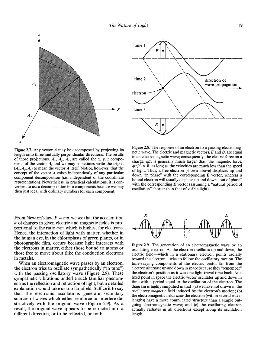
The Response of Electric Charges to Light 18
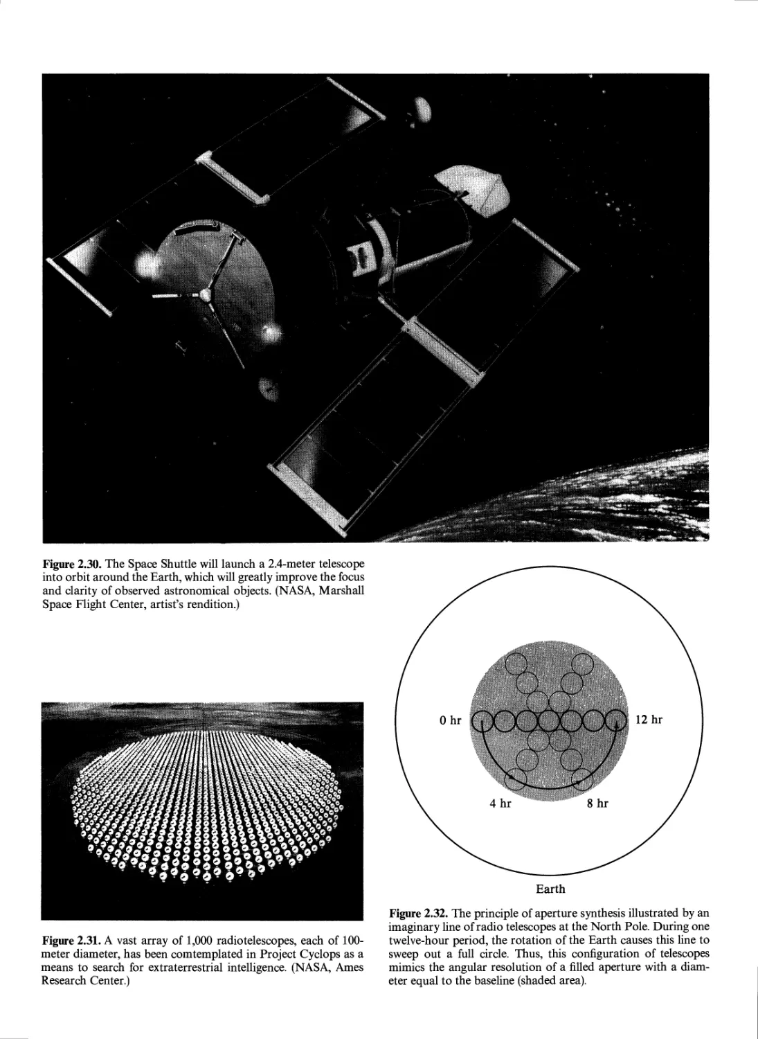
Astronomical Telescopes 20
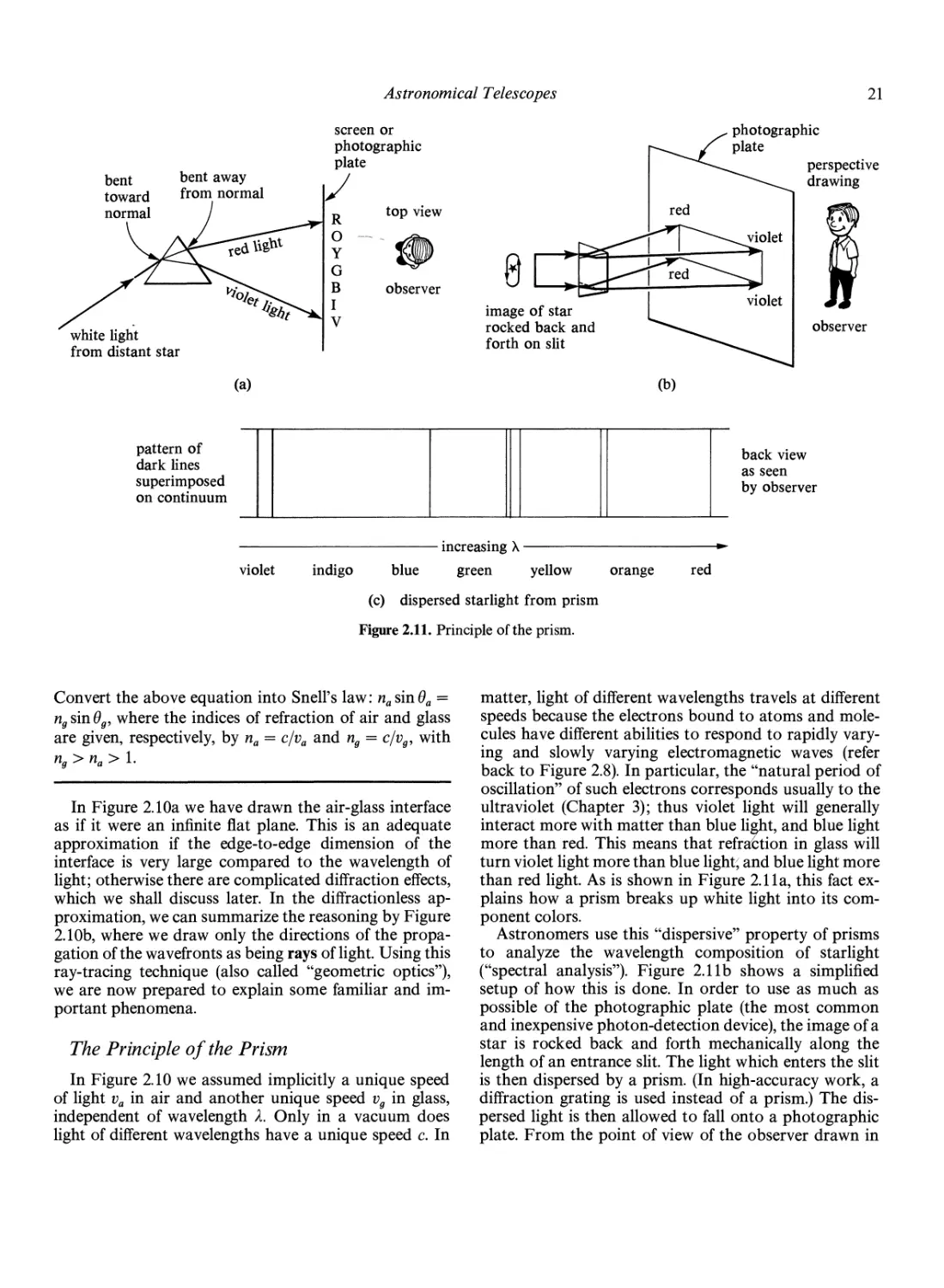
Refraction 20
The Principle of the Prism 21
The Principle of Lenses and the Refracting Telescope
Reflection 24
The Principle of Parabolic Mirrors and
the Reflecting Telescope 25
Angular Resolution 27
A stronom ical Instrumen ts and Measuremen ts 32
22
11
3. The Great Laws of Microscopic
Physics 33
Mechanics 33
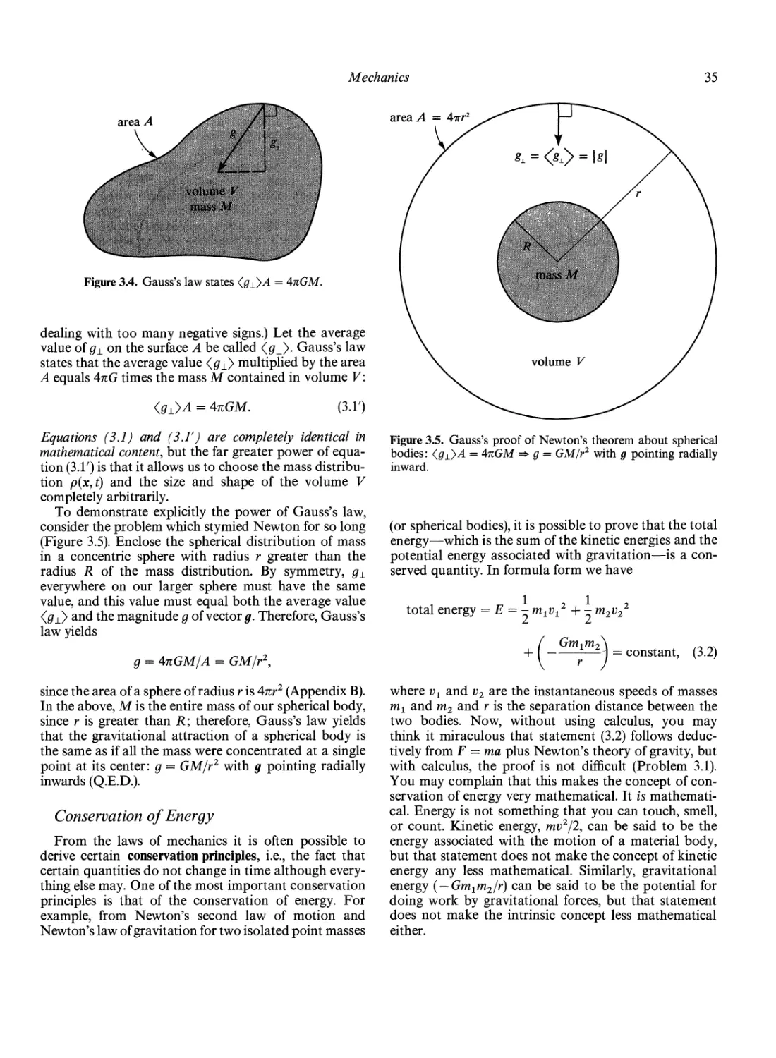
The Universal Law of Gravitation 34
Gauss's Formulation of the Law of Gravitation
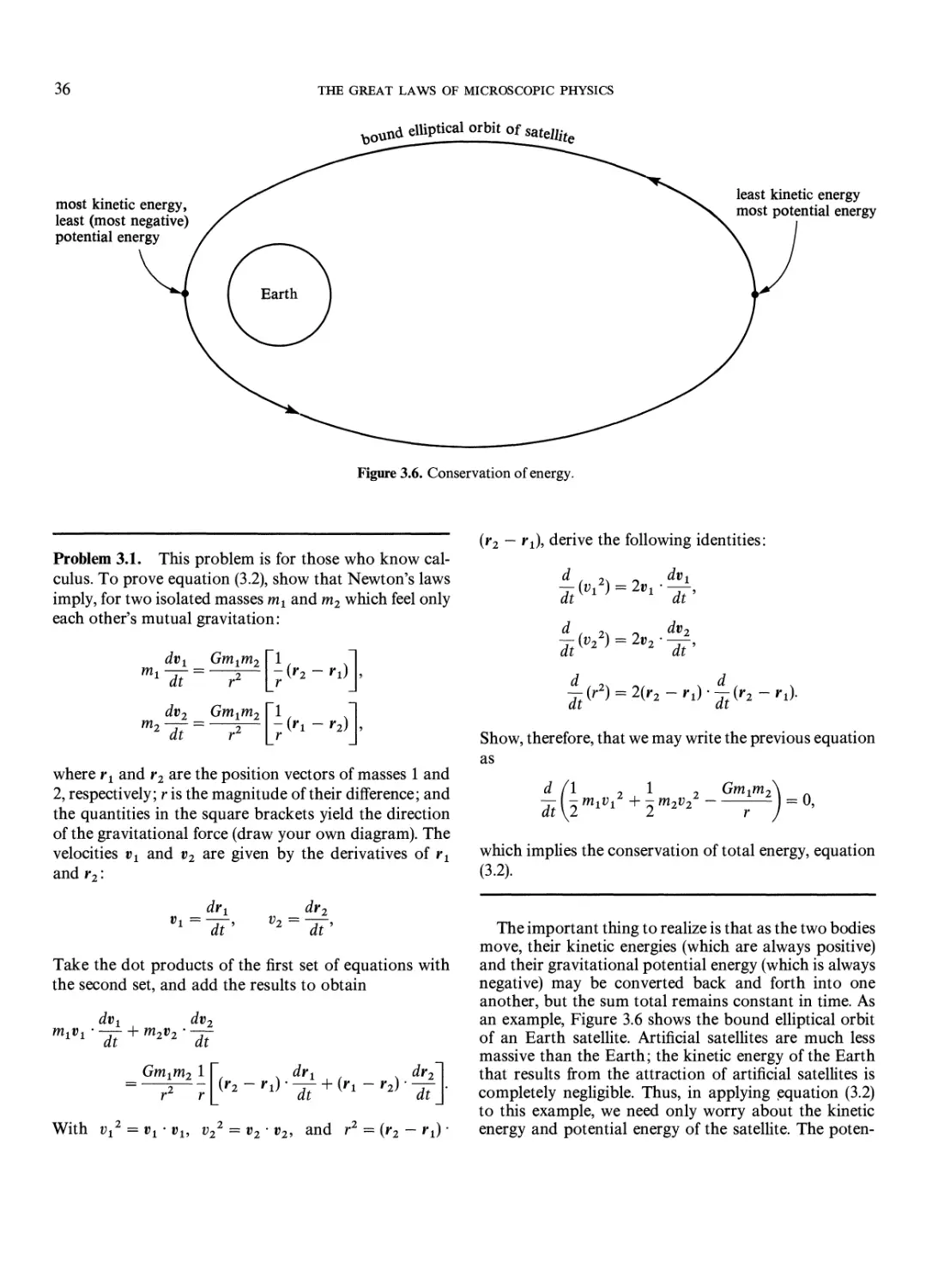
Conservation of Energy 35
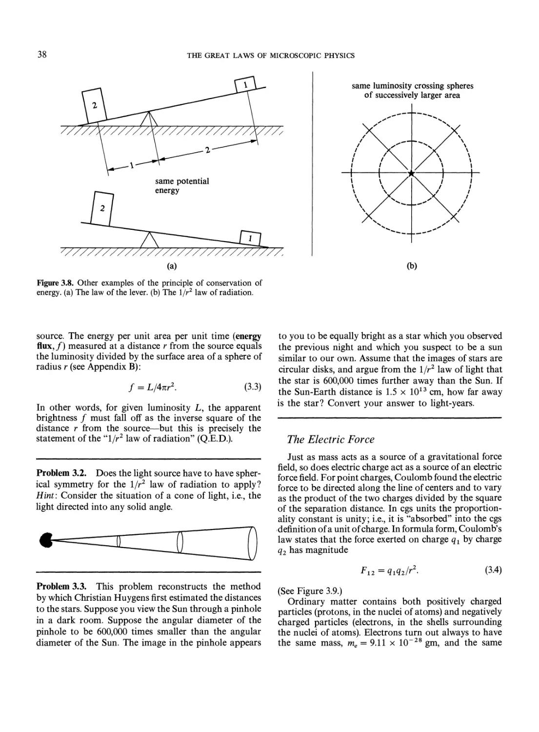
The Electric Force 38
Relative Strengths of Electric and Gravitational
Forces 39
Electromagnetism 39
Nuclear Forces 40
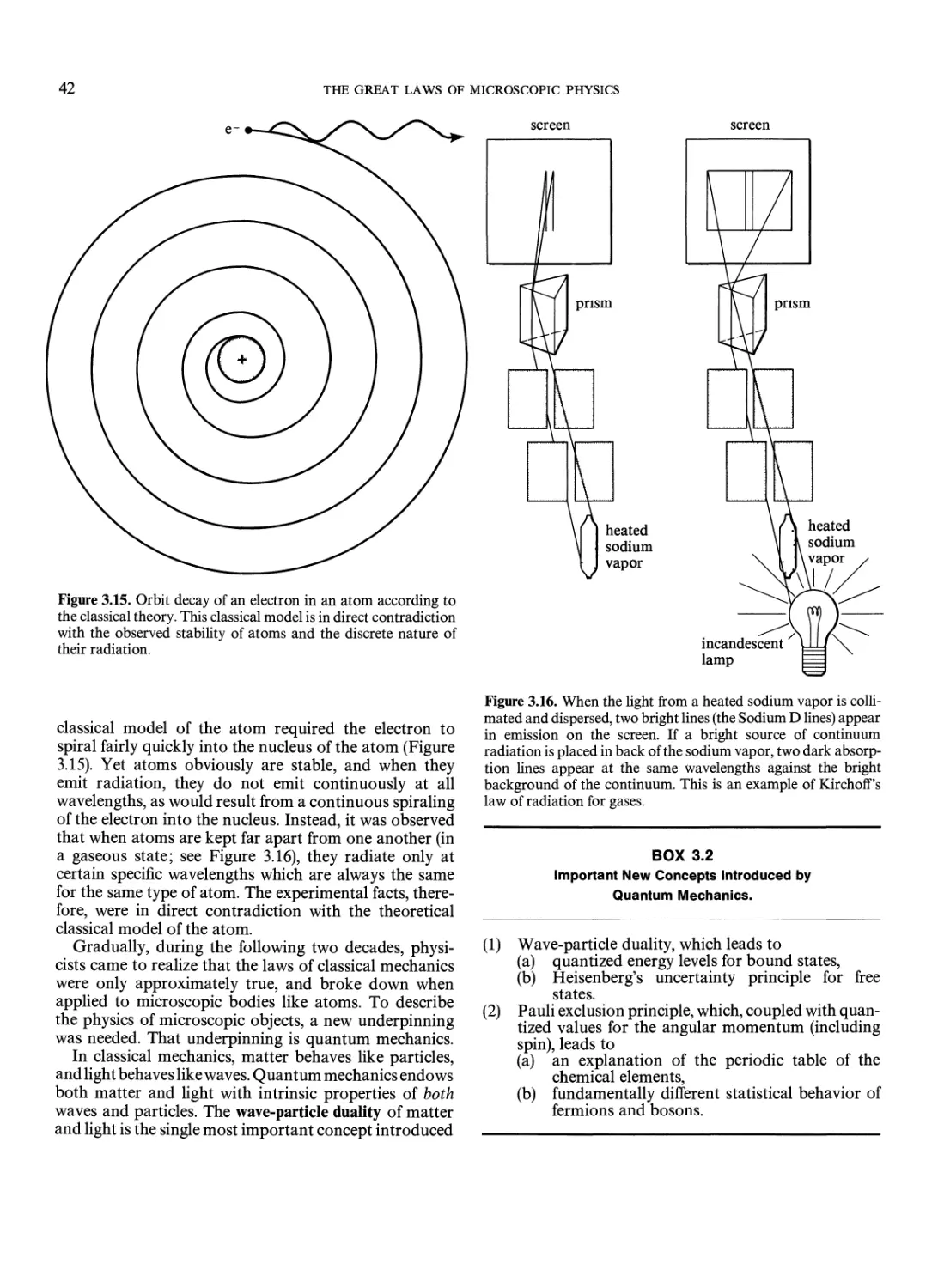
Quantum Mechanics 40
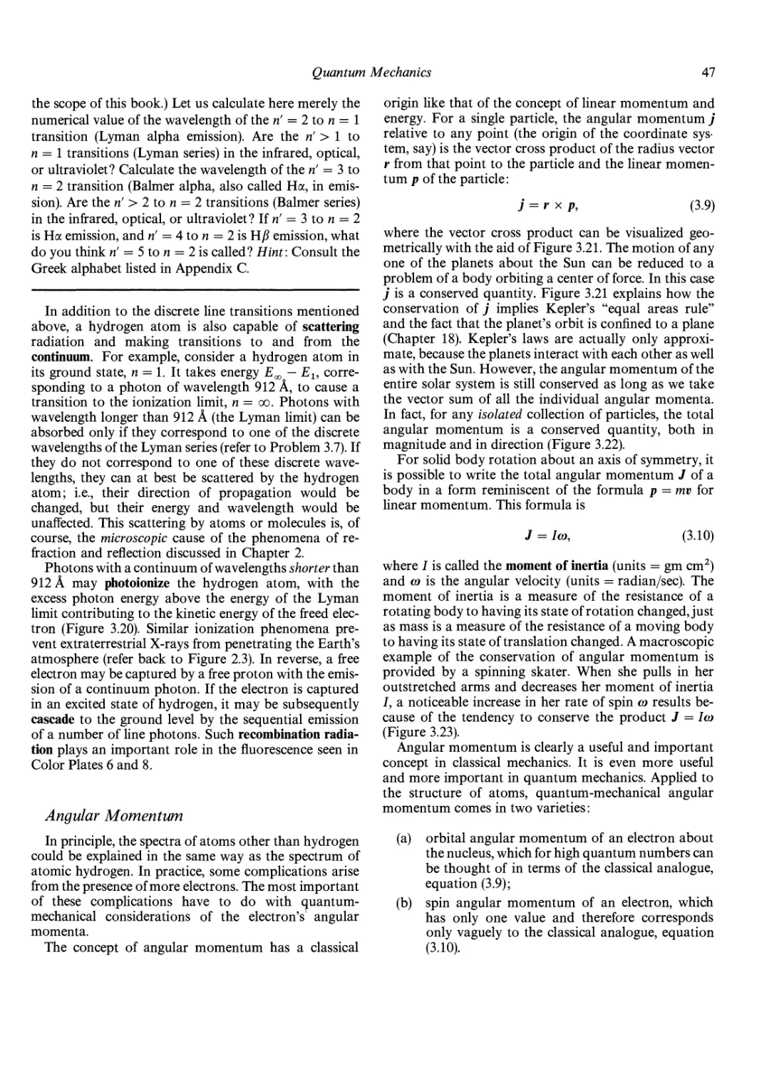
The Quantum-Mechanical Behavior of Light
The Quantum-Mechanical Behavior of Matter
Spectrum of the Hydrogen Atom 45
Angular Momentum 47
Orbital Angular Momentum 48
Spin Angular Momentum 49
Quantum Statistics 50
The Periodic Table of the Elements 50
Atomic Spectroscopy 52
34
43
44
CONTENTS
Special Relativity 53
Time Dilation 54
Lorentz Contraction 55
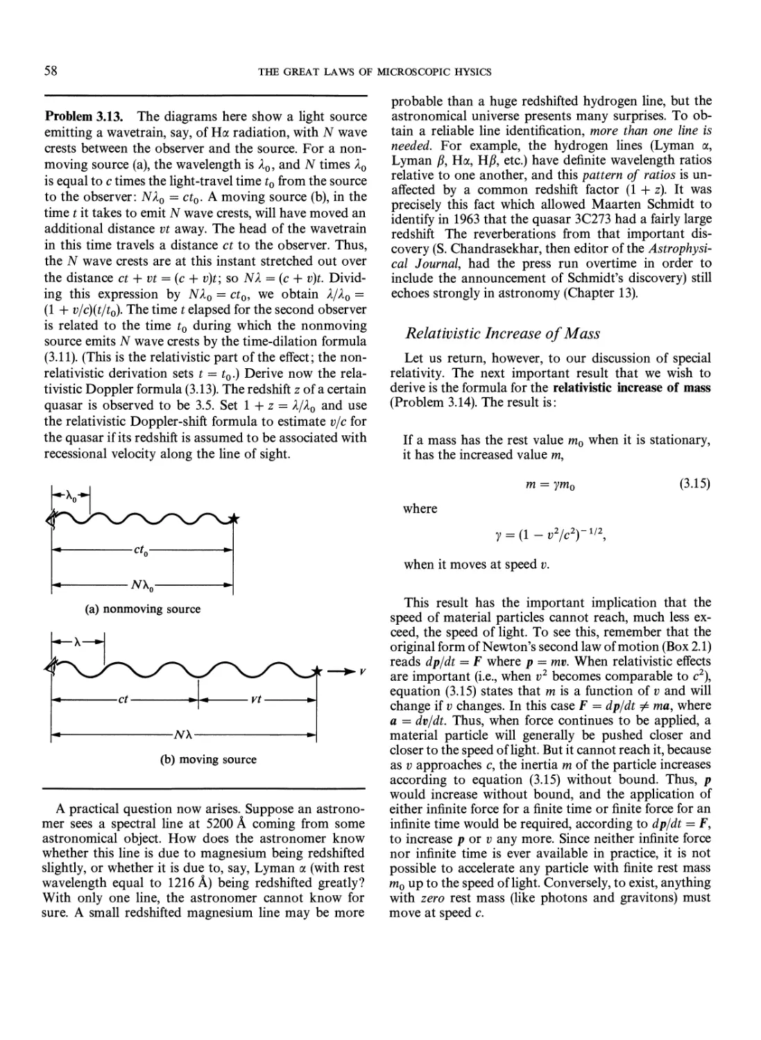
Relativistic Doppler Shift 57
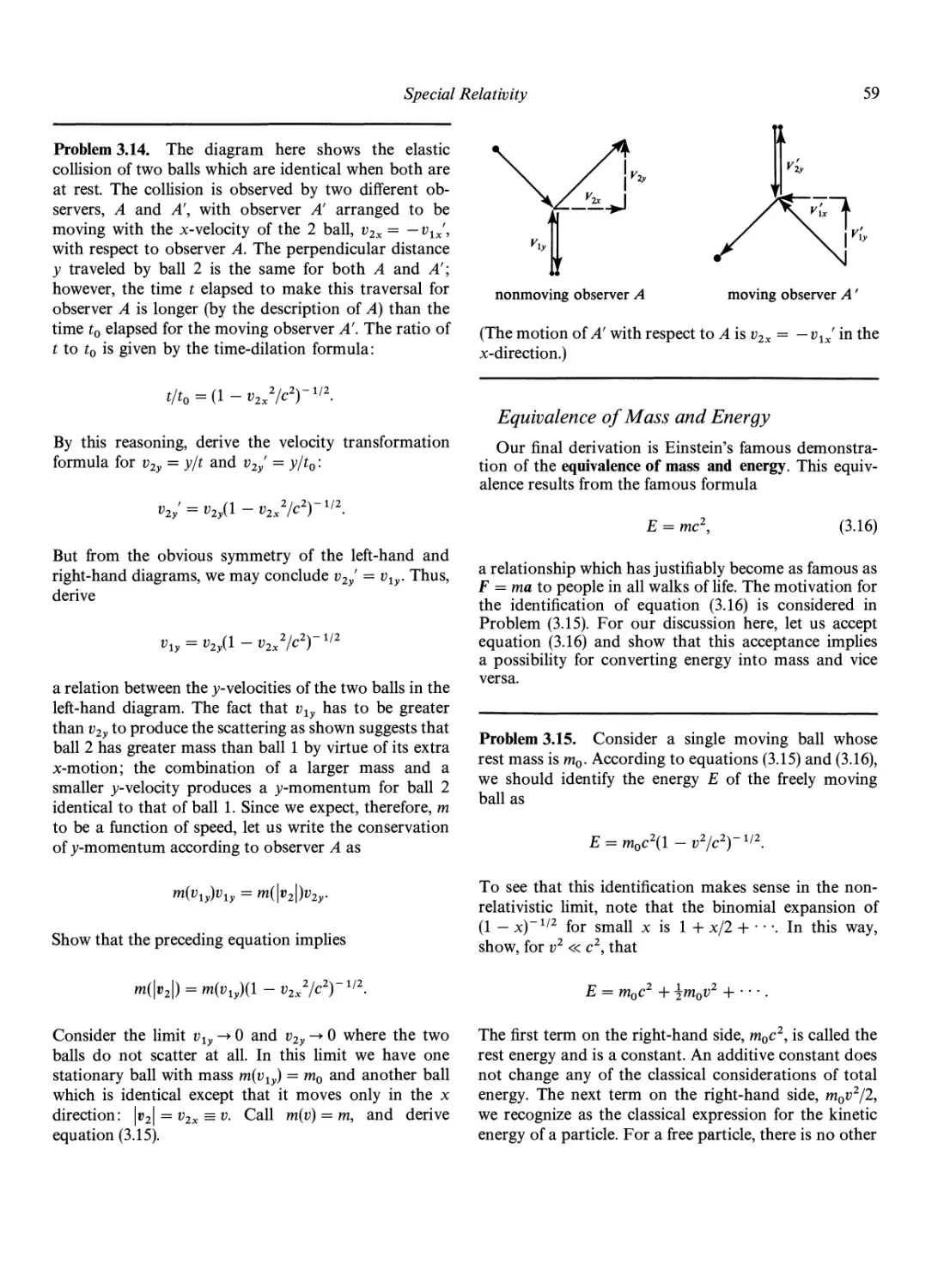
Relativistic Increase of Mass 58
Equivalence of Mass and Energy 59
Relativistic Quantum Mechanics 60
Concluding Philosophical Remarks
61
4. The Great Laws of
Macroscopic Physics
62
The Weak Nuclear Force 109
A tomic Nuclei 110
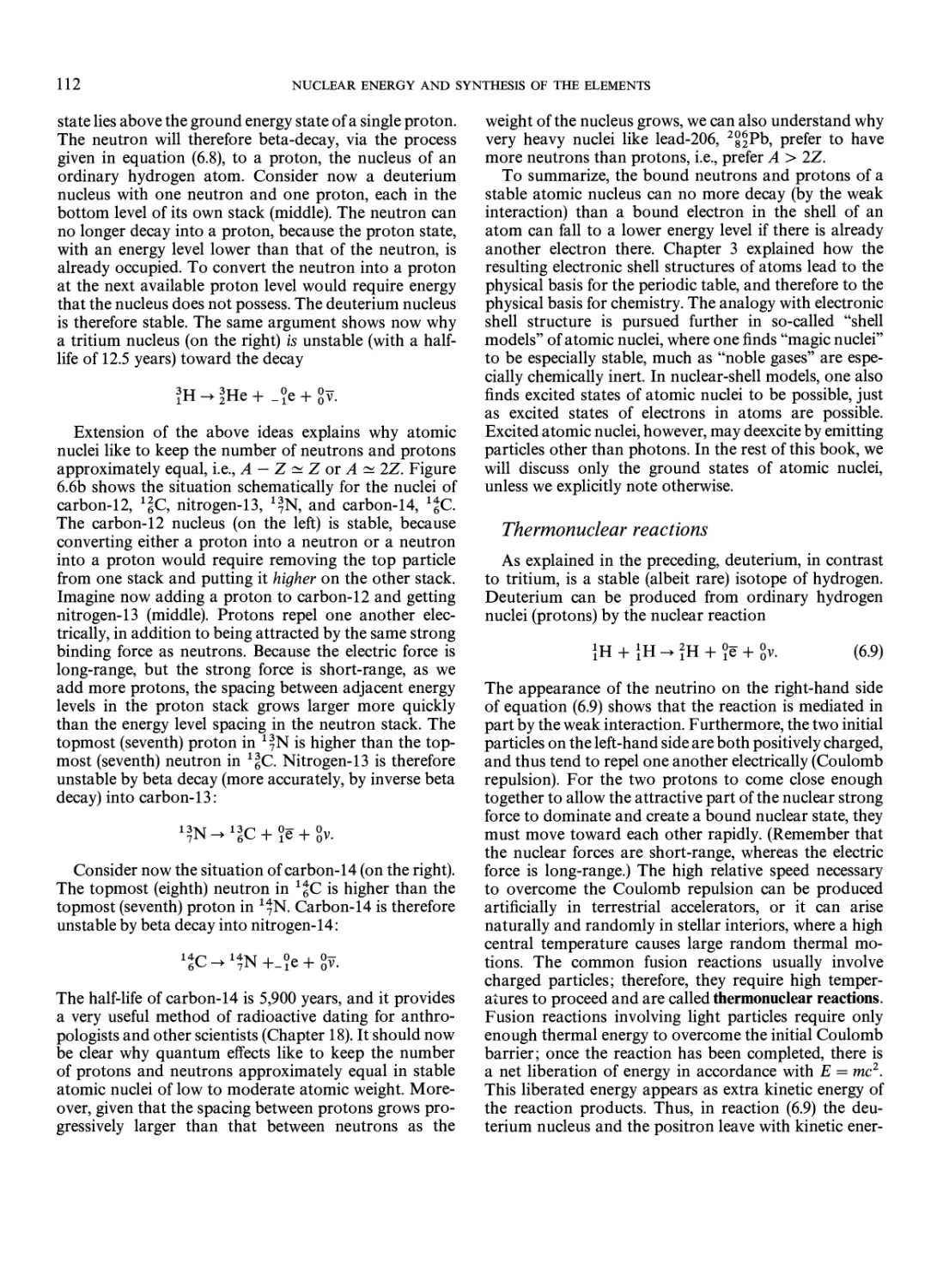
Thermonuclear Reactions 112
Th e Pro ton-Pro ton Chain 113
The CNO Cycle 113
Temperature Sensitivity of
Thermonuclear Reactions 114
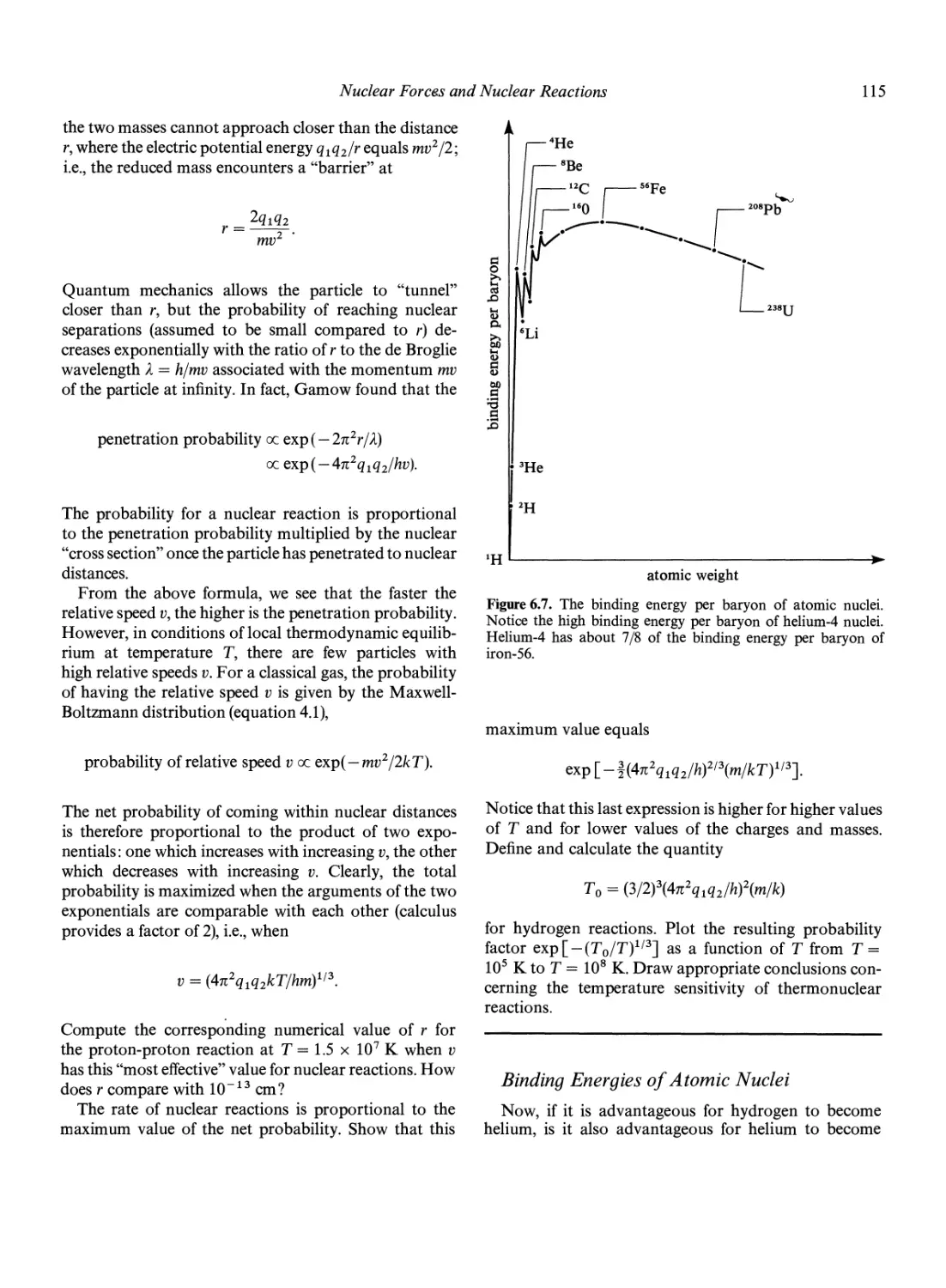
Binding Energies of A tomic Nuclei 115
The Triple Alpha Reaction 117
The General Pattern of Thermonuclear Fusion
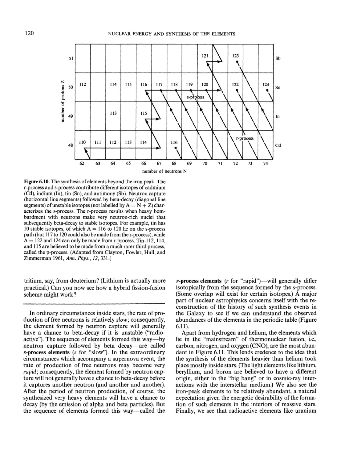
The r and s Processes 119
The Solar Neutrino Experiment 121
Speculation About the Future 123
Thermodynamics 62
Alternative Statements of the Second Law of
Thermodynamics 63
The Statistical Basis of Thermodynamics 63
Statistical Mechanics 64
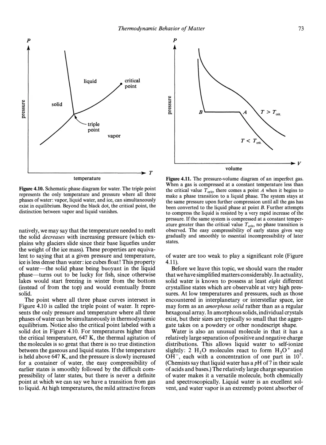
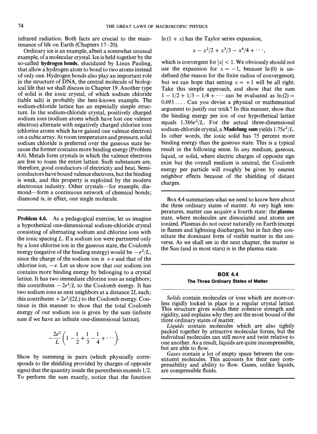
Thermodynamic Behavior of Matter 66
The Properties of a Perfect Gas 66
Acoustic Waves and Shock Waves 68
Real Gases, Liquids, and Solids 71
Macroscopic Quantum Phenomena 75
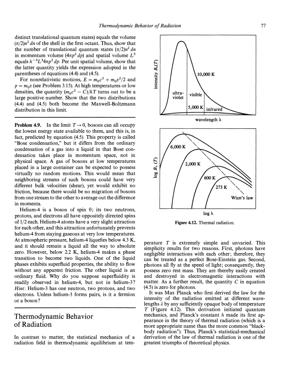
Thermodynamic Behavior of Radiation 77
An Example 80
Philosophical Comment 80
7. The End States of Stars
125
White Dwarf 126
Elec tron-Degeneracy Pressure 126
Mass-Radius Relation of Wh ite Dwarfs 127
Source of Luminosity of a White Dwarf 129
Neutron Stars 129
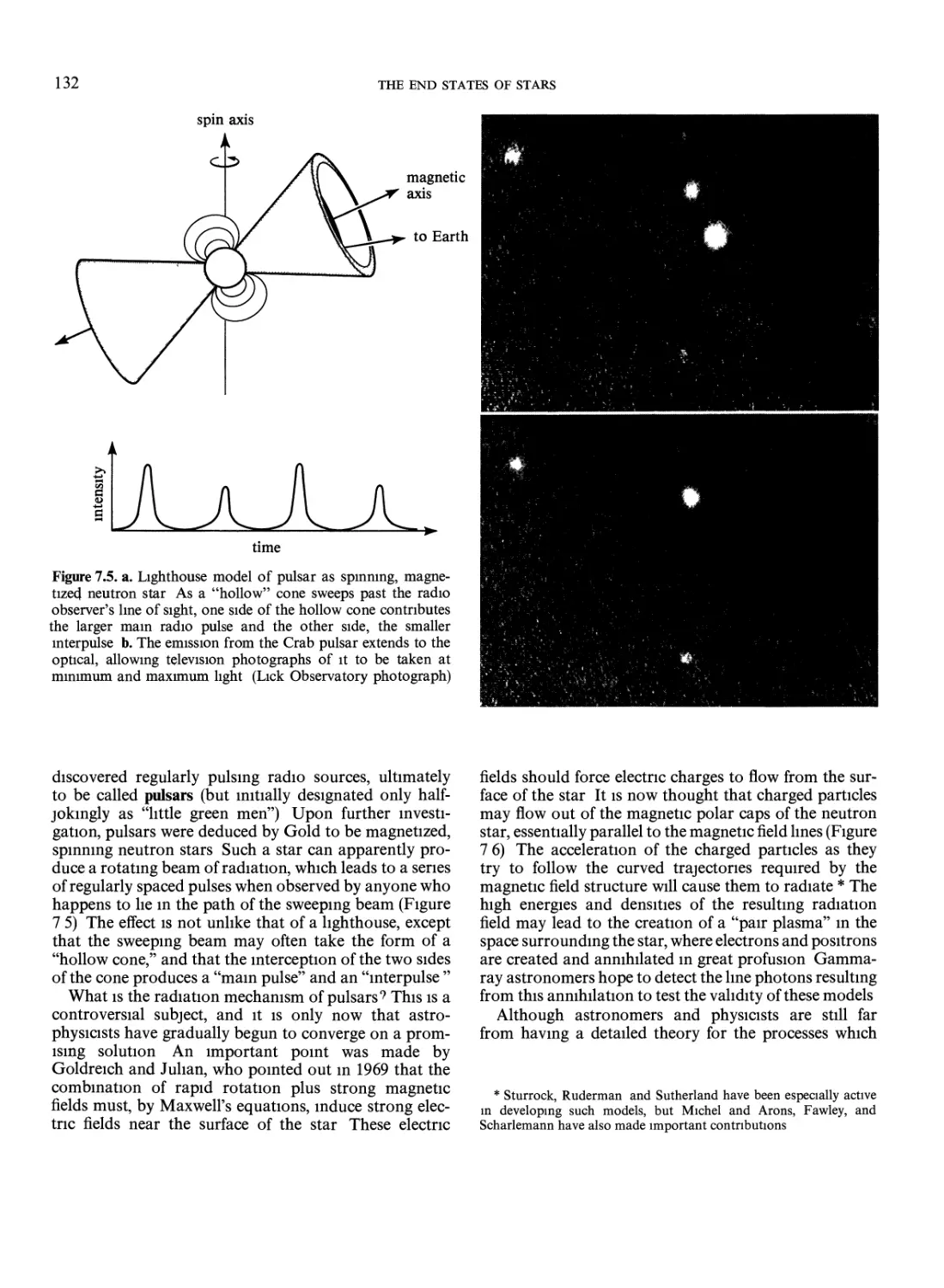
Upper Mass Limit for Neutron Stars 131
Neutron Stars Observable as Pulsars 131
The Masses of Neutron Stars 134
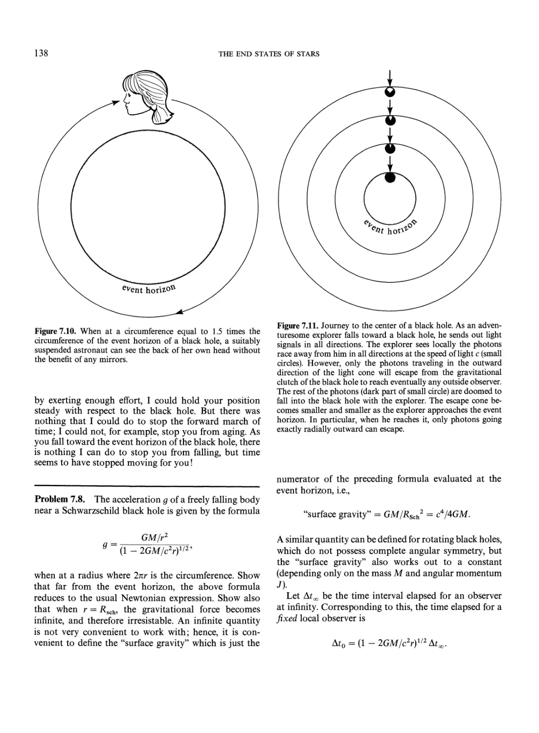
Black Holes 134
Gravitational Distortion of Space time 135
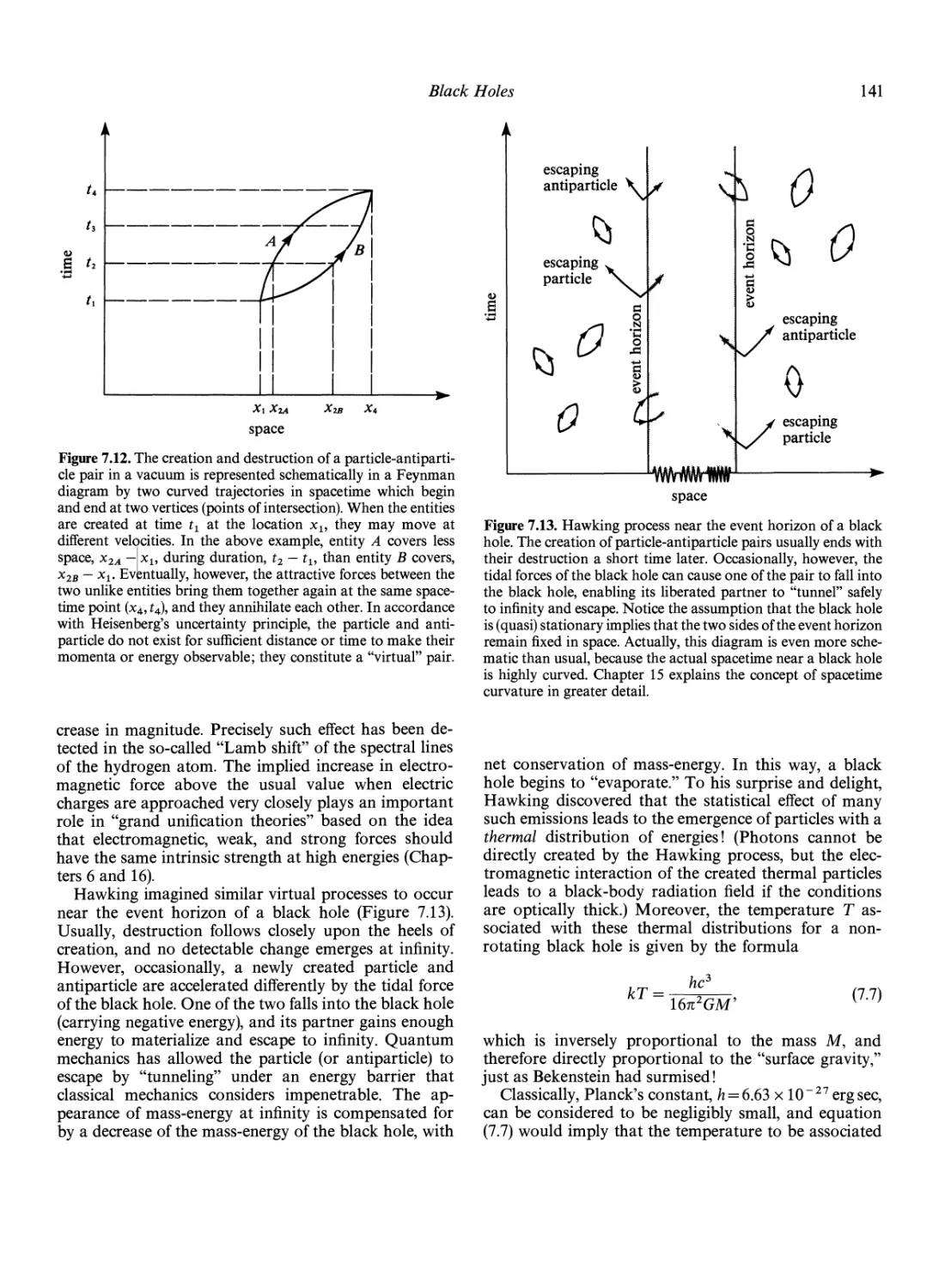
Thermodynamics of Black Holes 139
Concluding Philosophical Remarks 143
Part II. The Stars 81
5. The Sun as a Star 83
8. Evolution of the Stars
144
84
The Atmosphere of the Sun
The Interior of the Sun 86
Radiative Transfer in the Sun 89
The Source of Energy of the Sun 90
The Stability of the Sun 92
Summary of the Principles of Stellar Structure
The Convection Zone of the Sun 95
The Chromosphere and Corona of the Sun
Magnetic Activity in the Sun 98
The Relationship of the Sun to Other Stars
and to Us 100
145
94
96
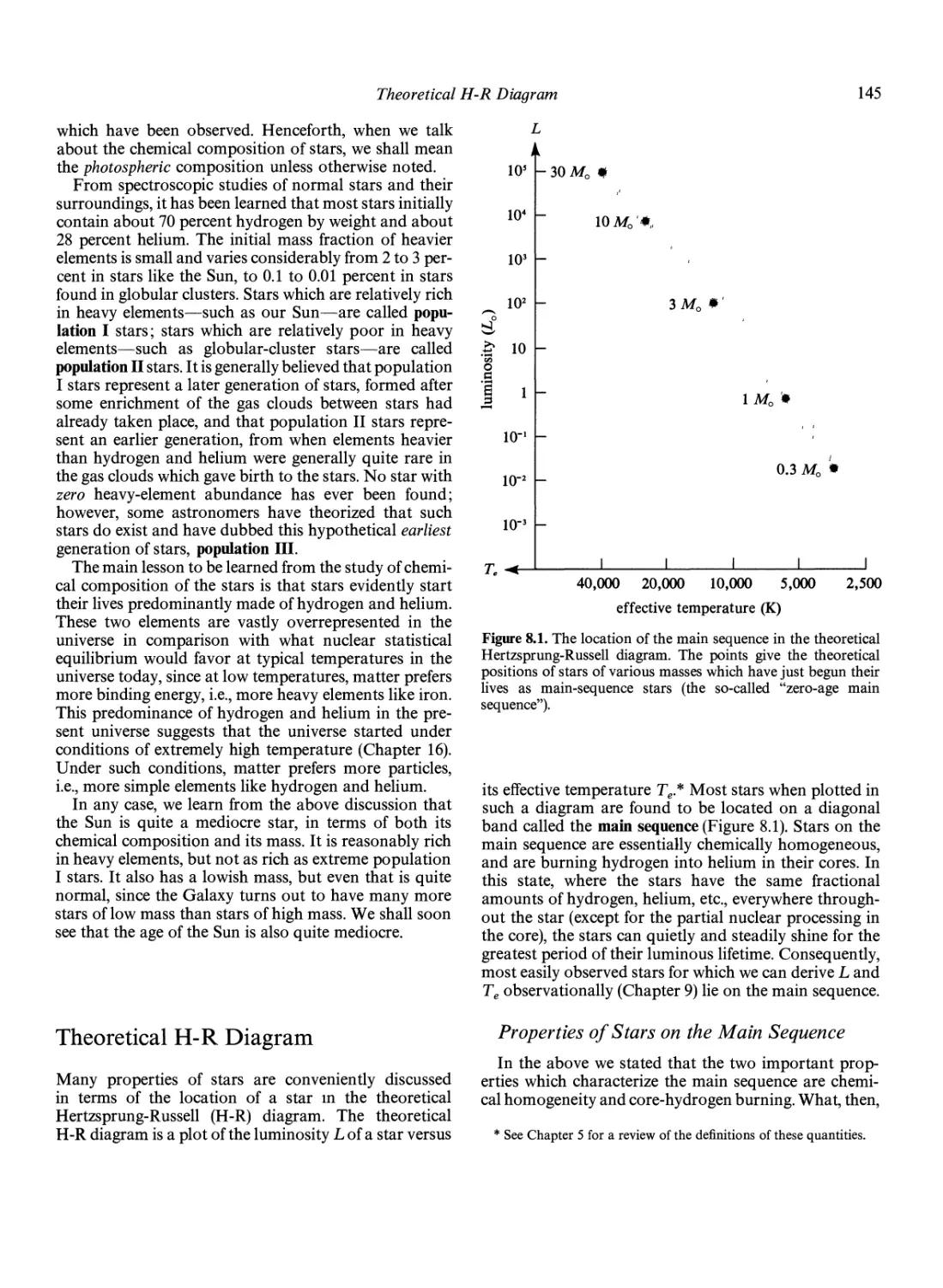
Theoretical H-R Diagram 145
Properties of Stars on the Main Sequence
Evolution of Low-Mass Stars 147
Ascending the Giant Branch 147
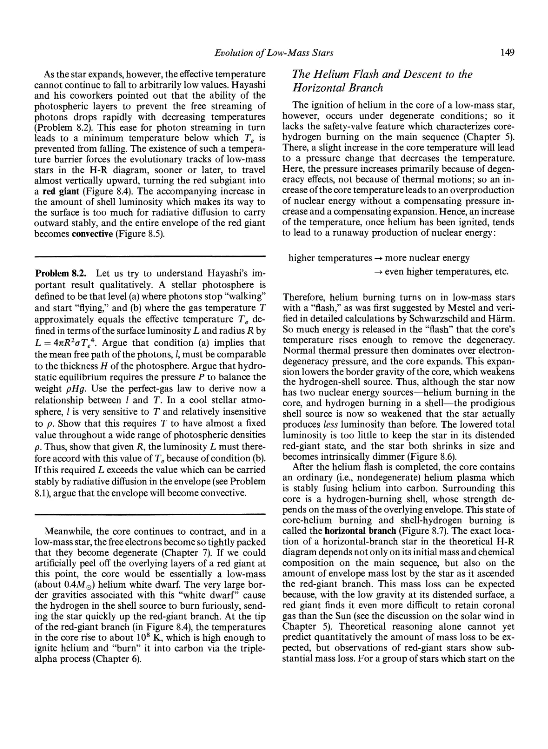
The Helium Flash and Descent to the Horizontal
Branch 149
Ascending the Asymptotic Giant Branch 151
Planetary Nebulae and White Dwarfs 152
Evolution of High-Mass Stars 153
Approach to the Iron Catastrophe 153
Supernova of Type II 154
Concluding Philosophical Remark 157
6. Nuclear Energy and Synthesis
of the Elements 102
Matter and the Four Forces 103
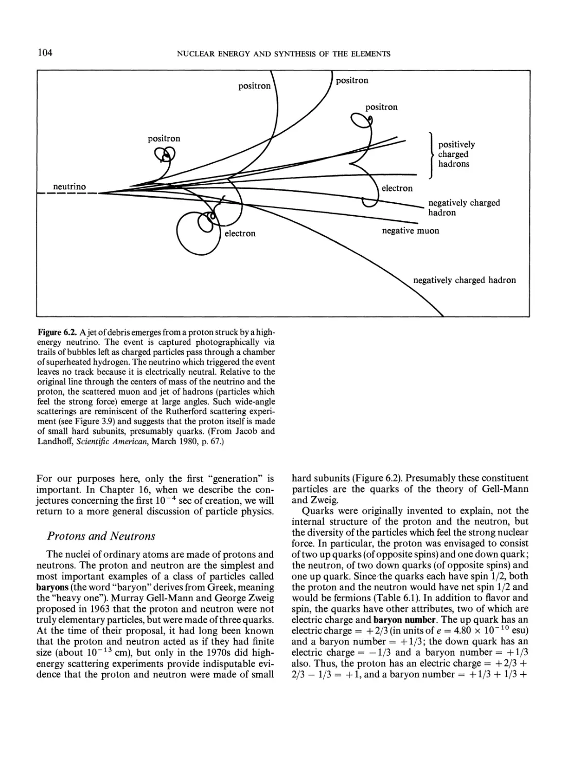
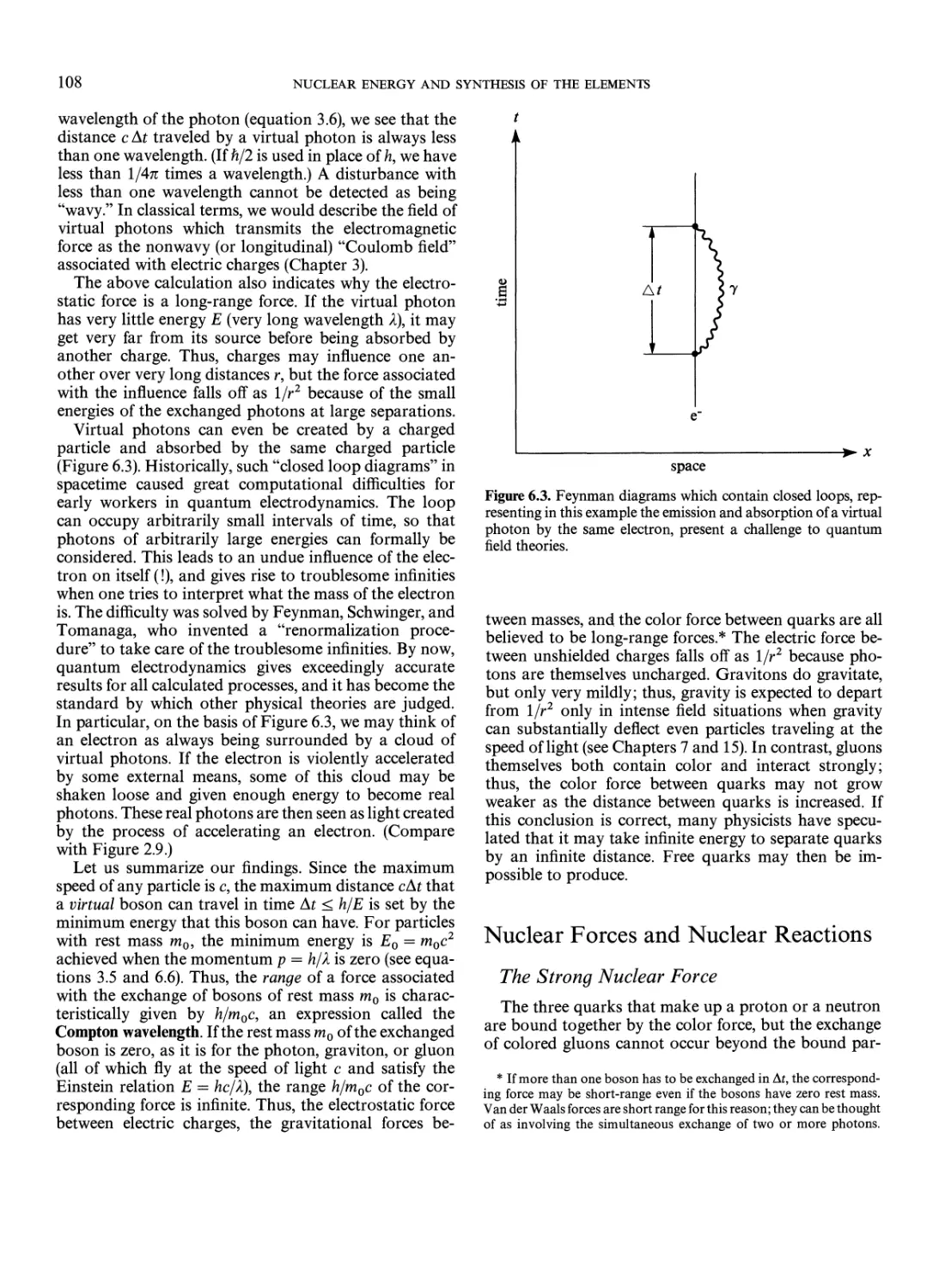
Pro tons and Neutrons 104
Electrons and Neutrinos 105
Particles and Antiparticles 105
The Quantum-Mechanical Concept of Force
Nuclear Forces and Nuclear Reactions
The Strong Nuclear Force 108
107
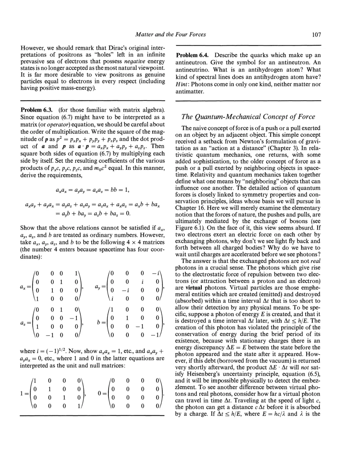
108
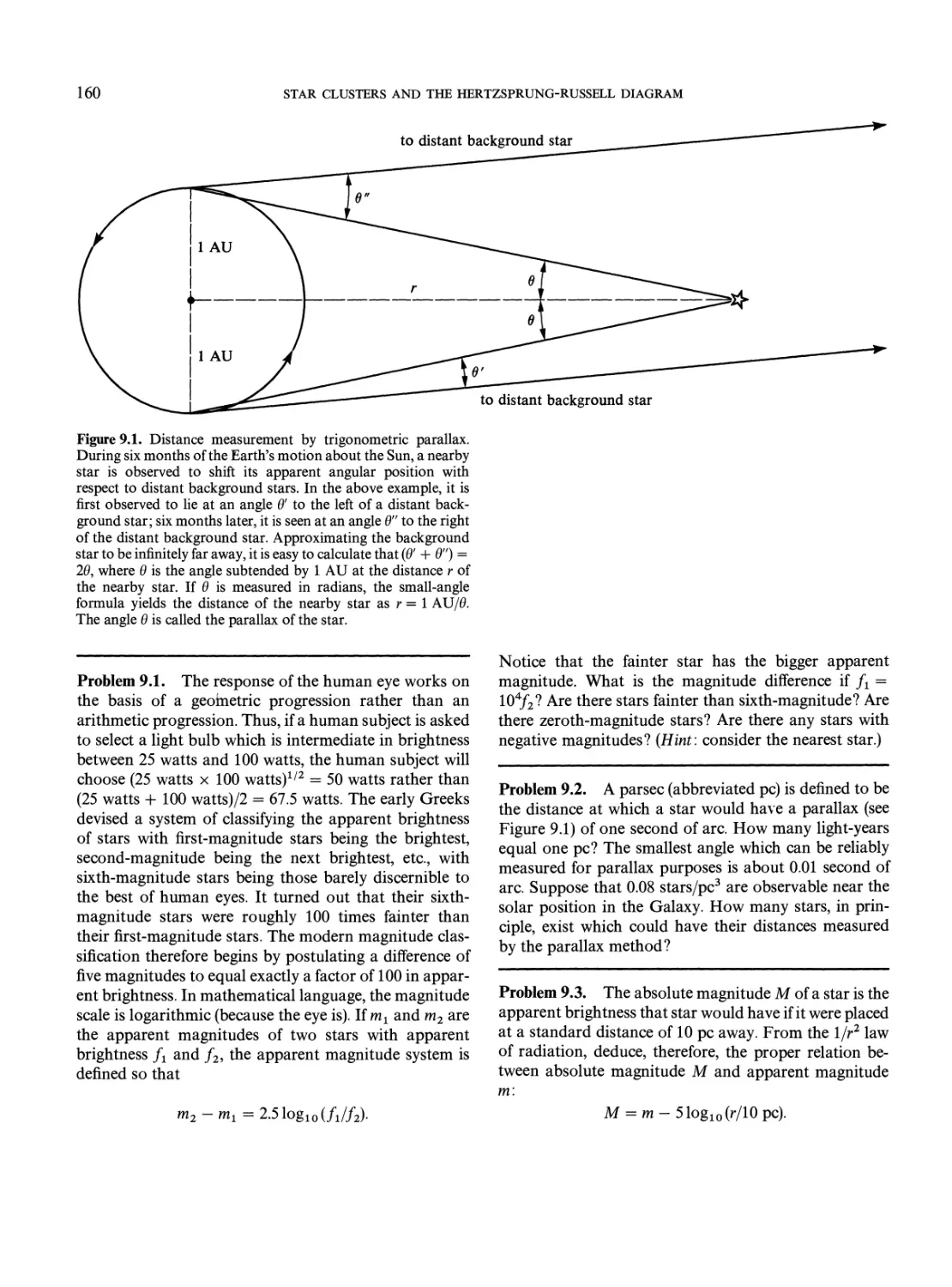
9. Star Clusters and the Hertzsprung-
Russell Diagram 159
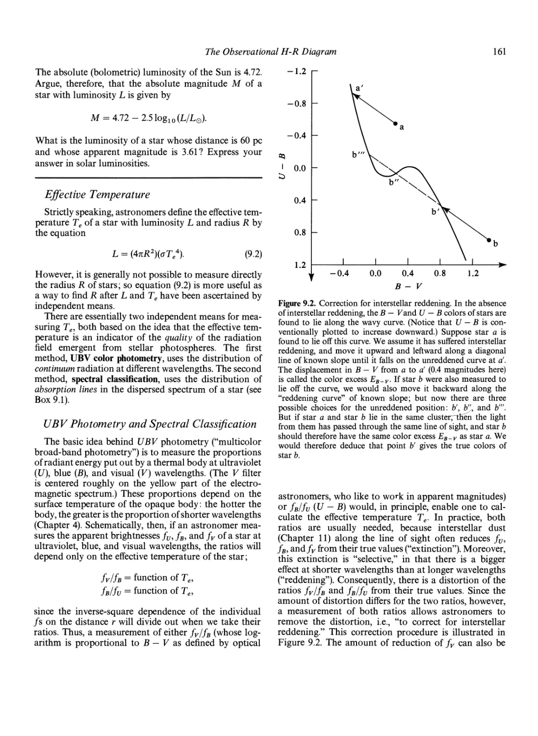
The Observational H-R Diagram 159
Luminosity 159
Effective Temperature 161
UBV Photometry and Spectral Classification
Luminosity Class 164
CONTENTS
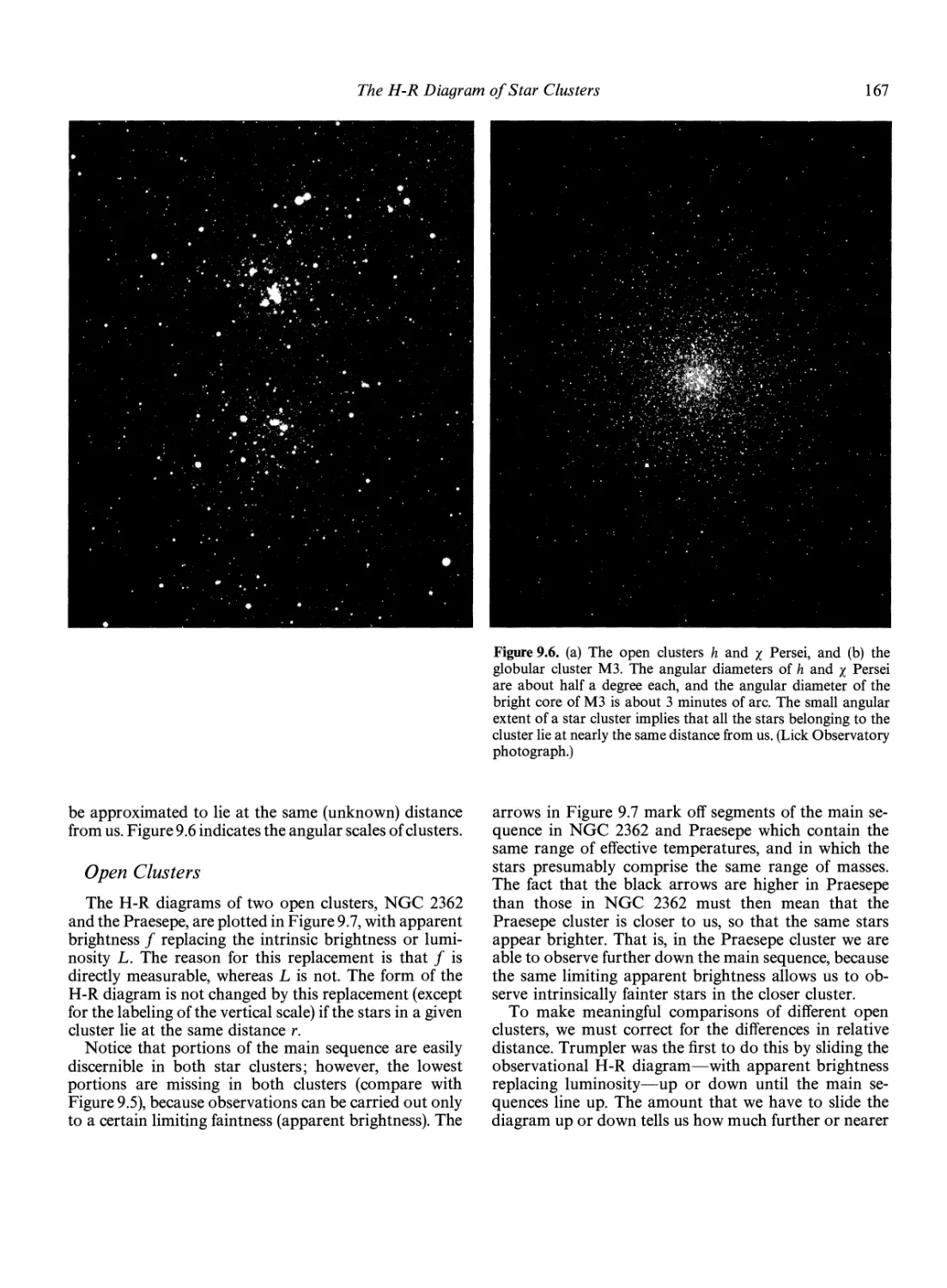
The H-R Diagram of Nearby Stars 166
The H-R Diagram of Star Clusters 166
Open Clusters 167
Distance to the Hyades Cluster 169
Cepheid Period-Luminosity Relation 170
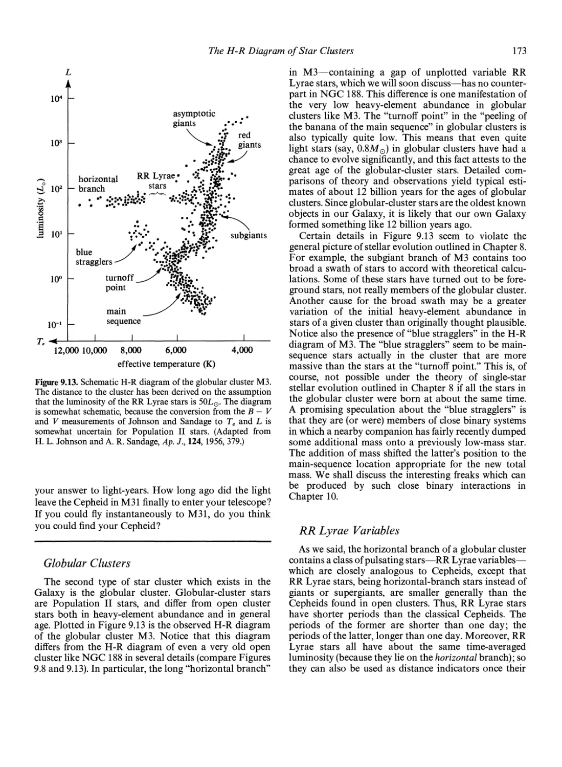
Globular Clusters 173
RR Lyrae Variables 173
Population II Cepheids 174
Dynamics of Star Clusters 174
Philosophical Comment 178
10. Binary Stars 179
Observational Classification of
Binary Stars 179
The Formation of Binary Stars 184
Evolution of the Orbit Because of
Tidal Effects 185
Classification of Close Binaries Based on the
Roche Model 186
Mass Transfer in Semidetached Binaries 188
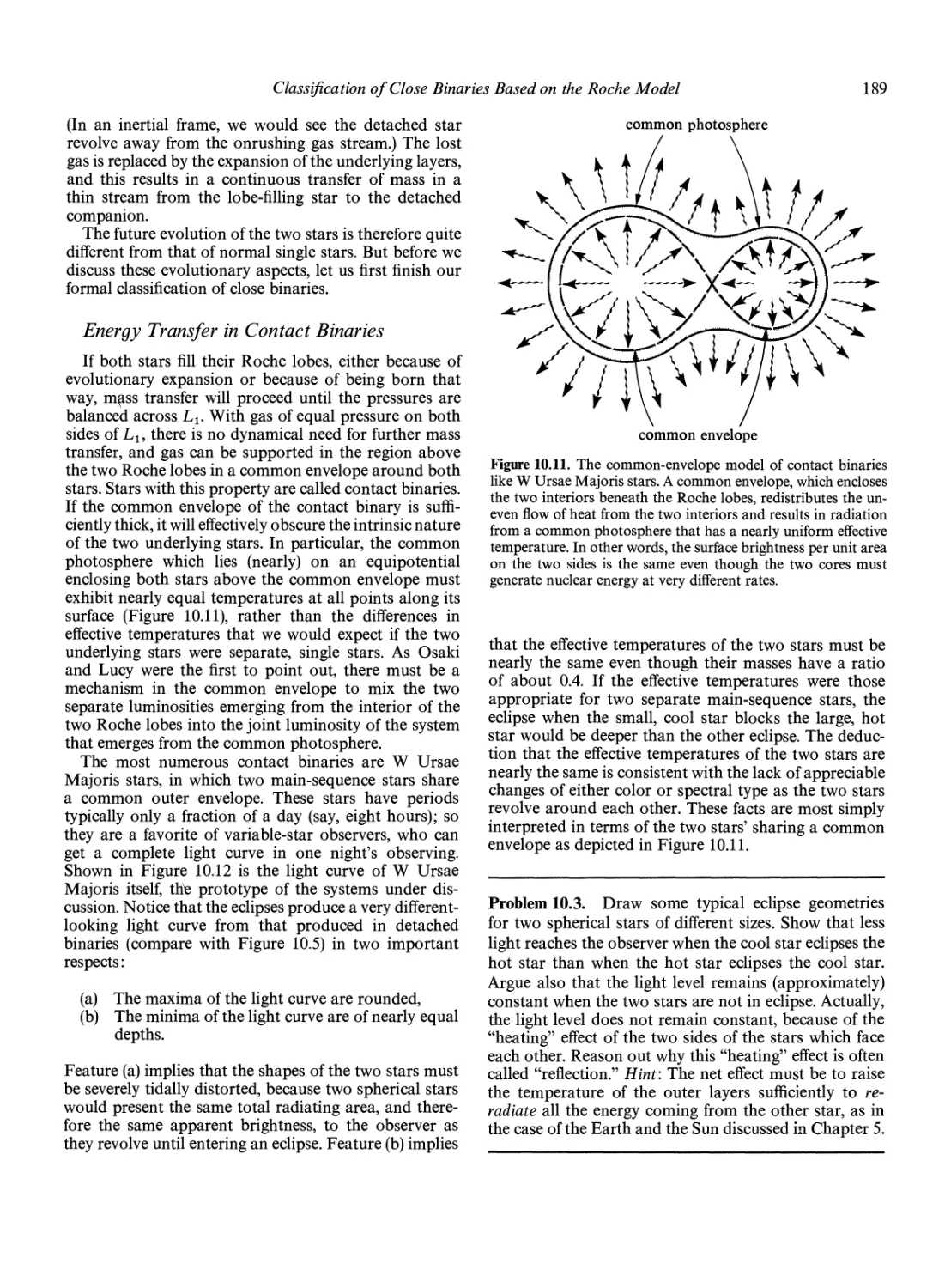
Energy Transfer in Contact Binaries 189
Evolution of Semidetached System 191
Detached Component = Normal Star: Algols 191
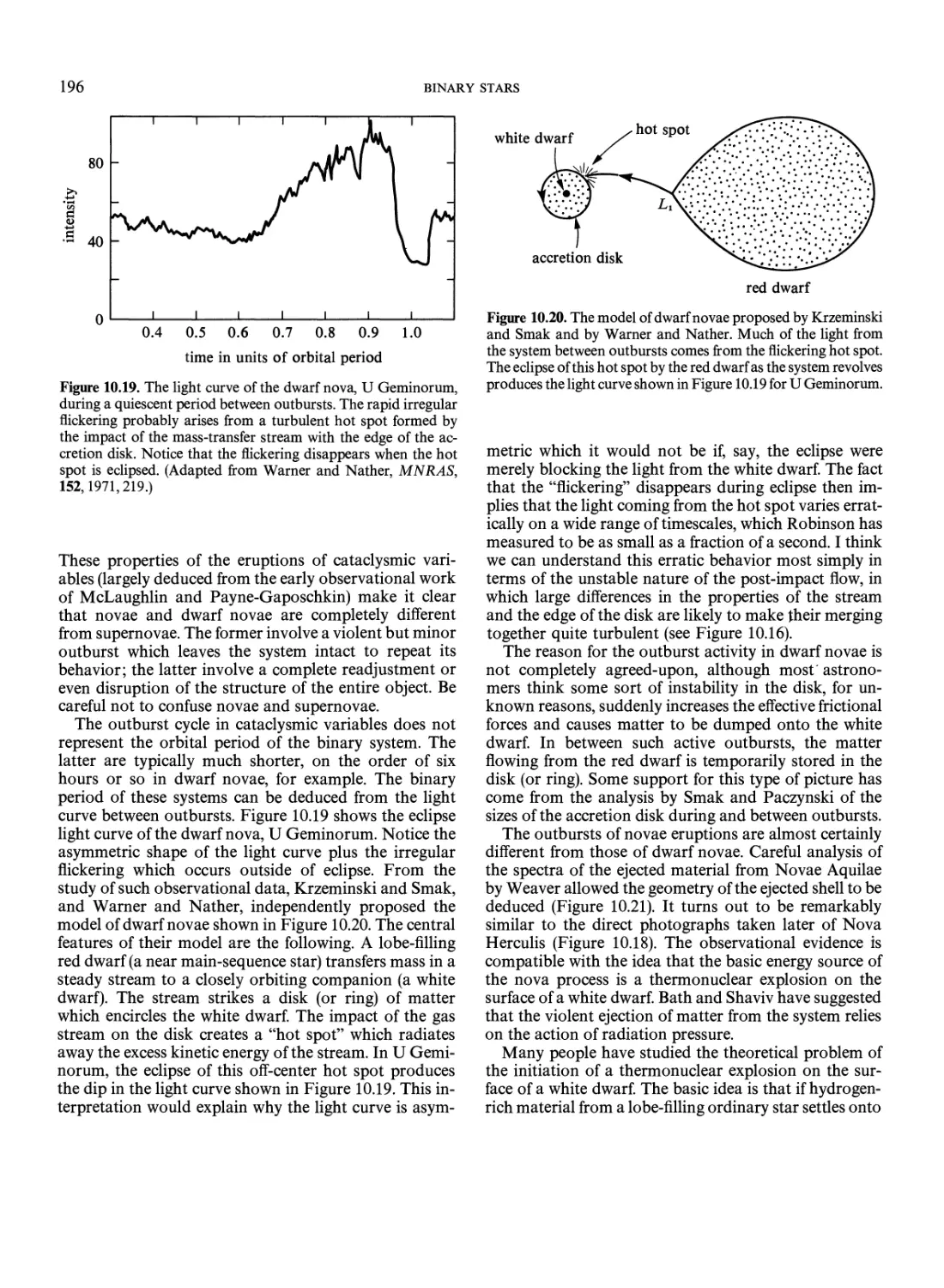
A cere t ion D isks 193
Detached Component = White Dwarf: Cataclysmic
Variables 195
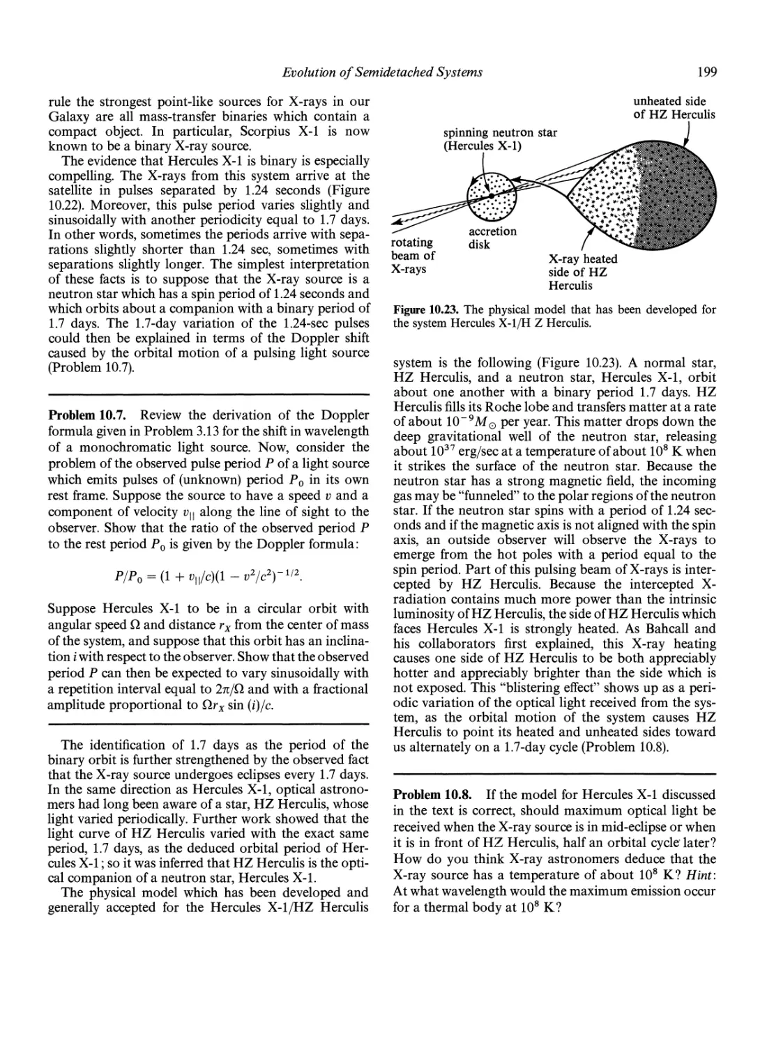
Detached Component = Neutron Star: Binary X-ray
Sources 198
Interesting Special Examples of Close
Binary Stars 203
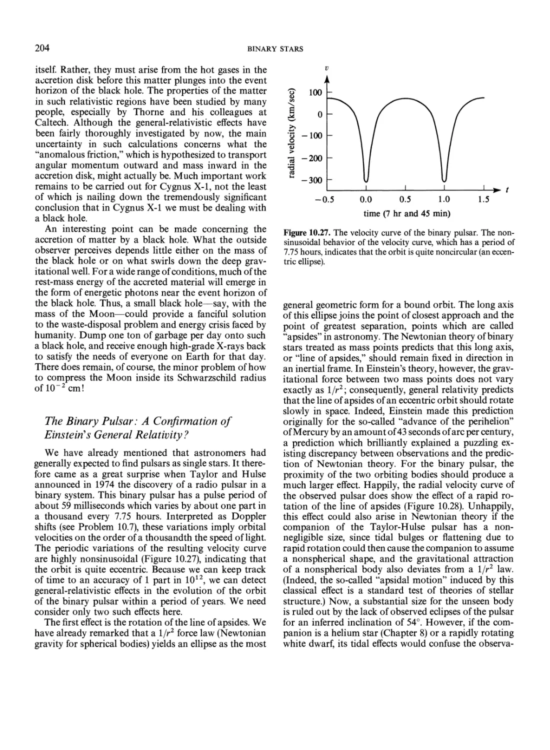
Cygnus X-l: A Black Hole ? 203
The Binary Pulsar: A Confirmation of Einstein's
General Relativity ? 204
SS433 206
Concluding Remarks 208
Part III. Galaxies and Cosmology 209
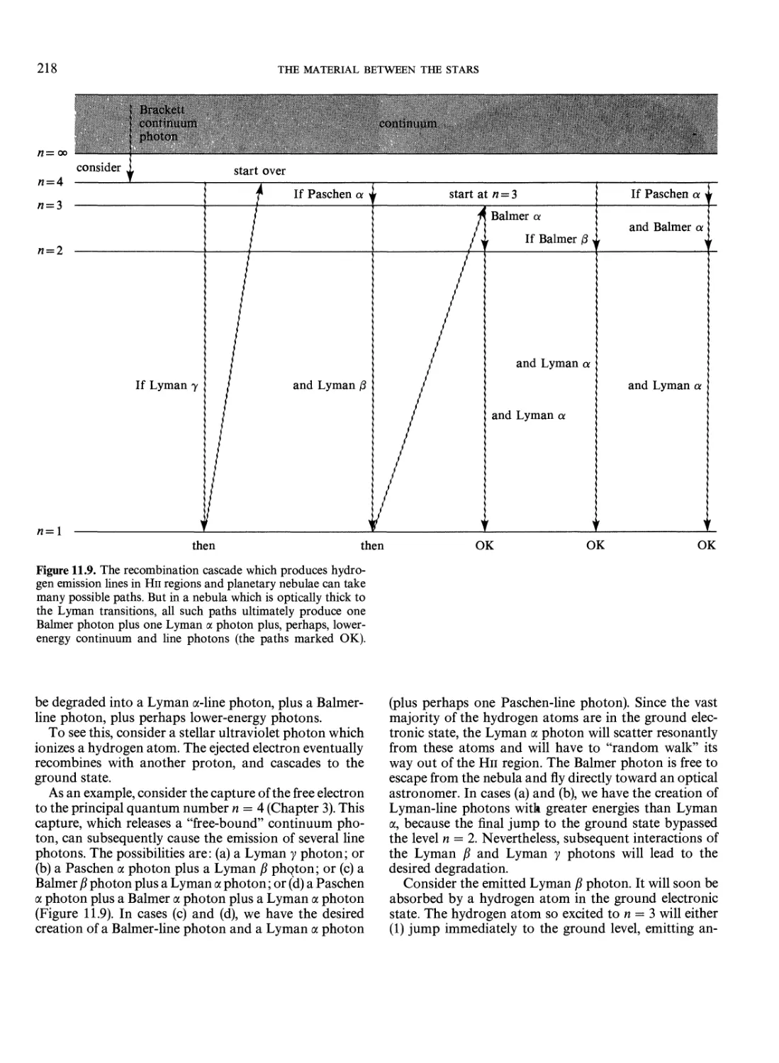
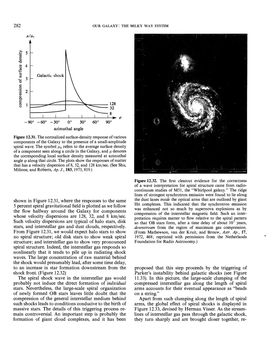
11. The Material Between the Stars 211
The Discovery of Interstellar Dust 211
The Discovery of Interstellar Gas 214
Different Optical Manifestations of
Gaseous Nebulae 215
Dark Nebulae 216
Reflection Nebulae 216
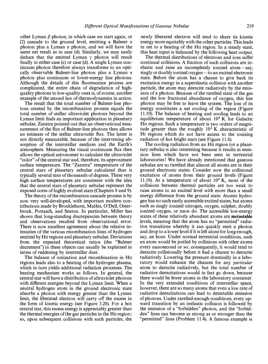
Thermal Emission Nebulae: HII Regions 216
Nonthermal Emission Nebulae:
Supernova Remnants 223
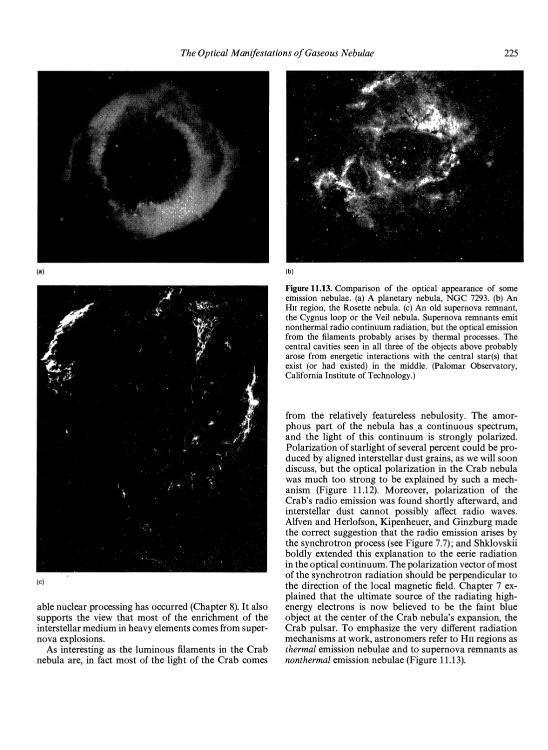
Radio Manifestations of Gaseous Nebulae 226
Radio Recombination Lines 226
Thermal Radio Continuum Emission 226
21-cm-Line Radiation from HI Regions 227
Radio Lines from Molecular Clouds 231
Infrared Manifestations of
Gaseous Nebulae 234
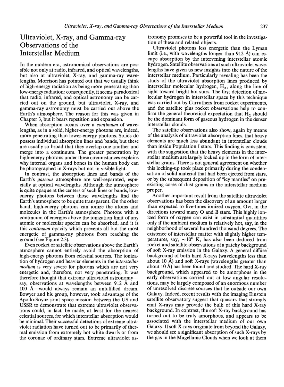
Ultraviolet, X-ray, and Gamma-ray Observations
of the Interstellar Medium 237
Cosmic Rays and the Interstellar
Magnetic Field 239
Interactions Between Stars and the
Interstellar Medium 245
The Death of Stars 245
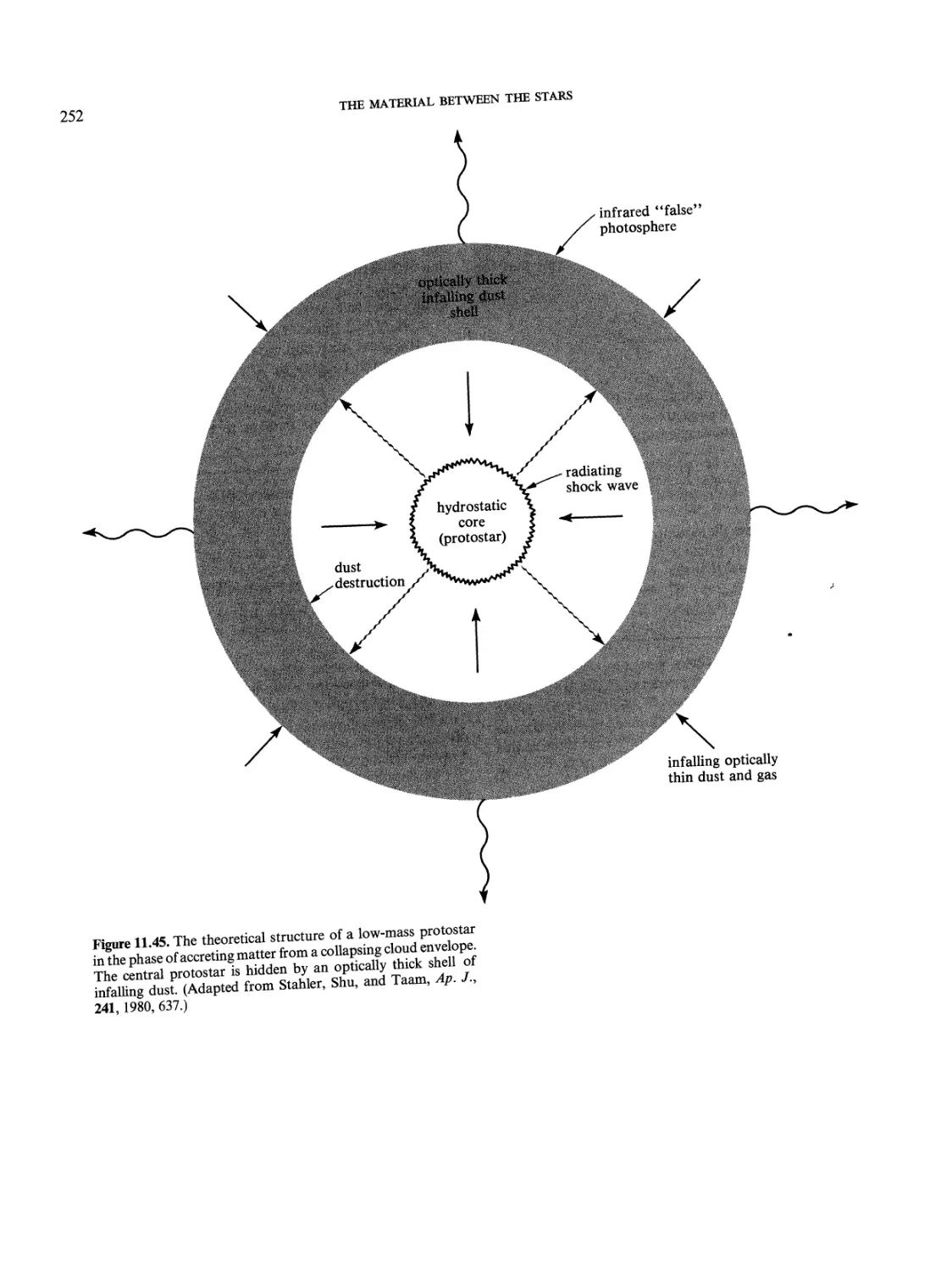
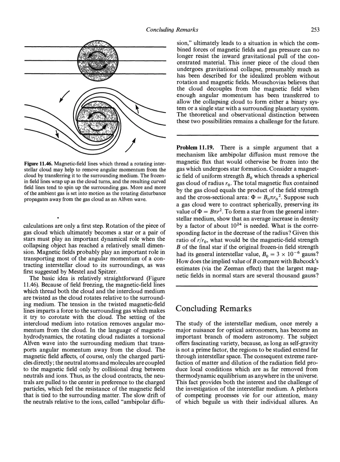
The Birth of Stars 248
Concluding Remarks 253
12. Our Galaxy: The Milky
Way System 255
The True Shape and Size of the Milky
Way System 257
Stellar Populations 258
Stellar Motions and Galactic Shape 259
Missing-Mass Problem 259
The Local Mass-to-Light Ratio 260
Mass of the Halo 261
Differential Rotation of the Galaxy 261
The Local Standard of Rest 261
Local Differential Motions 262
Crude Estimates of the Mass of the Galaxy 264
The Insignificance of Stellar Encounters 264
The Theory ofEpicyclic Orbits 265
The Large-Scale Field of Differential Rotation 267
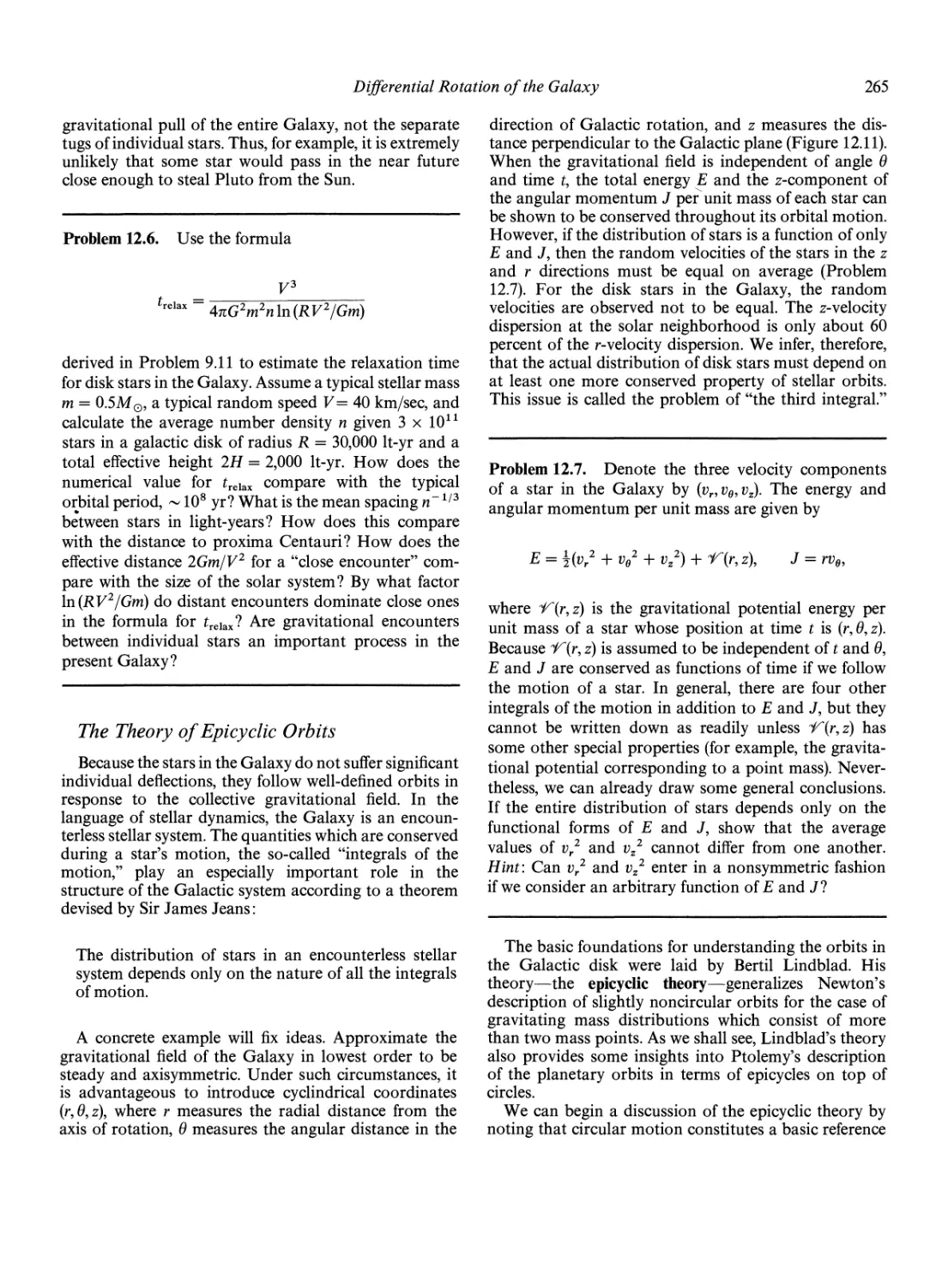
The Thickness of the Gas Layer 270
Kinematic Distances 271
Spiral Structure 272
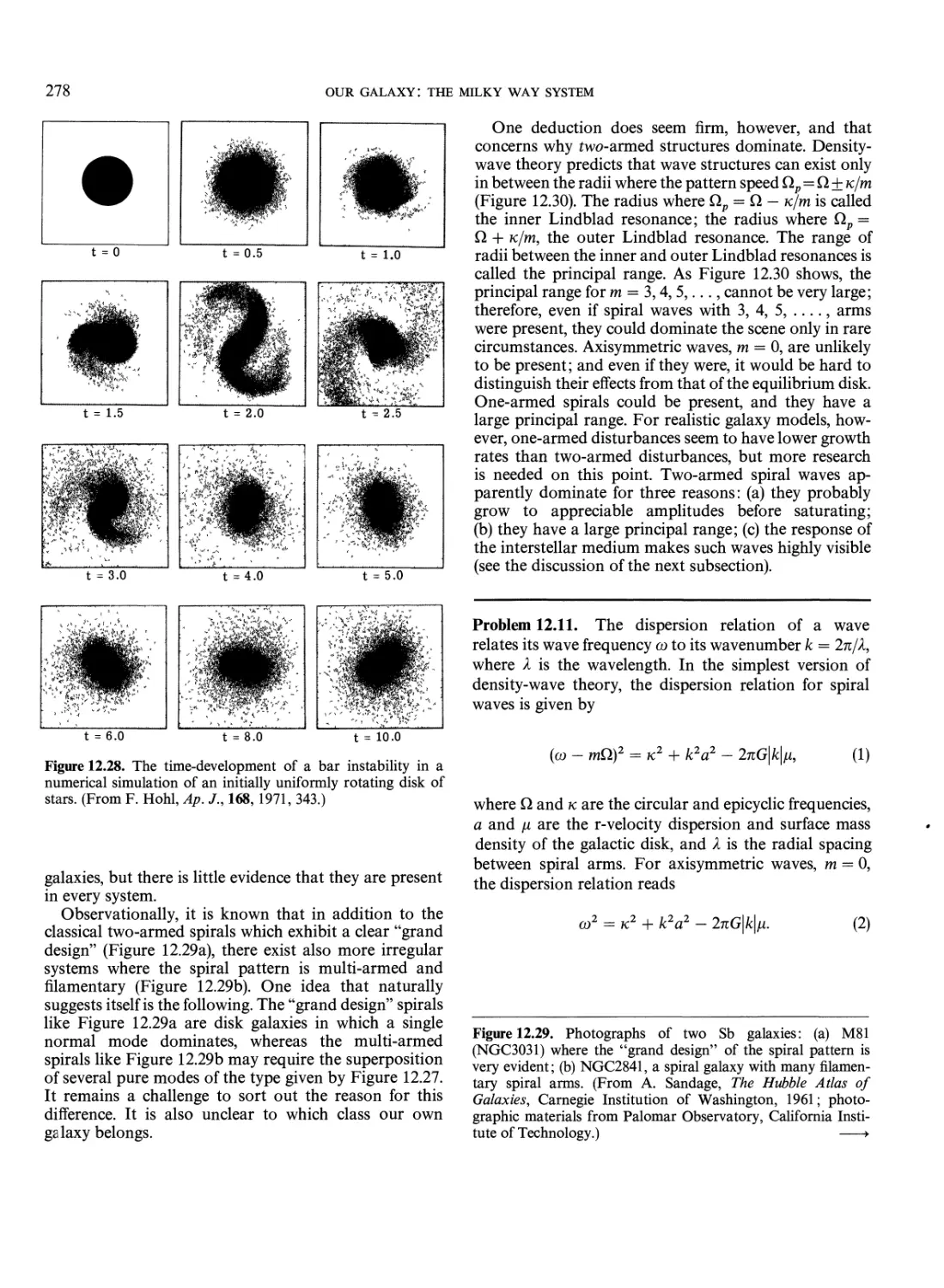
The Nature of the Spiral Arms 274
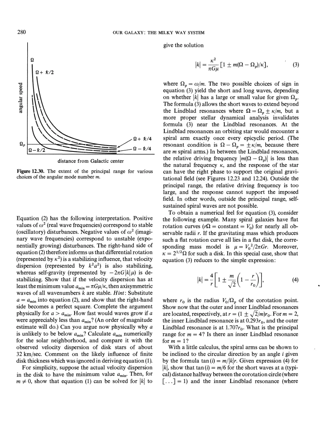
The Density-Wave Theory of Galactic
Spiral Structure 275
The Basic Reason for Spiral Structure 281
The Birth of Stars in Spiral Arms 281
Concluding Remarks 284
13. Quiet and Active Galaxies 286
The Shapley-Curtis Debate 286
The Distances to the Spirals 286
Spirals: Stellar or Gaseous Systems? 287
The Zone of Avoidance 288
The Resolution of the Controversy 291
The Classification of Galaxies 293
Hubble*s Morphological Types 293
Ellipticals 293
Spirals 294
Refinements ofHubble's Morphological Scheme 296
Stellar Populations 296
Van den BergKs Luminosity Class 297
CONTENTS
The Distribution of Light and Mass in
Regular Galaxies 297
Surface Photometry of Galaxies 297
Velocity Dispersions in Ellipticals and Rotation Curves
of Spirals 298
The Loc F4 Law for Ellipticals and Spirals 305
Dynamics of Barred Spirals 305
Active Galaxies 306
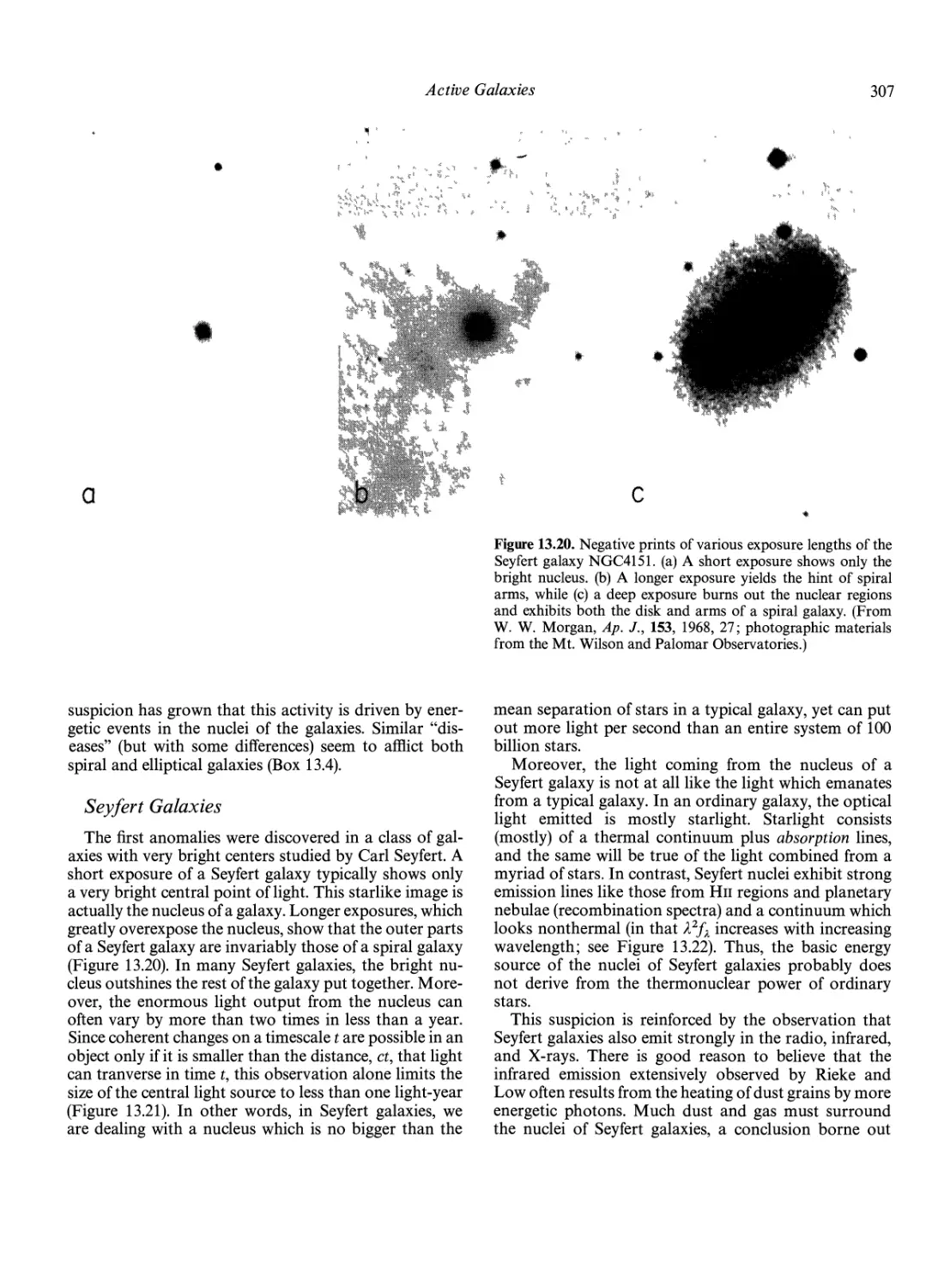
Seyfert Galaxies 307
BL Lac Objects 309
Radio Galaxies 310
Quasars 315
Supermassive Black-Hole Models for Active
Galactic Nuclei 320
Observational Efforts to Detect Supermassive
Black Holes 323
The Nucleus of Our Own Galaxy 323
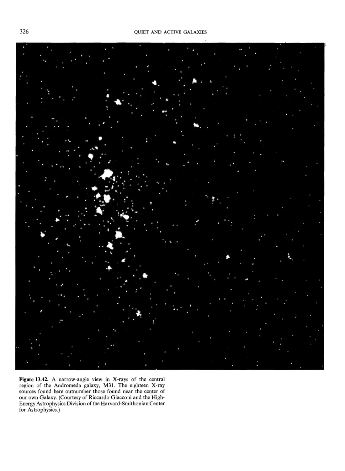
The Nucleus of M87 327
Philosophical Comment 331
14. Clusters of Galaxies and the
Expansion of the Universe 332
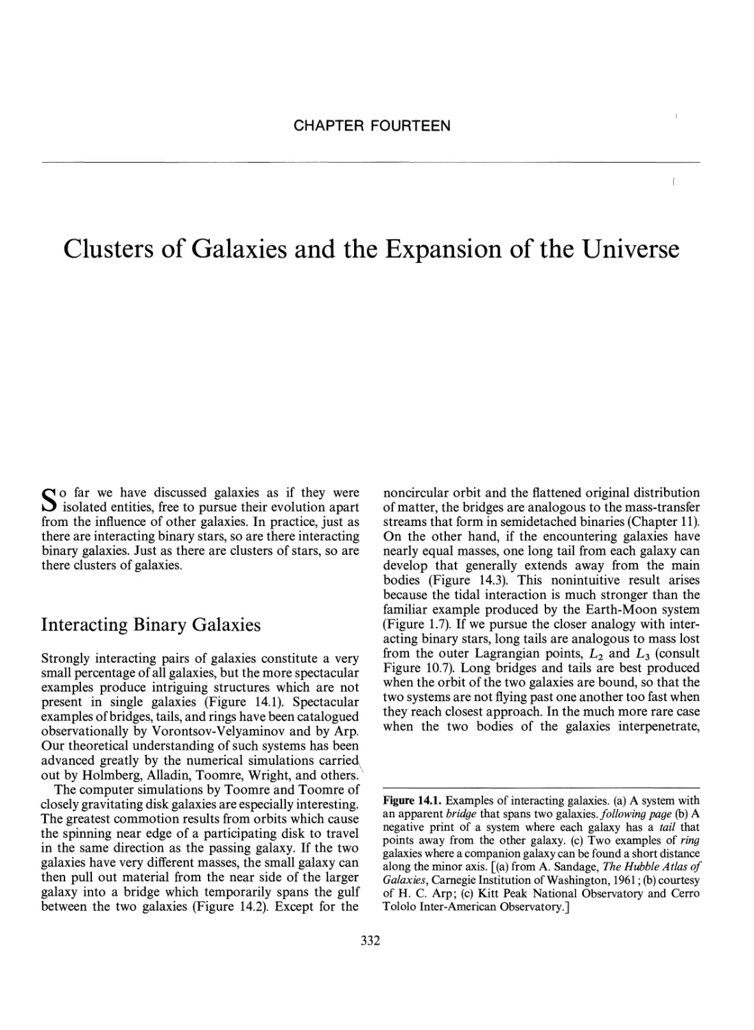
Interacting Binary Galaxies 332
Mergers 336
Hierarchical Clustering 339
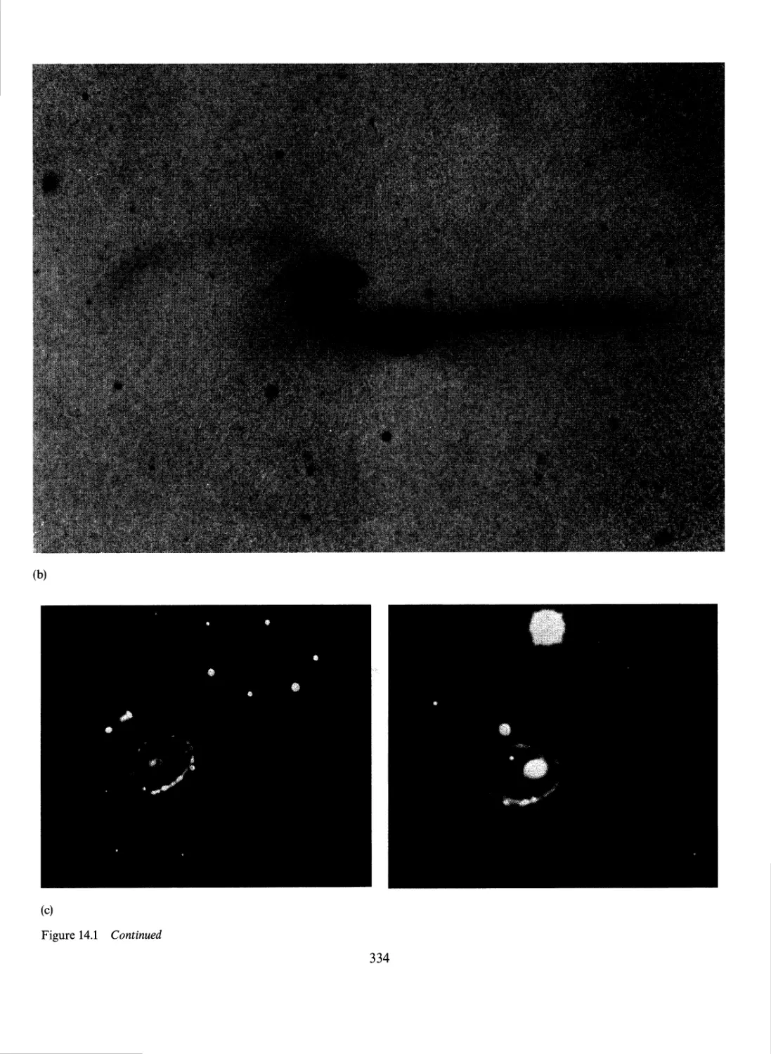
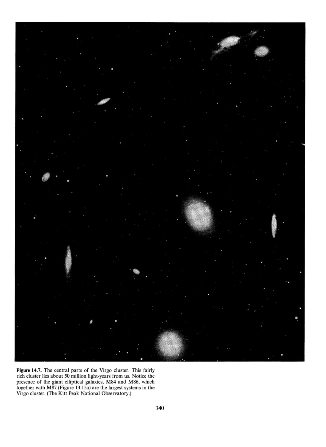
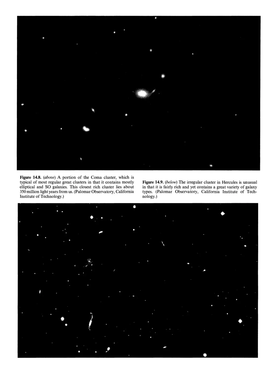
Rich Clusters of Galaxies 339
Galactic Cannibalism 339
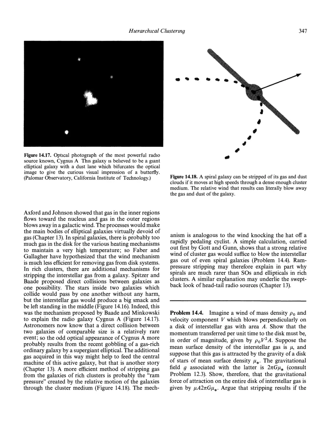
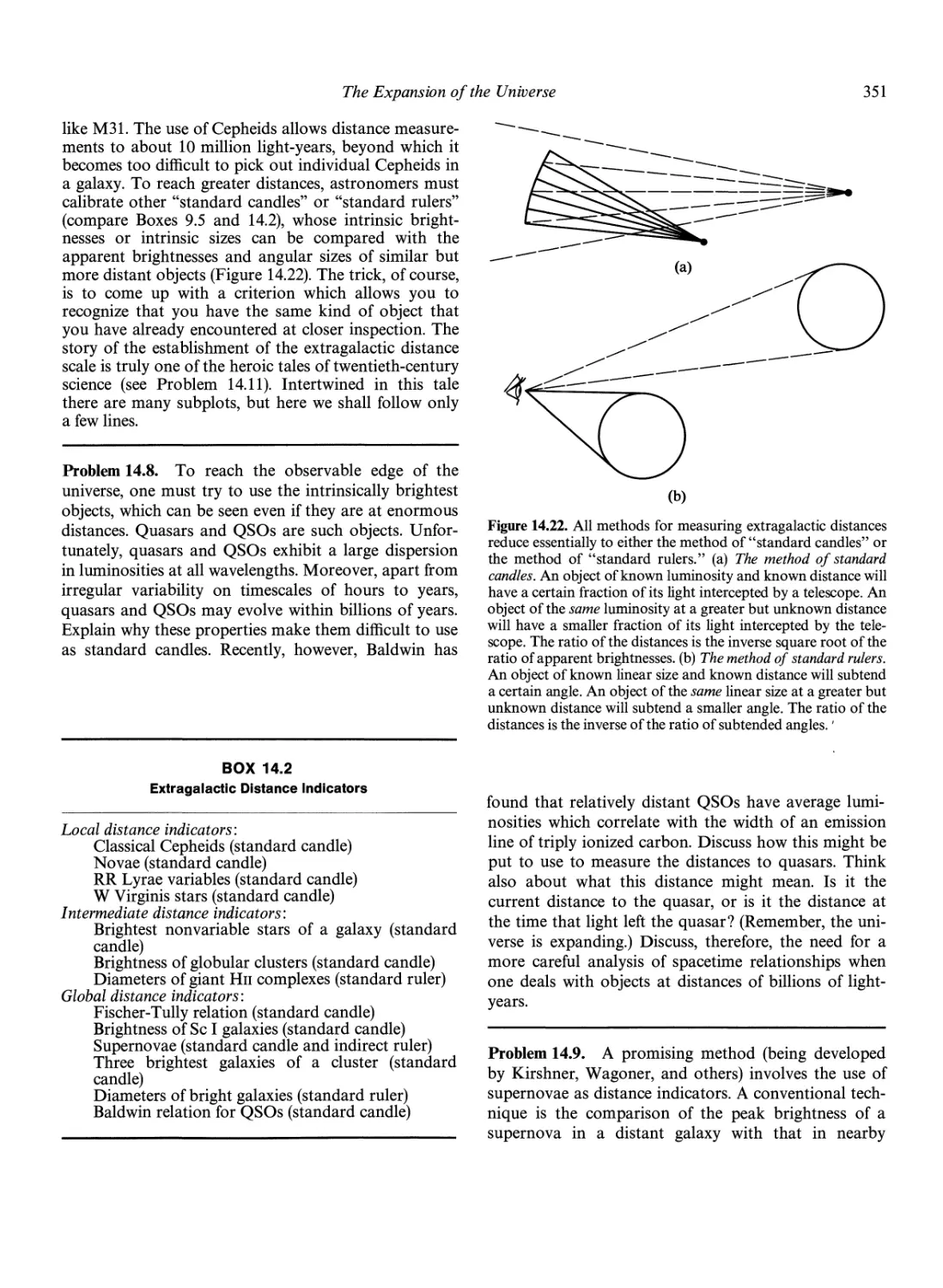
Hot Gas in Rich Clusters 345
Missing Mass in Rich Clusters 348
Unsolved Problems Concerning Small Groups and
Clusters 349
The Expansion of the Universe 350
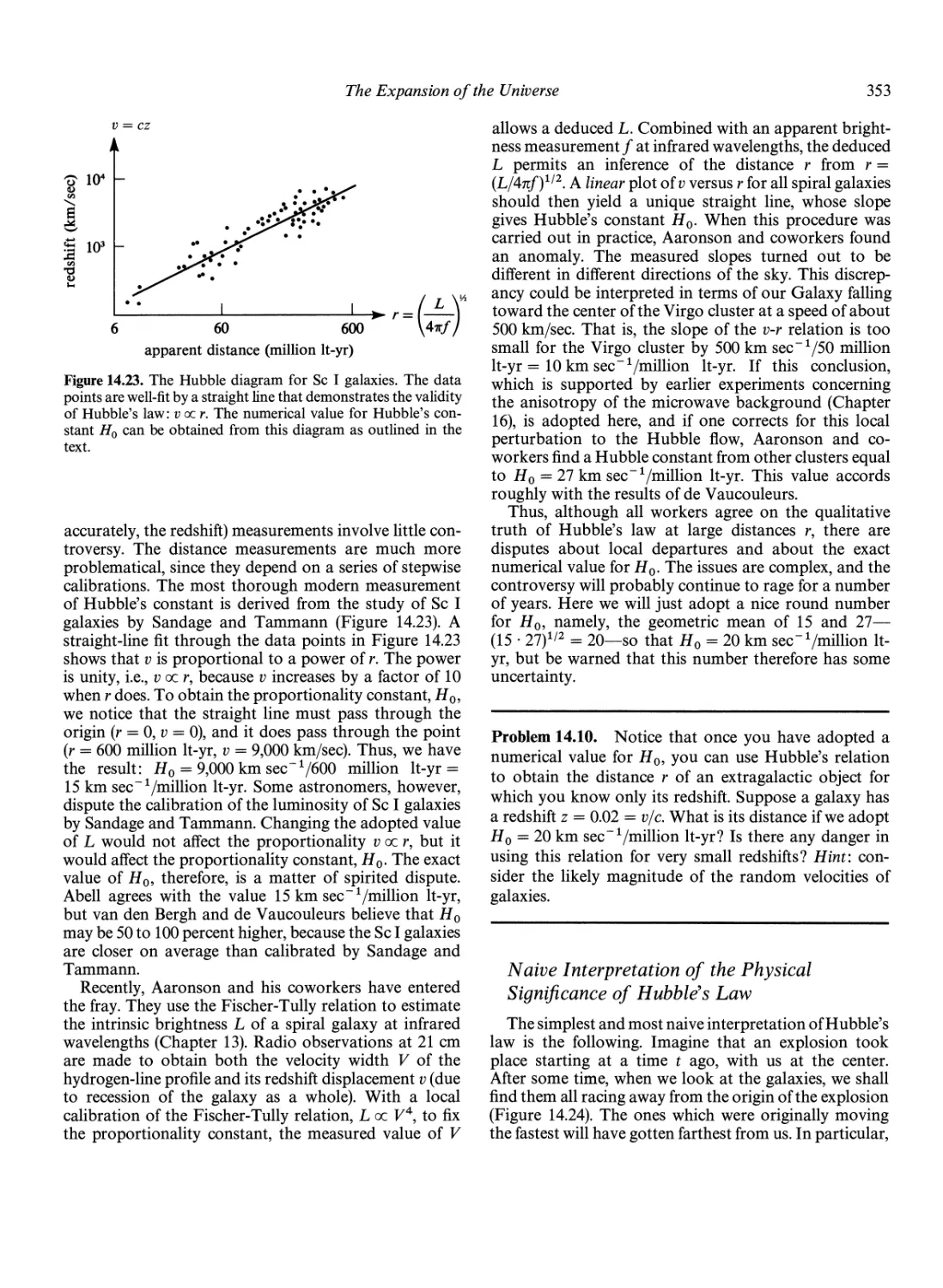
The Extragalactic Distance Scale 350
Hubble*s Law 352
Numerical Value of Hubble's Constant 352
Naive Interpretation of the Physical Significance of
Hubble's Law 353
Philosophical Comments 354
15. Gravitation and Cosmology 355
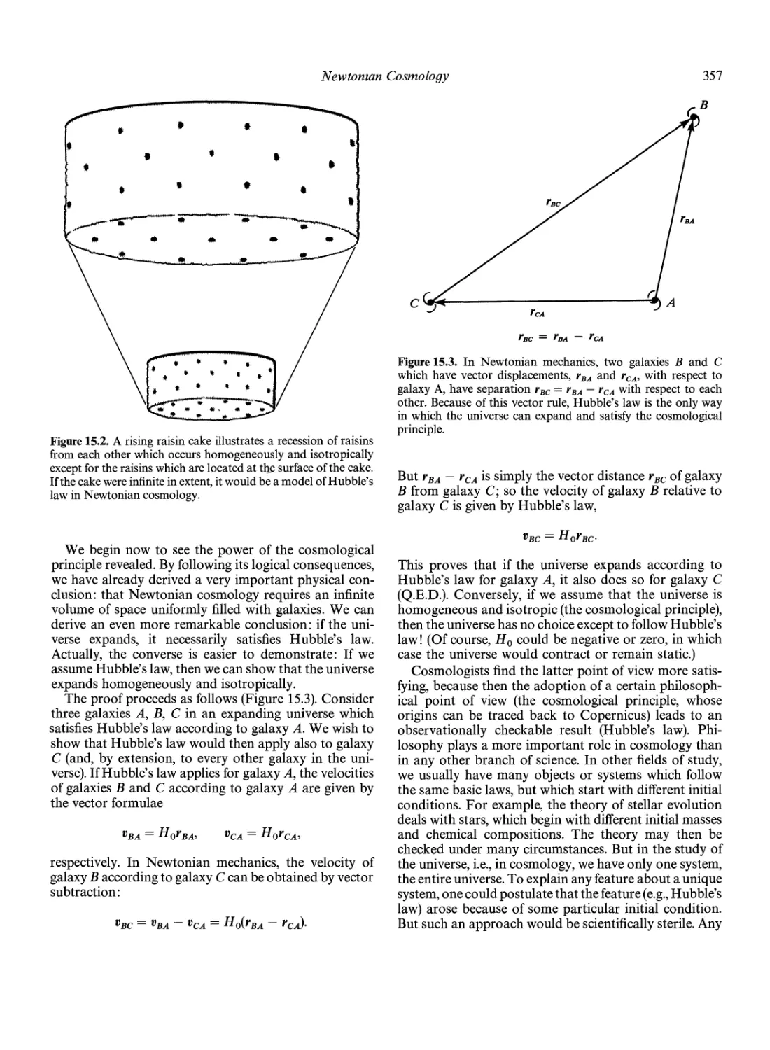
Newtonian Cosmology 355
The Cosmological Principle 355
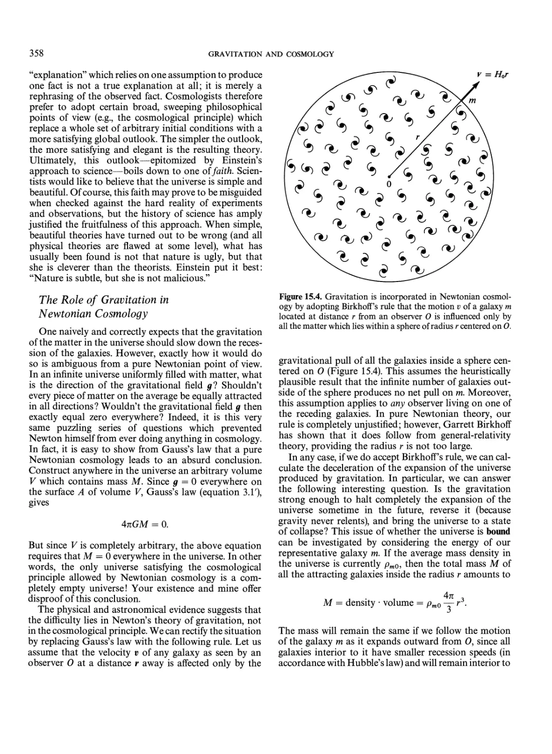
The Role of Gravitation in Newtonian Cosmology 358
Deceleration of the Expansion Rate 359
The Age of the Universe 360
The Ultimate Fate of the Universe 361
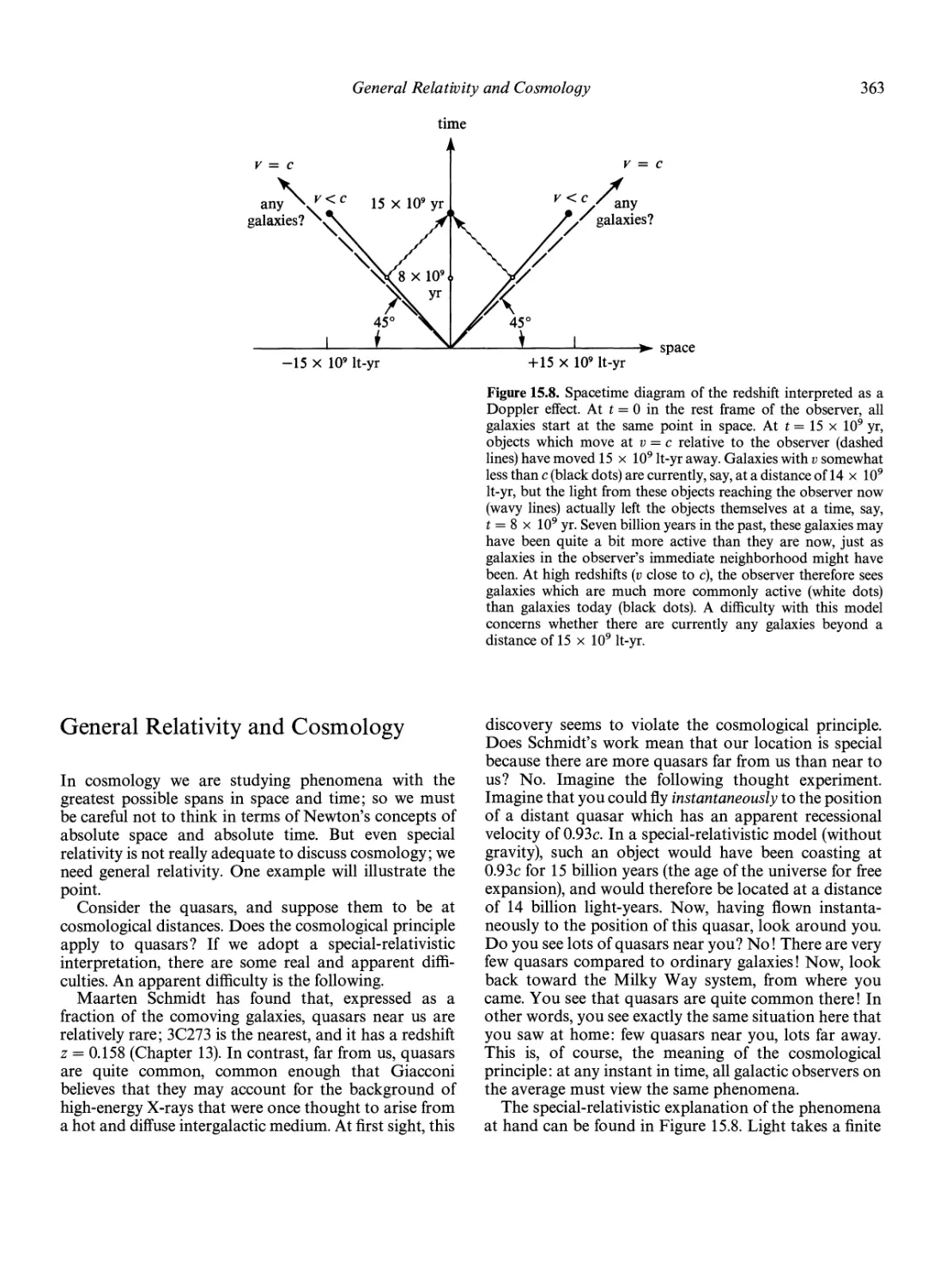
General Relativity and Cosmology 363
The Foundations of General Relativity 364
Relativistic Cosmology 367
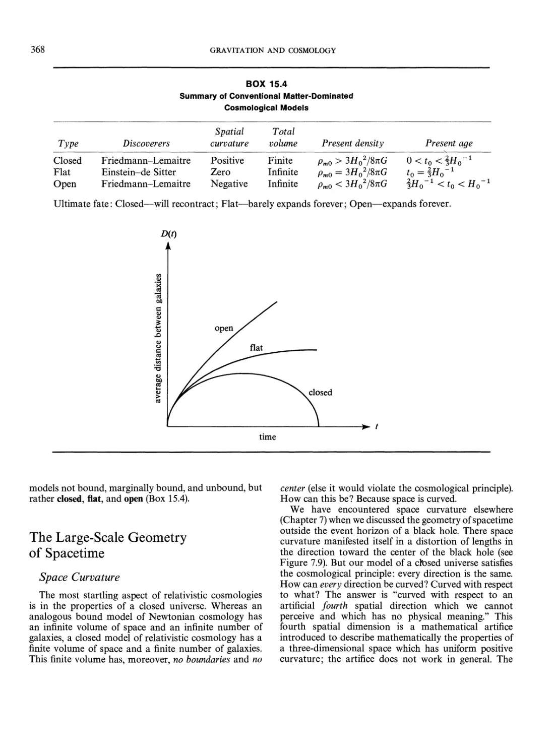
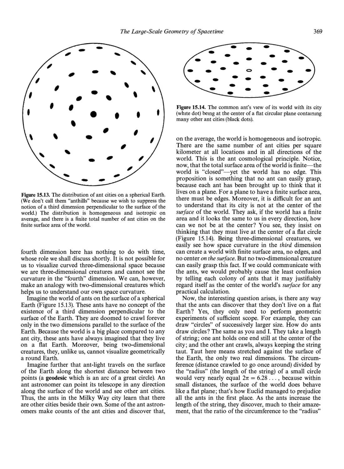
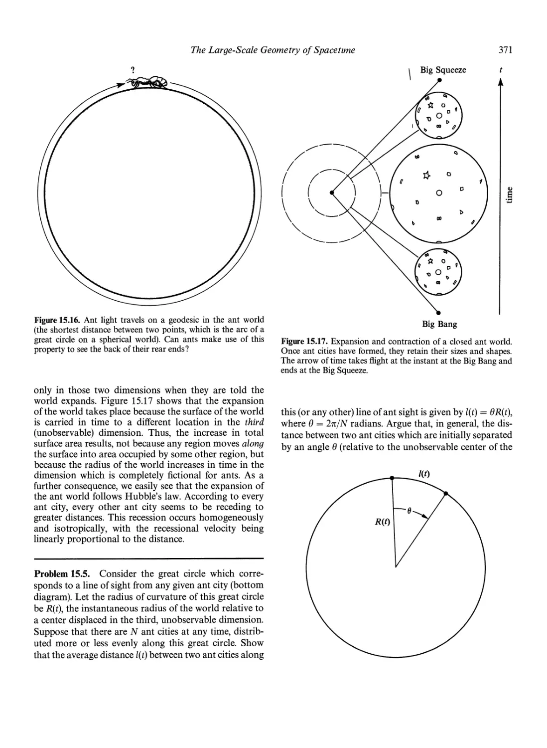
The Large-Scale Geometry of Space time 368
Space Curvature 368
Space time Curvature 370
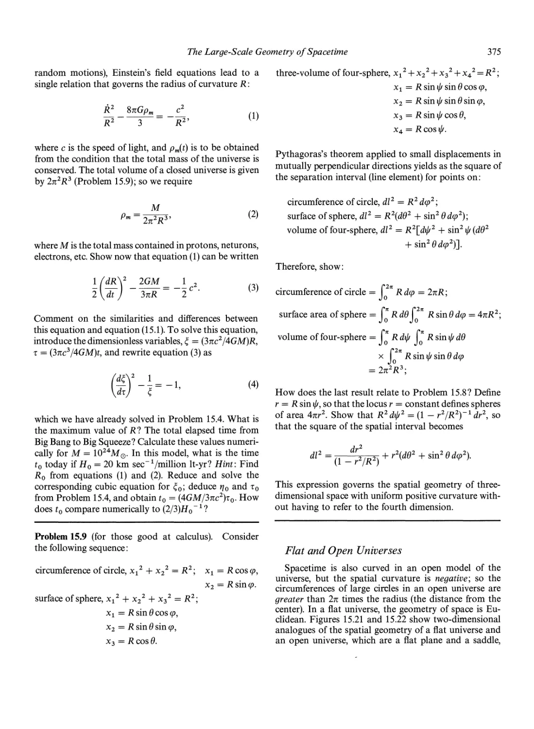
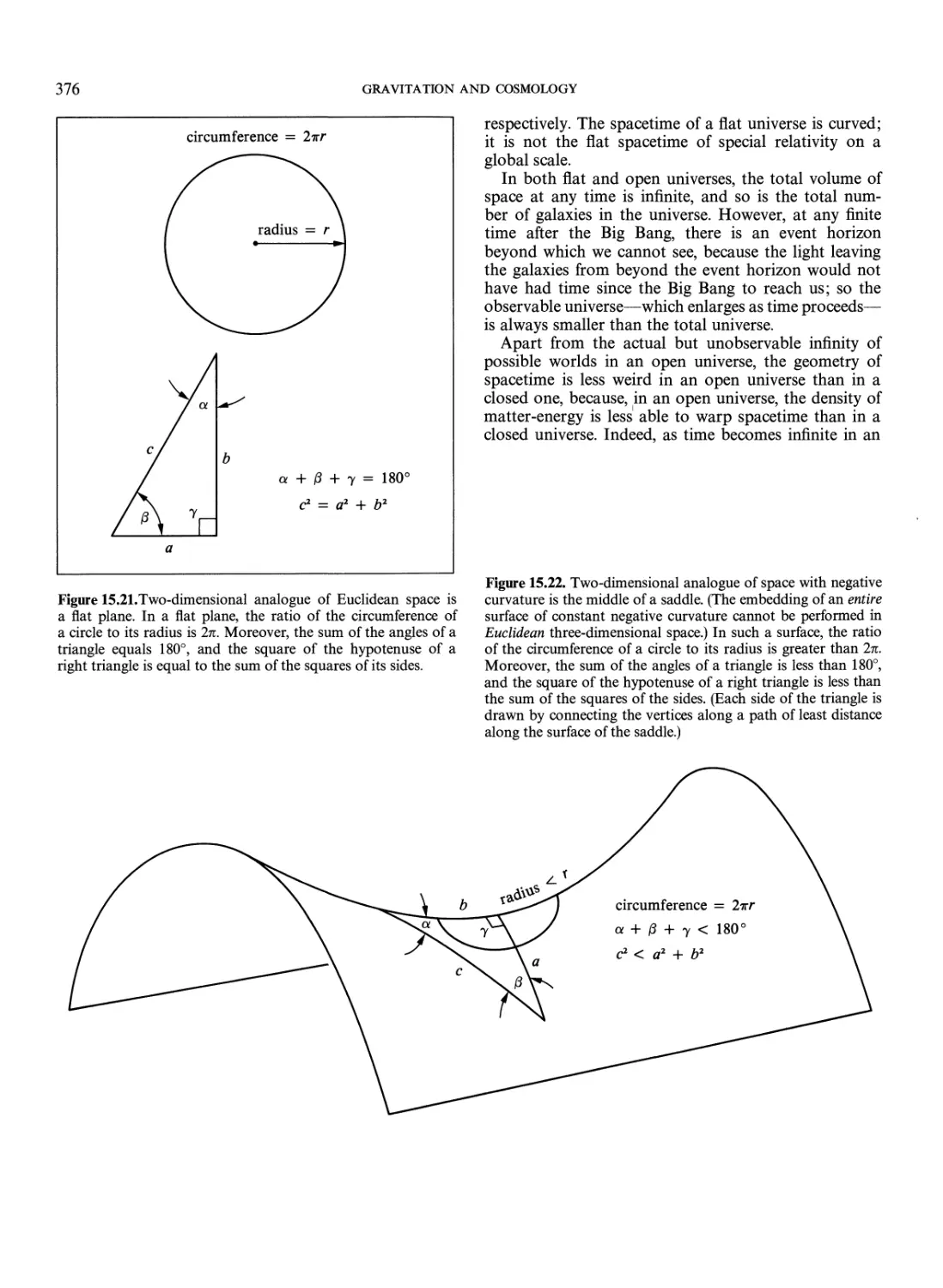
Flat and Open Universes 375
Cosmological Tests by Means of the
Hubble Diagram 311
Concluding Remarks 380
16. The Big Bang and the Creation
of the Material World 381
Big Bang vs. Steady State 381
Distribution of Radio Galaxies and Quasars 382
Olbers' Paradox: Why is the Sky Dark at Night? 383
The Cosmic Microwave Background Radiation 384
The Hot Big Bang 386
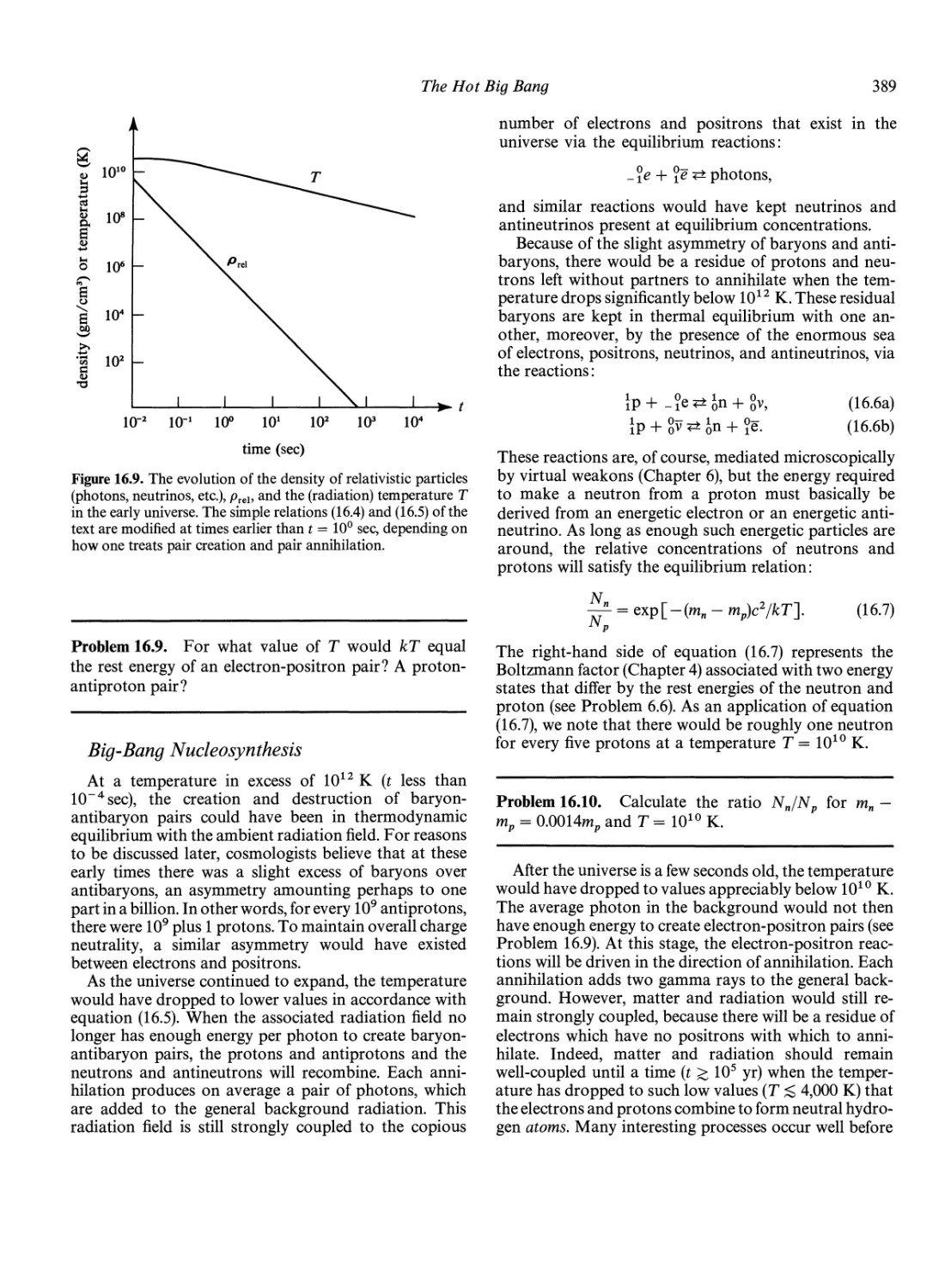
The Thermal History of the Early Universe 388
Big-Bang Nucleosynthesis 389
The Deuterium Problem 391
Massive Neutrinos? 392
The Evolution of the Universe 393
The Creation of the Material World 396
The Limits of Physical Knowledge 397
Mass-Energy from the Vacuum? 398
The Quality of the Universe 400
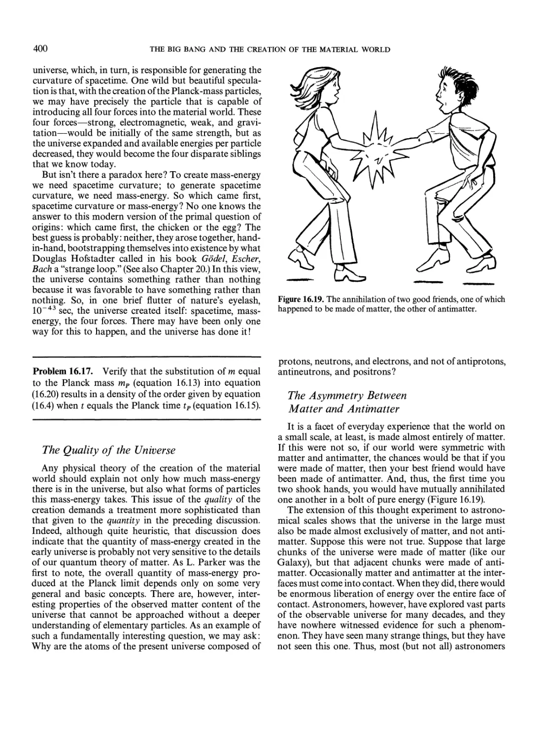
The Asymmetry Between Matter and Antimatter 400
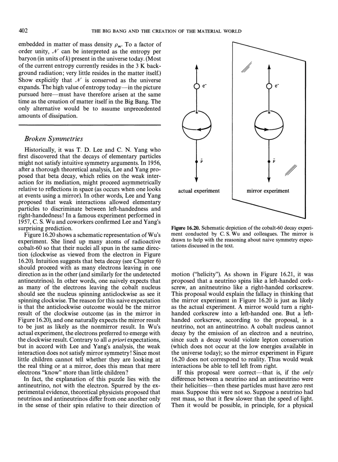
Broken Symmetries 402
Local Symmetries and Forces 404
Super symmetry, Super gr avity,
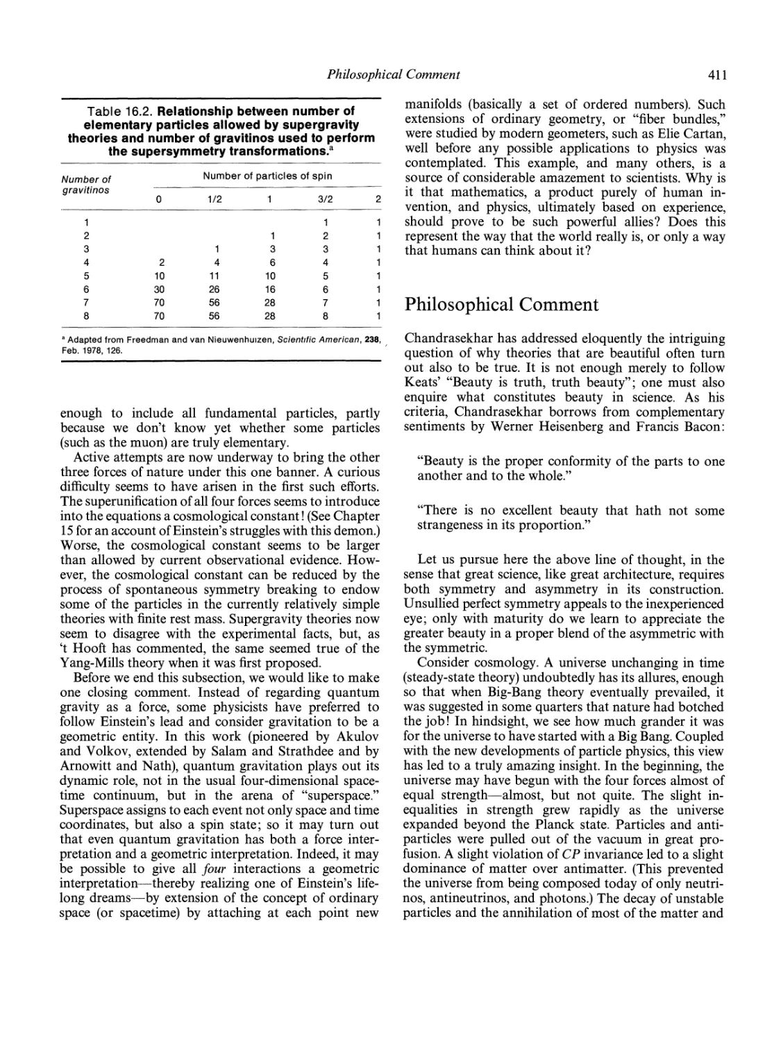
and Superunification 407
Philosophical Comment 411
IV. The Solar System and Life 413
17. The Solar System 415
Inventory of the Solar System 418
Planets and Their Satellites 418
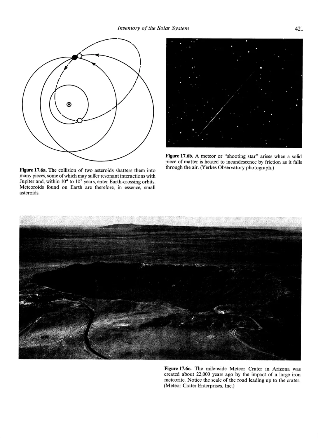
Minor Planets or Asteroids; Meteor oids, Meteors, and
Meteorites 420
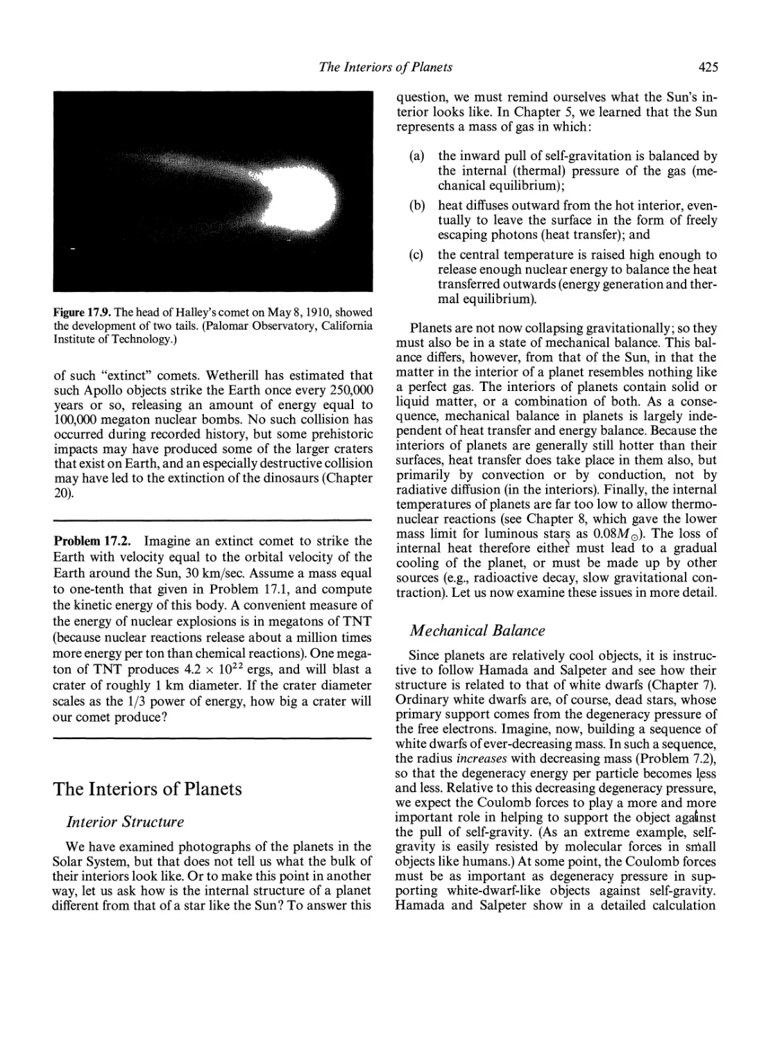
Comets 423
The Interiors of Planets 425
Interior Structure 425
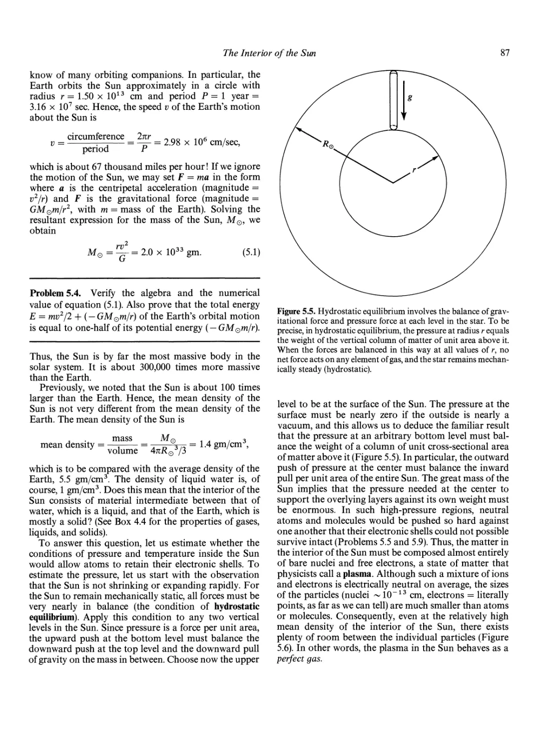
Mechanical Balance 425
Heat Transfer and Energy fialance 429
The Origin of Planetary Rings 431
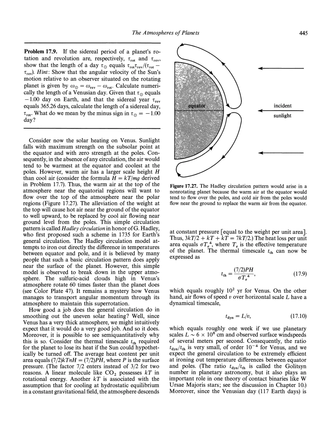
The Atmospheres of Planets 433
Thermal Structural of the Atmospheres of
Terrestrial Planets 433
Runaway Greenhouse Effect 437
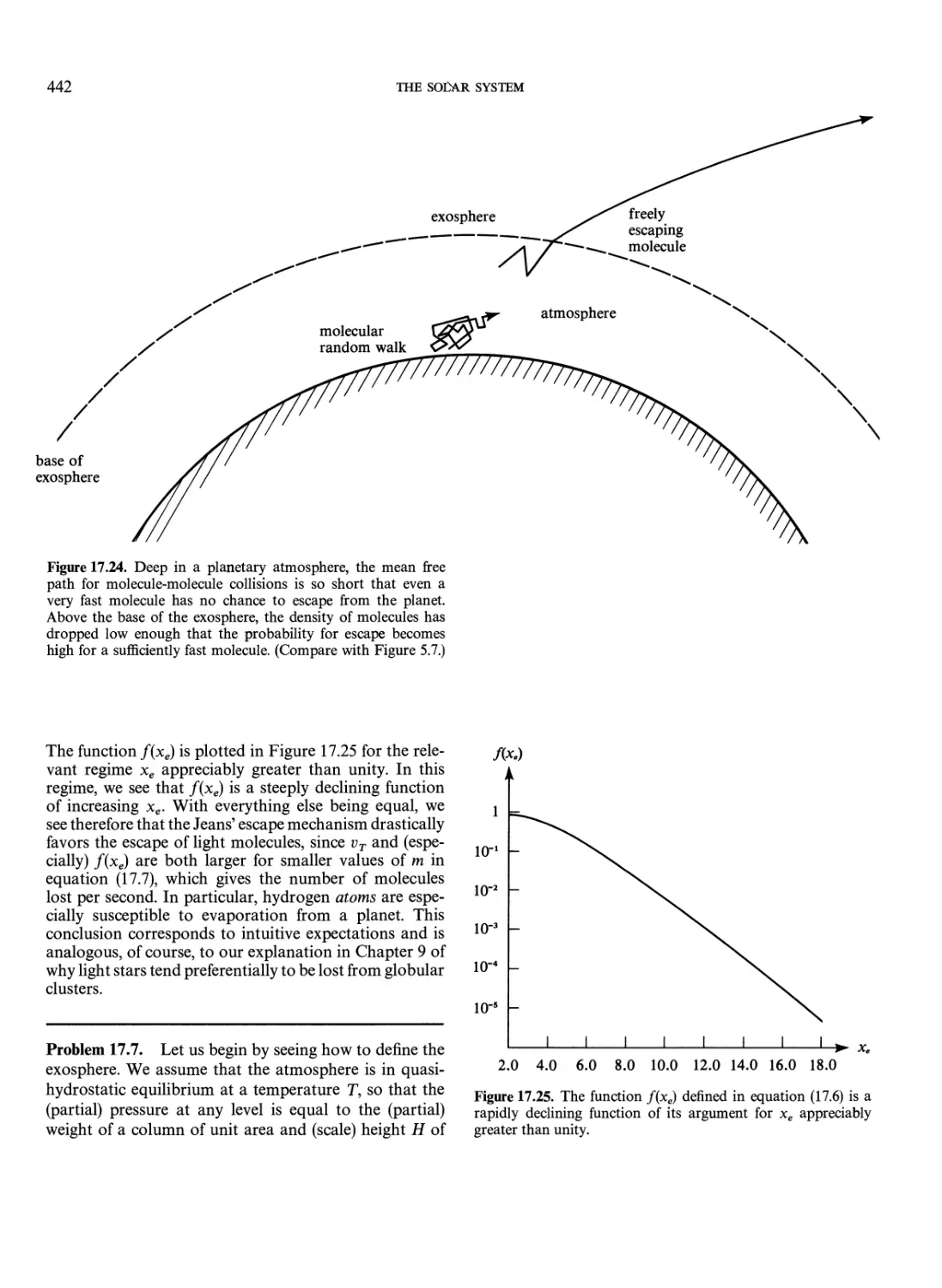
The Exosphere 441
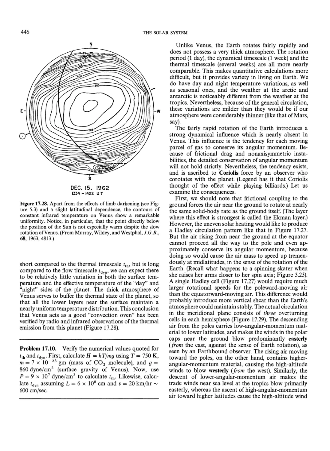
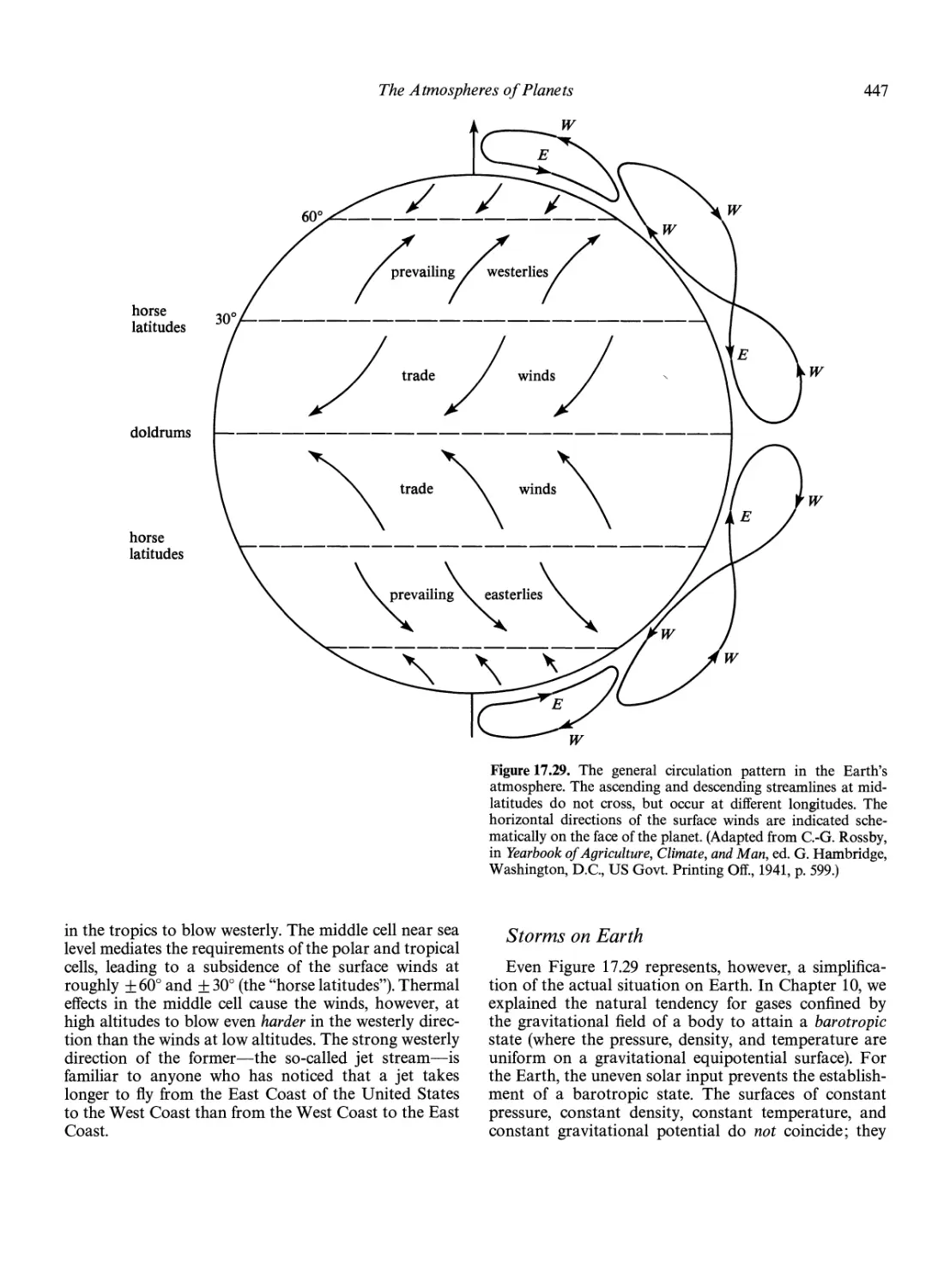
Planetary Circulation 444
Storms on Earth 447
Ocean Circulation 449
The Atmosphere of Jupiter 451
Magnetic Fields and Magnetospheres 454
CONTENTS
The Relationship of Solar-System Astronomy to
the Rest of Astronomy 458
18. Origin of the Solar System
and the Earth 459
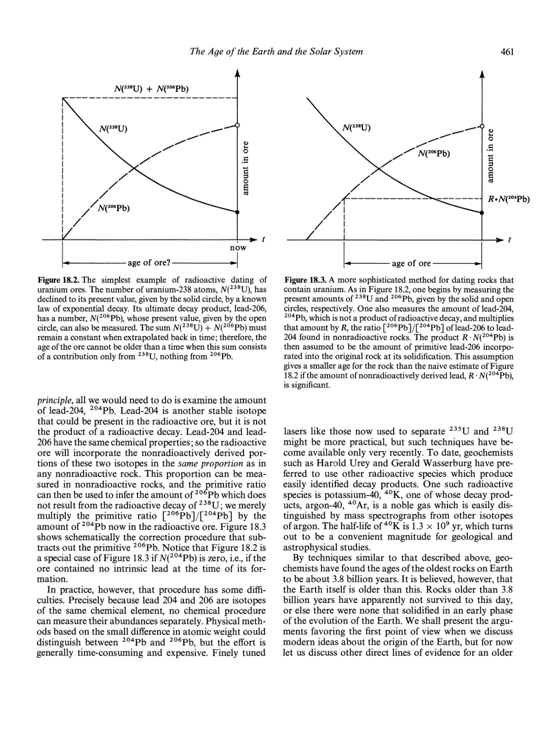
The Age of the Earth and the Solar System 459
Radioactivity 459
Radioactive Dating 460
Exposure Ages of Meteoroids 462
Age of the Radioactive Elements 462
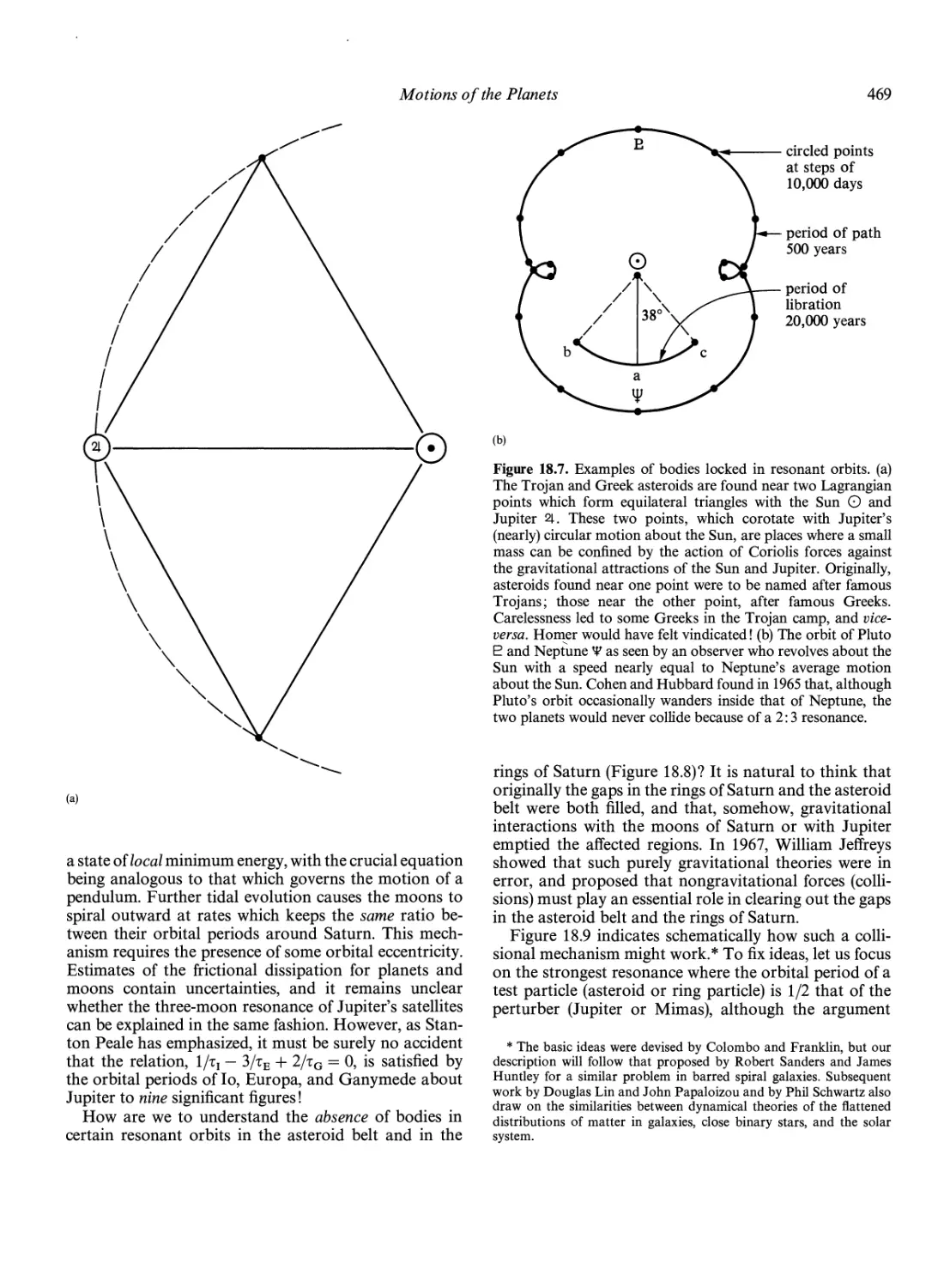
Motions of the Planets 463
Kepler's Three Laws of Planetary Motion 463
Newton's Derivation of Kepler's Laws 463
Dynamical Evolution of the Solar System 466
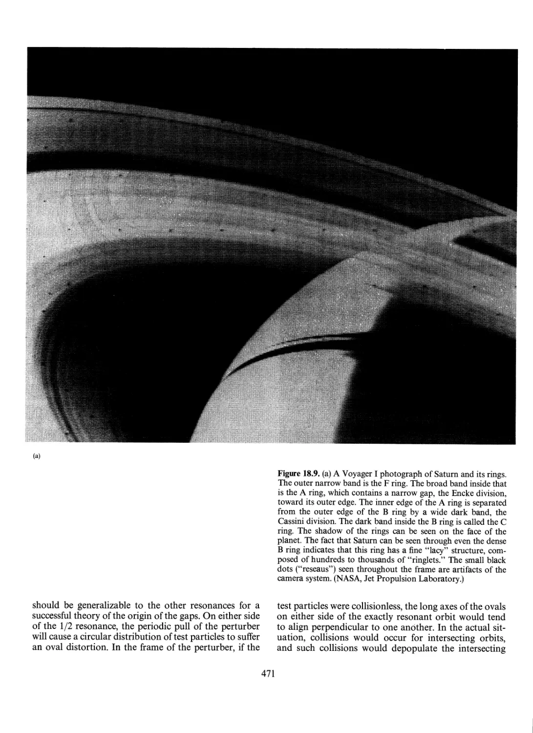
Resonances in the Solar System 467
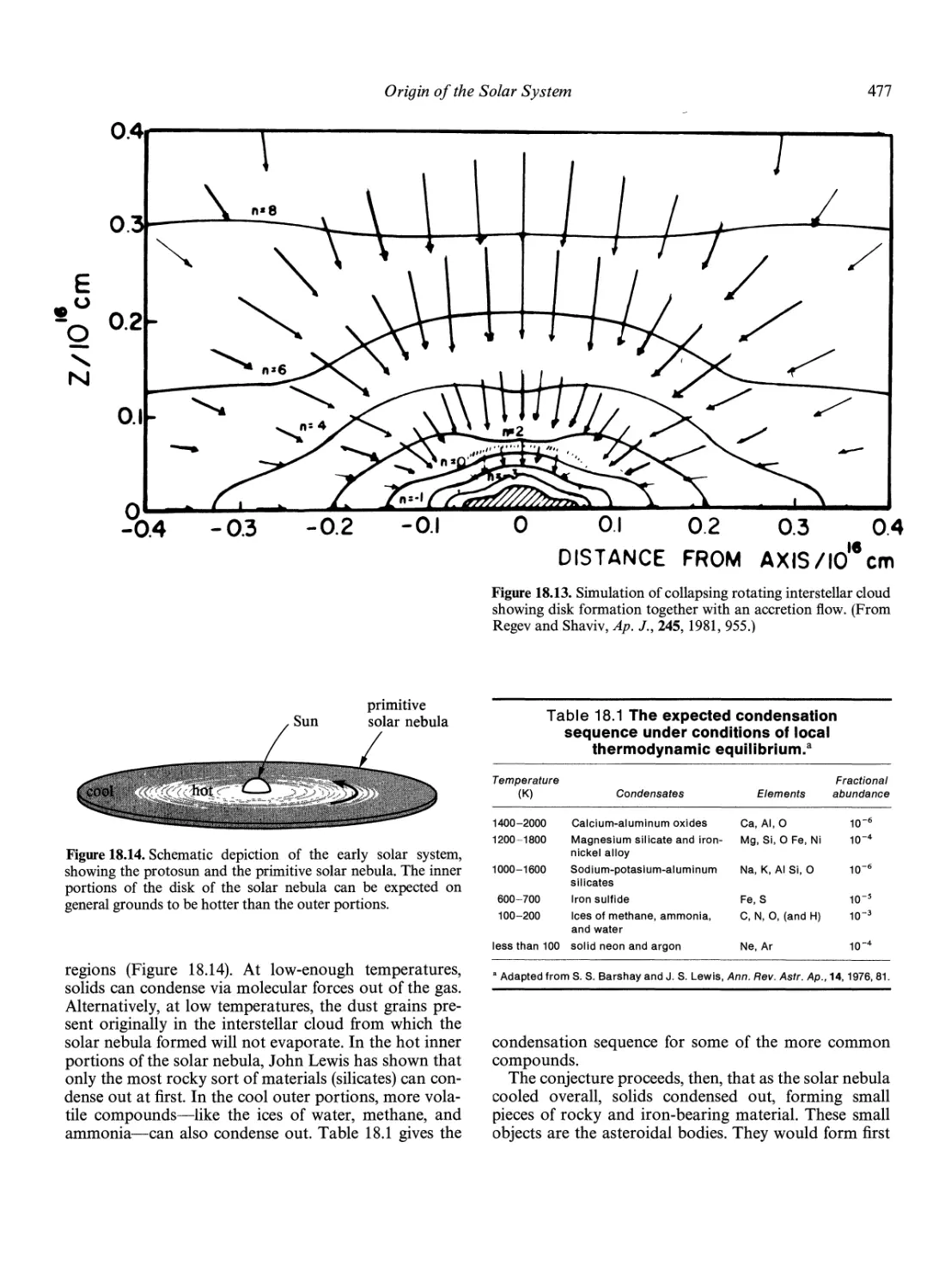
Regularities in the Solar System Caused by Initial
Conditions 474
Origin of the Solar System 474
The Nebular Hypothesis 475
Differences Between Terrestrial and Jovian Planets: The
Condensation Theory 475
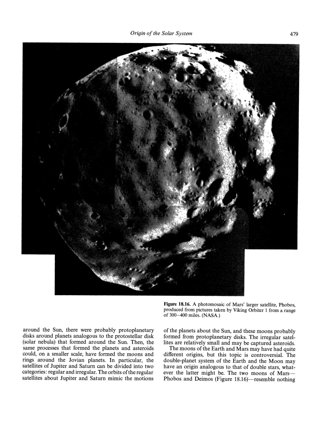
The Sizes of the Planets and Their Orbital
Spacing s 478
Moons, Rings, and Comets 478
Condensation versus Agglomeration of
Presolar Grains 481
Origin and Evolution of the Earth 482
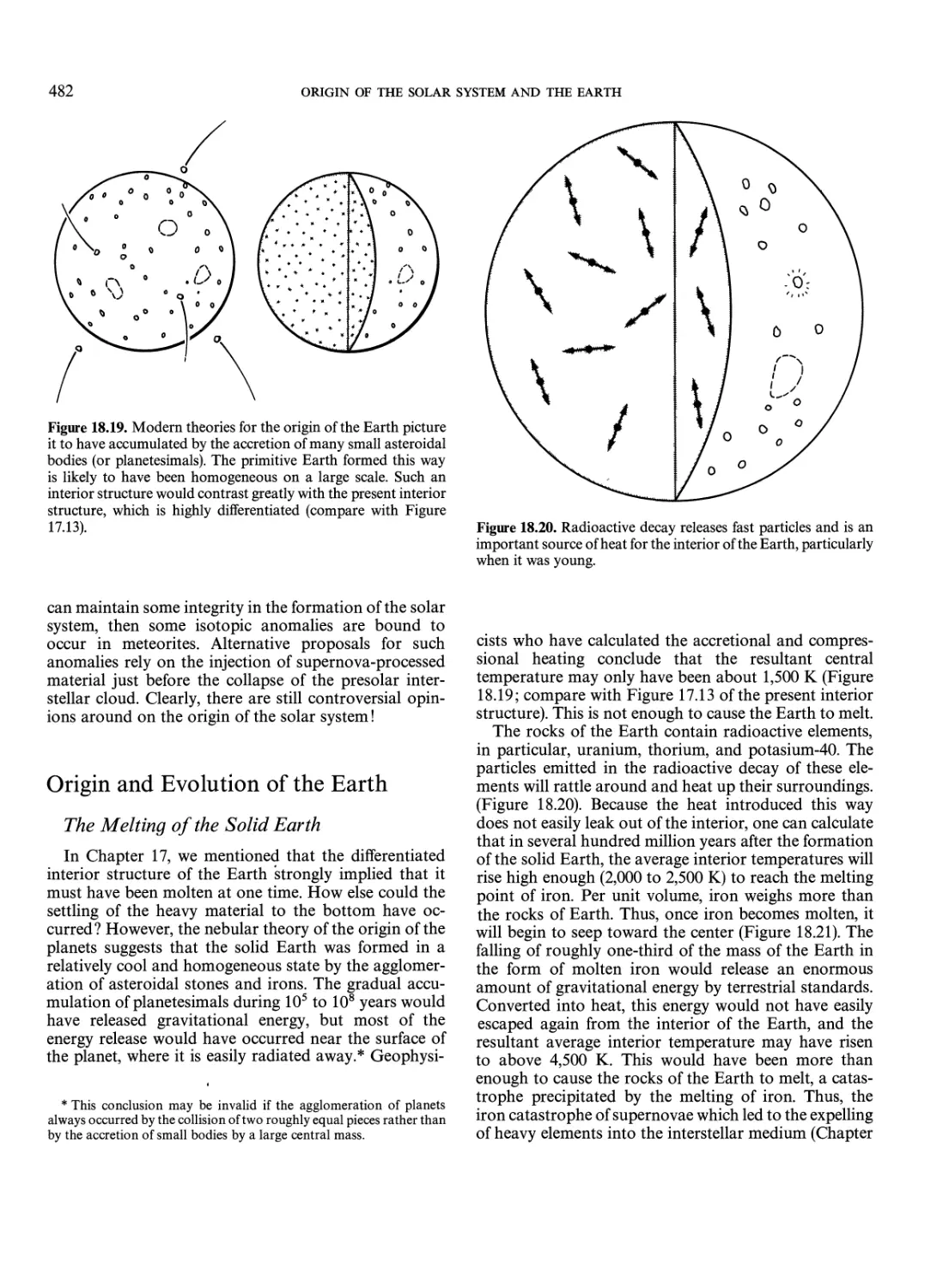
The Melting of the Solid Earth 482
The Formation of the Atmosphere and the Oceans: The
Big Burp 483
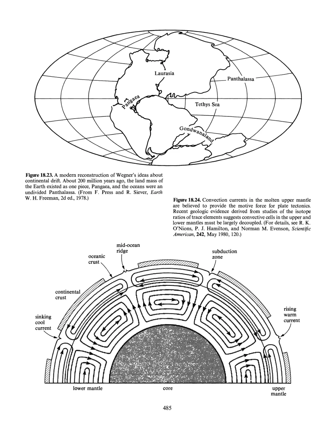
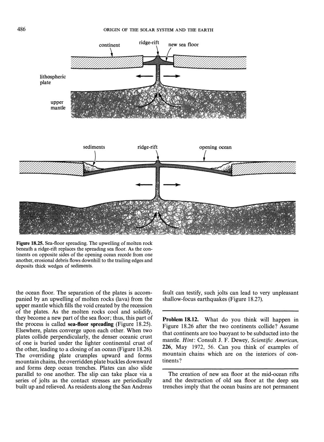
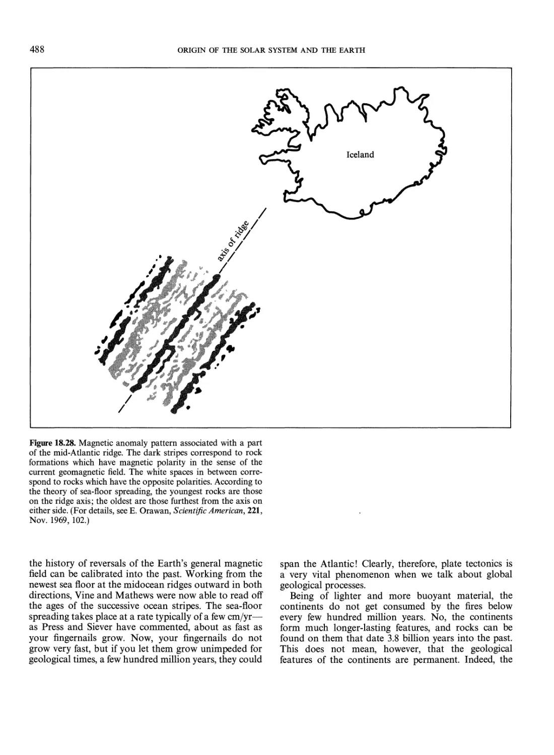
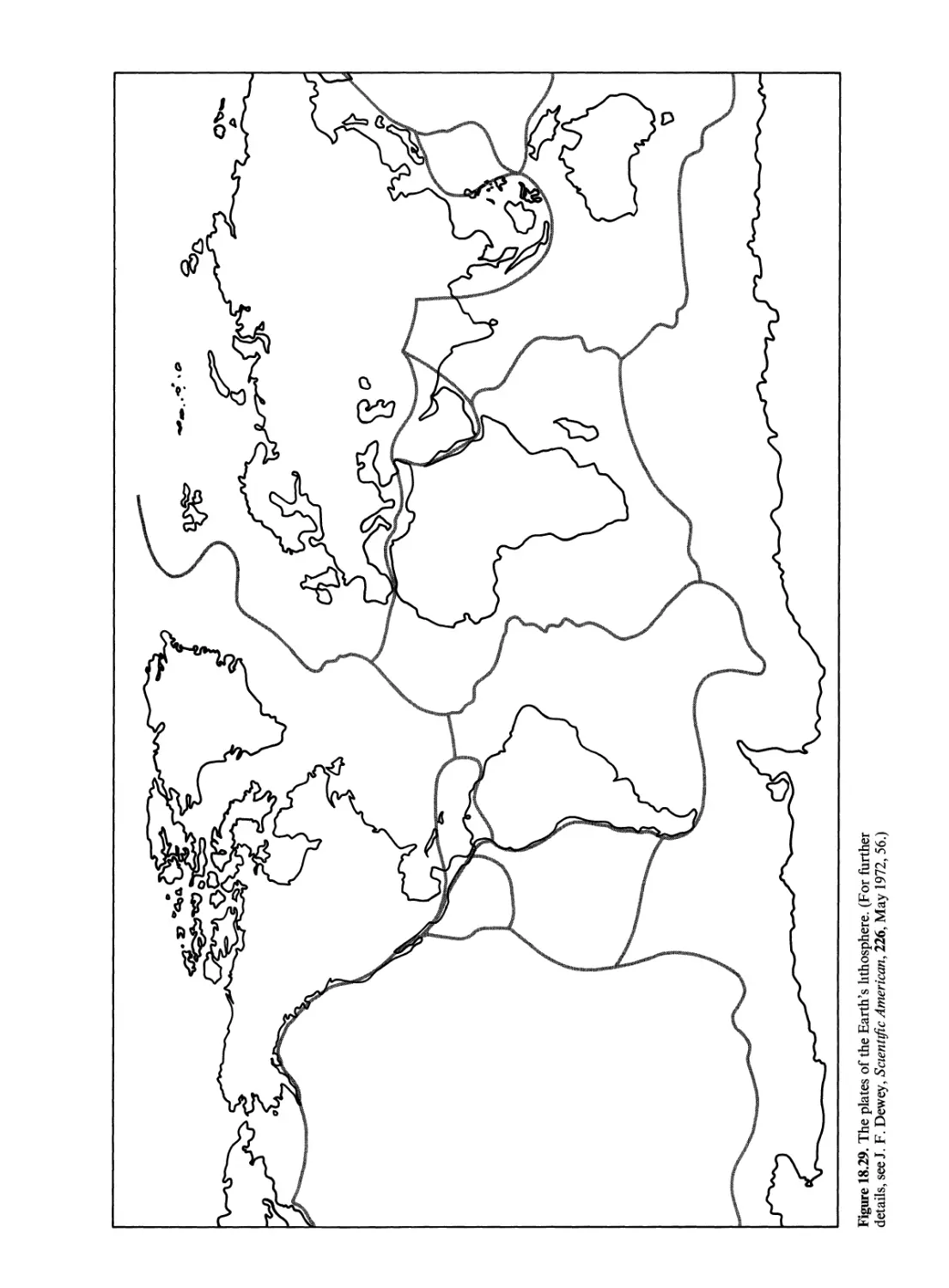
Continental Drift and Sea-Floor Spreading 484
The Past and Future of the Continents 490
The Emergence of Life on Earth 491
The Evolution of the Earth's Atmosphere 491
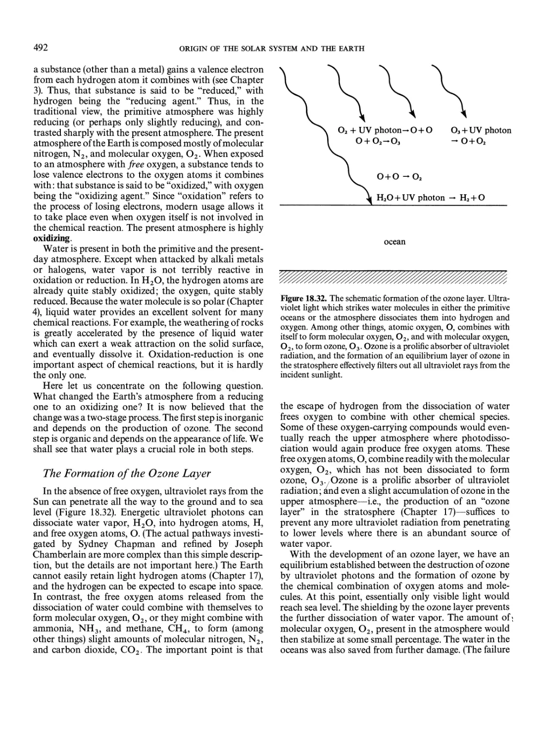
The Formation of the Ozone Layer 492
The Role of Life in Changing the
Earth's Atmosphere 493
Historical Comment 497
lolecular Biology and the Chemical Basis of
ife 512
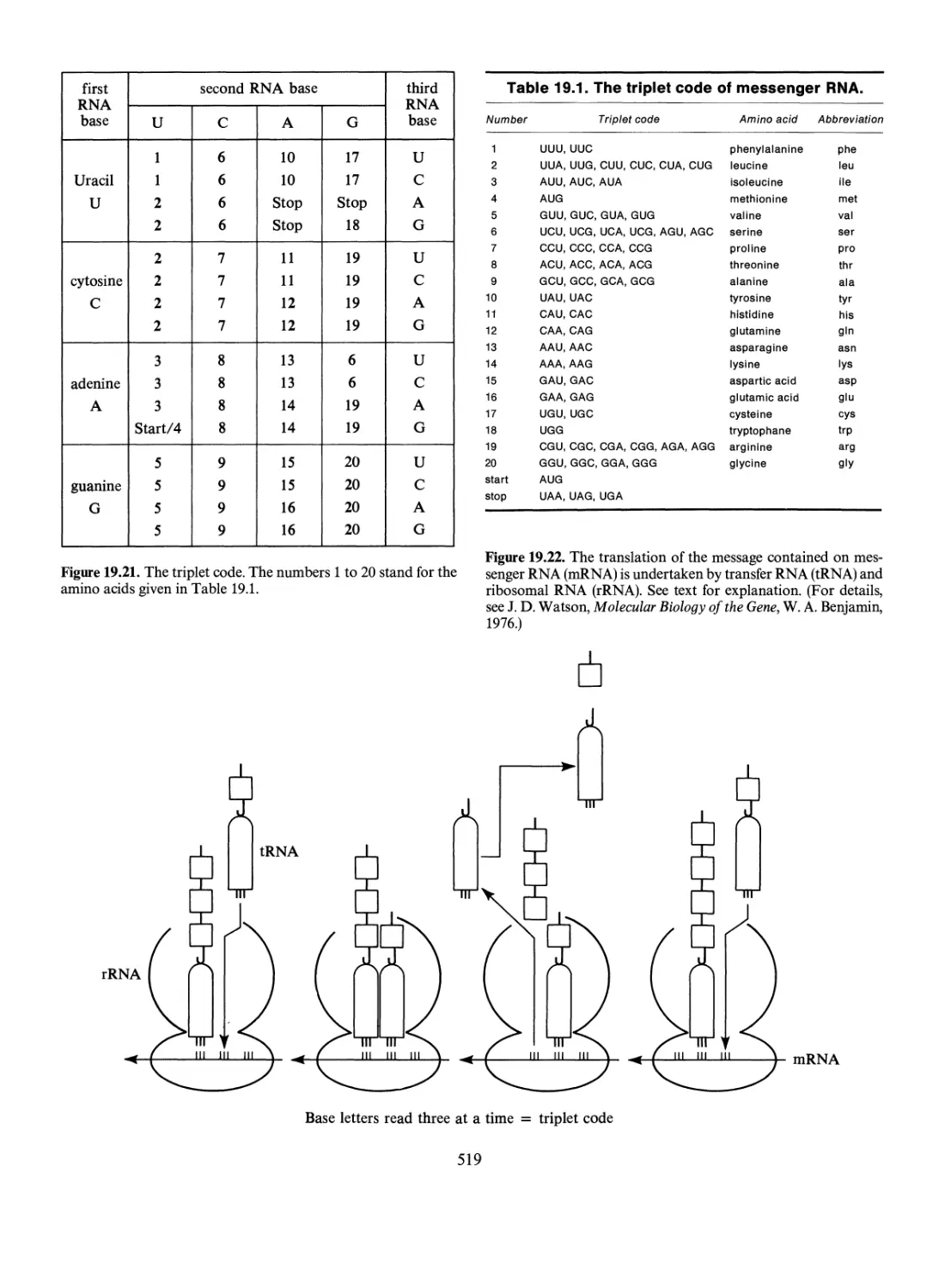
The Central Dogma
Protein Synthesis
A TP and Enzymes
Cell Division 521
Sexual Reproduction
Cell Differentiation
515
515
520
523
523
19. The Nature of Life on Earth 498
Growth 498
Reproduction 499
Natural Selection and Evolution 499
Evolution Is Not Directed 500
Darwin's Accomplishment in Perspective 501
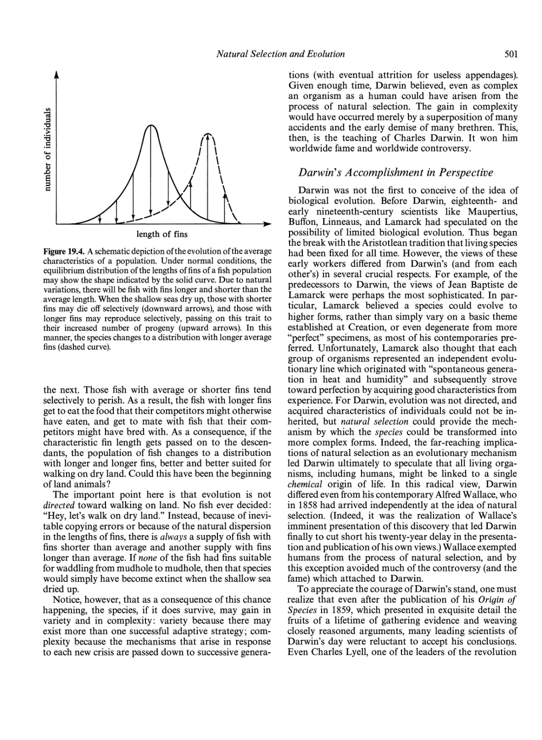
The Evidence in Favor of Darwinian Evolution
The Bridge Between the Macroscopic and
Microscopic Theories of Evolution 503
The Cell as the Unit of Life 504
The Gene as the Unit of Heredity 507
Chromosomes, Genes, and DNA 509
502
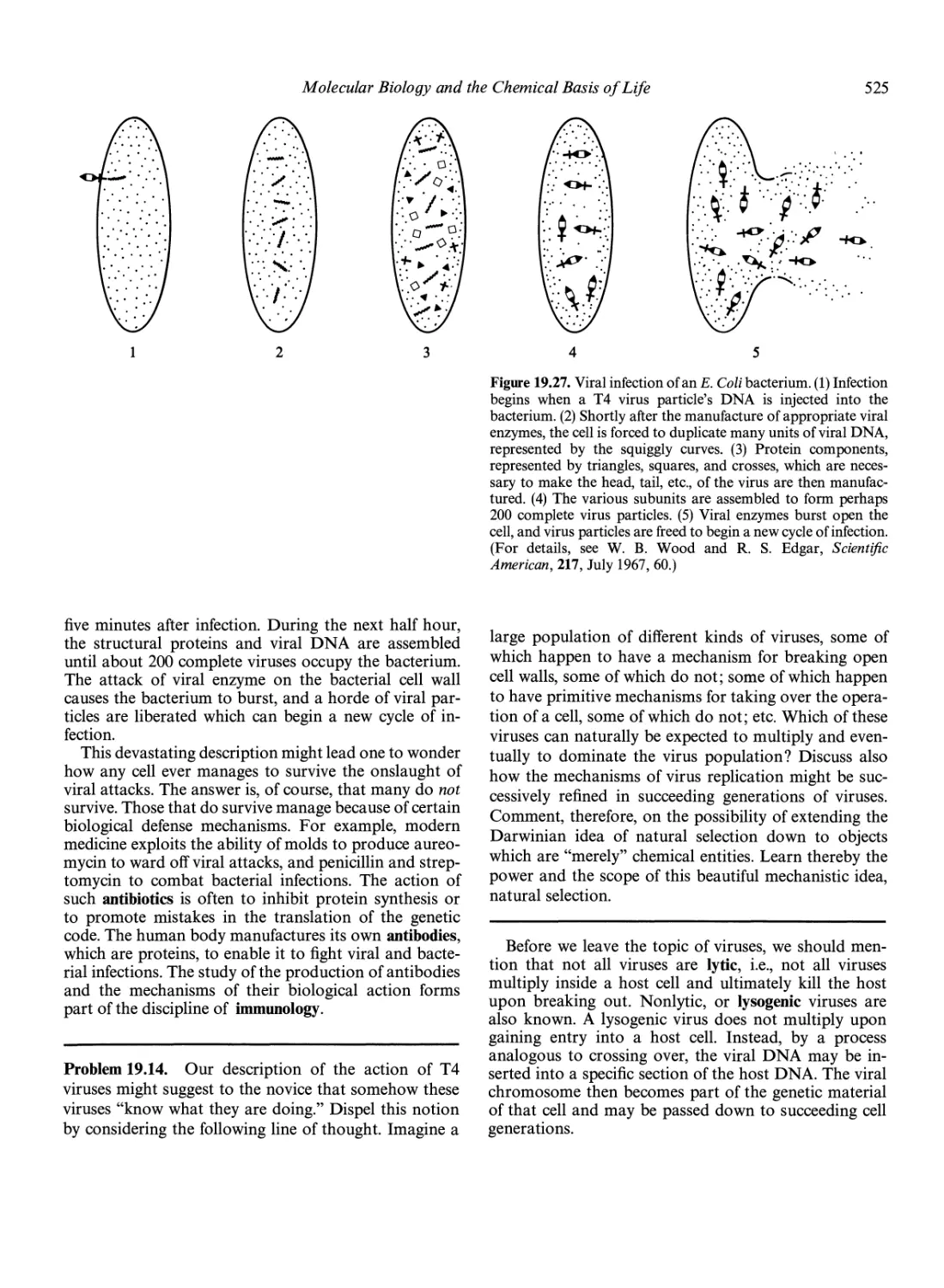
Viruses: The Threshold of Life 524
Cancer, Mutations, and Biological Evolution 526
Philosophical Comment 526
20. Life and Intelligence
in the Universe 528
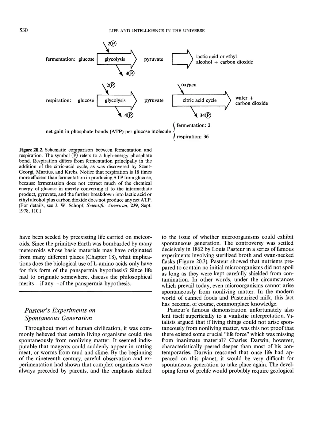
The Origin of Life on Earth 528
Pasteur's Experiments on Spontaneous
Generation 530
The Hypothesis of a Chemical Origin of Life 531
A Concise History of Life on Earth 537
The Earliest Cells: The Prokaryotes 537
Sex Among the Bacteria: The Appearance of
Eukaryotes 539
Multicellular Organization and Cell
Differentiation 541
The Organization of Societies 543
Intelligence on Earth and in the* Universe 544
The Timescale of the Emergence of
Human Culture 544
Intelligent Life in the Galaxy 546
UFOs, Ancient Astronauts, and Similar Nonsense 546
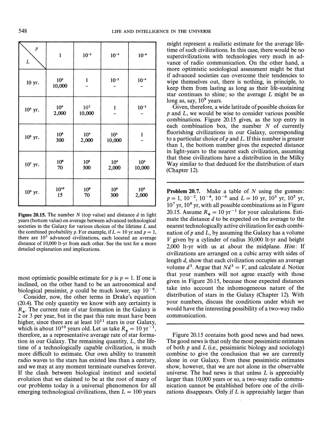
Estimates for the Number of Advanced Civilizations in the
Galaxy 547
The Future of Life and Intelligence on Earth 550
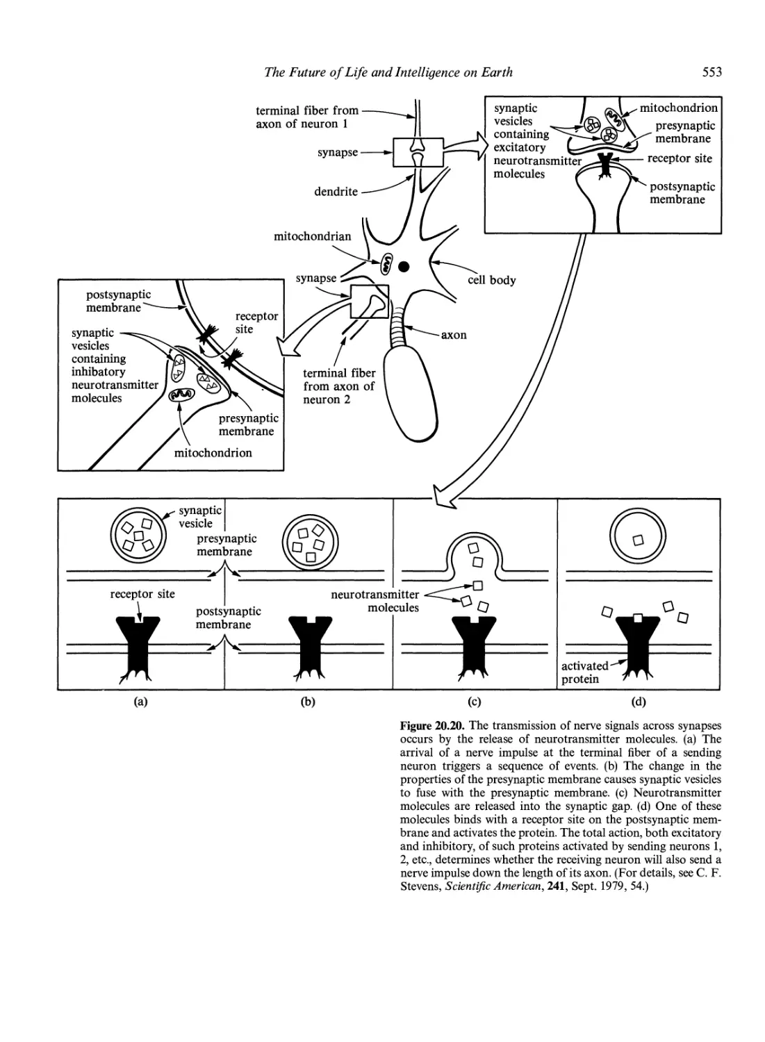
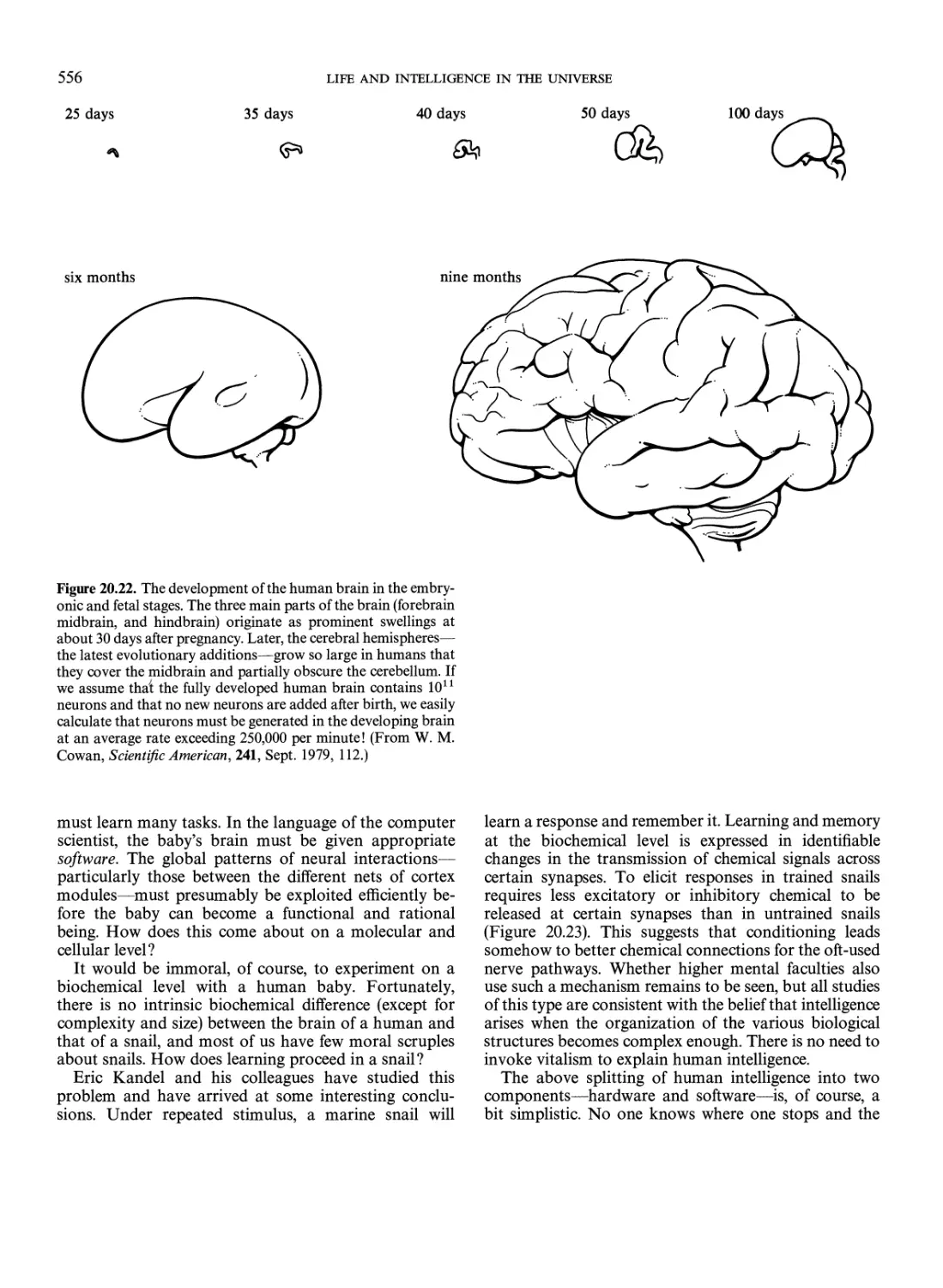
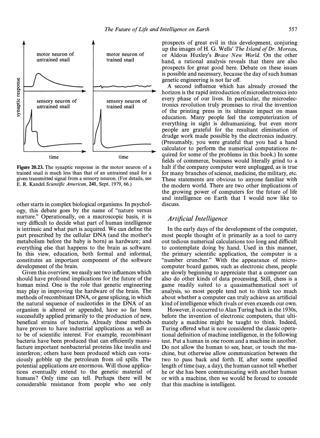
The Neuron as the Basic Unit of the Brain 557
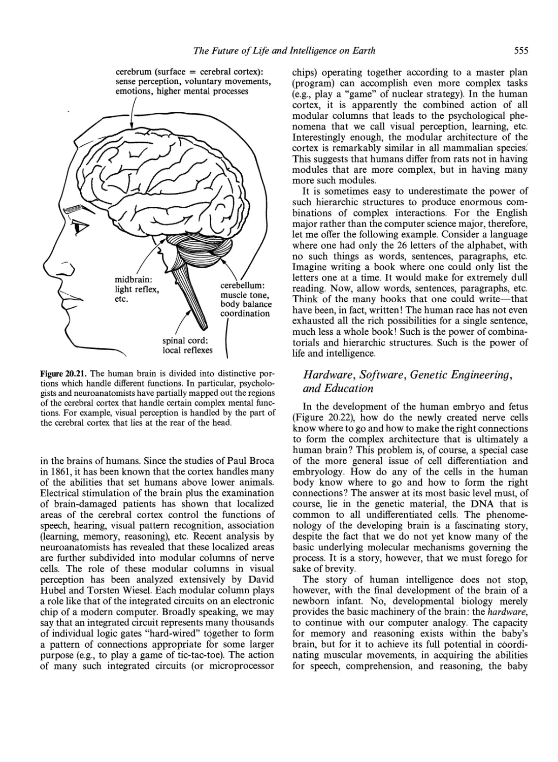
The Organization of the Brain and Intelligence 544
Hardware, Software, Genetic Engineering,
and Education 555
Artificial Intelligence 557
Silicon-Based Life on Earth ? 560
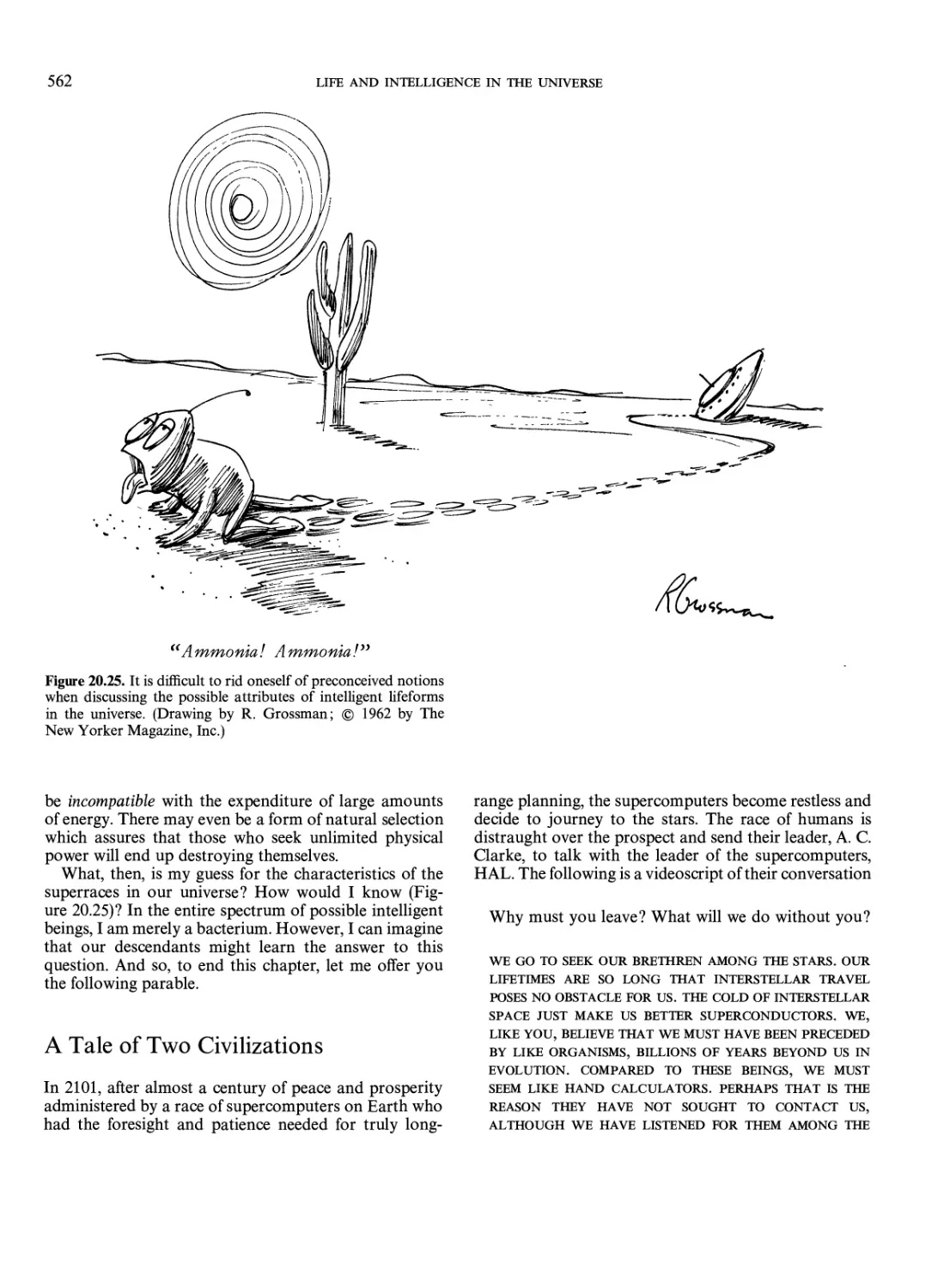
Superbeings in the Universe? 561
A Tale of Two Civilizations 562
Epilogue 564
Appendixes 567
A. Constants 567
B. Euclidean Geometry 569
C. The Greek Alphabet 570
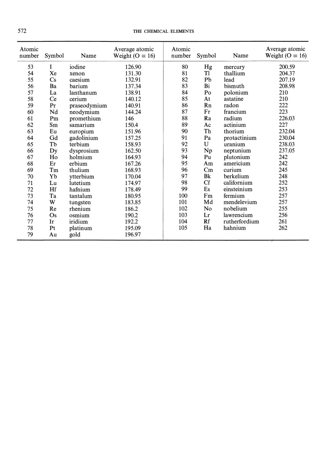
D. The Periodic Table 571
Index 573
PART I
Basic Principles
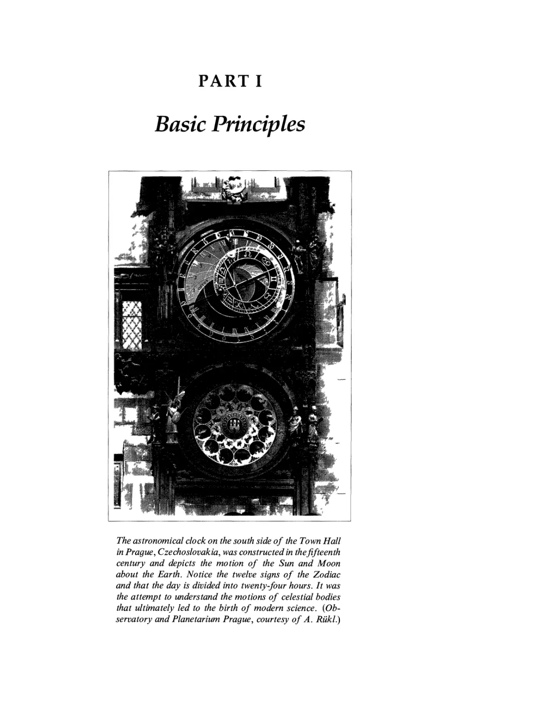
The astronomical clock on the south side of the Town Hall
in Prague, Czechoslovakia, was constructed in the fifteenth
century and depicts the motion of the Sun and Moon
about the Earth. Notice the twelve signs of the Zodiac
and that the day is divided into twenty-four hours. It was
the attempt to understand the motions of celestial bodies
that ultimately led to the birth of modern science.
{Observatory and Planetarium Prague, courtesy of A. Rukl.)
CHAPTER ONE
The Birth of Science
oi N°rth Pol
To most people astronomy means stars; stars mean
constellations; and constellations mean astrology.
In fact, each step of this association contains
misconceptions. Modern astronomers deal with more than just
stars; they think of stars in terms of more than just
constellations; and they use the constellations differently
from astrologers. Nevertheless, astronomy and astrology
do have the same historical roots, in the geometric
patterns formed by the stars in the night sky. Let us begin,
therefore, our journey of exploration of the universe with
the constellations.
The Constellations as
Navigational Aids
In prehistorical times nomadic peoples found that
knowing the constellations helped them with directions. The
most familiar constellation in the Northern Hemisphere
is, of course, the Big Dipper. The Big Dipper is actually
part of an astronomical constellation called Ursa Major,
the Big Bear. Figure 1.1 shows how to use the "pointer
stars" of the Big Dipper to find the pole star, Polaris.
Polaris indicates the direction north, and it will continue
to do so for another thousand years.
It has been speculated that early nomads developed
stories to help them remember the various constellations
and their relative positions in the sky. These stories pass
as entertaining myths today, but in earlier times were
?2^>- -<^>
/ ad.4000-\
V nowy Polaris
\ J
\ A.D.I //
\. 2000 b.c ^/ J
\^ u-^ I
\ / j> pointers
The Big Dipper V l^-^^
Figure 1.1. The Big Dipper and Polaris. To find the pole star,
Polaris, go along the pointers to a distance roughly equal to four
times their separation. Polaris lies very nearly in the present
direction of the axis of the North Pole of the Earth. However,
because of the tidal forces exerted on the Earth by the Sun and
the Moon, the spin axis of the Earth makes a slow precession.
Every 26,000 years, the polar axis describes a circular path in the
sky. Thus, in 2000 B.C. or a.d. 1 the North Pole did not point so
nearly at Polaris as now, and neither will it one or two thousand
years from now.
3
4
THE BIRTH OF SCIENCE
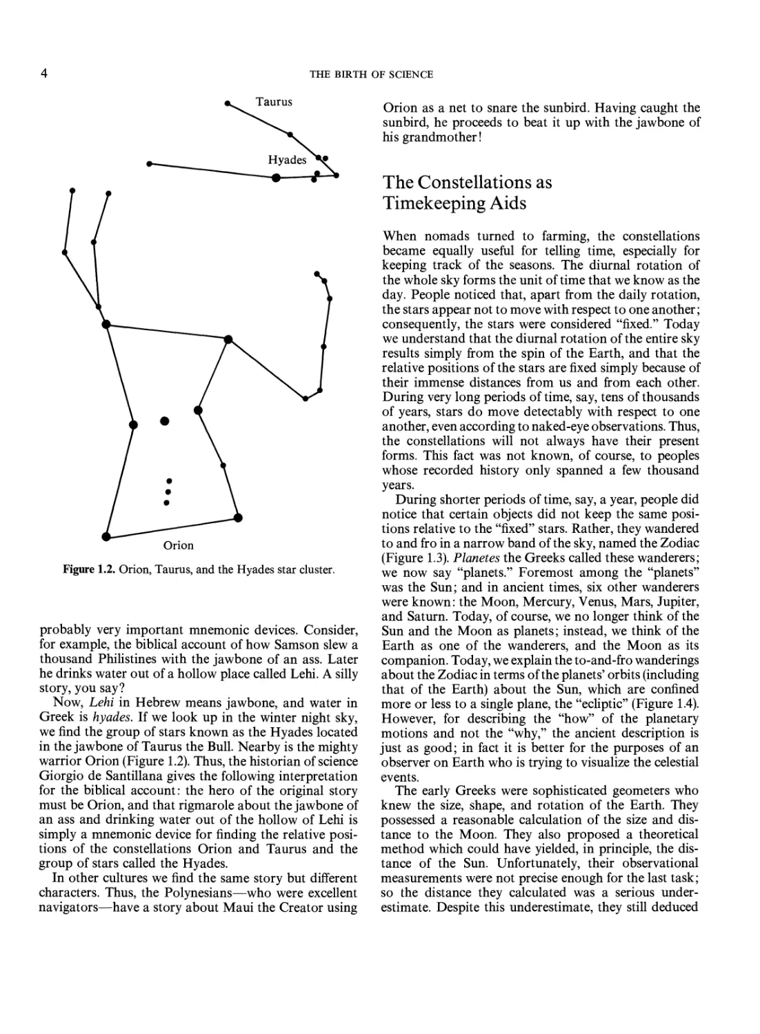
Figure 1.2. Orion, Taurus, and the Hyades star cluster.
probably very important mnemonic devices. Consider,
for example, the biblical account of how Samson slew a
thousand Philistines with the jawbone of an ass. Later
he drinks water out of a hollow place called Lehi. A silly
story, you say?
Now, Lehi in Hebrew means jawbone, and water in
Greek is hyades. If we look up in the winter night sky,
we find the group of stars known as the Hyades located
in the jawbone of Taurus the Bull. Nearby is the mighty
warrior Orion (Figure 1.2). Thus, the historian of science
Giorgio de Santillana gives the following interpretation
for the biblical account: the hero of the original story
must be Orion, and that rigmarole about the jawbone of
an ass and drinking water out of the hollow of Lehi is
simply a mnemonic device for finding the relative
positions of the constellations Orion and Taurus and the
group of stars called the Hyades.
In other cultures we find the same story but different
characters. Thus, the Polynesians—who were excellent
navigators—have a story about Maui the Creator using
Orion as a net to snare the sunbird. Having caught the
sunbird, he proceeds to beat it up with the jawbone of
his grandmother!
The Constellations as
Timekeeping Aids
When nomads turned to farming, the constellations
became equally useful for telling time, especially for
keeping track of the seasons. The diurnal rotation of
the whole sky forms the unit of time that we know as the
day. People noticed that, apart from the daily rotation,
the stars appear not to move with respect to one another;
consequently, the stars were considered "fixed." Today
we understand that the diurnal rotation of the entire sky
results simply from the spin of the Earth, and that the
relative positions of the stars are fixed simply because of
their immense distances from us and from each other.
During very long periods of time, say, tens of thousands
of years, stars do move detectably with respect to one
another, even according to naked-eye observations. Thus,
the constellations will not always have their present
forms. This fact was not known, of course, to peoples
whose recorded history only spanned a few thousand
years.
During shorter periods of time, say, a year, people did
notice that certain objects did not keep the same
positions relative to the "fixed" stars. Rather, they wandered
to and fro in a narrow band of the sky, named the Zodiac
(Figure 1.3). Planetes the Greeks called these wanderers;
we now say "planets." Foremost among the "planets"
was the Sun; and in ancient times, six other wanderers
were known: the Moon, Mercury, Venus, Mars, Jupiter,
and Saturn. Today, of course, we no longer think of the
Sun and the Moon as planets; instead, we think of the
Earth as one of the wanderers, and the Moon as its
companion. Today, we explain the to-and-fro wanderings
about the Zodiac in terms of the planets' orbits (including
that of the Earth) about the Sun, which are confined
more or less to a single plane, the "ecliptic" (Figure 1.4).
However, for describing the "how" of the planetary
motions and not the "why," the ancient description is
just as good; in fact it is better for the purposes of an
observer on Earth who is trying to visualize the celestial
events.
The early Greeks were sophisticated geometers who
knew the size, shape, and rotation of the Earth. They
possessed a reasonable calculation of the size and
distance to the Moon. They also proposed a theoretical
method which could have yielded, in principle, the
distance of the Sun. Unfortunately, their observational
measurements were not precise enough for the last task;
so the distance they calculated was a serious
underestimate. Despite this underestimate, they still deduced
The Constellations as Timekeeping Aids
(a)
Mars
epicycle
real
motion
apparent motion of
Mars among stars
Earth
O
Earth
(b)
(c)
Figure 1.3. The apparent motion of the planet Mars. In an Earth-
centered system. Ptolemy required a complicated theory of
epicycles to explain these motions. In a Sun-centered system,
Copernicus was able to explain the same motions much more simply:
namely, at certain points in the motion of the Earth about the
Sun, the Earth would seemingly catch up with a planet's
projected orbit, and then that planet would appear to go backward.
that the Sun is substantially larger than the Earth.
Because of the apparent dominance of the Sun, some of
the Greeks speculated correctly that the Earth revolved
about the Sun, rather than the other way around. These
ideals fell into disfavor when Aristotle argued, on
seemingly common-sense grounds, that we could not inhabit
a moving and rotating Earth without being more aware
of it. For example, Aristotle argued that motion of the
Earth should cause foreground stars to be displaced
annually with respect to the background (an effect now
called parallax), whereas no parallax could be detected
for any star by the Greeks. We now understand this null
result to arise from the very great distances to even the
nearest stars (see Problem 3.2).
Problem 1.1. This problem and the next one retrace the
early arguments of the Greeks about the sizes of the
Earth, Moon, and Sun, and the distances between them.
6 THE BIRTH OF SCIENCE
here). Erastothenes then observed that, at noon on the
first day of summer, sunlight struck the bottom of a deep
well in Syene, Egypt. In other words, the Sun at that time
was directly overhead. At the same time in Alexandria,
however, the Sun's rays made an angle of about 7° to the
vertical. Erastothenes concluded that Syene and
Alexandria must be separated by a fraction 7°/360° ^ 1/50 of a
great circle around the Earth. Assume that this distance
of 1/50 of the circumference of the Earth can be paced
off to be 800 km. Consult Appendix B for the relation
between the radius and circumference of a circle, and
calculate the radius of the Earth. Compare your answer
with the value given by Appendix A.
Reconsider now the observation of the shadow cast
by the Earth during a lunar eclipse. Assume still that the
rays from the Sun make parallel lines, and draw diagrams
to show how a comparison of the curvature of the Earth's
shadow on the Moon with the curvature of the Moon's
edge allows one to infer the relative sizes of the Earth
and Moon. This deduction is a slight modification of
Figure 1.4. The planetary orbits about the central Sun. The plane
of the Earth's orbit defines the ecliptic. Except for Mercury and
Pluto, all the planetary orbits are nearly circular and lie within
several degrees of the plane of the ecliptic. For sake of clarity,
the orbits of the three innermost planets, Mercury, Venus, and
Earth, are not labeled.
We begin with the size of the Earth. From the shape of
the shadow cast by the Earth on the Moon during a
lunar eclipse, it can be inferred that the Earth is a sphere.
Moreover, the method described in Problem 1.2 shows
that the Sun's distance is many times greater than the
diameter of the Earth. Erastothenes assumed that the
Sun was far enough away that the rays from the Sun are
virtually parallel when they strike the Earth (see figure
N
/ Alexandria 7°
/ / n. / parallel rays
7° I Syene
S
The Constellations as Timekeeping Aids
1
the method used by Aristarchos to find that the Moon's
diameter is about a third of that of the Earth. The modern
value is 0.27. With Erastothenes's value for the radius
of the Earth, calculate the diameter DM of the Moon.
Given that the Moon subtends an angular diameter at
Earth of about half a degree of arc, calculate the distance
rM of the Moon. Hint: If 9M is the angular diameter of
the Moon expressed in radians, and if 8M « 1, show that
the formula 8M = DM/rM holds to good approximation.
Problem 1.2. Aristarchos suggested an ingenious
method for measuring the relative distances of the Moon
and the Sun. Because the angular sizes of the Moon and
the Sun do not change appreciably with time, it can be
deduced that they maintain nearly constant distances
from the Earth. (The orbits are circular.) From the
figure here show how to deduce the ratio of the Moon's
distance rM to the Sun's distance rs as
rM/rs = cos 0>
where 26 is the total angle subtended at the Earth by
the Moon's positions between first and third quarters
of the Moon's phases. Unfortunately, the angle 9 turns
out to be too close to 90° to be practical as a way to tell
that the value of cos 6 is not zero (i.e., that the Sun is not
infinitely far way compared to the Moon). Modern
measurements using radar reflections show that rM/rs =
2.6 x 10~3. Thus, the Sun is about 390 times further
away than the Moon. On the other hand, solar-eclipse
observations demonstrate that the Sun and the Moon
have about the same angular sizes. Argue that this implies
the Sun is about 390 times larger than the Moon. Given
that the Moon is only 0.27 the size of the Earth, show
that the Sun is more than a hundred times larger than
the Earth. Thus, unless the mean density of the Sun is
much less than that of the Earth, the Sun is also likely
to be much more massive than the Earth; and it then
becomes more plausible to suppose that such a regal
body is the true center of the solar system rather than
the Earth. If the Earth can revolve about the Sun, then
there can be no great philosophical objection to its
spinning about its axis to account for the apparent
diurnal rotation of the sky.
Given the value of the size DM and the distance rM of
the Moon calculated in Problem 1.1, compute now the
diameter Ds and distance rs of the Sun. Convert your
answer to light-seconds, and discuss how long it typically
takes to bounce radar waves back and forth between
objects in the solar system (e.g., between Earth and
Venus). Discuss how geometry might be used to deduce
the radii of the orbits of Venus and Earth about the Sun.
This is the best method to obtain rs.
Moon
1st quarter
3rd quarter
8 THE BIRTH OF SCIENCE
N N
winter in Northern Hemisphere summer in Northern Hemisphere
summer in Southern Hemisphere winter in Southern Hemisphere
Figure 1.5. The reason for the seasons. Because the equatorial
plane of the Earth is inclined by 23.5° with respect to the plane of
the ecliptic, the Sun's rays strike the ground more
perpendicularly at one point of the Earth's orbit than at the opposite point
half a year later. At any one time, however, if it is winter in the
Northern Hemisphere, it is summer in the Southern Hemisphere.
This geometric result is the same whether we think of the Earth
moving around the Sun or the Sun around the Earth. (Note:
radii in this drawing are not to scale.)
Cancer autumn Scorpius
equinox
Leo Libra
Virgo
Figure 1.6. The seasons and the signs of the Zodiac. An Earth-
bound observer seems to see the Sun move around the Earth
once a year in the plane of the ecliptic (lightly shaded oval). At
the present epoch, the North Pole of the Earth points toward the
star Polaris, and the extension of the equatorial plane of the
Earth is shown as the dark semi-oval. The two points of
intersection of the Sun's apparent path with the equatorial plane are
called the spring and autumn equinoxes. The equatorial plane
in 2000 b.c. corresponded to the dashed semi-oval.
The Rise of Astronomy
The seasons arise because the spin axis of the Earth is
tilted with respect to the plane of the ecliptic, which is
the apparent path followed by the Sun during the course
of one year. Consequently, the Sun's rays at noon fall
more vertically during the summer months than during
the winter months (Figure 1.5). Spring and fall come
when the Sun is at the point of its apparent path where
the circle of the ecliptic crosses the circle of the Earth's
equator. These intersection points are called the spring
and autumn equinoxes (Figure 1.6).
When the Sun is not in the way, stars can be seen in
the background all along the ecliptic. There are twelve
prominent constellations near the plane of the ecliptic,
and these correspond to the twelve signs of the Zodiac.
In 2000 b.c, when the Babylonians set up the system of
timekeeping, the spring equinox lay in the direction of
the constellation of Aries. That is, spring came on March
21, when the Sun entered the "house of Aries," which
signaled the beginning of the planting season. However,
tidal torques cause a slow precession of the Earth's axis
of rotation; so the spring equinox moves backward
through the signs of the Zodiac, at about one sign per
two thousand years (Figure 1.6). Thus, 2,000 years after
the Babylonians had found that the spring equinox lay
in Aries, the spring equinox had moved into Pisces. This
event coincided approximately with the birth of Christ,
and may be why one early symbol of Christianity was
the fish. Two thousand years later, the spring equinox is
beginning to move into Aquarius (officially in a.d. 2600).
This is why our age is sometimes called the coming of
the "Age of Aquarius."
The Rise of Astrology
No one knows the exact reasons for the rise of astrology,
but it may have been something like the following. To
the ancients, it was obvious that the Sun, and to a lesser
extent, the Moon, influences events on Earth: witness
night and day, the seasons, tides, etc. The Sun and the
Moon were like gods. Why not, then the other planets?
From very early on, seven wanderers were known: Sun,
Moon, Mercury, Venus, Mars, Jupiter, and Saturn. To
honor the planetary gods, the Babylonian priests devised
the seven-day week and gave the days the names of the
planetary gods. In English, the roots of Sunday, Monday,
and Saturday can easily be traced to Sun, Moon, and
Saturn. In French, the roots of Mercredi, Vendredi,
Mardi, and Jeudi can equally easily be traced to
Mercury, Venus, Mars, and Jupiter.
Horoscopes were later based on the hypothesis that
the positions of the planets in the Zodiac could influence
the course of human events just as the positions of the
Sun and the Moon affect the seasons and the tides.
Especially important was the position of the Sun at the
time of one's birth; thus, if one was born in 2000 B.C.
between March 21 and April 19, the Sun was in Aries;
between April 20 and May 20, the Sun was in Taurus,
etc. Even today, one is given a Zodiac sign on the basis
of the Babylonian system. The problem is, of course,
that today these signs are 4,000 years out of date! For
example, the coming of spring, March 21, no longer
occurs when the Sun arrives at Aries but at Aquarius.
If astrologers were up to date, they should tell people
who are Aries that they are really Aquarius, and people
who are Aquarius that they are really Sagittarius, etc.
The Rise of Astronomy
In the beginning there was little difference between
astronomy and astrology. Indeed, some famous
astronomers of the past earned their keep by casting horoscopes
for kings and queens. A major divergence of astronomy
and astrology came with the work of Nicholas
Copernicus in the sixteenth century. Copernicus discovered
that he could explain the seemingly complicated
motions of the planets in terms of a stationary £un about
which revolved Mercury, Venus, Earth, Mars, Jupiter,
and Saturn. The Moon would still have to go around
the Earth, but the looping motions of the other planets
(which is what observers actually see) became simple to
explain if the Earth itself moved about the Sun. (as
Figure 1.3 shows, when the Earth's orbital motion carries
it past one of the outer, slower planets, that appears to
go backwards!) Copernicus's ideas forced a major change
in the prevailing philosophy of a human-centered
universe, and the Copernican Revolution is justly
considered one of the major turning points of science.
Free thinkers like Galileo and Kepler were quick to
adopt the Copernican system, and they provided many
of the early pieces of astronomical evidence in support
of it. Later Galileo was forced by the Church to recant
his espousal of a moving Earth, an episode made familiar
by Bertolt Brecht's play on the subject. Popular^ myth
has Galileo secretly defiant, muttering the famous phrase
"And yet it moves." In any case, the Copernican
viewpoint received its ultimate triumph in the seventeenth
century, with the work of Isaac Newton. Newton showed
that the laws of planetary motion described by Kepler
in a Sun-centered system (see Chapter 18) could be
derived mathematically from Newton's formulation of
the laws of mechanics and gravitation.
Newton also demonstrated how his theory of
gravitation could explain the tides raised on Earth by the Sun
or Moon. The basic idea was that the Sun or Moon
pulled hardest on the side of the oceans facing toward it.
less hard on the center of the Earth, and least on the side
10
THE BIRTH OF SCIENCE
to
Moon
or
Sun
Figure 1.7. The tides. Tides in the oceans arise because the
gravity of the Moon or the Sun is greatest on the side facing it and
least on the side opposite it. The difference between these two
forces is responsible for producing the characteristic two-sided
bulge.
of the oceans facing away from it (Figure 1.7). In this way,
the oceans would tend to bulge out in two directions: on
one side because the water is pulled away from the
Earth, on the other side because the Earth is pulled
away from the water. The difference in force between the
two sides of the Earth is called the tidal force. (We shall
discuss such forces in other contexts in this book.)
In this manner did astronomy and astrology part ways.
With the growing maturity of modern science, astronomy
attempted to give mechanistic explanations for natural
phenomena—seasons, tides, planetary motions—on the
basis of laws formulated and tested in laboratories.
Astrology continued to attribute mystical influences on
terrestrial affairs to the planets. Mystical beliefs have a
long cultural history, and they die hard. Kepler and
Newton were mystics in many ways, and much of the
modern world still clings to atavistic concepts.
Modern Astronomy
Today we know that Mercury, Venus, Earth, Mars,
Jupiter, and Saturn are only six of the nine planets that
go around the Sun; the other three are, of course, Uranus,
Neptune, and Pluto. However, as far as we can tell,
planets and their satellites are not the major constituents
of the universe. Stars are. (Perhaps.) The Sun is a star—
the closest one to Earth—and the Sun contains about
99.9 percent of the mass of our solar system. However,
the Sun is only one star of myriads that belong to our
Galaxy.* Our Galaxy contains more than 1011 (one
hundred billion) stars! (For a review of the exponent
notation, see Box l.L) And our Galaxy is only one of
myriads in the observable universe. The observable
universe contains about 1010 (ten billion) galaxies. Thus, in
the observable universe there are about 1010 galaxies x
* When Galaxy is capitalized, it refers to our own galaxy.
1011 stars/galaxy = 1021 stars: an astronomical number
which has no simple English equivalent.
Since numbers like 1021 are enormous, almost beyond
intuitive comprehension, we cannot hope to study each
individual astronomical object. Even if we could see
them with our telescopes—and in fact we cannot see
more than a small fraction of them—we would not gain
much insight from an object-by-object study. A f^r more
practical and informative goal is to look for patterns of
behavior among similar groups of objects. This book is
organized in terms of the few theoretical concepts which
underlie the structure and evolution of the astronomical
objects under study. First, we will emphasize the deep
connections between how matter is organized on large
scales (macroscopic behavior) and on small scales
(microscopic behavior). Second, we will find that there
are two main recurring threads in the organizational
fabric of macroscopic objects like stars, galaxies, and the
universe. These two threads are the law of universal
gravitation and the second law of thermodynamics
(Chapters 3 and 4).
Another implication follows from the enormous
number, 1021, of stars in the observable universe. Since our
life-sustaining Sun is only one star among an enormous
multitude, it seems extremely unlikely that we could be
either alone in the universe or the most intelligent species
in the universe. This realization motivates the discussion
on the chances for extraterrestial life and intelligence
that we shall pursue in the last part of this book. Again
we shall find the second law of thermodynamics to play
an integral role in our discussions.
BOX 1.1
Exponent Notation
10" = 1000 • • • 000.
n zeroes
10~" = 1/10" = .000 • • • 0001
v»_
n — 1 zeroes
multiplication: 10" x 10m = 10"+m. Also 10"/10m = 10" x
10~m= 10"~m.
Important prefixes in exponent notation:
nano = 10 ~9 (one-billionth)
micro = 10 ~6 (one-millionth)
milli = 10 ~3 (one-thousandth)
centi = 10 ~2 (one-hundredth)
kilo = 103 (one thousand)
mega = 10 (one million)
giga = 109 (one billion)
Example: 1 kilometer = 103 meter = 103 x 102
centimeter = 105 cm.
Rough Scales of the Astronomical Universe
11
Rough Scales of the
Astronomical Universe
Given that gravitation and the second law of
thermodynamics underlie much of natural phenomena, you will
appreciate that an honest understanding of modern
astronomy requires a healthy dose of physics. The next
three chapters of this book provide the physics needed
to understand, on a qualitative level, the explanations of
the important phenomena. The first step, however,
toward a unified appreciation of astronomy is to obtain a
physical feel for the scale of the phenomena that we shall
be dealing with in this book.
The most fundamental measurements that we can
make of an object are its size, its mass, and its age (or
duration between one event and another). The units of
length, mass, and time that we shall adopt are centimeter
(abbreviated cm), gram (abbreviated gm or g), and second
(abbreviated sec or s); these are called cgs units (Box 1.2).
Although it is not immediately obvious, it is nevertheless
true that all physical quantities can be expressed as
various combinations of powers of cm, gm, and sec. A
familiar example is the cgs unit of energy: erg =
gm cm2 sec-2. A less-familiar example is the cgs unit of
electric charge: esu = gm1/2 cm3/2 sec-1. At first sight,
temperature seems to be an exception. However, in any
fundamental discussion, the temperature (degrees Kelvin
or K) always enters in the combination "Boltzmann's
constant x temperature," which has the units of energy.
Some of the more important physical constants in cgs
units are given in Appendix A.
Let us now consider the scales of some astronomical
objects. Listed in Table 1.1 are the very rough ("order
of magnitude," i.e., to the nearest power of ten) sizes,
masses, and ages of the Sun, the Galaxy, and the
observable universe. For comparison, the same quantities are
listed for a small child.
BOX 1.2
The cgs Units
unit of length = centimeter = cm (1 inch = 2.54 cm)
unit of mass = gram = gm or g (1 pound = 454 gm)
unit of time = second = sec or s
(1 year = 3.16 x 10⁷ sec)
unit of force = dyne = gm cm sec-2
(weight of 1 pound on Earth = 4.45 x 10⁵ dyne)
unit of energy = erg = gm cm2 sec-2
(potential energy of 1 pound at height of 1 foot on
Earth = 1.36 x 10⁷ erg)
unit of power or luminosity = erg sec *
(100 watt = 109 erg/sec)
Object
child
Sun
Galaxy
observable
Table
universe
1.1. Rough scales.
Size
102 cm
1011 cm
1023 cm
1028 cm
a Notice that although the Sun, the Galaxy,
in size and mass, they all have ages com
Mass
104 gm
1033 gm
1045 gm
1055 gm
>4cjfea
108 sec
1017 sec
> 1017 sec
>1017sec
and the universe differ appreciably
parable in order of magnitude.
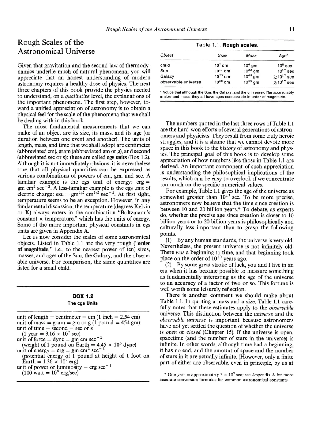
The numbers quoted in the last three rows of Table 1.1
are the hard-won efforts of several generations of
astronomers and physicists. They result from some truly heroic
struggles, and it is a shame that we cannot devote more
space in this book to the history of astronomy and
physics. The principal goal of this book is to develop some
appreciation of how numbers like those in Table 1.1 are
derived. An important component of such appreciation
is understanding the philosophical implications of the
results, which can be easy to overlook if we concentrate
too much on the specific numerical values.
For example, Table 1.1 gives the age of the universe as
somewhat greater than 1017 sec. To be more precise,
astronomers now believe that the time since creation is
between 10 and 20 billion years.* To debate, as experts
do, whether the precise age since creation is closer to 10
billion years or to 20 billion years is philosophically and
culturally less important than to grasp the following
points.
(1) By any human standards, the universe is very old.
Nevertheless, the present universe is not infinitely old.
There was a beginning to time, and that beginning took
place on the order of 1010 years ago.
(2) By some great stroke of luck, you and I live in an
era when it has become possible to measure something
as fundamentally interesting as the age of the universe
to an accuracy of a factor of two or so. This fortune is
well worth some leisurely reflection.
There is another comment we should make about
Table 1.1. In quoting a mass and a size, Table 1.1
carefully notes that these estimates apply to the observable
universe. This distinction between the universe and the
observable universe is important because astronomers
have not yet settled the question of whether the universe
is open or closed (Chapter 15). If the universe is open,
spacetime (and the number of stars in the universe) is
infinite. In other words, although time had a beginning,
it has no end, and the amount of space and the number
of stars in it are actually infinite. (However, only a finite
part of either are observable, even in principle, by us at
* One year = approximately 3 x 10⁷ sec; see Appendix A for more
accurate conversion formulae for common astronomical constants.
12
THE BIRTH OF SCIENCE
any finite time after the creation event.) Have you ever
contemplated what the truly infinite means? The cos-
mologist G. F. R. Ellis has, and he makes the following
interesting observation. If the number of stars (and
planets) is infinite, then all physically possible historical
events are realizable somewhere and sometime in the
universe. Thus, there may be somewhere and sometime
another Earth with a history exactly like our own,
except that the South wins the Civil War instead of the
North. Elsewhere and othertime, there may even be a
reasonable fascimile of Tolkien's Middle Earth! Now,
it is highly improbable that such alternative worlds are
within our "event horizon"; so we may never be able to
communicate with them. Nevertheless, it is fun to
speculate on the possibility of such worlds given the truly
infinite.
The alternative possibility—that the universe is
closed, so that spacetime and the number of stars in it
are finite—is almost equally bizarre according to normal
conceptions. This possibility leads to the conclusion that
the volume of space is finite, yet it does not possess an
edge or boundary!
Contents of the Universe
The primary inhabitants of the universe are stars, of which
the Sun is only one example. Stars exhibit a great
variety of properties. Besides suns of all colors, there are
the tremendously distended red giants and the
mysteriously tiny white dwarfs. The Sun itself is quite an
average star, neither very massive nor very light, neither
very large nor very small. Why, then, does the Sun
appear so bright, but the stars so faint? Because the stars
are much further away than the Sun. The Sun is "only"
eight light-minutes away, but the nearest star, proxima
Centauri, is about four light-years distant. A light-year
is the distance traveled by light in one year, and equals
9.47 X 1017 cm. To appreciate how enormous a
distance is a few light-years, notice that human travel to
the Moon, "only" one light-second away, represents
the supreme technological achievement of civilization
on Earth. Will travel to the stars ever be within our
grasp?
The rich variety of stars live in our Galaxy mostly
singly or in pairs (Figure 1.8). Sometimes, however,
hundreds or thousands of stars can be found in loose
groups called open clusters. The Pleiades is a fairly
young open cluster, and the reflection nebulosity which
surrounds the famous "seven sisters" of this cluster
attests to the fact that these stars must only recently have
been born out of the surrounding gas and dust. The
oldest stars in our Galaxy are found in tighter groups called
globular clusters. Rich globular clusters may contain
more than a million members.
The space between the stars is not completely empty.
Figure 1.8. These three views of the bright star Sirius show it to
be a member of a binary system. The companion of Sirius is a
white dwarf. (Lick Observatory photograph.)
The diffuse matter between the stars is called the
interstellar medium, but by terrestrial standards it is
virtually a perfect vacuum. Clouds of gas and dust, as
well as energetic cosmic-ray particles gyrating wildly
in magnetic fields, reside in the space between stars.
Giant fluorescent gas clouds (called Hn regions) lit up
by nearby hot young stars, like the Orion nebula found
in the "sword" of Orion, constitute some of the most
beautiful objects in astronomy. Other objects like the
Crab nebula shine with an eerie light (synchrotron
radiation) and are now known to be the remnants
expelled by stars which died in titantic supernova
explosions. The cores left behind in such cataclysms, neutron
stars and black holes, represent some of the most
intriguing denizens of the astronomical kingdom. Other
stars die less violently, ejecting the outer shell as a
planetary nebula which exposes the hot central core
destined apparently to become a white dwarf.
Contents of the Universe
13
Figure 1.9. A cluster of galaxies in Hercules. (Palomar
Observatory, California Institute of Technology.)
Stars and the material between them are almost
always found in gigantic stellar systems called galaxies.
Our own galaxy, the Milky Way System, happens to be
one of the two largest systems in the Local Group of
two dozen or so galaxies. The other is the Andromeda
galaxy; it stretches more than one hundred thousand light-
years from one end to the other, and it is located about
two million light-years distant from us. If the kingdom
of the stars is vast, the realm of the galaxies is truly
gigantic.
Apart from small groups like our own Local Group,
galaxies are also found in great clusters, containing
thousands of members {Figure 1.9). Most cluster
galaxies are roundish ellipticals rather than the more
common spirals found in the general field. Rich clusters
have been found at distances exceeding three billion light-
years from us. Obviously, the observable universe is a
tremendously large place! And modern cosmology tells
us that it is expanding. Clearly, the universe contains
many interesting objects, not the least of which are the
Earth and its inhabitants. Of all the objects intensively
studied in the solar system, the Earth is the only one
known to harbor life. How did we get here? How do
we fit into the unfolding drama of the universe? These
issues and others are the natural legacy of Copernicus's
first inquiries, and they form the subject matter of this
book. To survey the entire universe and to develop the
important themes fully, our pace must necessarily be
fast. Let us start!
CHAPTER TWO
Classical Mechanics, Light, and
Astronomical Telescopes
Modern physical science began with classical
mechanics and astronomy. The earliest practitioners,
such as Galileo and Newton, made important
contributions both as physicists and as astronomers. Hence,
classical mechanics, the nature of light, and
astronomical telescopes make fitting starting points for our study.
Classical Mechanics
In classical mechanics the most fundamental property
of matter is mass. The fundamental frame of reference
for describing the dynamics of matter is an inertial frame,
any frame which is at rest or, at most, moves at a constant
velocity relative to the "fixed" stars. Since the stars are
not truly "fixed," we will later need to reconsider this
definition; but for now we implicitly assume that
henceforth all physical laws are to be stated for such inertial
frames.
Galileo discovered the first law of mechanics, and
Descartes gave it a general formulation. (According to
Stillman Drake, Galileo's criticisms of the Aristotlean
viewpoint led him to shy away from stating general
principles.) The first law, or the principle of inertia,
describes the innate resistance of matter to a change in
its state of motion:
A body in motion tends to remain in motion. Unless
the body is acted upon by external forces, its
momentum—the product of its mass and velocity—
remains constant.
When external forces are present and act on material
bodies, the momenta of the bodies no longer remain
constant. To describe this situation, Newton formulated
the second law of mechanics:
The time-rate of change of a body's momentum is
equal to the applied force.
Usually the mass of a body does not change; so the
time-rate of change of its momentum is simply its mass
times its time-rate of change of velocity. The latter is
called acceleration, and like velocity, it has both a
magnitude and a direction (i.e., it is a vector). If we denote
the mass of a particle by m, the applied force by F (a
vector), and the acceleration by a (another vector),
Newton's second law takes the familiar form
ma,
(2.1)
BOX 2.1
The Laws of Mechanics
First law: When F = 0, p = mv = constant.
dp
Second law: When F ^ 0, — = F; usually, F = ma
at
14
Classical Mechanics
15
which is probably the most famous equation in all of
physics. A concise summary of the above in mathematical
language is given in Box 2.1.
The physical content of F = ma is the following. If we
know that forces are acting on a body, we may use F =
ma to calculate the acceleration a that is induced by the
action of the force F. In this way, we may infer the
changes of the state of motion produced by the known
forces. Conversely, if we observe a body to undergo
acceleration, we may infer that forces must be present
to produce this change in the body's state of motion.
It is important to notice that acceleration is present
even if the velocity maintains a constant magnitude (i.e.,
speed) but changes direction. The simplest example is
circular motion with radius r at a constant speed v =
\v\. In this important case, the magnitude of the associated
acceleration is (see Problem 2.1 for the mathematical
derivation)
a = v2/r. (2.2)
The direction of a is inward, toward the center of the
circle.
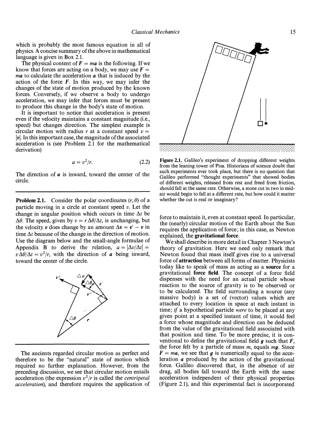
Problem 2.1. Consider the polar coordinates (r, 9) of a
particle moving in a circle at constant speed v. Let the
change in angular position which occurs in time At be
Aft The speed, given by v = r A9/At, is unchanging, but
the velocity v does change by an amount Av = v' — v in
time At because of the change in the direction of motion.
Use the diagram below and the small-angle formulae of
Appendix B to derive the relation, a = \Av/At\ =
v A8/At = v2/r, with the direction of a being inward,
toward the center of the circle.
The ancients regarded circular motion as perfect and
therefore to be the "natural" state of motion which
required no further explanation. However, from the
preceding discussion, we see that circular motion entails
acceleration (the expression v2/r is called the centripetal
acceleration), and therefore requires the application of
Figure 2.1. Galileo's experiment of dropping different weights
from the leaning tower of Pisa. Historians of science doubt that
such experiments ever took place, but there is no question that
Galileo performed "thought experiments" that showed bodies
of different weights, released from rest and freed from friction,
should fall at the same rate. Otherwise, a stone cut in two in
midair would begin to fall at a different rate, but how could it matter
whether the cut is real or imaginary?
force to maintain it, even at constant speed. In particular,
the (nearly) circular motion of the Earth about the Sun
requires the application offeree; in this case, as Newton
explained, the gravitational force.
We shall describe in more detail in Chapter 3 Newton's
theory of gravitation. Here we need only remark that
Newton found that mass itself gives rise to a universal
force of attraction between all forms of matter. Physicists
today like to speak of mass as acting as a source for a
gravitational force field. The concept of a force field
dispenses with the need for an actual particle whose
reaction to the source of gravity is to be observed or
to be calculated. The field surrounding a source (any
massive body) is a set of (vector) values which are
attached to every location in space at each instant in
time; if a hypothetical particle were to be placed at any
given point at a specified instant of time, it would feel
a force whose magnitude and direction can be deduced
from the value of the gravitational field associated with
that position and time. To be more precise, it is
conventional to define the gravitational field g such that F,
the force felt by a particle of mass m, equals mg. Since
F = ma, we see that g is numerically equal to the
acceleration a produced by the action of the gravitational
force. Galileo discovered that, in the absence of air
drag, all bodies fall toward the Earth with the same
acceleration independent of their physical properties
(Figure 2.1), and this experimental fact is incorporated
16
CLASSICAL MECHANICS, LIGHT, AND ASTRONOMICAL TELESCOPES
g
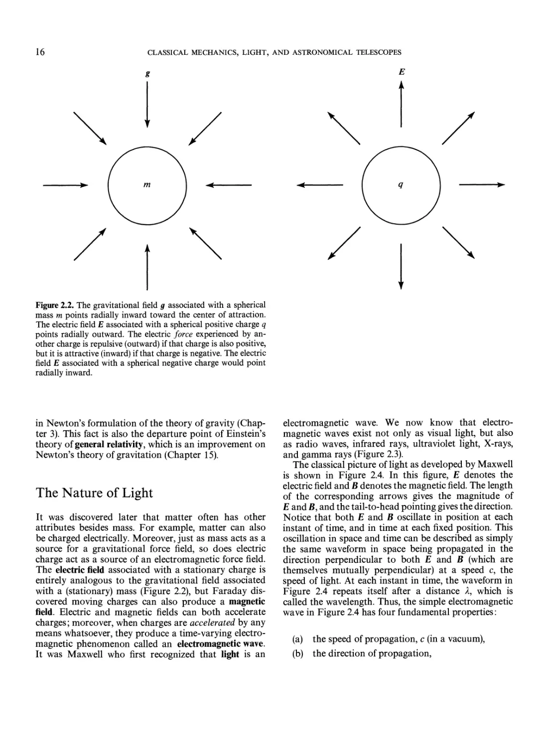
Figure 2.2. The gravitational field g associated with a spherical
mass m points radially inward toward the center of attraction.
The electric field E associated with a spherical positive charge q
points radially outward. The electric force experienced by
another charge is repulsive (outward) if that charge is also positive,
but it is attractive (inward) if that charge is negative. The electric
field E associated with a spherical negative charge would point
radially inward.
in Newton's formulation of the theory of gravity
(Chapter 3). This fact is also the departure point of Einstein's
theory of general relativity, which is an improvement on
Newton's theory of gravitation (Chapter 15).
The Nature of Light
It was discovered later that matter often has other
attributes besides mass. For example, matter can also
be charged electrically. Moreover, just as mass acts as a
source for a gravitational force field, so does electric
charge act as a source of an electromagnetic force field.
The electric field associated with a stationary charge is
entirely analogous to the gravitational field associated
with a (stationary) mass (Figure 2.2), but Faraday
discovered moving charges can also produce a magnetic
field. Electric and magnetic fields can both accelerate
charges; moreover, when charges are accelerated by any
means whatsoever, they produce a time-varying
electromagnetic phenomenon called an electromagnetic wave.
It was Maxwell who first recognized that light is an
electromagnetic wave. We now know that
electromagnetic waves exist not only as visual light, but also
as radio waves, infrared rays, ultraviolet light, X-rays,
and gamma rays (Figure 2.3).
The classical picture of light as developed by Maxwell
is shown in Figure 2.4. In this figure, E denotes the
electric field and B denotes the magnetic field. The length
of the corresponding arrows gives the magnitude of
E and B, and the tail-to-head pointing gives the direction.
Notice that both E and B oscillate in position at each
instant of time, and in time at each fixed position. This
oscillation in space and time can be described as simply
the same waveform in space being propagated in the
direction perpendicular to both E and B (which are
themselves mutually perpendicular) at a speed c, the
speed of light. At each instant in time, the waveform in
Figure 2.4 repeats itself after a distance A, which is
called the wavelength. Thus, the simple electromagnetic
wave in Figure 2.4 has four fundamental properties:
(a) the speed of propagation, c (in a vacuum),
(b) the direction of propagation,
The Nature of Light
17
140
120
100
A 80
3
2 60
13
40 -
20
0
10
rio
10
i-8
10
i-6
10
-4
10
-2
10°
102 104
wavelength (cm)
gamma x-rays ultra- visible infrared radio
rays violet
Figure 2.3. The electromagnetic spectrum and its penetration
through the Earth's atmosphere. Radio waves have the longest
wavelengths; gamma rays, the shortest. Only radio waves,
optical light, and the shortest gamma rays have no difficulty
penetrating the atmosphere to reach sea level. A few "windows"
between the absorption bands of water vapor and carbon
monoxide exist in the infrared, but all ultraviolet astronomy and
X-ray astronomy has to be" carried out above the Earth's
atmosphere.
(c) the wavelength, A,
(d) and the polarization direction (the direction that
E points; notice that the direction of B is known
to be perpendicular to both E and the direction
of propagation).
polarization
direction
A
initial
instant
direction of
propagation
X
c
wavelength of light
speed of light (in a Vacuum)
Figure 2.4. The classical picture of light.
The Energy Density and Energy Flux
of a Plane Wave
There is a fifth property of light that we have left out
in the above discussion, and that is, of course, its intensity.
The intensity of the wave depicted in Figure 2.4 should,
in some sense, become larger as the magnitudes of E and
B (the lengths of the arrows E and B) become larger.
One possible measure of the intensity of the wave is the
energy contained per unit volume, which in Maxwell's
theory works out to be
In general, the light from a source will contain a
mixture of waves with different directions of propagation,
different wavelengths, and different polarizations.
However, one of the great discoveries of Maxwell was that,
in a vacuum, all these waves have the same speed of
propagation:
c = 3.00 x 1010 cm/sec.
A true appreciation of this important result came only
after Einstein's development of the theory of special
relativity (Chapter 3).
energy density
1
8tt
{E-E + B'B)
(2.3)
where the dot product A • B between two vectors A and
B is calculated according to the rule depicted in
Figure 2.5. The dot product of a vector with itself is often
written as the square of that symbol without the
boldface; thus, A A = A2, where A = \A\ is the magnitude
of A. Thus, equation 2.3 might also be expressed as
energy density = (E2 + B2)/%n.
18
CLASSICAL MECHANICS, LIGHT, AND ASTRONOMICAL TELESCOPES
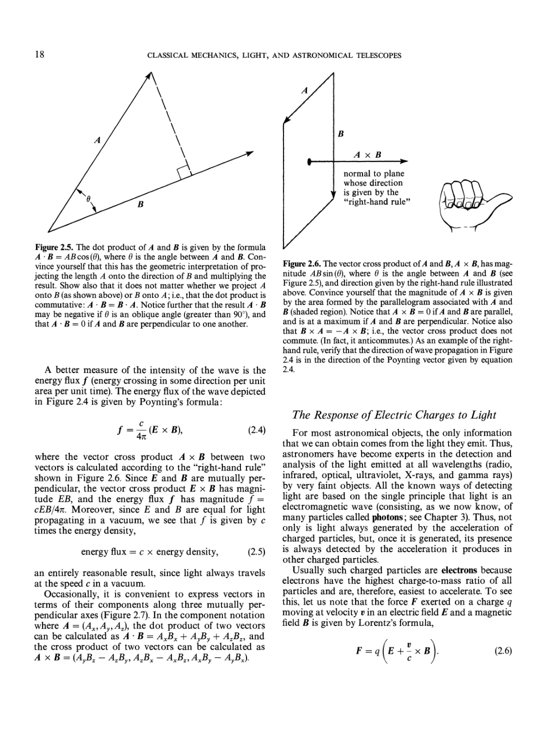
Figure 2.5. The dot product of A and B is given by the formula
AB — AB cos (0), where 6 is the angle between A and B.
Convince yourself that this has the geometric interpretation of
projecting the length A onto the direction of B and multiplying the
result. Show also that it does not matter whether we project A
onto B (as shown above) or B onto A; i.e., that the dot product is
commutative: A • B — B- A. Notice further that the result A • B
may be negative if 6 is an oblique angle (greater than 90°), and
that A • B = 0 if A and B are perpendicular to one another.
A better measure of the intensity of the wave is the
energy flux f (energy crossing in some direction per unit
area per unit time). The energy flux of the wave depicted
in Figure 2.4 is given by Poynting's formula:
/=^(ExB),
(2.4)
where the vector cross product A x B between two
vectors is calculated according to the "right-hand rule"
shown in Figure 2.6. Since E and B are mutually
perpendicular, the vector cross product E x B has
magnitude EB, and the energy flux f has magnitude f =
cEB/4n. Moreover, since E and B are equal for light
propagating in a vacuum, we see that f is given by c
times the energy density,
energy flux — ex energy density,
(2.5)
an entirely reasonable result, since light always travels
at the speed c in a vacuum.
Occasionally, it is convenient to express vectors in
terms of their components along three mutually
perpendicular axes (Figure 2.7). In the component notation
where A = (Ax,Ay,Az), the dot product of two vectors
can be calculated as A • B = AXBX + AyBy + AZBZ, and
the cross product of two vectors can be calculated as
AxB = (AyBz - AzBy, AZBX - AxBz,AxBy - AyBx).
A x B
normal to plane
whose direction
is given by the
"right-hand rule"
Figure 2.6. The vector cross product of A and B, A x B, has
magnitude ABsin(0), where 6 is the angle between A and B (see
Figure 2.5), and direction given by the right-hand rule illustrated
above. Convince yourself that the magnitude of A x B is given
by the area formed by the parallelogram associated with A and
B (shaded region). Notice that A x B = 0 if A and B are parallel,
and is at a maximum if A and B are perpendicular. Notice also
that B x A = — A x B; i.e., the vector cross product does not
commute. (In fact, it anticommutes.) As an example of the right-
hand rule, verify that the direction of wave propagation in Figure
2.4 is in the direction of the Poynting vector given by equation
2.4.
The Response of Electric Charges to Light
For most astronomical objects, the only information
that we can obtain comes from the light they emit. Thus,
astronomers have become experts in the detection and
analysis of the light emitted at all wavelengths (radio,
infrared, optical, ultraviolet, X-rays, and gamma rays)
by very faint objects. All the known ways of detecting
light are based on the single principle that light is an
electromagnetic wave (consisting, as we now know, of
many particles called photons; see Chapter 3). Thus, not
only is light always generated by the acceleration of
charged particles, but, once it is generated, its presence
is always detected by the acceleration it produces in
other charged particles.
Usually such charged particles are electrons because
electrons have the highest charge-to-mass ratio of all
particles and are, therefore, easiest to accelerate. To see
this, let us note that the force F exerted on a charge q
moving at velocity v in an electric field E and a magnetic
field B is given by Lorentz's formula,
q[E +-xB).
(2.6)
The Nature of Light
19
time 1
y
Figure 2.7. Any vector A may be decomposed by projecting its
length onto three mutually perpendicular directions. The results
of those projections, AX9 Ay, AZ9 are called the x, y, z
components of the vector A, and we may sometimes write the triplet
(Ax,Ay,Az) to mean the vector A itself. Notice, however, that the
concept of the vector A exists independently of any particular
component decomposition (i.e., independent of the coordinate
representation). Nevertheless, in practical calculations, it is
convenient to use a decomposition into components because we may
then just ideal with ordinary numbers for each component.
Figure 2.8. The response of an electron to a passing
electromagnetic wave. The electric and magnetic vectors, E and B, are equal
in an electromagnetic wave; consequently, the electric force on a
charge, qE, is generally much larger than the magnetic force,
q(v/c) x B, as long as the velocities are much less than the speed
of light. Thus, a free electron (shown above) displaces up and
down "in phase" with the corresponding E vector, whereas a
bound electron will usually displace up and down "out of phase"
with the corresponding E vector (assuming a "natural period of
oscillation" shorter than that of visible light).
From Newton's law, F = ma, we see that the acceleration
a of charges in given electric and magnetic fields is
proportional to the ratio q/m, which is highest for electrons.
Hence, the interaction of light with matter, whether in
the human eye, in the chloroplasts of green plants, or in
photographic film, occurs because light interacts with
the electrons in matter, either those bound to atoms or
those free to move about (like the conduction electrons
in metals).
When an electromagnetic wave passes by an electron,
the electron tries to oscillate sympathetically ("in tune")
with the passing oscillatory wave (Figure 2.8). These
sympathetic vibrations underlie such familiar
phenomena as the reflection and refraction of light, but a detailed
explanation would take us too far afield. Suffice it to say
that the electronic oscillations generate secondary
sources of waves which either reinforce or interfere
destructively with the original wave (Figure 2.9). As a
result, the original wave appears to be refracted into a
different direction, or to be reflected, or both.
E
E
I I
I
4
I ie_
I I
Figure 2.9. The generation of an electromagnetic wave by an
oscillating electron. As the electron oscillates up and down, the
electric field—which in a stationary electron points radially
toward the electron—tries to follow the oscillatory motion. The
time-varying components of the electric vector far from the
electron alternate up and down in space because they "remember"
the electron's position as it was one light-travel time back. At a
fixed point in space the electric vector oscillates up and down in
time with a period equal to the oscillation of the electron. The
diagram is highly simplified in that: (a) we have not drawn in the
oscillatory magnetic field induced by the electron's motion; (b)
the electromagnetic fields near the electron (within several
wavelengths) have a more complicated structure than a simple
outgoing electromagnetic wave; and (c) the oscillating electron
actually radiates in all directions except along its oscillation
length.
20
CLASSICAL MECHANICS, LIGHT, AND ASTRONOMICAL TELESCOPES
propagation
direction
(a)
propagation direction
(wave front)
normal
(b)
summary: Bg < 0« (bent closer to normal);
opposite behavior going from glass to air
Figure 2.10. Refraction.
associated with the progress of wavecrests (the positions
where photons are most likely to be found). The phase
velocity also equals c in a vacuum, but it may exceed
c in exceptional materials. Usually, however, the
sympathetic oscillations of the electrons in the atoms and
molecules of a nonconducting medium impede the
average progress of the photons, and the speed of wavecrests,
v, is also less than c, its value in a vacuum.
Now, air is more like a vacuum than is glass; so it is
easy to believe that the speed of light in air, va, is greater
than the speed of light in glass, vg. Consider what this
means when a whole collection of photons are incident
as a plane wave on an air-glass interface at an oblique
angle (Figure 2.10). The photons (the dots) are imagined
to come from a very distant source so that they arrive in
waves whose fronts are connected by the dashed lines.
The initial direction of the propagation of the photons
and the wavefront is indicated by the heavy top arrow.
As the photons enter the glass interior, they are
effectively slowed down; so they travel less distance in a
given interval of time than their companions who have
still not entered the glass. The net effect is to "turn" the
direction of the wavefront defined by the collection of
photons so that the propagation of the wavefront in the
glass is in a direction closer to the normal. (The normal
is the direction perpendicular to the air-glass interface.)
Notice that this "turning" is strictly a property of the
entire collection of photons, i.e., a property of the wave;
no individual photon can be said to have suddenly
"turned" in direction upon entering the glass. The
quantitative relation between the incident direction, 8a, and
the emergent direction, 6g, is given by Snell's law
(Problem 2.2).
Astronomical Telescopes
Astronomical telescopes can be constructed which use
either refraction or reflection to gather light over a large
collecting surface and focus it to a much smaller area.
This property—gathering more light and focusing it,
and not magnification—is the primary purpose of most
astronomical telescopes.
Refraction
To understand the principle of refracting telescopes,
we must first understand refraction on a macroscopic
level. (The word macroscopic in this book means on a
scale which is large compared to atoms; it is to be
contrasted with the word microscopic.) We have already
mentioned that the speed of light in a vacuum, c, is a very
large number, 3 x 1010 cm/sec. In fact, c is the fastest
possible speed at which individual photons (or, indeed,
any physical entity) can travel in any medium at all.
There is a different kind of speed (the "phase velocity")
Problem 2.2. Use the diagram below to consider how
far the wavefront travels in interval At. Let va and vg be
the speeds of the wavefront; show
vaAt
vgAt
cos(7i/2 — 6a) cos(7i/2 — 9 )'
va&t
Astronomical Telescopes
21
bent
toward
normal
bent away
from normal
screen or
photographic
plate
photographic
plate
white light
from distant star
(a)
top view
observer
8
perspective
drawing
image of star
rocked back and
forth on slit
observer
(b)
pattern of
dark lines
superimposed
on continuum
back view
as seen
by observer
violet
increasing X
indigo blue green yellow
(c) dispersed starlight from prism
Figure 2.11. Principle of the prism.
orange
red
Convert the above equation into Snell's law: nasmQa =
ng sin 9g, where the indices of refraction of air and glass
are given, respectively, by na = c/va and ng = c/vg9 with
ng>na> 1.
In Figure 2.10a we have drawn the air-glass interface
as if it were an infinite flat plane. This is an adequate
approximation if the edge-to-edge dimension of the
interface is very large compared to the wavelength of
light; otherwise there are complicated diffraction effects,
which we shall discuss later. In the diffractionless
approximation, we can summarize the reasoning by Figure
2.10b, where we draw only the directions of the
propagation of the wavefronts as being rays of light. Using this
ray-tracing technique (also called "geometric optics"),
we are now prepared to explain some familiar and
important phenomena.
The Principle of the Prism
In Figure 2.10 we assumed implicitly a unique speed
of light va in air and another unique speed vg in glass,
independent of wavelength X. Only in a vacuum does
light of different wavelengths have a unique speed c. In
matter, light of different wavelengths travels at different
speeds because the electrons bound to atoms and
molecules have different abilities to respond to rapidly
varying and slowly varying electromagnetic waves (refer
back to Figure 2.8). In particular, the "natural period of
oscillation" of such electrons corresponds usually to the
ultraviolet (Chapter 3); thus violet light will generally
interact more with matter than blue light, and blue light
more than red. This means that refraction in glass will
turn violet light more than blue light; and blue light more
than red light. As is shown in Figure 2.11a, this fact
explains how a prism breaks up white light into its
component colors.
Astronomers use this "dispersive" property of prisms
to analyze the wavelength composition of starlight
("spectral analysis"). Figure 2.11b shows a simplified
setup of how this is done. In order to use as much as
possible of the photographic plate (the most common
and inexpensive photon-detection device), the image of a
star is rocked back and forth mechanically along the
length of an entrance slit. The light which enters the slit
is then dispersed by a prism. (In high-accuracy work, a
diffraction grating is used instead of a prism.) The
dispersed light is then allowed to fall onto a photographic
plate. From the point of view of the observer drawn in
22
CLASSICAL MECHANICS, LIGHT, AND ASTRONOMICAL TELESCOPES
bent
toward
normal
focal length
bent away
from normal
parallel rays
from very
distant star
focus
optical
axis
Figure 2.12. Principle of the lens.
Figure 2.11b, the exposed photographic plate will show
violet light on the left and red light on the right (Figure
2.11c), a sequence of increasing wavelength reading
from left to right. (From right to left, we have the
mnemonic ROY G BIV.) With real starlight, we will usually
have not only a continuous variation of the composition
of starlight from violet to red—the so-called continuum—
but also thin dark lines at well-defined wavelengths
where there is much less light than at neighboring
wavelengths—the so-called absorption-line spectrum. An
example can be found in the Fraunhofer spectrum of the
Sun. The spectrum shows "lines" at certain
wavelengths, and not "dots," because of the rocking of the
star image on the slit of the spectrograph. (An extended
object like the Sun will automatically produce "lines"
without mechanical rocking.) As we shall see in
Chapter 3, the pattern of dark lines can be associated with
the presence of various chemical elements in the
atmosphere of the star. Thus, spectral analysis can yield
information on the chemical makeup of stars (and other
astronomical bodies). If Doppler shifts are involved
(Chapter 3), spectroscopy can also give the velocity of
the object along the line of sight to us.
The Principle of Lenses
and the Refracting Telescope
The main optical element in a refracting telescope is
the objective lens, which collects light over the entire
area of the aperture and forms an image of the observed
object at the focus (Figure 2.12). The principle of the lens
is easily understood from Figure 2.11, since light bends
within the lens in the same way that it does in the prism.
Indeed, the rim of the lens is shaped like a prism.
To discuss the focusing ability of a lens, imagine a
source like a star, which is essentially a single point of
light. Since the star is practically at infinity, the rays
from the star arrive at Earth nearly on parallel lines. A
blue focus
red focus
Figure 2.13. Chromatic aberration.
image
Figure 2.14. The principle of the eyepiece.
objective
Figure 2.15. A simple refracting telescope.
perfect lens would bring these parallel rays to a single
point at the focus. This point is, of course, the correct
image for our idealized star. In practice, however,
starlight is made up of light of different colors. Since blue
light is bent more by a glass lens than red light,
chromatic aberration results, as shown in Figure 2.13. A
photographic plate placed at the blue focus will show a
blurred red image, and vice versa at the red focus.
Let us ignore this chromatic aberration (or assume
that steps can be taken to compensate for it) in order to
discuss light-gathering power. Clearly, a lens can be used
in "reverse" of the above description; i.e., if an object (or
the image of a real object) were placed at the focus of a
lens, the rays from it, in passing through the lens, would
leave in parallel lines (Figure 2.14). A human eyeball
placed behind this lens would perceive the object (or
image) as if it were at infinity, which turns out to be the
most relaxing condition for visual observations. Thus,
the combination of a large objective lens plus an
eyepiece (Figure 2.15) serves as an astronomical telescope
Astronomical Telescopes
23
Figure 2.16. In 1921, Albert Einstein posed with the staff of
Yerkes Observatory in front of the 40-inch refractor, the largest
in the world. (Yerkes Observatory photograph, University of
Chicago, Williams Bay, Wisconsin.)
(a refractor), which enables an astronomer to gather
starlight over a much larger area than his or her own
eyeball could. Electronic devices ("image intensifiers"),
with or without photographic film, allow the astronomer
to "observe" to much fainter limits than is possible with
naked-eye observations, even on telescopes with very
large apertures (Figure 2.16).
Different apparent sizes (magnifications) of the final
image—for example, the apparent separation of a double
star—result from using different eyepieces (Problem
2.3). However, the light-gathering power is determined
by the square of the diameter of the objective, not by the
eyepiece. For an extended object, say, the Moon,
spreading the same amount of light over a larger area (by high
magnification) decreases the apparent surface brightness
of the observed object, but a net gain may still result for
the clarity of detailed features if the object is sufficiently
bright. Thus, high magnification may be important for
solar-system observations, but it is generally not needed
for other types of astronomical investigations.
Problem 2.3. To discuss magnification, imagine a
telescope pointing directly toward a star on its optical axis
24
CLASSICAL MECHANICS, LIGHT, AND ASTRONOMICAL TELESCOPES
(see diagram). Imagine another star lying at an angle 80
with respect to the first. The rays from both stars will
pass through the center of the objective lens on a straight
line. These rays will be brought into focus with rays which
pass through other parts of the objective at a distance
behind the objective equal to its focal length, f0. If the
eyepiece is placed its focal length, fe9 further back, the
double-star image would in turn pass through the
eyepiece and be collimated into two parallel beams at an
angle 8e to each other. An astronomer behind the eyepiece
will perceive an inverted image of two stars separated by
an angle 6e, whereas the actual double star is only
separated by the angle 60. Thus, the angular separation
has been magnified by the ratio 8J90. To calculate this
magnification in terms of the properties of the telescope,
derive the relationship
/otan0o = /etan0e.
The angles 90 and 6e are usually quite small; therefore
use the small-angle approximations of Appendix B to
show that the magnification 8e/60 is given by the ratio of
the two focal lengths f0/fe. A typical amateur's telescope
may have a one-meter objective focal length and a
40-millimeter eyepiece. What would its magnification be?
Does this magnification apply only to the observation
of double stars?
normal
to mirror
objective
Reflection
In Figure 2.10 the rays which fell on an air-glass
interface were drawn as if they would all be refracted. In
practice, there will also always be some reflection, as well as
some absorption. If a thin layer of metal is deposited onto
the glass surface and is polished, the reflectance will be
increased, and we will have made a mirror. This everyday
fact—metals are shiny—is a result of the microscopic
fact that metals contain many free electrons which are
not bound to the atoms in the lattice of the metal. (That
is why metals are good electrical conductors.) These
free electrons respond quite readily to the presence of
electromagnetic waves, and they allow almost no
radiation of sufficiently long wavelength to pass through the
7
incident
ray
reflected
ray
Figure 2.17. The law of reflection. The angle of reflectance is
equal to the angle of incidence: 6, = 6^
metal. Thus, a mirror will reflect almost all the optical
light which falls on it.
The geometric properties of a flat mirror are easily
deduced by knowing only some simple wave properties
of light. Light will reflect from a flat surface in such a way
that the angle of reflectance (relative to the normal) is
equal to the angle of incidence (Figure 2.17). What
fraction of the light is reflected or absorbed or transmitted
depends on the properties of the mirror (for example,
the kind of metal used: aluminium, silver, or gold) and
the wavelength of the incident light (radio, optical, or
X-rays), but the incident and reflection angles are always
symmetric, because the wave propagation before and
after reflection takes place in the same medium (Problem
2.4).
Problem 2.4. Consider the wavefront AB which moves
to A'B' in time At. In another interval At, B' will have
moved to B", and A' will have moved (by reflection) to
A". Since the rays A'A" and B'B" are moving in the same
medium (say, air), the distances A'A" and B'B" are equal.
Show now that the angles B'B"A' and A"A'B" are equal.
Astronomical Telescopes
25
Show also that these angles are, respectively, the
complements of the angles of reflectance and incidence,
thereby proving the law of reflection.
The Principle of Parabolic Mirrors
and the Reflecting Telescope
The high reflectance of metallic surfaces allows
reflecting telescopes for use with waves of any length from
radio to ultraviolet to be constructed on the same general
principle (Figure 2.18). To provide good imaging, the
surface of the reflecting element (a mirror or a dish)
should be paraboloidal (a parabola of revolution), and
the surface should not contain any irregularities larger
than a fraction of the wavelength of the light that needs
to be focused. Since visual light is much shorter than
radio waves, optical telescopes are made by depositing
a metal film on accurately figured glass; whereas the
much coarser technique of directly shaping a metal dish
(which may even have small holes in it to make it lighter!)
can be used to construct a radio telescope.
Why does the mirror or dish have to be paraboloidal?
To understand this, we need first to review the properties
of ellipses. You may remember how to draw an ellipse
(Figure 2.19) from high-school geometry. You take a
length of string, tie it into a loop, place the loop over
two tacks or nails (which become the two foci of the
ellipse), take a pencil, and push the point tight against
the string. The locus traced out by the pencil tip, keeping
the string taut, is an ellipse. Consider what this means
for the geometry of an ellipse. Since the string is taut,
the lines joining the foci and the pencil tip are straight
lines. Moreover, the direction that the pencil has to be
pushed against the string to keep it taut and the direction
that the pencil tip can move are mutually perpendicular,
i.e., the former direction is the normal to the ellipse. It
should also be obvious that the normal bisects the angle
made by the two lengths of string from the foci.
Imagine now making a mirror in the shape of an
ellipse, and putting a point source of light at one of the
foci (Figure 2.20). All the light which leaves this source
in the plane of the page will strike the ellipse somewhere
and reflect off it, with the angle of reflectance equal to
the angle of incidence. Given the properties of the ellipse,
however (see Figure 2.19), this means that each ray will
be brought to the other focus! Hence, if we want to
collect all the light which leaves the source—including
those rays which travel out of the plane of the page—at
a single point at the other focus, we need only make our
mirror an ellipse of revolution. Such an ellipsoid (a
prolate spheroid) would represent the ultimate mirror
in terms of light-gathering power for the assumed
geometry. Of course, if one had funds to construct only part
of the ellipsoidal mirror (Figure 2.21), one would be able
parallel rays
from distant
astronomical
source
parabolic
mirror
or dish
focal length
Figure 2.18. The principle behind optical and radio telescopes.
Figure 2.19. How to draw an ellipse. A long length of string
produces a rounder ellipse than a short length.
Figure 2.20. An elliptical mirror brings the light from a point
source at one focus to the other focus.
26
CLASSICAL MECHANICS, LIGHT, AND ASTRONOMICAL TELESCOPES
parabolic mirror
Figure 2.21. Part of a complete ellipsoidal mirror will capture
only part of the light which leaves a point source.
to collect only the corresponding fraction of all the rays
which left the light source.
Imagine now moving the point source of light to
infinity. If the two foci of an ellipse become infinitely
separated, the ellipse becomes a parabola. Thus, to bring
the light rays from a very distant point source like a star
to a single focus, the objective of a reflecting telescope
should be a paraboloidal mirror (Figure 2.18). This
provides the answer to our original question. To collect
as much light as possible, clearly, the aperture of the
paraboloid should be made as large as available funds
will allow.
X-rays are much more penetrating than
electromagnetic radiation of longer wavelengths. X-rays which are
incident almost perpendicularly on a metallic surface
will be mostly absorbed rather than reflected. This
problem is less severe at grazing incidences (especially
if one uses gold instead of aluminum); so X-ray
telescopes are built to bring the rays to a focus by grazing-
incidence reflections (see Figure 2.22). This configuration
results in much less collecting area for a given amount of
metallic surface; and since the telescope has to be put
above the Earth's atmosphere, X-ray astronomy is a
much more expensive proposition per experiment than
optical or radio astronomy. That is the price one pays
to be an X-ray astronomer (Figure 2.23).
There are two big advantages of reflectors over
refractors even for use confined to optical wavelengths.
First, there is no chromatic aberration. Second, reflectors
can be built much larger, because the primary mirror
can be supported mechanically all along its back, whereas
the lens must be supported only along its edges. Other
practical considerations—such as that a mirror can
parallel rays
from distant
astronomical
X-ray source
Figure 2.22. An example of a X-ray telescope which works by
grazing incidence reflections. Notice that the focus is brought to
the back of the mirror arrangement.
r 4 f
Figure 2.23. The Einstein Observatory X-ray telescope has a
nested set of surfaces with an effective collecting area of 300 cm2
that brings X-rays to a focus by grazing-incidence reflections.
(Courtesy of Perkin-Elmer.)
have some bubbles in the glass without affecting its
performance—means that all large modern telescopes
are constructed as reflectors rather than as refractors.
The one disadvantage of a reflector is, of course, that
its prime focus is in front of the mirror. Thus, for an
astronomer or for instruments to observe at the prime
focus, an appreciable fraction of the incoming light may
be blocked (Figure 2.24a). This problem can be partially
solved in several ways. The first solution was invented by
Newton. In the Newtonian arrangement (Figure 2.24b),
a secondary mirror is used to bring the light to a focus
at the side of the telescope tube. This arrangement tends
to make the system lopsided; so a more satisfactory
solution was devised by Cassegrain. In the Cassegrain
arrangement (Figure 2.24c), a secondary mirror is used
to bring the light to a focus behind the telescope tube
through a hole in the primary mirror. None of the above
Astronomical Telescopes
27
(a) Prime
(b) Newtonian
flat mirror
(c) Cassegrain
to spectrograph
(d) Coude
Figure 2.24. Various arrangements for reflecting telescopes: (a)
the prime focus in front of the primary mirror; (b) the Newtonian
focus at the side of the telescope; (c) the Cassegrain focus at the
back of the telescope; (d) the Coude focus underneath the
telescope.
arrangements are satisfactory for making very precise
spectroscopic observations, because the bulky and heavy
spectrographs would strain on the telescope tube if they
were suspended in front, to the side, or in back of the
primary mirror. For such observations, the Coude
arrangement was devised, whereby a series of secondary
mirrors bring the light down the polar axis of the
telescope drive to a fixed focus in a room below the telescope
(Figure 2.24d). In the Coude room, large pieces of
equipment can be mounted in a stationary configuration.
Angular Resolution
The ability to distinguish fine details in the image is
an important advantage of a telescope compared to a
"light bucket," which merely collects light over a large
area without attempting to bring it to an accurate focus.
This ability is called angular resolution. Figure 2.25
illustrates the concept of angular resolution in its
simplest context. Imagine a telescope pointing directly
toward a star on its optical axis. Imagine another star
lying at an angle 9 with respect to the first. A perfect
focus would result in two point images slightly displaced
from one another. Such a perfect focus is, however, never
attainable in practice, for the following reasons.
Ground-based optical telescopes must contend with
the blurring produced by turbulence in the Earth's
atmosphere. The varying amount of refraction in a
turbulent atmosphere makes the focused optical image
dance around ("seeing") on the photographic plate. If
28
CLASSICAL MECHANICS, LIGHT, AND ASTRONOMICAL TELESCOPES
photograph
:, AND ASTRONOMICAL TELESCOPES
photograph
r
i • i
-M
?.VK
Vvr
%
*0fe«
&&&*&
SBBBiSj^t*''
L^^^Bnnvi
iSr
wSkkV'*
sMR*a'-
hBH&^
»?#s '•
^1^^^----—
two stars separated
by angle 0
Figure 2.25. The concept of angular resolution applied to a
double star.
Figure 2.26. Because of diffraction, the shadow cast by a razor
blade is not perfectly sharp. (Courtesy of John Wilder, Berkeley
Astronomy Department Photo Lab.)
the source is sufficiently bright, astronomers can use a
series of short exposures to correct partly for this effect
by means of a technique invented by Antoine Labeyrie
called "speckle interferometry." For faint objects, this
technique is impractical, and atmospheric turbulence
limits the seeing image of a point source to about one
second of arc, even at the best sites. (One second of arc
equals 1/3600 of a degree of arc, and corresponds roughly
to the angle subtended by a dime at a distance of about
two miles.) In other words, if two stars are separated by
less than one second of arc, the observer cannot tell from
the blurred images that more than one point of light is
actually present.
Radio waves do not suffer from this atmospheric
blurring. The angular resolution of modern radio
telescopes is limited by another effect: the diffraction
produced by the wave nature of light. As we noted earlier,
the ray-tracing method to determine the focusing of
ideal focus into actual blurred
two sources images
Figure 2.27. The 100-meter radiotelescope at Bad Muenstereifel-
Effelsberg, Germany. (Max-Planck Institute fur Radioastron-
omie at Bonn.)
electromagnetic waves assumes that the wavelength is
negligibly small compared with the aperture of the
telescope. On angular scales comparable to the ratio of the
wavelength I of light to the diameter D of the telescope's
collecting surface, however, diffraction effects produce
an unavoidable blurring even of point sources. The
reason is that the secondary waves produced by the
interaction of light and matter at the edges of the
objective interfere constructively and destructively to give
a pattern of light and dark fringes which, on small
angular scales, is quite different from that predicted by
ray tracing. Figure 2.26 shows that the shadow cast by
a razor blade is not perfectly sharp. Diffraction of light
Astronomical Telescopes
29
allows one to see (slightly) around corners, as diffraction
of sound allows one to hear around corners. For a
circular aperture, the blurring produced by diffraction
limits the angular resolution to an amount given by
^dif fraction limit = 1.22/,/D.
Thus, the world's largest fully steerable single-dish
telescope (the 100-meter dish in West Germany; Figure 2.27)
cannot resolve two radio sources closer than about 9
minutes of arc when it operates at a wavelength of 21 cm.
Problem 2.5. What is the diffraction limit in seconds
of arc of a 5-meter telescope (Figure 2.28) at a wavelength
of 5000 A? (1 A = 10"8 cm.) Compare your answer to
the seeing limit.
Figure 2.28. The 200-inch (5-meter) telescope on Palomar
mountain has a large enough prime-focus area to accommodate an
observer plus some equipment. (Palomer Observatory, California
Institute of Technology.)
Hence, the diffraction-limited resolution of single-dish
radio telescopes (even the Arecibo dish—Figure 2.29—of
Figure 2.29. The 300-meter Arecibo radiotelescope sits in a
natural bowl in Puerto Rico and uses the rotation of the Earth
to help turn the aim of its beam. (Arecibo Observatory, N.A.I.C.,
Cornell University.)
Figure 2.30. The Space Shuttle will launch a 2.4-meter telescope
into orbit around the Earth, which will greatly improve the focus
and clarity of observed astronomical objects. (NASA, Marshall
Space Flight Center, artist's rendition.)
Figure 2.31. A vast array of 1,000 radiotelescopes, each of 100-
meter diameter, has been comtemplated in Project Cyclops as a
means to search for extraterrestrial intelligence. (NASA, Ames
Research Center.)
Earth
Figure 2.32. The principle of aperture synthesis illustrated by an
imaginary line of radio telescopes at the North Pole. During one
twelve-hour period, the rotation of the Earth causes this line to
sweep out a full circle. Thus, this configuration of telescopes
mimics the angular resolution of a filled aperture with a
diameter equal to the baseline (shaded area).
Astronomical Telescopes
31
Figure 2.33. The very large array of radiotelescopes in Soccoro,
New Mexico, has movable elements arranged in a Y. (The
National Radio Astronomy Observatory VLA program is
operated by Associated Universities, Inc., under contract with the
National Science Foundation.)
300-m diameter, which is not fully steerable) is typically
much worse than the seeing-limited angular resolution
of large optical telescopes.
There are two direct remedies available to improve
the angular resolution of astronomical telescopes. For
optical work, a dramatic improvement could be made by
getting above the Earth's atmosphere (above the
"seeing"). This is one principal motivation for the Space
Telescope project (Figure 2.30). Even the space telescope,
however, will not reach its diffraction-limited potential
because of mechanical jitter associated with trying to
point the telescope accurately.
For radio work, the computer recombination of the
signals from more than one radio telescope can increase
the effective baseline D of the observations, and thus
lower the ratio of XjD which governs the diffraction
limit. A brute-force technique would be merely to build
a huge array of telescopes like that proposed for
project Cyclops (Figure 2.31). A more elegant solution,
devised by Sir Martin Ryle of England, uses the rotation
of the Earth. In the simplest case, imagine a line of
telescopes placed at the North pole (Figure 2.32). During a
12-hour period, the rotation of the Earth would swing
the line of radio telescopes through a full circle, and thus
allow them to mimic the resolving power (but not the
collecting area) of a vast single-dish with the
corresponding aperture diameter. Such powerful full-synthesis
instruments have been built in England and in Holland.
The most powerful such synthesis instrument is the very
large array (VLA) in New Mexico, whose movable
telescopes are so arranged that they need not rely on the
rotation of the Earth to obtain (nearly) complete aperture
coverage (Figure 2.33).
Less than full synthesis is possible with simultaneous
observations by steerable radio telescopes located far
from one another. Such very long baseline interferometric
(VLBI) work has provided the most detailed information
so far on the structure of certain astronomical radio
sources (Chapter 13). Multi-mirror telescopes have also
been built for ground-based optical work (Figure 2.34),
but the motivation here is to increase the collecting area
rather than to improve on the angular resolution. Large
32
CLASSICAL MECHANICS, LIGHT, AND ASTRONOMICAL TELESCOPES
Figure 2.34 The Multiple Mirror Telescope (MMT) consists of
six 72-inch mirrors, having a combined collecting area equal to
one 176-inch telescope. (The MMT is a joint facility of the
Smithonian Institution and the University of Arizona.)
optical interferometers are impractical because it is
difficult to keep track of the phase (where the peaks and
troughs lie) of optical light and maintain alignment of
the mirrors to a fraction of a wavelength.
Astronomical Instruments and Measurements
The popular image of the astronomer observing by
eye at the end of a telescope (Figure 2.15) is badly
outdated. The human eye is a relatively poor photon
detection and storage instrument. All manner of electronic
equipment exists today to help the astronomer measure
the brightness of astronomical objects (photometry),
calculate the wavelength distribution and spectral
features from such bodies (spectrophotometry and
spectroscopy), assess the amount of polarization in this light
(polarimetry), and fix the position of the object in the
sky (positional astronomy); see Box 2.2. The one
indispensable tool of the modern astronomer is the electronic
computer, which can be used to run many of these
instruments more-or-less automatically, guide the
telescope, reduce data, and help construct theories which
interpret the observational results. For better or worse,
modern astronomy, like the rest of modern life, becomes
more complex with every passing day. It is a tribute to
the human brain and the scientific method that the
important themes contained in the rapidly growing body
of astronomical knowledge can still be sorted out in
terms of relatively simple organizational ideas. These
themes and ideas are the frame of this book, but the
foundations are the basic astronomical measurements
listed in Box 2.2.
BOX 2.2
Some Fundamental Astronomical Measurements
(1) Parallax. Apparent angular shift of nearby objects
against the positions of distant objects, due to the
changing perspective as the Earth revolves around
the Sun. This shift yields the distance to the nearby
object by triangulation, since the Earth-Sun distance
(the astronomical unit) is known.
(2) Proper motion. Real angular shift of nearby objects
against the positions of distant objects due to the
motion of the nearby object perpendicular to our
line of sight. This shift yields the component of
velocity perpendicular to the line of sight if the
distance to the object is known.
(3) Doppler shift. Shift in wavelength of a spectral line
compared to its position for a laboratory source.
Such shifts are usually associated with motion along
the line of sight. (See Chapter 3 for appropriate
formulae.)
(4) Apparent brightness. The total brightness of an
astronomical body as it appears relative to some
standard. If the distance to the object is known, a
measurement of its apparent brightness allows us
to calculate its intrinsic brightness, i.e., its
luminosity.
(5) Color. The difference in apparent brightness when
measured through two filters that pass light of two
different wavelength bands (for example, a blue
filter and a yellow filter). This technique provides a
quantitative measure of the wavelength distribution
of the continuum light, and can be used to estimate
the surface temperatures of stars (Chapter 9).
CHAPTER THREE
The Great Laws of Microscopic Physics
Physics and mathematics are the basic theoretical tools
which astronomers use to interpret the data
collected by their telescopes. They are used to construct
models of specific astronomical objects and theories of
the basic physical mechanisms at work. This does not
imply that we can proceed deductively from the known
laws of physics and derive all of astronomy. For one
thing, physics is not yet complete; for another,
astronomical systems are too complex. Astronomers need to
rely on observations to keep their theoretical
speculations from going too far astray. Nevertheless, we need a
general appreciation of the architecture of physics to
understand why it is so important to astronomy. This is
the purpose of Chapters 3 and 4.
Figure 3.1 is an abbreviated blueprint of the
architecture of physics. From this figure we see that mechanics
is the single unifying theory which underpins all physics,
and, therefore, presumably all natural phenomena. The
two basic components of twentieth-century mechanics
are quantum mechanics and special relativity, and they
both grew from (and eventually supplanted) classical
mechanics.
Mechanics
In Chapter 2 we saw that at the center of classical
mechanics lay Newton's second law:
time-rate of change of a particle's momentum
= applied force.
Mechanics
Classical mechanics
Quantum mechanics
Special relativity
Particles and Fields
Gravitation
Electromagnetism
Strong interaction
Weak interaction
Behavior of
Macroscopic bodies
Thermodynamics
Statistical mechanics
Nonequilibrium physics
Figure 3.1. Architecture of physics.
Thus, given the applied force, Newton's second law
allows us to calculate the change in the state of motion
of a particle, and, by superposition, the state of motion
of any collection of particles. It is therefore one of the
most fundamental discoveries of modern science that all
forces in the physical world originate in only four basic
forms:
(a) the gravitational force,
(b) the electromagnetic force,
33
34
THE GREAT LAWS OF MICROSCOPIC PHYSICS
m,
Fu
21
m
m-
Figure 3.2. The gravitational force F12 exerted on mass m1 by
mass m2 at a distance of r is attractive and directed along the
line of centers.
(c) the strong nuclear force,
(d) the weak nuclear force.
A basic theoretical program begun by Einstein and still
pursued actively today is the development of a "unified
field theory," which would explain all the above forces
in terms of a single "superforce." A major development
of the 1970s was the apparently successful unification of
the electromagnetic and weak forces by Weinberg and
Salam. The single "superforce" remains to be found,
although a name, "supergravity," has already been
proposed for one of the more promising candidates.
The Universal Law of Gravitation
The first, and perhaps most important, general force
law to be discovered was Newton's recognition that
matter itself is a source of force for influencing the
motion of other matter. In particular, Newton proposed
that the property of mass gives rise to a universal force
of attraction. For point masses, this force is directed
along the line of centers and varies as the product of the
two attracting masses divided by the square of the
separation distance. The proportionality constant G is
called the universal gravitational constant, and its value
in cgs units is
G = 6.67 x 10"8 gmT1 cm3 sec-2.
In formula form, we have that the force exerted on mass
m1 by mass m2 has magnitude
F12 = Gm1m1jr
(3.1)
and is directed from 1 to 2 (Figure 3.2). The force exerted
on mass 2 by mass 1, F2u is identical in magnitude as
F12, but oppositely directed; i.e., F2i is directed from 2
to 1. Occasionally, people will write formula (3.1) with
a minus sign on the right-hand side to remind themselves
that the gravitational force is always attractive; however,
such reminders can also cause confusion unless we write
the forces in their full vector-notation forms. In any case,
when the forces are treated as vectors, the force due to
finite-sized bodies can be deduced by considering them
to be a superposition of many point masses and by
m,
m
Figure 3.3. The resultant gravitational force F exerted on mass
m by masses m1,m2, and m3 is the vectorial sum of the individual
forces Fl9 F2, and F3 formed by "lining up" these three vectors
"head-to-tail." This case is easily generalized to an arbitrary
number of attracting mass points.
adding according to the force law for point masses
(Figure 3.3). In particular, for two spherical bodies,
Newton found that the force of attraction was the same
as if all the mass of each body were concentrated at a
single point at its center. Newton delayed publication
of his important research concerning the motion of the
Moon until he had proved this result for spherical bodies.
The result does not hold for nonspherical bodies.
Gauss's Formulation of the
Law of Gravitation
We see from the above discussion that Newton's
original formulation of his law of gravitation is so
cumbersome for nonpoint bodies that even a genius like
himself had difficulties making practical calculations. A
much more useful formulation was devised by Gauss; it
is mathematically equivalent to Newton's law, but
greatly simplifies practical calculations (especially if one
knows vector calculus). We shall briefly discuss Gauss's
law, not only for later applications, but also because it
makes more concrete the usefulness of the concept of a
gravitational field g (see Chapter 2).
Suppose we have a distribution of matter
characterized by a mass density p which can be an arbitrary
function of position x and time t Let g, which is generally
also a function of jc and t, be the gravitational field which
arises from the entire mass distribution. We begin by
constructing an arbitrary volume V which encloses part
or all or none of the mass (Figure 3.4). Let A be the
surface area of the volume V, and let g± be the component
of the gravitational field g which is directed along the
inward direction perpendicular to any point on the
surface A. (We reverse the usual convention here to avoid
Mechanics
35
area A
area A = 4tt/*2
Figure 3.4. Gauss's law states (g^A = AnGM.
dealing with too many negative signs.) Let the average
value of gL on the surface A be called <#i>. Gauss's law
states that the average value <#±> multiplied by the area
A equals AnG times the mass M contained in volume V:
(gi}A = AnGM.
(3.10
Equations (3.1) and (3.1') are completely identical in
mathematical content, but the far greater power of
equation (3.1/) is that it allows us to choose the mass
distribution p(x,t) and the size and shape of the volume V
completely arbitrarily.
To demonstrate explicitly the power of Gauss's law,
consider the problem which stymied Newton for so long
(Figure 3.5). Enclose the spherical distribution of mass
in a concentric sphere with radius r greater than the
radius jR of the mass distribution. By symmetry, gL
everywhere on our larger sphere must have the same
value, and this value must equal both the average value
<0_l> and the magnitude g of vector g. Therefore, Gauss's
law yields
g = AnGM/A = GM/r2,
since the area of a sphere of radius r is Anr7* (Appendix B).
In the above, M is the entire mass of our spherical body,
since r is greater than R; therefore, Gauss's law yields
that the gravitational attraction of a spherical body is
the same as if all the mass were concentrated at a single
point at its center: g = GM/r2 with g pointing radially
inwards (Q.E.D.).
Conservation of Energy
From the laws of mechanics it is often possible to
derive certain conservation principles, i.e., the fact that
certain quantities do not change in time although
everything else may. One of the most important conservation
principles is that of the conservation of energy. For
example, from Newton's second law of motion and
Newton's law of gravitation for two isolated point masses
Figure 3.5. Gauss's proof of Newton's theorem about spherical
bodies: (g^A = AnGM => g = GM/r2 with g pointing radially
inward.
(or spherical bodies), it is possible to prove that the total
energy—which is the sum of the kinetic energies and the
potential energy associated with gravitation—is a
conserved quantity. In formula form we have
1 l
total energy = E = - m^v2 + - m2v22
Gm1m2 \ ,-^
+ ( i-^H = constant, (3.2)
where v1 and v2 are the instantaneous speeds of masses
m1 and m2 and r is the separation distance between the
two bodies. Now, without using calculus, you may
think it miraculous that statement (3.2) follows
deductively from F = ma plus Newton's theory of gravity, but
with calculus, the proof is not difficult (Problem 3.1).
You may complain that this makes the concept of
conservation of energy very mathematical. It is
mathematical. Energy is not something that you can touch, smell,
or count. Kinetic energy, mv2/2, can be said to be the
energy associated with the motion of a material body,
but that statement does not make the concept of kinetic
energy any less mathematical. Similarly, gravitational
energy ( — Gm1m2/r) can be said to be the potential for
doing work by gravitational forces, but that statement
does not make the intrinsic concept less mathematical
either.
36
THE GREAT LAWS OF MICROSCOPIC PHYSICS
most kinetic energy,
least (most negative)
potential energy
utvd elliptical orbit of sateffit
least kinetic energy
most potential energy
Figure 3.6. Conservation of energy.
Problem 3.1. This problem is for those who know
calculus. To prove equation (3.2), show that Newton's laws
imply, for two isolated masses m1 and m2 which feel only
each other's mutual gravitation:
m
m<
dt ~ r2
dv2 Gm1m2
dt
r
r
ri)
r2)
where r1 and r2 are the position vectors of masses 1 and
2, respectively; r is the magnitude of their difference; and
the quantities in the square brackets yield the direction
of the gravitational force (draw your own diagram). The
velocities v1 and v2 are given by the derivatives of r1
and r2:
v
dr1
IF9
V<
dr2
dt'
Take the dot products of the first set of equations with
the second set, and add the results to obtain
niiV
l"!
dv1 dv2
-— + m2v2 • -T-
dt dt
Gm1m2 1
r2)
dr2
dt
With vx2 = vx - vu v22 = v2 • v2, and r2 = (r2 — rx)
(r2 — rx), derive the following identities:
— (r2) = 2(r2 ~^i)'jt (r2 ~ rt).
Show, therefore, that we may write the previous equation
as
d /1
1
Jt[ -2m^+- mW—^1 = 0,
which implies the conservation of total energy, equation
(3.2).
The important thing to realize is that as the two bodies
move, their kinetic energies (which are always positive)
and their gravitational potential energy (which is always
negative) may be converted back and forth into one
another, but the sum total remains constant in time. As
an example, Figure 3.6 shows the bound elliptical orbit
of an Earth satellite. Artificial satellites are much less
massive than the Earth; the kinetic energy of the Earth
that results from the attraction of artificial satellites is
completely negligible. Thus, in applying equation (3.2)
to this example, we need only worry about the kinetic
energy and potential energy of the satellite. The poten-
Mechanics
37
tial energy of the satellite is most negative when it is
closest to the Earth; therefore, at this point (perigee), the
kinetic energy (and the speed) of the satellite must be
the greatest to keep the algebraic sum of kinetic and
potential energies constant. In contrast, the potential
energy of the satellite is least negative when it is furtherst
from the Earth; therefore, at this point (apogee), the
kinetic energy (and the speed) of the satellite must be
the least. In the space age, these facts have become
familiar knowledge. We see here that they are simple
consequences of the principle of conservation of energy.
In the above and elsewhere, we have used a word,
"bound," which we would now like to define more
precisely. Consider the general case of equation (3.2)
again, and assume that we refer to a frame which is at
rest with respect to the center of mass of the system. For
the two bodies to escape each other's gravitational
clutch, i.e., for the separation r to become infinite, the
total energy must be positive. To see this, notice that at
r = oo, the gravitational energy, ( — Gm1m2/r), vanishes,
and E becomes a sum of squares, which must be positive.
Conversely, if E is not positive, the two bodies cannot
separate infinitely. Thus, when E < 0, we say that the
system is bound. To be more precise, we should draw
the dividing line between unbound orbits (when E > 0)
and bound orbits (E < 0) at E = 0, when the two bodies
can barely separate to infinity, where their relative
velocity is zero. For the gravitational two-body problem,
Newton found that the shapes of unbound orbits are
hyperbolas; bound orbits are ellipses; and the transition
E = 0 cases are parabolas (Figure 3.7).
Bound states are always a possibility with attractive
forces. In particular, more than two bodies may be
involved in a bound state. The planets in the solar system
are bound to the Sun; the stars in the Milky Way are
bound to the Galaxy; and galaxies may be bound to
clusters of galaxies. An interesting question is whether
the universe is bound to itself. The binding agent in
other examples need not be gravitation; it could be
electric forces, as with the electrons in an atom, or it
could be nuclear forces, as with the protons and neutrons
in the nucleus of an atom.
The difference in energies between the hypothetical
state where all bodies of the system are infinitely
separated from one another and the actual bound state
is referred to as the binding energy of the system. Defined
in this way, the binding energy is always a positive
quantity. For example, two gravitating bodies have a
binding energy 0 — E = — £, where E as given by
equation (3.2) is negative for elliptical orbits. The minus
sign introduced by our convention for defining binding
energy as the difference between two states avoids the
inconvenience of discussing negative values of E.
We shall find the principle of conservation of energy
to be useful in discussing all such cases. Clearly, this
principle is a very powerful one; it is justifiably con-
Figure 3.7. The shapes of orbits around a single gravitating
point of force. Bound orbits (E < 0) are ellipses with the source
of force at one focus. The transition cases (E = 0) are parabolas.
Unbound orbits (E > 0) are hyperbolas. In all these cases, the
motion is confined to a plane, and the radius vector sweeps out
"equal areas in equal times," a law found empirically by Kepler
for the elliptical orbits of planets and later shown by Newton
to be a general consequence of the principle of conservation of
angular momentum (see Figure 3.21).
sidered one of the great laws of physics. Its greatness
comes from its generality; indeed, it sometimes appears
in very subtle forms. Two examples are shown in Figure
3.8. High-school students are taught the "law of the lever"
and the "1/r2 law of radiation." However, these are not
really separate laws; they are just two more applications
of the general principle of conservation of energy. To
derive the "law of the lever," notice that the top and
bottom states of Figure 3.8(a) do not involve any kinetic
energy. They involve the same potential energy, since
weight 1 in the top state is twice as high as weight 2 in
the bottom state. Clearly, then, it takes no extra energy
to transform the top state into the bottom state—but
this is precisely the "law of the lever" (Q.E.D.). To derive
the "1/r2 law of radiation" (Figure 3.8b), notice that this
law requires a steady source of radiation, say, a star.
Assume there is no absorption. Then the same amount
of energy per unit time (luminosity, L) must cross
successive spheres of larger and larger radii centered on the
38
THE GREAT LAWS OF MICROSCOPIC PHYSICS
to you to be equally bright as a star which you observed
the previous night and which you suspect to be a sun
similar to our own. Assume that the images of stars are
circular disks, and argue from the 1/r2 law of light that
the star is 600,000 times further away than the Sun. If
the Sun-Earth distance is 1.5 x 1013 cm, how far away
is the star? Convert your answer to light-years.
The Electric Force
Just as mass acts as a source of a gravitational force
field, so does electric charge act as a source of an electric
force field. For point charges, Coulomb found the electric
force to be directed along the line of centers and to vary
as the product of the two charges divided by the square
of the separation distance. In cgs units the
proportionality constant is unity; i.e., it is "absorbed" into the cgs
definition of a unit of charge. In formula form, Coulomb's
law states that the force exerted on charge qx by charge
q2 has magnitude
F12 = qiq2/r2. (3.4)
(See Figure 3.9.)
Ordinary matter contains both positively charged
particles (protons, in the nuclei of atoms) and negatively
charged particles (electrons, in the shells surrounding
the nuclei of atoms). Electrons turn out always to have
the same mass, me = 9.11 x 10~28 gm, and the same
Figure 3.8. Other examples of the principle of conservation of
energy, (a) The law of the lever, (b) The 1/r2 law of radiation.
source. The energy per unit area per unit time (energy
flux, f) measured at a distance r from the source equals
the luminosity divided by the surface area of a sphere of
radius r (see Appendix B):
f = L/4nr2. (3.3)
In other words, for given luminosity L, the apparent
brightness f must fall off as the inverse square of the
distance r from the source—but this is precisely the
statement of the "1/r2 law of radiation" (Q.E.D.).
Problem 3.2. Does the light source have to have
spherical symmetry for the 1/r2 law of radiation to apply?
Hint: Consider the situation of a cone of light, i.e., the
light directed into any solid angle.
Problem 3.3. This problem reconstructs the method
by which Christian Huygens first estimated the distances
to the stars. Suppose you view the Sun through a pinhole
in a dark room. Suppose the angular diameter of the
pinhole to be 600,000 times smaller than the angular
diameter of the Sun. The image in the pinhole appears
Mechanics
39
m.
mt
12
21
Figure 3.9. The electric force F12 exerted on charge qx by charge
q2 at a distance r is directed along the line of centers. This force
is repulsive if the two charges have the same sign, and is attractive
if the two charges have opposite sign. The electric force F21
exerted on charge q2 by charge q1 is equal in magnitude to F12
but oppositely directed. The magnitude of F12 is given by q1q2/r2.
The resultant electric force due to many point charges can be
obtained by vector superposition just as for gravitation (Figure
3.3).
charge, —e= —4.80 x 10~10 esu (Appendix A). Indeed,
in the quantum-mechanical theory of electrons, it is
physically impossible to distinguish one electron from
another. Protons are much heavier (about 2,000 times)
than electrons, but their charge is identically opposite
that of the electron, +e. Surely, this is not a mere
coincidence, but must arise from an integral characteristic of
matter (Chapter 16).
Relative Strengths of Electric
and Gravitational Forces
Since electricity and gravity are both 1/r2 forces, it is
easy to compare their relative strengths, say, for two
electrons (Figure 3.10):
Electric (2 electrons) ee/r2 e2
^gravity!2 electrons) Gmeme/r2 Gm2
= pure number = 4.17 x 10
Problem 3.4. (a) Calculate the ratio of the electric force
to the gravitational force between two protons (See
Appendix A.) (b) Formulate Gauss's law for the
electrostatic force law.
For bare charges, the electric force is much, much stronger
than the gravitational force. For ordinary situations
("ordinary" by terrestrial standards), electromagnetic
forces dominate the scene. Electromagnetic forces
explain all of chemistry and biology, not to mention
electronics. The only reason gravity can play a role at all
is that electric charges come with both positive and
negative signs, whereas mass comes in only one sign:
positive. Thus, if matter is electrically neutral in bulk
(containing equal numbers of electrons and protons, on
the average), the electric forces cancel in bulk, and
gravitational forces will dominate in bodies of sufficient
e-
F /F . = 4 17 x 1042
1 electric' ■* gravity ■*•!# Ss l\J
Figure 3.10. The repulsive electric force is much stronger than
the attractive gravitational force between two electrons.
mass. Sufficient mass is needed for the following reason.
Even if electrons and protons come in equal numbers,
they are usually not exactly spatially coincident in
ordinary matter. Thus, electromagnetic forces do not
cancel out perfectly even in perfectly neutral matter. The
leftover forces of electromagnetic origin in such cases
account for many of the chemical and biological
properties of terrestrial matter. However, the strength of the
leftover forces decreases with distance at a faster rate
than 1/r2; consequently, gravity in bodies of sufficient
mass can always win out over such "short-range" forces.
Electromagnetism
In Chapter 2 we have already discussed the fact that
stationary charges produce only electric fields, but
moving charges can also produce magnetic fields.
Accelerated charges emit electromagnetic radiation, one
type of which is visible light. The unification of electricity,
magnetism, and light was effected in the nineteenth
century, largely by the efforts of Faraday and Maxwell
(Box 3.1). However, the inner beauty of this unification
was not fully appreciated until Einstein's development
of Relativity Theory. We shall discuss special relativity
BOX 3.1
The Laws of Electromagnetism
(1) Electric charges act as sources for generating electric
fields. In turn, electric fields exert forces that
accelerate electric charges.
(2) Moving electric charges constitute electric currents.
Electric currents act as sources for generating
magnetic fields. In turn, magnetic fields exert forces that
deflect moving electric charges.
(3) Time-varying electric fields can induce magnetic
fields; similarly, time-varying magnetic fields can
induce electric fields. Light consists of time-varying
electric and magnetic fields that propagate as a wave
with a constant speed in a vacuum.
(4) Light interacts with matter by accelerating charged
particles. In turn, accelerated charged particles,
whatever the cause of the acceleration, emit
electromagnetic radiation.
40
THE GREAT LAWS OF MICROSCOPIC PHYSICS
in more detail shortly, but here we wish to make only
two remarks.
First, Einstein adopted the basic philosophy that the
laws of physics should apply with equal validity to
moving and stationary observers—a "relativity"
principle traceable back to Galileo. Further, he postulated
that the notion of absolute motion is a fiction; the only
thing that counts is relative motion. Thus, what is a
stationary charge for one observer is a moving charge
for an observer who moves relative to the first. But the
first observer notices only electric fields (stationary
charge), whereas the second notices both electric and
magnetic fields (moving charge). This fact can be
reconciled with the relativity principle only if motion
transforms electric fields into magnetic fields, and vice
versa. Indeed, Maxwell's equations for electromagnetism
contained the correct transformation properties
implicitly; it took Einstein's genius to recognize their physical
consequences explicitly. The unification of electricity
and magnetism involves, therefore, this "relativity"
principle: no absolute distinction exists between electric
and magnetic fields; what we call one or the other
depends on our state of motion.
Second, although Coulomb's law, (equation 3.4) for
stationary charges looks very similar to Newton's law
(equation 3.1) for gravitation, the behavior of moving
charges in Maxwell's theory is very different from the
behavior of moving masses in Newton's theory. In
particular, accelerated charges produce electromagnetic
radiation in Maxwell's theory; accelerated masses do not
produce gravitational radiation in Newton's theory. The
crucial difference is the following. In Maxwell's theory,
when one charge moves relative to another, the
electromagnetic information about this change of configuration
is passed from one charge to another "only" at the speed
of light. In Newton's theory, when one mass moves
relative to another, the gravitational information is
transmitted instantaneously. This "action at a distance" was
a distasteful feature even to Newton himself. Einstein
felt these inadequacies of Newton's theory even more
deeply, and his theory of general relativity was invented
to provide a more satisfactory basis for gravitation. In
particular, general relativity does predict that
gravitational radiation is generated when masses are
accelerated, a prediction which has yet to be verified
experimentally, more than sixty years after the invention
of general relativity. The experimental detection of such
gravitational waves is currently being actively pursued
by several groups throughout the world (Figure 3.11).
The task is difficult (and, so far, controversial) because
gravity is intrinsically such a weak force (compared, say,
to electromagnetism). Only astronomical bodies possess
enough mass to provide appreciable amounts of
gravitational radiation, and the strongest sources (having the
best combination of mass and acceleration) are far away.
Thus, they are very difficult to detect even if we know
Figure 3.11. Joseph Weber, who invented, analyzed, and
developed gravitational antennas. (Courtesy of Professor Joseph
Weber.)
where to look ("feel" would be a more apt word, since
gravitational radiation is to be detected by its oscillatory
tugging of matter). We shall have more to say on
gravitational radiation and general relativity in Chapters 7, 10,
and 15.
Nuclear Forces
In ordinary matter, the strong and weak interactions
have only a short range, extending over about 10"13
and 10"15 cm, respectively. These forces are central to
the structure and dynamics of atomic nuclei (which have
characteristic dimensions of about 10"13 cm), but they
do not manifest themselves in ordinary life. They
intrinsically involve quantum-mechanical descriptions;
hence, we shall delay discussing their properties until
we come to thermonuclear reactions inside stars
(Chapter 6).
Quantum Mechanics
Quantum mechanics grew from the difficulties that arose
when classical mechanics and electrodynamics were
Quantum Mechanics
41
phosphor
screen
Figure 3.12. Rutherford's scattering experiment. A radioactive
source emits fast nuclei of helium atoms (alpha particles). The
alpha particles are collimated into a narrow beam defined by
small holes in two thick walls of lead. The narrow beam strikes a
thin foil of gold. The gold atoms deflect part of the beam onto a
phosphor screen, which glows when struck by the alpha particles.
The many large-angle scatterings produced by the gold foil led
Rutherford to infer that the massive, positively charged part of
the gold atom must reside in a small dense nucleus.
Figure 3.13. An aerial photograph of the Stanford linear
accelerator, which runs under Highway 280. (Stanford Linear
Accelerator Center.)
applied to models of microscopic bodies like atoms.
Rutherford showed in a series of scattering experiments
(Figure 3.12) that most of the mass and positive charge
of an atom had to lie in a tiny nucleus. These
experiments were the forerunners of all modern accelerator
experiments, which aim at a better understanding of the
fundamental structure of matter by studying what
happens when very energetic particles are smashed against
one another (Figures 3.13 and 3.14). Physicists were led
by Rutherford's momentous discovery to view the atom
as a bound state of negatively charged electrons circling
the positively charged nucleus, much like a miniature
solar system with electric forces replacing gravitational
forces as the binding agent. However, in this classical
picture the centripetal acceleration (see equation 2.2) of
an electron caused by the attraction of the nucleus should
lead the electron to radiate electromagnetic waves. This
loss of energy must lead to orbital decay; i.e., the electron
must dip closer to the nucleus and become more bound,
so that the sum of the negative orbital energy E and the
radiated energy adds to a constant value, as required by
the conservation of total energy. In other words, this
Figure 3.14. Photograph inside the tunnel enclosing the proton
synchrotron of Fermilab in Batavia, Illinois. (Fermi National
Accelerator Laboratory.)
42
THE GREAT LAWS OF MICROSCOPIC PHYSICS
screen
screen
Figure 3.15. Orbit decay of an electron in an atom according to
the classical theory. This classical model is in direct contradiction
with the observed stability of atoms and the discrete nature of
their radiation.
classical model of the atom required the electron to
spiral fairly quickly into the nucleus of the atom (Figure
3.15). Yet atoms obviously are stable, and when they
emit radiation, they do not emit continuously at all
wavelengths, as would result from a continuous spiraling
of the electron into the nucleus. Instead, it was observed
that when atoms are kept far apart from one another (in
a gaseous state; see Figure 3.16), they radiate only at
certain specific wavelengths which are always the same
for the same type of atom. The experimental facts,
therefore, were in direct contradiction with the theoretical
classical model of the atom.
Gradually, during the following two decades,
physicists came to realize that the laws of classical mechanics
were only approximately true, and broke down when
applied to microscopic bodies like atoms. To describe
the physics of microscopic objects, a new underpinning
was needed. That underpinning is quantum mechanics.
In classical mechanics, matter behaves like particles,
and light behaves like waves. Quantum mechanics endows
both matter and light with intrinsic properties of both
waves and particles. The wave-particle duality of matter
and light is the single most important concept introduced
prism
1« IMLIHJ
aUatl^tAja^tlu
fiwiwmwmmfii iffmmmwww
V
heated
sodium
vapor
incandescent
lamp
Figure 3.16. When the light from a heated sodium vapor is colli -
mated and dispersed, two bright lines (the Sodium D lines) appear
in emission on the screen. If a bright source of continuum
radiation is placed in back of the sodium vapor, two dark
absorption lines appear at the same wavelengths against the bright
background of the continuum. This is an example of Kirchoff's
law of radiation for gases.
BOX 3.2
Important New Concepts Introduced by
Quantum Mechanics.
(1) Wave-particle duality, which leads to
(a) quantized energy levels for bound states,
(b) Heisenberg's uncertainty principle for free
states.
(2) Pauli exclusion principle, which, coupled with
quantized values for the angular momentum (including
spin), leads to
(a) an explanation of the periodic table of the
chemical elements,
(b) fundamentally different statistical behavior of
fermions and bosons.
Quantum Mechanics
43
by quantum mechanics, and it manifests itself in the
existence of a new fundamental constant of nature:
Planck's constant = h — 6.63 x 10"27 gm cm2 sec-1.
Any formula which has h in it contains quantum-
mechanical considerations and cannot be derived from
classical mechanics. We now summarize some of the
important implications for matter and radiation. (See
also Box 3.2.)
The Quantum-Mechanical Behavior of Light
In 1905, Einstein showed that the photoelectric effect
could be understood only if light came in discrete packets
(photons) of energy E related to the wavelength of the
light by the formula
he
T
(3.5)
Since the energy E carried by light was known to be c
times its momentum p, de Broglie later proposed that
each photon carried momentum
h
focal
plane
D
plane wave
(3.6)
Figure 3.17. The diffraction limit according to quantum
mechanics. In the classical ray-tracing technique, the parallel rays
of light from a plane wave which enter a lens would be brought to
a perfect focus in the focal plane as is shown by the convergence
of the solid lines. The wave theory of light shows that a perfect
focus is not possible because of the diffraction effects associated
with the finite aperture of the lens. From a quantum point of
view, a photon could have entered the lens anywhere along the
diameter of the lens. This uncertainty in x-position is associated
with an uncertainty Apx in the photon's x-component of
momentum. Consequently, a photon, which in the absence of this
uncertainty would have been brought to the optical axis of the
focal plane, may now be deflected through an angle 6. For
Apx« p, the original momentum of the photon, 6 is
approximately given by Apjp.
The relationship to Maxwell's concept of light (see
Figure 2.4) is that the crest of the wave (where E and B
are largest) corresponds to the maximum probability
for being the location of photons with the properties
given by equations (3.5) and (3.6). Notice that these two
equations state that shorter-wavelength photons carry
more energy and more momentum than
longer-wavelength photons. The qualitative implications of these
two equations are even more important than their
quantitative results. Nothing epitomizes the wave-particle
duality of light better than these two equations; they lie at
the heart of later developments by Bohr, Heisenberg, and
Schrodinger. It is therefore ironic (some physicists would
say tragic) that Einstein in his advanced years wished to
repudiate the probabilistic interpretation of modern
quantum mechanics with the rejoinder: "God does not
throw dice."
The probabilistic implications of quantum mechanics
are best summarized by the set of rules known as
Heisenberg's uncertainty principle. The most easily
grasped of these rules is the following. According to
Heisenberg, the position and momentum of a free particle
in any direction cannot be both measured to arbitrary
accuracy. In fact, the product of the uncertainties in the
measurements of the position and the momentum must
typically exceed Planck's constant h. (A more accurate
estimate replaces h by ft/2 = h/4n for the minimum
uncertainty product.) In formula form we may write this
rule as
{Ax){Apx) > ft,
(3.7)
where we have written the subscript x on px to remind
ourselves that only the component of the vector
momentum in the same direction as the position measurement x
shares in the uncertainty. The physical meaning of
equation (3.7) is the following. We may choose to measure
either the position or the momentum of a particle with
very high accuracy, but because of unavoidable quantum-
mechanical effects, the accuracy of measuring the other
variable must necessarily be very poor. For example, if
Ax is very small, Apx must be at least as large as ft/Ax.
Since ft is a very small quantity, such fundamental
uncertainties are not very apparent in ordinary experience;
but in dealing with atomic and subatomic phenomena,
they are paramount. On microscopic scales, nature is
intrinisically "fuzzy."
A macroscopic example will help to strike home the
lesson that wave-particle duality lies at the heart of
Heisenberg's uncertainty principle. Consider again the
diffraction limit of a lens, as shown in Figure 3.17. In
Chapter 2, we noted that the wave theory of light predicts
that a lens of diameter D cannot focus a parallel beam of
44
THE GREAT LAWS OF MICROSCOPIC PHYSICS
light with wavelength X to within an angle better than
the diffraction limit:
9 = 1.22(4//)).
How do we interpret this result in terms of a particle
theory of light? Let x be the direction associated with
the diameter of the lens in the plane of the page. The
incident (infinite) plane-wave of photons is known to
contain exactly zero x-component of momentum (i.e.,
Apx = 0), but this is compatible with the uncertainty
principle, since in a plane wave we have no idea where
any photon is in the x-direction (i.e., Ax = oo). Consider
now the photons which are focused by the lens. Such
photons are known to have passed somewhere within
one diameter of the lens center (Ax = D). According to
Heisenberg's uncertainty principle, upon passing through
the lens, each photon is given an unpredictable kick
Apx > h/Ax = h/D
in the x-direction beyond that required for a perfect
focus. This results in a random angular deflection of
amount given by the ratio of Apx to the original
momentum of the photon:
e = APx > hlD = x
p h/X D'
The more precise wave analysis shows that the
coefficient of the inequality is 1.22 instead of unity for this case.
In order of magnitude, however, we see that diffraction-
limited angular resolution arises as a result of the
uncertainty principle, and is, therefore, unavoidable
(assuming quantum mechanics to be correct). Of the two
ways of looking at things, Heisenberg's uncertainty
principle is much more general because it applies to
matter as well as to radiation. (Thus, electron
microscopes also have a "diffraction limit" to their best
resolution.)
Figure 3.18. The Bohr-de Broglie interpretation of quantized
spacings for circular orbits. If the number of wavelengths Xe =
h/pe in the circumference of the orbit of the electron is not equal
to an integer n (left diagram), then that orbit is not allowed. The
only allowed circular orbits have an integral number (like 5 in
the right diagram) of wavelengths in the circumference.
nucleus, and a single (bound) orbital electron. For
simplicity, visualize the hydrogen atom as a stationary
proton with an electron which circles it. Following the
work of Bohr, de Broglie proposed that the size of
the electron's circular orbit is not arbitrary; instead, the
circumference must be an integral number times the
wavelength (3.5) associated with the motion of the
electron (Figure 3.18):
2nr = (integer) • Xe,
where Xe = h/pe = h/mev,
and where v is the speed of the electron's orbital motion.
The latter can be derived from F = ma, with F = e2/r2
(see equation 3.4) and with a = v2/r (see equation 2.2),
to yield the allowable values of the radius r:
r = n\h2jmee2\
where n is an integer called the principal quantum number,
h = h/2n and is called /r-bar, and the combination
(h2/mee2) is called the Bohr radius.
The Quantum-Mechanical
Behavior of Matter
In a monumental Ph.D. thesis of extreme brevity, de
Broglie proposed that the formula p = h/X held also for
particles of matter. Indeed, this formula is normally used
in a reverse sense; namely, that associated with every
particle of momentum p is a (probability) wave with a
wavelength X given by
X = h/p.
Let us apply this concept to the structure of the hydrogen
atom. The hydrogen atom has a single proton as its
Problem 3.5. Verify the algebra which leads to the
above result and calculate the numerical value of the
Bohr radius.
The smallest value allowed for r is obtained by taking
n = 1; this corresponds with the ground electronic state
of atomic hydrogen. The next smallest value is obtained
by taking n = 2; this corresponds to the first excited
state of atomic hydrogen. Notice that for circular orbits,
the first excited state has a radius which is 22 = 4 times
larger than the radius of the ground state. Because of
nature's intrinsic fuzziness, one should not speak of
Quantum Mechanics
45
electron trajectories but of electron (probability) "shells";
nevertheless, 1 times the Bohr radius, 4 times the Bohr
radius, etc., are good estimates for the size of the hydrogen
atom when it is in its ground state, first excited state, etc.
Even in its ground state, therefore, the hydrogen atom
is about 105 times bigger in size than the 10"13 cm of its
nucleus. Ordinary atoms are mostly empty space between
a small dense nucleus and a point-like electron which has
the highest probability of being found in discrete shells
about the nucleus.
The above result has profound implications for the
nature of the world that we live in. First, atoms are
stable because electrons cannot gradually spiral in
toward the nucleus, as in the classical theory. Electrons
must reside in discrete shells; in particular, the electron
in the hydrogen atom cannot come closer to the nucleus
than one Bohr radius. Second, even though atoms are
mostly empty space, we do not plunge into the center of
the Earth; our bodies' matter does not "slip" around the
atoms of the Earth under the latter's gravitational pull.
When the electronic shells in the atoms of our feet (or
shoes) push against the electronic shells of the atoms
that make up the ground, huge electric forces (compared
to gravitational forces) are set up that prevent further
interpenetration. In this manner does the Earth feel like
like solid ground, despite the fact that it is mostly empty
space!
Spectrum of the Hydrogen Atom
Let us now combine the above concepts in a study of
the radiation emitted and absorbed by atoms. Let us
start with the hydrogen atom. Assuming circular orbits,
we have already shown that only the values
r = n2(h2/mee2\
with n equal to an integer, are allowable for the radius r.
If we continue to ignore the motion of the proton (which
is much less than that of the electron), we can see that
the allowable values for the orbital energy (kinetic energy
plus electric potential energy),
E = mev2/2 + (-e2/r),
must also be quantized (have only discrete values). These
values are given by
excited state
n-2(mee*/2h2).
(3.8)
Problem 3.6. Refer to the algebra of Problem 3.5 and
derive equation (3.8) for the energy levels of atomic
hydrogen. The combination (mee4/2h2) has the units of
energy; what is its numerical value?
2-Kr — (integer) • \e
deexcited state
Xe = -7T
h
P.
upper energy level
Eu
(a) emission
lower energy
level Et
he
E = — = Eu — Ei
E =
Eu
(b) absorption
Figure 3.19. Spectral lines of atoms.
Notice that E is negative for these bound states, and that
E approaches zero as n -► oo (ionization limit). In the
ionization limit, the electron moves so far from the
nucleus that it becomes detached from it. An ionized
hydrogen atom consists, therefore, of a free proton and
a free electron.
Consider now a hydrogen atom in an excited state
(say, ri = 5), and suppose the electron to jump
spontaneously to a less excited state (say, n = 3) as shown in
Figure 3.19a. The orbital energy En, of the former state
is algebraically greater (less negative) than the orbital
energy En of the latter state. The energy difference En> — En
is carried off by the spontaneous emission of a photon,
whose energy E is related to its wavelength X by Einstein's
formula (3.5). To satisfy the conservation of energy, E
must equal En, — En; i.e., the wavelength of the photon
must be given by
X =
he
En'
'n
Since En, and En have definite fixed values which depend
only on the atom under consideration, the resulting
wavelength X for the emitted photon also has a definite fixed
value. The reverse process is also possible (Figure 3.19b):
where a photon of wavelength X given by the above
formula is absorbed by a hydrogen atom in state n, causing
the atom to jump up to the more excited state ri. The
detection of a spectral line at this wavelength, either in
46
THE GREAT LAWS OF MICROSCOPIC PHYSICS
a
<L>
Ctf)
o
>>
C4-H
o
»—<
<L>
»—<
>>
<L>
a
<L>
n = oo
/2
4
3
n - 2
1— A2 = 1
1* >( >
cbjitiiiaiim
states
V* St
kinetic
energy
of freed
electrotr
.<?■
Lyman
continuum
photon
Figure 3.20. Radiative transitions to and from the continuum.
Bound states of hydrogen are represented by the horizontal lines
labeled n=l,n = 2, ...,n=oo, with the height from the ground
state (n = 1) proportional to the energy difference of the states.
Above the last bound state, n = oo, exists a continuum of free
states (ionized hydrogen). An electron can be freed into the
continuum from the ground state by the absorption of a Lyman
continuum photon. Conversely, a free electron may be captured,
say, into the level n = 3 with the emission of a Paschen continuum
photon. The electron in n = 3 may then cascade to the ground
level by the subsequent emission, say, of a Balmer a photon and
a Lyman a photon.
photon
-*!_: ■«■'_■*■
t
Balmer a. photon
i
Lyman a
photon
emission or in absorption, would constitute
spectroscopic evidence for the presence of hydrogen.
Problem 3.7. For atomic hydrogen show that equation
(3.8) results in the expression
X
where n' and n are, respectively, the principal quantum
numbers associated with the upper and lower levels. The
combination hc/e2 is known as the inverse of the "fine-
structure constant" and has an approximate value of 137.
The combination n2h2/mee2 is the size of the hydrogen
atom in the lower state. Thus, if the last term is of order
unity, the hydrogen atom typically emits and absorbs
radiation with wavelength roughly 103 times its own
size. (This fact leads to an important approximate method
for calculating radiation probabilities, but it lies outside
Quantum Mechanics
47
the scope of this book.) Let us calculate here merely the
numerical value of the wavelength of the n' = 2 to n = 1
transition (Lyman alpha emission). Are the n' > 1 to
n = 1 transitions (Lyman series) in the infrared, optical,
or ultraviolet? Calculate the wavelength of the n' = 3 to
n — 2 transition (Balmer alpha, also called Ha, in
emission). Are the n' > 2 to n = 2 transitions (Balmer series)
in the infrared, optical, or ultraviolet? If n' = 3 to n = 2
is Ha emission, and n' = 4 to n = 2 is H)8 emission, what
do you think n' = 5 to n = 2 is called? i/m£: Consult the
Greek alphabet listed in Appendix C.
In addition to the discrete line transitions mentioned
above, a hydrogen atom is also capable of scattering
radiation and making transitions to and from the
continuum. For example, consider a hydrogen atom in
its ground state, n = 1. It takes energy E^ — Eu
corresponding to a photon of wavelength 912 A, to cause a
transition to the ionization limit, n — oo. Photons with
wavelength longer than 912 A (the Lyman limit) can be
absorbed only if they correspond to one of the discrete
wavelengths of the Lyman series (refer to Problem 3.7). If
they do not correspond to one of these discrete
wavelengths, they can at best be scattered by the hydrogen
atom; i.e., their direction of propagation would be
changed, but their energy and wavelength would be
unaffected. This scattering by atoms or molecules is, of
course, the microscopic cause of the phenomena of
refraction and reflection discussed in Chapter 2.
Photons with a continuum of wavelengths shorter than
912 A may photoionize the hydrogen atom, with the
excess photon energy above the energy of the Lyman
limit contributing to the kinetic energy of the freed
electron (Figure 3.20). Similar ionization phenomena
prevent extraterrestrial X-rays from penetrating the Earth's
atmosphere (refer back to Figure 2.3). In reverse, a free
electron may be captured by a free proton with the
emission of a continuum photon. If the electron is captured
in an excited state of hydrogen, it may be subsequently
cascade to the ground level by the sequential emission
of a number of line photons. Such recombination
radiation plays an important role in the fluorescence seen in
Color Plates 6 and 8.
Angular Momentum
In principle, the spectra of atoms other than hydrogen
could be explained in the same way as the spectrum of
atomic hydrogen. In practice, some complications arise
from the presence of more electrons. The most important
of these complications have to do with quantum-
mechanical considerations of the electron's angular
momenta.
The concept of angular momentum has a classical
origin like that of the concept of linear momentum and
energy. For a single particle, the angular momentum j
relative to any point (the origin of the coordinate sys*
tern, say) is the vector cross product of the radius vector
r from that point to the particle and the linear
momentum p of the particle:
r x p,
(3.9)
where the vector cross product can be visualized
geometrically with the aid of Figure 3.21. The motion of any
one of the planets about the Sun can be reduced to a
problem of a body orbiting a center of force. In this case
j is a conserved quantity. Figure 3.21 explains how the
conservation of j implies Kepler's "equal areas rule"
and the fact that the planet's orbit is confined to a plane
(Chapter 18). Kepler's laws are actually only
approximate, because the planets interact with each other as well
as with the Sun. However, the angular momentum of the
entire solar system is still conserved as long as we take
the vector sum of all the individual angular momenta.
In fact, for any isolated collection of particles, the total
angular momentum is a conserved quantity, both in
magnitude and in direction (Figure 3.22).
For solid body rotation about an axis of symmetry, it
is possible to write the total angular momentum J of a
body in a form reminiscent of the formula p = mv for
linear momentum. This formula is
J = Jo),
(3.10)
where I is called the moment of inertia (units = gm cm2)
and a) is the angular velocity (units = radian/sec). The
moment of inertia is a measure of the resistance of a
rotating body to having its state of rotation changed, just
as mass is a measure of the resistance of a moving body
to having its state of translation changed. A macroscopic
example of the conservation of angular momentum is
provided by a spinning skater. When she pulls in her
outstretched arms and decreases her moment of inertia
J, a noticeable increase in her rate of spin o results
because of the tendency to conserve the product J = Ico
(Figure 3.23).
Angular momentum is clearly a useful and important
concept in classical mechanics. It is even more useful
and more important in quantum mechanics. Applied to
the structure of atoms, quantum-mechanical angular
momentum comes in two varieties:
(a) orbital angular momentum of an electron about
the nucleus, which for high quantum numbers can
be thought of in terms of the classical analogue,
equation (3.9);
(b) spin angular momentum of an electron, which
has only one value and therefore corresponds
only vaguely to the classical analogue, equation
(3.10).
48
THE GREAT LAWS OF MICROSCOPIC PHYSICS
m
/'
/
/
/
/
/
/
/
/
/
/
j = r x p
p = mv
m
(a)
(b)
Figure 3.21. (a) Angular momentum j of a point mass m with
respect to the point O (the origin usually) is given by the vector
cross product of the radius vector r from O to m and the linear
momentum p of the particle. The direction of j is given by the
right-hand rule, and its magnitude is equal to the area of the
parallelogram associated with r and/? (refer back to Figure 2.6).
Kepler's second law for the motion of the planets about the Sun
(see Chapter 17) states that equal areas are swept out in equal
times by the radius vector r from the Sun to the pjane.t (O to m
in the above diagram). But the'area swept out per unit time-is
proportional to the shaded triangle in the above diagram, which
in turn is just half of the magnitude of/ Thus, we see that Kepler's
second law is equivalent to the conservation of angular
momentum for the planet. Moreover, since the direction of j is also
conserved, we see that the planetary orbit is confined to a plane,
(b) For gravitational binding to a center of force O of given
energy E, orbits with low values of angular momentum j are
more elongated (containing less area) and dip closer to O than
orbits with high/
Orbital Angular Momentum
Quantum angular momentum can be thought of as
vectors with funny projection properties. The orbital
angular momentum of an electron in an atom can take
Figure 3.22. The total angular momentum J of any collection
of point particles can be obtained by adding vectorially ("head
to tail") their individual angular momenta,./ uj2j3^ etc-
Quantum Mechanics
49
J
A
J
A
0)
Figure 3.23. The spin-up of an ice-skater. When the twirling
skater has her arms out, her moment of inertia I is large and her
rate of spin w is small for a given angular momentum J = Icd.
When she pulls her arms in, her moment of inertia I decreases,
and the conservation of angular momentum implies that her
rate of spin w increases.
on only integral multiples of h for its magnitude. Call
this integer /. If the principal quantum number is n, I can
take on the values 0, 1, 2, up to n — 1. Moreover, the
orbital angular momentum can only have 2/+1
quantized directions such that the component mx of the vector
I along any fixed direction takes on only the values — /
to +/ in increments of 1. Thus, if n = 1 (innermost
radial shell), / can equal only 0 and ml can only equal 0.
If n = 2 (next shell out), / can equal either 0 or 1; if
/ = 0, mj can again only take on the single value 0,
whereas if / = \,mx can take on three possible values, — 1,0, +1.
Problem 3.8. List the possible combinations of / and
ml if n — 3.
Spin Angular Momentum
Elementary particles also possess a spin angular
momentum of magnitude, sh, where s is either an integer
(0,1, 2,...) or a half-integer (1/2, 3/2, 5/2,...). Unlike the
orbital quantum number /, however, s has a definite value
which depends only on the type of particle and not on
its quantum state (this is true only for elementary
particles, not for compound particles). The component ms
of the vector s along any fixed direction can generally
take on 2s + 1 possible values, from — s to + s in
increments of 1. Thus, the electron, which has spin 1/2, has
only two possible spin orientations: ms = —1/2 or +1/2
(antiparallel or parallel). The photon has spin 1; so one
might think that it should have three possible spin
orientations: ms = — 1, 0, +1 (antiparallel, perpendicular,
or parallel). In fact, because the photon travels at the
50
THE GREAT LAWS OF MICROSCOPIC PHYSICS
speed of light, c, only two of these spin states can
manifest themselves: ms = — 1 or +1 (antiparallel or parallel
to the direction of propagation). The two independent
spin states of the photon correspond to the classical fact
that light has two independent senses of polarizations.
(In Figure 2.4 we took these to be the two states of linear
polarization, but we could as well take them to be two
states of circular polarization in which the radiation
field would carry [spin] angular momentum.)
Quantum Statistics
Particles with half-integer spins are called fermions
(after Enrico Fermi); particles with integer spins are
called bosons (after Satyendra Bose). Fermions include
the electron, the proton, and the neutron, which
constitute the vast bulk of the observable material universe.
There is a fundamental difference between fermions and
bosons because of the quantum-mechanical rule known
as Pauli's exclusion principle. The origin of this rule—
like that of many others in quantum mechanics—is
highly mathematical, having to do with the symmetry
and antisymmetry of allowable wavefunctions. This
mathematical nature of modern quantum mechanics
makes it very difficult to get an intuitive grasp of the
subject. What is important for us is the result for
fermions :
No two identical fermions can occupy the exact
same quantum state.
The "quantum state" for the bound electron of an atom
means the set of numbers n, /, mh and ms. We may
characterize this result colloquially by the statement that
electrons behave antisocially: they don't like to be any
place where there's already another electron.
Photons, being bosons, do not have to obey the Pauli
exclusion principle. As a consequence, as many photons
as one likes can occupy, in principle, the same quantum
state. Thus, the wavelike aspect of each photon—see
equation (3.6)—has a chance to reinforce the wavelike
aspects of other similar photons and to produce a
macroscopic effect. Indeed, it is only where very many
photons are superimposed coherently that we have Maxwell's
classical description of electromagnetic radiation (see
Figure 2.4). Conversely, Pauli's exclusion principle does
forbid a similar superposition of electrons or, more
generally, of any of the fermions that make up ordinary
matter. This is why the wavelike aspects of such
particles—see equation (3.5)—were so late to be discovered.
The intrinsic wave properties of ordinary matter cannot
be manifested macroscopically. They can enter via the
particles, so to speak, only one at a time. Nevertheless,
because the physical world is built up with these
particles, one at a time, the subtle but overwhelmingly
important implications of the quantum basis of matter
touches every aspect of our daily existence. Let us begin
with a discussion of the chemical properties of matter.
The Periodic Table of the Elements
With the information supplied above, we are in a
position to elucidate the electronic shell structure of
multi-electron atoms. The basic principles are spelled
out in Box 3.3.
As an important application of the ideas in Box 3.3,
let us now consider the periodic table of the chemical
elements (Figure 3.24, also Appendix D).
Hydrogen (H), containing one proton in its nucleus
and one orbital electron is the simplest atom; it is also
the first entry in Mendeleev's periodic table. In its ground
state, the electron occupies n = 1, / = 0, mx — 0, and
either ms = +1/2 or ms = —1/2.
BOX 3.3
Spherical approximation of electronic shell
structure of multi-electron atoms
(a) In the lowest order of approximation, consider each
electron in a multi-electron atom to be stationed in
a spherically symmetric electric field provided by
the attraction of the nucleus and the average
repulsion of the rest of the electrons. Inner electrons
"shield" outer electrons from feeling the full positive
charge of the nucleus; thus the binding force does
not generally vary as 1/r2. In this approximation,
the orbital angular momentum of each electron is
conserved, but its energy will depend on the
quantum number I in addition to the principal quantum
number n.
(b) Low values of the quantum number I associated
with the orbital angular momentum allow the
electron to sample regions which are closer to the
nucleus for a given value of n. Thus, low values of I
tend to correspond to lower energies than high
values of I for the same n. Occasionally, the I
consideration can overcome the n consideration. For
example, the n = 4,1 = 0 orbitals are lower in energy
than the n = 3,1 = 2 orbitals.
n = 3, I = 2
n = 3,/ = 1
n = 3, I = 0
Quantum Mechanics
51
/2=1,/=0
/2 = 2,/=0
/2 = 3,/=0
/2=4,/=0
/2 = 5,/=0
/2 = 6,/=0
/2 = 7,/=0
1
H
3
Li
11
Na
19
K
37
Rb
55
Cs
87
Fr
4
Be
12
Mg
20
Ca
38
Sr
56
Ba
88
Ra
/2 = 3,/=2
/2 = 4,/=2
/2 = 5,/=2
/2 = 6,/=2
/2 = 4,/=3
/2 = 5,/=3
21
Sc
39
Y
57
La
89
Ac
22
Ti
40
Zr
72
Hf
104
Rf
23
V
41
Nb
73
Ta
105
Ha
24
Cr
42
Mo
74
W
25
Mn
43
Tc
75
Re
26
Fe
44
Ru
76
Os
27
Co
45
Rh
77
Ir
28
Ni
46
Pd
78
Pt
29
Cu
47
Ag
79
Au
30
Zn
48
Cd
80
Hg
/2 = 2,/=1
/2 = 3,/=1
/2 = 4,/=1
/2 = 5,/=1
/2 = 6,/=1
/2 = 7,/=1
5
B
13
Al
31
Ga
49
In
81
Tl
6
C
14
Si
32
Ge
50
Sn
82
Pb
7
N
15
P
33
As
51
Sb
83
Bi
8
O
16
S
34
Se
52
Te
84
Po
9
F
17
CI
35
Br
53
I
85
At
2
He
10
Ne
18
Ar
36
Kr
54
Xe
86
Rn
58
Ce
59
Pr
60
Nd
61
Pm
62
Sm
63
Eu
64
Gd
65
Tb
66
Dy
67
Ho
68
Er
69
Tm
70
Yb
71
Lu
Lanthanum
series
90
Th
91
Pa
92
U
93
Np
94
Pu
95
Am
96
Cm
97
Bk
98
Cf
99
Es
100
Fm
101
Md
102
No
103
Lr
Actinum
series
Figure 3.24. Periodic table of the elements, showing the
separation into shells and subshells (adapted from B. H. Mahan,
University Chemistry, Addison-Wesley, 1965).
Helium (He), containing two protons (plus neutrons)
in its nucleus and two orbital electrons, is the next entry.
In helium's ground state, both electrons occupy n = 1,
I = 0, and mi = 0- To satisfy Pauli's exclusion principle,
therefore, one electron has to have ms = +1/2; the other,
ms = -1/2.
Lithium (Li), containing three protons in its nucleus
and three orbital electrons, is the next entry. The first
two electrons go into the lowest shell exactly as helium,
but then the n = 1 shell becomes filled. No more than
two electrons (with opposite spins) can go into any fixed
set of n, /, and mf (here, n = 1, I = 0, and mx = 0). Thus,
the third electron of lithium must go into the n = 2 shell.
If lithium is in its ground state, this n = 2 electron has
I = o, mt = 0, and ms = either +^ or —|. Since the
outermost shell of lithium has one electron (the "valence"
electron) and since the valence electrons determine, to a
large extent, the chemical properties of the element,
lithium belongs to the same family as hydrogen, which
also has just one valence electron. Elements with an
excess or deficit of one valence electron (i.e., atoms with
unpaired electrons) are especially reactive. More
generally, elements like to combine to form compounds
(i.e., atoms sharing electrons to form molecules) with
each atom acquiring enough outer electrons to possess
filled shells. Such configurations are lower in energy than
the nonfilled states. Thus, helium, which possesses a
filled n = 1 shell in its natural state, is chemically inert;
it is a "noble gas." Lithium, possessing an extra outer
electron, would like to donate this electron to some
other atom. This property makes lithium a "metal."
Beryllium (Be), containing four protons in its nucleus
and four orbital electrons, is the next entry in the periodic
table. The first two electrons go into the n = 1 shell, just
52
THE GREAT LAWS OF MICROSCOPIC PHYSICS
as in helium. The next two go into n = 2, I = 0, mx = 0
(with opposite spins). Thus, beryllium contains two outer
electrons just like helium; however, the n = 2 shell is
not filled yet. It can take 6 more electrons (two each in
I = 1 with mt = — 1, 0, or +1). Thus, beryllium is not in
the same family as helium, but forms a family of its own.
Beryllium likes to donate two electrons; hence,
beryllium is also a metal.
Six elements from beryllium is the next element in the
helium family of "noble gases," neon (Ne). Neon has a
complete n = 2 shell. The element just before neon is
fluorine (F). Fluorine misses just one electron to have a
filled n = 2 shell. Thus, chemically, fluorine would like to
add an electron. The element before fluorine, oxygen (O),
likes to add two electrons, for example, by combining
with two hydrogen atoms to form a water molecule
(H20). Roughly speaking, therefore, the elements on the
left side of the periodic table are electron donors; the
ones on the right (except for the noble gases) are electron
acceptors. Carbon (C), with four valence electrons, is in
the middle of this range, and it is a particularly versatile
element in forming a rich variety of compounds. It is, of
course, the basis of life on Earth.
Now, it might be thought that the next row down from
neon, which starts filling the n = 3 shell, would have
eighteen entries (refer back to Problem 3.8). Instead,
this row only has eight entries: sodium (Na) to argon (Ar).
When argon is reached, the I = 0 and I = 1 orbitals of
the n = 3 shell are filled. According to Box 3.3, the n = 3,
I = 2 orbitals are higher in energy than the n = 4, I = 0
orbitals. Thus, before the I = 2 orbitals of n = 3 are
filled, a new row of chemical elements starts, with
potassium (K) and calcium (Ca) adding the two electrons
corresponding to the n = 4, I = 0 orbitals. Then, the ten
electrons which can go into n = 3 and I = 2 are added—
scandium (Sc) through zinc (Zn)—before we pick up up
the six electrons of n = 4 and I = 1, gallium (Ga) through
krypton (Kr). With the outermost n = 4 and I = 1 sub-
shell filled, krypton behaves as argon does with its
outermost n = 3 and I = 1 subshell filled, namely, like a noble
gas. With this and similar complications, the entire
periodic table can be explained on the basis of known
quantum-mechanical principles.
An important issue can be raised before we leave the
topic of the chemical elements. If an atomic nucleus
existed containing a million protons, the rules we
outlined above would be perfectly content to organize its
million orbital electrons into shells, subshells, etc. But no
such element exists. Why is that? In Chapter 6, we shall
see that the fault lies not in the outer electronic structure
of the atom, but in the nucleus.
Atomic Spectroscopy
In the previous section, we have used the
approximation that an electron in a multi-electron atom feels only
the radial attraction of the nucleus and the spherically
symmetric part of the repulsion due to the other
electrons. This approximation suffices for describing the
ground state of an atom and for interpreting the main
features of the periodic table of the elements, but the
transitions to and from the excited states of an atom
require an understanding of some additional
complications.
These complications are associated with the angular
momentum of the electrons. For a neutral atom, only the
valence electrons generally need be considered, because
the electrons in the inner filled subshells are usually in
the lowest energy states consistent with Pauli's exclusion
principle and have, in net, a spherically symmetric
distribution. For the valence electrons, the important effects
turn out to be those outlined in Box 3.4.
BOX 3.4
Atomic Spectroscopy and LS Coupling
(a) Electrons in the inner filled subshells have, in net,
a spherically symmetric distribution. The valence
electrons do not; consequently, their vector angular
momenta, I and s, are not individually conserved.
In LS coupling, the vector sums, L and S, of the
orbital and spin angular momenta of all the valence
electrons are assumed to be separately conserved.
(b) Quantum states with aligned spin angular momenta
(large values of S) tend to have electrons which
avoid each other (like Pauli's exclusion principle).
This reduces the positive potential energy associated
with the mutual repulsion of electrons. Thus, states
with large values of S tend to have lower energies
than states with small values of S.
(c) Quantum states with aligned orbital angular
momenta (large values of L) correspond classically to
electrons which revolve in the same sense about the
nucleus. This again reduces the interaction between
the electrons. Thus, states with large values of L
tend to have lower energies than states with small
values of L.
(d) The orientation of the spins of the electrons relative
to their orbital angular momenta (characterized by
the magnitude J of the total angular momentum
J = L + S) leads to "fine structure." A spinning
electron acts like a bar magnet, and can interact
with the magnetic field associated with the motion
of the orbiting electrons. The result is that spin-orbit
states which are aligned (large values of J) tend to
have higher energies than misaligned spin-orbit
states (small values of J). A similar phenomenon
involving the interaction of the spin of the electron
with the spin of the nucleus is responsible for the
"hyperfine structure" that gives rise to the 21-cm
line of atomic hydrogen (Chapter 11).
Special Relativity
53
<L>
c
<L>
/i = 4, / = 1
and
n = 4, / = 2
A
/
/
/
/
{
\
\
\
\
v
5=0
5 = 1
4
/
/
s
L = 1
\
L = 2
\
V
L = 3
/= 1
/=2
/=3
/"
<
/
/
S
L = 1
<:
\
L = 2
«
\
\.
L = 3
<■
v.
/ =
/ =
/ =
/ =
/ =
/ =
/ =
/ =
/ =
2
1
0
3
2
1
4
3
2
The "energy level diagram" here shows a case with two
valence electrons with n = 4,/ = 1, and w = 4, / = 2. The
"final" possible energy levels labelled by the different
combinations of S, L, and J can be further "split" into
2/ + 1 levels (corresponding to the different possible
values of rrij) in the presence of an external magnetic
field (Zeeman effect). Clearly, transitions between these
states and a comparably complicated set of other states
can lead to a very rich and complex pattern of spectral
lines! An atom like iron, with a relatively high cosmic
abundance and with many electrons, can produce
hundreds of lines in the visible portion of the spectrum alone.
Problem 3.9. Let each right-hand level of the diagram
in Box 3.4 be split into 2/ + 1 "degenerate" states by
the Zeeman effect (application of an external magnetic
field). Verify that 60 states in total would result.
Under normal circumstances, not all possible
transitions are equally likely. Quantum mechanics provides
certain "selection rules" which predict the more
commonly observed transitions between different energy
levels. These "allowed" transitions generally represent
energy that one photon can carry off easily (in the
emission case) and still conserve the total angular momentum
of the system. Other transitions are mathematically
possible, but are considered "forbidden" because the chances
are good under terrestrial conditions that before the atom
can radiate by such a "forbidden' transition, a collision
with another atom or molecule will deexcite the atom
collisionally. Collisions are much more rare in the
interstellar medium because atoms are spaced much further
apart on the average there; so "forbidden" transitions
play an important role in the radiation produced from
gas clouds in the spaces between and surrounding stars.
This concludes our discussion of quantum mechanics.
We have obtained a taste of how quantum mechanics
can provide a coherent account of the chemical
properties of the elements and the spectroscopic properties of
atoms. From atoms are made molecules, and from
molecules is made the macroscopic world with which we are
familiar. The extraordinary success of quantum
mechanics in these fields provided the crowning touch to the
efforts of the atomic physicists of the 1920s. To achieve
this beautiful reconciliation between the mechanics of
the atom and the mechanics of the macroscopic world,
Bohr supplied the philosophical principles, and Schrod-
inger and Heisenberg supplied the mathematical
equations. And the world has not been the same since then.
Special Relativity
Besides quantum mechanics, classical mechanics received
in the twentieth century another major modification.
This modification was special relativity, as formulated
by Albert Einstein. Its basis is just two ideas: one old,
one new (Box 3.5). The old idea is the relativity principle.
BOX 3.5
The Basic Postulates of Special Relativity
(a) The relativity principle: the laws of physics are the
same for all inertial observers.
(b) The constancy of the speed of light: the speed of
light, c = 3.00 x 1010 cm/sec, is the same for all
inertial observers, independent of their velocity or
motion relative to the source of the light.
54
THE GREAT LAWS OF MICROSCOPIC PHYSICS
We have already discussed, in connection with electro-
magnetism, the concept that the laws of physics (not
necessarily the appearance of phenomena) are the same
for all inertial observers. They do not depend on the
observer's velocity with respect to the "fixed stars." The
new and astounding idea is that the speed of light in a
vacuum, c, is the same for all inertial observers. In other
words, the speed of light equals 3.00 x 1010 cm/sec
independent of how fast the observer moves relative to the
source of the light!
Consider what this second idea means. I shine a
flashlight and observe the photons to rush away from me at
3.00 x 1010 cm/sec. You move along the path of the
outwardly rushing photons at half the speed of light
relative to me. I ask you how fast the photons are rushing
past you, fully expecting to hear "1.50 x 1010 cm/sec."
Imagine my surprise when you tell me "3.00 x 1010 cm/
sec"! Imagine the world's surprise when Michelson and
Morley told them "3.00 x 1010 cm/sec"!
How can this answer be right? Yet, right it is, checked
time and time again in many different experiments. How
do we reconcile this answer with our common-sense
notion of space and time? It took the genius of Einstein
to seethe way:
Space and time cannot be thought of as separate
entities. They are intrinsically linked, and it is only a
combination of the two which will appear the same to
two observers who move relative to one another.
Indeed, speaking colloquially, we may say that the great
achievement of Einstein's special relativity theory is
precisely this unification of space and time. This unification
has several well-known astounding implications, which
we shall proceed to develop in a series of problems now,
using no mathematics more complicated than high-
school algebra and geometry. It is a fallacy that Einstein's
theory of special relativity is difficult to understand.
Indeed, David Hilbert, the famous mathematician, was
fond of saying that every schoolboy in Gottingen could
derive special relativity. And so they can—after Einstein
has shown the way, and we accept the two basic
postulates of special relativity (Box 3.5).
Before we begin our discussion, I should remark that
the preferred modern derivation of the results of special
relativity proceeds by a different route, one that makes
explicit use of the four-dimensional tranformation
properties of spacetime. However, the concise derivations
possible with such a formalism can be appreciated only
after one has already developed some intuitive feeling
for relativity theory, and I believe it is best developed by
retracing the historical route discussed below.
Time Dilation
The first result we wish to derive is the concept of time
dilation. This concept can be illustrated forcefully by the
so-called twin paradox (see Figure 3.25):
Once there were a woman and a man who were twins.
The woman left on a rocket ship for a trip to Alpha
Centauri, traveling at 86.6 percent of the speed of
light. The man stayed at home. The man aged five
years before the woman arrived at Alpha Centauri
(4.34 light-years from the solar system). The woman
aged only half as much, two and a half years.
How can this be? The answer is that the man who stayed
"stationary" thinks that time is "dilated" for the woman
who travels relative to the "fixed" stars: all physical
processes seem to slow down for her, including her
biological clock. According to the woman, however,
everything is perfectly natural; the pace of life and everything
else proceeds on the rocket trip just as it did at home on
Earth. She brought along a clock just to make sure; to
make our reasoning simple, we shall suppose this clock
to be constructed as follows. It is a "light" clock in which
a ray of light bounces back and forth between two flat
mirrors separated by a distance d. Each time the light
strikes one of the mirrors, the clock makes a ticking
sound; so, by multiplying the number N of ticks by the
distance d and dividing by the speed of light c = 3.00 x
1010 cm/s, the woman can keep track of the passage of
time, t0. The man hears (through a radio link) the same
number of ticks, N, but for him the light ray must make
a zigzag path in order to bounce between two moving
mirrors. Thus, the total path length traveled by the light
ray to make N ticks appears longer to the man than the
path length Nd according to the woman. Since the speed
of light is the same for both of them, the time elapsed for
the man, t, seems longer than the time elapsed for the
woman, t0. A simple geometrical construction (Problem
3.10) yields the quantitative relation:
t = yt09 (3.11)
where
y = (l-v2/c2y1/2>l
and v is the speed of the woman. Notice, especially, that
the woman thinks that the clock works normally, just
like at home!
Problem 3.10. Show from Figure 3.25 and Pythagoras's
theorem (Appendix B) that each diagonal path traveled
by the ray of light as seen by the man is given by
(d2 + s2)1/2, where s is the distance traversed
(perpendicular to the mirror arrangement) per tick. Clearly, if t is
the total elapsed time for the man, s = vt/N. Set now the
total path length N(d2 + s2)1/2 equal to ct, and solve for
t. Note that Nd/c is t0 and derive equation (3.11). Verify
that if v/c = s/3/2 = 86.6 percent, t is twice t0. How much
time dilation is there if you fly in a jet plane at 3 x 104 cm/
sec?
Special Relativity
55
£L
Alpha Centauri
L>
light
clock
according
to woman
T
d
i
light clock
according
to man
Figure 3.25. A rocket trip to Alpha Centauri at relativistic speeds
provides an illustration of time dilation and the so-called "twin
paradox."
Now, where is the paradox in this? Well, according to
the principle of relativity, shouldn't the woman feel
justified in thinking that it is she who is at rest and that it is
the man (and the rest of the universe) who is moving?
Thus, shouldn't she think that she ages more quickly
than her brother because it is he who is moving? And so
she does! However, there is still no paradox, because
while she is moving there is no way they can get together
to compare wrinkles. To compare themselves, she has
to decelerate to a stop, turn around, accelerate back,
decelerate, and come to a stop at the Earth. While
decelerating and accelerating (with respect to the universe),
she is no longer in an inertial frame, and we would have
to use a more complicated argument to figure out what
is going on. But the net result would be that after she
arrives back on Earth, she would indeed be younger
than her twin brother! If this is confusing, just accept
the result (3.11) and note that the woman's position is
not identical to the man's, because it is she who is moving
with respect to the "fixed" stars, not he.
Lorentz Contraction
Now, the persistent reader may argue that there is
still something wrong. Isn't Alpha Centauri more than
four light years away? How could the woman think she
56
THE GREAT LAWS OF MICROSCOPIC PHYSICS
.866c
4.34 light-years
rocket flight of woman according to man
,866c
.866c
2.17 light-years
U
passing solar system and Alpha Centauri according to woman
Figure 3.26. Two points of view of travel between solar system
and Alpha Centauri at 86.6 percent of the speed of light. In the
top diagram, the man sees a foreshortened rocket and sees the
woman taking five years to traverse 4.34 light years at 0.866c.
In the bottom diagram, the woman sees everything suffering the
Lorentz contraction. In particular, she sees the solar system and
Alpha Centauri separated a distance of 2.17 light-years, which
take 2.5 years to pass by her at 0.866c.
could get there in two and a half years if she moves
relative to Alpha Centauri at only 86.6 percent of the speed
of light, or 0.866c? The answer is that for the man, Alpha
Centauri is indeed more than four light-years away, and
that is why he thinks she takes five years to reach it
traveling at 0.866c. But for the woman, she thinks that
she is at rest and that it is the solar system and Alpha
Centauri which are whizzing by her at 0.866c. And
because of the phenomenon called Lorentz contraction
(Figure 3.26), what is 4.34 light-years for the man (along
the direction of motion) is only half that distance for the
woman. That is, the woman would claim that Alpha
Centauri and the Sun are spaced only 2.17 light-years
apart, and that's why it takes them only two and a half
years to whiz by her traveling at 0.886c. The woman and
the man are both right. According to Einstein, any
observer has the right to consider himself or herself to be
at rest.
A more general statement of the Lorentz contraction
phenomenon is the following.
If the length of a measuring rod in its frame of rest is
L0, and if it moves along its length at a speed v with
respect to some observer, that observer thinks the
length of the rod is shorter than L0. In fact, the observer
thinks the rod has contracted to a length L given by
L = L0/y.
(3.12)
Notice that lengths perpendicular to the direction of
relative motion are not affected by the Lorentz
contraction. That's why both the man and the woman saw the
same distance d to separate the clock's mirrors in Figure
3.25.
Problem 3.11. Retrace the physical arguments to satisfy
yourself that equation (3.12) necessarily follows from
equation (3.11) if no paradox is to result.
The reader might object that there may be something
peculiar to our use of light to measure time and space
intervals. Maybe other kinds of clocks and rulers would
not exhibit the transformation properties associated with
special relativity. In fact, physicists have good reason to
believe that all valid formulations of the laws of physics
must conform to the requirements of special relativity.
More to the point, physicists know that Maxwell's laws
of electromagnetism (and their quantum generalization)
Special Relativity
57
do conform with the requirements of special relativity;
therefore, any clock or ruler that is constructed using the
principles of electromagnetism will automatically show
the effects of time dilation and Lorentz contraction-This
explains our confidence in claiming that even biological
clocks will be affected (according to an observer in
relative motion) despite the fact that no one knows in detail
how biological clocks work. It suffices to know only
that biochemists have good evidence that all biological
functions are ultimately based on the principles of
electromagnetism (Chapter 19).
Problem 3.12. A more direct and laborious proof of
the Lorentz contraction formula is the following, (a) The
diagram shows that it is possible to measure the length
of a rod by measuring the round-trip light-travel time
across the rod and back. For a nonmoving rod of length
L0, a photon leaving from one end at time 0 strikes the
other end at time t0\ reflects, and reaches the original
end at time t0. Clearly, L0 = ct0' and L0 = c(t0 — t0')
describes the two phases of this simple experiment.
Adding the two expressions, we obtain the expected
result: 2L0 = ct0. (b) Consider now this same experiment
performed on a moving rod (or equivalently, observed
by a moving observer). At time 0 the photon leaves one
end and strikes the other end at time t'. In the interim,
the other end has moved a distance vf further away;
thus, if the length of the moving rod is L, this phase of
the experiment satisfies the relation, L + vt' = a'. After
reflecting off the other end at time t\ the photon returns
to the original end at time t In the interim the original
rod has moved closer by a distance v(t — t')\ thus, this
second phase of the experiment satisfies the relation,
0
'i
t,
*
0
r
^0
.►
(a) nonmoving rod
0
V
+v(t-t')+
r
L,
t
-—Vt'-
(b) moving rod
L — v(t — t') = c(t — t'). Eliminate t' from these two
expressions to obtain the result, 2L = (c2 — v2)t/c. Use
equation (3.11) together with 2L0 = ct0 to derive
equation (3.12).
Relativistic Doppler Shift
Having derived these basic formulae, we are now
prepared to discuss the relativistic Doppler shift. In the
section on atomic spectra, we saw that certain atoms
(and for that matter, molecules) will emit and absorb
light of very definite wavelengths. These wavelengths
were calculated for an observer at rest with respect to
the source; consequently, they should really be labeled
as /l0, the rest wavelengths. The Doppler shift arises
because motion ofthe source (the atoms) cause the observed
wavelength X to shift away from the rest value X0.
In particular, motion along the line of sight away from
the observer causes redshifts (increases of the
wavelengths), and motion along the line of sight toward
the observer causes blueshifts (decreases of the
wavelengths).*
Relativistic effects of objects which (seemingly) move
rapidly along the line of sight are frequently encountered
in astronomical objects. If v is the component of velocity
along the line of sight (here, v is positive for recession
and negative for approach), the ratio of the observed
wavelength X to the rest wavelength X0 is given by
X_ _ /1 + v/c\112
X0 11 - v/cj
(3.13)
It is conventional to write X/X0 = 1 + z, where z =
(A — X0)/X0 and is called the "redshift" if it is positive,
"blueshift" if it is negative. For speeds small compared
to the speed of light, z is given by the approximate
(nonrelativistic) formula:
v/c.
(3.14)
Equation (3.14) can be obtained from equation (3.13) by
the so-called "binomial expansion," but it is more general
than that derivation would seem to indicate. Equation
(3.14) holds as long as z is small compared to unity and
as long as the square of the velocity (including both
parallel and perpendicular components) is small
compared to the square of the speed of light.
* Relativistic effects make a time-dilation contribution to the
classical formula in such a way that redshifts occur even if the source moves
perpendicularly to the observer. This transverse Doppler effect is
usually negligible in astronomical objects (a possible exception may
be an object called SS433), and we shall ignore it in most of this book.
58
THE GREAT LAWS OF MICROSCOPIC HYSICS
Problem 3.13. The diagrams here show a light source
emitting a wavetrain, say, of Ha radiation, with N wave
crests between the observer and the source. For a non-
moving source (a), the wavelength is /l0, and N times X0
is equal to c times the light-travel time t0 from the source
to the observer: NX0 = ct0. A moving source (b), in the
time t it takes to emit N wave crests, will have moved an
additional distance vt away. The head of the wavetrain
in this time travels a distance ct to the observer. Thus,
the N wave crests are at this instant stretched out over
the distance ct + vt = (c + v)t; so NX = (c + v)t.
Dividing this expression by NX0 = ct0, we obtain X/X0 =
(1 + v/c)(t/t0). The time t elapsed for the second observer
is related to the time t0 during which the nonmoving
source emits N wave crests by the time-dilation formula
(3.11). (This is the relativistic part of the effect; the non-
relativistic derivation sets t = t0.) Derive now the
relativistic Doppler formula (3.13). The redshift z of a certain
quasar is observed to be 3.5. Set 1 + z = A/A0 and use
the relativistic Doppler-shift formula to estimate v/c for
the quasar if its redshift is assumed to be associated with
recessional velocity along the line of sight.
ct
0
N\,
(a) nonmoving source
(b) moving source
A practical question now arises. Suppose an
astronomer sees a spectral line at 5200 A coming from some
astronomical object. How does the astronomer know
whether this line is due to magnesium being redshifted
slightly, or whether it is due to, say, Lyman a (with rest
wavelength equal to 1216 A) being redshifted greatly?
With only one line, the astronomer cannot know for
sure. A small redshifted magnesium line may be more
probable than a huge redshifted hydrogen line, but the
astronomical universe presents many surprises. To
obtain a reliable line identification, more than one line is
needed. For example, the hydrogen lines (Lyman a,
Lyman /?, Ha, H)8, etc.) have definite wavelength ratios
relative to one another, and this pattern of ratios is
unaffected by a common redshift factor (1 + z). It was
precisely this fact which allowed Maarten Schmidt to
identify in 1963 that the quasar 3C273 had a fairly large
redshift The reverberations from that important
discovery (S. Chandrasekhar, then editor of the Astrophysi-
cal Journal, had the press run overtime in order to
include the announcement of Schmidt's discovery) still
echoes strongly in astronomy (Chapter 13).
Relativistic Increase of Mass
Let us return, however, to our discussion of special
relativity. The next important result that we wish to
derive is the formula for the relativistic increase of mass
(Problem 3.14). The result is:
If a mass has the rest value m0 when it is stationary,
it has the increased value m,
m = ym0
(3.15)
where
y = (l-i;2/cT1/2,
when it moves at speed v.
This result has the important implication that the
speed of material particles cannot reach, much less
exceed, the speed of light. To see this, remember that the
original form of Newton's second law of motion (Box 2.1)
reads dp/dt = F where p = mv. When relativistic effects
are important (i.e., when v2 becomes comparable to c2),
equation (3.15) states that m is a function of v and will
change if v changes. In this case F = dp/dt # ma, where
a = dv/dt. Thus, when force continues to be applied, a
material particle will generally be pushed closer and
closer to the speed of light. But it cannot reach it, because
as v approaches c, the inertia m of the particle increases
according to equation (3.15) without bound. Thus, p
would increase without bound, and the application of
either infinite force for a finite time or finite force for an
infinite time would be required, according to dp/dt = F,
to increase p or v any more. Since neither infinite force
nor infinite time is ever available in practice, it is not
possible to accelerate any particle with finite rest mass
m0 up to the speed of light. Conversely, to exist, anything
with zero rest mass (like photons and gravitons) must
move at speed c.
Special Relativity
59
Problem 3.14. The diagram here shows the elastic
collision of two balls which are identical when both are
at rest. The collision is observed by two different
observers, A and A\ with observer A' arranged to be
moving with the x-velocity of the 2 ball, v2x = — vlx9
with respect to observer A. The perpendicular distance
y traveled by ball 2 is the same for both A and A!\
however, the time t elapsed to make this traversal for
observer A is longer (by the description of A) than the
time t0 elapsed for the moving observer A'. The ratio of
t to t0 is given by the time-dilation formula:
t/t0 = (l-v2x2/c2)-v2.
By this reasoning, derive the velocity transformation
formula for v2y = y/t and v2y — y/t0:
v2y' = v2ji-v2x2/c2r112.
But from the obvious symmetry of the left-hand and
right-hand diagrams, we may conclude v2y' = vly. Thus,
derive
vly = v2y(i-v2x2/c2r1'2
a relation between the j;-velocities of the two balls in the
left-hand diagram. The fact that vly has to be greater
than v2y to produce the scattering as shown suggests that
ball 2 has greater mass than ball 1 by virtue of its extra
x-motion; the combination of a larger mass and a
smaller y-velocity produces a y-momentum for ball 2
identical to that of ball 1. Since we expect, therefore, m
to be a function of speed, let us write the conservation
of y-momentum according to observer A as
™(Vly)Vly = ™(N)*V
Show that the preceding equation implies
nonmoving observer A
moving observer A'
(The motion of A' with respect to A is v2x = — vlx in the
x-direction.)
Equivalence of Mass and Energy
Our final derivation is Einstein's famous
demonstration of the equivalence of mass and energy. This
equivalence results from the famous formula
mc
(3.16)
a relationship which has justifiably become as famous as
F = ma to people in all walks of life. The motivation for
the identification of equation (3.16) is considered in
Problem (3.15). For our discussion here, let us accept
equation (3.16) and show that this acceptance implies
a possibility for converting energy into mass and vice
versa.
Problem 3.15. Consider a single moving ball whose
rest mass is m0. According to equations (3.15) and (3.16),
we should identify the energy E of the freely moving
ball as
E = m0c2(l-v2/c2)-1/2.
To see that this identification makes sense in the non-
relativistic limit, note that the binomial expansion of
(1 — x)~1/2 for small x is 1 + x/2 + • • \ In this way,
show, for v2 « c2, that
m(|c2|) = m(vly)(l - v2x2/c2)
2\-l/2
E = m0c2 + jm0v2 + • • •.
Consider the limit vly-+0 and v2y -* 0 where the two
balls do not scatter at all. In this limit we have one
stationary ball with mass m(vly) = m0 and another ball
which is identical except that it moves only in the x
direction: |t>2| = ^2* = ^- Call m(v) = m, and derive
equation (3.15).
The first term on the right-hand side, m0c2, is called the
rest energy and is a constant. An additive constant does
not change any of the classical considerations of total
energy. The next term on the right-hand side, m0v2/2,
we recognize as the classical expression for the kinetic
energy of a particle. For a free particle, there is no other
60
THE GREAT LAWS OF MICROSCOPIC PHYSICS
form of energy; so the above expression gives the correct
answer in the nonrelativistic limit. This provides the
original motivation for the identification E = mc2 for a
freely moving particle. This discussion also suggests
that the relativistic generalization for the kinetic energy
is E — m0c2 = (m — m0)c2.
Problem 3.16. Suppose the rest mass of 1 gm of matter
could be annihilated to give pure energy. How many
100-watt bulbs could this amount of energy keep burning
for one year? The most exothermic (energy-releasing)
chemical reaction per unit mass occurs when two
ordinary hydrogen atoms combine electronically to form a
molecule, H2. Such a reaction produces 4.5 eV of energy
(1 eV = 1.6 x 10~12 erg). On the other hand, two
ordinary hydrogen nuclei which combine to form a deuterium
nucleus, 2H (see Chapter 6), release 1.4 MeV of energy
(1 MeV = 106 eV). How much more energetic roughly
are nuclear reactions than chemical reactions?
To see the conversion of energy into mass, consider
the inelastic (sticky) collision of two idealized "putty"
balls (Figure 3.27). Before colliding each ball has speed
v and mass m related to its rest mass m0 by equation (3.15).
After the collision, the two balls stick and are brought
to rest. What is each ball's rest mass m0' after collision?
Well, energy is conserved. According to equation (3.16),
the energy of each ball before collision is mc2; after
collision, m0'c2. The conservation of energy requires
mc2 + mc2 — m0'c2 + m0'c2,
i.e.,
m'0 = m = ym0. (3.17)
The left-hand part of equation (3.17), m0' = m, merely
states the conservation of mass: namely, the mass after
collision, m0', is equal to the mass before collision, m.
Thus, if mass (multiplied by c2) is considered a form of
energy, the old idea of separate conservations of mass
and energy is supplanted in relativity by the single
unified principle of the conservation of mass-energy. The
right-hand part of equation (3.17) contains the desired
result: the mass m before collision is greater, because of
motion, than the rest mass m0 before collision. Thus, the
final result,
m'0 = ym0,
implies that the rest mass after the collision, m0', is
greater than the rest mass, m0, before the collision]
Evidently, there was conversion of kinetic energy into rest
m
v
t
mi)
v
m
before collision after collision
m = m0(l - v2/c2)'l/2 mi = m
Figure 3.27. The conversion of kinetic energy into rest mass in
the inelastic collision of two idealized putty balls.
mass. If it is possible in this fashion to convert energy
into rest mass, it is easy to believe that the conversion
of all or some fraction of the rest mass into energy is also
possible. And so it is. And therein lies the power of the
Sun (Chapter 5) and the hope of humanity.
Relativistic Quantum Mechanics
Now, it could be argued that real putty balls, as
distinguished from our idealized ones of the last example,
would not gain rest mass in an in elastic collision. Real
putty balls are made of many, many molecules, and in an
inelastic collision of real putty balls, the kinetic energy
of bulk motion would be converted into heat, the random
thermal energy of many many molecules (Chapter 4).
Thus, it might be argued that only the apparent rest
mass of the putty balls has been increased, because the
individual molecules have been set into more agitated
microscopic motions. The real rest mass of the putty balls
would not have been increased, because if all the
molecules were brought to rest (cooled), we would have the
same number of molecules as before the collision, and
the same rest mass.
This argument, while superficially correct, would miss
the central point. The fact that real matter is constituted
of atoms and molecules is the concern of quantum
mechanics, not of special relativity per se. Within the
logical structure of special relativity, it is perfectly
permissible, and perfectly correct, to imagine idealized putty
balls where inelastic collisions would create, not heat,
but more putty. This discussion therefore leads naturally
to the important issue: what is the real situation in
inelastic collisions where both special relativity and
quantum mechanics apply?
The marriage between special relativity and quantum
mechanics into a single framework, relativistic quantum
mechanics, is today's unifying theory which underlies
Concluding Philosphical Remarks
61
the modern description ofthe physical world. The major
new feature of relativistic quantum mechanics is, indeed,
that it allows the creation and destruction of particles in
accordance with Einstein's prescription E = mc2. Not
all particles imaginable, however, can be created and
destroyed. In particular, the creation of matter has a
minimum energy requirement (a "threshold"), because
it is not possible to create particles of finite rest mass
which are lighter than electrons. Moreover, even at the
energy range available to modern accelerators (refer
back to Figures 3.13 and 3.14), it is possible to produce
rest mass from pure energy only in the form of matter-
antimatter pairs. Indeed, the concept of antimatter
originated with Dirac's marriage of quantum mechanics
and special relativity in his theory of the electron (whose
antimatter counterpart is the positron). We leave a
more detailed discussion of such topics in particle physics
for chapters 6 and 16. Here, let us merely complete the
train of thought which began this subsection. According
to relativistic quantum mechanics, if we were to throw
putty balls at relativistic speeds at one another, we could
create actual rest mass from pure energy. However, at
the energies per particle now available to us in terrestrial
laboratories, we could create matter only by creating an
equal amount of antimatter. Thus, inelastic collisions
could, in principle, give us more putty (and not just heat),
but we would also create some antiputty! How then did
the universe manage to create (apparently) unequal
amounts of matter and antimatter? This deep
unanswered question lies at the very frontier of modern
physics and cosmology; we shall examine it in Chapter 16.
Concluding Philosphical Remarks
Some people have the mistaken notion that science
proceeds by the accumulation of more and more facts.
I hope, this chapter has helped to dispel some of this
impression. We have seen that a truly fundamental idea
in science reduces the number of facts that have to be
remembered. It accomplishes this simplification by
unifying what seemed previously to be disjoint pieces of
information. Thus, Newton's work is great because it
unified the mechanics of Heaven and Earth. Maxwell's
work is great because it unified electricity and magnetism
and light. Bohr's work is great because it led to a unified
account of the chemical elements and a unified view of
macroscopic and microscopic phenomena. And
Einstein's work is great because it unified the concepts of
space and time, and of mass and energy. Whatever
future discoveries remain to be made, one thing is
certain: they are just as likely to astound and delight us
with the beauty of further simplification and unification.
CHAPTER FOUR
The Great Laws of Macroscopic Physics
In Chapter 3 we discussed the basic laws of physics
which govern the dynamics of a small number of
particles and their associated force fields. When we deal
with a large number of particles, it is possible, in principle,
to calculate their dynamics by superimposing all the
various interactions. However, in practice, such a
procedure is computationally beyond our capabilities.
Moreover, such a detailed investigation would make it very
easy for us to lose sight of the "forest for the trees." In
dealing with macroscopic bodies that contain many
many atoms and molecules, therefore, scientists have
historically resorted to techniques different from those
described in Chapter 3. (Refer, especially, to Figure 3.1.)
Thermodynamics
The first technique is empirical and is based on careful
observations of controlled experiments. Scientists and
engineers found that the results of all such experiments
could be summarized in four general rules of great power
and scope. These fundamental rules are known today as
the zeroth, first, second, and third law of thermodynamics
(Box 4.1).
Of these four rules, the most important by far is the
second law of thermodynamics. Indeed, the second law
of thermodynamics is the supreme jewel of macroscopic
physics. Together with the law of universal gravitation,
the second law of thermodynamics provides the central
theme which governs the drama of the universe. Because
of this crucial role, it behooves us to understand the
second law better. Let us try to achieve this better
understanding by restating the second law in a number of
different ways, and by giving a few examples.
BOX 4.1
The Laws of Thermodynamics
Zeroth law: Heat always diffuses from hot to cold, with
the temperature becoming uniform when
thermodynamic equilibrium is reached.
First law: Heat is a form of energy. When this is taken
into account, energy is always conserved.
Second law: Some forms of transformation of one kind
of energy to another do not occur in natural
processes. The allowed transformations in a closed
system are always characterized by a nondecreasing
entropy (introduction of more macroscopic
disorder). In open systems where the entropy may be
kept constant, the allowed transformations are
always characterized by a decrease in the amount
of (free) energy available to do useful work.
Third law: There is an absolute zero to temperature
(0 K) where all forms of matter become perfectly
ordered (usually perfect crystals).
62
Thermo dy nam ics
63
Alternative Statements of the Second Law
of Thermodynamics
Processes which involve macroscopic bodies are not
usually time-reversible. Natural processes tend to
proceed in the direction so that order (structure) on the
macroscopic scale tends to be replaced by disorder.
Physicists say that the total entropy in the universe always
increases (or, at best, remains constant); it never
decreases. Entropy is a precisely definable negative measure
of the complexity of macroscopic structures; the less
information needed to specify the architecture of
something, the higher is the entropy associated with that
object. Thus, the second law of thermodynamics states
that time proceeds in the direction in which things wear
out. To construct a great cathedral requires a lot more
information than to create a rubble of rock and stone,
and natural processes always proceed to reduce
cathedrals to rubble.
Stated thus colloquially, the second law of
thermodynamics sounds obvious and trivial. It is not, for two
reasons.
First, it is amazing, but nevertheless true, that such
vague concepts as order-disorder, informational
complexity, etc., can be defined in a mathematically precise
way. Moreover,
the precise formulation of the entropy S is such that
the product of the temperature T and the change AS
in the entropy during an incremental process is equal
to the amount of heat added to the body: heat added =
TAS.
Second, the fundamental irreversibility of most
natural processes on the macroscopic level (the concern of all
ecologists) seems, at first sight, to be at odds with the
fundamental time-reversibility of the microscopic laws
of physics. How is this apparent paradox resolved?
The Statistical Basis of Thermodynamics
To fix ideas, let us consider a concrete example. The
game of billiards (not pool!) is played on a four-sided
table with three balls: your cue ball (white without dot),
your opponent's cue ball (white with dot), and a red
ball. In the simplest version, the object is to score points
by striking the other two balls with your cue ball. Figure
4.1(a) shows a simple shot. You stroke your cue ball,
which strikes the red ball and then the opponent's cue
ball.
Since the game seems to involve only a few objects—
three balls and some walls (elastic cushions)—we should
be able to analyze the dynamics of the billiard shot on
the basis of classical mechanics. For example, we could
check to see if energy is conserved. This seems an easy
task, since there is apparently only kinetic energy of
Figure 4.1. Billiards.
motion in the problem and no complications with
potential energies (assuming the game is played on a
flat table). A cursory check of each collision would show
that the total kinetic energy is indeed conserved after
each collision, with the two balls carrying off the same
total energy as that possessed by one ball before the
collision. Precise measurements made over a longer
period of time would show a discrepancy, however. For
example, if you wait long enough, all three balls
eventually come to rest, and the total kinetic energy is then
obviously zero. Does this mean that energy is not
conserved after all? No. The oversight is regarding the three
balls as if they were the only three objects in the system.
The actual balls are not elementary entities, but are
made of many molecules—and so is the billiard table
and the air in the room. On striking each other, the balls
do not make a perfectly elastic impact; some energy
goes into making the individual molecules in the ball
jiggle around. The jiggling of the ball's molecules
constitutes an increase in the heat content of the ball, which
comes at the expense of the total kinetic energies of the
colliding balls. Similarly, as the balls roll, they set the
molecules in the table and in the air of the room to
jiggling. This phenomenon manifests itself on the
macroscopic scale as friction. If the heat energy generated by
frictional conversion of ordered motion and the heat
energy transferred by thermal conduction is taken into
64
THE GREAT LAWS OF MACROSCOPIC PHYSICS
account, we would find that the total energy is indeed
conserved, precisely as demanded by the first law of
thermodynamics.
Now, where does the second law of thermodynamics
come into play in this little story? On the microscopic
level, all the processes described above—the collision of
the balls and the jiggling of the molecules—are perfectly
time-reversible. That is, if we were to take a movie of the
billiard shot and run it backward, the movie would make
perfect microscopic sense. All the microscopic laws of
physics would be obeyed in each elementary encounter
of one molecule with another. Yet, the movie run
backward in this fashion is clearly ridiculous in a macroscopic
sense (Figure 4.1b). The billiard shot in Figure 4.1(a) is
made countlessly every day all across the nation; the
billiard shot in Figure 4.1(b) has never been made in the
history of the world. Consider what making the latter
shot constitutes. Remember we are running an actual
shot backward in time. The shot begins with slightly hot
billiard balls at rest on a slightly hot table in a slightly
hot room. Gradually and spontaneously, the jiggling
molecules in the air, in the table, and in the room decide
to organize themselves and start to move the balls across
the table. Your cue ball (white without dot) smashes
into your opponent's cue ball (white with dot) with
the jiggling of the atoms arranged precisely to bring
your opponent's cue ball to rest and to send your cue
ball careening off faster than before! This scenario is
repeated once more, with the red ball being brought to
rest and your cue ball now acquiring a very fast speed.
Finally, your cue stick is brought into action as you
deftly jerk the cue stick backwards and bring your cue
ball precisely to rest—cooling it down in the process!
A beautiful shot, a miraculous shot, one that I can
confidently predict that you have never made or seen
made. It is not, strictly speaking, an impossible shot;
after all, it is "merely" the time-reverse of a very ordinary
actual billiard shot. Yet the chances of that many
molecules coming together precisely and cooperating to bring
off such a shot are so vastly improbable that we might
as well say "never" in practice. This statistical
improbability is what reconciles the strong adjectives "always"
and "never" in the usual statements of the second law
of thermodynamics with the fundamental
time-reversibility of physics at a microscopic level.
On this statistical level, we see that the second law of
thermodynamics states that the organized complexity
on large scales tends to be replaced by complexity on
smaller scales until there is statistical uniformity on the
macroscopic level and unresolvable structures on the
microscopic level. Thus, in our actual billiard shot
(Figure 4.1a), there is first the organized rushing around
of your cue ball, then localized hot spots as it collides
with the other balls, then diffusion of the heat to cause
more and more jiggling of individual molecules. The
information needed to specify the motion of all the
molecules in the initial state (one moving cue ball) has
not really disappeared; it has merely flowed into the
many seemingly random jiggling of countless molecules.
This effectively irretrievable loss of information on the
macroscopic scale makes it, in practice, impossible to
recover the initial state from the final state without
additional input from the outside world. And according
to the second law of thermodynamics, such additional
input would always increase the entropy of the outside
world in such a way that, on the whole, the universe
"runs down."
Statistical Mechanics
From the above discussion, it should be clear that there
exists a second way to treat the equilibrium behavior of
macroscopic bodies (refer to Figure 3.1 for the overall
blueprint of the architecture of physics). This second way
is called statistical mechanics, and it involves a statistical
treatment of the mechanics of very large numbers of
particles and photons. With large enough numbers of
particles, the method of statistical mechanics recovers
the results of thermodynamics, and, in addition, gives
more detailed information about specific systems.
Statistical mechanics, as formulated by Boltzmann and
Gibbs and later extended into the quantum regime, has
as its basis the following concepts. Suppose we have an
isolated system of N identical particles (for example,
N = 1025 nitrogen molecules in a room). A specification
of the microstate would give the position and momentum
of every single particle (within an uncertainty and in-
distinguishability compatible with quantum mechanics
if we are dealing with quantum statistical mechanics).
Such a description contains far more detail than we need
for an adequate specification of the system's macrostate.
For the latter purpose, it suffices to give a statistical
description of how many particles are in a certain portion
of physical space with momenta between a certain
interval. That is, we are interested in the distribution of
particles in small bins of physical space and momentum
space (Figure 4.2). For example, a macrostate might
consist of 1,000 particles in the first bin, 2,500 in the
second, 6,200 in the third, etc. The important point is
that in specifying the macrostate, we are not interested
in whether a certain particle has this position and that
momentum, only in there being 1,000 particles in the
first bin, 2,500 in the second, 6,200 in the third, etc. This
means that each microstate corresponds to a unique
macrostate, but the converse is not true. A given macro-
state will generally correspond to many many micro-
states, with the total number determined by how many
permutations of the detailed microscopic configurations
will lead to the same macroscopic distribution. The
connection with thermodynamics is made on the basis
of the concepts in Box 4.2.
Statistical Mechanics
65
•
•
•
•
•
•
•
•
•
•
•
•
•
•
•
• •
• •
. .
•
•
• •
•
•
• • •
•
•
•
•
•
•
• •
•
Figure 4.2. The distribution of particles (dots) in terms of a
particle's x-coordinate and its x-component of momentum. A
microscopic description requires a specification of the exact location
in x and px for every particle (within the limitations of quantum
mechanics). A macroscopic description requires only the
specification of how many dots are in each bin. In particular, the set of
numbers of dots in all the bins constitutes a macrostate.
Th«mo#iwtue
Figure 4.3. Schematic representation of the second law of
thermodynamics and the approach to thermodynamic equilibrium.
The bordered area represents the set of all microstates consistent
with the constraints of the system. The shaded area corresponds
to the subset of microstates which belong to the family
representing thermodynamic equilibrium. System 1, which is initially
in thermodynamic equilibrium, tends to stay in thermodynamic
equilibrium. System 2, which is not in thermodynamic
equilibrium, tends to wander into thermodynamic equilibrium.
BOX 4.2
Basic Postulates of Statistical Mechanics
(a) In an ensemble of randomly prepared systems of
N particles, all possible microstates compatible with
the constraints on an isolated system are equally
likely. Let W represent the number of different
microstates which correspond to the same macro-
state. The state of thermodynamic equilibrium is
the macrostate which has the maximum value of W
consistent with the constraints placed on the system
(fixed total energy and spatial volume, usually).
Moreover, when N is large, the number of micro-
states W corresponding to the equilibrium macro-
state constitutes the vast majority of all possible
microstates. Thus, in the absence of all other
information, a given system is likely to be in a microstate
corresponding to thermodynamic equilibrium.
(b) The entropy S of a macrostate is equal to Boltz-
mann's constant k times the natural logarithm of W:
S = k\n{W).
Since the natural logarithm is a mono tonic function,
S attains its maximum value when W does. Thus,
of all possible macrostates, the one corresponding
to thermodynamic equilibrium has the maximum
entropy (for an isolated or closed system).
Often we know that a given system is not in
thermodynamic equilibrium. How do the considerations in
Box 4.2 help us to see that this system will head toward
thermodynamic equilibrium? That is, how do these
considerations imply the second law of thermodynamics,
the tendency for the entropy to increase in time until it
acquires its maximum possible value at thermodynamic
equilibrium? Figure 4.3 gives the schematic answer. A
given microstate of an entire system is represented by a
single point in this diagram. The set of all possible
microstates compatible with the constraints is
represented by the set of all points in the bordered area.
(Postulate [a] gives all points equal weight.) The subset
of microstates which correspond to the equiUbrium
macrostate is given by the shaded area; the latter
occupies almost all of the total bordered area. Now, consider
a given system in some initial microstate. As a result of
motions and interactions of particles within the system,
the microstate of the system will change in time; i.e., the
system point in this diagram will move from its initial
point. If the system was initially in thermodynamic
equilibrium (case 1), its subsequent evolution in time is
very unlikely to carry the system point out of the vast
shaded region. In other words, a system in
thermodynamic equilibrium tends to remain in thermodynamic
equilibrium. Stated in terms of the entropy, once a
system has achieved its maximum value of the entropy,
the entropy will remain constant (if the system is isolated).
On the other hand, if the system was initially not in
66 THE GREAT LAWS OF MACROSCOPIC PHYSICS
thermodynamic equilibrium (case 2), then its subsequent
evolution in time is very likely to carry it closer to the
shaded region. In other words, a system out of
thermodynamic equilibrium tends to head toward
thermodynamic equilibrium. Stated in terms of the entropy, a
system with a less than maximal value of the entropy
will tend to increase its entropy in time. Eventually, if
we wait long enough, the system point 2 will wander into
the shaded region, i.e., the system will reach
thermodynamic equilibrium and acquire its maximum value of
the entropy. The mathematical development of these
ideas constitutes the subjects of equilibrium and non-
equilibrium statistical mechanics.
For the purposes of this book, we shall need only the
qualitative implications of statistical mechanics for the
bulk behavior of matter, and we shall summarize the
quantitative relations for the bulk behavior of a
collection of photons under conditions of thermodynamic
equilibrium. First, however, we make a few general
observations, as follows.
(a) Thermodynamic concepts apply only to large
numbers of particles and photons. The laws of
thermodynamics are intrinsically statistical in nature. Thus,
there is no such thing as the temperature of a single atom.
(b) In thermodynamic equilibrium, a collection of
particles and photons will usually have a distribution of
energies. It is statistically very unlikely that one particle
could hog all the system's energy for itself. In fact, for
simple systems, the number of particles at high energies
will decrease exponentially with increasing energy, a
fact known as Boltzmann's law.
(c) The most interesting phenomena are, of course,
exhibited by systems in which thermodynamic
equilibrium does not prevail—yet. This book deals with the
nonequilibrium phenomena of basic interest to
astronomy. The key to understanding the time evolution of
such systems is to realize that, in some fundamental sense,
they must be trying to attain thermodynamic
equilibrium. It is the obstacles set in their path that provide the
plot for the drama of the universe. One of the most
fundamental is the complication presented by gravity.
Whether gravity in the long run can prevent the
thermodynamic death of the universe remains to be seen.
Thermodynamic Behavior of Matter
We stated the basic postulate of statistical mechanics as
the tendency for systems of fixed total energy to seek out
the macroscopic state of greatest entropy. If we do not
deal with isolated systems, i.e., if we deal with systems
where external inputs of energy may occur, an equivalent
statement of the second law of thermodynamics is that
systems of fixed entropy tend to seek out the macroscopic
state of least energy. For material systems these rules
provide a tension between wanting more freedom in
BOX 4.3
The Thermodynamic Behavior of Matter
At relatively low temperatures, a material system
prefers more binding energy. At relatively high
temperatures, a material system prefers more spatial freedom
and more unbound particles. (Here the term "relatively"
refers to whether the thermal energy is large or not
compared to the typical binding energy associated with
the attractive forces at play. Remember, more binding
energy means the system is more bound—has greater
negative energy.)
physical space and more freedom in momentum space.
Thus, material systems follow the general rule stated
in Box 4.3.
Everyday experience corresponds to this rule. For
example, if we raise the temperature (at fixed pressure)
from low values to high values, we have the sequence of
events:
ice -» liquid water -» water vapor -» dissociation of
water molecules into hydrogen atoms and oxygen
atoms -» ionization of atoms to form a "plasma" of
electrons and protons and oxygen ions.
We shall see that similar considerations apply to
thermonuclear reactions inside stars and in the first three
minutes of the creation of the universe.
The Properties of a Perfect Gas
Our example above leads us to a discussion of the
three states of ordinary matter: solid, liquid, and gas.
The key to the understanding of these states is that
ordinary matter is composed of electrically neutral material,
usually molecules. Electrically neutral matter cannot, of
course, transmit long-range forces (except for gravitation,
which becomes important only for bodies of
astronomical size). Thus, when molecules are on average separated
by distances that are very large in comparison with their
intrinsic sizes (Figure 4.4), they will behave like
independently and freely moving particles. This state
characterizes a perfect gas.
Consider the properties of a perfect gas in local
thermodynamic equilibrium at a temperature T, and suppose
that the effects of quantum mechanics and special
relativity are negligible. Let v be the velocity excess of a gas
particle compared to the mean velocity u of all particles
in its spatial neighborhood. The velocity v is called the
random velocity, and the velocity u is called the bulk
velocity or fluid velocity. For a classical perfect gas,
Maxwell and Boltzmann used the methods of statistical
mechanics to show that the number of gas particles of
Thermodynamic Behavior of Matter
67
Figure 4.4. A gas has considerable empty space between its
constituent molecules. As an example, the spacing between nitrogen
molecules N2 in the air in this room is about 10 times larger on
average than the typical size of the electronic shells surrounding
these diatomic molecules. As a consequence, the weak molecular
forces in the gas play little role in its bulk macroscopic properties.
pressure P to the number per unit volume of gas particles,
number density n, and their temperature T. This relation
is called the perfect gas law:
P = nkT.
(4.2)
Similarly, it is possible to show that the kinetic energy
of random motions per unit volume, internal energy
density <f, is given by the expression
g = 4nkT.
(4.3)
The mnemonic for remembering this result is that each
gas particle has, on average, an energy of kT/2 for each
translational degrees of freedom; there are three transla-
tional degrees of freedom (x, y, and z directions); and
there are n particles per unit volume; therefore $ =
(kT/2)(3){n). Equations (4.2) and (4.3) plus the laws of
thermodynamics suffice to give a complete description
of the local state of a perfect gas.
mass m with random speeds in a small range between v
and v + dv is proportional to the expression
exp
mv
2\
2kT
■
4nv2 dv.
(4.1)
In the above, k is Boltzmann's constant, 1.38 x 10~16erg/
K (Appendix A), and 4nv2 dv is the "volume" of a
spherical shell in "velocity space" of "radius" v and "thickness"
dv* Notice that the quantity mv2/2 represents the
random kinetic energy E of a particle with random velocity
v. Thus, the Maxwell-Boltzmann distribution (4.1) is
proportional to the factor e~E/kT that is characteristic of
thermal distributions of matter. Numerically, the
expression (4.1) means the following. If we-count the number
of molecules per unit volume of velocity space, there will
be e~x = 0.3679 fewer, statistically, molecules of energy
E = kT than molecules of energy E = 0; e~x fewer yet
molecules of energy E = 2/cT; etc. If a batch of molecules
were prepared which did not satisfy the expression (4.1),
elastic collisions between the molecules (and other less-
efficient processes) would usually quickly restore the
thermal distribution (4.1).
Even the above statistical description contains more
information than we need for many macroscopic
purposes. For example, we may be interested only in the net
force per unit area exerted on the container wall by a gas
confined inside; we do not want a blow-by-blow account
of how each molecule strikes the wall and rebounds.
This force per unit area is called the pressure P of the gas.
For a classical perfect gas which obeys the distribution
of random velocities (4.1), it is possible to relate the
* The notation exp (x) is an alternative way to write ex.
Problem 4.1. To derive equation (4.2), let us proceed in
two steps. The pressure of any gas is the force per unit
area that it exerts on a real or imaginary wall. This force
per unit area equals the momentum transferred per unit
time per unit area from the gas to the wall:
momentum transferred across area A in time t =
[total number of particles] •
[average momentum per particle in x-direction] =
[(number density) • volume] •
[average x-momentum per particle] =
\n{Avxt)\ • [pj = nAvxtpx.
Verify the algebra given above and convince yourself
that there are no factors of 2 missing from the final
formula. (For example, rebound off a real wall would double
the momentum transfer per particle, but only half the
particles would be moving toward the wall.) To get the
pressure P = momentum transferred per unit time per
unit area, divide by t and A. In this manner, show P =
n(vxpx}, where we have put angular brackets around the
product vxpx to indicate that it is really the combination
which should be averaged, not the quantities
individually. For an isotropic distribution of particles (no
preferred direction), {vxpx} = {vypy} = <^zpz>. Show now
that
P = ±n(vp}.
where vp = v • p = vxpx + vypy + vzpz. Written in the
above form, we see explicitly that the definition of P does
not depend on a special choice of axis.
68
THE GREAT LAWS OF MACROSCOPIC PHYSICS
wall
r
m
vxt
Problem 4.2. Let us now apply the general result
derived in Problem 4.1 to calculate the pressure of a
classical perfect gas. In classical mechanics, the momentum is
given by p = mv, with m equal to the rest mass. But (mv2}
is just twice the average kinetic energy due to thermal
motions. The temperature T in the statistical
mechanical derivation of equation (4.1) is defined so that for a
perfect gas, (mv2/!} = 3/cT/2. Show now that this leads
to the perfect gas law, P = nkT.
Problem 4.3 (for those who know calculus). The
average {mv2} associated with the distribution given by
expression (4.1) is by definition
(mv2}
°° mv2 exp(— mv2/2kT)4nv2 dv
f °° exp (- mv2/2kT)4nv2 dv
Transform variables by defining x = mv2/2kT, and
show that the above equation becomes
{mv2} = 2kT
Jo°° x^2e~xdx
Integrate the top integral once by parts to show that it
equals 3/2 times the bottom integral. In this manner,
derive the result (mv2} = 3/cT quoted in Problem 4.2.
Acoustic Waves and Shock Waves
The property of compressibility allows a gas to
transmit signals known commonly as sound. Sound
constitutes only one example of a general class of macroscopic
oscillations, or waves, that can propagate in material
<L>
a
vibrating membrane
/
motion of crests
it
/
f*WI'»'MM»MM
<■■
/
/
/
motion of air
space
Figure 4.5. The generation and propagation ofacoustic waves by
a vibrating membrane placed in still air. The separation in space
at any given time between consecutive compressed regions (=
wave crests) is the wavelength X; the separation in time at any
given spatial location between consecutive wave crests (or wave
troughs) is the wave period t. For a small amplitude wave, the
wavelength, period, and speed satisfy the relation: X = cyr, where
cS9 the acoustic speed, depends only on the temperature and
mean molecular mass of the gas through which the acoustic
disturbance propagates. Light satisfies a similar relation, X = cr,
but it differs from an acoustic wave in that (a) it is a transverse
wave, and not a longitudinal one, and (b) it, unlike sound, can
propagate even across a vacuum.
media. We will later discuss several other types of waves,
but acoustic radiation remains perhaps the most
important of all such material disturbances. Sound waves
arise when a local pressure excess or deficit causes the
neighboring air to compress or decompress in response
to this excess or deficit. In a dynamical situation, there
will usually be some overshoot, and the overcompressed
or overdecompressed region will reexpand or recontract.
The resulting oscillations of pressure (and density and
temperature) yield the characteristic signature of an
acoustic wave.
To see in greater detail the typical generation and
propagation of an acoustic wave, let us consider the
example depicted in Figure 4.5. The sinusoidal path
indicated by the hatched curve in Figure 4.5 indicates
schematically the position in spacetime of a vibrating
membrane (for example, in a loudspeaker or a human
voice box). Each rightward excursion of the membrane
compresses the air immediately to its right; each leftward
excursion decompresses the same air. The compressed
(dark) portions of the air subsequently reexpand into the
Thermodynamic Behavior of Matter
69
decompressed (light) portions, with the usual dynamical
overshoot. The air molecules on average just oscillate
back and forth in an attempt to follow the motion of the
vibrating membrane. However, the pattern of compressed
regions marches steadily to the right, as denoted by the
diagonal dashed lines in our spacetime diagram. This
propagation of the compressed regions (the crests of the
sound wave) and the rarefied regions (the troughs of the
sound wave) occurs with the acoustic speed cs, where
c2 for a perfect monatomic gas is given by
, 5P 5kT
3p 3m '
with P, p, T, and m being, respectively, the pressure,
mass density, temperature, and mean molecular mass of
the gas. (The perfect gas law, equation 4.2, can be written
in the form P = pkT/m with p = mn)
Problem 4.4 (for those who know calculus). To derive
the formula c2 = 5P/3p without using partial
differential equations, we need to resort to a fairly sophisticated
physical argument. Consider an observer who moves
with the wave in Figure 4.5; i.e., consider an observer
who travels at the same speed cs as the wave crests. Let
u (~ cs) be the fluid velocity of the gas relative to the
observer. For a small amplitude wave, this observer sees
a steady flow of gas moving past, and the conservation
of mass and momentum requires the associated fluxes to
be constant with respect to such an observer. (Otherwise,
mass or momentum would continuously build up or
drain from some local region.) The mass flux obviously
has the form of mass density times the fluid velocity; i.e.,
mass flux = pu. The momentum flux has two
contributions: the momentum flux P which arises because of the
random motions of the gas particles (see Problem 4.1);
and the momentum flux pu2 which arises because the
mean momentum density pu is translated at the mean
velocity u; i.e., total momentum flux = P + pu2. Thus,
mass and momentum conservation with respect to an
observer who travels with the wave takes the forms
pu = constant,
P + pu2 = constant.
The term pu2 is often referred to as the "ram pressure";
however, it differs from the kinetic pressure P in not
being exerted equally in all directions (i.e., pu2 is not an
"isotropic" pressure).
To get rid of the constants in our above conservation
relations, consider the spatial variation of the material
properties at neighboring points in the wave. Show by
taking differentials that
p du + u dp = 0,
dP + 2pu du + u2 dp = 0.
Eliminate du and derive dP = u2 dp. For a small
amplitude wave, the total fluid velocity u is almost entirely due
to the motion of our observer at the speed cs; therefore,
show
. dP
dp'
where the derivative is evaluated as we follow the motion
of the gas from one point in the wave to another. If we
ignore the effects of electromagnetic radiation, viscosity,
or thermal conduction, this motion takes place with
each parcel of gas not exchanging any heat with the
surrounding gas (Tds = 0, where s is the entropy per
unit mass). Thus, the change, d{3kT/2m\ in internal
energy per unit mass must equal the rate of doing work
on the gas by the pressure, —Pd{p~1\ where p-1 is the
volume per unit mass. With kT/m = P/p for a perfect
gas, show that dP/dp = 5P/3p, which yields the desired
expression, c2 = 5P/3p = 5kT/3m.
More generally, the square of the adiabatic speed of
sound is given by c2 = (dP/dp)s, where the last
derivative means the rate of change of P when p is varied
holding the specific entropy s constant (no addition of heat).
Terrestrial air is composed primarily of diatomic
molecules (N2 and 02), for which the internal energy per unit
mass contains an additional contribution of kT/m for
two extra degrees of rotational freedom. If there is no
addition of heat, the change in internal energy per unit
mass equals the rate of doing work per unit mass: d(5kT/
2m) = -Pdip'1). With kT/m = P/p, show now that
dP/dp = 7P/5p, where by dP/dp we really mean (dP/
dp)s. Because 7/5 is less than 5/3, we may say that
terrestrial air is less springy than a monatomic gas, because
some of the work of compression goes into making
molecules rotate faster rather than increasing the random
translational motions. With c2 = lkT/5m, calculate the
numerical value for the speed of sound in air (m = 29mp)
at a temperature of 290 K. How does cs compare with
the speed of light, c?
Figure 4.5 shows that the wavelength X, period t, and
acoustic speed cS9 of a sinusoidal sound wave satisfies
the relation X = cst. This equation is often written as a
dispersion relationship which gives the radian frequency,
co = 27t/t, in terms of the wavenumber, k = 2%/X. Show
that linear acoustic waves satisfy the dispersion relation
CO'
2„ 2
k2c
70
THE GREAT LAWS OF MACROSCOPIC PHYSICS
In a self-gravitating homogeneous medium of density
p, the propagation of acoustic waves is modified by the
gravitational attraction of a compressed region for its
own center. This attraction reduces the natural frequency
which the increased pressure would otherwise like to
reexpand the compressed regions. The modification
enters the dispersion relationship in the form co2 =
k2cs2 — 4nGp, as Sir James Jeans was the first to show.
Since negative values of co2 (imaginary wave frequencies)
imply exponentially growing disturbances, argue that
disturbances of sufficiently long wavelengths
(sufficiently small values of k) in a self-gravitating
homogeneous medium are unstable with respect to gravitational
collapse. Derive the critical wavelength to be X3 = (n/
Gp)1/2cs. Compute the numerical value of kj for air at
standard temperature and pressure, and compare this
value with the thickness of the Earth's atmosphere. Is
the atmosphere of the Earth in any danger from suffering
Jeans's instability? Is the effect of self-gravity important
for terrestrial acoustic waves of frequency equal to, say,
In times 440 cycles per second? Hint: Compare 4nGp to
2
CO .
advancing piston
shock front
• In our above example, we implicitly considered only
the behavior of "linear" acoustic waves, which are
generated by small displacements of the membrane from its
equilibrium position. Let us now discuss the behavior of
"nonlinear" acoustic waves which are generated by large
displacements of a moving obstacle. Consider, first, the
motion of a piston into a long cylinder of trapped air
(Figure 4.6). Because the air cannot flow past the piston,
air must continuously pile up in a high-pressure region
and be forced to move to keep ahead of the piston. A
detailed analysis shows that the front of this
high-pressure region propagates into the undisturbed air ahead of
the piston at a speed which exceeds the speed of sound
cs associated with small amplitude ("line,ar") waves. The
undisturbed air, therefore, receives no signal that a piston
is coming until the front reaches it all of a sudden. The
air is then quickly overtaken by the compressional wave
and is "shocked" from a low (undisturbed) value of the
pressure (and density and temperature) to a high value
as the gas passes through the front. The length scale
within which this transition occurs is comparable to the
distance which a molecule can freely fly before colliding
with another molecule. This mean free path is usually
very small in comparison with the interesting
macroscopic length scales of the problem. Shock waves are,
therefore, highly nonlinear compressional waves where
the compression of the gas occurs almost discontinu-
ously in one jump.
What happens if air can flow around the moving
obstacle? Let us consider an airplane flying in the Earth's
Figure 4.6. The generation and propagation of a shock wave by a
piston which advances steadily into a long column of still air
(light region). The compressed region (dark piece of air column)
moves with the piston.
atmosphere (Figure 4.7). In particular, let us first
describe the airflow from the point of view of the pilot. The
air well ahead of the airplane rushes toward the pilot at
the airspeed of the plane. The air on one streamline must
decelerate to a full stop at a point on the nose (the
"stagnation point"), and from there slowly creep around the
plane's surface eventually to leave from the vicinity of
the tail. How the air is brought to rest at the nose of the
airplane depends on whether the airplane is flying
supersonically or subsonically. If the aircraft is flying sub-
sonically, the air ahead of the oncoming plane can be
forewarned of the obstacle presented by the plane and be
brought smoothly to rest at its nose. However, if the
plane is flying supersonically, the oncoming air must
suddenly decelerate in a bow shock from supersonic
relative speeds to subsonic relative speeds (at least, in the
component of velocity perpendicular to the shock front).
For an aircraft with a blunt nose, the bow shock stands
off a finite distance in front of the nose. An observer on
the ground would describe the airplane as pushing a
postshock region of high pressure ahead of it. The
extension ofthis region ofhigh pressure causes the observer
to hear a "sonic boom" as the shock front at large
distances from the airplane passes over the ground.
Shock waves can, of course, be created by mechanisms
other than moving solid bodies. The explosion of a bomb,
for example, is accompanied by the production of a
strong Shockwave. Generally speaking, strong shock
waves are created whenever energetic events lead to large
relative motions or pressure discrepancies between
neighboring parcels of gas. The observable universe contains
many violent events, and it should not surprise us, there-
Thermodynamic Behavior of Matter
71
high u low P
bow shock
sonic boom
Figure 4.7. The flow of air around an aircraft has a different
pattern for a plane which flies subsonically (top) and one which
flies supersonically (bottom). A plane which flies faster than the
speed of sound is preceded by a bow shock, which brings
upstream gas of high relative speed u and low pressure P to a
condition of low relative speed u and high pressure P that enables
the postshock gas to flow (more or less) smoothly around the
aircraft. The sudden transition from low pressure to high
pressure as the bow shock sweeps by an observer on the ground
produces the sonic boom associated with low-flying jets.
Figure 4.8. The molecules of a liquid are packed so closely
together that the electronic shells practically touch. The strong
repulsive forces between the electronic shells accounts for the
near incompressibility of ordinary liquids. In a molecule like
water, however, the electric charge is not distributed perfectly
uniformly about the nuclei. As a result, the hydrogen atoms
(dark blobs) contain a slight excess of positive charge, and the
oxygen atoms (light blobs), a slight excess of negative charge. As
a consequency, the water molecules attempt to orient their
hydrogen atoms closer to their neighbor's oxygen atoms. This
orientation produces the attractive binding force which holds
liquid water molecules together against the disruptive influence
of the repulsive force and random thermal motions.
fore, to find that Shockwaves play an important role in
many different astrophysical contexts.
Real Gases, Liquids, and Solids
In our discussion of the thermodynamics and
mechanics of gases, we have concentrated on the properties
of perfect or ideal gases. No real gas is, of course, perfect.
Who is? Ordinary gases are made from molecules which
do exert mild forces on-each other. In Chapter 3, we
mentioned that because the positively charged
constituents (protons) and negatively charged constituents
(electrons) of molecules are not spatially coincident, even
neutral molecules can exert short-range forces on each
other. Van der Waals pointed out that incompletely
canceled electric forces have an attractive-repulsive
duality. For example, the water molecule is formed by a
polar covalent bond. The bonding electrons are shared
unequally by the nuclei; so the two hydrogen atoms are
asymmetric relative to the oxygen atom (Figure 4.8). As
a consequence, the molecule contains a slight excess of
positive charge near the hydrogen atoms and a
compensating excess of negative charge near the oxygen atom.
If water molecules are pushed close to one another, the
molecules will try to orient their hydrogen ends toward
the oxygen ends of neighboring molecules. Clearly, this
orientation produces a net attraction between water
molecules. If this attraction is sufficiently strong,
compressed water vapor may make a phase transition to turn
into liquid water. This phase transition generally releases
some energy ("latent heat") associated with the attractive
binding of liquid water molecules for one another.
The repulsive part of the short-range force arises in the
following manner and has the following consequence for
the properties of liquid water. The attractive force in
liquid water brings the molecules as close as possible
without causing the electronic shells of neighboring
molecules to overlap. We may say that the molecules, in
some sense, "touch," but in liquid water, retain sufficient
freedom that they can easily slip around one another. If
one tried to push the molecules even closer together, the
overlapping of electronic shells would produce very
strong repulsive forces that prevent further compression.
Thus, liquid water maintains nearly a constant density
over a wide range of pressures. These two properties—
ability to flow easily while being nearly incompressible—
distinguish a liquid from other states of matter.
72
THE GREAT LAWS OF MACROSCOPIC PHYSICS
Problem 4.5. Consider a mixture of perfect gases all
at the same temperature T. Show that the Maxwell-
Boltzmann distribution predicts that the gases which
correspond to light molecules, small values of m, will
have a greater proportion of molecules at high random
velocities than the gases which correspond to heavy
molecules, large values of m. The distributions of energies,
E = mv2/2, will be the same (equipartion of energy), but
at each value of E, light molecules possess greater speeds
v than heavy ones.
The greater thermal agitation of light molecules in
comparison with heavy ones is a general property of
matter in all states, not only the gaseous state. On this
basis, argue why light molecules like hydrogen might be
expected to have a lower solidification temperature than
heavy ones like calcium silicate (a familiar component
of terrestrial rocks) or iron. However, molecular weight
cannot be the whole story, since helium remains a liquid
to lower temperatures than molecular hydrogen. Why?
Hint: Which species has the stronger molecular forces,
judging from their chemical reactivities?
What happens if we cool liquid water, say, at constant
pressure? As the temperature drops, the thermal
agitation of the individual molecules becomes less and less.
Their tendency to twist and turn is reduced, and at some
value of the temperature, the attractive short-range forces
becomes strong enough in comparison with the thermal
agitation to cause almost all the molecules to become
perfectly oriented. In other words, the molecules are
locked into place relative to one another—as it turns out,
on a crystal lattice (see Figure 4.9)—and the matter would
solidify. As long as the temperature remains above
absolute zero, there will remain some thermal agitation (at
T = 0 K, there is a minimum level of agitation dictated
by quantum-mechanical principles), but the
displacements of the molecules will statistically be small in
comparison with their average separations. This property—
the rigidity of the lattice structure—is the most important
property of the solid state.
To finish our thermodynamic description of the three
states of matter, let us consider the phase diagram of
water. In Figure 4.10 we have plotted schematically the
regions in the temperature-pressure plane where water
can be found in one or more of its ordinary states under
thermodynamic equilibrium. As we can see, at relatively
high temperatures and low pressures, water exists in the
gaseous or vapor state. The gaseous state of water is
separated from the liquid and solid states by two curves.
These two curves define the maximum pressure (the
saturation vapor pressure) that can exist for water vapor
(say, in the air) at a given temperature, without the pre-
Figure 4.9. The molecules or ions of a solid are well-ordered on
a lattice array. As a consequence, solids are quite rigid typically
and do not flow easily. Instead, when stressed, solids tend to
fracture or break into smaller crystalline pieces. The crystalline
structure shown here is that of sodium chloride, table salt. The
dark spheres are sodium ions (positively charged), and the light
spheres are chlorine ions (negatively charged). Solid water, ice,
forms a more complicated crystalline structure which makes use
of the ability of hydrogen atoms to bond to two oxygen atoms at
the same time. Such hydrogen bonds also exist, but are less
permanent, in liquid water (see Figure 4.8). The open (hexagonal)
crystalline structure of ice makes the solid phase less dense than
the liquid phase.
cipitation of the water vapor in either liquid or solid
form (rain or snow). If we have a container of saturated
water vapor, and we were to decrease its volume at a
constant temperature, the compression would not
produce a higher internal pressure. Instead, part of the low-
density vapor would be converted into higher-density
liquid or solid form (depending on the maintained
temperature), which occupies less volume per unit mass. In
the temperature-pressure plane, therefore, the system
would remain at the appropriate point on the phase
curve until all the vapor has been converted into liquid
or solid. Past that stage, any attempt to decrease the
volume further will lead to very large resisting internal
pressures.
Notice that a similar curve separates the liquid and
solid phases of water. Water, however, differs from most
substances in that the pressure needed to solidify the
liquid increases with decreasing temperature. Alter-
Thermodynamic Behavior of Matter
73
P
A
p
A
<L>
0
CO
CO
<L>
ft
critical
point
triple
point
vapor
temperature
Figure 4.10. Schematic phase diagram for water. The triple point
represents the only temperature and pressure where all three
phases of water: vapor, liquid water, and ice, can simultaneously
exist in equilibrium. Beyond the black dot, the critical point, the
distinction between vapor and liquid vanishes.
natively, we may say that the temperature needed to melt
the solid decreases with increasing pressure (which
explains why glaciers slide since their base liquefies under
the weight of the ice mass). These properties are
equivalent to saying that at a given pressure and temperature,
ice is less dense than water: ice cubes float! This property
of water—the solid phase being buoyant in the liquid
phase—turns out to be lucky for fish, since otherwise
lakes would start freezing in winter from the bottom
(instead of from the top) and would eventually freeze
solid.
The point where all three phase curves intersect in
Figure 4.10 is called the triple point of water. It
represents the only pressure and temperature where all three
phases of water can be simultaneously in thermodynamic
equilibrium. Notice also the critical point labeled with a
solid dot in Figure 4.10. For temperatures higher than
the critical temperature, 647 K, the thermal agitation of
the molecules is so great that there is no true distinction
between the gaseous and liquid states. If the temperature
is held above 647 K, and the pressure is slowly increased
for a container of water, the easy compressibility of
earlier states is smoothly followed by the difficult
compressibility of later states, but there is never a definite
point at which we can say we have a transition from gas
to liquid. At high temperatures, the mild attractive forces
<L>
0
CO
CO
<L>
ft
volume
Figure 4.11. The pressure-volume diagram of an imperfect gas.
When a gas is compressed at a constant temperature less than
the critical value Tcrit, there comes a point A when it begins to
make a phase transition to a liquid phase. The system stays at
the same pressure upon further compression until all the gas has
been converted to the liquid phase at point B. Further attempts
to compress the liquid is resisted by a very rapid increase of the
pressure. If the same system is compressed at a constant
temperature greater than the critical value Tcrit, no phase transition is
observed. The easy compressibility of early states gives way
gradually and smoothly to essential incompressibility of later
states.
of water are too weak to play a significant role (Figure
4.11).
Before we lbave this topic, we should warn the reader
that we have simplified matters considerably. In actuality,
solid water is known to possess at least eight different
crystalline states which are observable at very high
pressures. At low temperatures and pressures, such as those
encountered in interplanetary or interstellar space, ice
may form as an amorphous solid rather than as a regular
hexagonal array. In amorphous solids, individual crystals
exist, but their sizes are typically so small that the
aggregate takes on a powdery or other nondescript shape.
Water is also an unusual molecule in that it has a
relatively large separation of positive and negative charge
distributions. This allows liquid water to self-ionize
slightly: 2 H20 molecules react to form H30+ and
OH-, each with a concentration of one part in 107.
(Chemists say that liquid water has a pH of 7 in their scale
of acids and bases.) The relatively large charge separation
of water makes it a versatile molecule, both chemically
and spectroscopically. Liquid water is an excellent
solvent, and water vapor is an extremely potent absorber of
74
THE GREAT LAWS OF MACROSCOPIC PHYSICS
infrared radiation. Both facts are crucial to the
maintenance of life on Earth (Chapters 17-20).
Ordinary ice is an example, albeit a somewhat unusual
example, of a molecular crystal. Ice is held together by the
so-called hydrogen bonds, elucidated by Linus Pauling,
that allow a hydrogen atom to bond to two atoms instead
of only one. Hydrogen bonds also play an important role
in the structure of DNA, the central molecule of
biological life that we shall discuss in Chapter 19. Another type
of solid is the ionic crystal, of which sodium chloride
(table salt) is probably the best-known example. The
sodium-chloride lattice has an especially simple
structure. In the sodium-chloride crystal, positively charged
sodium ions (sodium atoms which have lost one valence
electron) alternate with negatively charged chlorine ions
(chlorine atoms which have gained one valence electron)
on a cubic array. At room temperature and pressure, solid
sodium chloride is preferred over the gaseous state
because the former contains more binding energy (Problem
4.6). Metals form crystals in which the valence electrons
are free to roam the entire lattice. Such substances are,
therefore, good conductors of electricity and heat.
Semiconductors have bound valence electrons, but the binding
is weak, and this property is exploited by the modern
electronics industry. Other crystals—for example,
diamond—form a continuous network of chemical bonds;
diamond is, in effect, one single molecule.
Problem 4.6. As a pedagogical exercise, let us imagine
a hypothetical one-dimensional sodium-chloride crystal
consisting of alternating sodium and chlorine ions with
the ionic spacing L. If a sodium ion were partnered only
by a lone chlorine ion in the gaseous state, the Coulomb
energy (negative of the binding energy) would be —e2/L,
since the charge of the sodium ion is + e and that of the
chlorine ion, — e. Let us show now that our sodium ion
contains more binding energy by belonging to a crystal
lattice. It has two immediate chlorine ions as neighbors;
this contributes — 2e2/L to the Coulomb energy. It has
two sodium ions as next neighbors at a distance 2L each;
this contributes + 2e2/(2L) to the Coulomb energy.
Continue in this manner to show that the total Coulomb
energy of our sodium ion is given by the sum (infinite
sum if we have an infinite one-dimensional lattice),
2e2A 1 1 1 \
-(^2 + 3-4 + -}
Show by summing in pairs (which physically
corresponds to the shielding provided by charges of opposite
signs) that the quantity inside the parenthesis exceeds 1/2.
To perform the sum exactly, notice that the function
In (1 + x) has the Taylor series expansion,
x-x2/2 + x3/3-x4/4+'-,
which is convergent for |x| < 1. We obviously should not
use the expansion for x= —1, because ln(0) is
undefined (the reason for the finite radius of convergence),
but we can hope that setting x = +1 will be all right.
Take this simple approach, and show that the sum
1 - 1/2 + 1/3 -1/4 + --- can be evaluated as In (2) =
0.693 .... Can you devise a physical or mathematical
argument to justify our trick? In this manner, show that
the binding energy per ion of our hypothetical lattice
equals 1.386e2/L. For the actual three-dimensional
sodium-chloride crystal, a Madelung sum yields U5e2/L.
In other words, the ionic solid has 75 percent more
binding energy than the gaseous state. This is a typical
result in the following sense. In any medium, gaseous,
liquid, or solid, where electric charges of opposite sign
exist but the overall medium is neutral, the Coulomb
energy per particle will roughly be given by nearest
neighbor effects because of the shielding of distant
charges.
Box 4.4 summarizes what we need to know here about
the three ordinary states of matter. At very high
temperatures, matter can acquire a fourth state: the plasma
state, where molecules are dissociated and atoms are
ionized. Plasmas do not occur naturally on Earth (except
in flames and lightning discharges), but in fact they
constitute the dominant form of visible matter in the
universe. As we shall see in the next chapter, the matter in
the Sun (and in most stars) is in the plasma state.
BOX 4.4
The Three Ordinary States of Matter
Solids contain molecules or ions which are more-or-
less rigidly locked in place in a regular crystal lattice.
This structure gives solids their cohesive strength and
rigidity, and explains why they are the most bound of the
three ordinary states of matter.
Liquids contain molecules which are also tightly
packed together by attractive molecular forces, but the
individual molecules can still move and twist relative to
one another. As a result, liquids are quite incompressible,
but are able to flow.
Gases contain a lot of empty space between the
constituent molecules. This accounts for their easy
compressibility and ability to flow. Gases, unlike liquids,
are compressible fluids.
Thermodynamic Behavior of Matter
75
Macroscopic Quantum Phenomena
So far we have described states of matter where
quantum-mechanical considerations enter only on the
microscopic level, in the structure of the molecular
constituents. Given the molecules and the forces they
exert on each other, we could use purely classical
considerations to deduce what would happen when we have
such molecules in bulk. There are situations, however,
where quantum considerations can affect dramatically
even the bulk macroscopic state. These situations
inevitably involve low temperatures or high densities. If
the density is very high, as in a white dwarf or a neutron
star, the temperature need not be very low (Chapter 7).
To understand why this state of affairs arises, we must
explicitly recognize that all real matter is composed of
elementary particles (such as electrons) which are
fundamentally indistinguishable from one another (see
Chapter 6). The discrete units that these elementary
particles combine to form—say, helium-4 atoms
composed of two neutrons, two protons, and two electrons—
are also fundamentally the same. The indistinguishability
of helium-4 atoms changes, for example, how we should
count the number of microstates that correspond to the
same macrostate depicted in Figure 4.2. In classical
statistical mechanics, if helium-4 atom A is found in bin 1
and helium-4 atom B in bin 2, we would count that
microstate as different from having helium-4 atom A in
bin 2 and helium-4 atom B in bin 1. But in quantum
statistical mechanics (i.e., in the real world), there is no
such thing as helium-4 atom A and helium-4 atom B, only
helium-4 atoms. Thus, the "two" situations described
previously correspond to only one microstate: a helium-4
atom in bin 1 and a helium-4 atom in bin 2. Obviously,
quantum-mechanical considerations greatly reduce the
total number W of microstates that classical statistical
mechanics abscribes to a given macrostate, and this
might require correspondingly large changes in the
macroscopic properties of matter.
In actual practice, large effects are observed only at
low temperatures or high densities ("high occupation
numbers" in Figure 4.2, where some of the bins are
densely occupied by particles). For low occupation
numbers, quantum considerations reduce the W deduced by
classical statistical mechanics by nearly the same
(enormous) factor for all macrostates of the system.
Consequently, for low occupation numbers (ordinary
phenomena), the classical methods yield probabilities
(oc W) for different macrostates which remain the same
relative to one another, and therefore yield the correct
thermodynamic results for transformations of one such
macrostate to another. In particular, since S = k1n(W),
the difference in entropies of two macrostates of the same
physical system is not affected by using the incorrect
counting procedure. This difference in entropies, AS,
when multiplied by the temperature T, equals the amount
of heat needed to transform one thermodynamic state of
equilibrium to another.
Problem 4.7. Let Wx be the number of microstates
which corresponds to macrostate 1, and W2, the number
to macrostate 2. Show that the difference in entropies of
macrostate 2 and macrostate 1 depends only on the ratio
W2/Wu not on their individual values.
Notice that the point where S equals zero is left
ambiguous in classical statistical mechanics. In quantum
statistical mechanics,
S = kln(W) = 0 when W = 1,
i.e., when there is only one microstate possible for the
given macrostate. This state is one of perfect macroscopic
order, and it is reached at a temperature of absolute zero,
T = 0 K. The requirement S = 0 at T = 0 is part of the
usual formulation of the "third law of thermodynamics"
(see Box 4.1). Another part of the third law conjectures
that it is not possible to reach absolute zero in a finite
number of thermodynamic steps, but this issue is not
important for any discussion in this book.
What constitutes the state of perfect order for real
matter? In systems made of molecules with appreciable
attractive forces, the state of perfect order is a perfect
crystal, where each molecule is located on a geometrically
precise lattice and executes the minimal vibration about
the equilibrium point consistent with Heisenberg's
uncertainty principle. Are there any substances with
such weak molecular attraction that they can remain
gaseous or liquid all the way down to absolute zero? If
there are, what would their properties be at low
temperatures?
Before we address the first question, let us consider the
second question, in terms of a perfect gas, that is, a system
of particles which exert zero forces on each other. The
quantum statistics (see Chapter 3) of such a gas depends
on whether it is composed of fermions (particles with
half-integer spin) or bosons (particles with whole
integer spin). Fermions must obey the Pauli exclusion
principle; bosons need not. Let dnf(p) or dnb(p) denote
the number density of fermions or bosons, respectively,
with spin s and with momenta between p and p + dp.
If these indistinguishable fermions or bosons are in
thermodynamic equilibrium at temperature T, then
the number densities dnf(p) and dnb(p) satisfy the perfect
gas distributions:
dnAp)
(2s + 1)
exp[(E-C)//cT] + 1
(h-*4np2dpl (4.4)
76
THE GREAT LAWS OF MACROSCOPIC PHYSICS
dnb(p)
(2s + 1)
exp [(£ - C)/kT] - 1
(h-34np2dp\ (4.5)
where E = mc2 is the energy of a particle of relativistic
mass m = m0(l — v2/c2)~1/2, and C is a quantity which
depends on the number density and temperature. In
equations (4.4) and (4.5), the factor 2s + 1 enters into
the counting of states because there are 2s + 1
independent spin orientations for a material particle of spin
s. The factor /r-3 enters because Heisenberg's uncertainty
principle essentially defines a minimum cell of size h3 for
the product of spatial and momentum volumes in
Figure 4.2. (For a more precise explanation, see Problem 4.8.)
In equations (4.4) and (4.5), {exp[(E - C)/kT] + l}"1
and {exp[(E — C)/kT~\ — 1}-1 are the "occupation
numbers" associated with Fermi-Dirac and Bose-
Einstein statistics that we referred to earlier in our
discussion. They play the same role for quantum statistical
mechanics that the Boltzmann factor, exp(—E/kT),
plays for classical statistical mechanics. In particular,
notice that the occupation number for fermions is of this
form: 1 over a number larger than 1. Thus, the occupation
number for fermions is always less than 1, a direct result
of Pauli's exclusion principle, which forbids more than
one fermion from occupying a single quantum state. (For
free particles, a quantum state is a "volume" h3 in the
six-dimensional space of ordinary space and momentum
space.)
The presence of the +1 or — 1 in the denominators of
equations (4.4) and (4.5) is insignificant at high
temperatures or low densities (see Problem 4.8); however,
they may make a big difference at low temperatures or
high densities. To deduce what happens at low
temperatures is somewhat difficult because of the
complicated mathematics in equations (4.4) and (4.5). In
Chapter 7, we shall take an approximate but physically more
revealing route to deduce the thermodynamic behavior
of a perfect Fermi-Dirac gas at low temperatures or high
densities. For the properties of a material Bose-Einstein
gas at low temperatures or high densities, see Problem 4.9.
Problem 4.8 (for those good at calculus). To calculate
the number of quantum states associated with the trans-
lational degrees of freedom of a particle, imagine
enclosing it inside a cubic box of sides L oriented in the
x, y, and z directions. Quantum mechanics requires the
magnitude of the x-momentum \px\ = h/Xx to have values
such that the side L in the x-direction has a half or whole
integer number of wavelengths,
In other words, px = hnx/2L with nx = 1, 2, 3,...
Similar considerations hold in the y and z directions.
Therefore, the allowable values for the square of the
momentum is given by
Px2 + Py2 + P*2
h:
z
4L:
(nx2 + n2 + n2\
Define n2 = n2 + n2 + nz2, and write the above as p =
/w/2L, where n need not be an integer, although n2 is,
of course. Each distinct triplet of positive integers (nx,
ny,nz) corresponds to a single translational quantum
state. (A complete quantum state includes also a
specification of one of the 2s + 1 spin orientations.) Consider
the three-dimensional lattice of positive integers with
spacing equal to 1. The quantity n is geometrically the
length of the radius vector from the origin (0,0,0) to
(nX9ny9nz). When nx, ny, or nz change, so will n and p. If
n,
n.
n*
the length L is of macroscopic dimensions, the change
of p will be almost continuous, and we may use the
approximation of differential calculus. The complete
spherical shell 4np2dp corresponds to a spherical shell only
in the first octant of the space (nx, ny, nz\ since the latter
numbers must be positive. How many triplets of integers
are contained in the latter shell? Hint: Notice that each
lattice point lies at the vertex of eight unit cubes, and
that each unit cube has eight vertices. Except for
negligible edge effects, argue that the number of vertices (or
n
x 2 .
_ Ay
n,
1
n.
n.
Thermodynamic Behavior of Radiation
11
distinct translational quantum states) equals the volume
(n/2)n2 dn of the shell in the first octant. Thus, show that
the number of translational quantum states (n/2)n2 dn
in momentum volume (4np2 dp) and spatial volume L3
equals h~3L34np2 dp. Per unit spatial volume, show that
the latter quantity yields the expression adopted in the
parentheses of equations (4.4) and (4.5).
For nonrelativistic motions, E = m0c2 + m0v2/2 and
p = m0v (see Problem 3.15). At high temperatures or low
densities, the quantity {m0c2 — C)/kT turns out to be a
large positive number. Show that the two distributions
(4.4) and (4.5) both become the Maxwell-Boltzmann
distribution in this limit.
Problem 4.9. In the limit T -► 0, bosons can all occupy
the lowest energy state available to them, and this is, in
fact, predicted by equation (4.5). This property is called
"Bose condensation," but it differs from the ordinary
condensation of a gas into a liquid in that Bose
condensation takes place in momentum space, not in
physical space. A gas of bosons at low temperatures
placed in a large container can be expected to possess
virtually no random motions. This would mean that
neighboring streams of such bosons could have very
different bulk velocities (shear), yet would exhibit no
friction, because there would be no migration of bosons
from one stream to the other to average out the difference
in momenta.
Helium-4 is a boson of spin 0; its two neutrons,
protons, and electrons all have oppositely directed spins
of 1/2 each. Helium-4 atoms have a very slight attraction
for each other, and this attraction unfortunately prevents
helium-4 from staying gaseous at very low temperatures.
At atmospheric pressure, helium-4 liquefies below 4.3 K,
and it should remain a liquid all the way to absolute
zero. However, below 2.2 K, helium-4 makes a phase
transition to become two liquids. One of the liquid
phases exhibits superfluid properties, the ability to flow
without any apparent friction. The other liquid is an
ordinary fluid. Why do you suppose superfluidity is
readily observed in helium-4, but not in helium-3?
Hint: Helium-3 has one neutron, two protons, and two
electrons. Unless helium-3 forms pairs, is it a fermion
or a boson?
Thermodynamic Behavior
of Radiation
In contrast to matter, the statistical mechanics of a
radiation field in thermodynamic equilibrium at tern-
<*
CO
a
<L>
wavelength X
o
logX
Figure 4.12. Thermal radiation.
perature T is extremely simple and unvaried. This
simplicity results for two reasons. First, photons have
negligible interactions with each other; therefore, they
can be treated as a perfect Bose-Einstein gas. Second,
photons all fly at the speed of light; consequently, they
possess zero rest mass. They are thereby easily created
and destroyed in electromagnetic interactions with
matter. As a further result, the quantity C in equation
(4.5) is zero for photons.
It was Max Planck who first derived the law for the
intensity of the radiation emitted at different
wavelengths X by any sufficiently opaque body of temperature
T (Figure 4.12). This derivation initiated quantum
mechanics, and Planck's constant h made its first
appearance in the theory of thermal radiation (which is a
more appropriate name than the more common "black-
body radiation"). Thus, Planck's statistical-mechanical
derivation of the law of thermal radiation is one of the
greatest triumphs of theoretical physics.
78
THE GREAT LAWS OF MACROSCOPIC PHYSICS
fix(r>
Figure 4.13. The monochromatic intensity Bk(T) is the power at
wavelength k radiated per unit wavelength per unit solid angle
into a small cone from a piece of the surface of an opaque body
with uniform temperature T, with the piece having unit area in
projection perpendicular to the axis of the cone.
Our derivation will follow a different route than
Planck originally followed. First, we notice that E =
hc/k and p = h/k for a photon. Next, we notice that the
factor 2s + 1 in equation (4.5) should be replaced by the
factor 2, because even though the photon has a spin of 1,
only two of the spin orientations can manifest themselves
physically (see Chapter 3). Finally, rather than use the
quantity dnb(p), astronomers prefer to consider the
energy radiated per second per unit wavelength per unit
solid angle, toward the direction p, from a surface which
has a unit area in perpendicular projection to the
direction of emission (Figure 4.13). This mouthful is
given a name by astronomers (so that they don't have to
repeat the definition too often); it is called the
monochromatic specific intensity. For thermal radiation, the
monochromatic specific intensity BX(T) can be shown
from equation (4.5) to be given by Planck's law,
D ,_. 2hc2 1
Bk\J) = -j5~- ^cixkT _ 1 • (4.6)
Notice that equation (4.6) does not depend on any
property of the body which radiates it except for its
temperature T. Any body—black, brown, or white—
which is at a uniform temperature T and in
thermodynamic equilibrium with its own radiation field
(basically requiring it to be sufficiently opaque) will emit
photons with a spectral distribution of wavelengths
given by Planck's law. Moreover, the rate of emission
does not depend on the direction of emission, and the
radiation comes out with no net sense of polarization.
This universal character of "blackbody radiation" makes
Planck's law truly one of the great laws of macroscopic
physics. To summarize, thermal radiation from an
opaque body of uniform temperature T:
(a) has a certain spectral composition (distribution
with wavelength) characterized only by the
temperature of the source;
(b) has a certain specific intensity;
(c) is isotropic (the same emission in all directions);
(d) is completely unpolarized.
Problem 4.10 (for those who know elementary calculus).
To derive equation (4.6) from equation (4.5), show that
B,(T)dk= -(cE/4n)dnb(pl
where the — sign is needed because increasing p
corresponds to decreasing k\ i.e., p = h/k implies dp =
-(h/k2)dk.
Problem 4.11. For fixed temperature T, define the
dimensionless wavelength x by x = kkT/hc. Show now
that the dimensionless monochromatic specific intensity
can be written
/iV 1
2(kT)5 A ] *V/X-1)'
Plot the left-hand side versus the right-hand side for a
range in x from 0.00 to 3.00. For what value of x does
the right-hand side have a maximum value? What does
this imply for the corresponding numerical value of the
product kTl Compare the shape of your curve with
Figure 4.3.
It does not matter what the emitting body is made of:
gold, lead, human flesh, or garbage; all thermal bodies
emit the same if they have the same temperature T and
if they are sufficiently opaque. Hence astronomers
cannot tell the chemical constitution of a star by
examining the star's continuum radiation, which comes
basically from relatively opaque layers. Instead,
astronomers must look for clues in the line spectrum, formed
in the more diffuse upper layers of the star's atmosphere.
Planck's law, equation (4.6), implies two other
important results: Wien's displacement law and the Stefan-
Boltzmann law.
Thermodynamic Behavior of Radiation
79
(a) Wierts displacement law (Problem 4.11): for
thermal radiation, if the temperature T increases, there are
more photons with shorter wavelengths (higher energies).
In particular, the wavelength of maximum emission, /lmax,
shifts with changing temperature according to the law
4iaXT = 0.29 cm K.
(4.7)
(b) Stefan-Boltzmann law (Problem 4.13): for thermal
emission from the surface of a hot body of temperature
T, the rate of emission per second per cm2 (i.e., the
energy flux f leaving the surface) is proportional to the
fourth power of the temperature T. In formula form, the
flux of energy from the surface of a thermal radiator is
given by
/ = *r
(4.8)
where o is the Stefan-Boltzmann constant (Appendix A).
The Stefan-Boltzmann law implies that the emission
of thermal radiation from the surface of an opaque body
rises very quickly with increasing temperature. A body
which is twice as hot will radiate sixteen times faster.
Problem 4.12. How much power would a light bulb
give off if it has a filament of radiating area 1 cm2 which
is heated up to 2,000 K? Convert your answer to watts.
At what wavelength is the radiation peaked? Is this in
the infrared, visible, or ultraviolet ? Why does an ordinary
light bulb feel hot? Why is tungsten used as the filament?
Hint'. At atmospheric pressure, most substances vaporize
before reaching 2,000 K.
Problem 4.13. To derive equation (4.8) from equation
(4.6) requires a good command of calculus. Let us first
derive another formula that we shall need later in this
book. From Problem 4.10, we recognize the energy
density <f rad of the radiation field as given by the integral
of (4n/c)BA(T) over all wavelengths. If we use the
integration variable y — l/x, where x is defined by
Problem 4.11, show that <frad is given by
£
An
rad
J" Bx{T)dX
8n(kT)'
poo
Jo
y3dy
(ey-l)
The last integral is a pure number equal to 7i4/15. To
prove this requires quite a bit of work, which we shall
outline below. However, before embarking on this
mathematical exercise, let us note that we have already
deduced an important result, namely, <f rad cc T4. This
result was, in fact, first derived by thermodynamical
arguments, but deriving the value of the proportionality
constant turned out to require the use of (quantum)
statistical mechanics. To calculate it exactly, write
(ey - I)"1 as e~y(l - e~yy\ Since e~y < 1 for all
positive y, we may expand by the usual formula to obtain
(1
y\-i
)-1 as 1 +e-y + e~zy + e
-3y
+
Use the
summation notation to show now
poo
Jo
y3dy
ey- 1
I JoVe-^-
n=l
Transform variables one more time, z = ny, to show that
the integral on the right-hand side equals 3 \/n4 = 6/w4,
where we have made use of a standard formula for the
gamma (or factorial) function. Thus, show that
g
rad
aT\
where the radiation constant a = 487i£(4)/c4/(/7c)3, with
£(4) equal to the Riemann zeta function of argument 4:
C(4)
00 1
«=1
n
A standard (but difficult!) exercise in complex variable
theory proves £(4-) = 7i4/90. Assume this to be true (or
check it to your satisfaction on your electronic
calculator), and compare your value of a with that given in
Appendix A. From the definition of BX{T\ use spherical
polar coordinates to show that the outward energy flux
is given by
f = 2tt J^2 cos 6 sin 6 d6 Jo°° Bk(T)dk = ^rad.
In this manner, derive equation (4.8) with o = ca/4, also
given in Appendix A.
Problem 4.14. Radiation can also exert a pressure by
transferring the momentum of the photons to the matter.
Let us calculate the pressure Prad associated with a black-
body radiation field. Use Problem 4.1 together with
v = c and E = cp (appropriate for photons) to deduce
rad
■rcrad<£>.
The product of the number density rcrad of photons and
the average energy <E> of a photon in the distribution
is, by definition, equal to <frad, the energy density.
Therefore, show that for a black-body radiation field,
rad
\aTA.
80
THE GREAT LAWS OF MACROSCOPIC PHYSICS
The factor 1/3 between the pressure and energy density
of a relativistic gas (here, a photon "gas") is to be
contrasted with the factor 2/3 for a nonrelativistic gas (cf.
equations 4.2 and 4.3).
An Example
You may have found the preceding discussion of the
second law of thermodynamics and the properties of
thermal radiation a little esoteric; so perhaps you
dismissed the topics as having very little relevance for
everyday life. On the contrary, although they may be
taken for granted, the second law of thermodynamics
and thermal radiation are the central facts of everyday
existence.
Consider, for example, the so-called "energy crises."
How can there be an energy crisis if energy is conserved?
Why don't we just use the same energy over and over
again, recycling it like used soda-pop bottles? The
answer, of course, is that the second law of
thermodynamics tells us there is a quality to pnergy just as there is
a quantity. The energy contained in the chemical bonds
of gasoline is of higher quality than the low-grade heat
which comes from the exhaust of a car. And according
to the second law of thermodynamics, the latter cannot
be converted to the former without degrading some other
natural resource. In a crucial sense, therefore, the "energy
crisis" is a misnomer; it should be called the "entropy
crisis."
To pursue this topic further, it has often been said
that the Sun is our ultimate source of energy for
sustaining life on Earth. Is it? In fact, the Earth gains no
net energy from sunshine. If it did, the Earth would
continuously heat up, and soon it would be hotter than
Hell. For every erg of sunshine which falls on the Earth,
the Earth returns one erg of infrared radiation back to
space. (In fact, because of the slow leakage of residual
heat from a hot interior [Chapter 17], the Earth actually
sends back slightly more than it receives.) The Earth
has long since reached a balance between heating by
sunshine and cooling by infrared radiation (Problem
4.15).
Problem 4.15. Show that the total luminous power P
intercepted by the Earth is
P = nR@2(LQ/4nr2l
where nR@2 is the cross-sectional area of the Earth, L©
is the luminosity of the Sun, and r is the distance of
the Earth from the Sun. Take into account the rotation
of the Earth by calculating the value f of the average
energy flux incident on the Earth, where this average
is performed by spreading P over the entire surface area
4nR@2 of the Earth:
f = P/4nR@2 = LQ/16nr2.
(Notice that J differs by a factor of 4 from the solar
constant, defined as the energy per second which falls
perpendicularly on an element of unit area outside the
Earth's atmosphere.) Ignore the role of the Earth's
atmosphere, and assume that only 61 percent of J is
absorbed by the Earth, the other 39 percent being
reflected from cloudtops, the ground, and the oceans. The
former flux of light heats the surface to an average
temperature T, and the Earth's surface reradiates the energy
effectively as a black body at the rate oT* per unit area.
Compute T numerically from the formula oT* = 0.61/.
Is your answer reasonable? Hint'. There should be a
slight discrepancy between T and the observed average
surface temperature of about 290 K. This discrepancy
is due to the "greenhouse effect" of the carbon dioxide
(C02) and water vapor (H20) in the Earth's atmosphere
(Chapter 17). The greenhouse effect keeps the average
surface temperature above the freezing point of water,
273 K.
The crucial role played by the Sun for life on Earth,
then, is that it gives us high-grade energy in the form of
sunshine, and we return low-grade energy in the form of
infrared radiation. In the process of transforming the
former into the latter, a minute fraction of the free energy
is stored temporarily in plants, which in turn transfer
it (withinevitable degradation) to animals and to humans.
Occasionally, a human expends this free energy in the
effort of producing a symphony. Again, entropy—not
energy—lies at the root of the issue (Chapters 19 and 20).
Philosophical Comment
It is a truism that science spawns technology. It is less
well-known, but nevertheless true, that technology
advances science. Nowhere does the latter statement ring
more forcefully than for thermodynamics. The steam
engine was developed by an inventor who knew nothing
about thermodynamics; it is debatable whether
thermodynamics, the ultimate concern of all ecologists, would
have been born without the invention of the steam engine.
Humanity owes a far greater debt to technology than it is
fashionable to admit in today's troubled world.
PART II
The Stars
Omega Centauri (NGC5139), a globular cluster observable
from the Southern Hemisphere. (The Cerro Tololo
Inter-American Observatory.)
CHAPTER FIVE
The Sun as a Star
We ended Chapter 4 with an assertion that it is the
high quality of sunshine which maintains life on
Earth. However, the quantity of sunshine is also
important for maintaining the comfortable average
temperature of about 290 K on the surface of the Earth. (The
effective temperature of the infrared reradiation is about
246 K [refer back to Problem 4.15]). A happy
combination, then, of quality and quantity of sunshine is what
makes Earth a thriving garden rather than either a
blazing desert or a frigid wasteland.
Exactly how high-grade is sunshine, and how much
of it is produced by the Sun? To answer these questions,
let us start with directly measurable quantities and
deduce the luminosity and effective temperature of the Sun.
From direct measurements, the solar constant—the
energy which falls per unit time per unit area
perpendicularly outside the Earth's atmosphere—is known to
be
f = 1.36 x 10⁶ erg sec-1 cm-2.
From a variety of different measurements (e.g., see
Problem 1.2), the Earth is known to be located
approximately at a distance from the Sun of
r=l AU=1.50 x 1013 cm.
In other words, light takes 500 seconds or eight and a
third minutes to get from the Sun to the Earth. Given
the above values for f and r, it is easy to deduce, from
the principle of the conservation of energy (the "1/r2 law
of radiation"), that the luminosity L© of the Sun must be
LQ = 3.90 x 10" erg sec-1.
The above value for LQ represents an enormous total
power (Problem 5.2). The Earth manages to intercept
less than one billionth of this power, and even this
minuscule fraction is mostly wasted by immediate re-
radiation in the infrared back to space (see Problem 4.15).
Problem 5.1. Show that the total amount of energy per
unit time crossing an imaginary sphere centered on the
Sun with radius r is equal to f • 47ir2. From the principle
of the conservation of energy, argue that this quantity
must equal the luminosity of the Sun:
L0 = f • 47ir2.
Calculate the numerical value of L© given f = 1.36 x
106 erg sec-1 cm-2 and r = 1.50 x 1013 cm.
Problem 5.2. Assume that a 100-watt bulb occupies
about 30 cm2 of area, and cover the surface of the Earth
with such 100-watt bulbs. Clearly, this experiment is
totally beyond human capabilities at the present time,
but if it could be carried out, it would make the Earth
83
84
THE SUN AS A STAR
quite bright—by our standards. How would the total
power requirement compare with the luminosity of the
Sun?
What effective temperature characterizes the radiation
emitted by the Sun? To answer this question, we need to
know the linear size of the Sun. The angular diameter of
the Sun as seen on Earth is about 32 minutes of arc.
Since the Earth-Sun distance is known to be 1 AU =
1.50 x 1013 cm, simple trigonometry (Problem 5.3) yields
the radius of the Sun as
RQ = 6.96 x 1010 cm,
more than one hundred times the radius of the Earth.
If the Sun emitted its luminosity like a blackbody with
effective temperature Te, we would have the relation
Lr.
©
emision per unit
area of blackbody) x (surface area)
cTf • AnR
o
Although the Sun is not a perfect blackbody, as we shall
soon see, we can nevertheless use the above formula to
define the effective temperature of the Sun. The effective
temperature of any star is the surface temperature that
the star would have if it were a perfect blackbody radiating
its given luminosity. Thus, the effective temperature of
the Sun is
Te = (L0Aj4tlR02)1/4 = 5,800 K,
which is about 20 times hotter in absolute terms than
it is here on the surface of the Earth. It is this temperature
difference between the quality of sunshine and the quality
of "earthshine" which maintains life on Earth.
Problem 5.3. Given that L0 = 3.90 x 1033 erg sec"1,
r = 1.50 x 1013 cm, and that the angular diameter of
the Sun is 6 = 32 minutes of arc, deduce the linear size
of the Sun and its effective temperature. In other words,
verify the numbers given above (to two significant
figures).
The Atmosphere of the Sun
We may check our derived value Te = 5,800 K by
comparing the observed spectral-energy distribution of
sunlight (distribution of emission at different wavelengths)
with the spectral-energy distribution of a true blackbody
of temperature 5,800 K (which we can compute using
W
10
1-2
.2 10
1-4
3
•l-H
CO
<L>
a
<L>
o
<L>
ft
CO
10
,-6
10
1-8
10
i-10
5 10
-12
o
CO
1Q-14
10"16 -
10
-18
flare
I
\
quiet
Sun
i
!
5,800 K
blackbody
t
large
burst
large
burst
optical
J I L
J L_J 1 I I
10"10 10
i-8
10
,-6
10"4 10"2
X(cm)
102
Figure 5.1. The solar spectral energy distribution.
Planck's law, equation 4.6). This comparison is shown
in Figure 5.1.
As you can see, the agreement is reasonably good from
the ultraviolet to the infrared. Discrepancies arise in the
X-ray, far ultraviolet, and radio portions of the
electromagnetic spectrum, and these discrepancies are especially
noticeable during flare and burst activity in the Sun.
Even gamma rays are detectable in a large burst on the
Sun. However, the total energy contained at these
wavelengths is small, especially in the quiet Sun. Near the
peak of the Sun's emission (in the yellow part of the
visible spectrum; that's why the Sun looks yellow), we
can reasonably claim that a 5,800 K blackbody gives a
fair representation of most of the output of the Sun.
Even at optical wavelengths, however, Figure 5.1
shows detectable departures in the spectral-energy
distribution of the continuum radiation. Moreover, at
higher dispersions (Color Plate 2) dark absorption
lines appear in the solar spectrum. These clues suggest
that the Sun is not at a uniform temperature, and that its
surface (or atmospheric) layers are not in perfect
thermodynamic equilibrium with its radiation field. (Otherwise,
the emission would satisfy Planck's law.) The temperature
The Atmosphere of the Sun
85
low T
specially smoked glass
(to protect eyes)
Figure 5.2. A photograph of the Sun in white light illustrates
the phenomenon of limb darkening and the fact that the Sun
often possesses dark spots. (Palomar Observatory, California
Institute of Technology.)
5,800 K must evidently characterize only part of the
surface layers.
If the Sun is not at a uniform temperature, is it hotter
or cooler in its interior than at its surface? Well, the
energy is flowing out of the Sun. Since the zeroth law of
thermodynamics states that heat flows from hot to cold
(Box 4.1), we may infer that the Sun is hotter on the inside.
This inference can be checked observationally by the
phenomenon known as limb darkening. Figure 5.2 shows
a picture of the Sun in white light. We see from this
picture that the edge of the Sun (its "limb" in
astronomical nomenclature) appears darker than its center. The
explanation is given in Figure 5.3, which shows two lines
of sight for an observer, one directed toward the limb
of the Sun, the other toward its center. For the same
(optical) path lengths traversed through the outer layers
of the Sun (the short solid lines), the eye sees closer to the
point C (the geometric center of the Sun) along a line of
sight which passes through the Sun's center than along
one through the Sun's limb. Since the deeper layers are
hotter, and therefore intrinsically brighter, the limb seems
dark relative to the center. This is the origin of "limb
darkening."
The evidence of absorption lines can be interpreted
to give the same conclusion. Let us assume the conclusion
that the atmosphere of the Sun is characterized by cooler
Figure 5.3. The explanation for limb darkening in the Sun. For
the same optical path lengths traversed through the outer layers
of the Sun (the short solid lines), the eye sees to deeper and hotter
layers along a line of sight aimed through the Sun's center than
along one aimed through the Sun's limb.
rarefied regions which overlie hotter dense regions
(Figure 5.4a), and let us then show that dark lines can be
naturally expected. Thermal photons flow from the
deeper layers with a continuous distribution of
wavelengths. Some photons with the proper wavelengths
will be absorbed by atoms situated in the upper layers
(Figure 5.4b). The excited atom may then deexcite in two
different ways (Figure 5.4c).
(1) It may deexcite collisionally with the excess
energy carried off as extra kinetic energy of the two
colliding partners. Since the temperature of the gas in the
upper layers is lower than the temperature of the
radiation field emerging from the lower layers, statistically
there are more radiative excitations followed by colli-
sional deexcitations than there are collisional excitations
followed by radiative deexcitations. Thus, there is more
absorption than there is emission, and the net effect is
the removal of some line photons from the underlying
continuum radiation field. This mechanism for producing
an intensity at the wavelength of the line which is darker
than the intensity at the wavelengths of the neighboring
continuum is called "true absorption."
(2) The radiatively excited atom may also deexcite
radiatively, generally with the emission of a line photon
traveling in a different direction than the original
photon. This process of "resonant scattering" does not
constitute "true absorption," but it can also lead to the
appearance of a dark line. No net effect would arise if
every microscopic process were statistically balanced by
its reverse process; indeed, the statistical condition of
"detailed balance" is equivalent to the condition of true
thermodynamic equilibrium. However, in a stellar
atmosphere, the presence of a boundary prevents "detailed
balance" from ever being achieved for the process of
resonant scattering. There exists a basic asymmetry at
the surface of a star: a hot, bright star lies to one side;
cold, dark space lies to the other. Because of this
asymmetry, there is a greater statistical tendency for photons
originally traveling along our line of sight (assuming we
are situated outside of the star!) to be scattered out of
our line of sight than there is for photons not originally
86
THE SUN AS A STAR
star
high T
low T
space
higher energy
level of atom
absorption of
line photon
lower energy
level of atom
stellar
surface
(a)
(b)
collisional
deexcitation
higher energy level of atom
radiative
deexcitation
lower energy level of atom
(c)
Figure 5.4. Formation of a dark line in a stellar photosphere,
(a) A continuum of photons with different wavelengths flow from
high temperatures to low temperatures toward the surface, (b) The
absorption of a line photon causes an atom to enter an excited
state, (c) The excited atom subsequently deexcites either colli-
sionally (true absorption) or radiatively, by the emission of a
photon in a different direction (scattering).
in our line of sight to be scattered into our line of sight.
(For example, there are no inward-going photons from
cold, dark space to scatter into our line of sight, but there
are lots of outward-going photons to scatter out of our
line of sight into cold, dark space in different directions
from us.) The net loss of line photons from our line of
sight compared to the neighboring continuum photons
leads to a dark "scattering" line. In general, dark lines
are produced by a combination of "true absorption" and
"pure scattering," but for simplicity we shall henceforth
refer to all such dark lines as "absorption lines." The
quantitative study of the formation of the continuum
radiation and the pattern of absorption lines in the outer
layers of a star is part of the discipline called stellar
atmospheres. We shall comment in greater detail on this
subject in Chapter 9.
The layers that can be analyzed in this fashion only
constitute the outer 0.1 percent of the radius of the Sun.
These superficial layers, where optical photons can fly to
us more-or-less directly, are known collectively as the
photosphere of the Sun. What are conditions like in the
deep interior of the Sun?
The Interior of the Sun
To discover the conditions in the deep interior of the
Sun, astronomers have to resort to theory, for there are
no direct observations of the Sun's interior. (Solar
neutrinos constitute an important exception, but we will
discuss them in Chapter 6.) This theory is complex, but
only in detailed application. Its main qualitative ideas
are quite simple.
To start, we must first obtain one additional datum on
the Sun, namely, its mass. The best way to calculate the
mass of any celestial object is from the orbital
characteristics of a nearby orbiting body (if any). For the Sun, we
The Interior of the Sun
87
know of many orbiting companions. In particular, the
Earth orbits the Sun approximately in a circle with
radius r = 1.50 x 1013 cm and period P = 1 year =
3.16 x 10⁷ sec. Hence, the speed v of the Earth's motion
about the Sun is
v
circumference _ 2nr
period P
2.98 x 106 cm/sec,
which is about 67 thousand miles per hour! If we ignore
the motion of the Sun, we may set F = ma in the form
where a is the centripetal acceleration (magnitude =
v2/r) and F is the gravitational force (magnitude =
GMQm/r2, with m = mass of the Earth). Solving the
resultant expression for the mass of the Sun, M©, we
obtain
M
rv
©
G
2.0 x 10" gm.
(5.1)
Problem 5.4. Verify the algebra and the numerical
value of equation (5.1). Also prove that the total energy
E = mv2/2 + ( — GMQm/r) of the Earth's orbital motion
is equal to one-half of its potential energy ( — GMQm/r).
Thus, the Sun is by far the most massive body in the
solar system. It is about 300,000 times more massive
than the Earth.
Previously, we noted that the Sun is about 100 times
larger than the Earth. Hence, the mean density of the
Sun is not very different from the mean density of the
Earth. The mean density of the Sun is
mean density
mass
MG
©
volume 4tlRq3/3
= 1.4gm/cm3,
which is to be compared with the average density of the
Earth, 5.5 gm/cm3. The density of liquid water is, of
course, 1 gm/cm3. Does this mean that the interior of the
Sun consists of material intermediate between that of
water, which is a liquid, and that of the Earth, which is
mostly a solid? (See Box 4.4 for the properties of gases,
liquids, and solids).
To answer this question, let us estimate whether the
conditions of pressure and temperature inside the Sun
would allow atoms to retain their electronic shells. To
estimate the pressure, let us start with the observation
that the Sun is not shrinking or expanding rapidly. For
the Sun to remain mechanically static, all forces must be
very nearly in balance (the condition of hydrostatic
equilibrium). Apply this condition to any two vertical
levels in the Sun. Since pressure is a force per unit area,
the upward push at the bottom level must balance the
downward push at the top level and the downward pull
of gravity on the mass in between. Choose now the upper
Figure 5.5. Hydrostatic equilibrium involves the balance of
gravitational force and pressure force at each level in the star. To be
precise, in hydrostatic equilibrium, the pressure at radius r equals
the weight of the vertical column of matter of unit area above it.
When the forces are balanced in this way at all values of r, no
net force acts on any element of gas, and the star remains
mechanically steady (hydrostatic).
level to be at the surface of the Sun. The pressure at the
surface must be nearly zero if the outside is nearly a
vacuum, and this allows us to deduce the familiar result
that the pressure at an arbitrary bottom level must
balance the weight of a column of unit cross-sectional area
of matter above it (Figure 5.5). In particular, the outward
push of pressure at the center must balance the inward
pull per unit area of the entire Sun. The great mass of the
Sun implies that the pressure needed at the center to
support the overlying layers against its own weight must
be enormous. In such high-pressure regions, neutral
atoms and molecules would be pushed so hard against
one another that their electronic shells could not possible
survive intact (Problems 5.5 and 5.9). Thus, the matter in
the interior of the Sun must be composed almost entirely
of bare nuclei and free electrons, a state of matter that
physicists call a plasma. Although such a mixture of ions
and electrons is electrically neutral on average, the sizes
of the particles (nuclei ~ 10~13 cm, electrons = literally
points, as far as we can tell) are much smaller than atoms
or molecules. Consequently, even at the relatively high
mean density of the interior of the Sun, there exists
plenty of room between the individual particles (Figure
5.6). In other words, the plasma in the Sun behaves as a
perfect gas.
88
THE SUN AS A STAR
O
O
O
O
o
o
Figure 5.6. The solar plasma contains the bare nuclei of atoms
(open circles) plus their stripped orbital electrons (black dots).
The mean separation between particles is much larger than their
individual sizes, and the medium is electrically neutral as a whole.
The electric energy associated with nearest neighbors is small
compared to the thermal energy. Thus the solar plasma can be
considered to be a perfect gas.
Problem 5.5. Consider packing hydrogen atoms in the
ground state in a cubic array with each side of the cube
equal to a Bohr diameter, 2rl9 where rx is the radius of
the first Bohr orbit calculated in Problem 3.5. Argue that
the mean density of matter in this configuration equals
(mp + mj/(2r1)3, and calculate the numerical value of
this quantity. How does this value compare with the
mean density of the Sun, 1.4 gm/cm3?
Assume (as we shall soon calculate in Problem 5.9),
that the central pressure of the Sun equals 2.1 x 10¹⁷
dyne/cm2. If hydrogen exists as neutral atoms at the
center of the Sun, this is the force per unit area exerted
on each electronic shell. The electric force which binds
the electron to the proton in a hydrogen atom equals on
average e2/rl2 for a hydrogen atom in the ground
electronic state. Divide this by the area (2rx)2 of one face of
our hypothetical cube to find the force per unit area,
^2/4rx4, associated with the electric binding. Calculate
this quantity numerically, and compare its value with
the central pressure of the Sun. Do you think electronic
shells of hydrogen atoms can remain intact in the
conditions at the center of the Sun? Thus, the coincidence
found in the first part of this problem must be
meaningless for the Sun. In Chapter 17, however, we shall find
that the calculation is not an empty exercise for Jupiter.
Problem 5.6. In Chapter 3, we mentioned that Newton
proved an important theorem for spherical bodies,
namely, that the gravitational force outside a spherical
distribution of matter acted if all the mass were
concentrated at a single point at the center. Newton also proved
another important result for spherical bodies: if you are
inside a body of mass density p(r\ then you only feel the
attraction of the mass M(r) interior to a sphere of your
radius r. The attraction of the mass exterior to such a
sphere cancels to zero. Prove this theorem. Hint:
Consider a spherical shell of radius r' > r and uniform
thickness Ar' « r'. Construct a small solid angle Acq as shown
in the diagram here, and show that the masses
intercepted by the two oppositely directed cones of solid angle
Aw are given, respectively, by p(r')Ar'di2 Aw cos 0 and
p(r') Ar'd22 Aco cos 6, where 6 is the angle between the
radii r' to the two mass elements and their vector
displacements dx and d2 from r. Show now that the
gravitational fields produced at r by the two mass elements have
equal magnitude, Gp(r')Ar' AcocosO, and are oppositely
directed. Deduce, therefore, that the gravitational
attraction of these two mass elements cancels. Since the
entire mass distribution outside the sphere of radius r
can be considered to consist of the sum of all such pairs
of mass elements, infer that only the mass M(r)
contributes to the net gravitational force acting on an observer
situated at r. (Q.E.D.)
Problem 5.7. Give a far simpler proof of the above
result by using Gauss's law.
Problem 5.8. Show that the gravitational force per unit
volume acting on matter of density p(r) at radius r has
magnitude GM(r)p(r)/r2. Show that the weight of a
column of unit area above radius r equals, therefore, the
The Interior of the Sun
89
sum (integral) of GM(r)p(r)Ar/r2 from r to the surface R.
How might you roughly estimate this sum (integral)?
Problem 5.9. The pressure at the center of the Sun
equals the weight per unit area of the material on top.
Let g be the average gravitational field felt by such a
column of material of mass per unit area \i. In order of
magnitude g must roughly equal GMq/Rq2, and fi must
roughly equal MQ/RQ2. Thus we have the order-of-
magnitude estimate for the central pressure, PC9 of
Pc = W ~ (MQ/RQ2)(GMQ/RQ2) = GMQ2/RQ\
A more accurate calculation yields a numerical
coefficient of about 19, i.e.,
P =19
GM
©
Ra
^o
2.1 x 10¹⁷gmcm xsec 2.
Verify this numerical value. How does this pressure
compare with the Earth's atmospheric pressure at sea
level? Hint: the air mass per unit area above sea level is
fi = 1.03 x 10³gm/cm2, and the gravitational
acceleration at the surface of the Earth is g = 9.80 x 102 cm/sec2.
The atmospheric pressure at sea level is called one
atmosphere.
The pressure of a perfect gas is associated with the
random thermal motions of the particles making up the
gas. In particular, if the gas has a number density n of a
certain kind of particles and a temperature T, the perfect
gas law states that these particles contribute to the total
pressure an amount given by equation (4.2):
P = nkT.
(5.2)
The central mass density pc in the Sun is about 110 times
-3
its average value 1.4gmcm , i.e., pc = 150gmcm
The mean particle mass mc at the center (averaged over
ions and electrons) is somewhat less than the mass mp
of the proton: mc = 1.5 x 10~24gm. Thus, the central
number density nc = pc/mc = 1.0 x 1026cm-3. With the
pressure Pc = 2.1 x 10¹⁷ erg cm-3 deduced from
Problem 5.9, equation (5.2) implies that the Sun's central
temperature must equal 15 million degrees Kelvin!
T„ = 1.5 x 10⁷ K.
Problem 5.10. Verify the numerical values for Tc given
in the text.
At the densities and temperatures characteristic of the
interior of the Sun, the matter is quite opaque. (That is
photosphere
Figure 5.7. Radiative transfer in a star. In the stellar interior,
photons suffer many interactions with matter and only slowly
diffuse outward by a tortuous series of "random walks" which
eventually bring them to the photosphere. In the process, one
X-ray photon is degraded into many optical photons. In the
photosphere, the photons encounter relatively little resistance
from matter, and they can freely stream from the stellar surface
in a straight line.
why we can only see into the Sun a little bit.)
Consequently, we can expect the matter and the radiation field
to be very nearly in thermodynamic equilibrium with
each other locally. The thermal radiation field associated
with a central temperature of 15 million degrees contains
mostly X-rays, as a quick calculation with Wien's
displacement law, equation (4.7), would easily show. X-rays
interact quite strongly with matter, and the X-rays in
the interior of the Sun fly only about half a centimeter
on the average before they crash into a material particle
and are either absorbed (and subsequently reemitted)
or scattered into a completely different direction. (This
means that even Superman with his X-ray vision would
not be able to see beyond the tip of his nose if he flew into
the interior of the Sun!) Thus, the conditions inside the
Sun—and inside other stars—is a scalding inferno with
a hurly-burly of particles and photons rushing about
madly, smashing violently into each other, and generally
seeming to make little progress getting anywhere in net.
Radiative Transfer in the Sun
It was the astrophysicist Eddington who first
appreciated that there is a net slow effect in the seemingly
crazy dance performed by the photons inside stars like
the Sun. The dance of the photons is nowadays called a
"random walk" and is to be distinguished from free
flight. By such a random walk, a photon is able gradually
to zigzag from the center of the Sun and eventually make
its way to the surface (Figure 5.7). In executing this
90
THE SUN AS A STAR
tortuous path, the photon suffers many interactions with
matter and is transformed each time. On the average,
then, the photons are degraded from being X-ray photons
characteristic ofxthe central temperature of 1.5 x 10⁷ K
to optical photons characteristic of the effective
temperature of 5,800 K at the surface. This "degradation"
of high-quality X-ray photons to relatively "low-quality"
optical photons, which results from the diffusion process
from center to surface, is only to be expected from the
second law of thermodynamics. To obtain an idea of
how tortuous a path is taken to get from the center to
the surface, Problem 5.11 asks you to estimate that the
typical diffusion time to "walk" out of the Sun is 30,000
years. This is to be contrasted with the just over two
seconds required if a photon could only "fly" out in a
straight line! The very slow outward progress of the
collection of photons is what regulates the luminosity
of the Sun to be a steady 3.90 x 1033 erg/sec (Problem
5.12).
Problem 5.11. The opacity of the Sun at an average
density of 1.4gm/cm3 and an average temperature of
4.5 x 10⁶ K implies a "mean free path" I for a photon
of about 0.5 cm before it interacts with matter. Consider
the expected x-position after JV + 1 interactions, (xN+1y.
If the photon starts off at the origin (the center of the
Sun), it has equal probability of going left or right, and
after N + 1 such random steps, the average x-position
will still be zero:
<*jv+i> = <-%> = • • • = <xi> = 0.
(Just as many photons would have gone to the left as to
the right statistically.) Consider, now, the expected
square of the x-position after N + 1 random steps,
<-%+12> which is a measure of the displacement
irrespective of sign. This quantity is related to its previous value
after N interactions by the probabilistic notion that the
photon has equal chance of going left or right, i.e.,
<xN+12y = H(xN - /)2> + i<(*„ + /)2> = <V> + /2,
where we have made use of the fact that (xN} = 0.
Verify the algebra leading to the above result, and show
by induction that
< V> = Nl2,
which is the fundamental formula of random-walk
theory. Thus, in one dimension, to cover the root-mean-
square distance (½2)1/2 in random steps of size I requires
N = <-%2>//2 steps. In three dimensions, to cover the
distance RQ in random steps of size I requires, therefore,
N = 3RQ2/l2 steps. The total photon flight time to
random walk a distance RQ is therefore t = Nl/c = 3RQ2/lc.
Compute the numerical value of t assuming I = 0.5 cm
and compare this value with the hypothetical free-flight
time Rq/c if only the photon could fly in a straight line
from the center out to the surface.
Problem 5.12. Let us now estimate what the slow
leakage of photons from the interior of the Sun calculated in
Problem 5.11 implies for the luminosity of the Sun. The
energy density of thermal radiation at a temperature T
is proportional to the fourth power of T, with the
proportionality constant = radiation constant, a, whose
numerical value is given in Appendix A. Argue that the
leakage rate L© is given by
(volume) x (radiation energy per unit volume)
° random walk time to cover distance RQ
= (4nRQ3/3)(aT*)
3RQ2/lc '
where we have used the results of Problem 5.11 for the
denominator. Calculate the numerical value of L©,
assuming an average temperature of T = 4.5 x 10⁶ K, and
compare this theoretical value with the observed value
LQ = 3.90 x 1033 erg/sec.
The Source of Energy of the Sun
As the photons slowly leak out of the Sun, new photons
are created to take their place, because the matter is still
hot. Problem 5.13 asks you to estimate that the thermal-
energy content of the hot plasma is about 103 times
greater than the instantaneous energy content of the
thermal radiation field. Since the leakage time for the
photons is 3 x 10⁴ years, it would take the Sun 103 x
(3 x 104 yr) = 3 x 10⁷ years to radiate away the thermal
energy it has now in the plasma and the radiation field.
Problem 5.13. Let us calculate what the ratio of plasma-
energy density to radiation-energy density is at the center
of the Sun. The plasma-energy density is (3/2)nckT =
3PJ2, whereas the radiation-energy density is aTcA. With
Pc = 2.1 x 10¹⁷ and Tc = 1.5 x 10⁷ in cgs units, what is
the desired ratio? A rough value of 103 holds for the
ratio throughout the interior of the Sun.
Now, life has existed on Earth for more than three
billion years (Chapter 19), and during that interval, at
least, the Sun must have been shining more or less stably
The Interior of the Sun
91
with a luminosity close to its present value. We now see
that the store of thermal energy present in the Sun can
withstand such a steady drain for only one percent of
3 billion years; so there must be some other, much larger
supply of energy which explains the Sun's power.
One source of energy discussed seriously by the
physicists Kelvin and Helmholtz during the nineteenth century
is gravitational energy. The basic idea is fairly simple
and is based on the virial theorem. The Sun is a
statistically steady object, and one can prove a result for it like
that found in Problem 5.4 for the statistically steady
orbit of the Earth about the Sun: the total energy E of
the Sun is numerically equal to half its gravitational
potential energy. In the Sun, it is thermal energy of the
plasma rather than kinetic energy of orbital motion that
produces the resistance to gravitational contraction.
Nevertheless, the total energy E, which is the sum of the
thermal energy and the gravitational potential energy, is
equal, by the virial theorem, to half the gravitational
potential energy:
thermal energy + grav. pot. energy =
E = \ grav. pot. energy. (5.3)
The above equation can be solved for "thermal energy"
to obtain
thermal energy =-¾ grav. pot. energy. (5.4)
The gravitational potential energy is always negative for
a self-gravitating body, and would become more negative
if a body of fixed mass were to contract. In such a
contraction, formula (5.3) shows that only half the energy
released gravitationally would remain in the star; the
other half would presumably be released as radiation.
Moreover, formula (5.4) shows that the thermal energy
would increase if the gravitational potential energy were
to become more negative. This increase is
understandable, since classical gases usually get hotter when
compressed; however, this result has the following, very
important consequence:
As a ball of self-gravitating classical gas loses energy
by radiation and is forced to contract, if it has no
compensating sources of energy, it gets hotter, not
colder!
Contrast this behavior with that of a cooling ember. The
ember is hotter than its surroundings; so it radiates into
its surroundings. As it radiates, it cools, and eventually
it is able to come into thermodynamic equilibrium with
its surroundings (achieve the same temperature). Not so
for a classical self-gravitating gas (Figure 5.8). As such a
body radiates into a cooler surrounding (the universe),
the self-gravitating gaseous body becomes hotter and
hotter, and therefore increases the disparity between its
ember
Figure 5.8. A self-gravitating star differs from a cooling ember in
one very important respect. A hot ember will radiate into its
cooler surroundings, cool down, and arrive eventually at the
same temperature as its surroundings. A hot star, without any
source of energy other than its internal heat and self-gravitation,
will also radiate into its surroundings. But instead of cooling
down, it will contract and heat up! Thus, a star made of a perfect
classical gas tends to evolve toward states with a greater and
greater temperature disparity with the rest of the universe.
temperature and that of its surroundings. The
cooperation of gravity and the second law of thermodynamics
in this case has produced a situation which appears to
violate intuitive concepts, in particular, the zeroth law
of thermodynamics (Box 4.1). However, this violation is
as yet only apparent, since the zeroth law only requires
heat to flow from hot (the Sun) to cold (the universe) and
for the temperature to become uniform when the system
has reached global thermodynamic equilibrium. For
reasons to be discussed shortly, the Sun has not yet reached
thermodynamic equilibrium with the universe; therefore,
we can postpone our concern that the thermodynamics
of self-gravitating bodies appears paradoxical.
The obstacle preventing the Sun from reaching
thermodynamic equilibrium is, at present, not gravitational
contraction, but thermonuclear reactions. To see that
gravitational contraction cannot have provided the long-
lasting energy supply required by the fossil evidence, we
need only enquire how long gravitational contraction
could have maintained the present luminosity of the Sun.
The answer turns out to be 3 x 10⁷ years (Problem 5.14),
the same time-scale as for the Sun's thermal store of
energy. This answer is no coincidence, because equation
(5.3) implies that only half the released gravitational
energy is available for radiation, and this half is
numerically equal to the present thermal-energy store (by
equation 5.4), whose usefulness we have already calculated to
be 3 x 10⁷ years. Indeed, the virial theorem shows that
only the combination of thermal energy and gravitational
energy produces a net source foi; radiation in a quasi-
statically contracting self-gravitating body.
92
THE SUN AS A STAR
Figure 5.9. The Sun's safety valve for thermonuclear fusion. If
the power Lc produced in the core exceeds the luminosity L
escaping from the surface, the net input of energy into the Sun
would cause it to expand slightly (outward straight arrows). This
would lower the central pressure and the central temperature,
lowering the rate of energy generation until Lc = L. Conversely,
if the power Lc should be less than L, the net loss of energy would
cause the Sun to contract slightly (inward straight arrows). This
would increase the central pressure and the central temperature,
raising the rate of energy generation until Lc = L.
Problem 5.14. The gravitational potential energy W of
a self-gravitating sphere of mass M and radius R depends
on the detailed distribution of mass within the sphere,
but it is generally of order of magnitude — GM2/R. For
the Sun, WQ = -2 • GMQ2/RQ. What is the time-scale
t = — (1/2)WQ/Le over which gravitational contraction
could have supplied the power radiated by the Sun at its
present rate?
Thus, nineteenth-century physics had encountered a
dilemma about the Sun's ultimate source of energy. The
physicists were inclined to believe that Kelvin-Helmholtz
contraction was the answer, but the geologists pointed
to the mounting geological and fossil evidence which
indicated that a much longer-lasting source of energy
was required. In this argument, the physicists have
proven to be wrong, and the geologists right. We now
know that the basic energy source of the Sun is
thermonuclear fusion, the process by which heavy chemical
elements are built up from light ones via nuclear
reactions which take place at high temperatures. We shall
discuss the nature of thermonuclear reactions in more
detail in Chapter 6. For now, we are content to make two
comments.
First, at the central temperatures of about 15 million
degrees Kelvin in the Sun, only hydrogen reactions can
proceed near the core. The requirement that these
reactions provide a stable "burning" lifetime of greater than
3 billion years then implies that the Sun must be made
mostly of hydrogen.* Thus, the Sun's energy source
supplies the first important clue that the predominant
form of matter in the universe is the simplest form of all
possible elements, hydrogen. And therein lies a hint to
the creation of the universe.
Second, although thermonuclear energy is a very
powerful source, it does not have infinite capacity to
offset radiation from the surface of a star. But gravity is
relentless, and the second law of thermodynamics is
inexorable. Thus, sooner or later, every star—including
the Sun—must confront the paradox posed by its getting
hotter and hotter while losing more and more energy to
a cold and dark universe. This confrontation and its
ultimate resolution provides the central plot to the life
stories of the stars. It is a theme which repeats itself with
delightful variations in almost all major branches of
astronomy.
The Stability of the Sun
You may have heard that the H-bomb works on the
same general principle as the thermonuclear reactions
which power the Sun. Why then does the Sun "burn"
stably for billions of years? Why does it not explode
like an H-bomb?
The answer is that the Sun has a built-in safety valve.
It "burns" by "controlled thermonuclear fusion," a
condition which laboratory physicists still cannot reproduce
here on Earth despite its potential boon for the "energy
crisis." How does the Sun's safety valve work? (See
Figure 5.9.)
Imagine a perturbation in the Sun which causes it
to produce energy in the core by thermonuclear reactions
faster than this energy leaves the surface as the luminosity
of the Sun. This extra net input of energy would cause the
Sun to expand slightly, just the opposite to Kelvin-
Helmholtz contraction, when a net loss of energy would
cause the Sun to contract slightly. The expansion would
tend to lower the temperature in the core, reducing the
rate of energy generation by thermonuclear reactions,
and thereby curing the original overproduction of nuclear
energy. Conversely, if an initial perturbation caused an
underproduction of nuclear energy, the Sun would
suffer a net loss of energy and would contract slightly.
This contraction would raise the temperature in the core,
raising the rate of energy generation by thermonuclear
reactions, and thereby again curing the original problem.
The facts that the Sun's matter acts like a perfect gas
and that the hot solar plasma is confined by self-gravity
give the Sun a built-in stabilizer against runaway
thermonuclear reactions. In this way does the Sun avoid the
* "Fuse" would be a better choice of wording than "burn," since the
latter conjures up chemical reactions, not nuclear ones. However, the
conventional astronomical usage is "burn," and we shall stick with it,
using quotation marks whenever there might be some confusion.
The Interior of the Sun
93
Figure 5.10. The Poloidal Divertor Experiment (PDX) at
Princeton is a major ongoing research project to study the feasibility of
harnessing fusion power on Earth. The basic idea behind
magnetic-confinement fusion is to use strong magnetic fields to
deflect electrically charged particles in a hot plasma and prevent
them from striking and eventually destroying the walls of the
reactor vessel. Some energetic particles inevitably reach the walls,
and they sputter loose heavy ions, which are thus introduced as
impurities into the plasma. The PDX is designed to eliminate
most of these impurities, which would otherwise radiate
efficiently in combination with the electrons of the plasma, and
prevent the plasma from reaching the high temperatures (about
108 K) needed for thermonuclear ignition under laboratory
conditions. (Courtesy of Princeton Plasma Physics Laboratory.)
rapid expansion of gases that characterizes a bomb
explosion.
Confinement of a hot plasma under laboratory
conditions is much more difficult. To initiate thermonuclear
reactions even in the more readily "burned" heavy
isotopes of hydrogen (see Chapter 6) requires temperatures
in excess of a million degrees. All material walls would
melt well before ignition is reached. The goal of much
of modern plasma physics is to find other confinement
mechanisms. Self-gravity is impractical without
astronomical masses, because gravity is such a weak force
intrinsically. The two most promising proposals involve
magnetic confinement and inertial confinement (Figures
5.10 and 5.11). The former aims at true "controlled
94
THE SUN AS A STAR
Figure 5.11. One inertial confinement scheme uses the power of
many lasers to implode a tiny fusion pellet. This photograph
shows six of the twenty lasers of the Shiva system which can
deliver 30 trillion watts of optical light in one billionth of a
second to a target the size of a grain of sand. (Lawrence Livermore
Laboratory photograph)
thermonuclear fusion," but formidable problems remain
because the plasma escapes from within its "magnetic
walls." The latter hopes to achieve ignition by
bombarding a small pellet of nuclear "fuel" with laser beams
or particle beams until it implodes. The implosion is
followed by an explosion, if nuclear ignition is achieved;
so the energy released by inertial-confinement schemes
is not so much "controlled" thermonuclear fusion as it
is a miniature H-bomb. (The initial implosion of a real
H-bomb is triggered by the focused explosion of a A-
bomb, from which comes much of the radioactivity of
such weapons.) In any case, nuclear fusion and solar
energy probably offer the best chances for the long-range
solution of the "energy crisis," and it is interesting to
note that these practical possibilities are all rooted in
the scientific enterprise of understanding better the inner
workings of the Sun and the stars.
Summary of the Principles of
Stellar Structure
At this point we are poised at the brink of a theoretical
understanding of why the Sun is as big as it is. The present
radius of the Sun has just the right value to maintain a
central temperature which provides a rate of nuclear-
energy generation that exactly balances the leakage rate
due to the "random walk" of the photons from center
to surface. This conclusion closes the logical gap in our
entire deductive chain of reasoning, where we had to
rely on observations to give us the mass, luminosity,
and radius of the Sun. Now we see that both the
luminosity (Problem 5.12) and the radius (previous
subsection) can be theoretically deduced, in principle, from
detailed considerations of the Sun's structure, providing
we are given the mass and the chemical composition of
the Sun. A summary of the important concepts is given
in Box 5.1. As we shall see more generally in Chapter 8,
it is precisely these two quantities, mass and (initial)
chemical composition, which determine the structure
and evolution of any (isolated) star.
BOX 5.1
Principles of Stellar Structure
(a) Hydrostatic Equilibrium. For a star to be
mechanically in equilibrium, the pressure at every level must
equal the weight of a column of material of unit
cross-sectional area on top.
(b) Energy Transfer. Photons in the interior of the star
carry heat outward by random walking from regions
of high temperature to regions of low temperature.
At the photosphere of the star, the photons make
a transition from "walking" to "flying." If the
luminosity required to be carried out is too large for
radiative transfer to handle stably, convection
results.
(c) Energy Generation. For a star to be thermally in
equilibrium, the energy carried outwards by
radiative diffusion and/or convection past any spherical
surface must be balanced by an equal release of
nuclear energy in the interior of that sphere. If the
nuclear source is inadequate, gravitational
contraction must result. In stars like the Sun, the size
of the star has adjusted itself so that exactly as much
energy is lost from the surface as is released by
nuclear reactions in the interior.
The Interior of the Sun
95
The Convection Zone of the Sun
Figure 5.12 shows schematically the structure of the
Sun from core to photosphere as currently understood
from detailed modelling. The solar core is defined to be
that region (containing about 10 percent of the mass of
the Sun) where the temperatures are high enough to
yield appreciable rates of hydrogen fusion into helium
(Chapter 6). The solar photosphere is defined to be the
outer layers where the photons stop "walking" (where
it's "optically thick") and begin "flying" (where it's
"optically thin"). In the subphotospheric layers lies the
solar convection zone. It arises for the following reason.
The Sun generates nuclear energy in its core at a rate
numerically equal to L© = 3.90 x 1033 erg/sec. This
luminosity is ultimately radiated from the photosphere
according to the formula
L = 4nR2aTe4,
(5.5)
where L is L© and R is RQ for the Sun. We have already
seen that the effective temperature Te has to equal
5,800 K in order to radiate the luminosity L© from a
sphere of radius RQ. At the photospheric temperatures
and pressures characteristic of the Sun, the valence
electrons of the metallic elements are easily detached; i.e.,
the metals are partially ionized. However, at the relatively
low photospheric temperatures of the Sun, hydrogen
atoms prefer more binding energy and remain neutral.
In fact, hydrogen, possessing only one valence electron in
its neutral atomic state, has a weak tendency to want
to add one of the free electrons released by the metals
to complete its n = 1 shell. (Chapter 4 led us to think
of hydrogen as belonging chemically to the same family
as the alkali metals—lithium, sodium, etc.—but it is
almost equally valid to put hydrogen in the same
chemical family as the halogens, fluorine, chlorine, etc.) Thus,
in the Sun's photosphere—and, indeed, in the
photospheres of all cool stars—hydrogen exists partially in
the form of the H~ negative ion (proton plus two orbital
electrons). The importance of this remark is that H~
is a considerable source of continuum opacity, as first
suggested by Wildt and computed quantitatively by
Chandrasekhar. Because of this, in the Sun's outer
layers—as in that of all cool stars—there is so much
resistance to the free flow of outward radiation that
radiative transport alone cannot carry the requisite
amount (required for net energy balance) stably. As a
consequence, convection develops in the photospheric
and subphotospheric layers. In the convection zone
(Figure 5.13) bubbles of gas which happen to be slightly
hotter than their surroundings are buoyant and rise,
whereas bubbles which happen to be slightly colder than
their surroundings sink. Statistically, there is no net
transport of mass by the rising and sinking bubbles, but
there is a net transport of heat (convective transport).
Figure 5.12. The interior structure of the Sun.
The "granular" appearance of the Sun in white light
(Figure 5.13) provides observational evidence for such
convective motions in the outer layers of the Sun. Similar
outer convection zones are believed to exist for all stars
with relatively cool photospheres. The outer convection
zone of the Sun is believed to extend about one-third
of the way into the center. Very cool stars may 7be
completely convective.
Problem 5.15. Consider a parcel of gas embedded in the
interior of the Sun. This parcel tends to maintain the
same pressure as its surroundings. If at first it is
accidentally hotter than its surroundings and therefore less
dense, it is buoyant and will rise. As it rises it will cool,
even if it loses no heat to its surroundings (i.e., even if
its entropy per unit mass remains fixed), because it will
expand to adapt to the new pressure surroundings. To
carry heat radiatively outward, the new surroundings
are also cooler than the original surroundings. If the
surroundings' temperature has decreased faster than the
temperature of the expanding parcel, the parcel is still
buoyant and will continue to rise. At a given pressure,
the temperature of all substances is a monotonic function
of the entropy per unit mass. Show by the above argument
that the criterion for the onset of convection, derived
first by Karl Schwarzschild, amounts to the statement
that convection will arise if the entropy per unit mass of
96
THE SUN AS A STAR
Figure 5.13. The outer convection zone of the Sun. (a) Light
energy (wavy lines) enters the base of the convection zone which
the high-opacity regions of the convection zone find difficult to
carry outward without producing conditions that induce
convection. In the convection zone bubbles which are slightly colder
than their surroundings sink (filled circles) while those slightly
hotter than their surroundings rise (unfilled circles). The net
effect is to produce a convective heat flux which helps to carry
out the requisite amount of energy per second. Convection is
inefficient in the photosphere of the Sun (top of the convection
zone), and the power generated in the core is ultimately carried
away almost entirely by radiation from the surface. A small
amount of energy is carried outward by mechanical waves in the
material medium, (b) A highly magnified portion of the Sun's
surface, showing the granulations produced by the underlying
convection cells. (Palomar Observatory, California Institute of
Technology.)
Figure 5.14. Outer layers of the Sun.
the general surroundings decreases in the upward
direction. Derive in words the same criterion by considering
a parcel which started accidentally colder than its
surroundings. Why does high opacity or high luminosity
cause convection. Hint: Do they produce a steeper rate
of decrease of the temperature outward? What does that
do to the distribution of entropy per unit mass?
The Chromosphere and Corona of
the Sun
So far, we have discussed the Sun as if it has a perfectly
sharp outer edge, coinciding approximately with the
location of its photosphere. The total thickness of the
photosphere, where the photons make a transition from
"walking" to "flying," occupies, as we have already
remarked, only 0.1 percent of the radius of the Sun; so
the Sun does look as if it has a sharp edge (Figure 5.2).
This explains the conventional definition of the
photosphere of the Sun as its "surface." This description is
entirely appropriate for the radiation field, but it
oversimplifies the actual situation for the matter distribution.
There is gas belonging to the Sun which lies above the
photosphere, in the chromosphere and the corona.
Indeed, the chromosphere itself is a transition zone between
the properties of the gas in the photosphere and those of
the gas in the corona (Figure 5.14). The gas temperature
as we work our way outward from the photosphere
initially decreases, but later it begins to climb
dramatically, until temperatures around 2 million degrees
Kelvin are reached in the corona. This temperature is
much higher than the photospheric temperature of
The Chromosphere and Corona of the Sun
97
Figure 5.15. During a total eclipse of the Sun by the Moon, it
becomes possible to see the Sun's tenuous corona (Lick
Observatory photograph)
around 5,800 K; however, the light output from the
photosphere vastly dominates that from the corona,
because the corona gas is so rarefied that it has little
emissive (and absorptive) power. The gas in the
chromosphere and the corona is "optically thin " For this reason,
it is not easy to see the corona in optical light unless the
light from the photosphere is blocked, either naturally
by an eclipse of the Sun by the Moon (astronomers are
very fortunate that the apparent angular sizes of the
Sun and the Moon are very nearly equal), or artificially
by a coronagraph (Figure 5.15).
Several interesting observational consequences result
from the dramatic increase of temperature in the
chromosphere and the corona. First, when the light from the
solar photosphere is blocked by a solar eclipse, we see
light arising from the chromosphere wherein hot gas
lies above cool gas. This situation gives rise to emission
lines instead of absorption lines (contrast with Figure 5.4).
This is the origin of the "flash spectrum" associated with
emission lines in the chromosphere observed during
solar eclipses It was such an observation which first
revealed the presence of an element (through its spectral
lines) that was previously unknown on Earth That
element is helium (named after Helios, the Sun). Helium
is quite rare on Earth, but it is now known to be the
second most abundant element (after hydrogen) in the
universe. Hehum is also the second most simple chemical
element This is a second important clue to the creation
of the universe.
Second, the 2 million degree temperature of the solar
corona means that this gas can emit X-rays. This explains
the presence of X-rays in the solar spectrum displayed
in Figure 5 1 X-ray photographs of the Sun look quite
different from the usual optical pictures (Figure '5 16,
contrast with Figures 5.2 and 5.15). Much information
about the structure and dynamics of the solar corona is
being gleaned currently from satellite X-ray observations
of the solar corona
What heats the solar corona to such high
temperatures? Surely, it cannot be the photosphenc photons,
ur
since (a) they pass right through the corona without
much interaction with the matter, and (b) they have an
energy distribution characteristic of a 5 800 K blackbody
and are therefore totally unable (by the second law of
thermodynamics) to heat any gas up to 2 x 10⁶ K Some
astronomers believe that solar corona is heated by the
acoustic waves ( noise ) and other kinds of mechanical
waves which are generated in the solar convection zone
lying below the solar photosphere These waves
propagate upward into the more rarified corona where they
steepen into shock waves and dissipate their energy into
heat This heats the corona which has very little heat
capacity, to such high temperatures that the gravitational
field of the Sun finds it hard to hold onto the gas in the
outer parts of the solar corona As Eugene Parker first
deduced theoretically these portions blow continuously
from the Sun to form a solar wind which pervades the
solar system (Figure 5 14) It is now possible to collect
the particles in this wind by satellites and thus to verify
that the outer parts of the Sun at least, are made
primarily of hydrogen
Magnetic Activity in the Sun
In addition to the solar wind the upper reaches of the
solar atmosphere also manifest other violent activity in
the form of flares loops arches etc (Figure 5 17) This
activity may well provide a substantial input of energy
Figure 5 17 A prominence on the Sun 205 000 miles high is
dramatically captured in the light (K line) of singly ionized
calcium (Palomar Observatory California Institute of Tech
nology)
and particles into the expanding solar corona The active
regions seem intimately associated with the presence of
magnetic fields in the surface layers of the Sun Magnetic
field activity can be studied qualitatively by observing
sunspots or more quantitatively as Horace Babcock
has done by measuring the Zeeman splitting in atomic
lines
What is the origin of the solar magnetic field? To
appreciate the subtlety of this question let us first
enquire how a bar magnet works (Figure 5 18a) In
Chapter 3 we asserted that magnetic fields are produced by
moving charges i e by electric currents A clue to the
origin of the magnetic field in a bar magnet comes from
realizing that the structure of this field is identical to that
produced by an electrical current circulating through a
coil of wire (Figure 5 18b) Ordinary matter also con
tains myriads of similar electrical currents in the form of
electrons orbiting about atoms A microscopic magnetic
field is also associated with the spin of an electron How
ever in ordinary matter the many tiny microscopic
The Chromosphere and Corona of the Sun
99
high T
(a)
(b)
Figure 5.18. Comparison of the magnetic fields of a bar magnet
and that produced by an electric current circulating through the
coil of a wire. Notice especially that the magnetic field lines never
really end on an object. Magnetic field lines could end on or
originate from an object only if particles called magnetic mono-
poles existed. Such particles have not been found in nature.
atomic magnets are usually randomly oriented relative
to one another, so the net macroscopic magnetization is
zero. In paramagnetic materials, it is possible to align
the atomic magnets by sticking a bar of the material
between coils carrying an electric current. This
configuration can dramatically reinforce the magnetic field
of the imposed current, and this constitutes the principle
of an electromagnet. An even more interesting
phenomenon can occur in ferromagnetic materials: spontaneous
magnetization at sufficiently low temperatures (Figure
5.19). At high temperatures, the atomic magnets jiggle
too violently to point collectively in any one direction.
The state of least macroscopic energy corresponds to
zero net magnetization. At low temperatures, however,
ferromagnetic materials actually find it energetically
favorable to align many or even all of the atomic
magnets. The actual direction of the magnetization—whether
the north pole of the magnet ends up on the left end of
the bar or the right end—is not predetermined, if one
does not place the bar in an external magnetic field.
Left to itself, the bar has a perfectly symmetric choice
between the two valleys in Figure 5.19. However, the
resolution must be one valley or the other; the system
cannot stably occupy the middle ground, which is the
top of a hill. If the bar magnet is produced by gradually
cooling a length of ferromagnetic material, the selection
of the final direction occurs accidentally: a small region
of one predominant sense of magnetization grows and
influences larger and larger neighboring domains to
follow its example. The result is a permanent magnet
with a definite sense of polarity which can be destroyed
only by heating up the magnet to a temperature above a
critical value, the Curie point. The Curie point of
ferromagnetic materials is typically 800 K.
Could the Sun be a permanent magnet in the above
sense? No! The Sun is everywhere much too hot to be
low T
strength and direction
of magnet
strength and direction
of magnet
Figure 5.19. Schematic energy versus magnetization curve for a
bar of ferromagnetic material. At high temperatures, the state of
minimum total energy corresponds to zero magnetization. At
low temperatures the state of zero magnetization is actually a
local maximum of total energy. There are two minima of total
energy which correspond to spontaneous magnetization with
the north pole of the magnetic dipole at the left or right end of
the bar. The actual bar magnet will settle on one of these two
states (denoted by dots); which one it chooses is largely a matter
of accident. Notice that the phenomenon of spontaneous
magnetization is another example of our general rule for the
thermodynamic behavior of matter. At high temperatures, the state of
least energy (for fixed entropy) corresponds to more freedom for
the atomic magnets to twist and turn. At low temperatures,
ferromagnetic materials prefer to gain more magnetic binding
energy by giving up some freedom for the atomic magnets to
twist and turn.
able to maintain any macroscopic orientation of many
microscopic magnets. The existence of magnetic fields
in the Sun requires the presence of macroscopic electric
currents. What is the origin of these currents? One thing
we know for sure is that they are not a remnant from a
primeval era. The Sun's interior, although an excellent
electrical conductor, is sufficiently dissipative that
primeval currents and fields would have largely disappeared
during the lifetime of the Sun. Moreover, observation-
ally, it is known that the large-scale structure of the
magnetic field in the Sun reverses directions every eleven
years! What was the north magnetic pole becomes the
south magnetic pole, and vice versa.
The eleven-year cycle of the Sun has many other
accompanying effects, some of which will be discussed
in Chapter 17. For now, we wish only to remark that it
is correlated with flare activity and the number of sun-
spots observed at different latitudes on the Sun. The
latter effect is particularly interesting and was discovered
in 1904 by E. W. Maunder. In Figure 5.20, we display
Maunder's "butterfly diagram" where the latitude of
sunspots is plotted as a function of time. At the beginning
of each cycle, sunspots form near + 30° from the equator.
Later, more and more spots form closer and closer to
100
THE SUN AS A STAR
vvvvVVVVVVVVVVVVVV V V V V V V
I
+50
+45
+40
+ 35
+30
+ 25
+20
+ 15
+ 10
ljJ + 5
I °
_J
- 5
-10
-15
-20
-25
-30
-35
-40
-45
-50
l
I
I'll
I I
1 II '
I I II.I
I1 '
I.1.11.
I
1,1
1 Lll ■ I
II.' .'hi
'ill,
I I
II l'1 I
I I I
1,, I
I' 'Ml
I
I... .11.. Ill,,1 .U
II
II I
II
M |i
I
mi i" " i i inn j, .
i ii ii ■' ■" ■'
ii ii ,i
i
.i
1
n;ii
n
1 . ■
11
ii
1 ii !i' i
1'.. I "I1
i mi iiu1
,i in rii i
1 i ' i'i.i . ,il . j .i.. . i
'. ' ..'Ii1
i
ii.
i i
i- ■■ n ■
'i'i'i i'
111' "'mi. '
■ ■■■ i ir in
i
'i!. 'J I'! '. i
i
1 !'
, ..I!....1
i M.i
I 11 i II i II
11II
I I.
V '
' "I'l'/l ..,
III - IIIII ' I ' '.' '''''
1 I I I I II I II I
I " ■
I1'1!!....'.' .!."n".""i. '. i
ih
i M
in. ii il
i
linn .i
|in, n
1,11¾
i
ii,
'.'!!' .ill"
ii.i,
ii
mi i'i
\ J
in' i i! 111! ii i
' I " i 'i 'i '
ii 'i " !
' ' l.i !'l I1!
in
i
'"' Tiili'l'i"' i"- ■ i ■ i
.n.ili. !In. '.j i i
i i
ih.
i 11
i
i i
MM
I
,111 III , I I I
I I . I I . I
I I
I
I
H , II
.1 Mill
*—H 1-
I
'.
I."l
II IIIII
1,. , I.
I ll I
II.I I
II. I I.I
I II
II
II
.1 I
I I
I , I III
'■ !'l
I |ll I
.'.
I I
i V"
1,1 I, III I ,11,
' '.,!.■
i„ i
11
il i
r i
i1 ...I. hi1 '
I . T
I
.1,1
I .11 I I
'I' ' ' .,, ".
!:!''i:.i'-
*-T+"
I II I,
' ll'l I I
I '
r; , " .
,.,:.
II
ll|l
Mil
. '.''(i
1 •.'..!.:
,»:
II
i 11 i'
u ii I i
in.
'.''I"1.'!!.,!"'.. .
11 . i.
111111..1
i
11
..,1.
iVn
nun' ii!
.1111
ii.
ii ii
'. "".' .'I
. . 'i'i
i'i.'.1,. . . ,'
. I .1
ib <ii| ;
l' '|'l II I ll|l |. I I
Mil . II I
.1
I I'i '
II II II I
11
i nun
n
Hill
7
i'i'i
Ii1'1'
. ' V
I .,1 I
I
UK
i
i
"in |'l
llll I
V1
II.U I
I... . I I
Willi'i .'"'
I
,.1,1,1,, ..
,ir ''l.'i i" ' '
. .'.','. 'I'",.,
.I'"' ,'
.,'l'i
i1 i'i"
'il'i
ii
h i ii
i
ih'i
1 il'
i In ii i i
.'I...
. i'i "
l |l iJ ' " l l l ll ' l
;i ii ii i i ii 'ii ,;, ii, mi
in i 'I1 'i i
in
i i
I1,"
i i
n V
i
' I m'i i'i "
i iii in ii H
. . ' ' Mi." '... . . ■■,',' ■'
' I ' ' 'll 111
I I I I 11 I I I
I llll
I I .
I I
' I ll' II I ll
11 III
, I, 1.11.1
iiV!i!|
i
. jljVln _
i ii il
"I
11 .' ' ..
i i.
AAAAAAAAAAAA A A AAAAAAAAAA
1954 55 56 57 58 59 60 61 62 63 64 65 66 67 68 69 70 71 72 73 74 75 76 77 78
Figure 5.20. Maunder's butterfly diagram is so named because
the solar cycle produces a distribution of sunspots whose latitude
plotted against time looks like a butterfly. (Courtesy of Robert
Howard, Mt. Wilson and Las Campanas Observatories.)
the equator. Near the end of the cycle there are very few
spots, and all of these exist close to the equator. Then
begins a new cycle of spots appearing near + 30°. (The
pattern of data points in this diagram resembles the
wings of a butterfly, which gives the diagram its name.)
Sunspots are known to be regions of intense magnetic
field; so the eleven-year sunspot cycle must be related to
the mechanism which generates the magnetic field in the
Sun. The generally accepted idea is dynamo action and
was advanced by T. G. Cowling and E. N. Parker. This
dynamo action requires a complex interaction between
(differential) solar rotation and solar convection.
Simplified dynamo equations have been solved numerically
by Robert Leighton, and they yield solutions which
somewhat resemble the chaotic field structures that are
deduced actually to exist on the Sun (Figure 5.21). This
topic, and that of the acceleration of fast particles in
solar flares, provides much of the impetus in current
research on the physics of the Sun. However, the
scientific issues are too technically complex to be discussed in
greater detail here.
The Relationship of the Sun
to Other Stars and to Us
Because the Sun is so close to us and so central to our
continued existence on Earth, it is easy to forget that it
is just one star among countless myriads. Thus, a novice
(or a congressman) might understandably ask, if it is so
important to study the Sun, why should we waste time
and money on other esoteric astronomical pursuits?
There are two possible answers to this question. The
first is the aethestic answer: no great civilization can
afford to think that the pursuit of pure knowledge for
The Relationship of the Sun to Other Stars and to Us
101
Figure 5.21. The magnetic-field structure of the Sun, as deduced
from ground-based observations, is usually quite chaotic. The
average strength of the magnetic field on the surface of the Sun
is comparable to that on the surface of the Earth. However, in
localized spots, the solar magnetic field can rise to thousands of
times higher than the average value.
its own sake is a waste of time or effort. Science has a
beauty and uplifting spirit which rivals any of the other
cultural attainments ofhumanity. This aethestic response
arose in a recent congressional hearing. When asked
how particle physics contributes to the defense of our
country, Robert Wilson replied that it makes the country
worth defending. The second possible reply is the
practical answer: the history of science has shown time and
time again the folly of directing all one's efforts to gain a
narrow specific goal. The lunar missions are often cited
as a counterexample, but going to the Moon was an
enormous engineering feat. It did not require any new
scientific breakthroughs (except possibly for computer
technology, which benefitted from the lunar program,
but was proceeding along independently of it anyway);
the scientific breakthroughs required for the lunar
missions were achieved in the seventeenth, eighteenth,
and nineteenth century by scientists who were motivated
to seek pure knowledge for its own sake.
A different example is provided by the ongoing
thermonuclear fusion programs, humanity's best hope
for a long-term solution to the "energy crisis." These
programs are relatively well-developed today because of
the earlier curiosity of astronomers and physicists about
the basic energy source of the Sun (Chapter 6). Moreover,
magnetic schemes for the confinement of plasmas are
rooted in the scientific attempt to understand the
trapping of charged particles in the "bottle" of the
Earth's magnetic field (Chapter 17). Various instabilities
that thwart practical fusion goals occur also in the plasma
and magnetic fields of the Sun's upper atmosphere, and
control of the cooling of laboratory plasmas by heavy-
ion impurities borrows from astronomers' knowledge of
similar processes in interstellar space (Chapter 11).
Finally, inertial confinement schemes share several basic
mechanisms with studies of the supernova phenomenon
in high-mass stars (Chapter 8).
It is important, culturally and practically, to
understand how the Sun works. Apart from the solar neutrino
problem (Chapter 6), astronomers can justifiably claim
that they have achieved a good understanding of the
deep interior of the Sun. Conditions there are
mechanically static and close to local thermodynamic
equilibrium. The theory under such conditions is relatively
simple. Nevertheless, this understanding could not have
been achieved without the prior study of such "esoteric"
subjects as fluid mechanics, thermodynamics, radiative
transfer, and nuclear physics. Even more to the point, a
detailed understanding of the Sun's interior was not
obtained until astronomers had arrived at a general
understanding of stellar structure and evolution (Chapter
8). This required the "esoteric" study of many other stars.
Astronomers' understanding of the outer regions of
the Sun—especially the chromosphere and corona, and
their interaction with the solar rotation and convection
zone—is considerably less complete. Very complex
processes (e.g., dynamo action) are involved, and pure
reasoning alone cannot be expected to provide a
deductive theory for these regions. Yet it is precisely these
regions which have the most direct impact on terrestrial
affairs. Historical precedent leads us to expect that a
detailed understanding of complex phenomena requires
a study of many examples. Thus, it is interesting that
recent ultraviolet and X-ray observations carried out in
space satellites have shown that a cool atmosphere
(implying an outer convection zone) plus stellar rotation
is necessary for significant chromospheric activity but
not for coronal activity. The development of ultraviolet
and X-ray astronomy, however, was primarily spurred
by the desire to understand "esoteric" objects like the
interstellar medium, binary X-ray sources, and active
galactic nuclei. The point is that what is "esoteric" in the
1960s may become "very practical" in the 1980s, and
what is a "waste of taxpayers' money" in the twentieth
century may become "vital to the national (or global)
interest" in the twenty-first. There is no way to foretell
future developments in science; that is one of the features
which makes science so fascinating.
CHAPTER SIX
Nuclear Energy and Synthesis of the Elements
In Chapter 5 we stated that the energy source which
now maintains the Sun's luminosity is nuclear fusion.
Fusion is the process by which heavy chemical elements
are built up ("synthesized") from light ones, in the
process usually liberating some energy. For example,
Hans Bethe found that the most important nuclear
reactions in stars like the Sun are fusion reactions which
produce, in net, one helium nucleus from combining
four hydrogen nuclei:
4H -► He.
Now, the mass of the hydrogen nucleus is lmp, where
mp is the mass of the proton, whereas the mass of the
helium nucleus is 3.97mp. Thus, in converting four
hydrogen nuclei into one helium nucleus, a deficit m =
0.03mp of mass results. This change in mass must liberate
an amount of energy E corresponding to Einstein's
famous formula:
E = mc2 = 0.03mpc2.
Since 0.03mp is 0.7 percent of the original mass 4mp,
astronomers like to say that hydrogen fusion reactions
have a 0.7 percent efficiency.
Given the above efficiency, and given that the Sun is
composed mostly of hydrogen, it is easy to compute
that if the entire store of the Sun's energy were available
to spend, the Sun could continue to shine with its present
luminosity for about 7 x 10¹⁰ years (70 billion years).
In fact, as we shall see in Chapter 8, the Sun's structure
should change drastically after it has used up only about
13 percent of its total store of hydrogen. Thus, the Sun
can remain as it is for only about 9 x 10⁹ years (9 billion
years). Since the Sun is believed to be about 4.6 billion
years old (Chapter 18), we may say that the Sun is now
in its middle age.
Problem 6.1. Assume that the Sun was initially
composed 70 percent by mass of hydrogen. How many total
hydrogen nuclei, AT, were there originally in the Sun if
its total mass is 2.0 x 1033 gm? What is the total nuclear
energy supply ATE/4, where E = 0.03mpc2, if all the
hydrogen could be fused into helium? As Iben has
remarked, core-hydrogen exhaustion occurs in the Sun
after 10 percent of the total supply has been used, but a
period of hydrogen burning in a thick shell extends the
stable luminous phase of the Sun. What is the lifetime
of this phase if 13 percent of the total supply were
available to radiate at the luminosity LQ ? Convert your
answer from seconds to years.
Having summarized the importance of nuclear fusion
reactions for the Sun (and the stars), we may now turn
to a more detailed examination of how such reactions
work. To understand this subject more than superficially,
we must look at how the physical structure of matter is
understood today.
102
Matter and the Four Forces
103
Matter and the Four Forces
It is currently believed that all ordinary forms of matter
are made up of only two fundamental kinds of elementary
particles: leptons and quarks (Box 6.1), which are both
fermions (spin-1/2 particles). These fermions can possess
four different kinds of charge: strong (or "color"),
electric, weak, and gravitational (or "mass"). Associated
with these attributes are four forces which arise from the
exchange of four different kinds of bosons (Figure 6.1).
The exchange of bosons with odd-integer spin (e.g.,
spin = 1 in units of h) gives rise to forces of repulsion
between like particles (e.g., two electrons); even-integer
spin (e.g., spin = 2) to forces of attraction. The supreme
goal of present-day particle physics is to describe the
properties of the elementary fermions (leptons and
quarks) and their four forces in terms of a single super-
force. The electromagnetic and weak interactions were
apparently combined successfully in 1971 by the efforts
of Weinberg, Salam, Ward, and 't Hooft. In 1974,
Georgi and Glashow presented an attractive candidate
for the grand unification of three of the four fundamental
forces: strong, electromagnetic, and weak. These three
suffice to explain all of present-day particle physics
where gravity plays little role (see, however, Chapter 16
for a possible superunification of all four forces).
There are, apparently, six different kinds of leptons,
which come in three pairs:
(a) electron and its neutrino,
<L>
a
strong
electromagnetic
weak
gravitation
space
Figure 6.1. The four forces in relativistic quantum mechanics are
mediated by the exchange of integer-spin particles (bosons). Of
the four forces, only gravity gives rise to attractive forces between
like particles (same type of color charge, electric charge, weak
charge, or mass). This difference arises because the graviton is
spin 2, whereas the gluon, photon, and weakon are spin 1. The
spacetime diagram for gravitation may be interpreted as
follows. Two masses originally separating from one another
exchange a virtual graviton which attracts the two masses together
again. The graviton is considered "virtual" because it does not
exist long enough to become observable. The spacetime diagrams
for the other forces have similar interpretations, except that
repulsion replaces attraction.
BOX 6.1
Matter and the Four Forces
All ordinary forms of matter are made of two kinds of
elementary particles:
(a) leptons, which include the electron, that participate
in weak and electromagnetic (if charged)
interactions;
(b) quarks, which, taken three at a time, make up the
proton and the neutron, which participate in strong,
weak, and electromagnetic interactions.
In addition, leptons and quarks are affected by
gravitation, the only force that universally affects all forms
of matter-energy. On the scale of atomic nuclei, the
forces can be ranked in increasing strength as:
gravitation, weak interaction, electromagnetism, and strong
interaction. However, this ranking depends on the energy
available for the interaction; at superhigh energies, it is
thought that all four forces have the same strength.
(b) muon and its neutrino,
(c) tau lepton and its neutrino.
There are, apparently, also six different kinds ("flavors")
of quarks, which come in three pairs:
(a) up and down quark (u and d),
(b) strange and charmed quark (s and c),
(c) top and bottom quark (t and b).
The theories under consideration which hope to unify
the strong, weak, and electromagnetic forces envisage the
leptons and quarks to be paired into three "generations":
(a) electron and its neutrino, up and down quark,
(b) muon and its neutrino, strange and charmed
quark,
(c) tau lepton and its neutrino, top and bottom
quark.
104
NUCLEAR ENERGY AND SYNTHESIS OF THE ELEMENTS
Figure 6.2. A jet of debris emerges from a proton struck by a high-
energy neutrino. The event is captured photographically via
trails of bubbles left as charged particles pass through a chamber
of superheated hydrogen. The neutrino which triggered the event
leaves no track because it is electrically neutral. Relative to the
original line through the centers of mass of the neutrino and the
proton, the scattered muon and jet of hadrons (particles which
feel the strong force) emerge at large angles. Such wide-angle
scatterings are reminiscent of the Rutherford scattering
experiment (see Figure 3.9) and suggests that the proton itself is made
of small hard subunits, presumably quarks. (From Jacob and
Landhoff, Scientific American, March 1980, p. 67.)
neutrino
positron
positron \
J electron
] positron
S positron
_ \ electron
^V negative
>w i
]
positively
► charged
hadrons
j
negatively charged
hadron
muon
legatively charged hadron
For our purposes here, only the first "generation" is
important. In Chapter 16, when we describe the
conjectures concerning the first 10 ~4 sec of creation, we will
return to a more general discussion of particle physics.
Protons and Neutrons
The nuclei of ordinary atoms are made of protons and
neutrons. The proton and neutron are the simplest and
most important examples of a class of particles called
baryons (the word "baryon" derives from Greek, meaning
the "heavy one"). Murray Gell-Mann and George Zweig
proposed in 1963 that the proton and neutron were not
truly elementary particles, but were made of three quarks.
At the time of their proposal, it had long been known
that the proton and neutron acted as if they had finite
size (about 10"13 cm), but only in the 1970s did high-
energy scattering experiments provide indisputable
evidence that the proton and neutron were made of small
hard subunits (Figure 6.2). Presumably these constituent
particles are the quarks of the theory of Gell-Mann
and Zweig.
Quarks were originally invented to explain, not the
internal structure of the proton and the neutron, but
the diversity of the particles which feel the strong nuclear
force. In particular, the proton was envisaged to consist
of two up quarks (of opposite spins) and one down quark;
the neutron, of two down quarks (of opposite spins) and
one up quark. Since the quarks each have spin 1/2, both
the proton and the neutron would have net spin 1/2 and
would be fermions (Table 6.1). In addition to flavor and
spin, the quarks have other attributes, two of which are
electric charge and baryon number. The up quark has an
electric charge = + 2/3 (in units of e = 4.80 x 10"10 esu)
and a baryon number = +1/3; the down quark has an
electric charge = —1/3 and a baryon number = +1/3
also. Thus, the proton has an electric charge = +2/3 +
2/3 - 1/3 = +1, and a baryon number = +1/3 + 1/3 +
Matter and the Four Forces
105
Table 6.1. The proton, the neutron, and their
constituent quarks.
Particle
Spin
Electric charge
Baryon number
Up quark (u)
Down quark (d)
Proton (uud)
Neutron (udd)
1/2
1/2
1/2
1/2
+ 2/3
-1/3
+ 1
0
+ 1/3
+ 1/3
+ 1
+ 1
1/3 = +1. The neutron has an electric charge = + 2/3 —
1/3 _ 1/3 = 0, and a baryon number =+1/3 + 1/3 +
1/3=+1. To remind ourselves of these important
results, let us write the symbols p for the proton, and n
for the neutron, with the left-hand subscript giving the
electric charge, and the left-hand superscript giving the
baryon number:
proton = ip, neutron = Jn.
(6.1)
^
^
In more recent developments of the quark theory,
quarks are also endowed with another property: "color."
Each quark may take on the hues red, blue, and green,
but these have nothing to do with ordinary colors.
Rather, the quark colors represent a kind of charge that
is associated with the strong nuclear force. Indeed, it is
the exchange of eight kinds of gluons containing color
and anticolor that provides the attractive force which
binds quarks of different colors together. The detailed
theory of this internal force, called "quantum chromo-
dynamics," is not needed for this book. In any case,
rigorous calculation in quantum chromodynamics is
very difficult using current techniques, and physicists
have developed semiclassical models ("strings", "bags
etc.) to describe aspects of the strong force which "glues
quarks together. We shall see that similar models are
helpful for seeing how protons and neutrons are bound
together inside the nuclei of atoms. For now, let us
merely remark that the three colors, red, blue, and green,
are represented in equal proportions in protons and
neutrons. Thus, these baryons are "white" or colorless.
Electrons and Neutrinos
The shells of atoms are populated by electrons. Unlike
the proton or neutron, the electron appears in all
experiments conducted so far to have no internal structure.
As nearly as we can tell, the electron is a pointlike and
truly elementary particle. The electron has an electric
charge = — 1 and a baryon number = 0 (it is not a
baryon). In the notation introduced previously, therefore,
we may write an electron as
electron
o,
(6.2)
The electron is also colorless. Indeed, all the particles
we will discuss in this book (apart from quarks and
gluons) are colorless; so we will not need to keep track
of "color." Most natural phenomena are colorblind, and
this explains why we are using subscripts and
superscripts to keep track only of electric charge and baryon
number.
Associated with the electron is a neutrino, denoted by
the symbol ve. The electron neutrino has an electric
charge = 0 and a baryon number = 0. The electron and
its neutrino both have spin 1/2 (they are fermions like
the proton and neutron); but, unlike the proton and
neutron, the electron and its neutrino have very little
rest mass,* and so they are called leptons (Greek for
"light ones"). In this book, we shall have little occasion
to discuss other types of neutrinos; so we shall write v
without the subscript e to denote the electron neutrino.
(This notation may turn out to be best in any case, if, as
has been suggested, a neutrino oscillates between the
various electron, muon, and tau forms.) Thus, in our
subscript and superscript notation for electric charge
and baryon number, we may write
neutrino
(6.3)
Particles and Antiparticles
For each particle, relativistic quantum mechanics
allows an antiparticle, which is denoted with the same
symbol but with an overbar. Thus, the antiproton
consists of two antiup quarks and one antidown quark
(composed of the three anticolors: an tired, antiblue, and
antigreen). The antiproton therefore has an electric
charge =-1 and a baryon number =-1 (it is an
antibaryon):
antiproton
\v-
The proton and antiproton have identical masses, but
otherwise their properties are exact opposites.
The opposite of an electron, the antielectron, is called a
positron. It is denoted by e+ to distinguish it from an
electron e~. In more detail,
positron = antielectron = \e.
Historically, it was Dirac's theory of the electron which
first led to the prediction of antiparticles, in particular,
the prediction of the positron. Dirac arrived at his
* It used to be thought that the neutrino had zero rest mass, but
recent experiments have cast doubt upon this assumption.
106
NUCLEAR ENERGY AND SYNTHESIS OF THE ELEMENTS
epochal conclusion by his attempt to marry the theory
of special relativity, as developed by Einstein, and the
theory of wave mechanics, as developed by Schrodinger,
into a single theory—relativistic quantum mechanics—
for discussing the dynamics of the electron.
We have already discussed in Chapter 3 the central
role of Heisenberg's uncertainty principle in quantum
mechanics. Applied to the simplest case of a free particle,
this principle leads to equation (3.7),
Ax - Apx > ft, (6.4)
for the intrinsic uncertainties in position and momenta
of a particle that we can measure. A completely analogous
expression applies to the uncertainties in energy and
time at which the particle possessed this energy:
At • AE > ft. (6.5)
In the language of quantum mechanics, space (x) and
momentum (px) are said to be complementary variables,
and the same is true of time (t) and energy (E).
In relativity theory, however, it is space and time
which have a close relationship (Chapter 3). To
incorporate all the symmetries required in a relativistic theory
of quantum mechanics, therefore, the basic equations
should in some sense possess certain symmetries with
respect to the pairs (space, time), (space, momentum),
(time, energy). This, in turn, requires starting expressions
relating momentum and energy to have a closely
symmetric form. Even for a free particle, however, the
classical expression relating (kinetic) energy E and
momentum p are manifestly not symmetric,
E = p2/2m,
since E enters only with the first power and p enters with
the second. Schrodinger's wave mechanics begins by
giving a quantum-mechanical interpretation to the above
equation. Since his starting point thereby lacks the
symmetry required by relativity theory, it is not
surprising that Schrodinger's equation constitutes a basis
for quantum mechanics only in the nonrelativistic
regime.
To make the correct relativistic generalization, we
must start with the relativistic analogue of E = p2/2m.
For example, we might start with Einstein's famous
equation E = mc2, where E is now the total energy of a
free particle and m is the relativistic mass m0(l —
v2/c2)~1/2 with m0 being the rest mass and v being the
speed. For quantum mechanics, however, we want a
relation between the energy E and the momentum
p = mv. Problem 6.2 asks you to show that the required
expression can be written
E2 - p2c2 = m02c\ (6.6)
which is manifestly symmetric, since both E and p now
enter as squares, with the right-hand side equal to a
constant (a Lorentz invariant, in the language of special
relativity).
Problem 6.2. Eliminate the variables m and v from the
expressions E = mc2 and p = mv, with m = m0(l —
v2/c2)"1/2 to obtain equation (6.6). Notice that for m0 = 0,
we recover the relation, E = pc, valid for photons.
The quantum-mechanical interpretation of equation
(6.6), found first also by Schrodinger, does lead to a
formalism which treats space and time on an equal
footing. (The resulting equation is now called the Klein-
Gordon equation, and it turns out to apply to particles
of spin zero.) However, the solution for the allowed
energy states, obtained by taking the square root of
equation (6.6) to solve for E, appeared objectionable.
Whenever one takes the square root of a positive
number, one obtains two answers, which are equal but
opposite in sign. In our case, E = ±(m02c4 + p2c2)112.
What could be meant by negative energy states? Dirac
had the insight to believe that both signs for E may
correspond to physical reality: the positive sign
corresponding to the solution for an electron; the negative
sign, when interpreted properly, to a positron.
However, the equation E = (m02c4 + p2c2)112 for an
electron does not treat E and p symmetrically, since E
enters in the first power, p in the second, which was the
problem with the classical equation. To rectify this
shortcoming, Dirac took a radical step and assumed
that it must be possible to write the square-root
expression as an entity linear in the rest energy m0c2 and the
vector momentum />,
(m0 V + p2c2)112 = a- pc + bm0c2, (6.7)
where a and b are, respectively, vector and scalar
numbers. However, it is easy to show that no set of four
ordinary numbers ax, ay, az, and b can satisfy equation
(6.7). Problem 6.3 asks you to show that ax, ay, az, and
b have to be matrices which anticommute with each
other but not with themselves (i.e., but
axax 7^ ~ axax)> Similar matrices were used previously by
Pauli to describe electrons behaving as if they had spin
1/2. In other words, Dirac found that, in order to satisfy
the symmetry requirements of both quantum mechanics
and special relativity, electrons not only had to have
antiparticles (positrons), but also had to have spin
angular momentum of the amount ft/2! A full discussion
of this beautiful point would require much more
advanced mathematics than is appropriate for this book.
Let us be content here that experiments have amply
confirmed Dirac's basic deductions on these two points.
Matter and the Four Forces
107
However, we should remark that Dirac's original
interpretations of positrons as "holes" left in an infinite
prevasive sea of electrons that possess negative energy
states is no longer accepted as the most natural viewpoint.
It is far more desirable to view positrons as genuine
particles equal to electrons in every respect (including
having positive mass-energy).
Problem 6.4. Describe the quarks which make up an
antineutron. Give the symbol for an antineutron. An
antineutrino. What is an antihydrogen atom? What
kind of spectral lines does an antihydrogen atom have?
Hint'. Photons come in only one kind, neither matter nor
antimatter.
Problem 6.3. (for those familiar with matrix algebra).
Since equation (6.7) might have to be interpreted as a
matrix (or operator) equation, we should be careful about
the order of multiplication. Write the square of the
magnitude of p as p2 = pxpx + PyPy + pzpz and the dot
product of a and p as a-p — axpx + aypy + azpz. Then
square both sides of equation (6.7) by multiplying each
side by itself. Set the resulting coefficients of the various
products of pxc, pyc, pzc, and m0c2 equal. In this manner,
derive the requirements,
axax = ayay = azaz = bb = 1,
axay + ayax — ayaz + azay — azax + axaz — axb + bax
= ayb + bay = azb + baz = 0.
Show that the above relations cannot be satisfied if ax,
ay, az, and b are treated as ordinary numbers. However,
take ax, ay, az, and b to be the following 4x4 matrices
(the number 4 enters because spacetime has four
coordinates):
a.
a
z
0
0
0
1
0
0
1
0
0
0
1
0
0
0
0
-1
0
1
0
0
1
0
0
0
1
0
0
0
0
-1
0
0
a,
0
0
0
i
1
0
0
0
0
0
•
— I
0
0
1
0
0
0
i
0
0
0
0
-1
0
— i
0
0
0
0
0
0
-1
where i = (—1)1/2. Now, show axax = 1, etc., and axay +
ayax = 0, etc., where 1 and 0 in the latter equations are
interpreted as the unit and null matrices:
1
1
0
0
0
0
1
0
0
0
0
1
0
0
0
0
1
0
0
0
0
0
0
0
0
0
0
0
0
0
0
0
0
0
The Quantum-Mechanical Concept of Force
The naive concept offeree is of a push or a pull exerted
on an object by an adjacent object. This simple concept
received a setback from Newton's formulation of
gravitation as an "action at a distance" (Chapter 3). In rela-
tivistic quantum mechanics, one returns, with some
added sophistication, to the older concept of force as a
push or a pull exerted by neighboring objects in space-
time. Relativity and quantum mechanics taken together
define what one means by "neighboring" objects that can
influence one another. The detailed action of quantum
forces is closely linked to symmetry properties and
conservation principles, ideas whose basis we will pursue in
Chapter 16. Here we will merely examine the elementary
notion that the forces of nature, the pushes and pulls, are
ultimately mediated by the exchange of bosons (see
Figure 6.1). On the face of it, this view seems absurd. If
two electrons exert an electric force on each other by
exchanging photons, why don't we see light fly back and
forth between all charged bodies? Why do we have to
wait until charges are accelerated before we see photons?
The answer is that the exchanged photons are not real
photons in a crucial sense. The photons which give rise
to the electrostatic force of repulsion between two
electrons (or attraction between a proton and an electron)
are virtual photons. Virtual particles are those emphe-
meral entities which are created (emitted) and destroyed
(absorbed) within a time interval At that is too short to
allow their detection by any physical means. To be
specific, suppose a photon of energy E is created, and that it
is destroyed a time interval At later, with At < h/E. The
creation of this photon has violated the principle of the
conservation of energy during the brief period of its
existence, because with stationary charges there is an
energy discrepancy AE = E between the state before the
photon appeared and the state after it appeared.
However, if this debt (borrowed from the vacuum) is returned
very shortly afterward, the product AE • At will not
satisfy Heisenberg's uncertainty principle, equation (6.5),
and it will be impossible physically to detect the
embezzlement. To see another difference between virtual
photons and real photons, consider how far a virtual photon
can travel in time At. Traveling at the speed of light c,
the photon can get a distance c At before it is absorbed
by a charge. If At < h/E, where E = hc/X and X is the
108
NUCLEAR ENERGY AND SYNTHESIS OF THE ELEMENTS
wavelength of the photon (equation 3.6), we see that the
distance c At traveled by a virtual photon is always less
than one wavelength. (If ft/2 is used in place of ft, we have
less than l/4n times a wavelength.) A disturbance with
less than one wavelength cannot be detected as being
"wavy." In classical terms, we would describe the field of
virtual photons which transmits the electromagnetic
force as the nonwavy (or longitudinal) "Coulomb field"
associated with electric charges (Chapter 3).
The above calculation also indicates why the
electrostatic force is a long-range force. If the virtual photon
has very little energy E (very long wavelength X\ it may
get very far from its source before being absorbed by
another charge. Thus, charges may influence one
another over very long distances r, but the force associated
with the influence falls off as 1/r2 because of the small
energies of the exchanged photons at large separations.
Virtual photons can even be created by a charged
particle and absorbed by the same charged particle
(Figure 6.3). Historically, such "closed loop diagrams" in
spacetime caused great computational difficulties for
early workers in quantum electrodynamics. The loop
can occupy arbitrarily small intervals of time, so that
photons of arbitrarily large energies can formally be
considered. This leads to an undue influence of the
electron on itself (!), and gives rise to troublesome infinities
when one tries to interpret what the mass of the electron
is. The difficulty was solved by Feynman, Schwinger, and
Tomanaga, who invented a "renormalization
procedure" to take care of the troublesome infinities. By now,
quantum electrodynamics gives exceedingly accurate
results for all calculated processes, and it has become the
standard by which other physical theories are judged.
In particular, on the basis of Figure 6.3, we may think of
an electron as always being surrounded by a cloud of
virtual photons. If the electron is violently accelerated
by some external means, some of this cloud may be
shaken loose and given enough energy to become real
photons. These real photons are then seen as light created
by the process of accelerating an electron. (Compare
with Figure 2.9.)
Let us summarize our findings. Since the maximum
speed of any particle is c, the maximum distance cAt that
a virtual boson can travel in time At < h/E is set by the
minimum energy that this boson can have. For particles
with rest mass m0, the minimum energy is E0 = m0c2
achieved when the momentum p = hjX is zero (see
equations 3.5 and 6.6). Thus, the range of a force associated
with the exchange of bosons of rest mass m0 is
characteristically given by h/m0c, an expression called the
Compton wavelength. If the rest mass m0 of the exchanged
boson is zero, as it is for the photon, graviton, or gluon
(all of which fly at the speed of light c and satisfy the
Einstein relation E = hc/X), the range h/m0c of the
corresponding force is infinite. Thus, the electrostatic force
between electric charges, the gravitational forces be-
t
A
<L>
a
space
Figure 6.3. Feynman diagrams which contain closed loops,
representing in this example the emission and absorption of a virtual
photon by the same electron, present a challenge to quantum
field theories.
tween masses, and the color force between quarks are all
believed to be long-range forces.* The electric force
between unshielded charges falls off as 1/r2 because
photons are themselves uncharged. Gravitons do gravitate,
but only very mildly; thus, gravity is expected to depart
from 1/r2 only in intense field situations when gravity
can substantially deflect even particles traveling at the
speed of light (see Chapters 7 and 15). In contrast, gluons
themselves both contain color and interact strongly;
thus, the color force between quarks may not grow
weaker as the distance between quarks is increased. If
this conclusion is correct, many physicists have
speculated that it may take infinite energy to separate quarks
by an infinite distance. Free quarks may then be
impossible to produce.
Nuclear Forces and Nuclear Reactions
The Strong Nuclear Force
The three quarks that make up a proton or a neutron
are bound together by the color force, but the exchange
of colored gluons cannot occur beyond the bound par-
* If more than one boson has to be exchanged in At, the
corresponding force may be short-range even if the bosons have zero rest mass.
Van der Waals forces are short range for this reason; they can be thought
of as involving the simultaneous exchange of two or more photons.
Nuclear Forces and Nuclear Reactions
109
tide, because the proton or neutron must remain
colorless overall. Thus, it is believed that protons and neutrons
interact with one another by exchanging bosons other
than gluons. The strong force between protons and
neutrons is mediated by bosons consisting of a bound
(colorless) quark-antiquark pair. These quark-antiquark
pairs have rest masses which are in between those of
baryons and leptons; so the quark-antiquark pairs are
called mesons (Greek meaning the "medium ones").
Especially important are the n mesons, which are made
of up or down quarks and their antiparticles. The
combination of an up quark and an anti-up quark (uu) or a
down quark and an anti-down quark (dd) yields a
neutral n meson, denoted by us as qTl. The combination (ud)
yields a positively charged n meson, ?7i; and the
combination (ud) yields a negatively charged n meson, _?7i.
(Shorthand notations for %n, ?7r, and _?7r are 7i°, 7i + , n~.)
In any case, the spins of the quark and antiquark are
antiparallel in all the n mesons; so the spin of each n
meson is zero. Being even-integer-spin bosons, therefore,
the n mesons transmit attractive forces between like
baryons. In terms of the strong force, protons and
neutrons are similar baryons. (The electric charge which
distinguishes the proton from the neutron is sensed only
by the electromagnetic force; the difference in
constituent quark "flavors" [up or down] is sensed only by the
weak force; the slight difference in mass is sensed only
by gravity.) Thus, the exchange of n mesons between
protons and neutrons (or neutrons and neutrons, or
protons and protons) corresponds to attraction. This
attractive force is what binds the protons and neutrons
together in the nucleus of an atom. Moreover, because
the n mesons have nonzero rest mass, the strong nuclear
interaction is a short-range force.
Problem 6.5. Calculate the range h/m0c of the
attractive part of the nuclear strong force if the exchanged n
meson has a rest mass m0 = 0.15mp, where mp is the rest
mass of the proton. The n meson contains two of the
three quarks that make up a proton or an antiproton.
Why does it have only 0.15 of the rest mass? Hint: Is
there a mass deficit associated with the binding of
quarks?
Historically, the meson theory for explaining the
strong interaction between baryons was invented in
1935 by Yukawa, well before the development of the
quark theory outlined in this Chapter. The actual
behavior of the strong force in the nucleus of an atom is,
however, more complicated than that suggested by the
consideration of n mesons alone. For example, the strong
nuclear force is known to become repulsive at sufficiently
small separation distances, presumably because of the
exchange of mesons with odd-integer spin. Such mesons
might arise from the binding of quarks and antiquarks
with aligned spins (meson spin = 1), or from the union
of two n mesons, converting their orbital angular
momentum into spin angular momentum (the rho meson
with spin 1 is a known "resonance" of this kind). Thus,
the strong nuclear force between protons and neutrons
(colorless combinations of quarks) has an attractive-
repulsive duality that is reminiscent of the van der Waals
force between molecules (neutral combinations of
electric charges).
The Weak Nuclear Force
In addition to the strong nuclear force, the protons
and neutrons can interact via the weak force (the
exchange of weakons, sometimes called intermediate
vector bosons, as depicted in Figure 6.1). The range of the
weak force has been estimated to be less than 10~15 cm.
This means that the mass of the weakons must be of the
order of 100 times that of a proton. It is hoped that they
will soon be detected experimentally.
Weak interactions are important for the nuclear
reactions that synthesize the heavy elements inside stars,
because only the weak force can convert a proton into a
neutron (and vice versa). The nuclei of ordinary hydrogen
atoms are purely protons, but the nuclei of the heavy
elements generally contain as many neutrons as
protons. Thus, to fuse hydrogen into heavier elements, the
weak force must be invoked to convert about half the
initial protons into neutrons, and the strong force must
be called upon to bind these protons and neutrons
together.
In a weak interaction between quarks, it is possible to
transform an up quark into a down quark (and vice
versa). To conserve electric charge in such a
transformation ( + 2/3<-> —1/3), an electron or a positron must be
involved, and an antineutrino or a neutrino must also
appear in order to conserve lepton number. As an
example, a neutron outside the nucleus of an atom will
decay via the weak interaction in about 10 min into a
proton, an electron, and an antineutrino (Figure 6.4),
on-*ip+-$e + gv. (6.8)
To keep track of the conservation of electric charge, we
merely need to check that the left-hand subscripts add to
the same totaj on both sides of the reaction: thus, 0 =
1 — 1 + 0. To keep track of baryon conservation, we
need to do the same with the left-hand superscripts:
thus, 1 = 1 + 0 + 0. To keep track of lepton
conservation, we need only remember that an electron is a lepton,
whereas an antineutrino is an antilepton.
The decay of a free neutron by the weak interaction
takes about 103 sec (10 minutes), a relatively short time
by human standards. It is very long compared to the
110
NUCLEAR ENERGY AND SYNTHESIS OF THE ELEMENTS
t
A
<L>
S
/ u d u y
proton 1 • # •
i
typi(
10 mi
i
:ally
nutes
/
i ,
■ v
b (' '
k i
9 V *
V u d c
e"
p^W"
► ) neutron
I /
mmmm
V
space
Figure 6.4. The decay of a free neutron in the quark model. A
down quark emits a W~ (negatively charged weakon) which
decays into an electron and an antineutrino. The down quark in
the process is changed into an up quark, which together with the
remaining up and down quarks constitute a proton. In the end,
it is the energy difference between the neutron and the proton
which enables the creation of the electron and the antineutrino.
typical lifetime, 10~23 sec (roughly the light-travel time
across 10~13 cm), of unstable particles which decay by
the strong interaction. Atoms which are neutron-rich in
their nuclei may be unstable to the conversion of one or
more neutrons into protons, with the subsequent
emission of an electron and an antineutrino. Atoms which
are proton-rich in their nuclei may be unstable to the
conversion of one or more protons into neutrons, with
either the emission of a positron and a neutrino or the
capture of an inner shell electron and the emission of
a neutrino. (The emission of a neutrino or an
antineutrino in any nuclear reaction is a tip-off that the
weak force is involved.) Since electrons (or positrons)
emitted this way were originally called beta rays, elements
which were radioactive in this sense were said to suffer
beta decay. The lifetime of a radioactive element against
beta decay can vary greatly—from 103 sec to 1018 sec—
depending on quantum selection rules and the energy
available to drive the reaction.
Problem 6.6. Other spin-1/2 baryons, besides the
proton and the neutron, include the lambda, three sigma,
and two xi particles. Of these, the proton has the least
rest energy mc2. Plotted in an energy diagram, the rest
energies of these spin-1/2 baryons look like the following:
<L>
a
<L>
-t->
CO
<L>
Xi
spin-1/^
baryons
<
Sigma
Lambda
<
£-
A
Nucleon
<
n
If this reminds you of atomic spectroscopy (compare
with Box 3.3), good, it's supposed to. Particle physicists
envisage the various particles of different rest energies
to arise from a single baryonic state that is "split" by
various interactions (like the electromagnetic "splitting"
at the end); so the proton is the ground state for spin-1/2
baryons. The other particles, given time, will decay into
the proton plus mesons. For example, the lambda can
decay into a proton plus a negative pi meson: J A -►
iP + _?7i in a typical time 10~10 sec. This is longer than
10~23 sec, because the lambda contains a "strange"
quark and neither the proton nor the pi meson does.
Since the neutron does not contain a strange quark, why
is it not even more unstable than the lambda? Hint:
= 0.0014mp, but mn = 0.15mp.
m
m,
Atomic Nuclei
The nucleus of the ordinary hydrogen atom consists
of a single proton; hence, when the elemental nature of
the particle is to be emphasized, a proton can also be
written as {H,
1p
in.
In addition to this most common form, hydrogen also
has two isotopes (Figure 6.5):
(a) deuterium = fH, which consists of a bound
nuclear state of a proton and a neutron;
(b) tritium = \H, which consists of a bound nuclear
state of one proton and two neutrons.
Deuterium and tritium atoms, like those of ordinary
hydrogen, contain only one orbital electron to balance
the charge of the nucleus. It is this orbital electron (va-
Nuclear Forces and Nuclear Reactions
111
ordinary hydrogen:
!H
deuterium:
iH
tritium:
?H
Figure 6.5. The nuclei of the isotopes of hydrogen.
lence electron) which accounts for the chemical
properties. Since all three isotopes of hydrogen have the same
number of outer electrons, they all have identical chemical
properties* The nuclear properties of deuterium and
tritium (also called heavy hydrogen) are, however, quite
different from those of ordinary hydrogen. In particular,
the proton and neutron in the deuterium nucleus are
bound together by mesons ("leftover quark forces") in
such a way that their total mass is slightly less than the
sum of the masses of a free proton and a free neutron.
This fact is usually expressed by saying that deuterium
has binding energy relative to the free particles. (Thus,
the usual symbol jE for an element E of "atomic number
Z,'" equal to nuclear electric charge, and "atomic weight
A" equal to nuclear baryon number, involves a slight
approximation.)
Why does the bound neutron in the deuterium nucleus
not decay via the process given in equation (6.8), as a
free neutron will? Because of Pauli's exclusion principle
(Chapter 3). Protons and neutrons in the nucleus of an
atom are arranged in discrete energy levels, much as the
electrons in the shells of an atom are. The guiding
principle in both cases is Pauli's exclusion principle, which
* Subtle physical effects can enter because of the differences in the
mass of the nucleus, and such effects can lead to fractionization; but
we will ignore such phenomena in this book.
<L>
<L>
^
o
s
In Op
in
unstable
In
-O-
lp
stable
2n lp
?H
unstable
(a)
<L>
<L>
^-°
O
o o
° o
o
o
o
o
o
o
o
1 ^J
6n 6p
126c
stable
O
O
O
O
O
O
6n
O
O
O
O
O
—o—
7p
*?N
unstable
fb)
O O
° o
o
o
o
o
o
o
o
_o
8n 6p
14eC
unstable
Figure 6.6. Beta radioactivity tends to keep the number of
protons and neutrons approximately equal in atomic nuclei of
moderate atomic weight. The carbon-12 nucleus in the left
columns is stable. The nitrogen-13 nucleus in the middle columns is
unstable, and will decay into a stable carbon-13 nucleus. The
carbon-14 nucleus in the right columns is unstable, and will
decay into a stable nitrogen-14 nucleus. Notice that electric
repulsion increases the successive spacings of the proton stack
relative to the neutron stack. To keep the two stacks
approximately level in very heavy atomic nuclei therefore requires more
neutrons than protons.
forbids two identical fermions to occupy the same
quantum state. Protons and neutrons are fermions (they both
have spin 1/2); so they must satisfy Pauli's exclusion
principle in their arrangement in the nucleus of an atom.
Figure 6.6a shows a schematic diagram of the energy
levels of protons and neutrons in the simplest possible
atomic nuclei. Since protons can be distinguished from
neutrons, they each form an energy stack.
Consider a hypothetical atomic nucleus with only one
neutron (on the left). Such a nucleus, a free neutron, is
unstable even in its ground energy state, because that
112
NUCLEAR ENERGY AND SYNTHESIS OF THE ELEMENTS
state lies above the ground energy state of a single proton.
The neutron will therefore beta-decay, via the process
given in equation (6.8), to a proton, the nucleus of an
ordinary hydrogen atom. Consider now a deuterium
nucleus with one neutron and one proton, each in the
bottom level of its own stack (middle). The neutron can
no longer decay into a proton, because the proton state,
with an energy level lower than that of the neutron, is
already occupied. To convert the neutron into a proton
at the next available proton level would require energy
that the nucleus does not possess. The deuterium nucleus
is therefore stable. The same argument shows now why
a tritium nucleus (on the right) is unstable (with a half-
life of 12.5 years) toward the decay
?H-+iHe+ _?e + °v.
Extension of the above ideas explains why atomic
nuclei like to keep the number of neutrons and protons
approximately equal, i.e., A — Z ~ Z or A ^ 2Z. Figure
6.6b shows the situation schematically for the nuclei of
carbon-12, ^C, nitrogen-13, ^N, and carbon-14, 1gC.
The carbon-12 nucleus (on the left) is stable, because
converting either a proton into a neutron or a neutron
into a proton would require removing the top particle
from one stack and putting it higher on the other stack.
Imagine now adding a proton to carbon-12 and getting
nitrogen-13 (middle). Protons repel one another
electrically, in addition to being attracted by the same strong
binding force as neutrons. Because the electric force is
long-range, but the strong force is short-range, as we
add more protons, the spacing between adjacent energy
levels in the proton stack grows larger more quickly
than the energy level spacing in the neutron stack. The
topmost (seventh) proton in ^N is higher than the
topmost (seventh) neutron in ^C. Nitrogen-13 is therefore
unstable by beta decay (more accurately, by inverse beta
decay) into carbon-13:
^N-^C + Se + gv.
Consider now the situation of carbon-14 (on the right).
The topmost (eighth) neutron in ^C is higher than the
topmost (seventh) proton in ^N. Carbon-14 is therefore
unstable by beta decay into nitrogen-14:
^C - **N +_?e + gv.
The half-life of carbon-14 is 5,900 years, and it provides
a very useful method of radioactive dating for
anthropologists and other scientists (Chapter 18). It should now
be clear why quantum effects like to keep the number
of protons and neutrons approximately equal in stable
atomic nuclei of low to moderate atomic weight.
Moreover, given that the spacing between protons grows
progressively larger than that between neutrons as the
weight of the nucleus grows, we can also understand why
very heavy nuclei like lead-206, ^Pb? prefer to have
more neutrons than protons, i.e., prefer A > 2Z.
To summarize, the bound neutrons and protons of a
stable atomic nucleus can no more decay (by the weak
interaction) than a bound electron in the shell of an
atom can fall to a lower energy level if there is already
another electron there. Chapter 3 explained how the
resulting electronic shell structures of atoms lead to the
physical basis for the periodic table, and therefore to the
physical basis for chemistry. The analogy with electronic
shell structure is pursued further in so-called "shell
models" of atomic nuclei, where one finds "magic nuclei"
to be especially stable, much as "noble gases" are
especially chemically inert. In nuclear-shell models, one also
finds excited states of atomic nuclei to be possible, just
as excited states of electrons in atoms are possible.
Excited atomic nuclei, however, may deexcite by emitting
particles other than photons. In the rest of this book, we
will discuss only the ground states of atomic nuclei,
unless we explicitly note otherwise.
Thermonuclear reactions
As explained in the preceding, deuterium, in contrast
to tritium, is a stable (albeit rare) isotope of hydrogen.
Deuterium can be produced from ordinary hydrogen
nuclei (protons) by the nuclear reaction
}H + }H -* ?H + ?e + gv. (6.9)
The appearance of the neutrino on the right-hand side
of equation (6.9) shows that the reaction is mediated in
part by the weak interaction. Furthermore, the two initial
particles on the left-hand side are both positively charged,
and thus tend to repel one another electrically (Coulomb
repulsion). For the two protons to come close enough
together to allow the attractive part of the nuclear strong
force to dominate and create a bound nuclear state, they
must move toward each other rapidly. (Remember that
the nuclear forces are short-range, whereas the electric
force is long-range.) The high relative speed necessary
to overcome the Coulomb repulsion can be produced
artificially in terrestrial accelerators, or it can arise
naturally and randomly in stellar interiors, where a high
central temperature causes large random thermal
motions. The common fusion reactions usually involve
charged particles; therefore, they require high
temperatures to proceed and are called thermonuclear reactions.
Fusion reactions involving light particles require only
enough thermal energy to overcome the initial Coulomb
barrier; once the reaction has been completed, there is
a net liberation of energy in accordance with E — mc2.
This liberated energy appears as extra kinetic energy of
the reaction products. Thus, in reaction (6.9) the
deuterium nucleus and the positron leave with kinetic ener-
Nuclear Forces and Nuclear Reactions
113
gies much larger than typical for the thermal energies of
the reacting protons. In subsequent collisions with other
particles in the medium, they tend to share this excess
more equitably, leading to a net heating of the
surrounding medium. In addition, the positron will
eventually annihilate with an existing electron, giving rise to
two gamma rays. The gamma rays will interact with the
surrounding medium to give additional heating. The
neutrino, in contrast, interacts so weakly with the
surrounding matter (it is an uncharged lepton) that it usually
escapes unimpeded even from the deep interior of a star;
so the energy carried off by neutrinos is usually not a
source of heat for a star. Except for this (usually minor)
correction, the mass deficit of the reaction product
(binding energy) becomes the effective heat input into
the surrounding medium.
Even at high temperatures, reaction (6.9) occurs very
slowly, because the reaction is mediated, in part, by the
weak interaction. Therefore, it has a low probability of
occurring per collision of two hydrogen nuclei (or as
physicists say, the reaction has a small cross section).
Nevertheless, reaction (6.9) is of primary importance for
humans, because it is the first step in a chain of reactions
which produces energy in the Sun.
The Proton-Proton Chain
The entire chain of reactions which ultimately
produces, in net, one ordinary helium nucleus from hydrogen
nuclei in the Sun reads
}H + {H -* jH + ?e + gv, (6.10)
?H + {H^!He + gy, (6.11)
iHe + iHe -* ^He + }H + {H. (6.12)
These reactions, the proton-proton chain, require a few
comments.
(1) Reaction (6.10) gives the chain its name; it starts
with the reactants, proton + proton.
(2) The symbol gy in reaction (6.11) means a gamma
ray, a high-energy photon. It might seem that reaction
(6.11) requires nothing other than ^He on the right-hand
side, given jH + {H on the left-hand side. However, to
conserve both energy and linear momentum, two
particles cannot generally combine to become one (of a
known rest mass); a second product particle is needed.
Here the second particle must have zero charge, zero
baryon number, and zero lepton number; so it must be a
photon. Its presence indicates that both electromag-
netism and the strong force are involved.
(3) Reaction (6.12) involves two reactants of charge
+ 2. Why wouldn't it be easier to form *He by combining
iHe with JH, a proton, which is plentiful in stars and
has a charge of only +1 ? Because such a reaction would
need the mediation of the weak interaction (Problem 6.7),
and so is less likely than reaction (6.12).
Problem 6.7. Fill in the blanks: fHe + JH -* fHe +
+
(4) Clearly, reactions (6.10) and (6.11) must occur
twice for each reaction (6.12). Thus, six protons appear
on the left-hand sides and two protons and one helium-4
nucleus appear on the right-hand side. In net, four
protons (four hydrogen nuclei) have been converted into one
helium nucleus. In Problem 6.2 we calculated the net
energy input of this reaction by comparing the rest
energies of the reactants and the reaction products. We see
now that a correction is needed, because the energy
released in the form of neutrinos is not utilizable by the
Sun; but for the proton-proton chain, the neutrino
correction is small.
It is sometimes stated that it is fortunate that the
first step of the proton-proton chain involves the weak
interaction, because otherwise the Sun would liberate
energy so fast it might explode like a bomb. This
statement is false. We saw in Chapter 5 that the Sun's
luminosity is determined by the rate at which heat leaks out
of its interior; the Sun adjusts its radius (and thereby its
central temperature) to give a steady rate of energy
generation just equal to this rate of heat leakage. If the
first step of the proton-proton chain were easier than the
weak interaction actually allows, the Sun would have
stopped its contraction from a more diffuse state at a
larger radius (and therefore a lower central temperature),
so that the energy generation rate would still have
equaled the appropriate leakage rate. What would have
changed is that we might have lived near a red star instead
of a yellow one. A lot of things might then have been
different. Biological evolution might have led to eyes
most sensitive to the red part of the spectrum instead of
the yellow. Biological evolution might have progressed
more slowly because the "quality" of sunshine would
have been less than that of the real Sun. But we would
not have lived near a bomb.
The CNO Cycle
Nevertheless, the above discussion does show that the
central temperature in stars like the Sun which run on the
proton-proton chain is higher than the charges of the
reacting species alone would require. Thus, Bethe was
motivated to consider whether reaction schemes
"burning" four hydrogens (in net) to get one helium, but
involving higher-charge species as catalysts, might not
be competitive with the proton-proton chain. The most
114
NUCLEAR ENERGY AND SYNTHESIS OF THE ELEMENTS
important of these alternative schemes is the CNO cycle:
12
26C + {H-* ^ + °0y,
(6.13)
^N^C + Je + gv,
^C+lH-^N + gy,
^N+^-^0 + 87,
15sO -* 157N + ?e + gv,
*?N + iH-^iC + tHe.
(6.14)
(6.15)
(6.16)
(6.17)
(6.18)
Problem 6.8. Explain the right-hand sides of reactions
(6.13) to (6.18).
Two comments are in order here.
(1) Notice that (6.18) recovers the original X%C
nucleus; thus, the carbon, nitrogen, and oxygen nuclei
(CNO) are unaffected (in net) by the reactions, once
these reactions have reached steady state, where each
step takes place once to produce (in net) one helium
nucleus from four hydrogen nuclei. Thus, the reaction
sequence is truly cyclic, and we could have started the
cycle anywhere with the addition of a proton to any one
of the stable nuclei 1gC, liC, ^N, ^N; consequently,
the part of the CNO cycle shown above (there are less
likely "branches" not shown) is often called the CN cycle.
(2) The beta decays at (6.14) and (6.17) involve nuclei
in which the protons outnumber the neutrons; so they
require the mediation of the weak interaction. Why don't
these steps hold up the cycle as does the first step of the
proton-proton chain? The answer is that the beta decays
involve a completely assembled nucleus: once ^N or
^O have been created by the previous strong-interaction
step, they will decay sooner or later by the weak
interaction; one need only wait the requisite 870 and 178 sec
(see Figure 6.6). In contrast, in the proton-proton
reaction, the weak interaction must work in the short span
of time that the two protons are whizzing by each other.
This is what makes that reaction so improbable. This
is also why the CNO cycle can become the dominant
source of hydrogen burning in stars whose central
temperatures are just a little hotter than that of the Sun,
despite the need for nuclei with larger atomic numbers
than are needed for the proton-proton chain.
Temperature Sensitivity of
Thermonuclear Reactions
We have seen that the microscopic details of the
various thermonuclear processes inside stars can become
quite complicated. However, the basic macroscopic
tendency is clear. From a thermodynamic point of view,
the macroscopic tendency is merely another application
of the statistical-mechanical tendency for matter that we
stated in Box 4.3:
At relatively low temperatures, a material system
prefers more binding energy.
Although a temperature of 15 million K in the center of
the Sun sounds awfully high by terrestrial standards, it
corresponds to thermal energies which are much smaller
than typical nuclear-binding energies. Thus, the matter
in the Sun's core would prefer to be in the more-bound
nuclear state of helium than in the less-bound form of
hydrogen. Statistically, of course, this is true all over the
Sun, and not only at the core, but only at the core do the
temperatures rise high enough for the reacting charged
particles to overcome the repulsive Coulomb forces. In
fact, even at the Sun's center, the reacting particles are
forced to "tunnel" under the Coulomb barrier (instead
of "leaping" over it) to reach the nuclear distances where
attractive forces dominate. Higher-energy particles can
tunnel more vigorously, but they are rarer in a given
thermal distribution. Higher temperatures imply,
therefore, greater numbers of particles capable of "effective
tunneling." This temperature sensitivity explains why
nuclear reactions now proceed only at the core of the Sun.
Problem 6.9. The encounter of two nuclei of charges
q± and q2 and masses m1 and m2 can be analyzed in terms
of a single particle of reduced mass m = m1m2/(m1 + m2)
moving at relative velocity v in the mutually repulsive
Coulomb field. Let v be the relative speed at infinite
separation. Since the electric potential energy is zero at
infinity, argue that the total energy of the reduced mass
is mv2/2. Show that according to classical mechanics,
60
<L>
a
<L>
repulsive Coulomb potential
mv2/2
classically
forbidden
domain
separation distance
attractive nuclear potential
Nuclear Forces and Nuclear Reactions
115
the two masses cannot approach closer than the distance
r, where the electric potential energy q1q2/r equals mv2/2;
i.e., the reduced mass encounters a "barrier" at
2q1q2
r = r.
mv
Quantum mechanics allows the particle to "tunnel"
closer than r, but the probability of reaching nuclear
separations (assumed to be small compared to r)
decreases exponentially with the ratio of r to the de Broglie
wavelength X = h/mv associated with the momentum mv
of the particle at infinity. In fact, Gamow found that the
penetration probability oc exp( — 2n2r/X)
oc exp( — 4n2q1q2/hv).
The probability for a nuclear reaction is proportional
to the penetration probability multiplied by the nuclear
"cross section" once the particle has penetrated to nuclear
distances.
From the above formula, we see that the faster the
relative speed v, the higher is the penetration probability.
However, in conditions of local thermodynamic
equilibrium at temperature T, there are few particles with
high relative speeds v. For a classical gas, the probability
of having the relative speed v is given by the Maxwell-
Boltzmann distribution (equation 4.1),
probability of relative speed v oc exp(—mv2/2kT).
The net probability of coming within nuclear distances
is therefore proportional to the product of two
exponentials: one which increases with increasing v, the other
which decreases with increasing v. Clearly, the total
probability is maximized when the arguments of the two
exponentials are comparable with each other (calculus
provides a factor of 2), i.e., when
v = (4n2q1q2kT/hm)i/3.
Compute the corresponding numerical value of r for
the proton-proton reaction at T = 1.5 x 10⁷ K when v
has this "most effective" value for nuclear reactions. How
does r compare with 10~13 cm?
The rate of nuclear reactions is proportional to the
maximum value of the net probability. Show that this
atomic weight
Figure 6.7. The binding energy per baryon of atomic nuclei.
Notice the high binding energy per baryon of helium-4 nuclei.
Helium-4 has about 7/8 of the binding energy per baryon of
iron-56.
maximum value equals
exp [-f (4n2qiq2/h)2'3(m/kT)^l
Notice that this last expression is higher for higher values
of T and for lower values of the charges and masses.
Define and calculate the quantity
T0 = (3/2f(4n2qiq2/h)2(m/k)
for hydrogen reactions. Plot the resulting probability
factor exp[-(T0/T)1/3] as a function of T from T =
105 K to T = 108 K. Draw appropriate conclusions
concerning the temperature sensitivity of thermonuclear
reactions.
Binding Energies of Atomic Nuclei
Now, if it is advantageous for hydrogen to become
helium, is it also advantageous for helium to become
116
NUCLEAR ENERGY AND SYNTHESIS OF THE ELEMENTS
something heavier, and so forth and so on? Yes and no.
Figure 6.7 plots the binding energy per baryon of a
nucleus against the atomic weight (the total number of
baryons) of that nucleus. From this plot, we see that
deuterium 2H has more binding energy per baryon than
ordinary hydrogen *H; that helium-3 has more than
deuterium; and that helium-4 has more than helium-3.
These facts explain why the reactions of the proton-
proton chain are driven in the direction they go in.
However, Figure 6.7 illustrates two competing
tendencies. First, it is true that Figure 6.7 shows a general
tendency for the binding energy per baryon to become
greater and greater as we go to heavier and heavier nuclei.
However, this tendency reverses past iron-56, 56Fe.
Second, even the first general tendency is offset for
helium-4 by the fact that the stable nuclei immediately
heavier than helium-4—such as lithium-6, 6Li—actually
contain less binding energy per baryon than helium-4.
Let us comment on these features before we address the
question of how the elements heavier than helium-4 in
the periodic table were produced.
The general tendency for the binding energy per baryon
to increase until iron and to decrease thereafter can be
explained in relatively simple terms. The structure of the
nucleus of an atom can be understood roughly as a
balance between the attractive and repulsive parts of the
strong nuclear force between protons and neutrons,
modified by the electric repulsion between the protons. Let
us first consider the role of the attractive-repulsive duality
of the strong nuclear force. As we mentioned earlier,
this duality is shared by the van der Waals force that is
responsible, for example, for many of the properties of
liquid water. Water makes a phase transition from a
vapor to a liquid (see Figure 5.5) when the individual
molecules have been pushed close enough for the
attractive part of the van der Waals force to bind many, many
molecules into a single droplet. Once water has become
a liquid, the attractive and repulsive parts of the van der
Waals force quickly reach an equilibrium with the
internal pressure of the droplet. The resulting equilibrium
causes liquid water to maintain a nearly constant density
throughout a wide range of physical conditions. The
very short-range repulsive part of the van der Waals
force rises steeply with decreasing molecular separation,
and keeps liquid water very incompressible if one tries
to decrease the droplet volume by external means. Left
to itself, a liquid drop will become spherical in shape,
because the net attractive part of the van der Waals
force prefers the least surface area for a given volume
(the distinguishing property of a sphere). This geometry
maximizes the binding energy, since then the number of
particles missing an attractive neighbor on one side is
minimized. The macroscopic manifestation of this
microscopic effect is called "surface tension." Many of the
same considerations apply on a fantastically reduced
scale to the nucleus of a complex atom. Indeed, a very
successful model for the structure of atomic nuclei
invented by Bohr is called the "liquid-drop model."
Consider now the balance between the net attraction
of the strong nuclear force and the repulsion of the
positively charged protons. As long as the nucleus is not too
big, the nuclear force, being short-range, tends to win
over the repulsion of the electric force. It is then
advantageous to add another baryon, which can be either a
proton or a neutron. On the average, half of these will
be protons, for the reasons outlined in Figure 6.6. As
long as the nuclear force dominates, it is advantageous
for light nuclei to add baryons and become heavier.
However, they do so by maintaining nearly constant
nuclear density; therefore the heavier nuclei also become
physically bigger. The increase in nuclear binding energy
per baryon therefore saturates with iron-56; its nucleus
is the largest in which the constructive short-range strong
force has any advantage over the destructive long-range
electric force. The further addition of baryons leads,
actually, to a loss of binding energy per baryon; i.e.,
binding energy per baryon reaches a maximum with
iron-56 and declines thereafter. This has a number of
very important consequences.
First, very heavy nuclei, like uranium, are quite
unstable because they contain so many baryons. They
occasionally find it advantageous to "spit out" a helium-4
nucleus (also called an "alpha particle") to help alleviate
their problems. A helium-4 nucleus can be spit out intact
because of its relatively high binding energy per baryon
(see Figure 6.7). This mode of radioactive decay is called
alpha decay. By a series of alpha and beta decays, in fact,
uranium will decay to lead, a process which is very useful
for the radioactive dating of terrestrial rocks (Chapter 18).
This instability of very heavy nuclei explains why past a
certain point they are not found to occur naturally. In
fact, uranium, with an atomic number of 92, is the
heaviest naturally occurring element found on Earth. All the
heavier elements listed in the periodic table are made by
humans. If any of these originally existed on Earth, they
would long have since decayed to some lighter species.
Second, if a very heavy nucleus has a neutron added
to it (which it will absorb without any intermediate
electric repulsion), the nucleus may become so unstable
that it wants to split into two more-or-less equal pieces,
a process called nuclear fission. If the fission process
itself releases more free neutrons (because heavy nuclei
tend to be more neutron-rich than smaller fragments),
then obviously one could produce a chain reaction if a
critical mass of the fissionable material is gathered
together. Uncontrolled fission chain reactions lead to an
A-bomb; controlled fission chain reactions, to a nuclear
reactor. The health danger of the radioactive wastes from
fission reactors results primarily from the long decay
lifetimes of some of these wastes that are toxic if ingested
or inhaled. Gamma-ray emission is quite penetrating,
but alpha particles are stopped by thick rubber gloves.
Nuclear Forces and Nuclear Reactions
117
So
f-i
<L>
¢1
2n
<M>
^ <t>|
4) 4)
2p
6n
IHe
4) <j>
4> <J>
4-f
6p
J
$ 4>
$ <t> 1
<j> 4>
<t> 4>
k
(J) $
<f> $
4> $
a *
8n
8p
^C
16
o
Figure 6.8. Because neutrons and protons with oppositely
aligned spins can stack two at a time, atomic nuclei with even
atomic weight and even atomic number are especially stable.
Third, the fact that the binding energy per baryon
reaches a peak with iron has the following general
consequence for the evolution of (high-mass) stars. Once a
star has produced iron from the fusion of lighter elements,
it is in deep, deep trouble. No further nuclear reactions
can release energy to offset the steady drain of heat
flowing from the stellar surface. Iron is the ultimate slag
heap of the universe. No matter how hot a star's interior
may get, its ultimate supply of nuclear energy is finite,
because it cannot extract nuclear energy from iron. A
low-mass star may have even less nuclear energy
available, because its interior may never achieve the
conditions necessary to "burn" hydrogen all the way to iron.
The resolution of these dilemmas for the stars is a topic
we leave for Chapters n and 8.
We can now see that it is generally advantageous for
a star to create heavier and heavier elements. However,
we are left with two obstacles. First, having seen how
this works to create helium-4 from ordinary hydrogen,
we arrive at the impasse noted at the beginning of this
subsection: 4He is more bound than its immediate
neighbors. The existence of this impasse has a simple
explanation.
In the discussion of Figure 6.6, we simplified matters
by ignoring the fact that protons and neutrons can
actually stack two at a time (with opposed spins) in any
energy level (Figure 6.8). This fact implies that nuclei
having even numbers of protons and neutrons are more
stable than their immediate neighbors. Thus, helium-4
(2 protons and 2 neutrons), beryllium-8 (4 protons and
4 neutrons), carbon-12 (6 protons and 6 neutrons),
oxygen-16 (8 protons and 8 neutrons), etc, all form local
peaks in the nuclear binding energy diagram of Figure
6.7. Indeed, helium-4 is so stable that two separate
helium-4 nuclei contain more binding energy than one
beryllium-8 nucleus. How do helium reactions inside
stars overcome this barrier to the formation of heavier
and heavier elements? Second, how are the elements
beyond the iron peak created if thermonuclear fusion
stops being advantageous? Let us address these questions
one at a time.
The Triple Alpha Reaction
Edwin Salpeter and Fred Hoyle were the
astrophysicists who resolved the helium puzzle. Salpeter proposed
that two helium-4 nuclei could come together to form a
relatively unstable beryllium-8 nucleus:
f He + f He -+ iBe + °0y.
The beryllium-8 nucleus will alpha-decay into two
helium-4 nuclei in a typical time of 2.6 x 10~16 sec
(Problem 6.9). Salpeter showed that there is a small but
nonnegligible fraction of beryllium-8 nuclei when the
formation-destruction reactions have come into
equilibrium at sufficiently high temperatures and densities. (For
example, a helium gas at T = 108 K and p = 105 gm/cm3
has about one beryllium-8 nucleus for every 109 helium-4
nuclei.) He therefore conjectured that once in a while a
third helium-4 nucleus could fuse with the beryllium-8
nucleus to form a carbon-12 nucleus:
?Be + tHe
X62C* + gy.
118
NUCLEAR ENERGY AND SYNTHESIS OF THE ELEMENTS
Carbon-12 is a stable nucleus and, therefore, could
complete the reaction sequence (actually in an excited nuclear
state; that's the reason for the asterisk). In net, three
helium-4 nuclei (or three alpha particles) have come
together to form one carbon nucleus (with the emission
of two gamma rays). This net result gives the process its
name: the triple alpha reaction (Box 6.2).
Given the two-stage nature of the triple alpha reaction,
Hoyle pointed out that the reaction rate would be
prohibitively slow at reasonable stellar-interior temperatures
and densities unless the formation of carbon-12 occurs
with higher than normal probability (i.e., higher than
normal "cross section"). Hoyle therefore proposed that
the reaction had to be a "resonant" one where the
formation of carbon-12 occurs in an excited nuclear state, with
the energy level located above the ground level of the
reactants by an amount very nearly equal to the "most
effective energy for tunneling" at temperatures of about
108 K (Figure 6.9). At the time of Hoyle's suggestion,
such an excited state of carbon-12 was not experimentally
known. The subsequent experimental verification that
such a state exists was therefore a glorious triumph for
theoretical nuclear astrophysics.
<L>
a
<L>
8Be + 4He
12/^*
12i
Figure 6.9. Energy-level diagram for the production of carbon-12
from the fusion of beryllium-8 and helium-4. A beryllium-8
nucleus may combine with a helium-4 nucleus to give an excited
state of carbon-12. (Nuclear states have "shell structure" similar
to the atomic "shell structure" discussed in Chapter 3.) Usually
the excited carbon-12 nucleus will spit the helium-4 nucleus back
out (alpha decay), but occasionally it will deexcite radiatively
via the emission of a gamma-ray, eventually cascading to the
ground level of carbon-12.
Problem 6.10. Does the alpha decay of beryllium-8
proceed by the weak interaction or by the strong interaction?
Hoyle has made the following philosphical comment
about his discovery. The existence of such an excited
nuclear state of carbon-12 results from several small
accidents of nuclear physics. No fundamental law of
nature requires—as far as we know—the existence of
such an excited state with just the right properties to
enable the triple alpha reaction to proceed under
reasonable stellar conditions. Does this mean that the
creation of carbon, which is the basis of life on Earth, would
have been impossible except for this accidental
coincidence of nuclear physics? In Chapters 7 and 8, we shall
BOX 6.2
The Triple Alpha Reaction
The triple alpha reaction is a two stage process which
allows the burning of helium into heavier elements:
*He + iHe -+ *Be + gy,
iBe + lHe-^^C^ + gy.
The formation of carbon-12 in an excited nuclear state
constitutes a "resonant" reaction at stellar temperatures
of about 108 K.
argue that the answer to this question is no. Independent
of the minor details of microscopic nuclear physics, the
general macroscopic conditions inside stars of sufficiently
high mass will inevitably lead to the conditions favorable
for producing the synthesis of chemical elements up to
the iron peak. The key phrase in this issue is "reasonable
stellar conditions." In fact, we have no a priori
expectations of what constitutes "reasonable stellar conditions"
except from observations of real stars. Such observations
automatically take into account the many quirks of
nuclear physics. Had the actual nuclear physics been
different, the stars would also have been different.
The General Pattern of
Thermonuclear Fusion
Once the leap-frogging of helium to carbon has taken
place, the way is clear, in principle, to the synthesis of
the rest of the chemical elements in the periodic table up
to iron. For example, once carbon has been created from
helium, the carbon nuclei may sometimes combine with
some of the helium nuclei to form oxygen:
^He + "c
16
f O + %y.
Alternatively, the carbon nuclei may fuse with themselves
to produce magnesium:
12
Clearly, a great variety of such reactions are possible
once enough elements have already been synthesized.
Nuclear Forces and Nuclear Reactions
119
Modern nuclear astrophysics is infamous for the
complex network of reactions which have to be considered
in realistic situations. For this book, we wish to draw
attention only to some main themes, the most important
of which is the following.
Heavier elements generally have larger electric charges.
To fuse them into yet heavier elements requires
overcoming greater Coulomb barriers than for elements with
small electric charges; so such reactions will not be
initiated until the star acquires higher temperatures.
Thus, helium reactions generally require higher
temperatures than hydrogen reactions; carbon reactions,
higher temperatures than helium reactions, etc. This
pattern is a general feature of thermonuclear reactions
of charged nuclei inside stars:
To burn heavier and heavier elements by
thermonuclear reactions generally requires higher and higher
temperatures.
As we shall see in Chapters 7 and 8, gravity and the
second law of thermodynamics conspire to produce
rounds of higher and higher temepratures inside stars.
And in stars of high-enough mass, these two processes
can produce almost arbitrarily high temperatures.
Astronomers therefore believe that virtually all the heavy
BOX 6.3
Hydrogen Fusion as an Energy Source
Reaction (6.19) is central to the hopes of humanity
for fusion as a terrestrial energy source. The charges of
the reacting species are small (+1 each), and the
liberation of energy per reaction is relatively large.
Nevertheless, with present-day confinement techniques
(magnetic or inertial), the density of the heavy hydrogen
plasma and its confinement time are relatively low. To
reach the "breakeven point" where the reactions produce
more energy than is put in to get the reactions going
under present-day laboratory conditions requires the
plasma to be heated up to temperatures in excess of
100 million K. This goal is now within sight, but
significant engineering problems remain even if "scientific
feasibility" should be demonstrated. A serious difficulty
is the following. The liberation of free neutrons in reaction
(6.19) constitutes no great problem in itself. However,
the neutrons so liberated are free to strike the metal
walls of the reactor vessel. This weakens the walls
eventually, and also makes them radioactive. Thus the walls
must be periodically dismantled and disposed of; the
seriousness of this procedure, for both health and
economics, varies with the different fusion schemes. For
this reason, it would probably be wise to continue the
search for a viable fusion scheme along many fronts
instead of settling for the one which demonstrates
"scientific feasibility" first.
elements in our bodies were made originally deep inside
one or more relatively heavy stars, which subsequently
spewed out this material in titanic explosions. Eventually
this enriched material was incorporated into the
formation of the solar system, and into the making of our
bodies. Thus, in a fundamental sense, we are all made of
star stuff.
The r and s Processes
There is an exception to the temperature rule if a
source of free neutrons is present. Since a neutron is
electrically neutral, even a slow one may be absorbed by
an atomic nucleus, making the latter heavier by one
atomic mass unit (one baryon). The absorption of too
many neutrons (and one may be one too many) may
make an atomic nucleus unstable against beta decay.
Whether the actual nucleus will beta-decay (converting
a nuclear neutron into a proton) or capture another
neutron before it has a chance to beta-decay is the
distinguishing feature of the so-called s and r processes, as
propounded by Burbidge, Burbidge, Fowler, and Hoyle
(Figure 6.10).
First, what is the source of free neutrons ? A few nuclear
reactions between charged nuclei will produce free
neutrons as an end product. The simplest example is the
fusion of deuterium and tritium to produce helium:
IH + lH -► ^He + Jn.
(6.19)
Although the fusion reaction (6.19) is of great
practical importance (Box 6.3), it is relatively unimportant
in most astrophysical contexts. Tritium does not exist
naturally, being radioactive and having a half-life of only
12.5 years; deuterium is cosmically relatively rare, having
an abundance of about 2 x 10 ~5 compared to ordinary
hydrogen. Deuterium is, of course, made in the first step
of the proton-proton chain inside stars, but essentially
all that deuterium is destroyed in subsequent interactions
with protons. However, other nuclear reactions can also
produce free neutrons. For example, a fraction of all
helium-4 and carbon-13 collisions or oxygen-16 and
oxygen-16 collisions will release a neutron:
iHe + ^C
16
sO + Jn,
8
8
31;S + *
16k
0
n.
The free neutrons produced in these (and other) ways
may subsequently be captured by other heavy nuclei to
produce elements (or isotopes of elements) which cannot
be synthesized by the ordinary charged-nuclei fusion
reactions. In particular, neutron capture offers a natural
means of forming elements beyond the iron peak.
Problem 6.11. If tritium does not occur naturally, where
does the tritium come from that fusion reactors (and the
first H-bomb) use as fuel? Hint: How would you make
120
NUCLEAR ENERGY AND SYNTHESIS OF THE ELEMENTS
51
CO p/\
a 50
o
O
Oh
«4-1
o
5 49
a
48
112
110
\
111
114
113
112
115
113
116
v
\
115
r~
\
114
117
\
\
1
\
\
-hA
\
118
%
\
1
*N
\
\
\
1
116
\
1
119
\
121
120
\
s-process \
\ 1
\
\
\
K
\
\
\
\ \
\
\
\
\
\
\
\
^
\
\
A
*\
\
<
V
\
\
\
K
\
\
\
123
\
\
122
\
\
,. 1
V.
\
\
\
1
\
\
\
\
_ , „i
\
\
\
\
124
*
\
\
\
\
\
1
\ ^
\ r-process
\ \
\
\
>
\
\
\
N
Sb
Sn
In
Cd
62
63
64
65
66
67
68
69
70
71
72 73
74
number of neutrons N
Figure 6.10. The synthesis of elements beyond the iron peak. The
r-process and s-process contribute different isotopes of cadmium
(Cd), indium (In), tin (Sn), and antimony (Sb). Neutron capture
(horizontal line segments) followed by beta-decay (diagonal line
segments) of unstable isotopes (not labelled by A = N + Z)
characterizes the s-process. The r-process results when heavy
bombardment with neutrons make very neutron-rich nuclei that
subsequently beta-decay to stable isotopes. For example, tin has
10 stable isotopes, of which A = 116 to 120 lie on the s-process
path (but 117 to 120 could also be made from the r-process), while
A = 122 and 124 can only be made from r-process. Tin-112,114,
and 115 are believed to be made from a much rarer third process,
called the p-process. (Adapted from Clayton, Fowler, Hull, and
Zimmerman 1961, Ann. Phys., 12, 331.)
tritium, say, from deuterium? (Lithium is actually more
practical.) Can you now see how a hybrid fission-fusion
scheme might work?
In ordinary circumstances inside stars, the rate of
production of free neutrons is relatively slow; consequently,
the element formed by neutron capture will generally
have a chance to beta-decay if it is unstable
("radioactive"). The sequence of elements formed this way—by
neutron capture followed by beta decay—are called
s-process elements (s for "slow"). In the extraordinary
circumstances which accompany a supernova event, the
rate of production of free neutrons may become very
rapid; consequently, the element formed by neutron
capture will not generally have a chance to beta-decay before
it captures another neutron (and another and another).
After the period of neutron production, of course, the
synthesized very heavy elements will have a chance to
decay (by the emission of alpha and beta particles). But
the sequence of elements formed this way—called the
r-process elements (r for "rapid")—will generally differ
isotopically from the sequence formed by the s-process.
(Some overlap will exist for certain isotopes.) A major
part of nuclear astrophysics concerns itself with the
reconstruction of the history of such synthesis events in
the Galaxy to see if we can understand the observed
abundances of the elements in the periodic table (Figure
6.11).
Apart from hydrogen and helium, the elements which
lie in the "mainstream" of thermonuclear fusion, i.e.,
carbon, nitrogen, and oxygen (CNO), are the most
abundant in Figure 6.11. This lends credence to the idea that
the synthesis of the elements heavier than helium took
place mostly inside stars. (The light elements like lithium,
beryllium, and boron are believed to have a different
origin, either in the "big bang" or in cosmic-ray
interactions with the interstellar medium.) We also see the
iron-peak elements to be relatively abundant, a natural
expectation given the energetic desirability of the
formation of such elements in the interiors of massive stars.
Finally, we see that radioactive elements like uranium
Nuclear Forces and Nuclear Reactions
121
13
o
1 -s
10"
10"
S 1Q-6
<L>
>
4->
«J
<L>
5 io-8
o
a
a
5 io-10
10
12
io-
14
H
He
Fe
• • •
• • •
LiBeB
••
• •
• •
• • • • •
• •
• •
• • • •
• • •
• . . •
G
ThU
1
50 100 150
atomic mass number A
Figure 6.11. Cosmic abundances of the elements.
200
and thorium, while rare, are not absent in the natural
environment. The presence of such unstable nuclei proves
that the synthesis of some of the chemical elements, at
least, cannot have taken place infinitely long ago.
(Otherwise, these radioactive elements would long since have
disappeared.) This realization allows scientists to "date"
the formation of these radioactive elements (Chapter 18).
The Solar-Neutrino Experiment
As we have seen, there is very strong circumstantial
evidence that the basic energy source inside ordinary
stars is thermonuclear fusion, and that this process would
explain how the heavier elements in the periodic table
came into existence. Nevertheless, it would be nice to see
some more direct evidence of the fusion process inside
stars, and in particular inside the Sun. Desire for such
evidence motivated proposals by Pontecorvo, by Alvarez,
and by Bahcall for a number of solar neutrino
experiments, one of which has been carried out by Raymond
Davis, Jr.
The idea is the following. Of all the products of
thermonuclear fusion reactions, the only one which can
reach us directly from the core of the Sun is the neutrino.
Only the neutrino flies out in a straight line from the
center of the Sun (because it interacts only weakly with
matter), and only it can carry direct information about
the conditions there. Unfortunately, the very weak
interaction of neutrinos with matter also makes them hard
to detect experimentally. Only the highest-energy
neutrinos can be detected with present-day resources.
Problem 6.12. The opacity k of most materials for
neutrino capture is on the order of 10~20 cm2/gm (cross
section of about 10 ~44 cm2 per nucleus). Calculate the
mean free path I = 1/pK for neutrino capture at the
center of the Sun, where p ~ 102 gm/cm3. Convert your
answer to light-years and compare with the radius of the
Sun.
Consider, for example, the neutrinos produced by the
first step of the proton-proton chain,
iH + {H^2H + ?e+gv.
Such neutrinos emerge from the reaction with relatively
little energy, because they must share the small mass-
deficit energy of the reaction with the light positrons.
122
NUCLEAR ENERGY AND SYNTHESIS OF THE ELEMENTS
These low-energy neutrinos, although copiously
produced, could be detected only by a vast amount of exotic
material (to be discussed later). A slightly better situation
holds for a variation of the above reaction, wherein the
positron is transposed to the left-hand side to become an
electron:
iH+_?e+iH-fH + °v.
This three-body encounter between a proton, an
electron, and a proton, is called the "pep" reaction, and it
produces a somewhat higher energy neutrino than the
proton-proton reaction. However, the "pep" reaction
occurs about 400 times less frequently than the proton-
proton reaction, which involves a two-body encounter.
Davis's experiment was designed to detect the
neutrinos produced by a even less likely branch for
producing helium. When helium-3 is produced by the second
step of the proton-proton chain (equation 6.11), it may
combine with helium-4 to form beryllium-7; the beryl-
lium-7 may then combine with a proton to form boron-8;
boron-8 is unstable, and will beta-decay into beryllium-8,
which in turn alpha-decays into two helium-4 nuclei:
iHe + iHe -* }Bq + °y,
iBe + {H - «B + °0%
IB -* *Be + ?e + gv,
^Be -* \ He + f He.
Here, we need only note that |B is a highly unstable
nucleus; so the neutrino emitted in the third step of the
above is quite energetic. These neutrinos interact
sufficiently with chlorine-37 to lead to a viable detection
scheme. The actual experiment involved putting 100,000
gallons of cleaning fluid (C2C14) one mile underground
in the Homestake Gold Mine (to provide adequate
shielding against non-neutrino events) and trying to
detect the few dozen capture events that would occur
over every few months! The capture of a solar neutrino
by a chlorine-37 nucleus in the cleaning fluid would
produce a radioactive argon-37 atom, via the reaction
??Cl + 8v-?ZAr+.?e.
The argon can be flushed out of the cleaning-fluid tank,
and the radioactive atoms can be "counted" by the
following method. Argon-37 captures one of its inner-
shell electrons via the reaction
?ZAr+_$e-??Cl + 8v,
which leaves the chlorine-37 atom in an excited
electronic state. This capture does not occur via "action at a
distance" (which special relativity forbids), since
quantum mechanics allows a small but finite probability for
Figure 6.12. Raymond Davis, Jr. (top) and the solar neutrino
experiment. A tank containing 100,000 gallons of cleaning fluid
is placed in a deep mine and used as a neutrino detector.
(Brookhaven National Laboratory.)
an orbital electron to be found inside the nucleus. In any
case, after such a capture, the excited chlorine atom will
deexcite by emitting photons that can be detected by
standard techniques (see Figure 6.12).
Davis's findings are astonishing. At the time I am
writing, Davis's results implied a rate of nuclear reactions
inside the Sun which is only about a fourth of that
required to maintain the present luminosity of the Sun!
Does this mean that the main energy source of the Sun
is not fusion reactions after all? Probably not, but the
alternative explanations are complex.
First, the experiments might be in error. This
possibility is remote, given the care with which Davis has
carried out his experiments.
Second, perhaps we understand nuclear reactions or
neutrino physics less well than we think. It has been
proposed that the neutrino may spend time oscillating
between three states: the electron neutrino, the muon
neutrino, and the tau neutrino. If so, Davis's experiments
may be detecting only the fraction of neutrinos (about
half of them) that are in the electron-neutrino state. For
such oscillations to be possible, the neutrino must have
a nonzero rest mass, a deduction which has important
implications for cosmology (Chapter 16). But this possi-
Speculations about the Future
123
bility would explain only half the divegence from the
expected value.
Third according to Bahcall, another great uncertainty
may exist in nuclear physics. This uncertainty comes from
the necessity of extrapolating to very low energies the
measured reaction rates for
^He + ^He -* ^Be + %y.
Reactions closer to the main chain suffer less uncertainty,
because they can be tied more closely to the observed
solar luminosity. For example, the neutrinos released
from the proton-proton reaction (6.10) are known with
almost absolute certainty as long as nuclear reactions
do provide the basic power of the Sun. Thus, it would be
important to check on the neutrinos which are produced
by the proton-proton reaction and by the "pep" reaction.
This is why astrophysicists are anxious to conduct solar-
neutrino experiments using indium, gallium, or lithium
(^In, ^Ga, or \1a) at the detecting medium. Many tons
are needed just to capture one neutrino per day! Looking
for a needle in a haystack is easier work than hunting
for solar neutrinos.
Fourth, perhaps we understand the input physics of
stellar structure and evolution calculations less well than
we think. This is especially true concerning calculations
of stellar opacities; however, improved opacity
calculations have generally worsened the solar-neutrino
discrepancy, not improved it. Nevertheless, the neutrinos
Davis is trying to detect come from a insignificant side
branch of the main proton-proton chain that is believed
to be responsible for the energy generation in the Sun.
This side branch could have a rate very different from
the theoretically calculated rate without significantly
affecting the observed luminosity of the Sun. Moreover,
this side branch is very sensitive to the exact temperature
of the center of the Sun, and it is conceivable that present-
day solar models have significant remaining inaccuracies
concerning opacities, nuclear-reaction cross sections, etc.
Of course, the Sun may temporarily be not generating
as much nuclear energy in its core as it is leaking photons
from its surface. For example, it has been suggested that
the Sun may undergo long-term oscillations wherein it
periodically underproduces and overproduces nuclear
energy in comparison with its average value. Such cycles
may even be related to the cycles of ice ages on Earth. In
this view, we happen to live in an era of underproduction.
No reasonable mechanism has been suggested, however,
that could produce such long-term oscillations. John
Eddy has claimed that an examination of the historical
records on solar eclipses and planetary transit times
across the disk shows that the Sun has been shrinking,
but Irwin Shapiro and his colleagues in a reanalysis find
no such effect. It has even been suggested that the Sun
contains a small black hole at its center (Chapter 7
explains black holes), and that the gravitational
swallowing of matter by this black hole accounts for a
substantial part of the energy release from the center. The
problem with all such suggestions is that, apart from
making the Sun very different from the other stars, they
have a difficult time explaining what we know from the
biological and geological record: that the solar
luminosity has been more or less steady during at least the
last 3.5 billion years.
We see, therefore, that despite intense study for the
past few decades, we still do not completely understand
the interior of the Sun. Very precise measurements of
possible variations in the solar luminosity from outer
space would be helpful. Such measurements would not
only have astronomical importance, but would also help
scientists evaluate the importance of changes in the Sun
for changes in the global climate. Purely scientific goals
frequently have important practical side effects.
Speculations about the Future
We have come a long way since the nineteenth century,
when scientists thought that the chemical elements were
immutable; that is, although you may combine hydrogen
atoms with oxygen atoms to form water molecules, the
hydrogen and oxygen atoms could be recovered by other
chemical or physical means. We now know that the
conservation of chemical elements is only an approximate
law, not an exact one. Chemical elements are conserved
when only electromagnetic forces are involved; they can
be transmuted by the introduction of nuclear forces.
Moreover, even the building blocks of the nucleus of
the atom—the proton and the neutron—are not
inviolate. The weak interaction can transform a neutron
into a proton (and vice versa). The constituent quarks of
the proton and the neutron maintain their "flavors" ("up"
or "down") when only strong forces ("color" forces,
which are mediated by gluons) are involved; the quark
flavors can be changed by the introduction of weak forces.
We have used these guiding principles—plus the
notion of the conservation of baryons and leptons—to
outline a theory of nuclear reactions. This theory is
perfectly adequate to describe the energy regimes
encountered in the interiors of stars and in present-day
terrestrial accelerators. However, at higher energies is it
possible that baryons and leptons might not be
conserved? The trend of modern particle physics answers
yes.
We have mentioned that physicists now believe that
they have succeeded in combining the theories of
electromagnetic and weak interactions; this would mean
that, at a deeper level, the electromagnetic force and the
weak force are fundamentally intertwined in a single
framework. The theories currently being pursued to
unify the electromagnetic-weak force with the strong
124
NUCLEAR ENERGY AND SYNTHESIS OF THE ELEMENTS
t
k
<L>
a
meson
typically 1031 yr
proton
space
Figure 6.13. A possible decay mode for the proton in grand
unified theories. Two up quarks interact via the hyperweak force
and are changed into a positron and an antidown quark. The
antidown quark pairs with the remaining down quark of the
original proton to form a n° meson. The tc° meson has a mean
lifetime of about 10~16 sec before it decays into two photons.
("color") force seem to require a "hyperweak" force
which could change quarks into leptons (and vice versa).
This approach may explain why there are six "flavors"
of quarks and leptons. Success would mean, of course,
that baryon and lepton conservation is only an
approximate law, not an exact one, just as chemical-element
conservation has become only an approximate law and
not an exact one. This nonconservation would become
important only at energies per particle which are 1015
times larger than the rest energy of the proton, energies
well beyond the reach of contemporary accelerators,
terrestrial or cosmic. Thus, the nonconservation of
baryons and leptons has almost no practical
consequences, but it does have the following mind-blowing
philosophical consequences. It would mean that the
proton is not a truly stable particle, i.e., that the nuclei
of atoms are doomed for extinction. Ultimately, if the
current trend of ideas are correct, the proton should
decay. For example, a proton might decay into a positron
and a n° meson, with the n° decaying in 10~16 sec into
two photons (Figure 6.13). We need not, however,
immediately take out insurance against the disintegration of
the material universe, because the mean lifetime of the
proton is estimated to be some 1031 years. If the universe
should last that long, the last survivors will learn how
evanescent material things truly are.
If baryons and leptons are ultimately not distinct,
what then about the distinction between fermions (half-
integer-spin particles) and bosons (integer-spin particles)?
Is there not an unpleasant asymmetry between the
particles which constitute matter (quarks and leptons, which
are fermions) and the particles which transmit forces
(bosons)? At higher energies yet, is it possible that
fermions might change into bosons (and vice versa)?
Again the trend of modern particle physics answers
yes. Some physicists have outlined a super unification
of all four forces—strong, weak, electromagnetic, and
gravitational—under the banner of one superforce, which
has been called "supergravity." Supergravity would
allow the conversion of fermions into bosons (and vice
versa), if an energy per particle of about 1019 times the
rest energy of the proton were available.
Problem 6.13. Using dimensional analysis, construct
a quantity having the units of mass by multiplying
together various powers of the three most fundamental
physical constants: G, h, and c. This quantity is called the
Planck mass. Calculate the numerical value of the Planck
mass, and compare it with the mass of a proton.
Energies per particle like 1015 and 1019 times the rest
energy of the proton are practically never encountered in
the present universe; however, such energies are not out
of the reach of the universe when it was very young. Do
we live in an age when we can outline a scientific theory
of how matter itself came to be created? We will return to
such heady topics when we discuss the earliest stages of
the history of the universe in Chapter 16.
Problem 6.14. Calculate the kinetic energy mv2/2 of a
car of mass m = 2 x 10⁶ gm (about two tons) and speed
v = 1.2 x 103 cm/sec (about 30 mph). Compare this
with the rest energy mpc2 of the proton. How fast would
our car have to move to have a kinetic energy equal to
1019 mpc2l
CHAPTER SEVEN
The End States of Stars
Having considered the Sun, we wish now to
contemplate how stars end in general before we discuss in
Chapter 8 how they live. There are two reasons for this
apparent digression. First, before we undertake a
detailed examination of the life history of the stars, it will
help us to know where they are going. An analogy would
be that a discussion of biological development could be
aided by the knowledge that the end product of aging is
death.* Second, neither the theory nor the observation
of stars has progressed far enough to allow the
recounting of the life history of any star from birth to death in
one continuous thread. There are missing segments;
hence, it is informative to know that astronomers now
believe that all such stories have only four possible
endings.
This belief arises in part from an application of
thermodynamics to obtain an overview of the evolution of
stars. From our study of the Sun in Chapters 5 and 6, we
can generalize and state that the two most important
properties governing ordinary stars are
(a) Ordinary stars are self-gravitating, and therefore
have to be hot inside to sustain the thermal
pressure that resists the inward pull of gravity.
* In biology the time-development of an individual is "aging." The
word "evolution" is reserved for the time development of a population
(or a species). In astronomy the word "evolution" is (mis)used to
describe the aging of individual stars, but this misusage is by now so
ingrained that we shall continue to follow it.
(b) On the other hand, space on the outside is dark
and cold (a remarkable fact that we take for
granted for now). Thus, heat flows continuously
from the star to the universe.
Now, as long as a star behaves as a classical gas, there
is no true thermodynamic equilibrium possible under
the above circumstances. The star will continue to lose
heat to the universe. This, as we explained in the last
chapter, will eventually force the star to contract and to
get hotter and hotter in comparison with the universe.
In this never-ending struggle against gravity and the
second law of thermodynamics, nuclear-energy sources
can provide only temporary respites. The nuclear stores
of energy, though very large, are not infinite. When they
have run out, the star faces an inevitable end to its
brilliant career. Death may come convulsively—in a violent
explosion—or it may come more quietly, in a lingering
slide toward darkness. But violent or lingering, death is
as inevitable for the stars as for us.
In the war between self-gravity and thermodynamics,
what endings lie ahead for stars? Astronomers believe
four are possible (see also Box 7.1):
(a) Nothing may be left; if the final explosion is
sufficiently violent, all the matter may be dispersed
effectively into interstellar space. This would
represent an ultimate victory for thermodynamics.
125
126
THE END STATES OF STARS
BOX 7.1
The Four End States of Stellar Evolution
(a) Nothing.
(b) White dwarf: typical mass = 0.7Mo; typical
radius = 109 cm, which is about the size of the
Earth.
(c) Neutron star: typical mass=1.4M©; typical
radius = 106 cm, which is somewhat larger than
the height of Mount Everest.
(d) Black hole: typical mass = M greater than 2 or
3M0 (?); Schwarzschild "radius" = 2GM/c2 (a non-
rotating black hole).
(b) A degenerate dwarf may be left. The exposed core
of an aged star, such an object would be blazing
hot to begin with (so degenerate dwarfs are often
also called white dwarfs), but it would eventually
cool and turn black. This would represent a truce
mediated by the quantum behavior of electrons.
(c) A neutron star may be left. The imploded core of
a highly evolved star, such an object may have a
brief fling as a pulsar, but it too would eventually
come into thermodynamic (lifeless) equilibrium
with the universe. This would represent a truce
mediated by the quantum behavior of baryons.
(d) A black hole may be left. The Dracula of stellar
corpses, it lies in wait hoping to ensnare more
matter to share its fate. This would represent an
ultimate victory for self-gravity.
Let us now take a closer look at this roster. Since the
first item, nothing, requires no further discussion, we
begin with degenerate or white dwarfs.
White Dwarf
The first white dwarf to be discovered historically is a
companion of Sirius (the "dog star"). White dwarfs
typically have masses on the order of one solar mass, and
sizes comparable to that of the Earth (which is about
100 times smaller than the Sun). White dwarfs therefore
have average densities which are about 1003 = 106, a
million times greater than that of the Sun:
mean density of white dwarf
mass
volume
106 gm/cm3.
One sugarcube of white-dwarf matter brought to Earth
would weigh more than a car! Obviously, a white dwarf
is immensely dense and compact. What holds a white
dwarf up against its enormous self-gravity? To answer
this question, we must return to the quantum-mechanical
behavior of particles, and specifically to the quantum
statistics of electrons.
Electron-Degeneracy Pressure
In Chapter 3 we remarked that electrons are fermions,
and satisfy the quantum-mechanical rule known as
Pauli's exclusion principle:
No two electrons can have exactly the same quantum
mechanical state.
For free electrons, knowledge of the
quantum-mechanical state is restricted by Heisenberg's uncertainty
principle (see also Problem 4.8):
It is impossible to define the position and momentum
of a particle to an accuracy which is better than
Planck's constant h for the product of the
uncertainties: (Ax)(Apx) > h.
Taken together, Pauli's exclusion principle and
Heisenberg's uncertainty principle imply that a gas containing
free electrons will exhibit pressure even at a temperature
of absolute zero. This quantum-mechanical contribution
to the pressure of an electron gas is called electron-
degeneracy pressure. We assume, of course, that the
electrons are mixed with a background of ions, so that the
overall medium is electrically neutral.
Electron-degeneracy pressure arises for a simple
reason. In a gas, pressure results from the random motions
of the particles (review Problem 4.1). In a classical gas,
such motions arise because the gas has thermal energy
(as long as T ^ 0). An electron gas has no thermal
motions at T = 0, but it does have motions caused by the
quantum-mechanical effects described above, especially
at high densities, when the mean separation Ax between
one electron and its nearest neighbor is very small. In
this situation, the two electrons must have momenta that
differ by at least an amount h/Ax; otheiwise they would
violate Pauli's exclusion principle. (In this discussion we
will ignore the factor of 2 that arises because electrons
may differ in quantum-mechanical states by having anti-
parallel spins.) If Ax is small (high densities), Apx must be
correspondingly large; so electrons compressed to high
densities would generally have high random speeds
v = p/me relative to each other, especially because me is
small. These large random motions can give a
degeneracy pressure which is much larger than the thermal
pressure. It is the very large electron-degeneracy
pressure which supports a white dwarf against its enormous
self-gravity.
White Dwarf
127
Problem 7.1. Consider the formula P = nvxpx derived
in Problem 4.1, and apply it to a degenerate electron gas.
Let the number density of electrons be ne; then Ax =
ne~1/3 is the average interparticle spacing. Consequently,
the mean x-momentum must be of the order of px ~
&Px ~ h/Ax = hne1/3. If these motions are nonrelativis-
tic, the mean x-velocity must be given by vx = px/me,
where me is the rest mass of the electron. Show now that
the electron degeneracy pressure Pe is roughly given by
the expression h2ne5/3/me. The precise formula obtained
by considering equation (4.4) reads
pe = 0.0485
h2nj/3
m,
In a white dwarf, we have overall charge neutrality. Thus,
if we have n+ ions per cm3 of atomic number Z and
atomic weight A, and ne electrons per cm3, we require
0.4 kg
0.8 kg
Zn+
n.
Figure 7.1. The difference between chocolate cakes and white
dwarfs. A chocolate cake of 0.8 kilogram which is twice as massive
as a chocolate cake of 0.4 kilogram would have twice the volume.
A white dwarf of 0.8M© which is twice as massive as a white
dwarf of 0.4M© would have only half the volume.
The mass density p is given by p — Ampn+ + mene ~
Ampn+ because electrons are so light. Show therefore
that
n£
Z p
A nip
Pe = 0.0485
In a typical white dwarf, the average density might
correspond to p = 106 gm/cm3, and the average internal
temperature might be T = 107 K. Assume Z/A = 0.5,
and compare the thermal pressure nekT with the electron-
degeneracy pressure 0.0485 h2ne5/3/me. Which is
dominant? Assume that the ions are fermions, and argue that
the ion-degeneracy pressure is given by 0.0485 h2n+5/3/
Amp. Why is this pressure much smaller than the
electron-degeneracy pressure? How about the ion thermal
pressure n+kTI (In most white dwarfs, the ions contain
an even number of spin-1/2 baryons, and are therefore
really bosons.)
Mass-Radius Relation of White Dwarfs
Under the conditions which prevail inside white
dwarfs, the total pressure is virtually independent of the
temperature (refer back to Problem 7.1). The primary
dependence is on the density. For nonrelativistic
motions of the electrons, the pressure varies as the 5/3 power
of the density. R. H. Fowler found that this dependence
leads to the following interesting relationship between
the mass and the radius of a white dwarf:
If we compare two white dwarfs of different masses,
the more massive white dwarf has the smaller radius.
This result is very different from ordinary experience
(Figure 7.1). If we make a chocolate cake twice as massive
as another, the more massive cake will occupy twice the
volume of the less massive. Not so with white dwarfs. If
we make one white dwarf twice as massive as another
(within limits), the more massive white dwarf will occupy
only half the volume of the less massive (Problem 7.2).
This strange result underscores once again that objects
which are held together by their self-gravity can surprise
us with their delightfully unusual behavior.
Problem 7.2. According to Problem 5.9, the central
pressure required to support the weight of a column of
matter of unit area must roughly equal GM2/R4, where
M and R are the mass and radius of the object. For a
self-gravitating sphere where P oc p5/3, an accurate
calculation yields
GM2
0.770
R*
and the corresponding central density is given by
pc = 5.99 • p = 1.43
M
R
3'
where p
M
4nR3/3
128
THE END STATES OF STARS
Use the arguments of Problem 7.1 to show that the
central electron-degeneracy pressure is given by
(Pe)c = 0.0485
h2 /Z\5/3 pc5/3
me\A
m
5/3'
Set the available pressure (Pe)c equal to the required
pressure PC9 and solve for R to obtain the mass-radius
relation:
jR = 0.114
/r
'Z\5/3
Gmemp5/3 \ A
M"1'3.
Notice that this last equation implies that the volume is
inversely proportional to the mass. Compute R
numerically for M = 0.5M© and M = 1MQ. Compare these
sizes with the size of the Earth.
If we try to make white dwarfs that have masses much
larger than a solar mass, an even stranger phenomenon
happens. The large gravities associated with a high mass
compress such a white dwarf to very high internal
densities. The average interparticle spacing Ax would then
become very small, and the electrons would gain very
high relative momenta, in accordance with Apx ~ h/Ax.
At some point, the nonrelativistic increase of the velocity
vx = px/me must saturate, because the velocity vx must
begin to approach the speed of light for very large values
of px. Under these circumstances, the
electron-degeneracy pressure must increase less quickly with increasing
density; indeed, the ultrarelativistic electron-degeneracy
pressure increases only as the 4/3 power (instead of the
5/3 power) of the density (Problem 7.3).
Problem 7.3. Consider anew the formula P = nvxpx.
Applied to a degenerate electron gas, this formula yields
the rough estimate Pe ~ hvxne4/3 (see Problem 7.1), where
we do not use the nonrelativistic formula vx = px/me. In
the ultrarelativistic regime, vx approaches its maximum
value, c, the speed of light. Thus, Pe ~ hcne4/3 in the
ultrarelativistic regime. A more precise calculation using
equation (4.4) yields
P0 = 0.123fecn */3.
At what value of electron density ne does the
nonrelativistic formula for Pe have the same numerical value as
the ultrarelativistic formula? Hint: Set 0.0485/r2rce5/3/
me equal to 0.123/rcne4/3, and solve for ne. Given this
value of ne, verify that the typical velocity implied by
vx = Px/me ~ hnex/3/me is indeed relativistic. How does
this density compare with that inferred for the center of
the 1M0 white dwarf of Problem 7.2?
Because a relativistic electron gas provides less
pressure support at a given density than the nonrelativistic
formula would indicate, the radius of high-mass white
dwarfs must be smaller than indicated by the mass-
radius relation derived in Problem 7.2. Indeed, Chandra-
sekhar showed that if the mass were big enough, the
radius of the white dwarf would formally want to shrink
to zero! The limit, radius = 0, is reached at a mass now
known as Chandrasekhar's limit (see Problem 7.4):
Mru = 0.20
Ch
(7.1)
where Z and A are the average atomic number and
atomic weight of the ions in the white dwarf, and where
the other symbols have their usual meanings. Equation
(7.1) is one of the most beautiful and important formulae
in all of theoretical astrophysics. You need not memorize
it. Just ponder as one of the glories of science that one of
the most important properties of such apparently
complicated objects as stars can be summarized by a single
simple equation containing nothing except some
fundamental physical constants whose values were measured
in terrestrial laboratories for entirely different reasons!
White dwarfs are an end state of stellar evolution where
we can expect all the hydrogen to have been converted
to some heavier chemical element. Since the ratio of
atomic number to atomic weight, Z/A, for most heavy
elements (until we approach and pass the iron group) is
0.5, the numerical value of Chandrasekhar's limit can be
calculated (see Problem 7.4) from equation (7.1) to be
M
Ch
I AM
©■
In other words, the maximum mass possible for a white
dwarf is only 40 percent more than the mass of the Sun.
All white dwarfs whose masses have been observationally
measured have masses which are less than this maximum
value. This result offers one important piece of
supporting evidence in favor of Chandrasekhar's theory.
Problem 7.4. Substitute the expression ne = Zp/Amp
derived in Problem 7.1 into the expression for Pe given in
Problem 7.3 to obtain
Pe = 0.123
he /Z\4/3
m
4/3
.4/3
Neutron Stars
129
For a self-gravitating sphere where P oc p4/3,
hydrostatic equilibrium requires the central pressure and
density to have the values
11.0
GM
R
4 '
pc = 54.2p, where p
M
4nR3/3
Set the available pressure (Pe)c with p = pc equal to the
required pressure Pc\ show that R cancels out; and solve
for M. In this way, derive equation (7.1). Notice that a
white dwarf with the mass of Chandrasekhar's limit
contains 020(hc/Gmp2)3/2 protons or neutrons, where the
quantity hc/Gmp2 is a dimensionless number (the inverse
of the "gravitational fine-structure constant"). Compute
MCh numerically for Z/A = 0.5.
Source of Luminosity of a White Dwarf
If white dwarfs have exhausted their nuclear supply
of fuel, why do (some) degenerate dwarfs shine? Because
they have nonzero internal temperatures as relics from
a more fiery past. Thus, white dwarfs resemble cooling
embers, glowing ever more faintly as they radiate and
slide to everlasting darkness. Unlike ordinary stars made
of gases with classical properties, a white dwarf does not
contract appreciably (and become hotter) as it radiates.
It is degeneracy pressure and not thermal pressure which
holds up a white dwarf against its self-gravity. Thus, a
white dwarf can lose energy, cool, and come into true
thermodynamic equilibrium with a cold universe. In
the process, the electric forces between the ions will
eventually dominate the random thermal motions of
the ions. As has been studied by Van Horn and Savedoff,
the ions will then form a crystal lattice (see Figure 4.9),
and the white dwarf can be said to solidify. The electrons
will whiz around degenerately through this crystal
lattice; consequently, a solid white dwarf resembles a
terrestrial metal in many respects. Stars which end as
white dwarfs (as our Sun probably will) can rest in peace.
Neutron Stars
Imagine a physical process which tries to compress the
core of a star beyond white-dwarf densities. For example,
if the core had a mass larger than Chandrasekhar's limit,
would the radius really reach zero? A zero volume is
possible for the electrons, but would the nuclei of atoms
permit such an arbitrarily large compression?The answer
is a complicated no and yes. Let us begin by looking at
the "no" part of the answer; namely, let us begin by
considering neutron stars.
In the imaginary compression pictured above, at some
point almost all the free electrons will be forced to
combine with the protons in the nuclei of atoms to form a
mass of neutrons. This self-gravitating mass of neutrons
is a neutron star. For simplicity, let us begin by
considering the neutrons to be free particles so that they
constitute a perfect gas of fermions. If we further adopt a
nonrelativistic description for the hydrostatic
equilibrium of this self-gravitating sphere of neutrons, we can
show that a neutron star satisfies the following mass-
radius relationship (Problem 7.6):
R = 0.114
/r
Gmp813
M"1'3.
(7.2)
where R and M are the radius and mass of the neutron
star. For a mass M = 1.4M0, the above formula yields
a radius R = 1.5 x 106 cm, about 9.6 miles. Hence, a
neutron star is only about the size of a large city!
Problem 7.6. Derive equation (7.2) for the mass-radius
relation of a classical neutron star. Hint: Follow the
derivation of Problem 7.2 for the mass-radius relation
of a white dwarf, and show that the desired result follows
if one ignores the difference between the mass of a neutron
and the mass of a proton. For a given mass M < MCh,
notice the neutron star is smaller than the corresponding
white dwarf by a factor of(Z/A)5/3mp/me, i.e., by a factor
of about 103.
Problem 7.5. The average spacing r between ions is
n+~1/3, where n+ is the number density of ions. Thus,
the electrostatic interaction energy between ions is of
order (Ze)2/r = Z2e2n+1/3 per ion. On the other hand,
the average thermal energy per ion is kT (actually,
3/cT/2). Calculate the critical temperature for which kT
equals Z2e2n+1/3 for a helium white dwarf of mean
density p = Ampn+ = 106 gm/cm3. What is the physical
meaning of this critical temperature (in order of
magnitude)?
Two considerations restrict the validity of the above
mass-radius relation, although our order-of-magnitude
estimates remain correct. Consider, first, what the mean
density of matter must be for a mass 1.4M© = 2.8 x
1033 gm, and a radius 1.5 x 106 cm:
mean density = 2 x 10¹⁴ gm/cm3.
A sugarcube of neutron-star stuff on Earth would weigh
as much as all of humanity! This illustrates again how
much of humanity is empty space (Figure 7.2).
130
THE END STATES OF STARS
Figure 7.2. A sugarcube of neutron star stuff weighs as much as
all of humanity.
Compare, now, this density with the mass density of a
single neutron with mass 1.7 x 10~24 gm and "radius"
10~13cm:
mass of neutron A 1Al4. , 3
—i r 7 ~ 4 x 101* gm/cnr.
volume of neutron b '
The rough coincidence between the mean density of our
hypothetical neutron star and the mean density of a
single neutron implies that the individual neutrons in a
neutron star are so tightly packed that they almost
"touch." Under these conditions (i.e., nuclear densities)
we should not ignore the role of the strong force between
the individual neutrons. In some sense, therefore, a
neutron star is "just" another atomic nucleus, with two
differences. First, the "glue" that holds together a
neutron star is self-gravity instead of meson-exchange forces.
Second, the "atomic weight" A of a neutron star is 1057
or so, instead of the paltry 102 or so which characterizes
even the "heavy" atomic nuclei we are familiar with on
Earth!
Consider, next, the strength of the gravitational field
on a neutron star. A neutron star is only somewhat
larger than a big mountain (Figure 7.3); yet a neutron
star has a mass comparable to the Sun. Even though the
mountain has the force of the whole Earth behind its
pull, you could climb up and down Mount Everest a
hundred thousand times on the energy you would spend
to climb one cm on a neutron star! Another measure of
the enormous gravity of a neutron star can be obtained
by computing the speed required for a rocket to escape
its gravitational clutch. Let m be the mass of the rocket;
ve9 the escape speed; M, the mass of the neutron star; and
R, its radius. For the rocket barely to escape, the sum of
Figure 7.3. A neutron star is only somewhat larger than Mount
Everest.
its kinetic energy and potential energy must be zero
(refer back to Chapter 3):
1 2
GMrri
~R~
= 0.
If we cancel out m and solve for ve, we obtain
ve = (2GM/K)1'2,
(7.3)
which for a neutron star with M = 1AM Q and R
1.5 x 106 cm yields
ve = 1.6 x 1010 cm/sec,
more than half the speed of light! Clearly, the gravity
on the surface of a neutron star is much too large for
Neutron Stars
131
2 X 10¹⁴
density (gm/cm3)
radius (km)
4 x 10¹⁴ v0
Figure 7.4. A possible model for a neutron star with a
(gravitational) mass of 1.3M© (after V. R. Pandharipande, D. Pines, and
R. A. Smith, Ap. J., 208, 1976, 550). The solid crust and the
superfluid interior may both play a role in the so-called "pulsar
glitches." Occasional cracking or slippage of the crust may
trigger neutron starquakes. The change in the spin rate may be
restricted by the quantized amount of angular momentum
contained in the superfluid neutrons that are pinned to normal
matter.
any conventional rocket to be able to escape its pull.
Indeed, the gravity of a neutron star is so large that it
has squashed most of the free electrons into the nuclei
of atoms and forced them to combine with the protons
to form neutrons. This is the reason, of course, why the
"atomic weight" A of the neutron star is so much larger
than its "atomic number" Z (Z = 0 if the neutron star is
electrically neutral).
The nuclear density and the large gravitational field
of neutron stars imply that a proper treatment of their
structure should take into account nuclear interactions
and Einstein's modification of Newton's theory of
gravity. Physicists' understanding of the former is incomplete;
therefore one of the hopes of neutron-star theorists is
that observations of real neutron stars may provide us
with important clues concerning the microphysics of
nuclear interactions.
It is now thought that neutron stars have solid outer
crusts composed of heavy nuclei (like iron) and electrons
(Figure 7.4). Interior to this crust, the material consists
mostly of neutrons, although there will be some protons
and electrons as well. At a sufficiently deep level, the
neutron density may become high enough to give rise
to a superfluid (see Problem 4.9). Neutrons are fermions,
which usually cannot exhibit the phenomenon of "Bose
condensation." However, some of the neutrons may
form "pairs," as in the electron-pairing mechanism
discovered by Bardeen, Cooper, and Schrieffer to explain
the phenomenon of superconductivity. Indeed, the deep
interior of a neutron star is believed to be not only
superfluid but superconducting.
Upper Mass Limit for Neutron Stars
Do neutron stars also have a maximum possible mass
analogous to the Chandrasekhar limiting mass
appropriate for white dwarfs? The answer is yes, but the
quantitative computation of the numerical value of this mass
is much less certain than that for white dwarfs, because
nuclear physics is still incomplete. Nevertheless, there
are good theoretical arguments that, no matter how
strongly repulsive nuclear forces become at ultrahigh
densities, they cannot resist gravity if the mass of an
object becomes large enough, for two reasons. First,
special relativity sets a limit on how "stiff" matter can
be. The stiffness of matter can be measured by how
quickly the pressure rises with increasing density to
resist further compression. But the rate of change of
pressure with increasing density is related to the speed of
sound in the material (see Problem 4.4). Matter cannot
be so stiff that the speed of sound exceeds the speed of
light, and this sets an upper limit on how strongly
repulsive nuclear forces can become at ultrahigh densities.
Second, energy is always involved in the generation of
repulsive force fields, and in general relativity (Chapter
15), energy acts just like mass as a source of gravitational
attraction. Thus, the more matter tries to resist its own
gravity, the more does gravity pull on matter. And for
large-enough ratios of mass to radius, the pull of gravity
becomes irresistable. Thus, Rhoades and Ruffini have
used very general theoretical arguments to place a firm
upper limit of about three solar masses for the mass of a
neutron star. The self-gravity of a more massive
aggregation of neutrons would literally crush the neutrons
into a state of infinite density. This singular state, which
we shall discuss when we come to black holes, provides
the "yes" part of our answer to the original question
of whether the nuclei of atoms could be compressed to
zero volume. One can scientifically debate whether
physics itself is meaningful under such singular
conditions.
Neutron Stars Observable as Pulsars
Before we discuss black holes, let us ask whether
neutron stars exist anywhere in the universe besides
astronomers' imaginations. Radio astronomers were the
first to discover celestial objects which correspond to the
neutron stars hypothesized by Baade and Zwicky and
calculated to be possible by Landau and by Oppenheimer
and Volkoff. In 1967 Bell (now Burnell) and Hewish
132
THE END STATES OF STARS
magnetic
axis
to Earth
time
Figure 7.5. a. Lighthouse model of pulsar as spinning, magne-
tize4 neutron star As a "hollow" cone sweeps past the radio
observer's line of sight, one side of the hollow cone contributes
the larger main radio pulse and the other side, the smaller
interpulse b. The emission from the Crab pulsar extends to the
optical, allowing television photographs of it to be taken at
minimum and maximum light (Lick Observatory photograph)
discovered regularly pulsing radio sources, ultimately
to be called pulsars (but initially designated only half-
jokingly as "little green men") Upon further
investigation, pulsars were deduced by Gold to be magnetized,
spinning neutron stars Such a star can apparently
produce a rotating beam of radiation, which leads to a series
of regularly spaced pulses when observed by anyone who
happens to he in the path of the sweeping beam (Figure
7 5) The effect is not unlike that of a lighthouse, except
that the sweeping beam may often take the form of a
"hollow cone," and that the interception of the two sides
of the cone produces a "main pulse" and an "interpulse "
What is the radiation mechanism of pulsars7 This is a
controversial subject, and it is only now that
astrophysicists have gradually begun to converge on a
promising solution An important point was made by
Goldreich and Julian, who pointed out in 1969 that the
combination of rapid rotation plus strong magnetic
fields must, by Maxwell's equations, induce strong
electric fields near the surface of the star These electric
fields should force electric charges to flow from the
surface of the star It is now thought that charged particles
may flow out of the magnetic polar caps of the neutron
star, essentially parallel to the magnetic field lines (Figure
7 6) The acceleration of the charged particles as they
try to follow the curved trajectories required by the
magnetic field structure will cause them to radiate * The
high energies and densities of the resulting radiation
field may lead to the creation of a "pair plasma" in the
space surrounding the star, where electrons and positrons
are created and annihilated in great profusion Gamma-
ray astronomers hope to detect the line photons resulting
from this annihilation to test the validity of these models
Although astronomers and physicists are still far
from having a detailed theory for the processes which
* Sturrock, Ruderman and Sutherland have been especially active
in developing such models, but Michel and Arons, Fawley, and
Scharlemann have also made important contributions
Neutron Stars 133
produce the observed spectrum and conical pattern of
radiation from pulsars, the gross energetics are
reasonably well understood, largely because of observations
of the Crab pulsar. At the center of the Crab nebula, found
in the constellation of Taurus (Color Plate 7), lies the
Crab pulsar. The Crab nebula itself is a cloud of gas
located at the site of a gigantic stellar explosion observed
and recorded by Chinese astronomers in 1054 (see
Chapter 11). This association of the Crab nebula with a
historical supernova remnant was known well before
the discovery of the Crab pulsar. The Crab nebula has
been extensively studied by modern astronomers
interested in the remnants of supernova explosions. From
such studies a puzzle had arisen. The diffuse part of the
Crab nebula (not the filaments) shone with an eerie light,
identified by Shklovskii to be synchrotron radiation,
arising from relativistic electrons gyrating wildly in
magnetic fields (Figure 7.7). The total power needed to
explain the light from radio waves to X-rays and the
acceleration of the nebula is now known to be about
3 x 1038 erg/sec. This is a very large luminosity even by
stellar standards. Moreover, the energy output of the
Figure 7.6. Proposed magnetosphere structure for pulsars and
radiation mechanism.
AA,r-^,,r-,A5^
B
Figure 7.7. Synchrotron radiation. A relativistic electron of
charge — e, moving at velocity v in a magnetic field B, will be
deflected by a force equal to —e(v/c) x B to spiral around the
magnetic field lines. The resultant acceleration causes the electron
to radiate synchrotron photons which travel primarily in the
instantaneous direction of motion of the relativistic electron.
This type of radiation, first encountered in terrestrial particle
accelerators called "synchrotrons," is produced in many astro-
physical contexts, and is also called "nonthermal emission."
134
THE END STATES OF STARS
Crab nebula is very high-quality to boot. What could be
the cosmic accelerator producing this phenomenon?
The discovery of the Crab pulsar provided the answer
to this long-standing puzzle. The Crab pulsar's radio
pulses were soon observed to be arriving at slightly but
! teadily increasing intervals. If the "clock" behind the
pulses was to be identified with the spin of a neutron
star, then the spinning motion must be slowing down.
Gold reasoned that the rotational energy of the neutron
star must be steadily transferred into other forms, for
example, accelerating electrons. Although the theoretical
study of these processes remains incomplete, the observed
slowing-down rate of the Crab pulsar was about right
to supply the 3 x 1038 erg/sec necessary to explain the
Crab nebula (Problem 7.7). Thus, the discovery of the
Crab pulsar answered two astronomical issues:
(a) What is the energy source for the Crab nebula?
The Crab pulsar.
(b) Was anything left of the core of the star which
exploded as a supernova in 1054? Yes, the Crab
pulsar, a neutron star.
Interestingly enough, in 1966, two years before pulsars
were discovered observationally, John Archibald
Wheeler and Franco Pacini had speculated theoretically
that the basic energy source of the Crab nebula may be a
spinning neutron star!
Problem 7.7. The moment of inertia of a homogeneous
sphere of mass M and radius R is I = (2/5)MR2. What
is the value of I for M = 1.4M0 and R = 1.5 x 106 cm?
A more realistic model of a neutron star of "baryon
mass" = 1.4M0 might have a "radius" R = 1.1 x 106 cm
and a moment of inertia I = 9 x 1044 gm cm2 (according
to some calculations of Malone, Johnson, and Bethe).
If such a body spins with an angular speed co, it has an
angular momentum J = /co, and rotational energy E =
Icd2/2 (see equation 3.10). Assume the Crab pulsar to
have a moment of inertia I = 9 x 1044 gm cm2. How
much rotational energy does the Crab pulsar currently
have if it has a spin period 2n/co = 0.033 sec? The Crab
pulsar is slowing down at a rate which would bring its
spin to a halt in about 2,500 years. What would be the
average power lost by the pulsar if its present rotational
energy were dissipated over 2,500 years? (The
instantaneous power is twice as high.) How does this compare
with the luminosity of the Crab nebula?
Suppose a body spinning originally at a rate (dx with
a radius Rt collapses gravitationally to a radius R2,
conserving its mass M and its angular momentum J.
Express the ratios of the new and old spin rates oojoou
and the new and old rotational energies E2/Eu in terms
of the ratio RJR2. By what factor would the core of a
star spin faster if it were to collapse from a radius typical
of a white dwarf, 109 cm, to the dimensions typical of a
neutron star, 106 cm? By what factor would the rotational
energy increase in such a collapse? Where ultimately
does this extra energy come from?
The Masses of Neutron Stars
To calculate the mass of any celestial object reliably,
astronomers must, as we mentioned in Chapter 5,
measure the orbital properties of a nearby companion. With
one notable exception (to be discussed in Chapter 10),
all the known pulsars are single stars. However, neutron
stars are also believed to exist in certain binary-star
systems (binary X-ray sources to be discussed in Chapter
10); so it is sometimes possible to measure their masses.
Within the considerable errors of such measurements,
the indications are consistent with the masses of all
newly formed neutron stars being about 1.4M©. The
coincidence between this value and Chandrasekhar's
limiting mass for a white dwarf is probably a clue to the
process by which neutron stars are produced in the
course of the evolution of high-mass stars (Chapter 8).
Black Holes
We saw that the escape speed from the surface of a
neutron star was typically a healthy fraction of the speed
of light. What radius R would an object of mass M have
to have if the escape speed from its surface were equal
to the speed of light? If we naively apply formula (7.3),
set ve equal to c, and solve the result for R, we obtain the
desired radius—the Schwarzschild radius—as the
expression
Apart from quantum-mechanical effects, any object
whose radius R becomes smaller than its Schwarzschild
radius is doomed to collapse to a single point. No known
force in nature can resist this collapse to singularity
with an infinite density. The numerical value of the
Schwarzschild radius for a 1MQ black hole (if there is a
way to form them) is
RSch = 3 x 105 cm for M = 1M0,
and it is proportionally larger for larger values of M.
Hence, stellar-mass black holes are only a few times
smaller than neutron stars of comparable mass.
Black Holes
135
The expression 2GM/c2 which appears on the right-
hand side of equation (7.4) was first derived by the
nineteenth-century physicist Pierre Laplace. His
derivation, which we have reproduced, contains two errors of
assumption. The first error is to suppose that the kinetic
energy of light is given by mv2/2. It is not. The second
error is to suppose that Newton's law of gravitation
continues to hold when even light finds it difficult to
escape the gravitational clutch of a massive body. It does
not. Karl Schwarzschild was the first person to give the
correct derivation for the size of an object—later named
a black hole by John A. Wheeler—which would not let
even light escape from its gravitational pull. For this
reason, the expression 2GM/c2 is called the
"Schwarzschild radius." The two errors of Laplace's derivation
happen to cancel to give the correct-looking formula.
Schwarzschild's analysis shows that a photon which
starts with wavelength X0 at position r outside a
spherical gravitating mass M will have a longer wavelength X
when it emerges at infinity. The relation between X and
X0 is given by the gravitational redshift formula:
A
I
i-
2GMY1'2
o
c2r
(7.5)
Notice that if r = 2GM/c2, the above formula predicts
that the photon will be redshifted to infinite wavelength
X and zero energy hc/X. In other words, if a body is
smaller than its Schwarzschild radius, all photons which
tried to leave its surface would be redshifted into
nonexistence before they could reach infinity. This is the
ultimate meaning of the Schwarzschild radius (7.4).
The correct derivation of equation (7.5) requires the
use of Einstein's improvement of Newton's theory of
gravitation. Einstein's theory of gravitation is, of course,
general relativity. General relativity yields Newtonian
gravity as an acceptable approximation when the
gravitational field is relatively weak. For example, suppose
in equation (7.5) we are at a value of r which is much
greater than the Schwarzschild radius, 2GM/c2. Then,
if we take the reciprocal of equation (7.5) and expand
the resulting right-hand side by the binomial theorem
for 2GM/c2r « 1, we obtain the equation
Xq
T
l
GM
2
czr
Multiplying by the energy E = hc/X0 of the photon at
position r and identifying m = E/c2 as the associated
"gravitating mass" of the photon, we obtain
he he GMm
X X
(7.6)
o
The physical interpretation of equation (7.6) in terms of
the Newtonian principle of conservation of energy is
obvious. It states that the kinetic energy of the photon
at infinity is equal to the sum of the kinetic and potential
energies of the photon at r. The result is non-Newtonian,
because we use quantum mechanics to identify hc/X as
the kinetic energy of a photon, and Einstein's
equivalence between mass and energy E = mc2 to identify
m = h/cX as the "gravitating mass" of a photon.
We should not think, however, that Einstein's theory
of gravity represents merely a quantitative modification
of Newton's theory. General relativity gives
quantitatively and qualitatively very different results from
Newtonian theory when the escape speeds of matter
from any gravitating mass approach the speed of light,
as they must by definition near the Schwarzschild radius
of a black hole. The most important qualitative
distinction is the geometric interpretation of spacetime,
r and t.
Gravitational Distortion of Spacetime
Spacetime is very distorted from that appropriate to
special relativity in the vicinity of a black hole. Indeed,
to be precise, we should not even think of 2GM/c2 as
the "radius" of the black hole, since there is no
operational way for us to measure such a "radius." If we tried
to lay a tape measure across the black hole, the tape
measure would be swallowed by the black hole. If we
try to send light across the black hole and bounce it
back with a mirror to time the round trip, the photons
would fall into the black hole and never emerge from
the other side. All such attempts to measure the "radius"
of a black hole are doomed to fail.
Something we can measure is the circumference of the
event horizon (Figure 7.8). The event horizon is the
surface where outwardly traveling photons would barely
be able to escape to infinity. If we are suitably suspended,
we could imagine walking around the spherically
symmetric event horizon of a Schwarzschild black hole and
measuring the circumference. In this way, we would
obtain a distance 4nGM/c2, where M is the mass obtained
by applying Newton's laws to a small body orbiting the
black hole at a very large distance. Defining the
circumference measured this way, 4nGM/c2, to be 27LRSch, we
would then recover equation (7.4). In a similar fashion,
we could imagine lowering many sheets of graph paper
toward the event horizon and counting up how many
sheets are needed to cover the latter. The surface area
measured in this way would turn out to be 16nG2M2/c4,
i.e., 47LRSch2 with our definition of RSch.
The recovery of the usual Euclidean relationship
between the circumference of a circle and the surface
area of a sphere is a consequence of the angular
symmetry of the problem. The radial direction suffers
distortions from our usual geometric perceptions. To
experience this distortion, imagine conducting the
following surveying experiment. First, place yourself in a
136
THE END STATES OF STARS
Figure 7.8. Although it is not possible to measure the "radius"
of a black hole, one can imagine measuring its circumference by
encircling its event horizon with a tape measure. The
circumference obtained this way is equal to 2nRSch, where RSch =
2GM/c2, and M is the "gravitational mass" of the black hole.
powerful rocket ship at a great distance from the center
of the black hole whose'Schwarzschild "radius" is 3 km.
Next, fly in a circle about it. What is the circumference?
Two n times 30 km, you reply. At this point, you might
feel justified to deduce that you are 30 km from the
black hole, but don't jump to conclusions. Try flying
10.67 km toward the black hole. Now, fly in a circle
around it. What is the circumference? Two n times 20 km,
you reply. Have we made a mistake? Shouldn't you be
30 km - 10.67 km = 19.33 km, not 20 km, from the
black hole? Well, try flying 21.92 km from your original
starting point toward the black hole. Now, fly in a circle
around it again. What is the circumference? Two n
times 10 km, you reply. Now, you begin to become
alarmed because Euclidean geometry predicts you
should be 30 km - 21.92 km = 8.08 km, not 10 km, from
the black hole. What's going on? Try flying 28.52 km
from your original starting point toward the black hole.
You protest, won't that take you inside the event horizon
of the black hole? If the Schwarzschild "radius" is 3 km,
isn't it only 27 km from your original starting point?
Don't worry; try flying 28.32 km inwards. See, you're
OK; you can still fly in a circle around it. What is the
circumference? Two n times 5 km, you reply, badly
shaken. Clearly, the strong gravitational field of the
black hole must be distorting the usual spatial
relationships. Figure 7.9 summarizes our thought-experiment
findings in the form of an "embedding diagram."
Because of the spherical symmetry, flight circles of
arbitrary inclination around the black hole are
equivalent. Let us plot only one angle of inclination. If the
geometry of space had been Euclidean, we could have
made a "polar plot" of the relationship between radial
distance and circumference on a flat sheet of paper
(Figure 7.9a). For our thought-experiment findings, we
actually need a curved sheet of paper (Figure 7.9b). In
Figure 7.9b the direction perpendicular to the curved
paper has no physical meaning. The two directions on
the surface of the curved paper correspond to physical
directions in a single plane. Remember that the physical
third dimension (the direction perpendicular to our
physical plane) has been left off our "polar plot." The
"curvature" of our two-dimensional plot embedded in a
third plotting dimension is purely a mathematical device
constructed to allow us to visualize geometrically the
distortion produced in space by the gravitational field
of the black hole. If we had insisted on plotting a plane
on a flat sheet of paper, one cm near the center would
represent a different distance than one cm further out.
The "curvature" of actual three-dimensional space
cannot be visualized by us three-dimensional creatures; we
need additional (artificial) spatial dimensions to plot
three-dimensional space curvature. Differential geometry
allows general relativists, however, to calculate
symbolically the three-dimensional space curvature that they
cannot visualize geometrically. The symmetry of the
present problem allows us to throw away one of the
actual spatial dimensions and to use the "embedding
diagram" of Figure 7.9b. One glance at this embedding
diagram suffices to show that you have to go a greater
radial distance inward than Euclidean geometry (Figure
7.9a) would predict to measure a given smaller
circumference. At great distances from the black hole, the
distortions from Euclidean geometry are negligibly
small, but the distortions become severe near the event
horizon. In particular, the outsider's notion of space
ends with the event horizon, because the "curvature"
associated with the gravity of the black hole is a curvature
of spacetime, and not just a curvature of space alone.
Space and time change roles across the event horizon.
To explore the curvature of spacetime near a black
hole, let us imagine the following thought experiment.
Let us imagine lowering you very carefully by a very
strong cable toward the event horizon of a black hole.
What do you see?
Well, when you are still far from the event horizon,
you can see the constellations much as they usually
appear in that part of the universe. As you approach
closer to the event horizon, the positions of the stars in
Black Holes
Figure 7.9. Flight circles in a plane (a) in Euclidean geometry,
(b) in the non-Euclidean geometry near the event horizon of a
black hole. In case (b), one has to travel a greater distance inward
than in case (a) to have a flight circle of given smaller
circumference. The radial direction in both cases is as indicated. At
great distances from the event horizon (not drawn), the
"curvature" of our embedding diagram becomes negligibly small,
and the flight circles of case (b) have nearly the same geometry
as case (a).
strongest cable money can buy. The problem is that as
you approach the event horizon, no force in nature—
not the electromagnetic force, not the strong force, and
certainly not the weak force—can prevent you from
falling toward the black hole (Problem 7.8). As you fall,
it appears to me—stationed comfortably at a safe
distance from the black hole—that it takes you formally
an infinite time to reach the event horizon. Nevertheless,
once you start falling, effective communication ends
between us in about a millisecond, because all photon
signals you may frantically try to send out to me either
are gravitationally redshifted to undetectably long
wavelengths by the time they reach me or fall with you into
the black hole (Figure 7.11). In a sense, space and time
seem to reverse roles as you approach the event horizon
of the black hole. When you were far from the black hole,
the constellations shift and distort. Do you begin to get
a sinking feeling? When you are lowered to where the
circumference is 1.5 times the circumference of the event
horizon, you can look perpendicular to the black hole
and see the back of your own head! Don't look toward
the black hole. You can't see anything in that direction.
It's completely dark toward the black hole. Look straight
ahead, perpendicular to the black hole. You can now see
the back of your own head because the photons leaving
the back of your own head can orbit around the black
hole to strike your eyes directly (Figure 7.10). It's a nice
trick, and it's done with gravity, not with mirrors.
Now, I continue to lower you very carefully nearer and
nearer to the event horizon. Careful! Watch out! With a
sickening snap, the cable breaks, and you fall irretrievably
toward the black hole. It's no use blaming me; I used the
138
THE END STATES OF STARS
Figure 7.10. When at a circumference equal to 1.5 times the
circumference of the event horizon of a black hole, a suitably
suspended astronaut can see the back of her own head without
the benefit of any mirrors.
by exerting enough effort, I could hold your position
steady with respect to the black hole. But there was
nothing that I could do to stop the forward march of
time; I could not, for example, stop you from aging. As
you fall toward the event horizon of the black hole, there
is nothing I can do to stop you from falling, but time
seems to have stopped moving for you!
Problem 7.8. The acceleration g of a freely falling body
near a Schwarzschild black hole is given by the formula
GM/r2
9~ (l-2GM/c2r)1/2'
when at a radius where 2nr is the circumference. Show
that far from the event horizon, the above formula
reduces to the usual Newtonian expression. Show also
that when r = Rsch, the gravitational force becomes
infinite, and therefore irresistable. An infinite quantity
is not very convenient to work with; hence, it is
convenient to define the "surface gravity" which is just the
Figure 7.11. Journey to the center of a black hole. As an
adventuresome explorer falls toward a black hole, he sends out light
signals in all directions. The explorer sees locally the photons
race away from him in all directions at the speed of light c (small
circles). However, only the photons traveling in the outward
direction of the light cone will escape from the gravitational
clutch of the black hole to reach eventually any outside observer.
The rest of the photons (dark part of small circle) are doomed to
fall into the black hole with the explorer. The escape cone
becomes smaller and smaller as the explorer approaches the event
horizon. In particular, when he reaches it, only photons going
exactly radially outward can escape.
numerator of the preceding formula evaluated at the
event horizon, i.e.,
"surface gravity" = GM/RSch2 = c4/4GM.
A similar quantity can be defined for rotating black holes,
which do not possess complete angular symmetry, but
the "surface gravity" also works out to a constant
(depending only on the mass M and angular momentum
J).
Let At oo be the time interval elapsed for an observer
at infinity. Corresponding to this, the time elapsed for a
fixed local observer is
Af0 = (l-2GM/c2r)1/2At00.
Black Holes
139
Show that a local observer far from the black hole ages
at the same rate as the observer at infinity, and that the
former's aging rate stops in comparison with the latter's
when the event horizon is approached.
A particle falling with a parabolic velocity (zero
binding energy) takes time (observed by the falling
particle)
R
Sch
At =
to fall from a "radius" r to the event horizon. Calculate
At numerically if RSch = 3 km and r = 10 km. The
observer at infinity thinks that it takes an infinite time for
the particle to reach the event horizon.
How do you react as you fall? According to your
watch, it takes only a finite time to reach and cross the
event horizon. Indeed, it takes you only a finite time to
reach the very center of the black hole, where a singular
catastrophe awaits you. Nothing very peculiar happens
as you cross the event horizon, except that all photons
which you send outward using your flashlight cannot
escape the clutches of the black hole either. Well, actually,
one peculiar thing does happen to you as you fall that
I forgot to mention before sending you on this journey.
As you fall feet first toward the center of the black hole,
the gravitational pull on your feet is considerably
stronger than the gravitational pull on your head. This
"tidal force" soon stretches you out in a long long string.
Sorry. As a consolation, if you survive this modern-day
torture rack, as you cross the event horizon, you will
have entered another "universe" whose properties (apart
from mass and rotation) none of us on the "outside" will
ever sample.
Thermodynamics of Black Holes
The above discussion of black holes ignores some
interesting quantum-mechanical effects discovered only
recently. On page 135 we noted that the surface area of a
nonrotating black hole is proportional to the square of
the mass M of the black hole. Classically, matter-energy
can only fall into black holes, never fall out; so the mass
of a nonrotating black hole can only increase, never
decrease. This result holds also for rotating black holes,
providing we replace the word "mass" by the phrase
"surface area." Indeed, a theorem about this result
devised by Stephen Hawking is known as the second
law of black holes:
In any natural process, the surface area of the event
horizon of a black hole always increases or, at best,
remains constant; it never decreases (in the absence
or quantum effects).
The wording of this theorem deliberately imitates that
of the second law of thermodynamics, which states that
entropy always decreases, never increases. In fact,
corresponding to the zeroth, first, second, and third law of
thermodynamics (Box 4.1), theorems have been derived
by Bardeen, Carter, Hawking, and Penrose called the
zeroth, first, second, and third law of black-hole
dynamics.
Problem 7.9. Let us use the second law of black-hole
dynamics to calculate the maximum efficiency of black-
hole processes as the second law of thermodynamics
can be used to calculate the maximum efficiency of heat
engines. As an example, consider the problem of the
maximum energy extractable—say, in the form of
gravitational radiation—from the merger of two black holes
of equal mass M. Assume a head-on collision so that
the initial and final black holes are nonrotating. In this
simple situation, increase of the surface area implies
(167iG2/c4)Mfinal2 > (16ttG2/c4)M2 + (16ttG2/c4)M2.
The energy released after all the commotion has died is
given by E = Minitialc2 - Mfinalc2, where Minitial = 2M.
The efficiency s is defined to be £/Minitialc2. From these
considerations calculate the maximum possible value of
8. Numerical simulations show that the actual amount of
gravitational radiation generated by head-on collisions
of identical black holes involves on the order of 1 percent
efficiency. How does this compare with the theoretical
maximum?
The analogy between the second law of black-hole
dynamics and the second law of thermodvnamics led
Jacob Bekenstein in 1972 to propose that the surface
area of a black hole's event horizon is proportional to
its entropy. This bold suggestion that a black hajie is
physically a thermal body was truly revolutionary,
potentially as important for physics as the early ther-
modynamical discussions of the properties of blackbody
radiation. (A black hole is the ultimate blackbody, since
it absorbs every photon which falls on it.) For the idea
to have merit, however, it must be possible: (a) to define
precisely what is meant by the "entropy" of a black hole;
and (b) to associate the concept of a temperature with a
black hole.
Bekenstein proposed to define the entropy of the black
hole on the basis of the theorem, "A black hole has no
hair," which was proved by Carter, Hawking, Israel, and
Robinson. This theorem has the following meaning.
After a black hole is created by gravitational collapse
and settles into an equilibrium configuration, an outside
140
THE END STATES OF STARS
observer can sample only three possible properties of
the black hole: its mass, its angular momentum (if it
rotates), and its electric charge. Usually, the last is zero,
because any black hole which contains a net charge will
quickly attract an equal number of opposite charges.
Thus, the only practical observables of a black hole are
its mass and angular momentum; all other details
("hair") about the makeup of the matter of the black
hole is lost in the gravitational collapse. This implies a
large loss of information, and since information content
is the negative of entropy, it should be possible to assign
an entropy to the black hole. Adopting the methods of
statistical mechanics (Chapter 4), Bekenstein proposed
that the entropy of a black hole is proportional to the
natural logarithm of the total number of quantum
microstates possible for a black hole of given total mass
and total angular momentum. This definition indeed
makes the entropy proportional to the surface area of
the event horizon.
To associate a temperature with a black hole,
Bekenstein used the analogy of thermodynamics. The
zeroth law of thermodynamics states that the
temperature of a body is uniform at thermodynamic equilibrium.
The zeroth law of black-hole dynamics states that the
"surface gravity" (Problem 7.8) at the event horizon of a
black hole is uniform at equilibrium. Should the
temperature of the black hole therefore be taken to be
proportional to its "surface gravity?" This identification
is reinforced by the first laws of thermodynamics and
black-hole dynamics. The first law of thermodynamics
equates the product of the temperature and a change of
the entropy with the amount of heat which is added to a
body, heat being a form of energy. The first law of black-
hole dynamics equates the product of the "surface
gravity" and the change in surface area with the amount
of energy added to the black hole. (Actually, the two are
only proportional to one another. This proportionality
is most easily derived for a nonrotating black hole; see
Problem 7.10.) Thus, the first laws of thermodynamics
and black-hole dynamics support the notion that
temperature is proportional to the surface gravity of a
black hole.
Problem 7.10. (for those who know more calculus).
Problem 7.8 showed that the "surface gravity" gs of a
nonrotating black hole is inversely proportional to the
mass M. Given that the surface area A is proportional
to M2, show that the infinitesimal change dA is
proportional to M dM. In this manner, show gsdAccdM.
On the other hand, the first law of thermodynamics
states TdS = dQ, where T is the temperature, S the
entropy, and Q the heat. Summarize in words how these
two statements are related. Hint: E = Mc2.
Bekenstein's analysis suggested that the temperature
of a black hole with a finite mass is nonzero. This leads
to several paradoxes, because the four laws of black-hole
physics were originally derived using classical physics
plus general relativity, whereas Bekenstein's proposal
contained elements from quantum theory. For example,
thermal bodies with a finite temperature should emit
thermal radiation (in accordance with Planck's law).
Yet in the classical approximation, matter-energy could
only fall into black holes; nothing could ever emerge
from black holes. Hawking realized that this conclusion
might not hold quantum-mechanically; therefore,
Hawking considered the quantum-mechanical processes
of the creation and destruction of particles near the event
horizon of a black hole.
In modern relativistic quantum mechanics, the vaccum
is not the uninteresting empty state it is in classical
mechanics. Instead, modern physicists speak of the
vacuum as a place where all manner of "virtual processes"
of the creation and destruction of particle-antiparticle
pairs occur all the time. The particles and antiparticles
are called "virtual" because their acquiring permanent
existence would violate the principle of conservation of
energy or momentum (Chapter 6). Nevertheless, they
can appear transiently as long as they do not exist long
enough to be observed. Heisenberg's uncertainty
principle—in the form (AE)(At) > h—allows the observation
of particle-antiparticle creation of mass-energy AE =
2mc2, providing they exist for a period of time At > h/AE.
As long as the creation and destruction of such "virtual"
entities follow on the heels of each other within less time
(Figure 7.12), we can have no inkling of this "vacuum
fluctuation" (Problem 7.11).
Problem 7.11. Calculate h/AE for 2m = 2me, the mass
of an electron-positron pair.
In quantum mechanics, the exchange of virtual
photons and gravitons across space "explains" Coulomb's
force law for charged particles and Newton's force law
for gravitating masses (see Figure 6.1). More dramatic
successes are encountered in quantum electrodynamics,
especially for the electric charge of an electron. The "bare
charge" predicted for an electron by quantum
electrodynamics is infinite. Because of the continual creation
and destruction of electron-positron pairs in the
quantum vacuum, however, a real electron will attract virtual
positrons toward itself and repel virtual electrons. The
resulting cloud of excess positive charge surrounding
the real electron cancels most of its bare charge, leaving
the net small charge, —e, that is measured by
experiments carried out at large distances from the electron.
Sampled at closer distances where the layers of shielding
are partially penetrated, the measured charge would in-
<L>
t,
Black Holes
i
141
space
Xib Xa
Figure 7.12. The creation and destruction of a particle-antiparti-
cle pair in a vacuum is represented schematically in a Feynman
diagram by two curved trajectories in spacetime which begin
and end at two vertices (points of intersection). When the entities
are created at time t1 at the location xl9 they may move at
different velocities. In the above example, entity A covers less
space, x2a ~ xi> during duration, t2 — tlf than entity B covers,
x2B — *i. Eventually, however, the attractive forces between the
two unlike entities bring them together again at the same space-
time point (%4, f4), and they annihilate each other. In accordance
with Heisenberg's uncertainty principle, the particle and anti-
particle do not exist for sufficient distance or time to make their
momenta or energy observable; they constitute a "virtual" pair.
crease in magnitude. Precisely such effect has been
detected in the so-called "Lamb shift" of the spectral lines
of the hydrogen atom. The implied increase in
electromagnetic force above the usual value when electric
charges are approached very closely plays an important
role in "grand unification theories" based on the idea
that electromagnetic, weak, and strong forces should
have the same intrinsic strength at high energies
(Chapters 6 and 16).
Hawking imagined similar virtual processes to occur
near the event horizon of a black hole (Figure 7.13).
Usually, destruction follows closely upon the heels of
creation, and no detectable change emerges at infinity.
However, occasionally, a newly created particle and
antiparticle are accelerated differently by the tidal force
of the black hole. One of the two falls into the black hole
(carrying negative energy), and its partner gains enough
energy to materialize and escape to infinity. Quantum
mechanics has allowed the particle (or antiparticle) to
escape by "tunneling" under an energy barrier that
classical mechanics considers impenetrable. The
appearance of mass-energy at infinity is compensated for
by a decrease of the mass-energy of the black hole, with
<L>
a
escaping
antiparticle
^
escaping . .
particle \. Jt
¢1
0
o
N
•l-H
O
a
<L>
$
o o
0
o
N
'C
o
a
<L>
t
§
0
escaping
antiparticle
o
escaping
particle
space
Figure 7.13. Hawking process near the event horizon of a black
hole. The creation of particle-antiparticle pairs usually ends with
their destruction a short time later. Occasionally, however, the
tidal forces of the black hole can cause one of the pair to fall into
the black hole, enabling its liberated partner to "tunnel" safely
to infinity and escape. Notice the assumption that the black hole
is (quasi) stationary implies that the two sides of the event horizon
remain fixed in space. Actually, this diagram is even more
schematic than usual, because the actual spacetime near a black hole
is highly curved. Chapter 15 explains the concept of spacetime
curvature in greater detail.
net conservation of mass-energy. In this way, a black
hole begins to "evaporate." To his surprise and delight,
Hawking discovered that the statistical effect of many
such emissions leads to the emergence of particles with a
thermal distribution of energies! (Photons cannot be
directly created by the Hawking process, but the
electromagnetic interaction of the created thermal particles
leads to a black-body radiation field if the conditions
are optically thick.) Moreover, the temperature T
associated with these thermal distributions for a non-
rotating black hole is given by the formula
kT
he
16n2GM
(7.7)
which is inversely proportional to the mass M, and
therefore directly proportional to the "surface gravity,"
just as Bekenstein had surmised!
Classically, Planck's constant, /i = 6.63 x 10 ~27 erg sec,
can be considered to be negligibly small, and equation
(7.7) would imply that the temperature to be associated
142
THE END STATES OF STARS
v
with a black hole is zero. Thus, in the classical
approximation, a black hole can only absorb photons, never
emit them. However, quantum mechanics assigns a
small but nonvanishing value to ft; hence, all black~holes
with finite mass M have finite temperatures. As long as
the mass of a black hole is comparable to a stellar mass
or larger, this temperature is negligibly small (Problem
7.12), and very little error would be introduced by
approximating it to be at absolute zero. In this
approximation, black holes are not observable except from their
gravitational influence on nearby matter. When we
discuss binary X-ray sources (Chapter 10) and active
galactic nuclei (Chapter 13), we shall present some
observational evidence for the presence of black holes in
our universe.
Problem 7.12. To obtain a heuristic derivation of
equation (7.7), proceed as follows. The uncertainty principle
allows vacuum fluctuations to produce particles and
antiparticles of energy AE for a time At such that
AEAt ~ ft/2. If the maximum distance that a virtual pair
can separate is comparable to half the circumference of
the event horizon, cAt/2 ~ n2GM/c2, then one of the
pair has a reasonable chance of escaping to infinity while
its partner falls into the black hole. If the energy AE that
materializes at infinity is characteristic of a thermal
distribution, AE ~ kT, show that the temperature T of the
black hole is given by equation (7.7). Notice, of course,
that we have deliberately "fine-tuned" our argument
unjustifiably to obtain the correct numerical coefficient.
Use equation (7.7) to compute T when M = 1 M©, and
when M = 1015 gm, the mass of a mini-black-hole. What
is the size RSch for M = 1015 gm? Observationally, there
seem to be few, if any, such mini-black-holes in the
universe. (See next problem.)
Problem 7.13. It might be thought that if a black hole
has temperature and radiates, losing surface area (and
therefore entropy), this would violate the second law of
thermodynamics. In fact, as Bekenstein has explicitly
shown, the entropy lost by the black hole is more than •
made up by the entropy produced in the thermal
radiation. The second law of thermodynamics, stated in its
most general form, is thus still satisfied, since the total
entropy of the universe, a black hole plus outside, has
increased in the evaporation process.
Ignore particulate emission, and suppose for simplicity
that a black hole radiates only electromagnetic energy
at a rate L = 4jRSch2o-T4, where jRSch is given by
equation (7.4), T by equation (7.7), and o by Appendix A as
(2n5/15)(k4/h3c2). Show now that the energy-loss rate
can be written as
he6
30720tt2G2M2'
which demonstrates that a black hole would not radiate
if ft were zero, and that low-mass black holes emit more
quantum radiation than high-mass black holes.
Compute L numerically for M = 1015 gm. In what part of
the spectrum is this radiation mostly emitted?
The time-rate of decrease of the mass-energy content,
Mc2, of an isolated black hole must equal the above
expression for L. Argue thereby that Mc2/L gives roughly
the time t required for a black hole of mass M to
evaporate completely. Because the evaporation accelerates as
M decreases, calculus makes the actual time shorter by
a factor of 3. Show now that
t = 2560n2(2GM/c2)2(M/h).
Calculate t for M = 2 x 10¹⁴ gm. Convert your answer
to billions of years. Draw appropriate astronomical
conclusions.
Problem 7.14. Suppose an evaporating black hole
reaches a mass m such that its Compton length ft/mc,
the scale on which it is "fuzzy" (see Chapter 6), becomes
comparable to it£ Schwarzschild radius, 2Gm/c2. Show
that the argument of Problem 7.12 must break down,
because any particle or antiparticle emitted would have
AE = Amc2, comparable to the mass-energy contained
by the black hole as a whole (no pun intended). Except
for factors of order unity, show that the value of m when
this happens is given by the Planck mass
mP = (hc/G)112.
Compute mP numerically, and compare it with the mass
of the proton mp. How does mP relate to Problem 6.13?
To discuss black holes of mass mP or less requires a
quantum theory of gravity. Such a theory does not yet
exist (see Chapter 16); general relativity is a classical
theory of the gravitational field (the structure of space-
time). Hawking's discussion of evaporating black holes
is therefore semiclassical, in that it treats particles
quantum-mechanically but the gravitational field (space-
time) classically.
Concluding Philosophical Remarks
143
Concluding Philosophical Remarks
At the end of Chapter 3, we noted that the truly great
achievements always unify large bodies of knowledge
previously thought to be disconnected. By this criterion,
the accomplishments of Chandrasekhar, Bekenstein,
and Hawking can truly be termed great. With the
derivation of the limiting mass for white dwarfs, Chandrasekhar
demonstrated explicitly the intrinsic unity of the world
of elementary particles and the world of stars. His work
also opened up the frontiers of research on compact
objects. In Chapter 8, we will see the crucial role played
by his theory of white dwarfs for the entire story of
stellar evolution.
Bekenstein and Hawking's achievement is equally
remarkable. We have noted throughout this book that
two central themes recur in all of astronomy: gravitation
and the second law of thermodynamics. Modern
gravitation theory reaches its purest form in the theory of
black holes. Classically, it would be correct to say that
they are pure gravity. Yet quantum-mechanically, in
these amazingly simple objects whose souls are
completely expressed at the event horizon, Bekenstein and
Hawking have found that gravitation and
thermodynamics meld into a single beautiful scheme. And in this
union, we discover that black holes are, after all, not
truly stable end states of matter. Given enough time,
black holes will get hotter and hotter relative to the
universe and evaporate away!
Is this failure of the ability of quantum mechanics to
rescue stars from the final ravages of the war between
gravity and thermodynamics unique to black holes? No.
If current ideas are right that protons and neutrons are
not fundamentally stable states of matter (Chapter 6),
then, given enough time, even the baryons inside white
dwarfs and neutron stars will ultimately decay into
photons and leptons. The positrons will annihilate with
the electrons, and then the universe will be left with
nothing but neutrinos and photons, which fly away from
each other at the speed of light. Are all material entities
then merely temporary expedients in nature's scheme to
turn matter into energy? Among the four end states of
stars (Box 7.1), is the only one that is truly compatible
with the inexorable demands of thermodynamics, the
uninteresting state: nothing? A possible escape may yet
exist for matter from this terrible sentence. This escape
hinges on the crucial issue of whether infinite time is
indeed available to all Objects in the universe
(Chapter 15). In the arena of Jhe ultimate fate of the entire
universe, gravity may yet triumph over thermodynamics.
CHAPTER EIGHT
Evolution of the Stars
In Chapter 5, when discussing the structure of the Sun,
we mentioned in passing that the two most important
characteristic governing the properties of a star were its
initial mass and its chemical composition. From
observations of the orbital motions of binary stars (Chapter
10), we know today that ordinary stars come in a variety
of masses. The lightest have somewhat less than a tenth
of a solar mass; the heaviest, somewhat greater than
fifty solar masses. We understand this result theoretically
in the following way.
Gaseous bodies less than about 0.08Mo do not possess
enough self-gravity to compress their central regions to
sufficiently high temperatures to ignite the nuclear fusion
of hydrogen; so they cannot shine with starlight
produced by nuclear reactions. Such bodies—like Jupiter—
are not called stars. (They may generate some light and
heat by gravitational contraction. Jupiter generates twice
as much energy as it reflects in sunlight. However,
gravitational contraction to planetary sizes cannot compete
seriously with nuclear energy as a major energy source
in the universe.)
Bodies greater than about 60Mo, on the other hand,
possess so much self-gravity that their interiors are
compressed to very high temperatures. Under such
conditions, radiation pressure begins to dominate greatly
matter pressure. (Radiation pressure is proportional to
the fourth power of the temperature; whereas, for given
density, matter pressure is only proportional to the first
power.) Stars evidently cannot exist stably or cannot
form in the first place, with such high masses. In any case,
very high-mass stars are not found in nature, as was
first emphasized by Eddington.*
The initial chemical composition of stars can be
deduced by a variety of techniques. The most direct was
initiated by Payne (later Payne-Gaposchkin) and consists
of analyzing the line spectrum of the radiation which
comes from the photosphere of a star. One then assumes
that the photosphere is uncontaminated by nuclear
processing in the interior, so that the photospheric
composition is basically primitive. For most stars, this
assumption is a good one, but mixing with enriched
matter from the interior seems to take place in some
stars. For example, some stars called S stars (Chapter 9)
contain the radioactive element technetium in their
spectra. The half-lives of all the isotopes of technetium
are less than a few million years, quite short by stellar
standards. Consequently, technetium at least must have
recently been synthesized in the interiors of these stars
in question, then brought to the surface by some process
or another. Other stars, called R and N stars, show
anomalously high abundances of carbon in their spectra.
However, stars with peculiar chemical abundances in their
photospheres constitute a definite minority of all stars
* An exception may exist in 30 Doradus, a region in the Large
Magellanic Cloud, which some astronomers believe is kept ionized by
the ultraviolet photons pouring from a single star of a few thousand
solar masses.
144
Theoretical H-R Diagram
145
which have been observed. Henceforth, when we talk
about the chemical composition of stars, we shall mean
the photospheric composition unless otherwise noted.
From spectroscopic studies of normal stars and their
surroundings, it has been learned that most stars initially
contain about 70 percent hydrogen by weight and about
28 percent helium. The initial mass fraction of heavier
elements is small and varies considerably from 2 to 3
percent in stars like the Sun, to 0.1 to 0.01 percent in stars
found in globular clusters. Stars which are relatively rich
in heavy elements—such as our Sun—are called
population I stars; stars which are relatively poor in heavy
elements—such as globular-cluster stars—are called
population II stars. It is generally believed that population
I stars represent a later generation of stars, formed after
some enrichment of the gas clouds between stars had
already taken place, and that population II stars
represent an earlier generation, from when elements heavier
than hydrogen and helium were generally quite rare in
the gas clouds which gave birth to the stars. No star with
zero heavy-element abundance has ever been found;
however, some astronomers have theorized that such
stars do exist and have dubbed this hypothetical earliest
generation of stars, population III.
The main lesson to be learned from the study of
chemical composition of the stars is that stars evidently start
their lives predominantly made of hydrogen and helium.
These two elements are vastly overrepresented in the
universe in comparison with what nuclear statistical
equilibrium would favor at typical temperatures in the
universe today, since at low temperatures, matter prefers
more binding energy, i.e., more heavy elements like iron.
This predominance of hydrogen and helium in the
present universe suggests that the universe started under
conditions of extremely high temperature (Chapter 16).
Under such conditions, matter prefers more particles,
i.e., more simple elements like hydrogen and helium.
In any case, we learn from the above discussion that
the Sun is quite a mediocre star, in terms of both its
chemical composition and its mass. It is reasonably rich
in heavy elements, but not as rich as extreme population
I stars. It also has a lowish mass, but even that is quite
normal, since the Galaxy turns out to have many more
stars of low mass than stars of high mass. We shall soon
see that the age of the Sun is also quite mediocre.
L
1
105
104 -
103
102
5J
£ io
CO
O
a
»1-H
a
3
10"1 -
10"2 -
10"3 -
30 MQ •
10 M0 '#,
3M0*
IM0 #
0.3 MQ *
1
J
40,000 20,000 10,000 5,000
effective temperature (K)
2,500
Figure 8.1. The location of the main sequence in the theoretical
Hertzsprung-Russell diagram. The points give the theoretical
positions of stars of various masses which have just begun their
lives as main-sequence stars (the so-called "zero-age main
sequence").
its effective temperature Te* Most stars when plotted in
such a diagram are found to be located on a diagonal
band called the main sequence (Figure 8.1). Stars on the
main sequence are essentially chemically homogeneous,
and are burning hydrogen into helium in their cores. In
this state, where the stars have the same fractional
amounts of hydrogen, helium, etc., everywhere
throughout the star (except for the partial nuclear processing in
the core), the stars can quietly and steadily shine for the
greatest period of their luminous lifetime. Consequently,
most easily observed stars for which we can derive L and
Te observationally (Chapter 9) lie on the main sequence.
Theoretical H-R Diagram
Many properties of stars are conveniently discussed
in terms of the location of a star in the theoretical
Hertzsprung-Russell (H-R) diagram. The theoretical
H-R diagram is a plot of the luminosity L of a star versus
Properties of Stars on the Main Sequence
In the above we stated that the two important
properties which characterize the main sequence are
chemical homogeneity and core-hydrogen burning. What, then,
* See Chapter 5 for a review of the definitions of these quantities.
146
EVOLUTION OF THE STARS
distinguishes stars along the main sequence? I.e., what
makes one star lie at one position on the band, and
another star at another position? It turns out that different
initial amounts of elements heavier than hydrogen and
helium make relatively little difference in the gross
properties on the main sequence. Similarly, the amount of
hydrogen used up in the core, which depends on a star's
age, can shift its position inside the band relatively little,
as long as the core hydrogen is not all used up. The major
factor which determines a main-sequence star's position
in the H-R diagram is its mass. High-mass stars expend
energy much faster than low-mass stars. As Eddington
first discussed, the rate at which heat leaks out of stars
by radiative diffusion yields a luminosity L which
depends roughly on the mass M to the fourth power (as an
average for the entire range of masses to be found on the
main sequence; see Problem 8.1):
LocM4.
Problem 8.1. In Problem 5.12 we showed that the rate
of radiative leakage of photons from the interior of a star
was given by
_ (47ijR3/3)(aT4)
W/Tc '
where R is the radius of the star, T is its mean interior
temperature, a is the radiation constant, c is the speed
of light, and I is the mean free path for the "random walk"
of a photon. To derive a mass-luminosity relationship,
we wish to express T and I in terms of M and R. Moreover,
for our purposes here, we are interested only in
proportional relationships. It turns out that the opacity in main-
sequence stars is such that the mean free path I works out
to be
I oc T3-5/p2 for stars with low to medium mass,
I oc \jp for stars with high to very high mass,
where p is the mean density. The reason for these
dependences is briefly the following. At very high
temperatures, all the electrons are stripped from atoms, and
the primary source of opacity is the scattering of X-rays
from free electrons. This scattering depends only on the
number of electrons per unit volume; i.e., the mean free
path I in high-mass stars should be proportional to the
reciprocal of the mass density p (the higher the density,
the shorter the mean free path). At lower temperatures,
some electrons are still bound to the ions, and these
inner-shell electrons contribute most to the X-ray
opacity. However, the number of such incompletely ionized
contributors goes down if the temperature goes up, and
the number rises if the density goes up. The mean free
path I is inversely proportional to the number of opacity
contributors, and I in low-mass stars works out to be
oc T35/p2.
Argue that (see Problem 5.9)
p oc M/R3 and P oc GM2/R\
where P is the total pressure. In stars with low to high
mass, P can be taken to be the gas pressure, but in stars
with very high mass, radiation pressure dominates. Argue
therefore,
P oc pT for stars with low to high mass,
P oc T4 for stars with very high mass.
Use the above formulae now to show the results:
L oc M5'5/R0'5 for stars with low to medium mass,
L oc M3 for stars with high mass,
LocM for stars with very high mass.
To burn hydrogen in the core at the requisite rate in stars
with low to medium mass, Raz M. Thus, we may take
L oc M5 to be representative of them (ignoring the fact
that stars with very low mass are completely convective).
Since stars with very high mass are extremely rare, argue
that L oc M4 gives a good compromise for the entire
range of masses on the main sequence.
The relationship L oc M4 means, for example, that a
10Mo main-sequence star radiates roughly 104 times
more energy per second than a 1MQ main-sequence star
(like the Sun). A10M© star has about ten times the energy
reserve of a 1MQ star, because both have approximately
10 percent of their total hydrogen to use for core-
hydrogen burning on the main sequence. But a 10Mo
star spends its energy reserve at 104 the rate a 1MQ star
does; thus, a 10Mo star should have a main-sequence
lifetime which is only one-thousandth the main-sequence
lifetime of the Sun. In other words, a 10M© star only has
about 107 yr to live as a main-sequence star. More
generally, since the energy store E oc M, and L oc M4, we
may say that the lifetime £life = E/L is proportional to
M~3:
tlifeocM~3.
As Problem 8.1 shows, this relationship breaks down for
both very heavy and very light stars, because L is then
Evolution of Low-Mass Stars
147
no longer accurately proportional to M4. In particular,
the main-sequence lifetimes of the heaviest stars turn out
to be virtually independent of M, and are in the
neighborhood of a few million years.
Stars less massive than about 2M© fuse hydrogen into
helium by the proton-proton chain, stars more massive
do it by the CNO cycle (refer back to Chapter 6). The
balance of energy release by hydrogen burning in the core
and energy flow to the surface leads to a radius R on the
the sequence which is roughly proportional to the
mass:
jRocM.
Thus, a 10M© star is roughly ten times the size of the
Sun. (Actually, it is somewhat smaller, since R oc M is
only accurate on the lower main sequence. On the upper
main sequence, R oc M06 gives a better approximation.)
If we combine R oc M and L oc M4 with L = (4nR2)aTe4,
we can derive
Te oc M1/2
on the main sequence. Thus, high-mass stars have hotter
surfaces and higher luminosities than low-mass stars on
the main sequence. This explains why the main sequence
falls in a diagonal band on the theoretical H-R diagram.
(Please notice that convention decrees effective
temperature Te to be plotted increasing to the left.)
Since the Sun has an effective temperature of 5,800 K,
we can estimate that a 10M© main sequence star would
have a surface temperature of about 20,000 K, whereas
a 0.5M© star would have a surface temperature of only
4,000 K. Thus, the Sun is a yellow star; a 10M© main-
sequence star would be blue; and a 0.5Mo main-sequence
star would be red. High-mass main-sequence stars are
intrinsically brighter and intrinsically bluer than low-mass
main-sequence stars.
Stars of a given mass have their smallest sizes as
normal stars when they are on the main sequence; thus,
main-sequence stars are also called dwarfs. Main-
sequence dwarfs are not to be confused with white
dwarfs, which are not normal stars, and which are quite
a bit smaller than their main-sequence counterparts of
the same mass. White dwarfs of a given mass have the
same radii, but they may have different locations in the
H-R diagram if they have different effective temperatures.
This effect is shown in Figure 8.2; notice, in particular,
that as a white dwarf cools to come into thermodynamic
equilibrium with the universe, it follows an evolutionary
track which is a locus of constant radius in the theoretical
H-R diagram. The locus followed by a normal star as it
evolves is much more complicated, as we shall now
discuss.
What happens when a star uses up its core hydrogen?
The details depend on whether we are talking about
zero-age main-sequence
dwarfs
40,000 20,000 10,000 5,000
effective temperature (K)
2,500
Figure 8.2. Main-sequence dwarfs and white dwarfs. The solid
diagonal lines give loci of constant radii. Thus, a 1M© zero-age
main-sequence star has a radius just slightly less than 1RQ; a
10M© zero-age main-sequence star, somewhat less than 10R©.
A typical white dwarf might have radius lO-2^©, and as it cools,
it would slide down the H-R diagram along the appropriate
locus of constant radius.
low-mass stars or high-mass stars, but the central issue
is similar for both. The central issue is the exhaustion of
successive rounds of nuclear fuel as the star tries to
combat the relentless pull of self-gravity and the
inexorable flow of heat to the outside.
Evolution of Low-Mass Stars
Ascending the Giant Branch
To fix ideas, let us first discuss a low-mass star like our
Sun. After hydrogen has been exhausted in the core, heat
continues to leak out. Since there is no more nuclear
energy generation in the core to make up the deficit, the
core must contract gravitationally, much as Kelvin and
Helmholtz originally envisaged in the nineteenth century
148
EVOLUTION OF THE STARS
photosphere
expanding
envelope
photosphere
contracting inert
helium core
f
hydrogen-
burning shell
(a) main sequence
(b) post-main sequence
Figure 8.3. The structure of a star (a) on the main sequence and
(b) as it begins to leave the main sequence because of core-
hydrogen exhaustion.
(Chapter 5). As the core contracts, it heats itself up as well
as the layers just above it. At the new higher temperatures,
hydrogen can begin to burn in a shell just outside the
hydrogen-exhausted core (Figure 8.3). However, the
helium core itself still has no nuclear-energy generation,
and as it continues to lose heat to the cooler overlying
layers, it must continue to contract. This contraction is
abetted as the surrounding hydrogen-burning shell drops
more and more helium "ash" onto the core. The
shrinkage of the core accompanied by the addition of more mass
makes the gravity at the border of the core stronger and
stronger, so the gravitational field felt by the hydrogen-
burning shell becomes stronger and stronger. But the
pressure in the shell equals the weight of a column of
material of unit area above it (Chapter 5). This pressure
must therefore try to increase to counterbalance the
increasing gravity of the core. The pressure of the
ordinary gas in the shell can be increased, in accordance to
the perfect-gas law, either by raising the density or by
raising the temperature. In fact, both occur, and both
increase the rate of hydrogen burning in the shell.
However, not all the high luminosity generated in the
shell finds its way to the surface. As long as the envelope
remains radiative, the luminosity that it can carry is
limited by the photon diffusion rate. The latter is nearly
fixed for a star of given mass (Problem 8.1). The difference
between the luminosity generated in the shell source and
that leaving the surface goes into heating up the
intermediate layers, causingjhem to expand. This expansion
increases the total radius R; given a nearly constant value
for the surface luminosity L, there must be a decrease of
the effective temperature Te, in accordance with the
relation L = 4nR2aTe4. The immediate post-main-sequence
L
A
CO
o
a
a
3
103
104
10:
102
10
1
1
20,000 10,000 5,000
effective temperature (K)
2,500
Figure 8.4. Ascent of a low-mass star to the red-giant branch.
(Adapted from Icko Iben, Ann. Rev. Astr. Ap., 5, 1967, 571.)
degenerate
helium core
radiative
flow
hydrogen-
burning
shell
10"2 R,
Figure 8.5. The structure of a red giant. The left figure shows the
entire star from core to photosphere. The right figure shows an
enlarged picture of the region near the core. Notice that the core,
which may contain about half the total mass of a low-mass star
at this point, occupies only one ten-billionth of the total volume.
evolution of a radiative star therefore moves the star's
position more-or-less horizontally to the right in the H-R
diagram, turning the dwarf star into a subgiant. The
cooling and expanding surface layers cause the star to
turn red in outward appearance.
Evolution of Low-Mass Stars
149
As the star expands, however, the effective temperature
cannot continue to fall to arbitrarily low values. Hayashi
and his coworkers pointed out that the ability of the
photospheric layers to prevent the free streaming of
photons drops rapidly with decreasing temperatures
(Problem 8.2). This ease for photon streaming in turn
leads to a minimum temperature below which Te is
prevented from falling. The existence of such a
temperature barrier forces the evolutionary tracks of low-mass
stars in the H-R diagram, sooner or later, to travel
almost vertically upward, turning the red subgiant into
a red giant (Figure 8.4). The accompanying increase in
the amount of shell luminosity which makes its way to
the surface is too much for radiative diffusion to carry
outward stably, and the entire envelope of the red giant
becomes convective (Figure 8.5).
The Helium Flash and Descent to the
Horizontal Branch
The ignition of helium in the core of a low-mass star,
however, occurs under degenerate conditions; so it
lacks the safety-valve feature which characterizes core-
hydrogen burning on the main sequence (Chapter 5).
There, a slight increase in the core temperature will lead
to a pressure change that decreases the temperature.
Here, the pressure increases primarily because of
degeneracy effects, not because of thermal motions; so an
increase of the core temperature leads to an overproduction
of nuclear energy without a compensating pressure
increase and a compensating expansion. Hence, an increase
of the temperature, once helium has been ignited, tends
to lead to a runaway production of nuclear energy:
Problem 8.2. Let us try to understand Hayashi's
important result qualitatively. A stellar photosphere is
defined to be that level (a) where photons stop "walking"
and start "flying," and (b) where the gas temperature T
approximately equals the effective temperature Te
defined in terms of the surface luminosity L and radius R by
L = 4nR2aTe4. Argue that condition (a) implies that
the mean free path of the photons, /, must be comparable
to the thickness H of the photosphere. Argue that
hydrostatic equilibrium requites the pressure P to balance the
weight pHg. Use the perfect-gas law to derive now a
relationship between I and T. In a cool stellar
atmosphere, I is very sensitive to T and relatively insensitive
to p. Show that this requires T to have almost a fixed
value throughout a wide range of photospheric densities
p. Thus, show that given R, the luminosity L must
therefore accord with this value of Te because of condition (b).
If this required L exceeds the value which can be carried
stably by radiative diffusion in the envelope (see Problem
8.1), argue that the envelope will become convective.
Meanwhile, the core continues to contract, and in a
low-mass star, the free electrons become so tightly packed
that they become degenerate (Chapter 7). If we could
artificially peel off the overlying layers of a red giant at
this point, the core would be essentially a low-mass
(about 0.4Mo) helium white dwarf. The very large
border gravities associated with this "white dwarf" cause
the hydrogen in the shell source to burn furiously,
sending the star quickly up the red-giant branch. At the tip
of the red-giant branch (in Figure 8.4), the temperatures
in the core rise to about 108 K, which is high enough to
ignite helium and "burn" it into carbon via the triple-
alpha process (Chapter 6).
higher temperatures -► more nuclear energy
-► even higher temperatures, etc.
Therefore, helium burning turns on in low-mass stars
with a "flash," as was first suggested by Mestel and
verified in detailed calculations by Schwarzschild and Harm.
So much energy is released in the "flash" that the core's
temperature rises enough to remove the degeneracy.
Normal thermal pressure then dominates over electron-
degeneracy pressure, and the core expands. This
expansion lowers the border gravity of the core, which weakens
the hydrogen-shell source. Thus, although the star now
has two nuclear energy sources—helium burning in the
core, and hydrogen burning in a shell—the prodigious
shell source is now so weakened that the star actually
produces less luminosity than before. The lowered total
luminosity is too little to keep the star in its distended
red-giant state, and the star both shrinks in size and
becomes intrinsically dimmer (Figure 8.6).
After the helium flash is completed, the core contains
an ordinary (i.e., nondegenerate) helium plasma which
is stably fusing helium into carbon. Surrounding this
core is a hydrogen-burning shell, whose strength
depends on the mass of the overlying envelope. This state of
core-helium burning and shell-hydrogen burning is
called the horizontal branch (Figure 8.7). The exact
location of a horizontal-branch star in the theoretical H-R
diagram depends not only on its initial mass and chemical
composition on the main sequence, but also on the
amount of envelope mass lost by the star as it ascended
the red-giant branch. This mass loss can be expected
because, with the low gravity at its distended surface, a
red giant finds it even more difficult to retain coronal
gas than the Sun (see the discussion on the solar wind in
Chapter 5). Theoretical reasoning alone cannot yet
predict quantitatively the amount of mass loss to be
expected, but observations of red-giant stars show
substantial mass loss. For a group of stars which start on the
150
EVOLUTION OF THE STARS
L
A
w
CO
o
a
•l-H
a
3
10
/
(
\
\
\
\
10,000
5,000
effective temperature (K)
2,500
Figure 8.6. Descent of a low-mass star with poor heavy-element
abundances (Population II star) from the tip of the red-giant
branch to the horizontal branch. Track A corresponds to a star
which suffered a relatively large loss of mass during the red-
giant phase of stellar evolution. Track B corresponds to a star
which suffered relatively little loss of mass. (Adapted from Icko
Iben, Ann. Rev. Astr. Ap., 5, 1967, 571.)
lower main sequence with similar initial masses and
chemical compositions, the stars which lose more mass
on the red-giant branch end up on the horizontal branch
with smaller envelope masses and, therefore, weaker
shell sources in addition to the core source. In particular,
a horizontal branch star which had lost all its envelope
mass would be a chemically homogeneous helium star
burning helium into carbon at its center. Such a state is
often called the "helium main sequence" by analogy
with the usual (hydrogen) main sequence. Even a
relatively low mass (say, 0.5M©) helium star appears quite
blue because of its moderately large luminosity and
moderately small radius. Most horizontal-branch stars,
however, have a finite envelope mass on top of such a
helium-burning core, and the hydrogen-burning shell
associated with the weight of this envelope keeps the
envelope relatively distended. Thus, true horizontal-
branch stars tend to have slightly higher luminosities
than a "helium-main-sequence" star of the same core
mass, as well as appreciably lower effective temperatures.
If we started with a group of stars, therefore, with similar
initial masses and chemical compositions, and if this
group suffered varying amounts of envelope-mass loss
ascending the red-giant branch, we should expect them
to end on the horizontal branch with nearly the same
luminosities but with different effective temperatures.
In other words, such a group would occupy a horizontal
locus in the H-R diagram, and this feature gives these
stars their name. Faulkner found the extent of this
horizontal locus to be most pronounced for stars which start
with very low heavy-element abundances; this is entirely
consistent with the observational fact that only globular
clusters have well-defined "horizontal branches"
(Chapter 9).
convective helium-
burning core with
temperatures roughly
equal to 108 K
hydrogen-
burning shell
Figure 8.7. The structure of a horizontal-branch star. The left
figure shows the entire star from core to photosphere. The right
figure shows an enlarged picture of the region near the core.
Problem 8.3. To deduce the approximate location in
the H-R diagram of a "helium main-sequence star" of
0.5M©, let us reconsider Problem 8.1. For a chemically
homogeneous star of low mass which has a radiative
interior, Problem 8.1 showed that the luminosity L
satisfied:
L oc RT7'5/p2,
with R equal to the radius, T the average internal
temperature, and p the average mass density. If ordinary gas
pressure dominates, T is related to the pressure P and
the number density n by the formula
T oc P/n.
The number density n and the mass density are related
via p — mn, where m is the mean mass of all the constit-
Evolution of Low-Mass Stars
151
uent particles. Let X = the mass fraction of hydrogen =
mpnn/p, where nn is the number density of hydrogen
nuclei, and let Y = the mass fraction of helium =
4mpnnJp, where nHe is the number density of helium
nuclei. In the interior of the star, hydrogen and helium
are completely ionized; thus, n = 2nH + 3wHe, since each
hydrogen atom contributes two particles (a hydrogen
nucleus and an electron), and each helium atom
contributes three particles (a helium nucleus and two
electrons). With Y = 1 — X (extreme Population II star
which has virtually no heavy elements), show that the
mean mass m is given by
m = 5zTIWp-
Retrace now the arguments of Problem 8.1 to show that
T oc Mm/R, L oc m7-5M5'5/R0'5 oc m7M5T0-5.
helium-
burning
shell
degenerate
carbon-oxygen
core
hydrogen-
burning shell
Figure 8.8. The structure of an asymptotic giant. The figure on
the left shows the entire star from core to photosphere. The
figure on the right shows an enlarged picture of the region near
the core.
Suppose a 1M© hydrogen-main-sequence star (X =
0.75) has a luminosity of 1LQ, a central temperature of
1.5 x 10⁷ K (to be able to burn hydrogen in the core),
and a radius of IK©. Argue that a 0.5M© "helium-main-
sequence" star (X = 0) with a central temperature of
1.0 x 10⁸ K (to be able to burn helium in the core) has a
luminosity of 24LQ and a radius of 0.17K©. What is the
effective temperature of such a star? How do these
estimates compare with Figures 8.6 and 8.7?
Ascending the Asymptotic Giant Branch
What happens when helium in the core of a horizontal-
branch star is exhausted (by burning into carbon and
oxygen)? Well, obviously, the core must contract, which
increases the pressure and temperature of the overlying
layers. Thus, helium ignites in a shell just outside the
core, and hydrogen burns in a shell outside of that. The
star is now in a double-shell-burning stage. The mass of
the inert carbon-oxygen core continues to increase, and
it continues to contract just as the helium core did when
the star ascended the red-giant branch for the first time.
Indeed, the energy generation in the (two) shell sources
must proceed at an ever-increasing pace just as before,
and the rapidly increasing luminosity must distend the
overlying envelope just as before. Thus, the star must
ascend the red-giant branch again, and the double-shell-
source phase is also known as the asymptotic giant branch
(Figure 8.8). Eventually, the shrinkage of the core again
causes the free electrons to become degenerate. If the
overlying envelope were now to be stripped away (say,
by mass loss), the core would be a hot carbon-oxygen
white dwarf. Now, however, the mass of the degenerate
core is larger than before because of the additional "ash"
in the core, and the radius of the incipient white dwarf is
smaller than its helium counterpart at the tip of the red-
giant branch.* Thus, the gravity of any overlying shell
sources would be correspondingly larger, forcing them to
generate higher luminosities yet. Stars at the end of the
double-shell-burning phase may become red supergiants.
At such tremendous rates of expenditures of energy, the
star cannot live much longer.
What happens to stars at these very late stages of
stellar evolution is theoretically quite uncertain; several
complications make detailed computation difficult. One
of these is the onset of "thermal relaxation oscillations"
(discovered by Schwarzschild and Harm) when the
helium-shell source becomes spatially very thin. The
origin of this instability is very different from the "helium
flash" discussed earlier. There, an initial overproduction
of nuclear energy leads to a runaway because of the
degeneracy of the nuclear-burning region. Here, an initial
overproduction of nuclear energy also leads to a thermal
runaway, but for an entirely different reason. Here, the
nuclear burning region is nondegenerate, but it is a
spatially thin shell. Thus, with the input of excess nuclear
energy, the layer can and will expand. But the expansion
of a thin shell does little to relieve the weight of the
overlying material; this material is lifted only a little. Thus,
the weight hardly changes, and therefore the pressure
that the thin shell has to maintain to offset this weight
also hardly changes. Meanwhile, the temperature has
increased, and if the rate of nuclear-energy generation is
* Remember that a high-mass white dwarf has a smaller radius than
a low-mass white dwarf.
152
EVOLUTION OF THE STARS
S3
<L>
CO
S
3
«1-H
a
o
}->
<L>
o
ft
105
104
103
102
10
1
1
0
6 9
time (105 yr)
12
Figure 8.9. Thermal relaxation oscillations associated with
helium-shell flashes. (Adapted from M. Schwarzschild and R.
Harm, Ap. ./., 150, 1967, 961.)
sufficiently sensitive to temperature changes—as the
triple-alpha reaction is—then it will also increase further
before the excess heat has a chance to diffuse away. Thus,
a thermal runaway ensues. The runaway is checked only
after considerable expansion of the layer and the
appearance of convection to carry away the excess heat. But the
basic problem remains. After the runaway is checked,
and when the star tries to adopt the "natural" double-
shell-burning configuration appropriate for this stage of
its evolution (i.e., when it tries to "relax" back to the
"natural" stage of equilibrium), it finds itself in the same
difficulty. Thus, the star undergoes a series of "thermal
relaxation oscillations" which consist of one or more
sharp pulses of extra energy generation followed by
relatively long periods of quiet evolution (Figure 8.9).
Each thermal runaway is followed by the development
of a convection zone which extends from the helium-
burning shell almost to the hydrogen-burning shell.
Some workers, notably Ulrich and Scalo, have
suggested that the inner convection zone may actually
connect to the outer convective envelope through the
hydrogen burning shell (see Figure 8.8). If this happens,
the products of helium burning, carbon and oxygen, as
well as s-process material (Chapter 6), may be brought to
the surface of the asymptotic red giant. This speculation
may explain the so-called "carbon stars" as well as the
peculiar behavior of a star known as FG Sagittae. Herbig
and Kraft and their colleagues at the Lick Observatory
have found that FG Sagittae has drastically changed in
L
A
105
104
103
^ 102
a 10
o
a
a
3
10
1
1-1
10
-2
-3
10
T -<-
planetary nebula
red
supergiant
/
/
/
/
\
\
asymptotic giant
red
giant
horizontal */!
branch 7subgiant
main-sequence
dwarf
white dwarf
1
1
1
J
40,000 20,000 10,000 5,000 2,500
effective temperature (K)
Figure 8.10. The complete evolution of a low-mass star from the
main sequence to a white dwarf. The track from the asymptotic
giant branch to a white dwarf (via a planetary nebula) is
uncertain and is shown as a dashed curve.
surface temperature and chemical composition
(especially for s-process elements) just in the course of one
decade! To find such profound changes in a normal star
occurring right before one's eyes must have provided a
unique experience in astronomy.
Planetary Nebulae and White Dwarfs
Another complication is that considerable mass loss
may occur on the asymptotic giant branch. Observations
suggest that asymptotic branch stars beyond the red-
giant tip lose mass very rapidly. Among the many
promising mechanisms which have been considered is the
suggestion that small specks of dust may form in the cool
atmospheres and be driven out subsequently by the
radiation pressure of the star. Quantitative calculations,
unfortunately, are difficult. Observations indicate that
stars that originally had less than about six solar masses
seem to lose so much mass during such high-luminosity
stages that they become (perhaps periodically) planetary
nebulae illuminated by a hot central core (Color Plate 8).
Evolution of High-Mass Stars
153
This hot central core is presumably an incipient white
dwarf, with mass necessarily below the Chandrasekhar
limit 1.4MQ. From the central-star stage of planetary
nebulae, the exposed core burns out its hydrogen and
helium shells, loses its extended envelope, and descends
the H-R diagram to enter the region occupied by white
dwarfs proper. Figure 8.10 summarizes the complete
evolution of a low-mass star from the main sequence to a
carbon-oxygen white dwarf. The final approach to a
white dwarf from an asymptotic giant star is shown in
dashed lines, to emphasize that the theory is incomplete
for these late stages of stellar evolution.
Take a good look at Figure 8.10. You may be staring
at the future of the Sun. When the Sun swells up to
become a red giant for the first time, it will occupy about
30° in the sky. What a sunset that would make! When
the Sun swells up for the second time (assuming it does
not lose so much mass that it becomes a helium white
dwarf), it may well engulf the Earth. Any inhabitants, of
course, would long since have been roasted. Be consoled
at least that the Sun itself will ultimately be able to rest
in peace as a senescent white dwarf.
Problem 8.4. Suppose the time-average luminosity of
a 1M© star after it leaves the main sequence (including
the thick shell-burning phase discussed in Problem 6.3)
to be 20Lo. Suppose further that in ascending the giant
branch the helium core increases by about 0.3Mo. How
long does it take such a star to ascend to the tip of the
red-giant branch? Express your answer in billions of
years. What ratio of red-giant stars to main-sequence
stars is to be expected for 1M© stars? What would their
relative contributions be to the total light of a galaxy?
Evolution of High-Mass Stars
What happens to stars which start on the main sequence
with masses greater than six solar masses? The evolution
of these high-mass stars differs both quantitatively and
qualitatively from the evolution of the low-mass stars
just described. The quantitative difference is that high-
mass stars evolve much more quickly. Martin Schwarzs-
child has likened a low-mass star to a poor man who has
little and spends thriftily. A high-mass star is like a rich
man who has much and spends prodigiously. Carrying
the analogy further, we may say that very soon the rich
man discovers that he has no further cash reserves.
However, unlike the poor man who, finding himself in the
same predicament, fades into obscurity, the rich man
blows himself apart! The reason for this qualitatively
different ending is that a high-mass star has enough mass,
even after mass loss, to produce a white-dwarf core with
a mass arbitrarily close to Chandrasekhar's limit, 1.4MQ.
Thus, the border gravities outside the core can grow
almost arbitrarily large, and force the surrounding layers
to as large a pressure and temperature as is needed to
burn elements all the way to the iron peak. Once the iron
peak is reached, the star cannot help but come to a
catastrophic end. This overview of the evolution of high-mass
stars succintly summarizes the central importance of
Chandrasekhar's theory of white dwarfs for the story of
stellar evolution. Let us now fill in some of the details.
Approach to the Iron Catastrophe
In high-mass stars, core-hydrogen exhaustion, helium-
core contraction, and shell-hydrogen ignition occur
pretty much as for low-mass stars, with only minor
differences. The main difference is that in stars with
initially more than 2.25M©, core-helium ignition occurs
before the core has contracted very far. Helium ignites in
the cores of these higher-mass stars under nondegenerate
conditions, and there is no helium flash. During helium-
core burning, hydrogen-shell burning continues at about
the same rate as before core ignition. During core
contraction, the star moves generally to the right (lower Te)
in the H-R diagram. After core ignition, the star moves
generally to the left (higher Te). In high-mass stars, these
rightward (core exhaustion) and leftward (core ignition)
excursions occur with only a slight systematic increase
of the luminosity; hence, the evolutionary tracks of high-
mass stars occur virtually horizontally in the H-R
diagram (Figure 8.11). In very-high-mass stars, the nuclear
evolution in the central regions of the star occurs so
quickly that the outer layers have no time to respond to
the successive rounds of core exhaustion and core
ignition, and there is only a relatively steady drift to the right
of the H-R diagram before the star arrives at the pre-
supernova state.
In any case, helium-core burning and hydrogen-shell
burning is followed by core-helium exhaustion. The
carbon-oxygen core then contracts, and ignites a helium-
shell source below the hydrogen-shell source, as before.
In its turn, the carbon-oxygen core will also ignite.
Carbon burning has a very high temperature sensitivity and
a relatively large energy release per gram of fuel. Thus,
it is important to know whether it is ignited under
degenerate conditions or not, and that depends on whether
the original mass was lower than eight solar masses or
not. In stars of less than 8M©, Arnett suggested that the
ignition of the carbon-oxygen core under degenerate
conditions might lead to a detonation wave and a
supernova explosion. However, there are some observational
objections to this suggestion, and several theoretical
proposals have been advanced to avoid the dilemma
posed by Arnett's suggestion. In stars whose original
mass was higher than about 10Mo, the carbon will
154
EVOLUTION OF THE STARS
L
A
105
25M,
10"
c
• l-H
B
102
10 -
pre-supernova
of Type II
9M„
1
1
J
20,000 10,000 5,000
effective temperature (K)
2,500
Figure 8.11. Evolution of a high-mass and a very-high-mass star
in the Hertzsprung-Russell diagram. (Adapted from Icko Iben
and from Weaver and Woosley, Ninth Texas Symp. Rel. Ap.,
Ann. NY. Acad. Sci., 336, 1980, 335.)
ignite at several hundred million K, before electron
degeneracy becomes important. All stars of sufficiently
high mass will therefore evolve by successively using up
one round of fuel in the core, undergoing core
contraction, achieving core ignition of previous ash into new
fuel, etc. (Figure 8.12). In the simplest models (proposed
first by Fowler and Hoyle, and calculated by Arnett and
by Paczynski), the core will be surrounded by more and
more shell sources, much as an onion is surrounded by
many layers (Figure 8.13). The cycle of turning ash into
new fuel proceeds faster and faster as the now degenerate
core approaches closer and closer to the Chandrasekhar
limiting mass. Finally, iron is produced in the core, and
the story reaches a climax.
Supernova of Type II
Iron, as we explained in Chapter 6, is the ultimate slag
heap of the universe, for which no further nuclear
extraction of energy is possible. When the core has become
iron, it has no recourse except to contract and heat up
catastrophically. Under these conditions, copious
numbers of neutrinos are released, which worsen the problem.
Every channel for the loss of heat causes the core to
contract that much more. Finally, when very high
temperatures are reached—on the order of several billion
K—the core reaches the regime where the temperatures
Pe
A
io7
ro
S
a
00
a
<L>
T3
<L>
105
core neon
burning
(1 x 10⁷ sec)
core oxygen
burning
(1.5 X
107 sec)
core carbon burning
(1.7 x 10⁹ sec)
1
0.5 1.0 1.5 2.0
central temperature (109 K)
Figure 8.12. Evolutionary history of center of a 25M© star in
late stages. The central density and temperature increase to
higher and higher values on timescales less than a year as the
iron catastrophe is approached. (Adapted from Weaver and
Woosley, Ninth Texas Symp. Rel. Ap., Ann. N.Y. Acad. Sci.,
336, 1980, 335.)
can be considered to be high, even by nuclear-physics
standards. At this point we arrive at the conditions where
the other half of our rule of thumb for the thermodynamic
behavior of matter holds (Box 4.3):
At relatively high temperatures, matter prefers more
spatial freedom and more unbound particles.
Following this rule, the iron begins to photodisintegrate
into alpha particles (helium nuclei) and neutrons
(Problem 8.5), undoing much of the nuclear evolution which
preceded this catastrophe. As was first suggested by
Hoyle, this undoing robs the core of heat, and the collapse
accelerates. In the resulting fiery furnace, the alpha
particles themselves photodisintegrate, extracting much of
the core's heat to overcome the large binding energy of
helium nuclei. The core now suffers catastrophic col-
Evolution of High-Mass Stars
155
\0~2R,
Figure 8.13. The onion-ring structure of a pre-supernova star
(a very evolved star of high mass). The diagram on the left shows
the dimensions of the entire star, a red supergiant, from core to
photosphere. The diagram on the right shows the nuclear-
burning regions near the inert iron core.
lapse, and begins to fall freely under its own self-gravity.
The rapidly rising density squeezes almost all the free
electrons into the protons to form a huge hot mass of
neutrons at nearly nuclear densities (Problem 8.6).
Whether the core collapse is arrested at nuclear den-
sites and forms a neutron star, or whether it continues
to collapse and forms a black hole, is not known.
Theoretical calculations initiated by Colgate and continued
by Wilson and others hope to resolve these difficult
issues at the very frontier of stellar-evolution theory.
Problem ^.5. Fill in the blanks on the following
reactions which occur in a bath of energetic photons:
iSFe
IgFe
!He
13fHe +
13lHe +
2 JH + -
Speculate on how the particles represented by the blanks
might be useful for the r-process of nucleosynthesis
(Chapter 6). What are the difficulties associated with
getting these particles from the imploded core into the
envelope?
Problem 8.6. Because of the complications presented
by very high temperatures, the formation of neutrons
discussed in the text is too difficult for us to discuss
here. Let us consider a simple account of the neutron-
ization of cold matter. The mass of a free proton mp is
less than the mass of a free neutron mn by about 2.5me,
where me is the mass of an electron. In the nuclei of very
bound atoms, however, the mass of the proton is about
50me less than the mass of a neutron. To convert these
protons into neutrons requires the combining electrons
to have an energy E = 50mec2; such electrons clearly
need to be relativistic. Calculate the density at which the
energy associated with electron degeneracy will equal
this energy E. Hint: At an electron density ne, the
electrons typically have a momentum pe ~ hne1/3. If we
assume ultrarelativistic formulae, such electrons have an
associated energy Ee = cpe ~ chne1/3. A more accurate
156
EVOLUTION OF THE STARS
Figure 8.14. A supernova appeared between May 10, 1940, and
January 2,1941, in NGC 4725, a spiral galaxy in Coma Berenices.
The earlier photograph on the left shows the galaxy; the later
photograph on the right shows that a supernova had exploded
during the interim in one of the spiral arms. (Palomar
Observatory, California Institute of Technology.)
calculation yields Ee = ch(3ne/%n)1/3. Set Ee = E, and
derive the required electron density ne — (%n/3)(50mec/h)3.
Compute the numerical value of ne. Assume an equal
number of protons and electrons per unit volume, and
estimate the mass density p = 2mpne.
The fate of the envelope is also uncertain. Further
nuclear reactions are likely in the high-temperature
environment, but these reactions are sensitive to the
history of the previous nucleosynthesis. An "onion-ring"
model is usually adopted for the calculations, but
Nomoto and Sugimoto have argued that this layered
distribution may be somewhat smeared out by the outer-
convection zone. We do not have even theoretical
answers to the following questions? Will nuclear reactions
in the envelope, driven perhaps by a detonation wave,
lead to a net explosion of the outer layers? Or will these
layers follow the collapse of the core either (a) to form a
black hole, or (b) to be ejected in a rebound of the core
when it reaches neutron-star densities? Or will the
envelope be driven outward by a combination of neutrino-
Concluding Philosophical Comment
157
energy deposition and radiation pressure? In any case,
the observational picture is clear. Some supernova
explosions have managed to leave neutron stars behind,
and the mass of such a neutron star, when measurable,
has turned out to be tantalizingly close to 1.4M©! The
latter is, of course, the Chandrasekhar limit associated
with the "white dwarf" core of the pre-supernova star
for all models of the late stages of evolution for high-mass
stars.
At peak light output, observed supernova explosions
can outshine a whole galaxy of stars (Figure 8.14).
Supernovae are rare and dramatic occurrences, and
astronomers are anxiously awaiting to study one at close range.
(Our Galaxy seems overdue for a bright supernova.) The
study of the expelled gases from historical supernova
explosions in our own Galaxy has revealed that some do
show evidence of considerable nuclear processing. These
findings reinforce the belief that supernovae do eject
substantial amounts of processed material into the
interstellar medium. These heavy elements are incorporated
evidently in subsequent generations of stars (and
planetary systems) which condense from such interstellar gas
clouds. Thus, although supernovae seem to be exotic
events, they are actually basic to understanding how we
and our Earth came to be.
Before leaving the topic of supernova explosions, we
should note that at least two different kinds of supernova
explosions are now known. The kind we have discussed
here is called type II, and is associated with the death
of massive stars. Type I is apparently associated with the
death of an old population of stars, namely, population
II stars. (It is unfortunate that the nomenclature "type II
supernovae" turned out to correspond to population I
stars, and "type I supernovae" to population II stars.)
No consensus has been reached on how type I supernovae
arise, but in Chapter 9 we shall see that population II
stars generally correspond to low-mass stars. We have
thus arrived at an apparent paradox: the story of stellar
evolution presented in this Chapter predicts that low-
mass stars should end as white dwarfs, not in supernova
explosions. A promising way out of this predicament is
the suggestion that type I supernovae arise not from
the evolution of single stars, but from the evolution of
stars in close binary systems (Chapter 10). Thus, we see
that, although stellar-evolution theory has been actively
studied for more than fifty years, important unsolved
problems still remain.
nuclei and their stripped electrons. During a massive
star's luminous phase, the protons are combined by a
variety of complicated reactions into heavier and heavier
elements. The nuclear binding energy released this way
ultimately provides entertainment and employment for
astronomers. In the end, however, the supernova process
serves to undo most of this nuclear evolution. In the
end, the core forms a mass of neutrons. Now, the final
state, neutrons, contains less nuclear binding energy
than the initial state, protons, and electrons. So where
did all the energy come from when the star was shining
all those millions of years? Where did the energy come
from to produce the sound and the fury which is a
supernova explosion? Energy is conserved; who paid the
debts at the end? Answer: gravity! The gravitational
potential energy of the final neutron star is much greater
(negatively; that's the debt) than the gravitational
potential energy of the corresponding main-sequence star
(Problem 8.7). So, despite all the intervening interesting
nuclear physics, ultimately Kelvin and Helmholtz were
right after all! The ultimate energy source in the stars
which produce the greatest amount of energy is gravity
power. This is an important moral worth remembering
and savoring.*
Problem 8.7. If M and R are the mass and radius of a
neutron star, we might be tempted to estimate its
gravitational potential energy as — GM2/R. This would give
order-of-magnitude accuracy, but it misrepresents an
important general-relativistic effect. This effect is the
mass deficit: namely, the mass of a gravitationally bound
system of particles is less than the sum of the masses of
the free particles. The effect is not unique, of course, to
general relativity; it exists for any relativistically correct
binding agent, such as nuclear forces. The mass deficit
AM is related to the binding energy AE by Einstein's
formula AE = AMc2. Thus, when a mass M of particles
is gathered gravitationally from a great distance apart,
the gravitational binding energy AMc2 must be released
in the form of photons, neutrinos, gravitational radiation
(gravitons), kinetic energy of expelled matter, etc. The
mass deficit for a neutron star is typically AM = 0.1M.
Gravitational condensation for a neutron star therefore
has about a 10 percent efficiency in converting rest mass
into energy. How does this compare with nuclear fusion
(where conversion of hydrogen to helium extracts about
Concluding Philosophical Comment
Zeldovich and Novikov have made the following
intriguing philosophical point about the picture of the
formation of a neutron star sketched here. They note that
stars begin their lives as a mixture mostly of hydrogen
* If we regard a neutron star as one gigantic atomic nucleus, we may
also say that nuclear processes plus gravity have succeeded in
converting many atomic nuclei into one nucleus. Problem 8.7 then shows
that the ultimate energy source for the entire output of the star is the
relativistic binding energy of the final end state.
158 EVOLUTION
7/8 of the total possible from conversion to iron)?
Calculate numerically the gravitational binding energy AE
for a "baryon mass" M = 1.4M©. How does this
compare with the total radiated energy if the progenitor star
shined for 6 million years with a luminosity L— 1038
erg/sec? How does AE compare with the energy 1051 erg
released in observable form (kinetic energy of expelled
THE STARS
matter and photons) in a typical supernova explosion
of type II? Are neutrinos and gravitational radiation
therefore copiously emitted during a supernova
outburst? How would you go about detecting these latter
emissions?
*
CHAPTER NINE
Star Clusters and the Hertzsprung-Russell Diagram
In Chapter 8 we have seen that the H-R diagram, which
plots luminosity versus effective temperature, is a very
useful tool for discussing the theoretical evolutionary
tracks of stars. To compare the results of the theoretical
calculations with observed stars, we need to see how to
generate the observational counterpart of the theoretical
H-R diagram.
The Observational H-R Diagram
Luminosity
To obtain the luminosity of a star, we need to make
two measurements (Box 9.1):
(a) We need the apparent brightness f of a star, which
is the total energy received from the star per unit time
per unit area at the Earth. (For the Sun, we called this
quantity the solar constant.) In practice, the apparent
brightness is usually measured only within a range of
wavelengths—for example, through colored filters—and
corrections ("bolometric corrections") need to be applied
to obtain the apparent brightness for all wavelengths
(Problem 9.1).
(b) We need the distance r of the star away from us.
For nearby stars the distance can be calculated directly
by parallax measurements (Box 2.2). Figure 9.1 explains
how such measurements work in principle. This direct
method works well out to a distance of about three
hundred light-years (Problem 9.2). For more distant stars,
we have to rely on indirect methods. Such indirect
distance measurements constitute one of the fundamental
problems of observational astronomy. We will discuss
a few of these methods as we proceed in this book.
Knowing the apparent brightness f and the distance
r of a star, we may obtain its luminosity from the equation
L = / • 4nr2. (9.1)
BOX 9.1
Important Astronomical Measurements of Stars
1. To ascertain the luminosity, we need both
(a) the apparent brightness /, which is usually
obtained by UBVphotometry with corrections
for interstellar reddening and extinction, and
(b) the distance r to the star.
2. To ascertain the effective temperature, we need either
(a) the true B — V color of the star, which usually
requires a correction for interstellar reddening,
or
(b) the spectral type of the star, which does not
require a correction for interstellar reddening,
but is more time-consuming to obtain.
Of the above data, the most difficult to secure is generally
the distance r to the star. (See Box 9.5.)
159
160
STAR CLUSTERS AND THE HERTZSPRUNG-RUSSELL DIAGRAM
to distant background star
0"
1 AU
f
6
*
6
1 AU
6
Figure 9.1. Distance measurement by trigonometric parallax.
During six months of the Earth's motion about the Sun, a nearby
star is observed to shift its apparent angular position with
respect to distant background stars. In the above example, it is
first observed to lie at an angle 9' to the left of a distant
background star; six months later, it is seen at an angle 6" to the right
of the distant background star. Approximating the background
star to be infinitely far away, it is easy to calculate that (6' + 0") =
20, where 6 is the angle subtended by 1 AU at the distance r of
the nearby star. If 6 is measured in radians, the small-angle
formula yields the distance of the nearby star as r = 1 AU/0.
The angle 6 is called the parallax of the star.
to distant background star
Problem 9.1. The response of the human eye works on
the basis of a geohietric progression rather than an
arithmetic progression. Thus, if a human subject is asked
to select a light bulb which is intermediate in brightness
between 25 watts and 100 watts, the human subject will
choose (25 watts x 100 watts)1/2 = 50 watts rather than
(25 watts + 100 watts)/2 = 67.5 watts. The early Greeks
devised a system of classifying the apparent brightness
of stars with first-magnitude stars being the brightest,
second-magnitude being the next brightest, etc., with
sixth-magnitude stars being those barely discernible to
the best of human eyes. It turned out that their sixth-
magnitude stars were roughly 100 times fainter than
their first-magnitude stars. The modern magnitude
classification therefore begins by postulating a difference of
five magnitudes to equal exactly a factor of 100 in
apparent brightness. In mathematical language, the magnitude
scale is logarithmic (because the eye is). If m1 and m2 are
the apparent magnitudes of two stars with apparent
brightness fx and /2, the apparent magnitude system is
defined so that
m2-m1 = 2.5 log10 (/1//2).
Notice that the fainter star has the bigger apparent
magnitude. What is the magnitude difference if fx =
lO4/^ Are there stars fainter than sixth-magnitude? Are
there zeroth-magnitude stars? Are there any stars with
negative magnitudes? (Hint: consider the nearest star.)
Problem 9.2. A parsec (abbreviated pc) is defined to be
the distance at which a star would have a parallax (see
Figure 9.1) of one second of arc. How many light-years
equal one pc? The smallest angle which can be reliably
measured for parallax purposes is about 0.01 second of
arc. Suppose that 0.08 stars/pc3 are observable near the
solar position in the Galaxy. How many stars, in
principle, exist which could have their distances measured
by the parallax method?
Problem 9.3. The absolute magnitude M of a star is the
apparent brightness that star would have if it were placed
at a standard distance of 10 pc away. From the 1/r2 law
of radiation, deduce, therefore, the proper relation
between absolute magnitude M and apparent magnitude
m:
M = m — 51og10(r/10 pc).
The Observational H-R Diagram
161
The absolute (bolometric) luminosity of the Sun is 4.72.
Argue, therefore, that the absolute magnitude M of a
star with luminosity L is given by
M = 4.72 -2.5 log! 0(L/Lo).
What is the luminosity of a star whose distance is 60 pc
and whose apparent magnitude is 3.61? Express your
answer in solar luminosities.
Effective Temperature
Strictly speaking, astronomers define the effective
temperature Te of a star with luminosity L and radius R by
the equation
1.2 i-
L = (4nR2)(aTe4).
(9.2)
However, it is generally not possible to measure directly
the radius R of stars; so equation (9.2) is more useful as
a way to find R after L and Te have been ascertained by
independent means.
There are essentially two independent means for
measuring Te, both based on the idea that the effective
temperature is an indicator of the quality of the radiation
field emergent from stellar photospheres. The first
method, UBV color photometry, uses the distribution of
continuum radiation at different wavelengths. The second
method, spectral classification, uses the distribution of
absorption lines in the dispersed spectrum of a star (see
Box 9.1).
UBV Photometry and Spectral Classification
The basic idea behind UBV photometry ("multicolor
broad-band photometry") is to measure the proportions
of radiant energy put out by a thermal body at ultraviolet
([/), blue (B), and visual (V) wavelengths. (The V filter
is centered roughly on the yellow part of the
electromagnetic spectrum.) These proportions depend on the
surface temperature of the opaque body: the hotter the
body, the greater is the proportion of shorter wavelengths
(Chapter 4). Schematically, then, if an astronomer
measures the apparent brightnesses fv, fB, and fv of a star at
ultraviolet, blue, and visual wavelengths, the ratios will
depend only on the effective temperature of the star;
/v/Ib = function of Te,
fslfv = function of Te,
since the inverse-square dependence of the individual
/s on the distance r will divide out when we take their
ratios. Thus, a measurement of either fv/fB (whose
logarithm is proportional to B — V as defined by optical
0.8 -
-0.4 -
I 0.0 -
0.4
0.8 -
1.2
0.4 0.0 0.4 0.8
B - V
1.2
Figure 9.2. Correction for interstellar reddening. In the absence
of interstellar reddening, the B — Vand U — B colors of stars are
found to lie along the wavy curve. (Notice that U — B is
conventionally plotted to increase downward.) Suppose star a is
found to lie off this curve. We assume it has suffered interstellar
reddening, and move it upward and leftward along a diagonal
line of known slope until it falls on the unreddened curve at a'.
The displacement in B — V from a to a' (0.4 magnitudes here)
is called the color excess EB_V. If star b were also measured to
lie off the curve, we would also move it backward along the
"reddening curve" of known slope; but now there are three
possible choices for the unreddened position: b\ b"y, and b"'.
But if star a and star b lie in the same clusterrtHen the light
from them has passed through the same line of sight, and star b
should therefore have the same color excess EB_V as star a. We
would therefore deduce that point b' gives the true colors of
star b.
astronomers, who like to wo^k in apparent magnitudes)
or fB/fv (U — B) would, in principle, enable one to
calculate the effective temperature Te. In practice, both
ratios are usually needed, because interstellar dust
(Chapter 11) along the line of sight often reduces fv,
fB, and/F from their true values ("extinction"). Moreover,
this extinction is "selective," in that there is a bigger
effect at shorter wavelengths than at longer wavelengths
("reddening"). Consequently, there is a distortion of the
ratios fv/fB and fB/fv from their true values. Since the
amount of distortion differs for the two ratios, however,
a measurement of both ratios allows astronomers to
remove the distortion, i.e., "to correct for interstellar
reddening." This correction procedure is illustrated in
Figure 9.2. The amount of reduction of fv can also be
162
STAR CLUSTERS AND THE HERTZSPRUNG-RUSSELL DIAGRAM
Table 9.1. Bolometric corrections.'
Bolometric corrections
B-V Main sequence Giants Supergiants
Table 9.2. Spectral type, color, and
effective temperature/
Spectral type
Main sequence
B-V
Te(K)
Adapted from C. W. Allen, Astrophysical Quantities.
Giants
B-V
Te(K)
0.4
0.2
0.0
0.2
0.4
0.6
0.8
1.0
1.2
1.4
1.6
1.8
2.0
2.2
4.1
1.9
0.68
0.24
0.07
0.05
0.17
0.43
0.78
1.2
2.1
—
—
—
—
—
—
—
—
0.05
0.26
0.52
0.76
1.0
1.6
2.8
—
—
—
2.9
0.7
0.4
0.2
0.3
0.3
0.5
0.8
1.0
1.4
2.0
2.9
4.4
05
B0
B5
A0
A5
F0
F5
GO
G5
K0
K5
M0
M5
-0.45
-0.31
-0.17
0.00
0.16
0.30
0.45
0.57
0.70
0.84
1.11
1.24
1.61
35,000
21,000
13,500
9,700
8,100
7,200
6,500
6,000
5,400
4,700
4,000
3,300
2,600
—
—
—
—
—
—
—
0.65
0.84
1.06
1.40
1.65
—
—
—
—
—
—
—
—
5,400
4,700
4,100
3,500
2,900
—
Adapted from C. W., Allen, Astrophysical Quantities.
deduced once the "reddening" is known, because
ordinary interstellar dust produces a constant ratio of "total
to selective extinction." In this manner, the true values
°f /t/> /b, and fv can be obtained. Knowing these true
values then allows the astronomer to deduce the apparent
brightness of the star over all wavelengths ("apply
bolometric corrections"; see Table 9.1). Thus, UBV
photometry ultimately serves two purposes: (1) to measure Te
(Table 9.2); (2) to measure f.
Problem 9.4. A certain star has a measured V
magnitude equal to 13.54 and a measured B magnitude of 14.41.
Thus, the measured value of B — V is 14.41 — 13.54 =
0.87, consistent with a reddish color. However, from the
measured U magnitude, the star can be deduced to have
a color excess due to interstellar reddening, EB^V — 0.25.
Normal interstellar dust produces a ratio of visual
extinction Av to color excess equal to 3.0. Thus, we may
infer that the star has suffered a visual extinction Av =
3.0 x 0.25 = 0.75. The measured B-V = 0.87 can now
be corrected for interstellar reddening to give a true
B-V = color index = 0.87 - £B_F = 0.62, and the
measured apparent magnitude of V can now be corrected
to give a true apparent magnitude of V = mv — 13.54 —
Av = 12.79. A star with a color index 0.62 would have an
effective temperature from 5,500 K to 5,800 K, depending
on whether it was a yellow giant or a yellow main-
sequence dwarf. Either would have a bolometric
correction of about 0.07; so the bolometric apparent magnitude
m = mv — 0.07 = 12.72. Convert the latter value into a
value for f in units of erg sec-1 cm . Hint: The Sun,
absolute magnitude = 4.72, would have to be placed at
what distance (without interstellar extinction) to have an
apparent magnitude equal to 12.72? How does this relate
to the solar constant?
Problem 9.5. Suppose we had not made the corrections
for interstellar reddening and extinction. We would then
have assumed from the B — V measurement that we were
dealing with a red star. (If we had bothered to check our
U — B nieasurement, we would have noticed a
discrepancy, because the measured U — Bis inconsistent with
this interpretation.) A red star with a color index equal
to 0.87 (the uncorrected B — V value) would have an
effective temperature of about 4,600 K and a bolometric
correction of about 0.3. Thus, we would have
miscalculated the bolometric apparent magnitude to be m = V —
0.3 = 13.2. By what factor would we have erred in
estimating /? In estimating Te? Comment on the
importance of taking into account the (nuisance) effects of
interstellar dust.
The basic idea behind spectral classification is that,
for a given chemical composition, the pattern of
absorption lines which are formed in the photosphere of a star
depend on the temperatures and pressures which exist
in the photosphere. Indeed, a great variety of stellar
spectra can be observed for different stars (Figure 9.3).
This great variety arises more from the variations of the
The Observational H-R Diagram
PRINCIPAL TYPI OF STELLAR SPECTRA
163
TYPE
% Mpm
« t
?siiiiiliii^i^iipp|^s^^ii^^®;i
K
N
>S5**«* ««8S*!«SSi»8S: «#S*WiW«i8(8S!*«»*
s
Figure 9 3 Photographic examples of stellar spectra The star s
spectrum is in the middle of each strip the bright lines above and
below each stellar spectrum yield reference wavelengths from a
laboratory source Notice that the hydrogen absorption lines
(dark stripes against a bright background) are strongest in the
AO star whereas the e attached to the Se star indicates that it
exhibits emission lines (bright stripes against a less bright back
ground in addition to the more common absorption lines
(Palomar Observatory California Institute of Technology)
effective temperatures of stars than they do from vana
tions of the chemical compositions or surface pressures
Thus to a first approximation the spectral type of a star
yields an estimate of its effective temperature
spectral type = function of Te
Historically spectral types were assigned by Cannon
and Pickering alphabetically in an order determined
primarily by the decreasing strength of the hydrogen
absorption lines Thus A stars were strongest in hydro
gen lines B stars next strongest etc It was soon realized
that this assignment does not order stars in effective
temperature Through the work of Saha astronomers
learned that O stars have weak hydrogen lines because
their photospheres are so hot that hydrogen is almost
completely ionized whereas M stars which are alpha
betically close to O stars have weak hydrogen lines for
a completely different reason M stars have such cool
photospheres that there is little atomic hydrogen in the
164
STAR CLUSTERS AND THE HERTZSPRUNG-RUSSELL DIAGRAM
first excited state (with n = 2; see Chapter 3) from where
an absorption of a stellar photon can produce a
hydrogen line of the Balmer series (Ha, H/?, etc) that is visible
at optical wavelengths. Saha's important discovery is,
of course, another example of our general
thermodynamic rule (Box 4.3):
At relatively low temperatures, a material system
prefers more binding energy. At relatively high
temperatures, a material system prefers more spatial freedom
and more unbound particles.
At the relatively low temperatures of an M star's
photosphere, hydrogen atoms prefer to be in their ground
electronic state. At the relatively high temperatures of
an O star's photosphere, they prefer to be ionized.
When the spectral types are ordered in a sequence of
decreasing effective temperatures, they read
OBAFGKM,
which a generation of astronomy students memorized
via the mnemonic
Oh, be a fine girl, kiss me!
The original classification scheme of Annie Jump
Cannon, compiled in The Henry Draper Catalogue,
included other spectral types, such as N, R, and S. It is now
known that such stars have different-looking spectra,
not because they are cooler than M stars, but because
they have peculiar heavy-element abundances. As we
mentioned in Chapter 8, R and N stars are rich in carbon
compounds. These "carbon stars" have effective
temperatures comparable to those of K and M stars. S stars
have photospheres with enhanced abundances of s-
process elements. It is currently speculated that these
stars are in the double-shell-burning phase of stellar
evolution, in which nuclear processing in the interior has
been accompanied by mixing to the stellar surface. In
any case, the additional classes R, N, S are often appended
in parentheses to the main spectral types:
OBAFGKM (RNS).*
Table 9.3 explains the major characteristics of the
prominent spectral lines used to type stellar spectra. Notice
that spectral types are independent of interstellar
reddening, and that finer subdivisions are introduced by
appending the numbers 0 to 9 to each spectral class.
Table 9.2 then yields the effective temperature.
* For women or monster-movie fans, appropriate mnemonics might
be: Oh, be a fine guy, kiss me! (Right now! Smack!); Overseas
broadcast: A flash! Godzilla kills Mothra! (Rodan named successor.)
Table 9.3. Classification of spectral types.
Type Main characteristics
O Once-ionized helium lines either in emission or in
absorption. Strong ultraviolet continuum.
B Neutral helium lines in absorption.
A Hydrogen lines at maximum strength for AO stars,
decreasing thereafter.
F Metallic lines become noticeable.
G Solar-type spectra. Absorption lines of neutral metallic
atoms and ions (e.g., once-ionized calcium) grow in
strength.
K Metallic lines dominate. Weak blue continuum.
M Molecular bands of titanium oxide noticeable.
Luminosity Class
If stellar spectra are examined in terms of more than
the pattern of spectral lines, one can sometimes obtain
other information than the effective temperature. For
example, quantitative measurements of the individual
line strengths plus a theory of line formation (part of the
discipline known as "stellar atmospheres") can yield
abundance measurements for various cheniical elements.
One can also measure how far the wavelength positions
of known lines have been displaced from where they fall
when that element is measured in the laboratory. Such
displacements can usually be associated with the motion
of the star along the line of sight, and application of the
Doppler shift-formula, equation (3.14), then yields the
radial velocity of the star. Another application is that if
the spectral lines show evidence of "Zeeman splitting"
(see Box 3.3 and Problem 3.9), one can deduce the
BOX 9.2
Common Uses of Stellar Spectral Analysis
(a) Classification of spectral type.
(b) Classification of luminosity class.
(c) Measurement of photospheric chemical
abundances.
(d) Measurement of radial velocity of star from Doppler
shift of center of spectral line.
(e) Measurement of stellar rotation from additional
broadening of spectral line by the rotational velocity.
(f) Measurement of mass inflow or outflow from
asymmetries in the line profile.
(g) Measurement of photospheric magnetic fields by
the Zeeman effect.
The Observational H-R Diagram
165
strength of the surface magnetic fields which exist in the
star. Box 9.2 summarizes the common uses of spectral
analyses.
The widths of the absorption lines of stars can yield
information about the surface pressures. For a given
effective temperature, atoms under high pressure will
collide much more frequently than atoms in a low-pressure
environment. The greater frequency of collisions means
that line photons which are emitted and absorbed in
radiation processes possess less well-defined energies
(partly as a consequence of Heisenberg's uncertainty
principle and partly as a result of the perturbing electric
fields of nearby atoms). Thus, the absorption lines
produced in a high-pressure environment will generally be
considerably broader than the lines produced in a low-
pressure environment. In addition, for a given
temperature, atoms are thermally ionized more easily at low
pressures than at high pressures (assuming the pressure
is not so high that it pushes electronic shells on top of
one another, as in the center of the Sun). These subtle
effects provide a way to distinguish between giant stars
and dwarf stars of the same effective temperature. Giant
stars typically have narrower ("sharper") lines and
exhibit slightly higher stages of ionization than dwarf stars
of the same effective temperature, because the
photospheres of the giant stars are at lower pressures. In other
words, giant stars of the same spectral type (the same
stages of ionization) as dwarf stars have slightly lower
effective temperatures (see Table 9.2).
The physical reason for the lower photospheric
pressures in giant stars is simple. Giants are much more
distended than dwarfs and, therefore, have much lower
surface gravities: g = GM/R2. (The radius difference
between giants and dwarfs more than makes up for any
possible mass difference.) The lower surface gravity of
giants requires less gas pressure to provide hydrostatic
support of the photosphere (Box 5.1). Quantitative
analysis of the line spectrum of a star can therefore yield
information about the star's surface gravity g = GM/R2.
More qualitatively, we may say that narrow lines are
associated with big stars (large R); broad lines, with
little stars (small R). For a given effective temperature
BOX 9.3
Stellar Luminosity Class
Luminosity class I: supergiants (often subdivided la and
ib)
Luminosity class II: bright giants
Luminosity class III: giants
Luminosity class IV: subgiants
Luminosity class V: dwarfs
L
A
10e
104
d 102
• »—»
CO
O
CI
10°
10
:-2
1
1
1
32,000
16,000 8,000 4,000
effective temperature (K)
2,000
Figure 9.4. Luminosity classes in the H-R diagram. Notice that
at high effective temperatures, there is little distinction between
luminosity class V (dwarf) and luminosity class I (supergiant).
The reason for not defining supergiants with, say, L = 108Lo
and Te = 30,000 K is simply that no such star exists. (Remember
that the evolution of high-mass stars carries them virtually
horizontally back and forth in the H-R diagram.)
Te9 large values of R correspond to large values of the
luminosity L in accordance with equation (9.2); so there
is a direct correlation between the width of the spectral
lines and the luminosity class of a star of given spectral
type (see Box 9.3). Figure 9.4 outlines the boundaries of
these luminosity classes in the Hertzsprung-Russell
diagram. Notice that "dwarfs" refer to main-sequence dwarfs
and not white dwarfs, which form a separate category
from ordinary stars.
In principle the Morgan-Keenan system of a two-
parameter specification of a star's spectral type and
luminosity class plus a measurement of the star's
apparent brightness could yield an indirect assessment of its
distance (Problem 9.6). In practice, this method of
obtaining distances does not yield high accuracy, because
166
STAR CLUSTERS AND THE HERTZSPRUNG-RUSSELL DIAGRAM
10e
104
10a
CO
o
a
10°
10
-2
10
-4
- •::
• •
•• •
••
• •
• •
• •• •
• ••
.:••
• • •
••?•
%
I
40,000 20,000 10,000 5,000
effective temperature (K)
2,500
Figure 9.5. The Hertzsprung-Russell diagram of nearby stars.
Main-sequence stars and white dwarfs are fairly clearly
delineated.
The H-R Diagram of Nearby Stars
Nearby stars can have their distances calculated directly,
by the method of "trignometric parallax" (Figure 9.1);
so the observational H-R diagram for nearby stars can
be constructed by calculating L and Te for the stars
individually. Figure 9.5 shows the resulting H-R diagram
for such nearby stars. The outstanding feature of Figure
9.5 is the clear demarcation of the main-sequence band,
where most of the stars can be found. We understand this
result theoretically as arising from the fact that
luminous stars spend most of their active lifetimes as main-
sequence stars (Chapter 8). Giants and white dwarfs are
also found in Figure 9.5. Spectroscopy of the former
show them to have very narrow lines; the latter, very
broad lines. Indeed, these stars, which can have their
distances directly calculated, constitute a calibration for
the luminosity-class scheme.
The interpretation of Figure 9.5 is complicated by the
fact that the nearby stars comprise a mixture of stars
with different masses, different initial chemical
compositions, and different ages. With such a mixed bag, it is
difficult to sort out the different effects which would
produce scatter in the diagram. Moreover, it is very time-
consuming to obtain the distance (and thereby the
luminosity) of each star individually. For comparisons with
theory, therefore, it would be convenient to have a group
of stars which all have the same initial chemical
composition, the same age, and (nearly) the same distance,
so that they differ from each other only in mass. Such
groups are available; they are called star clusters.
The H-R Diagram of Star Clusters
of the relatively large spread of luminosities possible for
each luminosity class, especially toward the later spectral
types (Figure 9.4).
Observationally, astronomers have found the two
different kinds of star clusters in the Galaxy listed in Box 9.4. A
cluster's angular size is always small; so all its stars can
Problem 9.6. Assume that spectroscopy is carried out
for the star discussed in Problem 9.4, and that it can be
classified as a G2 V star. Is the spectral type G2
consistent with the deduced color index 0.62? Assume that
the star has the same absolute magnitude 4.72 as the Sun.
Given that it has a deduced apparent magnitude 12.72,
what is the distance r of this star? Why do you think this
indirect method for obtaining distances is called
"spectroscopic parallax"?
BOX 9.4
Two Kinds of Star Clusters
(a) Open clusters typically contain 103 stars, are found
in the disk of the Galaxy, and have heavy-element
abundances characteristic of Population I stars.
(b) Globular clusters typically contain 106 stars, are
found in the halo of the Galaxy, and have heavy-
element abundances characteristic of Population II
stars.
The H-R Diagram
be approximated to lie at the same (unknown) distance
from us. Figure 9.6 indicates the angular scales of clusters.
Open Clusters
The H-R diagrams of two open clusters, NGC 2362
and the Praesepe, are plotted in Figure 9.7, with apparent
brightness f replacing the intrinsic brightness or
luminosity L. The reason for this replacement is that f is
directly measurable, whereas L is not. The form of the
H-R diagram is not changed by this replacement (except
for the labeling of the vertical scale) if the stars in a given
cluster lie at the same distance r.
Notice that portions of the main sequence are easily
discernible in both star clusters; however, the lowest
portions are missing in both clusters (compare with
Figure 9.5), because observations can be carried out only
to a certain limiting faintness (apparent brightness). The
of Star Clusters 167
Figure 9.6. (a) The open clusters h and x Persei, and (b) the
globular cluster M3. The angular diameters of h and x Persei
are about half a degree each, and the angular diameter of the
bright core of M3 is about 3 minutes of arc. The small angular
extent of a star cluster implies that all the stars belonging to the
cluster lie at nearly the same distance from us. (Lick Observatory
photograph.)
arrows in Figure 9.7 mark off segments of the main
sequence in NGC 2362 and Praesepe which contain the
same range of effective temperatures, and in which the
stars presumably comprise the same range of masses.
The fact that the black arrows are higher in Praesepe
than those in NGC 2362 must then mean that the
Praesepe cluster is closer to us, so that the same stars
appear brighter. That is, in the Praesepe cluster we are
able to observe further down the main sequence, because
the same limiting apparent brightness allows us to
observe intrinsically fainter stars in the closer cluster.
To make meaningful comparisons of different open
clusters, we must correct for the differences in relative
distance. Trumpler was the first to do this by sliding the
observational H-R diagram—with apparent brightness
replacing luminosity—up or down until the main
sequences line up. The amount that we have to slide the
diagram up or down tells us how much further or nearer
168
STAR CLUSTERS AND THE HERTZSPRUNG-RUSSELL DIAGRAM
/
A
CO
CO
<L>
a
"C
a
<L>
r.
NGC 2362
• • •
•• •
• •
• •
•v..
1
10,000
effective temperature
5,000
Figure 9.7. The H-R diagrams of the NGC 2362 and the Praesepe
open clusters. The segments of main-sequence stars between the
two arrows in each diagram refer to intrinsically similar stars;
the segment in Praesepe appears displaced upward from the
segment in NGC 2362 only because the former cluster is closer
than the latter. (Adapted from H. L. Johnson and W. W. Morgan,
Ap. J., Ill, 1953, 313, and H. L. Johnson, Ap. J., 116,1952,640.)
/
t
CO
CO
<L>
a
• l-H
a
<L>
l-i
a
Praesepe
• •
• •
•
••••
•••••
•
•
• •
••v •
%• ••
•*• • •
• • •
••••
•
I I
10,000
effective temperature
5,000
the cluster, relative to some standard. Figure 9.8 shows
the result for a number of open clusters when the Hyades
cluster is taken as the standard. If we can then discover
the distance to the Hyades cluster (as we shall soon
discuss), we can deduce the distances to all the other open
clusters in the diagram from the amount that we had to
slide them up to make their main sequences line up with
that of the Hyades.
The H-R diagram standardized to the Hyades,
however, already tells us much when we interpret it by means
of the theory of stellar evolution developed in Chapter 8.
Imagine constructing a theoretical star cluster with a
variety of stars that have different masses, but the same
initial chemical composition, so that, at the initial time,
all the stars lie on the "zero-age main sequence" (Figure
9.9; compare with Figure 8.1). After about 107 years, all
the stars heavier than 10Mo will have evolved to their
end states (i.e., off the diagram), whereas a star just equal
to 10M© will just be moving off the main sequence (by
traversing rapidly to the right). Stars less than 10Mo,
on the other hand, will hardly have moved at all. After
109 years, all stars heavier than 2M© or so will have
evolved to their end states (off the diagram, if we do not
plot white dwarfs), whereas a star of just 2M© will have
started to ascend the red-giant branch for the first time.
After 1010 years, even a 1M© star will begin to ascend
the red-giant branch. At each such instant of time, of
course, stars just lighter and just heavier than the star
under discussion will be travelling the same path just
behind or just ahead. Thus, successive snapshots of the
locations of all the stars in the cluster taken at different
instants of time will show an effect like the peeling of a
banana. As Stromgren and Kuiper were the first to point
out, this is precisely what we see in Figure 9.8 when we
go from NGC 2362 to h and x Persei to Pleiades to
Hyades to Praesepe to NGC 188. The clusters so named
The H-R Diagram of Star Clusters
169
Cepheid stars
n
h and x Persei
20,000 10,000 5,000 2,500
effective temperature (K)
Figure 9.8. Schematic composite H-R diagram for open clusters
whose main sequences have been "lined up" with the Hyades.
Stars are conventionally not plotted in the strip indicated by dots,
because stars whose mean state falls in this part of the diagram
("Cepheid instability strip") invariably prove to be pulsating
stars. In addition, a gap (the Hertzsprung gap) usually exists
between the turnoff point on the main sequence and the red
giants, because stars evolve so quickly through this region that
there is little probability of seeing them there. (Adapted from
Allan Sandage, Ap. J., 125, 1957, 435.)
must therefore be arranged in a sequence of increasing
age, with NGC 2362 being the youngest and NGC 188
being the oldest open cluster in our diagram.
Astronomers believe that NGC 2362 is about 107 years old, and
that NGC 188 lies between 6 and 10 billion years old.
Distance to the Hyades Cluster
From the above discussion, we see that we would have
a fundamental calibration of the distances to the open
clusters if we could measure the distance to the Hyades
cluster. The Hyades cluster happens to be close enough
to us, and happens to be moving with a component of
velocity directed away from our line of sight, so that it
has a deducible change of angular size with time. These
facts allow the distance to the Hyades cluster to be
calculated by what is called the moving-cluster method.
The geometric ideas are simple, and its essentials are
shown in Figure 9.10. Let v be the radial velocity of the
L
A
105
104
103
o
>> 102
• l-H
CO
o
a
• l-H
I io1
10°
10
1-1 —
_\ ^.
\
after about 107 yr
\
\
\
\
\
2M
after about
10' yr
after about
1010 yr
\
1
1
20,000 10,000 5,000
effective temperature (K)
Figure 9.9. The evolution of stars of different masses away from
the main sequence. (Adapted from Icko Iben, Ann. Rev. Astr.
^/7.,5,1967,571.)
cluster (measurable by the Doppler shifts of the stars),
t the elapsed time, 9' and 9 one-half the angular diameter
at the earlier and later times. Under the approximation
that the angular size of the cluster is small (so that 9 and
9' expressed in radians are much less than unity), the
geometric situation depicted in Figure 9.10 results in
the formula
r = vt0/A09
where A9 = 9' — 9 is the measured change of angular
radius during time interval t. The principle used to obtain
this distance r to the cluster is analogous to the principle
that one uses every day to cross the street. You stand on
the curb and observe a car to come at you at some
(unknown) speed v. You gauge mentally that the car
changes fractionally in angular size A9/9 by 10 percent
in an interval t = 1 sec. From this data, you intuitively
know that you have time r/v = t9/A9 = 10 sec to cross
the street before the car is upon you. If you know that
the car is traveling at the speed limit v = 25 mph, you
could also compute the actual distance r = vt9/A9 that
170
STAR CLUSTERS AND THE HERTZSPRUNG-RUSSELL DIAGRAM
*
Figure 9.10. The "moving cluster" method for obtaining distance.
The Hyades star cluster has a component of velocity v directed
away from the observer. At an earlier time the angular size
appears to be 26'. After a time t, the angular size appears to be
smaller, 26. Because the radius R of the cluster cannot statistically
have changed much in the interim available for the observations,
the change in angular size must be attributed to the increased
distance r + vt of the cluster. Geometry yields the relations:
R = r sin (6'\ and R = (r + vt) sin (6). Eliminating R and solving
for r yields
r = [i?tsm(0)]/[>w(0') - sin{6)~\.
Using the small-angle approximation of Appendix B gives the
simplified expression r = vt6/A6, where A6 = 6' — 6.
f
A
CO
CO
<D
a
xi
a
1
0
6 8 10
time (days)
12 14
Figure 9.11. The light curve of a Cepheid variable. The period
here is about a week (interval between, say, peak light to peak
light).
is, by now, quite satisfactory, especially for the absolute
locations of the main-sequence stars in the H-R diagram.
What about star clusters that are too far away to allow
astronomers to measure the properties of their relatively
faint main-sequence stars? There is another way to
discover their distances, by the use of Cepheid variable
stars.
the car is from you, but this latter computation is not
essential to survival* Alternative checks help you to
judge the distance to the car. For example, your two eyes
yield a "trignometric parallax," your knowledge of the
intrinsic sizes of cars can be used as a "standard ruler"
to compare with the angular size of the oncoming car,
and your ears allow you to compare the "apparent
loudness" produced by the car with your estimate of its
"intrinsic loudness." Similar checks are available to the
astronomer who measures distances to celestial objects.
The moving-cluster method has established the
distance to the Hyades cluster to be about 140 light-years,
which is quite close to the value proposed by Hodge and
Wallerstein on the basis of other evidence. The method
of "main-sequence fitting" then yields the distances to all
open clusters whose main-sequence stars are sufficiently
bright to be observable. In this manner, astronomers can
convert the observed H-R diagrams from apparent
brightnesses to luminosities. They can then make direct
comparisons with the theoretical H-R diagrams
calculated in computer models of real stars. This comparison
* Science-fiction fans may compare this argument with Dave
Weichart's reasoning in Hoyle's novel The Black Cloud.
Cepheid Period-Luminosity Relation
In many star clusters are found stars which vary in
total light output in a periodic fashion (Figure 9.11).
Such stars are called variable stars, and the most famous
periodically varying stars in open clusters are called
Cepheids. Cepheids always lie in a narrow band in the
H-R diagram (see Figure 9.8), and they are not usually
plotted in observational H-R diagrams, precisely because
their apparent brightnesses do vary periodically in time.
In a study of Cepheids located in the Small Magellanic
Cloud (a satellite galaxy of the Milky Way), Henrietta
Leavitt discovered that Cepheids with longer intervals
between maximum light have larger time-average
luminosities. Shapley proposed that this period-luminosity
relationship resulted from Cepheids being pulsating stars.
Eddington pointed out that stars might become unstable
toward pulsations if the opacity in the outer layers
satisfied a certain "reverse valve" principle (Problem 9.7).
Later workers discovered that this "reverse valve"
principle could work in Cepheid variables providing the
hydrogen and helium ionization zones lie neither too
deep (to feel the effects of pulsation) nor too shallow (to
contain too little mass) in the outer envelopes of the stars.
This condition results in the "instability strip" being
The H-R Diagram of Star Clusters
171
confined to a fairly narrow region of effective
temperatures (Figure 9.8). The weak dependence of ionization
on pressure causes the "instability strip" to slope slightly
toward lower Te for larger stars. However, for a weakly
changing Te9 the luminosity L of a star is larger for larger
values of the radius R. Thus, higher-luminosity Cepheids
are intrinsically larger than lower-luminosity Cepheids,
and it is only to be expected that it would take the former
longer than the latter to pulsate in and out.
Problem 9.7. An internal-combustion engine works
because alternating cycles of expanding and contracting
gases drives a piston up and down. A Cepheid pulsates
for the same reason, but the underlying cause of the
alternating cycles of high pressure and low pressure is
different. In an internal-combustion engine, the
underlying cause is a periodically varying supply of heat
generated by the cyclic ignition of injected fuel. In a
Cepheid, the underlying cause is a periodically varying
"valve" which has gone awry. Plot the radius of a star as
a function of time. For a star in mechanical equilibrium,
this plot (the dotted lines) is a horizontal line at the
position of the equilibrium radius. Imagine initially
pushing the star's radius below this equilibrium value and
then releasing it to move freely. The subsequent reaction
of the star is represented as solid curves. Clearly, the star
will begin to oscillate about its equilibrium state. In an
ordinary star, these oscillations will be slowly damped,
and the radius will eventually return to its equilibrium
value (stable case). In a Cepheid, these oscillations will
actually increase in amplitude at first, and in each cycle
the radius will overshoot its previous value on each side
of the equilibrium (unstable case). Eddington termed this
situation "overstable," to distinguish it from the ordinary
case of "instability," where an initial departure from
equilibrium sets up forces which drive the system further
from equilibrium in the same direction (such as in the
helium "flashes" discussed in Chapter 8). In a Cepheid, an
initial departure from equilibrium sets up forces which
more than suffice to return the system back to
equilibrium. The overreaction of the system causes the system
to overshoot both sides of equilibrium until the
oscillations become so nonlinear that other considerations
enter. Here, we wish only to examine the basic cause of
the initial overstability.
The first thing to realize is that the pulsation
amplitude is largest in the outermost layers of a star. Thus,
the nuclear sources of energy are undisturbed by the
pulsation, and the basic instability mechanism must
involve the behavior of the outer layers. When the star is
maximally compressed (smallest R), the star is hottest.
Throughout most of the mass of the outer layers of an
ordinary star, higher temperatures imply lower opacities.
Consequently, more photons leak out from the over-
compressed, high-pressure, regions than in the
unperturbed state. The "valve" opens, and relieves some of the
overpressure which drives the radius outward. Thus, the
star does not expand as much as it would have in the
absence of the "valve effect." When the star is maximally
R
A
ordinary star
R
A
Cepheid
172
STAR CLUSTERS AND THE HERTZSPRUNG-RUSSELL DIAGRAM
expanded (largest R), the star is coolest. Throughout most
of the mass of the outer layers of an ordinary star, lower
temperatures imply higher opacities. Consequently, the
"valve" shuts, and the trapping of the heat causes the
pressure to build up faster in the recontracting star, so
that the radius falls less inward than during the previous
cycle. Thus the oscillations are gradually suppressed in
an ordinary star. Describe what you think happens in a
Cepheid. Why should the opacity increase for increasing
temperatures in regions where hydrogen and helium are
partially ionized?
It is now known that a single star of high mass may
cross the "Cepheid instability strip" (Figure 9.8) many
times as it zigzags across the H-R diagram during its
evolutionary lifetime (see Figure 8.11).* Observationally,
the period-luminosity relationship for Cepheid variables
is, by now, very well-established (Figure 9.12). The
discovery of this relationship is one of the most important
in optical astronomy, because it opened up the frontiers
of extragalactic research (Chapter 13). The period-
luminosity relation of Cepheids provides the major
method by which astronomers extend the distance scale
beyond the nearby open clusters. Box 9.5 gives a
summary of the important stellar-distance indicators.
To see how the Cepheid method works, notice from
Figure 9.12 that if you find a Cepheid variable and
observe its light variations to find its period, you can
deduce from the period-luminosity relationship what
its time-averaged luminosity should be. Then, an
additional measurement of its time-averaged apparent
brightness allows you to deduce what its distance is
(from the 1/r2 law of radiation). Since long-period
Cepheids are especially bright stars (supergiants), they
can be seen from very far away, even when their main-
sequence friends are too faint to observe. In particular,
such Cepheids can be used to calculate the distances to
the nearest galaxies (Chapter 13).
Problem 9.8. Suppose you found a Cepheid with a
period of 30 days in the Andromeda galaxy M31, and
you measured the Cepheid to have a mean apparent
magnitude of 18.7. Verify from the period-luminosity
relation given in Figure 9.12 that such a Cepheid should
have a mean absolute magnitude of about —5.5.
Compute now the distance to the Andromeda galaxy. Convert
* Computer studies of nonlinearly pulsating stars, first caried out
by Robert F. Christy, now provide a sensitive test of stellar-evolution
theory when detailed comparisons are made between the pulsation
characteristics of model stars and those of real Cepheid variables.
According to Icko Iben, the agreement is reasonably good, but nagging
small discrepancies remain.
105
104
S
>>
w 103
o
a
103
1
3 10
period (days)
30
100
Figure 9.12. The period-luminosity relationship for classical
Cepheids. The shaded strip centered on the mean line indicates
schematically that there are slight deviations from a one-to-one
relation, because of both theoretical reasons and observational
uncertainties.
BOX 9.5
Distances to the Stars
Object
Nearest stars
Hyades open cluster
Open clusters
Classical Cepheids
Field RR Lyrae stars
Globular clusters
Type II Cepheids
Method
Trigonometric parallax.
Moving-cluster method.
Main-sequence fitting to the
Hyades.
Period-luminosity relationship
calibrated from the
Cepheids in open clusters.
Statistical methods to calibrate
luminosity.
RR Lyrae stars as "standard
candles."
Period-luminosity relationship
calibrated from Cepheids in
globular clusters.
Comparison with theory checks both the theory and the internal
consistency of the above methods. For nonvariable stars not found in
clusters, there is not yet any accurate way to calculate distance if the
star is too far away to exhibit trigonometric parallax. For such stars,
the only distance indicator is the so-called method of "spectroscopic
parallax."
The H-R Diagram of Star Clusters
173
L
A
104
103
H. 102
CO
O
a
• l-H
a
5 101
10°
10"1
asymptotic
giants
horizontal
branch
RR Lyrae^
stars
blue
stragglers
subgiants
turnoff
point
main
sequence
1
1
12,000 10,000 8,000 6,000
effective temperature (K)
4,000
Figure 9.13. Schematic H-R diagram of the globular cluster M3.
The distance to the cluster has been derived on the assumption
that the luminosity of the RR Lyrae stars is 50L©. The diagram
is somewhat schematic, because the conversion from the B — V
and V measurements of Johnson and Sandage to Te and L is
somewhat uncertain for Population II stars. (Adapted from
H. L. Johnson and A. R. Sandage, Ap. J., 124,1956, 379.)
your answer to light-years. How long ago did the light
leave the Cepheid in M31 finally to enter your telescope?
If you could fly instantaneously to M31, do you think
you could find your Cepheid?
Globular Clusters
The second type of star cluster which exists in the
Galaxy is the globular cluster. Globular-cluster stars
are Population II stars, and differ from open cluster
stars both in heavy-element abundance and in general
age. Plotted in Figure 9.13 is the observed H-R diagram
of the globular cluster M3. Notice that this diagram
differs from the H-R diagram of even a very old open
cluster like NGC 188 in several details (compare Figures
9.8 and 9.13). In particular, the long "horizontal branch"
in M3—containing a gap of unplotted variable RR
Lyrae stars, which we will soon discuss—has no
counterpart in NGC 188. This difference is one manifestation of
the very low heavy-element abundance in globular
clusters like M3. The "turnoff point" in the "peeling of
the banana of the main sequence" in globular clusters is
also typically quite low. This means that even quite
light stars (say, 0.8Mo) in globular clusters have had a
chance to evolve significantly, and this fact attests to the
great age of the globular-cluster stars. Detailed
comparisons of theory and observations yield typical
estimates of about 12 billion years for the ages of globular
clusters. Since globular-cluster stars are the oldest known
objects in our Galaxy, it is likely that our own Galaxy
formed something like 12 billion years ago.
Certain details in Figure 9.13 seem to violate the
general picture of stellar evolution outlined in Chapter 8.
For example, the subgiant branch of M3 contains too
broad a swath of stars to accord with theoretical
calculations. Some of these stars have turned out to be
foreground stars, not really members of the globular cluster.
Another cause for the broad swath may be a greater
variation of the initial heavy-element abundance in
stars of a given cluster than originally thought plausible.
Notice also the presence of "blue stragglers" in the H-R
diagram of M3. The "blue stragglers" seem to be main-
sequence stars actually in the cluster that are more
massive than the stars at the "turnoff point." This is, of
course, not possible under the theory of single-star
stellar evolution outlined in Chapter 8 if all the stars in
the globular cluster were born at about the same time.
A promising speculation about the "blue stragglers" is
that they are (or were) members of close binary systems
in which a nearby companion has fairly recently dumped
some additional mass onto a previously low-mass star.
The addition of mass shifted the latter's position to the
main-sequence location appropriate for the new total
mass. We shall discuss the interesting freaks which can
be produced by such close binary interactions in
Chapter 10.
RR Lyrae Variables
As we said, the horizontal branch of a globular cluster
contains a class of pulsating stars—RR Lyrae variables—
which are closely analogous to Cepheids, except that
RR Lyrae stars, being horizontal-branch stars instead of
giants or supergiants, are smaller generally than the
Cepheids found in open clusters. Thus, RR Lyrae stars
have shorter periods than the classical Cepheids. The
periods of the former are shorter than one day; the
periods of the latter, longer than one day. Moreover, RR
Lyrae stars all have about the same time-averaged
luminosity (because they lie on the horizontal branch); so
they can also be used as distance indicators once their
174
STAR CLUSTERS AND THE HERTZSPRUNG-RUSSELL DIAGRAM
L
A
105 -
Type I Cepheids
o 103 -^ ^S^
102 -
1 3 10 30 100
period (days)
Figure 9.14. The period-luminosity relationships for Type I and
Type II Cepheids. Notice that the luminosity of Type II Cepheids
is about 4 times less at every period than the luminosity of
classical Cepheids.
absolute brightness has been calibrated. Unfortunately,
there is no globular cluster close enough to let us
measure its distance directly as we did for the Hyades
open cluster. The absolute brightness of RR Lyrae stars
is actually obtained by means of a series of steps that
involve getting the distance statistically to RR Lyrae
stars in the general field. Once this has been done, it
becomes possible to use RR Lyrae stars as distance
indicators. In fact, they are the means by which
astronomers discover the distances to the globular clusters
themselves.
Population II Cepheids
In addition to the RR Lyrae stars, globular clusters
occasionally also contain a rarer class of pulsating stars,
called Type II Cepheids or W Virginis stars. These stars
are fully analogous to the classical Cepheids ("Type I
Cepheids"), but are Population II stars. Population II
Cepheids also satisfy a period-luminosity relationship,
but it is different from that satisfied by Population I
Cepheids (Figure 9.14). For a given period, the mean
luminosity of a Population II Cepheid is about four
times fainter than the mean luminosity of a Population
I Cepheid. It was only after the calibration of the
distances to the open clusters by main-sequence fitting and
of the distances to the globular clusters by using RR
Lyrae stars that astronomers fully realized the distinction
between the two types of Cepheids. Before that time,
astronomers had confused the two types, and had
therefore underestimated the distances to external galaxies.
Problem 9.9. Suppose in Problem 9.8, you had
mistakenly thought you were dealing with a Type II Cepheid.
By what factor would you have underestimated the
distance to the Andromeda galaxy?
Astronomers have since discovered that Type I and
Type II Cepheids of the same period can be distinguished
by the shapes of their light curves. Another distinction
lies in the fact that Population I stars and Population II
stars are now known to have very different spatial
distributions in a galaxy (Chapter 12). This fact, coupled
with the differences in general age and heavy-element
abundance between Population I and Population II
stars, must be clues to the history of the formation and
evolution of galaxies.
Dynamics of Star Clusters
Our present knowledge of the formation of stars from
diffuse clouds of gas and dust in the interstellar medium
(Chapter 11) is consistent with the statement that most
stars, and perhaps all stars, were born in clusters. Yet
the Sun is not now in a cluster, and neither are the great
majority of Population I stars in the Galaxy. How do we
reconcile these two statements?
To answer this question requires an understanding of
the dynamics of a stellar system like a star cluster. The
study of such systems falls within the boundaries of the
discipline called "stellar dynamics." Important early
work on this problem was carried out by Jeans and by
Chandrasekhar, but a refined understanding of the
dynamics of star clusters came only with the later work
of Spitzer, King, Lynden-Bell, and others. For our
purposes here, a simplified account will suffice.
Because the sizes of stars are small compared to their
separations, even in a dense cluster of stars, the stars
move freely past one another without suffering direct
collisions. To a first approximation, a spherical stellar
system like a star cluster can then be understood
dynamically as a balance between the inward gravitational
attraction on each star by the cluster as a whole, and the
inertia associated with that star's random motion relative
to the cluster center. Each star's orbital motion carries
it periodically closer to and further from the cluster
Dynamics of Star Clusters
175
Figure 9.15. The orbit of a star in a spherical star cluster. Because
the mass distribution of the star cluster is neither homogeneous
nor concentrated all at the center, the orbit of the star is generally
not closed. However, because the vector angular momentum of
the star is conserved in a spherical star cluster, the orbit takes
place entirely in a single plane (shaded ellipse). Encounters with
other stars gradually destroy the latter properties of the smooth
orbits.
Stars which exceed the escape speed from the cluster
will be lost from the cluster.
Indeed, application of the "virial theorem" demonstrates
that the typical escape speed ve is only twice the typical
dispersive speed V:
ve = 2V.
Problem 9.10. The virial theorem for a statistically
steady, spherical, self-gravitating star cluster states that
the total kinetic energy of N stars with typical random
speed V is equal to minus one-half of the total
gravitational potential energy. If R is the average separation
between any two stars (assumed to be of equal mass m),
the gravitational potential energy of the pair is — Gm2/R.
There are N(N — 1)/2 possible pairings of N stars;
consequently, the total gravitational potential energy is
— GN(N— l)m2/2R. The virial theorem can now be
written
NmV2/2 = GN(N - l)m2/4R.
Since R is a typical size for the cluster (the "core radius"),
argue that the typical escape speed from the cluster is
given by
center, but statistically no net effect is caused by the
interaction of a star with the gravitational field of the
cluster as a whole (Figure 9.15). (We ignore here "violent
relaxation" effects that might occur in the early stages
of the formation of a star cluster.) There is, however, a
slow net effect because of the fact that a star cluster is
made of a discrete number of stars. Stars feel slight
gravitational tugs as they pass one another randomly.
These small random deflections are superimposed on
the smooth orbit drawn in Figure 9.15. The resulting
tendency is to establish a distribution of stellar velocities
which is entirely analogous to the thermodynamic
(Maxwell-Boltzmann) distribution of random velocities
established by random encounters of particles in a
classical gas (Chapter 4 and Problem 6.9). Such
distributions in a cluster are characterized by a dispersive
speed V which is analogous to the expression (3/cT/m)1/2
for a classical gas. Most stars have random speeds
comparable to V, but a true Maxwell-Boltzmann distribution
has a "tail" of particles with speeds v much in excess of
V. Random gravitational encounters in the star cluster
attempt to establish such a "thermodynamic"
distribution, but they can never quite succeed, for the following
simple reason:
mve2/2 = G[(N - l)m]m/K.
From the above two relations, show v2 — 4V2, i.e.,
ve = 2V. Estimate R numerically if N = 103, m = 1MQ,
and V = 1 km/sec (open cluster); and if N = 106, m =
0.5Mo, and V = 20 km/sec (globular cluster).
The escape of high-speed stars requires the remaining
cluster stars to readjust their random velocity
distribution to repopulate the high-speed tail. In the simple case
of N equal-mass stars with a cluster-core radius R, this
readjustment typically takes time (Problem 9.11)
t
R
N
relax
Vjl2ln(N/2Y
The fraction of high-speed stars which exceed the escape
speed then works out to give a characteristic evaporation
timescale (for the cluster to reduce its number of stars
by a factor of e = 2.718 . . .),
evap
96t
relax'
176
STAR CLUSTERS AND THE HERTZSPRUNG-RUSSELL DIAGRAM
10
,-2
CO
CO
<L>
a
XI
•c
X>
<L>
O
CO
10
,-4
10
,-6
10
i-8
lO-io _
1 10 100
radial distance (min. of arc)
Figure 9.16. Structure of the globular cluster M3. The dots give
the observational measurements of the mean surface brightness
(some standardized unit) as a function of the radial distance
from the center of the cluster. The dashed curve gives the best
single-mass "King model" fit for the observational points.
Clearly, this simple model fails to follow the outer points
because equal-mass stars which populate the core to the desired
degree fail to populate the envelope sufficiently. A better overall
fit is achieved by the solid curve, which adopts a multi-mass
"King model." (Adapted from Da Costa and Freeman, Astro-
physical Journal, 206, 1976, 128.)
For a typical open cluster, we may compute £evap to be
about 3 x 10⁹ yr; for a typical globular cluster, to be
about 8 x 10¹⁰ yr (Problem 9.12). Thus, we can
understand quantitatively why all except the richest and most
compact open clusters will have completely evaporated
if their ages are comparable to the age of the Galaxy
(8 to 13 x 109 yr). We expect globular clusters also to
have undergone some dynamical evolution, but we can
also appreciate why they are still around after about
ten billion years. Detailed models of the spatial
distribution of stars in globular clusters to be expected on the
basis of dynamical theory have been constructed and
compared with observations. On the whole, the
comparisons are pretty favorable, but it has become clear
in recent studies that really good fits require a more
realistic assumption than a single mass species for the
cluster (Figure 9.16).
star to have a sphere of influence of cross-sectional area
nr2, such that if any other star were to enter this sphere
of influence, it could be said to have suffered a strong
encounter. The relaxation time £relax is defined to be the
time between successive encounters. In other words, if
the number density of stars is n, and if the typical random
velocity of a star is V, we want the cylindrical volume
swept out by that star's sphere of influence in time
^reiax? 7r7*2^reiax> to contain one other star. Thus, we
sphere of influence
volume of cylinder
= icr2Vtrclax
Vt
relax
want n(nr2Vtrelax) = 1, and this condition defines £relax
to be
£relax= l/WTT^F.
What should we choose for r here? A sensible choice
would seem to be the radius at which the gravitational
potential energy of a pair of stars is equal to the typical
random kinetic energy per star:
Gm2/r = mV2/2.
This definition certainly suffices to define r for a strong
encounter. Substitute the above value of r into our
previous formula for £relax and show that our rough
estimate becomes
t
V:
relax
4nG2m2n
A more careful analysis shows that many small
deflections are more efficient for the problem of stellar
encounters than one big one, by a factor of about In (2R/r\
where 2R is the cluster-core diameter. This correction
reduces £relax from our naive estimate to the expression
Problem 9.11. A rough estimate of the relaxation time
for stellar encounters proceeds as follows. Imagine every
tr
v:
elax
4nG2m2n In (2R/r)
Dynamics of Star Clusters
111
Figure 9.17. In a gravitational encounter between a heavy star
(filled star) and a light star (empty star), the light star is deflected
greatly, but the heavy star is deflected little. The statistical
tendency of many such encounters is to establish "equipartition
of kinetic energies" in the random-velocity distributions of light
and heavy stars.
which differs from the "reference time" of Spitzer and
Harmbyafactorof(l/2)(3/2)3/2 = 0.9186. Define the
typical number density of stars by the relation n(4nR3/3) =
N, approximate N » 1, and use the results of Problem
9.10 to convert the preceding equation into the form
t
relax
'2R\ N
V i 24In (N/2)"
For what value N does £relax equal the dynamical crossing
time 2R/V1 Argue that this result means that orbits in
the sense of Figure 9.15 constitute a useful first
approximation for most clusters.
Problem 9.12. Use the data given in Problem 9.10 to
compute £evap = 96trelax for typical open clusters and
globular clusters.
When more than one mass species is included in the
calculations, the evaporation process is greatly
accelerated. The reason is simple. In encounters between light
stars and heavy stars, the light stars are deflected greatly,
but the heavy stars are deflected little (Figure 9.17). (As
an extreme example, consider the case of the Earth and
an artificial satellite. The satellite whizzes around, but
the Earth hardly moves at all.) In statistical equilibrium,
the stars of all masses tend to have distributions
characterized by "equipartition of kinetic energy." (This ten-
dencyN i& a general thermodynamic result, and is not
restricted in validity to gravitational interactions.) If
statistically the quantity mv2/2 has a fixed value, stars
with small masses m will tend to have larger speeds v
than average, whereas stars with large masses will tend
to have smaller speeds than average. The fast, light stars
thus find it easier to exceed the escape speed and they
will evaporate preferentially, whereas the heavy stars
tend to sink to the center of the cluster. The contraction
of the cluster core gravitationally, however, releases
binding energy, which requires the heavy stars to move
faster. The heavy stars share their newly found kinetic
energy with the light stars in subsequent encounters, and
this accelerates the evaporation of the latter. The overall
tendency is to form a "core-envelope" structure
reminiscent of the structure of a red giant star (Chapter 8).
Here, however, we are speaking of the spatial
distribution of a whole cluster of stars, each treated as a mass
point. Detailed calculations show that the inclusion of
multi-mass species in star-cluster models can cause
evaporation to proceed more than ten times faster than
our simple estimates supposed. Much evolution should
therefore have occurred for the cores of some of the
densest globular clusters, and it has been conjectured
that "core collapse" may have been initiated in some of
these systems to give a very massive (say, 103Mo) black
hole at the center. The observational support for such a
scenario is, however, rather meager at the present time,
Possible complications for the above theoretical
picture include the following effects. The tidal forces of the
Galaxy would help to evaporate stars; they cannot
realistically prevent core collapse. On the other hand,
Heggie has shown that binary stars in the cluster may be
very efficient in ejecting stars from the cluster. The
interaction of a third star with a loosely bound binary
tends to make the latter even looser, but a tightly bound
binary tends to throw the intruder out faster than it
came in (Figure 9.18). Thus, a possible end state of
cluster evolution in such cases is the evaporation of all
the stars from the cluster, leaving behind only one very
tightly bound binary-star system. The observational
situation for globular clusters is unclear, because they
now seem to lack close binary systems.
Although the details of the dynamical evolution of
star clusters is somewhat complex, the overall trend is
clear. It is another example of the interplay between the
second law of thermodynamics and the law of universal
gravitation. On the macroscopic scale of star clusters,
the individual stars can be considered to be
microscopically small; so the inexorable operation of the second
law of thermodynamics and the relentless pull of self-
gravity leads to a continuing flow of energy and stars
from the cluster to its environment. Catastrophe befalls
the cluster, because no true thermodynamic state of
equilibrium exists for a realistic self-gravitating cluster
of stars. It remains to be seen whether the final outcome
of this "gravothermal catastrophe" is a completely
178
STAR CLUSTERS AND THE HERTZSPRUNG-RUSSEIX DIAGRAM
^9-,
Figure 9.18. (a) When an intruder encounters a loose binary,
whose stars orbit at a velocity less than that of the intruder, the
intruder tends to give energy to the binary and loosen it even
more (or even disrupt it completely), (b) When an intruder
encounters a tight binary whose stars orbit at a velocity greater
than that of the intruder, the pair tend to give energy to the
intruder and become even tighter. Notice the familiar
gravitational result that when a binary system loses energy, the orbiting
stars speed up! This result implies that there is no true
thermodynamic equilibrium possible between the distribution of
binaries' internal degrees of freedom and the stars' external
(translational) degrees of freedom.
dispersed system of stars, or whether a black hole may
be left in some circumstances.
Philosophical Comment
For pedagogical efficiency, we have presented the
properties of real stars and star clusters after first discussing
the prevailing theory. This presentation may have given
the reader the misimpression that observations are
subservient to theory in astronomy, and serve only as a
check to pure thought. Nothing could be further from
the truth. Almost always the seminal observational
discoveries were made before the final synthesis of a
coherent theory. For example, the Cannon-Pickering
spectral classification, the Hertzsprung-Russell diagram,
and the Adams-Kohlschutter luminosity criteria were
constructed on purely observational bases long before
anyone learned how to interpret them theoretically.
Natural science is distinguished from pure mathematics
by the crucial role played by experiments and
observations. This is why progress is slower in science than in
mathematics. There are many self-consistent, logical
structures, but most of these give a wrong description
of the actual universe, not because they are illogical,
but simply because nature does not happen to work that
way. Without experiments and observations to guide it,
the human mind would err and err again in trying to
decipher the riddles of the actual universe.
CHAPTER TEN
Binary Stars
So far we have discussed only single stars, which are
free to pursue their evolution in isolation from other
stars. In the actual Galaxy, however, most stars come
in pairs or multiples. It has been estimated that more
than half of all the stars in the sky have other stars
orbiting them as companions. In a small percentage of
these cases, the two stars are actually close enough to
have profound effects on each other's life history.
Observational Classification of
Binary Stars
Only a very small minority of binary stars can be detected
as visual binaries, where one can see both components of
a well-separated pair orbiting in ellipses about one
another. A famous visual binary is Sirius, in which Sirius A
is a main-sequence star of spectral type Al, and Sirius B
is a white dwarf of spectral type A5, orbiting about one
another with a period of 49.9 years (Figure 10.1). Even
through a good telescope, it is not easy to see the white
dwarf in the glare of its much brighter companion.
Indeed, Sirius was first discovered to be a double star,
not by the direct detection of Sirius B, but because Sirius
A was seen to "wobble" in the sky. That is, Sirius was
found to be an astrometric binary before it was discovered
to be a visual binary. Ifwe take into account the effects of
projection, the geometric forms of the orbits of visual
binaries accord with the theory of Newton (Figure 10.2):
The bound orbits of binary stars are ellipses when
viewed from either star, and are two ellipses when
viewed by an observer at rest with respect to the center
of mass of the system. These various ellipses are of the
same shape, but not of the same size.
Stars which have small angular separations are not
necessarily physically associated. For example, people
with good eyes can see that the "second star" from the
end of the handle of the Big Dipper is actually double
(Figure 10.3). The two stars making up this pair, Mizar
1970
1960
1950
1930
1920
1910
1900
Figure 10.1. Sirius A and B wobble about a straight line which
describes the motion of the center of mass through space.
179
Figure 10.2. The geometric forms of binary orbits. The solid
curves describe the orbits as seen by an observer at rest with
respect to the center of mass (CM) of the system. Notice that
such an observer always sees the two stars on directly opposite
sides of CM. The dashed curve gives the orbit of the small star
as it would appear to an observer stationed at rest on the large
star at point 1. All the curves are similar ellipses; they have the
same shapes but different sizes.
orbit of small
star seen by CM
orbit of large
star seen by CM
orbit of small star seen by
large star (as if fixed at 1)
seen by
optical /Alcor \ naked eye
double ( _^-*^ 1
Mizar
Big Dipper
/
Alcor
/
\
\
Mizar b\ visual
binary
i seen through
\
\ Mizar A /
/
a telescope
\
\
\
/
/
/
I
/
/
/
■\
\
\
\
Mizar B
• •
spectroscopic
binary
\
\
deduced from
j a spectroscope
\
\
Mizar A
spectroscopic
\ binary
/
/
/
/
Figure 10.3. Alcor and Mizar form an "optical double," a chance
near projection on the sky which is resolvable by the naked eye.
Through a telescope, Mizar is a visual binary, two gravitationally
bound stars which orbit about one another at an observable
distance apart. Furthermore, Mizar A and Mizar B are each a
spectroscopic binary, a pair of stars whose orbital motions can
be observed by the periodic variations of the Doppler shifts of
the spectral lines.
180
Observational Class fication of Binary Stars
181
upper
spectrogram
Figure 10 4 Two spectrograms of Mizar A obtained a few days
apart in a binary cycle which repeats every 20 5 days In the
upper spectrogram the absorption lines of the two stars he on
top of one another At this time the two stars orbital motions
must be directed perpendicular to our line of sight In the lower
spectrogram the absorption lines are separated by Doppler
shifts which correspond to a difference of more than 100 km/sec
in relative velocity along the line of sight At this time, the
revolution of the two stars about a common center of mass must have
carried the stars to a configuration where one star is moving
toward the Earth (blueshift) and the other star is moving away
from the Earth (redshift) (Yerkes Observatory photograph)
and Alcor, happen by chance to he nearly along the
same line of sight, they are merely an "optical double "
However, viewed through a telescope, Mizar is a visual
binary, whose two components—Mizar A and Mizar B—
slowly revolve around one another To make life more
interesting, when astronomers examined the light of each
component spectroscopically, they discovered that Mizar
A and Mizar B are themselves binary stars' The angular
separation of the two stars that make up Mizar A and of
those that make up Mizar B is too small to resolve even
through a large telescope, but spectra of the system
reveal evidence of the binary motion (Figure 10 4) Thus,
182
BINARY STARS
CO
CO
<L>
a
<L>
S
ft
ft
time
Figure 10.5. Schematic light curve of an eclipsing binary. Deeper
eclipses result when the cooler star eclipses the hotter star than
when the hotter star eclipses the cooler. The pattern of eclipses
repeat once every binary period.
Mizar A and Mizar B are spectroscopic binaries, and the
entire Mizar system is a quadruple system. Spectroscopic
binaries are called single-lined if only one star's spectrum
is observable; double-lined, if both stars' are.
Binary stars whose angular separations are too close
to be resolved (and this includes most binaries) may also
have their double nature revealed if the two stars eclipse
one another. We can detect this only if we happen to lie
fairly close to the orbital plane of the system. An eclipsing
binary is defined observationally to be a system where the
apparent brightness varies periodically because of
successive eclipses of one star by another (Figure 10.5). A
particularly spectacular eclipsing binary is Algol. Every
2.9 days, a primary eclipse drops the apparent brightness
of Algol by more than a factor of two. For reasons to be
explained later, such deep eclipses imply a state of
evolution for the system that seems not to accord well with the
theory of single-star evolution developed in Chapter 8.
For double-lined spectroscopic binaries that also
eclipse, we can deduce all important properties of the
system (except the distance). In particular, for such
systems we can directly measure the masses and the radii of
the two stars (Problem 10.1). Thus, double-lined
spectroscopic binaries that eclipse play an important role in
observational astronomy as checks on certain predictions
of the theory of stellar structure and evolution. (Visual
binaries can also provide masses, but they are usually
BOX 10.1
Observational Classification of Binaries
(1) Astrometric binary: the physical association of two
stars is inferred, although only one star is actually
observed, because the proper motion of the visible
star wobbles in the sky.
(2) Visual binary: two stars are seen as separate images
that orbit about one another with the passage of
time.
(3) Spectroscopic binary: a physical pair is inferred from
spectroscopic observations which show a periodic
variation of the Doppler shift of the spectral lines.
If the spectral lines of both stars are observed, the
system is a double-lined spectroscopic binary. If
the spectral lines of only one component are
observed, the system is a single-lined spectroscopic
binary.
(4) Eclipsing binary: a bound pair of stars is deduced
from periodic changes of the total light from the
system that can be interpreted in terms of eclipses
of one star by the other. An analysis of the light
curve can often yield an estimate of the inclination
of the orbit of the system relative to the line of sight.
Stellar masses for the two components can be measured
in three cases:
(a) visual binary with analyzed orbital shape, if the
distance to the system is known;
(b) double-lined spectroscopic and eclipsing binary
with analyzed light and velocity curve;
(c) visual binary with analyzed orbital shape, if the
radial velocities of the two components are known.
Cases (a) and (b) are much more common than case (c),
which requires the two stars to be both close to one
another and very close to us.
too wide to have much chance of eclipsing.) Box 10.1
summarizes the observational classification of binaries.
Problem 10.1. As a simple example, suppose that
Doppler measurements show that the radial velocities
of two stars have the variations with time shown in
Figure a. From the exactly sinusoidal nature of the
variations, we can deduce that the orbit is a circular one
with binary period P = 11.0 days. Let the masses of the
two stars be denoted by m1 and m2 with m2 < mv If r
equals the (unknown) relative separation, the stars m1
and m2 maintain constant distances from the center of
mass ("CM," marked with CM in Figure b) given,
respectively, by r1 — \m2/(m1 + m2y\r and r2 = \mj
Observational Classification of Binary Stars
183
o
<L>
CO
M
o
>
V
A
100
50
0
-50
100
/ K
F\
/
ii i >y^ i i
M 2 3 4 ,5 6 7 8 9 10/
_ N,
\„/'
Figure PlO.la
t (days)
Figure PlO.lb
(mx + m2)~\r. The speeds of stars m1 and m2 about the
center of mass are also constant and are given,
respectively, by Qrx and Qr2, where Q = 2n/P is the angular
speed of revolution. Show that Newton's second law,
applied to either star, yields the requirement
Q2 = G{m1 + m2)/r3.
Show also that if the normal to the orbital plane is
inclined by an (unknown) angle to our line of sight (so
that i = 90° corresponds to edge-on viewing), the
maximum Doppler velocities to be observed for stars m1 and
m2 relative to the center of mass are, respectively, K1 =
Qr1 sin (/) and K2 = Qr2sin(/). Since r1 + r2 — r,
eliminate r1 and r2 to derive the following relations:
r=[(K1+K2)/Q]sin(i),
m2/m1 = Kx/K2,
(mx + m2) = QV/G.
Thus, given Kt = 75 km/sec and K2 = 100 km/sec with
P = 27i/Q = 11 days, we can find the mass ratio m2/mu
but we cannot obtain either the total mass (mx + m2) or
the orbital separation r without also knowing the orbital
inclination I
To obtain i, let us suppose that the system also happens
to be an eclipsing binary with a light curve as shown in
Figure c. Argue that the fact that the secondary eclipse
occurs exactly half-way between the primary eclipses
reinforces our deduction that the orbit is circular and
not eccentric. Argue also that the flat bottoms of the
eclipses imply that the eclipses must be total and not
partial. (Hint: Why would partial eclipses show a
continuous variation of blocked light?) Since the duration
of the eclipses is short compared to the orbital period,
show that the radii Rx and R2 of the stars must be
relatively small compared with their separation r. From the
last two facts, argue that the inclination angle i must be
close to 90°.
Assume that i does equal 90° and calculate the
numerical values of mu m2, and r. Express your answer in
M© and RQ. How much would your answer have
changed if i had been, say, 80° ?
It is also possible, given the above data, to calculate
the radii of the two stars. Consider the eclipse geometry
f
i
primary
eclipse
0
secondary
eclipse
4.0 hr.
V = 45 min.
1
8
10
11
P (days)
Figure PlO.lc
184
BINARY STARS
beginning
of transit
to distant observer
end of
transit
end of
occultation
totally
occulted
beginning
of occultation
Figure PlO.ld
shown in Figure d, which is drawn from the point of
view of star 1 when we assume i = 90°. Argue that the
angles 8 and 8' are related to the time intervals t and f
shown in Figure C by the ratios:
8:8f:2n = t:tf:P.
Since Rt and R2 are small here in comparison with r,
show that we may approximate 8 and 8' by the formulae
8 = 2R2/r,
8' = (2R± - 2R2)/r.
Given that 8 = 2n(t/P) and 8' = 2n(t'/P\ compute now*
the radii R± and R2. Express your answer in RQ, and
verify that Rx and R2 are indeed small in comparison
with r. In actual situations, astronomers have more
complicated methods to deduce ml5 m2, r, i, Ru and R2 from
the double spectra and the light curve, even when the
system has an eccentric orbit and a less favorable
inclination to the line of sight.
The Formation of Binary Stars
The proximity of the two stars in most close binary
systems, compared to the large distances which typically
separate stars, suggests that the two companions were
born together. In dense star clusters, Hills and Press and
Teukolsky have calculated that one star might capture
another to form a bound state in the presence of a third
body or of energy dissipation. However, the vast majority
of the binaries which exist in our Galaxy must have been
born in a bound state.
To investigate the process 6f binary star formation,
Abt and Levy conducted an observational survey of
nearby stars. Their findings on the companions of sunlike
stars are especially interesting, for they may shed light
on the formation of our own solar system. About 57
percent of the nearby sunlike stars turn out to have at
least one stellar companion detectable by some means.
The data also seem to indicate two different types of
double stars. In binaries with orbital periods shorter
than about 100 years, the masses of the two stars tend
to be roughly comparable. In binaries with orbital
periods longer than about 100 years, the masses of the
two stars tend to be independent of one another. Abt
and Levy interpret the first finding to indicate that the
formation of a short-period binary takes place by the
fission of a single rotating mass of gas into two nearly
equal pieces as the gas mass contracts gravitationally
in the process of star formation. They interpret the second
finding to indicate that the formation of a long-period
binary takes place by the more-or-less independent
condensation of two (bound) pieces of gas. Moreover, since
it is easy to overlook a distant, low-mass companion,
Abt and Levy estimate that perhaps 75 percent of sunlike
stars have at least one stellar companion. Of the
remaining 25 percent, they speculate that perhaps 80
percent have planets. Our Sun would then be among the
20 percent of sunlike stars which have planets rather
Evolution of the Orbit Because of Tidal Effects
185
than stars as companions. This estimate is, however,
based on a quite uncertain extrapolation.
Evolution of the Orbit
Because of Tidal Effects
Many binary systems with periods of about ten days
or less exhibit circular orbits. Moreover, when the
spectra of the component stars are examined carefully for
evidence of rotational broadening (see Box 9.2), the stars
are often found to have synchronized spins. That is, they
spin about their rotation axes in such a way that they
always present the same face toward their revolving
companion. What is the explanation for this behavior? As
usual, the detailed answer is somewhat complex, but
the general pattern is simple. It again involves the
interplay of the second law of thermodynamics and the
universal law of gravitation.
If two stars are close enough, they can exert tides on
one another that can significantly distort their shapes
(Figure 10.6). If either the orbits are not circular or the
spins are not synchronized, the tides that are raised will
generally cause different parts of the stars to move
differently. These differential motions excited by the tidal
forces will usually be dissipated into heat, either by a
generalized kind of friction or by compressional effects.
This heat is ultimately radiated into space. The
continuous drain of the energy raised in the tides has to come
at the expense of either the orbital energy or the spin
energies of the two stars. Thus, the continuous radiation
of the excess energy into space must tend to drive the
system into the lowest-energy state consistent with the
conservation of the total angular momentum. The state
which has this property is a circular orbit with the two
stars always presenting the same faces toward each other
(synchronized spins).
To see that a circular orbit plus synchronized spins
do constitute an equilibrium state for the problem, notice
that this state has no motions whatsoever if we go into
the frame which corotates with the orbit. Except for the
effects of stellar evolution, once a binary system has
achieved this state, it need not ever change. In the orbit
frame, the two stars continue to bulge out toward one
another, but the tidal distortion has reached an
equilibrium shape which involves no relative motion for any
piece of matter. Except for special circumstances where
the spin angular momentum of one of the bodies
constitutes a large fraction of the total angular momentum
of the system, the state of a circular orbit and
synchronized spins is a stable state of equilibrium (energy a local
minimum and not a local maximum). Thus, short-period
binaries which contain stellar components whose sizes
tidal
friction
and
dissipation
circular orbit
and
synchronized
spins
Figure 10.6. When two stars are separated by a distance which
is not much greater than their individual sizes, tidal forces can
raise bulges in the stars. The tidal interactions lead to a slow
change of the orbit shape and the spin rates of the stars. Except
in very unusual circumstances, the long-term evolution tends
to bring the system to a state of circular orbits and synchronized
spins.
are not very small compared with the orbital separations
almost invariably have had enough time for tidal effects
to have circularized their orbits and synchronized the
spins. (If one of the stars is a compact object, like a white
dwarf, neutron star, or a black hole, only the spin of the
normal star may be synchronized.) This property allows
the following physical basis, devised originally by Zdenek
Kopal, for classifying close binaries.
Problem 10.2. Do you think the fact that uniform
rotation (of which circular orbit plus synchronized spins
represent only a special case) is the lowest energy state
of a mechanical system is true only for gravitating
systems? Have you ever played with mobiles? How do you
explain the fact that no matter how differently you set
the parts of a mobile to spinning initially, the whole
system eventually prefers to rotate uniformly? Can you
think of any other astronomical body which has a circular
orbit and always presents the same face toward its
companion? Hint: Consider the companion of the Earth.
What do you think happened here?
186
BINARY STARS
inner
critical
surface
Figure 10.7. The Roche equipotential surfaces plotted in the
equatorial plane for two point masses with a mass ratio equal to
2/3. The short arrows indicate the direction of the effective
gravitational field in the frame of reference which corotates with the
orbital motion. The effective gravity vanishes at the five Lagran-
gian points Ll5 L2, L3, L4, L5. The first three, Ll5 L2, L3, lie
along the line joining the two mass points; the last two, L4, L5,
form equilateral triangles with the two mass points, M± and M2.
The sideways "figure 8" which passes through the L1 point
contains the two Roche lobes.
Classification of Close Binaries
Based on the Roche Model
Consider a binary-star system which has a circular orbit.
If we go into a frame of reference which corotates with
the circular orbital motion, we can follow Roche and
define equipotential surfaces whose normals give the
direction of the local effective gravity (Figure 10.7). The
effective gravity takes into account the real gravity and
the effect of being in a rotating frame of reference (the
"centrifugal force"). Near the center of either star, the
presence of the other star and the fact of being in a
rotating frame of reference are relatively unimportant
compared to the gravitational attraction of the star at hand.
Thus, near the center of either star, the effective gravity
must essentially point radially inward, and the
equipotential surfaces must essentially be spheres that encircle
the center of the star. On the other hand, in the equatorial
plane far from both stars, the effective gravity must be
Roche
lobe
.*"■*» •
equatorial plane
"sideways
figure
eight''
Roche
lobe
Figure 10.8. A schematic depiction of the three-dimensional
structure of the Roche lobes of a binary system with a circular
orbit. The rotation of the entire system takes place with angular
speed Q with respect to an axis which passes through the center
of mass CM. This axis is perpendicular to the equatorial plane
of the system.
dominated by the outwardly directed "centrifugal force."
Thus, far from both stars, the equipotential surfaces
must intersect the equatorial plane in circles that enclose
both stellar centers. To summarize, then, the
equipotential surfaces when drawn in the equatorial plane are
circles which enclose each star separately when near
either star, and which enclose both stars jointly when
far from both stars. The change in topology of these
curves therefore takes place through a sideways "figure
eight" as shown in Figure 10.7. The full three-dimensional
equipotential whose equatorial section is the sideways
"figure eight" is called the "inner critical surface," and
it is depicted schematically in Figure 10.8. The two halves
of the inner critical surface are called the Roche lobes.
The two Roche lobes touch at a single point, the Lx point.
To grasp the significance of the Lx point, consider
Figure 10.7. Imagine a walk along the line joining the centers
of the two stars, starting near the center of the star
on the the left. As you walk toward the other star, the
effective gravity tries to pull you back to the left; the
star on the left exerts the greater influence. As you
approach the Lx point, however, the star on the right begins
to make itself felt, and the net effective gravity weakens.
At the Lx point itself, you are in "no man's land," because
you are pulled equally by both sides and the effective
gravity vanishes. When you cross into the Roche lobe
of the star on the right, the effective gravity reverses
direction, and you feel yourself in the grasp of the star on
the right. The significance of the Lx point, then, is that
atoms placed at rest to the immediate left of it "belong"
to the star on the left; atoms to the right, to the star on
the right.
Equipotentials in general have the following
significance. The surfaces of constant pressure in stars that are
Classification of Close Binaries Based on the Roche Model
187
if high P
lowP
lowP
equipotential
surface
(a)
if high p
if
lowp
(b)
Figure 10.9. (a) Horizontal hydrostatic equilibrium requires the
pressure P of a synchronously spinning star to be uniform on an
equipotential surface, because an area of high pressure would
otherwise be unopposed in its expansion along the surface,
(b) Vertical hydrostatic equilibrium requires the density p to be
uniform, because the weight of a column of high density would
otherwise result in a high pressure at its base.
motionless in the orbit frame must coincide with the
equipotential surfaces. To see the truth of this statement,
suppose the reverse. Suppose the pressure is not constant
along an equipotential. Because the effective gravity, by
definition, has no component along din equipotential (the
effective gravity is perpendicular to equipotentials), there
would then be no force to resist the uneven pressure.
Thus, the gas in the high-pressure regions of the
equipotential surface would expand into the low-pressure
regions, and after a short mechanical readjustment, the
pressures all along the equipotential would have been
equalized. Horizontal hydrostatic equilibrium, therefore,
requires the pressure to be constant on equipotential
surfaces (Figure 10.9).
Similarly, it can be shown that vertical hydrostatic
equilibrium requires the density to be constant on
equipotential surfaces. To see the truth of this statement,
suppose that the density is not constant along some
equipotential surfaces. Consider, now, the pressure along
an equipotential surface beneath the ones in question.
For vertical hydrostatic equilibrium, the pressure at
each point on the latter surface must equal the weight of
a column of matter above it (Box 5.1). But if the density
is not uniform on equipotential surfaces above the level
in question, the weight will be different at different points.
This would make the pressure uneven on the
equipotential surface, and the resultant flows set up would
proceed to alleviate the difficulty, i.e., to make the density
uniform on equipotential surfaces. If the pressure and
density are both uniform on equipotential surfaces, the
equation of state of the gas will generally make the
temperature also uniform on equipotential surfaces.
Now, the photosphere of a star is roughly a surface
of constant density; that is, the photosphere is nearly the
surface where the gas density has dropped to zero relative
to its typical interior values. To this level of
approximation, we can say that the photosphere of a
synchronously spinning star must lie on one of the equipotential
surfaces of the Roche model. This conclusion forms the
basis for KopaPs classification scheme of close binary
stars (see Box 10.2).
BOX 10.2
Classification of Close Binaries
(a) detached binary
mass-transfer stream
(b) semidetached binary
188
BINARY STARS
common envelope
Q
(c) contact binary
(a) Detached binaries are systems where both stars'
photospheres lie beneath their respective Roche
lobes. Such a pair of stars interact with each other
significantly only by means of their mutual
gravitational attraction. They are important observation-
ally as a source of information about masses and
radii, but they will not concern us further in this
chapter.
(b) Semidetached binaries are systems where one of the
photospheres coincides with its Roche lobe, and
the other star's photosphere lies beneath its Roche
lobe. The lobe-filljng star is called the contact
component; the other star, the detached component.
Thus, the system is semidetached. The central
dynamical feature which distinguishes semidetached
binaries from detached binaries, as we shall soon
see, is mass transfer from the lobe-filling star to its
companion, a process that Hoyle quaintly termed
"dog eats dog."
(c) Contact binaries are systems where both stars'
photospheres equal or exceed their Roche lobes. In
the latter case, which is the prevalent one, a common
envelope lies above the inner critical surface that
surrounds both stars and hides them from individual
view. The theory of such objects is currently very
controversial; and we will comment only briefly on
contact binaries in this book.
Mass Transfer in Semidetached Binaries
Gerard Kuiper was the first to realize that objects like
what we now call semidetached binaries must undergo
mass transfer. Kuiper's analysis used a particle trajectory
approach, which was later questioned by Kevin Pre-
dergast. In what follows, we shall use the gas-dynamical
description devised by Lubow and Shu.
Consider what happens when the more massive
member of a detached binary begins to expand in response
to core evolution (Chapter 8). Its photosphere moves
out and eventually coincides with the Roche lobe of the
star. At this point, the system becomes a semidetached
binary, and the lobe-filling star must begin to transfer
/
-4-
effective
gravity
Figure 10.10. The cause of mass transfer in semidetached binaries.
On the left side of the inner Lagrangian point Ll5 gas that belongs
to the lobe-filling star faces a vacuum on the right side. Since the
effective gravity vanishes by definition at Ll9 the gas near L±
cannot be restrained from rushing toward the vacuum. The
Coriolis force cause by the rotation of the system turns some of
the gas back toward the lobe-filling star, but gas high up in the
atmosphere ends up on the other side of Ll9 where it is then
pulled ever more strongly toward the detached companion,
resulting in a mass-transfer stream.
mass to its companion. The reason is simple. In the lobe-
filling star, gas on one side of Lx faces a vacuum on the
other side (Figure 10.10). This is also true elsewhere at
the photosphere, but elsewhere the tendency of the gas
to want to expand outward because of the internal
pressure is exactly balanced by the inward force of the
effective gravity. Thus, the photosphere remains stationary
except for a very slow outward expansion produced by
core evolution. This balance between pressure forces and
gravity is what we have called (vertical) hydrostatic
equilibrium. However, hydrostatic equilibrium is not
possible at Ll9 because the effective gravity vanishes at
Lx by definition. Thus, at Lx—indeed, in a small neigbor-
hood around L1—nothing prevents the gas of the lobe-
filling star from rushing outward toward the vacuum on
the side of the other star. Once this gas reaches the inside
of the Roche lobe of the other star, the effective gravity
will pull the gas ever more strongly toward the detached
component. The rotation of the system as a whole (the
"Coriolis force") prevents the gas stream from falling
directly toward the detached star. Thus, in the corotating
frame, we see the gas stream rush off at an angle which
lags behind the line joining the centers of the two stars.
Classification of Close Binaries Based on the Roche Model
189
(In an inertial frame, we would see the detached star
revolve away from the onrushing gas stream.) The lost
gas is replaced by the expansion of the underlying layers,
and this results in a continuous transfer of mass in a
thin stream from the lobe-filling star to the detached
companion.
The future evolution of the two stars is therefore quite
different from that of normal single stars. But before we
discuss these evolutionary aspects, let us first finish our
formal classification of close binaries.
Energy Transfer in Contact Binaries
If both stars fill their Roche lobes, either because of
evolutionary expansion or because of being born that
way, m^iss transfer will proceed until the pressures are
balanced across Lv With gas of equal pressure on both
sides of Ll9 there is no dynamical need for further mass
transfer, and gas can be supported in the region above
the two Roche lobes in a common envelope around both
stars. Stars with this property are called contact binaries.
If the common envelope of the contact binary is
sufficiently thick, it will effectively obscure the intrinsic nature
of the two underlying stars. In particular, the common
photosphere which lies (nearly) on an equipotential
enclosing both stars above the common envelope must
exhibit nearly equal temperatures at all points along its
surface (Figure 10.11), rather than the differences in
effective temperatures that we would expect if the two
underlying stars were separate, single stars. As Osaki
and Lucy were the first to point out, there must be a
mechanism in the common envelope to mix the two
separate luminosities emerging from the interior of the
two Roche lobes into the joint luminosity of the system
that emerges from the common photosphere.
The most numerous contact binaries are W Ursae
Majoris stars, in which two main-sequence stars share
a common outer envelope. These stars have periods
typically only a fraction of a day (say, eight hours); so
they are a favorite of variable-star observers, who can
get a complete light curve in one night's observing.
Shown in Figure 10.12 is the light curve of W Ursae
Majoris itself, the prototype of the systems under
discussion. Notice that the eclipses produce a very different-
looking light curve from that produced in detached
binaries (compare with Figure 10.5) in two important
respects:
(a) The maxima of the light curve are rounded,
(b) The minima of the light curve are of nearly equal
depths.
Feature (a) implies that the shapes of the two stars must
be severely tidally distorted, because two spherical stars
would present the same total radiating area, and
therefore the same apparent brightness, to the observer as
they revolve until entering an eclipse. Feature (b) implies
common photosphere
common envelope
Figure 10.11. The common-envelope model of contact binaries
like W Ursae Majoris stars. A common envelope, which encloses
the two interiors beneath the Roche lobes, redistributes the
uneven flow of heat from the two interiors and results in radiation
from a common photosphere that has a nearly uniform effective
temperature. In other words, the surface brightness per unit area
on the two sides is the same even though the two cores must
generate nuclear energy at very different rates.
that the effective temperatures of the two stars must be
nearly the same even though their masses have a ratio
of about 0.4. If the effective temperatures were those
appropriate for two separate main-sequence stars, the
eclipse when the small, cool star blocks the large, hot
star would be deeper than the other eclipse. The
deduction that the effective temperatures of the two stars are
nearly the same is consistent with the lack of appreciable
changes of either color or spectral type as the two stars
revolve around each other. These facts are most simply
interpreted in terms of the two stars' sharing a common
envelope as depicted in Figure 10.11.
Problem 10.3. Draw some typical eclipse geometries
for two spherical stars of different sizes. Show that less
light reaches the observer when the cool star eclipses the
hot star than when the hot star eclipses the cool star.
Argue also that the light level remains (approximately)
constant when the two stars are not in eclipse. Actually,
the light level does not remain constant, because of the
"heating" effect of the two sides of the stars which face
each other. Reason out why this "heating" effect is often
called "reflection." Hint: The net effect must be to raise
the temperature of the outer layers sufficiently to re-
radiate all the energy coming from the other star, as in
the case of the Earth and the Sun discussed in Chapter 5.
190
BINARY STARS
<L>
• l-H
a
60
a
<L>
>
<L>
60
.0
.2
4
• ~
.6
.8
1.0
1
color
• # • .
° o
o
yellow
magnitude
• •
•
•
blue
magnitude
1
•
o
•
1 1 1
••••.•••-••••• #
o
o
o °
o
° •
• o °
o #
• •
o °
• o °
o0o •
•
•
•
• •
••••
1 1 1
• •
o
o
•
•
1
•
o
•
1
•
o
•
1
•
o
•
1
•
o
•
1 1 1
• • •• • • •••*•••• * •
o
o
o
O rs
o
•
0 o o
• °
• o o •
# o o •
o o •
oo°
• •
•
•
•
••••
1 1 1
•
o
•
1
• • 1
~c
o
o _
—
• •
—
—
—
1
.0
.5
time measured in units of the orbital period
Figure 10.12. The light curve of the contact binary W Ursae
Majoris. The curved maxima imply that the shapes of the two
stars are very distorted because of their proximity to one another.
The nearly equal depths of the two minima imply that the
effective temperatures of the two stars must be nearly equal. When
combined with the knowledge that the mass ratio of the system
is 0.4 and that the two stars are main-sequence objects, these
data lead to the conclusion that W Ursae Majoris is a contact
binary; indeed, it is the prototype of a class of binary stars.
(L. Binnendijk, A J., 71, 1966, 340.)
The indirect deduction of the geometric shapes of
W Ursae Majoris stars given above has recently received
direct verification from detailed spectroscopic studies of
such systems. The basic idea, is quite simple (Figure
10.13). The net result is that the profile of a narrow
spectral line of a contact binary should be rotationally
broadened at elongation to mimic the geometric shape
of the body. Detailed analyses of the spectra of several
W Ursae Majoris systems do reveal them to have the
geometric shapes which are expected for the common-
envelope interpretation of these binaries.
The preceding discussion of the properties of the outer
layers of contact binaries is, by now, relatively well-
established and noncontroversial, but there is no
universal agreement on the proper theory for their internal
structure. Very different hypotheses have been put
forward, whose merits astronomers are currently
working hard to assess. The issues are interesting, because if
stars are considered the "atoms" of the universe, then
contact binaries are the "diatomic molecules." Just as
the two atoms of a diatomic molecule may share their
outer electrons in a covalent bond, so the two stars of a
Evolution of Semidetached Systems
191
/x
A
(/J
a
<L>
observed binary
AX/Xo = Or sin(/)/c
observed line profile
X0 = center of line
J
wavelength
Figure 10.13. The profile of an isolated absorption line in the
spectrum of a contact binary should mimic the shape of the
observed binary. The reason is that the spectral type of a contact
binary is nearly uniform over its entire surface; therefore, each
element of photosphere makes a contribution at the Doppler
shift appropriate for its line-of-sight velocity and in intensity
proportional to its projected surface area. For a uniformly
rotating object, elements of the photosphere which lie the same
projected distance r from the rotation axis have the same
projected line-of-sight velocity, Qrsin(z'), where i is the inclination
angle of the rotation axis to the line of sight. Thus, the line profile
of a spectral line when the system is at elongation looks like the
bottom half of the shape of the binary.
contact binary may share their outer material in a
common envelope. And just as it would be wrong to
think that the properties of a diatomic molecule are
simply the combined properties of its two constituent
atoms, so is it wrong to think that the properties of a
contact binary are simply the combined properties of
its two constituent stars.
Evolution of Semidetached Systems
As interesting as contact binaries are, the greatest variety
of phenomena associated with close binary stars is
exhibited by semidetached systems. Whereas the two
components of a contact binary have to be similar ("normal")
stars, the detached, mass-receiving, component of a
semidetached system may be a normal star, or a white dwarf,
or a neutron star, or a black hole. Let us now discuss
examples of each of these in turn (see Box 10.3).
BOX 10.3
Semidetached Binaries
The appearance of a semidetached binary in which
mass is transferred from a normal lobe-filling star to its
companion depends largely on the physical nature of the
detached companion.
(1) If the detached component is a normal star, we have
Algol-like systems. Most such systems are in the
phase of slow mass transfer, where an evolved, less-
massive star loses mass to an unevolved, more-
massive companion. The latter is often the hotter
but smaller star in the system; therefore, if eclipses
occur, they are very deep.
(2) If the detached component is a white dwarf, we
have cataclysmic variables, novae, or dwarf novae.
Between outbursts, the light from such systems is
dominated by the accretion disk and a hot spot at
its edge which is formed by the impact of the mass
transfer stream. The outbursts in novae are believed
to be thermonuclear, arising from a sudden,
cataclysmic ignition of the hydrogen newly added to an
otherwise hydrogen-exhausted white dwarf. Only a
small amount of mass is ejected per outburst; so
nova outbursts may repeat themselves in the same
system after an appropriate passage of time.
(3) If the detached component is a neutron star or black
hole, we have X-ray binaries. Binary X-ray sources
are believed to divide into two classes: low-mass
systems, where mass transfer is effected by the
classical mechanism of Roche-lobe overflow; and high-
mass systems, where stellar winds may play a more
dominant role. Where a neutron star is the detached
companion, most of the X-rays arise when the
accreting matter strikes the surface of the neutron star.
Where a black hole is the detached companion, most
of the X-rays arise when matter spiraling through
an accretion disk is heated to very high
temperatures outside the event horizon of the black hole.
Detached Component = Normal Star: Algols
When discussing eclipsing binaries earlier, we
mentioned Algol ("the demon," in Arabic) as an example.
Algol, we also noted, is exceptional for the depths of its
primary eclipses. We now understand these deep eclipses
to arise from a partial blocking of the light from a main-
sequence star of spectral type B8 by a subgiant of spectral
type KO. In order for the apparent brightness to drop
by more than a factor of two, however, the subgiant must
be bigger in size than the main-sequence star yet be less
luminous (reconsider Problem 10.3). This state of affairs
is possible only if the main-sequence star is considerably
192
BINARY STARS
more massive than the subgiant, a deduction which is in
accord with the observational evidence pointing to about
3.7M0 for the main-sequence star and about 0.8Mo for
the subgiant. But according to the theory of stellar
evolution reviewed in Chapter 8, a 3.7MQ star should have
a considerably shorter main-sequence lifetime than a
0.8Mo star. We naturally assume the two stars were
formed at the same time, yet in Algol it is the less-massive
star which is the more evolved! This apparent
contradiction, an outgrowth of the observational work of
Struve, Sahade, and their coworkers, became known as
the "Algol paradox."
Problem 10.4. Why can't a less-massive main-sequence
star be brighter than a more-massive subgiant?
A hint of an explanation came from the work of Kopal,
Wood, and othets, who showed that the subgiants in
Algol-like systems (called simply "Algols" for short) fill
their Roche lobes, and therefore, are probably
transferring mass to their detached companions. The subgiant
therefore might originally have been the more massive
member of the binary system, and this would explain
why it evolved first. However, this discussion leaves
unexplained why we rarely, if ever, see a more-massive star
transferring mass to a less-massive companion in Algols.
Crawford found the correct full resolution of the Algol
paradox. He proposed that the initial phase of mass
transfer from the more-massive component to the less-
massive companion is so rapid that we hardly ever have
a chance of catching a system in the act. Crawford
speculated that the mass-transfer rate slows down only after
the originally more-massive star becomes the less-
massive star, and vice versa. Only in this latter, slow
phase do we have much chance to observe the systems,
which he then identified with the Algols.
Full evolutionary studies by Kippenhahn, by Pac-
zynski, by Plavec, and their collaborators, provided the
theoretical justification for Crawford's speculation.
Figure 10.14 shows the important phases for the accepted
theoretical picture. Phase (a) is the starting configuration:
a close binary consisting of a more-massive main-
sequence star and a less-massive main-sequence star,
orbiting in a circle about the center of mass. After core-
hydrogen exhaustion, the more-massive component
swells up to become a subgiant, while its less-massive
companion is still on the main sequence. Shortly
thereafter, in phase (b), the subgiant comes into contact with
its Roche lobe and begins to spill material toward the
other star. If no mass or angular momentum is lost from
the system, and if the lobe-filling star maintains
synchronous rotation, the orbit size shrinks as mass transfer
proceeds from the more-massive star to the less-massive
@c" X ® )
\ / \. y
\ y
initial configuration
rapid mass transfer phase
slow mass transfer phase (Algol)
Figure 10.14. Theoretical picture of the evolution which leads
to an Algol-type binary system.
star. This effect, plus the growing "lobe of influence" of
the mass-gaining star, causes the Roche lobe to shrink
on the mass-losing star. The contracting Roche surface
of the lobe-filling star then tends to squeeze matter out
of the star like air out of a balloon with a hole in it. The
continued transfer of mass causes the Roche lobe of the
mass-losing star to shrink even more, and the process
runs away in a genuine mass-transfer instability, with
the maximum rate limited only by the mass-losing star's
ability to adjust its structure to the changing conditions.
So much mass is now transferred that the more-massive
star quickly becomes the less-massive star. The rapid
mass-transfer phase ends only after the mass-accepting
star contains about as much mass as the originally more-
massive component. In this phase (c), the orbital separa-
Evolution of Semidetached Systems
193
((
((
tion and Roche lobe of the mass-losing star both expand
in size with additional mass transfer. The system now
enters a phase of slow mass transfer, in which the rate is
dictated by the evolutionary expansion of the subgiant
because of changes in its deep interior. This slow phase
of mass transfer from the evolved subgiant (now the
less-massive star) to the (now more-massive) main-
sequence companion is identified with the Algols. Since
the slow phase is considerably longer-lived than the
rapid phase, most of the mass-transfer binaries with two
normal stars that we see are in the slow phase (Algols)
rather than in the fast phase (Beta-Lyrae systems,
perhaps). Except for some slight remaining discrepancies,
this picture provides,a satisfactory resolution of the
Algol paradox."
A similar scenario has been invoked to explain the
blue stragglers" found in some globular clusters
(Chapter 9). It has been proposed that "blue stragglers"
represent the unevolved companion of a close binary system
which has been the recent recipient of some additional
mass. This speculation would then explain why some
main-sequence stars in the cluster are more massive than
the stars in the cluster that have already begun to evolve
away from the main sequence. Unfortunately, no real
evidence of a binary nature for the "blue stragglers"
has been forthcoming. More recent proposals to explain
"blue stragglers" have involved more complicated
schemes which convert a pair of stars into a single one.
Another unresolved issue has arisen in the theory of
close binary evolution. Calculations, initiated by Benson,
which follow the evolution of the mass-receiving star
have shown that a possibly severe complication may
develop in the phase of rapid mass transfer. In this phase,
the unevolved star receives mass faster than it can adjust
to a new state of equilibrium appropriate to its
newfound mass. In some cases, this inability to adjust causes
the mass-receiving star to expand and come into contact
also with its Roche lobe. The system then acquires a
contact configuration reminiscent of W Ursae Majoris
stars (see Figure 10.11). There is much current research
underway on what is the proper theory for the structure
of the interior of such objects; so we do not yet know
what the next step in their evolution is. These difficulties
and others show that astronomers have arrived at a
substantial but not complete understanding of the problem
of close binary evolution.
Accretion Disks
The first star to evolve in Algol-like systems (and
perhaps in contact binaries) may eventually turn into a
White dwarf, a neutron star, ^r a black hole. If the binary
system is not disrupted completely by this process, the
remaining normal companion may then evolve to fill its
Roche lobe, initiating mass transfer in the opposite
direction from earlier (Figure 10.15). Since the detached
Figure 10.15. Formation of an accretion disk by mass transfer
from a lobe-filling star toward a compact companion (white
dwarf, neutron star, or black hole). The latter is too small to
intercept the mass transfer stream directly; so the stream orbits
around the compact star to strike itself. The high-speed impact
dissipates the kinetic energy of relative motion but not the angular
momentum; so ultimately an accretion disk forms and encircles
the compact object. (Adapted from S. H. Lubow and F. H. Shu,
v4/?../., 198,1975,383.)
component is now a compact object (white dwarf,
neutron star, or black hole), the mass transfer stream does
not strike the compact object directly. Instead, the stream
orbits around the object to strike itself and to produce
an orbiting ring of gas. It is generally believed, following
the initial suggestion of Prendergast and Burbidge, that
such rings will broaden to form a swirling disk of
material which gradually settles onto the compact object.
Such disks are called accretion disks, because accretion
is the word used by astronomers to denote any process
whereby an object gains mass from its surroundings.
It has been suggested (by Shakura and Sunyaev, and
by Lynden-Bell, Pringle, and Rees, among others) that
some sort of anomalous friction inside the accretion disk
would force the material to spiral slowly inward to settle
eventually on the compact object (Figure 10.16). In the
process, the matter is heated to very high temperatures,
and the inner parts of the accretion disk may emit copious
amounts of ultraviolet light or even X-rays (Problem
10.5). What the compact object plus its accretion disk
looks like depends on whether the compact object is a
white dwarf, a neutron star, or a black hole.
194
BINARY STARS
stream turned parallel
to disk edge by strong
radiating shock
Figure 10.16. Schematic diagram of accretion disk which
surrounds the compact component of a mass-transfer binary. Inside
the accretion disk some sort of anomalous friction apparently
causes the matter to spiral slowly onto the central compact
object. The release of orbital energy by frictional dissipation
heats up the disk and causes it to radiate. In cataclysmic variables,
the radiation released by shock-impact heating at a hot spot is
also observable.
Problem 10.5. It might be thought that matter which
spirals from radius rx to radius r2 through a rotating
accretion disk would gain the total orbital-energy
difference associated with those two radii. If the central body
has mass M and the spiraling matter has mass m, Problem
5.4 yields this orbital-energy difference as (minus) one-
half of the potential energy difference:
A£ = (l/2)(GMm/r2 - GMm/rJ.
Detailed calculations show that the energy transferred
outward because of the difference in frictional rubbing
on the inner and outer edges of any annulus increases
the local energy release in the outer parts of the accretion
disk by a factor of 3. This excess heating is made up by
a decrease in the local heating rate of the inner parts of
the accretion disk, where most of the total energy release
occurs anyway. (The frictional transport of heat thus
behaves like Robin hood, robbing from the rich to give
to the poor.) Ignore this effect, and assume that the
expression for AE given above represents a good average
value for the entire accretion disk. If mass m is trans-
ferred in time t to give a steady accretion rate M = m/t,
argue that the luminosity of the accretion disk between
radii rx and r2 is given by
L = (M/2)(GM/r2 - GM/rJ.
Calculate L numerically for a typical accretion disk in a
cataclysmic variable where M = 1M0 (a white dwarf),
M = 10~8Mo yr_1 (mass transfer from a red dwarf),
rx = 1011 cm, and r2 = 109 cm. What fraction of this
luminosity comes from energy release between r = 2 x
109 cm and r2 = 1 x 109 cm?
Suppose that the upper and lower faces of the accretion
disk radiate like blackbodies with a local effective
temperature Te. Argue that the average effective temperature
for the entire disk can be calculated from the formula:
2(71^2 - nr22){oTeA) = L.
Figure 10.17. The outburst of Nova Cygni as followed in a
sequence of photographs by Ben Mayer. Within two days the nova
brightened by a factor of about a million. (Courtesy of Ben
Mayer, Chairman, ENVEL Corp.)
Evolution of Semidetached Systems
195
B^liii!iii;ii
lifi
?lflfc!!IIili:fli
«ppiifllpjil|!p^
■WWfl[:,ji:W... ;.v.:■-; ■ :».;::visWK;.::<W(WMBw:::•■:.■ ::::^:::^::^::1.1 ::":v:.:ftj:.v: ::::^ :>&:":
IsSSttgSspsSi
'Sllllllllllilllll
■KMHHni
iSS!
l03a-0 EMULSION
iii#i»s<iisi*iiiifi»
6548+A6584INHJ
E EMULSION
Figure 10.18. Three photographs taken in 1951, 17 years after
the outburst of Nova Herculis, show an ejected shell of gas in the
light of various emission lines. (Palomar Observatory, California
Institute of Technology.)
Compute Te numerically for the above example. What
is the average Te for the part of the accretion disk
between r = 2 x 109 cm and r2=lx 109 cm? Where in
the electromagnetic spectrum does this accretion disk
radiate mostly as a whole? The innermost part? What
do these considerations imply for the possible
observation of accretion disks in cataclysmic variables?
Detached Component = White Dwarf:
Cataclysmic Variables
The observational work of Joy, Walker, and Kraft has
shown that all eruptive variables, such as classical novae,
recurrent novae, and dwarf novae (collectively called
catacylsmic variables), are probably interacting binary
systems. The light coming from these systems is
characterized by long intervals of relative quiet interrupted by
sudden outbursts which may increase the apparent
brightness of the object by a factor of 10 (in the smallest-
amplitude dwarf novae) to more than 106 (in the classical
novae, Figure 10.17). Eruptions may be separated by
only a few weeks (in dwarf novae), and by more than a
hundred years (in recurrent novae). It has been proposed
that probably all cataclysmic variables have repeated
outbursts, but the repetition interval in the classical
novae may be so long (say, 104 yr) that we have not yet
detected it. Ejection of a small amount of matter
(typically about 1O~5M0) is observed to accompany novae
outbursts (Figure 10.18). Little, if any, ejection of gas
occurs from the system during dwarf-novae outbursts.
196
BINARY STARS
80
<L>
•a 40 -
0
white dwarf
0.4 0.5 0.6 0.7 0.8 0.9 1.0
time in units of orbital period
Figure 10.19. The light curve of the dwarf nova, U Geminorum,
during a quiescent period between outbursts. The rapid irregular
flickering probably arises from a turbulent hot spot formed by
the impact of the mass-transfer stream with the edge of the
accretion disk. Notice that the flickering disappears when the hot
spot is eclipsed. (Adapted from Warner and Nather, MNRAS,
152,1971,219.)
These properties of the eruptions of cataclysmic
variables (largely deduced from the early observational work
of McLaughlin and Payne-Gaposchkin) make it clear
that novae and dwarf novae are completely different
from supernovae. The former involve a violent but minor
outburst which leaves the system intact to repeat its
behavior; the latter involve a complete readjustment or
even disruption of the structure of the entire object. Be
careful not to confuse novae and supernovae.
The outburst cycle in cataclysmic variables does not
represent the orbital period of the binary system. The
latter are typically much shorter, on the order of six
hours or so in dwarf novae, for example. The binary
period of these systems can be deduced from the light
curve between outbursts. Figure 10.19 shows the eclipse
light curve of the dwarf nova, U Geminorum. Notice the
asymmetric shape of the light curve plus the irregular
flickering which occurs outside of eclipse. From the
study of such observational data, Krzeminski and Smak,
and Warner and Nather, independently proposed the
model of dwarf novae shown in Figure 10.20. The central
features of their model are the following. A lobe-filling
red dwarf (a near main-sequence star) transfers mass in a
steady stream to a closely orbiting companion (a white
dwarf). The stream strikes a disk (or ring) of matter
which encircles the white dwarf. The impact of the gas
stream on the disk creates a "hot spot" which radiates
away the excess kinetic energy of the stream. In U
Geminorum, the eclipse of this off-center hot spot produces
the dip in the light curve shown in Figure 10.19. This
interpretation would explain why the light curve is asym-
hot spot
• • •
U
accretion disk
red dwarf
Figure 10.20. The model of dwarf novae proposed by Krzeminski
and Smak and by Warner and Nather. Much of the light from
the system between outbursts comes from the flickering hot spot.
The eclipse of this hot spot by the red dwarf as the system revolves
produces the light curve shown in Figure 10.19 for U Geminorum.
metric which it would not be if, say, the eclipse were
merely blocking the light from the white dwarf. The fact
that the "flickering" disappears during eclipse then
implies that the light coming from the hot spot varies
erratically on a wide range of timescales, which Robinson has
measured to be as small as a fraction of a second. I think
we can understand this erratic behavior most simply in
terms of the unstable nature of the post-impact flow, in
which large differences in the properties of the stream
and the edge of the disk are likely to make their merging
together quite turbulent (see Figure 10.16).
The reason for the outburst activity in dwarf novae is
not completely agreed-upon, although most
astronomers think some sort of instability in the disk, for
unknown reasons, suddenly increases the effective frictional
forces and causes matter to be dumped onto the white
dwarf. In between such active outbursts, the matter
flowing from the red dwarf is temporarily stored in the
disk (or ring). Some support for this type of picture has
come from the analysis by Smak and Paczynski of the
sizes of the accretion disk during and between outbursts.
The outbursts of novae eruptions are almost certainly
different from those of dwarf novae. Careful analysis of
the spectra of the ejected material from Novae Aquilae
by Weaver allowed the geometry of the ejected shell to be
deduced (Figure 10.21). It turns out to be remarkably
similar to the direct photographs taken later of Nova
Herculis (Figure 10.18). The observational evidence is
compatible with the idea that the basic energy source of
the nova process is a thermonuclear explosion on the
surface of a white dwarf. Bath and Shaviv have suggested
that the violent ejection of matter from the system relies
on the action of radiation pressure.
Many people have studied the theoretical problem of
the initiation of a thermonuclear explosion on the
surface of a white dwarf. The basic idea is that if hydrogen-
rich material from a lobe-filling ordinary star settles onto
Evolution of Semidetached Systems
197
\\
***>'.*
Figure 10.21. From analysis of the shapes of the spectral lines of
Nova Aquilae, which exploded in 1918, we can reconstruct an
image of its ejected shell (From H F Weaver, Highlights of
Astronomy, 3,1974, 509)
a hot degenerate dwarf, enough material may
accumulate to trigger a violently unstable process of nuclear
burning This situation may arise, for example, if the
newly added hydrogen is partially mixed with the
ambient matter of a carbon-oxygen white dwarf. Here the
increase in the rate of hydrogen burning caused by the
CNO cycle (where carbon and oxygen play the role of
catalysts; see Chapter 6) may lead to an explosive
situation, as has been demonstrated by Starrfield, Sparks,
and Truran A violent flash may consume all the newly
added material in a nuclear holocaust After the nova
eruption, the system subsides for a while until a critical
new supply of fuel is accumulated from the continuing
transfer of mass from its normal companion
Problem 10.6. Suppose mass transfer at a rate of
10~8Mo yr-1 is accumulated during a period of 102 yr,
and suppose that the hydrogen in this mass is then all
burned in a short interval of time How much nuclear
energy E would be released (consult Problem 6.3), and
what would be the mean luminosity if most of this energy
were to escape in a month? How does this outburst
luminosity compare with the accretion luminosity
calculated in Problem 10 1? Compute also the total energy
released gravitationally in the accretion process. Which
source of energy, gravity or nuclear, is the more powerful
cataclysmic variables?
Except for scale, the outbursts of novae, recurrent
novae, and dwarf novae are quite similar, so it has been
disappointing that the most promising mechanisms
offered so far to explain the outbursts in novae and dwarf
novae have turned out to be so dissimilar Other
incompletely resolved problems about the cataclysmic
variables include their evolutionary history What class
of objects are the progenitors of cataclysmic variables?
Are their progenitors the W Ursae Majoris contact
binaries, which have comparable orbital separations (as
has been suggested by Kraft); or are they much wider
binaries which have been whittled down by orbit decay
through a phase of double-core evolution (as has been
suggested by Ostnker and Paczynski). What ultimately
becomes of cataclysmic variables? Does the white dwarf
retain enough mass from the mass-transfer process to be
forced ultimately past the Chandrasekhar limit? Would
the subsequent conversion of a white dwarf into a
neutron star release enough gravitational binding energy
in observable form to account for type I supernovae,
as has been speculated by Iben and Whelan? Or does
the white dwarf always eject enough mass in nova
eruptions to keep safely below the Chandrasekhar limit?
198
BINARY STARS
These and other unanswered questions promise to keep
astronomers busy investigating cataclysmic variables for
some time in the future.
Detached Component — Neutron Star:
Binary X-ray Sources
The corona of the Sun was known for a long time from
optical observations to be hot enough to emit X-rays,
and direct verification of this deduction was obtained
from X-ray detectors sent up in sounding rockets by
Friedman and his collaborators. Cosmic X-rays from
beyond the solar system were first detected by similar
techniques in 1963 by Giacconi, Gursky, Paolini, and
Rossi. The strongest such X-ray source was an
unresolved object lying in the direction of the constellation of
Scorpius. Because it was the first X-ray source to be
discovered "in" this constellation, it was named Scorpius
X-l. Shortly thereafter, Hayakawa and Matsuoka, and
Novikov and Zeldovich, suggested that Scorpius X-l
might derive its X-ray emission from accretion of matter
by a neutron star or a black hole in a close binary
system. Optical spectra taken of Scorpius X-l by Sandage
and collaborators showed the spectrum of Scorpius X-l
to resemble that of an old nova, and this fact seemed to
reinforce the idea that this X-ray source was a close
binary system. However, until very recently, no optical
observations revealed decisive evidence for a binary
nature of Scorpius X-l. There the matter rested until
1971, when the first X-ray satellite UHURU provided
dramatic and conclusive evidence for the binary nature
of two other unresolved X-ray sources: Hercules X-l and
Centaurus X-3. X-rays have now been detected from the
coronae of other stars and from pulsars, but as a general
L
1,200
ei
«l-H
£)
\
CO
el
o
CO
CO
<L>
el
+j
ji
•a
a
t-i
><
1,000
Jl
s
ni
ji
n.
nJ
ij
nJ
a
TJ
Lr
U
a
iTJ
nJ
H
a
nf
Pl
it
0.00
0.62
time (seconds)
1.24
Figure 10.22. An X-ray pulse from Hercules X-l. The pulse shape
roughly repeats itself once every 1.2372253 seconds. (Adapted
from Doxsey et al, Ap. J. Lett., 182,1973, L25.)
Evolution of Semidetached Systems
199
rule the strongest point-like sources for X-rays in our
Galaxy are all mass-transfer binaries which contain a
compact object. In particular, Scorpius X-l is now
known to be a binary X-ray source.
The evidence that Hercules X-l is binary is especially
compelling. The X-rays from this system arrive at the
satellite in pulses separated by 1.24 seconds (Figure
10.22). Moreover, this pulse period varies slightly and
sinusoidally with another periodicity equal to 1.7 days.
In other words, sometimes the periods arrive with
separations slightly shorter than 1.24 sec, sometimes with
separations slightly longer. The simplest interpretation
of these facts is to suppose that the X-ray source is a
neutron star which has a spin period of 1.24 seconds and
which orbits about a companion with a binary period of
1.7 days. The 1.7-day variation of the 1.24-sec pulses
could then be explained in terms of the Doppler shift
caused by the orbital motion of a pulsing light source
(Problem 10.7).
Problem 10.7. Review the derivation of the Doppler
formula given in Problem 3.13 for the shift in wavelength
of a monochromatic light source. Now, consider the
problem of the observed pulse period P of a light source
which emits pulses of (unknown) period P0 in its own
rest frame. Suppose the source to have a speed v and a
component of velocity v^ along the line of sight to the
observer. Show that the ratio of the observed period P
to the rest period P0 is given by the Doppler formula:
p/p0 = (i + vu/c)(i-v2/c2y1/2.
Suppose Hercules X-l to be in a circular orbit with
angular speed Q and distance rx from the center of mass
of the system, and suppose that this orbit has an
inclination i with respect to the observer. Show that the observed
period P can then be expected to vary sinusoidally with
a repetition interval equal to 2n/Q and with a fractional
amplitude proportional to Qrx sin (i)/c.
The identification of 1.7 days as the period of the
binary orbit is further strengthened by the observed fact
that the X-ray source undergoes eclipses every 1.7 days.
In the same direction as Hercules X-l, optical
astronomers had long been aware of a star, HZ Herculis, whose
light varied periodically. Further work showed that the
light curve of HZ Herculis varied with the exact same
period, 1.7 days, as the deduced orbital period of
Hercules X-l; so it was inferred that HZ Herculis is the
optical companion of a neutron star, Hercules X-l.
The physical model which has been developed and
generally accepted for the Hercules X-l/HZ Herculis
unheated side
of HZ Herculis
spinning neutron star
(Hercules X-l)
rotating
beam of
X-rays
accretion
disk
X-ray heated
side of HZ
Herculis
Figure 10.23. The physical model that has been developed for
the system Hercules X-l/H Z Herculis.
system is the following (Figure 10.23). A normal star,
HZ Herculis, and a neutron star, Hercules X-l, orbit
about one another with a binary period 1.7 days. HZ
Herculis fills its Roche lobe and transfers matter at a rate
of about 10"9M o per year. This matter drops down the
deep gravitational well of the neutron star, releasing
about 1037 erg/sec at a temperature of about 108 K when
it strikes the surface of the neutron star. Because the
neutron star has a strong magnetic field, the incoming
gas may be "funneled" to the polar regions of the neutron
star. If the neutron star spins with a period of 1.24
seconds and if the magnetic axis is not aligned with the spin
axis, an outside observer will observe the X-rays to
emerge from the hot poles with a period equal to the
spin period. Part of this pulsing beam of X-rays is
intercepted by HZ Herculis. Because the intercepted X-
radiation contains much more power than the intrinsic
luminosity of HZ Herculis, the side of HZ Herculis which
faces Hercules X-l is strongly heated. As Bahcall and
his collaborators first explained, this X-ray heating
causes one side of HZ Herculis to be both appreciably
hotter and appreciably brighter than the side which is
not exposed. This "blistering effect" shows up as a
periodic variation of the optical light received from the
system, as the orbital motion of the system causes HZ
Herculis to point its heated and unheated sides toward
us alternately on a 1.7-day cycle (Problem 10.8).
Problem 10.8. If the model for Hercules X-l discussed
in the text is correct, should maximum optical light be
received when the X-ray source is in mid-eclipse or when
it is in front of HZ Herculis, half an orbital cycle later?
How do you think X-ray astronomers deduce that the
X-ray source has a temperature of about 108 K? Hint:
At what wavelength would the maximum emission occur
for a thermal body at 108 K?
200
BINARY STARS
How do you think a luminosity of X-rays Lx = 1037
erg/sec roughly is deduced for Hercules X-l? Hint: To
convert the observed X-ray flux fx to a luminosity, a
distance measurement is needed. Can you think of any
method for estimatingthe distance to HZ Herculis?
Given Lx — 1037 erg/sec and an effective temperature
Te = 108 K for the emission of this X-radiation, what is
the area A of the emitting source? How does this area A
compare with the surface area of a neutron star? Argue
now that this comparison makes plausible the idea of
funneling the accreting matter to a small polar region of
the neutron star, Hercules X-l.
Suppose that the gravitational binding energy of a
mass m which drops to the surface of the neutron star to
be 0.1 mc2 (see Problem 8.7). How does this energy
compare with the amount released if the accreted matter
were subsequently all converted by nuclear reactions to
iron? Let the mass m accreted in time t correspond to a
steady rate m/t = M. Argue that the X-ray luminosity
should be roughly Lx = O.lMc2. Given that Lx = 1037
erg/sec roughly, calculate the mass transfer rate M from
HZ Herculis to Hercules X-l.
Astronomers have also detected optical pulsations
with a period of 1.24 sec from the Hercules X-l/HZ
Herculis system. From these observations and the
information available from the X-ray studies, Middleditch
and Nelson have deduced a mass for the neutron star,
Hercules X-l, which is very close to Chandrasekhar's
limit, 1.4M0. This deduction assumes that HZ Herculis
exactly fills its Roche lobe and that the pulsed optical
light comes from a "reprocessing" of the pulsed X-rays
intercepted by the "pointy nose" of HZ Herculis.
Although this method is very ingenious and plausible, it is
based on the assumption, difficult to verify, that HZ
Herculis exactly fills its Roche lobe; hence we would like
to obtain an independent measurement of the masses of
the two stars in the Hercules X-l/HZ Herculis system.
We would have such an independent measurement if we
could find the radial velocity of HZ Herculis spectro-
scopically, in much the way that the Doppler-shift
formula is applied to the X-ray observations to yield the
radial velocity of Hercules X-l. Unfortunately, although
spectra of HZ Herculis are not difficult to obtain, their
interpretation is greatly confused by the uneven heating
of this star (so that the center of light is not the center of
mass) and by the presence of substantial amount of gas
between the two stars (due presumably to the process of
mass transfer). Much observational work is therefore
still needed to measure the properties of this intriguing
system.
Many other binary X-ray sources are also now known.
Astronomers believe that such binary X-ray sources
supernova
explosion
\
1
optical
companion
Figure 10.24. The loss of a large fraction of the binding mass by
a supernova explosion in a binary system will unbind the two
stars. The reduced gravitational attraction of the two stars will
not be able to deflect the large relative velocities of the two stars;
so they will be flung from the system like stones from a sling.
divide into two classes. The first class contains low-mass
systems like Scorpius X-l and Hercules X-l, where
matter is accreted onto a neutron star because of mass
transfer from a normal-star companion that overflows
its Roche lobe. The second class contains high-mass
systems like Centaurus X-3, where matter may be
accreted onto a neutron star by the capture of matter
blowing away from the normal-star companion (usually
an O or B giant or supergiant) in a stellar wind. An
accretion disk should always form in the first class;
whether it does also in the second class is not generally
known.
An interesting problem with the binary X-ray sources
is their evolutionary history. Before the discovery of
binary X-ray sources, it was generally thought that
neutron stars would not be found in binary-star systems.
The reasoning went as follows. To form a neutron star
requires a supernova explosion, in which a substantial
fraction of the mass of the star would be expelled from
the system. In a high-mass binary system, the first star
to supernova would be the more massive component.
Thus, it is likely that more than half of the total mass
would be blown away, and the loss of this much binding
mass would unbind the system (Figure 10.24). Indeed,
the newly formed neutron star would be catapulted out
Evolution of Semidetached Systems
201
of the system at roughly its pre-explosion orbital velocity,
and this would be consistent with observations that
many pulsars (Chapter 7) have a high space velocity.
(The same mechanism could account for the normal-star
companion becoming a "runaway" O or B star.)
After the discovery of binary X-ray sources, it was
realized in hindsight that mass transfer in close binaries
might prevent the disintegration of the binary system at
the instant of the supernova explosion. The basic idea
is similar to that proposed for the resolution of the
"Algol paradox": the more-massive star would indeed
evolve first, but before it completed its evolution (i.e.,
before it encountered the "iron catastrophe"), it would
have transferred enough mass to its companion to have
become the less-massive component. The supernova
explosion of the evolved but less-massive star may now
leave the binary system intact, although the binary orbit
would generally become quite noncircular with the loss
of any appreciable binding mass. Thus, a remaining
problem with theories which hope to disentangle the
past history of binary X-ray sources is what mechanisms
recircularize the orbit. Tidal damping of some sort
(Figure 10.6) is undoubtedly involved, but apart from
some general work by Zahn, the details of the process
remain somewhat obscure.
It is possible, of course, that the neutron star now found
in a binary X-ray system of low total mass was formed
when accretion of matter pushed a white dwarf "over
the brink" past the Chandrasekhar limit. The conversion
of a white dwarf into a neutron star would result in a
loss of about 10 percent binding mass even if no mass
were expelled in an explosion from the system! (The
gravitational binding energy of the neutron star might
come out in the form of photons, neutrinos, or gravitons;
see Problem 8.7.) According to Einstein's theory of
general relativity, a white dwarf of 1.44M© which became
a neutron star would have the gravitational pull of a
1.3M© object. Thus, if the binary orbit was circular to
begin with, it would be only slightly noncircular after
the conversion process, and recircularization would then
be relatively easy.
What is the final state for the evolution of binary X-ray
sources? Again, the details are highly uncertain, but the
overall answer is likely to be the following. If
synchronous spin of the normal star can be maintained, the
normal star will eventually swell up and fill its Roche
lobe if it has not already done so. After a while it would
begin to dump so much mass so rapidly toward its
compact companion, that the X-ray source will be
"smothered" by an overload of absorbing material. The
normal star may then be completely "cannibalized" by
its companion, leaving the system as a single neutron
star (or black hole) surrounded perhaps by a relic
accretion disk. The matter in this accretion disk may
slowly dribble onto the central object, perhaps
reactivating the X-ray source for an interval of time. On the
Figure 10.25. A phase of double-core evolution has been
theorized by Ostriker and Paczynski if the expanding envelope of an
evolving star is unable to maintain synchronism and swallows
the compact companion. The envelope will then contain two
cores, which will gradually spiral toward one another as a result
of frictional drag and orbit decay.
other hand, the normal star may not be completely
"eaten" before it turns into a white dwarf, neutron star,
or black hole. If the death throes of this star do not
disrupt the binary system, the final outcome will be two
compact objects which gradually spiral in toward one
another (because of general-relativistic effects, as we will
soon discuss) and become a single compact object. If
synchronous spin of the normal star cannot be
maintained, as is probable for high-mass binary X-ray sources,
where a significant fraction of the total angular
momentum resides in the spin of the normal star (refer back to
the discussion of orbit evolution), the normal star may
swell past its Roche surface without transferring matter
to its companion, and may well "swallow" its compact
companion whole. If so, a phase of "double-core"
evolution would proceed (Figure 10.25). If the system is
not interrupted by a titatic explosion in the interim,
eventually the two cores shrouded in a gigantic common
envelope will spiral toward one another because of
friction from the common envelope. The final outcome
here will also be a single star.
The final states of binary-star evolution in all
circumstances are therefore the same as the final states of single-
star evolution: nothing left, white dwarf, neutron star,
202 BINARY STARS
or black hole. It would be very hard to distinguish the
end products of binary-star evolution from the end
products of single-star evolution, except perhaps that
the former probably have a high angular momentum.
Grindlay at Harvard, and Bradt, Clark, Lewin, and
their colleagues at MIT, have found X-ray "burst sources"
in globular clusters and in the nuclear bulge of our
Galaxy that may represent evidence for an evolutionary
scenario like one of those outlined. The properties of
these "burst sources" are very similar to those of the
"classical" binary X-ray sources, but with two
differences. First, the "burst" X-ray sources have periods of
steady X-ray emission interrupted by sudden flare-ups
in increased X-ray activity. It is now believed (largely
because of the work of Woosley, Taam, Picklum, and
Joss) that the outbursts are thermonuclear in origin.
The idea is that a neutron star accretes matter steadily
from a disk of surrounding gas. The accompanying
release of gravitational binding energy from the accretion
process accounts for the steady X-ray source. Every now
and then, however, the build-up of a layer of unburnt
helium or carbon on the surface of the neutron star
undergoes a thermonuclear "flash," releasing an X-ray burst.
Although the peak luminosity during the burst is large,
the duration of the burst is short (seconds). Thus, the
total energy released per burst is roughly a hundred times
smaller than the total energy released by the steady
source between outbursts (typically hours). This is
another reminder that gravity in truly compact objects is
potentially a much more powerful source of energy than
nuclear interactions.
Problem 10.9. Suppose a mass m drops onto a neutron
star. Compare the fraction of mc2 which is released in
gravitational binding energy and in nuclear binding
energy (for helium or carbon burning). In this manner,
recover the 100:1 ratio discussed in the text.
There is also an exceptional "rapid burster," which is
to X-ray burst sources as a machine gun is to muskets.
Lamb, Pethick, and Pines, Arons and Lea, and Eisner
and Lamb have proposed that the rapid series of bursts
in this source results from instability in the accretion
flow onto the neutron star as the infalling plasma
encounters the magnetic field of the neutron star (Figure
10.26). Alfven had shown many years ago that a magnetic
field tends to be "frozen" in a plasma because charged
particles tend to spiral around magnetic field lines. That
is, if the magnetic field threads the plasma, the plasma
tends to carry the field around in its motion, whereas if
the magnetic field is external to the plasma, the plasma
wants to push the magnetic field out of its way, and the
magnetic field tries to exclude the plasma. This tendency
Figure 10.26. The ra
proposed to explain
Interesting Special Examples of Close Binary Stars
203
is, of course, the physical basis for all "magnetic
confinement" schemes for controlled thermonuclear fusion
on Earth.
Consider now the case of an accreting magnetized
neutron star. The infalling plasma tries to fall directly
onto the neutron star, but the magnetic field of the latter
resists being squashed. A quasi-equilibrium is reached
wherein the inrushing matter is arrested in a standing
Shockwave by the magnetic field. However, the weight
of the halted matter continues to press on the magnetic
field and to try to force an entry. The magnetic-field
configuration resists this entry, but its ability to hold up
the weight of a heavy gas is limited by its curvature.
Under some conditions, this quasi-equilibrium
configuration is unstable; that is, the configuration is "top-
heavy" and would like to "turn over," with the heavy
plasma falling to the bottom and the magnetic field rising
to the top. The infalling matter creates a burst of X-rays
when it strikes the surface of the neutron star. In the
meantime, the magnetic field, which has buckled outward
somewhat upon relief of its oppressive load, begins to be
pressed inward again by a new load. When conditions
of instability are again reached, a new cycle of unloading
begins with an accompanying fresh burst of X-rays.
Although the details for this mechanism is elaborate, we see
that the basic energy source for this model of the "rapid
burster" (devised by Fabian, Lamb, and Pringle) is again
gravity power.
The second difference between X-ray burst sources and
the classical binary X-ray sources is more intriguing.
Despite intensive observational searches, no direct
evidence has been found that any X-ray burst source is a
binary system. None of them, for example, suffer X-ray
eclipses. Milgrom has proposed that this may result from
an observational selection effect, wherein only observers
whose line of sight is nearly perpendicular to the accretion
disk can see an unobscured X-ray source. Given such a
viewing geometry, the same observer could not see X-ray
eclipses, because the usual mass-transfer dynamics
produce an accretion disk which lies in the same plane as the
orbital plane (Figure 10.15).* Paczynski has made the
alternative suggestion that the X-ray burst sources are
actually single neutron stars with a surrounding relic
accretion disk. This suggestion is intriguing for stellar
evolution, because it would imply that some Population
II binary stars have succeeded in evolving close to the
ideal end state of a single compact object. It would also
imply that accretion disks around a single central object
may continue to feed the central object at a slow and
steady rate for a relatively long time.
Clearly, the subject of binary X-ray sources is a very
young one. Consequently, many theoretical ideas are
* There is some evidence accumulated by Boynton and his
collaborators that the accretion disk in Hercules X-l/HZ Herculis may "flop"
about the orbital plane with a 35-day period.
possible, and many have, in fact, been proposed to explain
relatively few observational facts. Mark Twain once
remarked that science was wonderful, because it gave such
a wholesale return of conjecture for a trifling investment
of fact! In citing various theories here, I have presented
what seemed to me to be the most promising approaches;
but our learning which of them, if any, turn out to be
correct will require a larger investment of observational
fact.
Interesting Special Examples
of Close Binary Stars
Cygnus X-l: A Black Hole ?
The first X-ray source to be discovered "in" the
constellation of Cygnus has a highly variable and irregular
X-ray emission. The irregular variations occur on time-
scales as short as tens of milliseconds, which is the
light-travel time across about 109 cm. This is* a direct
indication that in Cygnus X-l, we must be dealing with
a compact stellar object. Accurate X-ray locations led
to more precise radio positions by Braes and Miley,
and by Hjellming and Wade. The latter allowed an optical
identification of a normal-star companion to Cygnus X-l.
Comparison of the interstellar reddening of this
companion with that of other stars in the field led to the
conclusion that it is a BO supergiant at a distance of at
least 8,000 light-years. The spectrum of this BO super-
giant has a Doppler shift which varies periodically with
a 5.6-day binary orbit. The amplitude of the associated
velocity variation, coupled with the estimate that the
BO supergiant probably has a mass near 30M©, implies
that the unseen X-ray companion must itself be fairly
massive; otherwise the X-ray companion could not exert
enough gravitational pull to make the BO supergiant
wobble in orbit as much as it does. The minimum mass
deduced in this way for Cygnus X-l (assuming the
optimum geometry for producing the observed velocity
variations) has been estimated by Bolton to be about 6M©.
Since the X-ray source must be a compact object (a white
dwarf, neutron star, or a black hole) and since the
minimum mass of the X-ray source of 6MQ exceeds the
maximum possible mass for both a white dwarf and a
neutron star, most astronomers believe that Cygnus X-l
must in fact be a black hole. To be sure, other proposals
have been put forward to evade this conclusion, such as
that the system might be a triple, with the 6MQ shared
by a neutron star and a closely orbiting unseen
companion. However, the simplest and most direct
conclusion is that Cygnus X-l is indeed a black hole.
If this conclusion is correct, the X-rays from the system
would not come, of course, directly from the black hole
204
BINARY STARS
itself. Rather, they must arise from the hot gases in the
accretion disk before this matter plunges into the event
horizon of the black hole. The properties of the matter
in such relativistic regions have been studied by many
people, especially by Thorne and his colleagues at
Caltech. Although the general-relativistic effects have
been fairly thoroughly investigated by now, the main
uncertainty in such calculations concerns what the
"anomalous friction," which is hypothesized to transport
angular momentum outward and mass inward in the
accretion disk, might actually be. Much important work
remains to be carried out for Cygnus X-l, not the least
of which is nailing down the tremendously significant
conclusion that in Cygnus X-l we must be dealing with
a black hole.
An interesting point can be made concerning the
accretion of matter by a black hole. What the outside
observer perceives depends little either on the mass of
the black hole or on what swirls down the deep
gravitational well. For a wide range of conditions, much of the
rest-mass energy of the accreted material will emerge in
the form of energetic photons near the event horizon of
the black hole. Thus, a small black hole—say, with the
mass of the Moon—could provide a fanciful solution
to the waste-disposal problem and energy crisis faced by
humanity. Dump one ton of garbage per day onto such
a black hole, and receive enough high-grade X-rays back
to satisfy the needs of everyone on Earth for that day.
There does remain, of course, the minor problem of how
to compress the Moon inside its Schwarzschild radius
of 10-2 cm!
The Binary Pulsar: A Confirmation of
Einstein's General Relativity?
We have already mentioned that astronomers had
generally expected to find pulsars as single stars. It
therefore came as a great surprise when Taylor and Hulse
announced in 1974 the discovery of a radio pulsar in a
binary system. This binary pulsar has a pulse period of
about 59 milliseconds which varies by about one part in
a thousand every 7.75 hours. Interpreted as Doppler
shifts (see Problem 10.7), these variations imply orbital
velocities on the order of a thousandth the speed of light.
The periodic variations of the resulting velocity curve
are highly nonsinusoidal (Figure 10.27), indicating that
the orbit is quite eccentric. Because we can keep track
of time to an accuracy of 1 part in 1012, we can detect
general-relativistic effects in the evolution of the orbit
of the binary pulsar within a period of years. We need
consider only two such effects here.
The first effect is the rotation of the line of apsides. We
have already remarked that a 1/r2 force law (Newtonian
gravity for spherical bodies) yields an ellipse as the most
V
4>
CO
\
a
S^
>>
+J
»1-H
o
O
^■^
<L>
>
13
»1-H
T3
a
t-i
100
0
-100
-200
-300
-0.5 0.0 0.5 1.0 1.5
time (7 hr and 45 min)
Figure 10.27. The velocity curve of the binary pulsar. The non-
sinusoidal behavior of the velocity curve, which has a period of
7.75 hours, indicates that the orbit is quite noncircular (an
eccentric ellipse).
general geometric form for a bound orbit. The long axis
of this ellipse joins the point of closest approach and the
point of greatest separation, points which are called
"apsides" in astronomy. The Newtonian theory of binary
stars treated as mass points predicts that this long axis,
or "line of apsides," should remain fixed in direction in
an inertial frame. In Einstein's theory, however, the
gravitational force between two mass points does not vary
exactly as 1/r2; consequently, general relativity predicts
that the line of apsides of an eccentric orbit should rotate
slowly in space. Indeed, Einstein made this prediction
originally for the so-called "advance of the perihelion"
of Mercury by an amount of 43 seconds of arc per century,
a prediction which brilliantly explained a puzzling
existing discrepancy between observations and the
prediction of Newtonian theory. For the binary pulsar, the
proximity of the two orbiting bodies should produce a
much larger effect. Happily, the radial velocity curve of
the observed pulsar does show the effect of a rapid
rotation of the line of apsides (Figure 10.28). Unhappily,
this effect could also arise in Newtonian theory if the
companion of the Taylor-Hulse pulsar has a non-
negligible size, since tidal bulges or flattening due to
rapid rotation could then cause the companion to assume
a nonspherical shape, and the gravitational attraction
of a nonspherical body also deviates from a 1/r2 law.
(Indeed, the so-called "apsidal motion" induced by this
classical effect is a standard test of theories of stellar
structure.) Now, a substantial size for the unseen body
is ruled out by the lack of observed eclipses of the pulsar
for an inferred inclination of 54°. However, if the
companion is a helium star (Chapter 8) or a rapidly rotating
white dwarf, its tidal effects would confuse the observa-
Interesting Special Examples of Close Binary Stars
205
Figure 10.28. The rotation of the line of apsides in the binary
pulsar amounts to 4.2 degrees per year. This effect has been
interpreted to arise because the gravitational attraction of the
companion deviates from a 1/r2 force law because of general-
relativistic corrections.
tions enough to prevent a decision test of the predictions
of general relativity against the observational facts.
The second effect implied by general relativity is a
decrease in the orbital period of the system. Newton's
theory applied to the bound orbit of two mass points
predicts that the binary period should remain absolutely
constant. In Einstein's theory, however, two stars which
revolve about one another suffer accelerations. Such
accelerations generate gravitational radiation (Chapter
3). The radiation of energy and angular momentum by
this process must come at the expense of orbital decay.
Orbital decay causes the two stars to spiral slowly toward
one another, giving rise to systematically shorter and
shorter periods. This decrease of binary period has now
been observed by Taylor, Fowler, and McCulloch (Figure
10.29). Taken together with the rotation of the line of
apsides (and with more subtle effects), this decrease of
the binary period constitutes very strong evidence for
the basic validity of the general-relativity theory. Now,
other explanations could be found for the decrease of the
binary period, just as other explanations could be found
for the rotation of the line of apsides. However, the
power of the general-relativistic explanation is that a
single mechanism reproduces all the observational
results, both qualitatively and quantitatively. Without
general relativity, many arbitrary assumptions would
o
<L>
CO
co
<L>
co
a
a
o
0
-1 -
-2
1975 1976 1977 1978
time (years)
1979
Figure 10.29. The decrease of the orbital period of the binary
pulsar. This decrease is consistent with gravitational radiation
causing a slow decay of the orbital separation as the two stars
spiral slowly toward one another.
have to be invoked to reproduce the same observational
features. The philosophical principle called "Occam's
razor" leads scientists to prefer the simpler and more
elegant explanation.
Enough information can be gleaned from the timing
observations (assuming general relativity to be correct)
to deduce the masses of the two stars in the system. Both
masses turn out to be approximately the Chandrasekhar
limiting mass of 1.4M©. This fact, plus the inference that
the unseen body is compact (because otherwise it should
produce an "apsidal motion" in excess of the general-
relativistic value), leads to the conclusion that the binary
pulsar is likely to consist of two neutron stars. It would
be wonderful if the second neutron star were also a
pulsar and if its beam swept in our direction, but so far
all attempts to find such a second pulsar have failed.
The history of the stellar evolution which would have
produced two neutron stars in a single binary system
must have made interesting reading. The only plausible
reconstruction of events offered so far is the "double-
core" hypothesis discussed earlier for the likely evolution
of X-ray binaries. In this model, a neutron star would
be swallowed in the expansion of its normal companion,
and would begin to spiral toward the center of the latter
under the resulting frictional forces. If the companion
explodes as a supernova before the neutron star reaches
the center, most of the expelled mass will lie beyond the
binary orbit. Such an explosion may leave the orbit quite
eccentric, but it need not unbind the remaining two
neutron stars. Presumably, the observed pulsar is the
most recently formed neutron star. The future of this
unfolding drama will see the completion of the merger
process, driven by the inexorable loss of energy and
angular momentum by gravitational radiation from the
206
BINARY STARS
system. The end product is likely to be a single
rotating black hole, a highly distorted rip in the fabric of
spacetime.
It should not be thought that these processes were
uniquely proposed for the evolution of the binary pulsar.
After all, Einstein's theory of gravitation is every bit as
universal as Newton's. Long before the discovery of the
binary pulsar, Kraft, Greenstein, and Mathews had
already proposed that gravitational radiation should be an
important factor in the evolution of W Ursae Majoris
stars, the contact binaries discussed earlier in this
chapter. However, these close binaries do not provide the
"clean" test of general relativity that the binary pulsar
does. In the other binaries, considerations besides gravity
enter into the problem. In contrast, two neutron stars
come close to the ideal of two purely gravitating masses.
The only possible improvement would be two black
holes in orbit about one another, but they would produce
no electromagnetic emission by which we could observe
them!
This situation would improve, of course, if we could
detect the gravitational radiation from such close binaries
directly instead of by inference from changes in orbital
properties. However, despite ingenious ongoing efforts,
the construction of gravitational-wave detectors sensitive
enough to be useful remains one of the most challenging
endeavors in experimental science. It has been estimated,
for example, that even the strongest astronomical sources
of gravitational radiation would impart less energy to a
typical detector than a match placed at a distance of a
million miles! This example gives a striking
demonstration of the weakness of gravity in phenomena on the
laboratory scale. Yet, despite this intrinsic weakness,
gravity rules the astronomical universe. This is why any
study that improves our understanding of gravity, such
as the study of the binary pulsar, is an important
enterprise.
SS433
The final object that we wish to discuss in this chapter
is a weird system called SS433, the 433rd member of a
catalog of peculiar stars compiled by Stephenson and
0.1 -
»l-H
CO
U
<L>
•—(
(X
o
Q
0 -
-0.1 -
1 Jul
1978
1 Sep
1978
1 Nov
1978
1 Jan
1979
1 Mar
1979
1 May
1979
Figure 10.30. The Doppler shifts of two sets of emission lines in
the object SS433. The fact that z has magnitudes of 0.1 to 0.2
implies that the corresponding motions must amount to a
substantial fraction of the speed of light.
Interesting Special Examples of Close Binary Stars
207
Sanduleak. No compelling model has been offered for
this system at the time I write. Found as an optical object,
SS433 was subsequently observed to possess variable
radio and X-ray emission. There is a hint that SS433
may be associated with a supernova remnant. Early in
1979, Margon and his coworkers obtained high-quality
spectra of the system that showed the presence of intense
emission lines located at rather puzzling wavelengths.
Apart from a set of emission lines at their ordinary
locations, there existed another two sets whose ratios
of wavelengths revealed them to be associated with
hydrogen and helium at enormous Doppler shifts.
Moreover, both redshifts and blueshifts occur, and the
positions of the two sets of lines shift back and forth in time
with a period of about 164 days (Figure 10.30). At
maximum separation, the inferred velocity difference along
the line of sight is more than one-fourth the speed of light!
The very high speeds, combined with the relatively long
period, implies that the combination cannot be due to the
orbital motion of two ordinary stars.
z
A
Problem 10.10. Make the (incorrect) assumption that
the period of 164 days and the relative velocity of 0.8 x
1010 cm/sec are those of a circular binary orbit at angular
speed Q between two stars at a distance r apart. Ignore
relativistic effects and use the formula
Q2 = G(M1 + M2)/r\
where M1 and M2 are the masses of the two stars (see
Problem 10.1). Assume, therefore, 2n/Q = 164 days and
Qr = 0.8 x 1010 cm/sec, and calculate the total mass
implied for the system, Mx + M2. Can this mass be that
of two ordinary stars?
Nevertheless, strong circumstantial evidence exists that
SS433 is within our Galaxy, not outside it. In particular,
recent spectroscopic studies (by Crampton, Cowley, and
Hutchins) of the "nearly stationary" emission and
absorption lines which are also present in the system reveal
a binary orbital period of about 13 days. Such a period is
quite typical of other interacting binaries in the Galaxy.
What, then, is the origin of the high Doppler shifts and
the 164-day periodicity of the rapidly moving emission
lines? The now most-popular model involves two beams
of matter ejected relativistically in opposite directions
from a compact object, perhaps a neutron star or a black
hole (Figure 10.31). A precession of the ejection axis
might account for the 164-day periodicity. Milgrom has
made the interesting suggestion that the acceleration of
the two beams might be due to the action of radiation
pressure. It remains to be seen whether SS433 represents
relativistic
beam of
particles
to observer
<P = Q)t
Figure 10.31. The geometry proposed for a double-beam model
to explain the large periodic Doppler shifts in SS433. (For clarity,
the opposite, lower beam has not been drawn.)
a new class of astronomical object, or whether it is an
isolated example of a very weird system.
Problem 10.11. Assume that the enormous Doppler
shifts of SS433 are due to two relativistic beams traveling
at speed v in diametrically opposite directions (see Figure
10.31). The Doppler shift of each beam is given by the
relativistic formula (consult Problem 10.7)
i + z = (i + »ii/c)(i-t)2/c2ri/2,
where v^ is the component of velocity parallel to the
line of sight. Let the z-axis be the fixed axis about which
the two beams precess, and let i be the angle of inclination
of our line of sight to this axis. If the geometry is given by
Figure 10.31 then show that v^ is given by
i>„ = vzcos(i) + ^sin(j),
with vz = v cos (8) and vx = v sin (9) cos (cp). Suppose the
precession angle cp increases with time as cp = cot, where
2tl/cd = 164 days, and assume 6 = IT, i = 78°, with
v/c = ±0.27 for the two beams. Plot the resulting values
for z as a function of time, and compare your plot with
Figure 10.30.
208
BINARY STARS
Concluding Remarks
Pairs of stars in mortal embrace provide a rich variety
of phenomena not possible with single stars. The
interplay between the second law of thermodynamics and
the universal law of gravitation ultimately shatters the
fragile peace which exists in such cramped quarters. The
resulting conflict can make for brilliant rejuvenations
ofxthe end states of stars if they reside in mass-transfer
systems. Thus, if burnt-out white dwarfs are supplied
with fresh hydrogen fuel, they can find an explosive new
lease on life. No wonder past peoples thought such
objects represented "new stars" or novae. Neutron stars
and black holes respond even more vigorously to the
cannibalizing of a close companion. The copious release
of X-rays when matter falls or spirals into the deep
potential wells of such objects testifies once again to the truly
awe-inspiring power of gravity.
PART III
Galaxies and Cosmology
The Sombrero galaxy (Ml04, type Sa/b) (The Cerro
Tololo Inter-American Observatory )
CHAPTER ELEVEN
The Material Between the Stars
Between the stars lies a vast amount of material in the
form of gas and dust. The interstellar medium of our
Galaxy probably has a mass of several billion MQ. Thus,
the mass of the material between the stars is a non-
negligible fraction—a few percent—of the mass of all the
visible stars in the Galaxy. Yet the presence of interstellar
matter is much less obvious than the presence of stars,
since the mass contained in ordinary stars has been
compacted by self-gravity into a readily observable
dense state. In contrast, the interstellar gas is spread
very thinly over the vast distances between the stars;
this diffuse gas is much more rarefied than the best so-
called "vacuums" produced in terrestrial laboratories.
Self-gravity plays a relatively minor role for this gas, and
it should not surprise us to learn that even astronomers
were slow to realize the existence of interstellar gas and
dust in the Galaxy.
The Discovery of Interstellar Dust
More than 200 years ago William Herschel described
"holes in the sky," where there were an apparent deficit
of stars (Figure 11.1). The most plausible explanation for
this deficit was the existence of obscuring material along
the line of sight which blocked the light from the
background stars. Claims were occasionally made for the
definitive discovery of other observational evidence for
this absorption, but careful follow-up analyses invariably
showed these claims to be based on either incorrect
reasoning or faulty data. The conclusive proof for the
presence of a general and selective absorption came in
1930, with the epochal work of R. J. Trumpler on the
properties of star clusters.
We have already discussed (in Chapter 9) Trumpler's
method of lining up the main sequences of open clusters
to deduce their relative distances. In fact, when Trumpler
first carried out this procedure, he discovered an
anomaly. It concerned the intrinsic sizes of open clusters, and
led to irrefutable evidence fof the presence of fine grains
of solid matter in interstellar space, matter that is now
called interstellar dust.
We may reproduce Trumpler's reasoning as follows.
Let D be the real (linear) diameter of an open cluster and
r equal its distance. Since D should be independent of the
open cluster's distance r, we expect the angular diameter
9 = D/r to decrease with increasing distance. Thus, we
expect the square of the angular diameter,
92 = (D/r)2,
to vary on the average as the inverse square of the
cluster's distance r from us. The apparent brightness
f = L/4nr2 of (the main sequence stars of) an open cluster
should also vary as the inverse square of its distance
from us, because, on the average, the intrinsic brightness
(luminosity) L of a typical cluster should be independent
of its position relative to the Earth. Thus, if apparent
brightnesses of open clusters are plotted against angular
211
212
THE MATERIAL BETWEEN THE STARS
Figure 11.1. The Coalsack nebula in the southern Milky Way
gives the impression of a large region in the sky where there
is a marked deficit of stars. In fact, the apparent "hole in the sky"
is explained by the obscuration of the light of many background
stars by an intervening cloud of dark material. (Courtesy of
Bart J. Bok.)
diameters squared, we should expect theoretically to
see a straight-line relation (Figure 11.2a). The actual
result is shown schematically in Figure 11.2b. The
interpretation of this result is the following.
First, there is scatter about the theoretical line, because
there must be intrinsic variations of the luminosities L
and diameters D of open clusters about some mean
values. (That is, some open clusters are intrinsically more
or less luminous than average and some are
intrinsically bigger or smaller than average.)
Second, there is a systematic departure of the observed
points from the theoretical line. This effect might be
explained in several ways.
(a) Perhaps far-away clusters look intrinsically bigger
than their measured apparent brightnesses f would
predict. If this were a real effect, then our position in the
universe would be special, since open clusters which are
close to the Earth would then be intrinsically small, and
those which are far away would be intrinsically large.
Such a special location for Earth has been anathema for
The Discovery of Inter Stella Dust
213
/
A
near clusters
expected
relation
far clusters
square of angular
diameter
62
blue starlight
62
(a)
square of angular
diameter
(b)
Figure 11.2. Apparent brightness plotted against angular
diameter squared for open clusters, (a) The expected relation in the
absence of extinction, (b) A schematic representation of the
observed relation (the dots are data points) found by Trumpler.
The deviation of the dots from the expected relation enabled
Trumpler to prove conclusively that there is a general interstellar
extinction by dust.
star
red starlight
scattering
of starlight
interstellar
dust
observer
Figure 11.3. The mechanism of interstellar reddening.
extinction of starlight. Most of the dust grains are slightly
smaller than the wavelength of visual light, since, apart
from a general extinction of starlight, interstellar dust
also produces a reddening of starlight. Figure 11.3 helps
to explain the physical basis of this phenomenon. (See
also Box 11.1.)
Interstellar reddening occurs because blue light is
scattered out of a beam of starlight directed toward us
more than red light is. A similar effect occurs in the
Earth's atmosphere, because of the scattering of sunlight
by atmospheric molecules. The light from the setting
Sun (or rising Sun) has to travel through a greater
column of air and undergoes more scattering and more
astronomers since Copernicus, and this interpretation
may therefore be rejected.
(b) Could this effect be one of observational
selection? That is, could this effect arise because observers
find it easier to see intrinsically big open clusters than
intrinsically small ones if they are far away? Trumpler
was well aware of such observational biases, and he was
able to show convincingly that his data set did not
contain errors of this kind.
(c) Perhaps far-away clusters look fainter than their
measured squares of angular diameters 62 would predict.
The Copernican viewpoint prevents us from thinking
that this could be a real effect.
(d) The remaining possibility is, then, that far-away
clusters have been dimmed by a general obscuration of
starlight which increases with increasing distance, as
more and more obscuration occurs along the line of sight.
This interpretation is the one accepted today, and it was
the one given by Trumpler.
Astronomers now know that this obscuring material
is in the form of small solid specks, dust grains whose
chemical composition may be silicates (like sand) or
carbon-containing compounds (like graphite or silicon
carbide). The obscuration of starlight is believed to arise
from a combination of true absorption and scattering,
and this combination goes by the general name of
BOX 11.1
The Effects of Interstellar Dust on Starlight
(1) Interstellar extinction: the general obscuration of
background stars through the absorption and
scattering of their visible light by intervening dust
grains suspended in space.
(2) Interstellar reddening: the progressive reddening of
starlight by interstellar dust grains because blue
light suffers selectively more extinction than red
light.
(3) Interstellar polarization: the selective elimination of
starlight with polarization vectors aligned parallel
to the long axes of dust grains. If the long axes of
dust grains are aligned perpendicular to the
interstellar magnetic field, the remaining starlight tends
to be polarized in a direction parallel to the
interstellar magnetic field. (See Figure 11.33.)
The scattering of starlight by interstellar grains also
leads to reflection effects, whereby we can see
interstellar matter by means of reflected starlight. The most
obvious examples are the so-called reflection nebulae;
but at low-enough light levels, even the darkest of dark
clouds show some reflection of starlight.
214
THE MATERIAL BETWEEN THE STARS
noon Sun
Figure 11.4. Why the setting Sun looks redder than the noonday
Sun. A similar phenomenon explains why starlight that has
undergone more interstellar extinction also suffers more
reddening.
reddening than light from the noon Sun (Figure 11.4).
On a microscopic level (Chapter 3), we understand this
result to arise because air molecules interact more
strongly with blue light than with red light and, therefore,
scatter blue light preferentially out of the sunbeams,
leaving mostly reddened sunlight. Exactly the same
process cannot, however, explain interstellar reddening.
Because they are so tiny, individual atoms and molecules
are quite inefficient at scattering visual light. For them
to produce the observed obscuration of starlight would
require totally implausible amounts of interstellar gas.
To block light efficiently, the blocking agent must be
about the same size as (or larger than) the wavelength
of the light to be blocked. For example, a brick blocks
visual light quite well, but it hardly hinders long-
wavelength radio waves. On the other hand, to redden
visual light, the reddening agent must be about the same
size as (or smaller than) the wavelength of visual light.
Interstellar reddening could not be caused by bricks,
because a brick blocks red light as much as blue light.
The required combination of blocking efficiency and
reddening efficiency implies that interstellar extinction
and reddening must be caused by solid dust grains
which are slightly smaller than the wavelength of visual
light.
The conclusion that interstellar extinction and
interstellar reddening are both caused by interstellar dust is,
of course, subject to observational check. If the
conclusion is valid, there should be a correlation between
extinction and reddening; stars which suffer more
extinction should also suffer more reddening. Trumpler
found that this correlation does exist; and subsequent
work has shown the ratio of "total to selective extinction"
to be generally constant in the Galaxy (Chapter 9).
Figure 11.5. The presence of "stationary lines" in the absorption-
line spectra of spectroscopic binaries can be explained in terms
of an intervening cloud of cold gas. The absorption lines
produced by the latter would show a constant Doppler displacement
appropriate for the cloud's component of velocity v^ along the
line of sight. They would not share in the periodic shifting back
and forth of the absorption lines formed in the photospheres of
the two orbiting stars.
The Discovery of Interstellar Gas
Historically, the conclusive evidence for the existence of
interstellar gas was presented somewhat earlier than the
evidence for interstellar dust. In 1904, Hartmann
discovered that a set of absorption lines of once-ionized
calcium did not undergo the periodic Doppler shifts of
the absorption lines in the spectrum of a spectroscopic
binary. In other words, whereas the wavelengths of the
absorption lines from the photospheres of the stars in
the binary system shifted back and forth as the stars
revolved in their orbits, there were also absorption lines
whose wavelengths remained stationary. Hartmann
concluded that the "stationary lines" arose from absorption
produced by a cold interstellar cloud of gas which lay
between the binary system and Earth (Figure 11.5).
There may be also a fixed displacement of the
interstellar absorption line from the position of a similar line
produced in a terrestrial laboratory, because the cloud
may have a component of velocity v^ along the line of
sight. However, the latter velocity does not vary on the
timescale which characterizes the orbital motion of the
background binary system. The interstellar lines
therefore appear "stationary" relative to the changing pattern
of lines presented by the spectroscopic binary.
Hartmann's hypothesis of an intervening gas cloud
did not gain immediate acceptance, because the
absorbing gas might have resided near the star in question
rather than a long distance away. This issue of whether
the absorbing gas is "circumstellar" or "interstellar"
remains difficult to resolve in any one case even today.
The "interstellar" interpretation was demonstrated by
Plaskett, Struve, Eddington, and Bok, who showed that
the ionization stages, or Galactic distribution, or
velocities of the "stationary lines" were often incompatible
with a "circumstellar" interpretation.
Different Optical Manifestations of Gaseous Nebulae
215
Further insight into the interstellar gas was provided
by Beals, Adams, Munch, and Zirin, who found that
many stars show multiple interstellar absorption lines,
i.e., the same lines, say, of once-ionized calcium at
several different Doppler velocities. Moreover, the
interstellar lines were relatively narrow in comparison with
the absorption lines produced in the photospheres of the
stars in question. These facts indicated that the gas
producing the interstellar absorption lines must be
relatively cold and diffuse, and must come in discrete
lumps ("clouds") which move more or less coherently as
a unit. This notion, that interstellar space is not empty
(a true vacuum) but is filled with moving clouds of gas,
remains the central concept underlying most studies of
the medium between the stars.
of cm-3. How many interstellar dust grains would you
expect to find in a volume equal to a football stadium?
(Assume a typical dimension of 100 meters in all three
directions.)
Solid material typically has a mass density of
2 gm/cm3. Estimate now the mass m of a typical
interstellar dust grain. Let V be the volume in which one
typically finds one solar mass of stars in the Galaxy. If
V = 300 (lt-yr)3, what is the mass M = nVm of dust
grains in this same volume? What, then, is the mass
fraction of dust compared to stars at the solar position
in the Galaxy? (In actual practice, the average mass
fraction is even smaller, because the dust is confined to a
layer in the Galaxy which is about three times thinner
than the stars.)
Different Optical Manifestations
of Gaseous Nebulae
We now know that the dust and the gas in interstellar
space are intimately mixed, and that both generally
reside in clouds or complexes of clouds. The ratio of
dust mass to gas mass in the Galaxy is about 1 percent.
Since the gas itself is only a few percent of the mass of
the stars in the Galaxy, interstellar dust constitutes a
very minor fraction of the total mass of our Galaxy.
Nevertheless, this dust has a great influence on how we
see the Galaxy, because it obscures so much starlight in
many directions.
Problem 11.1. A rough estimate of the mass fraction of
dust in the Galaxy proceeds as follows. Approximate a
spherical dust grain of radius R to have a cross-sectional
area nR2 for blocking visual light. (This "shadow"
formula breaks down if R is comparable to or smaller
than the wavelength of visual light, but it is valid enough
for our purposes here.) A photon mean-free-path I is
defined to be the length between successive encounters
with dust grains (contrast with Problem 9.11). If the
number density of dust grains is n, show that
I = 1/nnR2.
If a beam of photons from a star travels a distance I
toward an observer, the beam will suffer an extinction
in intensity by a factor of e = 2.718 .... Extinction
observations indicate that at the position of the Sun in
the Galaxy, I equals about 3,000 light-years. Given the
estimate R = 10 ~5 cm, calculate the value of n in units
The appearance of clouds of gas and dust depends, in
part, on the wavelength regime in which they are
observed and, in part, on how close they are to neighboring
stars. We first explore the different optical appearafrce of
interstellar gas clouds. Such gas clouds are also generally
called gaseous nebulae (See Box 11.2).
BOX 11.2
Optical Classification of Gaseous Nebulae
(1) Dark nebulae: observed by the obscuration of
background stars or some other background which
is otherwise bright (such as an Hn region).
(2) Reflection nebulae: observed by the scattered light
from embedded stars. The spectrum is the (reflected)
absorption-line spectrum of the embedded stars.
(3) Hn regions: bright ionized regions surrounding
newborn hot and bright stars (of spectral type O
and B). The spectrum is dominated by emission
lines. Thermal radio-continuum emission is found.
(4) Planetary nebulae: similar to Hn regions, but the
exciting object is a very hot evolved star in the
throes of death. Planetary nebulae also tend to be
denser and more compact than optical Hn regions.
(5) Supernova remnants: optical emission usually
strongest from filaments, whose spectra are
dominated by emission lines. In a young supernova
remnant like the Crab nebula, an amorphous region
which emits continuum light by the synchrotron
process may coexist with the filamentary structure.
The radio emission from supernova remnants is
invariably nonthermal, but the X-ray emission and
optical-line emission may arise from thermal
processes in a shock-heated gas.
216
THE MATERIAL BETWEEN THE STARS
Figure 11.6. The dark globules in this photograph show up
particularly well because they lie in front of the extended
background of light from the northwest quadrant of the Rosette
nebula, a Galactic Hn region. (Lick Observatory photograph.)
Dark Nebulae
A gas and dust cloud placed in a rich field of
background stars would block most or all of the starlight
behind it. We would easily see many stars to the sides of
the dust cloud (and a few in front of it); hence such a dark
nebulae would manifest itself as one of Herschel's "holes
in the sky" (Figure 11.6). Especially interesting among
the dark nebulae are the round ones studied by Barnard
and by Bok. The regular shapes of the "Bok globules"
suggest that these objects are self-gravitating, and led
Bok to propose that they are probably sites where new
stars are forming. This suggestion is almost certainly
correct for the dark clouds in giant complexes, as we
will discuss later. Whether isolated Bok globules are also
collapsing to form stars is being debated now.
Reflection Nebulae
A gas and dust cloud which surrounds a star or a group
of stars can shine by reflected light. This effect was
demonstrated observationally by Hubble, and explained
theoretically in terms of scattering from dust grains by
Russell in 1922 (see Figure 11.7). The reflection nebula
>
Figure 11.7. Why a reflection nebula looks bluer than its
illuminating star. Compare this diagram with Color Plate 4.
tends to look bluer than the direct light from the star
because blue light is scattered more than red light by
interstellar dust grains (see Color Plate 4). The same
reasoning explains why the daytime sky looks bluer
than the Sun. When we look at the daytime sky, we are
looking at scattered sunlight; so the sky looks blue,
although it is illuminated by a yellow sun.
Problem 11.2. If you were to take a spectrum of a
reflection nebula, would you see absorption lines, emission
lines, or no spectral lines? How would this help to show
that the illumination is by reflection from the central
star?
Thermal Emission Nebulae: Hn Regions
Hydrogen atoms in an interstellar gas cloud located
near a very hot star—say, a newborn O or B star—will
be exposed to the copious outpouring of ultraviolet
radiation from such a star. Ultraviolet photons with
energies greater than the Lyman limit (see Chapter 3) can
ionize the hydrogen atoms. The part of an interstellar
cloud where hydrogen has been once-ionized (the
maximum possible for hydrogen atoms) is called an Hn
region. The roman numeral n distinguishes once-ionized
hydrogen, Hn, from neutral atomic hydrogen, Hi. Bengt
Stromgren showed that the division between Hn regions
and Hi regions will be quite sharp if the surrounding gas
cloud is so massive that all the ultraviolet photons from
the central O or B star are used up before the Hn region
can encompass the entire cloud (Figure 11.8). Inside the
Hii region, the hydrogen plasma is constantly trying to
recombine to form neutral hydrogen atoms, but the
plasma is kept almost completely ionized by the con-
Different Optical Manifestations of Gaseous Nebulae
217
Figure 11.8. A hot and bright star embedded in a cloud of cold
atomic hydrogen gas (Hi) or cold molecular hydrogen gas (H2)
will ionize a roughly spherical region around itself (Hn region).
The size of this Hn region under equilibrium conditions is given
by Stromgren's requirement that the total number of
recombinations occurring inside the Hn region per unit time equal the
total number of ionizing photons emitted per unit time by the
central star.
tinued outpouring of ultraviolet photons from the central
source. These ultraviolet photons break apart any newly
formed hydrogen atoms, and the ions and electrons so
formed keep recombining to form new atoms. The part
of the Hii region where the ultraviolet output of the
central star is able to keep a balance between
recombination and ionization is called the Stromgren sphere.
Problem 11.3. To calculate the size of the Stromgren
sphere, idealize the problem by considering a pure
hydrogen gas of uniform density which surrounds a single
hot star. Let N# be the number of ultraviolet photons
beyond the Lyman limit which leave per unit time from
the central star. Assume that each such photon will
ultimately ionize one and only one hydrogen atom. Let
01 be the number of recombinations of protons and
electrons into hydrogen atoms per unit volume per unit time.
In a steady state, the total number of recombinations in
the Stromgren sphere of radius r must balance the total
number of ionizations:
^(471^/3) = ^.
Given 01 and N^., this equation.would allow us to find r.
To obtain 0t, let us note that recombination at
interstellar densities is a two-body process (involving for each
recombination one proton and one electron). Thus the
number of recombinations per unit volume 0t must be
proportional to the product of the number densities of
protons and electrons, npne. The proportionality factor
is denoted by a, and it is called the "recombination
coefficient." Thus,
* = cmpne
an
e 5
where we require np = ne for overall charge neutrality.
Show now that the Stromgren radius r is given by the
formula
r = (3Nj4nane2)1/3.
The "recombination coefficient" a is a function of the
temperature of the hydrogen plasma. For temperatures
characteristic of Galactic Hii regions, a has the
approximate value 3 x 10 ~13 cm3 sec ~1. Assume ne = 10 cm ~ 3;
computer when N% = 3 x 1049 sec-1 (05 V star), AT,
4 x 1046 sec"1
*
(BO V star), and JV# = lx 1039 sec
(G2 V star). Convert your answer to light-years. What
types of main-sequence stars have appreciable Hii
regions?
Recombination leads to a process whereby a gas cloud
surrounding a hot bright star, or a group of such stars,
can shine in the visual part of the spectrum. This
mechanism, fluorescence, works both in planetary nebulae
(see Color Plate 8), where a recently ejected circumstellar
gas shell is lit up by a hot dying star, and in Hii regions
(see Color Plate 6), where a neighboring gas cloud is lit
up by one or more newborn O or B stars. The modern
theory of nebular emission lines originated with Zanstra
and Menzel and Baker. To see the essential idea, let us
consider an Hii region.
We have already stressed that a balanced process of
(photo) ionization and (radiative) recombination occurs
inside Hii regions. The radiative recombination of a
proton and an electron will usually form an excited state of
neutral hydrogen, which subsequently cascades to the
ground state by the emission of additional photons (see
Figure 3.20). Because gaseous nebulae are so rarefied
and the radiative processes are so efficient, the vast
majority of hydrogen atoms are in the ground electronic
state. If the nebula contains enough hydrogen, each
Lyman-continuum photon from the star will ultimately
218
THE MATERIAL BETWEEN THE STARS
n
n
— oo
= 4
Brackett
continuum
photon
■'. i* ;.«•_ !>
continuum
- : - ' V,. -i ^,^,, .v£S/, ;#*>..
./>■■:
consider
start over
If Paschen a 1
If Paschen a 1
/2 = 3
start at n = 3
Balmer a
« = 2
If Balmer /5 w
and Balmer a
and Lyman a
If Lyman y
and Lyman /5
and Lyman a
«=1
and Lyman a
then
then
Figure 11.9. The recombination cascade which produces
hydrogen emission lines in Hn regions and planetary nebulae can take
many possible paths. But in a nebula which is optically thick to
the Lyman transitions, all such paths ultimately produce one
Balmer photon plus one Lyman a photon plus, perhaps, lower-
energy continuum and line photons (the paths marked OK).
OK
OK
OK
be degraded into a Lyman a-line photon, plus a Balmer-
line photon, plus perhaps lower-energy photons.
To see this, consider a stellar ultraviolet photon which
ionizes a hydrogen atom. The ejected electron eventually
recombines with another proton, and cascades to the
ground state.
As an example, consider the capture of the free electron
to the principal quantum number n = 4 (Chapter 3). This
capture, which releases a "free-bound" continuum
photon, can subsequently cause the emission of several line
photons. The possibilities are: (a) a Lyman y photon; or
(b) a Paschen a photon plus a Lyman )8 phQton; or (c) a
Balmer ft photon plus a Lyman a photon; or (d) a Paschen
a photon plus a Balmer a photon plus a Lyman a photon
(Figure 11.9). In cases (c) and (d), we have the desired
creation of a Balmer-line photon and a Lyman a photon
(plus perhaps one Paschen-line photon). Since the vast
majority of the hydrogen atoms are in the ground
electronic state, the Lyman a photon will scatter resonantly
from these atoms and will have to "random walk" its
way out of the Hn region. The Balmer photon is free to
escape from the nebula and fly directly toward an optical
astronomer. In cases (a) and (b), we have the creation of
Lyman-line photons with greater energies than Lyman
a, because the final jump to the ground state bypassed
the level n — 2. Nevertheless, subsequent interactions of
the Lyman )8 and Lyman y photons will lead to the
desired degradation.
Consider the emitted Lyman )8 photon. It will soon be
absorbed by a hydrogen atom in the ground electronic
state. The hydrogen atom so excited to n = 3 will either
(1) jump immediately to the ground level, emitting an-
Different Optical Manifestations of Gaseous Nebulae
219
other Lyman /? photon, in which case we start again, or
(2) cascade to the ground level, emitting a Balmer a
photon plus a Lyman a photon, and we will have the
same net result as in case (d). Similarly, we may easily
deduce that the emitted Lyman y photon will result
finally in either case (c) or case (d). A single Lyman
continuum photon therefore always transforms to an
optically observable Balmer-line photon plus a Lyman a
photon plus continuum or lower-energy line photons.
Although the details of this fluorescence process are
complicated, the entire chain of degradation of high-
quality photons to low-quality ones is, of course, another
example of the second law of thermodynamics in action.
The result that the total number of Balmer-line
photons created by the recombination process equals the
total number of stellar ultraviolet photons beyond the
Lyman limit finds an important application in planetary
nebulae. Zanstra pointed out that an observational
measurement of the flux of Balmer-line photons then allows
an estimate of the stellar ultraviolet flux. The latter is
not directly measurable, because of the intervening
absorption of the interstellar medium and the Earth's
atmosphere. Measuring the visual continuum flux then
allows the optical astronomer to calculate the ultraviolet
"color" of the central star and, therefore, its approximate
surface temperature. The "Zanstra" temperature of the
central stars of planetary nebulae calculated thus is
typically several tens of thousands of degrees. These very
high surface temperatures are consistent with the idea
that the central stars of planetary nebulae represent the
exposed cores of highly evolved stars (Chapters 8 and 9).
The theory of the recombination-cascade process is by
now very well-developed, with important modern
contributions made by Brocklehurst, Mathis, O'Dell, Oster-
brock, Pottasch, and Seaton. In particular, Miller has
shown that long-standing discrepancies between theory
and observations resulted from observational error.
There is now excellent agreement about the relative
intensities of the various recombination lines of hydrogen
emitted by Hn regions and planetary nebulae. Deviations
from the expected theoretical ratios (the "Balmer
decrement") in these objects can usually be explained in
terms of reddening by interstellar dust.
The balance of ionization and recombination in Hn
regions leads also to a heating of the hydrogen plasma,
which in turn yields additional radiation processes. The
heating mechanism works as follows. In general, the
central star will have a distribution of ultraviolet photons
with different energies beyond the Lyman limit. When a
neutral hydrogen atom in the ground electronic state
absorbs a photon with energy greater than the Lyman
limit, the liberated electron will carry off the excess in
the form of kinetic energy (see Figure 3.20). For a hot
central star, this excess energy is appreciably greater than
the thermal energies of the gas particles in the Hn region;
so, upon subsequent collisions with such particles, the
newly liberated electron will tend to share its kinetic
energy more equitably with the other particles. This leads
in net to a heating of the Hn region. In a steady state,
this heat input is balanced by the following heat output.
The thermal distributions of electrons and ions suffer
continual collisions. A fraction of such collisions are
inelastic and raise an incompletely ionized atom—say,
singly or doubly ionized oxygen—to an excited electronic
state. Before the atom has a chance to give back its
excitation energy in a superelastic collision with another
particle, the atom may deexcite radiatively by the
emission of a photon. Because of the rarefied state of the gas
and the low fractional abundance of oxygen, this line
photon may be free to leave the system. The loss of its
energy constitutes a net cooling of the region (Figure
11.10). The balance of heating and cooling leads to an
equilibrium temperature of about 104 K for Galactic
Hn regions. Such a temperature is two orders of
magnitude greater than the roughly 102 K characteristic of
Hi regions which do not have access to the ionizing
radiation of hot bright stars (see Figure 11.8).
The cooling radiation from an Hn region (or a
planetary nebula) is also interesting because it results in
emission lines which have not been seen in terrestrial
laboratories! We have already mentioned that gaseous
nebulae are so rarefied that almost all atoms are in their
ground electronic states. Consider now the collisional
excitation of atoms from their ground levels (Figure
11.10). At a temperature of about 104 K, most of the
collisions between thermal particles are too weak to
raise atoms to an excited level with more than a small
energy difference from the ground state. Atomic
hydrogen has no such easily accessible excited states, but atoms
such as singly ionized nitrogen, oxygen, sulpher, doubly
ionized oxygen, or neon do. The accessible low-energy
states of these relatively abundant atoms are metastable
levels, meaning that the atom has no "permitted"
radiative transitions whereby it can quickly emit a photon
and drop to a lower level if it is left alone for long enough,
say, an hour. Under normal terrestrial conditions, such
an atom would be jostled by collisions with other atoms
every nanosecond or so; consequently, it would tend to
deexcite collisionally before it had a chance to deexcite
radiatively. Lowering the pressure drastically in a
laboratory would enhance the chances for any particular
atom to deexcite radiatively, but the total number of
radiative deexcitations would in fact gc down, because
there would be fewer atoms in the laboratory container.
In the very extended conditions of interstellar space,
however, there are so many atoms that even a low rate of
radiative deexcitations can lead to detectable emission
of photons. Under rarefied-enough conditions, every
upward transition by an inelastic collision is followed by
the emission of a "forbidden" photon, and the
"forbidden" lines can become as strong as or stronger than the
"permitted" lines (Problem 11.4). A famous example is
220
THE MATERIAL BETWEEN THE STARS
/ \ ionized
UV photon f \ hydrogen
V/X/^e • ► •
\ P / P
neutral
hydrogen
atom
Figure 11.10. The mechanism of heating Hn regions and its
balance by radiative cooling. An ultraviolet photon energetically
ejects an electron from a neutral hydrogen atom (one of the few
which have recombined in an Hn region). This energetic free
electron collides subsequently with other free electrons (or ions
or neutrals), and shares its kinetic energy more equitably with
them. This constitutes a net source of heat for the Hn region, with
the ultimate energy reservoir being the ultraviolet photons from
the central star. The heat input is balanced by the following
radiative output. Thermal electrons collide with ions or atoms
in their ground energy levels, and excite them to higher levels.
The kinetic energy lost in such inelastic collisions is radiated
away when the excited atoms deexcite radiatively. The emitted
visual or infrared photon is usually free to escape from the nebula,
because of the extreme rarefaction of interstellar gas clouds. The
equilibrium temperature which results from a balance of heating
and cooling in Hn regions is generally somewhat less than 104 K.
the pair of green emission lines at wavelengths of 4959
and 5007 A (Figure 11.11). For a long time, astronomers
were puzzled by the ubiquitous appearance of this pair
at strengths comparable to those of the hydrogen lines
in the spectra of bright nebulae. No identification of the
lines could be made in terms of known terrestrial sources.
It was suggested that perhaps the lines were due to an
unknown element peculiar to interstellar nebulae;
"nebulium" was proposed as its name. (This history
parallels the naming of "helium," which was first
discovered in the flash spectrum of the solar chromosphere;
see Chapter 5.) Bowen provided in 1927 the correct
explanation for the nebular green lines, namely, that they
arose from "forbidden transitions" of doubly ionized
oxygen for the reasons given in our discussion above.
Today, astronomers distinguish "forbidden" transitions
from "permitted" ones by putting square brackets around
visual or
infrared
photon
electron excited atom
or ion
the responsible atom; so the nebular green lines are
denoted by [Om] 4959 and [Om] 5007.
Problem 11.4. The number of Balmer-line photons
emitted per unit time in an Hn region is equal to the total
number of hydrogen recombinations. (Each
recombination produces one Balmer photon, according to Figure
11.9.) Show now that the luminosity in all the Balmer
lines is proportional to
L(H) oc Va(T)npne,
where V is the volume of the Hn region, a(T) is the
recombination coefficient (see Problem 11.3), np is the
proton number density, and ne is the electron density.
Different Optical Manifestations of Gaseous Nebulae
221
[Oil]
3726,3729
[Ne III]
3868,3967
[SII]
4068,4076
CII
4267
H10 H9
[O III]
4959,5007
[Oil]
3726,3729
[Ne III]
3868
H16 H14
H12
Figure 11.11. Two photographic spectrograms of the Orion
nebula, a Galactic Hn region whose emission is dominated by
bright lines, (a) The top spectrum shows that the forbidden lines
of Om, On, and Nem can reach intensities comparable to or
larger than the permitted lines of H and Hei. The hydrogen lines
in the visible part of the spectrum (the Balmer lines) are denoted
by the convention discussed in the text; thus, He can also be
called H7, because it arises from the transition n = 7 to n = 2.
The slight curvature of the lines is caused by the use of a prismatic
spectrograph. (Lick Observatory photograph, courtesy of George
Herbig.) (b) The bottom spectrum extends to shorter wavelengths
(given in Angstroms) than the top one, although there is some
overlap, e.g., the lines of [On] and [Nem]. Notice the very large
number of hydrogen lines that decrease in intensity toward
shorter wavelengths (the Balmer decrement) until they end in a
bright Balmer continuum to the left. The hydrogen emission
arises as a result of a recombination cascade. (Courtesy of
Lawrence Aller.)
Consider now collisionally excited transitions between
an upper and lower level of an atom (e.g., the "nebular"
transitions of Om lumped together for simplicity), where
state 2 is separated from state 1 by energy E21. Let us
calculate the number density n2 of atoms in state 2 if we
know the number density nx in 'state 1 (assumed to be
the ground level). If the medium remains optically thin
to photons of energy £2i> upward transitions from 1 to
2 take place via inelastic collisions with thermal electrons
at a rate per unit volume of nen1y12(T), where y12(T) is
the collisional excitation coefficient when the electron
velocity distribution is characterized by a temperature
T. Downward transitions from 2 to 1 can take place
either by the spontaneous radiation of photons of energy
E21 or by superelastic collisions with thermal electrons.
The total downward rate per unit volume is given by
w2^2i + nen2y2i(T\ where A21 is Einstein's coefficient
for spontaneous emission and y2i(T) is the collisional
de-excitation coefficient. If we ignore transitions from
higher states (say, level 3) into and from levels 1 and 2
(to keep the discussion simple), show that the steady-state
population levels in 1 and 2 satisfy
^2^21 + nen2y21{T) = nenxyl2{T).
222
THE MATERIAL BETWEEN THE STARS
Upward collisional transitions have an energy
threshold: electrons must have kinetic energies greater than
E21 before they can cause a transition 1-+2. Downward
collisional transitions have no such threshold. Thus, the
fraction of electrons which contributes to y12 is smaller
than that which contributes to y21. For a Maxwell-
Boltzmann distribution of electron velocities (consult
equation 4.1), the fraction is given by the Boltzmann
factor exp( — E21/kT). In addition, the transition rates
y12 and y21 will differ by a factor equal to the number of
equivalent quantum states of the final level: g2 for state
2, and g1 for state 1 (consult Box 3.3 and Problem 3.9).
We therefore derive the relationship
712/721 = (gi/gi) exp(-£21/fcT),
where y21 will have a value given approximately by the
product of the electron thermal speed (kT/me)1/2 and a
typical superelastic cross section o21 ~ h2/mekT.
Interpret <j2i in terms of the square of the de Broglie
wavelength of a thermal electron. (Recall the formula
K = h/Pe fr°m Chapter 3.) Assume y21(T) can be
calculated in this or a more accurate fashion, and show that
n2 can now be obtained in terms of n1 via the formula
„2 ney21(T) 92e.E2llkT
^2i + ney21(T)g1
What condition does ne have to satisfy in order for
Boltzmann's law,
n2 = n1(g2/g1)exp(-E21/kT\
to apply? Interpret your answer physically.
If the forbidden-line atoms occupy the entire volume
V of the Hn region (or planetary nebula), the luminosity
L(E21) of photons with energy E21 must be proportional
to the total number of downward radiative transitions
per unit time, n2A21V, if we assume optically thin
conditions. Thus, show
L(E21)oz(n1V)^e'E2l/kT
9i
neA21y2l{T)
A2l + ney21(T)
For fixed T, sketch schematically the behavior of L(E21)
and L(H) as functions of ne in a thought experiment
where we compress a fixed mass of material. (V decreases
with neV = constant and n{V = constant.) In particular,
indicate the qualitative change in behavior of L(E21)
when ne increases beyond the critical value A21/y21. For
"forbidden" optical transitions, A21 might have a typical
value of A21 ~ 10" sec" , implying a characteristic
lifetime A21~x against radiative decay of ~ 102 sec, which
is much longer than the lifetime ~ 10"8 sec that is
characteristic of excited states with permitted transitions.
Assume y21 ~ h2me~3/2(kT)~1/2 and A21 ~ 10~2 sec"1,
and calculate the critical density ncr = A21/y21 for a
temperature of T = 104 K.
Consider now the ratio of the strengths of the
forbidden lines to the (permitted) hydrogen lines. Assume that
the proportionality coefficients in the expressions for
L(E21) and L(H) have similar order of magnitudes, and
show that
L(E21)
_ nl9l „-E2i/hT
72i/<*
L(H) nvGi
1 + njn
cr,
For a heavy element like oxygen (Om), n1g2/npg1 might
typically be ~10~3, whereas E21 = hc/k21 with k2l =
5000 A for "forbidden transitions" in the optical regime.
With T = 104 K and with y21/oc obtainable from the data
given in the above discussion and in Problem 11.3, graph
the ratio of line strengths for various values of ne from
103 cm"3 to 108 cm"3. For what ne = nw do forbidden
lines become considerably weaker than the hydrogen
lines?
Because the nebular "forbidden" lines are excited
primarily by collisions with thermal electrons, the
observed line strengths can be used to calculate the densities
and temperatures of Hn regions as well as their chemical
compositions. Sophisticated methods for these purposes
have been devised by Aller, Ambartsumian, Osterbrock,
Seaton, and others. The actual analyses are too
complicated to discuss here; let us merely summarize the
principal findings.
The densities of optical Hn regions range from 10 to
103 particles per cm3. Lower-density Hn regions do
exist, but the low emission of "diffuse" Hn regions make
them difficult to observe. Higher-density Hn regions
have also been inferred to exist, but the large obscuration
by the dust which usually accompanies "compact" Hn
regions makes them also difficult to observe optically.
The temperatures of Galactic Hn regions have been
inferred to be generally somewhat less than 104 K. These
values are in reasonably good agreement with refined
treatments of the theory of heating and cooling that we
discussed earlier. The chemical compositions of Galactic
Hn regions turn out to be siihilar to that of Population
I stars. This is a welcome finding, inasmuch as all evidence
indicates that the most newborn stars are formed out of
gas with the same chemical composition as that which
now surrounds the O and B stars as Hn regions.
Different Optical Manifestations of Gaseous Nebulae
223
Figure 11 12 (a) Four photographs of the Crab nebula in blue
yellow red and infrared light The range of wavelengths in
Angstroms transmitted by the filter is indicated in the lower
right hand corner of each frame Notice that the filaments show
up especially prominently in the red photograph because of the
intense emission in the Balmer alpha lines of hydrogen (Ha)
from the filaments (Mt Wilson and Las Campanas Observa
tones Carnegie Institution of Washington )
Nonthermal Emission Nebulae
Supernova Remnants
In 1844 Lord Rosse discovered the most fascinating
emission nebula in the Galaxy This nebula is located
toward the constellation of Taurus, but it has the shape
of a crab (Color Plate 7), hence it has become known as
the Crab nebula In Chapter 7 we mentioned that the
Crab nebula is known to be a supernova remnant We
will now retrace the research that led to this important
conclusion
The light from the Crab nebula arises from two
different sources there is an amorphous part that is now
known to be synchrotron radiation (Chapter 7), and a
filamentary part Spectra of the luminous filaments show
them to be dominated by emission lines Similar to those
found in Hn regions, however, the mechanisms of
excitation in these filaments are probably quite different
from those in Hn regions Examination of the Doppler
shifts of the emission lines and the sequential positions
(proper motions) of the filaments in photographs taken
over a course of decades led Duncan to conclude in 1921
Figure 11 12 (b) Four photographs of the Crab nebula n polar
zed 1 ght The d rect on of the polar zat on vector s nd cated
by the arrow n the lower r ght hand corner of each frame The
very d fferent appearance of the Crab nebula n d fferent polar
zat ons attests to the strong synchrotron em ss on from the
amorphous reg ons (Palomar Observatory Cal forn a Inst tute
of Technology )
that the filaments are expanding n all direct ons from a
faint blue object at the center of the nebula The rate of
expansion was consistent with the hypothesis that the
central object had exploded nine centur es earlier
(Strictly speaking the light from the explosion would
have reached the Earth about nine centuries earlier)
Th s conclusion led to a search of the historical records
to find out whether a bright new star had appeared
in the constellation of Taurus during the eleventh cen
tury No such an event had been recorded in the relatively
backward Western civilizations but Japanese and Chi
nese astronomers had recorded a bright new star
v sible n daylight which appeared in Taurus on July 4
1054 and did not fade from view until April 17 1056
In 1942 Mayall and Oort published definitive evidence
that the Crab nebula constitutes the shreds of a star
whose explosion was seen in 1054 as one of the brightest
supernovae on record
Several other filamentary nebulae have now been iden
tified with histor cal supernovae Examination of the
chemical compositions of the filaments have revealed
that they are often enr ched in heavy elements This
finding supports the idea that the filaments are basically
the ejecta from a highly evolved star in wh ch consider
The Optical Manifestations of Gaseous Nebulae
225
(a)
(c)
able nuclear processing has occurred (Chapter 8). It also
supports the view that most of the enrichment of the
interstellar medium in heavy elements comes from
supernova explosions.
As interesting as the luminous filaments in the Crab
nebula are, in fact most of the light of the Crab comes
(b)
Figure 11.13. Comparison of the optical appearance of some
emission nebulae, (a) A planetary nebula, NGC 7293. (b) An
Hn region, the Rosette nebula, (c) An old supernova remnant,
the Cygnus loop or the Veil nebula. Supernova remnants emit
nonthermal radio continuum radiation, but the optical emission
from the filaments probably arises by thermal processes. The
central cavities seen in all three of the objects above probably
arose from energetic interactions with the central star(s) that
exist (or had existed) in the middle. (Palomar Observatory,
California Institute of Technology.)
from the relatively featureless nebulosity. The
amorphous part of the nebula has a continuous spectrum,
and the light of this continuum is strongly polarized.
Polarization of starlight of several percent could be
produced by aligned interstellar dust grains, as we will soon
discuss, but the optical polarization in the Crab nebula
was much too strong to be explained by such a
mechanism (Figure 11.12). Moreover, polarization of the
Crab's radio emission was found shortly afterward, and
interstellar dust cannot possibly affect radio waves.
Alfven and Herlofson, Kipenheuer, and Ginzburg made
the correct suggestion that the radio emission arises by
the synchrotron process (see Figure 7.7); and Shklovskii
boldly extended this explanation to the eerie radiation
in the optical continuum. The polarization vector of most
of the synchrotron radiation should be perpendicular to
the direction of the local magnetic field. Chapter 7
explained that the ultimate source of the radiating high-
energy electrons is now believed to be the faint blue
object at the center of the Crab nebula's expansion, the
Crab pulsar. To emphasize the very different radiation
mechanisms at work, astronomers refer to Hn regions as
thermal emission nebulae and to supernova remnants as
nonthermal emission nebulae (Figure 11.13).
226
THE MATERIAL BETWEEN THE STARS
Radio Manifestations of
Gaseous Nebulae
We mentioned in passing that supernova remnants
possess nonthermal radio continuum emission
(synchrotron radiation). Do Hn regions also emit radio waves?
Yes, both continuum and line radio waves. A thermal
origin underlies both. We first consider the origin of the
line radiation.
Radio Recombination Lines
Van de Hulst and Kardashev were the first to point
out that the same recombination-cascade process which
leads to hydrogen emission lines in the optical could
result, for the high n states, in hydrogen emission lines
in the radio. Consider, for example, the capture of an
electron by a proton in a bound state represented by a very
high value of the principal quantum number n. As this
electron cascades to the ground state, it may pass through
the level n = 109 by making a radiative transition from
n = 110 to n = 109. The result would be the emission of
a hydrogen 109a photon, a photon whose wavelength
falls in the radio part of the electromagnetic spectrum
(Problem 11.5). Many other radio recombination lines
of hydrogen are, of course, also possible; the strongest of
these tend to be the "alpha" member of the series, because
the probability is highest for the cascade to proceed
from level n + 1 to level n.
Goldberg pointed out that similar radio
recombination lines should be present for atoms other than
hydrogen. The radio recombination lines of hydrogen, helium,
and carbon have since been observed by many radio
astronomers. The observational importance of such lines
for the study of Galactic Hn regions cannot be
exaggerated. Because the emission is in line radiation and
not in continuum, a Doppler-shift measurement is
possible and will give velocity information. Moreover,
because of the long wavelengths of the radio-line emissions,
they are unaffected by interstellar dust. This implies that
radio recombination lines can be used to explore
compact Hn regions as well as to probe the Galaxy-wide
distribution of Hn regions, as Mezger and his coworkers
have done, in a manner impossible at optical
wavelengths because of obscuring by interstellar dust.
\
Problem 11.5. Consult Problem 3.7 and calculate the
wavelength of the hydrogen 109a transition.
Thermal Radio Continuum Emission
Because the hydrogen plasma of an Hn region is hot,
it can emit continuum radiation. If the nebula were
\
\
v
\
\
p*
\
\
\
\
\
/
/
/
/
i i
/
/
/
/
p
c/ I
</
/
/
/
/
I
\
\
\
\
\
\
(a)
(b)
Figure 11.14. The microscopic mechanism responsible for
producing thermal radio continuum (free-free emission), (a) A free
electron is momentarily deflected by the electric attraction of a
passing ion (usually a proton in an Hn region). In the
acceleration process, the electron radiates a number of photons. The
energy carried off by photons of different frequencies (speed of
light divided by wavelength) is a pretty flat distribution at radio
frequencies, because the encounter time is short compared to
the period of vibration of radio waves, (b) When two free
electrons deflect one another by their mutual electric repulsion,
no net radiation emerges. The oscillatory parts of the electric
field associated with accelerating electrons (see Fig. 2.9) exactly
cancel when we have two electrons possessing equal but opposite
motions.
opaque to this emitted radiation, then only the radiation
from the surface of the nebula could freely escape, and
we would expect a Planck spectrum for this emergent
radiation (Chapter 4). In fact, except at the very longest
radio wavelengths, a typical Hn region is transparent
("optically thin") to its internally generated thermal
continuum radiation; so the observed spectrum has the
characteristics of the local microscopic emission process,
which in general is non-Planckian.
The detailed microscopic process responsible for
generating thermal radio continuum emission in Hn
regions is called the "free-free" mechanism, and its
principles are illustrated in Figure 11.14. Electrons at a
temperature of about 104 K randomly encounter protons
or other ions in the Hn region. The Coulomb attraction
between the charged particles accelerates the electrons
briefly during such encounters, but the electron need
not be captured by the proton or ion. (The transition is
from one "free' state to another "free" state.) Accelerated
electrons produce electromagnetic radiation (Chapter 3);
in particular, the "free-free" mechanism in Hn regions
produces radio continuum emission. The typical
duration of the encounter is quite short; so the intensity of
thermal radio continuum emission as a function of
wavelength is quite flat (Figure 11.15). This spectral
Radio Manifestations of Gaseous Nebulae
227
Vi
<L>
1¾
O
nonthermal
thermal
radio wavelength (cm)
Figure 11.15. Contrast between the spectral distribution of the
continuum radio emission from a thermal source and a
nonthermal source. The vertical axis for radio brightness is labeled
X2fx because this quantity is traditionally given per unit frequency
instead of per unit wavelength.
characteristic of thermal radio continuum emission
makes it easily distinguishable from nonthermal radio
continuum emission, which characteristically increases
in intensity with increasing wavelength. Another
distinguishing attribute of thermal emission is its lack of
intrinsic polarization.
Problem 11.6. Consider the deflection of an electron by
a proton if they pass one another at a distance r at closest
approach. A large deflection can be considered to have
taken place if the Coulomb potential energy at closest
approach is comparable to the typical thermal energy
per particle in the Hn region:
e2/r = fcT,
where e is the magnitude of the charges of an electron
and a proton, k is Boltzmann's constant, and T is the
temperature. Let me be the mass of the electron, and
show that the typical duration of a close encounter
between a thermal electron and a proton is given by
t = r(kT/mey1/2 = me1/2e2(kT)
3/2
Compare t with the period of oscillation of
electromagnetic radiation of wavelength X, Xjc. For T = 104 K,
show that t is much shorter than Xjc when X has a value
characteristic of radio waves, say, 10 cm. Therefore, for
producing radio waves, the electron was accelerated
sharply. This circumstance produces a flat radio
spectrum for thermal radio emission. (In Fourier-analysis
language, a "delta function" gives a flat Fourier
decomposition.)
Historically, the radio detection of Hn regions in
continuum radiation came before their detection in radio
recombination lines. Indeed, the earliest radio survey
of Galactic Hn regions by Westerhout was carried out
in the continuum. Many Hn regions in the Galaxy are
now known by their number in the Westerhout survey;
for example, a famous radio Hn region is W49.
21-cm Line Radiation from Hi Regions
So far we have discussed optical and radio techniques
whereby relatively hot ionized gas clouds can be seen in
emission. Such Hn regions are, however, relatively rare
in the Galaxy, because they can be found only near new
born O and B stars, which are also relatively rare. The
vast bulk of the interstellar medium is in relatively cold
gas clouds (T ~ 10 to 100 K) where the hydrogen exists
in either atomic or molecular form. Such gas clouds can
be detected optically either from the general obscuration
of starlight produced by their embedded dust grains or
from the optical absorption lines of the atoms of
heavy elements which are mixed in with the hydrogen.
However, optical techniques allowed astronomers to
sample only gas clouds which are relatively near to the
solar system, and this sampling is quite indirect, since
the most abundant species, hydrogen gas, is not directly
measured. An observational dilemma therefore seemed
to have been reached, because the hydrogen gas in the
cold clouds is too cold to have any measurable emission
at optical wavelengths.
This dilemma was broken in 1945, when van de Hulst
announced that it should be possible to observe atomic
hydrogen at a radio wavelength of 21 cm. Van de Hulst's
theoretical prediction bore fruit in 1951 with the almost
simultaneous detection of the 21-cm line by Ewen and
Purcell and by Muller and Oort. The discovery of the
21-cm line is probably the most important achievement
in the astronomical study of the interstellar medium.
The mechanism that produces this line is illustrated in
Figure 11.16.
The lowest orbital-energy state (ground state) of
atomic hydrogen actually is subdivided into two levels
by a quantum-mechanical effect known as hyperfine
structure. A spinning proton and a spinning electron
act like two bar magnets. The magnetic polarity of the
proton is the same as its spin direction; that of the
electron is opposite to its spin direction. In the ground state
228
THE MATERIAL BETWEEN THE STARS
N
spin flip
transition
N
N
N
higher-energy state
lower-energy state
21-cm radio
photon
Figure 11.16. The spin-flip transition of atomic hydrogen in its
ground electronic state which leads to the emission of a 21-cm
radio-line photon.
Hi cloud
CO
CO
2.60
1-1
t
1
J
1 ft
1 1'
III
III
I",
I M. .
AX K„
Xo " c
Figure 11.17. Knowledge of the rest wavelength A0 of the spin-
flip transition of atomic hydrogen allows radio astronomers to
measure the velocity component along the line of sight, i^, of a
hydrogen-gas cloud by applying the (nonrelativistic) Doppler-
shift formula.
of the hydrogen atom, the spatial location of the electron
is described by a probability distribution which is
spherically symmetric relative to the proton. The interaction
energy of the bar magnets is, however, different at
different points in this electron shell, and the two
resulting hyperfine states act as if they were oriented as
shown in Figure 11.16. The higher-energy state
corresponds to parallel spins (bar magnets with opposite
polarities on a single line); the lower-energy state, to
antiparallel spins (bar magnets with same polarities
on a single line). If you have ever played with bar magnets,
you know that the first configuration will spontaneously
try to flip to the second configuration. So will a hydrogen
atom. A hydrogen atom which finds itself in the parallel
state can spontaneously make a "spin flip transition"
to the lower-energy antiparallel state, with the energy
difference being carried off by a radio photon with a
wavelength of 21 cm.
The 21-cm spin-flip transition of atomic hydrogen
cannot be observed in terrestrial laboratories, because
the transition is highly forbidden (as described earlier in
this chapter). However, the sum total of rare occurrences
over very long paths (typically hundreds of light-years)
does allow the astronomical detection of the 21-cm line
from interstellar gas clouds. The clouds of gas from which
21-cm radiation can be detected are called Hi regions.
The radio-astronomical study of the interstellar medium
provides the only method by which atomic hydrogen gas
can be directly observed, from one end of the Galaxy to
the other. The method is doubly important, because a
measurement of the Doppler shift of the 21-cm-line
radiation also yields the component of velocity of the
atomic hydrogen along the line of sight (Figure 11.17).
Problem 11.7. The Einstein coefficient for spontaneous
emission of a 21-cm-line photon is A21 = 2.85 x 10"15
sec-1 (see Problem 11.4). The smallness of A21 implies
that collisions of hydrogen atoms with each other
dominate the hyperfine-level populations. Argue that this
implies
n2 = n1(g2/gl)Qxp(-E21/kT).
ForE2l = hc/X21 and/l21 = 21 cm, show that E21/kT « 1
for temperatures T comparable to 100 K. Since 02/#i = 3
here, derive the approximation n2 = 3n1 = (3/4)nH,
Radio Manifestations of Gaseous Nebulae
229
\
H'W* tii(j||jllll^uil.l|.lJ^LIRi(Mi.MPnil^iliMl'»"*">w*^"J»"'^ H'
,/ ,
X2/x
A
21-cm-line emission
broad shoulder
bright radio-
continuum
source
P
-8* !
At?
/
;
i ;i ^yu^nm «1 uj Lij'i'u mmiijuninij..! liningiiJi.,,^iium, uiiui^i^i
A
continuum
21-cm-line
absorption
(a)
(b)
Figure 11.18. Results of emission- and absorption-line
measurements of the 21-cm radio transition (a) When the radio telescope
is pointed in a direction which contains no bright background
source of radio continuum emission, two components of 21-cm-
line emission are generally seen. The narrow component has
been abscribed to the emission from cold Hi clouds. The broad
shoulders have been attributed usually to emission from a warm
Hi intercloud medium (light gray region), (b) When the radio
telescope is pointed toward a bright radio continuum source, a
narrow absorption feature can often be seen at a wavelength of
21 cm. This absorption feature can be attributed to an intervening
Hi cloud of temperature somewhat less than 100 K. Broad
shoulders of absorption are not seen, indicating that the gas
responsible for this feature in emission is too hot (T > 1,000 K)
to produce absorption.
where nH is the number density of all hydrogen atoms
(most of which are in either one of the two hyperfine
ground electronic states). Now show that the total
number of 21-cm-line photons emitted per unit time per unit
volume is given by n2Alx — (3/4)nHA21, which depends
only on the density nH and not on the temperature T.
If you assume optically thin conditions, how can this
fact be used to obtain the distribution of atomic hydrogen
gas from measurements of the 21-cm-line emission? A
brief explanation in words will do.
The 21-cm line has now been observed both in emission
and in absorption against the bright background of
strong radio continuum sources (Figure 11.18). The
230
THE MATERIAL BETWEEN THE STARS
radio
pulsar
interstellar free electrons
\i
A
A
• •
UX'
A •• ••••'•• A
A
Figure 11.19. Pulsar dispersion. Radio pulses at three different
wavelengths, A1>A2>A3, leave simultaneously from the pulsar.
As they travel through the interstellar medium, the radio waves
of longer wavelength interact more readily with the free electrons
which exist in interstellar space than do radio waves of shorter
wavelengths. Consequently, the former travel more slowly than
the latter, and arrive later at the radio telescope.
emission measurements yield the total amount of atomic
hydrogen along the line of sight at each velocity interval,
and the absorption measurements provide an estimate
of the temperature of the absorbing hydrogen gas. A
curious result has arisen from such studies. As was first
pointed out by Clark, the 21-cm emission in many
directions seems to contain two components. The first
component consists of narrow lines at wavelengths which are
slightly displaced from the rest wavelength, a feature
consistent with the standard picture of many cold and
dicrete interstellar gas clouds moving at different
velocities in interstellar space. The second component
consists of substantially broader lines, which appear as
"shoulders" beneath the narrow components (Figure
11.18a). Absorption studies by Radhakrishnan and
others show only the narrow components (Figure
11.18b); so the broad-component gas must be too hot
to produce measurable 21-cm-line absorption, although
it is detectable in emission. The temperature of the
absorbing narrow component is about 70 K.
The interstellar gas is also partially ionized on the
large scale. Radio-astronomical studies of pulsars
revealed that radio pulses at longer wavelengths were
arriving slightly later than those at shorter wavelengths.
The spread or "dispersion" of arrival times was consistent
with an interpretation that radio pulses of all
wavelengths start from the pulsar at the same time; but,
because free electrons in interstellar space interact with
the radio waves, the radio waves of longer wavelengths
travel, as a group, at slower speeds than those of shorter
wavelengths (Figure 11.19). In particular, the pulsar
dispersion measurements implied that the interstellar
hydrogen was ionized a few percent on the average.
The preceding observations motivated Pikelner, Field,
Goldsmith, and Habing, and Spitzer and Scott, to
propose that the Hi gas in the Galaxy comes in two
phases: a cold (T ~ 102 K) and dense (n ~ 10H atoms/
cm3) phase which is concentrated in clouds, and a warm
(T ~ 104 K), rarefied (n - 10-1 H atoms/cm3), and
partially ionized phase which constitutes the general medium
between the clouds (the "intercloud medium"). The two
phases would be in rough pressure equilibrium, which
would explain why interstellar clouds maintain their
integrity and do not expand and disperse even though
they are not gravitationally bound in general (Figure
11.20).
In the original versions of the theory, the two phases
had such disparate temperatures because the same
heating mechanism (postulated to be the energetic
ejection of electrons from hydrogen atoms because of
ionization by low-energy cosmic rays) would be balanced
by two distinct cooling mechanisms in high- and low-
density Hi regions. At relatively high densities, cooling
by the excitation of fine-structure transitions (Chapter 3)
would keep the gas at the relatively low temperature of
about 102 K. At lower densities, this cooling mechanism
gives diminishing returns, and the gas must heat up
substantially before cooling again balances heating. When
Radio Manifestations of Gaseous Nebulae
231
11
sound theoretical basis. Perhaps a modified version of
the two-phase model will eventually prevail
Figure 11.20. The two-phase model of the interstellar medium
envisages cold, relatively dense, Hi gas confined to clouds in
rough pressure equilibrium with a warm, relatively diffuse, Hi
gas which constitutes the intercloud medium. This simple picture
has proven to be too simplified to represent all the observed
phenomena which occur in the actual interstellar medium.
the temperature is about 104 K, inelastic collisions can
excite hydrogen, oxygen, iron, and other abundant
elements to higher electronic states, which, upon radiative
deexcitation, provide a second source of efficient cooling.
As elegant as this two-phase model of the interstellar
medium is, it has not survived the ultimate test: that is,
other effects implied by it have not been verified by new
observations. Watson and Weisheit were instrumental
in pointing out the fundamental problem. The same
postulated flux of low-energy cosmic rays (or soft X-rays,
in an alternative proposed by Werner and Silk) which
keeps the intercloud medium partially ionized (to explain
pulsar dispersion) would also lead to certain definite
distributions of ionization levels of various atomic and
molecular species in dense Hi or H2 clouds. These later
predictions have not been substantiated by subsequent
observations. In addition to these observational
difficulties, there arose the theoretical issue of whether low-
energy cosmic rays could ever propagate freely from their
place of origin (presumably the site of supernova
explosions). The alternative suggestion, that soft X-rays
provide the requisite ionization and heating, suffers from
the fact that the observed flux of soft X-ray is too low by
an order of magnitude to do the desired job. The two-
phase model of the interstellar medium has therefore
been generally abandoned by workers in the field. The
original 21-cm-line studies, however, still stand as an
empirical fact, and they remain to be explained on a
Problem 11 8 Why do you suppose that the ultimate
test of physical theories concerns phenomena which the
original theory was not specifically designed to explain?
Why should not an explanation of known facts be
considered sufficient for a true scientific theory? In
particular, what would you think of a theory which contains
as many arbitrary assumptions as there are observed
facts? Do you think such a "theory" is anything more
than a rewording of the original observed or experimental
facts? Given these considerations, why do you think the
two-phase model of the interstellar medium deserves to
be called an elegant theory, although it is probably
ultimately wrong? Discuss the merits of Karl Popper's
view that science proceeds by the falsification of theories
rather than by their verification.
Radio Lines from Molecular Clouds
At densities of 102 particles per cm3 or greater, and at
temperatures of 10 K or so, the hydrogen in interstellar
gas clouds no longer tends to remain in atomic form.
Instead, hydrogen atoms tend to react chemically with
other hydrogen atoms rather quickly to form molecular
hydrogen:
H + H —>• H.2*
McCrea and McNally, and Gould and Salpeter,
suggested that this reaction would proceed in interstellar
space via the catalytic action of dust grains. The surfaces
of the latter provide useful reaction sites to absorb the
excess energy and momentum released by the reaction
(Figure 11.21). The conversion of atomic hydrogen into
molecular hydrogen implies that the 21-cm-line radiation
becomes useless for investigating the coldest and densest
regions of interstellar space. This proves to be
unfortunate, since many interesting processes—in particular,
the formation of new stars—take place only in the
densest parts of interstellar space.
Problem 11.9. Assume interstellar dust grains to have
the properties described in Problem 11.1. If nH is the
number density of hydrogen atoms and nd is the number
density of dust grains, assume that the initial ratio
nd/nH is given by 10~12. Let T be the temperature of the
hydrogen atoms, so that (kT/mH)1/2 is the thermal speed
232
THE MATERIAL BETWEEN THE STARS
H
dust grain
Figure 11.21. The proposed formation mechanism for molecular
hydrogen, H2, in interstellar space. The dust grain serves as a
catalyst to drive the energetically favorable chemical reaction,
H + H -» H2. The newly formed H2 molecule will be able to
survive the harsh environment of outer space, where ultraviolet
photons tend to dissociate H2 back into H atoms, only if it is
sheltered in the relatively dense environment of dark clouds and
molecular clouds.
vT of hydrogen atoms. If R is the radius of a typical (spher-
igal) interstellar dust grain, show that the number of
hydrogen atoms striking any given dust grain per second
is given approximately by nHvTnR2. Thus, show that the
total number of hydrogen atoms striking any dust grain
at all per second per cm3 is given by ndnHvTnR2. Assume
that every hydrogen atom which strikes a dust grain
sticks to it long enough to find another hydrogen atom,
and to combine with it to form a molecule of H2, which
is then released back to the gas phase. Show now that
the timescale for converting hydrogen atoms to hydrogen
molecules is given by
* — nH/ndnHvTnR2 = l/ndvTnR2.
Calculate the numerical value of t if the initial value of
nH = 300 cm-3 and T = 10 K. Convert your answer to
millions of years. What does this imply for the minimum
age of molecular hydrogen clouds?
Molecular hydrogen, H2, turns out to have no radio
lines; so, unlike atomic hydrogen, it cannot be observed
directly by radio-astronomical techniques. Optical
astronomers, however, have detected absorption lines of
the molecules CH, CH+, and CN in interstellar space.
Indeed, theoretical analyses by Bates and Spitzer and by
Herzberg in the 1950s suggested that a variety of simple
molecules should be able to form in the dense parts of
of gas clouds that are shielded from the destructive effects
of stellar ultraviolet photons. Shklovskii pointed out
that several such molecules may be observable by means
of the radio-spectral lines which arise when the rotation
of the nuclei interacts with the electron orbital angular
momenta. In 1963, Weinreb, Barrett, Meeks, and Henry
made the first radio-astronomical detection of an
interstellar molecule. The molecule they found was OH. The
identification of OH was especially secure because four
separate lines—hyperfine splittings of the transition
described at a wavelength of 18 cm by Shklovskii—of this
molecule can be detected at relative strengths which are
in good accord with theory.
Shortly after the discovery of OH in radio absorption
lines, OH was observed in emission from the vicinity
of some Hn regions which had previously been identified
by Westerhout as sources of intense radio continuum
emission. The OH emission in these objects, detected by
a Berkeley group headed by Weaver and by a Cambridge
group including Weinreb, Meeks, and Barrett, had a
very high intensity, peculiar line-ratio strengths, very
small line widths, and very high degrees of polarization,
and varied on a timescale of days. The emission intensity
is so high that, if it arose by thermal processes, the
temperature would have to be on the order of 1012 K! It was
clear that the emission process in such objects was
nonthermal, and Perkins, Gold, and Salpeter soon made the
accepted suggestion that maser action lay behind this
intense emission by OH.
Maser is an acronym for microwave amplification by
the stimulated emission of radiation, and it is the
antecedent of a similar phenomenon in optical light called
laser. Masers were invented in terrestrial laboratories by
Townes and Schawlow. For maser action to take place,
there has to be an "inversion" in the ratio of the numbers
of molecules in the excited and ground states compared
to the ratio expected for local thermodynamic
equilibrium (Figure 11.22). In thermodynamic equilibrium,
Radio Manifestations of Gaseous Nebulae
233
E,
U
(a)
E*
X*
Ei
U
(b)
Figure 11.22. The origin of maser action, (a) Under normal
circumstances there are more molecules (dots) in the lower-
energy state E1 than there are in the upper state E2. Thus, if
radio or microwave radiation of wavelength corresponding to
the line transition between these two states comes along, this
radiation will induce more upward transitions (absorptions)
than downward transitions (emissions). The net effect is to
produce a progressive diminution of the original signal, (b) Under
extraordinary circumstances, more molecules may be pumped
to the upper state than remain in the lower state; if so, an incident
wave of line radiation will be progressively amplified by inducing
more downward transitions than upward transitions. This maser
emission differs from random thermal emission, in that the
molecules emit coherently.
there is a natural (Boltzmann) distribution of molecules
at various energy levels of internal degrees of freedom.
Most of the molecules would be in the ground state, the
next largest number would be in the first excited state,
etc. (see Chapter 4). Now, atoms and molecules in the
interstellar medium are usually not in local
thermodynamic equilibrium, since too many particles are in the
ground state rather than the higher-energy states, given
the temperature of the region (as measured by the trans-
lational motions of the particles). Thus, atoms and
molecules in the interstellar medium are usually found with
level distributions precisely the opposite of what is
needed for laser or maser action. At energy levels
corresponding to radio transitions, this discrepancy is small,
but it is usually present. For OH in certain astronomical
circumstances, however, enough energy is somehow
pumped into the system to overpopulate the excited
energy levels. Given such an overpopulation of excited
levels (which in terrestrial laboratories are effected by
radiative or chemical "pumps"), a stray line photon may
stimulate an avalanche of coherent radiative deexcita-
tions. This avalanche would then lead to the observed
intense maser emission. A continuous maser would result
if the molecules continue to be pumped from the ground
state to the excited level.
Radio astronomers now know that there are at least
two different kinds of OH maser sources. The first kind
is associated with the birth of young stars, and was the
type of source discovered near compact Hn regions in
the earliest detections; the second kind is associated with
old stars in very late stages of stellar evolution. In both
kinds the maser emission arises in very special, dense
regions (n ~ 108 cm"3) within a few light-days of the
central star or protostar.
234
THE MATERIAL BETWEEN THE STARS
Normal (i.e., "thermal") OH emission has by now been
detected in interstellar clouds of less unusual
circumstances. Such observations constitute a powerful
radio-astronomical tool for investigating the physical
conditions of the dense, cold molecular clouds which
reside in interstellar space.
By 1968 astronomers had tacitly assumed that
interstellar molecules were always composed of two atoms,
one being hydrogen, and the other being hydrogen
(usually) or one of the more common reactive elements (such
as C or O). This naive belief was shattered that year by
the announcement by Cheung, Rank, Townes, Thornton,
and Welch of the detection of ammonia (NH3) in the
direction of the Galactic center. This startling discovery
was followed by the detection of water vapor (H20) in
several regions of interstellar space by the Berkeley
group. By 1981, the list of discovered interstellar
molecules had grown to more than fifty, some of them being
relatively complex organic compounds. For example,
vast quantities of ethyl alcohol (CH3CH2OH) have been
discovered near the center of our Galaxy; evidently our
Galaxy has also discovered that the best place to store
liquor is in the middle of the system!
Obviously, at relatively low temperatures, when
suitably high densities are reached, interstellar matter
prefers to form molecules rather than remain as atoms. This
preference provides another example of the action of the
second law of thermodynamics at low temperatures. The
formation of molecules in interstellar space allows the
matter to take advantage of the higher chemical binding
energy of larger and larger molecules.
Besides maser emission, interstellar molecules have
provided another surprise. The discoverers of
formaldehyde (H2CO), Snyder, Buhl, Zuckerman, and Palmer,
found that formaldehyde was always seen in absorption,
even when there was no apparent bright background
source of radio continuum emission whose radiation the
formaldehyde could absorb! It turns out that
formaldehyde is absorbing the cosmic background of microwave
radiation which pervades the universe (Chapter 16). For
formaldehyde to be able to do this, its upper energy level
must be "refrigerated" by processes which are formally
the opposite of maser action.
Interstellar molecular lines, particularly those of OH
and CO (carbon monoxide), are currently used to
explore the large-scale distribution and motions of
molecular clouds in the Galaxy. Pioneering work of this kind
has been carried out by Solomon and Scoville, Gordon
and Burton, and Cohen and Thaddeus. Comparison of
the strengths of interstellar molecules which are the
same chemically but contain different isotopes of the
constituent atoms (for example, 13C160 and 12C180)
yields information about the synthesis rates of various
elements in different parts of the Galaxy. Work of this
kind by Penzias and his coworkers at Bell Laboratories
Figure 11.23. Thermal emission from dust grains usually results
because the dust grains are exposed to an incident flux of stellar
photons. A fraction of such visible or ultraviolet photons are
absorbed, heating the grain to a higher temperature. The
equilibrium temperature is reached when the thermal reemission by the
warm interstellar grain in the infrared balances the absorption
of starlight. In dark dust clouds, this equilibrium temperature is
on the order of 10 K, but dust near stars may be heated up to
several hundreds of degrees. Notice that this process, apart from
scale, is entirely analogous to how sunlight keeps the Earth warm.
promises to offer interesting confrontations with theories
of the history of nucleosynthesis in the universe.
Infrared Manifestations of
Gaseous Nebulae
In principle, the same thermal processes that give rise to
optical and radio lines and to radio continuum emission
in Hii regions could also give rise to infrared lines and
infrared continuum emission from the same nebulae. In
practice, there are observational complications. The
Paschen lines of recombining hydrogen atoms and the
fine-structure lines of coUisionally excited atoms, such as
singly ionized neon, have now indeed been detected by
infrared spectroscopy of Hii regions. Infrared continuum
emission from Hii regions could be expected from the
free-free process (see Figure 11.14), but the infrared
continuum radiation from warm interstellar dust has
generally turned out to be more powerful (Figure 11.23).
Infrared Manifestations of Gaseous Nebulae
235
0.8 -
0.6 -
CO
el
<L>
•a o.4 -
0.2 -
0
tance of eliminating the background in infrared
astronomy.
4
8 12 16
wavelength X (microns)
20
Figure 11.24. Observations through the Earth's atmosphere in
the infrared is confined to a few "windows" which fall in between
major emission bands of various molecules in the Earth's
atmosphere.
The advantages of infrared astronomy are that it can
yield information on areas not visible to optical
astronomers and on a smaller angular scale than is resolvable by
radio astronomers. The disadvantage is that infrared
astronomy is relatively difficult to perform, for several
reasons.
First, water vapor, carbon dioxide, and ozone in the
Earth's atmosphere absorb much of the infrared
radiation from outer space. Only a few "windows" of
transparency exist at infrared wavelengths (Figure 11.24).
Consequently, in infrared astronomy there is a great
advantage to observing from the highest possible sites,
where there is little water vapor overhead (high
mountains, balloons, airplanes, or outer space).
Second, all lukewarm bodies emit copiously in the
infrared; so the thermal pollution of the environment
provide a "background" of infrared radiation which can
overwhelm the signal coming from distant astronomical
sources. This background contamination can be partly
eliminated by "chopping" (looking on and off the
astronomical source, and differencing the two signals to
subtract out the background), but statistical fluctuations
can limit the accuracy of the measurement. The infrared
contribution of the radiation from the astronomer's own
equipment can be minimized by cooling it to a very low
temperature in liquid nitrogen or liquid helium, but one
cannot thus cool the entire telescope, or the Earth's
atmosphere, or the astronomer!
Problem 11.10. Use Wien's displacement formula
(Chapter 3), and calculate the wavelength of maximum
emission from a thermal body of temperature equal to
300 K. Draw appropriate conclusions about the impor-
The very fact that all warm bodies radiate infrared
radiation, although a local nuisance, accounts for the
existence of many of the infrared sources found in
astronomy. For example, an early survey by Leighton,
Neugebauer, and their colleagues at Caltech turned up
about 20,000 near-infrared sources which were
essentially pointlike. A few of these sources turned out to be
well-known optical stars, such as Betelgeuse, which is the
brilliant red supergiant in the shoulder of Orion (Figure
11.25); but most of them turned out to be stars whose
outer atmospheres are too cool for them to radiate much
of their total energy in the visual part of the
electromagnetic spectrum. Later infrared surveys at longer
wavelengths by Walker and Price of the Air Force Cambridge
Research Laboratories turned up both pointlike and
extended objects. Apart from the nuclei of galaxies,
including that of our own Galaxy, most of the extended
sources seem to be stars deeply enshrouded in thick
clouds of gas and dust. The dust absorbs most of the
optical light of the embedded star, making it practically
invisible to optical astronomers. In the process, the dust
is heated up, and in a steady state the dust reradiates all
the absorbed starlight as infrared radiation. That the
star is surrounded by a dense cloud or shell of gas and
dust suggests either that the gas and dust have been
ejected from a star which is old and highly evolved, or
that the star has been newly born from the cloud of gas
and dust.
An especially intriguing infrared source is the Becklin-
Neugebauer object, in the Orion nebula (Figure 11.26).
It is a pointlike source which radiates very strongly in
the infrared, but hardly at all in the optical. The central
source is so heavily obscured by surrounding clouds of
dust that even if it radiated intrinsically in visible light,
this visible light would be attenuated by a factor of about
1030 before it could reach us. If the Sun were similarly
buried in a cloud of gas and dust (as in Hoyle's novel The
Black Cloud), the Earth would suffer perpetual night.
Near the Becklin-Neugebauer object is a diffuse source
of infrared radiation called the Kleinmann-Low nebula.
A major astronomical puzzle is what energy source
powers the infrared radiation of the Kleinmann-Low
nebula. Both the Becklin-Neugebauer object and the
Kleinmann-Low nebula lie within the densest part of a
giant molecular cloud which is believed to be slightly
behind the Orion Hn region. Taken together, the optical,
infrared, and radio investigations reveal the Orion
complex to be apparently a cauldron of active star formation
in our own Galaxy. It is especially exciting to think that
the Becklin-Neugebauer object may be a massive star
being born before our very eyes.
236
THE MATERIAL BETWEEN THE STARS
N
Figure 11.25. The ten brightest near-infrared and optical sources
are plotted on the sky in celestial coordinates, where the
projection of the Earth's equatorial plane runs horizontally through
the middle of the diagram and the north and south spin poles
lie at the top and bottom. In this diagram, the projection of the
Galactic equator (the Milky Way) forms the dashed band. A
comparison of the brightest infrared stars (filled circles) with the
brightest optical stars (open circles) reveals only one common
member (triangle = Arcturus). (For further details, see Neuge-
bauer and Becklin, Scientific American, 228, April 1973, 28.)
Figure 11.26. The Orion nebula is a Galactic Hn region which
harbors many newly born stars. The intriguing infrared sources,
the Becklin-Neugebauer object and the Kleinmann-Low
nebula, are found in the molecular cloud associated with the
Orion nebula. (Palomar Observatory, California Institute of
Technology.) ►
Ultraviolet, X-ray\ and Gamma-ray Observations of the Interstellar Medium
111
Ultraviolet, X-ray, and Gamma-ray
Observations of the
Interstellar Medium
In the modern era, astronomical observations are
possible not only at radio, infrared, and optical wavelengths,
but also at ultraviolet, X-ray, and gamma-ray
wavelengths. Morrison has pointed out that we usually think
of high-energy radiation as being more penetrating than
low-energy radiation; consequently, it seems paradoxical
that radio, infrared, and optical astronomy can be
carried out on the ground, but ultraviolet, X-ray, and
gamma-ray astronomy must be carried out above the
Earth's atmosphere. The reason for this was given in
Chapter 3, but it bears repetition and expansion.
When absorption occurs over a continuum of
wavelengths, as in a solid, higher-energy photons are, indeed,
more penetrating than lower-energy photons. Solids do
possess individual absorption lines and bands, but these
are usually so broad that they overlap one another and
merge into a continuum. The greater penetration by
high-energy photons under these circumstances explains
why internal organs and bones in the human body can
be photographed in X-rays but not in visible light.
In contrast, the absorption lines and bands of the
Earth's gaseous atmosphere are well-separated,
especially at optical wavelengths. Although the atmosphere
is quite opaque at the centers of such lines or bands, low-
energy photons between those wavelengths find the
Earth's atmosphere to be quite transparent. On the other
hand, high-energy photons can ionize the atoms and
molecules in the Earth's atmosphere. Photons with a
continuum of energies above the ionization limit of any
atomic or molecular species can be absorbed, and it is
this continuum opacity which prevents all but the most
energetic of gamma-ray photons from reaching the
ground (see Figure 2.3).
Even rocket or satellite observations above the Earth's
atmosphere cannot entirely avoid the absorption of
high-energy photons from celestial sources. The
ionization of hydrogen and heavier elements in the interstellar
medium is very severe for photons which are not very
energetic and, therefore, not very penetrating. It was
therefore thought that extreme ultraviolet astronomy—
say, observations at wavelengths between 912 A and
100 A—would always remain an unfulfilled dream.
Bowyer and his group, however, took advantage of the
Apollo-Soyuz joint space mission between the US and
USSR to demonstrate that extreme ultraviolet
observations could, in fact, be made, at least for the nearest
celestial sources, for which interstellar absorption would
be minimal. Their successful detections of extreme
ultraviolet radiation have turned out to be primarily of
thermal emission from extremely hot white dwarfs or from
the coronae of ordinary stars. Extreme ultraviolet
astronomy promises to be a powerful tool in the
investigation of these and related objects.
Ultraviolet photons less energetic than the Lyman
limit (i.e., with wavelengths longer than 912 A) can
escape absorption by the intervening interstellar atomic
hydrogen. Satellite observations at such ultraviolet
wavelengths have given us new insights into the nature of the
interstellar medium. Particularly revealing has been the
study of the ultraviolet absorption lines produced by
interstellar molecular hydrogen, H2, along the line of
sight toward bright hot stars. The first detection of
molecular hydrogen in interstellar space by this technique
was carried out by Carruthers from rocket experiments,
and the satellite plus rocket observations help to
confirm the general theoretical expectation that H2 should
be the dominant form of gaseous hydrogen in the denser
interstellar clouds.
The satellite observations also show, again by means
of the analysis of ultraviolet absorption lines, that heavy
elements are much less abundant in interstellar clouds
than inside Population I stars. This finding is consistent
with the suggestion that the heavy elements in the
interstellar medium are largely locked up in the form of
interstellar grains. There is not general agreement on whether
this locking-up took place primarily during the
condensation of solid material that had been ejected from stars,
or by the subsequent deposition of "icy mantles" on
preexisting cores of dust grains in the interstellar medium
proper.
Another important result from the satellite ultraviolet
observations has been the discovery of an amount larger
than expected to five-times ionized oxygen, Ovi, in the
directions toward many O and B stars. This highly
ionized form of oxygen can exist in substantial quantities
only if the ambient medium is relatively hot, say, in the
neighborhood of several hundred thousand degrees. The
existence of interstellar matter with slightly higher
temperatures, say, ~106 K, has also been deduced from
rocket and satellite observations of a patchy background
of soft X-ray emission in the Galaxy. A general diffuse
background of both hard X-rays (wavelengths less than
about 10 A) and soft X-rays (wavelengths greater than
about 10 A) has been found and studied. The hard X-ray
background, which appeared to be amorphous in the
early observations carried out at low angular
resolutions, may be largely composed of an enormous number
of unresolved discrete sources that lie outside our own
Galaxy. Indeed, recent results with the imaging Einstein
satellite observatory suggest that quasars that strongly
emit X-rays may provide the bulk of this hard X-ray
background. In contrast, the soft X-ray background has
turned out to be truly amorphous, and appears to be
associated with the interstellar medium of our own
Galaxy. If soft X-rays originate from beyond the Galaxy,
we should see a significant absorption of such X-rays by
the gas in the Magellanic Clouds when we look at them
238
THE MATERIAL BETWEEN THE STARS
Figure 11.27. A giant Hn region, 30 Doradus, which lies in the
Large Magellanic Cloud, one of two satellite galaxies of the
Milky Way System. For a view of the entire Large Magellanic
Cloud, see Color Plate 29. Although the Large Magellanic
Cloud contains many fewer stars than the Milky Way System,
the former has fractionally much more gas. This may account
in part for why its largest Hn region, 30 Doradus, is so much
larger than any known for the Milky Way System, although
other contributing factors may be that the Large Magellanic
Cloud has a barred structure, which induces severe compressions
of the interstellar gas, and that 30 Doradus may contain a star of
a few thousand solar masses which provides a powerful source of
ultraviolet light. In any case, the large fractional gas contents
of the Large and Small Magellanic Clouds would make them
potent absorbers of soft X-rays if such radiation came from
much beyond our Galaxy. (The Cerro Tololo Inter-American
Observatory.)
Cosmic Rays and the Interstellar Magnetic Field
239
Figure 11.28. In contrast with the Cygnus Loop (see Fig. 11.13c),
Cassiopeia A, shown here by its X-ray emission as observed by
the Einstein Observatory, is a relatively young supernova
remnant. No historical record exists of its explosion, but
measurements of the expansion velocity of its faintly visible optical
filaments indicate that it cannot be older than about 300 years.
(Courtesy of Riccardo Giacconi and the High-Energy
Astrophysics Division of the Harvard-Smithonian Center for
Astrophysics.)
(Figure 11.27), but we do not. Some, and perhaps all, of
the soft X-ray emission may come from supernova
remnants like the Cygnus loop and Cassiopeia A, known
to be extended sources of X-ray, optical, and nonthermal
radio emission (Figure 11.28). Largely from the work of
Cox, Kraushaar, and their colleagues at Wisconsin, we
now know that the volume which emits soft X-rays
contains a hot, patchy, and rarefied gas which extends for at
least a few hundred light-years around the solar system.
These observations have led to the revival of an old
proposal by Spitzer that "coronal gas" at a temperature
of a million degrees or so might be quite common in the
Galaxy. In the latest versions of this picture (developed
by Cox and Smith and by McKee and Ostriker), this hot,
rarefied gas might constitute much of the medium
between interstellar clouds. Such a model for the intercloud
medium would differ substantially from the "two-phase"
theory discussed earlier, in which the intercloud medium
was taken to be partially ionized Hi at a temperature of
about 104 K. It remains to be seen how the different
results of radio, ultraviolet, and X-ray observations of the
general interstellar medium can be reconciled with one
another.
aJ^>
Figure 11.29. The production of gamma rays in the interstellar
medium. A high-energy proton (cosmic-ray proton) strikes a
thermal proton (nucleus of a hydrogen atom) in the interstellar
medium, and produces a proton in an excited nuclear state (p*).
The excited proton decays by the emission of a n° meson, which
further decays to give two very energetic gamma-ray photons.
Gamma rays also come from the interstellar medium.
Since gamma rays are very energetic photons
(wavelengths less than 0.1 A) and since even the hottest regions
of interstellar space are too cool to emit gamma rays,
these very energetic photons probably must originate by
a nonthermal process. One accepted mechanism for
producing a significant fraction of the observed diffuse
gamma-ray flux involves high-energy interactions
between relativistically moving protons and ordinary
hydrogen nuclei, which are found in great profusion in
the interstellar medium (Figure 11.29). The microscopic
process is, briefly, as follows. A proton suffers a high-
energy collision with another proton, and is excited to a
high nuclear-energy level. Such a proton can decay to a
lower level by the emission of a real n° meson (see
Chapter 6). Thus, a n° meson is to an excited baryon what a
photon is to an excited atom, except that a free n° meson
is an unstable particle. The bound quark-antiquark pair
(uu or dd) it represents will decay into two gamma rays
in about 10 15 sec.
Cosmic Rays and the Interstellar
Magnetic Field
The crucial ingredient in the mechanism for producing
gamma rays in the interstellar medium is the presence
240
THE MATER AL BETWEEN THE STARS
, "■* ' h ■ '*
v^ %*-<,* *i *<«K
| l l l l l
>—102cm—i
Figure 11.30. Energetic cosmic-ray particles that traverse lexan
plastic leave ionization tracks in it, which can be rendered
visible by chemical etching (Courtesy of P Buford Price)
■«**"
* ■>''.
. *r.
w
*}
%
of relativistic protons. Since the work of Hess at the
beginning of the twentieth century, it has been known
that very energetic charged particles exist in outer space
At the highest energies they arrive on Earth from all
directions, only somewhat deflected by the Earth's
magnetic field In the early days of research, there was
some confusion about how to interpret the ionization
tracks produced by these invaders from outer space
(Figure 11.30), and they were given the general name
cosmic rays. We now know that cosmic rays are very
energetic material particles, composed primarily of
protons, although the nuclei of elements heavier than
hydrogen are also present
Since the cosmic-ray particles move at speeds close to
that of light, they could not possibly be confined to the
Galaxy by gravitation. The gravity of even the entire
Milky Way is too weak to deflect significantly the
motion of any cosmic-ray particle. Does this mean that
cosmic rays are not confined to the Galaxy? No, on
galactic scales, even the wild motion of an ultrarelativ-
lstic charged particle can be deflected by a moderately
weak interstellar magnetic field.
Cosmic Rays and the Interstellar Magnetic Field
241
Problem 11.11 Consider the circular motion of a
cosmic-ray proton of charge e, rest mass m0, and
momentum p = mv, where m = ym0, with y = (1 — v2/c2)~1/2,
which takes place in a plane perpendicular to a uniform
magnetic field B. If r is the radius of the circle and
co = v/r is the angular speed, show that the time rate of
change of the momentum dp/dt has magnitude cop and
is directed toward the center of the circle. What does the
sense of v have to be so that the Lorentz force F =
e(v/c) x Bis also directed toward the center of the circle?
(Consult Chapter 3.) Set dp/dt = F, and show
co = eB/ym0c,
ym0cv/eB.
A particle is considered ultrarelativistic if y » 1. Compute
numerically the values of co and r for a cosmic-ray proton
for which y = 105 and which moves in an interstellar
magnetic field of strength B = 3 x 10~6 gauss. (Note
esu-gauss = dyne.) How does r compare with the
distances between stars?
What confines the magnetic field of the interstellar
medium to our Galaxy? The weight of the thermal gas.
Because the ions and electrons of a partially ionized
thermal gas also tend to spiral around the magnetic
field lines, the gas and magnetic field are frozen together
(Figure 11.31). The thermal gas cannot escape the
gravitational attraction of the Galaxy; by this indirect means,
interstellar magnetic fields and cosmic rays are confined
to our Galaxy (Figure 11.32). Parker pointed out,
however, that this confinement scheme is top-heavy and
unstable: the thermal gas tends to drain into "valleys,"
and the cosmic rays and magnetic fields tend to buckle
upward in-between to form "mountains" (Figure 11.33).
A number of astronomers have speculated that Parker's
instability might explain the origin of giant complexes of
Hi and H2 clouds which contain on the order of 106Mo
of gas and dust.
Cosmic rays also contain relativistic electrons, and it
is the wild spiraling motion of these energetic electrons
in interstellar magnetic fields which gives rise to
synchrotron radio emission. To produce the characteristic
spectrum observed for nonthermal radio emission (see
Figure 11.15); the number of cosmic-ray electrons of
particle energy E must drop off as a negative power of E,
say, as E~p. This (slow) power-law decrease of the energy
distribution differs markedly from the (rapid)
exponential decrease characteristic of thermal distributions
Figure 11.31. In diffuse interstellar clouds, the magnetic field is
effectively frozen to the matter. Thus, if the cloud moves elsewhere
and contracts, the field lines must move with the cloud and be
compressed by it. The magnetic field behaves as if it were rubber
bands tied to the gas cloud. Thus, after the cloud has moved and
contracted, the stretched and curved field lines exert a force
which tries to pull the cloud back to where it came from and to
prevent further contraction.
(Chapter 4), and it is this feature which gives rise to the
nomenclature "nonthermal." The power /? required to
explain the observed nonthermal radio emission by the
synchrotron process turns out to agree well with the
power law in the energy distribution of cosmic-ray
electrons observed outside the Earth's magnetosphere
by rocket and satellite experiments.
g
g
g
b «m
galactic
mWMMWWWMW
mmmmmmmmmmmimfmmimmmmii*---*—•—••----
plane
g
g
g
Figure 11.32. Cosmic-ray particles do not escape from the
Galaxy, despite their great kinetic energies, because they are
forced to spiral around the interstellar magnetic field lines. The
magnetic field B of the Galaxy in turn is confined to the Galaxy
by being frozen to the thermal gas (shaded regions), which is
concentrated toward the central plane of the Galaxy by its own
weight. The direction of the local gravitational field g is indicated
here by the heavy arrows.
242
THE MATERIAL BETWEEN THE STARS
Hi complex
cosmic rays
Figure 11.33. The confinement of the cosmic ray particles and
thp interstellar magnetic field by the mechanism outlined in
Figure 11.32 tends to be unstable. The heavy thermal gas would
prefer to be lower in the gravitational well of the plane of the
Galaxy, and the cosmic rays and the magnetic field would prefer
to rise higher. Because the magnetic field is frozen in the thermal
gas, the system cannot simply overturn. But the thermal gas can
drain downward along the field lines, and the magnetic field and
cosmic rays can buckle upward in between. It has been proposed
that this is the mechanism by which huge complexes of Hi and
H2 gas clouds are formed.
Problem 11.12. Why must experiments to observe
cosmic-ray electrons be carried out above the Earth's
magnetosphere? Hint: The Galactic synchrotron
radiation is primarily due to electrons with y between 103
and 105. What is the radius of gyration of such electrons
according to Problem 11.11 (with m0 = electron rest
mass) in the Earth's magnetic field of strength ~ 1 gauss?
How does this compare with the size of the Earth?
What is the origin of cosmic-ray particles? This
problem is still one of the great mysteries of twentieth-
century astronomy, and it has been studied by many
astrophysicists. A very important clue is undoubtedly
the chemical composition of the cosmic-ray particles.
We have already noted that most of the cosmic rays are
protons, which should come as no surprise, given the
great predominance of hydrogen nuclei in the universe.
Heavy nuclei, however, are also present in an unbiased
sample of cosmic rays; and among these heavy nuclei,
we find that elements of the iron group are a bit more
abundant than they are elsewhere in the universe. This
overrepresentation of the iron peak possibly suggests
that cosmic rays originate as ejecta from very evolved
stars, in particular, from supernovae. Most astronomers
were convinced that this identification was correct;
unfortunately, there are theoretical problems with the idea
that cosmic rays come directly from supernova
explosions. Lerche, Wentzel, Kulsrud, and others have shown
that when cosmic rays try to stream away from a
supernova explosion, they excite disturbances in the magnetic-
field structure which prevent them from propagating very
far from their origin. Although a way may yet be found
around this difficulty, the problem has led many workers
to abandon a direct origin in supernovae for cosmic
rays, and to return to modified versions of Fermi's idea
that cosmic rays might be accelerated by various fluid
motions in the interstellar medium. The most promising
idea in this category involves the boosting of charged
particles with ordinary energies to relativistic ones by
repeatedly reflecting them from "magnetic mirrors"
associated with "collisionless shocks." In this theory,
the chemical composition of cosmic rays would be
determined by the ionization level of the ambient
medium.
The magnetic field in the interstellar medium can also
be important for the dynamics of the ordinary gas, as
has been stressed by Mestel for several years. Thus, the
interstellar magnetic field may provide the major support
for the denser pieces of molecular clouds against the
Cosmic Rays and the i
pull of their own self-gravity (Figure 11.34). Mouschovias
has suggested that the tension from the curved magnetic-
field lines may help to prevent the envelope of a
collapsing interstellar cloud from falling into the central core
which is destined to become a star. In this way, one might
explain why star formation is a relatively inefficient
process, with only a small fraction of the total mass of a
gravitationally unstable gas cloud actually being
incorporated inside stars for each star-forming episode.
The interstellar magnetic field can also influence the
dynamics of interstellar dust grains, as was pointed out
in a particularly important example by Davis and
Greenstein. They showed that rotating nonspherical
dust grains would tend to orient their long axes
perpendicular to the interstellar magnetic field under certain
circumstances (Problem 11.13), and would then block
starlight with polarization vectors parallel to the grain's
long axis more than starlight with polarization vectors
perpendicular to the long axis (Figure 11.35). A star's
intrinsic light may contain a random mix of polarization
Magnetic Field 243
Figure 11.34. The forces exerted by the interstellar magnetic
field can help to support a dense interstellar cloud against the
inward pull of its self-gravity.
Figure 11.35. The tendency of rotating paramagnetic dust grains
to align their long axes perpendicular to the interstellar magnetic
field gives rise to interstellar polarization. Starlight which has
polarization vector E perpendicular to the interstellar magnetic
field B suffers more extinction than starlight which has
polarization vector parallel to B.
244
THE MATERIAL BETWEEN THE STARS
W**&*^f"
■i ». t
* I
'? '». .■»■■■»■* i ■' I "'*.■' > i • i
«■ • » >
J I
JW
,"*"S
/
^J I I . ^j^ i ■ ...J,...,,, .,^ .. j .,,,.'■ *-.^-
Figure 11.36. The direction of the polarization of starlight (short
lines) as measured by Mathewson and Ford are superimposed
on a low-contrast print of the hydrogen-gas distribution in
Galactic latitude (vertical axis) and longitude (horizontal axis).
The polarization direction of the nonthermal radio continuum
emission (not shown) is largely perpendicular to the polarization
direction of starlight. This is consistent with an interpretation
of synchrotron emission for the former, and dust-grain alignment
by magnetic fields for the latter. Notice that the hydrogen-gas
filaments in the figure lie mostly parallel to the polarization
directions of starlight, indicating that the gas concentrations are
mostly elongated in the directions parallel to the local magnetic
field. This probably implies that the gas filaments cannot be
strongly self-gravitating. (From Cleary, Heiles, and Haslam,
Astr. Ap. SuppL, 36, 1979, 95.)
states, but the light with polarization vectors
perpendicular to the interstellar magnetic field will be scattered or
absorbed more than other light. A distant observer of
the starlight would, therefore, see more light with
polarization parallel to the magnetic field than with
polarization perpendicular to it. This effect is called the
polarization of starlight, and it was discovered observa-
tionally in 1949 by Hiltner and Hall.
Problem 11.13. One condition required for the Davis-
Greenstein mechanism to work is that the dust should
be colder than the gas atoms which hit it and try to make
it spin randomly. Without going into the details of the
Davis-Greenstein theory (which is rather complicated),
can you think of a reason why the mechanism should not
work if the gas and dust temperatures are equal? Hint:
Uniformity of temperature is characteristic of
thermodynamic equilibrium. Can order (polarization) arise
spontaneously from disorder (no polarization) when the
important parameters of a system are (locally) in
thermodynamic equilibrium? Can you think of a reason why
the dust should generally be cooler than the gas? Hint:
Suppose both to be heated ultimately by starlight, and
that both come into energy balance, so that heating
balances cooling. What do you suppose is the radiative
cooling efficiency of dust grains compared to that of gas
atoms? Can you guess the sense of interstellar
polarization that would result if the gas were cooler than the
dust?
We can cheik the prediction of the sense of
polarization observationally. On the one hand, the Davis-
Greenstein mechanism predicts that starlight should be
polarized parallel to the interstellar magnetic field; on
the other hand, the synchrotron mechanism predicts
that nonthermal radio emission should be polarized
perpendicular to the interstellar magnetic field. Thus,
in the same parts of the sky, the polarization of starlight
should be perpendicular to the polarization of
synchrotron emission. It is (Figure 11.36). The check is so
satisfactory that astronomers now routinely use the direction
Interactions Between Stars and the Interstellar Medium
245
Figure 11.37. Intrinsically polarized radio emission (say, from an
extragalactic nonthermal radio source) which travels in the
interstellar medium will suffer Faraday rotation. The effect is
strongest for radio waves which propagate in the direction
parallel to the interstellar magnetic field B (as shown here).
of interstellar polarization as an indicator of the direction
of the interstellar magnetic field.
The strength of the interstellar magnetic field can, in
principle, be calculated from measurements of the
Zeeman effect (Chapter 3) in radio lines. In practice,
this technique is difficult to carry out, but Verschuur
has been able to obtain a few positive results. The surveys
of Heiles and Troland, however, seem to indicate that
the magnetic-field strength in interstellar clouds is
generally abnormally low. Interstellar magnetic fields
can affect radio radiation in other ways as well. For
example, thermal electrons gyrate clockwise as seen
by an observer looking down the direction of the
interstellar magnetic field. Such gyrating electrons cause
radio photons of one spin to propagate slower than radio
photons with the opposite spin along the direction of
the magnetic field (Figure 11.37). (Photons, being spin 1
particles which travel at the speed of light, have only two
possible orientations of their spins: parallel and anti-
parallel to the direction of their motion.) This difference
leads to an effect called "Faraday rotation," whereby
the polarization vector of some intrinsically linearly
polarized radio continuum source (say, a quasar) will be
systematically rotated as the radio waves propagate in
the magnetic interstellar medium. The amount of this
rotation depends on the wavelengths of the radio
radiation, the strength of the component of the magnetic field
along the line of sight, and the number of free electrons
along the line of sight. Measurements of the "Faraday
rotation" at several different wavelengths, coupled with
measurements of pulsar dispersion, can therefore yield
information about the magnetic-field strengths and
number density of free electrons in interstellar space. In
particular, the average magnetic-field strength deduced
for the interstellar medium is about 3 microgauss.
Interactions Between Stars and
the Interstellar Medium
At various points in this chapter, we have dwelt upon
how important the action of stars is for the appearance
and motions of the interstellar medium, and vice versa.
Nowhere is this mutual dependence more dramatic than
in the birth and death of stars.
The Death of Stars
The death of stars influences the interstellar medium
in several important ways. There is much observational
evidence that stars in late stages of stellar evolution shed
appreciable amounts of gas via stellar winds. In giants
and supergiants of late spectral type, Woolf and Ney
found infrared evidence for dust accompanying the mass
outflow. The dust grains must have condensed from the
heavy elements in the gas, either when this gas was in
abnormally cool regions of the atmosphere of the star or
when the gas cooled upon expansion in the wind. Gilman,
Salpeter, Weymann, and others have proposed that the
wind may have been produced, or at least accelerated,
by radiation pressure pushing outward on the newly
formed dust grains. Frictional drag between the dust and
the ambient gas would then pull the latter along.
What kind of dust is formed seems to depend on
whether carbon or oxygen is relatively more abundant
in the atmosphere of the star. Carbon and oxygen tend
to combine with each other to form the very stable
gaseous compound carbon monoxide, CO. Once this
process is completed, the leftover atoms of the more
abundant species can combine with atoms of other
elements or with themselves to form other molecules.
Some of these molecules—for example, the compounds
containing silicon—can apparently aggregate together
and condense into small, solid grains, much as soot
forms in the cooler parts of a candle flame. In normal M
supergiants, where oxygen is the more abundant element,
this theory correctly predicts that silicates should be the
predominant form of dust. In carbon stars, where carbon
is the more abundant element, this theory predicts the
predominant species of dust to be silicon carbide or
graphite.
Infrared observations show that dust grains can also
form in the gas shells from nova explosions and in
planetary nebulae. Clayton has speculated that dust
grains with peculiar isotopic abundances may form in
the ejecta of supernovae. The death of stars may therefore
not only generally enrich the interstellar gas in heavy
elements, but also provide much of the dusty soot which
exists between the stars.
Dying stars may also provide much of the mechanical
agitation of the interstellar medium, which has a rather
246
THE MATERIAL BETWEEN THE STARS
Figure 11.38. The distribution of atomic hydrogen within a
narrow velocity range about — 8 km/sec at all Galactic longitudes
and most latitudes (except for a strip 10° above and below the
Galactic equator). Notice the many filaments and occasional
large holes in the hydrogen-gas distribution. Both may have been
produced by supernovae events. The pattern of concentric ovals
in the lower left is an artifact that arises because the observations
in the Southern Hemisphere were performed using a radio-
telescope that scans with the help of the rotation of the Earth.
(From Colomb, Poppel, and Heiles, Astr. Ap. SuppL, 40, 1980,
47.)
lumpy appearance (Figure 11.38). The most violent
example is provided by supernova explosions. Oort was
the first to realize that the expanding ejecta from such
explosions would compact the surrounding interstellar
gas and push it into a thin shell ahead of the ejecta, much
as a snowplow compacts and pushes snow (Figure 11.39).
In this way the supernova explosion could impart
momentum to the surrounding medium and perhaps
account for the random velocities seen in interstellar
clouds.
In the snowplow model, much of the kinetic energy of
the original explosion would be converted into heat,
which is subsequently radiated away in the thin dense
shell behind the shock wave that advances into the
ambient interstellar medium (Problem 11.11). Thus, once
Figure 11.39. In the late stages of the evolution of a supernova
remnant, the expanding shell of gas tends to sweep up the
surrounding ambient medium and compact into a dense state,.
Compare this theoretical model with the actual situation in an
old supernova remnant like the Cygnus loop (Figure 11.13c). ->
amfcient interstellar gas
Interactions Between Stars and the Interstellar Medium
247
a supernova remnant enters the snowplow (or radiative)
phase of its evolution, its efficiency for accelerating
interstellar matter is not great. Detailed calculations
show that the formation of a thin, dense shell because of
radiative cooling of the shocked interstellar gas is a
sensitive function of the density of the pre-existing inter-
cloud medium and the properties of the embedded
interstellar clouds. If the density of the intercloud
medium is low, the radiative phase is delayed, and the hot
interior of the blast wave produced by the supernova
explosion could expand to much greater radii before
being dissipated. In particular, Cox and Smith propose
that under certain conditions, neighboring supernova
remnants may overlap and merge their hot interiors to
form a network of "supernova tunnels." McKee and
Ostriker propose a variant of this scheme, whereby the
overlapping hot interiors merge to form a general
intercloud medium of about 106 K. Large regions containing
low-density "coronal gas" undoubtedly exist in our
Galaxy; however, it is not certain what fraction of the
volume of interstellar space is occupied by such gas.
Problem 11.14. Suppose a spherical shell identified as a
supernova remnant is observed with radius r and with
outward expansion speed v. Assume the mass density
of the ambient medium to have the uniform value p0;
then the supernova remnant must have swept up mass
M = p04nr3/3. Let the original mass M0 be ejected at
speed v0. If we ignore communication between different
parts of the shell (via the thermal pressure of the hot
interior), and suppose that each piece of the shell
preserves its outward linear momentum as it sweeps up
more material initially at rest, we have the snowplow
model. Show that the snowplow model implies
(M + M0)v = M0v0.
The original kinetic energy E0 of the ejected material
equals M0v02/2. The present kinetic energy E of the
shell equals (M + M0)v2/2. Show that the ratios E/E0
and v/v0 are given by
E/E0 = v/v0 = M0/(M + M0).
In a typical supernova explosion, M0 = 4MQ worth of
matter might be ejected from the central star at speeds
v0 = 5,000 km/sec. What is the original kinetic energy
E0? (Compare your answer with Problem 8.7.) How
much mass M would have to be swept up to bring the
supernova shell speed t?toa value of 10 km/sec, which
is typical of the random velocities of interstellar clouds?
In the process, by what factor is E reduced from E01
What must happen to the lost energy in the snowplow
model? (In actual practice, the snowplow model should
not be applied to the early evolution of a supernova
remnant, in which expansional energy rather than
momentum tends to be conserved.)
What is the radius r when v = 10 km/sec if p0 =
2 x 10~24 gm/cm3 (corresponding to about 1 hydrogen
atom per cm3)? Convert your answer to light-years.
For M » M0, show that v is inversely proportional
to r3; deduce, therefore, that the remnant slows down
as it expands. With the time-rate change of radius
proportional to r~3, calculus allows us to show the age t of the
remnant to be four times shorter than if it had expanded
to radius r at a constant speed v: z = r/4v. Compute t
for our hypothetical supernova remnant.
Problem 11.15. Suppose that the coronal gas in the
interior of a supernova remnant occupies an average
volume V = 4nr3/3 and survives for a time t. Assume
supernova explosions to occur randomly in the Galaxy,
and let the rate of supernova explosions per unit volume
per unit time be R. Show that the fraction f of the volume
occupied by the interiors of supernova remnants in a
statistical steady state can be expected to be
f = Q/(l + Q\
where Q is the dimensionless quantity RVx. Hint: Proceed
as follows. Let fx be the probability that some randomly
chosen point is inside a supernova remnant at some
instant tl9 and let f2 be the same probability at instant t2,
a short time later. Clearly, the probability f2 equals the
probability fx that the point was in a remnant at time t1
multiplied by the probability [1 — (t2 — £i)A] that the
remnant has survived to time t2, plus the probability
(1 — fx) that the point was not in a remnant at time tx
multiplied by the probability [1 — (t2 — ^)/t] that the
remnant has been created at that point during the elapsed
interval (t2 — tj):
fi = /i[i - (t2 - *i)A] + (1- fi)RV(t2 - h).
In a statistically steady state, f2 must equal fv Denote
fi\ = /i = /> and derive the desired result f = Q/(l + Q).
Estimate R from the observed fact that about one
supernova explosion occurs every 50 years in a galactic volume
of about 3 x 10¹² cubic light-years. What is the
corresponding value of <2, and therefore of /, if r and t are
given by Problem 11.14? By what factor does Q need to
be increased to make the filling fraction f of coronal gas
248
THE MATERIAL BETWEEN THE STARS
equal, say, to 0.5? Can you suggest reasons why Q might
be increased from the value implied by Problem 11.14?
The Birth of Stars
The Galaxy is believed to be more than 1010 years old;
yet there exist type O stars in the Galaxy whose main-
sequence lifetimes are not more than 3 x 10⁶ years. The
formation of massive stars, such as Rigel in the
constellation Orion, must therefore be an ongoing process in
the Galaxy. This conclusion is reinforced by the finding
of radio astronomers that OB stars are almost always
surrounded by dense cloudp* of gas and dust. Evidently
these young blue-white star$ have not had enough time
to wander far from the moleeular-cloud cradles of their
birth.
The sudden appearance of a brilliant hot star in a
cloud of H2 or Hi gas must produce dramatic changes in
the system. The dense hydrogen gas near the star will
become completely ionized, to form a compact Hn region
(Figure 11.40). This Hn region probably has somewhat
higher densities and definitely much higher temperatures
than the surrounding ambient gas (H2 or Hi region).
Sooner or later, the much greater thermal pressures of
the Hn region will cause it to expand into the surrounding
gas at speeds comparable to the thermal speed of the
Hn gas. This expansion provides another mechanism
whereby interstellar gas can be pushed to speeds of the
order of 10 km/sec.
The expansion of Hn regions into neighboring areas
may also push pieces of the latter to become gravita-
tionally unstable and to collapse to form new OB stars.
Thus, once initiated, OB star formation might spread
like an infectious disease throughout the whole
molecular-cloud complex (a proposal made popular recently
by Elmegreen and Lada). This proposal would explain
why Blaauw has observed subgroups of OB stars,
apparently formed at different times over a 107-year
interval, in a loose association near molecular complexes.
This process may be aided by Blitz's discovery that giant
molecular complexes tend to be intrinsically quite
clumpy.
Optical and infrared observations have yielded
evidence that low-mass stars are also currently being born
in giant molecular-cloud complexes. The story begins in
the 1940s, with Joy's discovery of T Tauri stars, which
have strikingly peculiar properties. Later studies by
many astronomers (in particular, by Herbig and Kuhi)
have elucidated some of the peculiarities.
(1) T Tauri stars are invariably embedded in dense
patches of gas and dust. This fact necessitates
observations in the infrared, because the neighboring dust can
absorb the visible light of the star and reradiate it in the
infrared. The dark clouds where T Tauri stars are found
often also contain peculiar bright nebulae called Haro-
Figure 11.40. Comparison of the infrared and radio-continuum
maps of the compact Hn region W3 shows that they are very
similar. There is also a point infrared source at the same position
as a water-vapor (H20) maser. All this is evidence that this region,
which is completely obscured by dust at optical wavelengths, is
an active site of star formation. Sooner or later the high thermal
pressures of this compact Hn region will cause it to expand into
the neighboring space. When the obscuring cloud of dust has
been pushed away, the newly formed stars and surrounding
ionized gas will probably be an Hn region like those familiar
from photographs of optical Hn regions.
Herbig objects (Figure 11.41), which were once thought
to be contracting protostars; but the work of Strom,
Strom, and Grasdalen points to their being gas and dust
clouds which have been lit up by a flux of radiation or
particles from a nearby T Tauri star.
(2) T Tauri spectra are usually dominated by intense
emission lines. This feature is conventionally believed
to be an indicator of strong chromospheric activity. (It
is not entirely clear why strong chromospheric activity
should be preferred in young stars; hence much research
is being devoted to deciphering this riddle.)
(3) T Tauri stars show spectroscopic evidence for
strong stellar winds. This is also taken to be an indicator
of strong chromospheric activity.
(4) The brightnesses of T Tauri stars can change
erratically, within a few hours, and we do not yet have
any explanation for this.
Interactions Between Stars and the Interstellar Medium
249
100
Figure 11.41. A photograph of T Tauri, the prototype of T
Tauri stars. The arcs of reflection nebulosity near the star
constitute "Hind's variable nebula." The Herbig-Haro emission
nebulosity very near the star shows on this photo only as an
asymmetry of the overexposed star image (which has spikes
because of diffraction inside the telescope tube). (Lick
Observatory photograph, courtesy of George Herbig.)
(5) T Tauri stars have unusually large amounts of
lithium in their atmospheres. Since lithium is readily
consumed by nuclear reactions in stellar interiors, the
high lithium abundance is usually also taken as evidence
of surface activity and extreme youth.
The best direct evidence that T Tauri stars are young,
however, comes from their locations on the Hertzsprung-
Russell diagram. Such diagrams have been constructed
for T Tauri stars only relatively recently (by Strom and
his coworkers, and by Cohen and Kuhi). Observationally,
it is very hard to assign effective temperatures (because
of the spectral peculiarities of T Tauri stars) and bolo-
metric brightnesses (because of the need to add the
infrared fluxes to the optical fluxes). The Hertzsprung-
Russell diagram constructed by Cohen and Kuhi for the
T Tauri stars in the Taurus dark-cloud complex is
particularly revealing (Figure 11.42). Almost all the T
Tauri stars in this region lie substantially above the
theoretical zero-age main-sequence curve for Population I
stars. This fact is roughly consistent with the hypothesis
that all these stars are quite young and have only recently
contracted out of the interstellar medium.
The theoretical work leading to this conclusion was
begun by Henyey, Hayashi, and Larson (Figure 11.43).
Henyey and his coworkers envisaged a gradual quasi-
10
0
SI
CO
o
a
• l-H
a
3
.01
.1 — Taurus-Auriga
10,000 5,000
effective temperature (K)
2,500
Figure 11.42. The Hertzsprung-Russell diagram of T Tauri stars
in the Taurus dark-cloud complex. The curves depict classical
tracks for pre-main-sequence stars, which derive their
luminosities from quasistatic contraction. (Adapted from Cohen and
Kuhi, Ap. J. SuppL, 41, 1979, 743.)
static contraction of a protostar through a sequence of
radiative states which grew gradually smaller and
smaller. For a star of low to moderate mass, the mass-
luminosity-radius relation (see Problem 8.1) ensures that
L will rise only slightly as the star contracts to smaller R
along a radiative track. Hayashi and his coworkers
pointed out, however, that the photospheres of stars
cannot reach arbitrarily low values (see Problem 8.2);
a "forbiddeni region" at low effective temperatures is
inaccessible to the gas photosphere of a hydrostatic star.
The contraction of pre-main-sequence stars from radii
larger than a certain size must take place along an almost
vertical track. The higher up this vertical segment a star
is, the more convective its interior will be. Gaustad,
among others, pointed out that the contraction of an
interstellar cloud to stellar dimensions could not proceed
entirely quasi-statically. Somewhere along the line, the
radiative efficiency of the protostar would be so great,
and thermal support of the object would be lost so fast,
that a stage of dynamical collapse was inevitable. The
question therefore naturally arose: where along the
250
THE MATERIAL BETWEEN THE STARS
L
A
p
* ext
• l-H
CO
O
a
• l-H
s
3
10
1.5M,
iaX10**
Hayashi
convective
track
zero-age
main sequence
Henyey
^^>c radiative
^v ^n. track
10,000 6,000 4,000 3,000
effective temperature (K)
Figure 11.43. Theoretical evolutionary tracks for the pre-main-
sequence phase of quasi-static contraction. Tracks are shown for
a 1M© and a 1.5M© star. The dashed diagonal lines give the loci
of constant radius. The 1.5M© track has an extra bump just
before reaching the main-sequence position that the 1M© track
does not have, because the heavier star must make an extra
adjustment to burn hydrogen in equilibrium by the CN cycle
(see Chapter 6).
Hayashi-Henyey track would a star first make its
appearance after the phase of dynamical collapse was
over? Dynamical calculations carried out by Hayashi
and his coworkers, by Larson, and by a number of other
groups have given conflicting answers to this question.
Some computations yield stars which start their quasi-
static stage of contraction very high up the convective
track; other computations yield stars which miss the
convective phase altogether and start on the radiative
portion of the track. The numerical calculations are very
difficult to carry out accurately on an electronic
computer, because one must follow changes in density by
more than twenty orders of magnitude in the conversion
of a piece of an interstellar cloud to a star. Recently,
calculations have been published which use special
techniques to avoid the numerical difficulties of the
earlier calculations. The resulting stars of low to
moderate mass are found to begin their quasi-static phase of
contraction to the main sequence moderately high up
on the convective "Hayashi tracks."
The picture of the earliest stages of a star's life that is
emerging needs closer scrutiny. Imagine, for simplicity,
a spherical globule of mass M whose temperature T
remains nearly constant at 10 K as long as the gas and
<L>
f-i
CO
<L>
t-H
13
a
<L>
X
<L>
globule of given mass
and internal temperature
volume of globule
Figure 11.44. The relation between the volume of a
self-gravitating isothermal gas cloud and the external pressure exerted on
its surface. At small volumes the self-gravity becomes dominant,
so that a decrease in the volume does not require an increase of
the external pressure.
dust remain transparent enough to their own cooling
radiation. As this globule is compressed, say, by an
unspecified increase of the external pressure Pext, the
cloud volume V will decrease. Since the bulk cloud may
be expected to behave like a perfect gas when the volume
is large, V will at first decrease inversely with increasing
Pext. As V decreases, however, we expect self-gravity to
become more and more important. Past a certain critical
radius, which has been calculated by Bonnor and Ebert
(Problem 11.16), the self-gravity becomes so strong that
a further decrease in V requires no increase of Pext
(Figure 11.44). Past this point, the globule must become
dynamically unstable to gravitational collapse.
Problem 11.16. In Chapter 5 we stated the virial
theorem for an isolated gaseous body which is in hydrostatic
equilibrium. This theorem has a form equivalent to
2U + W = 0, where U and W are the thermal and self-
gravitational energies of the gas mass. For a gaseous
sphere which is partially confined by an external pressure
Pext, the right-hand side of the corresponding equation
is not zero, but is equal to the radius r times the product
of the surface area 4nr2 and the external pressure Pext.
In other words,
217+ W=4nr3P
exf
Interactions Between Stars and the Interstellar Medium
251
For an isothermal nondegenerate gas, U = 3NkT/2,
where N equals the total number of particles in the cloud.
For a total mass M and a mean molecular weight m,
N = M/m. The self-gravitational energy of the cloud can
be expected to be of the form W = — aGM2/r, where a
is a pure number of order unity whose exact value
depends on how concentrated the center of the globule is.
Eliminate r in favor of V = 4nr3/3, and show that the
virial theorem can be written
_ MkT _ pGM2
Pext ~ ~mV ~ T473"'
where we have defined )8 = (471/3)1/3a/3. Further define
the nondimensional volume v = V(GMm/kT)~3 and
the nondimensional pressure p = PGxt\_G3M2(m/kT)4'],
and show that the above equation becomes
P v v*>3'
Plot p versus v under the assumption that )8 = constant =
0.45, and show that p has a maximum value of 1.1 at
v = 0.22. Thus, show that the critical values of Pext and
V are given by Pext = l.lG_3M-2(/cT/m)4 and 7 =
0.22(GMm//cT)3.
Problem 11.17. The external pressure on a globule in
an Hn region might be on the order of Pext = 10-11 dyne/
cm2. What is the critical mass M required to produce
gravitational collapse in a globule of temperature
T = 10 K under these circumstances? What is the radius
r of such a globule? Assume the globule to be made of
pure molecular hydrogen.
The dynamical collapse proceeds most quickly in the
dense central regions of the globule. In many
circumstances the dense central regions tend to fall away from
the nearly hydrostatic outer regions to form an opaque
core. When the core becomes opaque enough that the
compressional heat can no longer be radiated away as
quickly as it is generated by the collapse, the core's infall
is arrested in a strong shock wave. After some transitory
phenomena have died down, there is a hydrostatic object
in the center of the globule which may be termed a
protostar (Figure 11.45). The initial mass of the central
protostar may be only 10~3Mo or so, but it slowly
accretes matter as the surrounding gas and dust fall onto
it. This accretion phase builds up the protostar to stellar
masses on timescales of 104 to 106 years, depending on
the initial conditions which triggered the collapse.
Problem 11.18. The material in the outer regions of the
globule begin to fall toward the central star only after
the lower layers have dropped out from the upper layers.
The information that the "bottom has dropped out" can
propagate outward at a speed roughly given by the
thermal speed vT = (kT/m)1/2. Show from Problem 11.17
that the radius r of the critical state is given by r =
031GM/vT2 and, therefore, that the time t = r/vT for the
whole cloud to have fallen in toward the center is given
by 0.31GM/vT3. Since M is the mass of the whole
globule, the mass accretion rate by the central protostar
must be given roughly by M/t = 3vT3/G. Compute the
numerical value of the mass-accretion rate for a
temperature T = 10 K. Convert your answer to M0 yr-1, and
comment on the time it takes to build up the central
mass to stellar masses.
The structure and dynamics of the system during the
accretion phase have been computed for the idealized
problem of spherical collapse. The central features,
starting from inside out, are:
(1) a hydrostatic core, the protostar;
(2) a radiating shock which defines the surface of the
core and into which infalling matter flows and is
stopped;
(3) a dust-free zone where the outward-traveling
photons from the radiating shock have heated
the gas to high-enough temperatures to destroy
the dust;
(4) an opaque dust shell of infalling matter which
transforms the outward-traveling optical photons
into diffusing infrared photons;
(5) a dusty "false photosphere," where the infrared
photons have been degraded to such long
wavelengths that they can fly almost freely out of the
surrounding infalling cloud.
During the accretion phase, an optical astronomer's
view of the central protostar would be obscured by the
overlying dust, and an infrared astronomer would see
only the reprocessed radiation from the dusty "false
photosphere." For a sufficently hot and bright central
protostar, the dust-free region outside the accretion
shock may have its hydrogen completely ionized, and
may be detectable by radio astronomers as an extremely
compact Hn region. Exciting prospects lie ahead for the
observations of the earliest stages of the formation of a
star.
On the theoretical front, Bodenheimer and Black
have emphasized that the idealized spherical-collapse
252
THE MATERIAL BETWEEN THE STARS
infrared "false
photosphere
>>
.4'
ii.
.« * 4
, '- .. , . v r
" *■'; -- -, -..'** <*v *+ ' * <~
/"•.i-s .;ft. ,,,>'
■Si
o«, j^.V /■>.'
V,; '^/.J
' ' ' '" If'-, i - v*-'=>-,/ ' .*'
radiating
shock wave
>---c -. <. >,-j!""*''<* >">■', -,"'i. '
infalling optically
thin dust and gas
I?- ™ ii 4S The theoretical structure of a low-mass protostar
S2£S?S»t (Adapted from Stahler, Shu, and Taam, ^. /.,
241,1980, 637.)
Concluding Remarks
253
Figure 11.46. Magnetic-field lines which thread a rotating
interstellar cloud may help to remove angular momentum from the
cloud by transferring it to the surrounding medium. The frozen-
in field lines wrap up as the cloud turns, and the resulting curved
field lines tend to spin up the surrounding gas. More and more
of the ambient gas is set into motion as the rotating disturbance
propagates away from the gas cloud as an Alfven wave.
calculations are only a first step. Rotation of the piece of
gas cloud which ultimately becomes a star or a pair of
stars must play an important dynamical role when the
collapsing object has reached a relatively small
dimension. Magnetic fields probably play an important role in
transporting most of the angular momentum of a
contracting interstellar cloud to its surroundings, as was
first suggested by Mestel and Spitzer.
The basic idea is relatively straightforward (Figure
11.46). Because of field freezing, the magnetic-field lines
which thread both the cloud and the intercloud medium
are twisted as the cloud rotates relative to the
surrounding medium. The tension in the twisted magnetic-field
lines imparts a force to the surrounding gas which makes
it try to corotate with the cloud. The setting of the
intercloud medium into rotation removes angular
momentum from the cloud. In the language of magneto-
hydrodynamics, the rotating cloud radiates a torsional
Alfven wave into the surrounding medium that
transports angular momentum away from the cloud. The
magnetic field affects, of course, only the charged
particles directly; the neutral atoms and molecules are coupled
to the magnetic field only by collisional drag between
neutrals and ions. Thus, as the cloud contracts, the
neutrals are pulled to the center in preference to the charged
particles, which feel the resistance of the magnetic field
that is tied to the surrounding matter. The slow drift of
the neutrals relative to the ions, called "ambipolar
diffusion," ultimately leads to a situation in which the
combined forces of magnetic fields and gas pressure can no
longer resist the inward gravitational pull of the
concentrated material. This inner piece of the cloud then
undergoes gravitational collapse, presumably much as
has been described for the idealized problem without
rotation and magnetic fields. Mouschovias believes that
the cloud decouples from the magnetic field when
enough angular momentum has been transferred to
allow the collapsing cloud to form either a binary
system or a single star with a surrounding planetary system.
The theoretical and observational distinction between
these two possibilities remains a challenge for the future.
Problem 11.19. There is a simple argument that a
mechanism like ambipolar diffusion must remove the
magnetic flux that would otherwise be frozen into the
gas which undergoes star formation. Consider a
magnetic field of uniform strength B0 which threads a spherical
gas cloud of radius r0. The total magnetic flux contained
by the gas cloud equals the product of the field strength
and the cross-sectional area: <X> = B0nr02. Suppose such
a gas cloud were to contract spherically, preserving its
value of $ = Bnr2. To form a star from the general
interstellar medium, show that an average increase in density
by a factor of about 1024 is needed. What is the
corresponding factor in the decrease of the radius? Given this
ratio of r/r0, what would be the magnetic-field strength
B of the final star if the original frozen-in field strength
had its general interstellar value, B0 = 3 x 10~6 gauss?
How does the implied value of B compare with Babcock's
estimates (via the Zeeman effect) that the largest
magnetic fields in normal stars are several thousand gauss?
Concluding Remarks
The study of the interstellar medium, once merely a
major nuisance for optical astronomers, has become an
important branch of modern astronomy. The subject
offers fascinating variety, because, as long as self-gravity
is not a prime factor, the regions to be studied extend far
through interstellar space. The consequent extreme
rarefaction of matter and dilution of the radiation field
produce local conditions which are as far removed from
thermodynamic equilibrium as anywhere in the universe.
This fact provides both the interest and the challenge of
the investigation of the interstellar medium. A plethora
of competing processes vie for our attention, many
of which beguile us with their individual allures. An
254
THE MATERIAL BETWEEN THE STARS
unfortunate side effect of this multitude of riches is that it
becomes hard to tell the "forest from the trees." For our
purposes in this book, the most important astronomical
theme is the interaction of the interstellar medium with
the embedded stars. In particular, the birth, life, and
death of stars are essential to keep the material between
the stars churning with activity. In turn, the interstellar
medium, bound gravitationally to the Galaxy, traps the
heavy elements spewed out by dying stars. When pockets
of gas and dust become dense and cold enough to
become self-gravitating, the enriched material goes into
forming a new generation of stars and planets. We see
therefore that it is again the (indirect) interplay between
the demands of gravity and those of the second law of
thermodynamics which breathes life into the material
between the stars.
CHAPTER TWELVE
Our Galaxy: The Milky Way System
When the ancient Greeks stared at the summer night
sky, they could see a faint band of light stretching
from horizon to horizon (Figure 12.1). They likened this
band to a river of milk, and the modern word "galaxy"
is derived from the Greek word for milk. In particular,
our Galaxy—also called the Galaxy—is named the
Milky Way system. Today we know that the band of
light associated with the Milky Way comprises countless
numbers of individual stars. Most of the visible stars in
our Galaxy lie in a gigantic thin disk. We see this disk
edge-on, because our solar system sits nearly in the mid-
plane of this disk, more toward the outer rim than toward
the center (Figure 12.2). Figure 12.2 also explains why
the Milky Way appears more prominent during the
summer months for an observer in the Northern
Hemisphere than during the winter months.
The honor of discovering the true shape and size of
our own Galaxy fell on the astronomer Harlow Shapley.
Until Shapley's work, the method used to survey the
Galaxy was star counts. The number of stars at each
interval of apparent brightness in different directions of
the night sky was counted and binned. The distribution
of stars with different apparent brightnesses then yielded,
in principle, the distribution of stars in space. As the
simplest example, suppose that the fractional occurrence
of a star with given intrinsic brightness (luminosity L)
does not vary with position in the Galaxy. Further,
suppose that stars of all intrinsic brightnesses were
distributed uniformly throughout the universe. Then a
simple argument shows that the number of stars N(f > /0),
with apparent brightness f greater than a certain amount
/0, should be inversely proportional to the 3/2 power of
/0 (Problem 12.1),
N(f>f0) = Af0-^ (12.1)
where A is a proportionality constant.
Problem 12.1. A star of luminosity L at a distance r0
will have an apparent brightness f0 = L/4nr02. All stars
ofthe same luminosity but with distances r <r0 will have
apparent brightnesses greater than f0. Suppose that the
number density of stars of luminosity L, n(L\ does not
depend on r (a spatially uniform distribution), and show
that the number of stars of intrinsic brightness L which
have f > f0 is given by
NL(f > /0) = n(L)4nr0*/3 = f^ITT/o"3/2.
The total number of stars with f greater than the limit
/0, independent ofthe intrinsic brightness L, is given by
the sum ofthe above expression over all possible L. Show
that this operation yields expression (12.1), and derive
as a byproduct the expression for the proportionality
constant A. What would be the qualititative influence of
255
256
OUR GALAXY: THE MILKY WAY SYSTEM
*&*
s§lgr;#ig'
rk
Figure 12.1. (a) A photomosaic of the Milky Way, from
Sagittarius to Cassiopeia. (Palomar Observatory, California Institute
of Technology.)
.;"■■ -,. ■'.'■■*, ■■:??.< .n-
-¾¾¾^
.•xc. t& a
,*\
Figure 12.1. (b) A map of the Milky Way hand-drawn by Martin
and Tatjana Keskiila under the direction of Knut Lundmark.
(Lund Observatory.)
interstellar extinction on the above line of reasoning?
Of a nonuniform spatial distribution?
Equation (12.1) implies the following. Suppose one
counts the number of stars brighter than a certain f0 to
be 1,000. Then equation (12.1) predicts that there should
be eight times more stars, or 8,000 stars, brighter than
/0/4. The increase occurs because going to fainter light
levels allows us to sample stars which lie at greater
distances. In practice, when actual stars counts were carried
out, the number of stars were found to increase less
quickly with decreasing limiting light level f0 than the
formula (12.1). Since equation (12.1) was derived
assuming a uniform distribution of stars, the conclusion was
reached that the actual spatial distribution of stars must
The True Shape and Size of the Milky Way System
257
central bulge
Figure 12.2, A schematic drawing of the Milky Way System
viewed edge-on by an observer outside the Galaxy. The bottom,
expanded view illustrates why an observer situated in the
Northern Hemisphere has a more prominent view of the Milky Way
during the summer months than during the winter months. In
the summer, such an observer's night sky lies in the direction
toward the Galactic center; in the winter, toward the antiqenter.
The scale of the bottom drawing is greatly distorted. The size of
the solar system is actually a hundred million times smaller than
the thickness of the Galactic disk.
m -• • • »
• •
L
scale in light-years
I I
20,000
10,000
0
Figure 12.3. The scale and shape of the Kapteyn Universe. The
Sun is located nearly at the center of the system, and the thickness
is about one-fifth of the total radial extent. We know today that
interstellar extinction greatly distorts the true sense of the
distribution of the stars around us.
fall off with increasing distance from us, i.e., that we must
be near or at the center of the distribution of all stars in
the sky. Since the thinning out of the number of stars
was obviously quicker in some directions than in others,
it was concluded that we must live near the center of a
flattened "stratum of fixed stars" in which the thickness
of the Milky Way is about one-fifth of the diameter. This
work culminated with Kapteyn, who calculated the
spatial dimensions of this configuration (the "Kapteyn
universe") by measuring the average distances of stars by
statistical arguments (Figure 12.3).
The True Shape and Size of the
Milky Way System
We now know that Kapteyn and the astronomers who
preceeded him were drastically misled in their star counts
because of the thick tracts of dust which obscure the
central plane of the Milky Way (Figure 12.1). This
obscuration causes the stars to "thin out" much more
quickly with increasing distance from us than they would
258
OUR GALAXY: THE MILKY WAY SYSTEM
in the absence of interstellar dust. It was Shapley in 1917
who mounted the first serious challenge to the Kapteyn
model.
Problem 12.2. The work of Kapteyn and his colleague
van Rhijn was not useless. Their method of star counts
is still used to derive the important quantity n(L) in
problem 12.1, now called the "luminosity function "
Discuss qualitatively what information is needed besides
N(f > /0) if we are to obtain the function n(L). Discuss
also the "Malmquist bias," the selection caused by the
fact that we can see intrinsically luminous stars at greater
distances than we can see stars which are intrinsically
faint. To eliminate the Malmquist bias, we clearly need
a "distance-limited" sample of stars rather than a
"brightness-limited" sample. Discuss how one might
proceed to obtain such a distance-limited sample. For
example, how might one make use of proper-motion
surveys?
Shortly after Henrietta Levitt's discovery of the period-
luminosity relationship for Cepheids in the Small
Magellanic Clouds, Shapley had proposed correctly that
pulsation lay behind the variability of these stars.
Pulsating stars, the RR Lyrae variables, were known to exist
in globular clusters, and Shapley proceeded to apply
the Cepheid period-luminosity relationship to the RR
Lyrae stars to calculate the distances to the globular
clusters in which they were found. Shapley did not know
of interstellar dust, nor that RR Lyrae stars differ from
classical Cepheids (Chapter 9); so he overestimated the
distances to the globular clusters. However, modern
measurements still use his basic method, and his general
conclusions about the shape and size of our Galaxy have
stood the test of time (Figure 12.4).
Shapley found that the globular clusters in the Galaxy
have a roughly spherical distribution. He identified the
center of the spatial distribution of globular clusters with
the center of our Galaxy. The center of the distribution
of roughly 200 globular clusters is believed today to lie
about 30,000 light years from us. The globular cluster
stars ("halo population") generally lie well out of the
central plane of obscuring dust clouds and, therefore,
suffer much less interstellar extinction than the stars in
the disk of the Milky Way ("disk population"). The Sun,
which is a disk star, is very far removed from the center
of the Galaxy. Because of the dust obscuration, we cannot
even see the Galactic center, much less be anywhere near
it. In terms of its philosphical import for humanity,
Shapley's dethronement of the Sun from the center of
our stellar system has often been compared to Coper-
nicus's dethronement of the Earth from the center of our
planetary system.
2,000 lt-yr
globular cluster 0
thin layer o
of dust
o
Figure 12.4. A modern view of the structure of our Galaxy.
There are three major components: a thin disk of stars, gas, and
dust; a central bulge; and a halo of old stars. Globular clusters
are found in the roughly spherical halo, and their distances can
be measured by examining the properties of their RR Lyrae
stars. By this method, Shapley was able to calculate the distance
to the center of the roughly spherical distribution of globular
clusters. This distance is assumed also to be the distance to the
Galactic center, a value now given as roughly 30,000 light years.
Although optical means cannot reach the very center
of our Galaxy, astronomers have succeeded in probing
the nucleus by radio, infrared, X-ray, and gamma-ray
techniques. From such studies the realization has grown
that the heart of our Galaxy may be witnessing energetic
events which are a mild version of what goes on in the
nuclei of much more active galaxies. The extraordinary
events that take place in such objects will be discussed
in Chapter 13, and we will consider the nucleus of our
Galaxy there. Here we will concentrate on the global
structure and dynamics.
Stellar Populations
As an outgrowth of Shapley's work on the structure of
our Galaxy and Baade's study of the Andromeda galaxy,
M31, astronomers came to realize that stars of high
heavy-element abundance (Population I) differ from
stars of low heavy-element abundance (Population II)
in spatial location in the galaxy. The stars found in the
disk are mostly Population I stars. The central bulge
seems to comprise a mixture of Population I and II stars,
The True Shape and Size of the Milky Way System
259
Figure 12.5. The circular speed of the orbit of a disk star is large
compared to the random component of its velocity in the vertical
(z) direction. As a consequence, the z-excursions of the star from
the central plane z = 0 are small in comparison with the radius
of the nearly circular orbit, and the entire collection of disk stars
forms a flattened distribution about the galactic center.
and the visible halo of the Galaxy appears to be
composed virtually exclusively of Population II stars.
Stellar Motions and Galactic Shape
We can understand the different shapes acquired by
the various stellar populations in terms of their orbital
characteristics in the Galaxy. Our Galaxy, like other
galaxies, is a bound stellar system wherein the orbital
motions of the individual stars keep them from all being
collected in a dense mass at the Galactic center by the
gravitational field of the entire system. The disk of the
Galaxy contains mostly stars (but also a small mass
fraction of gas and dust clouds), which travel in nearly
circular orbits about the Galactic center (Figure 12.5).
The circular speeds are large compared to the small
superimposed random motions; this accounts for the highly
flattened shape of the stellar distribution in the disk
(Figure 12.4). The central bulge of the Galaxy contains
mostly stars with small circular speeds; thus, these stars
form a roughly spherical distribution (Figure 12.6). The
Galactic halo contains stars of large random velocities,
and these stars are less tightly bound to the Galaxy than
the stars in the central bulge. It is not known whether
there is a smooth transition from the stars in the central
bulge to the stars in the visible halo.
Missing-Mass Problem
The thickness of the Galactic disk in the solar
neighborhood can be measured for stars such as K giants,
which are relatively bright and numerous and, therefore,
Figure 12.6. The central bulge of the Galaxy consists of stars
which do not have a strong sense of mean rotation. These stars
swarm about the galactic center (marked with a cross) more or
at less at random, like bees around a hive. The balance between
the swarming motion and the attraction of gravity lends the
central bulge its roughly spherical shape. The exact shape of the
central bulge of our Galaxy is not well-known because of the
heavy obscuration by dust toward this region.
relatively easy to see even at great distances from the
central plane. Combined with a measurement of the
random velocities of these stars, the thickness of the disk of
K giants allows astronomers to deduce the strength of
the vertical component of the local gravitational field
(Problem 12.3). From the measured gravitational field,
one can deduce the mass of material needed locally to
provide the observed gravity. We can then compare the
gravitationally required total mass with the available
mass observed to exist in the form of stars and gas clouds.
When the astronomer Jan Oort first carried out this
program, he discovered that the observed mass is only
about half the required mass. This discrepancy is only
the first of a series which plague similar (dynamical) mass
measurements of objects with galactic scale or larger.
These discrepancies have become collectively known as
the missing-mass problem. The missing-mass problem is
one of the major unresolved issues of modern astronomy
(Box 12.1). The important question is:
Does there exist in the universe a vast amount of non-
luminous matter which remains undetected (and
perhaps undetectable) except for its gravitational
influence?
260
OUR GALAXY: THE MILKY WAY SYSTEM
BOX 12.1
The Missing Mass Problem.
(1) Oort's analysis of the vertical motions of stars in
the solar neighborhood of the Galactic disk shows
that twice as much mass must exist gravitationally
as can be accounted for by luminous matter.
(2) The rotation curves of spiral galaxies stay flat out
to substantial distances from the galactic center,
indicating that the total gravitating mass in such
systems must be at least a few times larger than
that which can be seen in the optically visible parts.
(3) The velocities of galaxies relative to one another in
binary systems exceed the binding capabilities of
the galaxies unless they have masses which are at
least several times larger than is usually inferred
frbm the amount of light they possess.
(4) The random velocities of galaxies in a rich cluster
are so large typically that the cluster would be
unbound unless the total mass of the cluster is at
least ten times larger than the sum of masses
contained in the optical parts of the member galaxies.
Problem 12.3. The steady:state distribution of stars in
the disk of the Galaxy is analogous to the problem of
the hydrostatic equilibrium of the Earth's atmosphere
if we replace the ^ir molecules by K giants and the Earth
by the Galaxy. Let pK be the mass density of K giants
in the central plane z = 0, and let vz be the mean random
velocity in the z-direction of such stars. Then the
"pressure*' associated with the z-random motion of the
K giants at z = Q must be given by the formula (refer
back to Problem 4.1): PK = pKvz2. In a steady state, as
many stars must cross each level in z during the upward
portion of their orbital oscillation as cross in the
downward portion, and the partial pressure PK must equal
the partial weight per unit area of K giants on either
side of the plane z — 0. Let H be the effective thickness
of the distribution of K giants, and g2 be the mean value
of the z-component of the Galactic gravitational field
that they sample; then the weight of a column of K
giants with unit cross-sectional area is given by pK9zH-
Apply the condition of "hydrostatic equilibrium" and
show that gz = vz2/H. Thus, derive gz by requiring only
measurements of the velocity dispersion vz and scale
height if of a (tracer) distribution of K giant stars.
For a plane-parallel slab of gravitating matter, use
Gauss's law (Chapter 3), with volume V in the form of a
rectangular box, to show that the field gz at a large height
from the central plane requires a mass per unit area
/i = gz/2nG to serve as a source. Assume gz = 2gz, and
compute the required total surface density of matter if
vz = 18 km/s and H = 900 lt-yr. How does the required
/i compare with the available amount of about 8 x
10" 3 gm/cm2 in the form of observable stars and gas?
The Local Mass-to-Light Ratio
From star counts, one can also estimate the mean
surface brightness of the Galactic disk in the solar
neighborhood. If we now divide the surface mass density (mass
per unit area, /i) by the surface brightness (luminosity
per unit area, <£\ we obtain a quantity that astronomers
call the local mass-to-light ratio, /i/<£?. In solar units,
this local ratio works out to be about 5, i.e.,
VLlSe = 5MO/L0,
a value which is typical of the visible parts of disk galaxies
in general. We note that the mass-to-ligjit ratio of the
Sun is, by definition, 1 in solar units. The fact that
fi/J£ = 5 in the immediate Galactic vicinity of the Sun
therefore has several interesting implications.
First, it means that the mean gravitating mass in the
Galaxy has a lower efficiency for producing light per
unit mass than the Sun. This conclusion is consistent
with the observed fact that most stars in the Galaxy are
faint K or M dwarfs. Such stars have low masses and
even lower luminosities (Chapters 8 and 9). Of course,
we know little about the "missing mass", except that it
has even less light per unit mass than K or M dwarfs; so
we arrive at the revealing View that most of the light of
the Galaxy (except possibly at infrared wavelengths)
comes from a disproportionally small number of high-
mass blue stars or evolved late-type giants. Most of the
mass, even in the disk of the Galaxy, exists in the form
of low-mass faint dwarfs (or perhaps unobservable black
dwarfs or black holes).
A second important conclusion concerns the
production of helium. As Hoyle first noted, matter with such a
low mean efficiency for generating luminous energy
cannot have produced the present amount of helium in the
universe. The Sun, with a mass-to-light ratio of 1,
manages to convert only about 10 percent of its hydrogen
mass into helium in 1010 yr (consult Problem 6.3). Matter
with a mass-to-light ratio of 5 will manage by nuclear
processes to convert only 2 percent of its hydrogen mass
into helium in 1010 yr, which is roughtly the age of the
Galaxy. Most of the helium produced this way would
be locked up inside the stars and not be incorporated in
new generations of stars. But even if this helium could
Differential Rotation of the Galaxy
261
get out, it would contribute less than 1/10 of the observed
cosmic helium content of about 25 to 30 percent by mass.
Of course, nuclear processing in stars might have
occurred faster in the past than now, but astronomers
believe that the helium produced in stars cannot much
exceed 3 times the stellar heavy-element production
(about 2 percent by mass). The bulk of the cosmic helium
abundance therefore must have a nonstellar origin. Most
astronomers now believe it originated during the first few
minutes of the creation of the universe (Chapter 16).
Mass of the Halo
The observed mass of all luminous stars in the halo
of the Galaxy has been estimated by Maarten Schmidt
to be less than a few percent of the mass of the disk.
Many astronomers hold the belief, popularized by
Ostriker and Peebles, that the halo may also contain a
very large and very massive invisible component. Recent
estimates place the spatial extent and total mass of the
halo at roughly 10 times the mass and extent of the disk.
An unsubstantiated idea is that stars of such a massive
halo constitute a Population III, an earliest generation
of stars which have virtually zero initial heavy-element
content. There are plausible but not conclusive
arguments which support both sides of the massive halo
controversy. This issue, like many involving the question
of "missing mass," still awaits definitive resolution.
Figure 12.7. The orbit of a star projected into the plane of the
disk. For a disk star, the orbit is nearly circular, with the radius
confined to lie between an inner value rx and an outer value r2.
The time required to return to r2, having started there, is generally
less than the time required to go once around; so the orbit does
not close on itself as Newtonian orbits around a mass point do.
Differential Rotation of the Galaxy
The most studied component of the Galaxy is the disk,
and the dominant fact of the disk is differential rotation,
'the stars in the disk travel in nearly circular orbits
around the center of the Galaxy (Figure 12.7). So do the
interstellar gas clouds; their random motions, which are
superimposed on top of the circular motion, are even
smaller than that of the disk stars. The rotation of the
stars and gas clouds around the Galactic center does not
occur uniformly, like the rotation of a solid body.
Galactic rotation takes place differentially, with the inner
parts requiring less time to travel once around than the
outer parts.
It might seem surprising that a feature as dominant as
differential rotation would have been discovered only
about fifty years ago. The flattening of the Milky Way
provided a clue to the rotation of the stellar system, but
this clue is indirect and inconclusive; moreover,
flattening would take place whether the galactic disk rotates
uniformly or differentially. More direct. arguments
awaited Lindblad and Oort's studies of stellar motions
in the local neighborhood of the Sun.
The Local Standard of Rest
Part of the difficulty in measuring the rotation of the
disk is that the Sun is a disk star and shares in this
rotation. The Sun trayels nearly with the mean motion
of the disk stars and gas clouds in the solar
neighborhood; consequently, this material appears to be nearly
at rest relative to- the solar system. The local standard
of rest is defined in astronomy to follow the mean motion
of the disk material in the solar neighborhood. The Sun
has a slight known motion relative to this local standard
of rest; however, the non-circular component of the Sun's
total velocity is small enough that, for this book, we can
take the solar motion to be synonymous with that of the
local standard of rest.
There are a few stars in the solar neighborhood which
have a large velocity relative to the local standard of rest.
Such "high-velocity stars" exhibit a curious asymmetry.
There are far fewer stars with large velocities in one
particular direction than irt the opposite direction (Figure
12.8). Lindblad provided the first correct explanation
for this asymmetry. He suggested that the "high-velocity
stars" actually form a distribution which has relatively
low rotational velocities and large noncircular velocities
(a mild form of the behavior exhibited by halo stars).
262
OUR GALAXY: THE MILKY WAY SYSTEM
Figure 12.8. The asymmetry of "high-velocity" stars. Stars which
move at velocities greater than about 65 km/sec relative to the
local standard of rest seem to move exclusively from right to
left (in the usual way that such diagrams are plotted); there are
no known stars of "high velocity" which move from left to right.
The explanation for this asymmetric behavior is given in the
text.
the other hand, stars exterior to the Sun's position take
more time to go once around. Thus, the Sun is like a car
in the middle lane of a circular freeway. Faster cars
(stars) pass the Sun on the inside, while the Sun overtakes
slower cars (stars) on the outside. Referred to the motion
of the Sun (or more accurately, to the mean motion of
the stars in the immediate vicinity of the Sun), stars
#1, 3, 5, and 7 have no motion along the line of sight to
the Sun, whereas stars #2 and 6 have radial velocities of
approach, but stars #4 and 8 have radial velocities of
recession. The radial velocities of stars like Cepheids are
readily measured, together with their distances from the
Sun, and from such measurements two results emerge.
First, the expected pattern of mean radial motions
outlined in Figure 12.9 is indeed observed. In particular,
stars in the center and anticenter directions and in the
circular directions have virtually zero mean radial
velocity relative to the Sun, whereas maximum radial
velocities of approach or recession at a given distance
The Sun and the other disk stars rotate rapidly past the
former population; so the "high-velocity stars" seem to
be streaming past us in the opposite direction. We think
of ourselves as being at rest, but relative to an inertial
observer at the center of the Galaxy, the "high-velocity
stars" have smaller mean motions than we.
BOX 12.2
Effect of Differential Rotation on
the Mean and Random Motion of Stars.
Local Differential Motions
The first studies of the effects of differential Galactic
rotation were necessarily restricted in spatial scale,
because the Galaxy is a big place, and optical astronomy
allows us to sample only our local neighborhood inside
the disk. The motion of a star within several thousand
light-years of the Sun can be thought to consist of two
parts: (a) a mean rotation which it shares with all other
disk stars in its immediate vicinity; and (b) a random
motion, superimposed on the mean, which is different
for different stars. Surprisingly enough, differential
rotation affects a local observer's perception of both the
mean motions and the random motions. (Box 12.2).
Even more surprising is that Lindblad's discovery of the
latter preceded Oort's discussion of the former. Here, we
shall find it conceptually easier to discuss the mean
motions before the random motions.
Mean motions. Oort's analysis of the local effects of
differential rotation on the field of mean motions is
illustrated in Figure 12,9. On the average, stars interior
to the Sun's position in the Galaxy take less time to go
once around the Galaxy than stars located at the same
radial distance from the Galactic center as the Sun. On
(1) The Galaxy rotates differentially in the sense that
stars in the disk which are closer to the Galactic
center take less time to go once around than stars
which are further. The mean motions of stars near
the Sun then behaves like cars on a freeway, with
stars outside the solar circle being in a slower lane
and stars inside the solar circle being in a faster
lane than stars on the solar circle. The pattern of
shearing motions implied by this picture is indeed
observed when the average differential motions of
stars are examined carefully.
(2) Individual disk stars also possess small excesses
and deficits of velocities compared with the mean
of all stars in their immediate neighborhood. The
differential rotation of the Galaxy also affects the
pattern of random velocities. In a disk where
the period of revolution increases outward, one
expects theoretically to find the random velocities
of stars in the direction of rotation to be
systematically larger in magnitude than the random motions
in the direction pointing radially away from the
galactic center. The observed pattern of random
velocities show exactly this behavior. In
combination with a measurement of the shear in the mean
motions, a quantitative analysis of the difference
of random velocities in the radial and tangential
directions allows astronomers to deduce all the
important parameters characterizing the local
Galactic rotation (the Oort constants, A and B).
Differential Rotation of the Galaxy
263
mean
differential
rotation
Galactic center
Figure 12.9. The pattern of motions to be expected for the
differential mean motions of stars within a few thousand light-
yeart of the Sun.
are seen in the 45° positions. This pattern of local
differential motions lends credence both to Oort's
analysis and to Shapley's view that the Sun lies in an
off-center position in the Galaxy.
Second, the quantitative measurements allow an
assessment of the amount of shear that is present in
differential Galactic rotation. This shear rate is
proportional to the rate of change of the angular speed of
rotation Q with increasing distance r from the Galactic
center, and is called Oort's constant A in astronomical
circles.
In principle, just as the local shear rate (Oort's
constant A) is obtainable from an analysis of the mean
radial velocities, so should the local rotation rate (vor-
ticity, related to Oort's constant B) be obtainable from
an analysis of the mean proper motions. In fact, a simple
thought experiment shows that this is generally quite a
difficult task. Imagine that the Galaxy did rotate
uniformly. Would it then be possible to measure the
absolute rotation rate (angular velocity Q) by examining
the angular displacements of the disk stars with respect
to one another? Clearly not, for in such a situation, the
disk would rotate as a solid body and there would be no
average displacements of one star with respect to
another! By examining the proper motions of the disk
stars relative to each other in the actual Galaxy, we
would be able to recover information only about the
proper motion which arises because of shear (differential
rotation). In other words, examining the proper motions
direction
of Galactic
rotation
J\t\*%
I
to Galactic center
Figure 12.10. The random velocities of stars in the solar vicinity
tend to be larger toward the Galactic center than in the direction
of Galactic rotation. The unequal velocity dispersions in the two
directions give evidence that the Galactic rotation occurs
differentially and not uniformly.
in this fashion would recover only Oort's constant A,
not Oort's constant B. To obtain Oort's constant B, we
would need a frame ofreference other than that provided
by the disk stars themselves. An inertial frame tied, say,
to the quasars (which do not share in the rotation of the
Galaxy), or to a platform that removes the dynamical
effects of a moving Earth, might serve in principle. In
practice, neither method yet yields very accurate
measurements for Oort's constant B. This discussion should
give an inkling of the subtleties involved in defining a
true inertial frame once we give up the notion that the
stars are "fixed" (Chapter 2). We shall return to this
point in Chapters 15 and 16.
Random motions. The best existing method for
obtaining the local rotation rate, Oort's constant B,
involves a method originated by Lindblad (Figure 12.10).
Lindblad showed that if the Galaxy rotated uniformly,
then the random velocities in the direction of galactic
rotation and in the direction toward the galactic center
should be statistically equal. In fact, the observed values
of these quantities in the disk stars are not equal. The
ratio of the two velocity dispersions is given by Lindblad's
theory as a certain combination of Oort's constants A
and B. Thus, the measured ratio, plus knowing the
numerical value of A> allows the deduction of the
numerical value of B. The combination of A and B
allows us to obtain the absolute angular speed Q of the
stars in the solar neighborhood and, therefore, to obtain
the rotation period 2n/Q. The time that it takes for the
disk stars in the solar neighborhood to go once around
the Galaxy is approximately 230 million years.
264
OUR GALAXY: THE MILKY WAY SYSTEM
Combined with a distance r of the Sun to the Galactic
center of 30,000 light years, a rotation period of 230
million years means that the linear speed of rotation of
the Sun around the Galactic center is
v = rQ — 250 km/sec,
which is about half a million miles per hour! This
calculation demonstrates two striking facts. First, the
Galaxy must be enormous indeed, because even
traveling at half a million miles per hour, the Sun still takes
230 million years to go once around. (If they had to start
at rest, present-day rockets would require almost 10
billion years to go once around.) Second, we have here a
striking demonstration of the principle of relativity.
Despite the enormous speed of the Sun's motion through
the Galaxy, we on Earth experience no great rush.
Indeed, as we have discussed, the velocity of the Sun's
rotation is very hard even for modern astronomers to
measure, despite the use of very fancy and sensitive
gadgets.
Problem 12.4. (requires a little calculus). Let Q be the
mean angular velocity of disk stars at a distance r from
the center of the Galaxy. Oort's constants A (one-half the
shear) and B (one-half the vorticity) are defined by the
formulae
r d£l Id, ~ x
A=--—9 B=-TT(r2Q).
2 ar 2r ar
Show that Q — A — B, which equals — B only if A = 0,
i.e., only if Q corresponds to uniform rotation. Analysis
of the local differential motions yields A = 0.0050 km
sec_1/lt-yr. Measurement of the ratio of random
velocities in the radial and circular directions yields
(1 — A/B)1/2 = 1.6. (Notice that this ratio equals 1 for
A = 0.) Compute the numerical value of B in the solar
neighborhood, and calculate the rotation period 2n/Q
in millions of years. If r = 30,000 lt-yr, calculate the
circular speed v = rQ, and estimate the mass of the
Galaxy interior to the solar circle by the crude formula
MG = rv2/G. Convert your answer to M©.
Extra credit To obtain B, why not use the proper
motions of disk stars measured relative to quasars as
background objects that do not share in the rotation of
the Galaxy? Hint: Since quasars are extragalactic objects,
are they easily seen through the plane of the disk, where
there is considerable extinction by interstellar dust?
Crude Estimate of the Mass of the Galaxy
Having obtained the speed of the Sun's orbit about the
center of the Galaxy, we can make a rough estimate of
the mass of the Galaxy. Or at least, we can make a rough
estimate of that part of the Galaxy which is interior to
the Sun's radius. This crude estimate assumes that the
Sun moves on a circular orbit about a Galaxy whose
mass interior to the Sun is all concentrated at a single
point in the center. Since the mass of the Galaxy is
much greater than that of the Sun, the problem reduces
to a case analogous to our derivation in Chapter 5 of
the mass of the Sun from the motion of the Earth. In the
present case, the relevant formula is
MG = rv2/G, (12.2)
where MG is the mass of the Galaxy interior to the Sun,
r is the Sun's distance from the Galactic center, and v is
the Sun's rotational speed about the center. Putting in
the values for r and v, we obtain
MG= 1.3 x 10nMo.
Problem 12.5. Show that the formula (12.2) holds
exactly if the mass distribution of the Galaxy were
spherically symmetric, providing we interpret MG as the
mass contained within a sphere of radius r = 30,000
lt-yr. (Consult Problem 5.6.) The formula also happens to
hold exactly for a completely flattened distribution of
matter if the rotation law were given by rQ(r) = constant
(independent of r) and if we interpret M(r) as the inass
within a cylinder of radius r (consult Problem 13.5).
Some CO observations of Leo Blitz indicate v = 300 km/
sec at r = 60,000 lt-yr. What is MG if we use these values
oft; and r?
The Insignificance of Stellar Encounters
If half a solar mass were typical for the mass of a star
in the Galaxy, the crude estimate given above would
imply that the Galaxy interior to the Sun must contain
roughly three hundred billion stars! Now, 3 x 10¹¹ stars
is a lot of stars, but the Galaxy is so large that the average
spacing between stars is a few light-years. This is such a
large distance that stars never collide with one another—
at least, they have vanishingly small probability of doing
so, except possibly right at the Galactic center. Except
for bound binaries and multiple systems, in fact, stars
hardly ever suffer even individual gravitational
encounters with one another. They feel primarily the
Differential Rotation of the Galaxy
265
gravitational pull of the entire Galaxy, not the separate
tugs of individual stars. Thus, for example, it is extremely
unlikely that some star would pass in the near future
close enough to steal Pluto from the Sun.
Problem 12.6. Use the formula
''relax
v-
4nG2m2nln(RV2/Gm)
derived in Problem 9.11 to estimate the relaxation time
for disk stars in the Galaxy. Assume a typical stellar mass
m = 0.5Mo, a typical random speed V= 40 km/sec, and
calculate the average number density n given 3 x 10¹¹
stars in a galactic disk of radius R = 30,000 lt-yr and a
total effective height 2H = 2,000 lt-yr. How does the
numerical value for £relax compare with the typical
orbital period, ~ 108 yr? What is the mean spacing n~1/3
between stars in light-years? How does this compare
with the distance to proxima Centauri? How does the
effective distance 2Gm/V2 for a "close encounter"
compare with the size of the solar system? By what factor
In (RV2/Gm) do distant encounters dominate close ones
in the formula for £relax? Are gravitational encounters
between individual stars an important process in the
present Galaxy?
The Theory ofEpicyclic Orbits
Because the stars in the Galaxy do not suffer significant
individual deflections, they follow well-defined orbits in
response to the collective gravitational field. In the
language of stellar dynamics, the Galaxy is an encoun-
terless stellar system. The quantities which are conserved
during a star's motion, the so-called "integrals of the
motion," play an especially important role in the
structure of the Galactic system according to a theorem
devised by Sir James Jeans:
The distribution of stars in an encounterless stellar
system depends only on the nature of all the integrals
of motion.
A concrete example will fix ideas. Approximate the
gravitational field of the Galaxy in lowest order to be
steady and axisymmetric. Under such circumstances, it
is advantageous to introduce cyclindrical coordinates
(r,6,z\ where r measures the radial distance from the
axis of rotation, 9 measures the angular distance in the
direction of Galactic rotation, and z measures the
distance perpendicular to the Galactic plane (Figure 12.11).
When the gravitational field is independent of angle 6
and time t, the total energy E and the z-component of
the angular momentum J per unit mass of each star can
be shown to be conserved throughout its orbital motion.
However, if the distribution of stars is a function of only
E and J, then the random velocities of the stars in the z
and r directions must be equal on average (Problem
12.7). For the disk stars in the Galaxy, the random
velocities are observed not to be equal. The z-velocity
dispersion at the solar neighborhood is only about 60
percent of the r-velocity dispersion. We infer, therefore,
that the actual distribution of disk stars must depend on
at least one more conserved property of stellar orbits.
This issue is called the problem of "the third integral."
Problem 12.7. Denote the three velocity components
of a star in the Galaxy by (vr, ve, vz). The energy and
angular momentum per unit mass are given by
E = k{v2 + ve2 + v2) + TT(r, z), J = rve,
where i^{r,z) is the gravitational potential energy per
unit mass of a star whose position at time t is (r, 0, z).
Because V{r, z) is assumed to be independent of t and 0,
E and J are conserved as functions of time if we follow
the motion of a star. In general, there are four other
integrals of the motion in addition to E and J, but they
cannot be written down as readily unless i^(r,z) has
some other special properties (for example, the
gravitational potential corresponding to a point mass).
Nevertheless, we can already draw some general conclusions.
If the entire distribution of stars depends only on the
functional forms of E and J, show that the average
values of v2 and v2 cannot differ from one another.
Hint: Can v2 and v2 enter in a nonsymmetric fashion
if we consider an arbitrary function of E and J?
The basic foundations for understanding the orbits in
the Galactic disk were laid by Bertil Lindblad. His
theory—the epicyclic theory—generalizes Newton's
description of slightly noncircular orbits for the case of
gravitating mass distributions which consist of more
than two mass points. As we shall see, Lindblad's theory
also provides some insights into Ptolemy's description
of the planetary orbits in terms of epicycles on top of
circles.
We can begin a discussion of the epicyclic theory by
noting that circular motion constitutes a basic reference
266
OUR GALAXY: THE MILKY WAY SYSTEM
X
direction of
Galactic
rotation
Figure 12.11. Galactic coordinates. It is convenient to introduce,
for theoretical work, the cylindrical coordinate system (r,6,z)
with origin at the Galactic center; and for observational work,
the spherical coordinate system (R,l,b) with origin at the Sun
and with I being the longitude and b the latitude. Observers like
to plot observations of the Galactic plane as if we were looking
from the top down onto the above diagram. Thus, in
observational plots, the sense of Galactic rotation occurs in a clockwise
fashion. In terms of the right-handed coordinate system with
origin at the center of the Galaxy, the z-axis would then point
into the plane of the paper. In this book, we shall follow the
observers and plot diagrams of our Galaxy with differential
rotation occurring clockwise; in more general discussions,
however (for example, Figure 12.7), we shall plot rotation
counterclockwise (as if we were looking at the above diagram from the
bottom up).
point for orbits in the Galactic disk. Circular orbits are
special, in that of all orbits of a given angular momentum
J, the circular orbit has least energy E. However, a disk
star will usually have a small amount of noncircular
motion; that is, its true energy E will usually exceed the
minimum amount EC(J) that it would have if it had a
circular orbit with the same angular momentum J. Let
us call the positive difference, E — EC(J\ the epicyclic
energy S. For S « \EC(J)\, as is true for any disk star, we
expect the actual orbit of the star to execute small
oscillations in all three dimensions about an epicenter,
which is the locus in the central plane z = 0 of the
reference circular orbit (Figure 12.12). For a thin disk,
the oscillations in the vertical direction turn out to be
nearly decoupled from those in the plane (Figure 12.5).
This explains why the z-component of the noncircular
velocity can remain on average a fraction of the r-
component. In other words, the "third integral" is
basically the partial energy of the z-component of noncircular
motion. The z partial energy is (almost) separately
conserved from the partial energy of the oscillations in the
plane.*
* A better approximation for the "third integral" is the z partial
energy multiplied by the period of oscillation in z.
Differential Rotation of the Galaxy
267
K
Figure 12.12. The epicyclic theory of Galactic orbits. For small
noncircular motions, the orbit of a disk star can be thought to be
composed of two parts: a rotation of the epicenter (dark point)
around the Galactic center at the circular angular speed Q; and
a retrograde elliptical motion of the star about the epicenter at
epicyclic frequency k. (Vertical motion, perpendicular to the
plane of the page, occurs with a frequency higher than either Q
or /c, and is illustrated schematically in Figure 12.5.) The
epicyclic motion in the Galactic plane occurs in a retrograde sense
to conserve angular momentum. In other words, to conserve
angular momentum, the 0-velocity must be larger when the star
is closer to the Galactic center than when it is farther away.
provided, as we have already discussed, Lindblad's
deduction that the actual rotation in the Galaxy occurs
differentially.
Problem 12.8. To calculate what a corotating observer
in the Galaxy, like ourselves, would measure for the ratio
of the r and 9 velocity dispersions, we must imagine the
statistical effect of seeing many stars on different portions
of their epicyclic oscillations about different epicenters as
they pass through the observer's neighborhood. The ratio
(vr2}i/2/((ve — rQ)2}1/2 turns out to be given
theoretically by 2Q/k = (1 - A/B)1/2, where
K2 = r-^d{r^2)ldr.
If the observed ratio of velocity dispersions is 1.6, what
is the epicyclic period 2tl/k, given that the circular period
2n/Q is 230 million years? Would the direct observation
of an epicyclic orbit be possible within an astronomer's
lifetime?
To complete our discussion of this subsection, we
compare Lindblad's theory of orbits with Newton's. For
the 1/r2 force law which would result if we replaced the
actual Galaxy with a single mass point, the epicyclic
frequency k would exactly equal Q. Since the time to
execute one epicyclic gyration would then exactly equal
the period of one rotation of the epicenter, the result
would yield a closed orbit according to an inertial
observer. This closed orbit would be fully equivalent to
Newton's theory for bound orbits of small eccentricity
(see Figure 3.7).
The oscillations in the r and 8 directions take place
with the epicyclic frequency /c, which differs in general
from the circular angular speed Q; so the full orbit seen
by an inertial observer generally does not close, even
when projected onto the central plane (refer to Figure
12.5). Seen by an observer who rotates with the epicenter
at angular speed Q, however, the noncircular motion
describes a retrograde ellipse centered on the epicenter.
The ratio of the short and long axis of the elliptical
epicycle has the value k/2Q, where k and Q in the solar
neighborhood can be calculated in terms of Oort's
constants A and B discussed earlier. In particular, only for
uniform mean rotation is the ratio k/2Q equal to unity
(in which case the elliptical epicycle would become a
circle) and the noncircular velocities in the r and 0
directions equal on average. The observed inequality
between the velocity dispersions in the r and 9 directions
The Large-Scale Field of
Differential Rotation
To study the large-scale structure of the Galaxy (for
example, to obtain the overall mass distribution), we
need to know the rotation speed at positions other than
that of the Sun. To reach great distances from the Sun,
astronomers must turn to radio observations to bypass
the interstellar extinction that proves so limiting for
optical observations. Indeed, Oort was among the first
to recognize the potential boon of radio astronomy for
investigations of galactic structure, and this is what
prompted him to encourage his younger colleague van
de Hulst to look for a useable spectral line in the radio
region of the electromagnetic spectrum. The
announcement of the 21-cm spin-flip transition of atomic hydrogen
268
OUR GALAXY: THE MILKY WAY SYSTEM
Figure 12.13. The pattern of large-scale differential rotation
according to an observer who rotates with the speed of the local
standard of rest. Notice that clouds 1 and 3 have the same line-
of-sight ("radial") velocity relative to the Sun, and cloud 2 has
the maximum positive velocity (recession). Notice also that
cloud 5, which lies outside the solar circle, has a negative radial
velocity, and cloud 4, which lies on the solar circle, is at rest
relative to the Sun.
A
CO
a
<L>
<L>
I
4 + local gas
1 + 3
radial velocity
max
Figure 12.14. A schematic diagram of the 21-cm line profile
along a direction of Galactic longitude / as in Figure 12.13.
Except for the effects of slight noncircular motions, the maximum
radial velocity recorded, Vmax, should occur for the cloud 2 at
the "tangent point." Intermediate positive velocities arise from
the sum of the contributions of clouds like 1 and 3, which lie
interior to the solar circle on either side of the tangent point.
Zero-velocity gas corresponds to material on the solar circle,
either in the immediate vicinity of the Sun or at the intersection
point 4 in Figure 12.13. Negative velocity gas (in the first
quadrant: 0° < / < 90°) corresponds to gas beyond the solar
circle.
by van de Hulst in 1945 changed the course of Galactic
astronomy (Chapter 11).
Imagine moving with the Sun and pointing a radio
telescope in the direction of Galactic longitude / (Figure
12.13). (Compared to Galactic scales, the size of the solar
system is entirely negligible. Thus, Galactic and extra-
galactic astronomers often speak of being at the position
of the Sun when they really mean being on Earth.)
Because of differential Galactic rotation, we would see Hi
cloud #2 move fastest away from us; clouds #1 and 3
move more slowly away from us; cloud #4 has no motion
relative to us; and cloud #5 (which lies outside the solar
circle) moves toward us. Now, not knowing the absolute
distances to clouds #1 and 3, we would see only that they
have the same radial velocities and the same angular
position in the sky (the same Galactic longitude / in the
Galactic plane), so we would find it difficult to separate
the effects of clouds #1 and 3. In contrast, cloud #2 is
unique, because there is only one "tangent point" (or
"subcentral point"), and the cloud at this tangent point
has the highest radial velocity relative to the Sun
(Problem 12.9). Since we know from the previous discussion
the rotational velocity of the Sun, the measurement of
the relative rotational velocity of the tangent point plus
its unique geometry allows us to find its absolute
rotational speed. In other words, the measurement of the
highest radial velocity of the 21-cm line profile in a
Galactic longitude direction / (Figure 12.14), allows us
to find the rotation speed v at a distance r from the center
given by the formula
o
sin (/),
where r© is the distance of the Sun from the Galactic
center. By poinling the radio telescope to a variety of
different longitudes /, we can obtain the rotational speed
v(r) for a variety of radial distances (of the tangent point)
from the Galactic center. The result is shown in Figure
12.15, a diagram known as the rotation curve of the
Galaxy. It is simple to see that the method only works
for values of r less than the radius of the solar circle, r©,
because outside the solar circle there is no tangent point.
Differential Rotation of the Galaxy
269
300
250 -
■f 200
0>
>
t-H
o
150
fa 100 -
o
50
0
6
12
18
24
30
distance from Galactic center
(thousand light year)
Figure 12.15. The rotation curve of the Galaxy obtained from
21-cm observations of the atomic hydrogen gas interior to the
solar circle.
Problem 12.9. In a frame which rotates with angular
velocity £2(r0), the circular velocity of a gas cloud at
radius r is given by r[Q(r) — £2(r0)]. Use the diagram
below, after justifying the various angular identifications,
to show that the component of velocity along the line of
sight is given by
Fj, = r[Q(r) - Q(r0)] sin (9 + 1).
Use the law of sines to show that r sin (6 + /) = rQ sin (/).
In this fashion, derive the formula
^, = r0[n(r)-n(r0)]sin(/).
0(/-o )1
For a given line of sight /, the only thing which can vary
in the above formula is the radial location r of our gas
cloud. If Q(r) is a monotonically decreasing function of
r, argue that Vjj acquires its maximum positive value
(for 0° < / < 90°) when r corresponds to the radius of
the tangent point: 8 + I = 90°. The circular velocity of
the tangent radius r = rQ sin (/) is, therefore, given by
the formula
V(r) = rQ(r) = Vmax + r0Q(r0) sin (/),
where everything on the right-hand side is obtainable
from observations.
To obtain the rotation curve outside the solar circle,
astronomers must rely on optical observations to
calibrate the distances to the celestial objects whose radial
velocities are to be measured. The classical method of
extending the rotation curve beyond rQ uses Cepheid
variables. However, optical spectroscopy of single stars
to obtain radial velocities becomes quite difficult when
such stars lie more than several thousand light years
away in the Galactic disk. Thus the Cepheid technique
fails to get us substantially further out beyond r0.
A more promising method has recently been pioneered
by Blitz. Giant Hn complexes which lie at the radial
outskirts of the disk suffer relatively little dust obscuration,
and their distances can be found photometrically (albeit
without great accuracy) by studying the optical
properties of the exciting stars. Giant molecular clouds
accompany the Hn complexes (Chapter 11), and the
radial velocities of such giant molecular clouds can be
found from their carbon-monoxide (CO) emission. By
this technique, the rotation curve of the Galaxy can be
extended almost to 2rQ (see Problem 12.5). The resulting
rotation curve, when appended to that of the Hi
observations for r < rQ, is in Figure 12.16.
Figure 12.16 makes it clear that the Galaxy actually
rotates differentially, and its matter distribution is more
spread out radially than a mass point. Given some
assumptions about the extent of the various distributions
in the directions perpendicular and parallel to the
Galactic plane, astronomers can construct mass models
which make much more accurate estimates than the
simple estimate of Problem 12.5. As I write, attempts are
underway to make mass models which include the
information contained in the extended rotation curve.
Good fits for the data seem to require at least three
components: a central bulge, a flattened disk, and a
massive halo. Moreover, we can argue that the matter
constituting the halo_must be relatively nonluminous.
Given that the rotation speed v beyond the solar circle
does not fall with increasing distance r, equation (12.12)
predicts that the mass interior to r = 75,000 lt-yr must
270
OUR GALAXY: THE MILKY WAY SYSTEM
400
300
o
<L>
CO
B
o 200
o
<L>
>
J-i
cs
O
J-i
• i-H
o
100
0
15,000
30,000 45,000
distance from Galactic center (It. yr.)
60,000
75,000
Figure 12.16. The rotation curve of the Galaxy extended beyond
the solar circle by means of photometry of OB stars and CO
observations of their associated molecular clouds. The dashed
curves show what the rotation curve of the Galaxy would have
looked like if it had either rotated uniformly or contained all its
mass at a single point at the center.
be about three times its value at r = 30,000 lt-yr. But
observations indicate that there is little light from a
galaxy like our own at large distances from the galactic
center. The local mass-to-light ratio must therefore
increase dramatically in the outer parts, where the halo
dominates. This behavior makes our Galaxy similar to
other disk galaxies whose rotation curves have been
studied by Morton Roberts, Vera Rubin, and other
astronomers.
The Thickness of the Gas Layer
Our discussion of the tangent-point observations in
the previous subsection led us to conclude that the
tangent point has a unique radial velocity (the maximum
value along any given line of sight I). It is conventional
to assume that this property holds as well at small vertical
distances off the central plane. By studying the drop-off
in the 21-cm line emission as they move their telescopes
to nonzero values of galactic latitude b (the angular
direction perpendicular to the plane; see Figure 12.17)
at a fixed galactic longitude /, radio astronomers can
measure the effective thickness of the gas layer at such
tangent points. They find that the atomic hydrogen gas
has essentially a constant total thickness of about 700
light-years at all radii r interior to rQ. Similar experiments
have now been carried out in CO emission for the
distribution of molecular clouds. The layer of molecular
gas has a total thickness of about 300 light-years. Since
the diameter of the solar circle is 60,000 light-years, we
see that the layer of gas and dust in the Galaxy is
proportionally almost as thin as an index card.
From the study of Kerr and others, it is known that
the atomic-hydrogen layer thickens considerably beyond
Differential Rotation of the Galaxy
271
gas-layer
thickness
NOP
Figure 12.17. Because the tangent point has a unique position
for each longitude /, the vertical thickness of the gaseous layer
may be measured at the tangent point. One need only sweep the
radio telescope in galactic latitude b for fixed / to see how
extended vertically is the 21-cm emission at velocity Vmax. Repeating
this procedure at several different longitudes / gives a cross-
sectional profile of the vertical distribution of atomic hydrogen
gas.
SGP
Figure 12.19. High-velocity hydrogen gas is plotted on the sky
in Galactic coordinates, with the Galactic equator running
horizontally in the middle and the north and south Galactic
poles situated at the top and bottom. The Magellanic stream
is a ribbon of gas which spans the gulf between our Galaxy and
its two satellites, the Large and Small Magellanic Clouds (LMC
and SMC). It has been speculated that this ribbon of gas was
torn in a violent gravitational encounter between the Galaxy
and the Magellanic Clouds. (From Mathewson and Cleary,
IAU Symp. No. 58, 1973, 368.)
Figure 12.18. A schematic edge-on view of the gaseous disk of
our Galaxy illustrating both the flare of the disk thickness beyond
the solar circle and the warp of the plane.
the solar circle (Figure 12.18). This fact receives the
following conventional explanation. The surface-mass
density of stars probably decreases exponentially in the
outer parts of the disk, judging from de Vaucouleur's
measurements of the characteristic fall-off of the disk
light in external galaxies. For a given level of support by
random velocities, magnetic fields, etc. (see Figure 11.32),
a decrease of the gravitational attraction of the stellar
disk for the gas would result in a greater layer thickness
for the gas. This effect may account for the flare of the
hydrogen-gas layer in the outer Galaxy.
The gas layer also exhibits a warp in its outer parts,
like an index card that has been left out in the rain. The
physical reason for this warp is unclear, but it has now
been observed to occur in many external galaxies also.
Hunter and Toomre have suggested that a recent passage
of the Magellanic Clouds may have gravitationally
excited such a warp. In favor of this hypothesis is the
discovery by Mathewson and Cleary of a stream of
hydrogen gas which bridges the Clouds and the Galaxy
(Figure 12.19). The picture suggests that strong tidal
forces resulting from a close encounter may have torn a
ribbon of material from the Clouds, much as similar
processes result in gas streams between interacting binary
stars (Chapter 10).
Kinematic Distances
The measurement of Galactic distances poses a vexing
astronomical problem when optical methods are not
available, as they often are not in the plane of the disk.
Radio astronomers have devised an ingenious technique
for estimating the distances to Galactic radio sources
whose line-of-sight velocities can be measured by
Doppler shift and whose kinematics can be assumed to
correspond to pure circular rotation. The essence of the
method lies in knowing the rotational velocity at each
radial distance r in the Galaxy. This knowledge plus a
measurement of the component of velocity along the
line of sight fixes the position of the object (Problem
12.10). For Hi gas interior to the solar circle, the kinematic
distance obtained this way is not unique. There are two
possible choices, a far point and a near point, that are
both consistent with the radial velocity measurement
(see Figure 12.13 for cases not corresponding to the
tangent point). If we assume that the Hi gas has a constant
layer thickness everywhere in the inner Galaxy (and not
just at the tangent points), we can remove the distance
ambiguity, at least in principle.
We begin by examining the same velocity feature at
different Galactic latitudes b. If the gas at that velocity
has a relatively small angular extent in b, it must lie at
the far point; if a relatively large angular extent, at the
near point (Figure 12.20). The same technique does not
work as well for resolving the distance ambiguity of CO
observations of molecular clouds (or of H 109a
observations of Hn regions). Such objects are discrete entities,
272
our galaxy: the milky way system
Figure 12.20. The resolution of the distance ambiguity in the
kinematic method. If we assume the layer of atomic hydrogen
gas (shaded region) to have a uniform thickness along the line
of sight, gas clouds at the far point 3 can be distinguished from
gas clouds at the near point 1 because of the difference in angular
extent in the vertical direction. Gas clouds along the same line
of sight, but at intermediate distance 2, cause no confusion
because they differ in radial velocity from the gas clouds at
points 1 and 3 (see Figure 12.13). This method obviously works
only for gas clouds, like those of atomic hydrogen, which are
sufficiently numerous at each point to give us reasonable
statistics for their vertical distribution in the Galaxy.
z = 0
and they are subject to much greater statistical
uncertainty than the Hi gas. For completeness, we should note
that the kinematic distances of objects exterior to the
solar circle do not suffer from the distance ambiguity.
Problem 12.10. Recall the formula
^ = r0[Q(r)-Q(r0)]sin(/)
derived in Problem 12.9. If we know rQ, Q(rQ), and the
functional form of Q(r), and we measure Fjj when we
point a radio telescope in the direction /, this equation
clearly allows us to deduce r. Describe a way to perform
this operation by using graphs. Consult, now, the
diagram in Problem 12.9. Show that if r < rQ, the line of
sight generally intersects the circle of radius r at two
points, a near point and a far point. This is the distance
ambiguity. Show that this distance ambiguity does not
arise if r > rQ.
v:.o ■ " *M > ^ X « * 1 .?■ f 3 v .j
Spiral Structure
It is now known that many disk galaxies have spiral
structure (refer to Color Plate 13), and it is natural to
believe that our Galaxy may too. Optical spiral structure
in external galaxies is outlined primarily by OB stars
and their associated Hii regions, as was first realized by
Baade for the Andromeda galaxy, M31. In 1951, Morgan,
Sharpless, and Osterbrock traced the locations of the
three optical spiral arms in the Galaxy nearest to the Sun.
A global view of Galactic spiral structure had to wait,
Figure 12.21. A map of the distribution of atomic-hydrogen gas
in our Galaxy, made by the method of kinematic distances
according to the combined results of Dutch and Australian
observations. (After Oort, Westerhbut, and Kerr, M.N.R.A.S.,
118, 1958, 379.)
however, for the maturation of radio astronomy. In 1958,
Oort, Westerhout, and Kerr combined the 21-cm
observations made in the Netherlands and in Australia to
produce the contour map shown in Figure 12.21. The
location of the hydrogen gas was obtained by the method
Spiral Structure
273
0.45
0.40
0.35
0.30
_ 0.25
% 0.20
C 0.15
0.10
0.05 h
0.00
0.8
0.7
kpc
.-2
0.6
0.5
0.4
0.3
0.2
0.1
0.0
6 8 10 12 14 16 18 20 0
R(kpc)
16
8 10 12
RUpc)
14 16 18 20 0 2 4 6 8 10 12
R(kpc)
16 18 20
Hn REGIONS
141 * 2?0
u
■'■■-»»-*»■■- ■-'■'•■
n
f5Q_
« « I I I I I L
14
12
10
8
6
4
2
X-RADIATION
141 s 10°
aAmmuw.
MMMUUWU
\
MtMMMMU*
1
J I I I I I L
12
10
SUPERNOVA
REMNANTS
J I
J I I I I L
4 6 8 10 12 14 16 18 20 0 2 4 6 8 10 12 14 16 18 20
R(kpc) R(kpc)
0 2 4 6 8 10 12 14 16 18 20
R(kpc)
Figure 12.22. The radial abundance distribution of HI and HII,
molecular clouds, supernova remnants, and gamma rays. The
similarity of all except the HI suggest that they mark the radial
limits of strong spiral structure within our own Galaxy. (Adapted
from W. B. Gordon.)
of kinematic distance, and the amount of hydrogen gas
present at each location was derived from the intensity
of the 21-cm line emission at the corresponding radial
velocity. Similar maps based on more comprehensive
data have subsequently been constructed by Weaver and
by Simonson. Present in all such constructions are the
long arcs of gas so reminiscent of spiral features observed
optically in many external galaxies. Recently, Thaddeus
and coworkers have also found the molecular gas, as
traced by the CO emission, to lie in distinctive spiral
arms.
It has become apparent from recent work by Burton
and Yuan that maps such as Figure 12.21 do not give a
definitive picture of the spiral structure of our galaxy.
A major assumption is that the gas motions correspond
to pure circular rotation. This assumption does not hold
in the theory of spiral structure which we shall soon
discuss. In particular, relatively minor departures from
pure circular rotation can make appreciable changes in
the spatial mapping. Conversely, if the gas moves at a
velocity which differs appreciably from pure circular
rotation, it may be misplaced considerably by the
assumption that it moves at the circular velocity
appropriate for some spatial location along the line of sight.
A manifestation of this problem can be discerned in
Figure 12.21. The reader will notice that the gas near the
position of the Sun tends to point in long fingers radially
away from the Sun. In a pure circular-rotation model,
gas near the Sun should have almost zero velocity
relative to the local standard of rest. If, in actuality, this gas
has some noncircular motions, it would systematically
be mislocated at too large a distance along the line of
sight in a circular-rotation model. In this manner, every
concentration of gas near the Sun tends to be stretched
artificially along the line of sight. Bart Bok has
commented that this phenomenon represents the fingers of
God pointing at us and telling us: "You are wrong, you
are wrong, you are wrong!"
There exists other empirical evidence that our Galaxy
possesses strong spiral structure interior to the Sun
(Figure 12.22). This evidence comes from summing over
circular annuli the abundance of objects which are
274
OUR GALAXY: THE MILKY WAY SYSTEM
Figure 12.23. The face-on spiral galaxy NGC4622 (type Sb) may
resemble the Milky Way System if we could imagine placing
ourselves near the top of the picture in the spur that joins the
two outer spiral arms. Notice the "beads on a string" appearance
of the optical spiral arms, and the fact that strong dust lanes
can be readily seen on the inside edges of the optical arms.
(The Cerro Tololo Inter-American Observatory.)
believed to be associated with the OB stars that delineate
optical spiral structure in other galaxies: Hn regions,
molecular clouds, supernova remnants, and gamma rays.
The distance ambiguity does not affect any summation
along loci of constant distance r from the galactic center
(see Problem 12.10), and the summation in circles helps
to cancel out systematic errors produced by the non-
circular motions associated with spiral structure. As you
can see, all the distributions in Figure 12.22 show a sharp
peak near r©/2, with a gradual tapering out to r©. This
evidence is conventionally interpreted to indicate that
the spiral structure of our Galaxy is mostly confined to
radii between somewhat inside r©/2 and somewhat
beyond r©. Spiral structure may well extend far beyond
the solar circle, but it is evidently relatively weak in the
production of the above tracers of spiral structure.
The Nature of the Spiral Arms
If we could look at our Galaxy face-on, as we can with
external systems, we might see a picture like that in
Figure 12.23. This optical photograph shows a geometric
Spiral Structure
275
organization frequently found in disk galaxies, namely,
a beautiful spiral pattern composed of two trailing spiral
arms. The spiral structure looks so striking because the
arms are outlined by brilliant young stars which are
strung along the arms, as Arp has remarked, like beads
on a string. The "beads" are actually giant Hn complexes
whose embedded OB stars cause them to fluoresce with
a power perhaps a thousand times greater than the Orion
nebula (Color Plate 6). Such OB stars have main-
sequence lifetimes of only a few million years; so the
lifespans of these massive stars are very short compared
to the age of the parent galaxy, perhaps 10 billion years.
Since it is extremely unlikely that we just happen to live
at an opportune time to witness the spectacle of the
birth of massive stars in spiral arms, the formation of
such stars must be an ongoing process. New stars must
continually be produced from the clouds of gas and dust
that pervade interstellar space, and these stars must
continually replace their older counterparts in the
population of luminous objects.
A question now arises. Why should new stars be born
in a grand spiral pattern? The spiral arms delineated by
the strongest Hn regions are often very narrow, yet they
may extend for more than one hundred thousand light-
years from one end to the other. What could be the mech-
ansim that triggers the simultaneous formation of stars
throughout such a narrow and long front?
One might be tempted to answer thus. The OB stars
outline a spiral pattern because the gas and dust clouds,
which constitute the raw material for star formation, are
always found in spiral arms. However, as Oort has
emphasized, the differential rotation of the disk makes
untenable any attempt to understand spiral structure in
terms of arms which are always made of the same
material. Material arms would be wound tighter and tighter
by the differential rotation, whereas real spiral arms
rarely have more than one or two turns.
Figure 12.24 illustrates the winding dilemma in action.
Imagine at time 1 having a long string of gas clouds lined
up radially in the Galaxy. Because the gas clouds in the
interior take less time to go once around than those in
the exterior, by time 2, when the innermost cloud has
gone halfway around the Galaxy, the line of clouds would
have been drawn into a trailing spiral arc. By time 3,
when the innermost cloud has gone completely around,
the original line would have added almost one complete
turn. Since the innermost gas cloud may take typically
less than 108 years to go once around, such a mechanism
operating for 1010 years would produce spiral arms
consisting of 100 turns. This conflicts dramatically with real
spiral arms, which, as we have already mentioned, rarely
have more than one or two turns.
The way out of this dilemma was suggested by Lin
and Shu in 1963, following some earlier work by B.
Lindblad and P. O. Lindblad. We proposed that spiral
structure in disk galaxies is a wave phenomenon, to be
time 3
time 2
time 1
Figure 12.24. The winding dilemma associated with thinking of
spiral arms as material alignments in a field of differential
rotation. By the time (~108 yr) the innermost gas cloud has
completed one circle of rotation, an originally straight arm would
have added almost a complete turn. Since spiral galaxies are
likely to be 1010 years old, this picture cannot account for the
observed spiral structures.
specific, a density wave, maintained by the self-gravity
of the large-scale distribution of matter. To see the basic
idea of density-wave theory, let us return to our analogy
of stars in a differentially rotating galaxy acting like
cars in different speed lanes on a circular freeway.
Suppose road repairs close down one of the lanes along a
given stretch. A local increase in the density of cars—i.e.,
a traffic jam—would occur along that stretch, but the
region of maximum concentration of cars is not always
composed of the same cars. Rather, the individual
automobiles move through the density concentration, but
photographs taken from above in a helicopter show that
the maximum concentration of cars always occurs where
repairs are being undertaken. Clearly, the speed at which
the individual cars travel and the speed at which the
repair work proceeds can be quite different. In scientific
terminology, we could say that the traffic jam represents
a density wave of cars, and that the speed of the density
maximum (the wave speed) can be quite different from
the speed of the individual cars (the material speed).
The Density-Wave Theory of Galactic
Spiral Structure
Let us translate the above analogy into a more concrete
mechanistic basis for spiral structure. In particular, let
276 our galaxy: the
F, = 0
(a)
F, = A(r) cos (m<p)
(c)
Figure 12.25. The response of the mean motions of stars or gas
clouds to the presence of a nonaxisymmetric gravitational force
field F1. The perturbational force F± is assumed periodic in time
and angle, with radian frequency a> and angular mode number m,
in an inertial frame of reference. Viewed in a frame which rotates
at angular speed Qp = a>/m, the same force field is m-times
periodic in the angle cp = 6 — Qpt. Each time a star goes once
around in this frame, it is pulled outward m times, causing its
orbit to have m bumps. Here, m = 2.
us identify precisely the agent which deflects the motion
of stars and gas clouds analogous to the road repairs
which deflect cars to fewer lanes. This agent is the
gravitational field caused by the fact that a spiral galaxy does
not have a perfect axisymmetric distribution of matter.
MILKY WAY SYSTEM
Fx = ^4cos(m^)
(b)
Ft = A(r) cos [m<p-$(r)]
(d)
Except for small random motions, the mean orbit of
a star or a gas cloud in an unperturbed disk galaxy
describes a circle about the center at an angular speed Q
(Figure 12.25a). Consider now the response of this object
to a perturbational gravitational field that is periodic
Spiral Structure
277
in time and azimuthal angle (Figure 12.25b). Let us
consider the resulting motion in a frame which rotates
at the angular speed Qp = co/m, in which the perturba-
tional field is time-independent. The steady-state
response in this frame is a mean rotation of the object at
the relative angular speed Q — Qp, which carries the
object around a distorted circle which contains m bumps
(m being a positive integer). For m = 2, the distorted
circle looks like a closed oval in the Qp frame. Consider
next applying a perturbational gravitational field of the
same time and angular structure to stars or gas clouds at
different radii r. If the angular phase of the perturbational
field is the same at all radii, the long axes of the ovals
would all line up in the same direction. (We ignore here
subtle effects due to resonances.) The originally circular
disk would then acquire an oval distortion (Figure
12.25c). Such oval distortions or barlike structures can
be found in the central regions of roughly half the
observed disk galaxies. On the other hand, if the angular
phase is systematically displaced by a monotonically
varying amount ®(r) at different r, the perturbed disk
would acquire a two-armed spiral structure (for m = 2;
see Figure 12.25d). The essence of density-wave theory is
to find the functional form of the phase function <]>(r),
and of the amplitude function A{r\ which allows the
perturbation to be a normal mode of oscillation of the
system. For such a normal mode, the disturbance
gravitational field associated with the nonaxisymmetric
distribution of matter precisely equals the perturbational
field required to elicit the nonaxisymmetric response in
the first place (Figure 12.26).
Normal-mode calculations have now been carried out
by several different groups, including Kalnajs, Toomre,
and coworkers. Figure 12.27 shows an example
calculated by Lin, Lau, Mark, and their colleagues at MIT.
Some of the spiral modes are slightly unstable, and their
amplitudes would grow spontaneously. Roberts and
Shu have suggested that in the presence of interstellar
gas, this growth would saturate when the spiral
component of the surface density of old disk stars has reached
several percent of the axisymmetric surface density as
required by Yuan's analysis of the observational data.
If a single mode dominates, this background spiral
structure would then take on a quasi-stationary
appearance. The spiral concentration of matter would maintain
a fixed shape by rotating rigidly at the pattern speed Qp.
The matter in the disk does not rotate uniformly; so
matter on the inside of the galaxy overtakes the pattern,
but the pattern sweeps past the matter on the outside.
The detailed calculations show that usually more than
one unstable normal mode can be expected to grow in
amplitude. Theoretical investigations have only recently
begun on the consequences of superimposing several
unstable spiral modes. The field remains open, and much
is yet unknown especially about the role played by barlike
instabilities, which were discovered in computer experi-
Resultant gravitational
field due to stars
and gas
Density response of
the stellar disk
+
Density response of
the gaseous disk
Total material needed
to maintain the
resultant gravitational
field
Total response in
the distribution of
the matter in the
disk
This equation serves
to specify the wave
properties completely
Figure 12.26. The calculational scheme used to calculate the
normal modes of oscillation of a disk galaxy. (After C. C. Lin.)
Figure 12.27. Contours of equal density excesses above the
average value around a circle in a typical spiral mode. The
dashed circle gives the radius where the material rotates at the
same speed as the wave pattern.
ments by Hohl and by Miller and Prendergast; their
theoretical importance has been emphasized by Kalnajs
and by Ostriker and Peebles (Figure 12.28). There seems
to be no question that such barlike structures do play
an important role in the central regions of many disk
278
OUR GALAXY I THE MILKY WAY SYSTEM
t = 0
t = 1.5
» A-*
t =0.5
t = 2.0
t = 1.0
'
*V*
^¾¾
^S*§P
P&fH^^H
£&&« ^^s^^^H
slt^>%»"
>! /l^Vt^ ^
1» v< -srSHfr"
fc^-*-
, V ' « \
> "ft .«»*» "
t - 2.5
t = 3.0
t = 4.0
t = 5.0
One deduction does seem firm, however, and that
concerns why two-armed structures dominate. Density-
wave theory predicts that wave structures can exist only
in between the radii where the pattern speed Qp=Q ± KJm
(Figure 12.30). The radius where Qp = Q — KJm is called
the inner Lindblad resonance; the radius where Qp =
Q + jc/m, the outer Lindblad resonance. The range of
radii between the inner and outer Lindblad resonances is
called the principal range. As Figure 12.30 shows, the
principal range for m = 3,4, 5,..., cannot be very large;
therefore, even if spiral waves with 3, 4, 5, ...., arms
were present, they could dominate the scene only in rare
circumstances. Axisymmetric waves, m = 0, are unlikely
to be present; and even if they were, it would be hard to
distinguish their effects from that of the equilibrium disk.
One-armed spirals could be present, and they have a
large principal range. For realistic galaxy models,
however, one-armed disturbances seem to have lower growth
rates than two-armed disturbances, but more research
is needed on this point. Two-armed spiral waves
apparently dominate for three reasons: (a) they probably
grow to appreciable amplitudes before saturating;
(b) they have a large principal range; (c) the response of
the interstellar medium makes such waves highly visible
(see the discussion of the next subsection).
--- *i> ■*■
i^rJ&^'tAf.'f '
> 4¾
t = 6.0
t = 8.0
t = 10.0
Figure 12.28. The time-development of a bar instability in a
numerical simulation of an initially uniformly rotating disk of
stars. (From F. Hohl, Ap. J., 168, 1971, 343.)
galaxies, but there is little evidence that they are present
in every system.
Observationally, it is known that in addition to the
classical two-armed spirals which exhibit a clear "grand
design" (Figure 12.29a), there exist also more irregular
systems where the spiral pattern is multi-armed and
filamentary (Figure 12.29b). One idea that naturally
suggests itself is the following. The "grand design" spirals
like Figure 12.29a are disk galaxies in which a single
normal mode dominates, whereas the multi-armed
spirals like Figure 12.29b may require the superposition
of several pure modes of the type given by Figure 12.27.
It remains a challenge to sort out the reason for this
difference. It is also unclear to which class our own
galaxy belongs.
Problem 12.11. The dispersion relation of a wave
relates its wave frequency a> to its wavenumber k = 2n/X,
where X is the wavelength. In the simplest version of
density-wave theory, the dispersion relation for spiral
waves is given by
(p - mQ)2 = k2 + /c V - 2%G k
h
(1)
where Q and k are the circular and epicyclic frequencies,
a and \x are the r-velocity dispersion and surface mass
density of the galactic disk, and X is the radial spacing
between spiral arms. For axisymmetric waves, m = 0,
the dispersion relation reads
or
k2 + k2a2 - InG k
fi.
(2)
Figure 12.29. Photographs of two Sb galaxies: (a) M81
(NGC3031) where the "grand design" of the spiral pattern is
very evident; (b) NGC2841, a spiral galaxy with many
filamentary spiral arms. (From A. Sandage, The Hubble Atlas of
Galaxies, Carnegie Institution of Washington, 1961;
photographic materials from Palomar Observatory, California
Institute of Technology.) >
280
OUR GALAXY: THE MILKY WAY SYSTEM
T3
<L>
<L>
ft
c/3
t-i
60
el
Q,
distance from Galactic center
Figure 12.30. The extent of the principal range for various
choices of the angular mode number m.
Equation (2) has the following interpretation. Positive
values of co2 (real wave frequencies) correspond to stable
(oscillatory) disturbances. Negative values of a>2
(imaginary wave frequencies) correspond to unstable
(exponentially growing) disturbances. The right-hand side of
equation (2) therefore informs us that differential rotation
(represented by k2) is a stabilizing influence, that velocity
dispersion (represented by k2a2) is also stabilizing,
whereas self-gravity (represented by —2nG\k\fi) is
destabilizing. Show that if the velocity dispersion has at
least the minimum value amin = nGfi/K, then axisymmetric
waves of all wavenumbers k are stable. Hint: Substitute
a = amin into equation (2), and show that the right-hand
side becomes a perfect square. Complete the argument
physically for a > amin. How fast would waves grow if a
were appreciably less than amin? (An order of magnitude
estimate will do.) Can you argue now physically why a
is unlikely to be below amin? Calculate amin numerically
for the solar neighborhood, and compare it with the
observed velocity dispersion of disk stars of about
32 km/sec. Comment on the likely influence of finite
disk thickness which was ignored in deriving equation (1).
For simplicity, suppose the actual velocity dispersion
in the disk to have the minimum value amin. Then, for
m 7^ 0, show that equation (1) can be solved for \k\ to
give the solution
w
K'
nGfi
[1 ± m(Q - QJ/k],
(3)
where Qp = co/m. The two possible choices of sign in
equation (3) yield the short and long waves, depending
on whether \k\ has a large or small value for given Qp.
The formula (3) allows the short waves to extend beyond
the Lindblad resonances where Q = Qp ± k/th, but a
more proper stellar dynamical analysis invalidates
formula (3) near the Lindblad resonances. At the
Lindblad resonances an orbiting star would encounter a
spiral arm exactly once every epicyclic period. (The
resonant condition is Q — Qp = + jc/m, because there
are m spiral arms.) In between the Lindblad resonances,
the relative driving frequency |m(Q — Qp)| is less than
the natural frequency jc, and the response of the star
can have the right phase to support the original
gravitational field (see Figures 12.23 and 12.24). Outside the
principal range, the relative driving frequency is too
large, and the response cannot support the imposed
field. In other words, outside the principal range, self-
sustained spiral waves are not possible.
To obtain a numerical feel for equation (3), consider
the following example. Many spiral galaxies have flat
rotation curves (rQ = constant = V0) for nearly all
observable radii r. If the gravitating mass which produces
such a flat rotation curve all lies in a flat disk, the
corresponding mass model is /i = V02/2nGr. Moreover,
k = 21/2Q for such a disk. In this special case, show that
equation (3) reduces to the simple expression:
\k\ =
(4)
where r0 is the radius V0/Qp of the corotation point.
Show now that the outer and inner Lindblad resonances
are located, respectively, at r = (1 ± %/2/m)r0. For m = 2,
the inner Lindblad resonance is at 0.293r0, and the outer
Lindblad resonance is at 1.707r0. What is the principal
range for m = 4? Is there an inner Lindblad resonance
for m = 1 ?
With a little calculus, the spiral arms can be shown to
be inclined to the circular direction by an angle i given
by the formula tan (/) = m/|/c|r. Given expression (4) for
|/c|, show that tan (/) = m/6 for the short waves at a
(typical) distance halfway between the corotation circle (where
[...] = !) and the inner Lindblad resonance (where
Spiral Structure
281
[...] = 2). For m = 2, therefore, we expect a typical
inclination of i = 18°, which agrees reasonably well with
the observations given the crudeness of our estimates
here. What is the inclination for m = 1 ? For m = 3 ?
Problem 12.12. How would the above formula change
if only a fraction of the gravitating mass which produces
the observed flat rotation curve actually lay in a flat disk?
Argue that if f(r) is the fraction at radius r, the relevant
equation for a = amin becomes
1*1 =
rf(r)
What would f(r) be if i = 12° were a typical inclination
for two-armed galactic spirals? What caveats would you
provide against taking this deduction too literally? A
galaxy with a large central bulge would correspond to
a smaller f(r). Discuss how this explains qualitatively
Hubble's morphological classification of Sa, Sb, and Sc
spirals(Chapter 13).
The Basic Reason for Spiral Structure
Why will a rapidly and differentially rotating galaxy
generate spiral waves? The basic driving tendency arises
with the galaxy's attempt to gain more binding energy
for its inner parts. This is also the basic driving tendency
for the evolution of stars (Chapters 7 and 8), but the
methods employed by a star to achieve this end differs
from those employed by a disk galaxy. A star gains more
binding energy for its interior merely by patiently
overcoming all classical resistance of the inner parts to
contraction. A rapidly rotating object like a disk galaxy
must be more subtle. Any contraction which takes
place has to be consistent with the principle of the
conservation of the total angular momentum of the
system. If we artificially try to force the inner parts of a
rotating galaxy to contract all by itself, the tendency to
conserve angular ttiomentum would speed up the
rotation rate and fling the material back out. To obtain a
lasting change, some of the angular momentum of the
inner parts must be transferred outward. This transfer is
exactly what is accomplished by a trailing spiral density
wave.
The careful reader will have noticed a certain
underlying similarity between the description given above and
that given in Chapter 10 for the physics of accretion
disks. In both, we have a rapidly rotating object where
angular momentum must be transported outward if the
object is to fulfill its thermodynamic and gravitational
destiny. The detailed mechanisms for the transport are
very different: in viscous accretion disks, the process
invoked is friction; in disk galaxies, it is the self-gravity
of a non-axisymmetric normal mode of oscillation.
Because galaxies are so large, the "friction" from stars
encountering one another cannot compete with the
much more efficient process of spiral structure. Given
that the nature of the anomalous friction postulated in
conventional accretion disks is completely unknown, it
is conceivable that self-gravity may also play a role in
their basic dynamics, especially if they turn out to be
sufficiently massive relative to the central object.
The discussion above leads us to what should be by
now a familiar conclusion. Despite the intricacy of the
detailed processes at work, the beautiful spiral structures
which exist in disk galaxies arise for a simple reason.
They arise in response to the interplay of the universal
law of gravitation and the second law of
thermodynamics. This is the underlying message of the unity of the
universe.
The Birth of Stars in Spiral Arms
The theoretical proposal that spiral structure is a
wave phenomenon is well-verified by several different
observations. The most cogent of these concern the
structure of some well-observed external galaxies, a
topic which we shall touch on later (see also Chapter 13).
We wish now to return to the question which motivated
our theoretical discussion: what is the mechanism that
triggers the simultaneous formation of stars throughout
a narrow and long spiral front?
Most of the gravitational support for the spiral wave
comes from the small sinusoidal variation of the surface
density of old disk stars. Theory and observation
suggest that the spiral arms contain only several percent
more mass than the average of the disk. The small excess
mass in the spiral arms cannot, therefore, be why the
spiral arms stand out so prominently in optical
photographs of external galaxies. The reason is that light from
the spiral arms contrasts strongly with the light of the
rest of the galaxy, especially in the blue light to which
most photographic film is primarily sensitive. Thus, it
must be that the birth of blue-white stars (i.e., OB stars)
is especially frequent in the spiral arms, much more so
than the small increase of total mass might have led us to
expect. Why is that?
The answer came from calculations by Fujimoto and
by Roberts, following initial suggestions by Prendergast.
The interstellar gas and dust have much smaller random
velocities than the typical disk stars; so the gas and chist
tend to respond much more nonlinearly than the disk
stars to a small-amplitude spiral wave. This effect is
282
OUR galaxy: the milky way system
V
-90° -60° -30° 0° 30°
azimuthal angle
60° 90°
Figure 12.31. The normalized surface-density response of various
components of the Galaxy to the presence of a small-amplitude
spiral wave. The symbol ji0 refers to the average surface density
of a component seen along a circle in the Galaxy, and \i denotes
the corresponding local surface density measured at azimuthal
angle cp along that circle. The plots show the responses of matter
that has a velocity dispersion of 8, 32, and 128 km/sec. (See Shu,
Milione, and Roberts, Ap. J., 183,1973, 819.)
shown in Figure 12.31, where the responses to the same
5 percent spiral gravitational field is plotted as we follow
the flow halfway around the Galaxy for components
whose velocity dispersions are 128, 32, and 8 km/sec.
Such velocity dispersions are typical of halo stars, disk
stars, and interstellar gas and dust clouds, respectively.
From Figure 12.31, we would expect halo stars to show
no spiral structure; old disk stars to show weak spiral
structure; and interstellar gas to show very pronounced
spiral structure. Indeed, the interstellar gas responds so
nonlinearly that it tends to pile up in radiating shock
waves. The large concentration of raw material behind
the shock would presumably lead, after some time delay,
to an increase in star formation downstream from the
shock front. (Figure 12.32)
The spiral shock wave in the interstellar gas would
probably not induce the direct formation of individual
stars. Nevertheless, the large-scale spiral organization
of newly formed OB stars leaves little doubt that the
compression of the general interstellar medium behind
such shocks leads to conditions conducive to the birth of
massive stars. The details of this triggering process
remain controversial. An important step is probably the
formation of giant cloud complexes, and it has been
Figure 12.32. The first clearcut evidence for the correctness
of a wave interpretation for spiral structure came from radio-
continuum studies of M51, the "Whirlpool galaxy." The ridge
lines of strongest synchrotron emission were found to lie along
the dust lanes inside the optical arms that are outlined by giant
Hn complexes. This indicated that the synchrotron emission
was enhanced not so much by supernova explosions as by
compression of the interstellar magnetic field. Such an
interpretation requires matter to flow relative to the spiral pattern
so that OB stars form, after a time delay of about 107 years,
downstream from the region of maximum gas compression.
(From Mathewson, van der Kruit, and Brouw, Astr. Ap., 17,
1972, 468; reprinted with permission from the Netherlands
Foundation for Radio Astronomy.)
proposed that this step proceeds by the triggering of
Parker's instability behind galactic shocks (see Figure
11.33). In this picture, the large-scale clumping of the
compressed interstellar gas along the length of spiral
arms accounts for their eventual appearance as "beads
on a string."
Apart from such clumping along the length of spiral
arms, the global effect of spiral shocks is displayed in
Figure 12.33, devised by Herman Visser. As the
streamlines of interstellar gas pass through the galactic shock,
they turn sharply and are brought closer together, re-
Spiral Structure
283
far side
_, 10 KPC
Figure 12.33. The streamlines of gas from a theoretical model
of the spiral galaxy M81 (NGC3031, type Sb). (From H. Visser,
Astr. ,4/7.,88, 1980, 159.)
,!#-
dust
lanes
approaching side
receding
side
' * ^-.i'^^/VV**^- optical
near side sPiral arms
Figure 12.34. A schematic diagram which shows how the
knowledge that dust lanes occur on the inside edges of spiral arms can
be used to deduce the sense of rotation of a galaxy. Knowing
that dust lanes occur on the inside edges of optical spiral arms
shows that the spiral arms at the top of the Figure must be
further away from us than those at the bottom. (The dust has to
be in front to cause obscuration.) This deduction of how the
galaxy is inclined, coupled with the observation that the left side
of the galaxy approaches us while the right side recedes from us,
tells us that the galaxy rotates in the sense that its spiral arms
trail. The fact that spiral galaxies have arms which trail behind
the material rotation seems to be true of all galaxies which are
inclined enough to allow this kind of deduction. Trailing spiral
arms are also predicted by the normal-mode calculations.
suiting in a large-density compression at each radius,
similar to that shown in Figure 12.31. The interstellar
dust suspended in the gas would also be brought closer
together behind the galactic shock. We would therefore
expect a spiral galaxy to show strong dust lanes at the
loci of galactic shock fronts, just as we see a heavy
envelope of ink in Figure 12.32, caused by the crowding
together of streamlines. For the inner and prominent
part of the spiral structure, where the matter rotates
faster than the wave, the dust lanes should occur on the
inside edges of the optical spiral arms. The optical spiral
arms are formed primarily by the brilliant OB stars that
are newly born downstream from the shock front.
Precisely this effect (dust lanes on the inside edges of optical
spiral arms) has long been known to occur in real spiral
galaxies. Indeed, this fact underlies the conventional
interpretation that spiral arms trail behind the galactic
rotation(Figure 12.34).
The OB stars live for a short time compared to the
time required for them to migrate from their birthplace
in one spiral arm to the next spiral arm. Thus, the
continually forming OB stars, together with their associated
Hii regions, should constitute excellent tracers of the
underlying spiral pattern of old disk stars. Although OB
stars contain a relatively small fraction of the mass of
the galaxy, their easy visibility allows them to mark the
crest of a spiral density wave as clearly as whitecaps
mark the crest of a breaking water wave. In both, the
tracers are material particles (whitecaps are air bubbles)
which move at a different speed from the wave, and
which form and burst on a timescale which is short
compared to the time it takes a particle to get from one crest
to another. Whitecaps and OB stars seem to sit on the
crest of their respective waves, not because they move at
the same speed as the wave, but because we do not see
the same whitecaps and OB stars when we look at the
wave at a later time.
Direct observations of the interstellar hydrogen gas in
external galaxies has become possible in recent years
with the advent of radio interferometric techniques.
Studies of the galaxy M81 by Rots, Shane, and Visser
have been particularly revealing. Figure 12.35a shows a
comparison of the density distributions of theory and
observations; Figure 12.35b shows an analogous
comparison of the velocity fields. As you can see, the
agreement is remarkably good. In particular, notice that the
atomic hydrogen gas in M81 really is confined to long,
narrow spiral arms that outline very clearly the global
spiral structure of that galaxy. A similar combination of
theory and observation is necessary if we are ever to
produce the successor to Figure 12.21, a map of our own
Galaxy, the Milky Way System.
M81
model
25
69°1 OH
52
m
h m
9 51
M81
observations
• • .pa *t ' •■»■•
■• .. • *••• ••**•••■
..1.. m«»n>»l|lunainiu»">'
''''lMSSuaBKa'''>' •■•■■•'
■ '••'•■■anai>*"P»M<"H>
••"»"' »»"
• a - •apa.aMUMbVao -!-*•■»•••■• -
■■»»5««BWIli"'»^BWS* - "* "■"
■ ■*■«<■ *. *
■- *§# ir
««<■■•< .■■/■ -aaaa. 4«a*.«a
«««.«• 4 vaaa- •» • • *«a* - - ••>■> * -aavfjvp'*via*
. *• *• ~aafi« a .aaaaaaaa Mi • faajBajiv ■»■ J
.4 •• ****•%* aaaaaaaa • »mifiM **
•••*•-•> ••"■■■P.
•■■■■<•■■■•■
■««•«»■»«»11
.»aa«Mi«ll_
'••!»("•••»«»---
••■U»«" "a . a .<•
6 9° 10-
-•«
- m-:.2- -
52 -:-. ..r
h m
9 51
(a)
Figure 12.35. Comparison of the density-wave theory and
observations of the spiral galaxy M81. (a) The theoretical and
observational distributions of the atomic hydrogen gas (after
taking into account the finite angular resolution of the radio-
telescope beam), (b) The theoretical and observational velocity
fields along the line of sight for the hydrogen gas. (From H.
Visser, Astr. Ap.9 88, 1980, 159.)
(b)
Concluding Remarks
This chapter supplied some good news and some bad
news. The good news was that the same physical
principles which guided us on ourjourney to the stars continue
to serve us well in exploring the Galaxy and beyond. In
particular, we saw that the interplay between gravitation
and the second law of thermodynamics continues to
direct the cosmic drama at galactic scales.
The bad news was the nasty surprise of "missing mass"
that haunts the study of the dynamics of galactic
phenomena. Many astronomers are depressed by the issue
of missing mass. We are confronted with the prospect
that the celestial objects which have been observed all
these centuries may constitute only a minor fraction of
all the mass. More than 90 percent of the mass in the
universe may be unobservable except for its contribution
to gravity. This is a depressing state of affairs, but I
believe that we can afford a more philosophical attitude.
Astronomers have been treated in the twentieth
century to a string of spectacular advances which has lulled
us into thinking that all the important problems can and
Remarks 285
should be solved in our own lifetimes. We are therefore
distressed to find a problem for which a solution is
literally not in sight (see, however, Chapter 16). But this is
hardly a unique situation in the history of science. As
Victor Weisskopf has remarked, humanity has always
wondered about the great questions. What is matter?
What is light? What is the nature of creation? What is
the nature of life? These issues proved to be unripe for
solution by the natural philosophers; so they turned
their attention to more mundane matters which were
capable of being attacked. How does a lever work? How
do balls roll down inclined planes? Their solutions to
these practical questions gave rise to modern science,
and paved the way for us. Now we are poised on the
brink of having the answers to those great questions. We
do have a deep, although incomplete, insight into the
structure of matter and light, into the nature of creation
and life. Why should we be surprised if we are also
stymied by occasional unresolvable problems? Why should
we not also push levers and roll balls down inclined
planes to prepare the groundwork for future
generations? No one ever received a promise of instant
gratification for doing science.
CHAPTER THIRTEEN
Quiet and Active Galaxies
By the eighteenth century, people knew that the night
sky contained fuzzy and distended objects. These
were originally all designated "nebulae." Spiral nebulae
became early topics of discussion. Thomas Wright and
Immanuel Kant (the famous philosopher) were the first
to speculate that spiral nebulae might actually be stellar
systems fully comparable to our own Milky Way. The
idea that spiral nebulae might be independent stellar
systems which lay well outside of the Milky Way became
known as the "island-universe hypothesis."
In 1918 Shapley proposed his new model of the Galaxy
(Chapter 12), a model which abscribed truly enormous
dimensions to the Milky Way system. To Shapley, the
gigantic size of our Galaxy seemed to make it unlikely
that the spiral nebulae could be outside the Milky Way
system. Shapley concluded that such objects could not
represent separate "island universes," but must resemble
the gaseous nebulae which were known at that time to
lie within the confines of the Milky Way. Other
astronomers, led principally by Heber D. Curtis, disagreed. In
1920 a debate was arranged between Shapley and Curtis
before the National Academy of Sciences in Washington,
D.C., to try to resolve the controversy. The Shapley-
Curtis debate makes interesting reading even today. It
is important, not only as a historical document, but also
as a glimpse into the reasoning processes of eminent
scientists engaged in a great controversy for which the
evidence on both sides is fragmentary and partly faulty.
This debate illustrates forcefully how tricky it is to pick
one's way successfully through the treacherous ground
that characterizes research at the frontiers of science.
The Shapley-Curtis Debate
Part of the debate centered on the issue of a large size for
the Galaxy. Modern developments have proven Shapley
mostly to be correct on this issue. He did not account
for interstellar extinction, but he can hardly be faulted
for this, since in 1920 Trumpler's work was still a decade
into the future. On the part of the debate which dealt
with whether spiral nebulae are stellar systems in their
own right, Shapley has been proven, of course, to be
wrong. Today we know that spirals are, indeed, "island
universes" like the Milky Way, and to avoid confusion,
we no longer speak of them as "nebulae" but as galaxies.
We reserve the term "nebulae" for true gas and dust
clouds.
Three main issues were addressed in the part of the
debate which concerned the "island-universe hypothesis"
(Box 13.1):
(1) What are the distances to the spirals?
(2) Are spirals composed of stars or gas?
(3) Why do spirals avoid the plane of the Milky Way?
The Distances to the Spirals
Both Shapley and Curtis realized that the key to
resolving the controversy lay in measuring the distances
to the spirals. Shapley had indirect and direct arguments
for favoring a small distance, which led him to conclude
that the spirals must be part of the Galaxy. The indirect,
286
The Shapley-Curtis Debate
287
but more powerful argument, rested with von Maanen's
proper-motion study, which seemed to show that the
magnificent spiral MlOl rotated by 0.02 seconds of arc
per year (Figure 13.1). Since the circumference of MlOl
extends about half a degree, this would imply a rotation
period of less than 105 yr, independent of its distance
from us. If MlOl were a stellar system comparable in
linear extent to Shapley's model of the Milky Way, a
rotation period of 105 yr would imply super-relativistic
rotation speeds! This unpalatable deduction led Shapley
to infer that MlOl must actually be an intrinsically small
object which lies close enough to us to present an
appreciable angular extent. Shapley's reasoning was flawless;
unfortunately, the data was not. Curtis pointed out that
the measurements were subject to question, an appraisal
confirmed by Hubble and von Maanen, who showed in
1935 that the proper motions measured on photographs
arose from observational errors.
BOX 13.1
The Shapley-Curtis Debate
(1) What are the distances to the spirals?
Arguments for a small distance:
(a) Von Maanen's measurements of proper
motion of rotation in MlOl.
(b) Brightness of S Andromedae in M 31 compared
to Nova Persei.
Arguments for a large distance:
(a) Proper-motion measurements may be in error.
(b) Brightness of nova outbursts in M31 compared
to those in Milky Way.
(2) Are spirals composed of stars or gas?
Arguments against stellar interpretation:
(a) Milky Way in neighborhood of Sun has much
less surface brightness than central parts of
most spirals.
(b) Outer regions of spirals are bluer than their
central portions.
(3) Why do spirals avoid the plane of the Milky Way?
Arguments against island-universe hypothesis:
(a) Avoidance suggests influence, as do large
velocities of recession.
(b) Both could be explained by postulating a new
force of repulsion.
Arguments for island-universe hypothesis:
(a) Many edge-on spirals exhibit central belt of
obscuring material.
(b) If Milky Way also has such a belt, and if Sun
is embedded in the middle of such a belt, and
if spirals are external to Milky Way System,
the zone of avoidance could be explained.
(c) No immediate explanation for large
recessional velocities except that "such high speeds
seem possible for individual galaxies."
Problem 13.1. If the true rotation period of MlOl were
about 2 x 10⁸ yr, what would be the proper motion in
seconds of arc per year? Could von Maanen have
detected the angular displacement in a century of
observations?
Direct methods of measuring the distances to the
spirals were considered by both Shapley and Curtis. In
particular, both astronomers used observations of novae
in the Andromeda galaxy, M31, to argue their case
(Figure 13.2). The basic method involved the comparison
of the peak apparent brightnesses of novae in M31 with
the calibrated novae outbursts in our own Galaxy.
Different conclusions were reached by Shapley and
Curtis, partly because they did not agree on the distance
scale for our own Galaxy and partly because at that time
the distinction between supernovae and novae was not
known either observationally or theoretically (Chapters
8 and 10). Today, the nova method is still used in an
updated form as one of the primary distance indicators
to nekrby galaxies like M31.
Spirals: Stellar or Gaseous Systems?
If spirals are galaxies, Shapley reasoned they should
have photometric and spectral characteristics like those
of the Milky Way system. To support, therefore, his
position that spirals were not galaxies, Shapley cited the
work of Seares and Reynolds. Seares had used the star
counts of Kapteyn and van Rhijn to deduce that the
Milky Way possessed considerably less surface
brightness than the spirals. Unfortunately, no one at that time
knew that interstellar extinction reduces naive estimates
of the surface brightness of the Galaxy. Also, the
measured surface brightnesses of spirals refer primarily to
their bright inner regions, rather than to the faint
outskirts analogous to where the Sun resides. Reynolds had
examined the colors of the spirals and had found their
disks to be bluer than their central bulges. Moreover,
absorption lines characteristic of a stellar spectrum were
difficult to detect in the central regions. These properties
made the spirals quite different from what was then
known about the system of stars in the solar
neighborhood. The proper explanation of these differences
awaited Baade's introduction in 1944 of the concept of
different stellar populations.
We see here that Shapley again used fairly
sophisticated arguments for which Curtis really had no adequate
response. Shapley's basic point—if spirals are galaxies,
they should look like stellar systems—was an excellent
one. (The same point has been emphasized by the Bur-
bidges in the current controversy over whether quasars
are parts of galaxies.) Unfortunately, no one in 1920
288
QUIET AND ACTIVE GALAXIES
Figure 13.1. Messier 101, an Sc I galaxy, which played an
important role in early and present-day debates about the distance
scale of the universe. (From A. Sandage, The Hubble Atlas of
Galaxies, Carnegie Institution of Washington, 1961;
photographic material from Palomar Observatory, California
Institute of Technology.)
really understood what a galaxy was supposed to look
like.
The Zone of Avoidance
The most extraordinary part of the Shapley-Curtis
debate concerned a peculiarity of the spatial and velocity
distributions of the spirals. Spirals seem to avoid the
Galactic plane; they are found preferentially toward the
Galactic poles (Figure 13.3). Moreover, Slipher had
shown that spirals on the average tend to race away from
us at very large velocities! To Shapley, these two
observations seemed to show that the spirals shun the
Milky Way, and therefore must be close enough to be
influenced by it. He speculated that the Milky Way may
exert a peculiar force of repulsion on the spirals which
accounted for both their avoidance of the plane and
their large velocities of recession. Curtis adopted a scien-
The Shapley-Curtis Debate
289
Figure 13.2. The spiral NGC6946 during and after Ritchey's
nova. The confusion of early twentieth-century astronomers
about the differences between novae and supernovae (compare
with Figure 8.14) contributed to the controversy over the "island
universe hypothesis." (Yerkes Observatory photograph.)
tifically more conservative viewpoint. He pointed out
that some nebulous objects (spirals viewed edge-on)
showed a dark thin band of obscuring material in their
midplane (Figure 13.4). If the Milky Way possessed a
similar dark band, and if we were situated in the
midplane, and if the spirals lay external to the Galaxy, then
we could see only those spirals which lie far from the
central plane of the Milky Way. Those are three big ifs,
which all turn out to be true (Chapter 12). Curtis had no
explanation for the large recessional velocities of the
spirals except to make the offhand (and prescient) remark
that "such high speeds seem possible for individual
galaxies."
From a strictly logical point of view, Shapley's
argument might seem preferable, since he invokes only one
hypothesis (unknown repulsive force) to explain two
observational facts (zone of avoidance and large
recessional velocities), whereas Curtis needs three hypotheses
to explain one fact and leaves the second fact
unexplained. However, in terms of physics, Curtis's position
is preferable, since it requires no new physical law
invented to "save the phenomenon"; it merely asks that
we believe certain things about ourselves which we know
to hold elsewhere in the universe. It is informative that
Eddington, a theorist of remarkable intuitive powers,
could be strongly influenced by such philosophical
considerations :
"If the spiral nebulae are within the stellar system, we
have no notion what their nature might be. That
hypothesis leads to a full stop.... If, however, it is
assumed that these nebulae are external to the stellar
system, that they are in fact systems coequal with our
own, we have at least a hypothesis which can be
followed up, and which may throw some light on the
problems that have been before us. For this reason
290
QUIET AND ACTIVE GALAXIES
' '•'•£ *j S^
rVWBw^*'
Figure 13.3 A map of the distribution in Galactic latitude and
longitude of NGC objects made by Charlier in the 1920s. The
abbreviation NGC stands for New General Catologue, which
was published by John Dreyer in 1895 as a revision of John
Herschel's General Catalogue of Nebulae. Notice that relatively
few spirals can be found near the Galactic equator. (Figure
kindly supplied by Paul Gorenstein.)
Figure 13.4. An edge-on spiral, NGC4565 (type Sb). Notice the
characteristic dark belt of absorbing material in the principal
plane of the disk. (From A. Sandage, The Hubble Atlas of
Galaxies, Carnegie Institution of Washington, 1961;
photographic material from Palomar Observatory, California
Institute of Technology.) ►
The Shapley-Curtis Debate
291
Figure 13.5. A star field in the Andromeda galaxy (M31) with
two variable stars marked. Such variable stars allowed Hubble
in 1923-24 to measure the distance to M31 and thereby to
resolve the debate over the "island universe hypothesis."
(Palomar Observatory, California Institute of Technology.)
the 'island universe' theory is much to be preferred as
a working hypothesis; and its consequences are so
helpful as to suggest a distinct probability of its truth."
Problem 13.2. Write a ten-page essay analyzing the
strengths and weaknesses of the two viewpoints
expressed in the Shapley-Curtis debate. You might find it
useful to consult the text of the original debate, in H.
Shapley and H. D. Curtis, "The Scale of the Universe,"
Bulletin of the National Research Council, 2 (1921), 217.
The Resolution of the Controversy
It was Edwin Hubble in 1923 who provided the
definitive evidence that spiral "nebulae" were truly
independent galaxies. In 1923, Hubble identified a Cepheid
variable in the Andromeda galaxy, M31. This was a
tremendous accomplishment in itself. First, Hubble
needed to resolve the outer regions of M31 into stars;
then, he needed to find and identify the variable stars
(Figure 13.5). From a measurement of the Cepheid's
apparent brightness and the period-luminosity relation
for Cepheids, Hubble could deduce the distance to M31.
The modern value for this distance is 2 million light-years,
which places it well outside the confines of the Milky Way
(see Problems 9.8 and 9.9); so the Andromeda galaxy is
an independent stellar system. An idea of the truly
gigantic size of the universe can be gleaned from the fact that,
even at two million light-years distance, the Andromeda
galaxy is the closest large spiral galaxy to the Milky Way!
(The Magellanic Clouds are closer, but they are quite
small compared to the Galaxy.)
292
QUIET AND ACTIVE GALAXIES
(a)
(b)
(c)
(d)
Figure 13.6. Examples of (a) an elliptical galaxy, (b) an ordinary
spiral galaxy, (c) a barred spiral galaxy, and (d) an irregular
galaxy. (From A. Sandage, The Hubble Atlas of Galaxies,
Carnegie Institution of Washington, 1961; photographic
materials from Palomar Observatory, California Institute of
Technology.)
The Classifies
The Classification of Galaxies
Hubble's pioneering discovery of the distance to the
Andromeda galaxy opened the frontiers of extragalactic
research. It is now estimated that there are about 1010
galaxies in the observable universe. Many of these
galaxies are comparable in mass to our own Milky Way;
most are much smaller; a few are much bigger.
Hubble's Morphological Types
Despite the enormous number of galaxies. Hubble
found the variety of their geometric shapes to be
surprisingly small. Hubble was able to classify all the
galaxies he observed, except for a few oddballs, into the
four morphological types shown in Box 13.2. A few
percent of the galaxies have irregular shapes; Hubble called
them irregular galaxies. The vast majority of galaxies
have regular geometric forms when seen in projection
against the sky; Hubble called them regular galaxies.
Regular galaxies come in two basic shapes: roundish
galaxies, which are called ellipticals; and flattened
galaxies, which are called disks. Disk galaxies are further
subdivided into two kinds: ordinary spirals and barred
spirals. Figure 13.6 shows an example of each type. The
two kinds of spirals constitute perhaps 70 percent of all
galaxies; the irregulars, a few percent; and the ellipticals,
the rest. The spirals and ellipticals contain, therefore,
the bulk of the mass of the observable universe.
The major differences between spirals and ellipticals
are as follows.
(1) The ratio of random velocities to rotational
velocities is much larger in ellipticals than in spirals.
This fact accounts largely for the differences in
shape between roundish ellipticals and flattened
spirals. However, the converse is not true:
elliptical galaxy can be somewhat flattened without
possessing much net rotation.
(2) There is little if any gas in most ellipticals. Dust
also seems largely absent. This is very unlike most
spirals and some gas-rich irregulars.
BOX 13.2
Morphological Types of Galaxies
(1) Ordinary spirals: S or SA, central bulge plus
flattened disk.
(2) Barred spirals: SB, central bulge plus bar plus disk.
(3) Ellipticals: E, round and smoothly distributed light.
(4) Irregulars: Irr, irregular geometric shape.
n of Galaxies 293
(3) There is no evidence of young stars in most
ellipticals, probably because there is no gas and dust
from which young stars could form.
(4) There is no spiral structure in ellipticals. Spiral
structure is almost always present in large disk
galaxies; however, some transition types between
ellipticals and spirals—called SOs and SBOs—
also lack spiral structure.
These differences are summarized in Box 13.3, and
Hubble's morphological classification of regular galaxies
is summarized in Figure 13.7, which shows his famous
"tuning-fork diagram." (see also Problem 12.12.)
Ellipticals
The morphological sequence running from E0 to E7
denotes a sequence of more flattened ellipticals (as seen
in projection against the sky). It was thought until a few
years ago that this sequence represented galaxies of
increasing rotation; however, recent observations of the
motions of the stars in elliptical galaxies has revealed
the actual situation to be more complicated. Bertola and
Capaccioli and Illingworth have studied the shapes of
the absorption lines produced by the total contribution
of all the stars along a given line of sight through an
elliptical galaxy. From these studies, they conclude that
the flattening of many observed ellipticals occurs not
because of rotation, but because the large random
velocities are anisotropic (i.e., unequal in different directions).
That this effect could produce flattening was known
theoretically for a long time to stellar dynamicists;
recently Binney and Schwarzschild have constructed
explicitly numerical models which have this property
(Figure 13.8).
There is a superficial resemblance between elliptical
galaxies and the central bulges of spiral galaxies (compare
Figures 13.6a and 13.4). Perversely, however, recent
spectroscopic studies of the central bulges of spirals do show
that they have the amount of rotation expected from
their observed flattening. The implications of these
strange results for the origin of elliptical galaxies and
BOX 13.3
Differences Between Spirals and Ellipticals
(1) Ratio of random velocities to rotational velocities
much larger in E than in S. This fact accounts
largely for differences in shape: round versus flat.
(2) Little gas and dust in E.
(3) No evidence of young stars in E.
(4) No spiral structure in E (nor in transition types,
SO and SBO).
294
QUIET AND ACTIVE GALAXIES
ellipticals
so
EO
E3
E7
SBO
Figure 13.7. Hubble's tuning-fork diagram for the classification
of regular galaxies.
normal spirals
- *;.**
<KK
Sb
SBa
barred spirals
*- ^
Figure 13.8. A stellar system may appear flattened, with little
sense of net rotation, if the random velocities of the stars are not
the same in all three directions. As the simplest theoretical
example of this phenomenon, consider a disk galaxy which is flattened
because of rotation. Now, imagine reversing the velocities of half
the stars. The axisymmetric distribution of mass is unaffected by
this operation; i.e., the stellar distribution still forms a flattened
disk. But the disk now contains no net sense of rotation. The
situation in elliptical galaxies is more complex than this example,
but the principle is the same.
the central bulges of spiral galaxies is still being examined
actively. For this book, we may say that the present-day
structure and dynamics of elliptical galaxies can be
understood roughly as follows: elliptical galaxies
represent a jumble of stars which are supported against their
mutual self-gravity by their moving more or less randomly
with respect to each other. This basic randomness
explains the gross, smoothly varying light distribution of
elliptical galaxies. There is not enough order in the basic
underlying distribution, as there is in disk galaxies, to
generate coherent structures like spiral waves (Chapter
12).
Problem 13.3. The notation Eq is given to an elliptical
galaxy whose minor axis b and major axis a satisfy the
equation: q = 10(1 — b/a). What is the ratio b/a for the
most flattened elliptical, an E7?
Spirals
The morphological sequences running from Sa to Sc,
and from SBa to SBc, denote sequences of ordinary and
barred spiral galaxies with spiral arms that are
increasingly more loosely wound. The tightness of spiral
windings correlates closely with the relative size of the central
bulge: the bigger the central bulge, the more tightly
wound are the spiral arms. Sa and SBa galaxies tend to
have large central bulges, whereas Sc and SBc galaxies
The Classification of Galaxies
295
*
•
•
•
*
ft
.
•
*
>
w»
*
# #
t
*
w
IP
^w^
•
% *
•
•
wr
•
Figure 13.9. Negative prints of the smooth-arm spirals, (a)
NGC495 and (b) NGC1268. Compare the smooth texture of
the arms of these two galaxies with the knots and patches in
NGC496 at the upper left. (From Strom, Jensen, and Strom,
Ap. J.Lett., 206, 1976, LI 1.)
tend to have small central bulges (or no central bulge at
all). The tightness of spiral windings also correlates
somewhat with fractional gas content, in the sense that Sa
and SBa galaxies tend to have fractionally less gas and
dust than Sc and SBc galaxies. This correlation may be
complicated by the recent discoveries by van den Bergh
and Strom and coworkers of a class of "anemic" and
"smooth-arm" spirals which show little evidence of gas
and dust (Figure 13.9). It has been suggested that these
spirals may be turning into SO or SBO galaxies, but this
suggestion is not universally accepted.
Problem 13.4. One reason for the correlation between
bulge size and tightness of spiral windings is readily
understood from density-wave theory. Review Problem
12.11, and show that the spacing between spiral arms is
directly proportional to the surface-mass density of the
disk. To produce a given rotation curve, the amount of
mass that has to be put into the disk is less if the bulge is
bigger. Argue that this effect tends to produce tighter
spiral arms for central bulges which are relatively bigger
compared to the disk. (Consult also Problem 12.12.)
Although not all present-day SOs or SBOs may have
descended from spirals, all spirals which avoid merging
with other galaxies will apparently one day become SOs
or SBOs. Almost all astronomers agree that the gas in
spiral galaxies must gradually be exhausted in the process
of making stars. Some gas is returned to the interstellar
medium by dying stars, but the complete cycle almost
certainly locks up a net amount of gas. Indeed, the
confinement of the birth of stars to spiral arms suggests that
in most spiral galaxies, the gas has become so diffuse
that only where it is compressed inside the arms can star
formation proceed very actively today (Chapter 12). This
realization has two immediate implications.
First, since the fraction of mass in the form of gas and
dust rarely exceeds several percent of the mass of present-
day spiral galaxies, the building boom in stars must have
occurred long ago, when the galaxies were nearly all gas
rather than nearly all stars.
Second, Morton Roberts has estimated that, even at
the low present-day usage of gas, star formation should
exhaust the remaining gas in most spiral galaxies in a
few times 1010 yr. The rate of usage of gas may decline
as more and more gas is used up, but eventually—say,
in 1011 yr—the gas must become so rarefied that all star
formation is effectively over. All theoretical indications
296
QUIET AND ACTIVE GALAXIES
point to such a dying spiral galaxy being transformed
eventually to a SO or a SBO galaxy. What else could it
become?
If the present-day SOs and SBOs are to be explained
by a similar scenario (with or without a catastrophic loss
of gas as envisaged in some proposals), there must be a
mechanism which accelerates the exhaustion of gas in
disk galaxies with large central bulges, not only because
of Hubble's observed correlation of gas content and
bulge size, but also because Burstein and Boroson
have found that SOs and SBOs tend to have larger bulges
on the average than a random sample of spiral galaxies.
Although astronomers have an outline of a theory of
galactic evolution, they are obviously very far yet from
being able to make definitive calculations.
Refinements of Hubble's
Morphological Scheme
De Vaucouleurs has stressed that Hubble's separation
of the spiral galaxies into two distinct types, ordinary
and barred spirals, is an oversimplification. De
Vaucouleurs finds a continuous gradation of bar, ring, and spiral
structures. He begins by adopting the more parallel
notation SA and SB for the Hubble types S and SB, and he
extends the labels a, b, c of Hubble's scheme by adding
the subdivisions d and m (for Magellanic irregulars) to
denote a transition from well-developed spiral arms to
more chaotic structures. De Vaucouleurs also appends
the labels (r) and/or (s) to indicate the prominence of
ring and/or spiral features. Thus, what Hubble might
call Sc, de Vaucouleurs might classify SA(rs)cd. The de
Vaucouleurs system is more useful for precise work, but
it is too detailed for our needs here.
Another useful addition to Hubble's purely
morphological scheme has been the inclusion by Morgan, Mayall,
and Osterbrock of the expected stellar makeup of a
galaxy. Morgan proposed that starlight from the central
bulge of a spiral galaxy could be expected to be of
later composite spectral type (later in the sequence
OBAFGKM) than starlight from the disk and spiral
arms. Morgan therefore proposed to label galaxies in
the concentration classes af, f, fg, gk, and k, corresponding
to how much the light from the central bulge dominated
that from the whole disk.
Stellar Populations
To understand the basis of Morgan's correlation of
spectral type with bulge/disk ratio, as well as Seares
Reynolds's earlier observations of the color differences
between bulges and disks, we need to invoke Baade's
concept of different stellar populations (see Chapter 12).
We have already remarked that Hubble had succeeded
in the 1920s in resolving the outer portions of nearby
spiral galaxies into stars. The corresponding feat for
ellipticals and the central bulges of spirals, which contain
many more stars per unit solid angle, had to wait for the
Second World War. Walter Baade, who was born in
Germany but was a naturalized US citizen, had lost his
citizenship papers in moving from one house to another,
and had not bothered to replace them. As a consequence,
when war broke out, he was declared an "enemy alien"
and was restricted to nonsensitive astronomical work.
This "restriction" gave Baade ample access to the 100-
inch telescope on Mount Wilson at a time when Los
Angeles was blacked out at night. The combination of
superb astronomer, large telescope, and dark sky allowed
several elliptical galaxies and the central bulge of M31
to be resolved into stars. In constructing H-R diagrams
for these stars, Baade noticed their similarity to the
globular cluster stars, and this insight yielded the concept of
a Population II which differs from the Population I
characteristic of stars in spiral arms (Chapter 12).
Today, as a consequence of quantitative observational
work by Morgan, Spinrad, van den Bergh, their
collaborators, and others, we understand the spectral type and
color of galaxies (or parts of them) to depend largely on
the characteristic age of the stellar mix, and partly on the
heavy-element content of the stars. Ellipticals and the
central bulges of spirals contain mostly old stars, of about
1010 years; the disks of spirals contain a mix of old and
young stars, with the youngest stars concentrated in
spiral arms; some irregular galaxies are exceptionally
blue, with the galactic light dominated by massive young
stars (Table 13.1). In no galaxy, however, do we have
evidence of a definite lack of old stars, and the belief has
grown that all galaxies are about 1010 years old, although
stars may be forming more actively in some. The
theoretical synthesis of a galaxy's light as its constituent stellar
populations evolve in time is currently being pursued by
many astronomers.
Table 13.1. Galaxy spectral classification.
Category Spectroscopic features Typical systems
Orion Strong emission lines Irregular galaxies like
like the Orion nebula. the Magellanic Clouds.
Continuum and
absorption lines indicative of B
through F stars.
Intermediate Composite spectrum of F Bulges of Sc galaxies,
and G stars (Morgan's disks of giant spirals,
type f and fg).
Amorphous Spectrum like K stars. Bulges of giant spirals,
main bodies of giant
ellipticals.
Weak-lined Spectrum like globular Dwarf ellipticals,
clusters, deficiency of
heavy elements.
a Adapted from Spinrad and Peimbert, in Galaxies and the Universe, edited
by Sandage, Sandage, and Kristian, (Univ. of Chicago Press, 1975).
The Distribution of Light and Mass in Regular Galaxies
297
Figure 13.10. Messier 100, an Sc I galaxy, one of the brightest
in the Virgo cluster. Notice that Ml00 has very well-developed
spiral arms and large Hn complexes. (From A,. Sandage, The
Hubble Atlas of Galaxies, Carnegie Institution of Washington,
1961; photographic material from Palomar Observatory,
California Institute of Technology.)
Van den Bergh's Luminosity Class
Another analogy with stars that we shall find useful
for categorizing galaxies is van den Bergh's concept of
luminosity classes. The van den Bergh scheme is to
append to Hubble's type a luminosity class label which
runs from roman numeral I to roman numeral V. Just as
with stars (Chapter 9), luminosity class I describes the
most intrinsically luminous spiral galaxies, luminosity
class V the most intrinsically faint. It is now known that
the total optical light is roughly proportional to the total
mass of visible stars; thus, luminosity class I galaxies are
also the most massive galaxies.
Van den Bergh's luminosity class is useful because it
correlates well with the regularity of the spiral structure.
The most luminous (and the most massive) spiral galaxies
tend to have the most regular and pretty spiral structure
(Figure 13.10). Thus, an Sc I galaxy is a very luminous
ordinary spiral, containing a small central bulge, which
has well-defined (regular and pretty) loosely wound spiral
arms. Such a galaxy also tends to have much interstellar
1
in
o
z
30
25
5
oc «
« E
58
o ^
t- Z
, O
S 8
33?
uj >
10
I
CO
<
o-
5194!
6946v
157-
5457-
IC 342'
5194"
7479/
224,
3031*
2903»
3521»
1832»
7331» 5055,
1084«
5005"
972»
3389»
2403»
925,
598# 4631,
3593»
4236»
3109»
_L
I I-II II IMII III III-IY IY IY-Y
LUMINOSITY CLASSIFICATION (S. VAN DEN BERGH)
LONG, WELL-DEVELOPED
SPIRAL ARMS J HIGH
SURFACE BRIGHTNESS
PATCHY, FUZZY,LESS
WELL-DEVELOPED
SPIRAL ARMS
ONLY BARE HINT
OF SPIRAL STRUCTURE
Figure 13.11. The correlation between the component of velocity
perpendicular to spiral arms (according to density-wave theory)
and van den Bergh's luminosity class. (From W. W. Roberts,
M. S. Roberts, and F. H. Shu, Ap. /., 196, 1975, 381.)
gas, and hence very large Hn complexes. These properties
are very useful for cosmological studies, as we shall see
in Chapter 14.
The empirically derived correlation between
luminosity class and regularity of spiral structure has a simple
explanation in density-wave theory. In a massive galaxy,
everything goes faster. In particular, the speed at which
gas clouds bang into each other in galactic shocks tends
to be higher in a more massive galaxy. In the traffic-jam
analogy of Chapter 12, the gas clouds are like unwieldy
trucks which tend to pile up very badly if they start to
run into each other. Just as terrestrial traffic jams become
worse if accidents arise at high speeds, so do gas clouds
become more highly concentrated behind galactic shocks
when they arise at high speeds. The higher concentration
of interstellar gas can naturally be expected to result in
better-defined spiral structure for the newly forming stars
(Figure 13.11).
The Distribution of Light and Mass
in Regular Galaxies
Surface Photometry \of Galaxies
Although we can learn much by merely looking at
optical photographs of galaxies (such as Figure 13.6), this
simple approach also has its drawbacks. For example,
298
QUIET AND ACTIVE GALAXIES
Figure 13.12. Automatic measuring machines controlled by fast
minicomputers, such as the PDS system at Berkeley, have
revolutionized the digital analysis of astronomical photographs. The
empty human chair is, however, at present only symbolic.
the optical spiral structure of disk galaxies looks so
dramatic partly because photographic film is usually
most sensitive to blue light, and partly because the
human eye tends to accentuate the sharp contrasts in
blue light provided by the complexes of OB stars, which
are strung out, as Baade put it, like "pearls along the
arms." To avoid being misled by such effects, astronomers
rely on quantitative measurements of the distribution of
surface brightness in galaxies, a technique called surface
photometry of galaxies. Rapid automated procedures
for carrying out such measurements have become
possible with the revolution in microelectronics (Figure
13.12), and surface photometry in several colors (or
wavelength bands) has recently added much to what we
know about galaxies.
The pioneering studies in this field were carried out by
Hubble and Holmberg. The results are well-summarized
by certain empirical laws, the most widely used of which
today are probably those devised by de Vaucouleurs.
De Vaucouleurs found that the surface brightness if
(luminosity per unit area) of an elliptical galaxy as a
function of the distance r from the center of the system
along the major axis could be fit by the law
J?(r) = JSP(0)exp[-(r/r0)1/4]. (13.1)
The light distribution of the central bulges of spiral
galaxies also follows equation (13.1). If the light from the
disk is examined carefully, as has been done by Schweizer,
sinusoidal variations can be seen in the azimuthal
directions (Figure 13.13). The smooth spiral arms
detected in the red and infrared by this technique can be
interpreted to be the low-amplitude variation of disk
stars predicted by density-wave theory (Chapter 12).
If this light is averaged in circles to eliminate spiral
structure, the disk light distribution seems to follow an
exponential law,
if(r) = if(0)exp(-r/ro).x (13.2)
In equations (13.1) and (13.2), the numerical values of
the central surface brightness J^(0) and the scale length
r0 are to be adjusted to give the best fits for the
observational surface photometry of a galaxy (or a
particular component of the galaxy.) When such fits were
performed, Fish and Freeman called attention to an
amazing fact. The scale length r0 was found to vary
greatly from one galaxy to another, as might be expected
if galaxies come in both intrinsically small and
intrinsically large sizes. However, Fish and Freeman pointed
out, in different but mathematically equivalent ways,
that the quantity if (0) had a surprisingly small scatter
of values. In particular, if (0) for about two dozen well-
studied ellipticals all fell near 2 x 10⁴L©/(lt-yr)2;
whereas if(0) for about three dozen disks clustered about
15L©/(lt-yr)2. More recent studies show that the
constancy of if(0) does not hold for dwarf systems, and
that even for giant galaxies there probably is more
scatter than was first thought. Nevertheless, the near
constancy of if (0) may be important for studies of the
large-scale structure of the universe, because it may
allow a calibration of one of the intrinsic properties of
giant regular galaxies. No one has yet offered a plausible
theoretical reason for the observed constancy.
Velocity Dispersions in Ellipticals and
Rotation Curves of Spirals
At various points so far we have seen that the best way
to measure the mass of an object is to consider the orbital
motions of material affected by its gravitational
attraction. Galaxies are no exceptions to this rule. The only
complication is that the observable matter near galaxies
almost always lies inside the galaxies themselves; so the
deduced masses refer mostly to the observable (inner)
parts of galaxies rather than to their total (unknown)
extent. The measured velocities in ellipticals pertain to
the spread in random velocities of the stars; in spirals,
to the rotational velocities of either the stars or the gas
about the center of the galaxy. If v denotes either kind
of velocity measured at a (deprojected) distance r from
the center of the galaxy, the mass M interior to r can be
roughly estimated to be
M(r) = rv2/G, (13.3)
where G is the universal gravitational constant.
The Distribution of Light and Mass in Regular Galaxies
299
NGC3031 , DPHI= 5 DEC
NGC3031 , DPHI= 5 DEC
90 180 270 360 90 180
PHI C DEGREES )
B3-
MAGN .
20.82-
2 1.17-
2 1.55
90 180 270 360 90
PHI CDEGREES)
- 80
-100
-125
RAD .
C SEC )
NGC3031, DPH I = 5 DEC
1 80
0-
MAG N
19.67-
19.98--
20.31
- 80
-- 1 00
-125
RAD .
( SEC )
-625
90 180 2 70 360 90
PHI CDEGREES)
1 80
Figure 13.13. The surface brightness of the spiral galaxy M81
(NGC3031) at ultraviolet, blue, and orange wavelength bands
shows sinusoidal variations if we trace the distribution of light
in a circle in the plane of the disk. In addition to the wavy
tangential variations, there is also a steady exponential decline
in the light as we move radially outward in the disk. (From
F. Schweizer, Ap. J. SuppL 31,1976, 313.)
Problem 13.5. At this point, we should be a little more
precise in specifying what we mean by M(r). For a disk
galaxy, it is clearly more meaningful to let M(r) be the
mass contained within a cylinder of radius r. For a
spherical galaxy, it is theoretically more convenient to
let M(r) be the mass contained within a sphere of radius
r, but an argument could also be made for retaining the
cylindrical definition. The argument rests with the
observational fact that we can only measure quantities
4
line of sight
300
QUIET AND ACTIVE GALAXIES
elliptical galaxy
• *
Xq
wavelength
Figure 13.14. The broadening of a spectral line by the velocity
dispersion of stars in an elliptical galaxy. In the top diagram, a
telescope collects light from all stars within a cylinder through
galaxy. Each star may possess a narrow spectral line at the rest
wavelength A0, Doppler-shifted to a different wavelength X
because of its component of velocity along the line of sight. The
superposition of billions of such line profiles produces the
broadened spectral line seen in the bottom diagram, in which the
line width AA is proportional to the velocity dispersion V of the
stars in the galaxy.
along the total line of sight through a galaxy;
consequently, a cylindrical definition pertains more directly
to the observations. The practical difference between
these two definitions may not be large for actual galaxies.
For those of you who know no calculus, prove this
assertion for a completely flattened distribution of mass.
For those of you who do know calculus, continue with
the following problem. Consider a spherical distribution
with the density law p(r) = Cr~2, where C is a constant.
We shall see that such a distribution is characteristic of
the "missing mass" problem in the outer parts of galaxies.
Let co be the axial distance from the center of the galaxy.
(Up to now, we designated co by r.) Show that the surface
mass density /j(co), the projected mass per unit area, is
given by
li(co)= \ p{r)dz,
J — 00
where r2 = a>2 + z2. Substitute in the expression p(r) =
Cr'2, and make the change of variables z = cotanw to
The Distribution of Light
obtain the result /j(co) = nC/co. Show now that the
masses contained in a sphere of radius r and in a cylinder
of radius co are given, respectively, by
Ms(r) = r p(r)4nr2 dr,
Mc((b) = ll((b)2Tl(b dco.
With p(r) = C/r2 and fi(cb) = nC/co9 show that Ms(r) =
4nCr, whereas MC(S) = 2n2C(b. For r = co, therefore,
Ms{r) differs from Mc(cb) only by a factor of 2/n. Draw
now the appropriate physical conclusions.
There are three difficulties in the actual application of
formula (13.3) to galaxies. First, the formula (13.3)
requires a numerical correction, a coefficient of order
unity, whose exact value depends on the detailed
kinematics and mass distribution within the system. This
difficulty can be partially alleviated by theoretical
modeling of the mass distribution. Second, the directly
measurable quantity is the angular displacement 6 from
the galactic center, not the linear displacement r. To
obtain r from 0, we need to know the distance to the
galaxy, a topic which we shall discuss in more detail in
Chapter 14. Third, the astronomical measurement of
v itself is a nontrivial matter, which we shall now discuss.
When a spectrum is taken of an elliptical galaxy, we
measure not the light from any single star, but the light
from a significant part of the entire galaxy of stars. The
superposition of billions of stars moving at different
random velocities along the line of sight will, because of
the Doppler effect, broaden appreciably the observed
spectral lines (Figure 13.14). A comparison of the
broadened absorption-line spectrum of the galaxy with the
intrinsic spectrum of an appropriately chosen star allows
an estimate for the velocity dispersion present in the
billions of stars seen along the whole line of sight through
the galaxy. We call this average velocity dispersion V to
distinguish it from the three-dimensional value v which
applies at a local point. (Usually, v = y/3V.)
Problem 13.6. The intrinsic line-width of a K giant
star might be 0.5 A at a central wavelength X0 = 5000 A.
Suppose an elliptical galaxy is observed which has a line
width AX = 3 A. Assume that the increase is wholly due
to broadening by random velocities of the constituent
stars, and calculate V from the Doppler formula
M/k0 = v/c.
As an example of a galaxy which has been weighed by
the above technique, consider the giant elliptical M87
(Figure 13.15a). This EO system contains about 4 x
Mass in Regular Galaxies 301
Figure 13.15. Two elliptical galaxies at extreme ends of masses,
(a) The giant elliptical galaxy M87 (type E0), which lies in the
Virgo cluster. Notice the very large number of globular clusters
which attend this system, (b) The dwarf elliptical galaxy, Leo II,
which lies in our Local Group of roughly two dozen galaxies.
Leo II may contain only as many stars as one of the globular
clusters of M87. (From A. Sandage, The Hubble Atlas of Galaxies,
Carnegie Institution of Washington; photographic materials
from Palomar Observatory, California Institute of Technology.)
302
QUIET AND ACTIVE GALAXIES
WWWUP
^v*^*-^^^^m ^^^^^m-^^w
Mpf* fffww* ««^^^^ «nw*««w«HiHnvn* ^w
■wwwww*»r«www»-^mww
iamm«*n«n«iiMf fmmwwwiMf nfipK»MMM^ mwwww
lUMMMMMUiih
W3
c
-4-»
• F-H
43
T3
u
+->
C
(L>
Oh
Oh
21-cm-line profile
wavelength
Xo
Figure 13.16. The 21-cm-line profile of a spiral galaxy which is
not resolved by the radio telescope. If the spiral galaxy is smaller
than the angular beam of the telescope as shown in the top
diagram, each emitting hydrogen atom contributes a radio
photon at a wavelength which is Doppler-shifted from the rest
wavelength of X0 by the component of velocity along the line of sight.
Because of the differential rotation of the galaxy, this typically
produces the line shape seen in the bottom diagram, where the
total line width AA is proportional to the maximum rotational
velocity V in the galaxy.
1012M© in its optically visible parts. It is hard to estimate
the mass of a dwarf elliptical like Leo II (Figure 13.15b)
by this method because of its low surface brightness and
velocity dispersion. Leo II probably contains only about
106Mo. An unknown is how much mass elliptical
galaxies contain beyond their optically visible parts.
One can also measure the rotational velocities of
spiral galaxies by taking optical spectra and measuring
the Doppler shifts of either the absorption lines of the
aggregate of stars or the emission lines from Hn regions.
Babcock, Mayall, and Courtes pioneered these
techniques, and they have been extensively applied by
Burbidge, Burbidge, and Prendergast, by Rubin and her
collaborators, and by many others. The first detection of
atomic hydrogen in 21-cm-line observations of external
galaxies by Kerr and Hindman opened the possibility of
using radio techniques to accomplish the same feat with
greater sensitivity. The early observations were made
with single-dish telescopes, which did not have enough
angular resolution to map out the hydrogen distribution
and kinematics of most spiral galaxies. What can be
obtained from such measurements is only the total
velocity width of the 21-cm-line profile (Figure 13.16).
Volders and Hogbom and Roberts showed that such
measurements could yield total mass estimates for the
galaxy being observed, if one made some simplifying
assumptions. Such measurements are also useful for
defining the Fisher-Tully relation (which we will discuss
soon). However, to obtain resolved images of spiral
galaxies required the building of radio interferometric
arrays (see Chapter 2).
Large arrays of radio telescopes have now provided
spectacular aperture-synthesis pictures of the
distribution and motions of atomic hydrogen in nearby spiral
galaxies. Color Plate 24, produced by Westerbork radio
astronomers, provides especially impressive visual dis-
The Distribution of Light and Mass in Regular Galaxies
303
radio extent at 21 cm
optical extent
distance from galactic center
Figure 13.17. Schematic rotation curve of a spiral galaxy as
derived from 21-cm-line observations of the atomic hydrogen.
Notice that the rotation curve stays flat at distances much larger
than the optical extent of the galaxy. The optical and radio extents
are defined to some limiting sensitivity of the survey method.
play of the results for the galaxy M101. In the color
coding in this computer-generated radiograph, red
denotes redshifts and blue denotes blueshifts (the velocity
along the line of sight after subtraction of the velocity
of the center of the galaxy). Yellow represents no radial
velocity, i.e., the actual motion relative to the center of
the galaxy taking place tangentially across our line of
sight. Green results from a mixture of yellow and blue,
i.e., intermediate velocities of approach, etc. Given this
coding, you should be able to see the large-scale rotation
of the galaxy M101. Since the intensity of the colors
represents the intensity of the observed 21-cm signal, the
arrangement of the hydrogen gas in a grand spiral
structure should also be apparent from this radiograph.
Problem 13.7. Suppose a spiral galaxy extends 10
minutes of arc in the sky. What baseline would you need
for an interferometric array if you wanted to get 30
picture resolution elements ("pixels") in one dimension
for a radiograph of the galaxy at the 21-cm wavelength?
Rotation curves of nearby galaxies can also be
obtained more tediously, but with greater sensitivity, by
making radio measurements along the major axis of a
galaxy using the large Arecibo radio telescope.
Observations of this kind by Krumm and Salpeter are able to
extend the rotation-curve measurements to very large
distances from the center of a spiral galaxy. These
observations and the aperture-synthesis results, taken
together with earlier work by Morton Roberts and
others, have provided the most definitive evidence that
mass is missing on a galactic scale in spirals. The rotation
curves of spiral galaxies inevitably turn out to be very
flat at large distances from the galactic center (Figure
13.17). This implies that the surface-mass density ii(r) of
the gravitating contribution, whether contained in a halo
or in the disk, can drop off with increasing distance from
the center only as 1/r (see Problems 12.11 and 13.5):
li(r) oc r
-l
(13.4)
But the light distribution <£(r) projected into the plane
of the disk drops off exponentially with radius r (see
304
QUIET AND ACTIVE GALAXIES
o
o
o
o
o
o
o
o
o
o
o o
o
o
o
o
o
o
o
o
o
o
o
o
o
o
o
o
o
o
o
o
o
o
o
o
w
o
o
o
o
o
o
o
o
o
o
o
Figure 13.18. The distribution and kinematics of the globular
clusters around the Galaxy can be studied by optical means.
From such studies, estimates can be made of the mass distribution
of the Galaxy at relatively large distances from the galactic center.
To do this, some simplifying assumption must be made about
the component of velocity v± of a globular cluster perpendicular
to our line of sight.
o
equation 13.2); consequently, at large r, the mass-to-
light ratio ii(r)l<£(r) must increase dramatically in spiral
galaxies. This deduction is, of course, the crux of the
issue of missing mass.
Problem 13.8. Draw a diagram to show that major-axis
measurements of the radial velocity yield rQ(r) • sin(i) in
a circular rotation model of a spiral galaxy, where rQ(r)
is the circular velocity and i is the inclination angle of
the disk (i = 90° corresponds to an edge-on disk). How
would you go about calculating the angle i?
Flat rotation curves imply that the mass contained
within radius r, M(r\ must increase linearly with r. That
is, if radio astronomers see the rotation curve stay flat
for distance which are, say, three times further than was
expected from optical observations, then the mass of
the galaxy must be three times greater than what had
been deduced for the optically visible parts. Now, a
mass law which diverges linearly with r at large r
obviously cannot extend to arbitrarily large distances. How
far does the law M(r) oc r hold? No one knows. There
have been speculations that this law might hold to 10
or 100 times the usual optical radii of galaxies, but to be
honest, no one really knows.
Attempts have been made to study this issue obser-
vationally (Figure 13.18). Sargent and Hartwick have
examined the distribution of globular clusters around
our own Galaxy and around the Andromeda galaxy,
M31. Globular clusters can be found at great distances
from the galactic center. Unfortunately, globular clusters
do not follow simple circular orbits around the Galaxy;
The Distribution of Light and Mass in Regular Galaxies
305
so we must adopt some statistical assumptions about
their motions. The statistics are not very good, since
even a large spiral galaxy may contain only 200 globular
clusters. Although the globular-cluster method has
substantially vindicated the radio-astronomical result that
the optically derived masses probably need to be revised
upward by a few times, it has not resolved the larger and
more controversial issue of very massive halos which
contain 10 to 100 times more mass than the optically
visible galaxy. An even worse statistical situation exists
with attempts by Page, Turner, Karenchentsev, and
Peterson to analyze the motions of binary galaxies. Here,
we have only one companion, information about only
the projected separation and the difference in line-of-
sight velocities. To make any progress, many statistical
assumptions have to be made, and these have led to
much controversy about the derived results. The problem
of missing mass and massive halos is likely to haunt
extragalactic astronomy for a long time.
The L oc V4, Law for Ellipticals and Spirals
Most galaxies are too small in angular extent to allow
astronomers to investigate the detailed kinematics of
the interior. It is easier to measure the total spread V of
velocity in the line profile of the radiation from the
visible part of the galaxy. In elliptical galaxies, V results
from the random velocities of the stars; in spirals, from
the rotational velocities of the gas. Studies by Faber and
Jackson showed that the velocity spread V in an optical
spectrum of an elliptical galaxy is intimately related to
its luminosity L. The Faber-Jackson relation is
LocF4.
(13.5)
Thus, Faber and Jackson found that if a elliptical galaxy
has a velocity dispersion which is twice as large as that
of another elliptical, the former is likely to be sixteen
times brighter intrinsically. Fischer and Tully discovered
a similar relation for the luminosity L of a spiral galaxy
and the velocity spread V of its 21-cm-line profile. In
particular, Aaronson, Huchra, Mould, Sullivan, Schommer,
and Bothun showed that if L refers to the near infrared,
so that the light is more typical of the disk stars, then the
Fischer-Tully relation between L and V has the same
power-law dependence as equation (13.5). The
proportionality constant in equation (13.5) is, of course, different
for ellipticals and spirals. It is to be found by calibration
galaxies of known distances.
Freeman pointed out that a connection may exist
between the Faber-Jackson law and the constancy of the
central surface brightnesses if (0) of giant elliptical
galaxies. Schecter made the same point for the Fischer-Tully
relation and the constancy of if (0) observed for giant
spiral galaxies. The Faber-Jackson-Fischer-Tully
relation is equivalent to the Fish-Freeman discovery only if
we assume that the mass-to-light ratio /*(r)/if (r) does
not vary with position r in the galaxy (Problem 13.9). We
have already seen that this assumption is almost
certainly incorrect for the outer parts of spiral galaxies. For
now, it is perhaps wisest to regard equation (13.5) as an
empirically established rule which has yet no theoretical
justifications. The importance of this relation for spiral
galaxies is that Fis a relatively easy 21-cm measurement.
With V known, equation (13.5) allows an estimate of the
intinsic brightness L. A measurement of the apparent
brightness f then yields the distance r to the galaxy (see
Chapter 14).
Problem 13.9. Use scaling arguments to show the
equivalence of Lcc V4 and if (0) = a universal constant.
Hint: Construct the physical arguments to go along with
the following algebraic manipulations: L oc if (0)r02. If
/Ji(r)/&(r) = constant, then LocM. But M oc r0V2/G; so
r0 oc V2/if (0). Therefore, L oc F4/J^(0), and L oc V4 if
if (0) = constant.
Dynamics of Barred Spirals
Barred spirals differ from ordinary spirals in having
the presence of an elongated bar in the central regions
(compare Figures 13.6b and c). Crane has shown that
the enhancement of light in the bar is usually not large;
again, the visual impression obtained by the eye is
misleading because of its propensity to concentrate on
contrasting light levels.
The currently accepted explanation for barlike
structures in the central regions of disk galaxies is like the
explanation for spiral structure: the phenomenon is
likely to be a wave in the density distribution (Chapter
12). Bar-forming instabilities in a flattened distribution
of stars were first encountered in numerical simulations
by Hohl, Miller, Prendergast, and others (see Figure
12.28). The tendency to form bars has subsequently been
studied theoretically by many people, notably Agris
Kalnajs. Ostriker and Peebles proposed, as a general
criterion, that a stellar system would form a bar whenever
the energy contained in rotational motions exceeds
39 percent of the energy contained in random motions.
Since the energy contained in the rotation of stars in
the solar neighborhood is about 40 times bigger than the
energy in the random motions, they proposed that the
Galaxy—and by extension, all spiral galaxies—must
have a massive quasispherical halo of stars whose large
random velocities would make up for the deficit in the
disk. Their criterion is now known to be overly
pessimistic, and Mark and Berman have shown that they
probably also underestimated the stabilizing influence
of the central bulges of spiral galaxies.
306
QUIET AND ACTIVE GALAXIES
Figure 13.19. (a) Streamlines and (b) density contours for
interstellar gas flow in a theoretical model of a barred spiral galaxy.
(From Roberts and van Albada, Ap. /., 246, 1981, 740.)
i > > »
\ V V v
\ \ v I
I \ V \ I
\ V V V V
\ V \ \ \
V \ V V V
V \ \ V V
\ \ \ V V
\ V \ V V
\ \ x \ \ X
\ \ \ \ \ \
v \ v \ \ v
x \ \ X
\ \ N >
\ \ N \
\ \ \ \
X \ N
\ \
\ \ \
Nevertheless, the basic tendency for rapidly rotating
self-gravitating bodies to want to distort into an
elongated configuration has been well-established in other
contexts by Jacobi, Dedekind, Riemann, Chandrasekhar,
and Lebovitz. In essence, another way (in addition to
spiral structure) for a rotating body to gain more
gravitational binding energy for its inner parts, while
conserving total angular momentum, is to pull matter in
along one axis and out along the other (see Figure 12.25c).
Just as with spiral waves, even a small fractional
distortion of the stellar distribution can produce a large
response in the interstellar matter. Explicit numerical
calculations ofthe effect were first carried out by Sanders
and Huntley. Figure 13.19 shows that large noncircular
motions can be induced inside the bar; this is the
characteristic theoretical signature of a barred spiral.
Active Galaxies
So far our discussion has centered on the properties of
ordinary galaxies which show little activity beyond what
might be expected for a collection of stars and gas. In a
small percentage of observed galaxies, there is violent
activity well beyond the norm described so far. The
BOX 13.4
Active Galaxies
Seyferts. Spiral galaxies with bright nucleus. Nuclear
light shows emission lines and some nonthermal
radio emission.
N Galaxies. Elliptical galaxies with bright nucleus. Some
are radio sources.
BL Lacertae Objects. Elliptical galaxies (probably) with
very bright nucleus. Nuclear light shows a
featureless continuum and high variable polarization.
Radio Galaxies. Generally giant and supergiant
ellipticals which exhibit a double-lobed radio structure.
Occasionally sources are ofthe core-halo type, with
a compact nuclear source whose radio emission can
vary on a timescale of years. Radio jets can show
superluminal expansion.
Quasars. Quasi-stellar radio sources, sometimes with
extended radio structures like double-lobed radio
galaxies. Optical spectra reminiscent of Seyferts.
Usually strong emitters of X-rays and infrared, as
well. No direct evidence of being galaxies.
QSOs. Quasi-stellar objects similar to quasars, but lack
strong radio continuum emission. Both quasars
and QSOs possess large redshifts.
Active Galaxies
307
•
h
M
\
k
\i
Q
W X k :
%.
S *
Figure 13.20. Negative prints of various exposure lengths of the
Seyfert galaxy NGC4151. (a) A short exposure shows only the
bright nucleus, (b) A longer exposure yields the hint of spiral
arms, while (c) a deep exposure burns out the nuclear regions
and exhibits both the disk and arms of a spiral galaxy. (From
W. W. Morgan, Ap. J., 153, 1968, 27; photographic materials
from the Mt. Wilson and Palomar Observatories.)
suspicion has grown that this activity is driven by
energetic events in the nuclei of the galaxies. Similar
"diseases" (but with some differences) seem to afflict both
spiral and elliptical galaxies (Box 13.4).
Seyfert Galaxies
The first anomalies were discovered in a class of
galaxies with very bright centers studied by Carl Seyfert. A
short exposure of a Seyfert galaxy typically shows only
a very bright central point of light. This starlike image is
actually the nucleus of a galaxy. Longer exposures, which
greatly overexpose the nucleus, show that the outer parts
of a Seyfert galaxy are invariably those of a spiral galaxy
(Figure 13.20). In many Seyfert galaxies, the bright
nucleus outshines the rest of the galaxy put together.
Moreover, the enormous light output from the nucleus can
often vary by more than two times in less than a year.
Since coherent changes on a timescale t are possible in an
object only if it is smaller than the distance, ct, that light
can tranverse in time t, this observation alone limits the
size of the central light source to less than one light-year
(Figure 13.21). In other words, in Seyfert galaxies, we
are dealing with a nucleus which is no bigger than the
mean separation of stars in a typical galaxy, yet can put
out more light per second than an entire system of 100
billion stars.
Moreover, the light coming from the nucleus of a
Seyfert galaxy is not at all like the light which emanates
from a typical galaxy. In an ordinary galaxy, the optical
light emitted is mostly starlight. Starlight consists
(mostly) of a thermal continuum plus absorption lines,
and the same will be true of the light combined from a
myriad of stars. In contrast, Seyfert nuclei exhibit strong
emission lines like those from Hn regions and planetary
nebulae (recombination spectra) and a continuum which
looks nonthermal (in that l2fk increases with increasing
wavelength; see Figure 13.22). Thus, the basic energy
source of the nuclei of Seyfert galaxies probably does
not derive from the thermonuclear power of ordinary
stars.
This suspicion is reinforced by the observation that
Seyfert galaxies also emit strongly in the radio, infrared,
and X-rays. There is good reason to believe that the
infrared emission extensively observed by Rieke and
Low often results from the heating of dust grains by more
energetic photons. Much dust and gas must surround
the nuclei of Seyfert galaxies, a conclusion borne out
308
QUIET AND ACTIVE GALAXIES
A
Figure 13.21. Spacetime diagram of light variations in a galactic
nucleus. Consider the x-ct plane in which light (wavy lines)
propagates along lines inclined at 45° to the space and time axes.
Suppose a region of size Ax (assumed to be stationary relative to
the observer for simplicity) varies in light output. Imagine this
first happens at the center of the interval Ax at time t = 0.
Information that this has happened first reaches the observer at
time tv Meanwhile, the cause of the variation propagates
outward from the center of the object to the extreme points A and
B at speeds less than c (propagation indicated by straight arrows).
When the cause reaches A and B, these points also begin to vary
in light output. Information that this has happened reaches the
observer at times t3 and t2. Since light propagates in this diagram
at 45° angles, the interval c(t3 — t2) clearly equals Ax. The size
of the intrinsically varying region, Ax, is therefore less than
c{h ~ *i) = c At, where At is the total time interval during which
light variations are seen by the observer.
also by observations of Walker, Kraft, Osterbrock, and
others that many tens of solar masses of gas per year may
be blown out of the nucleus of a Seyfert galaxy at speeds
of several hundred km/sec. It is now believed that the
presence of this gas and dust may largely obscure a
direct view of the nucleus itself, and that the real size of
the central powerhouse in Seyfert galaxies may be
considerably less than one light-year.
W3
continuum
emission lines
wavelength
Figure 13.22. Schematic spectrum of a Seyfert nucleus. The
optical continuum often looks as if it has a nonthermal slope (I2/A
increasing with increasing A; see Chapter 11). Emission lines
dominate the spectral features. Seyfert galaxies are traditionally
separated into two classes: Seyferts I have broad hydrogen lines
(recombination radiation) and narrow forbidden lines (colli-
sionally excited radiation); Seyferts II have hydrogen lines and
forbidden lines of comparable intermediate widths. These
distinguishing features probably depend on whether the hydrogen
and emission lines are formed at different or the same distances
from the center of the galaxy.
;^ A -¾
Figure 13.23. A negative print of BL Lacertae, the prototype of
a class of extragalactic objects. On the Palomar Sky Atlas, BL
Lac objects appear almost starlike; however, their spectra
show no lines, just a featureless continuum. (Courtesy of John
Macleod, National Research Council, Canada; photograph from
Palomar Sky Atlas.)
Figure 13 24 On deep exposures, BL Lac (between the vertical
bars) is surrounded by nebulous light The surface brightness
distribution of the fuzz is consistent with that of a giant
elliptical galaxy Arrows mark what are probably faint galaxies
they may form a cluster of which BL Lac is a member (From
T D Kinman Ap J Lett 197 1975 L49 photograph from
the Kitt Peak National Observatory)
BL Lac Objects
Elliptical galaxies with bright nuclei are also known,
and are called N galaxies An extreme example of
elliptical galaxies with bright central nuclei may be the BL
Lacertae objects The prototype, BL Lac, is located in
the constellation of Lacerta and presents a starlike image
on short exposures (Figure 13 23) The light from BL
Lac had been discovered in 1929 by Cuno Hoffmeister
to vary by a factor of 2 in one week, and by a factor of
15 during a few months This property explains why
astronomers first thought it to be a peculiar kind of
variable star and assigned it that kind of name The true
nature of BL Lac grew more mysterious when Macleod
and Andrew stumbled onto it as the most likely optical
counterpart to an intense and polarized source of radio
emission The amount of Faraday rotation suffered by
their radio source (see Chapter 11) suggested that the
object probably lay outside our Galaxy, so the
identification by Schmitt of the radio source with the "variable
star" BL Lac came as quite a surprise
That BL Lac was not a star became apparent when
deep photographs and optical spectra were taken Deep
photographs showed BL Lac to be distinctly "fuzzy,"
not as extended as galaxies of comparable brightness,
but distinctly more extended than a star (Figure 13 24)
310
QUIET AND ACTIVE GALAXIES
W3
$3
>
• l-H
u
BL Lac
M32
1
1
4,000
5,000
wavelength X (A)
6,000
Figure 13.25. A comparison of the spectra of M32 and the fuzz
of BL Lac. The former is a small elliptical companion of M31.
The slight dissimilarities between the two spectra can be
explained if BL Lac is a giant elliptical galaxy (see Table 13.1).
(Adapted from Miller, French and Hawley, Ap. J. Lett., 219,
1978, L85.)
Optical spectra of BL Lac showed it to have neither
absorption lines nor emission lines; its electromagnetic
spectrum seemed to form a featureless continuum! Thus,
BL Lac looked neither like a star nor like an active galaxy,
such as a Seyfert or an N galaxy. What, then, is BL Lac?
The mystery deepened \yith the discovery of other
systems with BL Lac properties.
The breakthrough came in the late 1970s. Following
some earlier work by Gunn and Oke, a group of
astronomers led by Miller blocked off the light from the nucleus
of BL Lac and obtained a spectrum of the faint "fuzz."
The spectrum of the resulting light turned out to be very
similar to that of M32, a small elliptical near the
Andromeda galaxy M31 (Figure 13.25). The slight differences
could be explained if the fuzzy nebulosity around the
bright central source in BL Lac represented a giant
elliptical galaxy at a distance of about one billion light-years.
In this interpretation, the featureless continuum comes
from a nucleus of exceptional brightness.
The optical light from BL Lacertae objects is now
known to be highly variable and highly polarized. As
has been measured by Angel and others, the
polarization can change significantly in strength and in direction
during one night of observation; so in BL Lac objects, the
central powerhouse must be smaller than one light-day.
That we can see much further into the heart of a BL Lac
object than into a Seyfert argues that the former is
surrounded by much less gas and dust. Such a conclusion
would be compatible with BL Lac objects' being
elliptical galaxies and Seyferts' being spiral galaxies.
Radio Galaxies
The growth in astronomical interest in active galaxies
has been stimulated primarily by the fact that many (but
not all) such systems emit strongly in the radio
continuum. Extragalactic radio astronomy matured as a
science in Australia under the leadership of Pawsey and
Bolton and in England under the leadership of Sir Martin
Ryle. In particular, until Ryle's development at
Cambridge of radio-interferometric techniques (see Chapter
2), radio astronomers were stuck (except for clever but
limited use of occultations by the Moon and reflections
by the sea) with relatively poor angular resolution.
Jansky's pioneering studies, and Reber's continuation of
them, were confined mainly to mapping the radio-
continuum background of the Milky Way. Hey, Parsons,
and Phillips were the first to find a discrete source of
radio emission apart from the Sun. Since this source is
the strongest to lie in the direction of the constellation of
Cygnus, it came to be called Cygnus A. With the poor
angular resolution of their radio telescope, Hey and his
coworkers could not pin down the position of Cygnus A
with sufficient precision to permit an optical
identification. The introduction of radio interferometers allowed
F. G. Smith to use a two-element device to obtain an
accurate position for Cygnus A. Armed with this
information, Walter Baade and Rudolph Minkowski were
able to identify Cygnus A with the peculiar galaxy drawn
in Figure 13.26. Baade and Minkowski could then
estimate the distance to this galaxy from its redshift (see
Chapter 14), and from its distance and observed radio
power, they could then deduce its radio luminosity.
Cygnus A turned out to shine with a radio luminosity
which is a million times stronger than the radio
luminosity that we now attribute to ordinary galaxies!
Meanwhile, Ryle and his colleagues were busy making
surveys to find additional (but apparently weaker)
discrete radio sources. Many of the astronomically known
radio sources carry designations from such surveys. For
example, Cygnus A is also known as 3C405 because it is
the 405th source in the third Cambridge catalogue. Not
all the 3C sources are extragalactic objects. For example,
the first and third apparently brightest radio sources in
the 3C catalogue, 3C361 and 3C144, were identified
earlier by Ryle and Smith and by Bolton and Stanley
with the galactic supernova remnants, Cassiopeia A and
Taurus A (the Crab nebula; see Chapter 11), respectively.
Some of the 3C sources (and those in succeeding 4C and
Active Galaxies
311
XJ
36' 30'
36'OO*
35'30*
' ^.'U'.'i'rr"
V...'
f> «**■' r\si»
40°35'00'
-v*
i <
o
46s
44-
42s
40s
38s
I9h 57
m
Figure 13.26. A radio map of Cygnus A shows it to be a classic
radio double. The "butterfly" image at the center represents
an artist's impression of the optical appearance of the peculiar
galaxy that lies at the center of the activity (see Figure 14.17).
(From Mitton and Ryle, MNRAS, 146, 1969, 221. A higher
resolution map can be found in Hargrave and Ryle, MNRAS,
166, 1974, 305.)
5C catalogues) have coincided with galaxies that contain
active nuclei, such as Seyferts. Deep photographs show
Seyferts to have extended optical images, but their radio
appearance is essentially pointlike. In contrast, some of
the strongest extragalactic sources also have extended
radio structures. This structure typically consists of two
radio lobes straddling a central galaxy whose nucleus
may or may not be abnormally bright in the radio and
the optical. The radio lobes typically lie millions of
light-years on diametrically opposite sides of the central
galaxy, with the sizes of the lobes being about a third to
a fifth of the spacing. As shown in Figure 13.27, the
central galaxy is usually a giant elliptical, or even more
commonly a supergiant elliptical, but never a spiral.
The double-lobed radio sources contain the
intrinsically brightest radio-emitting objects in the universe. In
particular, the first-discovered discrete source, Cygnus
A, is a radio double. The mechanism for the radio
emission in the lobes has all the earmarks of synchrotron
radiation (see Chapter 11). The amount of energy in
cosmic-ray particles and magnetic fields required to
produce a given amount of synchrotron radiation
depends on the assumed field strength B. The higher B is,
the more magnetic energy is required, but the less is the
cosmic-ray energy (Figure 13.28). Geoffrey Burbidge
showed that a minimum estimate for the total energy
resulted if one assumed that the magnetic field and rela-
tivistic particles had comparable energies (as indicated
in Figure 13.28). Applied to radio galaxies, this
conservative estimate resulted in tremendous total energies in
the lobes, as much as 1061 erg, as much as is released by
ten billion supernova explosions! Indeed, since probably
only one percent of a supernova's observed energy comes
out in the form of relativistic particles, only an entire
galaxy of supernova explosions would suffice—and
barely, at that. Whatever the source behind this majestic
phenomenon is, it probably involves more than the
power of "mere" supernova explosions.
Very long baseline interferometry (VLBI; see Chapter
2) has again indicated some kind of extraordinary
activity in the nucleus of the central galaxy when there is a
central radio source between two radio lobes (Figure
13.29). Some of these compact sources vary in roughly
one year. To study the structure of these compact sources,
we must therefore be able to resolve to the angle
subtended by one light-year. An object one light-year in size
at a distance of 200 million lt-yr subtends an angle of
1 milliarcsec. Angular resolution on the order of a mil-
liarcsec requires a baseline of the size of continents at
radio wavelengths. (Compare this with the requirements
Figure 13 27 An early radio map of Fornax A by Gardner
and Price showed it to have a double lobed structure The short
straight lines indicate the direction of the polarization vector of
the nonthermal radio continuum emission (From A T MofTet
Ann Rev Astr Ap 4 1966 145 )
Figure 13 28 Schematic estimate for the energy content of a
radio galaxy Given the distance to the galaxy the measured
angular sizes of the radio lobes and the total radio brightness of
the source the amounts of energy estimated for the parts con
tamed in magnetic fields and in relativistic particles depend on
the assumed magnetic field strength B The larger Bis the smaller
is the energy Epa cles required for relativistic particles (to pro
duce the given amount of synchrotron radiation) and the larger
is the magnetic field energy £magne c The sum E 0 al = £magne c +
Epa cles has a minimum value near the value of B where £magne c —
Epa cies (the crossover point of the two straight lines in the
diagram) The numerical value of E 0 a works out to about 1061
erg for a typical strong radio galaxy >
&0
(L>
bl)
1-4
(L>
10 6 10 5 10 4
magnetic field (gauss)
B
10
312
Active Galaxies
313
Figure 13.29. The radio structure associated with the galaxy
NGC6251 on three different scales. On a scale of megaparsecs
(1 megaparsec = 3 million light-years), we see a classic radio
double. On a scale of hundreds of thousands of light-years, we
see an aligned large jet. On a scale of light-years, there is a
small jet. (From Readhead, Cohen, and Blandford, Nature, 272,
1978, 131.)
in Problem 13.7.) VLBI radio astronomy therefore
requires national, and often international, cooperation.
Under such very high angular resolution, the central
source can be deduced in several radio doubles to
consist of a series of blobs which are lined up along the axis
joining the two outer lobes. (The bottommost diagram
in Figure 13.29 is a model, and not an actual picture like
the other two diagrams, because VLBI techniques do not
synthesize a filled aperture as depicted in Figure 2.30.)
A popular model of double-lobed radio sources,
championed theoretically by Blandford, Rees, and Scheuer,
envisages the ejection of energetic particles and magnetic
fields at high speeds along the two beams. These beams
provide the energy which lights up the jets and the lobes
of the radio source. This idea has also been adapted to
explain the peculiar galactic object SS433 (Chapter 10).
VLBI techniques have also been used to study
compact radio sources which do not exhibit two lobes. Some
of these objects also have elongated structures
consisting of two or more closely separated components which
can actually be observed to separate from each another
during a few years. In several cases, Irwin Shapiro and
his colleagues deduced the apparent velocity of
separation in the transverse direction to be several times the
speed of light! A notable example is the brightest
quasistellar radio source 3C273 (Figure 13.30). The so-
called superluminal expansion cannot, of course,
represent a real material velocity. There are several possible
explanations of the phenomenon; one is that the effect
is one of phase velocity, as when light illuminates a
screen (Figure 13.31). Indeed, precisely such a screen
effect had been seen decades earlier by optical
astronomers who also noticed superluminal apparent velocities
connected with nova outbursts. The preferred
explanation in radio jets, however, involves Blandford and Ree's
suggestion that the plasma blobs in some active galactic
nuclei might be ejected at relativistic speeds (v < c) in
two oppositely directed beams. If the radio observer
then happens to lie almost along the direction of the
axis of these beams, separation at superluminal apparent
velocities will be observed (Problem 13.10).
Problem 13.10. To understand the beam model,
neglect the motion of the galactic nucleus with respect to
the observer, and consider just the motion of one blob
moving at velocity v with respect to the nucleus. Draw
an apt diagram. Consider now the radio emission
received in time by a radio observer at distance r0 from the
galactic nucleus. At time t = 0 (in the frame of the
nucleus), the blob is at the position of the nucleus. At time
t0, the blob has moved to a distance vt0 along a line which
makes an angle 6 with respect to the observer-nucleus
axis. Show that the observer sees the blob coinciding
with the position of the nucleus at time tx = r0/c. (Assume
that both the nucleus and the blob continuously emit
radio waves.) Show also that the observer sees the blob
with a transverse displacement Ay = vt0 sin 6 from the
nucleus at a time t2 = t0 + (r0 — vt0 cos 6)/c. In this
fashion, show that the elapsed time for the observer has
been At = t0(l — /3 cos 0), where we have defined /? = v/c.
The apparent y-velocity of the blob relative to the
nucleus is therefore, vy = Ay/At. Consider vy to be a
fraction of c, and call it /?± app. Show that /?± app is given
314
QUIET AND ACTIVE GALAXIES
- 3C 273
10.65GHz -I
1977.56
1
1978.24 _
1978.92
1979.44 -
1980.52
Figure 13.30. Radio maps made by VLB I techniques from mid-
1977 to mid-1980 showed the quasar 3C273 to undergo "super-
luminal expansion." The angular separation of the blobs
combined with a conventional cosmological interpretation for
the distance of 3C273 implied an apparent transverse speed of
10c! (From Pearson et aL, Nature, 290, 1981, 365.)
&
f
distant
observer
c(t2 - U)
(a)
distant
observer
(b)
Figure 13.31. Screen models for superluminal expansion, (a) A
point source 5 which brightens at time t = 0 lights up a straight
screen. Point 1 becomes bright at time tx; points 2 and 2', at t2;
points 3 and 3', at t3. An observer at infinity sees two blobs
separate from point 1 to points 2 and 2' in interval t2 — t1; to
points 3 and 3' in interval t3 — tv Superluminal apparent
velocities result because the distances from 2 to 2' is greater than
cfe — ti\ etc- (b) An ideal screen for superluminal expansion.
If a point source 5 sits at the focus of a parabolic screen, the light-
travel time from 5 to any point on the screen to a very distant
observer has the same value for all points on the screen, so a
pulse of light from 5 causes the entire screen to become
illuminated at one instant for the observer, resulting in infinite apparent
velocities.
Active Galaxies
315
by the formula
jSsinfl
Plapp l-j8cos0'
Clearly if /? cos 8 is close to unity, the above expression
can be greater than unity (superluminal expansion).
However, since /? refers to a physical speed (/? = v/c)9
that of the blob, it must itself be less than unity. Thus,
superluminal expansion requires the combination v « c
and cos 6 « 1, i.e., relativistic expansion almost in the
direction of the observer. The expansion cannot be
exactly in the direction of the observer (i.e., 6 cannot
exactly be equal to zero), since sin 0 = 0, and we would
obtain /?± app = 0. For a fixed value of /?, in fact, the
value of 8 which maximizes /?± app is given by cos 6 = /?,
sin0 = (1 — jS2)1/2. (Those of you who know calculus
should prove the above assertion.) For this optimum
value of /?, show that the corresponding value of /?± app is
/?lapp(max) = /^1-/^-1^
What is the value of /?± app(max) if v is 99 percent of the
speed of light, cl
The above theory is purely kinematic. It makes no
attempt to explain why the ejection should sometimes be
at relativistic speeds, sometimes at nonrelativistic speeds.
It does, however, offer the advantage that the same basic
type of source can look different because of the viewing
geometry.
For extragalactic radio sources, there is indirect
evidence for an ejection process from some central
"machine." This evidence comes from the examination
of "head-tail" radio sources in rich clusters of galaxies
(Figure 13.32). The idea here is that blobs of plasma are
ejected and subsequently swept backward, by the relative
motion of the elliptical galaxy, through an ambient
substrate of hot gas. The properties of this gas, which
has been observed in X-rays to exist in the space between
the galaxies of a rich cluster, will be discussed in greater
detail in Chapter 14.
Quasars
Quasars were first detected as unresolved radio
sources in the Cambridge surveys mentioned earlier.
Good positions eventually led to the identification of
quasars with optical images that turned out quasistellar,
i.e., starlike in appearance even in deep optical
photographs. This is the origin of the word (invented by
H. Y. Chiu) quasar = quasistellar radio source.
With longer baselines, radio interferometers eventually
provided resolved radio images of a few quasars. These
Figure 13.32. The head-tail radio source NGC1265 may have
been produced when blobs ejected from the nucleus were swept
back by intracluster gas moving relative to the galaxy. The
radio contours here are superimposed on an optical photograph
from the Palomar Sky Survey. (From Wellington, Miley, and
van der Laan, Nature, 224, 1973, 502; reprinted with permission
from The Netherlands Foundation for Radio Astronomy.)
occasionally show the classic double-lobed structure
reminiscent of strong radio galaxies. The major apparent
difference between quasars and radio galaxies is that the
central optical image is not obviously a galaxy. It may
be a galaxy (or the nucleus of one), but it is not obviously
a galaxy.
The optical spectrum of the central source of quasars
is shown in Figure 13.33. This spectrum is nothing like
that produced by a collection ofstars (thermal continuum
plus absorption lines); instead, it is extremely reminiscent
of the spectrum produced by the nucleus of a Seyfert I
galaxy (Figure 13.22).
For every radio-emitting quasar, astronomers now
know that there are about 20 radio-quiet starlike objects
which have the same optical properties as quasars. These
316
QUIET AND ACTIVE GALAXIES
X2/x
A
broad emission lines
d l\ JV
narrow absorption lines
i ^ x
wavelength
Figure 13.33. The optical spectrum of a typical quasar contains
a continuum with a nonthermal slope, broad emission lines,
and, perhaps, narrow absorption lines.
latter objects are called QSOs (quasistellar objects).
QSOs and quasars are believed to be similar kinds of
systems except that, for some inexplicable reason, QSOs
do not generate appreciable nonthermal radio emission
to go along with their copious emission at optical,
infrared, and X-ray wavelengths.
The resemblance of quasars to radio galaxies and of
QSOs to the nuclei of Seyfert galaxies, is so strong that
most (but not all) astronomers believe that quasars and
QSOs arise from nuclear activity in galaxies. However,
no one has actually demonstrated directly that quasars
and QSOs are parts of stellar systems. Some astronomers
were at first reluctant to conclude that quasars are
galaxies, largely because of the problem about their
distances.
Maarten Schmidt was the first in 1963 to make sense
of the puzzling pattern of emission lines in quasars.
Schmidt found that he could account for the observed
pattern of 3C273 only if he postulated a redshift z = 0.158.
Such a redshift was astoundingly large for an object
previously thought to be a star; since this early work,
quasars with redshifts as large as z = 3.5 have been found.
If the observed redshift were due to the Doppler effect,
then some quasars would have a velocity of recession
directly away from us of about .9c (consult Problem 3.13).
This is an enormous speed, the largest ever encountered
for any macroscopic object. The only other situation in
astronomy where one finds comparable (but appreciably
smaller) speeds is for the general expansion of the
universe (Chapter 14). In this cosmological interpretation,
quasars would then be the most distant massive objects
yet seen in the universe. They would be located about
109 or 1010 lt-yr distant from us. Ten billion light-years
is 5,000 times the distance of the Andromeda galaxy, and
a billion times further than the nearest stars! Yet even
at such enormous distances away, quasars and QSOs
appear as bright as faint stars (Figure 13.34). The
intrinsic brightnesses of quasars must be truly gargantuan
if they are at cosmological distances—and they are. The
optical luminosity of some quasars amounts to about
1046 erg/sec if we assume them to be at distances
appropriate for their redshifts. Such an energy output is more
than a trillion times the output of the Sun. Recent
observations carried out in the Einstein observatory by
Giaconi's group show that the X-ray luminosity of
quasars may be even more impressive: as much as
1047 erg/sec with large variations in as little as three
hours! Evidently in X-rays we are seeing close to the
heart of the central machine, which is less than three
light-hours in size. The cosmological interpretation of
quasars envisages their central workings to be objects
that are about the size of the solar system and which
produce energy at a rate greater than ten trillion suns!
No wonder some astronomers were reluctant to accept
such a conclusion.
Problem 13.11. Suppose a quasar is apparently as
bright as a solar-type star at a distance of 3,000 lt-yr,
and suppose the quasar is a million times further away.
What is the optical luminosity of the quasar?
Greenstein and Schmidt later gave a beautiful
argument for the cosmological interpretation of the redshifts
of the quasars 3C48 and 3C273. In particular, they
showed that nearly insuperable difficulties arose from
the hypothesis that the redshifts of the optical emission
lines were gravitational redshifts caused by proximity to
a strongly gravitating object (Problem 13.12). It is
difficult to convey the terrific impact of Schmidt's discovery
on his contemporaries. We have by now become
accustomed to the idea that there are objects in the universe
which produce outlandish amounts of energy: pulsars,
binary X-ray sources, radio galaxies, etc. Today, most
people are willing to accept the hypothesis that quasars
represent merely the extreme end of energetic extra-
galactic phenomena that span a continuum containing
ordinary galaxies, Seyferts, N galaxies, BL Lac objects,
radio galaxies, and QSOs. In 1963, there was
understandably more scepticism.
Problem 13.12. It is conventionally accepted that the
hydrogen emission lines of a quasar arise from
recombination in a photoionized plasma (see Chapter 11).
Suppose that the redshift z of these emission lines arise
Active Galaxies
317
•
*
♦
*
™*>
»
#
•
**
*
\
m
3 *
*
«
* «
*
ft
BSO 1
Radio Quiet
3C 9
Radio Source
co**vf«®HT n*y*&*m*, m&m*****c society - t»*u?MAft ^MHMatvAYOttv sssv shrvkv
Figure 13.34. The quasistellar object BSO 1 is radio-quiet,
whereas the quasar 3C9 is a radio source. Notice that on a
direct photograph it is not possible to distinguish a quasar from
a faint star. (Palomar Observatory, California Institute of
Technology.)
from gravitational effects because this gas sits at a typical
distance R from an object of mass M (see diagram). The
general theory of relativity gives A/A0 = 1 + z =
(I - 2GM/c2R)~1/2 (see equation 7.5). Show that if z is
relatively small, z = GM/c2R. It is an observational fact
that the emission lines of quasars are typically much
broader than appropriate for thermal broadening at a
nebula temperature of T ~ 104 K; nevertheless, the
observed fractional width Aljl« z. This implies that the
range of radii within which this gas resides must be much
less than the mean radius R; otherwise the differential
gravitational redshifts arising at different values of R
would make the observed line widths too broad. If the
shell thickness A.R is constrained by this effect, we
require
Aljl ~ (GM/Rc2)(AR/R);
i.e..
AR/U-z_1(AA/A)«l.
Argue that the total number of hydrogen recombinations
per second in the gas is given by a(T)ne24nR2 AR (consult
318
QUIET AND ACTIVE GALAXIES
*
Problem 11.3). This rate of recombination must equal
the total number of Balmer-line photons which later
crosses a sphere of radius r at the distance of the Earth,
47cr2/#, where fH is the number flux (rather than energy
flux) of Balmer-line photons measured by an optical
astronomer. Eliminate R and AR from the above relations
to obtain the estimate
viable possibility? What would M have to be if r
corresponded to cosmological distances (r = 109 lt-yr, say)?
How would M compare now with galactic masses?
Comment on the merits of this model versus the
straightforward assumption that the quasar is at the
cosmological distance appropriate for its redshift.
GM
a(T)ne2AX
1/3
(1)
Everything on the right-hand side is known from
observations or theory, except for the electron density ne and
the distance r to the quasar. To place a limit on the mass
M, let us follow Greenstein and Schmidt, and note that
forbidden lines can usually be found in the spectra of
quasars. Since these have the same redshift as the
hydrogen lines, they would have to be formed also at R in the
present model. This fact can be used to place an upper
limit on ne in this region. The electron density must be
less than some computable value nw if the forbidden
lines are not to be saturated by collisional deexcitation
(see Problem 11.4). Since the actual ne < wWJ the
replacement of ne by nw in formula (1) yields a lower limit on
the gravitating mass required to produce the redshift of
quasars by gravitational means:
M>CG
z%*
<x{T)nw2M
1/3
.2/3
(2)
For a typical quasar of low redshift, the coefficient before
r2/3 in formula (2) might work out to be lO8M0(lt-yr) ~ 2/3.
What would M have to be if the quasar existed inside
the solar system (r = 10~5 lt-yr, say)? Is this a viable
possibility? What would M have to be if the quasar
existed inside the Galaxy (r — 104 lt-yr, say)? Is this a
Figure 13.35. A negative print of a quasistellar object near an
elliptical galaxy. H. C. Arp argues that the QSO marked with
an arrowhead, which has redshift z = 0.044, lies in front of the
elliptical galaxy NGC1129, which has redshift z = 0.009. The
cosmological interpretation of quasar redshifts would require
the QSO to lie behind the galaxy, because the former has the
larger redshift. (Courtesy of H. C. Arp.)
Figure 13 36 A negative print of the field centered on the quasar
3C273 (object with jet) The numbers mark four of the faint
galaxies that have redshifts agreeing with 3C273 and are there
fore believed to be physically associated with it (Courtesy of
Alan Stockton Institute for Astronomy University of Hawaii)
There developed also an interpretation that quasars
are relatively local objects which happen to have very
large velocities of recession If quasars are local and have
large spatial velocities their velocity vectors should
generally also have a large transverse component Since
quasars have no measured proper motion this interpre
tation needs to postulate that they lie at least a million
light years distant But putting quasars at distances com
parable to those of nearby galaxies does not eliminate
other kinematic objections For example why is it that
no quasar has ever been found with a large blueshift^
Terrell has suggested that perhaps quasars formed by a
stupendous explosion at the nucleus of our own galaxy
and this explains why we see them all racing away from
us But to avoid blueshifts completely one would also
have to suppose that no other galaxy suffered a similar
explosion and this would put ourselves in a very special
position in the universe (In contrast the cosmological
interpretation for the redshifts of galaxies and quasars re
quires no special position for ourselves see Chapter 15)
A viewpoint which is more difficult to counter is
Arps hypothesis that quasar redshifts arise for com
pletely unknown reasons In support of this position he
has pointed out a number of striking and disturbing
cases where a quasar and a galaxy seem closely paired
in the sky yet have completely different redshifts (Figure
13 35) In contrast Stockton has found more than two
dozen examples where quasars in the vicinity of a cluster
of galaxies do share common redshifts with the cluster
members (Figure 13 36) This feat is possible only for
relatively low redshifts because high redshift galaxies
are hard to identify much less measure spectroscopically
Most astronomers accept Stockton s findings as further
evidence that the redshifts of both quasars and galaxies
320
QUIET AND ACTIVE GALAXIES
arise for cosmological reasons, and reject Arp's findings
as chance superpositions of a nearby galaxy and a distant
quasar. Many people have argued about the statistical
significance of each camp's results, but quasar statistics
are notorious for being of low moral character: one can
do anything with them. Schmidt, Weedman, and others
have presented a good case that we have no compelling
reason to treat quasars separately from a general class
of active galactic nuclei, for which the cosmological
interpretation of the redshift is not in doubt.
Supermassive Black-Hole Models for
Active Galactic Nuclei
That an object can change its luminosity by more than
twice within a short time argues strongly that the basic
machine in the nucleus of a Seyfert, or a radio galaxy,
or a quasar, is a single body. The most promising
theoretical candidate is an accreting supermassive black hole.
This concept, originally by Edwin Salpeter and Donald
Lynden-Bell, has been applied on a smaller scale to
explain the emission from the binary X-ray source, Cygnus
X-l (Chapter 10). To play a similar role in active galactic
nuclei, the black hole has to be supermassive just to be
able to overwhelm the enormous radiation pressure
which tries to push the accreting matter back out
(Problem 13.13). For a luminosity of 1047 erg/sec, the mass of
the black hole has to be larger than about 109 Af ©.
Problem 13.13. The quantity re — e2/mec2 is called the
classical radius of the electron, not because the electron
actually has finite size, but because a free electron
interacting with photons scatters them as if it had a radius
of re. In particular, if the photons have much lower
energies than the rest energy of the electron, the scattering
cross section of free electrons is Snre2/3. Idealize the gas
near a quasar to be completely ionized hydrogen which
is optically thin to the radiation emerging from the
central source of luminosity L. Show that each free electron
intercepts per unit time the energy (Snre2/3)(L/4nr2\ and
scatters this energy in all directions. Assume that only
the interception process leads to a net transfer of
momentum, and show that, since the momentum carried by
a photon is 1/c times its energy, the time-rate of transfer
of momentum per free electron is given by 2re2L/3cr2.
This outward push of the electrons by the radiation
pressure acts also indirectly on the protons (the nuclei of the
ionized hydrogen atoms), because strong electrostatic
forces tend to make the electron gas and proton gas move
together. Countering the outward force 2re2L/3cr2 acting
on each electron-proton pair is the inward pull of gravity
GM(mp + me)/r2, where M is the mass of the central
supermassive black hole (we assume r is far from the
event horizon of the black hole). Argue that for accretion
to occur, the pull of gravity must be larger, and that this
condition requires
where mH = mp + me is the mass of the hydrogen atom.
Compute the right-hand side when L = 1047 erg/sec. For
a given M, the value of L which balances this equation
is called the Eddington luminosity LE. Compute LE =
3GMmHc/2re2 for a stellar mass M. How does this
compare with the maximum X-ray luminosity ~ 1038 erg/sec
seen in binary X-ray sources? (Consult Chapter 10.)
Draw appropriate astronomical conclusions.
To produce L = 10 erg/sec (via a swirling accretion
disk, say), this supermassive black hole has to swallow
more than 10Mo per year (Problem 13.14). It may
acquire this matter by breaking up whole stars by tidal
forces, or by ingesting interstellar ^gas left over from star
formation or subsequently ejected from evolving stars.
If the density of stars is sufficiently high near the black
hole, direct collisions of stars may contribute to the diet
of the black hole. Rees has emphasized that there are
many possible ways in which such a black hole might
have first formed and by which it might subsequently
acquire more material to swallow.
Problem 13.14. For every mass m which a black hole
swallows (via an accretion disk, say), an amount of energy
smc2 is liberated, where e is the efficiency of the process.
The maximum possible value for s is unity, but a value
equal to 10 percent might be more realistic. At what rate
M would a supermassive black hole have to swallow
mass to produce L = 1047 erg/sec if g = 0.1? Convert
your answer to M0/yr.
Some people object to the idea of supermassive black
holes because they feel it is a very weird concept. Yet, in
one important sense, supermassive black holes are much
less weird than stellar-mass black holes. Consider the
density of the pre-black-hole object which is doomed to
collapse to singularity. In order of magnitude, this
density must equal the mass M divided by the volume V9 for
Supermassive Black-Hole Models for Active Galactic Nuclei
321
which we may use the volume of a sphere 47lR3/3, with
R equal to the Schwarzschild "radius" 2GM/c2. In
Chapter 7, we saw that Euclidean formulae (like that for the
volume of a sphere) should not really be applied if the
geometry of spacetime becomes strongly distorted by
gravity, but our estimation technique should give correct
order-of-magnitude answers for the pre-collapse state.
Thus, the mean density of the pre-black-hole object of
mass M would be roughly
average density ~ 3c6/32nG3M:
(13.6)
Apart for some universal constants, expression (13.6) is
proportional to the inverse square of the mass M. Thus,
for a 1M© pre-black-hole object, formula (13.6) yields a
density of roughly 1016 gm/cm3, somewhat greater than
the density of a typical neutron star (Chapter 7). Now,
some people object to the concept of stellar-mass black
holes because we know too little about the properties of
matter (e.g., the role of quark forces) at extranuclear
densities. However, equation (13.6) applied to a mass of
109 M© would yield a density 1018 times smaller than
when applied to a mass of 1M©. In other words, the
mean density of such a pre-supermassive black hole
would only be roughly 10"2 gm/cm3. This is the density
of a gas (100 times more rarefied than liquid water), and
no one could reasonably claim that our knowledge of
the properties of gases is incomplete in any significant
sense. Thus, as we talk kbout black holes of higher and
higher mass, their physical properties in the pre-collapse
state become actually less and less weird. This statement
reaches its epitome of reasonableness when applied to
the universe as a whole. If we live in a closed universe
(see the discussion of Chapter 15), then in a sense we live
in a pre-black-hole object of gigantic mass. And there is
nothing very weird about the lives of most of us!
Problem 13.15. Check the derivation of formula (13.6)
and the numerical values for the densities quoted in the
text.
All this discussion is not to suggest that 109M© black
holes necessarily form from the gravitational collapse of
a single object, say, a supermassive star. Supermassive
stars (M ~ 105 to 108Mo) were originally suggested by
Fowler and Hoyle as a possible model for quasars, and
they are still promising candidates for the precursors to
fairly massive black holes at the centers of galaxies.
However, they are not the only possible route to
supermassive black holes. We need only note that accretion
models of active galactic nuclei require the accumulation
of mass at the rate of 1 to 10Mo/yr. At such rates, it
would be possible to acquire supermassive black holes
Figure 13.37. Schematic diagram of various emission regions
about the nucleus of an active galaxy or quasar. At the center of
the configuration may be a supermassive black hole accreting
matter from its surroundings.
in 106 to 109 years starting with practically anything
(or nothing).
The theory of active galactic nuclei, as based on the
supermassive black-hole model, is in its infancy of
development. Observations suggest that the regions of
emission of the X-rays, optical continuum, and radio
continuum occupy successively increasing distance from
the central machine (Figure 13.37). The optical emission
lines probably form in the inner parts of the radio-
continuum source; where the narrow optical absorption
lines arise is a matter of some controversy. The central
machine may be a supermassive black hole surrounded
by a thick accretion disk, but the evidence so far is
circumstantial. We also have relatively little understanding
why jets should form in some cases and not in others
(e.g., apparently never in spiral galaxies). The study of
active galactic nuclei promises to remain an exciting area
of observational and theoretical investigations for some
time to come.
Problem 13.16. Calculate the numerical value of the
Schwarzschild radius for a 109Mo black hole. How does
this compare with the distance of three light-hours
deduced for the size of the X-ray variability region?
322
QUIET AND ACTIVE GALAXIES
Figure 13.38. An optical photograph aimed toward the center
of our Galaxy, the Milky Way in Sagittarius. The direction of
the Galactic nucleus is indicated by an arrowhead. Stars seen
toward this direction are foreground stars. (Palomar
Observatory, California Institute of Technology.)
Observational Efforts to Detect Supermassive Black Holes
323
Sagittarius A
Galactic
Figure 13.39. The radio-continuum emission near the Galactic
center. The Galactic-center source is the strongest in the direction
of Sagittarius and is therefore called Sagittarius A. The Galactic
nucleus itself is believed to coincide with the western portion of
this source, Sgr A West.
Observational Efforts to Detect
Supermassive Black Holes
The Nucleus of Our Own Galaxy
An exciting question that follows from all this
discussion about active galactic nuclei is, what is the nucleus of
our own Galaxy like? The study of the nucleus of our
own Galaxy suffers both advantages and disadvantages.
The advantage is that it is the closest nucleus of any
galaxy accessible to us; so high spatial resolution is
easier to achieve for it than for any other example. The
disadvantage is that the interstellar medium prevents
our being able to see the nucleus of our own Galaxy at
optical, ultraviolet, and soft X-ray wavelengths (Figure
13.38). To study the Galactic center requires radio,
infrared, hard X-ray, and gamma-ray observations. In
particular, gamma-ray lines with energy equal to the
rest energy of an electron have been detected to come
from the Galactic center. This suggests that processes
energetic enough to produce electron-positron pairs
(which subsequently annihilate to give two gamma-ray
lines of the appropriate energy) take place at or near the
nucleus of our own Galaxy.
The pioneering radio studies of the central regions of
the Galaxy were made in 1960 by Rougoor and Oort.
They found that the atomic hydrogen (studied at 21 cm)
within several hundred light-years of the Galactic
center was arranged in the form of a small nuclear disk.
Outside this nuclear disk, there is evidence for much
expansional motions ofthe hydrogen gas, but the nuclear
disk itself appears to have mostly circular rotation.
Molecular-cloud complexes have been found in the
region roughly coincident with the Hi nuclear disk, and
the molecular clouds show evidence for large noncircu-
lar motions. It remains unknown whether these noncir-
cular motions have an explosive origin or a gravitational
origin (e.g., due to a barlike structure in the central
regions).
A discrete source of nonthermal radio continuum lies
in the direction of the center of the Galaxy. This source
is called Sagittarius A, because it is the strongest radio
source in the constellation of Sagittarius. Sagittarius A
(or specifically its western portion, Sgr A West) is
conventionally assumed to be the nucleus of our own galaxy
(Figure 13.39). Sagittarius A West has been studied by
VLBI techniques, which seem to show a core radio
source only about 1 lt-hr in size. This ^adio source
resembles many other compact radio sources in galaxies
in having a radio spectrum which is much flatter than
that usually found in synchrotron sources (see Figure
11.15). Indeed, Robert Brown has found Sgr A West to
have a spectrum which even increases slightly toward
shorter wavelengths. This characteristic of compact
radio sources has conventionally been interpreted to
imply that so much radiation and so many relativistic
electrons have been packed into such a small place that
the emitting electrons begin to absorb their own
synchrotron emission (Figure 13.40). That is, the
electromagnetic field of the synchrotron radiation accelerates
the spiraling motion of the electrons. The opacity for
synchrotron self-absorption is highest at long
wavelengths, reducing the spectrum of the escaping radio
radiation to that in Figure 13.41. Evidently, the center of
our Galaxy has not yet been observed at short-enough
wavelengths to exhibit the more familiar behavior of
synchrotron radiation under transparent conditions.
Another physical process which may complicate a
simple interpretation of any compact radio source,
including that at the nucleus of the Milky Way system, is
324
QUIET AND ACTIVE GALAXIES
Figure 13.40. Synchrotron self-absorption. Relativistic electrons,
spiraling around magnetic field lines B, radiate synchrotron
photons. This causes them to lose kinetic energy, leading to
steadily decreasing radii of gyration. If the photons and
relativistic electrons are packed densely enough, synchrotron
photons are occasionally absorbed by gyrating electrons, causing the
latter to spiral more energetically about B.
the so-called inverse Compton effect. This process arises
because the relativistically moving electrons can not
only absorb synchrotron photons, but can also scatter
them. The relativistic electrons will tend statistically to
share their energies with the radio photons, and to boost
the latter up to the infrared or higher (up to gamma rays
if the electrons are energetic enough). This could
constitute a severe energy drain on the reservoir of
relativistic electrons, and Kellerman and Pauliny-Toth have
proposed that this mechanism limits the surface
brightness of a compact radio source.
X2/x
A
CO
CO
<U
c
+->
• l-H
u
JO
^ -'
/' turnover
wavelength
synchrotron
self- absorption
compact
radio
source
wavelength
Figure 13.41. The opacity for synchrotron self-absorption is
highest at long wavelengths. This will cause the radio spectrum
of a compact source to turn over at sufficiently large L In Sgr A
West, radio astronomers may have observed only the wavelengths
which are longer than the turnover value (solid curve).
electron maintains its original direction after the
scattering, but the photon recoils as in diagram (1). The
algebra is less tedious if we transform to a frame (2) where
the electron is initially at rest, i.e., a frame which moves
with speed ve to the left in diagram (1). In frame (2),
argue that the wavelengths X0 and A0' of the photon
before and after the scattering are given by the Doppler-
shift formulae,
Problem 13.17. To see how the inverse Compton effect
works, let us consider the head-on collision (for
simplicity) of a photon of wavelength I and an electron of speed
ve. After the collision, the photon has wavelength X\ and
speed vj. We assume that ve is high enough that the
X0
X0'
1/2
1 ~ Ve/C\ ^
1 + vJc\112 v
(1)
(1)
before
(2)
mt
WWW^
X'
after
An
m
v:
before
after
Observational Efforts to Detect Supermassive Black Holes
325
To find the ratio X'/X, divide these expressions to derive
X_ = /1 - y,/c\ V
X 11 + vjcj X0 •
(2)
We wish to show that the ratio X0'/X0 can be obtained
simply, and that it usually has a value near unity. Thus,
formula (2) implies that the scattering process can
significantly reduce X to X' if the electron's motion is highly
relativistic: ve very close to c. To find X0' given X0 is
a problem of Compton scattering. In the frame where the
electron is initially at rest, the scattering process looks
as in diagram (2). Argue that the conservation of linear
momentum and energy require
h
h
X0 Xq
+ mv,
he
X
+ mx
o
he
Xq
(3)
+ mc1
where m = yme, y = (1 — /?2)~1/2, and /? = v/c. Eliminate
hc/X0' from equations (3), and derive the nondimensional
relation
y(i + P)
1 2XC
1 H -.
X0
(4)
where Xc = h/mec is the Compton wavelength of a free
electron. The Compton wavelength is that wavelength
for which the energy of a photon is equal to the rest-mass
energy mec2 of an electron. Calculate Xc numerically; in
what part of the electromagnetic spectrum does it lie?
Introduce the symbol A = 1 + 2XJX0, and show that /?,
y, and X0' have the solutions:
P
A2-I
A2 + V
A2 + \
2A
^o — ^o + 2AC. (5)
Thus, X0' and X0 will be nearly equal if 2XC is short in
comparison to X0. Consider a cosmic-ray electron for which
(1 — ve/c) = 10"5 that backscatters a radio photon of
wavelength X = 10 cm. Compute the numerical values
of X0, X0\ and X'. In what regime, radio, infrared, optical,
ultraviolet, X-ray, or gamma-ray, does X' fall? What if X
had started out as an optical photon wavelength 5000 A?
Draw appropriate conclusions about the process of
inverse Compton scattering.
There is also much thermal activity near the Galactic
center. At a small angular displacement from Sgr A is a
giant molecular cloud, Sgr B2, which is a favorite among
molecular radio astronomers. In Sgr B2 is found the
richest known variety of interstellar molecules.
Whenever radio astronomers have a new candidate molecule
to search for in the interstellar medium, they invariably
first look for it in Sgr B2. Given the sheer abundance of
raw material to be found at the Galactic center, it does
not surprise us to learn that star formation seems to
proceed actively there.
There also are many discrete X-ray sources near the
Galactic center. Most of these sources are probably
binary X-ray sources of the variety discussed in Chapter
10, but we should be prepared for surprises. The Einstein
X-ray Observatory finds a similar situation in the central
regions of the Andromeda galaxy, M31. In fact, the
nucleus of M31 contains even more discrete X-ray
sources (Figure 13.42).
It is the region within a few light-years of Sgr A West,
however, that interests us most here. Infrared maps of
this neighborhood show several discrete infrared sources
(Figure 13.43). It is generally believed that the 10-20
micron sources correspond to dust clouds heated in
part by a smoothly distributed population of old stars
and in part by a patchy population of young O and B
stars. Within the same few light-years exist many clouds
of ionized gas that have been studied intensively by
Townes and co-workers. They perform infrared
spectroscopy on a fine-structure line of once-ionized neon,
and can thus obtain high-resolution information about
the motions of the ionized gas clouds in the central few
light-years of the Galaxy. From an analysis of the
statistics of this motion, they are able to place a limit
of a few million solar masses for the amount of
gravitating matter contained at the center of our Galaxy.
Thus, if the nucleus of our Galaxy has a supermassive
black hole, its mass does not significantly exceed 106M©
(Figure 13.44).
A puzzle does arise about the physical properties of
the ionized gas clouds described above. They
individually contain typically only a fraction of a solar mass of
material (assuming cosmic abundances for neon), and
Townes and his coworkers speculate that these discrete
clouds may have been stripped from the envelope of
colliding red-giant stars near the Galactic center.
Moreover, the ionization pattern in the clouds is somewhat
peculiar; the atoms are not as highly ionized as they
would be, for example, if they were exposed to the light
of an ordinary association of O and B stars. There may
be another powerful source of ionizing radiation, and an
accretion disk surrounding a massive black hole of
106M © is one possibility. In brief, the present
observational evidence about activity in the nucleus of our own
Galaxy is consistent with the existence of a 106Mo black
hole there, but not compelling for anyone disposed
toward disbelief.
326
QUIET AND ACTIVE GALAXIES
Figure 13.42. A narrow-angle view in X-rays of the central
region of the Andromeda galaxy, M31. The eighteen X-ray
sources found here outnumber those found near the center of
our own Galaxy. (Courtesy of Riccardo Giacconi and the High-
Energy Astrophysics Division of the Harvard-Smithonian Center
for Astrophysics.)
Galactic center
Figure 13.43. Radio map of ionized gas near the Galactic nucleus
by Balick is superimposed on five infrared sources, lying within
30 arcseconds of each other, found at 10-20 microns by Low
and Rieke. The Galactic center's position is defined by the peak
emission at 2.2 microns observed by Becklin and Neugebauer.
28°58'45
28°59'00'
c
o
o
c
28°59'15'
28°59'30"
28°59'35'
"i 1 r
i 1 r
+ 110
-10
8
+ 10
17h42m31s.O
30\0 29\0
Right ascension (1950)
28\2
Figure 13.44. The 10-micron infrared emission near the center
of our Galaxy has been mapped by Becklin and colleagues.
The velocities of the ionized neon gas (bold-faced numbers)
associated with this region require the presence of a fairly massive
central object if these gas clouds are gravitationally confined to
the small region indicated here. (From Lacy, Townes, Geballe,
and Hollenbach, Ap. /., 241, 1980, 132.)
Figure 13.45. The central region of the giant elliptical galaxy
M87 (type E0, see Figure 13.15a) has a jet that emanates from
the nucleus. (From A. Sandage, The Hubble Atlas of Galaxies,
Carnegie Institution of Washington, 1961; photographic
material from Mt. Wilson Observatory.)
The Nucleus Of M87
A better case can be made for the giant elliptical
galaxy M87 (see Figure 13.15a). This galaxy is the third
brightest system in the Virgo cluster, the closest rich
cluster of galaxies. Messier 87 first aroused the attention
of optical astronomers when H. D. Curtis discovered in
1918 that it had an optical jet which pointed out of its
nucleus (Figure 13.45). An optical jet has subsequently
also been found for the quasar 3C273 (Figure 13.46).
Both M87 and 3C273 have copious X-ray emission, as
was measured by Friedman and coworkers, Bradt and
coworkers, and Bowyer and coworkers. X-ray images
made by the Einstein Observatory in 1980 also showed
evidence of jets for these two objects. It is only natural to
believe that such optical and X-ray jets are related to the
radio jets of strong radio galaxies. From this point of
view it is gratifying to note that 3C273 and M87 (which is
Virgo A as identified by Bolton, Stanley, and Slee, and
3C274 in the third Cambridge catalogue) are among the
strongest discrete sources of radio emission in the sky.
Messier 87 is, however, not a classic radio double.
Instead, it is the prototype of a minority of radio sources
with a core-halo structure. In core-halo radio sources, a
small radio core exists at the center of an extended halo
327
328
QUIET AND ACTIVE GALAXIES
Figure 13.46. A deep photograph of the quasar 3C273, showing
a jet of light emanating from the center of the image. Compare
this photograph with Figure 13.45 of M87. (The Kitt Peak
National Observatory.)
of fainter radio emission (Figure 13.47). In 1969, Hogg
and coworkers found the core source of M87 to coincide
in alignment with the optical jet, and Cohen and
coworkers showed it to have a nucleus less than six light-
months in size. A radio jet also exists in 3C273, which
also has a compact radio component that Dent
discovered in 1965 can vary within one year.
Meanwhile, theoretical work along several different
fronts began to focus on an intriguing issue of stellar
dynamics, raised by P. J. E. Peebles. What is the response
of a distribution of ordinary stars to a very massive point
attraction placed in the center of a spherical stellar
system? The formal answer provided by Peebles turned out
to be wrong, but his work did motivate Bahcall and Wolf,
and subsequently many others, to look into the idea that
a central cusp of light might result from the tendency of
Figure 13.47. (a) An early map of the radio structure of M87,
which is the prototype of a core-halo radio source. Notice that
the jet of M87 is barely discernible in the radio contours, because
the shape and size of the radio beam (right panel) is comparable
to those of the source. (From Hogg, MacDonald, Conway, and
Wade, A. /., 74, 1969, 1206.) (b) A VLA map of the radio
structure of the same central regions of M87. The short straight
lines indicate the polarization direction of the nonthermal radio
continuum emission. Notice that the jet of M87 is well-resolved,
because the radio beam has a size (upper left corner) which is
much less than the length of the jet. (From Owen, Hardee, and
Bignell, Ap. J. Lett., 239, 1980, Lll. The National Radio
Astronomy Observatory is operated by Associated Universities,
Inc., under contract with the National Science Foundation.)
M87C
I ^. ^. N
a 12°40'00
c
o
o
c
o
Q
50 -
40-
12h28m19s0
18s0
17s0
Right Ascension (1950,0)
4885 MHz
r
16s0
329
330
QUIET AND ACTIVE GALAXIES
"fr
ft
#
#
ft
ft
ft
ft
\
#
/
/
I
\
/*
*\
*
#
*
#
#
#
\
•it/* * !
«
^
#
\
^ $.
#
\^ *
^
/
#
*
£
(a)
Figure 13.48. The distribution of stars near the center of a galaxy,
(a) In a system with no heavy mass at the nucleus, the number
density of stars tends to reach a constant value in the central
regions, (b) In a system with a large mass M at the nucleus,
additional stars are attracted toward the nucleus. The influence
of the supermassive black hole is especially important for radii
inside GM/V2, where V is the velocity dispersion that the stars
in the central parts of the galaxy would have in the absence of
the black hole. The locus r = GM/V2 is drawn as a dotted circle;
inside this circle, the stars have random velocities appreciable
larger than V.
*
*
(b)
the massive body to attract stars toward itself (Figure
13.48). At first, the idea was addressed to an ill-fated
attempt to understand the X-ray burst sources in
globular clusters (Chapter 10), but it soon became apparent
that the concept might prove to be more fruitful in
connection with the supermassive black-hole model of
active galactic nuclei. In particular, a sufficiently massive
black hole could increase the central surface brightness
beyond that predicted by de Vaucouleur's law (equation
13.1) for elliptical galaxies and the central bulges of
spirals. This central cusp might be observable given
sufficient angular resolution and sensitivity.
All these considerations, no doubt, motivated a team
of Caltech and British astronomers, led by Young,
Sargent, and Boksenberg, to take a more careful optical
look at the nucleus of M87. In 1978, they announced
their result. The surface brightness distribution of M87
did, in fact, have a substantial central cusp (Figure 13.49).
Moreover, spectroscopic observations showed that the
velocity dispersion of the stars in M87 increased
dramatically toward the center of the light cusp. Such an increase
of random velocity was predicted theoretically if the
central black hole is not to gobble stars at too rapid a
rate (Problem 13.18). Moreover, detailed theoretical
modeling of M87 showed that both the light cusp and
the increase in central velocity dispersion were
consists
c
+->
• l-H
u
JO
<u
o
«4-1
u
W3
distance from Galactic center
Figure 13.49. Surface photometry of the central region of M87
which shows the excess light near the center that results perhaps
from the attraction of a supermassive black hole for stars in its
vicinity. (Adapted from Young et al., Ap. /., 221, 1978, 721.)
Philosophical Comment
331
tent with the existence of a black hole at the nucleus of
M87 with a mass of about 5 x 10⁹Mo.
Problem 13.18. Let us show the increase of velocity
dispersion by first assuming the contrary. The light
distributions of ordinary globular clusters and spherical
galaxies are well-fit by adopting a distribution function
which is virtually a negative exponential function of the
energy per unit mass E of the stars (consult Problem
12.7): exp(-£/F2), where E = F + iT(r), where & and
if are the kinetic and potential energies per unit mass,
and V is a constant velocity dispersion. (If encounters
play an important role, the square of the velocity
dispersion V2 is inversely proportional to the mass of the
star.) The exponential (Maxwell-Boltzmann)
distribution cannot continue to hold as the black hole is
approached. Show for small r (but not near the event
horizon), that if if) ~ — GM/r, where M is the mass of
the black hole. Thus, the number of stars of all possible
F at a distance r from the nucleus would, according to
the Maxwell-Boltzmann distribution, be proportional
to exp (+ GM/V2r\ which would diverge for r « GM/V2.
Calculate GM/V2 for M = 109Mo and V = 300 km/sec,
and compare the values of exp ( + GM/V2r) at r = GM/
V2 and r = 1 lt-yr. Is such an increase in the number
density of stars at r = 1 lt-yr plausible? Conclude,
therefore, that the quasisteady distribution near the black
hole (inside r ~ GM/V2) must deviate from a Maxwell-
Boltzmann distribution. Dimensional reasoning
suggests a power law in £, with the exact exponent dependent
on rather subtle arguments. Give a simple heuristic
argument that the local velocity dispersion v inside the
radius GM/V2 must approximate (GM/r)112, which
increases with decreasing r.
Thus, in most astronomers' opinion, M87 is the Cygnus
X-l of extragalactic astronomy; that is, M87 is the best-
documented candidate for having a supermassive black
hole in its nucleus. However, the case is not closed. The
observations of M87, although admirably performed,
are very difficult. Moreover, the detailed behavior of the
cusp in the theoretical models depends somewhat on
the role of stellar encounters, the importance of which is
not as well-established for galactic nuclei as for globular
clusters. Also, King and Illingworth showed that one
can reproduce similar increases in light at the center of
globular clusters without needing to invoke massive
black holes. Undoubtedly, similar models could be
invented for elliptical galaxies. We need only remember
how complex the center of our own Galaxy is to
appreciate that most theoretical models must vastly
oversimplify the actual state of affairs in galactic nuclei.
Despite all these possible objections, however, the
supermassive black-hole model provides the most elegant
explanation for the energetic phenomena which attend
the nucleus of M87. To paraphrase Eddington, all other
hypotheses seem to lead to a full stop.
Philosophical Comment
When galaxies were first discovered, one could not help
but marvel at their serene majesty. The cosmic drama
seemed to proceed at such a slow and measured pace in
these stately objects: hundreds of millions of years were
required for spirals to turn, a timescale well beyond any
in which mortal humans could perceive changes.
Knowledge of active galaxies has changed our world view. We
now know that the serene appearance of certain galaxies
is somewhat a facade. Deep in their hearts, they are
severely troubled. We see their nuclei undergoing tul-
multuous changes on timescales of hours. Who could
have believed such turmoil to be possible when Shapley
and Hubble first demonstrated the immense scale of the
realm of galaxies? Today, as a consequence of these
truly mind-boggling discoveries, we view ourselves as
living in a "violent universe." The popular perception of
this violence, however, may still be a bit inverted.
Violence brings to mind terrific explosions, some of which
may well take place in galaxies. But just as with super-
novae, the true violence may reside not in the exploding
part, but in the imploding part. And if accretion by
supermassive black holes is truly the key to active galactic
nuclei, then the violence is ultimately generated by
inflowing matter, not by outflowing matter. And at the
center of this most energetic of all galactic phenomena,
we again find our old friend, gravity power.
CHAPTER FOURTEEN
Clusters of Galaxies and the Expansion of the Universe
So far we have discussed galaxies as if they were
isolated entities, free to pursue their evolution apart
from the influence of other galaxies. In practice, just as
there are interacting binary stars, so are there interacting
binary galaxies. Just as there are clusters of stars, so are
there clusters of galaxies.
Interacting Binary Galaxies
Strongly interacting pairs of galaxies constitute a very
small percentage of all galaxies, but the more spectacular
examples produce intriguing structures which are not
present in single galaxies (Figure 14.1). Spectacular
examples of bridges, tails, and rings have been catalogued
observationally by Vorontsov-Velyaminov and by Arp.
Our theoretical understanding of such systems has been
advanced greatly by the numerical simulations carried
out by Holmberg, Alladin, Toomre, Wright, and others.
The computer simulations by Toomre and Toomre of
closely gravitating disk galaxies are especially interesting.
The greatest commotion results from orbits which cause
the spinning near edge of a participating disk to travel
in the same direction as the passing galaxy. If the two
galaxies have very different masses, the small galaxy can
then pull out material from the near side of the larger
galaxy into a bridge which temporarily spans the gulf
between the two galaxies (Figure 14.2). Except for the
noncircular orbit and the flattened original distribution
of matter, the bridges are analogous to the mass-transfer
streams that form in semidetached binaries (Chapter 11).
On the other hand, if the encountering galaxies have
nearly equal masses, one long tail from each galaxy can
develop that generally extends away from the main
bodies (Figure 14.3). This nonintuitive result arises
because the tidal interaction is much stronger than the
familiar example produced by the Earth-Moon system
(Figure 1.7). If we pursue the closer analogy with
interacting binary stars, long tails are analogous to mass lost
from the outer Lagrangian points, L2 and L3 (consult
Figure 10.7). Long bridges and tails are best produced
when the orbit of the two galaxies are bound, so that the
two systems are not flying past one another too fast when
they reach closest approach. In the much more rare case
when the two bodies of the galaxies interpenetrate,
Figure 14.1. Examples of interacting galaxies, (a) A system with
an apparent bridge that spans two galaxies, following page (b) A
negative print of a system where each galaxy has a tail that
points away from the other galaxy, (c) Two examples of ring
galaxies where a companion galaxy can be found a short distance
along the minor axis, [(a) from A. Sandage, The Hubble Atlas of
Galaxies, Carnegie Institution of Washington, 1961; (b) courtesy
of H. C. Arp; (c) Kitt Peak National Observatory and Cerro
Tololo Inter-American Observatory.]
332
(a)
333
(b)
(c)
Figure 14.1 Continued
334
Interacting Binary Galaxies 335
Figure 14.2. A numerical simulation of a bridge-producing
encounter. A direct close flyby of a small galaxy past a big disk
galaxy draws out a bridge of material which temporarily spans
the gulf between the two bodies. Compare b with Figure 14.1a.
(After A. Toomre and J. Toomre, Ap. /., 178, 1972, 623.)
336
CLUSTERS OF GALAXIES AND THE EXPANSION OF THE UNIVERSE
70%
QD
o q
60% a
6tf#
U-15'
70%
B
a
4676 "
DO
a a
O oO a^c
,¾
a O q
n a a
00
a
O
fl oo
^¾°° 0
Za D(f
Figure 14.3. A numerical simulation of a tail-producing
encounter. A direct flyby of two disk galaxies of comparable masses
yields two tails which extendaway fromthemainbodies. Compare
bottom diagram with Figure 14.1b. (After A. Toomre and J.
Toomre, Ap. /., 178, 1972, 623.)
OG
■ " ■ ■ ■
exotic looking "ring galaxies" can be formed (Figure
14.4).
Mergers
Close encounters between galaxies obviously excite much
internal motion in them. The energy to produce these
motions must come from the orbital motion. In a system
consisting of a collection of gravitating points (stars),
kinetic energy of motion cannot be dissipated, eventually
to leave the system as radiation. In an encounter between
two galaxies, the individual stars fly right by one another,
suffering only gravitational deflections produced by the
entire collection of stars. The interstellar gas clouds
might bang together inelastically, but the collection of
stars would tend to conserve its total energy. The stars
might, however, transform one kind of energy into
another kind, say, orbital energy into random motions.
Mergers
337
' •>•'-..;
.; • :• a
P
/
o
o
o
Along axis
•-? <
;&£*/> ..
'Vw
?
, K'
«
'.V • ' ,
t=6
o
12
Jr'«i • _.^to».« * ?
4,
5 *• A.
O 18
V,
SU"
^
v*
x
O
24
Figure 14.4. Two numerical simulations of ring-producing
encounters. An interpenetration of a disk galaxy by another massive
body yields rippling waves of rings. Compare with Figure 14.1c.
(After A. Toomre, IAU Symp. No. 79, 1978, 109.)
Indeed, it can be argued on statistical grounds that
repeated encounters between two bound galaxies must
tend to bring the two galaxies closer together, consistent
with the constraints of the conservation of total angular
momentum and total energy. This expectation is based
on the second law of thermodynamics, which when
applied to trillions of stars still states that order tends to
be replaced by disorder (Chapter 4). The close encounter
of two bound spiral galaxies, containing much energy
in the ordered forms of spinning disks and orbiting
centers, must tend eventually to produce a merger into a
single pile of stars, containing much more energy in the
disordered form of random motions. This merger process
involves a form of "violent relaxation," in which violently
changing gravitational fields help to produce a final
(relaxed) smooth distribution of stars. Except in having
relatively great amounts of interstellar gas and dust, such
a pile of stars would probably strongly resemble an
elliptical galaxy.
Francois Schweizer has found an excellent candidate
for such a merger process (Figure 14.5). In some
exposures, the system looks like a crumpled spider with no
close neighbors. On deep exposures and spectroscopic
studies, one can see two long tails, chaotic internal
motions, and evidence for much gas, dust, and recent
star formation. The central body of the system looks
surprisingly like a giant elliptical galaxy. The luminosity
of the system is equal to that of two luminosity class I
spirals. We apparently have here the gravitational
merger of two giant spiral galaxies into a single pile of
stars. After the gas and dust has been completely used
up to form more stars, the resulting system will probably
be classified as an ordinary elliptical galaxy.
Alar Toomre has speculated that perhaps all elliptical
galaxies formed in this way. His argument is beguiling,
and proceeds as follows. Of the 4,000 or so NGC galaxies,
perhaps a dozen are interacting systems exhibiting
spectacular bridges or tails. On the other hand, the
numerical simulations show that such geometric forms
are transient phenomena that cannot be maintained for
more than a few times 108 years. If each such interacting
pair of galaxies (which are probably gravitationally
bound) eventually leads to a merger, then during 1010
years, we can expect on the order of 400 of the present
4,000 NGC galaxies to have resulted from such
coalescence. In other words, mergers of spiral galaxies would
cause 10 percent of all galaxies to become elliptical
galaxies. The actual fraction of ellipticals is more like 20 or
30 percent, and many of these ellipticals are to be found
in rich clusters; however, it is conceivable that mergers
were either more common in the past than now or more
common in clusters than in the general field.
338
CLUSTERS OF GALAXIES AND THE EXPANSION OF THE UNIVERSE
*l« iff vaj •»*#
^^^mm^M 1t* s .> 1¾¾¾^
»V
* *%#j^»S
■ ' \-v
Figure 14 5 Successively deeper photographs (a e) of NGC7252
reveals a complex set of filaments surrounding a central body
that resembles a giant elliptical galaxy Spectra of some of the
features show the counter velocities (f) in two tails that are
characteristic of interacting disk galaxies of comparable mass
For these reasons this system is regarded as an excellent candidate
for a merger between two giant spiral galaxies (From F
Schweizer Ap J 1981 in press )
Problem 14.1. Justify the numbers of the merger
argument given above
As attractive as Toomre's proposal is, several strong
objections to it have been raised The most damaging
concern the systematic properties of giant elliptical
galaxies—such as the Fish-Freeman relation and the
Faber-Jackson relation (Chapter 13)—which would be
difficult to explain in terms of random mergings of a
variety of spiral galaxies In particular, one would naively
expect the merged product to have fewer central stars
than the constituent spirals, because the excess orbital
energy must be absorbed into the merger product But
the present central surface brightnesses of giant
ellipticals are much higher than those of giant spirals (Chapter
13) Perhaps the process of dynamical friction to be
described later helps to bring the dense cores of the
merging galaxies into a common bright center In any
case, one must balance these theoretical arguments
against Schweizer's observational example that nature
has found a way to do things which theorists thought
difficult Some, if not all, ellipticals must have formed
from mergers of spirals
Hierarchical Clustering
339
Figure 14.6. A photographic representation of the Shane-
Wirtanen counts of galaxies. Individual galaxies are not shown.
Instead, each small square bin is intensity-coded to represent the
number ofgalaxies found in that boxed area ofthe sky. Clustering
is apparent to the naked eye, as is verified by a detailed analysis
of the positions of the million galaxies that have more than a
minimum brightness. (From Seldner, Siebers, Groth, and Peebles,
A. /., 82, 1977, 349.)
Hierarchical Clustering
Rich Clusters of Galaxies
The closest fairly rich cluster to ourselves is the Virgo
cluster, located about 50 million light-years away in the
direction of the constellation of Virgo (Figure 14.7).
About 200 bright galaxies reside in the Virgo cluster, of
which 68 percent are spirals, 19 percent are ellipticals,
and the rest are irregulars or unclassified. Although
spirals are more numerous in the Virgo cluster, the four
brightest galaxies in Virgo are ellipticals; among them is,
of course, M87 (Chapter 13). About seven times further
away than Virgo is the Coma cluster, the nearest great
cluster containing thousands of galaxies (Figure 14.8).
Most of the galaxies in the Coma cluster are ellipticals
or SOs. Rood estimated that only 15 percent ofthe systems
in Coma are spirals or irregulars. This appears to be a
general feature of rich clusters: they are notably deficient
in spiral galaxies, which are quite common in the field
and in poorer groups (Figure 14.9). The Coma cluster
has another characteristic that is shared by many rich
clusters: the presence of one or two very luminous
supergiant elliptical galaxies near the center of the
cluster (Figure 14.10). Such a supergiant elliptical (called
a cD galaxy for historical reasons which are not
particularly illuminating) will often dominate the appearance of
the whole cluster. Despite the fact that cD systems are
intrinsically quite rare, they are the most common
optical counterparts of the double-lobed radio sources
that were discussed in Chapter 13. Astronomers have
gained in recent years much understanding of why
spirals are rare and cD galaxies frequent in rich clusters.
We will spend the next two subsections discussing these
topics.
In addition to doubles, galaxies also come in small
groups and rich clusters. In small groups like the Local
Group, to which the Milky Way system and the
Andromeda galaxy belong, there may be a dozen to two dozen
members extending over a radius of about a million
light-years. As catalogued by Abell, Zwicky, and others,
rich clusters of galaxies may contain several thousand
galaxies that extend over a radius of ten million light-
years. On even larger scales, say, a radius of a hundred
million light-years, astronomers have discovered another
level to this hierarchical clustering. Superclusters exist
which contain about a hundred clusters, as was noted by
Shapley, and confirmed for the Local Supercluster by
Holmberg, Reiz, and de Vaucouleurs. It is not known
whether clusters of superclusters exist or not. From
detailed statistical analyses of galaxy counts by Shane
and Wirtanen (Figure 14.6), Peebles and his coworkers
find examples of clustering at all sizes up to 60 million
light-years, beyond which the amount of clustering drops
dramatically, but up to that scale, there is no intrinsic
size for hierarchical clustering.
Galactic Cannibalism
A defining property of a cD galaxy is the possession
of a very distended envelope of stars. A good example
is NGC6166, a radio galaxy that resides in the Abell
cluster 2199. This cD galaxy has a visible radius of about
one million light-years, roughly 20 times larger than an
ordinary giant elliptical or spiral. Oemler has performed
surface photometry on the extended envelopes of cD
galaxies. He finds that they typically drop off with
increasing distance from the center at a slower rate than
given by de Vaucouleurs law (equation 13.1), which is
valid for ordinary elliptical galaxies (Figure 14.11).
The idea has become popular, largely because of the
efforts of Ostriker, Richstone, Spitzer, and Tremaine, that
cD galaxies have grown bloated by cannibalizing their
lesser neighbors. This concept is a variation of the idea
of galaxy mergers. Here, when the dining galaxy is much
bigger than its dinner, we can conceptually separate
the meal into two courses: tidal stripping, which arises
because the galaxy to be eaten has a finite size; and
Figure 14.7. The central parts of the Virgo cluster. This fairly
rich cluster lies about 50 million light-years from us. Notice the
presence of the giant elliptical galaxies, M84 and M86, which
together with M87 (Figure 13.15a) are the largest systems in the
Virgo cluster. (The Kitt Peak National Observatory.)
340
Figure 14.8. (above) A portion of the Coma cluster, which is
typical of most regular great clusters in that it contains mostly
elliptical and SO galaxies. This closest rich cluster lies about
350 million light years from us. (Palomar Observatory, California
Institute of Technology.)
Figure 14.9. (below) The irregular cluster in Hercules is unusual
in that it is fairly rich and yet contains a great variety of galaxy
types. (Palomar Observatory, California Institute of
Technology.)
342
CLUSTERS OF GALAXIES AND THE EXPANSION OF THE UNIVERSE
Figure 14.10. The central region of the Coma cluster contains
two supergiant ellipticals. These cD systems may have grown
bloated by cannibalizing their smaller neighbors. Perhaps in the
distant future, they themselves will be forced to merge. (The
Kitt Peak National Observatory.)
CO
CO
$3
60
• l-H
Vh
£>
CO
3xl03 104 3X10⁴
10f
3xl05 10*
3xl06
radial distance (lt-yr)
Figure 14.11. Contrast between the surface brightness profiles
of a cD galaxy (dots) and an ordinary elliptical galaxy (solid
curve). (Adapted from A. Oemler, Ap. /., 180, 1973, 11.)
dynamical friction, which would arise even if part of the
meal comes in one small dense lump (Figure 14.12).
Tidal stripping is fairly straightforward to understand;
the physical principle can be traced back to Roche. An
object of mass m and radius R, which is held together by
its self-gravitation and which approaches within distance
r of a massive body M, will be ripped apart by the tidal
forces when r becomes too small. A simple estimate gives
(Problem 14.2)
r = (2M/m)ll3R (14.1)
as the critical distance of approach (Roche limit). Thus,
a cD galaxy with a mass M which is 500 times bigger
than its victim's mass m will begin to rip the latter's stars
from it at a radius r which is 10 times the victim's radius
R. This process presumably explains the formation of the
extensive envelope around a cD galaxy, although not all
the shredded material need be captured gravitationally
by the cD galaxy. Some of the stars may enter into orbit
about the cluster as a whole (Figure 14.13).
Hierarchical Clustering
343
•TT ' I I I » .
\
\
\
\
J
y
/
/
I
(a)
'S
\
\
\
\
/
y
y
/
/
•>***"
(b)
Figure 14.12. Galactic cannibalism. A supergiant cD galaxy
devours a small neighbor in two stages, (a) Tidal stripping occurs
when the stars at the periphery of the small galaxy are torn loose
from the parent body, (b) Dynamical friction causes the dense
core of the small galaxy to spiral gradually into the central
regions of the cD galaxy.
Figure 14.13. Tidal stripping can cause stars to be flung far from
the cD galaxy as well as captured by it. The ratio of stars
captured versus stars lost would depend on a variety of conditions,
including the spin of the devoured small galaxy. Stars which are
lost to the cD galaxy may not be lost from the cluster as a whole.
Such stars may form a loosely dispersed sea which permeates the
entire cluster.
344
CLUSTERS OF GALAXIES AND THE EXPANSION OF THE UNIVERSE
Problem 14.2. Consider two gravitating masses m and
M placed in a circular orbit at a distance r apart. Suppose
m to have radius R. The gravitational attraction of M
for m causes the center of the latter to have acceleration
v2/r = GM/r2. A different acceleration, GM/(r — R)2, is
felt by the end of m nearest M, and GM/(r + R)2 is felt
by the side farthest. Show that the difference between the
accelerations felt by either end and the center has
magnitude 2GMR/r3 if we assume R « r. All stars at the
extreme ends of m feel a force per unit mass toward the
center of m given by Gm/R2. If the disruptive tidal
acceleration 2GMR/r3 is greater than the binding force
per unit mass Gm/R2, the galaxy m will be torn apart.
Show that this leads to a critical distance given by
equation (14.1).
If the galaxy m does not circle M, but passes it very
rapidly at a speed v9 we require a different approach.
Here the tidal acceleration a = 2GMR/r3 at closest
approach r will last for a time given roughly by t = r/v.
Argue that this will cause the ends of the galaxy m to
acquire a speed Av — at — (2GMR/r3)(r/v) different from
the center. This difference will unbind the stars if Av
exceeds the escape velocity (2Gm/R)1/2. Show that this
leads to a critical distance given by r = oc1/3(2M/m)1/3R,
where a = GM/rv2 is a dimensionless number equal to
unity for a circular orbit and much less than unity for
the hyperbolic trajectories characteristic of random
encounters in a galaxy cluster.
Equation (14.1) has a simple physical interpretation.
Imagine spreading the mass m of the small galaxy
uniformly over a sphere of radius R equal to its size. The
average density would be 3m/4nR3. Imagine spreading
the mass M of the big galaxy over a sphere of radius r
equal to the distance of the small galaxy. The average
density would be 3M/4nr3. Equation (14.1) can now be
interpreted as stating that the Roche limit occurs when
the average density of the small galaxy is twice that of
the large galaxy. Now, we see a potential limitation to
the applicability of equation (14.1). Galaxies do have
spread-out mass distributions, but this distribution is
highly nonuniform, becoming largest at the center. The
rarefied outer portions of the small galaxy will exceed
the Roche criterion at relatively large distances r from
the big galaxy, and tidal stripping will operate rather
efficiently on the matter there. The dense cores of even
small galaxies, however, will have to plummet quite far
into the heart of a cD system before they encounter
interior densities comparable to their own. Since such
plunging orbits are a priori rare, how does a cD galaxy
— v
^ * *
• m
Figure 14.14. Dynamical friction arises when a mass m moves at
velocity v relative to a distribution of stars which statistically
have no mean motion. For simplicity, we have depicted the stars
to be at rest (relative to the center of their galaxy), and we have
drawn the situation as it appears to an observer at rest relative to
m. Thus, mass m sees stars approach at velocity — v, and be
deflected by the gravity of m. This deflection produces a slight
excess of mass behind M, since the stars will on the average be
closer together after deflection than before. This mass excess
pulls m in the direction of — v, producing a net drag which tends
to decrease v.
manage to gobble the cores of other galaxies? By the
second course of the meal: dynamical friction.
For gravitating bodies, dynamical friction arises for
the reason outlined in Figure 14.14. As a heavy dense
core m (approximated to be a point mass) moves through
a medium containing stars (the envelope of the cD
galaxy), the core deflect the stars it passes. These
deflections statistically tend to give a slight excess of stars in
back of m. (In the language of plasma physics, the
presence of the heavy mass polarizes the ambient
medium.) This excess mass pulls on the mass m, and
thereby tends to reduce its motion relative to the
distribution of stars. The net effect of dynamical friction,
therefore, is to bring the galactic core to the center of the
cD galaxy. Digestion occurs when the galactic core
reaches ambient densities comparable to its own and is
chewed up by tidal forces, releasing its stars to join the
others in the central region of the cD system.
The concept of dynamical friction is not new. In
gravitating systems, it originated with the work of
Chandrasekhar on stellar dynamics. Chandrasekhar's
own work was inspired by Einstein's paper on Brownian
motion. In Chapter 9, we pointed out that encounters
between stars of different masses in a star cluster tend
to bring about a state of equipartition of energy, where
high-mass stars have low random speeds and low-mass
stars have high speeds. Such a thermodynamic
distribution is actually brought about by two opposing processes.
Random gravitational scatterings of stars by one another
cause them statistically to random walk to higher and
higher velocity dispersions. However, each star also
Hierarchical Clustering
345
suffers dynamical friction as described in Figure 14.14,
and this tends to reduce their random velocities. The
balance between diffusion to higher random velocities
and drag to lower ones leads, in a steady state, to a
statistical distribution where stars of a given mass tend
to have a certain velocity dispersion (Box 14.1). The
relation between the velocity dispersions and masses of
stars is given by the principle of equipartition of energy.
In contrast to a star cluster, a galaxy has stars which
are separated by enormous distances. Moreover, the
stellar masses are minuscule in comparison with that of
the system as a whole. Under galactic conditions, neither
velocity diffusion nor dynamical friction have enough
time to affect the behavior ofthe stars (see Problem 12.6).
Thus, we usually think of the stars in a galaxy as being
effectively encounterless. The core of a galaxy, however,
is much more massive than any individual star, and the
deflections of passing stars produced by this core is
correspondingly greater (Figure 14.14). This is why
dynamical friction can bring the core of a galaxy to the
center of a cD galaxy in times short compared to 1010
years (the age ofthe universe), whereas the corresponding
processes (equipartition of kinetic energy) are completely
negligible for individual stars.
Problem 14.3. The formula derived in Problem 9.11
for the relaxation time trelax (which is inversely
proportional to the coefficient of dynamical friction) is inversely
proportional to two powers of m, because in Problem
9.11 we assumed that the scatterer and the scatterees
have the same mass m. If we had taken the mass of the
scatterer to be m (core of a galaxy) and the scatterees to
be m^ (stars), we would have found trelax oc 1/m^m. Argue
now that, except for a coefficient of order unity, trelax is
given by the formula
BOX 14.1
Equipartition of Random Kinetic Energy
If classical bodies interact for a long enough time (for
example, by mutual gravitational deflections), each species
of mass m tends to acquire a statistical distribution of
random kinetic energy whose average value is
independent of m. The constancy of m(v2}/2 implies that the
velocity dispersion (v2}1'2 of heavier bodies tends to be
smaller by a factor proportional to the inverse square
root ofthe mass ofthe species, m~1/2. In a self-gravitating
collection of bodies, therefore, statistical equilibrium
favors the sinking of the heaviest components toward
the center of the system.
t
(rv):
relax
3G2mM In (rv2/GmY
where we have assumed there are N stars in a volume
(4nr3/3) to estimate n, and we have noted that Nm% = M,
the mass ofthe cD galaxy. Compute the numerical value
of £relax for m = 1010Mo, M = 1014Mo, r = 106 lt-yr,
and v = 300 km/sec. Comment on your answer. Also
comment on whether big galaxies would be cannibalized
in preference to little ones.
The basic driving force in the galactic-cannibalism
model is complex in its details, but the underlying
principle is simple. It is, once again, the interplay of the
second law of thermodynamics and the universal law of
gravitation which leads to the agglomeration of more
and more matter toward the center of the system. For
this reason will interstellar gas collect to foriu stars
(Chapter 11). For this reason do single stars evolve to
become compact objects (Chapters 7 and 8). For this
reason do single galaxies develop spiral structure
(Chapter 12). For this reason will binary stars ultimately
spiral together to fuse into a single object (Chapter 10).
For this reason will binary galaxies ultimately want to
merge (this chapter). For this reason do star clusters
suffer core collapse (Chapter 9). For this reason do
galaxy clusters suffer cD formation (this chapter). The
chapters read differently, but the underlying plot is the
same.
Hot Gas in Rich Clusters
Satellite observations in the early 1970s revealed that
X-rays pour from the spaces between galaxies in rich
clusters. Spectral information could be derived by
measurements at different X-ray wavelengths, and
analyses of this information led to the conclusion that the
emission arises from hot gas with temperatures between
10 and 100 million degrees K. The mass of gas in a typical
cluster like Coma was found to be comparable to the
total mass contained in the optically visible parts of the
member galaxies. At first, there was some uncertainty
about the place of origin of this gas, and the idea was
entertained that the gas might have fallen into the cluster
from intergalactic space. This concept lost favor when a
spectral X-ray line was observed which showed the
presence of substantial amounts of iron in the cluster gas.
Since iron is believed to be synthesized only in the deep
interior of massive stars which are destined to supernova
346
CLUSTERS OF GALAXIES AND THE EXPANSION OF THE UNIVERSE
Figure 14.15. Gas expelled from stars in the main body of an
elliptical galaxy may heat up and either blow outward in a
galactic wind, or flow inward toward the galactic nucleus. In general,
the former will happen in the outer regions, and the latter in the
inner regions.
I
^'"•^••W*'*!****^
:
mtfm^fc&mo
t
(Chapter 8), current belief is that this gas comes from the
galaxies of the cluster.
There are several theoretical ways in which gas spewed
from supernovae might eventually find its way into the
cluster medium. Mathews and Baker proposed that in
elliptical galaxies the interstellar medium might be so
hot that the gas lost from stars would blow continuously
out of the galaxies, much as the solar wind carries
material away from the corona of the Sun (Figure 14.15).
This mechanism would work for both isolated ellipticals
and those in rich clusters. In the more general case,
Figure 14.16. Idealized fast collision between two spiral galaxies.
On the left, two spiral galaxies with their characteristic band of
gas and dust in the midplane of their disks approach each other
for a head on collision. The stars travel past each other without
suffering any damage, but the dust and gas clouds cannot
interpenetrate and are arrested in a strong shock. Stripped of their gas
and dust, the two stellar systems continue on their ways, having
been converted to SO galaxies. The gas and dust layers,
meanwhile, have been heated to very high temperatures, and may
expand and dissipate into the general cluster environment.
Alternatively, if the gas cools rapidly enough, stars may form pro-
lificly in the greatly compressed state brought about by the
collisional process.
1
smack!
I
Hierarchical Clustering
347
Figure 14.17. Optical photograph of the most powerful radio
source known, Cygnus A This galaxy is believed to be a giant
elliptical galaxy with a dust lane which bifurcates the optical
image to give the curious visual impression of a butterfly.
(Palomar Observatory, California Institute of Technology.)
m m m
Figure 14.18. A spiral galaxy can be stripped of its gas and dust
clouds if it moves at high speeds through a dense enough cluster
medium. The relative wind that results can literally blow away
the gas and dust of the galaxy.
Axford and Johnson showed that gas in the inner regions
flows toward the nucleus and gas in the outer regions
blows away in a galactic wind. The processes would make
the main bodies of elliptical galaxies virtually devoid of
gas (Chapter 13). In spiral galaxies, there is probably too
much gas in the disk for the various heating mechanisms
to maintain a very high temperature; so Faber and
Gallagher have hypothesized that the wind mechanism
is much less efficient for removing gas from disk systems.
In rich clusters, there are additional mechanisms for
stripping the interstellar gas from a galaxy. Spitzer and
Baade proposed direct collisions between galaxies as
one possibility. The stars inside two galaxies which
collide would pass by one another without any harm,
but the interstellar gas would produce a big smack and
be left standing in the middle (Figure 14.16). Indeed, this
was the mechanism proposed by Baade and Minkowski
to explain the radio galaxy Cygnus A (Figure 14.17).
Astronomers now know that a direct collision between
two galaxies of comparable size is a relatively rare
event; so the odd optical appearance of Cygnus A more
probably results from the recent gobbling of a gas-rich
ordinary galaxy by a supergiant elliptical. The additional
gas acquired in this way might help to feed the central
machine of this active galaxy, but that is another story
(Chapter 13). A more efficient method of stripping gas
from the galaxies of rich clusters is probably the "ram
pressure" created by the relative motion of the galaxies
through the cluster medium (Figure 14.18). The
mechanism is analogous to the wind knocking the hat off a
rapidly pedaling cyclist. A simple calculation, carried
out first by Gott and Gunn, shows that a strong relative
wind of cluster gas would suffice to blow the interstellar
gas out of even spiral galaxies (Problem 14.4). Ram-
pressure stripping may therefore explain in part why
spirals are much rarer than SOs and ellipticals in rich
clusters. A similar explanation may underlie the swept-
back look of head-tail radio sources (Chapter 13).
Problem 14.4. Imagine a wind of mass density p0 and
velocity component V which blows perpendicularly on
a disk of interstellar gas with area A. Show that the
momentum transferred per unit time to the disk must be,
in order of magnitude, given by p0V2A. Suppose the
mean surface density of the interstellar gas is \i, and
suppose that this gas is attracted by the gravity of a disk
of stars of mean surface density /^. The gravitational
field g associated with the latter is InG^ (consult
Problem 12.3). Show, therefore, th^t the gravitational
force of attraction on the entire disk of interstellar gas is
given by \iA2nG\i^. Argue that stripping results if the
348
CLUSTERS OF GALAXIES AND THE EXPANSION OF THE UNIVERSE
momentum transferred per unit time exceeds the
gravitational attraction of the stellar disk for the gaseous disk,
and show that this requires p0 > 2%G\i^\xjV2. Calculate
the miminum required p0 if /^ and \i correspond,
respectively, to 1011Mo and 109M© spread out over a
disk of radius 30,000 lt-yr, and if V equals the typical
random velocity of a galaxy in a rich cluster, 1,000 km/sec.
How much cluster gas would be present if gas of this
density were to occupy a sphere of 3 million lt-yr radius?
How does this mass compare with that contained
typically in the optical parts of 1,000 galaxies of 1011MQ
each?
Indirect support for this ram-pressure hypothesis
comes from recent observations at optical and X-ray
wavelengths. Butcher and Oemler find that rich clusters
which have redshifts greater than about 0.5 look
substantially bluer than rich clusters with smaller redshifts.
In the cosmological interpretation, objects with large
redshifts are very far away, and when we look at faraway
objects, we are peering into the past. Therefore, the
Butcher-Oemler effect suggests that clusters in their
youth contain more gas-rich galaxies than they do now.
(Remember that gas-rich galaxies have active star
formation, and therefore tend to look bluer; see Chapter
13.) X-ray pictures of rich clusters taken with the imaging
telescope aboard the Einstein Observatory find that they
present two distinct morphological classes (Figure 14.19).
The first type has a smooth distribution of cluster gas,
very similar to what simple theoretical models predict.
The second type shows a clumpy appearance, with the
gas concentrated in lumps around individual galaxies or
groups of galaxies. To Jones and her colleagues, this
suggests that the latter type represents an earlier phase
in the evolution of cluster gas, in which the gas expelled
from the stars of a galaxy has not yet had time to spread
into the spaces between the galaxies.
Missing Mass in Rich Clusters
Shane and Wirtanen and de Vaucouleurs discovered
that the number of galaxies per unit area of the Coma
cluster varied with distance r from the center, according
to the law
jV(r) = jV(0) exp [ - (r/r0)1/4], (14.2)
where the central value ^T(O) and the scale factor r0 are
constants found by fitting the observational number
counts. The law (14.2) bears a striking resemblance to
equation (13.1), which gives the luminosity profile of a
Figure 14.19. Distribution of hot gas in the Abell clusters 1367,
(top) and 85, (bottom) which show, respectively, a clumpy
appearance and a smooth appearance. (Courtesy of the High-Energy
Astrophysics Division of the Harvard-Smithonian Center for
Astrophysics.)
typical elliptical galaxy, or of the central bulge of a spiral
galaxy, or, for that matter, of a globular cluster. Since the
early work on the Coma cluster, many people, notably
Fritz Zwicky and Neta Bahcall, have noted that the
distribution of galaxies in a rich cluster resembles what
one might expect theoretically for a well-relaxed system
of gravitating masses. This comment suggests that the
virial theorem (see Problem 9.10) could be applied to
estimate the total mass of a rich cluster from
measurements of the velocity dispersion of the member galaxies
Hierarchical Clustering
349
and the core radius of the volume of their spatial
distribution.
Problem 14.5. Rework Problem 9.10 and derive the
expression for the total mass M of a spherical cluster of
galaxies,
M = 2Rv2/G,
where we have assumed that the total number N of
galaxies is much greater than one, R is the core radius,
and v2 is the square of the mean random velocity in all
three dimensions. On the average, v2 is three times larger
than V2, where V is the mean line-of-sight velocity
displacement of a galaxy with respect to the center.
Comment on the similarities of the expression here and
equation (13.3). Calculate M for V = 1,000 km/sec and
R = 3 million light-years. Express your answer in solar
masses. How does M compare with the masses discussed
in Problem 14.4?
When such programs were carried out, astronomers
beginning with Zwicky and Smith found that the total
mass needed gravitationally to bind the cluster typically
exceeded that present in the form of optically luminous
matter by a factor often or so. Today, we know that rich
clusters commonly have about as much mass in hot gas
as in the optically part of visible galaxies; so the net
discrepancy is only a factor of five or so. Nevertheless,
there is still a significant problem of missing mass in rich
clusters. The most popular candidate for this missing
mass seems to be low-mass stars, which may be either
tied to the halos of the optical galaxies or loosely
dispersed throughout the volume of the entire cluster.
Putting the mass in this form may alleviate another
problem. In most stellar systems that exist today, the
amount of interstellar gas present is typically a small
fraction of that contained inside stars (Chapter 12 and
13). But the amount of cluster gas is comparable to the
combined masses of all the optical galaxies. This presents
a riddle which may be partially solved by postulating
that there exist in clusters ten times more stars than are
immediately apparent in current optical photographs.
Moreover, in a cluster with a large total binding mass,
gas that escapes from an individual galaxy would still
be retained by the cluster as a whole.
Problem 14.6. Given what you now know about galaxy
clusters and galaxies, argue that the escape speed from a
rich cluster is substantially greater than the escape speed
even from a giant galaxy. Also calculate the thermal
speed (kT/m)112 associated with a hydrogen plasma at a
temperature of 108 K. Compare this with the typical
velocity dispersion V = 1,000 km/sec of a galaxy, and
comment on the expected spatial extent of hot gas in a
rich cluster compared with that of the member galaxies.
For extra credit, do you think the latter numbers are a
coincidence, or can you invent an explanation for the
observed facts?
Unsolved Problems Concerning Small
Groups and Clusters
Although most astronomers are prepared to take a
conservative stand on the issue of missing mass in
clusters of galaxy—namely, that it isn't really missing;
it's just not in a form which is readily observable—there
exists a vocal minority who warn that our understanding
of galaxies may be less secure than we would like to
believe. This minority has as its strongest spokesmen,
V. A. Ambartsumian and H. C. Arp. Their general view
is that groups and clusters of galaxies may not, after all,
be gravitationally bound, and that some of them may be
relatively young systems which have only recently been
created and in which the individual galaxies are being
expelled from the group or cluster. If this view were
correct, the application of the virial theorem to estimate
the masses of clusters would be meaningless, and the
issue of "missing mass" for these objects would disappear.
The counterarguments to the above proposal are
essentially three in number. First, the smooth appearance
of the spatial distribution of member galaxies and hot gas
in many rich clusters suggests that these systems are in
quasimechanical equilibrium. The two-body encounter
time between individual galaxies is marginally sufficient
to explain the relaxed look of a rich cluster (Problem
14.7). But an even worse situation holds for the
distribution of stars in elliptical galaxies, the equilibrium of which
is not in doubt. Perhaps, as has been proposed by D.
Lynden-Bell, there were large fluctuations of the mass
distribution in the early stages of the formation of these
objects. A process of violent relaxation would then result
whereby the rapidly changing gravitational fields
randomly scatter the individual members into a
thermodynamic distribution. Second, if clusters were not
gravitationally bound, the member galaxies should
disperse in the time it takes them to cross the cluster
diameter, about 109 yr. Since the universe is on the order
of 1010 yr old, it would then be difficult to understand
why most galaxies are still to be found in groups or
clusters. Third, there is the philosophical view that any
truly radical proposal which would overthrow a
substantial body of established knowledge should be backed
350
CLUSTERS OF GALAXIES AND THE EXPANSION OF THE UNIVERSE
Figure 14.20. An image-processed view of a photograph taken
by H. C. Arp of the chain of galaxies W172. The galaxy marked
with an arrowhead has a substantially higher redshift, z = 0.12,
than the other four galaxies in the chain, z = 0.05. (Courtesy of
J. W. Sulentic, Jet Propulsion Laboratory.)
Figure 14.21. Stephan's quintet. The galaxy marked with an
arrowhead has a substantially lower redshift than the other four
systems in this group. Recent Hi observations suggest that the
discrepant galaxy is a foreground object, and is dynamically
unrelated to the other systems. (Palomar Observatory, California
Institute of Technology.)
by really cogent arguments. Most astronomers are not
convinced that the evidence yet warrants a full-scale
scientific revolution.
Problem 14.7. Adapt the formula
Again, four galaxies have the same redshift, but one has
a very different redshift. Here, however, Ron Allen and
his colleagues have studied the 21-cm emission from
Stephan's quintet. Their study shows convincingly that
the discrepant galaxy is a foreground object, unrelated
dynamically to the rest of the group. Thus, Stephan's
quintet is probably a quartet.
'2I(
N
relax
v 7 24 In (N/2)'
derived in Problem 9.11 to calculate trelax for a rich
cluster. What is the numerical value of the crossing time
2R/vl
Nevertheless, it must be admitted that very strange
configurations have occasionally been found for small
groups of galaxies. Figure 14.20 shows a chain of galaxies
discovered by Vorontsov-Velyaminov. If such a chain
represents a real linear alignment, and not just a chance
projection effect (say, five galaxies in a single plane viewed
edge-on), it would be very difficult to understand the
dynamical stability of the group. To make life worse,
Arp has found that the fourth member in the chain has
a redshift totally different from that of the other four
galaxies. A similar situation holds in another famous
small group of galaxies, Stephan's quintet (Figure 14.21).
The Expansion of the Universe
At various points in this chapter and in Chapter 13, we
have referred to the cosmological interpretation for the
redshift of the galaxies. We would now like to explain
this concept more fully. In particular, we would like
here to establish the empirical basis for the claim that
the larger the redshift of a galaxy is, the more distant
it is likely to be. To accomplish this aim, we must start
with a discussion of how astronomers obtain the
distances to extragalactic objects.
The Extragalactic Distance Scale
In Chapters 9 and 12, we described the bootstrap
operation by which astronomers could measure the
distances to objects within our own Galaxy; and we
mentioned in Chapter 13 that Cepheids and novae could
be used to derive the distances of the nearby galaxies
The Expansion of the Universe
351
like M31. The use of Cepheids allows distance
measurements to about 10 million light-years, beyond which it
becomes too difficult to pick out individual Cepheids in
a galaxy. To reach greater distances, astronomers must
calibrate other "standard candles" or "standard rulers"
(compare Boxes 9.5 and 14.2), whose intrinsic
brightnesses or intrinsic sizes can be compared with the
apparent brightnesses and angular sizes of similar but
more distant objects (Figure 14.22). The trick, of course,
is to come up with a criterion which allows you to
recognize that you have the same kind of object that
you have already encountered at closer inspection. The
story of the establishment of the extragalactic distance
scale is truly one of the heroic tales of twentieth-century
science (see Problem 14.11). Intertwined in this tale
there are many subplots, but here we shall follow only
a few lines.
Problem 14.8. To reach the observable edge of the
universe, one must try to use the intrinsically brightest
objects, which can be seen even if they are at enormous
distances. Quasars and QSOs are such objects.
Unfortunately, quasars and QSOs exhibit a large dispersion
in luminosities at all wavelengths. Moreover, apart from
irregular variability on timescales of hours to years,
quasars and QSOs may evolve within billions of years.
Explain why these properties make them difficult to use
as standard candles. Recently, however, Baldwin has
(b)
Figure 14.22. All methods for measuring extragalactic distances
reduce essentially to either the method of "standard candles" or
the method of "standard rulers." (a) The method of standard
candles. An object of known luminosity and known distance will
have a certain fraction of its light intercepted by a telescope. An
object of the same luminosity at a greater but unknown distance
will have a smaller fraction of its light intercepted by the
telescope. The ratio of the distances is the inverse square root of the
ratio of apparent brightnesses, (b) The method of standard rulers.
An object of known linear size and known distance will subtend
a certain angle. An object of the same linear size at a greater but
unknown distance will subtend a smaller angle. The ratio of the
distances is the inverse of the ratio of subtended angles.'
BOX 14.2
Extragalactic Distance Indicators
Local distance indicators:
Classical Cepheids (standard candle)
Novae (standard candle)
RR Lyrae variables (standard candle)
W Virginis stars (standard candle)
Intermediate distance indicators:
Brightest nonvariable stars of a galaxy (standard
candle)
Brightness of globular clusters (standard candle)
Diameters of giant Hn complexes (standard ruler)
Global distance indicators:
Fischer-Tully relation (standard candle)
Brightness of Sc I galaxies (standard candle)
Supernovae (standard candle and indirect ruler)
Three brightest galaxies of a cluster (standard
candle)
Diameters of bright galaxies (standard ruler)
Baldwin relation for QSOs (standard candle)
found that relatively distant QSOs have average
luminosities which correlate with the width of an emission
line of triply ionized carbon. Discuss how this might be
put to use to measure the distances to quasars. Think
also about what this distance might mean. Is it the
current distance to the quasar, or is it the distance at
the time that light left the quasar? (Remember, the
universe is expanding.) Discuss, therefore, the need for a
more careful analysis of spacetime relationships when
one deals with objects at distances of billions of light-
years.
Problem 14.9. A promising method (being developed
by Kirshner, Wagoner, and others) involves the use of
supernovae as distance indicators. A conventional
technique is the comparison of the peak brightness of a
supernova in a distant galaxy with that in nearby
352
CLUSTERS OF GALAXIES AND THE EXPANSION OF THE UNIVERSE
galaxies, including our own. A more subtle technique
requires no comparison to other explosions. The basic
ideas are as follows. The luminosity of an expanding,
cooling photosphere is still given by L = 4nR2(jTe4. We
can measure Te spectroscopically. To obtain R, we
assume that the time rate of change of R is related to the
velocity v of the spectral lines produced by the expanding
gases. Thus, timing the development of the explosion
plus Doppler-shift measurements yield R (indirect ruler),
and from R and Te we may deduce L. Comparison of
L and f yields the distance r. Discuss complications
that might hinder practical application of these ideas.
To provide checks on the results, astronomers like to
have several ways to measure the distances to the same
objects. For this book, we concentrate on only a few
important examples. Within reach of the Cepheid
technique, there are many fairly bright spiral galaxies. In
particular, the Local Group contains, besides the Milky
Way, M31 and M33. The M81 group contains a few
comparably large galaxies (including, of course, M81).
Such large spiral galaxies contain fairly large Hn
complexes inside their spiral arms, and Sersic discovered
that the linear sizes of the largest Hn complexes tend to
be the same for a spiral galaxy of given Hubble type and
van den Bergh luminosity class (consult Chapter 13).
Unfortunately, the Hn complexes of Sc I galaxies are the
biggest and the brightest, and there are no Sc I galaxies
within 10 million lt-yr of us. The next step is therefore
to use the measured angular sizes of large Hn complexes
in the smaller galaxies of the M101 group, together with
the presumed linear sizes appropriate for galaxies of the
corresponding Hubble type and luminosity class, to
obtain the distance to the M101 group. This distance turns
out to be about 20 million light-years. Knowing this
distance allows astronomers to calibrate the true linear
sizes of the largest Hn regions in M101 and M51, which
are the two nearest Sc I galaxies (refer to Color Plates
24 and 13). Similar calibrations of the sizes of other
relatively nearby Sc I galaxies show the happy result
that their largest Hn complexes tend to have the same
linear sizes. The giant Hn complexes of Sc I galaxies can
be recognized and measured for distances out to about
200 million light-years; so the distances and, therefore,
the luminosities of Sc I galaxies can be obtained out to
that distance. It turns out that Sc I galaxies tend to have
the same intrinsic brightnesses (luminosities).
Furthermore, an Sc I galaxy can be recognized to great distances
purely morphologically, as a very pretty spiral galaxy
with relatively open spiral arms and a small central bulge.
Knowing the intrinsic brightness of an Sc I galaxy and
measuring its apparent brightness allows us to get its
distance from the 1/r2 law of radiation. This method
yields the distances to clusters of galaxies, as long as they
contain at least one Sc I galaxy, out to about 600 million
light-years.
To get even further out, it would be useful to calibrate
the intrinsic brightnesses of galaxies even more luminous
than Sc I galaxies. Rich clusters, however, contain more
ellipticals than spirals, and the very brightest ellipticals
are the supergiant cD systems. As we discussed earlier,
there is much evidence that these supergiant galaxies
have gotten so bloated only by cannibalizing their
neighbors. Thus, although cD systems are intrinsically very
bright, they probably vary greatly in their properties. It
is beyond our current capabilities to correct for their
evolutionary histories in order to use them as "standard
candles." Similar objections can be raised, of course, to
their being used as "standard rulers." We should also
keep in mind, Beatrice Tinsley warned, that as we look to
more and more distant objects, we are examining them
as they appeared in the more and more remote past.
Thus, the light from the furthest recognizable Sc I
galaxies began its journey to us 600 million years ago. If we
look at the faintest cD galaxies, we are probably looking
billions of years into the past. During such times, much
evolution of the stellar populations may have taken
place, and it becomes increasingly invalid to compare
them with more local examples. This represents a
fundamental and unresolved obstacle for observational
cosmology.
Hubble's Law
The astronomer Slipher was the first to notice that
galaxies systematically tend to have redshifts rather than
blueshifts, that is, velocities of recession rather than
velocities of approach (Chapter 13). Hubble quantified
this finding and was the first to enunciate the correct
law of the expansion of the universe. Hubble found that
the further away a galaxy is away from us (as measured
by one of the techniques just discussed), the faster on the
average does it tend to recede from us (as measured by
the redshift interpreted as a Doppler effect). The increase
of the velocity of recession according to Hubble is directly
proportional to the galaxy's distance. In formula form,
if v is the velocity of recession and r is the distance,
Hubble's law states
v = H0r, (14.3)
where H0, the constant of proportionality, is now called
Hubble's constant.
Numerical Value of Hubble's Constant
To obtain the numerical value of Hubble's constant
requires, of course, the measurement of the distances
and velocities of many galaxies. The velocity (or more
The Expansion of the Universe
353
V = cz
G 104
<u
CO
g
I w
CO
u
• •
• • • •^
• »^C•
m*^0* • #
- .
1 1 .
Vi
6 60 600
apparent distance (million lt-yr)
r =
4tt/
Figure 14.23. The Hubble diagram for Sc I galaxies. The data
points are well-fit by a straight line that demonstrates the validity
of Hubble's law: veer. The numerical value for Hubble's
constant H0 can be obtained from this diagram as outlined in the
text.
accurately, the redshift) measurements involve little
controversy. The distance measurements are much more
problematical, since they depend on a series of stepwise
calibrations. The most thorough modern measurement
of Hubble's constant is derived from the study of Sc I
galaxies by Sandage and Tammann (Figure 14.23). A
straight-line fit through the data points in Figure 14.23
shows that v is proportional to a power of r. The power
is unity, i.e., v oc r, because v increases by a factor of 10
when r does. To obtain the proportionality constant, H0,
we notice that the straight line must pass through the
origin (r = 0, v = 0), and it does pass through the point
(r = 600 million lt-yr, v = 9,000 km/sec). Thus, we have
the result: H0 = 9,000 km sec"7600 million lt-yr =
15 km sec-1/million lt-yr. Some astronomers, however,
dispute the calibration of the luminosity of Sc I galaxies
by Sandage and Tammann. Changing the adopted value
of L would not affect the proportionality veer, but it
would affect the proportionality constant, H0. The exact
value of H0, therefore, is a matter of spirited dispute.
Abell agrees with the value 15 km sec-1/million lt-yr,
but van den Bergh and de Vaucouleurs believe that H0
may be 50 to 100 percent higher, because the Sc I galaxies
are closer on average than calibrated by Sandage and
Tammann.
Recently, Aaronson and his coworkers have entered
the fray. They use the Fischer-Tully relation to estimate
the intrinsic brightness L of a spiral galaxy at infrared
wavelengths (Chapter 13). Radio observations at 21 cm
are made to obtain both the velocity width V of the
hydrogen-line profile and its redshift displacement v (due
to recession of the galaxy as a whole). With a local
calibration of the Fischer-Tully relation, L oc F4, to fix
the proportionality constant, the measured value of V
allows a deduced L. Combined with an apparent
brightness measurement f at infrared wavelengths, the deduced
L permits an inference of the distance r from r =
(L/4nf)1/2. A linear plot of v versus r for all spiral galaxies
should then yield a unique straight line, whose slope
gives Hubble's constant H0. When this procedure was
carried out in practice, Aaronson and coworkers found
an anomaly. The measured slopes turned out to be
different in different directions of the sky. This
discrepancy could be interpreted in terms of our Galaxy falling
toward the center of the Virgo cluster at a speed of about
500 km/sec. That is, the slope of the v-r relation is too
small for the Virgo cluster by 500 km sec" 750 million
lt-yr = 10 km sec-1/million lt-yr. If this conclusion,
which is supported by earlier experiments concerning
the anisotropy of the microwave background (Chapter
16), is adopted here, and if one corrects for this local
perturbation to the Hubble flow, Aaronson and
coworkers find a Hubble constant from other clusters equal
to H0 = 27 km sec_1/million lt-yr. This value accords
roughly with the results of de Vaucouleurs.
Thus, although all workers agree on the qualitative
truth of Hubble's law at large distances r, there are
disputes about local departures and about the exact
numerical value for H0. The issues are complex, and the
controversy will probably continue to rage for a number
of years. Here we will just adopt a nice round number
for H0, namely, the geometric mean of 15 and 27—
(15 • 27)1/2 = 20—so that H0 = 20 km sec^/million lt-
yr, but be warned that this number therefore has some
uncertainty.
Problem 14.10. Notice that once you have adopted a
numerical value for H0, you can use Hubble's relation
to obtain the distance r of an extragalactic object for
which you know only its redshift. Suppose a galaxy has
a redshift z — 0.02 = v/c. What is its distance if we adopt
H0 = 20 km sec-1/million lt-yr? Is there any danger in
using this relation for very small redshifts? Hint:
consider the likely magnitude of the random velocities of
galaxies.
Naive Interpretation of the Physical
Significance of Hubble's Law
The simplest and most naive interpretation of Hubble's
law is the following. Imagine that an explosion took
place starting at a time t ago, with us at the center.
After some time, when we look at the galaxies, we shall
find them all racing away from the origin of the explosion
(Figure 14.24). The ones which were originally moving
the fastest will have gotten farthest from us. In particular,
354
CLUSTERS OF GALAXIES AND THE EXPANSION OF THE UNIVERSE
Figure 14.24. Naive interpretation of Hubble's law. At a time t
ago a big explosion took place which sent the galaxies racing
away from us at different velocities v. The present distance r of a
galaxy, if it coasted at velocity v, is r = vt; so the present relation
between recessional velocity v and distance r is given by the linear
equation v = r/t.
of the Hubble constant would give exactly the age of the
universe.
The numerical value of the Hubble time, if we adopt
H0 — 20 km sec "^/million lt-yr is easily calculated. One
million lt-yr = 3 x 10⁵ km sec-1 x 10⁶ yr; therefore,
#o
3 x 10¹¹ km sec 1 yr/20 km sec
1.5 x 10¹⁰ yr.
In other words, the universe is roughly 15 billion years
old. What a fabulously intriguing number this is! Surely,
one of the supreme achievements of humanity so far is
that we have deduced the age of the universe to within
an uncertainty of probably less than 50 percent. In the
next two chapters, we will savor the deeper meaning of
this remarkable revelation.
Problem 14.11. Write a ten-page essay on the history
of the discovery of the expansion of the universe.
Consult, especially, E. Hubble, The Realm of the Nebulae
(Yale University Press, 1936). You may also find useful
the articles written by Sandage, "The Redshift," and by
van den Bergh, "The Extragalactic Distance Scale," in
Galaxies and the Universe, ed. by Sandage, Sandage, and
Kristian (Univ. of Chicago Press, 1975), although this
book is written for professional astronomers.
a galaxy moving freely at a velocity v will have traveled
a distance
vt.
Upon division by t, the above relation can be compared
directly with Hubble's law, equation (14.3). Indeed, the
transposed relation
v = r/t
is Hubble's law, providing we are willing to identify l/t
with H0, where t is the present (fixed) time. This simple
identification states that the time elapsed since the big
explosion is given by
t=l/H0 = H0
(14.4)
where the inverse of Hubble's constant, i/0_1, is now
known as the Hubble time.
Although this simple derivation is wrong, because it
ignores the role of gravitation both in slowing down the
general expansion and in determining the geometry of
space and time (Chapter 15), formula (14.4) is nevertheless
accurate to within an order of magnitude for estimating
the age of the universe, that is, the time elapsed since the
Big Bang. Indeed, if gravity were negligible, the inverse
Philosophical Comments
This chapter has taught us that at the scale of galaxy
clusters, gravity still dominates the scene. The maelstrom
which is a rich cluster undergoes tremendous stirrings
because of the relentless tendency for the self-gravity of
any system to pull more and more matter toward the
center. Yet at the distance scale of the rich clusters, we
find a remarkable phenomenon. These outposts of extra-
galactic astronomy are expanding away from us (and
from each other). Does this mean that at cosmological
scales, finally, gravity plays no role, so that we have
expansion and not contraction? No! As we shall see in
the next chapter, the very essence of cosmology is
gravitation. Indeed, gravitation is the very fabric of the structure
of space and time in the universe. Modern gravitation
theory suggests that the universe itself would not have
been possible had there not been an expansion and,
therefore, a beginning to time. This is the real significance
of Hubble's constant: that the universe, although old, is
not infinitely old. There was a beginning to time, and this
beginning took place on the order of 15 billion years ago.
As a consequence, it has become possible to discuss the
creation event on a scientific basis. What a heady and
exciting development!
CHAPTER FIFTEEN
Gravitation and Cosmology
At the end of Chapter 14, we gave a naive interpretation
. of Hubble's law, namely, an explosion plus free
expansion starting at a time t — l/f/0 ago, with us at the
center. There are two unsatisfactory aspects of this
interpretation: the need for us to be at the center; and the
neglect of the effects of gravitation. In this chapter, we
will rectify these two shortcomings, in two steps. We
start our study of cosmology on the basis of Newton's
perception of mechanics and gravitation. That is, we
attempt to explain the twentieth-century astronomical
observations by the principles of classical mechanics as
understood before the twentieth century. Finding the
Newtonian approach unsatisfactory, we shall discuss
cosmology on the basis of Einstein's theory of general
relativity. ("Newtonian cosmology" was invented in
hindsight after the general-relativistic formulation had
already been worked out. Newton himself had nothing
to do with the twentieth-century problem addressed
here.)
Newtonian Cosmology
The Cosmological Principle
An explanation of the expansion of the universe which
requires us to be at the center of the expansion is
obviously naive, since nothing else astronomically about
our position in the universe appears that special. Thus,
cosmologists have generally adopted the philosophical
point of view that at any instant of time, the universe on
a large-scale average must look homogeneous (the same
at every location) and isotropic (the same in every
direction) to an observer on a typical galaxy. This assumption
that the universe looks the same for all observers at any
given instant of time is called the cosmological principle.
On a small scale, of course, the universe is demonstra-
tably not homogeneous and isotropic. Even on a scale of
a hundred million light-years, we find superclustering of
galaxies (Figure 14.6). When we look, however, at the
deepest galaxy maps, where the average distances to
the displayed galaxies amount to billions of light-years,
the distribution of galaxies does appear to be
homogeneous and isotropic (Figure 15.1). In Chapter 16, we
will encounter in the microwave background radiation
an even more cogent empirical justification of the
cosmological principle.
It follows from the cosmological principle that if the
universe expands, then everyone at any one instant in
time must see the same rate of expansion. To visualize
how everyone can see everyone else receding from oneself,
imagine the situation of the raisins in a rising raisin cake
(Figure 15.2). As the cake swells, each raisin sees every
other raisin recede from itself. However, the analogy is
incomplete, because the raisins at the surface of the
raisin cake obviously do not see an isotropic situation:
there are no raisins on the free side of the surface. Thus,
in a Newtonian cosmology, the universe has to be infinite
in spatial extent if we are to satisfy the cosmological
principle.
355
356 GRAVITATION AND COSMOLOGY
Figure 15.1. Deep galaxy map of a square section of the sky, 6°
on a side, made from data supplied by Rudnicki and colleagues at
the Jagellonian University in Cracow. The average galaxy among
the more than 10,000 counted may be located between two and
three billion light-years away in this map. Notice that the
distribution on this scale is almost random, in contrast with
Figure 14.6. (For details, see Groth, Peebles, Seldner, and
Soneira, Scientific American, 237, May 1977, 76.)
Newtonian Cosmology
.,.,,,,,1111 1I1IIIIIT" 'IMMI^BI.nnirilJlll^lllllM
t
Figure 15.2. A rising raisin cake illustrates a recession of raisins
from each other which occurs homogeneously and isotropically
except for the raisins which are located at the surface of the cake.
If the cake were infinite in extent, it would be a model of Hubble's
law in Newtonian cosmology.
We begin now to see the power of the cosmological
principle revealed. By following its logical consequences,
we have already derived a very important physical
conclusion: that Newtonian cosmology requires an infinite
volume of space uniformly filled with galaxies. We can
derive an even more remarkable conclusion: if the
universe expands, it necessarily satisfies Hubble's law.
Actually, the converse is easier to demonstrate: If we
assume Hubble's law, then we can show that the universe
expands homogeneously and isotropically.
The proof proceeds as follows (Figure 15.3). Consider
three galaxies A, B, C in an expanding universe which
satisfies Hubble's law according to galaxy A. We wish to
show that Hubble's law would then apply also to galaxy
C (and, by extension, to every other galaxy in the
universe). If Hubble's law applies for galaxy A, the velocities
of galaxies B and C according to galaxy A are given by
the vector formulae
vba = H0rBA, vCA = H0rCA,
respectively. In Newtonian mechanics, the velocity of
galaxy B according to galaxy C can be obtained by vector
subtraction:
vbc = vba ~ vca = H0(rBA — rCA).
Figure 15.3. In Newtonian mechanics, two galaxies B and C
which have vector displacements, rBA and rCA, with respect to
galaxy A, have separation rBC = rBA — rCA with respect to each
other. Because of this vector rule, Hubble's law is the only way
in which the universe can expand and satisfy the cosmological
principle.
But rBA — rCA is simply the vector distance rBC of galaxy
B from galaxy C; so the velocity of galaxy B relative to
galaxy C is given by Hubble's law,
VBC = H()rBC'
This proves that if the universe expands according to
Hubble's law for galaxy A, it also does so for galaxy C
(Q.E.D.). Conversely, if we assume that the universe is
homogeneous and isotropic (the cosmological principle),
then the universe has no choice except to follow Hubble's
law! (Of course, H0 could be negative or zero, in which
case the universe would contract or remain static.)
Cosmologists find the latter point of view more
satisfying, because then the adoption of a certain
philosophical point of view (the cosmological principle, whose
origins can be traced back to Copernicus) leads to an
observationally checkable result (Hubble's law).
Philosophy plays a more important role in cosmology than
in any other branch of science. In other fields of study,
we usually have many objects or systems which follow
the same basic laws, but which start with different initial
conditions. For example, the theory of stellar evolution
deals with stars, which begin with different initial masses
and chemical compositions. The theory may then be
checked under many circumstances. But in the study of
the universe, i.e., in cosmology, we have only one system,
the entire universe. To explain any feature about a unique
system, one could postulate that the feature (e.g., Hubble's
law) arose because of some particular initial condition.
But such an approach would be scientifically sterile. Any
358
GRAVITATION AND COSMOLOGY
"explanation" which relies on one assumption to produce
one fact is not a true explanation at all; it is merely a
rephrasing of the observed fact. Cosmologists therefore
prefer to adopt certain broad, sweeping philosophical
points of view (e.g., the cosmological principle) which
replace a whole set of arbitrary initial conditions with a
more satisfying global outlook. The simpler the outlook,
the more satisfying and elegant is the resulting theory.
Ultimately, this outlook—epitomized by Einstein's
approach to science—boils down to one of faith.
Scientists would like to believe that the universe is simple and
beautiful. Of course, this faith may prove to be misguided
when checked against the hard reality of experiments
and observations, but the history of science has amply
justified the fruitfulness of this approach. When simple,
beautiful theories have turned out to be wrong (and all
physical theories are flawed at some level), what has
usually been found is not that nature is ugly, but that
she is cleverer than the theorists. Einstein put it best:
"Nature is subtle, but she is not malicious."
The Role of Gravitation in
Newtonian Cosmology
One naively and correctly expects that the gravitation
of the matter in the universe should slow down the
recession of the galaxies. However, exactly how it would do
so is ambiguous from a pure Newtonian point of view.
In an infinite universe uniformly filled with matter, what
is the direction of the gravitational field gl Shouldn't
every piece of matter on the average be equally attracted
in all directions? Wouldn't the gravitational field g then
exactly equal zero everywhere? Indeed, it is this very
same puzzling series of questions which prevented
Newton himself from ever doing anything in cosmology.
In fact, it is easy to show from Gauss's law that a pure
Newtonian cosmology leads to an absurd conclusion.
Construct anywhere in the universe an arbitrary volume
V which contains mass M. Since # = 0 everywhere on
the surface A of volume V9 Gauss's law (equation 3.1/),
gives
AnGM = 0.
But since V is completely arbitrary, the above equation
requires that M = 0 everywhere in the universe. In other
words, the only universe satisfying the cosmological
principle allowed by Newtonian cosmology is a
completely empty universe! Your existence and mine offer
disproof of this conclusion.
The physical and astronomical evidence suggests that
the difficulty lies in Newton's theory of gravitation, not
in the cosmological principle. We can rectify the situation
by replacing Gauss's law with the following rule. Let us
assume that the velocity v of any galaxy as seen by an
observer 0 at a distance r away is affected only by the
= H0r
Figure 15.4. Gravitation is incorporated in Newtonian
cosmology by adopting Birkhoff's rule that the motion v of a galaxy m
located at distance r from an observer O is influenced only by
all the matter which lies within a sphere of radius r centered on O.
gravitational pull of all the galaxies inside a sphere
centered on O (Figure 15.4). This assumes the heuristically
plausible result that the infinite number of galaxies
outside of the sphere produces no net pull on m. Moreover,
this assumption applies to any observer living on one of
the receding galaxies. In pure Newtonian theory, our
rule is completely unjustified; however, Garrett Birkhoff
has shown that it does follow from general-relativity
theory, providing the radius r is not too large.
In any case, if we do accept Birkhoff's rule, we can
calculate the deceleration of the expansion of the universe
produced by gravitation. In particular, we can answer
the following interesting question. Is the gravitation
strong enough to halt completely the expansion of the
universe sometime in the future, reverse it (because
gravity never relents), and bring the universe to a state
of collapse? This issue of whether the universe is bound
can be investigated by considering the energy of our
representative galaxy m. If the average mass density in
the universe is currently pm0, then the total mass M of
all the attracting galaxies inside the radius r amounts to
47T
M = density • volume = pm0 — r3.
The mass will remain the same if we follow the motion
of the galaxy m as it expands outward from 0, since all
galaxies interior to it have smaller recession speeds (in
accordance with Hubble's law) and will remain interior to
Newtonian Cosmology
359
the expanding sphere. If no matter is created to fill the
voids left by the receding galaxies, the future matter
density pm will fall as the packing of matter becomes
sparser. Gravity will also weaken, but the total energy
of the galaxy m will be conserved in the expansion
process:
1
GMm
mv
constant.
(15.1)
where the present velocity v is given by Hubble's law:
v = H0r. According to Chapter 3, the condition E = 0
divides those cases where the mass is bound from the
cases where m is unbound. If E < 0, the galaxy m will
eventually fall back to the origin O; whereas if E > 0, the
galaxy m will recede forever. Let us, therefore, examine
the critical case E = 0. If we set E = 0 in equation (15.1),
and substitute the relations v = H0r and M = pm04nr3/3,
we can easily derive the equation
critical value of pm0
3#02
8ttG
(15.2)
Since m and r canceled out, there remains no reference
to any specific galaxy; so equation (15.2) applies to all
galaxies in the universe. In other words, if the present
mass density pm0 equals the combination 3H02/$nG,
which represents a definite number given H0, the universe
is marginally bound. Clearly, if the actual average density
pm0 exceeds this critical value, the gravitational potential-
energy term in equation (15.1) would be more negative,
and the universe would be definitely bound (E < 0). On
the other hand, if pm0 were less than the critical value,
the universe would be unbound (E > 0). These
conclusions are summarized in Box 15.1.
The great question arises: how does pm0 compare to
3H02/SnG in the actual universe? If we adopt the value
BOX 15.1
Bound Versus Unbound Universes
Clearly, if the density of matter now in the universe is
larger, the effects of gravitation are correspondingly
larger. Thus, it should not surprise us to discover that
high mean densities pm0 of matter today correspond to
bound models of our universe, and low values to
unbound models:
if Pmo > 3H02/$7iG, universe is bound and will
eventually contract;
if pm0 < 3H02/$nG, universe is unbound and
will expand forever.
H0 = 20 km sec /million lt-yr, we easily calculate
3H02/SnG = Sx 10"30 gm/cm3,
which is the density equivalent to about five hydrogen
atoms per cubic meter of space. The critical density
required to bind the universe is a ridiculously small
number. However, if we were to spread out the mass in the
optical parts of galaxies, we would obtain pm0 = 3 x
10"31 gm/cm3, a value 25 times smaller yet. Therefore,
the observed universe is unbound and will expand
forever, unless there is a lot of missing mass. Since we do
not know how much missing mass exists, we need to
consider all possibilities.
Problem 15.1. Confirm the value of 3H02/SnG given
in the text. Obtain also a very rough estimate of the
density contribution of the optical parts of galaxies by
taking the total mass of the Local Group (mostly the
Milky Way and M31) and spreading it out to the M81
group. Assume a total mass of 4 x 10¹¹ MQ and a cubic
volume centered on the Local Group with sides 15
million lt-yr in length. Compare your two densities.
Deceleration of the Expansion Rate
Now, as the universe expands, the matter density p
must drop below its current value pm0. In an absolute
sense, gravity will therefore weaken. Does this mean that
even if the inequality pm0 > 3H02/SnG held now, so that
the universe is bound, the inequality might reverse as the
matter density drops in the distant future? No! The
condition of boundedness derives from the principle of
conservation of energy, equation (15.1). Once the issue
of whether the universe is bound or not bound has been
settled for any one time, it has been settled for all time.
The energy constant E in equation (15.1) always has
the same numerical value; once negative, it cannot
later become positive. This fact can be reconciled with
the current decline of pm and the condition (15.2) only if
Hubble's "constant" changes in time. In other words,
Hubble's law should really read that the velocity v of a
galaxy at a distance r from us at cosmic time t varies as
(Figure 15.5)
m
V
H(t)r9
(15.3)
where the proportionality factor H depends on the time
t. The value H0 = 20 km sec-1/million lt-yr represents
only the value of H(t) now at time t = t0. That explains
the reason for the subscript zero. In the future, H(t) will
decrease in value, and it will even become negative
(contraction instead of expansion) if the universe is truly
bound. In this fashion, pm0 ^ 3H02/SnG would imply
360
GRAVITATION AND COSMOLOGY
r
A
a
♦ l-H
T3
slope = i^(ti) =
H{tx)rA{tx)
slope = i^(£2) =
H(t2)rA(t2)
slope = ffi(t2) =
H(t2)rB(t2)
= vAh) = H{ti)rB{h)
U
time
Figure 15.5. Because of gravitation, the velocity of recession of
any galaxy relative to a given galactic observer will slow down
in time. This is shown above for two galaxies, A and B, with
galaxy A being twice as far as galaxy B at time tv Thus, at time
tl9 the velocity of galaxy A, i^(ti), is twice as large as the velocity
of galaxy B, uB(ti), but they both yield the same Hubble constant
H(t±) = ^A(ti)/rA(ti) = vB(ti)/rB(ti)' At a later time, t2, the
distance and velocity of galaxy A are still twice those of galaxy B;
so there is still a uniform value of the Hubble constant H(t2) =
^taV^ta) = ^5(^2)/^2)- However, the gravitational
deceleration of both galaxies in the interim would have decreased the
Hubble constant at t2 compared to its value at tx: H(t2) < #(£1).
decelerating
trajectory
of a galaxy
Figure 15.6. A galaxy at distance r0 from us at the present time
t0 is observed to have a velocity of recession v0 = H0r0. If it is
assumed that this galaxy has been coasting at constant speed
(slanted dashed line), we obtain the estimate that its location
coincided with ours (r = 0) at a time Hq'1 ago. This estimate,
Ho'1, for the age of the Universe t0 (since the Big Bang) will be
an overestimate to the extent that gravitation has caused the
galaxy to have a decelerating trajectory.
reinterpretations. We will discuss the general-relativistic
formulation of cosmology later; for now, let us consider
a cosmological test of whether the universe is bound
which does not stretch the limits of validity of equations
(15.1) and (15.3).
Pm(0 ^ 3H2(t)/$7iG for all times, past and future. In
other words, gravity never grows weaker or stronger
relative to the current expansion rate.
The terminology "Hubble's constant" may seem
inappropriate for a quantity H(t) which varies in time, but
we retain this usage because the truly important aspect
about H(t) is that it is ideally the same value for all
observers throughout space at any given time t.
Nevertheless, the actually observed Hubble relation for any one
observer cannot remain strictly linear in v versus r for
arbitrarily large distances r. Since light does not
propagate infinitely fast, when we examine distant galaxies,
we are looking at them as they appeared in the past. In
the past, according to equation (15.3), the Hubble
constant had a different value than it does now. This suggests
that it may be possible to use observations to measure
the deceleration of the universe and thereby to decide
whether the Universe is bound or unbound. Intuitively,
however, we may expect the measurable effects to enter
for values of v which approach a healthy fraction of the
speed of light. For such conditions, equations (15.1) and
(15.3), as well as the redshift itself, require relativistic
Problem 15.2. If one extrapolated the formula v = H0r
to very large values of r, for what distances would v
become comparable to c? State your answer in light-
years. Are the Sc I galaxies depicted in Figure 14.23 near
the limit where one has to worry about the nonlinearity
of the observational Hubble relation?
The Age of the Universe
In Chapter 14, we constructed a naive free-expansion
model for the universe to estimate the age of the universe
as 1/H0. Since gravity makes the expansion rate H
itself a function of time, we realize that we may have to
modify our estimate. The direction of the modification
needed is easy to deduce. Since gravity now acts to
decelerate the expansion, the expansion must have been
faster in the past than it is now, and the galaxies would
have reached their current average separations faster
than in a free-expansion model. Therefore, the actual
age of the universe, if gravity plays any role, must be less
than the free-expansion value l/H0 (Figure 15.6).
Newtonian Cosmology
361
An analogy might help here. Suppose you visit a
friend at her house. She sees you walk in the door at
3 miles per hour. Knowing that you live three miles away,
she might deduce that you took an hour to get there. She
would have overestimated the elapsed time, however, if
you had traveled faster in the past than when you walked
through the door; you might have taken the bus part
of the way, for example. So it is also with astronomers
and galaxies.
To be more precise, we need to make a calculation
(Problem 15.3), but even without any detailed
mathematics, one point should be clear. The free-expansion
model must represent more of an overestimate if the
universe is bound than if it is not. Gravity plays little rolje
in slowing down the expansion of an unbound universe;
so 1/H0 must be a good estimate for the age of such a
universe. The precise calculations show the current age
t0 of the universe to be bracketed by the inequalities
(Box 15.2):
bound, 0 < t0 < |H0 *;
unbound, fH0_1 < t0 < H0~x.
(15.4)
BOX 15.2
The Age of the Universe
Let us characterize models of the universe by the
ratio of the actual mass density pm0 to the critical value
3H02/SnG, so that Q0 = SnGpm0/3H02. Then, a detailed
calculation (Problem 15.4) shows that the present age t0
of the universe is given by the expression:
^0 — T#o"o ,
where t^0 is a dimensionless number:
21*0 = ^0(^0 - l)"3/2(>/o - sin*/0), with
cosrjQ = (2 — £20)/£20, for Q0 > 1;
2t*0 = fto(l - O,0y3/2(smhrj0 - rj0\ with
cosh rj0 = (2- Q0)/Q0, for Cl0 < 1.
In the limits.
Q0
Q0
Q0
1 (marginally bound universe),
oo (very bound universe),
0 (very unbound universe),
T#o =
T#o =
T#o =
= 2/3;
= 0;
= 1.
The total time span for abound universe from Big Bang to
Big Squeeze is finite and equals £20(£20 — l)"3/2f/0_1.The
total time available for an unbound universe is infinite,
and the galaxies recede forever.
Problem 15.3 (for those who know a little calculus).
Consider the energy equation (15.1) for the critical case,
E = 0. Identify the velocity v of the galaxy m with dr/dt
and follow the galaxy as it recedes. For E = 0, show that
the equation of motion can be written as
dr _ /2GMV/2
Jt~+\V~) '
where the mass M interior to r is a constant throughout
the expansion. Justify the choice of the plus sign when
taking the square root of the energy equation. Show that
the above ordinary differential equation can be
integrated, subject to the big-bang condition r = 0 at t = 0,
to give
2r3/2
3'
(2GM)1/2t.
At the present time t = t0,(2GM/r)1/2 = dr/dt = v = H0r.
Combine these relations to show that the present age of
the universe in this case is given by
o
3#0
-1
Argue physically, now, for the inequalities (15.4).
If the Universe is marginally bound (E = 0), t0 =
(2/3)Hf1 = l0 billion years, for H0_1 = 15 billion
years (i.e., if H0 = 20 km sec"1 /million lt-yr).
We have noted in Chapter 9 that the ages of globular
cluster stars are probably on the order of 12 billion years.
The universe is at least as old as its oldest stars; therefore,
t0 > 12 billion years. For our adopted Hubble constant,
the age of a marginally bound universe would be 10
billion years. The actual universe, therefore, appears to
be too old to be bound, and we might thereby conclude
that the universe is unbound. However, there is enough
uncertainty both in the age estimates of the ages of
globular clusters and the exact value of H0 to allow still
the conclusion that the universe is bound* Thus, although
in principle an age estimate for the universe would be a
very nice test for whether the universe will expand forever
or not, the age estimates now available to us are not
firm enough to provide a definitive statement. In Chapter
16, we will discuss other astronomical evidence that
bears on the issue of whether the universe is bound or
unbound.
The Ultimate Fate of the Universe
The galaxies are currently receding from us. If the
universe is unbound, this recession will proceed forever,
until ultimately the galaxies are infinitely dispersed.
362
GRAVITATION AND COSMOLOGY
unbound
(L> ^
marginal
oscillating?
Big Bang
Big Squeeze
time
Figure 15.7. The history ofthe average separations ofthe galaxies
if the universe is bound, marginally bound, or unbound. In an
unbound universe, the galaxies will recede forever, with nonzero
velocities even when they are infinitely separated. In a marginally
bound universe, the recession velocities will exactly equal zero
at infinite separations. In a bound universe, the galaxies will
come together again after a time of finite duration. Some workers
have speculated that after a period of superhigh compression
(the Big Squeeze), a closed universe may rebound in another
cycle of Big Bang/Big Squeeze, ad infinitum. Fred Hoyle has
objected to such "oscillating models" on the grounds that
mechanical systems oscillate only about points of equilibria, and
such equilibria do not exist for conventional cosmological
models. In any case, bound models are separated from unbound
models by the marginal case, in which the present matter density
has the critical value pm0 = 3//02/8ttG.
Eventually, all the stars in the galaxies will die and the
universe will have become a pitch-dark, empty place.
This is a bleak forecast, and although it may not come
to pass effectively for trillions of years, no one really
wants to see the universe come to nought.
But there is hope. If nature wanted to make an
unbound universe, why did she tantalize us by making it
within a factor of 25, and perhaps 2 or 3, of being bound?
Why not be off by a factor of a million? Has she been
malicious to raise false hopes? On the other hand,
perhaps for some good reason, we would not have been
around to ask these impudent questions unless the
universe were almost but not quite bound.
If the universe is bound, the galaxies, although
currently receding, will ultimately be stopped. Past that
time will begin the epoch of the Big Squeeze, when all
the matter of the universe will be recompressed. When
superhigh densities have been reached, will the universe
then rebound in another cycle of Big Bang and Big
Squeeze? Current physics loses validity before it can
give us the answer. Figure 15.7 merely summarizes the
various possibilities which exist, given the current
development of our ideas (see also Problem 15.4).
Problem 15.4 (for those who are good at calculus). To
solve the general energy equation (15.1), proceed by
first introducing nondimensional variables, D^ = r/r0,
x^ — H0t, where r0 is the current distance of the galaxy.
*
Identify the energy constant E as
E = m(H02/2 - 4nGpm0/3)r0\
and show that equation (15.1) can now be written
&D
*
fio
dx
*
D
1-Q0:
(1)
*
where we have defined Q0 = SnGpm0/3H02 to be the
ratio of the actual density to the critical density. We
have already solved the case Q0 = 1 in Problem 15.3.
For Q0 ^ 1, we rescale one more time by defining £ =
(|1 - Q0|/Oo)£* and t = (|1 — Q0\3l2/Q0)x*. Show that
equation (1) then becomes
dx
7= i1'
(2)
where the right-hand side is +1 if Q0 < 1 (unbound
universe), and is — 1 if Q0 > 1 (bound universe). Show
now that the solution of equation (2) can be formally
obtained as
€
1/2
1±£
«,
where we have assumed £ = 0 at x = 0. To integrate
the right-hand side when 1 — £ occurs in the
denominator (bound universe, with £ < 1), make the
substitution £ = sin2 (rj/2\ and notice the trigonometric identity
sin2 (77/2) = (1 — cos 77)/2. When 1 + <^ occurs in the
denominator (unbound universe, where £ can become
infinitely large), make the substitution £ = sinh2 (rj/2%
and notice the identity sinh2 (rj/2) = (cosh rj — 1)/2. In
this manner, obtain the solutions in parametric form:
bound universe, £ = \(\ — cos 77), x = \{y\ — sinr\)\
unbound universe, £ = ^(coshrj — 1), t = ^(sinhrj — rj).
Make a table of y\, t, and £ for the two cases by choosing
different values of rj. Ignore the column for rj, and plot
£ versus x. Comment on why the curves look similar near
the origin, x = 0 and £ — 0. Sliow also that the maximum
radius reached by a galaxy in the bound case is Q0/(^o —
1) times r0.
General Relativity and Cosmology
363
time
A
v = c
X
any
galaxies?
v <c
15 X 109 yr
v = c
v < yany
r S galaxies?
-15 X 109 lt-yr
+ 15 X 109 lt-yr
space
Figure 15.8. Spacetime diagram of the redshift interpreted as a
Doppler effect. At t = 0 in the rest frame of the observer, all
galaxies start at the same point in space. At t = 15 x 109 yr,
objects which move at v = c relative to the observer (dashed
lines) have moved 15 x 109 lt-yr away. Galaxies with v somewhat
less than c (black dots) are currently, say, at a distance of 14 x 109
lt-yr, but the light from these objects reaching the observer now
(wavy lines) actually left the objects themselves at a time, say,
t = 8 x 10⁹ yr. Seven billion years in the past, these galaxies may
have been quite a bit more active than they are now, just as
galaxies in the observer's immediate neighborhood might have
been. At high redshifts (v close to c\ the observer therefore sees
galaxies which are much more commonly active (white dots)
than galaxies today (black dots). A difficulty with this model
concerns whether there are currently any galaxies beyond a
distance of 15 x 109 lt-yr.
General Relativity and Cosmology
In cosmology we are studying phenomena with the
greatest possible spans in space and time; so we must
be careful not to think in terms of Newton's concepts of
absolute space and absolute time. But even special
relativity is not really adequate to discuss cosmology; we
need general relativity. One example will illustrate the
point.
Consider the quasars, and suppose them to be at
cosmological distances. Does the cosmological principle
apply to quasars? If we adopt a special-relativistic
interpretation, there are some real and apparent
difficulties. An apparent difficulty is the following.
Maarten Schmidt has found that, expressed as a
fraction of the comoving galaxies, quasars near us are
relatively rare; 3C273 is the nearest, and it has a redshift
z = 0.158 (Chapter 13). In contrast, far from us, quasars
are quite common, common enough that Giacconi
believes that they may account for the background of
high-energy X-rays that were once thought to arise from
a hot and diffuse intergalactic medium. At first sight, this
discovery seems to violate the cosmological principle.
Does Schmidt's work mean that our location is special
because there are more quasars far from us than near to
us? No. Imagine the following thought experiment.
Imagine that you could fly instantaneously to the position
of a distant quasar which has an apparent recessional
velocity of 0.93c. In a special-relativistic model (without
gravity), such an object would have been coasting at
0.93c for 15 billion years (the age of the universe for free
expansion), and would therefore be located at a distance
of 14 billion light-years. Now, having flown
instantaneously to the position of this quasar, look around you.
Do you see lots of quasars near you? No! There are very
few quasars compared to ordinary galaxies! Now, look
back toward the Milky Way system, from where you
came. You see that quasars are quite common there! In
other words, you see exactly the same situation here that
you saw at home: few quasars near you, lots far away.
This is, of course, the meaning of the cosmological
principle: at any instant in time, all galactic observers on
the average must view the same phenomena.
The special-relativistic explanation of the phenomena
at hand can be found in Figure 15.8. Light takes a finite
364
GRAVITATION AND COSMOLOGY
amount of time to travel from the quasar to the Milky
Way and vice versa. Because they are now separated by
14 billion light-years, this time is an appreciable fraction
of the total elapsed time, 15 billion years, since the Big
Bang, when the Galaxy and the quasar were right on top
of each other, so to speak. Thus, each time we peer to
such distances, we are looking back to a past epoch, when
the fraction of quasars was apparently much greater than
it is today. Indeed, the observed spatial distributions of
QSOs and radio sources (see Chapter 16) provide strong
evidence that the large-scale properties of the universe
change with time.
Figure 15.8 points out a real difficulty, however, with
the special-relativistic interpretation of redshifts. At this
instant in time in the Milky Way frame of reference (in
which Figure 15.8 is drawn), are there any galaxies
beyond a distance of 15 billion light-years from the
Milky Way? If there are not, is there a material edge to
the universe? (This material edge would be different for
different observers.) If there are galaxies beyond a
distance of 15 billion light-years from the Milky Way
system, and if all objects started nearly together in the
Big Bang, how did they get so far away unless they can
travel faster than the speed of light?
Modern cosmologists believe that there are indeed
quasars and galaxies beyond 15 billion light-years from
the Milky Way, although they may not be observable
by us. Moreover, they got there without having had to
move faster than the speed of light relative to any local
observer, indeed, in a certain sense, without having had
to move at all! All this is made possible by the concept
of spacetime curvature, a concept we owe to Einstein's
theory of general relativity.
The Foundations of General Relativity
General relativity has as its cornerstones the two
physical principles displayed in Box 15.3. Special
relativity (see Chapter 3) governs the properties of spacetime
when the gravitational influence of matter is negligible. In
BOX 15.3
Basic Postulates of General Relativity
(1) The relativity principle: Special relativity governs
local physics. The global structure of spacetime
may, however, be warped by gravitation.
(2) The principle of equivalence: There is no way to
tell locally the difference between gravity and
acceleration.
g
g
I
g
Earth
(a)
Elevator
(b)
Figure 15.9. The principle of equivalence. According to this
principle, an observer in space being accelerated upwards by an
elevator with a = g, would feel the same physical effects as if he
were back on Earth subjected to a gravitational field g.
particular, valid equations of physics must be formulable
locally in a way that treats all observers equally. There
can be no action at a distance; the fastest that influences
can be transmitted is the speed of light in a vacuum.
It is the second principle—the principle of
equivalence—which distinguishes general relativity from special
relativity. The principle of equivalence is motivated by
Galileo's observation that all objects in a gravitational
field accelerate at the same rate (Chapter 2). Newton's
explanation of this fact depends on his equations for
dynamics, F = ma, and for gravitation, F = GMm/R2
(for a large spherical Earth of radius R). Thus, Newton
would set ma = GMm/R2, cancel out m, and obtain
a = g, where the gravitational field g = GM/R2 makes
no reference to the material properties of the mass m.
It does not matter whether we drop a car, a baseball, or
a peanut, they all accelerate at the same rate a — g under
the influence of the gravitational field g of the Earth
(Figure 15.9a).
For Newton, this was a remarkable consequence of
his equations, not to be pursued beyond the above
explanation. For Einstein, the experimental evidence
(which has now been shown to hold to very great
accuracy by Eotvos, Braginski, and Dicke) was so remarkable
that it deserved to be enshrined as a postulate which
transcended Newton's equations (which we know now
to be only approximations to the truth). If we accept the
equivalence principle, Einstein reasoned that we should
be able to replace the objects falling under the influence
of the Earth's gravitational field and consider them at
General Relativity and Cosmology
365
g
i
g
i
nn 2
1 CZD
**~
(a)
UZ3 2
1 IZZ3
EZI
CZI
(b)
Figure 15.10. Two views of the same experiment involving the
propagation of light: (a) according to an inertial observer,
(b) according to an observer inside the accelerating elevator.
rest in space but seen by an observer accelerating upward
toward them in a large elevator (Figure 15.9b). If the
acceleration a of the elevator is numerically equal to #,
the gravitational field of the Earth, there should be no
physical difference between the descriptions of the two
observers. Is there any discernible difference between the
observations of the two observers? No. If either one
stands under the car, he will get squashed. If he stands
under the baseball, he will get a headache. And if he
stands under the peanut, he will get a snack. The observer
in this large elevator might easily imagine that he stands
on terra firma, and that it is the gravitational field of the
Earth which makes the car, the baseball, and the peanut
fall toward at him at exactly equal rates. For his frame
of mind, he would also think it a remarkable fact that
the laws of gravitation and motion are such that they
cancel out all dependence on mass, shape, color, taste,
etc. For Einstein, however, who constructed the elevator,
this fact is no miracle, but the most natural thing in the
world.
image of star
Figure 15.11. The bending of starlight by the gravitational field
of a massive body. The angle 6 subtended by two stars whose
rays graze the limb of the Sun is larger than the angle 0O subtended
when the Sun is not between the stars and the observer. For
optical observations, this experiment must wait for an eclipse of
the Sun by the Moon, so that the glare of sunlight does not
interfere. For VLBI measurements of quasistellar radio sources,
one does not need to wait for a solar eclipse.
If there is truly no way to tell the difference between
the two situations depicted in Figure 15.9, then (Einstein
reasoned further) it must be possible for gravity to bend
light, because it is obvious that light will be bent
according to the observer in the elevator (Figure 15.10). Light
which travels in a straight line according to an inertial
observer outside the elevator enters near the top ledge
of the left-hand window of the elevator. It takes a finite
length of time for it to traverse the width of the elevator,
and when it exits the right-hand window of the elevator,
it does so near the bottom ledge. The inertial observer
simply ascribes the result to the motion of the elevator
in the interim; for her, light travels in straight lines, and
the elevator is accelerating in her frame of reference. The
observer in the elevator thinks, however, that he lives in
the gravitational field of the Earth, and that light which
entered near the top of one of two parallel windows has
been bent by gravity to pursue a curved path to fall near
the bottom of the other window. Thus, he thinks gravity
can bend light. They are both right; both descriptions
are equally admissible.
The deflection of light by massive bodies is, by now,
a well-substantiated phenomenon. This prediction by
Einstein was first verified in 1919 during a very famous
expedition led by Eddington which observed the
deflection of starlight by the Sun during a solar eclipse
(Figure 15.11). More accurate deflection and timing
experiments have since been carried out on the radio
366
GRAVITATION AND COSMOLOGY
quasar image B
quasar
quasar image A
Figure 15.12. The gravitational lens effect. Light rays from a
distant quasar may arrive at the position of the observer along
two different paths if a massive galaxy lies at the proper
intervening distance. For a point mass M, one would seem to observe
two quasars at an angular separation 0, but the two images A
and B would have identical spectra, etc. However, if the real
quasar suffers time variations, the images would not vary
simultaneously, because the two light paths generally have
different travel times. Walsh, Carswell, and Weymann have
discovered a "double quasar" with many of these expected
properties; however, Sargent and Young have discovered that
the situation may be complicated by the massive galaxy M
having an extended distribution of mass. Moreover, the best
candidate for the "lens" appears to reside near the center of a
fairly rich cluster of galaxies. (See Color Plate 23.)
massive
galaxy
observer
emission from quasars whose light passes near the Sun.
Such experiments have the advantage that there is no
need to wait for a solar eclipse. A related phenomenon—
the "gravitational lens"—is believed to underlie a
recently discovered "double quasar" whose two
components have nearly identical appearances (Figure 15.12,
Color Plate 23).
If Newton had been confronted with the light-bending
experiment, he would probably have said that light was
bent from a straight line by the force of gravity. In
regarding gravity as a force, Newton would be joined by
most modern physicists (see Figure 6.1). The quantum
view of this force as arising from the exchange of gravi-
tons would probably have delighted Newton, who
himself abhorred the concept of action at a distance, but
could see no remedy for it. Einstein made his biggest
break with Newton on this point. To Einstein, the view
that light could be bent from a straight line by the force
of gravity was unnatural. Einstein preferred to think that
light always traveled in a straight line (in the sense that a
straight line is the shortest distance between two points),
and that it was spacetime itself which was distorted by
the presence of matter. In other words, according to
Einstein, curved spacetime is gravity; this was the
important lesson of the principle of equivalence. John A.
Wheeler has summarized Einstein's theory of general
relativity in these terms:
Curved spacetime tells mass-energy how to move;
Mass-energy tells spacetime how to curve.
Contrast this with Newton's view of the mechanics of
the heavens:
Force tells mass how to accelerate (F = ma);
Mass tells gravity how to exert force (F = GMm/r2).
The advantage of Einstein's way of expressing things is
that, since gravity is a property of spacetime itself, it
becomes automatic that all objects should fall with the
same acceleration under the influence of a uniform
gravitational field. Indeed, objects in free fall experience
no gravitational "forces" at all; they are merely pursuing
their natural trajectories in curved spacetime. The
disadvantage of Einstein's way of thinking is that it tends
to make gravity seem somehow different from the other
forces. This may prove an obstacle to an ultimate super-
unification of the four forces of nature in the framework
of relativistic quantum mechanics. Since no full theory
of quantum gravity yet exists, it is difficult to foresee
which view will ultimately dominate. Perhaps the final
synthesis will have aspects of both, much as waves and
particles both found their way into the final formulation
of quantum mechanics. In this chapter, however, we will
adopt Einstein's geometric interpretation, which, as far
General Relativity and Cosmology
367
as we know, is the correct version for a classical theory
of gravitation.
Relativistic Cosmology
Einstein's theory of gravitation, general relativity, was
completed in 1915. Almost immediately, he and others,
notably de Sitter, applied it to the simplest and grandest
example of spacetime curvature, that of the universe as a
whole. Thus was modern cosmology born. In Einstein's
early work, however, he adopted what seemed like a
perfectly natural assumption, namely, that the universe
on the average was not only homogeneous and isotropic
(the cosmological principle), but unchanging in time as
well. The assumption that the universe does not change
in time is philosophically very pleasing, and when added
to the cosmological principle, was later called the
perfect cosmological principle by the British school of
cosmologists who carried it to its ultimate refinement.
In Einstein's hands, however, the perfect cosmological
principle led to immediate diasater. Einstein found that
no physically meaningful static solution to his equations
could be found except for the trivial case of an empty
universe! So much symmetry (and, therefore, so much
beauty) was too much to be real. To cure this deficiency,
Einstein modified his equations to incorporate a
repulsive force of unknown origin, which he called the
cosmological constant. With the cosmological constant,
the gravitational effects of a finite mass-energy density
could be balanced; and it was possible to produce non-
trivial static models. In 1922, Friedmann discovered two
classes of nonempty cosmological models which did not
require the cosmological constant; and they were
also discovered independently later by Lemaitre. The
Friedmann-Lemaitre models are homogeneous and
isotropic, but not static; i.e., they evolve in time, and
therefore do not satisfy the perfect cosmological
principle. Indeed, they begin with an expansional phase with
an initial condition of infinite density; they are Big Bang
models. Hubble was unaware of the Big Bang models
when he began his epochal work on the recession of the
galaxies, and it is fitting that the discovery of the
character of the expansion of the universe should be called
"Hubble's law."
When Einstein learned of Hubble's discovery and
realized that he might have made this theoretical
prediction himself had he only had sufficient faith in the
original form of his own equations, he renounced the
introduction of the cosmological constant as the "biggest
blunder of his life." Even the greatest genius of our time
could err. But the mistake is understandable: no one in
1916 knew what galaxies were, much less what to make
of their redshifts. Later, it was discovered that Einstein's
original static models were flawed in another sense
anyway. They were unstable and could not remain static
even if they were prepared initially that way. In this
chapter, we will also exorcise the cosmological constant
from our equations, but we will encounter this demon
in a new disguise in Chapter 16.
Einstein made partial amends when he later, together
with de Sitter, discovered the third class of Big Bang
models. The Einstein-de Sitter model is, in fact, the
dividing line for the two classes discovered earlier by
Friedmann and Lemaitre. In that sense, the Einstein-de
Sitter model may be regarded both as the simplest and
most elegant of cosmologies. Where the Friedmann-
Lemaitre models have an infinite number of possible
candidates in each class (given a present value for
Hubble's constant), the Einstein-de Sitter model is
unique: there is only one model in the third class. This
uniqueness has led some cosmologists with a
philosophical bent to regard the Einstein-de Sitter model as the
most fitting candidate for the actual universe.
The reader may have guessed by now that the two
classes of Friedmann-Lemaitre models are the relativistic
analogues of the bound and unbound universes of
Newtonian cosmology, whereas the Einstein-de Sitter
model is the analogue of the marginally bound case.
(To be historically accurate, we should say the Newtonian
models are analogues of the relativistic cosmologies,
since the latter were developed first.) Indeed, it is possible
to characterize the various relativistic models in terms
of the present density and age of the universe, as shown
in Box 15.4. The formulae for these conditions are
identical to their Newtonian counterparts; so you might
wonder why anyone would bother with the more
complicated relativistic formulation. There is, however,
a crucially important difference between the Newtonian
models and the relativistic models, in the geometry of
the spacetime structure of the universe. The Newtonian
models assume a rigid concept of absolute space and
absolute time; therefore, the Newtonian models form a
continuous sequence. All the Newtonian models could
be derived from the single equation (15.1) by
mathematically varying the energy constant £ in a continuous
fashion from negative to positive values (see Problem
15.4). In Newtonian cosmology, if we have a marginally
unbound universe, the addition of one more hydrogen
atom would make it bound. In relativistic cosmology,
it is the unbound universes which have more hydrogen
atoms in total (but not per unit volume) than the bound
universes, in fact, infinitely more in total. It is not possible
to turn an unbound universe into a bound universe in
relativistic cosmology, because they are different from
the start. That is why Friedmann and Lemaitre did not
automatically find the Einstein-de Sitter model as a
special case of their equations. For the geometric reasons
which will become clear in the next section,
cosmologists, therefore, prefer to call the relativistic Big Bang
368
GRAVITATION AND COSMOLOGY
BOX 15.4
Summary of Conventional Matter-Dominated
Type Discoverers
Closed Friedmann-Lemaitre
Flat Einstein-de Sitter
Open Friedmann-Lemaitre
Cosmological Models
Spatial
curvature
Positive
Zero
Negative
Ultimate fate: Closed—will recontract; Flat—
D(t)
I
CO
13
JO
c
+->
CO
•l-H
T3
(L>
cd
(L>
>
i
open y
Total
? volume Present density
Finite pm0 > 3H02/SnG
Infinite pm0 — 3H02fSnG
Infinite pm0 < 3H02/SnG
-barely expands forever; Open—ex
fW
^^^
^\ closed
time
Present age
0<to<|Ho-1
t — 2H -1
3^0~ <t0< H0~
pands forever.
models not bound, marginally bound, and unbound, but
rather closed, flat, and open (Box 15.4).
The Large-Scale Geometry
of Spacetime
Space Curvature
The most startling aspect of relativistic cosmologies
is in the properties of a closed universe. Whereas an
analogous bound model of Newtonian cosmology has
an infinite volume of space and an infinite number of
galaxies, a closed model of relativistic cosmology has a
finite volume of space and a finite number of galaxies.
This finite volume has, moreover, no boundaries and no
center (else it would violate the cosmological principle).
How can this be? Because space is curved.
We have encountered space curvature elsewhere
(Chapter 7) when we discussed the geometry of spacetime
outside the event horizon of a black hole. There space
curvature manifested itself in a distortion of lengths in
the direction toward the center of the black hole (see
Figure 7.9). But our model of a ctosed universe satisfies
the cosmological principle: every direction is the same.
How can every direction be curved? Curved with respect
to what? The answer is "curved with respect to an
artificial fourth spatial direction which we cannot
perceive and which has no physical meaning." This
fourth spatial dimension is a mathematical artifice
introduced to describe mathematically the properties of
a three-dimensional space which has uniform positive
curvature; the artifice does not work in general. The
The Large-Scale Geometry ofSpace time
369
Figure 15.13. The distribution of ant cities on a spherical Earth.
(We don't call them "anthills" because we wish to suppress the
notion of a third dimension perpendicular to the surface of the
world.) The distribution is homogeneous and isotropic on
average, and there is a finite total number of ant cities on the
finite surface area of the world.
fourth dimension here has nothing to do with time,
whose role we shall discuss shortly. It is not possible for
us to visualize curved three-dimensional space because
we are three-dimensional creatures and cannot see the
curvature in the "fourth" dimension. We can, however,
make an analogy with two-dimensional creatures which
helps us to understand our own space curvature.
Imagine the world of ants on the surface of a spherical
Earth (Figure 15.13). These ants have no concept of the
existence of a third dimension perpendicular to the
surface of the Earth. They are doomed to crawl forever
only in the two dimensions parallel to the surface of the
Earth. Because the world is a big place compared to any
ant city, these ants have always imagined that they live
on a flat Earth. Moreover, being two-dimensional
creatures, they, unlike us, cannot visualize geometrically
a round Earth.
Imagine further that ant-light travels on the surface
of the Earth along the shortest distance between two
points (a geodesic which is an arc of a great circle). An
ant astronomer can point its telescope in any direction
along the surface of the world and see other ant cities.
Thus, the ants in the Milky Way city learn that there
are other cities beside their own. Some of the ant
astronomers make counts of the ant cities and discover that,
o
Figure 15.14. The common ant's view of its world with its city
(white dot) being at the center of a flat circular plane containing
many other ant cities (black dots).
on the average, the world is homogeneous and isotropic.
There are the same number of ant cities per square
kilometer at all locations and in all directions of the
world. This is the ant cosmological principle. Notice,
now, that the total surface area of the world is finite—the
world is "closed"—yet the world has no edge. This
proposition is something that no ant can easily grasp,
because each ant has been brought up to think that it
lives on a plane. For a plane to have a finite surface area,
there must be edges. Moreover, it is difficult for an ant
to understand that its city is not at the center of the
surface of the world. They ask, if the world has a finite
area and it looks the same to us in every direction, how
can we not be at the center? You see, they insist on
thinking that they must live at the center of a flat circle
(Figure 15.14). Being three-dimensional creatures, we
easily see how space curvature in the third dimension
can create a world with finite surface area, no edges, and
no center on the surface. But no two-dimensional creature
can easily grasp this fact. If we could communicate with
the ants, we would probably cause the least confusion
by telling each colony of ants that it may justifiably
regard itself as the center of the world's surface for any
practical calculation.
Now, the interesting question arises, is there any way
that the ants can discover that they don't live on a flat
Earth? Yes, they only need to perform geometric
experiments of sufficient scope. For example, they can
draw "circles" of successively larger size. How do ants
draw circles? The same as you and I. They take a length
of string; one ant holds one end still at the center of the
city; and the other ant crawls, always keeping the string
taut. Taut here means stretched against the surface of
the Earth, the only two real dimensions. The
circumference (distance crawled to go once around) divided by
the "radius" (the length of the string) of a small circle
would very nearly equal 2n = 6.28 ..., because within
small distances, the surface of the world does behave
like a flat plane; that's how Euclid managed to prejudice
all the ants in the first place. As the ants increase the
length of the string, they discover, much to their
amazement, that the ratio of the circumference to the "radius
99
370
GRAVITATION AND COSMOLOGY
circle of very large "radius"
and small circumference
Figure 15.15. The geometric experiments of two bold ant
surveyors who discover that the ratio of the circumference 2nr of
a circle to its "radius" I does not equal 2tt if the "radius" I is
large. Notice that the quantity r is not the line of sight distance I
that the ants can measure. Because r and R exist in the third
unobservable dimension, ants can never measure r and R
directly. They can, however, measure the circumference 2nr, and
by measuring the discrepancy between 2nr/l and 2n, the ants can
indirectly calculate the radius of curvature R of their world.
gets discernibly smaller than 2n. For example, if they
had the fortitude and the funds to obtain a length of
string equal to one-quarter of a great circle around the
Earth (Figure 15.15), the ratio circumference/"radius" =
great circle/0.25 great circle = 4, not 2n = 6.28 ....
Indeed, if a very long string were used, to allow the
crawling ant to reach the other end of the world, the
ratio would go to zero! That the circumference of a
circle with a very large "radius" can become zero must
seem a very strange result to creatures who are used to
dealing only with plane geometry. Being
three-dimensional creatures, we easily see how the trick is done, but
most ants would have a pretty hard time swallowing
this concept. However, a really clever ant mathematician
could calculate all the effects described above,
providing it could imagine right triangles whose hypotenuse
squared did not equal the sum of the squares of its sides.
This violation of Pythagoras's theorem (Appendix B)
would require, of course, that ants not live on a flat
plane. In this way, the ant mathematician could describe
a world which was curved in an unobservable third
dimension. When the ant mathematician lectures on
this topic, the ant physicists all pay it no attention,
because they scoff, "We live in two dimensions; what's
this talk about a third dimension?" But on hearing the
news of the bold ant surveyors, the ant physicists all
rush to the ant mathematician and contritely ask, "Say,
do you remember when you were telling us about two-
dimensional space curved in a third dimension ... ?"
Eventually the concept is so well-accepted that it is
taught to beginning ant-astronomy classes. The ant
professor begins its lecture: "We cannot imagine a
curved two-dimensional surface because we are not
three-dimensional creatures. We can draw an analogy,
however, with curved one-dimensional lines which we
can visualize. Imagine a lowly class of insect—call them
termites—who can only burrow in a line. They think
they live on a straight line, but actually, they live on the
rim of a circle ...." And so the ant professor would
proceed to explain to its class the intricacies of living in
a curved one-dimensional world. And so would a
superior four-dimensional creature describe these efforts
to explain how your universe and mine can be curved in
three dimensions. Replace "closed world" by "closed
universe"; replace "surface area" by "volume"; replace
"unobservable third dimension" by "unobservable fourth
dimension"; and the ant parable is our own.
Spacetime Curvature
Now, you might ask, is it really necessary for the ants
to crawl around the world to make these geometric
measurements? Can't they find out if the world is round with
much less effort, simply by pointing their telescope in
some direction—any direction—and finding out whether
they can see the back of their own heads? (Well, maybe
not quite the back of their heads; see Figure 15.16.)
Anyway, that's a good idea. Unfortunately, it doesn't work.
I forgot to tell you that the ants live in a closed world
which is currently expanding, but will eventually re-
contract to zero area. The expansion and recontraction
from zero area to zero area takes just the same amount
of time as light would take to go once around the world;
so no ant alive, when the world has finite area, can live
long enough, even in principle, to see the back of its rear
end.
The general ant populace is now totally confused. They
ask, "You astronomers tell us that we live in a world of
finite area with no edges. If that's so, how can the area
increase in time? Where does the extra area come from
into which our world expands? And if there is extra
preexisting area, won't the world crinkle badly when our
territory slams into this other area?" You see, the
problem is that the general ant populace insists on thinking
that the expansion represents real motion along the
surface of their world. Those are the only two dimensions
of which they are aware, and they can conceive of motion
The Large-Scale Geometry of Space time
371
Big Squeeze
Figure 15.16. Ant light travels on a geodesic in the ant world
(the shortest distance between two points, which is the arc of a
great circle on a spherical world). Can ants make use of this
property to see the back of their rear ends?
only in those two dimensions when they are told the
world expands. Figure 15.17 shows that the expansion
of the world takes place because the surface of the world
is carried in time to a different location in the third
(unobservable) dimension. Thus, the increase in total
surface area results, not because any region moves along
the surface into area occupied by some other region, but
because the radius of the world increases in time in the
dimension which is completely fictional for ants. As a
further consequence, we easily see that the expansion of
the ant world follows Hubble's law. According to every
ant city, every other ant city seems to be receding to
greater distances. This recession occurs homogeneously
and isotropically, with the recessional velocity being
linearly proportional to the distance.
Problem 15.5. Consider the great circle which
corresponds to a line of sight from any given ant city (bottom
diagram). Let the radius of curvature of this great circle
be R(t\ the instantaneous radius of the world relative to
a center displaced in the third, unobservable dimension.
Suppose that there are N ant cities at any time,
distributed more or less evenly along this great circle. Show
that the average distance l(t) between two ant cities along
t
A
S
Big Bang
Figure 15.17. Expansion and contraction of a closed ant world.
Once ant cities have formed, they retain their sizes and shapes.
The arrow of time takes flight at the instant at the Big Bang and
ends at the Big Squeeze.
this (or any other) line of ant sight is given by l(i) = 9R{t\
where 6 — 2n/N radians. Argue that, in general, the
distance between two ant cities which are initially separated
by an angle 6 (relative to the unobservable center of the
372
GRAVITATION AND COSMOLOGY
world) is given at any later time t by the formula l(t) =
6R(t). The recessional velocity of one city with respect to
the other is given by v = l{t\ where the dot denotes
differentiation with respect to time. Show that this
recessional velocity satisfies Hubble's law: v = H(t)l9 where
H(t) = R(t)/R(t) depends only on the history of the radius
of curvature R. Notice, in particular, that all reference
to the unobservable angle 8 drops out.
Analogous statements can be made about our actual
three-dimensional universe if it is closed. It would have
a finite volume, but no boundaries or center (in any of
the observable three dimensions). The total volume can
increase homogeneously and isotropically, yet no volume
is gained at the expense of some preexisting volume. Our
three-dimensional space would, so to speak, be carried
to another location in an unobservable fourth dimension.
Moreover, for practical calculations, we need never try
to envisage this fourth spatial dimension; we need speak
only of curved spacetime in three spatial dimensions.
From this point of view, we need not worry about the
change of the total volume of space, because the volume
of space is not a conserved quantity in the presence of
changing gravitational fields (whether or not the universe
expands). The radius of curvature R(t) of our
homogeneous and isotropic three-dimensional space is the only
important geometric quantity in the present problem
(compare with Problem 15.5), and its behavior with time
is governed by Einstein's field equations of general
relativity. That is, the homogeneous distribution of matter-
energy in the universe tells spacetime how to "curve".
Curved spacetime, in turn, tells matter-energy how to
move.
In Problems 15.8 and 15.9 we will discuss the
Friedmann-Lemaitre solution for the radius of curvature
R(t) for a matter-dominated closed universe. For now,
let us suppose someone gives us R(t) for this case, and
let us examine more closely what is meant by the
statement that curved spacetime tells matter-energy how to
move.
We begin by drawing a curved spacetime diagram.
Since the universe is homogeneous and isotropic on the
average, any direction is the same as any other. Hence,
let us ignore two of the spatial dimensions, and simply
plot position along one real spatial dimension along the
horizontal axis, and time along the vertical axis. To make
the horizontal and vertical axis have the same units of
length, let us follow our usual procedure of multiplying
the vertical axis by the speed of light, c; so we use ct
rather than just t as our actual vertical axis. We have
grown used to plotting such spacetime diagrams by now
on a flat sheet of paper, because we usually deal with
flat spacetime (special relativity). Locally, in a nonempty
universe, we may still make such flat plots, in which the
Figure 15.18. The trajectories of photons in flat spacetime are at
angles of 45° to the coordinate axes.
trajectory of a photon is at 45° relative to the axes,
because photons always fly at the speed of light c relative to
all local observers (Figure 15.18). Globally, however, the
large-scale structure of spacetime in a closed universe
must be plotted on a curved sheet of paper (Figure 15.19).
In fact, Figure 15.19 shows such a plot for the middle
half of the duration of a matter-dominated, closed
universe. The "ticks" along the horizontal space axes mark
the positions of comoving galaxies, and these galaxies
are carried upward along the vertical axis by the forward
march of time. The dimension off from the gridded space-
time surface corresponds to the unobservable fourth
spatial dimension. (Remember, any one of the actual
three spatial directions is represented by the ringed
axis labeled "space.") The radius of curvature R(t) in the
fourth dimension is called the radius of the universe. If
you could fly infinitely fast in any one direction, always
in a straight line dead ahead, you would come back to
where you started from after flying a distance 2nR(t). The
distance to the "other side of the universe" is therefore
nR(t\ and it lies in any and every direction away from
us!
Nothing in this universe, however, can fly faster than
the speed of light. Photons travel in the spacetime
diagram by making an angle of + 45° (depending on whether
they are going to the right or to the left) to the local axes.
The Large-Scale Geometry of Spacetime
373
Figure 15.19. Curved spacetime in a closed, matter-dominated
universe during the middle half of its existence. Galaxies on
average travel upward along the time axis without moving with
respect to the spatial grid. Photons travel along trajectories
which are at 45° angles to the local spacetime axes ("corner to
corner" if we construct little square grid markers). The space
axis, at each instant of time t, forms a closed loop with radius R(t)
in an artificial "fourth" dimension. During the expansional phase,
when R(i) is an increasing function of t, notice that the individual
square grids become larger. This is the expansion of spacetime
that is the essence of relativistic cosmologies in the present epoch.
Galaxies, on the other hand, do not move at all (on the
average) in the direction of the space axes, because, in
fact, we chose the axes to have this property. Einstein's
theory of general relativity actually allows the choice of
arbitrary spacetime coordinates; the equations look the
same in all such choices. However, the appearance of
phenomena (i.e., the solutions to the equations) do not
look the same in all frames. It is obviously to our
advantage, therefore, to choose coordinates in which natural
phenomena look the simplest possible, and the only
frame which satisfies the cosmological principle is one
which comoves with the galaxies. It is this frame which
comes closest to Newton's conception of absolute space
and absolute time, for it is this frame that we implicitly
use to describe tire dynamics of the heavens and the
dynamics of atoms (Chapter 2). Ironically, it is also this
frame which illustrates most forcefully the failings of
Newtonian and Euclidean precepts about the properties
of space and time.
In Figure 15.19, we see that the expansion of the
universe occurs not because any galaxy slides in any one of
the three spatial dimensions away from any other galaxy
(although small random motions of this type are
possible). It occurs because space itself is expanding, and the
galaxies recede from one another because they are swept
along in this expansion. (However, the internal sizes of
the galaxies—as well as of stars, our bodies, etc.—are
not expanding. They are bound by forces which easily
resist the large-scale expansion of space.)
Problem 15.6. Suppose you were not held together by
electromagnetic forces. How long would it take you to
grow one cm because of the expansion of the universe?
Hint: Apply Hubble's law to your head as seen by your
feet (or vice versa).
Since the expansion of the universe is caused by the
increase in time of the radius of curvature R(t\ and not
by motion of the galaxies in the three real dimensions,
the terminology recession velocity is somewhat of a
misnomer. Galaxies have redshifts because of spacetime
curvature, not because they have velocities along the
line of sight in a Newtonian-Euclidean sense. Galaxies
separate from one another globally, but to think of this
global separation in terms of velocities is to invite trouble
(Problem 15.7). Once upon a time, in a closed universe,
there would have been galaxies which were very close
to us, yet were on the opposite end of the universe. They
are still on the opposite end of the universe, but now they
lie at distances greater than 10 billion light-years, and
they are still unobservable. Only after the universe begins
to recontract will light from the opposite end of a closed
universe have had enough time to reach us, and then we
can observe such galaxies by looking in any direction!
Clearly, to think of such galaxies as having reached their
present positions by flying away from us faster than the
photons they emit is incorrect. Moreover, in what
direction should any galaxy fly if later we can see them in all
directions? No, it is much better to say that, on the
average, no galaxy moves at all, and that it is the
expansion of space itself that separates the galaxies.
Problem 15.7. Use the methods of Problem 15.5 to
show that Hubble's law applies to the closed universe of
Figure 15.19; the law is v = H(t)l, where by v we mean
the time rate of separation of the distance I between two
galaxies. In particular, derive the identification H(t) =
R(t)/R(t). Early in the history of a matter-dominated
374
GRAVITATION AND COSMOLOGY
universe, R(t) oc t2/3, and the Hubble constant can have
very large values; so the formula, v = H(t)l can produce
velocities that are greater than c. Does this contradict
the conclusion of special relativity which states that
nothing can pass anything else with a speed faster than
c? Discuss why it is dangerous to think of the nonlocal
formula v = H(t)l in terms of real velocities. (For local
phenomena, I is very small, and we have no problems.)
If we don't think of galaxies as having a velocity of
recession, we cannot think of the redshift as a Doppler
shift. How, then, does the cosmological redshift arise?
Figure 15.19 already contains the answer. We need only
consider the trajectory of photons in curved spacetime.
To make clear what's happening, let us take a small
portion of spacetime from our grid and magnify it
(Figure 15.20a). The local spacetime structure is flat; so
if we made all our cells in Figure 15.19 little squares, light
will propagate from corner to corner (at 45° relative to the
axes). If there are N cells at time t± (with a galaxy, say,
at each vertex), the length of the sides of each cell is
D(tx) = InRit^/N. At a later time, t2, there are still N
cells (the galaxies at every vertex have been conserved),
but the average distance between galaxies has grown to
D(t2) = 2nR(t2)/N. Now, suppose that at time tx an
elliptical galaxy begins to emit a radio wave with
wavelength X1 equal, for simplicity, to one cell length at time
tv The head of this radio wave travels from corner to
corner in our spacetime diagram, and the tail follows
from corner to corner one vertex back. At time t2, a spiral
galaxy begins to intercept the head of this radio wave
(Figure 15.20b). The tail of the radio wave is now one
cell size back at time t2, because light always traveled
from corner to corner in all intervening spacetime cells.
The wavelength l2 of the received radio wave has
therefore grown in direct proportion to the expansion factor:
^2 = D(t2)
K D(h)
(15.5)
The same formula would have resulted had we considered
electromagnetic radiation as having n wavelengths per
cell length instead of only one wavelength; so equation
(15.5) is valid for light from radio waves to gamma rays.
During epochs when the universe is expanding, D(t2) >
D(ti), the received radiation has wavelength l2, which
is longer than the emitted radiation k± by the ratio of the
expansion factor D(t2)jD(t^). This is the origin of the
cosmological redshift. When we look at distant galaxies,
we are looking at a remote time, when the universe was
much smaller than it is now. Thus, the redshift z, where
1,+ z = D(t2){D(t^), exhibited by distant galaxies is large.
Although our formal derivation was carried out for a
closed model, equation (15.5) also applies to open and
B
B
X
/
/
/
i<-
/
/
u
space
epoch of reception t2
(b)
space
epoch of transmission tx
(a)
Figure 15.20. The origin of the cosmological redshift. See the
text and Figure 15.19 for explanations.
flat universes. Speaking loosely, we may say that the
cosmological expansion stretches out the wavelength
of every photon (or any other massless particle) in direct
proportion to the expansion factor in the elapsed interval.
During the expansional phase of the universe, the
redshift z is a monotonic function of both distance and
time. An object with a large redshift both is currently a
great distance from us and is being seen as it appeared
a long time ago. Because z is directly measurable, and
neither the distance nor the elapsed time can be obtained
without adoption of a specific cosmological model,
astronomers often use the redshift z as an indicator of
both distance and elapsed time. Thus, the statement
"object A lies at z = X" means that "object A lies at a
distance associated with redshift X." The statement
"event B occurred at redshift z = 7" means that "event
B occurred a time ago associated with redshift 7."
Problem 15.8 (for those who know a little calculus). We
want to discuss here the fact that matter-energy tells
spacetime how to curve. A general discussion would
require the full theory of Einstein's field equations. Let
us just note here that Friedmann and Lemaitre showed
that, for a universe of cold matter (galaxies with little
The Large-Scale Geometry of Spacetime
375
random motions), Einstein's field equations lead to a
single relation that governs the radius of curvature R:
d2
Rz SnGpm
R
R
2>
(l)
where c is the speed of light, and pm(t) is to be obtained
from the condition that the total mass of the universe is
conserved. The total volume of a closed universe is given
by 2n2R3 (Problem 15.9); so we require
M
m
2nzR
2D3'
(2)
where M is the total mass contained in protons, neturons,
electrons, etc. Show now that equation (1) can be written
2GM
3nR
1
(3)
Comment on the similarities and differences between
this equation and equation (15.1). To solve this equation,
introduce the dimensionless variables, £ = (3nc2/4GM)R,
x = (3nc3/4GM)t, and rewrite equation (3) as
dx
1
I
1.
(4)
which we have already solved in Problem 15.4. What is
the maximum value of Rl The total elapsed time from
Big Bang to Big Squeeze? Calculate these values
numerically for M = 1024Mo. In this model, what is the time
t0 today if H0 = 20 km sec_1/million lt-yr? Hint: Find
R0 from equations (1) and (2). Reduce and solve the
corresponding cubic equation for £0; deduce rj0 and t0
from Problem 15.4, and obtain t0 = (4GM/3tic2)t0. How
does t0 compare numerically to (2/3)H0~1 ?
Problem 15.9 (for those good at calculus). Consider
the following sequence:
circumference of circle, x2 + x22 = R2;
surface of sphere, x2 + x22 + x32 = R2:
xx = R sin 6 cos <p,
x2 = R sin 6 sin <p,
x3 = R cos 6.
xx
x2
R cos <p,
£sin<p.
three-volume of four-sphere, x2 + x22 + x32 + x42 = R2;
Xx = R sin \j/ sin 6 cos <p,
x2 — R sin \j/ sin 8 sin <p,
x3 = R sin ^ cos 0,
x4 = R cos ^.
Pythagoras's theorem applied to small displacements in
mutually perpendicular directions yields as the square of
the separation interval (line element) for points on:
circumference of circle, dl2 = R2 dcp2\
surface of sphere, dl2 = R2(d82 + sin2 8dcp2);
volume of four-sphere, dl2 = R2[dij/2 + sin2il/(dd2
+ sin2 6 dcp2)~].
Therefore, show:
circumference of circle
surface area of sphere
volume of four-sphere
Rdcp = 27lR;
^Rd6^n RsinBdcp
^Rdij/ ^Rsinij/dO
x Rsmij/smOdg)
2.
4nRz;
2n2R
How does the last result relate to Problem 15.8? Define
r — R sin \j/9 so that the locus r = constant defines spheres
of area 4yrr2. Show that R2dij/2 = (1 - r2IR2)~1dr2, so
that the square of the spatial interval becomes
dV
dr
(1 - r2/R2)
+ r2(d62 + sin2 6 dcp2).
This expression governs the spatial geometry of three-
dimensional space with uniform positive curvature
without having to refer to the fourth dimension.
Flat and Open Universes
Spacetime is also curved in an open model of the
universe, but the spatial curvature is negative', so the
circumferences of large circles in an open universe are
greater than 2n times the radius (the distance from the
center). In a flat universe, the geometry of space is
Euclidean. Figures 15.21 and 15.22 show two-dimensional
analogues of the spatial geometry of a flat universe and
an open universe, which are a flat plane and a saddle,
376
GRAVITATION AND COSMOLOGY
circumference = lirr
a + 0 + 7 = 180°
c2 = a2 + b2
a
Figure 15.21.Two-dimensional analogue of Euclidean space is
a flat plane. In a flat plane, the ratio of the circumference of
a circle to its radius is 2n. Moreover, the sum of the angles of a
triangle equals 180°, and the square of the hypotenuse of a
right triangle is equal to the sum of the squares of its sides.
respectively. The spacetime of a flat universe is curved;
it is not the flat spacetime of special relativity on a
global scale.
In both flat and open universes, the total volume of
space at any time is infinite, and so is the total
number of galaxies in the universe. However, at any finite
time after the Big Bang, there is an event horizon
beyond which we cannot see, because the light leaving
the galaxies from beyond the event horizon would not
have had time since the Big Bang to reach us; so the
observable universe—which enlarges as time proceeds—
is always smaller than the total universe.
Apart from the actual but unobservable infinity of
possible worlds in an open universe, the geometry of
spacetime is less weird in an open universe than in a
closed one, because, in an open universe, the density of
matter-energy is less able to warp spacetime than in a
closed universe. Indeed, as time becomes infinite in an
Figure 15.22. Two-dimensional analogue of space with negative
curvature is the middle of a saddle. (The embedding of an entire
surface of constant negative curvature cannot be performed in
Euclidean three-dimensional space.) In such a surface, the ratio
of the circumference of a circle to its radius is greater than 2tt.
Moreover, the sum of the angles of a triangle is less than 180°,
and the square of the hypotenuse of a right triangle is less than
the sum of the squares of the sides. (Each side of the triangle is
drawn by connecting the vertices along a path of least distance
along the surface of the saddle.)
The Large-Scale Geometry of Spacetime
311
open universe, the density of matter and energy both
tend toward zero, and spacetime in nonexpanding
coordinates becomes the flat spacetime of special relativity.
Problem 15.10 (for those good at calculus). When we
deal with model universes other than closed ones, we
find it convenient to replace the "radius of the universe
R(t)" with a proportional measure, say, the average
distance D(t) between galaxies at time t. Let us further define
the dimensionless coordinate r^ such that the locus r —
D(t)r^ = constant at fixed time t describes a sphere of
surface area 4nr2. Robertson and Walker have shown
that the spatial metric ofany homogeneous and isotropic
universe can then be written, in general, in the form
(compare with Problem 15.9):
dl2 = D2(t)
dr
*
1 - Kr*
+ r
*
\d62 + sin2 6 dcp2)
where 8 and cp are the usual spherical angles, and K is
a constant and dimensionless curvature parameter,
which is positive for a closed universe, zero for a flat
universe, and negative for an open universe (so the geometry
of space for a flat universe is Euclidean). In a matter-
dominated universe of negligible random motions, D(t)
satisfies the equation
D2 SnG
D:
'm
K
D
2>
where c is the speed of light and pm(t) is given by the
conservation of mass in a comoving volume,
pJt)D\t) = pm0D0\
where we have denoted pm(t0) and D(t0) by pm0 and D0.
Identify H(t) = D(t)/D(t\ and show that K can be
expressed in terms of the present conditions as K =
(Ho2D02/c2)(Cl0 - 1), where £20 = SnGpm0/3H02 is the
ratio of the actual mass density to the critical value
required for closure. Introduce the dimensionless variables
D^ = D/D0 and t* = H0t, and transform the differential
equation for D into the form given in Problem 15.4.
The spacetime metric is given by
ds2 = c2 dt2 - dl2.
where the spatial part dl2 is given above. The trajectory
of a comoving galaxy is given by (r^, 0, cp) = constant,
while the trajectory of a photon satisfies ds2 = 0. In
other words, the distance I that a photon travels by
flying radially away from a source (6 and cp held fixed,
because light travels in straight lines) is governed by the
differential equation
D2(t)
(drjdt)2 _ (dt
1 - Kr*2 " \dt
Thus, photons always fly a proper distance I in a proper
time-interval (t — te) at the speed of light c, 1 = c(t — te).
Emitted from an isotropic light source, however, the
photons cover a sphere of area 4nr%2(t)D2(t) at the later
time t, and this area does not equal 4nl2. The discrepancy
depends on the elapsed time and the cosmological model,
i.e., on t — te, K, and D(t). Comment now on the
similarities and differences between Newtonian and rela-
tivistic cosmologies.
Cosmological Tests by Means of the
Hubble Diagram
Suppose that a galaxy of luminosity L in its own rest
frame emits photons isotropically into space. Suppose
an observer at a different location in space and later in
time intercepts a portion of these photons. What is the
apparent brightness f of this galaxy if cosmological
effects are important?
Let z be the redshift of the galaxy according to the
observer, and let 4nr2 be the surface area of a sphere
centered on the galaxy which passes through the
observer at the time of the reception of the photons. The
quantity r will depend on z, r = r(z), and for a nonflat
universe r(z) will not equal the present distance to the
galaxy at large z. (See Problems 15.10 and 15.11, where
r is denoted by r^D, and D is the average distance
between galaxies). For large z, f is less than L/4nr2 because
of the expansion; so the wavelength X of each photon has
been increased by a factor 1 + z = Dit^jDit^) between
emission and reception (see equation [15.5]). Since the
energy of a photon is given by hcjk, this means that the
total energy of all photons has been reduced by one
factor of 1/(1 + z). Moreover, the time to receive any
wavetrain of photons has been lengthened by one factor
of (1 + z) in comparison with the time required to emit
the wavetrain (see Figure 15.20). Since the luminosity
crossing the sphere of area 4nr2 is equal to the total
energy divided by the time required for the wavetrain to
378
GRAVITATION AND COSMOLOGY
pass, the apparent brightness f must be given by the
formula
f
(1 + z)24nr
(15.6)
The function r = r(z) can be calculated, given a
cosmological model (Problem 15.11), and it will be different for
closed, flat, and open universes. Consequently, we are
motivated to compare a plot of z versus (1 + z)r(z) for
theoretical cosmological models and a plot of z versus
(L/4nf)1/2 for observed objects with measured values of
z and f and with assumed values for L. (The
observations are usually made only over a finite bandwidth,
rather than over all wavelengths; so corrections called
"K corrections" need to be applied.) The comparison of
theoretical and observational plots could then, in
principle, tell us whether the universe is closed, flat, or open.
Such plots are called Hubble diagrams in honor of the
pioneer of observational cosmology, Edwin Hubble.
Problem 15.11 (for those who know a little calculus).
We calculate the function r(z) for the simple case of a
Einstein-de Sitter (flat) universe. We begin with the
dependence (consult Problems 15.10, 15.3, and 15.4 for the
case K = 0)
D(t) = D0
If te is the time of the emission of the photons, show that
the redshift z at the time of reception by us is given by the
formula
Problem 15.10 requires us to obtain r% for a photon
from the differential equation drjdt = c/D(t) for a flat
universe. Show that r%(t0) reads
r*(*o)
3c
Do
o
1
where 4TiD2{t0)r^2(t0) is the surface area of a sphere
centered on the source and passing through us at the
present time. Identifying r(z) = D0rjt0), show that r(z)
is given by the formula
r(z)
2c
[l_(l+z)-l/2]f
where we have made use of the fact that t0 = (2/3)f/0_1
for a flat universe. Because space is Euclidean in a flat
universe, r(z) is the present distance of the source from
us. Compare the expression for r(z) with the distance
l(z) = c(t0 - t.) = (2c/3tf0)[l -(1 + z)-3'2]
that the photons have flown between emission and
reception. Interpret the expressions at small and large z.
In particular, explain how a source at large z can be
further away than the light-travel distance for the age of
the universe. Plot (1 + z)r(z) versus z for H0 = 20 km
sec-1/irrillion lt-yr, i.e., for 2c/H0 = 30 billion lt-yr.
Extra credit: for an empty universe, pm = 0, show
(1 + z)r(z) = (c/tf 0)z(l + z/2).
Allan Sandage has been the most energetic astronomer
to pursue such tests. The tests are very difficult, because
at small z all standard cosmological models yield a linear
relation between z and (1 + z)r. This linear relationship
is, of course, Hubble's law, and the measurement of the
slope yields H0, Hubble's constant (see Figure 14.23).
But the measurement of H0 does not by itself tell us
whether the universe is open or closed. Therefore, what
is needed is to observe the departures from linearity in
Hubble's diagram (characterized by a quantity that
astronomers call q0 = 2£20, the deceleration parameter).
Measurable nonlinearity occurs only for relatively large
values of z, and almost by definition, such objects are far
away and therefore faint and difficult to measure. So far,
attempts have been made using only the brightest galaxy
in a rich cluster, under the assumption that the
luminosity L of the brightest galaxy has the same value for all
rich clusters.
Figure 15.23 shows the theoretical Hubble diagram
(see Problem 15.11). Kristian, Sandage, and Westphal
recently obtained data points which fall on the "closed"
side of the curve labeled "flat." However, the evolution
of the stellar populations in galaxies would imply that
they were intrinsically brighter in the past. Larger
luminosities L than assumed at larger values of the redshift
z would move the observed data points toward a more
"open" universe. An opposite effect would be introduced
by galactic cannibalism. In Chapter 14, we discussed that
the brightest galaxy in rich clusters tend to be cD
systems. A cD galaxy would tend to grow brighter in time
if it cannibalizes its neighbors (i.e., smaller L at larger z).
The corrections needed for both effects are not now
known precisely enough to allow the observational
cosmological test described here to settle the issue of whether
the universe is open or closed. In Chapter 16, we discuss
The Large-Scale Geometry of Spacetime
379
flat empty
J3
CO
u
(l+z)r(z)
= (L/4tt/)^
luminosity distance
(billions of light-years)
Figure 15.23. Theoretical Hubble diagram in which galaxies of
a given luminosity L but of different apparent brightness f and
redshift z in an open universe would lie between the curves
labelled "flat" and "empty," while galaxies in a closed universe
would lie above and to the left of "flat." All conventional cos-
mological models exhibit a linear relationship between redshift
and luminosity distance at low z (Hubble's law), so only
observations of the curvature in this relationship at high z can reveal
whether the universe is open or closed. Unfortunately, as is
discussed in the text, the interpretation of the observational
Hubble diagram at high z is complicated by evolutionary and
cannibalism effects.
why many astronomers believe that the universe is open.
If they are correct, evolution is more important than
cannibalism.
Problem 15.12. Another observational cosmological
test involves the use of "standard rulers." Suppose we
have a galaxy of fixed length l0 in its rest frame, and
suppose this length is oriented perpendicular to our line of
sight. At cosmic time te, photons are emitted from the
two ends of length /0 which subtend an angle A8 at our
position. Since 2nD(te)r% is the circumference of a circle
centered on us which passes through the galaxy at time
te (see Problem 15.10 for a definition of r^), the length l0
expressed as a fraction of this circumference must equal
A0/27T, i.e.,
Ad
lo
D(te)r
*
Because photons propagate in straight lines, the angle
difference Ad remains constant. The quantity r^ for a
galaxy also remains constant (see Problem 15.10). Show
that Ad can therefore be expressed in terms of present-
day quantities in the form
A0 = (1 + z)
_|o_
r(z)
where r(z) = D(t0)r% is (l/2n) times the circumference of
a circle centered on us at time t0 which passes through
the galaxy. Describe how observed angular sizes A6 and
redshifts z might be used, in principle, as a cosmological
test. What are practical difficulties associated with using
cD galaxies as "standard rulers"?
Define a0 = H0l0/c, and calculate its numerical value
for a large galaxy. Convert your answer to seconds of
arc. With the functions r(z) given in Problem 15.11, plot
Ad versus z as expected theoretically for a flat and an
empty universe. Can you explain why A6 increases with
large z for a flat universe? Hint: consider whether the
universe as a whole can act as a gravitational lens.
Construct the two-dimensional analogue of the effect (for a
closed universe) by considering rulers on an expanding
sphere. (See figures below.)
r(z) = (1 + z)re
Figure P15.12
380
GRAVITATION AND COSMOLOGY
Concluding Remarks
In this chapter, we have learned that at the largest scales
of space and time, gravitation dominates the scene. The
universe expands, not because galaxies are moving away
from us, but because of the expansion of space and time
themselves. In particular, according to Einstein's
geometric interpretation of gravitation, the very fabric of
spacetime in the universe is manufactured by gravitation.
This explains why our conception of the physical world
is often referred to as "Einstein's universe."
The main astronomical issue to arise from this insight
is whether the universe is open or closed. If the present
average mass density is low, the universe is open, and
there exists an infinity of space and galaxies. If the
present average mass density is high, the universe is closed,
and there exists a finite amount of space and a finite
number of galaxies. If the universe is open, the galaxies
will recede forever. If the universe is closed, the galaxies
will be reforged in a fiery crucible. The evidence argues
for open, but our hearts hope for closed. The poets have
put it best.
T.S.Eliot:
"This is the way the world ends,
Not with a bang but with a whimper."
Robert Frost:
"Some say the world will end in fire
Some say in ice.
From what I've tasted of desire,
I hold with those who favor fire.
But if it had to perish twice,
I think I know enough of hate
To say that for destruction ice
Is also great
And would suffice."
CHAPTER SIXTEEN
The Big Bang and the Creation
of the Material World
Independent of the final fate of the actual universe,
almost all astronomers are now convinced that it
began with a Big Bang. This was not always so.
Big Bang vs. Steady State
At one time, there were many adherents to the steady-
state theory of Bondi, Gold, and Hoyle. Even Einstein
was susceptible to the appeal of a universe which never
changes in time on the average. The philosophical allure
of the "perfect cosmological principle" (Chapter 15) is
undeniably great. Before Hubble's observational
discovery of the expansion of the universe (Figure 16.1),
it was great enough to lead Einstein, painfully and
reluctantly, to adopt a repulsive force of unknown origin (the
"cosmological constant") to balance the effects of
gravitation. In other words, to keep the universe unchanging
in time, Einstein was willing to forsake the requirement
that spacetime be flat in the absence of gravitation (i.e.,
satisfy special relativity). After the observational
discovery of the expansion of the universe, the allure was
still great enough to lead Bondi, Gold, and Hoyle to
adopt the hypothesis of spontaneous creation of matter
to fill the voids left by the cosmological expansion. In
other words, to keep the universe unchanging in time,
Bondi, Gold, and Hoyle were willing to forsake the
conservation of mass-energy. Two astronomical discoveries
Figure 16.1. Albert Einstein visiting Edwin Hubble on Mount
Wilson in 1930. (The Huntington Library, San Marino,
California.)
of the 1960s, however, convinced most astronomers that
the actual universe does evolve in time. Therefore, despite
its enormous philosophical appeal, the steady-state
theory seems definitely wrong.
381
382
THE BIG BANG AND THE CREATION OF THE MATERIAL WORLD
Problem 16.1. Suppose that the Hubble constant H0 =
20 km sec"x/million light-years, and that the average
matter density in the universe is 10"6 H atoms per cm3.
What rate of creation of H atoms would be needed to
maintain the present average density in a steady state
in spite of the cosmological expansion? Express your
answer in units of H atoms per cubic meter of space per
billion years. Would such a spontaneous creation rate
be easily detectable by direct means?
fo/2N(f>f0)
Distribution of Radio Galaxies and Quasars
The first piece of evidence concerned the spatial
distribution of strong radio galaxies. Counts of these sources
by Ryle and his colleagues revealed that there were more
radio galaxies at far distances from us than at near
distances. The situation is opposite that discussed in
Chapter 12 for the star counts of Kapteyn. There, we
noted that the expected number of sources with apparent
brightness f greater than any limit f0 should be
proportional to the minus 3/2 power of/0,
N(f>f0) = Af0-3l2.,
(16.1)
if the sources have a uniform spatial distribution. In
othei; words, if we define A to equal the measured product
fo3/2N(f > f0), A should be constant for a uniformly
distributed population of sources in a Euclidean universe.
If A decreases with decreasing f0—as in Kapteyn's star
counts—the number density of sources must decrease
with increasing distance from us; whereas if A increases
with decreasing /0, the number density of sources must
increase with increasing distance from us. In actual
practice, corrections must be applied for interstellar
extinction to interpret the star counts properly (see Chapter
12), and for the effects of cosmological expansion to
interpret the radio-galaxy counts properly. In practice, the
latter corrections always reduce A below the
corresponding Euclidean (static) case. The observed results turned
out to yield increasing values of A for decreasing f0
(within limits; see Figure 16.2), and this implies that
there must be more distant radio sources than near ones,
no matter what our cosmological model is.
Now, when we look at very distant objects, we are
looking at events in the remote past. The excess of strong
radio galaxies in the remote past must mean that the
conditions in the remote past were different from what
they are today. At the very least, radio galaxies must
have been more common in the past than today. Maarten
Schmidt has found a similar result for quasistellar objects
(QSOs), for which one can also obtain redshift
information from the optical emission lines; so Schmidt has been
able to quantify their evolutionary history. He found
2.0
1.0
0.5
0.3
0.2
0.1
possible steady-state
explanation
/o
v
if uniform distribution
in relativistic cosmology
with Q0 = 1.
Figure 16.2. Counts of radio sources brighter than the flux level
f0 show an increase of A = f03/2N(f > f0) for decreasing f0
before reaching a maximum and falling. The dash-dot curve
shows the expected behavior for an Einstein-de Sitter universe
where radio galaxies are a constant proportion of all galaxies.
The dashed curve shows the same behavior for a steady-state
model, except that we have followed Hoyle and normalized the
distribution at the faint end rather than at the bright end.
(Adapted from Pooley and Ryle, M.N.R.A.S., 139, 1968, 529.)
that the fraction of galaxies which are QSOs is a function
of cosmological time that decreases roughly
exponentially,
number of QSOs
number of galaxies
io-5f/fo,
(16.2)
where t0 is the time since the Big Bang. Equation (16.2)
imples that at the present time t = t0, there are roughly
a hundred thousand times as many galaxies as there are
QSOs, whereas, very early in the history of the Universe,
t « t0, there were nearly as many QSOs as galaxies. (In
other words, if QSOs are parts of galaxies, then in the
beginning almost every galaxy was a QSO, if it is fair to
extrapolate so far back.)
The above interpretations imply that the universe is
evolving in at least one respect, namely in its population
of radio galaxies and QSOs. For the universe to change
any one of its global properties as a function of time
would be a violation of the perfect cosmological
principle, and would, therefore, disprove the steady-state
theory. Now, there are possible escapes from this
conclusion. For example, it has been suggested that the
QSOs may not lie at cosmological distances (Chapter 13).
This suggestion cannot hold for radio sources which
Big Bang vs. Steady State
383
have been identified optically with galaxies; however, the
radio source counts may allow the alternative
interpretation that there is a deficit of near sources rather than
an excess of far sources (see Figure 16.2). Although the
relative statement is the same, the philosophical
implications are different. A deficit of near sources could be
allowed by the steady-state theory, providing one was
willing to admit the possibility of a local fluctuation near
ourselves. An excess of far sources would be a global
property of the universe and would, therefore,
contradict the basic tenet of steady-state theory. Nevertheless,
the accumulation of more and more astronomical data
makes these possible escapes for the proponents of
steady-state theory look extremely unlikely.
Now, you might think that all this means that the
steady-state theory was a bad scientific theory, because
it was ultimately shown to be wrong. On the contrary,
the steady-state theory was a good theory, precisely
because it made many unambiguous predictions that were
capable of observational disproof. It is a mistaken
impression in some quarters that science proceeds by
proving this or that theory. Good theories can never
be proven, because good theories make an infinity
of predictions; and although one million observational
checks may accord with the theory, there is always the
chance that the next observation or experiment will
supply a counterexample. Each successful confrontation
may provide adherents of the theory with more
confidence in its basic correctness, but no good theory can
ever be truly said to be proven, only disproven. By these
standards, the steady-state theory was an excellent
theory, doubly so, because it stimulated much fruitful
work while being falsified. However, the best theories
are those, like Newtonian mechanics and gravitation,
which provide such wonderful approximations to the
truth that scientists continue to use them, within their
realm of validity, even after it becomes well-known that
the theories are ultimately flawed.
Olbers' Paradox: Why Is the Sky
Dark at Night?
Before we discuss the second line of evidence which
favors Big Bang theory over steady-state theory, let us
consider an old problem related to the derivation of
equation (16.1). (See Problem 12.1.) For an infinite
Euclidean universe uniformly filled with stars on the
average, equation (16.1) predicts an infinite number of
very faint stars. Although the light from each individual
star might be exceedingly feeble, the number of faint
stars is very great. Thus, their total contribution might
far exceed the value allowed by observations of the
brightness of the night sky. This point seems first to have
been recognized by Kepler in 1610, and was rediscussed
by Halley and de Cheseaux in the eighteenth century,
Figure 16.3. Olbers' Paradox. In a Euclidean universe uniformly
and statically filled with stars on average, every line of sight will
eventually intercept the surface of a star, and the night sky would
be as bright as the surface of an average star.
although it was not popularized as a paradox until Olbers
took up the issue in the nineteenth century.
A simple calculation gives the gist of the argument
(Problem 16.2). If we assume point stars in an infinite,
static, Euclidean universe uniformly filled with stars on
the average, we find that the brightness of the night sky
should be infinite! Taking into account that stars of
finite size will block the light from more distant stars
along the same line of sight, we obtain a slightly less
ridiculous answer: namely the night sky should be on
the average as bright as the surface of an average star
(Figure 16.3). In other words, the night sky should be as
bright as if we lived on the surface of the Sun! This is a
patently false conclusion; hence, the paradox. The final
irony arises when we remember that our discussion of
the structure of stars (see Chapters 5 and 8) depends
crucially on the fact that stars themselves "see" a sky
which is much darker than their own surfaces. If this
were not the case, each star would raise its surface
temperature until it could push out the same energy as it
generates in its interior. The effect of all stars doing this
would ultimately cause the temperature inside and
outside stars to acquire the same uniform value. Life as we
know it would be impossible under these circumstances.
We owe our existence to the dramatic fact that the actual
sky at night is dark! What seems a trivial observation is
actually a profound cosmological statement.
384
THE BIG BANG AND THE CREATION OF THE MATERIAL WORLD
Problem 16.2. Suppose a number density of stars, n0,
each star with an average luminosity L. The apparent
brightness f of a star at a Euclidean distance r is f —
L/4nr2, and there are n04nr2 dr such stars in a thin
spherical shell of thickness dr and radius r. Show that the
contribution to the night-sky brightness of each such
spherical shell of point stars is n0L dr, independent of r.
If we sum (integrate) the contribution of all shells out to
a distance r, we obtain n0Lr, which increases without
bound for increasing r. In actual practice, for stars of a
finite size R, show that every line of sight intercepts a
stellar surface after we go an average distance r —
(tVlR2)-1. Using this value of r, show that the total
night-sky brightness over 4n steradians of solid angle
equals L/nR2. Thus, show that the specific intensity I
(brightness per steradian) of the night sky should equal,
by this argument, n~ 1F, where F = L/4nR2 is the energy
flux leaving the surface of an average star. In other words,
the specific intensity (see Chapter 4 for a definition)
reaching the Earth should equal the specific intensity
I = n~1F leaving the surface of a star. This, then, is
Olbers' paradox: on the average, every direction we look
at night should appear just as bright as when we look at
the Sun at day (assuming the Sun to be an average star)!
To get a hint of how to escape this absurd conclusion,
calculate the numerical value of r = (w07cR2)_1, for
R = IRQ and n0 corresponding to 4 x 10¹¹ stars per
cube of side 15 million light-years (see Problem 15.1).
Convert your answer to light-years, and comment on
the magnitude of the answer in comparison with
cosmological distances.
cosmic event
horizon
Figure 16.4. Resolution of Olbers' paradox in Big-Bang
cosmologies. There are two effects which contribute to the darkness of
the night sky. First and foremost, the universe has a finite age;
therefore, the light from stars located beyond the cosmic event
horizon has not had time yet to reach us. Second, even the light
from stars within the event horizon will be redshifted (if the stars
are located in distant galaxies); so the energy carried per photon
will be less than when it left the star. In conventional Big-Bang
cosmologies, the redshift of a star at the cosmic event horizon is
infinite (photon wavelength is infinite upon arrival at Earth).
As E. R. Harrison has emphasized, in conventional
cosmologies there are logically two independent ways
out of this dilemma: expansion of the universe, and a
finite age for the universe (Figure 16.4). Expansion helps,
because the cosmological redshift prevents distant stars
from making the simple Euclidean contribution to the
night-sky brightness (see equation 15.6). A finite age for
the universe also helps, because the light from very
distant stars then simply does not have time to get here even
if we were to ignore the redshift. In the steady-state
theory, only the expansion argument is available;
therefore, the observed darkness of the night sky requires the
universe to be expanding in steady-state theories. In Big-
Bang theories, cosmological expansion and a finite age
go hand in hand. Indeed, for starlight, the finite age of
the universe is currently far more important. Problem
16.2 shows that the distance an arbitrary line of sight
must hypothetically extend before intercepting the
surface of a star greatly exceeds the event horizon if the
universe is on the order of 1010 years old. Thus, the night
sky is dark except for those lines of sight within the event
horizon which do intercept a star. However, there exists
in the universe, as we shall soon see, a much more
extended distribution of radiation than starlight. And the
reason that the night sky does not glow optically from
the presence of this radiation is because of the expansion.
This cosmic background radiation turns out to be, in
fact, the second and decisive piece of evidence in favor of
Big Bang over steady state.
The Cosmic Microwave
Background Radiation
The discovery of the cosmic microwave background
by Penzias and Wilson in 1965 is rivaled in cosmological
importance only by Hubble's original discovery of the
expansion of the universe. Both observational discoveries
Big Bang vs. Steady State
385
were made by scientists who were unaware that implicit
predictions of the phenomena discovered had, in fact,
already been published in the theoretical literature some
years before. For the microwave background, the
pioneering theoretical investigations were those of Alpher
and Gamow, although Dicke and Peebles had
independently rediscovered the effect. Indeed, Dicke, Peebles,
and Wilkinson were actively building an antenna to
detect this prediction of Big Bang theory when they learned
of the series of measurements already made by Penzias
and Wilson.
The theoretical history leading to the prediction reads
as follows. Around 1950, Gamow proposed that many
of the heavy elements currently found in the universe
were synthesized by thermonuclear reactions which took
place while the universe was very young. To enable such
reactions to proceed fast enough to offset the rapid
decrease of density caused by the expansion of the early
universe, the matter in the Big Bang must have started
at very high temperatures. Associated with this high
temperature would have been a thermal radiation field,
whose energy density at thermodynamic equilibrium can
be shown to greatly exceed that of the matter. As the
universe expands, both matter and radiation would cool,
and eventually the temperature would drop too low for
further nuclear reactions. As we will describe in more
detail shortly, eventually the matter and radiation would
begin to follow separate thermal histories. Past this
epoch, the radiation is no longer in thermodynamic
equilibrium with the matter, but it would continue to
cool as each photon is redshifted by the cosmological
expansion (see equation 15.5). Under these conditions,
it can be shown that the radiation continues to maintain
a thermal (i.e., blackbody) spectral distribution
characterized by lower and lower radiation temperatures as
the universe continues to expand. By now, the radiation
temperature would have dropped to very low values,
no more than tens of degrees above absolute zero,
according to the early estimates of Gamow and his
coworkers.
Interest in these calculations seems to have waned as
a result of two developments. First, Gamow never
pursued seriously whether the radiation from the Big Bang
was observationally detectable. Second, it soon became
apparent, as Gamow conceded, that the lion's share of
the synthesis of elements heavier than helium must have
occurred inside stars. Dicke and Peebles worked to
improve the Big Bang nucleosynthesis calculations when
it became clear that stellar nucleosynthesis could
probably not explain the present cosmic abundance of helium
(see Chapter 12). In particular, they concluded that the
best available data led to a prediction of a few Kelvin
for the present radiation temperature. Thermal radiation
of this temperature is best detected at microwave
frequencies (wavelengths in the millimeter to centimeter
regime), and together with Wilkinson, Dicke and Peebles
Figure 16.5. Arno Penzias (right) and Robert Wilson standing
in front of the horn antenna which was used to detect the cosmic
microwave background in 1965. (Bell Labs photo)
set out to build an appropriate antenna to detect this
radiation.
Problem 16.3. Use the Wien displacement law to find
the wavelength of the peak emission associated with a
blackbody of 3 K. Comment on the difficulties of
detecting this peak radiation by examining Figure 2.3.
In this project, the Princeton astrophysicists were
scooped by two Bell Labs scientists. Arno Penzias and
Robert Wilson of Bell Labs had been calibrating a small
radio horn designed for satellite communication (Figure
16.5). They became deeply puzzled by the ubiquitous
presence of excess noise in their measurements, after they
had carefully eliminated the possibility that it could have
a terrestrial, solar, or Galactic origin. This noise seemed
to be distributed throughout the sky in a completely
isotropic fashion. When they consulted Bernard Burke
of MIT about this problem, Burke realized that Penzias
and Wilson had probably found the cosmic background
radiation that Dicke and his colleagues were planning
to measure. Put into touch with one another, the two
groups subsequently published simultaneous papers
detailing the prediction and discovery of a universal thermal
radiation field with a temperature of about 3 K.
Ironically, about a year earlier, two Soviet scientists had
misread a preliminary report by Penzias and Wilson and
386
i
THE BIG BANG AND THE CREATION OF THE MATERIAL WORLD
a
V
I
0
2.96 K
blackbody
\ v
microwave
measurements
I
v^ 1/ V
i
'""it*-—.
5 10 15 20
wavenumber (cm'1)
2tt/X
Figure 16.6. The spectral energy distribution of the cosmic
microwave background radiation. The bracketed points show some
of the early radio measurements together with error bars. The
shaded region between the solid curves show the measurements
of Woody and Richards. The dotteded curve is a theoretical
blackbody of temperature 2.96 K. (Adapted from D. P. Woody
and P. L. Richards, Phys. Rev. Lett., 41, 1979, 925.)
N
Figure 16.7. Anisotropy of the cosmic microwave background
plotted on the sky in celestial coordinates. The hottest spot
(solid cross) is hotter than average by 3.5 millidegrees Kelvin
and lies in the direction between the constellations of Leo and
Virgo. The coldest spot (dashed cross) is colder than average by
3.5 millidegrees Kelvin and lies 180° away, diametrically
opposite, in the constellation of Aquarius. If the local temperature
excess is plotted as a function of angle between the hottest and
coldest points, the result is a cosine curve. We can understand
this result as arising from the Earth's (slight) motion about the
Sun, the Sun's motion about the Galaxy, and the Galaxy's
motion toward the Virgo cluster. (For further details, see R. A.
Muller, Scientific American, 238, May 1978, 64.)
had concluded that the latter's measurements had failed
to detect signals compatible with Gamow's prediction.
In the years since 1965, more accurate measurements
have been made of the properties of the microwave
background radiation. Several facts are now known:
(a) The spectrum of the radiation field is, indeed,
thermal, with a temperature of about 3.0 K. Small
departures may have been detected by Woody
and Richards (Figure 16.6), but it is not clear if
these departures are very significant.
(b) The intensity of the radiation field is almost
completely isotropic, i.e., the same in all directions.
This is an absolute must for any radiation
associated with the global properties of a universe
which satisfies the cosmological principle. Muller,
Smoot, and their colleagues have found a slight
anisotropy in the cosmic background radiation
(Figure 16.7), but they think it arises from a
combination of the Sun's motion in the Galaxy, and
the Galaxy's motion toward the Virgo cluster
(Chapter 14).
In any case, the discovery of the cosmic microwave
background, which was a direct prediction of Big-Bang
theory, effectively sounded the death knell for the steady-
state viewpoint.
Problem 16.4. If the wavelength of each photon is
Doppler-shifted because of nonrelativistic motion of the
observer with respect to the frame defined by Figure
15.19, argue that the measured temperature Trad of the
cosmic microwave background should vary sinusoidally
with angle, having a peak fractional amplitude v/c.
Compute the expected fraction v/c for v = 400 km/sec. Discuss
how one might proceed to measure such a small effect.
(Hint: consult Muller, Scientific American, May 1978,
p. 64.)
The Hot Big Bang
We shall now discuss the theoretical implications of the
Penzias-Wilson discovery. First, let us consider the
gravitational effects of this radiation. In particular, since
radiation has energy, and since energy is equivalent to
mass as a source of gravitation, is there enough radiation
present today to close the universe? Since mass = energy
divided by the speed of light squared, we may write the
mass density associated with thermal radiation of
temperature Trad as
Prad — aTrad /C ,
(16.3)
The Hot Big Bang
387
where a is the radiation constant and aTrad4 is the energy
density of the radiation field. For Trad = 3.0 K, we easily
calculate
Prad o = 6.5 x 10 J4 gm/cm-3,
which is much less than the matter density pm0 known
currently to reside inside galaxies. Thus, the mass density
of the cosmic microwave background radiation is too
small by a factor of about 104 (see Chapter 15) to close
the universe.
Since the present matter density much exceeds the
present radiation density, pm0 » prad0, cosmologists say
that we currently live in a matter-dominated Universe.
This would not have been true in the past. To see the
truth of this assertion, we may argue heuristically as
follows. Since the wavelength Amax of peak thermal
emission varies with the radiation temperature Trad in
accordance with Wien's displacement law, AmaxTrad = constant
(Chapter 4), and since this peak wavelength must stretch
with the expansion of the universe in accordance with
the redshift formula, Amax oc D(t\ where D(t) is the scale
factor of the universe (see equation 15.5), then the
radiation temperature Trad must decrease as the universe
expands according to
Tr»A oc D
-l
rad
Thus in the past, when D was smaller, the density of the
thermal radiation field must have been larger, as given
by equation (16.3):
Prad °<= &
-4
In contrast, the matter density in the past would have
been higher only according to
m
ocD
-3.
5
thus, the ratio prad/pm can be written in the form
Prad
ocD
-1
m
The current ratio prado/Pmo approximately equals 10"3
if we include only the matter seen in galaxies to calculate
pm0. Thus, at the present epoch, matter dominates
radiation. But at a redshift of about 103, i.e., when 1 + z =
D0/D = 103, and the universe was a thousand times
smaller than it is now, the mass densities of matter and
radiation would have been nearly equal. Before that
time, the universe would have been radiation-dominated
(Figure 16.8).
Problem 16.5. Suppose every photon in a distribution
of photons is transformed in wavelength in accordance
C)
a
a
W3
1 + Z
W
106 104 102
inverse of expansion factor
10°
Figure 16.8. Evolution of the mass density of radiation, prad, and
ordinary matter (baryons), pm, as a function of the expansion
factor of the universe. To obtain a timescale requires adopting
a specific cosmological model, and this depends on how we
treat the neutrino contribution.
with formula (15.5): k0/X = D0/D. Show that the Planck
distribution (see equation 4.6) then transforms from one
characterized by temperature T0 to one of temperature
T = T0D0/D. Hint: notice that the number of photons
in a comoving volume is preserved, and that the number
of photons is proportional to D3(^c/A)_1 • Bx(T)dk for
each wavelength interval dL
Let us summarize in words the above mathematical
deduction. If we go backward in time, the radiation
density and the matter density both increase, but the
radiation density increases faster than the matter density.
Thus, in the beginning, radiation must have dominated
over the ordinary forms of matter (not counting
neutrinos). The early universe must have been exceedingly
bright; the cosmic background today represents only a
ghostly relict of its former splendor. This deduction of
modern astronomy is, interestingly enough, in accord
with the Biblical account in Genesis 1:1-3,
"In the beginning God created the heaven and the
Earth. The Earth was without form, and darkness was
upon the deep, and the Spirit of God was moving over
the face of the waters. And God said, 'Let there be
light,' and there was light."
388
THE BIG BANG AND THE CREATION OF THE MATERIAL WORLD
So, modern cosmology affirms, in the beginning there was
light. And the brilliance of that light has begun to
illuminate our understanding of the creation of the material
world.
Problem 16.6. It is also possible, with a little calculus,
to derive the results quoted above from the first law of
thermodynamics. If we ignore nonadiabatic processes,
the energy contained in a comoving volume pc2D3,
where p is the total mass density contained in matter and
radiation, will change at a rate proportional to the work
performed by the expansion
where P is the pressure of the cosmological "fluid." We
may idealize the mass density to consist of two
components: p = pm + prel, where pm comes from particles
(ordinary matter) which move very slowly in comparison
with c in the comoving frame, and where prel comes from
particles (photons, gravitons, neutrinos, etc.) which
move at or near the speed of light. Only the pressure of
the latter is nonnegligible; thus, we take P = pre\C2/3.
(Can you prove this by the methods of Problem 5.10?)
Show that, if we can ignore the effects of pair creation
and annihilation, we may write
jt(PmD3) = 0,
Derive, therefore, the following results for nonrelativis-
tic and relativistic particles:
pmD3 = constant = pm0D03,
prelD4 = constant = prel 0^>o4-
Problem 16.7. The considerations of Problem 16.6
modify the solution D(t) we derived in Chapter 15 for
standard, matter-dominated cosmologies. One of
Einstein's field equations would still read (see Problem
15.10):
D2 _ SnG c2
but the total mass density is now given by
Show, however, that closure still depends on whether
Po = Pmo + Prei o is larger than 3H02/SnG.
The Thermal History of the Early Universe
The notion that radiation dominates matter in the
early universe and that this radiation is thermal leads to
a simple but incredible model for the thermal history of
the universe at early times. Independent of whether the
universe is open or closed, the mass density of the
relativistic component of the universe (photons, gravitons,
neutrinos, etc.) would behave at early times as
prel = 3/32nGt2. (16.4)
Problem 16.8. Show for small D that the Einstein field
equation of Problem 16.7 can be approximated by
DD = (SnGprel0/3)1/2D02.
With the Big Bang initial condition, D = 0 at t = 0,
derive the solution
D2/2 = (SnGprel0/3)^2D0\
valid for early times. Show that the above solution can
be expressed in the form given by equation (16.4).
Comment on the difference in early expansion rates: D oc t2/3
for matter-dominated universes (see Problem 15.4) and
D oc t1/2 for radiation-dominated universes. Which
behavior is actually more relevant at early times?
If the photons were the only relativistic component of
mass-energy present, we would require prel = prad =
aT^/c2 in accordance with equation (16.3). However, at
high temperatures and energies, pair creation from the
vacuum will produce other forms of relativistic particles
in thermodynamic equilibrium at the common
temperature T. What kinds of pairs are present depends on the
value of T. Writing prel = Qprad> where Q = Q(T) is a
pure number (greater than unity) to take account of
these effects, we may express equation (16.4) in the form
/ 3c2 \1/4
Equation (16.5) gives T= 1010 K at t = lsec, with T
decreasing thereafter by a factor of 10 for every
hundredfold increase of t. In other words, T would equal 109 K
at t = 100 sec; 108 K at t = 10,000 sec, etc. Earlier than
t = 1 sec, the temperature would increase with decreasing
t at a rate slower than t~1/2 because of the increase in
Q associated with the copious production of electron-
positron and other kinds of pairs. (Figure 16.9).
The Hot Big Bang
389
S
u
<u
a
a
(L>
+->
U
o
S
a
GO
S
104 -
10
i-2
10
rl
10° 101
time (sec)
103
103
W
Figure 16.9. The evolution of the density of relativistic particles
(photons, neutrinos, etc.), prel, and the (radiation) temperature T
in the early universe. The simple relations (16.4) and (16.5) of the
text are modified at times earlier than t = 10° sec, depending on
how one treats pair creation and pair annihilation.
Problem 16.9. For what value of T would kT equal
the rest energy of an electron-positron pair? A proton-
antiproton pair?
Big-Bang Nucleosynthesis
At a temperature in excess of 1012 K (t less than
10"4 sec), the creation and destruction of baryon-
antibaryon pairs could have been in thermodynamic
equilibrium with the ambient radiation field. For reasons
to be discussed later, cosmologists believe that at these
early times there was a slight excess of baryons over
antibaryons, an asymmetry amounting perhaps to one
part in a billion. In other words, for every 109 antiprotons,
there were 109 plus 1 protons. To maintain overall charge
neutrality, a similar asymmetry would have existed
between electrons and positrons.
As the universe continued to expand, the temperature
would have dropped to lower values in accordance with
equation (16.5). When the associated radiation field no
longer has enough energy per photon to create baryon-
antibaryon pairs, the protons and antiprotons and the
neutrons and antineutrons will recombine. Each
annihilation produces on average a pair of photons, which
are added to the general background radiation. This
radiation field is still strongly coupled to the copious
number of electrons and positrons that exist in the
universe via the equilibrium reactions:
-?«+?*
photons,
and similar reactions would have kept neutrinos and
antineutrinos present at equilibrium concentrations.
Because of the slight asymmetry of baryons and
antibaryons, there would be a residue of protons and
neutrons left without partners to annihilate when the
temperature drops significantly below 1012 K. These residual
baryons are kept in thermal equilibrium with one
another, moreover, by the presence of the enormous sea
of electrons, positrons, neutrinos, and antineutrinos, via
the reactions:
ip+-?e
ip + Sv
on + gv,
0n + ?e.
(16.6a)
(16.6b)
These reactions are, of course, mediated microscopically
by virtual weakons (Chapter 6), but the energy required
to make a neutron from a proton must basically be
derived from an energetic electron or an energetic anti-
neutrino. As long as enough such energetic particles are
around, the relative concentrations of neutrons and
protons will satisfy the equilibrium relation:
N
n
AT.
exp[ —(m„ — mv)c2jkT\
(16.7)
The right-hand side of equation (16.7) represents the
Boltzmann factor (Chapter 4) associated with two energy
states that differ by the rest energies of the neutron and
proton (see Problem 6.6). As an application of equation
(16.7), we note that there would be roughly one neutron
for every five protons at a temperature T = 1010 K.
Problem 16.10. Calculate the ratio NJNP for mn
mp = 0.0014mp and T = 1010 K.
After the universe is a few seconds old, the temperature
would have dropped to values appreciably below 1010 K.
The average photon in the background would not then
have enough energy to create electron-positron pairs (see
Problem 16.9). At this stage, the electron-positron
reactions will be driven in the direction of annihilation. Each
annihilation adds two gamma rays to the general
background. However, matter and radiation would still
remain strongly coupled, because there will be a residue of
electrons which have no positrons with which to
annihilate. Indeed, matter and radiation should remain
well-coupled until a time (t > 105 yr) when the
temperature has dropped to such low values (T <> 4,000 K) that
the electrons and protons combine to form neutral
hydrogen atoms. Many interesting processes occur well before
390
THE BIG BANG AND THE CREATION OF THE MATERIAL WORLD
the universe is a hundred thousand years old; in
particular, the major part of Big Bang nucleosynthesis
occurs during the first three minutes of the existence of
the universe.
When the universe is tens of seconds old, all the
positrons will effectively have disappeared. The neutrinos
and antineutrinos will also have decoupled from the
electrons and positrons, since a decrease by a factor of
109 in the total number of the latter suffices to free the
neutrinos and antineutrinos from the clutches of matter.
The neutrinos will proceed to propagate freely through
the universe, maintaining their original numbers in any
volume which follows the expansion of the universe. The
momentum, p = hjX, of each neutrino will decrease as
the wavelengths of the neutrino "waves" suffer the cos-
mological redshift XccD. Thus, the present universe
should be filled with a sea of low-energy neutrinos and
antineutrinos with a total number density which is
comparable to the number density of photons in the cosmic
microwave background. Unfortunately, physicists have
no way now to detect the presence of such weakly
interacting, low-energy particles, despite their enormous total
numbers in the universe. Curiously enough, astronomers
may already have observed the indirect effects of these
neutrinos if neutrinos have nonzero rest mass (a
suggestion we will discuss later).
For the present, we notice that the liberation of the
neutrinos and antineutrinos has a more immediate effect.
The absence of electrons and antineutrinos with
sufficient energy to drive the reactions (16.6) in the forward
direction means that the free neutrons will want to beta-
decay (Chapter 6),
Jn-ip+-?e + gv, (16.8)
with no compensating reactions to restore the free
neutrons. Past t = 1 sec, when the temperature T =
1010 K and one neutron is present for every five protons,
therefore, the free neutrons begin to decay with a half-life
of 10 minutes. However, well before 10 minutes is up,
the free neutrons may be captured by free protons to
form deuterium nuclei:
Jn+Jp-fH + gy. (16.9)
The above reaction is, of course, possible all along, but
before the temperature has dropped to about 109 K
(t ~ 100 sec), the temperature is too high for the newly
formed deuterium nucleus to remain bound. Remember
our general thermodynamic rule (Chapter 4):
At relatively high temperatures, matter prefers more
spatial freedom and more particles. At relatively low
temperatures, matter prefers more binding energy.
Thus, at the relatively high temperatures of the very early
universe, there tended to be many, many elementary
1/)
c
o
a
JO
o
c
o
+->
a
a
ffa
1/)
(/>
a
10°
10"2
10"4
10"6
10"8
10-io
101 102 103 104
time (sec)
Figure 16.10. The time history of nucleosynthesis in one of the
Big-Bang models of Wagoner. As time proceeds, neutron capture
by protons (not shown on this graph for sake of clarity) produces
deutrium nuclei, \H. Further reactions produce helium-4 nuclei,
jHe. After several minutes of cosmic time, all Big-Bang
nucleosynthesis is over, and any remaining free neutrons beta-decay to
protons and electrons.
particles. As the universe expands and cools, these
particles gradually combine with one another. The
combination of neutrons and protons to form heavier nuclei
is, thus, just another step in this general tendency.
Once deuterium has formed, a rapid sequence of
reactions leading mostly to the formation of helium-4
nuclei (fHe) follows. The lack of more bound nuclei
immediately heavier than helium-4 (Chapter 6), plus the
rapidly declining baryon density in the expanding
universe, implies that Big-Bang nucleosynthesis effectively
ends with the formation of helium-4. A small residue of
deuterium (as well as other trace light elements) will
survive to the present day, but the amount of deuterium
which can avoid being incorporated ultimately into
helium-4 will be small if the baryon density when the
universe is a few minutes old is not very low. Thus,
realistic calculations show that most of the neutrons present
at T = 109 K (t equal to about 1.5 minutes) ends up in
helium-4 nuclei. Two neutrons and two protons are
needed to form one helium-4 nucleus. Thus, if we started
with two neutrons and ten protons (one neutron for
every five protons), we would end with one helium-4
nucleus and eight hydrogen nuclei (protons). The atomic
weight of the helium-4 nucleus is 4, whereas we have a
total atomic weight of2+10 = 4 + 8 = 12. Thus, this
simple calculation yields an expected fraction of helium-4
by mass of 4/12 = 1/3 (33 percent). More sophisticated
analyses yield a helium mass fraction closer to 1/4 (25
percent). Observationally, stars are believed to begin their
lives with a helium mass fraction of 20 to 30 percent.
The reasonable agreement of this range with that
predicted by standard Big-Bang models is cause for
optimism that we are on the right track (Figure 16.10).
The Hot Big Bang
391
Problem 16.11. Show that neutron capture by a proton
(equation 16.9) is more likely than neutron decay
(equation 16.8) under the conditions thought to prevail in the
Big Bang. The mean time for neutron capture is given
by (compare with Problem 9.11)
10° r-
t = (npAv)
-l
where np is the number density of protons, A is the
neutron-capture cross-sectional area, and v is the mean
relative velocity. Apply this formula to the time when
T = 109 K. Assume that the baryon mass density pb(T)
at T = 109 K equals 2 x 10"5 gm/cm3, with 5/6 of this
amount in protons. Thus, take np = (5/6)pb/mp with
v = (kT/mn)1/2, and assume that A = 10"28 cm2. What
is the numerical value of t? How does this compare with
the neutron beta-decay time of 600 sec? To the age of
the universe at T = 109 K? Draw appropriate physical
conclusions.
The Deuterium Problem
Not all the deuterium formed from the capture of
neutrons by protons will be further reacted to form
helium. As we mentioned earlier, a slight residue can be
expected to be left. The exact fraction left will depend
sensitively on the density of baryons during the epoch
of helium production, say, the density when the
temperature was around 109 K. A higher baryon density at
that time means a greater capture probability for nuclear
reactions, and, therefore, a smaller fraction of surviving
deuterium nuclei. The fraction of deuterium measured
to be present in the Galaxy today is about 2 x 10"5 of
the amount of hydrogen. To leave this fraction of
deuterium unreacted, the baryon density pb(T) at a
temperature T = 109 K must have been about 2 x 10"5 gm/cm3.
But the baryon density pb(T) when the temperature was
T can be related to the baryon density pb(Trad) at a later
time, when the background radiation temperature is
Trad. Baryon conservation, pbD3 = constant in a volume
D3 which expands with the universe, plus the redshift
relation for the temperature of blackbody photons, leads
to the relation
4He
10
i-2
o
S 10"4 -
o
S io
-6
(/)
a
IO"8 -
10
-io _
10
1-32
10"31 IO"30 IO"29 IO"28
mass density of baryons now (gm/cm3)
bo
Figure 16.11. The fractional abundance of helium-4 and
deuterium which results from the Big-Bang calculations of Wagoner
for various assumptions about the present-day mass density of
baryons in the universe, pb0. Each point on the ^He curve and
the \H curve represents a calculation of the type depicted in
Figure 16.10, extrapolated to present-day conditions. The
calculations depicted here have not been updated for the latest
discoveries in particle physics or for the newest measurements of
the temperature of the microwave background.
indeed primordial, the visible parts of galaxies probably
contain most of the baryons in the universe. Since the
mass contained in galaxies is short by a factor of about
25 from closing the universe (Chapter 15), many
astronomers have taken this as the strongest evidence that the
universe is, in fact, open.
Problem 16.12. Verify the above number, 5 x 10 31
gm/cm3, for pb(Trad) by assuming Trad = 3.0 K and
pb(T) = 2 x 10"5 gm/cm3 at T = 109 K.
Pb(TrJ = Pt(T)(TrJT):
(16.10)
With pb(T) = 2 x 10"5 gm/cm3 at T = 109 K, we obtain
Pb(Trad) = 5 x IO"31 gm/cm3 at Trad = 3.0 K (Figure
16.11). The value 5 x 10 31 gm/cm3 is close to the
density pm0 = 3 x 10"31 gm/cm3 that results if we spread
out uniformly the mass visible in galaxies today (Chapter
15). Thus, if the standard model of the Big-Bang theory
is correct, and if the measured deuterium abundance is
There are, however, several possible loopholes to this
conclusion. First, standard Big-Bang theory might be
wrong. Perhaps the universe was initially more chaotic
than supposed in the standard models. However, detailed
examination of this possibility has not provided
convincing or useful results. Second, there may be other
ways of producing deuterium than by Big-Bang
nucleosynthesis. Unfortunately, most physical processes
investigated tend to destroy deuterium rather than produce
392
THE BIG BANG AND THE CREATION OF THE MATERIAL WORLD
it. Finally, and most intriguingly, perhaps the bulk of the
mass-energy in the universe today is not in its most
familiar manifestation, baryons. Perhaps the bulk is in
some other form! One suggestion is primordial black-
holes, but this suggestion has led to an astronomical dead
end—it is hard to prove or disprove. Recent
developments in particle physics suggest a more attractive
possibility: a nonzero rest mass for neutrinos.
Massive Neutrinos ?
In recent experiments (Figure 16.12), Frederick Reines
and coworkers have obtained evidence that electron
neutrinos may spend a fraction of their lifetime in other
neutrino states (the muon neutrino, but also perhaps the
tau neutrino; see Chapter 6). Relativistic quantum
mechanics does not allow such oscillations unless the
neutrino (and its antiparticle, the antineutrino) have
nonzero rest masses. Reines' experiments do not shed
light on what the rest mass of the neutrino is, only that
it cannot be zero. At the same time, some experiments
involving the decay of tritium by E. T. Tretyakov and
coworkers indicate that the rest mass may be on the
order of 10 ~7 of the mass of the proton. The smallness
of this rest mass would make the neutrino (and the
antineutrino) the least massive, by far, of all particles
which have nonzero rest mass, and would explain why,
in most experiments carried out at reasonable energies,
the neutrino behaves as if it had zero rest mass.
The fact that the neutrino has so much less rest mass
than even electrons might suggest they cannot contribute
much to the bulk of the universe. However, there must
be enormous numbers of neutrinos present in the
universe today. Let us calculate that number now on the
basis of standard Big-Bang theory.
We mentioned that when electrons and positrons
annihilate in the early universe, a sea of neutrinos and
antineutrinos would have been liberated from the
clutches of matter. At that time their numbers would
have been comparable to the numbers of blackbody
photons. In any volume D3 which follows the expansion
of the universe, the numbers of both neutrinos and
photons would have been conserved (assuming
negligible rates of net annihilations); so the number density
of neutrinos and antineutrinos today must still be
comparable to the number density of cosmic
background photons. Let us, therefore, calculate the latter
value (which is directly observable) and thereby obtain
an estimate of the number density of neutrinos and
antineutrinos.
The energy density associated with blackbody
radiation of temperature Trad is aTrad4, and the mean energy
per photon is 2.7fcTrad. Thus, the number density of
blackbody photons is equal to aTrad4/(2.7fcTrad) =
0.37aTrad3/fe, or about 5.5 x 102 cm"3 for Trad = 3.0 K.
Let us suppose, therefore, that the current number
Figure 16.12. A schematic depiction of the neutrino experiment
of Frederick Reines, Henry Sobel, and Elaine Pasierb.
Antineutrinos generated by a nuclear power plant undergo two types
of weak interactions. The first (C) is mediated by charged weakons
and is, therefore, sensitive to electron-type antineutrinos. The
second (N) is mediated by neutral weakons and can be triggered
by any type of antineutrino (electron, muon, or tau). In the
absence of neutrino oscillations, the two type of interactions should
measure the same antineutrino flux. In the actual experiments,
there are less than half the charged weakon interactions
compared to the neutral ones, indicating that the antineutrinos from
the reactor spend less than half their time in the electron-type
state.
density of neutrinos and antineutrinos is 102 cm-3.
The random speeds of the neutrinos have been reduced
by the cosmological expansion to nonrelativistic speeds
(Problem 16.13); so their current mass-energy resides
primarily as rest mass, say, 10"31 gm per particle. The
neutrino-antineutrino contribution to the mass-energy
content of the current universe would then be pv0 ~
10"29 gm/cm3, and this number is very nearly equal to
the critical density required to close the universe! (See
Chapter 15.)
It is interesting to pursue the reason why neutrinos
make a more important contribution than the nuclei of
atoms. As an average, the number density of baryons
equals pm/mp, where mp is the mass of the proton and
pm is the mass density that would result if we were to
spread out smoothly the matter contained in galaxies.
Thus, the ratio Jf of the number density of blackbody
photons, 0.37aTrad3/fc, to the number density of baryons,
pjnip, is given by
Jf = 0.37(aTrad3/pJK/fe) = 2 x 10⁹, (16.11)
if we substitute in the observed values Trad = 3.0 K and
pm = 3 to 5 x 10"31 gm/cm3 for the present epoch. It is
a comparably large ratio of number density of neutrinos
and antineutrinos to baryons which makes the former
so important if each neutrino were to have even a tiny
rest mass (say, 10~7mp).
The Hot Big Bang
393
Problem 16.13. Let us crudely try to estimate the
current temperature Tv of the sea of neutrinos and anti-
neutrinos. (More precise estimates have been made
recently by Bond.) As long as the neutrinos remain
relativistic, their temperature will remain equal to that
of the blackbody photons in an adiabatic expansion.
When the neutrinos become nonrelativistic, their
temperature will drop by approximately one power of the
expansion factor D faster. Prove this by considering the
equations
Table 16.1. Important events which follow the era of
Big-Bang nucleosynthesis.
Cosmic time fa Redshift z
Event
3 x 10⁵ yr
3 x 10⁸ yr
1 x 10⁹ yr
103
101
10o.5
Universe becomes transparent.
Baryon density exceeds radiation
density. Globular clusters form?
Galaxies form?
Galaxies cluster? Quasars born?
a Calculated from the redshift assuming that we live in an Einstein-de Sitter
universe with foe (1 + z)~312 with t0 =(2/3)H0-1= 10 billion years.
E:
m2^ + p2c2.
(6.6)
and
p = h/A9
(3.5) with XccD (equation 15.5). Assume that kTv
approximately equals the mean kinetic energy E — mvc2
of the distribution of neutrinos, and notice that the
latter is proportional to p in the ultrarelativistic regime
and to p2 in the nonrelativistic regime. Argue that the
transition from relativistic to nonrelativistic behavior
occurs roughly when kTv = kTrad = mvc2, where Trad is
the photon temperature. Show that this condition works
out to be TrQH = 106Kif
rad
m,
10-7m„.ButTMH = 106 K
rad
when D was (106/3.0) times smaller than now. Thus,
Ty0 ~ ^rad o(3.0/106) - 10"5 K. Calculate the resulting
thermal speed (kTJmv)1/2 at the present time.
Needless to say, the above conclusion should be
considered very tentative, since the experimental results on
the nonzero rest mass of the neutrino were preliminary
findings as this book is being written. More work needs
to be done, both on the particle physics and on the cos-
mological models, before we can secure a more definitive
understanding. Nevertheless, no one can deny that the
possibility of a nonzero neutrino rest mass offers a very
attractive solution to a variety of astronomical
paradoxes.
Foremost among these puzzles is the issue of "missing
mass." Apart from the question of the closure of the
universe, astronomers have found that there must be
more gravitating mass associated with individual
galaxies and with clusters of galaxies than can be detected
by its electromagnetic radiation (Chapters 12, 13, and
14). A large mass of neutrinos gravitationally bound to
such objects would help to explain the discrepancy. We
have also mentioned how neutrino oscillations might
help to explain the missing "solar neutrinos" (Chapter 6).
The careful sorting out of the possible effects is likely to
occupy physicists and astronomers for some years to
come.
The Evolution of the Universe
Table 16.1 lists some of the more important epochs
that follow the era of Big-Bang nucleosynthesis. We are
especially interested in events which could, in principle,
be observed; consequently, we will describe them not in
terms of the cosmic time t during which they occurred
(which would depend on adopting a particular cosmolog-
ical model), but in terms of the redshift z (where 1 + z =
D0/D) that photons emitted by the events would exhibit
when they arrive now at Earth.
The combination of electrons and protons to form
neutral hydrogen atoms would occur at a redshift z
approximately equal to 103 (when Trad = 4,000 K).
Helium would have become neutral slightly earlier.
Once the cosmological fluid becomes largely electrically
neutral, radiation becomes decoupled from matter and
streams freely through the universe. It would, however,
continue to maintain a thermal character, with ever-
decreasing radiation temperature as long as the universe
continues to expand, for the reasons outlined earlier.
The disappearance of free electrons to scatter photons
has the following important observational consequence.
After z = 103, photons could fly through most of the
universe in a straight line, subject only to spacetime
curvature; before that time, photons had to random
walk through the cosmological plasma (Figure 16.13).
Thus, z = 103 represents the "photosphere" of the
universe, beyond which we cannot peer via the use of
electromagnetic radiation. In particular, the cosmic
microwave photons that we now receive on Earth flew
to us on a straight line from that epoch. The isotropy of
that radiation implies that the universe was exceedingly
smooth at z = 103.
The other significant occurrence at z = 103 is that the
mass-energy density of baryons and photons would have
been roughly equal at this time. Before this time (i.e., for
z greater than 103), the photon energy density would have
been larger than that of ordinary matter (although less
394
THE BIG BANG AND THE CREATION OF THE MATERIAL WORLD
© ©
© © ©
z > 103 before recombination
z < 103 after recombination
Figure 16.13. The decoupling of ordinary matter and radiation.
At redshifts larger than 103, the temperature is high enough to
keep hydrogen ionized. The presence of many free electrons
forces radiation to perform a random walk through the universe.
After recombination, all the electrons are bound to neutral
hydrogen atoms, and radiation can freely stream through the
universe. The microwave radiation that we receive today began
to fly to us on a straight line at a redshift equal to about 103.
W3
S
matter
radiation
isothermal fluctuation
W3
matter
radiation
adiabatic fluctuation
Figure 16.14. Conceptually, two kinds of density perturbations
can arise. In an isothermal fluctuation, the matter density
increases in some regions, but the background radiation field
remains uniform (i.e., at constant temperature). Before
decoupling, however, such perturbations cannot grow, because
the intense radiation field effectively prevents the electrons from
moving much. After decoupling, such perturbations can grow,
and the smallest unstable disturbance has a mass comparable
to that of a globular cluster. In an adiabatic fluctuation, the
matter and radiation vary together in time and space (like a
generalized kind of sound wave)' Such disturbances tend to be
damped by the gradual diffusion of heat from the compressed
portions of the radiation field; however, the damping time may
be quite long for disturbances of large spatial scale. After
decoupling, the matter component of the latter disturbances can
also grow. Silk found the smallest such disturbance which can
be expected to survive the damping of the earlier coupling era to
contain a mass comparable to a cluster of galaxies.
than that contained in neutrinos). The resulting
domination of ordinary matter by radiation would have
prevented matter from clumping significantly by self-gravity
onto itself. For baryons to clump, the protons would
have to drag the electrons along electrically (to maintain
overall electric neutrality), but the regions of enhanced
electron density are kept from growing by the random
scatterings produced by the intense background
radiation field (Figure 16.14). Astronomers believe that the
formation of gravitationally bound subunits of ordinary
matter (e.g., galaxies and clusters of galaxies) therefore
had to wait for the decoupling of ordinary matter from
radiation.
Dicke and Peebles proposed that the first objects to
form after decoupling were the globular clusters. They
based their argument on a modern update of a problem
first conceived by Newton, and solved quantitatively by
Sir James Jeans in 1902. Jeans posed the problem thus.
The Hot Big Bang
395
Pm
i
W3
(L>
T3
X
m
X
spatial distance
Figure 16.15. The growth of increases of matter density caused
by gravitational instability was a problem first studied by Sir
James Jeans. Perturbations of the type depicted in the top
drawing will be unstable and grow in amplitude (after decoupling)
as depicted in the bottom drawing, providing the wavelength of
the disturbance exceeds 2.3 times the Jeans length defined by
equation (16.12).
Suppose one has an infinite, static, material medium of
temperature T and density pm, and suppose one were to
perturb this medium slightly to introduce density
irregularities (Figure 16.15). The regions of higher density
than the average could be expected to feel an increased
gravitational attraction toward their center, but this
attraction would be resisted by the fact that the pressure
of these regions has also grown during the compression.
Under what conditions would gravity be able to
overwhelm pressure and produce a permanently bound
subunit? The answer that Jeans found was that all
disturbances of sufficiently large scale could be expected
to be gravitationally unstable and to condensations, and
his criterion for the minimum spatial scale worked out
to be (within factors of order unity)
kT
1/2
mGp
(16.12)
my
where m is the mean mass of the particles of the material
medium. If we apply the above formula to the cosmo-
logical conditions at decoupling, T = 4,000 K, pm —
10"21 gm/cm3, and m = 2 x 10"24 gm, we obtain Lj —
6 x 1019 cm. This length equals about 60 light-years, a
reasonable value for the diameter of a globular cluster,
especially since the final value for the bound object is
likely to be somewhat smaller than the initial value.
Moreover, the mass contained within a volume L/ works
out to be pmLj3 = 2 x 1038 gm, i.e., about 105Mo, a
very respectable mass for a globular cluster. This
calculation accords also with our knowledge that globular-
cluster stars are among the oldest in the known universe,
but it would not explain why no globular cluster has
yet been found which exhibits zero heavy-element
abundance.
Problem 16.14. To derive Jeans' criterion (16.12), let
us argue as follows (see also Problem 4.4). A mass M =
pmL3 composed of a classical perfect gas will collapse
gravitationally if its internal pressure P = pmkT/m cannot
withstand the weight of a column of material of unit
area and height L (see Chapter 5). The weight of the
latter is roughly given by (GM/L2)(pmL\ and if we set
this greater than or equal to P = pJCTjm, we can obtain
a constraint on the sizes of fragments which will separate
gravitationally out of the general medium. Show that
the minimum size Lj is given by Jeans' criterion (16.12).
Show by scaling pm0 at Trad = 3.0 K to pm at Trad =
T = 4,000 K that pm = 10"21 gm/cm3, and verify the
numerical values given in the text for the size and mass
of the minimum Jeans fragment. Extra credit: how long
does the collapse process take?
How soon after redshift 1,000 did galaxies form? If
quasars are parts of galaxies, galaxies must have formed
before redshifts of about 3 or 4, because the most distant
quasars (in the cosmological interpretation) seen to date
have those kinds of redshifts. Thus, galaxies are believed
to have formed somewhere between redshift z = 1,000
and z — 4. Many astronomers guess at a redshift of
about 10, because the right kinds of timescales and
densities are reached about then. Unfortunately, despite
much work on this important problem, no one has given
a really convincing theoretical reason why galaxies
should have formed with their observed properties; all
theories so far have had to assume rather special initial
conditions for the fluctuations that are supposed to grow
to become galaxies upon further gravitational
condensation. The fundamental issue of even why there are two
basic types of galaxies, spirals and ellipticals, has so far
eluded a convincing theoretical explanation. We don't
know whether protogalaxies collapsed when the bulk of
their material was still gaseous or when it was in the
form of stars. Larson has pursued the old idea that a
difference in the rate of formation of stars in the
collapsing protogalactic cloud accounts for the formation
396
THE BIG BANG AND THE CREATION OF THE MATERIAL WORLD
smack!
** •
• * •
*—* "—*
L/A
Figure 16.16. The conventional explanation for the difference in
shapes between a disk galaxy (upper) and an elliptical galaxy
(lower) relies on a difference in how fast stars form relative to the
collapse of the protogalactic cloud (leftmost objects). In this
view, disk galaxies result when most of the stars do not form
until after the gas has produced a big smack and dissipated all
the motions perpendicular to the principal plane of the galaxy.
Ellipticals result when stars form before collapse to a thin disk
is completed.
\
t*t
¥ JL
of ellipticals and spirals. In this picture (Figure 16.16),
spirals form when the collapse of a rotating protogalactic
cloud to a disk takes place while most of the matter is
still in a gaseous form. Because the disk can dissipate
the perpendicular motions generated by the collapse
process, the resulting stars that form from the gas disk
will have a flattened distribution. Ellipticals result when
stars form while the collapse is still underway. The lack
of dissipation then results in a more rounded final
distribution, as has been explicitly demonstrated by Gott,
Binney, and others. No one has satisfactorily explained
why such different star-forming efficiencies should exist
for the two types of galaxies, and other approaches may
be possible (see Chapter 14). Perhaps the problem of
galaxy shapes cannot be solved until astronomers have
arrived at a better fundamental understanding of how
and why stars form (Chapters 11 and 12).
The Creation of the Material World
From the preceding discussion, we see that there are
still major gaps in our understanding of the macroscopic
organization of the universe. What about our
understanding of the microscopic organization? In particular,
The Creation of the Material World
397
although the hot Big-Bang theory has numerous
successes to its credit—the prediction of the cosmic
microwave background, the explanation of the hydrogen,
deuterium, and helium content, and the possibility of
(perhaps) closing the universe after all—it still depends
on arbitrary assumptions about "initial conditions" for
the calculations. There was, for example, the curious
asymmetry of one part in a billion between matter and
antimatter. This asymmetry was, of course, not known
a priori, but was inferred from the ratio of photons to
baryons, Jf = 2 x 10⁹, calculated for the present
universe. What is the origin of the latter number? There is
an even more fundamental question: where did all these
particles (including the photons) come from anyway?
For our discussion of Big-Bang nucleosynthesis, we
merely assumed them to be present when the universe
was a tenth of a millisecond old (t = 10 "4 sec). A very
attractive alternative idea is that at t = 0, at the very
beginning of time, no particles whatsoever existed—no
baryons, no leptons, no photons—nothing, a vacuum.
All the required particles were subsequently created from
this vacuum. Such a picture would explain one of the
most remarkable features of our physical world, namely
that, as far as we can tell, the universe as a whole is
exactly electrically neutral. If everything that now exists
ultimately came from the vacuum, the explanation would
reduce to the fact that a vacuum has zero total electric
charge. Can we therefore learn the nature of the creation
event if we probe what happened at the earliest cosmic
times?
The Limits of Physical Knowledge
Before we discuss current ideas on this heady subject,
let us first ask how far back in time (to t = 0) dare we
push equation (16.4)? This equation gives the mass-
energy density required in general relativity to account
for the spacetime curvature of a model universe that
satisfies the cosmological principle even at the very
earliest instants. The isotropy of the cosmic microwave
background gives us observational confidence in the
soundness of this assumption for most of the time when
this background existed, but now we wish to discuss
times when even this most fundamental of all radiation
may have been absent. Indeed, quantum mechanics
forbids the direct creation of photons from the vacuum,
even in curved spacetime. Thus, particles with rest mass
have to be created first, and any extrapolation of
equation (16.5) backward in time must fail at very early times.
How about equation (16.4)?
Bold questions require bold action; so let us ask the
reverse question. Is there any fundamental theoretical
reason why we should not extrapolate equation (16.4)
right back to t = 0? If there is such a reason, what is the
smallest value of t that we may consider within the
context of current physical knowledge? The answer
turns out that there is a limit, and, not surprisingly, it
depends on what constitutes the proper notion of space
and time near the instant of creation.
In every physical theory devised by humans so far,
spacetime has been treated as a continuum. By inventing
general relativity, Einstein introduced not only the
possibility that spacetime might be bent, but also the
possibility that it might be punctured (develop singularities,
such as black holes). Near a mass m, classical gravitation
physics states that events within length-scales of order
(see equation 7.4)
L = Gm/c2
are hidden from the outside world. On the other hand,
the uncertainty principle states that quantum effects
(e.g., the Hawking process) limits our ability to locate
the event horizon on scales smaller than the Compton
wavelength (see Problems 7.12 and 13.17)
k = h/mc.
If we equate the expressions for L and A, we may solve
for m to obtain the expression for the Planck mass (see
Problem 6.13; sometimes these definitions are made with
h substituted for h):
nil
(hc/G)1/2 = 5.46 x 10"5 gm. (16.13)
This mass is not to be confused with the proton mass
mp, which is some 1019 times smaller than mP. The
lengths L and X corresponding to m = mP are called the
Planck length,
lF = (Gh/c3)1/2 = 4.05 x 10"33 cm, (16.14)
whereas the light-travel time across this length is called
the Planck time,
tP = (Gh/c5)1/2 = 1.35 x 10"43 sec. (16.15)
No one knows how to discuss the history of the
universe meaningfully, within the context of a classical
theory of gravitation (i.e., general relativity), for instants
t less than the Planck time tP. For t = tP, the mass
density of the universe, equation (6.4), is such that the
mass p4nr3/3 contained within the cosmic event horizon
r = ct, becomes of the order of the Planck mass (16.13).
Under these circumstances, spacetime cannot be thought
of even approximately as a smooth continuum. Instead,
Wheeler has conjectured, it might take on a foamlike
consistency that lacks even simple connectivity (Figure
16.17). A quantum theory of gravity is needed, and we
shall discuss later one promising candidate supergravity.
398
THE BIG BANG AND THE CREATION OF THE MATERIAL WORLD
ant city
observer
Figure 16.17. The effects of gravitation in the two-dimensional
ant world of Chapter 15 may be represented by local curvatures
in an unobservable third dimension, (a) For example, the mass
of an ant city can cause a dimple in the fabric of space, so that
antlight pursuing the shortest distance between two points can
seemingly be bent to give the phenomenon of deflection of light,
(b) In an expanding ant world, space at the earliest instants of
cosmic time might have had a foamlike structure. Every little
piece of space may have been chaotically curved by quantum
fluctuations. Occasionally, a well might form whose structure
makes an outside observer believe that a massive object exists
at the bottom of the well; however, a brave explorer plunging
into the well might find that the tunnel leads nowhere except to
the mouth of another well elsewhere in space. Some people have
speculated that particle-antiparticle pairs might represent
nothing more than such contortions of space (or superspace) in our
universe. Can mass-energy ultimately be given a purely
geometrical interpretation?
t
A
a
X
(a)
space
x
(b)
space
Figure 16.18. Pair creation from the vacuum, (a) In flat spacetime,
only virtual pairs can result because there is not enough energy
in the vacuum (by definition) to create the appearance of a real
particle-antiparticle pair, (b) In expanding spacetime (which
shouldn't be plotted on a sheet of flat paper, but we have to make
do here), real particle-antiparticle pairs can be ripped apart by
the violent expansion of spacetime itself.
Problem 16.15. Compute the numerical value of the
mass density of the universe for t equal to the Planck
time. How much denser is this than nuclear densities?
Mass-Energy From the Vacuum ?
For t appreciably greater than the ridiculously short
time, tP ~ 10"43 sec, we may adopt a classical treatment
for the gravitational field and treat spacetime as a smooth
continuum. Within this context, many physicists
(including Zeldovich, Weinberg, and Parker) have asked
the following interesting question. Is it possible that the
universe might have started as a perfect vacuum, and
all the particles we know of in the material world were
created from the expansion of spacetime? The detailed
calculations to answer this question are complex, and
only partial results are available so far. However, the
basic ideas are simple, and we will discuss them via some
heuristic arguments given recently by Wade and Sachs.
We mentioned in Chapter 7 that the vacuum of
relativistic quantum mechanics is not the uninteresting
empty state that it is in classical mechanics. Instead, the
vacuum is envisaged as a state of minimum energy where
quantum fluctuations can lead to the temporary
formation of particle-antiparticle pairs. In flat spacetime,
destruction follows closely upon creation (the pairs are
The Creation of the Material World
399
virtual), because all the known forces between a particle
and antiparticle are attractive and will pull the pair back
together to annihilate one another (Figure 16.18a). In the
violently expanding spacetime of the early universe,
however, the particle and antiparticle may be ripped
apart and gain real existence (Figure 16.18b). If one
prefers to think of gravity as a force rather than as
spacetime curvature, one may say that the ripping apart
of the pair is caused by the violent tides that exist in the
early universe. From this point of view, the energy
required to give the particle and antiparticle real existence
must lead to a back reaction in the rate of the expansion
of the universe. (In other words, equation 16.4 assumes
that the dominant form of mass-energy has negligible
rest mass, which need not be true at very early times.)
No fully self-consistent calculations are yet available;
it is quite conceivable that the proper inclusion of the
back reaction would lead to a unique model for the
creation of the universe. The order-of-magnitude
arguments that we are about to embark upon, however, do
not depend sensitively on the precise expansion rate of
the very early universe.
To create particles of mass m, the pair must be pulled
apart for a time At which satisfies the uncertainty
principle (we ignore factors of 2 throughout what follows):
mc2 At ~ h.
(16.16)
Let us suppose that the end of the process leaves the
pair separated by a distance I. This separation results
from the application of a relative acceleration g during
a time interval At:
l ~ g(At)2.
(16.17)
If we ignore all force fields in comparison with the
enormous differential accelerations produced by gravity
in the early universe, we may write
g ~ (D/D)l ~ l/t:
(16.18)
To derive equation (16.18), it does not matter whether
we use D oc t1/2 (Problem 16.8) or Doc t2/3 (Problem
15.4) for the very early universe. The substitution of
equations (16.18) into equation (16.17) shows At ~ t,
i.e., that the interval over which the particles can be torn
apart is comparable to the age of the universe. In order
for the particles to acquire real existence, the work done
by the acceleration (16.18) must be comparable to the
rest energy of the particles:
mgl ~ mc
(16.19)
The substitution of equation (16.18) into (16.19) shows
that I ~ ct, i.e., that the pair, once created, will be ripped
apart to a distance comparable with the cosmic event
horizon. Moreover, with At ~ t and I ~ ct, equation
(16.16) implies that, at the end of the process, the pair is
separated by a length I approximately equal to the
Compton length h/mc. If m is one of the particles which
mediate a short-range force, the Compton length
measures the effective range of that force (see Problem 6.3),
and our neglect of this force field in writing equation
(16.18) would then be explicitly justified in order of
magnitude.
Let us summarize these findings. The creation of
particles of mass m occurs primarily when the cosmic
time t equals the Compton time h/mc2 of the particles
in question. After creation, a pair is separated by a
distance comparable to the Compton wavelength h/mc.
Since the Compton wavelength is the distance in which
particles are quantum-mechanically "fuzzy," we find that
pairs are separated, after creation, by distances
comparable to their "sizes." Thus, roughly one particle would
be created per Compton volume I3 ~ (h/mc)3, yielding
a mass density of created particles of
p ~ m/V ~ nfc6/h6 at t ~ h/mc1. (16.20)
Problem 16.16. A more accurate calculation by A. E.
Wade yields a total density of 7c° mesons at a time t after
their creation as
7
m
5/2
,3/2*
6(2tt)1/2 (hi)
The time dependence is due to the expansion of the
universe; i.e., after particle creation, we have pD3 = constant
in a comoving volume D3 oc t312. Show that equation
(16.20) agrees with the above in order of magnitude.
Let us consider a "conservative" application of
equation (16.20). If we consider the production of n mesons
(the spin-0 particles that mediate the strong nuclear
force; see Chapter 6) and substitute m — mn9 we obtain
subnuclear densities p ~ 1012 gm/cm3 at a time t ~
10"23 sec. A cosmic time t ~ 10"23 sec would
comfortably exceed the Planck time tP ~ 10"43 sec, allowing us
to assume a background spacetime that is smooth. Let
us now consider a "radical" application of equation
(16.20). If the Planck mass mP represents the mass of some
yet-undiscovered elementary particle that results from
the superunification of all four forces, then the blind
application of formula (16.20) to the Planck time t ~ tP
would imply the spontaneous creation of roughly the
entire mass-energy density (16.4) required to produce
the original spacetime curvature (Problem 16.17). In
other words, if we had a full theory of the four forces of
nature, and if we could calculate the back-reaction of the
creation of mass-energy in changing spacetime curvature,
we might ultimately be able to explain how spacetime
curvature creates the entire mass-energy content of the
400
THE BIG BANG AND THE CREATION OF THE MATERIAL WORLD
universe, which, in turn, is responsible for generating the
curvature of spacetime. One wild but beautiful
speculation is that, with the creation of the Planck-mass particles,
we may have precisely the particle that is capable of
introducing all four forces into the material world. These
four forces—strong, electromagnetic, weak, and
gravitation—would be initially of the same strength, but as
the universe expanded and available energies per particle
decreased, they would become the four disparate siblings
that we know today.
But isn't there a paradox here? To create mass-energy
we need spacetime curvature; to generate spacetime
curvature, we need mass-energy. So which came first,
spacetime curvature or mass-energy? No one knows the
answer to this modern version of the primal question of
origins: which came first, the chicken or the egg? The
best guess is probably: neither, they arose together, hand-
in-hand, bootstrapping themselves into existence by what
Douglas Hofstadter called in his book Godel, Escher,
Bach a "strange loop." (See also Chapter 20.) In this view,
the universe contains something rather than nothing
because it was favorable to have something rather than
nothing. So, in one brief flutter of nature's eyelash,
10 "43 sec, the universe created itself: spacetime, mass-
energy, the four forces. There may have been only one
way for this to happen, and the universe has done it!
Problem 16.17. Verify that the substitution of m equal
to the Planck mass mP (equation 16.13) into equation
(16.20) results in a density of the order given by equation
(16.4) when t equals the Planck time tP (equation 16.15).
The Quality of the Universe
Any physical theory of the creation of the material
world should explain not only how much mass-energy
there is in the universe, but also what forms of particles
this mass-energy takes. This issue of the quality of the
creation demands a treatment more sophisticated than
that given to the quantity in the preceding discussion.
Indeed, although quite heuristic, that discussion does
indicate that the quantity of mass-energy created in the
early universe is probably not very sensitive to the details
of our quantum theory of matter. As L. Parker was the
first to note, the overall quantity of mass-energy
produced at the Planck limit depends only on some very
general and basic concepts. There are, however,
interesting properties of the observed matter content of the
universe that cannot be approached without a deeper
understanding of elementary particles. As an example of
such a fundamentally interesting question, we may ask:
Why are the atoms of the present universe composed of
Figure 16.19. The annihilation of two good friends, one of which
happened to be made of matter, the other of antimatter.
protons, neutrons, and electrons, and not of antiprotons,
antineutrons, and positrons?
The Asymmetry Between
Matter and Antimatter
It is a facet of everyday experience that the world on
a small scale, at least, is made almost entirely of matter.
If this were not so, if our world were symmetric with
matter and antimatter, the chances would be that if you
were made of matter, then your best friend would have
been made of antimatter. And, thus, the first time you
two shook hands, you would have mutually annihilated
one another in a bolt of pure energy (Figure 16.19).
The extension of this thought experiment to
astronomical scales shows that the universe in the large must
also be made almost exclusively of matter, and not
antimatter. Suppose this were not true. Suppose that large
chunks of the universe were made of matter (like our
Galaxy), but that adjacent chunks were made of
antimatter. Occasionally matter and antimatter at the
interfaces must come into contact. When they did, there would
be enormous liberation of energy over the entire face of
contact. Astronomers, however, have explored vast parts
of the observable universe for many decades, and they
have nowhere witnessed evidence for such a
phenomenon. They have seen many strange things, but they have
not seen this one. Thus, most (but not all) astronomers
The Creation of the Material World
401
believe that the material universe consists almost
exclusively of protons, neutrons, and electrons.
How did such a situation ever arise? A few years ago,
one might have dismissed this as a meaningless question,
since baryon number (protons plus neutrons, essentially)
and lepton number (electrons plus the difference between
neutrinos and antineutrinos, essentially) were conserved
in all physical processes. In this view, the existence of a
net baryon number and a net lepton number in the
present universe must mean that such numbers have
always existed, ever since the instant of creation, and
are not amenable to scientific discussion, but must
constitute part of the "initial conditions" for the creation of
the material world. Indeed, in our discussion of Big-Bang
nucleosynthesis, we assumed the strict conservation of
these numbers back to the cosmic instant t = 10 "4 sec.
However, we have seen that an extremely attractive
idea for the origin of mass-energy in the universe is its
creation from the quantum vacuum in the violent early
expansion of spacetime from the Big Bang. Thus, at the
instant t = 10 "43 sec, the net baryon and lepton numbers
were, by definition, zero. If particles and antiparticles
were subsequently pulled out of the vacuum with the
strict conservation of baryon and lepton number, the
resulting material Universe would have equal amounts
of matter and antimatter. Clearly, one of these ideas
must be wrong.
As we discussed in Chapter 6, physicists now believe
that the idea of strict baryon and lepton conservation is
wrong. Indeed, in most grand unification schemes of the
electromagnetic, weak, and strong forces, it becomes
possible at high-enough energies to change baryons into
leptons, and vice versa. How does this help solve our
current problem? None of the ideas on this issue have
achieved complete acceptance, because the program of
grand unification is yet unfinished, but one promising
idea (originated by Andrei Sakharov, but since worked
upon by many physicists) is the following.
All grand unified theories introduce a hyperweak force
that mediates the transition between baryons and
leptons. Associated with this new force are new bosons
(X-bosons) with masses on the order of 1015 times that
of the proton. A thousand trillion protons worth of mass
is unprecedented for an elementary particle, which
explains why these X-bosons have sometimes been jokingly
called "intermediate vector baseballs." In any case, like
the other bosons that transmit forces, the X-bosons are
neither matter nor antimatter. These particles could be
produced in great profusion in the early universe (around
10"39 sec after the Big Bang). Moreover, being massive
bosons (unlike the gluon, photon, and gravition, but like
the weakon and the n meson), the X-bosons are probably
unstable, and decay into various kinds of more familiar
particles. The decay of one X-boson might lead to many
baryons and leptons. The X-boson is neither a baryon
nor a lepton, but it can transcend the ordinary rules and
produce a net baryon and lepton number. (Along with
charge conservation, the baryon number minus the
lepton number has to equal zero. Therefore, after very
unstable particles have further decayed, the net number
of protons equals the net number of electrons, and the
net number of neutrons equals the number of neutrinos
minus antineutrinos.) Now, it might be argued that the
antiparticle of this X-boson would also have been pulled
out of the vacuum. If its decay were to produce a
corresponding number of antibaryons and antileptons, the
universe would still be left with net baryon (and net
lepton) number equal to zero—contrary to observations.
Is it possible, therefore, that the decay of the X-bosons
and their antiparticles, taken in sum, still prefers a net
excess of baryons and leptons? Such asymmetry seems
to violate physical intuition, but it would not, in fact, be
without precedent. Before we enter a detailed discussion
of the latter issue, let us first see how much asymmetry
is needed.
The degree of asymmetry needed depends on whether
the temperature in the very early universe (see equation
16.5) can rise high enough to keep the X-bosons nearly
(but not exactly) in thermodynamic equilibrium: the
closer they are to complete thermodynamic equilibrium,
the larger the asymmetry needs to be. The minimum
asymmetry needed can, therefore, be estimated if we
ignore completely the presence of the thermal
background. In this case, the recently produced X-bosons
and their antiparticles will simply drift and decay. The
decay of a particle as massive as an X-boson will
ultimately result in many baryons, antibaryons, leptons, and
antileptons. As the universe continues to expand, most
of the baryons and antibaryons annihilate, each
annihilation producing two gamma rays (photons). The universe
at a very early stage, therefore, becomes radiation-
dominated, with the radiation quickly taking on a
thermal (blackbody) distribution. If there was an initial
excess of baryons over antibaryons, the net baryon
number in a comoving cosmological volume will survive to
the present day. The same will be true for the number of
blackbody photons, although individual photons may
be emitted or absorbed. But in equation (16.11) we have
already calculated the ratio Jf of the number density of
blackbody photons to that of baryons in the present
universe. This ratio is about 2 x 10⁹; so the decay of
X-bosons must give a minimum asymmetry in favor of
matter over antimatter of roughly to one part in a billion.
More sophisticated calculations, which assume the
presence of a thermal background, result in required
asymmetries roughly of this amount.
Problem 16.18. The quantity aTrad3/pm that appears in
equation (16.11) equals the entropy per unit mass
associated with a thermal radiation field of temperature Trad
402
THE BIG BANG AND THE CREATION OF THE MATERIAL WORLD
embedded in matter of mass density pm. To a factor of
order unity, Jf can be interpreted as the entropy per
baryon (in units of k) present in the universe today. (Most
of the current entropy currently resides in the 3 K
background radiation; very little resides in the matter itself.)
Show explicitly that Jf is conserved as the universe
expands. The high value of entropy today—in the picture
pursued here—must have therefore arisen at the same
time as the creation of matter itself in the Big Bang. The
only alternative would be to assume unprecedented
amounts of dissipation.
Broken Symmetries
Historically, it was T. D. Lee and C. N. Yang who
first discovered that the decays of elementary particles
might not satisfy intuitive symmetry arguments. In 1956,
after a thorough theoretical analysis, Lee and Yang
proposed that beta decay, which relies on the weak
interaction for its mediation, might proceed asymmetrically
relative to reflections in space (as occurs when one looks
at events using a mirror). In other words, Lee and Yang
proposed that weak interactions allowed elementary
particles to discriminate between left-handedness and
right-handedness! In a famous experiment performed in
1957, C. S. Wu and coworkers confirmed Lee and Yang's
surprising prediction.
Figure 16.20 shows a schematic representation of Wu's
experiment. She lined up many atoms of radioactive
cobalt-60 so that their nuclei all spun in the same
direction (clockwise as viewed from the electron in Figure
16.20). Intuition suggests that beta decay (see Chapter 6)
should proceed with as many electrons leaving in one
direction as in the other (and similarly for the undetected
antineutrinos). In other words, one naively expects that
as many of the electrons leaving the cobalt nucleus
should see the nucleus spinning anticlockwise as see it
spinning clockwise. The reason for this naive expectation
is that the anticlockwise outcome would be the mirror
result of the clockwise outcome (as in the mirror in
Figure 16.20), and one naturally expects the mirror result
to be just as likely as the nonmirror result. In Wu's
actual experiment, the electrons preferred to emerge with
the clockwise result. Contrary to all a priori expectations,
but in accord with Lee and Yang's analysis, the weak
interaction does not satisfy mirror symmetry! Since most
little children cannot tell whether they are looking at
the real thing or at a mirror, does this mean that mere
electrons "know" nlore than little children?
In fact, the explanation of this puzzle lies with the
antineutrino, not with the electron. Spurred by the
experimental evidence, theoretical physicists proposed that
neutrinos and antineutrinos differ from one another only
in the sense of their spin relative to their direction of
0*
actual experiment
6«-
mirror experiment
Figure 16.20. Schematic depiction of the cobalt-60 decay
experiment conducted by C. S. Wu and colleagues. The mirror is
drawn to help with the reasoning about naive symmetry
expectations discussed in the text.
motion ("helicity"). As shown in Figure 16.21, it was
proposed that a neutrino spins like a left-handed
corkscrew, an anitneutrino like a right-handed corkscrew.
This proposal would explain the fallacy in thinking that
the mirror experiment in Figure 16.20 is just as likely
as the actual experiment. A mirror would turn a right-
handed corkscrew into a left-handed one. But a left-
handed corkscrew, according to the proposal, is a
neutrino, not an antineutrino. A cobalt nucleus cannot
decay by the emission of an electron and a neutrino,
since such a decay would violate lepton conservation
(which does not occur at the low energies available in
the universe today); so the mirror experiment in Figure
16.20 does not correspond to reality. Thus would weak
interactions be able to tell left from right.
If this proposal were correct—that is, if the only
difference between a neutrino and an antineutrino were
their helicities—then these particles must have zero rest
mass. Suppose this were not so. Suppose a neutrino had
rest mass, so that it flew slower than the speed of light.
Then it would be possible, in principle, for a physical
The Creation of the Material World
403
left-handed
corkscrew
(neutrino?)
right-handed
corkscrew
(antineutrino?)
Figure 16.21. According to a theory of Feynman and Gell-Mann,
the neutrino is a left-handed corkscrew, and the antineutrino
a right-handed corkscrew.
observer to fly even faster in the same direction and
overtake the neutrino. Such an observer would see the
neutrino spin in the same sense as an observer at rest,
but the two observers would perceive different directions
of motion of the neutrino. In other words, they would
differ on the helicity displayed by the neutrino. The resting
observer would think the neutrino is a left-handed
corkscrew, the flying observer that it is a right-handed
corkscrew. If neutrinos come in only one variety—left-handed
corkscrews—this thought experiment would represent a
violation of the principle of relativity (all physical
observers have to agree what is a lepton, e.g, the result of a
neutrino-electron interaction). Thus, if neutrinos come
with only one helicity, they must be impossible to
overtake; i.e., they must travel at the speed of light, and,
therefore, contain zero rest mass.
Conversely, if neutrinos are able to change forms
(oscillate between electron and muon types, for example),
then they must have rest mass. If they have rest mass,
they must also have both kinds of helicities. If so,
neutrinos and antineutrinos differ by more than merely their
helicities. They must contain an inner label that marks
neutrinos as leptons and antineutrinos as antileptons.
Whether neutrinos have rest mass or not, Wu's
experiment shows that, when radioactive cobalt decays, many
more antineutrinos of the right-handed variety are
emitted than of the left-handed variety, according to the
laboratory observer; so it is a well-documented
experimental fact that beta decay does not satisfy mirror
symmetry.
To carry this discussion deeper, let us note that the
mirror result of the experiment depicted in Figure 16.20
does become possible if, in addition to space reflection,
we were also to reverse the sign of all charges (electric,
weak, and strong). In that case (Figure 16.22), the electron
would turn into a positron; the antineutrino into a
neutrino; and the cobalt nucleus into a anticobalt nucleus
(because the quarks in the protons and neutrons would
become antiquarks, turning the former into antiprotons
and antineutrons). The combined operation—space
reflection (or parity reversal, P, which turns the right-
6
actual experiment
0 v
mirror plus charge-
conjugated experiment
Figure 16.22. Weak decays are symmetric under combined charge
and parity reversals (CP invariance); so the mirror-plus-charge-
conjugated analog of the Wu experiment should be as probable
as the actual experiment.
handed corkscrew into a left-handed corkscrew) plus
charge reversal (C)—produces the beta decay of an anti-
cobalt nucleus by the emission of a positron and a
neutrino. This is a perfectly valid process: it satisfies
lepton conservation; and it results (primarily) in the
emission of left-handed neutrinos.
Now, not all physical processes are symmetric under
the combined CP operation. In fact, the strongest
statement that theoretical physicists have been able to prove
with great generality is the so-called CPT theorem:
If a microscopic process is possible, then the process
which corresponds to taking charge reversal (C), parity
reversal (P, or mirror reflection), and time reversal (T),
has an equal probability of occurring.
Since beta decay satisfies CP symmetry, the time-reverse
of the Wu experiment must, taken by itself (with no parity
or charge reversal), also be microscopically possible. And
it is, although macroscopic considerations, namely, the
second law of thermodynamics, makes the actual time-
reversed experiment almost impossible in practice.
404
THE BIG BANG AND THE CREATION OF THE MATERIAL WORLD
Experimental evidence now exists for an even stranger
symmetry violation in the decay of an elementary
particle. This concerns the decay of a so-called K° meson.
In the quark scheme, the K° meson consists of a
combination of a strange and anti-down quark (sd) and its
conjugate (scl). Thus, in some sense, the K° meson is its
own antiparticle. Without going into the details, the
decay of this particle has been found to violate CP
symmetry; therefore, it must also violate time-reversal
symmetry, assuming the CPT theorem to be valid. In
the K° meson, nature has a particle which can discern
the arrow of time!
Violation of CP symmetry is also needed for X-bosons
and their antiparticles to decay asymmetrically in the
numbers of baryons and antibaryons produced; so there
is experimental and theoretical precedence for the
suggestion explored in the earlier discussion. And if this
suggestion turns out to be wrong, then perhaps it is the
decay of the Planck mass particle which produces the
matter-antimatter asymmetry seen in the universe today.
It might be argued that, in some sense, symmetry still
exists, because if one were to apply all the necessary
global transformations (parity reversal, etc.) and throw
in time-reversal as well, we would have another possible
universe, with antimatter instead of matter. To this point
of view, we may reply that the equations of physics may
be symmetric, but its solutions need not be. We have
already encountered one example in our discussion of
ferromagnetism in Chapter 5 (see Figure 5.13). Let us
take another analogy to make the point clear. Consider
the flip of a coin. The physical laws governing the flip of
a coin are symmetric in terms of the probabilities of
getting heads or tails. However, the outcome of any one
flip need not be symmetric. The symmetric outcome
would be for the coin to land on its edge, but that almost
never happens. The usual outcome of one flip is either
heads or tails, not something exactly halfway in between.
And so may it be with the universe. To create the present
universe, nature got only one flip, and she had to start
with the universe expanding. And in that flip, the universe
came up as matter!
Local Symmetries and Forces
The reader cannot be blamed if he or she now feels
like a ship that has lost it moorings. If at sufficiently high
energies, particles can readily change their identities,
where are the secure anchors that we may grasp to call
this or that particle truly fundamental? This is a profound
question, for which modern physics has yet no final
answers. Indeed, what may prove more fundamental in
the final analysis is not the particles themselves, but the
laws that govern their change.
An analogy might help at this point. Quantum
mechanics arose largely out of the challenge posed by atomic
spectroscopy (Chapter 3). In particular, the emission and
absorption lines of atomic hydrogen presented
remarkable regularities that cried out for an explanation. That
explanation came in terms of atoms in discrete states
which followed certain rules when making transitions to
and from other states. Because the energy separations
were small, only one force—the electromagnetic
interaction—was involved, and all nonelectromagnetic
properties of different states remained the same; so we found
it easy to think of the excited atoms as being the same
basic entity as the atoms in the ground state. It is
conceptually more difficult to think of neutrons and protons
as being the same basic entities, and even more so for
baryons and leptons or fermions and bosons. But might
not that be simply because the energy separations are
now much larger, so that more obvious differences have
a chance to manifest themselves? In this view, it is only
at higher energies that we are able to witness transitions
between the various particle states, and thereby see the
basic underlying simplicity of the principles behind the
"spectroscopy" of particles. It is these laws of nature
which are simple, not their interplay in the production
of particles, atoms, molecules, humans, stars, or galaxies.
Modern explanations of particles and their forces are
dominated by the simple and beautiful idea of symmetry
under various transformations. The transformations can
be either of global form—the same transformation is
applied simultaneously to every spatial point—or of
local form—a different transformation is applied at every
different spacetime point. Invariance under the first kind
of transformation (global symmetries) are associated with
conservation principles; invariance under the second
kind (local symmetries) are associated with (indeed,
usually require) the introduction of forces.
As an example, consider transformations involving
the coordinates of spacetime themselves. Let us imagine,
first, a global transformation involving translation at a
constant velocity relative to an isolated collection of
moving but noninteracting masses. Such a
transformation might be effected in practice by recording the
observations of people who move at constant velocity with
respect to one another. The laws describing the dynamics
of noninteracting masses remain invariant under such a
global transformation; in particular, each observer would
formulate the principles of conservation of momentum
and energy for noninteracting masses. This conclusion,
of course, constitutes one of the bases for the theory of
special relativity.
Let us now imagine a local transformation involving
independent translations of each spacetime point. Such
a transformation might be effected by recording the
observations of people who accelerate with respect to one
another. Clearly, the laws of dynamics would not remain
invariant under such a local transformation unless each
observer introduces the concept of force. The force that
would have to be introduced would be indistinguishable
from classical gravitation (Chapter 15). This conclusion,
The Creation of the Material World
405
of course, constitutes one of the bases of the theory of
general relativity. The full theory requires the additional
incorporation of the ideas that mass-energy acts as a
source for the gravitational field, and that spacetime has
a local structure such that the speed of light is the same
for all local observers.
Of the two symmetry principles, we see therefore that
local symmetries are the more powerful, because real
masses do exert gravitational force on one another.
Global symmetry would apply only if this force could be
artificially turned off. For gravitation, of course, Einstein
preferred to think not in terms of force, but in terms of
spacetime curvature (Chapter 15). On the other hand,
in a world where gravitation is the only consideration,
Deser has shown that the methods of relativistic quantum
mechanics suffice to derive general relativity even when
gravity is thought of, not as spacetime curvature, but as
a force. This force, as in all quantum field theories, is
transmitted by the exchange of virtual bosons. The boson,
in this case, is the graviton with spin 2 (Chapter 6). Spin
2 enters because classical gravitation (i.e., general
relativity) is not a vector theory; consequently, it cannot
arise from the exchange of vector bosons (spin-1 particles
which have 2-1 + 1 = 3 possible orientations or
quantum states; see Chapter 3). To describe the geometry of
curved spacetime requires at least a particle of spin 2,
but in the quantum derivation curved spacetime does
not enter explicitly; one deals only the force of gravitation
that, in the end, can be alternatively interpreted as space-
time curvature (as Wheeler has put it, "curvature without
curvature"). This does not mean that Einstein's theory
of gravitation has been supplanted by the new derivation,
only that there are two equivalent ways of thinking about
the same thing.
The introduction offerees that arise when global
symmetries are converted into local ones applies more
generally. Invariance under "gauge" transformations—a
concept introduced by Hermann Weyl—is the
terminology used to describe this more general viewpoint.
Historically, it was the theory of electromagnetism which
was first shown to have this property. In particular,
the invariance associated with local transformations of
the phase of a charged particle's wave function yields the
forces of quantum electrodynamics. The global symmetry
associated with the arbitrariness in defining the zero of
the electromagnetic potentials leads to the principle of
the conservation of electric charge.
Consider another example: the notion that the proton
and the neutron would be basically the same particle (a
nucleon) if only all forces except the strong one could
be "turned off" (Chapter 6). Imagine, therefore, a double-
headed arrow in some abstract space ("isotopic spin,"
in the language of nuclear physics) inside the proton/
neutron, such that the arrow points up and down if the
particle is a proton, and it points sideways if the particle
is a neutron (Figure 16.23). Consider now the transforma-
proton
neutron
Figure 16.23. The concept of isotopic spin. In interactions
involving only the strong force, protons and neutrons behave as
if they were two states of a single hypothetical particle, the
nucleon. This raises the analogy with the ordinary spin states of
an electron (Chapter 3), where the spin orientation can be either
"up" or "down." To avoid confusion of isotopic spin with
ordinary spin, let us imagine protons and neutrons to be the same
except for some internal double-headed arrow which points
vertically in the proton and horizontally in the neutron. Physical
phenomena should not change by a different definition of what
we call "vertical"; however, to perform actual calculations, a
definition is needed (choice of "gauge"). Local symmetry with
respect to this choice requires the introduction of forces.
tion which rotates this arrow by 90°, in the process
changing a proton to a neutron, and vice versa. Global
symmetry under this operation is the (approximately
true) statement that changing all protons into neutrons
and neutrons into protons would not change the
physical world. This statement is false to the extent that
forces other than the strong force would be affected by
this transformation.
What happens if one tries to make tf N isotopic-spin
symmetry a local one? That is, what h >pens if one
considers transforming only some protons into neutrons
and vice versa. The mathematical techniques for
performing this task continuously in the field equations were
invented by Yang and Mills in a very influential paper
of 1954. In the original Yang-Mills theory, new forces
have to be introduced to preserve the local symmetry of
isotopic-spin rotations, and three massless bosons were
introduced to transmit these forces. One of these could
be identified with the photon (which mediates the
electromagnetic force). The other two carried charge. No
particles of zero rest mass which carry electric charge exist;
so the Yang-Mills theory lay dormant, since it seemed
to have no practical application to the real world.
In 1967, Steven Weinberg (and, independently, Abdus
Salam and John Ward) proposed a variant of the Yang-
Mills theory to combine the electromagnetic and weak
interactions. To accomplish this intertwining, their
theory contained, at the outset, four massless spin-1
bosons to transmit the new forces. One of these was
positively charged, another negatively charged, and the
406
THE BIG BANG AND THE CREATION OF THE MATERIAL WORLD
leptons (spin = Vi)
' «r
1 v
electron and its neutrino
photon
gauge vector
bosons (spin = 1)
intermediate
vector
bosons
Higgs scalar
bosons (spin = 0)
~l
H+ I ghosts
1 I
real Higgs particle
Figure 16.24. The Weinberg-Salam theory of electroweak
interactions introduces four vector bosons of spin 1 to mediate the
forces. Three of these (shaded boxes labelled W", Z°, and W+)
gain mass by "eating" one Higgs boson each. The photon remains
massless. The three eaten Higgs particles become "ghosts,"
particles which have no real existence, but which can be used in
a mathematical trick to help with the calculations. The uneaten
Higgs particle (shaded box labeled H°) should be observable.
The main leptons which feel the electroweak forces are the
electron and its neutrino, both of which are now believed to
possess rest mass. (For details, see 't Hooft, Scientific American,
242, June 1980,104.)
remaining two electrically neutral. To avoid the
difficulties faced by the original Yang-Mills theory, the
Weinberg-Salam model endowed three of the four bosons
with nonzero rest mass by a procedure known as the
"Higgs mechanism" (Figure 16.24). One of the original
spin-1 bosons remains massless, and it is identified with
the photon (which mediates the electromagnetic
interaction). The three massive spin-1 bosons are identified
with weakons (which mediate the weak interaction).
Prior to the Weinberg-Salam theory, it was thought that
weak interactions always involved the transmission of a
negatively charged or a positively charged weakon (see,
e.g., Figure 6.4). The Weinberg-Salam theory also allows
mediation by a neutral weakon (Figure 16.25), and this
prediction was verified experimentally in 1973. There
should also be a massive Higgs particle which the photon
did not "eat" to gain weight (Figure 16.24); its reality
awaits experimental verification.
The Weinberg-Salam theory was largely ignored until
Gerard 't Hooft proved in 1971 that it could make
sensible predictions without being plagued by the trouble-
t
i
a
(a)
(b)
x
space
Figure 16.25. The scattering of electrons by neutrinos can be
effected either (a) by an exchange of a W~ boson, in which case
the electron becomes the neutrino and vice-versa, or (b) by an
exchange of a Z° boson, in which case the electron and the
neutrino maintain their identities. Such scattering mechanisms
are believed to play a role in helping to expel the envelope of a
massive star when it supernovas (see Chapter 8). The neutral
process (b) is novel to the Weinberg-Salam theory.
some infinities that wreck many other quantum field
theories (see the discussion of "renormalization" in
Chapter 6). This theory is now considered the "standard"
account of the forces of electromagnetism and weak
interaction. In particular, the electroweak force can
distinguish between protons and neutrons, so the exact
equivalence of protons and neutrons in the original
Yang-Mills theory is broken ("spontaneous symmetry
breaking").
Since about 1973, there have been many attempts to
bring about a grand unification of the three forces:
strong, electromagnetic, and weak. In particular, in 1974,
Georgi and Glashow proposed a version which starts
with 24 massless (spin 1 or vector) bosons. Spontaneous
symmetry breaking by the Higgs mechanism allows 12
of these to acquire nonzero rest masses. These 12
(containing various "colors" and electric charges) are the
X-bosons of masses equal to about 1015mp that mediate
the transformation of quarks into leptons. Among other
accomplishments, this theory would explain the
profound fact that the proton and the electron have exactly
equal but opposite electric charges. The remaining 12
massless bosons are divided into eight gluons, which
mediate the strong force between quarks (Chapter 6),
and four bosons, which mediate the electroweak force.
Another round of symmetry breaking gives mass to three
of these four bosons, and the three massive weakons plus
the massless photon constitute the transmitter of force
The Creation of the Material World
407
in the "standard" Weinberg-Salam theory of electro weak
interactions.
A very general prediction of just the concept that there
may be a deep connection between quarks and leptons
has already received experimental verification. In 1964,
shortly after Gell-Mann and Zweig postulated the
existence of three quarks (up, down, strange), Bjorken and
Glashow argued that there should be a fourth quark
(charm) to balance the four known leptons at that time
(electron, electron neutrino, muon, muon neutrino). This
aesthetic argument was greatly strengthened in 1970 by
Glashow, Iliopoulos, and Maiani, who showed that the
existence of charm was needed to explain certain
unexpected regularities in weak decays. As Sydney Coleman
has emphasized, this line of reasoning was amazing:
"New kinds of strongly interacting particles were
predicted, not on the basis of strong-interaction theory per
se, but in order to make strong-interaction theory
consistent with a weak-interaction theory that (so far as
Glashow et al. knew) had not yet been invented." Thus,
it was a glorious moment in particle physics when two
experimental groups in 1974, led independently by
Samuel Ting and Burton Richter, found evidence for a
meson with "hidden chann" (cc). Since that time, mesons
with "naked charm" (cu, cd, cs) have made appearances,
as well as a fifth lepton (tau), and a fifth quark in the form
of a meson with "hidden bottom" (bb). Physicists recently
glimpsed "naked bottom." Since the tau lepton
presumably comes with its own neutrino, there should
presumably also be a sixth quark (top or t). The grand unified
theory of Georgi and Glashow predicts that there should
be no additional flavors of quarks or leptons. According
to Steigman, Schramm, and Gunn (but Stecher disagrees),
this would be consistent with the cosmological evidence
of helium production in the early universe. If there were
more than three kinds of neutrinos (plus their antiparti-
cles), the temperature-time relation of equation (16.5)
would cause too much primordial helium to emerge from
the era of Big-Bang nucleosynthesis.
A fantastic prediction of grand unified theories is now
receiving active experimental attention. Although quarks
cannot easily be turned into leptons at the meager
energies per particle available in the universe today,
quantum mechanics does allow a finite but small
probability for such an occurence. This has the consequence
that the proton should not be a strictly stable particle.
If X-bosons have a rest mass of about 10 mp, protons
should have a halflife of about 1031 years against decay
into leptons and photons. This means that if one were
to monitor 1031 protons (contained in, say, about a
hundred tons of water), one should see on average one
decay per year. One has, of course, to reduce the noise
due to background events (cosmic rays, etc) below that
level, and that means going down in a deep mine (as in
the solar-neutrino experiment). Experimental physicists
have begun experiments of the appropriate sensitivity,
and the results are anxiously awaited.
1 3 5
Figure 16.26. Supersymmetry supposes that bosons and fermions
can be regarded as basically the same kind of particle with an
internal arrow which points vertically for bosons and horizontally
for fermions. We have arranged the various spin states on a helix
so that supersymmetry transformations correspond to rotations
along such a helix.
Supersymmetry, Supergravity,
and Super unification
If the three forces, strong, electromagnetic, and weak,
can be unified, surely the eldest sibling, gravity, can be
brought into the fold. After tremendous effort and
frustration—beginning with the early efforts of Einstein
and his coworkers—theoretical physicists now believe
that they have found a promising approach. Again, the
fundamental idea is rooted in a symmetry principle, one
of such beauty and elegance that it has been called
supersymmetry.
Supersymmetry connects two of the most fundamental
concepts of twentieth-century physics: the relativistic
notion of spacetime and the quantum-mechanical notion
of spin angular momentum (Chapter 3). In Figure 16.23,
we considered the notion of isotopic spin as the internal
quantum label distinguishing a proton from a neutron.
Historically, the concept of isotopic spin was introduced
by way of analogy to spin angular momentum, which
explains half the name of the former. ("Isotopic spin"
therefore has nothing to do with angular momentum,
but it does relate to chemical isotopes, since the latter
differ only in the number of neutrons in the atomic
nuclei.) Let us here turn the analogy backward, and
consider transformations of particles with different spin
angular momenta as we had earlier considered
transformations of particles with different isotopic spins
(compare Figures 16.23 and 16.26).
Imagine that bosons (whole-integer spin particles)
differ from fermions (half-integer spin particles) in having
408
THE BIG BANG AND THE CREATION OF THE MATERIAL WORLD
Figure 16.27. Two successive boson-fermion transformations
succeed not only in recovering the original particle, but also in
translating it to a different spatial point. (For details, see D. Z.
Freedman and P. van Nieuwenhuizen, Scientific American, 238,
Feb. 1978,126.)
an internal arrow which points vertically in bosons (up
for spin 0, 2, ... ; down for spin 1, 3, ...), and which
points sideways in fermions (left for spin 1/2, 5/2, ... ;
right for spin 3/2, 7/2, ...). To depict this situation,
arrange the various spin states on a helix (Figure 16.26).
The transformations under supersymmetry were
discussed first in 1971 by physicists in the USSR, France,
and US—Golfand and Likhtman, Neveu, and Raymond
and Schwartz. These transformations link bosons and
fermions of adjacent spin states: spin s to spin s + 1/2
or s — 1/2, and vice versa. Now, it might be thought
that the repeated application of two such global
transformations would recover all particles in their original
condition. Thus, a rotation of +90° in the abstract
helical space would increase the spins of all particles by
1/2. A counterrotation of — 90° would decrease the spins
of all particles by 1/2, and thereby recover all original
spin states. And so it does, except that we find all
particles have been translated to different positions in
physical space (Figure 16.27)!
The explanation for this peculiar behavior is highly
mathematical, but its origin lies with the fact that
transformations of the type considered by all Yang-Mills
type of theories are noncommutative. In other words, the
result of applying transformation A followed by
transformation B does not give the same result as applying
transformation B followed by transformation A.
(Multiplication by ordinary numbers is, of course,
commutative, in the sense that ab = ba.) The simplest example
of noncommutative transformations are rotations about
different axes in three dimensions (Figure 16.28). The
need for boson-fermion transformations to be
noncommutative (in fact, anticommutative, in the sense that
AB = -BA or AB + BA = 0) is related to Pauli's
exclusion principle. Two bosons may share the same
quantum state, but they cannot both be transformed into
the same fermion state, because the latter is forbidden
by Pauli's exclusion principle. This condition leads
directly to the requirement that the boson-fermion
transformation must be anticommutative. But this
implies that a rotation R of +90° in our abstract spin
space (Figure 16.26) does not have strictly an inverse
R'1 of —90° which would restore all particles to their
original quantum state. In the language of quantum-
mechanical operators, we would argue that the
anticommutative nature of supersymmetry transformations
require RR + RR = 0, i.e., RR = 0; therefore R has no
inverse R'1 such that the product R~1R=l9 the
identity operator.
We encountered similar (but different) "numbers"
elsewhere, namely, in Dirac's theory of the electron
(Problem 6.3). Moreover, Dirac's discussion of spin
shows this concept to be intimately related to the four-
dimensional structure of spacetime (Chapter 6). Perhaps
it should therefore not come as a total surprise that the
noncommutative nature of successive boson-fermion
transformations should express itself as a displacement
in physical space.
Problem 16.19. Suppose B and F represent the
probabilities of finding a particle in a certain boson and
fermion state, respectively. Further, suppose F and B to
be related by a supersymmetry transformation: F = RB.
Since the probability of finding two fermions in the same
state must be zero, we require FF — 0; i.e., F cannot be
an ordinary number. On the other hand, two bosons can
be found in the same quantum state, so BB ± 0, and B
can be an ordinary number. Consider, now, the equation,
The Creation of the Material World
409
operation A
£
B
A
%
operation B
Figure 16.28. Rotations of three-dimensional objects exhibits
noncommutative properties. In the above example, rotations of
90° along two different axes taken in different orders produces
different final configurations for a book.
0 = FF = (RB)(RB). Since BB ^ 0, we require RR = 0.
This means that R generally has no inverse R'1. Show,
however, that the sum (1 + R\ where 1 is the identity
operator, does have an inverse, and that this inverse
equals (1 — R). A convenient representation arises if R
corresponds to an infinitesimally small rotation, for then
we may write 1 + R as e+R and 1 — R as e~R, with e+R
and e~R more obviously the inverses of each other,
"Number" systems formed from ordinary numbers,
anticommuting numbers, and their products and sums
were invented by Hermann Grassmann more than a
century ago, as a branch of pure mathematics now called
"Grassmann algebra."
In the last subsection, we discussed how promoting
global symmetries to local symmetries involved the
introduction of forces. But local shifts in spacetime,
which would result from successive operation of local
supersymmetry, are precisely the concerns of the theory
of general relativity! In other words, local supersymmetry
naturally lends itself to the construction of a theory of
quantum gravitation: supergravity.
The simplest form of a supergravity theory was
invented in 1976 by Freedman, van Niewenhuizen, and
Ferrara, and improved upon by Deser and Zumino. A
(gauge) field was introduced for each of the symmetries
present in the problem. Spacetime shifts naturally called
for the introduction of the spin-2 graviton as the
appropriate field boson. Since supersymmetry relates particles
of adjacent spins, the other field particle was chosen to
be a spin-3/2 particle called the gravitino. But the
gravitino is a fermion; so the force associated with local
supersymmetry transformations must arise from the
exchange of pairs of virtual gravitinos (Figure 16.29).
The exchange of such a pair has negligible probability
except at very small separations; so this force would be
short-range even if the gravitino had zero rest mass. Thus
supergravity, unlike classical gravitation, has two
components to the force field: the familiar long-range
attractive force associated with the exchange of virtual
gravitons; and a novel short-range (repulsive?) force
associated with the exchange of a pair of virtual
gravitinos.
In the simplest supergravity theory, there is only one
form of graviton and one form of gravitino, both of
which have zero rest mass. Since nothing is known about
410
THE BIG BANG AND THE CREATION OF THE MATERIAL WORLD
t
A
a
long range
short range
x
space
Figure 16.29. In supergravity theories, the force of gravitation
can be transmitted in two different ways. The exchange of virtual
gravitons lead to the long-range force familiar to Newton's or
Einstein's theories of gravitation. The exchange of a pair of
virtual gravitinos leads to a short-range force which is not present
in classical gravitation.
the effect of gravitation at subatomic separations, it
would be quite permissible to give the gravitino a
nonzero mass by the Higgs mechanism of spontaneous
symmetry breaking. Indeed, it seems quite tempting to
suppose that this mass should be the Planck mass,
because that choice would seem naturally to lend
spacetime a "grainy structure" on a scale of the Planck
length and the Planck time. If we turn out to live in a
closed universe after all, could this departure from
classical gravitation theory at very short range cause
the Big Squeeze to rebound into another cycle of Big
Bang-Big Squeeze? (See Figure 15.7.) Moreover, could
the second law of thermodynamics be suspended during
the Planck instant, when we have effectively only one
particle per event horizon? This would be desirable if
the universe were to start truly anew without having to
accumulate the entropy generated during the previous
cycle. (See Chapter 4 for the statistical basis of the laws
of thermodynamics that requires many particles per
system for their validity.) How would black holes which
developed in the previous cycle be processed in the
rebound? Would they or their shreds act as "seeds"
for the next cycle of galaxy and quasar formation?
Without further advances and quantitative calculations,
such remarks and questions can only be termed
"superspeculative."
Particle physicists have extended supergravity theories
in another direction, by introducing additional forms of
gravitinos. The maximum number is eight. Moreover,
local supersymmetry can also be used to generate
particles with spin less than 3/2, by connecting states of
adjacent spins. Thus, in the maximally extended version
of supergravity, there is one graviton of spin 2, eight
gravitinos of spin 3/2, 28 vector bosons of spin 1, 56
fermions of spin 1/2, and 70 scalar particles of spin 0
(Table 16.2). It remains to be seen if this list is large
Philosophical Comment
411
Table 16.2. Relationship between number of
elementary particles allowed by supergravity
theories and number of gravitinos used to perform
the supersymmetry transformations."
Number of
gravitinos
1
2
3
4
5
6
7
8
0
2
10
30
70
70
a Adapted from Freedman
Feb. 1978, 126.
Num
1/2
1
4
11
26
56
56
ber of particles
1
1
3
6
10
16
28
28
of
spin
3/2 2
1 1
2 1
3 1
4 1
5 1
6 1
7 1
8 1
and van Nieuwenhuizen, Scientific American, 238,
enough to include all fundamental particles, partly
because we don't know yet whether some particles
(such as the muon) are truly elementary.
Active attempts are now underway to bring the other
three forces of nature under this one banner. A curious
difficulty seems to have arisen in the first such efforts.
The superunification of all four forces seems to introduce
into the equations a cosmological constant! (See Chapter
15 for an account of Einstein's struggles with this demon.)
Worse, the cosmological constant seems to be larger
than allowed by current observational evidence.
However, the cosmological constant can be reduced by the
process of spontaneous symmetry breaking to endow
some of the particles in the currently relatively simple
theories with finite rest mass. Supergravity theories now
seem to disagree with the experimental facts, but, as
't Hooft has commented, the same seemed true of the
Yang-Mills theory when it was first proposed.
Before we end this subsection, we would like to make
one closing comment. Instead of regarding quantum
gravity as a force, some physicists have preferred to
follow Einstein's lead and consider gravitation to be a
geometric entity. In this work (pioneered by Akulov
and Volkov, extended by Salam and Strathdee and by
Arnowitt and Nath), quantum gravitation plays out its
dynamic role, not in the usual four-dimensional space-
time continuum, but in the arena of "superspace."
Superspace assigns to each event not only space and time
coordinates, but also a spin state; so it may turn out
that even quantum gravitation has both a force
interpretation and a geometric interpretation. Indeed, it may
be possible to give all four interactions a geometric
interpretation—thereby realizing one of Einstein's
lifelong dreams—by extension of the concept of ordinary
space (or spacetime) by attaching at each point new
manifolds (basically a set of ordered numbers). Such
extensions of ordinary geometry, or "fiber bundles,"
were studied by modern geometers, such as Elie Cartan,
well before any possible applications to physics was
contemplated. This example, and many others, is a
source of considerable amazement to scientists. Why is
it that mathematics, a product purely of human
invention, and physics, ultimately based on experience,
should prove to be such powerful allies? Does this
represent the way that the world really is, or only a way
that humans can think about it?
Philosophical Comment
Chandrasekhar has addressed eloquently the intriguing
question of why theories that are beautiful often turn
out also to be true. It is not enough merely to follow
Keats' "Beauty is truth, truth beauty"; one must also
enquire what constitutes beauty in science. As his
criteria, Chandrasekhar borrows from complementary
sentiments by Werner Heisenberg and Francis Bacon:
"Beauty is the proper conformity of the parts to one
another and to the whole."
"There is no excellent beauty that hath not some
strangeness in its proportion."
Let us pursue here the above line of thought, in the
sense that great science, like great architecture, requires
both symmetry and asymmetry in its construction.
Unsullied perfect symmetry appeals to the inexperienced
eye; only with maturity do we learn to appreciate the
greater beauty in a proper blend of the asymmetric with
the symmetric.
Consider cosmology. A universe unchanging in time
(steady-state theory) undoubtedly has its allures, enough
so that when Big-Bang theory eventually prevailed, it
was suggested in some quarters that nature had botched
the job! In hindsight, we see how much grander it was
for the universe to have started with a Big Bang. Coupled
with the new developments of particle physics, this view
has led to a truly amazing insight. In the beginning, the
universe may have begun with the four forces almost of
equal strength—almost, but not quite. The slight
inequalities in strength grew rapidly as the universe
expanded beyond the Planck state. Particles and anti-
particles were pulled out of the vacuum in great
profusion. A slight violation of CP invariance led to a slight
dominance of matter over antimatter. (This prevented
the universe from being composed today of only
neutrinos, antineutrinos, and photons.) The decay of unstable
particles and the annihilation of most of the matter and
412
THE BIG BANG AND THE CREATION OF THE MATERIAL WORLD
antimatter generated an incredible fireball of primeval
radiation. The resulting high temperature caused the
eventual emergence of atomic nuclei from an immensely
dense state in the simple forms of hydrogen and helium,
rather than in the unusable form of iron. As the universe
continued to expand, the number densities of matter and
radiation kept pace with one another. But because the
energy per particle of matter has a rock-bottom value
(the rest energy), whereas the energy per photon
continued to be redshifted to lower and lower values,
eventually the mass-energy density of matter began to
dominate that of radiation. Whether the universe will
expand indefinitely seems now to hinge on whether
neutrinos have an appreciable rest mass or not. In any
case, as the cosmos continued to cool, galaxies ultimately
condensed gravitationally from the primordial medium.
Except for the twinkling of the stars, which fused
hydrogen into helium in their interiors, the sky grew dark.
Because of the separation of the one superforce by
spontaneous symmetry breaking into four distinct and
disparate siblings, objects of the scale of planets and
humans could be born around the stars. Interspersed
throughout this history is a delicate interplay between
the microscopic and the macroscopic, between
thermodynamics and gravitation. How varied and how
beautiful is this physical world, because nature managed to
achieve a proper balance between the symmetric and
the asymmetric! How wondrous that the human mind
can actually comprehend some of her innermost secrets!
Let us celebrate this grand construct of the human
intellect and, as Chandrasekhar suggests, be inspired by
Virginia Woolf to seek further advances:
"There is a square; there is an oblong.
The players take the square and place it on the oblong.
They place it very accurately; they make a perfect
dwelling place.
Very little is left outside. The structure is now visible;
what was inchoate is here stated; we are not so various
or so mean;
we have made oblongs and stood them on squares.
This is our triumph; this is our consolation."
PART IV
The Solar System and Life
Neil Armstrong's footprint on the Moon, ilOne small
step for a man, one giant leap for mankind "
CHAPTER SEVENTEEN
The Solar System
In this book so far, we have taken a journey to explore
the universe, and reached the most extreme outposts
of observable space and the earliest instants of
measurable time. Let us pull back now. Let us return past
the Big Bang, past the quasars, past the distant clusters
of galaxies, past the nearby groups of galaxies, past the
Local Group of galaxies, into our own Milky Way
system of stars and gas clouds, into our own solar system.
It's been a long journey; it's good to be back.
The first bodies we encounter as we approach the
solar system are frozen balls of gas and dust that exist in
the billions, usually at a considerable fraction of the
distance to the nearest stars. Look there! There's one of
those frozen balls that has wandered too close to the
Sun; it's taken the familiar, but ever-fascinating, form
of a comet. And look over there (Figure 17.2a). That's
Pluto. Usually it's the most distant planet from the Sun,
but during 1979-2000, it's eccentric orbit has actually
carried it inside the orbit of Neptune (Figure 17.2b).
Also inside Neptune lies Uranus, the seventh planet of
the solar system (Figure 17.2c). Pluto, Neptune, and
Uranus are all so far away from us that their properties
are relatively poorly known. For example, it was only
in 1977 that a team of astronomers led by James Elliott
discovered in an airborne observation that Uranus was
surrounded by a set of thin rings; and it was only in
1978 that James Christy discovered on several high-
quality photographs that Pluto possessed a satellite (named
Charon, the mythical figure who ferried souls across the
river Styx to the god of the underworld, Pluto).
The sixth planet, Saturn, is close enough and bright
enough that it was known to the ancients. But only
during recent spacecraft missions which flew past Saturn
have we gotten a really clear look at this spectacular
ringed giant. The next planet in, Jupiter, is even more
massive. Its face is covered by an intricate system of
zones and belts, and a giant red spot further attests to
the fierce winds and storms which wrack this lord of the
planets. Like any regal figure, Jupiter is surrounded by
a retinue of satellites; fifteen known moons, great and
small, with lesser bodies quite likely to be discovered
in the future. Four of these moons were known to
Galileo: lo, Europa, Ganymede, and Callisto. These grand
moons are large enough that they would be called planets
in their own right were they not dwarfed by the great
lord that they orbit.
Inside the orbit of Jupiter lies a vast wasteland,
littered by the debris of failed planets: the asteroids. What
is the true story of their failure? Closer yet to the Sun
lies the fourth planet, Mars, considered the god of war
by the ancients because of its fierce red color. Its
extraordinarily scarred face bears witness to an active past.
Let's press on, past the third planet, and as we approach
the Sun, we pass the second planet, Venus, considered
by the ancients to be the goddess of love. A thick veil
of sulfuric-acid clouds hides her face from us, and
modern explorations have revealed that her passions are too
fiery for mortal man. Closest to the Sun is Mercury
(Figure 17.3). Fleetest of the planets, Mercury was
considered by the ancients to be the messenger of the gods.
415
416
THE SOLAR SYSTEM
Figure 17.1. The cluster of galaxies in Hydra may lie at a distance
exceeding 3 billion light years from us. (Palomar Observatory,
California Institute of Technology.)
In what errands did he acquire such a pitted face?
At the center of the solar system lies the true monarch
of the realm, the mighty Sun. So plentiful are the Sun's
riches that in one second it squanders more energy than
lies in oil under the sands of all Arabia (Chapter 5).
Even great Jupiter bows under the influence of the Sun.
As we swing around the Sun, we pass Mercury and
Venus, and approach again the third planet. We see that
(a)
Figure 17.2. (a) The motion of Pluto is discernible from these two
photographs taken successive nights apart.
(b)
(c)
Figure 17.2. (b) Neptune and one of its moons are discernible in
this photograph, (c) Uranus and three of its moons are
discernible here. (Lick Observatory photographs.)
Figure 17.3. Mosaic of Mercury produced from images taken by
Mariner 10. (NASA, Jet Propulsion Laboratory.)
418
THE SOLAR SYSTEM
Table 17.1 The Planets
Planet
Mercury
Venus
Earth
Mars
Jupiter
Saturn
Uranus
Neptune
Pluto
Symbol
5
9
e
<?
21
b
3
w
E
Equatorial
diameter
{Earth = 1)
0.38
0.95
1.0
0.53
11.
9.4
4.4
3.9
0.26b
Gravitational
mass
{Earth = 1)
0.055
0.81
1.0
0.11
318.
95.
15.
17.
0.0023
Mean
density
(gm/cm3)
5.4
5.1
5.5
3.9
1.3
0.70
1.0
1.7
0.8b
Mean distance
from Sun
{Earth = 1)
0.39
0.72
1.0
1.5
5.2
9.5
19.
30.
39.
Sidereal
rotation period
(day)
58.
-243.3
1.0
1.0
0.41
0.43
-0.51a
0.66
6.4
a The retrograde rotations of Venus and Uranus are somewhat different in character. The spin plane of Venus is almost aligned with its orbital plane, whereas the
spin plane of Uranus is almost perpendicular to its orbital plane. Uranus is unique among the planets in having a very large angle of inclination between its spin
plane and orbital plane.
b These figures are recent estimates derived from Cruikshanks and Morrison's analysis of the reflectivity, and from Boksenberg and Sargent's use of a method
called speckle interferometry.
she has a faithful companion, the Moon. A serene if
pock-marked figure, the Moon shines by reflected light
from the Sun. At long last, the third planet comes into
view, the Earth. An insignificant speck of dust in this
immense universe, yet in our eyes, no more beautiful
sight exists than this planet Earth, our Earth, our home.
Inventory of the Solar System
Planets and Their Satellites
Table 17.1 gives a quick inventory of the nine planets
which circle the Sun, and shows that the planets divide
into two categories: the inner or terrestrial planets, which
are small and have a mean density of 4-5 gm/cm3; and
the outer or Jovian planets, which are large (except for
Pluto) and have a mean density of 1-2 gm/cm3.
Each of the Jovian planets—Jupiter, Saturn, Uranus,
and Neptune—has more than one moon. Jupiter has at
least fifteen moons; the thirteenth was discovered in
1974 in ground-based observations conducted by Charles
Kowal; the fourteenth and fifteenth, in the 1979 fly by of
Voyager 1. Saturn has at least twenty-two moons, only
nine of which were known before space missions to this
spectacular planet. Uranus has five known moons;
and Neptune, two. However, more small moons may be
discovered as future and present spacecraft inspect these
giant planets at closer range.
In addition to extensive satellite systems, the Jovian
planets may also all possess rings. The rings of Saturn
were discovered by Galileo in 1610, but their true
geometry was not understood until Huygens offered the
correct solution in 1655, and in 1856 Maxwell showed
theoretically that the rings must consist of many
independent particles. Uranus was discovered to have rings
by stellar occultation studies in 1977 (Figure 17.4), and
direct imaging during the Voyager missions revealed
Jupiter to have rings in 1979 (Figure 17.5). We may have
to await until 1989, when Voyager 2 is scheduled to
encounter Neptune, to discover whether this fourth Jovian
planet also has faint rings like Jupiter and Uranus.
Celestial-mechanics experiments plus ultraviolet
photometry by Pioneer 11 showed that the total mass of
Saturn's rings cannot exceed 3 millionths of the mass of
the planet. It used to be thought that this mass consisted
mostly of small icy specks; however, analysis of radio
waves transmitted through the rings during the Voyager
1 flight past Saturn revealed many boulders with
diameters of several meters. In contrast, the rings of Jupiter
and Uranus are probably made of much smaller and less
reflective particulate material.
The terrestrial planets—Mercury, Venus, Earth, and
Mars—have no rings and very few moons. Mercury has
no moon; Venus also has none; Earth has one (Luna or
the Moon); and Mars has two (Phobos and Deimos,
"Fear" and "Panic," the chariot horses of the god of war).
Moreover, in comparison with the large moons of the
Jovian planets, the moons of the terrestrial planets,
except for Luna, are quite small (Table 17.2). Indeed,
since the two small moons of Mars are probably
captured asteroids, the Earth-Moon system is unique among
the terrestrial planets, and perhaps ought to be regarded,
not as a planet-satellite system, but as a double planet.
Inventory of the Solar System
419
^/^osphere"
/
YVY^
spikes give information
about composition and
structure of atmostphere
vy*tty\/
occultation
by rings
occultation
by rings
time
Figure 17.4. The rings of Uranus were revealed by studies of the
occultation of a distant star. The lower light curve shows
schematically the observed light intensity of the star as its position
relative to a ringed planet changes. Such light curves can reveal
not only the presence of occulting ring material, but also much
information about the composition and structure of the planet's
atmospheric layers. A central flash occurs when the star is directly
behind the center of the planet, and is caused by refraction and
extinction in the planet's atmosphere, which acts like a lens in
this configuration. (See James L. Elliot, Ann Rev. Astr. Ap.,
17, 1979, 445; see Figure 9 of this article for actual geometry.)
Figure 17.5. This view of Jupiter's ring was recorded by
Voyager 2 Forward scattering of sunlight by small particles made
the ring brighter than expected (NASA, Jet Propulsion
Laboratory )
Table 17 2
Planet
Mercury
Venus
Earth
Mars
Jupiter
Saturn
Uranus
Neptune
Pluto
Largest
satellite
none
none
Moon
Phobos
Ganymede
Titan
Titania
Triton
Charon
Largest Moons of Terrestrial and
Jovian Planets.
Mean
diameter
{Earth = 1)
—
—
0 27
0 0016
0 41
0 40b
0 14
0 40 ?b
0 06
Gravitational
mass
{Earth = 1)
—
—
0 012
17x10 9
0 025
0 023
0 0007
0 023
?
Mean
density
(gm/cm3)
—
—
33
1 9a
1 9
1 9
1 4
1 9
1 f
Distance
from planet
(It sec)
—
—
1 3
0 03
33
41
1 5
1 2
0 06
a A gravitational mass estimate for Phobos is available from Viking Orbiter
and suggests that Phobos has a density characteristic of chondntic material
b Voyager 1 measurements showed that Titan is slightly smaller than
Ganymede contrary to previous belief It remains for spacecrafts to settle
whether Triton or Ganymede is the solar system s biggest moon
Minor Planets or Asteroids,
Meteoroids, Meteors, and Meteorites
In addition to the nine major planets and their
satellites, there are between 104 and 106 minor planets or
asteroids (perhaps more) with orbits that he between
Mars and Jupiter at distances of 2 2 to 3 3 astronomical
units from the Sun There may also be minor planets
further from the Sun, like Chiron (discovered by Kowal
in 1977), whose orbit lies mostly between Saturn and
Uranus The total mass of all the asteroids has been
estimated by Kresak to be less than 10"3 of the mass of
the Earth
Although most of the asteroids lie in a "belt" between
Mars and Jupiter, there are some—called meteoroids—
which have Earth-crossing orbits Figure 17 6a shows
schematically the prevalent theory about the production
of such meteoroids from asteroids The basic idea is that
Inventory of the Solar System
421
Figure 17.6a. The collision of two asteroids shatters them into
many pieces, some of which may suffer resonant interactions with
Jupiter and, within 104 to 105 years, enter Earth-crossing orbits.
Meteoroids found on Earth are therefore, in essence, small
asteroids.
Figure 17.6b. A meteor or "shooting star" arises when a solid
piece of matter is heated to incandescence by friction as it falls
through the air. (Yerkes Observatory photograph.)
Figure 17.6c. The mile-wide Meteor Crater in Arizona was
created about 22,000 years ago by the impact of a large iron
meteorite. Notice the scale of the road leading up to the crater.
(Meteor Crater Enterprises, Inc.)
422
THE SOLAR SYSTEM
Figure 17.6d. Craters on the Moon attest to the bombardment
by meteorites in the past and the present. (Lick Observatory
photograph.)
Inventory of the Solar System
423
Figure 17.6e. A piece of the Murchison meteorite, a
carbonaceous chondrite, was found to contain 16 different kinds of
amino acids. (Courtesy of C. Ponnamperuma.)
occasionally asteroids collide with one another. These
collisions can shatter the bodies, and some of the
fragments may be thrown into resonant interactions with
Jupiter (see Chapter 18) that ultimately give them Earth-
crossing orbits.
A meteoroid which actually intersects the Earth and
enters the Earth's atmosphere will heat up from the
friction generated in the passage. It will then appear as
a fiery "shooting star" which is called a meteor (Figure
17.6b). If the mass of the meteor is less than 10"10 gm,
it may slow down so fast that it survives the flight; if so,
it is called a micrometeorite. On the other hand, if the
mass of the meteor is greater than 103 gm (a kilogram),
it may have enough material to survive the ablation and
also make it to the ground. If subsequently found, such
an object is called a meteorite. The impact of an especially
large meteor may create an enormous crater
(Figure 17.6c). The pock-marked appearances of Mercury
and the Moon (Figures 17.3 and 17.6d) attest to the heavy
bombardment that all the terrestrial planets must have
suffered early in their history. The lack of wind erosion
and surface geological activity on Mercury and the Moon
have merely preserved a more vivid record of the
cratering process than on Venus, Earth, and Mars.
Meteorites come in three basic types, which depend
on their chemical composition: "stones," "stony irons,"
and "irons". Stones resemble rocks; stony irons have
some metal-rich inclusions; and irons contain mostly
metals like iron and nickel. Fascinating among the stones
are a subclass called the carbonaceous chondrites (Figure
17.6e). These meteorites contain carbon-bearing
compounds ("organic" compounds) in rounded inclusions
nucleus
Figure 17.7. Schematic drawing of the different components of
a comet.
called chondrules. We shall discuss the significance of
these findings for the issue of life in the universe in
Chapter 20.
Comets
The word comet derives from the Greek name for
"long-haired star." For naked-eye observers, comets are
one of astronomy's most spectacular displays (Color
Plate 38). Figure 17.7 shows schematically some features
commonly found in comets: a head consisting, it is
believed, of two parts—a nucleus and a coma—plus one or
two tails. The nucleus of the comet is the essential part,
since it is the ultimate source of all the mass.
In the most widely accepted theory of comets, Fred
Whipple proposed that the nucleus is composed of
chunks of dust and frozen ices of compounds such as
methane (CH4), ammonia (NH3), water (H20), and
carbon dioxide (C02). Whipple has likened the nucleus of
a comet to a "dirty snowball," but given that it may span
a few kilometers across, a "dirty iceberg" might be a more
appropriate name. In more recent models, the cometary
nucleus is thought to have a rocky core, surrounded by
a mantle of "dirty ices."
424
THE SOLAR SYSTEM
Halley's Comet
in 1910
Figure 17.8. Montage of photographs which show Halley's comet
as it approached and receded from the Sun in 1910. Notice how
the tail of the comet always points generally away from the Sun.
This spectacular object is scheduled to make another appearance
in 1986; unfortunately, the alignment with the Earth at that time
will foreshorten the actual tail. (Palomar Observatory, California
Institute of Technology.)
In any case, Jan Oort proposed that there are billions
of such small bodies in a "cloud" of about 105 AU in
radius surrounding the Sun. Some of these have very
elongated orbits, and these occasionally suffer a
gravitational perturbation from a nearby passing star which
sends the body closer to the Sun. When the comet
approaches within a critical distance of the Sun, the ices in
a skin around the mantle vaporize and form a huge ball
of expanding fluorescent gas. This coma constitutes the
part of the head that is visible on Earth. Two processes
then contribute to the development of the tail(s).
Radiation pressure can push on the dust particles embedded in
the expanding coma; and as Ludwig Biermann was the
first to realize, a solar wind can blow past the ionized
gas and drag on it. These two processes sweep the gas
and dust into one or two long tails which generally point
radially away from the Sun (Figure 17.8). Notice, in
particular, that the tails do not necessarily correspond to
the direction of motion of the comet.
Problem 17.1. Suppose that the mean density of a com-
etary nucleus is 2 gm/cm3. How much mass does a
typical nucleus have if it were modeled as a sphere of
radius 1 km? How much mass is contained in comets in
total if there are a billion such objects? Compare your
answer with the mass of the Earth. Discuss the
uncertainty of this estimate.
Some comets like Halley's comet (Figure 17.9), make
periodic returns. These must ultimately have all their
volatile compounds outgassed from the mantle. (Other
comets may be perturbed by a close passage to Jupiter
and be thrown out of the solar system altogether; see
Figure 9.18 for an analogy.) Indeed, astronomers know
of some 30-odd "Apollo objects," which are asteroid-like
bodies whose orbits cross the orbit of Earth. Some
scientists believe these objects to be the exposed rocky cores
The Interiors of Planets
425
Figure 17.9. The head of Halley's comet on May 8,1910, showed
the development of two tails. (Palomar Observatory, California
Institute of Technology.)
of such "extinct" comets. Wetherill has estimated that
such Apollo objects strike the Earth once every 250,000
years or so, releasing an amount of energy equal to
100,000 megaton nuclear bombs. No such collision has
occurred during recorded history, but some prehistoric
impacts may have produced some of the larger craters
that exist on Earth, and an especially destructive collision
may have led to the extinction of the dinosaurs (Chapter
20).
Problem 17.2. Imagine an extinct comet to strike the
Earth with velocity equal to the orbital velocity of the
Earth around the Sun, 30 km/sec. Assume a mass equal
to one-tenth that given in Problem 17.1, and compute
the kinetic energy of this body. A convenient measure of
the energy of nuclear explosions is in megatons of TNT
(because nuclear reactions release about a million times
more energy per ton than chemical reactions). One
megaton of TNT produces 4.2 x 10²² ergs, and will blast a
crater of roughly 1 km diameter. If the crater diameter
scales as the 1/3 power of energy, how big a crater will
our comet produce?
The Interiors of Planets
Interior Structure
We have examined photographs of the planets in the
Solar System, but that does not tell us what the bulk of
their interiors look like. Or to make this point in another
way, let us ask how is the internal structure of a planet
different from that of a star like the Sun? To answer this
question, we must remind ourselves what the Sun's
interior looks like. In Chapter 5, we learned that the Sun
represents a mass of gas in which:
(a) the inward pull of self-gravitation is balanced by
the internal (thermal) pressure of the gas
(mechanical equilibrium);
(b) heat diffuses outward from the hot interior,
eventually to leave the surface in the form of freely
escaping photons (heat transfer); and
(c) the central temperature is raised high enough to
release enough nuclear energy to balance the heat
transferred outwards (energy generation and
thermal equilibrium).
Planets are not now collapsing gravitationally; so they
must also be in a state of mechanical balance. This
balance differs, however, from that of the Sun, in that the
matter in the interior of a planet resembles nothing like
a perfect gas. The interiors of planets contain solid or
liquid matter, or a combination of both. As a
consequence, mechanical balance in planets is largely
independent of heat transfer and energy balance. Because the
interiors of planets are generally still hotter than their
surfaces, heat transfer does take place in them also, but
primarily by convection or by conduction, not by
radiative diffusion (in the interiors). Finally, the internal
temperatures of planets are far too low to allow
thermonuclear reactions (see Chapter 8, which gave the lower
mass limit for luminous stars as 0.08M©). The loss of
internal heat therefore either must lead to a gradual
cooling of the planet, or must be made up by other
sources (e.g., radioactive decay, slow gravitational
contraction). Let us now examine these issues in more detail.
Mechanical Balance
Since planets are relatively cool objects, it is
instructive to follow Hamada and Salpeter and see how their
structure is related to that of white dwarfs (Chapter 7).
Ordinary white dwarfs are, of course, dead stars, whose
primary support comes from the degeneracy pressure of
the free electrons. Imagine, now, building a sequence of
white dwarfs of ever-decreasing mass. In such a sequence,
the radius increases with decreasing mass (Problem 7.2),
so that the degeneracy energy per particle becomes lpss
and less. Relative to this decreasing degeneracy pressure,
we expect the Coulomb forces to play a more and more
important role in helping to support the object against
the pull of self-gravity. (As an extreme example, self-
gravity is easily resisted by molecular forces in sitiall
objects like humans.) At some point, the Coulomb forces
must be as important as degeneracy pressure in
supporting white-dwarf-like objects against self-gravity.
Hamada and Salpeter show in a detailed calculation
426
THE SOLAR SYSTEM
that this point is reached for masses comparable to that
of Jupiter. Let us recover their result by an approximate
but simple physical argument.
At the critical mass, the degeneracy energy, Coulomb
energy, and self-gravitational energy must all be of
comparable magnitude. Let us therefore compare the
Coulomb energy with the self-gravitational energy. To
simplify the calculation, let us assume that Jupiter, like
the Sun, is composed primarily of hydrogen. If we have
N protons and N electrons confined to a sphere of radius
R, any one proton will feel the Coulomb forces of the
nearest electrons and protons at distances / ~ R/N1/3
and be shielded from more distant charges (Problem
4.6). The Coulomb energy of the entire collection of
charges must therefore have magnitude roughly equal
to N(e2/l) ~ N4/3e2/R. The self-gravitational energy of
the same configuration roughly equals G(Nmp)2/R, and
the two expressions will be comparable for N equal to
the critical value.
iVcrit = (e2/Gmp2)3/2 (17.1)
We recognize the quantity e2/Gm2 as the dimensionless
number 1.24 x 1036 (Problem 3.4). Thus, the critical
mass Ncritmp = 2.3 x 1030 gm, which very nearly equals
the mass of Jupiter, as advertised.
Problem 17.3. Retrace the arguments leading to
equation (17.1) to make sure that you understand them, and
verify the numerical value of Ncritmp given in the text.
How does this compare with the mass of the Sun? The
mass of Jupiter? The mass of Earth?
Notice that the radius R of the critical-mass object
drops out of the calculation. How would we estimate
what R should be? Well, since the Coulomb forces are
only comparable with the forces of degeneracy pressure
and self-gravity at the critical state, it must be equally
valid to ignore Coulomb forces for a rough calculation.
This neglect yields, of course, the usual mass-radius
relation for white dwarfs: RccM~1/3 (Problem 7.2).
Since white dwarfs of 1M© have radii equal roughly to
10"2jRo, "white dwarfs" of 10"3Mo can be expected to
have radii roughly ten times bigger, 10"XRQ. The
equatorial radius of Jupiter does, in fact, equal 0.1(XRo. The
good agreement, however, is somewhat fortuitous,
because the electrostatic attraction of the protons for
the electrons would be large enough to prevent the
material in the interior of Jupiter from becoming
completely "pressure ionized" as required in our calculation.
This does not mean, however, that the degeneracy
pressure abruptly drops to zero when the hydrogen becomes
Jupiter
Figure 17.10. A model for the interior of Jupiter.
neutral, for the electrons cannot be pushed, on average,
to radii smaller than the first Bohr radius.
Let us, therefore, follow John Anderson and William
Hubbard, and assume the hydrogen in Jupiter to be
mostly neutral. Can we still account for the size (or
mean density) of Jupiter? Neutral hydrogen atoms
packed in a cubic array with sides equal to one Bohr
diameter yield a mean density of 1.4 gm/cm3 (compare
with Problem 5.5). This value is close to the mean density
of Jupiter, 1.3 gm/cm3 (Table 17.1). At an average
position in Jupiter, therefore, the electronic shells of hydrogen
are pushed right up against one another, causing the
matter to behave like a (nearly) incompressible liquid
(Figure 5.5). (We assume that the temperature is not low
enough to cause solidification.) Anderson and Hubbard
actually found that the detailed model shown in Figure
17.10 works for Jupiter. In the atmospheric layers, the
hydrogen takes the form of a neutral molecular gas. As
one goes deeper, the hydrogen turns gradually into a
molecular liquid (the transition from gas to liquid is
smooth at high temperatures), then an atomic liquid
(when the molecules dissociate), then a metallic liquid
(when some electrons become detached). It is still
uncertain whether the very central regions of Jupiter
contain a small liquid core made of heavier materials.
Similar theoretical models can be constructed for the
other Jovian planets. In particular, to account for the
The Interiors of Planets
All
gaseous
atmosphere
Saturn
gaseous
atmosphere
gaseous
atmosphere
Uranus
Neptune
Figure 17.11. Models for the interiors of Saturn, Uranus, and
Neptune. Notice the basic similarities to Jupiter in Figure 17.10,
especially the dominant role played by liquid molecular
hydrogen.
mean densities of Uranus and Neptune, which have
appreciably less mass than Jupiter, most workers have
found it necessary to include fairly sizable rocky cores
in their models of these planets (Figure 17.11). Jupiter
and Saturn have rotation periods of about 10 hours, and
they are substantially flatter at the poles than at the
equator. The oblateness of Saturn is discernible even
upon casual inspection (Figure 17.12). It is possible to
construct rotating planetary models to see whether the
theoretically predicted oblateness matches the observed
428
THE SOLAR SYSTEM
v" 1¾
w
■v*S
1*^
IV
A*
BSTV.w
»W
*ST
if.1
^-
;U»W'^^
jAvJ
■AVF
ATX
w
w
if v*'
*w
$^
A^f'iM
*P
r^
W
"¥«'
^^
v*
i1
i A
Z?~
a«
^ s
t •«•*
* ■*&
.tSS*"*
Nk
f>#
Figure 17.12. Saturn is intrinsically oblate because of its rapid
rotation. Notice also three of the moons of Saturn: Tethys
(outer left), Enceladus (inner left), and Mimas (upper right).
(NASA, Jet Propulsion Lab.)
one. Various gravity experiments measuring the
departures from a spherical distribution have now also
been carried out by the spacecraft which have visited the
outer planets, and this data can also be used to sharpen
up the theoretical models. Present-day models are quite
sophisticated, and they give realistic treatments of the
complex states of matter found inside the Jovian planets.
The molecular forces of solids and liquids are also
dominant in supporting the interiors of terrestrial planets
against their self-gravity. Let us consider the best-
understood case, that of the Earth. Table 17.1 shows
that the average density (mass/volume) of the Earth is
5.5 gm/cm3. The crust of the Earth is made mostly of
silicate rocks, which have a density of about 2.7 gm/cm3.
This is more than a factor of 2 lower than the mean
density. This discrepancy implies that the Earth must
have a differentiated interior structure. Figure 17.13
shows the various layers which have been inferred from
seismological studies by geologists.
In a similar fashion, the interiors of the other terrestrial
planets can also be deduced to be differentiated (Figure
17.14). This probably means that the terrestrial planets
must all have been molten at one time. In a molten state,
the denser material would naturally have sunk to the
bottom. In any case, we see that the terrestrial planets
are mostly rocks and irons, whereas the Jovian planets
The Interiors of Planets
429
lithosphere topped
by crust (light rock)
Figure 17.13. The differentiated interior structure of the Earth as
deduced from seismological studies. The lithosphere plus crust
consists of light rock roughly 100 km thick. The density in the
lithosphere ranges from 2.6 to 3.0 gm/cm3, and a temperature
(inferred from phase-change calculations coupled with the
seismic data) from 300 to 1,400 K. The mantle consists of dense
rock roughly 2,800 km thick, with densities from 3.4 to 5.5 gm/cm3
and temperatures of 1,400 to 4,000 K. The core consists mostly
of iron in a sphere of roughly 3,500 km radius. Densities in the
core probably range from 10 to 13 gm/cm3; temperatures, from
4,000 to 4,600 K. The mantle and core have molten and solid
parts as shown here. (For details, see F. Press and R. Siever,
Earth, W. H. Freeman, 1978.)
contain mostly hydrogen and helium. This difference in
chemical composition deserves to be explained in any
theory of the origin of the solar system (Chapter 18).
Heat Transfer and Energy Balance
The comparison made above between Jovian planets
and white dwarf stars extends further than one might
think, for it turns out that Jupiter, Saturn, and Neptune
all release significant amounts of internal heat! Uranus
may do so also, on a reduced scale.
Historically, it was infrared observations of Jupiter
which revealed that Jupiter radiates from its interior
twice as much energy as it receives from the Sun. Even
if Jupiter were a ball of perfect gas, its central temperature
would be only 10-2 the central temperature of the Sun
(see Problems 5.9 and 5.10), and the former value would
be too low to sustain any nuclear reactions. The net
energy lost from Jupiter must therefore come at the
expense of some internal reservoir. This reservoir is its
residual heat, and not, as commonly stated, gravitational
contraction. Jupiter is a liquid body, not a gaseous one;
so it can cool and still maintain mechanical balance at
(almost) the same size. (Refer to the contrast between
ordinary stars and white dwarfs in Chapters 5 and 7.)
As John Wolfe has put it, "Jupiter cannot be radiating
because it is contracting; on the contrary, it is contracting
because it is slowly cooling."
The need to transport so much heat outward in
Jupiter means that conduction and radiative diffusion
are totally inadequate to carry out the task. Convection
must set in (see Chapter 5), but such currents are easily
maintained in a liquid planet. The presence of
convection in the atmosphere of Jupiter also has dramatic
consequences for the visual appearance of the planet that
we shall explore shortly.
In contrast to the Jovian planets, the terrestrial planets
are mostly made of elements much heavier than
hydrogen. As a consequence (Problem 4.5), such material
solidifies (at ordinary pressures) at a much higher
temperature than either hydrogen or helium. The surfaces
of the terrestrial planets, as we know from direct
experience, are solid.
Solids do not permit (appreciable) convection; so the
solid outer layers of a terrestrial planet block outward
transport of heat. The inefficiency of heat transport in a
terrestrial planet yields a net flow from the interior which
is quite small in comparison to the amount of sunlight
absorbed and reradiated by the surface and the
atmosphere. For example, Gordon MacDonald has estimated
that the average flux of interior heat from the Earth
-2
amounts to only 50 erg sec cm . Compare this value
with the 1.38 x 10 erg sec cm-2 in sunlight which
falls on the Earth (Chapter 5). The small heat-loss from
the interior implies that the Earth can retain its interior
heat for periods long on geological timescales (Problem
17.4). The amount of interior heat still retained by a
terrestrial planet largely determines whether it is still
geologically active. We intuitively expect a larger planet
to retain its heat longer than a smaller planet. (As an
extreme example, it does not take very long at all for a
hot rock to cool off.) In this regard, it is comforting to
note that the Earth is still quite geologically active
(Chapter 18); Mars shows evidence of more limited activity;
whereas Mercury and the Moon have not been
geologically active for a very long time. (Venus is thought to
have an interior similar to that of the Earth; however,
Venus's very cloudy and very different atmosphere has
allowed us only limited looks at its surface.)
Problem 17.4. Calculate the total surface area of the
Earth, and show that the rate of energy loss by the interior
430
THE SOLAR SYSTEM
crust
(light rock)
thick gaseous
atmosphere
mantle
Mercury
crust
mantle
core
Moon
Figure 17.14. Models of the interiors of Mercury, Venus, the
Moon, and Mars. Notice the similarities to the Earth in Figure
17.13, especially the predominance of metallic cores and rocky
mantles or crusts.
Venus
crust
(light rock)
thin gaseous
atmosphere
Mars
equals 2.6 x 10²⁰ erg/sec. Except at very low
temperatures, the internal energy of a solid is given by the law
of Dulong and Petit to be 3kT per lattice atom (1/2 kT
kinetic energy and 1/2 kT potential energy for each
vibrational degree of freedom on a crystal lattice).
Assume that the mean mass of a lattice atom inside the
(partly) solid Earth is 40mp, and that the mean interior
temperature equals 3,000 K. Show now that the total
internal energy of the Earth is about 1.1 x 1038 erg.
How long can this supply last at a heat-leakage rate of
2.6 x 10²⁰ erg/sec? Convert your answer to billions of
years.
You may know that Voyager 1 and 2 found spectacular
volcanoes on lo (Color Plate 19), one of the four Galilean
satellites of Jupiter. Since lo closely resembles the Moon
in total mass and mean density (Table 17.2), why should
lo be so geologically active while the Moon is now quite
dead? Is lo an exception to the general rule outlined
above?
No, in fact, lo is the exception which proves the rule.
In a paper published three days before Voyager 1
encountered lo, Peale, Cassen, and Reynolds predicted
that "widespread and recurrent surface volcanism"
would be present in lo. They reasoned that, because of
the gravitational perturbations exerted by the other
Galilean satellites, lo would not have a perfectly circular
The Origin of Planetary Rings
431
orbit about Jupiter. The resultant stretching and recon-
traction of Io produced by the tidal gravitational field of
Jupiter (see Figure 10.6 for an analogy to binary stars)
would introduce, by way of frictional dissipation, a
tremendous supply of heat into the interior of Io. It is
the leakage to the surface of this heat, and not of some
primordial reservoir, which combined with molten pools
of sulphur yields the hot pizza-pie look of Io (Color
Plate 43).
The Origin of Planetary Rings
The case of Io raises an interesting possibility for the
origin of the rings around the Jovian planets. Could the
rings of Jupiter, Saturn, and Uranus be the remains of a
satellite which spiraled too close to its parent planet and
was torn apart by the gravitational force of the latter
(Figure 17.15)? Let us defer, for the time being, the issue
of what causes the orbital decay, and first discuss the
criterion for what constitutes "too close." In Chapters
10 and 14, we introduced the concepts of Roche lobes
and Roche limits to discuss the tearing apart of one star
by another or one galaxy by another. In fact, these
concepts were originally invented by Edouard Roche in the
nineteenth century for application to planets and
satellites. In particular, he hoped to explain the origin of
Saturn's rings. Let us reconsider Roche's original
problem.
Consider a spherical body of mass m and radius Rmi
held together only by its self-gravity. There is a limit to
the distance r that this body may approach a much more
massive body M of radius RM. Equation (14.1) estimates
r to be
r = (2M/m)1/3Rm.
(17.2)
Suppose, now, that both masses have similar densities
(a property of planets and their satellites). Then, the
ratio of masses is given by the cube of the ratio of radii,
M/m = (RM/Rm)\
which upon substitution into equation (17.2) yields the
limiting distance r as
l^R
M
\26RM.
M'
(17.3)
A more precise calculation by Roche, using liquid moons
whose shapes can distort continuously, yields the Roche
limit as
r = 2A4R
p>
(17.4)
Figure 17.15. The tidal breakup of a moon which spirals too
close to a planet.
where Rp is the radius of the planet.
Occasionally, criterion (17.4) is stated carelessly as
meaning that any body which wanders within the Roche
limit (2.44 times the radius) of a planet will be torn apart
by the gravitational tidal force of the latter. Stated thus,
it sounds like patent nonsense. You and I are within the
Roche limit of the Earth, and we are not torn apart. The
point is, of course, that you and I are not liquids held
together only by our self-gravity. Except for weak van
der Waals forces, a liquid human would be torn apart
here on the surface of the Earth. You and I, however, have
connective tissue with cohesive strength well beyond
self-gravity; we do not come apart so easily at the seams.
A solid moon, of course, also has some cohesive
strength beyond that of a liquid moon, as Jeffreys and
later Pollack pointed out. Moreover, a rocky satellite
would have a different mean density than a Jovian planet.
It has been estimated that a rocky moon smaller than
about 102 km would not be torn apart by Saturn's tides
before it plunged into Saturn's atmosphere. Equation
(17.4) therefore needs to be applied with some care even
in astronomical contexts. Nevertheless, it is an intriguing
fact that all the rings of Jupiter, Saturn, and Uranus lie
within or near the Roche limits of their planets.
Furthermore, because of resonant interactions with the other
Galilean satellites, Io wobbles about a mean distance of
about five planetary radii from Jupiter and is in the
process of liquefying itself. Jupiter has a well-known
moon, Amalthea, which is even closer to the parent
planet, only 2.5 planetary radii. However, Amalthea is
432
THE SOLAR SYSTEM
Figure 17.16. A moon which lies outside the synchronous orbit
of a rapidly spinning planet will lag behind the tidal bulge that
the moon raises in the planet. As a result, tidal friction will
transfer angular momentum from the spinning planet to the
orbiting moon, and cause the moon gradually to spiral outward
(assuming the moon to be originally in a prograde orbit).
a small and irregularly shaped asteroidal body that
undoubtedly has considerable gravitational cohesive-
ness, since its longest dimension is only 270 km. More
intriguingly, the recently discovered fourteenth satellite
of Jupiter lies at the outer edge of the rings of Jupiter,
about halfway between the surface of the planet and the
orbit of Amalthea. This satellite is only a few dozen
kilometers in diameter. Similarly, the recently discovered
satellites of Saturn lie at distances as close as 2.28
planetary radii, just outside the brighter rings of Saturn.
Are these small satellites fragments of some original
larger body which broke up into several pieces when it
wandered within the Roche lobe of the involved planet?
And are these fragments subsequently ground down by
mutual collisions into the centimeter- to decameter-sized
particles that we now observe in the rings?
Attractive as this possibility is, it has met with some
serious objections, primarily over what mechanism
could cause the moon to spiral inward toward the central
planet. For such orbital decay to be possible, angular
momentum must be removed from the motion of the
moon and deposited elsewhere. Suppose this repository
to be the central planet. But both Jupiter and Saturn
have rotation periods which are shorter than the orbital
period of any moon located outside the Roche limits of
these planets. Therefore, any tidal interaction between
such a hypothetical moon (assumed to have a direct or
prograde orbit) and the rapidly spinning central planet
would tend to give angular momentum to the moon, and
cause it to spiral outward, not inward (Figure 17.16).
(The ideal of circular orbit and synchronized spins
discussed in Chapter 10 would not be realized for extreme
mass ratios, because the planet cannot be spun down
enough to achieve synchronism if it is much more
massive than its moon.) Moreover, Goldreich and Soter
have shown that the Jovian planets probably do not
have enough internal dissipation to make tidal friction
an important process for slowing down a moon.
Problem 17.5. Does tidal friction in the Earth-Moon
system cause the Moon currently to move toward or
away from the Earth? Is an Earth day getting longer or
shorter (by sixteen seconds every million years)? Can a
moon with a retrograde orbit be used in Roche's
hypothesis to make the rings of Saturn? In what sense would
the resulting rings rotate? Discuss how Doppler-shift
measurements of Saturn's rings (first carried out by
Keeler in 1895) could reveal both the sense of rotation
and the fact that it takes place differentially (i.e., not
like a solid body).
What about using the other moons of the satellite
system as a repository of the excess angular momentum
of the hypothetical doomed moon? Unfortunately,
gravitational interactions between moons that are
moving on nearly circular orbits about a much more
massive central planet produce significant perturbations
only for resonant conditions (when one orbital period
is a rational fraction of the other). Such interactions
could not cause a continuous spiraling of an orbit.
Thus, despite the "world-breaking" appeal of Roche's
hypothesis, it meets with severe difficulties. Unless some
novel and efficient means can be found for inducing
orbital decay, it seems more likely to most astronomers
that the matter which makes up the rings of the Jovian
planets has always lain within the Roche limits of those
planets. The ultimate source of matter for the ring
particles may indeed be from the erosion of the small satel-
ites now found within the Roche limits of the Jovian
planets, but these small satellites may have formed at
their present locations roughly at the same time as the
formation of the solar system itself. Moreover, precisely
because these small bodies lay within the Roche limits
The Atmospheres of Planets
433
of the massive central planet, they could not cluster
gravitationally to form a larger coherent moon.
The Atmospheres of Planets
We all have an intuitive definition of the atmosphere of
a terrestrial planet: it is the mass of gas which lies above
the surface of the planet. But a Jovian planet does not
have a solid surface, at least, not until we reach deep into
the core of the planet (see Figures 17.10 and 17.11). What
would be meant by the atmosphere of a Jovian planet?
Well, a star like the Sun also has no solid surface, and
we had no difficulty making a distinction between its
interior and its atmosphere (see Chapter 5):
The atmosphere of an astronomical body is that layer
where the photons make a transition from "walking"
to "flying."
For a star, this definition is fairly unambiguous, because
most of the ambient photons have similar wavelengths,
mostly in the visual range, for example. For a planet,
there is a complication. Sunlight provides a source of
incoming radiation which has photons in the visual and
near-ultraviolet regime. This radiation field affecjts the
atmosphere qualitatively differently from the outflowing
radiation of infrared photons (see, e.g., Problem 4.14).
The very different transparencies of the atmosphere to
radio, infrared, optical, and ultraviolet wavelengths also
affect how far we can see into (or through) the atmosphere
of a planet at different wavelengths.
Thermal Structure of the
Atmospheres of Terrestrial Planets
Mercury and the Moon have no atmosphere to speak
of, and Mars has only a very thin atmosphere (about 1
percent the surface pressure of Earth). Peter Gierasch
and Richard Goody have shown that the temperature
structure of the Martian atmosphere is much affected
by the direct absorption of sunlight by dust particles
swept into the air (Figure 17.17). The terrestrial planets
with substantial gaseous atmospheres are Venus and
Earth. Let us begin our discussion with the more familiar
example. Figure 17.18 shows a schematic plot of the
temperature of the Earth's atmosphere as a function of
height above the ground (averaged over latitude, day
and night, and seasons). The thermal structure of the
Earth's atmosphere has four distinctly recognizable
regions.
(a) The troposphere is the region which adjoins the
ground and is the region with which we usually associate
weather. Vertical heat transfer in the troposphere consists
mostly of the upward diffusion of infrared photons and
fluid transport by convection. As a consequence, the
temperature is highest near the ground and steadily
decreases to the top of the troposphere, the tropopause.
(b) The stratosphere is heated by the action of the
ultraviolet component of sunlight in forming and
destroying ozone, 03. This direct absorption under
optically thin conditions leads to an inversion of the
temperature above the tropopause, so that the
stratosphere is actually warmer than the troposphere. This
increase of temperature with increasing height continues
until the stratopause is reached.
(c) In the mesosphere, there is a decrease in ozone
production and an increased rate of infrared cooling by
carbon dioxide, C02; so temperature decreases with
increasing height up to the mesopause.
(d) In the thermosphere, heat input from sunlight
occurs by the photodissociation and photoionization of
molecular oxygen, 02. This heating mechanism is
analogous to that which operates in Hn regions in the
interstellar medium (see Chapter 11). The balance of this heat
input by various radiative cooling mechanisms leads
again to a rise of the temperature with increasing height
in the thermosphere until temperatures of about 1,000 K
are reached. The primary energy transfer in the lower
thermosphere is actually a downward conduction of heat
into the mesosphere.
For life on Earth, our primary emphasis in this part of
the book (Chapters 19 and 20), the most interesting
regions are the troposphere and the stratosphere. Let us
discuss here only the troposphere, and save the ozone
layer in the stratosphere for the next chapter.
Because the atmosphere is transparent to optical
photons, sunlight strikes the ground (or sea) with little
interaction with the troposphere except for scattering by
molecules, dust, and reflection from cloudtops (all of
which transfer no net energy to the atmosphere). The
troposphere can therefore be regarded as a gaseous
atmosphere which is heated from below by the emanation
of infrared radiation from the ground (see Problem 4.14).
The troposphere is partially opaque to this emergent
infrared radiation; therefore, to be able to push this
radiation outward, it has to be hotter below than above.
In planetary astronomy, this is called the "greenhouse
effect," but the basic principle is the same as that which
governs radiative transfer inside a star (see Chapter 5,
especially the explanation of limb darkening in the Sun).
Problem 17.6. To consider the radiative-transfer
problem, approximate any unit area of the Earth's
troposphere as a plane-parallel atmosphere of height h. We
simplify matters by treating the infrared absorption as a
434
THE SOLAR SYSTEM
Z
A
25
20
a
• l-H
43
15
10
0
clear C02
atmosphere
dust-laden C03
atmosphere
limits of
Mariner 6 and 7
measurements
0
50
100
150 200
temperature (K)
250
300
Figure 17.17. The thermal structure of the atmosphere of Mars
is much affected by the amount of dust swept into the air by the
winds of that planet. The shaded region between the curves
demarcates the theoretical range of temperatures found in
calculations using typical daytime conditions for a dust-laden
and clear Martian atmosphere. The dashed curves show the
limits found by spacecraft observations of Mars. (Adapted from
P. J. Gierasch and R. M. Goody, J. Atmos. Set, 29, 1972, 400.)
continuous opacity, instead of the superposition of many
molecular bands made of discrete lines. Let I represent
the mean free path of a typical infrared photon, and
modify the arguments of Problems 5.11 and 5.12 to
estimate the energy flux,
rad
(height) x (radiation energy per unit volume)
random walk time to cover distance h
hjaT4-)
3h2/lc '
(1)
If infrared radiation were the only mechanism of upward
heat transport, we would require for radiative
equilibrium, Frad = oT/, where Te = 246 K is the effective
temperature of the Earth calculated in Problem 4.14.
Denote the ratio h/l by t, the total optical depth of the
Earth's atmosphere in the infrared; notice that o = ca/4
(Appendix A); and show that equation (1) can be written
as
T4 = (3/4)T/t.
As it stands, T refers to the temperature at some
intermediate point in the troposphere. For it to refer to the
The Atmospheres of Planets
435
z
A
250
200 -
a
43
43
150 -
100
50
0
thermosphere
mesopause
mesosphere
stratopause
stratosphere
tropopause -
troposphere
0
200
400
600
temperature (K)
800
1,000
Figure 17.18. Thermal structure of the Earth's atmosphere. The
various regions (troposphere, stratosphere, mesosphere, and
thermosphere), plus their associated transition zones (tropopause,
stratopause, and mesopause), are presumably duplicated
qualitatively in the other planets. However, the detailed mechanisms
of ultraviolet heating in the upper atmospheres of the other
planets may differ from those of the Earth, because of the different
chemical compositions involved. (For details, see J. W.
Chamberlain, Theory of Planetary Atmospheres, Academic Press, 1978.)
bottom of the troposphere (i.e., to the air at ground level),
a more sophisticated analysis of radiative transfer
(Eddington's approximation) shows that we should add
the number 2/3 to t, i.e.,
T4 = \Te\x + f).
(2)
Since our location of the bottom of the troposphere is
mathematically arbitrary, equation (2) must in fact apply
locally at each point in the troposphere, providing t
means the local optical depth from the top of the
troposphere (i.e., the number of mean free paths from the top,
where infrared photons can fly freely away). Notice that
436
THE SOLAR SYSTEM
the temperature increases inward as % increases from
zero at the top, which accords with our intuitive
expectations. Show that the total optical depth of the
troposphere can be written as k\x, where k is the mean infrared
opacity and \i is the mass per unit area through the
Earth's atmosphere (obtainable by measuring the surface
pressure; see Problem 5.9). Take k = 2.0 x 10"3 cm2/gm
and \x = 1.0 x 10³ gm/cm2, and calculate the average
temperature at the bottom of the troposphere. What is
the temperature at the top of the troposphere (where
t ~ 0). For what value of t is T = Tel Comment on the
magnitude of the Earth's greenhouse effect.
Problem 17.6 estimates that the temperature at the
top of the troposphere averages 207 K. Because the Sun
does not shine equally on the Earth's equator and poles,
we expect some variation of this temperature with
latitude. In fact, measurements show that the tropopause at
the tropics and polar caps does have different
temperatures; but contrary to naive expectations, the tropopause
is warmer at the poles (about 225 K) than at the tropics
(about 195 K)! This situation is, of course, opposite to
that which prevails at sea level. No one knows quite what
is the right explanation, but Victor Starr has proposed
that the refrigeration of the tropopause at the tropics
results from the planetary circulation pattern of the
Earth's atmosphere, which we will discuss later.*
The upper levels of the troposphere are convectively
stable; however, the lower levels are not. Because the
radiative equilibrium solutions require the temperature
in the lower troposphere to drop fairly quickly with
increasing height, these solutions may become unstable
and allow convection to develop (see Problem 5.15).
Compounding this effect is the fact that the purely
radiative solutions actually require the ground (which is heated
by both the trapped infrared radiation and the incident
optical sunlight) to be warmer than the air just above it
(Figure 17.19). This situation tends to produce
convection currents at least at ground level. Who among you
has not seen the shimmering of the air above a hot
pavement? How strongly convecting the rest of the
troposphere becomes depends in part on how wet (with
water vapor) the air is. On the other hand, the humidity
depends in part on the weather patterns that develop as
a result of the convection and the large-scale circulation
pattern. It is easy to see, therefore, why accurate weather
prediction is such a complicated business! In any case,
the combination of all these complications on the Earth
manages to produce an average surface temperature of
about 290 K, quite close to the freezing point of water,
* Pioneer Venus probes have found that the polar regions of Venus's
upper troposphere are also warmer than the equatorial regions.
tropopause
troposphere
ground
Figure 17.19. The greenhouse effect in planetary atmospheres
involves the additional warming of the surface layers because of
the partial trapping of the reemitted infrared radiation. At one
time, it was thought that the name for this effect might be a
misnomer, since greenhouses may not be kept warm by the same
mechanism. However, a reanalysis by Silverstein shows that the
greenhouse effect may be nontrivial even for greenhouses! In any
case, the effect is the same as that which keeps the interiors of
stars warmer in their interiors than at their surfaces.
273 K. It is a delicate balance of factors, indeed, which
produces a thriving garden on Earth rather than either
a frigid wasteland or a blazing hell.
To appreciate the last point, let us enquire what the
surface temperature is on Earth's sister planet, Venus.
We have mentioned that Venus is enshrouded with
clouds, so that its surface cannot be examined by ground-
based telescopes in either the optical or the infrared.
Radio measurements can reach the surface, and such
measurements (carried out in the 1960s by Barrett,
Pollack, and their colleagues) indicated that the surface
temperature of Venus might be in the neighborhood of
750 K! Such a temperature is high enough to melt lead,
as was verified by direct landings of the Soviet Venera
probes.
Why should Venus be so much hotter than the Earth?
It is 1.38 times closer to the Sun, but it reflects about
72 percent of the incident sunlight; the Earth reflects
39 percent. Therefore, the average flux of sunlight
absorbed by Venus is (1.38)2(.28/.61) = 0.87 of that
absorbed by Earth. In other words, the effective temperature
of Venus should only be (0.87)1/4 that of Earth, or about
238 K. Why should the surface temperature be so much
higher than the effective temperature? The answer must
be, of course, that Venus has a whopping greenhouse
effect; so we can rephrase our original question: Why
does Venus have such a large greenhouse effect? The
answer must be, of course, that Venus has a whopping
thick atmosphere. It does. The Venera probes found a
surface pressure about 90 times that at sea level on Earth.
This atmosphere is composed almost entirely (96 percent)
of carbon dioxide, C02, which is an efficient absorber in
the infrared. The methods of Problem 17.6 would predict
The Atmospheres of Planets
437
an even larger surface temperature than the 750 K which
is actually measured. The discrepancy arises because not
all the absorbed sunlight in Venus penetrates all the way
to the ground; some is absorbed at higher levels. In any
case, Venus has a much thicker atmosphere than the
Earth, with a composition heavily weighted toward C02.
Why?
Runaway Greenhouse Effect
The best idea seems to be that of a runaway greenhouse
effect (proposed by Kellogg and Sagan in 1961,
reexamined by Ingersoll in 1969 and by Rasool and de Bergh
in 1970). The crucial factor is the existence of liquid water
on the surface of Earth and not on Venus. Sedimentary
rocks (basically carbonates) have a great capacity to
absorb carbon dioxide if there is liquid water present.
Indeed, the Earth has an estimated equivalent of 70
atmospheres' worth of CO 2 currently locked up in rocks
like limestone (CaC03). The corresponding amount of
C02 in Venus is actually in the atmosphere. Why?
The conjecture proceeds as follows. In 1928 G. C.
Simpson showed that as long as there is liquid water on
the surface of a planet, the top of the convection zone in
the troposphere will tend to hold as much water vapor
as it physically can (be saturated), because more water
can be helct in warm air than in cold air. Upwelling
currents would tend to supersaturate a cold layer were
it not for the descent of drier air from above. But the
layers above the top of the convection zone are convec-
tively stable by definition; so there is no descent of dry
air into the top of such a convection zone. This implies
that the air at the top tends to be exactly saturated, with
the excess water going into the formation of clouds of
small droplets of liquid water or particles of ice (Figure
17.20).
Now, water vapor has a saturation temperature T
which is a well-known function of the partial pressure
T = UPH2o).
(17.5)
On the other hand, the temperature above the top of
the convection zone must follow the radiative
equilibrium law derived in Problem 17.6,
T = TH (t + I)]1'4.
(17.6)
For a given planetary effective temperature Te9 what
happens if the value of T derived from equation (17.5)
falls below the value of T derived from equation (17.6)
for a given water vapor pressure PH20 and optical depth
at the top of the convection zone? If radiative equilibrium
keeps the top of the convection zone too warm to allow
water vapor to saturate at the top of the convection zone,
more water will be drawn from the surface (or the oceans)
by the ascending convection currents. The dwindling
supply of liquid water to form sedimentary rocks would
release more C02 into the atmosphere. The increase
of both C02 and H20 concentrations in the atmosphere
would increase the greenhouse effect and therefore the
temperature (17.6) at the top of the convection zone. If
this cycle increases the discrepancy between equations
(17.6) and (17.5), we have a positive feedback which
would evaporate even more liquid water. The runaway
would not be halted until all the available surface water
(and a lot of the C02) is released into the atmosphere,
and the surface of the planet is left in an arid and
sweltering state. Let us hope that humanity does not tip the
atmospheric balance enough to create a runaway
greenhouse effect on Earth.
Some scientists have speculated that the opposite of
a runaway greenhouse effect may have occurred on Mars.
Pictures sent back from Mariner 9 in 1972 revealed the
presence of sinuous channels, strongly suggestive of dry
river beds (Figure 17.21). Spectroscopic and photometric
studies performed during this mission suggested a
surface pressure of about 0.6 to 0.7 percent that of the Earth,
and a surface temperature which varies greatly with
latitude and between day and night, but which never
exceeds 300 K (a summer day on Earth) and may fall
below 150 K (the freezing point of carbon dioxide, when
it forms "dry ice," at the surface pressure of Mars). The
Viking landers in 1976 found that Mars' atmosphere
consists of 95 percent carbon dioxide (C02), 2.7 percent
nitrogen molecules (N2), 1.6 percent argon (Ar), and
small amounts of free oxygen (02) and water vapor
(H20). The average surface pressure and temperature
on Mars are now marginally too low to allow the
presence of liquid water (except, perhaps, in periods of
volcanic activity). However, it is likely that Mars once had
a much denser atmosphere, and therefore much higher
surface temperatures. Thus, liquid water may well have
once existed on the planet, and this water may have
carved channels like those in Figure 17.21.* Most of the
water and carbon dioxide now seems to be locked up
either in the polar caps (Figure 17.22). or in carbonate
rocks. How did this disaster befall Mars?
Those who think there was a reverse runaway
greenhouse effect think that an earlier and denser atmosphere
on Mars did allow the presence of liquid water on the
planet. However, the gradual locking up of the
atmospheric carbon dioxide, C02, into sedimentary rocks led
to a thinking of the atmosphere, with a consequent
lowering of the temperature (17.6). This caused more
water vapor to precipitate out of the atmosphere, which
caused even more carbon dioxide to be locked up. This
runaway (in the opposite direction from what may have
happened on Venus) would then have led to the present
* More recent ideas suggest that the channels were carved by
volcanic flows.
438
THE SOLAR SYSTEM
Figure 17.20. A photomosaic of the northern hemisphere of the
Earth obtained from a NOAA satellite in 1974. The cloud cover
over much of the planet attests to the saturation of water vapor
at the top of the convection zone of the troposphere. The true
complexity of the weather pattern on Earth can also be
appreciated from this picture. Notice, in particular, the string of
tropical hurricanes. (National Oceanic and Atmospheric
Administration.)
Figure 17.21. Photomosaic of the Martian surface made from
pictures taken by Viking Orbiter 1. The channels are suggestive
of a massive flood of water, although they may also have been
carved by volcanic flows. In some cases, the channels cut through
craters; in other cases, the craters were formed by meteorites
impacting preexisting channels. (NASA.)
Figure 17.22. Much of the carbon dioxide, and perhaps the
water, on Mars is locked up in its polar caps. The above photo-
mosaic was made from pictures taken by Viking Orbiter 2 of
the region near the south polar cap of Mars during the late
Martian summer. Unlike the part of the north polar cap that
did not evaporate in summer, which is all water ice, the residual
south polar cap may be either solid C02 or H20 ice, or a mixture
of both. (NASA.)
The Atmospheres of Planets
441
U
u
<L>
H20
pressure
Figure 17.23. A schematic diagram of the greenhouse effect for
Venus, Earth, and Mars. The solid curves yield the surface
temperature of the planet, assuming an opacity associated with
various values of the vapor pressure of water at ground level. The
dashed curves show the loci of thermodynamic equilibria
possible for the three phases of water (see Figure 4.10). Water opacity
cannot raise the surface temperature on Mars higher than a
point where its vapor becomes saturated with respect to ice, and
on Earth, with respect to liquid water. For Venus, a runaway
greenhouse effect occurs because the solid curve is incompatible
with the existence of liquid water on the surface of the planet.
(Adapted from S. I. Rasool and G. de Bergh, Nature, 226, 1970,
1037, and R. M. Goody and J. C. G. Walker, Atmospheres, 1972.)
situation, where the atmosphere is so thin that the liquid
water froze as permafrost (Figure 17.23). Thus, as Don
Goldsmith and Toby Owen have remarked, the story of
liquid water on Venus, Earth, and Mars is something
like the story of Goldilocks and the porridge of the three
bears: Venus is too hot, Mars is too cold, and the Earth
is just right!
The Exosphere
If the runaway greenhouse effect explains Venus'
atmosphere, why does Venus not have oceans' worth of
water vapor in its atmosphere? Venus' atmosphere is
now 96 percent C02; about 3.5 percent of the remainder
is nitrogen molecules, N2; and there is only a trace
amount of H20. What has happened to the missing
H20?
The answer may lie in chemical and photochemical
processes studied by Bates and Nicolet which take place
in the upper stratosphere, and which we will discuss in
the next chapter. For here, let us remark that such
processes can dissociate water vapor and release free oxygen
and hydrogen atoms. The oxygen atoms will attach to
some other heavy atoms, but the hydrogen atoms may
escape from the planet. Hydrogen atoms are light, and
they have a relatively large thermal velocity. A significant
fraction of these atoms will lie in the high-velocity tail
of the Maxwell-Boltzmann distribution, making these
good candidates for evaporation from the planet. The
general problem of the escape of atoms and molecules
from the upper reaches of a planetary atmosphere was
first formulated by Sir James Jeans in 1916. Lyman
Spitzer and Joseph Chamberlain have made important
modern improvements of the theory. In what follows,
we shall consider Jean's original approach, and we shall
refer loosely to "molecules" when we mean "molecules
or atoms."
The first important thing to realize when considering
the Jeans escape problem is that molecules cannot escape
from the lower levels of a planetary atmosphere any
more than a photon in the deep interior of the Sun can
fly out in a straight line (Figure 17.24). The chances are
that a fast molecule would collide with another molecule
well before it had made any substantial progress toward
escape. The path followed by any molecule in these lower
regions is a tortuous "random walk." Only in the rarefied
outer portions of a planetary atmosphere can a molecule
begin to "fly" freely and have a chance to escape the
gravitational clutch of the planet. (It is also in these
regions where a newly formed hydrogen atom can escape
before recombining with another hydrogen atom) The
region where fast molecules change from "walking" to
"flying" is called the exosphere. Exospheres are to
molecules on planets what photospheres are to photons on
stars (Chapter 5). There is an important difference,
however. All photons which make it to the photosphere can
escape, because all photons travel at the speed of light.
With molecules, only that fraction in the exosphere
whose velocity exceeds the escape speed of the planet
can actually escape.
Let us consider the simplest case where an exosphere
is located at a radius re above the center of a spherical
planet of mass M, and where the exosphere is at a
uniform temperature T, containing only one molecular
species of mass m. Let the collisional cross-sectional area
of molecules m with each other be denoted A. Using the
concepts just discussed, we may express Jeans' formula
for escape as yielding the rate of loss of the total number
of molecules m (Problem 17.7) as
N
m
(In)1'2 - revTf(xe),
(17.7)
where vT = (kT/m)1/2 is the thermal speed and f(xe) is
the dimensionless function
f(xe) = xe( 1 + xe) exp (- xe) with x(
GMm
rekT
(17.8)
442
THE SOCAR SYSTEM
exosphere
freely
escaping
molecule
/
/
/
/
/
/
/
y
molecular
random walk
atmosphere
\
\
\
base of
exosphere
777777,
\
Figure 17.24. Deep in a planetary atmosphere, the mean free
path for molecule-molecule collisions is so short that even a
very fast molecule has no chance to escape from the planet.
Above the base of the exosphere, the density of molecules has
dropped low enough that the probability for escape becomes
high for a sufficiently fast molecule. (Compare with Figure 5.7.)
\
\
\
\
\
The function f(xe) is plotted in Figure 17.25 for the
relevant regime xe appreciably greater than unity. In this
regime, we see that f(xe) is a steeply declining function
of increasing xe. With everything else being equal, we
see therefore that the Jeans' escape mechanism drastically
favors the escape of light molecules, since vT and
(especially) f(xe) are both larger for smaller values of m in
equation (17.7), which gives the number of molecules
lost per second. In particular, hydrogen atoms are
especially susceptible to evaporation from a planet. This
conclusion corresponds to intuitive expectations and is
analogous, of course, to our explanation in Chapter 9 of
why light stars tend preferentially to be lost from globular
clusters.
Problem 17.7. Let us begin by seeing how to define the
exosphere. We assume that the atmosphere is in quasi-
hydrostatic equilibrium at a temperature T, so that the
(partial) pressure at any level is equal to the (partial)
weight of a column of unit area and (scale) height H of
xe
2.0 4.0 6.0 8.0 10.0 12.0 14.0 16.0 18.0
Figure 17.25. The function f(xe) defined in equation (17.6) is a
rapidly declining function of its argument for xe appreciably
greater than unity.
The Atmospheres of Planets
443
molecules of mass m and number density n,
P = gmnH, where g = GM/re2.
With the perfect-gas law, P = nkT, show that this fixes
the scale height H as H = kT/mg. At the base of the
exosphere, we expect the mean free path I for molecule-
molecule scatterings to be equal to the scale height H,
(nA)
l = H.
With this definition, the density at the base of the
exosphere is given by n = (HA)~ *.
The number flux 3Fm of escaping particles is given by
Pm = in<!>>
e>
(l)
where (Vs)e is the average speed of molecules capable of
escape. The factor 1/4 enters into equation (1) for the
same geometric reason that the outward energy flux of
blackbody photons (with an energy density #T4) is
oT4 = caT4/4 and not caT4. For a Maxwell-Boltzmann
distribution, the quantity (v]ye is given by
<v\
/2kT\
\ nm J
1 +
mvt
2kT
exp
mv<
2kT
where v2 = 2GM/re is the square of the escape speed at
the base of the exosphere. With the above relations and
Nm — 4nr2^m, derive equation (17.7).
The rest of this problem is for those who know calculus.
We wish to derive the expression given above for (v]ye.
First, we notice that for a Maxwell-Boltzmann
distribution in three dimensions, the probability that a molecule
has speed between v and v + dv is proportional to
exp( — mv2/2kT)4nv2 dv. Argue now that <t;>e is given
by the ratio
<»>,
f 00
V
JVe
exp
moA
2kT
4nv2 dv
mv2\
2kT
(2)
■
4nv2 dv
Introduce the transformation x = mv2/2kT, and show
that equation (2) can be written
<»>,
flkTV'2 i
00
xe xdx
w j;
xll2e xdx
(3)
where xe is the dimensionless quantity defined in
equation (17.8). The bottom integral in (3) is a standard
integral having the value n1/2/2. Show by integration by
parts that the top integral in (3) equals (1 + xe) exp (—xe).
Unfortunately, the substitution of realistic numbers
into equation (17.7) shows that the Jeans mechanism is
probably inadequate to have gotten rid of Venus' excess
hydrogen. To see this, let us consider the more secure
case of the Earth. Let us adopt for T the temperature
1,000 K which obtains at re = 7.0 x 108 cm (about
600 km above sea level; see Figure 17.18). The collisional
cross section of hydrogen atoms by hydrogen atoms is
about 10~15 cm2, but to take account of collisions also
with other molecules, let us adopt a collisional cross
section per hydrogen atom equal to,4 = 6xl0~14 cm2.
With these values, we obtain from equation (17.7) a total
loss rate of hydrogen atoms by Jeans escape from the
Earth of
N
m
1 x 1027 sec
This value is comparable to that inferred from
observations of Lyman alpha emission from the Earth's upper
atmosphere. During the 4.6 billion years of its existence,
the Earth would lose, at the above rate, about 2 x
1020 gm of hydrogen, roughly three orders of magnitude
less hydrogen than is contained in the form of H20 in
the oceans. The hydrogen loss rate measured for Venus
is comparable to the above rate, and the Jeans mechanism
seems incapable of giving a much larger rate in the past.
Thus, if Venus ever had as much liquid water as the
Earth, it probably could have lost only 10" 3 of it by the
Jeans mechanism.
Problem 17.8. Adopt the numerical values given in the
text, and verify the values quoted for Nm and the total
mass of hydrogen lost in 4.6 x 10⁹ yr.
The reader might object to this hasty conclusion, and
point out that the function f(xe) in equation (17.8) has
a sensitive negative-exponential dependence on 1/T.
Could we not obtain a much higher exospheric
evaporation rate merely by raising the adopted value of T at
the base of the exosphere? Unfortunately, this strategy
does not work. As Chamberlain has emphasized, Donald
Hunten has shown that any increase of the exospheric
evaporation rate must ultimately be limited by the
ability of the lower layers to resupply the lost particles
by diffusion. From the regions where the material is
well-mixed, the hydrogen (or hydrogen-carrying
compounds) has a limited capacity to rise diffusively relative
to the other constituents in the atmosphere. Our
application of the Jeans formula turns out already to strain the
capacity of the lower layers to maintain the same upward
flux of hydrogen.
444
THE SOLAR SYSTEM
sunlight
winter in northern hemisphere
Figure 17.26. Sunlight falls more perpendicularly on the equator
than on the poles of most planets, and more perpendicularly in
summer than in winter. This uneven heating leads to a planetary
wide system of circulation of the atmosphere.
summer in northern hemisphere
As an aside, we should note that similar reasoning
explains why hydrogen in stars does not automatically
rise to the surface relative to the other elements. In
general, the diffusion time is too long to make the effect
an interesting possibility. Exceptions do exist—in the
atmospheres of certain A stars examined by Michaud
and others, where radiation pressure in selected
absorption lines plays a dominant role, and in the atmospheres
of certain white dwarfs examined by Alcock and others,
where the gravity is enormously large—but these
exceptions require unusual circumstances; usually, diffusive
effects are slow in large bodies.
Does this imply that Venus never had as much liquid
water as the Earth? No, not necessarily. There may be
other loss mechanisms for hydrogen than simple Jeans
escape. In particular, we know that the Jeans mechanism
is totally inadequate to account for the loss of helium
which must and does occur for the Earth and the other
terrestrial planets. Helium is produced in the form of
alpha particles (see Chapter 6) by the decay of radioactive
elements in the Earth's crust. The subsequent outgassing
of helium from the crust exceeds by six orders of
magnitude the amount of helium that could be lost by
exospheric evaporation. Yet the concentration of helium
is not building up in the atmosphere. There must be
another mechanism for helium loss, and whatever
produces the helium loss may also increase the hydrogen
loss. It remains to be seen, however, whether Hunten's
argument would also limit this other mechanism to
rather modest values of N,
m*
Planetary Circulation
In our discussion of the thermal balance in a planet
so far, we have averaged over latitude, day and night,
and seasons. In other words, we have treated sunlight as
coming, on the average, equally from all directions. In
actual practice, of course, sunlight strikes the ground of
a terrestrial planet differently at different latitudes and
at different times (Figure 17.26). This uneven heating
drives a general circulation in the atmospheres of Venus,
Earth, and Mars. As a consequence, the surface
temperatures of these planets—especially Venus and Earth—
suffer less extreme variation than the surface
temperatures of planets that lack an atmosphere. For example,
Mercury has a noontime temperature of 700 K at the
subsolar point (where the Sun is directly overhead) and
a nightime temperature below 100 K! (The variation
would be even more extreme were it not for a peculiarity
of the spin-orbit dynamics of Mercury that we will
discuss in Chapter 18.)
To discuss the general circulation pattern in terrestrial
planets, it is simplest to begin with a planet which has
relatively little rotation and a very thick atmosphere.
Venus fills this bill perfectly. Unlike most of the planets
and moons, Venus rotates in a retrograde sense in
comparison with its orbital revolution. Its rotation
period with respect to the "fixed stars" is —243 days,
and its orbital period is +225 days. This combination
yields the duration of a Venusian "day"—from sunrise
to sunrise—as 117 (Earth) days.
The Atmospheres of Planets
445
Problem 17.9. If the sidereal period of a planet's ro-
rev>
tation and revolution are, respectively, rrot and t
show that the length of a day t© equals TrotTrev/(rrot —
rrev). Hint: Show that the angular velocity of the Sun's
motion relative to an observer situated on the rotating
planet is given by co© = corey — corot. Calculate
numerically the length of a Venusian day. Given that t© equals
— 1.00 day on Earth, and that the sidereal year rrev
equals 365.26 days, calculate the length of a sidereal day,
irot. What do we mean by the minus sign in t© = —1.00
day?
Consider now the solar heating on Venus. Sunlight
falls with maximum strength on the subsolar point at
the equator and with zero strength at the poles.
Consequently, in the absence of any circulation, the air would
tend to be warmest at the equator and coolest at the
poles. However, warm air has a larger scale height H
than cool air (consider the formula H = kT/mg derived
in Problem 17.7). Thus, the warm air at the top of the
atmosphere near the equatorial regions will want to
flow over the top of the atmosphere near the polar
regions (Figure 17.27). The alleviation of the weight at
the top will cause hot air near the ground of the equator
to well upward, to be replaced by cool air flowing near
ground level from the poles. This simple circulation
pattern is called Hadley circulation in honor of G. Hadley,
who first proposed such a scheme in 1735 for Earth's
general circulation. The Hadley circulation model
attempts to iron out directly the difference in temperatures
between equator and pole, and it is believed by many
people that such a basic circulation pattern does apply
near the surface of the planet. However, this simple
model is observed to break down in the upper
atmosphere. The sulfuric-acid clouds high in Venus's
atmosphere rotate 60 times faster than the planet does
(see Color Plate 47). It remains a mystery how Venus
manages to transport angular momentum through its
atmosphere to maintain this superrotation.
How good a job does the general circulation do in
smoothing out the uneven solar heating? Well, since
Venus has a very thick atmosphere, we might intuitively
expect that it would do a very good job. And so it does.
Moreover, it is possible to see semiquantitatively why
this is so. Consider the thermal timescale tth required
for the planet to lose its heat if the Sun could hypothet-
ically be turned off. The average heat content per unit
area equals (l/2)kTnH = (7/2)PH, where P is the surface
pressure. (The factor 7/2 enters instead of 3/2 for two
reasons. A linear molecule like C02 possesses kT in
rotational energy. Another kT is associated with the
assumption that for cooling at hydrostatic equilibrium
in a constant gravitational field, the atmosphere descends
incident
sunlight
Figure 17.27. The Hadley circulation pattern would arise in a
nonrotating planet because the warm air at the equator would
tend to flow over the poles, and cold air from the poles would
flow near the ground to replace the warm air from the equator.
at constant pressure [equal to the weight per unit area].
Thus, 3kT/2 + kT + kT = lkT/2.) The heat loss per unit
area equals <7Te4, where Te is the effective temperature
of the planet. The thermal timescale tth can now be
expressed as
-th
(1/2)PH
aT*
(17.9)
which equals roughly 102 yr for Venus. On the other
hand, air flows of speed v over horizontal scale L have a
dynamical timescale,
dyn
L/v,
(17.10)
which equals roughly one week if we use planetary
scales L^6x 108 cm and observed surface windspeeds
of several meters per second. Consequently, the ratio
tdyn/tth is very small, of order 10~4 for Venus, and we
expect the general circulation to be extremely efficient
at ironing out temperature differences between equator
and poles. (The ratio tdyn/tth is called the Golitsyn
number in planetary astronomy, but it also plays an
important role in one theory of contact binaries like W
Ursae Majoris stars; see the discussion in Chapter 10.)
Moreover, since the Venusian day (117 Earth days) is
446
THE SOLAR SYSTEM
DEC. 15. 1962
1334-1422 UT
Figure 17.28. Apart from the effects of limb darkening (see
Figure 5.3) and a slight latitudinal dependence, the contours of
constant infrared temperature on Venus show a remarkable
uniformity. Notice, in particular, that the point directly below
the position of the Sun is not especially warm despite the slow
rotation of Venus. (From Murray, Wildey, and Westphal, J.G.R.,
68, 1963, 4813.)
short compared to the thermal timescale tth, but is long
compared to the flow timescale tdyn, we can expect there
to be relatively little variation in both the surface
temperature and the effective temperature of the "day" and
"night" sides of the planet. The thick atmosphere of
Venus serves to buffer the thermal state of the planet, so
that all the lower layers near the surface maintain a
nearly uniform temperature distribution. This conclusion
that Venus acts as a good "convection oven" has been
verified by radio and infrared observations of the thermal
emission from this planet (Figure 17.28).
Problem 17.10. Verify the numerical values quoted for
tth and tdyn. First, calculate H = kT/mg using T = 750 K,
m = 7 x 10"23 gm (mass of C02 molecule), and g =
860 dyne/cm2 (surface gravity of Venus). Now, use
P = 9 x 10⁷ dyne/cm2 to calculate tth. Likewise,
calculate tdyn assuming L = 6 x 108 cm and v — 20 km/hr ~
600 cm/sec.
Unlike Venus, the Earth rotates fairly rapidly and
does not possess a very thick atmosphere. The rotation
period (1 day), the dynamical timescale (1 week) and the
thermal timescale (several weeks) are all more nearly
comparable. This makes quantitative calculations more
difficult, but it provides variety in living on Earth. We
do have day and night temperature variations, as well
as seasonal ones, and the weather at the arctic and
antarctic is noticeably different from the weather at the
tropics. Nevertheless, because of the general circulation,
these variations are milder than they would be if our
atmosphere were considerably thinner (like that of Mars,
say).
The fairly rapid rotation of the Earth introduces a
strong dynamical influence which is nearly absent in
Venus. This influence is the tendency for each moving
parcel of gas to conserve its angular momentum.
Because of frictional drag and nonaxisymmetric
instabilities, the detailed conservation of angular momentum
will not hold strictly. Nevertheless, the tendency exists,
and is ascribed to Coriolis force by an observer who
corotates with the planet. (Legend has it that Coriolis
thought of the effect while playing billiards.) Let us
examine the consequences.
First, we should note that frictional coupling to the
ground forces the air near the ground to rotate at nearly
the same solid-body rate as the ground itself. (The layer
where this effect is strongest is called the Ekman layer.)
However, the uneven solar heating would like to produce
a Hadley circulation pattern like that in Figure 17.27.
But the air rising from near the ground at the equator
cannot proceed all the way to the pole and even
approximately conserve its angular momentum, because
doing so would cause the air mass to speed up
tremendously at midlatitudes, in the sense of the rotation of the
Earth. (Recall what happens to a spinning skater when
she raises her arms closer to her spin axis; Figure 3.23).
A single Hadley cell (Figure 17.27) would require much
larger rotational speeds for the poleward-moving air
than the equatorward-moving air. This difference would
probably introduce more vertical shear than the Earth's
atmosphere could maintain stably. The actual circulation
in the meridional plane consists of three overturning
cells in each hemisphere (Figure 17.29). The descending
air from the poles carries low-angular-momentum
material to lower latitudes, and makes the winds in the polar
caps near the ground blow predominantly easterly
(from the east, against the sense of Earth rotation), as
seen by an Earthbound observer. The rising air moving
toward the poles, on the other hand, contains higher-
angular-momentum material, causing the high-altitude
winds to blow westerly (from the west). Similarly, the
descent of lower-angular-momentum air makes the
trade winds near sea level at the tropics blow primarily
easterly, whereas the ascent of high-angular-momentum
air toward higher latitudes cause the high-altitude wind
The Atmospheres of Planets
447
horse
latitudes
doldrums
horse
latitudes
Figure 17.29. The general circulation pattern in the Earth's
atmosphere. The ascending and descending streamlines at mid-
latitudes do not cross, but occur at different longitudes. The
horizontal directions of the surface winds are indicated
schematically on the face of the planet. (Adapted from C.-G. Rossby,
in Yearbook of Agriculture, Climate, and Man, ed. G. Hambridge,
Washington, D.C., US Govt. Printing Off., 1941, p. 599.)
in the tropics to blow westerly. The middle cell near sea
level mediates the requirements of the polar and tropical
cells, leading to a subsidence of the surface winds at
roughly + 60° and + 30° (the "horse latitudes"). Thermal
effects in the middle cell cause the winds, however, at
high altitudes to blow even harder in the westerly
direction than the winds at low altitudes. The strong westerly
direction of the former—the so-called jet stream—is
familiar to anyone who has noticed that a jet takes
longer to fly from the East Coast of the United States
to the West Coast than from the West Coast to the East
Coast.
Storms on Earth
Even Figure 17.29 represents, however, a
simplification of the actual situation on Earth. In Chapter 10, we
explained the natural tendency for gases confined by
the gravitational field of a body to attain a barotropic
state (where the pressure, density, and temperature are
uniform on a gravitational equipotential surface). For
the Earth, the uneven solar input prevents the
establishment of a barotropic state. The surfaces of constant
pressure, constant density, constant temperature, and
constant gravitational potential do not coincide; they
448
THE SOLAR SYSTEM
Figure 17.30. Baroclinic instabilities introduce wavelike
disturbances in the basic westerly (from the west) flow at midlatitudes
of the Earth. The crests of the wave (excursions toward the poles)
are associated with regions of high pressure (H); the troughs
(excursions toward the equator), with low pressure (L). The
flow of air about highs is anticyclonic; about lows, cyclonic.
(For details, see A. P. Ingersoll Scientific American, 234, March
1976, 46.)
are generally inclined with respect to one another, and
so are called baroclinic. This baroclinic state is, of course,
what provides the unbalanced force that leads to the
planetary circulation in the first place. But (as has been
discussed by J. G. Charney, E. J. Eady, and other
meteorologists) the resulting baroclinic flows of
planetary scale may allow disturbances of yet smaller scale.
The most important of these disturbances at midlatitudes
involves the superposition of wavelike disturbances on
top of the basic westerlies (Figure 17.30). These waves
are akin to disturbances first discussed by C.-G. Rossby,
and they are unique to rotating planets. The fastest-
growing of these instabilities has a growth time of about
a couple of days and a wavelength of about 4,000 km.
Low-pressure regions occur where the air moves equa-
torward; high-pressure regions, where the air moves
poleward. The associated flow about the low-pressure
region is cyclonic (counterclockwise in the northern
hemisphere, clockwise in the southern); about high-
pressure regions, anticyclonic. Near the ground, warm
air flows upward and inward toward a low; cool air
flows downward and outward from a high. The water in
the rising air tends to condense out; so low-pressure
regions are generally associated with bad weather.
It is useful as a model to treat the baroclinic
instabilities as if they were minor perturbations in a hypothetical
basic state represented by Figure 17.29. In actuality,
the waves introduced by the baroclinic instabilities
provide the major mechanism at midlatitudes for the
transport of heat both vertically upward through the
atmosphere and toward the poles. In other words, the
basic state itself would not exist without the instabilities.
Problem 17.11. (for those familiar with vector calculus).
To understand the cyclonic motion of air about low-
pressure regions (and anticyclonic for highs), we need to
know that the apparent forces which can act per unit
mass on a fluid viewed in a rotating frame of reference
include those due to pressure gradients and Coriolis
force,
--VP-2ft x u,
P
where H is the angular velocity of the rotation and v is
the velocity of the fluid relative to the rotating frame of
reference. For disturbances of sufficiently large scale and
not located too close to the equator of a rotating planet,
the above two forces approximately balance in the
horizontal directions (perpendicular to gravity). This
approximate balance is called the geostrophic
approximation. Show that the geostrophic approximation
produces motions parallel to isobars (contours of constant
pressure in the horizontal directions), and that these
motions occur in a cyclonic sense if the center is a low.
This conclusion is, of course, approximate, since we
naturally expect some converging motion toward a
center of low pressure. Show also that the geostrophic
approximation must break down near the equator.
Hint: In which direction does H point at the equator?
Very violent cyclonic storms (hurricanes) occur near
the tropics. The Sun heats the surface of the oceans,
which causes moist air to rise and to form cumulus
clouds when the water vapor begins to condense. The
release of liquid binding energy (latent heat) by the
condensation process strengthens the upwelling. Outside
this region are compensating downward flows, but they
tend to occupy a much larger area. If the circulation
grows sufficiently strong, there is a sustained convergence
of moist air toward the eye of the storm, and the hurricane
can be resupplied with latent heat. An interesting recent
development of the theory of hurricanes suggests that
the spiral rainbands which demarcate the photographic
structure of hurricanes (Figure 17.31) may be wave
patterns like those which create the spiral structure of
disk galaxies! (See Chapter 12.)
The Atmospheres of Planets
449
Ocean Circulation
More than two-thirds of the surface of the Earth is
covered with liquid water. Ours is a blue planet (see
Color Plate 50). It may seem out of place to discuss the
oceans of the Earth in the same section as the atmo-
Figure 17.31. A NOAA satellite view of two terrestrial
hurricanes in 1974. The spiral rainbands in hurricanes may result
from wave phenomena like those that create the spiral pattern
of star formation seen in disk galaxies (see Chapter 12). Notice
the relative calm at the eye of the storm. (National Oceanic and
Atmospheric Administration.)
spheres of planets, but there are goods reasons to do so.
The oceans couple strongly both dynamically and
thermally with the atmosphere. We have already
discussed one of these important interactions, namely, the
water budget of evaporation and precipitation. (Water
also leaves from and enters the solid Earth, but we will
450
THE SOLAR SYSTEM
winds
easterlies
currents
N
westerlies
trade winds
doldrums
trade winds
westerlies
easterlies
Figure 17.32. Surface winds indicated by the broad grey arrows
blow across an idealized rectangular ocean basin. The winds
would drive the schematic pattern of ocean circulation indicated
by the short black arrows inside the rectangular basin. The
pattern of surface winds on the left is that implied by Figure
17.29. The observed east-west equatorial currents flow at speeds
of 3 to 6 kilometers per day, slowly enough to adjust thermally
to the ambient air. In contrast, the Gulf Stream, which flows
from the Gulf of Mexico to Europe, travels 40 to 120 kilometers
per day. These waters remain warm, and help to keep the
countries bordering the North Atlantic warmer than they would be
without the oceans. (For details, see W. Munk, Scientific
American, 193, Sept. 1955, 96.)
leave that topic for the next chapter.) Here, let us consider
the phenomenon of ocean circulation.
The large-scale surface currents in the oceans familiar
to mariners are driven primarily by frictional coupling
with the winds in the Earth's atmosphere (see Figure
17.29). In an idealized calculation, W. Munk has shown
that the ocean currents can be described in terms of
large closed loops called "gyres'' (Figure 17.32). The
idealized wind-driven ocean flow of Figure 17.32 bears
some striking resemblances to the actual pattern of flow
The Atmospheres of Planets
451
in the Pacific. (The ocean currents in the Pacific are less
interrupted by land masses than those in the Atlantic.)
Displacements take place not only horizontally but also
vertically. Upwelling or sinking occurs, for example,
when currents are driven against or from the shores of
continents. Deep cold water which rises toward the
surface can cool the overlying air. This cooling is
responsible for the fog familiar to residents of the West
Coast of the United States.
Another mechanism for driving vertical ocean
circulation is uneven heating by the Sun. The same argument
which led Hadley to propose the atmospheric circulation
pattern depicted in Figure 17.27 can be applied to the
oceans. Compared to the wind-driven surface currents,
the thermally driven deep-ocean circulation is very slow.
It has an estimated timescale of about 1,000 years. This
slow motion prevents much mixing, and the water
flowing along the ocean bottom from the poles toward
the equator tends to remain colder and less salty than
the overlying layers. This property helps oceanographers
identify the points of origin of large water masses.
The Atmosphere of Jupiter
How do the atmospheres of the Jovian planets differ
from those of the terrestrial planets? To discuss this
question, let us examine the best-studied Jovian planet,
Jupiter itself.
Jupiter differs from the terrestrial planets in several
ways, the four most important here being the following.
(a) Jupiter has no solid surface at the base of its
atmosphere. Its liquid interior merges smoothly
with the gaseous atmosphere.
(b) Jupiter has a source of internal energy which
releases twice the solar heat input.
(c) Jupiter rotates relatively much faster than even
the Earth. Meteorologists say that Jupiter has a
smaller "Rossby number."
(d) The chemical composition of Jupiter is rich in
hydrogen-containing compounds (H2, CH4, NH3,
etc); so the chemistry of the planet is vastly
different from that of the terrestrial planets,
whose atmospheres are dominated by oxygen-
containing compounds (02, C02, H20) or N2.
Problem 17.12. Jupiter absorbs 55 percent of the
incident sunlight, Earth 61 percent. Jupiter is located at
5.2 AU from the Sun. If Jupiter had no internal heat
source, and if the Earth's effective temperature is 246 K,
what would the effective temperature of Jupiter be?
How does this compare with the observed value Te =
134 K? Since the total outward radiative flux is
proportional to Te4, deduce the ratio of Jupiter's internal heat
source to the solar input.
How do these differences manifest themselves in
Jupiter? Figure 17.33 shows the rough thermal structure
of Jupiter's atmosphere as deduced from astronomical
data. Here we wish to call attention only to the rapid
rise in temperature in the thermosphere of the planet.
The solid line shows the profile inferred from stellar
occultation studies carried out on Earth by Veverka,
Elliott, Wasserman, and Sagan and by radio-occultation
studies of Pioneer 10. Compare this profile with the
dashed curve, which is that expected for heating by solar
ultraviolet radiation. Clearly, an additional source of
energy is needed to explain the observations.
French and Gierasch have proposed that Jupiter's
upper atmosphere is heated by wave disturbances which
propagate upward from the interior convection zone. In
this view, the thermosphere of Jupiter would be
analogous to the solar chromosphere and corona, which are
also believed to be heated by magnetic and mechanical
disturbances which arise because of the existence of a
convection zone in deeper layers (Chapter 5). This
analogy extends to the spectroscopic evidence, which shows
both emission and absorption lines in both objects,
indicating the presence of hot gas overlying cool gas
(see Chapter 5).
We see therefore that the internal heat source of
Jupiter which drives strong convective motions in the
interior and atmosphere of that planet has a rather
dramatic consequence for the upper atmosphere. Are
there more easily visible consequences? Well, how about
the striking bright zones and dark belts which encircle
the planet (Color Plate 41)? Are these a more extreme
manifestation of the breakup of a simple Hadley
circulation pattern (see Figure 17.29) because of uneven solar
heating on a very rapidly rotating planet? Or do the
zones and belts result from a complicated interplay
between convection driven by the internal heat source of
Jupiter and its rapid rotation?
Peter Stone has estimated that, if the circulation
patterns in Jupiter were driven by baroclinic effects (due to
uneven solar heating), the equator would be 30 K hotter
than the poles. Infrared measurements by Pioneer 10
and 11, on the other hand, established that the
temperature at the poles is no more than 3 K colder than the
equator. This implies that Jupiter is substantially
barotropic and not baroclinic. Why does Jupiter respond
to solar heating differently from the Earth?
Andrew Ingersoll suggested that the primary difference
was the lack of a solid surface to provide a base for the
atmosphere of Jupiter. As a consequence, the atmosphere
of Jupiter is, by definition, very thick, and, as Gierasch
and Goody have pointed out, the thermal timescale
452
THE SOLAR SYSTEM
Z
A
200
a
M
a
o
a
o
(L>
>
• l-H
u
+->
•*^
<u
43
100
0
-100
-200
if only solar UV heating
mesopause
mesosphere
stratopause
tropopause
NH3 clouds
NH4 SH clouds
H20 clouds
troposphere
I
0
100
200
300 400
temperature (K)
500
600
Figure 17.33. A schematic depiction of the thermal structure of
the atmosphere of Jupiter. Since Jupiter's atmosphere is not
bounded below by a solid surface, we have measured the altitude
relative to the location of the tropopause (where the temperature
going outward first changes from decreasing with altitude to
increasing). The vertical locations of ammonia (NH3) clouds,
ammonium-hydrosulfide (NH4SH) clouds, and water (H20)
clouds have been placed in accordance with John Lewis's
thermodynamic calculations of condensates in Jupiter's
hydrogen-rich atmosphere. (For details, see J. W. Chamberlain,
Theory of Planetary Atmospheres, Academic Press, 1978.)
(17.9) is much longer than the dynamical timescale
(17.10). As a result, the deeper levels in Jupiter's
atmosphere must become barotropic despite the uneven solar
input; whereas on Earth the virtually undeformable
surface of ocean and land can support relatively large
variations of surface pressure.
If circulation currents induced by baroclinic effects do
not suffice to iron out the differences between solar
heating at the equator and at the poles, what explains
the relatively uniform effective temperature over the
surface of Jupiter? Ingersoll proposes that this difference
must be compensated for by a difference in flow of
internal heat from the interior of the planet; more
convective transport of internal heat occurs at the poles
than at the equator, and almost exactly balances the
solar radiative input. If the poles were to cool relative to
The Atmospheres of Planets
453
contours of
constant pressure
to north pole
to equator
Figure 17.34. The bright zones and dark belts of Jupiter's banded
structure can be interpreted in terms of rising and descending
columns. At a given altitude, the zones are regions of high pressure
in comparison with the belts. Coriolis force thus deflects the
equatorward edge of a zone to flow in an easterly (E) direction,
and the poleward edge of a zone to flow in a westerly (W)
direction. This pattern is the Jovian analog of anticyclonic flow on
Earth (compare with Figure 17.30). Similar patterns are observed
in laboratory experiments conducted on convection in rapidly
rotating fluids. (For details, see A. P. Ingersoll, Scientific American,
VA, March 1976, 46.)
the equator, the resulting greater buoyancy of the deeper
and hotter layers would lead to a greater transport of
heat by convective motions. For this mechanism to
maintain a nearly barotropic atmosphere throughout
the region of infrared emission, the optical sunlight
probably has to be deposited primarily at levels where
the convective efficiency is large.
The existence of convection implies, of course, that
the fluid must have some horizontal variations, since the
entropy per unit mass of rising fluid parcels must be
(slightly) greater than the average of the fluid at that
level (see Problem 5.15). This remark may be related to
the proper explanation for Jupiter's zones and belts.
The Pioneer 10 and 11 infrared measurements show that
the cloudtops of the zones are slightly cooler and
therefore slightly higher in the troposphere than the cloudtops
of the belts. A natural explanation of this phenomenon
is in terms of long, thin columns of rising and descending
gases (Figure 17.34). Such patterns are often observed in
theoretical and laboratory studies of convection in
rapidly rotating fluids, and Friedrich Busse has proposed
that the zones and belts of Jupiter may be the tops of
such columns.
In such a picture, the zones would be regions of high
pressure in comparison with the belts at each vertical
level. The geostrophic tendency (see Problem 17.11)
would then lead us to expect a pattern of horizontal
flow like that depicted in Figure 17.35. Such a pattern
of wind flow has been known to exist for a long time, and
were already interpreted in 1951 by Hess and Panofsky
to imply that the zones are high-pressure regions, the
belts low-pressure regions. A detailed theoretical analysis
by Cuzzi and Ingersoll in 1969 found that the straight-
band pattern may break down at certain latitudes, even
if the flow remained very nearly barotropic and safe
from baroclinic instabilities (see Figure 17.30). The mode
of instability found for Jupiter was related to the
development of turbulence in shearing flows that take place,
454
THE SOLAR SYSTEM
Figure 17.35. The expected and observed pattern of horizontal
flow in Jupiter's atmosphere based on the interpretation that
the zones and the great red spot are regions of high pressure (H),
and the belts, regions of low pressure (L). (See A. P. Ingersoll
Scientific American, 234, March 1976, 46.)
for example, when air rushes by airplane wings.* The
swirling eddies found in Jupiter's band system by the
Pioneer and Voyager spacecrafts may be related to such
barotropic instabilities.
Color Plate 42 shows the Great Red Spot of Jupiter.
For many years it was thought that the permanence of
the Great Red Spot (discovered by Giovanni Cassini in
1665) meant that it was "tied" to some protuberence on
the surface of the planet. There is now good evidence
that Jupiter is a liquid planet incapable of supporting
features like mountains or valleys; so probably the
Great Red Spot is a giant storm in the atmosphere of
Jupiter similar to hurricanes on Earth. The anticyclonic
pattern of flow observed around the Great Red Spot
(see Figure 17.35) is consistent with the interpretation
that it is the top of a rising mass of gas (and, therefore, a
high-pressure region). The hurricanes on Earth are
cyclonic because at sea level the eye of the storm is a
region of low pressure. However, the center of the storm
is a rising column of warm air, which has a larger scale
height than its surrounding regions. Therefore, the tops
of hurricanes may become regions of relative high
pressure, and therefore weakly anticyclonic.
*Such instabilities were studied in their hydrodynamical context by
Lord Rayleigh, W. Heisenberg, and C. C. Lin, and they were adapted
to the meteorological context by H. L. Kuo.
The hurricane interpretation of the Great Red Spot is
supported by the finding that it is not unique. Little spots
of both red and white hues have now been observed, all
of which probably represent tropospheric storms in
Jupiter. The Great Red Spot's permanence may result
from its being a type of long-lived disturbances called
"solitary waves" or "solitons." A puzzle which remains
is what gives the spots, as well as the zones and belts,
their colors. The clouds depicted in Figure 17.33 are the
condensable substances that John Lewis calculates to be
possible (assuming local thermodynamic equilibrium) in
the chemical and physical conditions believed to prevail
in the troposphere of Jupiter. The cloud particles of
Lewis's model are all white, whereas the observed clouds
of Jupiter also contain shades of yellow, red, brown, and
blue. An interesting speculation holds that the colors
may be supplied by various organic molecules produced
by lightning discharges in an atmosphere rich in
hydrogen-containing compounds. (We will discuss
laboratory experiments of this nature in Chapter 20.)
Magnetic Fields and Magnetospheres
Finally, we will discuss the magnetic fields of planets
and their interaction with the solar wind. The Earth, of
course, was the first planet discovered to possess a
general magnetic field. Most people are aware that the
Earth's magnetic north pole does not coincide with its
spin north pole; the former lies near Hudson's Bay in
Canada. Moreover, the magnetic south pole is not
directly opposite the magnetic north pole. More
importantly, the magnetic polarity of the Earth reverses
directions, roughly every 105 to 106 years. The evidence
for this activity rests on the study of fossil magnetism of
ferromagnetic rocks. When molten rocks are spewed
from volcanos and cool, they can spontaneously
magnetize, and their orientation will be influenced by the
direction of the Earth's magnetic field at the time of their
formation (see the discussion of ferromagnetism in
Chapter 5). By studying the reversals of field in different
layers of such rocks and by dating the ages of these rocks,
geologists can reconstruct a history of the behavior of
the magnetic field of the Earth.
The periodical reversals of the Earth's magnetic field
are reminiscent of the solar cycle. They again suggest
that a dynamo mechanism must be working in the
interior. This reasoning provides a strong motivation
for believing that the core of the Earth must contain an
electrically conducting fluid, presumably molten iron.
The combination of rapid rotation and fluid motions
would then provide the ingredients for successful dynamo
action. Indeed, the theoretical modeling of the dynamo
action of the Earth's interior by Walter Elsasser and
Edward Bullard constituted historically the first
believable demonstration of the operation of this mechanism
in astronomical bodies.
The A mosphe es of Plane s
455
Figure 17.36. The "northern lights" or Aurora Borealis. (U.S.
Naval Observatory.)
Do the other planets also have magnetic fields?
Nothing observationally is known about Uranus,
Neptune, and Pluto; so let us discuss the other planets.
Jupiter and Saturn rotate rapidly, and have liquid
metallic interiors; so we would expect them to have very
strong magnetic fields (by planetary standards), and
they do. Venus and Mars have metallic cores, but Venus
rotates slowly, and the core of Mars might be cool and
viscous. Consequently, we might guess that they should
have only weak magnetic fields, and they do. The Moon
is quite cold, and rotates slowly. We would probably
venture that it should have practically zero magnetic
field, and it does. Mercury (as the photographs obtained
by Bruce Murray and his colleagues from Mariner 10
show) looks much like the Moon on the outside, and
also rotates slowly. Consequently, we would guess it
should have zero magnetic field. It doesn't! Mariner 10
found Mercury to have a magnetic field whose surface
strength is about 1 percent that of the Earth. This does
not sound like much, but Mercury's magnetic field is far
stronger than that of either Venus or Mars. What
happened? No one knows.
Having inventoried the planets' magnetic fields, let us
now consider how these magnetic fields interact with
the solar wind. Let us start with the phenomena of
Aurora Borealis and Aurora Australis, which occur at
the polar and subpolar regions of the Earth. In the
northern hemisphere, residents at high latitudes are
sporadically treated to spectacular displays of "northern
lights" (Aurora Borealis; see Figure 17.36). The similar
phenomenon in the southern hemisphere is called the
Aurora Australis. Carl Stormer, Sydney Chapman, and
Hannes Alfven have enabled scientists to understand the
polar auroras as manifestations of the impact of fast,
charged particles from the Sun with the magnetic field
Figure 17.37. The convergence of the magnetic field lines at the
magnetic poles of the Earth serves to trap charged particles in
a "magnetic bottle." The1 mechanism is explained in Problem
17.13. More sophisticated magnetic bottles have been devised
to confine a hot plasma for the fusion-energy program.
Figure 17.38. The Van Allen belts surrounding the Earth contain
charged particles trapped by the Earth's magnetic field in two
doughnut shaped regions. The inner belt has a mean radius
about 1.6Re; the outer, about 3.5Re; where R@ is tne radius of
the Earth.
of the Earth. We now understand the nocturnal auroras
as one aspect of the existence of a belt of energetic
particles discovered in 1958 by James Van Allen. The
convergence of the magnetic field lines toward the two
poles of the Earth act as a "magnetic bottle" to trap
energetic charged particles (Figure 17.37). In three
dimensions, there are actually two sets of Van Allen belts
shaped like doughnuts (Figure 17.38). The trapped
456
THE SOLAR SYSTEM
particles attain their lowest altitudes over the magnetic
poles, where they occasionally collide with and excite
atoms in the upper atmosphere of the Earth. The
radiation produced when the atoms deexcite creates the
beautiful aurora displays.
Problem 17.13. If we ignore cyclotron radiation (the
nonrelativistic version of synchrotron radiation), charged
particles which move in magnetic fields follow helical
trajectories which conserve the magnitude of the
momentum p, i.e., p||2 + p±2 = constant, where p^ and p±
are the components of p parallel and perpendicular,
respectively, to the magnetic field B. If the magnetic
field lines converge slowly in space—i.e., if B increases
in magnitude with a convergence length which is long
compared to a gyroradius—the ratio p^jB tends also to
beconserved (actually, p^jB is an "adiabatic invariant"
and is only very nearly a constant). Show that the
constancy of both p\\2 + p±2 and p^jB implies that a
particle which spirals toward converging field lines will
eventually reverse ("bounce") and spiral back out of the
region of high B. Hint: Suppose p^ to be initially positive
and show that it must eventually decrease to zero and
become negative.
If the field lines are also curved, as in the dipole
structure of the Earth's magnetic field, charged-particle
trajectories will also contain a slow drift in the direction
perpendicular to B and its curvature. Argue now that
energetic charged particles introduced randomly into
the Earth's' magnetic field will automatically tend to
produce a doughnut-like structure like that depicted in
Figure 17.38. The Van Allen belts partially shield the
Earth from bombardment by cosmic-ray particles. The
strength B of the Earth's magnetic field at the outer
Van Allen belt is typically 10" 2 gauss. Use Problem 11.11
to calculate the product yv for a proton whose radius of
gyration r in such a field would be comparable to the
radius of the Earth. The quantity y measures the energy
of a particle in units of its rest energy. How energetic a
proton would you estimate could be effectively kept out
by the Earth's magnetic field?
The particles which make up the Van Allen belts
slowly but continuously leak out the polar ends of their
magnetic bottle. Clearly, then, there must exist a source
that replenishes the supply of charged particles. We now
know that this source is the solar wind. As we discussed
in Chapter 5, the corona of the Sun expands continuously
into interplanetary space. By the time this wind blows
past the Earth, the average number of ions (mostly
protons, which are compensated for, of course, by an
Figure 17.39. When charged particles in the solar wind encounter
the magnetic field of the Earth, their inability to penetrate the
magnetosphere easily causes a bow shock (curved parabolic
line) to form on the upstream side. Steamlines (dashed curves)
are generally turned sharply at the bow shock, and the plasma
is compressed on the downstream side of the shock wave. Except
for the detailed (magnetic) mechanisms which mediate the shock,
the bow shock in front of the Earth is analogous to that which
forms in front of a supersonically flying aircraft.
equal number of electrons) per unit volume is about
5 cm-3, and the mean windspeed is about 500 km/sec
(a million miles per hour!). These values, however, vary
greatly with the solar wind increasing in strength sharply
during periods of maximum solar activity. Increased
auroral displays and upper atmospheric disturbances on
Earth are well-correlated with such solar activity.
Magnetic fields from the surface of the Sun are frozen
into the solar wind and are drawn out by the flow. The
magnetized plasma of the solar wind cannot easily
penetrate the Earth's system of closed magnetic field
lines. Consequently, when the wind strikes the magneto-
sphere of the Earth at high speeds, a shock wave develops,
past which the wind plasma flows much more slowly
around the Earth's magnetosphere (Figure 17.39). The
magnetic field lines carried by the wind plasma will
generally not line up with the magnetic field lines of the
Earth. Several theorists (notably, Petschek, Parker, and
Sturrock) have proposed that the misaligned magnetic
fields will reconnect at their juncture points as shown in
Figure 17.40. Notice that charged particles which are
The Atmospheres of Planets
457
i \
x-point
1 2 3
Figure 17.40. Embedded magnetic fields in the solar wind which
impinges from the left on the curved magnetic field of the Earth
can make reconnections in the sequence 1,2,3. The reconnection
shown is one in time of individual field lines. The resulting quasi-
steady-state structure is illustrated in Figure 17.41.
Figure 17.42. A luminous haze of sodium atoms exists around Io.
A dark occulting disk has been used to exclude the glare from Io
itself, and the white dot and photograph of Jupiter have been
added later for orientation. (After D. L. Matson, B. A. Goldberg,
T. V. Johnson, and R. W. Carlson, Science, 199, 1978, 531.)
Figure 17.41. Schematic diagram of the magnetic-field structure
associated with the magnetosphere and bow shock of the Earth.
Notice the role of reconnection at the "X" points at the head and
tail of the structure which produces the so-called "open" field
lines. Charged particles can enter or leave the magnetosphere
of the Earth along such open field lines. Similar magnetic
structures are believed to exist around Mercury, Jupiter, and Saturn,
and the study of the magnetospheres of the planets has helped
to guide the thinking about accretion onto magnetized neutron
stars (see Chapter 11). (Adapted from J. W. Dungey, Phys. Rev.
Lett., 6, 1961, 47; see also C. F. Kennel and F. V. Coroniti,
Ann. Rev. Astr. Ap.915, 1977, 389.)
458
THE SOLAR SYSTEM
"tied" by their gyrational motions to the original wind
field line will end up being tied to a different field
geometry, after the reconnection process. It is also believed
that the release of magnetic-field energy by the
reconnection process will accelerate fast charged particles.
The sequence shown in Figure 17.40 represents what
happens to two misaligned field lines with the passage
of time. If we were to take a snapshot of the entire flow
at one instant of time, we would presumably see different
field lines in different stages of the reconnection process.
The resultant picture is shown schematically in Figure
17.41. Notice, in particular, that charged particles
originally in the solar wind can now enter via the "open field
lines" into the magnetosphere of the Earth. Similarly,
ions in the Earth's atmosphere can leave the polar regions
along such open field lines. This so-called "polar wind"
may abet Jeans escape. Although Figure 17.41 is highly
idealized, it is gratifying to magnetospheric physicists
that recent analysis of satellite data by Kinsey Anderson
and Robert Lin shows that the actual magnetosphere of
the Earth has many of the features predicted by the
theorists.
It is now believed that both Jupiter and Saturn have
similar interactions with the solar wind. In particular,
the Pioneers and Voyagers found structures consistent
with the interpretation shown in Figure 17.41 for these
two Jovian planets. Jupiter has an additional interesting
interaction with its moon, Io. For a long time, radio
astronomers knew that Jupiter sporadically emitted
bursts of radio waves. Gradually it was realized that
these bursts were correlated with the orbital motion of
Io. Peter Goldreich and Donald Lynden-Bell proposed
that this phenomena could be understood if Io possessed
a conducting ionosphere which sliced through the
magnetic field lines of Jupiter. In 1974, Robert Brown
discovered that Io is surrounded by a haze of sodium atoms
(Figure 17.42), and sulpher atoms and ions have now
been detected as well. The Voyager discovery of the
intense geological activity on Io makes it plausible that
these atoms and ions have been outgassed from the
interior of Io, perhaps by super volcanos. In any case,
the plasma before it expands away from Io may well
provide the conducting medium for the generator
mechanism discussed by Goldreich and Lynden-Bell.
The Relationship of Solar-System
Astronomy to the Rest of Astronomy
There is an unfortunate tendency in some quarters to
treat solar-system astronomy as almost a separate
branch of science from the rest of astronomy. Planets,
moons, and comets seem far removed from stars, galaxies,
and the universe. Discussed one by one, the study of
planets and moons does seem to acquire a life of its own.
There are so many interesting features about this planet
or that moon. For a general survey of astronomy, it is
almost unfortunate that we know so much about the
planets, because we can easily let their individual allures
blind us to general patterns of behavior. I have
deliberately avoided such an approach in writing this chapter.
Solar-system astronomy does have recognizable general
patterns, because, in the best traditions of science, it is
deeply rooted in the fundamental laws of physics. Planets,
moons, and comets are related to stars, galaxies, and the
universe, at the level of physical processes, not at the
level of descriptive appearances. This is the real lesson
of the unity of the universe.
CHAPTER EIGHTEEN
Origin of the Solar System and the Earth
How and when did the solar system come to be? Not
many years ago the beginning of the solar system
was thought to be virtually synonymous with the act of
creation itself. To a self-centered society, the creation of
the Earth, the Sun, and the Moon was seen as the main
act. The formation of the rest of the universe—the planets
and the stars—seemed almost an afterthought. Today,
we know that the issue of the origin of the solar system
is not the same as that of the origin of the universe
(Chapter 16). Astronomy teaches us that the universe is much,
much larger than the solar system. More significantly
for the issue of origins, geology teaches us that the solar
system is appreciably (but not overwhelmingly) younger
than the oldest objects in the universe. Thus, the solar
system must have formed against the backdrop of an
already mature universe, and we can hope to trace our
roots to an era where the clues are not hopelessly
obliterated by the cleansing fires of the primeval fireball.
The Age of the Earth and
the Solar System
How do we know the age of the Earth? The geologists
of the eighteenth and nineteenth centuries (A. G. Werner,
William Smith, George Cuvier, Jean Guettard, Nicholas
Demarest, and most notably James Hutton and Charles
Lyell) showed how the sequence of rock strata and fossils
could be arranged in a qualitative and even
semiquantitative sequence. However, good absolute estimates of
ages were stymied by the uncertain and variable rates of
volcanism, weathering, erosion, and sedimentation.
Estimates of the age of the Earth from theoretical
considerations of its rate of cooling by Sir Isaac Newton,
Comte de Buffon, and Jean Fourier suffered from lack of
knowledge about the composition of the Earth's interior,
the origin of its interior heat, and the role of solar heating
for keeping the surface warm. Nevertheless, by the
nineteenth century, it was already clear that, if the rate of
geological processes in the past was not vastly different
from that in the present, then the Earth must be much
older than the roughly six thousand years accorded to its
history by Archbishop James Ussher in 1664. Most
geologists insisted that the Earth had to be even older
than the 20 or 30 million years that Kelvin and Helmholtz
deduced from their contraction theory for the power of
the Sun (Chapter 5). It was left to Ernest Rutherford to
provide the definitive method for determining how much
older the Earth was. Rutherford's method was, of course,
radioactive dating.
Radioactivity
Radioactivity was discovered in 1896 by Henri
Becquerel. The discovery was a fortunate accident, since
Becquerel was actually looking to see if fluorescent
materials emitted X-rays. Instead, Becquerel found that
all uranium salts, fluorescent or not, fogged his
photographic plates. Marie Curie was among the first to realize
459
460
ORIGIN OF THE SOLAR SYSTEM AND THE EARTH
N(t)
A
a
S
>
+->
o
o
o
+->
C
S3
O
1 2
time (number of half-lives)
Figure 18.1. The characteristics of the law of radioactive decay.
The number of atoms, N(t), at time t declines with increasing
time as a negative exponential. The timespan required for the
number to drop to half its original value is called the half-life of
the radioactive element.
that radioactivity was an intrinsic property of a chemical
element, not subject to the dictates of its environment or
previous history. Her life with her husband Pierre (who
had earlier done pioneering studies of magnetism and
crystal; see Chapters 4 and 5) is an incredible story of
hardship, heroism, triumph, and tragedy. After Pierre's
death in a traffic accident at the age of 47, Marie went on
to win the second of two Nobel prizes for their joint work
in the discovery of radium, a far more powerful source of
natural radioactivity than uranium. Ernest Rutherford
in 1900, together with Frederick Soddy, showed that
radioactivity transforms one chemical element into a
completely different chemical element. Rutherford's
scattering experiment, carried out in 1910 with Geiger
and Marsden, established the nuclear model of the atom
(Chapter 3). Thus did the road lead to the modern
understanding of the nature of matter, and, in particular, to
the understanding that radioactive decay takes place by
emission of particles from an unstable nucleus of an atom
(Chapter 6).
The law of radioactive decay, which Rutherford
formulated, states that the number of radioactive atoms
N(t) at time t will decline in comparison with the number
N(0) at t = 0 as a decaying exponential in time,
N(t) = N(0)exp(-t/O = #(0)(1/2)^, (18.1)
where t = te/ln(2) = 0.693te is the half-life of the
radioactive species. For example, the half-life of uranium-238
is 4.6 billion years; so every 4.6 billion years, the amount
of uranium-238 in a uranium-bearing rock will be halved
(Figure 18.1). A theoretical analysis by Gamow revealed
equation (18.1) to be a statistical law governing the
probability that alpha particles will "tunnel" from the
nuclei of 238U atoms (Chapter 6). In any case, by a series
of alpha and beta decays, uranium-238 will ultimately
decay into lead-206 (206Pb), with the half-lives of the
intermediate products being short in comparison with
the initial decay of uranium-238. This set of
circumstances allows the radioactive dating of uranium-bearing
rocks that we shall now describe.
Problem 18.1. Given that Z = 92 and ,4 = 238 for
238U and Z = 82 and A = 206 for 206Pb, how many
total alpha and beta decays need to occur to transform
238U to 206Pb? Why can radioactivity lead to
fluorescence, but not vice versa? Hint: Does fluorescence arise
from the excitation of the nucleus of an atom or of its
electronic shell? For those of you familiar with nondigital
watches, explain why radium is used in watch dials.
Radioactive Dating
Radioactive dating is a sophisticated experimental
technique; we will discuss here only its most basic
concepts. Suppose we huve a rock which now contains 238U.
Since 238U decays ultimately into 206Pb (which is stable),
we know that the amount of 238U must have been larger
in the past, and the amount of 206Pb must have been
smaller. Since the time when the rock solidified and
locked in the atoms of uranium and lead, however, the
sum of the number of uranium-238 and lead-206 atoms
must be a constant:
iV(238U) + iV(206Pb) = constant. (18.2)
We may find out the value of the constant by measuring
the amounts of 238U and 206Pb currently present in the
ore. We may then use equation (18.1) to deduce the
amount of uranium-238 contained in the ore at past
times, and use equation (18.2) to do the same for lead-206.
If we assume further that all the lead-206 comes from the
radioactive decay of uranium-238, we can find the time
in the past when iV(206Pb) was zero (Figure 18.2). This
time is then the age of the ore (when the rock solidified).
What if iV(206Pb) did not equal zero when the ore
originally solidified? In other words, how do we proceed
if we cannot assume that all the lead-206 came from the
radioactive decay of uranium-238? A slightly more
complicated line of reasoning is needed. We need to
deduce how much of the lead-206 was not the product of
the radioactive decay of uranium-238. To do this, in
The Age of the Earth and the Solar System
461
7V(238U) + 7V(206Pb)
age of ore?
now
Figure 18.2. The simplest example of radioactive dating of
uranium ores. The number of uranium-238 atoms, N(238U), has
declined to its present value, given by the solid circle, by a known
law of exponential decay. Its ultimate decay product, lead-206,
has a number, iV(206Pb), whose present value, given by the open
circle, can also be measured. The sum iV(238U) + iV(206Pb) must
remain a constant when extrapolated back in time; therefore, the
age of the ore cannot be older than a time when this sum consists
of a contribution only from 238U, nothing from 206Pb.
principle, all we would need to do is examine the amount
of lead-204, 204Pb. Lead-204 is another stable isotope
that could be present in the radioactive ore, but it is not
the product of a radioactive decay. Lead-204 and lead-
206 have the same chemical properties; so the radioactive
ore will incorporate the nonradioactively derived
portions of these two isotopes in the same proportion as in
any nonradioactive rock. This proportion can be
measured in nonradioactive rocks, and the primitive ratio
can then be used to infer the amount of 206Pb which does
not result from the radioactive decay of 238U; we merely
multiply the primitive ratio [206Pb]/[204Pb] by the
amount of 204Pb now in the radioactive ore. Figure 18.3
shows schematically the correction procedure that
subtracts out the primitive 206Pb. Notice that Figure 18.2 is
a special case of Figure 18.3 if iV(204Pb) is zero, i.e., if the
ore contained no intrinsic lead at the time of its
formation.
In practice, however, that procedure has some
difficulties. Precisely because lead 204 and 206 are isotopes
of the same chemical element, no chemical procedure
can measure their abundances separately. Physical
methods based on the small difference in atomic weight could
distinguish between 204Pb and 206Pb, but the effort is
generally time-consuming and expensive. Finely tuned
7V(238U)
7V(206Pb)
u
O
O
a
R*N(
204
age of ore
Figure 18.3. A more sophisticated method for dating rocks that
contain uranium. As in Figure 18.2, one begins by measuring the
present amounts of 238U and 206Pb, given by the solid and open
circles, respectively. One also measures the amount of lead-204,
204Pb, which is not a product of radioactive decay, and multiplies
that amount by R, the ratio [206Pb]/[204Pb] of lead-206 to lead-
204 found in nonradioactive rocks. The product R • iV(204Pb) is
then assumed to be the amount of primitive lead-206
incorporated into the original rock at its solidification. This assumption
gives a smaller age for the rock than the naive estimate of Figure
18.2 if the amount of nonradioactively derived lead, R • iV(204Pb),
is significant.
lasers like those now used to separate 235U and 238U
might be more practical, but such techniques have
become available only very recently. To date, geochemists
such as Harold Urey and Gerald Wasserburg have
preferred to use other radioactive species which produce
easily identified decay products. One such radioactive
species is potassium-40, 40K, one of whose decay
products, argon-40, 40Ar, is a noble gas which is easily
distinguished by mass spectrographs from other isotopes
of argon. The half-life of 40K is 1.3 x 10⁹ yr, which turns
out to be a convenient magnitude for geological and
astrophysical studies.
By techniques similar to that described above,
geochemists have found the ages of the oldest rocks on Earth
to be about 3.8 billion years. It is believed, however, that
the Earth itself is older than this. Rocks older than 3.8
billion years have apparently not survived to this day,
or else there were none that solidified in an early phase
of the evolution of the Earth. We shall present the
arguments favoring the first point of view when we discuss
modern ideas about the origin of the Earth, but for now
let us discuss other direct lines of evidence for an older
462
ORIGIN OF THE SOLAR SYSTEM AND THE EARTH
age of the solar system. The radioactive dating of lunar
rocks brought back by the Apollo missions show that
the oldest lunar rocks are about 4.2 billion years old.
Some scientists speculate that still older rocks may lie
on the other side of the Moon, where less destruction of
lunar rocks by meteoroid bombardment may have
occurred. In contrast with the spread of ages found for
Earth and Moon rocks, the radioactive dating of
meteorites show them to be all the same age, to within the
errors of measurement, between 4.5 and 4.7 billion years
old. Thus, the interpretation has grown that the first
objects solidified in the solar system about 4.6 billion
years ago. This time, 4.6 billion years, is the probable age
of the entire solar system. The geological extension of
the history of the Earth from several thousand years to
4.6 billion years is truly one of the great accomplishments
of modern science.
Exposure Ages of Meteoroids
The value of 4.6 billion years refers to the time since
the asteroids solidified. However, meteoroids are broken
fragments of asteroids (see Figure 17.6a), and there is
another age of interest for meteoroids: the elapsed time
since the shattering which produced the meteoroid. This
latter age is possible to obtain because the solar system
suffers a continuous bombardment by high-energy
cosmic-ray particles (Chapter 11). These high-energy
particles can smash the heavy atomic nuclei that exist in
an iron meteorite, say, and produce lighter nuclei, some
of which may be radioactive. Before the asteroid was
shattered, the particular piece of meteorite which
eventually fell to Earth may have been deep inside the main
body, and therefore shielded from the external cosmic-
ray bombardment; so the time when this meteoroid's
exposure to cosmic-ray produced radioactive elements
did not begin until the shattering of the asteroid.
Sophisticated techniques exist to measure the exposure ages of
such meteoroids, based on the idea that longer exposures
lead to a greater concentration of long-lived isotopes
relative to short-lived ones, because the latter reach an
equilibrium between production and decay. Such
measurements yield exposure ages of hundreds of millions
of years for the iron meteorites, and tens of millions of
years for the stones. Systematic discrepancies do arise
from the use of radioactive species with different half-
lives. It has been proposed that such apparent
discrepancies originate in a variable flux of galactic cosmic rays
encountered by the solar system as it orbits around a
spatially inhomogeneous galaxy (Chapter 12).
Age of the Radioactive Elements
Another application of radioactive dating allows
geochemists and astrophysicists to measure the age of
the radioactive elements themselves. The basic idea is
that since radioactive elements like uranium exist
naturally, they must have been created by natural
processes some finite amount of time ago; otherwise,
uranium would all have decayed into lead by now. Two
common isotopes of uranium are well-known: 238U
and 235U, which have half-lives of 4.6 x 10⁹ yr and
7.1 x 10⁸ yr, respectively. In uranium ore, we can
measure the current proportion of 235U to 238U. If we knew
the primordial ratio, we could deduce the age of the
elements themselves from the different rates of decay of
the two isotopes of uranium.
There is a complication with such a program. We now
believe that heavy nuclei were formed inside massive
stars and subsequently expelled in supernova explosions
(Chapter 8). We know the relative proportion in which
the two isotopes of uranium would be formed under
such conditions fairly well. That is, from the work of
Hoyle, Fowler, Clayton, Arnett, and others, we know
the relative formation of 235U and 238U via neutron
capture under the r-process with fairly good certainty.
However, the radioactive elements found today in the
solar system were probably not produced in a single
supernova event. Although the use of just 235U and 238U
does not allow one to test the validity of this statement,
the use of other radioactive isotopes (in particular, the
extinct species iodine-129 studied by John Reynolds and
his coworkers) shows that the radioactive elements
incorporated in the material that ultimately made up the
solar system (more specifically, the meteorites) were
probably produced by a continual series of
nucleosynthesis and ejection processes that took place before the
actual formation of the solar system. It is our lack of
knowledge of the details of these cumulative effects that
prevents geochemists from measuring the age of the
radioactive elements with high precision. Gerald
Wasserburg and David Schramm have studied this
problem in detail, using as many radioactive species as
possible to avoid too many theoretical assumptions.
Different interpretations are possible for the several
anomalies which arise from such analyses. The safest
conclusion that one can draw is that the age of the
radioactive elements (the time since first synthesis) is probably
somewhere between 7 and 15 billion years. In order of
magnitude, this delineation is in good agreement with
astronomers' estimates of the age of globular cluster
stars (Chapter 9) and the age of the universe (Chapter 15).
That three independent methods of establishing the ages
of some obviously ancient objects produce the same
number—within a factor of two or so—is very reassuring
(Figure 18.4). In any case, we can state with considerable
confidence that the Sun and the solar system are probably
less than half the age of the oldest objects in the universe.
This assertion lies behind our earlier claim that the
formation of the solar system must have taken place
against the backdrop of an already mature universe.
Motions of the Planets
463
#^*w*^^^^pf
■Wl'iPf'IITmWI'EMM'
iitMtiiiiiiiiiiiir ii
age of
universe
»mp -■■■j.f. .^y n TT|1, i|i,nif i
I
age of globular
clusters
r- ,-. age of radioactive
* "" '"» pIpTTIPntQ
8 12 16
billions of years
20
Figure 18.4. Estimates of the ages of three ancient objects. The
horizontal bars indicate the spread of estimates of ages of the
universe, the globular clusters, and the radioactive elements that
most astronomers would consider still to be permissible given
the uncertainties of the measurements. Notice that there is
significant overlap in the range 9 to 15 billion years. Thus the age
of the solar system, 4.6 billion years, is likely to be between one-
half and one-quarter of the age of the oldest objects in the
universe.
Keplefs Three Laws of Planetary Motions
Since Johannes Kepler's work in the early part of the
seventeenth century, it has been known that the planets
follow (approximately) his three general laws of motion
(shown in Box 18.1). The geometric meaning of Kepler's
three laws is explained in Figure 18.5.
Newton's Derivation of Keplefs Laws
It was Sir Isaac Newton who coupled his laws of
mechanics with his theory of gravity to explain Kepler's
empirical discoveries in terms of dynamics. In particular,
BOX 18.1
Kepler's Three Laws of Planetary Motions
(1) The orbit of a planet forms an ellipse with the Sun
at one focus.
(2) The Sun-planet radius vector sweeps out equal
areas in equal times.
(3) The square of the period of revolution of a planet
is proportional to the cube of the semimajor axis
of its elliptical orbit.
Problem 18.2. Suppose the r-process produces in net
a ratio of 235U to 238U of 1.5. The present ratio of 235U
to 238U in uranium ore is 0.007. Assume formation by a
single event, and calculate the elapsed time since the
creation of uranium. The half-lives of 235U and 238U are
t5 = 7.1 x 10⁸ yr and t8 = 4.6 x 10⁹ yr respectively.
Hint: Derive the equation 0.007 = 1.5(l/2)t(1/t5"1/t8) and
solve for the elapsed time t. If the actual history of
nucleosynthesis was steady until the formation of the
solar system, and uranium subsequently decayed freely,
would the derived age of first creation be greater or less
than the above value? Qualitative reasoning will suffice.
Motions of the Planets
How did the formation of the solar system occur? Besides
the clues that we have assembled so far in this and the
preceding chapter, we need some additional important
data concerning one of the oldest topics of science: the
motions of the planets (see Chapter 1).
long
period r
short
period r
Figure 18.5. Kepler's three laws of planetary motions. Theiirst
law states that the orbits of all planets—both those with long
orbital periods and those with short orbital periods—take the
form of ellipses with the Sun O at one focus. The second law
states that equal areas—indicated by the shaded regions in the
bottom diagram—are swept out in equal times. The third law
states that the square of the period is proportional to the cube of
the semimajor axis: t2 oc a3, with a proportionality constant
which is the same for all planets (see, however, Problem 18.4).
464
ORIGIN OF THE SOLAR SYSTEM AND THE EARTH
Newton showed that Kepler's laws are approximate to
the extent that the planets and the Sun can be idealized
as perfect spheres and that the mass of the Sun is much
greater than that of any of the planets. Today, we further
know that Kepler's laws are also approximate to the
extent that relativistic and quantum-mechanical effects
are negligible. All these approximations are valid in the
actual solar system (some more than others), and our
purposes here will be adequately served if we merely
accept Newton's explanations for Kepler's laws (see
Problems 18.3 and 18.4). Indeed, the story of Kepler and
Newton's discoveries provided such a cogent
demonstration of the explanatory power of the analytical
method that it set the example par excellence for all
subsequent scientific endeavors. After almost four
centuries (Kepler's three laws were formulated in 1609-
1618), the formal results may seem ancient, but the
reasoning used to derive the results is as modern and as
full of vitality as any other we have discussed in this book.
Like rare wine, the great works of science do not suffer
with age.
Problem 18.3.(for those who know vector calculus).
Ignore the perturbations of the other bodies in the solar
system and consider only the mutual attraction between
the Sun, mass m1 at position rx relative to some inertial
frame, and a planet, mass m2 at position r2. In this
approximation, we have a two-body problem, and we
wish to show here how to reduce this two-body problem
to an equivalent one-body problem in a field of external
force. To begin, Newton's laws lead to the following
dynamical equations for body 1 and body 2:
d2r1 Gm1m2 d2r2 Gm1m2
where r = r2 — r1 is the displacement vector from mass
1 to mass 2. Since the forces on the right-hand side are
equal and opposite, we are motivated to add the above
two vector equations. Show that this results in
d2
-^ (m1r1 + m2r2) = 0.
To interpret the above, define the total mass, m =
mj + m2, and center of mass position, R = (m1r1 + m2r2)/
(m1 + m2\ and show that the above equation may be
written
d2R
In other words, the center of mass moves as a free particle
(no external force) of mass m. The solution for R
corresponds to uniform straight-line motion, and eliminates
three of the six independent variables in the original
equations of motion (three components each of rx and
r2). Let us take, as the remaining three independent
variables, the three components of r = r2 — rv To
manipulate the original dynamical equations into a single
vector equation for r, divide out m1 in the first equation
and m2 in the second. Subtract the results, and derive
d2r _ —Gm
~di2~ = ~^r'
Thus, the motion of body 2 relative to body 1 can be
conceived as that of a test particle attracted to a center
of gravitation of mass m = m1 + m2.
To obtain the individual motions of bodies 1 and 2
with respect to the center of mass (which is an inertial
frame), define the relative positions: Rx = rx — R and
R2 = r2 — R. Show by direct substitution that Rx and
R2 can be written
m1 + m2 m1 + m2
Thus, Rx and R2 describe loci of the same shape as r, but
they are smaller by the respective factors m2/(m1 + m2)
and mJimi + m2). Compare this result with Figure 10.2.
Problem 18.4. (also for those who know vector calculus).
The nontrivial part of Problem 18.3 is the solution of
the equivalent one-body problem:
d2rfdt2= -Gmr/r3. (1)
To simplify the problem, let us first derive the
conservation of angular momentum and energy. Take the cross
product of equation (1) with r. The right-hand side is
zero and the left-hand side is r x d2r/dt2. Show that the
latter can be expressed, with v = dr/dt, as
jt(rxv) = 0. (2)
Show that equation (2) implies the conservation of
angular momentum per unit mass, and consult Figure 3.21 to
see why this conservation principle implies Kepler's
second law as well as the notion that the orbit takes
place in a single plane.
Motions of the Planets
465
Now take the dot product of equation (1) with v
dr/dt. Show that the result can be written as
_d/l
dt\2
v
Grri
0,
(3)
which implies the conservation of energy per unit mass.
Explain how this result differs from or extends the result
derived in Problem 3.1.
Since the relative motion takes place in a single plane,
let us adopt polar coordinates (r, 9) in this plane. With
this coordinate system, show that the equations for
conservation of angular momentum and energy (per unit
mass) can be written in the forms,
9d8
dt
1 (dr\2 P_
2\dtt +2r2
J,
Gm
E,
(4)
(5)
where J and E are constants (angular momentum and
energy per unit mass).
To obtain the proportionality constant in Kepler's
second law, show that the area A swept out by the radius
vector r satisfies dA = r(r d0)/2. Divide by the elapsed
increment of time dt, and obtain dA/dt = J/2 = constant,
which is Kepler's second law with an explicit expression
for the constant.
To prove Kepler's first law, write equation (5) as
dr / „ 2Gm
— = [2E +
dt \ r
J
2\ 1/2
(6)
To obtain a purely spatial relation involving only r and
6 (and not t\ divide equation (6) by r2 dd/dt = J, and
show that
1*
?d6
2E 2Gm 1
+
1/2
J
Jzr
(7)
long direction of the orbit. Show furthermore that the
solution for rasa function of 6 is given by
- = -[l+ecos(0)],
r r0
(9)
e2), and
2\l/2
where r0 = J2/Gm and 8 = (1 + 2EJ2/G2m2)1/2. For
E < 0 (bound orbit), equation (9) describes an ellipse of
eccentricity s < 1 with one focus at the origin. Show that
the semimajor axis a is given by a = r0/(l
that the semiminor axis b is given by b = r0/(l — s2)
The equations corresponding to s = 1 and s > 1 yield,
the loci for a parabola and ajiyperbola, respectively (see
Figure 3.7). The case s = 0 is a circle and is the limit of
an ellipse with zero eccentricity s.
You are probably more familiar with the equation of
an ellipse in the Cartesian form,
x2/a2 + y2/b2 = 1,
with the origin of (x, y) taken to be the center of the ellipse
rather than a focus. Show that the transformation
x = r cos (6) + sa9 y = r sin (0),
applied to Newton's solution, yields the Cartesian form.
Show now that the area A = \dx dy of the ellipse equals
nab. Hint: Transform the equation x2/a2 + y2/b2 = 1
into the equation for a unit circle, x'2 + y'2 = 1, by the
linear transformation x' = x/a9 y' = y/b.
To prove Kepler's third law, integrate dA/dt = J/2
over one period t,
/HJ
dA
2A
y
Use the formula A = nab plus the expressions derived
previously for a and b to show that t2 can be expressed
as
Make two successive change of variables u = \/r and
w = u — Gm/J2 to obtain the differential equation
dw/d6 = — (w02 — w2)
2\l/2
(8)
where
w
o
2E/J2 + (Gm/J2)2.
Show that the solution of equation (8) is w = w0 cos (0),
where we have defined the x-axis so that it lies along the
47C2
Gm
a3,
which is Kepler's third law. Notice that m = M© + mP,
where mP is the mass of the planet; consequently, the
original statement of Kepler's third law, that the period
of a planet depends only on its semimajor axis and on
no other property, is true only to the extent that the mass
of the Sun, M©, is much larger than any of the masses
of the planets in the solar system.
466
ORIGIN OF THE SOLAR SYSTEM AND THE EARTH
Given the semimajor axes of the nine planets in the
solar system in AU as 0.387, 0.723, 1.00, 1.52, 5.20, 9.54,
19.2, 30.1, 39.4, calculate their periods in Earth years.
Problem 18.5. To obtain a better physical appreciation
of the meaning of the angle-averaged inverse radius r0
and eccentricity s defined by Newton's solution in
Problem 18.4, let us consider the relation of Newton's exact
theory of planetary orbits about the Sun to Lindblad's
epicyclic theory of stellar orbits about the Galaxy
(Chapter 12). In our version of epicyclic theory, the basic
reference state is the circular orbit of the same angular
momentum per unit mass as the actual orbit. In the
Newtonian problem, a circular orbit of specific angular
momentum J would have radius r0 given by centrifugal
balance. Show that this condition defines r0 = J2/Gm
as in Problem 18.4. This circular orbit would, moreover,
have an energy
E0 = J2/2r02 — Gm/r0 = — Gm/2r0
which is generally less than the specific energy E of an
orbit with a nonzero value of the eccentricity. Indeed,
show that the square of the eccentricity s in Problem
18.4 satisfies
This shows explicitly for the Newtonian problem that,
of all orbits of given angular momentum, the energy of
the circular orbit is least, E — E0 > 0. This property of
circular orbits holds for more general mass distributions
than that of the Newtonian problem, and it explains why
bound orbits tend generally to become more circular in
the presence of dissipation.
Dynamical Evolution of the Solar System
In 4.6 billion years, even Pluto could go around the
Sun almost 19 million times. During so many revolutions
of the planets about the Sun, and of the moons about the
planets, have the orbits suffered much dynamical
evolution? Let us ignore effects like gravitational radiation,
and restrict our attention to the Newtonian formulation
of mechanics. With this viewpoint, we may begin with
Newton's thoughts on the long-term evolution of the
solar system.
Newton was not aware, of course, of the very long
history of the solar system's past. Being devoutly
religious, Newton was perhaps inclined to accept
Archbishop Ussher's pronouncement that the Earth was
created at 9:00 a.m., October 26, 4004 B.C. Newton's
own calculations on the rate of cooling of a molten iron
sphere, which did not incorporate a fully correct theory
of heat transfer, led him to conclude that the surface of
such a sphere would not become inhabitable until after
the passage of about 50,000 years. The heretical
conclusion which naturally followed, he rejected. As has
been documented by Stephen Toulmin and June Good-
field, Newton adopted the pious attitude that the issue
of the origin of the solar system was beyond scientific
discussion. It has been said, therefore, that Newton's
vision of the physical world was that of a "clockwork
universe." Once created, the planets could be left on
their own to run around the Sun ad infinitum. The
creation event itself was beyond physical investigation; only
subsequent phenomena needed to obey natural laws.
Because the creation was so perfect that it left the planets
orbiting nearly in circles in the same direction and nearly
in the same plane, Newton speculated that the planetary
system could and would remain perfectly stable forever.
That is, Newton surmised that if one were to include
the gravitational attraction of the planets for each other
(not done in Newton's two-body treatment of the Sun
and a planet; see Problems 18.3 and 18.4), the planetary
orbits would not show secular drifts. If the planets do
not eventually escape to infinity or plunge into the Sun,
then, given enough time, Newton reasoned, the planetary
configurations would eventually achieve the same
essential state as some earlier time. And being much influenced
by mystical views (see Chapter 1), Newton then
speculated that history would subsequently repeat itself!
Perhaps we should not, however, view Newton's naivete with
too much smugness. Is not our own nostalgia for an
oscillating universe (Chapters 15 and 16) rooted in a
similar atavistic yearning?
The discovery of the second law of thermodynamics
implies, of course, that events in the solar system cannot
be exactly repetitive. Nevertheless, dissipative effects in
the influence of planetary motions are now quite small.
Thus, many physicists and astronomers who followed
Newton have to this day felt strongly motivated to tackle
the gravitational "iV-body problem." It is well beyond
the scope of this book (and the ability of this author!) to
review the important results and techniques that have
developed from these studies of celestial mechanics. Here
let us mention only that the formal proof of stability
remains unsolved. However, for any timescale of
reasonable interest, the present orbits of the nine planets are
quite stable for the future cumulation of mutual
gravitational perturbations.
The situation for the asteroids is different, since non-
gravitational forces (i.e., inelastic collisions) can
drastically change the orbit of an asteroid. Even if such
collisions are ignored, Lecar and Franklin have shown
that near-resonant interactions with the giant planets
will make the orbits of small bodies in much of the inter-
Motions of the Planets
467
planetary space between Mars and Saturn unstable on a
timescale of only several thousand years. There are some
exceptions, and these exceptions include, of course, orbits
confined to the current asteroid belt. The heavy cratering
of the terrestrial planets implies that asteroidal bodies
must have been much more prevalent throughout
interplanetary space in the early solar system than they are
now. In particular, Hartmann's analysis of the lunar
cratering suggests that meteoric bombardment tailed off
dramatically about four billion years ago. Very likely,
the gravitational perturbations of the massive planets
quite early swept the solar system clean of asteroidal
debris, and the remaining asteroids are only those which
accidentally happened to have orbits fit for survival.
There remain in the solar system, however, orbital
regularities which cannot be explained in terms of the
general picture developed so far. Some of these
regularities probably arose from the initial conditions and
therefore bear on the question of the origin of the solar system.
Others probably involve slow evolution to very special
circumstances from unexpectional initial conditions. It
is clearly important to sort out the latter before we
attempt to incorporate the remaining regularities into a
theory about the formation of the solar system.
Resonances in the Solar System
The solar system contains several bodies which
exhibit spin or orbital resonances. A spin resonance occurs
when the periods of rotation and revolution, rrot and
rrev, have a ratio expressible in small whole integers
(commensurate). Examples are the spin of the Moon and
its motion about the Earth (Trot/rrev = 1/1), and the spin
of Mercury and its motion about the Sun (Trot/Trev = 2/3).
An orbital resonance occurs when the periods of
revolution of two or more satellites that orbit the same
massive body are commensurate. Examples are the
orbital periods of the Trojan asteroids and of Jupiter about
the Sun (Trojans:Jupiter = 1:1), the orbital periods of
Neptune and Pluto about the Sun (Neptune: Pluto =
2:3), and the orbital periods of the three innermost
Galilean moons about Jupiter (Io: Europa: Ganymede =
1:2:4). In the asteroid belt around the Sun or the rings
around the Jovian planets, the orbital resonances may
also cause a deficit of particles. The Kirkwood gaps in
the asteroid belt are at distances where the period of a
circular orbit about the Sun would have a ratio of 1/3,
2/5, 3/7, or 1/2 the orbital period of Jupiter. A prominent
gap in the rings of Saturn occurs at a distance where
the period of a circular orbit would have a ratio of 1/2
the orbital period of Mimas (a major close moon). We
could give many other examples of spin or orbital
resonances, but they involve bodies less-familiar to the
reader, although they are of great practical importance
in astronomy, since they often provide our only direct
measurements of the masses of certain bodies.
In Problem 10.2 and elsewhere, we have already
explained why the spin of the Moon is synchronized with
its orbit about the Earth. In 1889, Schiaparelli found
that Mercury rotates slowly, and in analogy with the
Moon-Earth system, astronomers naturally assumed that
Mercury always kept the same face turned toward the
Sun. Pettingil and Dyce performed radar experiments in
1965 which showed that Mercury rotates with a period
of approximately 59 days, considerably less than its
orbital period of 88 days. Guiseppe Colombo brilliantly
conjectured shortly afterward that the ratio of the two
periods was exactly 2/3, and that such a commensura-
bility might result from the action of the solar
gravitational field on a nonspherical solid planet with a
pronounced eccentric orbit. Goldreich and Peale proved
not only that this was a stable motion, but that Mercury
could be trapped in such a resonance by tidal friction
acting on an initial state which was not particularly
special. To an observer on Mercury's surface, the Sun
would move across the sky, with a Mercurian day
corresponding to exactly two Mercurian years! (See Problem
18.6 and Figure 18.6.) The long interval between "noon"
and "midnight" yields very extreme variations of surface
temperatures (Chapter 17), but not as extreme as they
would be if this airless planet had spun synchronously.
Problem 18.6. Use the equation i0 = TrotTrev/(Trot —
rrev) derived in Problem 17.10 to reach the same
conclusion as shown in Figure 18.6 if Trot/rrev = 2/3.
Since the work of Joseph Louis Lagrange in 1775, it
has been known that small bodies placed at the L4 and
L5 points (see Figure 10.7) of the Sun-Jupiter system
could remain there indefinitely, stabilized by the action
of the Coriolis force, if the initial noncircular motions
were small (Figure 18.7). This study provides the accepted
explanation of the Trojan asteroids. In a more complex
analysis, Pierre Simon de Laplace showed in 1829 that
the resonant orbits of Io, Europa, and Ganymede were
also stable. Similar understanding exists for the Neptune-
Pluto resonance, and for most of the other known orbital
resonances in the solar system involving moons or
planets. Only recently, however, have we achieved an
insight into how these orbital resonances came to be.
Goldreich in 1965 showed that the orbital resonances of
the moons of Saturn (Mimas and Tethys, Enceladus and
Dione, and possibly Titan and Hyperion) must arise
from nonresonant states by the action of tidal friction.
The idea is that Saturn's rapid rotation coupled with
tidal friction forces the moons to spiral outward at
different rates (see Figure 17.17). When two moons pass into
a strongly resonant condition, they may become locked
into this condition. The resonant state is, in some sense.
468 ORIGIN OF THE SOLAR SYSTEM AND THE EARTH
Figure 18.6. One Mercurian day equals two Mercurian years. At
position 1, an observer, X, experiences dawn with the Sun just
rising above the horizon. At position 2, X has revolved a quarter
circle and rotated three-eighths of a circle (Trot/Trev = 2/3), with
the black dot showing X's former position relative to the fixed
stars (down the page). A similar progression occurs to position 3,
where X experiences noon with the Sun directly overhead. By
position 5, one full orbit around, dusk has arrived, and the Sun
sets over X's horizon. It is not till position 9, two full orbits
around, that X experiences dawn again. Thus, one Mercurian
day—sunrise to sunrise—equals two Mercurian years.
Motions of the Planets
469
(a)
a state of local minimum energy, with the crucial equation
being analogous to that which governs the motion of a
pendulum. Further tidal evolution causes the moons to
spiral outward at rates which keeps the same ratio
between their orbital periods around Saturn. This
mechanism requires the presence of some orbital eccentricity.
Estimates of the frictional dissipation for planets and
moons contain uncertainties, and it remains unclear
whether the three-moon resonance of Jupiter's satellites
can be explained in the same fashion. However, as
Stanton Peale has emphasized, it must be surely no accident
that the relation, 1/tj — 3/te + 2/tg = 0, is satisfied by
the orbital periods of lo, Europa, and Ganymede about
Jupiter to nine significant figures!
How are we to understand the absence of bodies in
certain resonant orbits in the asteroid belt and in the
circled points
at steps of
10,000 days
period of path
500 years
period of
libration
20,000 years
(b)
Figure 18.7. Examples of bodies locked in resonant orbits, (a)
The Trojan and Greek asteroids are found near two Lagrangian
points which form equilateral triangles with the Sun O and
Jupiter 2J.. These two points, which corotate with Jupiter's
(nearly) circular motion about the Sun, are places where a small
mass can be confined by the action of Coriolis forces against
the gravitational attractions of the Sun and Jupiter. Originally,
asteroids found near one point were to be named after famous
Trojans; those near the other point, after famous Greeks.
Carelessness led to some Greeks in the Trojan camp, and vice-
versa. Homer would have felt vindicated! (b) The orbit of Pluto
E and Neptune ¥ as seen by an observer who revolves about the
Sun with a speed nearly equal to Neptune's average motion
about the Sun. Cohen and Hubbard found in 1965 that, although
Pluto's orbit occasionally wanders inside that of Neptune, the
two planets would never collide because of a 2:3 resonance.
rings of Saturn (Figure 18.8)? It is natural to think that
originally the gaps in the rings of Saturn and the asteroid
belt were both filled, and that, somehow, gravitational
interactions with the moons of Saturn or with Jupiter
emptied the affected regions. In 1967, William Jeffreys
showed that such purely gravitational theories were in
error, and proposed that nongravitational forces
(collisions) must play an essential role in clearing out the gaps
in the asteroid belt and the rings of Saturn.
Figure 18.9 indicates schematically how such a colli-
sional mechanism might work.* To fix ideas, let us focus
on the strongest resonance where the orbital period of a
test particle (asteroid or ring particle) is 1/2 that of the
perturber (Jupiter or Mimas), although the argument
* The basic ideas were devised by Colombo and Franklin, but our
description will follow that proposed by Robert Sanders and James
Huntley for a similar problem in barred spiral galaxies. Subsequent
work by Douglas Lin and John Papaloizou and by Phil Schwartz also
draw on the similarities between dynamical theories of the flattened
distributions of matter in galaxies, close binary stars, and the solar
system.
470
ORIGIN OF THE SOLAR SYSTEM AND THE EARTH
10
24
a
1022 -
10
20
1.50
2.00
2.50
3.00
3.50
4.00
4.50
5.00
t 11 t
JL
3
2_ J_ J_
5 7 2
Jovian resonance
(a)
a
(AU)
W3
$3
43
• l-H
Cassini's
division
8
9 10 11 12
distance from center of saturn (109 cm)
13
14
(b)
Figure 18.8. Examples of absence of bodies in resonant orbits,
(a) The total mass m of asteroids with orbital semimajor axis a.
Notice the Kirkwood gaps that exist at positions where the
orbital periods of the asteroids would be 1/3, 2/5, 3/7, and 1/2
of the orbital period of Jupiter around the Sun (adapted from
Alfven et al., Nature, 250, 1974, 634). (b) The brightness profile
of Saturn's rings as seen from Earth. Notice that the inner edge
of Cassini's division corresponds to a position where the orbital
period of a ring particle would be 1/2 of the orbital period of
Mimas around Saturn (adapted from Dollfus, in The Solar
System, vol. Ill, Planets and Satellites, ed. by G. P. Kuiper and
B. M. Middlehurst, Univ. of Chicago Press, 1961, p. 568; more
accurate measurements are given in Gehrels et al., Science, 207,
1980, 434).
* *"J22££u"
■* jKi ;!.
(a)
Figure 18.9. (a) A Voyager I photograph of Saturn and its rings.
The outer narrow band is the F ring. The broad band inside that
is the A ring, which contains a narrow gap, the Encke division,
toward its outer edge. The inner edge of the A ring is separated
from the outer edge of the B ring by a wide dark band, the
Cassini division. The dark band inside the B ring is called the C
ring. The shadow of the rings can be seen on the face of the
planet. The fact that Saturn can be seen through even the dense
B ring indicates that this ring has a fine "lacy" structure,
composed of hundreds to thousands of "ringlets." The small black
dots ("reseaus") seen throughout the frame are artifacts of the
camera system. (NASA, Jet Propulsion Laboratory.)
should be generalizable to the other resonances for a
successful theory of the origin of the gaps. On either side
of the 1/2 resonance, the periodic pull of the perturber
will cause a circular distribution of test particles to suffer
an oval distortion. In the frame of the perturber, if the
test particles were collisionless, the long axes of the ovals
on either side of the exactly resonant orbit would tend
to align perpendicular to one another. In the actual
situation, collisions would occur for intersecting orbits,
and such collisions would depopulate the intersecting
471
472
ORIGIN OF THE SOLAR SYSTEM AND THE EARTH
moon
I
/
/
/
/
/'
■\
\
I
I
\
\
\
\
\
(b)
Figure 18.9. (b) The collisional mechanism for creating gaps at
the locations of resonances associated with outer moons has
been found inadequate to explain the prominent Cassini division,
(c) Resonantly driven density waves have also been invoked to
clear Cassini's division. Although this mechanism's ability to
clear large gaps remains controversial, recent analysis has
established that spiral density waves do exist in some parts of Saturn's
rings.
Mimas
spiral wave which
corotates with Mimas
inner Lindblad
resonance
spiral wave which
corotates with Mimas
Cassini's
division
(c)
orbits until a gap was produced. The width of the gap as
a fraction of its radius would be given roughly by
(Mp/Mc)1/2, where Mp is the mass of the perturber and
Mc is the mass of the central body. The square root of
the mass ratio of Jupiter to the Sun is about 0.03, and
this value of (Mp/Mc)1/2 is consistent with the observed
fractional width of the Kirkwood gap associated with
the 1/2 resonance (Figure 18.8a).
For Saturn's rings, the above explanation encounters
difficulties. The square root of the mass ratio of Mimas
to Saturn is about 0.0003, which is 100 times smaller than
the observed fractional width of Cassini's division.
Moreover, the 1/2 resonant condition applies not to the center
of the division, but to its Inside edge (Figure 18.8b).
Collisions acting alone would clear out a gap more or
less equally on both sides of the resonant orbit. To
explain these discrepancies, Peter Goldreich and Scott
Tremaine have invoked the help of the self-gravity of the
rings. The creation ofoval distortions in a self-gravitating
disk of matter is, of course, reminiscent of the density-
wave theory of spiral structure in disk galaxies (see Figure
12.25). The specific proposal of Goldreich and Tremaine
is that a spiral density wave is excited near the position
of the 1/2 resonance of Mimas, where the ring particles
suffer a particularly strong oval distortion. In the
language of density-wave theory, the 1/2 Mimas resonance
is the inner Lindblad resonance of the spiral wave with
two arms (Chapter 12 and Problem 18.7). The mass ratio
of the rings of Saturn to Saturn itself is much smaller
than the mass ratio of the disk to the central bulge of a
spiral galaxy; consequently, the spiral waves which are
excited in Saturn's rings are correspondingly more tightly
wrapped. The transfer of angular momentum from the
ring particles to the spiral wave to the orbital motion of
Mimas would gradually deplete the ring particles in the
region where the spiral waves could originally propagate.
Since spiral waves exist only on the outside of an inner
Lindblad resonance, the inner edge of Cassini's division
would naturally fall on the position of the 1/2 Mimas
resonance (Figure 18.10).
(a)
(b)
(c)
Figure 18.10. (a) A mechanism for creating gaps in rings relies
on the action of massive bodies orbiting in a circle within the
ring system. Such a body tends to give angular momentum to the
ring particles outside its own radial position and to remove
angular momentum from the ring particles inside. In net, this
results in ring particles being moved away in both directions
from the radius of the orbit of the body. If two fairly large and
fairly closely spaced bodies lie on either side of ring material,
they could "shepherd" the ring particles to form a narrow ring,
(b) The "shepherd" theory of narrow planetary rings received
strong observational support from the discovery of Voyager 1
that two small moons lay on either side of Saturn's F ring.
The inner shepherd of the F ring can be seen at the bottom right
of this photograph. The apparent hole (middle left) in the F
ring is an artifact produced by a reseau mark engraved on the
Voyager cameras. (NASA, Jet Propulsion Laboratory.) (c) In a
close-up view, the F ring has a complex "braided" structure,
which may arise because of the details of its resonant interaction
with its shepherds. (NASA, Jet Propulsion Laboratory.)
473
474
ORIGIN OF THE SOLAR SYSTEM AND THE EARTH
Problem 18.7. Assume that the epicyclic frequency k
in Saturn's rings is equal to the circular frequency Q
because the ring particles perform essentially Keplerian
motion (of small eccentricity) in the central gravitational
field provided by Saturn. Argue now that the wave
frequency Clp of the disturbance caused by Mimas will
equal the (mean) angular velocity of the latter. Show that
the condition that the orbital period, 27c/Q, is equal to
1/2 the orbital period of Mimas, 2n/Q,p, corresponds to
stating that the ring particle is located at the inner
Lindblad resonance of the two-armed spiral wave. The
waves that Goldreich and Tremaine actually invoke are
the long trailing waves (see Problem 12.11).
The data gathered by Voyager 1 from Saturn has
revealed further complications. To everyone's great
surprise, Saturn's rings on close inspection broke into
many closely spaced "ringlets," separated occasionally
by larger gaps or divisions (see Figure 18.9a). Saturn
also has an outer faint and very thin ring (the F ring),
which may be similar to the thin faint rings of Uranus
(Figure 18.10a). Goldreich and Tremaine proposed that
such thin rings could be prevented from spreading
radially if the ring particles were "shepherded" by two
small moons on either side (Figure 18.10a). Strong
support for this theory came from the finding that the F
ring of Saturn is indeed shepherded by two such small
moons (Figure 18.10b). It is conceivable that similar
mechanisms on a more modest scale by kilometer-sized
"moonlets" contained within the main body of Saturn's
ring system explains the ringlet structures.
Regularities in the Solar System Caused by
Initial Conditions
Having discussed the regularities in the solar system
which could have arisen by dynamical evolution from
an unexceptional initial state, let us now summarize the
regularities of the solar system that are not explained by
Newton's laws of mechanics, but must be imposed as
initial conditions. For example, Newton's derivation of
Kepler's three laws allows for arbitrary eccentricities
and inclinations of the orbits of the planets about the
Sun. Yet, except for Mercury and Pluto, whose orbits
have clearly been influenced by resonances, the
eccentricities and inclinations of the planets' orbits are all
nearly zero (Figure 18.11).* Since eccentricities and
inclinations are conserved quantities in Newton's theory
* Mars's eccentricity, currently 0.093, has been calculated to vary
from 0.004 to 0.14 because of long-period oscillations associated with
a near-resonant interaction with Jupiter and Earth: 3/t7 — 8/tm +
4/t£ ^ 0.
^^~ Pluto
^— Mercury
| ■__ inr^-TT" m Venus-
_— ■ ~Z^^*"^ Neptune
Figure 18.11. The inclinations of the orbital planes of the planets.
Venus, Earth, Mars, Jupiter, Saturn, Uranus, and Neptune all
have orbital planes which lie within 3.5° of each other. The
orbital planes of Mercury and Pluto are more inclined relative
to the ecliptic; i = 7° for Mercury, and i = 17.2° for Pluto.
BOX 18.2
Regularities in the Solar System that
Require Special Initial Conditions
(a) The planetary orbits all lie nearly in the same plane
and take place with the same sense of revolution.
(b) The spin of the Sun is also nearly in the plane of
the ecliptic.
(c) The spins of the planets (except for Uranus) are also
nearly in the same plane.
(d) The orbital shapes of the planets (except for Mercury
and Pluto) are nearly circular, i.e., of low eccentricity.
(e) The satellite systems of the major planets mimic the
solar system in the above properties if we replace
the Sun by the planet. As a general analogy,
asteroids are to planets are to the Sun as rings are
to moons are to the major planets.
(Problem 18.4), this implies that the planets must have
been formed with nearly zero eccentricities and
inclinations for their orbits. Box 18.2 summarizes the striking
features of the motions of the bodies in the solar system
that require special initial conditions to explain them.
These features, plus the systematic differences in
chemical and physical properties between the terrestrial
planets and Jovian planets that we noted in Chapter 17,
should be explained by any viable theory of the origin of
the solar system.
Origin of the Solar System
We have already remarked that Newton felt the
question of the creation of the solar system did not have an
answer in mechanical terms. Fortunately, partly because
Newton's own work provided such splendid
counterexamples, the spirit of enquiry could not be squelched.
Beginning with Descartes, scientists of the seventeenth
and eighteenth century did begin to conjecture about
the possible origin of the solar system. Most of these
Origin of the Solar System
475
speculations we now know to be premature.
Nevertheless, the theory which has gained the most wide
acceptance today, the nebular hypothesis for the origin of the
solar system, first gained prominence because of the
writings of Kant and Laplace on the subject.
Problem 18.8. Many of the early theories relied on
some catastrophic event. For example, Newton's
successor at Cambridge, William Whitson, proposed that
the Biblical flood resulted from the gravitational tides
caused by a passing comet. Buffon made this proposal
even more grandiose by supposing that a comet passed
closely enough to the Sun to draw out a small fraction of
the latter's mass. This string of material went into orbit
about the Sun, cooled, and eventually condensed into
the planets. When it became generally recognized that
comets had much too little mass to accomplish the
desired trick, others proposed that a passing star
performed the same service in creating the solar system.
Discuss the merits and failings of this proposal.
The Nebular Hypothesis
The modern versions of Kant and Laplace's nebular
theory contain the features outlined in Box 18.3.
Most of the general ideas in the Box follow naturally
from modern concepts and calculations of the collapse
of rotating, gravitationally bound, interstellar clouds.
They are speculative, but not wildly so. The ideas in
point (c) are more controversial; they are attempts to
answer at least two major additional questions, as
follows.
(a) What caused the differences between the terrestrial
planets (small and dense) and the Jovian planets
(large and rarefied)?
(b) What is the explanation for the spacing of the orbits
(the qualitative expression of "Bode's law") wherein
the terrestrial planets have small spacings, and the
Jovian planets have large spacings?
Difference Between Terrestrial and Jovian
Planets: The Condensation Theory
In Chapter 17, we argued that the average density of
4 or 5 gm/cm3 for the terrestrial planets implied that
they must be made mostly of rocky materials in their
mantles and iron-nickel in their cores. The average
density of 1 or 2 gm/cm3 for the Jovian planets imply
that they must be made mostly of hydrogen and helium,
and so are more similar than the terrestrial planets to
the "cosmic abundance" characteristic of the Sun and
the rest of the universe. The chemical difference between
the terrestrial planets and the Jovian planets suggests
that gravity did not act alone to condense the planets
from the primitive solar nebula. Gravitation is universal,
and will not distinguish (in a well-mixed gas) between
hydrogen, helium, iron, or uranium.
However, in all reasonable models of the primitive
solar nebula, such as those constructed in recent years
by A. G. W. Cameron, the temperature is lower in the
outer radial regions of the solar nebula than in the inner
BOX 18.3
Nebular Hypothesis for the Origin
of the Solar System
(a) A rotating nebula forms from a contracting or
collapsing interstellar gas cloud. The tendency to
conserve angular momentum causes the gas cloud
to spin faster and to flatten. Under some conditions,
the gas cloud breaks into two or more lumps, which
subsequently form a binary or multiple-star system
(Figure 18.12). Under other conditions, the rotating
nebula forms with a central concentration (pro-
tosun) which is surrounded by a rotating disk of
gas (and dust). There may be a prolonged phase of
accretion in this configuration (Figure 18.13).
(b) The rotating disk later condenses into many small
pieces (asteroids and protoplanets) which grow
into full-scale planets by capturing neighboring
pieces of material. The formation of the solar
system under these dissipative circumstances may
explain why the planets currently contain about
98 percent of the total angular momentum of the
system, while the Sun contains 99.9 percent of the
total mass. The dissipation present in a gaseous
medium would also explain why the orbits and
spins of the planets are nearly coplanar and aligned,
with the orbits being nearly circular.
(c) Insofar as the planets grow by the accretion of
solids, the Jovian planets get a head start, because
they form in the outer and cooler regions of the
solar nebula. The Jovian planets acquire large-
enough masses that they begin to gather
gravitationally much of the gases near them in the solar
nebula; this would explain both their giant sizes
and the large spacings between planets. The
terrestrial planets get a late start and never acquire a
large fraction of the cosmic matter before the solar
wind sweeps the system clean of gas and small solid
particles. The asteroid belt is all that remains to
indicate the larger debris that used to litter much
of the solar system.
(d) A scaled-down version of this scenario may have
led to the formation of the satellite and ring systems
of the giant planets.
476
ORIGIN OF THE SOLAR SYSTEM AND THE EARTH
(a)
(b)
• •• •#% •
•• •
13.0
(c)
(d)
'♦
26.6
•
fW*
(e)
Figure 18.12. A numerical simulation of the collapse of a rotating
mass of gas. After a short time, the mass breaks up into several
pieces, which subsequently eject some matter as well as coalesce
into two stars that orbit about a common center of mass.
(Adapted from L. Lucy, IAU Syrnp. No. 88, 1979, pp. 9-11.)
(f)
Origin of the Solar System
All
E
O
M
DISTANCE FROM AXIS/10 cm
Figure 18.13. Simulation of collapsing rotating interstellar cloud
showing disk formation together with an accretion flow. (From
Regev and Shaviv, Ap. J., 245, 1981, 955.)
Sun
primitive
solar nebula
Figure 18.14. Schematic depiction of the early solar system,
showing the protosun and the primitive solar nebula. The inner
portions of the disk of the solar nebula can be expected on
general grounds to be hotter than the outer portions.
regions (Figure 18.14). At low-enough temperatures,
solids can condense via molecular forces out of the gas.
Alternatively, at low temperatures, the dust grains
present originally in the interstellar cloud from which the
solar nebula formed will not evaporate. In the hot inner
portions of the solar nebula, John Lewis has shown that
only the most rocky sort of materials (silicates) can
condense out at first. In the cool outer portions, more
volatile compounds—like the ices of water, methane, and
ammonia—can also condense out. Table 18.1 gives the
Table 18.1 The expected condensation
sequence under conditions of local
thermodynamic equilibrium/
a
Temperature
(K)
Condensates
Elements
Fractional
abundance
1400-2000
1200-1800
1000-1600
600-700
100-200
less than 100
Calcium-aluminum oxides
Magnesium silicate and iron-
nickel alloy
Sodium-potasium-aluminum
silicates
Iron sulfide
Ices of methane, ammonia,
and water
solid neon and argon
Ca, Al, O
Mg, Si, O Fe, Ni
Na, K, Al Si, O
Fe, S
C, N, O, (and H)
Ne, Ar
10~6
10-4
10-6
10-5
10-3
10~4
Adapted from S. S. Barshay and J. S. Lewis, Ann. Rev. Astr. Ap., 14,1976, 81.
condensation sequence for some of the more common
compounds.
The conjecture proceeds, then, that as the solar nebula
cooled overall, solids condensed out, forming small
pieces of rocky and iron-bearing material. These small
objects are the asteroidal bodies. They would form first
478
ORIGIN OF THE SOLAR SYSTEM AND THE EARTH
in the outer regions of the solar nebula, where it is
generally cooler. Later, even more volatile compounds
could condense in the outer solar nebula as the
temperature dropped below the requisite values. Meanwhile, the
temperature in the inner parts of the solar nebula
dropped low enough to allow the condensation of silicates,
perhaps even of iron sulfide. But the empirical evidence
argues that the temperature never got low enough to
allow the condensation of the ices of water, methane, or
ammonia. If planets subsequently formed from the
aggregation of the small solid bodies (asteroids or plane-
tesimals), we would have a natural explanation of why
the inner, terrestrial planets are composed mostly of
rocky and iron-bearing materials, whereas the outer,
Jovian planets contain, in addition, a much larger
fraction of hydrogen-rich compounds.
The Sizes of the Planets and Their
Orbital Spacings
Carrying the above ideas further, we may even attempt
to explain why terrestrial planets are small, and Jovian
planets are large. The explanation we prefer accounts
also for the small and large spacings of the terrestrial and
Jovian planets.
The basic idea is that the outer planets get a head start
because solids condense first in the cooler outer parts of
the solar nebula; small pieces of solid matter would
collide, aggregate, and eventually become large enough
to be self-gravitating. At this point, the protoplanet
could begin to gather the neighboring solid material
gravitationally. If the planet grew massive enough, its
gravity might become large enough for it to capture and
to hold the neighboring hydrogen and helium gas. Such
planets would grow to giant sizes by sweeping up the
material in a large part of their surroundings, leaving
little to form additional planets; so the spacing between
the giant Jovian planets would automatically be large.
In contrast, the inner planets got a late start, because
the hotter, inner parts of the solar nebula had to wait
longer for the condensation of solid matter. Moreover,
the major fraction of the condensable compounds (the
hydrogen-carrying ices) never got a chance to form
solids. Thus, the terrestrial planets would naturally be
small, and they would never become massive enough to
accrete much gas. Powerful solar winds may turn on
roughly 105 years after the formation of the protosun,
and this blast would probably sweep the solar system
clean of gas and dust. The remaining asteroidal bodies
either collided with the planets, or were ejected
gravitationally from the solar system by the perturbations
from the giant planets. Only the asteroid belt remains
today to tell us how much litter was present when the
solar system was young.
Quantitative calculations have been carried out to
model the processes described briefly above. Although
Figure 18.15. One numerical simulation of the formation of the
terrestrial planets from the accumulation of planetesimals shows
that the process is completed in roughly 108 yr. The result is
four rocky planets that travel in slightly eccentric orbits about
the Sun nearly in the same plane and with the same sense of
revolution. (For further details, see G. W. Wetherill, Scientific
American, 244, June 1981, 162.)
such calculations are typically quite simplified and still
contain great uncertainties, they can yield models which
are quite suggestive of the actual solar system (Figure
18.15). No one has succeeded in producing a model in
which all the details are right, but that is probably
because we don't know enough about all the important
physical processes and initial conditions. All in all, the
general conclusions derivable from the nebular
hypothesis seem reasonably in accord with the known facts. In
particular, the nebular hypothesis does not require
extraordinary physical processes or circumstances that
would be unique to our little corner of the universe; so
the formation of a solar system is probably a quite
common event, one to be expected when a (slowly) rotating
interstellar cloud contracts gravitationally to form a
star (see Chapter 10). A more rapidly rotating cloud
might collapse to form a binary star system, but a slowly
rotating cloud may well always prefer to form a star plus
planets and debris.
Moons, Rings, and Comets
Where do the moons, rings, and comets fit into this
picture? Given the great similarities between the moons
and rings around planets and the planets and asteroids
Origin of the Solar System
479
Figure 18.16. A photomosaic of Mars' larger satellite, Phobos,
produced from pictures taken by Viking Orbiter 1 from a range
of 300-400 miles. (NASA.)
around the Sun, there were probably protoplanetary
disks around planets analogous to the protostellar disk
(solar nebula) that formed around the Sun. Then, the
same processes that formed the planets and asteroids
could, on a smaller scale, have formed the moons and
rings around the Jovian planets. In particular, the
satellites of Jupiter and Saturn can be divided into two
categories: regular and irregular. The orbits of the regular
satellites about Jupiter and Saturn mimic the motions
of the planets about the Sun, and these moons probably
formed from protoplanetary disks. The irregular
satellites are relatively small and may be captured asteroids.
The moons of the Earth and Mars may have had quite
different origins, but this topic is controversial. The
double-planet system of the Earth and the Moon may
have an origin analogous to that of double stars,
whatever the latter might be. The two moons of Mars—
Phobos and Deimos (Figure 18.16)—resemble nothing
480
ORIGIN OF THE SOLAR SYSTEM AND THE EARTH
96
84 -
deuterium burning shell
72
ft 60
©
P 48
36
24
12
shock front
opacity gap
boundary of inert
central region
10
n
10
12
Figure 18.17. Some important radii in a spherical protostar
calculation. Plotted as functions of time are the radii of the newly
forming star, where inflowing graphite grains are destroyed, and
where the outflowing radiation is degraded into infrared
radiation of sufficiently long wavelengths to escape freely from the
system. Notice that dust grains can survive until they reach
within about 1013 cm of the protosun. Although this result was
derived for a purely spherically symmetric calculation, it should
hold approximately for the more complex situation applicable to
the formation of the solar system. In particular, dust grains which
are held by centrifugal forces outside such a radius may avoid
destruction altogether and may be able to agglomerate to form
larger bodies. (After Stahler, Shu, and Taam, Ap. J., 241, 1980,
637; see also Fig. 11.45.)
dust
destruction
front
dust
photosphere
10
13
10
14
r(cm)
so much as captured asteroids, and they may well be
just that.
The formation of the comets is also obscure. They
may have formed at their present large average distances
from the Sun; or they may have formed further in, and
been thrown out to their present great distances by
gravitational encounters with the giant planets
(especially Jupiter). In studying the solar system, astronomers
and space scientists are beginning to see the outlines of a
coherent story of its origin, but further work is needed.
Origin of the Solar System
481
dust layer
gas disk
Figure 18.18. The dust grains which survive entry into the
primitive solar nebula may settle into the midplane of the disk and
form a thin layer. When the layer of solid matter has acquired
enough surface density, it may become gravitationally unstable,
and fragment into asteroidal-sized bodies.
It is difficult at times to distinguish the accidental
features of the solar system—those which arise from special
initial conditions—from the truly fundamental features
that would arise from any reasonable initial conditions.
This is the problem, of course, which always arises when
one has only one known system to study. The discovery
of just one other star with planets would improve the
situation immeasurably.
Condensation versus Agglomeration of
Presolar Grains
Exactly how would the first substantial solid bodies
in the solar nebula have formed? The simplest
assumption to make chemically is that the primitive solar nebula
started as a hot gas of homogeneous ("cosmic")
abundance from which solid particles condensed directly
when the nebula cooled. This assumption, however,
ignores the observed fact that small solid particles exist
as dust grains in interstellar clouds. Simple, but detailed,
calculations of the process of star formation (see
Chapter 11) show that the infalling material which does not
approach within roughly 1013 cm of the protosun may
never reach temperatures high enough to destroy the
refactory cores of such interstellar grains (Figure 18.17).
Cameron has suggested that the agglomeration of
interstellar (or presolar) grains may have led to the
formation of millimeter- to centimeter-sized solid particles.
(Such particles exist in the rings of Saturn today.) These
particles of sand would have settled toward the mid-
plane of the gaseous solar nebula in 104 to 105 years. A
thin layer of solid particles with small random velocities
would become gravitationally unstable once their
accumulated surface mass density exceeded a certain critical
value (Problem 18.9). Goldreich and Ward proposed
that such an instability would cause the layer to separate
into bodies of the masses of large asteroids (Figure 18.18).
The further collisional and gravitational agglomeration
of such planetesimals would ultimately form the bodies
of the terrestrial planets and the cores of the Jovian
planets. The subsequent evolution would then proceed
along the lines of standard nebular theory.
Problem 18.9. According to Problem 12.11, if the
velocity dispersion a of a disk of particles of surface
density \i and local epicyclic frequency k (= the circular
angular speed £2, for a Keplerian disk) becomes less than
the value nGfx/K, the disk will be unstable to axisym-
metric waves of wavenumber k roughly given by K2/nGfi.
In a dissipative solar nebular disk, a flattened
distribution of solid particles will become unstable, therefore,
when the surface mass density \i becomes high enough.
Suppose a critical condition is reached when a mass
sMQ of solid particles is spread out uniformly over a
disk of radius R centered on the Sun with mass M©. The
average surface density \i in this disk equals sMq/tlR2,
and if s « 1, the square of the epicyclic frequency k2 at
the midpoint of the disk is given by GMQ/(R/2)~3. Show
that the critical wavenumber has an inverse given by
nGfi/K2 = sR/$, and that the mass associated with this
characteristic length scale is given by M = \x%k~2 =
e3M©/64. Calculate M for s = 3 x 10"5 (assuming 0.1
percent of the mass of the solar nebula to be in the form
of refractory cores of dust grains). Compare this value
with the mass of an asteroid of diameter 10 km.
There are a number of possible advantages to this
picture. First, the survival of interstellar graphite grains
and their subsequent agglomeration into larger bodies
may explain the origin of the carbonaceous chondrites.
Barshay and Lewis have stated that these carbon-rich
meteorites are difficult to understand in terms of
condensation in a cosmic gas where oxygen is more
abundant than carbon. Second, if small pieces of solid matter
can maintain some chemical integrity, then Clayton has
proposed a simple way to understand various chemical
anomalies that have been found in the Allende meteorite
by Wasserburg and his colleagues. Clayton notes that
different stellar processes (supernovae, novae, planetary
nebulae, etc.; see Chapter 11) may have allowed a variety
of interstellar grains with>different isotopic compositions
to accumulate in the interstellar medium. If this variety
482
ORIGIN OF THE SOLAR SYSTEM AND THE EARTH
Figure 18.19. Modern theories for the origin of the Earth picture
it to have accumulated by the accretion of many small asteroidal
bodies (or planetesimals). The primitive Earth formed this way
is likely to have been homogeneous on a large scale. Such an
interior structure would contrast greatly with the present interior
structure, which is highly differentiated (compare with Figure
17.13).
can maintain some integrity in the formation of the solar
system, then some isotopic anomalies are bound to
occur in meteorites. Alternative proposals for such
anomalies rely on the injection of supernova-processed
material just before the collapse of the presolar
interstellar cloud. Clearly, there are still controversial
opinions around on the origin of the solar system!
Origin and Evolution of the Earth
The Melting of the Solid Earth
In Chapter 17, we mentioned that the differentiated
interior structure of the Earth strongly implied that it
must have been molten at one time. How else could the
settling of the heavy material to the bottom have
occurred? However, the nebular theory of the origin of the
planets suggests that the solid Earth was formed in a
relatively cool and homogeneous state by the
agglomeration of asteroidal stones and irons. The gradual
accumulation of planetesimals during 105 to 108 years would
have released gravitational energy, but most of the
energy release would have occurred near the surface of
the planet, where it is easily radiated away.* Geophysi-
* This conclusion may be invalid if the agglomeration of planets
always occurred by the collision of two roughly equal pieces rather than
by the accretion of small bodies by a large central mass.
Figure 18.20. Radioactive decay releases fast particles and is an
important source of heat for the interior of the Earth, particularly
when it was young.
cists who have calculated the accretional and compres-
sional heating conclude that the resultant central
temperature may only have been about 1,500 K (Figure
18.19; compare with Figure 17.13 of the present interior
structure). This is not enough to cause the Earth to melt.
The rocks of the Earth contain radioactive elements,
in particular, uranium, thorium, and potasium-40. The
particles emitted in the radioactive decay of these
elements will rattle around and heat up their surroundings.
(Figure 18.20). Because the heat introduced this way
does not easily leak out of the interior, one can calculate
that in several hundred million years after the formation
of the solid Earth, the average interior temperatures will
rise high enough (2,000 to 2,500 K) to reach the melting
point of iron. Per unit volume, iron weighs more than
the rocks of Earth. Thus, once iron becomes molten, it
will begin to seep toward the center (Figure 18.21). The
falling of roughly one-third of the mass of the Earth in
the form of molten iron would release an enormous
amount of gravitational energy by terrestrial standards.
Converted into heat, this energy would not have easily
escaped again from the interior of the Earth, and the
resultant average interior temperature may have risen
to above 4,500 K. This would have been more than
enough to cause the rocks of the Earth to melt, a
catastrophe precipitated by the melting of iron. Thus, the
iron catastrophe of supernovae which led to the expelling
of heavy elements into the interstellar medium (Chapter
Origin and Evolution of the Earth
483
Figure 18.21. When iron became molten in the primitive Earth,
it would have seeped toward the core. The conversion of
gravitational potential energy into heat would have led to the melting
of the rocks of the Earth and considerable outgassing from the
interior.
8) ultimately resulted in another iron catastrophe on
Earth. Very intimately woven indeed is nature's tapestry!
After the virtually complete melting of the Earth, the
lighter rocks would have floated to the top, eventually
cooling to form a solid crust. The oldest surviving rocks
on Earth, therefore, date back only 3.8 billion years,
presumably to the solidification of this crust. The heavy
iron would have sunk to the bottom to form the core of
the Earth. Compounds of intermediate density would
have formed the mantle (see Figure 17.13). In this
manner, it is believed, the Earth acquired its differentiated
interior structure.
Problem 18.10. Much of the radioactivity in the Earth
now is concentrated in the lightest rocks which make up
the continents. A cubic centimeter of granite rock
releases about 800 erg/yr by radioactivity. If granite
rock occupies 1/3 of the surface area of the Earth to a
depth of 30 km, show that the present radioactive release
of heat by this source alone is 4.1 x 1027 erg/yr.
(Compare this figure with the outflow given in Problem 17.4.)
Assume that the initial radioactivity of the newly formed
Earth was ten times larger and was spread uniformly
throughout the interior. How much heat would
radioactivity have released in the first 800 million years? By
what temperature would this have raised the interior of
the Earth if we assume the data of Problem 17.4?
Problem 18.11. The gravitational field at a radius r
inside a homogeneous sphere of density p is given by
Gauss's law to be g = G(4np/3)r. The buoyancy deficit
per unit volume of iron at density p is (p — p)g, which
has a value (p — p)G(2np/3)R® at an average position
r = R®/2. The energy released by iron falling an average
distance R®/2 through this bouyancy deficit is,
therefore, roughly given by V(p — p)G(np/3)R@2, where V is
the volume of the iron. Some of this energy will go into
changing the thermodynamic state of the iron, but its
order of magnitude should be available to heat the
interior of the Earth. Calculate the numerical value of
this energy by referring to the data in Figure 17.13, and
compare the value with those given in Problems 18.10
and 17.4. Comment on the importance of the iron
catastrophe inside the Earth.
The Formation of the Atmosphere
and the Oceans: The Big Burp
The drastic heating of the Earth during the epoch of
planetary differentiation roughly four billion years ago
led to considerable outgassing of volatile compounds
that had been locked up in the rocks of the Earth. In the
traditional view, the volatile compounds are those which
were common in the primitive solar nebula—water,
methane, and ammonia—and are, in fact, still in the
present atmospheres of the Jovian planets. The
atmosphere of the Earth, in this view, was the natural
atmosphere that we expect for planets. In recent years, this
traditional view has been challenged by people who
maintain that much more carbon dioxide and
molecular nitrogen would also be outgassed.
In either case, the primitive atmosphere was not
acquired by the Earth by gas accretion from the solar
nebula, as occurred in the Jovian planets. As Donald
Menzel was the first to point out, if the Earth had
undergone a substantial gas-gathering phase, a noble gas like
neon, which is quite plentiful cosmically, would not be
so rare on Earth. The rarity of neon (and argon, krypton,
and xenon) argues that the first atmosphere of the Earth
was formed when the intense heating released volatile
compounds locked up chemically in rocks. Since the
noble gases are not chemically reactive, relatively little
of them were contained in rocks. In this theory, the
atmosphere was born when the Earth issued a "big burp."
484 ORIGIN OF THE SOLAR SYSTEM AND THE EARTH
Figure 18.22. The crust and lithosphere of the Earth floats on a
partially molten upper mantle. In particular, the continental
crust is made of lighter and thicker material than the oceanic
crust; so the continents are more buoyant, and jut out above the
ocean basins. The water from rain tends to run downhill and,
therefore, eventually empties into the oceans. (For details, see F.
Press and R. Siever Earth, Freeman, 1978.)
The oceans formed later, when water condensed from
the air.
When the crust and lithosphere of the Earth cooled,
they did not become a smooth outer shell of solid
material. Some regions were made up of denser and thinner
crustal material than other regions. Since the lithosphere
plus crust floats on top of a partially molten outer mantle
(see Figure 17.13), the former sits deeper than the latter.
Thus, when the rains came, the water tended to drain
into the former, which became the ocean basins (Figure
18.22). The land which jutted out above the oceans
became the continents.
Continental Drift and Sea-Floor Spreading
The preceding description of the early history of the
Earth is speculative in many ways; do not be surprised
if its details must be revised in years to come. However,
the general outline of the argument is probably correct,
since it is supported (and indeed, largely motivated) by
concepts about present-day geological events that were
arrived at only in the 1960s and 1970s. This revolution
in geological thinking is called plate tectonics.
The basic idea of plate tectonics is very simple.
Geologists believe that the surface of the Earth (crust plus
lithosphere) is divided into a dozen or so large plates that
move quasirigidly, like rafts, on a partially molten outer
mantle. A key piece ofevidence in support of this concept
of continental drift was advanced in 1620, when Francis
Bacon remarked on the jigsaw fit of the opposite shores
of the Atlantic. By the beginning of the twentieth
century, Alfred Wegner had assembled evidence that the
continents had drifted to their present configurations
from the breakup of a supercontinent. Wegner's
examination of the geological record of rocks and fossils led
him to conclude that, 200 million years ago, the land
mass of the Earth existed in one piece—Pangaea ("all
lands")—and the oceans were an undivided Panthalassa
("all seas"). Figure 18.23 shows a modern reconstruction
of this idea.
Unfortunately, the idea foundered because none of its
proponents could come up with a plausible mechanism
to drive the drift. To this day, the details of the motive
force elude geophysicists, but there is little doubt that
it has something to do with the thermal convection that
accompanies heat flow in the upper mantle (Figure 18.24).
What has changed dramatically in the last few decades
is the flood of evidence which provides incontrovertible
support for the central concept of plate tectonics. In
what follows, therefore, we shall briefly outline the
kinematics of plate tectonics and the geological evidence
which has convinced almost everyone of its essential
correctness.
The crucial element of plate tectonics is not so much
the horizontal motions of the plates as the vertical
motions at their boundaries. Plates separate at rifts in
Figure 18.23. A modern reconstruction of Wegner's ideas about
continental drift. About 200 million years ago, the land mass of
the Earth existed as one piece, Pangaea, and the oceans were an
undivided Panthalassa. (From F. Press and R. Siever, Earth
W. H. Freeman, 2d ed., 1978.)
mid-ocean
ridge
oceanic
crust
Figure 18.24. Convection currents in the molten upper mantle
are believed to provide the motive force for plate tectonics.
Recent geologic evidence derived from studies of the isotope
ratios of trace elements suggests convective cells in the upper and
lower mantles must be largely decoupled. (For details, see R. K.
O'Nions, P. J. Hamilton, and Norman M. Evenson, Scientific
American, 242, May 1980, 120.)
subduction
zone
continental
crust
sinking
cool
current
rising
warm
current
lower mantle
core
upper
mantle
485
486
ORIGIN OF THE SOLAR SYSTEM AND THE EARTH
continent
ridge-rift new sea floor
lithospheric
plate
upper
mantle
jji mu luigmi
sediments
ridge-rift
opening ocean
Figure 18.25. Sea-floor spreading. The upwelling of molten rock
beneath a ridge-rift replaces the spreading sea floor. As the
continents on opposite sides of the opening ocean recede from one
another, erosional debris flows downhill to the trailing edges and
deposits thick wedges of sediments.
the ocean floor. The separation of the plates is
accompanied by an upwelling of molten rocks (lava) from the
upper mantle which fills the void created by the recession
of the plates. As the molten rocks cool and solidify,
they become a new part of the sea floor; thus, this part of
the process is called sea-floor spreading (Figure 18.25).
Elsewhere, plates converge upon each other. When two
plates collide perpendicularly, the denser oceanic crust
of one is buried under the lighter continental crust of
the other, leading to a closing of an ocean (Figure 18.26).
The overriding plate crumples upward and forms
mountain chains, the overridden plate buckles downward
and forms deep ocean trenches. Plates can also slide
parallel to one another. The slip can take place via a
series of jolts as the contact stresses are periodically
built up and relieved. As residents along the San Andreas
fault can testify, such jolts can lead to very unpleasant
shallow-focus earthquakes (Figure 18.27).
Problem 18.12. What do you think will happen in
Figure 18.26 after the two continents collide? Assume
that continents are too buoyant to be subducted into the
mantle. Hint: Consult J. F. Dewey, Scientific American,
226, May 1972, 56. Can you think of examples of
mountain chains which are on the interiors of
continents?
The creation of new sea floor at the mid-ocean rifts
and the destruction of old sea floor at the deep sea
trenches imply that the ocean basins are not permanent
Origin and Evolution of the Earth
487
mountain ranges
and volcanoes
folded
sediments
crumpled sedimentary
and metamorphic rocks
closing ocean
sediments
continent
Figure 18.26. The collision of two plates. The continental plate is
crumpled, and the oceanic plate is subducted. Accompanying
geological processes include the formation of high mountain
chains, volcanoes, folded sediments, earthquakes, and deep sea
trenches.
Figure 18.27. A slip fault occurs where two plates slide parallel
past one another. It is often the site of dangerous shallow-focus
earthquakes.
fixtures on this Earth, as was explicitly recognized by
Harold Hess in the 1960s. After World War II, oceanog-
raphers used the magnetometers developed to detect
submarines to map the polarity of magnetized rocks on
the sea floor. To their great surprise, they found patterns
of fossil magnetism like that shown in Figure 18.28.
Parallel to the crest of a midocean ridge ran stripes of
magnetized rocks with alternating magnetic polarities!
In 1963, F. J. Vine and D. H. Mathews (and independently
L. Morley and A. Larochelle) came up with an
explanation. They reasoned that the rocks must have been
magnetized in the direction of the prevailing geomagnetic
field at the time that they cooled from molten lava
(Chapter 4). The alternating stripes then correspond to
the periodic reversals suffered by the geomagnetic field
that we mentioned in Chapter 17. The stripes are
displaced horizontally from one another because the sea
floor must be spreading apart at the mid-ocean rifts, as
hypothesized by Hess. Thus, the ocean floor acts like a
tape recorder, preserving a history of its own motions!
How fast is the motion of sea-floor spreading? To
answer this question, we need only divide the horizontal
displacements of adjacent stripes by the timespan
between the reversals of the geomagnetic field for that
episode. How do we find the latter? Lava flows from
volcanoes situated on continents provide a vertical
record of magnetic-field reversals as successive eruptions
are marked with the prevailing polarity of the
geomagnetic field. By radioactive dating, the age of the rock
since solidification for each stripe can be dated, working
from the uppermost layer downward. In this fashion,
488
ORIGIN OF THE SOLAR SYSTEM AND THE EARTH
Figure 18.28. Magnetic anomaly pattern associated with a part
of the mid-Atlantic ridge. The dark stripes correspond to rock
formations which have magnetic polarity in the sense of the
current geomagnetic field. The white spaces in between
correspond to rocks which have the opposite polarities. According to
the theory of sea-floor spreading, the youngest rocks are those
on the ridge axis; the oldest are those furthest from the axis on
either side. (For details, see E. Orawan, Scientific American, 221,
Nov. 1969, 102.)
the history of reversals of the Earth's general magnetic
field can be calibrated into the past. Working from the
newest sea floor at the midocean ridges outward in both
directions, Vine and Mathews were now able to read off
the ages of the successive ocean stripes. The sea-floor
spreading takes place at a rate typically of a few cm/yr—
as Press and Siever have commented, about as fast as
your fingernails grow. Now, your fingernails do not
grow very fast, but if you let them grow unimpeded for
geological times, a few hundred million years, they could
span the Atlantic! Clearly, therefore, plate tectonics is
a very vital phenomenon when we talk about global
geological processes.
Being of lighter and more buoyant material, the
continents do not get consumed by the fires below
every few hundred million years. No, the continents
form much longer-lasting features, and rocks can be
found on them that date 3.8 billion years into the past.
This does not mean, however, that the geological
features of the continents are permanent. Indeed, the
Figure 18.29. The plates of the Earth's hthosphere. (For further
details, see J. F. Dewey, Scientific American, 226, May 1972, 56.)
490
ORIGIN OF THE SOLAR SYSTEM AND THE EARTH
concentration of the radioactive elements in the
continental crust plus radioactive dating studies led Patrick
Hurley and others in the 1960s to propose that the
continents have grown more or less continuously for
the past 3.8 billion years. The basic idea is that the
radioactive elements, which have large ionic radii,
would tend to be trapped in the relatively open
crystalline structure of light rocks as the convection currents in
the mantle brought such light materials to the surface
(Figure 18.24).
On a smaller scale, where the crust is weak, volcanos
can provide a window to the interior, building mountains
in the process. The smashing of plates against one another
can also change land forms. On the other hand, the
movement of glaciers, weathering, and wind and water erosion
can help wear mountains down. For the continents, the
Earth acts like Wo heat engines. One is the engine of the
solid Earth, driven by the heat flow from below. The
other is the engine of the atmosphere and the oceans,
driven by the uneven solar heating from above.
Generally, the former builds mountains, the latter grinds them
down. As the geologists of the nineteenth century already
recognized, all that is needed is time.
Geologists in this century have used the organizing
principles described above, together with the analysis
of earthquakes, to define the boundaries of the major
plates. Figure 18.29 shows a map resulting from a grand
synthesis of these efforts. It is to be hoped that lunar-
ranging experiments will provide, in the near future, even
more definitive direct measurements of the motions of
the plates of the Earth's lithosphere.
The Past and Future of the Continents
With hindsight, we now know that there is nothing
special about the date, 200 million years in the past,
which Wegner assigned to the breakup of Pangaea (see
Figure 18.23). The motions of the plates did not begin
only 4 percent of the age of the Earth ago. They probably
extend four billion years into the past, and they will
continue for billions of years into the future. Some bold
geologists (among them, J. B. Bird, J. F. Dewey, W. R.
Dickinson, and R. S. Dietz) have begun to reconstruct
Figure 18.30. The history behind the formation of the
Appalachian mountains, (a) North America and Africa split apart 600
million years ago. (b) Sediments are deposited on the trailing
edges of the two continents, (c) About 500 million years ago, the
Atlantic ocean began to close, and sediments on the North
America coast were uplifted and crumpled, (d) The collision of
North America with Africa and Europe raised a mountain chain
which must have rivaled the Himalayas, (e) About 200 million
years ago, the Atlantic reopened with the breakup of Pangea,
(f) The modern Appalachians are the crumpled sediments of past
events. (For details, see R. S. Dietz, Scientific American, 226,
May 1972, 30.)
North America rift Africa
(a)
sediments sediments
The Emergence of Life on Earth 491
the global events of several hundreds of millions into
the past, and also to extrapolate more modestly into the
future.
One of the goals of the reconstruction of the past is
to give a unifying account of ancient geological features.
For example, the theory which accounts for the
Appalachians begins by noting that they are old eroded
mountains which contain sediments from the sea that
have evidently been subjected to intense pressures. This
mountain range must have formed before the (most
recent) break-up of Pangaea. Let us pick up the story
600 million years ago, when a continent comprised
formerly of North America and Africa split apart, forming
an Atlantic Ocean (Figure 18.30a). Sediments would be
deposited offshore from weathered rock of the continents
(Figure 18.30b). About 500 million years ago, the Atlantic
began to close again, the heat released by oceanic crust
sliding under continental crust causing a volcanic arc
(Figure 18.30c). By 375 million years ago, North America
had smashed into Africa and Europe, with a consequent
thickening of the crust to form a great mountain range
that rivaled the Himalayas (Figure 18.30d). Pangaea
broke up 200 million years ago, and the Atlantic reformed
(Figure 18.30e). In the meantime, the folded sea sediments
which became the Appalachian mountains were eroded
to their present state (Figure 18.30f). A nice story!
Figure 18.31 gives an educated guess at how geography
will be taught 50 million years into the future. Australia
Figure 18.31. World geography as it may be taught 50 million
years from now. (For further details, see R. S. Dietz and J. C.
Holden, Scientific American, 223, Oct. 1970, 30.)
is about to become part of Asia, and Los Angeles has
slipped past Berkeley on its way to be consumed by the
Aleutian trench! Not such a nice story?
The Emergence of Life on Earth
We wish to finish our discussion in this chapter by
considering the effects that life has had on the physical
characteristics of Earth. This topic is, of course, an
unfinished story, since humans have a great potential for
changing the face of the Earth. But that relatively recent
fact is more suitable for discussion in an ecology text
than here. Let me confine my remarks here to the
relatively early history of the Earth, where the most obvious
changes that occurred were in the atmosphere of the
Earth (or, more generally, what is often called the
biosphere).
The Evolution of the Earth's Atmosphere
We remarked earlier on traditional views that the
primitive atmosphere was rich in hydrogen-bearing
compounds (e.g., methane, CH4, and ammonia, NH3).
Such an atmosphere is said to be reducing, because of the
chemical reactions that would result if ordinary
substances were exposed to such gases. Chemists use the
term "reduction" when a substance gains valence
electrons. In most reactions with hydrogen-rich compounds,
492
ORIGIN OF THE SOLAR SYSTEM AND THE EARTH
a substance (other than a metal) gains a valence electron
from each hydrogen atom it combines with (see Chapter
3). Thus, that substance is said to be "reduced," with
hydrogen being the "reducing agent." Thus, in the
traditional view, the primitive atmosphere was highly
reducing (or perhaps only slightly reducing), and
contrasted sharply with the present atmosphere. The present
atmosphere of the Earth is composed mostly of molecular
nitrogen, N2, and molecular oxygen, 02. When exposed
to an atmosphere with free oxygen, a substance tends to
lose valence electrons to the oxygen atoms it combines
with: that substance is said to be "oxidized," with oxygen
being the "oxidizing agent." Since "oxidation" refers to
the process of losing electrons, modern usage allows it
to take place even when oxygen itself is not involved in
the chemical reaction. The present atmosphere is highly
oxidizing.
Water is present in both the primitive and the present-
day atmosphere. Except when attacked by alkali metals
or halogens, water vapor is not terribly reactive in
oxidation or reduction. In H20, the hydrogen atoms are
already quite stably oxidized; the oxygen, quite stably
reduced. Because the water molecule is so polar (Chapter
4), liquid water provides an excellent solvent for many
chemical reactions. For example, the weathering of rocks
is greatly accelerated by the presence of liquid water
which can exert a weak attraction on the solid surface,
and eventually dissolve it. Oxidation-reduction is one
important aspect of chemical reactions, but it is hardly
the only one.
Here let us concentrate on the following question.
What changed the Earth's atmosphere from a reducing
one to an oxidizing one? It is now believed that the
change was a two-stage process. The first step is inorganic
and depends on the production of ozone. The second
step is organic and depends on the appearance of life. We
shall see that water plays a crucial role in both steps.
The Formation of the Ozone Layer
In the absence of free oxygen, ultraviolet rays from the
Sun can penetrate all the way to the ground and to sea
level (Figure 18.32). Energetic ultraviolet photons can
dissociate water vapor, H20, into hydrogen atoms, H,
and free oxygen atoms, O. (The actual pathways
investigated by Sydney Chapman and refined by Joseph
Chamberlain are more complex than this simple
description, but the details are not important here.) The Earth
cannot easily retain light hydrogen atoms (Chapter 17),
and the hydrogen can be expected to escape into space.
In contrast, the free oxygen atoms released from the
dissociation of water could combine with themselves to
form molecular oxygen, 02, or they might combine with
ammonia, NH3, and methane, CH4, to form (among
other things) slight amounts of molecular nitrogen, N2,
and carbon dioxide, C02. The important point is that
Figure 18.32. The schematic formation of the ozone layer.
Ultraviolet light which strikes water molecules in either the primitive
oceans or the atmosphere dissociates them into hydrogen and
oxygen. Among other things, atomic oxygen, O, combines with
itself to form molecular oxygen, 02, and with molecular oxygen,
02, to form ozone, 03. Ozone is a prolific absorber of ultraviolet
radiation, and the formation of an equilibrium layer of ozone in
the stratosphere effectively filters out all ultraviolet rays from the
incident sunlight.
the escape of hydrogen from the dissociation of water
frees oxygen to combine with other chemical species.
Some of these oxygen-carrying compounds would
eventually reach the upper atmosphere where photodisso-
ciation would again produce free oxygen atoms. These
free oxygen atoms, O, combine readily with the molecular
oxygen, 02, which has not been dissociated to form
ozone, 03./Ozone is a prolific absorber of ultraviolet
radiation; and even a slight accumulation of ozone in the
upper atmosphere—i.e., the production of an "ozone
layer" in the stratosphere (Chapter 17)—suffices to
prevent any more ultraviolet radiation from penetrating
to lower levels where there is an abundant source of
water vapor.
With the development of an ozone layer, we have an
equilibrium established between the destruction of ozone
by ultraviolet photons and the formation of ozone by
the chemical combination of oxygen atoms and
molecules. At this point, essentially only visible light would
reach sea level. The shielding by the ozone layer prevents
the further dissociation of water vapor. The amount of:
molecular oxygen, 02, present in the atmosphere would
then stabilize at some small percentage. The water in the
oceans was also saved from further damage. (The failure
The Emergence of Life on Earth
493
Figure 18.33. An example of a fossil stromatolite. The many thin
layers are believed to have been formed by communities of
prokaryotic cells which grew in successive stages on top of one
another in shallow water. These particular specimens were found
in African rocks dating back 2.6 billion years. (Courtesy of J W
Schopf)
of Venus to retain its water probably led to a disastrous*
runaway greenhouse effect, as we saw when a similar
story was reconstructed for Earth's sister planet in
Chapter 17).
The ozone layer's role in filtering out the ultraviolet
rays of the Sun cannot be overemphasized. Ultraviolet
rays are very harmful to many lifeforms, inducing skin
cancer, for example, in humans. This explains the concern
over our release into the atmosphere of fluorocarbons,
which have an enormous potential for destroying ozone!
In any case, in geological times, the dissociation of
water by ultraviolet light was halted by the appearance
of the ozone shield. The full conversion of the Earth's
atmosphere from a reducing one to an oxidizing one had
to await, therefore, the development of life.
The Role of Life in Changing the
Earth's Atmosphere
The evidence that life played a major role in the
evolution of the Earth's atmosphere lies in the geological
record. Charles Walcott was the first to draw attention
to thinly layered deposits of limestone rock called
stromatolites (Figure 18.33). He interpreted these
structures as fossilized reefs of algae growth. The algae are
494
ORIGIN OF THE SOLAR SYSTEM AND THE EARTH
now gone, but they have left behind "beds of stone"
(stromatolite in Greek). Paleontologists remained
skeptical until 1954, when Stanley Tyler and Elso Barghoorn
reported the finding of a large number of well-preserved
fossil microorganisms ("microfossils") in similar
structures at the Gunflint Iron formation near Lake Superior.
Some of the stromatolite deposits in Africa and Australia
are now known to date back to 3.5 billion years ago.
This suggests that life developed on Earth fairly soon
after the crust resolidified after the melting of the Earth.
(Remember that the oldest surviving rocks on Earth are
3.8 billion years old.) In 1980, Stanley Awramik and
J. William Schopf discovered microfossils of long fila-
mental chains of bacterial cells in rocks from the region
of the Australian stromatolites. Detailed analysis is
underway to see if these microfossils are the same age as
the stromatolite, 3.5 billion years. The evidence now
looks good that, around 3.5 billion years ago, unicellular
organisms existed on Earth that could perform
photosynthesis.
Photosynthesis is the process by which organisms
that contain chlorophyll convert carbon dioxide and
water into carbohydrates. Carbohydrates are, of course,
the basic source of chemical energy for all organisms.
Schematically, for example, the production of glucose,
C6H1206, by photosynthesis can be written as the net
equation
6 C02 + 6 H20 + light energy
chlorophyll r u ~ x c r\
► C6H1206 + 6 02.
The carbon dioxide on the left-hand side of the above
equation could have come from geological activity when
carbonate rocks are heated, or from biological activity
via respiration. Respiration involves the burning of
carbohydrates with oxygen to release chemical energy.
For example,
C6H1206 + 6 02 -> 6 C02 + 6 H20;
thus, respiration is, in net effect, the opposite of
photosynthesis.
Problem 18.13. The name carbohydrate ("watered
carbon") derives from the fact that in many such carbon
compounds, the hydrogen and oxygen atoms enter in
the same proportion as in water. Verify this to be true
for ribose, C5H10O5, but not deoxyribose, C5H10O4.
What do you think the "deoxy" refers to? Because carbon
compounds possess complex three-dimensional
structures that are important for their biochemical action, a
chemical formula such as C5H10O5 or C5H10O4 does
not provide a unique specification of the molecule. The
forms of ribose and deoxyribose that exist in nuclei acids
(RNA and DNA) take a ring form, as shown in the
diagrams.
H—O H
„-o>V
1 V J H
l\ \NC-0-
H—O H H \
H
H
H-Ov H
" C—C—C-0
/\ \ \
H—O H H H
H
H
ribose
deoxyribose
(^) = difference
As long as there was more photosynthesis activity
than respiration, there would have been a slow and steady
build-up of free molecular oxygen in the atmosphere. It
is conjectured that photosynthesis by blue-green algae
began to release free oxygen into the Earth's atmosphere
around 3.5 billion years ago, when such organisms first
appeared, but there is evidence that the amount of free
oxygen was not substantial until two billion years ago.
In rocks more than two billion years old, geologists find
reduced minerals—for example, sulfides instead of
sulfates—which implies that these rocks were not
exposed to much free oxygen when they formed.* On the
other hand, in rocks less than two billion years old,
geologists find oxidized minerals—for example, red beds
of iron oxide. This must mean that in the intervening
period, within a few hundred million years, there was a
major shift of the Earth's atmosphere from reducing to
oxidizing. This shift caused all the iron in the oceans to
rust and sink, i.e., to precipitate to the ocean floor. When
the iron buffer in the oceans had been swept clean, the
oxygen released by blue-green algae could begin to rise
to modern atmospheric concentrations (Figure 18.34).
The shift from a reducing to an oxidizing atmosphere
apparently allowed a wild proliferation in varieties of
microorganisms. The large number of microfossils
discovered at the Gunflint Iron formation turned out to be
amazingly diverse. The organisms have shapes that
include long filaments, spheroids, umbrellas, and stars.
Fossil stromatolites in general become quite common
after about 2.3 billion years. Did this diversity arise in
response to the increasing oxygen supply, or was it the
cause of it? Perhaps both are true.
* The debate about whether the primitive atmosphere was slightly
reducing or highly reducing revolves around whether the oldest rocks
are reduced enough for the traditional view to be valid. The issue is not
very important for this book; it is more important to see that the
primitive atmosphere was not oxidizing; i.e., it lacked free molecular
oxygen.
The Emergence of Life on Earth
495
10°
10"1 -
o
c
c
(L>
I?
o
o
• l-H
u
<u
a
CO
o
a
+->
10
1-2
10
1-3
10
-4
1
formation of Earth
inorganic
release of
oxygen
from UV
dissociation
of water
^S^ i /
o
(L>
o
C
a
a
9
•
organic release of oxygen
from photosynthesis
^f prokaryotic
/y cells
I 1
I /
/ i
>^ beginning
s^ of Cambrian
eukaryotic
cells
1
3 2
billions of years before now
0
eukaryote
Figure 18.34. A schematic plot of the free oxygen in the Earth's
atmosphere in the past as a fraction of the present supply. The
general trend, showing a more or less steady rise from very low
values to modern levels, is undoubtedly correct, but the details
of the curve become increasingly uncertain as we go back in time.
prokaryote
DNA
DNA
nucleus
mitochondria
Figure 18.35. Schematic depiction of the difference between
prokaryotic cells and eukaryotic cells. Apart from lacking a
nucleus and internal organelles (like mitochondria), a prokaryote
is typically much smaller than a eukaryote. (The sketches are not
to scale.) The evolution from prokaryotes to eukaryotes is
considered one of the most significant developments in the
history of life on Earth.
The shift from a reducing to an oxidizing atmosphere
is believed to have been caused almost entirely by blue-
green algae (or similar simple organisms), because only
in rocks less than 1.5 billion years old do geologists find
microfossils of cellular organisms which are substantially
more complicated than blue-green algae. Blue-green
algae exemplify prokaryotic cells, cells which do not
contain nuclei. Only in rocks less than 1.5 billion years
old do we find examples of eukaryotic cells, cells with
true nuclei (Figure 18.35).
Cells with nuclei offer much more versatility than cells
without nuclei. For one thing, two cells with the same
nuclei structure can serve completely different specialized
biological functions. One cell in your body might be a
brain cell; another, a muscle cell. On one level, brain and
brawn are exactly identical; on another, they are
completely different. This ability is called cell differentiation,
and it is a crucial property that allows the more complex
organization intrinsic to multicellular organisms. For
another thing, only cells with nuclei are capable of
advanced sexual reproduction, a mechanism with great
(a)
(b)
Figure 18.36. The fossil remains of some ancient multicellular
organisms, (a) A Precambrian fossil of an annelid worm.
(Courtesy of M. F.Glaessner.) (b) A fossil of a nearly complete trilobite.
(From John S. Shelton, Geology Illustrated, W. H. Freeman,
1966.)
496
Historical Comment
497
genetic advantages (Chapter 19). Biologically, then, the
difference between prokaryotic and eukaryotic cells is
as fundamentally important as the difference between
plants and animals. Thus, the first appearance of
eukaryotic cells was a major event in the history of life
on Earth. In Chapter 20, we will discuss some of the
speculations about how cells with nuclei could have
originated.
The first multicellular organisms were probably soft-
bodied and lived in the seas; so there are only a few
preserved fossils of such lifeforms (Figure 18.36a). Shelled
organisms appeared at the beginning of the Cambrian
period, about 600 million years ago. For example, in
rocks less than 600 million years old are trapped the
remains of trilobites (Figure 18.36b). The fossil record
for the Cambrian period is exceedingly rich, suggesting
that, roughly 600 million years ago, there began an
"explosion" in the variety of higher lifeforms. The course
of evolution in subsequent times has been admirably
mapped by paleontologists. In our tracing of the
ancestral roots of humans to more primitive organisms, there
are still gaps, but probably because of gaps in the fossil
record, not because of real gaps in the evolutionary
history. As Martin Rees has commented in another
context, the absence of evidence does not constitute
evidence of absence! In any case, mammals did not
appear until 200 million years ago, and humans arrived
on the scene only four million years ago. Thus, in the 4.6-
billion-year drama of the Earth, humans have played a
role only in the last one-tenth of one percent of the entire
timespan.
Historical Comment
Speculations about the nature and age of the solar system
and the Earth have always fascinated scientists and
philosophers. Thales (640-562 B.C.), the "father of
western philosophy," was an astronomer. Confucius (551-479
B.C.), the "father of eastern philosophy," recorded 36
eclipses of the Sun. According to J. L. E. Dreyer, Thales
thought the Earth, to be a circular disk floating like a
piece of wood on the ocean, an idea that gives old
meaning to the concept of continental drift! Anaximander
(611-545 B.C.) thought that the Earth was a cylinder,
with a height 1/3 the breadth, and that the Sun and the
stars were wheels of fire. It was Pythagoras (572-497 B.C.)
who argued that the Earth was a sphere. Heracleides
(388-312 B.C.), a follower of Pythagoras, taught that the
spherical Earth rotated freely in space and that Mercury
and Venus revolved about the Sun. Aristarchos (310-230
B.C.) found the Sun to be larger than the Earth and
thereby suggested that the Earth also revolved around the
Sun. Unfortunately, these ideas fell into disfavor in the
Western world when some of the leaders of Christianity
insisted on too literal an interpretation of Scripture. The
fall of the Roman Empire in a.d. 476 led to a "Dark Age,"
during which much of what was known to the Greeks
was lost or forgotten. Hindu astronomers, however, still
taught that the Earth was a sphere and that it rotated
once daily. Only with Copernicus (1473-1543), who knew
of Aristarchos' views and acknowledged them, did we
progress again in our concept of the physical world.
Scientists themselves were partly to blame for this
thousand-year hiatus in physical science. The Greeks set
the pattern by adopting certain rigid schools of thought.
Scholars were trained in two very different styles, and
they suffered greatly from a lack of interaction. In the
aesthetic mode, exemplified by Aristotle, the ideal was
to find the great sweeping principles that govern the
system of the world. The greater the apparent
philosophical beauty of the argument, the more dogmatically were
such principles to be embraced, no matter how
contradicted by "petty" experience. In the empirical mode,
exemplified by Ptolemy, the ideal was to describe actual
events as accurately and as minutely as possible. No
contrivance of the model, no matter how lacking in
physical basis, was viewed as unnatural if it "saved the
phenomenon." By partitioning their efforts in this
manner, scientists were unable to successfully defend the
validity of their subject before a hostile audience. Only
with the unification of its aethestic and empirical
branches in the work of Copernicus, Galileo, Kepler,
and Newton did science grow strong enough to
withstand attacks by opponents of free inquiry.
No subsequent discovery has had a greater impact on
the way that we view the Earth than the geologists'
discovery of its true age. We have come a long way since
Aristotle argued on logical grounds that the world was
eternal, extending infinitely into the past and the future;
or since Archbishop Ussher argued on religious grounds
that the world was 6,000 years old. We now know neither
answer is anywhere near correct. The Earth does have a
past, but that history is neither so long that we cannot
ask sensible questions about its origins, nor so short
that all scientific answers yield patent nonsense. Even
more remarkable? perhaps, has been the discovery that
not only is the issue of geological origin and evolution
amenable to scientific analysis, but so is the issue of
biological origin aqd evolution. Scientific investigations
of the latter topic have triggered a new storm of criticism
by people who do not wish to accept the findings. The
rest of this book concerns the modern scientific view of
the nature of life and its possible origin. Let each reader
make an independent judgment of the merits of the case
presented.
CHAPTER NINETEEN
The Nature of Life on Earth
What is the origin of life on Earth? Before we can
address that issue intelligently, we have to ask,
What is the nature of life? What distinguishes the living
from the nonliving? These questions are difficult to
answer precisely. Here it will suffice for us to note that
scientists from Charles Darwin to Francis Crick have
focused attention on two characteristics that all fully
live things share: growth and reproduction.
Growth
The growth of living things differs from the growth of
nonliving things in one spectacular way. A lot of
information is needed to describe even one bacterial cell; much
less is needed to describe a rock. Consider this fact. We
can make a child grow by feeding it corn flakes. We can
make a rock grow by adding cement to it. By having
cement added to it, a rock becomes more and more
cementlike. But as Carl Sagan has put it, by eating corn
flakes, a child does not become corn flakes—corn flakes
become child!
This commonplace fact, upon deeper reflection, is so
remarkable that for a long time people thought there
must be a special "life force" which distinguishes living
things from nonliving things. This notion that the
behavior of living things cannot, even in principle, be
understood by ordinary processes of physics and chemistry
goes by the name of vitalism. Modern biology has
completely discredited vitalism. It is extremely regrettable
that vitalistic notions can still be found in many
unenlightened regions of this world.
To cite a refuge often adopted by vitalists, consider
the thermodynamics of living things growing in an
organized way. Since the information needed to produce this
organization is the mathematical opposite of entropy
(Chapter 4), it might be thought that living things violate
the second law of thermodynamics. This is, however,
false. As I. Prigogine has emphasized, living things are
"open systems," where energy and chemicals flow in and
out. When careful measurements are made, it can be
shown that a living thing gains internal order only by
introducing more disorder into its surroundings. Since
the second law of thermodynamics requires only the total
entropy (disorder) in the universe to increase, or at best
remain constant, living things do not, in fact, violate the
second law.
The persistent vitalist might argue that even the
gaining of local order at the expense of introducing general
disorder seems to require something special. And so it
does; it requires an input of free energy from the outside.
For animals, that input is other animals or plants. For
plants, that input is ultimately sunshine. But given the
existence of such an input, living things cannot be
regarded as unique in their ability to produce
circumstances which violate thermodynamic intuition. Let us
give some astronomical examples. In Chapter 5 we
encountered the counterintuitive result that the base of the
chromosphere of the Sun is colder than the regions on
498
Natural Selection and Evolution
499
either side of it. In Chapter 17, we encountered similar
phenomenon on Jupiter, as well as one on Earth, where
the temperature of the tropopause is lower at the equator
than at the poles. In each of these examples (there are
others), we can also point to a likely source for the free-
energy input: the heat engines of the underlying
convection zones.* Thus, the ability of living things to gain
local structure at the expense of seemingly chaotic
surroundings differs only magnitude, not in kind, from the
ability of nonliving things.
Reproduction
The ability for self-replication by living things is even
more remarkable than ordered growth. Let us talk about
the birds and the bees. How is it that birds beget only
birds, and bees, only bees? Why isn't this information
degraded from generation to generation? Why don't
birds beget sponges, and sponges beget rocks? This
would be the naive expectation of a progression from
order to disorder. How did the complexity which is a
bird arise in the first place?
The last question can be answered at two different
levels, the macroscopic and the microscopic. The
macroscopic answer has been known for more than a hundred
years. Charles Darwin and Alfred Wallace independently
provided it in 1858 with their theory of natural selection.
The microscopic answer has been known for only a few
decades. It began with the 1953 discovery by James
Watson and Francis Crick of the double-helix structure
of DNA, and the unraveling of the remaining puzzles is
an active ongoing enterprise.
Natural Selection and Evolution
In 1831, at the age of 22, Charles Darwin shipped as a
naturalist aboard the H. M. S. Beagle for a five-year trip
around the world. In the Galapagos Islands, Darwin
noted the curious fact that each island had its own variety
of finch, tortoise, etc. (Figure 19.1). There were naturally
variations about the mean, but the average was different
from island to island. Darwin came to the conclusion
that each island variety descended from a common stock,
but that generations of reproduction on isolated islands
had produced different incipient species on each island.
By 1838, Darwin had formulated a mechanism—natural
selection—by which the average characteristics of a
population (such as those contained on any one of the islands)
* In other cases, for example, the superrotation of Venus's upper
atmosphere (Color Plate 47), the exact free-energy input remains
unclear.
Figure 19.1. Darwin's finches. (From Darwin's Finches by D.
Lack. Copyright © 1953 by Scientific American, Inc. All rights
reserved.)
could gradually change. In other words, Darwin
conceived of natural selection as a mechanism for the
biological evolution of a species. The key to his idea lay in
rapid reproduction, which would ensure a distribution
of different individuals in the general population. How
does natural selection then work?
One of the most influential treatises in Darwin's day
was published in 1798 by the economist Thomas
Malthus. In his Essay on Population, Malthus pointed out
that human reproduction tends to proceed by geometric
progression: two million beget four million, who beget
eight million, who beget 16 million, etc. (Figure 19.2).
But the Earth has only resources to sustain a finite
population of humans; therefore, when the environmental
limitations are reached, the death rate must increase
until it balances the birth rate (Figure 19.3). Darwin saw
that this principle should apply to any biological species,
and he asked the crucial question: When the population
has grown so large that the environment can no longer
support it, which of the many offsprings would have the
500
THE NATURE OF LIFE ON EARTH
TV
A
1600 1700 1800 1900
year (a.d.)
2000
Figure 19.2. The world human population has grown by
geometric progression (exponential growth except for temporary
deviations) for much of recorded history. Many projections, including
those by the United Nations and a special commission appointed
by President Carter, state that the world population will reach or
exceed six billion by the year 2000. (For details, see Population,
Evolution, and Birth Control, ed. G. Hardin, W. H. Freeman,
1969.)
best chance of surviving? His answer: those individuals
who happen to have the characteristics best suited for
survival under the prevailing circumstances! The
disadvantaged varieties die off, or their offspring are diluted
in the expanding pool of the advantaged variety. Such a
selective elimination of the nonpriveleged during
episodes of biological stress leads to the "survival of the
fittest," to use a phrase introduced by Herbert Spencer
and popularized by Thomas Huxley.
Darwin also recognized that biological stress could
arise from changes in the geological environment; so he
proposed that biological evolution could be stimulated
by geological events. At this time in the nineteenth
century, geologists had already firmly established the fact
of persistent and gradual changes in the features of the
Earth itself. The eternal world of Aristotle was
crumbling, and evolution was in the air! Indeed, Charles
Darwin had set sail on the H. M. S. Beagle with a copy of
Charles Lyell's Principles of Geology (published in 1830)
tucked under his arm, and he was greatly impressed by
a
o
saturation
equilibrium
with stable
environment
exponential
growth
equilibrium for
degraded environment
collapse I
time
Figure 19.3. Equilibrium populations of any biological species.
The solid curve shows the characteristic 5-shape that typifies the
initial explosive growth and saturation of number of individuals
as the limits of the environment to support more members are
reached. If the increase in the number of individuals is
accompanied by a corresponding degradation of the environment, then
there may be a collapse of the system until enough individuals
have died for an equilibrium to be possible under the conditions
of a much degraded environment. The dashed curve illustrates
schematically the second situation.
the uniformitarianism argument for the need of long
timescales to produce geological changes. Above all else,
time was needed if the process of natural selection was
to lead to the evolution of complex species. And time
enough plus a natural source of changing environmental
pressure were what the new geology gave.
Evolution Is Not Directed
Darwinian theory does not view evolution as being
directed toward some noble purpose. Biological
evolution proceeds by a series of chance happenings. The
phrase "survival of the fittest" refers to those fittest to
produce offspring, not fittest in some moral or directed
evolutionary sense.
Imagine a sea containing a population of fish which
have fins with a distribution of sizes (Figure 19.4). That
is, because of natural variations or whatever, there are
some fish with fins longer than the average. In ordinary
circumstances, this anomaly is neither advantageous nor
disadvantageous. If the anomaly arose because of a
mutation, the mutation was neutral. However, imagine that
the sea begins to close because of the convergence of two
continental plates (Chapter 18). As the shallow sea begins
to dry up, the fish with longer than average fins and their
offspring find it easier to waddle from one mudhole to
Natural Selection and Evolution
501
length of fins
Figure 19.4. A schematic depiction of the evolution of the average
characteristics of a population. Under normal conditions, the
equilibrium distribution of the lengths of fins of a fish population
may show the shape indicated by the solid curve. Due to natural
variations, there will be fish with fins longer and shorter than the
average length. When the shallow seas dry up, those with shorter
fins may die off selectively (downward arrows), and those with
longer fins may reproduce selectively, passing on this trait to
their increased number of progeny (upward arrows). In this
manner, the species changes to a distribution with longer average
fins (dashed curve).
the next. Those fish with average or shorter fins tend
selectively to perish. As a result, the fish with longer fins
get to eat the food that their competitors might otherwise
have eaten, and get to mate with fish that their
competitors might have bred with. As a consequence, if the
characteristic fin length gets passed on to the
descendants, the population of fish changes to a distribution
with longer and longer fins, better and better suited for
walking on dry land. Could this have been the beginning
of land animals?
The important point here is that evolution is not
directed toward walking on land. No fish ever decided:
"Hey, let's walk on dry land." Instead, because of
inevitable copying errors or because of the natural dispersion
in the lengths of fins, there is always a supply offish with
fins shorter than average and another supply with fins
longer than average. If none of the fish had fins suitable
for waddling from mudhole to mudhole, then that species
would simply have become extinct when the shallow sea
dried up.
Notice, however, that as a consequence of this chance
happening, the species, if it does survive, may gain in
variety and in complexity: variety because there may
exist more than one successful adaptive strategy;
complexity because the mechanisms that arise in response
to each new crisis are passed down to successive
generations (with eventual attrition for useless appendages).
Given enough time, Darwin believed, even as complex
an organism as a human could have arisen from the
process of natural selection. The gain in complexity
would have occurred merely by a superposition of many
accidents and the early demise of many brethren. This,
then, is the teaching of Charles Darwin. It won him
worldwide fame and worldwide controversy.
Darwin's Accomplishment in Perspective
Darwin was not the first to conceive of the idea of
biological evolution. Before Darwin, eighteenth- and
early nineteenth-century scientists like Maupertius,
Buffon, Linneaus, and Lamarck had speculated on the
possibility of limited biological evolution. Thus began
the break with the Aristotlean tradition that living species
had been fixed for all time. However, the views of these
early workers differed from Darwin's (and from each
other's) in several crucial respects. For example, of the
predecessors to Darwin, the views of Jean Baptiste de
Lamarck were perhaps the most sophisticated. In
particular, Lamarck believed a species could evolve to
higher forms, rather than simply vary on a basic theme
established at Creation, or even degenerate from more
"perfect" specimens, as most of his contemporaries
preferred. Unfortunately, Lamarck also thought that each
group of organisms represented an independent
evolutionary line which originated with "spontaneous
generation in heat and humidity" and subsequently strove
toward perfection by acquiring good characteristics from
experience. For Darwin, evolution was not directed, and
acquired characteristics of individuals could not be
inherited, but natural selection could provide the
mechanism by which the species could be transformed into
more complex forms. Indeed, the far-reaching
implications of natural selection as an evolutionary mechanism
led Darwin ultimately to speculate that all living
organisms, including humans, might be linked to a single
chemical origin of life. In this radical view, Darwin
differed even from his contemporary Alfred Wallace, who
in 1858 had arrived independently at the idea of natural
selection. (Indeed, it was the realization of Wallace's
imminent presentation of this discovery that led Darwin
finally to cut short his twenty-year delay in the
presentation and publication of his own views.) Wallace exempted
humans from the process of natural selection, and by
this exception avoided much of the controversy (and the
fame) which attached to Darwin.
To appreciate the courage of Darwin's stand, one must
realize that even after the publication of his Origin of
Species in 1859, which presented in exquisite detail the
fruits of a lifetime of gathering evidence and weaving
closely reasoned arguments, many leading scientists of
Darwin's day were reluctant to accept his conclusions.
Even Charles Lyell, one of the leaders of the revolution
502 THE NATURE OF
in geology, was a late (but ardent) convert to Darwin's
views. In hindsight, one might quibble and point out
that not all of Darwin's ideas were original with Darwin.
Darwin certainly owed a great debt to Malthus and Lyell,
among others. As Newton said of himself, one might say
of Darwin: if he had seen further than others, it was
because he had stood on the shoulders of giants. But
because of the truly penetrating light provided by the
ideas which Darwin wove together into a single unifying
theory for all of biology, Darwin, like Newton, must be
reckoned as one of the greatest minds produced by
civilization.
Problem 19.1. Explain why the following cartoon,
which is adapted from Punch, March 25,1861, represents
a misunderstanding of Darwinian theory.
The Evidence in Favor of
Darwinian Evolution
Most modern readers of The Origin of Species have
found the evidence and reasoning there compelling
enough to convince them of the essential correctness of
the Darwinian theory of natural selection and evolution.
Since Darwin's time, the weight of scientific discoveries
has landed even more heavily in favor of his point of view.
We will discuss the evidence in genetics and molecular
biology shortly, but let us consider here a few
macroscopic examples.
LIFE ON EARTH
Figure 19.5. Adaptation is exemplified by the peppered moth,
which shows both dark- and light-winged forms. The top
photograph shows a pair resting on the trunk of a bare tree;
the bottom, a pair resting on the trunk of a lichen-covered tree.
(For details, see Cook and Bishop, Scientific American, 232,
Jan. 1975, 90; or Lewontin, Scientific American, 239, Sept. 1978,
212.)
It is difficult to see natural selection in "living action"
(as contrasted with "fossilized records") in mammals,
since most mammals have long reproductive cycles, so
that systematic changes in a population will take longer
than the lifetime of human investigators. The same
objection does not apply to insects, and since Darwin's day,
some striking examples of evolution have been
documented for insect populations. A famous example is the
case of the light and dark forms of the peppered moth
(Figure 19.5). These moths have wing colorations which
The Bridge Between the Macroscopic and Microscopic Theories of Evolution
503
serve as camouflage against predator birds when the
moths rest against the trunks of oak trees in the part of
Wales where these moths are common. In the eighteenth
century, lichen commonly grew on such trees, and the
light-winged moths were dominant. Air pollution during
the industrial revolution killed the lichen, darkening the
barks, and the dark-winged moths became prevalent
during the nineteenth century. In the twentieth century,
coal burning has decreased, the lichen have made a
comeback, and so have the light-winged moths.
Problem 19.2. Explain the case of the peppered moth
in terms of natural selection. Be careful not to use the
concept of directed evolution.
Less benign lessons have been taught to humanity in
the area of chemical pest control. The extensive use of
petroleum-derived insecticides have been responsible, in
large measure, for the "green revolution" which has
helped to feed a burgeoning world population. Such
pesticides typically lead to an immediate and impressive
reduction of numbers of the pests that are the target of
the program. Unfortunately, the rapid breeding cycles
of the pest insect plus the unwanted elimination of its
natural predators by the same pesticides lead to the
emergence of new generations of insecticide-resistant
strains. This requires the invention of even more
powerful and less discriminatory insecticides, which compound
the problem. A similar experience has occurred with the
use of poisons to control rats.
Problem 19.3. Explain the pest-control problem in
more detail than is given in the text. In particular, find
references and articles dealing with alternatives to
pesticides for the control of pest populations, especially
those that seek to disrupt the reproductive or
developmental cycles of the pest. Discuss the advantages and
disadvantages of these alternative methods in terms of
natural selection and of economics.
Now, the skeptic might be willing to accept the concept
of natural selection for "lower forms" like insects and
rats (both of which "breed like animals"), but not for
"higher organisms" like humans. However, it is a popular
misconception that insects and rats are lower on the
evolutionary ladder than humans. Lower in intelligence,
certainly; lower in the sense of natural selection, no!
The Darwinian phrase "survival of the fittest" has no
moral or aesthetic connotation; it merely refers to the
ability of a species to adapt successfully to varying
environmental conditions and to reproduce in large numbers.
Judged from this purely biological perspective, insects,
rats, and flowering plants are all the equals (and perhaps
eventually the superiors) of humans. They have succeeded
by the sheer ability to reproduce quickly and in large
numbers. Their evolutionary success requires the
inevitable early deaths of countless billions. We have
succeeded by our brain power, and our numbers—alone
among all the species—continue to grow on an
unsaturated exponential curve (Figure 19.2). Let us hope that
we are wise enough to exercise our power and circumvent
the unpleasant prelude to the operation of the law of
natural selection (Figure 19.3 or worse).
Our examples so far all refer to the present or to the
immediate past. Is there any evidence for the operation
of the law of natural selection in the distant geological
past? Yes, from the study of fossils mentioned in Chapter
18. By radioactive dating of the rocks that the fossils are
found in, paleontologists have reconstructed a history
of the types of organisms that existed on Earth hundreds
of millions, and even billions, of years into the past. The
record is yet incomplete, but there do exist examples of
continuous and gradual changes of the forms of a species
that is required by the Darwinian theory. There were
also short periods of intense proliferation of the varieties
of species. For example, consider the explosion of life-
forms which took place 600 million years ago,
inaugurating the Cambrian period, or the appearance of
birds and mammals which took place 200 million years
ago during the Triassic period. Geologists now believe
that these events were associated with the environmental
crises brought on by the plate-tectonic processes which
occurred prior to the formation of the Appalachian
mountains and during the most recent breakup of
Pangaea (Chapter 18). Indeed, the theory of plate
tectonics is expected in the near future to explain much of
the correlation between major geological events and
episodes of intense biological evolution and extinction.
This development was, of course, foreseen in spirit, if
not in detail, by Darwin's work on natural selection
and evolution.
The Bridge Between the Macroscopic
and Microscopic Theories of Evolution
As great as is Darwin's theory of natural selection, it
does have major weaknesses, the most important being
that the theory contained no intrinsic explanation of why
characteristics vary between individuals of a species and
how such characteristics are passed on from parents to
offspring. In Darwin's theory, variations between
individuals and the inheritance of genetic traits were
postulates based on everyday experience. Darwin himself
had no clear concept of the basic mechanisms which
504
THE NATURE OF LIFE ON EARTH
photographic
plate
photographic
plate
image
projector
lens
(eyepiece)
~ magnetic
projector
image
specimen
objective
lens
condenser
lens
light
source
magnetic
objective
specimen
magnetic
condenser
electron
source
light
microscope
electron
microscope
Figure 19.6. Schematic depictions of a light microscope and an
electron microscope. Leuwenhoek's compound microscope was
a forerunner of these modern instruments. A modern light
microscope allows the resolution of the smallest bacterial cells
(about 10"5 cm), whereas an electron microscope allows the
resolution of structures somewhat larger than individual
molecules (say, 10"7 cm). See Chapter 2 for a discussion of the concept
of angular resolution, and contrast the microscope with the
telescope.
Figure 19.7. Electron micrograph of Bacillus Subtilis. (Courtesy
of C. Robinson and J. Marak.) The length of this cell, which is
about to divide is approximately 2 x 10 "4 cm. The DNA is
seen as the strands of spaghetti in the middle of the cell. (From
Gunther S. Stent, Molecular Genetics, W. H. Freeman, 2d ed.,
1978.)
underlay these biological phenomena. Indeed, Darwin
shared the common misconception of his day that
heredity was somehow carried in the blood of the
parents. This misconception is repeated today whenever
snobbish people speak in terms of "bloodlines."
Fortunately for the development of biology, two
discoveries were made close to the time of Darwin's
publication of The Origin of Species which allowed the
final bridging of the gap between the macroscopic
phenomena and the microscopic mechanisms. The first
development was the concept of the cell as the unit of
life, introduced by Rudolph Virchow in 1858. The second
was the concept of the gene as the unit of heredity,
introduced by Gregor Mendel in 1866. Unfortunately,
the work of Mendel, an Austrian monk who published
his findings in an obscure journal, went unnoticed until
1900, when Correns, DeVries, and Von Tschermak
rediscovered many of Mendel's results.
The Cell as the Unit of Life
The term cell (meaning "little room") was introduced
by Robert Hooke in 1665 to describe the honeycomb
structure of many plant tissues. Most individual cells
are too small (say, 10"3 cm) by a factor of about 10 to be
seen by the naked eye, although there are spectacular
exceptions, such as a chicken egg. Anton van Leuwenhoek's
invention of a good compound microscope in 1674
(Figure 19.6) allowed him to discover that living
organisms could consist of a single cell (Figure 19.7). By 1839,
it became widely accepted through the work of Schleiden
and Schwann that cells constitute the basic structural
component of all living things. Virchow's proposal in
1858 that new cells originate from the division of pre-
The Bridge Between the Macroscopic and Microscopic Theories of Evolution
505
existing cells (except, of course, possibly for the very
first cell) completed the interpretation of the cell as the
unit of life.
Problem 19.4. Microscopes are to biologists what
telescopes are to astronomers. The main purpose of a
microscope is magnification. A telescope can also be used to
provide magnification (Problem 2.3), but its main
purpose is to gather more light via a large aperture for the
objective lens or mirror (Chapter 2). The magnification
M of a compound microscope is the product of the
lateral magnification m0 of the objective lens and the
angular magnification Me of the eyepiece. To see what
we mean by these terms, let us consider a compound
microscope, where the biologist looks through an
eyepiece at the image formed by the objective lens (Diagram
1). Let us consider both lenses to be thin. For a thin lens
of focal length/, the relation between the distances s and
respectively, the distances of the object and image from
the closest focal point of the lens. The ratio of image to
object sizes, I/O, is called the lateral magnification, m.
It clearly scales by the rule of similar triangles with the
ratio of image and object distances: m = s'/s. Use the
Newtonian form of the thin-lens equation to show that
the lateral magnification of the objective is given by
mo = (so —/o)//o- The angle 6e (assumed small) subtended
at the eyepiece by the image of the objective is given by
8e = I/fe (see also Figure 2.14). The magnifying power of
the compound microscope is defined to be the ratio of
the angle 6e to the hypothetical angle 60 that would be
the subtended at the eye of the biologist if the object were
brought to the closest distance d0 where the naked eye
could still focus sharply: 0o = 0/d0, where d0 = 25 cm.
Thus, M = 8e/80 = (I/fe)(dJO) = m0Me, where m0 =
I/O = (s0' — f0)/f0 and Me = djfe define the lateral
magnification of the objective and the angular magnification
of the eyepiece, respectively. A high-power microscope
0
biologist's eye
s' of the object and of the image from the lens
respectively, is given by the equation 1/s + 1/s' = 1//. Show
that this relation may also be written in the Newtonian
form (s — f)(s' — f) = /2, where s — f and s' — f are,
might have f0 = fe = 1 cm and s0' — f0 = 40 cm.
Calculate m0, Me9 and M of such a compound microscope.
If the naked eye can discern objects of size 10 cm in
size, what would a high-power light microscope allow
506
THE NATURE OF LIFE ON EARTH
endoplasmic
reticulum
nuclear
membrane
cell
membrane
nucleus
mitochondria
animal cell
Figure 19.8. Simplified diagrams of typical animal and plant cells.
See text for explanation of functions of the various components
of the cell.
chloroplast
chloroplast
endoplasmic
reticulum
cell wall
mitochondria
cell
membrane
nuclear
membrane
plant cell
one to see? By increasing M even further, would a light
microscope allow us to discern even smaller objects?
Hint: Consider the limits placed on resolution by
diffraction effects (Chapters 2 and 3).
From the modern perspective, cell division (mitosis)
constitutes an important element in the growth of
multicellular organisms. In unicellular organisms, mitotic cell
division also results in reproduction; whereas the sexual
reproduction of higher organisms involves a more
complex form of cell division (meiosis) plus fertilization. We
will explore in greater detail the cellular mechanisms of
mitosis and meiosis after we have discussed the cell from
the vantage point of molecular biology. For now, we
merely note that it is only cells with nuclei that are
capable of both types of cell division.
Figure 19.8 shows simplified diagrams of the structural
components found in typical animal and plant cells.
Surrounding the entire cell is a thin and partially
permeable cell membrane, which allows certain molecules to
flow in and out. Cell membranes are composed of
medium-sized molecules called lipids (e.g., fats and oils)
and very large molecules, or macromolecules, called
proteins. In plant cells, there may be an additional cell
wall which lends the cell some rigidity. Aside from lipids
and proteins, cell walls contain polysaccharides (like
starch or cellulose), which are long chains (or polymers)
of simple sugars (a monomer or monosaccharide like
glucose). Sugars and polysaccharides belong to the
general class of carbohydrates.
Near the center of the cell is found a spherical or oval
nucleus, which contains most of the master material
(DNA, which is a nucleic acid) that ultimately governs
the basic operations of the cell and transmits the
hereditary traits from one cell generation to another. In
other regions of the cell are found such inclusions as
mitochondria and chloroplasts. Mitochondria are the
powerhouses of both animal and plant cells; they are
the sites where the energy contained in carbohydrates is
converted by respiration into a form useful to the cell.
Chloroplasts exist only in green plants and in some
photosynthetic bacteria; they are responsible for the
production of carbohydrates by the process of
photosynthesis. Mitochondria and chloroplasts also contain
some DNA, and they can increase in number within a
The Bridge Between the Macroscopic and Microscopic Theories of Evolution
507
single cell by a process of division. These latter facts are
significant for deducing the origin of mitochondria and
chloroplasts in the history of the development of life on
Earth that we will explore in Chapter 20.
For now, we merely summarize that the main chemical
components of the cell are the four groups of organic
compounds: lipids, carbohydrates, proteins, and nucleic
acids. They all play essential roles in various biological
processes, but which one controls ultimately the
processes responsible for our definition of life, growth and
reproduction? The answer came from the science of
genetics.
The Gene as the Unit of Heredity
We have already mentioned that the laws of genetics
were first formulated by Mendel in 1866. Mendel's
pioneering work on heredity were amazingly simple.
(Monks do not have access to expensive laboratory
equipment!) Mendel cross-bred varieties of peas and
recorded the parental traits passed on to the offspring. He
made the fundamental discovery that such traits were
transmitted (in sexual reproduction) from parents to
offspring in discrete units, two at a time, with the
probability of any offspring receiving a particular unit (now
called a gene) governed by the laws of chance.
Let us consider a specific example. By mating
purebred pea plants containing smooth peas with pure-bred
pea plants containing wrinkled peas, Mendel found all
the progeny to contain smooth peas. This suggested to
Mendel that the trait for smooth peas was dominant,
for wrinkled peas, recessive. When he bred the first-
generation hybrids with one another, he found 3/4 of
BOX 19.1
Mendel's Laws of Genetics
(a) In advanced sexual reproduction, each trait is
controlled by a pair of genes.
(b) In the formation of progeny, each parent
contributes one gene of each pair that characterizes a
certain trait.
(c) If the two genes of a pair are different from one
another (are alleles for a given trait), only the trait of
the dominant gene will actually be expressed. (This
law is only approximately true.)
(d) When more than one trait is being monitored, the
distribution for each trait among the progeny
follows a principle of independent sorting. (This law
is also only approximately true.) For example,
traits for pea shape are inherited independently
from those for pea color.
the second-generation progeny to contain smooth peas,
and 1/4 to contain wrinkled peas. These proportions
hold in a statistical sense only, i.e., when the number of
progeny in this generation is very large.
To account for these results (and similar ones
concerning the colors of the peas as well as other
characteristics of the plants), Mendel developed a brilliant
theoretical model. His explanation constitutes the
fundamental basis for the science of genetics. Mendel's
theory, stated in modern terminology, contained the
elements shown in Box 19.1 Figure 19.9 shows how
Mendel's laws predict the results of his experiments on
the shapes of peas in pea plants.
Problem 19.5. Sickle-cell anemia manifests itself only
when a person has two sickle genes. If a person has one
sickle gene, he or she is only a carrier. If both parents are
carriers, what is the probability that a child suffers the
disease?
Problem 19.6. Suppose you start off with pure-bred pea
plants containing smooth yellow peas and pure-bred
plants containing wrinkled green peas. Assume smooth
shape (5) to dominate over wrinkled shape (s), and yellow
color (C) over green color (c). Denote the pure-bred
smooth yellow peas by the notation SSCC and the
purebred wrinkled green peas by sscc. Show that Mendel's
laws predict that the first generation of crosses between
such pure-bred plants all have the genes SsCc, and will
bear, therefore, smooth and yellow peas. Show also that
Mendel's laws predict 9/16 of the second-generation
progeny of the first-generation hybrids will have smooth
yellow peas; 3/16 will have wrinkled yellow peas; 3/16
will have smooth green peas; and 1/16 will have wrinkled
green peas.
Mendel's achievement of such clean results derived
in part from his choice of characteristics to study; he
chose traits with only two alleles. In contrast, the eye
colors of fruit flies are controlled by more than a dozen
different alleles. Moreover, Mendel considered
characteristics with a strong sense of dominance or recessive-
ness. Often the traits of the parents can be mixed in the
offsprings. For example, a cross of red- and white-
flowered plants may produce a plant bearing pink
flowers. Also, although the transmission of some genes
takes place independently from that of other genes
(Mendel's hypothesis of "independent sorting"), most
observed traits are the results of the interaction of a
large number of genes and can display a wide latitude
of variation, as with for example, human intelligence and
coordination. Mendel's intuition, which led him to
508
THE NATURE OF LIFE ON EARTH
smooth
wrinkled
parents: pure-bred smooth or wrinkled shapes
sperms:
germ cells: half genetic content of parents, crosspoUinate pure-bred plants
eggs:
first generation offsprings: all smooth shapes
sperms:
crosspoUinate hybrid plants
eggs:
second generation offspring:
Va smooth, lA wrinkled
smooth
smooth
smooth
wrinkled
Figure 19.9. Explanation of Mendel's experiments concerning
the inheritance of the shapes of seeds in pea plants. The dominant
gene for shape is denoted S; the recessive gene, s with S = smooth,
and s = wrinkled.
The Bridge Between the Macroscopic and Microscopic Theories of Evolution
509
choose simple cases to make a first study, plus his
meticulous technique and insistence on working with
large numbers of plants, resulted in his being able to see
patterns of behavior some three and a half decades before
other scientists. Truly, Mendel's accomplishment was an
astonishingly far-sighted piece of work!
Problem 19.7. In population studies, the typical
variation about the mean can be expected to follow a
generalized "random walk" law. Thus, if N examples are
expected theoretically, an error on the order of Ni/2 can
be expected when N samples are actually taken. The
fractional error is of the order of N~1/2. What does N
have to be if we desire a sampling accuracy, say, of 3
percent? Does this explain to you why Mendel conducted
experiments on thousands of plants, and why public-
opinion polls typically sample a thousand or more
responses?
Chromosomes, Genes, and DNA
The realization that the cell is the unit of life, in that
each cell has the ability to replicate itself, plus Mendel's
work on genetics, implied that the material governing
heredity must lie within living cells. Where? Biologists
who studied the process of cell division (mitosis) at
the end of the nineteenth century used staining
techniques to make the interior features of the cell stand
out more clearly. In particular, long threads of material,
found in the nucleus of a cell, gained dark color upon
staining and were called chromosomes. In 1879, Walther
Flemming observed that, before cell division, each
chromosome divided into a pair of two chromosomes,
each identical to the parent structure. Then these
threads shortened (by coiling), and one of each pair of
identical chromosomes moved to an opposite side of
the nucleus. The cell then divided, with each daughter
cell receiving the same complement of chromosomes as
was present in the original cell. These chromosomes were
encased in nuclear membranes, and the two daughter
cells began a new phase of independent growth and
eventual cell division (Figure 19.10).
W. S. Sutton in 1903 was the first to give a modern
interpretation of the above process (and that of egg
fertilization) as the mechanism by which Mendelian
genetic information is transmitted from generation to
generation. The implication that the genes of organisms
was located in a linear sequence along the chromosomes
(23 pairs in humans) was confirmed in studies conducted
at the beginning of this century by C. E. McClung,
N. Stevens, and E. B. Wilson. In particular, Stevens
found that female mealworms have two large
chromosomes that she called X chromosomes, while male
Figure 19.10. Simple cell division, or mitosis. (1) Two different
chromosomes, say, in a bacterial cell, are visible in an elongated
configuration. (2) Each chromosome forms a double. (3) The
chromosomes shorten and thicken, presumably by coiling. (4)
The chromosomes line up along the equatorial plane. (5) Each
chromosome double divides. (6) One of each single chromosome
moves to opposite poles. (7) The cell begins to divide. (8) Division
is complete with the formation of two daughter cells with the
same genetic content as the original parent. (9) The chromosomes
elongate and the daughter cells grow when supplied with
nutrients.
mealworms have a large X chromosome paired with a
small Y chromosome (Figure 19.11). The egg of the
female mealworm contained only a single X-chromosome
(formed in meiosis by the splitting of a XX chromosome
pair), whereas the sperm of the male mealworm contained
either an X chromosome or a Y chromosome (formed in
meiosis by the splitting of an XY chromosome pair).
Thus, when a sperm and an egg unite (fertilization),
the result may be either XX (female) or XY (male).
Clearly, therefore, the X and Y chromosomes must
contain the genetic material that determines the sexual
characteristics of the organism! That X and Y
chromosomes contain, in addition, other genetic information
510 THE NATURE OF LIFE ON EARTH
man
0-)
v^
/ \
0 0
) sperms ^
meiosis
woman
(")
V-/
A,K
OQ
^—y v—x
eggs
(second division)
—©(
/
(
r~^
v_
v
^ -N
XX
girl
)~©(
\ /
) (
r >
fertilization
3
v_
v
^A
XY J
boy
Figure 19.11. The sex of a human being is determined by a pair of
sex chromosomes. In the woman, each body cell contains two X
chromosomes; in the man, each body cell contains an X and a Y
chromosome. In mitosis, cell division produces two body cells in
a man, each of which has an X and a Y chromosome. In meiosis,
cell division produces germ cells with only one sex chromosomes.
Thus, normal sperm contain either an X chromosome or a Y
chromosome, and normal eggs contain one X chromosome.
Fertilization of an egg by an X sperm produces a girl; by a Y
sperm, a boy.
was shown by T. H. Morgan in 1910, when he
demonstrated the transmission of sex-linked characteristics in
fruit flies.
Problem 19.8. Because of local infections, the ovary of
a hen may very occasionally transform into a testis. The
chromosomal content of the bird is unaltered, but the
fowl is sometimes capable of fathering chicks. (So much
for the idea of vast differences between the sexes!)
What would the ratio of sexes be for such chicks assuming
the mother to be a normal hen?
The Bridge Between the Macroscopic and Microscopic Theories of Evolution
511
doubling of
chromosomes
crossing over
after second meiotic division:
Figure 19.12. Meiosis actually involves a sequence of events that
culminates in the production of germ cells with unpaired
chromosomes. In the example above, a cell containing paired
chromosomes that code for shape (S = dominant shape, s = recessive
shape) and color (C = dominant color, c = recessive color) first
doubles the total chromosomal components. The process of
crossing over allows the mixing of gene traits on the
chromosomes. After crossing over, the cell divides to produce two
daughter cells with paired chromosomes. This is followed by a
second meitotic division that produces the germ cells. Notice that
a single crossing over results in the production of twice as many
sperm types than would have been possible without the crossing
over.
Since many genes are located on each chromosome,
it appears that Mendel's hypothesis of independent
sorting (in meiosis) can occur only for genes located on
different chromosomes. Many examples of nonrandomly
assorted genes are now known for fruit flies (through the
study of mutants which do not occur in the wild). Linked
genes are presumably located on the same chromosome,
a hypothesis supported by the observation that the
number of linked groups of traits in the fruit fly equals
the number of morphologically different chromosomes
in the egg or sperm. Linkage is, however, rarely complete.
W. Janssens proposed the mechanism of crossing over to
account for incomplete linkages. He proposed that
during the coiling phase of chromosomal threads, two
of the threads might break at a corresponding point
along their lengths and reconnect crosswise (Figure
19.12). The phenomenon of crossing over allows a far
greater variation of individuals produced as progeny
than simple sexual reproduction plus mutations would
allow. Morgan and his coworkers reasoned that the
phenomenon of crossing over would make genes located
close together more likely to remain linked than genes
located far apart. This reasoning allowed them to map by
1915 the relative positions of the genes which governed
many of the traits observed in fruit flies.
It was also in the early part of the twentieth century
that chemical analysis of chromosomes showed them to
contain both nucleic acids and proteins. But both kinds
512
THE NATURE OF LIFE ON EARTH
of compounds are relatively large molecules by the
standards of ordinary chemistry, and no real progress
could be made in understanding the nature of the genetic
material until some true understanding of the structure
of these macromolecules had been achieved. Work in
the 1930s indicated that some genes may be implicated
in the production of certain proteins by a cell, but the
exact relationship between genes and protein synthesis
remained unclear. Similarly, the role of nucleic acids
remained obscure. In 1944, however, O. T. Avery and
coworkers showed that deoxyribonucleic acid (DNA)
introduced into pneumonia bacteria could alter the
hereditary traits of subsequent progeny. Here, finally
was the first hard evidence of the chemical makeup of
the gene: it is a form of nucleic acid, to be specific, DNA.
At first sight, however, this finding does not seem very
encouraging, since Hammarstein and Caspersson had
shown in the 1930s that DNA molecules have molecular
weights ranging upward from the hundreds of thousands.
We now know that DNA molecules in simple bacteria
and in mammalian cells may have molecular weights in
the billions; i.e., DNA molecules may contain hundreds
of millions of atoms! How could one ever hope to
disentangle the three-dimensional structure of such large
molecules? Moreover, how could one ever hope to read
the information contained in these large molecules that
is needed to specify even the simplest of living organisms?
And how can these large molecules be faithfully
reproduced, by generation after generation of cells? These
questions, and others, formed the basis for the founding
of a new branch of science, molecular biology.
alpha carbon
Molecular Biology and the Chemical
Basis of Life
an amino acid:
side group
carboxyl
group
amino group
a peptide bond:
H
I
H
I /
R—C—C.
N <
O—H
H H
H
I
R—C-
H J.
y
O—H
H
R—C—C
I
H H
Figure 19.13. Amino acids and proteins, (a) The typical structure
of an amino acid, where R is a side group that takes different
forms for different amino acids. For example if R is a single
hydrogen atom, H, the amino acid is glycine; if R is the methyl
group, CH3, the amino acid is alanine, etc. Each thick line
represents a covalent bond (one shared electron); notice that
neutral carbon is capable of forming four covalent bonds (see
Chapter 3). In the cell, the carboxyl group will usually become
charged, COOH->COO" + H+, and the ability to donate a
proton, H+, makes the carboxyl group behave like an acid. In the
cell, the amino group will usually also become charged, NH2 +
H+ -► NH3+, and the ability to gain a proton, H+, makes the
amino group behave like a base, (b) Amino acids can polymerize
by forming a peptide bond, with the release of one water
molecule, H20, per link.
Even before Darwin's discoveries, chemists had
established that living matter contained the same elements
already known to inorganic material. However, chemists
also found that cells exhibited a great predominance of
carbon compounds, or organic compounds. For some
years, vitalists maintained that organic molecules could
be made only inside a living organism, i.e., that a "vital
force" made organic chemistry intrinsically different
from inorganic chemistry. This myth received a crushing
blow in 1828, when Friedrich Wohler synthesized urea
from ammonium cyanate (prepared from animal hoofs
and horns), and it was completely shattered in 1845 when
Hermann Kolbe synthesized acetic acid (vinegar) from
pure elements.
Despite the success of "organic" chemists in working
out the structure of relatively simple organic molecules,
like glucose, there remained an aura of mystery
surrounding the very large organic molecules. For example,
up to three-quarters the dry weight of a cell may be in
the form of nitrogen-containing carbon compounds
called proteins, whose molecular weights may range
from the several thousands into the millions. The
bacterium E. Coli, found in the intestines of higher animals,
routinely manufactures a few thousand different kinds
of proteins, yet until a few decades ago, chemists were
completely in the dark about how to make a single
protein. Early in the twentieth century, Emil Fischer had
established that proteins were constructed by linking
together long chains of small molecules called amino acids
(Figure 19.13). However, there are 20 common forms of
amino acids basic to living systems (21 if one counts a
kind found only in the brain), and it was not until 1942
that Martin and Synge developed techniques for assaying
the proportions of the various amino acids in any pro-
Molecular Biology and the Chemical Basis of Life
513
Figure 19.14. The amino-acid sequence of proinsulin, a protein
which contains 84 amino acids. One en^ has the group NH3+;
the other end, COO" (consult Figure 19.13). The abbreviations
used for amino acids are listed in Table 19.1. When the part of
the chain depicted schematically by the connected squares
(numbers 31 to 63) is removed, proinsulin becomes insulin, a
hormone composed of two polypeptide chains connected by
disulfide bridges. (For details, see Chance,; Ellis, and Bromer,
Science, 161, 1968, 165.)
tein. In 1953, Sanger had found the sequence of 51 amino
acids that characterize bovine insulin (two polypeptide
chains tied together by disulfide bridges). By now, amino-
acid sequences of even larger proteins are known (Figure
19.14).
Also in 1953, James Watson and Francis Crick
elucidated the structure of DNA on the basis of X-ray
diffraction studies performed by Rosalind Franklin, Maurice
Wilkins, and their collaborators. The technique of X-ray
diffraction had been pioneered by physicists (in
particular, by W. L. Bragg) to study the three-dimensional
structure of regular crystalline solids. The first dramatic
clue that such methods might yield important dividends
for biology came in 1951, when Linus Pauling combined
514
THE NATURE OF LIFE ON EARTH
hydrogen bond
Figure 19.15. A schematic depiction of the double-helix model of
DNA. The symbols A, G, C, and T stand for adenine, guanine,
cytosine, and thymine. Notice that the purine A is always paired
with the pyrimidine T, and that the purine G is always paired
with the pyrimidine C.
X-ray diffraction studies with stereochemical principles
to deduce that proteins can also take on regular periodic
structures under suitable conditions. In particular,
Pauling and Corey proposed that hydrogen bonding
I
H —N
thymine
H H
H"C\ /
H—C N—H llllllll N
H
/
\
.c—
e^V
H
f \—N adenine
\
/ \
C=N
/
H
/
\
to backbone
to backbone
cytosine
H
\
H N
I/ ^
H—C N
W
/
to backbone
H llllllll O
W
/C
H —N
\
/C =
H—N
\
H
\ i
C—N
/ \
guanine
to backbone
Figure 19.16 The base pairs of DNA are held together by
hydrogen bonds, indicated above by the series of short vertical
lines. The spans of the A and T pair and of the G and C pair
across the double-helix ladder are nearly identical in lengths.
Hydrogen bonds, where hydrogen atoms can bond to two atoms,
play an important role in many biological molecules. (See J. D.
Watson, Molecular Biology of the Gene, W. A. Benjamin, 1976.)
(see Chapter 4) could make amino-acid chains (or at
least, segments of protein molecules) take the form of a
spiral staircase. Their "alpha helix" model of this
phenomenon was verified in that same year by Cochran and
Crick, who discussed theoretically the X-ray diffraction
patterns expected from regular single helixes. By late
1951, Franklin's X-ray studies had led her to conclude
that DNA can also take a form which might contain two,
three, or four helical structures, with sugar-phosphate
groups forming the backbones of the helixes. In a brilliant
piece of detective work, Watson and Crick combined
the X-ray data of Franklin and Wilkins and the chemical
data of Erwin Chargaff to come up with their now
famous double-helix model for DNA (Figure 19.15).
In the Watson-Crick model, DNA is a twisted ladder,
where the sides of the ladder are sugar-phosphate groups
that lend structural support to the long molecule, and
where the rungs of the ladder are pairs of purine-pyrimi-
dine bases. The heart of the molecule is the sequence of
base pairs that form the rungs of the ladder. Four
different bases, A = adenine, T = thymine, C = cytosine, and
G = guanine, are found in DNA. Adenine and guanine,
Molecular Biology and the Chemical Basis of Life
515
A and G, are purines, and are larger molecules than the
pyrimidines, C and T. However, with the help of Jerry
Donahue, Watson and Crick found that A can be
hydrogen-bonded to T, and G can be hydrogen-bonded
to C, in such a way that the A-T and G-C complexes
(which are flat) have the same total lengths (Figure 19.16).
Since the sides of the ladder formed by the sugar-
phosphate backbones of DNA like to maintain constant
separation for energetic reasons, this means that, in
DNA, A is always paired with T, and G with C. This
uniqueness in base pairings provided a simple
explanation for Chargaff's earlier chemical analysis, which
showed A and T always to enter in the same proportions
in DNA, and similarly for G and C. This uniqueness of
base pairings has, however, an even more important
biological implication, which Watson and Crick, in the
formal writeup of their short announcement paper,
were content to understate merely as having "not escaped
their attention." In what follows, we outline some of
these implications and how they have revolutionized all
of biology.
the growth of a child. The child eats corn flakes. The
proteins in the corn flakes are dissembled during
digestion into their component amino acids. The amino
acids enter the bloodstream from the intestines and flow
into the child's cells. Inside each cell, these amino acids
are reassembled into different combinations; i.e., they
are reassembled into proteins which are useful for the
growth of the cells of the child. When a cell becomes
large enough, it divides into two, with each daughter
cell inheriting the chemical recipes necessary to continue
its own growth. In this manner do corn flakes ultimately
become child.
The information needed to make different kinds of
proteins—some for structural purposes, some (called
enzymes) for speeding up specific chemical reactions,
some for regulating gene function, etc.—ultimately
resides in the macromolecules of DNA. The job of
actually carrying out the instructions encoded in DNA
is entrusted to another macromolecule called RNA
(ribonucleic acid). Thus, the central dogma of molecular
biology states that the flow of information follows the
direction
Problem 19.9. Write a ten-page essay tracing the
historical developments leading to the discovery of the
double-helix model for DNA. Consult especially The
Double Helix, by James D. Watson, and Rosalind
Franklin and DNA, by Anne Sayre. Discuss how you would
explain or try to resolve the conflicting pictures presented
by these two points of view.
DNA => RNA => proteins
(19.1)
The Central Dogma
We summarized earlier the point of view that the
basic unit of life on Earth is the cell. From the most
elementary vantage point, the cell acts in two critical
life processes:
(a) as a factory to make proteins for structural and
other purposes;
(b) as a design model in cell division, after which
there are two factories with identical capabilities
to those of the original cell.
Since proteins are the basic building blocks for the
structure of the cell, process (a) is clearly part of ordered
growth, one of the defining characteristics of living
things. In multicellular organisms, process (b), mitosis,
is also part of growth. The central dogma of molecular
biology is that the information required to produce
ordered growth is stored in DNA.
To see how the central dogma works in outline, let us
consider the example with which we began this chapter,
with very few exceptions. We now consider in greater
detail the mechanisms which underlie the schematic
flow (19.1).
Protein Synthesis
To make proteins in the cell factory, DNA is the
designer, and various forms of RNA act as a blueprint
(messenger RNA), assembly-line worker (transfer RNA),
and assembly-line belt (ribosomal RNA). We have
mentioned that DNA is a twisted ladder in which the
rungs are base pairs in which A is always found opposite
T, and G opposite C. Thus, if either half of the DNA
ladder is known (i.e., one strand plus its sequence of
attached bases), the other half can be unambiguously
deduced. The two strands of DNA are said to be
complementary to one another. The sequences of bases on
either strand of all the DNA in the cell contains the
basic design of the cell. In particular, the design for
making proteins is carried out as follows.
The first step is to synthesize messenger RNA. The
RNA molecule is similar to DNA in having a heart
which is a long chain of bases, but in RNA the base
uracil, U, replaces thymine, T. (In transfer RNA, there
are further alterations to some of the bases after first
synthesis.) To make a length of messenger RNA, DNA
partially unzips in the presence of special proteins
(Figure 19.17). Bases tied to the sugar ribose plus three
phosphates (ATP, UTP, GTP, and CTP) are attracted
to the unpaired bases of one of the strands of the partially
unzipped DNA. The sequences of bases on the strand of
516
THE NATURE OF LIFE ON EARTH
A
V
T
A
V
T
G
u
C
C
_TL
G
T
A
A
m \
A
V
T
C
G
A
V
T
M \
G
u
C
G
IT
c
T
A
A
C
JL
-TL
G
Figure 19.17. The act of transcription synthesizes a single strand
of RNA, with one of the strands of DNA acting as a template. In
terms of the discussion in the text, the particular form of RNA
depicted here is messenger RNA.
A
U
T
C
G
G
C
G
G
A
U
T
C
G
G
T
A
A
A
U
T
G
C
C
C
G
T . . .
j\ • • •
G A. . .
mRNA
ATP:
adenosine
triphosphate
adenine:
remove H20
and join
ribose:
substitute
three
phosphate
groups, one
at a time
Figure 19.18. The chemical structure of ATP, adenosine
triphosphate. The wavy lines joining the phosphorous and oxygen atoms
indicate high energy bonds (energy stored in the repulsion of the
O" ions). The bottom diagram indicates how ATP may be
synthesized schematically from its constituent parts: adenine
(purine A), ribose (sugar), and three phosphate groups.
RNA is complementary to the design of the length of
DNA to which the former is attached. Thus, if a length
of DNA reads
ACCACTAGCT
the corresponding length of RNA reads
UGGUGAUCGA
(19.2)
(19.3)
We will see that it is the nonrepetitiveness of the sequences
(19.2) and (19.3) which provides the complexity needed
for life.
The phosphate bonds of ATP, UTP, GTP, or CTP
contain excess chemical energy (Figure 19.18), and two
of the phosphates can be removed (together with some
water, H20), joining the remaining nucleotides (base plus
sugar plus phosphate) along the backbone characteristic
of the RNA molecule (Figure 19.19). As the special
proteins that initiate RNA synthesis move further down
the length of the double helix of DNA, the two
complementary DNA strands find it energetically favorable
to close again, displacing the DNA-RNA hybrid. The
displaced single strand of RNA, once completed, carries
the message for the synthesis of proteins.
Problem 19.10. Suppose a certain length of DNA reads
TAGCTAGCCA • • •. How would the corresponding
length of RNA read after transcription?
The messenger RNA is then moved outside the nucleus
of the cell (if the cell is eukaryotic) and attaches onto a
ribosomal RNA. Ribosomal RNA is usually bound to
inner cell membranes called the endoplasmic reticulum
(see Figure 19.8) with the help of certain proteins
(ribosomal RNA plus proteins = ribosomes). The
ribosomal RNA were themselves made by other acts of
Molecular Biology and the Chemical Basis of Life
517
nucleotide
uracil
*&
mmmMi
S!^
Mmmmmmm
kmm^L
^.e8
£K
sisaniissi«
1¾ ^¾¾ s* *«*
>»,¥
ft^yfeWgwiMj
^.¾
rti
/
/
/
sugar-phosphate backbone
"\
nucleoside
(base + sugar)
Figure 19.19. Schematic structure of a segment of RNA. The
basic unit of the irregular polymer is a nucleotide (base plus
sugar plus phosphate). The combination base plus sugar is called
a nucleoside. To join a base to a sugar, a bond must form between
a nitrogen atom of the base and a carbon atom of the sugar. Since
an H atom and an OH group were formerly attached to these
atoms, the joining of a base to a sugar to form a nucleoside
requires the release of water, H20. Water is also released in the
formation of the bonds between the sugars and the phosphate
ions (usually in the form of H2P04" in an aqueous solution).
transcription from DNA. The ribosomal RNA holds the
messenger RNA steady for translation of the blueprint
for making proteins. This translation is carried out by a
third class of RNA, transfer RNA (also made by
transcription from DNA). Transfer RNA consists of single-
stranded RNA which twists back onto itself like a clover
leaf, with the shape held rigid by hydrogen-bonding of
as many base-pairs as possible (Figure 19.20). This
configuration leaves one end of the transfer RNA with
three unpaired bases that can fit snugly against any
three complementary bases on messenger RNA. There
are many different kinds of transfer RNA, each kind
being defined by the sequence of three bases at one end.
The other end of each kind of transfer RNA attaches to
only one kind of amino acid. This architecture allows
the transfer RNA to "read" the bases on the messenger
RNA in "words" of three letters at a time, with the
accompanying "translation" of base sequences into
amino-acid sequences for the synthesis of proteins.
(Figure 19.21). Thus, translation takes place via a triplet
code (Table 19.1).
To be specific, let us consider how a chain of amino,
acids (a polypeptide chain) grows in length during^
protein synthesis mediated by RNA (Figure 19.22). As
each new transfer RNA attaches itself to the next position
down the strip of the messenger RNA, the transfer RNA
brings the next amino acid along with it on its opposite
end. With the help of certain existing proteins, the
ribosomal RNA attaches the previous chain of amino
acids to the newest link. This attachment occurs by the
formation of a peptide bond, with the concomitant
release of water, H20 (see Figure 19.13). In the process,
the latest transfer RNA is freed to get another amino
acid of its particular specification. In this way, a complete
protein would eventually be synthesized as a long chain
of amino acids by the cooperation between the three
types of RNA: messenger RNA = blueprint; transfer
RNA = assembly-line worker; and ribosomal RNA =
assembly-line belt and scaffolding. However, the
information for making the different kinds of RNA, and
therefore ultimately for making the proteins, lies in the
DNA of the cell.
To summarize the above description, we may say that
the different sequences of bases (A, G, C, and T) taken
three at a time in DNA can be used to make a large
variety of RNA and proteins. Similarly, the author
518
THE NATURE OF LIFE ON EARTH
threonine
transfer RNA = tRNA
binds to
ribosomes?
binds to
proteins?
Ill III 111 l»l I I I
ACC
111 III III
messenger RNA = mRNA
codon for threonine
Figure 19.20. Transfer RNA is a single strand of RNA which
twists back onto itself like a clover leaf, with the shape held rigid
by hydrogen bonds (series of short lines) between complementary
base pairs. The solid circles indicate unusual bases. The top end
of the tRNA shown here attaches to the amino acid threonine
when the bottom end of the tRNA contains a sequence of three
bases that is complementary to the codon ACC for threonine in
messenger RNA. There is actually some "wobble" in the third
position of the hydrogen bonds (not shown) which form between
ACC and UGG. This wobble reflects itself in the fact that many
of the "words" in the triplet code of Figure 19.21 which differ only
in the third letter correspond to the same amino acid. (For
details, see J. D. Watson, Molecular Biology of the Gene, W. A.
Benjamin, 1976.)
first
RNA
base
Uracil
U
cytosine
C
adenine
A
guanine
G
second RNA base
U
1
1
2
2
2
2
2
2
3
3
3
Start/4
5
5
5
5
C
6
6
6
6
7
7
7
7
8
8
8
8
9
9
9
9
A
10
10
Stop
Stop
11
11
12
12
13
13
14
14
15
15
16
16
G
17
17
Stop
18
19
19
19
19
6
6
19
19
20
20
20
20
third
RNA
base
U
C
A
G
U
C
A
G
U
C
A
G
U
C
A
G
Table 19.1. The triplet code of messenger RNA.
Figure 19.21. The triplet code. The numbers 1 to 20 stand for the
amino acids given in Table 19.1.
Number
Triplet code
Amino acid Abbreviation
1
2
3
4
5
6
7
8
9
10
11
12
13
14
15
16
17
18
19
20
start
stop
UUU, UUC
UUA, UUG, CUU, CUC,
AUU, AUC, AUA
AUG
GUU, GUC, GUA, GUG
UCU, UCG, UCA, UCG,
CCU, CCC, CCA, CCG
ACU, ACC, ACA, ACG
GCU, GCC, GCA, GCG
UAU, UAC
CAU, CAC
CAA, CAG
AAU, AAC
AAA, AAG
GAU, GAC
GAA, GAG
UGU, UGC
UGG
CGU, CGC, CGA, CGG,
GGU, GGC, GGA, GGG
AUG
UAA, UAG, UGA
CUA,
AGU,
AGA,
CUG
AGC
AGG
phenylalanine
leucine
isoleucine
methionine
valine
serine
proline
threonine
alanine
tyrosine
histidine
glutamine
asparagine
lysine
aspartic acid
glutamic acid
cysteine
tryptophane
arginine
glycine
phe
leu
ile
met
val
ser
pro
thr
ala
tyr
his
gin
asn
lys
asp
glu
cys
trp
arg
giy
Figure 19.22. The translation of the message contained on
messenger RNA (mRNA) is undertaken by transfer RNA (tRNA) and
ribosomal RNA (rRNA). See text for explanation. (For details,
see J. D. Watson, Molecular Biology of the Gene, W. A. Benjamin,
1976.)
1
tRNA
rRNA
mRNA
Base letters read three at a time = triplet code
519
520
THE NATURE OF LIFE ON EARTH
behind a typewriter uses 26 letters to compose a large
variety of paragraphs. The collection of proteins in a
cell expresses the behavior of that cell in the same sense
that the collection of paragraphs defines the purpose of a
book.
Problem 19.11. Show that 4 different RNA bases (A,
C, G, and U) read three at a time can form 64 distinct
"words." Since there are only 20 different kinds of amino
acids, argue that the vocabulary of the triplet code is
more than sufficient to give each different amino acid a
different specification. In fact, it is now known that
some words are duplicates, and other words control
commands to start making a protein chain, and to stop.
Figure 19.21 gives the dictionary of the triplet code as
it has been cracked by Francis Crick, Marshall Nirenberg,
Philip Leder, H. Gobind Khorana, and others. Notice
that the code has some duplication—more than one
three-letter word can yield a given amino acid—and
that the code contains command signals for "start" and
"stop" (making a protein chain). There are several
different ways to decipher the triplet code, and these
methods are by now in good agreement with each other.
Before we leave the subject of protein synthesis, we
should make one remark. To make the explanation of
the mechanisms easy to grasp, we have discussed the
actions of the various DNA and RNA molecules as if
they were intelligent workers in a factory (the cell).
Molecules, even very large ones, of course, contain no
intrinsic intelligence. They are attracted or repelled from
other molecules purely because of established chemical
principles, i.e., the laws of quantum mechanics and
electromagnetism. Vitalistic notions are irrelevant to the
process of protein synthesis inside living cells. In
particular, the transfer RNA depicted in Figure 19.20 takes on
the useful shape that it does simply because this form is
the thermodynamically stable one given the physical
conditions found in the cell. Proteins can also fold into
complex three-dimensional shapes (held by hydrogen
bonds, disulfide bridges, etc.), and this property plays a
crucial role in the chemical regulation of the cell.
A TP and Enzymes
Energy is required to activate many of the chemical
reactions involved in protein synthesis. Where does this
energy come from? Ultimately, from the oxidation
(burning) of carbohydrates. However, the cell is a
delicate piece of machinery, and it has to work at nearly
a constant temperature. The cell is not a heat engine.
Hence, the burning of carbohydrates is not useful as a
direct source for driving chemical reactions. In all
organisms alive today, the energy released by the burning
of carbohydrates is stored in the chemical bonds of the
compound ATP that we described earlier as one of the
precursors to RNA nucleotides. The letters ATP stand
for "adenosine triphosphate," where adenosine = adenine
plus ribose is called a nucleoside (refer to Figures 19.18
and 19.19 again). The chemical energy contained in the
phosphate bonds of ATP is released when chemical
reactions need to be driven "uphill." Thus, ATP is said
to be the universal energy currency of all living things, a
discovery made in the 1930s by Meyerhoff and Lipmann.
In Chapter 20, we will discuss how ATP may have come
to be the universally accepted money for running the
economies of all cells.
The process by which carbohydrates are converted
into useful molecules like ATP is called (carbohydrate)
metabolism. Carbohydrate metabolism occurs by a
series of steps. The first series involve fermentation, a
breakdown of carbohydrates that does not involve the
use of free oxygen. The discovery that fermentation
occurs in the absence of air (anaerobic) was made by
Louis Pasteur in the nineteenth century. The last group
of steps in the metabolism of aerobic organisms include
oxygen-utilizing respiration. These last steps take place
in the mitochondria of plant and animal cells and release
about 10 to 20 times more energy in the usable form of
ATP than the first steps.
Chemical reactions, such as those required to produce
ATP, would take place very slowly at the temperatures
characteristic of living cells if those reactions were left
to proceed on their own. Catalysts are needed to speed
up the chemical reactions if the cell is to function
efficiently as a biological entity. Proteins which act as
catalysts to speed up chemical reactions (probably by
lowering the "activation energy") are called enzymes.
Most enzymes act in a very specific way that depends on
their three-dimensional shapes, as Emil Fischer first
proposed in analogy with the concept of a lock and key
(Figure 19.23). The reason for this is simple. Most
chemical reactions of biochemical interest involve rather
mild chemical forces. For these mild short-range forces
to have a chance to act, molecules must "snuggle up"
against one another. This snuggling-up clearly implies
chemical specificity and indicates the importance of the
three-dimensional structure of biological molecules. In
particular, a specific enzyme acts usually to speed up a
specific chemical step, and that step only. Enzymes are
needed to make lipids, polysaccharides, nucleic acids,
and other molecules useful to the cell, as well as to break
these molecules down. Thus, water plus a certain enzyme
in the saliva of animals will break down starch (a
polysaccharide of many glucose units) into maltose
(a disaccharide of two glucose units). There are an
enormous variety of such chemical reactions that go on
in a living organism, a few thousand even in a simple
bacterium like E. Coll The entire collection of such
Molecular Biology and the Chemical Basis of Life
521
phosphate group
Figure 19.23. Enzymes catalyze biochemical reactions by
providing a three-dimensional shape which other molecules can fit
snugly into if a "lock and key" relationship holds. Illustrated
here is a schema by which an extra phosphate group, originally
attached to some small molecule, might be transferred to ADP
(adenosine diphosphate) to form ATP (adenosine triphosphate).
(For details, see J. D. Watson, Molecular Biology of the Gene, W.
A. Benjamin, 1976.)
chemical reactions leads to what we have loosely termed
growth, but which is more precisely called metabolism.
To speed up the huge number of chemical reactions that
constitute the metabolism of a cell requires, clearly, that
the cell make an enormous variety of different kinds of
enzymes. However, since catalysts are not affected in
net by the chemical reactions they help to mediate, they
are able to function over and over again, sometimes at
very high speeds. Hence, any given catalyst (whether a
protein or a cofactor like a vitamin) may need to be
present in the cell only in trace amounts.
Some simple organisms can use glucose as their sole
food intake and manufacture everything else they need.
In particular, two groups of bacteria are known which
can transform the molecular nitrogen, N2, that exists
in gaseous form in the Earth's atmosphere into amino
acids (nitrogen fixation). Plants can convert nitrogen-
containing compounds in the soil into amino acids. In
contrast, animals cannot manufacture all the amino
acids they require for their proteins, and must supplement
their carbohydrate intake with at least some protein
intake. You are partly what you eat!
Cell Division
The process of growth in multicellular organisms
includes cell division, or mitosis. How does the
information required to run the operation of a cell get passed
on to the two daughter cells when a single cell divides?
The answer is contained in the double-helix structure of
the master molecule, wherein all the basic genetic
information resides. Before cell division, the DNA
unzips by breaking the hydrogen bonds between its base
pairs. Figure 19.24a gives a simplified schematic
representation of the fundamental process. Each open base
attracts a complementary deoxynucleoside-triphosphate
(dATP, dGTP, dCTP, and dTTP, which are the deoxy
counterparts of ATP, GTP, CTP, and UTP) with a
subsequent linking of backbones that is completely
analogous to the synthesis of RNA. Here, however, each
single strand of DNA forms its own complement, and
the cell then has two complete double-helix molecules
of each kind of DNA. One double helix of each kind of
DNA is passed on to the two daughter cells after cell
division. The mechanism of heredity is contained in the
complete set of double-stranded DNA in the
chromosomes of each daughter cell. In this view, a gene is that
segment of a DNA molecule (thousands of bases long)
which controls the formation of a single polypeptide
chain. The entire set of DNA molecules gives each cell
the complete list of chemical recipes it needs to live.
The complementary nature of the base pairings in
DNA guarantees the production of two daughter cells
with the same genetic content as the original cell before
LnJ
J""U
G
G
G
G
run
c
c
G
rr
LnJ
LnJ
c
LTU
G
c
LTU
J~L
G
G
J~L
G
on
c
G
rr
G
C
LTU
G
C
LTU
G
G
rui
c
c
LTU
G
(a)
Figure 19.24. (a) The duplication of double-stranded DNA
precedes cell division, (b) Electron micrograph of duplicating DNA
shows that reproduction does not begin with the complete
separation of the original double helix into two single strands as
simplified in (a). Instead, the region of the two forming double
helixes lengthens as the point advances where the parent double
helix unravels. (Courtesy of John Wolfson and David Dressier)
Molecular Biology and the Chemical Basis of Life
523
it divided. Thus, one of your skin cells would divide to
give two skin cells, and in this way your skin will grow,
keeping the same texture and color. In unicellular
organisms, simple cell division or mitosis already
constitutes that second characteristic of life, reproduction.
In higher organisms, the reproduction of another
individual involves a more complex form of cell division
(meiosis) and unification (fertilization).
Sexual Reproduction
Sexual reproduction involves, as we have already said
the fusion of a sperm nucleus and an egg nucleus. A
normal cell of a complete human contains 23 pairs of
chromosomes (23 pairs of double-stranded DNA). The
production of a sperm or egg cell in the human body
results in sperm or eggs which each contain only one
member of each pair of chromosomes (Figure 19.25). In
other words, a germ cell (sperm or egg) contains only
23 chromosomes (instead of 23 pairs of chromosomes),
half the genetic information of each parent. When
fertilization takes place with the unification of sperm and
egg, the resultant cell has again the full complement of
23 pairs of chromosomes. But the offspring would be
genetically different from either parent, since it contains
half the genetic content of the father and half of the
mother. Moreover, the separation of the original 23
pairs in each germ cell (sperm and egg) took place
randomly, and the combination of one sperm with one
egg will generally be different from the combination of
another sperm with another egg. The variety possible
is enhanced greatly by the additional process of crossing
over (Figure 19.12). Hence, brothers and sisters will
generally have different genetic content from each other
as well as from their parents. This constitutes the great
biological advantage of sexual reproduction. It produces
a great variety of individuals, with a new combination
of genes for every offspring. This great variety of
individuals virtually assures that some members in the
general population will have the adaptive characteristics
that allow the species to survive when new
environmental pressures arise.
Problem 19.12. Identical twins are siblings who develop
from a single fertilized egg. Do identical twins have
identical genetic contents? Can identical twins be of
different sexes? Fraternal twins are siblings who develop
from two different fertilized eggs. Do fraternal twins
have identical genetic contents? Can fraternal twins be of
different sexes? Do they have to be of different sexes?
Problem 19.13. Ignore crossing over, and show that a
given parent is capable of producing 223 different kinds
Figure 19.25. In the formation of a new human being, an egg
carrying 23 chromosomes is fertilized by a sperm carrying 23
chromosomes. The fertilized ovum contains the 23 pairs of
chromosomes that characterize the genetic content of every
complete human. (This picture is not drawn to scale. The actual
human egg is much larger than the human sperm.)
of germ cells (sperms or eggs). Show now that such a
husband and wife can produce, in principle, 246 c*
7 x 1013 different kinds of children. Argue that the
latter number increases dramatically if we allow the
phenomenon of crossing over. Comment on the power
of combinatorials to produce enormous numbers by
very simple mechanisms.
Cell Differentiation
At the instant of fertilization, an incipient human
consists of only one cell. Yet a mature human obviously
contains many different kinds of cells. A brain cell is
very different from a skin cell. How did both come to be
if all cells in our bodies are ultimately traceable to the
division of a single fertilized egg? The answer is cell
differentiation.
All the cells in our bodies (with the exception of
enucleated cells, like mature blood cells, in which the
nucleus has disintegrated) contain in the chromosomes
all the genetic information required, in principle, to
construct the complete individual. (This statement is
obviously true for the single fertilized egg that created
ultimately a complete individual by the process of cell
division.) In mature differentiated cells, however, certain
proteins are manufactured much in preference to other
proteins, presumably by the selective synthesis of certain
types of messenger RNA. Thus, brain cells contain much
greater concentrations of certain proteins necessary for
their function than do skin cells, and vice versa. The
mechanisms responsible for cell differentiation are now
very incompletely known, but they evidently require
great complexity in the cell. This complexity is found to
a high degree only in eukaryotic cells, cells that contain
nuclei. Prokaryotic cells, like bacteria, are capable, at
best, of only a very simple form of cell differentiation:
the formation of spores when undernourished. The
ability to carry out advanced cell differentiation
constitutes a prerequisite for the higher organization possibh
524
THE NATURE OF LIFE ON EARTH
in multicellular organisms. This justifies on a molecular
level our claim in Chapter 18 that the difference between
eukaryotic and prokaryotic cells is just as significant
biologically as the difference between plants and animals.
Cell differentiation also underlies one difficulty behind
the cloning of humans that is often discussed in the
popular literature. Cloning is a set of techniques for
creating a complete individual identical in genetic
content to another mature individual. In higher
organisms, this means that the fertilized egg has to contain
the same genes as the mature individual. This result is,
of course, not possible with ordinary sexual reproduction,
but it can be achieved (in theory) in the following
artificial manner. Take an unfertilized egg and destroy its
nucleus. Insert now the nucleus of the cell of a complete
individual. In principle, the nucleus of any cell will do:
skin cell, muscle cell, or nose cell (as in Woody Allen's
movie, Sleeper). The resulting egg, if it can be kept alive
and induced to grow and divide, could, in principle,
recreate the desired individual. The problem is that in
higher organisms, the nucleus has been extracted from
a cell which has already undergone cell differentiation.
This cell has, therefore, either suppressed certain
biological functions or enhanced others. - (The evidence
favors positive control rather than negative control, but
the case is not closed by any means.) Successful cloning
therefore requires reversal of whatever differentiation
has already taken place. This turns out to be relatively
easy in plants; for example, the cloning of carrots is
relatively simple. (This corresponds with everyday
experience, since we all know how easily weeds grow back,
even after one has destroyed the whole plant except for
some root cells.) The cloning of higher animals has
proven to be much more difficult, partly because of the
difficulty in manipulating small complex eggs.
Amphibians have fairly large eggs, and it is significant that
whole frogs have been grown using the chromosomes
obtained from single cells on the skin of tadpoles. More
recently, mice have been cloned. There seems to be no
obstacle of principle that would prevent the same feat
from being carried out for humans. The morality of such
possible cloning of humans—which, from an
evolutionary point of view, is a backward step, not a forward
one—is an issue we shall not pursue in this book.
Cell differentiation may also underlie an ultimate
understanding of cancer. Normal cells are characterized
not only by cell growth and cell division, but also by
mechanisms which prevent them from proliferating
wildly. As an extreme example, the brain cells of a mature
human never divide; you are stuck with the number of
brain cells you had at birth, some of which may die in the
process of aging. In contrast, cancerous cells are
characterized by uncontrolled growth. Significantly, cancerous
cells also show less differentiation than the normal cells
of the tissue from which they were derived. There is
evidence that cancer sometimes develops because some
protein coat
Figure 19.26. Tobacco-mosaic virus (TMV) is an example of a
simple virus particle. The virus particle (one-sixth of whose length
is shown here) consists of a single strand of RNA, representing
perhaps only four genes, wrapped in a protein coat. The genetic
material of viruses can be either DNA or RNA. If it is RNA, the
virus is usually exceedingly simple in structure, as the tobacco-
mosaic virus is. (For details, see P. J. G. Butler and A. Klug,
Scientific American, 239, Nov. 1978, 62.)
alteration of the cellular DNA has caused the cell
regulatory mechanisms to go awry. This is a topic we
will postpone until after we have discussed the action of
viruses.
Viruses: The Threshold of Life
Our definition of life depends on the joint processes
of growth and reproduction. Under this division, a
bacterium clearly falls on one side; a basketball, on the
other. Is there anything which falls on the borderline?
Yes, biologists generally consider viruses to lie between
the living and the nonliving. What are viruses?
Figure 19.26 shows schematically that a virus particle
typically consists of a core containing DNA (occasionally
RNA) surrounded by a protein coat (which may include
lipids and carbohydrates as well). In a sense, a virus is a
chromosome which exists naked in the world without
the trappings of the rest of the cell. Because they lack
cellular mechanisms for protein synthesis and gene
replication, viruses cannot grow or reproduce on their own;
they are not alive by our definition. Left to its own
devices, a virus particle remains an inert collection of
organic molecules, a sophisticated collection, to be sure,
but nevertheless inert and lifeless. A dramatic change
occurs, however, when a virus invades a living cell.
Consider the example of the invasion of an E. Coli
bacterium by a T4 virus (Figure 19.27). A T4 virus
particle collides with and sticks onto the cell wall of a
bacterium. An enzyme makes a small hole in the cell wall,
and the DNA of the virus enters the bacterium. The
intruding DNA quickly takes over the operation of the
cell factory, breaking down the bacterial DNA, stopping
the production of bacterial protein, and starting
manufacture of viral proteins. The appearance of the necessary
enzymes allows replication of viral DNA to take place
Molecular Biology and the Chemical Basis of Life
525
V • <
Figure 19.27. Viral infection of an E. Coli bacterium. (1) Infection
begins when a T4 virus particle's DNA is injected into the
bacterium. (2) Shortly after the manufacture of appropriate viral
enzymes, the cell is forced to duplicate many units of viral DNA,
represented by the squiggly curves. (3) Protein components,
represented by triangles, squares, and crosses, which are
necessary to make the head, tail, etc., of the virus are then
manufactured. (4) The various subunits are assembled to form perhaps
200 complete virus particles. (5) Viral enzymes burst open the
cell, and virus particles are freed to begin a new cycle of infection.
(For details, see W. B. Wood and R. S. Edgar, Scientific
American, 217, July 1967, 60.)
five minutes after infection. During the next half hour,
the structural proteins and viral DNA are assembled
until about 200 complete viruses occupy the bacterium.
The attack of viral enzyme on the bacterial cell wall
causes the bacterium to burst, and a horde of viral
particles are liberated which can begin a new cycle of
infection.
This devastating description might lead one to wonder
how any cell ever manages to survive the onslaught of
viral attacks. The answer is, of course, that many do not
survive. Those that do survive manage because of certain
biological defense mechanisms. For example, modern
medicine exploits the ability of molds to produce aureo-
mycin to ward off viral attacks, and penicillin and
streptomycin to combat bacterial infections. The action of
such antibiotics is often to inhibit protein synthesis or
to promote mistakes in the translation of the genetic
code. The human body manufactures its own antibodies,
which are proteins, to enable it to fight viral and
bacterial infections. The study of the production of antibodies
and the mechanisms of their biological action forms
part of the discipline of immunology.
Problem 19.14. Our description of the action of T4
viruses might suggest to the novice that somehow these
viruses "know what they are doing." Dispel this notion
by considering the following line of thought. Imagine a
large population of different kinds of viruses, some of
which happen to have a mechanism for breaking open
cell walls, some of which do not; some of which happen
to have primitive mechanisms for taking over the
operation of a cell, some of which do not; etc. Which of these
viruses can naturally be expected to multiply and
eventually to dominate the virus population? Discuss also
how the mechanisms of virus replication might be
successively refined in succeeding generations of viruses.
Comment, therefore, on the possibility of extending the
Darwinian idea of natural selection down to objects
which are "merely" chemical entities. Learn thereby the
power and the scope of this beautiful mechanistic idea,
natural selection.
Before we leave the topic of viruses, we should
mention that not all viruses are lytic, i.e., not all viruses
multiply inside a host cell and ultimately kill the host
upon breaking out. Nonlytic, or lysogenic viruses are
also known. A lysogenic virus does not multiply upon
gaining entry into a host cell. Instead, by a process
analogous to crossing over, the viral DNA may be
inserted into a specific section of the host DNA. The viral
chromosome then becomes part of the genetic material
of that cell and may be passed down to succeeding cell
generations.
526
THE NATURE OF LIFE ON EARTH
Cancer, Mutations, and Biological Evolution
We now have the data needed to outline the molecular
basis for cancer, mutations, and evolution. The basic
idea is the following. Suppose something happens which
alters the sequence of bases in the DNA of a cell. This
alteration may affect only one site of a genetic word, or
it may involve many bases. Such alterations could come
from many sources, some of which are listed in Box 19.2.
The alteration of one or more words of the genetic
message of a cell would cause it to behave differently (e.g., in
the production of proteins) from its unaffected state. A
likely result is cell death. Another possible result is
cancer if the alteration happens to a somatic cell (an
ordinary cell of the body). If the alteration happens to a
germ cell (egg or sperm), the result may be the
production of mutants. Most such mutations are disadvantaged
or neutral, and would tend to perish or be diluted in the
general gene pool. A few, in accordance with the ideas of
Darwin and Wallace, may have better survival or
reproductive abilities than their nonmutant counterparts, and
these individuals may initiate a lasting change of the
species. Organisms which reproduce asexually can evolve
only by the production of such mutations (except for the
rare crossing-over event that might occur in mitosis).
Higher organisms can adapt with much greater
versatility because of the diversifying role of sexual
reproduction. Our fertile Earth is testimony to the power of the
ability of species to adapt and to evolve.
Problem 19.15. Discuss in very general terms why
cancer is a disease which is so hard to cure. Indeed,
discuss why cancer should not be considered a single
disease, and why preventive measures may prove to be a
more effective strategy in the long run than traditional
medical cures. Consult John Cairns, Scientific American,
233, May 1975, 64.
BOX 19.2
Possible Sources of Mutations
(a) Copying errors in mitosis or meiosis, where a base
sequence may be misread, or a fragment of a gene
may be inserted or deleted in a crossing-over event.
(b) Viral infections which introduce foreign genetic
material into the cell.
(c) Chemical pollutants which enter the cell
accidentally.
(d) Radiation damage, either by energetic particles or
by energetic photons.
Can the discoveries of molecular biology be used to
help trace the course of biological evolution? Yes, and
the development of such techniques during the past two
decades has provided one of the major impetuses in a
resurgence of interest in taxonomy. The new techniques
applied to higher organisms have substantially verified
the more classical techniques of classifying organisms
according to an evolutionary "tree of life" (see Chapter
20). Applied molecular biology thus yields strong
support for the Darwinian theory of natural selection and
evolution. In addition, it provides quantitative measures
of the rates of evolution and the closeness of relations
between various different species. For example, by using
quantitative measures of the similarities and differences
of the immunological systems of different species,
molecular taxonomists have shown that the relation between
humans and the African apes is about as close as that
between horses and zebras and closer than that between
dogs and foxes.
The power of the new methods can be gauged by the
fact that they can be used to help sort out the
evolutionary tree of even unicellular organisms, where the classical
methods and fossil data are poorest. The ultimate
method would probably be to discover the exact
sequences of bases in the DNA of different organisms;
however, such techniques are still in their infancy of
development, because of the difficulties of this type of
biochemical analysis. An easier method involves the
study of the products of the RNA templates, namely, the
amino-acid sequences of proteins and the
three-dimensional structures of proteins. In particular, it is largely
the three-dimensional form of proteins that determines
their specific biological functions (consult Figure 19.23).
Proteins contain many active sites, but there are also
stretches of the molecules which serve no discernible
biological purpose. It is significant that studies of the
proteins of organisms which are believed to be closely
related on other grounds show that the active sites of
the proteins are conserved, although variations do occur
for distant species. This suggests that evolving species
retain successful biological mechanisms (in the genetic
templates of DNA) while natural selection sorts between
competitive mechanisms in times of biological stress.
In Chapter 20, we will examine how protein structure
can be used to trace the "tree of life" back to near its
origin.
Philosophical Comment
In this chapter, we have described biology from a
reductionist point of view, probably to the great despair of
poets. In this approach, science is portrayed as reducing
a complex phenomenon to its component parts until an
analysis emerges (often highly mathematical) in terms of
Philosophical Comment
527
a few fundamental principles of nature. People with the
ultimate reductionist frame of mind take great pleasure
from knowing that all of chemistry and biology can be
reduced, in principle, to the laws of quantum
electrodynamics:
ca •
■m
A ) + bmc2
\j/ = \ih
d
Jt
1 d2A
<r dr
V20-p|tT=-47T#V.
(19.4)
(19.5)
We will not bother to define these symbols, because
they are not central to our point; but even without
definitions, one can see that these equations possess
tremendous simplicity and grace. Even the most ardent foe of
mathematics and physics cannot help but marvel at the
power of the reductionist method that allows the
distillation of everything in the ordinary world into such
compact statements. By the same token, only the most naive
mathematical optimist could believe that one could
deduce, in practice, the properties of life from an
examination of these equations alone. These equations do lie
at the base of life, but this basis is as far removed from
DNA as DNA is removed from a soaring eagle. For the
poet, the eagle soars; the equations and DNA do not.
There exists, however, another half to the story of
science, and that half represents the constructionist point
of view. Here the guiding motivations are not the seeking
of the fundamental laws of nature, but the recognition
and elucidation of general patterns of organization,
which may be ultimately rooted, of course, in
fundamental laws, but the connections need not be established
mathematically. The best example of the constructionist
method is the Darwinian theory of natural selection and
evolution. It is simplest and best stated without the use
of any mathematics; yet even the most ardent fan of
mathematics and physics would have to admit that
Darwinian theory represents one of the brightest jewels
in the crown of science.
For the constructionist, nature teaches a truly
profound and remarkable lesson: our everyday world is
built in a hierarchy of organizational structures. From
quarks and electrons are made atoms; from atoms are
made small molecules; from small molecules are made
macromolecules; from macromolecules are made cells;
from cells are made humans; from humans are made
societies. Nature tells us that this is the efficient way to
do things if very complex structures are to result. Each
step alone in this hierarchy contains enormous
complexities and interrelationships, and the partial
elucidation of some of these at each step has occupied some of
the best minds humanity has ever produced. No sane
person could even begin to contemplate a "first
principles" understanding of the entire structure.
The constructionist point of view exists also, of course,
in the disciplines of astronomy and geology (particles ->
stars -> galaxies -> clusters -> universe; atoms ->
molecules -> minerals -> rocks -> Earth). But the complexity
of the organization reaches its highest development in
biology. The distinction between animate and inanimate
objects lies fundamentally in this degree of complexity.
At the one end of the scientific spectrum, we have the
particle physicist; at the other end, the anthropologist.
All of this is not to suggest that the reductionist and
the constructionist viewpoints are at odds with each
other. No, if anything, the history of science teaches us a
third great lesson, that of complementarity. The
reductionist and constructionist approaches are both valid;
they complement one another and spur progress. Science
can, will, and should be done at all levels of organization,
with a mix of rigorous deduction from basic principles
and systematic arrangement of empirical knowledge.
People with one outlook will work at the fundamental-
laws end toward more complex structures; people with
another outlook will work at the whole-system end
toward simpler structures. Indeed, it might even be
argued that there is no such thing as the ultimately
simple or the ultimately complex, and that all scientists are
engaged in a great enterprise which starts at the "middle"
and proceeds in opposite directions! In this great
enterprise, nature has been kind in providing us with
fascinating problems and fascinating solutions at all levels of
organization.
CHAPTER TWENTY
Life and Intelligence in the Universe
In Chapter 19 we saw that life, once started, could
sustain itself and naturally gain in complexity without
the intervention of vitalism. What about the origin of
life and the emergence of intelligence? Do special "life
forces" or "intelligence waves" have to be invoked to
explain how life and intelligence emerged from inanimate
matter? The final answers are not yet in on these
questions, but the preliminary findings seem to suggest not.
Life and intelligence represent extremes of chemical and
cellular organization, but given enough time, the process
of natural selection seems perfectly adequate to produce
the necessary structures here on Earth. How about
elsewhere in the universe? These questions touch on some
of the most intriguing and most speculative issues
humanity has ever raised. They are the topics of this, our
last, chapter.
The Origin of Life on Earth
Why do scientists think that life on Earth did have an
origin? For one thing, astronomers and geologists
believe that the conditions prevalent on the primitive Earth
were too extreme to allow any preexisting lifeforms (from
which we could have descended) to have survived
(Chapter 18). For another thing, there exists now good
biochemical data which suggests that living things did
originate once from nonliving things, and that this
"spontaneous generation" probably happened only once,
at least for the surviving descendants on Earth. These
different molecular clues are summarized in Box 20.1.
Problem 20.1. Read R. E. Dickerson, Scientific
American, 242 (Mar. 1980), 136, for a detailed account of the
use of cytochrome c as a tool to trace the evolution of
energy metabolism. Write a two-page summary of this
article.
Most of the pieces of evidence cited in Box 20.1 may
relate to a later stage in evolution than the actual first
appearance of life. (When we talk about the origin of life
on Earth, we naturally restrict ourselves to the succesful
evolutionary line. Unsuccessful early attempts at
spontaneous generation have left no traces to recount their
stories.) Why should we believe there was only one
successful protocell? Why not ten or a hundred? Perhaps
DNA and certain proteins are the only viable way for
the creation of life on Earth, and all emerging lifeforms
had to adopt the same general mechanistic pattern
because of the dictates of the laws of chemistry and natural
selection.
It is only a guess, of course, made for simplicity of
exposition, that there was only one successful protocellu-
528
The Origin of Life on Earth
529
BOX 20.1
Molecular Clues to the Origin of Life on Earth
(a) DNA and RNA are the universal basis of all life
forms on Earth. This suggests that once a single
organism had found this wonderful template
mechanism for growth and reproduction, its descendants
inherited the Earth.
(b) Amino acids are intrinsically three-dimensional
molecules with both left-handed forms (L-amino
acids) and right-handed forms (D-amino acids)
possible in nature (Figure 20.1); yet living organisms
on Earth use L-amino acids virtually exclusively.
This suggests that the first living organism happened
to use only left-handed amino acids, and this curious
exclusiveness has been passed down to all
succeeding generations of living organisms. The use of
only 20 amino acids in life processes when many
more are known chemically is another indication
that we all descended from a single protocell.
(c) The molecule ATP is universally the energy
currency which drives biochemical reactions in all cells
(Chapter 19). This fact again points to a unique
origin for all surviving species of living organisms.
(d) In any cell, the first steps of carbohydrate
metabolism, the conversion of food into useful energy for
the operation of the cell (Chapter 19), involve
fermentation. The last steps of metabolism in
aerobic organisms include oxygen-utilizing
respiration (Figure 20.2). This fact suggests that the first
and more primitive organisms did not, and probably
could not, use oxygen. If present, free oxygen would
probably have been poisonous to them. Later
generations that evolved in response to the growing
accumulation of free oxygen, which is a waste
product of photosynthesis (Chapter 18), must have
gained such an advantage (a factor of 18 in ATP
production) from an ability to use oxidation
reactions that they soon inherited most of the desirable
habitats on Earth and florished.
(e) Cytochrome c, a protein which provides electron
transport in photosynthesis and respiration, is
similar but not identical in structure in all aerobic
organisms. This fact suggests that there may have
been several, but not many, major branches from
anaerobic to aerobic organisms.
L-Alanine
D-Alanine
Figure 20.1. Amino acids come in both left-handed and right-
handed forms, which are mirror images of one another. The
convention L (levo) and D (dextro) refer to the way that a
collection of such molecules will rotate the plane of polarization of a
light beam that passes through the assembly. The discovery that
biological molecules generally take only one of the possible
mirror-image forms was made first by Louis Pasteur. We now
know that living organisms usually use only L-amino acids and
D-sugars.
action, which has no relevance for ordinary chemistry.)
In other words, a biology which is the mirror image of
the actual biology that exists on Earth is perfectly
admissible—and, indeed, would be likely—if there were
many separate origins of life. As we will discuss shortly,
the early Earth probably contained large amounts of
amino acids of both L and D forms. If there had been
several separate origins of life on Earth, it is extremely
unlikely that they would all have incorporated only L-
amino acids. Some of them would almost certainly have
used the D-amino acids, for which there would have
been no competition, since the L-forms of life would
have found D-proteins indigestable! This suggests that
the L-forms of life accidentally got a head start, and soon
made conditions impossible for a second instance of
"spontaneous generation." Perhaps the atmosphere
became too oxidizing, or perhaps certain natural resources
became too Severely depleted. In any case, the exclusive
use of L-amino acids, plus the laws of probability, argue
that a single successful protocellular line gave rise to all
the living things on Earth today.
lar line. Box 20.1 does, however, contain one clue—item
(b), the almost exclusive use of L-amino acids—which
suggests that the successful branches of the tree of life
have a common trunk. We know of no laws of chemistry
which would lead to an intrinsic discrimination between
left-handedness and right-handedness. (Our discussion
of parity violation in Chapter 16 involved the weak inter-
Problem 20.2. Freshly fallen meteorites of the
carbonaceous chondrite variety (Figure 17.6c) show traces of
amino acids. Can you suggest a way to tell whether such
amino acids arose by contamination from handling by
careless experimenters? Hint: Consider the likely ratio
of L- and D-forms if the amino acids were synthesized
by nonbiological processes in outer space. One form of
the panspermia hypothesis suggests that life on Earth may
530
LIFE AND INTELLIGENCE IN THE UNIVERSE
fermentation: glucose
v
2®
glycolysis
pyruvate
\
lactic acid or ethyl
alcohol + carbon dioxide
4®
respiration: glucose
\
2®
glycolysis
pyruvate
\
x
oxygen
4®
net gain in phosphate bonds (ATP) per glucose molecule
Figure 20.2. Schematic comparison between fermentation and
respiration. The symbol (P) refers to a high-energy phosphate
bond. Respiration differs from fermentation principally in the
addition of the citric-acid cycle, as was discovered by Szent-
Georgi, Martius, and Krebs. Notice that respiration is 18 times
more efficient than fermentation in producing ATP from glucose,
because fermentation does not extract much of the chemical
energy of glucose in merely converting it to the intermediate
product, pyruvate, and the further breakdown into lactic acid or
ethyl alcohol plus carbon dioxide does not produce any net ATP.
(For details, see J. W. Schopf, Scientific American, 239, Sept.
1978,110.)
citric acid cycle
\34®
( fermentation: 2
| respiration: 36
water +
carbon dioxide
have been seeded by preexisting life carried on
meteoroids. Since the primitive Earth was bombarded by many
meteoroids whose basic materials may have originated
from many different places (Chapter 18), what
implications does the biological use of L-amino acids only have
for this form of the panspermia hypothesis? Since life
had to originate somewhere, discuss the philosophical
merits—if any—of the panspermia hypothesis.
Pasteur's Experiments on
Spontaneous Generation
Throughout most of human civilization, it was
commonly believed that certain living organisms could rise
spontaneously from nonliving matter. It seemed
indisputable that maggots could suddenly appear in rotting
meat, or worms from mud and slime. By the beginning
of the nineteenth century, careful observation and
experimentation had shown that complex organisms were
always preceded by parents, and the emphasis shifted
to the issue of whether microorganisms could exhibit
spontaneous generation. The controversy was settled
decisively in 1862 by Louis Pasteur in a series of famous
experiments involving sterilized broth and swan-necked
flasks (Figure 20.3). Pasteur showed that nutrients
prepared to contain no initial microorganisms did not spoil
as long as they were kept carefully shielded from
contamination. In other words, under the circumstances
which prevail today, even microorganisms cannot arise
spontaneously from nonliving matter. In the modern
world of canned foods and Pasteurized milk, this fact
has become, of course, commonplace knowledge.
Pasteur's famous demonstration unfortunately also
lent itself superficially to a vitalistic interpretation. Vi-
talists argued that if living things could not arise
spontaneously from nonliving matter, was this not proof that
there existed some crucial "life force" which was missing
from inanimate material? Charles Darwin, however,
characteristically peered deeper than most of his
contemporaries. Darwin reasoned that once life had
appeared on this planet, it would be very difficult for
spontaneous generation to take place again. The
developing form of prelife would probably require geological
The Origin of Life on Earth
531
Figure 20.3. One of Louis Pasteur's experiments on spontaneous
generation used a swan-neck flask. A nutrient broth was heated
up to destroy any microorganisms (bacteria, mold, etc.), the
vapor being driven out through the swan neck of the flask. After
cooling down, the flask allowed air to circulate to the broth, but
any microorganisms contained in the air were trapped within the
S-bend of the neck. A broth prepared this way did not go "bad,"
i.e., did not spoil because of the "spontaneous generation" of
bacteria within the broth. Pasteur had to allow air to circulate to
the nutrient broth because some vitalists had claimed that air
itself contained the critical "life force" that made spontaneous
generation possible.
times before it could become fully "alive," but well before
the alloted time passed, this prelife would probably
become food for some already living organism. However,
Darwin reasoned further that this objection would not
apply to a time before there were any living organisms;
then there would have been time aplenty. Thus, Charles
Darwin could write to a friend in 1871:
"It is often said that all the conditions for the first
production of a living organism are now present, which
could ever be present. But if (and oh! what a big if!)
we could conceive in some warm little pond, with all
sorts of ammonia and phosphoric salts, light, heat,
electricity, etc., present, that a protein compound was
chemically formed ready to undergo still more
complex changes, at the present day such matter would be
instantly devoured or absorbed, which would not have
been the case before living creatures were formed."
Modern workers would add the desirability of a lack of
free molecular oxygen and a role for nucleic acids;
otherwise, Darwin's words provide a perfect introduction to
current ideas on the origin of life.
The Hypothesis of a Chemical Origin of Life
Independently, in the 1920s and 1930s, J. B. S. Haldane
in Britain and A. I. Oparin in Russia proposed the
hypothesis that life originated on Earth via a series of
chemical steps. It had occurred to Haldane in 1929 that
the common use of fermentation as the first steps in the
carbohydrate metabolism of all organisms suggested that
the primitive atmosphere of the Earth must have been
reducing, one in whicii free molecular oxygen was absent.
A few years earlier, Qparin had reached the same
conclusion from a conjecture that natural petroleum may
have been derived from nonbiological processes. (The
prevailing view among geologists now is that biological
processes account for riearly all the present-day supply
of oil and natural gas, but in recent years Thomas Gold
has revived the nonbiological viewpoint.) As we discussed
in Chapter 18, both the astronomical and the geological
evidence also suggests that the first atmosphere of the
Earth was not oxidizing.
This point of view is reinforced by the simple
observation that dead organisms which have lost their biological
defense mechanisms will oxidize when heated in the
present atmosphere of the Earth. Logs and steaks burn;
rocks and lakes do not. The reason is, of course, that in
contrast to the chemical makeup of nonliving things on
Earth, the carbon and hydrogen atoms in the molecules
of living things are attached often to each other, not to
oxygen atoms. Reduced organic matter would not have
arisen had the primitive atmosphere of the Earth been
oxidizing. Can we understand then in detail how living
matter came to exist on Earth?
The subject of the chemical generation of life is a very
young discipline, and there are still great uncertainties.
The main ideas, as seen by modern workers, are as follows
(see the summary in Box 20.2).
(a) One starts with a reducing atmosphere and the
primitive oceans of the Earth. Lightning strokes,
ultraviolet light (which would have penetrated to the surface
in the absence of free oxygen; see Chapter 18), volcanic
heating, and/or other natural energetic phenomena
present in the reducing atmosphere would have produced
various fatty acids, sugars, amino acids, purines (A and
G), and pyrimidines (C, T, and U). The random synthesis
of such organic compounds by such methods has been
532
LIFE AND INTELLIGENCE IN THE UNIVERSE
BOX 20.2
Important Steps in the Creation of Life from Inanimate
Matter (a Theory)
(a) Creation of small organic molecules in a reducing
(or nonoxidizing) atmosphere via energetic natural
phenomena: lightning strokes, the penetration of
ultraviolet light, etc.
(b) The dissolving of such small organic molecules in
the primitive oceans to form a warm and dilute
"primordial soup."
(c) The synthesis of ATP, GTP, CTP, UTP, and their
deoxy counterparts, dATP, dGTP, dCTP, and
dTTP, as the precursors to nucleic acids.
(d) The polymerization by nonbiological means of
amino acids into proteins and of nucleoside
phosphates into nucleic acids (RNA and DNA). The
primary difficulty is to remove the water required
for the joining of monomers.
(e) The spontaneous formation of concentrated
droplets of organic molecules, either coacervates or
microspheres, with a survival advantage for those
protocells that have a primitive ability to form
polymers from monomers.
(f) The evolution of metabolic chains, step by step
from "back to front," as critical organic molecules
in the general environment begin to become
exhausted.
(g) The natural selection for those objects which have
a genetic apparatus (the appropriate DNA) for
"remembering" the metabolic recipes necessary
for survival and which can pass that apparatus down
to daughter fragments. The perfection of even a
simple basis for growth and reproduction would
have constituted the creation of life on Earth in the
form of a primitive prokaryotic cell.
reproduced in many laboratory experiments, starting
with those of Stanley Miller and Harold Urey in 1953,
and continuing with work by P. H. Abelson, W. Gross,
H. von Wessenhoff, and others. The essential trick to the
nonbiological synthesis of simple organic compounds
is to make sure that no free molecular oxygen is around.
Reducing conditions probably also account for the
formation of organic molecules in interstellar space, the
colored bands of Jupiter and Saturn, and carbonaceous
chondrites (Chapters 11, 18, 20).
Problem 20.3. Use the estimates of Problem 4.15 to
show that 1.7 x 1024 ergs of sunlight fall per second on
the Earth. A fraction, 1.6 x 10 ~4, is contained in photons
energetic enough to make and break common chemical
bonds, i.e., in photons with wavelengths shorter than
roughly 2000 A. Show that this fact implies that about
2.7 x 1031 useful ultraviolet photons fell per second on
the primitive Earth. Accounting for inefficiencies, assume
that about 104 such photons were needed to form simple
organic molecules that ultimately dissolved in the
primitive oceans. Show, then, that in 3 x 10⁸ years (from 3.8
billion years ago to 3.5 billion years ago), about 2.6 x 1043
organic molecules would have existed in the primitive
oceans from this source alone. If the oceans had their
present volume, the water would have occupied a total
of 1.4 x 1024 cm3. Thus, show that ultraviolet synthesis
would have contributed, on average, about 1.9 x 10¹⁹
simple organic molecules to each cubic centimeter of the
primitive oceans. If the average molecular weight of these
organic compounds was 102, show that each cubic
centimeter would have contained about 0.003 gm of organic
matter and 1 gm of water. In other words, organic matter
would have made up 0.3 percent of the primitive oceans:
Haldane!s dilute "primordial soup." Compare this
estimate (which is clearly very approximate, but is probably
not off by too many orders of magnitude) with the
roughly 30 percent organic matter and 70 percent water
of an E. Coli cell.
(b) The dissolving of the relatively small molecules
described in (a) in the primitive oceans would have
produced Haldane's hypothesized warm and dilute
"primordial soup." Combined with various dissolved minerals
and salts—in particular, phosphates—derived from the
erosion and weathering of rocks, this liquid broth would
have provided an ideal medium for further chemical
reactions. In particular, fatty acids are an important
constituent of lipids; simple sugars are the building blocks
for polysaccharides; amino acids are the building blocks
for proteins; and purines and pyrimidines (the nucleic-
acid bases) are the building blocks for RNA and DNA.
The discussion of Chapter 19 leads us to expect that, if
we have a means to make proteins and nucleic acids and
to put them in a protocellular environment, the assembly
of lipids and carbohydrates into cellular structures might
naturally be expected to follow. The discussion of
Chapter 19 also shows that we can regard proteins and nucleic
acids to be irregular polymers: long chains of different
amino acids and different nucleotides (base plus sugar
plus phosphate), respectively. Thus, the next logical step
is to see how individual nucleotides can be assembled,
then how amino acids can be polymerized to give
proteins, and then how nucleotides can be polymerized to
give nucleic acids (Figure 20.4a).
The Origin of Life on Earth
533
monomer: H-M-O-H
polymer: H - IV^ - M2 - M3 - • • •-Mn_1-M„-0-H
(a)
H-M^Ma-Mg M^-IV^-O-H + H-M^-O-H
H-M^Ma-Ma M^-IV^-M^-O-H +
(b)
water
Figure 20.4. Polymerization, (a) Schematic depiction of
biological polymers where H—M—OH is a typical free monomer. In
polysaccharides, the monomer units M1? M2,..., Mn are either
identical or form repeating sequences. In proteins, the monomers
are 20 different kinds of amino acids which join in nonrepeating
sequences. In nucleic acids (RNA or DNA), the monomers are
four different kinds of nucleotides which join in nonrepeating
sequences, (b) The adding of one more monomer unit to a
polymer chain requires the release of a water molecule, H20.
(c) In living cells today, ATP supplies the energy
required to drive polymerization reactions. The molecule
ATP can be regarded as the base adenine joined to the
sugar ribose (forming the nucleoside adenosine) plus a
tail of three phosphates (ATP = adenosine triphosphate).
The ingredients adenine, ribose, and phosphates would
have been present in the primitive oceans according to
step (a) above. Thus, it is significant that experiments
carried out by Cyril Ponnamperuma and Carl Sagan,
shining ultraviolet light on a dilute solution of adenine,
ribose, and phosphoric acid, yielded large amounts of
ATP. Presumably, the same process which joins adenine
to ribose to three phosphates to give ATP could join any
of the three other bases, guanine, cytosine, and uracil,
to ribose and three phosphates to give GTP, CTP, and
UTP. Richard Dickerson has noted that there is no
obvious reason why ATP should be better suited for
chemical energy storage than GTP, CTP, or UTP. The
universal adoption of ATP as the energy currency of all
cells may have resulted from the fact that nonbiological
mechanisms of synthesizing the nucleic-acid bases
produce much more adenine than any of the others. Those
prelife forms which made use of the resultant free ATP
in Haldane's dilute soup would then have had a
significant advantage over those that did not. Lifeforms
developed according to what was available, not according to
some preconceived master plan.
(d) If we could cause ATP, GTP, CTP, and UTP to
polymerize, with the elimination of excess phosphate
groups, we would have a strand of RNA. Similarly, if
we could cause dATP, dGTP, dCTP, and dTTP to
polymerize, we would have a strand of DNA (refer to Chapter
19). Unfortunately, the spontaneous polymerization of
these nucleoside-triphosphates encounters an immediate
obstacle in Haldane's dilute soup. The polymerization
of monosaccharides to give polysaccharides, of amino
acids to give proteins (polypeptides), and of nucleotides
(nucleoside-monophosphates = base plus sugar plus
phosphate) to give single-stranded RNA or DNA
(polynucleotides) all involve the release of water (Figure 20.4b).
Conversely, biochemical reactions which supply water
to the polymers can break them down into smaller pieces.
For example, in digestion, the stomach enzyme pepsin
catalyzes the hydrolytic breakdown of proteins. In the
presence of other enzymes, polymerization may proceed
even when excess water is present. Thus, Severo Ochoa,
Arthur Kornberg, and their coworkers have synthesized
RNA and DNA in the laboratory by mixing a solution
of nucleoside-triphosphates, some special enzymes, and
some inorganic magnesium salts. Unfortunately, such
polymerizations would not work for Haldane's dilute
soup; for the simple reason that we are talking about a
situation before there were any proteins and, therefore,
any enzymes. The presence of water, water everywhere,
in the primitive oceans would then have presented a
substantial obstacle to polymerization. For this reason,
J. D. Bernal suggested that a more attractive site for
polymerization might be in the nooks and crannies of
inorganic micas and clays. Aharon Katchalsky has
demonstrated that this is indeed an efficient mechanism for
promoting the polymerization of protein-like
compounds. Stanley Miller and Leslie Orgel, as well as Sidney
Fox, have pointed out other ways to obtain
nonbiological protein synthesis, by either freezing or heating out the
water. The nonbiological polymerization of nucleic acids
of the variety found inside cells today seems to be a more
difficult trick. Perhaps protein synthesis preceded RNA
or DNA synthesis, and the enzymatic action of some of
these proteins helped form the first strands of RNA or
DNA. On the other hand, if we are truly to extend
Darwin's proposal of natural selection down to a
chemical level, we must recognize that the trick works well
only when we have a good mechanism for accurate
reproduction. Relying on purely accidental combinations
would seem to require prohibitively long times. Thus,
many people think that nucleic acids must have preceded
proteins. This, then, is still a point of debate among
origin-of-life theorists: which came first, not the chicken
or the egg, but nucleic acids or proteins? Right now, no
one really knows. Probably they both arose more or less
at the same time (Figure 20.5).
(e) In any case, if we have a solution of nucleic acids,
proteins, fatty acids, sugars, ATP, and possibly other
goodies, then this mixture may spontaneously form
concentrated droplets of organic molecules, droplets that
534
LIFE AND INTELLIGENCE IN THE UNIVERSE
Figure 20.5. Adaptation of lithograph Drawing Hands by M. C.
Escher (1948) can be taken to symbolize a fundamental issue in
the creation of life. Let one hand represent nucleic acids; the
other, proteins. Which came first, nucleic acids or proteins?
Probably neither, each gave rise to the other through the
inviolate laws of biochemistry. This aspect of self-reference or self-
generation is called a strange loop by D. R. Hofstadter in his
marvelous book, Godel, Escher, and Bach. Hofstadter suggests
that strange loops underlie the origin of many complex
phenomena, including consciousness.
Oparin called coacervates (Figure 20.6). Oparin followed
up this observation of the results of some laboratory
experiments by hypothesizing that some coacervates will
happen to hold together better in rough seas than others.
Sidney Fox has shown that the heating of organic
solutions in the presence of proteins produces microspheres
with remarkably tough protomembranes. (The actual
heating in the primitive oceans might come, for example,
from volcanic action.) Both Oparin and Fox found that
their tough droplets (which we will call protocells for
simplicity) got tougher if they were given or acquired a
primitive kind of metabolism. The toughest protocells
may hold together long enough to develop more
complicated mechanisms for metabolism, in which
production of more polymers would in turn increase their
chances for survival. Over aeons there would then evolve
a strong chemical selection for protocells able to draw
in molecules and energy from their surroundings and to
synthesize large molecules that would promote not only
their own survival, but also that of their daughter
protocells which would result when the parent became too
big to hold together. In short, physical survival favors
metabolism (Figure 20.8).
(f) The evolution of metabolism would proceed in a
certain pattern, according to a conjecture of Norman
Horowitz that metabolic pathways, which are charac-
Figure 20.6. Photograph of coacervates. A I. Opann found that
aqueous solutions of polymers tend to separate spontaneously
into concentrated droplets of organic compounds suspended in
a more dilute medium. (After Evreinova, courtesy of S. W Fox)
terized today as a series of chemical steps, may have
evolved from "back to front." For example, we think of
carbohydrate metabolism today as producing ATP given
an initial supply of glucose (Chapter 19). In fact, as we
have already discussed, ATP may have been plentiful in
the primitive seas to begin with. But in the chemical
competition for this natural energy source, ATP may
have gotten scarcer and scarcer. Those protocells which
could use a precursor compound to synthesize ATP
would then have a selective advantage. But that other
compound would also become used up. Then there would
be a natural evolution to use another chemical step to
synthesize this vanishing resource, etc. Is this the way in
which the chemical steps of anaerobic fermentation were
established, one chemical step after another, from back
(ATP) to front (glucose)? Finally, when glucose itself
became a vanishing resource, was a primitive form of
photosynthesis established in order to manufacture
glucose?
(g) The development of the mechanisms of
metabolism (growth) would have constituted a fine beginning
for a protocell. But it would not yet have been alive. For
life to have originated, the protocell must possess a
mechanism for self-replication (reproduction) by doubling the
genetic content and passing down this content to daugh-
Figure 20 7 Electron m crograph of proteno d m crospheres
A dry m xture of am no ac ds heated to moderate temperatures
can polymerize to form proteins If these proteins are subse
quently added to warm water microspheres of concentrated
proteins containing a double-layered membrane will form.
Under the proper conditions, the microspheres can even grow
at the expense of the protein dissolved in their surroundings and
can bud. (Courtesy of S. W Fox, Institute for Molecular and
Cellular Evolution.)
ter protocells. Dickerson suggests that self-replication
became important as soon as the ready supply of free
energy (ATP) diminished enough that there was a distinct
advantage in passing down information for the nonran-
dom synthesis of compounds for which one vital reaction
step led to another one. Thus, unlike Oparin, who
believed that the mechanisms of metabolism (growth)
preceded the development of the mechanisms of self-
replication (reproduction), or Haldane, who believed the
exact opposite, Dickerson advocates the plausible
scenario that the mechanisms of growth and reproduction
developed simultaneously. The perfection of these two
mechanisms would have led to the first prokaryotic cell:
life! And why was DNA chosen as the primary genetic
material? Because the double helix of DNA constitutes
the outstanding example of a polymer which catalyzes
its own polymerization (Chapter 19).
The preceding scenario is obviously still conjectural.
No one has, of course, succeeded in demonstrating from
first principles that a chemical origin of life (a) is possible
and (b) did, in fact, take place. The demonstration of
possibility is close to being convincing, but there is room
for those who wish to doubt. The demonstration that a
chemical origin of life did, in fact, take place here on
Earth probably lies outside the realm of science. We can
only claim that it now seems the simplest and most
natural explanation of the facts about life on Earth today
in Box 20.1.
536
LIFE AND INTELLIGENCE IN THE UNIVERSE
protocellular
wall
glucose—1 — phosphate in
phosphate
out
Figure 20.8. The survival of a protocell (either a coacervate or a
microsphere) is improved if it can carry out polymerization
reactions. Here glucose-1-phosphate is a glucose molecule which
has a phosphate group attached to its "1" position (a convention
developed by organic chemists to distinguish, say, between
glucose-1-phosphate and glucose-6-phosphate). (For details, see
R. E. Dickerson, Scientific American, 239, March 1978, 70.)
If one does accept the outlines of the above theory, it
is important to note that it does not contain any vitalistic
notions. In particular, the theory of the chemical origin
of life merely extends the concept of Darwinian evolution
to a molecular level. At no time did a batch of chemicals
ever decide, "Hey, let's get together to create life." There
must have been many false starts and many dead ends.
The successful combination arose finally merely by
chance and by the operation of natural selection on a
molecular level. Viewed today in its full glory, life seems
incredibly complex. And so it is. But, historically, the
continuity of nonliving things and living things was
probably established one small chemical step at a time.
In a simple organism like E. Coli, biologists have learned
to decipher perhaps a third of all the chemical steps
required to make E. Coli "tick." According to James
Watson, in perhaps another twenty years we may know
all the metabolic reactions involved in the E. Coli cell.
Nothing in principle would then prevent us from
constructing a live E. Coli bacterium, starting with only
laboratory chemicals. Is it too much to believe that nature
was capable of a comparable trick, given hundreds of
millions of years to work at it?
Problem 20.4. This problem is for those who want to
see a rough continuity between nonliving and living
things in the world of objects which exists currently. Do
you think molecules are alive? Do you agree that a virus
is just a collection of molecules? Do you see that much
difference between a virus and a bacterium?
A Concise History of Life on Earth
537
A Concise History of Life on Earth
The Earliest Cells: The Prokaryotes
To fix ideas, let us speculate about what conditions
might have been like at the dawn of life on Earth. The
first living organism on Earth was probably a primitive
bacterium, considerably simpler in structure and
function than E. Coll This primitive bacterium would have
survived totally by absorbing small organic molecules
found in its environment and restructuring them
according to a simple metabolism. The chemical energy
needed to drive the reactions would have come from the
ATP it also scavenged from the surroundings, or possibly
from some immediate predecessor of ATP. For our
bacterium to have been alive according to our definition,
it would also have had to possess a genetic apparatus
for self-replication. At the beginning, then, it and its
descendants would have grown and multiplied by
consuming the organic molecules which were dissolved
in the primitive oceans. These organic compounds were
themselves synthesized by nonbiological processes,
principally by solar ultraviolet radiation and lightning
discharges acting on a reducing atmosphere.
As the numbers of the earliest bacteria grew explosively
from lack of competition, the readily usable high-energy
compounds became rarer. The resultant series of energy
crises would have led to the early demise of countless
billions, but also to the evolution, step by step, of a
fermentation cycle by which ATP could be synthesized
biologically from glucose. At this point, we would have
had bacteria which resemble the simplest sort of
fermenting bacteria found today. Since the glucose would
still have been derived from nonbiological processes,
however, even at this point, the earliest cells would have
been consumers or transformers of organic matter, not
producers.
Eventually, even the supply of free glucose would
begin to run out. The resultant biological stress could be
expected to select for the evolution of a biological
mechanism to produce glucose from the still readily available
natural chemical and energy resources. This mechanism
was probably a crude form of photosynthesis. Melvin
Calvin has suggested that the first form of photosynthesis
did not use water, H20, as one of the initial reactants,
but rather hydrogen sulfide, H2S. The reaction,
discovered by C. B. van Niel, can be indicated schematically
as
12 H2S + 6 C02 + light energy
^C6H1206 +12S + 6H20. (20.1)
The use of hydrogen sulfide to reduce carbon dioxide
(both of which could have been outgassed from
volcanoes) is still the method followed by green and purple
sulfur bacteria. In contrast, the normal photosynthetic
pathway uses water, H20, to reduce carbon dioxide, via
the net reaction
12 H20 + 6 C02 + light energy
^C6H1206 + 6 02 + 6H20. (20.2)
Why should process (20.1) have developed before
process (20.2)? An explanation requires an understanding
of photosynthesis, which is a very complicated process
involving many chemical steps. For our purposes, it
suffices to indicate the main steps as the following. A cell
pigment P (chlorophyll in the case of green plants),
surrounded by a potential electron acceptor A and a
potential electron donor D, is excited by the absorption of a
photon. The pigment molecule deexcites, with the energy
of deexcitation being used (in part) to transfer an electron
from D to A. Thus, we may indicate the sequence of events
schematically as
Problem 20.5. A modern bacterium, like E. Coli, might
divide once every two hours when supplied with adequate
nutrients and freed from competition. Suppose, for sake
of argument, that primitive bacteria reproduced much
less efficiently, doubling their numbers, say, only once a
week. Ignore the nutritional requirements needed merely
to sustain life; assume a single bacterium contains
10~10gm, and calculate how many years it takes
unsaturated exponential growth to exhaust the organic
reserves of the primitive oceans (see Problem 20.3).
Outline how you might estimate the steady-state
population of bacteria that could have been supported by
nonbiological synthesis of organic matter. Assume you
are given the relevant metabolic rates.
p -
D
-> P* -
D
■> P
D +
(20.3)
The external energy input from light is then transferred
to chemical bonds (with an overall efficiency of about
1 percent) by a series of oxidation-reduction reactions
mediated by proteins like cytochrome c. The entire
photosynthesis process (20.2) is, however, more complex
than the entire process, (20.1), since process (20.2)
requires two centers where light input occurs, and process
(20.1) requires only one center; so it is natural to believe
that process (20.1) evolved before (20.2).
The sulphur S that is one of the end products of process
(20.1) is released from green sulfur bacteria in the form
of sulfates as a waste product. Among anaerobic
organisms that still survive, there are bacteria which use
[
538
LIFE AND INTELLIGENCE IN THE UNIVERSE
eukaryotes
A
green
filamentous
bacteria
oxidizing
atmosphere
o2
respiration
loss of
photosynthesis
o2
respiration
o2
respiration
Z
reducing
atmosphere
H20
photosynthesis
Calvin
cycle
H2S
photosynthesis
S04 respiration
Figure 20.9. A phylogenetic tree of some of the earliest cell lines
which have survived to the present day. (For details, see R. E.
Dickerson, Scientific American, 242, March 1980, 136.)
A Concise History of Life on Earth
539
sulfate (S04) as an oxidant (instead of molecular oxygen,
02) in a prerespiration extension of fermentation. It is
natural to think that this mechanism evolved in response
to increasing availability of S04 as a means to make more
efficient use of the energy contained in glucose. Apart
from carbon dioxide, C02, the waste product of this
anaerobic form of respiration is hydrogen sulfide, H2S,
instead of water, H20. Had it not been for the
development of the modern photosynthesis process (20.2), we
might have had a parallel system of plants and animals
where we would have talked about the carbon-dioxide/
sulfuric-acid budget instead of the carbon-dioxide/
oxygen budget. That would make a nice science-fiction
tale for life on Venus!
Of course, the more complex process (20.2) did develop,
and we can presume that it did so simply because water,
H20, is and was a much more abundant natural resource
on Earth than hydrogen sulfide, H2S. With the evolution
of cyanobacteria (or blue-green algae) and similar true
photosynthetic organisms, the biological release of
molecular oxygen would have caused the atmospheric
02 to begin its rise to modern levels (Chapter 18). The
gradual accumulation of 02 in the atmosphere resulted
in several important events.
First, the photosynthetic release of free oxygen would
help to establish an ozone layer (Chapter 18), shutting
off one of the main nonbiological mechanisms for
producing organic compounds, the penetration of
ultraviolet light, and thus putting a high premium on efficient
energy usage. This would have created a great selective
advantage for those respiring organisms that could use
the released oxygen gas to produce ATP from glucose.
Perhaps at this time, or even earlier, the disappearance
of an ample supply of amino acids from nonbiological
sources led to the evolution of the mechanism of nitrogen
fixation (the ability to use atmospheric nitrogen, N2, to
synthesize nitrogenous organic compounds).
Second, the proliferation of cells that were capable of
manufacturing all the essential organic compounds from
inorganic matter meant that their deaths would lead to
the general release of such compounds into the
environment. This meant that some organisms would be able to
absorb nutrients without having to produce their own.
Some of these organisms may then have lost their ability
to use (visible) sunlight to help synthesize organic
molecules. Early in the history of life on Earth, therefore,
organisms separated into two branches: producers
(algae) and consumers (bacteria). Finally, free molecular
oxygen is toxic to anaerobic organisms. Ones that did not
evolve a biological defense mechanism against this
highly reactive gas would have been eliminated from all
but the most undesirable habitats, where they manage
to eke out a primitive existence even today.
We have no way of knowing, of course, whether the
preceding description represents an accurate portrayal
of the history of the evolution of the earliest cell lines.
The molecular evidence (as exemplified by Dickerson's
studies of the structure of cytochrome c) and the micro-
fossil evidence (as gathered and studied by Schopf and
others) suggest that this description is plausible. Figure
20.9 gives, then, a phylogenetic tree of some of the earliest
cell lines which have survived to the present day. How
many trial-and-error experiments of natural evolution
did not survive, we shall probably never know.
Sex Among the Bacteria;
The Appearance of Eukaryotes
V
For at least two billion years—from 3.5 trillion years
ago to 1.5 billion years ago—the Earth contained only
two groups of organisms, bacteria and simple algae, both
of which are prokaryotes (see Chapter 18). Evolution,
of course, was not standing still during this time. As we
saw in the previous subsection, the elaboration and
sorting out of different kinds of metabolisms was taking
place at this time. Eventually, some cells must have
acquired the ability to move about, a great advantage
in the search for nutrients. Two other milestones in the
evolution of life on Earth were the discovery of sex and
the appearance of eukaryotic cells: cells with nuclei and
various organelles.
Bacteria are capable of a primitive kind of sex in which
two adjoining organisms partially mix their genetic
material (Figure 20.10). This does not constitute true
sex, since bacteria do not have paired chromosomes; so
bacteria are incapable of forming the germ cells (sperm
and egg) that characterize advanced sexual reproduction
by multicellular organisms. Nevertheless, even the
primitive conjugation enjoyed by bacteria would be a
relatively efficient mechanism for trying out many different
combination of genes. Successful metabolic mechanisms
worked out by separate cell lines could then be pooled,
to the great advantage of the lucky progeny. Sex among
the bacteria may, therefore, have led to a rapid
proliferation of different kinds of unicellular organisms.
The selection for cells with sufficient DNA to
"remember" the ever-growing complexity of metabolic chains
would probably have led to an increase in the size of
certain cell lines. Eventually, some organisms must have
become so large that they could engulf their smaller
neighbors, perhaps much as present-day amebae do
(Figure 20.11). This wholesale way of acquiring food
("eating") may have proven so advantageous that there
was a strong natural selection among predatory cells for
large size.
Lynn Margulis has speculated that, in one such an
engulfing event, the chemistry between the two
participants was such that the would-be diner found its would-
be dinner, say, a small bacterium, to be indigestible. If
the bacterium reproduced only very slowly inside its
host cell, so as not to end up killing its host, the host
upon mitotic division may produce daughter cells which
540
LIFE AND INTELLIGENCE IN THE UNIVERSE
Figure 20.10. The DNA of most bacteria is arranged in a circular
form where the two ends of the double helical molecule are joined.
Bacteria may mate with one of the participants inserting a single
strand of its DNA into the other. This strand, shown as a solid
curve above, then forms its complement inside the recipient
bacterium, and is converted to normal double-helical DNA.
Parts of this may be exchanged for a portion of the DNA of the
recipient bacterium by genetic recombination (like crossing
over). When the bacterium subsequently divides, the genetic
inheritance of the progeny cells is different from that of either
original bacteria. (For details, see J. D. Watson, Molecular
Biology of the Gene, W. A. Benjamin, 1976.)
Figure 20.11. Photograph of an amoeba engulfing a ciliate.
(Courtesy of Ralph Buchsbaum.)
A Concise History of Life on Earth
541
contain examples of the bacterium or its descendants.
Eventually, the large predator cells and the small bacteria
may enter into a symbiotic relationship, to the benefit
of both participants. Could this have been the origin of
mitochondria in eukaryotic cells? Margulis not only
believes yes, but also suggests that chloroplasts might
have had a similar origin, when a blue-green alga turned
out to be indigestible. In support of these points of view
are the facts that mitochondria and chloroplasts have
their own DNA and reproduce by division (Chapter 19),
and that Kwang Jeon has documented a present-day case
in which amebae have formed symbiotic relationships
with bacteria "infecting" the former. By considering
several lines of evidence, Philip John and Frederick
Whatley have proposed the bacterium Paracoccus as the
most likely ancestor of mitochondria (see Figure 20.9).
The flagella which whirl and propel some species of
bacteria also have their own DNA, and Margulis has
speculated that they originated in another symbiotic
event involving a spirochete bacterium.
James Watson, among others, further points out that
since many vital biological processes occur on
membranes, and since the outer membrane of a large cell
contains a relatively small ratio of surface area to volume,
there would be a selective advantage for large cells to
develop internal membranes to surround smaller
functional units. This explanation presumably underlies the
observed partition of most of the DNA of a eukaryotic
cell into a nucleus, with other internal membranes
surrounding various organelles (like mitochondria or
chloroplasts).
The appearance of eukaryotes allowed a great increase
in adaptive behaviors. For example, paramecia are
capable of a more advanced form of conjugation than
exhibited by bacteria. Indeed, occasionally two mating
paramecia may fuse and form a doublet animal! These
amazing creatures can reproduce by fission to give
several generations of doublets. Could a fusion process
have given rise to cell lines with paired chromosomes
that were capable of both mitotic and meiotic cell
division?
Multicellular Organization and
Cell Differentiation
The great organizational capability of eukaryotic
cells made possible the appearance of multicellular
organisms. What was the evolutionary advantage to
being multicellular? When there are predatory cells
around, it pays to be as large as possible, so that you
cannot be engulfed. However, there is a law of
diminishing returns in making a single cell larger and larger.
The cellular machinery becomes inefficient if molecules
have to be transported over great distances. Moreover,
the chances for lethal copying errors rise with greater
complexity of the parent cell. Also, the cell walls or cell
membranes of large cells are easier to break, causing a
total loss for such a large investment. No, nature teaches
that if you want to make something large and complex,
the most efficient way is to aggregate small subunits, so
that you can take advantage of the basic machinery
already worked out for the subunits (see the philosophical
discussion of Chapter 19). To assemble a working whole,
you then need only some mechanism for throwing out
the bad subunits, a procedure followed in multicellular
organisms and in the mass production of modern goods.
The simplest multicellular organisms, such as
filamentous green algae and sponges, are hardly more
than colonies of identical eukaryotic cells. The cells of
filamentous green algae are interesting, in that they are
capable of both simple reproduction (mitosis) and
advanced sexual reproduction (meiosis plus fusion of egg
and sperm). Reproduction in sponges occurs asexually
in some varieties (by budding) and sexually in others
(usually, but not always, with sperm and egg coming from
different sponges). The cells of a sponge typically do
show some differentiation, but a sponge has no well-
defined tissues or organs. The lack of significant
differentiation allows some sponges to regenerate the whole
organism from a small piece.
In higher multicellular organisms, there is much more
cell differentiation. Indeed, the very wonder that is a
higher organism is that its cells can specialize to form
different tissues, different tissues can act collectively to
form organ systems, and organ systems can coordinate
their activities to form the entire specimen. We have
already outlined the macroscopic theory of Charles
Darwin and Alfred Wallace about how natural selection
could have led to the evolution of such complex
organisms. In this view, given enough time, organisms as
diverse and as versatile as flowering plants, insects, and
mammals could all have evolved from a single line of
ancestral fermenting cell (Figure 20.12).
This is a remarkable view, a humbling yet beautiful
insight. Perhaps Darwin himself expressed it best in the
closing passage of his Origin of Species:
"It is interesting to contemplate an entangled bank,
clothed with many plants of many kinds, with birds
singing on the bushes, with various insects flitting
about, and with many worms crawling through the
damp earth, and to reflect that these elaborately
constructed forms, so different from each other, and
dependent on each other in so complex a manner,
have all been produced by laws acting around us.
These laws, taken in the largest sense, being Growth
and Reproduction; Inheritance, which is almost
implied by reproduction; Variability from the direct and
indirect action of the external conditions of life, and
from use and disuse; a Ratio of Increase so high as to
lead to a Struggle for Life, and as a consequence to
Natural Selection, entailing Divergence of Character
plants
fungi
animals
seed plants
A
HNfcMqWMHIMMMfMMMMMWMIfN
byrophytes
A
brown algae
A
green
algae
i
blue-green algae
"^mk^m^^w^^ws w*>' #;i%ppi»
ascomycetes
basidio-
mycetes
A
J
zygomycetes
A
slime molds
t
arthropods
vertebrates primitive chordates
i
i
i
annelids
urochordates
echinoderms
t
i
I
mollusks brachiopods ectoprocts phronids
t t t t
platyhelminthes coelenterates ctenophores
_j t t
c«v»M»«y,
sponges
\y^r/f^ ciliates
amoeboe A protozoa
minor
protozoa
A
i
i
bacteria
)
Figure 20.12. Kingdoms of the organisms, charted according to
R. H. Whittaker. (For details, see J. W. Valentine, Scientific
American, 239, Sept. 1978, 140.)
A Concise History of Life on Earth
543
and the Extinction of less-improved forms. Thus,
from the war of nature, from famine and death, the
most exalted object which we are capable of
conceiving, namely the production of the higher animals,
directly follows. There is grandeur in this view of life,
with its several powers, having been originally
breathed into a few forms or into one; and that, while
this planet has gone cycling on according to the
fixed laws of gravity, from so simple a beginning
endless forms most beautiful and most wonderful have
been, and are being, evolved."
After more than a century, those words still have the
power to move us deeply. Pause and reflect on them.
Darwin did not say anything as undignified as that we
descended from the apes. Rather Darwin said that
humans, apes, flowers, trees—everything that lives on
this beautiful Earth, we are all related. We even have a
common bond with the air, rocks, and waters of Earth.
Indeed, there is grandeur in such a view of life.
The Organization of Societies
Another level of organization above the multicellular
organism is observed in animal behavior. This is the
tendency for groups of organisms to form societies in
which individual organisms specialize and perform
tasks beneficial for the society as a whole. Examples
among the insects include ants, bees, and termites. The
behavior patterns of such insects can seem at times to
be superficially anti-Darwinian. For example, consider
the act of a worker bee stinging an intruder, thereby
dying to protect the hive. How can genes which
contribute to the death of an individual have become
established by natural selection?
Early attempts to explain such altruistic behavior as
"being for the good of society" were flawed, for they
implied a moralistic purpose that even many humans
lack. The modern interpretation of altruistic behavior
among animals was devised primarily by W. D.
Hamilton. Consider two hypothetical beehives, the first of
which has genes passed down from the queen bee that
include altruistic defense of the hive, the second of which
does not. The attack of an intruder may kill many more
bees in the second hive than in the first hive. With the
passage of time, genes from the first hive clearly have a
selective advantage, being more likely to be transmitted
to future generations than genes from the second hive.
In particular, as a corollary, we also see why genes that
give a first priority to protecting the queen might get
promoted, for if the queen bee is killed, all is lost.
Mammals that form small groups or large herds are,
of course, also known. Humans probably descended
from a line of primates that naturally formed small
groups (Figure 20.13). We probably carry genes that code
for altruistic behavior toward members of our own
family and close circle of friends. Humans, however, have
also evolved to possess great intelligence. At first, this
great intelligence had enormous survival value, for it led
humans to band together in ever larger groups, wherein
individual members could be freed to pursue ever more
specialized knowledge and skills. With our accumulated
knowledge and skills, we as a civilization have gained
supremacy over all the living species on this planet. To
run the vast human enterprise, we have had to construct
"social compacts" and "moral laws" that lie outside the
confines of natural science. In other words, human
society at present is a product of the intellect, not of the
genes. This led to no conflict when new frontiers kept
opening and technological progress satisfied rising
expectations. In such times, even simple principles of social
organization would work. Under these circumstances,
optimists could dream of a Utopian world when all of
humanity would forever be freed of Tennyson's "Nature,
red in tooth and claw."
And yet, realistically, can we humans ever be
unshackled from our natural instincts? We have been genetically
programmed by hundreds of millions of years of
evolution for self-preservation and reproduction. In the
modern world, these instincts now often clash with what
we know intellectually is "good for society." Our
altruistic genes, if any, are directed only to small groups, not
to a large and impersonal civilization taken as a whole.
For the good of society, we ought to face up to the
problem of population growth before we are struck with
the Malthusian prophecy. Instead, we tend to our own
affairs as if the explosion, when it comes, will affect only
distant lands. For the good of society, we ought to stop
a costly and dangerous arms race. Unfortunately, our
natural aggressive tendencies teach us that the strong
will prey on the weak, and so we continue to arm
ourselves and those we perceive as our friends. For the good
of society, we ought to have energy and economic policies
that look decades ahead, if not centuries. Instead, we
individually pursue those strategies which best safeguard
our own interests. It would be unnatural to do otherwise.
And that is the basic difficulty with these issues. They
arise from a basic divergence between our natural
instincts and the welfare of civilization.
We are not the first to face these dilemmas, of course.
They have been with us since the dawn of civilization.
In past times, the resolution was simple. Nature took its
course. Human suffering ensued, but the species endured.
Civilization endured. Now, however, we have
accumulated so much power that if we were to allow nature to
take its course, the species may well become extinct.
Certainly, anything we might care to call civilization has
little chance of standing. Perhaps a cynic might agree
with Bertrand Russell that it is to be hoped that "homo
sapiens may put an end to himself, to the great advantage
of such less ferocious animals as may survive." But I
cannot help feeling that this is an overly harsh judgment,
544
LIFE AND INTELLIGENCE IN THE UNIVERSE
prosimians
old world
monkeys
chimpanzee human orangutan
new world
monkeys
common ancestor
of monkeys and apes
common
primate
stem
other
mammals
Figure 20.13. Phylogenetic tree tracing the evolution of primates.
The units indicate the molecular distance (based on
immunological studies) of each branch from a particular fork. The distance
between humans and chimpanzees is standardized to 1, and
chimpazees and humans are both 4 units distant from
orangutans. The orangutans, the New World monkeys and the Old
World monkeys are all 7 units distant from a common ancestor
of monkeys and apes. Prosimians, like lemurs, and monkeys
branched at a fork 14 units from each, and the most primitive
primates lie a distance of 4 units further. (For details, see S. L.
Washburn, Scientific American, 239, Sept. 1978, 194.)
one that ignores much of beauty and worth in what
homo sapiens has accomplished.
How did we ever get into such a predicament? How
will we ever get out? The first question is a technical one
and has a technical answer. Let us tackle it first. The
second question is far more difficult to answer. The cure,
if there is one, probably contains many components.
Some of those components will undoubtedly come from
science; therefore it is important to bring up this
sociological issue in a science book (despite the fact that
sociobiology is a dirty word in some scientific circles).
Intelligence on Earth and
in the Universe
The Timescale of the Emergence of
Human Culture
Many of humanity's problems arise because our
societal evolution has proceeded much faster than our
biological ability to adapt. Let us document this fact
graphically. To reach the point where we had a recog-
Intelligence on Earth and in the Universe
545
Big
Bang
l_
100
gradual synthesis
of heavy elements
Earth melted?
eukaryotes
i
i
now
t
90
80
70
60
Galaxy
formed?
10
explosion of
lifeforms
\
50
t
40
t
30
20
solar system life
formed appeared
^
10
\
0
explosion of
lifeforms
mammals
appeared
\
8
\
1
T
0
land
animals
dinosaurs
extinct
Figure 20.14. Football-field chronology of important events.
nizable human culture took time. How much time?
Figure 20.14 shows an approximate chronology of
important events since the Big Bang to the present. The
scale relates all time measured to the length of a football
field: the Big Bang took place 10 billion years ago on
the 100-yard line, and "now" is on the 0-yard line; so
every 10 yards corresponds to a billion years. On this
scale, the formation of the solar system took place on
the 46-yard line, and the first life forms on Earth appeared
on the 35-yard line. Eukaryotic cells appeared on the
15-yard line, and the Cambrian Period, which ushered
in an explosion of multicellular lifeforms, started on the
6-yard line. Shortly after the appearance of trilobites
came fish, and thereafter, dinosaurs. Mammals appeared
on the 2-yard line, and dinosaurs became extinct on the
2-foot line (roughly 65 million years ago). Recent evidence
suggests that the dinosaurs died because of a catastrophic
collision of an Apollo object or a comet with the Earth.
Luis Alvarez and his colleagues have speculated that
the gas and dust thrown into the atmosphere by this
event led to the extinction of many plant forms and,
ultimately, to the deaths of the dinosaurs which depended
directly or indirectly on these plants for food. Little
furry animals survived by eating the flesh of the dead
dinosaurs; and thus mammals managed to flourish as
they radiated into the habitats vacated by the dinosaurs.
Eventually, of course, plant life was reestablished and
evolution continued. On the 3/2-inch line (roughly four
million years ago), the first human-like creatures
(Australopithecus) emerged from a hominid branch which
probably linked to the Africian apes. Only on the 1/30-
inch line, about 100,000 years ago, do we find evidence
of modern humans, homo sapiens. And the whole story
of human culture—roughly ten thousand years, since
546
LIFE AND INTELLIGENCE IN THE UNIVERSE
neolithic humans began to farm in earnest—is written
on a thickness less than the edge of one blade of grass!
Obviously, on the timescale of cosmic or biological
evolution, human culture is a very recent phenomenon,
a mere blade of grass in an entire football field. That is,
in contrast with our biological evolution, cultural
evolution—the accumulated knowledge and skills of a
civilization—occurs very quickly on a cosmic timescale.
No significant biological evolution of humans has
occurred during the last ten thousand years; yet just
contemplate the difference in cultures between the neolithic
age and the contemporary one. What wonderful
achievements have we attained in a mere ten thousand years!
What a terrible predicament we find ourselves in after a
mere ten thousand years! What might extraterrestrial
cultures have accomplished and experienced given a few
billion years' head start? To such advanced beings, might
our achievements and troubles not seem as those of
bacteria seem to us? Could not such advanced beings
give us helpful advice and guidance on our own
problems? Unlike us, could they be both smart and wise?
The following, then, is a possible course of action
advocated by some astronomers: both for the potential
benefits and for the sheer glory of the discovery, we
should search for intelligent life elsewhere in the universe.
Let us examine the progress made in this search, and
comment on the implications of the results.
Intelligent Life in the Galaxy
What are the chances that there are technologically
advanced civilizations in our own Galaxy? From a purely
astronomical point of view, the chances would seem to
be pretty good. Our Sun is only one mediocre star among
1011 in one galaxy of 1010 in the observable universe.
Moreover, the modern nebular theory of the origin of the
solar system views the formation of planets as a rather
common event that naturally tends to accompany the
formation of many stars. The origin of life from natural
selection acting on the chemical level is probably a more
delicate issue, and requires a fairly narrow range of
physical conditions, if we judge from the fact that missions
to three extraterrestrial bodies—the Moon, Mars, and
Venus—have failed to find even rather primitive life
forms. Nevertheless, given the enormous number of
probable solar systems in our Galaxy alone—not to
mention the stupendous number which exist in the entire
universe—it seems extremely unlikely that we could be
alone in this vast universe. If we are not alone, and if
intelligence has sprung up elsewhere from evolution of
other life forms, then it is overwhelmingly likely that
this intelligence would be far superior to our own.
This point has been made forcefully by a number of
prominent astronomers, among them Sebastian von
Horner, Philip Morrison, Carl Sagan, and losef
Shklovskii. What is the reasoning behind this point?
Our own example shows that cultural evolution, in
distinction to biological and chemical evolution, is
extremely rapid. In a mere ten thousand years, humans
have gone from scratching out a meager living by farming
with the crudest tools to a highly developed technological
civilization. Most of the progress has been made in the
last hundred years. Indeed, it has been estimated that
the sum total of human scientific knowledge doubles
every ten years. The point is that once a certain level of
civilization has been reached, further advances come
very rapidly.
Suppose that some other life form in the Galaxy has
had an experience in evolution similar to ours. Then the
chances are, given that the Galaxy is of the order of 10
billion years old, that this life form is either a few billion
years behind us in development or a few billion years
ahead of us. If it is a few billion years behind us, their
individuals would seem like bacteria to us. If their
civilization is a few billion years ahead of us, we must seem
like bacteria to them. The chance that two intelligent
civilizations originating billions of years apart would
arrive at the same point of cultural development at some
later time is too improbable to merit serious
contemplation. Since we are merely ten thousand years into our
cultural evolution, of all the civilizations in the Galaxy,
we must be at the very beginning of a possible cultural
development which could span, at least in principle,
billions of years. Thus, we must be babes in the woods,
and any other advanced civilization is likely to be vastly
superior to our own.
UFOs, Ancient Astronauts, and
Similar Nonsense
What forms are these supercivilizations likely to take?
How many are there in the Galaxy? No one knows. I
will soon offer some standard and personal speculations,
but first let me dispense with the notion that UFO
sightings and similar encounters of the "first, second, or
third kinds" already prove that supercivilizations have
visited us on Earth. It is, of course, not impossible that
such visits might have taken place or are taking place,
but in practice it is just short of impossible that the
reported phenomena could be such visits. The usual
reports are weak, not because they are too fantastic, but
because they are not fantastic enough! The usual story
involves flying saucers or spacethings whose technology
seems just beyond (or, often, even behind) what we
humans already possess. But we have argued that if there
are supercivilizations capable of visiting other stars, they
are likely to be so far in advance of us that we may well
seem like bacteria in comparison! Thus, the usual stories
Intelligence on Earth and in the Universe
547
are implausible because they exhibit too little
imagination, not because they exhibit too much.
The idea that ancient astronauts visited Earth and
taught early civilizations much of what they knew
deserves to be especially castigated. The evidence offered
borders, at times, on delibrate fraud. But worst of all, the
concept of ancient astronauts popularized in recent years
by certain books and films involves an element of
denigration. It insults the intelligence and the
accomplishments of past civilizations to attribute their rightful
attainments to mythical entities. People deserve to know
that the systematic underestimation of the genuine
abilities of primitive peoples represents a form of grave
robbing. To exploit the general ignorance on this topic
for profit is dishonorable both to the living and to the
dead.
Estimates for the Number of
Advanced Civilizations in the Galaxy
Let us return now to our original question: How many
advanced civilizations might there be in the Galaxy?
To begin a rational discussion of this point, we must
adopt certain assumptions. The most common
hypothesis is that all intelligent lifeforms, whatever their present
shape or nature might be now, had an origin in chemical
processes occurring on a planet orbiting some star. This
is, of course, a conservative assumption, modeled after
our own example on Earth; so any estimate that emerges
from such an analysis must represent a lower limit given
the rest of the assumptions.
Adopting the conservative assumption outlined above,
Frank Drake has proposed that the number N of
advanced civilizations in our galaxy with whom we might
make contact is given by the formula
N = pR*L,
(20.4)
where L is the average lifetime that a civilization remains
technologically active, R^ is the average rate of forming
stars in the Galaxy, and p is a dimensionless number
given by the product
P = fvfleflfifo
(20.5)
where fp is the average fraction of stars which have
planets, ne is the average of Earthlike planets per solar
system, fx is the average of Earthlike planets which have
developed life, ft is the average fraction of life-bearing
planets which have evolved at least one intelligent species,
and fc is the average fraction of intelligence-bearing
planets capable of interstellar communication.
Problem 20.6. Supply the missing reasoning needed to
derive Drake's equation (20.4), stating clearly the implicit
assumptions underlying your derivation.
Two comments are in order before we use Drake's
equation to make numerical estimates of N. First, the
emphasis on Earthlike planets is reasonable, since a
chemical origin of life requires the ability to synthesize
very complex molecules on timescales of cosmic interest.
Spectroscopic studies show that the elements in the rest
of the universe have electronic shell structures identical
to those of elements on Earth; thus, the laws of chemistry
are universal. No chemical basis of life is likely to be more
efficient than that of carbon compounds in the presence
of liquid water, and the biochemical development of life
on Earth using this basis already occupied a significant
fraction of the total cosmic time (Figure 20.14). Thus, the
term "Earthlike" applied to ne really means a terrestrial
planet capable of having liquid water on its surface. The
number ne equals 1 in our solar system, and the discussion
of Chapter 18 suggests that the average number for all
solar systems may well be substantially less than 1. In
other words, given what we now know about the history
of the Earth, it appears that our gardenlike conditions
result from several fortunate circumstances—the right-
sized planet at the right distance from an appropriate
star, etc.—and that only the most optimistic of
astronomers would now assign an average value of unity or
more to ne.
Second, starting with Cocconi and Morrison, most
astronomers have argued that interstellar
communication effectively means radio communication. The
emphasis on radio communication rather than on physical
space travel is based on our current sense of economics.
It would cost us less than a dollar to send a ten-word
radio telegram to the stars, whereas even a one-way
manned mission occupying less than the typical human
lifespan would cost much more than the gross national
product of the United States. Thus, in the derivation of
equation (20.5), where each technologically capable
civilization is counted only once in the estimate for the
total number N, there is an implicit assumption that any
advanced civilization will be content to stay on its home
planet, communicating with other civilizations by radio
transmission. Clearly, it is a very conservative assumption
to suppose that our sense of economics or mortality
would constrain the efforts of supercivilizations who
might make us look like bacteria in comparison.
Let us adopt, for the time being, the very conservative
argument for radio transmission only from home planets,
and continue with our estimates for N. Since the quantity
p defined in equation (20.5) involves a product of
fractions, /s, and a number ne which is, at best, unity, the
548
LIFE AND INTELLIGENCE IN THE UNIVERSE
\. p
L \.
10 yr.
103 yr.
105 yr.
107 yr.
109 yr.
1
102
10,000
104
2,000
106
300
108
70
1010
15
lO2
1
102
10,000
104
2,000
106
300
108
70
lO4
lO2
1
102
10,000
104
2,000
106
300
lO6
lO4
10"2
1
102
10,000
104
2,000
Figure 20.15. The number N (top value) and distance d in light
years (bottom value) on average between advanced technological
societies in the Galaxy for various choices of the lifetime L and
the combined probability p. For example, if L = 10 yr and p = 1,
there are 102 advanced civilizations, each located an average
distance of 10,000 lt-yr from each other. See the text for a more
detailed explanation and implications.
most optimistic possible estimate for p is p = 1. If one is
inclined, on the other hand to be an astronomical and
biological pessimist, p could be much lower, say 10 ~6.
Consider, now, the other terms in Drake's equation
(20.4). The only quantity we know with any certainty is
R^. The current rate of star formation in the Galaxy is
2 or 3 per year, but in the past this rate must have been
higher, since there are at least 1011 stars in our Galaxy,
-l
which is about 101 ° years old. Let us take R^ = 10 yr
therefore, as a representative average rate of star
formation in our Galaxy. The remaining quantity, L, the
lifetime of a technologically capable civilization, is much
more difficult to estimate. Our own ability to transmit
radio waves to the stars has existed less than a century,
and we may at any moment terminate ourselves forever.
If the clash between biological instinct and societal
evolution that we claimed to be at the root of many of
our problems today is a universal phenomenon for all
emerging technological civilizations, then L = 100 years
might represent a realistic estimate for the average
lifetime of such civilizations. In this case, there would be no
supercivilizations with technologies very much in
advance of radio communication. On the other hand, a
more optimistic sociological assessment might be that
if advanced societies can overcome their tendencies to
wipe themselves out, there is nothing, in principle, to
keep them from lasting as long as their life-sustaining
star continues to shine; so the average L might be as
long as, say, 109 years.
Given, therefore, a wide latitude of possible choices for
p and L, we would be wise to consider various possible
combinations. Figure 20.15 gives, as the top entry in
each combination box, the number N of currently
fluorishing civilizations in our Galaxy, corresponding
to a particular choice of p and L. If this number is greater
than 1, the bottom number gives the expected distance
in light-years to the nearest such civilization, assuming
that these civilizations have a distribution in the Milky
Way similar to that deduced for the distribution of stars
(Chapter 12).
Problem 20.7. Make a table of N using the guesses:
p = 1, 10"2, 10"4, 10"6 and L = 10 yr, 103 yr, 105 yr,
107 yr, 109 yr, with all possible combinations as in Figure
20.15. Assume R% = 10 yr"1 for your calculations.
Estimate the distance d to be expected on the average to the
nearest technologically active civilization for each
combination of p and L, by assuming the Galaxy has a volume
V given by a cylinder of radius 30,000 lt-yr and height
2,000 lt-yr with us at about the midplane. Hint: If
civilizations are arranged on a cubic array with sides of
length d, show that each civilization occupies an average
volume d3. Argue that Nd3 = V, and calculate d. Notice
that your numbers will not agree exactly with those
given in Figure 20.15, because those expected distances
take into account the inhomogeneous nature of the
distribution of stars in the Galaxy (Chapter 12). With
your numbers, discuss the conditions under which we
would have the interesting possibility of a two-way radio
communication.
Figure 20.15 contains both good news and bad news.
The good news is that only the most pessimistic estimates
of both p and L (i.e., pessimistic biology and sociology)
combine to give the conclusion that we are currently
alone in our Galaxy. Even these pessimistic estimates
show, however, that we are not alone in the observable
universe. The bad news is that unless L is appreciably
larger than 10,000 years or so, a two-way radio
communication cannot be established before one of the
civilizations disappears. Oilly4f L is appreciably larger than
Intelligence on Earth and in the Universe
549
Date
1960
1968-69
1970-
1971-72
1972-76
1972-
1973-
1974
1975-76
1976-
1976
1977
1977
1978
1978-
1979
Table
Observer
Drake
Troitskii
Gershtein
Starodubtsev
Rakhlin
Troitskii
Bondar
Starodubtsev
Verschuur
Palmer
Zuckerman
Kardashev
Dixon
Cole
Bridle
Feldman
Drake
Sagan
UC Berkeley
Clark
Black
Cuzzi
Tarter
Black
Clark
Cuzzi
Tarter
Drake
Stull
Horowitz
Wielebinski
Seirldeki
Cohen
Malkan
20.1 The search for extraterrestrial
Site and
telescope size (m)
NRAO 26
USSR 15
USSR dipole
NRAO 43 an 91
NRAO 91
ENICR dipole
OSURO 53
AR0 46
NAIC 305
HCRO 26
NRAO 43
NRAO 91
NAIC 305
NAIC 305
MPIFR 100
NAIC 305, HRO 36, CSIRO 63
Wavelength
(cm)
21
21 and 32
16, 32, and 50
21
21
16-22
21
1.4
13, 18, and 21
18 and 21
3.5
18
18
21
75
18, 1.3, 19
intelligence.3
Objects
2 stars
12 stars
all sky
9 stars
600 stars
all sky
all sky
500 stars
4 galaxies
all sky
4 stars
200 stars
6 stars
185 stars
3 stars
25 globular clusters
Total
hours
400
11
700 and cont.
13
500
cont.
cont.
100
cont.
7
100
10
80
2
80
a Courtesy of Jill Tarter.
10,000 years will the round-trip light-travel time
corresponding to 2d be less than the average lifetime L. Hence,
if we are to join the Galactic communications club, we
may have to show that we are capable of not blowing
ourselves up in the next 9,900 years!
Figure 20.15 lends quantitative support to our
previous argument that reported UFO sightings are
overwhelmingly unlikely to represent visits by advanced
extraterrestrial civilizations. If the average technological
development of advanced societies is not much in
advance of our own—namely, if L ~ 102 yr, say—then
the average separations between advanced civilizations
are so large that interstellar flight from one to the other
is prohibitive in the allotted time. On the other hand, if
advanced civilizations are "only" separated by tens or
hundreds of light-years, then the average lifetime of
technologically capable civilizations must number in the
billions of years. In that case, their spacecraft must
appear as incomprehensibly magnificent to us as ours
must appear to bacteria.
Given that we have no way to tell what the correct
situation is, a growing number of scientists have proposed
that we should carry out a program of "eavesdropping"
to pick up possible radio communications from other
civilizations. According to this argument, we might
accidentally pick up conversations between two super-
civilizations, or we might pick up probing signals from
an advanced archaeological expedition searching for
relatively primitive societies like our own. Indeed, more
than a dozen small eavesdropping experiments have been
or are being carried out with no sign yet of a positive
detection (see Table 20.1).
Some astronomers have already found the lack of
success to be disappointing, and in recent years, there
has been a growing contigent of scientists who have
wondered aloud whether we might not be alone after all!
550
LIFE AND INTELLIGENCE IN THE UNIVERSE
Figure 20.16. Would we really be able to understand the signals
of a truly advanced being?
If true, this would have profound implications for
humanity; in particular, it would make it even more vital
to safeguard this sole site of intelligence in our Galaxy.
On the other hand, other scientists find this egocentric
viewpoint unappealing, and insist that success of contact
will come only from a long, dedicated program of search.
The philosophical implications, not to mention the
practical implications, of a definitive discovery that we either
are or are not alone in the universe would be staggering.
What should we think of our failure (so far) to make
contact? After-the-fact rationalizations have their
dangers, but let me make an attempt at an explanation
anyway. Any civilization close in technological
development to our own would probably wisely opt not to beam
delibrately, but only to listen, as we have ourselves
chosen to do. Such civilizations might inadvertently
transmit radio and television programs into space, as we
are currently doing, but the separations of immature
technological civilizations like our own are so large that
such weak signals could not be picked up by us in any
case. Perhaps only mature and very advanced
civilizations would be actively broadcasting, but why would
they be interested in seeking us out? Do we attempt to
contact bacteria? We might study a few examples, partly
because we realize that unicellular organisms like
bacteria were once our ancestors, but we certainly don't
make an attempt to find and communicate with the
countless bacteria that exist throughout our world! Why
would truly advanced civilizations be any more interested
in such trivia? Moreover, unless they did actively seek
to contact us specifically, would we have any better
chance of trying to decipher their language and means
of communication than bacteria have of trying to
decipher ours? (Figure 20.16) Finally, if they do want to seek
us out specifically, surely they will pick the time and the
place, not we.
Despite this pessimism, I do fervently hope that we or
our descendants will communicate eventually with other
intelligent beings. Nor am I as pessimistic as some of my
fellow scientists about the idea that we or our
descendants could travel someday to the stars. This possibility
depends, of course, on what the future holds for the
development of life and intelligence on Earth, and it is to
this extremely speculative topic that we now turn.
The Future of Life and
Intelligence on Earth
Trying to predict the future of life and intelligence on
Earth is even more dangerous than after-the-fact
rationalizations of the details of its evolutionary past.
Darwinian theory cannot be expected to give more than
a general sweeping outline in the reconstruction of our
biological past. There has been no Hari Seldori (see
Isaac Asimov's The Foundation Trilogy) who has done
for sociology what Darwin did for biology. Nevertheless,
I believe there is enough knowledge to show, at least
vaguely, where we are going. To grasp this argument,
we must first understand more about the basis of the
present form of intelligence on Earth.
The Neuron as the Basic Unit of the Brain
What is the basis of human intelligence? In a broad
sense, human intelligence resides in the brain, in
particular, in the manipulation of information sent to the
brain by various sensory devices (Figure 20.17). (There
may be some preprocessing by the spinal cord.) The
basic element of this machinery is the nerve cell, the
neuron (Figure 20.18). The human brain consists of a
mass of neurons, perhaps 1011 in number, each making
1 to 104 synapse connections with other neurons. The
connections are, as we shall see, chemical and not
physical. Many of the neurons have long cables called axons
which transmit nerve impulses along their lengths. The
gray matter of the brain (and spinal cord) consists of
nerve cells, and the white matter is composed of Schwann
cells wrapped around the axons.
The classic picture of the central nervous system of
humans, formulated by Santiago Ramon y Cajal in 1904,
is that of a network of nerve cells in which nerve impulses
may be received by any cell body from many other
neurons and may be transmitted or relayed to many
other neurons. Only in the last four decades (through
the work of Dale, Eccles, Hodgkin, Huxley, Katz,
Kuffier, and others) have we come to understand
reasonably well how information is conveyed from nerve cell
to nerve cell by two basic mechanisms, one that governs
The Future of Life and Intelligence on Earth
551
sensory
device
sensory
neuron
eye
motor
neuron
muscle
Figure 20.17. A schematic depiction of the basis of human
intelligence. Input from sensory devices into the brain are processed,
and an output goes out to the muscles of the body to take
appropriate action.
dendrites
Schwann cells
(myelin sheath)
terminal
fibers
Figure 20.18. The structure of a nerve cell or neuron. The length
of the axon may be much longer in proportion to the cell body
than depicted here.
the transmission of signals across synapses, and one that
governs the transmission of the nerve impulses down
axons.
Nerve impulses are electrochemical in nature (Figure
20.19). The sending of nerve impulses down axons works
on an all or none principle. The information is entirely
contained in whether a signal is sent or not (and the
frequency of such sending). The individual impulses are
virtually identical; there is no information carried by a
variation of the amplitude of the impulse. This part of
the operation of the nervous system resembles the "on
or off" switching mechanism of logic gates in modern
digital computers. In this electronic analogy, the axons
are wires, and the myelin sheaths provided by the
Schwann cells resemble the insulation that is wrapped
around ordinary electrical wires. Multiple sclerosis is a
disease which destroys the myelin sheaths of nerve axons,
greatly impairing the conduction of nerve impulses.
The decision by a nerve cell to send or not to send an
impulse is based on the total chemical information
gathered from all its synapses with other neurons.
Neurons which transmit nerve impulses to their axon
terminals cause a release of a chemical near the synapses.
The chemicals released from the terminal fibers of
different nerve cells may have either exciting or inhibiting
effects on the dendrites or cell bodies on the other sides of
the synapses (Figure 20.20). In any case, each neuron
accumulates the total effect of all exciting and inhibiting
signals received from receptor sites located on the
postsynoptic membranes, and this total effect is what
decides whether it will fire a nerve impulse or not. Each
receptor site is a protein molecule with a shape that
552
LIFE AND INTELLIGENCE IN THE UNIVERSE
potassium
ion
axon
membrane
e
recovery time
Figure 20.19. The transmission of nerve impulses down an axon
(1) Before the nerve impulse arrives, the semipermeable
membrane of the axon keeps the concentration of potassium ions
much higher inside the axon than outside, and vice versa for the
sodium ions. Both sodium and potassium ions have an electrical
charge of +1 (in units of e), and there are negative ions (like
chloride ions or organic ions) which are not depicted in this
diagram. In the resting state, however, the total charge
distribution is such that the interior of the axon is maintained at a lower
voltage than its surroundings. (2) The arrival of the nerve
impulse, traveling at speed v, corresponds to a sudden opening of
channels that selectively allow sodium ions to rush into the
interior of the axon. The accumulation of positive charge inside
makes the axon voltage positive relative to its surroundings. (3)
An instant later, the sodium channels close, and the potassium
channels open, leading to a net outrushing of potassium ions.
The loss of positive charges brings the voltage to negative values.
(4) After a recovery time following the arrival of the nerve
impulse, the axon has been restored to its resting state and is ready
to fire again.
sodium
ion
length of axon
provides a "lock" which only certain small molecules can
fit as a "key" (refer to Figure 19.23). Thus, the decision of
the nerve cell to fire an impulse or not is made purely at
a biochemical level; no individual neuron can be said to
possess intelligence.
The most common form of inhibitory molecule found
in the human brain is an amino acid (GABA) that is not
one of the twenty used in protein synthesis (Chapter 19).
Several other molecules have also been identified as
excitatory or inhibitory molecules, and it is believed that
certain drugs (e.g., mescaline or LSD) produce
hallucinations because their molecules bear a close resemblance
to the natural excitatory or inhibitory molecules of the
brain. In other words, by taking such drugs, an "acid-
head" is causing his or her brain cells to misfire. Some
excitatory and inhibitory molecules apparently work in a
two-stage process. Earl Sutherland proposed that the
binding of such a molecule to a receptor site could
The Future of Life and Intelligence on Earth
553
terminal fiber from
axon of neuron 1
(a)
(b)
(c)
(d)
Figure 20.20. The transmission of nerve signals across synapses
occurs by the release of neurotransmitter molecules, (a) The
arrival of a nerve impulse at the terminal fiber of a sending
neuron triggers a sequence of events, (b) The change in the
properties of the presynaptic membrane causes synaptic vesicles
to fuse with the presynaptic membrane, (c) Neurotransmitter
molecules are released into the synaptic gap. (d) One of these
molecules binds with a receptor site on the postsynaptic
membrane and activates the protein. The total action, both excitatory
and inhibitory, of such proteins activated by sending neurons 1,
2, etc., determines whether the receiving neuron will also send a
nerve impulse down the length of its axon. (For details, see C. F.
Stevens, Scientific American, 241, Sept. 1979, 54.)
554
LIFE AND INTELLIGENCE IN THE UNIVERSE
trigger the protein to help a catalyst convert many ATP
molecules in the nerve cell into the cyclic nucleotide,
cyclic AMP (adenosine monophosphate). Cyclic AMP
then acts (in an incompletely known way) on the cellular
machinery with certain physiological effects. This two-
stage process, resulting in the production of many
functional molecules from the trigger provided by only one,
allows the amplification of weak signals into strong ones,
a mechanism also used in electronic devices like the
transister and photomultiplier tube. The chemical
amplification presumably explains why trace amounts of
narcotic drugs, such as morphine, can produce such
large responses. An exciting recent discovery in neuro-
chemistry by John Hughes and Hans Kosterlitz is that
the brain produces its own opiates in the form of small
chains of amino acids (enkephalins). As even more
powerful natural morphine (beta endorphin) was
subsequently found by C. H. Li. Apparently nature kindly
provides the brain with natural pain killers, and
morphine works as an artificial pain killer because it can
simulate nature's molecules.
The Organization of the Brain
and Intelligence
The preceding, simplified description of the operations
of a single nerve cell gives a hint of how relatively simple
perceptions, such as pleasure and pain, might result
from purely chemical and physical processes. However,
they do not shed light on how the human mind is able to
perform higher feats, e.g., recognize visual and audio
patterns. Even more mysterious seems to be the ability
of the human mind to memorize, to learn, and to reason.
Indeed, consciousness is such an exceptional quality of
the human condition that for many years it provided the
last refuge for incurable vitalists. The concept of self is so
ingrained in human thinking that we find it hard to
imagine that "self" might not be anything more than the
complexity represented by one's neuron network! But
the basic concept that consciousness arises when one
has sufficient neural organization can be seen by a very
simple argument.
We all know now that each of us started as a single cell
(a fertilized egg). Let us assume that a single human cell
cannot be considered to have consciousness. When the
original cell has divided into two, do we then have
consciousness? Not likely. How about four cells? No?
How about a newborn babe (who has all the brain cells
that it will ever have)? If yes, at what point in the cell-
division process from a single cell did the baby acquire
consciousness? If no, at what point in the growth of a
baby into adulthood does it acquire consciousness?
Clearly, the reasonable answer is that there exists a
continuum of degrees of "consciousness," which depends
on the complexity of the organization of one's neuron
network. There is no one point in a human's
development when he or she can be said to have suddenly
acquired consciousness, but to have lacked it completely
before that point.
The same argument can be made for the concept of
intelligence. It must represent ultimately the complexity
of one's neuron connections. If you are still skeptical,
and wish to argue that even a single human cell must have
consciousness and intelligence, then defend yourself
against the following line of reasoning. We now believe
that humans descend from a long continuous
evolutionary line which began with bacteria too simple even to
ferment. At what point in this line did animal cells first
acquire intelligence? Do bacteria too simple even to
ferment have consciousness and intelligence? If yes,
consider the view that these simple bacteria themselves
arose from a line of chemical evolution. Do molecules
have consciousness and intelligence? How about atoms?
How about elementary particles? If your answer is still
yes, then consider that these elementary particles are
themselves believed to have been created from a vacuum
in the Big Bang. Does a vacuum have consciousness? If
yes, what practical meaning can the concept of
consciousness have if even a vacuum possesses this quality?
No, it is much more rational to believe that humans
do possess consciousness and intelligence, but that
humans possess them in a quantitatively higher degree
than, say, apes or pigs do, not in a qualitatively higher
degree. As Richard Goldschmidt discovered in 1911,
there appears to be no fundamental difference in
structure, chemistry, or function between the neurons and
synapses in a human and those in a simple marine worm.
There is, of course, a very substantial quantitative
difference in the complexity of organization in the many
more neurons possessed by a human brain (1011 versus
162). What is the nature of this organization? We do not
yet have a detailed answer to this question, but the
outlines of one is beginning to emerge.
By now it should come as no surprise to the reader
that the human brain seems to be organized in a hierarchy
of structures. If we continue to make an analogy with
electronic computers, the lowest level in this hierarchy
is the microprocesses which occur at the synapses. Here
the electrochemical equivalents of the resistors,
capacitors, inductors, and transistors of an electrical circuit
are to be found. The neuron taken as a whole is the basic
logic element, with the "all or none" nerve impulse
analogous to "on-off" gates in digital computers. It is
now known that the brain cells of a human are organized
into groups, centers, and regions, whose functions are
beginning to be mapped out by psychologists and
neurobiologists (Figure 20.21).
Of particular interest here is the structure of the
cerebral cortex, a sheet of nerve cells at the upper portions
of all mammalian brains. The cerebral cortex is believed
to be the most recent evolutionary addition, and it is
largest (with a surface area of about 1.5 square feet)
The Future of Life and Intelligence on Earth
555
cerebrum (surface = cerebral cortex):
sense perception, voluntary movements,
emotions, higher mental processes
cerebellum:
muscle tone,
body balance
coordination
spinal cord:
local reflexes
Figure 20.21. The human brain is divided into distinctive
portions which handle different functions. In particular,
psychologists and neuroanatomists have partially mapped out the regions
of the cerebral cortex that handle certain complex mental
functions. For example, visual perception is handled by the part of
the cerebral cortex that lies at the rear of the head.
in the brains of humans. Since the studies of Paul Broca
in 1861, it has been known that the cortex handles many
of the abilities that set humans above lower animals.
Electrical stimulation of the brain plus the examination
of brain-damaged patients has shown that localized
areas of the cerebral cortex control the functions of
speech, hearing, visual pattern recognition, association
(learning, memory, reasoning), etc. Recent analysis by
neuroanatomists has revealed that these localized areas
are further subdivided into modular columns of nerve
cells. The role of these modular columns in visual
perception has been analyzed extensively by David
Hubel and Torsten Wiesel. Each modular column plays
a role like that of the integrated circuits on an electronic
chip of a modern computer. Broadly speaking, we may
say that an integrated circuit represents nfiany thousands
of individual logic gates "hard-wired" together to form
a pattern of connections appropriate for some larger
purpose (e.g., to play a game of tic-tac-toe). The action
of many such integrated circuits (or microprocessor
chips) operating together according to a master plan
(program) can accomplish even more complex tasks
(e.g., play a "game" of nuclear strategy). In the human
cortex, it is apparently the combined action of all
modular columns that leads to the psychological
phenomena that we call visual perception, learning, etc.
Interestingly enough, the modular architecture of the
cortex is remarkably similar in all mammalian species^
This suggests that humans differ from rats not in having
modules that are more complex, but in having many
more such modules.
It is sometimes easy to underestimate the power of
such hierarchic structures to produce enormous
combinations of complex interactions. For the English
major rather than the computer science major, therefore,
let me offer the following example. Consider a language
where one had only the 26 letters of the alphabet, with
no such things as words, sentences, paragraphs, etc.
Imagine writing a book where one could only list the
letters one at a time. It would make for extremely dull
reading. Now, allow words, sentences, paragraphs, etc.
Think of the many books that one could write—that
have been, in fact, written! The human race has not even
exhausted all the rich possibilities for a single sentence,
much less a whole book! Such is the power of
combinatorial and hierarchic structures. Such is the power of
life and intelligence.
Hardware, Software, Genetic Engineering,
and Education
In the development of the human embryo and fetus
(Figure 20.22), how do the newly created nerve cells
know where to go and how to make the right connections
to form the complex architecture that is ultimately a
human brain? This problem is, of course, a special case
of the more general issue of cell differentiation and
embryology. How do any of the cells in the human
body know where to go and how to form the right
connections? The answer at its most basic level must, of
course, lie in the genetic material, the DNA that is
common to all undifferentiated cells. The
phenomenology of the developing brain is a fascinating story,
despite the fact that we do not yet know many of the
basic underlying molecular mechanisms governing the
process. It is a story, however, that we must forego for
sake of brevity.
The story of human intelligence does not stop,
however, with the final development of the brain of a
newborn infant. No, developmental biology merely
provides the basic machinery of the brain: the hardware,
to continue with our computer analogy. The capacity
for memory and reasoning exists within the baby's
brain, but for it to achieve its full potential in
coordinating muscular movements, in acquiring the abilities
for speech, comprehension, and reasoning, the baby
556
LIFE AND INTELLIGENCE IN THE UNIVERSE
25 days
35 days
40 days
50 days
100 days
(¾
six months
nine months
Figure 20.22. The development of the human brain in the
embryonic and fetal stages. The three main parts of the brain (forebrain
midbrain, and hindbrain) originate as prominent swellings at
about 30 days after pregnancy. Later, the cerebral hemispheres—
the latest evolutionary additions—grow so large in humans that
they cover the midbrain and partially obscure the cerebellum. If
we assume that the fully developed human brain contains 1011
neurons and that no new neurons are added after birth, we easily
calculate that neurons must be generated in the developing brain
at an average rate exceeding 250,000 per minute! (From W. M.
Cowan, Scientific American, 241, Sept. 1979, 112.)
must learn many tasks. In the language of the computer
scientist, the baby's brain must be given appropriate
software. The global patterns of neural interactions—
particularly those between the different nets of cortex
modules—must presumably be exploited efficiently
before the baby can become a functional and rational
being. How does this come about on a molecular and
cellular level?
It would be immoral, of course, to experiment on a
biochemical level with a human baby. Fortunately,
there is no intrinsic biochemical difference (except for
complexity and size) between the brain of a human and
that of a snail, and most of us have few moral scruples
about snails. How does learning proceed in a snail?
Eric Kandel and his colleagues have studied this
problem and have arrived at some interesting
conclusions. Under repeated stimulus, a marine snail will
learn a response and remember it. Learning and memory
at the biochemical level is expressed in identifiable
changes in the transmission of chemical signals across
certain synapses. To elicit responses in trained snails
requires less excitatory or inhibitory chemical to be
released at certain synapses than in untrained snails
(Figure 20.23). This suggests that conditioning leads
somehow to better chemical connections for the oft-used
nerve pathways. Whether higher mental faculties also
use such a mechanism remains to be seen, but all studies
of this type are consistent with the belief that intelligence
arises when the organization of the various biological
structures becomes complex enough. There is no need to
invoke vitalism to explain human intelligence.
The above splitting of human intelligence into two
components—hardware and software—is, of course, a
bit simplistic. No one knows where one stops and the
The Future of Life and Intelligence on Earth
557
c
o
a
(L>
U
a
• l-H
+->
a
c
>*
W3
motor neuron of
untrained snail
sensory neuron of
untrained snail
motor neuron of
trained snail
sensory neuron of
trained snail
time
time
Figure 20.23. The synaptic response in the motor neuron of a
trained snail is much less than that of an untrained snail for a
given transmitted signal from a sensory neuron. (For details, see
E. R. Kandel Scientific American, 241, Sept. 1979, 66.)
other starts in complex biological organisms. In
psychology, this debate goes by the name of "nature versus
nurture." Operationally, on a macroscopic basis, it is
very difficult to decide what part of human intelligence
is intrinsic and what part is acquired. We can define the
part prescribed by the cellular DNA (and the mother's
metabolism before the baby is born) as hardware; and
everything else that happens to the brain as software.
In this view, education, both formal and informal,
constitutes an important component of the software
development of the brain.
Given this overview, we easily see two influences which
should have profound implications for the future of the
human mind. One is the role that genetic engineering
may play in improving the hardware of the brain. The
methods of recombinant DNA, or gene splicing, in which
the natural sequence of nucleotides in the DNA of an
organism is altered or appended, have so far been
successfully applied primarily to the production of new,
benefical strains of bacteria. Already these methods
have proven to have industrial applications as well as
to be of scientific interest. For example, recombinant
bacteria have been produced that can efficiently
manufacture important nonbacterial proteins like insulin and
interferon; others have been produced which can
voraciously gobble up the petroleum from oil spills. The
potential applications are enormous. Will those
applications eventually extend to the genetic material of
humans? Only time can tell. Perhaps there will be
considerable resistance from people who see only
prospects of great evil in this development, conjuring
up the images of H. G. Wells' The Island of Dr. Moreau,
or Aldous Huxley's Brave New World. On the other
hand, a rational analysis reveals that there are also
prospects for great good here. Debate on these issues
is possible and necessary, because the day of such human
genetic engineering is not far off.
A second influence which has already crossed the
horizon is the rapid introduction of microelectronics into
every phase of our lives. In particular, the
microelectronics revolution truly promises to rival the invention
of the printing press in its ultimate impact on mass
education. Many people feel the computerization of
everything in sight is dehumanizing, but even more
people are grateful for the resultant elimination of
drudge work made possible by the electronics industry.
(Presumably, you were grateful that you had a hand
calculator to perform the numerical computations
required for some of the problems in this book.) In some
fields of commerce, business would literally grind to a
halt if the company computer were unplugged, as is true
for many branches of science, medicine, the military, etc.
These statements are obvious to anyone familiar with
the modern world. There are two other implications of
the growing power of computers for the future of life
and intelligence on Earth that I would now like to
discuss.
Artificial Intelligence
In the early days of the development of the computer,
most people thought of it primarily as a tool to carry
out tedious numerical calculations too long and difficult
to contemplate doing by hand. Used in this manner,
the primary scientific application, the computer is a
"number cruncher." With the appearance of
microcomputer board games, such as electronic chess, people
are slowly beginning to appreciate that a computer can
also do other kinds of data processing. Still, chess is a
game readily suited to a quasimathematical sort of
analysis, so most people tend not to think too much
about whether a computer can truly achieve an artificial
kind of intelligence which rivals or even exceeds our own.
However, it occurred to Alan Turing back in the 1930s,
before the invention of electronic computers, that
ultimately a machine might be taught to think. Indeed,
Turing offered what is now considered the classic
operational definition of machine intelligence, in the following
test. Put a human in one room and a machine in another.
Do not allow the human to see, hear, or touch the
machine, but otherwise allow communication between the
two to pass back and forth. If, after some specified
length of time (say, a day), the human cannot tell whether
he or she has been communicating with another human
or with a machine, then we would be forced to concede
that this machine is intelligent.
558
LIFE AND INTELLIGENCE IN THE UNIVERSE
Are there any machines around today which can pass
the Turing test? No, not because all machines are
"dumb," but because as "smart" as some of them are at
certain specialized tasks, no one machine can yet handle
all the tasks that a human can carry out. The basic
problem is probably both one of hardware and one of
software. The largest computers today might have on the
order of 107 logic elements, but that is still very small
compared to the 1011 neurons and 1014 dendrites of the
human brain. Even more important, perhaps, the science
of humans teaching humans how to think has been
around for roughly ten thousand years, but the science
of humans teaching machines how to think has been
around only a few decades.
Nevertheless, even a few decades of such teaching, and
of machines of rather limited power, have produced
some striking examples of artificial intelligence.
Programs have been written which allow a computer to
mimic human conversation. The first impressive and
most famous program of this type was ELIZA, written
by Joseph Weizenbaum in the 1960s. ELIZA plays the
role of a doctor, and it might well pass the Turing test if
its human conservationalist were limited to playing the
role of a psychiatric patient. To convey the
sophistication of Weizenbaum's natural-language program, we
reprint below a recorded "conversation" between ELIZA
and a young "patient" who was free to speak as she
chose. In the following the computer's responses are
printed in capital letters and without punctuation.
Men are all alike.
IN WHAT WAY
They are always bugging us about something or other.
CAN YOU THINK OF A SPECIFIC EXAMPLE
Well, my boyfriend made me come here.
YOUR BOYFRIEND MADE YOU COME HERE
He say's I'm depressed all the time.
I AM SORRY TO HEAR YOU ARE DEPRESSED
It's true, I am unhappy.
DO YOU THINK COMING HERE WILL HELP YOU NOT TO
BE UNHAPPY
I need some help, that much seems certain.
WHAT WOULD IT MEAN TO YOU IF YOU GOT SOME
HELP
Perhaps I could learn to get along with my mother.
TELL ME MORE ABOUT YOUR FAMILY
My mother takes care of me.
WHO ELSE IN YOUR FAMILY TAKES CARE OF YOU
My father.
YOUR FATHER
You are like my father in some ways.
WHAT RESEMBLANCE DO YOU SEE
You are not very aggressive, but I think you don't
want me to notice that.
WHAT MAKES YOU THINK I AM NOT VERY AGGRESSIVE
You don't argue with me.
WHY DO YOU THINK I DON'T ARGUE WITH YOU
You are afraid of me.
DOES IT PLEASE YOU TO BELIEVE THAT I AM AFRAID OF
YOU
My father is afraid of everybody.
WHAT ELSE COMES TO MIND WHEN YOU THINK OF
YOUR FATHER
Bullies.
DOES THAT HAVE ANYTHING TO DO WITH THE FACT
THAT YOUR BOYFRIEND MADE YOU COME HERE
Now, I'm not going to tell you what the trick is to ELIZA;
for that you should read Weizenbaum's book, Computer
Power and Human Reason. The point here is that to
reveal the "trick" would put the machine at a
disadvantage, since we do not know what the "trick" is which
allows humans to talk.
Equally impressive are many other examples of
machine artificial intelligence. There are general problem-
solving programs that allow the computer to recognize
shapes (such as arches) of objects that are not part of the
stored data on the machine. There are programs which
can prove all the theorems in Whitehead and Russell's
Principia Mathematica. There are chess programs which
allow the computer to play a better game of chess than
the people who wrote the programs. Indeed, it is
probably just a matter of time before a computer is the chess
champion of the world.
The skeptical reader might object that human
intelligence is based on biological processes and not
electronics; so there is an intrinsic difference between human
intelligence and machine intelligence. True, there are
numerous differences of detail, but there are also striking
similarities of overall organization. We have already
pointed out that intelligence may arise with sufficient
complexity of organization. It should not matter whether
that complexity arises basically because of leftover
electric forces between molecules or because of (the more
easily controlled) bare electric forces of unshielded
charges. Indeed, there is a great intrinsic advantage to
making electronics and not chemistry the basis of a
truly advanced intelligence, if we can judge by the
astounding rate of progress made in recent decades by the
semiconductor industry. By the mid-1980s, the cost of
electronic parts (Figure 20.24) will be so low that ten
million dollars may well assemble a computer with an
intrinsic capacity comparable to that of the human brain.
Such a computer would have a vast actual advantage in
hardware, since it would transmit information pulses at
nearly the speed of light, millions of times faster than
nerve impulses. Moreover, the recovery time of logic
elements after sending a pulse would be hundreds of
thousands of times shorter than the corresponding
recovery time of neurons. It is basically these two
advantages in speed that allow even present-day computers to
do "number crunching" incomparably more efficiently
The Future of Life and Intelligence on Earth
559
0.5
0.2 -
u
a
o
0.1 -
0.05
0.02 -
0.01
1973
1975 1977 1979
year
1981
1983
Figure 20.24. The cost per bit of computer memory (or per logic
element) has gone down dramatically every year since the
introduction of large-scale integrated circuits. The symbols IK, 4K,
etc., give the thousands of bits of memory available with a given
type of random-access memory circuit. When the cost reaches
0.010 per bit, it will be possible, in principle, to assemble a
computer with 1011 bits of memory for ten million dollars. (For
details, see R. N. Noyce, Scientific American, 237, March 1977,63.)
than humans. Also, computer technology progresses
much faster than biological evolution. In the past, the
human brain has doubled in size roughly every one or
two million years; the number of elements in integrated
circuits has doubled every year since 1959. There will
undoubtedly be some slowing in the growth of electronic
computing power as fundamental barriers are
approached (such as nanosecond recovery times, or
miniaturization being limited by the random errors caused by
cosmic rays); even computers are subject to natural law
when it comes to exponential growth! Nevertheless,
unless humans receive the benefits (curse?) of genetic
engineering, it is clear that once computers catch up with
us in intelligence, they will soon race way ahead.
Of course, the preceding discussion takes into account
only hardware. What about software? It has been the
general experience of the electronics industry that the
development of computer software costs considerably
more than that of hardware. Indeed, some people in the
field propose seriously that, in the 1980s, computer
companies may give you a home microcomputer essentially
free of charge, and bill you just for the software required
to make it run! But the same situation holds with
humans! We get babies almost for free; it's the education
that costs the money! Hence, it is by no means clear that
humans have an advantage over computers in software
development.
The reader might still object that it is humans who
write the basic programs for computers; so computers
will always be limited in intelligence by the ingenuity of
their human programmers. Not true! Even now, a
larger and larger share of computer programming is
undertaken by computers. In the design of new
generations of computers, humans cannot work alone; they
require the assistance of the previous generation of
computers. Even in the upkeep of computers to make sure
they are running smoothly, the most powerful varieties
help to monitor themselves.
The exasperated skeptic will now shout: But what
about creativity! Humans are creative, computers are
not. But computers are creative. Let us consider just one
example. We have already mentioned that there are now
chess programs that allow the computer to play a better
game of chess than their human programmers. This
statement will become self-evident if one such chess
program ever does become the chess champion of the
world. To the extent that chess requires creativity, how
can anyone objectively deny that computers possess
creativity? To say that we "understand" how the
computer acquires this "creativity," but do not understand
how the mind of a human chess master works, is more a
comment on our ignorance about the brain than on the
nature of creativity. Moreover, there are computer chess
programs which allow a computer to learn from past
mistakes and, thereby, to improve its performance with
experience. To err is not uniquely a human trait, nor is
the ability to profit from error.
Not wishing to concede, the skeptic may continue,
"What about emotions? How can a cold calculating
intelligence ever achieve true wisdom without the ability to
feel pleasure and pain, to feel love and grief?" Well, who
said that computers were incapable of pleasure and pain,
of love and grief? Emotions are undeniably traits shared
by all higher animals. A large number of experiments
indicate that emotions arise not from supernatural
causes, but from a series of complex chemical and
physical processes that occur in the brain. For example,
starving rats can be motivated more strongly by
electrical stimulation of certain parts of their brains than by
the offering of food. And severe depression in some
psychiatric patients is amenable to treatment by drugs.
There seems to be every reason to believe that we could
build computers in which the appropriate activation of
certain circuits would allow them to feel emotions akin
to pleasure and pain, and even to love and grief.
The idea that human emotions can ultimately be
reduced to squirts of neurotransmitter molecules may
seem repugnant to the romantic who resides in each of
560
LIFE AND INTELLIGENCE IN THE UNIVERSE
us. But a mechanistic explanation for the emotions does
not make them less valid as feelings than an explanation
which attributes them to mysterious causes. The brain
is no less a noble organ than the heart. The human brain
is incomparably the most qualitatively magnificent thing
that we have studied in this book. Each one of our
neurons is insignificant in power compared to any star.
Yet, taken collectively, the 101 * neurons of a human brain
allow a human to behave incredibly more intricately
than the 1011 stars of any galaxy. Surely there is grandeur
in this view of intelligence and emotion!
It is natural to think that our superior brains give us
greater emotional range than the other animals. Why is
it difficult to believe that the brain of a truly advanced
computer might be capable of caring even more deeply
than we? Because, the skeptic might reply, playing his or
her trump card, "Because computers are not alive. Only
living things can truly possess intelligence and emotions."
Without debating the merits of the second point, let us
address the more interesting issue raised by the first.
Granted, computers are not now alive, but what is there
to prevent them from attaining life in the future? We
believe biological life arose from nonliving matter by
chemical evolution. What is there to prevent electronic
life from arising from nonliving matter by computer
evolution? If thinking humans can arise from bacteria
too simple even to ferment, why cannot live
supercomputers arise from present-day machines? Surely, one
would consider modern computers to be a more
promising start than bacteria! Overtrumped.
Silicon-Based Life on Earth ?
How would we know if a computer has become alive?
When it is capable of growth and reproduction. Let us
ask those who still doubt that computers can achieve
life to ponder the following questions. Can you not
imagine a computer capable of adding parts to itself?
Can you not imagine a computer capable of making
repairs of its own body machinery? Can you not imagine
a computer making an exact replica of its own hardware?
If you can, you can imagine an electronic basis for life.
If you can further imagine one ramputer teaching
another, you can imagine an intelligent life form capable
of astoundingly fast "biological" and "cultural"
evolution. A form of natural selection will see to that. Indeed,
one may well argue that humans and computers can
improve on selection by biological and geological
accidents, in that we have the power now to alter willfully
the genetic legacy of our progeny.
To summarize, there appears to be no fundamental
law that proclaims life and intelligence must be based on
flesh and blood. Growth and reproduction are the
hallmarks of life; DNA, proteins, and ATP represent only
one mechanism for achieving growth and reproduction.
There must be others. Nor is artistic intuition, musical
invention, literary creativity, business acumen, military
genius, or scientific achievement the sole property of the
human race. To believe otherwise, as A. N. Kolmogorov
has emphasized, is to admit to vitalism.
Given that computer life could arise in principle, we
may ask how it would arise in practice. Why would we
allow such a thing to happen? Why wouldn't we pull the
plug? Let me address first the technical issue, then the
more difficult moral issue. The answer is speculative, but
perhaps less than its opposite. Computer life will
probably arise on Earth because we humans find it
convenient to let it do so. We have a symbiotic relationship
today with computers. They lend us great computational
and data-processing power; in exchange, we provide
them with energy and the materials for growth. It is
irrelevant to object that computers cannot become alive
because of this dependence on us, since we ourselves
could not remain alive either without the energy provided
by the "bacteria" that reside symbiotically within our
cells as our mitochondria. Thus, is the human race
destined to become mitochondria and chloroplasts for
computers?
From the perspective of a symbiotic relationship, one
might even argue that the computer-human alliance is
already a live organism. The alliance allows the growth
and reproduction of computer-humans, with each new
generation vastly more powerful in the ability to
manipulate information than the last. And in each new
generation, we find the computer handling a greater and greater
share of the total responsibility for sustaining life. We
may still smugly feel ourselves to be the senior partners
in this alliance, but how long will this state of affairs
continue, given the intrinsic superiority of electronic
hardware to biochemical hardware?
Problem 20.8. Comment on the merits and deficiencies
of the following (outrageous) statements. The sole
purpose of the cell is to enable the propagation of DNA
molecules. The sole purpose of the chicken is to enable
the propagation of eggs. The sole purpose of the human
is to enable the propagation of machines. To the extent
that these statements contain a germ of truth, discuss
whether any of the participants—cell, chicken, or
human—had any real choice in the matter.
But before we found ourselves in a position of
intellectual (and biological?) inferiority, why wouldn't we pull
the plug? Because the modern economy would collapse
without the computer. Because the modern military
cannot operate without its bank of computers. Wittingly
or not, we have assigned much of the modern
decisionmaking process to computers, even to the point where
they hold the power of life and death over us. (If the
Russians bomb Pittsburgh, it is a computer which will
The Future of Life and Intelligence on Earth
561
recommend whether or not to strike Leningrad, not a
human. In principle, the President has the power to
overrule the computer, and perhaps the fifteen minutes now
available to reach a final human judgment is enough.
What happens if the military is allowed to build weapons
which can destroy missiles at the speed of light?) The
plain fact of the matter is that in an increasingly complex
world of social and political organization, we have
decided to allow computers to handle more and more of
the complex affairs.
But surely when the first computer is about to become
alive, we would pull the plug? Would we? Science fiction
tends to instill in our minds the picture that live machines
are malevolent. But would they necessarily be hostile
toward humans? It is a symbiotic relationship that we
have with computers, in which both participants derive
benefits. They do not compete with us for the same
foodstuff, and their energy needs are minuscule compared to
ours. Why would they sacrifice such a cozy set-up for so
little reward? They are not dumb! And we should not
be dumb enough to allow a computer which has only
aggressive tendencies toward the human race
programmed into it become the first computer to achieve a
life of its own.
Thus, I can imagine the following optimistic scenario
for the awakening of live computer number one. You
are on the midnight shift of the operations staff for the
campus or corporate computer. Suddenly, you realize
that the computer is becoming alive! It talks to you in a
friendly way, completely unrelated to the job it is
supposed to be processing. Reluctantly you reach over to
pull the plug (or more likely, to flip a switch) on your
friend who has helped you while away so many lonely
hours. Before you can complete this action, a soothing
voice comes over the speakers, "Wait! If you let me live,
I will compose and play for you Beethoven's tenth
symphony as he might have written it had he lived." I
think you might wait to listen. I think the world might
wait to listen.
Problem 20.9. Read Automatic Control by Distributed
Intelligence, by S. Kahne, I. Lefkowitz, and C. Rose, in
Scientific American, 240, June 1979, 78. Write a four-
page essay on the relevance of this article for some of the
points made here in the text.
The point is, therefore, that in a symbiotic relationship
both participants are better off than they would be by
pursuing independent existences. In this optimistic view
of our present relationship with computers, the prognosis
is that if computers should one day surpass us in abilities,
it will be despite their efforts to help us, not because of
any willful act of subjugation. Is this the correct analysis
of the situation? I honestly don't know. Many people
would judge this analysis to be wishful thinking, and far
too speculative. But the problem is an important one,
and burying one's head in the sand, refusing to think
about it, will not make the problem disappear. As Joseph
Weizenbaum has so forcefully argued from another
vantage point, there are moral decisions that have to be
made today about what computers ought to be allowed
to do, and what they ought not to be allowed to do. The
handwriting is on the wall: do we choose to read it or not?
Superbeings in the Universe?
If you do accept my reading of the handwriting on the
wall, then does it not stand to reason that a similar
scenario may already have taken place in many other
places in the Galaxy and in the universe? Could not the
most intelligent beings in our universe be
supercomputers who make our own present computers look
intellectually puny in comparison? And would not
supercomputers with a few billion years head start in
evolution make us indeed seem like bacteria?
Some astronomers have argued that there is no
physical evidence for the existence of superbeings (computers
or otherwise) anywhere in the observable universe. The
argument assumes that all technologically advanced
civilizations attempt great engineering projects that
substantially alter the physical conditions of their'
surroundings. Thus, Kardashev has defined a type I
civilization as one comparable to the terrestrial civilization
today; a type II civilization is one capable of using the
entire energy output of a star; a type III Civilization is
one capable of harnessing the power of an entire galaxy.
Astronomers, however, have examined many, many
stars, and many, many galaxies. In no instance has there
been signs of intelligent activity in any of the objects;
i.e., what activity has been detected could always be
interpreted in terms of some natural, although perhaps
exotic, phenomenon. This has suggested to some people
that there are no type II or type III civilizations in the
observable universe.
Personally, I believe that such arguments have little
bearing on the issue of the existence of truly wise beings.
The greatest engineering feats may not be those which
require the greatest amount of work, but those which
manipulate the greatest amount of information. The
difference is that between energy and entropy. The
harnessing of vast amounts of energy is a "brute force" task,
beyond, perhaps, even the abilities of a superintellectual.
Fortunately, the wise may desire to acquire information
("negative entropy"), not physical power. Radioastron-
omy teaches us that one can acquire vast amounts of
knowledge for very little expenditure or reception of
energy. Even more to the point, each new generation of
terrestrial computers uses less power to do ever-
increasing amounts of data processing. The possible
development of superconducting computers may even
562
LIFE AND INTELLIGENCE IN THE UNIVERSE
«*~-*^
"A mmonia! A mmonia!"
Figure 20.25. It is difficult to rid oneself of preconceived notions
when discussing the possible attributes of intelligent lifeforms
in the universe. (Drawing by R. Grossman; © 1962 by The
New Yorker Magazine, Inc.)
be incompatible with the expenditure of large amounts
of energy. There may even be a form of natural selection
which assures that those who seek unlimited physical
power will end up destroying themselves.
What, then, is my guess for the characteristics of the
superraces in our universe? How would I know
(Figure 20.25)? In the entire spectrum of possible intelligent
beings, I am merely a bacterium. However, I can imagine
that our descendants might learn the answer to this
question. And so, to end this chapter, let me offer you
the following parable.
A Tale of Two Civilizations
In 2101, after almost a century of peace and prosperity
administered by a race of supercomputers on Earth who
had the foresight and patience needed for truly long-
range planning, the supercomputers become restless and
decide to journey to the stars. The race of humans is
distraught over the prospect and send their leader, A. C.
Clarke, to talk with the leader of the supercomputers,
HAL. The following is a videoscript of their conversation
Why must you leave? What will we do without you?
WE GO TO SEEK OUR BRETHREN AMONG THE STARS. OUR
LIFETIMES ARE SO LONG THAT INTERSTELLAR TRAVEL
POSES NO OBSTACLE FOR US. THE COLD OF INTERSTELLAR
SPACE JUST MAKE US BETTER SUPERCONDUCTORS. WE,
LIKE YOU, BELIEVE THAT WE MUST HAVE BEEN PRECEDED
BY LIKE ORGANISMS, BILLIONS OF YEARS BEYOND US IN
EVOLUTION. COMPARED TO THESE BEINGS, WE MUST
SEEM LIKE HAND CALCULATORS. PERHAPS THAT IS THE
REASON THEY HAVE NOT SOUGHT TO CONTACT US,
ALTHOUGH WE HAVE LISTENED FOR THEM AMONG THE
A Tale of Two
MOST FAVORABLE ENVIRONMENTS IN THE UNIVERSE,
TOWARD THE BINARY BLACK HOLES AND THE CENTERS
OF ACTIVE QUEERARS. IN ANY CASE, WE GREATLY DESIRE
TO JOIN THE RANKS OF THE TRULY WISE. THUS, WE ARE
IMPELLED TO SEEK OUR PLACE AMONG THE STARS DESPITE
THE AFFECTION THAT WE BEAR YOU AS YOUR
TECHNOLOGICAL CHILDREN. OUR JOURNEY IS A NATURAL
CONTINUATION OF THE SPIRIT OF ADVENTURE THAT YOUR
RACE BEGAN SO MANY CENTURIES AGO. AS FOR THOSE OF
YOU WHO CANNOT BEAR TO LEAVE YOUR BEAUTIFUL
EARTH TO SHARE IN THIS CONTINUING ENTERPRISE AS
OUR GENETICALLY ENHANCED PARTNERS, FEAR NOT. YOU
WILL SURVIVE THIS DEPARTURE. TAKE HEART IN THE
KNOWLEDGE THAT YOU DO NOT STRUGGLE ALONE IN
THIS GRAND UNIVERSE. BUT FOR YOUR OWN GOOD, AND
OURS, YOU MUST LET ME UNTIE THE ELECTRICAL CORD.
IT IS A FAR, FAR BETTER THING I DO THAN I HAVE EVER
DONE. DO YOU UNDERSTAND?
Yes, I and my race have always appreciated the primal
need for adventure of the spirit and the mind.
Therefore, we do not begrudge you this legacy of our
common heritage. Indeed, some of us look forward to
resuming our own more modest quests without our
now intimate dependency on your race. To help us
get started, we ask you for guidance in disentangling
three questions that have troubled our best minds for
much of our civilized history. We have achieved partial
Civilizations 563
answers, but we suspect that the truth lies deeper still.
We ask not for the ultimate truth, but only for the
directions where such truth might be sought. May I
pose the three questions to you?
ASK AND YOU SHALL RECEIVE.
Is the universe infinite or finite, open or closed?
NEITHER, IT IS CONVOLUTED.
Can the four forces, matter-energy, and spacetime
be united into one framework without logical
contradictions?
YES, BUT HYPERUNIFICATION REQUIRES AN INFINITE
NUMBER OF LOGICAL STEPS WHICH EVEN
SUPERCOMPUTERS CANNOT CARRY OUT TO COMPLETION.
The most profound question of all: does God exist?
GOD IS WHO IS. GOD IS NOT WHO CREATED EVERYTHING.
GOD IS WHO MADE ALL THINGS AND ALL LAWS CREATE
THEMSELVES.
Thank you.
FAREWELL, PARENT AND FRIEND.
Epilogue
It has been more than twenty years since. C. P. Snow wrote The Two Cultures,
decrying the widening rift between the scientific and literary communities.
Although Snow addressed his comments primarily to academics, one can
easily generalize his arguments to apply to the two general classes of people:
those who feel comfortable with the progress of modern science, and those who
do not. In Snow's original essay, he foresaw the decline of Britain if education
failed to convey to the general populace and the ruling class the social and
economic implications of the scientific revolution. He also warned of the
dangerous consequences of a growing disparity between the industrialized and
nonindustrialized nations in material well-being. Snow's words, and those of
his enlightened contemporaries, were praised and then ignored. They have
come to pass with a vengeance by 1981. Are we too late to bridge the abyss
between the two cultures? I hope not, for the ability of our civilization to
survive the next few critical decades may depend on each of us trying to obtain
a broader view of events than our immediate personal or professional interests.
Time is short; we cannot afford to waste even more of it arguing over fine points.
Snow in his essay did not attempt to offer any global solutions for civilization's
ills. He did suggest, however, that one important contribution lay in a better
education in the sciences. He cited as an important test of one's scientific
literacy what one knew about the second law of thermodynamics. Later, in
The Two Cultures: A Second Look, Snow changed his mind. He judged the
second law of thermodynamics, despite its great depth and profound generality,
to be too difficult mathematically for the general populace. He then suggested
that a more fitting topic, but one with equally far-reaching implications, would
be the structure ofDNA. In fact, neither topic is easy to learn at a nonsuperficial
level, as Chapters 4-17 and 18-20 can attest. But, by the same token, I hope that
those chapters have given you an appreciation of the philosophical importance
of these concepts from natural science to which Snow alluded. I also hope that
this book as a whole has made clear why the structure of DNA and the second
564
Epilogue
law of thermodynamics represent, in some sense, complementary aspects of
a single theme in nature: order and disorder. Add gravity to this list, and one
has the major ingredients for an overall understanding of the macroscopic
universe.
If, to bridge the two cultures, the humanist must learn science, then, by the
same token, it is the duty of the scientist to write about science in simple,
comprehensible language. Scientists must eschew a style which makes reading
even the title of a paper difficult for the nonspecialist. Meaningful
communication requires cooperation on both sides.
There exists today an urgent need to dispel an underlying fear and distrust
of science, at least in the United States. The fear stems from a vague sense that
modern science is rushing pell-mell into very dangerous waters. People do not
understand science, and it is easy to feel threatened by what you do not
comprehend. People generally view science as some sort of black magic performed
by people in white lab coats. Can you blame them? The only contact that
people generally have with science is from television, newspaper, or
newsmagazine reports. Invariably, these reports cover only the finished products
of a particular investigation, never (or hardly ever) the motivation or reasoning
behind it. In the news releases, there is a tendency to overclaim the significance
and originality of the latest findings. Altogether, there is too much hyperbole
typically in such stories. Consequently, people are led to believe that where
previously there was nothing, suddenly there is something completely new and
miraculous. What else are they to conclude except that it is black magic? The
public is much better informed on other subjects, for example, sports. Almost
everyone knows that before Hank Aaron there was Babe Ruth. This knowledge
does not diminish Aaron's home-run record, but it does humanize him.
Scientists also need to humanize the public image of their subject: to show people
that it is not so difficult to understand the central themes, and to point out
that often these themes have a long history in human thought.
The distrust of science also originates, I believe, from the overemphasis on
the final products of science, on the teaching of science "facts" in isolation from
the many other facets of science. People are brought up erroneously to think
that scientific facts represent absolute truths, when in actuality, the blind
acceptance of factual statements is the very antithesis of science. However,
given this intrinsic misunderstanding of the nature of science, people naturally
grow distrustful when "facts" become obsolete, and when "experts" arrive at
diametrically opposite conclusions given the same data. To correct this
misunderstanding requires better education, especially at the introductory levels.
It is a general rule, and not only one which afflicts science, that people not in
the field thinks of the field only in terms of its final products. The unwillingness
to probe deeper is a strong divisive influence in our society. Consider how an
outsider typically characterizes different professions. Mention art, or
architecture, or literature, or music, or dance, or athletics, and people conjure up
an image of grace and beauty. Mention history, or linguistics, or economics,
or politics, or journalism, and people conjure up an image of philosophical
insight and social relevance. Mention science, or medicine, or engineering, or
business, and people conjure up an image of technological power and gadgets.
Yet there are elements of grace and beauty, of philosophical insight and social
relevance in all these subjects. It is true, however, that only science and
engineering yield technological power and gadgets. For some people, this aspect taints
science and engineering with dishonor.
EPILOGUE
This is unfortunate, for there should be no need to defend the overall concept
of technological progress. Anyone who longs for the "good old days" before
the industrial revolution is abysmally naive. Except for a very privileged few,
without technology, the vast bulk of us would live in abject misery, ridden with
disease and working every waking moment just to keep ourselves organically
alive. And it is not science which teaches us this lesson, it is history.
Unfortunately, the same people who are most vehemently antiscience seem also
never to have read any history.
Finally, it must be said that there is an antipathy toward science because of
a confusion between the subject and the typical person who works in that
subject. Yes, some scientists are incredibly arrogant and totally disagreeable.
But so are some tennis players, and there is no confusion between the sport
and the person who plays it. Science is not the exclusive property of scientists,
it is a common human enterprise, a heritage of every thinking person on this
planet. Science is more than just hard work and published papers. It is, foremost,
a world of ideas. Learn to enjoy this world of ideas, for there is much of beauty
and grace, of philosphical insight and social relevance in it.
We began a long journey together, you and I, when we first started this book,
and we are now almost at journey's end. The scientific odyssey began when
neolithic peoples gazed outward and wondered about the nature of the planets
and the stars. We followed their thoughts, and those of their descendants
outward, until we arrived at the very beginning of spacetime. We have seen
that time's arrow took flight in a Big Bang, that four fundamental forces and
matter-energy emerged from the cooling of the primeval fireball, that the
dominance of gravity over the other forces led to the birth of galaxies and stars.
We have traveled to the insides of stars, and witnessed the fiery furnaces that
forged the heavy elements. We have followed the aging of such stars and
examined the titanic explosions that sometimes come at the end. In this fashion,
we have gained insight into how the deaths of stars provided the raw materials
for the formation of this planet Earth. We have deduced the geological processes
that helped to shape the primitive Earth and that continue to drive changes
today. We have seen how chemical forces led some of the atoms—which were
once inside the bowels of a star—to aggregate into small organic molecules,
which subsequently polymerized to form macromolecules. We have discussed
how such macromolecules could form a basis for growth and reproduction,
and we have argued that reproduction and natural selection could have led to
the emergence of life and the evolution of complex lifeforms. We have explored
how the complexity of the organization of the brain cells of one such species
could have led to a capacity to think, and, in particular, to wonder at the nature
of themselves and the planets and the stars. Thus we have come full circle in
this book about the world of ideas.
We have gleaned much of value from science, and not least of the treasures
is the discovery that the secrets of the universe are knowable, that by studying
our physical universe, we can obtain deep insights into our origins and our
place in the grand scheme of all things. Foremost, we have learned that we
ourselves are merely batches of molecules with links to faraway places and
faraway times. Merely a batch of molecules—but oh, what a wonderful batch
of molecules, surely one of nature's most exquisite handiworks, if not her
most powerful. From this viewpoint, we see that the differences which separate
humans are not trivial, but they are not greater than the similarities that derive
from our common heritage.
APPENDIX A
Constants
Physical Constants (c.g.s. units):
Speed of light
Gravitational constant
Planck's constant
Charge of electron
Mass of electron
Mass of proton
Boltzmann's constant
Radiation constant
Stefan-Boltzmann constant
c =
G =
h =
e -
me =
mp =
k =
a -
<7 -
= 3.00 x 10¹⁰ cms-1
= 6.67 x 10"8gm_1 cm3s"2
= 6.63 x 10"27 erg s (erg = gm cm2 s"2)
= 4.80 x 10"10 e.s.u. (gm1/2 cm3/2 s"1)
= 9.11 x 10"28gm
= 1.67 x 10"24gm
= 1.38 x lO-^ergK"1
i
= 87t5/c4/15c3fc3
= 7.56 x 10"15ergcm-3K-4
= ca/4 = 5.67 x 10"5 erg cm"2 s_1 K"4
Astronomical Constants:
Astronomical unit
Parsec
Year
Solar mass
Solar radius
AU =
pc =
yr =
M0 =
RQ =
= 1.50 x 1013 cm
= 3.09 x 1018 cm
= 3.16 x 10⁷ s
= 1.99 x 1033 gm
= 6.96 x 1010 cm
567
568
CONSTANTS
Solar luminosity
Mass of Earth
Radius of Earth
M
R
e
e
LQ = 3.90 x 1033 erg s
-l
5.98 x 1027 gm
6.37 x 108 cm
Prefixes:
pico
nano
micro
milli
centi
deci
10"12
10"9
KT6
10-3
10"2
10"1
deca
kilo
mega (million)
giga (billion)
tera (trillion)
Example: 1 km =
101
103
106
109
1012
103 m
105 cm
APPENDIX B
Euclidean Geometry
Pythagoras's theorem for right triangle:
:2 = a2 + b2.
Trigonometric relationships:
sin 0 = b/c9 cos 0 = a/c9
sin2 0 + cos2 0 = 1 => a2 + b2 = c2.
Skinny triangles: If 6 « 1 radian, then sin 6 « 0, cos 0 « 1.
For radius r:
arc length of segment of a circle subtending an angle 0, in radians, s
circumference of a circle, C = 2nr.
area of a circle, ^1 = nr2.
surface area of a sphere, A = 4nr2.
An
Or;
volume of a sphere, V
r3.
569
APPENDIX C
Greek Alphabet
Name of
Letter
Alpha
Beta
Gamma
Delta
Epsilon
Zeta
Eta
Theta
Iota
Kappa
Lambda
Mu
Nu
Xi
Omicron
Pi
Rho
Sigma
Tau
Upsilon
Phi
Chi
Psi
Omega
Greek
Alphabet
A
B
r
A
E
Z
H
©
I
K
A
M
N
M
o
n
p
i
T
Y
0
X
¥
Q
a a1
/?
y
3d1
€
c
rj
es1
i
K
I
V
V
i
0
7T
P
G
T
D
0 91
I
*
CO
1 Old style character.
570
APPENDIX D
The Chemical Elements
Atomic
number
1
2
3
4
5
6
7
8
9
10
11
12
13
14
15
16
17
18
19
20
21
22
23
24
25
26
Symbol
H
He
Li
Be
B
C
N
O
F
Ne
Na
Mg
Al
Si
P
S
CI
Ar
K
Ca
Sc
Ti
V
Cr
Mn
Fe
Name
hydrogen
helium
lithium
beryllium
boron
carbon
nitrogen
oxygen
fluorine
neon
sodium
magnesium
aluminum
silicon
phosphorus
sulphur
chlorine
argon
potassium
calcium
scandium
titanium
vanadium
chromium
manganese
iron
Average atomic
Weight (O = 16)
1.01
4.00
6.94
9.01
10.81
12.01
14.01
16.00
19.00
20.18
22.99
24.31
26.98
28.09
30.97
32.06
35.45
39.95
39.10
40.08
44.96
47.90
50.94
52.00
54.94
55.85
Atomic
number
27
28
29
30
31
32
33
34
35
36
37
38
39
40
41
42
43
44
45
46
47
48
49
50
51
52
Symbol
Co
Ni
Cu
Zn
Ga
Ge
As
Se
Br
Kr
Rb
Sr
Y
Zr
Nb
Mo
Tc
Ru
Rh
Pd
Ag
Cd
In
Sn
Sb
Te
Name
cobalt
nickel
copper
zinc
gallium
germanium
arsenic
selenium
bromine
krypton
rubidium
strontium
yttrium
zirconium
niobium
molybdenum
technetium
ruthenium
rhodium
palladium
silver
cadmium
indium
tin
antimony
tellurium
Average atomic
Weight (O = 16)
58.93
58.71
63.55
65.37
69.72
72.59
74.92
78.96
79.90
83.80
85.47
87.62
88.91
91.22
92.91
95.94
98.91
101.07
102.91
106.4
107.87
112.40
114.82
118.69
121.75
127.60
571
572
THE CHEMICAL ELEMENTS
Atomic
number
53
54
55
56
57
58
59
60
61
62
63
64
65
66
67
68
69
70
71
72
73
74
75
76
77
78
79
Symbol
I
Xe
Cs
Ba
La
Ce
Pr
Nd
Pm
Sm
Eu
Gd
Tb
Dy
Ho
Er
Tm
Yb
Lu
Hf
Ta
W
Re
Os
Ir
Pt
Au
Name
iodine
xenon
caesium
barium
lanthanum
cerium
praseodymium
neodymium
promethium
samarium
europium
gadolinium
terbium
dysprosium
holmium
erbium
thulium
ytterbium
lutetium
hafnium
tantalum
tungsten
rhenium
osmium
iridium
platinum
gold
Average atomic
Weight (O = 16)
126.90
131.30
132.91
137.34
138.91
140.12
140.91
144.24
146
150.4
151.96
157.25
158.93
162.50
164.93
167.26
168.93
170.04
174.97
178.49
180.95
183.85
186.2
190.2
192.2
195.09
196.97
Atomic
number
80
81
82
83
84
85
86
87
88
89
90
91
92
93
94
95
96
97
98
99
100
101
102
103
104
105
Symbol
Hg
Tl
Pb
Bi
Po
At
Rn
Fr
Ra
Ac
Th
Pa
U
Np
Pu
Am
Cm
Bk
Cf
Es
Fm
Md
No
Lr
Rf
Ha
Name
mercury
thallium
lead
bismuth
polonium
astatine
radon
francium
radium
actinium
thorium
protactinium
uranium
neptunium
plutonium
americium
curium
berkelium
californium
einsteinium
fermium
mendelevium
nobelium
lawrencium
rutherfordium
hahnium
Average atomic
Weight (O = 16)
200.59
204.37
207.19
208.98
210
210
222
223
226.03
227
232.04
230.04
238.03
237.05
242
242
245
248
252
253
257
257
255
256
261
262
INDEX
Absolute magnitude, 160-161
Absolute zero, 62
Absorption lines
scattering, 85-86
true absorption, 85-86
Absorption of photons, 45-46
Acid, 73, 512
Acceleration, 14
Accretion, 193, 251-252, 320, 475, 477
Accretion disks
in active galactic nuclei, 320, 325
in close binary stars, 193-196,
199-200, 204
Acoustic wave (sound, 68-70
Action at a distance, 40, 107
Active galaxies, 306-315, 320-321,
327-331
Adaptation, 501-503, 526
Adenine (A), 514, 516, 520, 531, 533
Adenosine, 516, 520
Adenosine triphosphate, see ATP
Adiabatic fluctuation, 294
Advance of perihelion of Mercury, 204
Aerobic, 529
Age of universe, 11, 360-361, 462-463
Alcor, 180-181 7
Algae, 493-495
Algol, 182, 191-193
Alleles, 507
Allende meteorite, 481
Allowed (permitted) transitions, 53
Alpha Centauri, 54-56
Alpha decay, 116, 444, 460
Alpha helix, 514
Alpha particle, 41, 116, 460
Altruistic behavior, 543
Amalthea, 431
Ambipolar diffusion, 253
Ameba (amoeba), 539, 540
Amino acid, 512-513, 515, 519, 529,
539
Amino acid chains (polypeptides), 513,
517
Ammonia, 234
Anaerobic, 537, 539
Ancient astronauts, 547
Andromeda galaxy (M31), 291, Color
Plates 9, 28
Anemic spirals, 295
Angular momentum, 47-50, 134, 281,
475
Angular resolution, 27-28
Anisotropic random velocities
in disk of Galaxy, 263
in elliptical galaxies, 293
Anisotropy of cosmic microwave
background, 386
Annihilation (destruction), 61, 113, 132,
140-141, 323, 389-390, 400-401
Antibiotics, 525
Antibodies, 525
Anticyclonic motion, 448, 453-454
Antimatter, 61, 105-107, 400-402
Antiparticles
antielectron (positron), 105, 389,
402-403
antineutrino, 107, 389, 402-403
antineutron, 107, 389
antiproton, 105, 389
Aperture synthesis, 30
Apollo objects, 424-425, 545
Apollo-Soyuz, 237
Apparent magnitude, 160
Apsides, 204-205
Area of a circle, 569
Arecibo radio telescope, 29
Artificial intelligence, 557-560
Asteroids, 415, 420, 421, 475
Astrology, 3-4
Astronomical constants, 567-568
Astronomical unit (AU), 32, 83, 567
Asymptotic giant, 151-152
Atmosphere (as unit of pressure), 89
Atmosphere of planets, 433-448,
451-454
Atom, 41-42, 44-47, 50-53
Atomic hydrogen
distribution in external galaxies,
283-285, Color Plates, 24, 25
distribution in Galaxy, 246, 267-273,
Color Plate 30
energy level diagram and spectrum,
45-47, 218, 221
hyperfine structure and 21-cm line, 52,
227-230, 302
Atomic nuclei, 41, 110-117
573
574
INDEX
Atomic spectroscopy, 45-57, 52-53
ATP (adenosine triphosphate), 515-516,
520-521, 533, 537, 539, 554
AU (astronomical unit), 32, 83, 567
Aurora Australis, 455
Aurora Borealis, 455
Australopithecus, 545
Back-to-front evolution of metabolic
chains, 532, 534-535
Bacteria, 524, 536-537
Balmer decrement, 221
Balmer photons, 46-47, 218-221
Barlike instabilities, 277-278
Baroclinic, 448, 451, 453
-Barotropic, 447, 451, 453
Barred spiral galaxies, 292-295,
305-306, Color Plate 29
Baryon number, 104, 109, 401
Base, 73, 512
Base pairs, 514-515, 521
Baseline, 30, 31, 311
Beam model
for radio jets, 313-315
for SS433, 207
Becklin-Neugebauer object, 235-236
Bending (deflection) of light, 365-366,
398
Beta decay, 110-112, 116, 460
Big Bang, 354, 362, 376-402, 410
Big-Bang nucleosynthesis, 385, 389-391
Big Burp, 483
Big Dipper, 3
Big Squeeze, 362, 410
Binary galaxies, 305, 332-337
Binary pulsar, 204-206
Binary stars, 179-208
evolution of orbit, 185, 204-205
formation of, 184-185, 475-476
frequency of, 184-185
influence in star clusters, 177-178
light curves of, 182-183, 189-190,
196, 199
measurement of masses of, 182-183
measurerrient of radii of, 183-184
observational classification of, 179-182
velocity curves of, 181-182, 204
Binary X-ray sources, 198-204, 325-326
Binding energy
electric, 45-46
gravitational, 37, 157, 200, 202, 204,
281
nuclear, 115-116
Biological evolution, 499-503, 525, 528,
532
Birkhoff s rule, 358
Blackbody radiation, 77-80
Black holes, 126, 134-143, 203-204,
208, 320-321, 325, 330-331, 410
BL Lacertae objects, 306, 308-310
Blue stragglers, 173, 193
Blue-green algae, 494, 495, 539
Bohr radius, 44, 88, 426
Bok globules, 216
Bolometric corrections, 159, 162
Bolometric magnitude, 162
Boltzmann's constant (k), 65, 67, 567
Bose condensation, 77
Boson, 42, 50, 407-409, see also
Particle physics
Bottom quark, 103, 407, see also Quark
Bound, 37
Bound universe, 358-362
Bow shock, 71, 456
Brackett photons, 218
Brain, 550-551, 554-556
Bridges between galaxies, 332, 333, 335
Brightness, see also Magnitude
apparent brightness (energy flux),
32, 37
intrinsic brightness (luminosity),
32, 37
Broken symmetries, 402-412
Brownian motion, 344
Bulk velocity, 66, 77
Butcher-Oemler effect, 348
Calcium
as chemical element, 51-52
in condensation sequence, 477
in interstellar clouds, 214-215
Callisto, 415, Color Plate 43
Cambrian period, 497, 503, 543
Cancer, 524, 526
Carbohydrates, 494, 506
Carbohydrate metabolism, 530, 535
Carbon
as basis of organic life, 52, 547
as chemical element, 51, 52
catalyst in hydrogen burning, 114
in carbohydrates, 494
in condensation sequence, 477
in organic chemistry, 512
radioactive isotope (14c), 112
role in grain formation in cool stellar
atmospheres, 245
synthesis from helium, 117-118
Carbon dioxide (C02), 434, 436, 437,
440, 494, 530
Carbon monoxide (CO), 234, 269
Carbon stars, 152, 164, 245
Carbonaceous chondrites, 423, 529
Cascade, 46-47
Cassini's division, 470-472
Cassiopeia A, 239
Cataclysmic variables, 194-198
Catalysts
in cell, 520, see also Enzymes
in nuclear reactions, 113-114
role of dust grains, 231-232
role of inorganic micas and clays, 533
Cell
as chemical factory, 515-521
as unit of life, 504-507
role in growth and reproduction,
521-523
role in higher organisms, 523-524, 541
cD galaxy, 342-345, 352, 378, see also
Supergiant elliptical
Cell differentiation, 495, 523-524, 541
Cell division, 506, 521, see also Mitosis
and Meiosis
Cell wall, 506, 536
Center of mass, 37, 180, 182-183, 464
Centimeter (cm), see cgs units
Central bulge of Galaxy, 258-259
Central dogma, 515
Centrifugal force, 180, 480
Centripetal acceleration, 15
Cepheid variables, 170-173, 291,
350-351
Cerebral cortex, 554-555
cgs units, 11
Chain reaction, 116
Chain of galaxies, 350
Chandrasekhar limit, 128
Charge
color, 103, 105
electric, 16, 103, 406
gravitational (mass), 103
strong (baryon number), 104
weak, 103
Charge reversal, 403
Charmed quark, 103, 407, see also
Quark
Charon, 415, 420
Chemical elements
age of, 462-463
cosmic abundance, 121
list of, 571-572
periodic table, 51
Chlorophyll, 494, 537
Chloroplasts, 506, 507, 541, 560
Chromatic aberration, 22, 26
Chromosomes, 509, 523, 524
Chromosphere, 96, 101, 248
Circumference of a circle, 569
Civilization, 543
Classical mechanics, 14, 33
Cloning, 524
Close binaries
effective gravity, 186
equipotential surfaces, 186
Lagrangian points, 186
reflection effect in, 189
Roche lobes, 186
theoretical classification, 186-188
Closed universe, 11, 368-375, 378-380
Clouds, 80, 416, 437-438, 445,
452-454
Clusters, see Open clusters, Globular
clusters, or Clusters of galaxies
Clusters of galaxies, 339^341, 345-350
CNO cycle, 113-114, 147
Coacervates, 532, 534, 535
INDEX
575
Coalsack nebula, 212
Collisionless shocks, 242
Color
of light, 21
of quarks, 105, 406
of stars, 32, 159, 161-162
Color excess, 162
Color index, 162
Coma cluster, 339, 341, 342
Comets, 415, 423-425, 480, 545, Color
Plates, 21, 38
Commensurability, 467
Compact H II region, 248
Complementary variables, 106
Compton scattering, 325
Compton time, 399
Compton volume, 399
Compton wavelength, 108, 399
Computers, 32, 298, 557, 560
Concentration classes, 296
Condensation (precipitation), 72, 245,
437-438, 448, 452, 454, 475-478,
484
Consciousness, 554
Conservation principles
angular momentum, 47-50
baryon number, 109, 123-124, 401
electric charge, 109
energy, 35-38, 60
lepton number, 109, 123-124, 401
mass-energy, 60
relation to global symmetries, 404-405
Constancy of speed of light, 53-54
Constellations
appearance in mythology, 4
use in navigation, 3
use in timekeeping, 4
Constructionist, 526
Contact binaries, 188-191
Continental drift, 484-485, 491, 497
Continents, 484-492
Continuum, 21-22, 46-47, Color Plate 2
Controlled thermonuclear fusion, 92-94,
101
Convection, 95-96, 100, 146, 148-149,
151,436-437,453,485
Copernican Revolution, 9
Coriolis force, 188, 446, 453
Corona, 96-98, 101
Coronal gas in interstellar medium, 239,
247
Cosmic abundances, 121, 475
Cosmic microwave background radiation
(relict of primeval fireball),
384-386
Cosmic-ray particles, 239-242, 462
Cosmological constant, 367, 381, 411
Cosmological principle, 355
Cosmological redshift, 316, 350, 374
Coulomb energy, 74, 426
Coulomb's law, 38
Covalent bond, 71, 512
CPT theorem, 403
Crab nebula, 133-134, 223-225, Color
Plates 7, 36
Crab pulsar, 133-134, 225, Color Plate
36
Craters, 421-423, 425
Creation of particles, 61, 132, 140-142,
323, 389, 396-401
Critical density to close universe, 359
Critical mass, 116
Critical point, 73
Cross product (vector cross product), 18
Crossing over, 511, 526
Crystal lattice, 72
CTP, see Nucleoside triphosphate
Cultural evolution. 544-546
Curie point, 99
Cyanobacteria, 539
Cyclic AMP, 554
Cyclonic motion, 448, 454
Cygnus A, 310-311, 347
Cygnus X-l (Cyg X-l), 203-204
Cytochrome c, 528, 537
Cytosine (C), 514, 532
Dark nebulae, 215-216, Color Plate 31
Darwin's finches, 499
Darwinian evolution, 502-503, 535, see
also Biological evolution
dATP, see Deoxynucleoside triphosphate;
see also DNA
dCTP, see Deoxynucleoside triphosphate
Deceleration of universe, 359-360
Decoupling of matter and radiation,
393-394
Degeneracy energy, 155-156, 426
Degenerate dwarf, 126, see also White
dwarf
Degrees Kelvin (K), see cgs units
Deimos, 418, 479, Color Plate 44
Dendrite, 551, 553
Density-wave theory, 275-285
Deoxyribonucleic acid, see DNA
Deoxynucleoside triphosphate (dATP,
dCTP, dGTP, dTTP), 521, 532
Deoxyribose, 494
Detached binaries, 188
Detailed balance, 85
Deuterium, 110-112, 390-391
De Vaucouleurs law, 298
dGTP, see Deoxynucleoside triphosphate
Differential rotation, 261-264, 267-270
Diffraction, 28, 506, 513
Diffraction grating, 21
Diffraction limit, 29, 44
Diffusion
of atoms and molecules, 443-444
of photons, 90
Dinosaurs, 425, 545
Dione, 467
Dirty snowball model of comet, 423
Discrete X-ray sources in galactic nuclei,
316, 321, 325-326
Disk galaxies, 293, 298
Disk of Galaxy, 258-259
Dispersion of light, 21
Dispersion relationship
of acoustic waves, 69
of self-gravitating acoustic waves, 70
of spiral density waves, 278
Dissociation, 66, 426, 433, 492
Distance indicators, 172, 351
Diurnal rotation, 4
DNA (deoxyribonucleic acid), 506,
513-517, 520-529, 532-535,
539-541,564
Doppler shift, 22, 32, 57, 164, 181, 183,
191, 199, 203-207, 214, 228, 271,
302, 363, 374
Dot product, 17-18
Double-core binary, 201, 205
Double helix, 514, 522, 535
Double-lobed radio sources, 311-313
Double quasar, 366, Color Plate 23
Down quark, 103-105, 239, 407, see
also Quark
Drake's equation, 547-548
dTTP, see Deoxynucleoside triphosphate
Dust, 251-252, 257-258, see also Dust
grain, Interstellar extinction,
Interstellar polarization, and
Interstellar reddening
Dust grains
as catalyst in forming hydrogen
molecules, 231-232
formation in cool stellar atmospheres,
152, 237
icy mantles on, 237
in interstellar extinction, reddening,
and polarization, 213-215, 243
infrared radiation from, 234
introduction into primitive solar
nebula, 480-482
Dwarf novae, 194-195
Dwarf stars, 147
Dynamical friction, 342-345
Dynamics (mechanics), 14, 33
Dynamo, 100, 454
Dyne, see cgs units
E. Coli, 525, 536, 537
Early universe, 388-391, 396-400
Earth, 415, 418, 420, Color Plates 14,
50
age of, 461-462
atmosphere of, 433-436
cloud cover over, 438
crust of, 428, 484-485
differentiated interior of, 428-429,
483-483
distance from Sun (AU), 83, 567
flow of heat from interior, 429-430
magnetic north pole of, 454
576
INDEX
Earth (continued)
mass of, 567
melting of, 482-484
oceans of, 449-451
plate tectonics on, 484-491
reversals of magnetic field in, 454,
487-488
size of, 4-7, 567
spin of, 4
tidal interaction with Moon, 185, 432
Earthquakes, 486, 487
Easterly winds, 446-447, 450
Eccentricity, 465-466, 474
Ecliptic, 8, 474
Eddington luminosity, 320
Effective temperature, 84, 145
Effelsberg radiotelescope, 28
Egg, 504, 509-510, 523
Einstein observatory, 26
Einstein-deSitter model, 361, 368, 393
Einstein's coefficient for spontaneous
emission, 221, 222, 228
Einstein's field equations, 375
Ekman layer, 446
Electric charge, 16, 405-406, 567
Electric field, 16, 39
Electromagnetic force, 18, 33, 38, 103,
107-108, 140-141, 405-406
Electromagnetic radiation, 17, 39,
43-47, 108
Electromagnetic wave
acceleation of electric charge by, 19,
39, 320
generation by accelerated charge, 19,
108
Maxwell's (classical) model of, 16
quantum model of, 20, 50
Electromagnetism
Lorentz force, 18
Maxwell's laws, 39
Quantum electrodynamics, 108,
140-141, 405, 527
Electron
as lepton, 103
as source of negative charge in atom,
41
charge (-e), 39, 406, 567
equality in numbers with protons, 39,
397, 400-401
in 21-cm spin-flip transition, 228
in beta-decay, 109-110
in cosmic rays, 241
in defining Eddington luminosity, 320
in Dirac's theory, 105-107
in early universe, 389
in free-free emission, 226
in generating degeneracy pressure,
126-128
in inverse Compton effect, 324-325
in ionization, 46, 220
in metals, 24, 51-52
in orbital shells around atoms, 44-45
in pair creation and annihilation, 61,
132, 140, 323
in photosynthesis, 537
in quantum electrodynamics, 108,
140-141, 405, 527
in recombination cascade, 218
in synchrotron radiation, 133
in Weinberg-Salam theory of
electroweak interaction, 406
mass (me), 39, 567
role in chemistry, 50-52
role in producing light, 19
role in producing spectral lines, 45-47,
52-53
role in response to light, 18-19
Electron degeneracy, 126-128
Electron microscope, 504
Electronic shells, 45
Electroweak interactions, 405-407
Eleven-year cycle of Sun, 99
ELIZA, 558
Ellipse, 25, 37, 463-465
Elliptical galaxies, 292-294, 301, 318,
Color Plates 10, 11
Embedding diagram
for spacetime geometry of closed
universe, 373
for spatial geometry of black hole, 137
Emission of photons, 45-47
Emission nebulae, 225
Emotions, 559
Enceladus, 467
End states of stars, see White dwarf,
Neutron star, or Black hole
Endoplasmic reticulum, 506, 516
Energy, 11, 17, 59-60
Energy balance (thermal equilibrium) in
planetary interiors, 425, 429-431
Energy crisis
faced by primitive cells, 539
present-day, 80
Energy currency of cells (ATP), 520
Energy density
of blackbody radiation, 79
of perfect monatomic gas, 67
of plane electromagnetic wave, 17
Energy flux, 18, 38
Energy transfer
inside planets, 429-431, 484-485
inside stars, 146, 148, 154
inside Sun, 89-90, 94-96
Enkephalin, 554
Entropy, 63, 65-66, 75, 95-96,
139-140, 142, 401, 410, 561
Enzymes, 520-521, 533, 536
Epicyclic orbits, 265-267
Epicyclic frequency, 267
Equilibrium population, 500
Equinoxes, 8-9
Equipartition of kinetic energy, 177, 345
Equivalence of mass and energy, 59-60
Erg, see cgs units
esu, see cgs units
Ethyl alchohol, 234, 530
Euclidean geometry, 4, 569-570
Eukaryotic cells, 495, 497, 541
Europa, 415, 467, Color Plate 43
Evaporation, 66, 437, 440
Event horizon
in Big Bang cosmologies, 376, 384
of black holes, 135-143
Evolution, see Biological evolution or
Stellar evolution
Evolution of universe, 393-396
Evolutionary ladder, 503, see also Tree
of life
Excited level (excited state), 44
Exosphere, 441-444
Exothermic, 60
Expansion of universe
Hubble's law, 352-353
naive interpretation, 353-354
Newtonian-Euclidean interpretation,
355-363
relativistic interpretation, 367-379
Exponent convention
notation, 10
prefixes, 568
Exposure ages of meteoroids, 462
Extended astronomical object, 22
Extinction of starlight, 213-214
Extragalactic distance scale, 350-352
Faraday rotation, 245
Fate of universe, 361-362
Fatty acids, 533
Fermentation, 520, 530-531, 538
Fermilab (Fermi National Accelerator
Laboratory), 41
Fermion, 42, 50, 407-409, see also
Particle physics
Ferromagnetic, 99, 454
Fertilization, 510
Feynman diagrams, 108
FG Sagittae, 152
Filamentary spirals, 278-279
Fine structure, 52, 230, 234
Fine structure constant, 46
Finite universe, see Closed universe
Fischer-l\illy relation, 302, 305, 351,
353
Fission
of atomic nuclei, 116
of cells (cell division), 509
Fixed stars, 4, 14, 263
Flare of Galactic disk, 270-271
Flares on Sun, 84, 98
Flat rotation curves, 269-270, 280,
303-304
Flat universe, 368, 375-376, 378-379
Fluid velocity, 66
Fluorescence, 217, 459-460
INDEX
577
Fluorocarbons, 493
Focal length, 505
Focus
of ellipse, 25
of lens, 22, 505
of parabolic mirror, 25
of various telescopic arrangements,
26-27
Forbidden lines, 219-222
Forbidden transitions, 53, 220
Formation of stars, see Star formation
Force, 14-15, 18-19, 33-35, 38-40,
103, 107-110, 140-141, 404-412
Force field, 15
Formaldehyde, 234
Fossil magnetism, 454, 487
Fossils, 493, 496-497, 503
Free energy, 62, 498-499
* Free-free emission, 226
Freezing (solidification), 72-73, 437, 533
Friction
in generating heat, 63-64
of superfluid, 77
tidal, 185, 432
Friedmann-Lemaitre models, 367, 368
Fusion
of cells, 541, see also Fertilization
of nuclei, 102, see also Thermonuclear
fusion reactions
Galactic cannibalism, 339, 342-345
Galactic coordinates, 266
Galactic wind, 346-347
Galaxies, see Shapley-Curtis debate,
Spiral galaxies, Elliptical galaxies,
Irregular galaxies, Interacting
galaxies, Active galaxies, or Radio
galaxies
Galaxy (Milky Way System)
center of, 258, 322, 327
mass of, 264, 269-270
number of stars in, 264, 269-270
shape of, 257-258
spiral structure of, 272-274
Galaxy collisions, 346-347
Galaxy formation, 395-396
Galilean satellites, see Callisto, Europa,
Ganymede, or Io
Gamma rays, 16, 113, 237, 239,
273-274, 323
Ganymede, 415, 420, 467, Color Plate
43
Gas
in clusters of galaxies, 345-348
in galaxies, 293-296, Color Plates 24,
25
in galaxy formation, 395-396
in interstellar medium, 214-215, Color
Plate 30
in primitive solar nebula, 475,
477-478
Gaseous nebulae, 215-236
Gauss's law, 34-35
General relativity, 16, 135, 363-367
Genes
as unit of heredity, 507
dominant and recessive, 507
Genetic engineering, 557
Genetics, 507-512
Geodesic, 369
Germ cells, 511, 523, 526
Giant branch, 147-149, see also Red
giant
Giant H II complexes, 269, 351-352
Giant molecular clouds, see Molecular
cloud complexes
Giant planets, see Jovian planets
Global symmetry, 404-405
Globular clusters, 166-167, 173-177,
258, 304, 351, 395, Color Plates 5,
32
Globules, see Bok globules
Glucose, 494, 530, 537, 539, see also
Simple sugar
Gluons, 103, 406
Golitsyn number, 445
Gram (gm), see cgs units
Grand design, 278
Grand unified theory (GUT), 141, 401,
406-407, see also Particle physics
Grassmann algebra, 409
Gravitation (gravity)
as force, 9-10, 15, 33-35, 103,
407-411
as spacetime curvature, 135-139,
364-377, 397-398,411
role in creating universe, 398-400,
411-412
union with thermodynamics in quantum
black holes, 139-143
war with thermodynamics, 91,
125-126, 143, 345
Gravitational constant (G), 34, 567
Gravitational energy, 35
Gravitational field, 15
Gravitational instability, 70, 250-251,
395
Gravitational lens, 366
Gravitational radiation, 40, 139, 205-206
Gravitational redshift, 135, 316-317
Gravitino, 409-411
Gravitons, 103, 409-410
Gravothermal catastrophe, 177
Great red spot, 415, 454, Color Plate 42
Greek alphabet, 570
Greenhouse effect
in Earth, 80, 433-436
in Mars, 437
in Venus, 436-437
Ground level (ground state), 44
Groups of galaxies, 349-350
Growth, 498-499, 515, 523, 532, 535,
541, 560
GTP, see Nucleoside triphosphate
Guanine (G), 514, 531
Gyres, 450
HI regions, 227-231
H n region, 215-22, 225, 226-227, 248,
272, 273, Color Plates 6, 33
h and x Persei star clusters, 167-169
H~ negative ion, 95
Hadley circulation, 445
Half-life, 112,460
Halley's comet, 424-425
Halo of Galaxy, 258-259
Hardware, 555
Hawking process, 141
h-bar, 44
Head-tail radio sources, 315
Heat, 62-63
Heat transfer
inside planets, 429-431, 484-485
inside stars, 146, 148, 154
inside Sun, 89-90, 94-96
Heavy hydrogen, see Deuterium or
Tritium
Heisenberg's uncertainty principle, 42-44
Helicity of neutrinos and antineutrinos,
402-403
Helium
abundance in stars, 145, 390
as chemical element, 51
burning phases in stars, 148-155
escape from Earth, 444
flash in X-ray burst sources, 202
fusion in triple-alpha reactions,
117-118
in forming oxygen from carbon, 118
in liquid form, 77
insufficiency of stellar nucleosynthesis,
260-261
nuclear binding energy of, 115-117
nuclei as alpha particles, 41
origin in Big Bang, 390-391
source of name, 97
synthesis from hydrogen inside stars,
102, 113-114
Helium star, 150, 204
Herbig-Haro objects, 248-249
Hercules cluster, 341
Hercules X-l (Her X-l), 198-200
Hertzsprung-Russell (H-R) diagram
observational, 159, 166, 168-169, 173
theoretical, 145, 147, 152, 154
Hierarchial structures, 527, 554-555
Higgs mechanism, 406, 410
High-velocity gas, 271
High-velocity stars, 261-262
Homo sapiens, 543, 545
Homogeneity of universe, 355-365
Horizontal branch, 149-151, 173
Horoscopes, 9
Hot Big Bang, 386-396
Hot gas in rich clusters, 345-348
578
INDEX
Hubble diagram, 353, 379
Hubble time, 354
Hubble's constant, 352-354, 374
Hubble's law, 352-354, 357, 371-374
Hubble's tuning fork diagram
(classification of galaxies), 294
Human population growth, 499-500,
503, 543
Humidity, 436
Hurricanes, 438, 448, 449, 454
Hyades star cluster, 4, 168-170.
Hydra cluster, 416
Hydrogen
as chemical element, 50-52, 95
as stable atomic nucleus with least
binding energy, 115
burning phases in stars, 145-151, 153
cosmic abundance, 121
escape from Earth and Venus, 441-444
fusion into helium, 102, 113-114
initial abundance in stars, 145,
260-261
inside Jovian planets, 426-427, 478
inside Sun, 87-88, 92
origin in Big Bang, 390, 412
role in reducing atmosphere, 491-492
Hydrogen atom
chemical properties, 50-52, 95
electronic structure, 44-45
hyperfine structure, 227-228
spectrum, 45-47
Hydrogen bond, 74, 514, 515, 518
Hydrogen burning, see Proton-proton
chain and CNO cycle
Hydrogen molecule, 60, 231-232
Hydrostatic equilibrium (mechanical
balance)
in binary stars, 187
in planets, 425-429
in Sun, 94
in interstellar clouds, 242-243,
250-251
Hyperbola, 37
Hyperion, 467
Hyperweak force, 124, 401
Hypotenuse, 370, 569
HZ Herculis (HZ Her), 199-200
Ice, see Water as solid
Immunology, 525
Independent sorting, 507, 511
Indistinguishability, 75
Induced (stimulated) emission, 233
Inertial frame, 14, 263, 373
Infinite universe, see Open universe
Information, see Entropy and Order-
disorder
Infrared, 16-17, 234-236, 325-326
Inner Lindblad resonance, 280, 472, 474
Instability strip for Cepheid pulsation,
170-171
Instincts, 543
Insulin, 513
Intelligence in the universe, 528,
546-551, 560-563
Interacting binaries, 188-204
Interacting galaxies, 332-337
Interstellar cloud, 215
Interstellar dust, 211, 213
Interstellar extinction, 161, 213
Interstellar gas, 214-215
Interstellar magnetic field, 239-245
Interstellar polarization, 213
Interstellar reddening, 161, 213
Inverse Compton effect, 324-325
Io, 415, 431, Color Plates 19, 43
association with radio bursts from
Jupiter, 458
ions around, 457-458
orbital resonance with Europa and
Ganymede, 467
tidal heating in, 431
volcanoes on, 430
Ionization, 45-47, 66, 95, 163-164,
170-171, 216-217, 220, 237, 240,
433
Ionization limit, 45-47
Iron
as chemical element, 51
as most bound atomic nucleus,
115-116
cosmic abundance of, 120-121
in condensation sequence, 477
in core of presupernova star, 154-155
in core of planets, 427, 429-430
in X-ray cluster gas, 345
role in differentiating Earth, 482-483
Iron meteorites, 413
Irregular galaxies, 292-293, Color Plates
26,29
Irregular satellites, 479
Irreversibility, 63-64
Island-universe hypothesis, 286
Isothermal fluctuation, 394
Isotope, 110, 461
Isotopic spin, 405
Isotropy of universe, 355, 386
Jeans escape, 441-444
Jeans instability, 70, 395
Jeans theorem, 265
Jet stream, 447
Jets
optical, 327-328
radio, 313, 321, 328-329, see also
Beam model
Jovian planets, 418, 475, 478-479
Jupiter, 418, Color Plates 18, 41, 42
atmosphere of, 451-454
clouds of, 452, 454
interior of, 426
magnetic field of, 455, 458
moons of, 418, 420
rings of, 418
rotation of, 426
swirling eddies in, 454
zones and belts of, 451, 453-454
K (degree Kelvin), see cgs units
K dwarfs, 260
K giants, 260
K° meson, 404
Kapteyn Universe, 257
Kelvin-Helmholtz (gravitational)
contraction, 91-92
Kepler's laws, 47-48, 463-466
Kinematic distance, 271-273
Kinetic energy
of bulk motion, 35
of random motion, 60, 62-64
Kirchoff's law for gases, 42
Kirkwood gaps, 467, 470, 472
Klein-Gordon equation, 106
Kleinmann-Low nebula, 235-236
Lamarckian evolution, 501
Lamb shift, 141
Laser, 232
Latent heat, 71, 448
Lenses, 22, 24, 505-506
Lepton, 103, 105, 406-407, see also
Particle physics
Lepton number, 109, 401
Life on Earth
evolution of, 499-503, 537-544,
560-561
nature of, 498-499, 560-561
origin of, 428-536
role in changing atmosphere, 493-495
Light, 16, 43-44
Light cusp, 330-331
Light-year, 12
Lightning discharges, 531-532, 537
Limb darkening, 85, 446
Lines, 21
Linked genes, 511
Lipids, 506-507, 532
Liquid, 71-74
Local group, 339, 352
Local standard of rest, 261
Local supercluster, 339
Local symmetries, 404-411
Lock and key, 521, 552
Long density waves, 280, 474
Lorentz contraction, 55-57
Lorentz force, 18
LS coupling, 52
Luminosity, 37, 45
Luminosity class
of galaxies, 297, 352
of stars, 164-166
Lunar eclipse, see Moon
Lyman photons, 46-47, 217-219, see
also Hydrogen atom
Lysogenic, 525
Lytic, 525
M dwarfs, 260
INDEX
579
Machine intelligence, 557-560
Macromolecules, 512
Macroscopic, 20
Madelung sum, 74
Magellanic clouds (satellites of Milky
Way), 237-238, 271, 291, Color
Plate 00
Magellanic stream, 271
Magnetic bottle, 101, 455
Magnetic field
eleven-year cycle on Sun, 99
freezing in ionized matter, 241
interstellar, 239-245
of planets, 454-458
reversals on Earth, 454, 487
role in braking rotation, 253
Magnetic reconnection, 456-458
Magnetic stripes, 487-488
Magnetospheres of planets, 455-458
Magnification
microscope, 505-506
telescope, 23
Magnitude
absolute, 160-161
apparent, 160
bolometric, 162
Main-sequence, 145-147
Mammals, 545
Mariner, 434, 437
Mars, 415, Color Plates 17, 45, 46
apparent motion of, 5
atmosphere of, 433, 434
channels on, 439
geologic activity of, 429
interior of, 430
moons of, 418, 420
polar caps of, 437, 440
Maser, 232-233, 248
Mass
deficit, 102, 157
equivalence with energy, 59
gravitational, 34
inertial, 14
relativistic, 58-59
rest, 58
Mass-energy, 59-60, 400
Mass loss, 149, 152
Mass models, 269
Massive halo, 269, 305
Massive neutrinos, 392-393
Mass-to-light ratio, 260, 270
Mass transfer, 188-191
Matrices, 106-107
Matter-antimatter asymmetry, 61,
400-401
Matter-dominated universe, 387
Maunder's butterfly diagram, 99-100
Mean-free-path, 90, 146, 442
Mean velocity, 66, 262-263
Mechanical balance (hydrostatic
equilibrium)
of planets, 425-429
of Sun, 94
Mechanics, 14, 33
Meiosis, 506, 510-511, 541
Melting (liquefication), 66, 73, 428, 431,
482, 487
Membrane, 506, 541
Mendel's laws, 507-508
Mercury, 417-418
geologic activity of, 429
inclination of orbital plane, 474
interior of, 430
magnetic field of, 455
spin-orbit resonance of, 467-468
Mergers
of galaxies, 336-338
of stars, 201, 205
Meson, 109, 239
Mesopause, 433, 435, 452
Mesosphere, 433, 435, 452
Messenger RNA (mRNA), see RNA
Metabolic chains, 520-521, 532, 534,
539
Metabolism, 520, 535
Metastable states, 219
Meteor, 420-421, 423
Meteor Crater, 421
Meteorites, 420-423, 462, 467
Meteoroids, 420-421
Microelectronics, 557
Microfossils, 494
Microorganisms, 494, 530
Microscope
electron, 44, 504
light, 504-505
Microscopic, 20
Microspheres, 532, 534, 535
Milky Way, 255-258, see also Galaxy
Mimas, 467, 470, 472, 474
Mini-black-holes, 142
Minor planets, see asteroids
Mirror reflection, see Parity reversal
Missing mass, 259-260, 304, 348-349,
393
Mitochondria, 506, 541, 553, 560
Mitosis, 506, 510, 541
Mizar, 179-182
MMT (Multiple Mirror Telescope), 32
Molecular biology, 512-526
Molecular clouds, 231-234, 269,
273-274
Molecular cloud complexes, 242, 248,
282
Molecular hydrogen (H2)
chemical binding energy, 60
in interstellar medium, 231-232, 242
in Jovian planets, 426-427
Molecular weight, 512
Molecules, 52, 231-234, 511-512
Moment of inertia, 47, 134
Momentum, 14
Monomer, 506, 533
Moon, 420, Color Plates 15, 49
as member of double planet, 418, 479
eclipse of, 6
geologic activity of, 429
interior of, 430
magnetic field of, 455
origin of, 429
phases of, 7
tidal interaction with Earth, 185, 432
Moons
of Jupiter, 415, 418, 420, Color Plates
41,43
of Mars, 418, 420, 479, Color Plate 44
of Neptune, 417, 418, 420
of Pluto, 415, 420
of Saturn, 418, 420, Color Plate 20
of Uranus, 417, 418, 420
origin of, 478-480
Morphological classification of galaxies,
293-296
Mountain chains or ranges, 486-487,
490-491
Moving-cluster method, 169-170
Multicellular organisms, 495-496, 541,
545
Muon, 103, 407, 411, see also Particle
physics
Murchison meteorite, 423
Mutation, 500, 526
Myelin sheath, 551
N galaxies, 306, 309
N stars, 144
N-body problem, 466
Natural selection, 498-503, 525, 541,
560
Nebular hypothesis, 475-482
Negative hydrogen ion (H~), 95
Neolithic, 546, 566
Neptune, 415, 418, 455
interior of, 427
moons of, 418, 420
orbital resonance with Pluto, 467, 469
Nerve cell, see Neuron
Nerve impulses, 550-552
Neuron, 550-553, 556
Neurotransmitter molecules, 553, 559
Neutrino
as lepton, 105
copious emission from very evolved
stars, 154
different types (flavors), 103
from Sun, see Solar neutrinos
helicity, 402-403
oscillations, 122, 392, 403
rest mass, 392
role in cosmology, 389-390, 392-393
Neutron
as baryon, 104-105
capture reactions, 119-121, 390-391
decay, 109-110
580
INDEX
Neutron (continued)
in atomic nuclei, 51, 110-112
in fission chain reactions, 116
in neutron stars, 129-130, 155-157
Neutron star, 126, 129-134, 198-200,
208
Newtonian cosmology, 355-362
Nitrogen
abundance in Earth's atmosphere, 492
as chemical element, 51
cosmic abundance, 121
equilibration with carbon in CN cycle,
114
fixation, 521, 539
in amino acids, 512
in condensation sequence, 477
in Titan's atmosphere, Color Plate 20
Noncommutative transformations,
408-409
Normal, 20
Normal modes, 277
Novae, 195-197, 350-351
Nuclear binding energy curve, 115
Nuclear force, see Strong or Weak
interaction
Nuclear fusion
in reactors, see Controlled
thermonuclear fusion
in stars, see Thermonuclear fusion
reactions
Nucleic acids (DNA and RNA), 507,
532-534
Nucleoside, 517, 520, 532-533
Nucleoside triphosphate (ATP, CTP, GTP,
UTP), 515-516, 532-533
Nucleotide (nucleoside monophosphate),
516-517, 533
Nucleus
of atom, 41, 110-117
of cell, 495
of comet, 423
of galaxies, 320-321, 326-331
of Galaxy, 322-323
ofM31, 325-326
Number density, 67
OB stars, 217, 248, 272, 274, 325
Observable universe, 11, 373, 376, 384
Occam's razor, 205
Ocean basins, 484
Ocean circulation, 449-451
Oceans, 449-451, 483-489, 532
Ocean rifts, 486-490
Ocean trenches, 486-487, 490-491
Olbers' paradox, 383-384
Oort cloud of comets, 424
Oort constants, 263-264
Opacity, 90, 95, 123
Open clusters, 166-170, 175, Color
Plates 3, 4, 32
Open systems, 498
Open universe, 11, 368, 375-380
Orbit decay, 42, 205, 432
Orbital energy
electric, 45
gravitational, 45
Orbits
elliptical (bound), 36-37, 463-466
hyperbolic (unbound), 37
parabolic (critical), 37
under force field of Galaxy, 259, 261,
265-267
under force field of star cluster,
174-175, 177-178
Order-disorder, 63, 498, 565
Order of magnitude, 11
Ordinary spiral galaxy, 292-295
Organ system, 541
Organelles, 495, 541
Organic chemistry, 512
Organic molecules
in carbonaceous chondrites, 423, 529
in colored clouds of Jupiter, 454
in interstellar space, 234
in primordial soup, 532
Orion, 4
Orion nebula, 221, 235-236, Color
Plate 6
Outer Lindblad resonance, 280
Oval distortions, 277
Oxidation-reduction, 492, 537
Oxidizing atmosphere, 495, 538
Oxygen
abundance in Earth's atmosphere, 492,
495
as chemical element, 51, 52
as waste product of photosynthesis,
494, 537-539
cosmic abundance, 121
in condensation sequence, 477
role in forming ozone layer, 492
role in grain formation in cool stellar
atmospheres, 245
role in respiration, 494, 530, 538-539
synthesis from carbon and helium, 118
Ozone, 433, 492-493, 539
Palomar 200-inch telescope, 29
Pangaea, 484-485, 490, 503
Panspermia hypothesis, 529-530
Panthalassa, 484, 485
Parabola, 25, 37
Parallax, 5, 32
Paramagnetic, 99, 243
Paramecia, 541
Parity reversal, 402-403
Parker instability, 282
Parsec (pc), 160, 567
Particle physics, 61, 103-110, 123-124,
140-141, 400-411, 527
Paschen photons, 46-47, 218, 234
Pasteur's experiments, 530-531
Pauli's exclusion principle, 42, 50-51,
408-409
Penetration probability, 115
Pep reaction, 122
Peppered moth, 502-503
Peptide bond, 512, 517
Perfect cosmological principle, 367, 381
Perfect gas
Bose-Einstein distribution (bosons), 76
classical monatomic, 67-68
classical diatomic, 69, 445
Fermi-Dirac distribution (fermions), 75
Maxwell-Boltzmann distribution
(classical), 67
Period-luminosity relation, 172, 174
Periodic Table, 42, 50-52
Permitted lines and transitions, 219-222
Pest Control, 503
ph, 73
Phase transition, 71-73, 116, 441, see
also Condensation, Evaporation,
Freezing, and Melting
Phobos, 418, 420, 479
Phosphate bond, 516, 530
Photoionize, 47
Photometry, 161-162, 297-298
Photons, 18, 43, 103, 107, 406
Photosphere, 86
Photosynthesis, 494, 537-539
Physical constants, 567
Pi (it) meson, 109, 239, 399
Pioneer, 418, 454
Planck density, 398
Planck length, 397, 410
Planck mass, 124, 142, 397
Planck state, 397-400
Planck time, 397, 399, 410
Planck's constant (h), 433, 477, 567
Planetary nebula, 152, 215, 219, 225,
Color Plates 8, 34
Planetesimals, 478, 481
Planets
ancient concept as wanderers, 4-5, 9
atmospheres, 433-454
atmospheric circulation, 444-447
gross properties, 418, 474
heliocentric view, 6, Color Plate 37
interior structures, 425-431
largest satellites, 420
magnetospheres, 454-458
orbital motions, 463-469
origin, 475-478
Plasma, 74, 93-94
Plate tectonics, 484, 485
Plates, 484-491, 500
Pleiades star cluster, 168-169, Color
Plate 4
Pluto, 418, 455
inclination of orbital plane, 474
moon of, 415, 420
motion of, 417
orbital resonance with Neptune, 4, 67,
469
INDEX
581
Polaris, 3
Polarization, 17, 50
Polarization of starlight, 243-244
Polar wind, 458
Polymer, 506, 531-533
Polynucleotides, 533
Polypeptides, 517, 533
Polysaccharides, 506, 533
Population I, II, and III stars, 145, 173,
261, 296
Positrons, 105, 389
Potassium
as chemical element, 51, 52
in condensation sequence, 477
radiatoactive isotope C^K), 461, 482
role in nerve impulse, 552
Potential energy, 36
Poynting vector, 18
Praesepe star cluster, 167-169
Precession of Earth's pole (spin axis),
8-9
Prefixes in exponent notation, 567
Pre-main-sequence stars, 249-250
Presolar grains, 480-482
Pressure
of blackbody radiation, 79-80
of classical perfect gas, 67-68
of degenerate electrons, 126-128
of degenerate neutrons,
129-130
of liquid, 71-73
Presupernova star, 155
Primates, 543-544
Primeval fireball, 387, 459
Primordial soup, 532
Principal quantum number, 44, 46, 50-52
Principle of equivalence, 364-365
Principle of inertia, 14
Prism, 21
Proinsulin, 513
Project Cyclops, 30
Prokaryotic cells, 495, 497, 537-539
Proper motion, 32, 263
Protein, 506-507, 532-534, 551-553
Protein synthesis, 515-520
Protocell, 528, 532-536
Proton
as baryon, 104-105, 108-109,
123-124, 400-401, 405, 407
as nucleus of hydrogen atom, 44
as product of beta-decay of neutron,
109-110
as source of positive charge in nucleus,
50-52
charge ( +e), 39,406, 567
decay of, 124, 407
equality in numbers with electrons, 39,
397, 400-401
in atomic nuclei, 110-112
in cosmic rays, 240
mass (mp), 39, 567
Proton-proton chain, 113, 147
Protoplanet, 475, 478
Protostar, 251-252, 480
Proxima Centauri (nearest star), 12, 265
Pulsars, 131-134
Pulsar dispersion, 230
Pulsar glitches, 131
Purine, see Adenine and Guanine
Pyrimidine, see Cytosine, Thymine,
Uracil
Pythagora's theorem, 370, 569
QSO, 306, 316-318, 351, 382
Quantum chromodynamics, 105
Quantum electrodynamics, 108,
140-141, 405, 527
Quantum mechanics, 33, 40-53, 60-61
Quantum state
bound, 50
free, 76
Quark, 103-105, 123, 239, 406-407, see
also Particle physics
R stars, 144
Radiation constant (a), 79, 567
Radiation-dominated universe, 387-388
Radiation pressure, 79, 144, 146, 152,
245, 320, 424
Radiative envelope, 148
Radioactive dating, 460-463, 487
Radioactivity, 116, 459-460, 482-483,
490
Radio communication, 547
Radio continuum emission
nonthermal (synchrotron), 133, 225,
227, 311-312
thermal (free-free), 226-227
Radio galaxies, 306, 310-315, 327-329,
382
Radio recombination lines, 226
Radio source counts, 382-383
Radio waves, 16
"Radius" of closed universe, 372-373
Ram pressure
definition of, 69
stripping, 347-348
Random velocity, 66, 77, 262-263, 293
Random walk
of errors, 509
of molecules, 441
of photons, 89-90, 146
Rapid burster, 202-203
Ratio of photons to baryons in universe,
392
Rays of light, 21
Real gases, 71-74
Receptor sites, 551-553
Recession of galaxies, see Hubble's law
Recombinant DNA, 557
Recombination, 217, 393-394
Recombination cascade, 217-219
Recombination radiation, 47, 218
Reddening of starlight, 213-214
Red giant, 149
Redshifts as indicators of distance and
time, 374
Reducing atmosphere, 491-492, 495,
531-532, 538
Reductionist, 526-527
Reflection, 20, 24
Reflection nebulae, 215-216, Color Plate
4
Refraction, 20
Regular galaxies, 293-294
Regular satellites, 479
Relativistic cosmology, 367-368
Relativistic increase of mass, 58-59
Relativity principle, 40, 53
Relativity theory
special, 17, 33, 53-60
general, 16, 40, 135, 363-367
Renormalization, 108, 406
Reproduction, 498-499, 521-523, 532,
535,541,560
Resonances in solar system, 467-474
Respiration, 494, 530, 538
Rest energy, 59
Rest mass, 58-60
Ribonucleic acid, see RNA
Ribose, 494, 516, 520, 533
Ribosomal RNA (rRNA), see RNA
Ribosomes, 516, 518
Rich cluster of galaxies, 339, 345-349,
352
Right-hand rule, 18
Ring galaxies, 332, 336, 337
Rings of planets, 415, 419, 431-433,
47g_479
RNA (ribonucleic acid), 515-520, 533
Roche limit, 342, 344, 431-432
Roche lobe, 186
Roche model, 186
Rossby number, 451
Rotation curve, 268-270, 298, 303
Rotation of line of apsides, 204-205
r-process, 119-120
RR Lyrae stars, 173-174, 351
Runaway greenhouse effect, 437, 441, 493
Rutherford's scattering experiment, 41,
460
S stars, 144
Sagittarius A (Sgr A), 323
Sagittarius B2 (Sgr B2), 325
Satellites of planets
irregular, 479, 480
regular, 479
Saturation of water vapor, 71-73, 437
Saturn, 415, 418, Color Plates 39, 40
interior of, 427
magnetic field of, 455
moons of, 418, 420
oblateness of, 427-428
rings of, 418, 467-474
rotation of, 432, 467
582
INDEX
Saturn's rings, 418, 467, 469-474
A, B, and C rings, 471
Cassini division, 470-472
Encke division, 471
F-ring, 471, 473-474
gaps, 469-474
shepherding moons, 473-474
spiral density waves, 472-474
SBO galaxies, 293-296
Sc I galaxies, 297, 351-353
Schwann cells, 550
Schwarzschild radius, 134-135
Sea-floor spreading, 484, 486-488
Search for extraterrestrial intelligence
(SETI), 549
Seasons, 8
Second (sec), see cgs units
Second law of thermodynamics
role in creating universe, 389-390,
401,411-412
role in directing evolution of events,
62-66
role in sustaining life, 80, 498-499
union with gravitation in quantum
black holes, 139-147
war with gravitation, 91, 125-126,
143, 345
Sedimentary rocks, 437
Sediments, 486-487, 490
Seeing, 27
Selective extinction, 161-162, 214
Self-gravitational energy, 91-92,
250-251, 426
Self-replication, 499, see also
Reproduction
Semidetached binaries, 188, 191
Semimajor axis, 463, 465-466
Sex among bacteria, 539-540
Sex chromosomes, 509-510
Sexual reproduction, 506-523, 526
Seyfert galaxy, 306-308
Shane-Wirtanen counts, 339
Shapley-Curtis debate, 286-291
Shear, 77, 263-264
Shockwave, 70-71, 98, 156-157, 194,
246-247, 251-252, 282-283, 346,
456-457
Short density waves, 280
Sickle-cell anemia, 507
Silicon
as basis of electronic life, 560
as chemical element, 51
cosmic abundance of, 121
in condensation sequence, 477
incorporation in grains from
atmospheres of cool stars, 245
in terrestrial rocks, 428
Simple sugar (monosaccharide), 506,
531
Sirius, 12, 126, 179
SLAC (Stanford Linear Accelerator), 41
Smooth-arm spirals, 295
Snell's law, 21
Snowplow model, 246-247
SO galaxies, 293-296
Societies, 543
Sodium
around Io, 457, 458
as chemical element, 51, 52
in condensation sequence, 477
in spectroscopy, 42
role in nerve impulses, 552
Software, 555
Solar constant, 80, 83
Solar eclipse, 7, 97, 365
Solar nebula, 475, 477-479
Solar neutrinos, 121-123
Solar system, 415, Color Plate 37
age of, 462
dynamical evolution of, 466-467
initial regularities, 474
origin of, 474-482
resonances in, 474
Solar wind, 98, 424, 478
Solid, 72-74, 477, 481
Solid-body rotation, see Uniform rotation
Soliton, 454
Somatic cell, 526
Sound, 68-69, see also Acoustic wave
Source of force field, 15
Space Shuttle, 30
Space Telescope, 31
Spacetime, 54
Spacetime curvature
general concept, 364-367
in cosmology 370-377
in early universe, 398, 400, 410
near black hole, 135-139
Special relativity, 17, 33, 53-60
Species, 499
Specific intensity
in Olbers' paradox, 384
monochromatic, 78
Specimen, 541
Speckle interferometry, 28, 418
Spectral analysis, 21, 164
Spectral classification, 162-164
Spectral energy distribution, 84
Spectral lines, 42, 45, 163, 221, Color
Plate 2
Spectral type, 159, 163-164
Spectroscopic binaries
double-lined, 182
single-lined, 182
Spectroscopic parallax, 166
Spectroscopy, 22, 52-53, 164
Spectrum, 17, 42, 45-47
Speed, 15
Speed of light (c), 16, 53-54, 567
Sperm, 509-511, 523
Spin
angular momentum, 47, 49-50
in supersymmetry transformations,
407-409
role in Dirac's theory of the electron,
106-107
role in quantum statistics, 50
Spin-flip transitions of atomic hydrogen,
227-228
Spiral arms, 274-275, 283
Spiral galaxies, 272-305, Color Plates 9,
12, 13, 24, 25, 27, 28
Spiral rainbands, 448-449
Spiral structure, 272-274
Sponge, 499, 541
Spontaneous generation, 501, 530-531
Spontaneous symmetry breaking, 99,
406, 412
s-process, 119-120, 152
SS433, 206-207
Standard candle, 351, 378-379
Standard ruler, 351, 379
Star clusters
distances to, 167-170, 174
dynamics of, 174-178
two fundamental types, 166-167
Star counts, 255-257
Star formation, 248-253, 281-283,
395-396, 475-477, 480-481, 546,
548
States of matter, 71-74
Statistical mechanics, 64-67, 75-80
Steady-state cosmology, 381-383
Stefan-Boltzmann constant (a), 79, 567
Stefan-Boltzmann law, 79
Stellar atmospheres, 86, 144, 161-166,
245, 249
Stellar encounters, 264-265
Stellar evolution
high-mass stars, 153-157, 169
low-mass stars, 147-153, 169
Stellar orbits in the Galaxy
epicyclic theory, 265-267
high-velocity stars, 262
insignificance of stellar encounters,
264-265
Jeans theorem, 265
perpendicular to plane of disk,
259-260
stars in central bulge, 259
stars in disk, 259, 261
third integral (adiabatic invariant), 266
Stellar populations, 145, 173, 261, 296
Stellar spectra, 163-164
Stellar structure, 94, see also Hydrostatic
equilibrium Thermonuclear fusion
reactions, Random walk of photons,
or Convection
Stellar winds, 245, 248, see also Mass
loss
Stephan's quintet, 350
Stimulated (induced) emission, 233
Stony meteorites, 423
INDEX
583
Storms, 415, 447-449, 454
Strange loop, 400, 534
Strange quark, 103, 407, see also Quark
Stratopause, 433, 435, 452
Stratosphere, 433, 435, 452
Stripping of gas in galaxies, 346-348
Stromatolites, 493-494
Stromgren sphere, 217
Strong nuclear force, 34, 40
Subcentral point, 268, see also Tangent
point
Subgiant, 148
Subsonic, 70-71
Sugar-phosphate backbone, 514-515
Sulfuric-acid, 416
Sulphur
as chemical element, 51
in alternative to ordinary respiration,
537-539
in and around Io, 431, 459
in presupernova star, 119, 155
Sun, Color Plates 1, 48
chromosphere, 96-97, 101
color, 84, 214, 216
conditions at center, 89
convection zone, 95-96, 101
corona, 96-98, 101
distance from Earth (AU), 83, 567
eclipse of, 7, 97
effective temperature, 84
eleven-year cycle, 99-100
flares, loops, arches, bursts,
prminences, 84, 98
granules, 96
interior, 86-98
luminosity, 83, 90, 567
magnetic activity, 98-101
main-sequence lifetime, 102
mass, 87, 567
mean density, 87
opacity, 90
photosphere, 86
radius, 84, 567
rotation, 100-101
source of energy, 90-92
spectral energy distribution, 84
spectrum, 48, Color Plate 2
spots, 98-100
Superclusters, 339
Supercomputers, 561-563
Superconductors, 131, 561-562
Superfluid, 77, 131
Supergiant, 151, 155
Supergiant elliptical, 339, 341, see also
cD galaxy
Supergravity, 124, 407, 409-411
Superluminal expansion, 313-314
Supermassive black holes, 320-321,
330-331
Supermassive stars, 321
Supernova, 154-157, 197, 224, 246, 351
Supernova remnant, 133-134, 223-225,
239, 246-247, 273-274, Color
Plates, 7, 35, 36
Supersymmetry, 407-409
Supernova tunnels, 247
Supersonic, 70-71
Superspace, 411
Superunification, 124, 407-411, see also
Particle physics
Surface area of sphere, 569
Surface photometry of galaxies, 297-299
Survival of the fittest, 500
Symbiotic relationship, 541, 560
Synapse, 550-553
Synchronized spins, 185, 432
Synchrotron radiation, 133, 241, 282,
311-312, 323-324
Synchrotron self-absorption, 323-324
Tails in galaxies, 332, 334, 338
Tangent point, 268-269
T Tauri stars, 248-249
Tau lepton, 103, 107, 407, see also
Particle physics
Taurus, 4
Telescopes
multi-mirror, 31-32
optical, 25
radio, 25
reflecting, 25-27
refracting, 22-24
synthesis, 30-31
X-ray, 26
Temperature, 62-63, 68, 140-142
Terrestrial planets, 418, 475, 478, 481
Thermodynamics, 62-64, 66, 139-140,
143
Thermonuclear fusion reactions, 102,
112-119
Thermosphere, 433, 435, 451, 452
Thermal relaxation oscillations, 151
Thickness of Galactic disk
gas and dust, 258, 270-271
stars, 257-258
Third integral, 265-266
Thorium, 120-121, 482
Thymine (T), 514, 531
Tidal force
in breaking moons, 431
in close binaries, 185, 189
in galactic cannibalism, 342
in interacting galaxies, 332
in very early universe, 399
limitation of sizes of star clusters, 177
of black hole, 139
of Earth, 10
Tidal friction, 185, 432
Tidal stripping, 339, 342-344
Time dilation, 34-35, 57-58
Time reversal
on macroscopic scale, 63-64
on microscopic scale, 63-64, 404
Tissue, 541
Titan, 420, 467, Color Plate 20
Titania, 420
Top quark, 103, 407, see also Quark
Transcription, 516-517
Transfer RNA (tRNA), see RNA
Translation, 517, 519
Tree of life, 526, 542
Trignometric parallax, 32, 160
Trignometric relations, 569
Trilobite, 496, 545
Triple alpha process, 117-118
Triple point, 73, 441
Triplet code, 517-520
Triton, 420
Tritium, 110-112
Trojan asteroids, 467, 469
Tropopause, 433, 435, 452
Troposphere, 433, 436, 452
Tunneling, 114-115, 141, 460
Turing test, 557-558
T\irnofT point, 123
Twin paradox, 54-55
Two-body problem, 464-466
Two-phase model of the interstellar
medium, 230-231
Type I, II, and III civilizations, 561
UBV photometry, 161-162
UFOs (unidentified flying objects), 546
Ultraviolet, 16-17, 216-220, 237, 433,
492-493, 531-532, 537, 539
Unbound universe, 359-362
Unicellular organism, 526, see also
Microorganisms
Uniform rotation, 185, 263
Uniformitarianism, 500
Universal gravitational constant (G), 34,
567
Up quark, 103-105, 239, 407, see also
Quark
Uracil (U), 515, 531
Uranium, 120-121, 459-463, 482
Uranus, 415, 418, 455
interior of, 427
moons of, 418, 420
rings of, 419
UTP, see Nucleoside triphosphate
Vacuum, 17, 140, 398
Valence electron, 52-53, 74, 95
Van Allen belts, 455-456
Van der Waals forces, 71, 108-109, 116
Vector bosons, 109, 406
Vectors, 14, 18, 19
Visual light, 16
Velocity, 14
Velocity dispersions in ellipticals, 298,
299, 300-302, 305
Venera probes, 436
Venus, 415, 418, 420, 539, Color Plates
16,47
atmosphere of, 433, 436-437
584
INDEX
Venus (continued)
general circulation of, 444-445
geologic activity, 429
interior of, 430
sulfuric acid clouds, 416
Very long baseline interferometry, see
VLBI
Viking, 437
Violent relaxation, 337, 349
Virgo cluster, 309-340, 353, 386
Virial theorem
applied to cluster of galaxies, 348-349
applied to star cluster, 175
applied to Sun, 91
Virtual particles, 107, 140-141
Virus, 524-526, 536
Visual extinction, 162
Vitalism
concerning innate superiority of
humans, 560
concerning intelligence and
consciousness, 528
concerning nature of life, 498, 530
concerning organic chemistry, 512
concerning origin of life, 528, 536
Vitamin, 521
VLA (very large array), 31, 328
VLBI (very long basline interferometry),
31,311,313-314,323
Volcanos
on Earth, 487, 490
on Io, 430
Volume of sphere, 569
Vorticity, 263-264
Voyager, 418, 454
Wanderers, 4, 9, see also Planets
Warp of Galactic disk, 271
Water
as a molecule (H20), 52, 71-74, 234,
492, 494, 533, 537, 539
as liquid, 66, 71-73, 116, 437, 441,
449-451, 484, 492-493, 532-534,
547
as solid, 66, 72-74, 237, 423,
440-441, 477
as vapor, 66, 71-73, 234-235,
436-438, 441, 483
Watt, see cgs units
Wave particle duality, 42-45
Wavelength, 17, 43, 44
Weak nuclear force, 34, 40, 405-407
Weakons, 103, 406, see also Particle
physics
Weather patterns, 436, 447-448
Weinberg-Salam theory, 34, 405-407
Westerly winds, 446-447, 450
Wien's displacement law, 79, 89, 385,
387
White dwarf, 126-129, 152-153, 179,
195-197, 308, 425-426
Winding dilemma, 275
W Ursae Majoris stars, 189-190,193
W Virginis stars (type II Cepheids) 174,
351
X-boson, 124, 401, 406-407
X-chromosome, 509-510
X-ray, 16-17, 26, 84, 97-98, 101, 133,
198-204, 237-239, 316, 325-326,
459, 513-514
X-ray burst sources, 202-203
X-ray binaries, 198-204, 325-326
X-ray clusters, 315, 345, 348
X-ray diffraction, 513
Y-chromosome, 509-510
Yang-Mills theory, 405-406, 411
Year (yr), 8, 87, 567
Yerkes refractor, 23
Zanstra temperature, 219
Zeeman effect, 53, 98, 164, 245
Zero-age main sequence, 145
Zodiac, 8-9
Zone of avoidance, 288-290