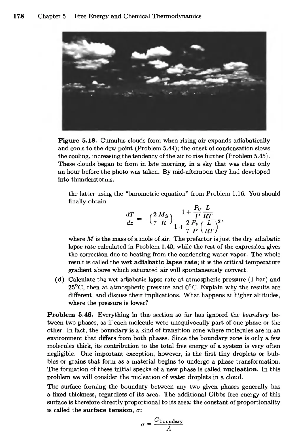
/


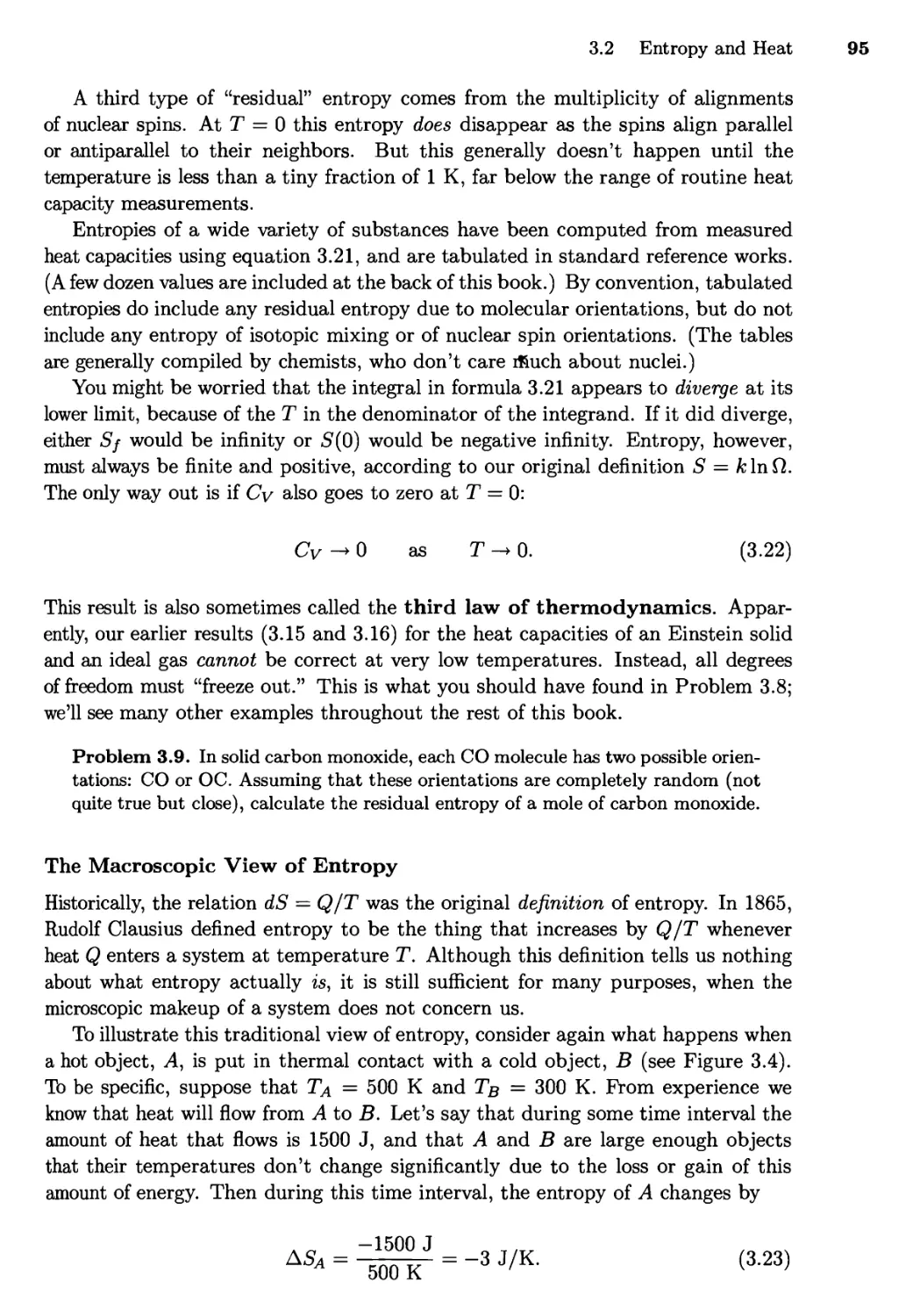


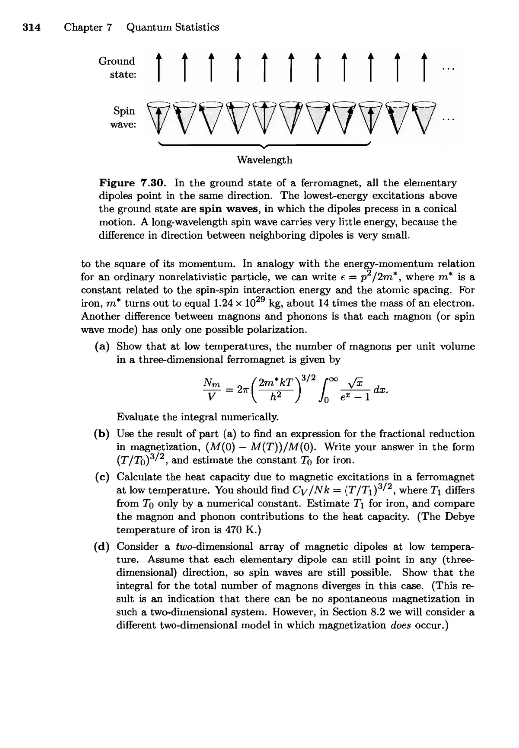


Текст
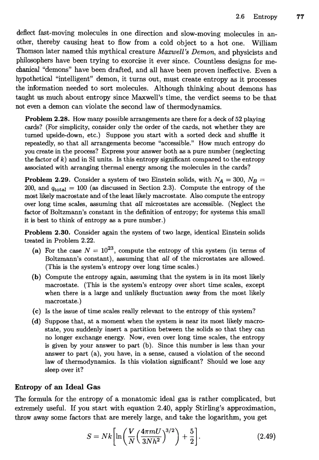
AN INTRODUCTION TO
Thermal
Physics
Daniel V. Schroeder
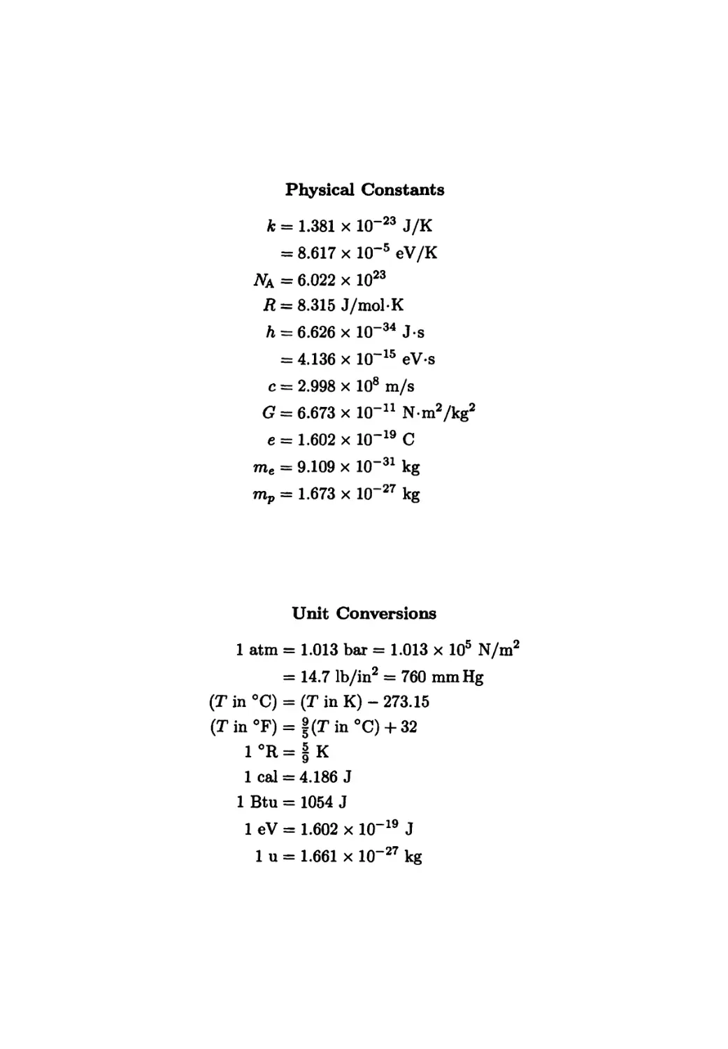
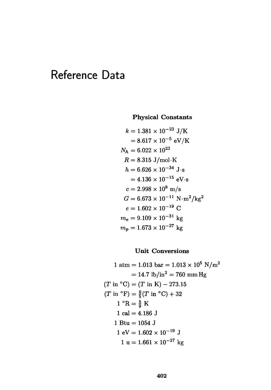
Physical Constants
k = 1.381 x 10"23 J/K
= 8.617 x 10~5 eV/K
NA = 6.022 x 10²³
R = 8.315 J/mol-K
ft = 6.626 x 10"34 Js
= 4.136 x 10~15 eV-s
c = 2.998 x 10⁸ m/s
G = 6.673 x 10_u Nm2/kg2
e = 1.602 x 10⁻¹⁹ C
me = 9.109 x 10⁻³¹ kg
mp = 1.673 x 10"27 kg
Unit Conversions
(T
(T
1 atm =
in °C) =
in °F) =
1°R =
1 cal =
lBtu =
leV =
lu =
= 1.013 bar =
= 14.7 lb/in2
: (T in K) -
= 1.013 x 10⁵ N/m2
= 760mmHg
273.15
:|(Tin°C) + 32
;IK
: 4.186 J
■■ 1054 J
: 1.602 x 10"
= 1.661 x 10"
19 J
"27kg
Thermal
Physics
Daniel V. Schroeder
Weber State University
^ ADDISON-WESLEY
An imprint of Addison Wesley Longman
San Francisco, California • Reading, Massachusetts • New York • Harlow, England
Don Mills, Ontario • Sydney • Mexico City • Madrid • Amsterdam
Acquisitions Editor: Sami Iwata
Publisher Robin J. Heyden
Marketing Manager: Jennifer Schmidt
Production Coordination: Joan Marsh
Cover Designer: Mark Ong
Cover Printer: Coral Graphics
Printer and Binder Maple-Vail Book Manufacturing Group
Copyright © 2000, by Addison Wesley Longman.
Published by Addison Wesley Longman. All rights reserved. No part of this publication
may be reproduced, stored in a retrieval system, or transmitted, in any form or by any
means, electronic, mechanical, photocopying, recording, or otherwise, without the prior
written permission of the publisher. Printed in the United States.
Library of Congress Cataloging-in-Publication Data
Schroeder, Daniel V.
Introduction to thermal physics / Daniel V. Schroeder.
p. cm.
Includes index.
ISBN 0-201-38027-7
1. Thermodynamics. 2. Statistical mechanics. I. Title.
QC311.15.S32 1999
536\7--dc21 99-316%
CIP
ISBN: 0-201-38027-7
123456789 10 —MVB —03 02 01 00
Contents
Preface 7
Part I: Fundamentals
Chapter 1 Energy in Thermal Physics 1
1.1 Thermal Equilibrium 1
1.2 The Ideal Gas 6
Microscopic Model of an Ideal Gas
1.3 Equipartition of Energy 14
1.4 Heat and Work 17
1.5 Compression Work 20
Compression of an Ideal Gas
1.6 Heat Capacities 28
Latent Heat; Enthalpy
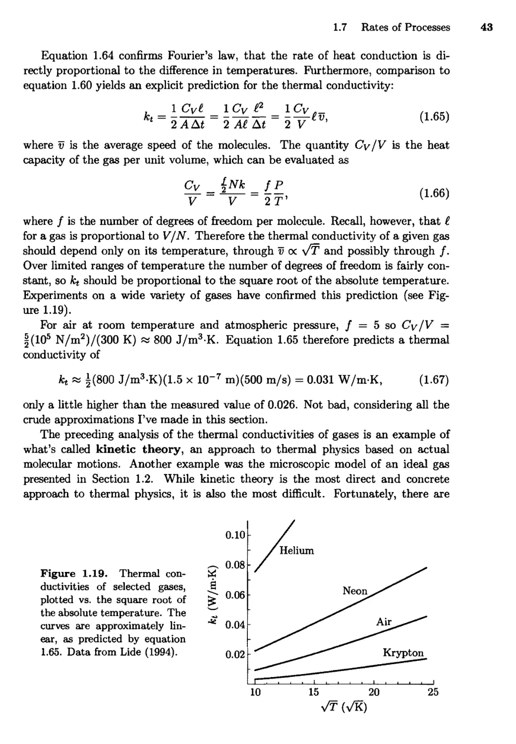
1.7 Rates of Processes 37
Heat Conduction; Conductivity of an Ideal Gas;
Viscosity; Diffusion
Chapter 2 The Second Law 49
2.1 Two-State Systems 49
The Two-State Paramagnet
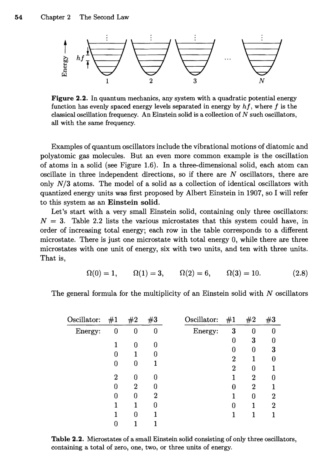
2.2 The Einstein Model of a Solid 53
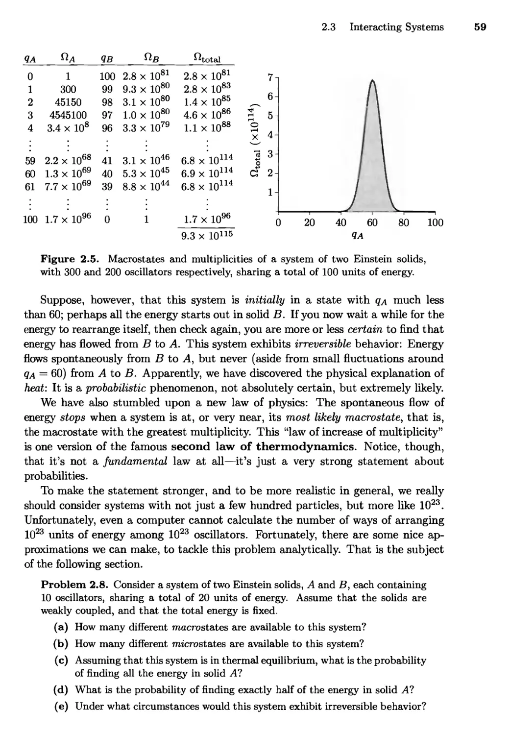
2.3 Interacting Systems 56
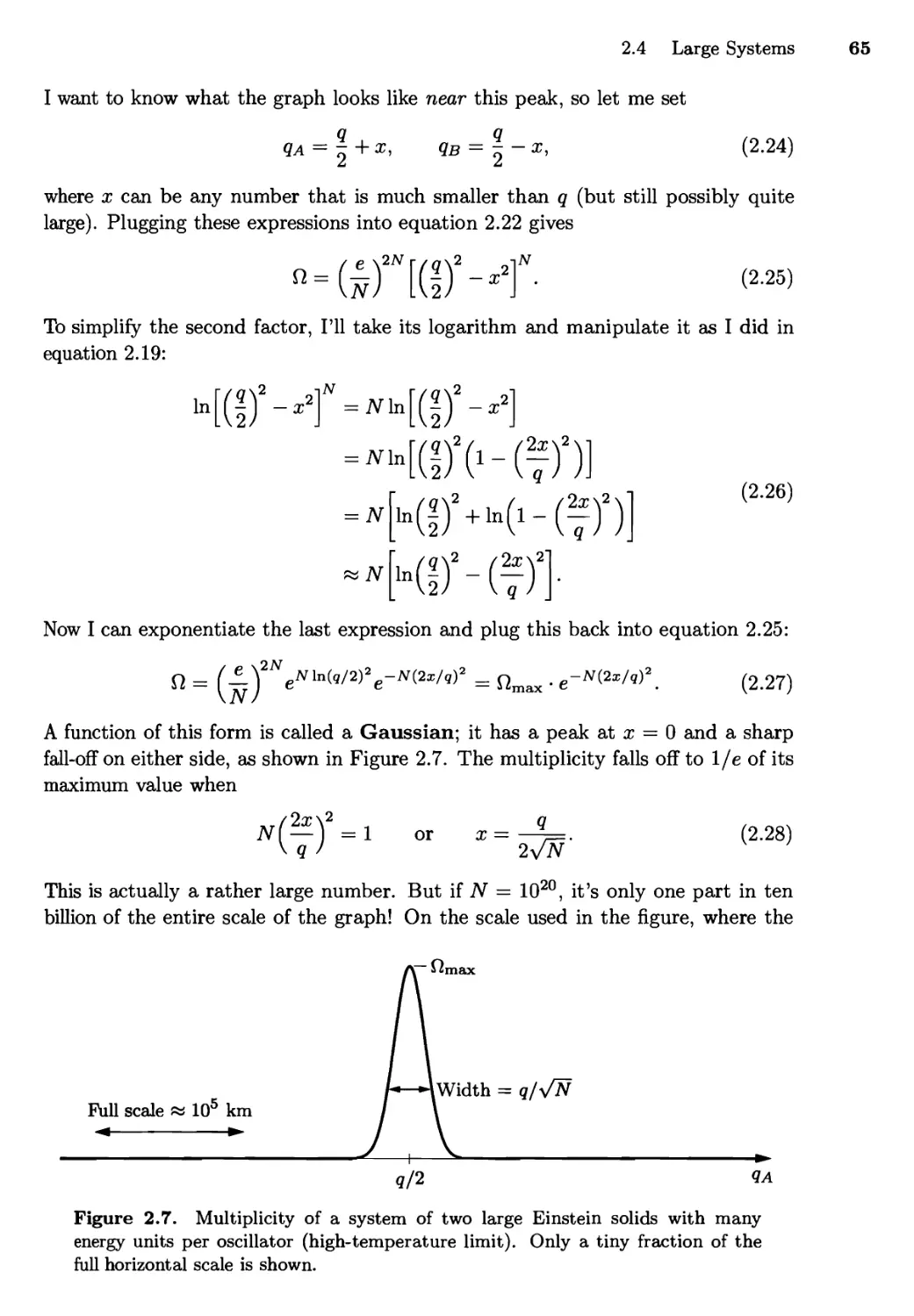
2.4 Large Systems 60
Very Large Numbers; Stirling}s Approximation;
Multiplicity of a Large Einstein Solid;
Sharpness of the Multiplicity Function
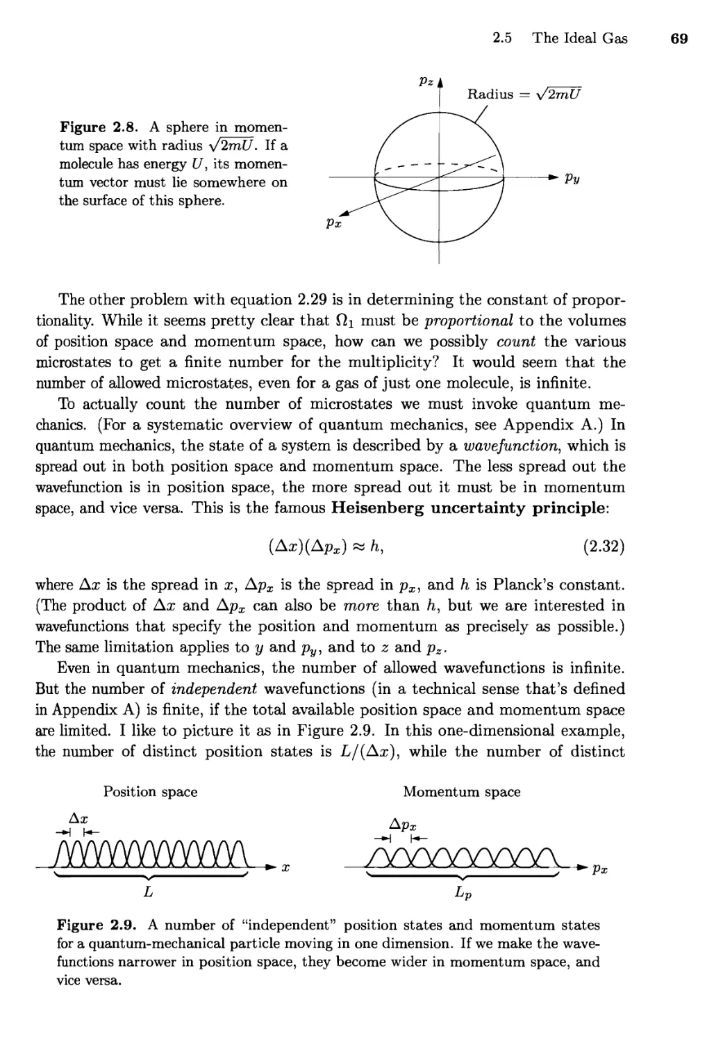
2.5 The Ideal Gas 68
Multiplicity of a Monatomic Ideal Gas;
Interacting Ideal Gases
2.6 Entropy 74
Entropy of an Ideal Gas; Entropy of Mixing;
Reversible and Irreversible Processes
iii
iv Contents
Chapter 3 Interactions and Implications 85
3.1 Temperature 85
A Silly Analogy; Real-World Examples
3.2 Entropy and Heat 92
Predicting Heat Capacities; Measuring Entropies;
The Macroscopic View of Entropy
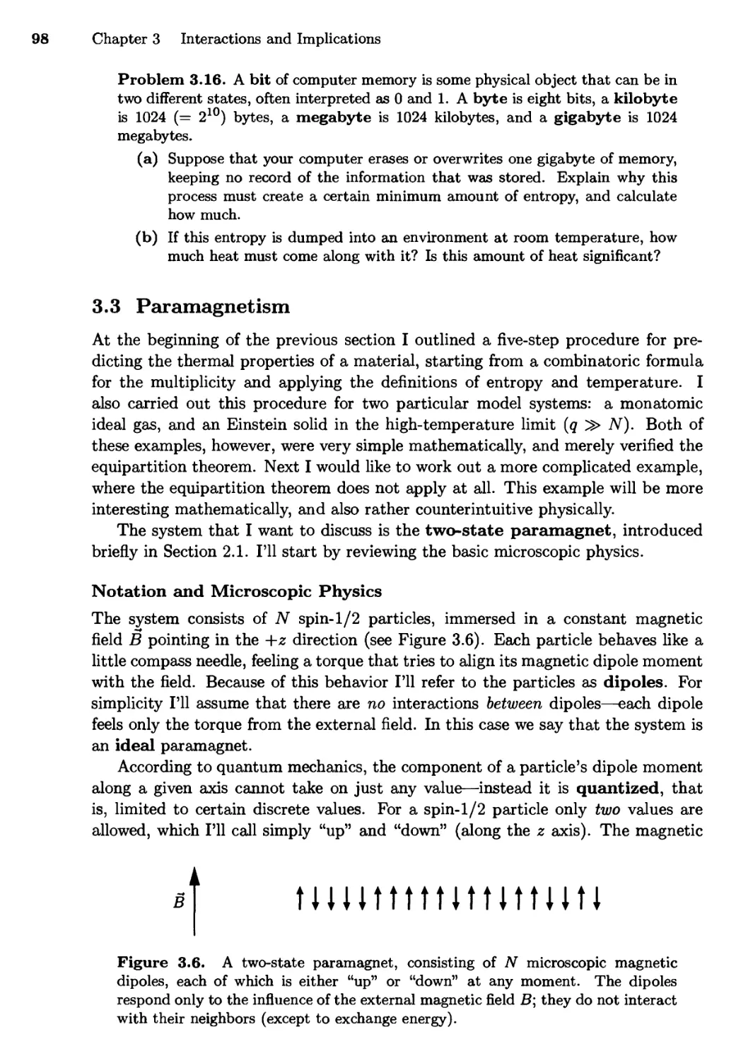
3.3 Paramagnetism 98
Notation and Microscopic Physics; Numerical Solution;
Analytic Solution
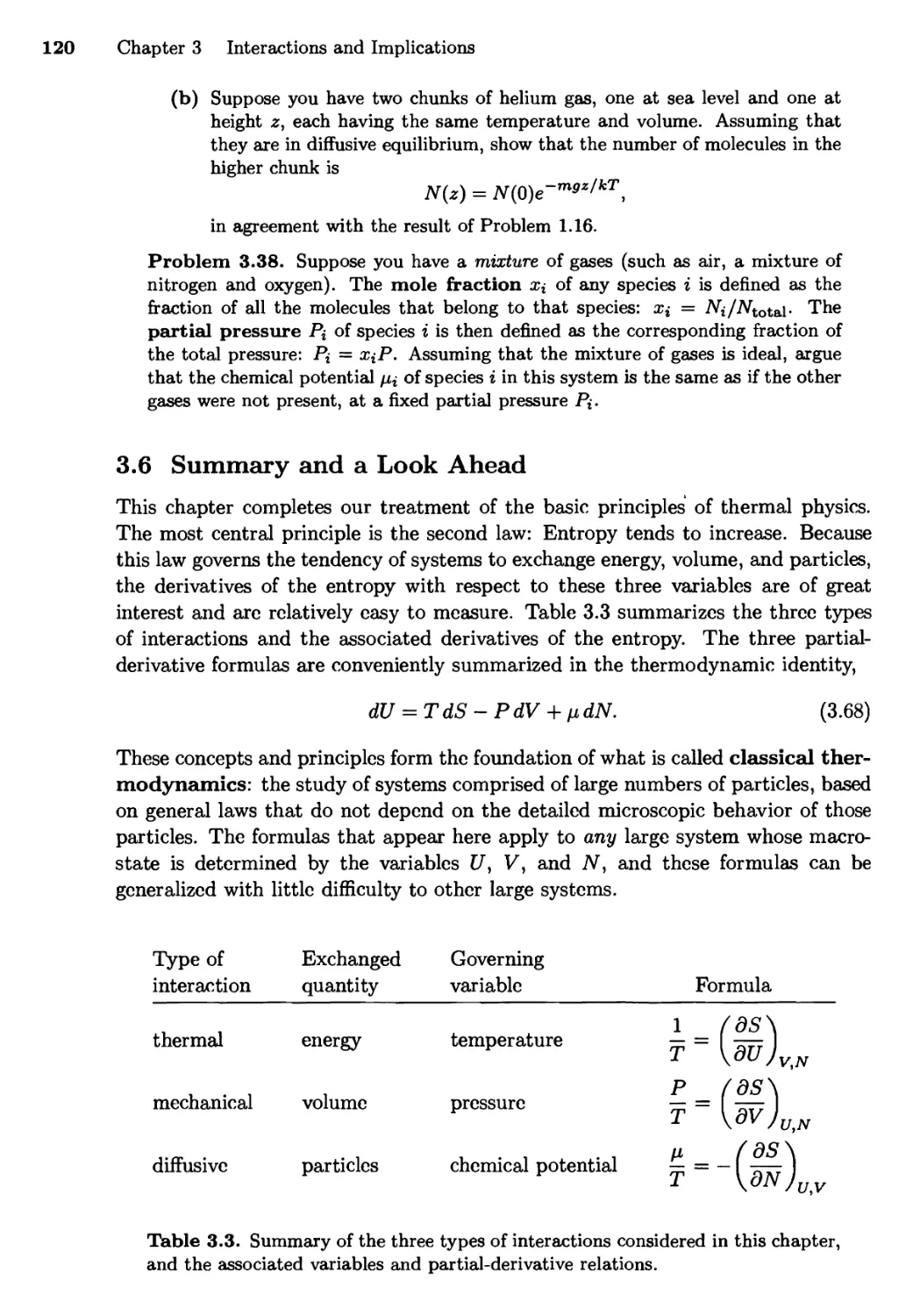
3.4 Mechanical Equilibrium and Pressure 108
The Thermodynamic Identity; Entropy and Heat Revisited
3.5 Diffusive Equilibrium and Chemical Potential 115
3.6 Summary and a Look Ahead 120
Part II: Thermodynamics
Chapter 4 Engines and Refrigerators 122
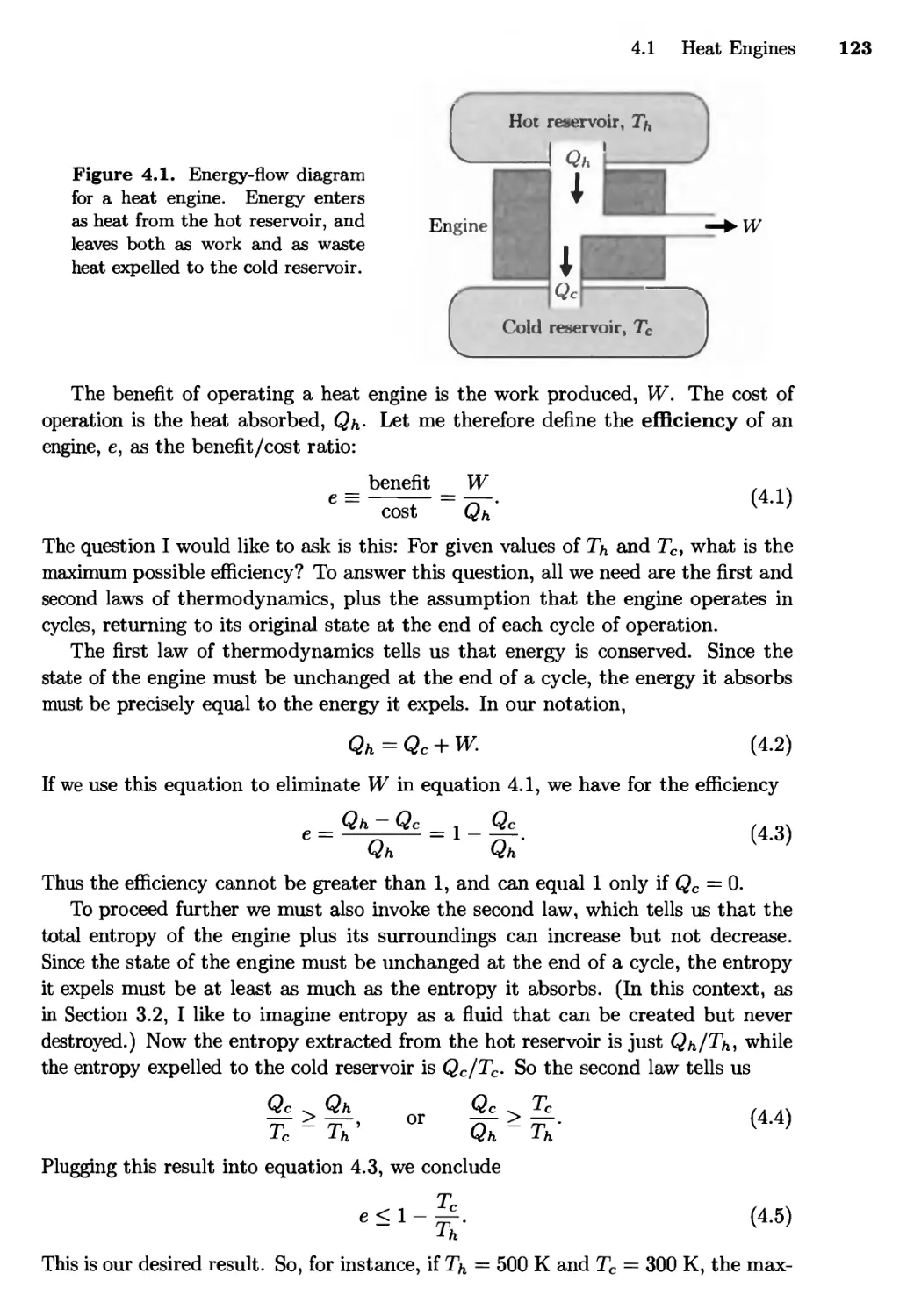
4.1 Heat Engines 122
The Carnot Cycle
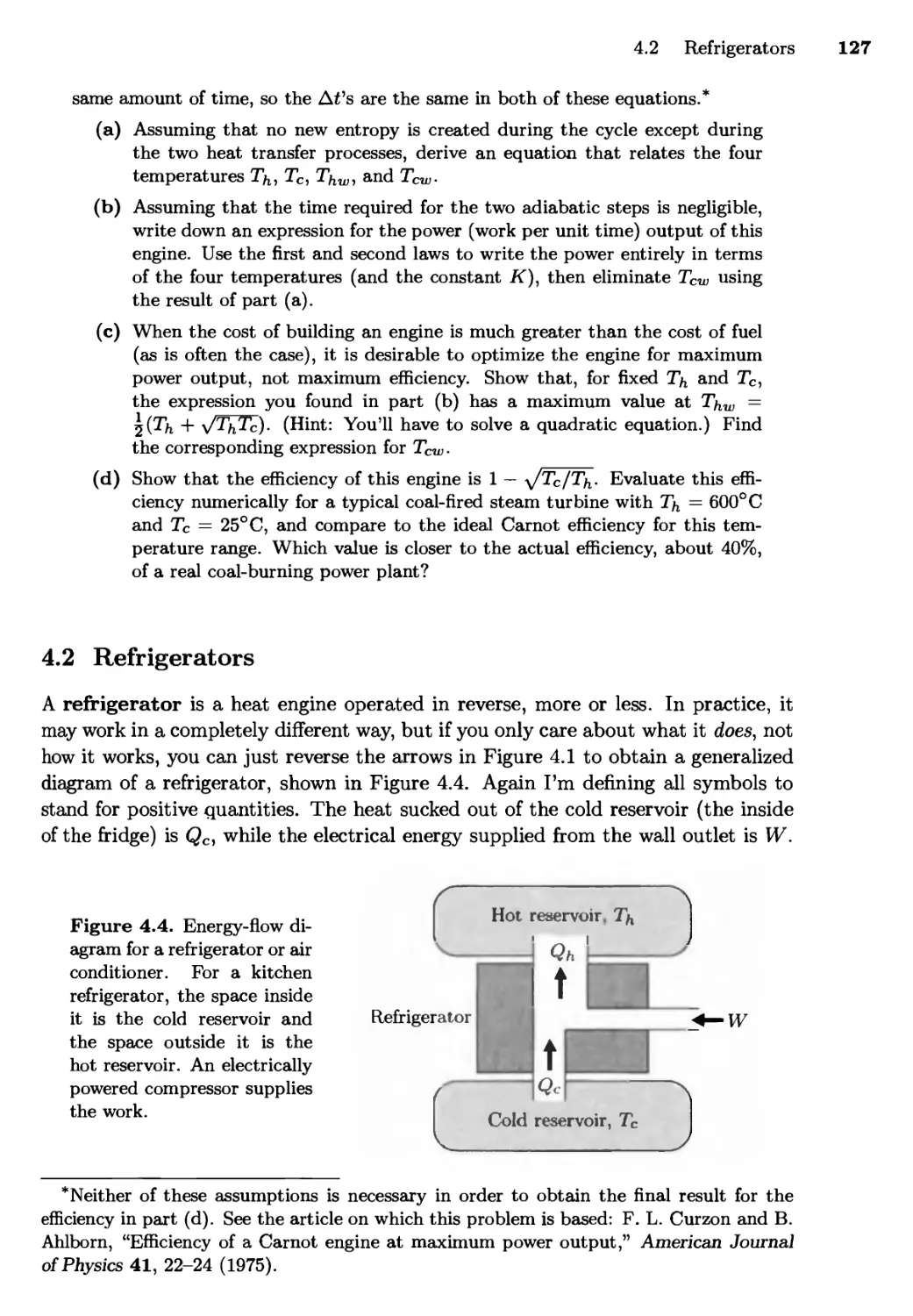
4.2 Refrigerators 127
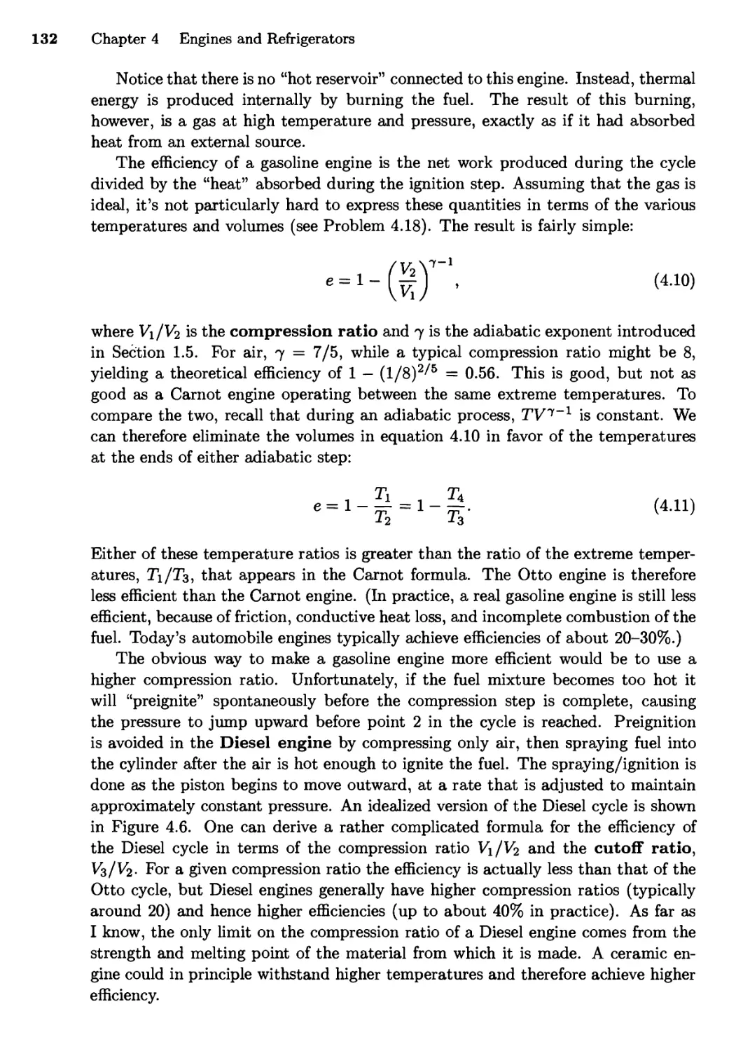
4.3 Real Heat Engines 131
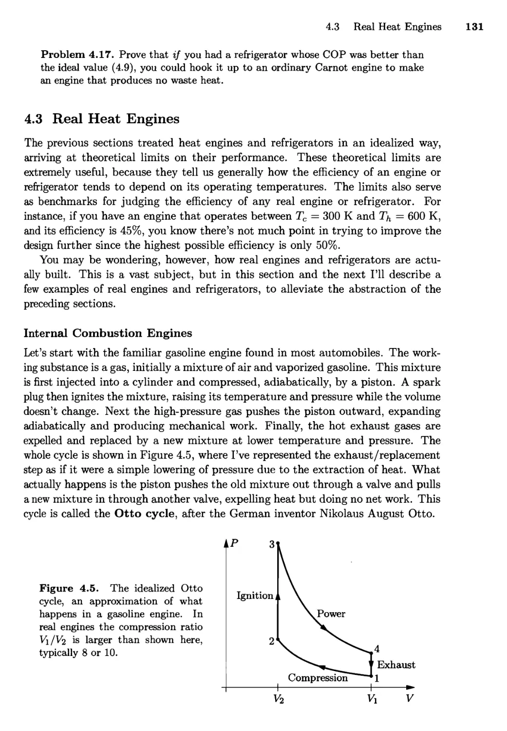
Interna] Combustion Engines; The Steam Engine
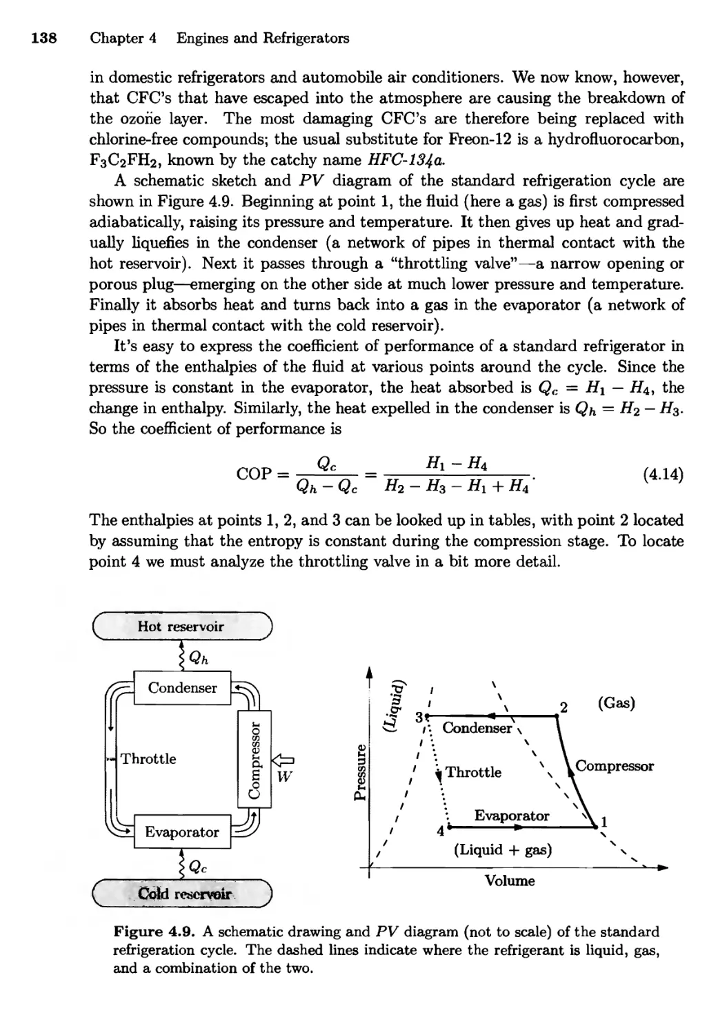
4.4 Real Refrigerators 137
The Throttling Process; Liquefaction of Gases;
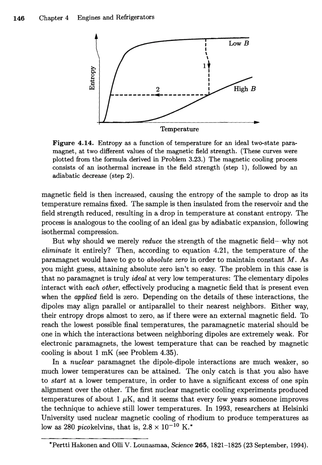
Toward Absolute Zero
Chapter 5 Free Energy and Chemical Thermodynamics 149
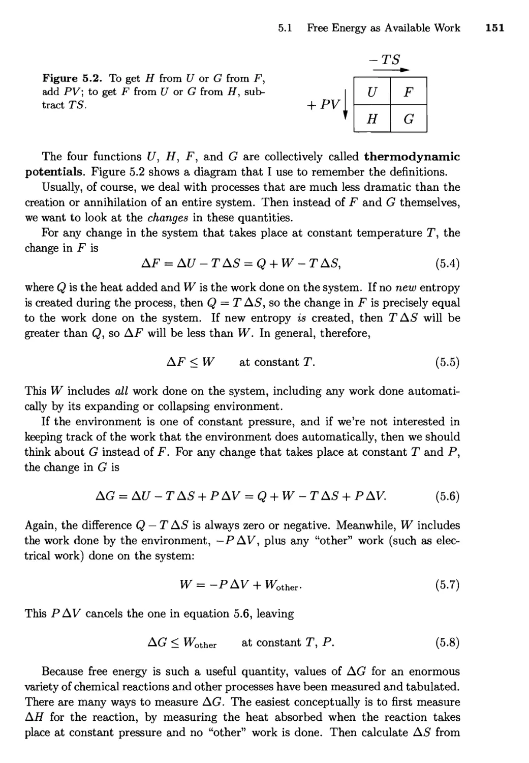
5.1 Free Energy as Available Work 149
Electrolysis, Fuel Cells, and Batteries;
Thermodynainic Identities
5.2 Free Energy as a Force toward Equilibrium 161
Extensive and Intensive Quantities; Gibbs Free Energy
and Chemical Potential
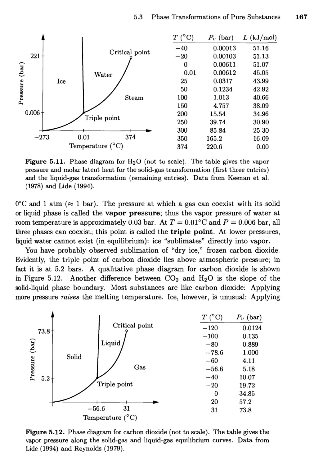
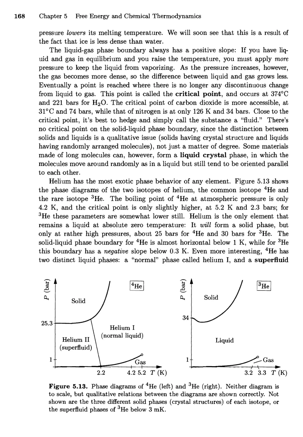
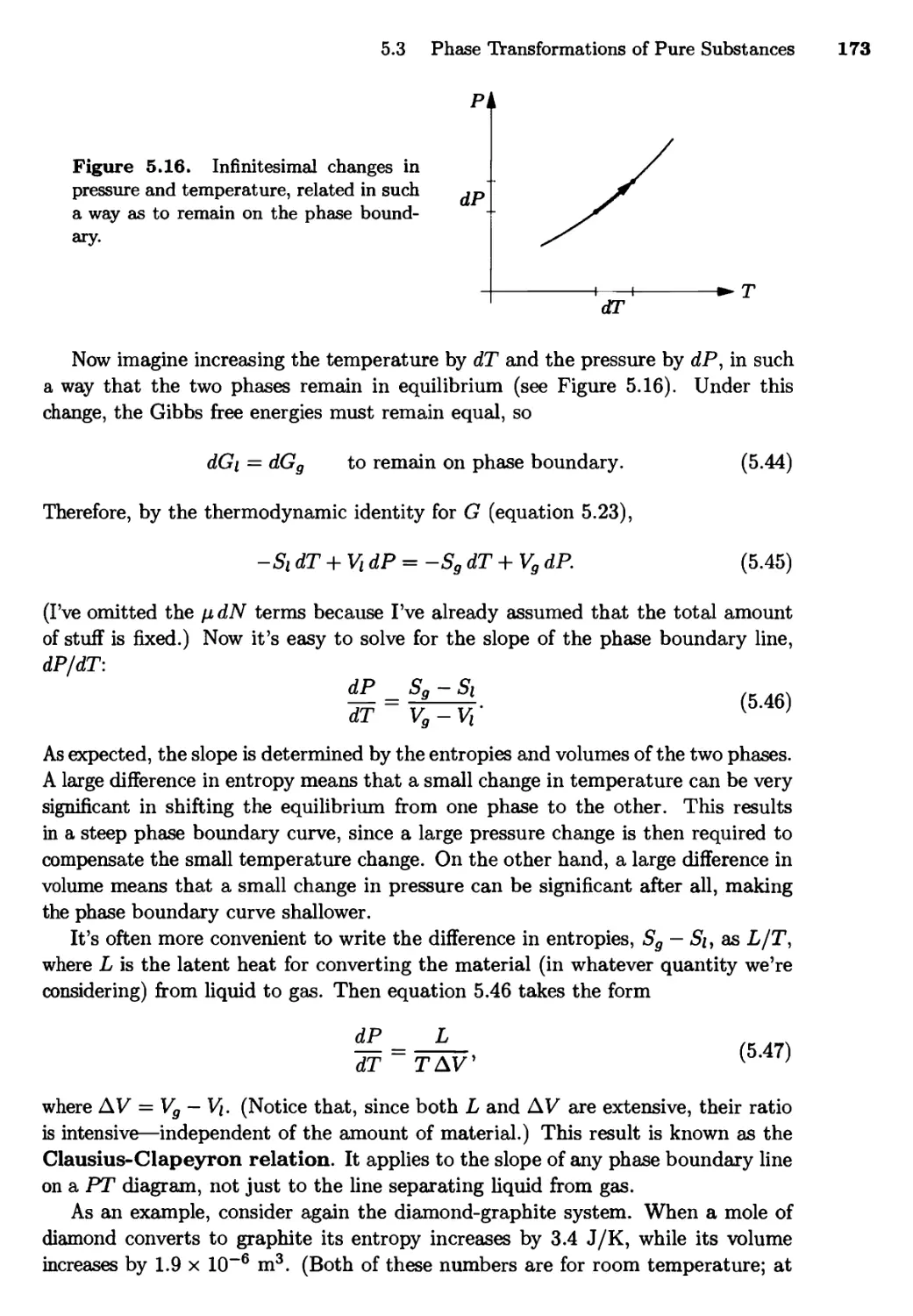
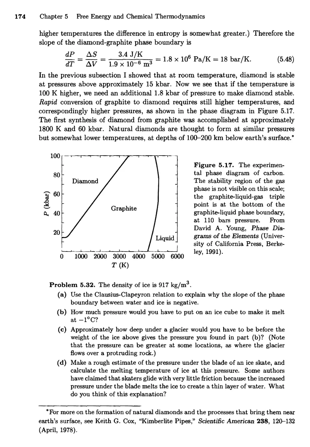
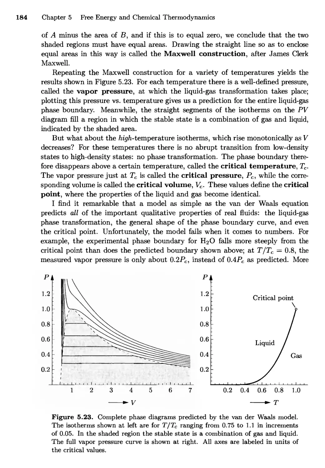
5.4 Phase Transformations of Pure Substances 166
Diamonds and Graphite; The Clausius-Clapeyron
Relation; The van der Waals Model
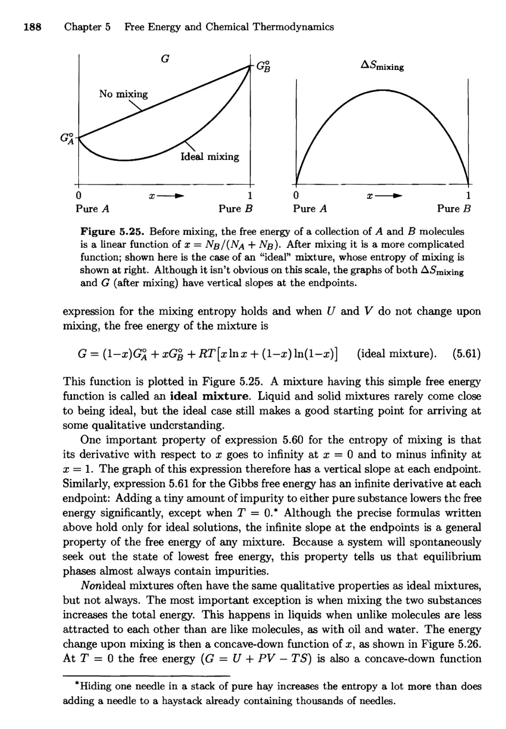
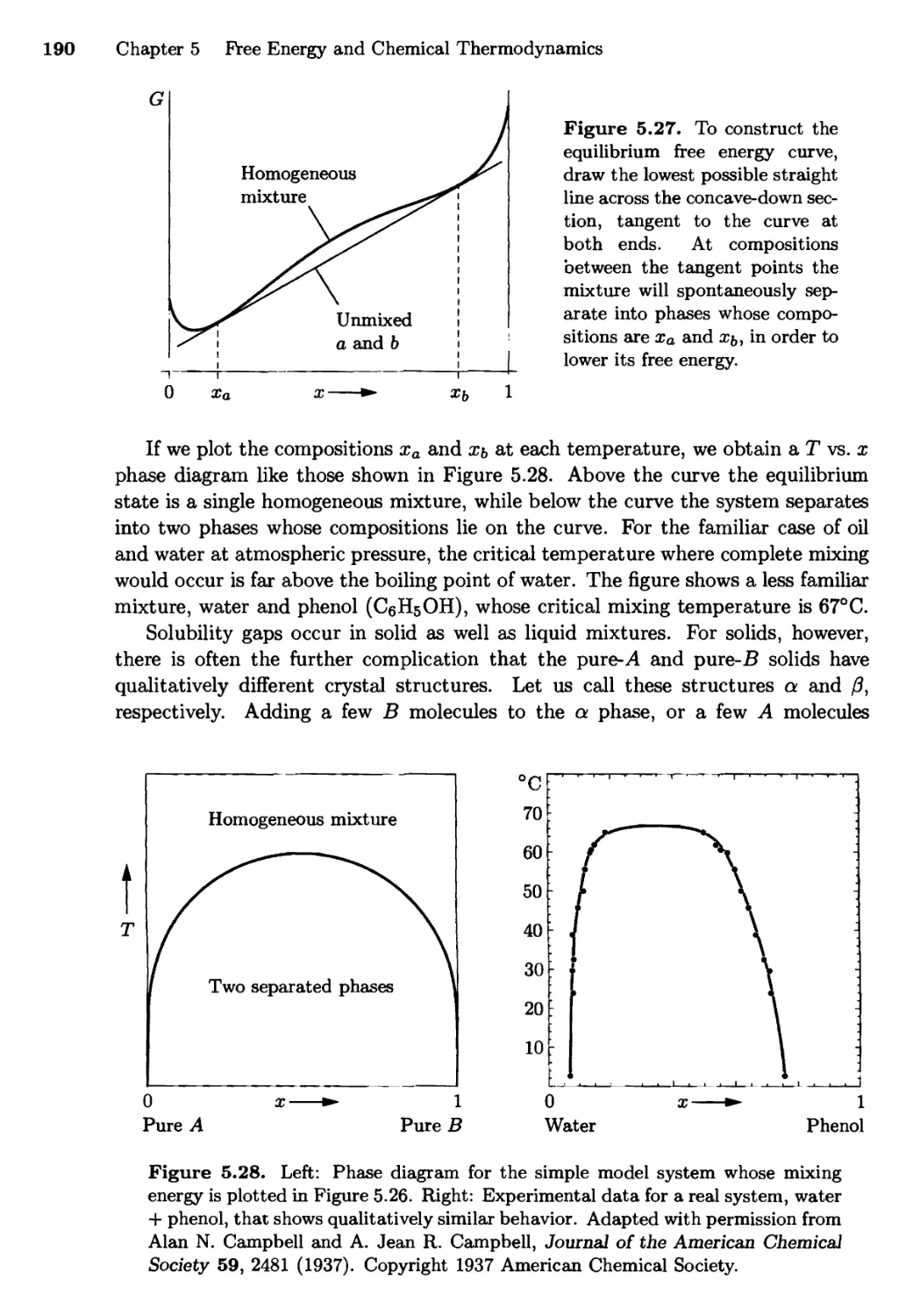
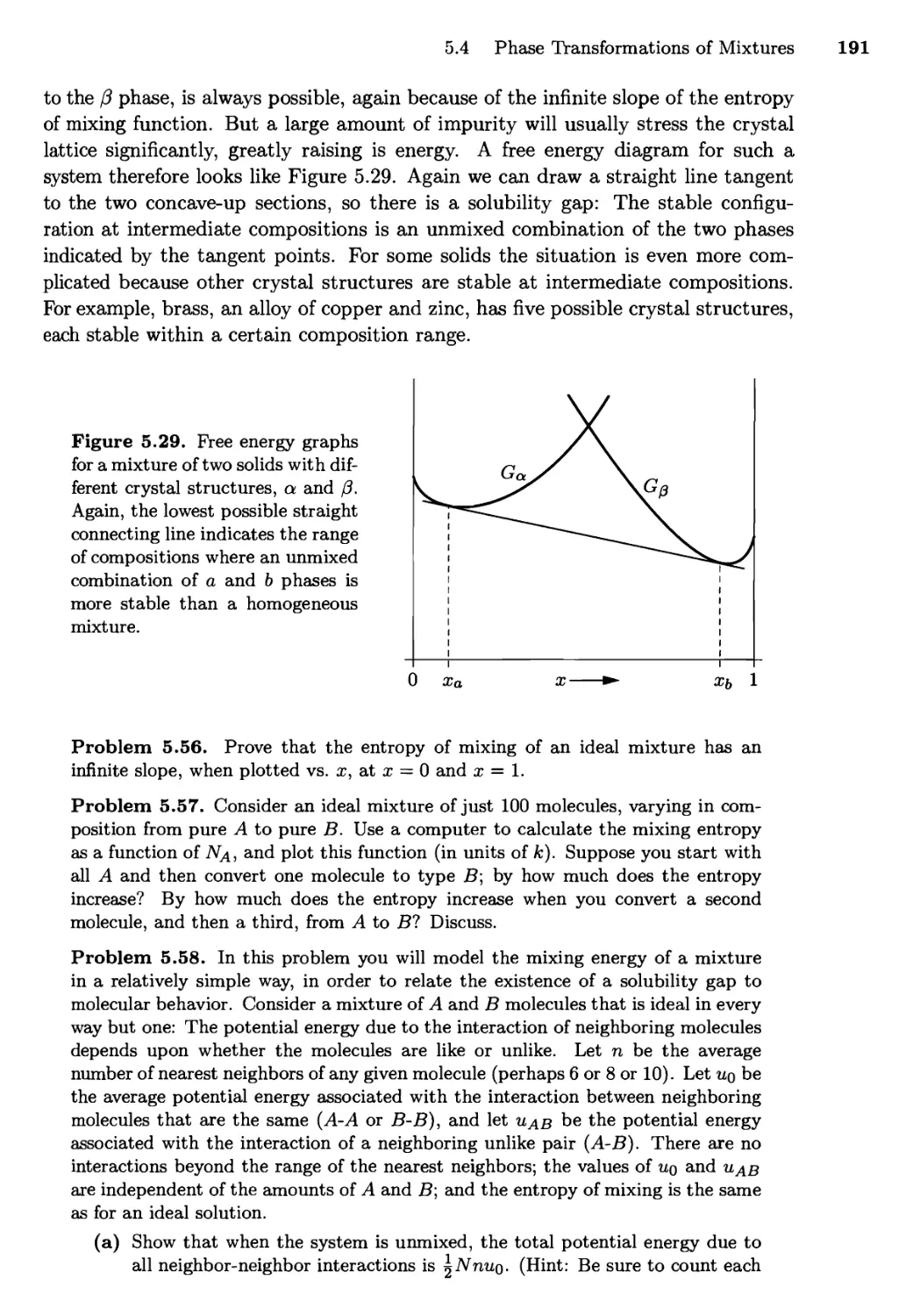
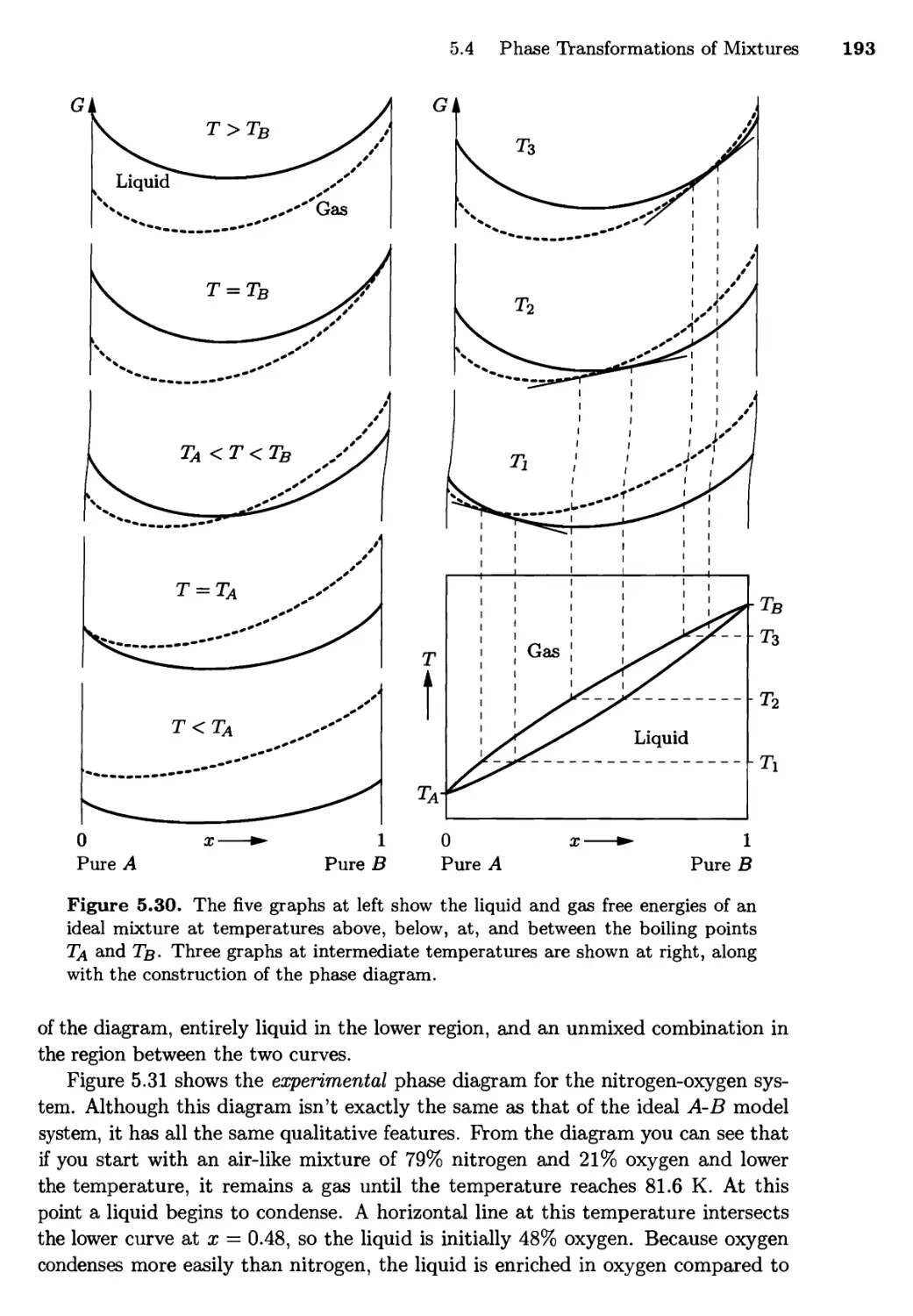
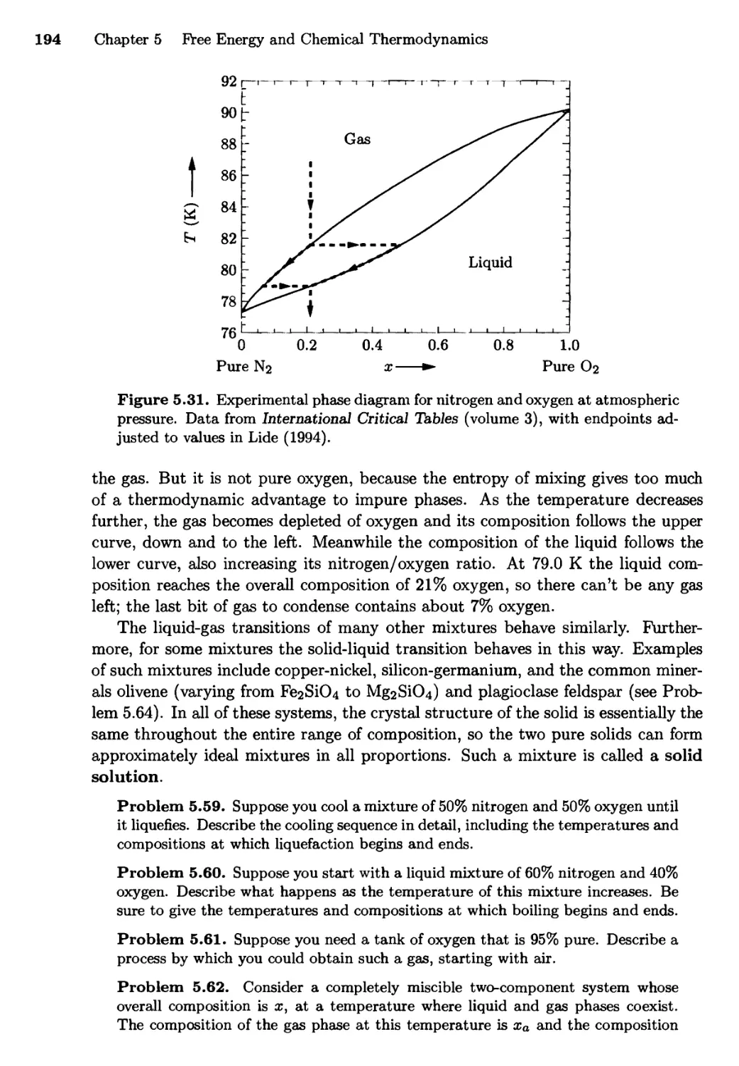
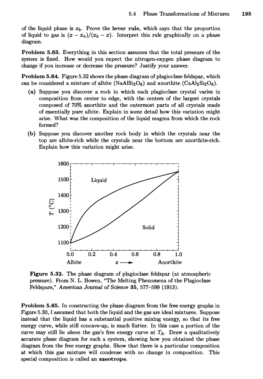
5.4 Phase Transformations of Mixtures 186
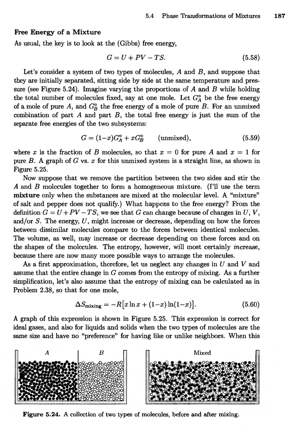
Free Energy of a Mixture; Phase Changes of a Miscible
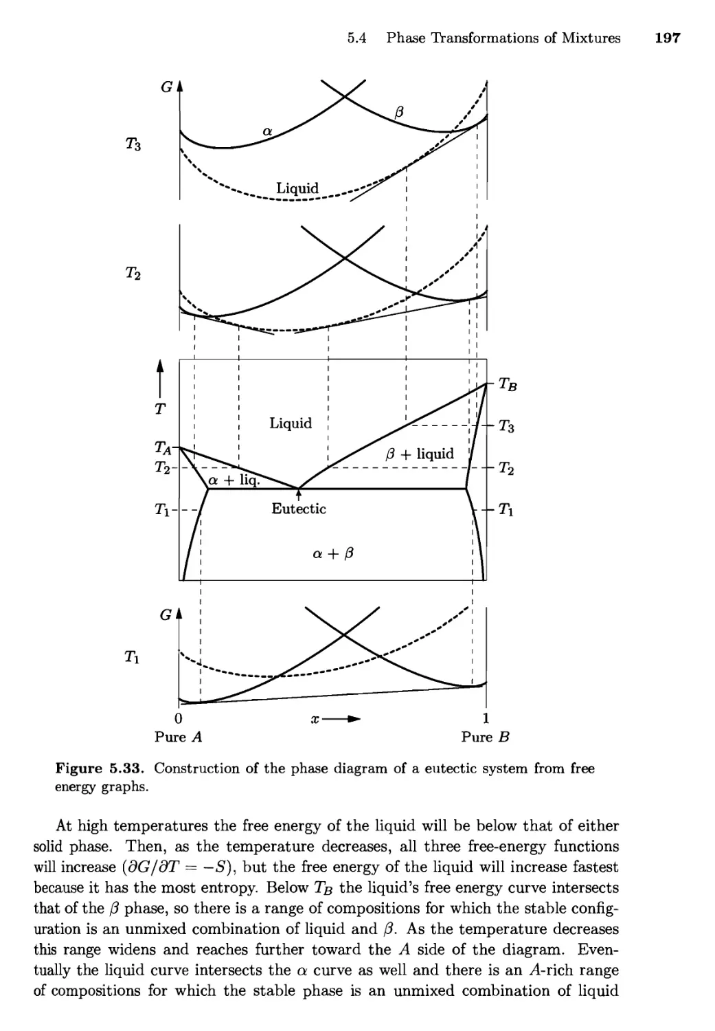
Mixture; Phase Changes of a Eutectic System
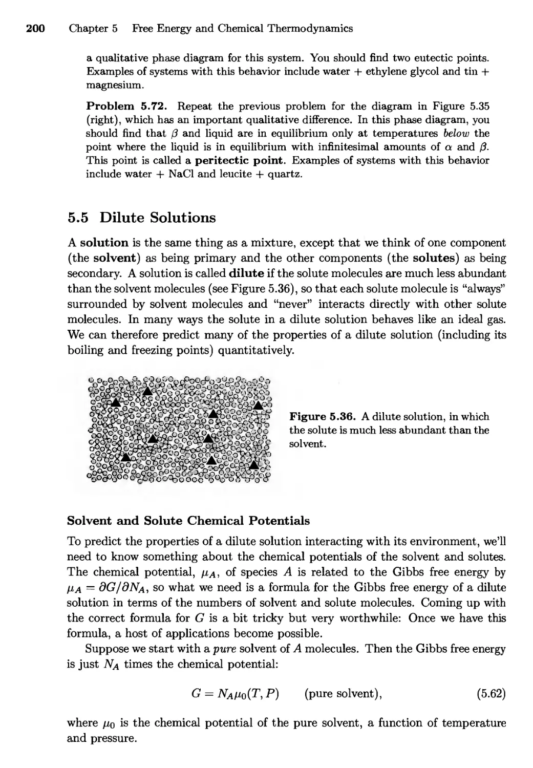
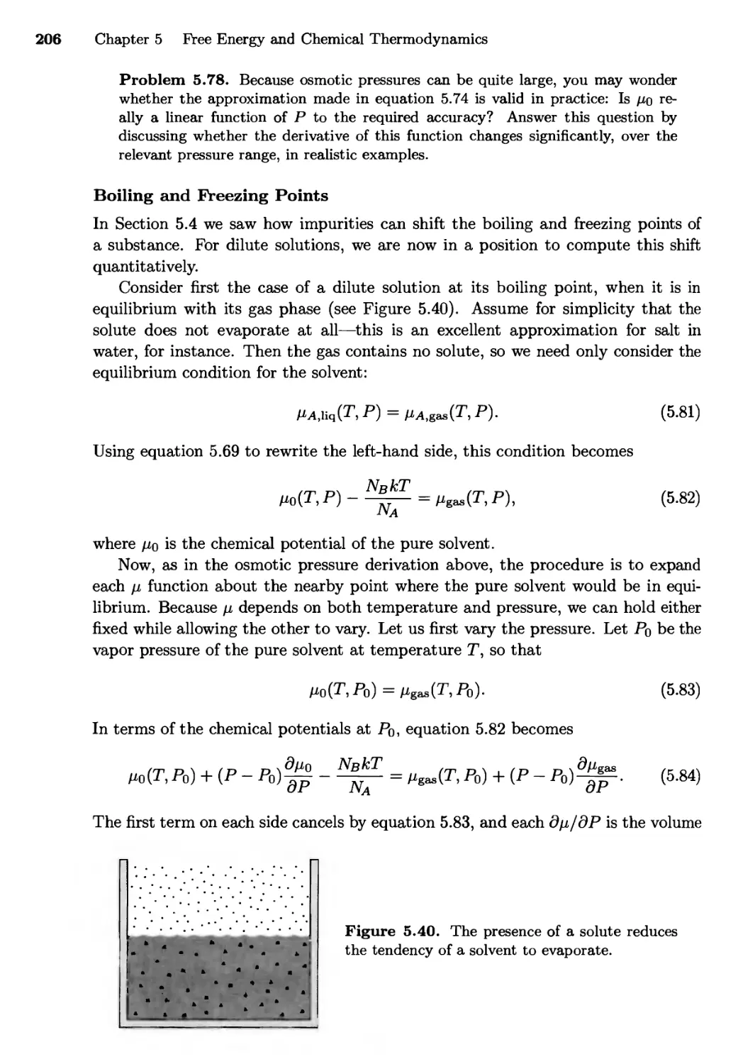
5.5 Dilute Solutions 200
Solvent and Solute Chemical Potentials; Osmotic Pressure;
Boiling and Freezing Points
5.6 Chemical Equilibrium 208
Nitrogen Fixation; Dissociation of Water; Oxygen
Dissolving in Water; Ionization of Hydrogen
Contents v
Part III: Statistical Mechanics
Chapter 6 Boltzmann Statistics 220
6.1 The Boltzmann Factor 220
The Partition Function; Thermal Excitation of Atoms
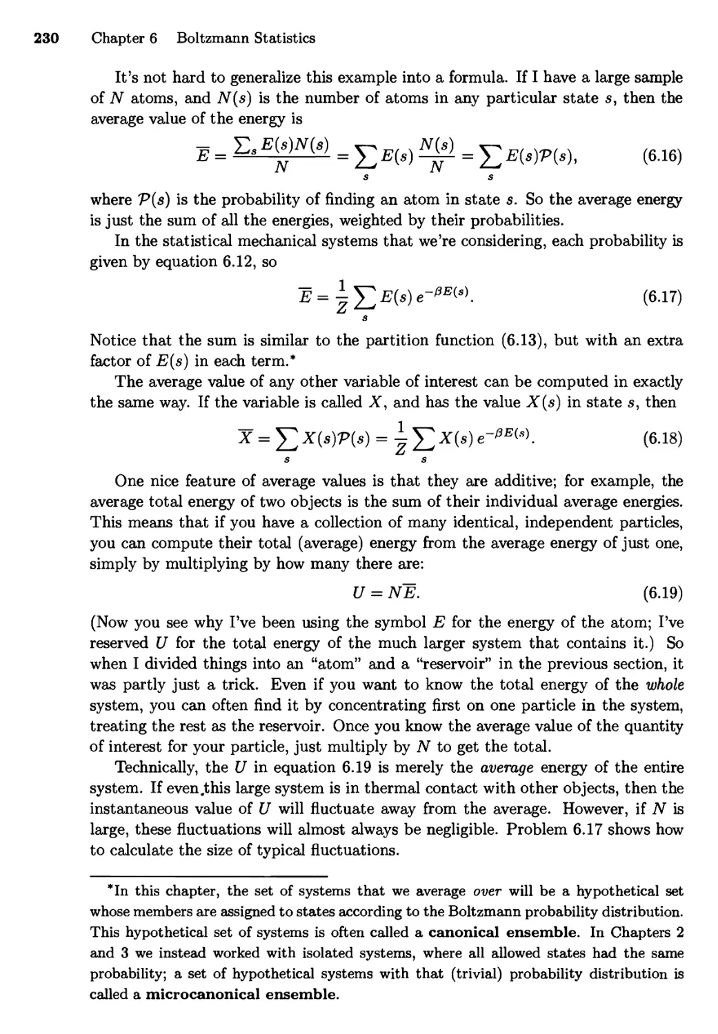
6.2 Average Values . . . 229
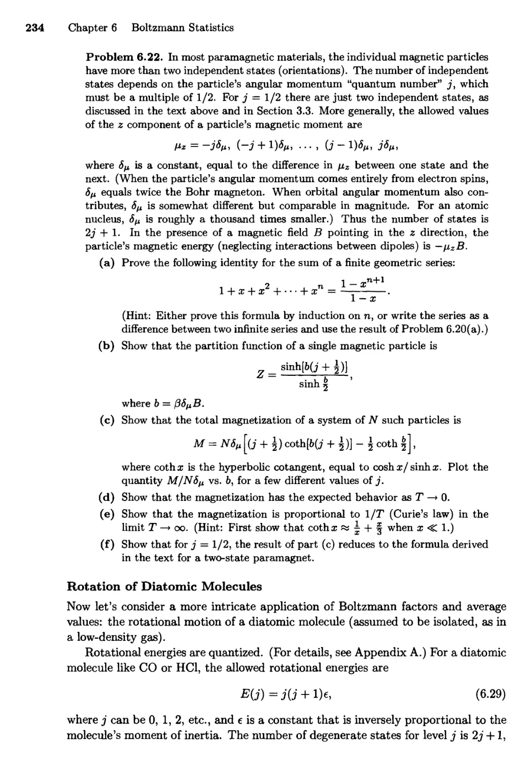
Paramagnetism; Rotation of Diatomic Molecules
6.3 The Equipartition Theorem 238
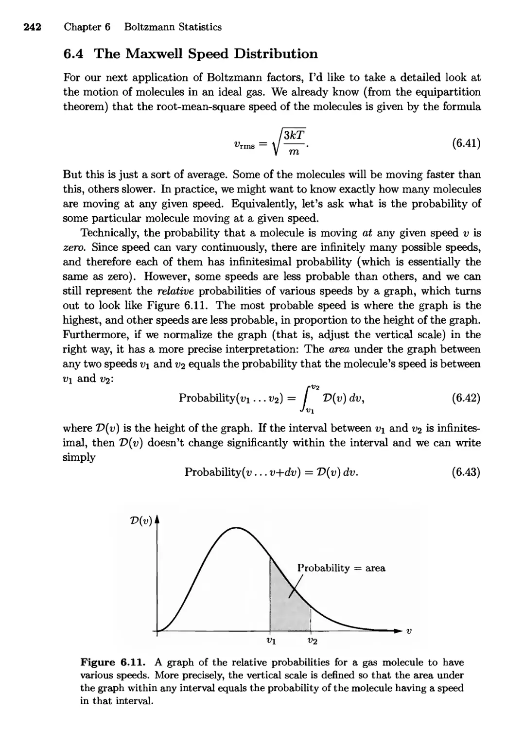
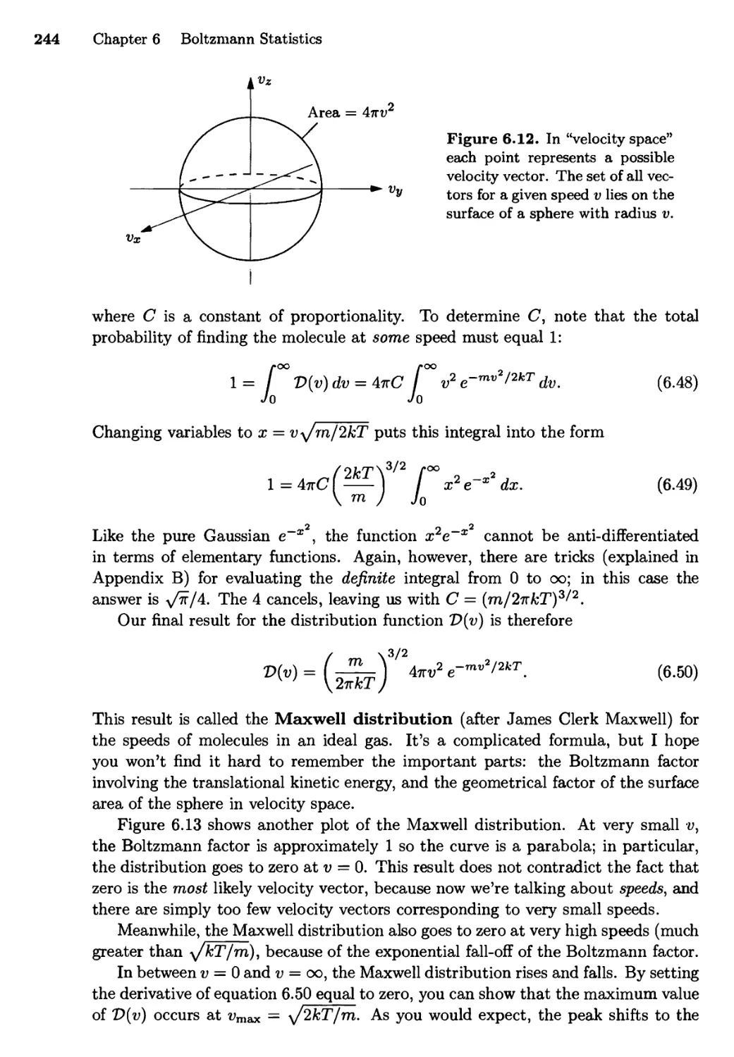
6.4 The Maxwell Speed Distribution 242
6.5 Partition Functions and Free Energy 247
6.6 Partition Functions for Composite Systems 249
6.7 Ideal Gas Revisited 251
The Partition Function; Predictions
Chapter 7 Quantum Statistics 257
7.1 The Gibbs Factor 257
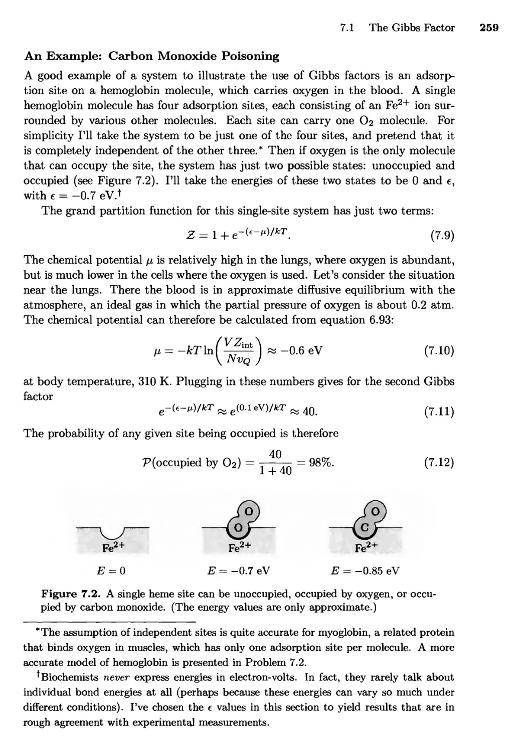
An Example: Carbon Monoxide Poisoning
7.2 Bosons and Fermions 262
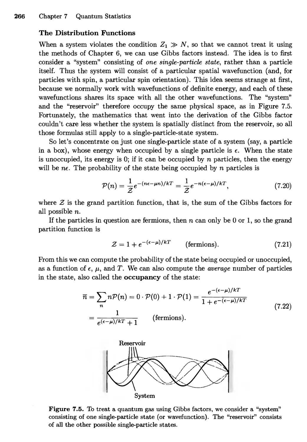
The Distribution Functions
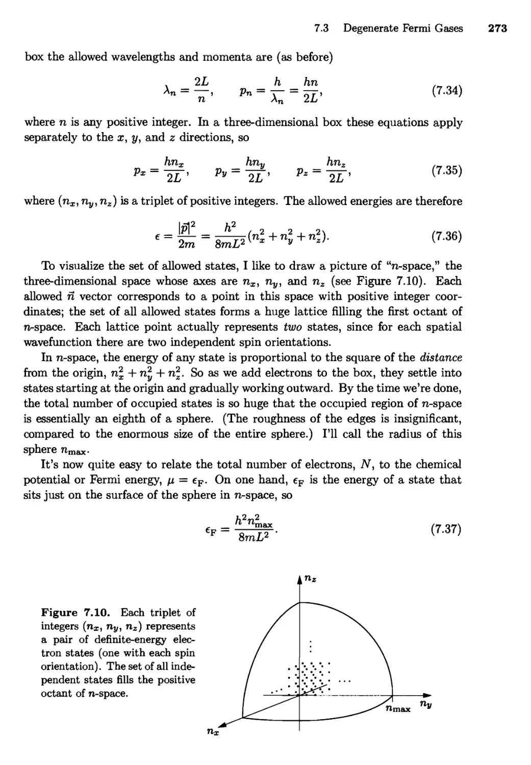
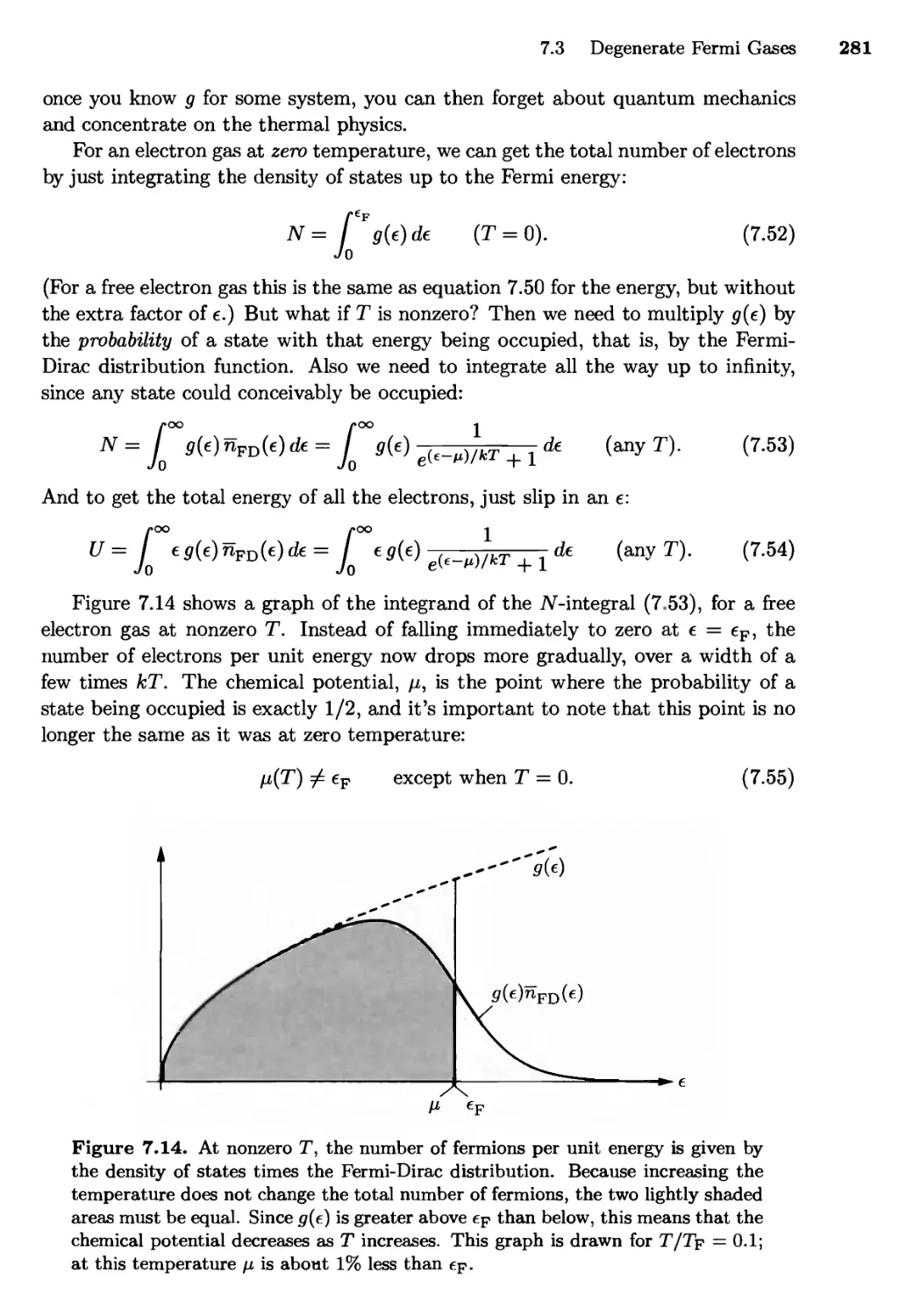
7.3 Degenerate Fermi Gases 271
Zero Temperature; Small Nonzero Temperatures;
The Density of States; The Sommerfeld Expansion
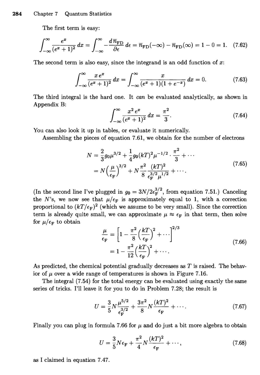
7.4 Blackbody Radiation 288
The Ultraviolet Catastrophe; The Planck Distribution;
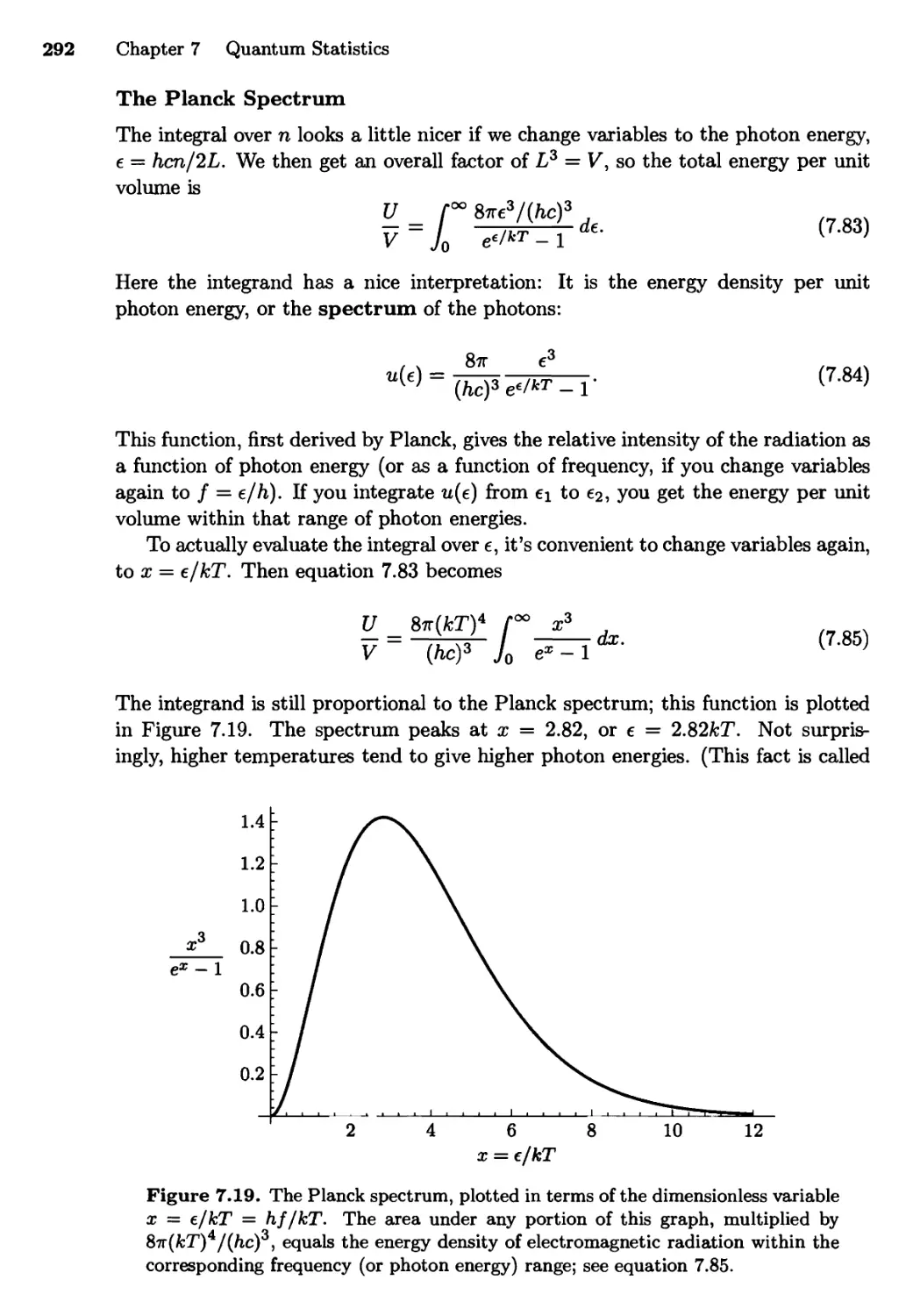
Photons; Summing over Modes; The Planck Spectrum;
Total Energy; Entropy of a Photon Gas; The Cosmic
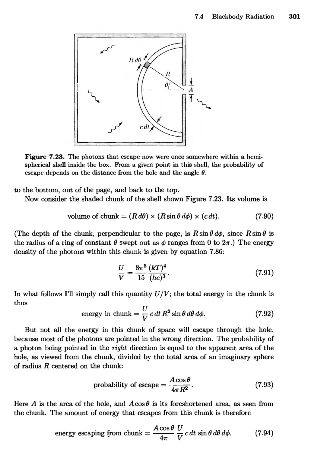
Background Radiation; Photons Escaping through a Hole;
Radiation from Other Objects; The Sun and the Earth
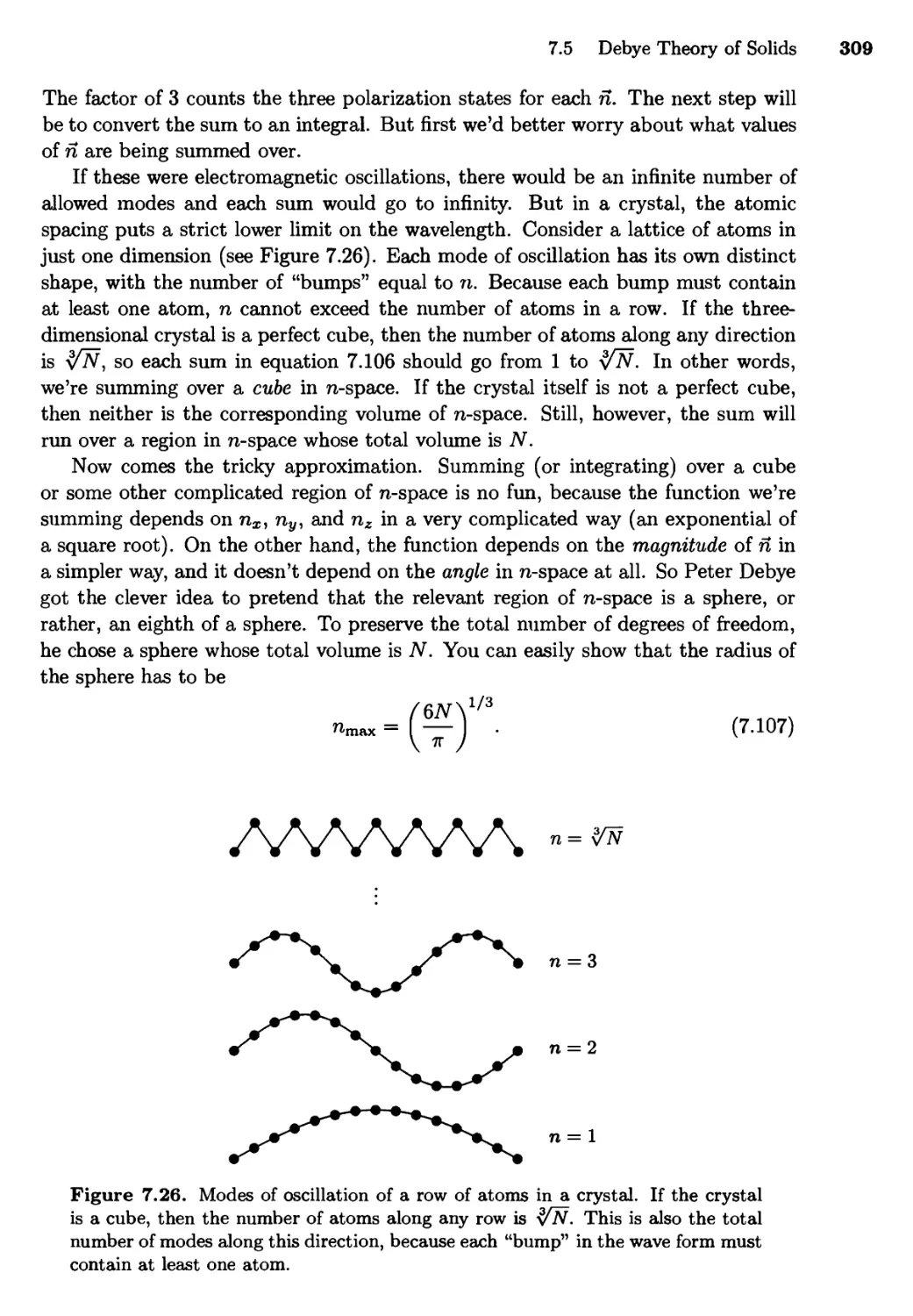
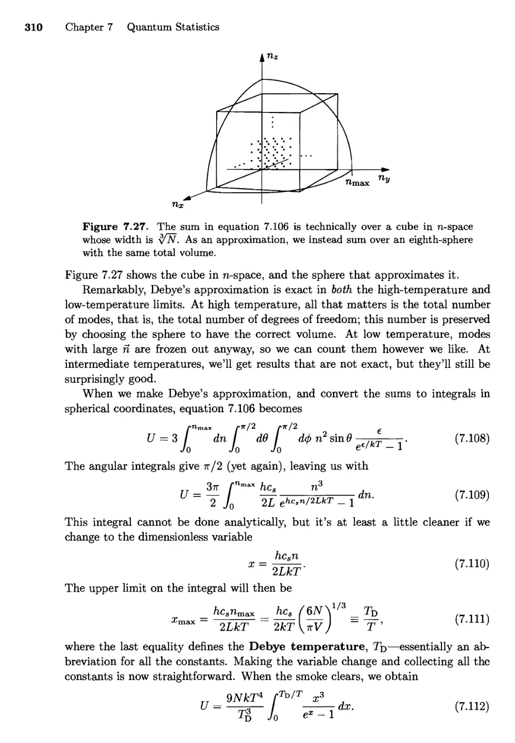
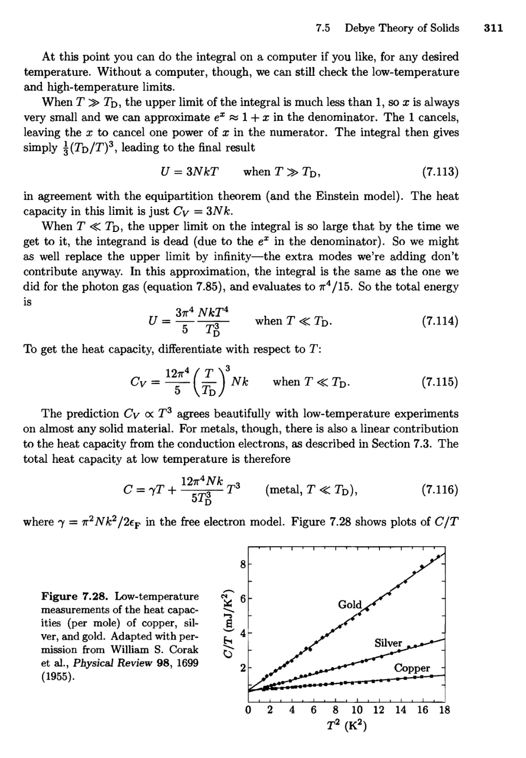
7.5 Debye Theory of Solids 307
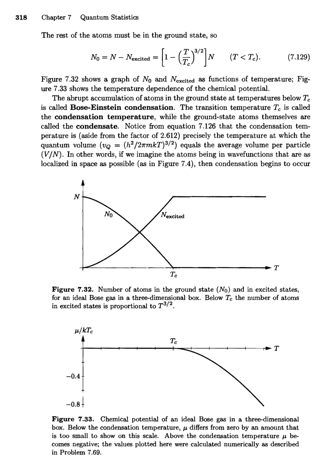
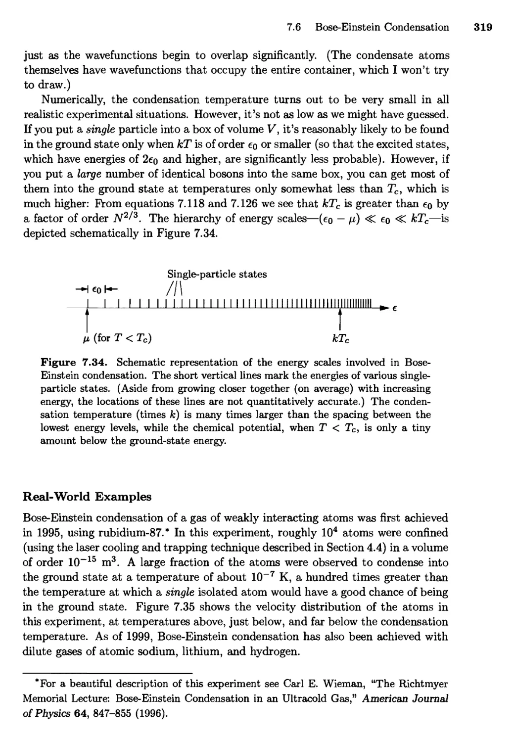
7.6 Bose-Einstein Condensation 315
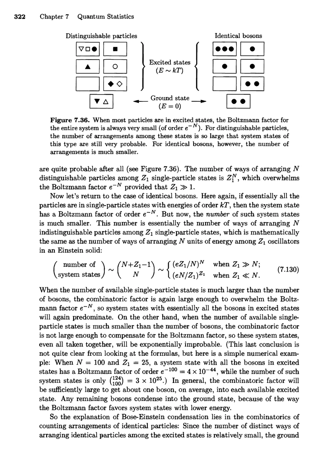
Real-World Examples; Why Does it Happen?
Chapter 8 Systems of Interacting Particles 327
8.1 Weakly Interacting Gases 328
The Partition Function; The Cluster Expansion;
The Second Virial Coefficient
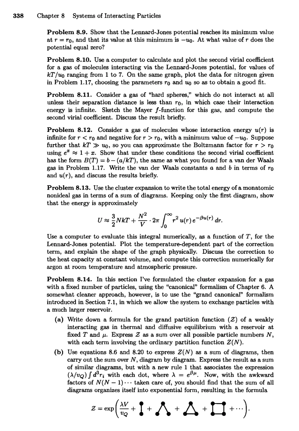
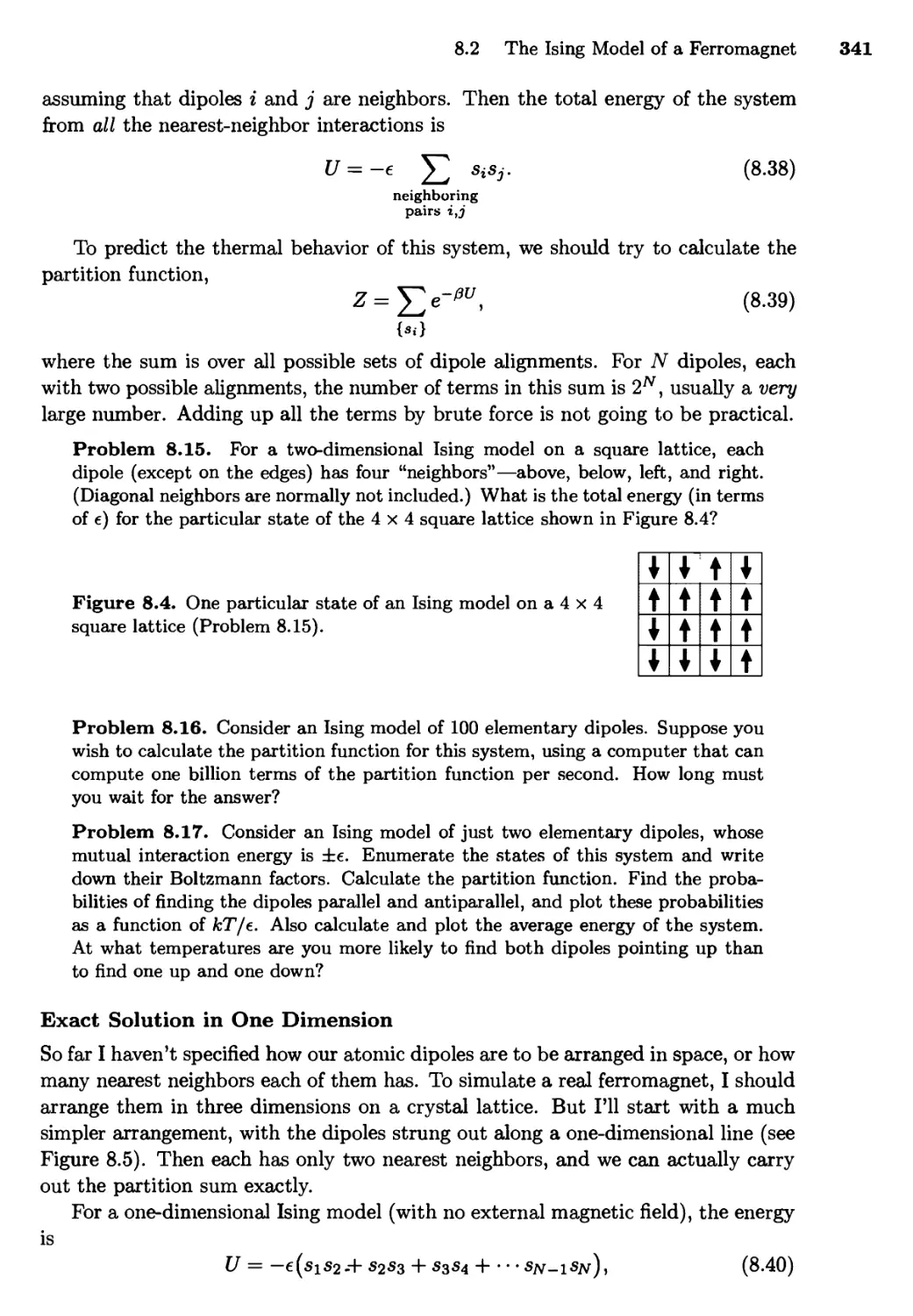
8.2 The Ising Model of a Ferromagnet 339
Exact Solution in One Dimension;
The Mean Field Approximation;
Monte Carlo Simulation
vi Contents
* * *
Appendix A Elements of Quantum Mechanics 357
A.l Evidence for Wave-Particle Duality 357
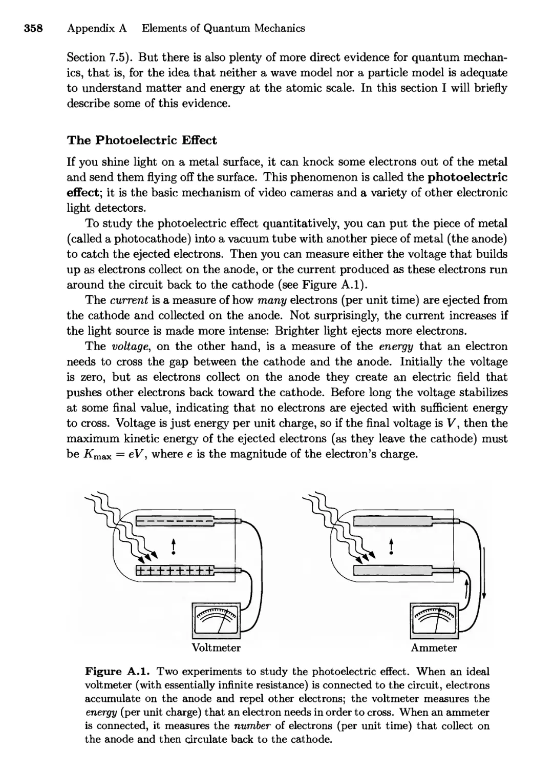
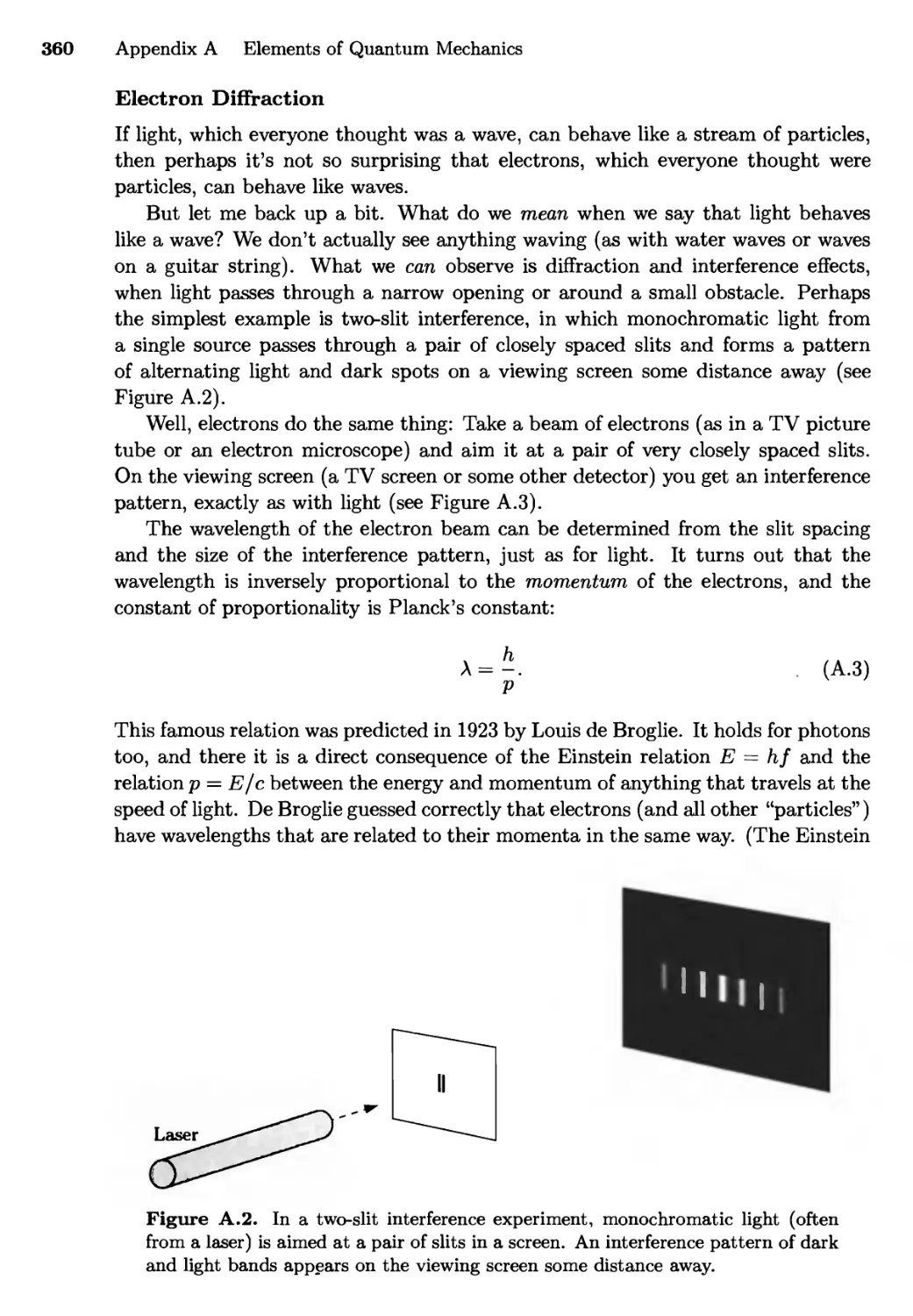
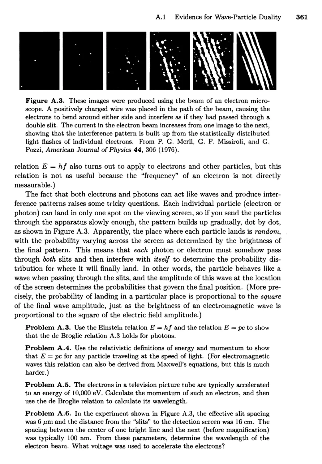
The Photoelectric Effect; Electron Diffraction ,
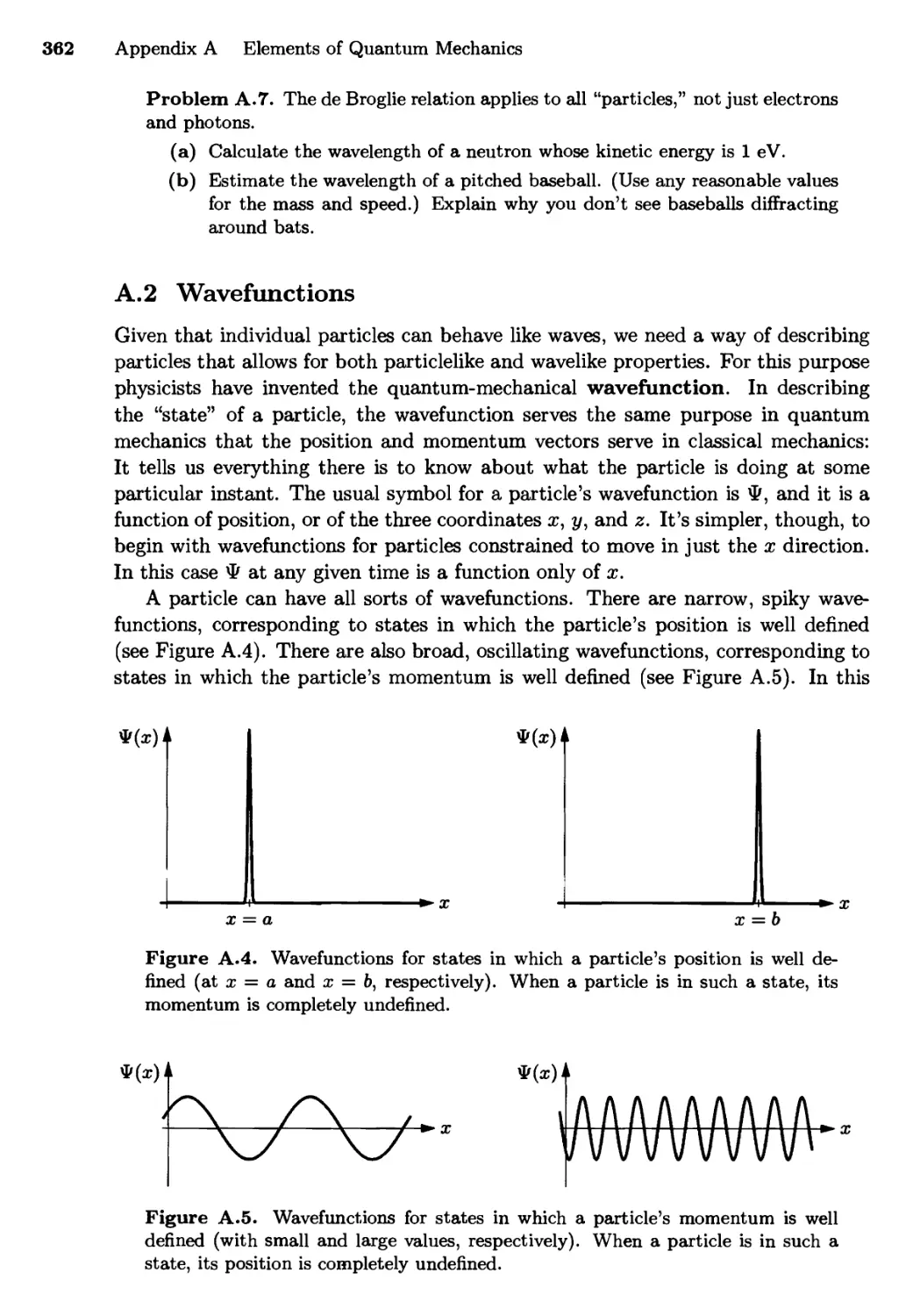
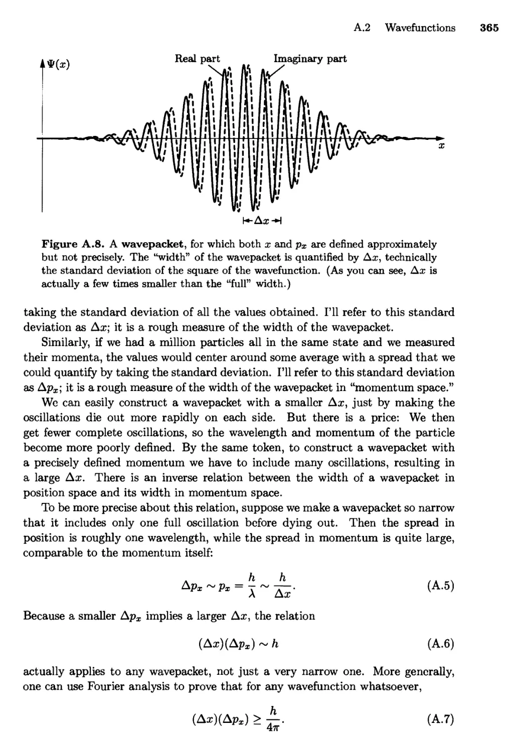
A.2 Wavefunctions 362
The Uncertainty Principle; Linearly Independent
Wavefunctions
A.3 Definite-Energy Wavefunctions 367
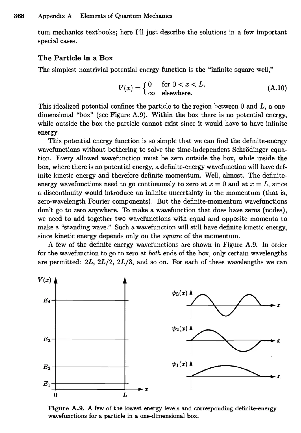
The Particle in a Box; The Harmonic Oscillator;
The Hydrogen Atom
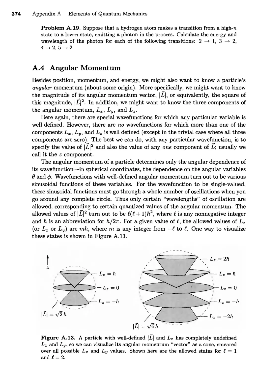
A.4 Angular Momentum 374
Rotating Molecules; Spin
A.5 Systems of Many Particles 379
A.6 Quantum Field Theory 380
Appendix B Mathematical Results 384
B.l Gaussian Integrals 384
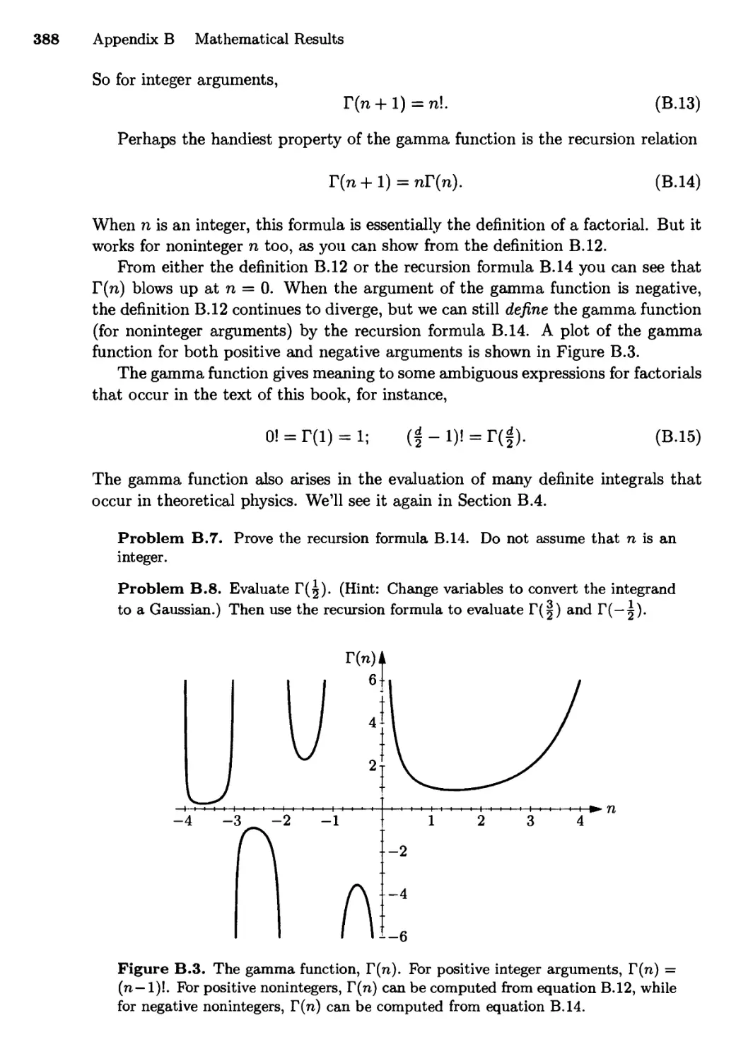
B.2 The Gamma Function 387
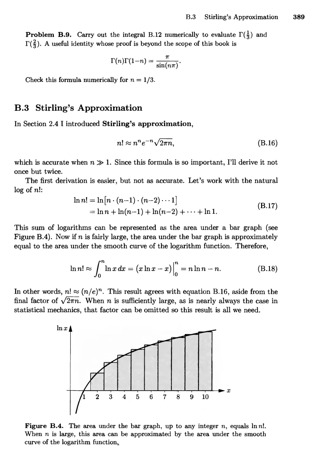
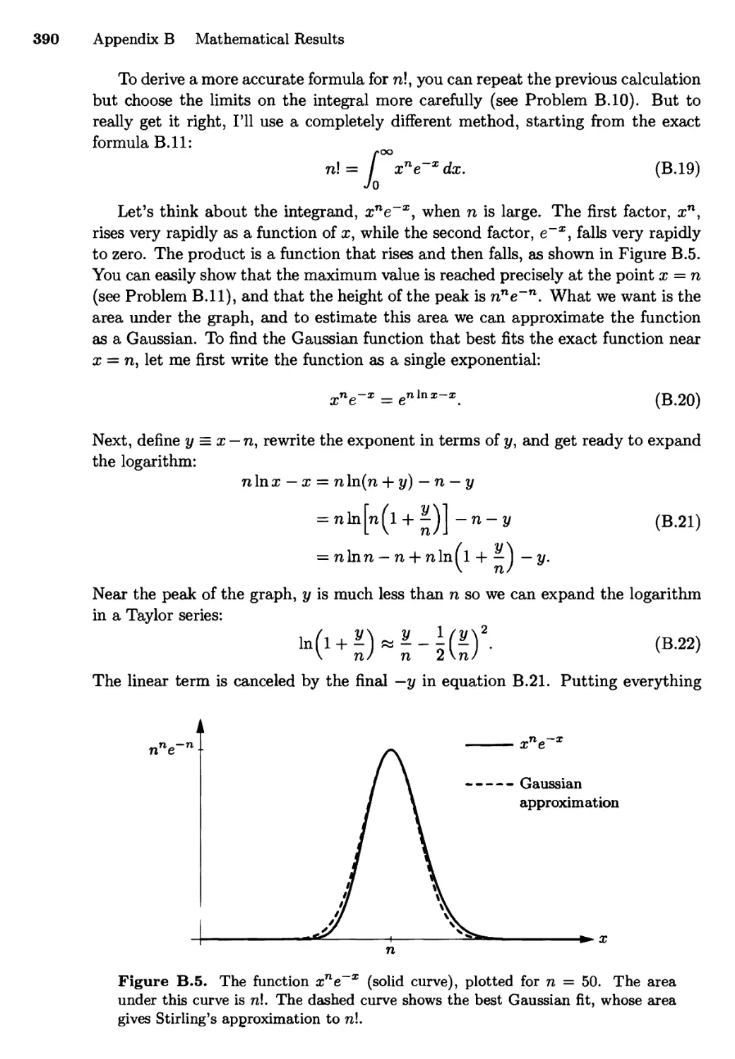
B.3 Stirling's Approximation 389
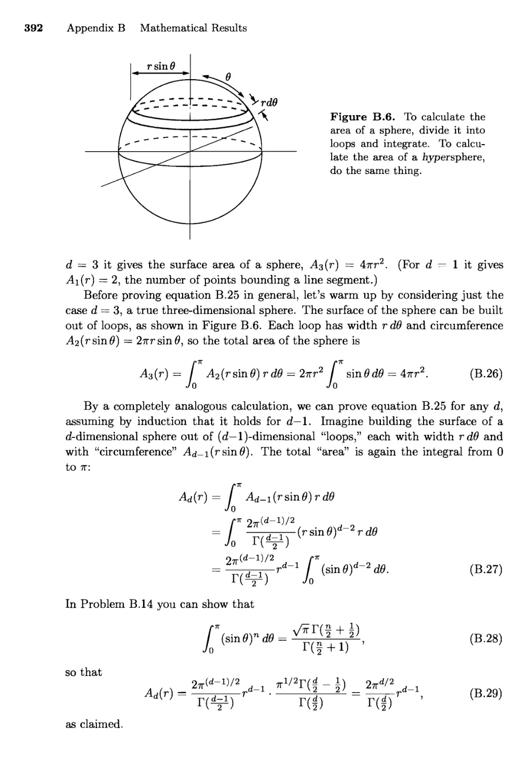
B.4 Area of a d-Dimensional Hypersphere 391
B.5 Integrals of Quantum Statistics 393
Suggested Reading 397
Reference Data 402
Index 406
Preface
Thermal physics deals with collections of large numbers of particles—typically
1023 or so. Examples include the air in a balloon, the water in a lake, the electrons
in a chunk of metal, and the photons (electromagnetic wave packets) given off by
the sun. Anything big enough to see with our eyes (or even with a conventional
microscope) has enough particles in it to qualify as a subject of thermal physics.
Consider a chunk of metal, containing perhaps 1023 ions and 1023 conduction
electrons. We can't possibly follow every detail of the motions of all these particles,
nor would we want to if we could. So instead, in thermal physics, we assume
that the particles just jostle about randomly, and we use the laws of probability
to predict how the chunk of metal as a whole ought to behave. Alternatively, we
can measure the bulk properties of the metal (stiffness, conductivity, heat capacity,
magnetization, and so on), and from these infer something about the particles it is
made of.
Some of the properties of bulk matter don't really depend on the microscopic
details of atomic physics. Heat always flows spontaneously from a hot object to a
cold one, never the other way. Liquids always boil more readily at lower pressure.
The maximum possible efficiency of an engine, working over a given temperature
range, is the same whether the engine uses steam or air or anything else as its
working substance. These kinds of results, and the principles that generalize them,
comprise a subject called thermodynamics.
But to understand matter in more detail, we must also take into account both
the quantum behavior of atoms and the laws of statistics that make the connection
between one atom and 1023. Then we can not only predict the properties of metals
and other materials, but also explain why the principles of thermodynamics are
what they are—why heat flows from hot to cold, for example. This underlying
explanation of thermodynamics, and the many applications that come along with
it, comprise a subject called statistical mechanics.
Physics instructors and textbook authors are in bitter disagreement over the
proper content of a first course in thermal physics. Some prefer to cover only
thermodynamics, it being less mathematically demanding and more readily applied
to the everyday world. Others put a strong emphasis on statistical mechanics, with
vii
Preface
its spectacularly detailed predictions and concrete foundation in atomic physics.
To some extent the choice depends on what application areas one has in mind:
Thermodynamics is often sufficient in engineering or earth science, while statistical
mechanics is essential in solid state physics or astrophysics.
In this book I have tried to do justice to both thermodynamics and statistical
mechanics, without giving undue emphasis to either. The book is in three parts.
Part I introduces the fundamental principles of thermal physics (the so-called first
and second laws) in a unified way, going back and forth between the microscopic
(statistical) and macroscopic (thermodynamic) viewpoints. This portion of the
book also applies these principles to a few simple thermodynamic systems, chosen
for their illustrative character. Parts II and III then develop more sophisticated
techniques to treat farther applications of thermodynamics and statistical
mechanics, respectively. My hope is that this organizational plan will accomodate a variety
of teaching philosophies in the middle of the thermo-to-statmech continuum.
Instructors who are entrenched at one or the other extreme should look for a different
book.
The thrill of thermal physics comes from using it to understand the world we
live in. Indeed, thermal physics has so many applications that no single author
can possibly be an expert on all of them. In writing this book I've tried to learn
and include as many applications as possible, to such diverse areas as chemistry,
biology, geology, meteorology, environmental science, engineering, low-temperature
physics, solid state physics, astrophysics, and cosmology. I'm sure there are many
fascinating applications that I've missed. But in my mind, a book like this one
cannot have too many applications. Undergraduate physics students can and do go
on to specialize in all of the subjects just named, so I consider it my duty to make
you aware of some of the possibilities. Even if you choose a career entirely outside
of the sciences, an understanding of thermal physics will enrich the experiences of
every day of your life.
One of my goals in writing this book was to keep it short enough for a one-
semester course. I have failed. Too many topics have made their way into the
text, and it is now too long even for a very fast-paced semester. The book is still
intended primarily for a one-semester course, however. Just be sure to omit several
sections so you'll have time to cover what you do cover in some depth. In my
own course I've been omitting Sections 1.7, 4.3, 4.4, 5.4 through 5.6, and all of
Chapter 8. Many other portions of Parts II and III make equally good candidates
for omission, depending on the emphasis of the course. If you're lucky enough to
have more than one semester, then you can cover all of the main text and/or work
some extra problems.
Listening to recordings won't teach you to play piano (though it can help),
and reading a textbook won't teach you physics (though it too can help). To
encourage you to learn actively while using this book, the publisher has provided
ample margins for your notes, questions, and objections. I urge you to read with
a pencil (not a highlighter). Even more important are the problems. All physics
textbook authors tell their readers to work the problems, and I hereby do the same.
In this book you'll encounter problems every few pages, at the end of almost every
Preface
section. I've put them there (rather than at the ends of the chapters) to get your
attention, to show you at every opportunity what you're now capable of doing. The
problems come in all types: thought questions, short numerical calculations, order-
of-magnitude estimates, derivations, extensions of the theory, new applications, and
extended projects. The time required per problem varies by more than three orders
of magnitude. Please work as many problems as you can, early and often. You
won't have time to work all of them, but please read them all anyway, so you'll
know what you're missing. Years later, when the mood strikes you, go back and
work some of the problems you skipped the first time around.
Before reading this book you should have taken a year-long introductory physics
course and a year of calculus. If your introductory course did not include any
thermal physics you should spend some extra time studying Chapter 1. If your
introductory course did not include any quantum physics you'll want to refer to
Appendix A as necessary while reading Chapters 2, 6, and 7. Multivariate calculus
is introduced in stages as the book goes on; a course in this subject would be a
helpful, but not absolutely necessary, corequisite.
Some readers will be disappointed that this book does not cover certain topics,
and covers others only superficially. As a partial remedy I have provided an
annotated list of suggested further readings at the back of the book. A number of
references on particular topics are given in the text as well. Except when I have
borrowed some data or an illustration, I have not included any references merely
to give credit to the originators of an idea. I am utterly unqualified to determine
who deserves credit in any case. The occasional historical comments in the text
are grossly oversimplified, intended to tell how things could have happened, not
necessarily how they did happen.
No textbook is ever truly finished as it goes to press, and this one is no
exception. Fortunately, the World-Wide Web gives authors a chance to continually
provide updates. For the foreseeable future, the web site for this book will be at
http://physics.weber.edu/thermal/. There you will find a variety of further
information including a list of errors and corrections, platform-specific hints on
solving problems requiring a computer, and additional references and links. You'll
also find my e-mail address, to which you are welcome to send questions, comments,
and suggestions.
Acknowledgments
It is a pleasure to thank the many people who have contributed to this project.
First there are the brilliant teachers who helped me learn thermal physics: Philip
Wojak, Tom Moore, Bruce Thomas, and Michael Peskin. Tom and Michael have
continued to teach me on a regular basis to this day, and I am sincerely grateful for
these ongoing collaborations. In teaching thermal physics myself, I have especially
depended on the insightful textbooks of Charles Kittel, Herbert Kroemer, and Keith
Stowe.
As this manuscript developed, several brave colleagues helped by testing it in
the classroom: Chuck Adler, Joel Cannon, Brad Carroll, Phil Fraundorf, Joseph
Ganem, David Lowe, Juan Rodriguez, and Daniel Wilkins. I am indebted to each of
Preface
them, and to their students, for enduring the many inconveniences of an unfinished
textbook. I owe special thanks to my own students from seven years of teaching
thermal physics at Grinnell College and Weber State University. I'm tempted to
list all their names here, but instead let me choose just three to represent them
all: Shannon Corona, Dan Dolan, and Mike Shay, whose questions pushed me to
develop new approaches to important parts of the material.
Others who generously took the time to read and comment on early drafts
of the manuscript were Elise Albert, W. Ariyasinghe, Charles Ebner, Alexander
Fetter, Harvey Gould, Ying-Cheng Lai, Tom Moore, Robert Pelcovits, Michael
Peskin, Andrew Rutenberg, Daniel Styer, and Larry Tankersley. Farhang Amiri,
Lee Badger, and Adolph Yonkee provided essential feedback on individual chapters,
while Colin Inglefield, Daniel Pierce, Spencer Seager, and John Sohl provided expert
assistance with specific technical issues. Karen Thurber drew the magician and
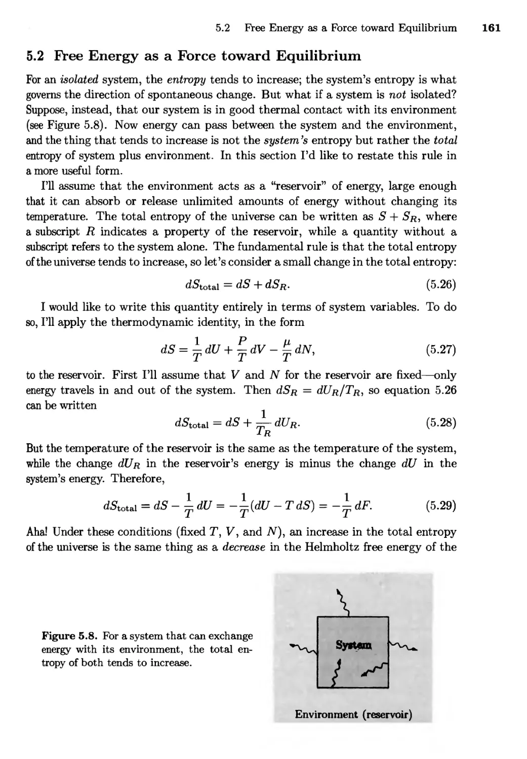
rabbit for Figures 1.15, 5.1, and 5.8. I am grateful to all of these individuals, and
to the dozens of others who have answered questions, pointed to references, and
given permission to reproduce their work.
I thank the faculty, staff, and administration of Weber State University, for
providing support in a multitude of forms, and especially for creating an environment
in which textbook writing is valued and encouraged.
It has been a pleasure to work with my editorial team at Addison Wesley
Longman, especially Sami Iwata, whose confidence in this project has always exceeded
my own, and Joan Marsh and Lisa Weber, whose expert advice has improved the
appearance of every page.
In the space where most authors thank their immediate families, I would like to
thank my family of friends, especially Deb, Jock, John, Lyall, Satoko, and Suzanne.
Their encouragement and patience have been unlimited.
1 E„eTO i„ TH„mal PMcs
1.1 Thermal Equilibrium
The most familiar concept in thermodynamics is temperature. It's also one of
the trickiest concepts—I won't be ready to tell you what temperature really is until
Chapter 3. For now, however, let's start with a very naive definition:
Temperature is what you measure with a thermometer.
If you want to measure the temperature of a pot of soup, you stick a thermometer
(such as a mercury thermometer) into the soup, wait a while, then look at the
reading on the thermometer's scale. This definition of temperature is what's called
an operational definition, because it tells you how to measure the quantity in
question.
Ok, but why does this procedure work? Well, the mercury in the thermometer
expands or contracts, as its temperature goes up or down. Eventually the
temperature of the mercury equals the temperature of the soup, and the volume occupied
by the mercury tells us what that temperature is.
Notice that our thermometer (and any other thermometer) relies on the
following fundamental fact: When you put two objects in contact with each other, and
wait long enough, they tend to come to the same temperature. This property is so
fundamental that we can even take it as an alternative definition of temperature:
Temperature is the thing that's the same for two objects, after they've
been in contact long enough.
I'll refer to this as the theoretical definition of temperature. But this definition
is extremely vague: What kind of "contact" are we talking about here? How long is
"long enough" ? How do we actually ascribe a numerical value to the temperature?
And what if there is more than one quantity that ends up being the same for both
objects?
1
Chapter 1 Energy in Thermal Physics
Before answering these questions, let me introduce some more terminology:
After two objects have been in contact long enough, we say that they are in
thermal equilibrium.
The time required for a system to come to thermal equilibrium is called the
relaxation time.
So when you stick the mercury thermometer into the soup, you have to wait for the
relaxation time before the mercury and the soup come to the same temperature (so
you get a good reading). After that, the mercury is in thermal equilibrium with
the soup.
Now then, what do I mean by "contact" ? A good enough definition for now is
that "contact," in this sense, requires some means for the two objects to exchange
energy spontaneously, in the form that we call "heat." Intimate mechanical contact
(i.e., touching) usually works fine, but even if the objects are separated by empty
space, they can "radiate" energy to each other in the form of electromagnetic waves.
If you want to prevent two objects from coming to thermal equilibrium, you need to
put some kind of thermal insulation in between, like spun fiberglass or the double
wall of a thermos bottle. And even then, they'll eventually come to equilibrium;
all you're really doing is increasing the relaxation time.
The concept of relaxation time is usually clear enough in particular examples.
When you pour cold cream into hot coffee, the relaxation time for the contents of
the cup is only a few seconds. However, the relaxation time for the coffee to come
to thermal equilibrium with the surrounding room is many minutes.*
The cream-and-coffee example brings up another issue: Here the two substances
not only end up at the same temperature, they also end up blended with each other.
The blending is not necessary for thermal equilibrium, but constitutes a second type
of equilibrium—diffusive equilibrium—in which the molecules of each substance
(cream molecules and coffee molecules, in this case) are free to move around but no
longer have any tendency to move one way or another. There is also mechanical
equilibrium, when large-scale motions (such as the expansion of a balloon—see
Figure 1.1) can take place but no longer do. For each type of equilibrium between
two systems, there is a quantity that can be exchanged between the systems:
Exchanged quantity Type of equilibrium
energy thermal
volume mechanical
particles diffusive
Notice that for thermal equilibrium I'm claiming that the exchanged quantity is
energy. We'll see some evidence for this in the following section.
When two objects are able to exchange energy, and energy tends to move
spontaneously from one to the other, we say that the object that gives up energy is at
*Some authors define relaxation time more precisely as the time required for the
temperature difference to decrease by a factor of e « 2.7. In this book all we'll need is a
qualitative definition.
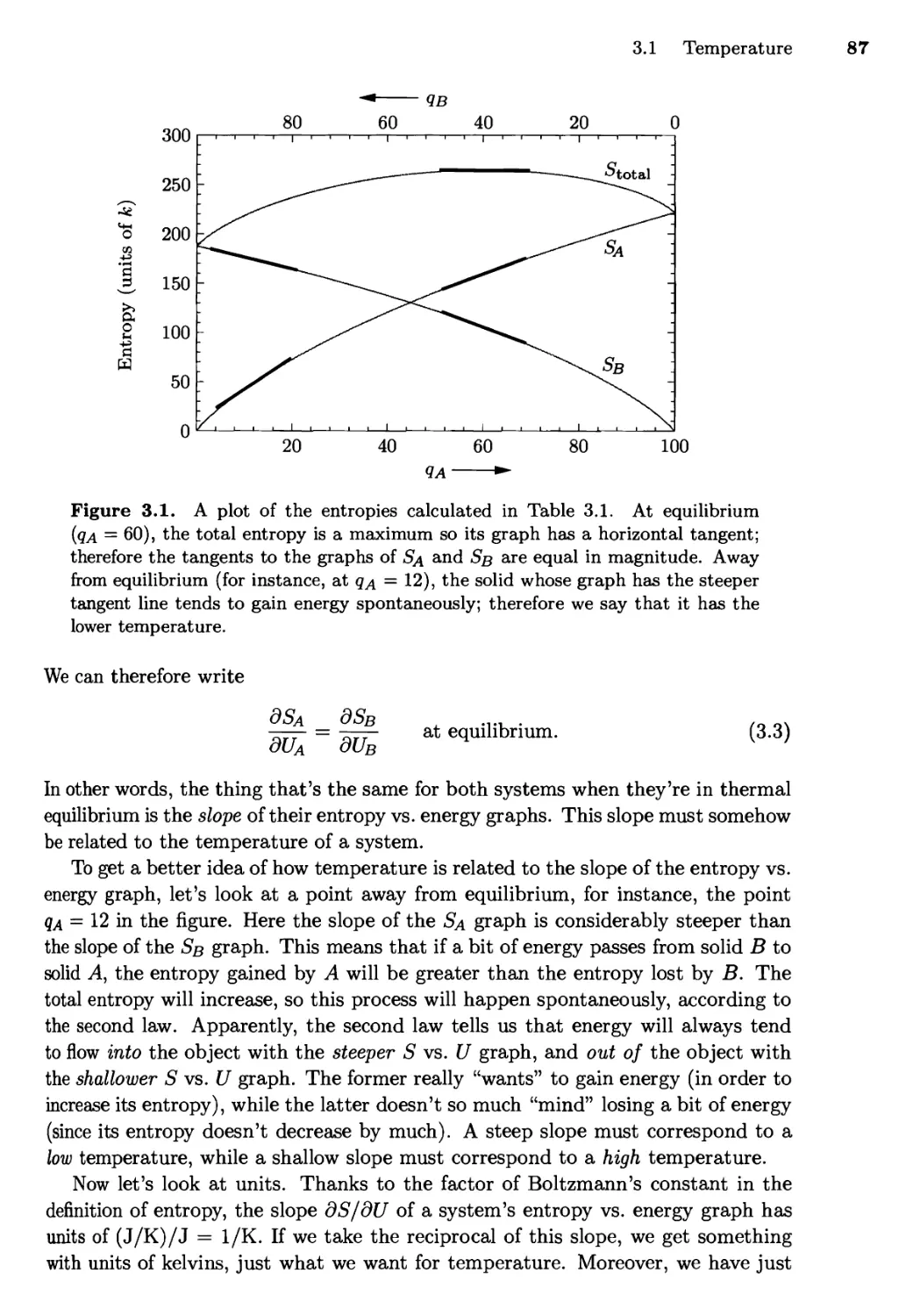
1.1 Thermal Equilibrium 3
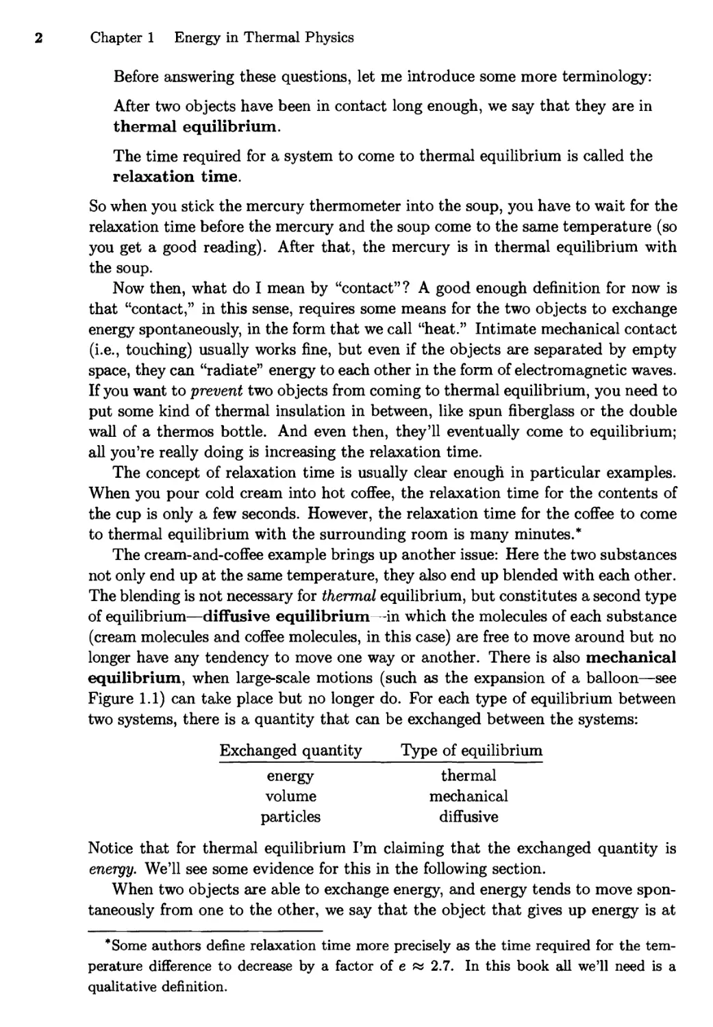
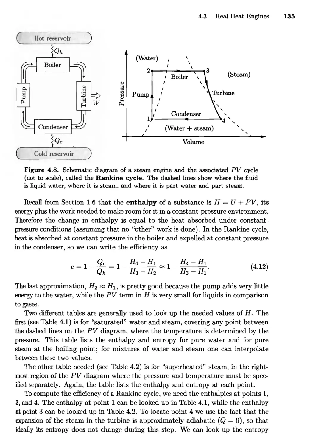
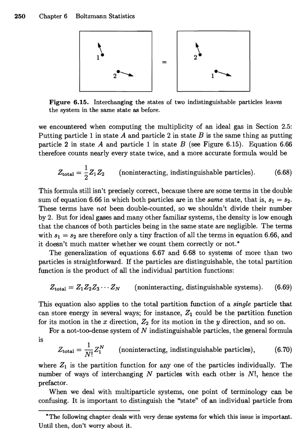
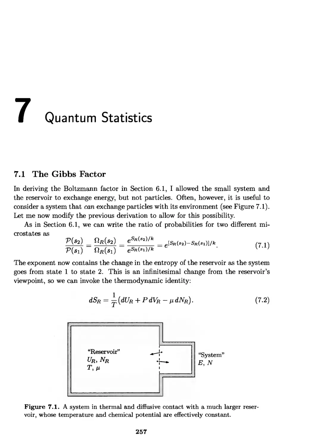
Figure 1.1. A hot-air balloon interacts thermally, mechanically, and diffusively
with its environment—exchanging energy, volume, and particles. Not all of these
interactions are at equilibrium, however.
a higher temperature, and the object that sucks in energy is at a lower
temperature. With this convention in mind, let me now restate the theoretical definition of
temperature:
Temperature is a measure of the tendency of an object to spontaneously
give up energy to its surroundings. When two objects are in thermal contact,
the one that tends to spontaneously lose energy is at the higher temperature.
In Chapter 3 I'll return to this theoretical definition and make it much more precise,
explaining, in the most fundamental terms, what temperature really is.
Meanwhile, I still need to make the operational definition of temperature (what
you measure with a thermometer) more precise. How do you make a properly
calibrated thermometer, to get a numerical value for temperature?
Most thermometers operate on the principle of thermal expansion: Materials
tend to occupy more volume (at a given pressure) when they're hot. A mercury
thermometer is just a convenient device for measuring the volume of a fixed amount
of mercury. To define actual units for temperature, we pick two convenient
temperatures, such as the freezing and boiling points of water, and assign them arbitrary
numbers, such as 0 and 100. We then mark these two points on our mercury
thermometer, measure off a hundred equally spaced intervals in between, and declare
that this thermometer now measures temperature on the Celsius (or centigrade)
scale, by definition!
Of course it doesn't have to be a mercury thermometer; we could instead exploit
the thermal expansion of some other substance, such as a strip of metal, or a gas
at fixed pressure. Or we could use an electrical property, such as the resistance, of
some standard object. A few practical thermometers for various purposes are shown
4 Chapter 1 Energy in Thermal Physics
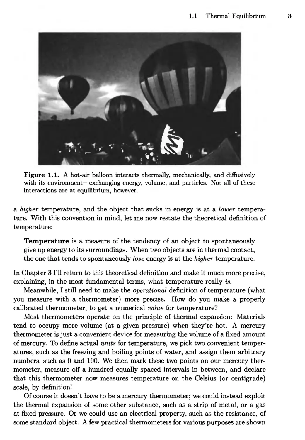
Figure 1.2. A selection of thermometers. In the center are two liquid-in-glass
thermometers, which measure the expansion of mercury (for higher temperatures)
and alcohol (for lower temperatures). The dial thermometer to the right measures
the turning of a coil of metal, while the bulb apparatus behind it measures the
pressure of a fixed volume of gas. The digital thermometer at left-rear uses a
thermocouple—a junction of two metals—which generates a small temperature-
dependent voltage. At left-front is a set of three potter's cones, which melt and
droop at specified clay-firing temperatures.
in Figure 1.2. It's not obvious that the scales for various different thermometers
would agree at all the intermediate temperatures between 0°C and 100°C. In fact,
they generally won't, but in many cases the differences are quite small. If you ever
have to measure temperatures with great precision you'll need to pay attention to
these differences, but for our present purposes, there's no need to designate any one
thermometer as the official standard.
A thermometer based on expansion of a gas is especially interesting, though,
because if you extrapolate the scale down to very low temperatures, you are led to
predict that for any low-density gas at constant pressure, the volume should go to
zero at approximately —273°C. (In practice the gas will always liquefy first, but
until then the trend is quite clear.) Alternatively, if you hold the volume of the gas
fixed, then its pressure will approach zero as the temperature approaches — 273° C
(see Figure 1.3). This special temperature is called absolute zero, and defines
the zero-point of the absolute temperature scale, first proposed by William
Thomson in 1848. Thomson was later named Baron Kelvin of Largs, so the SI
unit of absolute temperature is now called the kelvin.* A kelvin is the same size
as a degree Celsius, but kelvin temperatures are measured up from absolute zero
instead of from the freezing point of water. In round numbers, room temperature
is approximately 300 K.
As we're about to see, many of the equations of thermodynamics are correct
only when you measure temperature on the kelvin scale (or another absolute scale
such as the Rankine scale defined in Problem 1.2). For this reason it's usually wise
*The Unit Police have decreed that it is impermissible to say "degree kelvin"—the
name is simply "kelvin"—and also that the names of all Official SI Units shall not be
capitalized.
1.1 Thermal Equilibrium 5
1.6
1.4
1.2
1.0
0.8
0.6
0.4
0.2
-300 -200 -100 0 100
Temperature (°C)
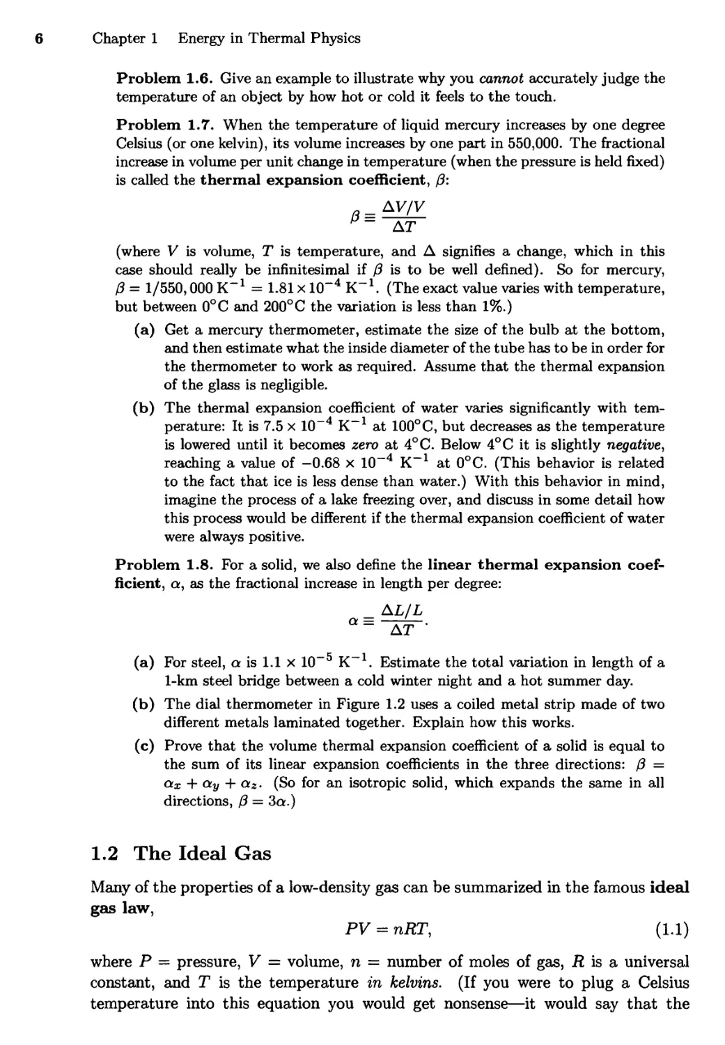
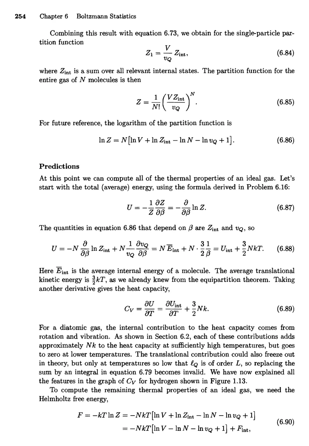
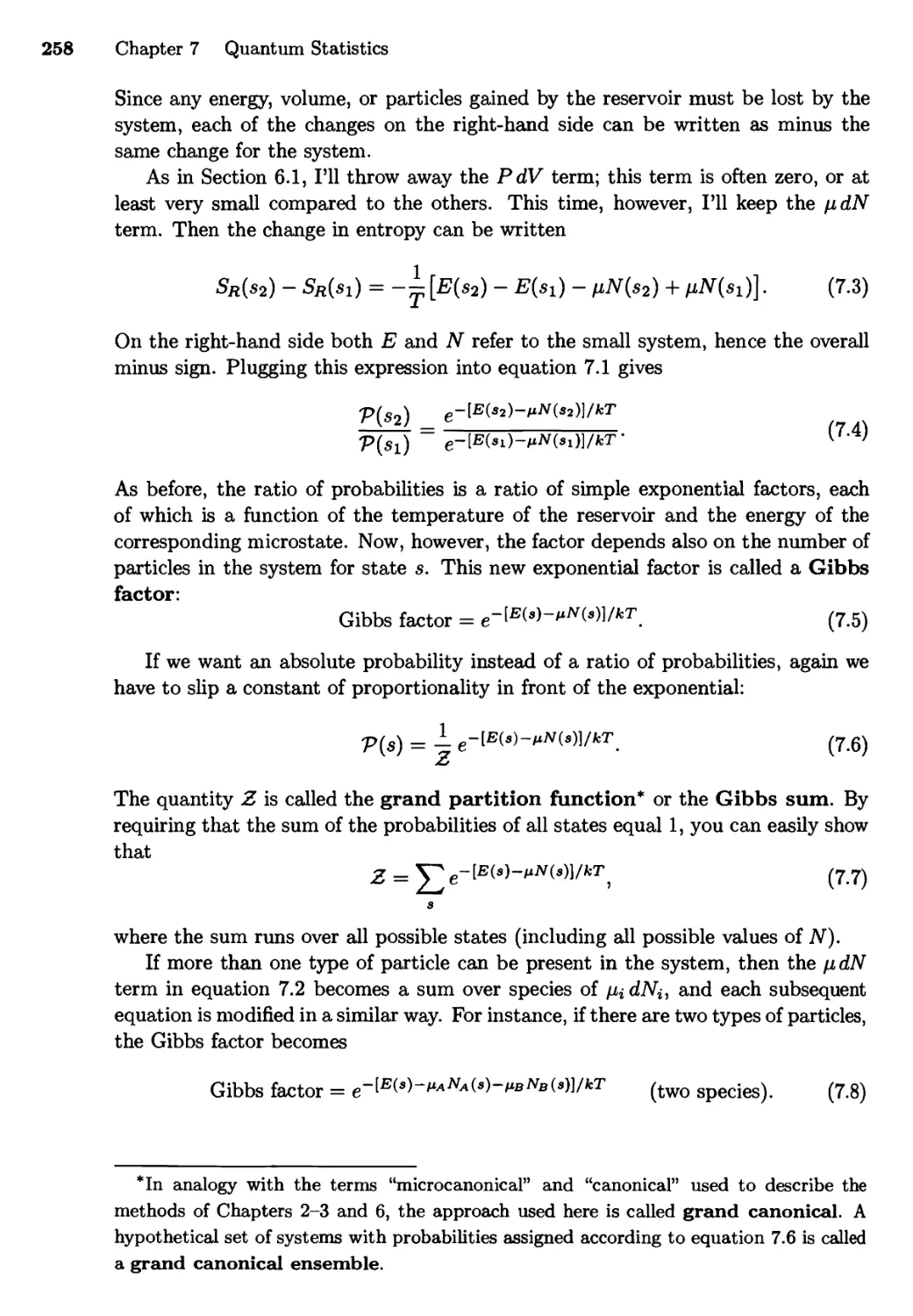
Figure 1.3. Data from a student experiment measuring the pressure of a fixed
volume of gas at various temperatures (using the bulb apparatus shown in
Figure 1.2). The three data sets are for three different amounts of gas (air) in the bulb.
Regardless of the amount of gas, the pressure is a linear function of temperature
that extrapolates to zero at approximately — 280° C. (More precise measurements
show that the zero-point does depend slightly on the amount of gas, but has a
well-defined limit of —273.15°C as the density of the gas goes to zero.)
to convert temperatures to kelvins before plugging them into any formula. (Celsius
is ok, though, when you're talking about the difference between two temperatures.)
Problem 1.1. The Fahrenheit temperature scale is defined so that ice melts at
32°F and water boils at 212°F.
(a) Derive the formulas for converting from Fahrenheit to Celsius and back.
(b) What is absolute zero on the Fahrenheit scale?
Problem 1.2. The Rankine temperature scale (abbreviated °R) uses the same
size degrees as Fahrenheit, but measured up from absolute zero like kelvin (so
Rankine is to Fahrenheit as kelvin is to Celsius). Find the conversion formula
between Rankine and Fahrenheit, and also between Rankine and kelvin. What is
room temperature on the Rankine scale?
Problem 1.3. Determine the kelvin temperature for each of the following:
(a) human body temperature;
(b) the boiling point of water (at the standard pressure of 1 atm);
(c) the coldest day you can remember;
(d) the boiling point of liquid nitrogen (—196°C);
(e) the melting point of lead (327° C).
Problem 1.4. Does it ever make sense to say that one object is "twice as hot" as
another? Does it matter whether one is referring to Celsius or kelvin temperatures?
Explain.
Problem 1.5. When you're sick with a fever and you take your temperature with
a thermometer, approximately what is the relaxation time?
6 Chapter 1 Energy in Thermal Physics
Problem 1.6. Give an example to illustrate why you cannot accurately judge the
temperature of an object by how hot or cold it feels to the touch.
Problem 1.7. When the temperature of liquid mercury increases by one degree
Celsius (or one kelvin), its volume increases by one part in 550,000. The fractional
increase in volume per unit change in temperature (when the pressure is held fixed)
is called the thermal expansion coefficient, (3:
0=^_
P AT
(where V is volume, T is temperature, and A signifies a change, which in this
case should really be infinitesimal if 0 is to be well defined). So for mercury,
(3 = 1/550,000 K"1 = 1.81 x 10~4 K_1. (The exact value varies with temperature,
but between 0°C and 200° C the variation is less than 1%.)
(a) Get a mercury thermometer, estimate the size of the bulb at the bottom,
and then estimate what the inside diameter of the tube has to be in order for
the thermometer to work as required. Assume that the thermal expansion
of the glass is negligible.
(b) The thermal expansion coefficient of water varies significantly with
temperature: It is 7.5 x 10⁻⁴ K"1 at 100°C, but decreases as the temperature
is lowered until it becomes zero at 4°C. Below 4°C it is slightly negative,
reaching a value of —0.68 x 10~4 K_1 at 0°C. (This behavior is related
to the fact that ice is less dense than water.) With this behavior in mind,
imagine the process of a lake freezing over, and discuss in some detail how
this process would be different if the thermal expansion coefficient of water
were always positive.
Problem 1.8. For a solid, we also define the linear thermal expansion
coefficient, a, as the fractional increase in length per degree:
AL/L
(a) For steel, aisl.lxlO~5K-1. Estimate the total variation in length of a
1-km steel bridge between a cold winter night and a hot summer day.
(b) The dial thermometer in Figure 1.2 uses a coiled metal strip made of two
different metals laminated together. Explain how this works.
(c) Prove that the volume thermal expansion coefficient of a solid is equal to
the sum of its linear expansion coefficients in the three directions: (3 =
&x + cty + az. (So for an isotropic solid, which expands the same in all
directions, fi = 3a.)
1,2 The Ideal Gas
Many of the properties of a low-density gas can be summarized in the famous ideal
gas law,
PV = nRT, (1.1)
where P = pressure, V = volume, n = number of moles of gas, R is a universal
constant, and T is the temperature in kelvins. (If you were to plug a Celsius
temperature into this equation you would get nonsense—it would say that the
1.2 The Ideal Gas 7
volume or pressure of a gas goes to zero at the freezing temperature of water and
becomes negative at still lower temperatures.)
The constant R in the ideal gas law has the empirical value
in SI units, that is, when you measure pressure in N/m2 = Pa (pascals) and volume
in m3. Chemists often measure pressure in atmospheres (1 atm = 1.013 x 10⁵ Pa)
or bars (1 bar = 105 Pa exactly) and volume in liters (1 liter = (0.1 m)3), so be
careful.
A mole of molecules is Avogadro's number of them,
NA = 6.02 x 10²³. (1.3)
This is another "unit" that's more useful in chemistry than in physics. More often
we will want to simply discuss the number of molecules, denoted by capital N:
N = nxNA. (1.4)
If you plug in N/NA for n in the ideal gas law, then group together the combination
R/NA and call it a new constant fc, you get
PV = NkT. (1.5)
This is the form of the ideal gas law that we'll usually use. The constant k is called
Boltzmann's constant, and is tiny when expressed in SI units (since Avogadro's
number is so huge):
k = -^- = 1.381 x 10"23 J/K. (1.6)
In order to remember how all the constants are related, I recommend memorizing
nR = Nk. (1.7)
Units aside, though, the ideal gas law summarizes a number of important
physical facts. For a given amount of gas at a given temperature, doubling the pressure
squeezes the gas into exactly half as much space. Or, at a given volume, doubling
the temperature causes the pressure to double. And so on. The problems below
explore just a few of the implications of the ideal gas law.
Like nearly all the laws of physics, the ideal gas law is an approximation, never
exactly true for a real gas in the real world. It is valid in the limit of low density,
when the average space between gas molecules is much larger than the size of a
molecule. For air (and other common gases) at room temperature and atmospheric
pressure, the average distance between molecules is roughly ten times the size of a
molecule, so the ideal gas law is accurate enough for most purposes.
Problem 1.9. What is the volume of one mole of air, at room temperature and
1 atm pressure?
8 Chapter 1 Energy in Thermal Physics
Problem 1.10. Estimate the number of air molecules in an average-sized room.
Problem 1.11. Rooms A and B are the same size, and are connected by an open
door. Room A, however, is warmer (perhaps because its windows face the sun).
Which room contains the greater mass of air? Explain carefully.
Problem 1.12. Calculate the average volume per molecule for an ideal gas at
room temperature and atmospheric pressure. Then take the cube root to get
an estimate of the average distance between molecules. How does this distance
compare to the size of a small molecule like N2 or H2O?
Problem 1.13. A mole is approximately the number of protons in a gram of
protons. The mass of a neutron is about the same as the mass of a proton, while
the mass of an electron is usually negligible in comparison, so if you know the
total number of protons and neutrons in a molecule (i.e., its "atomic mass"), you
know the approximate mass (in grams) of a mole of these molecules.* Referring to
the periodic table at the back of this book, find the mass of a mole of each of the
following: water, nitrogen (N2), lead, quartz (SiC^).
Problem 1.14. Calculate the mass of a mole of dry air, which is a mixture of N2
(78% by volume), 02 (21%), and argon (1%).
Problem 1.15. Estimate the average temperature of the air inside a hot-air
balloon (see Figure 1.1). Assume that the total mass of the unfilled balloon and
payload is 500 kg. What is the mass of the air inside the balloon?
Problem 1.16. The exponential atmosphere.
(a) Consider a horizontal slab of air whose thickness (height) is dz. If this slab
is at rest, the pressure holding it up from below must balance both the
pressure from above and the weight of the slab. Use this fact to find an
expression for dP/dz, the variation of pressure with altitude, in terms of
the density of air.
(b) Use the ideal gas law to write the density of air in terms of pressure,
temperature, and the average mass m of the air molecules. (The information
needed to calculate m is given in Problem 1.14.) Show, then, that the
pressure obeys the differential equation
dP mg
dz kT '
called the barometric equation.
(c) Assuming that the temperature of the atmosphere is independent of height
(not a great assumption but not terrible either), solve the barometric
equation to obtain the pressure as a function of height: P(z) = P(0)e~mp2/fcT.
Show also that the density obeys a similar equation.
The precise definition of a mole is the number of carbon-12 atoms in 12 grams of
carbon-12. The atomic mass of a substance is then the mass, in grams, of exactly one
mole of that substance. Masses of individual atoms and molecules are often given in
atomic mass units, abbreviated "u", where 1 u is defined as exactly 1/12 the mass of
a carbon-12 atom. The mass of an isolated proton is actually slightly greater than 1 u,
while the mass of an isolated neutron is slightly greater still. But in this problem, as in
most thermal physics calculations, it's fine to round atomic masses to the nearest integer,
which amounts to counting the total number of protons and neutrons.
1.2 The Ideal Gas 9
(d) Estimate the pressure, in atmospheres, at the following locations: Ogden,
Utah (4700 ft or 1430 m above sea level); Leadville, Colorado (10,150 ft,
3090 m); Mt. Whitney, California (14,500 ft, 4420 m); Mt. Everest, Nepal/
Tibet (29,000 ft, 8840 m). (Assume that the pressure at sea level is 1 atm.)
Problem 1.17. Even at low density, real gases don't quite obey the ideal gas
law. A systematic way to account for deviations from ideal behavior is the virial
expansion,
where the functions #(T), C(T), and so on are called the virial coefficients.
When the density of the gas is fairly low, so that the volume per mole is large,
each term in the series is much smaller than the one before. In many situations it's
sufficient to omit the third term and concentrate on the second, whose coefficient
B(T) is called the second virial coefficient (the first coefficient being 1). Here are
some measured values of the second virial coefficient for nitrogen (N2):
T(K) B (cm3/mol)
Too -160
200 -35
300 -4.2
400 9.0
500 16.9
600 21.3
(a) For each temperature in the table, compute the second term in the virial
equation, B(T)/(V/n), for nitrogen at atmospheric pressure. Discuss the
validity of the ideal gas law under these conditions.
(b) Think about the forces between molecules, and explain why we might
expect B(T) to be negative at low temperatures but positive at high
temperatures.
(c) Any proposed relation between P, V, and T, like the ideal gas law or the
virial equation, is called an equation of state. Another famous equation
of state, which is qualitatively accurate even for dense fluids, is the van
der Waals equation,
(p+~)(V-nb)=nRT,
where a and b are constants that depend on the type of gas. Calculate the
second and third virial coefficients (B and C) for a gas obeying the van der
Waals equation, in terms of a and b. (Hint: The binomial expansion says
that (1 + x)p « 1 + px 4- \p(p—\)x2, provided that \px\ < 1. Apply this
approximation to the quantity [1 — (nb/V)]"1.)
(d) Plot a graph of the van der Waals prediction for B(T), choosing a and b
so as to approximately match the data given above for nitrogen. Discuss
the accuracy of the van der Waals equation over this range of conditions.
(The van der Waals equation is discussed much further in Section 5.3.)
10 Chapter 1 Energy in Thermal Physics
Microscopic Model of an Ideal Gas
In Section 1.1 I defined the concepts of "temperature" and "thermal equilibrium,"
and briefly noted that thermal equilibrium arises through the exchange of energy
between two systems. But how, exactly, is temperature related to energy? The
answer to this question is not simple in general, but it is simple for an ideal gas,
as I'll now attempt to demonstrate.
I'm going to construct a mental "model" of a container full of gas.* The model
will not be accurate in all respects, but I hope to preserve some of the most
important aspects of the behavior of real low-density gases. To start with, I'll make the
model as simple as possible: Imagine a cylinder containing just one gas molecule,
as shown in Figure 1.4. The length of the cylinder is L, the area of the piston is
A, and therefore the volume inside is V = LA. At the moment, the molecule has
a velocity vector tf, with horizontal component vx. As time passes, the molecule
bounces off the walls of the cylinder, so its velocity changes. I'll assume, however,
that these collisions are always elastic, so the molecule doesn't lose any kinetic
energy; its speed never changes. I'll also assume that the surfaces of the cylinder and
piston are perfectly smooth, so the molecule's path as it bounces is symmetrical
about a line normal to the surface, just like light bouncing off a mirror.*
Here's my plan. I want to know how the temperature of a gas is related to
the kinetic energy of the molecules it contains. But the only thing I know about
temperature so far is the ideal gas law,
PV = NkT (1.8)
(where P is pressure). So what I'll first try to do is figure out how the pressure is
related to the kinetic energy; then I'll invoke the ideal gas law to relate pressure to
temperature.
Well, what is the pressure of my simplified gas? Pressure means force per unit
area, exerted in this case on the piston (and the other walls of the cylinder). What
Figure 1.4. A greatly
simplified model of an ideal gas,
with just one molecule
bouncing around elastically.
Length = L
*This model dates back to a 1738 treatise by Daniel Bernoulli, although many of its
implications were not worked out until the 1840s.
'These assumptions are actually valid only for the average behavior of molecules
bouncing off surfaces; in any particular collision a molecule might gain or lose energy, and can
leave the surface at almost any angle.
Piston area = A
m
V
Volume = V = LA
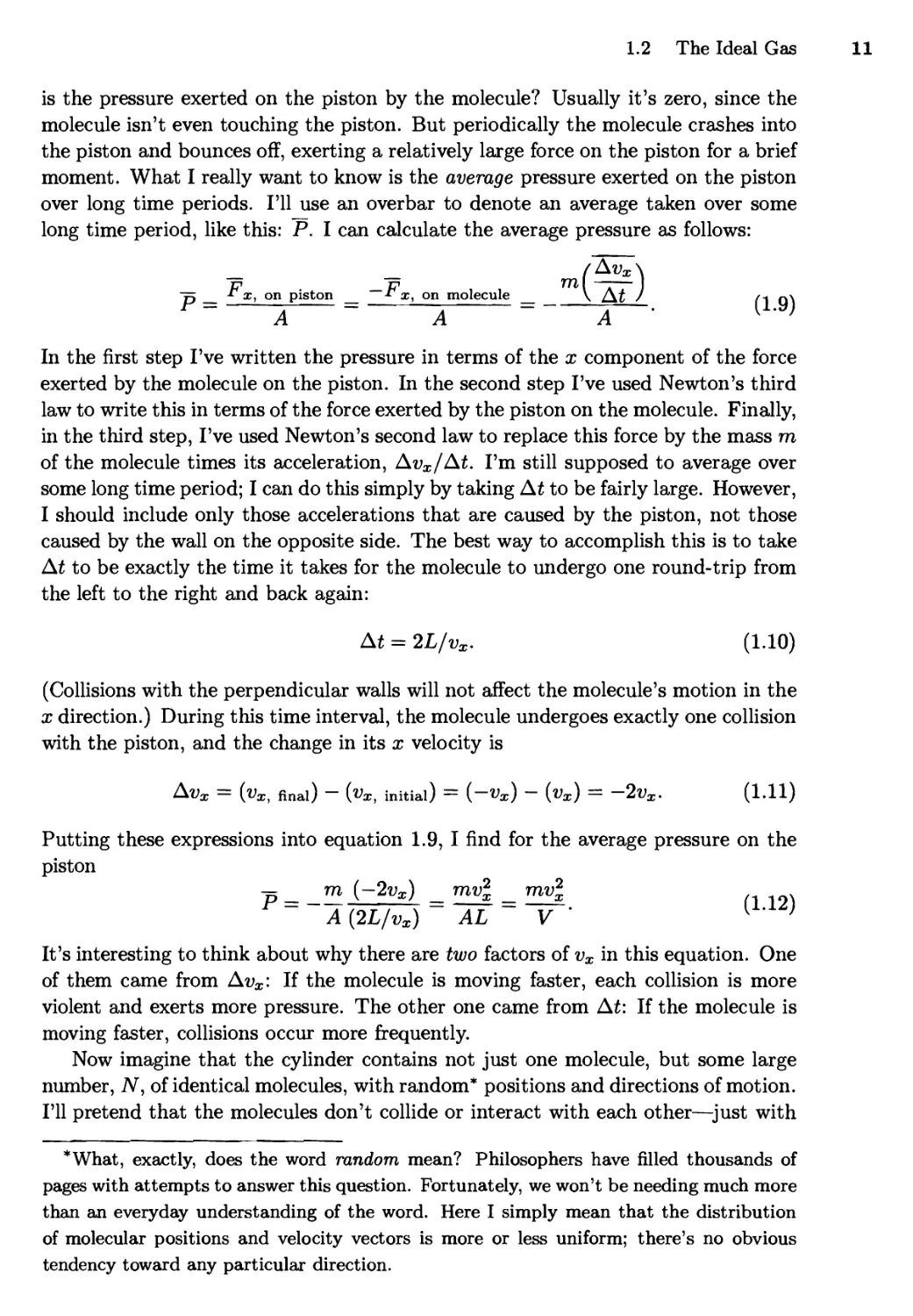
1.2 The Ideal Gas 11
is the pressure exerted on the piston by the molecule? Usually it's zero, since the
molecule isn't even touching the piston. But periodically the molecule crashes into
the piston and bounces off, exerting a relatively large force on the piston for a brief
moment. What I really want to know is the average pressure exerted on the piston
over long time periods. I'll use an overbar to denote an average taken over some
long time period, like this: P. I can calculate the average pressure as follows:
(Avx\
"p ^ x, on piston ~-^x, on molecule \ At / f1 Q^
■T x. on niston " -r
In the first step I've written the pressure in terms of the x component of the force
exerted by the molecule on the piston. In the second step I've used Newton's third
law to write this in terms of the force exerted by the piston on the molecule. Finally,
in the third step, I've used Newton's second law to replace this force by the mass m
of the molecule times its acceleration, Avx/At. I'm still supposed to average over
some long time period; I can do this simply by taking At to be fairly large. However,
I should include only those accelerations that are caused by the piston, not those
caused by the wall on the opposite side. The best way to accomplish this is to take
At to be exactly the time it takes for the molecule to undergo one round-trip from
the left to the right and back again:
At = 2L/vx. (1.10)
(Collisions with the perpendicular walls will not affect the molecule's motion in the
x direction.) During this time interval, the molecule undergoes exactly one collision
with the piston, and the change in its x velocity is
Avx = (vx, nnai) - (VX) initial) = (~VX) - (vx) = -2vx. (1.11)
Putting these expressions into equation 1.9, I find for the average pressure on the
piston
m(-2vx) mv* mv*
A{2L/vx) AL V ' K }
It's interesting to think about why there are two factors of vx in this equation. One
of them came from Avx: If the molecule is moving faster, each collision is more
violent and exerts more pressure. The other one came from At: If the molecule is
moving faster, collisions occur more frequently.
Now imagine that the cylinder contains not just one molecule, but some large
number, TV, of identical molecules, with random* positions and directions of motion.
I'll pretend that the molecules don't collide or interact with each other—just with
*What, exactly, does the word random mean? Philosophers have filled thousands of
pages with attempts to answer this question. Fortunately, we won't be needing much more
than an everyday understanding of the word. Here I simply mean that the distribution
of molecular positions and velocity vectors is more or less uniform; there's no obvious
tendency toward any particular direction.
12 Chapter 1 Energy in Thermal Physics
the walls. Since each molecule periodically collides with the piston, the average
pressure is now given by a sum of terms of the form of equation 1.12:
PV = mv\x + mv\x + mv\x + • • •. (1.13)
If the number of molecules is large, the collisions will be so frequent that the pressure
is essentially continuous, and we can forget the overbar on the P. On the other
hand, the sum of vx for all N molecules is just N times the average of their vx
values. Using the same overbar to denote this average over all molecules, equation
1.13 then becomes
PV = Nmv*. (1.14)
So far I've just been exploring the consequences of my model, without bringing
in any facts about the real world (other than Newton's laws). But now let me
invoke the ideal gas law (1.8), treating it as an experimental fact. This allows me
to substitute NkT for PV on the left-hand side of equation 1.14. Canceling the
iV's, we're left with
kT = my* or \mvl = \kT. (1.15)
I wrote this equation the second way because the left-hand side is almost equal to
the average translational kinetic energy of the molecules. The only problem is
the x subscript, which we can get rid of by realizing that the same equation must
also hold for y and z:
\mv% = \mvl = \kT. (1.16)
The average translational kinetic energy is then
#trans = ^TTIV2 = \m(v2x + v\ + v\) = \kT + \kT + \kT = § kT. (1.17)
(Note that the average of a sum is the sum of the averages.)
This is a good place to pause and think about what just happened. I started
with a naive model of a gas as a bunch of molecules bouncing around inside a
cylinder. I also invoked the ideal gas law as an experimental fact. Conclusion: The
average translational kinetic energy of the molecules in a gas is given by a simple
constant times the temperature. So if this model is accurate, the temperature of a
gas is a direct measure of the average translational kinetic energy of its molecules.
This result gives us a nice interpretation of Boltzmann's constant, k. Recall that
k has just the right units, J/K, to convert a temperature into an energy. Indeed, we
now see that k is essentially a conversion factor between temperature and molecular
energy, at least for this simple system. Think about the numbers, though: For an
air molecule at room temperature (300 K), the quantity kT is
(1.38 x 10"23 J/K)(300 K) = 4.14 x 10"21 J, (1.18)
and the average translational energy is 3/2 times as much. Of course, since
molecules are so small, we would expect their kinetic energies to be tiny. The joule,
though, is not a very convenient unit for dealing with such small energies. Instead
1.2 The Ideal Gas 13
we often use the electron-volt (eV), which is the kinetic energy of an electron that
has been accelerated through a voltage difference of one volt: 1 eV = 1.6 x 10~19 J.
Boltzmann's constant is 8.62 x 10~5 eV/K, so at room temperature,
kT = (8.62 x 1(T5 eV/K)(300 K) = 0.026 eV « ~ eV. (1.19)
Even in electron-volts, molecular energies at room temperature are rather small.
If you want to know the average speed of the molecules in a gas, you can almost
get it from equation 1.17, but not quite. Solving for v2 gives
&=—, (1.20)
m
but if you take the square root of both sides, you get not the average speed, but
rather the square root of the average of the squares of the speeds (root-mean-square,
or rms for short):
= V^= J^. (1.21)
V m
We'll see in Section 6.4 that vTms is only slightly larger than vy so if you're not too
concerned about accuracy, vTms is a fine estimate of the average speed. According
to equation 1.21, light molecules tend to move faster than heavy ones, at a given
temperature. If you plug in some numbers, you'll find that small molecules at
ordinary temperatures are bouncing around at hundreds of meters per second.
Getting back to our main result, equation 1.17, you may be wondering whether
it's really true for real gases, given all the simplifying assumptions I made in deriving
it. Strictly speaking, my derivation breaks down if molecules exert forces on each
other, or if collisions with the walls are inelastic, or if the ideal gas law itself fails.
Brief interactions between molecules are generally no big deal, since such collisions
won't change the average velocities of the molecules. The only serious problem is
when the gas becomes so dense that the space occupied by the molecules themselves
becomes a substantial fraction of the total volume of the container. Then the basic
picture of molecules flying in straight lines through empty space no longer applies.
In this case, however, the ideal gas law also breaks down, in such a way as to
precisely preserve equation 1.17. Consequently, this equation is still true, not only
for dense gases but also for most liquids and sometimes even solids! I'll prove it in
Section 6.3.
Problem 1.18. Calculate the rms speed of a nitrogen molecule at room
temperature.
Problem 1.19. Suppose you have a gas containing hydrogen molecules and oxygen
molecules, in thermal equilibrium. Which molecules are moving faster, on average?
By what factor?
Problem 1.20. Uranium has two common isotopes, with atomic masses of 238
and 235. One way to separate these isotopes is to combine the uranium with
fluorine to make uranium hexafluoride gas, UFg, then exploit the difference in the
average thermal speeds of molecules containing the different isotopes. Calculate
the rms speed of each type of molecule at room temperature, and compare them.
14 Chapter 1 Energy in Thermal Physics
Problem 1.21. During a hailstorm, hailstones with an average mass of 2 g and
a speed of 15 m/s strike a window pane at a 45° angle. The area of the window
is 0.5 m and the hailstones hit it at a rate of 30 per second. What average
pressure do they exert on the window? How does this compare to the pressure of
the atmosphere?
Problem 1.22. If you poke a hole in a container full of gas, the gas will start
leaking out. In this problem you will make a rough estimate of the rate at which
gas escapes through a hole. (This process is called effusion, at least when the
hole is sufficiently small.)
(a) Consider a small portion (area = A) of the inside wall of a container full
of gas. Show that the number of molecules colliding with this surface in
a time interval At is PAAt/(2rnvx~)1 where P is the pressure, m is the
average molecular mass, and Vx~ is the average x velocity of those molecules
that collide with the wall.
(b) It's not easy to calculate Vx~, but a good enough approximation is (vx)1 ,
where the bar now represents an average over all molecules in the gas. Show
that (v£)l/2 = y/WJm.
(c) If we now take away this small part of the wall of the container, the
molecules that would have collided with it will instead escape through the hole.
Assuming that nothing enters through the hole, show that the number N
of molecules inside the container as a function of time is governed by the
differential equation
dN_ = _A_ fkTN
dt ~ 2V V m
Solve this equation (assuming constant temperature) to obtain a formula
of the form N(t) = iV(0)e~*/T, where r is the "characteristic time" for TV
(and P) to drop by a factor of e.
(d) Calculate the characteristic time for a gas to escape from a 1-liter container
punctured by a 1-mm2 hole.
(e) Your bicycle tire has a slow leak, so that it goes flat within about an hour
after being inflated. Roughly how big is the hole? (Use any reasonable
estimate for the volume of the tire.)
(f) In Jules Verne's Hound the Moon, the space travelers dispose of a dog's
corpse by quickly opening a window, tossing it out, and closing the
window. Do you think they can do this quickly enough to prevent a significant
amount of air from escaping? Justify your answer with some rough
estimates and calculations.
1.3 Equipartition of Energy
Equation 1.17 is a special case of a much more general result, called the
equipartition theorem. This theorem concerns not just translational kinetic energy but
all forms of energy for which the formula is a quadratic function of a coordinate or
velocity component. Each such form of energy is called a degree of freedom. So
far, the only degrees of freedom I've talked about are translational motion in the
x, y, and z directions. Other degrees of freedom might include rotational motion,
vibrational motion, and elastic potential energy (as stored in a spring). Look at
1.3 Equipartition of Energy 15
the similarities of the formulas for all these types of energy:
\mvl, \mv\, \mv\, \lu2x, \lw\, \ksx2, etc. (1.22)
The fourth and fifth expressions are for rotational kinetic energy, a function of
the moment of inertia / and the angular velocity u. The sixth expression is for
elastic potential energy, a function of the spring constant ks and the amount of
displacement from equilibrium, x. The equipartition theorem simply says that for
each degree of freedom, the average energy will be \kT\
Equipartition theorem: At temperature T, the average energy of any
quadratic degree of freedom is \kT.
If a system contains N molecules, each with / degrees of freedom, and there are
no other (non-quadratic) temperature-dependent forms of energy, then its total
thermal energy is
^thermal = N •/■ \kT. (1.23)
Technically this is just the average total thermal energy, but if N is large,
fluctuations away from the average will be negligible.
I'll prove the equipartition theorem in Section 6.3. For now, though, it's
important to understand exactly what it says. First of all, the quantity t/thermai is
almost never the total energy of a system; there's also "static" energy that doesn't
change as you change the temperature, such as energy stored in chemical bonds or
the rest energies (rac2) of all the particles in the system. So it's safest to apply the
equipartition theorem only to changes in energy when the temperature is raised or
lowered, and to avoid phase transformations and other reactions in which bonds
between particles may be broken.
Another difficulty with the equipartition theorem is in counting how many
degrees of freedom a system has. This is a skill best learned through examples. In a
gas of monatomic molecules like helium or argon, only translational motion counts,
so each molecule has three degrees of freedom, that is, / = 3. In a diatomic gas
like oxygen (O2) or nitrogen (N2), each molecule can also rotate about two
different axes (see Figure 1.5). Rotation about the axis running down the length of the
molecule doesn't count, for reasons having to do with quantum mechanics. The
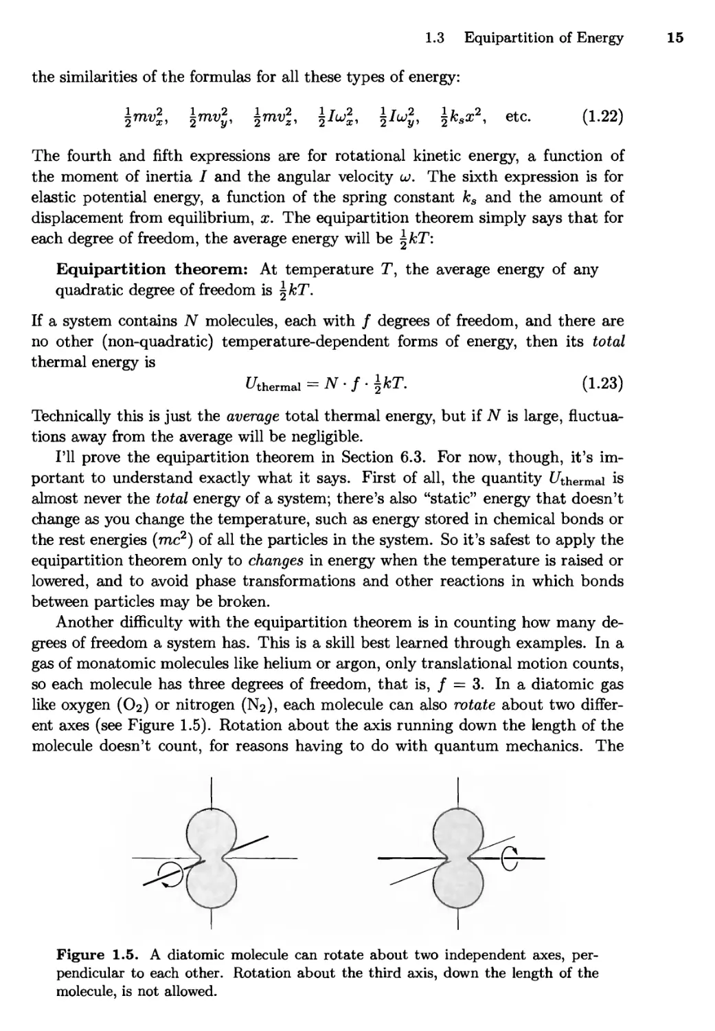
Figure 1.5. A diatomic molecule can rotate about two independent axes,
perpendicular to each other. Rotation about the third axis, down the length of the
molecule, is not allowed.
Chapter 1 Energy in Thermal Physics
same is true for carbon dioxide (CO2), since it also has an axis of symmetry down
its length. However, most polyatomic molecules can rotate about all three axes.
It's not obvious why a rotational degree of freedom should have exactly the same
average energy as a translational degree of freedom. However, if you imagine gas
molecules knocking around inside a container, colliding with each other and with the
walls, you can see how the average rotational energy should eventually reach some
equilibrium value that is larger if the molecules are moving fast (high temperature)
and smaller if the molecules are moving slow (low temperature). In any particular
collision, rotational energy might be converted to translational energy or vice versa,
but on average these processes should balance out.
A diatomic molecule can also vibrate, as if the two atoms were held together by
a spring. This vibration should count as two degrees of freedom, one for the
vibrational kinetic energy and one for the potential energy. (You may recall from classical
mechanics that the average kinetic and potential energies of a simple harmonic
oscillator are equal—a result that is consistent with the equipartition theorem.) More
complicated molecules can vibrate in a variety of ways: stretching, flexing, twisting.
Each "mode" of vibration counts as two degrees of freedom.
However, at room temperature many vibrational degrees of freedom do not
contribute to a molecule's thermal energy. Again, the explanation lies in
quantum mechanics, as we will see in Chapter 3. So air molecules (N2 and O2), for
instance, have only five degrees of freedom, not seven, at room temperature. At
higher temperatures, the vibrational modes do eventually contribute. We say that
these modes are "frozen out" at room temperature; evidently, collisions with other
molecules are sufficiently violent to make an air molecule rotate, but hardly ever
violent enough to make it vibrate.
In a solid, each atom can vibrate in three perpendicular directions, so for each
atom there are six degrees of freedom (three for kinetic energy and three for
potential energy). A simple model of a crystalline solid is shown in Figure 1.6. If we let
N stand for the number of atoms and / stand for the number of degrees of freedom
per atom, then we can use equation 1.23 with / = 6 for a solid. Again, however,
some of the degrees of freedom may be "frozen out" at room temperature.
Liquids are more complicated than either gases or solids. You can generally use
the formula \kT to find the average translational kinetic energy of molecules in a
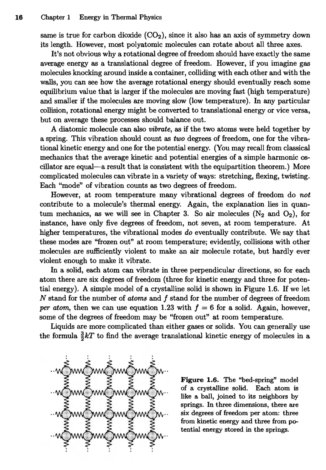
Figure 1.6. The "bed-spring" model
of a crystalline solid. Each atom is
like a ball, joined to its neighbors by
springs. In three dimensions, there are
six degrees of freedom per atom: three
from kinetic energy and three from
potential energy stored in the springs.
1.4 Heat and Work 17
liquid, but the equipartition theorem doesn't work for the rest of the thermal energy,
because the intermolecular potential energies are not nice quadratic functions.
You might be wondering what practical consequences the equipartition theorem
has: How can we test it, experimentally? In brief, we would have to add some energy
to a system, measure how much its temperature changes, and compare to equation
1.23. I'll discuss this procedure in more detail, and show some experimental results,
in Section 1.6.
Problem 1.23. Calculate the total thermal energy in a liter of helium at room
temperature and atmospheric pressure. Then repeat the calculation for a liter of
air.
Problem 1.24. Calculate the total thermal energy in a gram of lead at room
temperature, assuming that none of the degrees of freedom are "frozen out" (this
happens to be a good assumption in this case).
Problem 1.25. List all the degrees of freedom, or as many as you can, for a
molecule of water vapor. (Think carefully about the various ways in which the
molecule can vibrate.)
1.4 Heat and Work
Much of thermodynamics deals with three closely related concepts: temperature,
energy, and heat. Much of students' difficulty with thermodynamics comes from
confusing these three concepts with each other. Let me remind you that
temperature, fundamentally, is a measure of an object's tendency to spontaneously give up
energy. We have just seen that in many cases, when the energy content of a system
increases, so does its temperature. But please don't think of this as the definition of
temperature—it's merely a statement about temperature that happens to be true.
To further clarify matters, I really should give you a precise definition of
energy. Unfortunately, I can't do this. Energy is the most fundamental dynamical
concept in all of physics, and for this reason, I can't tell you what it is in terms
of something more fundamental. I can, however, list the various forms of energy—
kinetic, electrostatic, gravitational, chemical, nuclear—and add the statement that,
while energy can often be converted from one form to another, the total amount
of energy in the universe never changes. This is the famous law of conservation
of energy. I sometimes picture energy as a perfectly indestructible (and unmak-
able) fluid, which moves about from place to place but whose total amount never
changes. (This image is convenient but wrong—there simply isn't any such fluid.)
Suppose, for instance, that you have a container full of gas or some other
thermodynamic system. If you notice that the energy of the system increases, you can
conclude that some energy came in from outside; it can't have been manufactured
on the spot, since this would violate the law of conservation of energy. Similarly,
if the energy of your system decreases, then some energy must have escaped and
gone elsewhere. There are all sorts of mechanisms by which energy can be put into
or taken out of a system. However, in thermodynamics, we usually classify these
mechanisms under two categories: heat and work.
18 Chapter 1 Energy in Thermal Physics
Heat is defined as any spontaneous flow of energy from one object to another,
caused by a difference in temperature between the objects. We say that "heat"
flows from a warm radiator into a cold room, from hot water into a cold ice cube,
and from the hot sun to the cool earth. The mechanism may be different in each
case, but in each of these processes the energy transferred is called "heat."
Work, in thermodynamics, is defined as any other transfer of energy into or out
of a system. You do work on a system whenever you push on a piston, stir a cup
of coffee, or run current through a resistor. In each case, the system's energy will
increase, and usually its temperature will too. But we don't say that the system
is being "heated," because the flow of energy is not a spontaneous one caused by
a difference in temperature. Usually, with work, we can identify some "agent"
(possibly an inanimate object) that is "actively" putting energy into the system; it
wouldn't happen "automatically."
The definitions of heat and work are not easy to internalize, because both of
these words have very different meanings in everyday language. It is strange to
think that there is no "heat" entering your hands when you rub them together to
warm them up, or entering a cup of tea that you are warming in the microwave.
Nevertheless, both of these processes are classified as work, not heat.
Notice that both heat and work refer to energy in transit You can talk about
the total energy inside a system, but it would be meaningless to ask how much heat,
or how much work, is in a system. We can only discuss how much heat entered a
system, or how much work was done on a system.
I'll use the symbol U for the total energy inside a system. The symbols Q and
W will represent the amounts of energy that enter a system as heat and work,
respectively, during any time period of interest. (Either one could be negative, if
energy leaves the system.) The sum Q + W is then the total energy that enters the
system, and, by conservation of energy, this is the amount by which the system's
energy changes (see Figure 1.7). Written as an equation, this statement is
AC/ = Q + W, (1.24)
the change in energy equals the heat added plus the work done.* This equation is
*Many physics and engineering texts define W to be positive when work-energy leaves
the system rather than enters. Then equation 1.24 instead reads AU = Q — W. This
sign convention is convenient when dealing with heat engines, but I find it confusing in
other situations. My sign convention is consistently followed by chemists, and seems to
be catching on among physicists.
Another notational issue concerns the fact that we'll often want AU, Q, and W to be
infinitesimal. In such cases I'll usually write dU instead of AU, but I'll leave the symbols
Q and W alone. Elsewhere you may see "dQ" and "dW" used to represent infinitesimal
amounts of heat and work. Whatever you do, don't read these as the "changes" in Q
and W—that would be meaningless. To caution you not to commit this crime, many
authors put a little bar through the d, writing dQ and dW. To me, though, that d still
looks like it should be pronounced "change." So I prefer to do away with the d entirely
and just remember when Q and W are infinitesimal and when they're not.
1.4 Heat and Work 19
Figure 1.7. The total change in the energy of
a system is the sum of the heat added to it and
the work done on it.
really just a statement of the law of conservation of energy. However, it dates from
a time when this law was just being discovered, and the relation between energy
and heat was still controversial. So the equation was given a more mysterious name,
which is still in use: the first law of thermodynamics.
The official SI unit of energy is the joule, defined as 1 kg-m2/s2. (So a 1-kg
object traveling at 1 m/s has \ J of kinetic energy, \mv2.) Traditionally, however,
heat has been measured in calories, where 1 cal was defined as the amount of
heat needed to raise the temperature of a gram of water by 1°C (while no work is
being done on it). It was James Joule (among others*) who demonstrated that the
same temperature increase could be accomplished by doing mechanical work (for
instance, by vigorously stirring the water) instead of adding heat. In modern units,
Joule showed that 1 cal equals approximately 4.2 J. Today the calorie is defined
to equal exactly 4.186 J, and many people still use this unit when dealing with
thermal or chemical energy. The well-known food calorie (sometimes spelled with
a capital C) is actually a ta/ocalorie, or 4186 J.
Processes of heat transfer are further classified into three categories, according to
the mechanism involved. Conduction is the transfer of heat by molecular contact:
Fast-moving molecules bump into slow-moving molecules, giving up some of their
energy in the process. Convection is the bulk motion of a gas or liquid, usually
driven by the tendency of warmer material to expand and rise in a gravitational
field. Radiation is the emission of electromagnetic waves, mostly infrared for
objects at room temperature but including visible light for hotter objects like the
filament of a lightbulb or the surface of the sun.
Problem 1.26. A battery is connected in series to a resistor, which is immersed
in water (to prepare a nice hot cup of tea). Would you classify the flow of energy
from the battery to the resistor as "heat" or "work"? What about the flow of
energy from the resistor to the water?
Problem 1.27. Give an example of a process in which no heat is added to a
system, but its temperature increases. Then give an example of the opposite: a
process in which heat is added to a system but its temperature does not change.
*Among the many others who helped establish the first law were Benjamin Thompson
(Count Rumford), Robert Mayer, William Thomson, and Hermann von Helmholtz.
AU = Q + W
Ql
W
20 Chapter 1 Energy in Thermal Physics
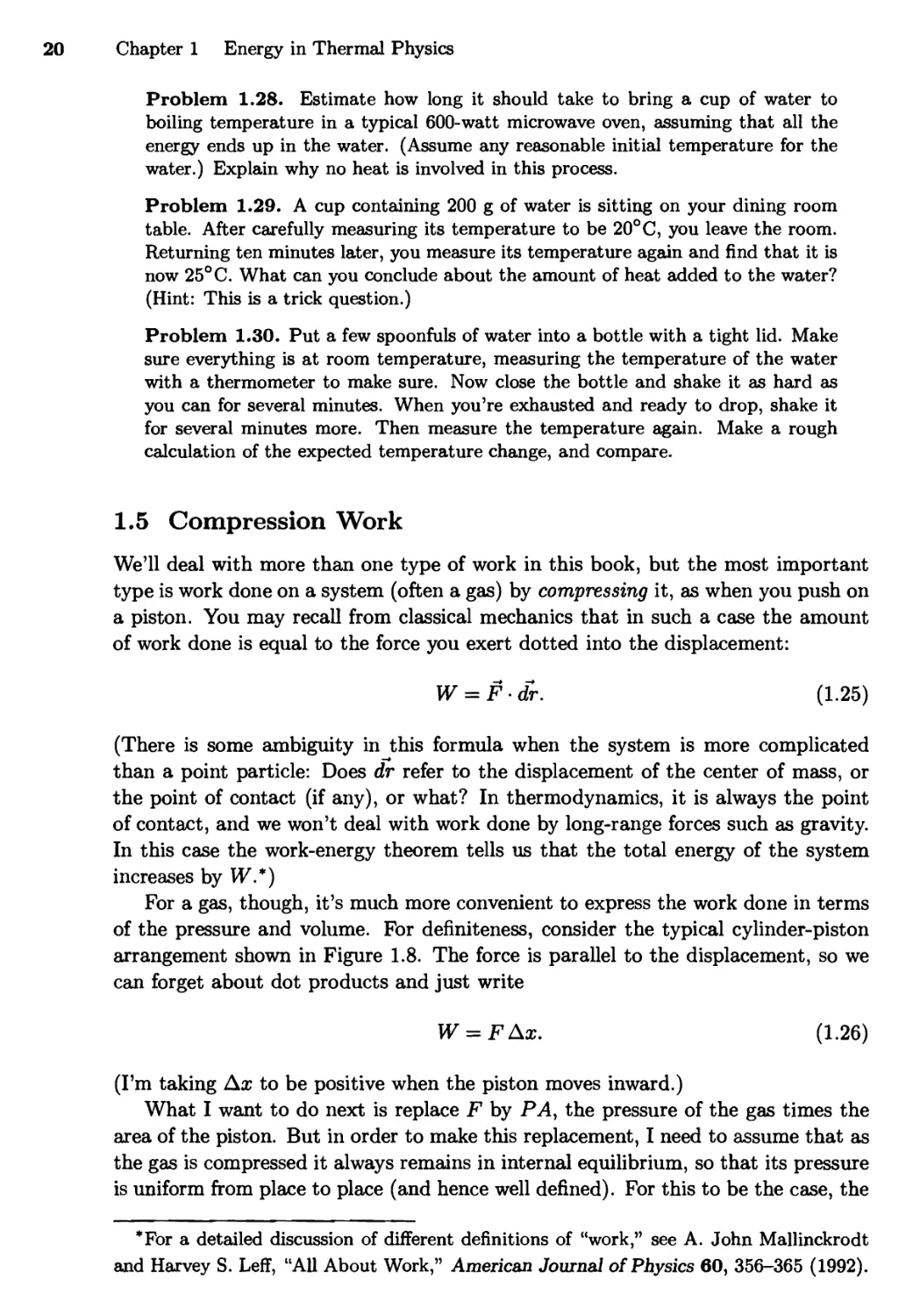
Problem 1.28. Estimate how long it should take to bring a cup of water to
boiling temperature in a typical 600-watt microwave oven, assuming that all the
energy ends up in the water. (Assume any reasonable initial temperature for the
water.) Explain why no heat is involved in this process.
Problem 1.29. A cup containing 200 g of water is sitting on your dining room
table. After carefully measuring its temperature to be 20°C, you leave the room.
Returning ten minutes later, you measure its temperature again and find that it is
now 25° C. What can you conclude about the amount of heat added to the water?
(Hint: This is a trick question.)
Problem 1.30. Put a few spoonfuls of water into a bottle with a tight lid. Make
sure everything is at room temperature, measuring the temperature of the water
with a thermometer to make sure. Now close the bottle and shake it as hard as
you can for several minutes. When you're exhausted and ready to drop, shake it
for several minutes more. Then measure the temperature again. Make a rough
calculation of the expected temperature change, and compare.
1.5 Compression Work
We'll deal with more than one type of work in this book, but the most important
type is work done on a system (often a gas) by compressing it, as when you push on
a piston. You may recall from classical mechanics that in such a case the amount
of work done is equal to the force you exert dotted into the displacement:
W = F • dr. (1.25)
(There is some ambiguity in this formula when the system is more complicated
than a point particle: Does dr refer to the displacement of the center of mass, or
the point of contact (if any), or what? In thermodynamics, it is always the point
of contact, and we won't deal with work done by long-range forces such as gravity.
In this case the work-energy theorem tells us that the total energy of the system
increases by W.*)
For a gas, though, it's much more convenient to express the work done in terms
of the pressure and volume. For definiteness, consider the typical cylinder-piston
arrangement shown in Figure 1.8. The force is parallel to the displacement, so we
can forget about dot products and just write
W = FAx. (1.26)
(I'm taking Ax to be positive when the piston moves inward.)
What I want to do next is replace F by P-4, the pressure of the gas times the
area of the piston. But in order to make this replacement, I need to assume that as
the gas is compressed it always remains in internal equilibrium, so that its pressure
is uniform from place to place (and hence well defined). For this to be the case, the
*For a detailed discussion of different definitions of "work," see A. John Mallinckrodt
and Harvey S. Leff, "All About Work," American Journal of Physics 60, 356-365 (1992).
1.5 Compression Work 21
Figure 1.8. When the
piston moves inward, the
volume of the gas changes by
AV^ (a negative amount) and
the work done on the gas
(assuming quasistatic
compression) is — PAV.
piston's motion must be reasonably slow, so that the gas has time to continually
equilibrate to the changing conditions. The technical term for a volume change that
is slow in this sense is quasistatic. Although perfectly quasistatic compression is
an idealization, it is usually a good approximation in practice. To compress the gas
non-quasistatically you would have to slam the piston very hard, so it moves faster
than the gas can "respond" (the speed must be at least comparable to the speed of
sound in the gas).
For quasistatic compression, then, the force exerted on the gas equals the
pressure of the gas times the area of the piston.* Thus,
W = PA Ax (for quasistatic compression). (1-27)
But the product A Ax is just minus the change in the volume of the gas (minus
because the volume decreases when the piston moves in), so
W = -PAV (quasistatic). (1.28)
For example, if you have a tank of air at atmospheric pressure (105 N/m2) and you
wish to reduce its volume by one liter (10-3 m3), you must perform 100 J of work.
You can easily convince yourself that the same formula holds if the gas expands;
then AV is positive, so the work done on the gas is negative, as required.
There is one possible flaw in the derivation of this formula. Usually the pressure
will change during the compression. In that case, what pressure should you use—
initial, final, average, or what? There's no difficulty for very small ("infinitesimal")
changes in volume, since then any change in the pressure will be negligible. Ah—
but we can always think of a large change as a bunch of small changes, one after
another. So when the pressure does change significantly during the compression,
we need to mentally divide the process into many tiny steps, apply equation 1.28
to each step, and add up all the little works to get the total work.
*Even for quasistatic compression, friction between the piston and the cylinder walls
could upset the balance between the force exerted from outside and the backward force
exerted on the piston by the gas. If W represents the work done on the gas by the piston,
this isn't a problem. But if it represents the work you do when pushing on the piston,
then I'll need to assume that friction is negligible in what follows.
Piston area = A
■:"-*—Force = F
AV = -AAx
Ax
22 Chapter 1 Energy in Thermal Physics
Pressure Pressure
Area = P.(Vf-Vi)
Vi Vf Volume V* Vf Volume
Figure 1.9. When the volume of a gas changes and its pressure is constant, the
work done on the gas is minus the area under the graph of pressure vs. volume.
The same is true even when the pressure is not constant.
This procedure is easier to understand graphically. If the pressure is constant,
then the work done is just minus the area under a graph of pressure vs. volume
(see Figure 1.9). If the pressure is not constant, we divide the process into a bunch
of tiny steps, compute the area under the graph for each step, then add up all the
areas to get the total work. That is, the work is still minus the total area under
the graph of P vs. V.
If you happen to know a formula for the pressure as a function of volume, P(V),
then you can compute the total work as an integral:
W=- P{V)dV (quasistatic). (1.29)
This is a good formula, since it is valid whether the pressure changes during the
process or not. It isn't always easy, however, to carry out the integral and get a
simple formula for W.
It's important to remember that compression-expansion work is not the only
type of work that can be done on thermodynamic systems. For instance, the
chemical reactions in a battery cause electrical work to be done on the circuit it is
connected to. We'll see plenty of examples in this book where compression-expansion
work is the only kind of relevant work, and plenty of examples where it isn't.
Problem 1.31. Imagine some helium in a cylinder with an initial volume of 1 liter
and an initial pressure of 1 atm. Somehow the helium is made to expand to a final
volume of 3 liters, in such a way that its pressure rises in direct proportion to its
volume.
(a) Sketch a graph of pressure vs. volume for this process.
(b) Calculate the work done on the gas during this process, assuming that there
are no "other" types of work being done.
(c) Calculate the change in the helium's energy content during this process.
(d) Calculate the amount of heat added to or removed from the helium during
this process.
(e) Describe what you might do to cause the pressure to rise as the helium
expands.
Area
■/
PdV
1.5 Compression Work
Problem 1.32. By applying a pressure of 200 atm, you can compress water
to 99% of its usual volume. Sketch this process (not necessarily to scale) on a
PV diagram, and estimate the work required to compress a liter of water by this
amount. Does the result surprise you?
Problem 1.33. An ideal gas is made to undergo the cyclic process shown in
Figure 1.10(a). For each of the steps A, B, and C, determine whether each of
the following is positive, negative, or zero: (a) the work done on the gas; (b) the
change in the energy content of the gas; (c) the heat added to the gas. Then
determine the sign of each of these three quantities for the whole cycle. What does
this process accomplish?
(a)
Oh
P2
kB
Vi
Figure 1.10. PV diagrams for Problems 1.33 and 1.34.
V2 Volume
Problem 1.34. An ideal diatomic gas, in a cylinder with a movable piston,
undergoes the rectangular cyclic process shown in Figure 1.10(b). Assume that
the temperature is always such that rotational degrees of freedom are active, but
vibrational modes are "frozen out." Also assume that the only type of work done
on the gas is quasistatic compression-expansion work.
(a) For each of the four steps A through Z), compute the work done on the gas,
the heat added to the gas, and the change in the energy content of the gas.
Express all answers in terms of Pi, P<z, V\> &nd ^2- (Hint: Compute AU
before Q, using the ideal gas law and the equipartition theorem.)
(b) Describe in words what is physically being done during each of the four
steps; for example, during step A, heat is added to the gas (from an external
flame or something) while the piston is held fixed.
(c) Compute the net work done on the gas, the net heat added to the gas, and
the net change in the energy of the gas during the entire cycle. Are the
results as you expected? Explain briefly.
Compression of an Ideal Gas
To get a feel for some of the preceding formulas, I'd like to apply them to the
compression of an ideal gas. Since most familiar gases (such as air) are fairly close
to ideal, the results we obtain will actually be quite useful.
When you compress a container full of gas, you're doing work on it, that is,
adding energy. Generally this causes the temperature of the gas to increase, as you
know if you've ever pumped up a bicycle tire. However, if you compress the gas very
slowly, or if the container is in good thermal contact with its environment, heat
24 Chapter 1 Energy in Thermal Physics
will escape as the gas is compressed and its temperature won't rise very much.*
The difference between fast compression and slow compression is therefore very
important in thermodynamics.
In this section I'll consider two idealized ways of compressing an ideal gas:
isothermal compression, which is so slow that the temperature of the gas doesn't
rise at all; and adiabatic compression, which is so fast that no heat escapes from
the gas during the process. Most real compression processes will be somewhere
between these extremes, usually closer to the adiabatic approximation. I'll start
with the isothermal case, though, since it's simpler.
Suppose, then, that you compress an ideal gas isothermally, that is, without
changing its temperature. This almost certainly implies that the process is qua-
sistatic, so I can use formula 1.29 to calculate the work done, with P determined by
the ideal gas law. On a PV diagram, the formula P — NkT/V, for constant T, is
a concave-up hyperbola (called an isotherm), as shown in Figure 1.11. The work
done is minus the area under the graph:
rVf rVf -.
W = - PdV = -NkT / - dV
JVi JVi v (130)
= -NkT (\nVf - InVJ) = NkT In ^.
Notice that the work done is positive if Vi > V), that is, if the gas is being
compressed. If the gas expands isothermally, the same equation applies but with
Vi < V/, that is, the work done on the gas is negative.
As the gas is compressed isothermally, heat must be flowing out, into the
environment. To calculate how much, we can use the first law of thermodynamics and
the fact that for and ideal gas U is proportional to T:
Q = AU-W = A(^NfkT) - W = 0 - W = NkT In ^. (1.31)
- Isotherm
Figure 1.11. For isothermal
compression of an ideal gas, the
PV graph is a concave-up
hyperbola, called an isotherm.
As always, the work done is
minus the area under the graph.
Vf Vi Volume
* Scuba tanks are usually held under water as they are filled, to prevent the compressed
air inside from getting too hot.
1.5 Compression Work
Thus the heat input is just minus the work done. For compression, Q is negative
because heat leaves the gas; for isothermal expansion, heat must enter the gas so
Q is positive.
Now let's consider adiabatic compression, which is so fast that no heat flows out
of (or into) the gas. I'll still assume, however, that the compression is quasistatic.
In practice this usually isn't a bad approximation.
If you do work on a gas but don't let any heat escape, the internal energy of
the gas will increase:
AU = Q + W = W. (1.32)
If it's an ideal gas, U is proportional to T so the temperature increases as well.
The curve describing this process on a PV diagram must connect a low-temperature
isotherm to a high-temperature isotherm, and therefore must be steeper than either
of the isotherms (see Figure 1.12).
To find an equation describing the exact shape of this curve, let me first use the
equipartition theorem to write
U = ^NkT, (1.33)
where / is the number of degrees of freedom per molecule—3 for a monatomic gas,
5 for a diatomic gas near room temperature, etc. Then the energy change along
any infinitesimal segment of the curve is
dU= {-NkdT. (1.34)
Meanwhile, the work done during quasistatic compression is —PdV, so equation
1.32, applied to an infinitesimal part of the process, becomes
f-NkdT = -PdV. (1.35)
This differential equation relates the changes in temperature and volume during
the compression process. To solve the equation, however, we need to write the
pressure P in terms of the variables T and V. The needed relation is just the ideal
gas law; plugging in NkT/V for P and canceling the Nk gives
/ dT dV
5t=-T (L36)
0>
Figure 1.12. The PV curve
for adiabatic compression (called |
an adiabat) begins on a lower- g
temperature isotherm and ends on ^
a higher-temperature isotherm.
Vf Vi Volume
26 Chapter 1 Energy in Thermal Physics
Now we can integrate both sides from the initial values (Vi and Ti) to the final
values (Vf and Tj):
{ln| = -ln^. (1.37)
To simplify this equation, exponentiate both sides and gather the i's and /'s. After
a couple of lines of algebra you'll find
VfTJ/2 = Vi T(/2, (1.38)
or more compactly,
VTf/2 = constant. (L39)
Given any starting point and any final volume, you can now calculate the final
temperature. To find the final pressure you can use the ideal gas law to eliminate
T on both sides of equation 1.38. The result can be written
V^P = constant, (1.40)
where 7, called the adiabatic exponent, is an abbreviation for (/ + 2)//.
Problem 1.35. Derive equation 1.40 from equation 1.39.
Problem 1.36. In the course of pumping up a bicycle tire, a liter of air at
atmospheric pressure is compressed adiabatically to a pressure of 7 atm. (Air is
mostly diatomic nitrogen and oxygen.)
(a) What is the final volume of this air after compression?
(b) How much work is done in compressing the air?
(c) If the temperature of the air is initially 300 K, what is the temperature
after compression?
Problem 1.37. In a Diesel engine, atmospheric air is quickly compressed to about
1/20 of its original volume. Estimate the temperature of the air after compression,
and explain why a Diesel engine does not require spark plugs.
Problem 1.38. Two identical bubbles of gas form at the bottom of a lake, then
rise to the surface. Because the pressure is much lower at the surface than at the
bottom, both bubbles expand as they rise. However, bubble A rises very quickly,
so that no heat is exchanged between it and the water. Meanwhile, bubble B rises
slowly (impeded by a tangle of seaweed), so that it always remains in thermal
equilibrium with the water (which has the same temperature everywhere). Which
of the two bubbles is larger by the time they reach the surface? Explain your
reasoning fully.
1.5 Compression Work 27
Problem 1.39. By applying Newton's laws to the oscillations of a continuous
medium, one can show that the speed of a sound wave is given by
where p is the density of the medium (mass per unit volume) and B is the bulk
modulus, a measure of the medium's stiffness. More precisely, if we imagine
applying an increase in pressure AP to a chunk of the material, and this increase
results in a (negative) change in volume AV, then B is defined as the change in
pressure divided by the magnitude of the fractional change in volume:
This definition is still ambiguous, however, because I haven't said whether the
compression is to take place isothermally or adiabatically (or in some other way).
(a) Compute the bulk modulus of an ideal gas, in terms of its pressure P, for
both isothermal and adiabatic compressions.
(b) Argue that for purposes of computing the speed of a sound wave, the
adiabatic B is the one we should use.
(c) Derive an expression for the speed of sound in an ideal gas, in terms of
its temperature and average molecular mass. Compare your result to the
formula for the rms speed of the molecules in the gas. Evaluate the speed
of sound numerically for air at room temperature.
(d) When Scotland's Battlefield Band played in Utah, one musician remarked
that the high altitude threw their bagpipes out of tune. Would you expect
altitude to affect the speed of sound (and hence the frequencies of the
standing waves in the pipes)? If so, in which direction? If not, why not?
Problem 1.40. In Problem 1.16 you calculated the pressure of earth's atmosphere
as a function of altitude, assuming constant temperature. Ordinarily, however, the
temperature of the bottommost 10-15 km of the atmosphere (called the
troposphere) decreases with increasing altitude, due to heating from the ground (which
is warmed by sunlight). If the temperature gradient \dT/dz\ exceeds a certain
critical value, convection will occur: Warm, low-density air will rise, while cool,
high-density air sinks. The decrease of pressure with altitude causes a rising air
mass to expand adiabatically and thus to cool. The condition for convection to
occur is that the rising air mass must remain warmer than the surrounding air
despite this adiabatic cooling.
(a) Show that when an ideal gas expands adiabatically, the temperature and
pressure are related by the differential equation
dT _ 2 T
dP ~/+2P'
(b) Assume that dT/dz is just at the critical value for convection to begin, so
that the vertical forces on a convecting air mass are always approximately
in balance. Use the result of Problem 1.16(b) to find a formula for dT/dz in
this case. The result should be a constant, independent of temperature and
pressure, which evaluates to approximately — 10°C/km. This fundamental
meteorological quantity is known as the dry adiabatic lapse rate.
28 Chapter 1 Energy in Thermal Physics
1.6 Heat Capacities
The heat capacity of an object is the amount of heat needed to raise its
temperature, per degree temperature increase:
C=^. (1-41)
(The symbol for heat capacity is a capital C.) Of course, the more of a substance
you have, the larger its heat capacity will be. A more fundamental quantity is the
specific heat capacity, defined as the heat capacity per unit mass:
c=£. (1.42)
m
(The symbol for specific heat capacity is a lowercase c.)
The most important thing to know about the definition (1.41) of heat capacity
is that it is ambiguous. The amount of heat needed to raise an object's temperature
by one degree depends on the circumstances, specifically, on whether you are also
doing work on the object (and if so, how much). To see this, just plug the first law
of thermodynamics into equation 1.41:
AT AT v ;
Even if the energy of an object is a well-defined function of its temperature alone
(which is sometimes but not always the case), the work W done on the object can
be anything, so C can be anything, too.
In practice, there are two types of circumstances (and choices for W) that are
most likely to occur. Perhaps the most obvious choice is W = 0, when there is no
work being done on the system. Usually this means that the system's volume isn't
changing, since if it were, there would be compression work equal to —PAV. So
the heat capacity, for the particular case where W = 0 and V is constant, is called
the heat capacity at constant volume, denoted Cy> Prom equation 1.43,
(The subscript V indicates that the changes are understood to occur with the
volume held fixed. The symbol d indicates a partial derivative, in this case treating
U as a function of T and V, with only T, not V, varying as the derivative is
taken.) A better name for this quantity would be "energy capacity," since it is the
energy needed to raise the object's temperature, per degree, regardless of whether
the energy actually enters as heat. For a gram of water, CV is 1 cal/°C or about
4.2 J/°C.
In everyday life, however, objects often expand as they are heated. In this case
they do work on their surroundings, so W is negative, so C is larger than CV:
you need to add additional heat to compensate for the energy lost as work. If
the pressure surrounding your object happens to be constant, then the total heat
1.6 Heat Capacities 29
needed is unambiguous, and we refer to the heat needed per degree as Cp, the heat
capacity at constant pressure. Plugging the formula for compression-expansion
work into equation 1.43 gives
The last term on the right is the additional heat needed to compensate for the
energy lost as work. Notice that the more the volume increases, the larger this
term is. For solids and liquids, dV/dT is usually small and can often be neglected.
For gases, however, the second term is quite significant. (The first term, (dU/dT)p,
is not quite the same as CV, since it is P, not V, that is held fixed in the partial
derivative.)
Equations 1.41 through 1.45 are essentially definitions, so they apply to any
object whatsoever. To determine the heat capacity of some particular object, you
generally have three choices: measure it (see Problem 1.41); look it up in a reference
work where measured values are tabulated; or try to predict it theoretically. The
last is the most fun, as we'll see repeatedly throughout this book. For some objects
we already know enough to predict the heat capacity.
Suppose that our system stores thermal energy only in quadratic "degrees of
freedom," as described in Section 1.3. Then the equipartition theorem says U =
\NfkT (neglecting any "static" energy, which doesn't depend on temperature), so
dU _ d (NfkTx _ Nfk
Cv = &f af\~2~) ~ 1"' (L46)
assuming that / is independent of temperature. (Note that in this case it doesn't
matter whether V or P is held fixed in the derivative dU/dT.) This result gives
us a direct method of measuring the number of degrees of freedom in an object,
or, if we know this number, of testing the equipartition theorem. For instance, in
a monatomic gas like helium, / = 3, so we expect CV = fiVA: = |n/i; that is,
the heat capacity per mole should be |i? = 12.5 J/K. For diatomic and polyatomic
molecules the heat capacity should be larger, in proportion to the number of degrees
of freedom per molecule. Figure 1.13 (see the following page) shows a graph of CV
vs. temperature for a mole of hydrogen (H2) gas, showing how the vibrational and
rotational degrees of freedom freeze out at low temperatures. For a solid, there are
six degrees of freedom per atom, so the heat capacity per mole should be |i2 = 3jR;
this general result is called the rule of Dulong and Petit. In this case, though,
all of the degrees of freedom freeze out at low temperature, so the heat capacity
approaches zero as T —> 0. What qualifies as "low" temperature depends on the
material, as shown in Figure 1.14.
What about heat capacities of gases at constant pressure? For an ideal gas, the
derivative dU/dT is the same with P fixed as with V fixed, and we can compute
the second term in equation 1.45 using the ideal gas law. At constant pressure,
(dV\ 3 (NkT\ Nk ,. _ . . . _
(^Jp = ot(—) = -f (ldealgas)- (L47)
30 Chapter 1 Energy in Thermal Physics
Cv
1%R
tyR
3d __^^
yS*^ |
^0<r \
^R T
Translation
Rotation
'
*
*
Vibration
t
10
100
1000
T(K)
Figure 1.13. Heat capacity at constant volume of one mole of hydrogen (H2) gas.
Note that the temperature scale is logarithmic. Below about 100 K only the three
translational degrees of freedom are active. Around room temperature the two
rotational degrees of freedom are active as well. Above 1000 K the two vibrational
degrees of freedom also become active. At atmospheric pressure, hydrogen liquefies
at 20 K and begins to dissociate at about 2000 K. Data from Woolley et al. (1948).
400
T(K)
Figure 1.14. Measured heat capacities at constant pressure (data points) for
one mole each of three different elemental solids. The solid curves show the heat
capacity at constant volume predicted by the model used in Section 7.5, with the
horizontal scale chosen to best fit the data for each substance. At sufficiently high
temperatures, Cy for each material approaches the value 3R predicted by the
equipartition theorem. The discrepancies between the data and the solid curves
at high T are mostly due to the differences between Cp and Cy. At T = 0 all
degrees of freedom are frozen out, so both Cp and Cy go to zero. Data from Y. S.
Touloukian, ed., Thermophysical Properties of Matter (Plenum, New York, 1970).
Therefore,
CP = Cy + Nk = Cy + nR (ideal gas).
(1.48)
In other words, for each mole of an ideal gas, the heat capacity at constant pressure
exceeds the heat capacity at constant volume by R, the gas constant. Oddly, the
1.6 Heat Capacities 31
additional term in the heat capacity doesn't depend on what the pressure is, so
long as it is constant. Apparently, if the pressure is high the gas expands less, in
such a way that the work done on the environment is independent of P.
Problem 1.41. To measure the heat capacity of an object, all you usually have
to do is put it in thermal contact with another object whose heat capacity you
know. As an example, suppose that a chunk of metal is immersed in boiling water
(100°C), then is quickly transferred into a Styrofoam cup containing 250 g of
water at 20° C. After a minute or so, the temperature of the contents of the cup is
24°C. Assume that during this time no significant energy is transferred between
the contents of the cup and the surroundings. The heat capacity of the cup itself
is negligible.
(a) How much heat is lost by the water?
(b) How much heat is gained by the metal?
(c) What is the heat capacity of this chunk of metal?
(d) If the mass of the chunk of metal is 100 g, what is its specific heat capacity?
Problem 1.42. The specific heat capacity of Albertson's Rotini Tricolore is
approximately 1.8 J/g°C. Suppose you toss 340 g of this pasta (at 25°C) into 1.5
liters of boiling water. What effect does this have on the temperature of the water
(before there is time for the stove to provide more heat)?
Problem 1.43. Calculate the heat capacity of liquid water per molecule, in terms
of A;. Suppose (incorrectly) that all the thermal energy of water is stored in
quadratic degrees of freedom. How many degrees of freedom would each
molecule have to have?
Problem 1.44. At the back of this book is a table of thermodynamic data for
selected substances at room temperature. Browse through the Cp values in this
table, and check that you can account for most of them (approximately) using the
equipartition theorem. Which values seem anomalous?
Problem 1.45. As an illustration of why it matters which variables you hold fixed
when taking partial derivatives, consider the following mathematical example. Let
w = xy and x = yz.
(a) Write w purely in terms of x and z, and then purely in terms of y and z.
(b) Compute the partial derivatives
and show that they are not equal. (Hint: To compute (dw/dx)y, use a
formula for w in terms of x and y, not z. Similarly, compute (dw/dx)z
from a formula for w in terms of only x and z.)
(c) Compute the other four partial derivatives of w (two each with respect to
y and z), and show that it matters which variable is held fixed.
32 Chapter 1 Energy in Thermal Physics
Problem 1.46. Measured heat capacities of solids and liquids are almost always
at constant pressure, not constant volume. To see why, estimate the pressure
needed to keep V fixed as T increases, as follows.
(a) First imagine slightly increasing the temperature of a material at constant
pressure. Write the change in volume, dV\, in terms of dT and the thermal
expansion coefficient P introduced in Problem 1.7.
(b) Now imagine slightly compressing the material, holding its temperature
fixed. Write the change in volume for this process, dV^, in terms of dP and
the isothermal compressibility «r, defined as
KT
- v\dp)T
(This is the reciprocal of the isothermal bulk modulus defined in
Problem 1.39.)
(c) Finally, imagine that you compress the material just enough in part (b)
to offset the expansion in part (a). Then the ratio of dP to dT is equal
to (dP/dT)y% since there is no net change in volume. Express this partial
derivative in terms of/? and kt- Then express it more abstractly in terms of
the partial derivatives used to define 0 and Kf. For the second expression
you should obtain
(3P\ (dV/dT)P
\dT)v- (dV/dP)T'
This result is actually a purely mathematical relation, true for any three
quantities that are related in such a way that any two determine the third.
(d) Compute /?, «j«, and (dP/dT)y for an ideal gas, and check that the three
expressions satisfy the identity you found in part (c).
(e) For water at 25°C, /? = 2.57 x 10"4 K_1 and kt = 4.52 x 10~10 Pa"1.
Suppose you increase the temperature of some water from 20° C to 30° C.
How much pressure must you apply to prevent it from expanding? Repeat
the calculation for mercury, for which (at 25°C) 0 = 1.81 x 10~4 K_1 and
kt = 4.04 x 10⁻¹¹ Pa-1. Given the choice, would you rather measure the
heat capacities of these substances at constant V or at constant P?
Latent Heat
In some situations you can put heat into a system without increasing its temperature
at all This normally happens at a phase transformation, such as melting ice or
boiling water. Technically, the heat capacity is then infinite:
C = -r= = -— = oo (during a phase transformation). (149)
However, you still might want to know how much heat is required to melt or boil
the substance completely. This amount, divided by the mass of the substance, is
called the latent heat of the transformation, and denoted L:
L = — to accomplish the transformation. (1.50)
m
Like the definition of heat capacity, this definition is ambiguous, since any amount
of work could also be done during the process. By convention, however, we assume
that the pressure is constant (usually 1 atm), and that no other work is done
1.6 Heat Capacities 33
besides the usual constant-pressure expansion or compression. The latent heat for
melting ice is 333 J/g, or 80 cal/g. The latent heat for boiling water is 2260 J/g,
or 540 cal/g. (To get a feel for these numbers, recall that raising the temperature
of water from 0°C to 100°C requires 100 cal/g.)
Problem 1.47. Your 200-g cup of tea is boiling-hot. About how much ice should
you add to bring it down to a comfortable sipping temperature of 65°C? (Assume
that the ice is initially at — 15°C. The specific heat capacity of ice is 0.5 cal/g°C.)
Problem 1.48. When spring finally arrives in the mountains, the snow pack
may be two meters deep, composed of 50% ice and 50% air. Direct sunlight
provides about 1000 watts/m2 to earth's surface, but the snow might reflect 90%
of this energy. Estimate how many weeks the snow pack should last, if direct solar
radiation is the only source of energy.
Enthalpy
Constant-pressure processes occur quite often, both in the natural world and in the
laboratory. Keeping track of the compression-expansion work done during these
processes gets to be a pain after a while, but there is a convenient trick that makes
it a bit easier. Instead of always talking about the energy content of a system, we
can agree to always add in the work needed to make room for it (under a constant
pressure, usually 1 atm). This work is PV, the pressure of the environment times
the total volume of the system (that is, the total space you would need to clear
out to make room for it). Adding PV onto the energy gives a quantity called the
enthalpy, denoted H:
H = U + PV (1.51)
This is the total energy you would have to come up with, to create the system out
of nothing and put it into this environment (see Figure 1.15). Or, put another way,
if you could somehow annihilate the system, the energy you could extract is not
just £/, but also the work (PV) done by the atmosphere as it collapses to fill the
vacuum left behind.
Figure 1.15. To create a rabbit out of nothing and place it on the table, the
magician must summon up not only the energy U of the rabbit, but also some
additional energy, equal to PV} to push the atmosphere out of the way to make
room. The total energy required is the enthalpy, H = U + PV.
34 Chapter 1 Energy in Thermal Physics
To see the usefulness of enthalpy, suppose that some change takes place in the
system—you add some heat, or chemicals react, or whatever—while the pressure is
always held constant. The energy, volume, and enthalpy can all change, by amounts
that I'll call AV, AU, and AH. The new enthalpy is
H + AH = [U + AU) + P(V + AV)
= (U + PV) + (AU + P AV) (1.52)
= H + {AU + PAV),
so the change in enthalpy during a constant-pressure process is
AH = AU + P AV (constant P). (1.53)
This says that enthalpy can increase for two reasons: either because the energy
increases, or because the system expands and work is done on the atmosphere to
make room for it.
Now recall the first law of thermodynamics: The change in energy equals the
heat added to the system, plus the compression-expansion work done on it, plus
any other work (e.g., electrical) done on it:
Ai/ = Q + (-P AV) + WotheT. (1.54)
Combining this law with equation 1.53, we obtain
AH = Q + Wother (constant P), (1.55)
that is, the change in enthalpy is caused only by heat and other forms of work,
not by compression-expansion work (during constant-pressure processes). In other
words, you can forget all about compression-expansion work if you deal with
enthalpy instead of energy. If no "other" types of work are being done, the change in
enthalpy tells you directly how much heat has been added to the system. (That's
why we use the symbol H.)
For the simple case of raising an object's temperature, the change in enthalpy
per degree, at constant pressure, is the same as the heat capacity at constant
pressure, Cp:
*-(&),■ (i-56)
This formula is really the best way to define Cp, though you can easily see that it is
equivalent to equation 1.45. Just as Cy should really be called "energy capacity,"
Cp should really be called "enthalpy capacity." And as with Cy, there doesn't
have to be any heat involved at all, since the enthalpy could just as well enter as
"other" work, as in a microwave oven.
Chemistry books are full of tables of AH values for more dramatic processes:
phase transformations, chemical reactions, ionization, dissolution in solvents, and
so on. For instance, standard tables say that the change in enthalpy when you boil
one mole of water at 1 atm is 40,660 J. Since a mole of water is about 18 grams
1.6 Heat Capacities 35
(16 for the oxygen and 2 for the hydrogen), this means that the change in enthalpy
(Mien you boil one gram of water should be (40,660 J)/18 = 2260 J, precisely the
Dumber I quoted earlier for the latent heat. However, not all of this energy ends
tip in the vaporized water. The volume of one mole of water vapor, according to
the ideal gas law, is RT/P (while the initial volume of the liquid is negligible), so
the work needed to push the atmosphere away is
PV = RT = (8.31 J/K)(373 K) = 3100 J. (1.57)
This is only 8% of the 40,660 J of energy put in, but sometimes it's necessary to
keep track of such things.
As another example, consider the chemical reaction in which hydrogen and
oxygen gas combine to form liquid water:
H2 + \02 —+ H20. (1.58)
For each mole of water produced, AH for this reaction is —286 kJ; in tables this
quantity is referred to as the enthalpy of formation of water, because it's being
."formed" out of elemental constituents in their most stable states. (The numerical
value assumes that both the reactants and the product are at room temperature
end atmospheric pressure. This number and others like it are tabulated in the data
section at the back of this book.) If you simply burn a mole of hydrogen, then
286 kJ is the amount of heat you get out. Nearly all of this energy comes from
the thermal and chemical energy of the molecules themselves, but a small amount
comes from work done by the atmosphere as it collapses to fill the space left behind
by the consumed gases.
You might wonder, though, whether some of the 286 kJ can't be extracted as
work (perhaps electrical work) rather than as heat. Certainly this would be a good
thing, since electricity is so much more useful and versatile than heat. In general
the answer is that much of the energy from a chemical reaction can be extracted
as work, but there are limits, as we'll see in Chapter 5.
Problem 1.49. Consider the combustion of one mole of H2 with 1/2 mole of O2
under standard conditions, as discussed in the text. How much of the heat energy
produced comes from a decrease in the internal energy of the system, and how
much comes from work done by the collapsing atmosphere? (Treat the volume of
the liquid water as negligible.)
Problem 1.50. Consider the combustion of one mole of methane gas:
CH4(gas) + 202(gas) —> C02(gas) + 2H20(gas).
The system is at standard temperature (298 K) and pressure (105 Pa) both before
and after the reaction.
(a) First imagine the process of converting a mole of methane into its elemental
consituents (graphite and hydrogen gas). Use the data at the back of this
book to find AH for this process.
(b) Now imagine forming a mole of C02 and two moles of water vapor from
their elemental constituents. Determine AH for this process.
36 Chapter 1 Energy in Thermal Physics
(c) What is AH for the actual reaction in which methane and oxygen form
carbon dioxide and water vapor directly? Explain.
(d) How much heat is given off during this reaction, assuming that no "other"
forms of work are done?
(e) What is the change in the system's energy during this reaction? How would
your answer differ if the H2O ended up as liquid water instead of vapor?
(f) The sun has a mass of 2 x 1030 kg and gives off energy at a rate of 3.9 x
1026 watts. If the source of the sun's energy were ordinary combustion of
a chemical fuel such as methane, about how long could it last?
Problem 1.51. Use the data at the back of this book to determine AH for the
combustion of a mole of glucose,
C6Hi206 + 602 —► 6C02 + 6H20.
This is the (net) reaction that provides most of the energy needs in our bodies.
Problem 1.52. The enthalpy of combustion of a gallon (3.8 liters) of gasoline is
about 31,000 kcal. The enthalpy of combustion of an ounce (28 g) of corn flakes is
about 100 kcal. Compare the cost of gasoline to the cost of corn flakes, per calorie.
Problem 1.53. Look up the enthalpy of formation of atomic hydrogen in the
back of this book. This is the enthalpy change when a mole of atomic hydrogen
is formed by dissociating 1/2 mole of molecular hydrogen (the more stable state
of the element). Prom this number, determine the energy needed to dissociate a
single H2 molecule, in electron-volts.
Problem 1.54. A 60-kg hiker wishes to climb to the summit of Mt. Ogden, an
ascent of 5000 vertical feet (1500 m).
(a) Assuming that she is 25% efficient at converting chemical energy from food
into mechanical work, and that essentially all the mechanical work is used
to climb vertically, roughly how many bowls of corn flakes (standard serving
size 1 ounce, 100 kilocalories) should the hiker eat before setting out?
(b) As the hiker climbs the mountain, three-quarters of the energy from the
corn flakes is converted to thermal energy. If there were no way to dissipate
this energy, by how many degrees would her body temperature increase?
(c) In fact, the extra energy does not warm the hiker's body significantly;
instead, it goes (mostly) into evaporating water from her skin. How many
liters of water should she drink during the hike to replace the lost fluids?
(At 25°C, a reasonable temperature to assume, the latent heat of
vaporization of water is 580 cal/g, 8% more than at 100°C.)
Problem 1.55. Heat capacities are normally positive, but there is an important
class of exceptions: systems of particles held together by gravity, such as stars and
star clusters.
(a) Consider a system of just two particles, with identical masses, orbiting in
circles about their center of mass. Show that the gravitational potential
energy of this system is —2 times the total kinetic energy.
(b) The conclusion of part (a) turns out to be true, at least on average, for any
system of particles held together by mutual gravitational attraction:
^potential = — ^l/kinetic
1.7 Rates of Processes 37
Here each U refers to the total energy (of that type) for the entire system,
averaged over some sufficiently long time period. This result is known as the
virial theorem. (For a proof, see Carroll and Ostlie (1996), Section 2.4.)
Suppose, then, that you add some energy to such a system and then wait
for the system to equilibrate. Does the average total kinetic energy increase
or decrease? Explain.
(c) A star can be modeled as a gas of particles that interact with each other
only gravitationally. According to the equipartition theorem, the average
kinetic energy of the particles in such a star should be §fcT, where T is
the average temperature. Express the total energy of a star in terms of its
average temperature, and calculate the heat capacity. Note the sign.
(d) Use dimensional analysis to argue that a star of mass M and radius R
should have a total potential energy of -GM2/#, times some constant of
order 1.
(e) Estimate the average temperature of the sun, whose mass is 2 x 1030 kg
and whose radius is 7 x 10 m. Assume, for simplicity, that the sun is made
entirely of protons and electrons.
1.7 Rates of Processes
Usually, to determine what the equilibrium state of a system is, we need not worry
about how long the system takes to reach equilibrium. Thermodynamics, by many
people's definitions, includes only the study of equilibrium states themselves.
Questions about time and rates of processes are then considered a separate (though
related) subject, sometimes called transport theory or kinetics.
In this book I won't say much about rates of processes, because these kinds
of questions are often quite difficult and require somewhat different tools. But
transport theory is important enough that I should say something about it, at least
the simpler aspects. That is the purpose of this section.*
Heat Conduction
At what rate does heat flow from a hot object to a cold object? The answer
depends on many factors, particularly on what mechanisms of heat transfer are
possible under the circumstances.
If the objects are separated by empty space (like the sun and the earth, or
the inner and outer walls of a thermos bottle) then the only possible heat transfer
mechanism is radiation. I'll derive a formula for the rate of radiation in Chapter 7.
If a fluid (gas or liquid) can mediate the heat transfer, then convection—bulk
motion of the fluid—is often the dominant mechanism. Convection rates depend on
all sorts of factors, including the heat capacity of the fluid and the many possible
forces acting on it. I won't try to calculate any convection rates in this book.
That leaves conduction: heat transfer by direct contact at the molecular level.
Conduction can happen through a solid, liquid, or gas. In a liquid or a gas the
*This section is somewhat outside the main development of the book. No other sections
depend on it, so you may omit or postpone it if you wish.
38 Chapter 1 Energy in Thermal Physics
energy is transferred through molecular collisions: When a fast molecule hits a
slow molecule, energy is usually transferred from the former to the latter. In solids,
heat is conducted via lattice vibrations and, in metals, via conduction electrons.
Good electrical conductors tend to be good heat conductors as well, because the
same conduction electrons can carry both electric current and energy, while lattice
vibrations are much less efficient than electrons at conducting heat.
Regardless of these details, the rate of heat conduction obeys a mathematical
law that is not hard to guess. For definiteness, imagine a glass window
separating the warm interior of a building from the cold outdoors (see Figure 1.16). We
would expect the amount of heat Q that passes through the window to be
directly proportional to the window's total area A, and to the amount of time that
passes, At. We would probably expect Q to be inversely proportional to the
thickness of the window, Ax. Finally, we would expect Q to depend on the indoor and
outdoor temperatures, in such a way that Q = 0 if these temperatures are the
same. The simplest guess is that Q is directly proportional to the temperature
difference, AT = T2 - Ti; this guess turns out to be correct for any heat transfer
by conduction (though not for radiation). Summarizing these proportionalities, we
can write
. A AT At Q dT
Q(X—Ax-' °r At0cA&" (L59)
The constant of proportionality depends on the material through which the heat
is being conducted (in this case, glass). This constant is called the thermal
conductivity of the material. The usual symbol for thermal conductivity is fe, but to
distinguish it from Boltzmann's constant I'll called it kt. I'll also put a minus sign
into the equation to remind us that if T increases from left to right, Q flows from
right to left. The law of heat conduction is then
£--M§. U.60)
This equation is known as the Fourier heat conduction law, after the same
J. B. J. Fourier who invented Fourier analysis.
To derive the Fourier heat conduction law, and to predict the value of kt for a
particular material, we would have to invoke a detailed molecular model of what
happens during heat conduction. I'll do this for the easiest case, an ideal gas, in the
itside
Ti
Area = A
/
Inside
Ti
Figure 1.16. The rate of heat conduction
through a pane of glass is proportional to
its area A and inversely proportional to its
thickness Ax.
-HAxh-
1.7 Rates of Processes 39
following subsection. For now, though, let's just take Fourier's law as an empirical
fact and treat kt as a property that you need to measure for any material of interest.
Thermal conductivities of common materials vary by more than four orders of
magnitude. In SI units (watts per meter per kelvin), a few representative values
are: air, 0.026; wood, 0.08; water, 0.6; glass, 0.8; iron, 80; copper, 400. Again, good
electrical conductors tend to be good thermal conductors. Note that the values
for air and water apply to conduction only, even though convection can often be
extremely important.
Back to our window, suppose it has an area of one square meter and a thickness
of 3.2 mm (1/8 inch). Then if the temperature just inside the window is 20°C and
the temperature just outside is 0°C, the rate of heat flow through it is
Q = (0.8W/m.K)(lmy93K-273K) = ^ ^
At 0.0032 m
If this number seems absurdly high to you, you're right. My assumption of such a
large temperature difference between "just inside" and "just outside" the window
is unrealistic, because there is always a thin layer of still air on each side of the
glass. The two air layers can provide many times more thermal insulation than the
glass itself, bringing the heat loss down into the range of a few hundred watts (see
Problem 1.57).
Problem 1.56. Calculate the rate of heat conduction through a layer of still air
that is 1 mm thick, with an area of 1 m2, for a temperature difference of 20° C.
Problem 1.57. Home owners and builders discuss thermal conductivities in terms
of the R value (R for resistance) of a material, defined as the thickness divided
by the thermal conductivity:
(a) Calculate the R value of a 1/8-inch (3.2 mm) piece of plate glass, and then
of a 1 mm layer of still air. Express both answers in SI units.
(b) In the United States, R values of building materials are normally given in
English units, °F-ft2hr/Btu. A Btu, or British thermal unit, is the energy
needed to raise the temperature of a pound of water by 1°F. Work out the
conversion factor between the SI and English units for R values. Convert
your answers from part (a) to English units.
(c) Prove that for a compound layer of two different materials sandwiched
together (such as air and glass, or brick and wood), the effective total
R value is the sum of the individual R values.
(d) Calculate the effective R value of a single piece of plate glass with a 1.0-
mm layer of still air on each side. (The effective thickness of the air layer
will depend on how much wind is blowing; 1 mm is of the right order of
magnitude under most conditions.) Using this effective R value, make a
revised estimate of the heat loss through a 1-m single-pane window when
the temperature in the room is 20° C higher than the outdoor temperature.
40 Chapter 1 Energy in Thermal Physics
Problem 1.58. According to a standard reference table, the R value of a 3.5-
inch-thick vertical air space (within a wall) is 1.0 (in English units), while the
R value of a 3.5-inch thickness of fiberglass batting is 10.9. Calculate the R value
of a 3.5-inch thickness of still air, then discuss whether these two numbers are
reasonable. (Hint: These reference values include the effects of convection.)
Problem 1.59. Make a rough estimate of the total rate of conductive heat loss
through the windows, walls, floor, and roof of a typical house in a cold climate.
Then estimate the cost of replacing this lost energy over the course of a month. If
possible, compare your estimate to a real utility bill. (Utility companies measure
electricity by the kilowatt-hour, a unit equal to 3.6 MJ. In the United States,
natural gas is billed in therms, where 1 therm = 105 Btu. Utility rates vary by
region; I currently pay about 7 cents per kilowatt-hour for electricity and 50 cents
per therm for natural gas.)
Problem 1.60. A frying pan is quickly heated on the stovetop to 200°C. It has
an iron handle that is 20 cm long. Estimate how much time should pass before
the end of the handle is too hot to grab with your bare hand. (Hint: The cross-
sectional area of the handle doesn't matter. The density of iron is about 7.9 g/cm3
and its specific heat is 0.45 J/g-°C).
Problem 1.61. Geologists measure conductive heat flow out of the earth by
drilling holes (a few hundred meters deep) and measuring the temperature as a
function of depth. Suppose that in a certain location the temperature increases by
20° C per kilometer of depth and the thermal conductivity of the rock is 2.5 W/m-K.
What is the rate of heat conduction per square meter in this location? Assuming
that this value is typical of other locations over all of earth's surface, at
approximately what rate is the earth losing heat via conduction? (The radius of the earth
is 6400 km.)
Problem 1.62. Consider a uniform rod of material whose temperature varies
only along its length, in the x direction. By considering the heat flowing from
both directions into a small segment of length Ax, derive the heat equation,
dt ~ dx2 '
where K — kt/cp, c is the specific heat of the material, and p is its density. (Assume
that the only motion of energy is heat conduction within the rod; no energy enters
or leaves along the sides.) Assuming that K is independent of temperature, show
that a solution of the heat equation is
T(x,t) = T0 + jle-*2/4Kt,
where To is a constant background temperature and A is any constant. Sketch
(or use a computer to plot) this solution as a function of x, for several values of t.
Interpret this solution physically, and discuss in some detail how energy spreads
through the rod as time passes.
1.7 Rates of Processes 41
Conductivity of an Ideal Gas
In a gas, the rate of heat conduction is limited by how far a molecule can travel
before it collides with another molecule. The average distance traveled between
collisions is called the mean free path. In a dilute gas the mean free path is many
times larger than the average distance between molecules, because a molecule can
pass by many of its neighbors before actually hitting one of them. Let me now
make a rough estimate of the mean free path in a dilute gas.
For simplicity, imagine that all the molecules in a gas except one are frozen
in place. How far does the remaining molecule travel between collisions? Well,
a collision happens when the center of our molecule comes within one molecular
diameter (2r, where r is the radius of a molecule) of the center of some other
molecule (see Figure 1.17). Collisions would occur just as often if our molecule
were twice as wide and all the others were points; let's therefore pretend that this
is the case. Then, as our molecule travels along, it sweeps out an imaginary cylinder
of space whose radius is 2r. When the volume of this cylinder equals the average
volume per molecule in the gas, we're likely to get a collision. The mean free path,
£, is roughly the length of the cylinder when this condition is met:
volume of cylinder = average volume per molecule
=► 7r(2r)2^^
* '*4^£ (L62)
The « symbol indicates that this formula is only a rough approximation for £,
because I've neglected the motion of the other molecules as well as the variation in
path lengths between collisions. The actual mean free path will differ by a numerical
factor that shouldn't be too different from 1. But there's not much point in being
more precise, because r itself is not well defined: Molecules don't have sharp edges,
Figure 1.17. A collision between molecules occurs when their centers are
separated by twice the molecular radius r. The same would be true if one molecule
had radius 2r and the other were a point. When a sphere of radius 2r moves in a
straight line of length £, it sweeps out a cylinder whose volume is 4.rrr2£.
42 Chapter 1 Energy in Thermal Physics
and most of them aren't even spherical.*
The effective radius of a nitrogen or oxygen molecule should be one or two
angstroms; let's say r = 1.5 A = 1.5 x 10~10 m. Treating air as an ideal gas,
the volume per particle is V/N = kT/P = 4 x 10~26 m3 at room temperature
and atmospheric pressure. With these numbers, equation 1.62 predicts a mean free
path of 150 nm, about 40 times greater than the average separation between air
molecules. We can also estimate the average time between collisions:
-a- I I 1.5xl0"7m n , ,0 ^ ^
A* = - » » ———- = 3 x 10 10 s. (1.63)
v vTma 500 m/s
Now back to heat conduction. Consider a small region within a gas where the
temperature increases in the x direction (see Figure 1.18). The heavy dotted line
in the figure represents a plane perpendicular to the x direction; my intent is to
estimate the amount of heat that flows across this plane. Let At be the average
time between collisions, so that each molecule travels a distance of roughly one
mean free path during this time. Then, during this time, the molecules that cross
the dotted line from the left will have started from somewhere within box 1 (whose
thickness is t), while the molecules that cross the dotted line from the right will
have started from somewhere within box 2 (whose thickness is also £). Both of
these boxes have the same area A in the yz plane. If the total energy of all the
molecules in box 1 is U\> then the energy crossing the dotted line from the left
is roughly J7i/2, since only half of the molecules will have positive x velocities at
this moment. Similarly, the energy crossing the line from the right is half the total
energy in box 2, or C/2/2. The net heat flow across the line is therefore
Q = \{Ux - U2) = -i(t/2 - UX) = -\Cv(T* - r,) = -\cvt. g, (1.64)
where Cy is the heat capacity of all the gas in either box and Xi and T2 are the
average temperatures in the two boxes. (In the last step I've used the fact that the
distance between the centers of the two boxes is L)
Figure 1.18. Heat conduction across
the dotted line occurs because the
molecules moving from box 1 to box 2
have a different average energy than
the molecules moving from box 2 to
box 1. For free motion between these
boxes, each should have a width of
roughly one mean free path.
*For that matter, I haven't even given a precise definition of what constitutes a collision.
After all, even when molecules pass at a distance, they attract and deflect each other
somewhat. For a more careful treatment of transport processes in gases, see Reif (1965).
1.7 Rates of Processes 43
Equation 1.64 confirms Fourier's law, that the rate of heat conduction is
directly proportional to the difference in temperatures. Furthermore, comparison to
equation 1.60 yields an explicit prediction for the thermal conductivity:
_\Cyt
Kt~2AAt
^Cvf_=lCyf-
2A£At 2 V '
(1.65)
where v is the average speed of the molecules. The quantity Cy/V is the heat
capacity of the gas per unit volume, which can be evaluated as
Cy
V
_JNk
2T'
(1.66)
where / is the number of degrees of freedom per molecule. Recall, however, that I
for a gas is proportional to V/N. Therefore the thermal conductivity of a given gas
should depend only on its temperature, through v oc VT and possibly through /.
Over limited ranges of temperature the number of degrees of freedom is fairly
constant, so kt should be proportional to the square root of the absolute temperature.
Experiments on a wide variety of gases have confirmed this prediction (see
Figure 1.19).
For air at room temperature and atmospheric pressure, / = 5 so Cy/V =
|(105 N/m2)/(300 K) « 800 J/m3K. Equation 1.65 therefore predicts a thermal
conductivity of
kt « |(800 J/m3.K)(1.5 x 10"7 m)(500 m/s) = 0.031 W/m-K,
(1.67)
only a little higher than the measured value of 0.026. Not bad, considering all the
crude approximations I've made in this section.
The preceding analysis of the thermal conductivities of gases is an example of
what's called kinetic theory, an approach to thermal physics based on actual
molecular motions. Another example was the microscopic model of an ideal gas
presented in Section 1.2. While kinetic theory is the most direct and concrete
approach to thermal physics, it is also the most difficult. Fortunately, there are
Figure 1.19. Thermal
conductivities of selected gases,
plotted vs. the square root of
the absolute temperature. The
curves are approximately
linear, as predicted by equation
1.65. Data from Lide (1994).
15 20
VT(Vk)
25
44 Chapter 1 Energy in Thermal Physics
much easier methods for predicting most of the equilibrium properties of materials,
without having to know the details of how molecules move. To predict the rates of
processes, however, we usually have to resort to kinetic theory.
Problem 1.63. At about what pressure would the mean free path of an air
molecule at room temperature equal 10 cm, the size of a typical laboratory apparatus?
Problem 1.64. Make a rough estimate of the thermal conductivity of helium at
room temperature. Discuss your result, explaining why it differs from the value
for air.
Problem 1.65. Pretend that you live in the 19th century and don't know the
value of Avogadro's number* (or of Boltzmann's constant or of the mass or size of
any molecule). Show how you could make a rough estimate of Avogadro's number
from a measurement of the thermal conductivity of a gas, together with other
measurements that are relatively easy.
Viscosity
Energy isn't the only thing that can spread through a fluid at the molecular level;
another is momentum.
Consider the situation shown in Figure 1.20: two parallel solid surfaces moving
past one another, separated by a small gap containing a liquid or gas. Let's work
in the reference frame where the bottom surface is at rest and the top surface
is moving in the +x direction. What about the motion of the fluid? At normal
temperatures the fluid molecules will be jostling with thermal velocities of hundreds
of meters per second, but let's ignore this motion for the moment and instead ask
about the average motion at the macroscopic scale. Taking a macroscopic view,
it's natural to guess that just above the bottom surface the fluid should be at rest;
a thin layer of fluid "sticks" to the surface. For the same reason (since reference
frames are arbitrary), a thin layer "sticks" to the top surface and moves along with
it. In between the motion of the fluid could be turbulent and chaotic, but let's
assume that this is not the case: The motion is slow enough, or the gap is narrow
enough, that the flow of the fluid is entirely horizontal. Then the flow is said to be
laminar. Assuming laminar flow, the x velocity of the fluid will increase steadily
in the z direction, as shown in the figure.
With only a few exceptions at very low temperatures, all fluids tend to resist
this kind of shearing, differential flow. This resistance is called viscosity. The top
layer of fluid gives up some of its forward momentum to the next layer down, which
gives up some of its forward momentum to the next layer, and so on down to the
bottom layer which exerts a forward force on the bottom surface. At the same time
(by Newton's third law) the loss of momentum by the top layer causes it to exert a
*Amedeo Avogadro himself, who died in 1856, never knew the numerical value of the
number that was later named after him. The first accurate determination of Avogadro's
number was not made until around 1913, when Robert Millikan measured the fundamental
unit of electric charge. Others had already measured the charge-to-mass ratio of the proton
(then called simply a hydrogen ion), so at that point it was easy to calculate the mass of
the proton and hence the number of them needed to make a gram.
1.7 Rates of Processes 45
i
Az I z^» ux
Area = A
Figure 1.20. The simplest arrangement for demonstrating viscosity: two parallel
surfaces sliding past each other, separated by a narrow gap containing a fluid. If
the motion is slow enough and the gap narrow enough, the fluid flow is laminar:
At the macroscopic scale the fluid moves only horizontally, with no turbulence.
backward force on the top surface. The more "viscous" the fluid, the more efficient
the momentum transfer and the greater these forces will be. Air isn't very viscous;
corn syrup is.
As with thermal conductivity, it isn't hard to guess how the viscous drag force
depends on the geometry of the situation. The simplest guess (which turns out to
be correct) is that the force is proportional to the common area of the surfaces,
inversely proportional to the width of the gap, and directly proportional to the
difference in velocity between the two surfaces. In the notation of Figure 1.20
(using ux for the macroscopic velocity to distinguish it from the much faster thermal
velocities),
A • \UX top — Ux.bottom) Fx Aux /
Fx oc —s_^ • L or — oe ——. (1.68)
Az A Az v '
The constant of proportionality is called the coefficient of viscosity or simply
the viscosity of the fluid; the standard symbol for this coefficient is 77, the Greek
letter eta. Our formula for the force is then
^4- = 7>^7' (L69)
where I've put absolute value bars around Fx because it could represent the force
on either plate, these two forces being equal in magnitude but opposite in direction.
The force per unit area has units of pressure (Pa or N/m2), but please don't call
it a pressure because it's exerted parallel to the surface, not perpendicular. The
correct term for such a force per unit area is shear stress.
From equation 1.69 you can see that the coefficient of viscosity has units of
pascal-seconds in the SI system. (Sometimes you'll still see viscosities given in a
unit called the poise; this is the cgs unit, equal to a dyne-second per cm2, which
turns out to be 10 times smaller than the SI unit.) Viscosities vary enormously from
one fluid to another and also vary considerably with temperature. The viscosity of
water is 0.0018 Pas at 0°C but only 0.00028 Pas at 100°C. Low-viscosity motor oil
(SAE 10) has a room-temperature viscosity of about 0.25 Pas. Gases have much
lower viscosities, for example, 19 //Pa-s for air at room temperature. Surprisingly,
the viscosity of an ideal gas is independent of its pressure and increases as a function
of temperature. This strange behavior requires some explanation.
Recall from the previous subsection that the thermal conductivity of an ideal
gas behaves in a similar way: It is independent of pressure and increases with
46 Chapter 1 Energy in Thermal Physics
temperature in proportion to \/T. Although the amount of energy carried by
a parcel of gas is proportional to the density of particles N/V, this dependence
cancels in kt because the mean free path, which controls how far the energy can
travel at once, is proportional to V/N. The temperature dependence of kt comes
from the remaining factor of v, the average thermal speed of the gas molecules (see
equation 1.65).
In exactly the same way, the transfer of horizontal momentum vertically through
a gas depends on three factors: the momentum density in the gas, the mean free
path, and the average thermal speed. The first two factors depend on the particle
density, but this dependence cancels: Although a dense gas carries more
momentum, random thermal motions transport that momentum through less distance at
a time. The molecules do move faster at high temperature, however. According
to this picture the viscosity of a gas should be proportional to y/T just like the
thermal conductivity, and experiments confirm this prediction.
Why, then, does the viscosity of a liquid decrease as its temperature increases?
In a liquid the density and the mean free path are essentially independent of
temperature and pressure, but another factor comes into play: When the temperature
is low and the thermal motions are slow, the molecules can better latch onto each
other as they collide. This binding allows a very efficient transfer of momentum
from one molecule to another. In the extreme case of a solid, the molecules are more
or less permanently bonded together and the viscosity is almost infinite; solids can
flow like fluids, but only on geological time scales.
Problem 1.66. In analogy with the thermal conductivity, derive an approximate
formula for the viscosity of an ideal gas in terms of its density, mean free path,
and average thermal speed. Show explicitly that the viscosity is independent of
pressure and proportional to the square root of the temperature. Evaluate your
formula numerically for air at room temperature and compare to the experimental
value quoted in the text.
Diffusion
Heat conduction is the transport of energy by random thermal motions. Viscosity
results from the transport of momentum, which in gases is accomplished mainly
by random thermal motions. A third entity that can be transported by random
thermal motions is particles, which tend to spread from areas of high concentration
to areas of low concentration. For example, if you drop a drop of food coloring
into a cup of still water, you'll see the dye gradually spreading out in all directions.
This spreading out of particles is called diffusion.*
Like the flow of energy and momentum, the flow of particles by diffusion obeys
an equation that is fairly easy to guess. Just as heat conduction is caused by a
temperature difference and viscous drag is caused by a velocity difference, diffusion
is caused by a difference in the concentration of particles, that is, the number of
particles per unit volume, N/V. In this section (and only in this section) I'll use the
* Problem 1.22 treats the simpler process of a gas escaping through a hole into a vacuum,
called effusion.
1.7 Rates of Processes 47
Figure 1.21. When the concentration of a
certain type of molecule increases from left to right,
there will be diffusion, a net flow of molecules,
from right to left.
symbol n for particle concentration. To keep the geometry simple, imagine a region
where n for a certain type of particle increases uniformly in the x direction (see
Figure 1.21). The flux of these particles across any surface is the net number that
cross it per unit area per unit time; the symbol for particle flux is J. Then, in
analogy with equations 1.60 and 1.69, we would probably guess that \J\ is proportional
to dn/dx. Again, this guess turns out to be correct under most circumstances.
Using the symbol D for the constant of proportionality, we can write
Jx = ~D% (L70)
The minus sign indicates that if dn/dx is positive, the flux is in the negative x
direction. This equation is known as Fick's law, after the 19th century German
physiologist Adolf Eugen Fick.
The constant D is called the diffusion coefficient; it depends both on the
type of molecule that is diffusing and on what it is diffusing through. In SI units
(m2/s), diffusion coefficients in water near room temperature range from 9 x 10~9
for H+ ions to 5 x 10~10 for sucrose to a few times 10~n for very large molecules
such as proteins. Diffusion in gases is faster: For CO molecules diffusing through air
at room temperature and atmospheric pressure, D = 2 x 10~5 m2/s. Other small
molecules diffusing through air have similar D values. As you would probably
expect, diffusion coefficients generally increase with increasing temperature.
Although diffusion is extremely important on the small scales of biological cells,
cloud droplets, and semiconductor fabrication, the small D values quoted above
indicate that it is not an efficient mechanism for large-scale mixing. As a quick
example, consider a drop of food coloring added to a glass of water. Imagine that
the dye has already spread uniformly through half of the glass. How long would
it take to diffuse into the other half? According to Fick's law, I can write very
roughly
A At Ax
where N is the total number of dye molecules, Ax is about 0.1 m and V « A • Ax.
I've written the particle flux in terms of the same N to indicate that I want At to be
the time for approximately all (that is, half) of the molecules to cross from one side
of the glass to the other. I don't know how big a molecule of food coloring is, but
48 Chapter 1 Energy in Thermal Physics
it can't be too different in size from sucrose so I'll guess D = 10-9 m2/s. Solving
for At then gives 107 seconds, or almost four months. If you actually perform an
experiment with water and food coloring, you'll probably find that they mix much
faster than this, due to bulk motion of the water—convection. You can see the
diffusion, though, if you look very closely at the interface between the colored and
clear water.
Problem 1.67. Make a rough estimate of how far food coloring (or sugar) will
diffuse through water in one minute.
Problem 1.68. Suppose you open a bottle of perfume at one end of a room. Very
roughly, how much time would pass before a person at the other end of the room
could smell the perfume, if diffusion were the only transport mechanism? Do you
think diffusion is the dominant transport mechanism in this situation?
Problem 1.69. Imagine a narrow pipe, fiDed with fluid, in which the concentration
of a certain type of molecule varies only along the length of the pipe (in the
x direction). By considering the flux of these particles from both directions into a
short segment Ax, derive Fick's second law,
dn _ d2n
dt ~ dx2'
Noting the similarity to the heat equation derived in Problem 1.62, discuss the
implications of this equation in some detail.
Problem 1.70. In analogy with the thermal conductivity, derive an approximate
formula for the diffusion coefficient of an ideal gas in terms of the mean free path
and the average thermal speed. Evaluate your formula numerically for air at room
temperature and atmospheric pressure, and compare to the experimental value
quoted in the text. How does D depend on T, at fixed pressure?
Humans are to a Jarge degree sensitive to energy fluxes rather than
temperatures, which you can verify for yourself on a cold, dark morning in the
outhouse of a mountain cabin equipped with wooden and metal toilet seats.
Both seats are at the same temperature, but your backside, which is not a
very good thermometer, is nevertheless very effective at telling you which is
which.
—Craig F. Bohren and Bruce A. Albrecht,
Atmospheric Thermodynamics (Oxford
University Press, New York, 1998).
^ The Second Law
The previous chapter explored the law of energy conservation as it applies to
thermodynamic systems. It also introduced the concepts of heat, work, and
temperature. However, some very fundamental questions remain unanswered: What is
temperature, really, and why does heat flow spontaneously from a hotter object to
a cooler object, never the other way? More generally, why do so many
thermodynamic processes happen in one direction but never the reverse? This is the Big
Question of thermal physics, which we now set out to answer.
In brief, the answer is this: Irreversible processes are not inevitable, they are
just overwhelmingly probable. For instance, when heat flows from a hot object to
a cooler object, the energy is just moving around more or less randomly. After we
wait a while, the chances are overwhelming that we will find the energy distributed
more "uniformly" (in a sense that I will make precise later) among all the parts of
a system. "Temperature" is a way of quantifying the tendency of energy to enter
or leave an object during the course of these random rearrangements.
To make these ideas precise, we need to study how systems store energy, and
learn to count all the ways that the energy might be arranged. The mathematics
of counting ways of arranging things is called combinatorics, and this chapter
begins with a brief introduction to this subject.
2.1 Two-State Systems
Suppose that I flip three coins: a penny, a nickel, and a dime. How many possible
outcomes are there? Not very many, so I've listed them all explicitly in Table 2.1.
By this brute-force method, I count eight possible outcomes. If the coins are fair,
each outcome is equally probable, so the probability of getting three heads or three
tails is one in eight. There are three different ways of getting two heads and a
tail, so the probability of getting exactly two heads is 3/8, as is the probability of
49
50 Chapter 2 The Second Law
Penny Nickel Dime
H
H
H
T
H
T
T
H
H
T
H
T
H
T
H
T
H
H
T
T
H
Table 2.1. A list of all possible
"microstates" of a set of three coins (where H
is for heads and T is for tails).
getting exactly one head and two tails.
Now let me introduce some fancy terminology. Each of the eight different
outcomes is called a microstate. In general, to specify the microstate of a system,
we must specify the state of each individual particle, in this case the state of each
coin. If we specify the state more generally, by merely saying how many heads or
tails there are, we call it a macrostate. Of course, if you know the microstate of
the system (say HHT), then you also know its macrostate (in this case, two heads).
But the reverse is not true: Knowing that there are exactly two heads does not
tell you the state of each coin, since there are three microstates corresponding to
this macrostate. The number of microstates corresponding to a given macrostate
is called the multiplicity of that macrostate, in this case 3.
The symbol I'll use for multiplicity is the Greek letter capital omega, Q. In
the example of the three coins, fi(3 heads) = 1, Q(2 heads) = 3, ft(l head) = 3,
and f2(0 heads) = 1. Note that the total multiplicity of all four macrostates is
1 + 3 + 3+1 = 8, the total number of microstates. I'll call this quantity fi(all).
Then the probability of any particular macrostate can be written
probability of n heads = . (2.1)
u&( all)
For instance, the probability of getting 2 heads is fi(2)/f2(all) = 3/8. Again, I'm
assuming here that the coins are fair, so that all 8 microstates are equally probable.
To make things a little more interesting, suppose now that there are not just
three coins but 100. The total number of microstates is now very large: 2100, since
each of the 100 coins has two possible states. The number of macrostates, however,
is only 101: 0 heads, 1 head, ... up to 100 heads. What about the multiplicities of
these macrostates?
Let's start with the 0-heads macrostate. If there are zero heads, then every coin
faces tails-up, so the exact microstate has been specified, that is, fl(0) = 1.
What if there is exactly one head? Well, the heads-up coin could be the first
one, or the second one, etc., up to the 100th one; that is, there are exactly 100
possible microstates: fi(l) = 100. If you imagine all the coins starting heads-down,
then 0(1) is the number of ways of choosing one of them to turn over.
To find ft(2), consider the number of ways of choosing two coins to turn heads-
up. You have 100 choices for the first coin, and for each of these choices you have
2.1 Two-State Systems 51
99 remaining choices for the second coin. But you could choose any pair in either
order, so the number of distinct pairs is
If you're going to turn three coins heads-up, you have 100 choices for the first,
99 for the second, and 98 for the third. But any triplet could be chosen in several
ways: 3 choices for which one to flip first, and for each of these, 2 choices for which
to flip second. Thus, the number of distinct triplets is
m.™g». (23)
Perhaps you can now see the pattern. To find fi(n), we write the product of n
factors, starting with 100 and counting down, in the numerator. Then we divide
by the product of n factors, starting with n and counting down to 1:
100-99---(100-n + l)
Q(n) = ^2l • (2>4)
The denominator is just n-factorial, denoted "n!". We can also write the numerator
in terms of factorials, as 100!/(100—n)!. (Imagine writing the product of all integers
from 100 down to 1, then canceling all but the first n of them.) Thus the general
formula can be written
n(n)=n!.(100-n)!'(nj- (2"5)
The last expression is just a standard abbreviation for this quantity, sometimes
spoken "100 choose n"—the number of different ways of choosing n items out
of 100, or the number of "combinations" of n items chosen from 100.
If instead there are N coins, the multiplicity of the macrostate with n heads is
Q(N, n) = -—^ = (N), (2.6)
v ' n\-(N-ri)l \nj
the number of ways of choosing n objects out of N.
Problem 2.1. Suppose you flip four fair coins.
(a) Make a list of all the possible outcomes, as in Table 2.1.
(b) Make a list of all the different "macrostates" and their probabilities.
(c) Compute the multiplicity of each macrostate using the combinatorial
formula 2.6, and check that these results agree with what you got by brute-
force counting.
Problem 2.2. Suppose you flip 20 fair coins.
(a) How many possible outcomes (microstates) are there?
(b) What is the probability of getting the sequence HTHHTTTHTHHHTHH-
HHTHT (in exactly that order)?
(c) What is the probability of getting 12 heads and 8 tails (in any order)?
52 Chapter 2 The Second Law
Problem 2.3. Suppose you flip 50 fair coins.
(a) How many possible outcomes (microstates) are there?
(b) How many ways are there of getting exactly 25 heads and 25 tails?
(c) What is the probability of getting exactly 25 heads and 25 tails?
(d) What is the probability of getting exactly 30 heads and 20 tails?
(e) What is the probability of getting exactly 40 heads and 10 tails?
(f) What is the probability of getting 50 heads and no tails?
(g) Plot a graph of the probability of getting n heads, as a function of n.
Problem 2.4. Calculate the number of possible five-card poker hands, dealt from
a deck of 52 cards. (The order of cards in a hand does not matter.) A royal flush
consists of the five highest-ranking cards (ace, king, queen, jack, 10) of any one
of the four suits. What is the probability of being dealt a royal flush (on the first
deal)?
The Two-State Paramagnet
You may be wondering what this silly coin-flipping example has to do with physics.
Not much yet, but actually there are important physical systems whose
combinatorics are exactly the same. Perhaps the most important of these is a two-state
paramagnet.
All materials will respond in some way to a magnetic field, because of the
electrical nature of electrons and atomic nuclei. A paramagnet is a material in
which the constituent particles act like tiny compass needles that tend to align
parallel to any externally applied magnetic field. (If the particles interact strongly
enough with each other, the material can magnetize even without any externally
applied field. We then call it a ferromagnet, after the most famous example, iron.
Paramagnetism, in constrast, is a magnetic alignment that lasts only as long as an
external field is applied.)
I'll refer to the individual magnetic particles as dipoles, because each has its
own magnetic dipole moment vector. In practice each dipole could be an individual
electron, a group of electrons in an atom, or an atomic nucleus. For any such
microscopic dipole, quantum mechanics allows the component of the dipole moment
vector along any given axis can take on only certain discrete values—intermediate
values are not allowed. In the simplest case only two values are allowed, one positive
and the other negative. We then have a two-state paramagnet, in which each
elementary compass needle can have only two possible orientations, either parallel
or antiparallel to the applied field. I'll draw this system as a bunch of little arrows,
each pointing either up or down, as in Figure 2.1.*
Now for the combinatorics. Let's define ATf to be the number of elementary
dipoles that point up (at some particular time), and Nj to be the number of dipoles
that point down. The total number of dipoles is then N = N^ + N±, and we'll
*A particle's dipole moment vector is proportional to its angular momentum vector; the
simple two-state case occurs for particles with "spin 1/2." For a more complete discussion
of quantum mechanics and angular momentum, see Appendix A.
2.2 The Einstein Model of a Solid
b\ niHtttmmmm
Figure 2.1. A symbolic representation of a two-state paramagnet, in which each
elementary dipole can point either parallel or antiparallel to the externally applied
magnetic field.
consider this number to be fixed. This system has one macrostate for each possible
value of JVf, from 0 to N. The multiplicity of any macrostate is given by the same
formula as in the coin-tossing example:
°™-{.»,)-WW <2-7)
The external magnetic field exerts a torque on each little dipole, trying to twist
it to point parallel to the field. If the external field points up, then an up-dipole has
less energy than a down-dipole, since you would have add energy to twist it from
up to down. The total energy of the system (neglecting any interactions between
dipoles) is determined by the total numbers of up- and down-dipoles, so specifying
which macrostate this system is in is the same as specifying its total energy. In
fact, in nearly all physical examples, the macrostate of a system is characterized,
at least in part, by its total energy.
2.2 The Einstein Model of a Solid
Now let's move on to a system that's a bit more complicated, but also more
representative of the systems typically encountered in physics. Consider a collection
of microscopic systems that can each store any number of energy "units," all of
the same size. Equal-size energy units occur for any quantum-mechanical
harmonic oscillator, whose potential energy function has the form ^ksx2 (where ks
is the "spring constant"). The size of the energy units is then hf* where h is
Planck's constant (6.63 x 10~34 J-s) and / is the natural frequency of the
oscillator (^y/ks/m). An abstract way of picturing a collection of many such oscillators
is shown in Figure 2.2.
*As explained in Appendix A, the lowest possible energy of a quantum harmonic
oscillator is actually \hf, not zero. But this "zero-point" energy never moves around, so
it plays no role in thermal interactions. The excited-state energies are |h/, |/i/, and so
on, each with an additional energy "unit" of hf. For our purposes, it's fine to measure all
energies relative to the ground state; then the allowed energies are 0, /i/, 2/i/, etc.
Elsewhere you may see the energy unit of a quantum oscillator written as ha:, where
h = h/2it and u) = 2ivf. The difference between hu and hf is nothing but a matter of
where to put the factors of 2n.
54 Chapter 2 The Second Law
12 3 AT
Figure 2.2. In quantum mechanics, any system with a quadratic potential energy
function has evenly spaced energy levels separated in energy by hf> where / is the
classical oscillation frequency. An Einstein solid is a collection of N such oscillators,
all with the same frequency.
Examples of quantum oscillators include the vibrational motions of diatomic and
polyatomic gas molecules. But an even more common example is the oscillation
of atoms in a solid (see Figure 1.6). In a three-dimensional solid, each atom can
oscillate in three independent directions, so if there are N oscillators, there are
only N/3 atoms. The model of a solid as a collection of identical oscillators with
quantized energy units was first proposed by Albert Einstein in 1907, so I will refer
to this system as an Einstein solid.
Let's start with a very small Einstein solid, containing only three oscillators:
N = 3. Table 2.2 lists the various microstates that this system could have, in
order of increasing total energy; each row in the table corresponds to a different
microstate. There is just one microstate with total energy 0, while there are three
microstates with one unit of energy, six with two units, and ten with three units.
That is,
O(0) = 1, 0(1) = 3, 0(2) = 6, 0(3) = 10. (2.8)
The general formula for the multiplicity of an Einstein solid with N oscillators
Oscillator: #1 #2 #3 Oscillator: #1 #2 #3
Energy: 0 0 0 Energy:
1 0 0
0 1 0
0 0 1
2 0 0
0 2 0
0 0 2
1 1 0
1 0 1
0 1 1
3
0
0
2
2
1
0
1
0
1
0
3
0
1
0
2
2
0
1
1
0
0
3
0
1
0
1
2
2
1
Table 2.2. Microstates of a small Einstein solid consisting of only three oscillators,
containing a total of zero, one, two, or three units of energy.
2.2 The Einstein Model of a Solid 55
and q energy units is
n(N,q)-{ g j =____. (2.9)
Please check this formula for the examples just given. To prove this formula, let
me adopt the following graphical representation of the microstate of an Einstein
solid: I'll use a dot to represent each energy unit, and a vertical line to represent
a partition between one oscillator and the next. So in a solid with four oscillators,
the sequence
# | # • • | | • # # #
represents the microstate in which the first oscillator has one unit of energy, the
second oscillator has three, the third oscillator has none, and the fourth oscillator
has four. Notice that any microstate can be represented uniquely in this way, and
that every possible sequence of dots and lines corresponds to a microstate. There
are always q dots and N - 1 lines, for a total of q + N — 1 symbols. Given q and
N, the number of possible arrangements is just the number of ways of choosing q
of the symbols to be dots, that is, (g+^_1).
Problem 2.5. For an Einstein solid with each of the following values of N and q,
list all of the possible microstates, count them, and verify formula 2.9.
(a) N = 3, q = 4
(b) TV = 3, q = 5
(c) TV = 3, q = 6
(d) N = 4,q = 2
(e) N = 4,q = 3
(f) N = 1, q = anything
(g) N = anything, q = 1
Problem 2.6. Calculate the multiplicity of an Einstein solid with 30 oscillators
and 30 units of energy. (Do not attempt to list all the microstates.)
Problem 2.7. For an Einstein solid with four oscillators and two units of energy,
represent each possible microstate as a series of dots and vertical lines, as used in
the text to prove equation 2.9.
You know, the most amazing thing happened to me tonight. I was coming
here, on the way to the lecture, and I came in through the parking lot.
And you won't believe what happened. I saw a car with the license plate
ARW 357! Can you imagine? Of all the millions of license plates in the state,
what was the chance that I would see that particular one tonight? Amazing!
—Richard Feynman, quoted by David
Goodstein, Physics Today 42, 73
(February, 1989).
56 Chapter 2 The Second Law
2.3 Interacting Systems
We now know how to count the microstates of an Einstein solid. To understand
heat flow and irreversible processes, however, we need to consider a system of two
Einstein solids that can share energy back and forth.* I'll call the two solids A
and B (see Figure 2.3).
First I should be clear about what is meant by the "macrostate" of such a
composite system. For simplicity, I'll assume that the two solids are weakly coupled,
so that the exchange of energy between them is much slower than the exchange of
energy among atoms within each solid. Then the individual energies of the solids,
Ua and Ub, will change only slowly; over sufficiently short time scales they are
essentially fixed. I will use the word "macrostate" to refer to the state of the
combined system, as specified by the (temporarily) constrained values of Ua and Ub-
For any such macrostate we can compute the multiplicity, as we shall soon see.
However, on longer time scales the values of Ua and Ub mil change, so I'll also
talk about the total multiplicity for all allowed values of Ua and Ub, counting all
possible microstates with only the sum C/totai = Ua + Ub held fixed.
Let's start with a very small system, in which each of the "solids" contains only
three harmonic oscillators and they contain a total of six units of energy:
NA = NB = 3; ftotai = QA + qB = 6. (2.10)
(Again I'm using q to denote the number of units of energy. The actual value of
the energy is U = qhf.) Given these parameters, I must still specify the individual
value of qA or qs to describe the macrostate of the system. There are seven possible
macrostates, with qA = 0, 1, ..., 6, as listed in Figure 2.4. I've used the standard
formula (9~l~^~~1) to compute the individual multiplicities Qa and £2# for each
macrostate. (I also computed some of them in the previous section by explicitly
counting the microstates.) The total multiplicity of any macrostate, fitotab is just
the product of the individual multiplicities, since the systems are independent of
each other: For each of the Qa microstates available to solid A, there are CIb
microstates available to solid B. The total multiplicity is also plotted in the bar
Figure 2.3. Two Einstein solids that can exchange energy with each other,
isolated from the rest of the universe.
*This section and parts of Sections 3.1 and 3.3 are based on an article by T. A. Moore
and D. V. Schroeder, American Journal of Physics 65, 26-36 (1997).
2.3 Interacting Systems 57
<1A
0
1
2
3
4
5
6
»A
1
3
6
10
15
21
28
Qb
6
5
4
3
2
1
0
ftg
28
21
15
10
6
3
1
^total = flA^B
28
63
90
100
90
63
28
"462" - C+JI-1)
"3
100
80
■a 60
40
20
0 12 3 4 5 6
QA
Figure 2.4. Macrostates and multiplicities of a system of two Einstein solids,
each containing three oscillators, sharing a total of six units of energy.
graph. Over long time scales, the number of microstates accessible to the system is
462, the sum of the last column in the table. This number can also be checked by
applying the standard formula to the entire system of six oscillators and six energy
units.
Now let me introduce a big assumption: Let's assume that, over long time scales,
the energy gets passed around randomly* in such a way that all 462 microstates are
equally probable. So if you look at the system at any instant, you are equally likely
to find it in any of the 462 microstates. This assumption is called the fundamental
assumption of statistical mechanics:
In an isolated system in thermal equilibrium, all accessible microstates are
equally probable.
I can't prove this assumption, though it should seem plausible. At the microscopic
level, we expect that any process that would take the system from state X to state Y
is reversible, so that the system can just as easily go from state Y to state XJ In
that case, the system should have no preference for one state over another. Still,
it's not obvious that all of the supposedly "accessible" microstates can actually
be reached within a reasonable amount of time. In fact, we'll soon see that for a
large system, the number of "accessible" microstates is usually so huge that only
a miniscule fraction of them could possibly occur within a lifetime. What we're
assuming is that the microstates that do occur, over "long" but not unthinkably
long time scales, constitute a representative sample. We assume that the transitions
* Exchange of energy requires some kind of interaction among the oscillators.
Fortunately, the precise nature of this interaction doesn't really matter. There is a danger,
though, that interactions among oscillators could affect the energy levels of each
particular oscillator. This would spoil our assumption that the energy levels of each oscillator
are evenly spaced. Let us therefore assume that the interactions among oscillators are
strong enough to allow the exchange of energy, but too weak to have much effect on the
energy levels themselves. This assumption is not fundamental to statistical mechanics,
but it makes explicit calculations a whole lot easier.
^This idea is called the principle of detailed balance.
58 Chapter 2 The Second Law
are "random," in the sense that they have no pattern that we could possibly care
about.*
If we invoke the fundamental assumption for our system of two small Einstein
solids, we can immediately conclude that, while all 462 rracrostates are equally
probable, some macrostates are more probable than others. The chance of
finding the system in the fourth macrostate (with three energy units in each solid) is
100/462, while the chance of finding it in the first macrostate (with all the energy
in solid B) is only 28/462. If all the energy is in solid B initially, and we wait a
while, chances are we'll find the energy distributed more evenly later on.
Even for this very small system of only a few oscillators and energy units,
computing all the multiplicities by hand is a bit of a chore. I would hate to do it
for a system of a hundred oscillators and energy units. Fortunately, it's not hard to
instruct a computer to do the arithmetic. Using a computer spreadsheet program,
or comparable software, or perhaps even a graphing calculator, you should be able
to reproduce the table and graph in Figure 2.4 without too much difficulty (see
Problem 2.9).
Figure 2.5 shows a computer-generated table and graph for a system of two
Einstein solids with
NA = 300, NB = 200, ftotai = 100. (2.11)
Now there are 101 possible macrostates, of which only a few are shown in the table.
Look at the multiplicities: Even the least likely macrostate, with all the energy in
solid B, has a multiplicity of 3 x 1081. The most likely macrostate, with qA = 60,
has a multiplicity of 7 x 10114. But what is important about these numbers is not
that they are large, but that their ratio is large: The most likely macrostate is more
than 1033 times more probable than the least likely macrostate.
Let's look at this example in a little more detail. The total number of microstates
for all the macrostates is 9 x 10115, so the probability of finding the system in its
most likely macrostate is not particularly large: about 7%. There are several other
macrostates, with qA slightly smaller or larger than 60, whose probabilities are
nearly as large. But as qA gets farther away from 60, on either side, the probability
drops off very sharply. The probability of finding qa to be less than 30 or greater
than 90 is less than one in a million, and the probability of finding qA < 10 is less
than 10~20. The age of the universe is less than 1018 seconds, so you would need to
check this system a hundred times each second over the entire age of the universe
before you had a decent chance of ever finding it with qA < 10. Even then, you
would never find it with qA=0.
* There can be whole classes of states that are not accessible at all, perhaps because
they have the wrong total energy. There can also be classes of states that are accessible
only over time scales that are much longer than we are willing to wait. The concept of
"accessible," like that of "macrostate," depends on the time scale under consideration. In
the case of the Einstein solids, I'm assuming that all microstates with a given energy are
accessible.
2.3 Interacting Systems 59
QA
QA
QB
nB
a
total
0
1
2
3
4
59
60
61
100
1
300
45150
4545100
3.4 x 10⁸
2.2 x 1068
1.3 x 1069
7.7 x 1069
1.7 x 1096
100
99
98
97
96
41
40
39
0
2.8 x 1081
9.3 x 1080
3.1 x 1080
1.0 x 1080
3.3 x 1079
3.1 x 1046
5.3 x 1045
8.8 x 1044
1
2.8 x 1081
2.8 x 1083
1.4 x 1085
4.6 x 1086
1.1 x 1088
6.8 x 10114
6.9 x 10114
6.8 x 10114
1.7 x 1096
9.3 x 10115
_^^
Tf
o
T—1
X
13
0
G
7
6
5
4
3
2
1
20
40 60
QA
80 100
Figure 2.5. Macrostates and multiplicities of a system of two Einstein solids,
with 300 and 200 oscillators respectively, sharing a total of 100 units of energy.
Suppose, however, that this system is initially in a state with qA much less
than 60; perhaps all the energy starts out in solid B. If you now wait a while for the
energy to rearrange itself, then check again, you are more or less certain to find that
energy has flowed from B to A. This system exhibits irreversible behavior: Energy
flows spontaneously from B to A, but never (aside from small fluctuations around
qA = 60) from Ato B. Apparently, we have discovered the physical explanation of
heat: It is a probabilistic phenomenon, not absolutely certain, but extremely likely.
We have also stumbled upon a new law of physics: The spontaneous flow of
energy stops when a system is at, or very near, its most likely macrostate, that is,
the macrostate with the greatest multiplicity. This "law of increase of multiplicity"
is one version of the famous second law of thermodynamics. Notice, though,
that it's not a fundamental law at all—it's just a very strong statement about
probabilities.
To make the statement stronger, and to be more realistic in general, we really
should consider systems with not just a few hundred particles, but more like 1023.
Unfortunately, even a computer cannot calculate the number of ways of arranging
1023 units of energy among 1023 oscillators. Fortunately, there are some nice
approximations we can make, to tackle this problem analytically. That is the subject
of the following section.
Problem 2.8. Consider a system of two Einstein solids, A and B, each containing
10 oscillators, sharing a total of 20 units of energy. Assume that the solids are
weakly coupled, and that the total energy is fixed.
(a) How many different macrostates are available to this system?
(b) How many different rmcrostates are available to this system?
(c) Assuming that this system is in thermal equilibrium, what is the probability
of finding all the energy in solid Al
(d) What is the probability of finding exactly half of the energy in solid Al
(e) Under what circumstances would this system exhibit irreversible behavior?
Chapter 2 The Second Law
Problem 2.9. Use a computer to reproduce the table and graph in Figure 2.4:
two Einstein solids, each containing three harmonic oscillators, with a total of six
units of energy. Then modify the table and graph to show the case where one
Einstein solid contains six harmonic oscillators and the other contains four harmonic
oscillators (with the total number of energy units still equal to six). Assuming
that all microstates are equally likely, what is the most probable macrostate, and
what is its probability? What is the least probable macrostate, and what is its
probability?
Problem 2.10. Use a computer to produce a table and graph, like those in this
section, for the case where one Einstein solid contains 200 oscillators, the other
contains 100 oscillators, and there are 100 units of energy in total. What is the
most probable macrostate, and what is its probability? What is the least probable
macrostate, and what is its probability?
Problem 2.11. Use a computer to produce a table and graph, like those in this
section, for two interacting two-state paramagnets, each containing 100 elementary
magnetic dipoles. Take a "unit" of energy to be the amount needed to flip a single
dipole from the "up" state (parallel to the external field) to the "down" state
(antiparallel). Suppose that the total number of units of energy, relative to the
state with all dipoles pointing up, is 80; this energy can be shared in any way
between the two paramagnets. What is the most probable macrostate, and what is
its probability? What is the least probable macrostate, and what is its probability?
2.4 Large Systems
In the previous section we saw that, for a system of two interacting Einstein solids,
each with a hundred or so oscillators, certain macrostates are much more probable
than others. However, a significant fraction of the macrostates, roughly 20%, were
still fairly probable. Next we'll look at what happens when the system is much
larger, so that each solid contains, say, 1020 or more oscillators. My goal, by the
end of this section, is to show you that out of all the macrostates, only a tiny
fraction are reasonably probable. In other words, the multiplicity function becomes
very sharp (see Figure 2.6). To analyze such large systems, however, we must first
make a detour into the mathematics of very large numbers.
i
S
N,q*
i
s few hundred
—► a a
i
S
N,q*
i
s few thousand
—►
QA
Figure 2.6. Typical multiplicity graphs for two interacting Einstein solids,
containing a few hundred oscillators and energy units (left) and a few thousand (right).
As the size of the system increases, the peak becomes very narrow relative to the
n20
full horizontal scale. For TV « q « 10 , the peak is much too sharp to draw.
2.4 Large Systems 61
Very Large Numbers
There are three kinds of numbers that commonly occur in statistical mechanics:
small numbers, large numbers, and very large numbers.
Small numbers axe small numbers, like 6, 23, and 42. You already know how
to manipulate small numbers.
Large numbers are much larger than small numbers, and are frequently made
by exponentiating small numbers. The most important large number in statistical
mechanics is Avogadro's number, which is of order 1023. The most important
property of large numbers is that you can add a small number to a large number
without changing it. For example,
1023 + 23 = 1023. (2.12)
(The only exception to this rule is when you plan to eventually subtract off the
same large number: 1023 + 42 - 1023 = 42.)
Very large numbers are even larger than large numbers, and can be made by
exponentiating large numbers. An example would be* 1010 . Very large numbers
have the amazing property that you can multiply them by large numbers without
changing them. For instance,
lO10" x 1023 = 10(lo23+23> = 101023, (2.13)
by virtue of equation 2.12. This property takes some getting used to, but can be
extremely convenient when manipulating very large numbers. (Again, there is an
exception: When you plan to eventually divide by the same very large number, you
need to keep track of any leftover factors.)
One common trick for manipulating very large numbers is to take the logarithm.
This operation turns a very large number into an ordinary large number, which is
much more familiar and can be manipulated more straightforwardly. Then at the
end you can exponentiate to get back the very large number. I'll use this trick later
in this section.
Problem 2.12. The natural logarithm function, In, is defined so that e = x
for any positive number x.
(a) Sketch a graph of the natural logarithm function.
(b) Prove the identities
In ab = In a + In b and In a = b In a.
(c) Prove that — lnx = -.
ax x
(d) Derive the useful approximation
ln(l + x) w x,
which is valid when |x| <& 1. Use a calculator to check the accuracy of this
approximation for x = 0.1 and x = 0.01.
*Note that xy* means x^yZ\ not (x^)*.
62 Chapter 2 The Second Law
Problem 2.13. Pun with logarithms.
(a) Simplify the expression e . (That is, write it in a way that doesn't
involve logarithms.)
(b) Assuming that b <C a, prove that ln(a + b) « (In a) + (b/a). (Hint: Factor
out the a from the argument of the logarithm, so that you can apply the
approximation of part (d) of the previous problem.)
Problem 2.14. Write e10 in the form 10*, for some x.
Stirling's Approximation
Our formulas for multiplicities involve "combinations," which involve factorials. To
apply these formulas to large systems, we need a trick for evaluating factorials of
large numbers. The trick is called Stirling's approximation:
TV! « NNe~NV2^N. (2.14)
This approximation is accurate in the limit where N ^> 1. Let me try to explain
why.
The quantity N\ is the product of N factors, from 1 up to N. A very crude
approximation would be to replace each of the N factors in the factorial by iV, so
N\ « NN. This is a gross overestimate, since nearly all of the N factors in N\ are
actually smaller than N. It turns out that, on average, each factor is effectively
smaller by a factor of e:
jV! « (~y = NNe~N. (2.15)
This is still off by a large factor, roughly y/2irN. But if AT is a large number, then
N\ is a very large number, and often this correction factor (which is only a large
number) can be omitted.
If all you care about is the logarithm of iV!, then equation 2.15 is usually good
enough. Another way to write it is
InNlnNlnN-N. (2.16)
It's fun to test Stirling's approximation on some not-very-large numbers, using
a calculator or a computer. Table 2.3 shows a sampling of results. As you can see,
N does not have to be particularly large before Stirling's approximation becomes
useful. Equation 2.14 is quite accurate even for TV = 10, while equation 2.16 is
quite accurate for N = 100 (if all you care about is the logarithm).
For a derivation of Stirling's approximation, see Appendix B.
N
1
10
100
N\ NHe-xVZwN Error
1 .922 7.7%
3628800 3598696 .83%
9 x 10157 9 x 10157 .083%
In AH NlnN-N Error
0 -1 oo
15.1 13.0 13.8%
364 360 .89%
Table 2.3. Comparison of Stirling's approximation (equations 2.14 and 2.16) to
exact values for TV = 1, 10, and 100.
2.4 Large Systems 63
Problem 2.15. Use a pocket calculator to check the accuracy of Stirling's
approximation for TV = 50. Also check the accuracy of equation 2.16 for In AT!.
Problem 2.16. Suppose you flip 1000 coins.
(a) What is the probability of getting exactly 500 heads and 500 tails? (Hint:
First write down a formula for the total number of possible outcomes. Then,
to determine the "multiplicity" of the 500-500 "macrostate," use Stirling's
approximation. If you have a fancy calculator that makes Stirling's
approximation unnecessary, multiply all the numbers in this problem by 10,
or 100, or 1000, until Stirling's approximation becomes necessary)
(b) What is the probability of getting exactly 600 heads and 400 tails?
Multiplicity of a Large Einstein Solid
Armed with Stirling's approximation, let me now estimate the multiplicity of an
Einstein solid containing a large number of oscillators and energy units. Rather
than working it out in complete generality, I'll consider only the case q^> TV, when
there are many more energy units than oscillators. (This is the "high-temperature"
limit.)
I'll start with the exact formula:
(N'q)-{ q )~ q\(N-l)\ ~^HVT- (2-17)
I'm making the last approximation because the difference between TV! and (TV — 1)!
is only a large factor (TV), which is insignificant in a very large number like £2. Next
I'll take the natural logarithm and apply Stirling's approximation in the form 2.16:
inn-- '{q + N)l
: = ln(<
q\N\
= ln(<? + N)\- Inq\-kiN\ (2.18)
« (q + N) ln(q + N) - (q + N) - q\nq + q - N\nN + N
= (q + N)ln(q + N)-qlnq-NlnN.
So fax I haven't assumed that q > N—only that both q and N are large. But now
let me manipulate the first logarithm as in Problem 2.13:
ln(« + JV) = In[g(l + -)]
= lngr + lnfl + — J (2.19)
N
w InaH .
Q
The last step follows from the Taylor expansion of the logarithm, ln(l + x) « x for
|x| < 1. Plugging this result into equation 2.18 and canceling the qlnq terms, we
obtain
lnfi«TVln|- + TV+—. (2.20)
TV q
64 Chapter 2 The Second Law
The last term becomes negligible compared to the others in the limit q » TV.
Exponentiating the first two terms gives
vW
Sl(N,q) * eNln^N^eN = (^) (when q > TV). (2.21)
This formula is nice and simple, but it's bizarre. The exponent is a large number, so
ft, is a very large number, as we already knew. Furthermore, if you increase either
TV or q by just a little bit, ft will increase by a lot, due to the large exponent TV.
Problem 2.17. Use the methods of this section to derive a formula, similar to
equation 2.21, for the multiplicity of an Einstein solid in the "low-temperature"
limit, q < TV.
Problem 2.18. Use Stirling's approximation to show that the multiplicity of an
Einstein solid, for any large values of N and q, is approximately
rq + N\<i(q + N\N
n(N,q) « x f ^=-.
'*' y/2nq(q + N)/N
The square root in the denominator is merely large, and can often be neglected.
However, it is needed in Problem 2.22. (Hint: First show that ft = ■$?
Do not neglect the y/2nN in Stirling's approximation.)
Problem 2.19. Use Stirling's approximation to find an approximate formula for
the multiplicity of a two-state paramagnet. Simplify this formula in the limit
N| <C N to obtain ft « (Ne/N^)Ni. This result should look very similar to your
answer to Problem 2.17; explain why these two systems, in the limits considered,
are essentially the same.
Sharpness of the Multiplicity Function
Finally we're ready to return to the issue raised at the beginning of this section:
For a system of two large, interacting Einstein solids, just how skinny is the peak
in the multiplicity function?
For simplicity, let me assume that each solid has TV oscillators. I'll call the total
number of energy units simply q (instead of (ftotai) for brevity, and I'll assume that
this is much larger than TV, so we can use formula 2.21. Then the multiplicity of
the combined system, for any given macrostate, is
0_(^)*(a)"_(ifW, „22)
where qA and qs are the numbers of energy units in solids A and B. (Note that
qA + Qb must equal q.)
If you graph equation 2.22 as a function of q^ it will have a very sharp peak at
Qa = ^/2, where the energy is distributed equally between the solids. The height
of this peak is a very large number:
/ e \2N /a\2N
<W=y © • (2-23)
2.4 Large Systems
65
I want to know what the graph looks like near this peak, so let me set
QA
Q
+ x,
«* = 2
•x,
(2.24)
where x can be any number that is much smaller than q (but still possibly quite
large). Plugging these expressions into equation 2.22 gives
»-(£)" [(!)'-*'
N
(2.25)
To simplify the second factor, I'll take its logarithm and manipulate it as I did in
equation 2.19:
'°[(!)2-*!
N
-"-[(!)'('-(t)')1
-"[K§)'+K'-(t)')]
(2.26)
Ki)
2 /2X\2
Now I can exponentiate the last expression and plug this back into equation 2.25:
v2JV
n
= {jf) eN^\~N^2=Qmax.e-
N(2x/q)2
(2.27)
A function of this form is called a Gaussian; it has a peak at x = 0 and a sharp
fall-off on either side, as shown in Figure 2.7. The multiplicity falls off to 1/e of its
maximum value when
N
(fr-
1
or
x =
2VN'
(2.28)
This is actually a rather large number. But if N = 1020, it's only one part in ten
billion of the entire scale of the graph! On the scale used in the figure, where the
Figure 2.7. Multiplicity of a system of two large Einstein solids with many
energy units per oscillator (high-temperature limit). Only a tiny fraction of the
full horizontal scale is shown.
66 Chapter 2 The Second Law
width of the peak is about 1 cm, the full scale of the graph would have to stretch
1010 cm, or 100,000 km—more than twice around the earth. And near the edge of
the page, where x is only ten times larger than q/2y/N, the multiplicity is less than
its maximum value by a factor of e-100 « 10"~44.
This result tells us that, when two large Einstein solids are in thermal
equilibrium with each other, any random fluctuations away from the most likely macrostate
will be utterly unmeasurable. To measure such fluctuations we would have to
measure the energy to an accuracy of ten significant figures. Once the system has had
time to come to thermal equilibrium, so that all rracrostates are equally probable,
we might as well assume that it is in its most likely macrostate. The limit where
a system becomes infinitely large, so that fluctuations away from the most likely
macrostate never occur, is called the thermodynamic limit.
Problem 2.20. Suppose you were to shrink Figure 2.7 until the entire horizontal
scale fits on the page. How wide would the peak be?
Problem 2.21. Use a computer to plot formula 2.22 directly, as follows. Define
z — qA/q> so that (1—z) = qsjq. Then, aside from an overall constant that we'll
ignore, the multiplicity function is [4z(l—z)]Ny where z ranges from 0 to 1 and the
factor of 4 ensures that the height of the peak is equal to 1 for any N. Plot this
function for N = 1, 10, 100, 1000, and 10,000. Observe how the width of the peak
decreases as N increases.
Problem 2.22. This problem gives an alternative approach to estimating the
width of the peak of the multiplicity function for a system of two large Einstein
solids.
(a) Consider two identical Einstein solids, each with N oscillators, in thermal
contact with each other. Suppose that the total number of energy units in
the combined system is exactly 2N. How many different macrostates (that
is, possible values for the total energy in the first solid) are there for this
combined system?
(b) Use the result of Problem 2.18 to find an approximate expression for the
total number of microstates for the combined system. (Hint: Treat the
combined system as a single Einstein solid. Do not throw away factors
of "large" numbers, since you will eventually be dividing two "very large"
numbers that are nearly equal. Answer:
(c) The most likely macrostate for this system is (of course) the one in which
the energy is shared equally between the two solids. Use the result of
Problem 2.18 to find an approximate expression for the multiplicity of this
macrostate. (Answer: 2 /(4irN).)
(d) You can get a rough idea of the "sharpness" of the multiplicity function
by comparing your answers to parts (b) and (c). Part (c) tells you the
height of the peak, while part (b) tells you the total area under the entire
graph. As a very crude approximation, pretend that the peak's shape is
rectangular. In this case, how wide would it be? Out of all the macrostates,
what fraction have reasonably large probabilities? Evaluate this fraction
numerically for the case TV = 1023.
2.4 Large Systems
Problem 2.23. Consider a two-state paramagnet with 1023 elementary dipoles,
with the total energy fixed at zero so that exactly half the dipoles point up and
half point down.
(a) How many microstates are "accessible" to this system?
(b) Suppose that the microstate of this system changes a billion times per
second. How many microstates will it explore in ten billion years (the age
of the universe)?
(c) Is it correct to say that, if you wait long enough, a system will eventually be
found in every "accessible" microstate? Explain your answer, and discuss
the meaning of the word "accessible."
Problem 2.24. For a single large two-state paramagnet, the multiplicity function
is very sharply peaked about TVj = N/2.
(a) Use Stirling's approximation to estimate the height of the peak in the
multiplicity function.
(b) Use the methods of this section to derive a formula for the multiplicity
function in the vicinity of the peak, in terms of x = Nf — (N/2). Check
that your formula agrees with your answer to part (a) when x = 0.
(c) How wide is the peak in the multiplicity function?
(d) Suppose you flip 1,000,000 coins. Would you be surprised to obtain 501,000
heads and 499,000 tails? Would you be surprised to obtain 510,000 heads
and 490,000 tails? Explain.
Problem 2.25. The mathematics of the previous problem can also be applied to
a one-dimensional random walk: a journey consisting of N steps, all the same
size, each chosen randomly to be either forward or backward. (The usual mental
image is that of a drunk stumbling along an alley.)
(a) Where are you most likely to find yourself, after the end of a long random
walk?
(b) Suppose you take a random walk of 10,000 steps (say each a yard long).
About how far from your starting point would you expect to be at the end?
(c) A good example of a random walk in nature is the diffusion of a molecule
through a gas; the average step length is then the mean free path, as
computed in Section 1.7. Using this model, and neglecting any small numerical
factors that might arise from the varying step size and the multidimensional
nature of the path, estimate the expected net displacement of an air
molecule (or perhaps a carbon monoxide molecule traveling through air) in one
second, at room temperature and atmospheric pressure. Discuss how your
estimate would differ if the elapsed time or the temperature were different.
Check that your estimate is consistent with the treatment of diffusion in
Section 1.7.
It all works because Avogadro's number is closer to infinity than to 10.
—Ralph Baierlein, American Journal of
Physics 46, 1045 (1978). Copyright
1978, American Association of Physics
Teachers. Reprinted with permission.
68 Chapter 2 The Second Law
2.5 The Ideal Gas
The conclusion of the previous section—that only a tiny fraction of the macrostates
of a large interacting system have reasonably large probabilities—applies to many
other systems besides Einstein solids. In fact, it is true for essentially any pair of
interacting objects, provided that the number of particles and the number of energy
units are both "large." In this section I'll argue that it is true for ideal gases.
An ideal gas is more complicated than an Einstein solid, because its
multiplicity depends on its volume as well as its total energy and number of particles.
Furthermore, when two gases interact, they can often expand and contract, and
even exchange molecules, in addition to exchanging energy. We will still find,
however, that the multiplicity function for two interacting gases is very sharply peaked
around a relatively small subset of macrostates.
Multiplicity of a Monatomic Ideal Gas
For simplicity, I'll consider only a monatomic ideal gas, like helium or argon. I'll
begin with a gas consisting of just one molecule, then work up to the general case
of N molecules.
So suppose we have a single gas atom, with total energy [7, in a container of
volume V. What is the multiplicity of this system? That is, how many microstates
could the molecule be in, given the fixed values of U and V?
Well, a container with twice the volume offers twice as many states to a
molecule, so the multiplicity should be proportional to V. Also, the more different
momentum vectors the molecule can have, the more states are available, so the
multiplicity should also be proportional to the "volume" of available momentum
space. (Momentum space is an imaginary "space" in which the axes are px, py,
and pz. Each "point" in momentum space corresponds to a momentum vector for
the particle.) So let me write schematically
fii oc V • Vp, (2.29)
where V is the volume of ordinary space (or position space), Vp is the volume of
momentum space, and the 1 subscript indicates that this is for a gas of just one
molecule.
This formula for fii is still pretty ambiguous. One problem is in determining
the available volume of momentum space, Vp. Since the molecule's kinetic energy
must equal U, there is a constraint:
U = lm(vl + vl + vl) = ±i(pl+pl+pl). (2.30)
This equation can also be written
pl+p2y+p2z = 2mU, (2.31)
which defines the surface of a sphere in momentum space with radius y/2mU (see
Figure 2.8). The "volume" of momentum space is really the surface area of this
sphere (perhaps multiplied by a small thickness if U is allowed to fluctuate
somewhat).
2.5 The Ideal Gas
Radius = y/2mU
Figure 2.8. A sphere in
momentum space with radius y/2mU. If a
molecule has energy U, its
momentum vector must lie somewhere on
the surface of this sphere.
The other problem with equation 2.29 is in determining the constant of
proportionality. While it seems pretty clear that fti must be proportional to the volumes
of position space and momentum space, how can we possibly count the various
microstates to get a finite number for the multiplicity? It would seem that the
number of allowed microstates, even for a gas of just one molecule, is infinite.
To actually count the number of microstates we must invoke quantum
mechanics. (For a systematic overview of quantum mechanics, see Appendix A.) In
quantum mechanics, the state of a system is described by a wavefunction, which is
spread out in both position space and momentum space. The less spread out the
wavefunction is in position space, the more spread out it must be in momentum
space, and vice versa. This is the famous Heisenberg uncertainty principle:
(Ax)(APx) « h,
(2.32)
where Ax is the spread in x, Apx is the spread in px, and h is Planck's constant.
(The product of Ax and Apx can also be more than /i, but we are interested in
wavefunctions that specify the position and momentum as precisely as possible.)
The same limitation applies to y and py, and to z and pz.
Even in quantum mechanics, the number of allowed wavefunctions is infinite.
But the number of independent wavefunctions (in a technical sense that's defined
in Appendix A) is finite, if the total available position space and momentum space
are limited. I like to picture it as in Figure 2.9. In this one-dimensional example,
the number of distinct position states is L/(Ax), while the number of distinct
Position space
Ax
/YYYYYYWYYYY\ ,
Momentum space
Apx
/YYYYYYYYX .
Px
Figure 2.9. A number of "independent" position states and momentum states
for a quantum-mechanical particle moving in one dimension. If we make the wave-
functions narrower in position space, they become wider in momentum space, and
vice versa.
Chapter 2 The Second Law
momentum states is Lp/(Apx). The total number of distinct states is the product,
— i^-^E, (2.33)
Ax Apx h
according to the uncertainty principle. In three dimensions, the lengths become
volumes and there are three factors of h:
fli = ^- (2.34)
This "derivation" of the constant of proportionality in £l\ is admittedly not
very rigorous. I certainly haven't proved that there axe no further factors of 2 or
7r in equation 2.34. If you prefer, just think of the result in terms of dimensional
analysis: The multiplicity must be a unitless number, and you can easily show that
h3 has just the right units to cancel the units of V and Vp.*
So much for a gas of one molecule. If we add a second molecule, we need
a factor of the form of equation 2.34 for each molecule, and we multiply them
together because for each state of molecule 1, there are Vt\ states for molecule 2.
Well, not quite. The Vp factors are more complicated, since only the total energy
of the two molecules is constrained. Equation 2.31 now becomes
Plx + vly + v\z + Plx + Ply + Plz = 2mtf, (2.35)
assuming that both molecules have the same mass. This equation defines the surface
of a six-dimensional "hypersphere" in six-dimensional momentum space. I can't
visualize it, but one can still compute its "surface area" and call that the total
volume of allowed momentum space for the two molecules.
So the multiplicity function for an ideal gas of two molecules should be
V2
f&2 = Tfi" x (area of momentum hypersphere). (2.36)
This formula is correct, but only if the two molecules axe distinguishable from each
other. If they're indistinguishable, then we've overcounted the microstates by a
factor of 2, since interchanging the molecules with each other does not give us a
distinct state (see Figure 2.10).* Thus the multiplicity for a gas of two
indistinguishable molecules is
IV2
^2 = o~T6" x (area of momentum hypersphere). (2.37)
* Don't worry about the fact that Vp is really a surface area, not a volume. We can
always allow the sphere in momentum space to have a tiny thickness, and multiply its
area by this thickness to get something with units of momentum cubed. When we get to
a gas of N molecules, the multiplicity will be such a huge number that it doesn't matter
if we're off a little in the units.
•This argument assumes that the individual states of the two molecules are always
different. The two molecules could be in a state where they both have the same position
and the same momentum, and such a state is not double-counted in equation 2.36. Unless
the gas is very dense, however, such states hardly ever occur.
2.5 The Ideal Gas
71
Figure 2.10. In a gas of two identical molecules, interchanging the states of the
molecules leaves the system in the same state as before.
For an ideal gas of TV indistinguishable molecules, the multiplicity function
contains N factors of V, divided by 3AT factors of h. The factor that compensates for
the overcounting is 1/AH, the number of ways of interchanging the molecules. And
the momentum-space factor is the "surface area" of a 37V-dimensional hypersphere
whose radius is (still) y/2mU:
1 VN
Hjv = tfttt^F x (area of momentum hypersphere).
(2.38)
To make this result more explicit, we need a general formula for the "surface
area" of a d-dimensional hypersphere of radius r. For d = 2, the "area" is just the
circumference of a circle, 27rr. For d = 3, the answer is Anr2. For general d, the
answer should be proportional to rd_1, but the coefficient is not easy to guess. The
full formula is
27Trf/2
(f-l)l'
„d-l
(2.39)
This formula is derived in Appendix B. For now, you can at least check the
coefficient for the case d = 2. To check it for d = 3, you need to know that (1/2)! = \pnj2.
Plugging equation 2.39 (with d = SN and r = \/2mU) into equation 2.38, we
obtain
SIn =
1 VN 2n3N/2
N\ h*N (M _ i)i
(y/2mU)
3N-1
1 VN 7T3iV/2
MhW(3N/2)\
(y/2^UfN. (2.40)
In the last expression I've thrown away some large factors, which is ok since Ojv is
a very large number.*
This formula for the multiplicity of a monatomic ideal gas is a mess, but its
dependence on U and V is pretty simple:
n(U,V,N) = f(N)VNU3N/2,
where f(N) is a complicated function of N.
(2.41)
*If you're not happy with my sloppy derivation of equation 2.40, please be patient. In
Section 6.7 I'll do a much better job, using a very different method.
72 Chapter 2 The Second Law
Notice that the exponent on U in formula 2.41 is 1/2 times the total number of
degrees of freedom (SN) in the monatomic gas. The same is true of the multiplicity
of an Einstein solid in the high-temperature limit, equation 2.21. These results
are special cases of a more general theorem: For any system with only quadratic
"degrees of freedom," having so many units of energy that energy quantization is
unnoticeable, the multiplicity is proportional to UNM2, where Nf is the total
number of degrees of freedom. A general proof of this theorem is given in St owe (1984).
Problem 2.26. Consider an ideal monatomic gas that lives in a two-dimensional
universe ("flatland"), occupying an area A instead of a volume V. By following
the same logic as above, find a formula for the multiplicity of this gas, analogous
to equation 2.40.
Interacting Ideal Gases
Suppose now that we have two ideal gases, separated by a partition that allows
energy to pass through (see Figure 2.11). If each gas has TV molecules (of the same
species), then the total multiplicity of this system is
"total = [f{N)]2{VAVB)N{UAUBfN'2. (2.42)
This expression has essentially the same form as the corresponding result for a pair
of Einstein solids (equation 2.22): Both energies axe raised to a large exponent.
Following exactly the same reasoning as in Section 2.4, we can conclude that the
multiplicity function, plotted as a function of Ua, has a very sharp peak:
width of peak = ^L. (2.43)
Provided that N is large, only a tiny fraction of the macrostates have a reasonable
chance of occurring, assuming that the system is in equilibrium.
In addition to exchanging energy, we could allow the gases to exchange volume;
that is, we could allow the partition to move back and forth, as one gas expands
and the other is compressed. In this case we can apply exactly the same argument
to volume that we just applied to energy. The multiplicity, plotted as a function
Figure 2.11. Two ideal gases, each confined to a fixed volume, separated by a
partition that allows energy to pass through. The total energy of the two gases is
fixed.
2.5 The Ideal Gas 73
Figure 2.12. Multiplicity of a system of two ideal gases, as a function of the
energy and volume of gas A (with the total energy and total volume held fixed). If
the number of molecules in each gas is large, the full horizontal scale would stretch
far beyond the edge of the page.
of Va , again has a very sharp peak:
width of peak = ^^. (2.44)
So again, the equilibrium macrostate is essentially determined, to within a tiny
fraction of the total volume available (if JV is large). In Figure 2.12 I've plotted
^totai as a function of both Ua and Va- Like Figure 2.7, this graph shows only a
tiny fraction of the full range of Ua and Va values. For N — 1020, if the full scale
were compressed to fit on this page, the spike would be narrower than an atom.
Instead of allowing the partition to move, we could just poke holes in it and
let the molecules move back and forth between the two sides. Then, to find the
equilibrium macrostate, we would want to look at the behavior of fitotai as a function
of Na and Ua- From equation 2.40, you can see that the analysis would be more
difficult in this case. But once again, we would find a very sharp peak in the graph,
indicating that the equilibrium macrostate is fixed to a very high precision. (As
you might expect, the equilibrium macrostate is the one for which the density is
the same on both sides of the partition.)
Sometimes you can calculate probabilities of various arrangements of molecules
just by looking at the volume dependence of the multiplicity function (2.41). For
instance, suppose we want to know the probability of finding the configuration
shown in Figure 2.13, where all the molecules in a container of gas are somewhere
in the left half. This arrangement is just a macrostate with the same energy and
number of molecules, but half the original volume. Looking at equation 2.41, we
see that replacing V by V/2 reduces the multiplicity by a factor of 2^. In other
74 Chapter 2 The Second Law
Figure 2.13. A very unlikely arrangement of gas molecules.
words, out of all the allowed microstates, only one in 2N has all the molecules in the
left half. Thus, the probability of this arrangement is 2~N. Even for N = 100, this
is less than 10"30, so you would have to check a trillion times per second for the
age of the universe before finding such an arrangement even once. For N = 1023,
the probability is a very small number.
Problem 2.27. Rather than insisting that all the molecules be in the left half
of a container, suppose we only require that they be in the leftmost 99% (leaving
the remaining 1% completely empty). What is the probability of finding such an
arrangement if there are 100 molecules in the container? What if there are 10,000
molecules? What if there are 1023?
2.6 Entropy
We have now seen that, for a variety of systems, particles and energy tend to
rearrange themselves until the multiplicity is at (or very near) its maximum value.
In fact, this conclusion seems to be true* for any system, provided that it contains
enough particles and units of energy for the statistics of very large numbers to
apply:
Any large system in equilibrium will be found in the macrostate with the
greatest multiplicity (aside from fluctuations that are normally too small to
measure).
This is just a more general statement of the second law of thermodynamics.
Another way to say it is simply:
Multiplicity tends to increase.
Even though this law is not "fundamental" (since I essentially derived it by looking
at probabilities), I'll treat it as fundamental from now on. If you just remember
to look for the macrostate with greatest multiplicity, you can pretty much forget
about calculating what the actual probabilities are.
*As far as I'm aware, nobody has ever proved that it is true for all large systems.
Perhaps an exception lurks out there somewhere. But the experimental successes of
thermodynamics indicate that exceptions must be exceedingly rare.
2.6 Entropy 75
Since multiplicities tend to be very large numbers, which are very cumbersome
to work with, we will find it convenient from now on to work with the natural
logarithm of the multiplicity instead of the multiplicity itself. For historical reasons,
we will also multiply by a factor of Boltzmann's constant. This gives us a quantity
called the entropy, denoted S:
S = klnn. (2.45)
In words, entropy is just the logarithm of the number of ways of arranging things
in the system (times Boltzmann's constant). The logarithm turns a very large
number, the multiplicity, into an ordinary large number. If you want to understand
entropy, my advice is to ignore the factor of k and just think of entropy as a unitless
quantity, In ft. When we include the factor of &, however, S has units of energy
divided by temperature, or J/K in the SI system. I'll explain the usefulness of these
units in Chapter 3.
As a first example, let's go back to the case of a large Einstein solid with N
oscillators, q units of energy, and q ^$> N. Since Ct = (eq/N)N,
S = k\n(eq/N)N = Nk[ln{q/N) + 1]. (2.46)
SoifiV=1022andg=1024,
S = Nk- (5.6) = (5.6 x 10²²)fc = 0.77 J/K. (2.47)
Notice also that increasing either q or N increases the entropy of an Einstein solid
(though not in direct proportion).
Generally, the more particles there are in a system, and the more energy it
contains, the greater its multiplicity and its entropy. Besides adding particles and
energy, you can increase the entropy of a system by letting it expand into a larger
space, or breaking large molecules apart into small ones, or mixing together
substances that were once separate. In each of these cases, the total number of possible
arrangements increases.
Some people find it helpful to think of entropy intuitively as being roughly
synonymous with "disorder." Whether this idea is accurate, however, depends on
exactly what you consider to be disorderly. Most people would agree that a shuffled
deck of cards is more disorderly than a sorted deck, and indeed, shuffling increases
the entropy because it increases the number of possible arrangements.* However,
many people would say that a glass of crushed ice appears more disorderly than
a glass of an equal amount of water. In this case, though, the water has much
more entropy, since there are so many more ways of arranging the molecules, and
so many more ways of arranging the larger amount of energy among them.
This example is actually somewhat controversial: Some physicists would not count
these rearrangements into the thermodynamic entropy because cards don't ordinarily
rearrange themselves without outside help. Personally, I see no point in being so picky.
At worst, my somewhat broad definition of entropy is harmless, because the amount of
entropy in dispute is negligible compared to other forms of entropy.
76 Chapter 2 The Second Law
One nice property of entropy is that the total entropy of a composite system is
the sum of the entropies of its parts. For instance, if there are two parts, A and £,
then
Stotai = fclnfltotai = kln{nAnB) = klnQA + fclnfiB = SA + SB. (2.48)
I'm assuming here that the macrostates of systems A and B have been specified
separately. If these systems can interact, then those macrostates can fluctuate over
time, and to compute the entropy over long time scales we should compute fitotai
by summing over all macrostates for the two systems. Entropy, like multiplicity, is
a function of the number of accessible microstates, and this number depends on the
time scale under consideration. However, in practice, this distinction rarely matters.
If we just assume that the composite system is in its most likely macrostate, we get
essentially the same entropy as if we sum over all macrostates (see Problems 2.29
and 2.30).
Since the natural logarithm is a monotonically increasing function of its
argument, a macrostate with higher multiplicity also has higher entropy. Therefore we
can restate the second law of thermodynamics as follows:
Any large system in equilibrium will be found in the macrostate with the
greatest entropy (aside from fluctuations that are normally too small to
measure).
Or more briefly:
Entropy tends to increase.
Note, however, that a graph of entropy vs. some variable (such as UA or VA) that
is allowed to fluctuate will generally not have a sharp peak. Taking the logarithm
smooths out the peak that was present in the multiplicity function. Of course this
does not affect our conclusions in the least; it is still true that fluctuations away
from the macrostate of greatest entropy will be negligible for any reasonably large
system.
Although "spontaneous" processes always occur because of a net increase in
entropy, you might wonder whether human intervention could bring about a net
decrease in entropy. Common experience seems to suggest that the answer is yes:
Anyone can easily turn all the coins in a collection heads-up, or sort a shuffled deck
of cards, or clean up a messy room. However, the decreases in entropy in these
situations are extremely tiny, while the entropy created by the metabohsm of food
in our bodies (as we take energy out of chemical bonds and dump most of it into
the environment as thermal energy) is always substantial. As far as we can tell, our
bodies are just as subject to the laws of thermodynamics as are inanimate objects.
So no matter what you do to decrease the entropy in one place, you're bound to
create at least as much entropy somewhere else.
Even if we can't decrease the total entropy of the universe, isn't it possible
that someone (or something) else could? In 1867 James Clerk Maxwell posed this
question, wondering whether a "very observant and neat-fingered being"* couldn't
* Quoted in Leff and Rex (1990), p. 5.
2.6 Entropy 77
deflect fast-moving molecules in one direction and slow-moving molecules in
another, thereby causing heat to flow from a cold object to a hot one. William
Thomson later named this mythical creature Maxwell's Demon, and physicists and
philosophers have been trying to exorcise it ever since. Countless designs for
mechanical "demons" have been drafted, and all have been proven ineffective. Even a
hypothetical "intelligent" demon, it turns out, must create entropy as it processes
the information needed to sort molecules. Although thinking about demons has
taught us much about entropy since Maxwell's time, the verdict seems to be that
not even a demon can violate the second law of thermodynamics.
Problem 2.28. How many possible arrangements are there for a deck of 52 playing
cards? (For simplicity, consider only the order of the cards, not whether they are
turned upside-down, etc.) Suppose you start with a sorted deck and shuffle it
repeatedly, so that all arrangements become "accessible." How much entropy do
you create in the process? Express your answer both as a pure number (neglecting
the factor of k) and in SI units. Is this entropy significant compared to the entropy
associated with arranging thermal energy among the molecules in the cards?
Problem 2.29. Consider a system of two Einstein solids, with Na = 300, Ng =
200, and cftotal = 100 (as discussed in Section 2.3). Compute the entropy of the
most likely macrostate and of the least likely macrostate. Also compute the entropy
over long time scales, assuming that all microstates are accessible. (Neglect the
factor of Boltzmann's constant in the definition of entropy; for systems this small
it is best to think of entropy as a pure number.)
Problem 2.30. Consider again the system of two large, identical Einstein solids
treated in Problem 2.22.
(a) For the case N = 10 , compute the entropy of this system (in terms of
Boltzmann's constant), assuming that all of the microstates are allowed.
(This is the system's entropy over long time scales.)
(b) Compute the entropy again, assuming that the system is in its most likely
macrostate. (This is the system's entropy over short time scales, except
when there is a large and unlikely fluctuation away from the most likely
macrostate.)
(c) Is the issue of time scales really relevant to the entropy of this system?
(d) Suppose that, at a moment when the system is near its most likely macro-
state, you suddenly insert a partition between the solids so that they can
no longer exchange energy. Now, even over long time scales, the entropy
is given by your answer to part (b). Since this number is less than your
answer to part (a), you have, in a sense, caused a violation of the second
law of thermodynamics. Is this violation significant? Should we lose any
sleep over it?
Entropy of an Ideal Gas
The formula for the entropy of a monatomic ideal gas is rather complicated, but
extremely useful. If you start with equation 2.40, apply Stirling's approximation,
throw away some factors that are merely large, and take the logarithm, you get
n *r, Ti fV /47rm[/\3/2\ 5
S = NT{n(wv) J+ 2
(2.49)
78 Chapter 2 The Second Law
This famous result is known as the Sackur-Tetrode equation.
Consider, for instance, a mole of helium at room temperature and atmospheric
pressure. The volume is then 0.025 m3 and the internal energy is %nRT = 3700 J.
Plugging these numbers into the Sackur-Tetrode equation, I find that the argument
of the logarithm is 330,000, but the logarithm itself is only 12.7. So the entropy is
S = Nk- (15.2) = (9.1 x 1024)fc = 126 J/K. (2.50)
The entropy of an ideal gas depends on its volume, energy, and number of
particles. Increasing any of these three variables increases the entropy. The simplest
dependence is on the volume; for instance, if the volume changes from Vi to Vf while
U and N are held fixed, the entropy changes by
AS = iVfcln^ ({/, N fixed). (2.51)
This formula applies, for instance, to the quasistatic isothermal expansion
considered in Section 1.5, where the gas pushes on a piston, doing mechanical work, while
we simultaneously supply heat from outside to keep the gas at constant
temperature. In this case we can think of the entropy increase as being caused by the heat
input. Putting heat into a system always increases its entropy; in the following
chapter I'll discuss in general the relation between entropy and heat.
A very different way of letting a gas expand is shown in Figure 2.14. Initially,
the gas is separated by a partition from an evacuated chamber. We then puncture
the partition, letting the gas freely expand to fill the whole available space. This
process is called free expansion. How much work is done during free expansion?
None! The gas isn't pushing on anything, so it can't do any work. What about
heat? Again, none: No heat whatsoever flowed into or out of the gas. Therefore,
by the first law of thermodynamics,
A[/ = Q + W = 0 + 0 = 0. (2.52)
The energy content of the gas does not change during free expansion, hence
formula 2.51 applies. This time, however, the entropy increase was not caused by the
input of heat; instead we have manufactured new entropy, right here on the spot.
Figure 2.14. Free expansion of a gas into a vacuum. Because the gas neither does
work nor absorbs heat, its energy is unchanged. The entropy of the gas increases,
however.
2.6 Entropy 79
Problem 2.31. Fill in the algebraic steps to derive the Sackur-Tetrode equation
(2.49).
Problem 2.32. Find an expression for the entropy of the two-dimensional ideal
gas considered in Problem 2.26. Express your result in terms of L7, A, and TV.
Problem 2.33. Use the Sackur-Tetrode equation to calculate the entropy of a
mole of argon gas at room temperature and atmospheric pressure. Why is the
entropy greater than that of a mole of helium under the same conditions?
Problem 2.34. Show that during the quasistatic isothermal expansion of a
monatomic ideal gas, the change in entropy is related to the heat input Q by the simple
formula
AS=f.
In the following chapter I'll prove that this formula is valid for any quasistatic
process. Show, however, that it is not valid for the free expansion process described
above.
Problem 2.35. According to the Sackur-Tetrode equation, the entropy of a
monatomic ideal gas can become negative when its temperature (and hence its energy)
is sufficiently low. Of course this is absurd, so the Sackur-Tetrode equation must
be invalid at very low temperatures. Suppose you start with a sample of helium at
room temperature and atmospheric pressure, then lower the temperature holding
the density fixed. Pretend that the helium remains a gas and does not liquefy.
Below what temperature would the Sackur-Tetrode equation predict that S is
negative? (The behavior of gases at very low temperatures is the main subject of
Chapter 7.)
Problem 2.36. For either a monatomic ideal gas or a high-temperature Einstein
solid, the entropy is given by Nk times some logarithm. The logarithm is never
large, so if all you want is an order-of-magnitude estimate, you can neglect it and
just say S ~ Nk. That is, the entropy in fundamental units is of the order of the
number of particles in the system. This conclusion turns out to be true for most
systems (with some important exceptions at low temperatures where the particles
are behaving in an orderly way). So just for fun, make a very rough estimate of
the entropy of each of the following: this book (a kilogram of carbon compounds);
a moose (400 kg of water); the sun (2 x 1030 kg of ionized hydrogen).
Entropy of Mixing
Another way to create entropy is to let two different materials mix with each other.
Suppose, for instance, that we start with two different monatomic ideal gases, A
and B, each with the same energy, volume, and number of particles. They occupy
the two halves of a divided chamber, separated by a partition (see Figure 2.15).
If we now remove the partition, the entropy increases. To calculate by how much,
we can just treat each gas as a separate system, even after they mix. Since gas A
expands to fill twice its initial volume, its entropy increases by
ASA = Nk In ^ = Nk In 2, (2.53)
80 Chapter 2 The Second Law
Figure 2.15. Two different gases, separated by a partition. When the partition
is removed, each gas expands to fill the whole container, mixing with the other
and creating entropy.
while the entropy of gas B increases by the same amount, giving a total increase of
AStotai = &Sa + ASB = 2Nk In 2. (2.54)
This increase is called the entropy of mixing.
It's important to note that this result applies only if the two gases are different,
like helium and argon. If you start with the same gas on both sides, the entropy
doesn't increase at all when you remove the partition. (Technically, the total
multiplicity does increase, because the distribution of molecules between the two sides
can now fluctuate. But the multiplicity increases only by a "large" factor, which
has negligible effect on the entropy.)
Let's compare these two situations in a slightly different way. Forget about the
partition, and suppose we start with a mole of helium in the chamber. Its total
entropy is given by the Sackur-Tetrode equation,
S = Nk
l\N(im) ) + 2[ (2-55)
If we now add a mole of argon with the same thermal energy [/, the entropy
approximately doubles:
^total = ^helium "I" ^argon* (2.56)
(Because the molecular mass enters equation 2.55, the entropy of the argon is
actually somewhat greater than the entropy of the helium.) However, if instead we
add a second mole of helium, the entropy does not double. Look at formula 2.55:
If you double the values of both N and [/, the ratio U/N inside the logarithm is
unchanged, while the N out front becomes 2N. But there's another TV, just inside
the logarithm, underneath the V, which also becomes 2N and makes the total
entropy come out less than you might expect, by a term 2Nk In 2. This "missing"
term is precisely the entropy of mixing.
So the difference between adding argon and adding more helium comes from
the extra iV under the V in the Sackur-Tetrode equation. Where did this N come
from? If you look back at the derivation in Section 2.5, you'll see that it came
2.6 Entropy 81
from the 1/N\ that I slipped into the multiplicity function to account for the fact
that molecules in a gas are indistinguishable (so interchanging two molecules does
not yield a distinct microstate). If I hadn't slipped this factor in, the entropy of a
monatomic ideal gas would be
S = Nk
(distinguishable molecules). (2.57)
This formula, if it were correct, would have some rather disturbing consequences.
For instance, if you insert a partition into a tank of helium, dividing it in half,
this formula predicts that each half would have significantly less than half of the
original entropy. You could violate the second law of thermodynamics simply by
inserting the partition! I don't know an easy way of proving that the world isn't
like this, but it certainly would be confusing.
This whole issue was first raised by J. Willard Gibbs, and is now known as
the Gibbs paradox. The best resolution of the paradox is simply to assume that
all atoms of a given type are truly indistinguishable. In Chapter 7 we'll see more
evidence to support this assumption.
Problem 2.37. Using the same method as in the text, calculate the entropy
of mixing for a system of two monatomic ideal gases, A and B, whose relative
proportion is arbitrary. Let N be the total number of molecules and let x be the
fraction of these that are of species B. You should find
Admixing = -Nk[xlllX -\- (l-x)\n(l-x)].
Check that this expression reduces to the one given in the text when x = 1/2.
Problem 2.38. The mixing entropy formula derived in the previous problem
actually applies to any ideal gas, and to some dense gases, liquids, and solids as
well. For the denser systems, we have to assume that the two types of molecules
are the same size and that molecules of different types interact with each other in
the same way as molecules of the same type (same forces, etc.). Such a system is
called an ideal mixture. Explain why, for an ideal mixture, the mixing entropy
is given by
Admixing — rCiTi
&)•
where N is the total number of molecules and Na is the number of molecules of
type A. Use Stirling's approximation to show that this expression is the same as
the result of the previous problem when both N and Na are large.
Problem 2.39. Compute the entropy of a mole of helium at room
temperature and atmospheric pressure, pretending that all the atoms are distinguishable.
Compare to the actual entropy, for indistinguishable atoms, computed in the text.
Chapter 2 The Second Law
Reversible and Irreversible Processes
If a physical process increases the total entropy of the universe, that process cannot
happen in reverse, since this would violate the second law of thermodynamics.
Processes that create new entropy are therefore said to be irreversible. By the
same token, a process that leaves the total entropy of the universe unchanged would
be reversible. In practice, no macroscopic process is perfectly reversible, although
some processes come close enough for most purposes.
One type of process that creates new entropy is the very sudden expansion of
a system, for instance, the free expansion of a gas discussed above. On the other
hand, a gradual compression or expansion does not (by itself) change the entropy
of a system. In Chapter 3 I'll prove that any reversible volume change must in fact
be quasistatic, so that W == — PAV. (A quasistatic process can still be irreversible,
however, if there is also heat flowing in or out or if entropy is being created in some
other way.)
It's interesting to think about why the slow compression of a gas does not cause
its entropy to increase. One way to think about it is to imagine that the molecules
in the gas inhabit various quantum-mechanical wavefunctions, each filling the entire
box, with discrete (though very closely spaced) energy levels. (See Appendix A for
more about the energy levels of particles in a box.) When you compress the gas,
each wavefunction gets squeezed, so the energies of all the levels increase, and each
molecule's energy increases accordingly. But if the compression is sufficiently slow,
molecules will not be kicked up into higher energy levels; a molecule that starts in
the nth level remains in the nth level (although the energy of that level increases).
Thus the number of ways of arranging the molecules among the various energy
levels will remain the same, that is, the multiplicity and entropy do not change.
On the other hand, if the compression is violent enough to kick molecules up into
higher levels, then the number of possible arrangements will increase and so will
the entropy.
Perhaps the most important type of thermodynamic process is the flow of heat
from a hot object to a cold one. We saw in Section 2.3 that this process occurs
because the total multiplicity of the combined system thereby increases; hence the
total entropy increases also, and heat flow is always irreversible. However, we'll
see in the next chapter that the increase in entropy becomes negligible in the limit
where the temperature difference between the two objects goes to zero. So if you
ever hear anyone talking about "reversible heat flow," what they really mean is very
slow heat flow, between objects that are at nearly the same temperature. Notice
that, in the reversible limit, changing the temperature of one of the objects only
infinitesimally can cause the heat to flow in the opposite direction. Similarly, during
a quasistatic volume change, an infinitesimal change in the pressure will reverse the
direction. In fact, one can define a reversible process as one that can be reversed
by changing the conditions only infinitesimally.
Most of the processes we observe in life involve large entropy increases and
are therefore highly irreversible: sunlight warming the earth, wood burning in the
fireplace, metabolism of nutrients in our bodies, mixing ingredients in the kitchen.
Because the total entropy of the universe is constantly increasing, and can never
2.6 Entropy 83
decrease, some philosophically inclined physicists have worried that eventually the
universe will become a rather boring place: a homogeneous fluid with the maximum
possible entropy and no variations in temperature or density anywhere. At the rate
we're going, though, this "heat death of the universe" won't occur any time soon;
our sun, for instance, should continue to shine brightly for at least another five
billion years.*
It may be more fruitful to ask instead about the beginning of time. Why did
the universe start out in such an improbable, low-entropy state, so that after more
than ten billion years it is still so far from equilibrium? Could it have been merely
a big coincidence (the biggest of all time)? Or might someone, someday, discover a
more satisfying explanation?
Problem 2.40. For each of the following irreversible processes, explain how you
can tell that the total entropy of the universe has increased.
(a) Stirring salt into a pot of soup.
(b) Scrambling an egg.
(c) Humpty Dumpty having a great fall.
(d) A wave hitting a sand castle.
(e) Cutting down a tree.
(f) Burning gasoline in an automobile.
Problem 2.41. Describe a few of your favorite, and least favorite, irreversible
processes. In each case, explain how you can tell that the entropy of the universe
increases.
Problem 2.42. A black hole is a region of space where gravity is so strong
that nothing, not even light, can escape. Throwing something into a black hole is
therefore an irreversible process, at least in the everyday sense of the word. In fact,
it is irreversible in the thermodynamic sense as well: Adding mass to a black hole
increases the black hole's entropy. It turns out that there's no way to tell (at least
from outside) what kind of matter has gone into making a black hole.' Therefore,
the entropy of a black hole must be greater than the entropy of any conceivable
type of matter that could have been used to create it. Knowing this, it's not hard
to estimate the entropy of a black hole.
(a) Use dimensional analysis to show that a black hole of mass M should have
a radius of order GM/c2, where G is Newton's gravitational constant and c
is the speed of light. Calculate the approximate radius of a one-solar-mass
black hole (M = 2 x 1030 kg).
(b) In the spirit of Problem 2.36, explain why the entropy of a black hole,
in fundamental units, should be of the order of the maximum number of
particles that could have been used to make it.
*For a modern analysis of the long-term prospects for our universe, see Steven Frautschi,
"Entropy in an Expanding Universe," Science 217, 593-599 (1982).
i'This statement is a slight exaggeration. Electric charge and angular momentum are
conserved during black hole formation, and these quantities can still be measured from
outside a black hole. In this problem I'm assuming for simplicity that both are zero.
84 Chapter 2 The Second Law
(c) To make a black hole out of the maximum possible number of particles,
you should use particles with the lowest possible energy: long-wavelength
photons (or other massless particles). But the wavelength can't be any
longer than the size of the black hole. By setting the total energy of the
photons equal to Mc , estimate the maximum number of photons that
could be used to make a black hole of mass M. Aside from a factor of Sir2,
your result should agree with the exact formula for the entropy of a black
hole, obtained* through a much more difficult calculation:
Sn2GM2 .
Sbh=—hc—k'
(d) Calculate the entropy of a one-solar-mass black hole, and comment on the
result.
There are 1011 stars in the galaxy. That used to be a huge number. But it's
only a hundred billion. It's less than the national deficit! We used to call
them astronomical numbers. Now we should call them economical numbers.
—Richard Feynman, quoted by David
Goodstein, Physics Today 42, 73
(February, 1989).
*By Stephen Hawking in 1973. To learn more about black hole thermodynamics, see
Stephen Hawking, "The Quantum Mechanics of Black Holes," Scientific American 236,
34-40 (January, 1977); Jacob Beckenstein, "Black Hole Thermodynamics," Physics Today
33, 24-31 (January, 1980); and Leonard Susskind, "Black Holes and the Information
Paradox," Scientific American 276, 52-57 (April, 1997).
O Interactions and Implications
In the previous chapter I argued that whenever two large systems interact, they
will evolve toward whatever macrostate has the highest possible entropy. This
statement is known as the second law of thermodynamics. The second law is not
built into the fundamental laws of nature, though; it arises purely through the
laws of probability and the mathematics of very large numbers. But since the
probabilities are so overwhelming for any system large enough to see with our
eyes, we might as well forget about probabilities and just treat the second law as
fundamental. That's what I'll do throughout most of the rest of this book, as we
explore the consequences of the second law.
The purpose of the present chapter is twofold. First, we need to figure out
how entropy is related to other variables, such as temperature and pressure, that
can be measured more directly. I'll derive the needed relations by considering
the various ways in which two systems can interact, exchanging energy, volume,
and/or particles. In each case, for the second law to apply, entropy must govern
the direction of change. Second, we'll use these relations and our various formulas
for entropy to predict the thermal properties of a variety of realistic systems, from
the heat capacity of a solid to the pressure of a gas to the magnetization of a
paramagnetic material.
3.1 Temperature
The second law says that when two objects are in thermal equilibrium, their total
entropy has reached its maximum possible value. In Section 1.1, however, I gave
another criterion that is met when two objects are in thermal equilibrium: I said
that they are then at the same temperature. In fact, I defined temperature to be
the thing that's the same for both objects when they're in thermal equilibrium. So
now that we have a more precise understanding of thermal equilibrium in terms of
entropy, we are in a position to figure out what temperature is, really.
85
86 Chapter 3 Interactions and Implications
Let's look at a specific example. Consider two Einstein solids, A and B, that
are "weakly coupled" so that they can exchange energy (but with the total energy
fixed). Suppose (as in Figure 2.5) that the numbers of oscillators in the two solids
are A^4 = 300 and Nb = 200, and that they are sharing 100 units of energy:
tftotai = 100. Table 3.1 lists the various macrostates and their multiplicities. Now,
however, I have also included columns for the entropy of solid A, the entropy of
solid B, and the total entropy (which can be obtained either by adding Sa and Sb,
or by taking the logarithm of fitotai)-
Figure 3.1 shows a graph of Sa, Sb, and 5totai (in units of Boltzmann's constant),
for the same parameters as in the table. The equilibrium point is at q^ = 60, where
Stotai reaches its maximum value. At this point, the tangent to the graph of Stotai
is horizontal; that is,
dfftotal
dqA
= 0
or
duA
— 0 at equilibrium.
(3.1)
(Technically it's a partial derivative because the number of oscillators in each solid
is being held fixed. The energy Ua is just qa times a constant, the size of each unit
of energy.) But the slope of the Stotai graph is the sum of the slopes of the Sa and
Sb graphs. Therefore,
-rrr + -%=- =0 at equilibrium.
dUA dUA
(3.2)
The second term in this equation is rather awkward, with B in the numerator and
A in the denominator. But (IUa is the same thing as —dUs, since adding a bit
of energy to solid A is the same as subtracting the same amount from solid B.
Qa
0
1
2
11
12
13
59
60
61
100
SIa
1
300
45150
5.3 x 10¹⁹
1.4 x 10²¹
3.3 x 10²²
2.2 x 1068
1.3 x 1069
7.7 x 1069
1.7 x 1096
SA/k
0
5.7
10.7
45.4
48.7
51.9
157.4
159.1
160.9
221.6
Qb
100
99
98
89
88
87
41
40
39
0
nB
2.8 x 1081
9.3 x 1080
3.1 x 1080
1.1 x 1076
3.4 x 1075
1.0 x 1075
3.1 x 1046
5.3 x 1045
8.8 x 1044
1
SB/k
187.5
186.4
185.3
175.1
173.9
172.7
107.0
105.5
103.5
0
"total
2.8 x 1081
2.8 x 1083
1.4 x 1085
5.9 x 1095
4.7 x 1096
3.5 x 1097
6.8 x 10114
6.9 x 10114
6.8 x 10114
1.7 x 1096
■Stotai A
187.5
192.1
196.0
220.5
222.6
224.6
264.4
264.4
264.4
221.6
Table 3.1. Macrostates, multiplicities, and entropies of a system of two Einstein
solids, one with 300 oscillators and the other with 200, sharing a total of 100 units
of energy.
3.1 Temperature 87
300
250
*8 200
X 150
2 ioo
w
50
*+ QB
80 60 40 20
20 40 60 80 100
QA ►
Figure 3.1. A plot of the entropies calculated in Table 3.1. At equilibrium
(QA = 60) > the total entropy is a maximum so its graph has a horizontal tangent;
therefore the tangents to the graphs of Sa and Sb are equal in magnitude. Away
from equilibrium (for instance, at q^ = 12), the solid whose graph has the steeper
tangent line tends to gain energy spontaneously; therefore we say that it has the
lower temperature.
We can therefore write
0SA = dSB
dUA 8UB
at equilibrium. (3.3)
In other words, the thing that's the same for both systems when they're in thermal
equilibrium is the slope of their entropy vs. energy graphs. This slope must somehow
be related to the temperature of a system.
To get a better idea of how temperature is related to the slope of the entropy vs.
energy graph, let's look at a point away from equilibrium, for instance, the point
qA = 12 in the figure. Here the slope of the Sa graph is considerably steeper than
the slope of the Sb graph. This means that if a bit of energy passes from solid B to
solid A, the entropy gained by A will be greater than the entropy lost by B. The
total entropy will increase, so this process will happen spontaneously, according to
the second law. Apparently, the second law tells us that energy will always tend
to flow into the object with the steeper S vs. U graph, and out of the object with
the shallower S vs. U graph. The former really "wants" to gain energy (in order to
increase its entropy), while the latter doesn't so much "mind" losing a bit of energy
(since its entropy doesn't decrease by much). A steep slope must correspond to a
low temperature, while a shallow slope must correspond to a high temperature.
Now let's look at units. Thanks to the factor of Boltzmann's constant in the
definition of entropy, the slope dS/dU of a system's entropy vs. energy graph has
units of (J/K)/J = 1/K. If we take the reciprocal of this slope, we get something
with units of kelvins, just what we want for temperature. Moreover, we have just
88 Chapter 3 Interactions and Implications
■(i
seen that when the slope is large the temperature must be small, and vice versa. I
therefore propose the following relation:
The temperature of a system is the reciprocal of the slope of its entropy vs. energy
graph. The partial derivative is to be taken with the system's volume and number
of particles held fixed;* more explicitly,
HSL-
From now on I will take equation 3.5 to be the definition of temperature. (To verify
that no further factors of 2 or other numbers are needed in equation 3.5, we need
to check an example where we already know the answer. I'll do so on page 91.)
You may be wondering why I don't just turn the derivative upside down, and
write equation 3.5 as
,dS/NtV
The answer is that there's nothing wrong with this, but it's less convenient in
practice, because rarely do you ever have a formula for energy in terms of entropy,
volume, and number of particles. However, in numerical examples like in Table 3.1,
this version of the formula is just fine. For instance, comparing the two lines in the
table for q& = 11 and qa = 13 gives for solid A
m 13e — lie ^ rt„ ., /rt „x
r* = 51.9fc-45.4fc=°-3l£/fc' (3J)
where e (= hf) is the size of each energy unit. If e = 0.1 eV, the temperature
is about 360 K. This number is the approximate temperature at qA = 12, in the
middle of the small interval considered. (Technically, since a difference of one or
two energy units is not infinitesimal compared to 12, the derivative is not precisely
defined for this small system. For a large system, this ambiguity will never occur.)
Similarly, for solid B,
As expected, solid B is hotter at this point, since it is the one that will tend to lose
energy.
It's still not obvious that our new definition of temperature (3.5) is in complete
agreement with the operational definition given in Section 1.1, that is, with the
result that we would get by measuring the temperature with a properly calibrated
* Volume isn't very relevant for an Einstein solid, although the size of the energy units
can depend on volume. For some systems there can be other variables, such as magnetic
field strength, that must also be held fixed in the partial derivative.
3.1 Temperature 89
thermometer. If you're skeptical, let me say this: For most practical purposes, the
two definitions are equivalent. However, any operational definition is of limited
scope, since it depends on the physical limitations of the instruments used. In our
case, any particular thermometer that you use to "define" temperature will have
limitations—it may freeze or melt or something. There are even some systems for
which no standard thermometer will work; we'll see an example in Section 3.3. So
our new definition really is better than the old one, even if it isn't quite the same.
Problem 3.1. Use Table 3.1 to compute the temperatures of solid A and solid B
when q& — 1. Then compute both temperatures when q^ = 60. Express your
answers in terms of e/k, and then in kelvins assuming that e = 0.1 eV.
Problem 3.2. Use the definition of temperature to prove the zeroth law of
thermodynamics, which says that if system A is in thermal equilibrium with
system 5, and system B is in thermal equilibrium with system C, then system A
is in thermal equilibrium with system C. (If this exercise seems totally pointless
to you, you're in good company: Everyone considered this "law" to be completely
obvious until 1931, when Ralph Fowler pointed out that it was an unstated
assumption of classical thermodynamics.)
A Silly Analogy
To get a better feel for the theoretical definition of temperature (3.5), I like to
make a rather silly analogy. Imagine a world, not entirely unlike our own, in which
people are constantly exchanging money in their attempts to become happier. They
are not merely interested in their own happiness, however; each person is actually
trying to maximize the total happiness of everyone in the community. Now some
individuals become much happier when given only a little money. We might call
these people "greedy," since they accept money gladly and are reluctant to give
any up. Other individuals, meanwhile, become only a little happier when given
more money, and only a little sadder upon losing some. These people will be quite
generous, giving their money to the more greedy people in order to maximize the
total happiness.
The analogy to thermodynamics is as follows. The community corresponds to
an isolated system of objects, while the people correspond to the various objects
in the system. Money corresponds to energy; it is the quantity that is constantly
being exchanged, and whose total amount is conserved. Happiness corresponds to
entropy; the community's overriding goal is to increase its total amount. Generosity
corresponds to temperature; this is the measure of how willingly someone gives up
money (energy). Here is a summary of the analogies:
money <-> energy
happiness <-> entropy
generosity <-> temperature
One can press this analogy even further. Normally, you would expect that as
people acquire more money, they become more generous. In thermodynamics, this
■rcnild mean that as an object's energy increases, so does its temperature. Indeed,
most objects behave in this way. Increasing temperature corresponds to a decreasing
90 Chapter 3 Interactions and Implications
o
w
"Normal"
o
Energy
"Miserly"
o
Energy
"Enlightened"
Energy
Figure 3.2. Graphs of entropy vs. energy (or happiness vs. money) for a "normal"
system that becomes hotter (more generous) as it gains energy; a "miserly" system
that becomes colder (less generous) as it gains energy; and an "enlightened" system
that doesn't want to gain energy at all.
slope on the entropy vs. energy graph, so the graph for such an objeet is everywhere
concave-down (see Figures 3.1 and 3.2).
However, every community seems to have a few misers who actually become
less generous as they acquire more money. Similarly, there's no law of physics
that prevents an object's temperature from decreasing as you add energy. Such an
object would have a negative heat capacity; its entropy vs. energy graph would be
concave-up. (Collections of particles that are held together by gravity, such as stars
and star clusters, behave in exactly this way. Any added energy goes into potential
energy, as the particles in the system get farther apart and actually slow down. See
Problems 1.55, 3.7, and 3.15.)
Even more unusual are those enlightened individuals who become happier as
they lose money. An analogous thermodynamic system would have an entropy-
energy graph with negative slope. This situation is extremely counterintuitive, but
does occur in real physical systems, as we'll see in Section 3.3. (The negative-slope
portion of the total entropy graph in Figure 3.1 is not an example of "enlightened"
behavior; here I'm talking about the equilibrium entropy of a single object as a
function of its total energy.)
Problem 3.3. Figure 3.3 shows graphs of entropy vs. energy for two objects, A
and B. Both graphs are on the same scale. The energies of these two objects
initially have the values indicated; the objects are then brought into thermal contact
with each other. Explain what happens subsequently and why, without using the
word "temperature."
SBk
.initial .initial
Figure 3.3. Graphs of entropy vs. energy for two objects.
3.1 Temperature 91
Problem 3.4. Can a "miserly" system, with a concave-up entropy-energy graph,
ever be in stable thermal equilibrium with another system? Explain.
Real-World Examples
The theoretical definition of temperature isn't just interesting and intuitive—it is
also useful. If you have an explicit formula for the entropy of an object as a function
of energy, you can easily calculate its temperature (also as a function of energy).
Perhaps the simplest realistic example is a large Einstein solid, in the limit
q^> N (where N is the number of oscillators). The total energy U is just q times
some constant that I'll call e. I computed the entropy in equation 2.46:
S = Nk[\n(q/N) + l] = Nk\nU-Nk ln(eTV) + Nk. (3.9)
Therefore the temperature should be
in other words,
U = NkT. (3.11)
But this result is exactly what the equipartition theorem would predict: The total
energy should be \kT times the number of degrees of freedom, and an Einstein
solid has two degrees of freedom for every oscillator. (This result verifies that no
factors of 2 or other constants are needed in equation 3.5.)
As another example, let us compute the temperature of a monatomic ideal gas.
Recall from equation 2.49 that the entropy is
5 = Nk In V + Nk In 173/2 + (a function of N) (3.12)
(where N is the number of molecules). The temperature is therefore
T=(l^)"\ (3.13)
Solving this equation for U gives U = ^NkT, again verifying the equipartition
theorem. (At this point we could reverse the logic of Section, 1.2 and derive the
ideal gas law, starting from the formula for U. Instead, however, I'll wait until
Section 3.4, and derive the ideal gas law from a much more general formula for
pressure.)
Problem 3.5. Starting with the result of Problem 2.17, find a formula for the
temperature of an Einstein solid in the limit q <C N. Solve for the energy as a
function of temperature to obtain U = Nee~e' (where e is the size of an energy
unit).
92 Chapter 3 Interactions and Implications
Problem 3.6. In Section 2.5 I quoted a theorem on the multiplicity of any system
with only quadratic degrees of freedom: In the high-temperature limit where the
number of units of energy is much larger than the number of degrees of freedom,
the multiplicity of any such system is proportional to UNf'2, where Nf is the
total number of degrees of freedom. Find an expression for the energy of such a
system in terms of its temperature, and comment on the result. How can you tell
that this formula for Q, cannot be valid when the total energy is very small?
Problem 3.7. Use the result of Problem 2.42 to calculate the temperature of a
black hole, in terms of its mass M. (The energy is Mc2.) Evaluate tr^e resulting
expression for a one-solar-mass black hole. Also sketch the entropy as a function
of energy, and discuss the implications of the shape of the graph.
3,2 Entropy and Heat
Predicting Heat Capacities
In the preceding section we saw how to calculate the temperature as a function of
energy (or vice versa) for any system for which we have an explicit formula for the
multiplicity. To compare these predictions to experiments, we can differentiate the
function U(T) to obtain the heat capacity at constant volume (or simply "energy
capacity"):
MIL-
For an Einstein solid with ?> N the heat capacity is
Cv = -^(MkT) = Nk, (3.15)
while for a monatomic ideal gas,
d_
°v = ^(%NkT) = iNk. (3.16)
In both of these systems, the heat capacity is independent of the temperature and
is simply equal to fc/2 times the number of degrees of freedom. These results agree
with experimental measurements of heat capacities of low-density monatomic gases
and of solids at reasonably high temperatures. However, other systems can have
much more complicated behavior. One example is the subject of Section 3.3; others
are treated in the problems.
Before considering more complicated examples, let me pause and list the steps
you have to go through in order to predict the heat capacity of a system using the
tools we have developed:
1. Use quantum mechanics and some combinatorics to find an expression for the
multiplicity, f2, in terms of U, V, N, and any other relevant variables.
2. Take the logarithm to find the entropy, S.
3. Differentiate S with respect to U and take the reciprocal to find the temperature,
T, as a function of U and other variables.
3.2 Entropy and Heat 93
4. Solve for U as a function of T (and other variables).
5. Differentiate U{T) to obtain a prediction for the heat capacity (with the other
variables held fixed).
This procedure is rather intricate, and for most systems, you're likely to get stuck
at step 1. In fact, there are very few systems for which I know how to write down
an explicit formula for the multiplicity: the two-state paramagnet, the Einstein
solid, the monatomic ideal gas, and a few others that are mathematically similar to
these. In Chapter 6 I'll show you an alternative route to step 4, yielding a formula
for U(T) without the need to know the multiplicity or the entropy. Meanwhile, we
can still learn plenty from the simple examples that I've already introduced.
Problem 3.8. Starting with the result of Problem 3.5, calculate the heat
capacity of an Einstein solid in the low-temperature limit. Sketch the predicted heat
capacity as a function of temperature. (Note: Measurements of heat capacities of
actual solids at low temperatures do not confirm the prediction that you will make
in this problem. A more accurate model of solids at low temperatures is presented
in Section 7.5.)
Measuring Entropies
Even if you can't write down a mathematical formula for the entropy of a system,
you can still measure it, essentially by following steps 3-5 in reverse. According
to the theoretical definition (3.5) of temperature, if you add a bit of heat Q to a
system while holding its volume constant and doing no other forms of work, its
entropy changes by
dS = — = — (constant volume, no work). (3-17)
Since heat and temperature are usually pretty easy to measure, this relation allows
us to compute the change in entropy for a wide variety of processes.* In Section 3.4
I'll show that the relation dS = Q/T also applies when the volume is changing,
provided that the process is quasistatic.
If the temperature of an object remains constant as heat is added to it (as during
a phase change), then equation 3.17 can be applied even when Q and dS are not
infinitesimal. When T is changing, however, it's usually more convenient to write
the relation in terms of the heat capacity at constant volume:
dS=^. (3.18)
Now perhaps you can see what to do if the temperature changes significantly as
the heat is added. Imagine the process as a sequence of tiny steps, compute dS for
*Equation 3.17 assumes not only fixed volume, but also fixed values of AT and any other
variables held fixed in equation 3.5. It also assumes that T doesn't vary within the system;
internal temperature variations would cause internal heat flow and thus further increases
in entropy.
94 Chapter 3 Interactions and Implications
each step, and add them up to get the total change in entropy:
T'CV
-*-*-f£
AS = Sf-Si= -£-dT. (3.19)
Often Cv is fairly constant over the temperature range of interest, and you can take
it out of the integral. In other cases, especially at low temperatures, CV changes
quite a bit and must be left inside the integral.
Here's a quick example. Suppose you heat a cup (200 g) of water from 20°C to
100°C. By how much does its entropy increase? Well, the heat capacity of 200 g of
water is 200 cal/K or about 840 J/K, and is essentially independent of temperature
over this range. Therefore the increase in entropy is
AS = (840 J/K) / - dT = (840 J/K) In ( — ) = 200 J/K. (3.20)
This may not seem like a huge increase, but in fundamental units (dividing by
Boltzmann's constant) it's an increase of 1.5 x 1025. And this means that the
multiplicity of the system increases by a factor of e15x10 (a very large number).
If you're lucky enough to know Cy all the way down to absolute zero, you can
calculate a system's total entropy simply by taking zero as the lower limit of the
integral:
Sf-S(0) = £'^-dT. (3.21)
But what is 5(0)? In principle, zero. At zero temperature a system should settle
into its unique lowest-energy state, so ft = 1 and 5 = 0. This fact is often called
the third law of thermodynamics.
In practice, however, there can be several reasons why 5(0) is effectively nonzero.
Most importantly, in some solid crystals it is possible to change the orientations
of the molecules with very little change in energy. Water molecules, for example,
can orient themselves in several possible ways within an ice crystal. Technically,
one particular arrangement will always have a lower energy than any other, but in
practice the arrangements are often random or nearly random, and you would have
to wait eons for the crystal to rearrange itself into the true ground state. We then
say that the solid has a frozen-in residual entropy, equal to k times the logarithm
of the number of possible molecular arrangements.
Another form of residual entropy comes from the mixing of different nuclear
isotopes of an element. Most elements have more than one stable isotope, but in
natural systems these isotopes are mixed together randomly, with an associated
entropy of mixing. Again, at T = 0 there should be a unique lowest-energy state
in which the isotopes are unmixed or are distributed in some orderly way, but in
practice the atoms are always stuck at their random sites in the crystal lattice.*
*An important exception is helium, which remains a liquid at T = 0, allowing the two
isotopes (3He and 4He) to arrange themselves in an orderly way.
3.2 Entropy and Heat 95
A third type of "residual" entropy comes from the multiplicity of alignments
of nuclear spins. At T = 0 this entropy does disappear as the spins align parallel
or antiparallel to their neighbors. But this generally doesn't happen until the
temperature is less than a tiny fraction of 1 K, far below the range of routine heat
capacity measurements.
Entropies of a wide variety of substances have been computed from measured
heat capacities using equation 3.21, and are tabulated in standard reference works.
(A few dozen values are included at the back of this book.) By convention, tabulated
entropies do include any residual entropy due to molecular orientations, but do not
include any entropy of isotopic mixing or of nuclear spin orientations. (The tables
are generally compiled by chemists, who don't care much about nuclei.)
You might be worried that the integral in formula 3.21 appears to diverge at its
lower limit, because of the T in the denominator of the integrand. If it did diverge,
either 5/ would be infinity or 5(0) would be negative infinity. Entropy, however,
must always be finite and positive, according to our original definition S = k\nQ.
The only way out is if Cy also goes to zero at T = 0:
Cy -> 0 as T -► 0. (3.22)
This result is also sometimes called the third law of thermodynamics.
Apparently, our earlier results (3.15 and 3.16) for the heat capacities of an Einstein solid
and an ideal gas cannot be correct at very low temperatures. Instead, all degrees
of freedom must "freeze out." This is what you should have found in Problem 3.8;
we'll see many other examples throughout the rest of this book.
Problem 3.9. In solid carbon monoxide, each CO molecule has two possible
orientations: CO or OC. Assuming that these orientations are completely random (not
quite true but close), calculate the residual entropy of a mole of carbon monoxide.
The Macroscopic View of Entropy
Historically, the relation dS = Q/T was the original definition of entropy. In 1865,
Rudolf Clausius defined entropy to be the thing that increases by Q/T whenever
heat Q enters a system at temperature T. Although this definition tells us nothing
about what entropy actually is, it is still sufficient for many purposes, when the
microscopic makeup of a system does not concern us.
To illustrate this traditional view of entropy, consider again what happens when
a hot object, A, is put in thermal contact with a cold object, B (see Figure 3.4).
To be specific, suppose that Ta = 500 K and Tg = 300 K. From experience we
know that heat will flow from A to B. Let's say that during some time interval the
amount of heat that flows is 1500 J, and that A and B are large enough objects
that their temperatures don't change significantly due to the loss or gain of this
amount of energy. Then during this time interval, the entropy of A changes by
as-=w'=-3j/k- <323»
96 Chapter 3 Interactions and Implications
ASA = -3 J/K ASB = +5 J/K
Figure 3.4. When 1500 J of heat leaves a 500 K object, its entropy decreases by
3 J/K. When this same heat enters a 300 K object, its entropy increases by 5 J/K.
Object A loses entropy, because heat is flowing out of it. Similarly, the entropy
of B changes by
Object B gains entropy, because heat is flowing into it. (Notice that the traditional
entropy unit of J/K is quite convenient when we compute entropy changes in this
way.)
Just as I often visualize energy as a "fluid" that can change forms and move
around but never be created or destroyed, I sometimes imagine entropy, as well, to
be a fluid. I imagine that, whenever energy enters or leaves a system in the form
of heat, it is required (by law) to carry some entropy with it, in the amount Q/T.
The weird thing about entropy, though, is that it is only half-conserved: It cannot
be destroyed, but it can be created, and in fact, new entropy is created whenever
heat flows between objects at different temperatures. As in the numerical example
above, the entropy that is "carried by" the heat is more when it arrives at the
cooler object than it was when it left the hotter object (see Figure 3.5). Only in
the limit where there is no temperature difference between the two objects will no
new entropy be created. In this limit, however, there is no tendency of heat to flow
in the first place. It's important to remember that fundamentally, the net increase
Figure 3.5. Each unit of heat energy (Q) that leaves a hot object is required to
carry some entropy (Q/T) with it. When it enters a cooler object, the amount of
entropy has increased.
3.2 Entropy and Heat 97
in entropy is the driving force behind the flow of heat. Fundamentally, though,
entropy isn't a fluid at all and my model is simply wrong.
Problem 3.10. An ice cube (mass 30 g) at 0°C is left sitting on the kitchen table,
where it gradually melts. The temperature in the kitchen is 25° C.
(a) Calculate the change in the entropy of the ice cube as it melts into water
at 0°C. (Don't worry about the fact that the volume changes somewhat.)
(b) Calculate the change in the entropy of the water (from the melted ice) as
its temperature rises from 0°C to 25° C.
(c) Calculate the change in the entropy of the kitchen as it gives up heat to
the melting ice/water.
(d) Calculate the net change in the entropy of the universe during this process.
Is the net change positive, negative, or zero? Is this what you would expect?
Problem 3.11. In order to take a nice warm bath, you mix 50 liters of hot water
at 55°C with 25 liters of cold water at 10° C. How much new entropy have you
created by mixing the water?
Problem 3.12. Estimate the change in the entropy of the universe due to heat
escaping from your home on a cold winter day.
Problem 3.13. When the sun is high in the sky, it delivers approximately
1000 watts of power to each square meter of earth's surface. The temperature
of the surface of the sun is about 6000 K, while that of the earth is about 300 K.
(a) Estimate the entropy created in one year by the flow of solar heat onto a
square meter of the earth.
(b) Suppose you plant grass on this square meter of earth. Some people might
argue that the growth of the grass (or of any other living thing) violates the
second law of thermodynamics, because disorderly nutrients are converted
into an orderly life form. How would you respond?
Problem 3.14. Experimental measurements of the heat capacity of aluminum at
low temperatures (below about 50 K) can be fit to the formula
Cv = aT + 6T3,
where Cy is the heat capacity of one mole of aluminum, and the constants a
and b are approximately a = 0.00135 J/K2 and b = 2.48 x 10"5 J/K4. From
this data, find a formula for the entropy of a mole of aluminum as a function of
temperature. Evaluate your formula at T = 1 K and at T = 10 K, expressing
your answers both in conventional units (J/K) and as unitless numbers (dividing
by Boltzmann's constant). [Comment: In Chapter 7 I'll explain why the heat
capacity of a metal has this form. The linear term comes from energy stored in
the conduction electrons, while the cubic term comes from lattice vibrations of the
crystal.]
Problem 3.15. In Problem 1.55 you used the virial theorem to estimate the heat
capacity of a star. Starting with that result, calculate the entropy of a star, first
in terms of its average temperature and then in terms of its total energy. Sketch
the entropy as a function of energy, and comment on the shape of the graph.
98 Chapter 3 Interactions and Implications
Problem 3.16. A bit of computer memory is some physical object that can be in
two different states, often interpreted as 0 and 1. A byte is eight bits, a kilobyte
is 1024 (= 210) bytes, a megabyte is 1024 kilobytes, and a gigabyte is 1024
megabytes.
(a) Suppose that your computer erases or overwrites one gigabyte of memory,
keeping no record of the information that was stored. Explain why this
process must create a certain minimum amount of entropy, and calculate
how much.
(b) If this entropy is dumped into an environment at room temperature, how
much heat must come along with it? Is this amount of heat significant?
3.3 Paramagnetism
At the beginning of the previous section I outlined a five-step procedure for
predicting the thermal properties of a material, starting from a combinatoric formula
for the multiplicity and applying the definitions of entropy and temperature. I
also carried out this procedure for two particular model systems: a monatomic
ideal gas, and an Einstein solid in the high-temperature limit (q ^> N). Both of
these examples, however, were very simple mathematically, and merely verified the
equipartition theorem. Next I would like to work out a more complicated example,
where the equipartition theorem does not apply at all. This example will be more
interesting mathematically, and also rather counterintuitive physically.
The system that I want to discuss is the two-state paramagnet, introduced
briefly in Section 2.1. I'll start by reviewing the basic microscopic physics.
Notation and Microscopic Physics
The system consists of N spin-1/2 particles, immersed in a constant magnetic
field B pointing in the +z direction (see Figure 3.6). Each particle behaves like a
little compass needle, feeling a torque that tries to align its magnetic dipole moment
with the field. Because of this behavior I'll refer to the particles as dipoles. For
simplicity I'll assume that there are no interactions between dipoles—each dipole
feels only the torque from the external field. In this case we say that the system is
an ideal paramagnet.
According to quantum mechanics, the component of a particle's dipole moment
along a given axis cannot take on just any value—instead it is quantized, that
is, limited to certain discrete values. For a spin-1/2 particle only two values are
allowed, which I'll call simply "up" and "down" (along the z axis). The magnetic
*t tuutttmmmm
Figure 3.6. A two-state paramagnet, consisting of N microscopic magnetic
dipoles, each of which is either "up" or "down" at any moment. The dipoles
respond only to the influence of the external magnetic field B\ they do not interact
with their neighbors (except to exchange energy).
3.3 Paramagnetism 99
Energy
A
Figure 3.7. The energy levels of a single +uB
dipole in an ideal two-state paramagnet are
—fiB (for the "up" state) and +fiB (for the
"down" state). °
~fiB
■ "Down"
"Up"
field, pointing in the -\-z direction, gives each dipole a preference for the up state.
To flip a single dipole from up to down we would have to add some energy; the
amount of energy required is 2/iB, where \i is a constant related to the particle's
magnetic moment (essentially the "strength" of the effective compass needle). For
the sake of symmetry, I'll say that the energy of a dipole that points up is — /i£?, so
that the energy of a dipole that points down is -\-\iB (see Figure 3.7).
The total energy of the system is
U = iiB{Ni - JVT) - fj,B(N - 2ATT), (3.25)
where N^ and JV| are the numbers of up and down dipoles, respectively, and N =
N^ + JVj. I'll define the magnetization, M, to be the total magnetic moment of
the whole system. Each "up" dipole has magnetic moment +// and each "down"
dipole has magnetic moment —/i, so the magnetization can be written
M = /x(ATT-iVi) = -|. (3.26)
We would like to know how U and M depend on temperature.
Our first task is to write down a formula for the multiplicity. We will keep N
fixed, and consider each different value of JVj (and hence U and M) to define a
different macrostate. Then this system is mathematically equivalent to a collection
of N coins with JVj heads, and the multiplicity is simply
W) = (*) = ^F7- (3-27)
Numerical Solution
For reasonably small systems, one can just evaluate the multiplicity (3.27) directly,
take the logarithm to find the entropy, and so on. Table 3.2 shows part of a
computer-generated table of numbers for a paramagnet consisting of 100 elementary
dipoles. There is one row in the table for each possible energy value; the rows are
written in order of increasing energy, starting with the macrostate with all the
dipoles pointing up.
100 Chapter 3 Interactions and Implications
7VT U/nB M/Nfi fi S/k kT/fiB C/Nk
100
99
98
97
52
51
50
49
48
1
0
-100
-98
-96
-94
-4
-2
0
2
4
98
100
1.00
.98
.96
.94
.04
.02
0
-.02
-.04
-.98
-1.00
1
100
4950
1.6 x 10⁵
9.3 x 1028
9.9 x 1028
1.0 x 1029
9.9 x 1028
9.3 x 1028
100
1
0
4.61
8.51
11.99
66.70
66.76
66.78
66.76
66.70
4.61
0
0
.47
.54
.60
25.2
50.5
oo
-50.5
-25.2
-.47
0
—
.074
.310
.365
.001
—
—
—
.001
.074
—
Table 3.2. Thermodynamic properties of a two-state paramagnet consisting of
100 elementary dipoles. Microscopic physics determines the energy U and total
magnetization M in terms of the number of dipoles pointing up, TVj. The
multiplicity H is calculated from the combinatoric formula 3.27, while the entropy S is
k In CI. The last two columns show the temperature and the heat capacity,
calculated by taking derivatives as explained in the text.
The behavior of the entropy as a function of energy is particularly interesting,
as shown in Figure 3.8. The largest multiplicity and largest entropy occur at U = 0,
when exactly half of the dipoles point down. As more energy is added to the system,
the multiplicity and entropy actually decrease, since there are fewer ways to arrange
the energy. This behavior is very different from that of a "normal" system such as
an Einstein solid (as discussed in Section 3.1).
Let's look at this behavior in more detail. Suppose the system starts out in its
minimum-energy state, with all the dipoles pointing up. Here the entropy-energy
graph is very steep, so the system has a strong tendency to absorb energy from
its environment. As its energy increases (but is still negative), the entropy-energy
graph becomes shallower, so the tendency to absorb energy decreases, just as for an
Einstein solid or any other "normal" system. However, as the energy of the
paramagnet goes to zero, so does the slope of its entropy-energy graph, so its tendency to
absorb more energy actually disappears. At this point, exactly half of the dipoles
point down, and the system "couldn't care less" whether its energy increases a bit
more or not. If we now add a bit more energy to the system, it behaves in a most
unusual way. The slope of its entropy-energy graph becomes negative, so it will
spontaneously give up energy to any nearby object whose entropy-energy graph has
a positive slope. (Remember, any allowed process that increases the total entropy
will happen spontaneously.)
In the preceding paragraph I have intentionally avoided any mention of
"temperature." But now let's think about the temperature of this system as a function
of energy. When more than half of the dipoles point up, so the total energy is
3.3 Paramagnetism 101
Figure 3.8. Entropy as a function of energy for a two-state paramagnet consisting
of 100 elementary dipoles.
negative, this system behaves "normally": Its temperature (the reciprocal of the
slope of the entropy-energy graph) increases as energy is added. In the analogy of
Section 3.1, the system becomes more "generous" with increasing energy. When
[7 = 0, however, the temperature is actually infinite, meaning that this system will
gladly give up energy to any other system whose temperature is finite. The
paramagnet is infinitely generous. At still higher energies, we would like to say that its
generosity is "higher than infinity," but technically, our definition of temperature
says that T is negative (since the slope is negative). There's nothing wrong with
this conclusion, but we have to remember that negative temperatures behave as if
they are higher than positive temperatures, since a system with negative
temperature will give up energy to any system with positive temperature. It would be
better, in this example, if we talked about 1/T (analogous to "greediness") instead
of T. At zero energy, the system has zero greediness, while at higher energies it has
negative greediness. A graph of temperature vs. energy is shown in Figure 3.9.
Negative temperatures can occur only for a system whose total energy is limited,
so that the multiplicity decreases as the maximum allowed energy is approached.
The best examples of such systems are nuclear paramagnets, in which the magnetic
Figure 3.9. Temperature as a
function of energy for a two-state
paramagnet. (This graph was
plotted from the analytic formulas
derived later in the text; a plot of the
data in Table 3.2 would look similar
but less smooth.)
Chapter 3 Interactions and Implications
dipoles are the atomic nuclei rather than the electrons. In certain crystals the
relaxation time for the nuclear dipoles (exchanging energy with each other) can be
much shorter than the relaxation time for the nuclear dipoles to equilibrate with
the crystal lattice. Therefore, on short time scales, the dipoles behave as an isolated
system with only magnetic energy, no vibrational energy. To give such a system
a negative temperature, all you have to do is start at any positive temperature,
with most of the dipoles parallel to the magnetic field, then suddenly reverse the
field so they're antiparallel. This experiment was first performed by Edward M.
Purcell and R. V. Pound in 1951, using the lithium nuclei in a lithium fluoride
crystal as the system of dipoles. In their original experiment the nuclear dipoles
came to thermal equilibrium among themselves in only 10~5 seconds, but required
approximately five minutes, after the field reversal, to return to equilibrium with
the room-temperature crystal lattice.*
I like the example of the paramagnet, with its negative temperatures and other
unusual behavior, because it forces us to think primarily in terms of entropy rather
than temperature. Entropy is the more fundamental quantity, governed by the
second law of thermodynamics. Temperature is less fundamental; it is merely a
characterization of a system's "willingness" to give up energy, that is, of the
relationship between its energy and entropy.
The sixth column of Table 3.2 lists numerical values of the temperature of
this system as a function of energy. I computed each of these using the formula
T = AU/AS, taking the U and S values from neighboring rows. (To be more
precise, I used a "centered-difference" approximation, subtracting the values in
the preceding row from those in the following row. So, for instance, the number
.47 was computed as [(-96) - (-100)]/[8.51 - 0].) In the last column I've taken
another derivative to obtain the heat capacity, C = AU/AT. Figure 3.10 shows
graphs of the heat capacity and the magnetization vs. temperature. Notice that the
heat capacity of this system depends strongly on its temperature, quite unlike the
constant values predicted by the equipartition theorem for more familiar systems.
At zero temperature the heat capacity goes to zero, as required by the third law
of thermodynamics. The heat capacity also goes to zero as T approaches infinity,
since at that point only a tiny amount of energy is required to achieve a very large
increase in temperature.
The behavior of the magnetization as a function of temperature is also
interesting. At zero (positive) temperature the system is "saturated," with all the dipoles
pointing up and maximum magnetization. As the temperature increases, random
jostling tends to flip more and more dipoles. You might expect that as T —> oo, the
energy would be maximized with all the dipoles pointing down, but this is not the
*For a more detailed description of this experiment, see the fifth (1968) or sixth (1981)
edition of Heat and Thermodynamics by Zemansky (with Dittman as coauthor on the
sixth edition). The original (very short) letter describing the experiment is published
in Physical Review 81, 279 (1951). For an even more dramatic example of negative
temperature, see Pertti Hakonen and Olli V. Lounasmaa, Science 265, 1821-1825 (23
September, 1994).
3.3 Paramagnetism 103
Figure 3.10. Heat capacity and magnetization of a two-state paramagnet
(computed from the analytic formulas derived later in the text).
case; instead, T = oo corresponds to the state of maximum "randomness," with
exactly half the dipoles pointing down. The behavior at negative temperature is
essentially a mirror image of the positive-T behavior, with the magnetization again
saturating, but in the opposite direction, as T —> 0 from below.
Problem 3.17. Verify every entry in the third line of Table 3.2 (starting with
iVT = 98).
Problem 3.18. Use a computer to reproduce Table 3.2 and the associated graphs
of entropy, temperature, heat capacity, and magnetization. (The graphs in this
section are actually drawn from the analytic formulas derived below, so your
numerical graphs won't be quite as smooth.)
Analytic Solution
Now that we have studied most of the physics of this system through numerical
calculations, let us go back and use analytic methods to derive some more general
formulas to describe these phenomena.
I will assume that the number of elementary dipoles is large, and also that at any
given time the numbers of up and down dipoles are separately large. Then we can
simplify the multiplicity function (3.27) using Stirling's approximation. Actually,
it's easiest to just calculate the entropy:
S/k = In AH - In ATT! - ln(AT - ATT)!
« N\nN - N - ATT lniVT + ATT - (AT-JVT) ln(AT-JVT) + (N-N^) (3.28)
= ATlnN - ATT In JVT - (AT-JVT) ln(JV-JVT).
From here on the calculations are fairly straightforward but somewhat tedious. I'll
outline the logic and the results, but let you fill in some of the algebraic steps (see
Problem 3.19).
104 Chapter 3 Interactions and Implications
To find the temperature, we must differentiate S with respect to U. It is simplest
to first use the chain rule and equation 3.25 to express the derivative in terms of ATf:
l=(dS\ =9N19S_ = _J_dS_
T \dUjNB dU dNi 2nB8N{ K '
Now just differentiate the last line of equation 3.28 to obtain
1 = k (N-U/fiBX
T 2{iB \N + U/fiBJ
Notice from this formula that T and U always have opposite signs.
Equation 3.30 can be solved for U to obtain
U = N»B{1+e2»B/kT) = -^Btanh(^), (3.31)
where tanh is the hyperbolic tangent function.* The magnetization is therefore
Af = N/xtanh^V (3.32)
The hyperbolic tangent function is plotted in Figure 3.11; it rises from the origin
with a slope of 1. then flattens to an asymptotic value of 1 as its argument goes to
infinity. So at very small positive temperatures the system is completely magnetized
(as we saw before), while as T —> oo, the magnetization goes to zero. To obtain
negative temperature, all we need to do is give the system a negative magnetization,
as described above.
Figure 3.11. The hyperbolic tangent function. In the formulas for the energy
and magnetization of a two-state paramagnet, the argument x of the hyperbolic
tangent is jiB/fcT.
*The definitions of the basic hyperbolic functions are sinhrr = j(ex — e~x), cosh re =
^(ex + e~x)y and tanhrr = (sinhx)/(coshx). From these definitions you can easily show
that ^ sinhx = cosh a: and ^ coshx = sinhrr (with no minus sign).
3.3 Paramagnetism 105
To calculate the heat capacity of the paramagnet, just differentiate equation 3.31
with respect to T:
\dTJ^B cosh2 (fiB/kT) K }
This function approaches zero at both low and high T, as we also saw in the
numerical solution.
In a real-world paramagnet, the individual dipoles can be either electrons or
atomic nuclei. Electronic paramagnetism occurs when there are electrons with
angular momentum (orbital or spin) that is not compensated by other electrons;
the circular currents then give rise to magnetic dipole moments. The number
of possible states for each dipole is always some small integer, depending on the
particle's total angular momentum. The simple case considered here, with just
two states, occurs when there is just one electron whose spin is uncompensated.
Ordinarily this electron would also have orbital angular momentum, but in some
environments the orbital motion is "quenched" by the neighboring atoms, leaving
only the spin angular momentum.
For an electronic two-state paramagnet the value of the constant /i is the Bohr
magneton,
eh
/xB = t = 9.274 x 1(T24 J/T = 5.788 x 1CT5 eV/T. (3.34)
(Here e is the electron's charge and me is its mass.) If we take B = 1 T (a pretty
strong magnet), then fiB = 5.8x 10~5 eV. But at room temperature, kT « 1/40 eV.
So at ordinary temperatures (more than a few kelvins), we can assume fiB/kT <C 1.
In this limit, tanhx « #, so the magnetization becomes
M » ^=^ (when ptB « kT). (3.35)
kT
The fact that M ocl/T was discovered experimentally by Pierre Curie and is known
as Curie's law; it holds in the high-temperature limit for all paramagnets, even
those with more than two angular momentum states. In this limit the heat capacity
falls off in proprtion to 1/T2.
Figure 3.12 shows experimental values of the magnetization of a real two-state
paramagnet, an organic free radical known as DPPH.* To minimize interactions
between the elementary dipoles, the DPPH was diluted with benzene to form a 1:1
crystalline complex. Notice that the magnetization follows Curie's law very closely
*The full name is a, a'-diphenyl-^-picrylhydrazyl, if you really want to know. This
rather large molecule is paramagnetic because there is a nitrogen atom in the middle of
it with an unpaired electron.
106 Chapter 3 Interactions and Implications
0.8
0.6
M
NfJL
0.4
0.2
0.1 0.2 0.3 0.4 0.5 0.6
1/T (K-1)
Figure 3.12. Experimental measurements of the magnetization of the organic
free radical "DPPH" (in a 1:1 complex with benzene), taken at B = 2.06 T and
temperatures ranging from 300 K down to 2.2 K. The solid curve is the prediction
of equation 3.32 (with // = Mb), while the dashed line is the prediction of Curie's
law for the high-temperature limit. (Because the effective number of elementary
dipoles in this experiment was uncertain by a few percent, the vertical scale of
the theoretical graphs has been adjusted to obtain the best fit.) Adapted from P.
Grobet, L. Van Gerven, and A. Van den Bosch, Journal of Chemical Physics 68,
5225 (1978).
down to temperatures of a few kelvins, but then deviates to follow the prediction of
equation 3.32 as the total magnetization approaches its maximum possible value.*
For a nuclear paramagnet, a typical value of /z can be found by replacing the
electron mass with the proton mass in expression 3.34 for the Bohr magneton.
Since a proton is nearly 2000 times heavier than an electron, /x is typically smaller
for nuclei by a factor of about 2000. This means that to achieve the same degree
of magnetization you would need to either make the magnetic field 2000 times
stronger, or make the temperature 2000 times lower. Laboratory magnets are
"This data is the best I could find for a nearly ideal two-state paramagnet. Ideal
paramagnets with more than two states per dipole turn out to be more common, or at
least easier to prepare. The most extensively studied examples are salts in which the
paramagnetic ions are either transition metals or rare earths, with unfilled inner electron
shells. To minimize interactions between neighboring ions, they are diluted with large
numbers of magnetically inert atoms. An example is iron ammonium alum, Fe2(S04)3 •
(NH4)2S04 • 24H2O, in which there are 23 inert atoms (not counting the very small
hydrogens) for each paramagnetic Fe3+ ion. The magnetic behavior of this crystal has
been shown to be ideal at field strengths up to 5 T and temperatures down to 1.3 K, at
which the magnetization is more than 99% complete. See W. E. Henry, Physical Review
88, 561 (1952). The theory of ideal multi-state paramagnets is treated in Problem 6.22.
3.3 Paramagnetism 107
limited to strengths of a few teslas, so in practice it takes temperatures in the
millikelvin range to line up essentially all of the dipoles in a nuclear paramagnet.
Problem 3.19. Fill in the missing algebraic steps to derive equations 3.30, 3.31,
and 3.33.
Problem 3.20. Consider an ideal two-state electronic paramagnet such as DPPH,
with [i = /ig. In the experiment described above, the magnetic field strength was
2.06 T and the minimum temperature was 2.2 K. Calculate the energy,
magnetization, and entropy of this system, expressing each quantity as a fraction of its
maximum possible value. What would the experimenters have had to do to attain
99% of the maximum possible magnetization?
Problem 3.21. In the experiment of Purcell and Pound, the maximum magnetic
field strength was 0.63 T and the initial temperature was 300 K. Pretending that
the lithium nuclei have only two possible spin states (in fact they have four),
calculate the magnetization per particle, M/N, for this system. Take the constant
/i to be 5 x 10 eV/T. To detect such a tiny magnetization, the experimenters
used resonant absorption and emission of radio waves. Calculate the energy that a
radio wave photon should have, in order to flip a single nucleus from one magnetic
state to the other. What is the wavelength of such a photon?
Problem 3.22. Sketch (or use a computer to plot) a graph of the entropy of a
two-state paramagnet as a function of temperature. Describe how this graph would
change if you varied the magnetic field strength.
Problem 3.23. Show that the entropy of a two-state paramagnet, expressed as
a function of temperature, is S = Nk[In(2 cosh x) — xtanhx], where x = fiB/kT.
Check that this formula has the expected behavior as T —► 0 and T —► oo.
* * *
The following two problems apply the techniques of this section to a different
system, an Einstein solid (or other collection of identical harmonic oscillators) at
arbitrary temperature. Both the methods and the results of these problems are
extremely important. Be sure to work at least one of them, preferably both.
Problem 3.24. Use a computer to study the entropy, temperature, and heat
capacity of an Einstein solid, as follows. Let the solid contain 50 oscillators
(initially), and from 0 to 100 units of energy. Make a table, analogous to Table 3.2, in
which each row represents a different value for the energy. Use separate columns
for the energy, multiplicity, entropy, temperature, and heat capacity. To calculate
the temperature, evaluate AU/AS for two nearby rows in the table. (Recall that
U = qe for some constant e.) The heat capacity (AC//AT) can be computed in a
similar way The first few rows of the table should look something like this:
q n S/k kT/e C/Nk
0 10 0 —
1 50 3.91 .28 .12
2 1275 7.15 .33 .45
(In this table I have computed derivatives using a "centered-difference"
approximation. For example, the temperature .28 is computed as 2/(7.15 — 0).) Make a
graph of entropy vs. energy and a graph of heat capacity vs. temperature. Then
change the number of oscillators to 5000 (to "dilute" the system and look at lower
108 Chapter 3 Interactions and Implications
temperatures), and again make a graph of heat capacity vs. temperature. Discuss
your prediction for the heat capacity, and compare it to the data for lead,
aluminum, and diamond shown in Figure 1.14. Estimate the numerical value of €, in
electron-volts, for each of those real solids.
Problem 3.25. In Problem 2.18 you showed that the multiplicity of an Einstein
solid containing N oscillators and q energy units is approximately
(a) Starting with this formula, find an expression for the entropy of an Einstein
solid as a function of N and q. Explain why the factors omitted from the
formula have no effect on the entropy, when N and q are large.
(b) Use the result of part (a) to calculate the temperature of an Einstein solid
as a function of its energy. (The energy is U = qe, where € is a constant.)
Be sure to simplify your result as much as possible.
(c) Invert the relation you found in part (b) to find the energy as a function
of temperature, then differentiate to find a formula for the heat capacity.
(d) Show that, in the limit T —> oo, the heat capacity is C = Nk. (Hint: When
x is very small, ex « 1 + x.) Is this the result you would expect? Explain.
(e) Make a graph (possibly using a computer) of the result of part (c). To
avoid awkward numerical factors, plot C/Nk vs. the dimensionless variable
t = kT/e, for t in the range from 0 to about 2. Discuss your prediction
for the heat capacity at low temperature, comparing to the data for lead,
aluminum, and diamond shown in Figure 1.14. Estimate the value of e, in
electron-volts, for each of those real solids.
(f) Derive a more accurate approximation for the heat capacity at high
temperatures, by keeping terms through x3 in the expansions of the exponentials
and then carefully expanding the denominator and multiplying everything
out. Throw away terms that will be smaller than (e/kT)2 in the final
answer. When the smoke clears, you should find C = Nk[l — ^(c/fcT)2].
Problem 3.26. The results of either of the two preceding problems can also be
applied to the vibrational motions of gas molecules. Looking only at the vibrational
contribution to the heat capacity graph for H2 shown in Figure 1.13, estimate the
value of € for the vibrational motion of an H2 molecule.
3.4 Mechanical Equilibrium and Pressure
Next I would like to generalize the ideas of this chapter to include systems whose
volumes can change as they interact. Just as the spontaneous exchange of energy
between systems is governed by their temperatures, so the exchange of volume
between systems is governed by their pressures. Hence, there must be a close
relation between pressure and entropy, analogous to the relation 1/T = dS/dU.
Consider, then, two systems (perhaps gases) separated by a movable partition
(see Figure 3.13). The systems are free to exchange both energy and volume, but the
total energy and volume are fixed. The total entropy is a function of two variables,
3.4 Mechanical Equilibrium and Pressure 109
Figure 3.13. Two systems that can exchange both energy and volume with each
other. The total energy and total volume are fixed.
Figure 3.14. A graph of entropy vs. Ua and Va for the system shown in
Figure 3.13. The equilibrium values of Ua and Va are where the graph reaches its
highest point.
Ua and Va, as shown in Figure 3.14. The equilibrium point is where Stotai attains
its maximum value. At this point, its partial derivatives in both directions vanish:
~mr=0) ~^r=°- (3-36)
We studied the first condition already in Section 3.1, where we concluded that this
condition is equivalent to saying that the two systems are at the same temperature.
Now let us study the second condition in the same way.
The manipulations are exactly analogous to those in Section 3.1:
= aStotai = OSa 8Sb = OSa _ 3Sb_ ( .
8VA dVA dVA dVA dVB' { }
The last step uses the fact that the total volume is fixed, so cIVa = —<1Vb (any
volume added to A must be subtracted from B). Therefore we can conclude
-^— = -=— at equilibrium. (3.38)
oVa oVb
110 Chapter 3 Interactions and Implications
The partial derivatives are to be taken with energy (Ua or Ub) held fixed, as well
as the number of particles (Na or Afe). Note, however, that I have assumed that
the systems are free to exchange energy, and in fact that they are also in
thermal equilibrium. (If the partition is allowed to move but does not allow heat to
pass through, then the energies of the systems are not fixed, and the equilibrium
condition is more complicated.)
Prom experience, though, we know that when two systems are in mechanical
equilibrium, their pressures must be equal. Therefore pressure must be some
function of the derivative dS/dV. To figure out what function, let's look at units.
Entropy has units of J/K, so dS/dV has units of (N/m2)/K, or Pa/K. To get
something with units of pressure, we need to multiply by a temperature. But can
we? Yes, since we've assumed already that the two systems are in thermal
equilibrium, they must be at the same temperature, so the quantity T(dS/dV) is also the
same for both systems.
We should also think about whether we want dS/dV to be large or small when
the pressure is large. When dS/dV is large, the system gains a lot of entropy upon
expanding just a little. Since entropy tends to increase, this system really "wants"
to expand. Yep, that's exactly what we mean when we say the pressure is large.
I therefore propose the following relation between entropy and pressure:
p=T(wl,„ (339)
I won't try to call this the definition of pressure, but I hope you agree that this
quantity has all the same qualities as pressure, and hence, that it probably is the
same thing as force per unit area.
Of course, it's always reassuring to check that the formula works in a case
where we already know the answer. So recall the formula for the multiplicity of a
monatomic ideal gas,
n = f(N)VNU3N/2, (3.40)
where f(N) is a complicated function of N only. Taking the logarithm gives
S = Nk\nV + %NklnU + klnf(N). (3.41)
So according to formula 3.39, the pressure should be
8 NkT
P = Tw(Nk\nV) = -£i (3.42)
that is,
PV = NkT. (3.43)
Indeed. So if you already believed formula 3.39, then we've just derived the ideal
gas law. Alternatively, you can think of this calculation as a verification of formula
3.39, and especially of the fact that no additional constant factors are needed in
that formula.
3.4 Mechanical Equilibrium and Pressure 111
The Thermodynamic Identity
There's a nice equation that summarizes both the theoretical definition of
temperature and our new formula for pressure. To derive it, let's consider a process in
which you change both the energy and the volume of a system by small amounts,
AU and AV. Question: How much does the system's entropy change?
To answer this question, let's mentally divide the process into two steps: In
step 1, the energy changes by AU but the volume is held fixed. Then, in step 2,
the volume changes by AV but the energy is held fixed. These two steps are shown
graphically in Figure 3.15. The total change in entropy is just the sum of the
changes during steps 1 and 2:
AS = (AS)! + (AS)2. (3.44)
Now multiply and divide the first term by AU, and multiply and divide the second
term by AV:
The subscripts indicate what quantity is being held fixed, as usual. Now if all of
the changes are small, the ratios in parentheses become partial derivatives, and the
change in entropy can be written
ip
= -dU + -dV,
where in the second line I have used the definition of temperature and formula 3.39
for pressure to evaluate the partial derivatives. This result is called the
thermodynamic identity. It is usually rearranged into the following form:
dU^TdS-PdV. (3.46)
This equation is true for any infinitesimal change in any system, provided that T
and P are well denned and no other relevant variables are changing. (For instance,
I've assumed that the number of particles in the system is fixed.)
Figure 3.15. To compute the change in
entropy when both U and V change,
consider the process in two steps: changing
U while holding V fixed, then changing
V while holding U fixed.
112 Chapter 3 Interactions and Implications
If you memorize only one formula from this chapter, make it the thermodynamic
identity, because from it you can recover the formulas for both temperature and
pressure as partial derivatives of the entropy. For instance, in a process that takes
place at constant volume (dV = 0), the thermodynamic identity says dU = TdS,
which can be rearranged to give the definition of temperature (equation 3.5). And
for a process in which dU = 0, the thermodynamic identity says TdS = PdV,
which reproduces equation 3.39 for the pressure.
Problem 3.27. What partial-derivative relation can you derive from the
thermodynamic identity by considering a process that takes place at constant entropy?
Does the resulting equation agree with what you already knew? Explain.
Entropy and Heat Revisited
The thermodynamic identity looks an awful lot like the first law of thermodynamics,
dU = Q + W. (3.47)
It is therefore tempting to associate Q with TdS and W with —PdV. However,
these associations are not always valid. They are valid if any change in volume takes
place quasistatically (so the pressure is always uniform throughout the system), if
no other forms of work are done, and if no other relevant variables (such as particle
numbers) are changing. Then we know that W = — PdV, so equations 3.46 and
3.47 imply
Q = TdS (quasistatic). (3.48)
Thus, under these restricted circumstances, the change in a system's entropy is
Q/T, even if work is being done on it during the process. (In the special case of an
adiabatic process (Q = 0) that is also quasistatic, the entropy is unchanged; such
a process is called isentropic. In short, adiabatic + quasistatic = isentropic.)
This result (3.48) allows us to go back and repeat much of the discussion in
Section 3.2, removing the restriction of constant volume. For example, when a liter
of water is boiled at 100°C and atmospheric pressure, the heat added is 2260 kj
and so the increase in its entropy is
AS=f = f|£ = 6060J/K. (3.49)
And for constant-pressure processes in which the temperature changes, we can write
Q = Cp dT, then integrate to obtain
(AS)P = £,^-dT. (3.50)
Since most tabulated heat capacities are for constant pressure rather than
constant volume, this formula is more practical than the analogous equation (3.19) for
constant volume.
But even though many familiar processes are approximately quasistatic, it's
important to remember that there are exceptions. As an example, suppose you have
3.4 Mechanical Equilibrium and Pressure 113
Figure 3.16. Two types of non-quasistatic volume changes: very fast compression
that creates internal disequilibrium, and free expansion into a vacuum.
a gas in a cylinder with a piston, and you hit the piston very hard, so that it moves
inward much faster than the gas molecules themselves are moving (see Figure 3.16).
Molecules build up in front of the piston, exerting a very large backward force on it
which you must overcome. Let's say that the piston stops after moving only a very
small distance, so that after everything settles down, the pressure has increased only
infinitesimally. The work you have done on the gas is now greater than —PdV, so
any heat that was simultaneously added must be less than TdS. In this example,
then,
dS > Q (when W > -PdV). (3.51)
You've created "extra" entropy, because you added extra energy to the gas—more
than was needed to accomplish the change in volume.
A related example is the free expansion of a gas into a vacuum, discussed in
Section 2.6. Suppose that a membrane partitions a chamber into two parts, one
filled with gas and the other containing a vacuum. The membrane is suddenly
broken, allowing the gas to expand into the vacuum. Here no work is done on or by
the gas, nor does any heat flow into it, so the first law tells us AU = 0. Meanwhile,
if the increase in the volume of the gas is very small, the thermodynamic identity
(3.46) must still apply, so TdS = PdV > 0, that is, there is a positive change in
the entropy of the gas. (If it's an ideal gas, you can also see this directly from the
Sackur-Tetrode equation for 5, as discussed in Section 2.6.)
In both of these examples, there is a mechanical process that creates new
entropy, over and above any entropy that might "flow" into the system through heat.
It's always possible to create more entropy. But the second law says that once
we've created it, we can never make it disappear.
Problem 3.28. A liter of air, initially at room temperature and atmospheric
pressure, is heated at constant pressure until it doubles in volume. Calculate the
increase in its entropy during this process.
Problem 3.29. Sketch a qualitatively accurate graph of the entropy of a substance
(perhaps H2O) as a function of temperature, at fixed pressure. Indicate where the
substance is solid, liquid, and gas. Explain each feature of the graph briefly.
114 Chapter 3 Interactions and Implications
Problem 3.30. As shown in Figure 1.14, the heat capacity of diamond near room
temperature is approximately linear in T. Extrapolate this function up to 500 K,
and estimate the change in entropy of a mole of diamond as its temperature is
raised from 298 K to 500 K. Add on the tabulated value at 298 K (from the back
of this book) to obtain 5(500 K).
Problem 3.31. Experimental measurements of heat capacities are often
represented in reference works as empirical formulas. For graphite, a formula that works
well over a fairly wide range of temperatures is (for one mole)
where a = 16.86 J/K, b = 4.77 x 10"3 J/K2, and c = 8.54 x 10⁵ JK. Suppose,
then, that a mole of graphite is heated at constant pressure from 298 K to 500 K.
Calculate the increase in its entropy during this process. Add on the tabulated
value of 5(298 K) (from the back of this book) to obtain 5(500 K).
Problem 3.32. A cylinder contains one liter of air at room temperature (300 K)
and atmospheric pressure (105 N/m2). At one end of the cylinder is a massless
piston, whose surface area is 0.01 m2. Suppose that you push the piston in very
suddenly, exerting a force of 2000 N. The piston moves only one millimeter, before
it is stopped by an immovable barrier of some sort.
(a) How much work have you done on this system?
(b) How much heat has been added to the gas?
(c) Assuming that all the energy added goes into the gas (not the piston or
cylinder walls), by how much does the internal energy of the gas increase?
(d) Use the thermodynamic identity to calculate the change in the entropy of
the gas (once it has again reached equilibrium).
Problem 3.33. Use the thermodynamic identity to derive the heat capacity
formula
which is occasionally more convenient than the more familiar expression in terms
of U. Then derive a similar formula for Cp, by first writing dH in terms of dS
and dP.
Problem 3.34. Polymers, like rubber, are made of very long molecules, usually
tangled up in a configuration that has lots of entropy. As a very crude model of
a rubber band, consider a chain of N links, each of length t (see Figure 3.17).
Imagine that each link has only two possible states, pointing either left or right.
The total length L of the rubber band is the net displacement from the beginning
of the first link to the end of the last link.
m « 9 « w l
m * • »■—• ■| » , —„ N links
m '' * ' • ', -
L
Figure 3.17. A crude model of a rubber band as a chain in which each
link can only point left or right.
3.5 Diffusive Equilibrium and Chemical Potential 115
(a) Find an expression for the entropy of this system in terms of N and Afo,
the number of links pointing to the right.
(b) Write down a formula for L in terms of JV and Nr.
(c) For a one-dimensional system such as this, the length L is analogous to
the volume V of a three-dimensional system. Similarly, the pressure P
is replaced by the tension force F. Taking F to be positive when the
rubber band is pulling inward, write down and explain the appropriate
thermodynamic identity for this system.
(d) Using the thermodynamic identity, you can now express the tension force F
in terms of a partial derivative of the entropy. From this expression,
compute the tension in terms of L, T, TV, and £.
(e) Show that when L <C N£, the tension force is directly proportional to L
(Hooke's law).
(f) Discuss the dependence of the tension force on temperature. If you increase
the temperature of a rubber band, does it tend to expand or contract? Does
this behavior make sense?
(g) Suppose that you hold a relaxed rubber band in both hands and suddenly
stretch it. Would you expect its temperature to increase or decrease?
Explain. Test your prediction with a real rubber band (preferably a fairly
heavy one with lots of stretch), using your lips or forehead as a
thermometer. (Hint: The entropy you computed in part (a) is not the total entropy
of the rubber band. There is additional entropy associated with the
vibrational energy of the molecules; this entropy depends on U but is
approximately independent of L.)
3.5 Diffusive Equilibrium and Chemical Potential
When two systems are in thermal equilibrium, their temperatures are the same.
When they're in mechanical equilibrium, their pressures are the same. What
quantity is the same when they're in diffusive equilibrium?
We can find out by applying the same logic as in the previous section. Consider
two systems, A and B, that are free to exchange both energy and particles, as
shown in Figure 3.18. (The volumes of the systems could also vary, but I'll take
these to be fixed for simplicity.) I've drawn a system of two interacting gases, but
it could just as well be a gas interacting with a liquid or solid, or even two solids in
which atoms gradually migrate around. I'm assuming, though, that both systems
are made of the same species of particles, for instance, H2O molecules.
Figure 3.18. Two systems that can exchange both energy and particles.
116 Chapter 3 Interactions and Implications
Assuming that the total energy and total number of particles are fixed, the total
entropy of this system is a function of Ua and Na . At equilibrium, the total entropy
is a maximum, so
(If the volumes of the systems are allowed to vary, then dStota\/dVA = 0 as well.)
Again, the first condition says that the two systems must be at the same
temperature. The second condition is new, but is entirely analogous to the condition on
volume from the previous section. Following the same reasoning as there, we can
conclude
0SA dSB
dNA dNB
at equilibrium, (3.53)
where the partial derivatives are taken at fixed energy and volume. We're free to
multiply this equation through by a factor of T, the temperature, since the systems
are also in thermal equilibrium. By convention, we also multiply by —1:
-T !§- = -T |^- at equilibrium. (3.54)
oNa oNb
The quantity —T(dS/dN) is much less familiar to most of us than temperature or
pressure, but it's still extremely important. It is called the chemical potential,
denoted \i\
--KiL- (3-55)
This is the quantity that's the same for both systems when they're in diffusive
equilibrium:
/M = fJ>B at equilibrium. (3.56)
If the two systems are not in equilibrium, then the one with the larger value of
dS/dN will tend to gain particles, since it will thereby gain more entropy than the
other loses. However, because of the minus sign in definition 3.55, this system has
the smaller value of fi. Conclusion: Particles tend to flow from the system with
higher /x into the system with lower /i (see Figure 3.19).
0
MA
Mst
Figure 3.19. Particles tend to flow toward lower
values of the chemical potential, even if both values
Particles are negative.
3.5 Diffusive Equilibrium and Chemical Potential 117
It's not hard to generalize the thermodynamic identity to include processes in
which N changes. If we imagine changing U by dU", V by dV', and TV by diV, then,
by the same logic as in the previous section, the total change in the entropy is
*-®).MS).M£h"
= ^dU+^-dV -£dN.
T T T
(3.57)
Solving for dU as before, we obtain
dU = TdS-PdV + fidN. (3.58)
Just as the —PdV term is usually associated with mechanical work, the (idN term
is sometimes referred to as "chemical work."
This generalized thermodynamic identity is a great way to remember the various
partial-derivative formulas for T, P, and ^, and to generate other similar formulas.
Notice that four quantities are changing in this equation: [/, S, V, and N. Now
just imagine a process in which any two of these are fixed. For instance, in a process
with fixed U and V,
\9Njuy
0 = TdS + fidN, that is, » = -T[-^] • (3-59)
Similarly, in a process with fixed S and V,
dU = fidN, that is, // = [ ^- 1 . (3.60)
m=(^L-
This last result is another useful formula for the chemical potential. It tells us
directly that /i has units of energy; specifically, // is the amount by which a system's
energy changes, when you add one particle and keep the entropy and volume fixed.
Normally, to hold the entropy (or multiplicity) fixed, you must remove some energy
as you add a particle, so /x is negative. However, if you have to give the particle some
potential energy (gravitational, if the system lives on a mountain top, or chemical,
if the system is a solid crystal) to get it into the system, this energy also contributes
to \i. In Chapter 7 we'll see an example where you have to give a particle kinetic
energy just to get it into a system.
Now let's look at some examples. First consider a very small Einstein solid, with
three oscillators and three units of energy. The multiplicity is 10, so the entropy
is k In 10. Now suppose we add one more oscillator (thinking of each oscillator as
a "particle"). If we leave all three units of energy in the system, the multiplicity
increases to 20 and the entropy increases to k In 20. To hold the entropy fixed, we
need to remove one unit of energy, as shown in Figure 3.20. Thus the chemical
potential of this system is
118 Chapter 3 Interactions and Implications
N = 3, q = 3, ft = 10
N = 4, q = 2, Q = 10
Figure 3.20. In order to add an oscillator (represented by a box) to this very small
Einstein solid while holding the entropy (or multiplicity) fixed, we must remove
one unit of energy (represented by a dot).
if € is the size of a unit of energy. (Because the addition of one particle is not an
infinitesimal change for such a small system, this example should be taken with a
grain of salt. Strictly speaking, the derivative dU/dN is not well defined. Besides,
in a real solid crystal, adding an atom would entail adding three oscillators, not
just one, and we would also have to add some negative potential energy to create
the chemical bonds around the added atom.)
As a more realistic example, let's compute \i for a monatomic ideal gas. Here
we need the full Sackur-Tetrode equation (2.49) for the entropy,
Differentiating with respect to N gives
(3.62)
,^, ['Vr/47rm£/\3/2
V /27rmA;T\3/2
(3.63)
= -kTln
—
N
{-*-)
(In the last line I used the relation U = \NkT.) At room temperature and
atmospheric pressure, the volume per molecule, V/N, is 4.2 x 10~26 m3, while the
quantity (h2/2nmkT)3/2 is much smaller. For helium, this quantity is 1.3 x 10~31 m3,
so the argument of the logarithm is 3.3 x 10⁵, the logarithm itself is 12.7, and the
chemical potential is
/x = -0.32 eV for helium at 300 K, 105 N/m2.
(3.64)
If the concentration is increased while holding the temperature fixed, /x becomes
less negative, indicating that the gas becomes more willing to give up particles
to other nearby systems. More generally, increasing the density of particles in a
system always increases its chemical potential.
Throughout this section, I've implicitly assumed that each system contains only
one type of particle. If a system contains several types of particles (such as air, a
mixture of nitrogen and oxygen molecules), then each species has its own chemical
potential:
V^^i Ju,vtN2 \dN2 su,vj
W
3.5 Diffusive Equilibrium and Chemical Potential 119
and so on for each species 1, 2, The generalized thermodynamic identity is then
dU = TdS - PdV + JZ/Xi dNu (3.66)
i
where the sum runs over all species, i — 1, 2, If two systems are in diffusive
equilibrium, the chemical potentials must be separately equal for each species:
Mia = V>\B, Via = V>2B, and so on, where A and B are the two systems.
The chemical potential is a central concept in the study of equilibrium in
chemical reactions and phase transformations. It also plays a central role in "quantum
statistics," the study of exotic, dense gases and other related systems. We'll make
use of it many times in Chapters 5 and 7.
One more comment: I should mention that chemists usually define the chemical
potential in terms of moles, not individual particles:
^chemistry = ~T \ — J , (3.67)
where n = N/N& is the number of moles of whatever type of particle is being
considered. This means that their chemical potentials are always larger than ours
by a factor of Avogadro's number, N&. To translate this section into chemistry
conventions, just change every N to an n, except in the examples in equations 3.61
through 3.64, where every formula for /i should be multiplied by N&.
Problem 3.35. In the text I showed that for an Einstein solid with three
oscillators and three units of energy, the chemical potential is fi = — e (where e is
the size of an energy unit and we treat each oscillator as a "particle"). Suppose
instead that the solid has three oscillators and four units of energy. How does the
chemical potential then compare to — e? (Don't try to get an actual value for the
chemical potential; just explain whether it is more or less than — e.)
Problem 3.36. Consider an Einstein solid for which both N and q are much
greater than 1. Think of each oscillator as a separate "particle."
(a) Show that the chemical potential is
<■-""(nF)-
(b) Discuss this result in the limits N ^> q and N <C q, concentrating on the
question of how much S increases when another particle carrying no energy
is added to the system. Does the formula make intuitive sense?
Problem 3.37. Consider a monatomic ideal gas that lives at a height z above sea
level, so each molecule has potential energy mgz in addition to its kinetic energy.
(a) Show that the chemical potential is the same as if the gas were at sea level,
plus an additional term mgz:
li(z) = -fcTln
V/27rmfcT\3/2
+ mgz.
(You can derive this result from either the definition fi — —T{dS/dN)uy
or the formula /x = (dU/dN)sy.)
120 Chapter 3 Interactions and Implications
(b) Suppose you have two chunks of helium gas, one at sea level and one at
height z, each having the same temperature and volume. Assuming that
they are in diffusive equilibrium, show that the number of molecules in the
higher chunk is
N(z) = N(Q)e-m9z/kT,
in agreement with the result of Problem 1.16.
Problem 3.38. Suppose you have a mixture of gases (such as air, a mixture of
nitrogen and oxygen). The mole fraction x\ of any species i is defined as the
fraction of all the molecules that belong to that species: X{ = Ni/Ntota\. The
partial pressure Pi of species i is then defined as the corresponding fraction of
the total pressure: Pi = XiP. Assuming that the mixture of gases is ideal, argue
that the chemical potential m of species i in this system is the same as if the other
gases were not present, at a fixed partial pressure Pi.
3.6 Summary and a Look Ahead
This chapter completes our treatment of the basic principles of thermal physics.
The most central principle is the second law: Entropy tends to increase. Because
this law governs the tendency of systems to exchange energy, volume, and particles,
the derivatives of the entropy with respect to these three variables are of great
interest and are relatively easy to measure. Table 3.3 summarizes the three types
of interactions and the associated derivatives of the entropy. The three partial-
derivative formulas are conveniently summarized in the thermodynamic identity,
dU = TdS-PdV + iidN. (3.68)
These concepts and principles form the foundation of what is called classical
thermodynamics: the study of systems comprised of large numbers of particles, based
on general laws that do not depend on the detailed microscopic behavior of those
particles. The formulas that appear here apply to any large system whose macro-
state is determined by the variables £/, V, and AT, and these formulas can be
generalized with little difficulty to other large systems.
Type of Exchanged Governing
interaction quantity variable Formula
thermal energy
mechanical volume
diffusive particles
Table 3.3. Summary of the three types of interactions considered in this chapter,
and the associated variables and partial-derivative relations.
temperature
pressure
chemical potential
I- (^
VtN
P_ fdS\
T " \dV)v,N
T \dNjuy
3.6 Summary and a Look Ahead 121
In addition to these very general concepts, we have also worked with three
specific model systems: the two-state paramagnet, the Einstein solid, and the mon-
atomic ideal gas. For each of these systems we used the laws of microscopic physics
to find explicit formulas for the multiplicity and entropy, and hence computed
heat capacities and a variety of other measurable quantities. The business of
using microscopic models to derive these kinds of predictions is called statistical
mechanics.
The remainder of this book explores further applications of thermal physics.
Chapters 4 and 5 apply the general laws of classical thermodynamics to a variety
of systems of practical interest in engineering, chemistry, and related disciplines.
Chapters 6, 7, and 8 then return to statistical mechanics, introducing more
sophisticated microscopic models and the mathematical tools needed to derive predictions
from them.
Problem 3.39. In Problem 2.32 you computed the entropy of an ideal monatomic
gas that lives in a two-dimensional universe. Take partial derivatives with respect
to U, A, and N to determine the temperature, pressure, and chemical potential of
this gas. (In two dimensions, pressure is defined as force per unit length.) Simplify
your results as much as possible, and explain whether they make sense.
A good many times I have been present at gatherings of people who, by the
standards of the traditional culture, are thought highly educated and who
have with considerable gusto been expressing their incredulity at the illiteracy
of scientists. Once or twice I have been provoked and have asked the company
how many of them could describe the Second Law of Thermodynamics. The
response was cold: it was also negative. Yet I was asking something which is
about the scientific equivalent of: Have you read a work of Shakespeare's ?
—C. P. Snow, The Two Cultures (Cambridge
University Press, Cambridge, 1959). Reprinted with
the permission of Cambridge University Press.
4 Engines and Refrigerators
4.1 Heat Engines
A heat engine is any device that absorbs heat and converts part of that energy
into work. An important example is the steam turbine, used to generate electricity
in most of today's power plants. The familiar internal combustion engine used in
automobiles does not actually absorb heat, but we can pretend that the thermal
energy comes from outside rather than inside and treat it, also, as a heat engine.
Unfortunately, only part of the energy absorbed as heat can be converted to work
by a heat engine. The reason is that the heat, as it flows in, brings along entropy,
which must somehow be disposed of before the cycle can start over. To get rid of
the entropy, every heat engine must dump some waste heat into its environment.
The work produced by the engine is the difference between the heat absorbed and
the waste heat expelled.
My goal in this section is to make these ideas precise, and to determine exactly
how much of the heat absorbed by an engine can be converted into work. Amazingly,
we can say a great deal without knowing anything about how the engine actually
works.
Figure 4.1 shows the flow of energy into and out of a heat engine. The heat
absorbed by the engine comes from a place called the hot reservoir, while the waste
heat is dumped into the cold reservoir. The temperatures of these reservoirs, Th
and Tc, are assumed fixed. (In general, a reservoir in thermodynamics is anything
that's so large that its temperature doesn't change noticeably when heat enters or
leaves. For a steam engine, the hot reservoir is the place where the fuel is burned
and the cold reservoir is the surrounding environment.) I'll use the symbol Qh for
the heat absorbed from the hot reservoir in some given time period, and Qc for the
heat expelled to the cold reservoir. The net work done by the engine during this
time will be W. All three of these symbols will represent positive quantities; in this
chapter I'm departing from my earlier sign conventions for heat and work.
122
4.1 Heat Engines 123
Figure 4.1. Energy-flow diagram
for a heat engine. Energy enters
as heat from the hot reservoir, and
leaves both as work and as waste
heat expelled to the cold reservoir.
The benefit of operating a heat engine is the work produced, W. The cost of
operation is the heat absorbed, Qh- Let me therefore define the efBciency of an
engine, e, as the benefit/cost ratio:
benefit W /A „x
e = = —-. (4.1)
cost Qh
The question I would like to ask is this: For given values of Th and Tc, what is the
maximum possible efficiency? To answer this question, all we need are the first and
second laws of thermodynamics, plus the assumption that the engine operates in
cycles, returning to its original state at the end of each cycle of operation.
The first law of thermodynamics tells us that energy is conserved. Since the
state of the engine must be unchanged at the end of a cycle, the energy it absorbs
must be precisely equal to the energy it expels. In our notation,
Qh = Qc + W. (4.2)
If we use this equation to eliminate W in equation 4.1, we have for the efficiency
Qh Qh
Thus the efficiency cannot be greater than 1, and can equal 1 only if Qc = 0.
To proceed further we must also invoke the second law, which tells us that the
total entropy of the engine plus its surroundings can increase but not decrease.
Since the state of the engine must be unchanged at the end of a cycle, the entropy
it expels must be at least as much as the entropy it absorbs. (In this context, as
in Section 3.2, I like to imagine entropy as a fluid that can be created but never
destroyed.) Now the entropy extracted from the hot reservoir is just Qh/Th, while
the entropy expelled to the cold reservoir is Qc/Tc. So the second law tells us
9l>9lt or ^>£. (4.4)
Plugging this result into equation 4.3, we conclude
e < 1 - Yh (4-5)
This is our desired result. So, for instance, if Th = 500 K and Tc = 300 K, the max-
124 Chapter 4 Engines and Refrigerators
imum possible efficiency is 40%. In general, for the greatest maximum efficiency,
you should make the cold reservoir very cold, or the hot reservoir very hot, or both.
The smaller the ratio Tc/Th, the more efficient your engine can be.
It's easy to make an engine that's less efficient than the limit 1 — Tc/Th, simply
by producing additional entropy during the operation. Then to dispose of this
entropy you must dump extra heat into the cold reservoir, leaving less energy to
convert to work. The most obvious way of producing new entropy is in the heat
transfer processes themselves. For instance, when heat Qh leaves the hot reservoir,
the entropy lost by that reservoir is Qh/Th\ but if the engine temperature at this
time is less than T&, then as the heat enters the engine its associated entropy will
be greater than
Qh/Thin deriving the limit (4.5) on the efficiency of an engine, we used both the first
and second laws of thermodynamics. The first law told us that the efficiency can't
be any greater than 1, that is, we can't get more work out than the amount of heat
put in. In this context, the first law is often paraphrased, "You can't win." The
second law, however, made matters worse. It told us that we can't even achieve
e = 1 unless Tc = 0 or Th = oo, both of which are impossible in practice. In this
context, the second law is often paraphrased, "You can't even break even."
Problem 4.1. Recall Problem 1.34, which concerned an ideal diatomic gas taken
around a rectangular cycle on a PV diagram. Suppose now that this system is
used as a heat engine, to convert the heat added into mechanical work.
(a) Evaluate the efficiency of this engine for the case V2 = 3Vi, P2 = 2Pi.
(b) Calculate the efficiency of an "ideal" engine operating between the same
temperature extremes.
Problem 4.2. At a power plant that produces 1 GW (109 watts) of electricity,
the steam turbines take in steam at a temperature of 500° C, and the waste heat
is expelled into the environment at 20° C.
(a) What is the maximum possible efficiency of this plant?
(b) Suppose you develop a new material for making pipes and turbines, which
allows the maximum steam temperature to be raised to 600° C. Roughly
how much money can you make in a year by installing your improved
hardware, if you sell the additional electricity for 5 cents per kilowatt-hour?
(Assume that the amount of fuel consumed at the plant is unchanged.)
Problem 4.3. A power plant produces 1 GW of electricity, at an efficiency of 40%
(typical of today's coal-fired plants).
(a) At what rate does this plant expel waste heat into its environment?
(b) Assume first that the cold reservoir for this plant is a river whose flow rate
is 100 m3/s. By how much will the temperature of the river increase?
(c) To avoid this "thermal pollution" of the river, the plant could instead
be cooled by evaporation of river water. (This is more expensive, but in
some areas it is environmentally preferable.) At what rate must the water
evaporate? What fraction of the river must be evaporated?
Problem 4.4. It has been proposed to use the thermal gradient of the ocean to
drive a heat engine. Suppose that at a certain location the water temperature is
22°C at the ocean surface and 4°C at the ocean floor.
4.1 Heat Engines 125
(a) What is the maximum possible efficiency of an engine operating between
these two temperatures?
(b) If the engine is to produce 1 GW of electrical power, what minimum volume
of water must be processed (to suck out the heat) in every second?
The Carnot Cycle
Let me now explain how to make an engine that does achieve the maximum possible
efficiency for a given T^ and Tc.
Every engine has a so-called "working substance," which is the material that
actually absorbs heat, expels waste heat, and does work. In many heat engines the
working substance is a gas. Imagine, then, that we first want the gas to absorb
some heat Qh from the hot reservoir. In the process, the entropy of the reservoir
decreases by Qh/Th, while the entropy of the gas increases by Qh/TgaiS. To avoid
making any new entropy, we would need to make Tgas = X^. This isn't quite
possible, because heat won't flow between objects at the same temperature. So
let's make Tgas just slightly less than T^, and keep the gas at this temperature (by
letting it expand) as it absorbs the heat. This step of the cycle, then, requires that
the gas expand isothermally.
Similarly, during the portion of the cycle when the gas is dumping the waste
heat into the cold reservoir, we want its temperature to be only infmitesimaHy
greater than Tc, to avoid creating any new entropy. And as the heat leaves the gas,
we need to compress it isothermally to keep it at this temperature.
So we have an isothermal expansion at a temperature just less than T^, and an
isothermal compression at a temperature just greater than Tc. The only remaining
question is how we get the gas from one temperature to the other and back. We
don't want any heat to flow in or out when the gas is at intermediate temperatures,
so these intermediate steps must be adiabatic. The entire cycle consists of four
steps, illustrated in Figures 4.2 and 4.3: isothermal expansion at T^, adiabatic
expansion from Th to Tc, isothermal compression at Tc, and adiabatic compression
from Tc back up to T^. The theoretical importance of this cycle was first pointed
out by Sadi Carnot in 1824, so the cycle is now known as the Carnot cycle.
It is possible to prove directly, from the formulas for isothermal and adiabatic
processes in Section 1.5, that an ideal gas taken around a Carnot cycle realizes the
maximum possible efficiency 1 — Tc/Th- But while the proof makes an interesting
exercise (see Problem 4.5), it is not really necessary once one understands entropy
and the second law. As long as we know that no new entropy was created during
the cycle, the strict equality must hold in equation 4.4, and therefore the efficiency
must be the maximum allowed by equation 4.5. This conclusion holds even if the
gas isn't ideal, and, for that matter, even if the working substance isn't a gas at all.
Although a Carnot cycle is very efficient, it's also horribly impractical. The heat
flows so slowly during the isothermal steps that it takes forever to get a significant
amount of work out of the engine. So don't bother installing a Carnot engine in
your car; while it would increase your gas mileage, you'd be passed on the highway
by pedestrians.
126 Chapter 4 Engines and Refrigerators
Figure 4.2. The four steps of a Carnot cycle: (a) isothermal expansion at T^
while absorbing heat; (b) adiabatic expansion to Tc; (c) isothermal compression
at Tc while expelling heat; and (d) adiabatic compression back to T^. The system
must be put in thermal contact with the hot reservoir during step (a) and with
the cold reservoir during step (c).
Figure 4.3. PV diagram for an
ideal monatomic gas undergoing
a Carnot cycle.
Problem 4.5. Prove directly (by calculating the heat taken in and the heat
expelled) that a Carnot engine using an ideal gas as the working substance has an
efficiency ofl-Tc/Th.
Problem 4.6. To get more than an infinitesimal amount of work out of a Carnot
engine, we would have to keep the temperature of its working substance below
that of the hot reservoir and above that of the cold reservoir by non-infinitesimal
amounts. Consider, then, a Carnot cycle in which the working substance is at
temperature T^w as it absorbs heat from the hot reservoir, and at temperature
Tcw as it expels heat to the cold reservoir. Under most circumstances the rates of
heat transfer will be directly proportional to the temperature differences:
|| = K(Th - Thw) and |^ = K{TCW - Tc).
I've assumed here for simplicity that the constants of proportionality (K) are the
same for both of these processes. Let us also assume that both processes take the
4.2 Refrigerators 127
same amount of time, so the At's are the same in both of these equations.*
(a) Assuming that no new entropy is created during the cycle except during
the two heat transfer processes, derive an equation that relates the four
temperatures T^, Tc, T^w, and Tcw-
(b) Assuming that the time required for the two adiabatic steps is negligible,
write down an expression for the power (work per unit time) output of this
engine. Use the first and second laws to write the power entirely in terms
of the four temperatures (and the constant K), then eliminate 1 cw using
the result of part (a).
(c) When the cost of building an engine is much greater than the cost of fuel
(as is often the case), it is desirable to optimize the engine for maximum
power output, not maximum efficiency. Show that, for fixed T^ and Tc,
the expression you found in part (b) has a maximum value at T^w =
\{Th + y/T^Tc). (Hint: You'll have to solve a quadratic equation.) Find
the corresponding expression for TCw-
(d) Show that the efficiency of this engine is 1 — y/T^/T\- Evaluate this
efficiency numerically for a typical coal-fired steam turbine with T^ = 600° C
and Tc = 25°C, and compare to the ideal Carnot efficiency for this
temperature range. Which value is closer to the actual efficiency, about 40%,
of a real coal-burning power plant?
4.2 Refrigerators
A refrigerator is a heat engine operated in reverse, more or less. In practice, it
may work in a completely different way, but if you only care about what it does, not
how it works, you can just reverse the arrows in Figure 4.1 to obtain a generalized
diagram of a refrigerator, shown in Figure 4.4. Again I'm defining all symbols to
stand for positive quantities. The heat sucked out of the cold reservoir (the inside
of the fridge) is Qc, while the electrical energy supplied from the wall outlet is W.
Figure 4.4. Energy-flow
diagram for a refrigerator or air
conditioner. For a kitchen
refrigerator, the space inside
it is the cold reservoir and
the space outside it is the
hot reservoir. An electrically
powered compressor supplies
the work.
* Neither of these assumptions is necessary in order to obtain the final result for the
efficiency in part (d). See the article on which this problem is based: F. L. Curzon and B.
Ahlborn, "Efficiency of a Carnot engine at maximum power output," American Journal
of Physics 41, 22-24 (1975).
128 Chapter 4 Engines and Refrigerators
There's also some waste heat, Q^, dumped into your kitchen. By the way, the same
diagram could apply to an air conditioner; then the cold reservoir is the inside of
your house while the hot reservoir is outside.*
How should we define the "efficiency" of a refrigerator? Again the relevant
number is the benefit/cost ratio, but this time the benefit is Qc while the cost
is W. To avoid confusion with equation 4.1, this ratio is called the coefficient of
performance:
COP = h-^ = %. (4.6)
cost W
Just as for a heat engine, we can now use the first and second laws to derive a
limit on the COP in terms of the temperatures Th and Tc. The first law tells us
Qh = Qc + w, so
Notice that there's no obvious upper limit on this quantity yet; in particular, the
first law allows the COP to be greater than 1.
Meanwhile, the second law says that the entropy dumped into the hot reservoir
must be at least as much as the entropy absorbed from the cold reservoir:
(This relation is the reverse of relation 4.4 because the entropy is flowing in the
opposite direction.) Plugging this inequality into equation 4.7 gives
COPS5w^T = ^- <«>
For a typical kitchen refrigerator (with freezer), Th might be 298 K while Tc might
be 255 K. In this case the coefficient of performance can be as high as 5.9. In other
words, for each joule of electrical energy drawn from the wall, the coolant can suck
as much as 5.9 J of heat from the inside of the refrigerator/freezer. In this ideal
case, the waste heat dumped into the kitchen would be 6.9 J. As you can see from
the formula, the COP is largest when Th and Tc aren't very different. A refrigerator
that cools something down to liquid helium temperature (4 K) would have to be
much less efficient.
To make an ideal refrigerator with the maximum possible COP, one can again
use a Carnot cycle, this time operated in reverse. In order to make the heat flow in
the opposite direction, the working substance must be slightly hotter than Th while
heat is being expelled, and slightly colder than Tc while heat is being absorbed.
Once again, this is a lousy way to do tilings in practice, because the heat transfer
is much too slow. A more practical refrigerator is described in Section 4.4.
*An air conditioner usually also has a fan, which blows air around inside your house to
speed up the heat flow on that side. Don't confuse the air (which never leaves the cold
reservoir) with the heat (which would flow outward, though more slowly, even without the
fan).
4.2 Refrigerators 129
Historically, heat engines and refrigerators played a crucial role in the
formulation of the second law and the identification of entropy as a quantity of interest.
Early versions of the second law, derived from experience, included the statements
that all heat engines must produce some waste heat, and that all refrigerators
require some work input. Carnot and others invented ingenious arguments to show
that these laws could be violated if you could make an engine or a refrigerator whose
efficiency exceeded that of a Carnot cycle (see Problems 4.16 and 4.17). Carnot
also recognized that for an ideal engine there must be a quantity, associated with
heat, that flows in from the hot reservoir and out to the cold reservoir in equal
amounts. But Carnot's 1824 memoir did not distinguish carefully enough between
this quantity and what we now call simply "heat." At that time the relation
between heat and other forms of energy was still controversial, and the simple formula
Q/T eluded scientists who had not yet adopted a temperature scale measured from
absolute zero. It wasn't until 1865, after these other issues were fully resolved, that
Rudolf Clausius brought Carnot's quantity to the full attention of the scientific
community and put it on a firm mathematical basis. He coined the term "entropy"
for this quantity, after a Greek word meaning "transformation" (and because the
word resembles "energy"). Clausius did not explain what entropy actually is,
however. Ludwig Boltzmann took up that question during the following years, and had
it figured out by 1877.
Problem 4.7. Why must you put an air conditioner in the window of a building,
rather than in the middle of a room?
Problem 4.8. Can you cool off your kitchen by leaving the refrigerator door
open? Explain.
Problem 4.9. Estimate the maximum possible COP of a household air
conditioner. Use any reasonable values for the reservoir temperatures.
Problem 4.10. Suppose that heat leaks into your kitchen refrigerator at an
average rate of 300 watts. Assuming ideal operation, how much power must it
draw from the wall?
Problem 4.11. What is the maximum possible COP for a cyclic refrigerator
operating between a high-temperature reservoir at 1 K and a low-temperature
reservoir at 0.01 K?
Problem 4.12. Explain why a rectangular PV cycle, as considered in Problems
1.34 and 4.1, cannot be used (in reverse) for refrigeration.
Problem 4.13. Under many conditions, the rate at which heat enters an air
conditioned building on a hot summer day is proportional to the difference in
temperature between inside and outside, T^ — Tc. (If the heat enters entirely by
conduction, this statement will certainly be true. Radiation from direct sunlight
would be an exception.) Show that, under these conditions, the cost of air
conditioning should be roughly proportional to the square of the temperature difference.
Discuss the implications, giving a numerical example.
130 Chapter 4 Engines and Refrigerators
Problem 4.14. A heat pump is an electrical device that heats a building by
pumping heat in from the cold outside. In other words, it's the same as a
refrigerator, but its purpose is to warm the hot reservoir rather than to cool the cold
reservoir (even though it does both). Let us define the following standard symbols,
all taken to be positive by convention:
Th = temperature inside building
Tc = temperature outside
Qh =r heat pumped into building in 1 day
Qc = heat taken from outdoors in 1 day
W = electrical energy used by heat pump in 1 day
(a) Explain why the "coefficient of performance" (COP) for a heat pump should
be defined as Qh/Wr.
(b) What relation among Q^, Qc, and W is implied by energy conservation
alone? Will energy conservation permit the COP to be greater than 1?
(c) Use the second law of thermodynamics to derive an upper limit on the
COP, in terms of the temperatures T^ and Tc alone.
(d) Explain why a heat pump is better than an electric furnace, which
simply converts electrical work directly into heat. (Include some numerical
estimates.)
Problem 4.15. In an absorption refrigerator, the energy driving the process is
supplied not as work, but as heat from a gas flame. (Such refrigerators commonly
use propane as fuel, and are used in locations where electricity is unavailable.*)
Let us define the following symbols, all taken to be positive by definition:
Qf = heat input from flame
Qc = heat extracted from inside refrigerator
Qr = waste heat expelled to room
Tf = temperature of flame
Tc = temperature inside refrigerator
Tr = room temperature
(a) Explain why the "coefficient of performance" (COP) for an absorption
refrigerator should be defined as Qc/Qf-
(b) What relation among Qf, Qc, and QT is implied by energy conservation
alone? Will energy conservation permit the COP to be greater than 1?
(c) Use the second law of thermodynamics to derive an upper limit on the
COP, in terms of the temperatures 7/, Tc, and TT alone.
Problem 4.16. Prove that if you had a heat engine whose efficiency was better
than the ideal value (4.5), you could hook it up to an ordinary Carnot refrigerator
to make a refrigerator that requires no work input.
*For an explanation of how an absorption refrigerator actually works, see an engineering
thermodynamics textbook such as Moran and Shapiro (1995).
4.3 Real Heat Engines 131
Problem 4.17. Prove that if you had a refrigerator whose COP was better than
the ideal value (4.9), you could hook it up to an ordinary Carnot engine to make
an engine that produces no waste heat.
4.3 Real Heat Engines
The previous sections treated heat engines and refrigerators in an idealized way,
arriving at theoretical limits on their performance. These theoretical limits are
extremely useful, because they tell us generally how the efficiency of an engine or
refrigerator tends to depend on its operating temperatures. The limits also serve
as benchmarks for judging the efficiency of any real engine or refrigerator. For
instance, if you have an engine that operates between Tc = 300 K and T^ = 600 K,
and its efficiency is 45%, you know there's not much point in trying to improve the
design further since the highest possible efficiency is only 50%.
You may be wondering, however, how real engines and refrigerators are
actually built. This is a vast subject, but in this section and the next I'll describe a
few examples of real engines and refrigerators, to alleviate the abstraction of the
preceding sections.
Internal Combustion Engines
Let's start with the familiar gasoline engine found in most automobiles. The
working substance is a gas, initially a mixture of air and vaporized gasoline. This mixture
is first injected into a cylinder and compressed, adiabatically, by a piston. A spark
plug then ignites the mixture, raising its temperature and pressure while the volume
doesn't change. Next the high-pressure gas pushes the piston outward, expanding
adiabatically and producing mechanical work. Finally, the hot exhaust gases are
expelled and replaced by a new mixture at lower temperature and pressure. The
whole cycle is shown in Figure 4.5, where I've represented the exhaust/replacement
step as if it were a simple lowering of pressure due to the extraction of heat. What
actually happens is the piston pushes the old mixture out through a valve and pulls
a new mixture in through another valve, expelling heat but doing no net work. This
cycle is called the Otto cycle, after the German inventor Nikolaus August Otto.
Figure 4.5. The idealized Otto
cycle, an approximation of what
happens in a gasoline engine. In
real engines the compression ratio
V1/V2 is larger than shown here,
typically 8 or 10.
132 Chapter 4 Engines and Refrigerators
Notice that there is no "hot reservoir" connected to this engine. Instead, thermal
energy is produced internally by burning the fuel. The result of this burning,
however, is a gas at high temperature and pressure, exactly as if it had absorbed
heat from an external source.
The efficiency of a gasoline engine is the net work produced during the cycle
divided by the "heat" absorbed during the ignition step. Assuming that the gas is
ideal, it's not particularly hard to express these quantities in terms of the various
temperatures and volumes (see Problem 4.18). The result is fairly simple:
■-'-(jf)'". <«°)
where V1/V2 is the compression ratio and 7 is the adiabatic exponent introduced
in Section 1.5. For air, 7 = 7/5, while a typical compression ratio might be 8,
yielding a theoretical efficiency of 1 - (I/8)2/5 = 0.56. This is good, but not as
good as a Carnot engine operating between the same extreme temperatures. To
compare the two, recall that during an adiabatic process, TV7"1 is constant. We
can therefore eliminate the volumes in equation 4.10 in favor of the temperatures
at the ends of either adiabatic step:
e=l-^ = l-^. (4.11)
Either of these temperature ratios is greater than the ratio of the extreme
temperatures, T1/T3, that appears in the Carnot formula. The Otto engine is therefore
less efficient than the Carnot engine. (In practice, a real gasoline engine is still less
efficient, because of friction, conductive heat loss, and incomplete combustion of the
fuel. Today's automobile engines typically achieve efficiencies of about 20-30%.)
The obvious way to make a gasoline engine more efficient would be to use a
higher compression ratio. Unfortunately, if the fuel mixture becomes too hot it
will "preignite" spontaneously before the compression step is complete, causing
the pressure to jump upward before point 2 in the cycle is reached. Preignition
is avoided in the Diesel engine by compressing only air, then spraying fuel into
the cylinder after the air is hot enough to ignite the fuel. The spraying/ignition is
done as the piston begins to move outward, at a rate that is adjusted to maintain
approximately constant pressure. An idealized version of the Diesel cycle is shown
in Figure 4.6. One can derive a rather complicated formula for the efficiency of
the Diesel cycle in terms of the compression ratio V1/V2 and the cutoff ratio,
V3/V2. For a given compression ratio the efficiency is actually less than that of the
Otto cycle, but Diesel engines generally have higher compression ratios (typically
around 20) and hence higher efficiencies (up to about 40% in practice). As far as
I know, the only limit on the compression ratio of a Diesel engine comes from the
strength and melting point of the material from which it is made. A ceramic
engine could in principle withstand higher temperatures and therefore achieve higher
efficiency.
4.3 Real Heat Engines 133
Figure 4.6. PV diagram for the
Diesel cycle.
Problem 4.18. Derive equation 4.10 for the efficiency of the Otto cycle.
Problem 4.19. The amount of work done by each stroke of an automobile engine
is controlled by the amount of fuel injected into the cylinder: the more fuel, the
higher the temperature and pressure at points 3 and 4 in the cycle. But according
to equation 4.10, the efficiency of the cycle depends only on the compression ratio
(which is always the same for any particular engine), not on the amount of fuel
consumed. Do you think this conclusion still holds when various other effects such
as friction are taken into account? Would you expect a real engine to be most
efficient when operating at high power or at low power? Explain.
Problem 4.20. Derive a formula for the efficiency of the Diesel cycle, in terms
of the compression ratio V1/V2 and the cutoff ratio V3/V2. Show that for a given
compression ratio, the Diesel cycle is less efficient than the Otto cycle. Evaluate
the theoretical efficiency of a Diesel engine with a compression ratio of 18 and a
cutoff ratio of 2.
Problem 4.21. The ingenious Stirling engine is a true heat engine that absorbs
heat from an external source. The working substance can be air or any other gas.
The engine consists of two cylinders with pistons, one in thermal contact with
each reservoir (see Figure 4.7). The pistons are connected to a crankshaft in a
complicated way that we'll ignore and let the engineers worry about. Between
the two cylinders is a passageway where the gas flows past a regenerator: a
temporary heat reservoir, typically made of wire mesh, whose temperature varies
Figure 4.7. A Stirling engine, shown during the power stroke when the
hot piston is moving outward and the cold piston is at rest. (For simplicity,
the linkages between the two pistons are not shown.)
134 Chapter 4 Engines and Refrigerators
gradually from the hot side to the cold side. The heat capacity of the regenerator
is very large, so its temperature is affected very little by the gas flowing past. The
four steps of the engine's (idealized) cycle are as follows:
i. Power stroke. While in the hot cylinder at temperature T^, the gas absorbs
heat and expands isothermally, pushing the hot piston outward. The piston in
the cold cylinder remains at rest, all the way inward as shown in the figure,
ii. Transfer to the cold cylinder. The hot piston moves in while the cold piston
moves out, transferring the gas to the cold cylinder at constant volume. While
on its way, the gas flows past the regenerator, giving up heat and cooling to Tc.
iii. Compression stroke. The cold piston moves in, isothermally compressing the
gas back to its original volume as the gas gives up heat to the cold reservoir.
The hot piston remains at rest, all the way in.
iv. Transfer to hot cylinder. The cold piston moves the rest of the way in while the
hot piston moves out, transferring the gas back to the hot cylinder at constant
volume. While on its way, the gas flows past the regenerator, absorbing heat
until it is again at T^.
(a) Draw a PV diagram for this idealized Stirling cycle.
(b) Forget about the regenerator for the moment. Then, during step 2, the gas
will give up heat to the cold reservoir instead of to the regenerator; during
step 4, the gas will absorb heat from the hot reservoir. Calculate the
efficiency of the engine in this case, assuming that the gas is ideal. Express
your answer in terms of the temperature ratio Tq/T^ and the compression
ratio (the ratio of the maximum and minimum volumes). Show that the
efficiency is less than that of a Carnot engine operating between the same
temperatures. Work out a numerical example.
(c) Now put the regenerator back. Argue that, if it works perfectly, the
efficiency of a Stirling engine is the same as that of a Carnot engine.
(d) Discuss, in some detail, the various advantages and disadvantages of a
Stirling engine, compared to other engines.
The Steam Engine
A very different type of engine is the steam engine, ubiquitous in the 19th century
and still used today in large power plants. The steam does work by pushing a
piston or a turbine, while the heat is provided by burning a fossil fuel or fissioning
uranium. A schematic diagram of the cycle is shown in Figure 4.8, along with
an idealized PV diagram for the cycle (called the Rankine cycle). Starting at
point 1, water is pumped to high pressure (2) and then flows into a boiler, where
heat is added at constant pressure. At point 3 the steam hits the turbine, where it
expands adiabatically, cools, and ends up at the original low pressure (4). Finally
the partially condensed fluid is cooled further in a "condenser" (a network of pipes
that are in good thermal contact with the low-temperature reservoir).
The working substance in a steam engine is most definitely not an ideal gas—
it condenses into a liquid during the cycle! Because of this complicated behavior,
there's no way to calculate the efficiency of the cycle straight from the PV diagram.
However, if you know the pressures everywhere and the temperature at point 3 you
can look up the data needed to compute the efficiency in what are called "steam
tables."
4.3 Real Heat Engines 135
Figure 4.8. Schematic diagram of a steam engine and the associated PV cycle
(not to scale), called the Rankine cycle. The dashed lines show where the fluid
is liquid water, where it is steam, and where it is part water and part steam.
Recall from Section 1.6 that the enthalpy of a substance is H = U + PV, its
energy plus the work needed to make room for it in a constant-pressure environment.
Therefore the change in enthalpy is equal to the heat absorbed under constant-
pressure conditions (assuming that no "other" work is done). In the Rankine cycle,
heat is absorbed at constant pressure in the boiler and expelled at constant pressure
in the condenser, so we can write the efficiency as
c = 1-£ = 1-fHrwl-fHr <4-12>
The last approximation, H2 ~ Hi, is pretty good because the pump adds very little
energy to the water, while the PV term in H is very small for liquids in comparison
to gases.
Two different tables are generally used to look up the needed values of H. The
first (see Table 4.1) is for "saturated" water and steam, covering any point between
the dashed lines on the PV diagram, where the temperature is determined by the
pressure. This table lists the enthalpy and entropy for pure water and for pure
steam at the boiling point; for mixtures of water and steam one can interpolate
between these two values.
The other table needed (see Table 4.2) is for "superheated" steam, in the
rightmost region of the PV diagram where the pressure and temperature must be
specified separately. Again, the table lists the enthalpy and entropy at each point.
To compute the efficiency of a Rankine cycle, we need the enthalpies at points 1,
3, and 4. The enthalpy at point 1 can be looked up in Table 4.1, while the enthalpy
at point 3 can be looked up in Table 4.2. To locate point 4 we use the fact that the
expansion of the steam in the turbine is approximately adiabatic (Q = 0), so that
ideally its entropy does not change during this step. We can look up the entropy
Chapter 4 Engines and Refrigerators
1 r -"water -"steam & water '-'steam
(°C) (bar) (kJ) (kJ) (kJ/K) (kJ/K)
0
10
20
30
50
100
0.006
0.012
0.023
0.042
0.123
1.013
0
42
84
126
209
419
2501
2520
2538
2556
2592
2676
0
0.151
0.297
0.437
0.704
1.307
9.156
8.901
8.667
8.453
8.076
7.355
Table 4.1. Properties of saturated water/steam. Pressures are given in bars,
where 1 bar = 105 Pa « 1 atm. All values are for 1 kg of fluid, and are measured
relative to liquid water at the triple point (0.01°C and 0.006 bar). Excerpted from
Keenan et al. (1978).
Temperature (°C)
P(bar) 200 300 400 500 600
1.0
3.0
10
30
100
300
H (kJ)
S (kJ/K)
ff (kJ)
5 (kJ/K)
i/(kJ)
S (kJ/K)
H (kJ)
5 (kJ/K)
J?(kJ)
S (kJ/K)
H (kJ)
S (kJ/K)
2875
7.834
2866
7.312
2828
6.694
3074
8.216
3069
7.702
3051
7.123
2994
6.539
3278
8.544
3275
8.033
3264
7.465
3231
6.921
3097
6.212
2151
4.473
3488
8.834
3486
8.325
3479
7.762
3457
7.234
3374
6.597
3081
5.791
3705
9.098
3703
8.589
3698
8.029
3682
7.509
3625
6.903
3444
6.233
Table 4.2. Properties of superheated steam. All values are for 1 kg of fluid, and
are measured relative to liquid water at the triple point. Excerpted from Keenan
et al. (1978).
at point 3 in Table 4.2, then interpolate in Table 4.1 to find what mixture of liquid
and gas has the same entropy at the lower pressure.
For example, suppose that the cycle operates between a minimum pressure
of 0.023 bar (where the boiling temperature is 20°C) and a maximum pressure of
300 bars, with a maximum superheated steam temperature of 600°C. Then for each
kilogram of water/steam, H\ = 84 kJ and H3 = 3444 kJ. The entropy at point 3 is
6.233 kJ/K, and to obtain this same entropy at point 4 we need a mixture of 29%
water and 71% steam. This same mixture has an enthalpy of #4 = 1824 kJ, so the
efficiency of the cycle is approximately
, 1824-84 A^ ,_oX
ewl- 3444-^3= 48%- (413>
4.4 Real Refrigerators 137
For comparison, an ideal Carnot engine operating over the same temperature range
would have an efficiency of 66%. While the temperatures and pressures assumed
here are typical of modern fossil-fuel power plants, these plants achieve an actual
efficiency of only about 40%, due to a variety of complications that I've neglected.
Nuclear power plants operate at lower temperatures for safety reasons, and therefore
achieve efficiencies of only about 34%.
Problem 4.22. A small-scale steam engine might operate between the
temperatures 20°C and 300°C, with a maximum steam pressure of 10 bars. Calculate the
efficiency of a Rankine cycle with these parameters.
Problem 4.23. Use the definition of enthalpy to calculate the change in enthalpy
between points 1 and 2 of the Rankine cycle, for the same numerical parameters
as used in the text. Recalculate the efficiency using your corrected value of H2,
and comment on the accuracy of the approximation H2 ~ H\.
Problem 4.24. Calculate the efficiency of a Rankine cycle that is modified from
the parameters used in the text in each of the following three ways (one at a
time), and comment briefly on the results: (a) reduce the maximum temperature
to 500°C; (b) reduce the maximum pressure to 100 bars; (c) reduce the minimum
temperature to 10° C.
Problem 4.25. In a real turbine, the entropy of the steam will increase somewhat.
How will this affect the percentages of liquid and gas at point 4 in the cycle? How
will the efficiency be affected?
Problem 4.26. A coal-fired power plant, with parameters similar to those used
in the text above, is to deliver 1 GW (10 watts) of power. Estimate the amount
of steam (in kilograms) that must pass through the turbine(s) each second.
Problem 4.27. In Table 4.1, why does the entropy of water increase with
increasing temperature, while the entropy of steam decreases with increasing
temperature?
Problem 4.28. Imagine that your dog has eaten the portion of Table 4.1 that gives
entropy data; only the enthalpy data remains. Explain how you could reconstruct
the missing portion of the table. Use your method to explicitly check a few of the
entries for consistency. How much of Table 4.2 could you reconstruct if it were
missing? Explain.
4.4 Real Refrigerators
The operation of an ordinary refrigerator or air conditioner is almost the reverse of
the Rankine cycle just discussed. Again the working substance changes back and
forth from a gas to a liquid, but here the fluid must have a much lower boiling
temperature.
Dozens of fluids have been used as refrigerants, including carbon dioxide (which
requires rather high pressures) and ammonia (which is still used in large industrial
systems, despite its toxicity). Around 1930, General Motors and du Pont developed
and produced the first of the nontoxic chlorofluorocarbon (CFC) refrigerants, giving
them the trade name Freon. Of these the most familiar is Preon-12 (CCI2F2), used
138 Chapter 4 Engines and Refrigerators
in domestic refrigerators and automobile air conditioners. We now know, however,
that CFC's that have escaped into the atmosphere are causing the breakdown of
the ozone layer. The most damaging CFC's are therefore being replaced with
chlorine-free compounds; the usual substitute for Freon-12 is a hydrofluorocarbon,
F3C2FH2, known by the catchy name HFC-134a.
A schematic sketch and PV diagram of the standard refrigeration cycle are
shown in Figure 4.9. Beginning at point 1, the fluid (here a gas) is first compressed
adiabatically, raising its pressure and temperature. It then gives up heat and
gradually liquefies in the condenser (a network of pipes in thermal contact with the
hot reservoir). Next it passes through a "throttling valve"—a narrow opening or
porous plug—emerging on the other side at much lower pressure and temperature.
Finally it absorbs heat and turns back into a gas in the evaporator (a network of
pipes in thermal contact with the cold reservoir).
It's easy to express the coefficient of performance of a standard refrigerator in
terms of the enthalpies of the fluid at various points around the cycle. Since the
pressure is constant in the evaporator, the heat absorbed is Qc = #1 — i/4, the
change in enthalpy. Similarly, the heat expelled in the condenser is Qh = H2 — H3.
So the coefficient of performance is
COP = Qc = gi-g* . (414)
Qh — Qc H2 — Hs — if 1 + H4
The enthalpies at points 1, 2, and 3 can be looked up in tables, with point 2 located
by assuming that the entropy is constant during the compression stage. To locate
point 4 we must analyze the throttling valve in a bit more detail.
Figure 4.9. A schematic drawing and PV diagram (not to scale) of the standard
refrigeration cycle. The dashed lines indicate where the refrigerant is liquid, gas,
and a combination of the two.
4.4 Real Refrigerators 139
The Throttling Process
The throttling process (also known as the Joule-Thomson process) is shown
in Figure 4.10. I find it helpful to pretend that the fluid is being pushed through
the plug by a piston, exerting pressure Pi, while a second piston, exerting pressure
P/, moves backward on the other side to make room. For a particular chunk of
fluid, let the initial volume (before going through the plug) be V*, while the final
volume (on the other side) is V). Since there is no heat flow during this process,
the change in the energy of the fluid is
Uf-Ui = Q + W = 0 + Wleet + J^t, (4.15)
where Wieft is the (positive) work done by the piston on the left, and Weight is
the (negative) work done by the piston on the right. (Ultimately, the net work
is actually performed by the compressor, way over on the other side of the cycle.
Here, however, we're concerned only with what's happening locally.) But the work
done from the left in pushing the entire volume V{ through the plug is PiVi, while
the work done from the right is —PfVf—negative because the piston is moving
backwards. Therefore the change in energy is
Uf-Ui = PiVi - PfVf. (4.16)
Putting the /'son the left and the z's on the right, this equation becomes
Uf + PfVf = Ui + PiVi, or Hf = Hi. (4.17)
The enthalpy is constant during the throttling process.
The purpose of the throttling valve is to cool the fluid to below the temperature
of the cold reservoir, so it can absorb heat as required. If the fluid were an ideal
gas, this wouldn't work at all, since
H = U + PV = {-NkT + NkT = ^^NkT (ideal gas). (4.18)
Constant enthalpy would imply constant temperature! But in a dense gas or liquid,
the energy U also contains a potential energy term due to the forces between the
molecules:
H = [/potential + ^kinetic + PV. (4.19)
Figure 4.10. The throttling process, in which a fluid is pushed through a porous
plug and then expands into a region of lower pressure.
Chapter 4 Engines and Refrigerators
The force between any two molecules is weakly attractive at long distances and
strongly repulsive at short distances. Under most (though not all) conditions the
attraction dominates; then E/potential is negative, but becomes less negative as the
pressure drops and the distance between molecules increases. To compensate for
the increase in potential energy, the kinetic energy generally drops, and the fluid
cools as desired.
If we use the fact that H± = H$ in the refrigeration cycle, the coefficient of
performance (4.14) simplifies to
COP = |^|*. (4.20)
112 — f*l
Now one only has to look up three enthalpies. Tables 4.3 and 4.4 give enthalpy and
entropy values for the refrigerant HFC-134a.
Problem 4.29. Liquid HFC-134a at its boiling point at 12 bars pressure is
throttled to 1 bar pressure. What is the final temperature? What fraction of the liquid
vaporizes?
p
(bar)
1.0
1.4
2.0
4.0
6.0
8.0
10.0
12.0
T
(°C)
-26.4
-18.8
-10.1
8.9
21.6
31.3
39.4
46.3
-"liquid
(kJ)
16
26
37
62
79
93
105
116
"gas
(kJ)
231
236
241
252
259
264
268
271
^liquid
(kJ/K)
0.068
0.106
0.148
0.240
0.300
0.346
0.384
0.416
Ogas
(kJ/K)
0.940
0.932
0.925
0.915
0.910
0.907
0.904
0.902
Table 4.3. Properties of the refrigerant HFC-134a under saturated conditions
(at its boiling point for each pressure). All values are for 1 kg of fluid, and are
measured relative to an arbitrarily chosen reference state, the saturated liquid
at — 40°C. Excerpted from Moran and Shapiro (1995).
Temperature (°C)
P(bar) 40 50 60
8.0
10.0
12.0
H (kJ)
S (kJ/K)
H (kJ)
S (kJ/K)
#(kJ)
S (kJ/K)
274
0.937
269
0.907
284
0.971
280
0.943
276
0.916
295
1.003
291
0.977
287
0.953
Table 4.4. Properties of superheated (gaseous) refrigerant HFC-134a. All values
are for 1 kg of fluid, and are measured relative to the same reference state as in
Table 4.3. Excerpted from Moran and Shapiro (1995).
4.4 Real Refrigerators 141
Problem 4.30. Consider a household refrigerator that uses HFC-134a as the
refrigerant, operating between the pressures of 1.0 bar and 10 bars.
(a) The compression stage of the cycle begins with saturated vapor at 1 bar and
ends at 10 bars. Assuming that the entropy is constant during
compression, find the approximate temperature of the vapor after it is compressed.
(You'll have to do an interpolation between the values given in Table 4.4.)
(b) Determine the enthalpy at each of the points 1,2,3, and 4, and calculate the
coefficient of performance. Compare to the COP of a Carnot refrigerator
operating between the same extreme temperatures. Does this temperature
range seem reasonable for a household refrigerator? Explain briefly.
(c) What fraction of the liquid vaporizes during the throttling step?
Problem 4.31. Suppose that the throttling valve in the refrigerator of the
previous problem is replaced with a small turbine-generator in which the fluid expands
adiabatically, doing work that contributes to powering the compressor. Will this
change affect the COP of the refrigerator? If so, by how much? Why do you
suppose real refrigerators use a throttle instead of a turbine?
Problem 4.32. Suppose you are told to design a household air conditioner using
HFC-134a as its working substance. Over what range of pressures would you have
it operate? Explain your reasoning. Calculate the COP for your design, and
compare to the COP of an ideal Carnot refrigerator operating between the same
extreme temperatures.
Liquefaction of Gases
If you want to make something really cold, you normally don't just stick it into
a refrigerator—instead you put it on dry ice (195 K at atmospheric pressure), or
immerse it in liquid nitrogen (77 K) or even liquid helium (4.2 K). But how are
gases like nitrogen and helium liquefied (or in the case of CO2, solidified) in the
first place? The most common methods all involve the throttling process.
You can liquefy carbon dioxide at room temperature, simply by compressing it
isothermally to about 60 atmospheres. Then throttle it back to low pressure and it
cools and partially evaporates just as in the refrigeration cycle discussed above. At
pressures below 5.1 atm, however, liquid CO2 cannot exist; instead the condensed
phase is a solid, dry ice. So to make dry ice, all you have to do is hook up a tank
of liquid CO2 to a throttling valve and watch the frost form around the nozzle as
the gas rushes out.
Liquefying nitrogen (or air) isn't so simple. Compress it all you want at room
temperature and it never undergoes a sudden phase transformation to a liquid—it
just gets denser and denser in a continuous way. (This behavior is discussed in more
detail in Section 5.3.) If you start with nitrogen at, say, 300 K and 100 atm and
throttle it down to 1 atm it does cool, but only to about 280 K. To get any liquid,
starting from this pressure, the initial temperature must be below about 160 K. At
higher initial pressures the initial temperature can be somewhat higher, but must
still be well below room temperature. The first liquefaction of oxygen and nitrogen
was achieved in 1877 by Louis Cailletet, who used an initial pressure of 300 atm and
precooled the gases using other cold liquids. A more convenient method, though, is
to use the throttled gas itself to precool the incoming gas. A device that does this
142 Chapter 4 Engines and Refrigerators
Figure 4.11. Schematic diagram of the Hampson-Linde cycle for gas liquefaction.
Compressed gas is first cooled (to room temperature is sufficient if it is nitrogen
or oxygen) and then passed through a heat exchanger on its way to a throttling
valve. The gas cools upon throttling and returns through the heat exchanger to
further cool the incoming gas. Eventually the incoming gas becomes cold enough
to partially liquefy upon throttling. From then on, new gas must be added at the
compressor to replace what is liquefied.
was invented by William Hampson and Carl von Linde (independently) in 1895; it
is shown schematically in Figure 4.11. Instead of being discarded, the throttled gas
is sent through a heat exchanger where it cools the incoming gas. When that gas
passes through the throttle it cools even more, and thus the system gradually gets
colder and colder until the throttled gas begins to liquefy.
Starting from room temperature, the Hampson-Linde cycle can be used to
liquefy any gas except hydrogen or helium. These gases, when throttled starting at
room temperature and any pressure, actually become hotter. This happens because
the attractive interactions between the molecules are very weak; at high
temperatures the molecules are moving too fast to notice much attraction, but they still
suffer hard collisions during which there is a large positive potential energy. When
the gas expands the collisions occur less frequently, so the average potential energy
decreases and the average kinetic energy increases.
To liquefy hydrogen or helium, it is therefore necessary to first cool the gas
well below room temperature, slowing down the molecules until attraction becomes
more important than repulsion. Figure 4.12 shows the range of temperatures and
pressures under which hydrogen will cool upon throttling. The temperature below
which cooling will occur is called the inversion temperature; for hydrogen the
maximum inversion temperature is 204 K, while for helium it is only 43 K. Hydrogen
was first liquefied in 1898 by James Dewar, using liquid air for precooling. Helium
was first liquefied in 1908 by Heike Kamerlingh Onnes, using liquid hydrogen for
precooling. Today, however, the precooling of helium is normally accomplished
without liquid hydrogen (and sometimes even without liquid nitrogen), by allowing
the helium to expand adiabatically as it pushes a piston. This technique is a great
advance in safety but is mechanically more challenging. The piston must operate
at temperatures as low as 8 K, at which any ordinary lubricant would freeze. The
helium itself is therefore used as a lubricant, with extremely small clearances to
prevent a significant amount from escaping.
4.4 Real Refrigerators 143
Figure 4.12. Lines of constant
enthalpy (approximately
horizontal, at intervals of 400 J/mol)
and inversion curve (dashed) for
hydrogen. In a throttling
process the enthalpy is constant,
so cooling occurs only to the
left of the inversion curve, where
the enthalpy lines have
positive slopes. The heavy solid
line at lower-left is the liquid-
gas phase boundary. Data from
Vargaftik (1975) and Woolley
et al. (1948).
Temperature (K)
77 (liq.) 77 (gas) 100 200 300 400 500 600
lbar -3407 2161 2856 5800 8717 11,635 14,573 17,554
100 bar -1946 4442 8174 11,392 14,492 17,575
Table 4.5. Molar enthalpy of nitrogen (in joules) at 1 bar and 100 bars.
Excerpted from Lide (1994).
Problem 4.33. Table 4.5 gives experimental values of the molar enthalpy of
nitrogen at 1 bar and 100 bars. Use this data to answer the following questions
about a nitrogen throttling process operating between these two pressures.
(a) If the initial temperature is 300 K, what is the final temperature? (Hint:
You'll have to do an interpolation between the tabulated values.)
(b) If the initial temperature is 200 K, what is the final temperature?
(c) If the initial temperature is 100 K, what is the final temperature? What
fraction of the nitrogen ends up as a liquid in this case?
(d) What is the highest initial temperature at which some liquefaction takes
place?
(e) What would happen if the initial temperature were 600 K? Explain.
Problem 4.34. Consider an ideal Hampson-Linde cycle in which no heat is lost
to the environment.
(a) Argue that the combination of the throttling valve and the heat exchanger
is a constant-enthalpy device, so that the total enthalpy of the fluid coming
out of this combination is the same as the enthalpy of the fluid going in.
(b) Let x be the fraction of the fluid that liquefies on each pass through the
cycle. Show that
_ #out — ffin
#out — #liq
where Hm is the enthalpy of each mole of compressed gas that goes into
the heat exchanger, HQut is the enthalpy of each mole of low-pressure gas
144 Chapter 4 Engines and Refrigerators
that comes out of the heat exchanger, and H\[q is the enthalpy of each mole
of liquid produced.
(c) Use the data in Table 4.5 to calculate the fraction of nitrogen liquefied on
each pass through a Hampson-Linde cycle operating between 1 bar and
100 bars, with an input temperature of 300 K. Assume that the heat
exchanger works perfectly, so the temperature of the low-pressure gas coming
out of it is the same as the temperature of the high-pressure gas going in.
Repeat the calculation for an input temperature of 200 K.
Toward Absolute Zero
At atmospheric pressure, liquid helium boils at 4.2 K. The boiling point decreases
as the pressure is reduced, so it's not hard to lower the temperature of liquid helium
still further, by pumping away the vapor to reduce the pressure; the helium cools
through evaporation. Below about 1 K, however, this procedure becomes
impractical: Even the smallest heat leak raises the temperature of the helium significantly,
and the best vacuum pumps cannot remove the vapor fast enough to compensate.
The rare isotope helium-3, whose normal boiling point is only 3.2 K, can be cooled
to about 0.3 K by pumping to low pressure.
But isn't 1 K cold enough? Why bother trying to attain still lower
temperatures? Perhaps surprisingly, there are a variety of fascinating phenomena that occur
only in the millikelvin, microkelvin, and even nanokelvin ranges, including
transformations of helium itself, magnetic behavior of atoms and nuclei, and "Bose-Einstein
condensation" of dilute gases. To investigate these phenomena, experimenters have
developed an equally fascinating array of techniques for reaching extremely low
temperatures.*
To get from 1 K to a few millikelvins, the method of choice is usually the
helium dilution refrigerator, shown schematically in Figure 4.13. The cooling
occurs by "evaporation" of liquid 3He, but instead of evaporating into a vacuum,
it dissolves into a liquid bath of the more common isotope, 4He. At subkelvin
temperatures the two isotopes are relatively immiscible, like oil and water. Below
about 0.1 K essentially no 4He will dissolve in pure 3He, while a small amount of
3He, about 6%, will dissolve into otherwise pure 4He. This is what happens in
the "mixing chamber," where 3He continuously dissolves ("evaporates") into the
4He, absorbing heat in the process. The 3He then diffuses upward through a heat
exchanger to a "still" at 0.7 K, where heat is supplied to make it evaporate (in
the conventional sense). The 4He is essentially inert during the whole process: It
is a "superfluid" in this temperature range, offering negligible resistance to the
diffusion of 3He atoms; and it is less volatile than 3He, so it does not evaporate
at a significant rate in the still. After evaporating in the still, the gasous 3He is
compressed, recooled to a liquid (by a separate bath of 4He), and finally sent back
through the heat exchanger to the mixing chamber.
*For a good overview of methods of reaching subkelvin temperatures, see Olli V. Lounas-
maa, "Towards the Absolute Zero," Physics Today 32, 32-41 (December, 1979). For more
details on helium dilution refrigerators, see John C. Wheatley, American Journal of Physics
36, 181-210 (1968).
4.4 Real Refrigerators 145
Figure 4.13. Schematic diagram of a
helium dilution refrigerator. The
working substance is 3He (light gray), which
circulates counter-clockwise. The He
(dark gray) does not circulate.
An alternative method of reaching millikelvin temperatures is magnetic
cooling, based on the properties of paramagnetic materials. Recall from Section 3.3
that the total magnetization of an ideal two-state paramagnet is a function of the
ratio of the magnetic field strength B to the temperature:
M = MJVT-^) = ^tanh(g). (4.21)
(For an ideal paramagnet with more than two states per particle, the formula is more
complicated but has the same qualitative behavior.) For an electronic paramagnet,
whose elementary dipoles are electrons, the value of /i is such that a magnetic field
of 1 T and a temperature of 1 K yield M/Np = 0.59: A significant majority of
the dipoles are pointing up. Suppose, now, that we start with the system in such
a state and then reduce the magnetic field strength without allowing any heat to
enter. The populations of the up and down states will not change during this
process, so the total magnetization is fixed and therefore the temperature must
decrease in proportion to the field strength. If B decreases by a factor of 1000, so
does T.
A good way to visualize this process is shown in Figure 4.14, where I've plotted
the entropy of the system as a function of temperature for two different values of
the magnetic field strength. For any nonzero field strength the entropy goes to
zero as T —> 0 (as all the dipoles line up) and goes to a nonzero constant value at
sufficiently high temperatures (as the alignments of the dipoles become random).
The higher the field strength, the more gradually the entropy rises as a function
of temperature (due to the greater tendency of the dipoles to remain aligned with
the field). In a magnetic cooling process, the sample is first put in good thermal
contact with a constant-temperature "reservoir" such as a liquid helium bath. The
146 Chapter 4 Engines and Refrigerators
Figure 4.14. Entropy as a function of temperature for an ideal two-state para-
magnet, at two different values of the magnetic field strength. (These curves were
plotted from the formula derived in Problem 3.23.) The magnetic cooling process
consists of an isothermal increase in the field strength (step 1), followed by an
adiabatic decrease (step 2).
magnetic field is then increased, causing the entropy of the sample to drop as its
temperature remains fixed. The sample is then insulated from the reservoir and the
field strength reduced, resulting in a drop in temperature at constant entropy. The
process is analogous to the cooling of an ideal gas by adiabatic expansion, following
isothermal compression.
But why should we merely reduce the strength of the magnetic field—why not
eliminate it entirely? Then, according to equation 4.21, the temperature of the
paramagnet would have to go to absolute zero in order to maintain constant M. As
you might guess, attaining absolute zero isn't so easy. The problem in this case is
that no paramagnet is truly ideal at very low temperatures: The elementary dipoles
interact with each other, effectively producing a magnetic field that is present even
when the applied field is zero. Depending on the details of these interactions, the
dipoles may align parallel or antiparallel to their nearest neighbors. Either way,
their entropy drops almost to zero, as if there were an external magnetic field. To
reach the lowest possible final temperatures, the paramagnetic material should be
one in which the interactions between neighboring dipoles are extremely weak. For
electronic paramagnets, the lowest temperature that can be reached by magnetic
cooling is about 1 mK (see Problem 4.35).
In a nuclear paramagnet the dipole-dipole interactions are much weaker, so
much lower temperatures can be attained. The only catch is that you also have
to start at a lower temperature, in order to have a significant excess of one spin
alignment over the other. The first nuclear magnetic cooling experiments produced
temperatures of about 1 /iK, and it seems that every few years someone improves
the technique to achieve still lower temperatures. In 1993, researchers at Helsinki
University used nuclear magnetic cooling of rhodium to produce temperatures as
low as 280 pzcokelvins, that is, 2.8 x 1CT10 K.*
*Pertti Hakonen and Olli V. Lounasmaa, Science 265, 1821-1825 (23 September, 1994).
4.4 Real Refrigerators
Meanwhile, other experimenters have reached extremely low temperatures using
a completely different technique: laser cooling. Here the system is not a liquid or
solid but rather a dilute gas—a small cloud of atoms, prevented from condensing
into a solid by its very low density.
Imagine that you hit an atom with laser light, tuned to just the right frequency
to excite the atom into a higher-energy state. The atom will absorb a photon as it
gains energy, then spontaneously emit a photon of the same frequency as it loses
the energy a split second later. Photons carry momentum as well as energy, so the
atom recoils each time it absorbs or emits a photon. But whereas the absorbed
photons all come from the same direction (the laser), the emitted photons exit in
all directions (see Figure 4.15). On average, therefore, the atom feels a force from
the direction of the laser.
Now suppose that we tune the laser to a slightly lower frequency (longer
wavelength). An atom at rest will rarely absorb photons of this frequency, so it feels
hardly any force. But an atom moving toward the laser will see the light Doppler-
shifted back to a higher frequency. It therefore absorbs plenty of photons and feels
a backward force, opposing its motion. An atom moving away from the laser feels
even less force than an atom at rest, but if we aim an identical laser beam at it
from the opposite side, then it too feels a backward force. With laser beams coming
from all six directions we can exert backward forces that tend to oppose motion in
any direction. Put thousands or millions of atoms into the region and they'll all
slow down, cooling to a very low temperature.
Even at very low speeds, though, the atoms would quickly hit the hot walls
of the container (or fall to the bottom) without an additional trapping force that
pushes them toward the center. Such a force can be created using nonuniform
magnetic fields to shift the atomic energy levels and thus vary their tendency to
absorb photons depending on where they are. The combination of laser cooling
and trapping can readily cool a cloud of atoms to about 1 mK, without any of the
hassle of liquid helium or conventional cryogenic equipment. Elaborations of the
technique have recently been used to reach temperatures in the microkelvin and
even nanokelvin ranges.*
Figure 4.15. An atom that continually absorbs and reemits laser light feels a
force from the direction of the laser, because the absorbed photons all come from
the same direction while the emitted photons come out in all directions.
*For an elementary review of laser cooling and its applications, see Steven Chu, "Laser
Trapping of Neutral Particles," Scientific American 266, 71-76 (February, 1992). A
bibliography of articles on trapping of neutral atoms has been compiled by N. R. Newbury
and C. Wieman, American Journal of Physics 64, 18-20 (1996).
148 Chapter 4 Engines and Refrigerators
Problem 4.35. The magnetic field created by a dipole has a strength of
approximately (/xo/47r)(^/r3), where r is the distance from the dipole and ^o is
the "permeability of free space," equal to exactly An x 10~7 in SI units. (In
the formula I'm neglecting the variation of field strength with angle, which is at
most a factor of 2.) Consider a paramagnetic salt like iron ammonium alum, in
which the magnetic moment \i of each dipole is approximately one Bohr magneton
(9 x 10" J/T), with the dipoles separated by a distance of 1 nm. Assume that
the dipoles interact only via ordinary magnetic forces.
(a) Estimate the strength of the magnetic field at the location of a dipole, due
to its neighboring dipoles. This is the effective field strength even when
there is no externally applied field.
(b) If a magnetic cooling experiment using this material begins with an external
field strength of 1 T, by about what factor will the temperature decrease
when the external field is turned off?
(c) Estimate the temperature at which the entropy of this material rises most
steeply as a function of temperature, in the absence of an externally applied
field.
(d) If the final temperature in a cooling experiment is significantly less than the
temperature you found in part (c), the material ends up in a state where
dS/dT is very small and therefore its heat capacity is very small. Explain
why it would be impractical to try to reach such a low temperature with
this material.
Problem 4.36. An apparent limit on the temperature achievable by laser cooling
is reached when an atom's recoil energy from absorbing or emitting a single photon
is comparable to its total kinetic energy. Make a rough estimate of this limiting
temperature for rubidium atoms that are cooled using laser light with a wavelength
of 780 nm.
Problem 4.37. A common (but imprecise) way of stating the third law of
thermodynamics is "You can't reach absolute zero." Discuss how the third law, as
stated in Section 3.2, puts limits on how low a temperature can be attained by
various refrigeration techniques.
According to this principle, the production of heat alone is not sufficient to
give birth to the impelling power: it is necessary that there should also be
cold; without it, the heat would be useless.
—Sadi Carnot, Reflections on the Motivi
Power of Fire, trans. R. H. Thurston
(Macmillan, New York, 1890).
sJ Free Energy and
Chemical Thermodynamics
The previous chapter applied the laws of thermodynamics to cyclic processes: the
operation of engines and refrigerators whose energy and entropy are unchanged
over the long term. But many important thermodynamic processes are not cyclic.
Chemical reactions, for example, are constrained by the laws of thermodynamics
but do not end with the system in the same state where it started.
The purpose of the present chapter is to apply the laws of thermodynamics to
chemical reactions and other transformations of matter. One complication that
arises immediately is that these transformations most often occur in systems that
are not isolated but are interacting with their surroundings, thermally and often
mechanically. The energy of the system itself is usually not fixed; rather its
temperature is held fixed, through interaction with a constant-temperature environment.
Similarly, in many cases it is not the volume of the system that is fixed but rather
the pressure. Our first task, then, is to develop the conceptual tools needed to
understand constant-temperature and constant-pressure processes.
5.1 Free Energy as Available Work
In Section 1.61 defined the enthalpy of a system as its energy plus the work needed
to make room for it, in an environment with constant pressure P:
H = U + PV. (5.1)
This is the total energy you would need, to create the system out of nothing and
put it in such an environment. (Since the initial volume of the system is zero,
AV = V.) Or, if you could completely annihilate the system, H is the energy you
could recover: the system's energy plus the work done by the collapsing atmosphere.
Often, however, we're not interested in the total energy needed or the total
energy that can be recovered. If the environment is one of constant temperature,
149
150 Chapter 5 Free Energy and Chemical Thermodynamics
the system can extract heat from this environment for free, so all we need to
provide, to create the system from nothing, is any additional work needed. And if
we annihilate the system, we generally can't recover all its energy as work, because
we have to dispose of its entropy by dumping some heat into the environment.
So Fd like to introduce two more useful quantities that are related to energy
and analogous to H. One is the Helmholtz free energy,
F = U-TS. (5.2)
This is the total energy needed to create the system, minus the heat you can get
for free from an environment at temperature T. This heat is given by T AS = TS,
where S is the system's (final) entropy; the more entropy a system has, the more of
its energy can enter as heat. Thus F is the energy that must be provided as work,
if you're creating the system out of nothing.* Or if you annihilate the system, the
energy that comes out as work is F, since you have to dump some heat, equal to TS,
into the environment in order to get rid of the system's entropy. The available, or
"free," energy is F.
The word "work" in the previous paragraph means all work, including any
that is done automatically by the system's surroundings. If the system is in an
environment with constant pressure P and constant temperature T, then the work
you need to do to create it, or the work you can recover when you destroy it, is
given by the Gibbs free energy,
G = U-TS + PV. (5.3)
This is just the system's energy, minus the heat term that's in F, plus the
atmospheric work term that's in H (see Figure 5.1).
Figure 5.1. To create a rabbit out of nothing and place it on the table, the
magician need not summon up the entire enthalpy, H = U + PV. Some energy,
equal to TS, can flow in spontaneously as heat; the magician must provide only
the difference, G = H — TS, as work.
*In the context of creating a system, the term free energy is a misnomer. The energy
that comes for free is TS, the term we subtracted to get F. In this context, F should be
called the costly energy. The people who named F were instead thinking of the reverse
process, where you annihilate the system and recover F as work.
5.1 Free Energy as Available Work 151
TS
u
H
F
G
Figure 5.2. To get H from U or G from F,
add PV; to get F from U or G from i/,
subtract TS. + PV
The four functions C/, if, F, and G are collectively called thermodynamic
potentials. Figure 5.2 shows a diagram that I use to remember the definitions.
Usually, of course, we deal with processes that are much less dramatic than the
creation or annihilation of an entire system. Then instead of F and G themselves,
we want to look at the changes in these quantities.
For any change in the system that takes place at constant temperature T, the
change in F is
AF = AC/ - T AS = Q + W - T AS, (5.4)
where Q is the heat added and W is the work done on the system. If no new entropy
is created during the process, then Q — T AS, so the change in F is precisely equal
to the work done on the system. If new entropy is created, then T AS will be
greater than Q, so AF will be less than W. In general, therefore,
AF < W at constant T. (5.5)
This W includes all work done on the system, including any work done
automatically by its expanding or collapsing environment.
If the environment is one of constant pressure, and if we're not interested in
keeping track of the work that the environment does automatically, then we should
think about G instead of F. For any change that takes place at constant T and P,
the change in G is
AG = AC/ - T AS + P AV = Q + W - T AS + P AV. (5.6)
Again, the difference Q — T AS is always zero or negative. Meanwhile, W includes
the work done by the environment, — P AV, plus any "other" work (such as
electrical work) done on the system:
W = -PAV + Wothei. (5.7)
This P AV cancels the one in equation 5.6, leaving
AG < Hither at constant T, P. (5.8)
Because free energy is such a useful quantity, values of AG for an enormous
variety of chemical reactions and other processes have been measured and tabulated.
There are many ways to measure AG. The easiest conceptually is to first measure
AH for the reaction, by measuring the heat absorbed when the reaction takes
place at constant pressure and no "other" work is done. Then calculate A5 from
152 Chapter 5 Free Energy and Chemical Thermodynamics
the entropies of the initial and final states of the system, determined separately
from heat capacity data as described in Sections 3.2 and 3.4. Finally, compute
AG = AH-TAS. (5.9)
Values of AG for the formation of selected compounds and solutions (at T = 298 K
and P = 1 bar) are given in the table at the back of this book. You can compute
AG values for other reactions by imagining first that each reactant is converted to
elemental form and then that these elements are converted into the products.
As with U and H, the actual value of F or G is unambiguous only if we include
all the energy of the system, including the rest energy (mc2) of every particle. In
everyday situations this would be ridiculous, so instead we measure U from some
other convenient but arbitrary reference point, and this arbitrary choice also fixes
the zero points for H, F, and G. Changes in these quantities are unaffected by our
choice of reference point, and changes are all we usually talk about anyway, so in
practice we can often avoid choosing a reference point.
Problem 5.1. Let the system be one mole of argon gas at room temperature and
atmospheric pressure. Compute the total energy (kinetic only, neglecting atomic
rest energies), entropy, enthalpy, Helmholtz free energy, and Gibbs free energy.
Express all answers in SI units.
Problem 5.2. Consider the production of ammonia from nitrogen and hydrogen,
N2 + 3H2—+2NH3,
at 298 K and 1 bar. From the values of AH and S tabulated at the back of this
book, compute AG for this reaction and check that it is consistent with the value
given in the table.
Electrolysis, Fuel Cells, and Batteries
As an example of using AG, consider the chemical reaction
H20 —> H2 + ±02, (5.10)
the electrolysis of liquid water into hydrogen and oxygen gas (see Figure 5.3).
Assume that we start with one mole of water, so we end with a mole of hydrogen
and half a mole of oxygen.
According to standard reference tables, AH for this reaction (at room
temperature and atmospheric pressure) is 286 kJ. This is the amount of heat you would
get out if you burned a mole of hydrogen, running the reaction in reverse. When
we form hydrogen and oxygen out of water, we need to put 286 kJ of energy into
the system in some way or other. Of the 286 kJ, a small amount goes into
pushing the atmosphere away to make room for the gases produced; this amount is
P AV = 4 kJ. The other 282 kJ remains in the system itself (see Figure 5.4). But
of the 286 kJ needed, must we supply all as work, or can some enter as heat?
To answer this question we must determine the change in the system's entropy.
The measured and tabulated entropy values for one mole of each species are
5h2o = 70 J/K; 5r2 = 131 J/K; 5o2 = 205 J/K. (5.11)
5.1 Free Energy as Available Work 153
Figure 5.3. To separate water into hydrogen and oxygen, just run an electric
current through it. In this home experiment the electrodes are mechanical pencil
leads (graphite). Bubbles of hydrogen (too small to see) form at the negative
electrode (left) while bubbles of oxygen form at the positive electrode (right).
Figure 5.4. Energy-flow diagram for electrolysis of one mole of water. Under ideal
conditions, 49 kJ of energy enter as heat (TA5), so the electrical work required is
only 237 kJ: AG = AH - TAS. The difference between AH and AU is PAV =
4 kJ, the work done to make room for the gases produced.
Subtract 70 from (131 + | • 205) and you get +163 J/K—the system's energy
increases by this amount. The maximum amount of heat that can enter the system
is therefore T AS = (298 K)(163 J/K) = 49 kJ. The amount of energy that must
enter as electrical work is the difference between 49 and 286, that is, 237 kJ.
This number, 237 kJ, is the change in the system's Gibbs free energy; it is
the minimum "other" work required to make the reaction go. To summarize the
computation,
AG = AH - T AS, ,
(5.12)
237 kJ = 286 kJ - (298 K)(163 J/K). v '
For convenience, standard tables (like the one at the back of this book) generally
include AG values, saving you from having to do this kind of arithmetic.
We can also apply AG to the reverse reaction. If you can combine hydrogen
and oxygen gas to produce water in a controlled way, you can, in principle, extract
237 kJ of electrical work for every mole of hydrogen consumed. This is the principle
154 Chapter 5 Free Energy and Chemical Thermodynamics
Figure 5.5. In a hydrogen fuel
cell, hydrogen and oxygen gas
pass through porous electrodes
and react to form water,
removing electrons from one electrode
and depositing electrons on the
other.
of the fuel cell (see Figure 5.5), a device that might replace the internal combustion
engine in future automobiles.* In the process of producing this electrical work, the
fuel cell will also expel 49 kJ of waste heat, in order to get rid of the excess entropy
that was in the gases. But this waste heat is only 17% of the 286 kJ of heat that
would be produced if you burned the hydrogen and tried to run a heat engine from
it. So an ideal hydrogen fuel cell has an "efficiency" of 83%, much better than any
practical heat engine. (In practice, the waste heat will be more and the efficiency
less, but a typical fuel cell still beats almost any engine.)
A similar analysis can tell you the electrical energy output of a battery, which
is like a fuel cell but has a fixed internal supply of fuel (usually not gaseous). For
example, the familiar lead-acid cell used in car batteries runs on the reaction
Pb + Pb02 + 4H+ + 2SO^ —► 2PbS04 + 2H20. (5.13)
According to thermodynamic tables, AG for this reaction is —390 kJ/mol, at
standard pressure, temperature, and concentration of the solution. So the electrical
work produced under these conditions, per mole of metallic lead, is 390 kJ.
Meanwhile, AH for this reaction is —312 kJ/mol, so the energy that comes out of the
chemicals is actually less than the work done, by 78 kJ. This extra energy comes
from heat, absorbed from the environment. Along with this heat comes some
entropy, but that's fine, since the entropy of the products is greater than the entropy
of the reactants, by (78 kJ)/(298 K) = 260 J/K (per mole). These energy flows are
shown in Figure 5.6. When you charge the battery, the reaction runs in reverse,
taking the system back to its initial state. Then you have to put the 78 kJ of heat
back into the environment, to get rid of the excess entropy.
You can also calculate the voltage of a battery or fuel cell, provided that you
know how many electrons it pushes around the circuit for each molecule that reacts.
To determine this number, it helps to look at the chemistry in more detail. For a
*See Sivan Kartha and Patrick Grimes, "Fuel Cells: Energy Conversion for the Next
Century," Physics Today 47, 54-61 (November, 1994).
5.1 Free Energy as Available Work 155
Figure 5.6. Energy-flow diagram for a lead-acid cell operating ideally. For each
mole that reacts, the system's energy decreases by 312 kj and its entropy increases
by 260 J/K. Because of the entropy increase, the system can absorb 78 kJ of heat
from the environment; the maximum work performed is therefore 390 kj. (Because
no gases are involved in this reaction, volume changes are negligible so AU « A//
and AF « AG.)
lead-acid cell, the reaction (5.13) takes place in three steps:
in solution: 2SC>1~ + 2H+ —► 2HSOJ;
at - electrode: Pb + HSO4 —> PbS04 + H+ + 2e"; (5.14)
at + electrode: Pb02 + HSOJ + 3H+ + 2e~ —> PbS04 + 2H20.
Thus, two electrons are pushed around the circuit each time the full reaction occurs.
The electrical work produced per electron is
dlrfLp5=3.24x,0-»J = 2.02eV. ^
But 1 volt is just the voltage needed to give each electron 1 eV of energy, so the cell
has a voltage of 2.02 V. In practice the voltage may be slightly different, because
the concentrations used are different from the standard concentration (one mole per
kilogram of water) assumed in thermodynamic tables. (By the way, a car battery
contains six lead-acid cells, giving a total of about 12 V.)
Problem 5.3. Use the data at the back of this book to verify the values of AH
and AG quoted above for the lead-acid reaction 5.13.
Problem 5.4. In a hydrogen fuel cell, the steps of the chemical reaction are
at - electrode: H2 + 20H" —► 2H20 + 2e";
at + electrode: ^02 + H20 + 2e~ —► 20H~.
Calculate the voltage of the cell. What is the minimum voltage required for
electrolysis of water? Explain briefly.
Problem 5.5. Consider a fuel cell that uses methane ("natural gas") as fuel. The
reaction is
CH4 + 202 —► 2H20 + C02.
(a) Use the data at the back of this book to determine the values of AH and
AG for this reaction, for one mole of methane. Assume that the reaction
takes place at room temperature and atmospheric pressure.
(b) Assuming ideal performance, how much electrical work can you get out of
the cell, for each mole of methane fuel?
156 Chapter 5 Free Energy and Chemical Thermodynamics
(c) How much waste heat is produced, for each mole of methane fuel?
(d) The steps of this reaction are
at - electrode: CH4 + 2H20 —> C02 + 8H+ + 8e";
at + electrode: 202 + 8H+ + 8e~ —> 4H20.
What is the voltage of the cell?
Problem 5.6. A muscle can be thought of as a fuel cell, producing work from the
metabolism of glucose:
C6Hi206 + 602 —> 6C02 + 6H20.
(a) Use the data at the back of this book to determine the values of AH and
AG for this reaction, for one mole of glucose. Assume that the reaction
takes place at room temperature and atmospheric pressure.
(b) What is the maximum amount of work that a muscle can perform, for each
mole of glucose consumed, assuming ideal operation?
(c) Still assuming ideal operation, how much heat is absorbed or expelled by
the chemicals during the metabolism of a mole of glucose? (Be sure to say
which direction the heat flows.)
(d) Use the concept of entropy to explain why the heat flows in the direction
it does.
(e) How would your answers to parts (a) and (b) change, if the operation of
the muscle is not ideal?
Problem 5.7. The metabolism of a glucose molecule (see previous problem)
occurs in many steps, resulting in the synthesis of 38 molecules of ATP (adenosine
triphosphate) out of ADP (adenosine diphosphate) and phosphate ions. When the
ATP splits back into ADP and phosphate, it liberates energy that is used in a host
of important processes including protein synthesis, active transport of molecules
across cell membranes, and muscle contraction. In a muscle, the reaction ATP
—► ADP + phosphate is catalyzed by an enzyme called myosin that is attached
to a muscle filament. As the reaction takes place, the myosin molecule pulls on
an adjacent filament, causing the muscle to contract. The force it exerts averages
about 4 piconewtons and acts over a distance of about 11 nm. Prom this data
and the results of the previous problem, compute the "efficiency" of a muscle,
that is, the ratio of the actual work done to the maximum work that the laws of
thermodynamics would allow.
Thermodynamic Identities
If you're given the enthalpy or free energy of a substance under one set of
conditions, but need to know its value under some other conditions, there axe some
handy formulas that are often useful. These formulas resemble the thermodynamic
identity,
dU = TdS-PdV + fj,dNi (5.16)
but are written for H or F or G instead of U.
I'll start by deriving the formula for the change in H. If we imagine changing
5.1 Free Energy as Available Work 157
H, 17, P, and V by infinitesimal amounts, then the definition H — U + PV tells us
that
dH = dU + PdV + V dP. (5.17)
The last two terms give the change in the product PV, according to the product
rule for derivatives. Now use the thermodynamic identity 5.16 to eliminate dU, and
cancel the P dV terms to obtain
dH = TdS + VdP + fidN. (5.18)
This "thermodynamic identity for if" tells you how H changes as you change the
entropy, pressure, and/or number of particles.*
Similar logic can be applied to F or G. From the definition of the Helmholtz
free energy (F = U — TS), we have
dF = dU - TdS -SdT. (5.19)
Plugging in equation 5.16 for dU and canceling the TdS terms gives
dF = -SdT-PdV + fidN. (5.20)
I'll call this result the "thermodynamic identity for F." From it one can derive
a variety of formulas for partial derivatives. For instance, holding V and TV fixed
yields the identity
«-(!&,■
Similarly, holding T and either N or V fixed gives
Finally, you can derive the thermodynamic identity for G,
dG = -SdT + VdP + iidN, (5.23)
and from it the following partial derivative formulas:
These formulas are especially useful for computing Gibbs free energies at
nonstandard temperatures and pressures. For example, since the volume of a mole of
* Because of the thermodynamic identity for [/, it is most natural to think of U as a
function of the variables 5, V, and N. Similarly, it is most natural to think of if as a
function of 5, P, and N. Adding the PV term to U is therefore a kind of change of
variables, from V to P. Similarly, subtracting TS changes variables from S to T. The
technical name for such a change is Legendre transformation.
158 Chapter 5 Free Energy and Chemical Thermodynamics
graphite is 5.3 x 10~6 m3, its Gibbs free energy increases by 5.3 x 10~6 J for each
pascal (N/m2) of additional pressure.
In all of these formulas I have implicitly assumed that the system contains only
one type of particles. If it is a mixture of several types, then you need to replace
fidN with ^2fiidNi in every thermodynamic identity. In the partial-derivative
formulas with N fixed, all the JV's must be held fixed. And each formula with
d/dN becomes several formulas; so for a mixture of two types of particles,
"1 = (^L„, ™d "*=(m)m <525)
Problem 5.8. Derive the thermodynamic identity for G (equation 5.23), and from
it the three partial derivative relations 5.24.
Problem 5.9. Sketch a qualitatively accurate graph of G vs. T for a pure
substance as it changes from solid to liquid to gas at fixed pressure. Think carefully
about the slope of the graph. Mark the points of the phase transformations and
discuss the features of the graph briefly.
Problem 5.10. Suppose you have a mole of water at 25°C and atmospheric
pressure. Use the data at the back of this book to determine what happens to its
Gibbs free energy if you raise the temperature to 30°C. To compensate for this
change, you could increase the pressure on the water. How much pressure would
be required?
Problem 5.11. Suppose that a hydrogen fuel cell, as described in the text, is to
be operated at 75°C and atmospheric pressure. We wish to estimate the maximum
electrical work done by the cell, using only the room-temperature data at the back
of this book. It is convenient to first establish a zero-point for each of the three
substances, H2, O2, and H2O. Let us take G for both H2 and O2 to be zero at
25°C, so that G for a mole of H20 is -237 kJ at 25°C.
(a) Using these conventions, estimate the Gibbs free energy of a mole of H2 at
75°C. Repeat for 02 and H20.
(b) Using the results of part (a), calculate the maximum electrical work done
by the cell at 75°C, for one mole of hydrogen fuel. Compare to the ideal
performance of the cell at 25° C.
Problem 5.12. Functions encountered in physics are generally well enough
behaved that their mixed partial derivatives do not depend on which derivative is
taken first. Therefore, for instance,
_d_(dU\ d_(9U\
dV\dSJ ~ dS\dVj'
where each d/dV is taken with S fixed, each d/dS is taken with V fixed, and N
is always held fixed. Prom the thermodynamic identity (for U) you can evaluate
the partial derivatives in parentheses to obtain
(&T\ __(dP\
\dv)s- \as)v'
a nontrivial identity called a Maxwell relation. Go through the derivation of
this relation step by step. Then derive an analogous Maxwell relation from each of
5.1 Free Energy as Available Work 159
the other three thermodynamic identities discussed in the text (for H, F, and G).
Hold N fixed in all the partial derivatives; other Maxwell relations can be derived
by considering partial derivatives with respect to AT, but after you've done four of
them the novelty begins to wear off. For applications of these Maxwell relations,
see the next four problems.
Problem 5.13. Use a Maxwell relation from the previous problem and the third
law of thermodynamics to prove that the thermal expansion coefficient (3 (defined
in Problem 1.7) must be zero at T = 0.
Problem 5.14. The partial-derivative relations derived in Problems 1.46, 3.33,
and 5.12, plus a bit more partial-derivative trickery, can be used to derive a
completely general relation between Cp and Cy.
(a) With the heat capacity expressions from Problem 3.33 in mind, first
consider S to be a function of T and V. Expand dS in terms of the partial
derivatives (dS/dT)y and {dS/dV)?- Note that one of these derivatives
is related to Cy.
(b) To bring in Cp, consider V to be a function of T and P and expand dV in
terms of partial derivatives in a similar way. Plug this expression for dV
into the result of part (a), then set dP = 0 and note that you have derived
a nontrivial expression for (3S/dT)p. This derivative is related to Cp, so
you now have a formula for the difference Cp — Cy.
(c) Write the remaining partial derivatives in terms of measurable quantities
using a Maxwell relation and the result of Problem 1.46. Your final result
should be
(d) Check that this formula gives the correct value of Cp — Cy for an ideal
gas.
(e) Use this formula to argue that Cp cannot be less than Cy.
(f) Use the data in Problem 1.46 to evaluate Cp—Cy for water and for mercury
at room temperature. By what percentage do the two heat capacities differ?
(g) Figure 1.14 shows measured values of Cp for three elemental solids,
compared to predicted values of Cy. It turns out that a graph of j3 vs. T for
a solid has same general appearance as a graph of heat capacity. Use this
fact to explain why Cp and Cy agree at low temperatures but diverge in
the way they do at higher temperatures.
Problem 5.15. The formula for Cp — Cy derived in the previous problem can also
be derived starting with the definitions of these quantities in terms of U and H.
Do so. Most of the derivation is very similar, but at one point you need to use the
relation P = -(dF/dV)T.
Problem 5.16. A formula analogous to that for Cp — Cy relates the isothermal
and isentropic compressibilities of a material:
TV/32
«r = «5 +
CP '
(Here ks — — (!/V)(dV/dP)s *s the reciprocal of the adiabatic bulk modulus
considered in Problem 1.39.) Derive this formula. Also check that it is true for an
ideal gas.
Chapter 5 Free Energy and Chemical Thermodynamics
Problem 5.17. The enthalpy and Gibbs free energy, as defined in this section, give
special treatment to mechanical (compression-expansion) work, — PdV. Analogous
quantities can be defined for other kinds of work, for instance, magnetic work.*
Consider the situation shown in Figure 5.7, where a long solenoid (N turns, total
length L) surrounds a magnetic specimen (perhaps a paramagnetic solid). If the
magnetic field inside the specimen is B and its total magnetic moment is M, then
we define an auxilliary field H (often called simply the magnetic field) by the
relation
where fio is the "permeability of free space," 4tt x 10-7 N/A2. Assuming cylindrical
symmetry, all vectors must point either left or right, so we can drop the ~* symbols
and agree that rightward is positive, leftward negative. From Ampere's law, one
can also show that when the current in the wire is J, the H, field inside the solenoid
is NI/L, whether or not the specimen is present.
(a) Imagine making an infinitesimal change in the current in the wire, resulting
in infinitesimal changes in jB, M, and H. Use Faraday's law to show that
the work required (from the power supply) to accomplish this change is
Wtotal = VHdB. (Neglect the resistance of the wire.)
(b) Rewrite the result of part (a) in terms of H and M, then subtract off the
work that would be required even if the specimen were not present. If
we define W, the work done on the system* to be what's left, show that
W = fi0HdM.
(c) What is the thermodynamic identity for this system? (Include magnetic
work but not mechanical work or particle flow.)
(d) How would you define analogues of the enthalpy and Gibbs free energy for
a magnetic system? (The Helmholtz free energy is defined in the same way
as for a mechanical system.) Derive the thermodynamic identities for each
of these quantities, and discuss their interpretations.
Figure 5.7. A long solenoid, surrounding a magnetic specimen, connected
to a power supply that can change the current, performing magnetic work.
*This problem requires some familiarity with the theory of magnetism in matter. See,
for instance, David J. Griffiths, Introduction to Electrodynamics, third edition (Prentice-
Hall, Englewood Cliffs, NJ, 1999), Chapter 6.
^This is not the only possible definition of the "system." Different definitions are
suitable for different physical situations, unfortunately leading to much confusion in
terminology. For a more complete discussion of the thermodynamics of magnetism see Mandl
(1988), Carrington (1994), and/or Pippard (1957).
5.2 Free Energy as a Force toward Equilibrium 161
5.2 Free Energy as a Force toward Equilibrium
For an isolated system, the entropy tends to increase; the system's entropy is what
governs the direction of spontaneous change. But what if a system is not isolated?
Suppose, instead, that our system is in good thermal contact with its environment
(see Figure 5.8). Now energy can pass between the system and the environment,
and the thing that tends to increase is not the system's entropy but rather the total
entropy of system plus environment. In this section I'd like to restate this rule in
a more useful form.
I'll assume that the environment acts as a "reservoir" of energy, large enough
that it can absorb or release unlimited amounts of energy without changing its
temperature. The total entropy of the universe can be written as S + Sr, where
a subscript R indicates a property of the reservoir, while a quantity without a
subscript refers to the system alone. The fundamental rule is that the total entropy
of the universe tends to increase, so let's consider a small change in the total entropy:
dStotai = dS + dSR. (5.26)
I would like to write this quantity entirely in terms of system variables. To do
so, I'll apply the thermodynamic identity, in the form
dS=^dU + ^dV-^dN, (5.27)
to the reservoir. First I'll assume that V and iV for the reservoir are fixed—only
energy travels in and out of the system. Then dSR = cJC/^/Tr, so equation 5.26
can be written
dStotal = dS + ±-dUR. (5.28)
But the temperature of the reservoir is the same as the temperature of the system,
while the change dl/R in the reservoir's energy is minus the change dU in the
system's energy. Therefore,
ductal = dS-^dU = -^(dU-TdS) = -^dF. (5.29)
Aha! Under these conditions (fixed T, V, and JV), an increase in the total entropy
of the universe is the same thing as a decrease in the Helmholtz free energy of the
Figure 5.8. For a system that can exchange
energy with its environment, the total
entropy of both tends to increase.
162 Chapter 5 Free Energy and Chemical Thermodynamics
system. So we can forget about the reservoir, and just remember that the system
will do whatever it can to minimize its Helmholtz free energy. By the way, we could
have guessed this result from equation 5.5, AF < W. If no work is done on the
system, F can only decrease.
If instead we let the volume of the system change but keep it at the same
constant pressure as the reservoir, then the same line of reasoning gives
dStotai = dS - i dU - £ dV = ~{dU -TdS + PdV) = -^ dG, (5.30)
so it is the Gibbs free energy that tends to decrease. Again, we could have guessed
this from equation 5.8, AG < Mother-
Let me summarize these points, just for emphasis:
• At constant energy and volume, S tends to increase.
• At constant temperature and volume, F tends to decrease.
• At constant temperature and pressure, G tends to decrease.
All three statements assume that no particles are allowed to enter or leave the
system (but see Problem 5.23).
We can understand these tendencies intuitively by looking again at the
definitions of the Helmholtz and Gibbs free energies. Recall that
F = U-TS. (5.31)
So in a constant-temperature environment, saying that F tends to decrease is the
same as saying that U tends to decrease while S tends to increase. Well, we already
know that S tends to increase. But does a system's energy tend to spontaneously
decrease? Your intuition probably says yes, and this is correct, but only because
when the system loses energy, its environment gains that energy, and therefore the
entropy of the environment increases. At low temperature, this effect tends to be
more important, since the entropy transferred to the environment for a given energy
transfer is large, proportional to 1/T. But at high temperature, the environment
doesn't gain as much entropy, so the entropy of the system becomes more important
in determining the behavior of F.
Similar considerations apply to the Gibbs free energy,
G = U + PV-TS. (5.32)
Now, however, the entropy of the environment can increase in two ways: It can
acquire energy from the system, or it can acquire volume from the system. So
the system's U and V "want" to decrease, while S "wants" to increase, all in the
interest of maximizing the total entropy of the universe.
Problem 5.18. Imagine that you drop a brick on the ground and it lands with
a thud. Apparently the energy of this system tends to spontaneously decrease.
Explain why.
5.2 Free Energy as a Force toward Equilibrium 163
Problem 5.19. In the previous section I derived the formula (dF/dV)? = —P.
Explain why this formula makes intuitive sense, by discussing graphs of F vs. V
with different slopes.
Problem 5.20. The first excited energy level of a hydrogen atom has an energy of
10.2 eV, if we take the ground-state energy to be zero. However, the first excited
level is really four independent states, all with the same energy. We can therefore
assign it an entropy of S = A; In 4, since for this given value of the energy, the
multiplicity is 4. Question: For what temperatures is the Helmholtz free energy of
a hydrogen atom in the first excited level positive, and for what temperatures is
it negative? (Comment: When F for the level is negative, the atom will
spontaneously go from the ground state into that level, since F = 0 for the ground state
and F always tends to decrease. However, for a system this small, the conclusion
is only a probabilistic statement; random fluctuations will be very significant.)
Extensive and Intensive Quantities
The number of potentially interesting thermodynamic variables has been growing
lately. We now have U, V, iV, S, T, P, /i, H, P, and G, among others. One way
to organize all these quantities is to pick out the ones that double if you simply
double the amount of stuff, adding the new alongside what you had originally (see
Figure 5.9). Under this hypothetical operation, you end up with twice the energy
and twice the volume, but not twice the temperature. Those quantities that do
double are called extensive quantities. Those quantities that are unchanged
when the amount of stuff doubles are called intensive quantities. Here's a list,
divided according to this classification:
Extensive: V, N, 5, U, H, P, G, mass
Intensive: T, P, /i, density
If you multiply an extensive quantity by an intensive quantity, you end up with
an extensive quantity; for example, volume x density = mass. By the same token,
if you divide one extensive quantity by another, you get an intensive quantity. If
you multiply two extensive quantities together, you get something that is neither;
if you're confronted with such a product in one of your calculations, there's a
good chance you did something wrong. Adding two quantities of the same type
V, U, S, P, T 2V, 2U, 25, P, T
Figure 5.9. Two rabbits have twice as much volume, energy, and entropy as one
rabbit, but not twice as much pressure or temperature.
164 Chapter 5 Free Energy and Chemical Thermodynamics
yields another quantity of that type; for instance, H = U + PV. Adding an
extensive quantity to an intensive one isn't allowed at all, so (for instance) you'll
never encounter the sum G-\- fi, even though G and \x have the same units. There's
nothing wrong with exponentiating an extensive quantity, however; then you get a
quantity that is multiplicative, like Q = es^k.
It's a good exercise to go back over the various equations involving F and G
and show that they make sense in terms of extensiveness and intensiveness. For
instance, in the thermodynamic identity for G,
dG = -S dT + V dP + J2 Vi dNu (5.33)
i
each term is extensive, because each product involves one extensive and one
intensive quantity.
Problem 5.21. Is heat capacity (C) extensive or intensive? What about specific
heat (c)? Explain briefly.
Gibbs Free Energy and Chemical Potential
Using the idea of extensive and intensive quantities, we can now derive another
useful relation involving the Gibbs free energy. First recall the partial-derivative
relation
This equation says that if you add one particle to a system, holding the
temperature and pressure fixed, the Gibbs free energy of the system increases by /i (see
Figure 5.10). If you keep adding more particles, each one again adds \i to the Gibbs
free energy. Now you might think that during this procedure the value of /i could
gradually change, so that by the time you've doubled the number of particles, /x has
a very different value from when you started. But in fact, if T and P are held fixed,
this can't happen: Each additional particle must add exactly the same amount
to G, because G is an extensive quantity that must simply grow in proportion to
the number of particles. The constant of proportionality, according to equation
5.34, is simply fi:
G = Nfi. (5.35)
This amazingly simple equation gives us a new interpretation of the chemical
potential, at least for a pure system with only one type of particle: /x is just the Gibbs
free energy per particle.
Figure 5.10. When you add a particle
to a system, holding the temperature and
pressure fixed, the system's Gibbs free
energy increases by /i.
5.2 Free Energy as a Force toward Equilibrium 165
The preceding argument is subtle, so please think it through carefully. Perhaps
the best way to understand it is to think about why the same logic can't be applied
to the Helmholtz free energy, starting with the true relation
*=(t£L (5-36)
The problem here is that to increase F by an amount //, you have to add a particle
while holding the temperature and volume fixed. Now, as you add more and more
particles, fi does gradually change, because the system is becoming more dense. It's
true that F is an extensive quantity, but this does not imply that F doubles when
you double the density of the system, holding its volume fixed. In the previous
paragraph it was crucial that the two variables being held fixed in equation 5.34, T
and P, were both intensive, so that all extensive quantities could grow in proportion
to AT.
For a system containing more than one type of particle, equation 5.35 generalizes
in a natural way:
G = TVi/ii + N2H2 + • • • = J2 N*to' (5'37)
i
The proof is the same as before, except that we imagine building up the system in
infinitesimal increments keeping the proportions of the various species fixed
throughout the process. This result does not imply, however, that G for a mixture is simply
equal to the sum of the G's for the pure components. The /i's in equation 5.37 are
generally different from their values for the corresponding pure substances.
As a first application of equation 5.35, let me now derive a very general formula
for the chemical potential of an ideal gas. Consider a fixed amount of gas at a fixed
temperature, as we vary the pressure. By equations 5.35 and 5.24,
dn_idG_v
dp ~ NdF ~ W {b-M)
But by the ideal gas law this quantity is just kT/P. Integrating both sides from
P° up to P therefore gives
/i(T,P) -/i(T,P0) = kT\n(P/P°). (5.39)
Here P° can be any convenient reference pressure. Usually we take P° to be
atmospheric pressure (1 bar, to be precise). The standard symbol for fi for a gas
at atmospheric pressure is /i°, so we can write
fi(T,P) = fi°(T) + fcTln(P/P°). (5.40)
Values of /i° (at least at room temperature) can be gotten from tables of Gibbs
free energies (// = G/N). Equation 5.40 then tells you how fi varies as the pressure
(or equivalently, the density) changes. And in a mixture of ideal gases, equation
5.40 applies to each species separately, if you take P to be the partial pressure of
that species. This works because ideal gases are noninteracting: How an ideal gas
interacts with its environment isn't going to be affected by the presence of another
ideal gas.
166 Chapter 5 Free Energy and Chemical Thermodynamics
Problem 5.22. Show that equation 5.40 is in agreement with the explicit formula
for the chemical potential of a monatomic ideal gas derived in Section 3.5. Show
how to calculate /x° for a monatomic ideal gas.
Problem 5.23. By subtracting /jlN from t/, if, F, or G, one can obtain four new
thermodynamic potentials. Of the four, the most useful is the grand free energy
(or grand potential).
$ = U - TS - txN.
(a) Derive the thermodynamic identity for $, and the related formulas for the
partial derivatives of $ with respect to T, V, and /i.
(b) Prove that, for a system in thermal and diffusive equilibrium (with a
reservoir that can supply both energy and particles), <£ tends to decrease.
(c) Prove that $ = -PV.
(d) As a simple application, let the system be a single proton, which can be
"occupied" either by a single electron (making a hydrogen atom, with
energy —13.6 eV) or by none (with energy zero). Neglect the excited states
of the atom and the two spin states of the electron, so that both the
occupied and unoccupied states of the proton have zero entropy. Suppose
that this proton is in the atmosphere of the sun, a reservoir with a
temperature of 5800 K and an electron concentration of about 2 x 10¹⁹ per
cubic meter. Calculate $ for both the occupied and unoccupied states, to
determine which is more stable under these conditions. To compute the
chemical potential of the electrons, treat them as an ideal gas. At about
what temperature would the occupied and unoccupied states be equally
stable, for this value of the electron concentration? (As in Problem 5.20,
the prediction for such a small system is only a probabilistic one.)
5.3 Phase Transformations of Pure Substances
A phase transformation is a discontinuous change in the properties of a
substance, as its environment is changed only infinitesimally. Familiar examples
include melting ice and boiling water, either of which can be accomplished with only
a very small change in temperature. The different forms of the substance—in this
case ice, water, and steam—are called phases.
Often there is more than one variable that can affect the phase of a substance.
For instance, you can condense steam either by lowering the temperature or by
raising the pressure. A graph showing the equiUbrium phases as a function of
temperature and pressure is called a phase diagram.
Figure 5.11 shows a qualitative phase diagram for H2O, along with some
quantitative data on its phase transformations. The diagram is divided into three regions,
indicating the conditions under which ice, water, or steam is the most stable phase.
It's important to realize, though, that "metastable" phases can still exist; for
instance, liquid water can be "supercooled" below the freezing point yet remain a
liquid for some time. At high pressures there are actually several different phases
of ice, with differing crystal structures and other physical properties.
The lines on a phase diagram represent conditions under which two different
phases can coexist in equilibrium; for instance, ice and water can coexist stably at
5.3 Phase Transformations of Pure Substances 167
221
U
B
V
Oh
0.006
T (°C) Pv (bar) L (kJ/mol)
Steam
-273
Triple point
0.01 374
Temperature (°C)
-40
-20
0
0.01
25
50
100
150
200
250
300
350
374
0.00013
0.00103
0.00611
0.00612
0.0317
0.1234
1.013
4.757
15.54
39.74
85.84
165.2
220.6
51.16
51.13
51.07
45.05
43.99
42.92
40.66
38.09
34.96
30.90
25.30
16.09
0.00
Figure 5.11. Phase diagram for H2O (not to scale). The table gives the vapor
pressure and molar latent heat for the solid-gas transformation (first three entries)
and the liquid-gas transformation (remaining entries). Data from Keenan et al.
(1978) and Lide (1994).
0°C and 1 atm (« 1 bar). The pressure at which a gas can coexist with its solid
or liquid phase is called the vapor pressure; thus the vapor pressure of water at
room temperature is approximately 0.03 bar. At T = 0.01°C and P = 0.006 bar, all
three phases can coexist; this point is called the triple point. At lower pressures,
liquid water cannot exist (in equilibrium): ice "sublimates" directly into vapor.
You have probably observed sublimation of "dry ice," frozen carbon dioxide.
Evidently, the triple point of carbon dioxide lies above atmospheric pressure; in
fact it is at 5.2 bars. A qualitative phase diagram for carbon dioxide is shown
in Figure 5.12. Another difference between CO2 and H2O is the slope of the
solid-liquid phase boundary. Most substances are like carbon dioxide: Applying
more pressure raises the melting temperature. Ice, however, is unusual: Applying
73.8
Oh 5.2
Critical point
Liquid j
Gas
Triple point
T (°C) Pv (bar)
-120
-100
-80
-78.6
-60
-56.6
-40
-20
0
20
31
0.0124
0.135
0.889
1.000
4.11
5.18
10.07
19.72
34.85
57.2
73.8
-56.6 31
Temperature (°C)
Figure 5.12. Phase diagram for carbon dioxide (not to scale). The table gives the
vapor pressure along the solid-gas and liquid-gas equilibrium curves. Data from
Lide (1994) and Reynolds (1979).
168 Chapter 5 Free Energy and Chemical Thermodynamics
pressure lowers its melting temperature. We will soon see that this is a result of
the fact that ice is less dense than water.
The liquid-gas phase boundary always has a positive slope: If you have
liquid and gas in equilibrium and you raise the temperature, you must apply more
pressure to keep the liquid from vaporizing. As the pressure increases, however,
the gas becomes more dense, so the difference between liquid and gas grows less.
Eventually a point is reached where there is no longer any discontinuous change
from liquid to gas. This point is called the critical point, and occurs at 374°C
and 221 bars for H2O. The critical point of carbon dioxide is more accessible, at
31°C and 74 bars, while that of nitrogen is at only 126 K and 34 bars. Close to the
critical point, it's best to hedge and simply call the substance a "fluid." There's
no critical point on the solid-liquid phase boundary, since the distinction between
solids and liquids is a qualitative issue (solids having crystal structure and liquids
having randomly arranged molecules), not just a matter of degree. Some materials
made of long molecules can, however, form a liquid crystal phase, in which the
molecules move around randomly as in a liquid but still tend to be oriented parallel
to each other.
Helium has the most exotic phase behavior of any element. Figure 5.13 shows
the phase diagrams of the two isotopes of helium, the common isotope 4He and
the rare isotope 3He. The boiling point of 4He at atmospheric pressure is only
4.2 K, and the critical point is only slightly higher, at 5.2 K and 2.3 bars; for
3He these parameters are somewhat lower still. Helium is the only element that
remains a liquid at absolute zero temperature: It will form a solid phase, but
only at rather high pressures, about 25 bars for 4He and 30 bars for 3He. The
solid-liquid phase boundary for 4He is almost horizontal below 1 K, while for 3He
this boundary has a negative slope below 0.3 K. Even more interesting, 4He has
two distinct liquid phases: a "normal" phase called helium I, and a superfluid
2.2 4.2 5.2 T (K) 3.2 3.3 T (K)
Figure 5.13. Phase diagrams of 4He (left) and 3He (right). Neither diagram is
to scale, but qualitative relations between the diagrams are shown correctly. Not
shown are the three different solid phases (crystal structures) of each isotope, or
the superfluid phases of 3He below 3 mK.
5.3 Phase Transformations of Pure Substances 169
phase, below about 2 K, called helium II. The superfluid phase has a number of
remarkable properties including zero viscosity and very high thermal conductivity.
Helium-3 actually has two distinct superfluid phases, but only at temperatures
below 3 raK.
Besides temperature and pressure, changing other variables such as composition
and magnetic field strength can also cause phase transformations. Figure 5.14 shows
phase diagrams for two different magnetic systems. At left is the diagram for a
typical type-I superconductor, such as tin or mercury or lead. The superconducting
phase, with zero electrical resistance, exists only when both the temperature and
the external magnetic field strength are sufficiently low. At right is the diagram
for a ferromagnet such as iron, which has magnetized phases pointing either up
or down, depending on the direction of the applied field. (For simplicity, this
diagram assumes that the applied field always points either up or down along a given
axis.) When the applied field is zero, phases that are magnetized in both
directions can coexist. As the temperature is raised, however, the magnetization of both
phases becomes weaker. Eventually, at the Curie temperature (1043 K for iron),
the magnetization disappears completely, so the phase boundary ends at a critical
point.*
Figure 5.14. Left: Phase diagram for a typical type-I superconductor. For lead,
Tc = 7.2 K and Bc = 0.08 T. Right: Phase diagram for a ferromagnet, assuming
that the applied field and magnetization are always along a given axis.
*For several decades people have tried to classify phase transformations according to
the abruptness of the change. Solid-liquid and liquid-gas transformations are classified as
"first-order," because S and V, the first derivatives of G, are discontinuous at the phase
boundary. Less abrupt transitions (such as critical points and the helium I to helium II
transition) used to be classified as "second-order" and so on, depending on how many
successive derivatives you had to take before getting a discontinuous quantity. Because of
various problems with this classification scheme, the current fashion is to simply call all
the higher-order transitions "continuous."
170 Chapter 5 Free Energy and Chemical Thermodynamics
Diamonds and Graphite
Elemental carbon has two familiar phases, diamond and graphite (both solids, but
with different crystal structures). At ordinary pressures the more stable phase is
graphite, so diamonds will spontaneously convert to graphite, although this process
is extremely slow at room temperature. (At high temperatures the conversion
proceeds more rapidly, so if you own any diamonds, be sure not to throw them into
the fireplace.*)
The fact that graphite is more stable than diamond under standard conditions
is reflected in their Gibbs free energies: The Gibbs free energy of a mole of diamond
is greater, by 2900 J, than the Gibbs free energy of a mole of graphite. At a given
temperature and pressure, the stable phase is always the one with the lower Gibbs
free energy, according to the analysis of Section 5.2.
But the difference of 2900 J is for standard conditions, 298 K and atmospheric
pressure (1 bar). What happens at higher pressures? The pressure dependence of
the Gibbs free energy is determined by the volume of the substance,
and since a mole of graphite has a greater volume than a mole of diamond, its Gibbs
free energy will grow more rapidly as the pressure is raised. Figure 5.15 shows a
graph of G vs. P for both substances. If we treat the volumes as constant (neglecting
the compressibility of both substances), then each curve is a straight line. The
slopes are V = 5.31 x 10~6 m3 for graphite and V = 3.42 x 10"6 m3 for diamond.
As you can see, the two lines intersect at a pressure of about 15 kilobars. Above
this very high pressure, diamond should be more stable than graphite. Apparently,
Figure 5.15. Molar Gibbs free energies of diamond and graphite as functions of
pressure, at room temperature. These straight-line graphs are extrapolated from
low pressures, neglecting the changes in volume as pressure increases.
*The temperature required to convert diamond to graphite quickly is actually quite
high, about 1500°C. But in the presence of oxygen, either diamond or graphite will easily
burn to form carbon dioxide.
5.3 Phase Transformations of Pure Substances 171
natural diamonds must form at very great depths. Taking rock to be about three
times as dense as water, it's easy to estimate that underground pressures normally
increase by 3 bars for every 10 meters of depth. So a pressure of 15 kbar requires
a depth of about 50 kilometers.
The temperature dependence of the Gibbs free energies can be determined in a
similar way, using the relation
W)p,n = ~s
As the temperature is raised the Gibbs free energy of either substance decreases,
but this decrease is more rapid for graphite since it has more entropy. Thus, raising
the temperature tends to make graphite more stable relative to diamond; the higher
the temperature, the more pressure is required before diamond becomes the stable
phase.
Analyses of this type are extremely useful to geochemists, whose job is to look
at rocks and determine the conditions under which they formed. More generally,
the Gibbs free energy is the key to attaining a quantitative understanding of phase
transformations.
Problem 5.24. Go through the arithmetic to verify that diamond becomes more
stable than graphite at approximately 15 kbar.
Problem 5.25. In working high-pressure geochemistry problems it is usually more
convenient to express volumes in units of kJ/kbar. Work out the conversion factor
between this unit and m .
Problem 5.26. How can diamond ever be more stable than graphite, when it has
less entropy? Explain how at high pressures the conversion of graphite to diamond
can increase the total entropy of the carbon plus its environment.
Problem 5.27. Graphite is more compressible than diamond.
(a) Taking compressibilities into account, would you expect the transition from
graphite to diamond to occur at higher or lower pressure than that
predicted in the text?
(b) The isothermal compressibility of graphite is about 3 x 10~6 bar^1, while
that of diamond is more than ten times less and hence negligible in
comparison. (Isothermal compressibility is the fractional reduction in volume per
unit increase in pressure, as defined in Problem 1.46.) Use this information
to make a revised estimate of the pressure at which diamond becomes more
stable than graphite (at room temperature).
Problem 5.28. Calcium carbonate, CaC03, has two common crystalline forms,
calcite and aragonite. Thermodynamic data for these phases can be found at the
back of this book.
(a) Which is stable at earth's surface, calcite or aragonite?
(b) Calculate the pressure (still at room temperature) at which the other phase
should become stable.
(5.42)
172 Chapter 5 Free Energy and Chemical Thermodynamics
Problem 5.29. Aluminum silicate, A^SiOs, has three different crystalline forms:
kyanite, andalusite, and sillimanite. Because each is stable under a different set
of temperature-pressure conditions, and all are commonly found in metamorphic
rocks, these minerals are important indicators of the geologic history of rock bodies.
(a) Referring to the thermodynamic data at the back of this book, argue that
at 298 K the stable phase should be kyanite, regardless of pressure.
(b) Now consider what happens at fixed pressure as we vary the temperature.
Let AG be the difference in Gibbs free energies between any two phases,
and similarly for AS. Show that the T dependence of AG is given by
rT2
AG(T2) = AG(Ti) - / AS(T) dT.
Although the entropy of any given phase will increase significantly as the
temperature increases, above room temperature it is often a good
approximation to take AS, the difference in entropies between two phases, to be
independent of T. This is because the temperature dependence of 5 is a
function of the heat capacity (as we saw in Chapter 3), and the heat
capacity of a solid at high temperature depends, to a good approximation,
only on the number of atoms it contains.
(c) Taking AS to be independent of T, determine the range of temperatures
over which kyanite, andalusite, and sillimanite should be stable (at
atmospheric pressure).
(d) Referring to the room-temperature heat capacities of the three forms of
A^SiOs, discuss the accuracy the approximation AS = constant.
Problem 5.30. Sketch qualitatively accurate graphs of G vs. T for the three
phases of H2O (ice, water, and steam) at atmospheric pressure. Put all three
graphs on the same set of axes, and label the temperatures 0°C and 100°C. How
would the graphs differ at a pressure of 0.001 bar?
Problem 5.31. Sketch qualitatively accurate graphs of G vs. P for the three
phases of H2O (ice, water, and steam) at 0°C. Put all three graphs on the same
set of axes, and label the point corresponding to atmospheric pressure. How would
the graphs differ at slightly higher temperatures?
The Clausius-Clapeyron Relation
Since entropy determines the temperature dependence of the Gibbs free energy,
while volume determines its pressure dependence, the shape of any phase boundary
line on a PT diagram is related in a very simple way to the entropies and volumes
of the two phases. Let me now derive this relation.
For defmiteness, I'll discuss the phase boundary between a liquid and a gas,
although it could just as well be any other phase boundary. Let's consider some
fixed amount of the stuff, say one mole. At the phase boundary neither the liquid
phase nor the gas phase is more stable, so their Gibbs free energies must be equal:
d = Gg at phase boundary. (5.43)
(You can also think of this condition in terms of the chemical potentials: If the
liquid and gas are in diffusive equilibrium with each other, then their chemical
potentials, i.e., Gibbs free energies per molecule, must be equal.)
5.3 Phase Transformations of Pure Substances 173
Figure 5.16. Infinitesimal changes in
pressure and temperature, related in such
a way as to remain on the phase
boundary.
Now imagine increasing the temperature by dT and the pressure by dP, in such
a way that the two phases remain in equilibrium (see Figure 5.16). Under this
change, the Gibbs free energies must remain equal, so
dGi = dGg to remain on phase boundary. (5.44)
Therefore, by the thermodynamic identity for G (equation 5.23),
-S, dT + VtdP = -Sg dT + Vg dP. (5.45)
(I've omitted the /x dN terms because I've already assumed that the total amount
of stuff is fixed.) Now it's easy to solve for the slope of the phase boundary line,
dP/dT:
(5.46)
dP _ Sg-Si
dT Vg - Vi
As expected, the slope is determined by the entropies and volumes of the two phases.
A large difference in entropy means that a small change in temperature can be very
significant in shifting the equilibrium from one phase to the other. This results
in a steep phase boundary curve, since a large pressure change is then required to
compensate the small temperature change. On the other hand, a large difference in
volume means that a small change in pressure can be significant after all, making
the phase boundary curve shallower.
It's often more convenient to write the difference in entropies, Sg — Si, as L/T,
where L is the latent heat for converting the material (in whatever quantity we're
considering) from liquid to gas. Then equation 5.46 takes the form
where AV — Vg — V\. (Notice that, since both L and AV are extensive, their ratio
is intensive—independent of the amount of material.) This result is known as the
Clausius-Clapeyron relation. It applies to the slope of any phase boundary line
on a PT diagram, not just to the line separating liquid from gas.
As an example, consider again the diamond-graphite system. When a mole of
diamond converts to graphite its entropy increases by 3.4 J/K, while its volume
increases by 1.9 x 10"6 m3. (Both of these numbers are for room temperature; at
174 Chapter 5 Free Energy and Chemical Thermodynamics
higher temperatures the difference in entropy is somewhat greater.) Therefore the
slope of the diamond-graphite phase boundary is
f"* = £g = ^*A*J* = 1.8 x 10⁶ Pa/K = 18 bar/K. (5.48)
dT AV 1.9 x 10~6 m3 ' / v ;
In the previous subsection I showed that at room temperature, diamond is stable
at pressures above approximately 15 kbar. Now we see that if the temperature is
100 K higher, we need an additional 1.8 kbar of pressure to make diamond stable.
Rapid conversion of graphite to diamond requires still higher temperatures, and
correspondingly higher pressures, as shown in the phase diagram in Figure 5.17.
The first synthesis of diamond from graphite was accomplished at approximately
1800 K and 60 kbar. Natural diamonds are thought to form at similar pressures
but somewhat lower temperatures, at depths of 100-200 km below earth's surface.*
Figure 5.17. The
experimental phase diagram of carbon.
The stability region of the gas
phase is not visible on this scale;
the graphite-liquid-gas triple
point is at the bottom of the
graphite-liquid phase boundary,
at 110 bars pressure. From
David A. Young, Phase
Diagrams of the Elements
(University of California Press,
Berkeley, 1991).
Problem 5.32. The density of ice is 917 kg/m3.
(a) Use the Clausius-Clapeyron relation to explain why the slope of the phase
boundary between water and ice is negative.
(b) How much pressure would you have to put on an ice cube to make it melt
at -1°C?
(c) Approximately how deep under a glacier would you have to be before the
weight of the ice above gives the pressure you found in part (b)? (Note
that the pressure can be greater at some locations, as where the glacier
flows over a protruding rock.)
(d) Make a rough estimate of the pressure under the blade of an ice skate, and
calculate the melting temperature of ice at this pressure. Some authors
have claimed that skaters glide with very little friction because the increased
pressure under the blade melts the ice to create a thin layer of water. What
do you think of this explanation?
*For more on the formation of natural diamonds and the processes that bring them near
earth's surface, see Keith G. Cox, "Kimberlite Pipes," ScientiGc American 238, 120-132
(April, 1978).
5.3 Phase Transformations of Pure Substances 175
Problem 5.33. An inventor proposes to make a heat engine using water/ice as the
working substance, taking advantage of the fact that water expands as it freezes.
A weight to be lifted is placed on top of a piston over a cylinder of water at 1°C.
The system is then placed in thermal contact with a low-temperature reservoir
at — 1°C until the water freezes into ice, lifting the weight. The weight is then
removed and the ice is melted by putting it in contact with a high-temperature
reservoir at 1°C. The inventor is pleased with this device because it can seemingly
perform an unlimited amount of work while absorbing only a finite amount of
heat. Explain the flaw in the inventor's reasoning, and use the Clausius-Clapeyron
relation to prove that the maximum efficiency of this engine is still given by the
Carnot formula, 1 - Tc/Th.
Problem 5.34. Below 0.3 K the slope of the 3He solid-liquid phase boundary is
negative (see Figure 5.13).
(a) Which phase, solid or liquid, is more dense? Which phase has more entropy
(per mole)? Explain your reasoning carefully.
(b) Use the third law of thermodynamics to argue that the slope of the phase
boundary must go to zero at T = 0. (Note that the He solid-liquid phase
boundary is essentially horizontal below IK.)
(c) Suppose that you compress liquid 3He adiabatically until it becomes a solid.
If the temperature just before the phase change is 0.1 K, will the
temperature after the phase change be higher or lower? Explain your reasoning
carefully.
Problem 5.35. The Clausius-Clapeyron relation 5.47 is a differential equation
that can, in principle, be solved to find the shape of the entire phase-boundary
curve. To solve it, however, you have to know how both L and AV depend on
temperature and pressure. Often, over a reasonably small section of the curve, you
can take L to be constant. Moreover, if one of the phases is a gas, you can usually
neglect the volume of the condensed phase and just take AV to be the volume of
the gas, expressed in terms of temperature and pressure using the ideal gas law.
Making all these assumptions, solve the differential equation explicitly to obtain
the following formula for the phase boundary curve:
P = (constant) x e~L/RT.
This result is called the vapor pressure equation. Caution: Be sure to use this
formula only when all the assumptions just listed are valid.
Problem 5.36. Effect of altitude on boiling water.
(a) Use the result of the previous problem and the data in Figure 5.11 to plot
a graph of the vapor pressure of water between 50° C and 100°C. How well
can you match the data at the two endpoints?
(b) Reading the graph backwards, estimate the boiling temperature of water at
each of the locations for which you determined the pressure in Problem 1.16.
Explain why it takes longer to cook noodles when you're camping in the
mountains.
(c) Show that the dependence of boiling temperature on altitude is very nearly
(though not exactly) a linear function, and calculate the slope in degrees
Celsius per thousand feet (or in degrees Celsius per kilometer).
176 Chapter 5 Free Energy and Chemical Thermodynamics
Problem 5.37. Use the data at the back of this book to calculate the slope of the
calcite-aragonite phase boundary (at 298 K). You located one point on this phase
boundary in Problem 5.28; use this information to sketch the phase diagram of
calcium carbonate.
Problem 5.38. In Problems 3.30 and 3.31 you calculated the entropies of diamond
and graphite at 500 K. Use these values to predict the slope of the graphite-
diamond phase boundary at 500 K, and compare to Figure 5.17. Why is the slope
almost constant at still higher temperatures? Why is the slope zero at T = 0?
Problem 5.39. Consider again the aluminosilicate system treated in Problem
5.29. Calculate the slopes of all three phase boundaries for this system: kyanite-
andalusite, kyanite-sillimanite, and andalusite-sillimanite. Sketch the phase
diagram, and calculate the temperature and pressure of the triple point.
Problem 5.40. The methods of this section can also be applied to reactions in
which one set of solids converts to another. A geologically important example is
the transformation of albite into jadeite -f quartz:
NaAlSi308 «—> NaAlSi206 + Si02.
Use the data at the back of this book to determine the temperatures and pressures
under which a combination of jadeite and quartz is more stable than albite. Sketch
the phase diagram of this system. For simplicity, neglect the temperature and
pressure dependence of both AS and A V.
Problem 5.41. Suppose you have a liquid (say, water) in equilibrium with its
gas phase, inside some closed container. You then pump in an inert gas (say, air),
thus raising the pressure exerted on the liquid. What happens?
(a) For the liquid to remain in diffusive equilibrium with its gas phase, the
chemical potentials of each must change by the same amount: dni = d\iQ.
Use this fact and equation 5.40 to derive a differential equation for the
equilibrium vapor pressure, PVy as a function of the total pressure P. (Treat
the gases as ideal, and assume that none of the inert gas dissolves in the
liquid.)
(b) Solve the differential equation to obtain
Pv(P)-Pv(Pv) = e<p-WNkT,
where the ratio V/N in the exponent is that of the liquid. (The term
Pv(Pv) is just the vapor pressure in the absence of the inert gas.) Thus,
the presence of the inert gas leads to a slight increase in the vapor pressure:
It causes more of the liquid to evaporate.
(c) Calculate the percent increase in vapor pressure when air at atmospheric
pressure is added to a system of water and water vapor in equilibrium
at 25°C. Argue more generally that the increase in vapor pressure due
to the presence of an inert gas will be negligible except under extreme
conditions.
5.3 Phase Transformations of Pure Substances 177
Problem 5.42. Ordinarily, the partial pressure of water vapor in the air is less
than the equilibrium vapor pressure at the ambient temperature; this is why a cup
of water will spontaneously evaporate. The ratio of the partial pressure of water
vapor to the equilibrium vapor pressure is called the relative humidity. When
the relative humidity is 100%, so that water vapor in the atmosphere would be in
diffusive equilibrium with a cup of liquid water, we say that the air is saturated.*
The dew point is the temperature at which the relative humidity would be 100%,
for a given partial pressure of water vapor.
(a) Use the vapor pressure equation (Problem 5.35) and the data in Figure 5.11
to plot a graph of the vapor pressure of water from 0°C to 40° C. Notice
that the vapor pressure approximately doubles for every 10° increase in
temperature.
(b) Suppose that the temperature on a certain summer day is 30°C. What is
the dew point if the relative humidity is 90%? What if the relative humidity
is 40%?
Problem 5.43. Assume that the air you exhale is at 35°C, with a relative
humidity of 90%. This air immediately mixes with environmental air at 5°C and
unknown relative humidity; during the mixing, a variety of intermediate
temperatures and water vapor percentages temporarily occur. If you are able to "see your
breath" due to the formation of cloud droplets during this mixing, what can you
conclude about the relative humidity of your environment? (Refer to the vapor
pressure graph drawn in Problem 5.42.)
Problem 5.44. Suppose that an unsaturated air mass is rising and cooling at the
dry adiabatic lapse rate found in Problem 1.40. If the temperature at ground level
is 25° C and the relative humidity there is 50%, at what altitude will this air mass
become saturated so that condensation begins and a cloud forms (see Figure 5.18)?
(Refer to the vapor pressure graph drawn in Problem 5.42.)
Problem 5.45. In Problem 1.40 you calculated the atmospheric temperature
gradient required for unsaturated air to spontaneously undergo convection. When
a rising air mass becomes saturated, however, the condensing water droplets will
give up energy, thus slowing the adiabatic cooling process.
(a) Use the first law of thermodynamics to show that, as condensation forms
during adiabatic expansion, the temperature of an air mass changes by
dT=2ridp-27^Rdn™>
where nw is the number of moles of water vapor present, L is the latent
heat of vaporization per mole, and I've assumed 7 = 7/5 for air.
(b) Assuming that the air is always saturated during this process, the ratio
nw/n is a known function of temperature and pressure. Carefully express
dnw/dz in terms of dT/dz, dP/dz, and the vapor pressure PV{T). Use the
Clausius-Clapeyron relation to eliminate dPv/dT.
(c) Combine the results of parts (a) and (b) to obtain a formula relating the
temperature gradient, dT/dz, to the pressure gradient, dP/dz. Eliminate
*This term is widely used, but is unfortunate and misleading. Air is not a sponge that
can hold only a certain amount of liquid; even "saturated" air is mostly empty space. As
shown in the previous problem, the density of water vapor that can exist in equilibrium
has almost nothing to do with the presence of air.
178 Chapter 5 Free Energy and Chemical Thermodynamics
Figure 5.18. Cumulus clouds form when rising air expands adiabatically
and cools to the dew point (Problem 5.44); the onset of condensation slows
the cooling, increasing the tendency of the air to rise further (Problem 5.45).
These clouds began to form in late morning, in a sky that was clear only
an hour before the photo was taken. By mid-afternoon they had developed
into thunderstorms.
the latter using the "barometric equation" from Problem 1.16. You should
finally obtain
i + ^A
dT (2Mg\ 1+ P RT
dz \7 R ) , 2*V_M2'
7 P \RTJ
where M is the mass of a mole of air. The prefactor is just the dry adiabatic
lapse rate calculated in Problem 1.40, while the rest of the expression gives
the correction due to heating from the condensing water vapor. The whole
result is called the wet adiabatic lapse rate; it is the critical temperature
gradient above which saturated air will spontaneously convect.
(d) Calculate the wet adiabatic lapse rate at atmospheric pressure (1 bar) and
25°C, then at atmospheric pressure and 0°C. Explain why the results are
different, and discuss their implications. What happens at higher altitudes,
where the pressure is lower?
Problem 5.46. Everything in this section so far has ignored the boundary
between two phases, as if each molecule were unequivocally part of one phase or the
other. In fact, the boundary is a kind of transition zone where molecules are in an
environment that differs from both phases. Since the boundary zone is only a few
molecules thick, its contribution to the total free energy of a system is very often
negligible. One important exception, however, is the first tiny droplets or
bubbles or grains that form as a material begins to undergo a phase transformation.
The formation of these initial specks of a new phase is called nucleation. In this
problem we will consider the nucleation of water droplets in a cloud.
The surface forming the boundary between any two given phases generally has
a fixed thickness, regardless of its area. The additional Gibbs free energy of this
surface is therefore directly proportional to its area; the constant of proportionality
is called the surface tension, a:
^boundary
— A
5.3 Phase Transformations of Pure Substances 179
If you have a blob of liquid in equilibrium with its vapor and you wish to stretch it
into a shape that has the same volume but more surface area, then a is the
minimum work that you must perform, per unit of additional area, at fixed temperature
and pressure. For water at 20°C, a = 0.073 J/m .
(a) Consider a spherical droplet of water containing Ni molecules, surrounded
by N — Ni molecules of water vapor. Neglecting surface tension for the
moment, write down a formula for the total Gibbs free energy of this system
in terms of AT, JV/, and the chemical potentials of the liquid and vapor.
Rewrite Ni in terms of v^ the volume per molecule in the liquid, and r,
the radius of the droplet.
(b) Now add to your expression for G a term to represent the surface tension,
written in terms of r and a.
(c) Sketch a qualitative graph of G vs. r for both signs of \Lg — \i\, an<^ discuss
the implications. For which sign of fig — m does there exist a nonzero
equilibrium radius? Is this equilibrium stable?
(d) Let rc represent the critical equilibrium radius that you discussed
qualitatively in part (c). Find an expression for rc in terms of fig — /xj. Then
rewrite the difference of chemical potentials in terms of the relative
humidity (see Problem 5.42), assuming that the vapor behaves as an ideal gas.
(The relative humidity is defined in terms of equilibrium of a vapor with
a flat surface, or with an infinitely large droplet.) Sketch a graph of the
critical radius as a function of the relative humidity, including numbers.
Discuss the implications. In particular, explain why it is unlikely that the
clouds in our atmosphere would form by spontaneous aggregation of water
molecules into droplets. (In fact, cloud droplets form around nuclei of dust
particles and other foreign material, when the relative humidity is close to
100%.)
Problem 5.47. For a magnetic system held at constant T and H (see
Problem 5.17), the quantity that is minimized is the magnetic analogue of the Gibbs
free energy, which obeys the thermodynamic identity
dGm = -SdT- noMdH.
Phase diagrams for two magnetic systems are shown in Figure 5.14; the vertical
axis on each of these figures is noH.
(a) Derive an analogue of the Clausius-Clapeyron relation for the slope of a
phase boundary in the H-T plane. Write your equation in terms of the
difference in entropy between the two phases.
(b) Discuss the application of your equation to the ferromagnet phase diagram
in Figure 5.14.
(c) In a type-I superconductor, surface currents flow in such a way as to
completely cancel the magnetic field (£, not 7i) inside. Assuming that M is
negligible when the material is in its normal (non-superconducting) state,
discuss the application of your equation to the superconductor phase
diagram in Figure 5.14. Which phase has the greater entropy? What happens
to the difference in entropy between the phases at each end of the phase
boundary?
180 Chapter 5 Free Energy and Chemical Thermodynamics
The van der Waals Model
To understand phase transformations more deeply, a good approach is to introduce
a specific mathematical model. For liquid-gas systems, the most famous model is
the van der Waals equation,
/ aN2\
(p + -yr) (y " Nb) = NkTi (5-49)
proposed by Johannes van der Waals in 1881. This is a modification of the ideal gas
law that takes molecular interactions into account in an approximate way. (Any
proposed relation among P, V, and T, like the ideal gas law or the van der Waals
equation, is called an equation of state.)
The van der Waals equation makes two modifications to the ideal gas law:
adding aN2/V2 to P and subtracting Nb from V. The second modification is
easier to understand: A fluid can't be compressed all the way down to zero volume,
so we've limited the volume to a minimum value of Nb, at which the pressure goes
to infinity. The constant b then represents the minimum volume occupied by a
molecule, when it's "touching" all its neighbors. The first modification, adding
aN2/V2 to P, accounts for the short-range attractive forces between molecules
when they're not touching (see Figure 5.19). Imagine freezing all the molecules in
place, so that the only type of energy present is the negative potential energy due to
molecular attraction. If we were to double the density of the system, each molecule
would then have twice as many neighbors as before, so the potential energy due to all
its interactions with neighbors would double. In other words, the potential energy
associated with a single molecule's interactions with all its neighbors is proportional
to the density of particles, or to N/V. The total potential energy associated with
all molecules' interactions must then be proportional to iV2/V, since there are N
molecules:
aN2
total potential energy = —, (5.50)
where a is some positive constant of proportionality that depends on the type
of molecules. To calculate the pressure, imagine varying the volume slightly while
holding the entropy fixed (which isn't a problem if we've frozen all thermal motion);
then by the thermodynamic identity, dU = —PdV or P = —(dU/dV)s- The
contribution to the pressure from just the potential energy is therefore
d ( aN2\_ aN2
^due to p.e. - ~-jy ^ y~J - -~y2~- ^'*l)
If we add this negative pressure to the pressure that the fluid would have in the
Figure 5.19. When two molecules come very close together they repel each other
strongly. When they are a short distance apart they attract each other.
5.3 Phase Transformations of Pure Substances 181
absence of attractive forces (namely, NkT/(V — Nb)), we obtain the van der Waals
equation,
P NkT aN" (552)
While the van der Waals equation has the right properties to account for the
qualitative behavior of real fluids, I need to emphasize that it is nowhere near exact.
In "deriving" it I've neglected a number of effects, most notably the fact that as
a gas becomes more dense it can become inhomogeneous on the microscopic scale:
Clusters of molecules can begin to form, violating my assertion that the number of
neighbors a molecule has will be directly proportional to N/V. So throughout this
section, please keep in mind that we won't be making any accurate quantitative
predictions. What we're after is qualitative understanding, which can provide a
starting point if you later decide to study liquid-gas phase transformations in more depth.
The constants a and b will have different values for different substances, and
(since the model isn't exact) will even vary somewhat for the same substance under
different conditions. For small molecules like N2 and H2O, a good value of b is about
6 x 10~29 m3 « (4 A)3, roughly the cube of the average width of the molecule.
The constant a is much more variable, because some types of molecules attract
each other much more strongly than others. For N2, a good value of a is about
4 x 10~49 J-m3, or 2.5 eV-A3. If we think of a as being roughly the product of
the average interaction energy times the volume over which the interaction can act,
then this value is fairly sensible: a small fraction of an electron-volt times a few tens
of cubic angstroms. The value of a for H2O is about four times as large, because
of the molecule's permanent electric polarization. Helium is at the other extreme,
with interactions so weak that its value of a is 40 times less than that of nitrogen.
Now let us investigate the consequences of the van der Waals model. A good
way to start is by plotting the predicted pressure as a function of volume for
a variety of different temperatures (see Figure 5.20). At volumes much greater
than Nb the isotherms are concave-up, like those of an ideal gas. At sufficiently high
Figure 5.20. Isotherms (lines of constant temperature) for a van der Waals fluid.
From bottom to top, the lines are for 0.8, 0.9, 1.0, 1.1, and 1.2 times Tc, the
temperature at the critical point. The axes are labeled in units of the pressure and
volume at the critical point; in these units the minimum volume {Nb) is 1/3.
182 Chapter 5 Free Energy and Chemical Thermodynamics
temperatures, reducing the volume causes the pressure to rise smoothly, eventually
approaching infinity as the volume goes to Nb. At lower temperatures, however,
the behavior is much more complicated: As V decreases the isotherm rises, falls,
and then rises again, seeming to imply that for some states, compressing the fluid
can cause its pressure to decrease. Real fluids don't behave like this. But a more
careful analysis shows that the van der Waals model doesn't predict this, either.
At a given temperature and pressure, the true equilibrium state of a system is
determined by its Gibbs free energy. To calculate G for a van der Waals fluid, let's
start with the thermodynamic identity for G:
dG = -SdT + VdP + »dN. (5.53)
For a fixed amount of material at a given, fixed temperature, this equation reduces
to dG = VdP. Dividing both sides by dV then gives
The right-hand side can be computed directly from the van der Waals equation
(5.52), yielding
(
dG\ NkTV 2aN2
dVJNT~ (V-Nb)*+ V2 •
(5.55)
To integrate the right-hand side, write the V in the numerator of the first term as
(V — Nb) + (Nb), then integrate each of these two pieces separately. The result is
a,-NkTHV-N„)+<^Qm-^f^n (5.56,
where the integration constant, c(T)y can be different for different temperatures
but is unimportant for our purposes. This equation allows us to plot the Gibbs free
energy for any fixed T.
Instead of plotting G as a function of volume, it's more useful to plot G vertically
and P horizontally, calculating each as a function of the parameter V'. Figure 5.21
shows an example, for the temperature whose isotherm is shown alongside.
Although the van der Waals equation associates some pressures with more than one
volume, the thermodynamically stable state is that with the lowest Gibbs free
energy; thus the triangular loop in the graph of G (points 2-3-4-5-6) corresponds to
unstable states. As the pressure is gradually increased, the system will go straight
from point 2 to point 6, with an abrupt decrease in volume: a phase transformation.
At point 2 we should call the fluid a gas, because its volume decreases rapidly with
increasing pressure. At point 6 we should call the fluid a liquid, because its volume
decreases only slightly under a large increase in pressure. At intermediate volumes
between these points, the thermodynamically stable state is actually a combination
of part gas and part liquid, still at the transition pressure, as indicated by the
straight horizontal line on the PV diagram. The curved portion of the isotherm
that is cut off by this straight line correctly indicates what the allowed states would
be if the fluid were homogeneous; but these homogeneous states are unstable, since
5.3 Phase Transformations of Pure Substances 183
P/Pc
0.8
0.6
0.4
0.2
0.4 0.6 0.8 p/Pc 1 2 3 y/Vc
Figure 5.21. Gibbs free energy as a function of pressure for a van der Waals fluid
at T = 0.9TC. The corresponding isotherm is shown at right. States in the range
2-3-4-5-6 are unstable.
there is always another state (gas or liquid) at the same pressure with a lower Gibbs
free energy.
The pressure at the phase transformation is easy enough to determine from the
graph of G, but there is a clever method of reading it straight off the PV diagram,
without plotting G at all. To derive this method, note that the net change in G as
we go around the triangular loop (2-3-4-5-6) is zero:
0=/" dG= f (^) dP= f VdP. (5.57)
./loop ./loop V0^*/T ./loop
Written in this last form, the integral can be computed from the PV diagram,
though it's easier to turn the diagram sideways (see Figure 5.22). The integral
from point 2 to point 3 gives the entire area under this segment, but the integral
from point 3 to point 4 cancels out all but the shaded region A. The integral from
4 to 5 gives minus the area under that segment, but then the integral from 5 to 6
adds back all but the shaded region B. Thus the entire integral equals the area
V
Figure 5.22. The same isotherm
as in Figure 5.21, plotted sideways.
Regions A and B have equal areas.
P
184 Chapter 5 Free Energy and Chemical Thermodynamics
of A minus the area of B, and if this is to equal zero, we conclude that the two
shaded regions must have equal areas. Drawing the straight line so as to enclose
equal areas in this way is called the Maxwell construction, after James Clerk
Maxwell.
Repeating the Maxwell construction for a variety of temperatures yields the
results shown in Figure 5.23. For each temperature there is a well-defined pressure,
called the vapor pressure, at which the liquid-gas transformation takes place;
plotting this pressure vs. temperature gives us a prediction for the entire liquid-gas
phase boundary. Meanwhile, the straight segments of the isotherms on the PV
diagram fill a region in which the stable state is a combination of gas and liquid,
indicated by the shaded area.
But what about the high-temper atme isotherms, which rise monotonically as V
decreases? For these temperatures there is no abrupt transition from low-density
states to high-density states: no phase transformation. The phase boundary
therefore disappears above a certain temperature, called the critical temperature, Tc.
The vapor pressure just at Tc is called the critical pressure, Pc, while the
corresponding volume is called the critical volume, Vc. These values define the critical
point, where the properties of the liquid and gas become identical.
I find it remarkable that a model as simple as the van der Waals equation
predicts all of the important qualitative properties of real fluids: the liquid-gas
phase transformation, the general shape of the phase boundary curve, and even
the critical point. Unfortunately, the model fails when it comes to numbers. For
example, the experimental phase boundary for H20 falls more steeply from the
critical point than does the predicted boundary shown above; at T/Tc — 0.8, the
measured vapor pressure is only about 0.2PC, instead of 0.4PC as predicted. More
P
1 2
Critical point
1.0
0.8
0.6
0.4
0.2
0.2 0.4 0.6 0.8 1.0
► T
Figure 5.23. Complete phase diagrams predicted by the van der Waals model.
The isotherms shown at left are for T/Tc ranging from 0.75 to 1.1 in increments
of 0.05. In the shaded region the stable state is a combination of gas and liquid.
The full vapor pressure curve is shown at right. All axes are labeled in units of
the critical values.
Liquid
Gas
5.3 Phase Transformations of Pure Substances 185
accurate models of the behavior of dense fluids are beyond the scope of this book,*
but at least we've taken a first step toward understanding the liquid-gas phase
transformation.
Problem 5.48. As you can see from Figure 5.20, the critical point is the unique
point on the original van der Walls isotherms (before the Maxwell construction)
where both the first and second derivatives of P with respect to V (at fixed T) are
zero. Use this fact to show that
Vc = 3Nb, Pc = l7± and kTc = ^.
Problem 5.49. Use the result of the previous problem and the approximate values
of a and 6 given in the text to estimate Tc, Pc, and Vc/N for N2, H2O, and He.
(Tabulated values of a and b are often determined by working backward from the
measured critical temperature and pressure.)
Problem 5.50. The compression factor of a fluid is defined as the ratio
PV/NkT; the deviation of this quantity from 1 is a measure of how much the
fluid differs from an ideal gas. Calculate the compression factor of a van der Waals
fluid at the critical point, and note that the value is independent of a and b.
(Experimental values of compression factors at the critical point are generally lower
than the van der Waals prediction, for instance, 0.227 for H2O, 0.274 for CO2,
0.305 for He.)
Problem 5.51. When plotting graphs and performing numerical calculations, it
is convenient to work in terms of reduced variables,
t = T/Tc, p = P/Pc, v = V/Vc.
Rewrite the van der Waals equation in terms of these variables, and notice that
the constants a and b disappear.
Problem 5.52. Plot the van der Waals isotherm for T/Tc = 0.95, working in
terms of reduced variables. Perform the Maxwell construction (either graphically
or numerically) to obtain the vapor pressure. Then plot the Gibbs free energy (in
units of NkTc) as a function of pressure for this same temperature and check that
this graph predicts the same value for the vapor pressure.
Problem 5.53. Repeat the preceding problem for T/Tc — 0.8.
Problem 5.54. Calculate the Helmholtz free energy of a van der Waals fluid, up
to an undetermined function of temperature as in equation 5.56. Using reduced
variables, carefully plot the Helmholtz free energy (in units of NkTc) as a function
of volume for T/Tc = 0.8. Identify the two points on the graph corresponding to the
liquid and gas at the vapor pressure. (If you haven't worked the preceding problem,
just read the appropriate values off Figure 5.23.) Then prove that the Helmholtz
free energy of a combination of these two states (part liquid, part gas) can be
represented by a straight line connecting these two points on the graph. Explain
why the combination is more stable, at a given volume, than the homogeneous state
represented by the original curve, and describe how you could have determined the
two transition volumes directly from the graph of F.
* Chapter 8 introduces an accurate approximation for treating weakly interacting gases,
as well as the more general technique of Monte Carlo simulation, which can be applied to
dense fluids.
186 Chapter 5 Free Energy and Chemical Thermodynamics
Problem 5.55. In this problem you will investigate the behavior of a van der
Waals fluid near the critical point. It is easiest to work in terms of reduced variables
throughout.
(a) Expand the van der Waals equation in a Taylor series in (V — V^), keeping
terms through order (V — Vc)3. Argue that, for T sufficiently close to Tc,
the term quadratic in (V — Vc) becomes negligible compared to the others
and may be dropped.
(b) The resulting expression for P(V) is antisymmetric about the point V = Vc.
Use this fact to find an approximate formula for the vapor pressure as a
function of temperature. (You may find it helpful to plot the isotherm.)
Evaluate the slope of the phase boundary, dP/dT> at the critical point.
(c) Still working in the same limit, find an expression for the difference in
volume between the gas and liquid phases at the vapor pressure. You
should find (V^ — V;) oc (TC—T)P, where 0 is known as a critical exponent.
Experiments show that /? has a universal value of about 1/3, but the van
der Waals model predicts a larger value.
(d) Use the previous result to calculate the predicted latent heat of the
transformation as a function of temperature, and sketch this function.
(e) The shape of the T = TC isotherm defines another critical exponent, called 6:
(P - Pc) oc (V - Vc)6. Calculate S in the van der Waals model.
(Experimental values of S are typically around 4 or 5.)
(f) A third critical exponent describes the temperature dependence of the
isothermal compressibility,
K- v{dp)T
This quantity diverges at the critical point, in proportion to a power of
(T — Tc) that in principle could differ depending on whether one approaches
the critical point from above or below. Therefore the critical exponents 7
and 7' are defined by the relations
UT-7
ICTc-:
'-Tc) 7 as T -+ Tc from above,
«cx < _ /
■T) 7 as T -► Tc from below.
Calculate k on both sides of the critical point in the van der Waals model,
and show that 7 = 7' in this model.
5.4 Phase Transformations of Mixtures
Phase transformations become a lot more complicated when a system contains two
or more types of particles. Consider air, for example, a mixture of approximately
79% nitrogen and 21% oxygen (neglecting various minor components for simplicity).
What happens when you lower the temperature of this mixture, at atmospheric
pressure? You might expect that all the oxygen would liquefy at 90.2 K (the boiling
point of pure oxygen), leaving a gas of pure nitrogen which would then liquefy at
77.4 K (the boiling point of pure nitrogen). In fact, however, no liquid at all forms
until the temperature drops to 81.6 K, when a liquid consisting of 48% oxygen
begins to condense. Similar behavior occurs in liquid-solid transitions, such as the
crystallization of alloys and igneous rocks. How can we understand this behavior?
5.4 Phase Transformations of Mixtures 187
Free Energy of a Mixture
As usual, the key is to look at the (Gibbs) free energy,
G = U + PV-TS. (5.58)
Let's consider a system of two types of molecules, A and J3, and suppose that
they are initially separated, sitting side by side at the same temperature and
pressure (see Figure 5.24). Imagine varying the proportions of A and B while holding
the total number of molecules fixed, say at one mole. Let G% be the free energy
of a mole of pure A, and G£ the free energy of a mole of pure B. For an unmixed
combination of part A and part B, the total free energy is just the sum of the
separate free energies of the two subsystems:
G = (l-x)G% + xG% (unmixed), (5.59)
where x is the fraction of B molecules, so that x = 0 for pure A and x = 1 for
pure B. A graph of G vs. x for this unmixed system is a straight line, as shown in
Figure 5.25.
Now suppose that we remove the partition between the two sides and stir the
A and B molecules together to form a homogeneous mixture. (I'll use the term
mixture only when the substances are mixed at the molecular level. A "mixture"
of salt and pepper does not qualify.) What happens to the free energy? From the
definition G = U + PV - TS, we see that G can change because of changes in {/, V,
and/or S. The energy, £/, might increase or decrease, depending on how the forces
between dissimilar molecules compare to the forces between identical molecules.
The volume, as well, may increase or decrease depending on these forces and on
the shapes of the molecules. The entropy, however, will most certainly increase,
because there are now many more possible ways to arrange the molecules.
As a first approximation, therefore, let us neglect any changes in U and V and
assume that the entire change in G comes from the entropy of mixing. As a further
simplification, let's also assume that the entropy of mixing can be calculated as in
Problem 2.38, so that for one mole,
ASmixing = -R[xlnx + (l-x)]n(l-x)]. (5.60)
A graph of this expression is shown in Figure 5.25. This expression is correct for
ideal gases, and also for liquids and solids when the two types of molecules are the
same size and have no "preference" for having like or unlike neighbors. When this
Figure 5.24. A collection of two types of molecules, before and after mixing.
188 Chapter 5 Free Energy and Chemical Thermodynamics
0 x ► 1 0 x ► 1
Pure A Pure B Pure A Pure B
Figure 5.25. Before mixing, the free energy of a collection of A and B molecules
is a linear function of x = Nq/(Na + Nb). After mixing it is a more complicated
function; shown here is the case of an "ideal" mixture, whose entropy of mixing is
shown at right. Although it isn't obvious on this scale, the graphs of both A5mixing
and G (after mixing) have vertical slopes at the endpoints.
expression for the mixing entropy holds and when U and V do not change upon
mixing, the free energy of the mixture is
G = (l-x)G% +xG% + RT[xlnx + (l-x)ln(l-x)] (ideal mixture). (5.61)
This function is plotted in Figure 5.25. A mixture having this simple free energy
function is called an ideal mixture. Liquid and solid mixtures rarely come close
to being ideal, but the ideal case still makes a good starting point for arriving at
some qualitative understanding.
One important property of expression 5.60 for the entropy of mixing is that
its derivative with respect to x goes to infinity at x = 0 and to minus infinity at
x = 1. The graph of this expression therefore has a vertical slope at each endpoint.
Similarly, expression 5.61 for the Gibbs free energy has an infinite derivative at each
endpoint: Adding a tiny amount of impurity to either pure substance lowers the free
energy significantly, except when T = 0.* Although the precise formulas written
above hold only for ideal solutions, the infinite slope at the endpoints is a general
property of the free energy of any mixture. Because a system will spontaneously
seek out the state of lowest free energy, this property tells us that equilibrium
phases almost always contain impurities.
Nonideal mixtures often have the same qualitative properties as ideal mixtures,
but not always. The most important exception is when mixing the two substances
increases the total energy. This happens in liquids when unlike molecules are less
attracted to each other than are like molecules, as with oil and water. The energy
change upon mixing is then a concave-down function of x, as shown in Figure 5.26.
At T = 0 the free energy (G = U + PV — TS) is also a concave-down function
* Hiding one needle in a stack of pure hay increases the entropy a lot more than does
adding a needle to a haystack already containing thousands of needles.
5.4 Phase Transformations of Mixtures 189
Figure 5.26. Mixing A and B can often increase the energy of the system; shown
at left is the simple case where the mixing energy is a quadratic function (see
Problem 5.58). Shown at right is the free energy in this case, at four different
temperatures.
(if we neglect any change in V upon mixing). At nonzero T, however, there is a
competition in G between the concave-down contribution from the mixing energy
and the concave-up contribution from — T times the mixing entropy. At sufficiently
high T the entropy contribution always wins and G is everywhere concave-up. But
even at very low nonzero T, the entropy contribution still dominates the shape of G
near the endpoints x = 0 and x = 1. This is because the entropy of mixing has
an infinite derivative at the endpoints, while the energy of mixing has only a finite
derivative at the endpoints: When there is very little impurity, the mixing energy is
simply proportional to the number of impurity molecules. Thus, at small nonzero T,
the free energy function is concave-up near the endpoints and concave-down near
the middle, as shown in Figure 5.26.
But a concave-down free energy function indicates an unstable mixture. Pick
any two points on the graph of G and connect them with a straight line. This line
denotes the free energy of an unmixed combination of the two phases represented by
the endpoints (just as the straight line in Figure 5.25 denotes the free energy of the
unmixed pure phases). Whenever the graph of G is concave-down, you can draw a
straight connecting line that lies below the curve, and therefore the unmixed
combination has a lower free energy than the homogeneous mixture. The lowest possible
connecting line intersects the curve as a tangent at each end (see Figure 5.27). The
tangent points indicate the compositions of the two separated phases, denoted xa
and Xb in the figure. Thus, if the composition of the system lies between xa and ar&,
it will spontaneously separate into an ^4-rich phase of composition xa and a S-rich
phase of composition x&. We say that the system has a solubility gap, or that the
two phases are immiscible. Decreasing the temperature of this system widens the
solubility gap (see Figure 5.26), while increasing the temperature narrows the gap
until it disappears when G is everywhere concave-up.
190 Chapter 5 Free Energy and Chemical Thermodynamics
Figure 5.27. To construct the
equilibrium free energy curve,
draw the lowest possible straight
line across the concave-down
section, tangent to the curve at
both ends. At compositions
between the tangent points the
mixture will spontaneously
separate into phases whose
compositions are xa and x^ in order to
lower its free energy.
If we plot the compositions xa and x^ at each temperature, we obtain a T vs. x
phase diagram like those shown in Figure 5.28. Above the curve the equilibrium
state is a single homogeneous mixture, while below the curve the system separates
into two phases whose compositions lie on the curve. For the familiar case of oil
and water at atmospheric pressure, the critical temperature where complete mixing
would occur is far above the boiling point of water. The figure shows a less familiar
mixture, water and phenol (CgHsOH), whose critical mixing temperature is 67°C.
Solubility gaps occur in solid as well as liquid mixtures. For solids, however,
there is often the further complication that the pure-A and pure-B solids have
qualitatively different crystal structures. Let us call these structures a and /3,
respectively. Adding a few B molecules to the a phase, or a few A molecules
Figure 5.28. Left: Phase diagram for the simple model system whose mixing
energy is plotted in Figure 5.26. Right: Experimental data for a real system, water
+ phenol, that shows qualitatively similar behavior. Adapted with permission from
Alan N. Campbell and A. Jean R. Campbell, Journal of the American Chemical
Society 59, 2481 (1937). Copyright 1937 American Chemical Society.
5.4 Phase Transformations of Mixtures 191
to the /3 phase, is always possible, again because of the infinite slope of the entropy
of mixing function. But a large amount of impurity will usually stress the crystal
lattice significantly, greatly raising is energy. A free energy diagram for such a
system therefore looks like Figure 5.29. Again we can draw a straight line tangent
to the two concave-up sections, so there is a solubility gap: The stable
configuration at intermediate compositions is an unmixed combination of the two phases
indicated by the tangent points. For some solids the situation is even more
complicated because other crystal structures are stable at intermediate compositions.
For example, brass, an alloy of copper and zinc, has five possible crystal structures,
each stable within a certain composition range.
Figure 5.29. Free energy graphs
for a mixture of two solids with
different crystal structures, a and (3.
Again, the lowest possible straight
connecting line indicates the range
of compositions where an unmixed
combination of a and b phases is
more stable than a homogeneous
mixture.
Problem 5.56. Prove that the entropy of mixing of an ideal mixture has an
infinite slope, when plotted vs. x, at x = 0 and x = 1.
Problem 5.57. Consider an ideal mixture of just 100 molecules, varying in
composition from pure A to pure B. Use a computer to calculate the mixing entropy
as a function of Na, and plot this function (in units of k). Suppose you start with
all A and then convert one molecule to type B; by how much does the entropy
increase? By how much does the entropy increase when you convert a second
molecule, and then a third, from A to Bl Discuss.
Problem 5.58. In this problem you will model the mixing energy of a mixture
in a relatively simple way, in order to relate the existence of a solubility gap to
molecular behavior. Consider a mixture of A and B molecules that is ideal in every
way but one: The potential energy due to the interaction of neighboring molecules
depends upon whether the molecules are like or unlike. Let n be the average
number of nearest neighbors of any given molecule (perhaps 6 or 8 or 10). Let uq be
the average potential energy associated with the interaction between neighboring
molecules that are the same (A-A or B-B), and let uab be the potential energy
associated with the interaction of a neighboring unlike pair (A-B). There are no
interactions beyond the range of the nearest neighbors; the values of uq and uab
are independent of the amounts of A and B': and the entropy of mixing is the same
as for an ideal solution.
(a) Show that when the system is unmixed, the total potential energy due to
all neighbor-neighbor interactions is ^Ntiuq. (Hint: Be sure to count each
192 Chapter 5 Free Energy and Chemical Thermodynamics
neighboring pair only once.)
(b) Find a formula for the total potential energy when the system is mixed, in
terms of x, the fraction of B.
(c) Subtract the results of parts (a) and (b) to obtain the change in energy
upon mixing. Simplify the result as much as possible; you should obtain
an expression proportional to x(l—x). Sketch this function vs. x, for both
possible signs of uab — uo-
(d) Show that the slope of the mixing energy function is finite at both end-
points, unlike the slope of the mixing entropy function.
(e) For the case uab > u0i pl°t a graph of the Gibbs free energy of this system
vs. x at several temperatures. Discuss the implications.
(f) Find an expression for the maximum temperature at which this system has
a solubility gap.
(g) Make a very rough estimate of uab — uq for a liquid mixture that has a
solubility gap below 100°C.
(h) Use a computer to plot the phase diagram (T vs. x) for this system.
Phase Changes of a Miscible Mixture
Now let us return to the process described at the beginning of this section, the
liquefaction of a mixture of nitrogen and oxygen. Liquid nitrogen and oxygen are
completely miscible, so the free energy function of the liquid mixture is everywhere
concave-up. The free energy of the gaseous mixture is also everywhere concave-up.
By considering the relation between these two functions at various temperatures,
we can understand the behavior of this system and sketch its phase diagram.
Figure 5.30 shows the free energy functions of a model system that behaves as
an ideal mixture in both the gaseous and liquid phases. Think of the components
A and B as nitrogen and oxygen, whose behavior should be qualitatively similar.
The boiling points of pure A and pure B are denoted Ta and Tb , respectively. At
temperatures greater than Tb the stable phase is a gas regardless of composition,
so the free energy curve of the gas lies entirely below that of the liquid. As the
temperature drops, both free energy functions increase (8G/dT = — 5), but that
of the gas increases more because the gas has more entropy. At T = Tb the curves
intersect at x = 1, where the liquid and gas phases of pure B are in equilibrium.
As T decreases further the intersection point moves to the left, until at T = Ta the
curves intersect at x = 0. At still lower temperatures the free energy of the liquid
is less than that of the gas at all compositions.
At intermediate temperatures, between Ta and Tb, either the liquid or the gas
phase may be more stable, depending on composition. But notice, from the shape of
the curves, that you can draw a straight line, tangent to both curves, that lies below
both curves. Between the two tangent points, therefore, the stable configuration is
an unmixed combination of a gas whose composition is indicated by the left tangent
point and a liquid whose composition is indicated by the right tangent point. The
straight line denotes the free energy of this unmixed combination. By drawing such
a straight line for every temperature between Ta and Tb, we can construct the T
vs. x phase diagram for this system. The mixture is entirely gas in the upper region
5.4 Phase Transformations of Mixtures 193
Figure 5.30. The five graphs at left show the liquid and gas free energies of an
ideal mixture at temperatures above, below, at, and between the boiling points
Ta and Tb> Three graphs at intermediate temperatures are shown at right, along
with the construction of the phase diagram.
of the diagram, entirely liquid in the lower region, and an unmixed combination in
the region between the two curves.
Figure 5.31 shows the experimental phase diagram for the nitrogen-oxygen
system. Although this diagram isn't exactly the same as that of the ideal A-B model
system, it has all the same qualitative features. From the diagram you can see that
if you start with an air-like mixture of 79% nitrogen and 21% oxygen and lower
the temperature, it remains a gas until the temperature reaches 81.6 K. At this
point a liquid begins to condense. A horizontal line at this temperature intersects
the lower curve at x = 0.48, so the liquid is initially 48% oxygen. Because oxygen
condenses more easily than nitrogen, the liquid is enriched in oxygen compared to
194 Chapter 5 Free Energy and Chemical Thermodynamics
Pure N2 x ► Pure O2
Figure 5.31. Experimental phase diagram for nitrogen and oxygen at atmospheric
pressure. Data from International Critical Tables (volume 3), with endpoints
adjusted to values in Lide (1994).
the gas. But it is not pure oxygen, because the entropy of mixing gives too much
of a thermodynamic advantage to impure phases. As the temperature decreases
further, the gas becomes depleted of oxygen and its composition follows the upper
curve, down and to the left. Meanwhile the composition of the liquid follows the
lower curve, also increasing its nitrogen/oxygen ratio. At 79.0 K the liquid
composition reaches the overall composition of 21% oxygen, so there can't be any gas
left; the last bit of gas to condense contains about 7% oxygen.
The liquid-gas transitions of many other mixtures behave similarly.
Furthermore, for some mixtures the solid-liquid transition behaves in this way. Examples
of such mixtures include copper-nickel, silicon-germanium, and the common
minerals olivene (varying from Fe2SiC>4 to Mg2SiC>4) and plagioclase feldspar (see
Problem 5.64). In all of these systems, the crystal structure of the solid is essentially the
same throughout the entire range of composition, so the two pure solids can form
approximately ideal mixtures in all proportions. Such a mixture is called a solid
solution.
Problem 5.59. Suppose you cool a mixture of 50% nitrogen and 50% oxygen until
it liquefies. Describe the cooling sequence in detail, including the temperatures and
compositions at which liquefaction begins and ends.
Problem 5.60. Suppose you start with a liquid mixture of 60% nitrogen and 40%
oxygen. Describe what happens as the temperature of this mixture increases. Be
sure to give the temperatures and compositions at which boiling begins and ends.
Problem 5.61. Suppose you need a tank of oxygen that is 95% pure. Describe a
process by which you could obtain such a gas, starting with air.
Problem 5.62. Consider a completely miscible two-component system whose
overall composition is x, at a temperature where liquid and gas phases coexist.
The composition of the gas phase at this temperature is xa and the composition
5.4 Phase Transformations of Mixtures 195
of the liquid phase is £&. Prove the lever rule, which says that the proportion
of liquid to gas is (x — £a)/0c& — x). Interpret this rule graphically on a phase
diagram.
Problem 5.63. Everything in this section assumes that the total pressure of the
system is fixed. How would you expect the nitrogen-oxygen phase diagram to
change if you increase or decrease the pressure? Justify your answer.
Problem 5.64. Figure 5.32 shows the phase diagram of plagioclase feldspar, which
can be considered a mixture of albite (NaAlSiaOs) and anorthite (CaAl2Si20s).
(a) Suppose you discover a rock in which each plagioclase crystal varies in
composition from center to edge, with the centers of the largest crystals
composed of 70% anorthite and the outermost parts of all crystals made
of essentially pure albite. Explain in some detail how this variation might
arise. What was the composition of the liquid magma from which the rock
formed?
(b) Suppose you discover another rock body in which the crystals near the
top are albite-rich while the crystals near the bottom are anorthite-rich.
Explain how this variation might arise.
1600
O
0.0 0.2
Albite
0.8 1.0
Anorthite
Figure 5.32. The phase diagram of plagioclase feldspar (at atmospheric
pressure). From N. L. Bowen, "The Melting Phenomena of the Plagioclase
Feldspars," American Journal of Science 35, 577-599 (1913).
Problem 5.65. In constructing the phase diagram from the free energy graphs in
Figure 5.30,1 assumed that both the liquid and the gas are ideal mixtures. Suppose
instead that the liquid has a substantial positive mixing energy, so that its free
energy curve, while still concave-up, is much flatter. In this case a portion of the
curve may still lie above the gas's free energy curve at Ta- Draw a qualitatively
accurate phase diagram for such a system, showing how you obtained the phase
diagram from the free energy graphs. Show that there is a particular composition
at which this gas mixture will condense with no change in composition. This
special composition is called an azeotrope.
196 Chapter 5 Free Energy and Chemical Thermodynamics
Problem 5.66. Repeat the previous problem for the opposite case where the
liquid has a substantial negative mixing energy, so that its free energy curve dips
below the gas's free energy curve at a temperature higher than T#. Construct the
phase diagram and show that this system also has an azeotrope.
Problem 5.67. In this problem you will derive approximate formulas for the
shapes of the phase boundary curves in diagrams such as Figures 5.31 and 5.32,
assuming that both phases behave as ideal mixtures. For definiteness, suppose
that the phases are liquid and gas.
(a) Show that in an ideal mixture of A and £, the chemical potential of
species A can be written
/M — AM + fcTln(l — x),
where ^l°a is the chemical potential of pure A (at the same temperature
and pressure) and x = Nb/(Na -f Afe). Derive a similar formula for the
chemical potential of species B. Note that both formulas can be written
for either the liquid phase or the gas phase.
(b) At any given temperature T, let x\ and xg be the compositions of the
liquid and gas phases that are in equilibrium with each other. By setting
the appropriate chemical potentials equal to each other, show that xi and
xg obey the equations
1 — Xg Xg
where AG° represents the change in G for the pure substance undergoing
the phase change at temperature T.
(c) Over a limited range of temperatures, we can often assume that the main
temperature dependence of AG° = AH° — T AS° comes from the
explicit T; both AH° and AS° are approximately constant. With this
simplification, rewrite the results of part (b) entirely in terms of A/f|, AHg,
7]4, and Tfe (eliminating AG and AS). Solve for X[ and xg as functions of T.
(d) Plot your results for the nitrogen-oxygen system. The latent heats of the
pure substances are AH^2 = 5570 J/mol and AHq2 = 6820 J/mol.
Compare to the experimental diagram, Figure 5.31.
(e) Show that you can account for the shape of Figure 5.32 with suitably chosen
AH° values. What are those values?
Phase Changes of a Eutectic System
Most two-component solid mixtures do not maintain the same crystal structure
over the entire range of composition. The situation shown in Figure 5.29 is more
common: two different crystal structures, a and /?, at compositions close to pure A
and pure B, with an unmixed combination of a and /3 being stable at intermediate
compositions. Let us now consider the solid-liquid transitions of such a system,
assuming that A and B are completely miscible in the liquid phase. Again the idea
is to look at the free energy functions at various temperatures (see Figure 5.33).
For definiteness, suppose that Tfe, the melting temperature of pure B, is higher
than T4, the melting temperature of pure A.
5.4 Phase Transformations of Mixtures 197
Figure 5.33. Construction of the phase diagram of a eutectic system from free
energy graphs.
At high temperatures the free energy of the liquid will be below that of either
solid phase. Then, as the temperature decreases, all three free-energy functions
will increase (dG/dT — — 5), but the free energy of the liquid will increase fastest
because it has the most entropy. Below Tb the liquid's free energy curve intersects
that of the (3 phase, so there is a range of compositions for which the stable
configuration is an unmixed combination of liquid and f3. As the temperature decreases
this range widens and reaches further toward the A side of the diagram.
Eventually the liquid curve intersects the a curve as well and there is an A-rich range
of compositions for which the stable phase is an unmixed combination of liquid
198 Chapter 5 Free Energy and Chemical Thermodynamics
and a. As T decreases further this range reaches toward the B side of the diagram
until finally it intersects the liquid + P range at the eutectic point. At still lower
temperatures the stable configuration is an unmixed combination of the a and /?
solids; the free energy of the liquid is higher than that of this combination.
The eutectic point defines a special composition at which the melting
temperature is as low as possible, lower than that of either pure substance. A liquid
near the eutectic composition remains stable at low temperatures because it has
more mixing entropy than the unmixed combination of solids would have. (A solid
mixture would have about as much mixing entropy, but is forbidden by the large
positive mixing energy that results from stressing the crystal lattice.)
A good example of a eutectic mixture is the tin-lead solder used in electrical
circuits. Figure 5.34 shows the phase diagram of the tin-lead system. Common
electrical solder is very close to the eutectic composition of 38% lead by weight
(or 26% by number of atoms). Using this composition has several advantages: the
melting temperature is as low as possible (183°C); the solder freezes suddenly rather
than gradually; and the cooled metal is relatively strong, with small crystals of the
two phases uniformly alternating at the microscopic scale.
Many other mixtures behave in a similar way. Most pure liquid crystals freeze
at inconveniently high temperatures, so eutectic mixtures are often used to obtain
liquid crystals for use at room temperature. A less exotic mixture is water +
table salt (NaCl), which can remain a liquid at temperatures as low as —21°C,
at the eutectic composition of 23% NaCl by weight.* Another familiar example is
the coolant used in automobile engines, a mixture of water and ethylene glycol
(HOCH2CH2OH). Pure water freezes at 0°C5 and pure ethylene glycol at -13°C,
Atomic percent lead
10 20 30 40 50 60 70 80 90
Liquid
0 10 20 30 40 50 60 70 80 90 100
Sn Weight percent lead Pb
Figure 5.34. Phase diagram for mixtures of tin and lead. From Thaddeus B.
Massalski, ed., Binary Alloy Phase Diagrams, second edition (ASM International,
Materials Park, OH, 1990).
*The water + NaCl phase diagram is shown in Zemansky and Dittman (1997).
5.4 Phase Transformations of Mixtures 199
so neither would remain a liquid on winter nights in a cold climate. Fortunately,
a 50-50 mixture (by volume) of these two liquids does not begin to freeze until
the temperature reaches —31°C. The eutectic point is lower still, at —49°C and a
composition of 56% ethylene glycol by volume.*
Although the phase diagram of a eutectic system may seem complicated enough,
many two-component systems are further complicated by the existence of other
crystal structures of intermediate compositions; Problems 5.71 and 5.72 explore
some of the possibilities. Then there are tfiree-component systems, for which the
composition axis of the phase diagram is actually a plane (usually represented by a
triangle). You can find hundreds of intricate phase diagrams in books on metallurgy,
ceramics, and petrology. All can be understood qualitatively in terms of free energy
graphs as we have done here. Because this is an introductory text, though, let us
move on and explore the properties of some simple mixtures more quantitatively.
Problem 5.68. Plumber's solder is composed of 67% lead and 33% tin by weight.
Describe what happens to this mixture as it cools, and explain why this
composition might be more suitable than the eutectic composition for joining pipes.
Problem 5.69. What happens when you spread salt crystals over an icy sidewalk?
Why is this procedure rarely used in very cold climates?
Problem 5.70. What happens when you add salt to the ice bath in an ice cream
maker? How is it possible for the temperature to spontaneously drop below 0°C?
Explain in as much detail as you can.
Problem 5.71. Figure 5.35 (left) shows the free energy curves at one
particular temperature for a two-component system that has three possible solid phases
(crystal structures), one of essentially pure A, one of essentially pure £?, and one
of intermediate composition. Draw tangent lines to determine which phases are
present at which values of x. To determine qualitatively what happens at other
temperatures, you can simply shift the liquid free energy curve up or down (since
the entropy of the liquid is larger than that of any solid). Do so, and construct
Figure 5.35. Free energy diagrams for Problems 5.71 and 5.72.
*For the full phase diagram see J. Bevan Ott, J. Rex Goates, and John D. Lamb,
Journal of Chemical Thermodynamics 4, 123-126 (1972).
200 Chapter 5 Free Energy and Chemical Thermodynamics
a qualitative phase diagram for this system. You should find two eutectic points.
Examples of systems with this behavior include water + ethylene glycol and tin +
magnesium.
Problem 5.72. Repeat the previous problem for the diagram in Figure 5.35
(right), which has an important qualitative difference. In this phase diagram, you
should find that /3 and liquid are in equilibrium only at temperatures below the
point where the liquid is in equilibrium with infinitesimal amounts of a and (3.
This point is called a peritectic point. Examples of systems with this behavior
include water + NaCl and leucite + quartz.
5.5 Dilute Solutions
A solution is the same thing as a mixture, except that we think of one component
(the solvent) as being primary and the other components (the solutes) as being
secondary. A solution is called dilute if the solute molecules are much less abundant
than the solvent molecules (see Figure 5.36), so that each solute molecule is "always"
surrounded by solvent molecules and "never" interacts directly with other solute
molecules. In many ways the solute in a dilute solution behaves like an ideal gas.
We can therefore predict many of the properties of a dilute solution (including its
boiling and freezing points) quantitatively.
Figure 5.36. A dilute solution, in which
the solute is much less abundant than the
solvent.
Solvent and Solute Chemical Potentials
To predict the properties of a dilute solution interacting with its environment, we'll
need to know something about the chemical potentials of the solvent and solutes.
The chemical potential, /i^, of species A is related to the Gibbs free energy by
\ia = dG/dNA, so what we need is a formula for the Gibbs free energy of a dilute
solution in terms of the numbers of solvent and solute molecules. Coming up with
the correct formula for G is a bit tricky but very worthwhile: Once we have this
formula, a host of applications become possible.
Suppose we start with a pure solvent of A molecules. Then the Gibbs free energy
is just Na times the chemical potential:
G = NaMt, P) (P^e solvent), (5.62)
where /io is the chemical potential of the pure solvent, a function of temperature
and pressure.
5.5 Dilute Solutions 201
Now imagine that we add a single B molecule, holding the temperature and
pressure fixed. Under this operation the (Gibbs) free energy changes by
dG = dU + PdV-T dS. (5.63)
The important thing about dU and P dV is that neither depends on Na'- Both
depend only on how the B molecule interacts with its immediate neighbors,
regardless of how many other A molecules are present. For the TdS term, however,
the situation is more complicated. Part of dS is independent of Na, but another
part comes from our freedom in choosing where to put the B molecule. The
number of choices is proportional to Na, so this operation increases the multiplicity by
a factor proportional to Na, and therefore dS, the increase in entropy, includes a
term fclnA^:
dS = A: In Na + (terms independent of Na)- (5.64)
The change in the free energy can therefore be written
dG = /(T, P) - kTInNA (adding one B molecule), (5.65)
where /(T, P) is a function of temperature and pressure but not of Na-
Next imagine that we add two B molecules to the pure solvent. For this
operation we can almost apply the preceding argument twice and conclude that
dG = 2/(T, P) - 2kTIn NA (wrong). (5.66)
The problem is that there is a further change in entropy resulting from the fact
that the two B molecules are identical. Interchanging these two molecules does not
result in a distinct state, so we need to divide the multiplicity by 2, or subtract
fcln2 from the entropy. With this modification,
dG = 2/(T, P) - 2kT In NA + kT In 2 (adding two B molecules). (5.67)
The generalization to many B molecules is now straightforward. In the free
energy we get Nb times f(T, P) and Nb times — kT\nNa. To account for the inter-
changeability of the B molecules, we also get a term kT In NBl « kTNB(\nNB — 1).
Adding all these terms to the free energy of the pure solvent, we finally obtain
G = NAfio(T, P) + NBf{T, P) - NBkT\nNA + NBkT\nNB - NBkT. (5.68)
This expression is valid in the limit Nb <C Na, that is, when the solution is dilute.
For a nondilute solution the situation would be much more complicated because
the B molecules would also interact with each other. If a solution contains more
than one solute, all the terms in equation 5.68 except the first get repeated, with
NB replaced by Nc, Nd, and so on.
The solvent and solute chemical potentials follow immediately from equation
5.68:
HB = (■£§-) = /(T>p) + kTln(NB/NA). (5.70)
\dNB)
T,P,NA
202 Chapter 5 Free Energy and Chemical Thermodynamics
As we would expect, adding more solute reduces the chemical potential of A and
increases the chemical potential of B. Note also that both of these quantities, being
intensive, depend only on the ratio Nb/Na, not on the absolute number of solvent
or solute molecules.
It is conventional to rewrite equation 5.70 in terms of the molality* of the
solution, which is defined as the number of moles of solute per kilogram of solvent:
, ,. moles of solute /_^n
molality = m = — -—■ -. (5.71)
kilograms of solvent
The molality is a constant times the ratio Nb/Na, and the constant can be absorbed
into the function /(T, P) to give a new function called /x°(T, P). The solute chemical
potential can then be written
fjiB = »°{T, P) + kTlnrriB, (5.72)
where ms is the molality of the solute (in moles per kilogram) and fx° is the chemical
potential under the "standard" condition tub = 1. Values of /i° can be obtained
from tables of Gibbs free energies, so equation 5.72 relates the tabulated value to
the value at any other molality (so long as the solution is dilute).
Problem 5.73. If expression 5.68 is correct, it must be extensive: Increasing both
Na and Nb by a common factor while holding all intensive variables fixed should
increase G by the same factor. Show that expression 5.68 has this property. Show
that it would not have this property had we not added the term proportional to
InAfe!.
Problem 5.74. Check that equations 5.69 and 5.70 satisfy the identity G =
NaI*>A ■+■ NbUb (equation 5.37).
Problem 5.75. Compare expression 5.68 for the Gibbs free energy of a dilute
solution to expression 5.61 for the Gibbs free energy of an ideal mixture. Under
what circumstances should these two expressions agree? Show that they do agree
under these circumstances, and identify the function /(T, P) in this case.
Osmotic Pressure
As a first application of equation 5.69, consider a solution that is separated from
some pure solvent by a membrane that allows only solvent molecules, not solute
molecules, to pass through (see Figure 5.37). One example of such a
semipermeable membrane is the membrane surrounding any plant or animal cell, which is
permeable to water and other very small molecules but not to larger molecules or
charged ions. Other semipermeable membranes are used in industry, for instance,
in the desalination of seawater.
According to equation 5.69, the chemical potential of the solvent in the solution
is less than that of the pure solvent, at a given temperature and pressure. Particles
* Molality is not the same as molarity, the number of moles of solute per liter of
solution. For dilute solutions in water, however, the two are almost identical.
5.5 Dilute Solutions 203
Figure 5.37. When a solution
is separated by a semipermeable
membrane from pure solvent at
the same temperature and
pressure, solvent will spontaneously
flow into the solution.
tend to flow toward lower chemical potential, so in this situation the solvent
molecules will spontaneously flow from the pure solvent into the solution. This flow of
molecules is called osmosis. That osmosis should happen is hardly surprising:
Solvent molecules are constantly bombarding the membrane on both sides, but more
frequently on the side where the solvent is more concentrated, so naturally they hit
the holes and pass through from that side more often.
If you want to prevent osmosis from happening, you can do so by applying
some additional pressure to the solution (see Figure 5.38). How much pressure
is required? Well, when the pressure is just right to stop the osmotic flow, the
chemical potential of the solvent must be the same on both sides of the membrane.
Using equation 5.69, this condition is
AioCT, Pi) = Mr, Pa) - ^-, (5-73)
where Pi is the pressure on the side with pure solvent and P<z is the pressure on
the side of the solution. Assuming that these two pressures are not too different,
we can approximate
/i0(T,P2) « /uo(T,Pi) + (P2 - Pi)§^, (5.74)
and plug this expression into equation 5.73 to obtain
d/io NBkT
{P2~Pl)W ~Fu~- (5-75)
To evaluate the derivative dn$/dP, recall that the chemical potential of a pure
substance is just the Gibbs free energy per particle, G/N. Since dG/dP = V (at
Figure 5.38. To prevent osmosis, P2 must exceed Pi by an amount called the
osmotic pressure.
204 Chapter 5 Free Energy and Chemical Thermodynamics
fixed T and N), our derivative is
IF = N> (5J6)
the volume per molecule of the pure solvent. But since the solution is dilute, its
volume per solvent molecule is essentially the same. Let's therefore take V in
equation 5.76 to be the volume of the solution, and N to be the number of solvent
molecules in the solution, that is, Na- Then equation 5.75 becomes
(p p^V -NBkT (.77,
or simply
«_*,_*«:_ a*: (5.78)
(where tib/V is the number of moles of solute per unit volume). This pressure
difference is called the osmotic pressure. It is the excess pressure required on the
side of the solution to prevent osmosis.
Equation 5.78 for the osmotic pressure of a dilute solution is called van't HofFs
formula, after Jacobus Hendricus van't Hoff. It says that the osmotic pressure is
exactly the same as the pressure of an ideal gas of the same concentration as the
solute. In fact, it's tempting to think of the osmotic pressure as being exerted
entirely by the solute, once we have balanced the pressure of the solvent on both
sides. This interpretation is bad physics, but I still use it as a mnemonic aid to
remember the formula.
As an example, consider the solution of ions, sugars, amino acids, and other
molecules inside a biological cell. In a typical cell there are about 200 water
molecules for each molecule of something else, so this solution is reasonably dilute. Since
a mole of water has a mass of 18 g and a volume of 18 cm3, the number of moles
of solute per unit volume is
tib
( 1 \/ lmol \ /100 cm \3 0^0 w 3
= (so) {iw) hir) =278 mol/m ■ (5J9)
If you put a cell into pure water, it will absorb water by osmosis until the
pressure inside exceeds the pressure outside by the osmotic pressure, which at room
temperature is
(278 mol/m3)(8.3 J/mol-K)(300 K) = 6.9 x 10⁵ N/m2, (5.80)
or about 7 atm. An animal cell membrane subjected to this much pressure will
burst, but plant cells have rigid walls that can withstand such a pressure.
5.5 Dilute Solutions 205
Problem 5.76. Seawater has a salinity of 3.5%, meaning that if you boil away a
kilogram of seawater, when you're finished you'll have 35 g of solids (mostly NaCl)
left in the pot. When dissolved, sodium chloride dissociates into separate Na+ and
Cl~ ions.
(a) Calculate the osmotic pressure difference between seawater and fresh water.
Assume for simplicity that all the dissolved salts in seawater are NaCl.
(b) If you apply a pressure difference greater than the osmotic pressure to a
solution separated from pure solvent by a semipermeable membrane, you
get reverse osmosis: a flow of solvent out of the solution. This process
can be used to desalinate seawater. Calculate the minimum work required
to desalinate one liter of seawater. Discuss some reasons why the actual
work required would be greater than the minimum.
Problem 5.77. Osmotic pressure measurements can be used to determine the
molecular weights of large molecules such as proteins. For a solution of large
molecules to qualify as "dilute," its molar concentration must be very low and hence
the osmotic pressure can be too small to measure accurately. For this reason, the
usual procedure is to measure the osmotic pressure at a variety of concentrations,
then extrapolate the results to the limit of zero concentration. Here are some data*
for the protein hemoglobin dissolved in water at 3°C:
Concentration Ah
(grams/liter) (cm)
5.6 2.0
16.6 6.5
32.5 12.8
43.4 17.6
54.0 22.6
The quantity Ah is the equilibrium difference in fluid level between the solution and
the pure solvent, as shown in Figure 5.39. Prom these measurements, determine
the approximate molecular weight of hemoglobin (in grams per mole).
Figure 5.39. An experimental
arrangement for measuring osmotic pressure.
Solvent flows across the membrane from
left to right until the difference in fluid
level, Ah, is just enough to supply the
osmotic pressure.
*Prom H. B. Bull, An Introduction to Physical Biochemistry, second edition (F. A.
Davis, Philadelphia, 1971), p. 182. The measurements were made by H. Gutfreund.
206 Chapter 5 Free Energy and Chemical Thermodynamics
Problem 5.78. Because osmotic pressures can be quite large, you may wonder
whether the approximation made in equation 5.74 is valid in practice: Is no
really a linear function of P to the required accuracy? Answer this question by
discussing whether the derivative of this function changes significantly, over the
relevant pressure range, in realistic examples.
Boiling and Freezing Points
In Section 5.4 we saw how impurities can shift the boiling and freezing points of
a substance. For dilute solutions, we are now in a position to compute this shift
quantitatively.
Consider first the case of a dilute solution at its boiling point, when it is in
equilibrium with its gas phase (see Figure 5.40). Assume for simplicity that the
solute does not evaporate at all—this is an excellent approximation for salt in
water, for instance. Then the gas contains no solute, so we need only consider the
equilibrium condition for the solvent:
/i^liq(T,P)=/iA,gas(T,P). (5.81)
Using equation 5.69 to rewrite the left-hand side, this condition becomes
K>(T, P) ~ ^~ = AW*1, P), (5.82)
where /i0 is the chemical potential of the pure solvent.
Now, as in the osmotic pressure derivation above, the procedure is to expand
each /j, function about the nearby point where the pure solvent would be in
equilibrium. Because /i depends on both temperature and pressure, we can hold either
fixed while allowing the other to vary. Let us first vary the pressure. Let Pq be the
vapor pressure of the pure solvent at temperature T, so that
/i0(T,Po) = //gas(T,P0). (5.83)
In terms of the chemical potentials at Po, equation 5.82 becomes
MT,Po) + (P- Po)^ - ^ = /WT, Po) + (P- Po)^P- (5.84)
The first term on each side cancels by equation 5.83, and each dfi/dP is the volume
Figure 5.40. The presence of a solute reduces
the tendency of a solvent to evaporate.
5.5 Dilute Solutions 207
per particle for that phase, so
The volume per particle in the gas phase is just kT/P0, while the volume per
particle in the liquid is negligible in comparison. This equation therefore reduces
to
-Nr P Nb
p-p° = ivfp° " n-'-w (586)
The vapor pressure is reduced by a fraction equal to the ratio of the numbers
of solute and solvent molecules. This result is known as Raoult's law. At the
molecular level, the reduction in vapor pressure happens because the addition of
solute reduces the number of solvent molecules at the surface of the liquid—hence
they escape into the vapor less frequently.
Alternatively, we could hold the pressure fixed and solve for the shift in
temperature needed to maintain equilibrium in the presence of the solute. Let T0 be
the boiling point of the pure solvent at pressure P, so that
/xo(r0,P) = /WT0,P). (5-87)
In terms of the chemical potentials at To, equation 5.82 becomes
MT0, P) + (T-T»)d-^-^-= /WTo, P) + (T- T0)^p. (5.88)
Again the first term on each side cancels. Each dfi/dT is just minus the entropy
per particle for that phase (because dG/dT = —S), so
It's simplest to set the N under each S equal to Na, remembering that each S
now refers to Na molecules of solvent. The difference in entropy between the gas
and the liquid is L/T0, where L is the latent heat of vaporization. Therefore the
temperature shift is
r_7b = ^ = !^) (590)
Li Li
where I've approximated T « Tq on the right-hand side.
As an example let's compute the boiling temperature of seawater. A convenient
quantity to consider is one kilogram; then L is 2260 kJ. A kilogram of seawater
contains 35 g of dissolved salts, mostly NaCl. The average atomic mass of Na and
CI is about 29, so 35 g of salt dissolves into 35/29 = 1.2 moles of ions. Therefore
the boiling temperature is shifted (relative to fresh water) by
T (ljMi)(8Jj^|.iO(mK)'_MK-
zzoU kJ
208 Chapter 5 Free Energy and Chemical Thermodynamics
To compute the shift in the vapor pressure at a given temperature, we need to know
that a kilogram of water contains 1000/18 = 56 moles of water molecules. Hence,
by Raoult's law,
AP 1.2 mol rt „nn ,„ _
—- = - — r = -0.022. (5.92)
P0 56 mol v ;
Both of these effects are quite small: Seawater evaporates almost as easily as fresh
water. Ironically, the shift in boiling temperature becomes large only for a nondilute
solution, when the formulas of this section become inaccurate (though they can still
give a rough estimate).
A formula essentially identical to equation 5.90 gives the shift in the freezing
temperature of a dilute solution. Because the proof is so similar, I'll let you do
it (see Problem 5.81). I'll also let you think about why the freezing temperature
is reduced rather than increased. For water and most other solvents the shift in
freezing temperature is somewhat larger than the shift in boiling temperature, due
to the smaller value of L.
Together with osmotic pressure, the shifts in the vapor pressure, boiling
temperature, and freezing temperature are all known as colligative properties of dilute
solutions. All of these effects depend only on the amount of solute, not on what
the solute is.
Problem 5.79. Most pasta recipes instruct you to add a teaspoon of salt to a pot
of boiling water. Does this have a significant effect on the boiling temperature?
Justify your answer with a rough numerical estimate.
Problem 5.80. Use the Clausius-Clapeyron relation to derive equation 5.90
directly from Raoult's law. Be sure to explain the logic carefully.
Problem 5.81. Derive a formula, similar to equation 5.90, for the shift in the
freezing temperature of a dilute solution. Assume that the solid phase is pure
solvent, no solute. You should find that the shift is negative: The freezing
temperature of a solution is less than that of the pure solvent. Explain in general terms
why the shift should be negative.
Problem 5.82. Use the result of the previous problem to calculate the freezing
temperature of seawater.
5.6 Chemical Equilibrium
One interesting fact about chemical reactions is that they hardly ever go to
completion. Consider, for example, the dissociation of water into H+ and OH~ ions:
H2O^H+ + OH-. (5.93)
Under ordinary conditions, this reaction tends strongly to go to the left; an ordinary
glass of water at equilibrium contains about 500 million water molecules for every
pair of H+ and OH~ ions. Naively, we tend to think of the water molecule as being
"more stable" than the ions. But this can't be the whole story—otherwise there
would be no ions in a glass full of water, when in fact there are quadrillions of
them.
5.6 Chemical Equilibrium 209
One way to understand why there are always some "unstable" ions even at
equilibrium is to visualize the collisions at the molecular level. At room temperature,
the water molecules are constantly colliding with each other at rather high speed.
Every once in a while, one of these collisions is violent enough to break a molecule
apart into two ions. The ions then tend to become separated, and do not recombine
until they chance to meet new partners in the very dilute solution. Eventually an
equilibrium is reached between the breaking apart and recombining, both of which
occur rather rarely.
At a more abstract level, we can think about equilibrium in terms of the Gibbs
free energy. At room temperature and atmospheric pressure, the concentration of
each species at equilibrium is determined by the condition that the total Gibbs free
energy,
G = U - TS + PV, (5.94)
be minimized. We might expect that the minimum would occur when there are only
water molecules, with no ions present. Indeed, it is true that a glass of water has
much less Gibbs free energy than a glass full of H+ and OH- ions, simply because
it has so much less energy. However, breaking just a few molecules apart into
ions can lower the Gibbs free energy still further, because the entropy increases
substantially. At higher temperature this entropy will contribute more to G, so
there will be more ions.
It is instructive to plot the Gibbs free energy as a function of the extent of the
reaction, which in this case is the fraction x of the water molecules that are split
into ions. If every water molecule is intact then x = 0, while if every molecule were
dissociated then x would equal 1. If we were to keep the dissociated ions separate
from the intact water, then a graph of G vs. x would be a straight line with a large
positive slope (see Figure 5.41). When we let the ions mix with the molecules,
however, the entropy of mixing introduces an additional concave-upward term in G.
As discussed in Section 5.4, the derivative of this term is infinite at the endpoints
x = 0 and x = 1. Therefore, no matter how great the energy difference between
the reactants and the products, the equilibrium point—the minimum of G—will lie
G
Figure 5.41. If reactants
and products remained
separate, the free energy would
be a linear function of the
extent of the reaction. With
mixing, however, G has a
minimum somewhere
between x = 0 and x = 1.
0 T x ► 1
Reactants | Products
Equilibrium
Without
mixing
With
mixing
210 Chapter 5 Free Energy and Chemical Thermodynamics
at least a little bit inward from the lower of the two endpoints. (In practice it may
be closer than one part in Avogadro's number; in such cases the reaction effectively
does go to completion.)
We can characterize the equilibrium point by the condition that the slope of
the Gibbs free energy graph is zero. This means that if one more H2O molecule
dissociates, G is unchanged:
0 = dG = J2»idNi' (5-95)
i
In the last expression I've used the thermodynamic identity for G, plus the
assumption that the temperature and pressure are fixed. The sum runs over all three
species: H2O, H+, and OH". But the changes in the three N^s are not
independent: An increase of one H+ is always accompanied by an increase of one OH" and
a decrease of one H2O. One set of possible changes is
dNn2o = -1, dNK+ = 1, dJVOH- = 1. (5.96)
Plugging these numbers into equation 5.95 yields
/'h2o = Mh++Moh-- (5-97)
This relation among the chemical potentials must be satisfied at equilibrium. Since
each chemical potential is a function of the concentration of that species (a higher
concentration implying a higher chemical potential), this condition determines the
various concentrations at equilibrium.
Before generalizing this result to an arbitrary chemical reaction, let's consider
another example, the combination of nitrogen and hydrogen to form ammonia:
N2 + 3H2 <—> 2NH3. (5.98)
Again, the reaction is at equilibrium when J2i A*t ^Ni = 0. One possible set of dN's
is
dNN2 = -1, dNU2 = -3, diVNH3 = +2, (5.99)
resulting in the equilibrium condition
Mn2 + 3Mh2=2/zNH3. (5.100)
By now you can probably see the pattern: The equilibrium condition is always
the same as the reaction equation itself, but with the names of the chemical species
replaced by their chemical potentials and <-► replaced by =. To write this rule as
a formula we need some notation. Let Xi represent the chemical name of the ^th
species involved in a reaction, and let V{ represent the stoichiometric coefficient
of this species in the reaction equation, that is, the number of i molecules that
participate each time the reaction happens. (For instance, vU2 = 3 in the previous
example.) An arbitrary reaction equation then looks like this:
viXi + 1/2X2 H <—► ^3^3 + ^4^4 H • (5.101)
5.6 Chemical Equilibrium 211
In the corresponding equilibrium condition, we simply replace each species name
with its chemical potential:
Vifli + U2fl2 H = ^3^3 + ^4/^4 H • (5.102)
The next step in understanding chemical equilibrium is to write each chemical
potential /x^ in terms of the concentration of that species; then one can solve for the
equilibrium concentrations. I could try to explain how to do this in general, but
because gases, solutes, solvents, and pure substances must all be treated differently,
I think it's easier (and more interesting) to demonstrate the procedure through the
four worked examples that make up the rest of this section.
Problem 5.83. Write down the equilibrium condition for each of the following
reactions:
(a) 2H~H2
(b) 2CO 4- 02 <-► 2C02
(c) CH4 4- 202 <-► 2H20 + C02
(d) H2S04 <-► 2H+ 4 SO^-
(e) 2p 4- 2n <-► 4He
Nitrogen Fixation
First consider the gaseous reaction 5.98, in which N2 and H2 combine to form
ammonia (NH3). This reaction is called nitrogen "fixation" because it puts the
nitrogen into a form that can be used by plants to synthesize amino acids and
other important molecules.
The equilibrium condition for this reaction is written in equation 5.100. If we
assume that each species is an ideal gas, we can use equation 5.40 for each chemical
potential to obtain
Mn2 +^ln(^) +3^2 +3fcTln(^) =2^H3 +2fcrin(^). (5-103)
Here each fi° represents the chemical potential of that species in its "standard
state," when its partial pressure is P°. Normally we take P° to be 1 bar. Gathering
all the /x°'s on the right and all the logarithms on the left gives
fcTln(§f) +3fcTln(^) -2fcTln(^) =2^h3 -Mn2 -3Mh2- (5-104)
Now if we multiply through by Avogadro's number, what's on the right is the
"standard" Gibbs free energy of the reaction, written AG°. This quantity is the
hypothetical change in G when one mole of pure N2 reacts with three moles of
pure H2 to form two moles of pure ammonia, all at 1 bar. The important thing
about AG0 is that you can often look it up in reference tables. Meanwhile, we can
combine the logarithms on the left into one big logarithm; thus,
«™(jM^)=^, (5.105,
212 Chapter 5 Free Energy and Chemical Thermodynamics
or with a bit more rearranging,
P*m3(P°) _ -AG°/RT
"n2 ™h2
e"AG/Ki. (5.106)
Equation 5.106 is our final result. On the left-hand side are the equilibrium
partial pressures of the three gases, raised to the powers of their stoichiometric
coefficients, with reactants in the denominator and products in the numerator. There
are also enough powers of the reference pressure P° to make the whole
expression dimensionless. The quantity on the right-hand side is called the equilibrium
constant, K:
K-e-AG°/RT (51Q7)
It is a function of temperature (both through AG° and through the explicit T) but
not of the amounts of the gases that are present. Often we compute K once and
for all (at a given T) and then simply write
P£h3(P°)2
^N2^H2
K. (5.108)
This equation is called the law of mass action (don't ask me why).
Even if you don't know the value of A', equation 5.108 tells you quite a bit about
this reaction. If the gases are initially in equilibrium and you add more nitrogen
or hydrogen, some of what you add will have to react to form ammonia in order
to maintain equilibrium. If you add more ammonia, some will have to convert to
nitrogen and hydrogen. If you double the partial pressure of both the hydrogen
and the nitrogen, the partial pressure of the ammonia must quadruple in order to
maintain equilibrium. Increasing the total pressure therefore favors the production
of more ammonia. One way to remember how a system in equilibrium will respond
to these kinds of changes, at least qualitatively, is Le Chatelier's principle:
When you disturb a system in equilibrium, it will respond in a way that
partially offsets the disturbance.
So for instance, when you increase the total pressure, more nitrogen and hydrogen
will react to form ammonia, decreasing the total number of molecules and thus
reducing the total pressure.
To be more quantitative, we need a numerical value for the equilibrium
constant K. Sometimes you can find tabulated values of equilibrium constants, but
more often you need to compute them from AG° values using equation 5.107. For
the production of two moles of ammonia at 298 K, standard tables give the value
AG° = -32.9 kj. The equilibrium constant at room temperature is therefore
/ +32,900 J \ „rt * /. ,^x
K = CXK(8.31J/k)(298K)J = 59 X 10 ' ^
so this reaction tends strongly to the right, favoring the production of ammonia
from nitrogen and hydrogen.
5.6 Chemical Equilibrium 213
At higher temperatures, K becomes much smaller (see Problem 5.86), so you
might think that industrial production of ammonia would be carried out at
relatively low temperature. However, the equilibrium condition tells us absolutely
nothing about the rate of the reaction. It turns out that, unless a good catalyst
is present, this reaction proceeds negligibly slowly at temperatures below about
700°C. Certain bacteria do contain excellent catalysts (enzymes) that can fix
nitrogen at room temperature. For industrial production, though, the best known
catalyst still requires a temperature of about 500° C to achieve an acceptable production
rate. At this temperature the equilibrium constant is only 6.9 x 10~5, so very high
pressures are needed to produce a reasonable amount of ammonia. The industrial
nitrogen-fixation process used today, employing an iron-molybdenum catalyst,
temperatures around 500°C, and total pressures around 400 atm, was developed in the
early 20th century by the German chemist Fritz Haber. This process has
revolutionized the production of chemical fertilizers, and also, unfortunately, facilitated
the manufacture of explosives.
Problem 5.84. A mixture of one part nitrogen and three parts hydrogen is
heated, in the presence of a suitable catalyst, to a temperature of 500° C. What
fraction of the nitrogen (atom for atom) is converted to ammonia, if the final total
pressure is 400 atm? Pretend for simplicity that the gases behave ideally despite
the very high pressure. The equilibrium constant at 500°C is 6.9 x 10 . (Hint:
You'll have to solve a quadratic equation.)
Problem 5.85. Derive the van't Hoff equation,
dlnK _ AH°
dT " RT2 '
which gives the dependence of the equilibrium constant on temperature.* Here
AH° is the enthalpy change of the reaction, for pure substances in their standard
states (1 bar pressure for gases). Notice that if AH0 is positive (loosely speaking,
if the reaction requires the absorption of heat), then higher temperature makes the
reaction tend more to the right, as you might expect. Often you can neglect the
temperature dependence of Ai/°; solve the equation in this case to obtain
Problem 5.86. Use the result of the previous problem to estimate the
equilibrium constant of the reaction N2 + 3H2 <-► 2NH3 at 500°C, using only the room-
temperature data at the back of this book. Compare your result to the actual
value of K at 500° C quoted in the text.
* Van't Hoff's equation is not to be confused with van't Hoff's formula for osmotic
pressure. Same person, different physical principle.
214 Chapter 5 Free Energy and Chemical Thermodynamics
Dissociation of Water
As a second example of chemical equilibrium, consider again the dissociation of
water into H+ and 0H~ ions, discussed briefly at the beginning of this section:
H20<—>H++OH-. (5.110)
At equilibrium the chemical potentials of the three species satisfy
Mh2o = /%+ + Moh- • (5.111)
Assuming that the solution is dilute (a very good approximation under normal
conditions), the chemical potentials are given by equations 5.69 (for H2O) and 5.72
(for H+ and OH"). Furthermore, the deviation of /xHa0 from its value for pure
water is negligible. The equilibrium condition is therefore
Mh2o = Mh+ + kT\nmH+ +/iQH- + kT\nmou-, (5.112)
where each fj>° represents the chemical potential of the substance in its "standard
state"—pure liquid for H2O and a concentration of one mole per kilogram solvent
for the ions. The ra's are molalities, understood to be measured in units of one
mole solute per kilogram of solvent.
As in the previous example, the next step is to gather the /Lt°'s on the right, the
logarithms on the left, and multiply through by Avogadro's number:
RT\n(mn+mOH_) = -NA(^ + /^H_ - ^2o) = -AG°, (5.113)
where AG° is the standard change in G for the reaction, again a value that can be
looked up in tables. A bit of rearrangement gives
™h+™oh- = e-AG°/«T) (5 n4)
the equilibrium condition for the ion molalities.
Before plugging in numbers, it's worthwhile to pause and compare this result to
the equilibrium condition in the previous example, equation 5.106. In both cases
the right-hand side is called the equilibrium constant,
K = e-^/KT, (5 n5)
and is given by the same exponential function of the standard change in the Gibbs
free energy. But the "standard" states are now completely different: pure liquid
for the solvent and 1 molal for the solutes instead of 1 bar partial pressure for
the gases of the previous example. Correspondingly, the left-hand side of equation
5.114 involves molalities instead of partial pressures (but still raised to the powers
of their stoichiometric coefficients, in this case both equal to 1). Most significantly,
the amount or concentration of water does not appear at all on the left-hand side
of equation 5.114. This is because in a dilute solution there is always plenty of
5.6 Chemical Equilibrium
solvent available for the reaction, no matter how much has already reacted. (The
same would be true of a pure liquid or solid that reacts only at its surface.)
A final difference between ideal gas reactions and reactions in solution is that
in the latter case, the equilibrium constant can in principle depend on the total
pressure. In practice, however, this dependence is usually negligible except at very
high (e.g., geological) pressures (see Problem 5.88).
The value of AG° for the dissociation of one mole of water at room temperature
and atmospheric pressure is 79.9 kJ, so the equilibrium constant for this reaction
K—'(-(ajiT/g^Kl)-"1""'" (WM>
If all the H+ and OH~~ ions come from dissociation of water molecules, then they
must be equally abundant, so in this case
mH+ = mOH_ = 1.0 x 1(T7. (5.117)
The 7 in this result is called the pH of pure water. More generally, the pH is
defined as minus the base-10 logarithm of the molality of H+ ions:
pH = -log10mH+. (5.118)
If other substances are dissolved in water, the pH can shift significantly. When
the pH is less than 7 (indicating a higher H+ concentration) we say the solution is
acidic, while when the pH is greater than 7 (indicating a lower H+ concentration)
we say the solution is basic.
Problem 5.87. Sulfuric acid, H2SO4, readily dissociates into H+ and HSO4 *ons:
H2SO4—>H++HSOJ.
The hydrogen sulfate ion, in turn, can dissociate again:
HSOJ 4—► H+ + SO^~\
The equilibrium constants for these reactions, in aqueous solutions at 298 K, are
approximately 102 and 10~1,9, respectively. (For dissociation of acids it is usually
more convenient to look up K than AG0. By the way, the negative base-10
logarithm of K for such a reaction is called pK, in analogy to pH. So for the first
reaction pK = —2, while for the second reaction pK = 1.9.)
(a) Argue that the first reaction tends so strongly to the right that we might as
well consider it to have gone to completion, in any solution that could
possibly be considered dilute. At what pH values would a significant fraction
of the sulfuric acid not be dissociated?
(b) In industrialized regions where lots of coal is burned, the concentration of
sulfate in rainwater is typically 5 x 10~5 mol/kg. The sulfate can take any
of the chemical forms mentioned above. Show that, at this concentration,
the second reaction will also have gone essentially to completion, so all the
sulfate is in the form of SO2". What is the pH of this rainwater?
(c) Explain why you can neglect dissociation of water into H+ and OH~ in
answering the previous question.
(d) At what pH would dissolved sulfate be equally distributed between HSO4
and SO!"?
216 Chapter 5 Free Energy and Chemical Thermodynamics
Problem 5.88. Express d(AG°)/dP in terms of the volumes of solutions of
reactants and products, for a chemical reaction of dilute solutes. Plug in some
reasonable numbers, to show that a pressure increase of 1 atm has only a negligible
effect on the equilibrium constant.
Oxygen Dissolving in Water
When oxygen (O2) gas dissolves in water (see Figure 5.42), there is no chemical
reaction per se, but we can still apply the techniques of this section to find out how
much O2 will dissolve. The "reaction" equation and tabulated AG° value are
02(g) <—► 02(aq), AG° = 16.4 kJ, (5.119)
where g is for "gas" and aq is for "aqueous" (i.e., dissolved in water). The AG°
value is for one mole of oxygen at 1 bar pressure dissolving in 1 kg of water (to give
a solution with molality 1), all at 298 K.
When the dissolved oxygen is in equilibrium with the oxygen in the adjacent
gas, their chemical potentials must be equal:
Mgas = /^solute- (5.120)
Using equation 5.40 for /igas and equation 5.72 for /isoiute> we can write both
chemical potentials in terms of standard-state values and the respective concentrations:
/i°as + kT \n(P/P°) = Ms°olute + kT In m. (5.121)
Here P is the partial pressure of 02 in the gas, P° is the standard pressure of 1 bar,
and m is the molality of the dissolved oxygen in moles per kilogram of water. Once
again, the procedure is to gather the /i°'s on the right and the logarithms on the
left, then multiply through by Avogadro's number:
RT\n(^pj = NA(n°so]ute - M°as) = AG0; (5.122)
or equivalently,
^ = e~AG°/RT- (5-123)
Figure 5.42. The dissolution of a gas in a
liquid, such as oxygen in water, can be treated as a
chemical reaction with its own equilibrium
constant.
5.6 Chemical Equilibrium 217
Equation 5.123 says that the ratio of the amount of dissolved oxygen to the
amount in the adjacent gas is a constant, at any given temperature and total
pressure. This result is known as Henry's law. As in the previous example, the
dependence of AG° on the total pressure is usually negligible unless the pressure
is very large. The constant on the right-hand side of the equation is sometimes
called a "Henry's law constant," but one often finds these constants tabulated in
very different ways—as reciprocals and/or in terms of mole fraction rather than
molality.
For oxygen in water at room temperature the right-hand side of equation 5.123
is
^(-(s-si^k)) = 000133- tHo> (5124)
meaning that if the partial pressure of oxygen is 1 bar, about 1/750 of a mole of
oxygen will dissolve in each kilogram of water. In our atmosphere at sea level the
partial pressure of oxygen is only about 1/5 as much, and the amount of dissolved
oxygen in water is proportionally less. Still, each liter of water contains the
equivalent of about 7 cm3 of pure oxygen (if it were a gas at atmospheric pressure),
enough for fish to breathe.
Problem 5.89. The standard enthalpy change upon dissolving one mole of oxygen
at 25°C is —11.7 kJ. Use this number and the van't HofF equation (Problem 5.85)
to calculate the equilibrium (Henry's law) constant for oxygen in water at 0°C and
at 100° C. Discuss the results briefly.
Problem 5.90. When solid quartz "dissolves" in water, it combines with water
molecules in the reaction
Si02(s) + 2H20(1) <—► H4Si04(aq).
(a) Use this data in the back of this book to compute the amount of silica
dissolved in water in equilibrium with solid quartz, at 25°C.
(b) Use the van't HofF equation (Problem 5.85) to compute the amount of silica
dissolved in water in equilibrium with solid quartz at 100°C.
Problem 5.91. When carbon dioxide "dissolves" in water, essentially all of it
reacts to form carbonic acid, H2CO3:
C02(g) + H20(1) «—> H2C03(aq).
The carbonic acid can then dissociate into H+ and bicarbonate ions,
H2C03(aq) <—♦ H+(aq) + HCO3 (aq).
(The table at the back of this book gives thermodynamic data for both of these
reactions.) Consider a body of otherwise pure water (or perhaps a raindrop) that
is in equilibrium with the atmosphere near sea level, where the partial pressure of
carbon dioxide is 3.4 x 10 bar (or 340 parts per million). Calculate the molality
of carbonic acid and of bicarbonate ions in the water, and determine the pH of the
solution. Note that even "natural" precipitation is somewhat acidic.
218 Chapter 5 Free Energy and Chemical Thermodynamics
Ionization of Hydrogen
As a final example of chemical equilibrium, let's consider the ionization of atomic
hydrogen into a proton and an electron,
H
■p + e,
(5.125)
an important reaction in stars such as our sun. This reaction is so simple that
we can compute the equilibrium constant from first principles, without looking up
anything in a table.
Following the same steps as in the previous examples, we can write the
equilibrium condition for the partial pressures as
ATln|^]=M; + ^
/%>
(5.126)
where each /.l° is the chemical potential of that species at 1 bar pressure. Under
most conditions we can treat all three species as structureless monatomic gases, for
which we derived an explicit formula for /i in Section 3.5:
-JfeTln
V /27rmfeT\3/2-
N\ h2 )
-JfeTln
kT /2irmkT\W
P \ h2
(5.127)
(Here m is the mass of the particle, not molality.) The only subtlety is that this
formula includes only kinetic energy, taking the energy zero-point to be the state
where all the particles are at rest. In computing the difference of the /a°'s we also
need to include the ionization energy, / = 13.6 eV, that you need to put in to
convert H to p + e even if there is no kinetic energy. I'll put this in by subtracting
I from fiH:
rfcT/27rmHA:T\3/2l
/*h
-JfeTln
/.
(5.128)
For p and e, the formulas for /i° are identical but with different masses and without
the final -I.
Plugging all three /i0,s into equation 5.126 gives a big mess, but since mp « ran,
everything except the —/in the chemical potentials of these two species cancels.
Dividing through by — fcT, we're left with
-In
PnP°
P P
1 p1 e
In
kT /2nmekT\3/2
P°\ ^ )
I
kT'
A bit of algebra then yields the following result:
kT /2irmekT\W
.(
PA /i2
-I/kT
(5.129)
(5.130)
This formula is called the Saha equation. It gives the ratio of the amount of
ionized hydrogen (that is, protons) to the amount of un-ionized hydrogen as a
5.6 Chemical Equilibrium 219
function of temperature and the concentration of electrons. (Note that the
combination Pe/kT is the same as Ne/V, the number of electrons per unit volume.) At
the surface of the sun the temperature is about 5800 K, so the exponential factor
is only e~^kT = 1.5 x 10~12. Meanwhile the electron concentration is roughly
2 x 10¹⁹ m~3; the Saha equation thus predicts a ratio of
Pp (1.07 x 1(F m-3)(1.5 x 1Q-") 5
PH~ 2xl0">m-3 -8X1° • (5131)
Even at the surface of the sun, less than one hydrogen atom in 10,000 is ionized.
Problem 5.92. Suppose you have a box of atomic hydrogen, initially at room
temperature and atmospheric pressure. You then raise the temperature, keeping
the volume fixed.
(a) Find an expression for the fraction of the hydrogen that is ionized as a
function of temperature. (You'll have to solve a quadratic equation.) Check
that your expression has the expected behavior at very low and very high
temperatures.
(b) At what temperature is exactly half of the hydrogen ionized?
(c) Would raising the initial pressure cause the temperature you found in
part (b) to increase or decrease? Explain.
(d) Plot the expression you found in part (a) as a function of the dimension-
less variable t = kT/I. Choose the range of t values to clearly show the
interesting part of the graph.
Thermodynamics has something to say about everything but does not tell us
everything about anything.
—Martin Goldstein and Inge F. Goldstein,
The Refrigerator and the Universe.
Copyright 1993 by the President and Fellows of
Harvard College. Reprinted by permission
of Harvard University Press.
Boltzmann Statistics
Most of this book so far has dealt with the second law of thermodynamics: its
origin in the statistical behavior of large numbers of particles, and its applications
in physics, chemistry, earth science, and engineering. However, the second law by
itself usually doesn't tell us all we would like to know. In the last two chapters
especially, we have often had to rely on experimental measurements (of enthalpies,
entropies, and so on) before we could extract any predictions from the second law.
This approach to thermodynamics can be extremely powerful, provided that the
needed measurements can be made to the required precision.
Ideally, though, we would like to be able to calculate all thermodynamic
quantities from first principles, starting from microscopic models of various systems of
interest. In this book we have already worked with three important microscopic
models: the two-state paramagnet, the Einstein solid, and the monatomic ideal
gas. For each of these models we were able to write down an explicit combinatoric
formula for the multiplicity, fi, and from there go on to compute the entropy,
temperature, and other thermodynamic properties. In this chapter and the next two,
we will study a number of more complicated models, representing a much greater
variety of physical systems. For these more complicated models the direct
combinatoric approach used in Chapters 2 and 3 would be too difficult mathematically.
We therefore need to develop some new theoretical tools.
6.1 The Boltzmann Factor
In this section I will introduce the most powerful tool in all of statistical mechanics:
an amazingly simple formula for the probability of finding a system in any particular
microstate, when that system is in thermal equilibrium with a "reservoir" at a
specified temperature (see Figure 6.1).
The system can be almost anything, but for definiteness, let's say it's a single
atom. The microstates of the system then correspond to the various energy levels of
220
6
6.1 The Boltzmann Factor 221
"System"
Energy = E
Figure 6.1. A "system" in thermal contact with a much larger "reservoir" at
some well-defined temperature.
the atom, although for a given energy level there is often more than one independent
state. For instance, a hydrogen atom has only one ground state (neglecting spin),
with energy —13.6 eV. But it has four independent states with energy —3.4 eV, nine
states with energy —1.5 eV, and so on (see Figure 6.2). Each of these independent
states counts as a separate microstate. When an energy level corresponds to more
than one independent state, we say that level is degenerate. (For a more precise
definition of degeneracy, and a more thorough discussion of the hydrogen atom, see
Appendix A.)
If our atom were completely isolated from the rest of the universe, then its energy
would be fixed, and all microstates with that energy would be equally probable.
Now, however, we're interested in the situation where the atom is not isolated, but
instead is exchanging energy with lots of other atoms, which form a large "reservoir"
with a fixed temperature. In this case the atom could conceivably be found in any
of its microstates, but some will be more likely than others, depending on their
energies. (Microstates with the same energy will still have the same probability.)
Energy
-1.5 eV
-3.4 eV
-13.6 eV ■; ,'
Figure 6.2. Energy level diagram for a hydrogen atom, showing the three lowest
energy levels. There are four independent states with energy —3.4 eV, and nine
independent states with energy —1.5 eV.
«2
222 Chapter 6 Boltzmann Statistics
Since the probability of finding the atom in any particular microstate depends
on how many other microstates there are, I'll simplify the problem, at first, by
looking only at the ratio of probabilities for two particular microstates of interest
(such as those circled in Figure 6.2). Let me call these states si and 52, their
energies E(si) and £($2), and their probabilities 'P(si) and V(s2). How can I
find a formula for the ratio of these probabilities? Let's go all the way back to
the fundamental assumption of statistical mechanics: For an isolated system, all
accessible microstates are equally probable. Our atom is not an isolated system,
but the atom and the reservoir together do make an isolated system, and we are
equally likely to find this combined system in any of its accessible microstates.
Now we don't care what the state of the reservoir is; we just want to know what
state the atom is in. But if the atom is in state si, then the reservoir will have some
very large number of accessible states, all equally probable. I'll call this number
Qr(si)'- the multiplicity of the reservoir when the atom is in state si. Similarly, I'll
use CIr(s2) to denote the multiplicity of the reservoir when the atom is in state S2-
These two multiplicities will generally be different, because when the atom is in a
lower-energy state, more energy is left for the reservoir.
Suppose, for instance, that state si has the lower energy, so that £lR{si) >
Qr(s2)- As a specific example, let's say £lR(si) = 100 and £lR(s2) = 50 (though
in a true reservoir the multiplicities would be much larger). Now fundamentally,
all microstates of the combined system are equally probable. Therefore since there
are twice as many states of the combined system when the atom is in state $i
than when it is in state 52, the former state must be twice as probable as the latter.
More generally, the probability of finding the atom in any particular state is directly
proportional to the number of microstates that are accessible to the reservoir. Thus
the ratio of probabilities for any two states is
p(s2) nfl(S2)
v{Sl) nR(siy { '
Now we just have to get this expression into a more convenient form, using some
math and a bit of thermodynamics.
First I'll rewrite each Q, in terms of entropy, using the definition S = k In £1:
?M = *SR(92)/k - elSM«)-sM/k ,6 2x
The exponent now contains the change in the entropy of the reservoir, when the
atom undergoes a transition from state 1 to state 2. This change will be tiny,
since the atom is so small compared to the reservoir. We can therefore invoke the
thermodynamic identity:
dSR = ^ (dUR + PdVR-ti dNR). (6.3)
The right-hand side involves the changes in the reservoir's energy, volume, and
number of particles. But anything gained by the reservoir is lost by the atom, so
6.1 The Boltzmann Factor 223
we can write each of these changes as minus the change in the same quantity for
the atom.
I'm going to throw away the PdV and jidN terms, but for different reasons.
The quantity PcLVr is usually nonzero, but much smaller than oUr and therefore
negligible. For instance, when an atom goes into an excited state, its effective
volume might increase by a cubic angstrom, so at atmospheric pressure, the term
PdV is of order 1CT25 J. This is a million times less than the typical change in the
atom's energy of a few electron-volts. Meanwhile, dN really is zero, at least when
the small system is a single atom, and also in the other cases that we'll consider in
this chapter. (In the following chapter I'll put the dN term back, in order to deal
with other types of systems.)
So the difference of entropies in equation 6.2 can be rewritten
Sr(s2) - SR(Sl) = ±[UR{s2) - UR(Sl)} = ~[E(a2) - E(Sl)], (6.4)
where E is the energy of the atom. Plugging this expression back into equation 6.2,
we obtain
H*2) . c-m^-E<.^*r _ *-E{s*)/kT (65)
p(flx) e-E(Sl)/kT' yp-°)
The ratio of probabilities is equal to a ratio of simple exponential factors, each of
which is a function of the energy of the corresponding microstate and the
temperature of the reservoir. Each of these exponential factors is called a Boltzmann
factor:
Boltzmann factor = e-E{s)/kT. (6.6)
It would be nice if we could just say that the probability of each state is equal
to the corresponding Boltzmann factor. Unfortunately, this isn't true. To arrive at
the correct statement, let's manipulate equation 6.5 to get everything involving s\
on one side and everything involving S2 on the other side:
e-E{s2)/kT e-E(si)/kT' ^ '
Notice that the left side of this equation is independent of s\\ therefore the right
side must be as well. Similarly, since the right side is independent of S2? so is the
left side. But if both sides are independent of both si and 52, then in fact both
sides must be equal to a constant, the same for all states. The constant is called
1/Z; it is the constant of proportionality that converts a Boltzmann factor into a
probability. In conclusion, for any state s,
V(s) = ^e-E(s)/kT (6g)
Zj
This is the most useful formula in all of statistical mechanics. Memorize it.*
* Equation 6.8 is sometimes called the Boltzmann distribution or the canonical
distribution.
224 Chapter 6 Boltzmann Statistics
To interpret equation 6.8, let's suppose for a moment that the ground state
energy of our atom is Eq = 0, while the excited states all have positive energies.
Then the probability of the ground state is 1/Z, and all other states have smaller
probabilities. States with energies much less than kT have probabilities only slightly
less than 1/Z, while states with energies much greater than kT have negligible
probabilities, suppressed by the exponential Boltzmann factor. Figure 6.3 shows a
bar graph of the probabilities for the states of a hypothetical system.
But what if the ground state energy is not zero? Physically, we should expect
that shifting all the energies by a constant has no effect on the probabilities, and
indeed, the probabilities are unchanged. It's true that all the Boltzmann factors get
multiplied by an additional factor of e~E°/kT, but we'll see in a moment that Z gets
multiplied by this same factor, so it cancels out in equation 6.8. Thus, the ground
state still has the highest probability, and the remaining states have probabilities
that are either a little less or a lot less, depending on how their energies, as measured
from the ground state, compare to kT.
CO
O
Oh
E(s)
kT 2kT 3kT
Figure 6.3. Bar graph of the relative probabilities of the states of a hypothetical
system. The horizontal axis is energy. The smooth curve represents the Boltzmann
distribution, equation 6.8, for one particular temperature. At lower temperatures
it would fall off more suddenly, while at higher temperatures it would fall off more
gradually.
Problem 6.1. Consider a system of two Einstein solids, where the first "solid"
contains just a single oscillator, while the second solid contains 100 oscillators.
The total number of energy units in the combined system is fixed at 500. Use
a computer to make a table of the multiplicity of the combined system, for each
possible value of the energy of the first solid from 0 units to 20. Make a graph of
the total multiplicity vs. the energy of the first solid, and discuss, in some detail,
whether the shape of the graph is what you would expect. Also plot the logarithm
of the total multiplicity, and discuss the shape of this graph.
Problem 6.2. Prove that the probability of finding an atom in any particular
energy level is V{E) = (l/Z)e~F/fcT, where F = E - TS and the "entropy" of a
level is k times the logarithm of the number of degenerate states for that level.
6.1 The Boltzmann Factor 225
The Partition Function
By now you're probably wondering how to actually calculate Z. The trick is to
remember that the total probability of finding the atom in some state or other
must be 1:
1 - £ W = £ \ e~Bis)/kT = \ £e-^)/fer. (6.9)
S3 S
Solving for Z therefore gives
Z = ^ e~E{s)/kT = sum of all Boltzmann factors. (6.10)
3
This sum isn't always easy to carry out, since there may be an infinite number of
states s and you may not have a simple formula for their energies. But the terms in
the sum get smaller and smaller as the energies Es get larger, so often you can just
compute the first several terms numerically, neglecting states with energies much
greater than kT.
The quantity Z is called the partition function, and turns out to be far more
useful than I would have suspected. It is a "constant" in that it does not depend on
any particular state s> but it does depend on temperature. To interpret it further,
suppose once again that the ground state has energy zero. Then the Boltzmann
factor for the ground state is 1, and the rest of the Boltzmann factors are less than 1,
by a little or a lot, in proportion to the probabilities of the associated states. Thus
the partition function essentially counts how many states are accessible to the atom,
weighting each one in proportion to its probability. At very low temperature, Z « 1,
since all the excited states have very small Boltzmann factors. At high temperature,
Z will be much larger. And if we shift all the energies by a constant £?o, the whole
partition function just gets multiplied by an uninteresting factor of e~E°/kT', which
cancels when we compute probabilities.
Problem 6.3. Consider a hypothetical atom that has just two states: a ground
state with energy zero and an excited state with energy 2 eV. Draw a graph of the
partition function for this system as a function of temperature, and evaluate the
partition function numerically at T = 300 K, 3000 K, 30,000 K, and 300,000 K.
Problem 6.4. Estimate the partition function for the hypothetical system
represented in Figure 6.3. Then estimate the probability of this system being in its
ground state.
Problem 6.5. Imagine a particle that can be in only three states, with energies
—0.05 eV, 0, and 0.05 eV. This particle is in equilibrium with a reservoir at 300 K.
(a) Calculate the partition function for this particle.
(b) Calculate the probability for this particle to be in each of the three states.
(c) Because the zero point for measuring energies is arbitrary, we could just as
well say that the energies of the three states are 0, +0.05 eV, and -f-0.10 eV,
respectively. Repeat parts (a) and (b) using these numbers. Explain what
changes and what doesn't.
226 Chapter 6 Boltzmann Statistics
Thermal Excitation of Atoms
As a simple application of Boltzmann factors, let's consider a hydrogen atom in the
atmosphere of the sun, where the temperature is about 5800 K. (We'll see in the
following chapter how this temperature can be measured from earth.) I'd like to
compare the probability of finding the atom in one of its first excited states (S2) to
the probability of finding it in the ground state (si). The ratio of probabilities is
the ratio of Boltzmann factors, so
V{s2) e-*/™ _ (E,-B,V*r ,6Ux
The difference in energy is 10.2 eV, while kT is (8.62 x 10⁻⁵ eV/K)(5800 K) =
0.50 eV. So the ratio of probabilities is approximately e~20A = 1.4 x 10~9. For
every billion atoms in the ground state, roughly 1.4 (on average) will be in any one
of the first excited states. Since there are four such excited states, all with the same
energy, the total number of atoms in these states will be four times as large, about
5.6 (for every billion in the ground state).
Atoms in the atmosphere of the sun can absorb sunlight on its way toward
earth, but only at wavelengths that can induce transitions of the atoms into higher
excited states. A hydrogen atom in its first excited state can absorb wavelengths
in the Balmer series: 656 nm, 486 nm, 434 nm, and so on. These wavelengths are
therefore missing, in part, from the sunlight we receive. If you put a narrow beam
of sunlight through a good diffraction grating, you can see dark lines at the missing
wavelengths (see Figure 6.4). There are also other prominent dark lines, created by
other types of atoms in the solar atmosphere: iron, magnesium, sodium, calcium,
and so on. The weird thing is, all these other wavelengths are absorbed by atoms
H Ca H Fe H Ca Fe H Mg H
I IY I I \ I I I I
16 Cyg A
5800 K
7 UMa
9500 K
380 400 420 440 460 480
Wavelength (nm)
Figure 6.4. Photographs of the spectra of two stars. The upper spectrum is of
a sunlike star (in the constellation Cygnus) with a surface temperature of about
5800 K; notice that the hydrogen absorption lines are clearly visible among a
number of lines from other elements. The lower spectrum is of a hotter star (in Ursa
Major, the Big Dipper), with a surface temperature of 9500 K. At this temperature
a much larger fraction of the hydrogen atoms are in their first excited states, so
the hydrogen lines are much more prominent than any others. Reproduced with
permission from Helmut A. Abt et al., An Atlas of Low-Dispersion Grating Stellar
Spectra (Kitt Peak National Observatory, Tucson, AZ, 1968).
6.1 The Boltzmann Factor 227
(or ions) that start out either in their ground states or in very low-energy excited
states (less than 3 eV above the ground state). The Balmer lines, by contrast,
come only from the very rare hydrogen atoms that are excited more than 10 eV
above the ground state. (A hydrogen atom in its ground state does not absorb any
visible wavelengths.) Since the Balmer lines are quite prominent among the others,
we can only conclude that hydrogen atoms are much more abundant in the sun's
atmosphere than any of these other types.*
Problem 6.6. Estimate the probability that a hydrogen atom at room
temperature is in one of its first excited states (relative to the probability of being in
the ground state). Don't forget to take degeneracy into account. Then repeat
the calculation for a hydrogen atom in the atmosphere of the star 7 UMa, whose
surface temperature is approximately 9500 K.
Problem 6.7. Each of the hydrogen atom states shown in Figure 6.2 is actually
twofold degenerate, because the electron can be in two independent spin states,
both with essentially the same energy. Repeat the calculation given in the text
for the relative probability of being in a first excited state, taking spin degeneracy
into account. Show that the results are unaffected.
Problem 6.8. The energy required to ionize a hydrogen atom is 13.6 eV, so you
might expect that the number of ionized hydrogen atoms in the sun's atmosphere
would be even less than the number in the first excited state. Yet at the end of
Chapter 5 I showed that the fraction of ionized hydrogen is much larger, nearly
one atom in 10,000. Explain why this result is not a contradiction, and why it
would be incorrect to try to calculate the fraction of ionized hydrogen using the
methods of this section.
Problem 6.9. In the numerical example in the text, I calculated only the ratio of
the probabilities of a hydrogen atom being in two different states. At such a low
temperature the absolute probability of being in a first excited state is essentially
the same as the relative probability compared to the ground state. Proving this
rigorously, however, is a bit problematic, because a hydrogen atom has infinitely
many states.
(a) Estimate the partition function for a hydrogen atom at 5800 K, by adding
the Boltzmann factors for all the states shown explicitly in Figure 6.2. (For
simplicity you may wish to take the ground state energy to be zero, and
shift the other energies accordingly.)
(b) Show that if all bound states are included in the sum, then the partition
function of a hydrogen atom is infinite, at any nonzero temperature. (See
Appendix A for the full energy level structure of a hydrogen atom.)
(c) When a hydrogen atom is in energy level n, the approximate radius of
the electron wavefunction is a$n , where ao is the Bohr radius, about
5 x 10-11 m. Going back to equation 6.3, argue that the PdV term is
not negligible for the very high-n states, and therefore that the result of
part (a), not that of part (b), gives the physically relevant partition function
for this problem. Discuss.
*The recipe of the stars was first worked out by Cecilia Payne in 1924. The story is
beautifully told by Philip and Phylis Morrison in The Ring of Truth (Random House,
New York, 1987).
228 Chapter 6 Boltzmann Statistics
Problem 6.10. A water molecule can vibrate in various ways, but the easiest
type of vibration to excite is the "flexing" mode in which the hydrogen atoms move
toward and away from each other but the HO bonds do not stretch. The oscillations
of this mode are approximately harmonic, with a frequency of 4.8 x 10 Hz. As
for any quantum harmonic oscillator, the energy levels are \hf, |/i/, |/i/, and so
on. None of these levels are degenerate.
(a) Calculate the probability of a water molecule being in its flexing ground
state and in each of the first two excited states, assuming that it is in
equilibrium with a reservoir (say the atmosphere) at 300 K. (Hint: Calculate Z
by adding up the first few Boltzmann factors, until the rest are negligible.)
(b) Repeat the calculation for a water molecule in equilibrium with a reservoir
at 700 K (perhaps in a steam turbine).
Problem 6.11. A lithium nucleus has four independent spin orientations,
conventionally labeled by the quantum number m = —3/2, —1/2, 1/2, 3/2. In a magnetic
field £, the energies of these four states are E = m\iB, where the constant /x is
1.03 x 10~7 eV/T. In the Purcell-Pound experiment described in Section 3.3, the
maximum magnetic field strength was 0.63 T and the temperature was 300 K.
Calculate the probability of a lithium nucleus being in each of its four spin states
under these conditions. Then show that, if the field is suddenly reversed, the
probabilities of the four states obey the Boltzmann distribution for T = —300 K.
Problem 6.12. Cold interstellar molecular clouds often contain the molecule
cyanogen (CN), whose first rotational excited states have an energy of4.7xlO~4eV
(above the ground state). There are actually three such excited states, all with the
same energy. In 1941, studies of the absorption spectrum of starlight that passes
through these molecular clouds showed that for every ten CN molecules that are
in the ground state, approximately three others are in the three first excited states
(that is, an average of one in each of these states). To account for this data,
astronomers suggested that the molecules might be in thermal equilibrium with
some "reservoir" with a well-defined temperature. What is that temperature?*
Problem 6.13. At very high temperatures (as in the very early universe), the
proton and the neutron can be thought of as two different states of the same
particle, called the "nucleon." (The reactions that convert a proton to a neutron
or vice versa require the absorption of an electron or a positron or a neutrino, but
all of these particles tend to be very abundant at sufficiently high temperatures.)
Since the neutron's mass is higher than the proton's by 2.3 x 10"30 kg, its energy
is higher by this amount times c2. Suppose, then, that at some very early time,
the nucleons were in thermal equilibrium with the rest of the universe at 1011 K.
What fraction of the nucleons at that time were protons, and what fraction were
neutrons?
Problem 6.14. Use Boltzmann factors to derive the exponential formula for the
density of an isothermal atmosphere, already derived in Problems 1.16 and 3.37.
(Hint: Let the system be a single air molecule, let s\ be a state with the molecule
at sea level, and let 52 be a state with the molecule at height z.)
*For a review of these measurements and calculations, see Patrick Thaddeus, Annual
Reviews of Astronomy and Astrophysics 10, 305-334 (1972).
6.2 Average Values 229
6.2 Average Values
In the previous section we saw how to calculate the probability that a system is
in any particular one of its microstates s, given that it is in equilibrium with a
reservior at temperature T:
V(s) = ^e-0E(a\ (6.12)
where /? is an abbreviation for 1/fcT. The exponential factor is called the Boltz-
mann factor, while Z is the partition function,
Z = J2e-0E{s\ (6.13)
that is, the sum of the Boltzmann factors for all possible states.
Suppose, though, that we're not interested in knowing all the probabilities of
all the various states our system could be in—suppose we just want to know the
average value of some property of the system, such as its energy. Is there an easy
way to compute this average, and if so, how?
Let me give a simple example. Suppose my system is an atom that has just
three possible states: The ground state with energy 0 eV, a state with energy 4 eV,
and a state with energy 7 eV. Actually, though, I have five such atoms, and at the
moment, two of them are in the ground state, two are in the 4-eV state, and one
is in the 7-eV state (see Figure 6.5). What is the average energy of all my atoms?
Just add 'em up and divide by 5:
-=(0eV)-2 + (4eV)-2 + (7eV)-l=3eV
5
But there's another way to think about this computation. Instead of computing
the numerator first and then dividing by 5, we can group the 1/5 with the factors
of 2, 2, and 1, which represent the numbers of atoms in each state:
E = (0 eV) • % + (4 eV) • % + (7 eV) • \ = 3 eV. (6.15)
5 5 5
In this expression, the energy of each state is multiplied by the probability of that
state occurring (in any particular atom chosen from among my sample of 5); those
probabilities are just 2/5, 2/5, and 1/5, respectively.
7eV
Figure 6.5. Five hypothetical atoms distributed ^ 4 V # #
among three different states. -
♦ ♦
230 Chapter 6 Boltzmann Statistics
It's not hard to generalize this example into a formula. If I have a large sample
of N atoms, and N(s) is the number of atoms in any particular state s, then the
average value of the energy is
E=2«£>=5>(,)^>=£E(S)PW, (6,6,
S S
where V{s) is the probability of finding an atom in state s. So the average energy
is just the sum of all the energies, weighted by their probabilities.
In the statistical mechanical systems that we're considering, each probability is
given by equation 6.12, so
E-ljX.Je-W). (6.17)
S
Notice that the sum is similar to the partition function (6.13), but with an extra
factor of E(s) in each term.*
The average value of any other variable of interest can be computed in exactly
the same way. If the variable is called X, and has the value X(s) in state s, then
X = £ X(s)V(s) = I £ X(s) e-^W (6.18)
s s
One nice feature of average values is that they are additive; for example, the
average total energy of two objects is the sum of their individual average energies.
This means that if you have a collection of many identical, independent particles,
you can compute their total (average) energy from the average energy of just one,
simply by multiplying by how many there are:
U = NE. (6.19)
(Now you see why I've been using the symbol E for the energy of the atom; I've
reserved U for the total energy of the much larger system that contains it.) So
when I divided things into an "atom" and a "reservoir" in the previous section, it
was partly just a trick. Even if you want to know the total energy of the whole
system, you can often find it by concentrating first on one particle in the system,
treating the rest as the reservoir. Once you know the average value of the quantity
of interest for your particle, just multiply by N to get the total.
Technically, the U in equation 6.19 is merely the average energy of the entire
system. If even .this large system is in thermal contact with other objects, then the
instantaneous value of U will fluctuate away from the average. However, if N is
large, these fluctuations will almost always be negligible. Problem 6.17 shows how
to calculate the size of typical fluctuations.
*In this chapter, the set of systems that we average over will be a hypothetical set
whose members are assigned to states according to the Boltzmann probability distribution.
This hypothetical set of systems is often called a canonical ensemble. In Chapters 2
and 3 we instead worked with isolated systems, where all allowed states had the same
probability; a set of hypothetical systems with that (trivial) probability distribution is
called a microcanonical ensemble.
6.2 Average Values 231
Problem 6.15. Suppose you have 10 atoms of weberium: 4 with energy 0 eV, 3
with energy 1 eV, 2 with energy 4 eV, and 1 with energy 6 eV.
(a) Compute the average energy of all your atoms, by adding up all their
energies and dividing by 10.
(b) Compute the probability that one of your atoms chosen at random would
have energy E, for each of the four values of E that occur.
(c) Compute the average energy again, using the formula E = ^2S E(s)V(s).
Problem 6.16. Prove that, for any system in equilibrium with a reservoir at
temperature T, the average value of the energy is
where 0 = 1/kT. These formulas can be extremely useful when you have an
explicit formula for the partition function.
Problem 6.17. The most common measure of the fluctuations of a set of numbers
away from the average is the standard deviation, defined as follows.
(a) For each atom in the five-atom toy model of Figure 6.5, compute the
deviation of the energy from the average energy, that is, Ei — E, for i = 1 to 5.
Call these deviations AEi.
(b) Compute the average of the squares of the five deviations, that is, (AEi)2.
Then compute the square root of this quantity, which is the root-mean-
square (rms) deviation, or standard deviation. Call this number o^. Does
&e give a reasonable measure of how far the individual values tend to stray
from the average?
(c) Prove in general that
that is, the standard deviation squared is the average of the squares minus
the square of the average. This formula usually gives the easier way of
computing a standard deviation.
(d) Check the preceding formula for the five-atom toy model of Figure 6.5.
Problem 6.18. Prove that, for any system in equilibrium with a reservoir at
temperature T, the average value of E2 is
z dp *
Then use this result and the results of the previous two problems to derive a
formula for 0& in terms of the heat capacity, C = dE/dT. You should find
aE = kTy/CJk.
Problem 6.19. Apply the result of Problem 6.18 to obtain a formula for the
standard deviation of the energy of a system of N identical harmonic oscillators
(such as in an Einstein solid), in the high-temperature limit. Divide by the average
energy to obtain a measure of the fractional fluctuation in energy. Evaluate this
fraction numerically for N = 1, 104, and 1020. Discuss the results briefly.
232 Chapter 6 Boltzmann Statistics
Paramagnetism
As a first application of these tools, I'd like to rederive some of our earlier results
(see Section 3.3) for the ideal two-state paramagnet.
Recall that each elementary dipole in an ideal two-state paramagnet has just two
possible states: an "up" state with energy —fiB, and a "down" state with energy
+fiB. (Here B is the strength of the externally applied magnetic field, while the
component of the dipole's magnetic moment in the direction of the field is ±/i.)
The partition function for a single dipole is therefore
Z = ^ e-^W = e+^B + e~^B = 2 cosh(/?/xfl). (6.20)
s
The probability of finding the dipole in the "up" state is
V^ = ~^~ = 2cosh((3fiBY (6<21)
while the probability of finding it in the "down" state is
e-(3fiB e-(3tiB
Vi = ~~Z~ = 2cosh(/3/x£)- (6,22)
You can easily check that these two probabilities add up to 1.
The average energy of our dipole is
E = Y,E(*)V(8) = (-/iB)PT + (+/iB)7>i = -M5(7>T - ^l)
S
ePl*B _ e-PnB
= ~»B 2cosH^B) =-^tanh(^).
(6.23)
If we have a collection of N such dipoles, the total energy is
U = -NfiB tanh(/3/i£), (6.24)
in agreement with equation 3.31. In Section 3.3, however, we had to work much
harder to derive this result: We started with the exact combinatoric formula for
the multiplicity, then applied Stirling's approximation to simplify the entropy, then
took a derivative and did lots of algebra to finally get U as a function of T. Here
all we needed was Boltzmann factors.
According to the result of Problem 6.16, we can also compute the average energy
by differentiating Z with respect to /3, then multiplying by —1/Z:
Let's check this formula for the two-state paramagnet:
-1 O -1
E=-- —- 2 cosh(P fiB) = --(2fiB) sinh(/3/xB) = -/xBtanh(/3/xB). (6.26)
Zi ofj Z
6.2 Average Values 233
Yep, it works.
Finally, we can compute the average value of a dipole's magnetic moment along
the direction of B:
Wz = J2nz{s)V(s) = (+/i)pT + (-/x)^ = /xtanh(/?/zB). (6.27)
s
Thus the total magnetization of the sample is
M = Nfi; = Nn tamh(PfiB), (6.28)
in agreement with equation 3.32.
Problem 6.20. This problem concerns a collection of TV identical harmonic
oscillators (perhaps an Einstein solid or the internal vibrations of gas molecules) at
temperature T. As in Section 2.2, the allowed energies of each oscillator are 0, hf,
2hf, and so on.
(a) Prove by long division that
= 1 + x + x2 + x3 + •...
1 - X
For what values of x does this series have a finite sum?
(b) Evaluate the partition function for a single harmonic oscillator. Use the
result of part (a) to simplify your answer as much as possible.
(c) Use formula 6.25 to find an expression for the average energy of a single
oscillator at temperature T. Simplify your answer as much as possible.
(d) What is the total energy of the system of N oscillators at temperature T?
Your result should agree with what you found in Problem 3.25.
(e) If you haven't already done so in Problem 3.25, compute the heat capacity
of this system and check that it has the expected limits as T —> 0 and
T->oo.
Problem 6.21. In the real world, most oscillators are not perfectly harmonic.
For a quantum oscillator, this means that the spacing between energy levels is not
exactly uniform. The vibrational levels of an H2 molecule, for example, are more
accurately described by the approximate formula
En « e(1.03n - 0.03n2), n = 0, 1, 2, ... ,
where e is the spacing between the two lowest levels. Thus, the levels get closer
together with increasing energy. (This formula is reasonably accurate only up to
about n = 15; for slightly higher n it would say that En decreases with increasing n.
In fact, the molecule dissociates and there are no more discrete levels beyond
n « 15.) Use a computer to calculate the partition function, average energy, and
heat capacity of a system with this set of energy levels. Include all levels through
n = 15, but check to see how the results change when you include fewer levels.
Plot the heat capacity as a function of kT/e. Compare to the case of a perfectly
harmonic oscillator with evenly spaced levels, and also to the vibrational portion
of the graph in Figure 1.13.
234 Chapter 6 Boltzmann Statistics
Problem 6.22. In most paramagnetic materials, the individual magnetic particles
have more than two independent states (orientations). The number of independent
states depends on the particle's angular momentum "quantum number" j, which
must be a multiple of 1/2. For j = 1/2 there are just two independent states, as
discussed in the text above and in Section 3.3. More generally, the allowed values
of the z component of a particle's magnetic moment axe
M* = ~3&n, (-j + 1)<V> • • • i U - 1)<^> jifi,
where dp is a constant, equal to the difference in \iz between one state and the
next. (When the particle's angular momentum comes entirely from electron spins,
Sfj, equals twice the Bohr magneton. When orbital angular momentum also
contributes, 6fx is somewhat different but comparable in magnitude. For an atomic
nucleus, 6^ is roughly a thousand times smaller.) Thus the number of states is
2j + 1. In the presence of a magnetic field B pointing in the z direction, the
particle's magnetic energy (neglecting interactions between dipoles) is —\izB.
(a) Prove the following identity for the sum of a finite geometric series:
l + x + x2 + -- + xn =
1 - xn+1
1-x
(Hint: Either prove this formula by induction on n, or write the series as a
difference between two infinite series and use the result of Problem 6.20(a).)
(b) Show that the partition function of a single magnetic particle is
sinh[fe(j + ^)]
Z =
sinh 5
where 6 = fiS^B.
(c) Show that the total magnetization of a system of N such particles is
M = N6„ [y + \) coth[6(j + \)\-\ coth |],
where cothx is the hyperbolic cotangent, equal to cosh x/ sinh x. Plot the
quantity M/N8^ vs. 6, for a few different values of j.
(d) Show that the magnetization has the expected behavior as T —> 0.
(e) Show that the magnetization is proportional to 1/T (Curie's law) in the
limit T —> oo. (Hint: First show that cothx « ^ 4- § when x <gi 1.)
(f) Show that for j = 1/2, the result of part (c) reduces to the formula derived
in the text for a two-state paramagnet.
Rotation of Diatomic Molecules
Now let's consider a more intricate application of Boltzmann factors and average
values: the rotational motion of a diatomic molecule (assumed to be isolated, as in
a low-density gas).
Rotational energies are quantized. (For details, see Appendix A.) For a diatomic
molecule like CO or HC1, the allowed rotational energies are
E(j)=j(j + l)e, (6.29)
where j can be 0, 1, 2, etc., and e is a constant that is inversely proportional to the
molecule's moment of inertia. The number of degenerate states for level j is 2j +1,
6.2 Average Values 235
Energy
A
12e{ j = 3
Figure 6.6. Energy level dia- |
gram for the rotational states t
of a diatomic molecule. 6e | j = 2
2e{ j = l
o{ j = 0
as shown in Figure 6.6. (I'm assuming, for now, that the two atoms making up the
molecule are of different types. For molecules made of identical atoms, like H2 or
N2, there is a subtlety that I'll deal with later.)
Given this energy level structure, we can write the partition function as a sum
over j:
00 00
Zrot = 5>j + l)e~E^kT = £(2j + l)c-'<i+iWW\ (6.30)
j=o j=0
Figure 6.7 shows a pictorial representation of this sum as the area under a bar
graph. Unfortunately, there is no way to evaluate the sum exactly in closed form.
But it's not hard to evaluate the sum numerically, for any particular temperature.
Even better, in most cases of interest we can approximate the sum as an integral
that yields a very simple result.
Let's look at some numbers. The constant e, which sets the energy scale for
rotational excitations, is never more than a small fraction of an electron-volt. For a
CO molecule, for instance, e = 0.00024 eV, so that e/k = 2.8 K. Ordinarily we are
interested only in temperatures much higher than e/k, so the quantity kT/e will be
much greater than 1. In this case the number of terms that contribute significantly
kT/e = 3
0 2 4 0 2 4 6 8 10 12 14
Figure 6.7. Bar-graph representations of the partition sum 6.30, for two different
temperatures. At high temperatures the sum can be approximated as the area
under a smooth curve.
236 Chapter 6 Boltzmann Statistics
to the partition function will be quite large, so we can, to a good approximation,
replace the bar graph in Figure 6.7 with the smooth curve. The partition function
is then approximately the area under this curve:
^rot
/ (2j + l)e-3{3+WkT dj = ^_ (when kT > e) (g 31)
JO e
(To evaluate the integral, make the substitution x = j(j + l)e/hT.) This result
should be accurate in the high-temperature limit where ZTOt > 1. As expected,
the partition function increases with increasing temperature. For CO at room
temperature, ZTOt is slightly greater than 100 (see Problem 6.23).
Still working in the high-temperature approximation, we can calculate the
average rotational energy of a molecule using the magical formula 6.25:
*~-4f=-(/3e)li=d=kT (whenkT>ye)- (632)
This is just the prediction of the equipartition theorem, since a diatomic molecule
has two rotational degrees of freedom. Differentiating E with respect to T gives
the contribution of this energy to the heat capacity, simply k (for each molecule),
again in agreement with the equipartition theorem. At low temperature, however,
the third law tells us that the heat capacity must go to zero; and indeed it does, as
you can confirm from the exact expression 6.30 (see Problem 6.26).
So much for diatomic molecules made of distinguishable atoms. Now, what
about the case of identical atoms, such as the important molecules N2 and O2?
The subtlety here is that turning the molecule by 180° does not change its spatial
configuration, so the molecule actually has only half as many states as it
otherwise would. In the high-temperature limit, when Z ^> 1, we can account for this
symmetry by inserting a factor of 1/2 into the partition function:
kT
Zrot » -o- (identical atoms, kT » e). (6.33)
The factor of 1/2 cancels out of the average energy (equation 6.32), so it has no
effect on the heat capacity. At lower temperatures, however, things become more
complicated: One must figure out exactly which terms should be omitted from the
partition function (equation 6.30). At ordinary pressures, all diatomic gases except
hydrogen will liquefy long before such low temperatures are reached. The behavior
of hydrogen at low temperature is the subject of Problem 6.30.
Problem 6.23. For a CO molecule, the constant e is approximately 0.00024 eV.
(This number is measured using microwave spectroscopy, that is, by measuring the
microwave frequencies needed to excite the molecules into higher rotational states.)
Calculate the rotational partition function for a CO molecule at room temperature
(300 K), first using the exact formula 6.30 and then using the approximate formula
6.31.
Problem 6.24. For an O2 molecule, the constant e is approximately 0.00018 eV.
Estimate the rotational partition function for an O2 molecule at room temperature.
6.2 Average Values 237
Problem 6.25. The analysis of this section applies also to linear polyatomic
molecules, for which no rotation about the axis of symmetry is possible. An example is
CO2, with e = 0.000049 eV. Estimate the rotational partition function for a CO2
molecule at room temperature. (Note that the arrangement of the atoms is OCO,
and the two oxygen atoms are identical.)
Problem 6.26. In the Zoiu-temperature limit (kT <C e), each term in the
rotational partition function (equation 6.30) is much smaller than the one before.
Since the first term is independent of T, cut off the sum after the second term and
compute the average energy and the heat capacity in this approximation. Keep
only the largest T-dependent term at each stage of the calculation. Is your
result consistent with the third law of thermodynamics? Sketch the behavior of the
heat capacity at all temperatures, interpolating between the high-temperature and
low-temperature expressions.
Problem 6.27. Use a computer to sum the exact rotational partition function
(equation 6.30) numerically, and plot the result as a function of kT/e. Keep enough
terms in the sum to be confident that the series has converged. Show that the
approximation in equation 6.31 is a bit low, and estimate by how much. Explain
the discrepancy by referring to Figure 6.7.
Problem 6.28. Use a computer to sum the rotational partition function (equation
6.30) algebraically, keeping terms through j = 6. Then calculate the average energy
and the heat capacity. Plot the heat capacity for values of kT/e ranging from 0 to 3.
Have you kept enough terms in Z to give accurate results within this temperature
range?
Problem 6.29. Although an ordinary H2 molecule consists of two identical atoms,
this is not the case for the molecule HD, with one atom of deuterium (i.e., heavy
hydrogen, H). Because of its small moment of inertia, the HD molecule has a
relatively large value of e: 0.0057 eV. At approximately what temperature would
you expect the rotational heat capacity of a gas of HD molecules to "freeze out,"
that is, to fall significantly below the constant value predicted by the equipartition
theorem?
Problem 6.30. In this problem you will investigate the behavior of ordinary
hydrogen, H2, at low temperatures. The constant e is 0.0076 eV. As noted in
the text, only half of the terms in the rotational partition function, equation 6.30,
contribute for any given molecule. More precisely, the set of allowed j values is
determined by the spin configuration of the two atomic nuclei. There are four
independent spin configurations, classified as a single "singlet" state and three
"triplet" states. The time required for a molecule to convert between the singlet
and triplet configurations is ordinarily quite long, so the properties of the two types
of molecules can be studied independently. The singlet molecules are known as
parahydrogen while the triplet molecules are known as orthohydrogen.
(a) For parahydrogen, only the rotational states with even values of j are
allowed.* Use a computer (as in Problem 6.28) to calculate the rotational
*For those who have studied quantum mechanics, here's why: Even-j> wavefunctions are
symmetric (unchanged) under the operation of replacing r with —r, which is equivalent to
interchanging the two nuclei; odd-j wavefunctions are antisymmetric under this operation.
The two hydrogen nuclei (protons) are fermions, so their overall wavefunction must be
antisymmetric under interchange. The singlet state (jj, — IT) 1S already antisymmetric in
238 Chapter 6 Boltzmann Statistics
partition function, average energy, and heat capacity of a parahydrogen
molecule. Plot the heat capacity as a function of kT/e*
(b) For orthohydrogen, only the rotational states with odd values of j are
allowed. Repeat part (a) for orthohydrogen.
(c) At high temperature, where the number of accessible even-j states is
essentially the same as the number of accessible odd-j states, a sample of
hydrogen gas will ordinarily consist of a mixture of 1/4 parahydrogen and
3/4 orthohydrogen. A mixture with these proportions is called normal
hydrogen. Suppose that normal hydrogen is cooled to low temperature
without allowing the spin configurations of the molecules to change. Plot
the rotational heat capacity of this mixture as a function of temperature.
At what temperature does the rotational heat capacity fall to half its high-
temperature value (i.e., to k/2 per molecule)?
(d) Suppose now that some hydrogen is cooled in the presence of a catalyst
that allows the nuclear spins to frequently change alignment. In this case
all terms in the original partition function are allowed, but the odd-j terms
should be counted three times each because of the nuclear spin
degeneracy. Calculate the rotational partition function, average energy, and heat
capacity of this system, and plot the heat capacity as a function of kT/e.
(e) A deuterium molecule, D2, has nine independent nuclear spin
configurations, of which six are "symmetric" and three are "antisymmetric." The
rule for nomenclature is that the variety with more independent states gets
called "ortho-," while the other gets called "para-." For orthodeuterium
only even-j rotational states are allowed, while for paradeuterium only odd-
j states are allowed.' Suppose, then, that a sample of D2 gas, consisting of
a normal equilibrium mixture of 2/3 ortho and 1/3 para, is cooled without
allowing the nuclear spin configurations to change. Calculate and plot the
rotational heat capacity of this system as a function of temperature.*
6.3 The Equipartition Theorem
I've been invoking the equipartition theorem throughout this book, and we've
verified that it is true in a number of particular cases, but so far I haven't shown you
an actual proof. The proof is quite easy, if you use Boltzmann factors.
The equipartition theorem doesn't apply to all systems. It applies only to
systems whose energy is in the form of quadratic "degrees of freedom," of the form
E(q)=cq2, (6.34)
where c is a constant coefficient and q is any coordinate or momentum variable,
like x, or px, or Lx (angular momentum). I'm going to treat just this single degree
spin, so its spatial wavefunction must be symmetric, while the triplet states (TT> ii, and
Tl + IT) are symmetric in spin, so their spatial wavefunctions must be antisymmetric.
*For a molecule such as O2 with spin-0 nuclei, this graph is the whole story; the only
nuclear spin configuration is a singlet and only the even-j states are allowed.
* Deuterium nuclei are bosons, so the overall wavefunction must be symmetric under
interchange.
*For a good discussion of hydrogen at low temperature, with references to experiments,
see Gopal (1966).
6.3 The Equipartition Theorem 239
l l l l I l l l I I l l l I l l l l I l l I I l l l l l l I I l l l I l l l I l l l l l l l l I ► q
Aq
Figure 6.8. To count states over a continuous variable q, pretend that they're
discretely spaced, separated by Aq.
of freedom as my "system," assume that it's in equilibrium with a reservoir at
temperature T, and calculate its average energy, E.
I'll analyze this system in classical mechanics, where each value of q corresponds
to a separate, independent state. To count the states, I'll pretend that they're
discretely spaced, separated by small intervals A#, as shown in Figure 6.8. As long
as Aq is extremely small, we expect it to cancel out of the final result for E.
The partition function for this system is
Z = J2 e~0E{q) = £ e"^ • (6-35)
Q Q
To evaluate the sum, I'll multiply by Aq inside the sum and divide by Aq outside
the sum:
z=h,^e~0cq2^q- (6-36)
q
Now the sum can be interpreted as the area under a bar graph whose height is
determined by the Boltzmann factor (see Figure 6.9). Since Aq is very small, we
can approximate the bar graph by the smooth curve, changing the sum into an
integral:
'-si/.'"*** (637)
Before trying to evaluate the integral, let's change variables to x = yfflcq, so that
dq = dx/y//3c. Then
1 -I /*oo
Z = - =/ e~x2dx. (6.38)
Boltzmann factor, e~^cq
Figure 6.9. The partition function is the area under a bar graph whose height
is the Boltzmann factor, e~"cq . To calculate this area, we pretend that the bar
graph is a smooth curve.
240 Chapter 6 Boltzmann Statistics
The integral over x is now just some number, whose value isn't very important as far
as the physics is concerned. However, the integral is rather interesting
mathematically. The function e~x is called a Gaussian, and unfortunately its antiderivative
cannot be written in terms of elementary functions. But there is a clever trick
(described in Appendix B) for evaluating the definite integral from —oo to oo, and
the result is simply y/n. So our final result for the partition function is
where C is just an abbreviation for y/n/c/Aq.
Once you have an explicit formula for the partition function, it's easy to calculate
the average energy, using the magical formula 6.25:
zap c/3-1/2 dp p
(6.40)
This is just the equipartition theorem. Notice that the constants c, Ag, and 0r
have all canceled out.
The most important fact about this proof is that it does not carry over to
quantum-mechanical systems. You can sort of see this from Figure 6.9: If the
number of distinct states that have significant probabilities is too small, then the
smooth Gaussian curve will not be a good approximation to the bar graph. And
indeed, as we've seen in the case of an Einstein solid, the equipartition theorem is
true only in the high-temperature limit, where many distinct states contribute and
therefore the spacing between the states is unimportant. In general, the
equipartition theorem applies only when the spacing between energy levels is much less
than kT.
Problem 6.31. Consider a classical "degree of freedom" that is linear rather
than quadratic: E = c\q\ for some constant c. (An example would be the kinetic
energy of a highly relativistic particle in one dimension, written in terms of its
momentum.) Repeat the derivation of the equipartition theorem for this system,
and show that the average energy is E = kT.
Problem 6.32. Consider a classical particle moving in a one-dimensional potential
well u(x), as shown in Figure 6.10. The particle is in thermal equilibrium with a
reservoir at temperature T, so the probabilities of its various states are determined
by Boltzmann statistics.
(a) Show that the average position of the particle is given by
X~ fe-M*)dx '
where each integral is over the entire x axis.
6.3 The Equipartition Theorem 241
u(x)k
Figure 6.10. A one-dimensional
potential well. The higher the
temperature, the farther the particle will
stray from the equilibrium point.
Xq
(b) If the temperature is reasonably low (but still high enough for classical
mechanics to apply), the particle will spend most of its time near the bottom
of the potential well. In that case we can expand u(x) in a Taylor series
about the equilibrium point xq:
Xq
+Vx~xo)2i£
Xq
u(x) = u(xo) + (x - xo) -r-
+ 3P 0) dx*
Show that the linear term must be zero, and that truncating the series after
the quadratic term results in the trivial prediction x = xo.
(c) If we keep the cubic term in the Taylor series as well, the integrals in
the formula for x become difficult. To simplify them, assume that the
cubic term is small, so its exponential can be expanded in a Taylor series
(leaving the quadratic term in the exponent). Keeping only the smallest
temperature-dependent term, show that in this limit x differs from xo by
a term proportional to kT. Express the coefficient of this term in terms of
the coefficients of the Taylor series for u(x).
(d) The interaction of noble gas atoms can be modeled using the Lennard-
Jones potential,
*)-«•[(?)"-'(?/
Sketch this function, and show that the minimum of the potential well is
at x = xo, with depth uo- For argon, xo = 3.9 A and uq = 0.010 eV.
Expand the Lennard-Jones potential in a Taylor series about the equilibrium
point, and use the result of part (c) to predict the linear thermal expansion
coefficient (see Problem 1.8) of a noble gas crystal in terms of uq.
Evaluate the result numerically for argon, and compare to the measured value
a = 0.0007 K"1 (at80K).
242 Chapter 6 Boltzmann Statistics
6.4 The Maxwell Speed Distribution
For our next application of Boltzmann factors, I'd like to take a detailed look at
the motion of molecules in an ideal gas. We already know (from the equipartition
theorem) that the root-mean-square speed of the molecules is given by the formula
3kT r*AU
Vrms = \/ ' (6-41)
But this is just a sort of average. Some of the molecules will be moving faster than
this, others slower. In practice, we might want to know exactly how many molecules
are moving at any given speed. Equivalently, let's ask what is the probability of
some particular molecule moving at a given speed.
Technically, the probability that a molecule is moving at any given speed v is
zero. Since speed can vary continuously, there are infinitely many possible speeds,
and therefore each of them has infinitesimal probability (which is essentially the
same as zero). However, some speeds are less probable than others, and we can
still represent the relative probabilities of various speeds by a graph, which turns
out to look like Figure 6.11. The most probable speed is where the graph is the
highest, and other speeds are less probable, in proportion to the height of the graph.
Furthermore, if we normalize the graph (that is, adjust the vertical scale) in the
right way, it has a more precise interpretation: The area under the graph between
any two speeds V\ and v2 equals the probability that the molecule's speed is between
V\ and V2'
Probability^ ...v2)= / V(v)dv, (6.42)
where V{v) is the height of the graph. If the interval between v\ and v2 is
infinitesimal, then T>(v) doesn't change significantly within the interval and we can write
simply
Probability^... v+dv) = V(v) dv. (6.43)
Figure 6.11. A graph of the relative probabilities for a gas molecule to have
various speeds. More precisely, the vertical scale is defined so that the area under
the graph within any interval equals the probability of the molecule having a speed
in that interval.
6.4 The Maxwell Speed Distribution 243
The function V(v) is called a distribution function. Its actual value at any
point isn't very meaningful by itself. Instead, V(v) is a function whose purpose in
life is to be integrated. To turn V(v) into a probability you must integrate over
some interval of v's (or, if the interval is small, just multiply by the width of the
interval). The function V(v) itself doesn't even have the right units (namely, none)
for a probability; instead, it has units of 1/v, or (m/s)"1.
Now that we know how to interpret the answer, I'd like to derive a formula for the
function V{v). The most important ingredient in the derivation is the Boltzmann
factor. But another important element is the fact that space is three dimensional,
which implies that for any given speed, there are many possible velocity vectors. In
fact, we can write the function V(v) schematically as
^/ n /probability of a molecule\ / number of vectors v \ ,„A^
V(v)(x ,.,.,- x I ,. . , • (6.44)
\ having velocity v ) \corresponding to speed vj
There's also a constant of proportionality, which we'll worry about later.
The first factor in equation 6.44 is just the Boltzmann factor. Each velocity
vector corresponds to a distinct molecular state, and the probability of a molecule
being in any given state s is proportional to the Boltzmann factor e~E^s^kT. In
this case the energy is just the translational kinetic energy, \mv2 (where v = |tf|),
so
/probability of a molecule\ ^ e-mv2/2kT (6 45)
\ having velocity v J
I've neglected any variables besides velocity that might affect the state of the
molecule, such as its position in space or its internal motion. This simplification is valid
for an ideal gas, where the translational motion is independent of all other variables.
Equation 6.45 says that the most likely velocity vector for a molecule in an ideal
gas is zero. Given what we know about Boltzmann factors, this result should hardly
be surprising: Low-energy states are always more probable than high-energy states,
for any system at finite (positive) temperature. However, the most likely velocity
vector does not correspond to the most likely speed, because for some speeds there
are more distinct velocity vectors than for others.
So let us turn to the second factor in equation 6.44. To evaluate this factor,
imagine a three-dimensional "velocity space" in which each point represents a
velocity vector (see Figure 6.12). The set of velocity vectors corresponding to any
given speed v lives on the surface of a sphere with radius v. The larger v is, the
bigger the sphere, and the more possible velocity vectors there are. So I claim that
the second factor in equation 6.44 is the surface area of the sphere in velocity space:
/ number of vectors v \ A 0 . _.
, oc 4irv2. (6.46)
\corresponding to speed vj
Putting this "degeneracy" factor together with the Boltzmann factor (6.45), we
obtain
V(v) = C • 4nv2 e-mv^2kT, (6.47)
244 Chapter 6 Boltzmann Statistics
Figure 6.12. In "velocity space"
each point represents a possible
velocity vector. The set of all
vectors for a given speed v lies on the
surface of a sphere with radius v.
where C is a constant of proportionality. To determine C, note that the total
probability of finding the molecule at some speed must equal 1:
/•OO rOO
1 = / V(v) dv = AttC / v2 e-mv '2kT dv. (6.48)
Jo Jo
Changing variables to x = Vy/rn/2kT puts this integral into the form
,3/2 ^oo
mi:
1 = 4ttC / x2e-x dx. (6.49)
o *E flio -FiTn/^+inn t»^/> ^
Like the pure Gaussian e~x , the function x2e~x cannot be anti-differentiated
in terms of elementary functions. Again, however, there are tricks (explained in
Appendix B) for evaluating the definite integral from 0 to oo; in this case the
answer is v/tt/4. The 4 cancels, leaving us with C = (ra/27rfcT)3/2.
Our final result for the distribution function T>(v) is therefore
/ \3/2
v{v) = \^f) 4™2e~™2/2fcT- (6-5°)
This result is called the Maxwell distribution (after James Clerk Maxwell) for
the speeds of molecules in an ideal gas. It's a complicated formula, but I hope
you won't find it hard to remember the important parts: the Boltzmann factor
involving the translational kinetic energy, and the geometrical factor of the surface
area of the sphere in velocity space.
Figure 6.13 shows another plot of the Maxwell distribution. At very small v,
the Boltzmann factor is approximately 1 so the curve is a parabola; in particular,
the distribution goes to zero at v — 0. This result does not contradict the fact that
zero is the most likely velocity vector, because now we're talking about speeds, and
there are simply too few velocity vectors corresponding to very small speeds.
Meanwhile, the Maxwell distribution also goes to zero at very high speeds (much
greater than y/kT/rn), because of the exponential fall-off of the Boltzmann factor.
In between v = 0 and v = oo, the Maxwell distribution rises and falls. By setting
the derivative of equation 6.50 equal to zero, you can show that the maximum value
of T>(v) occurs at vmax = >/2fcT/rn. As you would expect, the peak shifts to the
6.4 The Maxwell Speed Distribution 245
V(v)
Parabolic / \ Dies exponentially
%ax V V rms
Figure 6.13. The Maxwell speed distribution falls off as v —► 0 and as v —► oo.
The average speed is slightly larger than the most likely speed, while the rms speed
is a bit larger still.
right as the temperature is increased. The most likely speed is not the same as the
rms speed; referring to equation 6.41, we see that the rms speed is the greater of
the two, by about 22%. The average speed is different still; to compute it, add up
all the possible speeds, weighted by their probabilities:
v = ^2 vT>(v)dv. (6.51)
all v
In this equation I'm imagining the various speeds to be discretely spaced, separated
by dv. If you turn the sum into an integral and evaluate it, you get
^, (6.52)
7T771
which lies in between fmax and vTms.
As an example, consider the nitrogen molecules in air at room temperature.
You can easily calculate the most probable speed, which turns out to be 422 m/s at
300 K. But some of the molecules are moving much faster than this, while others are
moving much slower. What is the probability that a particular molecule is moving
faster than 1000 m/s?
First let's make a graphical estimate. The speed 1000 m/s exceeds t;max by a
factor of
1000 m/s
422 m/s v J
Looking at Figure 6.13, you can see that at this point the Maxwell distribution is
rapidly dying out but not yet dead. The area under the graph beyond 2.37^max
looks like only one or two percent of the total area under the graph.
Quantitatively, the probability is given by the integral of the Maxwell
distribution from 1000 m/s to infinity:
/ m \^/^ P°°
Probability^ > 1000 m/s) =47r(—— 1 / v2 e~mv2/2kT dv. (6.54)
\2TTkTJ ./lOOOm/s
246 Chapter 6 Boltzmann Statistics
With this nontrivial lower limit, the integral cannot be carried out analytically; the
best option is to do it numerically, by calculator or computer. You could go ahead
and plug in numbers at this point, instructing the computer to work in units of
m/s. But it's much cleaner to first change variables to x = vy/m/2kT = v/vmax,
just as in equation 6.49. The integral then becomes
47r(_a_y/2 (2j^)3/2 r x* e-*>dx = 4 /- x2 e_x,
\2nkT) \mj JXmin ^ JXmln
where the lower limit is the value of x when v = 1000 m/s, that is, xmin =
(1000 m/s)/(422 m/s) = 2.37. Now it's easy to type the integral into a
computer. I did so and got an answer of 0.0105 for the probability. Only about 1% of
the nitrogen molecules are moving faster than 1000 m/s.
Problem 6.33. Calculate the most probable speed, average speed, and rms speed
for oxygen (O2) molecules at room temperature.
Problem 6.34. Carefully plot the Maxwell speed distribution for nitrogen
molecules at T = 300 K and at T = 600 K. Plot both graphs on the same axes, and
label the axes with numbers.
Problem 6.35. Verify from the Maxwell speed distribution that the most likely
speed of a molecule is ^2hT/m.
Problem 6.36. Fill in the steps between equations 6.51 and 6.52, to determine
the average speed of the molecules in an ideal gas.
Problem 6.37. Use the Maxwell distribution to calculate the average value of v2
for the molecules in an ideal gas. Check that your answer agrees with equation 6.41.
Problem 6.38. At room temperature, what fraction of the nitrogen molecules in
the air are moving at less than 300 m/s?
Problem 6.39. A particle near earth's surface traveling faster than about 11 km/s
has enough kinetic energy to completely escape from the earth, despite earth's
gravitational pull. Molecules in the upper atmosphere that are moving faster than
this will therefore escape if they do not suffer any collisions on the way out.
(a) The temperature of earth's upper atmosphere is actually quite high, around
1000 K. Calculate the probability of a nitrogen molecule at this temperature
moving faster than 11 km/s, and comment on the result.
(b) Repeat the calculation for a hydrogen molecule (H2) and for a helium atom,
and discuss the implications.
(c) Escape speed from the moon's surface is only about 2.4 km/s. Explain why
the moon has no atmosphere.
Problem 6.40. You might wonder why all the molecules in a gas in thermal
equilibrium don't have exactly the same speed. After all, when two molecules
collide, doesn't the faster one always lose energy and the slower one gain energy?
And if so, wouldn't repeated collisions eventually bring all the molecules to some
common speed? Describe an example of a billiard-ball collision in which this is not
the case: The faster ball gains energy and the slower ball loses energy. Include
numbers, and be sure that your collision conserves both energy and momentum.
6.5 Partition Functions and Free Energy 247
Problem 6.41. Imagine a world in which space is two-dimensional, but the laws of
physics are otherwise the same. Derive the speed distribution formula for an ideal
gas of nonrelativistic particles in this fictitious world, and sketch this distribution.
Carefully explain the similarities and differences between the two-dimensional and
three-dimensional cases. What is the most likely velocity vector? What is the
most likely speed?
6.5 Partition Functions and Free Energy
For an isolated system with fixed energy U, the most fundamental statistical
quantity is the multiplicity, Q(U)—the number of available microstates. The logarithm
of the multiplicity gives the entropy, which tends to increase.
For a system in equilibrium with a reservoir at temperature T (see Figure 6.14),
the quantity most analogous to ft is the partition function, Z{T). Like Sl(U), the
partition function is more or less equal to the number of microstates available to
the system (but at fixed temperature, not fixed energy). We might therefore expect
its logarithm to be a quantity that tends to increase under these conditions. But
we already know a quantity that tends to decrease under these conditions: the
Helmholtz free energy, F. The quantity that tends to mcrease would be —F, or, if
we want a dimensionless quantity, —F/kT. Taking a giant intuitive leap, we might
therefore guess the formula
F=-kT\nZ or Z = e~F/kT. (6.56)
Indeed, this formula turns out to be true. Let me prove it.
First recall the definition of F:
F = U-TS. (6.57)
Also, recall the partial derivative relation
[/fixed
S = k\nQ
Figure 6.14. For an isolated system (left), S tends to increase. For a system at
constant temperature (right), F tends to decrease. Like 5, F can be written as
the logarithm of a statistical quantity, in this case Z.
248 Chapter 6 Boltzmann Statistics
OF
df~
-klnZ-
, U
- kT—= =
kT2
F
~T~
u
" r'
Solving equation 6.57 for S and plugging into equation 6.58 gives
This is a differential equation for the function F(T), for any fixed V and N. Tb
prove equation 6.56, I'll show that the quantity — kT In Z obeys the same differential
equation, with the same "initial" condition at T = 0.
Let me define the symbol F to stand for the quantity — kT In Z. Holding V and
N fixed, I want to find a formula for the derivative of this quantity with respect
toT:
^- = ^-(-kTlnZ) = -klnZ-kT-^-\nZ. (6.60)
dT dTK ' dT J
In the second term I'll use the chain rule to rewrite the derivative in terms of
0 = 1/JfeT:
d dp d -l \az u
&TlnZ = &rd0lnZ= Wzap = hF- (6-61)
(Here I'm using U instead of E for the system's average energy, because these ideas
are most useful when applied to fairly large systems.) Plugging this result back
into equation 6.60, we obtain
TT Z7 TT
(6.62)
that is, F obeys exactly the same differential equation as F.
A first-order differential equation has an infinite family of solutions,
corresponding to different "initial" conditions. So to complete the proof that F = F, I need
to show that they're the same for at least one particular value of T, say T = 0.
At T = 0, the original F is simply equal to [/, the energy of the system when it
is at zero temperature. This energy must be the lowest possible energy, C/o, since
the Boltzmann factors e~u^s^kT for all excited states will be infinitely suppressed
in comparison to the ground state. Meanwhile, the partition function at T = 0 is
simply e_L/°/A:T, again since all other Boltzmann factors are infinitely suppressed
in comparison. Therefore
F(0) = -ATlnZ(O) = U0 = F(0), (6.63)
completing the proof that F = F for all T.
The usefulness of the formula F = — kT In Z is that from F we can compute the
entropy, pressure, and chemical potential, using the partial-derivative formulas
'--oa, '~(sfl- --(say ™
In this way we can compute all the thermodynamic properties of a system, once we
know its partition function. In Section 6.7 I'll apply this technique to analyze an
ideal gas.
6.6 Partition Functions for Composite Systems 249
Problem 6.42. In Problem 6.20 you computed the partition function for a
quantum harmonic oscillator: Z^.o. = 1/(1 —e-^6), where e = hf is the spacing between
energy levels.
(a) Find an expression for the Helmholtz free energy of a system of N harmonic
oscillators.
(b) Find an expression for the entropy of this system as a function of
temperature. (Don't worry, the result is fairly complicated.)
Problem 6.43. Some advanced textbooks define entropy by the formula
S = -*5]P(s)lnP(s),
where the sum runs over all microstates accessible to the system and V(s) is the
probability of the system being in microstate s.
(a) For an isolated system, V(s) — I/O. for all accessible states s. Show that in
this case the preceding formula reduces to our familiar definition of entropy.
(b) For a system in thermal equilibrium with a reservoir at temperature T,
V(s) = e~E{s)/kT/Z. Show that in this case as well, the preceding formula
agrees with what we already know about entropy.
6.6 Partition Functions for Composite Systems
Before trying to write down the partition function for an ideal gas, it is useful to ask
in general how the partition function for a system of several particles is related to
the partition function for each individual particle. For instance, consider a system
of just two particles, 1 and 2. If these particles do not interact with each other, so
their total energy is simply E\ + E<i, then
Ztotai = £e-^W+B2<s>] = £ e-^We-^W (6.65)
S S
where the sum runs over all states s for the composite system. If, in addition, the
two particles are distinguishable (either by their fixed positions or by some intrinsic
properties), then the set of states for the composite system is equivalent to the set
of all possible pairs of states, (51,52), for the two particles individually. In this
case,
Ztotai = ££c-/"*C0e-<"&<«>, (6.66)
*1 S2
where si represents the state of particle 1 and 52 represents the state of particle 2.
The first Boltzmann factor can be moved outside the sum over 52. This sum, now
of just the second Boltzmann factor, is simply the partition function for particle 2
alone, Z2. This partition function is independent of 5i, and can therefore be taken
out of the remaining sum. Finally, the sum over 5i gives simply Zi, leaving us with
Ztotai = ^1^2 (noninteracting, distinguishable particles). (6.67)
If the particles are indistinguishable, however, the step going from equation
6.65 to equation 6.66 is not valid. The problem is exactly the same as the one
250 Chapter 6 Boltzmann Statistics
\
2*
• ^^^
1
Figure 6.15. Interchanging the states of two indistinguishable particles leaves
the system in the same state as before.
we encountered when computing the multiplicity of an ideal gas in Section 2.5:
Putting particle 1 in state A and particle 2 in state B is the same thing as putting
particle 2 in state A and particle 1 in state B (see Figure 6.15). Equation 6.66
therefore counts nearly every state twice, and a more accurate formula would be
Ztota\ = -^ZxZi (noninteracting, indistinguishable particles). (6.68)
This formula still isn't precisely correct, because there are some terms in the double
sum of equation 6.66 in which both particles are in the same state, that is, si = $2.
These terms have not been double-counted, so we shouldn't divide their number
by 2. But for ideal gases and many other familiar systems, the density is low enough
that the chances of both particles being in the same state are negligible. The terms
with si = 52 are therefore only a tiny fraction of all the terms in equation 6.66, and
it doesn't much matter whether we count them correctly or not.*
The generalization of equations 6.67 and 6.68 to systems of more than two
particles is straightforward. If the particles are distinguishable, the total partition
function is the product of all the individual partition functions:
^totai = Z1Z2Z3 • • ■ Zfq (noninteracting, distinguishable systems). (6.69)
This equation also applies to the total partition function of a single particle that
can store energy in several ways; for instance, Z\ could be the partition function
for its motion in the x direction, Z2 for its motion in the y direction, and so on.
For a not-too-dense system of N indistinguishable particles, the general formula
is
^totai = -j^Z\ (noninteracting, indistinguishable particles), (6.70)
where Z\ is the partition function for any one of the particles individually. The
number of ways of interchanging N particles with each other is AH, hence the
prefactor.
When we deal with multiparticle systems, one point of terminology can be
confusing. It is important to distinguish the "state" of an individual particle from
*The following chapter deals with very dense systems for which this issue is important.
Until then, don't worry about it.
6.7 Ideal Gas Revisited 251
the "state" of the entire system. Unfortunately, I don't know of a good concise
way to distinguish between these two concepts. When the context is ambiguous,
I'll write single-particle state or system state, as appropriate. In the preceding
discussion, s is the system state while s\ and «2 are single-particle states. In
general, to specify the system state, you must specify the single-particle states of
all the particles in the system.
Problem 6.44. Consider a large system of N indistinguishable, noninteracting
molecules (perhaps in an ideal gas or a dilute solution). Find an expression for
the Helmholtz free energy of this system, in terms of Z\, the partition function for
a single molecule. (Use Stirling's approximation to eliminate the N\.) Then use
your result to find the chemical potential, again in terms of Z\.
6.7 Ideal Gas Revisited
The Partition Function
We now have all the tools needed to calculate the partition function, and hence all
the other thermal quantities, of an ideal gas. An ideal gas, as before, means one in
which the molecules are usually far enough apart that we can neglect any energy
due to forces between them. If the gas contains N molecules (all identical), then
its partition function has the form
z = jj\z?> (6J1)
where Z\ is the partition function for one individual molecule.
To calculate Zi, we must add up the Boltzmann factors for all possible mi-
crostates of a single molecule. Each Boltzmann factor has the form
e-E(s)/kT = e-Etr(s)/kTe-Eint(s)/kT ^ {^.72)
where EtT is the molecule's translational kinetic energy and E-mt is its internal
energy (rotational, vibrational, or whatever), for the state s. The sum over all
single-particle states can be written as a double sum over translational states and
internal states, allowing us to factor the partition function as in the previous section.
The result is simply
Zi = ZtrZint, (6.73)
where
Ztr= J2 e~Et'/kT ^d Z^= E e~E^kT. (6.74)
translational internal
states states
The internal partition functions for rotational and vibrational states are treated in
Section 6.2. For a given rotational and vibrational state, a molecule can also have
various electronic states, in which its electrons are in different independent wave-
functions. For most molecules at ordinary temperatures, electronic excited states
have negligible Boltzmann factors, due to their rather high energies. The electronic
252 Chapter 6 Boltzmann Statistics
ground state, however, can sometimes be degenerate. An oxygen molecule, for
example, has a threefold-degenerate ground state, which contributes a factor of 3 to
its internal partition function.
Now let us put aside the internal partition function and concentrate on the
translational part, Ztr. To compute Ztr, we need to add up the Boltzmann factors
for all possible translational states of a molecule. One way to enumerate these
states is to count all the possible position and momentum vectors for a molecule,
slipping in a factor of l//i3 to account for quantum mechanics as in Section 2.5.
Instead, however, I'd now like to use the more rigorous method of counting all the
independent definite-energy wavefunctions, just as we've been doing with internal
states of atoms and molecules. Fll start with the case of a molecule confined to a
one-dimensional box, then generalize to three dimensions.
A few of the definite-energy wavefunctions for a molecule in a one-dimensional
box are shown in Figure 6.16. Because the molecule is confined to the box, its
wavefunction must go to zero at each end, and therefore the allowed standing-wave
patterns are limited to wavelengths of
2L
\n = —, n = l, 2, ..., (6.75)
n
where L is the length of the box and n is the number of "bumps." Each of these
standing waves can be thought of as a superposition of left- and right-moving
traveling waves with equal and opposite momenta; the magnitude of the momentum is
given by the de Broglie relation p = /i/A, that is,
Pn=K = 2L- (6-76)
Finally, the relation between energy and momentum for a nonrelativistic particle
is E = p2/2m, where m is its mass. So the allowed energies for a molecule in a
one-dimensional box are
(6.77)
Vl _ h*n*
n 2m 8mL2'
x 2L
\ 2L
Ai =2L
Figure 6.16. The three lowest-energy wavefunctions for a particle confined to a
one-dimensional box.
6.7 Ideal Gas Revisited 253
Knowing the energies, we can immediately write down the translational partition
function for this molecule (still in one dimension):
Zid = Yl e~En/kT = 2 e"/l2n2/8mL2fcT. (6.78)
n n
Unless L and/or T is extremely small, the energy levels are extremely close together,
so we may as well approximate the sum as an integral:
where ^q is defined as the reciprocal of the square root in the previous expression:
£Q = , * . (6.80)
I like to call £q the quantum length; aside from the factor of 7r, it is the de Broglie
wavelength of a particle of mass m whose kinetic energy is kT. For a nitrogen
molecule at room temperature, the quantum length works out to 1.9 x 10⁻¹¹ m.
The ratio L/£q is therefore quite large for any realistic box, meaning that many
translational states are available to the molecule under these conditions: roughly
the number of de Broglie wavelengths that would fit inside the box.
So much for a molecule moving in one dimension. For a molecule moving in
three dimensions, the total kinetic energy is
£tr = — + — + —, (6.81)
2m 2m 2m
where each momentum component can take on infinitely many different values
according to formula 6.76. Since the n's for the three momentum components can
be chosen independently, we can again factor the partition function, into a piece
for each of the three dimensions:
ztr = y^e~Etr/kT = y^y^y^e"^n2/8mL2fcTe~fe^
flx Ky 1*z
£q £q £q VQ'
Lix L/y Liz V
(6.82)
where V is the total volume of the box and vq is the quantum volume,
"-i-hoarf- (6'83)
The quantum volume is just the cube of the quantum length, so it's very small for
a molecule at room temperature. The translational partition function is essentially
the number of de Broglie-wavelength cubes that would fit inside the entire volume
of the box, and is again quite large under ordinary conditions.
254 Chapter 6 Boltzmann Statistics
Combining this result with equation 6.73, we obtain for the single-particle
partition function
Zi = — Zint, (6.84)
VQ
where Zmt is a sum over all relevant internal states. The partition function for the
entire gas of N molecules is then
For future reference, the logarithm of the partition function is
InZ = N[lnV + lnZint - InN - \nvQ + l]. (6.86)
Predictions
At this point we can compute all of the thermal properties of an ideal gas. Let's
start with the total (average) energy, using the formula derived in Problem 6.16:
»--i%--h**- (687)
The quantities in equation 6.86 that depend on /? are Zint and vq, so
U = -N |- lnZint + N— 2g£ = NEint +N-~ = Uint + ^NkT. (6.88)
d/3 vq op 2(3 2
Here E{nt is the average internal energy of a molecule. The average translational
kinetic energy is \kT, as we already knew from the equipartition theorem. Taking
another derivative crives the heat canacitv.
Kinetic energy is |Aei , as we already knew
another derivative gives the heat capacity,
For a diatomic gas, the internal contribution to the heat capacity comes from
rotation and vibration. As shown in Section 6.2, each of these contributions adds
approximately Nk to the heat capacity at sufficiently high temperatures, but goes
to zero at lower temperatures. The translational contribution could also freeze out
in theory, but only at temperatures so low that £q is of order L, so replacing the
sum by an integral in equation 6.79 becomes invalid. We have now explained all
the features in the graph of Cy for hydrogen shown in Figure 1.13.
To compute the remaining thermal properties of an ideal gas, we need the
Helmholtz free energy,
F = -kTlnZ = -NkTllnV + lnZint - InN - lnvQ + ll
, (6.90)
= -NkT In V - InN - ]nvQ + 1 ] + Fint,
6.7 Ideal Gas Revisited 255
where F[nt is the internal contribution to F, namely — NkT In Zmt. Prom this
expression it's easy to compute the pressure,
I'll let you work out the entropy and chemical potential. The results are
and
mTV-Mm-
If we neglect the internal contributions, both of these quantities reduce to our earlier
results for a monatomic ideal gas.
Problem 6.45. Derive equations 6.92 and 6.93 for the entropy and chemical
potential of an ideal gas.
Problem 6.46. Equations 6.92 and 6.93 for the entropy and chemical potential
involve the logarithm of the quantity VZ[nt/NvQ. Is this logarithm normally
positive or negative? Plug in some numbers for an ordinary gas and discuss.
Problem 6.47. Estimate the temperature at which the translational motion of a
nitrogen molecule would freeze out, in a box of width 1 cm.
Problem 6.48. For a diatomic gas near room temperature, the internal
partition function is simply the rotational partition function computed in Section 6.2,
multiplied by the degeneracy Ze of the electronic ground state.
(a) Show that the entropy in this case is
S = Nk
H
VZeZIot\ + 7
Nvq J 2
Calculate the entropy of a mole of oxygen (Ze = 3) at room temperature
and atmospheric pressure, and compare to the measured value in the table
at the back of this book.*
(b) Calculate the chemical potential of oxygen in earth's atmosphere near sea
level, at room temperature. Express the answer in electron-volts.
Problem 6.49. For a mole of nitrogen (N2) gas at room temperature and
atmospheric pressure, compute the following: U, H, F, G, 5, and //. (The electronic
ground state of nitrogen is not degenerate.)
Problem 6.50. Show explicitly from the results of this section that G = Nfi for
an ideal gas.
*See Rock (1983) or Gopal (1966) for a discussion of the comparison of theoretical and
experimental entropies.
256 Chapter 6 Boltzmann Statistics
Problem 6.51. In this section we computed the single-particle translational
partition function, Ztr, by summing over all definite-energy wavefunctions. An
alternative approach, however, is to sum over all possible position and momentum
vectors, as we did in Section 2.5. Because position and momentum are continuous
variables, the sums are really integrals, and we need to slip in a factor of 1/h? to
get a unitless number that actually counts the independent wavefunctions. Thus,
we might guess the formula
where the single integral sign actually represents six integrals, three over the
position components (denoted d r) and three over the momentum components
(denoted d3p). The region of integration includes all momentum vectors, but only
those position vectors that lie within a box of volume V. By evaluating the
integrals explicitly, show that this expression yields the same result for the translational
partition function as that obtained in the text. (The only time this formula would
not be valid would be when the box is so small that we could not justify converting
the sum in equation 6.78 to an integral.)
Problem 6.52. Consider an ideal gas of highly relativistic particles (such as
photons or fast-moving electrons), whose energy-momentum relation is E = pc
instead of E = p2/2m. Assume that these particles live in a one-dimensional
universe. By following the same logic as above, derive a formula for the single-
particle partition function, Z\, for one particle in this gas.
Problem 6.53. The dissociation of molecular hydrogen into atomic hydrogen,
H2 <—> 2H,
can be treated as an ideal gas reaction using the techniques of Section 5.6. The
equilibrium constant K for this reaction is defined as
P2
K - H
where P° is a reference pressure conventionally taken to be 1 bar, and the other P's
are the partial pressures of the two species at equilibrium. Now, using the methods
of Boltzmann statistics developed in this chapter, you are ready to calculate K
from first principles. Do so. That is, derive a formula for K in terms of more basic
quantities such as the energy needed to dissociate one molecule (see Problem 1.53)
and the internal partition function for molecular hydrogen. This internal partition
function is a product of rotational and vibrational contributions, which you can
estimate using the methods and data in Section 6.2. (An H2 molecule doesn't have
any electronic spin degeneracy, but an H atom does—the electron can be in two
different spin states. Neglect electronic excited states, which are important only at
very high temperatures. The degeneracy due to nuclear spin alignments cancels,
but include it if you wish.) Calculate K numerically at T = 300 K, 1000 K, 3000 K,
and 6000 K. Discuss the implications, working out a couple of numerical examples
to show when hydrogen is mostly dissociated and when it is not.
7
Quantum Statistics
7.1 The Gibbs Factor
In deriving the Boltzmann factor in Section 6.1, I allowed the small system and
the reservoir to exchange energy, but not particles. Often, however, it is useful to
consider a system that can exchange particles with its environment (see Figure 7.1).
Let me now modify the previous derivation to allow for this possibility.
As in Section 6.1, we can write the ratio of probabilities for two different mi-
crostates as
VM = OrM = es*W = e[sR{s2)-sR(sim (7 u
The exponent now contains the change in the entropy of the reservoir as the system
goes from state 1 to state 2. This is an infinitesimal change from the reservoir's
viewpoint, so we can invoke the thermodynamic identity:
dSR = i (dUR + PdVR-fi dNR). (7.2)
"System"
E, N
Figure 7.1. A system in thermal and diffusive contact with a much larger
reservoir, whose temperature and chemical potential are effectively constant.
257
258 Chapter 7 Quantum Statistics
Since any energy, volume, or particles gained by the reservoir must be lost by the
system, each of the changes on the right-hand side can be written as minus the
same change for the system.
As in Section 6.1, I'll throw away the PdV term; this term is often zero, or at
least very small compared to the others. This time, however, I'll keep the pdN
term. Then the change in entropy can be written
Sr{s2) - Sfl(si) = ~ [E(s2) - E(Sl) - pNfa) + »N(Sl)]. (7.3)
On the right-hand side both E and N refer to the small system, hence the overall
minus sign. Plugging this expression into equation 7.1 gives
V(s2) e-lE(s2)-»N(s2)]/kT
As before, the ratio of probabilities is a ratio of simple exponential factors, each
of which is a function of the temperature of the reservoir and the energy of the
corresponding microstate. Now, however, the factor depends also on the number of
particles in the system for state 5. This new exponential factor is called a Gibbs
factor*
Gibbs factor = c-[sW-m"(»)1/m\ (7 5)
If we want an absolute probability instead of a ratio of probabilities, again we
have to slip a constant of proportionality in front of the exponential:
7>(S) = 1 c-[BW-/.N(.)]/fcT (7 6)
The quantity Z is called the grand partition function* or the Gibbs sum. By
requiring that the sum of the probabilities of all states equal 1, you can easily show
that
2 = V e-lsW-^Ml/*^ (7 7)
3
where the sum runs over all possible states (including all possible values of N).
If more than one type of particle can be present in the system, then the iidN
term in equation 7.2 becomes a sum over species of fiidNi, and each subsequent
equation is modified in a similar way. For instance, if there are two types of particles,
the Gibbs factor becomes
Gibbs factor = e-[^(5)-^^(5)-/xBivB(5)]/A;T (two speciesy (7>8)
*In analogy with the terms "microcanonical" and "canonical" used to describe the
methods of Chapters 2-3 and 6, the approach used here is called grand canonical. A
hypothetical set of systems with probabilities assigned according to equation 7.6 is called
a grand canonical ensemble.
7.1 The Gibbs Factor 259
An Example: Carbon Monoxide Poisoning
A good example of a system to illustrate the use of Gibbs factors is an
adsorption site on a hemoglobin molecule, which carries oxygen in the blood. A single
hemoglobin molecule has four adsorption sites, each consisting of an Fe2+ ion
surrounded by various other molecules. Each site can carry one O2 molecule. For
simplicity I'll take the system to be just one of the four sites, and pretend that it
is completely independent of the other three.* Then if oxygen is the only molecule
that can occupy the site, the system has just two possible states: unoccupied and
occupied (see Figure 7.2). I'll take the energies of these two states to be 0 and e,
with e = -0.7 eV.t
The grand partition function for this single-site system has just two terms:
Z = l + e-(£-^/fcT. (7.9)
The chemical potential \x is relatively high in the lungs, where oxygen is abundant,
but is much lower in the cells where the oxygen is used. Let's consider the situation
near the lungs. There the blood is in approximate diffusive equilibrium with the
atmosphere, an ideal gas in which the partial pressure of oxygen is about 0.2 atm.
The chemical potential can therefore be calculated from equation 6.93:
\i = -fcTlnf —^ J « -0.6 eV (7.10)
at body temperature, 310 K. Plugging in these numbers gives for the second Gibbs
fROtOT*
e-(6-/i)/fcT _ e(0.i eV)/fcT _ 4Q (7A1)
The probability of any given site being occupied is therefore
40
^(occupied by 02) = -—— = 98%. (7.12)
E = 0 E = -0.7 eV E = -0.85 eV
Figure 7.2. A single heme site can be unoccupied, occupied by oxygen, or
occupied by carbon monoxide. (The energy values are only approximate.)
*The assumption of independent sites is quite accurate for myoglobin, a related protein
that binds oxygen in muscles, which has only one adsorption site per molecule. A more
accurate model of hemoglobin is presented in Problem 7.2.
t Biochemists never express energies in electron-volts. In fact, they rarely talk about
individual bond energies at all (perhaps because these energies can vary so much under
different conditions). I've chosen the e values in this section to yield results that are in
rough agreement with experimental measurements.
260 Chapter 7 Quantum Statistics
Suppose, however, that there is also some carbon monoxide present, which can
also be adsorbed into the heme site. Now there are three states available to the site:
unoccupied, occupied by O2, and occupied by CO. The grand partition function is
Z = 1 + e-^-^'kT + e-(c'-"'>/*T, (7.13)
where e' is the negative energy of a bound CO molecule and \d is the chemical
potential of CO in the environment. On the one hand, CO will never be as abundant
as oxygen. If it is 100 times less abundant, then its chemical potential is lower by
roughly fcTlnlOO = 0.12 eV, so \J is roughly -0.72 eV. On the other hand, CO is
more tightly bound to the site than oxygen, with e' « —0.85 eV. Plugging in these
numbers gives for the third Gibbs factor
e-(€'-M')/*T ^ e(0.13eV)/*T ^ m (j U)
The probability of the site being occupied by an oxygen molecule therefore drops
to
40
7>(occupied by 02) = 1+4Q + 12Q = 25%. (7.15)
Problem 7.1. Near the cells where oxygen is used, its chemical potential is
significantly lower than near the lungs. Even though there is no gaseous oxygen near
these cells, it is customary to express the abundance of oxygen in terms of the
partial pressure of gaseous oxygen that would be in equilibrium with the blood. Using
the independent-site model just presented, with only oxygen present, calculate
and plot the fraction of occupied heme sites as a function of the partial pressure of
oxygen. This curve is called the Langmuir adsorption isotherm ("isotherm"
because it's for a fixed temperature). Experiments show that adsorption by myosin
follows the shape of this curve quite accurately.
Problem 7.2. In a real hemoglobin molecule, the tendency of oxygen to bind to
a heme site increases as the other three heme sites become occupied. To model
this effect in a simple way, imagine that a hemoglobin molecule has just two sites,
either or both of which can be occupied. This system has four possible states
(with only oxygen present). Take the energy of the unoccupied state to be zero,
the energies of the two singly occupied states to be —0.55 eV, and the energy of
the doubly occupied state to be —1.3 eV (so the change in energy upon binding
the second oxygen is —0.75 eV). As in the previous problem, calculate and plot the
fraction of occupied sites as a function of the effective partial pressure of oxygen.
Compare to the graph from the previous problem (for independent sites). Can you
think of why this behavior is preferable for the function of hemoglobin?
Problem 7.3. Consider a system consisting of a single hydrogen atom/ion, which
has two possible states: unoccupied (i.e., no electron present) and occupied (i.e.,
one electron present, in the ground state). Calculate the ratio of the probabilities
of these two states, to obtain the Saha equation, already derived in Section 5.6.
Treat the electrons as a monatomic ideal gas, for the purpose of determining /x.
Neglect the fact that an electron has two independent spin states.
7.1 The Gibbs Factor
Problem 7.4. Repeat the previous problem, taking into account the two
independent spin states of the electron. Now the system has two "occupied" states,
one with the electron in each spin configuration. However, the chemical potential
of the electron gas is also slightly different. Show that the ratio of probabilities is
the same as before: The spin degeneracy cancels out of the Saha equation.
Problem 7.5. Consider a system consisting of a single impurity atom/ion in a
semiconductor. Suppose that the impurity atom has one "extra" electron compared
to the neighboring atoms, as would a phosphorus atom occupying a lattice site in
a silicon crystal. The extra electron is then easily removed, leaving behind a
positively charged ion. The ionized electron is called a conduction electron,
because it is free to move through the material; the impurity atom is called a
donor, because it can "donate" a conduction electron. This system is analogous
to the hydrogen atom considered in the previous two problems except that the
ionization energy is much less, mainly due to the screening of the ionic charge by
the dielectric behavior of the medium.
(a) Write down a formula for the probability of a single donor atom being
ionized. Do not neglect the fact that the electron, if present, can have two
independent spin states. Express your formula in terms of the temperature,
the ionization energy /, and the chemical potential of the "gas" of ionized
electrons.
(b) Assuming that the conduction electrons behave like an ordinary ideal gas
(with two spin states per particle), write their chemical potential in terms
of the number of conduction electrons per unit volume, Nc/V.
(c) Now assume that every conduction electron comes from an ionized donor
atom. In this case the number of conduction electrons is equal to the
number of donors that are ionized. Use this condition to derive a quadratic
equation for Nc in terms of the number of donor atoms (iV^), eliminating /i.
Solve for Nc using the quadratic formula. (Hint: It's helpful to introduce
some abbreviations for dimensionless quantities. Try x = Nc/N^, t = kT/I,
and so on.)
(d) For phosphorus in silicon, the ionization energy is 0.044 eV. Suppose that
there are 1017 P atoms per cubic centimeter. Using these numbers,
calculate and plot the fraction of ionized donors as a function of temperature.
Discuss the results.
Problem 7.6. Show that when a system is in thermal and diffusive equilibrium
with a reservoir, the average number of particles in the system is
Z dfi1
where the partial derivative is taken at fixed temperature and volume. Show also
that the mean square number of particles is
1 z V
Use these results to show that the standard deviation of N is
aN = yJkT{dN/dfi),
in analogy with Problem 6.18. Finally, apply this formula to an ideal gas, to obtain
a simple expression for <r/v in terms of N. Discuss your result briefly.
262 Chapter 7 Quantum Statistics
Problem 7.7. In Section 6.5 I derived the useful relation F — —kTln Z between
the Helmholtz free energy and the ordinary partition function. Use an analogous
argument to prove that
$ = -fcTln£,
where Z is the grand partition function and $ is the grand free energy introduced
in Problem 5.23.
7.2 Bosons and Fermions
The most important application of Gibbs factors is to quantum statistics, the
study of dense systems in which two or more identical particles have a reasonable
chance of wanting to occupy the same single-particle state. In this situation, my
derivation (in Section 6.6) of the partition function for a system of N
indistinguishable, noninteracting particles,
z = jnztf> (7-16)
breaks down. The problem is that the counting factor of AT!, the number of ways of
interchanging the particles among their various states, is correct only if the particles
are always in different states. (In this section I'll use the word "state" to mean a
single-particle state. For the state of the system as a whole I'll always say "system
state.")
To better understand this issue, let's consider a very simple example: a system
containing two noninteracting particles, either of which can occupy any of five states
(see Figure 7.3). Imagine that all five of these states have energy zero, so every
Boltzmann factor equals 1 (and therefore Z is the same as Q).
If the two particles are distinguishable, then each has five available states and
the total number of system states is Z = 5 x 5 = 25. If the two particles are
indistinguishable, equation 7.16 would predict Z = 52/2 = 12.5, and this can't be
right, since Z must (for this system) be an integer.
So let's count the system states more carefully. Since the particles are
indistinguishable, all that matters is the number of particles in any given state. I can
therefore represent any system state by a sequence of five integers, each representing
the number of particles in a particular state. For instance, 01100 would represent
the system state in which the second and third states each contain one particle,
Figure 7.3. A simple model of five
single-particle states, with two particles
that can occupy these states.
7.2 Bosons and Fermions 263
while the rest contain none. Here, then, are all the allowed system states:
11000
10100
10010
10001
01100
01010
01001
00110
00101
00011
20000
02000
00200
00020
00002
(If you pretend that the states are harmonic oscillators and the particles are energy
units, you can count the system states in the same way as for an Einstein solid.)
There are 15 system states in all, of which 10 have the two particles in different
states while 5 have the two particles in the same state. Each of the first 10 system
states would actually be two different system states if the particles were
distinguishable, since then they could be placed in either order. These 20 system states, plus
the last 5 listed above, make the 25 counted in the previous paragraph. The factor
of 1/AT! in equation 7.16 correctly cuts the 20 down to 10, but also incorrectly cuts
out half of the last five states.
Here I'm implicitly assuming that two identical particles can occupy the same
state. It turns out that some types of particles can do this while others can't.
Particles that can share a state with another of the same species are called bosons,*
and include photons, pions, helium-4 atoms, and a variety of others. The number
of identical bosons in a given state is unlimited. Experiments show, however, that
many types of particles cannot share a state with another particle of the same
type—not because they physically repel each other, but due to a quirk of quantum
mechanics that I won't try to explain here (see Appendix A for some further
discussion of this point). These particles are called fermions,* and include electrons,
protons, neutrons, neutrinos, helium-3 atoms, and others. If the particles in the
preceding example are identical fermions, then the five system states in the final
column of the table are not allowed, so Z is only 10, not 15. (In formula 7.16, a
system state with two particles in the same state is counted as half a system state,
so this formula interpolates between the correct result for fermions and the correct
result for bosons.) The rule that two identical fermions cannot occupy the same
state is called the Pauli exclusion principle.
You can tell which particles are bosons and which are fermions by looking at
their spins. Particles with integer spin (0, 1, 2, etc., in units of h/2ir) are bosons,
while particles with half-integer spin (1/2, 3/2, etc.) are fermions. This rule is not
the definition of a boson or fermion, however; it is a nontrivial fact of nature, a deep
consequence of the theories of relativity and quantum mechanics (as first derived
by Wolfgang Pauli).
* After Satyendra Nath Bose, who in 1924 introduced the method of treating a photon
gas presented in Section 7.4. The generalization to other bosons was provided by Einstein
shortly thereafter.
'After Enrico Fermi, who in 1926 worked out the basic implications of the exclusion
principle for statistical mechanics. Paul A. M. Dirac independently did the same thing,
in the same year.
264 Chapter 7 Quantum Statistics
In many situations, however, it just doesn't matter whether the particles in a
fluid are bosons or fermions. When the number of available single-particle states is
much greater than the number of particles,
Zl > N, (7.17)
the chance of any two particles wanting to occupy the same state is negligible.
More precisely, only a tiny fraction of all system states have a significant number
of states doubly occupied. For an ideal gas, the single-particle partition function is
Z\ — VZ[nt/vQ, where Zmt is some reasonably small number and vq is the quantum
volume,
"°=Mot/- (7i8)
roughly the cube of the average de Broglie wavelength. The condition (7.17) for
the formula Z — Z± /N\ to apply then translates to
Jj » VQ, (7-19)
which says that the average distance between particles must be much greater than
the average de Broglie wavelength. For the air we breathe, the average distance
between molecules is about 3 nm while the average de Broglie wavelength is less
than 0.02 nm, so this condition is definitely satisfied. Notice, by the way, that
this condition depends not only on the density of the system, but also on the
temperature and the mass of the particles, both through vq.
It's hard to visualize what actually happens in a gas when condition 7.17 breaks
down and multiple particles start trying to get into the same state. Figure 7.4,
though imperfect, is about the best I can do. Picture each particle as being smeared
out in a quantum wavefunction filling a volume equal to vq . (This is equivalent to
putting the particles into wavefunctions that are as localized in space as possible.
To squeeze them into narrower wavefunctions we would have to introduce uncer-
Normal gas, V/N ^> vq Quantum gas, V/N « vq
Figure 7.4. In a normal gas, the space between particles is much greater than the
typical size of a particle's wavefunction. When the wavefunctions begin to "touch"
and overlap, we" call it a quantum gas.
7.2 Bosons and Fermions
tainties in momentum that are large compared to the average momentum /i/^q,
thus increasing the energy and temperature of the system.) In a normal gas, the
effective volume thus occupied by all the particles will be much less than the volume
of the container. (Often the quantum volume is less than the physical volume of
a molecule.) But if the gas is sufficiently dense or vq is sufficiently large, then
the wavefunctions will start trying to touch and overlap. At this point it starts to
matter whether the particles are fermions or bosons; either way, the behavior will
be much different from that of a normal gas.
There are plenty of systems that violate condition 7.17, either because they are
very dense (like a neutron star), or very cold (like liquid helium), or composed of
very light particles (like the electrons in a metal or the photons in a hot oven). The
rest of this chapter is devoted to the study of these fascinating systems.
Problem 7.8. Suppose you have a "box" in which each particle may occupy any
of 10 single-particle states. For simplicity, assume that each of these states has
energy zero.
(a) What is the partition function of this system if the box contains only one
particle?
(b) What is the partition function of this system if the box contains two
distinguishable particles?
(c) What is the partition function if the box contains two identical bosons?
(d) What is the partition function if the box contains two identical fermions?
(e) What would be the partition function of this system according to
equation 7.16?
(f) What is the probability of finding both particles in the same single-particle
state, for the three cases of distinguishable particles, identical bosons, and
identical fermions?
Problem 7.9. Compute the quantum volume for an N2 molecule at room
temperature, and argue that a gas of such molecules at atmospheric pressure can be
treated using Boltzmann statistics. At about what temperature would quantum
statistics become relevant for this system (keeping the density constant and
pretending that the gas does not liquefy)?
Problem 7.10. Consider a system of five particles, inside a container where
the allowed energy levels are nondegenerate and evenly spaced. For instance, the
particles could be trapped in a one-dimensional harmonic oscillator potential. In
this problem you will consider the allowed states for this system, depending on
whether the particles are identical fermions, identical bosons, or distinguishable
particles.
(a) Describe the ground state of this system, for each of these three cases.
(b) Suppose that the system has one unit of energy (above the ground state).
Describe the allowed states of the system, for each of the three cases. How
many possible system states are there in each case?
(c) Repeat part (b) for two units of energy and for three units of energy.
(d) Suppose that the temperature of this system is low, so that the total energy
is low (though not necessarily zero). In what way will the behavior of the
bosonic system differ from that of the system of distinguishable particles?
Discuss.
266 Chapter 7 Quantum Statistics
The Distribution Functions
When a system violates the condition Z\ ^> AT, so that we cannot treat it using
the methods of Chapter 6, we can use Gibbs factors instead. The idea is to first
consider a "system" consisting of one single-particle state, rather than a particle
itself. Thus the system will consist of a particular spatial wavefunction (and, for
particles with spin, a particular spin orientation). This idea seems strange at first,
because we normally work with wavefunctions of definite energy, and each of these
wavefunctions shares its space with all the other wavefunctions. The "system"
and the "reservoir" therefore occupy the same physical space, as in Figure 7.5.
Fortunately, the mathematics that went into the derivation of the Gibbs factor
couldn't care less whether the system is spatially distinct from the reservoir, so all
those formulas still apply to a single-particle-state system.
So let's concentrate on just one single-particle state of a system (say, a particle
in a box), whose energy when occupied by a single particle is e. When the state
is unoccupied, its energy is 0; if it can be occupied by n particles, then the energy
will be ne. The probability of the state being occupied by n particles is
p(n) = le-(n£-/m)/fcT = !e-n(c-/i)/fcT y 2Q)
where Z is the grand partition function, that is, the sum of the Gibbs factors for
all possible n.
If the particles in question are fermions, then n can only be 0 or 1, so the grand
partition function is
Z = l + e-{e-»)/kT (fermions). (7.21)
From this we can compute the probability of the state being occupied or unoccupied,
as a function of 6, /i, and T. We can also compute the average number of particles
in the state, also called the occupancy of the state:
-(e-/x)//cT
n = ^ nV(n) = 0 ■ V(0) + 1 ■ V(l) = {e_^)/kT
+ (7.22)
(fermions).
e(e-/x)/fcT + i
Figure 7.5. To treat a quantum gas using Gibbs factors, we consider a "system"
consisting of one single-particle state (or wavefunction). The "reservoir" consists
of all the other possible single-particle states.
7.2 Bosons and Fermions 267
This important formula is called the Fermi-Dirac distribution; Til call it nFD:
nFD~ e(€-")/fcT + l'
(7.23)
The Fermi-Dirac distribution goes to zero when c » /x, and goes to 1 when
c < fjL. Thus, states with energy much less than \i tend to be occupied, while states
with energy much greater than \i tend to be unoccupied. A state with energy
exactly equal to ft has a 50% chance of being occupied, while the width of the
fall-off from 1 to 0 is a few times kT. A graph of the Fermi-Dirac distribution vs.
c for three different temperatures is shown in Figure 7.6.
If instead the particles in question are bosons, then n can be any nonnegative
integer, so the grand partition function is
Z = l + e-(€-MkT + e-2(c-">/*T + • • •
= 1 + c-(«-M)/*T + (e-(c-M)AT)2 + . .
1
(7.24)
1 _ c-(€-m)/*T
(bosons).
(Since the Gibbs factors cannot keep growing without limit, /i must be less than e
and therefore the series must converge.) Meanwhile, the average number of particles
in the state is
n = ^2 n^(n) = 0 • V(0) + 1 • V(l) + 2 • V{2) + ....
n
To evaluate this sum let's abbreviate x = (e - n)/kT. Then
n = £n—- = -_£-<
dx Z dx
(7.25)
(7.26)
LowT
Figure 7.6. The Fermi-Dirac distribution goes to 1 for very low-energy states
and to zero for very high-energy states. It equals 1/2 for a state with energy /i,
falling off suddenly for low T and gradually for high T. (Although /x is fixed on
this graph, in the next section we'll see that /i normally varies with temperature.)
268 Chapter 7 Quantum Statistics
You can easily check that this formula works for fermions. For bosons, we have
n = -(1 - e"») |-(1 - e-*)"1 = (1 - e-)(l - e-x)-2(c-)
1 (7-27)
= e(«-M)/tr _ i (bosons).
This important formula is called the Bose-Einstein distribution; I'll call it nBE:
«BE = e(e-f,)/kT_1' (7'28)
Like the Fermi-Dirac distribution, the Bose-Einstein distribution goes to zero
when e ^> [x. Unlike the Fermi-Dirac distribution, however, it goes to infinity as e
approaches jjl from above (see Figure 7.7). It would be negative if e could be less
than fa but we've already seen that this cannot happen.
To better understand the Fermi-Dirac and Bose-Einstein distributions, it's
useful to ask what n would be for particles obeying Boltzmann statistics. In this case,
the probability of any single particle being in a certain state of energy e is
V(s) = -i- e-e/kT (Boltzmann), (7.29)
so if there are N independent particles in total, the average number in this state is
^Boltzmann = NV(s) = ^ e'^7'. (7.30)
But according to the result of Problem 6.44, the chemical potential for such a
system is /x = —kT\xi{Z\/N). Therefore the average occupancy can be written
%oitzman„ = e»'kT e-'l™ = e-<«-">/"\ (7.31)
When 6 is sufficiently greater than /x, so that this exponential is very small, we can
neglect the 1 in the denominator of either the Fermi-Dirac distribution (7.23) or
the Bose-Einstein distribution (7.28), and both reduce to the Boltzmann
distribution (7.31). The equality of the three distribution functions in this limit is shown
in Figure 7.7. The precise condition for the three distributions to agree is that the
exponent (e — fi)/kT be much greater than 1. If we take the lowest-energy state to
have 6 « 0, then this condition will be met for all states whenever jjl <C —kT, that
is, when Z\ ;$> N. This is the same condition that we arrived at through different
reasoning at the beginning of this section.
We now know how to compute the average number of particles occupying a
single-particle state, whether the particles are fermions or bosons, in terms of the
energy of the state, the temperature, and the chemical potential. To apply these ideas
to any particular system, we still need to know what the energies of all the states are.
This is a problem in quantum mechanics, and can be extremely difficult in many
cases. In this book we'll deal mostly with particles in a "box," where the quantum-
mechanical wavefunctions ure simple sine waves and the corresponding energies can
7.2 Bosons and Fermions 269
Boltzmann
Fermi-Dirac
/x fi + kT
Figure 7.7. Comparison of the Fermi-Dirac, Bose-Einstein, and Boltzmann
distributions, all for the same value of /x. When (e — fi)/kT » 1, the three distributions
become equal.
be determined straightforwardly. The particles could be electrons in a metal,
neutrons in a neutron star, atoms in a fluid at very low temperature, photons inside a
hot oven, or even "phonons," the quantized units of vibrational energy in a solid.
For any of these applications, before we can apply the Fermi-Dirac or Bose-
Einstein distribution, we'll also have to figure out what the chemical potential is.
In a few cases this is quite easy, but in other applications it will require considerable
work. As we'll see, /i is usually determined indirectly by the total number of
particles in the system.
Problem 7.11. For a system of fermions at room temperature, compute the
probability of a single-particle state being occupied if its energy is
(a) 1 eV less than /x
(b) 0.01 eV less than /x
(c) equal to /x
(d) 0.01 eV greater than /x
(e) 1 eV greater than /x
Problem 7.12. Consider two single-particle states, A and B, in a system of
fermions, where e^ = fj, — x and eg = /x + x; that is, level A lies below /x by
the same amount that level B lies above /x. Prove that the probability of level B
being occupied is the same as the probability of level A being unoccupied. In other
words, the Fermi-Dirac distribution is "symmetrical" about the point where e = /x.
Problem 7.13. For a system of bosons at room temperature, compute the average
occupancy of a single-particle state and the probability of the state containing 0,
1, 2, or 3 bosons, if the energy of the state is
(a) 0.001 eV greater than /x
(b) 0.01 eV greater than /x
(c) 0.1 eV greater than /x
(d) 1 eV greater than /x
270 Chapter 7 Quantum Statistics
Problem 7.14. For a system of particles at room temperature, how large must
e — // be before the Fermi-Dirac, Bose-Einstein, and Boltzmann distributions agree
within 1%? Is this condition ever violated for the gases in our atmosphere?
Explain.
Problem 7.15. For a system obeying Boltzmann statistics, we know what jz
is from Chapter 6. Suppose, though, that you knew the distribution function
(equation 7.31) but didn't know //. You could still determine // by requiring that
the total number of particles, summed over all single-particle states, equal N.
Carry out this calculation, to rederive the formula \x = —kT\n(Zi/N). (This is
normally how \i is determined in quantum statistics, although the math is usually
more difficult.)
Problem 7.16. Consider an isolated system of N identical fermions, inside a
container where the allowed energy levels are nondegenerate and evenly spaced.* For
instance, the fermions could be trapped in a one-dimensional harmonic oscillator
potential. For simplicity, neglect the fact that fermions can have multiple spin
orientations (or assume that they are all forced to have the same spin orientation).
Then each energy level is either occupied or unoccupied, and any allowed system
state can be represented by a column of dots, with a filled dot representing an
occupied level and a hollow dot representing an unoccupied level. The lowest-energy
system state has all levels below a certain point occupied, and all levels above
that point unoccupied. Let rj be the spacing between energy levels, and let q be
the number of energy units (each of size 77) in excess of the ground-state energy.
Assume that q < N. Figure 7.8 shows all system states up to q = 3.
(a) Draw dot diagrams, as in the figure, for all allowed system states with
q = 4, q = 5, and q = 6.
(b) According to the fundamental assumption, all allowed system states with
a given value of q are equally probable. Compute the probability of each
energy level being occupied, for q = 6. Draw a graph of this probability as
a function of the energy of the level.
(c) In the thermodynamic limit where q is large, the probability of a level being
occupied should be given by the Fermi-Dirac distribution. Even though 6
is not a large number, estimate the values of fj, and T that you would have
to plug into the Fermi-Dirac distribution to best fit the graph you drew in
part (b).
Figure 7.8. A representation of
the system states of a fermionic
system with evenly spaced,
nondegenerate energy levels. A filled dot
represents an occupied single-particle
state, while a hollow dot represents
an unoccupied single-particle state.
This problem and Problem 7.27 are based on an article by J. Arnaud et al., American
Journal of Physics 67, 215 (1999).
7.3 Degenerate Fermi Gases 271
(d) Calculate the entropy of this system for each value of q from 0 to 6, and
draw a graph of entropy vs. energy. Make a rough estimate of the slope
of this graph near q = 6, to obtain another estimate of the temperature of
this system at that point. Check that it is in rough agreement with your
answer to part (c).
Problem 7.17. In analogy with the previous problem, consider a system of
identical spin-0 bosons trapped in a region where the energy levels are evenly spaced.
Assume that AT is a large number, and again let q be the number of energy units.
(a) Draw diagrams representing all allowed system states from q = 0 up to
q = 6. Instead of using dots as in the previous problem, use numbers to
indicate the number of bosons occupying each level.
(b) Compute the occupancy of each energy level, for q = 6. Draw a graph of
the occupancy as a function of the energy of the level.
(c) Estimate the values of /i and T that you would have to plug into the Bose-
Einstein distribution to best fit the graph of part (b).
(d) As in part (d) of the previous problem, draw a graph of entropy vs. energy
and estimate the temperature at q = 6 from this graph.
Problem 7.18. Imagine that there exists a third type of particle, which can share
a single-particle state with one other particle of the same type but no more. Thus
the number of these particles in any state can be 0, 1, or 2. Derive the distribution
function for the average occupancy of a state by particles of this type, and plot the
occupancy as a function of the state's energy, for several different temperatures.
7.3 Degenerate Fermi Gases
As a first application of quantum statistics and the Fermi-Dirac distribution, I'd
like to consider a "gas" of fermions at very low temperature. The fermions could
be helium-3 atoms, or protons and neutrons in an atomic nucleus, or electrons in
a white dwarf star, or neutrons in a neutron star. The most familiar example,
though, is the conduction electrons inside a chunk of metal. In this section I'll say
"electrons" to be specific, even though the results apply to other types of fermions
as well.
By "very low temperature," I do not necessarily mean low compared to room
temperature. What I mean is that the condition for Boltzmann statistics to apply
to an ideal gas, V/N ^> vq, is badly violated, so that in fact V/N <C vq. For an
electron at room temperature, the quantum volume is
"«=(s)s-("nm)3- <7-32)
But in a typical metal there is about one conduction electron per atom, so the
volume per conduction electron is roughly the volume of an atom, (0.2 nm)3. Thus,
the temperature is much too low for Boltzmann statistics to apply. Instead, we are
in the opposite limit, where for many purposes we can pretend that T = 0. Let
us therefore first consider the properties of an electron gas at T = 0, and later ask
what happens at small nonzero temperatures.
272 Chapter 7 Quantum Statistics
Zero Temperature
At T = 0 the Fermi-Dirac distribution becomes a step function (see Figure 7.9).
All single-particle states with energy less than /i are occupied, while all states with
energy greater than fi are unoccupied. In this context /i is also called the Fermi
energy, denoted eF:
eF=/i(T = 0). (7.33)
When a gas of fermions is so cold that nearly all states below eF are occupied while
nearly all states above eF are unoccupied, it is said to be degenerate. (This use
of the word is completely unrelated to its other use to describe a set of quantum
states that have the same energy.)
The value of eF is determined by the total number of electrons present. Imagine
an empty box, to which you add electrons one at a time, with no excess energy.
Each electron goes into the lowest available state, until the last electron goes into a
state with energy just below €F. To add one more electron you would have to give it
an energy essentially equal to eF = /i; in this context, the equation /i = {dU/dN)sy
makes perfect physical sense, since dU = \i when dN = 1 (and S is fixed at zero
when all the electrons are packed into the lowest-energy states).
In order to calculate eF, as well as other interesting quantities such as the total
energy and the pressure of the electron gas, I'll make the approximation that the
electrons are free particles, subject to no forces whatsoever except that they are
confined inside a box of volume V — L3. For the conduction electrons in a metal,
this approximation is not especially accurate. Although it is reasonable to neglect
long-range electrostatic forces in any electrically neutral material, each conduction
electron still feels attractive forces from nearby ions in the crystal lattice, and I'm
neglecting these forces.*
The definite-energy wavefunctions of a free electron inside a box are just sine
waves, exactly as for the gas molecules treated in Section 6.7. For a one-dimensional
Figure 7.9. At T = 0, the Fermi-Dirac distribution equals 1 for all states with
€ < fi and equals 0 for all states with c > (jl.
* Problems 7.33 and 7.34 treat some of the effects of the crystal lattice on the conduction
electrons. For much more detail, see a solid state physics textbook such as Kittel (1996)
or Ashcroft and Mermin (1976).
7.3 Degenerate Fermi Gases 273
box the allowed wavelengths and momenta are (as before)
where n is any positive integer. In a three-dimensional box these equations apply
separately to the x, y, and z directions, so
hnx hrty hnz
Px = -rf-, Py = -77/, Pz = -wr, (7.35)
where (nx, ny, nz) is a triplet of positive integers. The allowed energies are therefore
Ip12_ ft2
€ =
^ = ^< + ny + nV- <7-36)
To visualize the set of allowed states, I like to draw a picture of "n-space," the
three-dimensional space whose axes are nx, ny, and nz (see Figure 7.10). Each
allowed ft vector corresponds to a point in this space with positive integer
coordinates; the set of all allowed states forms a huge lattice filling the first octant of
r^space. Each lattice point actually represents two states, since for each spatial
wavefunction there are two independent spin orientations.
In n-space, the energy of any state is proportional to the square of the distance
from the origin, nx + n* + n*. So as we add electrons to the box, they settle into
states starting at the origin and gradually working outward. By the time we're done,
the total number of occupied states is so huge that the occupied region of n-space
is essentially an eighth of a sphere. (The roughness of the edges is insignificant,
compared to the enormous size of the entire sphere.) I'll call the radius of this
sphere nmax.
It's now quite easy to relate the total number of electrons, iV, to the chemical
potential or Fermi energy, ji = €F. On one hand, €F is the energy of a state that
sits just on the surface of the sphere in n-space, so
*-!&■ (737)
Figure 7.10. Each triplet of
integers (nx, ny, nz) represents
a pair of definite-energy
electron states (one with each spin
orientation). The set of all
independent states fills the positive
octant of n-space.
274 Chapter 7 Quantum Statistics
On the other hand, the total volume of the eighth-sphere in n-space equals the
number of lattice points enclosed, since the separation between lattice points is 1
in all three directions. Therefore the total number of occupied states is twice this
volume (because of the two spin orientations):
1 4 7T71
N = 2 x (volume of eighth-sphere) = 2 • - • -nn^ = —^. (7.38)
8 3 3
Combining these two equations gives the Fermi energy as a function of N and the
volume V = L3 of the box:
= ff_(3N\2/3
~ 8m \irVj
*=«=: 37 • (™9)
Notice that this quantity is intensive, since it depends only on the number density
of electrons, N/V. For a larger container with correspondingly more electrons, cF
comes out the same. Although I have derived this result only for electrons in a
cube-shaped box, it actually applies to macroscopic containers (or chunks of metal)
of any shape.
The Fermi energy is the highest energy of all the electrons. On average, they'll
have somewhat less energy, a little more than half eF. To be more precise, we have
to do an integral, to find the total energy of all the electrons; the average is just
the total divided by N.
To calculate the total energy of all the electrons, I'll add up the energies of the
electrons in all occupied states. This entails a triple sum over nx, nyy and nz:
u=2^2^2^2 <n) = 2 /// 6(™)dn* dnv dn*- (7-4°)
nx nv nz
The factor of 2 is for the two spin orientations for each n. I'm allowed to change
the sum into an integral because the number of terms is so huge, it might as well be
a continuous function. To evaluate the triple integral I'll use spherical coordinates,
as illustrated in Figure 7.11. Note that the volume element dnxdnydnz becomes
Figure 7.11, In spherical coordinates (n, 0, <f>), the infinitesimal volume element
is (dn)(nd0)(n sin9d<l>).
7.3 Degenerate Fermi Gases 275
n2 sin 0 dn dO d<j>. The total energy of all the electrons is therefore
U = 2 dn del etyn2sin0e(n). (7.41)
Jo Jo Jo
The angular integrals give 7r/2, one-eighth the surface area of a unit sphere. This
leaves us with
U = „jo <(nWdn=^Jo nUn=1^ = lNeF. (7.42)
The average energy of the electrons is therefore 3/5 the Fermi energy.
If you plug in some numbers, you'll find that the Fermi energy for conduction
electrons in a typical metal is a few electron-volts. This is huge compared to the
average thermal energy of a particle at room temperature, roughly kT « 1/40 eV.
In fact, comparing the Fermi energy to the average thermal energy is essentially
the same as comparing the quantum volume to the average volume per particle, as
I did at the beginning of this section:
V
— < vq is the same as kT < eF. (7.43)
When this condition is met, the approximation T « 0 is fairly accurate for many
purposes, and the gas is said to be degenerate. The temperature that a Fermi gas
would have to have in order for kT to equal eF is called the Fermi temperature:
Tp = eF/k. This temperature is purely hypothetical for electrons in a metal, since
metals liquefy and evaporate long before it is reached.
Using the formula P = —{dU/dV)s,Ni which you can derive from the
thermodynamic identity or straight from classical mechanics, we can calculate the pressure
of a degenerate electron gas:
'--*
lN!L(*>Lf*v-*i>
5 8m V 7T /
^ = ?£. (7.44)
This quantity is called the degeneracy pressure. It is positive because when you
compress a degenerate electron gas, the wavelengths of all the wavefunctions are
reduced, hence the energies of all the wavefunctions increase. Degeneracy pressure
is what keeps matter from collapsing under the huge electrostatic forces that try
to pull electrons and protons together. Please note that degeneracy pressure has
absolutely nothing to do with electrostatic repulsion between the electrons (which
we've completely ignored); it arises purely by virtue of the exclusion principle.
Numerically, the degeneracy pressure comes out to a few billion N/m2 for a
typical metal. But this number is not directly measurable—it is canceled by the
electrostatic forces that hold the electrons inside the metal in the first place. A
more measurable quantity is the bulk modulus, that is, the change in pressure
when the material is compressed, divided by the fractional change in volume:
_ JJdP\ 10 U ,_.
B = -v{dv)T = JV (7'45)
276 Chapter 7 Quantum Statistics
This quantity is also quite large in SI units, but it is not completely canceled by the
electrostatic forces; the formula actually agrees with experiment, within a factor of
3 or so, for most metals.
Problem 7.19. Each atom in a chunk of copper contributes one conduction
electron. Look up the density and atomic mass of copper, and calculate the Fermi
energy, the Fermi temperature, the degeneracy pressure, and the contribution of
the degeneracy pressure to the bulk modulus. Is room temperature sufficiently low
to treat this system as a degenerate electron gas?
Problem 7.20. At the center of the sun, the temperature is approximately 107 K
and the concentration of electrons is approximately 10 per cubic meter. Would
it be (approximately) valid to treat these electrons as a "classical" ideal gas (using
Boltzmann statistics), or as a degenerate Fermi gas (with T « 0), or neither?
Problem 7.21. An atomic nucleus can be crudely modeled as a gas of nucleons
with a number density of 0.18 fm"3 (where 1 fm = 10~15 m). Because nucleons
come in two different types (protons and neutrons), each with spin 1/2, each spatial
wavefunction can hold four nucleons. Calculate the Fermi energy of this system,
in MeV. Also calculate the Fermi temperature, and comment on the result.
Problem 7.22. Consider a degenerate electron gas in which essentially all of the
electrons are highly relativistic (e >• mc2), so that their energies are e = pc (where
p is the magnitude of the momentum vector).
(a) Modify the derivation given above to show that for a relativistic electron
gas at zero temperature, the chemical potential (or Fermi energy) is given
by /i = hc(3N/87rV)l/3.
(b) Find a formula for the total energy of this system in terms of N and jjl.
Problem 7.23. A white dwarf star (see Figure 7.12) is essentially a degenerate
electron gas, with a bunch of nuclei mixed in to balance the charge and to provide
the gravitational attraction that holds the star together. In this problem you will
derive a relation between the mass and the radius of a white dwarf star, modeling
the star as a uniform-density sphere. White dwarf stars tend to be extremely hot
by our standards; nevertheless, it is an excellent approximation in this problem to
set T = 0.
(a) Use dimensional analysis to argue that the gravitational potential energy
of a uniform-density sphere (mass M, radius R) must equal
it ( * ^GM*
c/grav = —(constant)———,
where (constant) is some numerical constant. Be sure to explain the minus
sign. The constant turns out to equal 3/5; you can derive it by calculating
the (negative) work needed to assemble the sphere, shell by shell, from the
inside out.
(b) Assuming that the star contains one proton and one neutron for each
electron, and that the electrons are nonrelativistic, show that the total (kinetic)
energy of the degenerate electrons equals
h2M5/3
^kinetic = (0.0086)
5/3 D2
memp K
7.3 Degenerate Fermi Gases 277
Figure 7.12. The double star system Sir-
ius A and B. Sirius A (greatly overexposed
in the photo) is the brightest star in our
night sky. Its companion, Sirius B, is
hotter but very faint, indicating that it must
be extremely small—a white dwarf. From
the orbital motion of the pair we know that
Sirius B has about the same mass as our
sun. (UCO/Lick Observatory photo.)
The numerical factor can be expressed exactly in terms of tt and cube roots
and such, but it's not worth it.
(c) The equilibrium radius of the white dwarf is that which minimizes the total
energy t/grav + ^kinetic- Sketch the total energy as a function of i£, and
find a formula for the equilibrium radius in terms of the mass. As the mass
increases, does the radius increase or decrease? Does this make sense?
(d) Evaluate the equilibrium radius for M = 2 x 1030 kg, the mass of the sun.
Also evaluate the density. How does the density compare to that of water?
(e) Calculate the Fermi energy and the Fermi temperature, for the case
considered in part (d). Discuss whether the approximation T = 0 is valid.
(f) Suppose instead that the electrons in the white dwarf star are highly
relativists. Using the result of the previous problem, show that the total
kinetic energy of the electrons is now proportional to 1/R instead of 1/R2.
Argue that there is no stable equilibrium radius for such a star.
(g) The transition from the nonrelativistic regime to the ultrarelativistic regime
occurs approximately where the average kinetic energy of an electron is
equal to its rest energy, mc2. Is the nonrelativistic approximation valid for
a one-solar-mass white dwarf? Above what mass would you expect a white
dwarf to become relativistic and hence unstable?
Problem 7.24. A star that is too heavy to stabilize as a white dwarf can collapse
further to form a neutron star: a star made entirely of neutrons, supported
against gravitational collapse by degenerate neutron pressure. Repeat the steps
of the previous problem for a neutron star, to determine the following: the mass-
radius relation; the radius, density, Fermi energy, and Fermi temperature of a
one-solar-mass neutron star; and the critical mass above which a neutron star
becomes relativistic and hence unstable to further collapse.
Small Nonzero Temperatures
One property of a Fermi gas that we cannot calculate using the approximation
T — 0 is the heat capacity, since this is a measure of how the energy of the system
depends on T. Let us therefore consider what happens when the temperature is
very small but nonzero. Before doing any careful calculations, I'll explain what
happens qualitatively and try to give some plausibility arguments.
At temperature T, all particles typically acquire a thermal energy of roughly kT.
However, in a degenerate electron gas, most of the electrons cannot acquire such
a small amount of energy, because all the states that they might jump into are
already occupied (recall the shape of the Fermi-Dirac distribution, Figure 7.6).
278 Chapter 7 Quantum Statistics
The only electrons that can acquire some thermal energy are those that are already
within about kT of the Fermi energy—these can jump up into unoccupied states
above eF. (The spaces they leave behind allow some, but not many, of the lower-
lying electrons to also gain energy.) Notice that the number of electrons that can
be affected by the increase in T is proportional to T. This number must also be
proportional to AT, because it is an extensive quantity.
Thus, the additional energy that a degenerate electron gas acquires when its
temperature is raised from zero to T is doubly proportional to T:
additional energy oc (number of affected electrons) x (energy acquired by each)
oc (NkT) x (kT)
oc N(kT)2. (7.46)
We can guess the constant of proportionality using dimensional analysis. The
quantity N(kT)2 has units of (energy)2, so to get something with units of (energy)1,
we need to divide by some constant with units of energy. The only such constant
available is eF, so the additional energy must be N(kT)2/eF, times some constant
of order 1. In a few pages we'll see that this constant is 7r2/4, so the total energy
of a degenerate Fermi gas for T <C eF/k is
U = |iVeF + ^N&^. (7.47)
5 r 4 eF
Prom this result we can easily calculate the heat capacity:
~2e
Cv = {&r)v = ~^^' (7-48)
tF
Notice that the heat capacity goes to zero at T = 0, as required by the third
law of thermodynamics. The approach to zero is linear in T, and this prediction
agrees well with experiments on metals at low temperatures. (Above a few kelvins,
lattice vibrations also contribute significantly to the heat capacity of a metal.)
The numerical coefficient of 7r2/2 usually agrees with experiment to within 50% or
better, but there are exceptions.
Problem 7.25. Use the results of this section to estimate the contribution of
conduction electrons to the heat capacity of one mole of copper at room
temperature. How does this contribution compare to that of lattice vibrations, assuming
that these are not frozen out? (The electronic contribution has been measured at
low temperatures, and turns out to be about 40% more than predicted by the free
electron model used here.)
Problem 7.26. In this problem you will model helium-3 as a noninteracting
Fermi gas. Although 3He liquefies at low temperatures, the liquid has an unusually
low density and behaves in many ways like a gas because the forces between the
atoms are so weak. Helium-3 atoms axe spin-1/2 fermions, because of the unpaired
neutron in the nucleus.
(a) Pretending that liquid 3He is a noninteracting Fermi gas, calculate the
Fermi energy and the Fermi temperature. The molar volume (at low
pressures) is 37 cm3.
7.3 Degenerate Fermi Gases 279
(b) Calculate the heat capacity for T <C Tp, and compare to the experimental
result Cy = (2.8 K~l)NkT (in the low-temperature limit). (Don't expect
perfect agreement.)
(c) The entropy of solid 3He below 1 K is almost entirely due to its multiplicity
of nuclear spin alignments. Sketch a graph 5 vs. T for liquid and solid 3He
at low temperature, and estimate the temperature at which the liquid and
solid have the same entropy. Discuss the shape of the solid-liquid phase
boundary shown in Figure 5.13.
Problem 7.27. The argument given above for why Cy ex T does not depend on
the details of the energy levels available to the fermions, so it should also apply
to the model considered in Problem 7.16: a gas of fermions trapped in such a way
that the energy levels are evenly spaced and nondegenerate.
(a) Show that, in this model, the number of possible system states for a given
value of q is equal to the number of distinct ways of writing q as a sum of
positive integers. (For example, there are three system states for q = 3,
corresponding to the sums 3, 2 + 1, and 1 + 1 + 1. Note that 2+1 and
1 + 2 are not counted separately.) This combinatorial function is called
the number of unrestricted partitions of q, denoted p(q). For example,
p(3) = 3.
(b) By enumerating the partitions explicitly, compute p(7) and p(8).
(c) Make a table of p(q) for values of q up to 100, by either looking up the
values in a mathematical reference book, or using a software package that
can compute them, or writing your own program to compute them. From
this table, compute the entropy, temperature, and heat capacity of this
system, using the same methods as in Section 3.3. Plot the heat capacity
as a function of temperature, and note that it is approximately linear.
(d) Ramanujan and Hardy (two famous mathematicians) have shown that
when q is large, the number of unrestricted partitions of q is given
approximately by
Check the accuracy of this formula for q = 10 and for q = 100. Working in
this approximation, calculate the entropy, temperature, and heat capacity
of this system. Express the heat capacity as a series in decreasing powers of
kT/rj, assuming that this ratio is large and keeping the two largest terms.
Compare to the numerical results you obtained in part (c). Why is the
heat capacity of this system independent of TV, unlike that of the three-
dimensional box of fermions discussed in the text?
The Density of States
To better visualize—and quantify—the behavior of a Fermi gas at small nonzero
temperatures, I need to introduce a new concept. Let's go back to the energy
integral (7.42), and change variables from n to the electron energy e:
h2 2 /8mL2 r J l8mL2 1 _, ,„ Agx.
€=8^n' n=V-tf"^ dn=y-hT27ed€' {7A9)
Chapter 7 Quantum Statistics
With this substitution, you can show that the energy integral for a Fermi gas at
zero temperature becomes
[n{8mL*\3/2
-f-ism*:
de (T = 0). (7.50)
The quantity in square brackets has a nice interpretation: It is the number of single-
particle states per unit energy. To compute the total energy of the system we carry
out a sum over all energies of the energy in question times the number of states
with that energy.
The number of single-particle states per unit energy is called the density of
states. The symbol for it is #(e), and it can be written in various ways:
^) = ^^=^f^ (7'51)
The second expression is compact and handy, but perhaps rather confusing since
it seems to imply that g(e) depends on iV, when in fact the N dependence is
canceled by eF. I like the first expression better, since it shows explicitly that g(e)
is proportional to V and independent of N. But either way, the most important
point is that g(e), for a three-dimensional box of free particles, is proportional to y/e.
A graph of the function is a parabola opening to the right, as shown in Figure 7.13.
If you want to know how many states there are between two energies ei and 62,
you just integrate this function over the desired range. The density of states is a
function whose purpose in life is to be integrated.
The density-of-states idea can be applied to lots of other systems besides this
one. Equation 7.51 and Figure 7.13 are for the specific case of a gas of "free"
electrons, confined inside a fixed volume but not subject to any other forces. In
more realistic models of metals we would want to take into account the attraction of
the electrons toward the positive ions of the crystal lattice. Then the wavefunctions
and their energies would be quite different, and therefore g(e) would be a much more
complicated function. The nice thing is that determining g is purely a problem of
quantum mechanics, having nothing to do with thermal effects or temperature. And
Figure 7.13. Density of states for a system of noninteracting, nonrelativistic
particles in a three-dimensional box. The number of states within any energy
interval is the area under the graph. For a Fermi gas at T = 0, all states with
e < ep are occupied while all states with e > ep are unoccupied.
7.3 Degenerate Fermi Gases 281
once you know g for some system, you can then forget about quantum mechanics
and concentrate on the thermal physics.
For an electron gas at zero temperature, we can get the total number of electrons
by just integrating the density of states up to the Fermi energy:
TV:
r9(e)de (T = 0). (7.52)
Jo
(For a free electron gas this is the same as equation 7.50 for the energy, but without
the extra factor of e.) But what if T is nonzero? Then we need to multiply g(e) by
the probability of a state with that energy being occupied, that is, by the Fermi-
Dirac distribution function. Also we need to integrate all the way up to infinity,
since any state could conceivably be occupied:
/•OO /»oo -i
N = j g(e)nFD(e)de = J g(e) e(e_^)/kT + 1 de (any T). (7.53)
And to get the total energy of all the electrons, just slip in an e:
/OO /»00 -i
eg(e)nFD(e)de = J eg(e) e(6_M)/fcT + 1 de (any T). (7.54)
Figure 7.14 shows a graph of the integrand of the TV-integral (7.53), for a free
electron gas at nonzero T. Instead of falling immediately to zero at e = eF, the
number of electrons per unit energy now drops more gradually, over a width of a
few times kT. The chemical potential, /i, is the point where the probability of a
state being occupied is exactly 1/2, and it's important to note that this point is no
longer the same as it was at zero temperature:
^(T) ^ eF except when T = 0. (7.55)
Figure 7.14. At nonzero T, the number of fermions per unit energy is given by
the density of states times the Fermi-Dirac distribution. Because increasing the
temperature does not change the total number of fermions, the two lightly shaded
areas must be equal. Since #(e) is greater above eF than below, this means that the
chemical potential decreases as T increases. This graph is drawn for T/T? = 0.1;
at this temperature /i is about 1% less than eF.
282 Chapter 7 Quantum Statistics
Why not? Recall from Problem 7.12 that the Fermi-Dirac distribution function is
symmetrical about e = //: The probability of a state above \i being occupied is
the same as the probability of a state the same amount below fi being unoccupied.
Now suppose that /i were to remain constant as T increases from zero. Then since
the density of states is greater to the right of /x than to the left, the number of
electrons we would be adding at e > \i would be greater than the number we are
losing from e < //. In other words, we could increase the total number of electrons
just by raising the temperatiure! To prevent such nonsense, the chemical potential
has to decrease slightly, thus lowering all of the probabilities by a small amount.
The precise formula for fi{T) is determined implicitly by the integral for JV,
equation 7.53. // we could carry out this integral, we could take the resulting
formula and solve it for /x(T) (since AT is a fixed constant). Then we could plug
our value of fi(T) into the energy integral (7.54), and try to carry out that integral
to find U(T) (and hence the heat capacity). The bad news is that these integrals
cannot be evaluated exactly, even for the simple case of a free electron gas. The
good news is that they can be evaluated approximately, in the limit kT <C eF. In
this limit the answer for the energy integral is what I wrote in equation 7.47.
Problem 7.28. Consider a free Fermi gas in two dimensions, confined to a square
area A = L2.
(a) Find the Fermi energy (in terms of N and A), and show that the average
energy of the particles is ep/2.
(b) Derive a formula for the density of states. You should find that it is a
constant, independent of e.
(c) Explain how the chemical potential of this system should behave as a
function of temperature, both when kT «C cF and when T is much higher.
(d) Because g(e) is a constant for this system, it is possible to carry out the
integral 7.53 for the number of particles analytically. Do so, and solve for
fj, as a function of N. Show that the resulting formula has the expected
qualitative behavior.
(e) Show that in the high-temperature limit, kT :» ep, the chemical potential
of this system is the same as that of an ordinary ideal gas.
The Sommerfeld Expansion
After talking about the integrals 7.53 and 7.54 for so long, it's about time I explained
how to evaluate them, to find the chemical potential and total energy of a free
electron gas. The method for doing this in the limit kT <C eF is due to Arnold
Sommerfeld, and is therefore called the Sommerfeld expansion. None of the
steps are particularly difficult, but taken as a whole the calculation is rather tricky
and intricate. Hang on.
Fll start with the integral for N:
/»oo /»oo
W= / g(e)nFD(e)de = go el/2nFD{e)de. (7.56)
Jo Jo
(In the second expression I've introduced the abbreviation go for the constant that
multiplies y/e in equation 7.51 for the density of states.) Although this integral
7.3 Degenerate Fermi Gases 283
runs over all positive e, the most interesting region is near e = //, where nFD(e) falls
off steeply (for T < eF). So the first trick is to isolate this region, by integrating
by parts:
,jf>(-%V- (7-57)
"-^W< + ?*f>(-^>.
The boundary term vanishes at both limits, leaving us with an integral that is much
nicer, because dnFD/de is negligible everywhere except in a narrow region around
6 = /jl (see Figure 7.15). Explicitly, we can compute
dnFD
d
(e<c-">/fcr + l) =
de deK~ ' ~' fcT(e* + l)2'
where x = (e - fi)/kT. Thus the integral that we need to evaluate is
(7.58)
N
2 f°° 1
= 390Jo a
kT (ex + l)2
<?'2dt
2 r
= 390L
M/feT (ex +1):
ez'2dx, (7.59)
where in the last expression I've changed the integration variable to x.
Because the integrand in this expression dies out exponentially when |e — /i| >■
kT, we can now make two approximations. First, we can extend the lower limit
on the integral down to —oo; this makes things look more symmetrical, and it's
harmless because the integrand is utterly negligible at negative e values anyway.
Second, we can expand the function e3//2 in a Taylor series about the point e = /x,
and keep only the first few terms:
€3/2 = /x3/2 + (e_/x) d 3/2
at
d2
2 _^3/2
de2
+
e=/x
= M3/2 + 3(€_/x>1/2 + 3(e_/x)V1/2 +
With these approximations our integral becomes
ex
(7.60)
AT
2 r*
= 390L
t(e* + l)2
M3/2 + 3 fcjy/2 + |(xfcT)2M-l/2 +
2 8
dx. (7.61)
Now, with only integer powers of x appearing, the integrals can actually be
performed, term by term.
Figure 7.15. The derivative of the
Fermi-Dirac distribution is negligible
everywhere except within a few kT
Of fJL.
284 Chapter 7 Quantum Statistics
The first term is easy:
/°° ex f°° dn
———dx = J ^de = nPD(-c»)-nFD(oo) = 1-0 = 1. (7.62)
The second term is also easy, since the integrand is an odd function of x:
/°° xex f°° x
77odx= / t -rr: -dx = 0. (7.63)
The third integral is the hard one. It can be evaluated analytically, as shown in
Appendix B:
/.
00 x2 ex
dx = —. (7.64)
-00(6* + 1)2 3
You can also look it up in tables, or evaluate it numerically.
Assembling the pieces of equation 7.61, we obtain for the number of electrons
3/2 n2 (kT)2 (7-65)
tj + 8 ,3/2 fV2
(In the second line I've plugged in #0 = 3N/2eJ , from equation 7.51.) Canceling
the iV's, we now see that /i/eF is approximately equal to 1, with a correction
proportional to (kT/eF)2 (which we assume to be very small). Since the correction
term is already quite small, we can approximate fi « eF in that term, then solve
for /x/eF to obtain
-.2/3
€F
, 7r2/fcT\2
= 1" 12 (l^) +"
(7.66)
As predicted, the chemical potential gradually decreases as T is raised. The
behavior of /j, over a wide range of temperatures is shown in Figure 7.16.
The integral (7.54) for the total energy can be evaluated using exactly the same
series of tricks. I'll leave it for you to do in Problem 7.28; the result is
Finally you can plug in formula 7.66 for fx and do just a bit more algebra to obtain
C/=|ATeF + ^iV^^ + ..-, (7.68)
5 4 eF
as I claimed in equation 7.47.
7.3 Degenerate Fermi Gases 285
mAf
-1
-2
Figure 7.16. Chemical potential of a noninteracting, nonrelativistic Fermi gas
in a three-dimensional box, calculated numerically as described in Problem 7.31.
At low temperatures fi is given approximately by equation 7.66, while at high
temperatures fi becomes negative and approaches the form for an ordinary gas
obeying Boltzmann statistics.
Now admittedly, that was a lot of work just to get a factor of 7r2/4 (since we
had already guessed the rest by dimensional analysis). But I've presented this
calculation in detail not so much because the answer is important, as because the
methods are so typical of what professional physicists (and many other scientists
and engineers) often do. Very few real-world problems can be solved exactly, so it's
crucial for a scientist to learn when and how to make approximations. And more
often than not, it's only after doing the hard calculation that one develops enough
intuition to see how to guess most of the answer.
Problem 7.29. Carry out the Sommerfeld expansion for the energy integral
(7.54), to obtain equation 7.67. Then plug in the expansion for \i to obtain the
final answer, equation 7.68.
Problem 7.30. The Sommerfeld expansion is an expansion in powers of fcT/ep,
which is assumed to be small. In this section I kept all terms through order
(kT/e-p) , omitting higher-order terms. Show at each relevant step that the term
proportional to T is zero, so that the next nonvanishing terms in the expansions
for /i and U are proportional to T . (If you enjoy such things, you might try
evaluating the T terms, possibly with the aid of a computer algebra program.)
Problem 7.31. In Problem 7.28 you found the density of states and the chemical
potential for a two-dimensional Fermi gas. Calculate the heat capacity of this gas
in the limit kT <C ep. Also show that the heat capacity has the expected behavior
when kT ^> ep. Sketch the heat capacity as a function of temperature.
Problem 7.32. Although the integrals (7.53 and 7.54) for N and U cannot be
carried out analytically for all T, it's not difficult to evaluate them numerically
using a computer. This calculation has little relevance for electrons in metals (for
which the limit kT <gi ep is always sufficient), but it is needed for liquid He and
for astrophysical systems like the electrons at the center of the sun.
(a) As a warm-up exercise, evaluate the N integral (7.53) for the case kT = ep
and fi = 0, and check that your answer is consistent with the graph shown
286 Chapter 7 Quantum Statistics
above. (Hint: As always when solving a problem on a computer, it's best to
first put everything in terms of dimensionless variables. So let t = fcT/ep,
c = /i/ep, and x = e/kT. Rewrite everything in terms of these variables,
and then put it on the computer.)
(b) The next step is to vary /i, holding T fixed, until the integral works out to
the desired value, N. Do this for values of kT/ep ranging from 0.1 up to 2,
and plot the results to reproduce Figure 7.16. (It's probably not a good idea
to try to use numerical methods when kT/ep is much smaller than 0.1, since
you can start getting overflow errors from exponentiating large numbers.
But this is the region where we've already solved the problem analytically.)
(c) Plug your calculated values of fi into the energy integral (7.54), and evaluate
that integral numerically to obtain the energy as a function of temperature
for kT up to 2ep. Plot the results, and evaluate the slope to obtain the
heat capacity. Check that the heat capacity has the expected behavior at
both low and high temperatures.
Problem 7.33. When the attractive forces of the ions in a crystal are taken into
account, the allowed electron energies are no longer given by the simple formula
7.36; instead, the allowed energies are grouped into bands, separated by gaps
where there are no allowed energies. In a conductor the Fermi energy lies within
one of the bands; in this section we have treated the electrons in this band as
"free" particles confined to a fixed volume. In an insulator, on the other hand,
the Fermi energy lies within a gap, so that at T = 0 the band below the gap is
completely occupied while the band above the gap is unoccupied. Because there
are no empty states close in energy to those that are occupied, the electrons are
"stuck in place" and the material does not conduct electricity. A semiconductor
is an insulator in which the gap is narrow enough for a few electrons to jump across
it at room temperature. Figure 7.17 shows the density of states in the vicinity of
the Fermi energy for an idealized semiconductor, and defines some terminology
and notation to be used in this problem.
(a) As a first approximation, let us model the density of states near the bottom
of the conduction band using the same function as for a free Fermi gas, with
an appropriate zero-point: g(e) = <7o\A ~~ €c, where go is the same constant
as in equation 7.51. Let us also model the density of states near the top
9(e)
Conduction
band
Figure 7.17. The periodic potential of a crystal lattice results in a density-
of-states function consisting of "bands" (with many states) and "gaps"
(with no states). For an insulator or a semiconductor, the Fermi energy
lies in the middle of a gap so that at T = 0, the "valence band" is completely
full while the-"conduction band" is completely empty.
7.3 Degenerate Fermi Gases 287
of the valence band as a mirror image of this function. Explain why, in
this approximation, the chemical potential must always He precisely in the
middle of the gap, regardless of temperature.
(b) Normally the width of the gap is much greater than kT. Working in this
limit, derive an expression for the number of conduction electrons per unit
volume, in terms of the temperature and the width of the gap.
(c) For silicon near room temperature, the gap between the valence and
conduction bands is approximately 1.11 eV. Roughly how many conduction
electrons are there in a cubic centimeter of silicon at room temperature?
How does this compare to the number of conduction electrons in a similar
amount of copper?
(d) Explain why a semiconductor conducts electricity much better at higher
temperatures. Back up your explanation with some numbers. (Ordinary
conductors like copper, on the other hand, conduct better at low
temperatures.)
(e) Very roughly, how wide would the gap between the valence and conduction
bands have to be in order to consider a material an insulator rather than
a semiconductor?
Problem 7.34. In a real semiconductor, the density of states at the bottom of
the conduction band will differ from the model used in the previous problem by
a numerical factor, which can be small or large depending on the material. Let
us therefore write for the conduction band g(e) = <?Oc\A ~~ €c, where goc is a new
normalization constant that differs from go by some fudge factor. Similarly, write
g(e) at the top of the valence band in terms of a new normalization constant, gov.
(a) Explain why, if gov ¥" 90c the chemical potential will now vary with
temperature. When will it increase, and when will it decrease?
(b) Write down an expression for the number of conduction electrons, in terms
of T, /x, €c, and goc. Simplify this expression as much as possible, assuming
€c - \i » kT.
(c) An empty state in the valence band is called a hole. In analogy to part (b),
write down an expression for the number of holes, and simplify it in the
limit fx — ev > kT.
(d) Combine the results of parts (b) and (c) to find an expression for the
chemical potential as a function of temperature.
(e) For silicon, goc/9o = 1-09 and gov/go = 0.44.* Calculate the shift in /x for
silicon at room temperature.
Problem 7.35. The previous two problems dealt with pure semiconductors,
also called intrinsic semiconductors. Useful semiconductor devices are instead
made from doped semiconductors, which contain substantial numbers of impurity
atoms. One example of a doped semiconductor was treated in Problem 7.5. Let
us now consider that system again. (Note that in Problem 7.5 we measured all
energies relative to the bottom of the conduction band, ec. We also neglected the
distinction between go and goc; this simplification happens to be ok for conduction
electrons in silicon.)
* These values can be calculated from the "effective masses" of electrons and holes. See,
for example, S. M. Sze, Physics of Semiconductor Devices, second edition (Wiley, New
York, 1981).
288 Chapter 7 Quantum Statistics
(a) Calculate and plot the chemical potential as a function of temperature, for
silicon doped with 1017 phosphorus atoms per cm3 (as in Problem 7.5).
Continue to assume that the conduction electrons can be treated as an
ordinary ideal gas.
(b) Discuss whether it is legitimate to assume for this system that the
conduction electrons can be treated as an ordinary ideal gas, as opposed to a
Fermi gas. Give some numerical examples.
(c) Estimate the temperature at which the number of valence electrons
excited to the conduction band would become comparable to the number of
conduction electrons from donor impurities. Which source of conduction
electrons is more important at room temperature?
Problem 7.36. Most spin-1/2 fermions, including electrons and helium-3 atoms,
have nonzero magnetic moments. A gas of such particles is therefore paramagnetic.
Consider, for example, a gas of free electrons, confined inside a three-dimensional
box. The z component of the magnetic moment of each electron is ±/*b- In the
presence of a magnetic field B pointing in the z direction, each "up" state acquires
an additional energy of —fi^By while each "down" state acquires an additional
energy of +//B-B.
(a) Explain why you would expect the magnetization of a degenerate electron
gas to be substantially less than that of the electronic paramagnets studied
in Chapters 3 and 6, for a given number of particles at a given field strength.
(b) Write down a formula for the density of states of this system in the presence
of a magnetic field B, and interpret your formula graphically.
(c) The magnetization of this system is ^b (Nj - TVj), where N^ and AT| are the
numbers of electrons with up and down magnetic moments, respectively.
Find a formula for the magnetization of this system at T = 0, in terms of
AT, /xb> B, and the Fermi energy.
(d) Find the first temperature-dependent correction to your answer to part (c),
in the limit T <C Tp. You may assume that fx^B <g. kT\ this implies
that the presence of the magnetic field has negligible effect on the chemical
potential \x. (To avoid confusing ^b with //, I suggest using an abbreviation
such as S for the quantity mb^-)
7.4 Blackbody Radiation
As a next application of quantum statistics, Fd like to consider the electromagnetic
radiation inside some "box" (like an oven or kiln) at a given temperature. First let
me discuss what we would expect of such a system in classical (i.e., non-quantum)
physics.
The Ultraviolet Catastrophe
In classical physics, we treat electromagnetic radiation as a continuous "field" that
permeates all space. Inside a box, we can think of this field as a combination
of various standing-wave patterns, as shown in Figure 7.18. Each standing-wave
pattern behaves as a harmonic oscillator with frequency / = c/X. Like a
mechanical oscillator, each electromagnetic standing wave has two degrees of freedom,
7.4 Blackbody Radiation 289
E = kT
_ Total energy = kT • oo
E = kT
E = kT
Figure 7.18. We can analyze the electromagnetic field in a box as a superposition
of standing-wave modes of various wavelengths. Each mode is a harmonic
oscillator with some well-defined frequency. Classically, each oscillator should have an
average energy of kT. Since the total number of modes is infinite, so is the total
energy in the box.
with an average thermal energy of 2 • \kT. Since the total number of
oscillators in the electromagnetic field is infinite, the total thermal energy should also
be infinite. Experimentally, though, you're not blasted with an infinite amount of
electromagnetic radiation every time you open the oven door to check the cookies.
This disagreement between classical theory and experiment is called the
ultraviolet catastrophe (because the infinite energy would come mostly from very short
wavelengths).
The Planck Distribution
The solution to the ultraviolet catastrophe comes from quantum mechanics.
(Historically, the ultraviolet catastrophe led to the birth of quantum mechanics.) In
quantum mechanics, a harmonic oscillator can't have just any amount of energy;
its allowed energy levels are
En = 0, hf, 2hf, ..
(7.69)
(As usual I'm measuring all energies relative to the ground-state energy. See
Appendix A for more discussion of this point.) The partition function for a single
oscillator is therefore
1
1 - c-W '
and the average energy is
_ iaz hf
zap ehf/kT-l'
(7.70)
(7.71)
If we think of the energy as coming in "units" of hf, then the average number of
units of energy in the oscillator is
"pi = eWfcr.!- (7-72)
290 Chapter 7 Quantum Statistics
This formula is called the Planck distribution (after Max Planck).
According to the Planck distribution, short-wavelength modes of the
electromagnetic field, with hf ;» kT> are exponentially suppressed: They are 'frozen
out," and might as well not exist. Thus the total number of electromagnetic
oscillators that effectively contribute to the energy inside the box is finite, and the
ultraviolet catastrophe does not occur. Notice that this solution requires that the
oscillator energies be quantized: It is the size of the energy units, compared to fcT,
that provides the exponential suppression factor.
Photons
"Units" of energy in the electromagnetic field can also be thought of as particles,
called photons. They are bosons, so the number of them in any "mode" or wave
pattern of the field ought to be given by the Bose-Einstein distribution:
Here e is the energy of each particle in the mode, that is, e = hf. Comparison with
equation 7.72 therefore requires
fi = 0 for photons. (7.74)
But why should this be true? I'll give you two reasons, both based on the fact
that photons can be created or destroyed in any quantity; their total number is not
conserved.
First consider the Helmholtz free energy, which must attain the minimum
possible value at equilibrium with T and V held fixed. In a system of photons, the
number N of particles is not constrained, but rather takes whatever value will
minimize F. If N then changes infinitesimally, F should be unchanged:
f —- j =0 (at equilibrium). (7.75)
But this partial derivative is precisely equal to the chemical potential.
A second argument makes use of the condition for chemical equilibrium derived
in Section 5.6. Consider a typical reaction in which a photon (7) is created or
absorbed by an electron:
e <—► e + 7. (7.76)
As we saw in Section 5.6, the equilibrium condition for such a reaction is the same
as the reaction equation, with the name of each species replaced by its chemical
potential. In this case,
He = Me + AS (at equilibrium). (7.77)
In other words, the chemical potential for photons is zero.
By either argument, the chemical potential for a "gas" of photons inside a box
at fixed temperature is zero, so the Bose-Einstein distribution reduces to the Planck
distribution, as required.
7.4 Blackbody Radiation 291
Summing over Modes
The Planck distribution tells us how many photons are in any single "mode" (or
"single-particle state") of the electromagnetic field. Next we might want to know
the total number of photons inside the box, and also the total energy of all the
photons. To compute either one, we have to sum over all possible states, just as
we did for electrons. FU compute the total energy, and let you compute the total
number of photons in Problem 7.44.
Let's start in one dimension, with a "box" of length L. The allowed wavelengths
and momenta are the same for photons as for any other particles:
n ZL
(Here n is a positive integer that labels which mode we're talking about, not to
be confused with nP1, the average number of photons in a given mode.) Photons,
however, are ultrarelativistic particles, so their energies are given by
hen
€=PC=^L {7,79)
instead of e = p2 /2m. (You can also derive this result straight from the Einstein
relation e = hf between a photon's energy and its frequency. For light, / = c/A,
so e = hc/X = hcn/2L.)
In three dimensions, momentum becomes a vector, with each component given
by h/2L times some integer. The energy is c times the magnitude of the momentum
vector:
e = CVte+p2+p2 = ^n2+n2+n2 = ^> (7.80)
where in the last expression Fm using n for the magnitude of the n vector, as in
Section 7.3.
Now the average energy in any particular mode is equal to e times the occupancy
of that mode, and the occupancy is given by the Planck distribution. To get the
total energy in all modes, we sum over nx, ny, and nz. We also need to slip
in a factor of 2, since each wave shape can hold photons with two independent
polarizations. So the total energy is
nx fiy n>z *ixinyinz
As in Section 7.3, we can convert the sums to integrals and carry out the integration
in spherical coordinates (see Figure 7.11). This time, however, the upper limit on
the integration over n is infinity:
roo rn/2 W2 t |
U = i dnL d9L ^^fe^/^-l- (782)
Again the angular integrals give 7r/2, the surface area of an eighth of a unit sphere.
292 Chapter 7 Quantum Statistics
The Planck Spectrum
The integral over n looks a little nicer if we change variables to the photon energy,
e = hcn/2L. We then get an overall factor of L3 = V, so the total energy per unit
volume is
8tt€3/(M3
u_r
V~Jo
ee/kT _ !
de. (7.83)
Here the integrand has a nice interpretation: It is the energy density per unit
photon energy, or the spectrum of the photons:
This function, first derived by Planck, gives the relative intensity of the radiation as
a function of photon energy (or as a function of frequency, if you change variables
again to / = e/h). If you integrate u(e) from ei to €2, you get the energy per unit
volume within that range of photon energies.
To actually evaluate the integral over e, it's convenient to change variables again,
to x = e/kT. Then equation 7.83 becomes
U _ SnjkT)4 f°° x
V ~ {he)*
r00 x3
L —idx- <7-85>
The integrand is still proportional to the Planck spectrum; this function is plotted
in Figure 7.19. The spectrum peaks at x = 2.82, or e = 2.82fcT. Not
surprisingly, higher temperatures tend to give higher photon energies. (This fact is called
Figure 7.19. The Planck spectrum, plotted in terms of the dimensionless variable
x = e/kT = hf/kT. The area under any portion of this graph, multiplied by
87r(fcT)4/(/ic)3, equals the energy density of electromagnetic radiation within the
corresponding frequency (or photon energy) range; see equation 7.85.
7.4 Blackbody Radiation 293
Wien's law.) You can measure the temperature inside an oven (or more likely, a
kiln) by letting a bit of the radiation out and looking at its color. For instance, a
typical clay-firing temperature of 1500 K gives a spectrum that peaks at e = 0.36 eV,
in the near infrared. (Visible-light photons have higher energies, in the range of
about 2-3 eV.)
Problem 7.37. Prove that the peak of the Planck spectrum is at x = 2.82.
Problem 7.38. It's not obvious from Figure 7.19 how the Planck spectrum
changes as a function of temperature. To examine the temperature dependence,
make a quantitative plot of the function u{e) for T = 3000 K and T — 6000 K
(both on the same graph). Label the horizontal axis in electron-volts.
Problem 7.39. Change variables in equation 7.83 to A = hc/e, and thus derive a
formula for the photon spectrum as a function of wavelength. Plot this spectrum,
and find a numerical formula for the wavelength where the spectrum peaks, in
terms of hc/kT. Explain why the peak does not occur at hc/(2.S2kT).
Problem 7.40. Starting from equation 7.83, derive a formula for the density of
states of a photon gas (or any other gas of ultrarelativistic particles having two
polarization states). Sketch this function.
Problem 7.41. Consider any two internal states, si and 52, of an atom. Let 52
be the higher-energy state, so that E(s2) — E(si) = e for some positive constant e.
If the atom is currently in state 52, then there is a certain probability per unit time
for it to spontaneously decay down to state 51, emitting a photon with energy e.
This probability per unit time is called the Einstein A coefficient:
A = probability of spontaneous decay per unit time.
On the other hand, if the atom is currently in state s\ and we shine light on it with
frequency / = e/h, then there is a chance that it will absorb a photon, jumping into
state 52. The probability for this to occur is proportional not only to the amount
of time elapsed but also to the intensity of the light, or more precisely, the energy
density of the light per unit frequency, u(f). (This is the function which, when
integrated over any frequency interval, gives the energy per unit volume within
that frequency interval. For our atomic transition, all that matters is the value of
u(f) at / = e/h.) The probability of absorbing a photon, per unit time per unit
intensity, is called the Einstein B coefficient:
probability of absorption per unit time
Finally, it is also possible for the atom to make a stimulated transition from 52
down to 51, again with a probability that is proportional to the intensity of light
at frequency /. (Stimulated emission is the fundamental mechanism of the laser:
Light Amplification by Stimulated Emission of Radiation.) Thus we define a third
coefficient, B1, that is analogous to B:
1 _ probability of stimulated emission per unit time
As Einstein showed in 1917, knowing any one of these three coefficients is as good
as knowing them all.
294 Chapter 7 Quantum Statistics
(a) Imagine a collection of many of these atoms, such that N\ of them are in
state s\ and N2 are in state $2- Write down a formula for dN\/dt in terms
of 4, B,B', NuN2i andu(/).
(b) Einstein's trick is to imagine that these atoms are bathed in thermal
radiation, so that u(f) is the Planck spectral function. At equilibrium, N\
and N2 should be constant in time, with their ratio given by a simple
Boltzmann factor. Show, then, that the coefficients must be related by
B' = B and 4 = *^.
B c3
Total Energy
Enough about the spectrum—what about the total electromagnetic energy inside
the box? Equation 7.85 is essentially the final answer, except for the integral over x,
which is just some dimensionless number. Prom Figure 7.19 you can estimate that
this number is about 6.5; a beautiful but very tricky calculation (see Appendix B)
gives it exactly as 7r4/15. Therefore the total energy density, summing over all
frequencies, is
V ~ l5(ft^p (7'86)
The most important feature of this result is its dependence on the fourth power
of the temperature. If you double the temperature of your oven, the amount of
electromagnetic energy inside increases by a factor of 24 = 16.
Numerically, the total electromagnetic energy inside a typical oven is quite small.
At cookie-baking temperature, 375°F or about 460 K, the energy per unit volume
comes out to 3.5 x 10""5 J/m3. This is tiny compared to the thermal energy of the
air inside the oven.
Formula 7.86 may look complicated, but you could have guessed the answer,
aside from the numerical coefficient, by dimensional analysis. The average energy
per photon must be something of order kT, so the total energy must be proportional
to NkT, where N is the total number of photons. Since N is extensive, it must
be proportional to the volume V of the container; thus the total energy must be of
the form
VkT
U = (constant) • -^—, (7.87)
where £ is something with units of length. (If you want, you can pretend that each
photon occupies a volume of £3.) But the only relevant length in the problem is the
typical de Broglie wavelength of the photons, A = h/p = hc/E oc hc/kT. Plugging
this in for £ yields equation 7.86, aside from the factor of 87r5/15.
Problem 7.42. Consider the electromagnetic radiation inside a kiln, with a
volume of 1 m3 and a temperature of 1500 K.
(a) What is the total energy of this radiation?
(b) Sketch the spectrum of the radiation as a function of photon energy.
(c) What fraction of all the energy is in the visible portion of the spectrum,
with wavelengths between 400 nm and 700 nm?
7.4 Blackbody Radiation 295
Problem 7.43. At the surface of the sun, the temperature is approximately
5800 K.
(a) How much energy is contained in the electromagnetic radiation filling a
cubic meter of space at the sun's surface?
(b) Sketch the spectrum of this radiation as a function of photon energy. Mark
the region of the spectrum that corresponds to visible wavelengths, between
400 nm and 700 nm.
(c) What fraction of the energy is in the visible portion of the spectrum? (Hint:
Do the integral numerically.)
Entropy of a Photon Gas
Besides the total energy of a photon gas, we might want to know a number of other
quantities, for instance, the total number of photons present or the total entropy.
These two quantities turn out to be equal, up to a constant factor. Let me now
compute the entropy.
The easiest way to compute the entropy is from the heat capacity. For a box of
thermal photons with volume V,
Cv={%\=ial°- <7-88)
where a is an abbreviation for 87r5fc4V/15(/ic)3. This expression is good all the
way down to absolute zero, so we can integrate it to find the absolute entropy.
Introducing the symbol V for the integration variable,
s(n = £2ap*r-*£(rr*r-f»r» = ^v(g)'t (7.89)
The total number of photons is given by the same formula, with a different numerical
coefficient, and without the final k (see Problem 7.44).
The Cosmic Background Radiation
The grandest example of a photon gas is the radiation that fills the entire
observable universe, with an almost perfect thermal spectrum at a temperature of 2.73 K.
Interpreting this temperature is a bit tricky, however: There is no longer any
mechanism to keep the photons in thermal equilibrium with each other or with anything
else; the radiation is instead thought to be left over from a time when the universe
was filled with ionized gas that interacted strongly with electromagnetic radiation.
At that time, the temperature was more like 3000 K; since then the universe has
expanded a thousandfold in all directions, and the photon wavelengths have been
stretched out accordingly (Doppler-shifted, if you care to think of it this way),
preserving the shape of the spectrum but shifting the effective temperature down
to 2.73 K.
The photons making up the cosmic background radiation have rather low
energies: The spectrum peaks at e = 2.82fcT = 6.6 x 10~4 eV. This corresponds to
296 Chapter 7 Quantum Statistics
wavelengths of about a millimeter, in the far infrared. These wavelengths don't
penetrate our atmosphere, but the long-wavelength tail of the spectrum, in the
microwave region of a few centimeters, can be detected without much difficulty.
It was discovered accidentally by radio astronomers in 1965. Figure 7.20 shows
a more recent set of measurements over a wide range of wavelengths, made from
above earth's atmosphere by the Cosmic Background Explorer satellite.
According to formula 7.86, the total energy in the cosmic background radiation
is only 0.26 MeV/m3. This is to be contrasted with the average energy density
of ordinary matter, which on cosmic scales is of the order of a proton per cubic
meter or 1000 MeV/m3. (Ironically, the density of the exotic background radiation
is known to three significant figures, while the average density of ordinary matter
is uncertain by nearly a factor of 10.) On the other hand, the entropy of the
background radiation is much greater than that of ordinary matter: According to
equation 7.89, every cubic meter of space contains a photon entropy of (2.89 x 10⁹)fc,
nearly three billion "units" of entropy. The entropy of ordinary matter is not easy
to calculate precisely, but if we pretend that this matter is an ordinary ideal gas
we can estimate that its entropy is Nk times some small number, in other words,
only a few k per cubic meter.
Figure 7.20. Spectrum of the cosmic background radiation, as measured by the
Cosmic Background Explorer satellite. Plotted vertically is the energy density per
unit frequency, in SI units. Note that a frequency of 3 x 10¹¹ s_1 corresponds
to a wavelength of A = c/f = 1.0 mm. Each square represents a measured data
point. The point-by-point uncertainties are too small to show up on this scale; the
size of the squares instead represents a liberal estimate of the uncertainty due to
systematic effects. The solid curve is the theoretical Planck spectrum, with the
temperature adjusted to 2.735 K to give the best fit. Prom J. C. Mather et al.,
Astrophysical Journal Letters 354, L37 (1990); adapted courtesy of NASA/GSFC
and the COBE Science Working Group. Subsequent measurements from this
experiment and others now give a best-fit temperature of 2.728 ± 0.002 K.
7.4 Blackbody Radiation 297
Problem 7.44. Number of photons in a photon gas.
(a) Show that the number of photons in equilibrium in a box of volume V at
temperature T is
\ he J J0 ex-l
The integral cannot be done analytically; either look it up in a table or
evaluate it numerically.
(b) How does this result compare to the formula derived in the text for the
entropy of a photon gas? (What is the entropy per photon, in terms of k?)
(c) Calculate the number of photons per cubic meter at the following
temperatures: 300 K; 1500 K (a typical kiln); 2.73 K (the cosmic background
radiation).
Problem 7.45. Use the formula P = —(dU/dV)s,N to show that the pressure of
a photon gas is 1/3 times the energy density (U/V). Compute the pressure exerted
by the radiation inside a kiln at 1500 K, and compare to the ordinary gas pressure
exerted by the air. Then compute the pressure of the radiation at the center of
the sun, where the temperature is 15 million K. Compare to the gas pressure of
the ionized hydrogen, whose density is approximately 105 kg/m .
Problem 7.46. Sometimes it is useful to know the free energy of a photon gas.
(a) Calculate the (Helmholtz) free energy directly from the definition F =
U — TS. (Express the answer in terms of T and V.)
(b) Check the formula S = —(dF/dT)y for this system.
(c) Differentiate F with respect to V to obtain the pressure of a photon gas.
Check that your result agrees with that of the previous problem.
(d) A more interesting way to calculate F is to apply the formula F = — kT In Z
separately to each mode (that is, each effective oscillator), then sum over
all modes. Carry out this calculation, to obtain
F = 87rV^^- [°°x2\n(l-e-x)dx.
(he)3 J0
Integrate by parts, and check that your answer agrees with part (a).
Problem 7.47. In the text I claimed that the universe was filled with ionized gas
until its temperature cooled to about 3000 K. To see why, assume that the universe
contains only photons and hydrogen atoms, with a constant ratio of 109 photons
per hydrogen atom. Calculate and plot the fraction of atoms that were ionized
as a function of temperature, for temperatures between 0 and 6000 K. How does
the result change if the ratio of photons to atoms is 108, or 1010? (Hint: Write
everything in terms of dimensionless variables such as t = kT/I, where / is the
ionization energy of hydrogen.)
Problem 7.48. In addition to the cosmic background radiation of photons, the
universe is thought to be permeated with a background radiation of neutrinos (v)
and antineutrinos (v), currently at an effective temperature of 1.95 K. There are
three species of neutrinos, each of which has an antiparticle, with only one allowed
polarization state for each particle or antiparticle. For parts (a) through (c) below,
assume that all three species are exactly massless.
298 Chapter 7 Quantum Statistics
(a) It is reasonable to assume that for each species, the concentration of
neutrinos equals the concentration of antineutrinos, so that their chemical
potentials are equal: fiu = /ip. Furthermore, neutrinos and antineutrinos
can be produced and annihilated in pairs by the reaction
v + v «-► 27
(where 7 is a photon). Assuming that this reaction is at equilibrium (as it
would have been in the very early universe), prove that /x = 0 for both the
neutrinos and the antineutrinos.
(b) If neutrinos are massless, they must be highly relativistic. They are also
fermions: They obey the exclusion principle. Use these facts to derive
a formula for the total energy density (energy per unit volume) of the
neutrino-antineutrino background radiation. (Hint: There are very few
differences between this "neutrino gas" and a photon gas. Antiparticles
still have positive energy, so to include the antineutrinos all you need is
a factor of 2. To account for the three species, just multiply by 3.) To
evaluate the final integral, first change to a dimensionless variable and
then use a computer or look it up in a table or consult Appendix B.
(c) Derive a formula for the number of neutrinos per unit volume in the
neutrino background radiation. Evaluate your result numerically for the
present neutrino temperature of 1.95 K.
(d) It is possible that neutrinos have very small, but nonzero, masses. This
wouldn't have affected the production of neutrinos in the early universe,
when mc would have been negligible compared to typical thermal
energies. But today, the total mass of all the background neutrinos could be
significant. Suppose, then, that just one of the three species of neutrinos
(and the corresponding antineutrino) has a nonzero mass m. What would
mc2 have to be (in eV), in order for the total mass of neutrinos in the
universe to be comparable to the total mass of ordinary matter?
Problem 7.49. For a brief time in the early universe, the temperature was hot
enough to produce large numbers of electron-positron pairs. These pairs then
constituted a third type of "background radiation," in addition to the photons and
neutrinos (see Figure 7.21). Like neutrinos, electrons and positrons are fermions.
Unlike neutrinos, electrons and positrons are known to be massive (each with the
same mass), and each has two independent polarization states. During the time
period of interest the densities of electrons and positrons were approximately equal,
so it is a good approximation to set the chemical potentials equal to zero as in
Figure 7.21. When the temperature was
greater than the electron mass times c2/fc, the
universe was filled with three types of radiation:
electrons and positrons (solid arrows);
neutrinos (dashed); and photons (wavy). Bathed in
this radiation were a few protons and neutrons,
roughly one for every billion radiation particles.
7.4 Blackbody Radiation 299
the previous problem. Recall from special relativity that the energy of a massive
particle is e = y/(pc)2 + (rac2)2.
(a) Show that the energy density of electrons and positrons at temperature T
is given by
U _ 16tt(A;T)4
V (/ic)3
where
"CO,
u(T) = f
Jo
°°xVg2 + (mc2/feT)2^
eV^2+(mc2/fcT)2 + x
(b) Show that u(T) goes to zero when kT <C rac2, and explain why this is a
reasonable result.
(c) Evaluate u(T) in the limit kT > rac2, and compare to the result of the
previous problem for the neutrino radiation.
(d) Use a computer to calculate and plot u(T) at intermediate temperatures.
(e) Use the method of Problem 7.46, part (d), to show that the free energy
density of the electron-positron radiation is
F _ l6n(kT)4
V (/ic)3
where
f(T),
f(T) = J x2ln(l + e-V-+<«cVW)') ^
Evaluate f(T) in both limits, and use a computer to calculate and plot
f(T) at intermediate temperatures.
(f) Write the entropy of the electron-positron radiation in terms of the
functions u(T) and f(T). Evaluate the entropy explicitly in the high-T limit.
Problem 7.50. The results of the previous problem can be used to explain why the
current temperature of the cosmic neutrino background (Problem 7.48) is 1.95 K
rather than 2.73 K. Originally the temperatures of the photons and the neutrinos
would have been equal, but as the universe expanded and cooled, the interactions
of neutrinos with other particles soon became negligibly weak. Shortly thereafter,
the temperature dropped to the point where kT/c2 was no longer much greater
than the electron mass. As the electrons and positrons disappeared during the next
few minutes, they "heated" the photon radiation but not the neutrino radiation.
(a) Imagine that the universe has some finite total volume V, but that V is
increasing with time. Write down a formula for the total entropy of the
electrons, positrons, and photons as a function of V and T, using the
auxiliary functions u(T) and f(T) introduced in the previous problem. Argue
that this total entropy would have been conserved in the early universe,
assuming that no other species of particles interacted with these.
(b) The entropy of the neutrino radiation would have been separately conserved
during this time period, because the neutrinos were unable to interact with
anything. Use this fact to show that the neutrino temperature Tv and the
photon temperature T are related by
\T*) [45
,4
+ u(T) + /(T)
= constant
300 Chapter 7 Quantum Statistics
as the universe expands and cools. Evaluate the constant by assuming that
T — Tv when the temperatures are very high.
(c) Calculate the ratio TjTv in the limit of low temperature, to confirm that
the present neutrino temperature should be 1.95 K.
(d) Use a computer to plot the ratio T/Tu as a function of T, for kT/mc
ranging from 0 to 3.*
Photons Escaping through a Hole
So far in this section I have analyzed the gas of photons inside an oven or any
other box in thermal equilibrium. Eventually, though, we'd like to understand the
photons emitted by a hot object. To begin, let's ask what happens if you start with
a photon gas in a box, then poke a hole in the box to let some photons out (see
Figure 7.22).
All photons travel at the same speed (in vacuum), regardless of their
wavelengths. So low-energy photons will escape through the hole with the same
probability as high-energy photons, and thus the spectrum of the photons coming out
will look the same as the spectrum of the photons inside. What's harder to figure
out is the total amount of radiation that escapes; the calculation doesn't involve
much physics, but the geometry is rather tricky.
The photons that escape now, during a time interval dt, were once pointed at
the hole from somewhere within a hemispherical shell, as shown in Figure 7.23. The
radius R of the shell depends on how long ago we're looking, while the thickness of
the shell is cdt. I'll use spherical coordinates to label various points on the shell,
as shown. The angle 0 ranges from 0, at the left end of the shell, to 7r/2, at the
extreme edges on the right. There's also an azimuthal angle </>, not shown, which
ranges from 0 to 27r as you go from the top edge of the shell into the page, down
Figure 7.22. When you open a hole in
a container filled with radiation (here
a kiln), the spectrum of the light that
escapes is the same as the spectrum of
the light inside. The total amount of
energy that escapes is proportional to
the size of the hole and to the amount
of time that passes.
*Now that you've finished this problem, you'll find it relatively easy to work out the
dynamics of the early universe, to determine when all this happened. The basic idea is to
assume that the universe is expanding at "escape velocity." Everything you need to know
is in Weinberg (1977).
7.4 Blackbody Radiation 301
Figure 7.23. The photons that escape now were once somewhere within a
hemispherical shell inside the box. Prom a given point in this shell, the probability of
escape depends on the distance from the hole and the angle 0.
to the bottom, out of the page, and back to the top.
Now consider the shaded chunk of the shell shown Figure 7.23. Its volume is
volume of chunk = (R d0) x (R sin 0 d<j>) x (c dt). (7.90)
(The depth of the chunk, perpendicular to the page, is i?sin0d0, since i?sin0 is
the radius of a ring of constant 0 swept out as <j) ranges from 0 to 2n.) The energy
density of the photons within this chunk is given by equation 7.86:
U _ 8tt5 jkT)4
V " 15 (he)3 '
(7.91)
In what follows I'll simply call this quantity U/V\ the total energy in the chunk is
thus
energy in chunk = —cdtR2 sin 0 d0 d<j). (7.92)
But not all the energy in this chunk of space will escape through the hole,
because most of the photons are pointed in the wrong direction. The probability of
a photon being pointed in the right direction is equal to the apparent area of the
hole, as viewed from the chunk, divided by the total area of an imaginary sphere
of radius R centered on the chunk:
A cos 0
probability of escape = 0 . (7.93)
Here A is the area of the hole, and AcosO is its foreshortened area, as seen from
the chunk. The amount of energy that escapes from this chunk is therefore
energy escaping from chunk = — t?c^ sin0d0d<l>. (7-94)
47T V
302 Chapter 7 Quantum Statistics
To find the total energy that escapes through the hole in the time interval dt,
we just integrate over 6 and <t>:
,2* W2 Acos0 U
total energy escaping = / d<p I dv — -jcdt smu
Jo Jo 4?r V
= 27r T~ 77 c dt / cos ^ sin 0 d0 (7-95)
AU A*
= Hvcdt
The amount of energy that escapes is naturally proportional to the area A of the
hole, and also to the duration dt of the time interval. If we divide by these quantities
we get the power emitted per unit area:
cU
power per unit area = - —. (7.96)
Aside from the factor of 1/4, you could have guessed this result using dimensional
analysis: To turn energy/volume into power/area, you have to multiply by
something with units of distance/time, and the only relevant speed in the problem is
the speed of light.
Plugging in formula 7.91 for the energy density inside the box, we obtain the
more explicit result
2ir5(ifcr)4 ^ tf9g^
power per umt area = —- 3 2 = crT% (7.97)
where a is known as the Stefan-Boltzmann constant,
2tt5&4 km ^ o W ,_N
(This number isn't hard to memorize: Just think "5-6-7-8," and don't forget the
minus sign.) The dependence of the power radiated on the fourth power of the
temperature is known as Stefan's law, and was discovered empirically in 1879.
Radiation from Other Objects
Although I derived Stefan's law for photons emitted from a hole in a box, it also
applies to photons emitted by any nonreflecting ("black") surface at temperature T.
Such radiation is therefore called blackbody radiation. The proof that a black
object emits photons exactly as does a hole in a box is amazingly simple.
Suppose you have a hole in a box, on one hand, and a black object, on the other
hand, both at the same temperature, facing each other as in Figure 7.24. Each
object emits photons, some of which are absorbed by the other. If the objects are the
same size, each will absorb the same fraction of the other's radiation. Now suppose
that the blackbody does not emit the same amount of power as the hole; perhaps
7.4 Blackbody Radiation 303
/
\
Box of photons Blackbody
Figure 7.24. A thought experiment to demonstrate that a perfectly black surface
emits radiation identical to that emitted by a hole in a box of thermal photons.
it emits somewhat less. Then more energy will flow from the hole to the blackbody
than from the blackbody to the hole, and the blackbody will gradually get hotter.
Oops! This process would violate the second law of thermodynamics. And if the
blackbody emits more radiation than the hole, then the blackbody gradually cools
off while the box with the hole gets hotter; again, this can't happen.
So the total power emitted by the blackbody, per unit area at any given
temperature, must be the same as that emitted by the hole. But we can say more. Imagine
inserting a filter, which allows only a certain range of wavelengths to pass through,
between the hole and the blackbody. Again, if one object emits more radiation at
these wavelengths than the other, its temperature will decrease while the other's
temperature increases, in violation of the second law. Thus the entire spectrum of
radiation emitted by the blackbody must be the same as for the hole.
If an object is not black, so that it reflects some photons instead of absorbing
them, things get a bit more complicated. Let's say that out of every three photons
(at some given wavelength) that hit the object, it reflects one back and absorbs the
other two. Now, in order to remain in thermal equilibrium with the hole, it only
needs to emit two photons, which join the reflected photon on its way back. More
generally, if e is the fraction of photons absorbed (at some given wavelength), then
e is also the fraction emitted, in comparison to a perfect blackbody. This number
e is called the emissivity of the material. It equals 1 for a perfect blackbody, and
equals 0 for a perfectly reflective surface. Thus, a good reflector is a poor emitter,
and vice versa. Generally the emissivity depends upon the wavelength of the light,
so the spectrum of radiation emitted will differ from a perfect blackbody spectrum.
If we use a weighted average of e over all relevant wavelengths, then the total power
radiated by an object can be written
power = aeAT4, (7.99)
where A is the object's surface area.
Problem 7.51. The tungsten filament of an incandescent light bulb has a
temperature of approximately 3000 K. The emissivity of tungsten is approximately
1/3, and you may assume that it is independent of wavelength.
304 Chapter 7 Quantum Statistics
(a) If the bulb gives off a total of 100 watts, what is the surface area of its
filament in square millimeters?
(b) At what value of the photon energy does the peak in the bulb's spectrum
occur? What is the wavelength corresponding to this photon energy?
(c) Sketch (or use a computer to plot) the spectrum of light given off by the
filament. Indicate the region on the graph that corresponds to visible
wavelengths, between 400 and 700 nm.
(d) Calculate the fraction of the bulb's energy that comes out as visible light.
(Do the integral numerically on a calculator or computer.) Check your
result qualitatively from the graph of part (c).
(e) To increase the efficiency of an incandescent bulb, would you want to raise
or lower the temperature? (Some incandescent bulbs do attain slightly
higher efficiency by using a different temperature.)
(f) Estimate the maximum possible efficiency (i.e., fraction of energy in the
visible spectrum) of an incandescent bulb, and the corresponding filament
temperature. Neglect the fact that tungsten melts at 3695 K.
Problem 7.52.
(a) Estimate (roughly) the total power radiated by your body, neglecting any
energy that is returned by your clothes and environment. (Whatever the
color of your skin, its emissivity at infrared wavelengths is quite close to 1;
almost any nonmetal is a near-perfect blackbody at these wavelengths.)
(b) Compare the total energy radiated by your body in one day (expressed in
kilocalories) to the energy in the food you eat. Why is there such a large
discrepancy?
(c) The sun has a mass of 2 x 10 kg and radiates energy at a rate of 3.9 x
10 watts. Which puts out more power per units mass—the sun or your
body?
Problem 7.53. A black hole is a blackbody if ever there was one, so it should
emit blackbody radiation, called Hawking radiation. A black hole of mass M
has a total energy of Mc2, a surface area of 167rG2M2/c4, and a temperature of
hc3/l67r2kGM (as shown in Problem 3.7).
(a) Estimate the typical wavelength of the Hawking radiation emitted by a
one-solar-mass (2 x 1030 kg) black hole. Compare your answer to the size
of the black hole.
(b) Calculate the total power radiated by a one-solar-mass black hole.
(c) Imagine a black hole in empty space, where it emits radiation but absorbs
nothing. As it loses energy, its mass must decrease; one could say it
"evaporates." Derive a differential equation for the mass as a function of time,
and solve this equation to obtain an expression for the lifetime of a black
hole in terms of its initial mass.
(d) Calculate the lifetime of a one-solar-mass black hole, and compare to the
estimated age of the known universe (1010 years).
(e) Suppose that a black hole that was created early in the history of the
universe finishes evaporating today. What was its initial mass? In what
part of the electromagnetic spectrum would most of its radiation have been
emitted?
7.4 Blackbody Radiation 305
The Sun and the Earth
Prom the amount of solar radiation received by the earth (1370 W/m2, known as
the solar constant) and the earth's distance from the sun (150 million kilometers),
it's pretty easy to calculate the sun's total energy output or luminosity: 3.9 x 1026
watts. The sun's radius is a little over 100 times the earth's: 7.0 x 10⁸ m; so its
surface area is 6.1 x 10¹⁸ m2. From this information, assuming an emissivity of 1
(which is not terribly accurate but good enough for our purposes), we can calculate
the sun's surface temperature:
T=(^!^y/4 = 5800K. (7.100)
Knowing the temperature, we can predict that the spectrum of sunlight should
peak at a photon energy of
c = 2.82 kT = 1.41 eV, (7.101)
which corresponds to a wavelength of 880 nm, in the near infrared. This is a testable
prediction, and it agrees with experiment: The sun's spectrum is approximately
given by the Planck formula, with a peak at this energy. Since the peak is so close
to the red end of the visible spectrum, much of the sun's energy is emitted as visible
light. (If you've learned elsewhere that the sun's spectrum peaks in the middle of
the visible spectrum at about 500 nm, and you're worried about the discrepancy,
go back and work Problem 7.39.)
A tiny fraction of the sun's radiation is absorbed by the earth, warming the
earth's surface to a temperature suitable for life. But the earth doesn't just keep
getting hotter and hotter; it also emits radiation into space, at the same rate, on
average. This balance between absorption and emission gives us a way to estimate
the earth's equilibrium surface temperature.
As a first crude estimate, let's pretend that the earth is a perfect blackbody at
all wavelengths. Then the power absorbed is the solar constant times the earth's
cross-sectional area as viewed from the sun, nR2. The power emitted, meanwhile, is
given by Stefan's law, with A being the full surface area of the earth, 47ri?2, and T
being the effective average surface temperature. Setting the power absorbed equal
to the power emitted gives
(solar constant) • itR2 = AnR2aT4
ji \i/4 (7.102)
, / 1370 W/m2 Y7 = 279 K
^4 • 5.67 x 10⁻⁸ W/m2-KV
This is extremely close to the measured average temperature of 288 K (15°C).
However, the earth is not a perfect blackbody. About 30% of the sunlight
striking the earth is reflected directly back into space, mostly by clouds. Taking
reflection into account brings the earth's predicted average temperature down to a
frigid 255 K.
306 Chapter 7 Quantum Statistics
Since a poor absorber is also a poor emitter, you might think we could bring
the earth's predicted temperature back up by taking the imperfect emissivity into
account on the right-hand side of equation 7.102. Unfortunately, this doesn't work.
There's no particular reason why the earth's emissivity should be the same for
the infrared light emitted as for the visible light absorbed, and in fact, the earth's
surface (like almost any nonmetal) is a very efficient emitter at infrared wavelengths.
But there's another mechanism that saves us: Water vapor and carbon dioxide in
earth's atmosphere make the atmosphere mostly opaque at wavelengths above a
few microns, so if you look at the earth from space with an eye sensitive to infrared
light, what you see is mostly the atmosphere, not the surface. The equilibrium
temperature of 255 K applies (roughly) to the atmosphere, while the surface below
is heated both by the incoming sunlight and by the atmospheric "blanket." If
we model the atmosphere as a single layer that is transparent to visible light but
opaque to infrared, we get the situation shown in Figure 7.25. Equilibrium requires
that the energy of the incident sunlight (minus what is reflected) be equal to the
energy emitted upward by the atmosphere, which in turn is equal to the energy
radiated downward by the atmosphere. Therefore the earth's surface receives twice
as much energy (in this simplified model) as it would from sunlight alone. According
to equation 7.102, this mechanism raises the surface temperature by a factor of
21/4, to 303 K. This is a bit high, but then, the atmosphere isn't just a single
perfectly opaque layer. By the way, this mechanism is called the greenhouse
effect, even though most greenhouses depend primarily on a different mechanism
(namely, limiting convective cooling).
Sunlight
Atmosphere
Ground
Figure 7.25. Earth's atmosphere is mostly transparent to incoming sunlight, but
opaque to the infrared light radiated upward by earth's surface. If we model the
atmosphere as a single layer, then equilibrium requires that earth's surface receive
as much energy from the atmosphere as from the sun.
Problem 7.54. The sun is the only star whose size we can easily measure directly;
astronomers therefore estimate the sizes of other stars using Stefan's law.
(a) The spectrum of Sirius A, plotted as a function of energy, peaks at a photon
energy of 2.4 eV, while Sirius A is approximately 24 times as luminous as
the sun. How does the radius of Sirius A compare to the sun's radius?
(b) Sirius B, the companion of Sirius A (see Figure 7.12), is only 3% as luminous
as the sun. Its spectrum, plotted as a function of energy, peaks at about
7 eV. How* does its radius compare to that of the sun?
7.5 Debye Theory of Solids 307
(c) The spectrum of the star Betelgeuse, plotted as a function of energy, peaks
at a photon energy of 0.8 eV, while Betelgeuse is approximately 10,000
times as luminous as the sun. How does the radius of Betelgeuse compare
to the sun's radius? Why is Betelgeuse called a "red supergiant"?
Problem 7.55. Suppose that the concentration of infrared-absorbing gases in
earth's atmosphere were to double, effectively creating a second "blanket" to warm
the surface. Estimate the equilibrium surface temperature of the earth that would
result from this catastrophe. (Hint: First show that the lower atmospheric blanket
is warmer than the upper one by a factor of 21' . The surface is warmer than the
lower blanket by a smaller factor.)
Problem 7.56. The planet Venus is different from the earth in several respects.
First, it is only 70% as far from the sun. Second, its thick clouds reflect 77% of all
incident sunlight. Finally, its atmosphere is much more opaque to infrared light.
(a) Calculate the solar constant at the location of Venus, and estimate what
the average surface temperature of Venus would be if it had no atmosphere
and did not reflect any sunlight.
(b) Estimate the surface temperature again, taking the reflectivity of the clouds
into account.
(c) The opaqueness of Venus's atmosphere at infrared wavelengths is roughly 70
times that of earth's atmosphere. You can therefore model the atmosphere
of Venus as 70 successive "blankets" of the type considered in the text,
with each blanket at a different equilibrium temperature. Use this model
to estimate the surface temperature of Venus. (Hint: The temperature of
the top layer is what you found in part (b). The next layer down is warmer
by a factor of 21' . The next layer down is warmer by a smaller factor.
Keep working your way down until you see the pattern.)
7.5 Debye Theory of Solids
In Section 2.2 I introduced the Einstein model of a solid crystal, in which each
atom is treated as an independent three-dimensional harmonic oscillator. In
Problem 3.25, you used this model to derive a prediction for the heat capacity,
Cv = SNk \L-fr±—-7T (Einstein model), (7.103)
(ee'K1 — \y
where N is the number of atoms and e = hf is the universal size of the units of
energy for the identical oscillators. When kT ^> e, the heat capacity approaches a
constant value, 3Nk, in agreement with the equipartition theorem. Below kT « e,
the heat capacity falls off, approaching zero as the temperature goes to zero. This
prediction agrees with experiment to a first approximation, but not in detail. In
particular, equation 7.103 predicts that the heat capacity goes to zero
exponentially in the limit T —> 0, whereas experiments show that the true low-temperature
behavior is cubic: Cy oc T3.
The problem with the Einstein model is that the atoms in a crystal do not
vibrate independently of each other. If you wiggle one atom, its neighbors will also
start to wiggle, in a complicated way that depends on the frequency of oscillation.
308 Chapter 7 Quantum Statistics
There are low-frequency modes of oscillation in which large groups of atoms are
all moving together, and also high-frequency modes in which atoms are moving
opposite to their neighbors. The units of energy come in different sizes, proportional
to the frequencies of the modes of vibration. Even at very low temperatures, when
the high-frequency modes are frozen out, a few low-frequency modes are still active.
This is the reason why the heat capacity goes to zero less dramatically than the
Einstein model predicts.
In many ways, the modes of oscillation of a solid crystal are similar to the modes
of oscillation of the electromagnetic field in vacuum. This similarity suggests that
we try to adapt our recent treatment of electromagnetic radiation to the mechanical
oscillations of the crystal. Mechanical oscillations are also called sound waves, and
behave very much like light waves. There are a few differences, however:
• Sound waves travel much slower than light waves, at a speed that depends on
the stiffness and density of the material. I'll call this speed c5, and treat it as a
constant, neglecting the fact that it can depend on wavelength and direction.
• Whereas light waves must be transversely polarized, sound waves can also be
longitudinally polarized. (In seismology, transversely polarized waves are called
shear waves, or S-waves, while longitudinally polarized waves are called
pressure waves, or P-waves.) So instead of two polarizations we have three. For
simplicity, I'll pretend that all three polarizations have the same speed.
• Whereas light waves can have arbitrarily short wavelengths, sound waves in
solids cannot have wavelengths shorter than twice the atomic spacing.
The first two differences are easy to take into account. The third will require some
thought.
Aside from these three differences, sound waves behave almost identically to
light waves. Each mode of oscillation has a set of equally spaced energy levels, with
the unit of energy equal to
€ = hf=hc, = h^ (7104)
In the last expression, L is the length of the crystal and n = \n\ is the magnitude
of the vector in n-space specifying the shape of the wave. When this mode is in
equilibrium at temperature T, the number of units of energy it contains, on average,
is given by the Planck distribution:
(This n is not to be confused with the n in the previous equation.) As with
electromagnetic waves, we can think of these units of energy as particles obeying Bose-
Einstein statistics with \x = 0. This time the "particles" are called phonons.
To calculate the total thermal energy of the crystal, we add up the energies of
all allowed modes:
C/ = 3EEEe^iW- (7-106)
7.5 Debye Theory of Solids
The factor of 3 counts the three polarization states for each n. The next step will
be to convert the sum to an integral. But first we'd better worry about what values
of n are being summed over.
If these were electromagnetic oscillations, there would be an infinite number of
allowed modes and each sum would go to infinity. But in a crystal, the atomic
spacing puts a strict lower limit on the wavelength. Consider a lattice of atoms in
just one dimension (see Figure 7.26). Each mode of oscillation has its own distinct
shape, with the number of "bumps" equal to n. Because each bump must contain
at least one atom, n cannot exceed the number of atoms in a row. If the three-
dimensional crystal is a perfect cube, then the number of atoms along any direction
is \/N, so each sum in equation 7.106 should go from 1 to yfN. In other words,
we're summing over a cube in n-space. If the crystal itself is not a perfect cube,
then neither is the corresponding volume of n-space. Still, however, the sum will
run over a region in n-space whose total volume is N.
Now comes the tricky approximation. Summing (or integrating) over a cube
or some other complicated region of n-space is no fun, because the function we're
summing depends on nx, nyy and nz in a very complicated way (an exponential of
a square root). On the other hand, the function depends on the magnitude of ft in
a simpler way, and it doesn't depend on the angle in n-space at all. So Peter Debye
got the clever idea to pretend that the relevant region of n-space is a sphere, or
rather, an eighth of a sphere. To preserve the total number of degrees of freedom,
he chose a sphere whose total volume is N. You can easily show that the radius of
the sphere has to be
1/3
(7.107)
AVvWv\ »=**
n = 3
n = 2
n = l
Figure 7.26. Modes of oscillation of a row of atoms in a crystal. If the crystal
is a cube, then the number of atoms along any row is tyN. This is also the total
number of modes along this direction, because each "bump" in the wave form must
contain at least one atom.
_ ;6N
^max — .
7T
310 Chapter 7 Quantum Statistics
Figure 7.27. The sum in equation 7.106 is technically over a cube in n-space
whose width is y/~N. As an approximation, we instead sum over an eighth-sphere
with the same total volume.
Figure 7.27 shows the cube in n-space, and the sphere that approximates it.
Remarkably, Debye's approximation is exact in both the high-temperature and
low-temperature limits. At high temperature, all that matters is the total number
of modes, that is, the total number of degrees of freedom; this number is preserved
by choosing the sphere to have the correct volume. At low temperature, modes
with large n are frozen out anyway, so we can count them however we like. At
intermediate temperatures, we'll get results that are not exact, but they'll still be
surprisingly good.
When we make Debye's approximation, and convert the sums to integrals in
spherical coordinates, equation 7.106 becomes
rn/2 rn/2
U = 3 dn dO d<j) n2sin0 —^—-. (7.108)
Jo Jo Jo e€/ ~ 1
The angular integrals give ir/2 (yet again), leaving us with
p-tjT" £■»»■£■■-i* (7109)
This integral cannot be done analytically, but it's at least a little cleaner if we
change to the dimensionless variable
The upper limit on the integral will then be
,1/3
hcs (6NV'* _ TD ,„,„,
Xmax~ 2LkT ~2kT\irVj ~T' (t '
where the last equality defines the Debye temperature, 7b—essentially an
abbreviation for all the constants. Making the variable change and collecting all the
constants is now straightforward. When the smoke clears, we obtain
9JVA;T4 fTD/T x3
U ~ T3
7.5 Debye Theory of Solids 311
At this point you can do the integral on a computer if you like, for any desired
temperature. Without a computer, though, we can still check the low-temperature
and high-temperature limits.
When T > Td, the upper limit of the integral is much less than 1, so x is always
very small and we can approximate ex « 1 + x in the denominator. The 1 cancels,
leaving the x to cancel one power of x in the numerator. The integral then gives
simply ±(Td/T)3, leading to the final result
U = 3NkT when T»TD, (7.113)
in agreement with the equipartition theorem (and the Einstein model). The heat
capacity in this limit is just Cy = SNk.
When T «C Td, the upper limit on the integral is so large that by the time we
get to it, the integrand is dead (due to the ex in the denominator). So we might
as well replace the upper limit by infinity—the extra modes we're adding don't
contribute anyway. In this approximation, the integral is the same as the one we
did for the photon gas (equation 7.85), and evaluates to 7r4/15. So the total energy
is
u = %- ^r- when T«T»- <7-114)
0 iD
To get the heat capacity, differentiate with respect to T:
1 lir^ / T* \3
Cv = —r- IjrjNk when T < TD. (7.115)
The prediction Cv oc T3 agrees beautifully with low-temperature experiments
on almost any solid material. For metals, though, there is also a linear contribution
to the heat capacity from the conduction electrons, as described in Section 7.3. The
total heat capacity at low temperature is therefore
C = 7T + 12^ffc T3 (metal, T < TD), (7.116)
where 7 = ir2Nk2/2eF in the free electron model. Figure 7.28 shows plots of C/T
Figure 7.28. Low-temperature
measurements of the heat
capacities (per mole) of copper,
silver, and gold. Adapted with
permission from William S. Corak
et al., Physical Review 98, 1699
(1955).
312 Chapter 7 Quantum Statistics
vs. T2 for three familiar metals. The linearity of the data confirms the Debye theory
of lattice vibrations, while the intercepts give us the experimental values of 7.
At intermediate temperatures, you have to do a numerical integral to get the
total thermal energy in the crystal. If what you really want is the heat capacity, it's
best to differentiate equation 7.109 analytically, then change variables to x. The
result is
/T\3 fTD/T 4 px
<v-w*(ibU W^?dx- (7117)
A computer-generated plot of this function is shown in Figure 7.29. For comparison,
the Einstein model prediction, equation 7.103, is also plotted, with the constant e
chosen to make the curves agree at relatively high temperatures. As you can see, the
two curves still differ significantly at low temperatures. Figure 1.14 shows further
comparisons of experimental data to the prediction of the Debye model.
The Debye temperature of any particular substance can be predicted from the
speed of sound in that substance, using equation 7.111. Usually, however, one
obtains a better fit to the data by choosing To so that the measured heat capacity
best fits the theoretical prediction. Typical values of Td range from 88 K for lead
(which is soft and dense) to 1860 K for diamond (which is stiff and light). Since the
heat capacity reaches 95% of its maximum value at T = Td, the Debye temperature
gives you a rough idea of when you can get away with just using the equipartition
theorem. When you can't, Debye's formula usually gives a good, but not great,
estimate of the heat capacity over the full range of temperatures. To do better,
we'd have to do a lot more work, taking into account the fact that the speed of a
phonon depends on its wavelength, polarization, and direction of travel with respect
to the crystal axes. That kind of analysis belongs in a book on solid state physics.
Figure 7.29. The Debye prediction for the heat capacity of a solid, with the
prediction of the Einstein model plotted for comparison. The constant e in the
Einstein model has been chosen to obtain the best agreement with the Debye
model at high temperatures. Note that the Einstein curve is much flatter than the
Debye curve at low temperatures.
7.5 Debye Theory of Solids 313
Problem 7.57. Fill in the steps to derive equations 7.112 and 7.117.
Problem 7.58. The speed of sound in copper is 3560 m/s. Use this value to
calculate its theoretical Debye temperature. Then determine the experimental
Debye temperature from Figure 7.28, and compare.
Problem 7.59. Explain in some detail why the three graphs in Figure 7.28 all
intercept the vertical axis in about the same place, whereas their slopes differ
considerably.
Problem 7.60. Sketch the heat capacity of copper as a function of temperature
from 0 to 5 K, showing the contributions of lattice vibrations and conduction
electrons separately. At what temperature are these two contributions equal?
Problem 7.61. The heat capacity of liquid 4He below 0.6 K is proportional
to T3, with the measured value Cy/Nk = (T/4.67 K)3. This behavior suggests
that the dominant excitations at low temperature are long-wavelength phonons.
The only important difference between phonons in a liquid and phonons in a solid
is that a liquid cannot transmit transversely polarized waves—sound waves must
be longitudinal. The speed of sound in liquid 4He is 238 m/s, and the density is
0.145 g/cm . From these numbers, calculate the phonon contribution to the heat
capacity of 4He in the low-temperature limit, and compare to the measured value.
Problem 7.62. Evaluate the integrand in equation 7.112 as a power series in x,
keeping terms through x . Then carry out the integral to find a more accurate
expression for the energy in the high-temperature limit. Differentiate this expression
to obtain the heat capacity, and use the result to estimate the percent deviation
of Cv from 3Nk at T = TD and T = 2TD.
Problem 7.63. Consider a two-dimensional solid, such as a stretched drumhead
or a layer of mica or graphite. Find an expression (in terms of an integral) for the
thermal energy of a square chunk of this material of area A = L2, and evaluate
the result approximately for very low and very high temperatures. Also find an
expression for the heat capacity, and use a computer or a calculator to plot the
heat capacity as a function of temperature. Assume that the material can only
vibrate perpendicular to its own plane, i.e., that there is only one "polarization."
Problem 7.64. A ferromagnet is a material (like iron) that magnetizes
spontaneously, even in the absence of an externally applied magnetic field. This happens
because each elementary dipole has a strong tendency to align parallel to its
neighbors. At T = 0 the magnetization of a ferromagnet has the maximum possible
value, with all dipoles perfectly lined up; if there are N atoms, the total
magnetization is typically ~2//bN, where /lib is tne Bohr magneton. At somewhat higher
temperatures, the excitations take the form of spin waves, which can be visualized
classically as shown in Figure 7.30. Like sound waves, spin waves are quantized:
Each wave mode can have only integer multiples of a basic energy unit. In analogy
with phonons, we think of the energy units as particles, called magnons. Each
magnon reduces the total spin of the system by one unit of h/27r, and therefore
reduces the magnetization by ~2/zb- However, whereas the frequency of a sound
wave is inversely proportional to its wavelength, the frequency of a spin wave is
proportional to the square of 1/A (in the limit of long wavelengths). Therefore,
since e = hf and p = h/X for any "particle," the energy of a magnon is proportional
314 Chapter 7 Quantum Statistics
Ground
state:
Spin
wave:
Wavelength
Figure 7.30. In the ground state of a ferromagnet, all the elementary
dipoles point in the same direction. The lowest-energy excitations above
the ground state are spin waves, in which the dipoles precess in a conical
motion. A long-wavelength spin wave carries very little energy, because the
difference in direction between neighboring dipoles is very small.
to the square of its momentum. In analogy with the energy-momentum relation
for an ordinary nonrelativistic particle, we can write e = p /2m*, where ra* is a
constant related to the spin-spin interaction energy and the atomic spacing. For
iron, ra* turns out to equal 1.24 x 1029 kg, about 14 times the mass of an electron.
Another difference between magnons and phonons is that each magnon (or spin
wave mode) has only one possible polarization.
(a) Show that at low temperatures, the number of magnons per unit volume
in a three-dimensional ferromagnet is given by
-Mm ta-
V
Evaluate the integral numerically.
(b) Use the result of part (a) to find an expression for the fractional reduction
in magnetization, (M(0) — M(T))/M(0). Write your answer in the form
(T/Tq) ' , and estimate the constant To for iron.
(c) Calculate the heat capacity due to magnetic excitations in a ferromagnet
at low temperature. You should find Cv/Nk = (T/Ti)3/2, where 7\ differs
from To only by a numerical constant. Estimate T\ for iron, and compare
the magnon and phonon contributions to the heat capacity. (The Debye
temperature of iron is 470 K.)
(d) Consider a fauo-dimensional array of magnetic dipoles at low
temperature. Assume that each elementary dipole can still point in any (three-
dimensional) direction, so spin waves are still possible. Show that the
integral for the total number of magnons diverges in this case. (This
result is an indication that there can be no spontaneous magnetization in
such a two-dimensional system. However, in Section 8.2 we will consider a
different two-dimensional model in which magnetization does occur.)
7.6 Bose-Einstein Condensation 315
7.6 Bose-Einstein Condensation
The previous two sections treated bosons (photons and phonons) that can be
created in arbitrary numbers—whose total number is determined by the condition of
thermal equilibrium. But what about more "ordinary" bosons, such as atoms with
integer spin, whose number is fixed from the outset?
I've saved this case for last because it is more difficult. In order to apply the
Bose-Einstein distribution we'll have to determine the chemical potential, which
(rather than being fixed at zero) is now a nontrivial function of the density and
temperature. Determining /x will require some careful analysis, but is worth the
trouble: We'll find that it behaves in a most peculiar way, indicating that a gas
of bosons will abruptly "condense" into the ground state as the temperature goes
below a certain critical value.
It's simplest to first consider the limit T —> 0. At zero temperature, all the atoms
will be in the lowest-energy available state, and since arbitrarily many bosons are
allowed in any given state, this means that every atom will be in the ground state.
(Here again, when I say simply "state" I mean a single-particle state.) For atoms
confined to a box of volume V = L3, the energy of the ground state is
which works out to a very small energy provided that L is macroscopic. At any
temperature, the average number of atoms in this state, which I'll call No, is given
by the Bose-Einstein distribution:
When T is sufficiently low, iVo will be quite large. In this case, the denominator of
this expression must be very small, which implies that the exponential is very close
to 1, which implies that the exponent, (eo — fx)/kT, is very small. We can therefore
expand the exponential in a Taylor series and keep only the first two terms, to
obtain
1 kT
1 + (co - M/kT - 1 e0 - M
The chemical potential \i, therefore, must be equal to eo at T = 0, and just a tiny
bit less than eo when T is nonzero but still sufficiently small that nearly all of the
atoms are in the ground state. The remaining question is this: How low must the
temperature be, in order for Nq to be large?
The general condition that determines jj, is that the sum of the Bose-Einstein
distribution over all states must add up to the total number of atoms, N:
N=Eeic.-J/kT_1- (7-121)
all s
In principle, we could keep guessing values of \x until this sum works out correctly
316 Chapter 7 Quantum Statistics
(and repeat the process for each value of T). In practice, it's usually easier to
convert the sum to an integral:
N
= / 9(e)
Jo
c(e-M)/fcT _ I
de.
(7.122)
This approximation should be valid when kT ^> eo, so that the number of terms
that contribute significantly to the sum is large. The function g{e) is the density of
states: the number of single-particle states per unit energy. For spin-zero bosons
confined in a box of volume V, this function is the same as what we used for
electrons in Section 7.3 (equation 7.51) but divided by 2 because now there is only
one spin orientation:
Figure 7.31 shows graphs of the density of states, the Bose-Einstein distribution
(drawn for /x slightly less than zero), and the product of the two, which is the
distribution of particles as a function of energy.
Unfortunately, the integral 7.122 cannot be performed analytically. Therefore
we must guess values of /x until we find one that works, doing the integral
numerically each time. The most interesting (and easiest) guess is /x = 0, which should
work (to a good approximation) at temperatures that are low enough for No to be
large. Plugging in /x = 0 and changing variables to x = e/kT gives
2 /W»/a f Vede
^Vh? ) Vo e(/kT-l
_ _2_ /27rmfcT\3/2 r°° ^dx
-yz\ v ) VJ0
(7.124)
ex-l
The integral over x is equal to 2.315; combining this number with the factor of
2/y/if yields the formula
N = 2.612(^)3/V. (7.125)
This result is obviousty wrong: Everything on the right-hand side is independent
Bose-Einstein
distribution
Particle distribution
M^)nBE(e)
kT
Figure 7.31. The distribution of bosons as a function of energy is the product of
two functions, the density of states and the Bose-Einstein distribution.
7.6 Bose-Einstein Condensation 317
of temperature except T, so it says that the number of atoms depends on the
temperature, which is absurd. In fact, there can be only one particular temperature
for which equation 7.125 is correct; I'll call this temperature Tc:
But what's wrong with equation 7.125 when T ^ Tcl At temperatures higher than
Tc, the chemical potential must be significantly less than zero; from equation 7.122
you can see that a negative value of fi will yield a result for TV that is smaller than
the right-hand side of equation 7.125, as desired. At temperatures lower than Tc,
on the other hand, the solution to the paradox is more subtle; in this case, replacing
the discrete sum 7.121 with the integral 7.122 is invalid.
Look carefully at the integrand in equation 7.124. As e goes to zero, the density
of states (proportional to y/e) goes to zero while the Bose-Einstein distribution
blows up (in proportion to 1/e). Although the product is an integrable function,
it is not at all clear that this infinite spike at e = 0 correctly represents the sum
7.121 over the actual discretely spaced states. In fact, we have already seen in
equation 7.120 that the number of atoms in the ground state can be enormous
when /i « 0, and this enormous number is not included in our integral. On the
other hand, the integral should correctly represent the number of particles in the
vast majority of the states, away from the spike, where e > eo. If we imagine
cutting off the integral at a lower limit that is somewhat greater than €o but much
less than kT, we'll still obtain approximately the same answer,
Wexcited= 2.612 (—_J V (when T <TC). (7.127)
This is then the number of atoms in excited states, not including the ground state.
(Whether this expression correctly accounts for the few lowest excited states, just
above the ground state in energy, is not completely clear. If we assume that the
difference between N and the preceding expression for A^exciteci is sufficiently large,
then it follows that /i must be much closer to the ground-state energy than to
the energy of the first excited state, and therefore that no excited state contains
anywhere near as many atoms as the ground state. However, there will be a narrow
range of temperatures, just below Tc, where this condition is not met. When the
total number of atoms is not particularly large, this range of temperatures might
not even be so narrow. These issues are explored in Problem 7.66.)
So the bottom line is this: At temperatures higher than Tc, the chemical
potential is negative and essentially all of the atoms are in excited states. At temperatures
lower than Tc, the chemical potential is very close to zero and the number of atoms
in excited states is given by equation 7.127; this formula can be rewritten more
simply as
Excited = (yJ/2N (T < Tc). (7.128)
318 Chapter 7 Quantum Statistics
The rest of the atoms must be in the ground state, so
No = N - ATexcited = \l - (yJ/2] N (T< Tc)' (7'129)
Figure 7.32 shows a graph of No and Nexcited as functions of temperature;
Figure 7.33 shows the temperature dependence of the chemical potential.
The abrupt accumulation of atoms in the ground state at temperatures below Tc
is called Bose-Einstein condensation. The transition temperature Tc is called
the condensation temperature, while the ground-state atoms themselves are
called the condensate. Notice from equation 7.126 that the condensation
temperature is (aside from the factor of 2.612) precisely the temperature at which the
quantum volume (vq = (/i2/27rrafcT)3/2) equals the average volume per particle
(V/N). In other words, if we imagine the atoms being in wavefunctions that are as
localized in space as possible (as in Figure 7.4), then condensation begins to occur
Figure 7.32. Number of atoms in the ground state (No) and in excited states,
for an ideal Bose gas in a three-dimensional box. Below Tc the number of atoms
in excited states is proportional to T3'2.
Figure 7.33. Chemical potential of an ideal Bose gas in a three-dimensional
box. Below the condensation temperature, /z differs from zero by an amount that
is too small to show on this scale. Above the condensation temperature \x
becomes negative; the values plotted here were calculated numerically as described
in Problem 7.69.
7.6 Bose-Einstein Condensation 319
just as the wavefunctions begin to overlap significantly. (The condensate atoms
themselves have wavefunctions that occupy the entire container, which I won't try
to draw.)
Numerically, the condensation temperature turns out to be very small in all
realistic experimental situations. However, it's not as low as we might have guessed.
If you put a single particle into a box of volume V, it's reasonably likely to be found
in the ground state only when kT is of order eo or smaller (so that the excited states,
which have energies of 2eo and higher, are significantly less probable). However, if
you put a large number of identical bosons into the same box, you can get most of
them into the ground state at temperatures only somewhat less than Tc, which is
much higher: Prom equations 7.118 and 7.126 we see that kTc is greater than eo by
a factor of order AT2/3. The hierarchy of energy scales—(eo - ft) <^ eo <£ kTc—is
depicted schematically in Figure 7.34.
Single-particle states
Figure 7.34. Schematic representation of the energy scales involved in Bose-
Einstein condensation. The short vertical lines mark the energies of various single-
particle states. (Aside from growing closer together (on average) with increasing
energy, the locations of these lines are not quantitatively accurate.) The
condensation temperature (times k) is many times larger than the spacing between the
lowest energy levels, while the chemical potential, when T < Tc, is only a tiny
amount below the ground-state energy.
Real-World Examples
Bose-Einstein condensation of a gas of weakly interacting atoms was first achieved
in 1995, using rubidium-87.* In this experiment, roughly 104 atoms were confined
(using the laser cooling and trapping technique described in Section 4.4) in a volume
of order 10""15 m3. A large fraction of the atoms were observed to condense into
the ground state at a temperature of about 10~7 K, a hundred times greater than
the temperature at which a single isolated atom would have a good chance of being
in the ground state. Figure 7.35 shows the velocity distribution of the atoms in
this experiment, at temperatures above, just below, and far below the condensation
temperature. As of 1999, Bose-Einstein condensation has also been achieved with
dilute gases of atomic sodium, lithium, and hydrogen.
*For a beautiful description of this experiment see Carl E. Wieman, "The Richtmyer
Memorial Lecture: Bose-Einstein Condensation in an Ultracold Gas," American Journal
of Physics 64, 847-855 (1996).
320 Chapter 7 Quantum Statistics
T = 200 nK T = 100 nK T « 0
Figure 7.35. Evidence for Bose-Einstein condensation of rubidium-87 atoms.
These images were made by turning off the magnetic field that confined the atoms,
letting the gas expand for a moment, and then shining light on the expanded cloud
to map its distribution. Thus, the positions of the atoms in these images give a
measure of their velocities just before the field was turned off. Above the
condensation temperature (left), the velocity distribution is broad and isotropic, in accord
with the Maxwell-Boltzmann distribution. Below the condensation temperature
(center), a substantial fraction of the atoms fall into a small, elongated region
in velocity space. These atoms make up the condensate; the elongation occurs
because the trap is narrower in the vertical direction, causing the ground-state
wavefunction to be narrower in position space and thus wider in velocity space.
At the lowest temperatures achieved (right), essentially all of the atoms are in the
ground-state wavefunction. From Carl E. Wieman, American Journal of Physics
64, 854 (1996).
Bose-Einstein condensation also occurs in systems where particle interactions
are significant, so that the quantitative treatment of this section is not very
accurate. The most famous example is liquid helium-4, which forms a superfiuid phase,
with essentially zero viscosity, at temperatures below 2.17 K (see Figure 5.13).
More precisely, the liquid below this temperature is a mixture of normal and
superfiuid components, with the superfiuid becoming more predominant as the
temperature decreases. This behavior suggests that the superfiuid component is a
Bose-Einstein condensate; indeed, a naive calculation, ignoring interatomic forces,
predicts a condensation temperature only slightly greater than the observed value
(see Problem 7.68). Unfortunately, the superfiuid property itself cannot be
understood without accounting for interactions between the helium atoms.
If the superfiuid component of helium-4 is a Bose-Einstein condensate, then you
would think that helium-3, which is a fermion, would have no such phase. And
indeed, it has no superfiuid transition anywhere near 2 K. Below 3 rmZ/ikelvin,
however, 3He turns out to have not one but two distinct superfiuid phases.* How
*These phases were discovered in the early 1970s. To achieve such low temperatures the
experimenters used a helium dilution refrigerator (see Section 4.4) in combination with
the cooling technique described in Problem 5.34.
7.6 Bose-Einstein Condensation 321
is this possible for a system of fermions? It turns out that the "particles" that
condense are actually pairs of 3He atoms, held together by the interaction of their
nuclear magnetic moments with the surrounding atoms.* A pair of fermions has
integer spin and is therefore a boson. An analogous phenomenon occurs in a
superconductor, where pairs of electrons are held together through interactions with
the vibrating lattice of ions. At low temperature these pairs "condense" into a
superconducting state, yet another example of Bose-Einstein condensation.*
Why Does it Happen?
Now that I've shown you that Bose-Einstein condensation does happen, let me
return to the question of why it happens. The derivation above was based entirely on
the Bose-Einstein distribution function—a powerful tool, but not terribly intuitive.
It's not hard, though, to gain some understanding of this phenomenon using more
elementary methods.
Suppose that, instead of a collection of identical bosons, we have a collection of
N distinguishable particles all confined inside a box. (Perhaps they're all painted
different colors or something.) Then, if the particles don't interact with each other,
we can treat each one of them as a separate system using Boltzmann statistics.
At temperature T, a given particle has a decent chance of occupying any single-
particle state whose energy is of order fcT, and the number of such states will be
quite large under any realistic conditions. (This number is essentially equal to the
single-particle partition function, Z\.) The probability of the particle being in the
ground state is therefore very small, namely \/Z\. Since this conclusion applies
separately to each one of the N distinguishable particles, only a tiny fraction of the
particles will be found in the ground state. There is no Bose-Einstein condensation.
It's useful to analyze this same situation from a different perspective, treating
the entire system all at once, rather than one particle at a time. From this
viewpoint, each system state has its own probability and its own Boltzmann factor. The
system state with all the particles in the ground state has a Boltzmann factor of 1
(taking the ground-state energy to be zero for simplicity), while a system state with
total energy U has a Boltzmann factor of e~u/kT. According to the conclusion of
the previous paragraph, the dominant system states are those for which nearly all
of the particles are in excited states with energies of order kT; the total system
energy is therefore U ~ NkT, so the Boltzmann factor of a typical system state is
something like e~NkT/kT = e~N. This is a very small number! How can it be that
the system prefers these states, rather than condensing into the ground state with
its much larger Boltzmann factor?
The answer is that while any particular system state with energy of order NkT
is highly improbable, the number of such states is so huge that taken together they
*For an overview of the physics of both isotopes of liquid helium, see Wilks and Betts
(1987).
tFor review articles on Bose-Einstein condensation in a variety of systems, see A. Griffin,
D. W. Snoke, and S. Stringari, eds., Bose-Einstein Condensation (Cambridge University
Press, Cambridge, 1995).
322 Chapter 7 Quantum Statistics
Distinguishable particles
Identical bosons
|vD#|
■
A
1 °
♦ O
T A
Excited states
(E ~ kT)
Ground state
(E = 0)
• ##
1 •
• 1
1 •
• •
• •
Figure 7.36. When most particles are in excited states, the Boltzmann factor for
the entire system is always very small (of order e~N). For distinguishable particles,
the number of arrangements among these states is so large that system states of
this type are still very probable. For identical bosons, however, the number of
arrangements is much smaller.
are quite probable after all (see Figure 7.36). The number of ways of arranging N
distinguishable particles among Z\ single-particle states is Z^ which overwhelms
the Boltzmann factor e~N provided that Z\^>\.
Now let's return to the case of identical bosons. Here again, if essentially all the
particles are in single-particle states with energies of order AT, then the system state
has a Boltzmann factor of order e~~N. But now, the number of such system states
is much smaller. This number is essentially the number of ways of arranging N
indistinguishable particles among Z\ single-particle states, which is mathematically
the same as the number of ways of arranging N units of energy among Z\ oscillators
in an Einstein solid:
/ number of \
\system states/ \
(N+Zx-\\ f {eZ^/N)" when Z1 > N;
N
'H
(eN/Zi)z* when Zx <C N.
(7.130)
When the number of available single-particle states is much larger than the number
of bosons, the combinatoric factor is again large enough to overwhelm the
Boltzmann factor e"N, so system states with essentially all the bosons in excited states
will again predominate. On the other hand, when the number of available single-
particle states is much smaller than the number of bosons, the combinatoric factor
is not large enough to compensate for the Boltzmann factor, so these system states,
even all taken together, will be exponentially improbable. (This last conclusion is
not quite clear from looking at the formulas, but here is a simple numerical
example: When N — 100 and Z\ = 25, a system state with all the bosons in excited
states has a Boltzmann factor of order e~100 = 4 x 10~44, while the number of such
system states is only (J^4) = 3 x 1025.) In general, the combinatoric factor will
be sufficiently large to get about one boson, on average, into each available excited
state. Any remaining bosons condense into the ground state, because of the way
the Boltzmann factor favors system states with lower energy.
So the explanation of Bose-Einstein condensation lies in the combinatorics of
counting arrangements of identical particles: Since the number of distinct ways of
arranging identical particles among the excited states is relatively small, the ground
7.6 Bose-Einstein Condensation 323
state becomes much more favored than if the particles were distinguishable. You
may still be wondering, though, how we know that bosons of a given species are
truly identical and must therefore be counted in this way. Or alternatively, how
do we know that the fundamental assumption, which gives all distinct states (of
the system plus its environment) the same statistical weight, applies to systems
of identical bosons? These questions have good theoretical answers, but the
answers require an understanding of quantum mechanics that is beyond the scope of
this book. Even then, the answers are not completely airtight—there is still the
possibility that some undiscovered type of interaction may be able to distinguish
supposedly identical bosons from each other, causing a Bose-Einstein condensate
to spontaneously evaporate. So far, the experimental fact is that such interactions
do not seem to exist. Let us therefore invoke Occam's Razor and conclude, if only
tentatively, that bosons of a given species are truly indistinguishable; as David
Griffiths has said,* even God cannot tell them apart.
Problem 7.65. Evaluate the integral in equation 7.124 numerically, to confirm
the value quoted in the text.
Problem 7.66. Consider a collection of 10,000 atoms of rubidium-87, confined
inside a box of volume (10~5 m)3.
(a) Calculate eo» the energy of the ground state. (Express your answer in both
joules and electron-volts.)
(b) Calculate the condensation temperature, and compare kTc to eo-
(c) Suppose that T = 0.9TC. How many atoms are in the ground state? How
close is the chemical potential to the ground-state energy? How many
atoms are in each of the (threefold-degenerate) first excited states?
(d) Repeat parts (b) and (c) for the case of 106 atoms, confined to the same
volume. Discuss the conditions under which the number of atoms in the
ground state will be much greater than the number in the first excited
state.
Problem 7.67. In the first achievement of Bose-Einstein condensation with
atomic hydrogen,* a gas of approximately 2 x 10¹⁰ atoms was trapped and cooled
until its peak density was 1.8 x 10¹⁴ atoms/cm3. Calculate the condensation
temperature for this system, and compare to the measured value of 50 /xK.
Problem 7.68. Calculate the condensation temperature for liquid helium-4,
pretending that the liquid is a gas of noninteracting atoms. Compare to the observed
temperature of the superfluid transition, 2.17 K. (The density of liquid helium-4
is 0.145 g/cm3.)
Problem 7.69. If you have a computer system that can do numerical integrals,
it's not particularly difficult to evaluate /j, for T > Tc.
(a) As usual when solving a problem on a computer, it's best to start by
putting everything in terms of dimensionless variables. So define t = T/Tc,
* Introduction to Quantum Mechanics (Prentice-Hall, Englewood Cliffs, NJ, 1995),
page 179.
tDale G. Pried et al., Physical Review Letters 81, 3811 (1998).
324 Chapter 7 Quantum Statistics
c = /ji/kTc, and x = e/kTc. Express the integral that defines /x, equation
7.122, in terms of these variables. You should obtain the equation
2.315- ' ^^
-J
Jo
e(x-c)/t _ i'
(b) According to Figure 7.33, the correct value of c when T = 2TC is
approximately —0.8. Plug in these values and check that the equation above is
approximately satisfied.
(c) Now vary /x, holding T fixed, to find the precise value of /x for T = 2TC.
Repeat for values of T/Tc ranging from 1.2 up to 3.0, in increments of 0.2.
Plot a graph of /x as a function of temperature.
Problem 7.70. Figure 7.37 shows the heat capacity of a Bose gas as a function of
temperature. In this problem you will calculate the shape of this unusual graph.
(a) Write down an expression for the total energy of a gas of N bosons confined
to a volume V, in terms of an integral (analogous to equation 7.122).
(b) For T < Tc you can set /x = 0. Evaluate the integral numerically in this
case, then differentiate the result with respect to T to obtain the heat
capacity. Compare to Figure 7.37.
(c) Explain why the heat capacity must approach %Nk in the high-T limit.
(d) For T > Tc you can evaluate the integral using the values of /x calculated in
Problem 7.69. Do this to obtain the energy as a function of temperature,
then numerically differentiate the result to obtain the heat capacity. Plot
the heat capacity, and check that your graph agrees with Figure 7.37.
Figure 7.37. Heat capacity of an ideal Bose gas in a three-dimensional
box.
Problem 7.71. Starting from the formula for Cy derived in Problem 7.70(b),
calculate the entropy, Helmholtz free energy, and pressure of a Bose gas for T < Tc.
Notice that the pressure is independent of volume; how can this be the case?
7.6 Bose-Einstein Condensation 325
Problem 7.72. For a gas of particles confined inside a fauo-dimensional box, the
density of states is constant, independent of e (see Problem 7.28). Investigate
the behavior of a gas of noninteracting bosons in a two-dimensional box. You
should find that the chemical potential remains significantly less than zero as
long as T is significantly greater than zero, and hence that there is no abrupt
condensation of particles into the ground state. Explain how you know that this
is the case, and describe what does happen to this system as the temperature
decreases. What property must g(e) have in order for there to be an abrupt Bose-
Einstein condensation?
Problem 7.73. Consider a gas of N identical spin-0 bosons confined by an
isotropic three-dimensional harmonic oscillator potential. (In the rubidium
experiment discussed above, the confining potential was actually harmonic, though
not isotropic.) The energy levels in this potential are e = nhf, where n is any
nonnegative integer and / is the classical oscillation frequency. The degeneracy of
level n is (n + l)(n 4- 2)/2.
(a) Find a formula for the density of states, #(e), for an atom confined by this
potential. (You may assume n ^> 1.)
(b) Find a formula for the condensation temperature of this system, in terms
of the oscillation frequency /.
(c) This potential effectively confines particles inside a volume of roughly the
cube of the oscillation amplitude. The oscillation amplitude, in turn, can
be estimated by setting the particle's total energy (of order kT) equal to the
potential energy of the "spring." Making these associations, and neglecting
all factors of 2 and n and so on, show that your answer to part (b) is
roughly equivalent to the formula derived in the text for the condensation
temperature of bosons confined inside a box with rigid walls.
Problem 7.74. Consider a Bose gas confined in an isotropic harmonic trap, as in
the previous problem. For this system, because the energy level structure is much
simpler than that of a three-dimensional box, it is feasible to carry out the sum in
equation 7.121 numerically, without approximating it as an integral.*
(a) Write equation 7.121 for this system as a sum over energy levels, taking
degeneracy into account. Replace T and \i with the dimensionless variables
t = kT/hf and c = fx/hf.
(b) Program a computer to calculate this sum for any given values of t and c.
Show that, for N = 2000, equation 7.121 is satisfied at t = 15 provided
that c = —10.534. (Hint: You'll need to include approximately the first
200 energy levels in the sum.)
(c) For the same parameters as in part (b), plot the number of particles in each
energy level as a function of energy.
(d) Now reduce t to 14, and adjust the value of c until the sum again equals
2000. Plot the number of particles as a function of energy.
(e) Repeat part (d) for t = 13, 12, 11, and 10. You should find that the
required value of c increases toward zero but never quite reaches it. Discuss
the results in some detail.
"This problem is based on an article by Martin Ligare, American Journal of Physics
66, 185-190 (1998).
326 Chapter 7 Quantum Statistics
Problem 7.75. Consider a gas of noninteracting spin-0 bosons at high
temperatures, when T » Tc. (Note that "high" in this sense can still mean below IK.)
(a) Show that, in this limit, the Bose-Einstein distribution function can be
written approximately as
nBE = e-(£-")/fcT [1 + e-(<-")/fcT + ...].
(b) Keeping only the terms shown above, plug this result into equation 7.122
to derive the first quantum correction to the chemical potential for a gas
of bosons.
(c) Use the properties of the grand free energy (Problems 5.23 and 7.7) to show
that the pressure of any system is given by P = (kT/V) In Z, where Z is the
grand partition function. Argue that, for a gas of noninteracting particles,
In Z can be computed as the sum over all modes (or single-particle states)
of \nZi, where Zi is the grand partition function for the ith mode.
(d) Continuing with the result of part (c), write the sum over modes as an
integral over energy, using the density of states. Evaluate this integral
explicitly for a gas of noninteracting bosons in the high-temperature limit,
using the result of part (b) for the chemical potential and expanding the
logarithm as appropriate. When the smoke clears, you should find
p=NkT( NvQ\
V \l aV2VJ
again neglecting higher-order terms. Thus, quantum statistics results in a
lowering of the pressure of a boson gas, as one might expect.
(e) Write the result of part (d) in the form of the virial expansion introduced
in Problem 1.17, and read off the second virial coefficient, B(T). Plot the
predicted B(T) for a hypothetical gas of noninteracting helium-4 atoms.
(f) Repeat this entire problem for a gas of spin-1/2 fermions. (Very few
modifications are necessary.) Discuss the results, and plot the predicted virial
coefficient for a hypothetical gas of noninteracting helium-3 atoms.
Ten percent or more of a complete stellar inventory consists of white dwarfs,
just sitting there, radiating away the thermal (kinetic) energy of their carbon
and oxygen nuclei from underneath very thin skins of hydrogen and helium.
They will continue this uneventful course until the universe recontracts,
their baryons decay, or they collapse to black holes by barrier penetration.
(Likely time scales for these three outcomes are 1014, 1033, and 1010 —years
for the first two and for the third one it doesn 't matter.)
—Virginia Trimble, SLAC Beam Line
21, 3 (fall, 1991).
O Systems of Interacting Particles
An ideal system, in statistical mechanics, is one in which the particles (be they
molecules, electrons, photons, phonons, or magnetic dipoles) do not exert significant
forces on each other. All of the systems considered in the previous two chapters
were "ideal" in this sense. But the world would be a boring place if everything
in it were ideal. Gases would never condense into liquids, and no material would
magnetize spontaneously, for example. So it's about time we considered some
nonideal systems.
Predicting the behavior of a nonideal system, consisting of many mutually
interacting particles, is not easy. You can't just break the system down into lots of
independent subsystems (particles or modes), treat these subsystems one at a time,
and then sum over subsystems as we did in the previous two chapters. Instead
you have to treat the whole system all at once. Usually this means that you can't
calculate thermodynamic quantities exactly—you have to resort to approximation.
Applying suitable approximation schemes to various systems of interacting particles
has become a major component of modern statistical mechanics. Moreover,
analogous approximation schemes are widely used in other research fields, especially in
the application of quantum mechanics to multiparticle systems.
In this chapter I will introduce just two examples of interacting systems: a
gas of weakly interacting molecules, and an array of magnetic dipoles that tend
to align parallel to their neighbors. For each of these systems there is an
approximation method (diagrammatic perturbation theory and Monte Carlo simulation,
respectively) that not only solves the problem at hand, but has also proved useful
in tackling a much wider variety of problems in theoretical physics.*
*The two sections of this chapter are independent of each other; feel free to read them
in either order. Also, aside from a few problems, nothing in this chapter depends on
Chapter 7.
327
328 Chapter 8 Systems of Interacting Particles
8.1 Weakly Interacting Gases
In Section 5.3 we made a first attempt at understanding nonideal gases, using
the van der Waals equation. That equation is very successful qualitatively, even
predicting the condensation of a dense gas into a liquid. But it is not very accurate
quantitatively, and its connection to fundamental molecular interactions is tenuous
at best. So, can we do better? Specifically, can we predict the behavior of a nonideal
gas from first principles, using the powerful tools of statistical mechanics?
The answer is yes, but it's not easy. At least at the level of this book, a
fundamental calculation of the properties of a nonideal gas is feasible only in the limit
of low density, when the interactions between molecules are still relatively weak.
In this section I'll carry out such a calculation, ultimately deriving a correction to
the ideal gas law that is valid in the low-density limit. This approach won't help
us understand the liquid-gas phase transformation, but at least the results will be
quantitatively accurate within their limited range of validity. In short, we're trading
generality for accuracy and rigor.
The Partition Function
As always, we begin by writing down the partition function. Taking the viewpoint
of Section 2.5 and Problem 6.51, let us characterize the "state" of a molecule by its
position and momentum vectors. Then the partition function for a single molecule
is
Z^^jd'rd'pe-^, (8.1)
where the single integral sign actually represents six integrals, three over the
position components (denoted d3r) and three over the momentum components (denoted
d?p). The region of integration includes all momentum vectors, but only those
position vectors that lie within a box of volume V. The factor of 1/h3 is needed to give
us a unitless number that counts the independent wavefunctions. For simplicity I've
omitted any sum over internal states (such as rotational states) of the molecule.
For a single molecule with no internal degrees of freedom, equation 8.1 is
equivalent to what I wrote in Section 6.7 for an ideal gas (as shown in Problem 6.51).
For a gas of N identical molecules, the corresponding expression is easy to write
down but rather frightening to look at:
z=m hk jdZri'"'d3rN d3pi'''d3pN e~0U- (8,2)
Now there are 6N integrals, over the position and momentum components of all N
molecules. There are also N factors of l//i3, and a prefactor of 1/iV! to account for
the indistinguishability of identical molecules. The Boltzmann factor contains the
total energy U of the entire system.
If this were an ideal gas, then U would just be a sum of kinetic energy terms,
2m 2m
(8.3)
8.1 Weakly Interacting Gases 329
For a nonideal gas, though, there is also potential energy, due to the interactions
between molecules. Denoting the entire potential energy as £/pot» the partition
function can be written as
Z=~ h3n ■ ■ ■ d3rN d3Pl ■ ■ ■ d3pN e-W» l2/2-... c-W* l2/2m e-pupot
Nl rv5" J
(8.4)
Now the good news is, the 3N momentum integrals are easy to evaluate. Because
the potential energy depends only on the positions of the molecules, not on their
momenta, each momentum pi appears only in the kinetic energy Boltzmann factor
e-P\pi\ /2m^ an(j foe integral over this momentum can be evaluated exactly as for
an ideal gas, yielding the same result:
fd*Pi e-^l2/2™ = (V2^kf)\ (8.5)
Assembling N of these factors gives us
(8.6)
= Zi,
ideal
where Zideai is the partition function of an ideal gas, equation 6.85. Thus, our task
is reduced to evaluating the rest of this expression,
z° = w jd^ ■ • ■ d3r» e~0Upot • (8-7)
called the configuration integral (because it involves an integral over all
configurations, or positions, of the molecules).
The Cluster Expansion
In order to write the configuration integral more explicitly, let me assume that the
potential energy of the gas can be written as a sum of potential energies due to
interactions between pairs of molecules:
Upot = Ui2 + 1*13 H + U1N + U23 + h tZtf-l,AT
= S>- (8-8)
pairs
Each term Uij represents the potential energy due to the interaction of molecule i
with molecule j, and FU assume that it depends only on the distance between these
two molecules, |fj — fj\. This is a significant simplification. For one thing, Fm
neglecting any possible dependence of the potential energy on the orientation of a
molecule. For another, Fm neglecting the fact that when two molecules are close
together they distort each other, thus altering the interaction of either of them with
330 Chapter 8 Systems of Interacting Particles
a third molecule. Still, this "simplification" doesn't make the configuration integral
look any prettier; we now have
Zc=w Id3n ■ ■ ■ d*rN n e~0uii > <8-9)
pairs
where the [J symbol denotes a product over all distinct pairs i,j.
Eventually we'll need to assume an explicit formula for the function Uij. For
now, though, all we need to know is that it goes to zero as the distance between
molecules i and j becomes large. Especially in a low-density gas, practically all pairs
of molecules will be far enough apart that u^ <C kT, and therefore the Boltzmann
factor e~&Uij is extremely close to 1. With this in mind, the next step is to isolate
the deviation of each Boltzmann factor from 1, by writing
e-fo^l + fa, (8.10)
which defines a new quantity fij, called the Mayer /-function. The product of
all these Boltzmann factors is then
rje-^ = rj(i + /i.)
pairs pairs (8.11)
= (1 + /i2)(l + /is) •••(! + /in)(1 + /23) •••(! + /n-i,n).
If we imagine multiplying out all these factors, the first term will just be 1. Then
there will be a bunch of terms with just one /-function, then a bunch with two
/-functions, and so on:
rje-^=l+£/y+ £ fijfki + -. (8.12)
pairs pairs distinct
pairs
Plugging this expansion back into the configuration integral yields
Z' = W [d3n---d3rN(l+1£/fij+ £ /«/« + •••).
(8.13)
pairs distinct
pairs
Our hope is that the terms in this series will become less important as they contain
more /-functions, so we can get away with evaluating only the first term or two.
The very first term in equation 8.13, with no /-functions, is easy to evaluate:
Each d3r integral yields a factor of the volume of the box, so
yFJ<?n-"<PrN(l) = l. (8.14)
In each of the terms with one /-function, all but two of the integrals yield trivial
factors of V; for instance,
-^ />n • • • d3rN f12 = ± VN~2 /d3n d3r2 /12
J r (8-15)
d3nd3r2fi2,
=h!c
8.1 Weakly Interacting Gases 331
because /12 depends only on fi and F2. Actually, since it doesn't matter which
molecules we call 1 and 2, every one of the terms with one /-function is exactly
equal to this one, and the sum of all of them is equal to this expression times the
number of distinct pairs, N(N — l)/2:
d3rx • - • d*rN ( £ fj\ = lN(Nv;1} fd*ri d3r2/12. (8.16)
^ pairs '
Before going on, Vd like to introduce a pictorial abbreviation for this expression,
which will also give us a physical interpretation of it. The picture is simply a
pair of dots, representing molecules 1 and 2, connected by a line, representing the
interaction between these molecules:
The rules for translating the picture into the formula are as follows:
1. Number the dots starting with 1, and for each dot z, write down the expression
(1/V) J d?n. Multiply by N for the first dot, N - 1 for the second dot, N - 2
for the third dot, and so on.
2. For a line connecting dots i and j, write down a factor fy.
3. Divide by the symmetry factor of the diagram, which is the number of ways of
numbering the dots without changing the corresponding product of /-functions.
(Equivalently, the symmetry factor is the number of permutations of dots that
leave the diagram unchanged.)
For the simple diagram in equation 8.17, these rules give precisely the expression
written; the symmetry factor is 2, because /12 = /21. Physically, this diagram
represents a configuration in which only two molecules are interacting with each
other.
Now consider the terms in the configuration integral (8.13) with two /-functions.
Each of these terms involves two pairs of molecules, and these pairs could have one
molecule in common, or none. In a term in which the pairs share a molecule, all
but three of the integrals give trivial factors of V; the number of such terms is
N(N — 1)(N — 2)/2, so the sum of these terms is equal to the diagram
This diagram represents a configuration in which one molecule simultaneously
interacts with two others. In a term in which the pairs do not share a molecule there
are four left-over integrals; the number of such terms is N(N — l)(iV — 2)(N — 3)/8,
so the sum of these terms is
( j jj . i«f=tS|AA^A)M, (8.19)
This diagram represents two simultaneous interactions between pairs of molecules.
For either diagram, the rules given above yield precisely the correct expression.
VN j
332 Chapter 8 Systems of Interacting Particles
By now you can probably guess that the entire configuration integral can be
written as a sum of diagrams:
^+i+A+(ii)+A+~r+n mM
- ^ ^ ^ - (8.20)
+(IA)+(III)+--
Every possible diagram occurs exactly once in this sum, with the constraints that
every dot must be connected to at least one other dot, and that no pair of dots can be
connected more than once. I won't try to prove that the combinatoric factors work
out exactly right in all cases, but they do. This representation of the configuration
integral is an example of a diagrammatic perturbation series: The first term,
1, represents the "ideal" case of a gas of noninteracting molecules; the remaining
terms, represented by diagrams, depict the interactions that "perturb" the system
away from the ideal limit. We expect that the simpler diagrams will be more
important than the more complicated ones, at least for a low-density gas in which
simultaneous interactions of large numbers of molecules should be rare. Although
you would never want to calculate the more complicated diagrams, they still give
a way to visualize interactions involving arbitrary numbers of molecules.
But even for a low-density gas, we can't get away with keeping only the first
couple of terms in the diagrammatic expansion of Zc. We'll soon see that even
the simplest two-dot diagram evaluates to a number much larger than 1, so the
subseries
i+i+(ii)+(iii)+- <8»>
does not converge until after many terms, when the symmetry factors grow to be
quite large. Physically, this is because simultaneous interactions of many isolated
pairs are very common when N is large. Fortunately, though, this sum can be
simplified. At least as a first approximation, we can set N = N — 1 = jV — 2 = • •.
Then, because a disconnected diagram containing n identical subdiagrams gets a
symmetry factor of n! in the denominator, this series is simply
1
H(I)'+a(IJ,+~—•(!)■ <8-22>
In other words, the disconnected diagrams gather themselves into a simple
exponential function of the basic connected diagram. But that's not all. At the next
level of approximation, when we keep terms that are smaller by a factor of Ny it
turns out that the series 8.22 even includes the connected diagram 8.18 (see
Problem 8.7). Similar cancellations occur among the more complicated diagrams, with
the end result being that Zc can be written as the exponential of the sum of only
those diagrams that are connected, and that would remain connected if any single
dot were to be removed:
Zc = exp(J + ^ + £J + I3 + £<J + •••)• (8.23)
8.1 Weakly Interacting Gases 333
This formula isn't quite exact, but the terms that are omitted go to zero in the
thermodynamic limit, N —> oo with N/V fixed. Similarly, at this stage it is valid
to set N = N — 1 = N — 2 = • • • in all subsequent calculations. Unfortunately, the
general proof of this formula is beyond the scope of this book.
Each diagram in equation 8.23 is called a cluster, because it represents a cluster
of simultaneously interacting molecules. The formula itself is called the cluster
expansion for the configuration integral. The cluster expansion is a well-behaved
series: For a low-density gas, a cluster diagram with more dots is always smaller
than one with fewer dots.
Now let's put the pieces back together. Recall from equation 8.6 that the whole
partition function for the gas is equal to the configuration integral times the
partition function for an ideal gas:
Z = Zideai • Zc. (8.24)
In order to compute the pressure, we really want to know the Helmholtz free energy,
F = -feTlnZ = -fcTlnZideal - kT In Zc. (8.25)
We computed Zjdeai in Section 6.7; plugging in that result and the cluster expansion
for Zc, we obtain
*"w*rh(5&)-'!r(i+A+n+-)-
(8.26)
The pressure is therefore
"~ (&L-^+M£(I +A ♦£!+■••)• <->
Thus, if we can evaluate some of the cluster diagrams explicitly, we can improve
upon the ideal gas law.
Problem 8.1. For each of the diagrams shown in equation 8.20, write down the
corresponding formula in terms of /-functions, and explain why the symmetry
factor gives the correct overall coefficient.
Problem 8.2. Draw all the diagrams, connected or disconnected, representing
terms in the configuration integral with four factors of fij. You should find 11
diagrams in total, of which five are connected.
Problem 8.3. Keeping only the first two diagrams in equation 8.23, and
approximating N « N — 1 « N — 2 « •••, expand the exponential in a power series
through the third power. Multiply each term out, and show that all the
numerical coefficients give precisely the correct symmetry factors for the disconnected
diagrams.
Problem 8.4. Draw all the connected diagrams containing four dots. There
are six diagrams in total; be careful to avoid drawing two diagrams that look
superficially different but are actually the same. Which of the diagrams would
remain connected if any single dot were removed?
334 Chapter 8 Systems of Interacting Particles
The Second Virial Coefficient
Let's now consider just the simplest, two-dot diagram:
\=\^JdZr^d\2h2. (8.28)
Because the /-function depends only on the distance between the two molecules,
let me define f = r2 — f\ and change variables in the second integral from f2 to f:
_ liV2
where
I =l£f**(f **&))> (8.29)
/(r) = e"^(r) - 1 (8.30)
and u(r) is the potential energy due to the interaction of any pair of molecules, as a
function of the distance between their centers. To evaluate the integral over f we'll
have to do a bit of work, but we can say one thing about it already: The result
will be some intensive quantity that is independent of f\ and of V. This is because
f(r) goes to zero when r is only a few times larger than the size of a molecule, and
the chance of r\ being within this distance of the wall of the box is negligible. So
whatever the value of this integral, the remaining integral over f\ will simply give
a factor of V:
\=VvjdZrf{r)- (831)
Having all the V's written explicitly, we can plug into equation 8.27 for the
pressure:
„ NkT ,m d (\N2 fj3 . , A
NkT-kT-~jd*rf(r) + ... (8.32)
V
NkT
V
(i-JS/*,M + ...).
It is conventional to write this series in the form of the virial expansion,
introduced in Problem 1.17:
„ NkT/ B(T) C(T) \ /0„„.
We are now in a position to compute the second virial coefficient, B(T):
B{T) = -\Jd*rf{r). (8.34)
To evaluate this last triple integral I'll use spherical coordinates, where the
measure of the integral is
d3r = (dr)(rd0)(r sin6dcf>) (8.35)
8.1 Weakly Interacting Gases 335
(see Figure 7.11). The integrand f(r) is independent of the angles 0 and 0, so the
angular integrals give simply 47r, the area of a unit sphere. Even more explicitly,
then,
/»oo /»oo
B(T) = -2tt r2f(r)dr = -2ir r2{e~^r) -1) dr. (8.36)
Jo Jo
This is as far as we can go without an explicit formula for the intermolecular
potential energy, u(r).
To model the intermolecular potential energy realistically, we want a function
that is weakly attractive at large distances and strongly repulsive at short distances
(as discussed in Section 5.3). For molecules with no permanent electric dipole
moment, the long-distance force arises from a spontaneously fluctuating dipole moment
in one molecule, which induces a dipole moment in the other and then attracts it;
one can show that this force varies as 1/r7, so the corresponding potential energy
varies as 1/r6. The exact formula used to model the repulsive part of the potential
turns out not to be critical; for mathematical convenience a term proportional to
1/r12 is most often used. The sum of these attractive and repulsive terms gives
what is called the Lennard-Jones 6-12 potential; with appropriately named
constants it can be written
„M = «0[(?f-2(?/]. (8.37)
Figure 8.1 shows a plot of this function, and of the corresponding Mayer /-function
for three different temperatures. The parameter ro represents the distance between
the molecular centers when the energy is a minimum—very roughly, the diameter
of a molecule. The parameter ito is the maximum depth of the potential well.
If you plug the Lennard-Jones potential function into equation 8.36 for the
second virial coefficient and integrate numerically for various temperatures, you
Figure 8.1. Left: The Lennard-Jones intermolecular potential function, with a
strong repulsive region at small distances and a weak attractive region at somewhat
larger distances. Right: The corresponding Mayer /-function, for three different
temperatures.
336 Chapter 8 Systems of Interacting Particles
Figure 8.2. Measurements of the second virial coefficients of selected gases,
compared to the prediction of equation 8.36 with u(r) given by the Lennard-Jones
function. Note that the horizontal axis is logarithmic. The constants ro and u$
have been chosen separately for each gas to give the best fit. For carbon dioxide,
the poor fit is due to the asymmetric shape of the molecules. For hydrogen and
helium, the discrepancies at low temperatures are due to quantum effects. Data
from J. H. Dymond and E. B. Smith, The Virial Coefficients of Pure Gases and
Mixtures: A Critical Compilation (Oxford University Press, Oxford, 1980).
obtain the solid curve shown in Figure 8.2. At low temperatures the integral of the
/-function is dominated by its large upward spike at r0, that is, by the attractive
potential well. A positive average / leads to a negative virial coefficient, indicating
that the pressure is lower than that of an ideal gas. At high temperatures, however,
the negative potential well shows up less dramatically in /, so the integral is
dominated by the negative portion of / that comes from the repulsive short-distance
interaction; then the virial coefficient is positive and the pressure is greater than
that of an ideal gas. At very high temperatures, though, this effect is lessened
somewhat by the ability of high-energy molecules to partially penetrate into the
region of repulsion.
Figure 8.2 also shows experimental values of B(T) for several gases, plotted
after choosing ro and uo for each gas to obtain the best fit to the theoretical curve.
For most simple gases, the shape of B(T) predicted by the Lennard-Jones
potential agrees very well with experiments. (For molecules with strongly asymmetric
shapes and/or permanent dipole moments, other potential functions would be more
appropriate, while for the light gases hydrogen and helium, quantum-mechanical
effects become important at low temperatures.*) This agreement tells us that the
*As shown in Problem 7.75, the contribution of quantum statistics to B(T) should be
negative for a gas of bosons like hydrogen or helium. However, there is another quantum
effect not considered in that problem. The de Broglie wave of one molecule cannot pen-
8.1 Weakly Interacting Gases 337
Lennard-Jones potential is a reasonably accurate model of intermolecular
interactions, while the values of 7*0 and uo that are used to fit the data give us quantitative
information about the sizes and polarizabilities of the molecules. Here, as always,
statistical mechanics works in both directions: Prom our theoretical understanding
of microscopic physics, it gives us predictions for the bulk behavior of large numbers
of molecules; and from measurements of the properties of bulk matter, it lets us
infer a great deal about the molecules themselves.
In principle, we could now go on to compute the third and higher virial
coefficients of a low-density gas using the cluster expansion. In practice, though, we
would encounter two major problems. The first is that the remaining diagrams
in equation 8.27 are very difficult to evaluate explicitly. But worse, the second
problem is that when clusters of three or more molecules interact, it is often not
valid to write the potential energy as a sum of pair-wise interactions as I did in
equation 8.8. Both of these problems can be overcome,* but a proper calculation
of the third virial coefficient is far beyond the scope of this book.
Problem 8.5. By changing variables as in the text, express the diagram in
equation 8.18 in terms of the same integral as in equation 8.31. Do the same for the
last two diagrams in the first line of equation 8.20. Which diagrams cannot be
written in terms of this basic integral?
Problem 8.6. You can estimate the size of any diagram by realizing that f(r) is
of order 1 out to a distance of about the diameter of a molecule, and / % 0 beyond
that. Hence, a three-dimensional integral of a product of /'s will generally give a
result that is of the order of the volume of a molecule. Estimate the sizes of all
the diagrams shown explicitly in equation 8.20, and explain why it was necessary
to rewrite the series in exponential form.
Problem 8.7. Show that, if you don't make too many approximations, the
exponential series in equation 8.22 includes the three-dot diagram in equation 8.18.
There will be some leftover terms; show that these vanish in the thermodynamic
limit.
Problem 8.8. Show that the nth virial coefficient depends on the diagrams in
equation 8.23 that have n dots. Write the third virial coefficient, C(T), in terms
of an integral of /-functions. Why it would be difficult to carry out this integral?
etrate the physical volume of another, so when the average de Broglie wavelength (£q)
becomes larger than the physical diameter (ro), there is more repulsion than there would
be classically. The effect of quantum statistics would become dominant only at still lower
temperatures, when £q is comparable to the average distance between molecules. Both
hydrogen and helium have the inconvenient habit of liquefying before such low temperatures
are reached. For a thorough discussion of virial coefficients, including quantum effects,
see Joseph O. Hirschfelder, Charles F. Curtiss, and R. Byron Bird, Molecuiar Theory of
Gases and Liquids (Wiley, New York, 1954).
*For a discussion of the computation of the third virial coefficient and comparisons
between theory and experiment,-see Reichl (1998).
338 Chapter 8 Systems of Interacting Particles
Problem 8.9. Show that the Lennard-Jones potential reaches its minimum value
at r = ro, and that its value at this minimum is — uq. At what value of r does the
potential equal zero?
Problem 8.10. Use a computer to calculate and plot the second virial coefficient
for a gas of molecules interacting via the Lennard-Jones potential, for values of
kT/uo ranging from 1 to 7. On the same graph, plot the data for nitrogen given
in Problem 1.17, choosing the parameters ro and u$ so as to obtain a good fit.
Problem 8.11. Consider a gas of "hard spheres," which do not interact at all
unless their separation distance is less than ro, in which case their interaction
energy is infinite. Sketch the Mayer /-function for this gas, and compute the
second virial coefficient. Discuss the result briefly.
Problem 8.12. Consider a gas of molecules whose interaction energy u(r) is
infinite for r < ro and negative for r > ro, with a minimum value of —uq. Suppose
further that kT >• t*o, so you can approximate the Boltzmann factor for r > ro
using ex « 1 -f- x. Show that under these conditions the second virial coefficient
has the form B(T) — b — (a/kT), the same as what you found for a van der Waals
gas in Problem 1.17. Write the van der Waals constants a and b in terms of ro
and u(r), and discuss the results briefly.
Problem 8.13. Use the cluster expansion to write the total energy of a monatomic
nonideal gas in terms of a sum of diagrams. Keeping only the first diagram, show
that the energy is approximately
q 7W-2 TOO
U « ±NkT + -j- • 2tt / r2 u(r) e~^r) dr.
2 V Jo
Use a computer to evaluate this integral numerically, as a function of T, for the
Lennard-Jones potential. Plot the temperature-dependent part of the correction
term, and explain the shape of the graph physically. Discuss the correction to
the heat capacity at constant volume, and compute this correction numerically for
argon at room temperature and atmospheric pressure.
Problem 8.14. In this section I've formulated the cluster expansion for a gas
with a fixed number of particles, using the "canonical" formalism of Chapter 6. A
somewhat cleaner approach, however, is to use the "grand canonical" formalism
introduced in Section 7.1, in which we allow the system to exchange particles with
a much larger reservoir.
(a) Write down a formula for the grand partition function (Z) of a weakly
interacting gas in thermal and diffusive equilibrium with a reservoir at
fixed T and \i. Express Z as a sum over all possible particle numbers N,
with each term involving the ordinary partition function Z(N).
(b) Use equations 8.6 and 8.20 to express Z(N) as a sum of diagrams, then
carry out the sum over TV, diagram by diagram. Express the result as a sum
of similar diagrams, but with a new rule 1 that associates the expression
(X/vq) Jdrri with each dot, where A = e^M. Now, with the awkward
factors of N(N — 1) • • • taken care of, you should find that the sum of all
diagrams organizes itself into exponential form, resulting in the formula
—(^I + A + A + n+4
8.2 The Ising Model of a Ferromagnet 339
Note that the exponent contains all connected diagrams, including those
that can be disconnected by removal of a single line.
(c) Using the properties of the grand partition function (see Problem 7.7),
find diagrammatic expressions for the average number of particles and the
pressure of this gas.
(d) Keeping only the first diagram in each sum, express N(fi) and P(/x) in
terms of an integral of the Mayer /-function. Eliminate /z to obtain the
same result for the pressure (and the second virial coefficient) as derived in
the text.
(e) Repeat part (d) keeping the three-dot diagrams as well, to obtain an
expression for the third virial coefficient in terms of an integral of /-functions.
You should find that the A-shaped diagram cancels, leaving only the
triangle diagram to contribute to C(T).
8.2 The Ising Model of a Ferromagnet
In an ideal paramagnet, each microscopic magnetic dipole responds only to the
external magnetic field (if any); the dipoles have no inherent tendency to point
parallel (or antiparallel) to their immediate neighbors. In the real world, however,
atomic dipoles are influenced by their neighbors: There is always some preference
for neighboring dipoles to align either parallel or antiparallel. In some materials
this preference is due to ordinary magnetic forces between the dipoles. In the more
dramatic examples (such as iron), however, the alignment of neighboring dipoles
is due to complicated quantum-mechanical effects involving the Pauli exclusion
principle. Either way, there is a contribution to the energy that is greater or less,
depending on the relative alignment of neighboring dipoles.
When neighboring dipoles align parallel to each other, even in the absence of
an external field, we call the material a ferromagnet (in honor of iron, the most
familiar example). When neighboring dipoles align antiparallel, we call the
material an antiferromagnet (examples include Cr, NiO, and FeO). In this section
I'll discuss ferromagnets, although most of the same ideas can also be applied to
antiferromagnets.
The long-range order of a ferromagnet manifests itself as a net nonzero
magnetization. Raising the temperature, however, causes random fluctuations that decrease
the overall magnetization. For every ferromagnet there is a certain critical
temperature, called the Curie temperature, at which the net magnetization becomes
zero (when there is no external field). Above the Curie temperature a ferromagnet
becomes a paramagnet. The Curie temperature of iron is 1043 K, considerably
higher than that of most other ferromagnets.
Even below the Curie temperature, you may not notice that a piece of iron
is magnetized. This is because a large chunk of iron ordinarily divides itself into
domains that are microscopic in size but still contain billions of atomic dipoles.
Within each domain the material is magnetized, but the magnetic field created by
all the dipoles in one domain gives neighboring domains a tendency to magnetize
in the opposite direction. (Put two ordinary bar magnets side by side and you'll
see why.) Because there are so many domains, with about as many pointing one
340 Chapter 8 Systems of Interacting Particles
way as another, the material as a whole has no net magnetization. However, if you
heat a chunk of iron in the presence of an external magnetic field, this field can
overcome the interaction between domains and cause essentially all the dipoles to
line up parallel. Remove the external field after the material has cooled to room
temperature and the ferromagnetic interaction prevents any significant realigning.
You then have a "permanent" magnet.
In this section I'd like to model the behavior of a ferromagnet, or rather, of a
single domain within a ferromagnet. I'll account for the tendency of neighboring
dipoles to align parallel to each other, but I'll neglect any long-range magnetic
interactions between dipoles. To simplify the problem further, I'll assume that the
material has a preferred axis of magnetization, and that each atomic dipole can
only point parallel or antiparallel to this axis.* This simplified model of a magnet is
called the Ising model, after Ernst Ising, who studied it in the 1920s.t Figure 8.3
shows one possible state of a two-dimensional Ising model on a 10 x 10 square
lattice.
Notation: Let N be the total number of atomic dipoles, and let Si be the
current state of the ith dipole, with the convention that Si = 1 when this dipole is
pointing up, and s» = — 1 when this dipole is pointing down. The energy due to
the interaction of a pair of neighboring dipoles will be —6 when they are parallel
and +e when they are antiparallel. Either way, we can write this energy as —€SiSj}
Figure 8.3. One of the many possible states
of a two-dimensional Ising model on a 10 x 10
square lattice.
*I should point out that in many respects this model is not an accurate representation
of a real ferromagnet. Even if there really is a preferred axis of magnetization, and even
if the elementary dipoles each have only two possible orientations along this direction,
quantum mechanics is more subtle than this naive model. Because we do not measure
the orientation of each individual dipole, it is only the sum of their magnetic moments
that is quantized—not the moment of each individual particle. At low temperatures,
for instance, the relevant states of a real ferromagnet are long-wavelength "magnons"
(described in Problem 7.64), in which all the dipoles are nearly parallel and a unit of
opposite alignment is spread over many dipoles. The Ising model therefore does not yield
accurate predictions for the low-temperature behavior of a ferromagnet. Fortunately, it
turns out to be much more accurate near the Curie temperature.
'For a good historical overview of the Ising model see Stephen G. Brush, "History of
the Lenz-Ising Model," Reviews of Modern Physics 39, 883-893 (1967).
8.2 The Ising Model of a Ferromagnet 341
assuming that dipoles i and j are neighbors. Then the total energy of the system
from all the nearest-neighbor interactions is
U=-e Y, SiSi' (8*38)
neighboring
pairs i,j
To predict the thermal behavior of this system, we should try to calculate the
partition function,
Z=J2e-(3U, (8.39)
{Si}
where the sum is over all possible sets of dipole alignments. For N dipoles, each
with two possible alignments, the number of terms in this sum is 2N, usually a very
large number. Adding up all the terms by brute force is not going to be practical.
Problem 8.15. For a two-dimensional Ising model on a square lattice, each
dipole (except on the edges) has four "neighbors"—above, below, left, and right.
(Diagonal neighbors are normally not included.) What is the total energy (in terms
of e) for the particular state of the 4x4 square lattice shown in Figure 8.4?
Figure 8.4. One particular state of an Ising model on a 4 x 4
square lattice (Problem 8.15).
Problem 8.16. Consider an Ising model of 100 elementary dipoles. Suppose you
wish to calculate the partition function for this system, using a computer that can
compute one billion terms of the partition function per second. How long must
you wait for the answer?
Problem 8.17. Consider an Ising model of just two elementary dipoles, whose
mutual interaction energy is ±e. Enumerate the states of this system and write
down their Boltzmann factors. Calculate the partition function. Find the
probabilities of finding the dipoles parallel and antiparallel, and plot these probabilities
as a function of kT/e. Also calculate and plot the average energy of the system.
At what temperatures are you more likely to find both dipoles pointing up than
to find one up and one down?
Exact Solution in One Dimension
So far I haven't specified how our atomic dipoles are to be arranged in space, or how
many nearest neighbors each of them has. To simulate a real ferromagnet, I should
arrange them in three dimensions on a crystal lattice. But I'll start with a much
simpler arrangement, with the dipoles strung out along a one-dimensional line (see
Figure 8.5). Then each has only two nearest neighbors, and we can actually carry
out the partition sum exactly.
For a one-dimensional Ising model (with no external magnetic field), the energy
is
U = -e(sis2-+ s2s3 + s3s4 H sN-isn), (8.40)
342 Chapter 8 Systems of Interacting Particles
Mitt t
i=l 2 3 4 5 N
Si = 1 -1 -1 1 1 1
Figure 8.5. A one-dimensional Ising model with N elementary dipoles.
and the partition function can be written
Z = ^2J2'"J2 e?€ai'*e?€8*8' - - • ePes"-lSN, (8.41)
Sl S2 SN
where each sum runs over the values —1 and 1. Notice that the final sum, over $n,
is
J2 /c*»-i*» = f* + c-* = 2 coshfc (8.42)
SN
regardless of whether sjv-i is H-l or — 1. With this sum done, the sum over sn-i
can now be evaluated in the same way, then the sum over $n-2, and so on down
to 52, yielding N — 1 factors of 2 cosh /3e. The remaining sum over s\ gives another
factor of 2, so the partition function is
Z = 2N(cosh/?e)"-1 « (2cosh/?e)N, (8.43)
where the last approximation is valid when N is large.
So we've got the partition function. Now what? Well, let's find the average
energy as a function of temperature. By a straightforward calculation you can
show that
U = - — In Z = -Ne tanh fa (8.44)
op
which goes to — Ne as T —► 0 and to 0 as T —» oo. Therefore the dipoles must
be randomly aligned at high temperature (so that half the neighboring pairs are
parallel and half are antiparallel), but lined up parallel to each other at T = 0
(achieving the minimum possible energy).
If you're getting a sense of dejd vu, don't be surprised. Yes indeed, both Z
and U for this system are exactly the same as for a two-state paramagnet, if you
replace the magnetic interaction energy fiB with the neighbor-neighbor interaction
energy e. Here, however, the dipoles like to line up with each other, instead of with
an external field.
Notice that, while this system does become more ordered (less random) as its
temperature decreases, the order sets in gradually. The behavior of U as a function
of T is perfectly smooth, with no abrupt transition at a nonzero critical
temperature. Apparently, the one-dimensional Ising model does not behave like a real
three-dimensional ferromagnet in this crucial respect. Its tendency to magnetize is
not great enough, because each dipole has only two nearest neighbors.
8.2 The Ising Model of a Ferromagnet 343
So our next step should be to consider Ising models in higher dimensions.
Unfortunately, though, such models are much harder to solve. The two-dimensional
Ising model on a square lattice was first solved in the 1940s by Lars Onsager. On-
sager evaluated the exact partition function as N —* oo in closed form, and found
that this model does have a critical temperature, just like a real ferromagnet.
Because Onsager's solution is extremely difficult mathematically, I will not attempt to
present it in this book. In any case, nobody has ever found an exact solution to the
tfiree-dimensional Ising model. The most fruitful approach from here, therefore, is
to give up on exact solutions and rely instead on approximations.
Problem 8.18. Starting from the partition function, calculate the average energy
of the one-dimensional Ising model, to verify equation 8.44. Sketch the average
energy as a function of temperature.
The Mean Field Approximation
Next I'd like to present a very crude approximation, which can be used to "solve"
the Ising model in any dimensionality. This approximation won't be very
accurate, but it does give some qualitative insight into what's happening and why the
dimensionality matters.
Let's concentrate on just a single dipole, somewhere in the middle of the lattice.
I'll label this dipole z, so its alignment is Si which can be —1 or 1. Let n be the
number of nearest neighbors that this dipole has:
2 in one dimension;
4 in two dimensions (square lattice);
n = < 6 in three dimensions (simple cubic lattice); (8.45)
8 in three dimensions (body-centered cubic lattice);
12 in three dimensions (face-centered cubic lattice).
Imagine that the alignments of these neighboring dipoles are temporarily frozen,
but that our dipole i is free to point up or down. If it points up, then the interaction
energy between this dipole and its neighbors is
El = -6 ^ ^neighbor = -€718, (8.46)
neighbors
where s is the average alignment of the neighbors (see Figure 8.6). Similarly, if
Figure 8.6. The four neighbors of this particular
dipole have an average s value of (+1—3)/4 = —1/2.
If the central dipole points up, the energy due to its
interactions with its neighbors is +2e, while if it
points down, the energy is — 2e.
344 Chapter 8 Systems of Interacting Particles
dipole i points down, then the interaction energy is
£x = +ens. (8.47)
The partition function for just this dipole is therefore
Zi = e^n5 + e-P™ = 2 cosh(/?6ns), (8.48)
and the average expected value of its spin alignment is
Now look at both sides of this equation. On the left is si? the thermal average
value of the alignment of any typical dipole (except those on the edge of the lattice,
which we'll neglect). On the right is s, the average of the actual instantaneous
alignments of this dipole's n neighbors. The idea of the mean field
approximation is to assume (or pretend) that these two quantities are the same: li = s. In
other words, we assume that at every moment, the alignments of all the dipoles
are such that every neighborhood is "typical"—there are no fluctuations that cause
the magnetization in any neighborhood to be more or less than the expected
thermal average. (This approximation is similar to the one I used to derive the van
der Waals equation in Section 5.3. There it was the density, rather than the spin
alignment, whose average value was not allowed to vary from place to place within
the system.)
In the mean field approximation, then, we have the relation
s = tanh(/?ens), (8.50)
where s is now the average dipole alignment over the entire system. This is a
transcendental equation, so we can't just solve for s in terms of /?en. The best
approach is to plot both sides of the equation and look for a graphical solution (see
Figure 8.7). Notice that the larger the value of /?en, the steeper the slope of the
hyperbolic tangent function near s = 0. This means that our equation can have
either one solution or three, depending on the value of (3en.
Figure 8.7. Graphical solution of equation 8.50. The slope of the tanh function
at the origin is Pen. When this quantity is less than 1, there is only one solution,
at s = 0; when this quantity is greater than 1, the s = 0 solution is unstable but
there are also two nontrivial stable solutions.
8.2 The Ising Model of a Ferromagnet 345
When /3en < 1, that is, when kT > n€, the only solution is at s = 0; there is no
net magnetization. If a thermal fluctuation were to momentarily increase the value
of 5, then the hyperbolic tangent function, which dictates what s should be, would
be less than the current value of s, so s would tend to decrease back to zero. The
solution s = 0 is stable.
When j3en > 1, that is, when kT < rce, we still have a solution at s = 0 and we
also have two more solutions, at positive and negative values of s. But the solution
at s = 0 is unstable: A small positive fluctuation of s would cause the hyperbolic
tangent function to exceed the current value of s, driving s to even higher values.
The stable solutions are the other two, which are symmetrically located because
the system has no inherent tendency toward positive or negative magnetization.
Thus, the system will acquire a net nonzero magnetization, which is equally likely
to be positive or negative. When a system has a built-in symmetry such as this, yet
must choose one state or another at low temperatures, we say that the symmetry
is spontaneously broken.
The critical temperature Tc below which the system becomes magnetized is
kTc = ne, (8.51)
proportional to both the neighbor-neighbor interaction energy and to the number
of neighbors. This result is no surprise: The more neighbors each dipole has,
the greater the tendency of the whole system to magnetize. Notice, though, that
even a one-dimensional Ising model should magnetize below a temperature of 2e/k,
according to this analysis. Yet we already saw from the exact solution that there is
no abrupt transition in the behavior of a one-dimensional Ising model; it magnetizes
only as the temperature goes to zero. Apparently, the mean field approximation
is no good at all in one dimension.* Fortunately, the accuracy improves as the
dimensionality increases.
Problem 8.19. The critical temperature of iron is 1043 K. Use this value to make
a rough estimate of the dipole-dipole interaction energy e, in electron-volts.
Problem 8.20. Use a computer to plot s as a function of kT/e, as predicted by
mean field theory, for a two-dimensional Ising model (with a square lattice).
Problem 8.21. At T = 0, equation 8.50 says that 5 = 1. Work out the first
temperature-dependent correction to this value, in the limit pen ^> 1. Compare
to the low-temperature behavior of a real ferromagnet, treated in Problem 7.64.
Problem 8.22. Consider an Ising model in the presence of an external magnetic
field B, which gives each dipole an additional energy of — p^B if it points up and
+fj,&B if it points down (where /^b is the dipole's magnetic moment). Analyze this
system using the mean field approximation to find the analogue of equation 8.50.
Study the solutions of the equation graphically, and discuss the magnetization of
this system as a function of both the external field strength and the temperature.
Sketch the region in the T-B plane for which the equation has three solutions.
* There do exist more complicated versions of the mean field approximation that lack
this fatal flaw, predicting correctly that the one-dimensional Ising model magnetizes only
at T = 0. See, for example, Pathria (1996).
346 Chapter 8 Systems of Interacting Particles
Problem 8.23. The Ising model can be used to simulate other systems besides
ferromagnets; examples include antiferromagnets, binary alloys, and even fluids.
The Ising model of a fluid is called a lattice gas. We imagine that space is divided
into a lattice of sites, each of which can be either occupied by a gas molecule or
unoccupied. The system has no kinetic energy, and the only potential energy
comes from interactions of molecules on adjacent sites. Specifically, there is a
contribution of — ito to the energy for each pair of neighboring sites that are both
occupied.
(a) Write down a formula for the grand partition function for this system, as
a function of uq, T, and /x.
(b) Rearrange your formula to show that it is identical, up to a multiplicative
factor that does not depend on the state of the system, to the ordinary
partition function for an Ising ferromagnet in the presence of an external
magnetic field B, provided that you make the replacements u$ —► 4e and
\x —> 2/zb-B — 8e. (Note that \i is the chemical potential of the gas while ^b
is the magnetic moment of a dipole in the magnet.)
(c) Discuss the implications. Which states of the magnet correspond to low-
density states of the lattice gas? Which states of the magnet correspond
to high-density states in which the gas has condensed into a liquid? What
shape does this model predict for the liquid-gas phase boundary in the P-T
plane?
Problem 8.24. In this problem you will use the mean field approximation to
analyze the behavior of the Ising model near the critical point.
(a) Prove that, when x <3C 1, tanhx « x — ^x3.
(b) Use the result of part (a) to find an expression for the magnetization of the
Ising model, in the mean field approximation, when T is very close to the
critical temperature. You should find M oc (Tc — T)*, where /3 (not to be
confused with 1/kT) is a critical exponent, analogous to the j3 defined
for a fluid in Problem 5.55. Onsager's exact solution shows that (3 = 1/8 in
two dimensions, while experiments and more sophisticated approximations
show that 0 « 1/3 in three dimensions. The mean field approximation,
however, predicts a larger value.
(c) The magnetic susceptibility x is defined as \ — (dM/dBfo- The behavior
of this quantity near the critical point is conventionally written as \ oc
(T — Tc)~7, where 7 is another critical exponent. Find the value of 7
in the mean field approximation, and show that it does not depend on
whether T is slightly above or slightly below Tc. (The exact value of 7 in
two dimensions turns out to be 7/4, while in three dimensions 7 « 1.24.)
Monte Carlo Simulation
Consider a medium-sized, two-dimensional Ising model on a square lattice, with
100 or so elementary dipoles (as shown in Figure 8.3). Although even the fastest
computer could never compute the probabilities of all the possible states of this
system, maybe it isn't necessary to consider all of them—perhaps a random sampling
of only a million or so states would be enough. This is the idea of Monte Carlo
summation (or integration), a technique named after the famous European
gambling center. The procedure is to generate a random sampling of as many states as
8.2 The Ising Model of a Ferromagnet 347
possible, compute the Boltzmann factors for these states, and then use this random
sample to compute the average energy, magnetization, and other thermodynamic
quantities.
Unfortunately, the procedure just outlined does not work well for the Ising
model. Even if we consider as many as one billion states, this is only a tiny
fraction—about one in 1021—of all the states for a modest 10 x 10 lattice. And at
low temperatures, when the system wants to magnetize, the important states (with
nearly all of the dipoles pointing in the same direction) constitute such a small
fraction of the total that we are likely to miss them entirely. Sampling the states
purely at random just isn't efficient enough; for this reason it's sometimes called
the naive Monte Carlo method.
A better idea is to use the Boltzmann factors themselves as a guide during the
random generation of a subset of states to sample. A specific algorithm that does
this is as follows: Start with any state whatsoever. Then choose a dipole at random
and consider the possibility of flipping it. Compute the energy difference, At/, that
would result from the flip. If AU < 0, so the system's energy would decrease or
remain unchanged, go ahead and flip this dipole to generate the next system state.
If AU > 0, so the system's energy would increase, decide at random whether to
flip the dipole, with the probability of the flip being e~AU/kT. If the dipole does
not get flipped, then the new system state will be the same as the previous one.
Either way, continue by choosing another dipole at random and repeat the process,
over and over again, until every dipole has had many chances to be flipped. This
algorithm is called the Metropolis algorithm, after Nicholas Metropolis, the first
author of a 1953 article* that presented a calculation of this type. This technique
is also called Monte Carlo summation with importance sampling.
The Metropolis algorithm generates a subset of system states in which low-
energy states occur more frequently than high-energy states. To see in more detail
why the algorithm works, consider just two states, 1 and 2, which differ only by the
flipping of a single dipole. Let U\ and U<z be the energies of these states, and let us
number the states so that U\ < U^. If the system is initially in state 2, then the
probability of making a transition to state 1 is 1/j/V, simply the probability that
the correct dipole will be chosen at random among all the others. If the system
is initially in state 1, then the probability of making a transition to state 2 is
(l/N)e~(U2~Ul^kT, according to the Metropolis algorithm. The ratio of these two
transition probabilities is therefore
P(l -> 2) _ (l/N)e-^'u^kT _ e-u*'kT
V{2 -> 1) ~ (1/N) ~~ e-Ut/kT' t8'52)
simply the ratio of the Boltzmann factors of the two states. If these were the only
*N. Metropolis, A. W. Rosenbluth, M. N. Rosenbluth, A. H. Teller, and E. Teller,
"Equation of State Calculations for Fast Computing Machines," Journal of Chemical
Physics 21, 1087-1092 (1953). In this article the authors use their algorithm to calculate
the pressure of a two-dimensional gas of 224 hard disks. This rather modest calculation
required several days of computing time on what was then a state-of-the-art computer.
348 Chapter 8 Systems of Interacting Particles
two states available to the system, then the frequencies with which they occur would
be in exactly this ratio, as Boltzmann statistics demands.*
Next consider two other states, 3 and 4, that differ from 1 and 2 by the flipping
of some other dipole. The system can now go between 1 and 2 through the indirect
process 1 <-► 3 <-* 4 <-> 2, whose forward and backward rates have the ratio
p(l __» 3 -> 4 -> 2) _ e-"»/*r e~^/fcT e-^/fcT _ e~u*/kT
p(2->4->3-> 1) ~ e-r/i/fcT e-u3/kT e-u4/kT ~ e-ujkT' v8'53)
again as demanded by Boltzmann statistics. The same conclusion applies to
transitions involving any number of steps, and to transitions between states that differ by
the flipping of more than one dipole. Thus, the Metropolis algorithm does indeed
generate states with the correct Boltzmann probabilities.
Strictly speaking, though, this conclusion applies only after the algorithm has
been running infinitely long, so that every state has been generated many times.
We want to run the algorithm for a relatively short time, so that most states are
never generated at all! Under these circumstances we have no guarantee that the
subset of states actually generated will accurately represent the full collection of
all system states. In fact, it's hard to even define what is meant by an "accurate"
representation. In the case of the Ising model, our main concerns are that the
randomly generated states give an accurate picture of the expected energy and
magnetization of the system. The most noticeable exception in practice will be that
at low temperatures, the Metropolis algorithm will rapidly push the system into a
"metastable" state in which nearly all of the dipoles are parallel to their neighbors.
Although such a state is quite probable according to Boltzmann statistics, it may
take a very long time for the algorithm to generate other probable states that differ
significantly, such as a state in which every dipole is flipped. (In this way the
Metropolis algorithm is analogous to what happens in the real world, where a large
system never has time to explore all possible microstates, and the relaxation time
for achieving true thermodynamic equilibrium can sometimes be very long.)
With this limitation in mind, let's now go on and implement the Metropolis
algorithm. The algorithm can be programmed in almost any traditional computer
language, and in many nontraditional languages as well. Rather than singling out
one particular language, let me instead present the algorithm in "pseudocode,"
which you can translate into the language of your choice. A pseudocode program
for a basic two-dimensional Ising simulation is shown in Figure 8.8. This program
produces only graphical output, showing the lattice as an array of colored squares—
one color for dipoles pointing up, another color for dipoles pointing down. Each
time a dipole is flipped the color of a square changes, so you can see exactly what
sequence of states is being generated.
The program uses a two-dimensional array called s(i,j) to store the values
of the spin orientations; the indices i and j each go from 1 to the value of size,
which can be changed to simulate lattices of different sizes. The temperature T,
*When the transition rates between two states have the correct ratio, we say that the
transitions are in detailed balance.
8.2 The Ising Model of a Ferromagnet 349
Monte Carlo simulation of a 2D Ising
model using the Metropolis algorithm
Width of square lattice
Temperature in units of e/k
Main iteration loop
Choose a random row number
and a random column number
Compute At/ of hypothetical flip
If flipping reduces the energy ...
then flip it!
program ising
size = 10
T = 2.5
initialize
for iteration = 1 to 100*size~2 do
i = int(rand*size+l)
j = int(rand*size+l)
deltaU(i,j,Ediff)
if Ediff <= 0 then
s(i,j) = -s(i,j)
colorsquare(i,j)
else
if rand < exp(-Ediff/T) then
s(i,j) = -s(i,j)
colorsquare(i,j)
end if
end if
next iteration
end program
subroutine deltaU(i, j ,Ediff) Compute At/ of flipping a dipole
(note periodic boundary conditions)
if i = 1 then top = s(size,j) else top = s(i-l,j)
if i = size then bottom = s(l,j) else bottom = s(i+l,j)
if j = 1 then left = s(i,size) else left = s(i,j-l)
if j = size then right = s(i,l) else right = s(i,j+l)
Ediff = 2*s(i,j)*(top+bottom+left+right)
end subroutine
otherwise the Boltzmann factor
gives the probability of flipping
Now go back and start over
subroutine initialize Initialize to a random array
for i = 1 to size
for j = 1 to size
if rand < .5 then s(i,j) = 1 else s(i,j) = -1
colorsquare(i,j)
next j
next i
end subroutine
subroutine colorsquare(i,j)
Color a square according to $ value
(implementation depends on system)
Figure 8.8. A pseudocode program to simulate a two-dimensional Ising model,
using the Metropolis algorithm.
350 Chapter 8 Systems of Interacting Particles
measured in units of e/A;, can also be changed for different runs. After setting these
two constants, the program calls the subroutine initialize to assign the initial
value of each s randomly.*
The heart of the program is the "main iteration loop," which executes the
Metropolis algorithm 100 times per dipole so that each dipole will have many
chances to be flipped. The value 100 can be changed as appropriate. (Note that *
represents multiplication, while ~ represents exponentiation.) Within the loop, we
first choose a dipole at random; the function rand is assumed to return a random
real number between 0 and 1, while int() returns the largest integer less than
or equal to its argument. The subroutine deltaU, defined later in the program,
computes the energy change upon hypothetically flipping the chosen dipole; this
energy change (in units of e) is returned as Edif f. If Edif f is negative or zero, we
flip the dipole, while if Edif f is positive, we use it to compute a Boltzmann factor
and compare this to a random number to decide whether to flip the dipole. If the
dipole gets flipped, we call the subroutine colorsquare to change the color of the
corresponding square on the screen.
The subroutine deltaU requires further explanation. There is always a problem,
when a simulation uses a relatively small lattice, in dealing with "edge effects." In
the Ising model, dipoles on the edge of the lattice are less constrained to align with
their neighbors than are dipoles elsewhere. If we're modeling a very small system
whose size is the same as that of our simulated lattice, then we should treat the
edges as edges, with fewer neighbors per dipole. But if we're really interested in the
behavior of much larger systems, then we should try to minimize edge effects. One
way to do this is to make the lattice "wrap around," treating the right edge as if it
were immediately left of the left edge and the bottom edge as if it were immediately
above the top edge. Physically this would be like putting the array of dipoles on
the surface of a torus. Another interpretation of this wrapping is to imagine that
the lattice is flat and infinite in all directions, but that its state is always perfectly
periodic, so that moving up, down, left, or right by a certain amount (the value of
size) always takes you to an equivalent place where the dipoles have exactly the
same alignments at all times. Based on this latter interpretation, we say that we
are using periodic boundary conditions. Back to the subroutine deltaU, notice
that it correctly identifies all four nearest neighbors, whether or not the chosen
dipole is on an edge. The change in energy upon flipping is then twice the product
of s(i, j) with s of the neighbor, summed over the four neighbors.
To convert my pseudocode into a real program that runs on a real computer,
you first need to pick a computer system and a programming language. The syntax
for arithmetic operations, variable assignments, if-then constructions, and for-next
loops will vary from language to language, but almost any common programming
language should provide easy ways to do these things. Some languages require that
*In principle, the initial state can by anything. In practice, the choice of initial state can
be important if you don't want to wait forever for the system to equilibrate to a "typical"
state. A random initial state works well at high temperatures; a completely magnetized
initial state would work better at low temperatures.
8.2 The Ising Model of a Ferromagnet 351
variables be declared and given a type (such as integer or real) at the beginning
of the program. Variables that are accessed both in the main program and in
subroutines may require special treatment. The least standardized element of all
is the handling of graphics; the contents of the subroutine colorsquare will vary
wildly from system to system. Nevertheless, I hope that you will have little trouble
implementing this program on your favorite computer and getting it to run.
Running the ising program is great fun: You get to watch the squares
constantly changing colors as the system tries to find states with relatively large Boltz-
mann factors. It is tempting, in fact, to imagine that you are watching a simulation
of what really happens in a magnet, as the dipoles change their alignments back and
forth with the passage of time. Because of this similarity, a Monte Carlo program
using importance sampling is usually called a Monte Carlo simulation. But please
remember that we have made no attempt to simulate the real time-dependent
behavior of a magnet. Instead we have implemented a "pseudodynamics," which flips
only one dipole at a time and otherwise ignores the true time-dependent dynamics
of the system. The only realistic property of our pseudodynamics is that it
generates states with probabilities proportional to their Boltzmann factors, just as the
real dynamics of a magnet presumably does.
Figure 8.9 shows some graphical output from the ising program for a 20 x 20
lattice. The first image shows a random initial state generated by the program,
while the remaining images each show the final state at the end of a run of 40,000
iterations (100 per dipole), for various temperatures. Although these snapshots are
no substitute for watching the program in action, they do show what a typical state
at each temperature looks like. At T = 10 the final state is still almost random,
with only a slight tendency for dipoles to align with their neighbors. At successively
lower temperatures the dipoles tend to form larger and larger clusters* of positive
and negative magnetization until, at T = 2.5, the clusters are about as large as
the lattice itself. At T = 2 a single cluster has taken over the whole lattice, and
we would say that the system is "magnetized." Small clusters of dipoles will still
occasionally flip, but they don't last long; we would have to wait a very long time
for the whole lattice to flip to a (just as probable) state of opposite magnetization.
The T = 1.5 run happens to have settled into the opposite magnetization, and at
this temperature fluctuations of individual dipoles are becoming uncommon. At
T = 1 we might expect the system to magnetize completely and stay that way, and
indeed, sometimes it does. About half the time, however, it instead becomes stuck
in a metastable state with two domains, one positive and the other negative, as
shown in the figure.
Based on these results, we can conclude that this system has a critical
temperature somewhere between 2.0 and 2.5, in units of e/k. Recall that the mean
field approximation predicts a critical temperature of Ae/k—not bad qualitatively,
though off by nearly a factor of 2. But a 20 x 20 lattice is really quite small; what
*I'm making no attempt here to precisely define a "cluster"—just look at the pictures
and use your intuition. A careful definition of the "size" of a cluster is given in
Problem 8.29.
352 Chapter 8 Systems of Interacting Particles
Random initial state T = 10 T = 5
T = 4 T = 3 T = 2.5
T = 2 T = 1.5 T = 1
Figure 8.9. Graphical output from eight runs of the ising program, at
successively lower temperatures. Each black square represents an "up" dipole and each
white square represents a "down" dipole. The variable T is the temperature in
units of tjk.
happens in larger, more realistic simulations?
The answer isn't hard to guess. As long as the temperature is sufficiently high,
so that the size of a typical cluster is much smaller than the size of the lattice,
the behavior of the system is pretty much independent of the lattice size. But a
larger lattice allows for larger clusters, so near the critical temperature we should
use as large a lattice as possible. With sufficiently long runs with large lattices one
can show that the size of the largest clusters approaches infinity at a temperature
of 2.27e/fc (see Figure 8.10). This, then, is the true critical temperature in the
thermodynamic limit. And indeed, this result agrees with Onsager's exact solution
8.2 The Ising Model of a Ferromagnet 353
Figure 8.10. A typical state generated by the ising program after a few billion
iterations on a 400 x 400 lattice at T = 2.27 (the critical temperature). Notice that
there are clusters of all possible sizes, from individual dipoles up to the size of the
lattice itself.
of the two-dimensional Ising model.
Similar simulations have been performed for the ^ree-dimensional Ising model,
although this requires much more computer time and the results are harder to
display. For a simple cubic lattice one finds a critical temperature of approximately
4.5e/fc, again somewhat less than the prediction of the mean field approximation.
The Monte Carlo method can also be applied to more complicated models of ferro-
magnets and to a huge variety of other systems including fluids, alloys, interfaces,
nuclei, and subnuclear particles.
Problem 8.25. In Problem 8.15 you manually computed the energy of a particular
state of a 4 x 4 square lattice. Repeat that computation, but this time apply
periodic boundary conditions.
Problem 8.26. Implement the ising program on your favorite computer, using
your favorite programming language. Run it for various lattice sizes and
temperatures and observe the results. In particular:
354 Chapter 8 Systems of Interacting Particles
(a) Run the program with a 20 x 20 lattice at T = 10, 5, 4, 3, and 2.5, for at
least 100 iterations per dipole per run. At each temperature make a rough
estimate of the size of the largest clusters.
(b) Repeat part (a) for a 40 x 40 lattice. Are the cluster sizes any different?
Explain.
(c) Run the program with a 20 x 20 lattice at T = 2, 1.5, and 1. Estimate
the average magnetization (as a percentage of total saturation) at each of
these temperatures. Disregard runs in which the system gets stuck in a
metastable state with two domains.
(d) Run the program with a 10 x 10 lattice at T = 2.5. Watch it run for 100,000
iterations or so. Describe and explain the behavior.
(e) Use successively larger lattices to estimate the typical cluster size at
temperatures from 2.5 down to 2.27 (the critical temperature). The closer
you are to the critical temperature, the larger a lattice you'll need and the
longer the program will have to run. Quit when you realize that there are
better ways to spend your time. Is it plausible that the cluster size goes to
infinity as the temperature approaches the critical temperature?
Problem 8.27. Modify the ising program to compute the average energy of the
system over all iterations. To do this, first add code to the initialize subroutine
to compute the initial energy of the lattice; then, whenever a dipole is flipped,
change the energy variable by the appropriate amount. When computing the
average energy, be sure to average over all iterations, not just those iterations in
which a dipole is actually nipped (why?). Run the program for a 5 x 5 lattice for T
values from 4 down to 1 in reasonably small intervals, then plot the average energy
as a function of T. Also plot the heat capacity. Use at least 1000 iterations per
dipole for each run, preferably more. If your computer is fast enough, repeat for a
10 x 10 lattice and for a 20 x 20 lattice. Discuss the results. (Hint: Rather than
starting over at each temperature with a random initial state, you can save time
by starting with the final state generated at the previous, nearby temperature.
For the larger lattices you may wish to save time by considering only a smaller
temperature interval, perhaps from 3 down to 1.5.)
Problem 8.28. Modify the ising program to compute the total magnetization
(that is, the sum of all the s values) for each iteration, and to tally how often
each possible magnetization value occurs during a run, plotting the results as a
histogram. Run the program for a 5 x 5 lattice at a variety of temperatures, and
discuss the results. Sketch a graph of the most likely magnetization value as a
function of temperature. If your computer is fast enough, repeat for a 10 x 10
lattice.
Problem 8.29. To quantify the clustering of alignments within an Ising magnet,
we define a quantity called the correlation function, c(r). Take any two dipoles
i and j, separated by a distance r, and compute the product of their states: S{Sj.
This product is 1 if the dipoles are parallel and —1 if the dipoles are antiparallel.
Now average this quantity over all pairs that are separated by a fixed distance r, to
obtain a measure of the tendency of dipoles to be "correlated" over this distance.
Finally, to remove the effect of any overall magnetization of the system, subtract
off the square of the average s. Written as an equation, then, the correlation
function is
c(r) =SiSj-Ji2,
8.2 The Ising Model of a Ferromagnet 355
where it is understood that the first term averages over all pairs at the fixed
distance r. Technically, the averages should also be taken over all possible states
of the system, but don't do this yet.
(a) Add a routine to the ising program to compute the correlation function
for the current state of the lattice, averaging over all pairs separated either
vertically or horizontally (but not diagonally) by r units of distance, where
r varies from 1 to half the lattice size. Have the program execute this
routine periodically and plot the results as a bar graph.
(b) Run this program at a variety of temperatures, above, below, and near the
critical point. Use a lattice size of at least 20, preferably larger (especially
near the critical point). Describe the behavior of the correlation function
at each temperature.
(c) Now add code to compute the average correlation function over the
duration of a run. (However, it's best to let the system "equilibrate" to a typical
state before you begin accumulating averages.) The correlation length is
defined as the distance over which the correlation function decreases by a
factor of e. Estimate the correlation length at each temperature, and plot
a graph of the correlation length vs. T.
Problem 8.30. Modifiy the ising program to simulate a one-dimensional Ising
model.
(a) For a lattice size of 100, observe the sequence of states generated at various
temperatures and discuss the results. According to the exact solution (for
an infinite lattice), we expect this system to magnetize only as the
temperature goes to zero; is the behavior of your program consistent with this
prediction? How does the typical cluster size depend on temperature?
(b) Modify your program to compute the average energy as in Problem 8.27.
Plot the energy and heat capacity vs. temperature and compare to the
exact result for an infinite lattice.
(c) Modify your program to compute the magnetization as in Problem 8.28.
Determine the most likely magnetization for various temperatures and
sketch a graph of this quantity. Discuss.
Problem 8.31. Modify the ising program to simulate a three-dimensional Ising
model with a simple cubic lattice. In whatever way you can, try to show that this
system has a critical point at around T = 4.5.
Problem 8.32. Imagine taking a two-dimensional Ising lattice and dividing the
sites into 3x3 "blocks," as shown in Figure 8.11. In a block spin
transformation, we replace the nine dipoles in each block with a single dipole, whose state
is determined by "majority rule": If more than half of the original dipoles point
up, then the new dipole points up, while if more than half of the original dipoles
point down, then the new dipole points down. By applying this transformation
to the entire lattice, we reduce it to a new lattice whose width is 1/3 the original
width. This transformation is one version of a renormalization group
transformation, a powerful technique for studying the behavior of systems near their
critical points.*
*For more about the renormalization group and its applications, see Kenneth G. Wilson,
"Problems in Physics with Many Scales of Length," Scientific American 241, 158-179
(August, 1979).
356 Chapter 8 Systems of Interacting Particles
Figure 8.11. In a block spin transformation, we replace each block
of nine dipoles with a single dipole whose orientation is determined by
"majority rule."
(a) Add a routine to the ising program to apply a block spin transformation to
the current state of the lattice, drawing the transformed lattice alongside
the original. (Leave the original lattice unchanged.) Have the program
execute this routine periodically, so you can observe the evolution of both
lattices.
(b) Run your modified program with a 90 x 90 original lattice, at a variety
of temperatures. After the system has equilibrated to a "typical" state
at each temperature, compare the transformed lattice to a typical 30 x 30
piece of the original lattice. In general you should find that the transformed
lattice resembles an original lattice at a different temperature. Let us call
this temperature the "transformed temperature." When is the transformed
temperature greater than the original temperature, and when is it less?
(c) Imagine starting with a very large lattice and applying many block spin
transformations in succession, each time taking the system to a new
effective temperature. Argue that, no matter what the original temperature,
this procedure will eventually take you to one of three fixed points: zero,
infinity, or the critical temperature. For what initial temperatures will you
end up at each fixed point? [Comment: Think about the implications of
the fact that the critical temperature is a fixed point of the block spin
transformation. If averaging over the small-scale state of the system leaves
the dynamics unchanged, then many aspects of the behavior of this
system must be independent of any specific microscopic details. This implies
that many different physical systems (magnets, fluids, and so on) should
have essentially the same critical behavior. More specifically, the different
systems will have the same "critical exponents," such as those defined in
Problems 5.55 and 8.24. There are, however, two parameters that can still
affect the critical behavior. One is the dimensionality of the space that the
system is in (3 for most real-world systems); the other is the
dimensionality of the "vector" that defines the magnetization (or the analogous "order
parameter") of the system. For the Ising model, the magnetization is one-
dimensional, always along a given axis; for a fluid, the order parameter is
also a one-dimensional quantity, the difference in density between liquid
and gas. Therefore the behavior of a fluid near its critical point should be
the same as that of a three-dimensional Ising model.]
f^ Elements of Quantum Mechanics
You don't need to know any quantum mechanics to understand the basic principles
of thermal physics. But to predict the detailed thermal properties of specific
physical systems (like a gas of nitrogen molecules or the electrons in a chunk of metal),
you do need to know what are the possible "states" and corresponding energies of
these systems. The states and their energies are determined by the principles of
quantum mechanics.
Even so, you don't need to know much quantum mechanics in order to read this
book. At each point in the text where a quantum mechanics result is needed I have
summarized that result, in enough detail for the calculation at hand. If you don't
care where the result comes from, then you need not read this appendix. At some
point, however, you may want to see a more systematic overview of the quantum
mechanics that is used in this book. This appendix is intended to provide that
overview, whether you choose to read it before or after reading the main text.*
A.l Evidence for Wave-Particle Duality
The historical roots of quantum mechanics are intimately entwined with the
development of statistical mechanics around the turn of the 20th century. Especially
important in this history was the breakdown of the equipartition theorem, both for
electromagnetic radiation (the "ultraviolet catastrophe" described in Section 7.4)
and for the vibrational energy of solid crystals (evidenced by anomalously low heat
capacities at low temperature, as investigated in Problems 3.24 and 3.25 and in
* There are many good quantum mechanics textbooks that you may wish to consult
for a less superficial treatment of the subject. I especially recommend An Introduction
to Quantum Physics by A. P. French and Edwin F. Taylor (Norton, New York, 1978),
and Introduction to Quantum Mechanics by David J. Griffiths (Prentice-Hall, Englewood
Cliffs, NJ, 1995).
357
358 Appendix A Elements of Quantum Mechanics
Section 7.5). But there is also plenty of more direct evidence for quantum
mechanics, that is, for the idea that neither a wave model nor a particle model is adequate
to understand matter and energy at the atomic scale. In this section I will briefly
describe some of this evidence.
The Photoelectric Effect
If you shine light on a metal surface, it can knock some electrons out of the metal
and send them flying off the surface. This phenomenon is called the photoelectric
effect; it is the basic mechanism of video cameras and a variety of other electronic
light detectors.
To study the photoelectric effect quantitatively, you can put the piece of metal
(called a photocathode) into a vacuum tube with another piece of metal (the anode)
to catch the ejected electrons. Then you can measure either the voltage that builds
up as electrons collect on the anode, or the current produced as these electrons run
around the circuit back to the cathode (see Figure A.l).
The current is a measure of how many electrons (per unit time) are ejected from
the cathode and collected on the anode. Not surprisingly, the current increases if
the light source is made more intense: Brighter light ejects more electrons.
The voltage, on the other hand, is a measure of the energy that an electron
needs to cross the gap between the cathode and the anode. Initially the voltage
is zero, but as electrons collect on the anode they create an electric field that
pushes other electrons back toward the cathode. Before long the voltage stabilizes
at some final value, indicating that no electrons are ejected with sufficient energy
to cross. Voltage is just energy per unit charge, so if the final voltage is V, then the
maximum kinetic energy of the ejected electrons (as they leave the cathode) must
be lfmax = eV, where e is the magnitude of the electron's charge.
Voltmeter Ammeter
Figure A.l. Two experiments to study the photoelectric effect. When an ideal
voltmeter (with essentially infinite resistance) is connected to the circuit, electrons
accumulate on the anode and repel other electrons; the voltmeter measures the
energy (per unit charge) that an electron needs in order to cross. When an ammeter
is connected, it measures the number of electrons (per unit time) that collect on
the anode and then circulate back to the cathode.
A.l Evidence for Wave-Particle Duality 359
Here's the surprise: The final voltage, and hence the maximum electron kinetic
energy, is independent of the brightness of the light source. Brighter light ejects
more electrons, but does not give an individual electron any more energy than
faint light. On the other hand, the final voltage does depend on the color of the
light, that is, on the wavelength (A) or frequency (/ = c/A). In fact, there is a
linear relation between the maximum kinetic energy of the ejected electrons and
the frequency of the light:
Kmax = hf-h (A.l)
where ft is a universal constant called Planck's constant and <j> is a constant
that depends on the metal. This relation was first predicted in 1905 by Einstein,
extrapolating from Planck's earlier explanation of blackbody radiation.
Einstein's interpretation of the photoelectric effect is simple: Light comes in
tiny bundles or particles, now called photons, each with energy equal to Planck's
constant times the frequency of the light:
^photon = hf. (A.2)
A brighter beam of light contains more photons, but the energy of each photon
still depends only on the frequency, not on the brightness. When light hits the
photocathode, each electron absorbs the energy of just one photon. The constant
<f> (called the work function) is the minimum energy required to get an electron
out of the metal; once the electron is free, the maximum energy it can have is the
photon's energy (hf) minus 0.
We don't normally notice that light comes in discrete bundles, because the
bundles are so small: The value of Planck's constant is only 6.63 x 10⁻³⁴ Js, so
visible-light photons have energies of only about two or three electron-volts. A
typical light bulb gives off 1020 photons per second. But the technology needed
to detect individual photons (from photomultiplier tubes in physics laboratories to
CCD cameras for astronomy) is rather commonplace today.
Problem A.l. Photon fundamentals.
(a) Show that he = 1240 eV-nm.
(b) Calculate the energy of a photon with each of the following wavelengths:
650 nm (red light); 450 nm (blue light); 0.1 nm (x-ray); 1 mm (typical for
the cosmic background radiation).
(c) Calculate the number of photons emitted in one second by a 1-milliwatt
red He-Ne laser (A = 633 nm).
Problem A.2. Suppose that, in a photoelectric effect experiment of the type
described above, light with a wavelength of 400 nm results in a voltage reading of
0.8 V.
(a) What is the work function for this photocathode?
(b) What voltage reading would you expect to obtain if the wavelength were
changed to 300 nm? What if the wavelength were changed to 500 nm?
600 nm?
360 Appendix A Elements of Quantum Mechanics
Electron Diffraction
If light, which everyone thought was a wave, can behave like a stream of particles,
then perhaps it's not so surprising that electrons, which everyone thought were
particles, can behave like waves.
But let me back up a bit. What do we mean when we say that light behaves
like a wave? We don't actually see anything waving (as with water waves or waves
on a guitar string). What we can observe is diffraction and interference effects,
when light passes through a narrow opening or around a small obstacle. Perhaps
the simplest example is two-slit interference, in which monochromatic light from
a single source passes through a pair of closely spaced slits and forms a pattern
of alternating light and dark spots on a viewing screen some distance away (see
Figure A.2).
Well, electrons do the same thing: Take a beam of electrons (as in a TV picture
tube or an electron microscope) and aim it at a pair of very closely spaced slits.
On the viewing screen (a TV screen or some other detector) you get an interference
pattern, exactly as with light (see Figure A.3).
The wavelength of the electron beam can be determined from the slit spacing
and the size of the interference pattern, just as for light. It turns out that the
wavelength is inversely proportional to the momentum of the electrons, and the
constant of proportionality is Planck's constant:
A=-. . (A.3)
P
This famous relation was predicted in 1923 by Louis de Broglie. It holds for photons
too, and there it is a direct consequence of the Einstein relation E = hf and the
relation p = E/c between the energy and momentum of anything that travels at the
speed of light. De Broglie guessed correctly that electrons (and all other "particles")
have wavelengths that are related to their momenta in the same way. (The Einstein
ii
Figure A.2. In a two-slit interference experiment, monochromatic light (often
from a laser) is aimed at a pair of slits in a screen. An interference pattern of dark
and light bands appears on the viewing screen some distance away.
A.l Evidence for Wave-Particle Duality 361
Figure A.3. These images were produced using the beam of an electron
microscope. A positively charged wire was placed in the path of the beam, causing the
electrons to bend around either side and interfere as if they had passed through a
double slit. The current in the electron beam increases from one image to the next,
showing that the interference pattern is built up from the statistically distributed
light flashes of individual electrons. Prom P. G. Merli, G. F. Missiroli, and G.
Pozzi, American Journal of Physics 44, 306 (1976).
relation E = hf also turns out to apply to electrons and other particles, but this
relation is not as useful because the "frequency" of an electron is not directly
measurable.)
The fact that both electrons and photons can act like waves and produce
interference patterns raises some tricky questions. Each individual particle (electron or
photon) can land in only one spot on the viewing screen, so if you send the particles
through the apparatus slowly enough, the pattern builds up gradually, dot by dot,
as shown in Figure A.3. Apparently, the place where each particle lands is random,
with the probability varying across the screen as determined by the brightness of
the final pattern. This means that each photon or electron must somehow pass
through both slits and then interfere with itself to determine the probability
distribution for where it will finally land. In other words, the particle behaves like a
wave when passing through the slits, and the amplitude of this wave at the location
of the screen determines the probabilities that govern the final position. (More
precisely, the probability of landing in a particular place is proportional to the square
of the final wave amplitude, just as the brightness of an electromagnetic wave is
proportional to the square of the electric field amplitude.)
Problem A.3. Use the Einstein relation E = hf and the relation E = pc to show
that the de Broglie relation A.3 holds for photons.
Problem A.4. Use the relativistic definitions of energy and momentum to show
that E = pc for any particle traveling at the speed of light. (For electromagnetic
waves this relation can also be derived from Maxwell's equations, but this is much
harder.)
Problem A.5. The electrons in a television picture tube are typically accelerated
to an energy of 10,000 eV. Calculate the momentum of such an electron, and then
use the de Broglie relation to calculate its wavelength.
Problem A.6. In the experiment shown in Figure A.3, the effective slit spacing
was 6 /mi and the distance from the "slits" to the detection screen was 16 cm. The
spacing between the center of one bright line and the next (before magnification)
was typically 100 nm. From these parameters, determine the wavelength of the
electron beam. What voltage was used to accelerate the electrons?
362 Appendix A Elements of Quantum Mechanics
Problem A.7. The de Broglie relation applies to all "particles," not just electrons
and photons.
(a) Calculate the wavelength of a neutron whose kinetic energy is 1 eV.
(b) Estimate the wavelength of a pitched baseball. (Use any reasonable values
for the mass and speed.) Explain why you don't see baseballs diffracting
around bats.
A, 2 Wavefunctions
Given that individual particles can behave like waves, we need a way of describing
particles that allows for both particlelike and wavelike properties. For this purpose
physicists have invented the quantum-mechanical wavefunction. In describing
the "state" of a particle, the wavefunction serves the same purpose in quantum
mechanics that the position and momentum vectors serve in classical mechanics:
It tells us everything there is to know about what the particle is doing at some
particular instant. The usual symbol for a particle's wavefunction is #, and it is a
function of position, or of the three coordinates #, y, and z. It's simpler, though, to
begin with wavefunctions for particles constrained to move in just the x direction.
In this case \I> at any given time is a function only of x.
A particle can have all sorts of wavefunctions. There are narrow, spiky wave-
functions, corresponding to states in which the particle's position is well defined
(see Figure A.4). There are also broad, oscillating wavefunctions, corresponding to
states in which the particle's momentum is well defined (see Figure A.5). In this
Figure A.4. Wavefunctions for states in which a particle's position is well
defined (at x = a and x = 6, respectively). When a particle is in such a state, its
momentum is completely undefined.
Figure A.5. Wavefunctions for states in which a particle's momentum is well
defined (with small and large values, respectively). When a particle is in such a
state, its position is completely undefined.
A.2 Wavefunctions 363
latter case, the momentum p of the particle is related to the wavelength A by the
de Broglie relation, p = h/X.
Actually the wavelength of the wavefunction tells us only the magnitude of the
particle's momentum. Even in one dimension, px could be positive or negative, and
you can't tell which it is from looking at Figure A.5. In order for # to completely
determine the state of the particle, we need to make it a two-component object,
that is, a pair of functions. For a particle with well-defined momentum, the second
component has the same wavelength as the first component but is out of phase by
90° (see Figure A.6). For the case shown, the momentum is in the +x direction. To
give the particle the opposite momentum, we just flip the second component upside
down, so it's 90° out of phase in the other direction. The two components of \P are
normally represented by a single complex-valued function, whose "real part" is the
first component and whose "imaginary part" (which is no less, or more, real) is the
second component. If you want, you can imagine plotting the imaginary part of \£
along an axis that points up out of the page. Then the three-dimensional graph
of a definite-momentum wavefunction is a helix or corkscrew, with a right-handed
twist for positive px and a left-handed twist for negative px.
Besides definite-position wavefunctions and definite-momentum wavefunctions,
there are all sorts of others (see Figure A.7). For any wavefunction, though, there
is a precise interpretation that's very important. First, take your wavefunction and
compute its square modulus:
|#(x)|2 = (Re*)2 + (Imtf)2. (A.4)
*\x) Real part Imaginary part
Figure A.6. A more complete illustration of the wavefunction of a particle with
well-defined momentum, showing both the "real" and "imaginary" parts of the
function.
Vix) V(x) -A-
x
v./ U
Figure A.7. Other possible wavefunctions for which neither the position nor the
momentum of the particle is well defined.
364 Appendix A Elements of Quantum Mechanics
This function, when integrated between any two points x\ and #2, gives you the
probability of finding the particle somewhere between those two points if you were
to measure its position at that time. (So |\I>|2 is a function whose purpose in life
is to be integrated.) Qualitatively, you are more likely to find the particle where
its wavefunction is large in magnitude, and less likely to find the particle where its
wavefunction is small in magnitude. For a narrow spiky wavefunction you're certain
to find the particle at the location of the spike, while for a definite-momentum
wavefunction you could find the particle absolutely anywhere.
There's also a way to compute the probabilities of getting various outcomes
if you were to measure a particle's momentum. Unfortunately, the procedure is
mathematically intricate: First you have to take the "Fourier transform" of the
wavefunction, which is a function of the "wavenumber" k = 2n/\. Then change
variables to px = /ifc/27r, and square this function to get a function which, when
integrated between two values of px, gives the probability of getting a momentum
within that range.
Qualitatively, you can usually tell just by looking at a wavefunction whether its
momentum is reasonably well defined. A perfectly sinusoidal wavefunction (with the
proper relation between real and imaginary parts) has a perfectly precise wavelength
and therefore a perfectly well-defined momentum, while a definite-position spiky
wavefunction has no wavelength at all: If you were to measure the momentum of
such a particle, you could get any result whatsoever.
Problem A.8. A definite-momentum wavefunction can be expressed by the
formula ^(x) = A(cos kx + i sin kx), where A and k are constants.
(a) How is the constant k related to the particle's momentum? (Justify your
answer.)
(b) Show that, if a particle has such a wavefunction, you are equally likely to
find it at any position x.
(c) Explain why the constant A must be infinitesimal, if this formula is to be
valid for all x.
(d) Show that this wavefunction satisfies the differential equation dW/dx =
-iky.
(e) Often the function cos0 -f isinO is written instead as e . Treating the
i as an ordinary constant, show that the function Ae obeys the same
differential equation as in part (d).
The Uncertainty Principle
Another important type of wavefunction is what I sometimes call a "compromise"
wavefunction, more often called a wavepacket. A wavepacket is approximately
sinusoidal within a certain region but then dies out beyond so it's still reasonably
localized in space (see Figure A.8). For such a wavefunction both x and px are
defined approximately, but neither is defined precisely. If we were to measure the
position of a particle in such a state, we could get a range of values. If we had
a million particles, all in this same state, and we measured their positions, the
values would center around some average with a spread that we could quantify by
A.2 Wavefunctions 365
Figure A.8. A wavepacket, for which both x and px are defined approximately
but not precisely. The "width" of the wavepacket is quantified by Ax, technically
the standard deviation of the square of the wavefunction. (As you can see, Ax is
actually a few times smaller than the "full" width.)
taking the standard deviation of all the values obtained. I'll refer to this standard
deviation as Ax; it is a rough measure of the width of the wavepacket.
Similarly, if we had a million particles all in the same state and we measured
their momenta, the values would center around some average with a spread that we
could quantify by taking the standard deviation. I'll refer to this standard deviation
as Apx; it is a rough measure of the width of the wavepacket in "momentum space."
We can easily construct a wavepacket with a smaller Ax, just by making the
oscillations die out more rapidly on each side. But there is a price: We then
get fewer complete oscillations, so the wavelength and momentum of the particle
become more poorly defined. By the same token, to construct a wavepacket with
a precisely defined momentum we have to include many oscillations, resulting in
a large Ax. There is an inverse relation between the width of a wavepacket in
position space and its width in momentum space.
To be more precise about this relation, suppose we make a wavepacket so narrow
that it includes only one full oscillation before dying out. Then the spread in
position is roughly one wavelength, while the spread in momentum is quite large,
comparable to the momentum itself:
Apx~Pl = ^~A (A.5)
Because a smaller Apx implies a larger Ax, the relation
(Ax)(Apx)-/i (A.6)
actually applies to any wavepacket, not just a very narrow one. More generally,
one can use Fourier analysis to prove that for any wavefunction whatsoever,
(Ax)(APx) > A (A.7)
366 Appendix A Elements of Quantum Mechanics
This is the famous Heisenberg uncertainty principle. It says that if you
prepare a million particles with identical wavefunctions, then measure the positions of
half of the particles and the momenta of the other half and compute the standard
deviations, the product of the standard deviations can't be less than h/4n.
Therefore, no matter how you prepare a particle, you can't put it into a state in which
both Ax and Apx are arbitrarily small. A properly constructed wavepacket can
attain the best-case limit where the product equals h/4ir; for most wavefunctions,
however, the product is greater.
Problem A.9. The formula for a "properly constructed" wavepacket is
*(x) = AeikoXe-ax\
where A, a, and ko are constants. (The exponential of an imaginary number is
defined in Problem A.7. In this problem, just assume that you can manipulate
the i like any other constant.)
(a) Compute and sketch |\P(x)|2 for this wavefunction.
(b) Show that the constant A must equal (2a/7r)1/4. (Hint: The probability of
finding the particle somewhere between x = — oo and x = oo must equal 1.
See Section 1 of Appendix B for help with the integral.)
(c) The standard deviation Ax can be computed as — xz, and the average
value of x is just the sum of all values of x , weighted by their probabilities:
-/:
oo
x2\*(x)\2dx.
-oo
Use these formulas to show that for this wavepacket, Ax = l/(2\/o).
(d) The Fourier transform of a function \£(x) is denned as
1 rOO
V(k) = -±= / e-ikxV(x)dx.
Show that V(h) = (A/y/2a)exp[-(k—ho)2/4a] for a properly constructed
wavepacket. Sketch this function.
(e) Using formulas analogous to those in part (c), show that, for this wave-
function, Ak = y/a. (Hint: The standard deviation does not depend on &o,
so you can simplify the calculation by setting ko = 0 from the start.)
(f) Compute Apx for this wavefunction, and check whether the uncertainty
principle is satisfied.
Problem A.10. Sketch a wavefunction for which the product (Ax)(Apx) is much
greater than h/An. Explain how you would estimate Ax and Apx for your wave-
function.
Linearly Independent Wavefunctions
As you can tell from the preceding illustrations, the number of possible
wavefunctions that a particle can have is enormous. This poses a problem in statistical
mechanics, where we need to count how many states are available to a particle.
There is no sensible way to count all the wavefunctions; what we need is a way to
count independent wavefunctions, in a sense that I will now make precise.
A.3 Definite-Energy Wavefunctions 367
If a wavefunction \I> can be written in terms of two others \Pi and \I>2>
9(x) = a$i(x) + bV2 (x), (A.8)
for some (complex) constants a and b, then we say that * is a linear combination
of #1 and *2- On the other hand, if there are no constants a and b for which
equation A.8 is true, then we say that \I> is linearly independent of \&i and ^2-
More generally, if we have some set of functions ^n(x), and ty(x) cannot be written
as a linear combination of the \£n's, then we say that \I> is linearly independent
of the \Pn's. And if none of the wavefunctions in a collection can be written as a
linear combination of the others, then we say they are all linearly independent.
What we want to do in statistical mechanics is count the number of linearly
independent wavefunctions available to a particle. If the particle is confined within
a finite region and its energy is limited, this number is always finite. Even so,
there are many diflFerent sets of linearly independent wavefunctions that we can
work with. In Section 2.5 I used wavepackets, approximately localized in both
position space and momentum space. Usually, though, it is more convenient to use
wavefunctions with definite energy, to be discussed in the next section.
Problem A.11. Consider the functions ^i(x) = sin(x) and ^2(x) = sin(2a;),
where x can range from 0 to 7r. Write down formulas for three different nontrivial
linear combinations of ^i and \p2> and sketch each of your three functions. For
simplicity, keep your functions real-valued.
A.3 Definite-Energy Wavefunctions
Among all the possible wavefunctions a particle can have, the most important are
the wavefunctions with definite total energy. Total energy is kinetic plus potential;
for a nonrelativistic particle in one dimension,
E=& + V{x), (A.9)
where the potential energy function V(x) can be practically anything. In the special
case where V(x) = 0, the total energy is the same as the kinetic energy, which
depends only on momentum, and so any definite-momentum wavefunction is also a
definite-energy wavefunction. When V(x) is nonzero, however, the potential energy
is not well defined for a definite-momentum wavefunction, so the definite-energy
wavefunctions will be different.
To find the definite-energy wavefunctions for a given potential energy V(x) you
have to solve a differential equation, called the time-independent Schrodinger
equation/ This equation and methods of solving it are discussed at length in quan-
* There's also a time- dependent Schrodinger equation, whose purpose is completely
different: It tells you how any wavefunction changes with the passage of time. Definite-energy
wavefunctions oscillate from real to imaginary and back again with frequency / = E/h,
while other wavefunctions evolve in more complicated ways. Because definite-energy wave-
functions have the simplest possible time dependence, there is a close mathematical
relation between the two Schrodinger equations.
368 Appendix A Elements of Quantum Mechanics
turn mechanics textbooks; here I'll just describe the solutions in a few important
special cases.
The Particle in a Box
The simplest nontrivial potential energy function is the "infinite square well,"
0 for 0 < x < L, (A.10)
oo elsewhere.
V(x) = {
This idealized potential confines the particle to the region between 0 and L, a one-
dimensional "box" (see Figure A.9). Within the box there is no potential energy,
while outside the box the particle cannot exist since it would have to have infinite
energy.
This potential energy function is so simple that we can find the definite-energy
wavefunctions without bothering to solve the time-independent Schrodinger
equation. Every allowed wavefunction must be zero outside the box, while inside the
box, where there is no potential energy, a definite-energy wavefunction will have
definite kinetic energy and therefore definite momentum. Well, almost. The definite-
energy wavefunctions need to go continuously to zero at x = 0 and at x = L, since
a discontinuity would introduce an infinite uncertainty in the momentum (that is,
zero-wavelength Fourier components). But the definite-momentum wavefunctions
don't go to zero anywhere. To make a wavefunction that does have zeros (nodes),
we need to add together two wavefunctions with equal and opposite momenta to
make a "standing wave." Such a wavefunction will still have definite kinetic energy,
since kinetic energy depends only on the square of the momentum.
A few of the definite-energy wavefunctions are shown in Figure A.9. In order
for the wavefunction to go to zero at both ends of the box, only certain wavelengths
are permitted: 2L, 2L/2, 2L/3, and so on. For each of these wavelengths we can
Figure A.9, A few of the lowest energy levels and corresponding definite-energy
wavefunctions for a particle in a one-dimensional box.
A.3 Definite-Energy Wavefunctions 369
use the de Broglie relation to find the magnitude of the momentum, then compute
the energy as p2/2m. Thus the allowed energies are
En
2m 2m \ X
n) ~ 2m\2Lj
= £L = J_(AY = —(—! =
h2n2
8mL2'
(A.11)
where n is any positive integer. Notice that the energies are quantized: Only certain
discretely spaced energies are possible, because the number of half wavelengths that
fit within the box must be an integer. More generally, any time a particle is confined
within a limited region, its wavefunction must go to zero outside this region and
have some whole number of "bumps" inside, so its energy will be quantized.
Definite-energy wavefunctions are important not just because they have
definite energy, but also because any other wavefunction can be written as a linear
combination of definite-energy wavefunctions. (In the case of the particle-in-a-box
wavefunctions, this statement is the same as the theorem of Fourier analysis that
says that any function within a finite region can be written as a linear combination
of sinusoidal functions.) Furthermore, the definite-energy wavefunctions are all
linearly independent of each other (at least for a particle in one dimension that is
confined to a limited region). So counting the definite-energy wavefunctions gives
us a convenient way to count "all" the states available to a particle.
For a particle confined inside a £/iree-dimensional box, we can construct a
definite-energy wavefunction simply by multiplying together three one-dimensional
definite-energy wavefunctions:
il>(x,y,z) = ipx(x)ipy(y)il>z{z)}
(A.12)
where ipXi ipy, and tj)z can each be any of the sinusoidal wavefunctions for a one-
dimensional box. (For definite-energy wavefunctions it's conventional to use a
lowercase ip.) These products aren't all the definite-energy wavefunctions, but the others
can be written as linear combinations of these, so counting wavefunctions that
decompose in this way suffices for our purposes. The total energy also decomposes
nicely into a sum of three terms:
U?|2
2m0'*
£=St = ^+,*+p2) = ^
1
2m
/hnx
hnz
hnxy (hnyY ffinz\
2LX) \2LV) \2LZ)
(A.13)
where Lx, Ly, and Lz are the dimensions of the box and nx, ny, and nz are any
three positive integers. If the box is a cube, this formula reduces to
E =
h2
s^(<+ < + <).
(A.14)
Each triplet of n's yields a distinct linearly independent wavefunction, but not every
triplet yields a distinct energy: Most of the energy levels are degenerate,
corresponding to multiple linearly independent states that must be counted separately
in statistical mechanics. (The number of linearly independent states that have a
given energy is called the degeneracy of the level.)
370 Appendix A Elements of Quantum Mechanics
Problem A. 12. Make a rough estimate of the minimum energy of a proton
confined inside a box of width 10~15 m (the size of an atomic nucleus).
Problem A. 13. For ultrarelativistic particles such as photons or high-energy
electrons, the relation between energy and momentum is not E = p2 /2m but
rather E = pc. (This formula is valid for massless particles, and also for massive
particles in the limit E ^> mc2.)
(a) Find a formula for the allowed energies of an ultrarelativistic particle
confined to a one-dimensional box of length L.
(b) Estimate the minimum energy of an electron confined inside a box of width
10~15 m. It was once thought that atomic nuclei might contain electrons;
explain why this would be very unlikely.
(c) A nucleon (proton or neutron) can be thought of as a bound state of three
quarks that are approximately massless, held together by a very strong force
that effectively confines them inside a box of width 10~15 m. Estimate the
minimum energy of three such particles (assuming all three of them to be
in the lowest-energy state), and divide by c to obtain an estimate of the
nucleon mass.
Problem A. 14. Draw an energy level diagram for a nonrelativistic particle
confined inside a three-dimensional cube-shaped box, showing all states with energies
below 15 • (h2/8mL2). Be sure to show each linearly independent state separately,
to indicate the degeneracy of each energy level. Does the average number of states
per unit energy increase or decrease as E increases?
The Harmonic Oscillator
Another important potential energy function is the harmonic oscillator potential,
V{x) = \ksx2, (A.15)
where ks is some "spring constant." The definite-energy wavefunctions for a particle
subject to this potential are not easy to guess, but can be found by solving the time-
independent Schrodinger equation. A few of them are shown in Figure A. 10. These
are not sinusoidal functions, but they still have an approximate local "wavelength,"
which is smaller near the middle (where there is less potential energy and hence
more kinetic) and larger off to either side (where there is very little kinetic energy).
As with the particle in a box, the definite-energy wavefunctions for a quantum
harmonic oscillator must go to zero at each side, with an integer number of "bumps"
in between, so the energies are quantized. This time the allowed energies turn out
to be
E=\hf, §/*/, §/i/, ..., (A.16)
where / = ^ y/ks/m is the natural frequency of the oscillator. The energies are
equally spaced, instead of getting farther apart as you go up as they do for a particle
in a box. (This is because the harmonically oscillating particle can "travel" farther
to either side if its energy is larger, allowing more space for the wavefunction and
hence longer wavelengths.) Often it is convenient to measure all energies relative
to the ground-state energy, so that the allowed energies become
E = 0, A/, 2/i/,
(A.17)
A.3 Definite-Energy Wavefunctions 371
V(x) V2(x)
Ei Vi(*)
E2
Ei
tp0(x)
E0
Figure A. 10. A few of the lowest energy levels and corresponding wavefunctions
for a one-dimensional quantum harmonic oscillator.
Shifting the zero-point in this way has no effect on thermal interactions. See
Problem A.24, however, for a situation in which the zero-point energy does matter.
Many real-world systems oscillate harmonically, at least to a first approximation.
A good example of a quantum oscillator is the vibrational motion of a diatomic
molecule such as N2 or CO. The vibrational energies can be measured by looking
at the light emitted as the molecule makes a transition from one state to another;
an example is shown in Figure A. 11.
Problem A.15. A CO molecule can vibrate with a natural frequency of 6.4 x
1013 8-1.
(a) What are the energies (in eV) of the five lowest vibrational states of a CO
molecule?
(b) If a CO molecule is initially in its ground state and you wish to excite it
into its first vibrational level, what wavelength of light should you aim at
it?
Problem A. 16. In this problem you will analyze the spectrum of molecular
nitrogen shown in Figure A.ll. You may assume that all of the transitions are
correctly identified in the energy level diagram.
(a) What is the approximate difference in energy between the upper and lower
electronic states, neglecting any vibrational energy (aside from the zero-
point energies \hf)l
(b) Determine the approximate spacing in energy between the vibrational
levels, for both the lower and upper electronic states.
(c) Repeat part (b) using a different set of spectral lines, to verify that the
diagram is consistent.
(d) How can you tell from the spectrum that the vibrational levels (for either
electronic state) are not quite evenly spaced? (This is an indication that
the potential energy function is not exactly quadratic.)
372 Appendix A Elements of Quantum Mechanics
Wavelength (nm)
300 310 320 330 340 350 360 370 380 390 400 410
4
3
2
1
0
7
6
5
4
3
2
1
0
Figure A.ll. A portion of the emission spectrum of molecular nitrogen, N2. The
energy level diagram shows the transitions corresponding to the various spectral
lines. All of the lines shown are from transitions between the same pair of electronic
states. In either electronic state, however, the molecule can also have one or more
"units" of vibrational energy; these numbers are labeled at left. The spectral lines
are grouped according to the number of units of vibrational energy gained or lost.
The splitting within each group of lines occurs because the vibrational levels are
spaced farther apart in one electronic state than in the other. From Gordon M.
Barrow, Introduction to Molecular Spectroscopy (McGraw-Hill, New York, 1962).
Photo originally provided by J. A. Marquisee.
(e) For the lower electronic state, what is the effective "spring constant" of the
bond that holds the two nitrogen atoms together? (Hint: First determine
the spring constant for each half of the spring, by considering each atom
to be oscillating relative to the fixed center of mass. Then think carefully
about how the spring constant (force per amount of stretch) of a whole
spring is related to the spring constant of each half.)
Problem A. 17. A £wo-dimensional harmonic oscillator can be considered as
a system of two independent one-dimensional oscillators. Consider an isotropic
two-dimensional oscillator, for which the natural frequency is the same in both
directions. Write a formula for the allowed energies of this system, and draw an
energy level diagram showing the degeneracy of each level.
Problem A. 18. Repeat the previous problem for a £/&ree-dimensional isotropic
oscillator. Find a formula for the number of degenerate states with any given
energy.
A.3 Definite-Energy Wavefunctions 373
The Hydrogen Atom
A third important potential energy function is
V(r) = -^-, (A.18)
r
the Coulomb potential experienced by the electron in a hydrogen atom. (Here e
is the charge of the proton and ke is the Coulomb constant, 8.99 x 10⁹ N-m2/C2.)
This is a three-dimensional problem, and solving the time-independent Schrodinger
equation is a bit of a chore, but the resulting formula for the energy levels is quite
simple:
27r2mee4fce2 1 13.6 eV
E~ h? ^ = ^~' {A,19)
for n = 1, 2, 3, The number of linearly independent wavefunctions
corresponding to level n is n2: 1 for the ground state, 4 for the first excited state, and so on. In
addition to these negative-energy states, there can also be states with any positive
energy; for these states the electron is ionized, no longer bound to the proton.
An energy level diagram for the hydrogen atom is shown in Figure A. 12. The
definite-energy wavefunctions are interesting and important, but hard to draw in a
small space because they depend on three variables (and there are so many of them).
You can find pictures of the wavefunctions (or, more commonly, the squares of the
wavefunctions) in most textbooks of modern physics or introductory chemistry.
V{t)
E3 = -1.5 eV
^^ 9 states
E2 = -3.4 eV 4 states
Ei = -13.6 eV
Figure A. 12. Energy level diagram for a hydrogen atom. The heavy curve is
the potential energy function, proportional to — 1/r. In addition to the discretely
spaced negative-energy states, there is a continuum of positive-energy (ionized)
states.
374 Appendix A Elements of Quantum Mechanics
Problem A. 19. Suppose that a hydrogen atom makes a transition from a high-n
state to a low-n state, emitting a photon in the process. Calculate the energy and
wavelength of the photon for each of the following transitions: 2 —► 1, 3 —► 2,
4 -► 2, 5 -► 2.
A.4 Angular Momentum
Besides position, momentum, and energy, we might also want to know a particle's
angular momentum (about some origin). More specifically, we might want to know
the magnitude of its angular momentum vector, |Z|, or equivalently, the square of
this magnitude, |Z|2. In addition, we might want to know the three components of
the angular momentum, Lx, Ly, and Lz.
Here again, there are special wavefunctions for which any particular variable is
well defined. However, there are no wavefunctions for which more than one of the
components Lx, Ly, and Lz is well defined (except in the trivial case where all three
components are zero). The best we can do, with any particular wavefunction, is to
specify the value of \L\2 and also the value of any one component of L; usually we
call it the z component.
The angular momentum of a particle determines only the angular dependence of
its wavefunction—in spherical coordinates, the dependence on the angular variables
6 and <j>. Wavefunctions with well-defined angular momentum turn out to be various
sinusoidal functions of these variables. For the wavefunction to be single-valued,
these sinusoidal functions must go through a whole number of oscillations when you
go around any complete circle. Thus only certain "wavelengths" of oscillation are
allowed, corresponding to certain quantized values of the angular momentum. The
allowed values of \L\2 turn out to be £{£ + l)ft2, where £ is any nonnegative integer
and h is an abbreviation for h/2n. For a given value of £) the allowed values of Lz
(or Lx or Ly) are mh, where m is any integer from — £ to £. One way to visualize
these states is shown in Figure A. 13.
Figure A. 13. A particle with well-defined \L\ and Lz has completely undefined
Lx and Ly, so we can visualize its angular momentum "vector" as a cone, smeared
over all possible Lx and Ly values. Shown here are the allowed states for £ = 1
and £ = 2.
A.4 Angular Momentum 375
Angular momentum is most important in problems with rotational symmetry.
Then, classically, angular momentum is conserved. In quantum mechanics,
rotational symmetry implies that we can find definite-energy wavefunctions that also
have definite angular momentum. An important example is the hydrogen atom, for
which the ground state must have \L\2 = 0, the first excited state (n = 2) can have
\L\2 = 0 or \L\2 = 2ft2 (that is, £ = 0 or £ = 1), and so on. (The general rule for
the hydrogen atom is that £ must be less than n, the integer that determines the
energy. By the way, integers like n, £, and m are called quantum numbers.)
Problem A.20. A very naive, but partially correct, way to understand
quantization of angular momentum is as follows. Imagine that a particle is confined to
travel around a circle of radius r. Its angular momentum about the center is then
±rp, where p is the magnitude of its linear momentum at any moment. Let s be
a coordinate that labels the position of the particle around the circle, so that s
ranges from 0 to 2nr. The wavefunction of this particle is a function of s. Now
suppose that the wavefunction is sinusoidal, so that p is well defined. Using the
fact that the wavefunction must undergo an integer number of complete
oscillations over the entire circle, find the allowed values of p and the allowed values of
the angular momentum.
Problem A.21. Enumerate the quantum numbers (n, £> and m) for all the
independent states of a hydrogen atom with definite E, |L|2, and Lz, up to n = 3.
Check that the number of independent states for level n is equal to ra2.
Rotating Molecules
An important application of angular momentum in thermal physics is to the
rotation of molecules in a gas. The analysis divides conveniently into the three cases of
monatomic, diatomic, and polyatomic molecules.
A monatomic molecule (that is, a single atom) doesn't really have any rotational
states. It's true that the electrons in the atom can carry angular momentum, and
this angular momentum can have various orientations (all with the same energy if
the atom is isolated). But to change the magnitude of the electrons5 angular
momentum would require putting them into excited states, which typically requires a
few electron-volts of energy, more than is available at ordinary temperatures. In
any case, these excited states are classified as electronic states, not molecular
rotational states. The nucleus, in addition, can possess an intrinsic angular momentum
("spin"), which can have various orientations, but changing the magnitude of its
angular momentum requires huge amounts of energy, typically 100,000 eV.
More generally, when we talk about the rotational states of a molecule, we are
not interested in the rotation of individual nuclei, nor are we interested in excited
electronic states. It's appropriate, therefore, to model the nuclei as point masses,
and to neglect the electrons entirely since they're merely "along for the ride." I'll
make both of these simplifications throughout this discussion.
In a diatomic molecule, the bond holding the two atoms together is normally
quite stiff, so we can picture the two nuclei being held together by a rigid, massless
rod. Let's suppose that the center of mass of this "dumbbell" is at rest (that is, we'll
neglect any translational motion). Then classically, the configuration of the system
376 Appendix A Elements of Quantum Mechanics
in space depends only on two angles, 0 and 0, specifying the direction toward one
of the nuclei in spherical coordinates. (The position of the second nucleus is then
completely determined, on the side opposite the first.) The energy of the molecule
is determined by its angular momentum vector, conventionally called J (instead
of L) in this case. More precisely, the energy is just the usual rotational kinetic
energy,
£rot = ^f, (A.20)
where J is the moment of inertia about the center of mass (that is, J = m^2 -fm2r2,
where m* is the mass and r* is the distance from the rotation axis for the zth
nucleus).
Quantum mechanically, the wavefunction of this system is a function only of
the angles 0 and <j>. Therefore, specifying the angular momentum state (| J\2 and
Jz) is sufficient to specify the entire wavefunction, and the number of independent
wavefunctions available to the molecule is the same as the number of such angular
momentum states. Furthermore, the value of \J\2 determines the molecule's
rotational energy, according to equation A.20. Quantization of \J\2 therefore implies
quantization of energy, with the allowed energies being
B^-Xtg*. (A.21)
Here j is basically the same as the quantum number £ used above, with the allowed
values 0, 1, 2, — The degeneracy of each energy level is simply the number of
distinct Jz values for that value of j, namely 2j 4-1. An energy level diagram for
a rotating diatomic molecule is shown in Figure 6.6.
What I've just said, however, applies only to diatomic molecules made of
distinguishable atoms: CO, or CN, or even H2 where the two hydrogen atoms are of
different isotopes. If the two atoms are indistinguishable, then there are only half as
many distinct states, because interchanging the two atoms with each other results
in exactly the same configuration. Basically this means that half of the j values in
equation A.21 are allowed and half are not; Problem 6.30 explains how to figure
out which half is which.
For any diatomic molecule, the spacing between rotational energy levels is
proportional to h2/2I. This quantity is largest when the moment of inertia is small,
but even for the smallest molecules it turns out to be less than 1/100 eV. Generally,
therefore, the rotational energy levels of a molecule are much more closely spaced
than the vibrational levels (see Figure A.14). Because kT ^> h2/2I for nearly all
molecules at room temperature, rotational "degrees of freedom" normally hold a
significant amount of thermal energy.
A linear polyatomic molecule, like CO2, is similar to a diatomic molecule in
that its rotational configuration can be specified in terms of only two angles. The
rotational energies of such a molecule are therefore again given by equation A.21.
Most polyatomic molecules, however, are more complicated. For example, the
orientation of an H20 molecule is not completely specified by the position of one of
the hydrogen atoms relative to the center of mass; even holding the hydrogen atoms
A.4 Angular Momentum 377
Figure A.14. Enlargement of a portion of the N2 spectrum shown in Figure A.11,
covering approximately the range 370-390 nm. Each of the broad lines is actually
split into a "band" of many narrow lines, due to the multiplicity of rotational levels
for each vibrational level. Prom Gordon M. Barrow, Introduction to Molecular
Spectroscopy (McGraw-Hill, New York, 1962). Photo originally provided by J. A.
Marquisee.
fixed, the oxygen atom can still travel around in a little circle. So to specify the
orientation of a nonlinear polyatomic molecule we need a third angle. This means
that the rotational wavefunctions are now functions of three variables instead of
two, and the total number of states available is greater than for a diatomic molecule.
The energy level structure is usually quite complex, because the moments of inertia
about the three possible rotation axes are usually all different. At reasonably high
temperatures, where many rotational states are available, the number of such states
is enough to count as three "degrees of freedom." Beyond this important fact, the
detailed behavior of polyatomic molecules is beyond the scope of this book.*
Problem A.22. In Section 6.2 I used the symbol e as an abbreviation for the
constant h /2I. This constant is ordinarily measured by microwave spectroscopy:
bombarding the molecule with microwaves and looking at what frequencies are
absorbed.
(a) For a CO molecule, the constant e is approximately 0.00024 eV. What
microwave frequency would induce a transition from the ,7 = 0 level to the
j = 1 level? What frequency would induce a transition from the j = 1 level
to the j — 2 level?
(b) Use the measured value of e to calculate the moment of inertia of a CO
molecule.
(c) Prom the moment of inertia and the known atomic masses, calculate the
"bond length," or distance between the nuclei, for a CO molecule.
Spin
In addition to angular momentum due to its motion through space, a quantum-
mechanical particle can have an internal or "intrinsic" angular momentum, called
spin. Sometimes, if you look closely enough, the particle turns out to have internal
structure and its spin is merely the result of the motion of its constituents. But
in the case of "elementary" particles like electrons and photons, it's best to just
*More details on polyatomic molecules can be found in physical chemistry textbooks
such as Atkins (1998).
378 Appendix A Elements of Quantum Mechanics
think of spin as an intrinsic angular momentum that can't be visualized in terms
of internal structure.
As with other forms of angular momentum, the magnitude of the spin angular
momentum can have only certain values: y/s(s + l)h, where 5 is a quantum number
analogous to L However, it turns out that 5 does not have to be an integer; it can
also be a half-integer, that is, 1/2 or 3/2 or 5/2, etc. Each species of elementary
particle has its own value of 5, which is fixed once and for all. For electrons, protons,
neutrons, and neutrinos, s = 1/2; for photons, 5 = 1. For composite particles
there are various rules for combining the spins and orbital angular momenta of the
constituents to obtain the total spin; a helium-4 atom in its ground state turns out
to have 5 = 0, for instance, because the spins of its constituents cancel each other
out.
(By the way, when the angular momentum of a system comes from a combination
of orbital motion and spin, or when we don't want to commit ourselves as to which
it is, we normally call it J, and use the quantum number j instead of £ or 5.)
Given the value of 5 for a particle, the component of its spin angular momentum
along the z axis (or any arbitrary axis) can still take on several possible values.
Just as with orbital angular momentum, these values range from sh down to —sh
in integer steps. So if 5 = 1/2, for instance, the z component of the angular
momentum can be +h/2 or — h/2. If 5 = 3/2, there are four possible values for the
z component: 3/1/2, h/2, —h/2, and —3h/2. For a massless particle, there's one
more twist to the rules: Only the two most extreme values of the z component are
allowed, for instance, ±h for the photon (5 = 1), and ±2h for the graviton (5 = 2).
A spinning charged particle acts like a little bar magnet, whose strength and
orientation are characterized by a magnetic moment vector, /L For a
macroscopic loop of electric current, \jl\ is the product of the amount of current and the
area enclosed by the loop, while the direction of jl is determined by a right-hand
rule. This definition isn't very useful for microscopic magnets, though, so it's best
to just define jl in terms of the energy needed to twist the particle when it's in
an external magnetic field B. The energy is lowest when jl is parallel to B and
highest when it is antiparallel; if we take the energy to be zero when jl and B are
perpendicular, the general formula is
-^magnetic = ~~ M ' "• (A.22)
It's usually most convenient to call the direction of B the z direction, in which case
^magnetic = —fl>z\B\. (A.23)
Now since jl is proportional to a particle's angular momentum, a quantum-
mechanical particle has quantized values of \xz\ two possible values for a spin-1/2
particle, three for a spin-1 particle, and so on. For the important case of spin-1/2
particles introduced in Section 2.1, I've written
V>z = ±M>
(A.24)
A.5 Systems of Many Particles 379
so /i = l/is |. But while this notation is convenient, please note that this /i is not
the same as |/i|, any more than \JZ\ is the same as \J\ for a quantum-mechanical
angular momentum.
Problem A.23. Draw a cone diagram, as in Figure A. 13, showing the spin states
of a particle with s = 1/2. Repeat for a particle with s = 3/2. Draw both diagrams
on the same scale, and be as accurate as you can with magnitudes and directions.
A. 5 Systems of Many Particles
A system of two quantum-mechanical particles has only one wavefunction. In one
spatial dimension, the wavefunction of a two-particle system is a function of two
variables, x\ and #2, corresponding to the positions of the two particles. More
precisely, if you integrate the square of the wavefunction over some range of x\
values and over some range of x2 values, you get the probability of finding the first
particle within the first range and the second particle within the second range.
Some two-particle wavefunctions can be factored into a product of single-particle
wavefunctions:
*(xux2) = ^a(xi)9b(x2). (A.25)
This is an enormous simplification, which is valid only for a tiny fraction of all two-
particle wavefunctions. Fortunately, though, all other two-particle wavefunctions
can be written as linear combinations of wavefunctions that factor in this way.
So if we're only interested in counting linearly independent wavefunctions, we're
free to consider only those wavefunctions that factor. (The preceding statement is
true whether or not the two particles interact with each other. But if they do not
interact, there is a further simplification: The total energy of the system is then
the sum of the energies of the two particles, and if we take $a and ^b to be the
appropriate single-particle definite-energy wavefunctions, then their product will
be a definite-energy wavefunction for the combined system.)
If the two particles in question are distinguishable from each other, there's
not much more to say. But quantum mechanics also allows for particles to be
absolutely indistinguishable, so that no possible measurement can reveal which is
which. In this case, the probability of finding particle 1 at position a and particle 2
at position b must be the same as the probability of finding particle 1 at position b
and particle 2 at position a. In other words, the square of the wavefunction must
be unchanged under the operation of interchanging its two arguments:
|*(xi,x2)|2 = |*(x2(x1)|2. (A.26)
This almost implies that $ itself is unchanged under this operation, but not quite;
another possibility is for $ to change sign:
9(xux2) = ±*(a?2,a:i). (A.27)
(Since interchanging the arguments a second time must restore * to its original
form, these are the only two possibilities; multiplying by i or some other complex
number won't do.)
380 Appendix A Elements of Quantum Mechanics
It turns out that nature has taken advantage of both possible signs in equation
A.27. For some types of particles, called bosons, \I> is unchanged under interchange
of its arguments. For other particles, called fermions, \£ changes sign under this
operation:
*(x1)x2) = (+*JX2'Xl! fr bosons, (A.28)
^ iJ *> \-y(x2,Xi) for fermions. v ;
(In the first case we say that \fr is "symmetric," while in the second case we say
that $ is "antisymmetric") Examples of bosons include photons, pions, and many
types of atoms and atomic nuclei. Examples of fermions include electrons, protons,
neutrons, neutrinos, and many other types of atoms and nuclei. In fact, it turns out
that all particles with integer spin (or more precisely, integer values of the quantum
number s) are bosons, while all particles with half-integer spin (that is, s = 1/2,
3/2, etc.) are fermions.
The most straightforward application of rule A.28 is to the case where both
particles are in the same single-particle state:
V(XUX2) = *a(Sl)*a(*2). (A.29)
For bosons, this equation guarantees that * will be symmetric under interchange
of x\ and #2- For fermions, however, such a state isn't possible at all, because such
a function cannot be equal to minus itself (unless it is zero, which isn't allowed).
(When we take the spin orientation of a particle into account, the situation
is actually a bit more complex. The "state" of a particle includes not just its
spatial wavefunction but also its spin state, so for a fermion, the spatial part of
the wavefunction can be symmetric as long as the spin part is antisymmetric. For
the important case of spin-1/2 particles, the bottom line is that any given spatial
wavefunction can be occupied by at most two such particles of the same species,
provided that they are in what's called an antisymmetric spin configuration.)
All of the statements and formulas of this section generalize in a natural way to
systems of three or more particles. The wavefunction of a system of several identical
bosons must be unchanged under the interchange of any pair of the corresponding
arguments, while the wavefunction of a system of several identical fermions must
change sign under the interchange of any pair. Any given single-particle state
(where "state" means both the spatial wavefunction and the spin configuration)
can hold arbitrarily many identical bosons, but at most one fermion.
A-6 Quantum Field Theory
Classical mechanics deals not just with systems of pointlike particles, but also
with continuous systems: strings, vibrating solids, and even "fields" such as the
electromagnetic field. The usual approach is to first pretend that the continuous
object is really a bunch of point particles connected together by little springs,
and eventually take the limit where the number of particles goes to infinity and
the space between them goes to zero. The result is generally some kind of partial
A.6 Quantum Field Theory 381
differential equation (for instance, the linear wave equation or Maxwell's equations)
that governs the motion as a function of place and time.
When this partial differential equation is linear, it is most easily solved by
Fourier analysis. Think of the initial shape of the system (say a string) as a
superposition of sinusoidal functions of different wavelengths. Each of these "modes"
oscillates sinusoidally in time, with its own characteristic frequency. To find the
shape of the string at some future time, you first figure out what each mode will
look like at that time, then add them back up in the same proportions as initially.
So much for classical continuum mechanics; what if we now want to apply
quantum mechanics to a continuous system? Here again, the most fruitful approach
is usually to work with the Fourier modes of the system. Each mode behaves as
a quantum harmonic oscillator, with quantized energy levels determined by the
natural frequency of oscillation:
E=\hf, §/i/, §/i/, .... (A.30)
So for any given mode, there is a "zero-point" energy of \hf (which we usually
neglect), plus any integer number of energy units with size hf. Since different
modes have different frequencies, the system as a whole can have energy units with
lots of different sizes.
In the case of the electromagnetic field, these units of energy are called photons.
Being discrete entities, they behave very much like particles that are in definite-
energy wavefunctions. And since definite-energy states are not the only states of
the field, we can even mix different modes together to make a "photon" that is
localized in space. Thus, we are again confronted with wave-particle duality, this
time in an even richer context. We started with a classical field, spread out in
space. By applying the principles of quantum mechanics to this system, we see
that the field acts in many ways like a collection of discrete particles. But now we
have a system in which the number of particles is dependent on the current state,
rather than being built in and fixed from the outset. In fact, the field can be in
states for which the number of particles is not even well defined. These are just
the features required to build an accurate model of the quantum fluctuations of the
electromagnetic field, and to describe reactions in which photons are created and
destroyed.*
Analogously, the units of vibrational energy in a solid crystal are called pho-
nons. Like photons, they can be localized or spread-out, and can be created and
destroyed in various reactions. Fundamentally, of course, phonons are not "real"
particles: Their wavelengths and energies are limited by the nonzero atomic spacing
in the crystal lattice, and they behave simply only when their wavelengths are much
larger than this distance. For this reason, phonons are called quasi particles. Still,
*For a good, brief treatment of the quantized electromagnetic field, see Ramamurti
Shankar, Principles of Quantum Mechanics, second edition (Plenum, New York, 1994),
Section 18.5. For a more complete introduction to quantum field theory, a good place to
start is F. Mandl and G. Shaw, Quantum Field Theory, second edition (Wiley, Chichester,
1993).
382 Appendix A Elements of Quantum Mechanics
the phonon picture provides a beautifully accurate description of the low-energy
excitations of a crystal. Furthermore, the low-energy excitations of many other
materials, from magnetized iron to liquid helium, can be similarly described in
terms of various types of quasiparticles.
At a more fundamental level, we can use quantum fields to describe all the other
species of "elementary" particles found in nature. Thus there is a "chromodynamic"
field, for the force that holds the proton together, manifested as particles called
"gluons." There is also an electron field, a muon field, various neutrino fields,
quark fields, and so on. Fields corresponding to particles that are fermions need to
be set up rather differently, so that each mode can hold only zero units of energy
or one, not an unlimited number as with bosons. Fields corresponding to charged
particles (electrical or otherwise) turn out to have two types of excitations, one for
the particle and another for its "antiparticle," a particle with the same mass but
opposite charge. Quite generally, the quantum theory of fields seems to include
all the features needed to build an accurate model of elementary particle physics
as we now understand it. However, it seems very likely that at sufficiently short
wavelengths and high energies, this model will break down, just as the phonon model
breaks down when the wavelength becomes comparable to the atomic spacing.
Perhaps someday we will discover a new level of structure at some very small length
scale, and conclude that all the "particles" of nature are actually quasiparticles.
Problem A.24. According to equation A.30, each mode of a quantum field has
a "zero-point" energy of \hf even when no further units of energy are present.
If the field is really a vibrating string or some other material object, this isn't a
problem because the total number of modes is finite: You can't have a mode whose
wavelength is shorter than half the atomic spacing (see Section 7.5). But for the
electromagnetic field and other fundamental fields corresponding to elementary
particles, there is no obvious limit on the number of modes, and the zero-point
energies can add up to something embarassing.
(a) Consider just the electromagnetic field inside a box of volume L3. Use
the methods of Chapter 7 to write down a formula for the total zero-point
energy of all the modes of the field inside this box, in terms of a triple
integral over the mode numbers in the x, y, and z directions.
(b) There are good reasons to believe that most of our current laws of physics,
including quantum field theory, break down at the very small length scale
where quantum gravity becomes important. By dimensional analysis, you
can guess that this length scale is of order y/Gh/c^, a quantity called the
Planck length. Show that the Planck length indeed has units of length,
and calculate it numerically.
(c) Going back to your expression from part (a), cut off the integrals at a mode
number corresponding to a wavelength of the Planck length. Then evaluate
your expression to obtain an estimate of the energy per unit volume in
empty space, due to the zero-point energy of the electromagnetic field.
Express your answer in J/m3, then divide by c2 to obtain the equivalent
mass density of empty space (in kg/m3). Compare to the average mass
density of ordinary matter in the universe, which is roughly equivalent
to one proton per cubic meter. [Comment: Since most physical effects
depend only on differences in energy, and since the zero-point energy never
A.6 Quantum Field Theory 383
changes, a large energy density in "empty" space would be harmless as far
as most of the laws of physics are concerned. The only exception, and it's
a big one, is gravity: Energy gravitates, so a large energy density in empty
space would affect the expansion rate of the universe. The energy density
of empty space is therefore known as the cosmological constant. From
the observed expansion rate of the universe, cosmologists estimate that the
actual cosmological constant cannot be any greater than 10-7 J/m3. The
discrepancy between this observational bound and your calculated value is
one of the greatest paradoxes in theoretical physics. (The obvious solution
would be to find some negative contribution to the energy density coming
from some other source. In fact, fermionic fields give a negative contribution
to the cosmological constant, but nobody knows how to make this negative
contribution cancel the positive contribution from bosonic fields to the
required precision.*)]
*For more about the cosmological constant paradox and various proposed solutions, see
Larry Abbott, Scientific American 258, 106-113 (May, 1988); Ronald J. Adler, Brendan
Casey, and Ovid C. Jacob, American Journal of Physics 63, 620-626 (1995); and/or Steven
Weinberg, Reviews of Modern Physics 61, 1-82 (1989).
B
Mathematical Results
Although no mathematics beyond multivariable calculus is needed to understand
the material in this book, in a few places I have quoted mathematical results that
are not normally derived in a first course in calculus. The purpose of this appendix
is to derive those results. If you're willing to take the results on faith (or better,
check them approximately or in special cases), then there's no need to read this
appendix. But some of the tools used in the derivations are more broadly applicable
in theoretical physics, while all of the derivations themselves are quite lovely. So I
hope you'll read on and enjoy this excursion along some of the less-traveled (but
very scenic) byways of calculus.
B.l Gaussian Integrals
2
The function e~x (called a Gaussian) has an antiderivative, but there's no way
to express that antiderivative in terms of familiar functions (like roots and powers
and exponentials and logs). So if you're confronted with an integral of this function
you'll probably just want to evaluate it numerically.
However, if the limits of the integral are 0 or ±00, you're in luck. It turns out
that the integral of e~x from —00 to 00 is exactly equal to v^,
/
00 2
e"x dx = V5F, (B.l)
and since the integrand is an even function (see Figure B.l), the integral from 0
to 00 is just half of this, ypHjl. The proof of this simple result makes use of a
too-dimensional integral in polar coordinates.
Let me define
/oo
-00
°° ,2
e~x dx. (B.2)
384
B.l Gaussian Integrals 385
Figure B.l. The Gaussian function e x , whose integral from — oo to oo is y/n.
The trick is to square this quantity:
J* = (j°° e-*2dx) (j°° e-y'dy) , (B.3)
where I've carefully renamed the integration variable to y in the second factor so as
not to confuse it with the integration variable in the first factor. Now the second
factor is just a constant, so I can move it inside the x integral. And the function
e~x is independent of y, so I can move it inside the y integral:
/OO / /»OC \ /*O0 /»OC
e~x[ e-y2dy)dx= / e~x'e^ dy dx. (B.4)
-OO \J — OO / J — OO J — OO
What we now have is the integral over all of two-dimensional space of the function
e-(x +2/ ) i»n carry out this integral in polar coordinates, r and 0 (see Figure B.2).
2
The integrand is simply e~r , while the region of integration is r from 0 to oo and
(f) from 0 to 2n. Most importantly, the infinitesimal area element dx dy becomes
(dr)(r d(j>) in polar coordinates, as shown in the figure. Therefore our double integral
becomes
/•oo p2n noo -i \ |°°
I2= / e~r\d(j)dr = 2iT re"r2dr = (27r)(--e-rJ = tt, (B.5)
./o Jo Jo v 2 ylo
verifying formula B.l.
dr- rd(p
Figure B.2. In polar coordinates, the
infinitesimal area element is {dr)(rd<j)).
386 Appendix B Mathematical Results
Prom equation B.l you can perform a simple substitution to get the more general
result
P-.^^, (B.6)
where a is any positive constant. And from this equation we can get another useful
result by differentiating with respect to a:
-I
da JQ
°°e-°*2dX = 44-a-V\ (B.7)
2 da
On the left-hand side we can move the derivative inside the integral, where it
hits e~ax and brings down a factor of —x2. Evaluating the right-hand side and
canceling the minus signs gives
Jo
>xVaxadx = i,/^. (B.8)
This trick of "differentiating under the integral" is an incredibly handy way to
evaluate all sorts of definite integrals of transcendental functions multiplied by
powers of x. (The alternative is to integrate by parts, but that's much slower.)
Integrals of Gaussian functions come up all the time in physics and mathematics,
so you may want to make yourself a small reference table of the results of this section
(including the problems below). In statistical mechanics, Gaussian integrals arise
most commonly as integrals of a Boltzmann factor, where the energy is a quadratic
function of the integration variable (as in Sections 6.3 and 6.4).
2
Problem B.l. Sketch an antiderivative of the function e x .
Problem B.2. Take another derivative of equation B.8 to evaluate / x c
Jo
2
Problem B.3. The integral of xne ax is easier to evaluate when n is odd.
f°° -arc2
(a) Evaluate / xe dx. (No computation allowed!)
«/—oo
^2
(b) Evaluate the indefinite integral (i.e., the antiderivative) of xe ax , using a
simple substitution.
f°° -ax2
(c) Evaluate / xe dx.
Jo
f°° - 2
(d) Differentiate the previous result to evaluate / x e~ax dx.
Jo
Problem B.4. Sometimes you need to integrate only the "tail" of a Gaussian
function, from some large x up to infinity:
/
Jx
00 -t2
e dt = ? when x ^> 1.
x
Evaluate this integral approximately as follows. First, change variables to s = t2,
to obtain a simple exponential times something proportional to s-1'2. The integral
is dominated by the region near its lower limit, so it makes sense to expand s-1'2
B.2 The Gamma Function 387
in a Taylor series about that point, keeping only the first few terms in the series.
Do this to obtain a series expansion for the integral. Evaluate the first three terms
of the series explicitly to obtain
f°° _t« -**/ 1 13 \
Jx 6 dt = € ^-4SF + 8?-"7-
Note: When x is fairly large, the first few terms of this series will converge very
rapidly toward the exact answer. However, if you calculate too many terms, the
coefficients in the numerators will eventually start to grow more rapidly than the
denominators and the series will diverge. This happens sooner or later no matter
how large x is! Series expansions of this type are called asymptotic expansions.
They're incredibly useful, though they make me rather queasy.
Problem B.5. Use the methods of the previous problem to find an asymptotic
expansion for the integral of t e~l , from x to oo, when x » 1.
2
Problem B.6. The antiderivative of e , set equal to zero at x = 0 and multiplied
by 2/^, is called the error function, abbreviated erf x:
erf x = —= / e~ dt.
V* Jo
(a) Show that erf (±oo) = ±1.
Jrx 2 _t2
' t e dt in terms of erf x.
0
(c) Use the result of Problem B.4 to find an approximate expression for erf x
when x >> 1.
B.2 The Gamma Function
If you start with the integral
e'axdx = a~l (B.9)
/»oo
/ c
JO
/0
and repeatedly differentiate with respect to a, you'll eventually be convinced that
/•OO
/ xne-nidx = (n!)a-(n+1). (B.10)
Jo
Setting a = 1 then gives a formula for n!:
%e~xdx. (B.ll)
/»oo
n! = / xn
Jo
I'll use this formula in the following section to derive Stirling's approximation for
n!.
The integral B.ll can be evaluated (not necessarily analytically) even when n
isn't an integer, so it gives us a way to generalize the factorial function to nonin-
tegers. The generalization is called the gamma function, denoted T(n), and for
some reason it's defined with an offset of 1 in its argument:
/•OO
r(n + l)=/ xne~*dx. (B.12)
388 Appendix B Mathematical Results
So for integer arguments,
r(n + l) = n!. (B.13)
Perhaps the handiest property of the gamma function is the recursion relation
r(n + l) = nr(n). (B.14)
When n is an integer, this formula is essentially the definition of a factorial. But it
works for noninteger n too, as you can show from the definition B.12.
Prom either the definition B.12 or the recursion formula B.14 you can see that
T(n) blows up at n = 0. When the argument of the gamma function is negative,
the definition B.12 continues to diverge, but we can still define the gamma function
(for noninteger arguments) by the recursion formula B.14. A plot of the gamma
function for both positive and negative arguments is shown in Figure B.3.
The gamma function gives meaning to some ambiguous expressions for factorials
that occur in the text of this book, for instance,
0! = r(l) = l; (f-l)! = r(f). (B.15)
The gamma function also arises in the evaluation of many definite integrals that
occur in theoretical physics. We'll see it again in Section B.4.
Problem B.7. Prove the recursion formula B.14. Do not assume that n is an
integer.
Problem B.8. Evaluate T(^). (Hint: Change variables to convert the integrand
to a Gaussian.) Then use the recursion formula to evaluate T(|) and T(—^).
Figure B.3. The gamma function, T(n). For positive integer arguments, T(n) =
(n — 1)!. For positive nonintegers, T(n) can be computed from equation B.12, while
for negative nonintegers, T(n) can be computed from equation B.14.
B.3 Stirling's Approximation 389
Problem B.9. Carry out the integral B.12 numerically to evaluate T(^) and
r(|). A useful identity whose proof is beyond the scope of this book is
r(n)r(l-n) = ^-v
sm(n7r)
Check this formula numerically for n = 1/3.
B.3 Stirling's Approximation
In Section 2.4 I introduced Stirling's approximation,
n! « nne-nV27m, (B.16)
which is accurate when n » 1. Since this formula is so important, I'll derive it not
once but twice.
The first derivation is easier, but not as accurate. Let's work with the natural
log of n!:
lnn! = ln[n-(n-l)-(n-2)...ll
1 K } v ; J (B.17)
= lnn + ln(n-l) + ln(n-2) + --- + lnl.
This sum of logarithms can be represented as the area under a bar graph (see
Figure B.4). Now if n is fairly large, the area under the bar graph is approximately
equal to the area under the smooth curve of the logarithm function. Therefore,
fn \n
Inn! « / Inxdx = (xInx — x)\ =n\nn — n. (B.18)
Jo lo
In other words, n! « (n/e)n. This result agrees with equation B.16, aside from the
final factor of \/27rn. When n is sufficiently large, as is nearly always the case in
statistical mechanics, that factor can be omitted so this result is all we need.
lnx ^^
f1
8 9 10
Figure B.4. The area under the bar graph, up to any integer n, equals Inn!.
When n is large, this area can be approximated by the area under the smooth
curve of the logarithm function..
390 Appendix B Mathematical Results
To derive a more accurate formula for rc!, you can repeat the previous calculation
but choose the limits on the integral more carefully (see Problem B.10). But to
really get it right, I'll use a completely different method, starting from the exact
formula B.ll:
/♦OO
n!= / xne-xdx. (B.19)
Jo
Let's think about the integrand, xne~x, when n is large. The first factor, xn,
rises very rapidly as a function of x, while the second factor, e~x, falls very rapidly
to zero. The product is a function that rises and then falls, as shown in Figure B.5.
You can easily show that the maximum value is reached precisely at the point x = n
(see Problem B.ll), and that the height of the peak is nne~n. What we want is the
area under the graph, and to estimate this area we can approximate the function
as a Gaussian. To find the Gaussian function that best fits the exact function near
x = n, let me first write the function as a single exponential:
xne~x = enlnx-x. (B.20)
Next, define y = x - n, rewrite the exponent in terms of y, and get ready to expand
the logarithm:
nlnx -x = nln(n + y) —n — y
= nln[n(l + -JJ - n - y (B.21)
= nlnn — n + nlnflH—J —y.
Neax the peak of the graph, y is much less than n so we can expand the logarithm
in a Taylor series:
-('♦2K-5(5)'- <B-22>
The linear term is canceled by the final —y in equation B.21. Putting everything
Figure B.5. The function xne~x (solid curve), plotted for n = 50. The area
under this curve is n\. The dashed curve shows the best Gaussian fit, whose area
gives Stirling's approximation to n!.
B.4 Area of a d-Dimensional Hypersphere 391
else together, we obtain the approximation
xne~x « nne-ne"2/2/2n, with y = x - n. (B.23)
This is the best Gaussian approximation to the exact integrand in equation B.19;
it is shown as the dashed curve in Figure B.5. To get n!, we want to integrate this
function from x = 0 to x = oo. But we might as well start the integral at x = — oo,
since the function is negligible at negative x values anyway. Using the integration
formula B.6, we obtain
-/
e-y2/2n dy = nne~n v7^, (B.24)
in agreement with equation B.16.
Problem B.10. Choose the limits on the integral in equation B.18 more carefully,
to derive a more accurate approximation to n!. (Hint: It's the upper limit that is
more critical. There's no obvious best choice for the lower limit, but do the best
you can.)
Problem B.ll. Prove that the function xne~x reaches its maximum value at
x = n.
Problem B.12. Use a computer to plot the function xne~x', and the Gaussian
approximation to this function, for n = 10, 20, and 50. Notice how the relative
width of the peak (compared to n) decreases as n increases, and how the Gaussian
approximation becomes more accurate as n increases. If your computer software
permits it, try looking at even higher values of n.
Problem B.13. It is possible to improve Stirling's approximation by keeping
more terms in the expansion of the logarithm (B.22). The exponential of the new
terms can then be expanded in a Taylor series to yield a polynomial in y multiplied
by the same Gaussian as before. Carry out this procedure, consistently keeping
all terms that will end up being smaller than the leading term by one power of n.
(Since the Gaussian cuts off when y is of order y/n, you can estimate the sizes of
various terms by setting y = y/n.) When the smoke clears, you should find
n! « nne"ny/2nn(l + ^-).
Check the accuracy of this formula for n = 1 and for n = 10. (In practice, the
correction term is rarely needed. But it does provide a handy way to estimate the
error in Stirling's approximation.)
B.4 Area of a d-Dimensional Hypersphere
In Section 2.5 I claimed that the surface "area" of a d-dimensional "hypersphere"
of radius r is
Mr)-(i-l)\r -T(i)r ■ (R25)
For d = 2 this formula gives the circumference of a circle, ^(r) = 27rr, while for
392 Appendix B Mathematical Results
Figure B.6. To calculate the
area of a sphere, divide it into
loops and integrate. To
calculate the area of a hypersphere,
do the same thing.
d = 3 it gives the surface area of a sphere, As(r) = Anr2. (For d — 1 it gives
A\{r) = 2, the number of points bounding a line segment.)
Before proving equation B.25 in general, let's warm up by considering just the
case d = 3, a true three-dimensional sphere. The surface of the sphere can be built
out of loops, as shown in Figure B.6. Each loop has width rd6 and circumference
A2(rsm0) = 27rrsin#, so the total area of the sphere is
/•7T /»7T
- / A2(rsm6) rd6 = 27rr2
Jo Jo
A3(r)= A2(rsm6) rd6 = 27rr2 sin6dO = 4irr2. (B.26)
Jo Jo
By a completely analogous calculation, we can prove equation B.25 for any d,
assuming by induction that it holds for d—1. Imagine building the surface of a
d-dimensional sphere out of (d—1)-dimensional "loops," each with width rdO and
with "circumference" Ad-i(rsin6). The total "area" is again the integral from 0
to 7r:
Ad(r)= [ Ad.1(rsm6)rd0
Jo
r 2tt^-1^2
/
Jo
(r sin 6)d-zrd6
W)
^I— r*"1 / (sin0)d-^0. (B.27)
Jo
In Problem B.14 you can show that
I
v/5Fr(f + i)
, (sing)"d9= *,„"/', (B.28)
0 L I 2 "^ l)
so that
Mr) = ^71zTVrd-1 ■ " l)2 2/ = ^-r^1, (B.29)
as claimed.
B.5 Integrals of Quantum Statistics 393
Problem B.14. The proof of formula B.28 is by induction.
(a) Check formula B.28 for n = 0 and for n = 1.
(b) Show that
fn(smO)ndO = (J^) ^(sinO)71-2dO.
(Hint: First write (sin0)n as (sin#)n_2(l — cos20). Integrate the second
term by parts, differentiating one factor of cos 0 and integrating everything
else.)
(c) Use the results of parts (a) and (b) to prove formula B.28 by induction.
Problem B.15. A cleaner, but much trickier, derivation of formula B.25 is similar
to the method used in Section B.l to evaluate the basic Gaussian integral. The
2
trick is to consider the integral of the function e r , over all space, in d dimensions.
(a) First evaluate this integral in rectangular coordinates. You should obtain
nd'2.
(b) Because the integral has spherical symmetry, you can also evaluate it in d-
dimensional spherical coordinates. Explain why the angular integrals must
give a factor of -4^(1), the area of a d-dimensional unit hypersphere. Thus,
show that the integral is equal to ^4^(1) • f£° r e~r dr.
(c) Evaluate the integral over r in terms of the gamma function, and thus
derive equation B.25.
Problem B.16. Derive a formula for the volume of a d-dimensional hypersphere.
B.5 Integrals of Quantum Statistics
In quantum statistics (Chapter 7) we frequently encounter integrals of the form
Jo
ex±l
dx, (B.30)
when summing over states for a system of bosons (- in the denominator) or fermions
(+ in the denominator). These integrals can, of course, be done numerically. When
n is an odd integer, however, the answer can be expressed exactly in terms of 7r.
The first step is to rewrite the integral as an infinite series. Momentarily putting
aside the factor of xn, note that the rest of the integrand can be written as a
geometric series:
1 _ — X
—x\2 . /_—x\3 .
— = e-*T(e-xf + (e-xyT'
ex±l lie-* ' v ' v ' ' (B.31)
= e~x t e~2x + e~3x =p e"4* + • • •.
Now it's easy to multiply by xn and integrate term by term. For the case n = 1 we
obtain
/»oo /»OC
/ ——— dx= (xe~x T xe~2x + xe~3x ^--)dx
J0 e*±l J0 ^B32)
= llF22+ 32 ^ 42+'"*
394 Appendix B Mathematical Results
This type of infinite series comes up a lot in mathematics, so mathematicians
have given it a name. The Riemann zeta function, C(n)> 1S defined as
11 °° i
Therefore we can write simply
-dx = C(2). (B.34)
When the integrand has a plus in the denominator the series alternates, so we need
to do a bit of manipulation:
f°° * J /, 1 1 \ „/ 1 1 1 \
= <(2)-Jr(i + ^ + p + -)
= C(2)-|C(2)
= |C(2). (B.35)
It's only a little harder (see Problem B.17) to derive the more general results
/ __dx = r(n+l)C(n+l);
k C l (B.36)
/»00 71 1
(When n is an integer, r(n+l) = n!.)
Now the problem is "simply" to sum the infinite series B.33 that defines the
Riemann zeta function. Unfortunately, getting a simple answer is not a simple task
at all. I'll do it in a very tricky, roundabout way that uses a Fourier series.*
The trick is to consider a square-wave function, with period 2ir and amplitude
7r/4 (see Figure B.7). Fourier's theorem states that any periodic function can be
written as a linear superposition of sines and cosines. For an odd function such as
ours only sines are necessary, so we can write
oo
/(x) = ^ofcsin(fcx), (B.37)
L
*How anyone ever thought of this method in the first place is beyond me. I learned it
from Mandl (1988).
B.5 Integrals of Quantum Statistics 395
Figure B.7. A square-wave function with period 2-rr and amplitude 7r/4. The
Fourier series for this function yields values of £(n) when n is an even integer.
for some set of coefficients a*. Notice that the first sine wave in the sum has the
same period as /(#), while the rest have periods of 1/2, 1/3, 1/4 as much, and so
on. To solve for the coefficients we can use "Fourier's trick": Multiply by sin(jx)
(where j is any positive integer) and integrate over one period of the function:
/ f{x)sm(jx)dx = y2ak / sin(A:x)sin(jx)dx. (B.38)
Jo k=1 Jo
The integral on the right-hand side is zero except when k = j, when it equals n.
Keeping only this nonzero term and renaming j —> &, we obtain, for any k,
i r2* 2 r
ak = - / f(x) sm{kx) dx = - / f(x) sin(fcr) dx. (B.39)
* Jo * Jo
This formula gives the Fourier coefficients of any odd function f(x) with period 27r.
For our square-wave function, the coefficients are
2 T* wi. w J1/* for A: = 1,3, 5,...,
ak = - / — sin(fcr) dx = < (B.40)
Wo 4 v ; \o forA; = 2,4,6,.... V '
Therefore, for 0 < x < 7r,
sin(fca:)
'j = E =P- <*■«>
4 odd fc fc
The final trick is to integrate this expression successively with respect to x, then
evaluate the result at ir/2. Integrating carefully from x = 0 to x = x' gives
__/ 1 pX -i
T=EW sm{kx)dx= Y, „(1-C08fcc'), (B.42)
4 odd fc K •/o odd it K
and plugging in x' = n/2 yields simply
£-?> (B'43)
odd fc
396 Appendix B Mathematical Results
But £(2) is the sum over all positive integers:
odd A: even A;
~ 8 + \22 + 42 62+"V
-H. 1(1. J_ _L "i
~ 8 +4U2 + 22 + 32+'"i
In other words,
= y + ^<(2). (B.44)
4 7T2 7T2
C(2) = 3^ = T. (B.45)
This result suffices to evaluate our original integral (B.30) for the case n = 1, with
either sign in the denominator. For higher odd values of n the procedure is to
take more derivatives of equation B.42, then again evaluate the result at n/2 and
manipulate the series slightly (see Problem B.19). Unfortunately, this method does
not yield any values of C(n) for odd n; in fact, these cannot be written in terms
of 7r so they must be evaluated numerically.
Problem B.17. Derive the general integration formulas B.36.
Problem B.18. Use a computer to plot the sum of sine waves on the right-hand
side of equation B.41, terminating the sum first at k = 1, then at A: = 3, 5, 15,
and 25. Notice how the series does converge to the square-wave function that we
started with, but the convergence is not particularly fast.
Problem B.19. Integrate equation B.42 twice more, then plug in x = 7r/2 to
obtain a formula for 2odd(Vk4)- Use this formula to show that £(4) = 7r4/90,
and thus evaluate the integrals B.36 for the case n = 3. Explain why this procedure
does not yield a value for C(3).
Problem B.20. Evaluate equation B.41 at x = 7r/2, to obtain a famous series
for 7r. How many terms in this series must you evaluate to obtain it to three
significant figures?
Problem B.21. In calculating the heat capacity of a degenerate Fermi gas in
Section 7.3, we needed the integral
F
J — <
x2ex . 7T2
ax = —.
, (e* + l)2 3
To derive this result, first show that the integrand is an even function, so it suffices
to integrate from 0 to oo and then multiply by 2. Then integrate by parts to relate
this integral to the one in equation B.35.
Problem B.22. Evaluate C(3) by numerically summing the series. How many
terms do you need to keep to get an answer that is accurate to three significant
figures?
Suggested Reading
Undergraduate Thermal Physics Texts
Callen, Herbert B., Thermodynamics and an Introduction to Thermostatistics, second
edition (Wiley, New York, 1985). Develops thermodynamics from an abstract, logically
rigorous approach. The application chapters are somewhat easier, and clearly written.
Carrington, Gerald, Basic Thermodynamics (Oxford University Press, Oxford, 1994). A
nice introduction that sticks to pure classical thermodynamics.
Kittel, Charles, and Herbert Kroemer, Thermal Physics, second edition (W. H. Freeman,
San Francisco, 1980). An insightful text with a great variety of modern applications.
Mandl, F., Statistical Physics, second edition (Wiley, Chichester, 1988). A clearly written
text that emphasizes the statistical approach.
Reif, F., Fundamentals of Statistical and Thermal Physics (McGraw-Hill, New York,
1965). More advanced than most undergraduate texts. Emphasizes the statistical
approach and includes extensive chapters on transport theory.
Stowe, Keith, Introduction to Statistical Mechanics and Thermodynamics (Wiley, New
York, 1984). Perhaps the easiest book that takes the statistical approach. Very well
written, but unfortunately marred by an incorrect treatment of chemical potential.
Zemansky, Mark W., and Richard H. Dittman, Heat and Thermodynamics, seventh edition
(McGraw-Hill, New York, 1997). A classic text that includes good descriptions of
experimental results and techniques. Earlier editions contain a wealth of material
that didn't make it into the most recent edition; I especially like the fifth edition
(1968, written by Zemansky alone).
Graduate-Level Texts
Chandler, David, Introduction to Modern Statistical Mechanics (Oxford University Press,
New York, 1987). My favorite advanced text: short and well written, with lots of
inviting problems. A partial solution manual is also available.
Landau, L. D., and E. M. Lifshitz, Statistical Physics, third edition, Part I, trans. J. B.
Sykes and M. J. Kearsley (Pergamon Press, Oxford, 1980). An authoritative classic.
Pathria, R. K., Statistical Mechanics, second edition (Butterworth-Heinemann, Oxford,
1996). Good systematic coverage of statistical mechanics.
Pippard, A. B., The Elements of Classical Thermodynamics (Cambridge University Press,
Cambridge, 1957). A concise summary of the theory as well as several applications.
Reichl, L., A Modern Course in Statistical Physics, second edition (Wiley, New York,
1998). Encyclopedic in coverage and very advanced.
397
398 Suggested Reading
Introductory Texts
Ambegaokar, Vinay, Reasoning About Luck: Probability and its Uses in Physics
(Cambridge University Press, Cambridge, 1996). An elementary text that teaches
probability theory and touches on many physical applications.
Fenn, John B., Engines, Energy, and Entropy: A Thermodynamics Primer (W. H.
Freeman, San Francisco, 1982). A gentle introduction to classical thermodynamics,
emphasizing everyday applications and featuring cartoons of Charlie the Caveman.
Feynman, Richard P., Robert B. Leighton, and Matthew Sands, The Feynman Lectures
on Physics (Addison-Wesley, Reading, MA, 1963). Chapters 1, 3, 4, 6, and 39-46 treat
topics in thermal physics, with Feynman's incredibly high density of deep insights per
page.
Moore, Thomas A., Six Ideas that Shaped Physics, Unit T (McGraw-Hill, New York,
1998). This very clearly written text inspired my approach to the second law in
Sections 2.2 and 2.3.
Reif, F., Statistical Physics: Berkeley Physics Course—Volume 5 (McGraw-Hill, New
York, 1967). A rather advanced introduction, but much more leisurely than Reif
(1965).
Popularizations
Atkins, P. W., The Second Law (Scientific American Books, New York, 1984). A nice
coffee-table book with lots of pictures.
Goldstein, Martin, and Inge F. Goldstein, The Refrigerator and the Universe (Harvard
University Press, Cambridge, MA, 1993). An extensive tour of thermal physics and
its diverse applications.
Zemansky, Mark W., Temperatures Very Low and Very High (Van Nostrand, Princeton,
1964; reprinted by Dover, New York, 1981). A short paperback that focuses on physics
at extreme temperatures. Very enjoyable reading, except when the author slips into
textbook mode.
Engines and Refrigerators
Moran, Michael J., and Howard N. Shapiro, Fundamentals of Engineering
Thermodynamics, third edition (Wiley, New York, 1995). One of several good encyclopedic texts.
Whalley, P. B., Basic Engineering Thermodynamics (Oxford University Press, Oxford,
1992). Refreshingly concise.
Chemical Thermodynamics
Atkins, P. W., Physical Chemistry, sixth edition (W. H. Freeman, New York, 1998). One
of several good physical chemistry texts, packed with information.
Findlay, Alexander, Phase Rule, ninth edition, revised by A. N. Campbell and N. 0. Smith
(Dover, New York, 1951). Everything you ever wanted to know about phase diagrams.
Haasen, Peter, Physical Metallurgy, third edition, trans. Janet Mordike (Cambridge
University Press, Cambridge, 1996). An authoritative monograph that doesn't shy away
from the physics.
Rock, Peter A., Chemical Thermodynamics (University Science Books, Mill Valley, CA,
1983). A well-written introduction to chemical thermodynamics with plenty of
interesting applications.
Smith, E. Brian, Basic Chemical Thermodynamics, fourth edition (Oxford University
Press, Oxford, 1990). A nice short book that covers the basics.
Suggested Reading 399
Biology
Asimov, Isaac, Life and Energy (Doubleday, Garden City, NY, 1962). A popular account
of thermodynamics and its applications in biochemistry. Old but still very good.
Stryer, Lubert, Biochemistry, fourth edition (W. H. Freeman, New York, 1995). Mar-
velously detailed, though not as quantitative as one might like.
Tinoco, Ignacio, Jr., Kenneth Sauer, and James C. Wang, Physical Chemistry: Principles
and Applications in Biological Sciences, third edition (Prentice-Hall, Englewood Cliffs,
NJ, 1995). Less comprehensive than a standard physical chemistry text, but with many
more biochemical applications.
Earth and Environmental Science
Anderson, G. M., Thermodynamics of Natural Systems (Wiley, New York, 1996). A
practical introduction to chemical thermodynamics, with a special emphasis on geological
applications.
Bohren, Craig F., Clouds in a Glass of Beer: Simple Experiments in Atmospheric Physics
(Wiley, New York, 1987). Short, elementary, and delightful. Begins by observing that
"a glass of beer is a cloud inside out." Bohren has also written a sequel, What Light
Through Yonder Window Breaks? (Wiley, New York, 1991).
Bohren, Craig F., and Bruce A. Albrecht, Atmospheric Thermodynamics (Oxford
University Press, New York, 1998). Though intended for meteorology students, this textbook
will appeal to anyone who knows basic physics and is curious about the everyday world.
Great fun to read and full of food for thought.
Harte, John, Consider a Spherical Cow: A Course in Environmental Problem Solving
(University Science Books, Sausalito, CA, 1988). A wonderful book that applies
undergraduate-level physics and mathematics to dozens of interesting environmental
problems.
Kern, Raymond, and Alain Weisbrod, Thermodynamics for Geologists, trans. Duncan
McKie (Freeman, Cooper and Company, San Francisco, 1967). Features a nice
selection of worked examples.
Nordstrom, Darrell Kirk, and James L. Munoz, Geochemical Thermodynamics, second
edition (Blackwell Scientific Publications, Palo Alto, CA, 1994). A well-written
advanced textbook for serious geochemists.
Astrophysics and Cosmology
Carroll, Bradley W., and Dale A. Ostlie, An Introduction to Modern Astrophysics
(Addison-Wesley, Reading, MA, 1996). A clear, comprehensive introduction to astrophysics
at the intermediate undergraduate level.
Peebles, P. J. E., Principles of Physical Cosmology (Princeton University Press, Princeton,
NJ, 1993). An advanced treatise on cosmology with a detailed discussion of the thermal
history of the early universe.
Shu, Frank H., The Physical Universe: An Introduction to Astronomy (University Science
Books, Mill Valley, CA, 1982). An astrophysics book for physics students, disguised
as an introductory astronomy text. Full of physical insight, this book portrays all of
astrophysics as a competition between gravity and the second law of thermodynamics.
Weinberg, Steven, The First Three Minutes (Basic Books, New York, 1977). A classic
account of the history of the early universe. Written for lay readers, yet gives a
physicist plenty to think about.
400 Suggested Reading
Condensed Matter Physics
Ashcroft, Neil W., and N. David Mermin, Solid State Physics (Saunders College,
Philadelphia, 1976). An excellent text that is somewhat more advanced than Kittel (below).
Collings, Peter J., Liquid Crystals: Natureys Delicate Phase of Matter (Princeton
University Press, Princeton, NJ, 1990). A short, elementary overview of both the basic
physics and applications.
Goodstein, David L., States of Matter (Prentice-Hall, Englewood Cliffs, NJ, 1975;
reprinted by Dover, New York, 1985). A well written graduate-level text that surveys
the properties of gases, liquids, and solids.
Gopal, E. S. R., Specific Heats at Low Temperatures (Plenum, New York, 1966). A nice
short monograph that emphasizes comparisons between theory and experiment.
Kittel, Charles, Introduction to Solid State Physics, seventh edition (Wiley, New York,
1996). The classic undergraduate text.
Wilks, J., and D. S. Betts, An Introduction to Liquid Helium, second edition (Oxford
University Press, Oxford, 1987). A concise and reasonably accessible overview.
Yeomans, J. M., Statistical Mechanics of Phase Transitions (Oxford University Press,
Oxford, 1992). A brief, readable introduction to the theory of critical phenomena.
Computer Simulations
Gould, Harvey, and Jan Tobochnik, An Introduction to Computer Simulation Methods,
second edition (Addison-Wesley, Reading, MA, 1996). Covers far-ranging applications
at a variety of levels, including plenty of statistical mechanics.
Whitney, Charles A., Random Processes in Physical Systems: An Introduction to
Probability-Based Computer Simulations (Wiley, New York, 1990). A good elementary
textbook that takes you from coin nipping to stellar pulsations.
History and Philosophy
Bailyn, Martin, A Survey of Thermodynamics (American Institute of Physics, New York,
1994). A textbook that gives a good deal of history on each topic covered.
Brush, Stephen G., The Kind of Motion We Call Heat: A History of the Kinetic Theory
of Gases in the 19th Century (North-Holland, Amsterdam, 1976). A very scholarly
treatment.
Kestin, Joseph (ed.), The Second Law of Thermodynamics (Dowden, Hutchinson k. Ross,
Stroudsburg, PA, 1976). Reprints (in English) of original papers by Carnot, Clausius,
Thomson, and others, with helpful editorial comments.
Leff, Harvey S., and Andrew F. Rex (eds.), MaxweWs Demon: Entropy Information,
Computing (Princeton University Press, Princeton, NJ, 1990). An anthology of important
papers on the meaning of entropy.
Mendelssohn, K., The Quest for Absolute Zero, second edition (Taylor & Francis, London,
1977). A popular history of low-temperature physics, from the liquefaction of oxygen
to the properties of supernuid helium.
Von Baeyer, Hans Christian, Maxwell's Demon: Why Warmth Disperses as Time Passes
(Random House, New York, 1998). A brief popular history of thermal physics with
an emphasis on the deeper issues. Highly recommended.
Suggested Reading 401
Tables of Thermodynamic Data
Keenan, Joseph H., Frederick G. Keyes, Philip G. Hill, and Joan G. Moore, Steam Tables
(S.I. Units) (Wiley, New York, 1978). Fascinating.
Lide, David R. (ed.), CRC Handbook of Chemistry and Physics, 75th edition (Chemical
Rubber Company, Boca Raton, FL, 1994). Cumbersome but widely available. Editions
published since 1990 are better organized and use more modern units.
National Research Council, International Critical Tables of Numerical Data (McGraw-Hill,
New York, 1926-33). A seven-volume compendium of a great variety of data.
Reynolds, William C, Thermodynamic Properties in SI (Stanford University Dept. of
Mechanical Engineering, Stanford, CA, 1979). A handy compilation of properties of
40 important fluids.
Vargaftik, N. B., Handbook of Physical Properties of Liquids and Gases (Hemisphere,
Washington, DC, 1997). Detailed property tables for a variety of fluids.
Woolley, Harold W., Russell B. Scott, and F. G. Brickwedde, "Compilation of Thermal
Properties of Hydrogen in its Various Isotopic and Ortho-Para Modifications," Journal
of Research of the National Bureau of Standards 41, 379-475 (1948). Definitive but
not very accessible.
An awkward aspect of reading any new textbook is getting used to the notation.
Fortunately, many of the notations of thermal physics have become widely accepted and
standardized through decades of use. There are several important exceptions, however,
including the following:
Quantity This book Other symbols
Total energy
Multiplicity
Helmholtz free energy
Gibbs free energy
Grand free energy
Partition function
Maxwell speed distribution
Quantum length
Quantum volume
Fermi-Dirac distribution
Density of states
U
n
F
G
$
z
V(v)
*Q
VQ
nFD(e)
9(e)
E
W g
A
F
0
Q, Q
P(v)
A, At
AT) 1/jiq
/(«)
£>(£)
Reference Data
Physical Constants
k = 1.381 x 10"23 J/K
= 8.617 x 10⁻⁵ eV/K
NA = 6.022 x 10²³
R = 8.315 J/molK
ft = 6.626 x 10⁻³⁴ Js
= 4.136 xlO_15eVs
c = 2.998 x 10⁸ m/s
G = 6.673X10⁻¹¹ N-m2/kg2
e = 1.602 x 10⁻¹⁹ C
me = 9.109 x 10⁻³¹ kg
mp = 1.673 x 10⁻²⁷ kg
Unit Conversions
1 atm = 1.013 bar = 1.013 x 10s N/m2
= 14.7 lb/in2 = 760 mmHg
(T in °C) = (T in K) - 273.15
(rin°F) = f(Tin0C) + 32
1 °R = § K
1 cal = 4.186 J
1 Btu = 1054 J
1 eV = 1.602 x 10~19 J
1 u = 1.661 xlO-27 kg
402
The atomic number (top left) is the number of protons in the nucleus. The atomic mass (bottom) is weighted by isotopic abundances in the earth's
surface. Atomic masses are relative to the mass of the carbon-12 isotope, defined to be exactly 12 unified atomic mass units (u). Uncertainties range
from 1 to 9 in the last digit quoted. Relative isotopic abundances often vary considerably, both in natural and commercial samples. A number in
parentheses is the mass of the longest-lived isotope of that element no stable isotope exists. However, although Th, Pa, and U have no stable isotopes,
they do have characteristic terrestrial compositions, and meaningful weighted masses can be given. For elements 110-112, the mass numbers of known
isotopes are given. Prom the Review of Particle Physics by the Particle Data Group, The European Physical Journal C3, 73 (1998).
1
IA
18
VIMA
1 H
Hydrogen
1.00794
3 Li
Lithium
6.941
11 Na
Sodium
22.989770
19 K
Potassium
39.0983
37 Rb
Rubidium
85 4678
55 Cs
Cesium
132 90545
87 Fr
Francium
(223 019731)
2 13 14 15 16 17
IIA
4 Be
Beryllium
9 012182
12 Mg
Magnesium
24.3050
20 Ca
Calcium
40.078
38 Sr
Strontium
87.62
56 Ba
Barium
137.327
88 Ra
Radium
(226 025402)
Periodic Table of the Elements
3 4 5 6 7 8 9 10 11 12
1MB IVB VB VIB VIIB ■ VIII —
21 Sc
Scandium
44.955910
39 Y
Yttrium
88.90585
57-71
Lantha-
nides
89-103
Actinides
22 Ti
Titanium
47 867
40 Zr
Zirconium
91224
72 Hf
Hafnium
178 49
104 Rf
Rutherford
(261.1089)
23 V
Vanadium
50.9415
41 Nb
Niobium
92.90638
73 Ta
Tantalum
180.9479
105 Db
Dubnium
(262 1144)
24 Cr
Chromium
51.9961
42 Mo
Molybd.
95.94
74 W
Tungsten
183.84
106 Sg
Seaborg.
(263.1186)
25 Mn
Manganese
54.938049
43 Tc
Technet.
(97 907215)
75 Re
Rhenium
186 207
107 Bh
Bohrium
(262.1231)
26 Fe
Iron
55 845
44 Ru
Ruthen.
10107
76 OS
Osmium
190 23
108 Hs
Hassium
(265.1306)
27 Co
Cobalt
58 933200
45 Rh
Rhodium
102 90550
77 lr
Iridium
192.217
109 Mt
Meitner.
(266.1378)
i
28 Ni
Nickel
58.6934
46 Pd
Palladium
106.42
78 Pt
Platinum
195.078
110
(269, 273)
IB MB
29 Cu
Copper
63.546
47 Ag
Silver
107.8682
79 Au
Gold
196 96655
111
(272)
30 Zn
Zinc
65.39
48 Cd
Cadmium
112 411
80 Hg
Mercury
200 59
112
(277)
IMA IVA VA VIA VIIA
5 B
Boron
10.811
13 Al
Aluminum
26 981538
31 Ga
Gallium
69.723
49 In
Indium
114.818
81 TI
Thallium
204.3833
6 C
Carbon
12 0107
14 Si
Silicon
28.0855
32 Ge
German.
72 61
50 Sn
Tin
118.710
82 Pb
Lead
207 2
7 N
Nitrogen
14.00674
15 P
Phosph.
30 973761
33 As
Arsenic
74.92160
51 Sb
Antimony
121.760
83 Bi
Bismuth
208 98038
8 O
Oxygen
15 9994
16 S
Sulfur
32.066
34 Se
Selenium
78.96
52 Te
Tellurium
127.60
84 Po
Polonium
(208.982415)
9 F
Fluorine
18.9984032
17 CI
Chlorine
35 4527
35 Br
Bromine
79.904
53 1
Iodine
126 90447
85 At
Astatine
(209 987131)
2 He
Helium
4.002602
10 Ne
Neon
20.1797
18 Ar
Argon
39.948
36 Kr
Krypton
83.80
54 Xe
Xenon
13129
86 Rn
Radon
(222 017570)
Lanthanidc
scries
Actinide
57 La
Lanthanum
138.9055
58 Ce
Cerium
140.116
59 Pr
Praseodym.
140.90765
60 Nd
Neodym.
144.24
61 Pm
Prometh.
(144.912745)
62 Sm
Samarium
150.36
63 Eu
Europium
151964
64 Gd
Gadolin.
157.25
65 Tb
Terbium
158.92534
66 Dy
Dyspros.
162.50
67 Ho
Holmium
164.93032
68 Er
Erbium
167 26
69 Tm
Thulium
168.93421
70 Yb
Ytterbium
173.04
71 Lu
Lutetium
174 967
89 Ac
Actinium
(227 027747)1
90 Th
Thorium
232.0381
91 Pa
Protactin.
231.03588
92 U
Uranium
238.0289
93 Np
Neptunium
1(237 048166)
94 Pu
Plutonium
(244.064197)1
95 Am
Americium
1(243.061372)
96 Cm
Curium
(247 070346)
97 Bk
Berkelium
(247 070298)1
98 Cf
Californ.
1(251.079579)1
99 Es
Einstein
(252 08297)
100 Fm
Fermium
(257 095096)
101 Md
Mendelev.
(258 098427)1
102 No
Nobelium
(259.1011)
103 Lr
Lawrcnc.
(262.1098)
ff
O
CO
404 Reference Data
Thermodynamic Properties of Selected Substances
All of the values in this table are for one mole of material at 298 K and 1 bar. Following
the chemical formula is the form of the substance, either solid (s), liquid (1), gas (g), or
aqueous solution (aq). When there is more than one common solid form, the mineral
name or crystal structure is indicated. Data for aqueous solutions are at a standard
concentration of 1 mole per kilogram water. The enthalpy and Gibbs free energy of
formation, AjH and AfG, represent the changes in H and G upon forming one mole of
the material starting with elements in their most stable pure states (e.g., C (graphite),
O2 (g), etc.). To obtain the value of AH or AG for another reaction, subtract Ay of the
reactants from Ay of the products. For ions in solution there is an ambiguity in dividing
thermodynamic quantities between the positive and negative ions; by convention, H+ is
assigned the value zero and all others are chosen to be consistent with this value. Data
from Atkins (1998), Lide (1994), and Anderson (1996). Please note that, while these data
are sufficiently accurate and consistent for the examples and problems in this textbook,
not all of the digits shown are necessarily significant; for research purposes you should
always consult original literature to determine experimental uncertainties.
Substance (form)
aT^j
AkSiOs (kyanite)
AkSiOs (andalusite)
AkSiOs (sillimanite)
Ar(g)
C (graphite)
C (diamond)
CH4 (g)
C2H6 (g)
C3H8 (g)
C2H5OH (1)
C6Hi2C>6 (glucose)
CO(g)
C02 (g)
H2CO3 (aq)
HCO3 (aq)
Ca2+ (aq)
CaC03 (calcite)
CaC03 (aragonite)
CaCl2 (s)
Cl2 (g)
CP (aq)
Cu(s)
Fe(s)
AfH (kJ)
0
-2594.29
-2590.27
-2587.76
0
0
1.895
-74.81
-84.68
-103.85
-277.69
-1268
-110.53
-393.51
-699.65
-691.99
-542.83
-1206.9
-1207.1
-795.8
0
-167.16
0
0
AfG (kJ)
0
-2443.88
-2442.66
-2440.99
0
0
2.900
-50.72
-32.82
-23.49
-174.78
-910
-137.17
-394.36
-623.08
-586.77
-553.58
-1128.8
-1127.8
-748.1
0
-131.23
0
0
S (J/K)
28.33
83.81
93.22
96.11
154.84
5.74
2.38
186.26
229.60
269.91
160.7
212
197.67
213.74
187.4
91.2
-53.1
92.9
88.7
104.6
223.07
56.5
33.150
27.28
CP (J/K)
24.35
121.71
122.72
124.52
20.79
8.53
6.11
35.31
52.63
73.5
111.46
115
29.14
37.11
81.88
81.25
72.59
33.91
-136.4
24.44
25.10
V (cm3)
9.99
44.09
51.53
49.90
5.30
3.42
58.4
36.93
34.15
51.6
17.3
7.12
7.11
Reference Data 405
Substance (form)
57(g)
H(g)
H+ (aq)
H20 (1)
H20 (g)
He(g)
Hg(l)
N2(g)
NH3(g)
Na+ (aq)
NaCl (s)
NaAlSi308 (albite)
NaAlSi206 (jadeite)
Ne(g)
02(g)
02(aq)
OH" (aq)
Pb(s)
Pb02 (s)
PbS04 (s)
SO*" (aq)
HSO^ (aq)
Si02 (a quartz)
H4Si04 (aq)
AfH (kj)
0
217.97
0
-285.83
-241.82
0
0
0
-46.11
-240.12
-411.15
-3935.1
-3030.9
0
0
-11.7
-229.99
0
-277.4
-920.0
-909.27
-887.34
-910.94
-1449.36
AfG (kJ)
0
203.25
0
-237.13
-228.57
0
0
0
-16.45
-261.91
-384.14
-3711.5
-2852.1
0
0
16.4
-157.24
0
-217.33
-813.0
-744.53
-755.91
-856.64
-1307.67
S (J/K)
130.68
114.71
0
69.91
188.83
126.15
76.02
191.61
192.45
59.0
72.13
207.40
133.5
146.33
205.14
110.9
-10.75
64.81
68.6
148.5
20.1
131.8
41.84
215.13
CP (J/K)
28.82
20.78
0
75.29
33.58
20.79
27.98
29.12
35.06
46.4
50.50
205.10
160.0
20.79
29.38
-148.5
26.44
64.64
103.2
-293
-84
44.43
468.98
V (cm3)
18.068
14.81
-1.2
27.01
100.07
60.40
18.3
22.69
Index
Abbott , Larry , 383
Absolute temperature scale . 4 - 5 , 129
Absolute zero , 4 - 5 , 94 - 95 , 146 , 148
Absorption , by a surface , 303
by an atom , 293 - 294
Absorption refrigerator , 130
Abt , Helmut A . , 226
Accessible states , 57 - 58 , 67 , 76 , 225
Acids , 215 , 217
Adiabat , 25
Adiabatic compression/expansion , 24 - 27 ,
125 - 126 , 159 , 175
Adiabatic cooling , 27 , 142 , 146 , 177 - 178
Adiabatic exponent , 26 , 132
Adiabatic lapse rate , 27 , 177 - 178
Adiabatic , relation to isentropic , 112
Adler , Ronald J . , 383
Adsorption , 259 - 260
Age of the universe , 58
Ahlborn , B . , 127
Air , 7 - 8 , 17 , 39 , 43 , 45 , 47
liquefaction of , 186 , 193 - 194
Air conditioners , 127 - 129 , 137 - 138 , 141
Albite , 176 , 195
Albrecht , Bruce A . , 48 , 399
Alloys , 186 , 191 , 194 , 198 - 200 , 346 , 353
a (expansion coefficient) , 6
Altitude , effect on boiling water , 175
effect on speed of sound , 27
Aluminum , 30 , 97
Aluminum silicate , 172 , 176
Ambegaokar , Vinay , 398
Ammonia , 137 , 152 , 210 - 213
Andalusite , 172 , 176
Anderson , G . M . , 399 , 404
Angular momentum , 52 , 105 , 234 , 374 -
379
Anharmonic oscillator , 233 , 371
Annihilating a system , 33 , 149 - 150
Anorthite , 195
Antiferromagnet , 339 , 346
Antifreeze , 198 - 200
Antiparticles , 297 - 300 , 382
Approximation schemes , 285 , 327
Aqueous solutions , 202 , 216
Aragonite , 171 , 176
Area of a hyperspherc , 70 - 71 , 391 - 393
Argon , 152 , 241 , 336
Arnaud , J . , 270
Ashcroft , Neil W . , 272 , 400
Asimov , Isaac , 399
Astronomical numbers , 84
Astrophysics , see also Black holes ,
Cosmology , Stars , Sun
Asymptotic expansion , 387
Atkins , P . W . , 377 , 398 , 404
atm (atmosphere) , 7 , 402
Atmosphere , density of , 8 , 120 , 228
molecules escaping from , 246
opacity of , 306
solar , 226 - 227
temperature gradient of , 27 , 177 - 178
Atmospheric pressure , 7 , 402
Atomic mass (unit) , 8
Atoms , excitation of , 226 - 227 , 293
ATP (adenosine triphosphate) , 156
Automobile engine , 131 - 133
Available work , 150
Average energy , 12 - 15 , 229 - 231
number of particles , 261 , 266 - 268
pressure , 11 - 12
406
Index
Average speed , 13 , 245 - 256
values , 11 - 13 , 229 - 231
Avogadro , Amedeo , 44
Avogadro's number , 7 , 44 , 61 , 67 , 119 ,
210 , 402
Azeotrope , 195 - 196
B (bulk modulus) , 27
B (magnetic field) , 98
B(T) (second virial coefficient) , 9
Bagpipes , 27
Baierlein , Ralph , 67
Bailyn , Martin , 400
Balloon , hot - air , 2 - 3 , 8
Balmer lines , 226 - 227
bar (unit of pressure) , 7
Barometric equation , 8 , 178
Barrow , Gordon M . , 372 , 377
Baseball , wavelength of , 362
Basic solution , 215
Battery , 19 , 154 - 155
Battlefield Band , 27
Beckenstein , Jacob , 84
Bed - spring model of a solid , 16
Beginning of time , 83
Benefit/cost ratio , 123 , 128
Bernoulli , Daniel , 10
0 (1/fcT) , 229
0 (critical exponent) , 186 , 346
0 (expansion coefficient) , 6
Betelgeuse , 307
Betts , D . S . , 321 , 400
Bicycle tire , 14 , 26
Big bang , see Early universe
Billiard - ball collision , 246
Binomial distribution , see Two - state
systems
Binomial expansion , 9
Biological applications , 36 , 47 , 97 , 156 ,
204 - 205 , 259 - 260 , 304 , 399
Bird , R . Byron , 337
Black holes , 83 - 84 , 92 , 304 , 326
Blackbody radiation , 302 - 307 , 359
Block spin transformation , 355 - 356
Blood , 259 - 260
Body temperature , 5
Body , radiation from , 304
Bohr magneton , 105 , 148 , 234 , 313
Bohr radius , 227
Bohren , Craig F . , 48 , 399
Boiling point , effect of solute , 206 - 208
Boiling water , 33 - 35 , 175
Boltzmann distribution , 223 , 268 - 269
Boltzmann factor , 223 - 256 , 321 - 322 , 347
Boltzmann , Ludwig , 129
Boltzmann statistics , 220 - 256 , 265 , 270
applicability of , 264 - 265 , 268 - 269 , 271
Boltzmann's constant , 7 , 12 - 13 , 75 , 402
Bose gases , 290 - 326
Bose , Satyendra Nath , 263
Bose - Einstein condensation , 144 , 315 - 325
Bose - Einstein distribution , 268 - 271 , 290 ,
308 , 315 - 316
Bosons , 238 , 263 , 265 , 267 - 271 , 290 , 315 ,
326 , 380 - 383
Boundary between phases , 178
Bowen , N . L . , 195
Box , particles in , 252 , 255 , 290 , 368 - 370
Brass , 191
Breaking even , 124
Brick , dropping , 162
Brillouin function , see Paramagnet
Brush , Stephen G . , 340 , 400
Btu (British thermal unit) , 39
Bubbles expanding , 26
Bulk modulus , 27 , 159 , 275 - 276
Bull , H . B . , 205
c (specific heat) , 28
C (heat capacity) , 28
Cailletet , Louis , 141
Calcium carbonate (calcite) , 171 , 176
Calculus , 1009 , 384
Callen , Herbert B . , 397
Calorie , 19
Campbell , A . J . R . and A . N . , 190
Canonical distribution , 223
Canonical ensemble , 230
Carbon dioxide , 16 , 137 , 141 , 167 - 168 ,
217 , 237 , 306 , 336
Carbon monoxide , 95 , 235 - 236 , 371 , 377
poisoning , 259 - 260
Carbon , phases of , 170 - 171 , 173 - 174
Carbonic acid , 217
Cards , playing , 52
shuffling , 75 - 77
Carnot cycle , 125 - 126 , 128
Carnot , Sadi , 125 , 129 , 148
Carrington , Gerald , 160 , 397
Carroll , Bradley W . , 37 , 399
Casey , Brendan , 383
Cells , biological , 47 , 202 , 204
408 Index
Celsius temperature scale , 3 - 6
Centered - difference approximation , 102
Centigrade , 3
Chandler , David , 397
Chemical equilibrium , 208 - 219 , 290
Chemical potential , 115 - 120
and Gibbs free energy , 157 , 164 - 165
at equilibrium , 210 - 211
in quantum statistics , 267 - 269
of Bose gases , 315 - 319 , 324
of an Einstein solid , 117 - 119
of Fermi gases , 272 , 281 - 288
of an ideal gas , 118 - 120 , 165 - 166 , 255
of multipartide system , 251 , 270
of gases in blood , 259
of a photon gas , 290
of solute , solvent , 201 - 202
Chemical thermodynamics , 149 , 398
Chemical work , 117
Chlorofluorocarbons , 137 - 138
Choosing n from AT , 51
Chu , Steven , 147
Classical partition function , 239 , 256
Classical physics , 239 - 240 , 288 - 289
Classical thermodynamics , 120
Clausius , Rudolf , 95 , 129
Clausius - Clapeyron relation , 172 - 179
Clay - firing temperature , 4 , 293
Clouds , 47 , 177 - 179 , 305
Cluster expansion , 332 - 333
Clusters of dipoles , 351 - 355
Clusters of molecules , 181 , 332 - 333
Coefficient of performance , 128 , 130 - 131 ,
138 , 140 - 141
Coin flipping , 49 - 52 , 67
Colligative properties , 208
Collings , Peter J . , 400
Collision time , 42
Collisions , 11 , 41 42 , 246
Combinations , 51
Combinatorics , 49 - 55 , 92 , 279 , 322 - 323 ,
331 - 332
Complex functions , 363 - 366
Composite systems , 249 - 251
Compressibility , 32 , 159 , 171 , 186
Compression factor , 185
Compression ratio , 131 - 133
Compression work , 20 - 26
Computer problems , 1009
Computer simulations , 346 - 356 , 400
Computing , entropy creation during , 98
Concentration , and chemical potential ,
118 , 201 - 202
Concentration , standard , 155 , 404
Condensate , 318
Condensation temperature , 317 - 320 , 325
Condensed matter physics , 400
see also Critical point , Helium , Low
temperatures , Magnetic systems ,
Phase transformations , Quantum
statistics , Solid state physics
Condenser , 134 - 135 , 138
Conduction electrons , 38 , 271 - 288 , 311
Conduction , of heat , 19 , 37 - 44
Conductivity , electrical , 287
Conductivity , thermal , 38 - 44
Cone diagrams , 374 , 379
Cones , potter's , 4
Configuration integral , 329 - 333
Conservation of energy , 17 - 19
Constants , 402
Convection , 19 , 27 , 37 , 48 , 177 - 178 , 306
Conversion factors , 402
Cookie - baking temperature , 294
Cooking pasta , 31 , 175 , 208
Cooking time , at high altitude , 175
Coolant , 198 - 200
Cooling , see Adiabatic cooling ,
Evaporative cooling , Refrigerators
COP (coefficient of performance) , 128
Copper , 39 , 276 , 278 , 311 , 313
Corak , William S . , 311
Corn flakes , 36
Corrections to this book , 1009
Correlation function , 354 - 355
cosh function , 104
Cosmic background radiation , 228 , 295 -
300 , 359
Cosmological constant , 383
Cosmology , 83 , 228 , 295 - 300 , 399
Costly energy , 150
Coulomb potential , 373
Counting arrangements , 49 - 59 , 68 - 71 ,
262 - 263 , 321 - 323
Counting wavefunctions , 367 , 369
Cox , Keith G . , 174
Creating a system , 33 , 149 - 150
Critical exponents , 186 , 346 , 356
Critical point , 167 - 169 , 184 - 186 , 339
of Ising model , 343 , 345 - 346 , 351 - 356
Crystal structures , 166 , 343
Cumulus clouds , 177 - 178
Index
Curie temperature , 169 , 339 - 340 , 345
Curie's law , 105
Curie , Pierre , 105
Curtiss , Charles F . , 337
Curzon , F . L . , 127
Cutoff ratio , 132 - 133
Cyanogen , 228
Cyclic processes , 23 , 122 - 141
Dark matter , see Neutrinos
Data , tables of , 136 , 140 , 143 , 401 - 405
De Broglie wavelength , 252 - 253 , 264 ,
336 - 337 , 360 - 361 , 369
De Broglie , Louis , 360
Debye temperature , 310 - 314
Debye theory , 307 - 313
Debye , Peter , 309
Decay , atomic , 293 - 294
Deficit , national , 84
Definite - energy wavefunctions , 252 , 367 -
376 , 379
Definition , operational , 1
Degeneracy pressure , 275 - 277
Degenerate Fermi gases , 272 - 288
Degenerate states , 221 , 224 , 227 - 228 , 243 ,
369 , 372
Degrees of freedom , 14 - 17 , 29 , 72 , 92 ,
238 - 240 , 290 - 291 , 310 , 376 - 377
Degrees (temperature) , 4
S (critical exponent) , 186
AG0 (standard AG) , 211
Demon , Maxwell's , 76 - 77
Density of energy in the universe , 296
Density of states , 280 - 282 , 316
in a harmonic trap , 325
in a magnetic field , 288
in a semiconductor , 286 - 287
in two dimensions , 282
of a relativistic gas , 293
Derivatives , numerical , 102
Desalination , 202 , 205
Detailed balance , 57 , 348
Deuterium (HD , D2) , 237 - 238
Dew point , 177 - 178
Dewar , James , 142
Diagrammatic perturbation series , 327 ,
331 - 333 , 338
Dial thermometer , 4 , 6
Diamond , 170 - 171 , 173 - 174 , 176
entropy of , 114 , 176
heat capacity of , 30 , 114 , 312
Diamond , formation of , 174
Diatomic gases , 15 - 16 , 29 - 30 , 233 - 238 ,
255 , 371 - 372 , 375 - 377
Diesel engine , 26 , 132 - 133
Differentials , 18
Differentiating under the integral , 386
Diffraction , 360 - 362
Diffusion , 46 - 48 , 67
Diffusive equilibrium , 2 - 3 , 115 - 116 , 120
Dilute solutions , 200 - 210 , 214 - 217
Dilution refrigerator , 144 - 145 , 320
Dimensional analysis , 70 , 83 , 278 , 285 ,
294 , 302
Dimensionless variables , 108 , 185 , 246 ,
286 , 297 , 323 - 324
Dipoles , magnetic , 52 - 53 , 98 - 107 , 232 -
234 , 339 - 356 , 378 - 379
field created by , 148
interactions among , 146 , 148 , 339 - 356
Dirac , Paul A . M . , 263
Disorder , 75
Dissociation of hydrogen , 30 , 233 , 256
Dissociation of water , 208 - 210 , 214 - 215
Distinguishable particles , 70 , 80 - 81 , 235 -
237 , 249 - 250 , 262 , 321 - 322 , 376 , 379
Distribution functions , in quantum
statistics , 266 - 269
Distribution of molecular speeds , 242 - 247
Dittman , Richard H . , 198 , 397
Domains , 339 , 351 - 352
Doppler effect , 147 , 295
DPPH , 105 - 107
Dry adiabatic lapse rate , 27
Dry ice , 141 , 167
Du Pont , 137
Dulong and Petit , rule of , 29
Dumbbell model of a molecule , 375
Dymond , J . H . , 336
e (efficiency) , 123
e (fundamental charge) , 373
E (energy of a small system) , 223 , 230
Early universe , 228 , 295 - 300 , 304
Earth , heat flow from , 40
surface temperature of , 305 - 306
Earth science , see Geological applications ,
Meteorology
Economical numbers , 84
Edge effects , 350
Efficiency , of engines , 123 - 127 , 132 - 137
of fuel cells , 154
410 Index
Efficiency of human body , 36 , 156
of incandescent bulb , 304
see also Coefficient of performance
Effusion , 14 , 46
Einstein A and B coefficients , 293 - 294
Einstein , Albert , 54 , 263 , 293 , 359
Einstein relation , 291 , 359 - 361 , 363
Einstein solid , 53 - 55 , 107 - 108 , 117 - 119 ,
233 , 307 , 312
in high - T limit , 63 - 66 , 75 , 91 , 92 , 231
in low - T limit , 64 , 91 , 93 , 307 , 312
pair of , exchanging energy , 56 - 60 , 64 -
66 , 77 , 86 - 88 , 224
Electrical conductivity , 38 , 287
Electrical work , 19 , 21 , 152 - 156
Electrolysis , 152 - 153
Electromagnetic field , 288 - 289 , 380 - 381
Electron - positron pairs , 298 - 300
Electron - volt , 13
Electronic states , 251 - 252 , 375
see also Hydrogen
Electrons , as magnetic dipoles , 52 , 105 -
107 , 145 , 288
diffraction of , 360 - 361
in chemical reactions , 154 - 156
in metals , 38 , 271 - 288
in semiconductors , 261 , 286 - 288
wave nature of , 360 - 361
Elementary particles , 382
Emission , see Blackbody radiation ,
Spectrum
Emissivity , 303 - 304
Energy , 1 - 383
capacity , 228
definition of , 17
conservation of , 17 - 19
exchange of , 2 , 56 - 60 , 64 - 66 , 72 , 85 - 91
fluctuations of , 65 - 66 , 72 , 231
in quantum mechanics , 367 - 383
of interacting particles , 17 , 240 - 241 ,
329 , 335 , 341
of mixing , 188 - 192 , 195 - 196
of the vacuum , 382 - 383
relation to temperature , 2 - 3 , 10 , 12 17 ,
85 - 92 , 229 - 231
relativistic , 240 , 276 , 291 , 299 , 370
tendency to decrease , 162
see also Free energy , Heat , Work
Energy levels , of a harmonic oscillator ,
53 - 54 , 289 , 370 - 371
of a hydrogen atom , 221 , 373
Energy levels , of a magnetic dipole , 99 ,
228 , 232 , 234 , 378
of a particle in a box , 252 , 368 - 369
of a rotating molecule , 234 - 238 , 376
probabilities of being in , 220 - 224
Engines , 122 - 137 , 175 , 398
English units , 39
Enlightened behavior , 90
Ensembles , 230 , 258
Enthalpy , 33 , 149 - 160
capacity , 34
for magnetic systems , 160
in refrigeration , 138 - 144
in a throttling process , 139 - 144
of formation , 35 , 404
of hydrogen , 143
of nitrogen , 143
of water and steam , 135 - 137
Entropy , 75 - 84
alternative definition , 249
analogy to happiness , 89 - 90
and human action , 76
and information , 76 , 98
and phase changes , 171 - 176 , 179
fluid model of , 96 - 97
in cyclic processes , 122 - 130
measurement of , 93 - 95 , 112 - 114 , 255
of system plus environment , 161 - 162
of mixing , 79 - 81 , 187 - 188 , 194
order - of - magnitude estimates of , 79
origin of term , 129
original definition of , 95 , 129
relation to heat , 78 - 79 , 92 - 98 , 112 - 115 ,
129
relation to multiplicity , 75
relation to pressure , 108 - 110
relation to temperature , 85 - 92
residual (at T = 0) , 94 - 95
tabulated values , 95 , 136 , 140 , 404
see also entries under various systems
Environment , 161 - 162
Environmental science , 399
Enzymes , 156 , 212
e (small amount of energy) , 88 , 266 , 340
ep (Fermi energy) , 272
Equation of state , 9 , 180
Equilibrium , 2 - 3 , 66 , 72 - 74 , 85 , 212
diffusive , 115 - 116
chemical , 208 - 219
in contrast to kinetics , 37 , 44 , 213
internal , 20 - 21
Equilibrium , mechanical , 108 - 110
thermal , 2 - 3 , 85 , 110
Equilibrium constant , 212 - 217 , 256
Equipartition theorem , 14 - 17 , 25 , 29 - 30 ,
91 , 238 - 240 , 290 - 291 , 307 , 311 , 357
Error function , 387
Errors in this book , 1009
Escape of gas from a hole , 14
Escape of photons from a hole , 300 - 302
Escape velocity , 300
Ethylene glycol , 198 - 200
Eutectic , 197 - 200
Evaporation , 176 - 177
Evaporative cooling , 36 , 124 , 144
Evaporator , 138
Everest , Mt . , 9
Exchanged quantities , 2 , 85 , 120
Exclusion principle , 263 , 275 , 339 , 380
Exhaling water vapor , 177
Expansion of a gas , 24 , 31 , 78
Expansion of the universe , 295
Expansion , thermal , 1 - 6 , 28
Expansion work , 21 - 26
Explosives , 212
Exponential atmosphere , 8 , 120 , 228
Exponential function , 61 - 62 , 364
Extensive quantities , 163 - 164 , 202
Extent of reaction , 209
/ (number of degrees of freedom) , 15 - 16
/ (frequency) , 53 , 370
/ - function , Mayer , 330 - 335 , 339
F (Helmholtz free energy) , 150
Factorials , 51 , 53 , 62 , 387 - 391
Fahrenheit scale , 5
Feldspar , 194 - 195
Fenn , John B . , 398
Fermi - Dirac distribution , 267 - 288
Fermi energy , 272 - 288
Fermi , Enrico , 263
Fermi gases , 271 - 288 , 326
relativistic , 276 - 277 , 298 - 300
two - dimensional , 282 , 285
Fermi temperature , 275
Fermions , 237 , 263 , 265 - 288 , 297 - 300 ,
321 , 326 , 380 - 383
Ferromagnets , 52 , 169 , 179 , 339 - 359
low - energy excitations of , 313 - 314
Fertilizers , 212
Feynman , Richard P . , 55 , 84 , 398
Fiberglass batting , 40
Fick , Adolph Eugen , 47
Fick's laws , 47 - 48
Field theory , quantum , 380 - 383
Field , electromagnetic , 290 - 291 , 380 - 383
Findlay , Alexander , 398
First law of thermodynamics , 19 , 123 -
124 , 128
First - order phase transition , 169
Flipping coins , 49 - 52 , 67
Fluctuations , 66 , 230 - 231 , 261 , 344
Fluid , energy as , 17
entropy as , 96 - 97
Ising model of , 346
near critical point , 168 , 356
van der Waals model of , 180 - 186
Flux of energy , 48
Flux of particles , 47
Food coloring , 46 - 48
Force , see Interactions , Pressure , Tension
Formation , enthalpy of , 35 , 404
free energy of , 152 , 404
Fourier , J . B . J . , 38
Fourier analysis , 365 - 366 , 381 , 394 - 396
Fourier heat conduction law , 38 , 43
Fowler , Ralph , 89
Frautschi , Steven , 83
Free energy , 149 - 165
see also Gibbs f . e . , Helmholtz f . e .
Free expansion , 78 - 79 , 113
Free particles , 272
density of states for , 280
Freezing out , 16 , 29 - 30 , 95 , 240 , 255 , 290 ,
308 , 310
see also Third law of thermodynamics
Freezing point , of a solution , 208
French , A . P . , 357
Freon , 137 - 138
Frequency , 53 , 307 - 308 , 370
in quantum mechanics , 361 , 367
Friction , during compression , 21
Fried , Dale G . , 323
Frying pan , 40
Fuel cell , 154 - 156 , 158
Fundamental assumption , 57 , 270 , 323
Fundamental particles , 382
Furnace , electric , 130
g(e) (density of states) , 280
G (Gibbs free energy) , 150
7 (adiabatic exponent) , 26
7 (critical exponent) , 186 , 346
412 Index
Gamma function , 387 - 389
Gas thermometer , 4
Gases , diffusion through , 47
liquefaction of , 141 - 144
nonideal , 9 , 180 - 186 , 328 - 339
thermal conductivities of , 39 - 43
virial coefficients of , 336
viscosity of , 45 - 46
weakly interacting , 328 - 339
see also Ideal gas
Gasoline engine , 131 - 133
Gasoline , combustion of , 36
Gaussian functions , 65 , 240 , 244 , 390
integrals of , 384 - 387 , 393
General Motors , 137
Generosity , 89 90 , 101
Geological applications , 40 , 170 - 176 , 194 -
195 , 200 , 217 , 399
Geometric series , 233 , 234 , 267 , 289 , 393
Geothermal gradient , 40
Gibbs factor , 258 - 260 , 262 , 266
Gibbs free energy , 150 - 217
for magnetic systems , 179 , 160
how to measure , 151 - 152
of a dilute solution , 201
of mixtures , 187 - 192
of reaction , 153 , 211
of van der Waals fluid , 182
pressure dependence of , 170 - 171
tabulated values of , 404
temperature dependence of , 171 - 172
tendency to decrease , 162
Gibbs , J . Willard , 81
Gibbs paradox , 81
Gibbs sum , 258
Glacier , 174
Glass , thermal conductivity of , 39
Glucose , metabolism of , 36 , 156
Gluons , 382
Goates , J . Rex , 199
God , 323
Goldstein , I . F . and M . , 219 , 398
Goodstein , David L . , 55 , 84 , 400
Gopal , E . S . R . , 255 , 400
Gould , Harvey , 400
Grand canonical ensemble , 258 , 338
Grand free energy , 166 , 262 , 326
Grand partition function , 258 - 260 , 262 ,
266 - 267 , 338 - 339 , 346
Grand potential , 166 , 262 , 326
Graphite , 114 , 170 - 171 , 173 - 174 , 176
Grass , 97
Gravitationally bound systems , 36 - 37 ,
83 - 84 , 90 - 92 , 97 , 276 - 277
Greediness , 89 , 101
Greenhouse effect , 306 - 307
Griffin , A . , 321
Griffiths , David J . , 160 , 323 , 357
Grimes , Patrick , 154
Grobet , P . , 106
Ground state energy , 53 , 224 - 225 , 315 ,
370 - 371 , 381 - 383
Ground state occupancy , 315 - 325
Gutfreund , H . , 205
h (Planck's constant) , 53 , 359
h {h/2n) , 53 , 374
H (enthalpy) , 33
H (magnetic field) , 160
H20 , 166 - 168
see also Ice , Steam , Water
Haasen , Peter , 398
Haber , Fritz , 212
Hailstorm , 14
Hakonen , Pertti , 102 , 146
Hampson , William , 142
Hampson - Linde cycle , 142 144
Happiness , entropy as , 89 - 90
Hard disks , gas of , 347
Hard spheres , gas of , 338
Hardy , G . H . , 279
Harmonic oscillator , 16 , 53 - 55 , 107 - 108 ,
233 , 288 , 370 - 372
free energy of , 249
in field theory , 288 - 289 , 381 - 382
partition function of , 233
two - and three - dimensional , 372
see also Einstein solid , Vibration
Harmonic trap , 265 , 270 - 271 , 325
Harte , John , 399
Hawking radiation , 304
Hawking , Stephen , 84
Haystack , needle in , 188
Heat capacity , 28 34
at absolute zero , 95
empirical formula for , 114
measurement of , 31
negative , 36 - 37 , 90
of a Bose gas , 324
of an Einstein solid , 92 - 93 , 107 - 108 ,
233 , 307 , 312
of a Fermi gas , 277 - 279 , 396
Heat capacity , of a ferromagnet , 313 , 354
of an ideal gas , 29 - 30 , 92 , 254
of the Ising model , 354
of nonideal gases , 338
of a paramagnet , 102 - 103 , 105
of a photon gas , 295
of solids , 29 - 30 , 93 , 97 , 278 , 311 - 312 ,
357
predicting , 92 - 93
relation between Cp and Cy , 159
relation to energy fluctuations , 231
relation to entropy , 93 - 94 , 114
rotational , 30 , 236 - 238
tabulated values , 112 , 404
vibrational (of gases) , 30 , 108 , 233
Heat , 2 , 17 - 20 , 49
cause of , 56 , 59
during compression , 23 - 24
flowing out of earth , 40
rate of flow , 37 - 44 , 126
relation to entropy , 92 - 98 , 112 - 115
reversible , 82
waste , 122 - 124 , 154
Heat conduction , 37 - 44
Heat death of the universe , 83
Heat engines , 122 - 137 , 175 , 398
Heat equation , 40 , 48
Heat exchanger , 142 , 144 - 145
Heat pump , 130
Heisenberg uncertainty principle , 69 - 70 ,
364 - 366
Helium (general and 4He) , 17 , 22 , 43 - 44 ,
78 , 118 , 181 , 246 , 326 , 336 , 382
cooling with , 144 - 145
isotopes of , 94 , 168 - 169
liquefaction of , 141 - 142
phases of , 168 - 169
phonons in liquid , 313
superfluid , 168 - 169 , 320 - 321 , 323
Helium - 3 , 144 - 145 , 168 - 169 , 175 , 278 -
279 , 285 , 288 , 320 - 321
Helium dilution refrigerator , 144 - 145 , 320
Helmholtz free energy , 150 - 152 , 155 - 165 ,
224
in the early universe , 299
of a Bose gas , 324
of a harmonic oscillator , 249
of an ideal gas , 254
of a magnetic system , 160
of a photon gas , 290 , 297
of a multiparticle system , 251
Helmholtz free energy , cont .
of a nonideal gas , 333
of a van der Waals fluid , 185
relation to Z , 247 - 248
tendency to decrease , 161 - 163
Helmholtz , Hermann von , 19
Helsinki University , 146
Hemoglobin , 205 , 259 - 260
Henry's law , 217
Henry , W . E . , 106
HFC - 134a , 138 , 140 - 141
High - temperature limit , see Equipartition
theorem
Hiking , 36
Hirschfelder , Joseph O . , 337
Historical comments , 1009 , 4 , 10 , 19 , 76 - 77 ,
95 , 129 , 141 - 142 , 213 , 357
Historical references , 400
Hole , escape of gas from , 14
escape of photons from , 300 - 303
Hooke's law , 115
Human intervention , 76
Humidity , 177 , 179
Humpty Dumpty , 83
Hydrofluorocarbons , 138
Hydrogen , 13 , 35 , 152 - 155 , 158 , 319 , 323 ,
336 , 401
atomic excitations of , 163 , 221 , 226 -
227 , 373 - 375
dissociation of , 30 , 36 , 256
heat capacity of , 29 - 30 , 254
ionization of , 166 , 218 - 219 , 227 , 260 -
261
liquefaction of , 141 - 143
normal , 238
rotation of , 236 - 238
vibration of , 108 , 233
Hyperbolic functions , 104
Hypersphere , 70 - 71 , 391 - 393
Ice , 33 , 94 , 174 - 175
Ice cream making , 199
Ideal gas , 6 - 17 , 68 - 74 , 93 , 121 , 139 , 251 -
256
chemical potential of , 118 - 120 , 165 - 166 ,
255
diffusion in , 48
energy of , 12 , 15 - 17 , 91 , 254
entropy of , 77 - 78 , 255
free energy of , 254
heat capacity of , 29 - 30 , 92 , 254
414 Index
Ideal gas , cont .
mixing of , 79
multiplicity of , 68 - 72
pair of , interacting , 72
partition function of , 251 - 254
pressure of , 6 - 7 , 110 , 255
thermal conductivity of , 41 - 44
viscosity of , 45 - 46
Ideal gas law , 6 - 7 , 12
correction to , 9 , 333 - 336
derivation of , 110 , 255
Ideal mixture , 81 , 187 - 188 , 191 , 202
Ideal paramagnet , 98 , 146 , 232 - 234 , 339
Ideal systems , 327
Identical particles , 70 - 71 , 80 - 81 , 236 ,
250 - 251 , 262 - 265 , 322 - 323 , 376 , 379
Igneous rocks , 186 , 194 - 195
Immiscible mixtures , 144 , 189 - 192
Importance sampling , 347
Incandescent light , 303 - 304
Independent wavefunctions , 69 , 367 , 379
Indistinguishable , see Identical
Inert gas , effect on vapor pressure , 176
Inexact differentials , 18
Infinite temperature , 101 , 103
Infinitesimal changes , 18 , 21
Information , and entropy , 76 , 84 , 98
Inhomogeneities , 181
Initial conditions , 59
in Monte Carlo , 350
of the universe , 83
Insulator , 286
Integrals , 384 - 396
see also Sums
Intensive quantities , 163 - 164
Interactions (between systems) , 56 - 60 ,
72 , 85 - 87 , 108 - 110 , 115 - 116 , 120 ,
161 - 162 , 220 - 223 , 257 - 258
Interactions (between particles) , 57 , 146 ,
148 , 180 - 181 , 320 , 327 - 356
Interchanging particles , 70 , 81 , 201 , 250
Interference , two - slit , 360 - 361
Intermolecular potential energy , 17 , 241 ,
329 - 330 , 334 - 338
Internal combustion engines , 122 , 131 - 133
Internal energy , of gas molecules , 251 , 254
Internal partition function , 251 - 256
Internal temperature variations , 93
Inversion temperature , 142 - 143
Ionization of hydrogen , 166 , 218 , 227 , 297
Ions in solution , 208 - 210 , 214 - 215
Iron ammonium alum , 106 , 148
Iron , 39 , 40 , 169 , 313 - 314 , 339 , 345
Irreversible processes , 49 , 56 , 59 , 82 - 83
Isentropic , 112
Isentropic compressibility , 159
Ising , Ernst , 340
Ising model , 340 - 356
exact solution of , 341 - 343
in one dimension , 341 - 343 , 345 , 355
in two dim . , 340 - 341 , 343 , 346 - 356
in three dimensions , 343 , 353 , 355
with external magnetic field , 345
ising program , 348 - 356
Isotherm , 24 25 , 181 - 186
Isothermal compressibility , 32 , 159
Isothermal processes , 24 - 25 , 78 , 125 - 126
Isotopes , 13 , 94 - 95 , 237 - 238 , 376
Jacob , Ovid C , 383
Jadeite , 176
Joule (unit) , 19
Joule , James P . , 19
Joule - Thomson process , 139
k (Boltzmann's constant) , 7
K (equilibrium constant) , 212
Kartha , Sivan , 154
Keenan , Joseph H . , 401
Kelvin temperature scale , 4 - 6
Kelvin , Baron , 4
Kern , Raymond , 399
Kestin , Joseph , 400
Kiln , 293 , 294 , 297 , 300
Kilowatt - hour , 40
Kinetic energy , 12
Kinetic theory , 43 - 44
Kinetics , 37
Kittel , Charles , 272 , 397 , 400
Kroemer , Herbert , 397
Kyanite , 172 , 176
£q (quantum length) , 253
L (latent heat) , 32 , 173
Lamb , John D . , 199
Laminar flow , 44 - 45
Landau , L . D . , 397
Langmuir adsorption isotherm , 260
Large numbers , 61 , 84
Large systems , 60 - 67
Laser , 293 , 359 , 360
Laser cooling , 147 - 148 , 319
Latent heat , 32 - 33 , 36 , 167 , 173 - 178 , 186
Lattice gas , 346
Lattice vibrations , 38 , 102
see also Einstein solid , Debye theory
Law of mass action , 212
Le Chatelier's principle , 212
Lead , 5 , 17 , 30 , 169 , 198 - 199 , 312
Lead - acid cell , 154 - 155
Leadville , Colorado , 9
Leff , Harvey S . , 20 , 76 , 400
Legendre transformation , 157
Leighton , Robert B . , 398
Lennard - Jones potential , 241 , 335 - 338
Lenz - Ising model , 340
Lever rule , 195
License plates , 55
Lide , David R . , 143 , 167 , 194 , 401 , 404
Life , and entropy , 76 , 97
Lifshitz , E . M . , 397
Ligare , Martin , 325
Light bulb , 303 - 304 , 359
Linde , Carl von , 142
Linear independence , 366 - 367 , 369
Linear thermal expansion , 6 , 241
Liquefaction of gases , 141 - 144 , 186 , 194
Liquid crystals , 168 , 198
Liquid helium , see Helium
Liquids , 16 - 17 , 46 , 166 - 208
Liter , 7
Lithium , 102 , 107 , 228 , 319
Logarithm function , 61 - 63 , 389
Lounasmaa , Olli V . , 102 , 144 , 146
Low temperatures , 106 - 107 , 144 - 148 ,
169 , 319 - 320 , 323
see also Bose - Einstein condensation ,
Helium , Paramagnet
Low - energy excitations , 382
Luminosity , of the sun , 305
m (mass) , 11
m (molality) , 202
M (magnetization) , 99
Macrostate , 50 , 56 , 59 , 74
Magician , 33 , 150
Magnetic cooling , 144 - 146 , 148
Magnetic systems , 160 , 169 , 179
see also Ferromagnets , Paramagnets
Magnetic moment , 99 , 234 , 321 , 378 379
Magnetization , 99 , 160
of a ferromagnet , 313 - 314
Magnetization , of the Ising model , 354
of a paramagnet , 99 , 102 - 106 , 233 - 234
Magnons , 313 - 314 , 340 , 382
Mallinckrodt , A . John , 20
Mandl , F . , 160 , 381 , 394 , 397
Marquisee , J . A . , 372 , 377
Massalski , Thaddeus , 198
Mather , J . C , 296
Maxwell , James Clerk , 76 , 244
Maxwell construction , 183 - 185
Maxwell relations , 158 - 159
Maxwell speed distribution , 242 - 247
Maxwell's Demon , 76 - 77
Mayer / - function , 330 335 , 339
Mayer , Robert , 19
Mean field approximation , 343 - 346
Mean free path , 41 - 44 , 67
Mechanical interaction , 2 - 3 , 108 - 110 , 120
Melting ice , 33 , 167 - 168 , 174 - 175
Membrane , semipermeable , 202 - 205
Mendelssohn , K . , 400
Mercury , 1 , 3 , 6 , 32 , 159
Merli , P . G . , 361
Mermin , N . David , 272 , 400
Metabolism of food , 36 , 76 , 156
Metallurgy , 199
Metals , conduction electrons in , 280
heat capacity of , 311 - 312
heat conduction in , 38
Metastable states , 166 , 170 , 348 , 351
Meteorology , 27 , 177 - 179 , 399
Methane , 35 - 36 , 155 - 156 , 336
Metropolis algorithm , 347 - 350
Metropolis , Nicholas , 347
Microcanonical ensemble , 230
Microstate , 50
Microwave oven , 18 , 20
Millikan , Robert , 44
Miscible mixtures , 187 - 188 , 192 - 196
Miserly behavior , 90 - 91
Missiroli , G . F . , 361
Mixing , 46 - 48 , 186 - 192
energy of , 188 - 192 , 195 - 196
entropy of , 79 - 81 , 94 - 95 , 187 - 188 , 209
Mixing clouds , 177
Mixtures , 120 , 158 , 186 - 219
ideal , 81 , 187 - 188 , 191 , 202
miscible , 187 - 188 , 192 - 196
phase changes of , 186 - 200 , 206 - 208
nonideal , 144 , 188 - 192
Modes of vibration , 16 , 308 - 309
416 Index
Molality , 202
Mole , 7 , 119
Mole fraction , 120
Molecular clouds , 228
Molecular weights , 205
Moment of inertia , 376 - 377
Momentum , quantum , 363 - 364
Momentum space , 68 - 71 , 320 , 365 - 366
Momentum transport , 44 - 46
Monatomic gas , see Gases , Ideal gas
Money , 89 - 90
Monte Carlo simulation , 327 , 346 - 356
Moon , atmosphere of , 246
Moore , Thomas A . , 56 , 398
Moran , Michael J . , 130 , 140 , 398
Morrison , Philip and Phylis , 227
Motor oil , 45
Mt . Everest , 9
Mt . Ogden , 36
Mt . Whitney , 9
/i (magnetic moment) , 99 , 378 - 379
fiB (Bohr magneton) , 105
fji (chemical potential) , 116
fi° (standard chem . potential) , 165 , 202
Multiparticle systems , 249 - 251 , 262 - 265 ,
379 - 382
Multiplicity , 50 - 75 , 92 - 94 , 247
of a classical system , 72
of an Einstein solid , 55
of an ideal gas , 68 - 72
of interacting systems , 56 - 60 , 64 - 66 , 72
of a paramagnet , 53 , 99
of a two - state system , 51
Munoz , James L . , 399
Muscle , energy conversion in , 156
Myoglobin , 259 - 260
Myosin , 156
n (number of moles) , 6
n (quantum number) , 252 , 369 - 375
n (number of particles in a mode) , 266
fi (average occupancy) , 266
N (number of particles) , 7
N (number of atoms) , 16 , 307
N (number of oscillators) , 54
N& (Avogadro's number) , 7
n - space , 273
Needle in a haystack , 188
Negative temperature , 101 - 102 , 228
Neon , 43 , 336
Neutrinos , 263 , 297 - 300 , 382
Neutron , 8 , 228 , 362 , 370
Neutron star , 277
Never , 58 , 66
Newbury , N . R . , 147
Newton's laws , 11
Nitrogen (N2) , 5 , 8 , 9 , 13 , 168 , 181 , 245 -
246 , 255 , 338
enthalpy table , 143
liquefaction of , 141 - 142
mixed with oxygen , 193 - 194
spectrum of , 372 , 377
vibrational states of , 371 - 372
Nitrogen fixation , 211 - 213
Noble gas solids , 241
Nonideal gases , 180 - 186 , 328 - 339
Nonideal mixtures , 188 - 192
Nonideal paramagnets , 146 , 148 , 339
Nonideal systems , 327 - 356
Non - quasistatic processes , 112 - 113
Noodles , cooking , 31 , 175 , 208
Nordstrom , Darrell Kirk , 399
Normal behavior , 89 - 90
Normal gas , 264 - 265
Normal hydrogen , 238
Notation , 18 , 401
Nuclear paramagnets , 101 - 102 , 106 - 107 ,
146 , 228
Nuclear power plants , 137
Nuclear spin entropy , 95
Nucleation , 178
Nucleon , 228 , 370
Nucleus , as a box of particles , 276 , 370
Nucleus , rotation of , 375
Numerical integration , 246 , 285 , 297 , 299 ,
304 , 311 , 323 , 335
Numerical summation , 325
Occam's Razor , 323
Occupancy , 266 - 269
Ocean thermal gradient , 124 - 125
Ogden , Mt . , 36
Ogden , Utah , 9
Olivene , 194
fi (multiplicity) , 50
Onnes , Heike Kamerlingh , 142
Onsager , Lars , 343
Onsager's solution , 343 , 346 , 352
Operational definition , 1 , 3 - 4
Order parameter , 356
Orthohydrogen , 237 - 238
Oscillator , see Anharmonic oscillator ,
Einstein solid , Harmonic oscillator
Osmosis and osmotic pressure , 203 - 205
Ostlie , Dale A . , 37 , 399
Other work , 34 , 151
Ott , J . Bevan , 199
Otto cycle , 131 - 133
Otto , Nikolaus August , 131
Oven , radiation in , 289
Overbar notation , 11 - 12
Overcounting , see Interchanging particles
Oxygen , 13 , 255 , 236 , 238
binding to hemoglobin , 259 - 260
dissolving in water , 216 - 217
liquefaction of , 141 - 142
mixed with nitrogen , 192 - 194
Ozone layer , 138
p (momentum) , 68
P (pressure) , 6
P° (standard pressure) , 165
Pv (vapor pressure) , 167
V (probability) , 222
Pa (pascal) , 7
Pairs , electron - positron , 298 - 300
Parahydrogen , 237 - 238
Paramagnet(s) , 52 - 53 , 98 - 107 , 145 - 146 ,
232 - 234 , 342
electronic , 105 , 145 , 148
entropy of , 100 - 101 , 107 , 145 - 146 , 148
Fermi gas as , 288
heat capacity of , 102 - 103 , 105
ideal , 98 , 146 , 232 - 234 , 339
magnetization of , 102 - 106 , 233 - 234
multi - state , 106 , 145 , 228 , 234
multiplicity of , 53 , 64 , 67 , 99
nonideal , 146 , 148 , 339
nuclear , 101 - 102 , 106 - 107 , 146 , 228
pair of , interacting , 60
Paramagnetic salts , 106 , 148
Partial derivatives , 28 , 31 , 32 , 111 , 158 -
159
Partial pressure , 120 , 165 , 211 - 213 , 260
Particles , exchange of , 2 - 3 , 115 - 120 , 257
Particles , quantum , 358 , 381 - 382
Particles , transport of , 46 - 48
Partition function , 225 , 247 - 251
internal , 251 - 252 , 254 - 256
of a composite system , 249 - 251
of a harmonic oscillator , 233 , 289
of an ideal gas , 251 - 256
Partition function , cont .
of the Ising model , 341 - 342
of a magnetic dipole , 232 - 234
of a multiparticle system , 262 , 321 - 322
of a weakly interacting gas , 328 - 333
rotational , 236 - 238
thermodynamic properties from , 231 ,
247 - 248
translational , 251 - 253 , 256
Partition , insertion of , 77 , 81
Partitions (combinatoric) , 279
Pascal , 7
Pasta , cooking , 31 , 175 , 208
Pathria , R . K . , 345 , 397
Pauli exclusion principle , 263 , 339 , 380
Pauli , Wolfgang , 263
Payne , Cecilia , 227
Peebles , P . J . E . , 399
Perfume , 48
Periodic boundary conditions , 350 , 353
Periodic table , 403
Peritectic point , 200
Perturbation series , 331 - 333
pH , 215 , 217
Phase , 166
Phase diagrams , 166 - 169
carbon , 174
carbon dioxide , 167
ferromagnet , 169
H20 , 167
helium , 168
magnetic systems , 179
mixtures , 193 - 200
nitrogen + oxygen , 194
plagioclase feldspar , 195
showing solubility gap , 190 , 192
superconductor , 169
tin + lead , 198
van der Waals fluid , 184
water + phenol , 190
Phase transformations , 15 , 32 - 33 , 166 -
200 , 206 - 208 , 279 , 346
classification of , 169
Phenol , 190
$ (grand free energy) , 166
Phonons , 308 - 313 , 381 - 382
Photoelectric effect , 358 - 359
Photon gas , 292 - 297
Photons , 290 - 304 , 359 , 371 - 374 , 381 - 382
Physical constants , 402
7r , series for , 396
418 Index
Pippard , A . B . , 160 , 397
pK , 215
Plagioclase feldspar , 194 - 195
Planck distribution , 289 - 291 , 308
Planck length , 382
Planck , Max , 290 , 359
Planck spectrum , 292 - 294 , 296
Planck's constant , 53 , 359
Playing cards , 52 , 75 , 77
Plumber's solder , 199
Poise , 45
Poker hands , 52
Polar coordinates , 385
Polarization , of photons , 291
Polarization , of sound waves , 308
Polyatomic molecules , 16 , 376 - 377
Polymers , 114 - 115
Pomeranchuk cooling , see Helium - 3
Porous plug , 138 - 139
Position space , 68 - 69
Positrons , 298 - 300
Potential energy , 14 - 16 , 117 , 276
intermolecular , 17 , 139 - 142 , 329 - 330 ,
334 - 338
Potentials , thermodynamic , 151
Pound , R . V . , 102 , 107
Power , maximizing , 127
Power of radiation emitted , 302 - 303
Power plants , 124 , 137
Pozzi , G . , 361
Pressure , 10 - 12 , 108 - 110 , 120
constant , 28 - 35 , 149 , 162
degeneracy , 275
due to intermolecular forces , 180
effect on equilibrium , 215 - 216
of a photon gas , 297
of an ideal gas , 6 - 12 , 110 , 255
of a nonideal gas , 333 - 336
of quantum gases , 324 , 326
of a two - dimenisional gas , 347
partial , 120
under ground , 171
variation with altitude , 8
Probability , 49 - 52 , 58 , 220 - 228 , 242 - 247 ,
257 - 258
in quantum mechanics , 361 - 364
relation to entropy , 249
Proteins , 156 , 205
Proton , 8 , 44 , 228 , 370
Purcell , Edward M . , 102
Purcell - Pound experiment , 102 , 107 , 228
Purpose in life , of a function , 243 , 280 ,
292 , 364
q (number of energy units) , 55
Q (heat) , 18
Quadratic energies , 14 - 17 , 238 - 240
Quantization of energy , 369 - 370 , 376
Quantum field theory , 380 - 383
Quantum gas , 264 - 265
Quantum length , 253 , 337
Quantum mechanics , 53 , 69 , 240 , 268 ,
280 , 289 , 323 , 327 , 336 , 357 - 383
Quantum numbers , 375 , 378
Quantum statistics , 262 - 326 , 336
Quantum volume , 253 - 255 , 264 - 265
Quarks , 370
Quartz , 8 , 176 , 217
Quasiparticles , 381 - 382
Quasistatic , 21 , 82 , 112 - 113
R (gas constant) , 6 - 7
R value of insulation , 39 - 40
Rabbit , 33 , 150 , 163
Radiation , 2 , 19 , 37 , 288 - 307
Rainwater , 215 , 217
Ramanujan , Srinivasa , 279
Random fluctuations , 66
Random , meaning of , 11
Random processes , 11 , 49 , 57 - 58
Random walk , 67
Randomness , in quantum mechanics , 361
Rankine cycle , 134 - 137
Rankine temperature scale , 4 - 5
Raoult's law , 207 - 208
Rates of processes , 37 - 48 , 126 - 127 , 212 ,
300 - 304
Reference point (for energies) , 152
Reference data , 402 - 405
Reflection of radiation , 303 , 305
Refrigerants , 137 - 138 , 140
Refrigeration cycle , 138 , 140 - 141
Refrigerators , 127 - 131 , 137 - 148 , 398
Regenerator , 133 - 134
Reichl , L . , 337 , 397
Reif , F . , 42 , 397 , 398
Relative humidity , 177 , 179
Relativistic energy and momentum , 240 ,
291 , 299 , 361 , 370
Relativistic gases , 256 , 276 - 277 , 298 - 300
Relaxation time , 2 , 5 , 102 , 348
Renormalization group , 355
Reservoir , 122 , 161 , 221 , 247 , 257 , 266
Reverse osmosis , 205
Reversible processes , 82
Rex , Andrew F . , 76 , 400
Reynolds , William C , 167 , 401
Rhodium , magnetic cooling of , 146
Riemann zeta function , 393 - 396
Rock , density of , 171
thermal conductivity of , 40
Rock , Peter A . , 255 , 398
Room temperature , 4 , 13 , 16
Root - mean - square deviation , 231 , 366
Root - mean - square speed , 13 , 245 - 246
Rosenbluth , A . W . and M . N . , 347
Rotation , molecular , 14 - 16 , 228 , 234 - 238 ,
254 , 375 - 377
Rotational heat capacity , 29 - 30 , 236 - 238
partition function , 236 - 238
Rotini Tricolore , 31
Royal flush , 52
Rubber , 114 - 115
Rubidium , 148 , 319 - 320 , 323 , 325
Rumford , Count , 19
s (state of a system) , 222
S (entropy) , 75
Sackur - Tetrode equation , 78 - 81
Saha equation , 218 , 260 - 261
Salt water , 198 , 200
Sands , Matthew , 398
Saturation , of air , 177
Sauer , Kenneth , 399
Schrodinger equation , 367 - 368 , 370
Scuba tanks , 24
Seawater , 202 , 205 , 207 - 208
Second law of thermodynamics , 59 , 74 ,
76 , 85 , 120 - 121
applied to an engine , 123
applied to refrigerator , 128
early versions of , 129
paraphrase of , 124
violation of , 74 , 76 - 77 , 81 , 97 , 303
Second virial coefficient , 9 , 326 , 334 - 339
Second - order phase transition , 169
Seismic waves , 308
Semiconductors , 47 , 261 , 286 - 288
Semipermeable membrane , 202 - 205
Shakespeare , 121
Shankar , Ramamurti , 381
Shapiro , Howard N . , 130 , . 140 , 398
Shaw , G . , 381
Shear stress , 45
Shu , Prank H . , 399
Shuffling cards , 75 - 77
SI units , 4
Sign convention for Q , W , 18 , 122
Silica , dissolved , 217
Silicon , 261 , 287 - 288
Sillimanite , 172 , 176
Silly analogy , 89 - 90
Silver , heat capacity of , 311
Simulation , Monte Carlo , 346 - 356
Single - particle state , 251
sinh function , 104
Sirius A and B , 277 , 306
Small numbers , 61
Smith , E . Brian , 336 , 398
Snoke , D . W . , 321
Snow , C . P . , 121
Snow , melting of , 33
Sodium , 319
Solar constant , 305
Solder , 198 - 199
Solid solution , 194
Solid state physics , 272 , 312 , 400
Solids , 16 , 29 - 30 , 38 , 46 , 54 , 107 - 108
see also Conduction electrons , Debye
theory , Einstein solid , Magnetic
systems , Phase transformations
Solubility gap , 189 - 192
Solute , 200
Solutions , 194 , 200 - 210 , 214 - 217
Solvent , 200
Sommerfeld expansion , 282 - 285
Sommerfeld , Arnold , 282
Sound , 21 , 27 , 308 , 312
Space travelers , 14
Specific heat capacity , 28
Spectrum , of nitrogen , 372 , 377
of thermal radiation , 292 , 300 , 303 - 307
of sunlight , 226 - 227 , 295
of stars , 226 - 228
Speed of sound , 21 , 27 , 308 , 312
Speeds , of gas molecules , 13 , 242 - 247
Spherical coordinates , 274 - 275 , 291 , 300 -
301 , 334 , 374
in d dimensions , 393
Spin , 52 , 95 , 105 , 227 , 234 , 261 , 263 , 266 ,
377 - 379
see also Dipoles
Spin waves , 313 - 314
420 Index
Spontaneous emission , 293 - 294
Spontaneous processes , 2 - 3 , 59 , 76 , 162
Spontaneously broken symmetry , 345
Spreadsheet program , 58
Spring , energy stored in , 14 - 16 , 53 , 370 ,
372
Stability , of mean field solutions , 344 - 345
of phases , 170 - 172 , 182 - 183 , 185 , 189 -
192 , 197
of thermal equilibrium , 91
Standard deviation , 231 , 261 , 365 - 366
Standard states , 155 , 214 , 404
Standing wave , 368
Star clusters , 36 , 90
Stars , 36 - 37 , 84 , 90 , 97 , 226 - 228 , 276 -
277 , 306 - 307
State , in quantum mechanics , 357 , 362
micro - vs . macro - , 50
of a gas molecule , 69 , 252 , 328
single particle vs . system , 250 - 251
Statistical mechanics , 1007 , 121 , 220 , 337
Steam engine , 122 , 134 - 137
Steam tables , 134 - 137
Steel , expansion of , 6
Stefan's law , 302
Stefan - Boltzmann constant , 302
Stiffness , see Bulk modulus
Stimulated emission , 293 - 294
Stirling engine , 133 - 134
Stirling's approximation , 62 - 63 , 389 - 391
Stoichiometric coefficient , 210
Stowe , Keith , 72 , 397
Stringari , S . , 321
Stryer , Lubert , 399
Sublimation , 167
Subnuclear particles , 353
Subscripts , 28
Sulfuric acid , 215
Summary , 120 - 121
Sums approximated as integrals , 235 ,
239 - 240 , 274 , 291 , 316 317 , 389 - 391
Sun , 36 - 37 , 79 , 305 - 306
conditions at center , 37 , 276 , 285
energy output of , 304 - 305
energy received from , 33 , 97 , 305
life expectancy of , 36 , 83
spectrum of , 226 - 227 , 305
surface conditions , 219 , 226 - 227 , 295
Superconductors , 169 , 179 , 321
Supercooling , 166
Superfluid , 168 - 169 , 320 - 321
Superfluid , cont .
see also Helium , Helium - 3
Surface tension , 178 - 179
Susceptibility , magnetic , 346
Susskind , Leonard , 84
Symmetry , in Ising model , 345
System , in quantum statistics , 266
System , magnetic , 160
System state , 251 , 321 - 323
Sze , S . M . , 287
t (time) , 38
T (temperature) , 6
Tc (critical temperature) , 184
Tq (Debye temperature) , 310
Tp (Fermi temperature) , 275
Tables of data , 136 , 140 , 143 , 167 , 401 -
405
tanh function , 104 , 346
Taylor , Edwin F . , 357
Taylor series , 63 , 241 , 283 , 315
Tea , sipping temperature , 33
Teller , A . H . and E . , 347
Temperature , 1 - 7 , 17 , 49 , 85 - 92 , 120 , 129
analogy to generosity , 89 - 90
held constant , 24 - 25 , 149 , 161 - 162 ,
220 - 223 , 247
infinite , 101 , 103
negative , 101 - 102 , 107 , 228
relation to energy , 10 - 17 , 28 , 49 , 85 - 90
relation to entropy , 85 - 90 , 102
Tension force , 115
Thaddeus , Patrick , 228
Therm , 40
Thermal conductivity , 38 - 44 , 169
Thermal contact , 1 - 2
Thermal energy , 15
Thermal equilibrium , 1 - 3 , 85 , 91 , 110
Thermal excitation of atoms , 226 - 227
Thermal expansion , 3 - 6 , 28 , 32 , 159 , 241
Thermal interaction , 1 - 3 , 85 , 120
Thermal physics , 1007
Thermal pollution , 124
Thermocouple , 4
Thermodynamic data , 136 , 140 , 143 , 167 ,
401 , 404 - 405
Thermodynamic identity , 111 - 115 , 117 ,
119 - 120 , 156 - 158 , 222 , 257
for F , G , and H , 157 - 158
for $ , 166
Thermodynamic limit , 66
Index 421
Thermodynamic potentials , 151 , 166
Thermodynamics , 1007 , 37 , 120 , 219
Thermometers , 1 - 6 , 48 , 88 - 89
Thermos bottle , 2
Third law of thermodynamics , 94 - 95 ,
102 , 148 , 159 , 278
Third virial coefficient , 337 , 339
Thompson , Benjamin , 19
Thomson , William , 4 , 19 , 77
Three - component systems , 199
Throttling process , 138 - 144
Time and rates of processes , 37 - 48
Time , beginning of , 83
Time between collisions , 42
Time scales , 2 , 56 , 58 , 76 , 77 , 102 , 326
Tin 4 - lead , 198 - 199
Tinoco , Ignacio , 399
Tobochnik , Jan , 400
Toilet seats , 48
Touloukian , Y . S . , 30
Transcendental equation , 344
Transitions , atomic , 226 , 293 , 374
molecular , 371 - 372
Translational motion and energy , 12 , 30 ,
251 - 256
Transport theory , 37
Trimble , Virginia , 326
Triple point , 167 , 176
Troposphere , 27
Tungsten filament , 303 - 304
Turbine , 134 - 137
Two Cultures , The , 121
Two - dimensional systems , 72 , 79 , 121 ,
247 , 347
Bose gas , 325
Fermi gas , 282 , 285
Ising model , 340 - 341 , 343 , 346 - 356
magnet , 314
solid , vibrations of , 313
Two - particle system , quantum , 379 - 380
Two - slit interference , 360 - 361
Two - state systems , 49 - 53
u (atomic mass unit) , 8
U (energy of a large system) , 15 , 18 , 230
Ultraviolet catastrophe , 288 - 290 , 357
Uncertainty principle , 69 - 70 , 364 - 366
Unit conversions , 402
Unit Police , 4
Universality , see Critical exponents
Universe , 58 , 83
see also Early Universe
Unstable states , see Stability
Uranium hexafluoride , 13
Utility rates , 40
vq (quantum volume) , 253
V (volume) , 6
Vacuum , energy of , 382 - 383
Van den Bosch , A . , 106
Van der Waals , Johannes , 180
Van der Waals model , 9 , 180 - 186 , 328 ,
338 , 344
Van Gerven , L . , 106
Van't Hoff equation , 213
Van't Hoff's formula , 204
Van't Hoff , Jacobus Hendricus , 204
Vapor pressure , 167 , 175 - 178 , 184
effect of an inert gas , 176
effect of a solute , 207 208
Vapor pressure equation , 175
Vargaftik , N . B . , 143 , 401
Velocity space , 243244
Venus , 307
Verne , Jules , 14
Very large numbers , 61 , 326
Vibration , 14 - 17
of gas molecules , 16 - 17 , 29 - 30 , 54 , 108 ,
228 , 233 , 254 , 371 - 372
of a solid , 16 , 29 - 30 , 38 , 54 , 307 - 313
Violation of the second law , 74 , 76 - 77 ,
81 , 97 , 303
Virial expansion , 9 , 326 , 334 - 336 , 339
Virial theorem , 37 , 97
Viscosity , 44 - 46 , 169
Voltage , 154 - 155 , 358 - 359
Volume , exchange of , 2 - 3 , 72 - 73 , 108 -
110 , 120
fluctuations in , 73
held constant , 161 - 162
of a molecule , 180 , 337
of a hydrogen atom , 223 , 227
tabulated values , 404
Von Baeyer , Hans Christian , 400
W (work) , 18
Wang , James C , 399
Waste heat , 122 - 124 , 154
422 Index
Water , 3 , 6 , 8 , 19 , 23 , 28 , 32 , 35 , 39 , 45 ,
47 , 181
electrolysis of , 152 - 153
individual molecule , 17 , 228
phases of , 167 - 168
vapor pressure of , 167 , 175 - 178
Water vapor , as greenhouse gas , 306
Wave equation , 381
Wave - particle duality , 357 - 362 , 381
Wavefunctions , 69 , 264 , 362 - 380
during compression , 82
for multiparticle systems , 379 - 380
ground - state , 320
in a box , 252 , 272 , 368
Wavelength , in quantum mechanics , 360 -
363 , 368 - 370
Wavepacket , 364 - 366
Weakly coupled systems , 56
Weakly interacting gases , 328 - 339
Web site , be
Weberium , 231
Weinberg , Steven , 300 , 383 , 399
Weisbrod , Alain , 399
Wet adiabatic lapse rate , 178
Whalley , P . B . , 398
Wheatley , John C , 144
White dwarf stars , 276 - 277 , 306 , 326
Whitney , Mt . , 9
Wieman , Carl E . , 147 , 319 - 320
Wien's law , 293
Wiggling atoms , 307
Wilks , J . , 321 , 400
Wilson , Kenneth G . , 355
Window , heat conduction through , 38 - 39
Window , pressure on , 14
Woolley , Harold W . , 30 , 143 , 401
Work , 17 - 26
chemical , 117
different definitions of , 20
during heating , 28
electrical , 19 , 21 , 152 - 156
magnetic , 160
other , 34 - 35
to create a system , 150
to make room , 33 , 35
Work function , 359
Working substance , 125
World - Wide Web , ix
Yeomans , J . M . , 400
Young , David A . , 174
Z (partition function) , 225
Z (grand partition function) , 258
Zemansky , Mark W . , 102 , 198 , 397 , 398
Zero - point energy , 53 , 371 , 381 - 383
Zeroth law of thermodynamics , 89
Zeta function , 393 - 396