/


Текст
Introduction to
Physical Gas Dynamics
Walter G. Vincenti
Department of Aeronautics and Astronautics
Stanford University
Charles H. Kruger, Jr.
Department of Mechanical Engineering
Stanford University
r (...._ . j .; i" /"
I; (:'.y1 \.1. t I .
I-
t r t:j:, \; _/: ,;::t'", .... }of"! ' t
. '!' AI.'
" .: <"!
'\;'': ;'
. ( I (\ "I
-t \ I .' . \, I
I.. t " fo> - ,I f . I \1 J'" I / I
t
11 J . jlC tJh Th \
KRIEGER PUBLISHING COMPANY
MALABAR, FLORIDA
Original Edition 1965
Second Printing, August, 1967
Reprint 1975, 1977, 1982, 1986
with corrections
Printed and Published by
ROBERT E. KRIEGER PUBLISHING CO., INC.
KRIEGER DRIVE
MALABAR, FLORIDA 32950
Copyright @ 1965 by
JOHN WILEY & SONS, INC.
Reprinted by Arrangement
All rights reserved. No part of this book may be reproduced in any fonn or by
any electronic or mechanical means including information storage and
retrieval systems without permission in writing from the publisher.
No liability is assumed with respect to the use of the information contained
herein.
Printed in the United States of America
Library of Congress Cataloging in Publication Data
Vincenti, Walter Guido, 1917-
Introduction to physical gas dynamics.
Reprint of the 1967 ed. published by Wiley, New York.
Includes bibliographies.
1. Gas dynamics. I. Kruger, Charles H., joint author.
QC168.V55 1975 533'.2
ISBN 0-88275-309-6
II. Title.
75-5806
20 19 18 17 16 I' 14 13 12 11
To Joyce and Margaret
Preface
This book is the outgrowth of a series of courses developed over the
past five years in the departments of Aeronautics and Astronautics and of
Mechanical Engineering at Stanford University. These courses were
introduced to instruct our students in the general features of high-
temperature and nonequilibrium gas flows. Requests for the lecture notes
that were prepared have encouraged us to believe that a book on these
subjects might be useful for similar purposes in other schools of engineer-
ing. Since a knowledge of kinetic theory of gases, statistical mechanics,
chemical thermodynamics, and chemical kinetics is basic to our subject,
material on these disciplines is included. In the book, as in the courses,
emphasis is placed on the ideas and structure of the subject and on certain
basic results, rather than on technological problems of current concern.
The aim is to bring the student to the point where he can understand more
advanced treatises in the relevant sciences as well as the pertinent research
literature in gas dynamics. In this way we attempt to do for high-tempera-
ture and nonequilibrium flows what existing books do for the classical
field of the dynamics of perfect gases.
In developing the material we have attempted to maintain a balance,
appropriate for engineering purposes, between microscopic physics and
macroscopic gas dynamics. The term "physical gas dynamics" is intended
to convey this idea. The treatment itself thus alternates between the
discussion of physical and chemical processes and the illustration of how
these processes influence the behavior of fluid flow. The material of the
book falls, in a still different sense, into two major parts. Except for a
brief discussion of transport phenomena in Chapter I, the first six chapters
deal with questions of equilibrium. Here the physics and chemistry
predominate, and gas dynamics appears only in Chapter VI. The second
six chapters are concerned with noneq uilibrium phenomena-molecular
vibration and chemical reactions (which are essentially similar), molecular
transport, and radiative transport. These are taken up separately and in
order, with a chapter on the process itself followed by a chapter on the
related gas dynamics. We do not mean to suggest that t]1 various phe-
nomena arise so neatly separated in practical problems. Our concern is
VII
VJJ1 Preface
rather to illustrate the essential effects of each process with a minimum of
complexity.
The assumed background for the book is that common to senior or
first-year-graduate students in most engineering schools in the United
States. For deliberate reasons, there is a considerable difference in the
level at which the physics and chemistry and the gas dynamics begin.
In the latter we assume that the student has had or is taking concurrently
a course in classical gas dynamics based on material such as that found in
the books by Liepmann and Roshko (Elements of Gas Dynamics, Wiley,
1957) or Shapiro (The Dynamics and Thermodynan1ics oj' Compressible
Fluid Flow, Ronald, 1953). In the molecular physics and physical
chemistry, on the other hand, we suppose only that the student has had
the usual first undergraduate courses in physics and chemistry for
engineers. At Stanford, and perhaps at other schools, these circumstances
are in fact the case. This situation is now changing in engineering schools
generally and eventually will cease to be true. In the meantime, the
elementary material in the early chapters is available for first study,
reference, or review. With regard to thermodynamics, we suppose that
the student has had a general course in classical (i.e., equilibrium) thermo-
dynamics as taught to most engineering students but has no acquaintance
with the special topic of chemi 1 thermodynamics. As to mathematics,
Chapters I through VII presuppose a knowledge of elementary calculus
plus a few topics from ordinary differential equations and advanced
calculus. The later chapters assume also a familiarity with elementary
partial differenfial equations to the extent required in gas dynamics at the
level treated by Liepmann and Roshko or Shapiro. In general, the degree
of sophistication of the book-and we trust that of the student-increases
as the book progresses.
At Stanford, which operates on the quarter system, the material has
been used in five ten-week courses, each meeting for three hours per week.
A primary series of three courses extends over one academic year at the
first-year graduate level and covers Chapters I through X. Only the first
of these courses, covering the basic material of Chapters I through IV, is
required as prerequisite for the third, which deals with the kinetic theory
of Chapters IX and X. Most students, however, follow the complete
series. A fourth graduate course, on radiative gas dynamics, is based on
Chapters XI and XII. Again, only the first course in the primary series is
a prerequisite. Chapters I, II, and IV also form the basis for a senior-
level undergraduate course in kinetic theory and statistical mechanics.
A reader wanting to do independent, specialized study may be assisted
by the groupings of topics and background materia1 1isted below, which
can be pursued separately from a study of the remainder of the book.
Preface IX
Here Roman numerals indicate chapters, and Arabic numerals indicate
sections. Items in parentheses are not essential for an understanding of
the later material.
Equilibrium gas properties: III, IV, V
Equilibrium flow: III, IV, V, VI
Kinetic theory: I, II, (IV -9), IX, X
Transport properties: I, II, IX, X-I to 8
Chemically reacting flow: III, IV, V -2 and 3, VII, VIII
Flow with vibrational nonequilibrium: IV-l to 12, VII-l to 3, 10, and
11, VIII
Radiative gas dynamics: (11-2 and 3), (IV -1 to 5), (IX-2), XI, XII
References throughout the book are listed alphabetically according to
author at the end of each chapter. Citing of references in the text is by
the author's name and the year of publication. The references have been
chosen for the most part to provide fundamental derivations, alter ative
treatments, more advanced reading, or practical numerical data. Where
we have relied heavily on some particular book, we have tried to acknowl-
edge this fact. We have made no attempt in general to always cite
original papers or to assess historical priority. This seemed hardly prac-
tical in a textbook covering such a diversity of subject matter. We have
avoided using industrial or university reports, since such reports are often
not available to the student even with considerable effort. A few ex-
ceptions have been made where important material was not available
otherwise. It may be that our policies of referencing have led us to slight
some of our colleagues. If so, we hope they will accept our apologies.
An index of mathematical symbols, akin to the usual subject index, is
provided at the rear of the book.
WALTER G. VINCENTI
CHARLES H. KRUGER, JR.
Stanford, California
July, 1965
Acknowledgments
We are especially grateful to the John Simon Guggenheim Memorial
Foundation, which helped to support one of us (W. G. V.) during a sab-
batical year devoted to writing. Without the understanding aid of this
exemplary organization the book could not have been completed in a
reasonable time. The same can be said of the cooperation of certain of our
associates at Stanford, in particular, Dean Joseph M. Pettit of the School of
Engineering and our department heads, Nicholas J. Hoff and William M.
Ka ys.
Many people, faculty and students, have contributed to the book over
the past five years. We do not mention all of them only because they are
so numerous. Special thanks are due, however, to the following, who
have read and criticized various chapters at length:
Barrett S. Baldwin, Jr., Ames Research Center, NASA
George Emanuel, Aerospace Corporation
Robert H. Eustis, Stanford University
Robert A. Gross, Columbia University
Morton Mitchner, Stanford University
Frederick S. Sherman, University of California, Berkeley
M.ilton D. Van Dyke, Stanford University
Pierre Van Rysselberghe, Stanford University
()ur appreciation goes as well to Krishnamurty Karamcheti, our colleague
at Stanford, who participated in the inception and teaching of the courses
from which the book evolved. Recognition is also properly given to
several of our students: Harris McKee, who checked several chapters in
detail, and Glenn Hohnstreiter and Frederick Morse, who aided in the
Pl.cparation of the figures. The bulk of the typing was capably handled by
Mrs. Katherine Bradley and Miss Christine Najera. Valuable assistance
011 the proofs and index was provided by Miss Margaret Vincenti and
Marc Vincenti.
( crtain of the material, particularly in Chapters VII, VIII, and XII,
draws on our own research at Stanford, which was supported by the
National Science Foundation and the Air Force Office of Scientific
Resca rc h.
xu Acknowledgments
finally, we want to acknowledge our great debt to our own teachers,
wl}ose high standards of excellence we hope we have in some measure
maintained: Stephen P. Timoshenko and Elliott G. Reid (for W. G. Y.)
/and Ascher H. Shapiro (for C. H. K.).
W. G. V.
C. H. K.
Contents
CHAPTER I INTRODUCTORY KINETIC THEORY
1
1 Introduction, 1
2 Molecular Model, 2
3 Pressure, Temperature, and Internal Energy, 4
4 Mean Free Path, 12
5 Transport Phenomena, 15
6 Molecular Magnitudes, 23
CHAPTER II EQUILIBRIUM KINETIC THEORY
27
1 Introduction, 27
2 Velocity Distribution Function, 27
3 Equation of State for a Perfect Gas, 31
4 Maxwellian Distribution-Condition for Equilibrium, 35
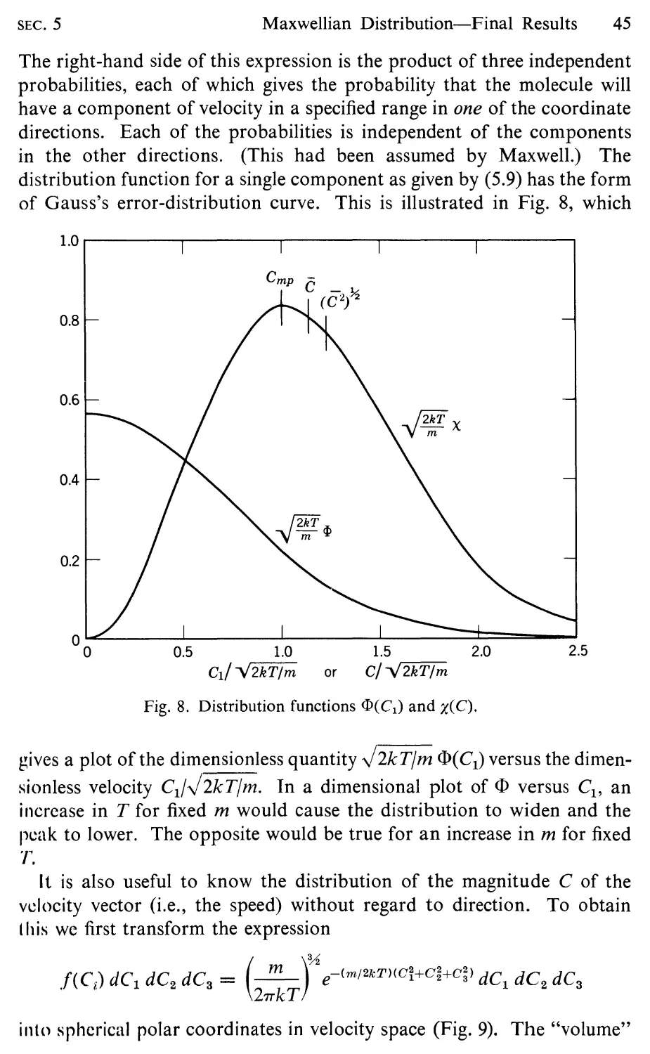
5 Maxwellian Distribution-Final Results, 42
6 Collision Rate and Mean Free Path, 48
7 Chemical Equilibrium and the Law of Mass Action, 55
{ I(APTER III CHEMICAL THERMODYNAMICS
59
1 Introduction, 59
2 Thermodynamic Systems and Kinds of Equilibrium, 60
3 Conservation of Mass, 63
4 Conservation of Energy; First Law, 65
5 The Second Law, 66
6 The Gibbs Equation for a Chemically Reacting System, 70
7 Entropy Production in Chemical Nonequilibrium; Con-
dition for Reaction Equilibrium, 75
H Mixtures of Perfect Gases, 77
9 Law of Mass Action, 82
10 Heat of Rcaction; van't Hoff's Equation, 83
XIII
XIV Contents
CHAPTER IV STATISTICAL MECHANICS
86
1 Introduction, 86
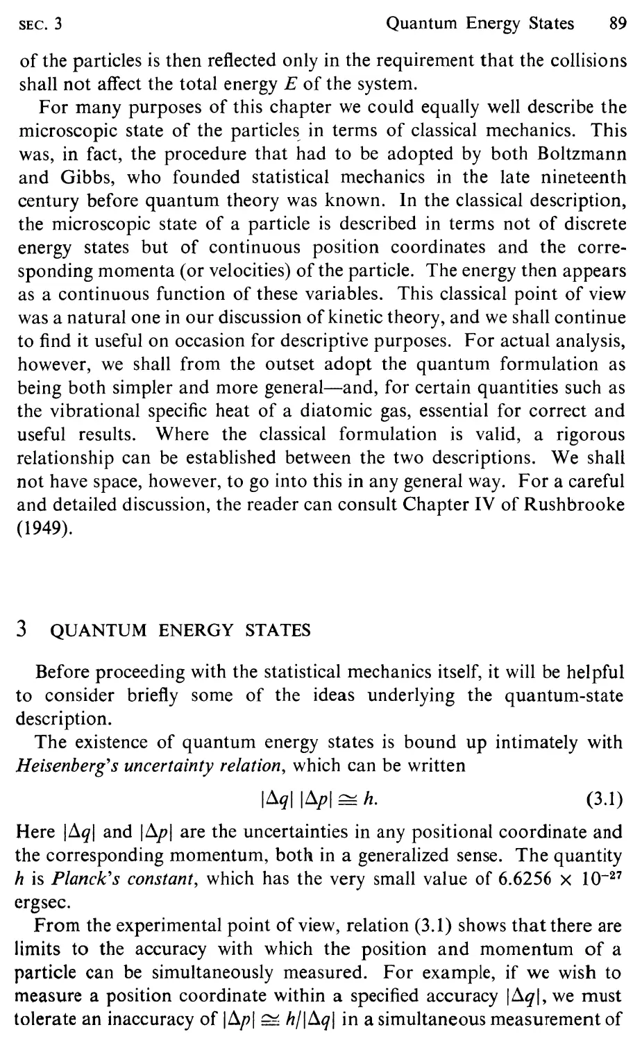
2 Macroscopic and Microscopic Descriptions, 88
3 Quantum Energy States, 89
4 Enumeration of Microstates, 93
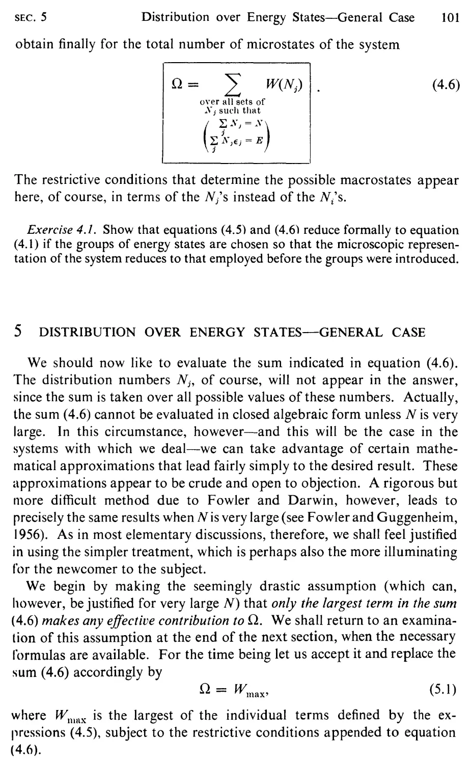
5 Distribution over Energy States-General Case, 101
6 Distribution over Energy States-Limiting Case, 104
7 Relation to Thermodynamics; Boltzmann's Relation, 112
8 Thermodynamic Properties, 117
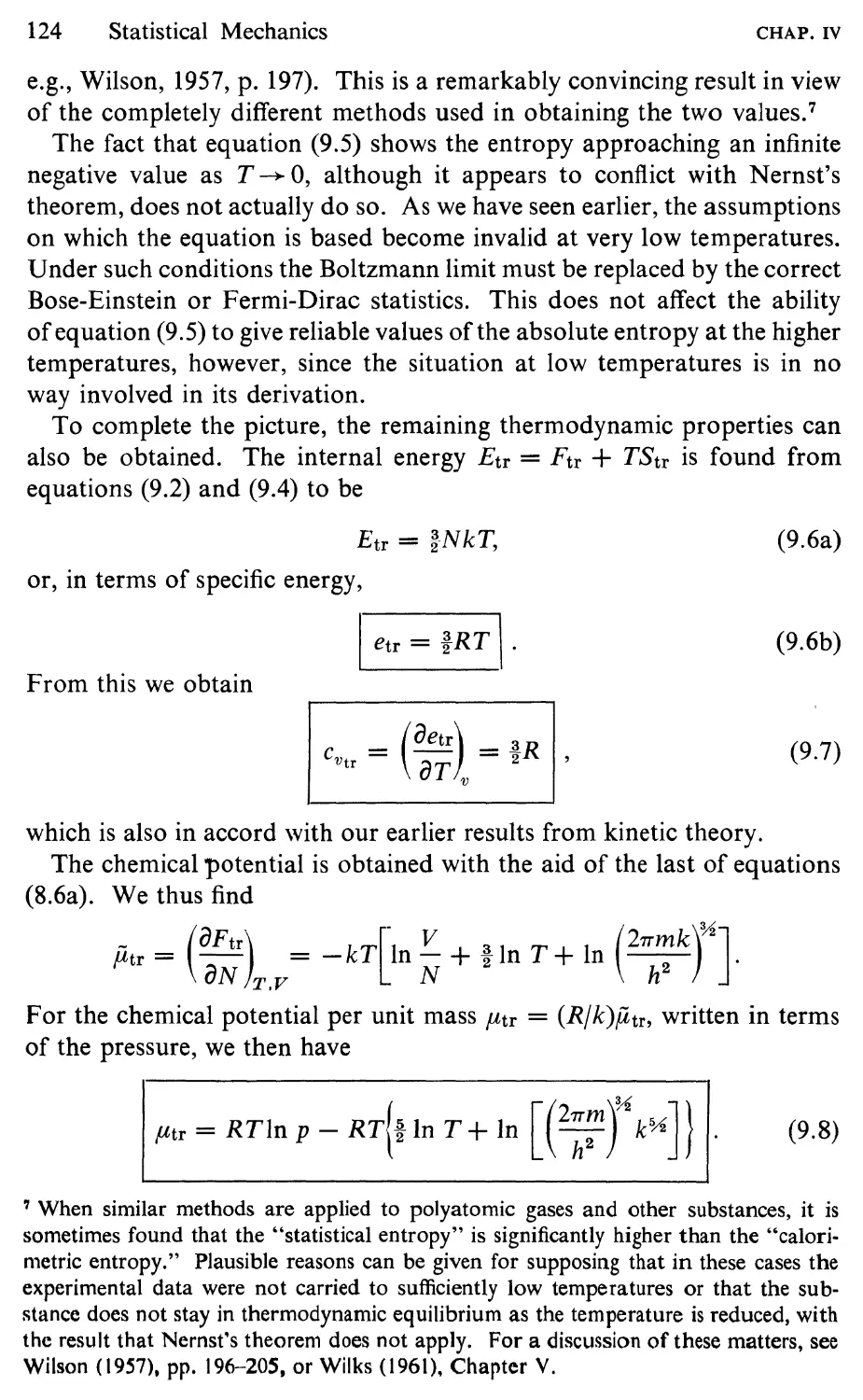
9 Properties Associated with Translational Energy, 120
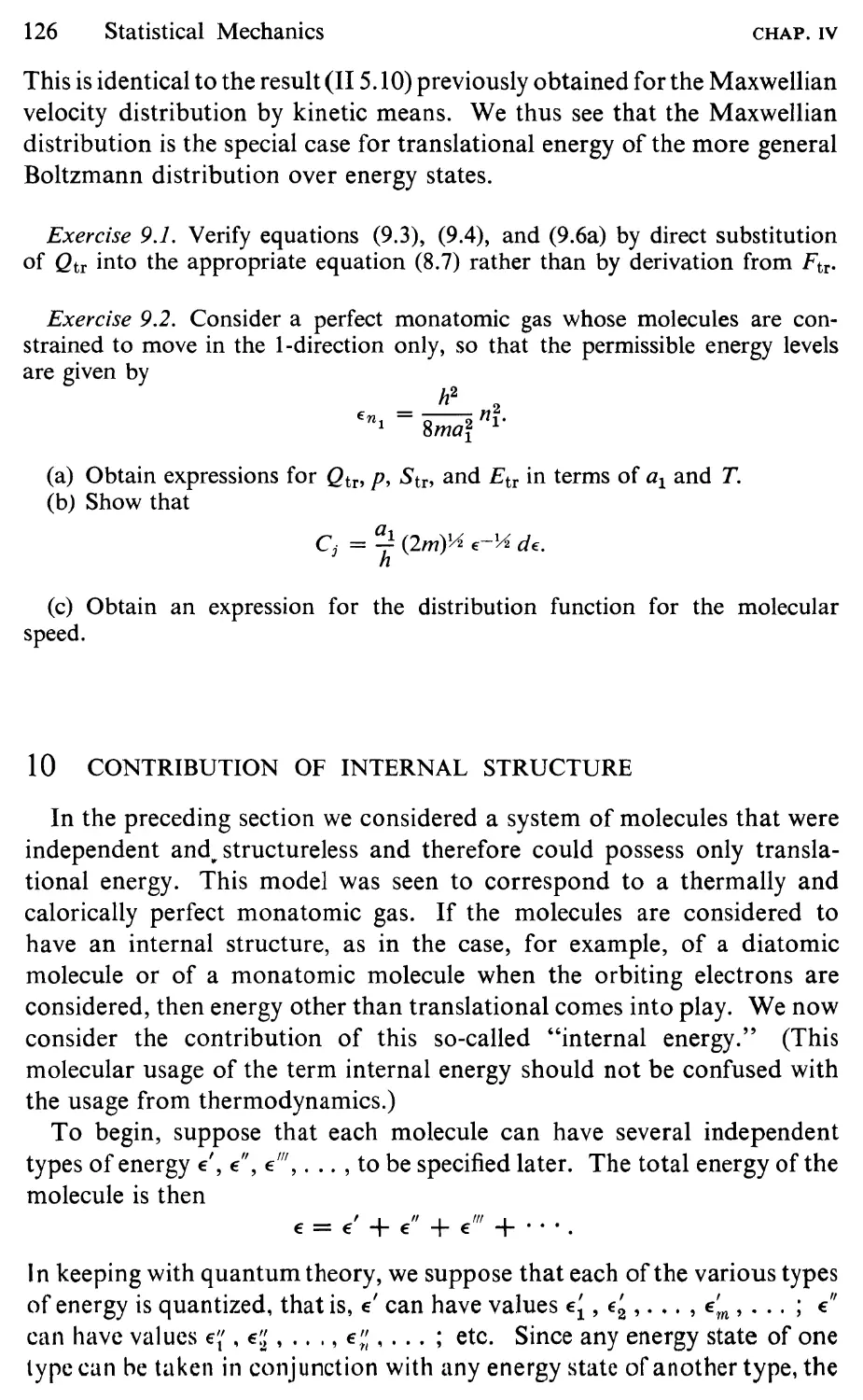
10 Contribution of Internal Structure, 126
11 Monatomic Gases, 129
12 Diatomic Gases, 132
13 Chemically Reacting Systems and Law of Mass Action, 139
14 Dissociation-Recombination of Symmetrical
Diatomic Gas, 148
CHAPTER V EQUILIBRIUM GAS PROPERTIES
152
1 Introduction, 152
2 Symmetrical Diatomic Gas, 152
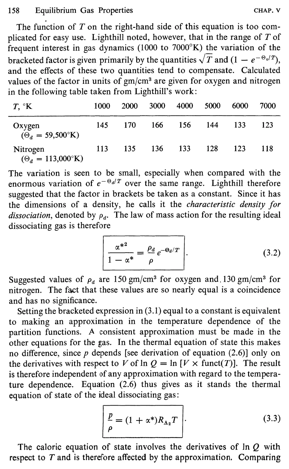
3 Ideal Dissociating Gas, 157
4 Ionization Equilibrium; The Saha Equation, 162
5 MixtU[e of Gases, 165
6 Properties of Equilibrium Air, 171
CHAPTER VI EQUILIBRIUM FLOW
178
1 Introduction, 178
2 Steady Shock Waves, 179
3 Steady Nozzle Flow, 183
4 Prandtl-Meyer Flow, 187
5 Frozen Flow, 191
CHAPTER VII VIBRATIONAL AND CHEMICAL RATE PROCESSES 197
1 Introduction, 197
2 Vibrational Rate Equation, 198
3 Entropy Production by Vibrational Nonequilibrium, 206
4 Chemical Rate Equations-General Considerations, 210
5 Energy I nvolvcd in Collisions, 216
Contents xv
6 Rate Equation for Dissociation-Recombination Reactions,
222
7 Rate Equation for Complex Mixtures, 228
8 High-Temperature Air, 229
9 Symmetrical Diatomic Gas; Ideal Dissociating Gas, 232
10 Generalized Rate Equation, 234
11 Local Relaxation Time; Small Departures from Equi-
librium, 236
CHAPTER VIII FLOW WITH VIBRATIONAL OR CHEMICAL
NONEQUILIBRIUM 245
1 Introduction, 245
2 Basic Nonlinear Equations, 246
3 Equilibrium and Frozen Flow, 251
4 Acoustic Equations, 254
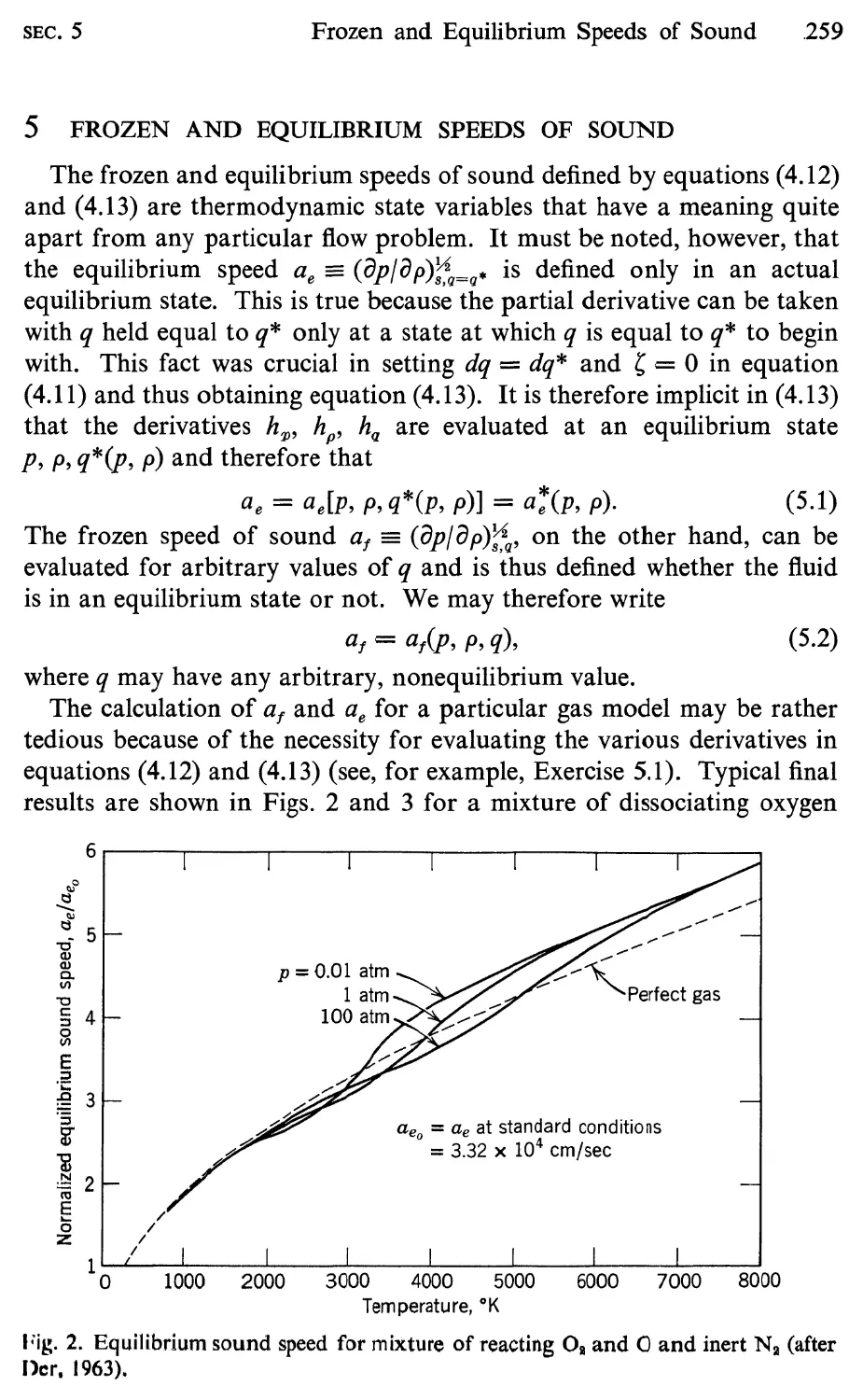
5 Frozen and Equilibrium Speeds of Sound, 259
6 Propagation of Plane Acoustic Waves, 261
7 Equation for Small Departures from a Uniform Free
Stream, 269
8 Flow over a Wavy Wall, 274
9 Linearized Flow behind a Normal Shock Wave, 281
10 Equations for Steady Quasi-One-Dimensional Flow, 286
11 Nonlinear Flow behind a Normal Shock Wave, 290
12 Fully Dispersed Shock Wave, 292
13 Nozzle Flow, 293
14 Method of Characteristics, 300
15 Supersonic Flow over a Concave Corner, 305
16 Supersonic Flow over a Convex Corner, 310
CIIAPTER IX NONEQUILIBRIUM KINETIC THEORY
316
1 Introduction, 316
2 The Conservation Equations of Gas Dynamics, 317
3 The Boltzmann Equation, 328
4 Equilibrium and Entropy, 334
5 The Equations of Equilibrium Flow, 344
6 Moments of the Boltzmann Equation, 346
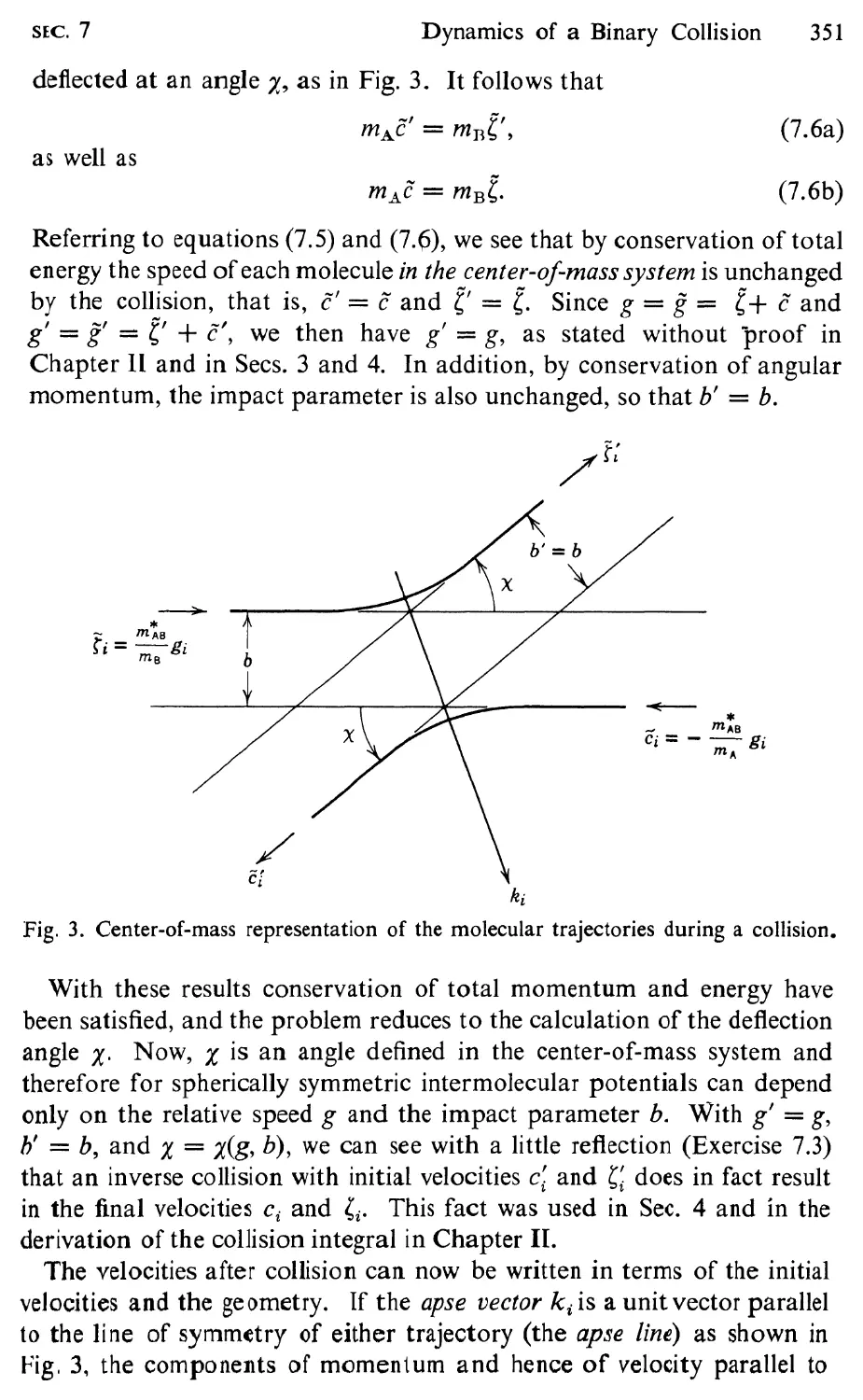
7 Dynamics of a Binary Collision, 348
X The Evaluation of Collision Cross-Sections, 356
<) The Evaluation of Collision Integrals, 361
10 Gas Mixtures, 368
XVI Contents
CHAPTER X FLOW WITH TRANSLATIONAL NONEQUILIBRIUM 375
1 Introduction, 375
2 The Bhatnagar-Gross-Krook Collision Model, 376
3 The Chapman-Enskog Solution of the Krook Equation, 379
4 The Chapman-Enskog Solution of the Boltzmann Equation,
385
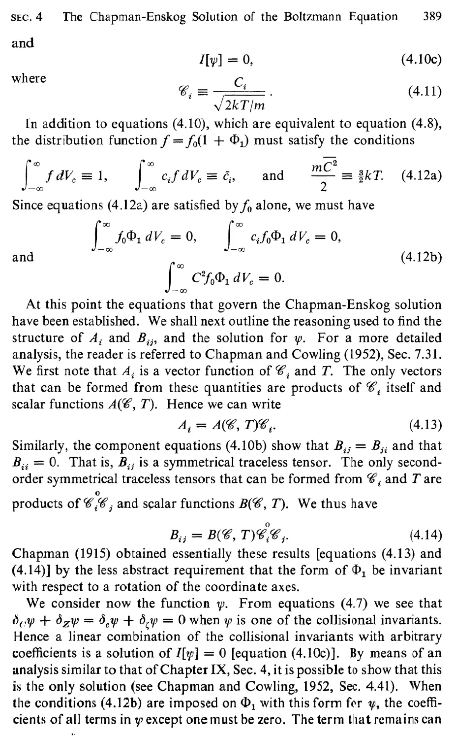
5 The Navier-Stokes Equations, 390
6 Expansion in Sonine Polynomials, 394
7 Transport Properties, 403
8 Bulk Viscosity, 407
9 The Structure of Shock Waves, 412
10 Linearized Couette Flow, 424
CHAPTER XI RADIATIVE TRANSFER IN GASES
436
1 Introduction, 436
2 Energy Transfer by Radiation, 437
3 The Equation of Radiative Transfer, 443
4 Radiative Equilibrium, 446
5 The Interaction of Radiation with Solid Surfaces, 450
6 Emission and Absorption of Radiation, 452
7 Quasi-Equilibrium Hypothesis, 458
8 Forma ISolution of the Equation of Radiative Transfer, 462
9 Simplifications and Approximations, 465
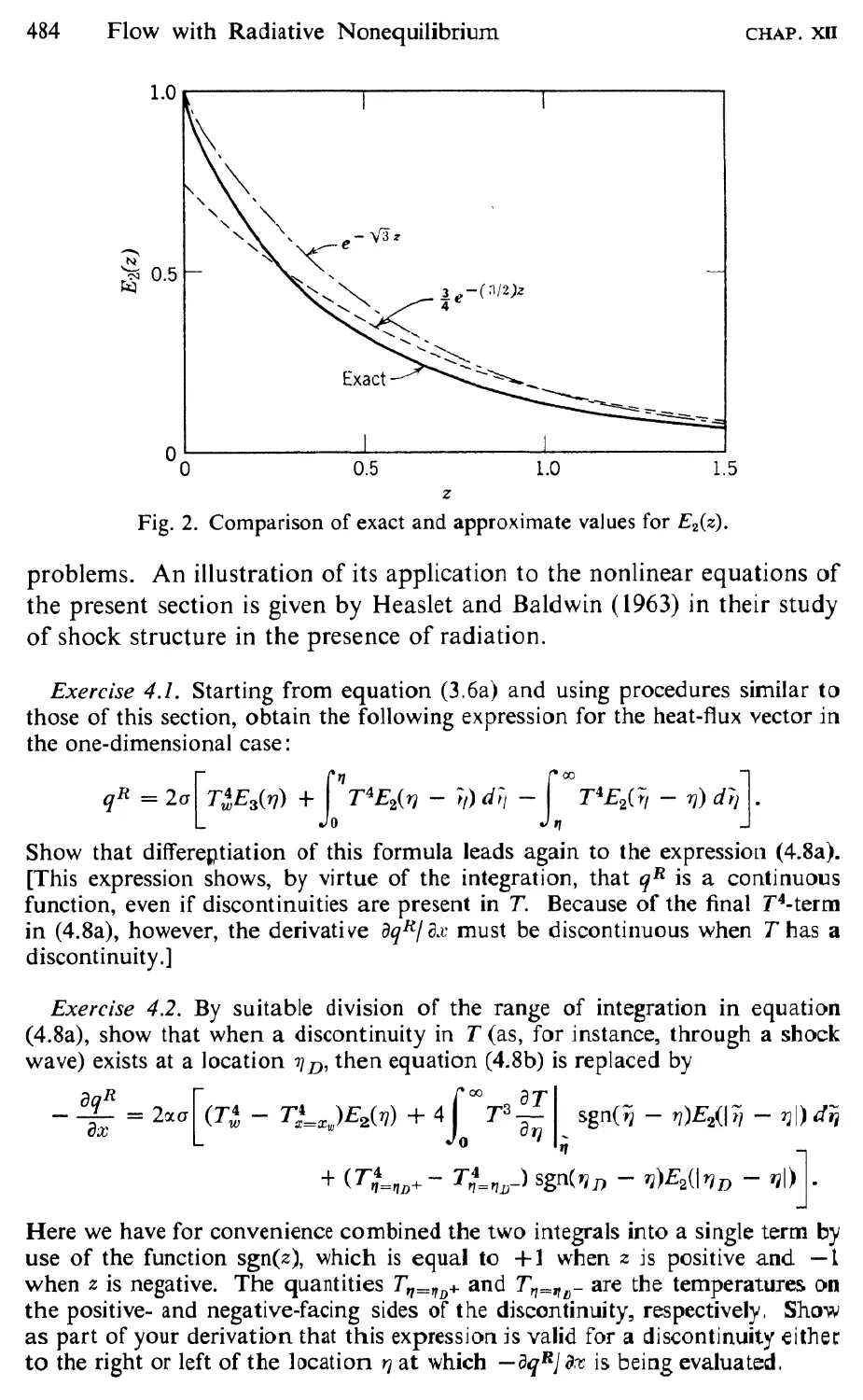
CHAPTER XII FLOW WITH RADIATIVE NONEQUILIBRIUM 473
1 Introduction, 473
2 Basic Nonlinear Equations, 474
3 Asymptotic Situations; Grey-Gas Approximation, 476
4 One-Dimensional Equations, 479
5 Linearized One-Dimensional Equations, 485
6 Differential Approximation, 491
7 Acoustic Equation, 496
8 Propagation of Plane Acoustic Waves, 499
9 Equation for Small Departures from a Uniform Free
Stream, 505
10 Linearized Flow through a Normal Shock Wave, 508
II Nonlinear Flow through a Normal Shock Wave, 515
Contents XVll
APPENDIX 523
1 Definite Integrals, 523
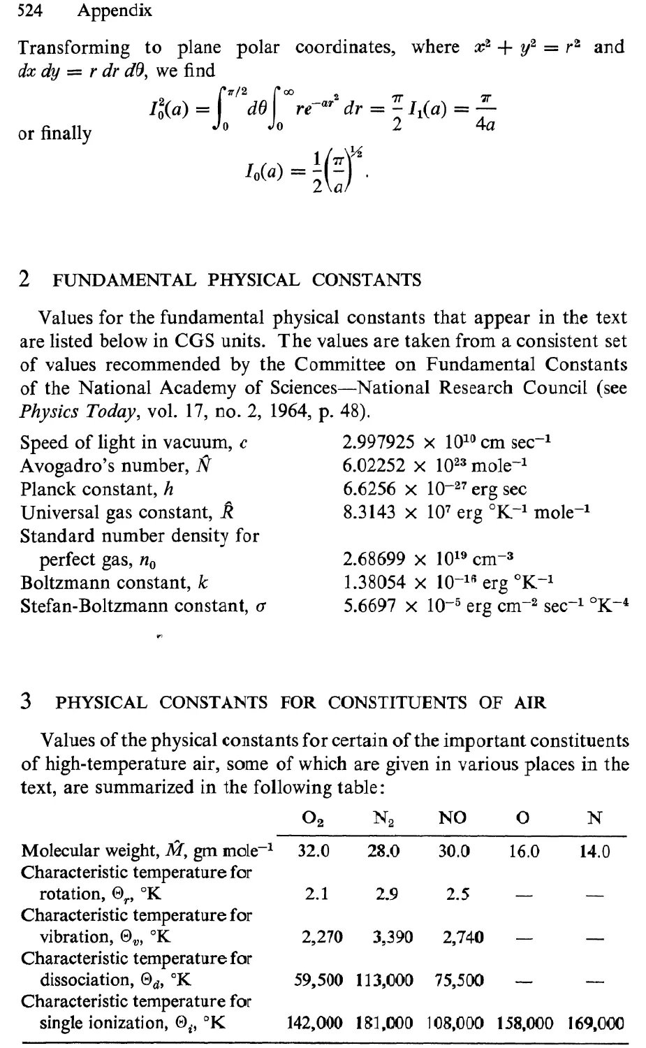
2 Fundamental Physical Constants, 524
3 Physical Constants for Constituents of Air, 524
SUBJECT INDEX
525
SYMBOL INDEX
535
Chapter I
Introductory Kinetic Theory
1 INTRODUCTION
We begin our study of physical gas dynamics with a discussion of some
of the pertinent problems from the kinetic theory of gases. In kinetic
theory a gas is considered as made up at the microscopic level of very
small, individual molecules in a state of constant motion. If there is no
movement of the gas at the macroscopic level, this motion is regarded as
purely random and is accompanied by continual collisions of the molecules
with each other and with any surfaces that may be present. The movement
of a given molecule is thus to be thought of as a kind of random banging
about, with its velocity undergoing frequent and more or less discontinuous
changes in both magnitude and direction. Indeed, it is this freedom of
motion of the molecules, limited only by collisions, that differentiates a
gas from the n10re ordered situation that exists in a liquid or a solid.
When there is a general macroscopic movement of the gas, as is the
usual situation in gas dynamics, the motion of the molecules is not
completely random. This statement is, in fact, merely two ways of saying
the same thing-the general motion is only a macroscopic reflection of
the nonrandomness of the molecular motion. In particular, the familiar
flow velocity of continuum gas dynamics is, from the molecular point of
view, merely the average velocity of the molecules taken over a volume
large enough to contain many molecules but small relative to the dimen-
sions of the flow field. Zero flow velocity, that is, an average molecular
velocity of zero, corresponds to random absolute motion of the molecules
(i.e., molecules of a given speed have no preferred direction). In a flowing
gas the molecular motion, although not random from an absolute point
of view, win appear almost so to an observer moving at the local flow
ve1ocity. These ideas will be made precise in Chapter IX when we consider
2
Introductory Kinetic Theory
CHAP. I
the flow of a nonuniforn1 gas in detail. For the time being we are interested
primarily in the properties of the gas as such, and for this a consideration
of the random motion is for the most part sufficient.
To make the foregoing ideas quantitative, we must introduce a precise
assumption regarding the molecular model, that is, regarding the nature
of the molecules and of the forces acting between them. Given such a
model and the usual laws of mechanics, it would then be possible, in
principle, to trace out the path of each molecule with time, assuming that
the initial conditions are known (which, of course, they are not). Such a
calculation, though of interest theoretically, would be enormously difficult.
Fortunately it is also of little necessity. What we are really concerned
with in most practical applications is the gross, bulk behavior of the gas
as represented by certain observable quantities such as pressure, tempera-
ture, and viscosity, which are manifestations of the molecular motions
averaged in space or time. It is the primary task of kinetic theory to relate
and "explain" these macroscopic properties in terms of the microscopic
characteristics of the molecular model.
The approach to this problem in the present chapter will be deliberately
rough and nonrigorous-refinement will come later in Chapter II. The
aim here is a qualitative understanding of certain ideas and some feeling
for the numerical magnitudes that are involved. The results, however,
are essentially correct.
The reader who wants to study kinetic theory more extensively than we
shall be able to here will probably enjoy the book by Jeans (1940). His
mechanical description (pp. 11-15) of the theory in terms of balls on a
Ifl
billiard table is particularly helpful in fixing the basic ideas. Among the
other useful books in the field are those of Kennard (1938), Present (1958),
and Loeb (1961). Other references will be given later in Chapter IX.
2 MOLECULAR MODEL
Further word on the molecular model is necessary. Aside from the
fundamental attribute of mass, a molecule possesses an external force
field and an internal structure. The external field is, as a matter of fact, a
consequence of the internal structure, that is, of the fact that the molecule
consists of one or more atomic nuclei surrounded by orbiting electrons.
The somewhat arbitrary concentration of our attention separately on the
"outside" and "inside" of the molecules, however, is a useful procedure.
(For a discussion of the origin of interatomic and intermolecular forces
at a hcgil1l1ing level, see Slater, 1939, Chapter XXII.)
SEC. 2
Molecular Model
3
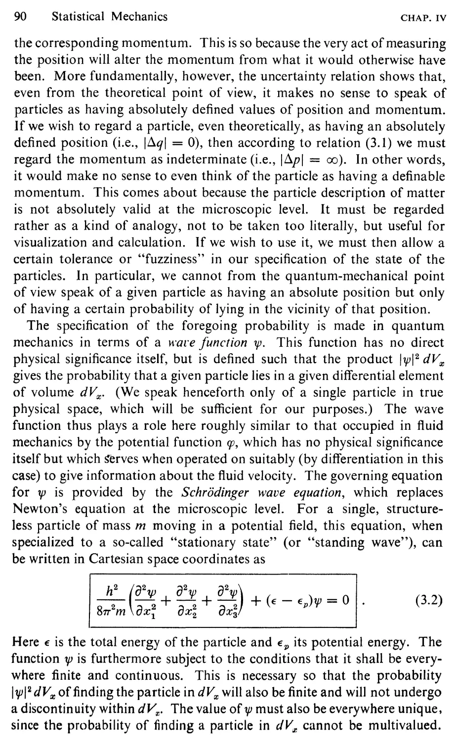
The external force field is generally assumed to be spherically symmetric.
This is very nearly true in many cases and to assume otherwise is almost
prohibitively difficult. On this basis, the force field can be represented as
in Fig. 1, which shows the force F between two molecules as a function of
the distance r between them. At large distances the true representation
( solid curve) shows a weak attractive force that tends to zero as the distance
increases. At short distances there is a strong repulsive force that increases
rapidly as the orbiting electrons of the two molecules intern1ingle. At
F
True representation
(Repulsion)
t
I
I
I
I
I
d
Rigid elastic spheres
l'
(Attraction)
'\ Sutherland model
Fig. 1. Intermolecular force F as a function of the distance r between two molecules.
some intermediate distance, F passes through zero. The molecules, if
they had no kinetic energy, would remain in equilibrium indefinitely at
this distance.
Even with the simplest possible equation for the curve just described,
the analysis is complicated. For this reason further approximation is
often made. The simplest (Fig. 1) is to regard the molecules as rigid
elastic spheres with zero attractive force when apart and an infinite
repulsive force at the instant of contact. For like molecules, contact will
take place when the distance between the center of the spheres is d, where
d is the assumed diameter of the spherical molecule. A considerable
amount of surprisingly accurate information can be obtained on the basis
of this crude model, provided we chose d to give agreement between the
resulting theory and the experimental data for some basic quantity such
as viscous stress. Some improvement can be obtained at the expense of
further con1plication by going to the so--called "Sutherland model." This
4
Introductory Kinetic Theory
CHAP. I
model supplements the rigid sphere by adding a weak attractive force
when the spheres are not in contact. Other models are also possible. One
that we shall find useful in Chapter IX dispenses entirely with the idea of
solid spheres and assumes a pure repulsive force varying with some
inverse power of the intermolecular distance.
The internal structure of the molecules is important primarily for its
effect on the energy content of the gas. Being composed of nuclei and
electrons that have motion relative to the center of mass of the molecule,
the molecules can possess forms of energy (rotation, vibration, etc.) above
and beyond that associated with their translational motion. In addition,
the internal structure may be expected to affect the collisional interaction
of the molecules at short range. Inclusion of the effects of internal
structure considerably complicates the kinetic theory.
In the present book the treatment of intermolecular forces in any but
the simplest way will be reserved for the discussion of nonequilibrium
kinetic theory in Chapters IX and X. The effects of internal structure, at
least insofar as the internal energy is concerned, will be taken up in detail
in the discussion of equilibrium statistical mechanics in Chapter IV. For
the present the molecular model that will be assumed, except for certain
digressions, is that of the structureless, perfectly elastic sphere with no
attractive forces and with repulsive forces existing only during contact.
The characteristics of this "billiard-ball" model are completely specified
by giving the mass and diameter of the various types of molecules, the
number of each type of molecule per unit volume, and some measure of
the speed of the l random motion. Our task is to relate the macroscopic
properties of the gas to these assumedly given microscopic quantities.
3 PRESSURE, TEMPERATURE, AND INTERNAL ENERGY
Consider a gas mixture in a state of equilibrium inside a cubical box.
Suppose that the box is at rest so that the molecular motion is purely
random. We wish to study the pressure exerted on the walls of the box
by this random motion.
For simplicity we assume that the molecules do not collide with each
other but only with the walls. We also assume that upon collision with a
wall a molecule is reflected specularly (i.e., angle of reflection equals angle
of incidence) and with its speed unchanged. It must be emphasized that
neither of these assumptions is true; the fate of a given molecule upon
collision with the wall is not known, and molecules do in reality collide
with each other with great freq uency. I ntermolecular coli isions are, in
I
SEC. 3
Pressure, Temperature, and Internal Energy
5
fact, the chief mechanism for bringing the gas to its final state of equilib-
rium. Nevertheless, once the equilibrium state has been established, the gas
behaves, at least insofar as the pressure is concerned, as if the assumptions
were correct. This is because the condition of equilibrium requires that
in any region the number of molecules of a given species and having
velocity closely equal, in both magnitude and direction, to any given value
must not vary with time. Thus, in a small region in the vicinity of a given
point, for every molecule deflected away from its original velocity by a
collision, there will at the same time be another of the same species
deflected into this velocity. This molecule can be regarded as carrying on
the n10tion of the original molecule just as if no collision had occurred.
Somewhat similar ideas can be applied at the wall. Here the essential fact
is that within a gas in equilibrium there can be no preferred direction.
That is to say, in any region of the gas the number of molecules of a given
species and having velocity closely equal in magnitude to a given value
must be the same irrespective of the direction of the velocity. If this
requirement is applied in a small region immediately adjacent to the wall,
it implies that for every molecule arriving at a small element of the wall,
another of the same species will at the same tin1e leave that element with
a specularly oriented velocity of equal magnitude. Thus the gas 1?ehaves
as if a given molecule were reflected specularly and without change of
speed.
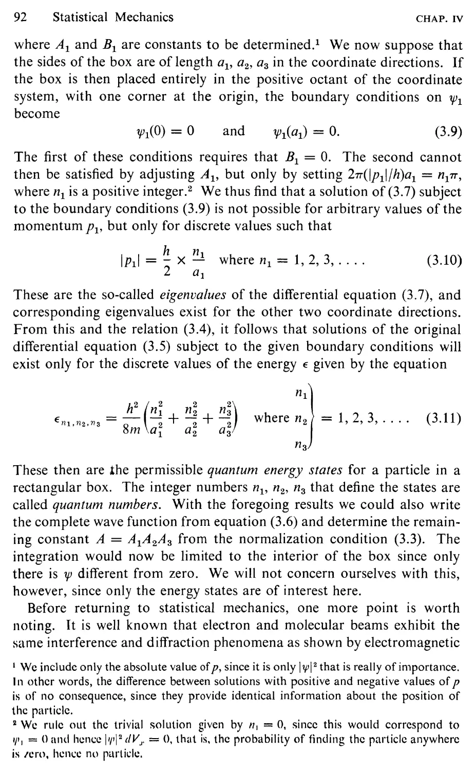
Under the assumption of no intermolecular collisions and specular,
elastic reflection at the walls, the motion of a given molecule is as shown
in two-dimensional projection in Fig. 2. The molecule in this purely
fictitious situation moves at a constant speed C irrespective of its direction.
When it collides with the wall, its velocity component perpendicular to
the wall is reversed whereas that parallel to the wall is unaltered. If
coordinate axes Xl' X 2 , X 3 are taken along three edges of the box, the
magnitudes of the corresponding velocity components thus have fixed
values ICII, IC 2 1, IC 3 1, where Ci + C + C; = C2.
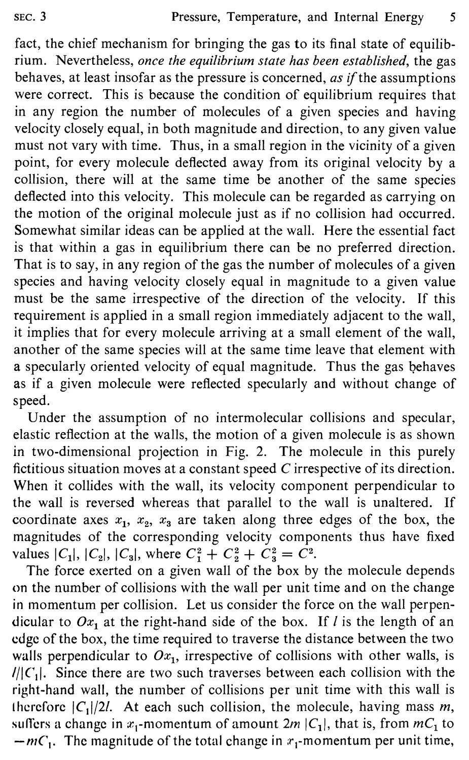
The force exerted on a given wall of the box by the molecule depends
on the number of collisions with the wall per unit time and on the change
in tnomentum per collision. Let us consider the force on the wall perpen-
dicular to OX I at the right-hand side of the box. If I is the length of an
edge of the box, the time required to traverse the distance between the two
walls perpendicular to Ox l , irrespective of collisions with other walls, is
IIICf.l. Since there are two such traverses between each collision with the
right-hand wall, the nunlber of collisions per unit time with this wall is
(hcreforc I C l 1/21. At each such collision, the molecule, having mass m,
sutlers a change in x 1 -nl0mentum of amount 2rn IC]I, that is, from mC! to
-111('1. The magnitude of the total change in ;r 1 -momentum per unit time,
6
Introductory Kinetic Theory
CHAP. I
which is equal to the total force exerted on the wall by the molecule, is
thus
mC 2
2m IC 1 1 X IC 1 1/21 = ---1. .
1
Since the area of the wall is [2, the corresponding pressure on the wall is
mC = mC
[3 V
where V = [3 is the volume of the box.
X2j
l
>"-
Xl
Fig. 2. Projection on the Xl' x 2 -plane of the path of a molecule in a cubical box in the
ficticious situation of no intermolecular collisions and specular, elastic reflection at the
walls.
o
Now suppose that the gas mixture consists of a large number of molecules
of different mass ma, m b , mc, . . . moving with speeds C a , C b , C c , . . .. The
total pressure exerted on the wall perpendicular to OX 1 by all the molecules
is then
1 ( C 2 2 C 2 ) 1 2
- ma al + mbC b1 + me CI + . .. = - k mZC ZI .
V V Z
But under the assumed conditions of equilibrium the pressure on this wall
is the same as on the other walls of the box. Denoting this common
pressure by p, we can therefore equate the foregoing pressure to p and
wri te
1 '" 2
P = - mZC Z1 .
V
Corresponding equations hold for the pressure calculated on the faces
SEC. 3
Pressure, Temperature, and Internal Energy
7
perpendicular to OX 2 and Ox 3 . Taking the sum of these equations for the
three coordinate directions and dividing by three, we also obtain
1, 2 2 2 1, 2
P = - £. mZ(C Z1 + C Z2 + C Z3 ) = - £. mzC z .
3V z 3V z
Since the total energy of translation Etr of the molecules is t I mzC:, this
equation can be written Z
(3.1)
I pV = iEtr I .
(3.2)
The same final results will be rederived in Chapter lIon the basis of a
more realistic analysis.
The foregoing kinetic-theory equation of state ean be compared with
the empirically derived equation of state for a thermally perfect gas from
classical thermodynamics. This is, in one of its forms,
pV = .HRT,
where R is the universal gas constant (i.e., gas constant per mole),l .AI is
the number of moles of gas in the volume V, and T is the gas temperature.
We see that the theoretical formula and the empirical equation are
iden tical if we take
3 J/' A
Etr = 2./ r RT .
(3.3a)
This equation relates the energy of translation of the molecules in kinetic
theory to the absolute temperature as defined in classical thermodynamics.
The temperature may thus be interpreted as a measure of the molecular
energy. Equation (3.3a) is sometimes taken, from a somewhat different
point of view (cf. Chapter IX, Sec. 2), as giving a kinetic definition of
tempera ture.
The result (3.3a) can be reexpressed in terms of the average kinetic
energy per molecule by dividing both sides by the total number N of
molecules. This gives
_ E tr 3 JV' A 3 R
etr = - = - x - RT = - x T
N 2 N 2 N'
where IV = N/.AI is the nun1ber of molecules per mole, which is Avogadro's
number, another universal constant. The quotient RjN, which is in the
nature of a "gas constant per molecule," is thus also a universal constant,
usually denoted by k and called the Boltzmann constant. We thus write
1 The value of this and other fundamental physical constants is given in the appendix
at the end of the book.
8
Introductory Kinetic Theory
CHAP. I
for the average kinetic energy per molecule
etr = IkT.
(3.3b)
We can also obtain the specific kinetic energy etr per unit mass by dividing
both sides of equation (3.3a) by the total mass M = I m z . Noting that
z
the combination JV RIM is the ordinary gas constant R (i.e., gas constant
per unit mass), we thus obtain
etr = iRT. (3.3c)
Under our assumption that the molecules have no internal structure,
the energy of translation constitutes the entire molecular energy of the
gas. It can therefore be taken as equal to the internal energy e of thermo-
dynamics. We thus find for the specific heat at constant volume in the
present case
c = ( ae \ = detr = R.
v aT }v dT 2
1'he specific heat at constant pressure, as given by the thermodynamic
relation c p - C v = R, valid for a thermally perfect gas, is
C p = tR,
and the ratio of specific heats y = cpjc v is therefore
Y -.Q.
- 3.
Since our assumed gas model has constant specific heats, it is calorically as
well as thermally perfect. 2 The calculated value of C v is in good agreement
with experimental data for monatomic gases at ordinary temperatures.
This indicates that our model is a reasonable one for such gases.
The foregoing theory can also be used to obtain an estimate of molecular
speeds. For this purpose we return to equation (3.1) and divide both sides
by M = I m z . Introducing the mass density p = M/ Vand a mean-square
z
molecular speed defined by
mzC;
C 2 = z
- ,
Im z
z
(3.4)
2 When a gas is both thermally and caloricalJy perfect, we shall ordinarily describe it
by the unmodified term "perfect gas." When we wish to distinguish between thermal
perfection (a gas obeying the equation p V = .Al'RT) and caloric perfection (a gas with
constant specific heats), we shall try to remember to add the adjectives. The reader
will recall that a gas can be thernlally perfect and calorically imperfect, but not vice
versa.
SEC. 3
Pressure, Temperature, and Internal Energy
9
we thus obtain
l!. = 1 c 2
P 3
(3.5)
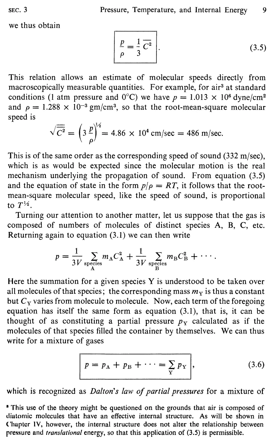
This relation allows an estimate of molecular speeds directly from
macroscopically measurable quantities. For example, for air 3 at standard
conditions (1 atm pressure and O°C) we have p = 1.013 X 10 6 dyne/cm 2
and p = 1.288 X 10- 3 gm/cm 3 , so that the root-mean-square molecular
speed is
.J C 2 = (3 r = 4.86 x 10 4 cm/sec = 486 m/sec.
This is of the same order as the corresponding speed of sound (332 m/sec),
which is as would be expected since the molecular motion is the real
mechanism underlying the propagation of sound. From equation (3.5)
and the equation of state in the form pi p = RT, it follows that the root-
mean-square molecular speed, like the speed of sound, is proportional
to T IA .
Turning our attention to another matter, let us suppose that the gas is
composed of numbers of molecules of distinct species A, B, C, etc.
Returning again to equation (3.1) we can then write
1, 2 1, 2
p=- mAC A +- mBC B +....
3 V species 3 V species
A B
Here the summation for a given species Y is understood to be taken over
all molecules of that species; the corresponding mass my is thus a constant
but C y varies from molecule to molecule. Now, each term of the foregoing
equation has itself the same form as equation (3.1), that is, it can be
thought of as constituting a partial pressure py calculated as if the
molecules of that species filled the container by themselves. We can thus
write for a mixture of gases
1 P = PA + PB + · . · = py I ,
(3.6)
which is recognized as Dalton's law of partial pressures for a mixture of
· This use of the theory might be questioned on the grounds that air is composed of
diuton1ic mo1ecules that have an effective internal structure. As will be shown in
('hurter IV, however, the internal structure does not alter the relationship between
pressure and translational energy, so that this application of (3.5) is permissible.
10
Introductory Kinetic Theory
CHAP. I
perfect gases. The partial pressure is given analogously to equation (3.2)
by
pyV = iEy tr ,
(3.7)
where Ey = i I myC is the total molecular energy of translation of
tr y
species Y. The corresponding thermodynamic equation here is
pyV = .AI' yRT,
where ;V y is the number of moles of species Y in the mixture, and the
common temperature T is used since at equilibrium all gases in the mixture
n1ust have the same temperature. Comparing the two equations we
obtain, as in equation (3.3a),
3 j/, ".
Ey = 2 /r yRT.
tr
(3.8a)
If we now divide by the total number Ny of molecules of species Y and
note that IV = Ny/.AI' y is again Avogadro's number, we find for the
average translational energy per molecule of species Y
e y = !kT.
tr
(3.8b)
The right-hand side of this equation is identical to that of equation (3.3b)
for the entire mixture. Equations (3.8b) and (3.3b) thus show that
eA = eB =... = et .
tr tr r
(3.9)
That is to say, when a number of gases are mixed at the same temperature,
the average kinetic energy of their molecules is the same. It follows that
the heavy molecules must move, on the average, slower than the light
molecules.
One remark needs to be made. The foregoing development has used
our prior thermodynamic knowledge of the equation of state of a thermally
perfect gas and of the existence of the universal gas constant and Avogadro's
number. The appeal to thermodynamics in this restricted way, however,
is not essential and has been used here only for the sake of brevity. An
alternative-and perhaps logically preferable-approach is given in Jeans'
book (pp. 21-30). Proceeding from considerations of the mechanics of
molecular collisions for elastic spheres, one can, with a little work,
establish the result of equation (3.9) from mechanical considerations alone
and with no reference to thermodynamics. The identification of the
average kinetic energy with the thermodynamic temperature [equation
(3.8b)] is then made from general thermodynamic considerations of
internal energy and entropy without recourse to the equation of state.
The cq uation of state for a thermally perfect gas then follows directly
SEC. 3
Pressure, Temperature, and Internal Energy
11
from the basic kinetic equation (3.2). From this point of view, the
thermodynamic form of the equation of state together with Avogadro's
law (which is equivalent to the existence of the universal gas constant)
emerge as logical deductions from the kinetic approach rather than as
independently introduced empirical findings.
Equations (3.3b) and (3.8b) are a special case of the general principle of
equipartition of energy, which we shall encounter again later. This principle
states that for any part of the molecular energy that can be expressed as the
sum of square terms, each such term contributes an average energy of tkT
per molecule. By a "square term" we mean a term that is quadratic in
some appropriate variable used to describe the energy. In the kinetic
energy of translation, for example, the energy of any molecule can be
written in the form tm( C; + C + cg), which is the sum of three square
terms. The average translational energy per molecule is therefore !k T in
agreement with (3.3b) and (3.8b). For molecules with internal structure,
the total number of square terms may be greater. If the total number of
such terms is , the average molecular energy, now expressed per unit
mass rather than per molecule, is given by
-"
e = (tRT) = -RT.
2
(3.10)
The corresponding specific heats and thei ratio yare then
c =-R
v 2 '
_ +2 R
c p - ,
2
+2
y=
(3.11)
A given type of molecular energy (rotational, vibrational, etc.) cannot
always validly be expressed as a sum of square terms. For this to be
possible, the type of energy in question must be "fully excited." The
meaning of this term will become apparent when we study the effects of
internal structure from the quantum-mechanical point of view (see
Chapter IV, Sec. 12). For a diatomic gas such as air there are at ordinary
temperatures five square terms, three for translation and two for rotation
about the two major axes of the molecule. We thus have in this case
= 5 and hence y = i, which is a well-known approximate value for
diatomic gases.
The treatment leading up to the basic equation (3.1) is unrealistic in
that it assumes specular reflection and a special shape of container and
ignores the intermolecular collisions that are a characteristic feature of
kinetic theory. It also does not demonstrate that the pressure is the same
for a1l regions on the surface of the container. These objections will be
overcome in Chapter II. The resu1ts, however, will not be altered.
12
Introductory Kinetic Theory
CHAP. I
4 MEAN FREE PATH
We now wish to say something about the collisions between molecules,
which were ignored in the previous discussion. A concept of fundamental
importance here is that of the mean free path, which can be defined
as the average distance that a molecule travels between successive collisions.
We wish in particular to obtain an expression for the mean free path in
tern1S of the quantities that define the gas model.
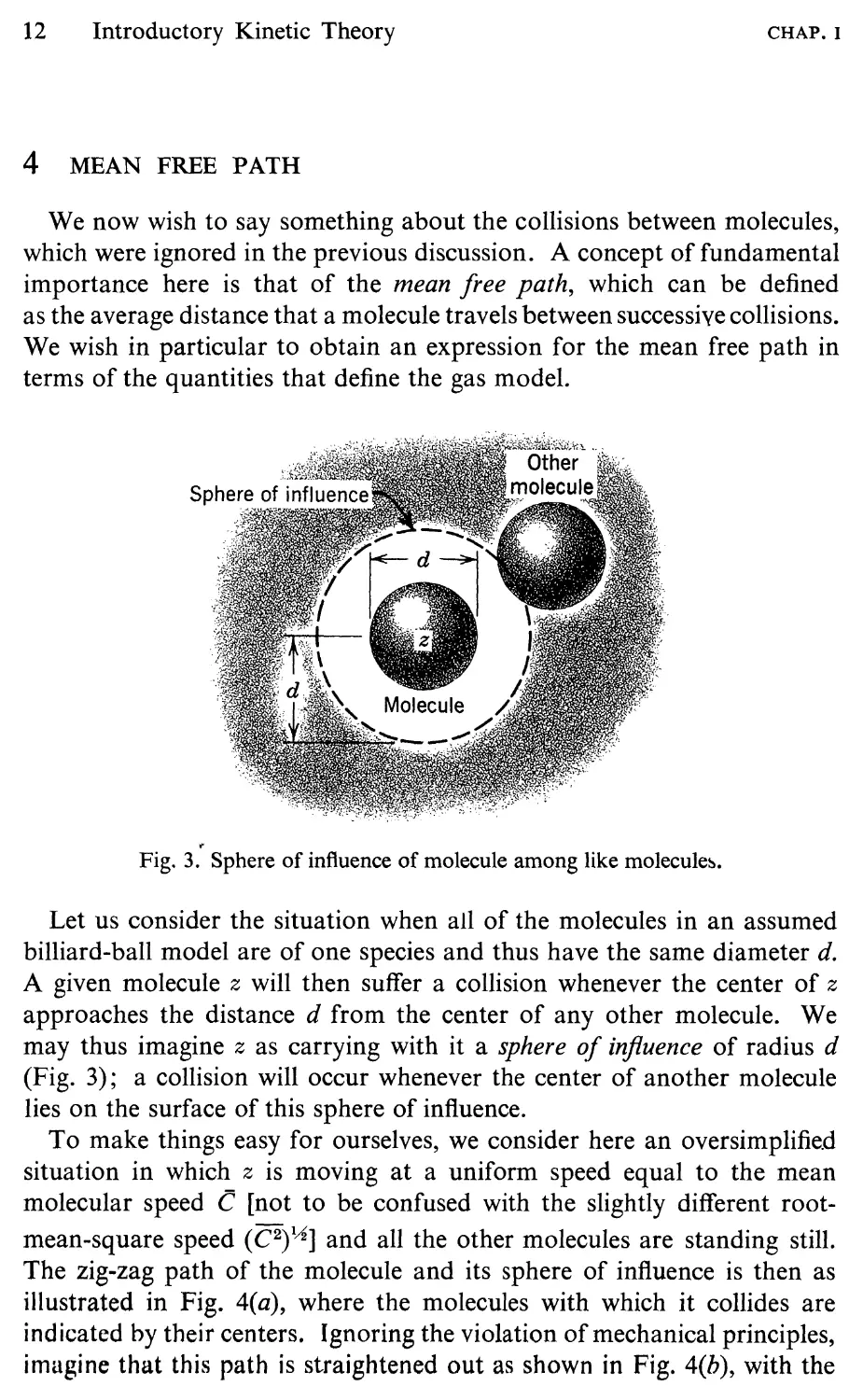
'i'
Fig. 3. Sphere of influence of molecule among like molecule .
Let us consider the situation when all of the molecules in an assumed
billiard-ball model are of one species and thus have the same diameter d.
A given molecule z will then suffer a collision whenever the center of z
approaches the distance d from the center of any other molecule. We
may thus imagine z as carrying with it a sphere of influence of radius d
(Fig. 3); a collision will occur whenever the center of another molecule
lies on the surface of this sphere of influence.
To make things easy for ourselves, we consider here an oversimplified
situation in which z is moving at a uniform speed equal to the mean
molecular speed C [not to be confused with the slightly different root-
mean-square speed ( C 2 ) 4] and all the other molecules are standing still.
The zig-zag path of the molecule and its sphere of influence is then as
illustrated in Fig. 4(a), where the molecules with which it collides are
indicated by their centers. Ignoring the violation of mechanical principles,
imagine that this path is straightened out as shown in Fig. 4(b), with the
SEC. 4
Mean Free Path
13
centers of the target molecules retaining their position relative to the path
of the moving molecule prior to the collision. These centers will then all
lie within the straight cylindrical volume swept out by the sphere of
influence. Since the molecule is traveling at the uniform speed C, the
volume swept out per unit time is obviously 'Trd 2 C. If n denotes the number
of molecules per unit volume of gas, the number of centers lying within
Fig. 4. Path of molecule z among stationary molecules.
the cylindrical volume is 'Trd 2 Cn. Since each of these centers corresponds
to a collision, this product must also represent the number 0 of collisions
per unit time for molecule z, that is,
o = 'Trd 2 Cn.
(4.1 )
But the distance traveled by molecule z per unit time is C. It follows that
the average distance traveled per collision, which is the mean free path A,
IS
C 1
,1----
- 0 - 'Trd 2 n .
(4.2)
I n view of the approximations involved, this gives accurately the mean
free path for a particle moving with a speed infinitely greater than that of
14
Introductory Kinetic Theory
CHAP. 1
the other particles. It follows from equation (3.9) that this is approxi-
mately the case for a free electron (very small mass) moving in a gas of
normal molecular mass. 4 For improved accuracy in purely molecular
collisions, the derivation should be modified to account for the motion of
the target molecules, and this will be done in Chapter II, Sec. 6. The
modified expression for A turns out to be
1
,1= .
.J 2 'lTd 2 n
( 4.3a)
The factor .J 2 in the denominator arises essentially from the fact that the
correct speed to use for the evaluation of 0 in equation (4.1) is really the
mean relative speed of the molecules, and this can be shown to be .J 2 C.
Equation (4.3a) can also be written in terms of the mass density p = mn,
where m is the mass of the assumedly identical molecules. This gives
m
,1= - .
.J2 'lTd 2 p
(4.3b)
Thus for a given value of p, the mean free path for the rigid-sphere model
is independent of T and depends only on the mass and diameter of the
molecules.
Exercise 4.1. The Knudsen number, which plays an important role in low-
density flow prgblems, is defined as the dimensionless ratio AIL, where A is the
mean free path and L is some characteristic length of the boundaries. Flow for
which AIL > 1 is sometimes called free-molecule flow. Consider a sphere
1 foot in diameter traveling through the atmosphere, and take the diameter of
the sphere as the characteristic length. Using the results of this section, find the
altitude above which free-molecule flow prevails, assuming that the density of
the atmosphere is given to a sufficient approximation by
!:. = e -(J.H
,
Po
where H is the altitude, (X = 4.25 x 10- 5 /ft, and Po is the sea-level density
1.23 x 10- 3 gm/cm 3 . The molecular quantities required in the calculation can
be taken from Sec. 6.
[This problem is intended only as an illustration, and the results should not
be taken literally. To obtain correct results it would be necessary to take
account of the variation of the effective molecular diameter with temperature
(see final paragraphs of Sec. 5) as well as to use a more accurate density-altitude
relation.]
4. In this case, however, d must be interpreted as the arithmetic mean of the diameters
of the electron and molecule, which is very nearly equal to the radius of the molecule.
SEC. 5
Transport Phenomena
15
Exercise 4.2. Consider an equilibrium mixture of two species of molecule
A and B with different diameters d A and dB. Using the simplest possible
methods, find an expression for the collision frequency e A of one A-molecule
with all other molecules and for the mean free path A A of A-molecules.
5 TRANSPORT PHENOMENA
The phenomena that we have treated so far have had to do with a gas
in thermodynamic equilibrium, that is, in which all macroscopic properties
are uniform in space and time. When the gas is out of equilibrium by
virtue of a nonuniform spatial distribution of some macroscopic quantity
(flow velocity, temperature, composition, etc.), additional phenomena
arise as a result of the microscopic molecular motion. Very briefly, the
molecules in their random thermal movement from one region of the gas
to another tend to transport with them the macroscopic properties of the
region from which they come. If these macroscopic properties are
nonuniform, the molecules thus find themselves out of equilibrium with
the properties of the region in which they arrive. The result of these
molecular transport processes is the appearance at the macroscopic level
of the well-known nonequilibrium phenomena of viscosity, heat conduc-
tion, and diffusion. (For a more detailed description of the mechanism
of transport processes, see Present, 1958, pp. 38-39.) The situation can
be summarized as follows:
Macroscopic Cause
Molecular Transport
Macroscopic Result
Nonuniform flow velocity
Nonuniform temperature
Nonuniform composition
Momentum
Energy
Mass
Viscosity
Heat conduction
Diffusion
For the simplest possible case of nonuniformity in one direction only,
l11acroscopic (i.e., continuum) theory assumes the following relations for
the foregoing phenomena, where the symbols are as defined below:
dU 1
T=fl-,
dX 2
(5.1)
dT
q = -K-,
dX 2
! ' D dnA
A = - AB - .
dX 2
( 5.2)
(5.3)
16
Introductory Kinetic Theory
CHAP. I
Here the nonuniformities are taken to be in the x 2 -direction. In equation
(5.1), UI is the component of flow velocity in the xl-direction (the other
con1ponents being zero), fl is the coefficient of viscosity, and T is the
shearing stress. In equation (5.2), T is the temperature, K is the coefficient
of thermal conductivity, and q is the heat flow per unit area per unit time,
where it is understood that the area is taken nor-mal to the x 2 -axis. In
equation (5.3), nA is the number density of molecules of species A in an
assumed mixture of species A and B, DAB is the coefficient of diffusion in
such a mixture, and r A is the flow of A-molecules per unit area per unit
time. We shall now use the methods of kinetic theory in a crude way to
X2
X2
X20
OX2
----r
a ( X2 0 )
a (X2)
Xl a (X2)
Fig. 5. Assumed situation for calculation of transport properties.
deduce the same equations and to obtain expressions for the transport
coefficients. In this we follow essentially the unified treatment given by
Present (1958, Chapter 3).
Let a(x 2 ) denote some mean molecular quantity (n1easured per molecule),
which varies in the x 2 -direction only (Fig. 5). When a molecule crosses a
plane X 2 = X2o' it transports a value of a characteristic mainly of the place
at which it made its last collision but dependent to some extent on the
location of previous collisions. Let a(x 2o - DX 2 ) represent the mean value
of a transported in the positive x 2 -direction by a molecule from below
X20 and a(x 2o + DX 2 ) the value transported in the negative x 2 -direction by
a molecule from above. In a first approximation, DX 2 would represent the
average distance from the plane to the point at which the molecule made
its last collision before crossing; in a higher approximation it will depend
on the location of previous collisions and on the nature of the quantity
being transported. Whatever the approximation, we may expect that its
value is roughly the same as that of the local mean free path. We therefore
set DX 2 = aA, where a is a number that is only slightly different from
unity and varies somewhat depending on the quantity a in question.
Furthermore, to a first approximation the average number of molecules
crossing the plane per unit area per unit time from either above or below
SEC. 5
Transport Phenomena
17
is proportional to nC, where n is the number density of molecules and C
is the average speed of the random molecular motion, both evaluated at
X2o. This result can be arrived a by dimensional reasoning or by pro-
portion-doubling either n or C would certainly double the flux of
molecules. The net amount of ii transported in the positive x 2 -direction
per unit area per unit time, denoted by Arb is therefore
A{i = 17 nC [ii(x 2o - Cl{iA) - ii(x 2o + Cl{iA)],
where 17 is a constant of proportionality. Expanding ii in a Taylor's series
and retaining only first-order terms in A, we obtain
- dii
A- = - {3 -nCA - ,
a a d
X
2
(5.4)
where (3{i = 217LI.{i is a new constant of proportionality and dii/dx 2 is the
gradient of a evaluated at the plane under consideration. Equation (5.4)
X2
-Aa-
Xl
Fig. 6. Correspondence between momentum flux and positive shearing stress.
is the general transport equation. From it three equations equivalent to
(5.1) to (5.3) can be obtained as described in the following paragraphs.
(a) Momentum Transport. In this case the quantity being transported
is the mean xl-momentum of the molecules. Since the mean molecular
velocity in a moving fluid is equal to the flow velocity, we have specifically
a = mu 1 (x 2 ), where m is the mass of one molecule, all of which are here
taken to be alike. The resulting flux of a (momentun1 per unit area per
unit time) is then equivalent by Newton's law to a shearing stress (force
per unit area). In Fig. 6, for example, a net flux of momentum into the
material below the plane in question is equivalent to a shearing stress 7 on
that material in the positive xl-direction. If this stress is counted as
positive in accord with the usual sign convention for shearing stress, a
negative flux then corresponds to a positive stress, and we have specifically
18
Ihtroductory Kinetic Theory
CHAP. I
-Aa = 'T. Equation (5.4) thus becomes
- dU1 - dU1
'T = f3jlnmCA - = {3jlpCA - ,
dX 2 dX 2
where we have written f3jl for simplicity. Comparison with the phenomeno-
logical equation (5.1) shows that
I /l = (J/LpCJc I .
(5.5)
We have already seen in equation (4.3b) that A is inversely proportional
to p. It follows that for a given value of C, which like (C2 ) is proportional
to TIA, the value of fl is independent of density. This result was first
obtained in 1860 by Maxwell, who found it so surprising that he would
not rest until he had confirmed it by experiment. Of the dependence on
T, we shall have more to say later.
(b) Energy Transport. Here the quantity being transported is the mean
energy of the random and internal motions of the molecules. (We take
into account here the internal structure.) We thus have, following
equations (3.10) and (3.11), a = e = (;j2)kT = (;j2)mRT = mcvT. The
resulting flux Aa is the heat flow q. Equation (5.4) thus becomes
- dT - dT
q = -{3KnmCAc v - = -f3KPCAc v -,
dX 2 dX 2
and compariso with (5.2) shows that
I K = {JKPCJcc v ·
(c) Mass Transport. Properly speaking, we are concerned here with a
mixture of gases, and the quantity being transported is the mass-and
with it the identity-of the different species. It will be sufficient for our
purposes, however, to continue to deal with a single species. To have
something to be transported, we must then imagine that certain of the
molecules are "tagged" in son1e way that distinguishes them from the
others without significantly altering their molecular properties. This
would be the case, for example, with radioactive tracer molecules. The
transport of such tagged molecules through otherwise identical molecules
as the result of a concentration gradient is called self diffusion. The
property being transported is then the identity of the molecule, that is,
the probability that it is a tagged molecule. This probability is expressed
quantitatively by the fraction nAjn, where nA is the nurnbcr density of
(5.6)
SEC. 5
Transport Phenomena
19
tagged molecules, called A-molecules, and n is the number density of all
molecules. We thus have ii = nAln. The corresponding flux is taken as
Aa = r A' where r A is the net transport of A-molecules per unit area per
unit time. Putting these expressions into (5.4) we obtain, on the assumption
that the total number of molecules n is uniform, 5
r - (J C -1 d(nAln) - (J C -1 dnA
A - - Dn I\, - - D I\, .
dX 2 dX 2
Comparison with equation (5.3) gives
D AA = PDt;, I ,
(5.7)
where we have written D AA for the coefficient of self-diffusion. Equation
(5.7) is also a reasonable approximation for the diffusion of one gas
through another that is nearly identical. This is the situation, for example,
with nitrogen and carbon monoxide, which have very similar molecules
with nearly the same molecular weight. For the so-called mutual diffusion
of truly dissimilar molecules, the analysis leading up to equation (5.4)
does not apply. In this case we must take account of the fact that the mean
free path and mean velocity of the different species are different (see., e.g.,
Jeans, 1940, Chapter VIII, or Present, 1958, Chapter 4). We shall not
attempt to treat this more difficult problem. Further discussion of the
motion of mixtures of gases will be given in Chapter IX, Sec. 10.
The precise determination of the constants {J Jl' {J K' and {J D is a matter of
considerable difficulty. To illustrate the results, we shall mention here
only the first two of these, and then only very briefly. (For a more
complete discussion see Jeans, 1940, Chapters VI and VII. For a treatment
of (J D see the same reference, Chapter VIII.) The simplest possible
approximation assumes that: (a) the effective slant path of each molecule
as regards the value of ii that it transports across X20 is exactly A (i.e., the
effect of collisions prior to the one before crossing is negligible), and (b)
all molecules have precisely the speed C. This leads to the result that
{JJl = {J K = t. (5.8a)
Taking account of the actual distribution of molecular speeds about the
mean (cf. Chapter II) reduces the value to
{J - {J _1
Jl - K - 3.
I ncluding the effect of previous collisions ("persistence of velocity")
increases the effective distance X2 from which the molecules come and
(5.8b)
" This corresponds to the assumption that the temperature and pressure are uniform.
20
Introductory Kinetic Theory
CHAP. I
thus tends to increase f3 Jl and f3 K again. In the transport of energy there
is also a correlation between the velocity of the molecule and the amount
of energy transported (i.e., molecules with high translational energy tend
to come from greater distances away from x 2o ) and this increases f3 K still
further. The final result of including these and other secondary effects for
monatomic gases is that
f3 Jl = 0.499 :::. i
and
f3 ,....., 5
K ="4.
(5.8c)
For more complex gases no such simple results are available.
The relation between fl and K implied by equations (5.5) and (5.6) is of
interest. Combining these equations we obtain
K = fJK ftc v .
f3 1t
If the transport of momentum and energy followed the same mechanism
[equations (5.8a) or (5.8b )], we would have
K = flC v .
(5.9a)
Owing primarily to the velocity correlation in the transport of energy, we
actually obtain [equations (5.8c)]
! 5
K = t ftc v = 2: ftCv.
From this we find for the Prandtl number Pr = cpfllK, which is an important
dimensionless R,arameter in viscous heat-transfer problems,
(5.9b)
C p cvfl 2
Pr = - X - = - y.
C v K 5
This checks well with experiment for a monatomic gas (y = i and hence
Pr = i). For diatomic gases such as air, however, it is known that
Pr :::. ! and y = t, and these do not check well with equation (5.10). This
is not surprising, since the theoretical values of f3 K and {J It used in equation
(5.9b) were those for a monatomic gas.
A crude method for taking account of the effects of internal structure
for polyatomic molecules was suggested by Eucken. His method divides
the molecular energy into two parts
(5.10)
e = e tr + e int ,
where e tr is the energy of translational motion and e int is the energy
associated with the internal structure. We have correspondingly
C v = C Vtr + c1)Jnt.
(5.11)
SEC. 5
Transport Phenomena
21
The assumption is now made that transport of translational energy
involves correlation with the velocity as for a monatomic gas [equation
(5.9b )], but that transport of internal energy involves no correlation and
is therefore similar to that of momentunl [equation (5.9a)]. We write
accordingly
K = Ktr + K int = !,uc v + f.lC v . ,
tr mt
or, in view of equation (5.11),
K = f.l(!C Vtr + c v ).
Using C Vtr = !R, which follows from equation (3.3c), together with the
perfect-gas relation C v = R/(y - 1), we obtain finally for the Prandtl
number
Pr = 4y
9y - 5
(5.12)
This is known as Eucken's relation. It gives the same result as the previous
relation for a monatomic gas (y = i and Pr = i) and is a reasonably
good approximation for other gases at ordinary temperatures (e.g., for
air y = i- and Pr = ii = 0.737 :::. i).
We close this section with a brief discussion of the effect of temperature
on the coefficient of viscosity f.l. This will serve also to illustrate the effect
of the intermolecular forces, which we have up till now ignored. The
discussion proceeds from equations (5.5) and (4.3b), which show that for
11 fixed value of m
f.ll"'o../ C / d 2 .
(5.13)
Since C is proportional to TIA (this will be shown in Chapter II), it follows
that for the billiard-ball model we have ,u 1"'0../ T 2. Actually, f.l is found to
vary more rapidly than this, the difference being due to the variation of
the intermolecular force with distance.
Consider, for example, the Sutherland model (Fig. 1), which has a
rigid-sphere center surrounded by a weak field of attraction. As two
spheres of this kind approach each other their paths are deflected even
hcfore the spheres actually strike. From the point of view of an observer
fixed relative to a given molecule z, the path of a colliding molecule is as
shown in Fig. 7. As a result of the attractive force, the center of the
colliding molecule follows the curved path PQR, with a collision occurring
when the center is at the point Q on the sphere of influence of z. The
overall change in direction of the molecule as the result of the encounter
is the same as if it had followed the straight-line path PQ'R, with the
collision occurring at the point Q' on some larger, effective sphere of
influence. The gross behavior of the spheres with a weak attractive field
22
Introductory Kinetic Theory
CHAP. I
is thus equivalent to that of nonattractive spheres of a somewhat larger
diameter. The effect of the attractive force can thus be accounted for to
a first approximation by replacing d in relation (5.13) by an effective
diameter d eff . The larger the relative speed of the molecules, the less time
there is for the attractive forces to deflect them and the smaller is d eff
relative to d. Detailed analysis of the dynamics of the situation (Loeb,
R
Effective sphere
of influence
r
I
! Path of center of equivalent
/ i nonattracting sphere
, /Q'
p
True path of center
of colliding molecule
Geometric sphere
{'
of Influence
Fig. 7. Collision of two Sutherland molecules as seen by observer fixed relative to
molecule z.
1961, p. 221; Kennard, 1938, p. 154) shows that
d ff = d 2 [1 + l fg2 f" - F(r) drJ.
where F(r) is the intermolecular force as in Fig. 1 and l/g2 is the mean of
l/g2, where g is the relative speed of the molecules. Since it can be shown
that l/g 2 I/T, this equation has for a given force field the form
d ff = d 2 (1 + ),
where X is a constant that is positive for attractive forces (F' < 0). Using
SEC. 6
Molecular Magnitudes
23
a;ff in (5.13) in place of d 2 and noting as before that C TIA, we obtain
finally
fl ( T ) 1 + XITref
flref = Tref 1 + xlT '
where flref is the coefficient of viscosity at some reference temperature
Trcr. This is Sutherland's formula. Although it is still rather crude from
a theoretical point of view, it does provide a more rapid variation of fl
than the simple TY2. With the constants determined empirically, it gives
accurate results for certain gases such as oxygen and nitrogen and is
therefore of considerable practical value.
(5.14)
Exercise 5.1. The thickness c5 of a laminar boundary layer at a given angular
position on a circular cylinder of diameter D varies as c51 D I"oJ II v Re . Here the
Reynolds number Re is defined by Re = p 00 U 00 D I /l 00, where U 00 is the flow
velocity of the undisturbed stream relative to the cylinder and P 00 and /l 00 are
the corresponding density and coefficient of viscosity. If A 00 is the mean free
path in the undisturbed stream, find how the ratio A 001 c5 vari es as a function of
Re and M, where M is the Mach number M = U oo/v yRT 00.
Exercise 5.2. In the treatment of energy transport in this section we in effect
assumed (by considering only the energy of the random and internal motions)
that there was no macroscopic motion of the gas. Consider now a gas with not
only a temperature gradient dT/dx 2 but also a gradient of flow velocity du 1 1dx 2
as in the treatment of momentum transport. By the mean-free-path methods
of this section, show that the flux of molecular energy in the x 2 -direction is now
given by
dT dU 1
A = - K - - u 1 f.J - = q - u 1 T.
dX 2 dX 2
The second term on the right is interpreted at the macroscopic level as the work
done by the shear stress.
6 MOLECULAR MAGNITUDES
We are now in a position to use macroscopic measurements to make an
estimate of the magnitudes involved in molecular phenomena. Among
the quantities that can be measured macroscopically are p, p, fl, and lVI,
where M is the molecular weight (mass per mole). We should like to find
t he following four quantities that characterize the molecular model: m, d,
11, and J C 2 . Since nl = MIN, the determination of m also entails the
determination of Avogadro's number N.
24
Introductory Kinetic Theory
CHAP. I
We shall consider air, which has the following macroscopic properties
at standard conditions of 1 atm and ooe:
p = 1.013 X 10 6 dynefcm 2 ,
P = 1.288 X 10- 3 gmfcm 3 ,
fl = 171 X 10- 6 gmfcnl sec.
We shall ignore the fact that air is a mixture of gases, and consider it to
be made up of fictitious identical molecules. Since the molecular weights
of N 2 and O 2 are not very different, this assumption is not far from the
truth. On this basis the molecular weight is M '"" 28.9 gmfmole.
The root-mean-square molecular speed at the above conditions has
already been found following equation (3.5) and is
j= ( P )
V C 2 = 3 ; 5 X 10 4 em/sec. (6.1)
We can estimate d and N simultaneously by the following procedure.
From equations (5.5) and (5.8c) plus equation (4.3b) we can write
- - m 1 M C
ft = !pCA = !pC j-' 2 = j- X x 2 '
-V 2 7T d p 2-v 2 7T N d
or, if we take C '"" C2 and 2 2 7T '"" 9,
2
Nd2 ! Me . (6.2)
9 ft
Since the qUa.Ptities on the right are known, this gives a relation between
Nand d. A second relation can be found by going outside kinetic theory
and considering the situation in liquid air. We assume as a rough estimate
that each molecule in the liquid state occupies a cube of side d. If PL
denotes the density of the liquid state, we then have m = p Ld 3 or, since
m = MfN,
Nd 3 '"" M .
PL
Dividing (6.3) by (6.2) and substituting the known values of ft, J C2 , and
PL = 0.86 gmfcm 3 , we find
(6.3)
d '"" 9ft '"" 3 7 10 -8
= P L .J C 2 = . X em .
Returning to equation (6.3), we then obtain for Avogadro's number
N M 6.7 X 10 23 /mole
P d3
L
(6.4 )
SEC. 6
Molecular Magnitudes
25
The accepted value of this universal constant, from accurate considera-
tions based on measurements of electronic charge, is
N = 6.02252 x 10 23 /mole.
(6.5)
With the foregoing results, we now find for the mass of one n10lecule
m = £'1/ N '" 4.80 x 10- 23 gm,
and for the number density
no = E- '" 2.69 x 10¹⁹/cm 3 . (6.6)
m
This last is the number of molecules per cubic centimeter of air at standard
conditions of p = 1 atm and T = O°C. Since the perfect-gas equation an
be written p = nkT, the same number must hold, to the accuracy of perfect-
gas theory, for any gas at that pressure and temperature. This standard
number density, which we denote by the addition of the subscript ()o, is
known also as Loschmidt's number.
We have thus found the four quantities that we set out to evaluate. It
is also of interest to calculate the average spacing between molecules.
Since the average volume available per molecule is l/no, this is given by
= L '" 3.3 X 10- 7 cm.
n;3
We can also find the mean free path, which is
A. = _ 1 2 6 X 10- 6 em,
2TTn o d
and the frequency of collisions per molecule, which is
- J 2
o = c '" '" 10 10 /sec.
A A
It is of interest to compare the various microscopic distances that we
have obtained. On the basis of the foregoing results we can write
A : : d = 6 x 10- 6 : 3.3 x 10- 7 : 3.7 x 10- 8 '" 1 70: 1 0: 1.
'(,hus the lnean free path is much greater than the average spacing, which
i 11 t urn is much greater than the molecular diameter. Since the effective
rHl1ge of intermolecular forces is of the order of the diameter, this justifies
the assumption that the gas molecules interact only during some kind of
:ollision process of relatively short duration. This idea is implicit in our
cntire dcyclopl11ent of kinetic theory. It remains valid so long as the density
IS 110t too high.
26
Introductory Kinetic Theory
CHAP. I
The foregoing picture, with its minute distances and astronomical
number density, would be fantastic if we were not already accustomed to
molecular ideas. Some feeling for the wonder of it may be regained with
the following quotation from Jeans (1940, p. 32):
. . . , a man is known to breathe out about 400 c.c. of air at each breath, so
that a single breath of air must contain about 10 22 molecules. The who]e
atmosphere of the earth consists of about 10 44 molecules. Thus one molecule
bears the same relation to a breath of air as the latter does to the whole atmos-
phere of the earth. If we assume that the last breath of, say, Julius Caesar has
by now become thoroughly scattered through the atmosphere, then the chances
are that each of us inhales one molecule of it with every breath we take. A
man's lungs hold about 2000 c.c. of air, so that the chances are that in the
lungs of each of us there are about five molecules from the last breath of Julius
Caesar.
References
Jeans, J., 1940, An Introduction to the Kinetic Theory of Gases, Cambridge University
Press.
Kennard, E. H., 1938, Kinetic Theory of Gases, McGraw-Hill.
Loeb, L. B., 1961, The Kinetic Theory of Gases, 3rd ed., Dover.
Present, R. D., 1958, Kinetic Theory of Gases, McGraw-Hill.
Slater, J. C., 1939, Introduction to Chemical Physics, McGraw-Hill.
Chapter II
Equilibrium Kinetic Theory
1 INTRODUCTION
The mean-free-path methods of Chapter I are as far as we shall go for
the present in our discussion of nonequilibrium kinetic theory. We shall
return to nonequilibrium theory and transport processes in a more rigorous
way in Chapters IX and X. For the time being we restrict our attention to
a more detailed and rigorous consideration of the equilibrium state. In
this chapter in particular, we shall (1) give a more rigorous discussion of
the equation of state of a perfect gas, (2) look into the distribution of
n10lecular velocities and the resulting implications with regard to molecular
collisions and the mean free path, and (3) examine the conditions of
cquilibriuln of a reacting gas mixture from the kinetic point of view. Some
of the results, although obtained from equilibrium ideas, will also be useful
later in certain nonequilibrium situations.
2 VELOCITY DISTRIBUTION FUNCTION
All molecules of a gas do not move with the same velocity, nor does the
velocity of a given molecule remain constant with time. For a detailed and
rigorous discussion of kinetic theory, we must have some statistical way
of specifying this fact. This is provided by the velocity distribution function.
'I 'he distribution function is a general concept in statistics, and there
l'an he distribution functions for all sorts of quantities. We shall introduce
I he velocity distribution function by analogy to a kind of distribution
rUllction with which the student is presumably familiar but which he may
l10l have recognized as such. This is the mass density p in a nonuniform
den sity field.
27
28
Equilibrium Kinetic Theory
CHAP. II
To begin, let us consider a gas uniformly distributed throughout a
container of volume V. We consider al1 the molecules to be alike of mass
m and suppose that there are N of these molecules. The mass density of
x 3 the gas is thus
N
p = m V = mn, (2.1)
where n = NjV is the corresponding
number density. Since the gas is uni-
formly distributed, p and n each have
the same value for all subvolumes of V,
provided these volumes contain a suf-
ficient number of molecules.
If the gas is nonuniformly distributed
in the container, we introduce the idea
of a local mass density p( Xl' X 2 , X 3 ) =
p(x i ). Here Xi is shorthand notation for
the position vector with Cartesian com-
ponents Xl' X 2 , X 3 (Fig. 1); this type of
Xl notation will be used for vectors
Fig. 1. Volume element in physical throughout the book. To relate the
space. familiar macroscopic idea of a local
density to microscopic molecular ideas,
we proceed as follows. Let 6.N be the number of molecules contained in
the volume 6. V x located between Xl and Xl + 6.x I , X 2 and X 2 + 6.x 2 ,
'i'l
X 3 and X 3 + 6.x 3 0 We then have, analogous to (2.1),
p(x i ) = lim m tlN = m lim tlN = mn(x i ). (2.2)
AVx""'O 6. Va; AVx""'O 6. Va;
Here the limit is taken to mean that 6. Va; approaches zero on the scale of
the container but remains large on the scale of the molecular spacing.
Thus 6. Va; is given a macroscopic interpretation even in the limit. Since
the molecular spacing is normally very tiny (see Chapter I, Sec. 6), this is
a valid procedure except for gases so rarefied as to be of little practical
interest. The local number density n(x i ) = 1im (6.Nj6. V x ) in equation
(2.2) gives the number of molecules per unit volume as a function of
position. It is thus a measure of the distribution of molecules with regard
to position in space-in shorj it is a position distribution function. If we
know this function, the numler of molecules dN in the macroscopically
infinitesimal element dVa; = ax! dX 2 dX 3 located at the position Xi is then
dN = n(x i ) d V",.
(2.3a)
SEC. 2
Velocity Distribution Function
29
This will be the case so long as the dimensions of the subvolumes are large
compared with the average spacing between the molecules. Since p(xJ is
proportional to n(x i ) by (2.2), the local mass density may also be looked
on as a position distribution function, the only difference being that it
applies to mass rather than to molecular number. Knowing this distribu-
tion function, we can find the mass dM in an infinitesimal volume located
at Xi from the relation
dM = p(x i ) dV x ,
(2.3b)
a procedure that is presumably familiar. Generally-and loosely-
speaking, a distribution function gives the concentration of some quantity
per unit "volume" as a function of position in some sort of "space." To
find the amount of that quantity in an infinitesimal volume located at a
given position in that space, we merely proceed as in equations (2.3), that
is, we multiply the distribution function by the infinitesimal element of
volume.
Although n(x i ) can be taken as the position distribution function for
tnolecules, it is sometimes convenient to define a normalized quantity
( )(Xi) = n(xi)fN, and speak of this function w(x i ) as the distribution
function. The number of molecules located in the volume dV x is then
dN = Nw(x i ) dV x .
(2.4)
'rhe fractional number of molecules within the volume is thus w(x i ) dV x .
'rhis can also be interpreted as the probability that a n10lecule chosen at
random will lie within the given volume. Since the total number of
rnolecules in V is N, w(x i ) is subject to the condition that
r Nw(x i ) dV x = N,
J v
or
Iv w(x i ) dV x = 1,
(2.5)
where the integration is taken over the volume V.
The foregoing illustrates what we mean by a distribution function. We
ure interested here, however, not in the spatial distribution of molecules in
u nonuniform gas but in the distribution of molecular velocities in a
spatially uniform gas.
We return therefore to a consideration of the uniform gas of N molecules
j 11 the volume V. At every instant, each of the N molecules will have a
vcl()city that can be completely specified by its three Cartesian com-
poncnts C 1 , C 2 , C 3 . The molecule can thus be represented uniquely by a
poi nt in a Cartesian space having the velocity components as coordinates
30
Equilibrium Kinetic Theory
CHAP. II
(Fig. 2). In this so-called velocity space the molecule is thus represented by
a point located at the end of the velocity vector C i laid off from the origin.
The entire gas in the volume V is represented correspondingly by a cloud
of N points in this space. The situation is thus analogous to (but definitely
different from) the distribution of the molecules themselves in physical
C space. As before, a local point density
3 F( Ci)-points per unit "volume," anal-
ogous to n(xi)-can be introduced. It
is defined such that the number of
molecular points whose coordinates in
velocity space lie in the element of
volume dV c = dC I dC 2 dC 3 located be-
tween C I and C I + dCI' C 2 and C 2 +
dC 2 , and C 3 and C 3 + dC 3 is equal to
F( C i ) dV c. Since each point represents
a molecule, this also gives the number
of molecules for which the velocity com-
ponents lie between the same limits, or
equivalently, for which the velocity vec-
tors end inside the volume dV c. The
function F( C i ) is referred to as a velocity
C 1 distribution function. As before, it is
Fig. 2. Volume element in velocity sometimes convenient to replace F( C i )
space. by a normalized distribution function,
defined by f( C i ) = F( Ci)j N. The num-
ber of molecu1es whose components of velocity lie in the range C I to
C I + dCI' C 2 to C 2 + dC 2 , and C 3 to C 3 + dC 3 is then
dN = Nf(C i ) dV e I ' (2.6a)
or, in terms of the number density n = NjV,
dn = nf( C i ) dV c. (2.6b)
The probability of any given molecule having velocity cOlnponents within
the specified range is f( C i ) dV c. Since all the N molecules must lie some-
where in the velocity space,f( C i ) is subject to the condition
L: Nf(C i ) dV e = N,
or
L:,.r(Cf,) dV(' = 1 .
(2.7)
SEC. 3
Equation of State for a Perfect Gas
31
where the integration extends over all of velocity space, that is, from
- 00 to 00 for each velocity component.
In the work that follows we shall often want to take averages of quantities
that depend on the velocity of the molecule. Let Q = Q(C i ) be any
quantity (measured per molecule) that is a function of the velocity. The
average value of Q for the whole assembly of N molecules is then
_ Jv Q dN L: Q(Ci)Nf(C i ) dV o
Q= N - N
or
Q = L: QfdV o ,
(2.8)
where the functional notation is omitted for brevity.
Throughout this book we shall work with the normalized distribution
function, which we have denoted by f( C i ). Some authors prefer to write
their equations in terms of the non-normalized function, which we have
called F( C i ), but use the symbol f( C i ) to denote this latter function. Their
equations are readily obtained from ours by formally replacing f(Ci) in
our equations by .r( C i )/ N or f( Ci)/n.
J EQUATION OF STATE FOR A PERFECT GAS
With the aid of the distribution function we can now give a derivation
or the perfect-gas law that does not depend on the special assumptions
lIsed in the earlier analysis. For simplicity, we assume here that all
Illo1ccules are alike and thus have the same mass m.
We consider a locally planar element dS of a fixed, solid wall and choos\"
it 11 ;(,1' x 2 , X 3 coordinate system with the x 3 -axis normal to the element as
h()wn in ig. 3. Molecules will strike and leave dS in various directions,
depending on the direction of the velocity vector of the particular molecule.
We assume that each molecule that strikes the element is brought to rest
ill t he positive x 3 -direction and then emitted with a component of motion
i It t he negative direction. The molecule loses momentum normal to the
willi in being brought to rest and gains negative momentum in being
(-1)1 i ttcd. Each such change in mon1entum is accompanied by a force on
t Ill- wall, and this force will fluctuate with time. In a gas at equilibrium
till- t i 1l1 average of the force, measured per unit area, is the pressure of the
gn .
32
Equilibrium Kinetic Theory
CHAP. II
In calculating the force in this instance we make no supposition about
the nature of the reflection for a given molecule. In particular, we dispense
with the unrealistic assumption, made in Sec. 3 of the preceding chapter,
that the reflection is specular and without change in speed. This can be
done by considering the incoming and outgoing molecules in two separate
groups.
We look first at the incoming molecules, that is, at molecules with
positive values of C 3 . Of these, let us consider to begin with only those with
X2
Xl
X3
Fig. 3. Element of wall and coordinate system.
velocities infinitesimally close to a specific velocity vector C i . We consider,
in other words, a special class of incoming molecules with velocity com-
ponents in the range C I , C 2 , C 3 to C I + dCI' C 2 + dC 2 , C 3 + dC 3 , where
'1'1
C I , C 2 , C 3 have given numerical values. We speak of these as "molecules
of class C i ." All classes will be accounted for later by integration. The
molecules of class C i that strike dS in an interval of time dt will be those
that, at the beginning of the interval, are contained in the slant cylinder with
base dS and surface elements parallel to C i and of length C dt (Fig. 4).
Molecules belonging to the class C i but lying outside the cylinder obviously
cannot reach dS in the interval dt; by the same token, all molecules of
class C i that lie inside the cylinder must reach dS in the stated interva1. 1
1 In making these statements we have ignored the effect of molecular collisions inside
the slant cyJinder. This is justified if we take dt small enough that the distance C dt is
small compared with the mean free path. In a sufficiently dilute gas the molecular
spacing is sufficiently small compared with the mean free path that this can be done
and a large number of molecules still retained in the cylinder. The neglect of collisions
can also be argued on equilibrium grounds-that is, at equilibrium as many molecules
are knocked into the given class in time dt as are knocked out of it. We prefer the
first argument, however, since we shall want to apply certain of the resulting expres-
sions to nonequilibriun1 situations in Chapter IX.
SEC. 3
Equation of State for a Perfect Gas
33
Molecules of other classes, of course, will also reach dS in time dt, but
we are for the time being not interested in these. Now, the altitude of the
cylinder in question is C 3 dt, and its volume is therefore C 3 dt dS. Further-
more, by expression (2.6b), the number of molecules of class C i per
unit volume in the physical space is nf( C i ) dC l dC 2 dC 3 . The number
of molecules of class C i striking dS in the interval dt is therefore
nC 3 f(C i ) dC I dC 2 dC 3 dS dt, and the flux of such molecules (number per
Xl
X3
Fig. 4. Slant cylinder containing molecules of class C i that strike dS in time dt.
unit area per unit time) arriving at dS is correspondingly
nC 3 f(C i ) dC I dC 2 dC 3 . (3.1)
To obtain the flux of molecules arriving at an element of area perpendicular
to the X I - or x 2 -axes we need merely replace C 3 ahead of f by C I or C 2 .
Expressions of this kind will have considerable use later. If dS is regarded
as an open area rather than a wall, expression (3.1) also gives the flux of
molecules of class C i through that area.
The calculation of the normal stress (normal force per unit area) on dS
due to the incoming molecules is now simple. Since each such molecule
loses normal momentum in the amount mC 3 when it strikes the wall, the
total normal momentum lost by incoming molecules of class C i per unit
area per unit time is
nmC;f(C i ) dC I dC 2 dC 3 .
The normal stress (J I exerted on dS by all incoming molecules is equal to
the total loss of normal momentum for all such molecules. This is found
hy integrating over all classes of incoming molecules as follows:
(1[ = nmf"L:L: C;!(C i )dC 1 dC 2 dC a .
34
Equilibrium Kinetic Theory
CHAP. II
The integration with respect to C 1 and C 2 extends from - 00 to 00. That
with respect to C 3 extends only from 0 to 00, as is appropriate for incoming
molecules.
The foregoing arguments can be repeated with regard to outgoing
molecules. We thus find for the normal stress a o exerted on dS by all such
molecules
<Yo = nm J ooL:L: C;f(C i ) dC l dC 2 dC 3 .
Here the integration with respect to C 3 extends from - 00 to 0 since
outgoing molecules have negative values of C 3 .
The complete normal stress a on the wall is the sum of a I and a o . We
thus have
<Y = nm 1 00 L:L: C;f(C i ) dC l dC 2 dC 3
+ nm foo L: L: C;f( C i ) dC l dC 2 dC 3
= nm L: CUdV o
or, in view of equation (2.8),
a = nmC;.
No assumption of equilibrium has been made in the development to this
point. The foregoing expressions thus hold whether the gas is in equi-
librium or not.
'i'
We now assume the gas to be in equilibrium, that is, there are no
gradients of temperature or mean velocity. It is implicit, of course, that
the wall is also in equilibrium with the gas, that is, that it has the same
temperature. Since the container is at rest, the molecular velocity C i must
now be entirely random. Under these conditions every direction is
statistically like every other direction; or, as stated in Chapter I, Sec. 3,
- - -
no direction is preferred. We must thus have, in particular, C; = C: = C;.
But since C2 = C; + C: + C;, it follows that
C 2 = ci + C + C: = 3C;.
(3.2)
Since at equilibrium the normal stress on the wall is equal to the pressure
p of the gas, we can thus write finally, with p = nm,
p. = ! C 2 .
P 3
(3.3)
SEC. 4
Maxwellian Distribution-Condition for Equilibrium
35
This is identical to equation (I 3.5), which was obtained from cruder
arguments. The results based on the earlier equation, or on the equivalent
equation (I 3.2), thus follow as before.
The foregoing result can be interpreted directly in terms of the pressure
in the interior of the gas if we define the normal stress as the momentum
transport per unit area per unit time across an imaginary element dS within
the gas. The stress a I is now interpreted as arising from the flux of
momentum through dS in one direction and a o from the flux in the opposite
direction. The pressure p at equilibrium then follows as before.
Throughout this section we have assumed, as justified by the calculations
at the end of Chapter I, that the molecules experience a force only during
an actual collision. In other words, we assume that the average spacing
of the molecules is much greater than the range of the intermolecular
forces. As a result the molecules cannot, so to speak, "reach out" across
the element dS in the interior of the gas and exert a force on the molecules
on the other side. The only way they can exert such a force is to actually
pass through dS and undergo a collision. It is thus reasonable to define
the pressure at equilibrium solely in terms of a momentum flux. This is
crucial to the kinetic-theory derivation of the perfect-gas equation of
state. If the density is high enough that the molecular spacing is at all
comparable to the range of the intermolecular forces, then the so-called
u van der Waals forces" become important and the definition of pressure
and the resulting equation of state must be modified accordingly (see
Jeans, 1940, Chapter III).
Note that we have nowhere in this section made the explicit assumption
t hat the molecules collide according to the billiard-ball model. All that
we have really assumed is that there exists some sort of loosely defined
collision process of relatively short duration (cf. Chapter IX, Sec. 3). The
perfect-gas result thus corresponds, not to the billiard-ball model alone,
hut to any gas provided it is sufficiently dilute.
4 MAXWELLIAN DISTRIBUTION-CONDITION FOR
EQUILIBRIUM
'rhe result of equation (3.3) was obtained without finding the form of
.l( (1 i ). To proceed further we can no longer ignore this question.
As first published by Maxwell in 1860, the velocity distribution function
for a gas at equilibrium is
l«('i) = f«("l 1 , C 2 , C 3 ) = ( m ) %ex p [ - (C + C + c;) ] .
. 2 kT 2kT
36
Equilibrium Kinetic Theory
CHAP. II
Unfortunately, the establishment of this formula by kinetic theory repre-
sents a pedagogical dilemma in an elementary discussion. The simple
treatments, such as that used by Maxwell himself, are lacking in rigor and
physical content; the rigorous treatment devised by Boltzmann, although
instructive physically, is long and complicated. We shall give here an
abbreviated discussion that follows the general approach of the rigorous
treatment but cites some of the details without proof. The proof of these
details is provided later in Chapter IX. An alternative derivation by the
entirely different methods of statistical mechanics is also given in Chapter
IV. With molecular-beam techniques, the distribution of molecular
velocities can be measured directly and is found to be in excellent agreement
with the above formula. The Maxwellian distribution can thus, if we wish,
be taken as a fundamental physical law that requires no theoretical proof.
From this point of view, the present treatment could be regarded as a kind
of plausibility argument.
Our argument proceeds fron1 a consideration of the rate of change of
the number of molecules in a given class C i as the result of collisions.
Each time a molecule of this class collides with another molecule, its
velocity is changed and it is removed from the class. Such collisions thus
tend to deplete the molecules in the class in question. Conversely,
when a collision between two molecules occurs such that one of them
emerges with the velocity C i , a molecule is added to the class. Such
collisions act to replenish the number of molecules of the class C i . At
equilibrium the net change from the two types of collisions must be zero,
and this fact can be used to find the distribution function.
To make thege ideas explicit, we consider first a general collision between
two molecules of arbitrary classes U i and Y i , that is, with velocity com-
ponents in the respective ranges U I , U 2 , U 3 to U I + dU I , U 2 + dU 2 ,
U 3 + dU 3 and Y I , Y 2 , Y 3 to Y I + dY I , Y 2 + dY2' Y 3 + dY 3 . The
relative-velocity vector of the molecule of class Y i relative to the molecule
of class U i will be denoted by gi. It has the magnitude
g = [(Y 1 - U I )2 + (Y 2 - U 2 )2 + (Y 3 - U3)2] ( (4.1)
Let us temporarily take a molecule of class Vi as the focus of attention.
If we assun1e a billiard-ball model, we can then say, as in Chapter I, Sec. 4,
that at the instant of impact the center of the molecule of class Y i must lie
on the sphere of influence of radius d about the center of the molecule of
class U i (Fig. 5). To completely specify the collision, however, it is also
necessary to give the direction of the line connecting the centers of the
two molecules at the instant of impact, the so-called line 0.( centers. Two
angles are required for this purpose. A convenient choice for one of these
is the acute angle "I' hetwccn the line of' centers and the line or the vector
SEC. 4
Maxwellian Distribution-Condition for Equilibrium
37
gi. These two lines define a plane, which we call the plane of the collision.
The direction of the line of centers is then completely specified if we specify
the orientation of this plane. This we do by taking as our second angle the
angle E that the plane makes with some arbitrary reference plane parallel
to gi.
We now ask: What is the frequency of collisions occurring between
molecules of classes U i and Y i and such that the direction of the line of
Cylinder containing center
of molecule of class Yi
Plane of collision
g dt
. ,'" ....
Velocity gi of molecule
of class Y i relative to
molecule of class U i at
instant of impact
Reference plane
parallel to g i
I,'ig. 5. Construction for calculation of collision rate between molecules of classes Vi
CI nd Yz.
centers lies in the range 'ljJ, E to 'ljJ + d1p, E + dE? At the instant of this
particular type of collision the center of the nlolecule of class Y i must lie
01\ the small rectangle cut out on the sphere of influence of the molecule
or class U i by the angles d1p and dE (Fig. 5). The area of this rectangle is
d'J. sin 'ljJ d'ljJ dE. If such a collision is to occur within a small interval of
t i nlC dt, then at the beginning of that interval the molecule of class Y i
111 list lie within a slant cylinder based on the small rectangle and having
surface elements parallel to gi and of length g dt. Since the altitude of this
cyl i nder is K dt cos 'ljJ, the volume of the cylinder is d 2 sin 1p cos 'ljJ d'ljJ dE g dt.
Now, a cylinder of this kind can be associated with each of the molecules
or class Vi. These are present in a unit volume of gas in the number
I r( il,.) dV{ r, where n is the nunlber density of molecules in physical space
38
Equilibrium Kinetic Theory
CHAP. II
and dV u is, as before, the volume element dU! dU 2 dU 3 in velocity space.
It follows that the total volume of the slant cylinders associated with all
the molecules of class U i taken together is
n d'1( Ui)g sin 1p cos 'ljJ d'ljJ dE dV u dt.
The number of molecules of class Y i having centers within this collection
of cylinders can be found by multiplying the foregoing expression by the
number of molecules of class Y i per unit volume, which is nf( Y i ) dV y.
Since each of these molecules satisfies the conditions for a collision, we
thus find for the number of collisions of the specified type per unit volume
of gas per unit time
n 2 d'1( Ui)f( Yi)g sin 'ljJ cos 'ljJ d'ljJ dE dV u dV y.
(4.2)
This is the answer to the question posed at the beginning of the paragraph.
We now wish to apply this formula to the collisions that deplete and
replenish the particular class C i that was originally under discussion. In
doing this we shall pair off a specific type of depleting collision with a
corresponding type of replenishing collision in a special way. As the typical
depleting collision we take those collisions that occur between molecules
of the given class C i and some other specific class Zi and that have their
line of centers in a specified range 'lfJ, E to 'ljJ + d'ljJ, E + dE. The two mole-
cules entering such a collision do so with initial velocities C i and Zi and
leave with final velocities denoted respectively by C; and Z;. We shall see
from detailed ,onsideration of collision dynamics in Chapter IX, Sec. 7
that if C i , Zi' 'ljJ, and E are given, then C; and Z; are completely deter-
mined. This is because the four conservation equations (one for energy
and three for momentum) plus the two quantities 'ljJ and E give, in effect, six
relations for the determination of the six components of C; and Z;. We
can write accordingly that
C = C ( C i , Zi' 'ljJ, E)
and
Z = Z ( C i , Zi' 'ljJ, E).
( 4.3)
We now consider the inverse collision to the foregoing. The inverse to a
given collision is by definition a collision having (a) initial velocities equal
to the final velocities of the given collision and (b) the same direction of
the line of centers. The inverse to the foregoing collision thus has initial
velocities C; and Z; and the same direction of the line of centers as before.
As will be seen from the detailed considerations of collision dynamics in
Chapter IX, the final velocities of the molecules leaving this inverse collision
are then precisely C i and Zi. That is to say, an inverse collision reproduces
the velocities at which the molecules entered the corresponding original
SEC. 4
Maxwellian Distribution-Condition for Equilibrium
39
collision. An example of a collision and its inverse is shown in Fig. 6. 2
Since the inverse collision here produces a molecule with velocity C i , it
constitutes a replenishing collision in the sense originally discussed. The
reason for pairing a given type of depleting collision with the inverse
replenishing collision is that the initial velocities of the latter can then be
expressed in terms of the initial velocities of the former [cf. equations (4.3)].
As will be seen, this facilitates the integration necessary to determine the
net change in the number of molecules in the class C i as the result of all
possible depleting and replenishing collisions.
..--
.-- c
--
..-- Z i
c.
z
(a) Original collision
(b) Inverse collision
Fig. 6. Example of a collision and its inverse.
We now apply expression (4.2) to the types of collisions just discussed,
which are illustrated in terms of relative velocity in Fig. 7. The diagram
is drawn here from the point of view of an observer fixed relative to the
molecule of class C i or C;. By reference to Fig. 5 and expression (4.2), we
write at once for the number of depleting collisions per unit volume per
unit time
n 2 d2J( Ci)f(Zi)g sin 'ljJ cos 'ljJ d'ljJ dE dV c dV z.
Since each depleting collision removes one molecule from the class C i ,
this also gives the rate of removal of molecules by collisions of the given
type. To treat the inverse replenishing collisions we note that the relative
velocity g; leaving the depleting collision lies in the plane of the collision.
Furthermore it has a magnitude g' equal to the magnitude g of the incom-
ing velocity and makes an angle 'ljJ' with the line of centers equal to the
incoming angle 'ljJ. For the present billiard-ball model, we shall take the
truth of the foregoing statements as reasonably obvious; they can be
Note that an inverse collision is not the same as a reverse collision, in which the final
velocities of the original collision are reversed and the molecules retrace their original
I I
paths. In a reverse collision here the initial velocities would be -C i and -Zi and the
final velocities - C i and -Zit
40
Equilibrium Kinetic Theory
CHAP. II
demonstrated precisely from the later considerations of Chapter IX, Sec.
7. Now, for the inverse replenishing collision the velocity entering the
collision must also be g . Since the line of centers is the same for the two
collisions, it follows that this velocity must again lie in the p]ane of the
original collision, that is, the plane of collision for the original and inverse
collisions is identical in the present frame of reference. The orientation
of this plane is still specified by the same angle E as originally defined. It
Depleti ng
collision
Sphere of influence of
molecule of class C i or C i '
Inverse replenishing
collision
)
Fig. 7. Details of depleting collision and inverse replenishing collision in terms of
relative velocities.
is thus easy to see that (4.2) can be applied to the inverse replenishing
collisions with the same dE as before. Making this application, we thus
write for the number of such collisions per unit volume per unit time
n2d'1(C )f(Z )g' sin 1p' cos 1p' d1p' dE dVc' dV z ,.
Each such collision restores one molecule to the class C i . Subtracting the
first of the foregoing expressions from the second and making use of the
aforementioned fact that g' = g and 1p' = 1p, we then obtain the following
expression for the net rate of change of the number of molecules of class
C i per unit volume of gas as a result of a given type of depleting collision
and its inverse:
n2d2Lf(C )f(Z ) dV(1' dV z , - f(Ci)f(Zi) dV(1 dVz)g sin 1p cos 1p d1p de:.
(4.4)
SEC. 4
Maxwellian Distribution-Condition for Equilibrium
41
To find the total effect of all collisions on the number of molecules in
class C i , expression (4.4) must be integrated over all types of depleting
collisions, that is, over all values of Zi for a fixed C i and over all values of
'ljJ and E. The replenishing collisions are automatically taken care of in this
process, since they have been paired off with the depleting collisions_ 3
To actually carry out the integration of the first term in the square brackets
it would be necessary to transform the variables of integration from C;
and Z to Zi' 'ljJ, and E. This can be done for the arguments of the functions
f by direct substitution from the relations of the form (4.3). The trans-
formation of the differential product dV e , dV z' = dC; dC dC dZ dZ
dZ can also be carried out on the basis of these relations; again the details
will be left to Chapter IX, Sec. 7. As it turns out, we obtain simply dV e ,
dV z, = dV e dV z. (This is a special case of an important general dynamic
result known as Liouville's theorenl.) With these substitutions the limits
of integration are then from 0 to 1Tj2 for 'ljJ and from 0 to 21T for E (see Fig.
5) and over all of velocity space for Zi. The result gives the total rate of
change of the number of molecules in the given class C i per unit volume of
gas as the result of collisions. Since the number of such molecules is
nf( C i ) dV e , this quantity can also be written
{ a[nf(C i ) dYe] } = { a[nf(C i )] } dYe.
at coll at coll
Equating the two expressions and cancelling the common differential
dV e , we obtain finally
{ a } J 00 1 2iT l iT/2
- [nf(C i )] = n 2 d 2 [f(C;)f(Z;) - f(Ci)f(Zi)]g sin 1p cos 1p d1p dE dV z '
at call - 00 0 0
(4.5)
where it is understood that C; and Z; are given by equations of the form
(4.3). This expression will play an important role in the development of
nonequilibrium kinetic theory in Chapter IX.
F or the time being we are interested only in a gas in equilibrium. In
this situation the number of molecules in every velocity class must be
constant, that is, {a[nf(Ci)]jat}coll = 0 for all C i - Equation (4.5) shows
t hat this will be the case if.! is such that
f(CDf(Z ) - f(Ci)f(Zi) = 0
( 4 .6)
a I t is apparent that this accounts for all replenishing collisions. If there were others,
I heir inverse wou]d be a depleting collision and these are in fact all taken care of in
the integration.
42
Equilibrium Kinetic Theory
CHAP. II
As far as we can ten at the moment, this is only a sufficient condition for
equilibrium. The vanishing of the integral in (4.5) does not demand the
vanishing of the integrand but only the cancellation of positive and negative
contributions to the integral from different parts of the region of integra-
tion. It will be shown in Chapter IX, Sec. 4, however, that (4.6) is also a
necessary condition for equilibrium, that is, that it is the only condition
under which the integral will vanish. This shows that in equilibrium it is
not enough for the overall effect of all collision processes to be zero; it is
necessary that each detailed process and its inverse be individually in
balan ce.
The foregoing is a special instance of the principle of detailed balancing,
which we shall have occasion to use in several places later. The principle
in its general form is a result of quantum theory, and it can be formulated
precisely only within the framework of that theory (see Heitler, 1954,
pp. 412-414 or Wu and Ohmura, 1962, pp. 423-424). For purposes of this
book it may be taken as requiring that in a system at equilibrium each
individual molecular process and its inverse proceed, on the average, at
the same rate. By the inverse of a given process we mean in each case the
process that differs from the given one by interchange of the initial and
final conditions. The principle does not, in fact, apply with absolute
generality (see preceding references). The exceptions, however, are of no
concern in the processes with which we deal.
To arrive at equation (4.5) and thence the condition (4.6), we have for
simplicity assumed a billiard-ball model. As will be explained in Chapter
IX, Sec. 3, however, a collision integral with form similar to (4.5) and
containing the lsame bracketed terms can be obtained for any type of
molecule with a spherically symmetrical force field. The condition (4.6)
thus applies to any dilute gas whose molecules satisfy this req uirement.
5 MAXWELLIAN DISTRIBUTION-FINAL RESULTS
The problem of finding the velocity distribution function for a gas in
equilibrium is now reduced to that of finding a function f that satisfies
equation (4.6). This could be done with formal mathematical methods,
but it is easier to proceed from our knowledge of mechanics. To do this
we take the logarithm of (4.6) and write
Inf(C ) + Inf(ZD = Inf(C i ) + Inf(Zi).
(5.1)
Since a collision changes C i , Zi to C;, Z;, this equation states that there is
u certain function In,l of the 1110lccular velocity such that the SUI11 of that
SEC. 5
Maxwellian Distribution-Final Results
43
function for the two n10lecules in a collision is the same both before and
after the collision. From mechanics we know four functions of velocity
that have this property: the energy tm( C; + c; + C;) and the three
components of momentum mC 1 , mC 2 , mC 3 . Any ,linear combination of
these four quantities will also have the required property, and it can be
shown that this is the most general function of which this is so (see, e.g.,
Kennard, 1938, pp. 42-45). The general solution of equation (5.1) and
hence of equation (4.6) is therefore
Inf(C i ) = b m (C; + C + C;) + a 1 mC 1 + a 2 mC 2 + a 3 mC 3 + a 4 ,
2
where b and the a's are constants. That this is in fact a solution can be
verified by substitution into (5.1) and use of the conservation equations of
mechanics. The foregoing solution can also be written
Inf(C i ) = b m [(C 1 - 1)2 + (C 2 - 2)2 + (C 3 - 3)2] + 4'
2
or finally
i(C i ) = A exp {-{3 ; [(Cl - (Xl)2 + (C 2 - (X2)2 + (C a - (Xa)2]}, (5.2)
where A, (3, 1' 2' and 3 are new constants. The minus sign is used with
(3 in anticipation of the conditions on A and (3 that will be satisfied later.
The constants in (5.2) can be evaluated with the aid of known conditions
on C i and I( C i ). We note first that (C 1 - l) occurs in (5.2) only through
its square. Thus corresponding positive and negative values of this
quantity occur w ith equa l probability and its average value must obviously
- - - -
be zero, that is, C 1 - l = C 1 - l = O. It follows that l = l = C 1 ,
that is, l is equal to the average value of C 1 . But for our equilibrium
system at rest, the velocity C i is random and we have C 1 = O. We therefore
obtain l = 0, with a similar result for 2 and 3. Equation (5.2) thus
red uces to
f(Ci) = A exp [ -{3 ; (C; + C + C;)].
To :find the remaining constants A and (3, we first obtain a relationship
between the two by putting (5.3) into equation (2.7), which requires that
L:f(C i ) dV c = 1. This gives
A L: e- P (m/2)Cf dCl J-: e-P(m/2W dC 2 L: e- p (m/ 2w f dC a = 1.
(5.3)
rhe integral here is one of a general form that will appear often; it is
t rcntcd in the appendix at the rear of the book. Using the results given
44
Equilibrium Kinetic Theory
CHAP. II
there, we find for the typical integral
t: e- p (m/2)z' dz = ( ;: t,
and hence from the foregoing equation we have
A = ( : r.
(5.4)
With this relationship, we can now find (3 by calculating C:, which is
already known from equations (3.2) and (3.3) to be equal to C2/3 =
pi p = RT = (klm)T. Using equation (2.8), substituting from (5.3) and
(5.4), and evaluating the integrals from the results in the appendix, we find
C; = t: cir(C;) dV e
= ( (3m ) % f oo f oo f oo C e-j3(m/2)(Ci+c +ci) dC l dC 2 dC 3 = --.L. (5.5)
27T -00 -00 -00 (3m
Equating this result to (klm)T gives (3 finally as
1
(3=-.
kT
(5.6)
The value of A follows from (5.4) and is
( ) %
A= m
27TkT .
'i'
(5.7)
With these values of A and (3, equation (5.3) becomes finally
( ) % [ ]
m m 2 2 2
f(Ci) = exp - - (C 1 + C 2 + C 3 )
27TkT 2kT
(5.8)
This is the famous Maxwellian distribution cited at the beginning of the
preceding section. If we define
<I>(C 1 ) = ( m ) Y2 exp [ _ Ci ]
27TkT 2kT
and similarly for the other directions, the probability that a given molecule
chosen at random will have velocity in the range C I , C 2 , C 3 to C I + dCI'
C 2 + dC 2 , C 3 + dC a is
.l( C,.) dC. d("1'}. dC 3 = (1)( ('d dC, X <1>( C 2 ) dC 2 X (»{ C: J ) dC 3 .
(5.9)
SEC. 5
Maxwellian Distribution-Final Results
45
The right-hand side of this expression is the product of three independent
probabilities, each of which gives the probability that the molecule will
have a component of velocity in a specified range in one of the coordinate
directions. Each of the probabilities is independent of the conlponents
in the other directions. (This had been assumed by Maxwell.) The
distribution function for a single component as given by (5.9) has the form
of Gauss's error-distribution curve. This is illustrated in Fig. 8, which
1.0
0.2
C mp
0.8
0.6
0.4
o
o
0.5 1.0
cli -V 2kT/m or
1.5 2.0
C/ -V 2kT/m
2.5
Fig. 8. Distribution functions <D(C!) and X(C).
gives a plot of the dim ensionl ess quantity J2kT/m <D(C l ) versus the dimen-
sionless velocity C 1 /J2kT/m. In a dimensional plot of <D versus C 1 , an
increase in T for fixed m would cause the distribution to widen and the
peak to lower. The opposite would be true for an increase in m for fixed
'/....
It is also useful to know the distribution of the magnitude C of the
velocity vector (i.e., the speed) without regard to direction. To obtain
t his we first transform the expression
( ) %
(( C.) d( dC dC = m e-(m/2kT)(Ci+C +c ) dC dC dC
. I, 1 2 3 21TkT 1 2 3
into spherical polar coordinates in velocity space (Fig. 9). The "volume"
46
Equilibrium Kinetic Theory
CHAP. II
element on the right then becomes dC l dC 2 dC 3 = (C d ) (C sin d())
dC = C2 sin d d() dC, and C; + C: + C; is replaced by C2. Redefining
the left-hand side, we thus obtain the following expression for the proba-
bility that a given molecule has velocity in the range C, , () to C + dC,
+ d , () + d():
f( C, , ()) dC d d() = C7r:T r C 2 e-<m/2kTW' sin d d() de.
By integrating over all values of and () we find for the probability that a
C 3
C 2
C sin cp dO
'"
Fig. 9. Polar coordinates and volume element in velocity space.
given molecule has speed between C and C + dC regardless of direction
f 1T f 21T ( ) % 2
x(C) dC = sin d d() m C 2 e-(m/2kT)C dC,
o 0 2'TTkT
whence we obtain
( ) %
X(C) = 47T - C 2 e-(m/2kT)C 2 .
27TkT
(5.10)
The speed distribution function xC C) has the form shown in Fig. 8.
Certain special speeds that can be evaluated with the aid of x( C) are of
interest:
1. The most probable speed, as determined by the position of the
maximum of the distribution curve, is easily found by differentiation and
SEC. 5
Maxwellian Distribution-Final Results
47
IS
= ( 2kT )
Cm'P .
m
2. The average speed C is obtained from
C = 1 00 Cx(C) de.
U sing the integrals from the appendix we find
- 2 ( 2kT )
C = - 1"-1 1.13C m 'P.
1T 2 m
(5.11)
(5.12)
3. The root-mean-square speed is obtained from
C 2 = 1 00 C2x(C) dC,
and turns out to be
2 y ( 3kT )
(C) = -;;; 1"-1 1.22C m 'P.
This is equivalent to the earlier result of equation (3.3) as it should be.
The position of the foregoing speeds in relation to the curve for x( C) is
indicated on Fig. 8. They can also be compared with the speed of sotlnd
given by a = (ykT/m) . For a monatomic gas (y = i), this gives
a 1"-1 0.91 Cm'P. The speed of sound is thus of the same order of magnitude
as the previous molecular speeds. The value of all these speeds increases
as T increases and decreases as m increases.
(5.13)
Exercise 5.1. A perfect gas containing a single species of molecular weight
Nt is enclosed in a container at equilibrium at pressure p and temperature T.
The gas escapes into vacuum through a small circular hole of area A in the wall
of the container. Assume the following ideal conditions: (1) The wall of the
container is negligibly thick and is planar in the vicinity of the hole. (2) The
diameter of the hole is appreciably smaller than the mean free path, but
considerably larger than the molecular diameter.
(a) Show that the number of molecules escaping from the hole per unit area
per unit time is given by nC/4.
(b) 9btain an e",xpression for the rate of mass outflow in terms of (and only of)
1', T, M, A, and R.
(c) Show that the mean kinetic energy of the escaping molecules is greater
than that of the molecules inside the container in the ratio 4/3. Can you give a
physical explanation of this result?
Rxercise 5.2. Consider a gas of molecules of mass m at equilibrium at
temperature T. Let C t be the magnitude of the component of molecular
velocity parallel to one of the coordinate planes in physical space.
48
Equilibrium Kinetic Theory
CHAP. II
(a) Obtain an expression for the fraction of molecules with C t in the range
C t to C t + dCt. Check that the integration of this expression over all molecules
gives unity.
(b) Show that
(C t)mv
C mv
- Gr,
C t _ 7T
C - 4'
( : r = Gr.
Exercise 5.3. Consider again a gas of molecules of mass m at equilibrium
at temperature T. ;
(a) Obtain an expression for the fraction of molecules having kinetic energy
E = tmC2 in the range E to E + dE.
(b) Show that E mp = tkT and E = !kT.
(c) If the error function (a tabulated function) is defined by
erf x = 2 - I x e-z2 dz,
V 7T 0
show that the fraction of molecules with kinetic energy equal to or greater than
a specified value E is given by
.-
1 + 2 J E e- E / kT - erf (J E ) .
V 7T kT kT
(d) What percentage of the total kinetic energy of molecular motion is pos-
sessed by the molecules that have an individual kinetic energy less than one-
tenth of the average kinetic energy? (Do not attempt to evaluate any integrals
in closed form. Use a suitable infinite series instead and retain only the first
two terms.) Ans.: 0.24 %.
6 COLLISION RATE AND MEAN FREE PATH
We are now in a position to make an improved calculation of the
frequency of molecular collisions and of the length of the mean free path.
The results will be of particular use when we take up the collision theory of
chen1ical reaction rates in Chapter V II. With this in mind, we shall
generalize the work somewhat here by considering collisions between two
different n10lecular species A and B of a gas mixture. (The mixture may
also contain other species, but that will not concern us for the mon1ent.)
We assunle once again the billiard-ball model, to which the formulas of.
this section are as they stand specifically restricted.
Expression (4.2) for the frequency of collisions between billiard-ball
mole'cules of classes U i and Y i is easily generalized to collisions between
different species. The developtncnt is fairly obvious, and we leave the
details to the student. I n the generalized ex pression, ./'( ili) is replaced by
SEC. 6
Collision Rate and Mean Free Path
49
fA( C i ), where fA is the distribution function for molecules of species A and
C i now denotes any velocity for molecules of this particular species. The
functionf( Y i ) is similarly replaced by fB(Zi), where Zi is now the velocity
for molecules of species B. In place of the common diameter d, we obtain
the average diameter dAB = (d A + dp,)/2, where d A and dB are the diam-
eters of the molecules of the two species. The result is the following
expression for the frequency of collisions per unit volun1e of gas between
molecules of species A of class C i and molecules of species B of class Zi:
nAnB d BfA(Ci)fB(Zi)g sin VJ cos VJ dVJ dE dV e dV z . (6.1)
Here n A and nB are the number density of molecules of the two species,
and g is the relative speed
g = [(Zl - C 1 )2 + (Z2 - C 2 )2 + (Z3 - C3)2] ( (6.2)
Expression (6.1) becomes identical to expression (4.2) when only a single
species is present. Although we shall not go into the details here, it can be
shown (see Jeans, 1940, pp. 114-115) that in a n1ixture of gases each species
individually follows a Maxwellian distribution at the comn10n equilibrium
temperature of the mixture. Replacing the .f's by means of equation (5.8)
we thus obtain in place of (6.1)
( 31
n n mAmBf d 2 g e-(1/2kT)(m A e2+mnz2)
A n (27TkT)3 AB
x sin VJ cos VJ dVJ dE dC 1 dC 2 dC 3 dZ 1 dZ 2 dZ 3 , (6.3)
where C2 = C; + C: + C; and Z2 = z; + Z: + Z and the volume
elements dV e and dV z in velocity space have been written out explicitly.
We now want to find the total frequency of collisions between molecules
of species A and B. For this it is necessary to integrate expression (6.3)
over all directions of the line of centers and over all velocity classes for
both species. The integration with respect to VJ and E, which defines the
direction of the line of centers, is trivial and could be carried out immedi-
ately; we choose to defer it, however, since SOlne of the intern1ediate
expressions will be of use in later work. The integration with respect to
the velocity classes, on the other hand, is difficult because of the appearance
of the components of C i and Zi in a complicated way in g.
To circumvent this difficulty, we transform the variables of integration
fron1 the con1ponents of velocity of the n10lecules then1selves to the
con1ponents of the relative velocity and of the velocity of the center of
111ass. The xl-component of the velocity gi of molecule B relative to mole-
cule A is
1 = Zl - C 1 ,
(6.4)
50
Equilibrium Kinetic Theory
CHAP. II
and similarly for the other components. The xl-coordinate of the center of
mass of the n10lecule pair is
mAxA I + mBxBI
XCI = ,
mA + mB
from which it follows by differentiation that the xl-component of the
velocity Wi of the center of mass is
mA C 1 + mB Z 1
W 1 = . (6.5)
mA + mB
From equations (6.4) and (6.5) we easily obtain
mB mA
C 1 = W 1 - gl, Zl = W 1 + gl. (6.6)
mA + mB mA + mB
These and the corresponding equations in the other coordinate directions
give the desired transformation. By means of these equations we can write
2 2 ( ) 2 mAmB 2
m A C 1 + mB Z 1 = mA + mB W 1 + gl.
mA + mB
Con1bining equations of this type for each component and defining the
reduced mass
* mAmB
mAB =
mA + mn
we obtain for the sum appearing in the exponential factor of (6.3)
tnz A C 2 + tm B Z 2 = t(m A + m B )W 2 + tmlng2. (6.8)
I(f
To transform the differentials we have, for the xl-direction,
(6.7)
dC dZ = a(C 1 , Zl) dW d (6.9)
1 1 o(W 1 , gl) 1 gl,
where the Jacobian of the transformation is found from (6.6) as
oC 1 oC 1 1 mB
o(C 1 , Zl) _ OWl Ogl _ mA + mE = 1.
o(W 1 , gl) OZl OZl 1 mA
OWl Ogl mA + mB
Corresponding results hold for the other directions. With these relations,
the expression (6.3) can be rewritten
(mAmn)% 2 { 1 2 * 2 }
I1Al1n ') dABg exp - - [(mA + mn)W + mABg ]
(27TkT)' 2kT
X sin 1/' ens "1' (/1p dr:; dW I dW d , ilK. tiKI}. dKa. (6.11)
(6.10)
SEC. 6
Collision Rate and Mean Free Path
51
The next step is to transform the "volume" elements in each of the new
velocity spaces Wi and g i from Cartesian to spherical coordinates by the
rela tions (cf. Sec. 5)
dW 1 dW 2 dW 3 = W2 sin CPT/f7 d4>w d()JF dW,
dg 1 dg 2 dg 3 = g2 sin 4>g d4>g d() g dg.
(6.12)
With this transformation, the required integrations can be readily carried
out, since the expression to be integrated now has the form of a product
of functions of the individual variables of integration.
The integration will first be nlade over all possible velocities of the center
of mass. To do this we integrate with respect to w, ()TV' and W from,
respectively, 0 to 7T, 0 to 27T, and 0 to 00. (The integration with respect to
W requires the use of one of the integrals in the appendix.) This leads
finally to the expression
( * ) i
n n mAB d 2 g 3 e -<mAB/2kT)g2 sin"'/" sin 'IIJ cos 'IIJ d'IIJ dE d"'/" d() d g .
A B 27TkT AB 'fig , " 'fig g
(6.13)
Too btain all possible velocities of the center of mass we have 0 bviousJy
had to take account of all possible absolute velocities of both species of
molecule. The foregoing integration thus, in effect, encompasses all
possible velocities of both species. The expression (6.13) is therefore to be
interpreted as giving the frequency of collisions per unit volume of gas
between all molecules of species A and all molecules of species B and such
that the relative velocity is in the range g, g, (}g to g + dg, 4>g + d g,
(}g + d()g, and the direction of the line of centers in the range VJ, s to
VJ + dVJ, E + dE. By "all" molecules of a given species we mean all
classes of absolute velocity of that species. This is in contrast to the limited
classes of velocity accounted for in the original expression (6.1).
We now take account of all possible directions (but not nlagnitudes) of
the relative velocity by integrating with respect to g from 0 to 7T and with
respect to ()g from 0 to 27T. To obtain an expression that we shall need
later, we also take partial account of the possible directions of the line of
centers by integrating with respect to s over its range from 0 to 27T. We
thus obtain the following expression for the frequency of collisions per
unit volume of gas between all molecules of species A and all molecules
of species B and such that the relative speed is in the range g to g + dg
and the line of centers lies in the angular range VJ to VJ + d1p measured
from the direction of the relative motion:
( * ) %
m * 2
87T 2 n n AB d 2 g 3 e -<mAD/2kT)g sin 111 cos 'IIJ d'IIJ d g .
A B 27TkT AB , "
(6.14)
52
Equilibrium Kinetic Theory
CHAP. II
This expression will be used in the development of the collision theory of
chemical reaction rates in Chapter VI I.
Finally, we can find the total frequency of collisions per unit volume of
gas between n10lecules of species A and B by integrating with respect to
'lfJ from 0 to 7T/2 and with respect to g from 0 to 00. This so-called bimolec-
ular collision rate, denoted by ZAJh comes out to be
2 ( 87TkT )
ZAB = nAnBd AB * .
mAD
(6.15a)
Equation (6.15a) as it stands cannot be used to obtain the mutual
collision rate within a given species A by formally replacing 8 with A. In
performing the integrations necessary to obtain the foregoing results from
the original expre sion (6.1) we have, as already pointed out, summed over
all velocity classes of both collision partners. If we consider two specific
velocity classes U i and Y i with no regard as to which species is associated
with which velocity, a collision between molecules with these velocities
will appear in the summation twice, once with C i = Vi' Zi = Y i and
once with C i = Y i , Zi = Vi. In collisions of unlike molecules these are
two distinct cases. In collisions of like molecules, however, they are
identical, that is, interchanging the molecules between the velocity classes
does not provide a different collision. This is illustrated in Fig. 10, where
in (b) only the artifice of different intensities of shading for the two colli-
sion partners allows us to recognize that an interchange has been made;
without this artifice the interchange is unrecognizable and therefore
meaningless. If we had carried through the foregoing analysis for like
/fl
molecules we would thus have counted each collision twice. To obtain the
collision rate within a given species we must therefore divide the integrated
results by 2. The same forn1ulas can be made to serve for both cases if we
write the bimolecular collision rate (6.15a), for example, as
z - nAnB d2 ( 87TkT )
AB - AD * '
I (] mAB
""here a is a symmetry factor that is 1 for unlike n10lecules (B A) and 2
for like molecules (8 = A). It should be noted that the reduced mass
mAn does not go over into the molecular mass when the results are applied
to like n10lecules. Instead we have mlA = mAmA/(m A + m... J = mA/2.
Exercise 6.2 gives an application of the ideas of this paragraph and may be
he] pful in understanding them.
The foregoing results can be used to find the mean free path as follows.
Each collision included in Z.\ H in equation (6.15a) terminates one free
(6.15b)
SEC. 6
Collision Rate and Mean Free Path
53
path for one species of molecule-say A-by collision with another
species-say B. The formula (6.15b) with (J = 1 can thus be interpreted as
also giving the number of free paths of the nA molecules of species A per
unit volume of gas that are terminated per unit time through collisions
with species B. In the case of like molecules, however, each collision
terminates two free paths for molecules of the given species. To find the
number of free paths terminated per unit time by the nA molecules of
z. = y.
l l
y.
l
y.
l
c. = U.
1, l
u.
1,
u.
1,
Zi = Ui
y.
l
y.
l.
c. = y.
1, 1,
U.
l
u.
1,
(a) Unlike molecules
(b) Like molecules
Fig. 10. Interchange of collision partners for unlike and like molecules.
species A through collisions with other molecules of the same species, we
n1ust therefore multiply the right-hand side of equation (6.15b) by 2. This
has the effect of canceling the factor (J = 2 introduced in the formula when
A = B. The end result is thus the same in either case. We can therefore
write the common expression
2 ( 87TkT )
nAnyd Ay *
mA.Y
for the number of free paths terminated by nA molecules of species A per
unit volume of gas through collisions with some species Y, and this is
correct whether Y is species A itself or some other species. The number of
rr e paths terminated per unit tillle by one of the molecules out of the I1A
54
Equilibrium Kinetic Theory
CHAP. II
can be found by dividing the foregoing result by n A and is
2 ( 81TkT ) 2
8 Ay = nyd Ay - .
mAY
Since this equation holds for any target species Y, the number of free
paths terminated per unit time by one molecule of species A through
collisions with all species in a complex mixture can be found by summation
and is
8 ' 8 / ,ny d y / , 2 J 1 1
M A =£., MAY = v 81TkT £., ' = V 811'kT £.,nytl Ay -+-,
y y mAY y mA my
where the summation extends over all species in the mixture. Now, the
average distance traveled by a molecule of species A per unit time is [see
equation (5.12)]
C A = 8kTI11'mA.
It follows that the average distance traveled between each termination of a
free path, which is the mean free path for molecules of species A, is
1
11' L ny diy l + (mAlmy) .
y
When there is only a single species present this reduces to
') _ C A
I\.A - -
8 A
( 6.16)
,1= 1
J2 11' d 2 n '
which was cited ithout proof as equation (I 4.3a).
Exercise 6.1. Measurements made in argon (molecular weight 40) at a
temperature of 300 0 K and a mass density of 2 x 10- 3 gmjcm 3 give a coefficient
of viscosity of 2100 x 10- 7 gmjcm sec. (These values are not strictly correct,
having been altered slightly to facilitate the numerical work.) Calculate the rate
of collision between pairs of argon molecules. Ans.: 1.14 x 10 29 jcm 3 sec.
Exercise 6.2. (a) Consider a gas consisting of a single molecular species with
mass m, diameter d, number density n, and temperature T. Write the expression
for the rate Z of bimolecular collisions per unit volume.
(b) Consider a gas made up of two molecular species A and B with mass mA
and mn, diameter d A and dB' and number density n A and nB, also at the tem-
perature T. Obtain an expression for the total rate Z of bimolecular collisions
of' all kinds per unit volume.
(c) Show that the result of (b) reduces to that of (a) if the two species are
made identical and the total number density is unaltered.
Exercise 6.3. This exercise will serve to review many of the ideas and pro-
cedures of Chapters r and II. Consider a gas whose molecu1es are flat discs
SEc.7
Chemical Equilibrium and the Law of Mass Action
55
sliding on a frictionless plane (e.g., poker chips sliding on a frictionless billiard
table). Assume that the molecules exhibit those properties of the familiar
billiard-ball model that are consistent with their two-dimensional motion.
Supposing that the gas obeys the equation of state pi p = RT, where now p is
the force per unit length and p is the density per unit area, find the following:
(a) The relation connecting p, p, and C 2 using the methods of Chapter I,
Sec. 3. Check whether the principle of equipartition of energy holds.
(b) An approximate expression for the mean free path, using the methods of
Chapter I, Sec. 4.
(c) The velocity distribution function at equilibrium. (Use either the argu-
ments of Chapter II, Secs. 4 and 5, or the functional form of the three-dimensional
distribution function plus some suitable reasoning.) Find C and C2 and compare
with the results of (a).
(d) The bimolecular collision rate for unlike molecules, using the method of
this section. Compute the mean free path A when there is only one species
present, and compare with the result of (b).
7 CHEMICAL EQUILIBRIUM AND THE LAW OF MASS
ACTION
In the foregoing sections we have supposed that any gas mixtures with
which we were concerned were chemically inert, so that no changes in
molecular structure took place upon collision. In this section we consider
briefly the conditions of equilibrium in a chemically reacting mixture of
gases from the kinetic point of view. We shall later treat the same problem
more extensively with entirely different methods.
To fix our ideas we take up the problem here in terms of a specific reac-
tion, namely, that for the decomposition of hydrogen iodide. The chemical
formula, or chemical equation, that describes this reaction is
2HI H 2 + 1 2 .
(7.1 )
The numbers that precede the chemical symbols and that "balance" the
equation are called the stoichiometric coefficients. The equation expresses
the fact that 2 molecules (or moles) of HI must disappear for every molecule
(or mole) each ofH 2 and 1 2 that appears. In any system in equilibrium both
the forward ( ) and the backward ( ) reactions go on simultaneously and
continuously. The seemingly constant state of equilibrium represents a
dynamic balance between the forward and backward directions. On a time-
averaged basis, there are definite proportions of the various species in the
equilibrium mixture, and we wish to know what these proportions are.
For a gas reaction to take place, a minimum requirement is that the
reacting molecules must be in collision with each other. It is often
56
Equilibrium Kinetic Theory
CHAP. II
necessary further that the molecules have considerably more than the
average amount of energy, but this latter requirement need not concern us
for the time being. Let us consider first the forward reaction. For de-
composition of the HI to occur, there must be a bimolecular collision
between two HI molecules. We assume that in a certain fraction of these
collisions, which fraction may depend on the temperature, a reaction will
occur. The nun1ber of reacting co11isions per unit volume per unit time is
therefore proportional to the corresponding rate of bimolecular collisions.
Using equation (6.15b) for this collision rate, we can thus write
nun1ber of decomposing COlliSionS } = k ( T ) 2
per unit volume per unit tin1e f n H1 ,
(7.2)
where kf(T) is a coeiJ.icient depending on the temperature and the physical
properties of the molecules. That this expression must depend on the
square of the number density of HI molecules can also be argued directly
on elementary grounds: If we double the number of HI molecules we
plainly double the chance that one will be found at the point where the
collision will take place, and furthermore we double the chance that, if one
is there, another will be there also.
For the formation of HI (i.e., the backward reaction) to take place,
there must be a bin10lecular col]ision between a hydrogen and an iodine
molecule. On the same assumptions as before regarding reacting collisions,
we can write, again with the aid of equation (6.15b),
number of forming collisions } _ k (T)
per unit volun1e per unit time - b n H2 n I2 ,
'i"
(7.3)
where kb(T) is the coefficient appropriate to the backward reaction.
For equilibrium to be maintained, the number of decomposing collisions
(7.2) must just equal the nun1ber of forming collisions (7.3). Equating
the two expressions, we find the following condition for the particular
values of the number densities at equilibrium, denoted by asterisks:
n 2n kf(T)
*2 = = K(T).
n HI kb(T)
(7.4)
This is a special case of the fan10us law of mass action first formulated in
1867 by the Norwegian scientists Guldberg and Waage. It is more often
written in terms of the concentration in moles per unit volun1e, denoted
for any arbitrary species Y by [V]. Since ny = N[Y], where fI is A vo-
gadro's number, we have in these terms
[H ]*[I ]* = K , ( T).
[1111*2 I
(7.5)
SEC. 7
Chemical Equilibrium and the Law of Mass Action
57
Here Kc( T) is the equilibrium constant for concentrations. I t is called a
"constant" because reaction equilibrium is often studied experinlentalIy
at a fixed tern perature; actually it is a function of T.
Equation (7.5) is not sufficient in itself to provide a solution for the
three quantities [H 2 ]*, [[2]*' and [HI]*. We require two additional
equations, which are given in this case by the fact that the reaction cannot
change the total nun1ber of hydrogen and iodine atoms in the system. The
equations expressing this fact are
[HI]* + 2[H 2 ]* = n ,
N
(7.6)
[HI]* + 2[1 2 ]* = n; ,
N
where nl[ and 11[ are the nun1ber of hydrogen and iodine aton1S per unit
volume irrespective of whether they are present in the pure species or in
the hydrogen iodide. Their val ue presun1ably would be known or calculable
from the given conditions in any particular problem.
From the foregoing equations we can find, for example, the effect on
the equilibriun1 of adding-say-H 2 at constant temperature and volume.
If the H 2 did not react, then the left-hand side of (7.5) would increase,
which would violate the equation at constant T. The only way that the
cq ual ity can be maintained is for SOine of the added H 2 to react with the
1 2 already present to form additional HI. This will reduce [H 2 ] and [[2]
and increase [HI] until the equality (7.5) is satisfied. Such changes are
seen to be compatible (as indeed they must) with equations (7.6), where
I1H would have been increased by the addition of H 2 while n I remained
unchanged.
Equation (7.5) can be rewritten in tern1S of the equilibrium partial
pressures I) r instead of the concentrations by means of the relation
* * '"
py = nykT = [Y]* RT,
which assumes that each gas in the mixture behaves as a perfect gas. The
result, which is typical of a form often encountered, is
* *
PH 2 PT 2 = K ( T ) = K ( T )
*2 c p'
PIfI
(7.7)
()thcr equivalent forms can be obtained, but we shall not go into them
here. Equation (7.5) can also be extended without difficulty to more
()I11 plcx chemical reactions involving a greater number of chemical
pccics. We shall defer this, however, until the next chapter, where we
ta ke Lip an alternative derivation by the methods of chelnical thern1o-
d yna 111 i s.
58
Equilibrium Kinetic Theory
CHAP. II
The foregoing derivation does not give us an expression for the function
Kc( T). Indeed the derivation of such an expression by purely kinetic
methods is impossible, since such a derivation would require knowledge
of the probability that a given collision will result in a reaction, and such
knowledge is not available on purely theoretical grounds. Fortunately,
conditions of equilibrium can be treated by other, more powerful methods
that are capable of giving more complete results within their own restricted
sphere. We address ourselves to these methods in the next two chapters.
Exercise 7.1. Consider a unit volume containing a mixture of gaseous hydrogen
and iodine reacting according to the chemical equation (7.1). The equilibrium
composition at T = 675°K was measured by chemical methods and found to
consist of 9.664 mole-' of HI, 0.168 moles of H 2 , and 0.168 moles of 1 2 . If we
add one mole of 1 2 to the mixture keeping the volume and temperature constant,
what will be the composition after equilibrium is reestablished?
References
Heitler, W., 1954, The Quantum Theory of Radiation, Oxford University Press.
Jeans, J., 1940, An Introduction to the Kinetic Theory of Gases, Cambridge University
Press.
Kennard, E. H., 1938, Kinetic Theory of Gases, McGraw-Hill.
Wu, T.-Y., and T. Ohmura, 1962, Quantum Theory of Scattering, Prentice-Hal1.
Chapter III
Chemical Thermodynamics
1 INTRODUCTION
In this chapter we temporarily forsake the molecular approach to take
up certain ideas of chemical thermodynamics. Chemical thermodynamics,
like all of thermodynamics, treats matter in bulk, that is, with no regard
for its detailed molecular structure. Unlike kinetic theory, which can
provide a certain amount of information about the rates of chemical
processes, chemical thermodynamics can give only the final, equilibrium
conditions. Within this restricted range, however, it provides n10re
complete and satisfactory information-for example, it tells us something
about the dependence of the equilibrium constant on the temperature.
As always with thermodynamics, the results contain certain quantities,
such as specific heats, that cannot be obtained from thermodynamics
itself and for which we often resort to measurement. Only when we
return to the molecular considerations of statistical mechanics in Chapter
I V will we be able to obtain all of the bulk properties in terms of a basic
111 olecular model.
There are two somewhat different approaches to chemical thermo-
dynamics: (I) the classical approach developed originally by J. Willard
(jibbs in this country in the latter half of the nineteenth century, and (2)
the more recent approach of irreversible, or nonequilibrium, thermo-
dynamics as pioneered by De Donder, Prigogine, and their co-workers in
Belgium, starting about 1920. We here follow the second approach, more
or Jess as exen1plified in the excellent book by Prigogine (1961). (See also
Prigogine and Defay, 1954, and Van Rysselberghe, 1963.) This approach
gives a straightforward development of chemical thermodynamics and at
t he same time provides certain ideas from irreversible thermodynamics
t hat we shaH need in our later work. Most texts follow the classical
it pproach, and the student will probably have to familiarize himself with
59
60
Chemical Thermodynamics
CHAP. III
this sooner or later. Useful books for this purpose are those of Zemansky
(1957), Rossini (1950), and Denbigh (1963). We assume that the reader
is acquainted with the basic ideas and results of classical thermodynamics
but has no familiarity with chemical thermodynamics as such or with the
ideas of nonequilibrium thermodynamics.
2 THERMODYNAMIC SYSTEMS AND KINDS OF EQUILIBRIUM
Application of the methods of thermodynamics requires the choice of
a thermodynamic system. A system is any quantity of matter separated
from the surroundings by an enclosure of macroscopic dimensions. The
enclosure can be any closed mathematical surface; it need not be a solid
wall. Systems can be usefully classified according to the exchanges of
energy (heat and work) and matter that can take place across the enclosure.
1. Isolated systems exchange neither energy nor matter with their
surroundings.
2. Closed systems exchange energy but not matter.
3. Open systems exchange both energy and matter.
We shall concern ourselves in this chapter mainly with isolated or closed
systems. The extension to open systems will be made only when required.
Classical thermodynamics concerns itself with systems in equilibrium.
Here it is useful to think about three distinct kinds of equilibrium.
1. Mechanical equilibrium exists when there is no unbalanced force in
the interior of a system or between a system and its surroundings. In the
absence of body forces this implies a uniform pressure in the system.
2. Thermal equilibrium exists when all parts of a systen1 are at the same
terTI perature and this temperature is the same as that of the surroundings.
3. Chemical equilibrium exists when a system has no tendency to undergo
a spontaneous change in chemical composition, no matter how slow.
When the conditions for all three kinds of equilibrium are simultaneously
satisfied, we say that the system is in a state of thermodynamic equilibrium.
Such states of complete equilibrium can be described in terms of macro-
scopic coordinates (i.e., state variables) that do not change with time.
Classical thermodynamics can make predictions only about states of
thcrnlodynumic equilibriu111; it can tell us nothing about the rates at
which processes take place. When a process is followed by means of
classical thcrl110dynanlics it IllLlS1 be regarded as consisting of a succession
SEC. 2
Thermodynamic Systems and Kinds of Equilibrium
61
of states of thermodynamic equilibrium, that is, as taking place infinitely
slowly. Such processes are necessarily reversible.
In the physical world we must deal with irreversible processes that are
a succession of nonequilibrium states. To do this in any detail the notions
of classical thermodynamics must be supplemented by other ideas. For
systems in mechanical or thermal nonequilibrium we usually proceed by
dividing the system into a large number of subsystems that are of infini-
tesimal size relative to the original system but still of macroscopic size
relative to the molecular structure of the medium. By assuming that each
subsystem is in local equilibrium internally (but not necessarily in equilib-
rium with its surrounding subsystems), we can apply equilibrium thermo-
dynamics and the concept of state variables to the subsystems. We can
thus build up, by integration, a picture of the behavior of the entire
nonequilibrium system. This is what we normally do in gas dynamics and
heat transfer-so successfully, in fact, that we rarely give it a second
thought. (The limits of applicability of this approach are, as a matter of
fact, a subtle matter that has yet to be clarified in any general sense. The
microscopic basis for the procedure will be examined for nonuniform
gases in Chapters IX and X.)
When we come to the description ofa system in chemical nonequilibrium,
the procedure must be somewhat different. We shall here assume that the
system is in mechanical and thermal equilibrium and that it is homogeneous
in space. We assume that the system has a definite volume V and, since
it is in mechanical and thermal equilibrium, we can assign to it a definite
pressure p and temperature T. Furthermore, since the system is homoge-
neous, its composition can be specified by giving the number of moles 5s
of each of the constituent chemical species XS. (We assume only a single
phase, i.e., the gaseous one, throughout.) Thus the thermodynamic state
of a system of I chemical species can be completely specified by specifying
the values of p, V, T, ,AI v AI 2' . . . , ,# z. Similar to the situation in
equilibrium thermodynamics, we assume that the foregoing variables are
not independent but are connected by an equation of state of the form
p = p(V, T, All' '#2' . . . , ,All).
(2.1 )
Consistent with this we also assume that we can assign to the system values
of internal energy E and entropy S given by relations of the same form.
The foregoing description holds for a system in chemical nonequilibrium;
it assumes only mechanical and thermal equilibrium. During a change of
chcrn ical state, the mole numbers AI s' which determine the chern ical
<':0111 position, will change. In general, for a given set of conditions p, V, T
or a givcn system there will be one set of values of the JV s's for which the
systCI11 is in chcmical and therefore thermodynamic equilibrium (cf.
62
Chemical Thermodynamics
CHAP. III
Chapter II, Sec. 7). The equations (2.1) that relate the state properties of
the system when it is out of equilibrium must obviously reduce to those
for thermodynamic equilibrium when the equilibrium values of the .A/'s's
are substituted. To assure that this requirement is satisfied we make the
following assumption, which we shall illustrate below:
The state equation for any property of a system in chemical nonequilibrium
as a function of any other two properties and all of the Ys's is identical in
form to the corresponding equation .for the system in thermodynamic
equilibrium.
The foregoing assumption tells us at once how to obtain a state relation
for a system in chemical nonequilibrium from the already known relation
for the system in complete equilibrium. For example, for a mixture of
thermally perfect gases in thermodynamic equilibrium we know that we
can write, following Dalton's law of partial pressures,
1 " * A
P = - L. JV s RT.
V s
(2.2)
Here the n10le numbers AI: are the equilibrium values obtained from
equations such as (II 7.5) and (II 7.6) with [XsJ* replaced by AI: / V. To
represent the pressure of the system in chemical nonequilibrium, the
foregoing assumption requires merely that we remove the asterisk. We
thus obtain for the noneq uili brium case
0"1
1 J / A
P = - Jr RT.
J/ s S
(2.3)
This equation obviously reduces to the equilibrium relation (2.2) when
the J'V/s have their special equilibrium values, that is, equation (2.2) can
now be regarded as a special case of the more general equation (2.3).
The foregoing assumption obviously does not exhaust the mathematical
possibilities for assuring the required behavior of the relations in the
eq uilibrium situation. There could, for example, be a multiplying factor
in the right-hand side of (2.1) that would reduce to unity when AI s = AI:.
Experience indicates that this is not the case and that the assumption is a
good one so long as only chemical nonequilibrium is present. When other
types of nonequilibrium occur simultaneously, the assumption is not
always valid.
I n the present chapter we shaH use the foregoing ideas primarily for the
dctcflllination of the equilihriuI11 values of the l110Je numbers, that is, for
a thermodynamic derivation of the law of nU1SS action. Later, however,
SEC. 3
Conservation of Mass
63
we shall use them for the treatment of nonequilibrium systems in their
own right.
3 CONSER V A TION OF MASS
In a closed system, which is our main concern in this chapter, the total
mass of the contents cannot change. If chemical nonequilibrium exists,
however, the amounts of the individual species will vary. These variations
are governed by chemical equations such as that given in Chapter II,
Sec. 7 for the decomposition of hydrogen iodide:
2HI H 2 + 1 2 .
(3.1)
The meaning of this equation, as explained previously, is that the changes
in the mole numbers of HI, H 2 , and 1 2 are in the ratio - 2: + 1 : + 1. If
this is the only reaction occurring, we can thus write for infinitesimal
changes d% s
d%HI:d.A/'H2:dJVI2 = -2:+1:+1.
We can therefore introduce a common, infinitesimal factor of propor-
tionality d such that
d% HI = d% H, = d% I. = d ,
-2 +1 +1
or
d,,/V II1 = -2 d ,
d% H2 = + 1 d ,
d%I2 = +1 d .
The quantity so introduced is called the degree of advancement of the
reaction. Its advantage is that it allows us to keep track of the changes in
the mole numbers of the various species in terms of only a single variable.
The chemical equation for an arbitrary reaction involving I species Xs
can be written
CXIX I + CX2X2 + · · · + CXjX j {Jj+IX i + 1 + · · · + {JzXz, (3.2)
where the species on the left are the reactants with stoichiometric coeffi.:
cients CX s and those on the right are the products with stoichiometric
coefficients f3 s. Which are taken as reactants and which as products is
purely a matter of choice; the reaction may proceed in either direction
and we may interchange the left- and right-hand sides as we wish. Once
our choice has been made, however, we must stay with it consistently.
To write mole-number relations for equation (3.2), it is convenient to
introduce a new stoichiometric coefficient v s such that v s = - CX s for
64
Chemical Thermodynamics
CHAP. III
reactants and v s = (3 s for products. The stoichiometric coefficient is thus
counted as negative for reactants and positive for products. With this
convention the proportionality relation for the infinitesimal changes dJ1l's
can be generalized to
d ' .i/'. d ' .i/'. · . . . d ' J /' = I'll . I'll . . . . . I'll
Jr 1. Jr 2. . Jr l "1 . "2. . "l.
From this we obtain, in terms of the common factor of proportionality d ,
dJV 1 dJV 2 dAl l
- - - - - d e
- -...- - ,
V 1 V 2 V l
(3.3a)
or
dAl I = VI d ,
(3.3b)
d.A/'l = V l d .
If JV So denotes the number of moles of the various species at some initial
or reference condition at which is counted as zero, equations (3.3b) can
be integrated to obtain
All - All = VI '
o
(3.4)
JV l - All = Vl .
o
For example, if the initial condition for the reaction (3.1) is one containing
only HI, we have
"IV HI = (AI HI)O - 2 ,
JV H 2 = , (3.5)
All = .
2
It follows from (3.4) that for a closed system in which a single reaction
occurs we may replace the JV s's in the thermodynamic state relations by
the quantities Also and the degree of advancement . For a system in
which the composition at some reference condition is known, the thermo-
chemical state of the system can thus be specified by giving two of the
physical coordinates, say V and T, and the single chemical variable .
For example, the state relation (2.1) can be written
p = p(V, T, ).
The q uantity can thus itself be regarded as a state variable. Chemical
"Iuilibrium for a given V and T will correspond to certain values ,/1 ': of
I , 'If a nd hence to a s peciflc val ue * of .
SEC. 4
Conservation of Energy; First Law
65
The foregoing considerations have been for a single reaction. They can
easily be extended to multiple, simultaneous reactions by introducing a
degree of advancement for each reaction, writing down equations similar
to (3.3b) for the contribution of each reaction, and summing over all
reactions.
Exercise 3.1. What is the relation of equations (3.5) to the atom-conservation
equations (II 7.6)? What is the equation for the equilibrium value;* = ;*( V, T)
for reaction (3.1)?
4 CONSERVATION OF ENERGY; FIRST LAW
The law of conservation of energy (or first law of thermodynamics)
postulates the existence of a function of state called the internal energy
E of the system and relates the change of this function to the flow of
energy from the surroundings. For a closed system undergoing an
infinitesimal reversible process, the law is usually expressed in classical
(i.e., equilibrium) thermo dynamics by the equ ation
dE = dQ - P dV I , (4.1)
where dQ is the amount of heat received by the system from the surround-
ings and p and V are the pressure and volume of the system. Here E and
p are state functions in the usual sense of equilibrium thermodynamics.!
For simple systems they are related to the other state variables Vand T
by state equations of the form
p = p(V, T),
E = E(V, T).
( 4.2)
The justification of equation (4.1) lies, of course, in experience.
F or the study of chemical nonequilibrium, the law of conservation of
energy can still be applied in the form (4.1). It is only necessary that we
redefine p and E in the way indicated in Sec. 2. The state equations (4.2)
are thus replaced by
p = p(V, T, A l'...' All)' E = E(V, T, L¥l'...' All)' (4.3a)
or, for a system with a single reaction, by
p = p(V, T, ),
E = E(V, T, ).
(4.3b)
1 The reader is reminded that the change dE between two given adjacent states, being
the differential of a state variable, does not depend on the nature of the process; dQ is
not the differential of a state variable and does depend on the process.
66
Chemical Thermodynamics
CHAP. III
When the system is in equilibrium, the mole numbers or the degree of
advancement are given in turn by equations of the form ../V: = %:( V, T)
or * = *(V, T). The state equations (4.3) then reduce to the equilibrium
relations (4.2). The situation for complete thermodynamic equilibrium thus
appears again as a special, limiting case of chemical nonequilibrium. The
justification for the extension of equation (4.1) to nonequilibrium
situations lies again in experience. (For an interesting discussion of the
ideas underlying the first law, see the book by Bridgman, 1952.)
In nonequilibrium thermodynamics, as in equilibrium, it is useful to
define the enthalpy given by the equation
H = E + P V.
(4.4)
F or chemical nonequilibrium, H is thus also given by a state relation of
the form
H = H(V, T, %1' . . . , ..All)
or
H = H(V, T, ).
(4.5)
With the definition (4.4), equation (4.1) for the first law can be rewritten
dH = dQ + V dp.
(4.6)
When applied to a unit mass, as is often necessary in gas dynamics,
equations (4.1) and (4.6) can be written
de = dq - p d(;), (4.7)
1
dh = dq + - dp, (4.8)
p
where e and h are quantities per unit mass, dq is the heat received per unit
mass, and p is the mass density.
The actual evaluation of E and H for application of the first law to
chemically reacting systems requires some care. This will be taken up in
principle in Sec. 8 of this chapter and in detail in Chapter V, Sec. 5.
5 THE SECOND LAW
The second law of thermodynamics postulates the existence of a state
function called the entropy and defines the basic properties of this function.
One of the basic differences between equilibrium and nonequilibrium
thermodynamics is in the way in which the second law is stated.
SEC. 5
The Second Law
67
In classical-or equilibrium-thermodynamics, with which the reader
is presumed familiar, the law is often stated in two parts as follows:
There exists a variable of state called the entropy S, such that:
1. For a closed system that undergoes a change from one state of
thermodynamic equilibrium A to another such state B, the change in
entropy is given by
SB - SA = J B ( d Q ) ,
A T rev
(5.la)
where dQ is the heat received and T is the corresponding absolute
temperature (see below) for any reversible path leading from A to B.
2. For the same system undergoing an irreversible (i.e., real) process
between the same two equilibrium end states A and B we must have
J B ( d Q '
SB - SA > - ,
A T );rrev
(5.1b)
where dQ is the heat received in the particular process in question.
The temperature T is in both cases the absolute temperature of the
reservoir that supplies the (positive or negative) elements of heat dQ.
Since in a reversible process the temperature of the reservoir and the
temperature of the system are equal, T in equation (5.Ia) is also the
temperature of the system to which the heat is supplied. For the irreversible
process of (5.1 b), the temperature of the system is undefined within the
context of classical thermodynamics.
Part 1 of the second law tells us how to evaluate the change in entropy
between two equilibrium states; we merely devise a hypothetical reversible
path between the two states (such paths can always be found and anyone
will do) and evaluate the integral S dQ/T over this path. Part 2 puts a
restriction on how any irreversible process between two equilibrium end
states must proceed; it must proceed such that the integral S dQ/T
evaluated for the actual irreversible process is less than the change in
entropy as calculated by the prescription of part 1. The justification for
t his statement of the second law resides in the fact that it can, by a purely
logical process, be transformed into equivalent statements about heat flow,
perpetual-motion machines, etc. that are in accord with experience.
In irreversible-or nonequilibrium-thermodynamics the second law
can be stated as follows:
There exists a variable of state called the entropy S, such that:
1. For any system whatever undergoing any process whatever, the
68
Chemical Thermodynamics
CHAP. III
change in entropy dS ca n be split into two parts
I dS = deS + diS , (5.2a)
where deS is the flow of entropy into the system from the surroundings
and diS is the production of entropy by irreversible processes within
the system.
2. The entropy production diS is never negative. It is zero if the system
undergoes only reversible processes and positive if it undergoes irrevers-
ible processes, that is,
diS = 0 (reversi b Ie processes)
diS > 0 (irreversible processes)
(5.2b)
3. For a closed system undergoing any process whatever (reversible
or irreversible), deS is given by
d S = dQ
e T
(closed system, any process) ,
(5.2c)
where dQ is the heat received by the system at absolute temperature T.
The temperature T is here the absolute temperature of the system itself,
which is assumed to be definable in the nonequilibrium situation.
The irreversible statement of the second law is more powerful than the
classical statement in that it applies to systems while they are actually in a
nonequilibrium state and not merely to equilibrium end states. [This is
implied by the differential form of the irreversible equations; strictly
speaking, equation (5 .1 b) of the classical statement cannot logically be
written in general in differential form.] That the classical statement is
included within the irreversible statement can be seen as follows. For a
closed system (deS = dQ/T) undergoing a reversible process (diS = 0),
equation (5.2a) reduces to dS = (dQ/T)rev. This can be written after
integration as
f B ( d Q ) "
SB - SA = - ,
.A. T rev
( 5.3a)
which is identical to equation (5.la) of the classical statement. Part I of
the classical statement is thus included within the irreversible statement.
For a closed system undergoing an irreversible process, equation (5.2a)
becomes, after integration,
f B ( d Q ) f B..
S H - SA = - + diS.
A T trrt V A
(5.3b)
SEC. 5
The Second Law
69
Since for an irreversible process diS > 0, this equation includes the
inequality ( 5.1 b) of the classical statement. 2 Part 2 of the classical statement
is thus also included within the irreversible statement. The latter statement,
however, is much more powerful than the former in that it replaces an
inequality by an equality and thus implies an ability to actually calculate
diS. A central problem of irreversible thermodynamics, in fact, is the
development of formulas for the entropy production diS in specific cases.
Without them equation (5.3b) would be really no more than part 2 of the
classical statement.
The irreversible statement has not been established on as firm a
foundation as is possible with the classical statement. It assumes that a
meaningful temperature and entropy can be assigned to systems that are
out of equilibrium, and that explicit evaluation of the production of
entropy can be made under these conditions. For a few cases this pro-
cedure can be shown to be completely in accord with the classical ideas;
for others (such as heat conduction and viscous flow) it is in accord with
well-established practice or with kinetic theory; for still others (explosions,
etc.) it is probably not valid. For a critical discussion of the irreversible
law and of the formulas for diS, the student can refer to the book by
Bridgman (1952) and the article by Tolman and Fine (1948). According
to Prigogine and Defay (1954, p. xviii), in the present case of partial
(i.e., chemical) nonequilibrium the treatment is valid provided that the
reaction is sufficiently slow that the equilibrium distribution of energy
among the component molecules is not disturbed appreciably. The
applicability of the irreversible approach is thus conditional, in contrast
to the classical approach, which is always valid. Thus the irreversible
statement, although more powerful, is limited to a more restricted class
of problems.
We note that for an isolated system (dQ = 0 and hence deS = 0),
equation (5.2a) reduces, with the aid of (5.2b), to
dS = diS > 0 (isolated system).
(5.4)
rhis is equivalent to the well-known classical statement that the entropy
of an isolated system can never decrease.
2 A minor difficulty arises here from the fact that T in equation (5.3b) is the temperature
'/ of the system whose entropy is being studied whereas T in the inequality (5.1 b) is
the temperature Tr of the reservoir supplying the heat. This difficulty can be resolved
hy noting that positive values of dQ must be accompanied by Tr > Ts, whereas negative
valucs of dQ must be accompanied by Tr < Ts. In either case, it follows that, alge-
hraically speaking, dQ/1'.'1 > dQ/ Tn that is, the integrand of the first integral in (5.3 b)
cannot be smaller than the integrand in (5.1 b). The difference in T thus serves to
reinforce the statement that (5. t b) is included within (5.3b).
70
Chemical Thermodynamics
CHAP. III
We shall not have space here to go into the various interesting applica-
tions of the irreversible form of the second law or to discuss the methods
for calculating diS for various nonequilibrium phenomena. For this the
student should see the article by Tolman and Fine referred to earlier or
the book by Prigogine (1961). Here we must restrict ourselves to a
discussion of chemical nonequilibrium.
6 THE GIBBS EQUATION FOR A CHEMICALLY REACTING
SYSTEM
The calculation of the entropy production in cases of chemical non-
equilibrium rests on a formula introduced by Gibbs in his original
development of chemical thermodynamics. It can be obtained as a formal,
mathematical consequence of the assumption introduced in Sec. 2 with
regard to the specification of the state of a system in chemical non-
equilibrium. It may be helpful, however, to introduce it on a somewhat
more physical basis.
For this purpose it will be convenient to work with a new thermodynamic
state variable G, called the Gibbs free energy, defined by
G = E + P V - TS.
(6.1 )
The Gibbs free energy, like the enthalpy defined in equation (4.4), is a
secondary sta variable. The entire physical content of thermodynamics
has already been embodied in the properties of p, V, T, E, and S, and the
development of chemical thermodynamics could be carried out with these
primary variables alone. It is purely a matter of convenience that we
introduce additional functions. In terms of the enthalpy, G can also be
wri tten
G = H - TS
,
( 6.2a)
or in differential form
dG = dH - T dS - S dT.
(6.2b)
It follows from these relations that G, like E, V, S, and H, is an extensive
property; that is, the total value of the property for the system is equal
to the sum of the values for the constituent parts. This is in contrast to
the intensive properties such as p and T, which are the same for all parts
of a system in mechanical and thermal equilibrium.
On the basis of the first and second laws we can write at once an
expression for dG for a closed system undergoing a reversible process.
SEC. 6
The Gibbs Equation for a Chemically Reacting System
71
From the first law for a closed system, equation (4.6) gives dH =
dQ '+ V dp. With the additional requirement of a reversible process, the
second law as stated by equations (5.2) gives dQ = T dS. Putting these
expressions into (6.2b), we obtain
dG = V dp - S dT (closed system, reversible process). (6.3)
We now wish to extend this formula to irreversible chemical processes.
To do this let us give up temporarily our restriction to closed systems. We
also assume to begin with that no chemical reactions take place, that is,
that the various species in the system are inert. Imagine now that
infinitesimal amounts d e .Al1' d e .Al2' . . . , deAl l of the various species are
/-
Wall permeable
only to Xs
R efrige rator
Fig. 1. Device for reversible addition of species at constant p and T.
added reversibly from outside the system, which is taken 'to be the interior
of the large cylinder in Fig. 1. This can be accomplished with the aid of a
small piston and cylinder, one for each species Xs, separated from the
system by a wall permeable only to the given species. (Such semipermeable
membranes actually exist for some gases and may be imagined generally.)
If the infinitesimal amount of gas de.Als in the small cylinder, assumed to
be at the same temperature T as the system, is pushed into the system
infinitely slowly, the pressure and concentration gradients can be kept as
small as we like; and, since the species are inert, the entire addition can
he done reversibly.
Now suppose that at the same time a piston is withdrawn slowly in the
lurge cylinder and, if necessary, heat is removed by a refrigerator, both in
such a way that the pressure and temperature of the system are held
constant. According to equation (6.3) there can then be no changes in G
from changes in p and T. Since the system is larger after the mass addition
than it was before, however, the value of the extensive property G must
ohviously have been changed. A term must therefore be added to (6.3)
to account for the change. It seems reasonable to assume in doing this
t hut the contribution to dG from the addition of a given species Xs will be
72
Chen1ical Thermodynamics
CHAP. III
proportional to the amount of that species added. If the pertinent factor
of proportionality is denoted by its, we thus write in place of (6.3)
dG = Vdp - SdT+ !/ts deAls (open system, reversible process). (6.4)
s
Equation (6.4) was set up on the assumption that all the species involved
were chemically inert and hence that there could be no irreversible
processes as the result of chemical reactions within the system. Now let
us suppose that chemical reactions occur. In this case the mole numbers
may change both by mass addition from outside the system and by
IIIJ ///////// ///////
Surroundmgs of
total system
I I
I I
I d t u1; de
I \. y ) I
: dJY; :
I
I
I I
L-.________....J
Total system
Species Xs
Fig. 2. Total system and coexisting subsystems.
chemical reactions within the system. Under these conditions, an infinites-
imal process involving a change in p, T, and the v1/ s's will, in general, be
irreversible, since chemical equilibrium may not exist. To calculate the
corresponding change in G, we assume that equation (6.4) can be used
directly. It is only necessary that we drop the subscript e from de.ffs in
recognition of the fact that the changes in Als may come from mass
addition to the system or from chemical reactions, or both.
The justification for this extension of (6.4) can be argued on the following
grounds. Let us consider that each species Xs of our system constitutes a
separate open subsystem contained within, but coextensive with the
original total system as shown in Fig. 2. This idea of "separate but
coexisting" subsystems is, in a rough sense, similar to our concept of the
total pressure of a mixture of perfect gases as being the sum of the partial
pressures of the individual gases. According to this concept, the
"surroundings" of each subsystem are regarded as consisting of all of the
other subsystems plus the surroundings of the original total system. Since
each subsystem contains only one species, no chemical reactions can take
place }1;,ithin it, that is, each such subsystem is interna1ly inert. The
chenlical reactions of the total system and hence the irreversible processes
SEC. 6
The Gibbs Equation for a Chemically Reacting System
73
that accompany them are to be regarded as taking place, so to speak,
entirely bet 1'een the subsystems. Assuming that mechanical and thermal
equilibrium are maintained at all times, we can thus regard each subsystem
as an inert open system with no internal irreversible processes, which
means that we can calculate its change in G from equation (6.4) as it
stands. We thus write for each species Xs considered as a separate
subsystem
dG s = V dps - Ss dT + ;1s dAis,
where now the addition d%s from the surroundings of the subsystem
will in general include a part de,-Y s coming from the surroundings of the
total system and a part diAls coming from the other species as a result of
the chemical reactions within the total system. We have here in effect
assumed a mixture of perfect gases by assuming well-defined partial
quantities Ps, etc. for the subsystem independent of the other subsystems.
Summing the foregoing equation over all species, that is, over all sub-
systems, and noting that G = ! G s , S = 2 ss, and p = !Ps, we obtain
ror the total system s s s
dG = 'Vdp - SdT+ !;1sdAis
s
( open system, irreversible ) (6.5)
chemical processes .
This is precisely what is obtained by dropping the subscript e from
equation (6.4) in accord with the assumption of the preceding paragraph.
Although this plausibility argument for (6.5) has been in terms of a
,nixture of perfect gases, the equation itself is valid for a homogeneous
,nixture of any kind.
Equation (6.5) is consistent with our ideas regarding the specification
of the state of a system in chemical nonequilibrium. Following the notions
in Sec. 2 we can write
G = G(p, T, %1' . . . , AI 1)'
or in differential form
(6. 6a)
dG = ( G ) dp + ( ) dT + ! ( aa; ) d%s, (6.6b)
p T.S s P'%s s S PIT.S;
where the subscript AI: in the last term indicates that all mole numbers
except fA/'s itself are held constant when the derivative is taken. Equation
(6.6b) is seen to be of the same form as (6.5). We can therefore write
v _ ( aG )
- a P 7' ...1'.'
S = _ ( aG )
aT '
11 , A./" .
74
Chemical Thermodynamics
CHAP. III
and most important
(is = C 1 .TJ ·
(6.7)
This may, in fact, be taken as the definition of fts, .which was originally
introduced as a somewhat indefinitely defined proportionality factor. It
is known as the chemical potential and plays an important role in chemical
thermodynamics. As we shall see, it is an intensive variable and is in
general a function of the state of the system as given by-say-p, T, and
all of the AI s's. Even though a species may not be present in a system,
its chemical potential is nevertheless not zero. There is always the
possibility of introducing it into the system, in which case the value of G
must be altered and the value of the corresponding fts hence must be
different from zero.
By taking the differential of the defining equation (6.1) and introducing
dG from equation (6.5), we can write
dS = 1. dE + P dV - 1. ! 1 duf
T T T7 s s
( open system, irreversible )
chemical processes .
( 6.8)
This may be regarded as the fundamental equation of chemical thermo-
dynamics. We shall refer to it as the Gibbs equation, although Gibbs
himself intro uced it as an expression for dE and had only reversible
changes in mind. As written here, it provides the differential form of the
state relation
S = SeE, V, All' . . . , ..#z).
(6.9)
By the procedures of the preceding paragraph, it leads to
A - T ( )
fls - - /' ,
a./ti s E. V ..¥
and other alternative expressions for the chemical potential can also be
obtained (see Exercise 6.1).
One more equation, which follows from (6.6a) and (6.7), will be useful
later. Imagine a system at given p and T in which the number of moles of
each species, originally of amounts .All' . . . , All' is increased by a common
factor A. Since the Gibbs function G is an extensive property, it must
also be increased by the same factor, that is,
(6.10)
G(p" T" A.,f')"..., A,IV Z ) = lG(p, T" ..i"I""" .AI' l ).
SEC. 7
Entropy Production in Chemical Nonequilibrium
75
Differentiating with respect to A we obtain
aG(.. . , AJV"s, . .) x a(A Y1) + . . . + aG(. . . , A .lVs, . . .) x a(Aff z ) = G
a(AvY 1 ) aA a(AvY z ) aA'
or
aG(. . . , Aff s' . . .) .k" . . . aG(. . . , ,1,% s' . . .) .IV _
o(Aff 1 ) 1 + + o(Aff l ) 'I - G,
where it is understood that p and T are constant. But this equation must
be true for all values of A, in particular for A = 1. In this case we obtain
aG .A/ +... + aG vY = G
avY 1 1 avY z z ,
or in view of equation (6.7)
IG= t1s'%s ·
(6.11)
This result shows clearly that the chemical potentials n1ust be intensive
properties. They are in fact the specific Gibbs free energy measured per
mole of species and evaluated at the conditions of the mixture. They
might therefore be denoted more logically by gs, although the notation
/18 is customary. Since t1s is an intensive property, it can be a function of
the mole numbers of the system only through some intensive property
such as the corresponding mole fraction .%s/! vY s .
s
Exercise 6.1. Show that the chemical potential is given alternatively by
(is = ( O 1 'T.f; = ( O .t 'V'f; = ( ::.t 'P'f; = ( o s t'V'f;'
I n the last of these, F is the Helmholtz free energy, which is defined by F = E -
TS and which will be used in Chapter IV.
7 ENTROPY PRODUCTION IN CHEMICAL NONEQUILIBRIUM;
CONDITION FOR REACTION EQUILIBRIUM
With the Gibbs equation (6.8) it is a simple matter to obtain the
ex pression for entropy production in chemical nonequilibrium. Since
irreversible chemical processes are included in (6.8), dS can be replaced
uccording to equation (S.2a) of the second law by
dS = deS + diS.
76
Chemical Thermodynamics
CHAP. III
If we restrict ourselves once more to closed systems, deS is given by
equation (5.2c) of the second law as deS = dQ/T and dQ is given in turn
by the first law (4.1) as dQ = dE + P dV. We thus have for the flow of
entropy into the nonequilibrium system from its surroundings
d S = .! dE + P dV.
e T T
For the closed system the changes in the mole numbers are given entirely
by the chemical reactions between the species, so that
dAis = diAls.
Using these expressions in equation (6.8) we find for the production of
entropy by chemical reactions
diS = - .! .L t1s diAl's .
Ts
(7.1 )
For simplicity equation (7.1) has been derived here for a closed system.
The identical result can be obtained with slightly more difficulty for
chemical reactions in an open system (see Prigogine, 1961, p. 28).
If we restrict ourselves to a single reaction, the changes dAis = diAls
for the closed system are given in terms of the change d in the degree of
advancement by equation (3.3a), which we now write as
diAls =: V s d .
Again, the same equation can be obtained for a chemical reaction in an
open system. Putting this into (7.1) we have in general for the entropy
production
diS = - ( V s t1 s ) d .
Now, the second law requires that diS given by this equation be either
positive, corresponding to an irreversible process, or zero, corresponding
to a reversible process. But saying that a process is reversible in the
present context is equivalent to saying that the system is in chemical
equilibrium at all times, or, in other words, that the process is one of an
infinitely slow succession of states of chemical equilibrium. The condition
for chemical equilibriun1 is therefore that diS be zero at all times, which
requires that
2 l'sfl: = 0 ,
.
(7.2)
where 11. is the value of the chcnlical potential at the equilibrium state.
SEC. 8
Mixtures of Perfect Gases
77
Equation (7.2) is the equation of reaction equilibrium. It is not restricted
to perfect gases-or even to gases, for that matter-and may be looked
on as a universally valid formulation of the law of mass action. The
quantity - 'Vs;1s is known in chemical literature as the affinity of the
chemical reaction and is commonly denoted by the symbol A. The af-
finity plays a central role in chen1ical thermodynamics as elaborated by
De Donder and his school (Prigogine and Defay, 1954).
8 MIXTURES OF PERFECT GASES
To apply the equations of the preceding section to nonequilibrium
mixtures of thermally perfect gases, which are our primary concern in gas
dynamics, we must find expressions for (ls for such mixtures. In line with
the basic assumption of Sec. 2, it will suffice for this purpose to study
mixtures in thermodynamic equilibrium. But a mixture in a state of
thermodynamic equilibrium has a well-defined and fixed composition.
For purposes of calculating the state variables (but not necessarily their
derivatives) we may therefore ignore the chemical reactions and treat the
mixture as if it were inert.
The partial pressure of one species in an inert mixture of thennally
perfect gases, and hence by the foregoing reasoning in a nonequilibrium
reacting mixture of such gases as w l1, is given by
1
Ps = - JV'sRT.
V
The combined pressure p = LPs is then
(8.1)
s
1 2 1
P = - JV' RT= - <-/VRT
V s s V '
(8.2)
where we have introduced the notation A/ = 2 A/s for the total number
s
of moles. With this notation Ps can also be written
1 A/s A/ 5s
Ps = V JV' Jr RT = <-AI p.
(8.3)
· fhe mole fraction JV' s/ JV' is sometimes a convenient means of specifying
I he composition in place of the mole numbers themselves. It is often
denoted by the single symbol Xs = <-#s/A/, although we shall not do so
here. We note that
,A1. _ "' .IV - 1
7 a/V' - .;11' '7 · s - ,
78
Chemical Thermodynamics
CHAP. III
so that if all but one mole fraction is known, the remaInIng one IS
determined.
F or a perfect gas, the specific energy and enthalpy per mole are functions
only of the temperature, which is the same for all gases in the mixture.
The combined energy and enthalpy of the mixture are thus easily obtained
by summing over the component gases and are
E = "2,%se s (T) = "2,%s (f T cv. dT+ e 80 ) ,
s s To
H = "2,%shs(T) = "2,%s (f T C'P.dT+ 11 80 ) ,
s s To
where (")8 denotes specific quantities measured per mole of species Xs.
They are related to the specific quantities measured per unit mass by
(")s = Ms( )s, where Ms is the molecular weight of the species. The
quantities eso and hso are the values of e s and hs at some reference tempera-
ture To.
The evaluation of the entropy of the mixture requires more care, since
the specific entropy of a perfect gas depends on pressure as well as
temperature and the partial pressure is different for the different gases.
We might expect that the combined entropy would be the sum of the
partial entropies, each calculated in terms of the appropriate partial
pressure, that is,
(8. 4a)
(8.4b)
s = "2, %sss(T, Ps).
(8.5)
s
That the foregoing is correct can be seen as follows. Consider a mixture
containing only two species Xl and X 2 and imagine a device capable of
separating the mixture reversibly into its component species. The device
(Fig. 3) consists of two equal compartments each of volume V separated
by a fixed wall permeable only to Xl. Two pistons are incorporated,
coupled to move together, and made of materials such that one is
impermeable and one is permeable only to X 2 . The initial state with the
mixture in the left-hand compartment is as shown in (a). Now suppose
that the pistons (which are frictionless) are moved to the right infinitely
slowly and that the whole system is kept at a constant temperature. This
provides a reversible isothermal process. When the pistons have been
moved as far to the right as they will go [Fig. 3( c)], the two gases will be
completely separated into two compartments, each of which has the same
volume as that occupied by the original mixture. Now let us consider an
infinitesinlal intermediate step in the process [Fig. 3(b)]. Since the process
is reversible and the gases are inert, the change in entropy is given by the
first and second laws as
T dS = dQ = dE - dW,
SEC. 8
Mixtures of Perfect Gases
79
where dW is the work done on the gas. Since the volume occupied by
each gas is constant and the temperature is constant, the pressure of each
gas is also constant. Thus at any intermediate position the force on
the moving piston, which is permeable to X 2 and hence does not feel the
pressure P2, is PI times the piston area. This force is directed toward the
left. The force on the solid piston is PI times the piston area and is
Fixed wall permeable
to Xl
Xl and X 2
Impermeable piston
Piston permeable
to X 2
Vacuum
Equal volumes V
(a) Initial state
Xl
X 2 and Xl Vacuum
X 2 g
f-
(b) Intermediate state
X 2
Xl
(c) Final state
Fig. 3. Reversible separation of two gases.
directed toward the right. It follows that the net force required to move
the coupled piston system is zero and hence that dW = O. Also, since the
process is isothermal and the internal energy of a perfect gas depends only
on T, we have dE = O. It follows from the equation that dS = 0 for each
infinitesimal step and hence that
Sinitial = Sfinal.
But Sinitial is the desired value for the entropy S of the mixture of gases,
whereas Stinal is the sum of the entropies of the component gases each at
the common temperature T and at the partial pressure that that gas
possesses in the mixture. We therefore have
S = Sl(T, PI) + S2(T, P2). (8.6)
80
Chemical Thermodynamics
CHAP. III
This is an example of Gibbs's theorem. The generalization to any number
of component gases is simple. The result, when put in terms of the molar
entropies, gives equation (8.5).
By substitution of the well-known expression for the entropy of a
thermally perfect gas, equation (8.5) can be written
S ,Ji (i T '" dT '" I Ps "' )
= £.. JY s C ps - - R n - + Sso '
s To T Po
(8.7a)
where sso is the value of S.<; at the reference temperature To and reference
pressure Po. This result can be put in terms of the complete pressure p by
substitution for Ps from equation (8.3). This gives
S = LJVs (f T cps d T T - R In p + &8 0 ) - R IJV 8 In 8 . (8.7b)
s To Po s JY
These are completely equivalent expressions for the entropy of the gas
mixture.
The two summations in the expression (8. 7b) can be given a physical
interpretation. The first summation represents the total entropy that the
gases that make up the mixture would have if they were in some way
partitioned off in separate compartments and each had the same tempera-
ture T and pressure p as was assigned to the mixture. For this to be the
case the equation of state requires that each gas would have to occupy a
volume V s = (./Vs/JV) V, and the sum of the individual volumes would
thus equal the volume V occupied by the mixture. The situation is as
shown in Fig. 4- The gas mixture, with entropy S as given by (8. 7b), can
be obtained from this system by removing the partitions and allowing the
gases, which are here inert, to diffuse into each other. The second
summation on the right must therefore represent the entropy generated
by the diffusion process, which is thus seen to be irreversible. Since the
mole fractions JVs/JV are less than one, this term will always be positive,
as it must by the second law applied to the present adiabatic process.
The magnitude of the term depends only on the mole numbers and is
independent of the nature of the gases.
Note that the diffusive mixing described here is quite a different thing
from the reversible mixing that would be accomplished by running the
device of Fig. 3 from state (c) back to state (a). The increase in entropy
occurs in the diffusive case because the individual gases each occupy a
larger volume after mixing than before. When the entropy of a mixture
is calculated from (8. 7b), the second term is sometimes called the entropy
0.[ mixing. This does not imp]y, however, that a diffusive process such as
we have described actually took place.
SEC. 8
Mixtures of Perfect Gases
81
The Gibbs free energy for a mixture of thermally perfect gases follows
directly from the relation G = H - TS and the expressions (8.4b) and
(8. 7b). It can be written
G = Als (T) + RT(In P + In s ) J. (8.8a)
where ft (T) is a function purely of the temperature and is given by
.u (T) = C cps dT - T(T cps dT + hso - TS so - RTln Po. (8.8b)
To .,T o T
Comparison of (8.8a) with equation (6.11) for G = L ftsJ1ls shows that
s
Common temperature T
and common pressure
A
p = JV'RT/V (by definition)
A !
p = IRT/VI
therefore
VI = (J¥"l/vY)V
A
P = J1Il RT/Vz
therefore
Vz = (J¥"l/JY)V
Total volume = VI + ... + Vz
( .AI + ... + v1l )
= V= V
vY
Fig. 4. System of separate gases having combined entropy given by first summation in
equation (8. 7b).
the chemical potential of one gas in a mixture of thermally perfect gases is
.us = .u (T) + RT (In p + In Als ) .
\ AI
(8.9a)
The chemical potential of one species thus depends on p and T of the
mixture and, through AI, on the mole numbers of all of the species. As
anticipated following equation (6.11), the mole numbers appear combined
into the mole fraction Als/AI. The meaning of the quantity ft (T) is also
apparent from (8.9a). For a given temperature, it is the chemical potential
(or Gibbs free energy per mole) of the species in the pure state (Jl/ s = AI)
at unit pressure. Equation (8.9a) can be simplified by rewriting it in
terms of the partial pressure Ps = (JYs/./V)p, which gives
o
I{. = Its(T) + RT In PS' (8.9b)
82
Chemical Thermodynamics
CHAP. III
9 LA W OF MASS ACTION
To find the equilibrium condition for a mixture of thermally perfect
gases it is now only necessary to substitute expression (8.9b) for its into
the equation (7.2) for reaction eq uilibrium: L vsit; = O. This gives for
the equilibrium partial pressure p; s
, o , *
£. Vsfls + RT £. V s In ps = 0,
s s
or equivalently
11 (p:r 's = Kp(T) ,
(9.1a)
s
where
KiT) = exp ( - v.r! / RT).
(9 .1 b)
This result can also be written in tern1S of the molar concentrations
[X s ]* by means of the relationp; = [Xs]*RT. We thus obtain
11 [xs]*v s = Kc(T) ,
(9.2a)
s
where
/ ... LV s
Kc(T) = Kp(T) (RT) s .
(9 .2b)
Equations (9.1 a.) and (9.2a) are general forms of the la v of mass action
for mixtures of thermally perfect gases. A specific case of these equations
for the reaction 2HI H 2 + 1 2 was obtained from kinetic considerations
in Chapter II, Sec. 7. The present thermodynamic derivation has the
advantage of telling us something about the form of the equilibrium
constant through equations (9 .1 b) and (9 .2b). The function on the right
in (9.1 b) is still not completely known, of course, since it depends on c ps '
hso' and 5so' and these cannot be found by thermodynamic considerations
alone. Within the context of chemical thermodynamics, therefore, the
determination of the equilibrium constant must come from experiment.
This task can be facilitated, however, by the knowledge embodied in
equation (9 .1 b). A brief indication of this is given in the next section.
Exercise 9.1. Consider an equilibrium mixture of monatomic and diatomic
oxygen reacting according to the dissociation-recombination reaction O 2 20.
If the mass density of the mixture is I x 10-- 3 gm/cm 3 and the temperature is
3000 n K, what is the partial pressure or 0, assuming that Kt, for the reaction is
15,000 dync/cm 2 at this temperaturc'! Ails.: 339,000 dyne/cm2.
SEC. 10
Heat of Reaction; van't Hoff's Equation
83
Exercise 9.2. Suppose that four thermally perfect gases react according to
the equa tion
cx 1 X 1 + cx 2 X 2 fJ3 X 3 + fJ4 X 4.
Consider a stoichiometric mixture consisting initially of only Xl and X 2 - (A
mixture is said to be stoichiometric when the mole numbers of the constituents
are in exact proportion to their stoichiometric coefficients.)
(a) Show that for such a mixture the progress of the reaction can be specified
in terms of the degree of reaction 0 defined by
All - All
o = 0
%1 0
Al 2 _.AI'
o 2
-
Al20
The quantity 0 thus specifies the fraction of the initial constituents that have
become products. Its value can vary from 0 to 1.
(b) Show that the equilibrium value of 0 is given by
[ (fJ3)P3(fJ4)P4 ] (O*)P3+P4 [ cx 1 + CX 2 - (cx 1 + rt 2 - fJ3 - fJ4)O* ] a.l+a.2-P3-P4
(cx1)a.1( C(2)a.2 (1 - 0 *)'%1 +(%2 P
= Kp(T),
where p is the pressure of the mixture.
(c) Obtain an equation equivalent to that of (b) for the general dissociation-
recombination reaction A 2 2A. (In this case 0 becomes identical to the degree
of dissociation cx, which we shall encounter again in Chapter V.)
10 HEAT OF REACTION; VAN'T HOFF'S EQUATION
In the experimental study of chemical equilibrium, an important role
is played by the heat of reaction fI. This is by definition the heat
absorbed by a closed system at constant pressure and temperature per
unit change in the degree of advancement , that is,
fI = ( d Q ) .
d p,T
An expression for fI can be found from the first law for a closed system
in the form (4.6):
(10.1)
dQ = dH - V dp.
Writing the state relation H = H(p, T, %1' _ . . , JV'l) in differential form
similar to (6.6b) and substituting into this equation, we obtain, since
d%s = V s d ,
dQ =
[( OR ) J ( OR ) ( oH )
- - V dp + - dT + L - V s d;.
op T,.A,1s or P,.AI's s O%S1J.T,%
84
Chemical Thermodynamics
CHAP. III
From this and (10.1) it follows that
'" ( aH )
flH = £. V s - .
s aAi s p,T,,A/
For a mixture of thermally perfect gases H is given by equation (8.4b) as
If = L Alshs(T), and hence by differentiation we have
s
( j!l ) = hs(T).
aJV s p,T J.A/'
We thus find finally for the heat of reaction of a mixture of thermally
perfect gases
fl = L vshs(T).
(10.2)
s
In this case fl is a function only of the temperature.
The heat of reaction can be related to the equilibrium constant by
writing equation (9 .1 b) as
In Kp(T) = - L Vs ( )
s RT
and differentiating with respect to T to obtain
d In K p = _ L v .!!..- ( ) .
dT s s dT RT
Here the ordinary derivative is used since the quantities being differentiated
are functions only of T. Substituting for fl from (8.8b) and carrying out
the differentiation,"'we find
( f T ) '"
d In K p ,1 '" d h " ,hs
= -£..vs - c ps T- So =£..vs ,
dT s RT To s RT
or in view of equation (10.2)
d In Kp = fI
dT RT 2
( lO.3a)
This is van't Hoff's equation, which together with the law of mass action
itself, is among the n10st important equations of chen1ical thermodynamics.
It can also be written
dIn Kp _ _ ft
d(1/T) - R.
(10.3b)
van't H ofT's cq uation can he used either to calculate il 1'ron1 the
l11caslIr..:d tClnpcraturc va riatiol1 of A',I or alternatively, if /i is known
SEC. 10
Heat of Reaction; van't Hoff's Equation
85
from calorimetric measurements, to study the variation of Kp with T. For
details of these matters see, for example, Zeman sky (1957, pp. 435-440).
In either case some measurements of a macroscopic nature are necessary.
F or a con1plete determination of Kp in terms of a microscopic molecular
n10del, which means in effect determining c p8 , hso' and sso in equation
(8.8b), we must go beyond thermodynamics to statistical mechanics. We
proceed to this subject in the next chapter.
Exercise 10.1. The forward direction in the gaseous reaction 2HI H 2 + 1 2
is endothermic. That is, heat must be added when the reaction proceeds from
left to right at constant pressure and temperature. In which direction will the
equilibrium of the reaction be shifted by an increase in temperature at constant
pressure?
Exercise 10.2. Consider the decomposition of water vapor according to the
equation 2H 2 0 2H 2 + 02. The heat of reaction fI was found experimentally
to be practically constant at the value 119,600 cal/mol in the temperature range
from 1500 to 2200 0 K at a pressure of 1 atm. The equilibrium constant Kp as
measured at the same pressure and at a temperature of 1500° K was found to be
3.80 x 10- 12 atm. If we start with 10 moles of pure H 2 0 vapor in a container
at T = 1900 0 K and p = 1 atm, what will be the value of the degree of advance-
ment ; at equilibrium at the same temperature and pressure?
Ans.: 1.65 x 10- 2 moles.
References
Bridgman, P. W., 1952, The Nature of Some of Our Physical Concepts, Philosophical
Li brary.
Denbigh, K., 1963, The Principles 0.( Chemical Equilibrium, Cambridge University Press.
Prigogine, I., 1961, Thermodynamics of Irreversible Processes, 2nd ed., Interscience.
Prigogine, I., and R. Defay, 1954, Chemical Thermodynamics, Longmans, Green.
Rossini, F. D., 1950, Chemical Thermodynamics, Wiley.
Tolman, R. C., and P. C. Fine, 1948, On the Irreversible Production of Entropy. Revs.
Mod. Phys., vol. 20, no. 1, p. 51.
Van R ysselberghe, P., 1963, Thermodynamics of Irreversible Processes, Blaisdell.
Zemansky, M. W., 1957, Heat and Thermodynamics, 4th ed., McGraw-Hill.
Chapter IV
Statistical Mechanics
1 INTRODUCTION
We now return to the microscopic-or molecular-approach and take
up the study of statistical mechanics. Statistical mechanics, like kinetic
theory, goes beyond thermodynamics in that its aim is to interpret and,
insofar as possible, predict the bulk properties of matter in terms of the
microscopic particles of which it is composed. The most obvious difference
between the two disciplines lies in the manner in which the interaction of
the particles is treated. In kinetic theory we concern ourselves, sometimes
at considerable length, with the detailed mechanics of the collision process;
in statistical mechanics we are able to a void these details by means of
certain powerful and general statistical ideas. By virtue of this simplifica-
tion, statistical thechanics can penetrate more deeply than does kinetic
theory. Historically, however, this greater depth has been paid for by
the restriction of statistical mechanics primarily to equilibrium situations.
This restriction, as we shall see in Chapters VII and IX, does not apply
to kinetic ideas. Only in recent years has the statistical mechanics of
nonequilibrium phenomena been developed in any systematic way (see,
e.g., Prigogine, 1962).
The primary ai m of this chapter will be the very practical one of using
the methods of statistical mechanics to calculate the equilibrium properties
of matter that are needed in the application of macroscopic thermo-
dynamics. The required connection that this implies between statistical
mechanics and thermodynamics can be approached from two points of
view. On the one hand, we could develop statistical mechanics initially
with no reference to thermodynamic ideas. With this done, we could
then show that certain mathematical expressions that appear in the
statistical development have the same properties as the macroscopic
quantities of thermodynamics and can therefore be taken as statistical
86
SEC. 1
In troduction
87
definitions of these quantities, for example, statistical temperature, and
statistical entropy. From this point of view, thermodynamics is merely
statistical mechanics at the macroscopic level. As an alternative to this
approach, we can consider the definitions and relationships of equilibrium
thermodynamics as given and use this knowledge wherever appropriate
in the development of the statistical ideas. This point of view, which is
similar to that followed in Chapters I and II, will be adopted here as
probably the simpler for a beginning treatment. It is also perhaps the
more natural for an engine r, who will often deal interchangeably with
statistical and thermodynamic ideas in practical applications.
The formal connection between statistical mechanics and thermo-
dynamics will be provided by the following important relation, which is
postulated for reasons to be explained later:
S = k In Q.
(1.1)
The quantity S on the left is the entropy as defined in macroscopic
thermodynamics. It will be noted that this quantity played no part in the
equilibrium kinetic theory of Chapter II; it occupies, however, a central
role here. The factor k on the right is a constant that need not concern
us for the present. Statistical considerations at the microscopic level enter
through the variable Q, which is a measure of the "randomness" or
"disorder" of the collection of particles that constitute the system under
consideration. More exactly, it is the number of ways in which the
microscopic particles of the system can be arranged consistent with the
nature of the particles and with the given macroscopic circumstances.
The precise definition and determination of Q, and the calculation thence
of S, is the central problem of this chapter.
Conceptually, statistical mechanics, lacking as it does the concrete
collisional models of kinetic theory, is an abstract nd subtle science.
Furthermore, there exist alternative approaches to various aspects of the
subject. These, when combined in various possible ways, lead to different
presentations that may have little superficial resemblance, especially at
the outset. This is sometimes a source of difficulty for the beginning
student. We shall attempt to mention certain of these alternatives as we
go along. In the interest of getting on to the applications, however, we
shall have to ignore a number of fundamental difficulties. We shall also
restrict ourselves purely to gaseous systems, in fact, to perfect gases or
ll1ixtures thereof. Readers interested in pursuing the subject more deeply
Inay consult the texts by Rushbrooke (1949) and Huang (1963) or the
1110re advanced treatises by Mayer and Mayer (1940), Fowler and
Guggenheim (1946), or Tolman (1938).
88
Statistical Mechanics
CHAP. IV
2 MACROSCOPIC AND MICROSCOPIC DESCRIPTIONS
We consider then an assembly of a very large number of microscopic
particles, which taken together constitute a macroscopic thermodynamic
system. The particles with which we deal will be mainly aton1S and
molecules, but they could equally well be ions, electrons, etc. We assume
for the time being that all particles of the system are identical, although
this assumption will be relaxed later. Under this assumption, the macro-
scopic, that is, thermodynamic, state of the system is specified if we know
the total number N of the given particles, their total energy E, and the
volun1e V of the system. (The total energy of the particles is, of course,
identical to the thermodynamic internal energy E.)
As in kinetic theory, we assume that the microscopic particles of the
system interact with each other, either through direct collisions or some
other process. These interactions give rise to an exchange of energy
between the particles. As a result, the particles will at different times have
different states and arrangements on the microscopic scale, all corre-
sponding to the same macroscopic state of the overall system. To study
the situation on the microscopic level by equilibrium statistical mechanics,
we ignore the details of the interaction process and proceed directly from
considerations of the energy of the particles.
In specifying the energy of the particles we shall here take the point
of view of quantum mechanics. The distinctive feature of quantum
mechanics, which we shall examine more closely in the next section, is
that for anyone microscopic particle there exists a unique set of per-
missible energy states. These may be identified conveniently in sequence
by the corresponding value of the energy-saY-E 1 , E 2 , . . . , E i , . . . , where
E i 11 > E i . These energy values are discrete, although they may be very
close together, and no particle may exist in more than one energy state
at anyone time. (The equal sign in the foregoing relation has been
included to allow for the possibility that more than one state may have
the same value of the energy. We shall refer to this so-called "degenerate"
situation in more detail later.) In ascribing energy states to the individual
particles rather than to the overall system, we have tacitly assumed that
the particles are only weakly interacting, that is, that at any given instant
t he state of anyone particle is unaffected by the state of any of the other
particles. This im plies that the only mechanism for energy interchange
is hy direct col1ision and that the time occupied by such colJisions is
negligible cOlnparcu with the tirne bct 'ccn collisions. The interdependence
SEC. 3
Quantum Energy States
89
of the particles is then reflected only in the requirement that the collisions
shall not affect the total energy E of the system.
For many purposes of this chapter we could equally well describe the
microscopic state of the particle in terms of classical mechanics. This
was, in fact, the procedure that had to be adopted by both Boltzmann
and Gibbs, who founded statistical mechanics in the late nineteenth
century before quantum theory was known. In the classical description,
the microscopic state of a particle is described in terms not of discrete
energy states but of continuous position coordinates and the corre-
sponding momenta ( or velocities) of the particle. The energy then appears
as a continuous function of these variables. This classical point of view
was a natural one in our discussion of kinetic theory, and we shall continue
to find it useful on occasion for descriptive purposes. For actual analysis,
however, we shall from the outset adopt the quantum formulation as
being both simpler and more general-and, for certain quantities such as
the vibrational specific heat of a diatomic gas, essential for correct and
useful results. Where the classical formulation is valid, a rigorous
relationship can be established between the two descriptions. We shall
not have space, however, to go into this in any general way. For a careful
and detailed discussion, the reader can consult Chapter IV of Rushbrooke
(1949).
3 QUANTUM ENERGY STATES
Before proceeding with the statistical mechanics itself, it will be helpful
to consider briefly some of the ideas underlying the quantum-state
description.
The existence of quantum energy states is bound up intimately with
Heisenberg's uncertainty relation, which can be written
I qll pl h.
(3.1)
Here Idql and I pl are the uncertainties in any positional coordinate and
the corresponding momentum, both in a generalized sense. The quantity
h is Planck's constant, which has the very small value of 6.6256 x 10- 27
ergsec.
.From the experimental point of view, relation (3.1) shows that there are
limits to the accuracy with which the position and momentum of a
particle can be simultaneously measured. F or example, if we wish to
measure a position coordinate within a specified accuracy I ql, we must
tolerate an inaccuracy of I pl hll ql in a simultaneous measurement of
90
Statistical Mechanics
CHAP. IV
the corresponding momentum. This is so because the very act of measuring
the position will alter the momentum from what it would otherwise have
been. More fundanlentally, however, the uncertainty relation shows that,
even from the theoretical point of view, it makes no sense to speak of
particles as having absolutely defined values of position and momentum.
]f we wish to regard a particle, even theoretically, as having an absolutely
defined position (i.e., I ql = 0), then according to relation (3.1) we must
regard the momentum as indeterminate (i.e., I pl = (0). In other words,
it would make no sense to even think of the particle as having a definable
monlentum. This comes about because the particle description of matter
is not absolutely valid at the microscopic level. It must be regarded
rather as a kind of analogy, not to be taken too literally, but useful for
visualization and calculation. If we wish to use it, we must then allow a
certain tolerance or "fuzziness" in our specification of the state of the
particles. In particular, we cannot from the quantum-mechanical point
of view speak of a given particle as having an absolute position but only
of having a certain probability of lying in the vicinity of that position.
The specification of the foregoing probability is made in quantum
mechanics in terms of a ware junction "P. This function has no direct
physical significance itself, but is defined such that the product 1"P1 2 dV x
gives the pro bability that a given particle lies in a given differential element
of volume dV x . (We speak henceforth only of a single particle in true
physical space, which will be sufficient for our purposes.) The wave
function thus plays a role here roughly similar to that occupied in fluid
mechanics by the potential function cp, which has no physical significance
itself but which erves when operated on suitably (by differentiation in this
case) to give information about the fluid velocity. The governing equation
for 1p is provided by the Schrodinger wave equation, which replaces
Newton's equation at the microscopic level. For a single, structure-
less particle of mass m moving in a potential field, this equation, when
specialized to a so-called "stationary state" (or "standing wave"), can
be written in Cartesian space coordinates as
h 2 ( a 21p a2"P a2"P )
8 2 _ a 2 + _ a 2 + _ a 2 + (E - Ep)"P = 0 ·
1T m Xl X 2 X 3
(3.2)
Here E is the total energy of the particle and E p its potential energy. The
function 1p is furthermore subject to the conditions that it shall be every-
where finite and continuous. This is necessary so that the probability
11Jl1 2 dV x offinding the particle in dV x will also be finite and will not undergo
a discontinuity within dV x ' The value of"P must also be everywhere unique,
since the probability of finding a particle in dV IX cannot be multivalued.
SEC. 3
Quantum Energy States
91
There are also conditions on the derivatives of 'lp, but they need not
concern us here. Since there is a certainty, that is, a probability of 1,
that the particle will be found somewhere, 'lp is also subject to the "normali-
zation" condition
JI1I'12 dV x = 1,
(3.3)
where the integration is carried out through all space. Like Newton's
equation and other basic equations of physics, Schrodinger's equation
cannot be derived but must be postulated. Its validity rests on the success
of its results.
We now apply equation (3.2) to a particle moving in field-free space
inside a rectangular box with impenetrable walls. This will illustrate the
occurrence of discrete energy states as well as provide results needed in our
later analysis of the gas properties associated with molecular translation.
Since the space is field-free, the potential energy Ep interior to the box is
zero and the total energy of the particle is equal to the kinetic energy, that
IS,
E = tm(C + C + C=) = ...!... (p + p + p=), (3.4)
2m
where C b C 2 , C 3 are the velocity components and P1 = mC 1 , etc. are the
corresponding momenta. Equation (3.2) thus becomes
h 2 ( a 2 'lp a2'lp a 2 'lp ) 1 2 2 2
8 2 a 2 + _ a 2 + _ a 2 + _ 2 (P1 + P2 + P3)'lp = O.
1T m Xl X 2 X 3 m
Since the probability of finding the particle outside the box is nil, 'lp must be
zero everywhere external to the box; and, since 'lp must be continuous, it
must therefore be zero at the walls of the box as well. This supplies the
required boundary condition on 'lp.
To solve equation (3.5) we separate variables by assuming 1p in the form
(3.5)
1p(X 1 , X 2 , x 3 ) = 'lpl(X 1 )'lp2(X 2 )'lp3(X 3 ).
(3.6)
Substituting this into equation (3.5) we see that the equation will be satis-
fied if we have
h 2 a 2 'lp1 2
4 2 _ a 2 + PI'lp1 = 0,
1T Xl
(3.7)
with similar equations in the X 2 - and x 3 -directions. The general solution
of this equation can be written at once as
"PI = A 1 sin 21T !PI! Xl + B 1 cos 21T !PI! Xl'
h h
(3.8)
92
Statistical Mechanics
CHAP. IV
where Al and B I are constants to be determined. 1 We now suppose that
the sides of the box are of length aI' a 2 , a3 in the coordinate directions. If
the box is then placed entirely in the positive octant of the coordinate
system, with one corner at the origin, the boundary conditions on "PI
become
"PI (0) = 0
and
"PI (a I ) = O.
(3.9)
The first of these conditions requires that B I = o. The second cannot
then be satisfied by adjusting AI' but only by setting 27T(lp i l/h)a I = n I 7T,
where n i is a positive integer. 2 We thus find that a solution of (3.7) subject
to the boundary conditions (3.9) is not possible for arbitrary values of the
momentum Pi' but only for discrete values such that
h n1
Ip11 = - X - where n 1 = 1,2, 3, . . . .
2 Q}
(3.10)
These are the so-called eigenvalues of the differential equation (3.7), and
corresponding eigenvalues exist for the other two coordinate directions.
From this and the relation (3.4), it follows that solutions of the original
differential equation (3.5) subject to the given boundary conditions will
exist only for the discrete values of the energy E given by the equation
n 1
h 2 ( 2 2 2 )
n 1 n 2 n3
E n l,n2,r13 = _ 8 2 + 2 + 2
m a 1 Q2 Q3
where n 2 = 1,2,3, . . . .
(3.11)
n 3
These then are the permissible quantum energy states for a particle in a
rectangular box. The integer numbers n 1 , n 2 , n 3 that define the states are
called quantum numbers. With the foregoing results we could also write
the complete wave function from equation (3.6) and determine the remain-
ing constant A = AIA2A3 from the normalization condition (3.3). The
integration would now be limited to the interior of the box since only
there is "P different from zero. We will not concern ourselves with this,
however, since only the energy states are of interest here.
Before returning to statistical mechanics, one n10re point is worth
noting. It is well known that electron and molecular beams exhibit the
same interference and diffraction phenomena as shown by electronlagnetic
1 We inc1ude only the absolute value of p, since it is only 111'1 2 that is really of in1portance.
111 other words, the difference between solutions with positive and negative values of p
is of no consequence, since they provide identical inforn1ation about the position of
the particle.
2 We rule out the trivial solution given by 111 = 0, since this would correspond to
'1'1 = 0 and hcnr.;c 1'/'1 2 dV J . = 0, that is, the probability of finding the particle anywhere
is tcrn, hencc no parikh.:.
SEC. 4
Enumeration of Microstates
93
radiation. These phenomena can be accounted for if matter, like light, is
imagined as having a wave as well as a particle nature. SpecificaHy, matter
behaves as if it has, associated with each component of momentum p, a
wavelength A given by
h
A --
- .
Ipl
(3.12)
This is the de Broglie relation, and A is the de Broglie »'avelength. Com-
bining this equation with the result (3.10), we obtain the following relation-
ship between the dimension of the box and the corresponding de Broglie
wavelength:
A 1
a 1 = n 1 - .
2
(3.13)
Thus, for a permissible energy state, the state of motion must be such that
one-half of the de Broglie wavelength in a given coordinate direction fits
into the box in that direction an integral number of times. This is a reflec-
tion, of course, of the fact that the de Broglie wavelength (3.12) is here
identical to the wavelength of the wave function "PI given by equation (3.8).
The foregoing results were derived for the translational motion of a
single particle. For a weakly interacting system as assumed in Sec. 2,
however, equation (3.11) will also give the translational energy states for
each individual particle in the complete system. Results for the pernlissible
energy states associated with other types of motion, as for example, the
rotation and vibration of diaton1ic molecules, can be obtained by solving
the appropriate Schrodinger equation. For want of space, we shall merely
state these results as we need them. For a complete treatment, the reader
should consult any standard text on quantum mechanics (e.g., Pauling and
Wilson, 1935, or Leighton, 1959).
4 ENUMERATION OF MICROSTATES
We now return to the mainstream of statistical mechanics. The situation
that we have postulated can be summarized as follows: We have a macro-
scopic system of N identical microscopic particles, each of which occupies
at any instant one of its permissible energy states E 1 , E2'...' E i , . . .
(considered now in a general sense). The total energy of the system is E.
We now ask the following question that will be fundamental to our
considerations: In how many different ways can the foregoing situation
94
Statistical Mechanics
CHAP. IV
occur? Or, putting it different! y, in how many different ways can the N
particles be distributed over the given permissible energy states, consistent
with a specified value of the total energy E? Following the usual termi-
nology, we shall refer to each of these possible distributions as a microstate
of the system. In other words, a microstate is any distribution of the
microscopic particles over the available quantum energy states in such a
way as to be consistent with the macroscopic state of the system. Our
question then amounts to asking briefly, how many microstates are there
corresponding to the given macroscopic situation?
fl = 0 E2 = 2 E3 = 2 E4 = 4 E5 = 6
I I I I I
I I I I I
I
. . . . I Microstate 1
I I I I I
. I + I . Microstate 2
. I I I
I . I I
t . I , I Microstate 3
I I I I
I I
I ; t . Not a microstate
I I I
I I I I I
I I I I I
etc.
Fig. 1. Partial enumeration of microstates for N = 4, E = 8.
The reason for asking the foregoing question is that the answer, for
reasons that will be explained later, will be identified with the quantity
Q in our postulated equation (1.1). This answer will come out, of course,
as a function of the given quantities Nand E, as well as of the volume V
of the system. This last enters, as we shall see, through the energy states
E i . We thus arrive at a statistical relationship of the form 0 = O(E, V, N),
and the postulated equation (1.1) then leads in turn to the result that
S = SeE, V, N). This is consistent with the fact that S, introduced origin-
ally as a thermodynamic state variable, must depend on the macroscopic
state of the system, which was taken as specified (see opening paragraph
of Sec. 2) by the variables E, V, N. The entire formulation is thus self-
consistent, as indeed it must be.
The answer to the question of our first paragraph could be obtained, in
principle, by simple trial and error. We could imagine ourselves, for
example, as apportioning the N particles out to the given energy states in
successively different ways, checking each time to see if the total energy
has the required value E. This is illustrated in Fig. 1 for the grossly
ovcrsinlplificd case of N = 4 and E = 8, with five energy states given by
£1 = 0, € = 2, £a = 2, E"4 = 4, and E'I) = 6. The first three trials are seen
SEC. 4
Enumeration of Microstates
95
to fulfill the conditions for a microstate of the system; the fourth trial
does not. The reader can satisfy himself that there are a total of eleven
microstates for the given system. If N i denotes the number of particles in
the arbitrary energy state E i , the foregoing process can be indicated for-
mally by the summation
Q = 2: 1. (4.1)
over all sets of
N i such that
( 7.N z = "'''' )
N iEz = E
i
The meaning of this perhaps curious looking equation is that each set of
the N/s that is found to satisfy the restrictive conditions in the parentheses
constitutes a microstate and is therefore tallied as contributing 1 toward the
total value of O. In addition to the restrictive condition on the total
energy, represented by the equation L NiEi = E, the specification of the
i
number of particles N must also be regarded as supplying the condition
L N i = N.
i
In carrying out the foregoing enumeration we have tacitly imposed still
another condition. This is that the particles with which we deal are
completely indistinguishable. This means that it is only the number of
particles in a given energy state that counts for our enumeration, not the
identity of the particles, which is in fact nonexistent. Thus, for example, in
Fig. 1, the interchange of the particles between states E3 and E4 in micro-
state 1 does not create a new microstate. Since the particles are indistin-
guishable, the resulting situation is in no way different from the original
one. The reasons for this assumption of indistinguishability lie basically in
quantum-mechanical considerations of the overall wave function for
collections of particles. Such matters are beyond the scope of our treat-
ment. (For a brief discussion, see Fast, 1962, pp. 185-192.) We can only
observe that microscopic particles of a given kind possess of themselves no
"labels" (i.e., color, number, etc.) that can be used to tell them apart.
Thus, aside from their energy state, which is not an intrinsic characteristic
of the particle itself, an observer will find it impossible to distinguish
between two particles of the same kind. The assumption of indistinguisha-
bility is therefore essential.
We have also assumed in the foregoing that there is no restriction on the
number N i of particles that can be in anyone energy state at a given instant.
Quantum mechanics indicates that this is in fact the case for atoms and
Inolecules made up of an even number of elementary material particles
(e.g., electrons, protons, neutrons). Systems composed of such atoms or
n101ecules are said to be governed by Bose-Einstein statistics. For systems
96
Statistical Mechanics
CHAP. IV
composed either of the elelnentary material particles themselves (e.g., an
electron gas) or of atoms and molecules made up of an odd number of
such particles, a further condition must be imposed. This is given by the
Pauli exclusion principle, which states that no quantum energy state may
contain more than one particle, that is, that all the N/s must be either 0
or 1. In counting up the microstates of such systems, this must also be
added as a restrictive condition to the summation (4.1). With this further
restriction, the example of Fig. 1 would have only one possible microstate,
namely, "microstate I." The statistics of systems subject to the exclusion
principle are referred to as Fermi-Dirac statistics. The difference between
the two types of systems lies basically in the symmetry properties of the
associated quantum-mechanical wave functions. These details are again
beyond the present treatment.
Let us now return to the problem of carrying out the enumeration
indicated by equation (4.1). The trial-and-error method of counting up the
n1icrostates, although possible in principle, becomes absurdly impractical
when the number of particles and energy states is large, as is the case for
systems of practical interest. Fortunately , however, this difficulty can be
overcome. To do this we make use of the usual fact that the quantum
energy states, in terms of their energy values, lie very close together. That
this is so can be shown by considering the energy states for weakly inter-
acting particles in a box as given by equation (3.11). For simplicity, we
assume that the box is a cube of volume V, so that we have a = a =
a = V%, and equation (3.11) becomes
h 2 2 2 2 h 2 2 (
E n 'f..rt2 ,n3 = 8m V % (n! + 11 2 + n 3 ) = 8m V% n , 4.2)
where we have introduced the notation n 2 = n + n + n . To get a
rough idea of the spacing of the energy states, we inquire how many of the
states have an energy less than a certain value E, to be chosen later. These
states must satisf y the condition En n n < E, which reduces with the aid
l' 2' 3
of the foregoing equation to
1 /
V / 3
1-'2
n < 2 - (2mE)/ .
h
Let us consider the octant of a Cartesian space defined by the necessarily
positive quantum numbers n 1 , n 2 , n 3 (see Fig. 2). The foregoing inequality
shows that in this "quantum-number space" the energy states in question
In ust lie within the spherical surface having a radius ns given by the right-
hand side of the inequality. But, since the quantum numbers lTIUst be
integers" each cube of unit volume in the Cartesian space will contain, in
clrcet, just one energy state. If the radius of the sphere is sufliciently
SEC. 4
Enumeration of Microstates
97
large, the number of energy states that we seek will therefore be very nearly
equal to the volume of the one-eighth sphere of radius shown. We thus
find for the number r of states with energy less than €
[ yY3 J 3 Y
r = 1 X t 7T 2 h (2m€)\--2 = t7T h 3 (2md 1.
(4.3)
For the sake of argument, let us take € equal to the average kinetic energy
of the particles, which we know from kinetic theory to be ikT[cf. equation
n3
v 7.;
n s = 2 h (2mE) 2
Fig. 2. Quantum-number space. Each dot represents a particular combination of
integer values of n" n2> n3 (i.e., a particular quantum state) and thus occupies the center
of a cube of unit volume.
(I 3.3b)]. Then, for nitrogen molecules (m = 4.65 X 10- 23 gm) in a
volume of 1 cm 3 at a temperature of O°C, equation (4.3) gives a value
of approximately 2 X 10 26 . Although the quantum states will not be
equally spaced in terms of their energy, it is apparent that their average
spacing must be very small indeed. It is also pertinent to note that the
number of molecules in the foregoing volume at 1 atm pressure, as given
by Loschmidt's number (see Chapter I, Sec. 6), is about 2.7 X 10 19 . Even
if all these molecules are in the 2 x 10 26 states that have less than the
average energy (which is, of course, impossible), the distribution over the
available states will still be exceedingly sparse-so sparse, in fact, that
the great majority of the states are empty and only about one in every
10 7 contains a particle. This fact will be of importance later.
98
Statistical Mechanics
CHAP. IV
In view of the very close spacing of the quantum energy states it is
possible and, as we shall see, useful to divide the states into groups, each
of which is regarded as characterized by a unique value of the energy.
To be specific, we conceive of the scale of energies E i as divided into
successive regions, denoted by subscript j, and each containing a range of
energy values ( Ei)j. The values of the ( Ei)j are taken large enough to
encompass many energy states but small compared with the total energy E.
This is possible because of the close spacing of the states. Since the (DEi) j
are small in comparison with E, all the states in a given group, although still
individually identifiable, can be treated to a sufficient accuracy as having
the same energy Ej. This could be, for example, the mean energy of the
group, although precise definition is not important. We denote the
number of energy states in a group by C j . The number of particles in
the group is then denoted by N j . Once the manner of subdivision is chosen,
the Ej and C j are fixed quantities and only the N j are variable. In the usual
terminology each set of the distribution numbers N j is said to define a
macrostate of the system. A change of a particle from one energy state to
another within a specified group, although it will alter the microstate of the
system, will not affect the value of N j for that group. Each macrostate may
thus comprise many microstates. In explicit terms, a macrostate may
therefore be defined as a set of all those microstates that have the same
specific values for the numbers N j of particles in the various groups into
which the range of quantum energy states has been divided.
Our task of enumerating the total number of microstates Q can now be
carried out in two steps as follows: (1) Find the number of microstates for
a given fixed macrostate, that is, for given values of the N/s. (2) Sum these
numbers over all possible macrostates, that is, over all values of the
N/s consistent with the thermodynamic state of the system.
To carry out step (1), we concentrate our attention first on a single
group of C j specified states containing a given number N j of indistinguish-
able particles. We then ask in how many ways the N j particles can be
distributed over the C j states. This is equivalent to asking how many ways
there are to place N j indistinguishable particles into C j identifiable
containers. The answer to this question will, of course, be different
depending on whether we employ Bose-Einstein or Fermi-Dirac statistics.
Bose-Einstein Statistics
Here there is no limit to the number of particles in anyone container.
Let us imagine a straight-line array of N j particles (represented by x's)
and C j - 1 vertical partitions as follows:
xx I xxx I x I I xx I . . . I xx.
I 2 3 4 5 lj
SEC. 4
Enumeration of Microstates
99
The spaces between the partitions and to the left and right of the final
partitions at each end are taken to represent the C j containers. The
identity of the containers is specified by numbering their position from left
to right in the array, that is, 1, 2, 3, . . . , C j . Let us begin by thinking of
the N j particles and the C j - 1 partitions as in some way labeled and
distinguishable. The number of distinct ways in which the sequence of
particles and partitions can be arranged, proceeding again from left to
right, is then (N j + C j - I)!. This is so because the first in the sequence
can be chosen from a total of (N j + C j - 1) objects, the second from the
remaining (N j + C j - 2) objects, the third from the (N j + C j - 3)
objects that then remain, and so on, giving altogether (N j + C j - 1)
(N j + C j - 2)(N j + C j - 3). . .2 x 1 = (N j + C j - I)! ways ofchoos-
ing the sequence. We observe, however, that considering the partitions as
distinguishable is actually improper for our purposes. That is, the identity
of the containers, which is the only thing of consequence, is fixed purely
by their position from left to right in the array and is in no way dependent
on the assumed identity of the partitions. Thus, the mere interchange of
partitions does not in fact lead to different situations. Since the distinguish-
able partitions, considered alone, can be arranged in (C). - I)! different
ways, this means that for a given distribution of the particles to the
containers we have counted (C j - I)! times too many situations by the
foregoing scheme. We must therefore divide our result by (C j - I)! to
correct for the assumed distinguishability of the partitions. We observe,
furthermore, that contrary to our original assumption the particles are also
indistinguishable. Since N j distinguishable particles can by themselves be
arranged in N j ! different ways, we must therefore, by reasoning similar to
the foregoing, divide by N j ! to correct for this assumed distinguishability.
Thus we arrive at the expression
(N} + C j - I)!
(C j - I)! N j !
for the number of ways in which N j indistinguishable particles can be
placed in C j identifiable containers with no restriction on the number of
particles in each container.
( 4.4a)
Fermi-Dirac Statistics
Here there can be no more than one particle in each container, which
ITIeanS that N j < Cjo The reasoning is then simpler than that given
previously . We think of the N j particles at first as being distinguishable-
say by numbering I, II, III, . . . , Nj-and imagine them laid out in numeri-
caJ order from left to right as follows:
x x x
I II III
x.
N,
J
;I" " 'i' >; .
.... f \ .1. ct"'i.1 ,.," "r'lt ., ( ..- ,
?, ... , t:. } , i r " . :: ," , '"
. .. j I f;'. ..
[.i , f"'....' - ,r" . ". .
[,/ , l U f f :?( :. #\ : i .. " . ',' .' . 'I
100
Statistical Mechanics
CHAP. IV
We then imagine that N j of the C j identifiable containers are filled by
placing them one by one over the individual particles, proceeding from
left to right. There are C j !/( C j - N j )! distinct ways of doing this, since
the first can be chosen from (1j containers, the second from (C j - 1),
and so on, with the last being chosen from [C j - (N j - 1)]. The total
number of ways of choosing the sequence of containers is thus Cj(C:j - 1)
. . . (C j - N j + 1), which is equal to C j !/( C j - N j )!. The particles,
however, are not in fact distinguishable, that is, do not have identity
I, II, . . .. A mere rearrangement on the particles of one of the foregoing
choices of N j containers thus does not really constitute a different situation.
Since there are N j ! ways in which this rearrangement can be performed, we
have therefore counted N j ! times too many situations by the above scheme.
We must therefore divide by N j !, which gives
C .,
J .
(C j - N j )! N:j!
for the number of ways in which N j indistinguishable particles can be
placed in C j identifiable containers with not more than one particle to a
container.
The foregoing expressions give the number of arrangements possible
for the N j particles in a single group of C j states. This number for anyone
group is independent of the arrangement in the other groups. To find the
total number of combined arrangements for the complete system for a
given set of the N/s, we therefore take the product of these expressions over
all of the groups. We thus obtain the following expressions for the number
Ul of microstate ' in a given macrostate:
For Bose-Einstein statistics:
(4.4b)
W(N.) = II (N; + C; - 1)!
J j (C j - I)! N j !
(4.5a)
For Fermi-Dirac statistics:
C . ,
W e N .) = II J .
J . (C . - N . ) ' N .' .
J J ). J.
(4.5b)
The notation W(N j ) indicates that the value of W will differ depending
on the value of the N/s for the macrostate in question. This completes
step (1).
We now proceed to step (2) and sum the foregoing quantities over all
possihle macrostates, that is, over all possible sets of the NJ"s. We thus
SEC. 5
Distribution over Energy States-General Case
101
obtain finally for the total number of microstates of the system
Q = 2: W(N j )
over all sets of
S j sueh that
( 7?"V) = ..V )
L 1\ ]Ej = E
j
(4.6)
The restrictive conditions that determine the possible macro states appear
here, of course, in terms of the N/s instead of the N/s.
Exercise 4.1. Show that equations (4.5) and (4.6) reduce formally to equation
(4.1) if the groups of energy states are chosen so that the microscopic represen-
tation of the system reduces to that employed before the groups were introduced.
5 DISTRIBUTION OVER ENERGY STATES-GENERAL CASE
We should now like to evaluate the sum indicated in equation (4.6).
The distribution numbers Nj, of course, will not appear in the answer,
since the sum is taken over all possible values of these numbers. Actually,
the sum (4.6) cannot be evaluated in closed algebraic form unless N is very
large. In this circumstance, however-and this will be the case in the
systen1s with which we deal-we can take advantage of certain mathe-
matical approximations that lead fairly simply to the desired result. These
approximations appear to be crude and open to objection. A rigorous but
rnore difficult method due to Fowler and Darwin, however, leads to
precisely the same results when N is very large (see Fowler and Guggenheim,
1956). As in most elementary discussions, therefore, we shall feel justified
in using the simpler treatment, which is perhaps also the more illuminating
for the newcomer to the subject.
We begin by making the seemingly drastic assumption (which can,
however, be justified for very large N) that only the largest term in the sum
(4.6) makes any effective contribution to Q. We shall return to an examina-
tion of this assumption at the end of the next section, when the necessary
formulas are available. For the time being let us accept it and replace the
sum (4.6) accordingly by
Q = W max ,
(5.1)
where W mnx is the largest of the individual terms defined by the ex-
pressions (4.5), subject to the restrictive conditions appended to equation
( 4. 6).
102
Statistical Mechanics
CHAP. IV
The problem is now one of picking out W max. For this purpose we
find it convenient to deal, not with W itself, but with In Wand to look for
a maximum of this latter function. Accordingly, we write, from equations
(4.5), for Bose-Einstein statistics,
In W=! [In(N j + C j - I)! -In (C j - I)! -In N j !], (5.2a)
j
and for Fermi-Dirac statistics,
In W = L [In C j ! - In (C j - N j )! - In N j !].
j
(5.2b)
To find the maximum of In W, we make use of two additional assump-
tions, namely, that the factorial functions in (5.2) may be approximated by
means of Stirling's formula (see below) and that In W may then be treated
as a continuous function of the N/ s. Stirling's formula states that, for
sufficiently large values of the argument z, the value of In z! is given
approximately by
In z! z In z - z + ! In 21TZ.
(5.3a)
F or the very large values of z encountered in statistical mechanics this may
be further approximated to the following form, which we shall use
throughout:
IlnZ! zlnz - z I . (5.3b)
(For a derivation of Stirling's formula, see, e.g., Wilks, 1962,'pp. 175-177.
The reader may find it instructive to test the accuracy of equations (5.3) by
substitution of ",increasing numerical values of z.) The application of
Stirling's formula to equations (5.2) implies that, not only are the C/s
Jarge as assumed, but all of the N/s as well. Strictly speaking, this is
impossible, since the finiteness of the total energy must obviously require
that N j 0 as Ej OC). The groups for which N j is small, however,
contribute little to the value of In W, so that the ensuing error is negligible.
Applying Stirling's formula (5.3b) to equations (5.2), we then obtain, after
some regrouping of terms,
In W = t [ ::i:C j In (1 :i: ) + N j In ( ; :i: 1) J. (5.4)
J J
where it is understood that the upper sign in the ::I:: refers to Bose-Einstein
statistics and the lower to Fermi-Dirac statistics. To obtain the Bose-
Einstein result, unity in equation (5.2a) has been justifiably neglected in
conl parison with C j .
The condition for In W to be a maximum is that the small change
()(In W) corresponding to any sI11all changes ()N j tnust be equal to zero.
SEC. 5
Distribution over Energy States-General Case
103
Since we assume that In W may now be treated as a continuous function,
this condition can be written
b(ln W) = 2 a(ln W) bN; = O.
j aN.
J
Substitution for In W from equation (5.4) and simplification of the result-
ing equation then leads to the following condition on the N/s:
t [In ( :i: 1) J bN j = O.
J
(5.5)
The small changes Nj, of course, are not independent, but are related by
the following equations obtained from the restrictive conditions on
equation (4.6):
bN . = 0
£.., J '
j
2 E j ON j =0.
j
(5.6)
A convenient method for solving an equation such as (5.5) subject to
restrictive conditions such as (5.6) is given by Lagrange's method of
undetermined multipliers. (For a development of this method see, e.g.,
Rushbrooke, 1949, pp. 18-19, or Mayer and Mayer, 1940, Appendix A VI.)
According to Lagrange's method, the most general value that In (Cjl N j ::I::
1) can have so as to satisfy equation (5.5) subject to the conditions (5.6) is
the following linear combination of the coefficients unity and Ej of the
ON j in conditions (5.6):
In ( j :i: 1) = oc x 1 + {3 x €j = oc + {3€j. (5.7)
J
Here r:J.. and {3 are undetermined multipliers whose value is to be found
later. That this is indeed a solution can be verified by substitution into
the left-hand side of (5.5) to obtain
[ In ( Cj ::I:: 1 )J Nj = (Ll + (3E j ) DN j = Ll DN j + {3 Ej Nj'
J N j J J J
which is zero for all values of DN j for which the conditions (5.6) are
satisfied. The particular values of N j that make In Wand hence W a
maximum (it can be shown that there is no real minimun1) are thus, from
equation (5.7),
N 1
---L =
C . e(X+P€j =F 1
J
(5.8)
where the minus sign is for the Bose-Einstein statistics and the plus sign
for the Fermi-Dirac statistics. The asterisk has been added to these
104
Statistical Mechanics
CHAP. IV
particular values of the N/s for clarity. We shall sometimes drop it later
when there is no possibility of confusion.
The values of lJ.. and f3 could, in principle, be found from the following
equations obtained by substituting (5.8) into the restrictive conditions
! N j = Nand! NjEj = E:
j j
C.
=N
f ea+fJ<J '1= 1 '
! E jC j
= E.
j e a +j3Ej 1= 1
(5.9)
These equations supply, in principle, two sin1ultaneous equations for the
determination of lJ.. and f3 as functions of Nand E and the given C j and Ej.
With rJ.. and f3 known, the expressions (5.8) could then be substituted into
equation (5.4) to find In W nwx , and our task would be completed.
Unfortunately, the determination of lJ.. and f3 directly from equations
(5.9) is not possible in general.
6 DISTRIBUTION OVER ENERGY STATES-LIMITING CASE
The determination of lJ.. and f3 and the completion of the analysis is, in
fact, simple only in a limiting situation, which fortunately covers the cases
of practical interest for our purposes. This situation is obtained when the
temperature is sufficiently high so that the particles are distributed widely
over the permissible energy states. As was exemplified in Sec. 4, the energy
levels will then be sparsely populated, and we can write that C j » N j .
",
The only way that equation (5.8) can be consistent with this result is for
the exponential term in the denominator to be very large. In this situation,
unity can be neglected in comparison with the exponential term, and we
obtain from both types of statistics the common limiting result
N
--L = e-(X-PE j.
C.
}
(6.1) .
Similarly, by applying the condition C j » N j in equation (5.4) and using
the approximation In (1 :l:: x) ::I::x for x « 1, we obtain the following
common limiting equation for In W:
In w= [ N j + N j In Ci J = Nj ( ln Cj + 1 ) . (6.2)
} N.} N.
3 J
A common result is obtained because the energy states under normal
conditions are so sparsely populated that most of them are empty. In the
typical case considered in Sec. 4" for exam pie" we saw that only about one
SEC. 6
Distribution over Energy States-Limiting Case
105
in every 10 7 states contains a particle. The likelihood that a state will
contain more than one particle, even if permitted, is thus practically nil.
It is to be expected therefore that the Bose-Einstein and Fermi-Dirac
statistics will lead to identical results in the limit.
The foregoing limiting results can also be obtained directly on the basis
of the so-called Boltzmann statistics. This approach, which was appropri-
ate to the classical methods used before quantum statistical mechanics
was known, assun1es in counting up the microstates that the particles are
truly distinguishable. This leads without difficulty to equation (6.1), but
an approximate and much argued over correction to account for the actual
indistinguishability is needed to arrive at equation (6.2). Because of this
difficulty we have chosen to avoid the Boltzmann statistics here and obtain
our results solely as the limit of the correct quantum statistics. For
convenience we shall refer to these results as corresponding to the
Boltzmann limit.
Since Ej has a wide range of values, including possibly zero, the only
way that the exponential term in equation (5.8) can be large for all groups
of states is to have lJ.. »1. It can be shown (see Exercise 1 0.1) that this
condition for the validity of the Boltzmann limit is exactly equivalent to
the condition 3
( ) %
V X 27rmkT »1.
N h 3
(6.3)
This requirement would be violated, for example, when the particle mass
m is very small and the number density Nj V is sufficiently large, as is the
case for an electron gas in metals. It is also violated for normal molecular
values of m and NjV when T is very low. In this situation the particles
tend to crowd together in the lower energy states, and it obviously makes
considerable difference whether more than one particle is allowed in a
given state. There is then a significant difference between the Bose-Einstein
and Fermi-Dirac statistics. 4 Whenever condition (6.3) is violated, the gas
is said to be degenerate and care must be taken to use the appropriate
statistics. For most systems with which we deal in gas dynamics, the
condition is satisfied, and the Boltzmann limit is sufficient. We shall
assume that this is the case throughout the subsequent work unless stated
otherwise.
a Note that this condition is, except for a constant factor, the same as the approximate
condition that would be obtained by requiring that the number of quantum states
with energy less than ikT, as given by equation (4.3), be much greater than the number
of particles N.
.1 Even before this happened, however, the gas would in most cases cease to be a system
of weakly interacting particles and this would also have to be taken into account.
106
Statistical Mechanics
CHAP. IV
After these digressions, we can return to equations (6.1) and (6.2).
Elimination of is now a simple matter. Neglecting unity in comparison
with the exponential term in the first of equations (5.9) we obtain
N
e- rx -
- ! C je-j3Ej .
i
(6.4)
Putting this into (6.1) we then find
C -fJEj
N = N je .
3 ! C j e-j3Ej
j
(6.5)
The elimination of {3 is not so sin1ple, since the second of equations (5.9)
reduces in the limit, and with the aid of equation (6.4), to
€ .C .e-j3E j
£.. J J
N j = E.
! C je-j3E j
j
(6.6)
The solution of this equation for {3 is still not possible in practice. Fortu-
nately, there are easier ways to find (3, as we shall see later.
Equation (6.5) gives the values Nj that maximize In W in the Boltzmann
limit. Substitution into equation (6.2) therefore gives the value of In W max '
and the assumption (5.1) that Q = W max then leads to the value of In Q.
We thus obtain finally, with the aid of the equations ! N j = Nand
N.€. = E j
£.., JJ ,
j
If' ( ! C je- fJEj )
In Q = N In ; N + 1 + {3E .
(6.7)
This result provides the answer, in the Boltzmann limit, to the question
posed at the beginning of Sec. 4, namely, what is the total number Q of
microstates consistent with the overall specification of the system?
Up to this point we have regarded the distribution numbers Nj given
by equation (6.5) as merely intermediate values to be used in the determina-
tion of W max and thence of Q. They can, however, be given a direct
physical meaning. This arises out of the fact that all the terms W(N j ) that
actually contribute significantly to the sum (4.6)-we here revert to the
true situation that Q Wrnax-correspond to values of N j that lie very
close to Nj. That is to say, the maximum of W as a function of the N/s
is a sharp one. To see this let us calculate, for the Boltzmann limit, the
number of ways W in which a distribution can occur for values of N j close
to Nj. To do this we set N j = Nj + NJ and substitute into equation
SEC. 6
Distribution over Energy States-Limiting Case
107
(6.2) to obtain
In W = 2 (N: + Ni)[ -In (N: + Nj) + In C j ] + N.
j
Ifwe assume I Njl/Nj« 1, we can expand In (N; + Nj) as
* * ( N . )
In (N j + Nj) = In N j + In 1 + -;-
\ N.
1
* N . 1 ( N " ) 2
= In N. + -1 - - --I +....
1 N 2 N
1 1
Putting this into the previous equation, we obtain, to the second order in
the N/s,
! * c . ! [ ( C . ) 1 ( N .)2 J
In W = N. In -2.. + N - N. 1 - In -L + - 1 +... .
. 1 N* . 1 N * 2 N *
1 j 1 j j
But the condition on the total number of particles gives ! Nj = 0 and
j
equation (5.5) provides the result, for C j » N j , that! [In (C j / Nj)] Nj =
j
O. We thus find, with the aid of equation (6.2) written for Nj,
In W = In W max - ! [ ! (!J,.N:)2 + . . . J ,
j 2 N.
1
or finally, to the second order,
In W = _ ! ! ( !J,. j ) 2N:.
W max 2 i N j
(We note in passing that the right-hand side of this equation is always
negative, showing that the extremum previously calculated is indeed a
maximum.) Consider 1 cm 3 of gas at 1 atm pressure and O°C, for which
(see Chapter I, Sec. 6) N = Nj 2 X 10 19 . Suppose that we have an
average deviation for all values of} of(I NjIINj)av = 10- 3 . The foregoing
equation then gives
I ' 2
In W = _ ( I!J,. jl ) ! N: = -! x 10- 6 X 2 X 10 19 = _10 13 ,
W max 2 N j av j
or
_10 13
=e ,
W max
W
which is an extremely small number indeed. This shows that in a system
with a large number of particles, even a small (e.g., 0.1 %) deviation in the
distribution numbers from the special values N: leads to an enormous
reduction in the number of microstates corresponding to a given macro-
state. Conversely, the macrostates for which the number of microstates is
at alJ comparable to W wax must have values of N j extremely close to Nt.
108
Statistical Mechanics
CHAP. IV
We now introduce the fundamental physical assumption of statistical
mechanics, namely, that
all possible microstates oj'the system corresponding to given values oj' N, E,
and the E/S are a priori equally probable.
That is to say, everyone of the possible microstates that goes to make up
the number Q is equally likely. Or, in more physical terms, the system, if
left alone, will in time explore without favoritism all possible microstates
consistent with its prescribed values of N, E, and Ej. We make this
assun1ption since there is no reason to do otherwise, that is, there is no
apparent reason why nature should prefer one microstate to another. It
is, of course, a physical assumption and its final justification must rest on
the success of the theory built on it.
The situation is thus as follows:
1. According to our assumption, the system will, as the result of
collisions between the particles, pass through all possible microstates with
equal frequency.
2. By the preceding analysis, the overwhelming majority of the possible
microstates corresponds to distribution numbers N j in the imn1ediate
vicinity of Nt.
I t follows from these two statements that the system must spend most of
the time in the nlacrostate corresponding to Nt, or some macrostate only
negligibly different from it. In other words, if we could in some way
n1easure the number of particles with energy Ej, we would expect to find
essentially the alue N:. The fact that any measurement must be an
average over some period of time only serves to strengthen this expectation.
Although the discussion here has been in terms of the Boltzmann limit, the
conclusions are equally true in the Bose-Einstein and Fermi-Dirac
statistics.
The foregoing discussion gives a physical as well as mathen1atical
meaning to the p1acrostate described by the numbers [cf. equation (6.5)]
C .e- Ej / kT
N = N J
J C je- Ej / kT '
j
(6.8)
where we have, for convenienee of reference, anticipated the later result
that (1 IjkT. It is, for all practical purposes, the actual distributIon over
energy groups of the particles in a system in equilibrium. This important
distrihution is known as the Bolf:nlann distrihutiofl. The sum in the
dcnominator of (6.H) is called the molecular partitiol1./;lnction and wi)) be
SEC. 6
Distribution over Energy States-Limiting Case
109
denoted here by
I Q == t Cje €i/kT I '
(6.9)
or, written out,
Q = C1e-El/kT + C2e-E2/kT + . . . .
We see that the successive terms in the partition function are proportional
to the number of particles in the corresponding group of energy states.
That is, from equation (6.8), for two groups j and k we have
N C .e- E j /kT
----L _ J
N: - Cke-Ek/kT .
The reason for the name of the partition function is thus apparent: it
tells us how the particles are partitioned, or divided up, among the
energy groups.
The foregoing results are in terms of groups of energy states, all states in
a given group being treated as having the same energy Ej. It is sometimes
desirable to revert back to our original description in terms of individual
states, all with perhaps different energies E i . Since the energies E i of the
states in a given group are only very slightly different from the value of Ej
for that group, and since there are C j such states in the group, we can
write the partition function (6.9) within the accuracy of our formulation as
Q = 2 Cje-Ej/kT = 2 e-Ei/kT,
j i
(6.10)
where the second summation is now taken over all energy states. Turning
to equation (6.8), let us write this equation in the form
N * -E j/kT
--L=N e
C. , C .e- Ej / kT '
J J
j
(6.11 )
where Nt IC j now gives the average number of particles in each energy
state within the given group j. This, together with equation (6.10), suggests
writing for the population of the individual states the equation
e - Ez / kT
N.*' = N
'l 2 e- Ez / kT .
'l
(6.12)
'rhis is a reasonable extension since summing this equation over all states
i within a given group j leads, to the accuracy of our formulation, directly
hack to equation (6.11). Equation (6.12), which will be useful later, in
effect defines the population numbers Nt'. Since e-EllkT is approximately
c4 ual to e Ellk'I' within a given group, it follows from equations (6.11) and
110
Statistical Mechanics
CHAP. IV
(6.12), together with equation (6.10), that Nt' N j * fC j . Furthermore,
since C j » N:, the numbers Nt' are smaller than unity. They cannot
therefore represent the number of particles in a given state at a particular
instant and are not to be confused with the numbers N i of equation (4.1),
which are necessarily integers. They are nevertheless useful as giving a
kind of measure of the average population (over a time interval) of a given
state.
It is also convenient at times to have these results in terms of energy
levels instead of energy states. An energy level is defined as consisting of
all energy states having identical values of the energy E i . A level containing
more than one state is then said to be degenerate. We denote the number
of states contained in a given level of common energy E z by the symbol g l'
commonly called the degeneracy of that level. To write equations (6.10)
and (6.12) in terms of levels, we need only collect the energy states together
into groups for which E i = EZ. We thus obtain
and
Q = 2 gze-EZ!kT,
l
* , g e-Ez/kT
N = N z
z 2 gze-Ez!kT '
z
(6.13)
(6.14)
where the summations are now taken over all energy levels. These
equations have a formal resemblance to equations (6.9) and (6.8). They
are, however, essentially different. The values of the energy for the states
in a given level in (6.13) and (6.14) are identically equal, whereas those for
the states in a gi\4en group in (6.9) and (6.8) are only approximately so.
Each group of states, in fact, will often contain a considerable number of
levels.
We note that in the forms (6.12) and (6.14) the numbers Cj, which
represent the number of states in our earlier groups, have been eliminated
from the final results. This is reasonable since the original division of the
energy states into groups was an artificial process introduced for analytical
purposes. The numbers C j thus have no inherent physical significance and
should be expected to disappear eventually. In some instances, however,
it win still be convenient to employ the results in the form (6.11).
Before moving on to other matters, we can now fe-examine our seemingly
drastic assumption that Q = W max . We may justifiably ask whether there
are not other terms W(N j ) in the vicinity of W max that will contribute to
the sum (4.6) for the exact value of O. The answer is that there are, but
that it does not matter. This is because it is not Q that we are really
interested in, but In Q. For example, suppose for the sake of discussion
that there are as many as N terms in the sum all equal to W nmx and that
SEC. 6
Distribution over Energy States-Limiting Case
111
all other terms are negligible. We then have Q = NW max' from which we
can obtain
In 0 In N
=1+
In HV max In HV max
The value of In W max is known from equation (6.7), which was derived
on the assumption that Q = W max . Putting that result into the foregoing
relation we can write
In Q = 1 + In N .
In HV max N(ln Q - In N + 1) + (3E
If we assume for simplicity that the particles of our system have only
translational energy, we can write from our earlier results of kinetic theory
that E = N(!kT). We thus finally obtain
In Q = 1 + In N
In HV max N(ln Q - In N + 1 + t{3kT) .
Since Q and (3 are independent of N, the second term on the right will
approach zero as N 00, and we find accordingly that In Q In W max.
This rough example suggests that our assumption that Q = W max is
reasonable for sufficiently large values of N. A further circumstance
favoring the present method is the fact that the use of Stirling's formula
(5.3b) in the evaluation of W max leads to a value that is larger than that
obtained when more accurate methods are used. This error tends to
cancel the previous error made by omitting terms other than W max from
the correct sum (4.6) for Q.5 These remarks should be regarded, however,
only as plausible explanations for the success of our seemingly approxi-
mate methods. A firmer justification lies, as mentioned at the beginning
of Sec. 5, in the fact that our special assumptions, which were purely
mathematical, are not essential but can be removed by more rigorous
analysis. There is no change in the final results.
Exercise 6.1. Consider helium at a pressure of 1 atm in a volume of 1 cm 3 .
Assuming that the helium may be regarded as a thermally perfect gas, check
the degree to which the inequality (6.3) for the validity of the Boltzmann limit
is satisfied (a) at 273 oK and (b) at 4.2°K. (The latter is the boiling point of
liquid helium, at which the Boltzmann limit would not be expected to apply.)
Exercise 6.2. It is known that the sum
N N'
n o n! (N n)!
n For a detailed discussion of these questions see Davidson (1962), pp. 302-308, or
Wilson (1957), pp. 90-94.
112
Statistical Mechanics
CHAP. IV
has the exact value 2 N . Evaluate the sum approximately by (a) assuming that
the entire sum is equal to the largest term and (b) picking out this largest term
with the aid of Stirling's formula. What does your result show regarding the
effect of approximations (a) and (b) in this instance?
7 RELATION TO THERMODYNAMICS;
BOLTZMANN'S RELATION
Our main interest in statistical mechanics for the present book lies in its
ability to throw light on and in some instances predict the macroscopic
properties of matter with which we deal in thermodynamics. For these
purposes we must find some link between the variables of thermodynamics
and the statistical quantities that we have discussed. This link can be
made in various ways. The one that we shall use has already been set
down as equation (1.1), and we shall now attempt to make this important
equation plausible.
The basis for equation (1.1) lies in a recognition of the analogy that
exists between the entropy of a system and the degree of molecular
disorder or randomness of the system. This can best be illustrated by
several examples. For convenience we revert to the classical description
in terms of the position and velocity of the particles, although this is not
essential. We deal in each case with a closed system, that is, a system in
which the number N of particles is fixed.
Expansion into t!l Vacuum. Let us consider the expansion of a gas from a
high-pressure chamber, through a stopcock, and into another chamber
originally at a vacuum, the entire system being thermally insulated. We
know from thermodynamics that the equalization of pressure in the two
chambers after the stopcock is opened is accompanied by an increase in
entropy. It is also obviously accompanied by an increase in our degree of
uncertainty about the collection of molecules that make up the gas.
Specifically, we know less than we did about the possible location of any
given molecule, since each molecule now has a greater volume available to
it than it did originally. Since disorder and uncertainty go hand in hand,
the increase in entropy of the assembly is thus accompanied by an increase
in disorder. (The molecular velocity, i.e., temperature, is the same before
and after the expansion, so there is no change in our uncertainty in this
regard. )
Mixing of Two Gases h.v D(f1usion. We consider two different gases
originally at the sanlC tenlperature and pressure and separated from each
other hy a removahlc partition. As we have seen in Chapter III, Sec. 8,
SEC. 7
Relation to Thermodynamics; Boltzmann's Relation
113
the diffusive mixing that follows removal of the partition is accompanied
by an increase in entropy. It is also accompanied by an increase in
uncertainty or disorder, since the mixing reduces our knowledge regarding
the possible location of a given molecule of either kind. (The molecular
velocities are unchanged by the mixing, so again this does not enter the
picture. )
Reversible Heating of a Gas. We consider the reversible heating of a gas
in a fixed volume. This is known from thermodynamics to involve an
increase in entropy. Since the volume is fixed there is no increase in
uncertainty regarding the location of the gas molecules. There is, however,
an increase in temperature, which is accompanied by a widening of the
Maxwellian velocity distribution [cf. eq. (II 5.10)] and a resulting increase
in uncertainty about the velocity of any given molecule.
We thus see that in all three processes that we have examined for a
closed system, two irreversible and one reversible, an increase in entropy
corresponds to an increase in molecular disorder. The same can be found
in other examples. We may therefore surmise that the entropy of a system
is in some way a measure of the degree of disorder of the system.
To make the foregoing idea useful, we must have some quantitative
measure of the disorder. In the discussion of the three examples that we
have considered, we implicitly regarded the microscopic state of the
system at any instant as specified in terms of the position and velocity of
every nlolecule at that instant. We then assessed the degree of disorder of
the system by, in effect, assessing the number of different microscopic
states that the assembly could attain consistent with its macroscopic
situation, that is, the more possible positions or velocities in which the
molecules could find themselves, other things being equal, the greater the
degree of disorder. This leads us to define the disorder of an assembly as
measured by the number of different microscopic states in which the
assembly can be arranged consistent with its overall situation. If this
number of microscopic states is denoted as before by 0, the conclusion of
the preceding paragraph can then be expressed by a relation of the form
s = 4>(0.),
(7.1)
where 4> is an unknown, universal function of the single argument 0. for
a system of fixed N.
It should be noted that the quantity 0 is to be regarded here in a very
general sense. It will take different forms for different types of systems,
and it may be evaluated in terms of positions and velocities from the point
of view of classical mechanics (as in this section) or in terms of energy
states from the point of view of quantum mechanics (as in our preceding
work). This win depend on what is appropriate to the problem at hand.
114
Statistical Mechanics
CHAP. IV
The expressions for 0 given in the preceding sections apply primarily to
gaseous systems treated from the quantum-mechanical point of view.
The properties of Sand Q allow an immediate solution for the form of
the function 4> in the relation (7.1). Let us consider two systems with
numbers of particles N 1 and N 2 and having entropies Sl and S2 and numbers
of microstates 0 1 and O 2 . We then consider the combined system formed
by taking the two systems together (but not intermixed). Since entropy is
additive, the entropy S12 of the combined system with number of particles
N 12 = N 1 + N 2 must be
S12 = Sl + S2.
(7.2)
Furthermore, since every microstate of the first system can exist in con-
junction with O 2 microstates of the second system, the number of micro-
states 0 12 of the combined system is
0 12 = 0 1 0 2 . (7.3)
Putting the relation (7.1) into (7.2) and substituting from equation (7.3),
we obtain the following relation governing the function 4>:
4>(0 1 0 2 ) = 4>(0 1 ) + 4>(0 2 ).
(7.4)
A differential equation for 4> can now be obtained by differentiating this
relation successively with respect to 0 1 and O 2 . The first differentiation
gIves
12 2 4>'(0 1 0 2 ) = 4>'(0 1 ),
and from the secorW we have
0 1 0 2 4>"(0 1 0 2 ) + 4>'(12 1 0 2 ) = 0,
or, in terms of the general argument 0,
fJ4>" (12) + 4>'(0) = o.
The general solution of this second-order differential equation is
4>(0) = A(N) In 0 + B(N),
(7.5)
where A(N) and B(N) are constants for a given system of fixed N but may
vary from one system to another. The forms of A and B can be found by
rewriting the original governing relation (7.4) with the aid of this result.
This gives
A(N 1 + N 2 ) In Q1 + A(N 1 + N 2 ) In O 2 + B(N 1 + N 2 )
= A(N 1 ) In 0 1 + B(N 1 ) + A(N ) In Q2 + B(N 2 ).
For this equation to be satisfied, A must be an absolute constant-say
SEC. 7
Relation to Thermodynamics; Boltzmann's Relation
115
k-and B must have the linear form B(N) = bN, where b is a second
constant. This completes the solution for cpo
With equation (7.5) and the foregoing results for A and B, equation
(7.1) becomes
S = k In Q + So,
where So = bN is a constant for a given system. It is convenient (see
below) to take S = 0 for every system in a completely ordered state
Fig. 3. Memorial to Ludwig Boltzmann, Central Cemetery, Vienna (photo by Gerard
Van Hoven).
(i.e., 0 -= 1). We thus set So = 0 for all systems and write, as anticipated
by our earlier equation (1.1),
IS=klnQI .
(7.6)
This beautifully simple relation is commonly known as Boltzmann's
relation, although Boltzmann himself never wrote it in precisely this form.
In recognition of its importance, it stands carved on the memorial over
Boltzmann's grave in the Central Cemetery in Vienna (Fig. 3).
The theoretical reasons for setting So = 0 to obtain equation (7.6) are
somewhat subtle (see Wilks, 1961, pp. 88-89, and Schrodinger, 1952,
pp. 16-17). They boil down to the fact that the really important thing is
that So is a constant for a given system and that there is no need ever to
know its value. The sensible and consistent thing therefore is to set it
equal to zero for all systems. With this choice, the entropy of all systems
will tend to zero as the absolute temperature tends to zero if the number
116
Statistical Mechanics
CHAP. IV
of possible microstates Q tends to one, that is, if the limit T 0 actually
leads to the completely ordered state. This behavior has been demonstrated
on the basis of quantum mechanics for certain particular systems, but no
general proof has been derived. Writers on the subject differ as to whether
such a proof is theoretically possible.
The choice of So = 0 and the conjecture that Q 1 as T 0 is the
statistical-mechanical counterpart of Nernst's heat theorem of macroscopic
thermodynamics, also known as the third law of thermodynamics. Nernst's
theorem, which is a generalization from experimental observations,
asserts in one of its possible forms (that due to Planck) that the entropy
of all substances in complete thermodynamic equilibrium tends to a
common value as T 0; this common value is arbitrarily taken as zero.
Various other statements are also given in the literature, particularly to
allow for the existence at low temperatures of states that are only partially
in equilibrium. Since we shall not have occasion to use Nernst's theorem,
we shall not go into it further. For an up-to-date discussion of the subject,
which has been notable for the disagreement that it has evoked in the
past, the reader can consult Wilks (1961) or Wilson (1957), Chapter 7.
The discussion of this section is not to be regarded as a derivation of
Boltzmann's relation, but merely as a plausibility argument for the existence
of such a relation. The relation will be taken here as an hypothesis whose
validity is to be judged on the basis of the success of the theory erected
upon it. The constant k in the equation will be identified later with
Boltzmann's constant, but it is to be regarded for the time being merely as
an unspecified constant of proportionality.
1"1
Exercise 7.1. Give a possible interpretation, in molecular terms similar to
those used in the three examples at the beginning of this section, of the fact that
when reversible work is done by changing the volume of a gas in a perfectly
insulated container, the entropy remains constant.
Exercise 7.2. Consider a gaseous system composed of a fixed number of
identical molecules N contained in a variable volume V. For a given, ,fixed
temperature (and hence a fixed distribution of the molecules as regards velocity),
the number of microstates can be assessed classically in terms of the position
of the molecules by dividing the volume up into z small cells of identical size
such that z »N. The size of the cells is fixed and does not change as V changes.
(a) Write an expression for the number of microstates 0, where 0 now has
the special meaning of the number of ways in which the N indistinguishable
molecules can be placed in the z cells. Since z »N, you may ignore the
possibility that two molecules are in the same cell.
(b) Using Stirling's formula and the approximation that ]n (1 - :{ ) ,.....' -x
for ; . « I, show tha.t
N
In 11 = N In + N.
SEC. 8
Thermodynamic Properties
117
(c) If two volumes are in the ratio r = V 2 / V 1 so that accordingly z2 = rZb
find an expression for In (0. 2 /0. 1 ) in terms of V 2 / V 1 and N.
(d) Using only your knowledge from macroscopic thermodynamics, write an
expression for the entropy difference S2 - Sl. Assume that the gas is perfect
and recall that the temperature has been assumed to have a fixed value independent
of the volume.
(e) By comparing the results of (c) and (d), show that for this specific example,
at least,
S2 - Sl = k In 0. 2 - k In 0. 1 ,
or
S = k In D..
8 THERMODYNAMIC PROPERTIES
With Boltzmann's relation we can now proceed to the statistical calcula-
tion of thermodynamic properties. Substituting the earlier results of
equation (6.7) into Boltzmann's relation, we obtain at once for the entropy
of a system in the Boltzmann limit
[ ( .z Cje- PEj ) ]
S = k N In ; N + 1 + (3E .
(8.1 )
In this result, (3 is still unknown. We can evaluate it, however, by
reference to the general thermodynamic relation (III 6.8). Written for a
single-component gas, this relation is
dS = .1 (dE + p dV - fi dN),
T
(8.2)
where we have used fi, the chemical potential per molecule, in place of p,
the chemical potential per mole. From this we see that we must have
( : tN = .
(8.3)
Differentiating (8.1), and noting that (3 is a function of E as dictated by
equation (6.6), we obtain
, { [ ( .2 C je- PEj ) ] }
( as ) = k (3 + N In i + 1 + (3E a(3 .
aE V,N af3 N aE
In the partial derivative with respect to fJ (with everything else fixed, of
118
Statistical Mechanics
CHAP. IV
course), we have
o [ ( !C je-{Jf:; ) ] - ! E jC je-{J€;
- N In ; + 1 + (3E = N i fI + E
ofJ N Cje- €;
'i
= - N E + E = 0,
N
where use has been made of equation (6.6). We thus obtain
( OS ) = kfJ.
oE V.N
Comparison with equation (8.3) shows that
1
fJ=-.
kT
Introducing this and the relation (6.10) for the partition function into
equation (8.1), we can thus write for the entropy
where
S = Nk(ln ; + 1) + :
Q = ! Cje-€;/kT = ! e-€i!kT
j i
(8.4)
It is convenient at this point to introduce the thermodynamic state
variable called the H e/mho/tz free energy F, which is defined by the equa-
. I/'
tlon
F = E - TS.
(8.5)
The useful properties of this variable can be found by differentiating this
definition, which gives
dF = dE - T dS - S dT,
and then eliminating dE - T dS between this relation and equation (8.2)
to obtain 6
dE = - S dT - P dV + /1 dN.
We see from this equation that
S _ _ ( OF ) P _ _ ( OF )
- oT V,N' - oV T,N'
_ ( OF )
fl = aN '
T,V
(8.6a)
8 Con1parison of this equation with equation (III 6.5) shows that Fis the natural variable
to use when the conditions of the system are given in terms of T and V, whereas G is the
natural variab1e when they are given in terms of T and p. This ill ustrates the convenience
of defining different thermodynamic variables for different purposes.
SEC. 8
Thermodynamic Properties
119
and hence from the definition (8.5) that
E = F - T ( aF ) = - T2 ( a(F/T) ) . (8.6b)
aT V,N aT V.N
We thus see that if F is known as a function of T, V, and N, all other
variables of interest can be found from equations (8.6).
The value of F for the present system can be found from equations (8.4)
and (8.5). The result can then be substituted into equations (8.6) to find
the other thermodynamic variables. We thus obtain finally the following
expressions for the thermodynamic properties of our system (where note
has been taken that the E/S and hence Q are independent of N):
F = -NkT(ln ; + 1)
S = N k [ In Q + 1 + T a(ln Q) J
N aT
E = NkT 2 a(ln Q)
aT
= NkT a(ln Q)
P av
fl = -kT In Q
N
(8.7)
We see that the partition function is the key to the problem; if it can be
found as a function of T and V, the thermodynamic state variables follow
at once from the foregoing equations.
Before we proceed to the problem of finding Q, an alternative approach
to statistical mechanics should be mentioned. In the foregoing develop-
ment we have treated the equilibrium properties of a system by direct
consideration of the quantum energy states of the individual particles.
This method is essentially a quantum-mechanical extension of the
pioneering classical work of Boltzmann. It is perfectly valid for weakly
interacting particles, and, as we shall see, leads to correct results for a
thermally perfect gas or for mixtures of such gases. The method fails,
however, for particles that are more than weakly interacting, and it
cannot therefore be applied to imperfect gases. This is due to the fact
that the quantum energy states of the system as a whole cannot then be
described in terms of the states of the individual particles but must be
considered directly. This difficulty can be overcome by adopting an
alternative method due originally to Gibbs. In this method one abandons
120
Statistical Mechanics
CHAP. IV
the attempt to study a collection of particles and studies instead a collection
or ensemble of systems of structure similar to the system of actual interest
and distributed over a range of different possible quantum states of the
system as a whole. By evaluating the average behavior of the systems in an
appropriate ensemble, one can then predict what is to be expected on the
average for the single system of actual interest. The ensembles may be of
several kinds, depending on one's knowledge of the system, and the
averaging may be done in various ways-these are matters of detail. When
a certain type of ensemble (the so-called microcanonical ensemble) is
applied to weakly interacting particles, the method becomes essentially
equivalent to what we have done and the same results are obtained. Since
in gas dynamics we are concerned mostly with cases of weak interaction,
we shall not pursue the matter further. For particularly lucid accounts of
the ensemble method, the reader may consult Denbigh (1955), Chapters
11 and 12, or Andrews (1963). In the following sections we shall direct
ourselves to the determination of the partition function and thence the
thermodynamic properties of our system of weakly interacting particles.
Exercise 8.1. Since one part of the energy, the potential energy, may be
measured from any zero that we wish, the values Ei of the energy are not in
general absolute but may be changed by a constant. Let us arbitrarily decide.
to measure the particle energies from a new origin such that the new energy E
is greater than the old by a fixed amount E*, that is, E = Ei + E*. If the new
partition function is evaluated formaBy in terms of E rather than Ei, show by
means of equations (8.7) that the new thermodynamic properties (indicated by
primes) are related to the old by
F'=F+NE*, IfJS'=S, E'=E+NE*, p'=p, il'=il+E*.
Thus the choice of the zero point for the energy affects F, E, and il but not S
and p.
9 PROPERTIES ASSOCIATED WITH TRANSLATIONAL ENERGY
We shall first apply the foregoing results to calculate the thermodynamic
properties of a system of N structureless molecules moving freely in a
volume V. By structureless we mean that the molecules have mass but no
internal structure. The only energy that they can possess is therefore
translational. This, with the assumption of weak interaction (i.e., only
upon co11ision), is the same model that led in our discussions of kinetic
theory to the relations for a thermal1y and calorical1y perfect monatomic
gas. We should expect therefore, provided our entire structure of statistical
mechanics is valid, to obtain once again the relations for such a gas.
SEC. 9
Properties Associated with Translational Energy
121
If the volume V is a rectangular box having sides of length ab a 2 , and a3,
then according to our earlier result (3.11) the possible energy states of a
particle of mass m moving in this box are
h 2 ( n n n: )
€i = Ent.n2,n3 = - 2 + 2 + 2
8m a 1 a2 a 3
where
n 1 ]
n2 = 1, 2, 3, . . . .
n 3
The partition function Q = L e-£ /kT is therefore as follows, where we
i
1.0
1
e
o
1 2 3 4
etc.
nl = 1
T
nl
00
Fig. 4. Determination of the sum L e-T2n .
nl=l
must sum over a 11 values of n 1 , n 2 , and n3 to include all the energy states:
00 00 00 [ ( n2 n2 n 2 ) h2 J
Qtr = L L L exp - --1 + +
nl=l n2=1 n3=1 a a a: 8mkT
00 ( n h 2 ) 00 ( n h 2 ) 00 ( n; h 2 )
= L exp - - L exp - - L exp --
nl=l a 8mkT n2=1 a 8mkT ns=l a: 8mkT .
With later use in mind, we append the subscript tr to denote quantities
associated with translation. Let us consider one representative sum of
this triple product, say
00 ( n2 h 2 ) 00 2 2
L exp - -1 = L e- T n 1 ,
n 1 =1 a 8mkT n 1 =1
where 7 2 = h2/8ma kT. When T 2 is very small (e.g., 10- 16 , as would be the
case for a hydrogen atom, m = 1.67 X 10- 24 gm, with a 1 = 1 cm and
T = O°C), the curve of e-T2n will appear as shown in Fig. 4. The value
of 7 2 determines the horizontal spread of the curve; when T 2 is small, the
122
Statistical Mechanics
CHAP. IV
curve falls very gradually. Now, it can be seen that the sum
00 22 ex) 22
2 e- r nl = L (e- r nl X 1)
nl=l nl=l
represents the area under the stepped curve in the figure; and if r 2 is very
small this area will be sensibly equal to the area under the exponential
curve. For very small r 2 we may therefore, with .only negligible error,
replace the summation by an integral and write
00 _r2n2 f oo _r2n2 ; 21TmkT
LeI = e 1 dn 1 = - = a 1 ,
nl=l 0 2T h
where the value of the integral has been obtained from the formulas in the
appendix. With this resu lt we ca n the n write
21TmkT 21TmkT 21TmkT
Qtr = a 1 a 2 a 3 ,
h h h
or finally, since a1a2a3 = V,
( )
Qtr = V 27T: T .
(9.1 )
The same result can be obtained on the basis of a more general volume than
a rectangular box.
The thermodynamic properties associated with Qtr are now readily
found. Substitution into the first of equations (8.7) gives for Ftr
'I'
[ V ( 21Tmk ) % ]
Ftr = -NkT In N + i In T + In h 2 + 1 .
(9.2)
Differentiating according to the second of equations (8.6a), we then find
for the pressure
( aFk ) 1
p = - - = NkT x -,
av T.N V
or
IpV=NkT\ .
(9.3)
We have thus derived the equation of state for a thermally perfect gas by
statistical-mechanical methods, provided we identify the constant of
proportionality k, which was introduced originally in the equation S =
k In 0, as Boltzmann's constant. This identification can be made on more
general grounds than this, but we shall not have space to go into the matter
here.
SEC. 9
Properties Associated with Translational Energy
123
The entropy can be found from equation (9.2) and the first of equations
(8.6a) and is
loF ) [ V ( 2 k ) -2 J
Str = - ( a; V.N = Nk In N + i In T + In 7Th +!, (9.4)
or, after substitution from equation (9.3) in the form In (V/N) = In T - In
p + In k,
Str = Nk{! In T - In p+ In [ e; r k%J + t}.
(9.5a)
This is the famous Sackur- Tetrode equation for the absolute translational
entropy. It can be written in terms of entropy per unit mass Str = Str/mN
as
Str = tR In T- R In p + R{In [ e; r k% J + t}, (9.5b)
where R = k/m is the gas constant per unit mass. This is seen to be
identical in form to the well-known thermodynamic result
S = c p In T - R In p + const
for the specific entropy of a thermally and calorically perfect gas. The
present results agree with our earlier findings from kinetic theory that for
a monatomic gas C p = c Ptr = iRe They go much farther, however, in
that they also provide us with a value for the constant, which both thermo-
dynamics and kinetic theory were powerless to evaluate.
A partial check on the validity of our entire theoretical structure can be
obtained from the foregoing results. One first calculates the entropy of a
suitable monatomic gas., say gaseous mercury, at a given temperature and
pressure by means of equation (9.5a). This equation was derived purely
from molecular considerations of the gaseous state and requires no
knowledge of the fact that the substance in question is liquid or solid at
lower temperatures. One can also calculate the entropy quite independ-
ently by integrating the classical thermodynamic formula dS = (dQfT)rev
from absolute zero, making use of experimental values of the specific
heat in the solid, liquid, and gaseous states and of the heats of fusion and
vaporization. It is also necessary to invoke Nernst's heat theorem that
S = 0 at T = 0 (see Sec. 7) and to extrapolate the experimental data in the
vicinity of absol ute zero. This calculation thus makes detailed use of the
entire "history" of the substance, but requires no knowledge whatsoever
of the existence of molecules. When the calculations are made and the
two values are compared, the agreement is found to be excellent (see,
124
Statistical Mechanics
CHAP. IV
e.g., Wilson, 1957, p. 197). This is a remarkably convincing result in view
of the completely different methods used in obtaining the two values. 7
The fact that equation (9.5) shows the entropy approaching an infinite
negative value as T 0, although it appears to conflict with Nernst's
theorem, does not actually do so. As we have seen earlier, the assumptions
on which the equation is based become invalid at very low temperatures.
Under such conditions the Boltzmann limit must be replaced by the correct
Bose-Einstein or Fermi-Dirac statistics. This does not affect the ability
of equation (9.5) to give reliable values of the absolute entropy at the higher
temperatures, however, since the situation at low temperatures is in no
way involved in its derivation.
To complete the picture, the remaining thermodynamic properties can
also be obtained. The internal energy Etr = Ftr + TS tr is found from
equations (9.2) and (9.4) to be
Etr = iNkT,
or, in terms of specific energy,
(9.6a)
I etr = IRT \ .
(9.6b)
From this we obtain
c - ( aetr ) - R
Vtr - aT - 2 ,
v
(9.7)
which is also in accord \vith our earlier results from kinetic theory.
The chemical potential is obtained with the aid of the last of equations
(8.6a). We thus find
(a [ ( ) % ]
_ Ftr V 27Tmk
{ttr = aN t.v = -kT In N + fIn T + In h 2 .
For the chemical potential per unit mass fltr = (R/k)fltr, written in terms
of the pressure, we then have
{ttr = RTIn p - RT{i In T + In [ e r k% ]}. (9.8)
'1 When similar methods are applied to polyatomic gases and other substances, it is
sometimes found that the "statistical entropy" is significantly higher than the "calori-
n1etric entropy." Plausible reasons can be given for supposing that in these cases the
experimental data were not carried to sufficiently low temperatures or that the sub-
stance does not stay in thermodynamic equilibrium as the temperature is reduced, with
the result that Nernsfs theorem does not apply. For a discussion of these matters, see
Wilson (1957). pp. 196-205, or Wilks (1961). Chapter V.
SEC. 9
Properties Associated with Translational Energy
125
This agrees with equation (III 8.9a) for t1 = (R./ R)f-l when that equation is
specialized to a single species (.Al s = .AI). Statistical mechanics, however,
provides a complete expression for the function t1°(T) = (R/R)f-l°(T),
which was previously only partially defined. 8
I t remains to examine the distribution of molecules over the energy
states. This is given in general by equation (6.8):
C .e- Ej / kT
N = N J .
J Q
The value of Q for the present case of translational energy is known from
equation (9.1). We consider the general group of states j to consist of all
those quantum states having energy in the small range from E to E + dE,
where E is a continuous variable. If ( E) is the distribution function for
molecular energy, we. can then write for the number Nt of molecules in
the group
(9.9)
Nt = N (E) dE.
The number C j of energy states in the group can be found with the aid of
equation (4.3), which gave the total number r of states with energy less
than E. By differentiation, we have specifically9
dr d V ) %
C. = - E = 21T - ( 2m E dE.
3 dE h 3
(9.10)
Substituting these two expressions together with Qtr from equation (9.1)
into equation (9.9), and setting Ej = E in accord with our choice of the
group j, we obtain the following expression for the distribution of molecular
energy:
E e- E / kT
(E) dE = 21T % dE.
(1TkT) 2
The right-hand side of this equation can be re-expressed in terms of the
velocity magnitude C by means of the relations E = mC 2 /2 and dE =
mC dC. Redefining the transformed result as x( C) dC, we thus find for
the distribution of molecular speed
( ) 3
XeC) dC = 41T m / C2e-mC2/2kT dC.
21TkT
(9.11 )
H Note that this expression cannot be obtained by carrying out the integration of
equation (III 8.Sb) with c p = R, since c p is not in fact a constant over the fun range
of temperature.
II With reference to Fig. 2, C; can be interpreted as one-eighth of the volume of a
spherical shell having radius ns and thickness dns, where ns is related to E as shown
in the figu reo
126
Statistical Mechanics
CHAP. IV
This is identical to the result (115.10) previously obtained for the Maxwellian
velocity distribution by kinetic means. We thus see that the Maxwellian
distribution is the special case for translational energy of the more general
Boltzmann distribution over energy states.
Exercise 9.1. Verify equations (9.3), (9.4), and (9.6a) by direct substitution
of Qtr into the appropriate equation (8.7) rather than by derivation from Ftr.
Exercise 9.2. Consider a perfect monatomic gas whose molecules are con-
strained to move in the l-direction only, so that the permissible energy levels
are given by
h 2
E - n 2
n 1 - _ 8 2 1.
mal
(a) Obtain expressions for Qtr, p, Str, and Etr in terms of a 1 and T.
(b) Show that
C j = :1 (2m)!-i c!-i dE.
(c) Obtain an expression for the distribution function for the molecular
speed.
10 CONTRIBUTION OF INTERNAL STRUCTURE
In the preceding section we considered a system of molecules that were
independent and.. structureless and therefore could possess only transla-
tional energy. This model was seen to correspond to a thermally and
calorically perfect monatomic gas. If the molecules are considered to
have an internal structure, as in the case, for example, of a diatomic
molecule or of a monatomic molecule when the orbiting electrons are
considered, then energy other than translational comes into play. We now
consider the contribution of this so-called "internal energy." (This
molecular usage of the term internal energy should not be confused with
the usage from thermodynamics.)
To begin, suppose that each molecule can have several independent
types of energy E', E", E/!/, . . . , to be specified later. The total energy of the
molecule is then
' + " I!! +
E=E E +E ....
In keeping with quantum theory, we suppose that each of the various types
f . . d h . , h 1 " , "
o energy tS quantIze , t at IS, E can ave va ues E 1 , €2 ' · · · , Ern , . . . ; E
can have val ues € ' E ' . . I , E , ' . . . ; etc. Since any energy state of one
type can he taken in conjunction with any energy state of another type, the
SEC. 10
Contribution of Internal Structure
127
permissible values of E are then given by
, + " + If' +
E rn . n . v .... = Em En Ep . . . .
Substituting this expression into the relation Q = L e-£ /kT for the
partition function, we obtain i
..L
Q = L exp ( -E"m.n,p,..-) = L exp [ _ (E + E + E;' + . . .) J
m.n,p,... kT m.n,]).... kT
= L e-E /kT L e-E;/kT L e-<;/kT . . .
m n P
= Q'Q"Q'" . . . . (10.1)
We thus find the important.factorization property of the partition function.
That is, the complete partition function for a molecule is expressible as the
product of individual partition functions for each kind of independent
energy.
The extent to which the energy may be broken down into independent
kinds depends on the accuracy required. For gases with weakly interacting
particles, the separation into a translational energy Etr and an internal
energy E int is completely appropriate. Detailed study shows that at all but
very low, temperatures E int may with excellent accuracy be divided in turn
into two terms, one due to electronic excitation and one due to the com-
bined effects of molecular vibration and rotation (present, of course, only
in molecules made up of more than one atom). To a somewhat poorer
approximation, the latter term may also be separated. The inaccuracy in
this step is caused by the fact that the rotation of the molecule gives rise to
a centrifugal field that affects the vibration, while the vibration is accom-
panied by changes in moment of inertia that affect the rotation. For most
engineering purposes, however, these influences may be neglected. We
therefore write for the total energy of the molecule
E = Etr + Erot + Evib + Eel, (10.2)
where Erot' Evib' and Eel are the energies associated with rotation, vibration,
and electronic excitation respectively. In accordance with equation (10.1),
the partition function can then be written as
Q = QtrQrotQvibQel = Qtr x IT Qint, (10.3)
Int
where the product is to be taken over the various internal partition
functions.
In the foregoing we have ignored the contributions of the nucleus, in
particular the nuclear spin. For chemical purposes this is justified, since,
except for the special case of hydrogen where the spin is important at low
tenl peratures, the nucleus plays no part in normal chemical processes. The
possible effects of isotope mixing are similarly ignored on the grounds that
128
Statistical Mechanics
CHAP. IV
the isotopic composition usually remains almost constant. In both cases,
therefore, the corresponding partition functions are effectively set equal to
1. As a result, the entropies so calculated are not in fact absolute values.
This is of no practical consequence, however, since the foregoing effects
cancel when we consider changes in entropy, which are the quantities of
practical importance. In the foregoing we have also ignored the effects of
ionization and chemical reaction. These require special treatment since
they involve mixtures of more than one kind of particle. These matters are
discussed later in Secs. 13 and 14.
Expressions for the thermodynamic variables in terms of the individual
partition functions can now be obtained by substituting (10.3) into the
equations (8.7). For the energy, written now in terms of the specific
energye = EjlnN, we thus find, since R = kim,
? a
e = R T" - In Q
aT
2 a '2 a
= RT -lnQtr + £.,RT -lnQint
aT int aT
= etr + 2 eint.
int
(10.4)
Hence for the specific heat c v = (ael a T)t., we have
C v = cL" t + 2 Cr' t .
r . In
ll1t
(10.5)
The thermodynamic internal energies and the specific heats are thus
additive, as wou!,d be expected from the original equation (10.2).
For the specific entropy s = SjfnN we find from the second of equations
(8.7)
s = R [ In Q + 1 + T In Q ]
N aT
= R [ ln Qtr + 1 + T In Qtr J + 2 R [ ln Qint + T In Qint J
N aT int aT
= Str + L Sint.
int
(10.6)
Note here that the expressions thus defined for Str and Sint have a different
form. The factor N and the term 1 01ust be included with Str to give agree..
tnent with the results for the translational entropy from Sec. 9 [cf. equations
(9.1) and (9.4)].
Turning to the pressure f), we obtain fron1 the fourth of equations (8.7)
a a a
p = MRT-In Q = MRT-ln Qtr + I MRT-In Q1nt.
av av lilt av
SEC. 11
Monatomic Gases
129
As we shall see, the Qint are all independent of the volume V. This is a
result of the fact that for weakly interacting particles the permissible
internal quantum states of the particles have no relation to the geometry
of the container. As a result, the only contribution to the pressure is from
Qtr. As in Sec. 9, therefore, we reproduce the equation of state for a
thermally perfect gas. The gas with internal contributions to the molecular
energy is thus still thermally perfect. Since the Qint will be functions of T,
however, the specific heat as given by equation (10.5) will vary with
temperature. The gas is therefore no longer calorically perfect.
When the ideas of this section are applied, the convention is usually
adopted of measuring each of the various kinds of internal energy in
equation (10.2) from the lowest or so-called ground state of that particular
kind of energy. (This is permissible, since the energies are independent.)
Thus Erot is counted as zero when the molecule is in its rotational ground
state, and similarly for EVib and Eel. When all three kinds of internal
energy are in their ground state simultaneously, the molecule as a whole is
in its internal ground state, and the total internal energy E int is counted as
zero. The translational energy Etr is taken as zero, not in the lowest
translational state [n 1 = n 2 = n 3 = 1 in equation (3.11)], but in some
hypothetical-and, according to equations (3.10) and (3.11), unattainable
. '-state of zero translational motion. 10 This we refer to as a state of
rest. On the basis of these conventions, each molecule may be thought of,
relative to its own energy scale, as having zero total energy when it is in its
internal ground state and at rest. The specific energy e as calculated for a
system of identical molecules from equation (10.4) is then reckoned on the
same basis.
Exercise 10.1. Using results from this and the preceding section, show that
the undetermined multiplier r:J. of Sec. 6 is given in the Boltzmann limit by
[ V ( 27rmkT' ) % ]
r:J. = In N h 2 + In Qint.
, III t
It follows from the results of subsequent sections that the Qint are not » 1.
'fhis equation thus confirms a posteriori that the condition r:J. » 1 for the vaJidity
of the Boltzmann limit is equivalent to the condition (6.3) previously cited.
II MONATOMIC GASES
I n this and the following section, we consider the properties of calorically
illlpcrfect monatomic and diatomic gases. For brevity we confine our
III The valuc of €tr for III = Ill}. = n 3 = 1 is, however, very small.
130
Statistical Mechanics
CHAP. IV
attention to the internal energy and the specific heat, although the other
properties can be found if required.
For a monatomic gas, rotation and vibration are absent (i.e., €rot =
€vib = 0). The partition function as given by equation (10.3) then reduces
to simply Q = QtrQel' with corresponding simplification in the equations
for e and C v . The contribution of molecular translation has already been
evaluated in equations (9.1), (9.6), and (9.7). We need consider here only
the effect of the electrons that are present in the atom.
For many gases and many purposes, the quantum energy levels of the
electrons can be ignored. In some cases, however, the levels are degenerate
so that even an unexcited atom has a choice of electron states. In others
the lower excited levels are sufficiently close to the unexcited (or ground)
level that they can become occupied even at practical temperatures. The
electronic effects may then be important and must at times be taken into
account.
Since the electron states group into degenerate levels, it is convenient to
write the electronic partition function, following equation (6.13), as
Qel = ! gl e-€zlkT = go e-€olkT + gle-€l/kT + g2e-€2/k'lT + . . . ,
l
where go, gl, g2, . .. are the degeneracy factors of the levels of energy
EO, Eb €2, . . .. In accordance with our convention, the energy of the
ground level is taken as zero (i.e., EO = 0) and €1, €2, . . . are measured from
that datum. If the quantities E1/k, E2/k, . . . , which have the dimensions of
temperature, are taken to define the characteristic temperatures for
electronic excitation, denoted by 8b 8 2 , . . . , we then have
Qel = go + gl-e- fhIT + g2e-021T + . · · .
(11.1)
In most cases the 8l are large enough that only the first one, two, or three
terms make any effective contribution for practical values of T.ll Physically
speaking, this means that only the first one, two, or three energy levels are
significantly populated.
Let us assume, as is sometimes the case, that all beyond the first two
terms are negligible, so that
I Qel = go + g l e-@1!IT I .
( 11.2)
Differentiating this in accordance with equation (10.4), we find for the
11 For a discussion of atomic energy levels and of the origin of the terms in equation
(11.1), see Herzberg (1944).
SEC. 11
Monatomic Gases
131
electronic contribution to the internal energy
( / ) -8l/T
eel = R8 gl go e
1 1 + (g11 go)e-( hIT ,
(11.3)
and hence for the corresponding specific heat
C _ R ( 81 ) 2 (gl/go)e-el/T
Vel - T [1 + (g11 go)e-e 1/ T]2 .
(11.4)
The resulting variation of C 'eJ R as a function of TI81 is shown in Fig. 5
for two values of gl/go. The value of C Vel vanishes for both large and small
0.5
0.1
1 _1
gl go - -
2
0.4
0.3
--..
;;)
0.2
00
1
2
3
4
5
TIel
Fig. 5. Variation of electronic specific heat as a function of temperature.
values of TI81 and has a sharp maximum near TI81 0.4. The height
of the maximum is strongly dependent on gl/go. The shape of the curves
for large values of TI81 should not, of course, be taken literally. As T
increases for fixed values of 01' 8 2 , etc. in equation (11.1), the higher energy
levels eventually become populated, and the terms of Qel beyond the first
two become important. The variation of C Vel at the larger values of T is
then different from that shown in the figure and may possess several
InaXlma.
The values of the constants in equation (11.1) are found by spectroscopic
st udy of the transitions between the various energy levels. (For tabulated
data see Moore, 1949, et seq.) From such results we can write, for example,
fOI" atolnic oxygen, if T is in oK,
Q o _ 5 + 3 -228fT + -326/T
('1 - e e,
(ll.Sa)
132
Statistical Mechanics
CHAP. IV
where terms of order e- 23 ,OOO/T have been neglected, and for atomic
nitrogen
Qel = 4, (11.5b)
where terms of order e- 28 ,OOO/T have been neglected. Although Q
consists of three terms in (II.Sa), the values of 8l for the second and third
terms are sufficiently close that c el will behave more or less as given by
equation (11.4) for a value of 8 1 of about 270 and gl = 3 + 1 = 4. The
maximum will thus occur at about IOOoK. At temperatures high enough
for atomic oxygen to be formed (i.e., above about 3000 0 K), the exponential
factors in (II.5a) are essentially unity. If the temperature remains low
enough that the neglected terms are in fact negligible, it is then sufficiently
accurate for practical purposes to set Q = 9. Similar remarks apply to
other species with low characteristic temperatures for electronic excitation
(e. g., nitric oxide in Sec. 12).
A partition function consisting of only the constant term, as in equation
(lI.5b) for Q , contributes nothing toward e and c v ' since these quantities
depend only on the derivatives of Q. It is of importance, however, in the
calculation of absolute entropy and in the treatment of chemical equi-
librium, where the value of Q itself appears (see Sec. 13).
12 DIATOMIC GASES
For diatomic gases the molecular rotation and 'vibration enter the
'1'1
picture and, from the practical point of view, overshadow the electronic
effects.
We consider first the rotation. Here, in view of our separation of the
energy into various kinds, it is sufficient to regard the molecule as a rigid
"dumbell," characterized by a constant moment of inertia I. From solution
of the appropriate Schrodinger equation it is found that such a molecule
can exist in degenerate energy levels, the value of whose energy is given by
h 2
E = - 1 ( 1 + 1 )
l 87T 2 I
where I = 0, 1, 2, 3, . . . .
(12.1)
The existence of the degeneracy, that is, of a number of states with identical
energy, arises from the possibility of different directions of the axis of
rotation. The degeneracy is given here by gz = 2/ + 1. We therefore
have for the rotational partition function, from equation (6.13),
Qrot = ! (21 + I) ex p [ -1(1:- I)h2 J ,
l . 0 X7T J k T
(12.2)
SEC. 12
Diatomic Gases
133
or
Qrot = 1 + 3e- 20 r/T + 5e- 60r / T + . . . ,
where 8r is a characteristic temperature for rotation given by
h 2
o =
r - 87T 2 Ik .
(12.3)
(12.4)
Numerical values of 0 r must be found again by spectroscopic study . (For
spectroscopic data on diatomic molecules see, e.g., Herzberg, 1950.)
For T « 8r we have from equation (12.3), Qrot r-.J 1. We also find corre-
spondingly that e rot r-.J 0 and C Vrat r-.J 0, that is, at sufficiently low tempera-
tures the contribution from the rotation vanishes.
Unfortunately, the right-hand side of equation (12.3) cannot be summed
explicitly for arbitrary T. In most cases, however, 8r is near absolute zero
(c.g., 2.1°K for O 2 , 2.9°K for N 2 , and 2.5°K for NO), so that at ordinary
temperatures the ratio 8r ITis very small. Under these conditions the sum
can be replaced by an integral on the basis of an argument similar to that
lIsed in Sec. 9 in connection with Qtr, that is, the sum is essentially equal
to the area under a curve of (21 + 1) exp [-/(1 + 1)8rIT] versus I. We
thus find, with the aid of the substitution z = 1(1 + 1),
Qrot = LX) (21 + l)e- ZU +1)@rIT d I = {XC e-z@r IT dz,
from which finally
T
Qrot = 8 .
r
(12.5)
I :rom this we find, on the basis of equation (10.4),
11 nd hence
I erot = R T I ,
I e = R
Vrat .
(12.6)
(12.7)
'I'h us at sufficiently high temperatures the rotation contributes RT to the
internal energy per unit mass. The rotation is then said to be fully excited.
'I'his is another example of the equipartition of energy (cf. Chapter I,
Sec. 3). That is, when the rotational energy is fully excited it can validly
he ex pressed on the basis of classical mechanics as the sum of two square
tcn11S and each square term then contributes tRT to the internal energy.
'rile term "fully excited" is perhaps unfortunate in that it suggests that no
rurlhcr energy can then be taken up by the motion under consideration and
that the corresponding internal energy is therefore constant. What is
rcnlly nlcant is that the energy increases linearly with T; it is C v that is
134
Statistical Mechanics
CHAP. IV
constant. The increase of C Vrot from the zero value applicable at very low
temperatures to the fully excited value R takes place at temperatures in
the vicinity of 0 r and is therefore of no consequence in practical gas
dynamics.
Equation (12.5) for Qrot is actually correct only for heteronuclear
molecules, that is, for diatomic molecules in which the two atoms are
dissimilar. For homonuclear molecules, for example, O 2 and N 2 , the
previous result must be divided by 2. The true reasons for this have to do
with symmetry considerations of the quantum-mechanical wave functions
and are too lengthy to go into here (see, e.g., Fast, 1962, pp.275-280).
From the classical point of view, it may be thought of as due to the fact
that rotation of a homonuclear molecule through 180 0 results in a spatial
situation that is in no way distinguishable from the original one. In any
event, we must in general write
Qrot = ( ) ,
r
(12.8)
where a is a symmetry factor that is 2 for homonuclear and 1 for hetero-
nuclear molecules. This modification does not affect the results for e rot
and C Vrot ' which depend only on the derivative of In Qrot.
We now turn to the effects of molecular vibration. Here the molecule
may be regarded to a good approximation as a harmonic oscillator of
frequency v. According to quantum mechanics, the permissible energy
states-there is no question here of degenerate levels-are given by
'f'
E i = (i + t)hv where i = 0, 1, 2, 3, . . . . (12.9a)
Even in the vibrational ground state (i = 0) the molecule possesses a
non-zero vibrational energy EO = thv, the so-called zero-point energy.
Consistent with the convention adopted in Sec. 10, we omit this zero-point
energy and measure the vibrational energies from the ground state. This
is permissible, since the zero-point energy is a constant and plays no part
in the changes of state of the system. We thus write in place of (12.9a)
E i = ihv where i = 0, 1, 2, 3, . . . . (12.9b)
Substituting this expression into equation (6.10) we obtain for the vibra-
tional partition function
00
Q . _ e -ihv/kT
vlb - .
i=O
We recognize this sum as the simple geometrical series
1
= 1 + x + x 2 + · · · = Xi,
- X i 0
. SEC. 12
Diatomic Gases
135
with x = e-hvlkT. If we define a characteristic temperature for vibration by
hv
8v = - , (12.10)
k
we thus obtain finally
1
QVib = 0 IT .
1 -"v
-e
(12.11)
From this we find, again on the basis of equation (10.4),
R8
v
evib = Co l'l '
Ov l '
e -
(12.12)
and hence 12
( 8v ) 2 e0vlT [ 8v/2T ] 2
C =R - =R
vvib T (e 0vlT - 1)2 sinh (8 v /2T) .
(12.13)
It can be seen from these formulas that as Tj8 v tends to zero the contri-
bution of vibration to both the internal energy and the specific heat
vanishes. When Tj8 v becomes very large, it is readily shown that e vib
tends to RT and C v . tends to R. The vibration is then full y excited, and
vlb
the results are again in accord with the equipartition of energy. (The
energy of vibration consists, classically speaking, of two square terms, one
from the kinetic energy and one from the potential energy.) Between the
two limits the variation of c v . is as shown in Fi g . 6. In contrast to the
vlb
situation for rotation, the value of 8v, as obtained from spectroscopic data,
l11ay be large (e.g., 2270 0 K for 02' 3390 0 K for N 2 , and 2740 0 K for NO).
The variation of C VVib with temperature may thus be significant at tempera-
tures encountered in modern gas dynamics.
The contribution of electronic effects has already been discussed in
connection with monatomic gases. The same general considerations apply
here. Typical expressions for the electronic partition function for diatomic
guses, to be compared with the previous equations (11.5), are as follows
for oxygen, nitrogen, and nitric oxide:
Q 2 = 3 + 2e- 11 ,390 I T,
Q 2 = 1,
(12.14a)
(12.14b)
(12.14c)
Q NO = 2 + 2e-1741T
el '
II If the zero-point energy had been retained, as is sometimes done, we would have
ohluincd a factor exp (-("')v/2T) in place of unity in the numerator of equation (12.11),
with a subsequent addition of a constant term in evib but no change in C Vvib .
136
Statistical Mechanics
CHAP. IV
Here terms of order e- 19 ,OOO/T, e-100,ooo/T, and e- 65 ,OOO/T respectively have
been neglected. From these and the results of Fig. 5 we see that the
contribution to the specific heat will have a maximum for O 2 at about
4500 0 K and for NO at about 70 o K. For N 2 the contribution is everywhere
zero to the present accuracy.
Since the electronic contribution in the range of temperatures of interest
is often relatively small (cf. Figs. 5 and 6), it may often be ignored in
practical applications. The total specific heat for diatomic gases is then
1.0
............
O.5
::>
i;..)
o
o
1
2
3
T/8v
Fig. 6. Variation of vibrational specific heat as a function of ten1perature.
found by summing the translational, rotational, and vibrational contribu-
tions. We thus find, from equations (9.7), (12.7), and (12.13),
{ 5 [ 8 /2 T ] 2 }
c =R-+ v
v 2 sinh (8 v /2T)
(12.15)
This simple formula is useful for many practical purposes. The contribu-
tion of !R due to molecular translation and rotation can be-and indeed
originally was-obtained on purely classical grounds, that is, with no
reference to quantum mechanics. The contribution of vibration, however,
depends essentially on quantum-mechanical concepts. Classical statistical
mechanics is capable of giving only the high-temperature value of C VVib =
R. It thus provides no variation of c v with T, a result in notorious contra-
diction to the experimental evidence. Success in accounting for the
variation of C 1 , with T was, in fact, one of the early triumphs of quantum
statistical mechanics.
In the foregoing, the vibrating nl01ccule has becn regarded as a silnple
SEC. 12
Diatomic Gases
137
harmonic oscillator. This is, of course, actually not the case, and a brief
l11ention of the so-called anharmonic effects is appropriate. The situation
can be visualized with the aid of Fig. 7, in which the horizontal scale is the
distance, between the centers of the two atoms that make up the diatomic
rnolecule. As this distance changes due to vibration, work must be done
against the interatomic forces, attractive at large distances and repulsive
at short distances. This results in a change in the internal potential energy
€
j
hv
1
I
I
--------_____J
-------------1 €p, harmonic oscillator
I
-------------1
o
D
j
> r
( )hv ro
Fig. 7. Potential energy and vibrational levels for a diatomic molecule.
',1 of the molecule. At some distance ro, where the force F = -dEpjdr is
1.crn, the energy Ep is a minimum, and the atoms would be able to remain
Itt rest for an unlimited period. The true value of Ep, shown by the solid
curvc, increases rapidly as r becomes smaller than '0' and approaches
IIsynlptotically to a certain dissociation energy D as r becomes very large,
Ihn t is, as the atoms of the diatomic molecule become dissociated. Use
uf the harmonic-oscillator approximation corresponds to replacing this
truc curve by a parabola (shown dashed) whose curvature matches that of
the true curve at '0. The vibrational energy states given by equation (12.9),
11 uti shown by horizontallines in the figure, are then symmetrical horizon-
tally about '0. They are infinite in number and are spaced vertically at
uniform increments hv, with a zero-point energy of ihv. 13 In the true case
I Note that the energy zero in the figure is taken at the ground vibrational state in
f-1n.:ord wilh ollr earlier convention, and D is n1easured accordingly. The figure is only
. 'h lllUlic und the spacings shown are not to scale.
138
Statistical Mechanics
CHAP. IV
the vibrational states are not in fact symmetrical about,o and their spacing
decreases as Ep increases. The zero-point energy is also changed slightly,
and there is a finite limit to the number of states as dissociation is
approached.
Despite the qualitative inaccuracies of the harmonic-oscillator approxi-
mation, the results that it gives are sufficiently accurate for most practical
purposes. For precise work, however, or for temperatures high enough
that the upper vibrational states are appreciably populated, the anharmonic
effects must be taken into account. When this is done, the coupling between
vibration and rotation must be included, since the two effects are in
principle of the same order of magnitude. Landau and Lifshitz (1958,
p. 145) give an approximate method for this, based on assumptions of
classical statistical mechanics valid at sufficiently high temperatures.
They find that the anharmonic and coupling effects result in an additive
correction to the specific internal energy of magnitude
1 ( 3 (3 15 2 ) k 2
eanh = - 1 + 3ex - - + - ex R 2 T ,
2 2 8 Iv
where ex and {3 are constants that can be expressed in terms of the spectro-
scopic constants of the molecule. With the previous definitions 0v = hvfk
and 0r = h 2 f87T 2 1k, this can be written
CR 0r T 2
eanh = 2 '
o
v
(12.16)
where C is a constant for a given molecule. The corresponding correction
to be added to 'the specific heat is therefore
o
C Vanh = 2CR e; T. (12.17)
v
In view of the relative magnitudes of 0 rand 0 v as previously mentioned,
this contribution will generally be small. For a complete quantum-
mechanical treatment of the anharmonic and coupling effects, the reader
can consult Mayer and Mayer (1940), pp. 160-166.
Exercise 12.1. Show that the specific rotational entropy when the rotation is
fully excited is given by
Srot = R[ln l1 r + 1].
Exercise 12.2. Show that the specific vibrational entropy is given by
[ 1 ( - e /'11 0v/ T ]
Svib = R - n 1 - e v) + e 0 v/7. 1 _ 1 ·
What is the limiting form of this result for T » ),,?
SEC. 13
Chenlically Reacting Systems and Law of Mass Action
139
Exercise] 2.3. Show that the specific electronic entropy corresponding to the
two-term approximation (11.2) for QeI is
sel = R [ ln g o + In ( 1 + gl e-81/T ) ' + (gl!go)(01!T)e-81 T J .
go 1 + (gl!gO)e- 81 !l
Exercise ]2.4. Using the foregoing results, calculate the percentage con-
tribution of the various types of energy to the total specific entropy s for
diatomic oxygen at a temperature of 1000)K and a pressure of 1 at m.
Exercise ]2.5. Consider nitric oxide (NO) in equilibrium at 850'JK. What
numerical percentage of the molecules have both (i.e., simultaneously) a ro-
tational energy corresponding to the quantum level I = 1 and a vibrational
energy corresponding to the quantum state i = 0, irrespective of the orientation
of the axis of rotation or of the state of translational energy or electronic
excitation?
Exercise J 2.6. At temperatures sufficiently high that dissociation occurs, it is
sometimes desired to take account of the fact that the number of vibr2tional
states is actually finite. A crude way of doing this is to retain the harmonic-
oscillator model, with its uniform spacing of vibrational states, but arbitrarily
truncate the summation for QvilJ at the vibrational state immediately below
dissociation. We thus write
n-l
Qvib = L e-ik '/kT,
i=O
where n is related to the dissociation energy D by n = D/ hv. Show that this
leads to
1 - e - 8 d/ T
QvilJ = 1 _e-8,)lT '
where e d = D / k is a characteristic temperature for dissociation. Find the
\:orresponding expressions for evib ..nd C Vvib .
13 CHEMICALLY REACTING SYSTEMS AND LAW OF
MASS ACTION
I n all the foregoing work we have considered systems of N identical
partic1es. Here we shall extend our considerations to a system made up of
1110l"C than one type of particle. To be specific, we consider in particular a
ilSCOUS system in a specified volume Vand containing N A A-particles and
NuB-particles. These particles could be either atoms or molecules, but
we shall speak of them as atoms. We suppose further that these atoms can
cxisl separately as A- and B-atoms or can interact chemically to form
140
Statistical Mechanics
CHAP. IV
AB-molecules according to the chemical equation
A + B AB.
(13.1)
We wish to inquire into the equilibrium composition and thermodynamic
properties of the system. We shall see that this inquiry leads us to a
statistical-mechanical derivation of the law of mass action, which we have
obtained in Chapter lIon kinetic grounds and in Chapter III on thermo-
dynamic grounds.
As before we assume that the particles of the system are weakly inter-
acting, that is, that they exchange energy or react chemically only upon
actual collision. We suppose further that each A-atom has possible energy
states E , E , E , ..., E ,..., each B-atom has possible energy states
Ef, E .. E , . . . , E , . . . , and each AB-molecule has possible energy states
E b, E b, E b, . . . , E b, . . .. As before we then divide the energy states for
A-atoms into groups such that each of the C states in a given group has
approximately the same energy E . The number of atoms in the group is
denoted by N . The states for B-atoms and AB-molecules are divided in
similar fashion. Once this division is made, a macrostate of the system is
defined by the values of the distribution numbers
N , N , . . . , N , . . .
N , N , . . . , N , . . .
N ab N ab N ab
l' 2"", j"..
To evaluate the total number of microstates Q of the system, we first
suppose that tl1e distribution numbers have certain specific values and
ask how many microstates exist for this specific macrostate. Considering
the A-atoms alone, and referring back to the discussion leading up to
equations (4.5), we write for the number of ways w a that the A-atoms can
be arranged over their energy states
W a = wa(N ),
where the right-hand side is given in terms of the specified N and the chosen
C by equations (4.5a) or (4.5b), depending on whether the Bose-Einstein
or Fermi-Dirac statistics are appropriate. Similar expressions can be
written for correspondingly defined quantities W b and W ab . But each of
the arrangements that go to make up w a can occur in combination with
anyone of the arrangements that go to make up W b , and similarly with
regard to W ab . The number of combined arrangements, which gives the
number of microstates W corresponding to the specified macrostate, is
therefore
W( N(j, N , N(j') = Wrl(N(J) X W Il ( N ) X W all ( N /).
( 13.2)
SEC. 13
Chemically Reacting Systems and Law of Mass Action
141
This product replaces the single expression (4.5) that applied for a system
of identical particles. To find the total number of microstates we must, as
before, take the sum of the values of W for all possible sets of the distribu-
tion numbers, that is,
Q = L wa(N ) X Wb(N ) X wab(N b).
( over all POSSible )
sets of
i\ 'a , 'b " a b
l'J' J' J
(13.3)
The possible sets of the distribution numbers are restricted by the re-
quirements that (a) the total number of A-atoms and B-atoms in the system,
combined or uncombined, shall be N A and N n respectively, and (b) the
total energy of the system shall be E. The first restriction can be expressed
at once by the atom-conservation equations
L N + L N b = N A'
j j
(13.4)
LN + LN b = N E .
j j
The expression of the second restriction requires some care with regard
to the zero from which the energies are measured. Following the conven-
tion adopted in Sec. 10, we presume, as is usually (but not always) done,
that the energies E , E , E b are each measured from the ground state of the
corresponding particle at rest. As vve have seen in connection with Fig. 7,
however, the dissociation of an AB-molecule from its ground state into
an A-atom and B-atom, both in their ground state, requires the expendi-
ture of an energy of dissociation D. That is, an AB-molecule in its ground
state and at rest has an energy D less than that of an A-atom and a B-atom
both in their ground state and at rest. Thus the zero for the measurement
of E b according to our convention is D below the zero for E and E , as
illustrated in Fig. 8. 14 To express the total energy of the system, however,
we must choose some arbitrary common zero, or reference state of the
system, from which all energies will be measured. For reasons that we shall
not go into here, it is logical, though not essential, to take this zero as
identical with the energy zero for atoms. This corresponds to saying that
the energy E of the system is taken arbitrarily as zero when all constituents
a f'C in the atomic form and are in their ground state and at rest (i.e., at
t cnlperature absolute zero); the energy of other states of the assembly is
t hen measured relative to this reference state. With this choice of a
1.1 The student nlay find it helpful to think of D as the energy required to dissociate an
A 1J..,nolcculc at absolute-zero temperature into "an A-atom and a B-atom, also at
It hsolutc-zcro tcnlpcraturc.
142
Statistical Mechanics
CHAP. IV
common zero, the energy contributed to the system by the several species
IS
E a = '" N( E
£., J J'
j
E b = '" N' E'
£. J J'
j
E ab = I N b(E b - D),
j
and the total energy E is then the sum of these, that is,
L N E + I N E + N ')(E b - D) = E.
j j j
(13.5)
Thi s equation, with E constant, expresses the second restriction on the
distribution numbers.
.
.
E3
E a
2
E a
1
1
t)Q
Q) .
c::
LJJ .
.
D
J
.
.
.
E b
3
Eb
2
Eb
1
Zero for A- and S-
atoms at rest (also
common zero for all
species in system)
fab
3
E ab
2
Eab
1
Zero for AS-molecules
at rest
Fig. 8. Energy zeros for species in a reacting system.
To evaluate Q from equation (13.3) subject to the restrictions (13.4) and
(13.5), we proce d as in Sec. 5, that is, we replace (13.3) by the approxi-
mation Q = W max and pick out W max with the aid of Stirling's approxi-
mate formula for the factorial function. As before, we find it convenient
to deal with In W rather than W itself. We therefore write from equation
(13.2) In W = In wa + In W b + In W ab . (13.6)
By application of Stirling's formula to appropriate expressions of the form
(4.5) for wa, W b , and W ab , each term on the right could now be replaced
by a summation of the form (5.4) for either Bose-Einstein or Fermi-Dirac
statistics. For present purposes, however, we may as well proceed directly
to the Boltzmann limit at this point rather than wait until the end of the
analysis. We therefore use the common limiting form (6.2), which is valid
when C j » Nj, and write for In wa
In W a = t Ni(ln ; + 1), (13.7)
with similar expressions for In W" and In W(:tb. Putting these expressions
SEC. 13
Chemically Reacting Systems and Law of Mass Action
143
into (13.6) we then have in the Boltzmann limit
In w= N ( ln c + 1 ) + N ( ln c: + 1 ) + N b ( ln c:: + 1 ) .
} N. } N. } N.
} } }
(13.8)
To find the maximum value of In W we proceed as before and set the
small change (1n W) corresponding to any small changes Nj, N , N b
equal to zero as follows:
( ln W) = '" GOn W) r5W + '" GOn W) r5N b + '" GOn W) r5W b = o.
t aN } t aN } t aN b }
} } }
Substitution from (13.8) then leads immediately to the condition
C a C b cab
" In -.i N + "In -.!... N + " In --L N b = o. ( 13.9 )
N a } N b } N ab }
} j } j } j
The changes bN j are not independent but must be related by the following
equations obtained from the restrictive conditions (13.4) and (13.5):
L N + N b = 0,
j j
L N + L N b = 0,
j j
(13.10)
" E bN + " E N + " ( E b - D ) N b = 0
£.} } £.} J £. } }.
j j j
It can be shown by Lagrange's method of undetermined multipliers that
the most general solution of equation (13.9) subject to the conditions
(13.10) is
I C {3 a
n - = ('J.a + Ej,
N
)
c b
In - = ('J. b + {3 E.
N }'
}
cab
In ---L b = ('J.a + ('J.b + (3( E b - D),
Na.
}
(13.11)
where (J..a' (J..b, and {3 are three undetermined multipliers. That this is
indeed a solution of (13.9) can be verified by substitution as before
[ef. material following equation (5.7)]. We thus find for the values of the
distribution numbers that make In Wa maximum
* a
N a - C a e -(Xa-PEj
j - j ,
* b
N = C e-(Xb-/lEj
} } ,
* ab
N b = C b e-(Xa-(Xb+/lD-/lEj .
(13.12)
144
Statistical Mechanics
CHAP. IV
Summing over the distribution numbers for each species and defining
N a * = L N *, N b * = L NJ*, Nab* = L N b*, we can write
j
j j
* a
N a = e-(Xa , C e-fJEJ
£. J '
j
* b
N b = e- CXb , Cl e-fJEJ
£. J ,
j
* ab
Nab = e-CXa-cxb+fJD L C be-fJEJ .
j
(13.13)
These equations can be used respectively to eliminate - (J.a' - (J.b, and
-(J.a - (J.b + {3D from equations (13.12). Anticipating again the result
that (3 = IjkT and introducing a partition function for each species
according to the general definition Q = L Cje-E)kT [cf. equation (6.9)],
we thus obtain finally j
*
N
J
a b
* C a .e -EJ IkT C b e -EJlkT
= N a J N * = N b * j
Qa J Qb
ab
* * Ca.be-EJ /kT
Na. b = Nab )
J Qctb
(13.14)
These results are analogous to equation (6.8) for a simple system and
show that each species follows a Boltzmann distribution within itself.
The total number of particles of each species, as given by the quantities
Na*, Nb*, and Nab* that appear on the right-hand side of these equations,
are not known a priori, however. They are related by the following
equation obtained by eliminating (J.a and (J.b between the three equations
(13.13):
au * Q ab
N D/7cT
* * =-e
N a Nb QaQb .
(13.15)
This equation, plus the atom-conservation equations (13.4) rewritten in
the form
Na* + Nab* = N A
N b * + Nab* = N n
( 13 .16)
provide three equations from which the values of Na*, N b *, and Nab* can
be calculated if the partition functions are known. The individual
distribution numbers can then be calculated fronl equations (13.14).
l"hc partition function is thus again the key to the problem.
SEC. 13
Chemically Reacting Systems and Law of Mass Action
145
The distribution numbers given by the foregoing equations were derived
to make In W a maximum. As before, however, they can be given a
physical as well as a mathematical meaning. They provide, for all practical
purposes, the actual distribution of the species in a system in chemical
equilibrium.
To find the thermodynamic properties of the system, we equate the
entropy S to k In Q in accord with Boltzmann's relation and set In Q =
In W max by our assumption. To find In W max we substitute the particular
distribution numbers (13.14) into equation (13.8). We thus obtain, since
Na* = L N *, etc.,
j
S = k[Na*(ln ;:* + 1) + (3 t Nf€j
+ Nb* ( ln Qb* + 1 ) + (3 L N *E
N b j
+ Nab*(ln ;::* + 1) + {3 t Njb*€jb].
(13.17a)
where we have replaced IjkT by (3, which is in fact still unknown. With
the aid of equation (13.5), this can also be written
S = k[Na*(ln ;:* + 1) + Nb*(ln ;:* + 1)
+ Nab*(ln ;::* + 1) + (3(E + Wb*D)]. (13.17b)
These equations can be compared with their counterpart (8.1) for the
single-species system. We thus see, as might be expected from our
assumption of weak interaction, that the entropy of the reacting system
is the sum of the entropies of the various species considered separately.15
F or this to be true, however, it must be understood that the individual
entropies are all evaluated at the same Vand T, both of which enter into
the partition functions. This is in agreement with Gibbs's theorem f
Chapter III, Sec. 8.
As before, (3 can now be found by reference to the Gibbs equation
(III 6.8). This equation, when written for the present system, is
dS = 1.. (dE + p dV - pa dN a - pb dN b - pab dN ab ), (13.18)
T
In The presence of the term Nab* D in (13.17b) arises merely out of the choice of origin
1'01' Incasurin g the energy E.
146
Statistical Mechanics
CHAP. IV
from which it follows that
( )v,Na,Nb,Nab = .
Differentiation of (13.17) and comparison of the final result with this
relation shows again that fJ = l/kT.16
With the foregoing results, the Helmholtz free energy F = E - TS can
be written as
F = -kT[Na*(ln ;:* + 1) + Nb*(ln ;:* + 1)
+ N ab * (In ;::* + 1) ] - N"b* D
. (13.19)
As in our previous work, all the thermodynamic properties of the
system can be derived from the expression for F. We shall carry out
the derivation only for the pressure. This can be shown by means of
the Gibbs equation (13.18) and the definition of F, to be given by
( oF'
p- -
- - OV)T,Na,Nb,Nab'
(13.20)
To carry out the differentiation we observe that V, which enters the
analysis only through the contribution of the translational motion,
appears as a multiplying factor in the partition function Q [cf. equations
(9.1) and (10.3)]. We therefore have, for each of the species,
( 0 nv Q )T,Na,Nb,Nab= d v = .
Substituting equation (13.19) into (13.20) and using the foregoing result,
we readily obtain
I pV = (Na* + N b * + Nab*)kT I .
(13.21)
This result is reminiscent of the thermal equation of state (9.3) for a
perfect gas. The sum in parentheses, however, is not a constant since the
total number of molecules changes as the chemical balance changes. It
must be calculated in any given case from equations (13.15) and (13.16).
lit Care rnust again be taken to recognize, as in the development following equation
(8.3), that the Q's arc functions of {J and hence of c'.
SEC. 13
Chemically Reacting Systems and Law of Mass Action
147
Equation (13.15), which is the crucial equation here, can be recognized
as the law of mass action in a somewhat new disguise. For comparison
with earlier forms, we introduce the equilibrium partial pressures of the
three species according to the equations
* a* * b* * b*
Pa V = N kT, Pb V = N kT, Pab V = N a kT.
Equation (13.15) can then be written
* V Q ab
Pab = _ X - e D / kT . (13.22a)
* * kT Q a Q b
PaPb
Since V appears as a multiplying factor in each of the partition functions
Q, the right-hand side of this equation is a function of T only, and we
can write
*
ab* = Kp(T).
PaPb
This agrees precisely with equation (III 9. 1 a)-which was derived from
thermodynamic considerations-when that equation is specialized to the
reaction A + B AB. As usual, however, statistical mechanics goes
beyond thermodynamics by giving us a complete recipe for calculating
Kp(T).
(13.22b)
Exercise 13.1. Carry through an analysis similar to the one given in this
section but for a mixture of three inert gases, that is, for three gases that do not
react chemically. In particular, obtain expressions for S, F, and p and compare
these with equations (13.17b), (13.19), and (13.21).
Exercise 13.2. Assume, consistent with our assumption of Chapter III, Sec. 2,
that F for a system in mechanical and thermal equilibrium but chemical non-
equilibrium is still given by equation (13.19) if the asterisks are removed. This
amounts to assuming that each species individually still has a Boltzmann
distribution as given by equation (13.14) but that equation (13.15) defining the
chemical equilibrium no longer holds. By suitable differentiation as implied by
equation (13.18) and the definition of F, obtain expressions for the chemical
potentials [la, [lb, and [lab. Show that at chemical equilibrium these chemical
potentials satisfy the equation of reaction equilibrium vs[l = 0, which was
8
obtained from thermodynamic considerations in Chapter III, Sec. 7.
Exercise 13.3. We can also define chemica] potentials f1 A and f1B by writing
the Gibbs equation as
dS = (dE + P dV - i1A dN A - i1B dN B ).
These potentials are thus the chemical potentials for changes in the number of
A- or B-atoms in the system with no regard to whether they are combined or
148
Statistical Mechanics
CHAP. IV
uncombined the potentials li,a and fib by contrast are the potentials for changes
in the number of atoms present in the uncombined form. The foregoing
equation, together with the definition of F, implies that
_ ( aF ) _ ( aF )
fl A = aN ' flB = aN .
A T, V,...i\T B B T, V,N A
On the basis of equation (13.19), and noting that Na*, Nb*, and Nab* are
functions of N A and N B , obtain the simplest possible expressions for /1 A and
fi, B for a system in chemical equilibrium. Your results should show, when
compared with those of Exercise 13.2, that at chemical equilibrium fia = ,Ll...\.
and fib = fiB' that is, the chemical potential of a given type of atom is the same
whether it is uncombined or combined with another type of atom.
14 DISSOCIATION-RECOMBINATION OF SYMMETRICAL
DIATOMIC GAS
Before leaving this chapter, it is pertinent to consider the dissociation-
recombination reaction for a symmetrical (or homonuclear) diatomic gas
A 2 :
A + A A 2 .
(14.1 )
It might seem at first that results for this reaction could be obtained at
once from those for the reaction A + B AB by simply identifying
B-atoms as A-atoms. The situation, however, is not that simple.
The necessary development is similar to that of the preceding section
and will be given Rere only in broad outline. The student should fill in
the steps to make sure that he has mastered the procedures. We consider
a system of N A A-particles, which may exist either as A-atoms or A 2 -
molecules. We suppose that each A-atom has possible energy states
E , E , E , . . . , E , . . . , and each A2-molecule has possible energy states
a.(, aa aa aa A b J:' d . . d h .
E l ', E 2 , E3 , . . . , E i , . . . . s elore we IVI e t e energy states Into
groups j with the number of atoms or molecules in each group denoted
by the distribution numbers N and N a. The total number of microstates
of the system is then given by
Q = L wa(N ) X waa(N a),
( over all POSSible )
sets of
1{C!- NC!-a
3 . 3
( 14.2)
where the expressions for W(N j ) are as given by equations (4.5). The
possihle sets of Nj, Nja are those compatible with the atom-conservation
equation
2. N + 2 NT t = N A'
J j
( 14.3)
SEC. 14 Dissociation-Recombination of Symmetrical Diatomic Gas 149
and the energy equation
L N E + L N a(E a - D) = E.
j j
(14.4)
As in all our work, we evaluate Q by equating it to the largest term in
the sum (14.2), after finding this term with the aid of Stirling's formula.
The condition for the largest term, in the Boltzmann limit, comes out to
be [cf. equation (13.9)]
a aa
b ( ln W ) = , In -1 DNa. + ' In -L DNa. a = o. ( 14.5)
N a J N aa J
J j J j
The restrictive conditions as obtained fron1 equation (14.3) and (14.4) are
L DN + 2 L oN a = 0,
j j
(14.6)
L E bN + L (E a - D) DN a = o.
j j
(14.7)
These equations can be solved as before by the method of undetermined
multipliers. Omitting the details, we write the final result as
a
* a.e-Ej /kT
N a * = Na J
j
Qa
aa
* * a.ae-Ej /kT
Na. a = Naa 3
3 Qaa
(14.8)
where f3 has been given its usual value l/kT. The equilibrium composition
turns out to be given by
*
Naa Qaa
_ _ e D / kT
* -
(!Va )2 (Qa)2
* *
N a + 2N aa = N A
(14.9>,
(14.10)
With the foregoing results, the entropy can be found from S = kIn W max
and the free energy from F = E - TS. We thus obtain finally
F = -kT [ N a * (In ;:. + 1) + N aa ' (In ;::* + 1) ] - N aa * D
(14.11)
(\)111parison of these results with equations (13.15), (13.16), and (13.19)
for the reaction A + B AB shows that (14.9) could be obtained from
the earlier results by formally replacing b by G, but (14.10) and (14.11)
could not.
150
Statistical Mechanics
CHAP. IV
Exercise 14.1. Consider the chemical reaction
A + v B ABv.
For simplicity, we denote the compound ABv by C. By following procedures
similar to those of this and the preceding section, show that the law of mass
action for this reaction is
NC.
Na.(Nb.)v
QC D/kT
- Qa(Qb)v e ,
where D is the energy required to dissociate an ABv-molecule into an A-atom
and vB-atoms.
Exercise 14.2. Suppose that NAB AB-molecules and N CD CD-molecules are
placed in a container of volume V, where they can react according to the
formula
AB + CD AC + BD.
By the methods of this chapter (which assume, of course, that only the gaseous
phase is present) prove that the equilibrium composition at temperature T is
given by the system of equations
Nac.Nbd. QacQbd
Nab.Ncd. = QabQcd exp [(Dac + Dbd - Dab - DCd)jkT],
Nab. + Nac. = NAB'
Ned. + Nbd. = N CD,
Nac. = Nbd.
,
where Dac, Dbd, etc. are the energies required to dissociate the various molecules
into their constituent atoms. Note that in this case the equilibrium composition
is independent of the volume V.
References
Andrews, F. C., 1963, Equilibrium Statistical Mechanics, Wiley.
Davidson, N., 1962, Statistical Mechanics, McGraw-Hill.
Denbigh, K., 1955, The Principles of Chemical Equilibrium, Cambridge University Press.
Fast, J. D. 1962, Entropy, McGraw-Hill.
Fowler, R., and E. A. Guggenheim, 1956, Statistical Thermodynamics, Cambridge
University Press.
Herzberg, G., 1944, Atomic Spectra and Atomic Structure, 2nd ed., Dover.
Herzberg, G., 1950, Molecular Spectra and Molecular Structure. l. Spectra of Dia-
tomic Molecules, 2nd ed., Van Nostrand.
Huang, K., 1963, Statistical Mechanics, Wiley.
Landau, L. D., and E. M. Lifshitz, 1958, Statistical Physics, Addison-Wesley.
Leighton, R. B., 1959, Principles of Modern Physics, McGraw-Hill.
Mayer, J. E., and M. G. Mayer, 1940, Statistical Mechanics, WHey.
Moore, C. E., t 949, 1952, 1958, Atomic Energy Levels. Natl. Bur. Standards Circ.
467, vols. I, II, III.
References 151
Pauling, L., and E. B. Wilson, 1935, Introduction to Quantum Mechanics, McGraw-Hill.
Prigogine, I., 1962, Non-equilibrium Statistical Mechanics, Interscience.
Rushbrooke, G. S., 1949, Introduction to Statistical Mechanics, Oxford University Press.
Schrodinger, E., 1952, Statistical Thermodynamics, 2nd ed., Cambridge University Press.
Tolman, R. C., 1938, The Principles of Statistical Mechanics, Oxford University Press.
Wilks, J., 1961, The Third Law of Thermodynamics, Oxford University Press.
Wilks, S. S., 1962, Mathematical Statistics, Wiley.
Wilson, A. H., 1957, Thermodynamics and Statistical Mechanics, Cambridge University
Press.
Chapter V
Equilibrium Gas Properties
1 INTRODUCTION
In this chapter we illustrate how the methods of the pr.eceding chapters
are used to calculate the equilibrium properties of gases of engineering
interest. As a typical example-and because of its obvious importance
in aerodynamics-we have chosen to concentrate on air. Since air before
dissociation is a mixture primarily of O 2 and N 2, we begin by extending
our treatment of the symmetrical diatomic gas. In this connection we
consider in particular the useful approximation of the "ideal dissociating
gas." Since ionization may play an important role in some problems, a
treatment is also given of ionization equilibrium in a simple case. Finally,
a discussion is provided of how the properties of air are calculated on the
basis of more realistic models involving a considerable number of species.
The species that make up the gas mixtures are assumed in all cases to
behave individually as thermally perfect gases.
2 SYMMETRICAL DIATOMIC GAS
The results of Chapter IV, Sec. 14 are not in a form convenient for use
in gas dynamics. To write them more conveniently we introduce a new
variable lJ.. called the degree of dissociation and defined by
N a
cx = -.
N A
'The value of tl thus gives the number of dissociated A...atoms expressed
as a fraction of the total nunlbcr of A-atoills present in the rnixture. If
(2.1 )
152
SEC. 2
Symmetrical Diatomic Gas
153
m is the mass of an A-atom, we can also write
mN a mass of dissociated A-atoms
-
mN A total mass of gas
so that (1. may also be thought of as the mass fraction of dissociated gas.
The value of (1. will vary from 0 for the completely combined gas (Na = 0)
to 1 for the completely dissociated gas (Na = N A). On the basis of
equation (2.1) and equation (IV 14.10), which apply whether the system
is in equilibrium or not, we obtain Na and Naa in terms of the single
variable (1. as follows:
('/..=
(2.2)
N a = (1.N A,
N aa = 1 - (1. N
2 A.
(2.3)
Substitution of these relations into equation (IV 14.9), then gives for the
degree of dissociation (1. * at equilibrium
1 - (1.* 1 Qaa D/kT
X -=-e .
('/..*2 2N A (Qa)2
It is convenient at this point to introduce a characteristic temperature.for
dissociation defined by
D
Q =-
\Jd - .
k
(2.4 )
Taking the reciprocal of the previous equation and setting N A = P Vim,
where p is the mass density of the gas mixture, we thus obtain the following
convenient form of the law of mass action for the symmetrical diatomic
gas:
(1.*2 = X (Qlt)2 e- Sa / T
1 - (1.* 2p V Qaa
(2.5)
Since the Q's are functions of Vand T, with V contained as a multiplying
factor, the right-hand side of this equation is of the formf(T)/ p. Equation
(2.5) thus serves to give (1. * = (1. *(p, T) for a symmetrical diatomic gas in
chemical equilibrium. The quantity (1. *, being a function of the two
intensive state variables p and T, is itself an intensive state variable.
"("ypical values of 0d are 59,500 o K for oxygen and 113,000oK for nitrogen.
The thermal equation of state for the gas mixture can be found from
clluation (IV 14.11), and the relation p = -(OF/aV)T Na Naa. This leads,
, ,
as we might expect, to the equation
p V = (Na* + Naa*)kT.
154
Equilibrium Gas Properties
CHAP. V
Substituting from equations (2.3), we obtain, again with the aid of the
relation N A = P Vim, the following thermal equation of state for the
symmetrical diatomic gas:
p
- = (1 + et.*)R A2 T .
p
(2.6)
Here R A2 = kl2m is the gas constant per unit mass for the diatomic
species A 2 . The thermal equation of state for an imperfect gas is often
written formally as
p
- = Z(p, T)RoT,
p
(2.7)
where Z is known as the compressibility factor and Ro is the ordinary gas
constant at standard low ten1peratures. Since p for a gas in equilibrium
must be a function of the two variables p and T, this equation in effect
defines Z. Comparison of (2.6) and (2.7) shows that for the special case
of the symmetrical diatomic gas, Z has the analytical form Z(p, T) =
1 + et.*(p, T). Its value will vary from 1 (no dissociation) to 2 (complete
dissociation).
The caloric equation of state could be found, as in Chapter IV, Sec. 8,
from equation (IV 14.11) and the thermodynamic relation
E - F _ T ( aF ) = _T 2 ( a(F/T» )
- ,aT V,Na,Naa aT v,Na,Naa.
To illustrate an ' alternative method, however, we shall proceed here
directly from equation (IV 14.4):
* *
E = LN E + 1,N a (€ a - D).
j j
(2.8)
With the aid of equations (IV 14.8) for N:* and N:a*, this relation can be
wri tten
a
E C e-E j /kT
* 4 1 1
E = N a 3
Qa
aa
"" E ac ae-£j /kT
* 4 1 1
+ Naa 3
Qaa
.
- N aa D.
But we can write in general
C -Ej/kT
a a . 1 4 € j je
-In Q = - In 2 C .e-€3/ k T = - 3
aT aT j 3 kT 2 Q
We thus obtain
E = kT 2 [ N". .2-1n Q" + Na"o ..2.. In Qan J - Na(t* D.
aT aT
SEC. 2
Symmetrical Diatomic Gas
155
By means of equations (2.3) and the relations N A = P Vim, R A2 = k/2m,
and 0d = Djk, this can be written in terms of the specific internal energy
e = E/ pV as
e = R A2 T 2 [ 2a* In Qa + (1 - a*) In Qaa J - (1 - (/,.*)R A2 8 d .
aT aT
(2.9)
Since the partition functions are of the form V x funct(T), the factors
a
aT In Q are functions of T only. Thus, since (/,. * = (/,. *(p, T), equation
(2.9) gives e = e(p, T). This is in contrast to the situation for a non-
reacting perfect gas, where e = e(T).
Equations (2.5), (2.6), and (2.9), with the partition functions expressed
in terms of V and T, give three equations for the five quantities (/,. *, p, T,
p, and e. It follows that if any two of these quantities are given, the other
three are thereby determined. Thus for the reacting diatomic gas in
equilibrium, as for a simple nonreacting gas, the specification of two
intensive state variables fixes the state of the gas. This is an example of a
general result for reacting gases in equilibrium.
For a given species Y, the energy per unit mass of that species can be
obtained from [cf. equation (IV 10.4)]
ey = R y T 2 In Q'Y,
aT
where Ry is the gas constant per unit mass of the species and QY is the
partition function for the species. With this and the relation R A = k/m =
2(kj2m) = 2R A2 , equation (2.9) can also be written
I e = a*eA + (I - a*)eA. - (1 - a*)R A .0 a I . (2.10)
'rhe first two terms on the right are both of the form
nlass of species Y energy of species Y energy of species Y
unit mass of mixture x unit mass of species Y - unit mass of mixture ·
Their sum would give the total energy per unit mass of mixture if the
cncrgies of the individual species were measured from the same zero. The
I h ird term is necessary to take care of the fact that the zeros from which
the individual energies are measured are displaced by the dissociation
cncrgy D. When the energies of the species are already known, an
Cli uation such as (2.10) can be used instead of the more fundamental
cli uation (2.9).
156
Equilibrium Gas Properties
CHAP. V
As a simple example of the application of equation (2.10), suppose we
are concerned with the temperature range where the rotational and
vibrational energy of the A 2 are both fully excited. If the electronic energy
is assumed negligible, we can write from the results of Chapter IV
e A2 = (e A2 )tr + (e A2 )rot + (e A2 )Vib = RA2T + R A2 T + R A2 T = lx R A2 T ,
(2.11a)
and
e A = (eA)tr = fRAT = 3R A2 T.
(2.11 b)
Putting these expressions into equation (2.10), we obtain in this case
[ 7 * ]
e = R A2 T - (1 - cx*)0 d .
(2.12)
In all the foregoing, the energy of the mixture has been reckoned from
the ground state of A-atoms at rest. Equation (2.10) accordingly gives
e = 0 for the gas in the completely atomic state ( * = 1) at a temperature
of absolute zero (eA = 0). Such a state is, of course, impossible but may
be imagined as a convenient reference. An alternative procedure would
be to take as the reference state of zero energy the completely diatomic
state at absolute zero. Our results can be re-expressed relative to this
reference by observing that the transition from the diatomic to the atomic
state would require the dissociation of N A/2 molecules, each with dissocia-
tion energy D. The atomic reference state thus has energy above that of
the diatomic reference state by the amount E = (N A/2)D, or, in terms
of specific energy, e = R A 2 e d. If e' denotes the energy measured from
the diatomic reference state, we thus have
e' = e + R A2 8 d ,
or, after substitution from equation (2.10),
e' = rx.*e A + (1 - *)eA2 + *RA2ed.
(2.13)
This equation properly gives e' = 0 for the gas in the completely diatomic
state ( * = 0) at a temperature of absolute zero (e A2 = 0).
The choice of reference is determined by individual preference or
particular requirements. The completely monatomic state leads to the
simplest "bookkeeping" in calculations for complex gas mixtures. For
certain gas.dynamic purposes, however, the completely diatomic state is
preferable, since it leads to near-zero values for the energy of the equilib-
rium nlixture at low temperatures and avoids the occurrence of negative
values entirely.
SEC. 3
Ideal Dissociating Gas
157
3 IDEAL DISSOCIATING GAS
The results for the symmetrical diatomic gas, as given by equations
(2.5), (2.6), and (2.9) plus the appropriate expressions for the partition
functions, are still somewhat complicated for easy use in gas dynamics.
For this reason Lighthill (1957) proposed a simplified model, which he
termed the ideal dissociating gas. This model has proved useful in the
approximate study of dissociating gas flow.
The simplification starts from the law of mass action, equation (2.5).
By the factorization property of the partition function (Chapter IV,
Sec. 10), we write
Qa = Q rQ I,
Q aa Q aa Q aa Q aa Q aa
= tr rot vib el.
The translational partition function for A-atoms IS gIven by equation
(IV 9.1) as
Q a = V ( 2nmkT ) %
tr h 2 '
where m is again the mass of an A-atom. Obviously, Qt is the same
except that m is replaced by 2m. The rotational partition function is
given by equation (IV 12.8) and is
( \
aa 1 T
Qrot = 2 0 )'
r
where the symmetry factor is taken as 2 for the symmetrical gas. The
vibrational partition function reckoned from the ground state of A 2 -
rnolecules is provided by equation (IV 12.11) as
Q aa 1
vib = e IT .
1 - e-" v
rrhe electronic partition function has been discussed in general in Chapter
I V., Sec. 11; specific expressions are given for 0 and N in equations
(IV t 1.5) and for O 2 and N 2 in equations (IV 12.14). Putting the foregoing
expressions into equation (2.5), we obtain for the law of mass action of a
dissociating gas
CX*2 e-ed/T [ ( 7Tmk ) % - _ e-E>vIT ) (Q I)2 J .
= m - h 2 0r)T(1 Qua
- (J. ate P el
(3.1 )
158
Equilibrium Gas Properties
CHAP. V
'"
The function of T on the right-hand side of this equation is too com-
plicated for easy use. Lighthill noted, however, that in the range of T of
frequent interest in gas dynamics (1000 to 7000 0 K) the variation of the
bracketed factor is given prin1arily by the quantities ,J T and (1 - e- 8 v I T ),
and the effects of these two quantities tend to compensate. Calculated
values of the factor in units of gmjcm 3 are given for oxygen and nitrogen
in the following table taken from Lighthill's work:
T, OK 1000 2000 3000 4000 5000 6000 7000
Oxygen 145
(8 d = 59,500 0 K)
Nitrogen 113
(8 d = 113,0000K)
The variation is seen to be small, especially when compared with the
enormous variation of e- 8 d l T over the same range. Lighthill therefore
suggested that the factor in brackets be taken as a constant. Since it has
the dimensions of a density, he calls it the characteristic density for
dissociation, denoted by Pd. The law of mass action for the resulting ideal
dissociating gas is therefore
170
166
156
144
133
123
135
136
133
128
123
118
*2
Pd -ediT
= -e .
1 - * P
(3.2)
Suggested values of Pd are 150 gmjcm 3 for oxygen and. 130 gmjcm 3 for
nitrogen. The fact that these values are so nearly equal is a coincidence
and has no significance.
Setting the bracketed expression in (3.1) equal to a constant is equivalent
to making an approximation in the temperature dependence of the
partition functions. A consistent approximation must be made in the
other equations for the gas. In the thermal equation of state this makes
no difference, since p depends [see derivation of equation (2.6)] only on
the derivatives with respect to V of In Q = In [V x funct(T)]. The result
is therefore independent of any approximation with regard to the tempera-
ture dependence. Equation (2.6) thus gives as it stands the thermal
equation of state of the ideal dissociating gas:
p
- = (1 + rJ.*)R.A2 T .
p
(3.3)
The ca10ric equation of state involves the derivatives of ]n Q with
respect to T and is therefore affected by the approximation. Comparing
SEC. 3
Ideal Dissociating Gas
159
equations (2.5) and (3.2), we see that the approximation made in obtaining
the latter is equivalent to setting
m(Qa)2
= Pd = const,
2VQaa
from which it follows by differentiation that
In Qua = 2 In Qa,
aT aT
With this relation equation (2.9) can be written, consistent with our
present approximation, as
a
e = 2R A2 T 2 -In Qa - (1 - a.*)RA2 0 d.
aT
I n the range of T of interest the variation of Qa is given almost solely by
Q r and the contribution from Q l is negligible. We therefore set Q l =
constant and write
Qa = const X Qtr = const X VT%,
from which
lnQa= x.!.,
aT 2 T
We thus obtain finally for the caloric equation of state of the ideal
dissociating gas
I e = R A .[3T - (l - oc*)0 d J ·
This result can be interpreted physically by returning to equation (2.10)
for the internal energy in the general case. Neglecting electronic con-
tributions, we have as in equation (2.11 b)
(3.4)
eA = (eA)tr = IRAT = 3R A T.
2
I f we assume arbitrarily that the energy of molecular vibration of A 2 has
one-half its fully excited value, we have
(' A = ( eA )tr + (eA )rot + (eA )vib = IRA T + R A T + iR A T = 3R A T.
I 2 2 2 2 2 2 2
With these values for eA and eA 2 , equation (2.10) for e goes over precisely
into the present equation (3.4). The ideal dissociating gas may thus be
'huught of as having the vibrational energy of its diatomic component
nlwuys "half excited." It follows that for the diatomic component, we
hnvc (C ,I ) Ai = 3RAII and Y Aa = [(CV)A a + R At )/(c v )A 2 = t.
160
Equilibrium Gas Properties
CHAP. V
1.0
0.8
0.6
a*
0.4
0.2
0
loglO ( :d ) = 7
6
5
--
---
"-
" h/RA2 ad =
"
,.<
........ '\v
"./ \
........, $
"
---
---
---
-
.......
...............1.:...00
........
---
--- s
..........
--- O
- -.:.. \.J 0
..........
0.04
0.045 0.05
0.06
0.08 0.10 0.12 0.16
T
ad
Fig. 1. Degree of dissociation for ideal dissociating gas (after Lighthill, 1957).
Lighthill himself takes as the reference for zero energy the completely
diatomic state at absolute zero. He therefore obtains in place of equation
(3.4)
e = R A2 [3T + *0d].
(3.5)
The properties of the ideal dissociating gas are summarized in Figs. 1
and 2, which are taken from Lighthill's paper. Figure 1 shows the degree
11"
1.50
1.25
1.00
CD
C'I
< 0.75
0.50
0.25
0
0 5
IOglO (P:) = 5.0)
lo g ( PdRA28d ) = 5.5 / 60
10 p /.
/
10
15
S
R A2
20
25
30
Fig. 2. Mollier diagram for ideal dissociating gas (after Lighthill, 1957).
SEC. 3
Ideal Dissociating Gas
161
of dissociation as a function of temperature for three values of the density.
We see that for Pd/ P = 10 5 , which is typical of atmospheric densities, the
gas is almost completely dissociated when T is still only about 0.12 of
8 d. Curves of constant enthalpy are also included in Fig. 1. These are
calculated from the following relation obtained from equations (3.3) and
(3.5):
h = e + p. = R A2 [(4 + *)T + *0d].
P
Figure 2 is a classical enthalpy-entropy plot (Mollier diagram) with lines
of constant T, p, P, and *. The entropy here was calculated from the
equation of Exercise 3.2 with the constant taken arbitrarily as zero. Note
that the enthalpy is not constant for a given temperature as with a perfect
gas but rises as the gas dissociates. Figure 2 is qualitatively typical of the
Mollier diagram for a mixture of dissociating gases such as air.
(3.6)
Exercise 3.1. Consider a mixture of molecular and atomic oxygen.
(a) Calculate and plot the degree of dissociation as a function of temperature
for a pressure of one atmosphere. Do not assume an ideal dissociating gas.
(b) What is the density in gm/cm3 of atomic oxygen in the mixture at a
temperature of 4500 0 K and a pressure of one atmosphere?
Exercise 3.2. Obtain the following equation for the specific entropy of the
ideal dissociating gas:
s T
- = 3 In - + (X *( 1 - 2 In (X *) - (1 - (X *) In (1 - (X *)
R A2 8d
- (1 + (X *) In.!: + const.
Pd
Exercise 3.3. Derive an expression for the specific heat c p at constant pressure
for an ideal dissociating gas as a function of the degree of dissociation (X* and
the temperature T. This expression will contain certain appropriate constants,
but should not contain any state variables other than (X * and T.
Exercise 3.4. From thermodynamics it is known that the thermal and caloric
cq uations of state are not independent but must satisfy the so-called "reciprocity
relations." One form of these relations (see, e.g., Liepmann and Roshko, 1957,
pr. 22-23) is
( :; t = v - T (: t
where Iz is the specific enthalpy and v = II p.
(a) If the approximations for the ideal dissociating gas have been made
cnnsistentIy, the final relations for this gas should satisfy the foregoing equation.
Verify that this is indeed the case.
162
Equilibrium Gas Properties
CHAP. V
(b) Since the contribution from Q l has been arbitrarily neglected in obtaining
e for the ideal dissociating gas, a question might arise as to whether in fact the
approximations were made consistently. Why does this arbitrary approximation
have no effect insofar as the satisfaction of the foregoing equation is concerned?
(Hint: What would happen if the approximation were not made?)
Exercise 3.5. Consider pure oxygen in equilibrium at a temperature of 5900 0 K
and a pressure of 31.4 x 10 7 dynes/cm 2 . If the oxygen is regarded as an ideal
dissociating gas and the zero for internal energy is taken as corresponding to the
completely atomic state at OaK, what is the specific enthalpy of the gas?
Ans.: -7.66 x 10 9 dyne cm/gm.
4 IONIZATION EQUILIBRIUM; THE SAHA EQUATION
At sufficiently high temperatures an atom or molecule may lose one or
more electrons and become ionized. The equilibrium properties of the
resulting mixture of ions, electrons, and neutral particles can be analyzed
by means of the law of mass action. Since ionization reactions have
certain special features, it will be useful to set the development down in
some detail.
We consider the simple single-ionization reaction
z+ + e Z,
(4.1 )
where Z represents a neutral atom or molecule, z+ is the corresponding
singly-ionized particle, and e is an electron. This reaction is formally
identical to the reaction A + B AB of Chapter IV, Sec. 13, with z+
and e playing the roles of the separate particles A and Band Z corre-
sponding to the combination AB. The results of that section can therefore
be applied directly. Thus, for the law of mass action we find, from
equation (IV 13.15),
N Z
QZ e I / kT
+ ,
QZ Qe
(4.2)
+
N Z N e
where I is the ionization energy. For simplicity we have dropped the
asterisks denoting the equilibrium composition. Proceeding formally
from the conservation equations (IV 13.16), we also have
+
NZ + NZ = const,
Ne + NZ = canst,
where the appropriate values for the constants are perhaps not immediately
obvious. They can be evaluated by supposing that our mixture developed
from an originally low-temperature state at which there is no ionization.
SEC. 4
Ionization Equilibrium; The Saha Equation
163
If this state is denoted by ( )0' we thus have N + = 0, N = 0, and the
foregoing equations become
NZ+ + NZ = N , (4.3a)
Ne + NZ = N . (4.3b)
These equations are formally identical to equations (IV 13.16) except
that here N A = N E . Subtracting the second from the first, we thus find
NZ+ = Ne.
(4.4)
This equation, which will be used in place of (4.3b), expresses the fact that
the net electrical charge on the originally neutral gas must always remain
zero. Equation (4.3a) expresses the associated fact that the total number
of atomic nuclei or heavy particles must remain constant. These equations
could, of course, have been written from physical principles. We have
chosen to proceed formally, however, since the derivation of the law of
mass action in Chapter IV depended on two equations of the form (4.3).
Equation (4.2) can now be put in a more convenient form. We define
the degree of ionization 4> as the fraction of the originally neutral particles
that have become ionized, that is,
z+
cp = :z . (4.5)
o
From this and equations (4.4) and (4.3a) we have
N Z + = N , N e = N , N Z = (1 - )N . (4.6)
Substituting into the reciprocal of equation (4.2) and using the relation
N = p Vjmz, where mz is the mass of a Z-particle, we obtain
+
2 = m z X QZ Qe e-E>i/T
1 - cp p V QZ '
(4.7)
where 8 i is a characteristic temperature for ionization defined by
I
0 . =-
- .
k
(4.8)
In accord with equation (IV 10.3), the partition functions can be written
Qe = Qtr II Qint,
int
Z+ z+ II z+
Q = Qtr Qint,
int
QZ = Q:r II Qrnt.
int
'rhe only internal energy possessed by an electron alone is that associated
with its spin. This gives rise to two permissible quantum energy states,
164
Equilibrium Gas Properties
CHAP. V
both lying in a single ground level of degeneracy 2. We therefore have
for the internal contribution of the electron
IT Qint = Q Pin = 2.
int
The translational partition function for the electron is obtained from
equation (IV 9.1) and is
Q e = V ( 27TmekT ) %
tr h 2 I'
where me is the mass of the electron. The masses of the ion and the
neutral particle differ only by the relatively very small mass of the electron
and may be taken equal. We thus have to a very good approximation
z+
Qtr = Qir.
Putting the foregoing expressions into (4.7), we obtain
,1.2 3 2 IT Qi:t
'fJ = mz ( 27Tm e kT ) !i int e-e;/T (4.9)
1 - 4> P h 2 II Qint .
int
This equation gives 4> = (p, T).
Equation (4.9) can be put in terms of the pressure by means of equation
(IV 13.21), which becomes in this case
pV = (Nz+ + Ne + NZ)kT.
I
With equations (4.6) and the relation N = p V/mz, this equation can be
wri tten
p. = (1 + c/»!5.- T.
p mz
Using this to eliminate p from (4.9), we obtain
( 4.10)
IT z+
J..2 (2 ) % 2 Qint
'P =! 1Tme (kT)% int e-ei/T.
1 - 2 P h 2 IT Qint
int
(4.11 )
An equation of the type (4.9) or (4.11) is referred to loosely as the
Saha equation. When the species Z is a monatomic gas, the internal
partition functions are merely those due to electronic excitation (see
Chapter IV, Sec. 11). If excitation above the ground level is ignored,
SEC. 5 Mixture of Gases 165
they become merely constants, and equation (4.11) can be written
,1..2 T
'r = C - e- 0dT ( 4.12 ) '
1 _ 2 P ,
where C is a constant. It is in essentially this form that Saha (1920) first
derived the equation on the basis of classical thermodynamics. Approxi-
mations for an ionizing gas similar to those made by Lighthill for the
dissociating gas have been proposed by several authors (see, e.g., Laporte,
1958, and Duclos et aI., 1962).
Results similar to those of this section can also be derived for reactions
involving doubly-ionized particles Z++ (see, e.g., Cambel et aI., 1963,
pp. 48-55).
5 MIXTURE OF GASES
The foregoing work has illustrated the methods necessary to calculate
the equilibrium properties of mixtures simple enough to be governed by
a single reaction equation. Mixtures with enough species to involve
Inore than a single reaction can be handled by an extension of the same
Inethods. Air at high temperatures forms a typical example of particular
interest.
For gas-dynamic purposes, air at temperatures up to about 8000 0 K
Inay be regarded (see Sec. 6) as composed of essentially five chemical
species: O 2 , 0, N 2 , N, and NO. Although ionization will normally have
little effect on the energy balance of fluid flow, the presence of free
electrons may be important for electromagnetic reasons. Of the five
species listed, NO has the lowest ionization energy and is the first to
produce electrons as the temperature is increased. If electromagnetic
considerations are important, we may therefore add NO+ and e to the
list of species. The equilibrium of the resulting mixture of seven species
eLl n be taken to be controlled by the following four reactions, identified
by letter r:
r = 1: O 2 0 + 0, 5. 12 ev (5.1a)
2: N 2 N + N, 9.76 ev (5.1 b)
3: NO N + 0, 6.49 ev (5.1c)
4: NO NO+ + e. 9.25 ev (5.1 d)
I'he dissociation or ionization energy in electron-volts is given in each
166
Equilibrium Gas Properties
CHAP. V
case on the right. 1 The foregoing is far from exhausting the list of reactions
than can actually occur between the species. As we shall see later, how-
ever, there is no need\ to introduce all possible reactions when we are
interested only in the equilibrium properties of the mixture.
In order for the mixture to be in overall equilibrium, that is, for the
concentration of each species to be a constant, each of the four reactions
must be in equilibrium individually. This could be shown by setting the
problem up in general statistical-mechanical terms, parallel to the treat-
ment in Chapter IV. It also follows at once from the principle of detailed
balancing, which states that at equilibrium every molecular process and
its inverse must be individually in balance (cf. Chapter II, Sec. 4). What-
ever the reasoning, the equilibrium composition is to be found by applying
the law of mass action individually to the various reactions.
In applying the law of mass action to problems of this kind, it is often
the practice to proceed, not from the law in the statistical form as has
been used here, but in the equivalent chemical form derived in Chapter
III. The relation between the two forms is easily seen. For reaction
(5.1a), for example, the statistical form as given by equation (IV 14.9)
can be written
( NO)2 = (QO)2 e- D0 2/ kT .
N00 QOo
If [V] is the concentration of any given species Y in moles per unit volume
and N is Avogadro's number, we have NY = NV[Y]. The foregoing
equation in terms of molar concentrations is therefore
[0]2 = (QO)2 e- D0 2/ kT
[0 2 ] NVQoo '
where the right-hand side is now a function only of T. This is a special
case of the law of mass action in the general chemical form obtained in
equation (III 9.2a):
'i'
II [Xs]V s = Kc(T).
(5.2)
s
In this equation Xs denotes the chemical species, differentiated one from
another by the subscript s = 1, 2, 3, . . . , I, and v s is the corresponding
stoichiometric coefficient in the reaction equation (cf. equation (III 3.2),
et seq .). As before, Kc(T) is the equilibrium constant [..()r concentrations.
The general equation (5.2) was derived in Chapter III by thermodynamic
1 An electron-volt, which is a convenient unit of energy on the microscopic scale, is
the amount of energy acquired by an electron when accelerated through a potential
difference of 1 volt. One electron-volt is equiva1ent to a characteristic temperature )
of II ,600 u K.
SEC. 5
Mixture of Gases
167
methods. With the aid of statistical mechanics the equilibrium constant
can always be expressed in terms of the appropriate partition functions.
The molar concentration is an awkward variable in gas dynamics, where
specific quantities measured per unit mass of fluid are more natural. A
convenient variable here is the number of moles per unit mass of mixture,
called the mole-mass ratio and denoted by the symbol n. This is related to
the concentration by [X s ] = pns. In terms of this new variable the law of
mass action has the form
II (nsY' = + KlT) .
p .....V s
s s
( 5.3)
We now apply equation (5.3) successively to the four reactions (5.1).
We thus obtain for the conditions of equilibrium of the mixture
n = .J K c . 1 (T), n = 1. K c ,2(T), nNnO =1. Kc,a(T),
n 02 P n N2 P nNO P
nenNO+ = 1. Kc,iT), (5.4)
n NO P
where for convenience in the specific example we have reverted to our
frequent use of the chemical symbol itself as the subscript. In these
equations Kc,r(T) is the equilibrium constant for reaction r. The fore-
going equations, which are four equations in seven unknowns, must be
supplemented by three equations expressing the conservation of oxygen
and nitrogen nuclei and the fact of zero net charge. These are, in terms of
the mole-mass ratios,
2no2 + no + nNO + nNO+ = 2(no 2 )0,
2nN2 + n N + nNo + nNO+ = 2(n N2 )0'
n NO + - ne = 0,
(5.5a)
(5.5b)
( 5. 5c)
where (ny)o pertains to the composition at low temperatures where the
mixture is completely O 2 and N 2 . (These equations are related to earlier
equations in terms of numbers of particles by ny = NY/NpV.) Equations
(5.4) and (5.5) constitute a nonlinear set of seven equations containing seven
rnole-mass ratios ny. When p and T and the low-temperature composition
urc given, the set can be solved to find ny = ny(p, T). Because of the
nonlinear nature of the law of mass action, the actual solution for the
cq uilibrium composition of a complex gas mixture is a difficult problem.
Vurious special methods have been developed for handling the problem on
electronic computi ng machines (see, e.g., Gordon, Zeleznik, and Huff,
1959, and H ilsenrath, Klein, and Sumida, 1959).
168
Equilibrium Gas Properties
CHAP.Y
For engineering purposes the equilibrium constants in equations (5.4)
can be approximated over a limited range of temperature by
K = C T"ce- 0 / T
c c ,
(5.6)
where C c , rJc, and 0 are constants. Values of these constants for the four
reactions (5.1) are given in Table A. The units are such that Kc for these
reactions is in moles/cm 3 . The values in the table were obtained by Wray
(1962) to give the best fit to the partition-function results over the range
from 3000 to 8000 o K. They yield the correct equilibrium constants to
Table A Values of Constants in Equation (5.6) for Kc
Reaction
r Cc 'Y)c o oK
,
1 1.2 X 10 3 -0.5 59,500
2 18 0 113,000
3 4.0 0 75,500
4 14.4 X 10- 10 +1.5 107,000
within 10% over this range. Values of (n y)o that are a good approximation
to real air are (no)o = 0.00733 mole/gm, (nN)O = 0.0273 mole/gm.
It was remarked earlier that the chemical equations (5.1) do not exhaust
the possible reactions between the seven species in the mixture. The reader
may wonder, therefore, what would happen if we were to add a fifth
reaction to the system, say
Ifl
r=5: 02+N2 2NO. 1.90ev
(5.7)
For this reaction to be in equilibrium, equation (5.3) gives the condition
2
nNO
= Kc,5(T),
n 02 nN 2
(5.8)
and the addition of this equation to the system (5.4) and (5.5) might appear
to make the problem overdetermined, that is, we would have eight
equations for the seven quantities n y. 2 But we can write alternatively, with
the aid of equations (5.4),
n O = ( nNO rn n = KC'1 C'2 ,
n 02 nN 2 nOnN n0 2 n N2 K c ,3
II Note that the dimensions of the equilibrium constant here are different from those
of the equiJibdum constants in equations (5.4). This is a con1n1on situation and calls
for care in actual calculations.
SEC. 5
Mixture of Gases
169
and it can further be shown from the general thermodynamic expressions
(III 9.2b) and (III 9.1 b) for Kc(T) that K c ,l K C,2! K ,3 = Kc,s. It follows
that equation (5.8) will automatically be satisfied if the first three of
equations (5.4) are satisfied. In other words, the first three of equations
(5.4) and equation (5.8) are not independent, but anyone of them can be
derived from the other three. As a result the system is not really over-
determined by the addition of the reaction (5.7). This is a consequence of
the fact that the reaction equations (5.1) and (5.7) are themselves not
independent but can be linearly related, that is, (5.7) can be obtained
from the linear combination (5.1a) + (5.1b) - 2(5.1c). To calculate the
equilibrium composition in any given case we need only include as many
of the possible reactions as are necessary to constitute a complete, linearly
independent set. The corresponding laws of mass action plus the equations
expressing the conservation of atomic nuclei and net charge will then
always be sufficient to determine the composition for given values of p
and T.
With values of TIs known, the thermodynamic properties of the mixture
are easily found. Since we assume a mixture of perfect gases, the partial
pressure of each species is given by an equation of the form
Ps = pTIsRT,
where R is the universal gas constant (gas constant per mole). Summing
over all species then gives for the thermal equation of state of the mixture
E = ! TIsRT .
p s
(5.9)
'fhis equation, like the equations that follow, is not limited to the seven-
s pccies mixture discussed earlier.
If the effect of electronic excitation is ignored, the specific internal energy
pl1r mole for each species is given by the following equation, whose individ-
lIal terms we shall take up in order:
e = e + e + D.e .
s Str+rot Svib s
(5.10)
()n the assumption that the rotational energy is fully excited, the con-
trihution of translation and rotation eS t is !RT for the monatomic
r+rot
pccies and the electrons and iRTfor the diatomic species. The vibrational
cncrgy e,IIVib' which is of course zero for the monatomic species and electrons,
is given for the diatomic species by equation (IV 12.12):
R0
v,
e R = ·
vlb e0V81T - 1
170
Equilibrium Gas Properties
CHAP. V
The quantity D.e s is included to refer the energy of all species to a common
zero; its value depends on the reference state chosen. For a complex gas
mixture, the simplest choice for the reference state of zero energy-and
the choice that we shall make for the common zero for the individual
species-is the completely atomic state at OaK, that is, with all the atoms
in their ground state and at rest (cf. Chapter IV, Secs. 13 and 10). The
value of e s for a given species is then the energy required (positive if
added, negative if subtracted) to form one mole of that species at OaK from
its constituent atoms, also at OaK. For neutral monatomic species we
therefore have es = 0, and for neutral diatomic species D.e s = - Ds,
where Ds is the dissociation energy per mole. For ionized monatomic
species we set es = Is, where Is is the ionization energy per mole, and for
ionized diatomic species we set D.e s = - Ds + Is. Since the ionization
energy is thus taken to go entirely into forming the ions, the value of
D.e s for the electrons is taken as zero. This is because in a complex mixture
there is no unique way offorming electrons, that is, they may originate from
the ionization of various species, all with different ionization energies.
The caloric equation of state of the mixture can be obtained by multiplying
equation (5.10) by ns and summing over all species. Generalizing the result
to allow for the use of any desired reference state for the mixture, we thus
write for the specific energy per unit mass of gas
e = ! nsCe s + e s . + D.e s ) + D.e .
tr+rot vlb
s
(5.11 )
The quantity /Xe, which makes possible the change of reference state, is
the specific energy required to form the completely atomic reference
state at OaK from the constituents of the new reference state, also at OaK.
A choice often made for a new reference state is the nonionized, completely
diatomic state at OaK. In this case we have
,.
D.e = ! (nd)o (D)d'
d
where the subscript d pertains to the non ionized diatomic species only and
the (nd)o specify the composition of the completely diatomic state. Equa-
tions (2.10) and (2.13) for the symmetrical diatomic gas are, in effect, special
cases of equation (5.11).
The laws of mass action (5.3), the associated equations for conservation
of nuclei and net charge, and the equations of state (5.9) and (5.11) are
, + 2 eq uations for the I + 4 quantities n 1 , . . . , np p, T, p, and e (where
I in the exampJe given above was 7). The specification of any two of these
quantities is therefore sufficient to determine the state of the system.
SEC. 6
Properties of Equilibrium Air
171
The entropy, if required, can be obtained either by integration of the
general equilibrium relation T ds = de + p d(lj p) or by means of the
thermodynamic equation (III 8.7) for a mixture of thermally perfect gases
(which can be shown to be consistent with the statistical-mechanical
formulas). All the thermodynamic properties could also be obtained, of
course, from the statistical-mechanical formulas involving the partition
functions, but this is unnecessarily cumbersome when the specific properties
of the individual species are already known, as is often the case.
Although we have used air as an example, the ideas of this section can be
applied to any mixture of thermally perfect gases. The thermochemical
data necessary for the purpose are found in a wide variety of sources.
Latest and most inclusive among the general tabulations are the cumulative,
looseleaf JANAF Tables (Stull et aI., 1960). Other tabulations are given,
for example, by Rossini, Wagman et al. (1952), Rossini, Pitzer et al.
(1953), and McBride et al. (1963). For a listing of sources as of 1955, as
well as an explanation of the use of the data in its standard chemical form,
see also Rossini (1955), pp. 103-108.
Exercise 5.1. On the basis of the general thermodynamic equations (III 9.2b)
and (III 9.1 b) for Kc(T), show as stated following equation (5.8) that for the
chemical reactions (5.1) and (5.7) we have K C ,l K C.2/ K ;,3 = KCIs.
Exercise 5.2. On the basis of the equations of this section, obtain an expression
giving the heat of reaction dH (defined in Chapter III, Sec. 10) as a function of
T for the reaction 2A A 2 .
6 PROPERTIES OF EQUILIBRIUM AIR
More complicated models for equilibrium high-temperature air have
heen treated by a number of workers in the United States and abroad.
.fheir results are essentially the same. For a summary of the situation as
of this writing, the reader should consult the review article by Hochstim
(1963) or the book by Cambel et al. (1963). Here we shall mention only
t he results of Hilsenrath and his co-workers at the National Bureau of
Standards (NBS), which are widely used in the United States.
The NBS work has appeared in a series of three reports. In all of these,
tahular values are given for the thermodynamic properties as functions of
density and temperature for the temperature range from 1500 to 15000 o K.
· rhe calculations are based on highly refined evaluations of the partition
functions, including anharmonic effects as well as the effects of high-energy
lates that are only infrequently excited even at high temperatures. In all
172
Equilibrium Gas Properties
CHAP. V
cases the chemical composition at low temperatures is chosen to approxi-
mate that of sea-level air. The three reports differ in the number of species
considered and in the omission or inclusion of imperfect-gas effects.
Hilsenrath and Beckett (1956), which was in the nature of a preliminary
report, considered sixteen species derived from oxygen and nitrogen and
treated each species as a thermally perfect gas. Hilsenrath, Klein, and
Woolley (1959) improved the gas model by including twelve additional
species mainly involving the minor elements carbon, argon, and neon,
again on the perfect-gas assumption. The most recent work, by Hilsenrath
and Klein (1963), uses the same gas model as the second report but in-
cludes certain of the imperfect-gas effects due to interparticle forces. These
effects become practically significant at densities greater than atmospheric.
Values of specific heat and speed of sound based on the data of Hilsenrath
and Klein have been given by Lewis and Neel (1964). The properties of
air at temperatures below those considered in the above reports are
tabulated by Hilsenrath, Beckett, Benedict et al. (1960) and by Humphrey
and Neel (1961).3 All these reports give results at constant values of
temperature. The high-temperature data of Hilsenrath and Klein and the
low-temperature data of Humphrey ,and Neel have been interpolated and
retabulated for constant values of (a) entropy and (b) pressure by Neel
and Lewis (1964a, 1964b).
Typical results taken from Hilsenrath, Klein, and Woolley (1959) are
shown in Figs. 3 and 4. The gas model here consists of the following 28
specIes:
0, N, C, Ar, Ne, e, N 2 , 02' NO, CO, CO 2 , N0 2 ,
N 2 0, 0-, 0+, 0++, N+, N++, C+, C++, Ar+, Ar++,
Ne+, 02' ot, Nt, NO+, CO+.
This list gives some measure of the complexity of the work: 28 partition
functions had to be calculated and a nonlinear set of 28 simultaneous
equations solved for each set of values of p and T.
Figure 3 shows the compressibility factor Z as defined by the equation
p
- = ZRoT,
p
where Ro is the ordinary gas constant for the mixture at standard low-
temperature conditions (273°K and atmospheric density). For a mixture
8 Certain tabulations made prior to about 1955 are in error because of the use of the
previously accepted but incorrect value of 7.37 ev for the dissociation energy of nitrogen.
The correct value'is now accepted to be 9.76 ev as listed with equation (5.1 b). Care
must be taken to check as to which value was employed before using any of the older
tabulations.
SEC. 6
Properties of Equilibrium Air
173
5
T oK
15,000
3
4
z
2
1
1,500
o
-5
log 10 (pI po)
-10
I"ig. 3. Compressibility factor for high-temperature air; Po = 1.293 X 10- 3 gm/em 3
(after Hilsenrath, Klein, and Woolley, 1959).
or perfect gases, as is assumed by Hilsenrath, Klein, and Woolley, Z is
eq ual to the number of moles of mixture at the given conditions for each
111 ole at standard conditions (see Chapter VI, Sec. 5).
I 'igurc 4 shows typical results for the detailed composition as a function
of tCITI perature. The dependent variable here is the mole percent, which is
174
Equilibrium Gas Properties
CHAP. V
the number of moles of the particular species at the given conditions
expressed as a percentage of the total number of moles at the same con-
ditions. The results shown are for Iia of standard atmospheric density,
but other densities follow more or less the same qualitative trends. We see
100
--.........
-- ../ --......
N 2 " / N'-
'" /
X
/ J /
\f. 0 --V<
10
,0 2 . , " ........
\ . \ I ........
\ I \ " ""
\ I \ //
\ I \ //
, I \ // ./
//N+ /v
, \ }.I /
...... !J \ \// /i+
c:
Q)
(.)
I
Q)
a. 1 . " V I
Q) ............. " IV I
1/\ ,
(5 \. ........ /, \ /
\. """""'- II \ /
\ II I
- \ -
\ \ 1/ V
\NO I f\ ""',
0.1 VI \ /X
, ,
\ I A- I \ ,
\ I n I \ //Ar+
\ / 1\/ \
'1'1 \ I I \ \ /
\ I I I \/
C02 \ fA \ X
-c V I " NO+ j\
0.01 I \ X\Jjc li \
2 4 6 8 10 12 14 16
T, .1000 oK
Fig. 4. Equilibrium composition of air at density of 10- 2 atm (after Hilsenrath, Klein,
and Woolley, 1959).
that in the temperature range considered, the only species that appear in
amounts of more than one percent are 02' 0, N 2 , N, NO, 0+, N+, and e.
At temperatures below about 8000 o K, only the first five of these species
appear in this amount at the present density. This is the justification for the
choice of neutral species used in Sec. 5. The rise of NO to a maximum at
relatively low temperatures and its subsequent disappearance is character-
istic. The first species to become ionized and thus produce electrons as the
SEC. 6
Properties of Equilibrium Air
175
temperature increases is seen to be NO, which was also recognized in the
gas model of Sec. 5. The NO+, however, like the neutral NO, soon
disappears, and N+, 0+, and later Ar+ take over as the predominating ions.
The simple model of Sec. 5 would have to be modified accordingly at the
higher temperatures. At first glance, Fig. 4 seems to show the amount of
inert argon decreasing with temperature even before it begins to ionize
significantly. This is only because the results have been presented in mole
percent; the number of moles of argon, even when constant, becomes
continually smaller relative to the total number of moles, which is con-
tinually increasing as the result of dissociation.
The references cited earlier give results primarily in tabular form. For
gas-dynamic calculations it is often useful to have them in the form of
graphs. A large Mollier diagram (enthalpy versus entropy) based on the
data of Hilsenrath and Beckett (1956) has been prepared by Feldman
(1957). This diagram is particularly convenient and has been widely used.
The same data are presented in a plot of enthalpy versus pressure by
Moeckel and Weston (1958). A Mollier diagram based primarily on the
data of Hilsenrath and Klein (1963) is given in sectional form by Little
(1963); this diagram is also available as a large single sheet (see reference).
For engineering calculations and for use in computer subroutines, it is
useful to have results in closed analytical form. This has been accomplished
by Hansen (1959; see also Hansen and Hodge, 1961) for a gas model
consisting of O 2 , 0, N 2 , N, N+, 0+, and e. The results are derived by using
simplified expressions for the partition functions and by dividing the range
of temperatures into three regions in which different effects predominate.
Hansen's method has been refined and extended by Hochstim (1960, 1961).
A second method for obtaining closed-form results is by fitting empirical
equations to the tabular data of the earlier references. This has been done
by various workers (e.g., Lewis and Burgess, 1963).
Exercise 6.1. Write the equations, similar to equations (5.4) and (5.5), that are
necessary to determine the equilibrium composition of a gas mixture composed
of the species that appear in Fig. 4.
Exercise 6.2. In a so-called "hotshot" wind tunnel, the air in a closed reservoir
is heated to a high temperature and pressure by the discharge of electrical
energy (which has been stored in a bank of capacitors) across an arc gap in the
reservoir. Suppose that the volume of the reservoir is 400 cm 3 , the temperature
of the air in the reservoir before discharge is 300 o K, and the density in the
reservoir before discharge is 50 times standard atmospheric density. If 250,000
joules of energy are stored in the capacitor bank and if the effective efficiency of
delivery of this energy to the air is 80%, what is the temperature (in OR), the
enthalpy (in Btu/lb), and the pressure (in psia) of the air in the reservoir after
t he discharge ? Use the Mollier diagram of Feldman (1957) or some other
176
Equilibrium Gas Properties
CHAP. V
suitable chart for the calculations. Consider the air before discharge to be a
perfect gas with y = t.
Ans. (as obtained from Mollier diagram of Feldman):
T = 11,250 o R, h = 4,280 Btujlb, P = 18,510 psia.
References
Cambel, A. B., D. P. Duclos, and T. P. Anderson, 1963, Real Gases, Academic.
Duclos, D. P., D. P. Aeschliman, and A. B. Cambel, 1962, Approximate Equation for
Perfect Gas Plasma. ARS Jour., vol. 32, no. 4, p. 641.
Feldman, S., 1957, Hypersonic Gas Dynamic Charts for Equilibrium Air. A VCO Res.
Lab., Everett, Mass.
Gordon, S., F. J. Zeleznik, and V. N. Huff, 1959, A General Method for Automatic
Computation of Equilibrium Compositions and Theoretical Performance of
Propellants. NASA, TN D-132.
Hansen, C. F., 1959, Approximations for the Thermodynamic and Transport Properties
of High-Temperature Air. NASA, TR R-50.
Hansen, C. F., and M. E. Hodge, 1961, Constant Entropy Properties for an Approxi-
mate Model of Equilibrium Air. NASA, TN D-352.
Hilsenrath, J., and C. W. Beckett, 1956, Tables of Thermodynamic Properties of
Argon-Free Air to 15,00ooK. Arnold Engr. Devel. Center, AEDC- TN-56-12.
Hilsenrath, J., C. W. Beckett, W. S. Benedict et aI., 1960, Tables 0.( Thermodynamic
Properties o.l Air, Argon, Carbon Dioxide, Carbon Monoxide, Hydrogen, Nitrogen,
Oxygen, and Steam, Pergamon.
Hilsenrath, J., and M. Klein, 1963, Tables of Thermodynamic Properties of Air in
Chen1ical Equilibrium including Second Viria] Corrections from 1,500 o K to
15,000oK. Arnold Engr. Devel. Center, AEDC-TDR-63-161. (Superceded in 1965
by AEDC- TR-65-58 by same authors and under same title.)
Hilsenrath, J., M. Klein, and D. Y. Sumida, 1959, Mechanized Computation of Thermo-
dynamic Table 1 at the National Bureau of Standards: The Calculation of the
Equilibrium Composition and Thermodynamic Properties of Dissociated and
Ionized Gaseous Systems; in Thermodynamic and Transport Properties of Gases,
Liquids and Solids, Am. Soc. Mech. Engrs.
Hilsenrath, J., M. Klein, and H. W. Woolley, 1959, Tables of Thermodynamic Prop-
erties of Air Including Dissociation and Ionization from 1,500 o K to 15,000oK.
Arnold Engr. Devel. Center, AEDC- TR-59-20.
Hochstim, A. R., 1960, Approximations to High Temperature Thermodynamics of Air
in Closed Form; in Kinetics, Equilibria and Performance of High Temperature
Systems, Butterworths.
Hochstim, A. R., 1961, Electron Concentration in Closed Form for High Temperature
Air and Air with Addi1ives; in Planetary and Space Science, Vol. 6, Electro-
magnetic Effects of Re-entry, Pergamon.
Hochstim, A. R., 1963, Theoretical Calculations of Thermodynamic Properties of Air;
in Combustion and Propulsion, FIfth AGARD Colloquium, ed. by R. R. Hagerty
ct. a1., Macn1il1an.
H unlphrcy. R. L., and C. A. Nee1, 1961, Tables of the Thern10dynanlic Properties of
Air fron1 90 to 1500" K. Arnold Engr. Del'el. Center, AEDC- TN-61-1 03.
Laporte, 0., t 95H, High- Tcmpcratu re Shock Waves; in Combustion alld Propul.w'on,
Third A (,' A R f) lO//O(/u;u,n, Pergamon.
References 177
Lewis, C. H., and E. G. Burgess, III, 1963, Empirical Equations for the Thermodynamic
Properties of Air and Nitrogen to 15,000oK. Arnold Engr. Devel. Center, AEDC-
TDR-63-138.
Lewis, C. H., and C. A. Nee], 1964, Specific Heat and Speed of Sound Data for Imperfect
Air. Arnold Engr. Devel. Center, AEDC-TDR-64-36.
Liepmann, H. W., and A. Roshko, 1957, Elements of Gasdynamics, Wiley.
Lighthill, M. J., 1957, Dynamics of a Dissociating Gas. Part I. Equilibrium Flow.
Jour. Fluid Mech., vol. 2, pt. 1, p. 1.
Little, W. J., 1963, Mollier Diagram for Air. Arnold Engr. Devel. Center, AEDC-TDR-
63-190. (Available also in a large single sheet from AEDC, Arnold Air Force
Station, Tenn.)
McBride, B. J., S. Heimel, J. G. Ehlers, and S. Gordon, 1963, Thermodynamic Prop-
erties to 6,000oK for 210 Substances involving the First 18 Elements. NASA,
SP-3001.
Moeckel, W. E., and K. C. Weston, 1958, Composition and Thermodynamic Properties
of Air in Chemical Equilibrium. NACA, TN 4265.
Neel, C. A., and C. H. Lewis, 1964a, Interpolations of Imperfect Air Thermodynamic
Data I. At Constant Entropy. Arnold Engr. Devel. Center, AEDC-TDR-64-183.
Neel, C. A., and C. H. Lewis, 1964b, Interpolations of Imperfect Air Thermodynamic
Data II. At Constant Pressure. Arnold Engr. Devel. Center, AEDC-TDR-64-184.
Rossini, F. D., 1955, Fundamentals of Thermodynamics; in Thermodynamics and
Physics of Matter, ed. by F. D. Rossini, Princeton University Press.
Rossini, F. D., K. S. Pitzer, R. L. Arnett, R. M. Braun, and G. C. Pimentel, 1953t
Selected Values of Physical and Thermodynamic Properties o.f Hydrocarbons and
Related Compounds, Carnegie Press.
Rossini, F. D., D. D. Wagman, W. H. Evans, S. Levine and I. Jaffe, 1952, Selected
Values of Chemical Thermodynamic Properties. Natl. Bur. Stand. Circ. 500,
U.S. Govt. Print. Off.
Saha, M. N., 1920, Ionization in the Solar Chromosphere. Phil. Mag., vol. 40, no.
238, p. 472.
Stull, D. R. et aI., 1960, JANAF Thermochemical Tables, Dow Chemical Co., Midland,
Mich.
Wray, K. L. 1962, Chemical Kinetics of High Temperature Air; in Hypersonic Flow
Research, ed. by F. R. Riddell, Academic.
Chapter VI
Equilibrium Flow
1 INTRODUCTION
With the thermodynamic properties of the gas (e.g., air) known, we are
in a position to make calculations for various types of flow. To this end
we assume that an element of fluid moving through a nonuniform flow field
obeys the same thermodynamic relations that we have obtained for a
stationary system in complete thermodynamic equilibrium. This allows us
to incorporate the equilibrium thermodynamic relations directly into the
structure of gas dynamics, as is required to relate the various state variables
that appear in the conservation equations. In writing these equations we
assume that the effects of molecular transport-that is, viscosity, thermal
conductivity, and diffusion-are negligible. Since these are manifestations
of nonequilibrium jn the translational and rotational motion of the mole-
cules (see Chapters IX and X), this amounts to an assumption of local
equilibrium in these motions. The resulting flow, which is thus one of
c0111plete local thermodynamic equilibrium, is referred to for brevity as
equilibrium flow. As we shall see in Chapters VIII and X, the assumption
of complete local equilibrium implies that all molecular processes take
place within the gas infinitely rapidly, that is, tl1at the gas can adjust
instantaneously to changes in its environment.
General relations and conclusions for the equilibrium flow of imperfect
as well as perfect gases are given in most textbooks on gas dynamics (e.g.,
Liepmann and Roshko, 1957, Chapters 2 and 7). For example, for the
adiabatic case it is shown that (1) the entropy of a fluid element is constant
except during passage through a shock wave and (2) the total enthalpy in
steady flow without body forces is constant along a streamline. When
specialized to a perfect gas, these conclusions lead to simple analytical
results for a number of problems. Because of the more complicated
thermodynamic relations that obtain for inlperfect gases, however, no
178
SEC. 2
Steady Shock Waves
179
simple specific results are possible in the general case. In the range of
temperatures below dissociation (less than about 3000 0 K for air), the
analytical results can be modified to account for thermal imperfections due
to interparticle forces and for caloric imperfections due to molecular
vibration. (For useful results see Eggers, 1950, and Ames Research Staff,
1953.) The resulting equations, however, are far from simple. Once
dissociation has set in, even this is no longer possible, and graphical or
numerical procedures must be employed.
Since the general conclusions are well known and specific results at
high temperatures require specific calculations, we shall not attempt an
extended treatn1ent of equilibrium flow. Instead we shall treat only a few
specific problems with an eye primarily toward illustrating the com plica-
tions and differences brought about by the introduction of the imperfect
gas. We assume that the reader is acquainted with the qualitative conclu-
sions for imperfect gases as cited earlier and with the specific results for
perfect gases as given in any standard textbook on gas dynamics.
2 STEADY SHOCK WAVES
We consider first a standing normal shock wave as shown in Fig. 1.
If u denotes the fluid speed, the pertinent conservation equations of fluid
flow are then as follows (Liepmann and Roshko, 1957, p. 56):
Mass:
PbUb = PaUa,
(2.1 )
(2.2)
(2.3)
Momentum: Pb + Pb U ; = Pa + Pa u :,
Energy: hb + tu; = ha + tu:,
where a and b denote conditions upstream and downstream of the shock.
If the conditions a are known, these constitute three equations for the four
unknowns U b , Pb, Pb, hb. The system can be completed by assuming the
gas to be in thermodynamic equilibrium on each side of the wave, which
supplies the state equation
P = p(p, h).
(2.4)
To the foregoing we add the requirement, given by the second law of
thermodynamics, that Sb > Sa. This is necessary to assure the uniqueness
or the solution.
I n the case of a perfect gas, equation (2.4) has the analytical form h =
[J1/(Y - l)]p/ P, where y is the ratio of specific heats. The system can then
he solved explicitly, as is done in any standard text on gas dynamics.
180
Equilibrium Flow
CHAP. VI
In the case of a general gas, where the functional relation (2.4) may be
given by a table or chart, we can obtain a numerical solution as follows:
We first use equation (2.1) to rewrite equations (2.2) and (2.3) in the form
Pb = Pa + PaU (l - :: ),
(2.5)
hb = ha + [1 - ( :: Jl
(2.6)
These supply a convenient system for the iterative calculation of normal
shock waves. We first guess a value of Pal Pb-say zero-and calculate trial
values of Pb and hb from (2.5) and (2.6).
We then find the corresponding value
of Pb from the state relation (2.4) in tab-
ular or graphical form, as given for
U a Ub exam pIe in the references cited in
Chapter V, Sec. 6. With this improved
approximation to Pb known, we can
then calculate a revised value of Pal Pb.
The cycle is then repeated successively
Fig. 1. Standing normal shock wave. until the initial and final values agree.
Once the final value of Pb is known, U b
can be calculated from (2.1). The convergence of the process is usually
fairly rapid (about three cycles for ordinary engineering accuracy),
especially at hypersonic speeds where Pal Pb « 1. 1
The results of the calculation just described can be represented, for a
given gas, by the functional relation
Pb = funct (Pa' Pa, U a ).
Pa
F or a perfect gas the independent variables can be combined into a single
parameter such that
Pb = funct [ / U a ] = funct (M a ),
Pa V Y(Pal Pa)
where Ma is the Mach number upstream of the shock. In the general case
no such simplification is possible, and any collection of numerical results
must be given in terms of the three variables Pa' Pa, U a . This leads to
extensive sets of tables or charts. To obtain some reduction, results are
often given in terms of flight at a given speed U a at a given altitude H.
(2.7)
] For other nlcthods of solution of the norn1al..shock rclations, see Treanor (t 960) and
Priunl0rc Brown (1962).
SEC. 2
Steady Shock Waves
181
Since Pa = Pa(H) and Pa = Pa(H), the relation (2.7) can then be written
Pb = funct (H, u a ),
Pa
and representation on a single graph becon1es possible. Typical results of
this kind are given by Feldman (1957) and Huber (1958). Tables providing
more general results as functions of three variables (Pa, Ta, and u a ) for
normal undissociated air ahead of the wave are given by Crutchfield (1957).
Because of the complexities in the imperfect-gas relations, it is difficult
to make general quantitative statements about shock waves in air at very
high speeds. We can say something, however, about how Pb, h b , Pb, etc.
vary relative to what they would be if the gas downstream of the wave
behaved as a perfect gas (i.e., no dissociation or vibration). This can be
examined conveniently in terms of the density ratio Pal Pb, which plays a
key role in problems in hypersonic aerodynamics. As can be seen from
equations (2.5) and (2.6), the thermodynamic characteristics of the gas
downstream of the wave influence Pb and hb only through their effect on this
ratio. To study this effect we consider a very strong shock wave (u a very
large) in an oncoming stream at atmospheric conditions. In this case
Pa is small compared with the second term in (2.5); and, if the zero reference
state for energy and enthalpy is taken as the diatomic state at OaK, ha
is small compared with the second term in (2.6). We can therefore write
to a good approximation in the strong-shock case
Pb = PaU ( 1 - pa ), (2.8)
Pb/
hb = t [l_ ( ;] l
(2.9)
Elimination of u between these two equations then leads to the following
relation for the density ratio in terms of quantities on the downstream side
of the shock:
Prt =
1
(2.10)
Pb 2h b Pb - 1
Pb
I.'or the special case of a perfect gas, where h = [y/(y - 1)]p/ p, this gives
Pa Y - 1
-= ,
Pb Y + 1
which is the well-known result for the limiting density ratio across a normal
hock in a perfect gas as !-vIII --- 00 (cf. Licpnlann and Roshko, 1957, p. 59).
(2.11 )
182
Equilibrium Flow
CHAP. VI
For an example of imperfect-gas effects, we can consider the ideal
dissociating gas. Here the thermal and caloric equations of state, as
obtained from equations (V 3.3) and (V 3.6), are
p. = (1 + rJ..*)R A2 T,
P
Substitution into (2.10) gives, after some rearrangement,
*
Pa = ! X 1 + IXb * . (2.13)
Pb 7 1 + t[1 + 2(8 d /T b )]rJ.. b
If there were no dissociation through the shock wave (rJ..6 = 0), the result
would be independent of T b , and we would obtain Pal Pb = t. This agrees
with what can be found from the perfect-gas equation (2.11) with y = t,
which is the value appropriate to the diatomic component of the ideal
dissociating gas (see Chapter V, Sec. 3). Whether dissociation will
increase or decrease the density ratio depends on the relative values of the
coefficients of rJ..: in the numerator and denominator of (2.13). For strong
shock waves the temperature ratio TblTa is typically of the order of 25, so
that for atmospheric conditions (Ta approximately 300 0 K), we have
Tb I"J 7500 o K. We thus find, considering air as pure nitrogen for a rough
approximation,
! ( 1 + 2 0 d ) = ! ( 1 + 2 113,000 ) I"J 4.5.
7 Tb 7 7500
h = R A2 [(4 + rJ..*)T + rJ..* 8 d ].
(2.12)
It follows from &quation (2.13) that the effect of dissociation (rJ..: > 0) is
to decrease Pal Pb relative to what it would be in the absence of dissociation.
This is typical of a general result, to wit: at hypersonic flight speeds in
atmospheric air the imperfect-gas effects tend to decrease the density ratio
relative to what it would be for a perfect gas. As a result Pal Pb decreases
from the value of 1 for air considered as a perfect gas (y = i) to values of
t-", or less (see, e.g., Feldman, 1957).
In view of the small values of Pal plJ, we can go a step further and neglect
this ratio in (2.8) and (2.9). This gives
2
Pb = PaUa
and
hb = u:/2.
To this rough approximation the values of Pb and hb are completely
independent of the behavior of the gas behind the shock. To see the effect
of dissociation on the temperature, we can write from the second of equa-
tions (2.12)
T _ hbIR - cx.:0d
b - ..
4 + (1",)
SEC. 3
Steady Nozzle Flow
183
Since hb is essentially the same with or without dissociation, the effect of
dissociation must be to decrease the tern perature Tb. This effect is as we
might expect; the dissociation soaks up energy that would otherwise go
into translation, and the temperature behind the shock drops accordingly.
The same can also be said with regard to molecular vibration.
The methods and results for normal shock waves can be extended readily
to oblique waves by superposing a uniform velocity parallel to the wave in
the usual fashion (Liepmann and Roshko, 1957, p. 85). Results for oblique
waves are given, for example, by Feldman (1957), Moeckel (1957), and
Trimpi and Jones (1960).
Exercise 2.1. Consider the strong normal shock wave directly ahead of a
blunt body flying at very high speed and high altitude. Conditions are such
that, immediately behind the shock wave, molecular vibration of the molecules
of air is in equilibrium in a partially excited state, but no dissociation occurs.
Show how the fluid density immediately behind the shock wave will differ from
what it would be if no molecular vibration occurred.
3 STEADY NOZZLE FLOW
In this section we consider the steady quasi-one-dimensional adiabatic
flow out of a reservoir and through a converging-diverging nozzle of given
area distribution A(x) (Fig. 2). We suppose that conditions in the reservoir
are such that supercritical (i.e., subsonic-supersonic) flow exists in the
nozzle and that the assumption of a perfect gas is not admissible. Assum-
ing thermodynamic equilibrium, we wish to calculate the conditions along
the nozzle, as specified by the speed u(x) and any two thermodynamic state
variables, say h(x) and p(x). We assume that the flow is free of shock
wa ves, as will be the case if the pressure at the nozzle exit is sufficiently
Jow.
The conservation equations for steady quasi-one-dimensional adiabatic
flow of a fluid in thermodynamic equilibrium and without shock waves
can be taken as follows (Liepmann and Roshko, 1957, pp. 40-49):
Mass: puA = const, (3.1)
Energy: h + iu 2 = const, (3.2)
Entropy: s = const. (3.3)
The third of these equations, which is used here in place of the momentum
clI uation, reflects the fact that the entropy of a fluid element is everywhere
the same in the absence of shock waves. It can be obtained as a formal
184
Equilibrium Flow
CHAP. VI
consequence of the momentum and energy equations in differential form;
it is also an immediate logical consequence of our basic assumptions that
the flow is adiabatic and in equilibrium (i.e., reversible). A determinate
set of four equations in four unknowns can be obtained by adding the
state relation
p = p(h, s),
(3.4)
which is most conveniently employed here in the form of a Monier diagram.
Our first task is to find the constants in equations (3.1), (3.2), and (3.3).
These are determined by the conditions of the problem, which are as
follows:
1. A specified thermodynamic state exists in the reservoir, that is,
h = ho
and
S = So
at
u = o.
(3.5)
These conditions are usually given in terms of other state variables, such
Po
A (x)
uo = 0
x
To
Fig. 2. Reservoir and nozzle.
as Po and To; we must then find ho and So from, say, the Mollier diagram
,
according to the state relations ho = h(Po, To), So = sCpo, To).
2. The speed of flow is equal to the speed of sound at the throat, that is,
u* = a* at A = A*. This is in accord with our basic supposition of
supercritical flow and follows from the usual differential area-velocity
relation, which is valid for any gas in thermodynamic equilibrium (see
Liepmann and Roshko, 1957, p. 52). Since the speed o f sound a is itself a
thermodynamic state variable, that is, a = (apl a p)s = a(h, s), we can
write this condition as
u* = a(h*, s*)
at
A = A*.
(3.6)
This specifies a relation at the throat between the kinematic state of the
fluid (as given by u) and the thermodynamic state (as given by hand s).
The constants in the energy and entropy equations follow immediately
from the conditions (3.5). We thus obtain at once for equations (3.2) and
(3.3)
h + u 2 = h()
and
s = So.
SEC. 3
Steady Nozzle Flow
185
The determination of the constant in equation (3.1) is a bit more compli-
cated, and proceeds as follows: With the aid of the two foregoing equations,
the condition (3.6) can be written
2(ho - h*) = a(h*, so),
(3.7)
which is a single relation for h*. The condition at the throat thus resolves
itself into a determination of h* such as to satisfy this relation. If a Mollier
diagranl is available with lines of constant a (as in the chart of Feldman,
1957), this can be done by trial and error, with a being obtained as a
h*
(h ol so)
ho
h
s
So
Fig. 3. Determination of condition u* = a* from Mollier diagram.
function of hand s from the diagram. It can also be done by first preparing
an auxiliary moveable scale graduated in values of u, with the graduations
determined from the relation u = 2 h (see Fig. 3). The graduations of
this scale must, of course, be compatible with the scale to which h is plotted
in the Mollier diagram. We then go to the line s = So in the Mollier
diagram and place the scale vertically with origin at hoe The desired value
of h* is then found at the point where u on the vertical scale is equal to a as
read from the Mollier diagram along the line s = SO.2 Equation (3.7) shows
that h* is, in effect, fixed once ho and So are given, that is, h* = h*(h o , so).
\I If a MolHer diagram is not available with lines of constant a, h* can be found from
the cond ition that pu is a maximum at a sonic throat. This is done by calculating
pli :c p V' 2(h o - h) from the diagram as a function of h along the line s = So and finding
the luaxil11Un1. by plotting the results.
186
Equilibrium Flow
CHAP. VI
From the foregoing determination, we also know a* = a(h*, s*) =
a*(h o , so) and can read correspondingly p* = p(h*, s*) = p*(h o , so). As
with a perfect gas, the throat conditions are thus unique functions of the
conditions in the reservoir, although the functional relationships are now
more complicated. The constant in the continuity equation is then found
by applying that equation at the throat to obtain
puA = p*(h o , so)a*(h o , so)A* = f(h o , so)A*.
The value of the constant thus depends on ho, so, and A*.
With the constants determined, the system of equations can now be
written
puA = f(h o , so)A *,
s = so,
(3.8)
(3.9)
(3.10)
(3.11 )
h + iu 2 = ho,
p = p(h, s) = p(h, so),
wherefA*, ho, and So are now known numbers. With these equations we
can find the flow quantities along the nozzle. This must be done by
trial-and-error or iteration if we want the flow quantities for some given
A(x). If we follow the indirect procedure of finding x for a given fluid
state, however, the solution can proceed along the line s = So in the
Mollier diagram as follows:
1. Choose a value of h.
2. Calculate u"from equation (3.9): u = 2(ho - h).
3. Read p from the Mollier diagram according to equation (3.11).
4. Calculate A from equation (3.8): A = (fl pu)A *.
5. Find x from the inverse relation x = x(A).
1 n place of the Mollier diagram, we can also use the constant-entropy
properties tabulated for air by Hansen and Hodge (1961) and by Neel
and Lewis (1964).
As should be apparent from the foregoing, the results here follow a
functional relationship of the form
A
- = funct (ho, so; u).
A.
Since Q* = a* (ho, so), this can also be written
= funct ( ho, So; ) .
A. a.
(3.12)
SEC. 4
Prandtl-Meyer Flow
187
In the case of a perfect gas, this relation reduces to the well-known form
A!A* = funct (u!a*), and the reservoir conditions appear only implicitly
through their influence on a*. For the imperfect gas, however, no such
simplification is possible, and the explicit dependence on the reservoir
conditions cannot be eliminated. Useful results for the flow of air in
hypersonic nozzles have been given by a number of authors, for example,
Erickson and Creekmore (1960), Yoshikawa and Katzen (1961), and
Jorgensen and Baum (1962).
Exercise 3.1. Consider the steady flow of chemically reacting air through the
converging-diverging nozzle of a hypersonic wind tunnel. Assume that the flow
is in complete thermodynamic equilibrium. From measurements of tem-
perature and pressure in the reservoir of the tunnel, the specific enthalpy and
entropy at that location are found to be 5.35 x 10 10 cm 2 jsec 2 and 8.07 x 10 7
cm 2 jsec 2 oK, respectively. The cross-sectional area of the nozzle at the throat
is 3.710 x 10- 2 cm 2 , and the density and speed of flow at the throat are known
to be 5.49 x 10- 2 gmjcm 3 and 1.13 x 10 5 cmjsec. The cross-sectional area at
the test section is 576 cm 2 . With the aid of the following table, which gives the
density of air as a function of enthalpy for the foregoing value of the entropy,
calculate the dynamic pressure of the flow in the test section.
Enthalpy, cm 2 jsec 2 Density, gmJcm 3
0.25 X 10 10 12.2 X 10- 6
0.20 X 10 10 6.97 X 10- 6
0.15 x 10 10 3.42 X 10- 6
0.10 x 10 10 1.23 X 10- 6
0.05 x 10 10 0.22 X 10- 6
4 PRANDTL-MEYER FLOW
As an example of a typical Prandtl-Meyer flow, we consider the semi-
infinite flow field above a convex wall as shown in Fig. 4. Here an
originally uniform, parallel supersonic flow is expanded to higher speeds
hy an increase in the local flow angle () (measured clockwise from some
convenient reference direction). As in supersonic flow generally, a key
rule is played here by the Mach lines, which are lines inclined relative to
t he local flow direction at the Mach angle
It = tan -1 1 . ( 4.1 )
u2!a2 - 1
l.i ke all Prandtl-Meyer flows, the flow of Fig. 4 has the property that the
Much I ines emanating from the wall are straight and the flow variables-u,
188
Equilibrium Flow
CHAP. VI
B, h, a, fl, etc.-are constant along these lines (see Liepmann and Roshko,
1957, pp. 93-98). The problem of finding the flow over the wall thus
resolves itself into finding the speed u and the thermodynamic state h, a,
etc., as functions of the initial conditions ( )a and the change in flow
direction imposed at the wall. The entire flow field can then be constructed
by drawing the Mach lines at the appropriate angle from the wall and
thus finding the location of the deduced values of u, h, a, etc. in the field.
.
U a > aa
h a , Sa
8
Fig. 4. Prandtl-Meyer flow.
The governing differential equation for Prandtl-Meyer flow can be
found by considering the differential velocity change across a Mach line,
regarded as a w ak, discrete expansion wave. Since the wave can exert
no force parallel to itself, the vectorial change DU i in the velocity vector
U i in passing from one side of the wave to the other must be normal to
the wave direction. 3 The situation must therefore be as shown in Fig. 5.
The dynamics of the problem have been put in by drawing this figure and
writing equation (4.1); from here on the derivation is a matter of geometry.
From the angular relationships indicated in the figure, we write, using
simple trigonometry, . ( 7T )
SIn - + #
U + du ,2
-
sin ( - ,u - dO )
u
cos fl cos fl
- -
cos (fl + dO) cos fl cos dB - sin fl sin dO
:I Here, as throughout the book, we en1ploy the Cartesian vector notation introduced in
('hapter I I, Sec. 2.
SEC. 4
Prandtl-Meyer Flow
189
For vanishingly small dB this becomes
1 + du = cas f1 _ 1 = 1 + tan f1 X de,
u cos p - sin p X dB 1 - tan p X dB
and we obtain finally with equati on (4.1)
dB = u 2 fa 2 - 1 du . (4.2)
u
This is the well-known differential equation for Prandtl-Meyer flow. In
the present derivation no assumption has been made as to a perfect gas.
Weak expansion wave
(Mach line)
To obtain a solution, the foregoing equation must be supplemented by
the adiabatic energy equation
h+ 12- h+ 12- h
2 U - a 2 U a = t,
a
where ht is the total enthalpy, plus the thermodynamic state relation
(4.3)
a = a(h, s) = a(h, sa).
(4.4)
I n equation (4.4) recognition has again been taken of the fact that the
entropy of a fluid element is constant, so that s = Sa. With conditions in
the initial stream given, equations (4.2), (4.3), and (4.4) constitute three
cq uations for the four quantities B, u, a, and h. We can thus find any
three of these-say, u, a, and h-as a function of the fourth-say B.
To carry out the solution for a general gas, it is convenient to define a
new quantity
u 2
F = ht - h = - .
a 2
(4.5)
With this, equation (4.2) becomes upon inte gration
i f F I J 2F
11() = () - (}a = - - - - 1 dF.
2 I/' F a 2
a
(4.6)
190
Equilibrium Flow
CHAP. VI
The integral in this equation can be evaluated numerically or graphically
with the aid of a Mollier diagram. We merely proceed downward along
the line S = Sa with h as the independent variable, calculating F from (4.5)
and reading a = a(h, sa) from the diagram. The integration must, of
course, be performed anew for each new set of initial conditions. It
follows from the equations that the results have the functional form
u = .J 2£ = u(u a , ha, Sa; (j),
h = h( U a , ha, Sa; (j),
a = a(u a , ha, Sa; (j).
The corresponding p, T, and p can be found from the Mol1ier diagram
according to the state relations p = p(h, a), etc., and the local Mach
number is given by
U
M = - = M(u a , ha, sa; (j).
a
(4.7)
The Mach angle can be found from equation (4.1), and the entire flow
field can be constructed by laying off the straight Mach lines from the
wall at the location of the corresponding value of (j. In the special case
of a perfect gas the initial conditions in equation (4.7) combine, in effect,
into a single variable, the initial Mach number Ma. We then have the
classical Prandtl-Meyer results according to the relationship M =
M(Ma; (j), which can be obtained in implicit analytical form (see
Liepmann and Roshko, 1957, pp. 98-100). In the general case no such
simplification is possible. 4
Typical results for a Prandtl-Meyer expansion as calculated by Heims
(1958) are shown in Fig. 6. The gas here is the argon-free model of air
for which thermodynamic calculations were made by Hilsenrath and
Beckett (1956). The initial conditions for this particular case are Ma =
1.00, Ta = 6140 o K, and Pa = 1.2 atm. Results are shown by solid lines
for equilibrium flow on the basis of the methods just outlined. Results
are also shown by dashed lines under the assumption that the chemical
composition and vibrational energy are arbitrarily fixed at the initial
state and do not participate in the energy exchange during the flow
process. This so-called frozen flow is thus a perfect-gas flow with an
appropriate fixed value of y (obtained as explained in the next section).
The results are calculated accordingly on the basis of the usual perfect-gas
formulas.
As can be seen from Fig. 6, the pressure is here more sensitive to the
4 For alternative formulations of the Prandtl-Meyer flow, which are instructive in
showing the relationship to the solution for a perfect gas, see Hayes and Probstein
(19059), pp. 259-262.
SEC. 5
Frozen Flow
191
thermodynamic behavior of the gas than is the density. This is in contrast
to the situation in the compression through a shock wave, where, as we
saw, the pressure behind the wave is insensitive to the assumption regarding
the gas model whereas the density is not. As we would expect, the tempera-
ture in the frozen expansion is much lower than in the equilibrium
expansion. This is because in the frozen-flow case the energy originally
present in dissociation and vibration is locked in and is thus unavailable
1.0 1.0
"
""'-
"
"-
0.1 "'-
"
t:S Frozen flow"- t:S
I:l. ..::: 0.1
-... "-
I:l. \ Q..
0.01 \
\
\
\
0.001 0 \ 0.01 0
20 40 60 80 20 40 60 80
f18, deg f18, deg
1.0 10
"- 8
"-
'"
"- 6 /-
0.5 "- ./'
"- ./'"
" 4 /
......... " ,....,
r-.. .......... ---'
........... ---
........ 2
...........--
00 20 40 60 80 20 40 60 80
f18, deg f18, deg
Fig. 6. Results for Prandtl-Meyer expansion; Ma = 1.00, Ta = 6140 o K, pa = 1.2 atm
(after Heims, 1958).
for transformation to random translational energy as the gas expands.
The generally lower temperatures in the frozen-flow case are reflected also
in generally higher Mach numbers, although the speed of flow has a
secondary influence here.
5 FROZEN FLOW
It is sometimes useful, as in the previous section, to make flow calcula-
tions for a partially dissociated gas under the assumption that the gas
192
Equilibrium Flow
CHAP. VI
composition is arbitrarily fixed at some initial value. This would be the
situation if the chemical reactions could in some way suddenly be
inhibited, so that, although molecular collisions still take place, there is
no accompanying change in molecular structure. We assume that
molecular translation of all species and molecular rotation of polyatomic
species are at all times in equilibrium. The vibrational energy of the
polyatomic species can be taken to be either (a) fixed at some initial value
or (b) in equilibrium at its fully excited value. With these assumptions
our mixture of perfect gases of now fixed composition will behave as a
thermally and calorically perfect gas. Flow calculations are then readily
carried out on the basis of the well-known equations for a perfect gas
provided R, c V , c p , and yare given the constant values appropriate to the
assumed situation. As we shall see in the discussion of nonequilibrium
nozzle flow in Chapter VIII, Sec. 13, circumstances do occur in which
such frozen flow does effectively exist. Frozen flow is also useful as giving
one bound (equilibrium flow being the other) on the flow variables in a
general nonequilibrium situation.
The values of the constants for the assumed frozen flow can be found
as follows. For a reacting mixture of perfect gases the thermal equation
of state is given by equation (V 5.9) as
l!. = nRT, (5.1)
p
where TI = L ns is the total number of moles per unit mass of gas and R
s
is the universal gas constant (gas constant per mole). The equation of
state for an imperfect gas can also be written formally [cf. equation (V 2.7)]
as
l!. = ZRoT, (5.2)
p
where Z is the compressibility factor and Ro is the ordinary gas constant
(gas constant per unit mass) at a low-temperature reference state at which
the gas is completely undissociated. Comparison of (5.1) and (5.2) shows
that for a mixture of perfect gases ZRo = TIR. Since Ro = TIoR, where no
is the number of moles per unit mass at the reference state, this gives
z = = AI , (5.3)
no JV 0
where ,;f/' denotes the total number of moles in the mixture. As already
l11cntioned in Chapter V, Sec. 6, the compressibility factor for a mixture
or perfect gases is thus equal to the number of moles in the mixture at the
givcn conditions per mole at the Jow-temperature reference state. If the
SEC. 5
Frozen Flow
193
composition of the mixture is assumed frozen, the value of TI and hence
of Z will be constant. In this case equations (5.1) and (5.2) are both of
the usual perfect-gas form
p
- = RfT,
p
where Rf is the ordinary gas constant for the frozen gas. The appropriate
value of R for the frozen gas is thus given by
Rf = TIR = ZRo.
(5.4)
Values of Z can be found in the various tables and charts for high-
temperature gases, so that the value of Rf is readily obtained for any
assumed condition of freezing.
To find the specific heats for the frozen gas, we assume that the mixture
consists only of monatomic and diatomic gases, as is very nearly true for
air at temperatures up to about 8000 o K. If subscripts m and d denote
the monatomic and diatomic species, respectively, we can then write
C v = nmc v + TIdC v ,
f m d
where C v is the specific heat per unit mass of the mixture, TIm and 11d are
f
the total number of moles per unit mass of mixture for the two classes of
species, and C v is the appropriate specific heat per mole of each class. We
make no restriction as to how many different species there are in each
class, so that TIm and TId may each represent a sum of the values of TIs for
a number of monatomic and diatomic gases. From our work of Chapter
I V we have C v = IR and C v == AR, where A == -i if the vibrational
m d
energy is assumed to be frozen and A = i if it is assumed to be in equilib-
rium at its fully excited value. The foregoing equation can thus be written
C v = R(!TIm + And). (5.5)
f
This equation can also be put in terms of Z as follows. We assume
t hat the low-temperature state consists entirely of diatomic species, that
is, no = nd. The number of moles of diatomic species that have dis-
o
sociated at some high-temperature state is then TIo - TI d , and since each
such mole that dissociates contributes two moles of monatomic species
we have 11m = 2(TI o - TI d ). But we can also obviously write that TIm =
11 - Hit. Equating these two expressions for 11m and solving for TI d , we
find
n d ,= 2TIo - TI,
whence the relation 11m = n - 11d gives
TIm = 2(TI - 11 0 ),
194
Equilibrium Flow
CHAP. VI
Replacing TI in these two expressions by n = TIoZ from equation (5.3)
then leads to
TId = no(2 - Z)
and
TIm = 2no(Z - 1),
and substitution of these expressions into (5.5) gives, since TIoR = Ro,
C Vf = Ro[(2A - 3) + (3 - A)Z].
Since for a perfect gas c p = C v + R = C v + ZRo, we also obtain
C p = Ro[(2A - 3) + (4 - A)Z].
f
The value of Yf is found from Yf = C p /cv .
f f
We can now write specific formulas for the two special cases as follows:
1. Chemical composition and vibrational energy both frozen. 5 In this
case the value of A is !, and we obtain
C v = Ro(2 + tZ),
f
C p = Ro(2 + l-Z),
i
4 + 3Z
Yt = 4 + Z .
2. Chemical composition frozen, vibrational energy active at its fully
excited equilibrium value. In this case A is i and we find
C v = Ro(4 - tZ), c p = Ro(4 + tZ),
f f
(5.6)
8+Z
Yi = 8 - Z .
(5.7)
¥"I
Note that for a purely monatomic mixture of gases we have, by equation
(5.3), Z ,= TIm/no = 2 and the foregoing equations for Yf both give t. This
is as it should be for purely monatomic gases. For a purely diatomic
mixture we have Z = 1, and equation (5.6) gives Yf = t whereas equation
(5.7) gives Yf = t. These again are the correct values for a purely diatomic
gas under the assumed conditions regarding the vibrational energy.
Exercise 5.1. In the equilibrium flow of an imperfect gas it is important to
distinguish between the isentropic exponent and the ratio of specific heats,
which are in general not one and the same thing. This can be seen from the
following exercise. .
(a) On the basis of the equations of equilibrium thermodynamics and the
relations between partial derivatives, show that the speed of sound as defined
by a 2 == (op/op)s for a gas in equilibrium is given, with complete generality as
6 This should not be taken to imp1y that the vibrational energy is zero. We merely
assunle that, whatever value it has, it plays no part in the energy interchange. The gas
thus behaves as fthe vibration of the diaton1ic species were unexcited.
SEC. 5
Frozen Flow
195
regards the gas model, by
a 2 = Cp ( OP ) ,
C v 0 P T
(5.8)
where as usual c p = (ohl oT)p and C v = (oel oT)po
(b) If the isentropic exponent Ye is defined by Ye = (0 In pi 0 In p) s, show that
a 2 is also given quite generally by
a 2 = Ye l!... . (5.9)
p
(c) Under what conditions with regard to the gas model will
Ye = cplc v = Y (common value)?
For this situation to be realized is it necessary that the common value Y be a
constant?
(The quantity Y e is important in the equilibrium flow of an imperfect gas
since it relates the speed of sound directly to the density and pressure. The ratio
of specific heats c p / C v is of little use outside the dynamics of perfect gases.)
(d) With the aid of a Mollier diagram containing lines of constant a (e.g.,
Feldman, 1957), or of some suitable tabular data, use equations (5.8) and (5.9)
to make a numerical evaluation of cplc v and Y e for air at some high-temperature
condition (T > 8000 0 K). How do these values compare with the values of Yf
obtained at the same condition from equations (5.6) and (5.7) 'f In physical
terms, what are the reasons for the differences of these various quantities
relative to the value of Y = t for air at ordinary room temperature?
Exercise 5.2. For the reservoir conditions after discharge as found in Chapter
V, Exercise 6.2, calculate and plot a curve of Mach number M as a function of
area ratio AI A * for the nozzle of the hotshot tunnel under the following
assumptions regarding the working medium:
(a) Air in complete thermochemical equilibrium.
(b) Air with the chemical composition and vibrational energy frozen at the
conditions existing in the res rvoir.
lnclude the subsonic portion of the curve, and carry the calculations as far as
you can with the thermodynamic charts available (preferably the Mollier
diagram of Feldman, 1957).
Exercise 5.3. Suppose that a pitot tube is placed in the flow of Exercise 5.2
ut the point in the nozzle at which the static temperature is 3200 0 K.
(a) What is the value of the pressure measured by the pi tot tube? Assume
that the flow from the normal shock ahead of the tube to the stagnation point
itt the entrance to the tube is adiabatic and that the air is at all times in
thermochemical equili brium.
Ans. (as obtained with Mollier diagram of Feldman): 3300 psia.
(b) What is the temperature at the stagnation point? Compare this tem-
perature with the temperature in the reservoir. How does the situation here
differ qua1itatively from what one finds in the flow of a perfect gas? What is
the reason for this difference?
196
Equilibrium Flow
CHAP. VI
References
Ames Research Staff, 1953, Equations, Tables, and Charts for Compressible Flow.
NACA, Rept. 1135.
Crutchfield, J. E., 1957, Normal Shock Tables for Air. Arnold Engr. Devel. Center,
AEDC-TM-57-30.
Eggers, A. J., Jr., 1950, One-dimensional Flows of an In1perfect Diatomic Gas. NACA,
Rept. 959.
Erickson, W. D., and H. S. Creekmore, 1960, A Study of Equilibrium Real-Gas
Effects in Hypersonic Air Nozzles, including Charts of Thermodynamic Properties
for Equilibrium Air. NASA, TN D-231.
Feldman, S., 1957, Hypersonic Gas Dynamic Charts for Equilibrium Air. A VCO
Res. Lab., Everett, Mass.
Hansen, C. F., and M. E. Hodge, 1961, Constant Entropy Properties for an Approxi-
mate Model of Equilibrium Air. NASA, TN D-352.
Hayes, W. D., and R. F. Probstein, 1959, Hypersonic Flow Theory, Academic.
Heims, S. P., 1958, Prandtl-Meyer Expansion of Chemically Reacting Gases in Local
Chemical and Thermodynamic Equilibrium. NACA, TN 4230.
Hilsenrath, J., and C. W. Beckett, 1956, Tables of Thermodynal11ic Properties of
Argon-Free Air to 15,000oK. Arnold Engr. Devel. Center, AEDC-TN-56-12.
Huber, P. W., 1958, Tables and Graphs of Normal-Shock Parameters at Hypersonic
Mach Numbers and Selected Altitudes. NACA, TN 4352.
Jorgensen, L. H., and G. M. Baum. 1962, Charts for Equilibrium Flow Properties of
Air in Hypervelocity Nozzles. NASA, TN D-1333.
Liepmann, H. W., and A. Roshko, 1957, Elements of Gasdynamics, Wiley.
Moeckel, W. E., 1957, Oblique-Shock Relations at Hypersonic Speeds for Air in
Chemical Equilibrium. NACA, TN 3895.
Neel, C. A., and C. H. Lewis, 1964, Interpolations of Imperfect Air Thermodynamic
Data 1. At Constant Entropy. Arnold Engr. Devel. Center; AEDC-TDR-64-183.
Pridmore Brown, B. N., 1962, Conditions behind a Shock in Real-Gas Flow. J. Aero-
space Sci., vor 29, no. 4, p. 484.
Treanor, C. E., 1960, A Graphical Solution for Normal Shock Waves in Real Gases.
J. Aerospace Sci., vol. 27, no. 2, p. 158.
Trimpi, R. L., and R. A. Jones, 1960, A Method of Solution with Tabulated Results
for the Attached Oblique Shock-Wave System for Surfaces at Various Angles of
Attack, Sweep, and Dihedral in an Equilibrium Real Gas including the Atmosphere.
NASA, TR R-63.
Yoshikawa, K. K., and E. D. Katzen, 1961, Charts for Air-Flow Properties in Equi-
librium and Frozen Flows in Hypervelocity Nozzles. NASA, TN D-693.
Chapter VII
Vibrational and
Chemical Rate Processes
I INTRODUCTION
In the preceding chapter we assumed that a moving element of fluid is
in complete thermodynamic equilibrium at every instant as it moves
through a continuously changing flow field. Actually, this assumption
can never be realized exactly, since any readjustment of thermodynamic
equilibrium to a change in environment requires a length of time. This
is so because every redistribution of internal energy among the molecular
states requires a number of molecular collisions and hence a certain
characteristic time, depending on the conditions of temperature and
density. The assumption of equilibrium demands that this characteristic
time for readjustment by collisions be negligible compared with the time
required for a fluid element to encounter a significant change in conditions
as it moves through the flow field. In many cases this requirement is
satisfied, and the assumption of complete thermodynamic equilibrium is
a valid working approximation.
If, as can happen, however, the characteristic time for readjustment by
collisions is of the same order as the characteristic time of the fluid flow,
then the equilibrium assumption is not satisfied, and nonequilibrium
effects must be taken into account. Such effects can occur in connection
with any of the molecular processes-translation, rotation, vibration,
chemical composition, etc. The adjustment of translation and rotation
rcq uires relatively few collisions, and the corresponding characteristic
ti mes are accordingly short. Nonequilibrium in these processes will
therefore become important only when the characteristic flow time is very
sltull1, that is, when the gradients in the flow field are large. The non-
equilibrium phenomena that then arise, which go by the familiar names
197
198
Vibrational and Chemical Rate Processes
CHAP. VII
of viscosity, thermal conductivity, and diffusion, do not depend for their
existence on a high level of temperature. Their discussion from the
molecular point of view in all but the most elementary way (cf. Chapter I)
is difficult and will be deferred until Chapters IX and X. Other processes-
for example, vibrational and chemical-are relatively slow to adjust.
N onequilibrium effects in these processes may therefore occur when the
gradients in the flow are still small compared with those pertinent to
translation and rotation. Since the processes in question are not active
at low temperatures, the existence of a high temperature level is essential
here. This kind of situation is found, for example, in the flow downstream
of a strong shock wave or in the expansion through the nozzle of a hyper-
velocity wind tunnel. Vibrational and chemical nonequilibrium are in
some respects simpler than translational and rotational. They are therefore
appropriately discussed first.
The present chapter is concerned with establishing the basic differential
equations that govern the vibrational and chemical rate processes in some
special but practically important situations. As before, we establish these
relations first for a closed stationary system. They can then be applied
to flow problems by assuming that the rate processes in a nonuniform
moving fluid are the same as in the closed stationary system. This will be
done in Chapter VIII.
2 VIBRATIO AL RATE EQUATION
We consider first the case of vibrational nonequilibrium due to collisional
processes. 1 To be specific we consider a system of harmonic oscillators,
which have permissible energy states [see equation (IV 12.9a)]
Ei ,= (i + t)hv
where i = 0, 1, 2, . . . .
(2.1 )
This system, which we may think of as made up of diatomic molecules, is
assumed to be capable of collisional interchange of energy with the
translational degrees of freedom of a heat bath having a constant tempera-
ture T. Such a heat bath can be provided, for example, by a large excess
of inert gas containing a small concentration of the diatomic species. It
can also be provided by the translational and rotational degrees of freedom
of a pure diatomic species itself if only a small fraction of the molecules
is excited. In either case, when the system of oscillators is in equilibrium
1 For a more detailed development see Rubin and Shuler (t 956). For an extended
treatnlcnt of relaxation processes generally, see Herzfeld and Litovitz (1959),
SEC. 2
Vibrational Rate Equation
199
with the heat bath, the distribution of oscillators over the energy states is
given by the Boltzmann distribution [see equation (IV 6.12)]
e-Ei/kT
N = N
! e-Ei/kT '
i
(2.2)
where N is now the total number of oscillators and Ni (written for con-
venience without the prime) is the number in the energy state Ei at equi-
librium. Individual oscillators are continually changing from one energy
state to another upon interaction with the heat bath, but the overall
effect at equilibrium is to maintain the distribution (2.2).
We now assume that the equilibrium distribution is disturbed by some
external agency as, for example, by irradiation by a short-duration,
high-intensity light. After the source of the disturbance is removed, the
oscillators continue to change from one energy state to another upon
collision with the heat bath. The overall effect, however, must be for the
distribution numbers N i to change with time in such a way as to return
eventually to their equilibrium value. We wish here to study this non-
equilibrium rate process, sometimes referred to as vibrational relaxation.
In particular, we would like to obtain an equation telling us how the total
energy contained in the system of oscillators approaches its equilibrium
value.
We begin by establishing the differential equation that governs the rate
of change of the nonequilibrium values of N i as a function of time. To
this end, we assume, consistent with detailed quantum-mechanical studies
of transition probabilities during weak interaction, that the changes in
energy of the oscillators upon collision take place only between adjacent
states, that is, i = :f: 1. Let k i ,i-I.l denote the rate constant for transitions
from one state to the next, that is, the fraction of oscillators in state i that
make the transition to statei:f: 1 per unit time. The value of the k's,
which need not concern us in detail at the moment, will depend on the
following two factors:
1. The number of collisions per unit time between the oscillators and
l hose molecules of the heat bath that possess sufficient energy to cause
transition. 2 This will depend in turn on the temperature and density of
t he heat bath.
2. The probability that a single collision will result in a transition.
Hy means of the rate constants, we can write for the rate of change of the
Ie I n Ii ne with our assumption of a small relative concentration of oscillators, we may
neglect osci11ator..oscillator collisions. The concentration of oscillators is then un-
i III po rta n t.
200
Vibrational and Chemical Rate Processes
CHAP. VII
number of oscillators in any given state i
dN.
----.! = -k. . +I N. + k' +l .N' +l - k. . I N. + k. 1 .N. 1 ( 2.3 )
d t , 1., 1" 1.- 1.- , -'
The first two terms represent the interchange of oscillators between the
i and i + 1 states; the last two the interchange between the i and i-I
states. An infinite number of equations (2.3) exists, one for each energy
state.
The various rate constants that appear in equation (2.3) are not
independent. In particular, in the special circumstance when the system
is in equilibrium we must obviously have dNddt ,= O. Furthermore, by
the principle of detailed balancing introduced in Chapter II, Sec. 4, the
net interchange between any two adjacent states must individually be zero.
This requirement, when applied to the i and i-I states, provides the
condition
-k.. 1 N + k. 1 .N 1 = 0
,'t- 1. -, 1.- .
Here the k's have the same value as when the system is out of equilibrium,
since they depend only on the state of the heat bath, which is assumed
constant. This leads, in view of equations (2.2) and (2.1), to the following
relation between the k's:
N: e-Ei/kT
k. 1 . = k.. 1 - = k. . 1 = k.. 1 e-hV/kT ( 2.4 )
1.- , 't, - N 1.,1.- e -Ei-l/kT 1.,1.- .
1.-1
We see from this relation that k i - 1 ,i is smaller than k i ,i-1. This is so
because collisions that activate a molecule require more energy than
collisions that deactivate a molecule and are therefore rarer. Since there
are more molecules available to be activated than there are to be de-
activated, how'ever, the net interchange at equilibrium is zero.
A second relation between the k's is provided by the equation
k.. 1 = ik 1 ° ( 2.5 )
,'t- , ,
which is obtained from the quantum-mechanical study of transition
probabilities for a harmonic oscillator (see Pauling and Wilson, 1935,
pp. 82 and 306). Equation (2.5) says, in effect, that the value of k for
transitions from one state to the next state below is proportional to the
quantum number of the upper state.
With the aid of the relations (2.4) and (2.5), the rate equation (2.3) can
be written in terms of the single rate constant k 1 ,o' Putting (2.5) into (2.4),
we write first
k. . = ik e- hv / kT
1.-1, 1,0 .
Replacing i by i + 1 in this relation and in relation (2.5), we also have
k - (I + I )k and I. - (, ' + I )1\ ' e - IIv/k7'
i iI, i -' I,ll 1\ i. ill - 1 . () ·
SEC. 2
Vibrational Rate Equation
201
By substituting the foregoing expressions into equation (2.3), we can
write that equation as
d;; = k 1 . O { - iN; + (i + l)Ni+l + e- 8vIT ( -(i + l)N; + iN;-lJ), (2.6)
where we have again introduced the notation 0v = hv/k. Equation (2.6)
was derived here for collisional exchange of energy between translation
and vibration. An equation of the same form can be obtained for
collisional vibration-vibration exchange (Montroll and Shuler, 1957) and
for radiative exchange (Rubin and Shuler, 1957); only the multiplying
factor in front of the braces is different. The infinite set of equations (2.6)
can be solved directly for the N/s as functions of t (see Montroll and
Shuler, 1957), but we shall not go into that here.
Instead of the N/s themselves, we are more concerned for gas-dynamic
purposes with the total vibrational energy of the system of oscillators.
, rhis is given by the sum
00 00
E = "" E-N- = hv "" iN-
v £., £., p
i=O i=l
(2.7)
where the energy has been reckoned from the ground state in writing the
last expression and the term for i = 0 is omitted since it then contributes
nothing. Differentiation of (2.7) and substitution of dNddt from (2.6)
t hen gives
1 / v = hvk1.OI, {-i 2 N; + i(i + l)Ni+1 + e- 8vIT ( -i(i + l)N; + i 2 N;_1J}.
d t i=l
(2.8)
We note that each of the N/s appears twice in the summation of the first
two terms inside the braces, once when i = s and once when i = s - 1.
rhese two terms can be combined into a single sum as follows, where we
hcgin by writing i = s - 1 in the second term 3 :
111 00 00
{-i 2 N i + i(i + 1)N i + 1 } = - 2: i 2 N i + I (s - 1)sN 8
I- t i=l s=2
00 00 00 00 00
= - ! i 2 N i + ! s2N s - ! sN s = -N l - ! sN s = - ! iN i .
i=l 8=2 8=2 s=2 i=O
By a similar procedure the last two terms can be combined into a single
llln to obtain
00 00
[-i(i + l)N i + i 2 N i _ 1 ] = 2 (i + l)N i -
i -"l i=O
II This may be looked on as akin to changing the variable of integration in a definite
t IIlcgra I.
202
Vibrational and Chemical Rate Processes
CHAP. VII
With these two results equation (2.8) can be rewritten
dEv = h'J!k1,o [- iN i + e- 0vIT (i + l)N i J
d t i=O
= h'Vk1,o [ e 0"IT I N i - (1 - e- 0vIT ) i Ni ] .
z=O z=O
00
With the aid of equation (2.7) and the relation N = 2: N i , this equation
can further be rewritten i=O
d v = h'J!kl,o[e 0vITN - (1 - e 0vIT) :;]
= k 1 ,o(1 - e- 0vIT ) [ e0V h 1 - Ev].
Since Nhv = mN(k/m)(hvJk) = mNR0 v , where m is the mass of an
oscil1ator molecule, the first term inside the brackets can be recognized
[see equation (IV 12.12)] as the vibrational energy that the system of
oscillators would have if it were in equilibrium at the temperature T of the
heat bath. Denoting this equilibrium energy by E: and introducing the
notation T = [k1,o(1 - e- 0 t .!T)] - \ we write finally
dEv = E: - Ev
dt T
(2.9)
This remarkably simple equation shows that the vibrational energy of
the system of oscillators will always tend toward the equilibrium value,
as we might expect. It shows further-and there is no obvious reason to
expect this-that the rate at which it so tends at any instant is linearly
proportional to the amount that jt departs from equilibrium at that
instant. It should be noted that in deriving this equation no assumption
has been made as to how the oscillators are distributed over the energy
states when they are out of equilibrium. In particular, no assumption of
a Boltzmann distribution (at some temperature other than T) is necessary.
It will also be noted that no direct assumption has been made regarding
the size of the difference (E: - Ev). The linear result (2.9) is therefore
valid even for large departures from equilibrium, at least insofar as the
assumed harmonic oscillator is concerned. Since the harmonic oscillator
itself is a valid appro imation only for the lower vibrational levels,
however (see Chapter IV, Sec. 12), the equation is in fact limited, to some
unknown extent, to small departures from equilibrium. (For a discussion
of anharmonic effects in vibrational nonequiJibrium, see Bazley et aI.,
1958.) The quantity 7" appearing in equation (2.9) has the dimensions of
SEC. 2
Vibrational Rate Equation
203
El'
I (El'n - E,.*)
,
Ev*
o
t
T
Fig. 1. Illustration of relaxation time.
time and is called the relaxation time. It is a function of the temperature
and density ( or pressure) of the heat bath and of the characteristics of
the vibrating species. 4
Since the conditions of the heat bath are constant, 'T and E: are constants
and equation (2.9) can be solved at once. As can be verified by direct
substitution, the solution is
Ev = Ce- t / T + E:,
where C is a constant. If Ev = Ev at t = 0, then C = Ev - E v *' and the
o 0
solution can be written
*
Ev - Ev = e- t / T (2.10)
Evo - E:
'('he relaxation time T is thus seen to be the time required for the difference
I ',I' - E: to fall to 1/ e of its initial value (see Fig. 1). The smaller the
val ue of T, the faster the relaxation process.
The differential equation (2.9) was derived on the assumption that the
system of oscillators is contained in a heat bath of constant state and that
t he number of oscillators is relatively small. The extent to which it is
t ruc in more complicated situations is a subject of current research. For
practical purposes it is general1y assumed that equation (2.9) is valid
irrespective of the number of excited molecules and that it can be applied
i 11 a time-varying heat bath if we take E: and T as functions of the instan-
tn I1COUS state of the bath. For example, if T and p are the temperature
4 I 411ation (2.9) was obtained, in effect, by taking the so-called "first moment" of the
tli fl'crcntiaJ equation (2.6). This kind of procedure is used in the later discussion of
Irunslutional nonequilibrium (Chapter IX) to obtain the macroscopic differential
('ltun t ions of fluid motion from the integro-differential Boltzmann equation, which
J.:& 1vcrns the situation at the microscopic level in that case. For a general discussion of
the relation between nlacroscopic and microscopic relaxation equations for vibrational
lIonc4l1ilihrium, see Shuler (1959).
204
Vibrational and Chemical Rate Processes
CHAP. VII
and pressure of the heat bath, we set E: = mNR0vl(e8vlT - 1) and
T = T(T, p) where T ,= T(t) and p = p(t), and write equation (2.9) as
dEv = E:(T) - Ev
dt T(T, p)
(2.11)
Since T and p are now functions of t, the equation can no longer be
integrated to obtain the solution (2.10), and T loses its previous simple
significance. It is now referred to as a local relaxation time, even though
the process is no longer a relaxation (i.e., exponential) process in the
strict sense. For the integration of (2.11) in any given situation, numerical
methods must usually be used.
For application of equations (2.10) or (2.11) we require an explicit
relation for T = T(T, p). The theoretical derivation of this relation is a
difficult problem, and the results depend on the approximations. The
most commonly cited theory is the original one of Landau and Teller
(1936) who obtained the result
K 1 T% exp (K 2 /T)IA
T = , (2.12)
p(l - e-ev/T)
where K 1 and K 2 are positive constants that depend on the physical
properties of the molecule. 5 At sufficiently low temperatures, the tem-
perature variation in (2.12) is given largely by the exponential function in
the numerator. We can then write to a good approximation
If
T = C exp (K 2 /T) Yo
P
(2.13a)
or
( K )
In T = - In p + In C,
,T
(2.13b)
where C is a constant. Thus, at a given pressure, T decreases as Tincreases,
and a plot of In T versus I/TIA would be expected to give approximately
a straight line. For a given species of oscillator molecule, the value of C
is different for different types of heat-bath molecule. This follows from
the fact that the effectiveness of transfer of energy upon collision depends
on the nature of the molecules involved. At high temperatures the factor
(1 - e- 8vIT ) becomes significant in equation (2.12), and simple results
of the type (2.13) would not be expected to apply.
In the present state of the theory, the evaluation of T must depend on
experimental measurements interpreted in the light of the foregoing
1'1 For alternative results see Widom (1957) and Parker (1959),
SEC. 2
Vibrational Rate Equation
205
theoretical results. The basic results in this field insofar as the constituents
of air are concerned are those of Blackman (1956), who made shock-tube
studies of vibrational relaxation in pure oxygen and pure nitrogen. These
results have since been confirmed by other investigators. Blackman, like
most of the subsequent investigators, made use of the flow in the relaxation
zone behind a normal shock wave. (For a description of this flow, see
Chapter VIII, Sec. 9.) By assuming that the flow behind the shock wave
provides a heat bath of constant T and p (which is in error by about 20 %),
he was able to deduce the values of T from the density variation behind
the wave as measured by an optical interferometer. 6 Similar work by
Camac (1961) in oxygen-argon mixtures, but with ultraviolet-absorption
rather than interferometric techniques, allows the separation of the
effectiveness of O 2 and Ar as heat-bath molecules in oxygen relaxation.
Similar data for nitric oxide have been obtained by Wray (1962b) in his
work on mixtures of NO and Ar, again by ultraviolet techniques. Values
of the constants C and K 2 deduced by fitting curves of the type (2.13b) to
the available data are listed in Table A. We see that 02-Ar collisions are
only about t as effective as O 2 -0 2 collisions; NO-Ar collisions are less
than T!O as effective as NO-NO collisions. No such data are available
Table A Values of Constants in Equation (2.13a) for 'T
Approximate
Heat-Bath C, Range of T,
Species Molecule atm-microsec K 2 , oK oK
O 2 O 2 5.42 X 10- 5 2.95 X 10 6 800-3200
O 2 Ar 3.58 x 10- 4 2.95 X 10 6 1300-4300
N 2 N 2 7.12 x 10- 3 1.91 X 10 6 800-6000
NO NO 4.86 X 10- 3 1.37 X 10 5 1500-3000
NO Ar 6.16 x 10- 1 1.37 X 10 5 1500-4600
ror N 2 with various heat-bath molecules at this writing. In the absence
of data to the contrary, it is usually assumed that all heat-bath molecules
have the same effectiveness in the vibrational relaxation of a given species.
As the results of Table A indicate, however, this is probably not the case.
With the foregoing results we can estimate the number of molecular
collisions required for the equilibration of vibrational energy. For
example, if we consider pure O 2 at p = 1 atm and T = 2000 o K, we find
from equation (2.13a) and Table A that T = 4.9 X 10- 6 sec. We know
I"rol11 the results of Chapter I, Sec. 6 that the frequency of collisions
f\ I:or a critical discussion of the methods used in the analysis of vibrational-relaxation
dutu, see Blythe (1961).
206
Vibrational and Chemical Rate Processes
CHAP. VII
experienced by a single molecule at p = 1 atm and T = 273°K IS
0(273) = 10 1 °jsec. From the results of Chapter I we also have
C T T p
8 = - 1"..1 - 1"..1 - 1"..1 -
A 11 p Tip T '
so that at the same pressure of 1 atm we find
0(2000) = J 273 0(273) = 0.37 X 10 10 sec.
2000
Taking the product T X 0(2000) we see that a single molecule experiences
18,100 collisions in the time T. At the given conditions, each molecule
must thus undergo an average of about 18,000 molecular collisions to
reduce the "out-of-equilibrium" vibrational energy to lie of its initial
value. This is large compared with the number (less than 10) required
for a similar effect on translational or rotational energy.
We have discussed here vibrational relaxation due only to inelastic
collisions, which may be expected to be the primary mechanism at
temperatures up to perhaps 8000 o K. For a survey of other mechanisms
that may be important at higher temperatures, see Bauer and Tsang (1963).
3 ENTROPY PRODUCTION BY VIBRATIONAL NONEQUILIBRIUM
Vibrational relaxation, being a nonequilibrium process, is irreversible.
It is of interest to examine the resulting production of entropy.
For a discussion of entropy production, the system of harmonic oscil-
lators must possess a definable entropy. This will be the case if we
introduce the special assumption, not made in the work of the last section,
that the oscillators have a Boltzmann distribution over their energy
states. We can then speak of the system of oscillators as having an
assignable vibrational temperature Tv, related to the vibrational energy by
the equation [cf. equation (IV 12.12)]
E = mNR0" (3.1)
v e8v/T v-I '
where m is the mass of an oscillator molecule and R is the corresponding
gas constant. This equation, in effect, defines Tv. The Boltzmann
distribution of oscillators is given correspondingly in terms of Tv by
e-ihV/lcT"
N. = N ,
Qv
(3.2)
SEC. 3
Entropy Production by Vibrational Nonequilibrium
207
where the vibrational partition function Qv is now [cf. equation (IV 12.11)]
Q = i e-ihv/kTv = 1 . (3.3)
v i=O 1 _ e- 0vlT v
Substitution of Qv into the third of equations (IV 8.7) with o( )/oT
replaced by o( )/oT v leads directly to equation (3.1); the theoretical
structure is thus self consistent. The entropy and other thermodynamic
variables of the system of oscillators follow in similar fashion from the
other of equations (IV 8.7). Note, however, that the pressure Pv of the
oscillators is to be taken as zero, since Qv is not a function of V. This
is reasonable because the vibrational motion possesses no net translational
momentum and hence is incapable of exerting a pressure.
Since the heat bath, which was assumed to be in equilibrium originally,
and the system of oscillators now have assignable entropies, we can
proceed to apply the ideas of irreversible thermodynamics. We consider
the heat bath and the assembly of oscillators as together constituting a
complete thermodynamic system. The heat bath and the oscillators then
each constitute by themselves a separate (but coexisting) closed subsystem,
each with its appropriate temperature and with the oscillator subsystem
contained within the heat bath (Fig. 2). We suppose that the heat bath
can give up heat to the oscillators in infinitesimal amount dQ1 and receive
heat in amount dQo from the external world, with corresponding negative
amounts if the heat flows in the opposite direction. The heat bath thus
constitutes the "surroundings" of the oscillators, and the oscillators and
external world constitute the "surroundings" of the heat bath. For the
complete system of heat bath plus oscillators, the surroundings are the
external world only. The foregoing picture is easily modified, without
change in the final results, to allow for heat flow directly from the external
world to the oscillators as well. For collisional processes this mechanism
is unlikely, however, in view of the short relaxation time of the translational
heat bath as compared with that of the oscillators.
- 1-------1 I
/I I
, : :, , L_______-.J
. " // "
Oscillators
(temperature Tv)
> dQl
Heat bath
(temperature T)
Fig. 2. Model for calculation of entropy production.
208
Vibrational and Chemical Rate Processes
CHAP. VII
From the extensive property of entropy, the entropy Sc of the complete
system of heat bath plus oscillators can be written as the sum of the
entropy S h of the heat bath and the entropy Sv of the oscillators:
Sc = Sh + Sm
from which
dS c = dS h + dS v .
(3.4)
From the statement of the second law of irreversible thermodynamics as
given in Chapter III, Sec. 5, we can write for any closed system
dQ
dS = d S + d.S = - + d.S,
e Z T Z
(3.5)
where T is the temperature at which the amount of heat dQ is received.
We now analyze our assumed situation by applying equation (3.5) in turn
to ( a) the heat bath, (b) the oscillators, and (c) the complete system.
(a) For the heat bath, we have an amount of heat dQh = dQo - dQ1
received at the temperature T. Since the heat bath is internally in
equilibrium, the production of entropy within the bath is zero, that is,
diSh = O. Applying (3.5) to the heat bath, we therefore obtain
dS h = dQo - dQ1 .
T
(3.6)
(b) For the oscillators, we have an amount of heat dQv = dQ1 received
at the temperature Tv. Since the oscillators have a Boltzmann distribution,
they are at all times internally at equilibrium at the instantaneous value
of Tv. The production of entropy within the oscillators is therefore
also zero, that is, diS V = O. Applying (3.5) to the subsystem of oscillators,
we thus have
dS v = dQ1 .
Tv
( 3.7)
(c) For the complete system of heat bath plus oscillators, the amount
of heat dQc = dQo is received at the temperature T. Since the complete
system is not in thermal equilibrium, however, the production of entropy
in this case is not zero, that is, diSc =fi O. Applying (3.5) to the complete
system we thus have
dQo
dS c = - + diSc.
T
(3.8)
By equation (3.4), however, we can also find dS c by adding dS h as given
by (3.6) and dS v as given by (3.7). We thus find alternatively
ciS. = dQo - dQI + dQl = dQo + ( _ .!.) clQ.. (3.9)
( T , T , 7
SEC. 3
Entropy Production by Vibrational Nonequilibrium
209
Comparing this with equation (3.8) we obtain for the entropy production
in the complete system
diSc = ( - 1- ) dQl. (3.10)
Tv T
From the first law we can write in general that dE;: dQ - P dV, and
hence for the subsystem of oscillators, where Pv ;: 0, that dEv ,= dQv =
dQ1. Equation (3.10) can therefore be written
d.S = ( - ! ) dE
Tn TV,
v
(3.11)
where we have dropped the now superfluous subscript c. Since the two
subsystems in our model are in internal equilihrium, this irreversible
production of entropy must be thought of, within the context of our
model, as arising entirely at the "interface" between the subsystems. The
situation is analogous to that for chemical nonequilibrium as analyzed
in Chapter III, Sec. 6.
Equation (3.11) shows that the entropy production can be zero under
two conditions: (1) when the complete system is in equilibrium, which
will be the case when T = Tv; or (2) when the system is not in equilibrium
(T Tv) but the vibrational energy is "frozen," that is, dEv = O. If
neither of these conditions is satisfied, then diS will always be positive,
for if T > Tv, then we know that dEv > 0, whereas if T < Tv, then
dEv < O. This is as it should be according to part (2) of the second law
from irreversible thermodynamics (see Chapter III, Sec. 5).
Returning to equation (3.9) with dQ1 = dEv and dropping the now
superfluous subscripts c and 0, we can write for the complete system
dQ ( 1 1 )
dS = - + - - - dE.
T T v
v
With the aid of the first law applied to the system, this can be written
dS = 1. dE + .E. dV + ( 1 - 1. ) dE .
T T Tv T v
I f the heat bath is considered to be the translational and rotational degrees
of' freedom of the vibrating species itself, then this is the counterpart
ror a vibrating gas of the Gibbs equation (III 6.8) for a chemically
reacting gas. In terms of specific quantities per unit mass of gas it becomes
(3.12a)
1 p ( 1 ) ( 1 1 )
ds = - de + - d - + - - - de v .
T T p Tv T
(3.12b)
210
Vibrational and Chemical Rate Processes
CHAP. VII
Exercise 3.1. (a) Obtain a formula for the total amount of entropy produced
when a system of harmonic oscillators in contact with a constant-temperature
heat bath relaxes from an initial nonequilibrium vibrational energy Eva to the
final equilibrium energy E;. This formula should give the total production of
entropy as a function of Evo and E; and any necessary physical constants of
the systen1. It should not include any temperatures.
(b) Expand the total entropy production of part (a) in a power series in the
quantity = (E vo - E;)/E;. Carry the expansion only as far as the first
non-zero term in the series. What does this result demonstrate with regard to the
total production of entropy?
4 CHEMICAL RATE EQUATIONS-GENERAL CONSIDERATIONS
The study of the rates of chemical reactions, commonly called chemical
kinetics, is a complex and difficult science, both experimentally and
theoretically. Although an enormous body of knowledge has been
accumulated, the field is still in an incomplete state of development, and
no generally satisfactory theory exists. We shall discuss here only a few
of the ideas and results that are pertinent to the reactions that occur in
gaseous air and shall take up only the simplest of the several theories, the
so-called collision theory. We limit ourselves to homogeneous reactions,
that is, to those that occur within the gas itself rather than at the solid or
liquid surfaces that bound the gas. This is not because surface reactions
are unimportant in practical gas dynamics-quite the contrary-but
simply to keep th discussion within limits. We also exclude all photo-
chemical reactions, that is, reactions that depend on radiation. Our
discussion will depend rather heavily on that of Fowler and Guggenheim
(1956), which the reader may consult for further details. More extended
treatments of chemical kinetics in general, are given by Hinshelwood
(1940), Laidler (1950), Benson (1960), and Frost and Pearson (1961).
If Xs denotes any given chemical species, the chemical equation
describing the overall change from reactants to products may be written
in the general form
V X1 + v;X 2 + · · · v{X 1 + V X2 + · · · ,
( 4.1a)
or
l l
v Xs L V XS,
8=1 s=l
(4.1b)
where we for the time being consider the reaction proceeding in only the
one direction as indicated. The reader will note that the convention for
writing the chemical equation here is different from that used in Chapter
II I, Sec. 3. Here a given species X H appears on both sides of the equation,
SEC. 4
Chemical Rate Equations-General Considerations
211
and the stoichiometric coefficients v: for reactants and v; for products
are given separate symbols and are all counted as positive. The earlier
formulation was the more convenient for chemical equilibrium; the
present has certain advantages in chemical kinetics. Both are in common
use in the literature, and the student will have to become accustomed to
them. In the present formulation, if a given chemical species Xs does not
occur on one side or the other of the equation, then the corresponding
value of v or v; is zero.
The detailed mechanism of the actual reaction mayor may not be
represented by the overall reaction equation (4.1). For example, the
reacti on
H 2 + 1 2 --+ 2HI (4.2)
for the formation of hydrogen iodide (cf. Chapter III, Sec. 7) does take
place through a bimolecular collision involving a single hydrogen and a
single iodine molecule. On the other hand, the reaction for the formation
of hydrogen bromide, which is represented by the similar overall equation
H 2 + Br 2 --+ 2HBr, (4.3)
is known to actually take place via five elementary reaction processes as
follows:
Br 2 + M --+ 2Br + M
Br + H 2 --+ HBr + H
H + Br2 --+ HBr + Br (4.4)
HBr + H --+ Br + H 2
2Br + M--+Br 2 + M.
In the first and last of these equations, the symbol M on both sides of the
equation represents any molecule that may be present, for example, any
one of the species H, Br, H 2 , Br 2 , or HBr. In contrast to the situation in
equilibrium calculations, this so-called catalytic molecule must be included
here. Although it does not itself undergo change in the given reaction,
it plays an essential role, as will be explained later. In general, the detailed
mechanism in a complex reaction cannot be predicted from the overall
equation. It must be sorted out by careful experiments and theoretical
reasonIng.
The rates of chemical reactions are customarily studied in terms of the
concentrations of the various species, denoted by [X s ] and measured in,
say, moles per unit volume. It is an experimentally observed fact that the
rate of formation of anyone of the products in many (but not all) reactions
can be expressed by an equation of the form
d[X..J = v" k . ( T )[ X ] Zl [ X ] Z2 . · · ( 4.5a )
dt , (, 1 2 ,
212
Vibrational and Chenlical Rate Processes
CHAP. VII
where the product on the right is taken over all reactants. The stoichio-
metric coefficient v is included explicitly, since the change in the number
of moles of a given species as a result of the reaction must be in proportion
to its stoichiometric coefficient. This is apparent from equations (III 3.3)
as applied to a unit volume; the remaining product on the right is then,
in effect, an expression for d jdt in those equations. The so-called rate
constant kc, which appears in (4.5a) and which is associated with the given
reaction, is a function only of the temperature. With the present con-
vention for the stoichiometric coefficients, the rate of disappearance of
anyone of the reactants is given similarly by the equation
d s] = -v kc(T)[Xl]"1[X2Y2. . . ,
(4.5b)
where a negative sign is included since the coefficient v.: is by definition
positive. Letting Z = Zl + Z2 + . . . , we say that the reaction to which
equations (4.5) are applicable is of the zth order (Zl th order with respect
to Xl' z2th order with respect to X 2 , etc.). It is evident that for a given
reaction, the rate constant kc must have the dimensions (molesjvolume)l-Z
(time)-l.
In general, the zs's may be integers or fractions and mayor may not be
related to the stoichiometric coefficients in the chemical equation (4.1).
When the overall reaction takes place in a single, simple step, as with the
hydrogen-iodine reaction (4.2), then-as we shall see-the zs's are equal
to the respective stoichiometric coefficients v . The same is true of the
rate expressions th t can be written for the individual, elementary processes
in a complex overall reaction such as (4.3). This is because the elementary
processes themselves constitute simple, single-step reactions. For the
overall reaction made up of anum ber of elementary processes, however,
the zs's in the overall rate expressions are not necessarily the same as the
corresponding stoichiometric coefficients. Often one of the elementary
steps will be slower than the rest and will thus determine the overall rate.
The rates can then be described by expressions of the form (4.5), but the
z,/s are not necessarily integers. If there is no single step much slower
than the rest, it is not usually possible to describe the rates by a formula
of the type (4.5). This is the case, for example, for the hydrogen-bromine
reaction (4.3), for which the rate of formation of HBr follows the empirical
rela tion
d[H Br]
dt
kfl [H 2 ] [ Br 2] %
,
1 + k,)[HBr]j[Br 2 ]
(4.6)
where k(t and k" are constants for a given temperature.
SEC. 4
Chemical Rate Equations-General Considerations
213
The task of theoretical chemical kinetics is to derive rate equations
such as (4.5) and (4.6) and, in particular, to obtain expressions for the
constants k. To do this in any given case requires some assumption
regarding the detailed mechanism of the overall reaction, that is, some
assumed breakdown of the reaction into its elementary processes. This
will depend on past experience or on experimental evidence, often of
spectroscopic nature. The decision is often a difficult one and must be
checked at the end by comparing the derived theoretical rates against the
measured values.
Once the reaction has been divided into its elementary processes, the
rates of these processes must then be assessed. This breaks down in turn
into two questions:
1. What conditions must be satisfied by the molecules if they are to react?
2. How frequently are these conditions satisfied?
The first of these is a problem in quantum theory that is usually too
complex to be solved in practice. At present we can answer this question
in most instances only by assuming certain physically reasonable conditions
and at the end checking the derived rates against the measured values.
With the answer to (1) assumed, usually in the form of some condition
regarding the nature of the molecular collisions, the answer to (2) is
calculated by means of equilibrium kinetic theory. This quasi-equilibrium
procedure implies that the presence of the nonequilibrium reaction does
not seriously disturb the distribution of molecular energy from what it
would be if the gas were in equilibrium at the prevailing instantaneous
state. The requirements for this assumption to be valid will be made more
explicit further on.
Assuming an answer to question (1) implies an assumption regarding
the mechanism whereby the elementary reaction takes place. This involves
the concept of the molecularity of the reaction, that is, the number of
molecules that come together in the course of the reaction. Various
possibilities in this regard are as follows:
1. Bimolecular mechanism: Reaction occurs during the collision of two
1l10lecules. The dissociation reaction AB + M ---+ A + B + M is a simple
example of this.
2. Termolecular mechanism: Reaction occurs at a collision between
three 1110lecules. The recombination reaction A + B + M ---+ AB + M
is of this type.
3. U nimolecular mechanism: Reaction occurs spontaneously by de-
:onlposition of a single molecule that has previously been activated to a
high energy level by collisions or otherwise. This is exemplified by the
dissociation reaction AB* - A + B, where AB* represents the activated
214
Vibrational and Chemical Rate Processes
CHAP. VII
molecule. The unimolecular mechanism, which is the most difficult
theoretically, is of little importance for gas-dynamic purposes, and we
shall not be concerned with it.
Most gaseous reactions can be accounted for by one or more of the
foregoing elementary mechanisms. Collisions involving four or more
molecules are so infrequent as to be of no importance.
We now turn our attention specifically to the dissociation reaction
AB + M --+ A + B + M, which is of primary importance in the chemistry
of air at high temperatures. This reaction takes place in a single step by
a bimolecular mechanism. The simplest possible answer to question (1)
regarding the conditions for the reaction would be that every collision
between a molecule AB and a catalytic molecule M results in dissociation
of the AB-molecule. The answer to question (2) regarding the frequency
with which these conditions are satisfied is then given directly by the
bimolecular collision rate ZCD from equation (II 6.15b):
Z - ncn D d 2 ( 87TkT )
CD - CD * '
(] mCD
(4.7)
where we have altered the subscripts from the earlier equation to avoid
confusion with the particular chemical species now being considered.
Applying this to the present reaction and transforming to concentrations
by means of the relation ny = N[Y], where N is Avogadro's number, we
easily obtain a rate equation for [AB] having the form (4.5b). The
expression for the rate constant so obtained will obviously depend on
temperature as r Y2 . Unfortunately for this simple theory, the results are
not borne out by experiment. First, the values of the rate constant
calculated on this basis are usually about 10 8 times larger than those
actually measured. Second, the actual dependence on T is much more
pronounced than the factor TY2 would indicate. In fact, before any theory
whatsoever was known, it was recognized on experimental grounds that
for many reactions a plot of In ke versus liT gives an essentially straight
line of negative slope, which leads to a relation of the form
ln ke = - i + const,
kT
or
k = Ce-£a/ kT
c ,
( 4.8a)
where C and Ea are independent of T. This important equation is
commonly called the Arrhenius equation, after the Swedish physicist-
chemist Arrhenius who first (1889) gave it a theoretical interpretation.
The constant Ea is often referred to as the Arrhenius actil'ation energy.
SEC. 4
Chemical Rate Equations-General Considerations
215
Precise measurements, usually very difficult to make, indicate that In kc
versus 1fT is sometimes not exactly a straight line and that ke is better
fitted by an equation of the form
I kc = CTq e-<o/kT I ,
(4.8b)
where C, rJ, and EO are independent of T [apd C and EO are different from
their counterparts in (4.8a)]. In any event, the exponential dependence
in these empirical equations shows that something is obviously missing
from the crude theory proposed earlier.
The fact that the rate at which molecules react is so much less than the
rate at which they collide indicates that some condition is required for
reaction beyond mere collision. It suggests, in particular, that a collision
that results in reaction must involve considerably more energy than is
available in just any collision. As we shall see, this condition is in accord
with the exponential form of the equations (4.8). Furthermore, we might
suppose that not even all collisions involving the required energy will
result in reaction, but only those in which the relative orientation of the
molecules at collision is such that the energy can be effective in altering
the chemical bonds. Considerations of this kind lead us to attempt an
expression for the rate of reaction in the form
( Rate of )
reacting =
collisions
x
( Rate of )
collisions
Fraction of
collisions that
involve sufficient
energy
x
Fraction of sufficiently
energetic collisions
that actually result
in reaction
. (4.9)
The first factor on the right is known, for a bimolecular collision, from
our previous work in equilibrium kinetic theory. The second factor, the
activation or energy factor, will be evaluated in the next section, again
from equilibrium theory. The third factor, the steric factor in chemical
language, poses an insoluble problem in quantum theory and must be
found empirically.
We can now state more explicitly the limitation imposed by the use of
equilibrium theory to calculate rates in a system that is actually out of
equilibrium. Since a reacting collision must involve at least one molecule
with much more than ordinary energy, the reaction will tend to deplete
the supply of these highly energetic molecules. But if we are to calculate
the relative number of highly energetic molecules from equilibrium
considerations, their number must not be seriously affected by this
216
Vibrational and Chemical Rate Processes
CHAP. VII
depletion process. This means that the molecular processes that tend to
maintain the equilibrium (i.e., Boltzmann) distribution must operate much
faster than the chemical processes that use up the highly energetic
molecules. Experimental evidence indicates that this condition is fairly
well satisfied for those chemical reactions that are slow enough to have
been accessible to measurement.
The collision theory, which we have outlined above and which we shall
formulate in detail in the following sections, actually leaves much to be
desired. This is because it does not in fact come to grips with the basic
question of how the molecules actually interact to break one set of chemical
bonds and form another. As a result, the steric factor is left completely
undetermined, as is also the activation energy that appears in the activation
factor. The theory is nevertheless useful as a tool in the understanding
and interpretation of experimental data. For an account of the more
recent theory of absolute reaction rates, which goes more deeply into the
underlying processes, see the references listed in the first paragraph of the
section or the book by Glasstone, Laidler, and Eyring (1941).
Exercise 4.1. The decomposition of nitrogen dioxide (N0 2 ) is a second-order
reaction with values of the rate constant ke as follows (from experimental
measurements) :
T, oK: 592 603.2
ke, cm 3 /mole sec: 522 755
By means of suitable plots, find the following:
(a) The Arrhenius activation energy Ea;
(b) The energy EO in the equation
'iiI
k c = CTlA e - EolkT.
627
1700
651.5
4020
656
5030
5 ENERGY INVOLVED IN COLLISIONS
Pursuing the foregoing ideas, we assume that a molecular collision, if
it is to bring about a reaction, must involve an energy greater than a
certain value EO. This turns out to be the activation energy in equation
(4.8b) and must eventually be found empirically. To make the foregoing
condition quantitative, we shall at first ignore the energy involved in the
internal degrees of freedom of the molecules and consider only the kinetic
energy of translation. This restriction is merely for simplicity and will be
removed later. Not all the energy of translation, however, is of importance.
First, the translational energy of the center of mass of the colliding
Inolecules is irrelevant, and only the energy of their relatil'e motion can
be of importance. This is because two molecules that have identical
SEC. 5
Energy Involved in Collisions
217
velocities and hence no relative motion will never collide and hence can
never react. Second-and this is open to some argument-we shall
assume for the time being that only that part of the relative translational
energy in the direction of the line of centers at the moment of impact is of
consequence. The energy associated with motion perpendicular to the
line of centers would correspond to a sideswiping and might therefore be
expected to be ineffective in promoting a reaction. Under these assump-
tions the evaluation of the activation factor resolves itself into the deter-
mination of the fraction of collisions in which the relative translational
energy along the line of centers at collision exceeds the specified value EO.
To solve this problem we return to our earlier discussion of molecular
collisions in Chapter II, Sec. 6. In particular, we start with the expression
(II 6.14) for the rate of bimolecular collisions having relative speed in the
range g to g + dg and angle between the relative velocity and the line of
centers at impact in the range 1p to 1p + d1p:
( m ) % */ 2.
87T2ncn D 27T% 3 d Dg3 e-(m CD 2kT)g SIll 1p COS 1p d1p dg.
Dividing this by the total bimolecular collision rate, given by equation
(II 6.15a) as
( 81TkT )
ncn Dd D * '
mCD
we obtain for the fraction of collisions within the aforementioned ranges 7
( m* ) 2 . 2.
41T 2 CD g3 e -(m CD !2kT)g sIn 1p cos 1p d1p dg.
21TkT
We now evaluate the fraction of collisions in which the component of
in the direction of the line of centers exceeds some value Vo, that is, such
that g cas 1p > V o or cos 1p > volg. This can be found by integration first
with respect to cos 1p from 1 to voig and then with respect to g from v o to
00. The first integration provides the factor
l eos 1p='I.,o/g J VO!g 1 ( V2 )
sin 1p cos 1p d1p = - cos 1p d(cos 'ljJ) = - 1 - .
COS 'p=l 1 2 g
I ntegrating with respect to g, we then write for the fraction of collisions
i 11 question
21T2 ( m6D ) 2 CX) g3 ( 1 _ v! ) e-(m D!2kT)g2 dg.
21TkT .. Vo g
" This last expression is correct as it stands for bimolecular collisions between both like
nl1l1 unlike molecules [cf. paragraph following equation (II 6.15a)]. In the case of the
collision rate between like molecules, both of the foregoing expressions would have to
he divided by 2, but this factor will cancel out in taking the ratio.
218
Vibrational and Chemical Rate Processes
CHAP. VII
X 3
The integral is easily evaluated, by means
of the substitution z = -(m6D/2kT)g2
and use of standard integral forms, and
has the value
t(2kT/ m D)2 e -( m D/2kT)v 5.
We thus obtain finally for the desired
fraction of collisions
e-(m D/2kT}t'5. (5.1)
This reduces correctly to unity when
Co = o.
The expression im Dv can be recog-
nized as that part of the kinetic energy
Xl of the two molecules associated with
their components of velocity taken along
Fig. 3. Alignment of axes for calcu-
lation of EO' the line of centers and measured relative
to the center of mass of the molecules.
To show this, we can for present purposes align the xl-axis with the line
of centers at the instant of collision (Fig. 3). The kinetic energy in question
is then
EO = - me(C1 - W 1 )2 + !mD(Zl - W 1 )2,
(5.2)
where C 1 and Zl are here the xl-components of the velocity of the molecules
of type C and D respectively and W 1 is the xl-component of the velocity
of the center of I1Jlass. But by equations (II 6.6), the values of (C 1 - W 1 )
and (Zl - W 1 ) corresponding to a relative speed V o along the line of
centers (i.e., gl = l'o) are
mn
C 1 - WI = - V o ,
me + mu
me
2 1 - W 1 = V o .
me + m D
We thus find, since m D = mrmD/(mC + m D ),
( ) 2 ( ) 2
_ 1 mD 1 me _ 1 * 2
EO - 2 m e V o + "2 m D V o - 2 m CDV O .
me + mD 1nc + mD
We can thus say from the expression (5.1) that, if Z( EO) denotes the
frequency of collisions in which the relative translational energy along
the line of centers exceeds some specified value EO = -ln6Dv , then the
fraction of such collisions compared with the total number is
Z( €o) -(o/k7'
-=e .
Z
(5.3)
SEC. 5
Energy Involved in Collisions
219
This surprisingly simple expression is a special case of a more general
result that covers types of energy other than translational and applies
to collisions other than bimolecular. To demonstrate this we must
recognize that all types of energy with which we deal can be written,
when treated classically, in a similar quadratic form. For example, we
have: (1 ) for kinetic energy of translation, !mC2; (2) for kinetic energy
of rotation, tlw 2 ; (3) for potential energy of vibration (as in a harmonic
oscillator with spring constant k), ikx 2 . All of these can be represented
in general by the "square term" E = iAz2, where A is a constant and z is
some continuous variable. The corresponding momentum p in the
generalized sense is Az, so that we can write alternatively E = p2/2A. Let
us now analyze the distribution of molecules with respect to the generalized,
continuous energy E. This can be done on the basis of the equilibrium,
Boltzmann distribution of molecules over groups of quantum energy
states, given by equation (IV 6.8) as
N C .e-£j/kT
---.L = 3
N L C je-£j/kT '
j
(5.4)
where Nj is the number of molecules in the C j closely spaced states with
essentially the same energy Ej. It can be shown quite generally (see, e.g.,
Mayer and Mayer, 1940, pp. 42 and 126) that this can be used to represent
the distribution in terms of continuous variables if these variables and
the numbers C j are appropriately chosen. Specifically, we must take as
variables the momentum p and the corresponding generalized "position"
coordinate q and set C j = dp dq/h, where h is Planck's constant. The
number Nj is then the number dN* of molecules in the differential element
tip dq/h. Equation (5.4) thus becomes, with the summation now appro-
priately replaced by an integral,
dN* _ e-£/kT dp dqjh e-£/kT dp e-£/kT dp
N i'XJe-<fkTdPdq/h - {X>e-p2f2AkTdP - (1T/2)AkT'
Since p dp = A dE or dp = A dE/ 2AE , this can also be written
dN* E-IAe-£/kT dE
--
N 1TkT
(5.5)
'I'his gives the fraction of molecules for which the energy associated with
II given square term lies in the range E to E + dE. It thus gives the
prohahility that the energy associated with the given square term lies in
t Ita t range.
220
Vibrational and Chemical Rate Processes
CHAP. VII
Let us now consider the joint contribution of two square terms 1 and 2.
By means of the foregoing expression, we can write for the joint probability
that two square terms have energies simultaneously in the ranges E 1 to
E1 + dEl and E2 to E 2 + dE 2
E- IA e-f.l!kT dE E- IA e-f.2!kT dE".
7TkT 1 1 2 ..
We now make the transformation €2 = rJ and E 1 + E 2 = E, from which
E} = E - 1}. Using the Jacobian of the transformation, we obtain
aE1 aE 1
a ( ) a; arJ 11 - 1
dE} dE2 = E1, E2 dE drJ = I dE drJ = I dE drJ = dE drJ,
a( E, rJ) aE2 aE2 0 1
- -
aE arJ
so that the above expression transforms to
(E - rJ)-IArJ-IAe-f.!kT dE drJ.
7TkT
This represents the probability that the two square terms together have
a total energy in the range E to E + dE while a particular one of them alone
has energy in the range rJ to rJ + d'f). By integrating with respect to rJ
over all its possible values (i.e., from 0 to E) we find the total probability
that the two terms together have energy in the range E to E + dE. This is
e-</kT dE « (E - 'i}rYl'i}-v. d'i) = e-</kT dE, (5.6)
7TkT Jo kT
11"1
where the integral has been evaluated as 7T by means of the substitution
rJ = E sin 2 rf... We can now find the probability that the two square terms
together have energy exceeding some value EO by integrating this expression
from EO to 00. The result is
1 f oo
- e-f.!kT dE = e-£o!kT.
kT £0
(5.7)
This result is identical to that obtained previously in equation (5.3). This
is as it should be since, as seen from equation (5.2), the kinetic energy of
relative motion along the line of centers is made up basically of two
sq uare terms.
By using the expression (5.5) repeatedly in the manner described in the
last paragraph (see Hinshelwood, 1940, p. 39), it can be shown that the
probability of 2s square terms together having energy in the range E to
€ + de is
e- c / k 'l'e(8-1) dE
(s - 1)! (kTY
SEC. 5
Energy Involved in Collisions
221
This reduces to the previous result (5.6) when s = 1. The probability
that the combined energy will exceed EO is then
1 f 00 -£/kT (s-l) d
e E E.
(s - 1)! (kT)S £0
This can be integrated successively by parts to obtain
[ 1 ( ) S-l 1 ( ) ' s- 2 ]
e-£o/kT + +. . . + 1
(s - 1)! kT (s - 2)! kT .
The ratio of the first and second terms in this series is (Eo/kT)/(s - 1). If
EO » (s - l)kT, as will usually be the case in situations of interest, the
series may therefore be approximated by the first term. We thus obtain
finally
Probability that s square ) (E / kT)S-l
terms have combIned 0 e-£o/kT
energy exceeding EO - (s - 1)! .
(5.8)
This reduces to the result of equations (5.3) and (5.7) when s = 1, in
which case EO » (s - l)k T = 0, and the use of the first term in the series
is exact.
We have represented the number of square terms by 2s, where s is an
integer, so that the total number of terms will be even. When the number
of terms is odd, the development is more involved, and the simple result
(5.8) must be modified (see Fowler and Guggenheim, 1956, p. 499). The
assessment of the number of square terms that should be included,
however, is not sufficiently exact to warrant this complication.
I f in a collision between any number of molecules the energy involved
can be described by 2s square terms, then equation (5.8) gives to a good
n pproximation the fraction of such collisions with total energy greater
than EO. There is nothing in the derivation that restricts the equation to
any particular kind of energy. It thus provides the result that we need
ror the activation factor in the collision theory of reaction rates.
h:rercise 5.1. Obtain an integrated expression for the fraction of collisions in
which the total kinetic energy of relative translational motion exceeds some
Npcci ticd value EO. Compare your result with the equations preceding equation
( .H). From your comparison, how many square terms would you ,deduce that
I he (otal kinetic energy of relative motion must contain? What does this imply
n hout the relative motion (cf. statements in next to last paragraph of Sec. 6)?
222
Vibrational and Chemical Rate Processes
CHAP. VII
6 RATE EQUATION FOR DISSOCIATION-RECOMBINATION
REACTIONS
We shall illustrate the ideas of the foregoing sections by applying them to
the dissociation reaction
k f
A 2 + M-+2A + M. (6.1)
Here the dissociation of an A 2 -molecule comes about by collision with a
second body M. This second body can be another molecule A 2 , a dis-
sociated atom A, or some entirely different species. The quantity k f
above the arrow in (6.1) is the rate constant of this so-called "forward"
reaction, "forward" meaning that the reaction proceeds from left to right
in the chemical equation. The value of k f will differ depending on the
nature of the particular body M under consideration.
To write a rate equation for the reaction (6.1), we begin by writing, in
line with the ideas expressed in equation (4.9),
Number of reacting ) Z()
collisions per unit volume = Z P,
per unit time Z
where Z is the bimolecular collision rate, Z( EO)/Z is the fraction of collisions
involving energy greater than some value EO that is required to cause
dissociation, and P is the steric factor. Since each reacting collision
'1'1
produces two A-atoms and removes one A 2 -molecule, we can write for
the rate of change of the molecular concentrations
( dn A ) = 2P Z(€o) Z,
dt f Z
Either of these equations may
reaction.
The bimolecular collision rate Z is given by equation (4.7) and is, with
obvious simplifications in notation,
Z = 2 nA2 n M d2 ( 27TkT ) .
a m*
( dn_f\2 ) = _ P Z(E O ) Z.
dt f Z
be taken as the rate equation for the
and
(6.2)
( 6.3)
where (] = 1 for M A 2 and (j ,= 2 for M = A 2 . The average diameter
a and the reduced mass m* are different for different catalytic bodies M.
With reference to the fraction Z( EO)/Z, it is reasonable to assume that the
minimum energy Eo req uired for dissociation is equal to the dissociation
energy D per molecule, known from spectroscopic data. Certainly, less
SEC. 6
Rate Equation for Dissociation-Recombination Reactions. 223
energy would not be expected to cause dissociation. 8 With this assump-
tion, the activation factor is given by equation (5.8) as
Z(EO) = ZeD) = ( R ) S-l e-D/kT .
Z Z kT (s - 1)!
(6.4)
The value of s is for the time being left unspecified. Putting these
expressions into the first of equations (6.2), we can then write finally, in
terms of molar concentrations [V] = ny/ N,
( d[A] ) = 2 [ P 2f/(P ( 27Tk ) T ( 0d ) S-le-ed/T J [A2][M], (6.5)
d t f a( s - 1)! m * T
where 0d = D/k is the characteristic temperature for dissociation as in
Chapter V, Sec. 2. This equation is of the form
( d [A ] )
- = 2kf[ 2][M] ,
dt f
( 6. 6a)
where the rate constant k f is identified with the complicated expression
in brackets in (6.5). Following the same procedure with the second of
equations (6.2), we can also obtain
( d[A 2 ] ) = _ k f [A 2 ] [M].
dt f
Equations (6.6) are of the same general form as equations (4.5). As in
those equations, the stoichiometric coefficient of the species whose rate is
being calculated appears as a factor on the right-hand side of the equation
[c.g., 2 in (6.6a) and 1 in (6.6b )]. The exponents Zs in this elementary
one-step reaction are seen to be equal to the corresponding stoichiometric
coefficients v; in the chemical equation (6.1). The order of the bimolecular
reaction is thus 2. The expression for k f in equation (6.5) has the form
previously described in eq uation (4.8b), that i s,
I k f = CfT fe- ediT I ' (6.7a)
(6.6b)
where in this case
C f = P 2f/([2 ( 27Tk ) 0 -1
a( s - 1)! m *
" For other than dissociation reactions such as (6.1), the value of the activation energy
r U is not so simply obtained and must come from reaction-kinetics experiments.
Various rules have also been proposed for th rough calculation of Eo for certain
types of reactions (see Benson, 1960, p. 316).
and
'YJf = ! - s.
(6.7b)
224
Vibrational and Chemical Rate Processes
CHAP. VII
We now turn our attention to the recombination reaction
A 2 + M 2A + M,
kb
(6.8)
where kb is the rate constant for this so-called "backward" reaction. This
reaction requires a three-body collision between two A-atoms and some
third body M. The third body is necessary here to maintain the energy
balance by carrying off at least part of the chemical energy released by
the recombination. In the absence of such a third body, the recombination
energy would merely be transferred to the one vibrational mode of the
newly formed diatomic molecule and would thus remain to cause the
molecule to dissociate again one-half period of vibration later. Recom-
bination is thus just the reverse of dissociation, where the second body M
is needed to supply part of the energy absorbed by the dissociation.
Expressions for the rate of the recombination reaction could be obtained
by the same procedure as before, except that Z would now have to be the
collision rate for termolecular instead of bimolecular collisions. It is
simpler, however, to proceed via the already known conditions for
chemical equilibrium as follows. For the combined forward and back-
ward reactions, which will always occur simultaneously anyway, the net
rate of change of [A] can be written
d[A] = ( d[A] ) + ( d[A] ) = 2k f [A 2 ][M] + ( d[A] ) .
dt dt f dt b dt b
This equation is applicable at all times. In particular, it will apply at
equilibrium when d[A]/dt = O. Denoting equilibrium conditions by [ ]*,
we thus obtain For the rate of the backward reaction at equilibrium
( d[A] ) * = -2kAA 2 ]*[M]*.
dt b
By the principle of detailed balancing (Chapter II, Sec. 4), this same
equation, with, of course, the appropriate value for k f , must hold for
each possible third body in an equilibrium mixture. By the law of mass
action (III 9.2a), which must apply at equilibrium, we also have
2
[A]* _ K ( T )
[A 2 ]* - c ,
where Kc is the equilibrium constant for the combined reactions (6.1)
and (6.8). We can thus write, in terms of the reactants of the backward
reaction,
(6.9)
( d[A] ) * = -2 [A]*2[M]*.
d t II K ('
SEC. 6
Rate Equation for Dissociation-Recombination Reactions
225
We now introduce the common assumption that, for given values of the
temperature and the reactant concentrations, the rate at which a reaction
proceeds in a given direction is the same whether the system is or is not in
equilibrium. This is not necessarily true since other simultaneous non-
equilibrium processes, such as vibration, can in principle alter the rate of
the reaction. The assumption is, however, the only one consistent with
our present quasi-equilibrium approach, which considers the rate constant
to be a function only of the temperature and independent of the non-
equilibrium variables. It is also borne out by experiment in many cases.
On the basis of this assumption, we remove the asterisks from the fore-
going equation and write the rate of the recombination reaction in general
as
( d l = -2k b [A]2[M] ,
(6.10)
where the backward rate constant kb is related to k f and Ke by
k f
K =-
e kb
(6.11)
This latter important relation is applicable not only to the present disso-
ciation-recombination reaction, but to any simple, single-step reaction.
The recombination reaction is seen from equation (6.10) to be of third
order. This is consistent with the necessity for a three- body collision in
this elementary, single-step reaction. The equilibrium constant is known
accurately from statistical mechanics and is of the form [cf. equation (6.9)
and equation (IV 14.9)] Ke = f(T)e- 8d / T . As in equation (V 5.6), this
can be approximated over a restricted range of temperatures by Ke =
{"f(:Tr 1 ce -8 d /T. We thus find for the backward rate constant, from equations
(6.11) and (6.7a),
C
k - -.!. T '1f-"c - C T "b
b - - b .
Ce
(6.12)
l'hc exponential factor is thus absent from the backwald rate constant;
I hat is to say, the activation energy EO of the recombination reaction is
zcro. The variation of kb with T is thus much less than th(it of k f . This is a
result peculiar to recombination and certain other reactiolls. For reactions
i 11 general, both the forward and backward rate processes have a nonzero
&activation energy.
226
Vibrational and Chemical Rate Processes
CHAP. VII
By combining equations (6.6a) and (6.10), a rate equation can be ob-
tained for the combined dissociation-recombination reaction
kf
A 2 + M 2A + M.
kb
( 6.13)
This can be written, with the aid of equation (6.11),
d[A] = 2kAM] { [A 2 ] _ 1... [A]2 }
dt Ke
(6.14)
When the system is in equilibrium (i.e., d[A]/dt = 0), the quantity in braces
must be zero, and we reproduce, as we should, the equilibrium relation
(6.9). If the system is out of equilibrium, for example in such a way that
[A] is greater than its equilibrium value, we see from equation (6.9) that
[A]2fKe > [A 2 ], and it follows from equation (6.14) that d[A]/dt is negative.
The system thus tends necessarily toward equilibrium.
Methods similar to the foregoing can be used to treat the reaction
k j
AB + M A + B + M.
kb
(6.15)
This leads to the following equation analogous to (6.14):
d[A] = k [M] { [AB] - 1... [A][B] } .
dt f K
e
(6.16)
Here the initial factor of 2 that appears in (6.14) is missing, since the
stoichiometric coefficient of A in equation (6.15) is 1 as compared with 2
in equation (6.13). The equation thus conforms with our previous con-
vention for the definition of the rate constant.
If we are concerned wjth a mixture containing several possible catalytic
bodies M, then equation5 of the type (6.14) or (6.16) must be summed over
the various possible reactions. For example, in a mixture of dissociating-
recombining A 2 and A, either of the two species may be the catalytic body.
We must therefore take into account both of the reactions
kj,l k f ,2
A2+A 2A+A and A2+A2 2A+A2. (6.17)
kb,l k b ,2
Writing equation (6.14) for each of these reactions and adding, we obtain
for the total change in [A]
d[A] { 1 2 }
dt = 2{k,,1[A] + k f ,i[A 2 ]} [A 2 ] - Kc [A] ·
(6. t 8)
SEC. 6
Rate Equation for Dissociation-Recombination Reactions
227
In the present state of knowledge, values of the rate constants k must be
obtained experimentally. Collision theory is useful, despite its grossly
oversimplified character, in helping to account for the proper form of these
quantities. Because of the presence of the unknown steric factor P, how-
ever, complete numerical values cannot be obtained from the theory alone.
The proper value for s, which is related to the number of square terms that
contribute effectively to the energy of collision, is also open to doubt.
Thus, in the final analysis, the values of C and 'YJ in equations (6.7a) or
(6.12) must come from experiment.
To make a rough estimate of s, and hence of'YJf [see equation (6.7b)], we
can count up, the number of square terms involved in a bimolecular
collision. As we have seen, the relative translational energy along the
line of centers provides two such terms. Whether or not the relative
translation perpendicular to the line of centers should be taken into account
is open to doubt. If it were, it would provide two more square terms. This
is true because, to an observer moving with the center of mass, the motion
of the molecules must appear coplanar (this will be shown in Chapter IX,
Sec. 7) with the result that there are two transverse components of velocity
to be taken into account. As regards vibration, there are two square terms
for each vibrational mode, one for kinetic energy and one for potential
energy. Thus, if we are concerned with diatomic molecules, there are
four square terms present for vibration in a molecule-molecule collision
and two in a molecule-atom collision. There is some doubt in the former
case, however, as to whether the vibration of the catalytic molecule can
be effective, so that the number of effective terms may be two in both
instances. As regards rotation, there are again four square terms present
in a molecule-molecule collision and two in a molecule-atom collision.
I t can be shown, however, that the requirements of conservation of angular
rnomentum keep two of these from being effective in both cases. The
number of effective square terms is thus 2 and 0 respectively. The entire
situation can be summarized as follows:
Relative translation along line of centers
Rclative translation perpendicular to line of
centers 2 or 0 2 or 0
Vibration 4 or 2 2
Rotation 2 0
Total=2s - 10t06 6t04
We see that there is a wide choice possible for s, depending on what
nssumptions we are willing to make. The experimental evidence indicates
l hut s is definitely Jarger than the value of unity that would be indicated if
onl y the translational energy along the line of centers were considered,
Mol.- Mol.
2
Mo1.-Atom
2
228
Vibrational and Chemical Rate Processes
CHAP. VII
although how much larger is difficult to say. The problem is complicated
by the fact that the overshadowing exponential variation with T in
equation (6.7a) makes the experimental determination of fJf with any
precision a difficult matter.
In all the foregoing we have ignored the coupling that must exist to
some extent between the chemical reactions artd other nonequilibriuln
processes, particularly vibration. Such phenomena, which may be expected
to become more important as the temperature increases, have only recently
begun to be investigated (see, for example, Wray, 1962c, Treanor and
Marrone, 1962, Marrone and Treanor, 1963, and Heims, 1963). Their final
understanding will probably require considerable experimental study of
the detailed processes.
Exercise 6.1. Consider the dissociation reaction
k f
O 2 + O 2 ---+ 20 + O 2
taking place in a mixture having a temperature of 6500 o K. Other things being
equal, what would be the numerical ratio between the values of the rate constant
k f calculated by means of collision theory on the basis of the following two
alternative assumptions regarding the types of energy effective in the dissociation
collisions: (a) The energy of relative translation along the line of centers at
impact and the energy of vibration of both colliding molecules (but no other
types of energy) are effective. (b) Only the energy of relative translation along
the line of centers is effective. Ans.: 41 (approx.).
I
7 RATE EQUATION FOR COMPLEX MIXTURES
In a complex gas mixture, such as high-temperature air, a considerable
number of chemical leactions can occur simultaneously. The rate
equations applicable to such a mixture can be obtained as follows.
Consider a general gas mixture containing a total of I species Xs capable
of undergoing y elementary chemical reactions. The chemical equation
for the general elementary reaction r can be written, similarly to equation
(4.1b), as
l kt,r l
2: v ,rXs ! v;,rXs,
s=1 b,r 8=1
(7.1 )
where V;,1 and v, ,r are tne stoichiometric coefficients appearing on the left
and right in the reaction rand k f,r and k1),r are the forward and backward
rate constants. On the basis of equations (4.5), the rate of change of the
SEC. 8
High-Temperature Air
229
concentration of any species Xs as a result of this particular elementary
reaction is
( d[Xsf ) _ ( " _ ' )k rr l [X ] V ,r + ( ' - " )k rr l [X ] V;,r (7 2)
- vs,r vs,r f,r s vs,r vs,r b,r S. .
dt r S=1 S=1
By applying this at equilibrium and invoking the law of mass action plus
the same assumptions that lead to equation (6.10), we can write again that
K = kf,r
e,r k
b,r
(7.3)
Here Ke,r is the equilibrium constant in the law of mass action (III 9.2a)
applied to the reaction (7.1), namely,
l "
rr[Xs1*vs,r
s=l - K
l , - e,r.
rr [X s ]* Vs,r
s=l
(7.4 )
With equation (7.3), equation (7.2) can be written
( d[X s ] ) = ( v" _ v' ) k {rr l [ X ] v ,r _ rr l [X ] v;,r } . ( 7.5)
d s,r s,r f,r s K s
t r s=l e,r s=l
'fo find the total rate of change of [XsJ we must sum equation (7.5) over
all reactions r. We thus obtain finally
d[XsJ = (v" _ v')k {rr l [X y;.r - rr l [X J v ;.r } . (7 .6 )
d s,r S,T f,r s K s
t r-1 s=l e,r s=l
'['his is the general rate equation for a complex gas mixture. To make sure
that he understands its application, the reader should satisfy himself that
i l reproduces equation (6.18) when applied formally to the simultaneous
reactions (6.17).
H HIGH-TEMPERATURE AIR
'rhe kinetics of high-temperature air is a complex problem that is the
lI hjcct of current research. Review articles appear from time to time in the
literature, the most recent generally available one being that by Wray
(1962a), who gives numerous references to the original sources. As we
230
Vibrational and Chemical Rate Processes
CHAP. VII
have seen in Chapter V, Sec. 6, if we limit ourselves to temperatures below
about 8000 o K, the only species present in sizeable amounts are O 2 , N 2 , 0,
N, and NO. Consideration of the numerous reactions possible between
these species indicates that the following six are significant for nonequi-
librium gas-dynamic calculations (Wray, 1962a, Lin and Teare, 1963):
r = 1:
2:
3:
4:
5:
6:
O 2 + M 20 + M
N 2 + M 2N + M
NO + M N + 0 + M
NO + 0 O 2 + N
N 2 + 0 NO + N
N 2 + O 2 2NO.
5.12 ev
9.76 ev '
6.49 ev
1.37 ev
3.27 ev
1.90 ev
The reactions are all written so that the forward reaction is endothermic;
the net amount of energy required to form the molecules on the right from
the molecules on the left is given in electron-volts beside the equation. The
first three reactions are the neutral-particle dissociation-recombination
reactions used in the equilibrium considerations of Chapter V, Sec. 5;
each one actually represents a number of possible reactions, one for each
catalytic body M. The fourth and fifth reactions are rearrangement
reactions involving NO; they provide nitrogen atoms at a much lower
energy input than is required for the direct dissociation of the nitrogen
molecule. The sixth reaction is the direct bimolecular reaction for the
formation of NO. Only three of the six reactions in this list are linearly
independent in the sense discussed in Chapter V, Sec. 5. In rate calcula-
tions, all the significant elementary reactions must be included. A linearly
independent set is not sufficient, since it is the actual mechanism of reaction
that is important, not just the overall balance.
If it is desired to include a first approximation to the ionization rate
processes, the significant reaction is not the simple dissociation-recombina-
tion reaction used in Chapter V, Sec. 5:
NO + M NO+ + e + M.
9.25 ev
In a noble gas such as argon, this type of reaction, with an electron serving
as the catalytic body M, is indeed the important one (see Petschek and
Byron, 1957). For nitric oxide, however, because of its diatomic nature,
the first important reaction is the associative-ionization reaction
r = 7:
N + 0 NO+ + e.
2.76 ev
(For a discussion of this and the host of other ionization reactions that
can occur, see Lin and Teare, 1963.) Here, because of the chemical energy
SEC. 8
High-Temperature Air
231
released by the association of the Nand 0, the net energy that must be
supplied is considerably less than the full ionization potential of 9.25 ev
needed in the earlier reaction.
Experimental values for the constants in the equation for the forward
rate constant
k f = CfT"fe-EO/kT
(8.1)
are given in Table B for reactions r = 1 through 7. These values were
Table B Values of Constants in Equation (8.1) for k f
Approximate
Reaction Catalytic Range of T,
r Body C f 'YJf Eof/k, oK oK Source
Ar, (N), (NO) 3.6 X 10 19 -1.0 59,500 3300-7500 Camac and
Vaughan (1961)
(N 2 ) 4.8 X 10 20 -1.5 59,500
O 2 1.9 X 10 21 -1.5 59,500 2800-5000 Byron (1959)
0 6.4 X 10 23 -2.0 59,500 5000-7500 Camac and
Vaughan (1961)
2 Ar, (0), (0 2 ), (NO) 1.9 X 10 17 -0.5 113,000 6000-9000 Byron (see
Wray, 1962a)
N 2 4.8 X 10 17 -0.5 113,000 6000-9000 Byron (see
Wray, 1962a)
N 4.1 X 10 22 -1.5 113,000 6000-9000 Byron (see
Wray, 1962a)
3 Ar, (N 2 ), (0 2 ) 3.9 X 10 20 -1.5 75,500 4200-6600 Wray and
Teare (1962)
NO, (0), (N) 7.9 X 10 21 -1.5 75,500 3000-8000 Wray and
Teare (1962)
4 3.2 X 10 9 +1.0 19,700 450-5000 Wray and
Teare (1962)
5 7.0 X 10 13 0 38,000 2000-3000 Glick et al.
(1957)
6 4.6 X 10 24 -2.5 64,600 1400-43()0 Freedman and
Daiber (1961)
7 6.5 X 10¹¹ 0 31,900 4000-5000 Lin and Teare
(1963)
Hclected by the authors from the available data; their source is shown in
the table. The units in the table are such that k f is in all cases in cm 3 fmole
NCC. For the catalytic bodies listed without parentheses in reactions 1, 2,
unu 3, the values are experimental results taken from the stated sources;
for t he bodies in parentheses, they are merely estimates. The values given
in this and other listings may at first appear considerably different. Such
dil1crcnces are due, in those cases where reliable data are available,
pri Inn ri I y to differences in judgement regarding the choice of the value for
'1,. In the range of temperature in which the data were ob1ained, the actual
vnlucs of k f calculated from the various listings will in most cases be in
rcnsonablc agreement. For catalytic bodies for which data are available,
232
Vibrational and Chemical Rate Processes
CHAP. VII
the rate constant for oxygen dissociation is known at the present writing
to a factor of about 2. The rates for the remaining reactions are known
with varying degrees of accuracy up to a factor of about 10. Since kinetic
data are difficult to obtain, this sort of accuracy is not unusual. There is no
discernable consistency to the observed variation of 'fJj; we can only say
that the resulting value of s [see equation (6. 7b)] is almost always greater
than unity. In view of the tentative nature of some of the results in Table
B, the reader should consult the latest sources and review articles before
embarking on any serious calculations.
To find the backward rate constant k b , we can use the foregoing data
for k f together with the relation Kc = kjjkb. For engineering purposes the
equilibrium constant Kc can be obtained or deduced for the reactions of
Table B from the data given in connection with equation (V 5.6).
9 SYMMETRICAL DIATOMIC GAS; IDEAL DISSOCIATING
GAS
We shall be interested particularly in the symmetrical diatomic gas,
whose rate equation has already been given in equation (6.18). It will be
convenient to have this equation in terms of the degree of dissociation (f..
introduced in Chapter V, Sec. 2. Since (f.. is equal to the mass fraction of
dissociated A-atoms [see equation (V 2.2)], we can write
[A] = ' rx and [A 2 ] = pO A- rx) = p(1 rx) , (9.1)
AlA A1 A2 2A1 A
where My is the molecular weight of the particular species Y. The chemical
rate equations that we have discussed all give the rate of change of con-
centration [V] as a result purely of chemical reactions. As they stand,
therefore, they give d[Y]fdt for a closed system of fixed volume. This is
because either changes jn volume or the introduction of additional Y
from the outside would cause a change in concentration even in the absence
of chemical reactions. We accordingly regard p as a constant in substitut-
ing (9.1) into (6.18) and obtain for the rate equation in terms of ex
d (f.. ( . 1 - r:t. ) P [ 2 P 2 ]
- = k j ,lr:t. + k f ,2 (1 - (f..) - A (f.. .
dt 2 M A MAKe
(9.2)
We see that d(f..jdt is a fUllction of the three quantities T, p, and (x" with T
appearing through the equilibrium constant Ko and the rate constants k I'
SEC. 9
Symmetrical Diatomic Gas; Ideal Dissociating Gas
233
Equation (9.2) has been specialized by Freeman (1958) to a form appro-
priate for use with the ideal dissociating gas discussed in Chapter V, Sec. 3.
To do this, we consider the equilibrium condition drJ..ldt = 0, in which case
equation (9.2) gives
2
rJ..* MAKe
-
1 - rJ..* 2p
This may be compared with the law of mass action for the ideal dissociating
gas [equation (V 3.2)]:
2
ct.* P
= -!!:. e-ed/T.
1 - rJ..* P
We see that to make equation (9.2) reduce to the result appropriate to the
ideal dissociating gas at equilibrium, we need only replace 2pl MAKe by
(pi Pd)e 8dIT . Freeman assumes further that the first parenthetical factor in
(9.2) is for all practical purposes independent of rJ.. and can be written as a
single rate constant of the form of equation (6.7a), that is,
(k + k 1 - ct. ) C T " -ediT
1..1rJ.. 1,2 2 = I Ie .
With these changes equation (9.2) can be approximated by
doc = Cp p [ (1 - rJ..)e-ed/T - P- rJ..2 ] ,
dt Pd
(9.3)
where C = CIIM A and 'Y) = 'Y}f are constants. This rate equation is often
used for approximate studies of the reacting flow of a symmetrical diatomic
gas. The combination (CTr; p)-l has the dimensions of time and may be
taken as a kind of characteristic time of the rate process.
The change in entropy associated with chemical reactions has already
hccn discussed in general terms in Chapter III. For later work with the
sYlllmetrical diatomic gas it will be useful to have the Gibbs equation
('III 6.8) in terms of oc. Writing this equation for a unit mass of gas and
upplying it to the mixture of A and A 2 , we have
ds = de + d( ) - {PA d( [ ] ) + P A 2 d( [:2] ) },
wht:rc ,ly is the chemical potential per mole of species Y. Substitution
I'n Ull cq uations (9.1) then gives
1 p ( 1 ) 1
ds=-de+-d - +-(#A2-#A)drJ..,
T T p. T
(9.4)
234
Vibrational and Chemical Rate Processes
CHAP. VII
where #y = t1y/ AI y is now the chemical potential per unit mass of species
Y. When the gas mixture is in equilibrium, it follows from equation
(III 7.2) that 2t11 - t1!2 = O. In terms of the combination of potentials
per unit mass appearing in equation (9.4), this becomes #1 2 - #1 = o.
Equation (9.4) is general for any symmetrical diatomic gas. To apply it to
the ideal dissociating gas it would be necessary to evaluate the chemical
potentials appropriately for the constituents of that gas (cf. Chapter V,
Sec. 3).
Exercise 9.1. (a) If * denotes the equilibrium degree of dissociation corre-
sponding to arbitrary values of p and T, convert the rate equation (9.3) for the
ideal dissociating gas to the equivalent pseudo-relaxation form
d
- = F x ( * - )
dt '
where F is a specific function of p, T, , and * (but does not include Pd).
(b) Assuming that P and T are constant, obtain an expression relating and
t for an ideal dissociating gas that is initially out of equilibrium at some given
value o at t = O.
(c) Assuming that the departures from equilibrium are at all times small,
approximate the result of (b) to a form linear in these departures. Compare
your result with the results for vibrational nonequilibrium in Sec. 2. In the
light of this comparison, how is chemical nonequilibrium like vibrational
nonequilibrium and how is it different?
Exercise 9.2. The dissociation-recombination of hydrogen iodide takes place
according to the reaction
k f
2 HI H 2 + 1 2 .
kb
Both the forward and backward reactions take place by means of a bimolecular
mechanism, no catalytic molecule being required. We consider a mixture of
HI, H 2 , and 1 2 that is composed entirely of HI at sufficiently low temperatures.
Assume that the mass and volume of the mixture are fixed. If H 2 denotes the
mass fraction of H 2 (i.e., the mass of H 2 per unit mass of mixture), derive the
following chemical rate equation: .
dLt. H 2 _ { "'" [ 1 - (1 + M I2 /M H2 ) Lt. H2 ] 2 L2 )
- - pk f 4M H2 "" - " ,
dt M I2 + M H2 KcMH2
where M I2 and M II 2 are the molecular weights of 1 2 and H 2 .
10 GENERALIZED RATE EQUATION
We now take up some matters that apply to both the vibrational and
chemical rate equations. If in the vibrational anaJysis we consider the
SEC. 10
Generalized Rate Equation
235
heat bath to be the translational and rotational degrees of freedom of the
vibrating species itself, the vibrational rate equation (2.11) applied to a
unit mass of a single, vibrating gas is
de v = e:(T) - e v
dt T(p, T)
(10.1)
Here we consider T as a function of p and T in place of the previous p and
T, the change being made by means of the thermal equation of state. As
a representative chemical rate equation we take that for the symmetrical
diatomic gas. In the form (6.18) this is
d[A] = 2 { k f l(T)[A] + k f 2(T)[A2] }{ [A2] _ 1 [A]2 } ,
dt ' , Kc(T)
and in the form (9.2)
drx = [ k f ,l(T)IX + k f ,2(T) 1 - IX ] -f:- [ (1 - rx) - '" 2p rx2 ] . (10.3)
dt 2 M A MAKe(T)
(10.2)
As has already been observed in connection with the chemical equations,
these rate equations apply as derived to a closed system of fixed volume.
They also assume a constant temperature T. By necessity they are custom-
arily extended to open systems of varying volume and temperature by
identifying p and T as the instantaneous values for the system. This
procedure, which has already been mentioned in a more restricted sense
in Sec. 2, implies that the instantaneous chemical or vibrational rate
process is not altered by the presence of the additional rate processes
nccessary to change the mass, volume, or temperature. This is in the spirit
of the entire quasi-equilibrium nature of the discussion leading to the rate
c4 uations; it is probably val d so long as the additional rate processes are
not too rapid.
When the foregoing extension is made, changes in the quantity whose
rate is being studied may come from changes in mass and volume as well
us from the internal rate process. The quantities given by the foregoing
rate equations should therefore be distinguished by (dev/dt)Vib' (d[A]/dt)chem'
und (drx/dt)chem to emphasize that they are now merely the contribution of
the internal rate process noted in the subscript. Care must then be taken
in calculating the total rate for any given quantity in any given system to
i ncl ude all other effects that may be pertinent. A simple instance of this is
ivcn in Chapter VIII, Sec. 2.
'rhc rates of the internal processes as given by the foregoing equations
depcnd only on the instantaneous state of the system. If q denotes a
cncral nonequilibrium variable measured per unit mass rev in equation
236
Vi brational and Chemical Rate Processes
CHAP. VII
(10.1), rx in equation (10.3)], then equations (10.1) and (10.3) can both be
written in the general form
( d d q ) . = w(p, T, q) .
tInt proc
(10.4)
Here w denotes the complete function on the right, and the three variables
p, T, q specify the state of the system. Rate equations for other than
dissociation-recombination reactions can also be put in this form. By
using this generalized equation we shall avoid the necessity for distin-
guishing between vibrational and chemical nonequilibrium (or in the latter
case of specifying the particular chemical reaction) in much of our later
theory.
11 LOCAL RELAXATION TIME; SMALL DEPARTURES FROM
EQUILIBRIUM
For gas-dynamic purposes, it will be useful to reformulate equation
(10.4) by generalizing the idea of a local relaxation time, which appears
already in a special form in equation (10.1). To this end, we observe from
equation (10.4) that the function w has the dimensions of q divided by time.
The partial derivative (awjoq)p,T must therefore have the dimensions of
(time)-l. We can thus define a local characteristic time T of the rate
process by
T(p, T, q) =
1
(owjOq)p,T .
(11.1)
The negative sign has been introduced since T should be positive and the
value of the derivative is itself always negative. 9 The meaning of Twill
be examined more precjsely below. With the foregoing definition, the
rate equation (10.4) can be rewritten
( d q ) X(p, T, q)
dt int proc = T(p, T, q) ,
( 11.2)
9 This can be demonstrated from the fact that in a stable system a change in q away
from an equi1ibriun1 situation n1ust give rise to a sign of dq/dt that tends to return the
system to equi1ibriun1.
SEC. 11
Small Departures from Equilibrium
237
where the function X(p, T, q) is defined by
w
X(p, T, q) = - (ow/Oq)p,T · (11.3)
For the vibrational rate equation, the original equation (10.1) is already
in the form (11.2) and the foregoing formalism was not really necessary.
The reader can satisfy himself that when it is applied to equation (10.1) it
merely reproduces that equation. The meaning of T in that case is therefore
clear.
To examine the meaning of T in the general case, we must first generalize
the notion of a local equilibrium condition, which appears also in a special
form in (10.1). To do this we consider equation (11.2) and return tem-
porarily to the original situation where p and T were constant. Under
these conditions an equilibrium state can be thought to actually exist and
corresponds to the condition dq I dt = (dq I dt)int proc = O. This defines, for
all finite values of T, a true equilibrium value of q-say q*-given according
to equation (11.2) by
x(p, T, q*) = 0,
(11.4a)
from which we obtain
q* = q*(p, T).
(11.4b)
This expression for q* must agree with that from equilibrium thermo-
dynamics or statistical mechanics. In the completely time-dependent
situation, when p = pet) and T = T(t), it is useful to introduce a local
equilibrium value q* = q*(t). This is by definition to be calculated formally
from equations (11.4), that is,
q*(t) = q* [p(t), T(t)],
(11.5a)
or
x[p(t), T(t), q*(t)] = O.
(11.5b)
It is important to note that, so long as T is non-zero, q*(t) cannot, in
general, actually exist in the system over any interval of time as the result
pu rely of internal processes. This follows from the fact that if it could,
then q in both sides of equation (11.2) would be equal to q* and the equa-
t ion would lead, in view of equation (11.5b), to the conclusion that
dq* Idt = (dq* Idt)int proc = 0 or q* = const. But this is in contradiction
to the requirement of the definition (11.5a) that q* is a function of t. 10
'I'he loea] equilibrium value must therefore be regarded, except in certain
rccial situations, as purely fictitious. It is the value that q would have if
III This contradiction could be eJiminated by taking T = 0, i.e., zero characteristic
I illlC for the rate process. This physical1y inlpossible but inlportant singular case will
he t rented in a gas-dynamical context in the next chapter.
238
Vibrational and Chemical Rate Processes
CHAP. VII
the system }}'ere in equilibrium at the local values of p and T. It has no
relation to the value of q that actually exists at any time in a general non-
equilibrium situation. The quantity e:(T) with T = T(t) in equation (10.1)
is an example of a local equilibrium value.
To see the meaning of T we now consider nonequilibrium states that are
a small departure from a known reference state that is independent of time.
If ( yr) denotes the reference state and ( )' denotes the departures
therefrom, we have
p = p(r) + p', T= T(r) + T',q = q(r) + q',q* = q*(r) + q*'.
F or the reference state to be independent of time it must be an equilibrium
state, that is, q(r) = q*(r). Expanding the function X of equation (11.2)
about the reference state, we write to the first order in the departure
quantities
X(p, T, q) = z£/!.2 , pr) J (1 af:(r'l + ( ax ) (rJ p' + ( aX ) (r) T' + ( ax ) <r J q',
a p T,q aT p,q aq p,T
(11.6)
where the leading term is zero by virtue of equation (11.4a). This expansion
is exemplified in Fig. 4, where constant values of X are to be imagined as
represented by surfaces in a p, T, q-space. In the same manner, X(p, T, q*),
q
( .'. ) (r)
aq'" ,
ap T P
Fig. 4. Illustration of S1l1,lll dcrartures frolll un eguilibriun1 reference state.
SEC. 11
Small Departures from Equilibrium
239
which is always equal to zero by equation (11.5b), can be expanded to
obtai n
o = X(p, T, q *) = yJ,,,( T ), T( T ) J if *( + ( aX ) (T) p' + ( aX ) (T) T' + ( ax ) (T) q*'.
ap T,q aT P,Q. aq p,T
(11.7)
This may be thought of (see Fig. 4) as giving the displacement q*'
necessary to stay on the equilibrium surface X(p, T, q*) = 0 for the same
displacements p', T' appearing in equation (11.6). Subtracting (11.7) from
(11.6) we thus obtain to the first-order
( ax ) (r)
X(p, T, q) = - - (q*' - q').
aq p,T
( 11.8)
To evaluate the derivative in this equation, we first rewrite equation (11.3)
as X(awfaq)p,T = -wand differentiate with respect to q to obtain
( ax ) ( aw ) + x ( a 2 W ) = _ ( aW )
aq p,T aq p,T aq2 p.T aq p,T.
Application of this relation at the reference state, where X(T) = X(p(T),
T(r), q*(T» = 0, then gives
( ax ) (T) = -1.
aq p,T
Using equation (11.8) with this value for the derivative and writing
T = T(T) + T' = T(p(r), T(r), q*(T» + T', we may approximate equation
(11.2) by the linear equation
( d q ' ) q*' (p', T') - q'
dt int proc = T(p(T), T(T), q*(T» .
(11.9)
This is the general rate equation for small departures from an equilibrium
reference state.
The meaning of T as defined by equation (11.1) is now apparent. If
p' and T' are zero, q*' (p', T') is zero and equation (11.9) can be integrated
in the same manner as was done with equation (2.9). The quantity T can
thus be interpreted as the relaxation time for small departures of q from
an equilibrium state at constant p and T. When the departures are large
and p and T are not constant, it may be referred to with less precision as a
local relaxation time.
Equation (11.9) will also be of direct use as the linearized form of
equation (11.2). It shows, in terms of Fig. 4, that to a first order the rate
depends only on the net displacement (q' - q*') from the equilibrium
240
Vibrational and Chemical Rate Processes
CHAP. VII
surface in the direction parallel to the q-axis. The quantity q*' in the
equation can be found explicitly in terms of p', T' by solving equation
(11.7). This gives
*'( I T') = _ (OX/op ) q I _ (OX/oT) T ' (1 LlOa)
q p , (OX/oq) : p (i)X/Oq) )T ·
The ra.tio of derivatives in the first term on the right can be written, from
the usual relations for partial derivatives, as
_ (aX/ap)<; q = ( aq ) (r) = ( aq* ) (r).
(ax/aq) )T apT ,x apT
The second equality follows from the fact that the reference state is an
equilibrium state, which means that the middle derivative is taken at the
constant value X = 0 and hence along the equilibrium surface q = q*. A
similar result applies for the ratio of derivatives in the second term. Equa-
tion (11. lOa) thus becomes finally
I ( 0 * ) (r) ( a * ) (r)
q*'(p', T') = i)qp T pi + o p T' · (1 LlOb)
This is the linearized form of the defining equation (11.5a) for q* [pCt),
T(t)]. Obviously, the value of q*'(p', T') depends, not only on p' and
T' as recognized in the notation, but on p(r) and T(r) as well.
It is important to note that the foregbing kind 0[. development is not
unique. In line with our ideas of Chapter III, the system when out of
vibrational or ch mical equilibrium is still assumed to obey a thermal
equation of state of the form T = T(p, p, q)-for example, equation
(V 2.6) with the asterisk removed-and this equation can be used to
rewrite (10.4) in the form
( d d q ) . = w(p, p, q). (11.11)
tInt proc
Here p, p, q are taken as the primary state variables, and still other com-
binations would be possible. As before, equation (11.11) can be rewritten
as
( d q ) i(p,p,q)
dt int proc = f(p, p, q) ,
1
'f(p, p, q) = - (ow/oq)1J,P ,
(11.12)
where now
(11.13a)
and
x(p, p, q) == - (Ow/ q)1J'P ·
(11.13b)
SEC. 11
Small Departures from Equilibrium
241
For any given state, the functions w(p, T, q) and w(p, p, q) in equations
(10.4) and (11.11) are equal. The derivatives (ow/Oq)p,T and (ow/oq)p,p,
however, are not. As a result the quantities f and i given by equations
(11.13a) and (11.13b) are not in general equal to T and X given by equations
(11.1) and (11.3). The relaxation time in a nonequilibrium situation is thus
not unique but will differ depending on what is held constant in the defining
derivative. The various relaxation times are connected through purely
thermodynamic relations. Their numerical values are not greatly different,
and in practical applications they may be interchanged without serious
error. In analytical work, however, the different definitions must be kept
distinct. Bars have therefore been added to the present notation as a
reminder of the difference.
The local equilibrium values also differ depending on the choice of input
variables. Consistent with our second development we can, for example,
define a fictitious equilibrium value of q to be calculated by substituting
the local nonequilibrium values of pet) and p(t) formally into the equi-
librium relation
q* = ij*(p, p)
(11.14)
to obtain
ij*(t) = ij* [p(t), pet)].
( 11.15)
This is in contrast to the previous value (11.5a) that was based on the
equilibrium relation (11.4b):
q* = q*(p, T). (11.16)
Since they derive from purely equilibrium considerations, the functions on
the right in (11.14) and (11.16) are related to each other through the
equilibrium equation of state T ,= T*(P, p), that is,
q*(p, T) = q* [p, T*(P, p)] = ij*(P, p).
This relation would be satisfied by a system actually in equilibrium. For
a system out of equilibrium, however, T, p, and p are connected through
the nonequilibrium equation of state T = T[p(t), pet), q(t)], and we have
q* [p(t), T(t)] = q*{p(t), T[p(t), p(t), q(t)]}
= q* [pet), pet), q(t)] =/= q* [pet), pet)].
l1his says that the value of q* [pet), T(t)], when re-expressed in terms of
p(t) and pet), depends also on q(t). Its value for particular instantaneous
values of p and p will thus vary depending on q; it is therefore not equal
to ij* [p(t), pet)], which is fixed purely by the instantaneous values of p and p.
'rhe fictitious local equilibrium value, 1ike the relaxation time, is therefore
not unique. It is best to look on it in a nonequilibrium situation as merely
242
Vibrational and Chemical Rate Processes
CHAP. VII
a convenient, shorthand notation for a certain formally defined function
of p and T, or p and p, or whatever variables are chosen.
Following the same procedures as before we can also approximate
equation (11.12) for small departures from an equilibrium reference state.
We obtain
( d q ' q*' (p', p') - q'
dt ) . = f(p(T) p(T) q*(r» '
Int proc "
(11.1 7)
where
_*, , , _ ( aif* ) (T), ( aq* ) (T),
q (p, p ) - _ a p + _ a p .
'P p p 1)
(11.18)
These are analogous to equations (11.9) and (11. lOb). The differences
between q*' and q*' and between T and T are such that the right-hand sides
of (11.17) and (11.9) are equal within the accuracy of the linear approxi-
mation. This can be proven formally by manipulation of partial-derivative
relations based on the definitions of the various quantities involved.
The formalism of this section can, of course, also be carried out using
other combinations of variables, such as p, T, q; h, p, q; etc.
Exercise 11.1. The words "in general" were included in the sentence following
equation (11.5b) in recognition of the existence of a special circumstance in
which the sentence is not true. What is this circumstance? That is, if T is non-
zero, how can density and temperature be changed with time in a special way
such that q remains equal to q*(t) indefinitely, provided it is so initially? What
relation must connect p(t) and T(f) for this exceptional situation to exist?
Interpret this situattbn in terms of the equilibrium surface of Fig. 4.
Exercise 11.2. Show that the vibrational rate equation (2.11) can be written,
for small departures from an equilibrium reference state, in the form
dT'
---..! =
dt
T' - T'
v
T( p(r), T(r») ,
where Tv is the departure in the vibrational temperature Tv defined in Sec. 3.
This equation is sometimes used as the vibrational rate equation. Unlike
equations (2.9) and (2.11), however, it is not valid for large departures from
equilibrium, even for the harmonic oscillator.
Exercise 11.3. (a) Obtain an expression for T(p, T, 0:) for (1) the general rate
equation (10.3) for the symmetrical diatomic gas, and (2) the specialized rate
equation (9.3) for the ideal dissociating gas.
(b) What is the relationship between the result for the ideal dissociating gas
when appljed at an equilibrium reference state and the result previously obtained
in Exercise 9.1(c)?
References 243
References
Bauer, S. H., and S. C. Tsang, 1963, Mechanisms for Vibrational Relaxation at High
Temperatures. Phys. Fluids, vol. 6, no. 2, p. 182.
Bazley, N. W., E. W. Montroll, R. J. Rubin, and K. E. Shuler, 1958, Studies in Non-
equilibrium Rate Processes. III. The Vibrational Relaxation of a System of
Anharmonic Oscillators. J. Chern. Phys., vol. 28, no. 4, p. 700. (For errata, see
also vol. 29, no. 5, p. 1185.)
Benson, S. W., 1960, The Foundations of Chemical Kinetics, McGraw-Hill.
Blackman, V. H., 1956, Vibrational Relaxation in Oxygen and Nitrogen. J. Fluid Mech.,
vol. 1, pt. 1, p. 61.
Blythe, P. A., 1961, Comparison of Exact and Approximate Methods for Analysing
Vibrational Relaxation Regions. J. Fluid Mech., vol. 10, pt. 1, p. 33.
Byron, S. R., 1959, Measurement of the Rate of Dissociation of Oxygen. J. Chern.
Phys., vol. 30, no. 6, p. 380.
Camac, M., 1961, O 2 Vibration Relaxation in Oxygen-Argon Mixtures. J. Chern. Phys.,
vol. 34, no. 2, p. 448.
Camac, M., and A. Vaughan, 1961, O 2 Dissociation Rates in 02-Ar Mixtures. J.
Chern. Phys., vol. 34, no. 2, p. 460.
Fowler, R., and E. A. Guggenheim, 1956, Statistical Thermodynamics, Cambridge
University Press.
Freedman, E., and J. W. Daiber, 1961, Decomposition Rate of Nitric Oxide between
3000 and 4300 o K. J. Chern. Phys., vol. 34, no. 4, p. 1271.
Freeman, N. C., 1958, Non-equilibrium Flow of an Ideal Dissociating Gas. J. Fluid
Mech., vol. 4, pt. 4, p. 407.
Frost, A. A., and R. G. Pearson, 1961, Kinetics and Mechanism, 2nd ed., Wiley.
Glasstone, S., K. J. Laidler, and H. Eyring, 1941, The Theory of Rate Processes,
McGraw-Hill.
Glick, H. S., J. J. Klein, and W. Squire, 1957, Single-Pulse Shock Tube Studies of the
Kinetics of the Reaction N 2 + O 2 2NO between 2000-3000 o K. J. Chern. Phys.,
vol. 27, no. 4, p. 850.
Heims, S. P., 1963, Moment Equations for Vibrational Relaxation Coupled with
Dissociation. J. Chern. Phys., vol. 38, no. 3, p. 603.
Herzfeld, K. F., and T. A. Litovitz, 1959, Absorption and Dispersion o.f Ultrasonic Waves,
Academic.
Hinshelwood, C. N., 1940, The Kinetics of Chemical Change, Oxford University Press.
Laidler, K. J., 1950, Chemical Kinetics, McGraw-Hill.
Landau, L., and E. Teller, 1936, Zur Theorie der Schalldispersion. Physik Z. Sow-
jetunion, b. 10, h. 1, p. 34.
Lin, S-C., and J. D. Teare, 1963, Rate of Ionization behind Shock Waves in Air. II.
Theoretical Interpretations. Phys. Fluids, vol. 6, no. 3, p. 355.
Marrone, P. V., and C. E. Treanor, 1963, Chemical Relaxation with Preferential
Dissociation from Excited Vibrational Levels. Phys. Fluids, vol. 6, no. 3, p. 1215.
Mayer, J. E., and M. G. Mayer, 1940, Statistical Mechanics, Wiley.
Montroll, E. W., and K. E. Shuler, 1957, Studies in Nonequilibrium Rate Processes. I.
The Relaxation of a Systeln of Harmonic Oscillators. J. Chern. Phys., vol. 26,
no. 3, p. 454.
Purkcr, J. G., 1959, Rotational and Vibrational Relaxation in Diatomic Gases. Phys.
f i luids, vol. 2, no. 4, p. 449.
244
Vibrational and Chemical Rate Processes
CHAP. VII
Pauling, L., and E. B. Wilson, 1935, Introduction to Quantum Mechanics, McGraw-Hil1.
Petschek, H., and S. Byron, 1957, Approach to Equilibrium Ionization behind Strong
Shock Waves in Argon. Ann. Phys., vol. 1, no. 3, p. 270.
Rubin, R. J., and K. E. Shuler, 1956, Relaxation of Vibrational Nonequilibrium
Distributions. I. Collisional Relaxation of a System of Harmonic Oscil1ators. J.
Chem. Phys., vol. 25, no. 1, p. 59.
Rubin, R. J., and K. E. Shuler, 1957, On the Relaxation of Vibrational Nonequilibrium
Distributions. III. The Effect of Radiative Transitions on the Relaxation Behavior.
J. Chem. Phys., vol. 26, no. 1, p. 137.
Shuler, K. E., 1959, Relaxation Processes in Multistate Systems. Phys. Fluids, vol. 2,
no. 4, p. 442.
Treanor, C. E., and P. V. Marrone, 1962, Effect of Dissociation on the Rate of Vibra-
tional Relaxation. Phys. Fluids, vol. 5, no. 9, p. 1022.
Widom, B., 1957, Inelastic Molecular Collisions with a Maxwellian Interaction Energy.
J. Chem. Phys., vol. 27, no. 4, p. 940.
Wray, K. L., 1962a, Chemical Kinetics of High Temperature Air; in Hypersonic Flow
Research, ed. by F. R. Riddel1, Academic.
Wray, K. L., 1962b, Shock-Tube Study of the Vibrational Relaxation of Nitric Oxide.
J. Chem. Phys., vol. 36, no. 10, p. 2597.
Wray, K. L., 1962c, Shock-Tube Study of the Coupling of the 02-Ar Rates of Dissocia-
tion and Vibrational Relaxation. J. Chern. Phys,. vol. 37, no. 6, p. 1254.
Wray, K. L., and J. D. Teare, 1962, Shock-Tube Study of the Kinetics of Nitric Oxide
at High Temperatures. J. Chem. Phys., vol. 36, no. 10, p. 2582.
Chapter VIII
Flow with Vibrational
or Chemical Nonequilibrium
1 INTRODUCTION
With the necessary rate equations in hand, we can take up the study of
flow with vibrational or chemical nonequilibrium. To this end we utilize
the assumption, anticipated in the preceding chapter, that the internal rate
processes in a moving fluid at a given instantaneous state are the same as
those that occur at the same state in a closed system of fixed volume and
temperature. As we shall see, the resulting theory, in addition to providing
useful results for the nonequilibrium flow itself, sheds new light on the
conditions underlying the classical equilibrium flow. In particular, we
shall find that the equilibrium flow is, with certain exceptions, the limiting
case of nonequilibrium flow when the characteristic time of the rate process
tends to zero.
We shall assume throughout this chapter that the flow is everywhere in
instantaneous translational and rotational equilibrium, or, in other words,
that all effects of viscosity, heat conduction, and diffusion are negligible.
For simplicity, we shall allow for only one nonequilibrium process, that is,
vibrational or chemical nonequilibrium, but not both. An extension to
1l1ultiple processes is possible but greatly complicates the details. To
keep the treatment within the desired length, we presume that the reader
is acquainted with the governing equations and fundamental results for
three-dimensional classical flow as presented in the standard textbooks on
gns dynamics (see, e.g., Liepmann and Roshko, 1957, to which we shall
I1Hlkc frequent reference). An alternative treatment of some of the prob-
Ic nls discussed in this and later chapters is found in the book by Clarke
und McChesney (1964).
245
246
Flow with Vibrational or Chemical Nonequilibrium
CHAP. VIII
The neglect of translational and rotational nonequilibrium is consistent
with our philosophy, mentioned in the Preface, of considering only one
kind of nonequilibrium at a time. The nonequilibrium effects of trans-
lation and rotation are considered in Chapter IX and X, there with the
assumption of no vibration or chemical reaction. We shall make no
attempt to combine the various phenomena, as one must, for example,
in the important problems of combustion or chemically reacting boundary
layers. For the former the reader may consult the book by Williams (1965)
and for the latter the articles by Lees (1958) and Moore (1964).
2 BASIC NONLINEAR EQUATIONS
We first set down the basic equations under the assumptions just
outlined. We take as spatial variables the Cartesian coordinates Xl' X 2 , X 3
and allow for variations with both time and position. For brevity, we
adopt the repeated-subscript notation. With this notation, the repetition
of a letter subscript within a given term indicates that this term is to be
thought of as written three times with the repeated subscript having the
successive values 1, 2, 3 and the sum then taken of these three terms. Thus,
for example, the term UjU j is shorthand notation for the sum ui + u: + u;.
The substantial derivative, that is, the derivative following a fluid element,
is then written
D( ) = a( ) + u a( ) + u o( ) + u a() = a( ) + u . a() ( 2.1 )
""'I 1 a 2 0 3 a 0 3 '
Dt ot Xl X 2 X 3 t uX j
where U i is the flow-velocity vector with components U b U2, u 3 .
We first set down the usual macroscopic conservation equations for
nonviscous, nonconducting, nondiffusing flow . (For a detailed derivation
in the same notation used here, see Liepmann and Roshko, 1957, Chapter
7.) These equations are derived in most books on the assumption of
complete thermodynamic equilibrium. The derivations are equally valid
for flows with vibrational and chemical nonequilibrium, however, provided
the thermodynamic variables are given their extended definition appropriate
to the nonequilibrium situation (cf. Chapter III, Sec. 4). A derivation of
the same equations from the microscopic (i.e., kinetic-theory) point of
view will be given in Chapter IX, Sec. 5.
The continuity equation for the fluid, as obtained by applying the law of
conservation of mass to the flow through a fixed volume element, is
op + (pu j ) = O. (2.2a)
at OX j
SEC. 2
Basic Nonlinear Equations
247
This can also be written with the aid of (2.1) as
D p au j 0
- + p - = . (2.2b)
Dt aX j
Euler's equations of motion, which can be obtained by applying Newton's
law to an element of unit mass moving with the fluid, are, in the absence of
body forces,
DU i ap 0
p-+-= .
Dt aX i
This is a vector equation with three scalar components, one for each of the
values of i. Under the present assumptions, the energy equation can be
obtained most readily by applying the first law of thermodynamics to an
adiabatic element of unit mass moving with the fluid. Taking the first law
in the form (III 4.8), we thus have
(2.3)
p Dh _ Dp = O.
Dt Dt
An alternative form can be obtained by multiplying equation (2.3) through
by U i (which has the effect at the same time of summing the equation
over the three coordinate directions) and using the result to replace Dp/ Dt
in (2.4a). This gives
(2. 4a)
p E- (h + !,u 2 ) _ op = O.
Dt at
The conservation equations (2.2), (2.3), and (2.4) provide five scalar
equations for the six unknowns p, U i , p, and h. In the study of equilibrium
flow in Chapter VI, the set was completed by the addition of an equation
of state in the form h = h*(p, p), where an asterisk is now added to
distinguish the equilibrium-flow situation. For nonequilibrium flow,
however, we must introduce a third variable to specify the vibrational or
chemical state of the gas. If, as in Chapter VII, Sec. 10, we give this
l10nequilibrium variable the general symbol q, the state equation is then
of the form
(2.4b)
h = h(p, p, q).
'rhe equilibrium-flow situation corresponds to setting
identically equal to its equilibrium value q* == q*(P, p),
Cli uation (2.5) becomes
h = h[p, p, q*(p, p)] = h*(P, p).
(2.5)
q everywhere
In which case
(2.6)
'rhe introduction of the additional variable q requires an additional
cl)lIution. This is provided by the rate equation for t1e nonequilibrium
248
Flow with Vibrational or Chemical Nonequilibrium
CHAP. VIII
process. To write this equation for a moving fluid, we follow a procedure
similar to that commonly used to obtain the continuity equation (2.2a).
We take as our system of interest a fixed infinitesimal element of volume
(Fig. 1) and consider the rate of change inside that volume of a quantity Q,
which is the extensive counterpart of the intensive variable q. Here,
however, the net rate of change of Q in the volume is influenced not only by
the inflow of Q into the volume but by the nonequilibrium production of
U Q Ul dX2 dX3
..............
[U Q U 1 + a: 1 (U Q u1)dxl ] dX 2 dx 3
Fig. 1. Fixed infinitesimal element of volume.
Q inside the volume as well. Assuming that the nonequilibrium process
is the same as in a static system, we can separate the effect into two parts
and write
aG Q = ( 00' Q ) + ( OG Q )
) ot ot net inflow ot int proc
(2.7)
Here G Q = pq is the amount of Q per unit volume inside the element and
(OG Q ;Ot)int proc is the internal rate of production of Q per unit volume
obtained from consideration of the processes in a closed system of fixed
volume. As usual the inflow term can be evaluated by considering the
net inflow for a pair of faces of the volume element (Fig. 1) and then
summing over the three coordinate directions. We thus obtain
( aa Q ) 0
- = - - (GQU j ).
ot net inflow ax.
J
(2.8)
This assumes, when applied to chemical nonequilibrium, that diffusion
is negligible, so that the mean velocity of each species is identical with
the mass velocity of the fluid as a whole. If diffusion is not negligible,
the velocity in (2.8) must be the mean velocity of the species identified
with Q, and the difference between this and the mass velocity U; of the
fluid as a whole then hecomes signifh;ant (see C harter I X, Sec. 10). For
SEC. 2
Basic Nonlinear Equations
249
zero diffusion, substitution of (2.8) into (2.7) gives
oaQ + (aQu j ) = ( aG Q ) ,
ot ox . ot int proc
J
which has an obvious resemblance to equation (2.2a).
equality GQ = pq, this equation can also be written
E.. (pq) + (pqu;) = [ O(pq) ] = P ( Oq ) . (2.9b)
ot ax. ot int proc at int proc
J
Since the derivative on the right is evaluated for a closed system of fixed
volume (see Sec. 1), we may take p inside or outside the derivative as we
wish. Taking it outside and using equation (VII 11.12) to find (oq fOt)int proc,
we obtain
(2.9a)
In view of the
(pq) + 1...- (pqu j ) = p X(p, p, q) .
ot oX j T(p, p, q)
We have chosen to use p, p, q in specifying the right-hand side of (2.10)
because these appear as the natural variables in the earlier conservation
equations. Since we shall use these variables exclusively from now on, we
have dropped the bars from X and T. Equation (2.10) is one form of the
general rate equation for the moving fluid. Along with equations (2.2)
through (2.5), it provides seven equations for the seven unknowns p, U i ,
p, h, and q.
If a Q in equation (2.9a) is taken to be the number of moles of a species
Y per unit volume, we have aQ = [V] = pyfM y, where py is the mass
density of species Y and AI y is its molecular weight. Equation (2.9a) can
t hen be specialized to
Opy + ( ) _ M '" ( o[Y] )
pyU j - y .
at ox . at chern
J
This so-called continuity equation for species Y is sometimes used as the
rate equation in chemically reacting flow.
Returning to the general equation (2.10), we can pui this equation in
sirnpler form by rewriting the left-hand side as follows:
(2.10)
(2.11 )
oq ap oq 0 X
p - + q - + pu j - + q - (pu j) = p - .
at at oX j oX j r
By the continuity equation (2.2a), the second and fourth terms on the left
l'oll1hine to give zero. We thus obtain the rate equation. for the moving
f1uid in the form
Dq = X(p, p, q)
j) r T( P'I p, q)
(2.12)
250
low with Vibrational or Chemical Nonequilibrium
CHAP. VIII
This equation is formally similar to the rate equation (VII 11.12) for the
internal process alone. It shows that (provided we neglect diffusion in
the case of chemical nonequilibrium) the change in Q in an element of
fixed mass moving with the mass velocity of the fluid is due entirely to
the internal rate process. We shall find it convenient to use the rate equa-
tion in the form (2.12) in our subsequent work.
In any given problem the foregoing equations must be supplemented by
appropriate boundary conditions. Insofar as the velocity or pressure are
concerned, these are the same as the well-known conditions from classical
theory. The new feature here is that we must now add appropriate condi-
tions on the additional variable q. In the nonequilibrium flow behind a
shock wave, for example, we impose the condition that at a given location
on the wave the value of q immediately behind the wave is the same as that
immediately ahead of the wave. The reasons for this will be explained in
Sec. 9. Insofar as solid surfaces are concerned, in problems of chemical
nonequilibrium they are assumed to be noncatalytic, that is, their presence
has no direct influence on the chemical reaction. To satisfy any other
chemical condition at the surface is, in fact, impossible unless diffusion
is taken into account. The situation is analogous to that of the classical
no-slip condition on tangential velocity at a solid surface, which can be
satisfied only if viscosity is included. In problems of vibrational non-
equilibrium the surfaces are assumed, consistent with our assumption of
adiabatic flow, to undergo no exchange of energy with the vibrational
mode of the gas. The variable q at the surface is thus. in either case free
to take on whatever value is dictated by the other conditions of the
problem. )
Although the entropy is not essential in the above set of equations, it is
sometimes of interest to examine the entropy production in nonequilibrium
flow. To do this we note that both equation (VII 3.12b) for the vibrating
gas and equation (VII 9.4) for the dissociating gas can be put in the
common form
Tds = de + P d G ) + t dq,
where ,= (T/Tv - 1) for vibration (q = e v ) and ,= (fl.A 2 - flA) for
dissociation (q = ex). The quantity' is a function of the state of the gas
and can be written' = (p, p, q). From our previous work, its value is
zero when the gas isin equilibrium, that is, (p, p, q*) <= O. In terms of the
enthalpy h = e + p/ p, the foregoing relation becomes
1
Tds = dh - - dp + 'dq.
p
(2. t 3)
SEC. 3
Equilibrium and Frozen Flow
251
Applying this to the changes following a fluid element, we obtain, in view
of the energy equation (2.4a),
Ds = ..f Dq (2.14)
Dt T Dt
This equation gives the rate of entropy production following a fluid element,
which in general is not zero in a nonequilibrium flow.
It should be noted that for steady flow (i.e., o( )/ot = 0) the energy
equation in the form (2.4b) can be integrated at once to obtain
h + -lu 2 = constant along a streamline, (2.15)
where the combination on the left is the usual total enthalpy ht = h + u 2 /2.
The presence of vibrational or chemical nonequilibrium thus does not
alter the result, well known from equilibrium-flow theory, that in steady
flow the total enthalpy is constant along a streamline.
The foregoing formulation is not valid in general for flows with ioniza-
tion nonequilibrium. In such flows, because of the large mass ratio
between the electrons and the molecules and ions, very many collisions are
required to distribute the translational energy between the electron gas and
the molecule-ion gas (see Petschek and Byron, 1957). Consequently it
cannot always be assumed that the translational energy of the electrons
corresponds to the same temperature as does that of the heavy particles.
It is necessary, therefore, to introduce at least two nonequilibrium variables,
the electron temperature and the degree of ionization.. An additional
equation is then provided by an energy balance on the electrons (see, e.g.,
Appleton and Bray, 1964).
Exercise 2.1. Note that the rate equation for the moving fluid can also be
written in the form
D(pq) X Dp
=p-+q-.
Dr T Dr
What is the physical meaning of the terms in this equation?
3 EQUILIBRIUM AND FROZEN FLOW
I t is of interest to examine the behavior of the foregoi[1g equations, in
purticular the rate equation (2.12), when the relaxatio:n time T of the
noneq uilibrium process is vanishingly small or infinitely l rge.
We first examine the limi t as T -+ O. In general, we do not expect to find
infinite values of Dql Dt in a nonequilibrium flow, and it is reasonable to
UNsume that this will remain true in the limit (except, as \'Ie shall see later,
252
Flow with Vibrational or Chemical Nonequilibrium
CHAP. VIII
at certain singular instants or singular surfaces, lines, or points). On
the basis of this assumption that Dql Dt remains finite, it follows from
equation (2.12) that X 0 as T O. But we have seen [cf. equation
(VII 11.4a)] that X(P, p, q) = 0 defines the equilibrium value q*(P, p),
which was used as in equation (2.6) to complete the set of equations for
equilibrium flow. We thus see that the limit T 0 leads to the equilibrium
flow discussed in Chapter VI. This is in line with the intuitive idea that
an infinitely fast rate process will lead to the instantaneous establishment
of local equilibrium as a fluid element moves through the flow. In Secs.
6 and 8 we shall see specific examples of how the equilibrium flow appears
as the natural limit of the nonequilibrium flow as T o. We also see
from the foregoing that when T is identically zero the differential equation
(2.12) is replaced by the algebraic equation X(P, p, q*) = O. Thus the order
of the system of differential equations drops discontinuously by one at the
limit of equilibrium flow. This behavior, which is characteristic of so-
called "singular perturbation problems," will appear again later.
It is important to note clearly that equilibriumjiow is essentially different
from simple equilibrium at fixed conditions in a closed system. In both
cases we have X = o. In equilibrium flow, however, we have Dq* I Dt 0
and T = 0, whereas in simple equilibrium we have dq/dt = 0 for all values
of T. That is to say, equilibrium flow involves changes in q (e.g., species
production) whereas equilibrium in a static system does not.
Actually, of course, the limit of equilibrium flow (i.e., T = 0) can never
be physically realized. An internal rate processes require molecular
collisions, and these in turn require a certain amount of time. The
departure from equilibrium, in fact, provides the "driving force" for the
internal changes, and without it no changes would take place. The name
"equilibrium flow" is thus in reality a contradiction in terms. If, however,
the characteristic time of the rate process is very small compared with the
time intervals of interest in the flow, then the flow will behave essentially
as if it were in local insta.ntaneous equilibrium. Under these conditions
the assumption of equilibrium flow, as made in Chapter VI, is a useful
working approximation.
The reasoning of our earlier paragraph regarding the equilibrium-flow
limit has an important exception. For the equilibrium flow to be ap-
proached uniformly everywhere in the flow field as T 0, the initial and
boundary conditions on q must in the limit satisfy the equilibrium relation
q = q*(p, p). There are situations, however, where this is not so. For
example, as mentioned earlier, the value of q immediately behind a shock
wave is by requirement equal to the value immediately ahead of the wave.
As a result the value of X(p p, q) at such a boundary is fixed at some non-
zero value. It follows from the rate equation (2.12) that in this situation
SEC. 3
Equilibrium and Frozen Flow
253
Dq f Dt ---+ 00 as T 0, and this contradicts our original assumption that
Dqf Dt remains everywhere finite. Under these conditions the flow cannot
approach the equilibrium flow uniformly at all points in the field. Adjacent
to the boundaries there will be, even as we approach the lin1it, narrow
regions of nonequilibrium flow embedded in the otherwise nearly equi-
librium field. A simple example of this appears later in Sec. 9. This sort
of nonuniform behavior is again a characteristic of singular perturbation
pro blems. I t is a reflection of the drop in the order of the system of
differential equations precisely at the limit, with a resulting inability of the
equilibrium-flow equations to satisfy the boundary condition on q. The
situation is analogous to that encountered in viscous-flow theory with
regard to the condition on the tangential velocity at a solid surface as the
viscosity coefficient tends to zero. (For a general discussion of singular
perturbation problems in fluid mechanics, see Van Dyke, 1964.)
The limit T ---+ (fJ is both different and similar. Here the rate equation
(2.12) shows that Dq/ Dt ---+ 0, irrespective of the value of x. Thus in the
limit of an infinitely slow rate process the value of q for a fluid element
remains constant. This is the special case of frozen flow discussed pre-
viously in Chapter VI, Sec. 5. The frozen-flow limit also is singular in that
the differential rate equation reduces in the limit to Dq/ Dt = 0, which
integrates immediately to the algebraic equation q = constant. The order
of the system of differential equations thus again drops discontinuously by
one at the limit. In this instance the singular behavior is reflected in the
now field by a nonuniform approach to frozen flow in the vicinity of
positions at which the velocity goes to zero, as for example, a stagnation
point or an infinite reservoir. At such positions the local characteristic
ti me of the flow (or residence time of the fluid element) tends to infinity,
and its ratio to the relaxation time can remain finite locally even when
T --., 00. This situation is mathematically less obvious than the nonuni-
formity at the boundary in the equilibrium-flow limit. It is evident in
the calculated results for the nonequilibrium flow over blunt bodies (see,
c.g., Conti, 1964).
When a gas that is capable of vibrating or reacting at high temperatures
is ut sufficiently low temperature, then the characteristic time T is very large
nnd the equilibrium value of q is essentially constant independent of p
and p. Under these conditions nonequilibrium effects never arise in any
now that starts from an equilibrium condition, and such a flow is at the
Nnmc time both an equilibrium and a frozen flow. In terms of the fore-
oing limits, we have here T ---+ 00 and X ---+ 0 simultaneously. This is the
sit lIution, for example, in air at room temperatures.
For both equilibrium flow and frozen flow, the entropy production as
ivcn by equation (2.14) is zero. This follows from the fact that Dq/ Dt = 0
254
Flow with Vibrational or Chemical Nonequilibrium
CHAP. VIII
when the flow is frozen and = (p, p, q*) ,= 0 when the flow is every-
where in local equilibrium. For any intermediate case (Dq/ Dt -:F 0 and
, 0), Ds/ Dt must be greater than zero in accord with the second law of
thermodynamics.
4 ACOUSTIC EQUATIONS
In the study of nonequilibrium flow, one of the first questions that arises
concerns the speed of sound, that is, the speed of propagation of a small
disturbance. This question arises immediately if we set out to calculate
the speed of sound from the familiar formula a 2 = (op/ 0 P )s. In the present
case, the thermochemical state is defined by the three variables p, P, q, so
that we have for the entropy s = s(p, p, q) or, inversely, p = pep, s, q).
We thus see that the derivative (opjop)s is not unique. It can, for example,
be taken with q fixed, as indicated by
( )s,q'
( 4.1a)
or with q held equal to its equilibrium value q ,= q*(p, s), as indicated by
( : ) s,q=i
(4.1b)
There is also an unlimited number of other possibilities. The question
thus arises as to which of the possible derivatives, properly speaking, gives
the speed of sound in a nonequilibrium situation. As it turns out, the
problem is somewhat complicated, and both the foregoing derivatives play
an important role.
To study this question we proceed on the basis of the linearized, or
"acoustic," equivalent of the equations of the preceding section. These
equations will also be of use to us later in providing convenient access
to linearized flow theory through a suitable transformation. We concern
ourselves, as usual in acoustic theory, with small disturbances propagating
into a uniform fluid initially at rest at conditions Po, Po, qo, hoe The
undisturbed fluid is assumed to be in equilibrium, that is, qo = qri. With
disturbance quantities denoted by primes, the state quantities within the
disturbance are p = Po + p', p;:: Po + p', etc. Since the undisturbed
fluid is at rest, the velocity components are given directly by the disturbance
quantities, that is, U i = u .
In the foregoing situation, the convective term in the expression (2.1)
for the substantial derivative becomes ujo( )/ox j = u;a( )'/ox j , which is
SEC. 4
Acoustic Equations
255
of second order in the disturbance quantities. The linearized form of the
substantial derivative is therefore simply D( )/ Dt = o( )Iot. The con-
servation equations (2.2b), (2.3), and (2.4a) thus become after linearization
0p' + ou; _ 0
O Po 0 - ,
t x.
J
ou; + op' _ 0
Po 0 - ,
tuX.
'l.
oh' op'
Po - - - = o.
ot ot
( 4.2)
( 4.3)
(4.4)
The linearized form of the state equation (2.5) is obtained by expanding
h in a Taylor's series about the conditions in the undisturbed fluid and
retaining only the first-order terms. This gives
h' = hpoP' + hpoP' + hqoq', (4.5)
where we have for simplicity adopted the subscript notation for differ-
entiation. The first subscript thus indicates differentiation with respect
to the noted variable, the other two of the three variables p, P, q remaining
fixed, for example, hpo = [(ohlop)p,q]o. We will understand, unless stated
otherwise, that all thermodynamic quantities are taken as functions of
these three variables. The linearized form for the right-hand side of the
rate equation (2.12) has been given in Chapter VII, Sec. 11. Using
equation (VII 11.17) we thus write the linear counterpart of equation
(2.12) as
oq' = q*' - q'
at TO
(4.6)
where the undisturbed fluid has been taken as the equilibrium reference
state. Here we have simplified the notation again by understanding,
consistent with the foregoing, that q*' = q* '(p', p') and TO = f(Po, Po, qo).
The disturbance quantity q*' = q* - qci = q* - qv is related to p' and
p' by equation (VII 11.18), which in subscript notation is
*, - * , + * ,. (4 7)
q - qpop qpop . .
I 4 uations (4.2) through (4.7) constitute eight constant-coefficient linear
clluations for the eight unknowns p', u;, p', h', q', and q*'.
We shall now show that the foregoing equations can be combined into
n single equation for a potential function. To do this we first differentiate
the rute equation (4.6) with respect to t and write the result as
(} ( Oq' ) (} ( ' *' ) 0
'To - - + - q - q =.
at at at
( 4.8)
256
Flow with Vibrational or Chemical Nonequilibrium
CHAP. VIII
We now consider the derivative aq'rat in the first term of this equation.
By inverting the state equation (4.5) to find q', differentiating the resulting
equation with respect to t, and then eliminating ap'/at and ah'/at by
means of equations (4.2) and (4.4), we find
aq' = h po ( _ hpo - l/p o ap' + o au; ) . (4.9)
at hqO hpo at aX j
Now let us consider the second term in (4.8). By differentiating equation
(4.7) with respect to t and using equation (4.2) to eliminate ap'/at, we
obtain
oq*' * ap' * au
_ a = qpo -;- - Poqpo _ a .
t ut x.
J
Subtracting this result from equation (4.9), we have for the second term
in (4.8), after some simple algebraic manipulation,
(q' _ q*') = hpo + h qo q : o ( _ h po + hqoq:o -* l/po ap' + Po aU; ) . (4.10)
at h qO hpo + hqoqpo at aX j
The expressions (4.9) and (4.10) could be substituted into (4.8) to obtain
a single equation in terms of p' and u;.
The coefficients of ap' / a t in (4.9) and (4.10) are related to the partial
derivatives (4.1) mentioned at the outset of the section. To see this we
utilize the differential state relationship (2.13):
) Tds=dh-!dp+,dq.
p
By means of the equation of state (2.5) in the differential form dh =
hp dp + hp dp + hq dq, this can also be written
T ds = (h p - ;) dp + hp dp + (h q + t) dq.
This is purely a differential state relation for s = s(p, p, q) and is in no
way restricted to the flow situation under discussion. By taking ds = 0
and dq = 0, we find at once
(4.11 )
( a p ) hp _ 2
ap S,Q = - hp - 1/ p = a f .
( 4.12)
We give this the symbol a for reas()ns that will appear later. Returning
to equation (4.11), we can also take ds = 0 and q == q*(p, p). The latter
SEC. 4
Acoustic Equations
257
implies that dq = dq* = q: dp + q; dp and = (p, p, q*) = 0, so that
we obtain
( OP ) _ hp + hqq; _ 2
op S,q=q* - - h p + hqq: - lip = a e .
(4.13)
We give this the symbol a;. The coefficients of op' / at in (4.9) and (4.10)
are thus each the inverse of one of the derivatives (4.1), evaluated at the
conditions of the undisturbed fluid.
A potential function qJ can be introduced through the linearized Euler
equations (4.3), which were not used in obtaining (4.9) and (4.10). It can
be seen by direct substitution that these equations are satisfied if we
define qJ = qJ(x i , t) such that
, oqJ
p = - Po at '
( 4.14a)
, oqJ
U i = - ·
ox.
z
(4.14b)
The governing equation for qJ is then found by substituting these
expressions into (4.9) and (4.10) and putting the results into the differ-
entiated rate equation (4.8). Using the notation (4.12) and (4.13), we
thus find the following as the single equation for the one unknown qJ:
+ 0 ( 1 a 2 qJ a 2qJ ) ( 1 a 2 qJ a 2qJ )
TO at a;o ot 2 - aX j aX j + a o at 2 - aX j aX j = 0 , (4.15)
where Tt is a new relaxation time given by
+ _ Tohpo
TO = * ·
hpo + hqoqpo
The linear, third-order equation (4.15) is the counierpart for non-
cq uilibrium flow of the classical wave equation
1- (j2qJ _
a ot 2
a 2 qJ
= o.
OX. ax.
J J
(4.16)
'('his classical second-order equation is derived, in effect, 011 the assumption
t hut h is a function only of p and p, which we knowto be true [cf. equations
(2.5)and (2.6)] foreither frozen or equilibrium flow, The general solution of
258
Flow with Vibrational or Chemical Nonequilibrium
CHAP. VIII
the classical equation in the one-dimensional case (a2cpjax = a 2 cpjox; = 0)
is 1
cp = f(x 1 - aot) + g(x 1 + aot),
( 4.1 7)
where f and g are arbitrary functions. These functions represent plane
waves traveling in the positive and negative xl-directions respectively
without change of form and with a unique speed a o = (apjap) . This
speed is fixed by the conditions in the undisturbed gas. Similar results
hold for cylindrical and spherical waves, except that the form of these
waves changes as a result of their geometrical spreading.
Certain properties of nonequilibrium acoustic propagation emerge at
once from the differential equation (4.15). This equation is a combination
of two classical wave operators, one based on a eo and one based on afo.
In the limit as 'T -+ O-that is, for equilibrium flow-the equation reduces
to the classical equation (4.16) with a o = a eo (provided the derivatives
remain finite as assumed earlier). It follows from the foregoing remarks
concerning the classical equation that the speed of propagation of an
acoustic wave is then given by a eo . The quantity a e = (apjap) =q* is
therefore known as the equilibrium speed of sound. In the limit as 'Tt -+ 00
-that is, for frozen flow-only the derivative of the first wave operator
remains in the equation (4.15). This can be integrated at once to obtain
a 2 cp _
a 2 ot 2
fo
a 2 cp
= F(x i ),
ax. ax.
, :J
\
where F(x i ) is a function only of position. Since the disturbances at some
time must have been zero throughout the fluid, we set F(x i ) = O. The
equation thus reduces in this limit to the classical equation (4.16) with
a o = afo. In this limit the speed of an acoustic wave is therefore given
by alo. The quantity aT = (ap/ap) is known accordingly as the frozen
speed of sound. The foregoing results will appear formally as the limits
in the solution for harmonic plane waves in Sec. 6. It will also develop
that for values of 'T illtermediate between the two limits the classical
results do not hold, that is, there is no unique speed of propagation that
depends only on the conditions in the undisturbed gas.
Consistent with the discussion in the preceding section, the governing
equation (4.15) is seen to drop discontinuously from third to second
order at both limits.
1 We assume that the readeris familiar with the classical wave equation and the inter..
pretation of its solution, a! given for e:xample by Liepmann and Roshko (1957),
pp. 65-69.
SEC. 5
Frozen and Equilibrium Speeds of Sound
.259
5 FROZEN AND EQUILIBRIUM SPEEDS OF SOUND
The frozen and equilibrium speeds of sound defined by equations (4.12)
and (4.13) are thermodynamic state variables that have a meaning quite
apart from any particular flow problem. It must be noted, however, that
the equilibrium speed a e = (apl()p) q=q* is defined only in an actual
equilibrium state. This is true because the partial derivative can be taken
with q held equal to q* only at a state at which q is equal to q* to begin
with. This fact was crucial in setting dq = dq* and = 0 in equation
(4.11) and thus obtaining equation (4.13). It is therefore implicit in (4.13)
that the derivatives h'P' hp' hq are evaluated at an equilibrium state
p, p, q*(P, p) and therefore that
a e = ae[p, p, q*(p, p)] = a:(p, p). (5.1)
The frozen speed of sound a f = (aplap) q' on the other hand, can be
evaluated for arbitrary values of q and is thus defined whether the fluid
is in an equilibrium state or not. We may therefore write
a f = a,(p, p, q), (5.2)
where q may have any arbitrary, nonequilibrium value.
The calculation of a, and a e for a particular gas model may be rather
tedious because of the necessity for evaluating the various derivatives in
equations (4.12) and (4.13) (see, for example, Exercise 5.1). Typical final
results are shown in Figs. 2 and 3 for a mixture of dissociating oxygen
6
r:;;O
fj
"'-.
r:;;
fj- 5
"0
Q)
Q)
c..
U)
"0
5 4
o
U)
E
::s
'j;;
..c 3
::s
g-
i
. 2
ro
E
....
o
Z
p = 0.01 atm
1 atm
100 atm
,..
.,.,.,
,..
-
-
-
,..
,..
,..
-
,........./'pertect gas
a eo = a e at standard conditions
= 3.32 x 10 4 em/see
1
o 1000 2000 3000 4000 5000 6000 7000 8000
Temperature, OK
Fig. 2. Equilibrium sound speed for mixture of reacting 011 and 0 and inert N:a (after
I)cr. 1963).
260
Flow with Vibrational or Chemical Nonequilibrium
CHAP. VIII
1.20
c:s
.......
u)
"'C
1.16
Co
(/)
"'C
c:
:J
1.12
E
:J
.
..0
5- 1.08
Q)
o
....
/-
"-
/ ,Pure oxygen, 1 atm
/ \
I \
/ \
/ \
I \
I \
/ \
P = 0.01 atm I \
I \
\
\
\
\
100 atm \
\
c:
Q)
1.04
--
--
o
o
:p
& 1.00 a
1000
2000 3000 4000 5000
Temperature, oK
6000
7000
8000
Fig. 3. Ratio of frozen to equilibrium sound speeds for mixture of reacting O 2 and 0
and inert N 2 (after :ber, 1963).
and inert nitrogen in percentages by mass of 23.3 and 76.7 (see Der, 1963).
This may be taken as a rough approximation to air at temperatures up to
about 5000 0 K (see Chapter V, Fig. 4). Figure 2 shows a e as a function of
temperature for three representative pressures. Also shown for comparison
is the value calculated from the perfect-gas formula a = (yRT)IA, with y
and R held constant at the values appropriate to the mixture at standard
conditions (p c::: 1 atm, T = 273°K). The departures from the perfect-gas
curve are a measure of 1he effects of oxygen dissociation and of caloric
imperfections due to the vibration of the O 2 and N 2 , which are assumed to
behave as harmonic oscillators. The ratio affa e is shown in Fig. 3. Also
included is a curve for pure dissociating oxygen to show the effect of the
dilution by the inert nitrogen.
The result, observed in Fig. 3, that a f is greater than a e is a general one.
It can be demonstrated, quite independently of the gas model, from
general thermodynamic considerations based on the assumption of
thermodynamic stability, that is, of the tendency of the disturbed gas to
return to an equilibrium state (see De Groot and Mazur, 1962, pp.
323-325). In most practical cases, the difference between a f and a e is not
large.
The result that at ,= a at low temperatures is due to the fact, mentioned
near the end of Sec. 3, that at such temperatures q* is for all practical
purposes independent of p and p, so that q; == q; = O. The equality of
a/ and ae. then fol1ows from equations (4.12) and (4.13). This result is
SEC. 6
Propagation of Plane Acoustic Waves
261
valid for both chemical reactions and molecular vibration. The result of
Fig. 3 that at is again equal to a e at sufficiently high temperatures, however,
is peculiar to the chemical case and depends on the choice of the gas model.
It is due in the present instance to the fact that at high temperatures the
oxygen is completely dissociated so that q* is once more essentially
independent of p and p. This is not true for molecular vibration, however.
Once the vibration is fully excited, for example, we have q* e: ,=
RT ,= pip, which is not independent of p and p. For vibration we thus
have at = a e only at low temperatures.
Results for the speeds of sound in more complicated models of air are
available in the literature. For typical values for a case similar to the
seven-species model discussed in Chapter V, Sec. 5, see Gross and Eisen
(1959).
Exercise 5.1. (a) Derive the following expressions for the frozen and equilib-
rium speeds of sound for the ideal dissociating gas:
2 _ R T (4 + (X )(1 + (X)
at - .A2 3 '
2 (X*(1 - (X*2)(1 + 2Tj0 d ) + (8 + 3(X* - (X*3)(Tj0 d )2
a = R .A T 2 ·
e 2 (X*(1 - (X*) + 3(2 - (X*)(Tj0 d )
(b) U sing these and any other necessary expressions and employing the
numerical constants appropriate to oxygen, calculate and plot the ratio afja e as
a function of T for a gas in thermodynamic equilibrium at 1 atm pressure.
6 PROPAGATION OF PLANE ACOUSTIC WAVES
For a detailed examination of the propagation of acoustic disturbances
in a nonequilibrium situation, we shall study the case of plane waves, as,
for example, in a duct of constant area. If we adopt the subscript notation
for partial differentiation, equation (4.15) for p(x, t) is in this case
+ ( 1 ) 1 _
'To 2 'Ptt - CPxx + 2 'Ptt - 'Pxx - 0,
a fo t a eo
where x is now the single space variable.
A simple general solution to this equation, analogous to (4.17) for the
classical equation (4.16), is not possible. We restrict ourselves therefore
tot he special case of harmonic disturbances propagating to infinity in the
pusitive x..direction. These could be caused, for examp1e, by a piston
with n1can position at x = 0 (see Fig. 4) and executing the harmonic
(6.1 )
262
Flow with Vibrational or Chemical Nonequilibrium
CHAP. VIII
> x
"'" ""
4 X=€ sin vt
Fig. 4. Harmonically oscillating piston.
motion X = E sin vt, where v is the radian frequency. For small amplitudes
of oscillation E, the appropriate boundary condition, which expresses the
fact that the fluid at the face of the piston must move with the velocity of
the piston, is
dX
u'(O, t) = - = VE cos vt.
dt
Here the boundary condition has been transferred from x ,= X to x = 0,
as is permissible, in linear theory (see Liepmann and Roshko, 1957,
p. 207). Since the boundary condition is on u ' = 'Px rather than 'P, it is
convenient to work with a differential equation for u ' . This can be found
by differentiating equation (6.1) with respect to x to obtain
( 6.2)
+ ( 1 I I ) 1, , 0
7 0 2 U tt - U xx + 2 Utt - u xx = .
a fo t a eo
(6.3)
We therefore seek a solution to (6.3) subject to the boundary condition
(6.2).
To simplify tht equations, we first introduce the dimensionless variables
x = vxlafo'
I = vt,
-I ' I
U = u VE,
( 6.4)
and the notation
k = V7 , b = a;o/a: o > 1, (6.5)
where the inequality in the second expression follows from the fact that
a fo > a eo . The differentjal equation (6.3) then becomes
k( -I -, ) + b -, - I 0
Url - U xx l Ull - U xx = ,
(6.6)
and the boundary condition (6.2) is
ii'(O, I) = cos I.
(6.7)
The quantity k introduced by the first of equations (6.5) is the dimension-
less ratio of the characteristic time 7t of the rate process to the character...
istic time I/v of the piston oscillation.
Lt is clear from the nature of the boundary condition (6.7) that at any
point a10ng the duct the motion of the fluid will be periodic with the same
SEC. 6
Propagation of Plane Acoustic Waves
263
frequency as that of the piston. Furthermore, since the problem is linear,
this periodic motion, like that of the piston, will be harmonic. This
suggests a solution of the form
u'(x, i) = Re[/(x)e il ], (6.8)
where I(x) is complex, and we take the real part in order eventually to
satisfy the boundary condition (6.7). Putting this assumed solution into
(6.6) gives the following complex, ordinary differential equation for f:
f" + b + ik f = 0, (6.9 )
1 + ik
where a prime indicates differentiation with respect to x. A solution of
this equation is given formally by
f = Ce cx , (6.10)
where C and c are complex constants. The value of c is given by the
following equation obtained by substituting (6.10) into (6.9):
c2 = _ b + ik . (6.11 )
1 + ik
This equation has two complex roots with equal positive and negative
values. We can represent these roots in terms of real quantities and A by
c = :f:( + iA),
( 6.12)
where is by definition positive. The general solution of equation (6.9)
can then be written
1= C+e-(o+i;..)x + C-e(o+i;..)x,
( 6.13)
where C+ and C- are constants. The notation for these constants is
oppositely related to the sign of the corresponding root c for reasons that
will appear later.
To find and A we substitute the expression (6.12) into (6.11) and
rewrite the resulting equation as
( + iA)2 = 2 - ,12 + i2 A
= _ b + ik x 1 - ik = _ b + k 2 - ik(b - 1)
1 + ik 1 - ik 1 + k 2 '
from which we obtain the two simultaneous equations
2 _ ,12 = _ b + k 2 = P
1 + k 2 '
2t5A = k(b - 1) == Q.
1 + k 2
(6.14a)
(6. 14b)
264
Flow with Vibrational or Chemical Nonequilibrium
CHAP. VIII
Since fJ is by definition positive and b is greater than 1, it follows from
the second of these equations that A is also positive. The formal solution
of equations (6.14) in terms o f P and Q is
b = ::I:: [t(P ::I:: p2 + Q2)] , A = ::I:: [t( -p ::i: p2 + Q2)] .
Since \ p2 + Q2\ > Ipl, it is necessary to take the plus sign with the
inner radical in order to have b and A real. The outer sign must in both
cases be taken as plus since b and A are both positive. The final expressions
for b and A, obtained by substituting for P and Q from (6 .14), are then
b } = { 1 [=T(b + k 2 ) + (1 + k 2 )(b 2 + k 2 )] } J--2 (6.15)
A 2( 1 + k 2 ) ,
where the upper sign goes with b and the lower sign with A.
The general solution for il' is obtained by putting (6.13) into (6.8) and is
u'(x, f) = Re {C+ exp [-bx + i(f - AX)] + c- exp [bx + i(f + AX)]}
( 6.16a)
= C+ e-o x cos (f - AX) + c- eO x cos (f + AX). (6.16b)
In the second form it is understood that C+ and c- are now real constants.
The C+- and C-.terms in the solution (6.16) represent damped harmonic
waves traveling in the positive and negative x-directions respectively. The
notation for the constants was chosen with this in mind. To solve
the problem posed in Fig. 4, we retain the first term and set c- = O. The
boundary condition (6.7) then gives C+ = 1. We thus find for the final
solution in the original dimensional variables
u'(x, t) = VE exp [ - ( v ) X ] cos [ v(t - X )] ,
a fo a fo
( 6.1 7)
where b and A are given by equation (6.15). The speed of propagation V
of the disturbance is thus
a fO
v=-
A '
( 6.18)
while the damping per unit length of x increases exponentially with
y(5fa fo . Both A and J, and hence the speed and the damping, depend on
the relaxation time and the frequency through the dimensionless quantity
k, and on the ratio of the frozen and equilibrium speeds of sound through
t he dimensionless ratio b.
Eq uations (6.15) and (6.17) show exp1icit1y how the nonequilibrium
results tcnd to the classical findings in the limits of equilibrium and
SEC. 6
Propagation of Plane Acoustic Waves
265
frozen flow. The equilibrium-flow case corresponds to 'Tci 0 and hence
k 0, in which case (6.15) shows that b 0 and A -Jb = a f /a e . In
o 0
this limit, therefore, the wave propagates without change of form and at
the equilibrium speed of sound a eo . The frozen-flow case corresponds to
'Tt 00 and hence k 00, in which case we obtain 0 and A 1.
Thus the wave propagates again without change of form but at the frozen
speed of sound a fo .
1.0
a eo / afo
l/'A
0.8
'0
"'C
c:
('Q
--<
-...
...-i
0.6
0.4
0.2
0 0
Equilibrium flow
or zero frequency
0.5
1.0
k
1.5
2.0
Frozen flow or
infinite frequency
Fig. 5. Variation of <5 and III with k for afola eo = t .
For intermediate values of k, the values of and 1/,1 for a representative
fixed value of afo/a eo vary as shown in Fig. 5. As we go from equilibrium
flow to frozen flow, the wave speed increases monotonically from a eo to
the somewhat larger value afo. The damping increases from zero to a
rnaximum and then decreases back again toward zero.
I n the discussion thus far, changes in k have been regarded as corre-
sponding to changes in the relaxation time, that is, to changes in 'Tt for a
fixed, finite frequency Y. Since k = V'Tt, the same variation in k can also
he uhtained by varying v for a fixed 'Tci. Regarded from this point of view,
t he wave speed and damping are seen to be frequency dependent. The
Ii 111 its k --Jo- 0 and k 00 now correspond to v 0 and v -+ 00. It follows
It 1 once that waves of vanishingly small frequency travel at the speed a eo '
whereas those of infinitely high frequency travel at the speed afo. For
this reason, a,. and O f are known also as the "low-fre q uenc y " and
" (I
266
Flow with Vibrational or Chemical Nonequilibrium
CHAP. VIII
"high-frequency" speeds of sound. The damping, which depends on the
product vol a fo ' now requires careful consideration. In the low-frequency
limit, both v and D tend to 0, with the result that the waves are undamped.
In the high-frequency limit, v tends to 00 whereas fJ tends to 0, so that a
detailed investigation is required. To examine this point, we return to
equation (6.15) and approximate 0 2 to the fi rst or der in l/k 2 as follows,
where use is made of the approximation .J 1 + x 1"'../ 1 + x/2, valid for
x « 1 :
2 = 2(1: 1/k2) [ -(1 + :2 ) + J(1 + b )(1 + : )J
1"'../ 1 [ -1 - + J 1 b2 + 1 J
= 2(1 + 1/k2) k 2 + k 2
1 b 2 - 2b + 1 ( b - 1 ) 2
2(1 + 1/ k 2 ) X 2k 2 2k .
From this we obtain in the limit as v 00
vO x b - 1 = 1 ( a;o _ 1 ) (6.19)
a fo a fo 2k 2a fo 'Tt a o '
which shows the existence of damping at very high frequencies. Other
things being equal, low-frequency waves will thus persist over greater
distances than do high-frequency waves. This is a reflection of the fact
that in the first case, a fluid element remains close to equilibrium, and the
rate of entropy",production is essentially zero. In the second case the
changes occur so rapidly that deviations from equilibrium are significant,
and the rate of entropy increase is relatively large.
It is also of interest to examine the pressure disturbance p'. To do this,
we first find cp by integrating the following relation, which we obtain by
transforming variables in equation (4. 14b) and substituting from equation
(6.16a) with C+ = 1 and c- = 0:
a
f{Jx = -1.2 CPx = Eafou' = Ea fo Re {exp [-ox + i(f - AX)]}.
v
Carrying out the integration with respect to x gives
cp = E a fo Re { - b - iA exp [- x + i(f - AX)] + f(i) } .
b 2 + ,12
The function of integration f(l) can be evaluated from the fact that cp,
Ii ke a', must be a periodic function of i. But a periodic function of l alone
(i.e., unmultiplied by a function of x) cannot satisfy the differential
SEC. 6
Propagation of Plane Acoustic Waves
267
equation (6.1), hence we must take I(i) = O. Equation (4.14a) then gives
p' as
p' = -Pof!Jt = -vpof!Ji = vepOa!o Re { ;2: i: 2 exp [-bx + i(f - AX)]}
= vEpOa fo Re { .J 1 exp [- bx + i(i + l:1i - AX)] } .
b 2 + ,12
where i = tan- 1 (bl A). Reverting to the dimensional variables, we thus
find finally
p' = vEpOa fo e -(v{)/afo)X cos [ V ( t + t p - X )] , (6.20)
.Jb 2 + ,12 a fo
where
1 1 b
t p = - tan- -.
v A
The pressure disturbance thus also propagates as a damped harmonic
wave with speed afol A. Comparison of equations (6.17) and (6.20) shows
that, in general, the pressure and velocity disturbances are out of phase,
the pressure at a given station x leading the velocity in time by the amount
t p . Since b 0 as k approaches both 0 and 00, this phase shift disappears
in both the equilibrium-flow and frozen-flow (or low-frequency and
high-frequency) limits.
The foregoing results can be used to obtain the disturbance resulting
from any arbitrary piston motion by analysis of the disturbance in terms
of its Fourier components. Since the high-frequency components travel
faster and are more damped than the low-frequency ones, the disturbance
in the present theory must change form as it propagates. This is in
contrast to the situation in classical acoustic theory, where any small
plane disturbance propagates without distortion. In the language of
acoustics, the distortion due to the frequency-dependent velocity is called
dispersion and that due to the damping is called absorption. It should be
noted that the wave distortion that occurs here as the result of dispersion
und absorption is purely a linear, small-disturbance effect associated with
the nonequilibrium process. It is in no way related to the well-known
distortion that is found in a large-amplitude wave in classical theory as a
result of nonlinear effects (see, e.g., Liepmann and Roshko, 1957, pp.
74 77).
'rhc propagation of a discrete acoustic wave has been studied by Chu
(1957). Here the piston is assumed to start impulsively from rest at t = 0
It Ild 1110VC with a constant velocity u . The analysis involves Laplace-
t I'll 11 sf Of 111 methods and is too lengthy to reproduce here. The results,
which arc instructive, are as shown qualitatively in Fig. 6. At the initial
268
:flow with Vibrational or Chemical Nonequilibrium
CHAP. VIII
instant the disturbance is a step wave. As would be anticipated from the
preceding results, this step begins at once to distort, the initial signal
running out ahead at the frozen speed a fo and the rest of the wave following
along at a somewhat lesser speed. The initial signal remains a step. Like
the high-frequency harmonic waves, it is highly damped; the distributed
part of the wave less so. At a sufficiently large time t the wave thus
appears as a step disturbance of reduced, size traveling at the speed a fo '
followed at a distance proportional to t by the main part of the wave
traveling at more or less the speed a eo . At a time t > 2T!/(b - 1) [cf.
equation (6.19)], the front of the wave is practically negligible, and the
U: I
Up
Proportional to .y 70+ t
t= 0
Large t
Decays exponentially
with t/70 +
a i
x
aeot
Proportional to t
afo t
Fig. 6. Propagation of discrete acoustic wave due to impulsive piston motion.
disturbance appears as a somewhat diffuse wave having a width pro-
portional to .J 'Tt t and traveling at essentially the equilibrium speed of
sound a eo . If'T6 is very small, this condition arises very close to the piston.
In the limit 'T! --+ 0 (equilibrium flow), the distortion disappears, and the
disturbance travels purely as a step wave at the equilibrium speed a eo . In
the limit 'T --+ 00 (frozen flow), it travels as a step wave at the frozen
speed a'oe
It must be emphasized that the wave front travels at the frozen speed
of sound a ,o irrespective of the value of the relaxation time, unless it is
identically zero. Physically, this is because the wave is propagating into
a medium that has no way of knowing of the approaching disturbance.
Thus the fluid has no opportunity to alter its state during the passage of
the initial signal, and that signal must therefore travel at the speed
appropriate to the frozen internal state of the gas.
Equations such as (6.1), which are made up of several wave operators
with different signal speeds, are characteristic of acoustic problems
involving dissipative effects. We shall encounter another example, in this
case a fifth-order equation in our discussion of radiative gas dynamics in
SEC. 7 Equation for Small Departures from a Uniform Free Stream 269
Chapter XII. A general equation of this type of arbitrary order has been
studied in a fundamental way by Whitham (1959), with results that are as
exemplified by the discrete wave discussed above. In general, he finds
that for small time the wave motion defined by the highest-order terms
dominates; for very large time the lowest-order terms ultimately describe
the main disturbance. For the wave motion defined by terms of a given
order, the presence of lower-order terms produces an exponential damping,
while the presence of higher-order terms produces a diffusion.
As in classical theory, the inclusion of nonlinear effects will to some
extent modify the results discussed here. These matters are the subject
of current research. A treatment of the nonlinear effects due to fluid
convection in the expansion wave from an impulsively retracting piston
has been given by Jones (1964).
Exercise 6.1. Obtain an expression, analogous to (6.20), for the density
disturbance p' in a harmonic wave. How does the phase shift of the density
disturbance compare with that of the pressure disturbance, both measured
relative to the velocity?
Exercise 6.2. Develop a formula for the work done on the gas by the piston
of Fig. 4 (per unit piston area) during one cycle of oscillation. Show by means of
a suitable qualitative graph how the work done by the piston varies with the
nonequilibrium parameter k for a fixed frequency v. What would you say
happens, within the context of acoustic theory, to the energy given to the gas
by the work done by the piston?
Exercise 6.3. Consider the exponential piston motion X = €el(t, where the
piston started from x = 0 at t = - 00. The quantities € and K are positive
real constants. Derive the following expression for the resulting disturbance
velocity according to the nonequilibrium acou stic th eory of this section:
u'(x, t) = KE exr[ K(t - J : :J J '
where in this case k = KTt. Discuss the nature of this solution and its behavior
in the equilibrium- and frozen-flow limits.
7 EQUATION FOR SMALL DEPARTURES FROM A UNIFORM
FREE STREAM
In gas dynamics we often want to study the flow around an object
pluccd in a uniform free stream. A great part of classical aerodynamics,
in particular, is concerned with the disturhances caused by slender objects
270
Flow with Vibrational or Chemical Nonequi1ibrium
CHAP. VIII
under conditions of equilibrium or frozen flow. Here we shall examine
the same problem in the nonequilibrium case.
A linearized equation governing the steady, nonequilibrium flow about
a slender object in a uniform parallel stream can be obtained by returning
to the basic equations of Sec. 2 and proceeding suitably therefrom. This
procedure is folJowed, for example, by Vincenti (1959). Here we shall
obtain the desired equation from the acoustic equation of Sec. 4.
Moving coordinate system
fixed relative to body
Stationary coordinate system
fixed relative to undisturbed fluid
X2
U oo
Xl
X2
Xl
1<
--
------
Uoot
J
t = 0
Fig. 7. Fixed and moving coordinate systems.
Consider an object flying at a constant speed U 00 parallel to the xl-axis
of a Cartesian coordinate system Xl' X 2 , X 3 fixed relative to undisturbed
fluid (Fig. 7). The state of the undisturbed fluid is denoted by subscript
00. If the distumances caused by the object are small (and U 00 is not too
large or too close to the speeds of sound), we might hope to analyze the
flow by means of the acoustic equation (4.15), which will here be written
a ( 1 a 2 a 2 ) ( 1 a 2 a 2 )
7"+ - - - - cp + - - - cp = o.
00 at a oo at 2 aX j aX j a;co at 2 aX j aX j
(7.1)
In the foregoing situation it is often convenient to transform to a
coordinate system x b x 2 , x 3 fixed relative to the moving body. To an
observer moving ,with this coordinate system the body will appear to be
immersed in a uniform parallel stream with undisturbed velocity U 00 in
the direction opposite to that of the original motion of the body. If the
coordinate systems are taken to coincide at some arbitrary time t = 0,
the situation 'at time t will be as shown in the figure. The transformation
from one coordinate system to the other is given by
x] = Xl + Urnt,
X 2 = x 2 ,
X 3 = x 3 ,
1 = t.
(7.2)
SEC. 7 Equation for Small Departures from a Uniform Free Stream 271
If the disturbance field in the new coordinate system is time dependent,
as would be the case with a time-dependent attitude or shape of the body,
it will be described by a disturbance potential ip(x i , i). Since the disturbance
field itself is not changed by the coordinate transformation, we have
ip(X i , i) = cp(x i , t).
(7.3)
Now, if z is anyone of the original independent variables, we have in
general
a( ) = a( ) ai + a( ) ax; .
az ai az aX j az
In particular we find
-
ax. - ax. '
ill= +u .
at ai 00 aX 1
(7.4)
Applying these expressions in equation (7.1), we obtain for the potential
equation in the new coordinate system
+ ( a a ) [ 1 ( a a ) 2 a2 J -
'T -+u - - -+u - - cP
00 ai 00 aX 1 a;oo ai 00 aX 1 aX j aX j
+ [ ( + u ) 2 _ a 2 J - = o. (7.5)
a;"" of "" oX l oX j oX j cP
When the attitude and shape of the body are independent of time, the
disturbance field in the new coordinate system is also independent of time,
that is, a( )/ai = O. If we define frozen and equilibrium Mach numbers
according to
M = U oo
foo -
a foo
M = U oo
eoo -
a eoo
(7.6)
equation (7.5) then reduces to
7'+ U [( M2 _ 1 ) a2cp _ a 2 cp _ a 2cp J
00 00 a foo a 2 a 2 a 2
Xl Xl X 2 X 3
+ [( M 2 _ 1 ) a2cp _ a 2 cp _ a 2cp J = 0 ( 7.7 )
eoo a 2 a 2 a 2 '
Xl X 2 X 3
where we have discarded the now superfluous tilde notation. The product
T,;, U W that appears here defines a relaxation length for the rate process in
t he present situation. The velocity components in the new coordinate
272
Flow with Vibrational or Chemical Nonequilibrium
CHAP. VIII
system are given, in view of equations (4.14b) and (7.2) through (7.4), by
U 1 = U 00 + u{,
,
U 2 = U 2 ,
U 3 = u , where u = arp/ox i , (7.8)
where the tilde notation has again been dropped. The disturbance
pressure in steady flow is given, in view of equations (4.14a) and (7.4), by
am aip ,
p' = - Poo --I-. = - PooU 00 -=- = - Poo U oou 1 . (7.9)
at aX 1
This agrees with the usual result obtained by linearizing the Euler equations
(2.3) for the case of steady flow. 2
Equation (7.7) is the governing equation for steady nonequilibrium
flows that are a small departure from a uniform parallel stream. It has
an obvious relationship to the classical Prandtl-Glauert equation (see
Liepmann and Roshko, 1957, p. 205):
(M 2 _ 1) ()2tp _ ()2tp _ ()2rp = 0 (7.10)
00 a x2 ax2 ax 2 '
123
where Moo = U oo/a 00 is the free-stream Mach number. This equation,
like the classical wave equation (4.16), is valid under the assumption that
h is a function only of p and p. If we set T = 0 in equation (7.7), it
reduces, as we would expect, to the Prandtl-Glauert equation for equilib-
rium flow. In the limit T 00, it goes over into the Prandtl-Glauert
equation for frozen flow.
The coefficients of a 2 <p( ax in equation (7.7) are related to the regions
of influence of adl infinitesimal disturbance in supersonic flow. As we
have seen, in nonequilibrium flow the front of a discrete acoustic disturb-
ance travels in general with the frozen speed a f 00 relative to the fluid into
which it propagates. It follows from the well-known construction of
Fig. 8( a) that when U 00 > at rtJ the influence of an infinitesimal disturbance
is confined to the interior of a cone with semi-apex angle
-1 afoot -1 1
Pi = tan = tan
00 J ( U oc t)2 - (a foot)2 M 00 - 1
(see Liepmann and Roshko, 1957, p. 228). This result is true irrespective
of the value of the relaxation ti me T , so long as it is not identically zero.
In two-dimensional or axially symmetric flow, the up- and down-going
directions that make the angle flfro with the xl-axis are the characteristic
(7.11 )
2 I qLlation (7.9) is applicable only for two-dimensional flow or for so-called planar
systcn1s in thrcc-dinlcnsional flow. For a consistent approximation for axially syn1nlctric
bodies it is necessary to rctai 11 ccrtai n sccond-order terms (cr. Licplnann and Rosh ko,
1957, p. 224).
SEC. 7 Equation for Small Departures from a Uniform Free Stream 273
directions of the differential equation (7.7), which are defined by the
third-order terms when 'T =F 0. 3 In the situation where 'T is identically
zero, the front of a discrete disturbance travels at the equilibrium speed
a e 00' and the region of influence is given by the angle
-1 1
fleoo = tan
M 2 -1
eoo
(7.12)
The directions defined by this angle are the characteristic directions of the
X3
X3
U oo > afro
Xl
Xl
(a)
(b)
Fig. 8. Regions of influence in nonequilibrium and equilibrium flow.
second-order, Prandtl-Glauert equation that appears discontinuously from
equation (7.7) when 'T = O. By analogy to the classical theory, lines laid
off according to equations (7.11) and (7.12) are known as frozen and
equilibrium Mach lines, and flf 00 and fle 00 are the frozen and equilibrium
Mach angles. Since a foo > a eoo ' it follows that M foo < Meoo and hence that
1"100 > fleoo. The frozen Mach line thus stands at a steeper inclination to
the flow than does the equilibrium Mach line [see Fig. 8(b)]. The dis
continuous change in the direction of the characteristics when 'T = 0 is
,tnother manifestation of the singular nature of the equilibrium-flow limit.
The characteristic directions defined by equations (7.11) and (7.12) are
real only if the sign of the quantity under the radical is positive. When
:1 J"or a discussion of the theory of characteristics of partial differential equations,
which would take us too far afield, see Courant and Hilbert (1962), Chapter V, or
( ()lIrant and Friedrichs (1948), Chapter II. According to this theory, the third-order
cli uatiol1 (7.7) has an additional characteristic direction given by the lines parallel to the
.I'I-axis. This is the counterpart in the linear approxin1ation of the fact that the stream-
lincs urc also characteristics, as wilJ be discussed ror the nonlinear equations in Sec. 14.
274
Flow with Vibrational or Chemical Nonequilibrium
CHAP. VIII
this is the case the differential equation is said in mathematical terminology
to be hyperbolic; when real characteristics do not exist it is said to be
elliptic. For all values of T other than zero, the differential equation
(7.7) thus changes from elliptic to hyperbolic at the stream speed defined
by M foo = U oo/a foo = 1. When Tt is identically zero the change takes
place at the somewhat lower speed defined by Meoo = U oo/a eoo = 1. 4
For later use we shall also need the steady-flow equivalent of equation
(4.9). Introducing a fo and cP into equation (4.9) by means of equations
(4.12) and (4.14) and transforming to steady flow by means of the
equations of this section, we obtain finally
u oq' = _ Poohpoo [( M2 _ 1 ) 02cp _ 02cp _ 02cp J .
00 h 100 0 2 2 2
UX 1 qoo Xl UX 2 UX3
(7.13)
Before leaving this section, it should be pointed out that the differential
equation (7.7) is not suitable for the study of the flow over slender objects
at high speeds and high altitudes, which is a problem of primary importance
in nonequilibrium aerodynamics. In this problem the undisturbed flow
is at a low temperature so that 'T is essentially 00. Reactions and hence
nonequilibrium processes come into play only because of the large
temperature disturbances that accompany the passage of even a slender
object at hypersonic speeds. In equation (7.7) on the other hand, the
undisturbed stream, although in equilibrium, is assumed in effect to be
already at a high enough temperature so that 'T is finite and the flow is
capable of undergoing a reaction when even a small disturbance passes.
The linear equatioa (7.7) is therefore incapable of handling the hypersonic
flight problem, which is essentially nonlinear. It is useful nevertheless in
illustrating some of the basic properties of nonequilibrium flow. It may
also be of use in studying slender objects immersed in an already reactive
flow, as, for example, a vane in a rocket exhaust or a disturbance in a
supersonic nozzle flow.
8 FLOW OVER A WAVY WALL
The flow over a wavy wall offers a simple example of the solution of
equation (7.7). The solution of this problem for the Prandtl-Glauert
equation (7.10) was first given by Ackeret (1928) and is reproduced in any
4 The original acoustic equation (4.15) could similarly be discussed in terms of its
characteristic directions. In that case, however, the characteristics are always real, and
the equation is always hyperbolic.
SEC. 8
Flow over a Wavy Wall
275
standard textbook on gas dynamics. It is instructive to reexamine the
problem for nonequilibrium flow.
The solution follows lines similar to those of Sec. 6 for plane harmonic
waves. To begin we write equation (7.7) in the two-dimensional, subscript
form
'T U 00 [(M;oo - l)qJxx - qJyy]x + (M;oo - l)qJxx - qJyy = 0, (8.1)
where we have changed to x and y for the independent variables. The
corresponding disturbance velocities are denoted by u ' and v' . We concern
ourselves (see Fig. 9) with the flow in the semi-infinite space above the
.Y
E
Y = E: sin 27r f
l
Fig. 9. Sinusoidally wavy wall.
x
infinite sinusoidal wall Y = E sin 2TT(xjl). The linearized boundary
condition expressing the fact that the flow must be tangential to the wall
is then
v'(x, 0) = dY = 2TT cos ( 2TT ) .
U 00 dx I 1
Here we have again transferred the boundary condition to the axis y = 0,
as is permissible in the linear approximation. Since the boundary condition
is on v' = qJy, we shall replace equation (8.1) with the following equation
obtained by differentiating (8.1) with respect to y:
(8.2)
'T U 00 [(M f 2 - l)v x - V y]x + (M; - l)v x - V y = o. (8.3)
00 00
In addition to (8.2), we impose the usual condition that the disturbances
rcrnain finite as y 00.
'The sol ution proceeds much as in Sec. 6. To simplify the equation, we
introduce the dimensionless variables
x
J' = 2TT - ,
l
ij = 21r !!.
II / '
v'
[3' = ,
277'( e:/ I) U r1i
(8.4)
276
Flow with Vibrational or Chemical Nonequilibrium
CHAP. VIII
and the notation
K = 271''T V 00
I
a = M; - 1,
00
b = M; - 1.
00
(8.5)
The differential equation (8.3) then becomes
K( -, -' ) + b -' -, 0
av xx - Vfjy i Vjj - Vijfi = ,
(8.6)
and the boundary condition (8.2) is
i/ (x, 0) = cos x.
(8.7)
The dimensionless quantity K is proportional to the ratio of the relaxation
length 'T U (X) of the rate process to the characteristic length I of the
boundary. Equation (8.6) is seen to contain one more constant than does
the corresponding equation (6.6) of Sec. 6. One of these could have been
formally eliminated by including a factor -J in the definition of y. Since
the value of a can be negative as well as positive, however, this introduces
the complication of complex quantities into the transformation. It is
simpler to avoid these complications by retaining the additional constant.
Following reasoning similar to that in Sec. 6, we again attempt a
solution in the form
v'(x, y) = Re [f(y)e i . c ].
(8.8)
Proceeding as before we find for the function fey)
f = c+ e-e +iA)fj + c- e(t1.+iA)ii,
(8.9)
where and A are real quantities, with positive by definition, and C+
and c- are constants. The values of and A are given by the simultaneous
eq uations
2 _ A 2 = _ b + aK 2 = p
1 + K 2 '
2 A = K (b - a) = Q.
1 + K 2
Since Meoo > Mfoo' we have b > a. It therefore follows from equation
(8.10b) that A, like , is positive. The formal solution of equations (8.10)
is given once more by (see Sec. 6)
(8.10a)
(8.10b)
L\ = :i:[' (P:!: p2 + Q2)]Y2, A = :i:[i( -P:f: Jp2 + Q2)] . (8.11)
Lt is again necessary to take the plus sign with the inner radical in order
to have and A real. The outer signs must also be taken as plus in order
SEC. 8
Flow over a Wavy Wall
277
to have and A positive. The final expressions, put in terms of K, Meoo'
and M foo by means 'of equations (8.10), are then
} - { 1 [ =1= ( M2 1 ) 1= K2 ( M 2 1 )
A - 2(1 + K2) e oo - foo -
+ (1 + K 2 )(IM: ro - 11 2 + K2IM;oo - 11 2 ) ]r. (8.12)
Absolute-value signs have been introduced under the radical to emphasize
the fact that, as a result of the squaring, the sign of the quantities
(M;oo - 1) and (M;oo - 1) is here of no importance. The same is not true,
however, for these quantities outside the radical.
The general solution for i/, obtained by putting (8.9) into (8.8), is
13'(x, y) = Re {C+ exp [- y + i(x - Ay)] + c- exp [ y + i(x + Ay)]}
(8.13a)
= C+e- fj cos (x - Ay) + C-e Y cos (x + Ay), (8.13b)
where it is understood in the second form that c+ and c- are real. The
condition that the disturbances remain finite as y -+ 00 requires that
C- = 0, and the boundary condition (8.7) gives c+ = 1. After trans-
formation back to the original variables, the solution for v' is then
complete. The value of u' can be found by a procedure similar to that
used to obtain p' in Sec. 6. We first integrate CPfj = (1/27T)cpy = EU 0013' with
respect to y to obtain cP and then differentiate with respect to x to find
u' = CPx = (27T/I)cpx. The final results for u' and v' are thus, in the original
dimensional variables,
U' 27T( E/ 1) -2rrt1(y/ Z). [2 ( X - Ay Xv ) ]
- = e SIn 7T - - ,
U OO J 2+A2 I I
v' 2 E -2rr (Y/Z) [2 x - A y ]
- = 7T - e cos 7T
U I I
00
(8.14a)
(8.14b)
where
X p 1 -1 A
- = - tan -.
1 271"
'fhe nature of the flow is apparent from these results. Under all
conditions the disturbance velocities decay exponentially with y along the
lines x - Ay = constant, which are straight lines with slope (measured
from the vertical) of
(8.15)
=A.
till
(8.16)
278
Flow with Vibrational or Chemical Nonequilibrium
CHAP. VIII
The rate of decay is proportional to the value of . Along the straight
lines (8.16) the vertical disturbance velocity is in phase with the corre-
sponding slope of the wall. The horizontal disturbance velocity, however,
is out of phase with the wall. At a given value of y, it lags behind the
corresponding ordinate of the wall by the horizontal distance x p given
by equation (8.15).
In the limits of equilibrium flow (K = 0) and frozen flow (K = (0),
equation (8.12) gives the following simple results for 8 and A:
K=O K= 00
Equilibrium flow Frozen flow
Subsonic Supersonic Subsonic Supersonic
Meoo < 1 Meoo > 1 M foo < 1 M foo > 1
8 .J 1 - M2 0 .J 1 - M2 0
eoo foo
A 0 .J M2 - 1 0 .J M oo - 1.
eoo
In both limiting cases, therefore, the disturbance velocities are given by
equations of the following form:
For subsonic flow,
= J 27T(e/l) exp ( - 27T -J 1 - M JL ) sin (27T ) ,
U 00 1 - M 2 1 ' \ 1
00
'I'
= 27T exp ( -27T 1 _ M 2 ) cas ( 217 x ) .
U OC) 1 00 1 1 '
For supersonic flow,
= _ 27T(E/l) cas ( 27T x - JM - 1 y ) ,
U OC) .J M - 1 1
v' 2 E (2 x - .J M - 1 Y )
- = 7T - cas 7T .
UOC) 1 1
These equations have the same form as the classical results obtained by
Ackeret on the basis of the Prandtl-Glauert equation (see, e.g., Liepmann
and Roshko, 1957, pp. 208-214). The decay of the velocity field is zero
for supersonic flow. For subsonic flow, decay takes place along lines
whose rotation from the vertical is zero. The only difference between the
results for equilibrium and frozen flow is in the speed of sound on which
the Mach number is based.
SEC. 8
Flow over a Wavy Wall
279
The variation of 8 and A for an intermediate value of K is shown in
Fig. 10, together with curves for the two limiting cases. The results are
plotted as functions of Me oo for the representative value afoofae oo = t!.
It follows that M f = (a e fa f )Me = t M e . The value K = 1 g ives
00 00 oc 00 00
very nearly the maximum value of the variables in the regions in which
the variation with K is not monotonic.
Figure 10 shows that the presence of the nonequilibrium process
removes certain of the qualitative differences that distinguish subsonic
1.4
1.2
1.0
<: 0.8
""0
c:
ro
<1 0.6
0.4
0.2
0 0
- K = 0 (equilibrium flow)
---K= 1
- - - K = 00 (frozen flow)
K = 0 and 00
1.0 1.2 1.4 1.6
Me
00
1.8 2.0
Fi g . 10. Values of Ll and A as functions of Me for a t /ae = tie
00 00 00
flow from supersonic flow in the two limiting cases. (The change from one
type of flow to the other, in fact, is no longer precisely defined.) The
exponential decay of the velocity field, as measured by the value of ,
now persists throughout the Mach-number range. As before, it decreases
rapidly in the near-sonic region. It never disappears entirely, however,
as it does for both equilibrium and frozen flow at supersonic speed. The
rearward rotation of the lines of exponential decay, which is measured by
the value of A, is now zero for incompressible flow only (Meoo = 0). As
in the two limiting cases, it grows rapidly in the near-sonic region. It is
evident to a slight extent, however, even at lower speeds.
To study the drag on the wall we can examine the horizontal force d
exerted on one wavelength and over a unit width of wall perpendicular
to the direction of flow. This can be evaluated by integrating the x.
conlponent of the force exerted by the disturbance pressure p' according
280
Flow with Vibrational or Chemical Nonequilibrium
CHAP. VIII
to the formula
d = (lp'(x,O) dY dx.
Jo dx
In terms of the drag coefficient Cd per unit width of wall, this gives, in
view of equation (7.9),
Cd = 1 d 2 = -2 (1 u'(x, 0) dY d ( ) .
2PooU oo l Jo V oo dx I
Substituting from equations (8.2) and (8.14a) and carrying out the
integration, we find
C = 47T 2 ( - )
d 2 2 N .
The factor A/(6. 2 + A 2) is plotted in Fig. 11. In the two limits we see the
classical Ackeret result of zero drag at subsonic speeds, a discontinuous
1.5
- K = 0 (equilibrium flow)
---K=l
- - - K = 00 (frozen flow)
1.0
(8.1 7)
I
I
I
I
I
<: + I
:".j I
<] I/"
,
0.5 I
,
/
/
00 0.2 0.4 0.6 0.8 1.0 1.2 1.4 1.6 1.8 2.0
Me
00
Fig. 11. Drag parameter as a function of Me oo for a f oo/a eoo = tie
jump to infinite drag at the sonic speed, and a decreasing drag coefficient
in the supersonic range. As would be expected from the previous
discussion, nonequilibrium effecls eliminate the discontinuous behavior
at transonic speeds. The maximum in the near-sonic range for K = 1 is
still large, so much so as to be wen outside the figure. It is, nevertheless,
not infinite. The non-zero drag that is now evident for M('IYI < 1 is due
SEC. 9
Linearized Flow behind a Normal Shock Wave
281
to the presence of a mechanism for entropy increase even at subsonic
speeds [cf. equation (2.14)]. At supersonic speeds there are now two
sources of entropy rise. One of these is provided by shock waves, whose
action is well known from classical gas dynamics. Such waves do not
appear explicitly in the linearized solution for the wavy wall, but they
would have to be present in the flow some distance above the wall in any
nonlinear treatment. Their influence appears in the drag even in the linear
theory. The second mechanism is again the nonequilibrium process,
which acts in the regions between shock waves. The combined effect is
evidently to cause the drag for Mew> afwla ew to lie between the values
calculated for equilibrium and frozen flow.
Although nonequilibrium effects eliminate the discontinuous behavior
that obviously invalidates the Prandtl-Glauert theory at transonic speeds,
it should not be inferred that the linearized nonequilibrium results are
reliable at such speeds. To obtain an accurate nonequilibrium transonic
theory it is still necessary to include the essentially nonlinear character of
the transonic range (see Ryhming, 1963).
Exercise 8.1. On the basis of the results (8.14), develop an expression for the
disturbance q' in the nonequilibrium parameter at the surface of the wavy wall.
9 LINEARIZED FLOW BEHIND A NORMAL SHOCK WAVE
In terms of the discussion of Sec. 3, the wavy wall is an example in
which the flow tends to the corresponding equilibrium or frozen flow
uniformly in all parts of the flow field as T tends to its limiting values.
A simple example in which this is not so is given by the relaxation zone
behind a normal shock wave.
When the stream ahead of the wave is in equilibrium, the velocity
profile through a standing normal shock in a vibrating and reacting gas
is, for a considerable range of conditions, as shown in Fig. 12(a). Since
molecular translation and rotation equilibrate in fewer collisions than do
vibration or chemical composition, the profile divides into two overlapping
but distinguishable regions. In the first of these, which has typically a
thickness of a few mean free paths, the velocity drops precipitately as
translational and rotational adjustment take place. In this region the
d issi pative mechanisms of viscosity and thermal conductivity are con-
trolling, as win be discussed in Chapter X. Following this region is a
rn lIch longer region where the vibration and chemica] composition come
Inure slowly into equilibrium. Here the velocity continues to fal1 toward
282
Flow with Vibrational or Chemical Nonequilibrium
CHAP. VIII
its final downstream value, but at a more gradual rate. If conditions are
such that the vibration comes into equilibrium much faster than the
chemical composition, this region may itself appear as two subregions.
Whatever the situation, the final condition (subscript b) is one of complete
equilibrium, and we can write that hb = h*(Pb' Pb). When the upstream
condition (subscript a) is an equilibrium condition also, then the shock
wave separates two regions of uniform equilibrium flow, and the overall
change from U a to U b can be calculated from the equilibrium-flow theory
U
Region of
translational and
rotational adjustment
\ Region of vibrational
and chemical
adjustment
U a I \
U
Frozen shock wave
Relaxation
zone
Ub
Ub
::>
Direction of flow
::>
Di recti on of flow
x
x
(a)
(b)
Fig. 12. Velocity distribution through a normal shock wave. (a) True situation;
(b) Idealized model.
If'
of Chapter VI, Sec. 2. For the shock wave to exist, the flow ahead of the
wave must, as usual, be supersonic. Since only equilibrium conditions
are in question both ahead of and behind the wave, the appropriate speed
of sound to use here is the equilibrium one. This is, in fact, the only
sound speed that enters naturally into the equilibrium-flow theory. A
condition for the existence of a wave such as we have described is therefore
tha t U a > a e .
a
For many purposes the true wave can be replaced by an idealized model
as shown in Fig. 12(b). Here the regions are completely separated, and
the adjustment to equilibrium is assumed to take place in two distinct
stages. In the first of these the translation and rotation are assumed to
adjust to a new equilibrium value instantaneously. If, as here, we allow
for only one nonequilibrium process and this is the vibrational one, the
vibrational energy is assumed frozen during this change. If chemistry is
the pertinent nonequilibrium process, the vibration is also taken to adjust
instantaneously in the first stage, and the chemical composition is taken
SEC. 9
Linearized Flow behind a Normal Shock Wave
283
to be frozen. In either case, if condition a is one of equilibrium, the
velocity across this frozen shock wave drops discontinuously to a value
Us > U b . In the second stage the vibration (or chemical composition) is
assumed to relax gradually to an equilibrium value while the translation
and rotation (and possibly vibration) continue in local equilibrium. In
this relaxation zone the velocity decreases continuously from Us to U b . By
our assumption, the nonequilibrium variable on the downstream side of
the frozen shock wave has the known value qs = qa. The corresponding
values of Ps, Ps, and Us can be found from the usual conservation equations
for a normal shock wave (see Chapter VI, Sec. 2) with hs = h(ps, Ps, qa).
These values and the known value qs = qa then provide the initial condi-
tions for the nonequilibrium flow in the relaxation zone. Because the flow
ahead of the frozen shock wave must be supersonic, the condition for the
application of this flow model is that U a > aja. The appropriate speed of
sound here is the frozen one, since the flow through the shock wave is
frozen. Since a j a > a ea , there will be a narrow range of upstream
conditions for which a wave of the general type described in the preceding
paragraph may exist but where the idealized model of this paragraph is
not applicable. The situation under these conditions is discussed in
Sec. 12.
The reader will have noticed a difference of terminology in the foregoing
paragraphs. From one point of view, the entire disturbance region from
U a to U b may be regarded as a shock wave that is embedded in an otherwise
equilibrium flow. The whole idealized model of Fig. 12(b) is then some-
times referred to as a "partly dispersed" wave. Alternatively, the dis-
continuous jump in the idealized mode] may be referred to as the shock
wave and the following region as a relaxation zone. We shall generally
prefer the latter terminology, although we shall not hesitate to use the
former when it is appropriate. The student of the literature must become
accustomed to both.
I f conditions are such that the difference between Us and U b is small, the
relaxation zone may be treated with the linearized equations of Sec. 7.
The appropriate reference condition in this case is the equilibrium state
far downstream. Under these conditions the governing equation (7.7),
applied to one-dimensional flow and written in terms of u' = ocpjox, is
( dU' ) + ..1- X ;3; du' = 0
dx dx TtUb 137 dx '
where fJ = M;" - 1 and {3 = M;b - 1. This can be integrated at once
to obtain ( :)') )
du' IJ X
- = C ex p - - X - . ( 9.2 )
)') I
d or. IJ; 7(j till
(9.1)
284
Flow with Vibrational or Chemical Nonequilibrium
CHAP. VIII
The constant C can be evaluated with the aid of equation (7.13). Applying
this equation at the point s, we obtain the following condition on du' /dx:
(dU' ) _ hQb 2 ub ( d q ' ) _ hQb(q;' - q;) (9.3)
\ dx s Pbhp,J3f dx s TbPbhpb(3
where the linearized, steady-flow rate equation ub(dq' /dx) = (q*' - q')/Tb
[cf. equations (4.6) and (7.4)] has been used in the second equality.
Equation (9.3) shows clearly that the velocity gradient at the downstream
side of the frozen shock wave depends on the condition on q at that point.
If the origin of x is taken at the frozen shock wave and (9.3) is used to
evaluate C, equation (9.2) can be written
d ' hqb(q: - qs) ( (3; X X ) d
u = - ex p - - - X
2 2 + '
T b Pb h p/J(3f (3f Tb Lib
where the identity q;' - q: = (q: - q ) - (qs - qb) = q: - qs has also
been employed. The solution can now be obtained by integrating on the
left from u' to 0 and on the right from x to + 00. We thus obtain finally,
with the aid of the equation for Tt following equation (4.15),
ubhqb(qs* - qs) ( (3; x )
U - U b = * 2 exp - 2 x - .
Pb(h pb + h qb qpb)(3e fi f Tb U b
(9.4)
Of the various quantities in the coefficient on the right, hq is generally
positive, 5 (h p + hqq;) is generally negative, and (3; = M;b - 1 is in this
instance negative. The velocity difference (u - u b ) will thus have the sign
of (q: - qs).
The resemblance of the present results to the vibrational relaxation
process of equation (VII 2.10) is evident. If we apply equation (9.4)
at x = 0, we see that the complicated multiplier of the exponential
function on the right must equal Us - U b (see also Exercise 9.1). As the
flow proceeds downstream, this velocity difference relaxes with a relaxation
length given by TtUb(3;/ (3;. Here, however, the temperature, density, and
other flow quantities change as well. The variation of u with x for different
values of Tt, all other parameters being fixed, is shown qualitatively in
Fig. 13. In this figure the stream ahead of the shock has been assumed
in eq uilibrium as in our original discussion. As a result of the increase in
temperature and density through the frozen shock wave, we then have
q,: > qH = qa and the velocity Us is greater than U b as in Fig. 12(b). We
see that as T :)- -+- 0, the solution does not everywhere approach the
on Except possibly for a dissociating gas at very high tcn1peraturcs.
SEC. 9
Linearized Flow behind a Normal Shock Wave
285
equilibrium-flow result, which in this case would be a uniform velocity
U b downstream of the shock. There always remains a small relaxation
zone, which in the limit squeezes down to a spike coincident with the
downstream side of the frozen shock wave. This situation is in contrast
to that for the wavy wall, where the solution approaches the equilibrium-
flow result uniformly as T -+ o. This difference is an example of the
situation discussed in Sec. 3. It is the result of the existence in the present
case of the boundary condition on q at the downstream side of the frozen
shock wave. This condition imposes the requirement that qs = qa -:;t. q;,
and it follows from equation (9.3) that as Tb -+ 0, (du' jdx)s must approach
u
T t decreasing
+
7/)=00
Us
Tt = 0
Uh
x
Fig. 13. Velocity distribution in the relaxation zone behind a normal shock wave
according to linearized theory.
00 rather than O. For the wavy wall there is no fixed condition on q
anywhere in the flow, and the entire field is free to approach the equilib-
rium-flow solution.
In the preceding paragraph-although not in the analysis leading to
equation (9.4)-we have considered that the stream ahead of the shock
wave is in equilibrium, that is, that qa = q: . Since we always have
q < q;, it follows in this situation that q s = qa < q;. Thus, if we speak
specifically in terms of a dissociation-recombination reaction, the flow in
the relaxation zone is a dissociating one. It also follows, as we have seen
from equation (9.4), that the velocity then decreases with x. It may
sometimes happen, however, that the flow ahead of the frozen shock wave
is out of equilibrium, usually in the direction of overdissociation, that is,
q" > q . This is the case, for example, in the nonequilibrium nozzle flow
t hat win be discussed in Sec. 13. If the overdissociation ahead of the
wave is sufficient, the flow behind the frozen shock, although heated and
cOin pressed, may still be overdissociated, that is, qs = qa > q;. In this
case the flow in the relaxation zone involves recombination, and the
velocity given by equation (9.4) increases with x. Under special conditions
it can happen that the nonequilibrium degree of dissociation ahead of the
wave is precisely equal to the equilibrium value in the heated and com-
rr sscd flow behind the shock, that is, q... = qa = q:. Under these
286
Flow with Vibrational or Chemical Nonequilibrium
CHAP. VIII
conditions the flow behind the frozen shock wave neither dissociates nor
recombines, and the velocity given by equation (9.4) is uniform. Thus
the compression due to the shock puts the fluid precisely into equilibrium
and nothing further need happen.
Here, as throughout the chapter, we have considered flow with only a
single nonequilibrium process. For a basic discussion of the complications
introduced by multiple, coupled reactions in steady flow in the linearized
6ne-dimensional case, see Napolitano (1964).
Exercise 9.1. By setting x = 0 in equation (9.4) we see that the velocity Us
immediately behind the frozen shock wave must be given by
ubhqb(q - qs)
Us - Ub = ( h h * ) R 2 ·
Pb Pb 1- qbqPb pe
Verify this relationship directly by applying the conservation equations of
Chapter VI, Sec. 2 from station s to station b and introducing the linearizing
assumption that the changes in all quantities from one station to the other are
small.
10 EQUATIONS FOR STEADY QUASI-ONE-DIMENSIONAL FLOW
In Sees. 4 through 8 we discussed the linearized theory of non equilibrium
flow in more than one independent variable. In this section we return to
the nonlinear situation of Secs. 2 and 3 but restrict ourselves to one
independent variable, that is, to steady quasi-one-dimensional flow in a
channel of varying area. In the nonlinear case little can be done analytically
and recourse must be had to numerical calculations.
The steady quasi-one-dimensional equivalents of the nonlinear con-
servation equations of Sec. 2 have the following well-known form (see,
e.g., Liepmann and Roshko, 1957, Chap. 2):
dp + du + dA = 0,
p u A
pu du + d p = 0,
u du + dh = O.
Mass:
(10.1)
Momentum:
Energy:
(10.2)
(10.3)
Equations (10.2) and (10.3) can be obtained by specializing equations (2.3)
and (2.4b) to steady one-dimensional flow. Equation (10.1) cannot be
obtained directly from equation (2.2), but is found by differentiating the
continuity relation puA = constant. As in Sec. 2 the set is completed by
SEC. 10
Equations for Steady Quasi-One-Dimensional Flow
287
adding the equation of state
h = h(p, p, q),
(10.4)
and a rate equation of the form
u dq = x(p, p, q) .
dx T(p, p, q)
Here the substantial derivative Dql Dt of equation (2.12) has been replaced
by the special form u dqldx applicable to steady one-dimensional flow.
If A(x) is a known function of position along the channel, these equations
constitute five equations for the five unknowns p, u, p, h, and q. The
same arguments as before apply concerning entropy production, total
enthalpy, and the limits of equilibrium and frozen flow.
To obtain the equivalent of the usual stream-tube relation we replace
dp in equation (10.2) by (dpldp) dp and then eliminate dp by means of
equation (10.1). This gives
(10.5)
du
dAIA
(10.6)
u 2
-1
dpldp
u
It follows as usual that accelerating or decelerating flow through a throat
(i.e., du ¥- 0 at dA = 0) can exist only if
2 ( d P )
Uthroat = - d .
P throat
(10.7)
This is the same as the usual result from classical gas dynamics except
that here the entropy s in general is not a constant in the flow. As a
result, dpldp cannot be related to the speed of sound (either equilibrium
or frozen), and is thus no longer a function purely of the local thermo-
dynamic state of the gas. The condition (10.7) therefore loses its previous
utility and importance. It is, in particular, no longer useful for a direct
evaluation of conditions at the throat when reservoir conditions are given
(cf. Chapter VI, Sec. 3). Such conditions can now be found only by a
complete integration of the equations of motion from the reservoir (or
other initial point) to the throat.
For carrying out a solution (e.g., by numerical integration), equation
(10.6) is not particularly useful in view of the appearance of the flow
derivative dp/dp in the denominator. A more suitable equation can be
found by eliminating dh from equation (10.3) by means of the state
equation in the differential form dh = h1J dp + hp dp + ha dq and then
suostituting for dp and dp from equations (10.2) and (10.1). We thus
288
Flow with Vibrational or Chemical Nonequilibrium
CHAP. VIII
obtain finally
du
dA _ h q dq
A ph p
u 2 ja; - 1
(10.8)
u
where, as in equation (4.12), a f = af(p, p, q) is given by
2 hp
a f = - .
hp - 1j P
With a little algebraic manipulation it can be seen that equation (10.8) is
essentially the quasi-one-dimensional nonlinear equivalent of equation
(7.13), the combination of terms (02({Jjox + 02({JjoX ) in that equation
being replaced here by (ujA) dAjdx. If q = constant, equation (10.8)
reduces to the classical streamtube equation applied to frozen flow, that
is, to equation (10.6) with dpjdp = a = (opjop)s,q. The behavior in the
equilibrium-flow limit is not as immediately obvious as in the linear
equations (4.15) and (7.7), where we considered small disturbances from
an equilibrium state and the equilibrium speed of sound appeared directly.
Here we must set q = q* and hence dq = dq* = q; dp + q; dp in the
right-hand side of equation (10.8). If we eliminate dp and dp again by
means of (10.2) and (10.1) and solve once more for duju, we now find
(10.9)
du _ dA/A dAjA
u _u 2 hp + hqq: -* 1/ p _ 1 - u 2 /a; - 1
hp + hqqp
In the second form on the right we have introduced the equilibrium speed
of sound given by equation (4.13). Thus in this limit equation (10.8) goes
over, as we might expect, into the classical streamtube equation (10.6)
applied to equilibrium flow. In either limiting case, a change in velocity
can be caused only by a change in streamtube area.
When the flow is neither frozen nor in equilibrium, equation (10.8)
shows that a change in velocity can occur even at constant area. This
was the case, for example, in the relaxation zone behind a normal shock
wave as discussed in the preceding section. In this situation it follows
from equation (10.6) that the flow must be such that u 2 = dpjdp at all
points in the streamtube, although as pointed out previously, dpjdp can
be eq uated neither to a nor a;.
In supercritical (i.e., continuously accelerating) nozzle flow, the numera..
tor and denominator of equation (10.8) must go to zero simultaneously
at some point in the nozzle. In general, this does not occur precisely at
SEC. 10
Equations for Steady Quasi-One-Dimensional Flow
289
the throat, as it does, for example, in frozen flow. The direction of
displacement of this point relative to the throat can be seen by considering
the sign of the quantities in the numerator of equation (10.8). In general,
hp is negative and, except perhaps at extremely high temperatures, hq is
positive. In an accelerating flow, dq is negative as a result of the falling
temperature. It follows that the combination (hql ph p ) dq in equation (10.8)
is positive and hence that the numerator can go to zero only where dA is
positive. Since the denominator must go to zero simultaneously, we
thus see that in a supercritical nonequilibrium nozzle flow the. point at
which u = at must lie somewhat downstream of the throat. The amount
of the displacement depends on the degree to which the flow departs from
frozen flow. It reaches a maximum in the limit of equilibrium flow, in
which case the condition u = a e < at must then occur at the throat.
For actual calculatio s, dq in equation (10.8) is given by the rate equation
(10.5). Substituting this equation into (10.8) and reverting to the original
notation w <= xlT from Chapter VII, Sec. 11, we can write
du
--
dx
u dA h q
----w
A dx ph p
u 2 la; - 1
(10.10)
This is a convenient form for the numerical integration of a nonequilibrium
channel flow when A(x) is given. For any such integration, a specific gas
model must be assumed.
Exercise 10.1. Consider the steady, adiabatic, quasi-one-dimensional flow of
a gas in vibrational nonequilibrium, but with no other nonequilibrium processes.
The variation with x of the local equilibrium vibrational energy e: is as follows:
x
()n a similar plot, draw the corresponding variation of the actual vibrational
cncrgy em assuming that the flow started from an equilibrium situation at
some distance in the negative x-direction and never goes far out of equilibrium,
lhut is, (1'1" although visibly different from e:, is always close to it. Also draw
n qualitatively correct curve showing the variation with x of the specific entropy
of a fluid element. These curves will have certain essential and mutually rclated
rcuturcs. What are they?
290
Flow with Vibrational or Chemical Nonequilibrium
CHAP. VIII
11 NONLINEAR FLOW BEHIND A NORMAL SHOCK WAVE
For flow at constant area, that is, for truly one-dimensional flow,
equation (10.10) simplifies to
du - h w
- - q
dx php(u2Ia - 1) ·
An equation such as this can be used to study the nonlinear flow in the
relaxation zone behind a normal shock wave, discussed already in the
linear approximation in Sec. 9. This has been done by Freeman (1958)
for the ideal dissociating gas. In this case the nonequilibrium variable q
is taken as (x, the degree of dissociation. The state and rate expressions are
given by equation (V 3.6), with the asterisks removed, and equation
(VII 9.3):
(11.1)
h = R A2 [(4 + (X)T + (X0 d ],
(11.2)
OJ = CPp{(1 - rx)e- 0aIT - rx 2 }, (11.3)
where T can be expressed in terms of p, P, and (X by means of the thermal
equation of state (V 3.3), again without the asterisk:
l!. = (1 + (X)R A2 T. (11.4)
P
Typical results ' obtained by Freeman by numerical integration of an
equation equivalent to (11.1) are shown in Fig. 14. Freeman assumes
that the shock wave is sufficiently strong that the pressure and enthalpy
in the stream ahead of it are negligible (cf. Chapter VI, Sec. 2). The
results can then be presented in generalized form by considering the
dependent variables to be functions of the dimensionless distance x =
xPaCIR12u -2" for various values of the dimensionless ratios p = Pal Pd and
fl = (u /2)/RA2 0 d . These are a measure of the density and specific kinetic
energy respectively of the flow ahead of the shock. 6 The free stream is
taken to be in equilibrium at (Xa "'-/ O. The results shown are for 'YJ = 0; the
values of p are typical of the part of the atmosphere at which the density is
from a tenth to a hundredth of its sea-level value.
6 The characteristic time (Cu:" Pal R.A 2 )-1 appears here only in the dimensionless in-
dependent variable. This is possible because the only given length in the problem is the
relaxation length u a ( Cu " Pal RA 2 )-1. A similar procedure could have been followed in
Fig. 13, but we chose not to do so in order to illustrate the dependence on 7f;.
0.8
0.6
p = 10 -7 , Jl = 1 XO.95 = 106
--- - - ===--- -=-=-=.-=- - - - --==
--=-- _-- - -- 51
;::.---- P = 10- 6 , jI = 1
x = 00
0.4
570
p = 10 -6, M = i
0 0
50
100
150
200
250
-
x
(a)
0.14
I
\
0.12 \
\
\
:::s 0.10 \
"
"-
"
-
....: --- ---
0.08 -- --=- -:.::.=- -= - - - - - - --
--------.
0.06
o
20
30
40
50
10
x
(b)
0.15
0.10
...
<
\\
"
'-
-... -==- -= ::::..::: = -===- ---::...::::. -::. - - - -
- - -= =- -=-=- -- -==-=--==
0.05
30
x
(c)
I:ig. 14. Flow variables in the relaxation zone behind a normal shock wave; 1/ = 0
(lifter Frecmun, 1958). (a) Degree or dissociation; (h) Velocity; ((') Temperature.
0 0
20
40
50
10
291
292
Flow with Vibrational or Chemical Nonequilibrium
CHAP. VIII
All curves show a rapid variation near the frozen shock and a much
slower variation near equilibrium. As might be anticipated, the overall
effects of dissociation are increased by increasing the kinetic energy or
decreasing the density of the free stream. A measure of the distance
required to reach equilibrium is given by the distance required for rx to
reach 95 percent of its final value. This distance, denoted by X O . 95 ' is
included in Fig. 14(a). A decrease in the kinetic energy of the free stream
from the dissociation energy (fi = 1) to half that value (fi = !) is seen to
cause an increase in X O . 95 by a factor of about 10. The decrease in tempera-
ture in the relaxation zone [Fig. 14(c)] may be thought of as due to the
"heat-sink" effect of the dissociation process, that is, as dissociation
proceeds energy is withdrawn from the translational, rotational, and
vibrational degrees of freedom and the temperature drops accordingly.
The variation in pressure through the relaxation zone (not shown in Fig.
14) is small, amounting at most to about 10 percent for the cases considered.
The literature on nonequilibrium effects behind steady shock waves is
large and continually growing. Representative references are as follows:
vibrational nonequilibrium, Johannesen et al. (1962); ionization non-
equilibrium, Lin and Teare (1963); chemical nonequilibrium of complex
mixtures, Duff and Davidson (1959); coupled vibrational and chemical
nonequilibrium, Marrone and Treanor (1963). A general review article
with useful references to the Russian literature is that of Losev and
Osipov (1962). For a discussion of the effects of vibrational and chemical
nonequilibrium on the propagation of unsteady shock waves, see Spence
(1961 ).
'Ii
12 FULLY DISPERSED SHOCK WAVE
The question remains (cf. Sec. 9) as to what happens when a ea < U a < afa'
so that a shock wave of some kind can exist but the partly dispersed model
of Fig. 12(b) is not applicable. The answer to this question is implicit in
equation (11.1).
In general, u may be expected to decrease through a shock wave while
the temperature and hence a f increase. Since we specify that U a < a f a to
begin with, it follows that u < a f everywhere within the wave. Further-
more, as we have mentioned previously, hq is positive and hp is negative;
and, in a shock wave, w = u dqfdx must be positive. It follows that the
value of dufdx given by equation (11.1) will be everywhere negative and
finite. We can therefore imagine constructing step by step a solution of
eq uation (11.1) in which u decreases continuously from U a to U U . This
SEC. 13
Nozzle Flow
293
would not be so if we had started with U a > afa. In this case we would
need to have u = a f at some point within the wave, which would imply an
infinite value of dufdx. It turns out that equation (11.1) alone cannot then
provide a solution. The only way we can overcome the difficulty is to
insert a discontinuity.
We thus see that when a ea < U a < afa a continuous shock profile can
exist purely as a result of the dissipative effects of vibrational or chemical
nonequilibrium. Such a profile is sometimes known as a "fully dispersed"
shock wave. Since a f is only slightly greater than a e , such fully dispersed
waves are necessarily weak. For stronger waves, that is, U a > afa' the
vibrational and chemical processes are insufficient to give rise to a con-
tinuous profile, and the dissipative effects of viscosity and thermal
conductivity must come into play. If the details of the profile are not
important, these effects can be represented by a discontinuous, frozen
shock, as in the partly dispersed model of Sec. 9.
An analytical solution for the fully dispersed wave in the case of
vibrational nonequilibrium has been given by Lighthill (1956) and subse-
quently modified by Griffith (1961). The existence of such a wave was
confirmed experimentally by Griffith and Kenny (1957) using inter-
ferometric, shock-tube measurements of wave propagation in carbon
dioxide.
13 NOZZLE FLOW
F or the flow in a nozzle or other channel of varying area, the full
differential equations of Sec. 10 must be integrated. In the special situa-
tions of equilibrium and frozen flow, the basic conservation equations,
when written so as to involve the entropy, integrate immediately into a
system of purely algebraic equations (cf. Chapter VI, Sec. 3). As a result,
the conditions at a point can be expressed purely as a function of the
initial conditions and of the area ratio at that point [see equation (VI 3.12)].
rhe solution at a given location is thus independent of the detailed past
history of the flow-this, in fact, is the physical meaning of the appearance
or the pureJy algebraic equations. In nonequilibrium flow the conservation
cl.luations cannot be integrated independently of the details of the flow
situation. As a result, conditions at a point now depend not only on the
urea ratio at that point, but on the entire history of the flow between the
initial point and the point in question.
A sinlple solution that illustrates this fact can be found by considering a
lIl1iforlll f1ow originally in equilibriun1, entcring an area change starting
294
Flow with Vibrational or Chemical Nonequilibrium
CHAP. VIII
at a point 0 (Fig. 15). If the area change is small, the equations may be
linearized about the equilibrium conditions at O. A governing equation
analogous to (7.7) can then be obtained by starting from the linearized
form of the basic equations (10.1) through (10.5) and combining them in a
manner similar to that of Sec. 4. It is simpler, however, to take advantage
of the equivalence that was noted immediately following equations (10.8)
and (10.9). With this equivalence the quasi-one-dimensional counterpart of
the linearized equation (7.7) can be written down at once as follows, where
W//////////////////////////////////H////Y.{1f27////h@'
t-- x
q - q *
0- 0
::-
7/////////////////////////////////////////////06W' Q$$-=
Fig. 15. Uniform equilibrium flow entering an area change.
U' = U - U o = ogJfox, A' = A - Ao, and reference conditions are now
those at 0:
'Triu o !!... ( p; du' _ Uo dA' ) + {3; du' _ U o dA' = O. (13.1)
dx \ dx Ao dx dx Ao dx
As in Sec. 9, we have introduced the notation {3; = M;o - 1 and {3 =
M;o - 1. (Note that when dA' fdx = 0, equation (13.1) reduces to equation
(9.1), which we have already used to analyze the linea'rized flow behind
a normal shock.. wave.) The one-dimensional counterpart of equation
(7.13) is similarly
U o dq' = _ pohpo ( p; du' _ U o dA' ) . (13.2)
dx h qO dx Ao dx
Equation (13.1) can immediately be integrated once from 0 to x. Since
qo ,= qri, it follows from the rate equation [e.g., equation (10.5)] that
(dq'fdx)o = O. Hence, by equation (13.2), the combination in parentheses
in equation (13.1) is zero at the lower limit of integration. Since we also
have u = 0 and A = 0, the integration of (13.1) thus gives
T+U ( R2 du' _ u o , dA' ) + R2U' _ U o A' = 0
o 0 f-'f dx Ao dx f-'e Ao '
(13.3)
which can be written after rearrangement as
du' R2 1 u ( dA' A' )
+ f-'e X ' 0 +
- 2 -u = - -:;-.
dx PI 'Ttu o (3 fAO dx 'To U()
(13.4)
SEC. 13
Nozzle Flow
295
This equation is of the type dy/dx + Py = Q, which has the general
solution (see, e.g., Coddington, 1961, p. 43)
y = exp (- iZPdZ)[C + i ZQ exp (fPdZ) d l
(13.5)
where C is a constant. Applying this to equation (13.4) and setting C = 0
to satisfy the condition that u' = u = 0 at x = 0, we obtain
, U o i X ( dA' + A' ) ( (3; x - ) d
u = fJ;A o 0 d Triu o exp - fJ; X Triuo ·
The derivative dA' /d can be removed by integrating the first term in the
integral once by parts. We thus obtain finally
I
u'(x) = o [ A'(X) - fJ fJ; i zA'( ) exp ( - fJ; X x -:- )P; : J .
{3f A o {3e 0 {3f TOU O {3fT o u o
( 13 . 6)
This result shows explicitly that the velocity at a point x depends not
only on the net change of area, as given by A'(x), but on the area variation
A'( ) over the entire interval of integration. In the limit Tt --+ 00 (frozen
flow) the integral term is zero and we obtain simply
u'(x) = o A'(x). (13.7a)
{3 fAo
This is the classical result that the change in velocity depends only on the
net area change. In the limit Tt --+ 0 (equilibrium flow) the integrand is
indeterminate of the form 0/0, and we must proceed more carefully. We
note that for very small values of Tt, the value of the exponential function
in the integrand dies off very rapidly as x - changes from zero. The
major contribution by far to the integral thus comes from the region very
close to = x, in which we may consider A'( ) to have essentially the fixed
value A'(x). We thus write for very small values of Tt
f x ( (32 X - ) (3; d
A'( ) exp - X + 2
o {3f TOU O {3fT o u o
f x ( {32 X - ) (32 d
A'(x) exp - --.!l X --.!l_ .
- 0 {3; Ttu o {3; Ttuo
It can be shown quite rigorously, in fact, that the difference between these
two expressions vanishes as Tt --+ o. Carrying out the integration on the
right, we obtain
f'A'( )eXp ( - {1 X x ) fJ A'(x) [ 1 - exp ( _ fJ; -;-) ] .
C) /1 I T u U () f1 ! T U U 0 fJ! T ) U ()
296
Flow with Vibrational or Chemical Nonequilibrium
CHAP. VIII
It follows that in the limit as Tt 0, the value of the integral is simply
A'(x). Putting this result into (13.6), we obtain for the equilibrium-flow
limit
u'(x) = (1 - P - P; )A'(X) = A'(x)
{3;Ao (3; {3;Ao.
Thus we recover again the classical result that the change in velocity
depends only on the net change in area, except that here {3 is replaced by
{3;. Only in the two limits, however, does this simple result hold true.
Because of the dependence of the nonequilibrium flow on its entire past
history, it is not possible to find the mass flow in the supercritical case by
proceeding at once to the throat, as can be done in equilibrium or frozen
flow [see equation (VI 3.7) et seq.]. Instead one must perform repeated
numerical integrations downstream from the reservoir on the basis of
assumed values of the mass flow. This is done until a value is found that
allows smooth passage through the singular point of equation (10.10) at
the point where u = at" Since the location of this point is unknown and
must itself come out of the solution, the problem is difficult. (F or a
systematic approach, see Emanuel, 1964.)
Integration of equations equivalent to (10.10) have been carried through
by Bray (1959) for the ideal dissociating gas. The appropriate thermo-
chemical equations have already been set down in Sec. 11. The nozzle
was taken to have the area distribution
(13.7b)
A = Athroat + 1T(tan 2 0)x 2 ,
where x is measured from the throat. For large values of x the nozzle, if
axisymmetric, approaches a cone with half angle 0. Typical results are
shown in Fig. 16. These results are for a dimensionless reservoir tempera-
ture and pressure of To/0d = 0.1 and PO/RA Pd0a = 5 X 10- 6 , which
° 2
correspond to 5900 K and 115 atm for oxygen and 11 ,300 o K and 215 atm
for nitrogen. The accompanying degree of dissociation is (:(0 = 0.690.
Results are given for several values of a di mension less rate parameter
<I> = CTgPd J Athroat ,
2J1T tan 0 RA20d
which contains the characteristics of the nozzle as well as the chemical
properties of the gas. 7 All results shown are for 'YJ = O.
7 Here the characteristic time (CT Pd) -1 must appear in a parameter of the problem and
cannot be absorbed into the independent variable, which has been taken for convenience
as the ar ea rati o A/Athroat instead of x. 'Ihis is because a characteristic geometrical
length V Athroat appears in the statement of the problem.
SEC. 13
Nozzle Flow
297
0.8
Frozen flow
0.6
=o
3 X 10 8
0.4
L Approximate model
- ------------ 10
3 x 10
3 X 10 12
0.2
Equilibrium
flow
00
0 1
10
100
AI A throat
(a)
1000
10, 000
0.12
0.08
Equilibrium flow
"'tj
o
0.04
0 1
100
A I A throat
(b)
1000
10,000
I "ig. 16. Flow variables in hyperbolic nozzle; To/0d = 0.1, po/RA2Pd0d = 5 X 10- 6 ,
'I = () (after Bray, 1959). (a) Degree of dissociation; (b) Temperature.
298
Flow with Vibrational or Chemical Nonequilibrium
CHAP. VIII
For a given value of<l> between 0 (frozen flow) and OCJ (equilibrium flow),
the flow starts out by following very closely to the equilibrium-flow curve.
As the fluid expands down the nozzle, however, rx begins to lag noticeably
behind its equilibrium-flow value and then very quickly approaches a
constant [Fig. 16(a)]. Once this happens the flow is effectively frozen at a
value of rx intermediate between the reservoir value rxo and the continually
falling equilibrium-flow value. This is consistent with the form of the rate
expression (11.3). Because of the falling temperature, this expression is
dominated in the downstream part of the nozzle by the recombination
term, with the result that
drx p2
U - = (}) -CT" - rx 2 .
dx - Pd
Thus, for any finite value of C, the density will eventually become sufficien-
tly low as a result of the expansion that for all practical purposes docfdx = O.
Once the freezing occurs, the temperature drops very quickly from the
equilibrium-flow value toward the value for frozen flow [Fig. 16(b)].
This is because in the equilibrium flow the exothermic recombination
process transfers energy to the mechanical degrees of freedom of the
molecules and thus helps to keep the temperature up. With the disap-
pearance of the recombination process, the temperature therefore falls.
Bray's results also show that the nonequilibrium effects are relatively
small on P and u, but large on at and hence on M r For a given set of
reservoir conditions, the nonequilibrium effects are delayed and decreased
in magnitude if C and hence <D are increased, as in, say, changing from
oxygen to nitrogen. For a given value of C they are decreased by an
increase in Po at fixed To and increased by an increase in To at fixed Po.
The suddenness of the freezing process in Fig. 16(a) suggests an approxi-
mate model in which the freezing is assumed to take place instantaneously
from the equilibrium flow at an appropriate point in the nozzle. On the
basis of certain qualitative arguments, Bray proposes the following
criterion for estimating the position of this point:
_ ( u drx ) = KC[T"p(l - oc)e- 0dIT ]e.
dx e
Here K is a constant of order unity, and the subscript e denotes that the
various quantities are evaluated for the equilibrium flow. This criterion
is equivalent to saying that at the freezing point the value of - Dex/ Dt is
of the same order of magnitude as the rate of dissociation [cf. equation
(11.3)]. Results obtained from this relationship with K = 1 are included
in Fig. 16(a) for <I> = 3 X 10 10 . The va.riation in temperature that follows
SEC. 13
Nozzle Flow
299
is shown in Fig. 16(b). Other approximate methods for finding the frozen
value of the nonequilibrium variable have been proposed in the literature.
Tbese methods are discussed in the light of a more rigorous examination
of the freezing process by Blythe (1964).
The essential correctness of the theoretical results has been confirmed by
Wegener (1959) in nozzle experiments on the dissociation-recombination
E
.....
m
6: 0.1
z
N
o
z
.o
..e 0
' /.
/
'o
/
P'
cf'
To
oK (see caption)
400 0.0228
409 0.0427
Po
atm
o 2.16
1.0 . 2.21
0.01
Kp
250
300
T, oK
350
Fig. 17. Experimental results for nozzle flow; = mole fraction of N0 2 in reservoir
(after Wegener, 1959).
of nitrogen tetroxide. The reacting gas was carried in inert nitrogen at
mole fractions of less than 0.05, so that the predominant reaction was
N 2 0 4 + N 2 2N0 2 + N 2 .
'fhi s reaction has the advantage that its kinetic and equilibrium properties
are well known and that it is completed in the moderate temperature range
rrom 200 to 400 o K. It also has the convenient property that, whereas the
N:a04 and N 2 are highly transparent to blue light, the N0 2 is absorbent,
and its concentration can be measured by photometric means. The mixture
has the disadvantage that it is toxic and corrosive, so that care must be
taken in its handling. Resu1ts are shown in terms of partial pressures in
300
Flow with Vibrational or Chemical N onequilibrium
CHAP. VIII
Fig. 17, which is taken from Wegener's paper. If the flow were in equilib-
rium the ordinate P 02/PN204 would be equal to the equilibrium constant
Kp [see equation (III 9.1a)]. A considerable departure from equilibrium is
seen to occur in the downstream part of the nozzle. It can be shown that
the results shortly after the point of departure correspond to frozen flow,
in qualitative agreement with Bray's theoretical findings.
Typical additional work on nonequilibrium nozzle flow has been
reported for vibrational nonequilibrium by Erickson (1963), Stollery,
Smith, and Park (1964), and Hurle, Russo, and Hall (1964); for ionization
nonequilibrium by Eschenroeder (1962), Rosner (1962), and Bray (1964);
and for complex gas mixtures involving multiple nonequilibrium processes
by Penner (1955), Eschenroeder, Boyer, and Hall (1962), Emanuel and
Vincenti (1962), and Emanuel (1963).
14 METHOD OF CHARACTERISTICS
As in classical gas dynamics, a useful method of calculation for certain
nonlinear problems in nonequilibrium flow is given by the method of
I
s
Fig. 18. Local natural coordinate system.
characteristics. This method takes advantage of the properties of the
characteristic directions of hyperbolic differential equations, already
mentioned in connection with the linear equation (7.7). The following brief
treatment assumes that the reader is acquainted with similar discussions
for a perfect gas (see, for example, Liepmann and Roshko, 1957, Chapter
12 or Meyer, 1953). We limit ourselves to the case of steady, two-
dimensional supersonic flow, which is sufficient to illustrate the complica-
tions introduced by the nonequilibrium process. The extension to axially
symn1etric steady flow or to unsteady one-dimensional flow is then obvious
from the classical treatments.
SEC. 14
Method of Characteristics
301
We start with the steady two-dimensional equivalent of the nonlinear
conservation equations of Sec. 2. It is convenient here to use as independ-
ent variables the local, natural coordinates sand n, where s is the distance
along a streamline and n the distance along its normal trajectory (Fig. 18).
The momentum equation in the s-direction and the energy equation can
be obtained at once by specializing equations (2.3) and (2.4b) in an
Xl' x 2 coordinate system oriented to coincide locally with the s, n system.
The continuity equation and the momentum equation in the n-direction
are best set up directly in the s, n coordinates (see, e.g., Rotty, 1962,
Chapter 10). If () is the angle of inclination of the streamline relative to
some arbitrary direction, the equations are as follows:
Mass: ! a p + ! au + o(} = 0, (14.1)
p os u os on
s-momentum: ou op (14.2)
pu - + - = 0,
as os
n-momentum: pu2 o(} + op = 0, (14.3)
os on
Energy: u ou + oh = o. (14.4)
os os
Again the set is completed by adding the equation of state
h = h(p, p, q)
and the rate equation, written here in the form
oq
u - = w(p, p, q).
os
This is a set of six equations for the six unknowns p, u, (), p, h, and q. The
energy equation (14.4) can, of course, be integrated at once to obtain
( 14.5)
(14.6)
iu 2 + h = constant on a streamline.
( 14. 7)
Th us the minimum number of first-order differential equations in the set
is four.
A useful combination of the foregoing equations can be arrived at by
n rst differentiating the state equation (14.5) with respect to s and replacing
oil/os and oqjos in the result by means of (14.4) and (14.6). We then use
the resulting equation to replace oplos in the continuity equation (14.1).
If we final1y eliminate Gulos from the result in favor of oplos by means of
( 14.2), we obtain .
( U2 ) 0 P I) 00 Iz 11
-:; - 1 - + plio.< - - - U(t) = 0,
.a; as all h"
(14.8)
302
Flow with Vibrational or Chemical Nonequilibrium
CHAP. VIII
where at is given again by equation (10.9). In equations (14.2), (14.3),
(14.6), and (14.8) we have four first-order differential equations with only
the four unknowns u, p, (), and q appearing in the derivatives. Equation
(14.8) will be recognized as the two-dimensional analog of equation
(10.10) with p used in place of u.
The characteristic directions of a system of partial differential equations
can be defined in a number of ways, all of which are essentially equivalent
(see Courant and Hilbert, 1962, p. 408). A useful definition for present
purposes is that they are the special directions along which the system of
partial differential equations reduces to a system of ordinary differential
equations. The resulting ordinary differential equations, which then form
a convenient basis for numerical calculations, are known as the compati-
bility relations. Of the present equations, (14.2), (14.4), and (14.6) are
already, in effect, ordinary differential equations, since they contain
derivatives with respect only to s. It follows that the streamline is a triply
covered characteristic direction, and equations (14.2), (14.4), and (14.6)
supply as they stand the corresponding compatibility relations. As pointed
out, (14.4) can be integrated at once to obtain the algebraic relation (14.7).
The remaining equations (14.3) and (14.8) can be used to obtain two
more characteristic directions as follows. Let us form a linear combination
of these two equations by multiplying (14.3) by a factor A and adding the
result to (14.8). This gives
[( u 2 _ 1 ) + A J p + PU2 [ A + J () - h q uw = O. (14.9)
a; as on os on hp
Now, the first expfiession in brackets is a directional derivative in a direction
whose slope relative to the s-direction is
( dn ) A
ds 1 = u 2 ja; - 1 .
Similarly, the expression in the second set of brackets is a directional
derivative in the direction
( d n ) 1
ds 2 = ;: ·
The equation will involve derivatives in only one direction, and so be
effectively an ordinary differential equatio n, if the se two slopes are the
same. This is the case if we take A = :f:J u2/a - 1. The common slope
thus has the two possible values
dn = :I: 1 = :f: at .
ds Ju 2 ja; - 1 Ju 2 - a;
(14.10)
SEC. 14
Method of Characteristics
303
The directions so defined are thus recognized as characteristic directions.
Equ ation (14. 9) t hen beco mes
u2Ia; - 1 [ u2Ia; - 1 :s ::!:: :J p
2 [ / 2 2 0 0 ] () hq
::l: pu Y u fa f - 1 - ::l: - - - uw = o.
os an hp
These are the compatibility relations in the directions (14.10). They can
be put in convenient form by multiplying through by affu and by noting
that (cf. Fig. 19)
d
af [ u2/a; _ 1 i ::!:: J = U2 - a; i ::!:: at = d'Y}
u os on u os u on d
d
where d1] and d are differential elements of length along the left- and
right-running characteristics, respectively.
dn at
ds = -V u 2 -a 2
/ _ f
/
.1/
0:/
/
// I-L f
/
/ 8
I-Lf
........ ........./......... -.i
.................
(/) -............
:(''''4' . dn Dt
ds = - -Vu2-a2
f
dn,-lo.f
u,? - Gf
ds,-J
S
y
x
Fig. 19. Left- and right-running characteristics.
If () is measured relative to the x-axis of an x, y coordinate system, the
five compatibility relations can finally be written as follows:
pu du + dp = 0 )
u dq - w ds = 0
!u 2 + h = const
along t!J1. = tan 0,
dx
(14.1Ia)
(14.1tb)
304
Flow with Vibrational or Chemical Nonequilibrium
CHAP. VIII
and
.J u 2 /a; - 1 dp :f: pu 2 dO - hq a l w { d 17 } = 0 (14.12a)
hp d
along dy = tan (0 :f: Ill)' . (14.12b)
d x
Here Pf = tan- 1 (If.J u2fa - 1), and the upper and lower signs go with
d1] and d respecti vel y. The characteristics (14.12b) are recognized as the
frozen Mach lines already introduced in Sec. 7, and fll is the frozen Mach
angle. For frozen flow (w = 0), equations (14.12a) reduce at once to a
particularly simple form of the compatibility relations for such flow (see
Hayes and Probstein, 1959, Chapter VII).
Streamline
/
/
/
/
/
/
Frozen Mach lines
Fig. 20. Construction for finite-difference calculation.
Equations (14.11) and (14.12) form a convenient basis for the step by
step calculation of nonequilibrium flow when u > a f . Written in finite-
difference form (cf. Liepmann and Roshko, 1957, pp. 293-296), they
provide five simultaneous equations for the calculation of p, (), u, h, and q
at a point 4 when the data are known at points 1, 2, and 3 on a non-
characteristic line (Fig. 20). The details of a typical application are given
by Der (1963).
The compatibility relations are given in different form by different
writers (see, for example, Wood and Kirkwood, 1957, and Chu, 1957).
In particular, the entropy is often introduced in place of one of the de-
pendent variables used here. The entropy loses much of its usefulness in
l10nequilibrium flow, however, since it no longer has the property, so
convenient in classical flow, of being constant along streamlines. Thermo-
dynamic relations involving entropy are also more complicated and tedious
SEC. 15
Supersonic Flow over a Concave Corner
305
to use than state relations of the form (14.5). The use of entropy as a
variable may therefore be inadvisable in nonequilibrium flow.
15 SUPERSONIC FLOW OVER A CONCAVE CORNER
We conclude this chapter with a description of the supersonic non-
equilibrium flow over concave and convex corners in the two-dimensional
case [Fig. 21(a) and (b)]. In the corresponding classical flow, there is no
characteristic length in the statement of the problem, and the flow fields
are correspondingly simple. They consist in both cases of two uniform
parallel flows, one upstream and one downstream, separated for a concave
corner by a straight oblique shock wave and for a convex corner by a
y
y
Mfa> 1
Mfa> 1
-0
x
x
"
o
(a)
(b)
na U:s I LJ
Ut I
U a
LJUt
U nb
U a
(c)
(d)
o
(e)
I :ig. 21. Properties of nonequilibriun1 flow over corners. (a) Concave corner; (b) Con-
vex corner; (c t ) Partly dispersed norll1al shock wave plus transverse velocity; (d) Flow
over a concave corner followed by a concave wall: (e) Flow over a concave corner.
306
Flow with Vibrational or Chemical Nonequilibrium
CRAP. VIII
Prandtl-Meyer fan. In the nonequilibrium flow a characteristic relaxation
length enters through the fluid properties, and the problem is no longer a
simple one.
To gain some insight into the flow over a concave corner, we can return
to our results for the partly dispersed normal shock wave [Fig. 12(b)] and
superpose a uniform transverse velocity u t parallel to the wave. This is a
well-known device for converting a normal shock wave into an oblique
wave (see Liepmann and Roshko, 1957, p. 85). It leads in the classical
case to a uniform resultant velocity both ahead of and behind the wave.
In the nonequilibrium case the result is as shown in Fig. 21( c), where the
velocity component Un normal to the wave is identical with the velocity U
of Sees. 9 and 11. Here, if we take the flow ahead of the wave to be in
equilibrium, the normal component decreases with distance behind the
wave (see Fig. 14), and the resultant velocity is rotated accordingly toward
the wave. If we reorient the velocity ahead of the wave in a more con-
ventional manner [Fig. 21(d)], we thus obtain a flow that can be inter-
preted as that over a sharp concave corner followed by a concave wall.
The oblique shock wave from the corner is straight at the angle a, and the
resultant velocity is constant along lines parallel to the wave. To assess the
turning angle we remember that the initial part of the partly dispersed wave
is a frozen-flow normal shock. It follows that the turning angle at the
corner must be the angle b f appropriate to a frozen-flow oblique shock at
the wave angle a. The entire partly dispersed wave, however, may be
looked on as a normal shock in an equilibrium flow. This means that the
turning angle far downstream must be the angle be appropriate to an
oblique shock in equilibrium flow at the same wave angle a.
We can now imagine that the simple concave corner of Fig. 21(a) is
obtained by straightening out the concave wall of Fig. 21(d). This may be
expected to give rise to expansion waves propagating out from the wall.
As in classical flow over a convex body, these would be expected to interact
with the oblique wave causing it to weaken and bend back as it proceeds
out from the corner. Since the interaction cannot yet be effective precisely
at the corner, the wave angle there is unaltered from what it was in Fig.
2l (d). In a notation more suitable to the present situation, it is the angle
(1{ appropriate to a frozen-flow oblique wave at the corner turning angle b.
To assess conditions far from the corner, we can regard the entire flow from
the point of view of an observer removed to a distance large compared
wi th the relaxation length. At this distance the nonequilibrium effects
might be expected to seem insignificant and the flow field to appear
essentially as an equilibrium one. At large distances from the corner,
therefore, the wave angle would be expected to approach the angle <1{',
appropriate to an oblique shock wave in equilibrium flow at the same
SEC. 15
Supersonic Flow over a Concave Corner
307
turning angle b. Consistent with the foregoing, the conditions on the wall
immediately behind the shock wave will be those for frozen flow behind a
corner of angle D; far downstream they would be expected to approach the
values for equilibrium flow over the same corner. For reasons that we
shall see presently, however, this last conclusion is only partially correct.
The problem of the concave corner in the linearized theory has been
solved approximately by Moore and Gibson (1960) and exactly by Clarke
(1960). Clarke's solution proceeds by Laplace-transform methods applied
to the linear equation (7.7). He finds that the initial disturbance, which in
the linear theory lies along the frozen Mach line through the corner,
decays exponentially with distance from the corner. This is the best that
the linear theory can do to simulate a shock wave of decreasing angle. For
the pressure p( x) on the wall, Clarke finds
p(x) - Pa 2D [ ( f3e2/f3; + 1 X ) ( f3;/f3; - 1 x )
= - exp - X - I X -
1. 2 f3 2 + 0 2 +
2Pa U a t 'TaUa 'TaUa
J X/T Ua ( f3;/ f3; + 1 ) ( f3;/ f3; - 1 ) ( ) ]
+ ex p - X - I X - d - ,
2 + 0 2 + +
o 'T a U a 'T a U a ''T a U a
(15.1)
where f3; = M;a - 1, f3; = M; a-I, 10 is the modified Bessel function of
the first kind of order 0, and x is measured downstream from the corner.
At x = 0 the bracketed quantity is 1, and we have [p(O) - Pa]/!Pau .=
2D/ f3 t . This agrees with the classical result from the Prandtl-Glauert
equation applied to frozen flow (see Liepmann and Roshko, 1957, p. 216).
As x ---+ 00 the bracketed quantity can be shown to approach f3t/ f3e, and
we obtain [pC (0) - Pa]/tPau = 2D/ f3e. This again is the classical result,
now applied to equilibrium flow. The linear' theory thus agrees with our
intuitive ideas regarding conditions at small and large distances. For
values of x between 0 and 00 the pressure given by (15.1) decreases
monotonically with x.
To solve the nonlinear problem it is necessary to use a numerical method
of characteristics similar to that discussed in Sec. 14. This has been done
for the ideal dissociating gas by Capiaux and Washington (1963). Results
from their work are reproduced in Fig. 22 for the case specified by the
data in part (a) of the figure. These results correspond to an equilibrium
free stream with fXa O. The results are plotted as functions of the dimen-
sionless distance x = xPaC/R12u -2", where x is measured parallel to the
initial stream. This is the same dimensionless variable used previously
in Fig. 14. In Figs. 22(b) and (c) results are given along several streamlines,
identified by their initial vertical location Ya = YaPaC/ R12u -2" in the
undisturbed stream. The calculations here were based on a value of
-2.5 for the exponent r; in the rate expression (11.3).
308
Flow with Vibrational or Chemical Nonequilibrium
CHAP. VIII
31
30
Q,)
"'C
b
29
28
27
10- 5
0.22
0.21
N
.......
0.20
0.19
10- 5
16
14
c: l N
I
12
10
U e = 27.1°
Mfa = 32,0 = 25.2°
(ua,12)/R A2 ad = 3.26
Pal Pd = 1.23 X 10- 8
10- 4
10- 2
10- 1
X
10- 3
(a)
1.02 x 10- 3
Equilibrium-flow value = 0.195
10- 4
10- 3
10- 2
10- 1
x
(b)
'I'
10- 5
10- 4
10- 2
10- 1
X
10- 3
(c)
Fig. 22. Results for nonequilibrium flow over a concave corner; 1] = - 2.5 (after
Capiaux and Washington, 1963). (a) Shock-wave angle; (b) Pressure; (c) Entropy.
SEC. 15
Supersonic Flow over a Concave Corner
309
Figure 22(a) illustrates how the shock wave bends back as we proceed
along the wave. Figure 22(b) shows that, except close to the shock wave
itself, the pressure on all streamlines has a uniform value at any given
station x and that this approaches the value for completely equilibrium
flow as x becomes large. This again is consistent with our earlier ideas that
an observer at a large distance would see the flow as essentially a uniform,
equilibrium one. The entropy of Fig. 22(a), however, shows no sign of
approaching a uniform value as x increases, and this situation continues
no matter how far downstream the calculations are carried. The entropy
thus fails to approach the uniform, equilibrium-flow solution at large
distances, and other state variables show a similar behavior. This does
not mean that the flow on each streamline does not itself approach an
equilibrium state-obviously it must if we go far enough downstream.
It does mean, however, that the eventual equilibrium state on each stream-
line is different and is, in particular, not the same as the uniform state for
completely equilibrium flow. Our earlier ideas are thus seen to be over-
simplified and in fact correct only as regards the pressure.
An explanation that accounts for the observed phenomena can be had
by assuming that the flow at large distances behind the shock is parallel to
the wall. We further assume that at large distances above the wall the
partly dispersed wave formed by the shock and the subsequent relaxation
zone is straight, which means that the overall changes across it are the same
as for an oblique shock in equilibrium flow. Taken together, these two
assumptions imply that at large distances behind the shock and large
distances above the wall, the pressure is the same as that calculated on a
wedge of angle a in an equilibrium flow. Furthermore, since the curvature
of the parallel flow assumed to exist far downstream is zero, this same pres-
sure will prevail all the way in to the wall. This is in conformity with the
numerical findings. No such argument can be made for other quantities,
however. The entropy, on the contrary, should be expected to undergo a
different increase on different streamlines, both from the different wave
angles at the shock and the different history in the nonequilibrium flow
behind the shock. The approach observed here to the equilibrium-flow
value in the pressure but not in the other quantities is a reflection of the
singular-perturbation nature of nonequilibrium flow in the equilibrium-
flow limit. The precise mathematical reasons for this have been studied by
Lee (1963), who also gives an analytical treatment of the corner problem
va lid in certain situations (see also Lee, 1964). Numerical calculations for
vihrational nonequilibrium by Sedney, South, and Gerber (1964) also lead
t () SiJll i la r cone] usions.
l'he foregoing discussion and example are for a situation in which the
initial How is in cllui1ihriunl at a low t tnrcratl1r and the flow downstream
310
Flow with Vibrational or Chemical Nonequilibrium
CHAP. VIII
of the shock is therefore one of dissociation. If the initial stream is frozen
out of equilibrium, as discussed previously at the end of Sec. 9, the
downstream flow may involve either dissociation or recombination, and
the shock wave may be curved either backward or forward. If conditions
are such that the shock wave puts the flow precisely into equilibrium, the
flow behind the wave is uniform, as was the case in Sec. 9, and the wave
itself is straight. This problem has been analyzed in the linear approxilna-
tion by Vincenti (1962). In certain unusual circumstances, especially at
very high speeds, the wave may be curved forward or have a reflex shape,
even when the initial flow is in equilibrium. This is discussed in detail by
Capiaux and Washington (1963).
Exercise 15.1. Consider the linearized, two-dimensional potential equation
(8.1), and assume that the flow is everywhere supersonic.
(a) Find a solution of this equation of the form qJ = I(x - AY), where A is a
given positive real constant and.f is a specific function that you are to find.
(b) Show that this solution with x > AY can be used to obtain a linearized
representation of the flow over a curved wall supporting a straight oblique
shock wave, as depicted in Fig. 2I(d). For this purpose consider, similar to the
procedure in Sec. 9, that the linearization is made with respect to the equilibrium
condition at infinity downstream (condition b). In addition, take the origin of
the x, y coordinate system at the concave corner with the x-axis parallel to the
wall at downstream infinity. The constant A will then be related to the direction
of the oblique shock. Find, in particular, an expression for the pressure in the
entire flow field behind the shock in terms of the angles (J, Of' and 0c, the conditions
at infinity downstream, and the independent variables x and y.
If'
16 SUPERSONIC FLOW OVER A CONVEX CORNER
The nonequilibrium flow over a convex corner takes place, as in the
classical case, through an expansion fan centered on the corner (Fig. 23).
Here, however, the dependence of the flow speed u on the local flow
direction () is not unique, as in a Prandtl-Meyer fan, but differs from one
streamline to the next. Near the corner the transit time through the fan
is small compared with the relaxation time, with the result that the non-
equilibrium variable q undergoes little change. At the corner itself the
transit time is zero, and q remains constant at the initial value qa. The
dependence of velocity on flow direction right at the corner is therefore
identical to that for frozen Prandtl- Meyer flow. The relaxation of q to a
new equilibrium value then takes place entirely along the wall following the
corner. On streamlines far from the corner the situation is different. Here
the transit time through the fan is large compared with the relaxation time,
SEC. 16
Supersonic Flow over a Convex Corner
311
and the values of q can approach those for local equilibrium. At infinity
the relationship between velocity and flow direction is that for an equi-
librium Prandtl-Meyer flow, and an the change of q to a final equilibrium
value takes place within the fan. Because of these differences, the Mach
lines from the corner are not straight as in Prandtl- Meyer flow, except for
the initial Mach line, which is everywhere at the frozen Mach angle flf a
of the undisturbed stream. Similarly, the flow following the expansion fan
is not uniform but varies from point to point. As a result, a. simple
analytical treatment, such as that for Prandtl-Meyer flow, is not possible.
o
Mf.
a =-
Fig. 23. Flow over a convex corner.
To the linear approximation, Clarke's solution (15.1) serves equally
well for the convex and concave corner. It is only necessary that here
be counted as negative. Again the pressure on the wall immediately
behind the corner is that for linearized frozen flow; far downstream it
approaches the value for linearized equilibrium flow. In between, the
pressure now increases monotonically with distance along the wall.
Results for the nonlinear flow for an ideal dissociating gas have been
obtained by Appleton (1963) by a numerical method of characteristics.
Typical results for quantities on the wall downstream of the corner are
shown in Fig. 24 for three values of the overall deflection angle. The value
of 'fJ in the rate expression (11.3) was taken as 0; the data for the equilib-
rium initial stream are listed in part (b) of the figure. The independent
variable (in the p resent case of 1] = 0) is the dimensionless distance
,t. = XCPd/.J R A2 8d measured parallel to the undisturbed stream. The
pressure [Fig. 24(a)] is seen to rise downstream from the corner, but not
1110notonically as in the linear theory. Instead it overshoots the final
vnluc. which it then approaches from above. As with the concave corner,
312
Flow with Vibrational or Chemical Nonequilibrium
CHAP. VIII
1.0
0
....-4
X
-
0
- (i)'tj
Q"
I C'I 0.5
Q" <
o = - 20°
-
./
./
/
/
...--- - - -- --
---
---
---
Equilibrium-flow
values
-10°
---
----
--
--
______ - - 30°
/'
/'"
,,-
/
//
5
10
15
XX 10- 13
(a)
20
25
30
0.52
\ ... '-...... - 30°
\ "-
\ ...............,
\
\ ,
\ "-....
\ "-
\ ................
\ ............
\ ......
o = -10°
Mfa = 2
Pa/ R A2 8 d P d = 0.87 X 10- 8
Ta/ed = 0.06
0.50
Equilibrium-flow
value
0.48
'\.
'\.
",,-20°
"
'"
........
---
"-
............
,
............
.....................
,
...............
.......-..............
0.46
o
5
10
15
x X 10- 13
(b)
20 25
30
'f'
Fig. 24. Flow variables on wall downstream of a convex corner; YJ = 0 (after Appleton,
1963). (a) Pressure measured relative to value immediately behind corner; (b) Degree of
dissociation.
the final value (at least for = -10 0 where the results extend sufficiently
far to leave no doubt) agrees with that for completely equilibrium flow.
The degree of dissociation fY... falls downstream of the corner, but apparently
does not approach the equilibrium-flow value. Thus the equilibrium state
that must eventually be reached on each streamline is again not the same
from one streamline to another. As with the concave corner, physical
arguments can be made that the pressure should approach the uniform
equilibrium-flow value far downstream but that other quantities should not.
Exercise 16.1. What will be the behavior of the flow in the limit as the
relaxation time of the fluid tends to zero for (a) a concave corner and (b) a
convex corner? What would the behavior be if the convex corner were not
sl1arp but slightly rounded?
References 313
References
Ackeret, J., 1928, -aber Luftkrafte bei sehr grossen Geschwindigkeiten insbesondere
bei ebenen Stromungen. Helv. Phys. Acta. vol. 1, p. 301.
Appleton, J. P., 1963, Structure of a Prandtl-Meyer Expansion in an Ideal Dissociating
Gas. Phys. Fluids, vol. 6, no. 8, p. 1057.
Appleton, J. P., and K. N. C. Bray, 1964, The Conservation Equations for a Non-
equilibrium Plasma. J. Fluid Mech., vol. 20, pt. 4, p. 659.
Blythe, P. A., 1964, Asymptotic Solutions in Non-equilibrium Nozzle Flow. J. Fluid
Mech., vol. 20, pt. 2, p. 243.
Bray, K. N. C., 1959, Atomic Recombination in a Hypersonic Wind-Tunnel Nozzle.
J. Fluid Mech., vol. 6, pt. 1, p. 1.
Bray, K. N. C., 1964, Electron-Ion Recombination in Argon Flowing through a
Supersonic Nozzle; in The High Temperature Aspects of Hypersonic Flow, ed. by
W. C. Nelson, Macmillan.
Capiaux, R., and M. Washington, 1963, Nonequilibrium Flow past a Wedge. AIAA
Jour., vol. 1, no. 3, p. 650.
Chu, B. T., 1957, Wave Propagation and the Method of Characteristics in Reacting Gas
Mixtures with Applications to Hypersonic Flow. Wright Air Development Center,
TN-57-213.
Clarke, J. F., 1960, The Linearized Flow of a Dissociating Gas. J. Fluid Mech., vol. 7,
pt. 4, p. 577.
Clarke, J. F., and M. McChesney, 1964, The Dynamics of Real Gases, Butterworths.
Coddington, E. A., 1961, Ordinary Differential Equations, Prentice-Hall.
Conti, R. J., 1964, Stagnation Equilibrium Layer in Nonequilibrium Blunt-Body Flows.
AIAA Jour., vol. 2, no. 11, p. 2044.
Courant, R., and K. O. Friedrichs, 1948, Supersonic Flow and Shock Waves, Inter-
science.
Courant, R., and D. Hilbert, 1962, Methods o.f Mathematical Physics, vol. II, Inter-
science.
De Groot, S. R., and P. Mazur, 1962, Non-equilibrium Thermodynamics, Interscience.
Der, J. J., 1963, Theoretical Studies of Supersonic Two-Dimensional and Axisymmetric
Nonequilibrium Flow, including Calculations of Flow through a Nozzle. NASA,
TR R-164.
Duff, R. E., and N. Davidson, 1959, Calculations of Reaction Profiles behind Steady
State Shock Waves. II. The Dissociation of Air. J. Chem. Phys., vol. 31,no.4,p.l018.
Emanuel, G., 1963, Problems Underlying the Numerical Integration of the Chemical
and Vibrational Rate Equations in a Near-Equilibrium Flow. Arnold Engr. Devel.
Center, AEDC-TDR-63-82.
E01anuel, G., 1964, A General Method for Numerical Integration through a Saddle-
Point Singularity, with Application to One-Dimensional Nonequilibrium Nozzle
Flow. Arnold Engr. Devel. Center, AEDC- TDR-64-29.
Etnanuel, G., and W. G. Vincenti, 1962, Method for Calculation of the One-Dimen-
sional Nonequilibrium Flow of a General Gas Mixture through a Hypersonic
Nozzle. Arnold Engr. Devel. Center, AEDC-TDR-62-131.
Erickson W. D., 1963, Vibrational-Nonequilibrium Flow of Nitrogen in Hypersonic
Nozzles. NASA, TN-D-1810.
E chcnrocdcr, A. Q., 1962, Ionization Nonequilibrium in Expanding Flows. ARS
.Iollr., vol. 32, no. 2, p. 196.
!.j
314
Flow with Vibrational or Chemical Nonequilibrium
CHAP. VIII
Eschenroeder, A. Q., D. W. Boyer, and J. G. Hall, 1962, Nonequilibrium Expansions of
Air with Coupled Chemical Reactions. Phys. Fluids, vol. 5, no. 5, p. 615.
Freeman, N. C., 1958, Non-equilibrium Flow of an Ideal Dissociating Gas. J. Fluid
Mech., vol. 4, pt. 4, p. 407.
Griffith, W. C., and A. Kenny, 1957, On Fully-Dispersed Shock Waves in Carbon
Dioxide. J. Fluid Mech., vol. 3, pt. 3, p. 286.
Griffith, W. C., 1961, Vibrational Relaxation Times; in Fundamental Data Obtained
from Shock-Tube Experiments, ed. by, A. Ferri, Pergamon.
Gross, R. A., and C. L. Eisen, 1959, On the Speed of Sound in Air. Phys. Fluids, vol. 2,
no. 3, p. 276.
Hayes, W. D., and R. F. Probstein, 1959, Hypersonic Flow Theory, Academic.
Hurle, I. R., A. L. Russo, and J. G. Hall, 1964, Spectroscopic Studies of Vibrational
Nonequilibrium in Supersonic Nozzle Flows. J. Chem. Phys., vol. 40, no. 8, p. 2076.
Johannesen, N. H., H. K. Zienkiewicz, P. A. Blythe, and J. H. Gerrard, 1962, Experi-
mental and Theoretical Analysis of Vibrational Relaxation Regions in Carbon
Dioxide. J. Fluid Mech., vol. 13, pt. 2, p. 213.
Jones, J. G., 1964, On the Near-Equilibrium and Near-Frozen Regions in an Expansion
Wave in a Relaxing Gas. J. Fluid Mech., vol. 19, pt. 1, p. 81.
Lee, R. S., 1963, A Study of Supersonic Nonequilibrium Flow over a Wedge, Ph.D.
Dissertation, Stanford University (available from University Microfilms, Ann
Arbor, Mich.).
Lee, R. S., 1964, A Unified Analysis of Supersonic Nonequilibrium Flow over a
Wedge. I. Vibrational Nonequilibrium. AIAA Jour., vol. 2, no. 4, p. 637.
Lees, L., 1958, Convective Heat Transfer with Mass Addition and Chemical Reactions;
in Combustion and Propulsion, Third AGARD Colloquium, ed. by M. W. Thring
et aI., Pergamon.
Liepmann, H. W., and A. Roshko, 1957, Elements of Gasdynamics, Wiley.
Lighthill, M. J., 1956, Viscosity Effect in Sound Waves of Finite Amplitude; in
Surveys in Mechanics, ed. by G. K. Batchelor and R. M. Davies, Can1bridge
University Press.
Lin, S. C., and J. D. Teare, 1963, Rate of Ionization behind Shock Waves in Air. II.
'fIi
Theoretical Interpretations. Phys. Fluids, vol. 6, no. 3, p. 355.
Losev, S. A., and A. I. Osipov, 1962, The Study of Nonequilibrium Phenomena in
Shock Waves. Soviet Phys. Usp., vol. 4, no. 4, p. 525.
Marrone, P. V., and C. E. Treanor, 1963, Chemical Relaxation with Preferential
Dissociation from Excited Vibrational Levels. Phys. Fluids, vol. 6, no. 9, p. 1215.
Meyer, R. E., 1953, The Method of Characteristics; in Modern Developments in Fluid
Dynamics, High Speed Flow, vol. I, ed. by L. Howarth, Oxford University Press.
Moore, F. K., 1964, Hypersonic Boundary Layer Theory; in Theory of Laminar Flows,
ed. by F. K. Moore, Princeton University Press.
Moore, F. K., and W. E. Gibson, 1960, Propagation of Weak Disturbances in a Gas
subject to Relaxation Effects. J. Aerospace Sci., vol. 27, no. 2, p. 117.
Napolitano, L. G., 1964, Chemical Relaxation for Channel Flows of Doubly Reacting
Mixtures; in Supersonic Flow, Chemical Processes and Radiative Transfer, ed. by
D. B. Olfe and V. Zakkay, Macmillan.
Penner, S. S., 1955, Chemical Reactions in Flow Systems, Butterworths.
Petschek, H., and S. Byron, 1957, Approach to Equilibrium Ionization behind Strong
Shock Waves in Argon. Ann. Phys., vol. 1, no. 3, p. 270.
Rosner, D. E., 1962, Estimation of Electrical Conductivity at Rocket Nozzle Exit
Sections. ARS Jour., vol. 32, no. 10, p. 1602.
Rotty. R. M., 1962 Introduction to Gas Dynamics, Wiley.
References 315
R yhming, I. L., 1963, Non-equilibrium Flow inside a Wavy Cylinder. J. Fluid Mech., vol.
17, pt. 4, p. 551.
Sedney, R., J. C. South, and N. Gerber, 1964, Characteristic Calculation of Non-
Equilibrium Flows; in The High Temperature Aspects of Hypersonic Flow, ed. by
W. C. Nelson, Macmillan.
Spence, D. A., 1961, Unsteady Shock Propagation in a Relaxing Gas. Proc. Roy. Soc.,
ser. A, vol. 264, p. 221.
Stollery, J. L., J. E. Smith, and C. Park, 1964, The Effects of Vibrational Relaxation on
Hypersonic Nozzle Flows; in The High Temperatures Aspects of Hypersonic Flow,
ed. by W. C. Nelson, Macmillan.
Van Dyke, M. D., 1964, Perturbation Methods in Fluid Mechanics, Academic.
Vincenti, W. G., 1959, Non-equilibrium Flow over a Wavy Wall. J. Fluid Mech., vol. 6,
pt. 4, p. 481.
Vincenti, W. G., 1962, Linearized Flow over a Wedge in a Nonequilibrium Oncoming
Stream. J. Mecan., vol. I, no. 2, p. 193.
Wegener, P. P., 1959, Supersonic Nozzle Flow with a Reacting Gas Mixture. Phys.
Fluids, vol. 2, no. 3, p. 264.
Whitham, G. B., 1959, Some Comments on Wave Propagation and Shock Wave
Structure with Application to Magnetohydrodynamics. Comm. Pure and Appl.
Math., vol. XII, no. 1, p. 113.
Williams, F. A., 1965, Combustion Theory, Addison-Wesley.
Wood, W. W., and J. G. Kirkwood, 1957, Hydrodynamics of a Reacting and Relaxing
Fluid. J. Appl. Phys., vol. 28, no. 4, p. 395.
Chapter IX
Nonequilibrium Kinetic Theory
1 INTRODUCTION
In Chapter VII we observed that the adjustment of translational and
rotational nonequilibrium in a gas flow requires relatively few collisions as
compared with that of vibrational and chemical nonequilibrium. Accord-
ingly, we were able to discuss the latter effects separately, considering
translation and rotation to be in local equilibrium. When gradients in the
flow field are large, however, as for example in a boundary layer or shock
wave, translational nonequilibrium results in the phenomena known as
viscous stress and heat conduction, and the Maxwellian distribution
function ceases to give an adequate description of the translational
molecular velocities. Rotational nonequilibrium, through the effect of the
so-called bulk viseosity, is also of quantitative importance, although it
does not alter the qualitative description in as significant a way. The
molecular study of these situations, involving from the thermodynamic
point of view, mechanical and thermal nonequilibrium, requires the
application of new concepts and methods of analysis, which will be the
subject of this and the following chapter.
As before we shall for the most part treat separately the major effect
under consideration, translational nonequilibrium. Hence, unless ex-
plicitly stated to the contrary, we shall focus our attention on a monatomic
gas composed of a single chemical species and ignore internal atomic
structure. Gases with internal degrees of freedom will be included,
however, in our discussion of the conservation equations in Sec. 2, and a
brief description will be given in Chapter X regarding the calculation of
their transport properties. Rotational nonequilibrium will be discussed in
Chapter X, Sec. 8. Certain important characteristics of gas mixtures will
be described in Sec. 10 and in Chapter X, Sec. 7, but for a detailed treat-
ment of such phenomena as diffusion the reader will have to consult the
316
SEC. 2
The Conservation Equations of Gas Dynamics
317
ci ted references. The interesting kinetic theory of ionized gases is beyond
the scope of this book, although an understanding of the theory of neutral
gases provides an appropriate background for such a study. In spite of
the restrictions that we shall place on our discussion, it is hoped that the
reader will nevertheless gain some appreciation of the fact that the applica-
tion of kinetic theory in practical situations is not limited to simple
monatomic gases.
These chapters, which comprise an introduction to advanced kinetic
theory, are intended to serve two principal functions. The first is to provide
a molecular interpretation of macroscopic gas dynamics, including an
indication of the methods whereby transport properties can be evaluated
from molecular considerations. The second is to develop concepts and
methods useful in the study of physical situations that may be outside the
range of validity of conventional gas dynamics, as are encountered in the
interior of strong shock waves and in the study of rarefied-gas dynamics.
The present chapter is concerned with the framework of kinetic. theory
including the general conservation equations the derivation of the
Boltzmann equation for the distribution function, and the analysis of
molecular collisions. In Chapter X several methods of evaluating the
distribution function are discussed together with certain applications, with
an emphasis on the Chapman-Enskog expansion leading to the Navier-
Stokes equations.!
2 THE CONSERVATION EQUATIONS OF GAS DYNAMICS
Before examining in detail the concepts and consequences of advanced
kinetic theory, we can gain in understanding and insight from a molecular
formulation of mass, momentum, and energy conservation in a gas. In
addition to providing general results for later use, this will enable us to
extend in more precise terms the molecular interpretation of thermo-
dynamic properties, viscous stress, and heat flux given in Chapter I.
Let us consider a volume of arbitrary dimensions fixed in space and
enclosed by an imaginary surface through which a gas is flowing. We can
I For brevity we use the term Navier-Stokes equations to refer to the set of partial
dilTcrcntial equations, including the energy equation, that describe the motion of a
viscous, heat-conducting fluid, rather than in the precise sense of only the mon1entum
equations. These equations can be derived by considering the fluid as a continuous
Incdiult1 (continuum) in which the viscous stress is proportional to the rate of strain and
the heat flux is proportional to the temperature gradient. A prior knowledge of the
N avicr-Stol<cs cquat i()ns is not necessary to an understanding of these chapters and
is not f'rcslInlcd.
318
Nonequilibrium Kinetic Theory
CHAP. IX
then say the following:
1. The time rate of change of mass within the volume must equal the
net inward rate at which mass crosses the surface.
2. The time rate of change of the total momentum of the molecules
within the volume (a vector quantity) must equal the net inward rate at
which molecular momentum crosses the surface, plus the net force of
external origin acting on the molecules within the volume.
3. The time rate of change of the total energy of the molecules within the
volume must equal the net inward rate at which energy crosses the surface,
plus the net rate of increase in energy resulting from the action of external
forces.
To formulate the conservation relations quantitively, we shall need
expressions for the molecular densities (quantities per unit volume) and
fluxes (quantities per unit area per unit time) of mass, momentum, and
energy. In writing these expressions we depart, for clarity, from our
previous convention and now interpret quantities written in the subscript
notation in terms of components. Thus, we now use the symbol C i to
represent the components C b C 2 , C 3 of the molecular velocity vector. The
principal motivation for this distinction arises in connection with the
molecular momentum flux (2.6b ). We shall revert later in this section to
the interpretation of a quantity such as C i as a vector.
F or a gas composed of a single chemical species, the mass density is the
product of the mass m per molecule and the number n of molecules per unit
volume:
I
p = mn.
(mass density)
(2.1 )
The momentum density is obtained by summing the momentum per
molecule over all molecules in a unit volume, that is, by integrating over
velocity space the momentum per molecule times the product of the
number density and the distribution function. 2 The component of mom en-
turn per molecule in the i-direction is mc i . The i-momentum density is
then
L:1:L: mc; nf dC I dC 2 dC 3 = p L:L:L: cJ dC I dC 2 dc 3 .
This can be written more compactly with the aid of the general expression
for the mean value Q of an arbitrary function Q(c i ) of the components of
2 We remind the reader that our definition of the distribution function is such that
J 00 f 00 J 00 f dCl dC2 dC 3 = 1 [see equation (II 2.7)]. Other authors (e.g., Chapman
--00 00 -00 J oo J oo J oo
and Cow1ing 1952) use the alternate normalization .f dCI dC 2 dc s = n.
Our j' is therefore their fin. - 00 -- 00 - 00
SEC. 2
The Conservation Equations of Gas Dynamics
319
molecular velocity, defined by equation (II 2.8):
Q = L:L:L: Q(ci)f dC l dC 2 dc 3 .
An integral of this form is often referred to as a moment of the distribution
function. Since we are describing a general rather than an equilibrium
situation, the distribution function must here be interpreted as a function
of position and time as well as molecular velocity, namely,
and hence
f = f(c i , Xi' t)
Q = Q(x i , t).
With this understood, the i-momentum density is then equal to the product
of the local mass density and the component in the i-direction of the local
mean velocity:
pC i .
(momentum density)
(2.2)
The translational energy per unit volume can simil arly be writt en
L:L:L: !m(c + c + c ) nf dC l dC 2 dC 3 = tp(c + c + c ). (2.3)
It is convenient here to define a thermal or peculiar velocity, with com-
ponents C i , measured with respect to the mean velocity, that is, the
velocity seen by an observer moving with the mean velocity of the gas.
Thus we write
C i = C i - c i .
(2.4)
The symbol C i was used for the molecular velocity in Chapters I and II,
since there we were concerned primarily with the random motion of the
molecules. The rjght-hand side of equation (2.3) for the energy density
can now be expanded and simplified by means of the definition (2.4) and
certain properties of mean quantities that can be deduced from their
definition as averages over the distribution function. For example, we
have
C i = J oo f oo J oo (Ci - ci)f dC 1 dC 2 dC 3 = c i - c i = o.
-C[) -00 -00
W e can also w rite
(' + c + c; = L:L: L: (d + c + c;)f dC l dC 2 dC 3 = c; + c + c: ,
where, with C. t = 0,
:.! ( .. C ) -2 + 2 - ( 'f') -:.'. ( '2
('1 = {'t + I = ('t ('1 L 1 + t = ('t + l' etc,
320
Nonequilibrium Kinetic Theory
CHAP. IX
If we denote the absolute magnitude of a vector quantity by the omission
of the subscript, we have
c 2 = c 2 + C2 + C2
- 1 2 3'
c 2 = C 2 + C 2 + C2
- 1 2 3'
and the energy density (2.3) becomes
tpc 2 + tpC 2 .
(density of translational energy)
(2.5)
The molecular fluxes of mass, i-momentum, and translational energy
across a plane that is perpendicular to the j-direction can be calculated by
means of the general expression, derived in Chapter II, Sec. 3, for the flux
across such a plane of molecules in the velocity range between c 1 , C 2 , C 3
and C 1 + dc 1 , C 2 + dc 2 , C 3 + dc 3 : 3
cjnf dC1 dC 2 dc 3 .
The fluxes of mass, i-momentum, and translational energy are thus
f oof:"J:oo mc;nf dC l dC 2 dC 3 = pc;,
(mass flux)
(2.6a)
J ooJ ooJ:oo mcicjnf dC l dC 2 dC3 = p CiC; ,
(flux of i-momentum)
(2.6b)
and
If'
) '00 J oo J oo
-00 -00 -00 lmc 2 c;nf dC l dC 2 dC 3 = lpc 2 c j o
(flux of trans-
lational energy) (2.6c)
It will be convenient for later use to rewrite the last two expressions by
expansion in terms of the components C i of the thermal velocity. With
the definition (2.4) for C i , the right-hand side of equation (2.6b) becomes
pCiC j = p(c i + Ci)(c j + C j ) = p(cic j + ciC j + cjC i + CiC j )
= P c.c. + P C.C.
J l'
and thus the momentum flux is
pCiC j + pCiC j .
(flux of i-momentum)
(2.7)
a This expression follows fron1 equation (II 3.1), which is expressed in tern1S of the
velocity C0l11pOncnts Ct. There the nlcan velocity (and hen e the distinction bctwcen
(', and ('i) is takcn to be zero. To convert to the present situation we replace C'i by C i'
SEC. 2
The Conservation Equations of Gas Dynamics
321
In the expression (2.6c) for the energy flux, we have
c 2 c j = [(C1 + C 1 )2 + (c 2 + C 2 )2 + (c 3 + C 3 )2][C j + C j ]
- - - - -
= c j c 2 + C j C2 + 2( c i CjC I + C 2 C j C 2 + C 3 C j C 3 ) + C j C2,
where zero terms such as 2C j C 1 C 1 have been omitted (see Exercise 2.1).
With the repeated-subscript notation for summation, the expression
(2. 6c) then becomes
pC j (!C 2 + !C2) + !pC j C2 + pCjCkC k .
(flux of translational energy)
(2.8)
With the expressions that we have obtained for the densities and fluxes
of mass, momentum, and energy, the conservation equations in differential
form can now be derived by considering an elementary volume of fixed
dimensions dx l , dx 2 , dX3. The rate of change with respect to time of the
mass within this volume is, from equation (2.1),
a ap
- (p dX1 dX2 dx 3 ) = - dX 1 dX2 dX3.
at at
From Fig. 1, which is based on equation (2.6a) and shows the mass flow
across the six faces of the volume, it can be seen that the net inward mass
flow across the two faces that are perpendicular to the xl-direction is
- (pc I ) dXI dX2 dX3'
aX 1
Conservation of mass requires that the time derivative of the mass within
the volume be equal to the sum of this expression and two similar
quantities for the net mass flow across the faces perpendicular to the X 2 -
and x 3 -directions, as follows:
(Jp dX I dX 2 dX 3 = - (pc l ) dX I dX 2 dX 3 - (pc 2 ) dX2 dX I dx 3
at aX 1 aX 2
- (pc 3 ) dX 3 dX I dx 2 .
OX3
I )ividing by dX 1 dX 2 dX 3 and using the repeated-subscript summation
notation, we obtain the familiar continuity equation
(Jp + (pc;) = o.
at a :Cj
By derivations sin1ilar to that of the continuity equation, the n10mentum
a I1d cncrgy L:onsc rvation equations i 11 the absence or external I'orces can be
(2.9)
322
Nonequilibrium Kinetic Theory
CHAP. IX
X3
[pea + a: 3 (pc3)dx3]dxldx2
X2
Xl
- [p c 2 + -!- (p c 2) dX2]dxl dx 3
UX2
;r
[PCl +:!- (pc 1) d.xl]dx2dx3
uXl
pC3dxldx2
Fig. 1. Mass flow across the six surfaces of dV.x;.
If'
stated: the time derivative of the pertinent density plus the divergence of
the corresponding flux is equal to zero. In the subscript notation the
divergence of a quantity containing an un summed subscript j is obtained
by multiplication of the quantity by a; ax j , as can be seen from the con-
tinuity equation (2.9). If there exists an external force with components
F i per unit mass, which in general may depend on the molecular velocity,
an additional term nmf i = pE i must be added to the momentum equation.
U sing the momentum density and flux relations (2.2) and (2.7), we then
have for the momentum equation
a (pCi) + - a O [pCiC; + p CiC; ] = pFio
t x.
J
(2.1 0)
The reader will notice that it has not been necessary to consider separately
'.surface forces" such as pressure. As we shall see shortly, these "forces"
arc in fact included in our calculation of the molecular momentum flux.
SEc.2
The Conservation Equations of Gas Dynamics
323
The rate of increase of the energy of a molecule resulting from the action
of the ex.ternal force is mFjc j ; when we sum over all molecules the net
rate is pFjc j . Incorporating the energy density and flux from the ex-
pressions (2.5) and (2.8), we thus obtain the energy equation
[ 1 -2 + 1 C 2 ] + a [ - ( 1 -2 1 C 2 ) 1 C C 2 C C - ] - - p
2PC 2:P - C j 2PC + 2P + 2P j + P j kCk - P jC j .
ot OX j
(2.11)
Here it should be noted that the repeated-subscript notation is used twice
in the last term on the left, so that this term represents the sum of nine
terms.
Implicit in our derivation of the conservation equations is the assump-
tion that the state of the gas may be meaningfully described by certain
mean quantities such as density and mean velocity. These quantities are
often interpreted as molecular averages taken over a volume in physical
space or a time interval that is sufficiently large that the average includes a
great many molecules, yet small enough that the quantities of interest vary
smoothly with position and time.. Since there are about 3 x 10 19 mole-
cules per cubic centimeter at standard conditions, this restriction is amply
satisfied in many practical situations. On the other hand, it is important
to note that these fI?ean quantities and the distribution function itself
cannot be applied literally to a point in space and time. This observation
leads to two interpretations of the distribution function: one, as pre-
viously stated, in terms of an actual density in velocity space defined only
for volumes in physical space and time intervals that are "not too small or
not too large," and the other as a probability or expected value. The latter
interpretation refers to averages taken (in thought) over a great many
repeated experiments or identical systems (such an ensemble of systems
was mentioned in Chapter IV, Sec. 8). Although we do not wish to go into
the more subtle points here, the definition of the distribution function as
an expected value both clarifies its interpretation and extends its applica-
bility to situations for which the time and volume averages suggested
earlier are no longer appropriate (see Grad, 1958, Sec. 9). Such an
interpretation will be implied in the material that follows.
The conservation equations (2.9), (2.10), and (2.11) can be put in more
conventional form by relating the mean quantities appearing therein to the
familiar terms of gas dynamics. The mass density and flux and hence
the continuity equation [equations (2.1), (2.6a), and (2.9)], as well as the
momentum density [equation (2.2)], depend as they stand only on p and
( i as in conven tional gas dynamics. (The s)'m bol U i was used for the gas-
dynamic velocity in the conservation equations in Chapter VIII and
324
Nonequilibriunl Kinetic Theory
CHAP. IX
corresponds to c l here.) The energy density [equation (2.5)] can be
rewritten in terms of the energy of translational thermal motion per unit
mass etr as
- l C 2
etr -"2 ,
(2.12)
which in turn can be related to the temperat'ure. Here there are two
alternatives: to identify the translational thermal energy per molecule
with a temperature defined in thermodynamics, or to define independ-
ently a translational kinetic temperature
. kT = mC2
(2.13)
that agrees with the thermodynamic temperature under conditions of
mutual applicability. The former approach has been taken in previous
chapters (see Chapter I, Sec. 3 and Chapter IV, Sec. 1); we shall here
adopt the latter interpretation to avoid questions of validity in non-
equilibrium situations such as in the interior of a strong shock wave.
Recalling that the gas constant per unit mass R is related to Boltzmann's
constant k, the gas constant per molecule, by
R=
,
111
we then have as in Chapter I
3 k
etr = - - T = t R T.
2m
(2.14)
The term pCzCj' appearing in the momentum equation (2.10) is the flux
of i-momentum across a plane that is perpendicular to the j-direction as a
result of the thermal motions of the molecules. This momentum flux is
that which would be seen by an observer moving with the mean velocity
of the gas. In a nonequilibrium situation the pressure is defined as the
average over the three directions of the normal components of the thermal
momentum flux:
- 1 [C 2 + C 2 + C 2 ] - 1 C 2
P = 3P 1 2 3 - 3P .
(2.15)
Thus, from the definition of temperature (2.13), we have the perfect-gas
relation
p = nkT = pRT ,
(2.16)
in agreement with the familiar phenomenological relation of gas dynamics
a nd with our equilibrium calculations of Chapter I]. The viscou s stress
r i} is defined as the negative of the thermal momentum flux with the
SEc.2
The Conservation Equations of Gas Dynamics
325
pressure subtracted fro m the normal component s, that is,
Tij == - [pCiC j - POij] I ,
where the Kronecker delta oij is such that
(2.17)
6.. = 1
'1-1
0.. = 0
'l-J
if 1 = J,
if i ¥:- j.
With these definitions the gradient of the thermal momentum flux can be
wri tten
(p CiC j ) = op _ OT,j .
ax. ax. ax.
J 'I- J
We continue to apply the notation of gas dynamics to the conservation
equations by noting that the energy equation (2.11) contains terms in
- - -
pC2 and pCiC j (written there pCjC k ). When these terms are replaced by
e tr and T ij from equations (2.12) and (2.17), the enthalpy
htr = etr + P.. = %RT
p -
arises naturally on the left-hand side of the energy equation as a conse-
quence of the molecular energy flux. The remaining term to be rewritten in
the energy equation is ipC j C2, the only energy flux that is non-zero when
viewed by an observer moving with the mean velocity of the gas. This
term can hence be identified with the heat flux qi' and written 4
(2.18)
qi = tpC i C2 .
(2.19)
Arguments similar to those used in the calculation of the pressure at a wall
ill Chapter It show that, in addition to describing the momentum and
energy flux in the interior of a gas, p, T ij , and qi as defined here are appro-
pri ate to the momentum and energy interaction between a gas and a solid
surface, with the restriction that the mean velocity of the gas at the wall be
Il:ro.
111 setting up the conservation equations, we have interpreted an
cq uati()n such as (2.19) as representing three equations for each of three
l'OlnpOI1Cnts of C i and qi. Since a knowledge of the three components of a
vector cot11plete1y specifies the vector, we can now revert to our previous
I With the Stlnll'11 t1ion convel1tion quantities such as Tij and q,. often appear in our
l.YlIations in c<.1l1ivalcnt forll)s that arc writtcn with other subs<.:ripts tc.g. Tlk and (Ii)'
WhCI1 we Inak a gCI1f..:ral rclcrcl1l:c to slich qlHtlllities we shalilisc the notation TII and (/,.
326
Nonequilibrium Kinetic Theory
CHAP. IX
notation introduced in Chapter II, inter preti ng equation (2.19) as a vector
equation and the quantities q" C" and C l C2 as vectors. We shall use this
convention in the material that follows, so that for example the mOlnentum
equation (2.10) will be considered a vector equation. Thus any quantity
with a single unsummed subscript (e.g., ("";,) is a vector, whereas a quantity
- --
with no unsummed subscripts (e.g., C2 = C)C j ) is a scalar. There remain,
-
however, certain quantities such as pCIC j and TI) with two unsumnled
subscripts. These quantities represent the nine components, obtained by
taking a1l possible values of the subscripts land j, of the mOlnentuln flux
and viscous stress. They have a mathematical as well as a physical signifi-
cance, and as slich they are termed second-order tensors (vectors being tirst-
order tensors). The nine components are often represented as arranged
in a three-by-three nlatrix, the column denoted by the subscript i and the
row by j. Our use of tensors will be largely a nlatter of convenience,
with the hope of gaining clarity through a simple and concise notation.
Application of the straightforward rules of subscript notation Inakes a
detailed discussion of tensor products and tensor calculus unnecessary for
our purposes; for a mathematical treatment of tensors and their properties
the reader is referred to Jeffreys (1957) and Chaplnan and Cowling (] 952).
Before \ve rewrite the conservation eq uations in the notation of gas
dynamics, it is also useful to consider the modifications required for a gas
with internal molecular structure. A review of our developnlent will show
that only those quantities involving energy are affected. Although the
definition of translational kinetic temperature is unchanged, we must
include, as in Chapter IV, the energy associated with the internal structure
'Ii
of the molecule in our expressions for the energy per unit mass e and the
enthalpy h:
:3
e = etr + eint = '2 RT + eint,
(2.20a)
p 5
h = e + - = - RT + eint.
p 2
(2.20b)
If the internal molecular energy is distributed over the various internal
energy states according to the Boltzmann distribution, the methods of
Chapter IV can be used to calculate e int . In addition if E int denotes the
internal energy of a single molecule, the heat-flux vector q, must now be
written 5
qt = pCtC2 + nC1Eillt.
(2.21 )
j The second term on the right in equation (2.21) is n10st easily interpreted di rcctly as
a sun1 of the internal energy transported across a plane per un it area per un it tinlc hy
the thcrr11al translational Inotions of the nlolecules. The intcrpn"tatiol1 as a 1l10tl1cnt
of the distribution function requires an extension of ollr LIse of the distribution fll I1l:ti 011.
SEC. 2
The Conservation Equations of Gas Dynamics
327
In general the internal molecular energy can also be involved in an energy
exchange with an external force field or by radiation. We shall not
include these effects here.
When we cornbi ne the results of this section, the mass, momentum,
and energy conservation equations (2.9), (2.10), and (2.11) become
ap (} _
- + - (pc j) = 0
at (}X j
a ( - ) + ( - - ) (} p + OTij + F -
- pc; pc;c; = - - - p;
at ox. ox. ox.
) )
o ( + 1 -2 ) + a [ - (h + 1 -2 )] _ a ( - ) + F -
- pe "2 pc - pC j 2 C - - TjkCk - qj P jC j
at ox. ox.
) J
(2.22)
(2.23a)
. (2.24a)
These equations frequently appear in other forms, obtained from the
above by subtracting the continuity equation, multiplied by the mean
velocity, from the momentum equation and by similar manipulations
involving the energy equation (see Exercise 2.3). In particular the
momentum and energy equations in the forms
Dc. op aT" -
p _1 = - - + -22 + pF i
Dt ox. ox.
)
D (h 1 -2 ) a p a ( - ) + F -
P Dt +2 C = ot + OX. TjkCk-qj pjC j ,
)
where
(2.23b)
(2.24b)
!2= +c -.
- )'
Dt at aX j
reduce to equations (VIII 2.3) and (VIII 2.4b) when Tzj, qi, and F i are
zero.
At this point the reader would do weB to examine the various terms
that appear in the foregoing conservation equations and review their
l1101ecular and macroscopic interpretations. Consideration should be
given to such matters as to whether a given term arises from the mean or
tIle thermal motion of the gas, and the role of external and "surface"
f()rces,
With our molecular analysis we have obtained the general macroscopic
exrressions of the fundamental conservation principles that govern the
nl0tiol1 of gases. Even for a monatomic gas in the absence of external
furces, l1owever, these five equations [the momentum equation (2.23a) or
(2.23b) ls c()untcd three times] and the c(luations of st(ltc (2.14), (2. J 6),
328
N onequilibriunl Kinetic Theory
CHAP. IX
and (2.18) are not sufficient to determine the five quantities usually of
greatest interest: p, c i , and T (or e). This results from the appearance in
the conservation equations of the additional moments 'Tij and qi of the
distribution function. A major task of kinetic theory is to establish
methods by which either the distribution function itself or a relationship
between the moments Tij and qi and the quantities p, c i , and T can be
obtained.
Exercise 2.1. Verify the expression (2.8) for the flux of translational energy
by performing in detail the expansion of t pC 2 Cj in terms of C j and Cj.
Exercise 2.2. Use the reasoning leading to Eucken's relation in Chapter I, Sec.
S to explain why, in eq uation (2.21) for the heat flux in a gas with internal
molecular energy, nCiEint need not be zero eve n tho ugh C i is by definition zero.
Find a simple mean-free-path expression for nCiEint.
Exercise 2.3. From the conservation equations (2.22), (2.23a), and (2.24a)
obtain: (a) momentum and energy equations in terms of the momentum-flux
tensor (also caned the pressure tensor) Pij = POij - Tij rather than the viscous-
stress tensor Tij, (b) the momentum and energy equations (2.23b) and (2.24b),
and (c) an energy equation in the form of equation (VIII 2.4a), but including
viscous and heat-flux terms. Assume in part (c) that the external force is
independent of molecular velocity.
Exercise 2.4. For a monatomic gas in the absence of external forces, show
that with the use of the equations of state there are thirteen dependent variables
in the conservation"'l equations (2.22), (2.23a), and (2.24a). Count separately
each component of a vector or tensor but note that T12 = T21, etc., and that the
sum Tjj = O.
3 THE BOLTZMANN EQUATION
Since the conservation equations derived in the previous section are
incomplete by themselves, the application of kinetic theory to problems
of translational nonequilibrium requires additional information concerning
the moments 'T if and q z of the distri bution function. In the continuum
formulation leading to the Navier-Stokes equations, the relations between
viscous stress and velocity gradient and heat flux and temperature gradient
arc taken as assumptions that can be verified by experiment. It would
seem, however, that if the nature of the molecular-collision process were
known the motion of the gas could be completely specified without such
SEc.3
The Boltzmann Equation
329
a priori assumptions. With this reasoning in mind it might be expected
at first that the logical approach to kinetic theory would be to follow the
dynamical trajectories of individual molecules from given initial conditions.
Such a procedure is seldom if ever feasible, except in a certain sense in
problems of free-molecule flow, where intermolecular collisions are
unimportant in some region of the gas. Still another method is the
physically motivated mean-free-path theory discussed in Chapter I.
Although this method is helpful in obtaining a qualitative understanding
of translational nonequilibrium, it has not proved suitable either for
accurate calculations or for extension to general situations. In our
discussion we shall give up any hope of following individual particles and
shall concentrate instead on the distribution function and on average or
expected values of the quantities of interest. In contrast to the limitations
inherent in the mean-free-path theory, an accurate knowledge of such
average quantities could be realized generally if we could develop methods
of obtaining the distribution function itself.
With this goal in mind we shall formulate an equation that describes
the rate of change, with respect to position and time, of the distribution
function. This equation, known as the Boltzmann equation, can be derived
by a procedure that is analogous to that used in obtaining the conservation
equations. Since we are now concerned with the number of molecules in
a given velocity range, rather than a "conserved" quantity, we expect a
source term to appear in the Boltzmann equation.
If we fix our attention on those molecules (the class c i ) with a velocity
differing by only a small amount from the vector C i , the expected number
of such molecules simultaneously in the volume element dV x = dX 1 dX 2 dX 3
in physical space and the volume element dV c = dC 1 dC 2 dC 3 in velocity
space is nf(c i ) dVo: dV c . Here we have writtenf(c i ) rather thanf(c i , Xi' t)
for brevity and to emphasize our concentration upon molecules of class
c,.. Any rate of increase in the number of molecules of class C i in these
(lixed) volume elements, as denoted by
(7
- [nf(c i )] dV x dV c ,
ot
(3.1a)
111l1 t result from either a "convection" of molecules across the surfaces
or dV x and dV c or from intermolecular collisions within dV x (the source
tt:rln ).
We first consider convecti on across the surfaces of dV x . The flux of
Inolcculcs in the velocity range dV c across a surface of dV x that is perpen-
dk:ular to thcj-dircction is (,/1f«(') ,IV('. By the reasoning used in deriving
tht.:'-.:ol1linuity equation (2.9), tile net inward flux oCsuch t1101ccules across
.
330
Nonequilibrium Kinetic Theory
CHAP. IX
the six surfaces of dV x is
- [c1nf(c i )] dV c dX 1 dX 2 dX 3 - [c 2 nf(c i )] dV c dX 2 dX 1 dX 3
aX 1 aX 2
a
- - [c3 n f(c i )] dV c dX 3 dX 1 dX 2
aX 3
a
= -Cj - [nf(c i )] dV c dV x . (3.1b)
ax.
J
On the right-hand side of this expression we have used the fact that the
position and velocity coordinates are independent, so that c j can be taken
outside the differentiation with respect to Xj. It is important to note the
difference between this concept and the familiar idea from gas dynamics,
which remains true in the present context, that the mean velocity vector
c i is a function of position and time. Thus we have C i '¥:- Ci(X i , t) but
c i = clx i , t).
We next consider convection across the surfaces of dV c . An external
force mF i per molecule will cause an acceleration F i of the molecules in
dV x . This alters the number of molecules of class C i and will be seen as a
drift of the otherwise stationary molecules through the volume element
dV c in velocity space. The time rate of change of "position" in velocity
space (the drift "velocity") is the acceleration F i . Since the density in dV c
of molecules under consideration is (n dVx)f(c i ), the flux of molecules
across a surface of dV c that is perpendicular to c j is then Fjnf(c i ) dV x .
Hence the net inward flux across the six surfaces of dV c is 6
'1'1
a
- - [Fjnf(c i )] dV x dV c .
ac.
:J
(3.1c)
Finally we denote by
{ l [nf(c;)] } dVx dV c
ate 011
the rate of increase of the number of molecules of class C i resulting from
collisions. If we now equate the time derivative (3.1 a) to the sum of the
convection and source terms (3.1 b, c, d) and divide all terms by dV x dV e ,
we obtain the Boltzmann equation
(3.1d)
l [nf(c i )] + c j [nf(c;)] + [Fjnf(c i )] = { i [nf(c;)] } . (3.2a)
at aX j ac j at colI
The collision term that appears on the right-hand side of the Boltzmann
equation was evaluated in Chapter II for elastic-sphere molecules.
() The nun1ber density n could be removed from within the differentiation in this
expression. This forn1 is used here for symmetry with the other terms.
SEc.3
The Boltzmann Equation
331
Applying that result [equation (II 4.5)] in the present situation, we have 7
{ [ni(c;)] } = J ro 1 2 r /2n2[f(c;)i(W
vt colI -00 0 Jo
- f(ci)f( i)] gd 2 sin VJ cos VJ d'lp dE dV . (3.2b)
We have used here the variables C i and i in place of C i and Zi' so that
the relative speed g is given by I t - C i I. The collision integral (3.2b)
represents the effect on the distribution function of two competing
processes: collisions between molecules with velocities C i and i which
deplete the number of molecules of class C i , and inverse collisions between
molecules with velocities c; and ; which replenish the number of such
molecules. It will be remembered that for a fixed direction of the line of
centers at impact (see Chapter II, Figs. 5 and 7) the velocities c; and
before an inverse, replenishing collision are equal to the velocities after a
depleting collision (the converse being true as well). The velocities c; and
can be determined from the dynamics of a binary collision as functions
of C i , i' VJ, and E, where VJ and E are the two angles that specify the
direction of the line of centers. (This relation will be worked out in detail
in Sec. 7, and the statements regarding the collision process given without
proof here and in Chapter II will be verified.)
At this point the reader would do well to examine the Boltzmann
equation (3.2a, b) in detail to assure that he understands the meaning of
each term. For example, it should be apparent that each term including
the collision integral is in general a function of c i , Xi' and t. A useful
exercise would be to determine, in thought, how it could be established
whether or not a trial distribution function actually satisfies the Boltzmann
equation, with particular reference to how the collision integral (3 .2b)
would be evaluated given an explicit form of the distribution function.
The reader might also confirm that if the collision integral were written
as the difference of two integrals,f( cJ could be taken outside the integrals
in the term representing the frequency of depleting collisions, whereas
such a simplification would not be possible with the term arising from the
replenishing col1isions.
We shall be interested later in representing the collision process in a
111 ore general way than by assuming that the molecules behave as rigid
clastic spheres. There are several ways of doing this, depending on which
geometric variables are used to specify the orientation of the molecules
in a colI ision. For example, if we define the impact parameter b as the
d i st ance of closest approach of the centers of two molecules if there were
7 The appearance of c( and t as arguments off in f(cz)f( ,) does not imply use of the
SlII11111atioil c()l1vcntion; the <Iistribution function itself is a scalar, although its arguo1ent
(,'Hll be considered a vector.
332
Nonequilibrium Kinetic Theory
CHAP. IX
no collision (see Fig. 2), then for elastic spheres we have b = d sin 'ljJ,
db = d cas 'ljJ d1.p, and d 2 sin "p cos 'ljJ d'ljJ dE = b db dE. A straightforward
extension of the arguments leading to the calculation of the collision
frequency in Chapter II will show that b db dE remains a valid representa-
tion of the differential cross-section for colli ion if the molecules are no
longer taken as elastic spheres but are considered point centers of force.
For generality at this point, we shall rewrite the collision integral (3.2b)
in terms of such a differential cross-section, which will be denoted by dP e
Fig. 2. The impact parameter b, elastic-sphere molecules.
and will involv two geometric variables such as "p and E or band E. The
exact form of dPc for use in our later calculations is established in Sec. 7.
For the reader who prefers a definite representation, dPe can be considered
an abbreviated notation for b db dE. Replacing d 2 sin 'ljJ cas "p d'ljJ dE by
dP e in the collision integral and dropping the argument C i of f( c i ) on the
left for compactness, we then can write the Boltzmann equation (3.2a, b)
in the form
a (} a
- (nf) + C j "- (nf) + - (Fjnf)
at ax. ac.
J J
= J oo r n 2 (f(c;)f(W - f(ci)f('i)]g dPe dV, ·
-00 JdP c
(3.3)
At this point a note of caution is probably warranted. Although the
derivation of the Boltzmann equation given here satisfactorily represents
the physical situation, a more general derivation based on the Liouville
SEC. 3
The Boltzmann Equation
333
equation better illustrates the limitations of the Boltzmann equation. These
limitations are often overlooked, and there may be a tendency to regard
the Boltzmann equation as the last word in the microscopic description
of gases. The more basic Liouville equation is a continuity equation for
the N-particle distribution function in a six-N dimensional phase space
that represents the position and momenta of a system of N particles, and
is an exact consequence of the laws of mechanics. The Boltzmann equation
for the one-particle distribution function f'(c i ) is obtained by integrating
the Liouville equation over all six-N coordinates except for Xi and mC i
corresponding to a single particle (see Hirschfelder, Curtiss, and Bird,
1964, Sec. 7.1c or Grad, 1958, for such a derivation).
In obtaining the final form of the Boltzmann equation from the Liouville
equation certain restrictions must be made, restrictions that have been
implied in our derivation as well. In particular we have assumed a
molecular representation of a gas in agreement with the order-of-magnitude
estimates given in Chapter I, Sec. 6. That is, we have assumed that the
range of intermolecular forces is small compared with the molecular
spacing which in turn is small compared with the average distance a
molecule travels between collisions. This representation implies a straight-
line trajectory through relatively empty space interrupted occasionally by
abrupt collisions. 8 It is a valid approximation for an electrically neutral
gas when the density is not too high. Thus we were able to consider only
binary (two-body) collisions in our evaluation of the collision integral,
and intermolecular forces did nC't appear in the formulation of the
conservation equations. (In view of the latter simplification, the model
that we are considering corresponds to a thermally perfect gas.) Since
successive collisions of a single molecule are widely separated relative to
the molecular spacing, we assumed no correlation between the initial
velocities C i and i of the two molecules in a collision (molecular chaos).
In addition to these conditions, we also assumed implicitly that the
distribution function does not vary appreciably over a distance of the
order of the range of the intermolecular force or in a time comparable to
the duration of a collision. If this were not so the functions f(c;) and
f( ) would have to be evaluated at a different position or time thanf(c i )
and f( i).
Using the Boltzmann equation derived in this section, we can now turn
our attention to a rigorous derivation of the Maxwellian distribution
function first obtained in Chapter II.
,.. As a resu It of the straight-line molecular trajectories, the Cartesia.n coordinate system
is particularly appropriate for kinetic theory. The left-hand si<le of the Boltzmann
c.:q lIHtion takes on a different form in other coordinate systcn1s (see Lees, 1959, or Lees
l\l1d Lill, J 962).
334
Nonequilibrium Kinetic Theory
CHAP. IX
4 EQUILIBRIUM AND ENTROPY
An exact solution to the Boltzmann equation can be obtained for the
important special case of a gas in equilibrium. If we restrict our attention
to situations without external force fields, at equiiibrium all position and
time derivatives must be zero. The left-hand side of the Boltzmann
equation (3.2) is then zero, and the equilibrium distribution function is
the solution of
[ .i (nf) ] = J oo J " n2(f (c;)f( ;) - f( Ci)fGi)]g dPc dV = o. (4.1)
at colI -(1) dPc
This equation represents the balance at equilibrium between the total
number of depleting collisions, which reduce the number of molecules
with the velocity C i , and the total number of replenishing collisions, which
add to the number of such molecules. The solution can be obtained
without further consideration of the details of intermolecular collisions.
As we saw in Chapter II, Sec. 4, a sufficient condition for equilibrium is
for the integrand in equation (4.1) to be always zero. Then we have
f( c;)f( , ) = f( c i ) f( i)'
(4.2)
and each depleting collision is exactly balanced by its inverse, replenishing
collision (detailed balancing).
Referring to the analysis of Chapter II, Sec. 5, we find that the most
general solution of equation (4.2), consistent with the definition (2.13) of
temperature and the normalization of the distribution function [equation
(II 2.7)] is the Maxwellian distribution function 10 given by
( m ) % 2 ( m ) % [ m ]
fo = 27TkT e- mC /2kT = 27TkT exp - 2kT (Ic i - c i l)2
( 4.3)
The first form of 10 in equation (4.3) was given by equation (II 5.8). In
Chapter II we were concerned only with the random molecular motion.
As we have previously noted, in such a situation wherein the mean velocity
is zero the distinction between C i and C i vanishes. Here we have written
the second form for fo to indicate explicitly for later use that this form,
which is obtained from the first with the definition C i = C i - c i , is an
equivalent expression of the solution of equations (4.1) and (4.2). This
form corresponds to the general solution (II 5.2). For a gas in equilibrium,
(":i in equation (4.3), if not zero, must be regarded as resulting from a
uniform translation of the gas as a whole relative to the observer, that is,
SEC. 4
Equilibrium and Entropy
335
from a Galilean transformation of the coordinate system. Our present
purpose is to show that equation (4.2) is also a necessary condition for
equilibrium, and hence that at equilibrium the Maxwellian distribution
(4.3) is the most general solution of the Boltzmann equation.
Now, if the collision integral (4.1) is zero, it is necessary that all of its
moments must also be zero. In particular we shall examine the moment
involving the function 1 + In (Anf), where A is a constant as yet un-
specified; the physical motivation for this choice will become apparent
later in this section. If we multiply equation (4.1) by 1 + In (Anf) and
integrate over all velocities C i , then by the foregoing reasoning we have
as a necessary condition for equilibrium
5 00 [1 + In (Anf)] [ (n!) ] dVe
-00 at coll
= L: L: ipc [1 + In (An!)]
X n2[f(c )f( ) - f(Ci)f( i)]g dPc d dV e = O. (4.4)
Thus to prove that equation (4.2) is a necessary condition for equilibrium
we need only show that (4.2) is necessary in order that the single moment
(4.4) be zero.
At this point it is convenient for later use to proceed indirectly by
discussing several general transformations involving moments of the
collision integral. Let Q( c i ) be any function of the molecular velocity C i .
Then it can be shown that
L: L: Lpp(c i )n 2 [!(c;)!(W - !(Ci)!( i)]g dPc dV, dV c (4.5a)
= -1 5 00 f oo J (beQ + Q)
-00 -ex) dPc
X n2[f(c )f( ) - f(Ci)f( i)]g dPc dV dV c (4.5b)
= t L: L: ipc (bcQ + b,Q)n 2 !(c i )!Gi)g dPc dV, dV c (4.5c)
= L: L: Ipc bcQ nY(Ci)!( i)g dPc dV, dV c , (4.5d)
where
and
ocQ = Q(c;) - Q(c i )
o,Q == Q(';) - Q( i)
arc the changes in Q eval u ated for each of the two molecules in a col1ision.
336
NonequiHbrium Kinetic Theory
CHAP. IX
The equality of the various integrals (4.5) follows from a careful
consideration of their physical meaning. We first note that a simple
change in notation for the velocities of the two molecules in a collision by
the interchange of C i and i (and hence of c; and D, cannot affect the
value of the integral (4.5a). Hence we have
L: L: Ipp(c i )n 2 [f(C;)fm) - f(ci)f('i)]g dPe dV, dV e
= L: L: [pp<'i)n 2 (f(Wf(C;) - f('i)f(ci)]g dPe dV e dV(
= i L: L: Ipc(Q(C i ) + Qai)]
X n2[f(cDf( ) - f(Ci}f( i)]g dPc dV dV c . (4.6)
Here the last expression follows from the fact that in general two quantities
that are equal to each other are each equal to one-half their sum. Similarly
if Q(c i , c:) is a function of both C i and c;, we obtain
L: L: IpcQ(C i , c;)n 2 [f(c;)fa;) - f(ci)fai)]g dPe dV, dV e
= L: L: IpcQ('i, Wn 2 (f(Wf(c;) - fai)f(ci)]g dPe dV e dV,
= t J oo J oo f [Q(Ci' c ) + Q( i' )]
-00 -00 dP c
) X n 2 [f( c;)f( ;) - f( ci)f( i)]g dP c dV dV c . (4.7)
The next point is somewhat more difficult. The integral
L: L: Lpcn2f(cJfai)g dPe dV, dYe'
which was used in Chapter II, Sec. 6, represents the total number of
collisions per unit volume per unit time. This integral is unchanged by a
change from unprimed to primed velocities in our method of counting
collisions, so that
L: L: Lpcn:f(Ci)!('i)g dPe dV\ dV e
= J OC) roo J > n:f(c;)f(Wg' dP e dV(. dV e ..
-00 J -00 dl c
That is to say, since every collision is the inverse of some other collision,
the total number of co11isions can be calculated either by summing over
al] original collisions or by sUl11ming over all inverse collisions. (This
SEc.4
Equilibrium and Entropy
337
does not imply that the collision integral (4.1) is always zero, since the
latter is not summed over all velocities c i .) Similarly it follows that
L: L: Lpc Q(ci)n"l(ci)f( i)g dPe dVr; dV e
= L: L: il'P(c )n (C )f(Wg' dPe dVr;o dV e ., (4.8)
Remembering that the velocities after an inverse collision are equal to the
velocities before the original collision (which means that the inverse of an
inverse collision is the original collision), we can also write
L: fOoo fdJ>p(c D n 2 !(C i )!Gi)g dPe dVr; dV e
= J oo J oo J Q(ci)n2f(c )f( )g' dPc dV , dV c " (4.9)
-00 -00 dl c
This equation can be interpreted physically as the equality of two
equivalent expressions for the sum over all collisions of the value after
collision of the quantity Q. In eq uation (4.9) cion the right- hand side is
to be regarded as a function of c;, ,;, and the two geometric variables
appearing in dP c , whereas the converse is true on the left. Again each of
the equal integrals in equations (4.8) and (4.9) is equal to one-half their
sum. Since, as we shaIl verify in Sec. 7, g = g' and dV dV c = dV r dV c "
by direct combination using equations (4.8) and (4.9) we then have
L: 1: Lpp(c i )n 2 [j(C;)!(W - !(ci)f( i)]g dPe dVr; dV e
= f J OC; J oo f > [Q(c i ) - Q(cD]
-00 -r::f.) dl c
X n2[f(c )f( ) - f(ci)f('i)]g dPc dV dV c . (4.10)
Now by considering t[Q(c i ) - Q(c:)] = -i 0cQ in equation (4.10) as
a special case of Q(ct cD inequation (4.7), we obtain the first of the desired
transformations (4.S):
L: L: Ll',Q(c i )n 2 [j(C;)!(W - !(ci)fGi)]g dPe dVr; dV e
- - i f 00 f rfJ f ) (OcQ + o Q)
-00 -ex) dl c
X n2Lf(c ).f( ;) - f(Ci)f( ,J]g dPc dV dV('. (4.11)
'fhe remaining two equalities in (4.5) can be cstab1ished hy a straight-
forward ex1cI1sion or 1hese argun1cn1s and arc considcr d in Exercise 4.3.
338
Nonequilibrium Kinetic Theory
CHAP. IX
Returning now to our consideration of the equilibrium distribution
function, we can apply the transformation (4.11) to the moment (4.4) of
the collision integral, remembering that a necessary condition for equilib-
rium is for the integral (4.4) to be zero. With Q(c i ) = 1 + In (An!) in
(4.11), equation (4.4) becomes
- t L: L: il'yn [Anf(c;)] - In [Anf(cJ]
+ In [Anf( )] - In [Anf( i)]}
X n2[f(c )f( ) - f(ci)f( J]g dP c dV dV e = 0 (4.12a)
or
- t f oo f oo f in [ f(C >'f( ) ]
-00 -00 dPc f(Citf( i)
X n2[f(c )f( ;) - f(Ci)f( i)]g dPe dV dV e = o. (4.12b)
Examination of this expression shows that the logarithmic factor is
positive or negative depending upon whether f(c;)f( ) is greater or less
than f(ciif( ). The two factors involvingfin the integrand must therefore
be of the same algebraic sign; hence the integrand itself must be either
always positive or zero. Since the integrand (and thus the integral) is
zero only when f(c;)f( ;) = f(Ci)f( i)' we are led to the conclusion that
f(c;)f( ;) = j'(ci)f( i) is a necessary as well as a sufficient condition for
the equilibrium solution of the Boltzmann equation (4.1 ). We have thus
proved that the equilibrium distribution function is necessarily Maxwellian.
In our discussion of equilibrium we have assumed a one-to-one
correspondence between equilibrium and a state of the gas that is uniform
in space and time. It is also interesting to consider the approach to
equilibrium. In particular, we shall examine the idealized situation of the
approach to equilibrium with time, starting from an initially non-
equilibrium state, of a gas that is isolated from its environment and
spatially uniform. This situation of a spatially uniform nonequilibrium
gas, which we adopt for simplicity, is from a strict point of view physically
unrealistic. For an extension of the arguments to a spatially nonuniform
gas, see Chapman and Cowling (1952), Sec. 4.13.
From thermodynamics we know that an important property of the gas
in the description of a nonequilibrium process is the entropy; we further
expect that the entropy of the gas will increase with time, reaching a
maximum value at equilibrium. If we wish then to investigate this
entropy change on a microscopic basis, we can extend the methods of
statistical mechanics discussed in Chapter IV. It is quite important,
however, to distinguish between the approach of that chapter and our
present rcquirenlents. In Chapter IV we were interested in a microscopic
SEC. 4
Equilibrium and Entropy
339
evaluation of equilibrium thermodynamic properties, and we considered
these properties defined within the context of macroscopic thermo-
dynamics. Here we are concerned with the approach to equilibrium and
so require an interpretation of entropy that is appropriate to non-
equilibrium circumstances. As with temperature and pressure, we shall
now adopt a definition of entropy that is valid whether or not the gas is
in equilibrium, and that agrees with the thermodynamic definition in their
range of mutual applicability. A thorough discussion of such distinctions
is given by Grad (1961) in his article, "The Many Faces of Entropy."
In equations (IV 7.6) and (IV 4.6), we found that the el1tropy of a
system of N particles can be written
S = k In Q = k In [ W(Nj)]. (4.13)
where W(N j ) is the number of possible arrangements or microstates
associated with the macrostate described by the distribution numbers N j .
The number Q of microstates available to the system is then the sum of
W(N j ) over all possible distributions N j consistent with a fixed number
of particles N and energy E. For purely mathematical convenience in our
evaluation of S, we replaced L W(N j ) by W max = WeNt), the number of
N j
microstates associated with the most probable distribution Nt [equation
(IV 5.1)].
In our present nonequilibrium context we shall write in place of (4.13)
S = k In W(N j ),
(4.14)
where N j pertains to the expected distribution at a given time. It should
be noted that equation (4.14) is not an approximation to (4.13) but a
reinterpretation of entropy appropriate to our new purposes. As the gas
approaches equilibrium, N j --+ N j * and therefore the entropy that we shall
calculate will approach the value obtained in Chapter IV.
To perform this calculation of the entropy we note that the gas molecules
are distributed widely over the permissible energy states so that we can
apply the Boltzmann limit in evaluating In W(N j ). (If the situation were
otherwise our classical treatment of kinetic theory would be invalid.)
Then, using equation (4.14) and equation (IV 6.2), we have
S = k In W(N j ) = k Nj ( ln Cj + 1 ) , (4.15)
J N.
J
where C j is the number of quantum states associated with the jth sub-
division of such states. n I f we associate each subdivision with a volume
" Here the notutioll is that of Ch£lptcr IV and SUI11tllutions arc indicuted cxplicity rather
than by rcpc..ltcd subscripts.
.
340
Nonequilibrium Kinetic Theory
CHAP. IX
element dV e in velocity space, N j and C j are given by
N j = Nf(c i ) dVe'
and
( m 3 V )
C j = h3 dV e ,
where the expression for C j follows from equation (IV 9.10) and the
transf 0 rma ti on
1 () % 1 ) %
€ dE = - m (47TC 2 dc) = _ ( 'n dVe.
27T 2 27T.2
Our expression for the entropy then becomes
S = k f oo Nf(Ci) [ ln ( 3m3V ) + 1 J dVe
-00 h Nf(c i )
= kN - kvL: in ( :33 n f ) nf dV c .
(4.16)
(The reader may wish to compare our discussion with a brief and largely
self-contained development of this result, in somewhat different notation,
given by Landau and Lifshitz, 1958, 940.)
We can now apply equation (4.16) to our examination of the change in
entropy with time in a spatially uniform gas in the absence of external
forces. Differentiating (4.16) with respect to time, we obtain
dS J 00 [ ( h3 )] d
- = I-kV 1 + In 3 nf - (nf) dVe.
dt -00 m dt
The Boltzmann equation (3.2a) under these conditions is simply
a d [ a J
- (nf) = - (nf) = - (nf) .
at dt at coll
We can then write
dS = -kV J oc [ 1 + In ( '.!{ n! )J [ a(nf) J dVe.
dt -00 m 3 at coll
( 4.17)
The right-hand side of this expression for the entropy change can be
eval uated by means of the analysis of the first part of this section.
Comparing the integral in equation (4.17) with the moment of the collision
integral for Q = 1 + In (An.f) in equation (4.4), we see that they are
identical if we Jet A = (hJm)3. Thus by applying the transformation (4.11),
as we did in obtaining equations (4.12), we find that the rate of change of
SEC. 4
Equilibrium and Entropy
341
entropy with respect to time is given by
d S k V I (fJ J 00 J [ I ( c ) f ( ) J
dt = 4 -00 -00 dP, In !(Ci)J('i)
x n2[f(c )f( ) - f(Ci)f( i)]g dPc dV dV c . (4.18)
As before, the integrand in this expression is always positive unless
f(c;)f( ,;) = f(ci)f( i)' In which case the integrand is zero. Hence we
conclude that
dS > 0
dt - ,
( 4.19a)
and
dS = 0 if and only if f(c;)f( ) = f(Ci)f( i). (4.19b)
dt
Since we have shown that the condition f( c )j'( ) = f( ci)f( i) leads to
f = fo, the entropy of an isolated system must continually increase until
at equilibrium it reaches a maximum and the distribution function is
Maxwellian. These arguments were first made by Boltzmann and are
frequently called the Boltzmann H-theorem. The symbol H is then used
for the quantity L: (In rif) dYe' although Boltzmann himself used E in
his original paper.
If we evaluate the entropy at equilibrium whenf = fo, we find by direct
substitution of equation (4.3) for fo into equation (4.16) for S that S is
given by
S = kN{ln [ e7T;2kT rJ + },
( 4.20)
in complete agreement, as we would expect, with the Sackur- Tetrode
equation for the translational entropy of a perfect gas [equation (IV 9.5a)].
In the foregoing discussion we have been able to find a relationship and
agreement between the disciplines of kinetic theory, statistical mechanics,
and thermodynamics. There remains, however, one point that requires
further clarification. Nowhere, it would seem, within our formulation of
kinetic theory have we introduced on the molecular level an irreversible
J11cchanism. We would expect, for example, that our analysis would be
appropriate to gas composed literally of perfectly elastic spheres. Yet the
results indicate an irreversible approach to equilibrium [equations (4.19)].
'file question then arises as to how microscopically reversible phenomena
l:an Icad to 111acroscopic irreversibility. Th is apparent paradox has been
the subject of much discussion in the period since the publication of
(i()1 tznltl nl1 s /-1..thcorCI11. ....or a time the fundarTIcntal foundations of
If.'
342
Nonequilibrium Kinetic Theory
CHAP. IX
kinetic theory and statistical mechanics were seriously questioned. Even
today the arguments used to justify and interpret irreversibility are
involved and closely reasoned, and there still exist differences of opinion,
at least with regard to emphasis.
For clarity we shall illustrate our discussion with an example of one
aspect of the paradox. If we consider the familiar insulated container-
divided initially by a partition into two parts, one at a perfect vacuum
and the other containing a gas-then removal of the partition will result
after a time in a new equilibrium state with a redistribution of the gas
throughout the container and an increase in entropy. Now if we were
able to stop the motion at some time after removing the partition and
reverse the velocities of the gas molecules, the motion would be reversed.
The gas would then move back toward its initial configuration, with a
consequent decrease in entropy . (We assume that molecular collisions
with the walls of the container are exactly reversed and for clarity consider
only times prior to reattainment of the initial configuration.) Thus certain
molecular motions are possible for which the entropy of an isolated
system decreases rather than increases, in apparent contradiction to our
previous conclusions. It should be noted here that we have momentarily
taken the entropy as a definite function of the actual molecular velocities
rather than as an expectation or a thermodynamic property. We shall
have more to say about this distinction shortly.
There are three points that aid substantially in the clarification of the
situation. First, the principle of irreversible increase in entropy is more
than amply verified by experiment. In our present example there can for
practical purposes be no question as to the outcome of removing the
partition. Second, our analysis leading to the H-theorem [equations
(4.19)], although simplified physically, is mathematically exact and follows
directly from the Boltzmann equation, so that no contradictions arise
from purely mathematical approximation. Thus any criticism of the
H-theorem implies a criticism of the Boltzmann equation itself. Third,
and this is the key point, the microscopic derivation of macroscopic
irreversibility is a theorem of statistical mechanics rather than of particle
dynamics. We have renounced from the beginning any hope of following
the exact individual molecular trajectories from precise initial conditions;
the Boltzmann equation and the H-theorem must be regarded as giving
a description of the expected motion of the gas. Thus, as we go more
deeply into the subject, it is appropriate to consider the kinetic theory of
nonuniform gases as one aspect of the broader field of nonequilibrium
statistical mechanics.
The implications of the third point require further discussion. Although
"reverse" molecular motions as in our example are possible, it can be
SEC. 4
Equilibrium and Entropy
343
shown that the probability of their occurrence is so small that they may
be neglected, except when we are explicitly considering fluctuation
phenomena such as Brownian motion. (Such effects can themselves also
be successfully understood by means of statistical mechanics.) The
principle of increase of entropy is then a statement of the overwhelming
probability of irreversible behavior for systems actually occurring in
nature. Since the H-theorem is a consequence of statistical mechanics
rather than particle dynamics, there is no internal contradiction within
the theory.
It is then pertinent to ask in what respects are our statistical methods
justified. The collision integral in the Boltzmann equation accounts for
collisions by an implied averaging and incorporates the assumption of
molecular chaos. As emphasized in the lucid exposition by Born (1949),
the resulting irreversibility is a consequence of just such an explicit
introduction of uncertainty into the formulation. In our example we were
confident that the gas in the first instance would expand once the partition
was removed, with only the broadest possible knowledge of the state of
the gas. To obtain the "reverse" motion, on the other hand, we had to
specify exactly the location and velocity of each molecule. Born shows
that it is sufficient to relax our specification for a single molecule to assure
irreversibility. Such an uncertainty is of course inherent in the modern
description of microscopic motions by means of wave mechanics. It
should be evident that this does not mean that fluctuations from the most
probable state or motion are not allowed, but to the contrary that the
statistical formulation of the principle of increase of entropy is consistent
with the statistical nature of wave mechanics.
There remains the question as to whether irreversibility can be satis-
factorily understood purely on the basis of classical mechanics. Although
the reasons are far too involved to go into here, the answer is yes, provided
that we are concerned with a system containing a large number of molecules
and adopt the reasonable assumption of equal a priori probabilities, in
effect neglecting highly improbable "reverse" motions. For a thorough
discussion of the classical foundations of irreversibility the reader is
referred to Ehrenfest and Ehrenfest (1959), Tolman (1938), and Grad
(1961).
Exercise 4.1. Show by direct substitution of equation (4.3) in equation (4.1)
that the Maxwel1ian distribution function .to, in the second form given by
equation (4.3), is a solution of equation (4.1). To obtain the velocities after
col1ision you will have to apply to the two molecules involved in a collision the
conditions of conservation of mass, momentum, and energy.
Exercise 4.2, Show that the Maxwellian distribution function is also a solution
() r th Boltzmal1n equation for a steady-state isothermal gas with zero mean
,..
344
Nonequilibrium Kinetic Theory
CHAP. IX
velocity in the presence of a gravity field. Take the gravity force g per unit mass
as acting in the direction of the x 3 -axis and show that the Boltzmann equation is
satisfied if dpjdx 3 = pg. (For a general discussion of equilibrium in the presence
of external forces see Chapman and Cowling (1952), Sec. 4.14.)
Exercise 4.3. Derive the transformations (4.5c) and (4.5d) by extension of
the methods of this section.
Exercise 4.4. Verify that equation (4.20) follows from equations (4.16) and
(4.3) and show that this expression (4.20) for the entropy is in agreement with
equation (IV 9.5a).
5 THE EQUATIONS OF EQUILIBRIUM FLOW
In the preceding section the Maxwellian distribution function was found
to apply to a gas in equilibrium, when all gradients are zero. Aside from
the possibility of a translation of the coordinate system, this would require
the gas to be at rest. All technically interesting flows, however, involve
changes in velocity and gas properties from point to point; such changes
provide, in fact, the necessary driving forces for the flow. It seems
reasonable to expect, nevertheless, that there will exist certain classes of
flows or certain regions in a given flow in which the gradients are sufficiently
small that the gas can be considered as if it were in local equilibrium. Thus,
if the relaxation time for translational nonequilibrjum is negligible
compared with the characteristic flow time, the Maxwellian distribution
function would be expected to apply locally. The situation here is similar
to that discussed in Chapter VIII, Sec. 3 with regard to reacting flows in
local chemical equilibrium.
An assessment of the validity of the assumption of equilibrium flow
can be made with confidence only by considering the limit of the corre-
sponding nonequilibrium situation. In the present case of translational
nonequilibrium this will be postponed until Chapter X. Here we shall
examine the consequences of such an assumption and compare the
resulting form of the conservation equations with the equations of
macroscopic gas dynamics.
If the distribution function is locally Maxwellian, explicit expressions
can be obtained for the heat-flux vector qi and the viscous-stress tensor
T ij. In performing this calculation, we must now consider the Maxwellian
distribution [equation (4.3)]
( m ) % 2 ( m ) % [ m ]
' = e- mC /2kT = ex p - - ( Ie. - c. I )2
J() 27TkT 2rrkT 2kT z
SEC. 5
The Equations of Equilibrium Flow
345
in terms of the l()cal temperature T and, through C i = C i - c i , the local
mean velocity c i . Then, for example, when j' = 10 we have by definition
712 = -pC 1 C 2
= -p( m ) % J oo J XJ J oc C1C2e-m(C +c;+C;)/2kT dC 1 dC 2 dC 3
,2nk T -00 -00 - XJ
= _ p ( m ) J oo C1e-mC /27cT dC 1
2nk T -00
x L: C2e-mci/2kT dc 2 L: e- mC ;/2kT dC a .
Here we have used the fact that dC 1 = dC 1 + dC 1 = dC 1 , etc., in an
integration over velocity space. Inspection shows that, since C 1 itself is
an odd function of C 1 whereas the exponential is an even function, the
integration with respect to C 1 must vanish. The same is true for the
integration with respect to C 2 . Therefore we obtain T12 = O. By similar
evaluations in Exercise 5.1 we find that in general
T.. = O }
o
when 1 = 10 .
qi = 0
(5.1 )
Applying these results to the conservation equations (2.22), (2.23b),
and (2.24b), we obtain the equations of equilibrium f1o ' as follows:
ap + (pc;) = 0
ot ax j
Dc. ap -
p -2 = - - + pF i
Dt ax.
(5. 2a)
(5.2b)
D (h 1 -2 ) _ ap F -
P - + 2 C - + P .C.
Dt at J J
(5.2c)
These equations are seen to be identical (except for the external-force
terms) to the equations of macroscopic gas dynamics as used in Chapter
VIII, Sec. 2. These equations apply to situations where the gradients
in the flow field are small. We can thus interpret such situations as
involving negligible departures from the Maxwellian distribution function.
By the same token, however, it is apparent that an understanding of flows
in translational nonequi1jbrium, as for example boundary layers and the
interior of shock waves, will involve a study of the noncquilibrium
346
Nonequilibriunl Kinetic Theory
CHAP. IX
distribution function. Before undertaking such a study, we must develop
additional tools of analysis.
Exercise 5.}. Calculate Tij and qi when 1 = 10 [see equations (5.1)].
Exercise 5.2. For f = .to, calculate by di rect integration (rather than by the
manipulation of mean quantities such as ! pc 2 c) the flux of translational energy
across a plane that is perpendicular to the .i-direction. Express your result in
terms of the enthalpy.
6 MOMENTS OF THE BOLTZMANN EQUATION
We have previously d\iscussed moments of the distribution function and
moments of the collision integral. Similarly, a moment of the Boltzmann
equation is obtained by multiplying the Boltzmann equation (3.3) by any
function of molecular velocity and integrating over velocity space. Such
equations, also called moment equations or equations of transfer, play an
important part in advanced kinetic theory. In application they can
represent a less ambitious formulation than the Boltzmann equation
itself. We shall see in Chapter X that in certain approximate methods
solutions are obtained to a limited number of moment equations rather
than to the Boltzmann equation.
If Q(c i ) is some function of C i but not of position and time, the equation
of transfer of Q( C i) is
'I'
f oo [ a a a ]
Q(c i ) - (nf) + C j - (nf) + - (Fjnf) dV c
-00 at aX j aC j
= f OO Q(Ci) [ (n!) ] dVc. (6.1)
-00 at coIl
This equation can be simplified by interchanging the order of integration
and differentiation on the left-hand side. If we also define
[Q] = f oo Q(Ci) [ (nf)] aVe'
-00 at coIl
and as before use barred quantities to denote averages over the distribution
function, we obtain
a - a - - aQ
- (nQ) + - (ncjQ) - nF j - = L\[Q]
at ox. ac.
J 3
(6.2)
SEc.6
Moments of the Boltzmann Equation
347
Here use has been made of the fact that c i , Xi' and t are all independent
variables, so that, for example,
a a
QC j - (nf) = - (Qcjnf)
ax- ax.
J J
and
J 00 a a [f 00 ] a -
QC j - (nf) dV c = - Qcjnf dV c = - (ncjQ).
-00 ax. ax. -00 ax.
J J J
The third term on the left in equation (6.1) has been simplified by
integration by parts with the assumption that QFjnf approaches zero as
the velocity approaches infinity in any direction. Thus we have
J oo a
Q - (F 1 nf) dV c
-00 aC 1
J oo J oo [ ] Cl=OO J oo ( aQ ) aQ
= F 1 Qnf dC 2 dC 3 - F 1 - nf dV c = -nF1 -.
-00 -00 Cl=-OO -00 aC 1 aC 1
The transformations (4.5) of moments of the collision integral give us
several alternate expressions for [Q]. The two of greatest interest are
MQ] = L: L: Ipc oeQ n"i(ci)fGi)g dPe dV, dV e (6.3a)
MQ] = t L: L: Ipc (oeQ + o,Q)n"i(ci)fGJg dPe dV, dV e , (6.3b)
where as before 0cQ = Q(c ) - Q(c i ) and o Q = Q(' ) - Q(,).
The equation of transfer in the form (6.2) with [Q] given by equation
(6.3a) or (6.3b) can be considered a continuity equation for Q(c i ), the
right-hand side [Q] being a source term. If equation (6.3b) is used for
[Q], the change in Q is counted for both molecules in a collision. By
integration over dV and dV c the change in Q in each collision is then
counted twice (see Chapter 1[, Sec. 6); hence the factor!. With this
physical interpretation in mind, the equation of transfer can be derived
directly, as were the conservation equations, without recourse to the
Boltzmann equation. In fact Maxwell did just this in his original derivation
in 1866, prior to the formulation in 1872 of the Boltzmann equation.
In general, the equation of transfer cannot be further simplified without
a knowledge of both the distribution function and the details of molecular
collisions. If, however, Q(c i ) is taken to be the mass, momentum, or
cn rgy rCf 1110lcctlle (rn, mt j , or mc 2 /2), the change in Q for both molecules
Illllst b zero in cacl1 collision. For this reason nl, nl(,; and /1'1('2/2 are
348
Nonequilibrium Kinetic Theory
CHAP. IX
called the collisional invariants. When Q is one of these invariants we
have r5 c Q + b,Q = 0 and, by equation (6.3b), [Q] = O. The equations
of transfer (6.2) for these quantities then reduce to the five conservation
equations (2.22), (2.23), and (2.24) (see Exercise 6.1). In verifying this
result the reader should note that since we have considered only trans-
lational energy in the equation of transfer, the energy, enthalpy, and
heat-flux vector in the energy equation (2.24) must be written in a form
appropriate to monatomic gases.
Certain adcijtional forms of [Q] and related integrals are of particular
interest to us and will be considered in Sec. 9. To perform the calculations
of Sec. 9, however, we must first discuss the details of molecular collisions;
such a discussion is the subject of the next section.
Exercise 6.1. Verify that the equation of transfer (6.2) reduces to the
conservation equations (2.22), (2.23a), and (2.24a) when Q = m, mCi, and
mc 2 /2, respectively.
7 DYNAMICS OF A BINARY COLLISION
Thus far we have specified a collision only as a rather abrupt change
in the trajectories of two molecules as a result of their mutual interaction.
We have in addition restricted our attention to binary collisions between
electrically neutral molecules in which the force between the molecules
depends only on""the distance between their centers and in which there is
no interchange between translational and internal molecular energy.
Collisions satisfying the last restriction are called elastic collisions.
Although the elastic-sphere model employed in most of Chapters I and
II is qualitatively useful, it is known that a more realistic representation
of intermolecular forces is necessary for an accurate description of the
motion of gases. A few comments in addition to those already given in
Chapter I, Sec. 2 with regard to such forces may clarify our discussion of
binary collisions. We shall discuss these forces here largely in terms of the
intermolecular potential energy (or simply the intermolecular potential).
Such a representation is consistent with modern usage and particularly
suitable to the consideration of quantum effects. Since we are concerned
with spherically symmetric forces and potentials, the force F between two
molecules at any distance of separation r (between centers) acts in the
r-direction and is related to the potential V by
dV
F ---
- .
dr
(7. 1)
SEC. 7
Dynamics of a Binary Collision
349
The theoretical and experimental investigation of the nature and
magnitude of intermolecular potentials has resulted in a large body of
knowledge in the fields of atomic and molecular physics. Because of the
difficulties associated with direct evaluation, these potentials are often
represented in kinetic theory by simple analytic expressions (the form of
which may be based on theoretical considerations) involving one or more
unspecified constants. The constants can then be determined, depending
on the nature of the molecules involved in the collision, on the basis
of empirical information obtained from thermodynamic and transport
properties (see, for example, Mason and Rice, 1954). To be definite we
shall adopt such models of the intermolecular potential for particular
calculations, but the results of our discussion will be expressed largely in
terms of certain integrals involving the potential. The evaluation of the
potential by experimental and theoretical means for actual gases is beyond
our present purposes. It should be reemphasized here that, in accord
with observation for neutral gases at sufficiently low densities, we are
considering potentials whose effective extent (roughly the molecular
"diameter") is much smaller than the molecular spacing or the average
distance between collisions. With this restriction on the density, it is
possible to discuss a thermally perfect gas on the basis of realistic inter-
molecular potentials. At higher densities, departures from the elastic-
sphere model are also important in the study of imperfect gas effects.
Although a fundamental description of the intermolecular potential itself
may require application of the methods of wave mechanics, we shall
describe the motion of the molecules in classical terms, except when
noting certain limitations imposed by wave mechanics. For a qualitative
description of the nature of intermolecular potentials the reader is referred
to Hirschfelder, Curtiss, and Bird (1964), Sec. 1.3; an extensive account
is given in Part III of that book.
In writing the collision integral in the Boltzmann equation, it was
understood that for a given intermolecular potential the six components
of the molecular velocities c; and after a collision can be found as
functions of the velocities Ci and i before collision by means of the four
conservation equations of momentum and energy and the two geometric
parameters that are needed to specify the relative orientation of the
tl101ecules before collision. Since the total momentum of the two molecules
is unchanged during a collision, it is convenient in performing this
en lculation to adopt, as in Chapter II, Sec. 6, a coordinate system moving
wi th the constant velocity Wi of the center of mass:
rnAc?, + 111"'i
Wi =
rn:\ + III H
(7.2)
350
Nonequilibrium Kinetic Theory
CHAP. IX
Here for generality we have allowed for different masses (m , mB) of the
colliding molecules. The velocities c i and i in the center-of-mass reference
frame are then
,... mn
C i = C i - Wi = - mA + mn gi'
(7.3a)
and
- mA
i = i - Wi = gi'
n1A + Inn
(7.3b)
where the relative velocity gi is defined by
gi = i - C i .
(7.3c)
Using equations (7.3) and the reduced mass m!n = mAmn/(m A + mn),
we can write the momenta of the two molecules as
.... *
mAci = -mABgi,
(7. 4a)
and
- *
mB i = n1ABgi.
(7 .4b)
The sum of the kinetic energies can be found from equations (7.3) [see
Exercise 7.1 and equation (II 6.8)] and is
1 -2 + 1 Y 2 + 1 ( + ) 2 _ 1 2 + 1 Y2
2 m A C 2nln 2 mA mn W - 2 m A C 2mB ,
(7.5)
where as before the magnitude of a vector is written without a subscript.
Thus the kineti energy of the two molecules in the center-of-mass
coordinate system plus the kinetic energy of the total mass moving with
the speed of the center of mass is equal to the total kinetic energy in the
laboratory coordinate system.
It can be seen from equatiolls (7.3) that in the center-of-mass reference
frame the velocities of the two molecules are parallel and hence their
trajectories will lie initially in a single plane, the plane of Fig. 3. The
force between the two molecules is assumed to act between their centers.
The trajectories will therefore remain in the same plane throughout the
collision. The angle E (which was introduced in Chapter II and used in
Sec. 3) is then the angle specifying the orientation of this plane with respect
to an arbitrary reference plane parallel to gi.
Now, in the center-of-mass reference frame the initial momenta of the
two molecules are equal and opposite by equations (7.4). Furthermore,
the force on each of the two molecules is at every instant equal in magnitude
but opposite in direction. As a result the final momenta are also equal
and opposite. The molecular velocities therefore remain parallel but
SEC. 7
Dynamics of a Binary Collision
351
deflected at an angle l, as in Fig. 3. It follows that
-I :;,
mAc = mB ,
(7.6a)
as well as
mAC = mB .
(7.6b)
Referring to equations (7.5) and (7.(5), we see that by conservation of total
energy the speed of each molecule in the center-oj-mass system is unchanged
by the collision, that is, e' = c and ' = . Since g = g = + e and
g' = g' = ' + e', we then have g' = g, as stated without proof in
Chapter II and in Sees. 3 and 4. In addition, by conservation of angular
momentum, the impact parameter is also unchanged, so that b ' = b.
/f;
--;..
*
- mAB
ri = -gi
mB
*
..., mAB
Ci = - - gi
mA
/
ki
Fig. 3. Center-of-mass representation of the molecular trajectories during a collision.
Ef
With these results conservation of total momentum and energy have
been satisfied, and the problem reduces to the calculation of the deflection
angle X. Now, X is an angle defined in the center-of-mass system and
therefore for spherically symmetric intermolecular potentials can depend
only on the relative speed g and the impact parameter b. With g' = g,
h' = b, and X = leg, b), we can see with a little reflection (Exercise 7.3)
that an inverse collision with initial velocities c; and ,; does in fact result
in the final velocities C i and i. This fact was used in Sec. 4 and in the
derivation of the collision integral in Chapter II.
The velocities after collision can now be written in terms of the initial
veJocities and the geometry. If the apse vector k i is a unit vector parallel
to the line of symmetry of either trajectory (the apse line) as shown in
Fig, 3, the components of momentum and hence of velocity parallel to
352
Nonequilibrium Kinetic Theory
CHAP. IX
k i are reversed by the collision, whereas the perpendicular components
are unchanged. Therefore we can write
c; - Ci = c; - Ci = -2(c j k j )k i = 2mB (gjkj)ki> (7.7a)
mA + mB
and
- - - -2mA
; - i = ; - i = -2( jkj)ki = + (gjkj)k i .
mA mB
(7.7b)
This result can be verified by noting that cik j is the dot product of the
vectors c i and k i , so that (cjkj)k i is the component of c i parallel to k i
(negative for C i and positive for i). The final form of equations (7.7)
then follows from equations (7.3). At this point it is also possible to show
that dV , dV c ' = dV dV c . The reader is referred to Chapman and
Cowling (1952), Sec. 3.52 for such a proof.
For use in our later calculations it will be convenient to rewrite equations
(7.7) for the change in velocity of the two molecules in a collision directly
in terms of the velocities C i and 'i and the angles X and E. Referring to
Fig. 3, we see that the vector k i can be resolved into two vectors, one kill
of magnitude cas i(7T - X) = sin (X/2) and parallel to gi = i - C i and
the other ki-l of magnitude cos CX/2) and perpendicular to gi. The dot
product of g i and k i l.. is zero, so that
g .k. = g .k' il = g sin
J J 1 3 2 .
The unit vector in the gi direction is gi/g. Therefore we have
Vi
k gi' X
_ II = - SIn -
1, g 2'
and
(g jkj)k i = (g sin ) ( i sin + ku)
Equations (7.7) then become
, 2mn X ( OX k )
c. - c. = SIn - g . sIn - + g . 1.
z 1, + 2 1, 2 1,
mA mB
'/ ' r - 21n A . X ( OX k )
Si - '='i = sIn - gi sIn - + g i1.
m t\ + mB 2 2
(7.8a)
(7.8b)
We shall now take the reference plane from which the angle E is measured
as the plane formed by the directions of the vector gi and the xl-axis
(see Fig. 4). By purely geometrical reasoning (see Jeans, 1925, Sec. 284),
SEC. 7
Dynamics of a Binary Collision
353
the components of kil. can then be written in terms of the variables of
interest as
1<11- = cos -Jl - g /g2cos E
2
(7.9a)
1. X ( g2g1 COS E + gg3 sin E )
"21- = -cos-
2 gJ g2 - gi
1. X ( g3g1 COS E - gg2 sin E )
"u = -cos 2 g-J g2 _ g ·
(7 .9b)
(7.9c)
Equations (7.8) and (7.9) give the changes in velocity of the two molecules
in terms of C i , 'i, X, and E. Since for elastic-sphere molecules the impact
angle 1p is related to X by 1p = !( 1T - X), this result substantiates the
statements made without proof in Chapter II, Sec. 4, and in Sec. 3.
/
gi
Fig. 4. Specification of the angle E. The plane of gi and g; is the plane of Fig. 3.
To evaluate the collision integral and integrals related to it, we must
relate the deflection angle X to the intermolecular potential and the relative
speed g. This relationship can be made by means of the collision cross-
s('c'ion (}'(g, X) f()r deflection into the differential solid angle dO., Let us
cunsidcr R situa tion wl1ere there are nc molecules per unit volume with
velocity c i and n, molecules per unit volun1e with veJocity ',., We shall
354
Nonequilibrium Kinetic Theory
CHAP. IX
:fix our attention on collisions between molecules of these two classes for
which the relative velocity g; after collision lies in the solid angle dQ
centered about the djrection specified by the angles X and e: (Fig. 5). The
cross-section a{g, X) is defined such that the number of collisions per unit
volume of the above type per unit time is ncn g(](g, X) dO. Thus a(g, X),
/
g.
l
g
I
" Fig. 5. Specification of the solid angle dD..
which has the dimensions of an area, is proportional to the probability
that a collision at a relative speed g will result in a deflection x. As such,
(] will depend on the nature of the intermolecular potential. In terms of
the distribution function we have nc = nf(c i ) dV c and n = nf('i) dV,. It
then follows that we can write the collision integral in the Boltzmann
equation (3.3) as
[ (nf) ] = J <:D {411n2[f(c )f(W - f(ci)f('i)]ga dQ dV, . (7.10)
at coIl -00 J 0
Thus the differential cross-section dPc introduced in Sec. 3 is replaced by
a dD..
The solid angle dO. is defined in the center-of-mass reference frame
(as is X); since the magnitude of a solid angle is equal to the area subtended
on a unit sphere, dO. = sin X dX dE. In the collision integral (7.10) we
SEC. 7
Dynamics of a Binary Collision
355
then have
f"dQ = r"L"sin X dX dE.
I
We also have the following correspondence between (] dQ and the
impact-parameter representation of Sec. 3:
I 0" dO I = I b db dE I. (7 .11 a)
Equation (7.11a) is written in terms of absolute values to account for the
fact that at large values of the impact parameter b the deflection angle X
will be small, whereas at b .= 0, X c::: 1T. Thus, we have
ab < 0
aX '
and, for the correspondence of the limits of integration,
L" ( ) db f ( ) dX = - So"( ) dx.
To avoid the awkward double negative implied by these relations we write,
as indicated by equation (7.11a),
b ab
(] = - (7.11b)
SIn X aX
with the understanding that in integrals over X and b the lower limit is to
be taken as zero in both cases. 10
We shall adopt the form (7.10) of the collision integral in our further
discussion of the Boltzmann equation. By using the cross-section (] we
take X and E as the two geometric parameters that specify a collision,
rather than, for example, the impact parameter band E. The advantage
of using (] is that it lends itself to direct experimental determination or to
evaluation for a given intermolecular force by either classical or wave
mechanics. An introductory discussion of the collision cross-section
which the reader may find helpful is given by Present (1958), Sec. 8.2.
Exercise 7.1. Verify equation (7.5) for the sum of the kjnetic energies in the
center-of-mass coordinate system and compare this expression with equation
(II 6.8).
Exercise 7.2. Sketch the molecular trajectories in a relative coordinate system
i It which the molecule with mass nl A. remains at rest. Relate the velocities and
the deflection angle in this system to those in the center-of-ma.ss system.
In In sontc cases, which win not concern us, b is not a single-valued function of X and
(he lrunsfornlations (7.11) n1ust be reconsidered. Nonetheless, the representation
" d1! r lnains val id.
356
N.onequilibrium Kinetic Theory
CHAP. [X
Exercise 7.3. Show that for a fixed direction of the apse line an inverse
collision with initial velocities c and reproduces the velocities Ci and {i with
which the molecules entered the corresponding original collision. Note that the
apse vector of the inverse collision is the negative of the apse vector of the
original collision. Consider the situation first in the center-of-mass coordinate
system and then transform your results to the laboratory coordinate system.
8 THE EVALUATION OF COLLISION CROSS-SECTIONS
We next consider the particular forms of the cross-section a for two
simple models of the intermolecular potential, dropping now any distinc-
tion between the nature of the two molecules in a collision. If the
molecules are represented as elastic spheres of diameters d, the angle of
incidence is equal to the angle of reflection and the impact angle 1p (see
Fig. 2) is related to X by tp = t(7T - X). From equation (7.11 b) for G, we
then have, with b = d sin 1p from Fig. 2,
d 2
G = -.
4
(elastic spheres)
(8.1)
It can be seen that the cross-section for elastic spheres is independent of
both the relative speed g and the deflection angle x.
A more flexible model, having two free parameters, is one in which the
intermolecular potential varies as some inverse power Ci. of the distance r
between centers of the molecules, that is,
Vi
a
V --
- .
rex
(8.2a)
The force between the molecules is then
dV a
F=--=r:x-.
d r r ex + 1
(8.2b)
The constants a and ex can be adjusted to conform to experimental data
for a given gas over a range of conditions. The properties of many neutral
gases can be correlated on the basis of inverse-power repulsive forces with
values of (X lying between 4 and 00. (In a certain limit, r:x .= 00 corresponds
to the elastic-sphere model.) For this inverse-power model the evaluation
of (] is algebraically more involved, although it remains a straightforward
problem in two-body dynamics (Chapman and Cowling, 1952, Sec. 10.3).
The result cannot be written as a simple explicit function of g and X, and
the deflection angle X must be related to the relative speed and the
SEC. 8
The Evaluation of Collision Cross-Sections
357
impact parameter b through the integral
I lJ/TO [ ( b ) 2 2 ( b ) Cl ] - / ( b )
X='1T"-2 1----- d-.
o r rx fJr r
(803a)
Here f3 is a pure number given by
_ ( m g2 ) 1/a
fJ=b- ,
2rxa
(8.3b)
and "0' the separation at closest approach, is found by solution of the
equation
1 _ ( ) 2 _ ( ) rx = 00
ro rx ,fJr o
(803c)
The reader should satisfy himself that for a given value of rx equations
(8.3) give X as a function of (3 only [which can also be interpreted as
X = x(g, b)]. The differential cross-section itself can be written 11
(J dO. = e:a tag-4Iap dp ds.
(inverse-power molecules) (8.4)
It should be noted at this point that we have for inverse-power molecules
a different relationship between c; and ; and the variables appearing in
(T d! than when a is known as a function of g and X. In the latter case to
cvaluate, for example, the collision integral (7.10) for a given distribution
function we have c; = c;(c i , i' x, E) from equations (7.8) and (7.9) and
(f = (f(g, X), so that the integrations over X and E can be performed
directly. For inverse-power molecules the functional dependence of c
rcnulins unchanged, but now the intermediate step X = X(fJ) from
cli uations (8.3) is introduced and the integrations are performed over f3
Lind E as indicated by equation (8.4).
For accurate calculations, more realistic and more complicated models
of the intermolecular potential are often required. For example, both the
Sutherland model (introduced in Chapter I) of elastic spheres surrounded
hy an attractive inverse-power potential and the Lennard-Jones model,
which superimposes inverse-power attractive and repulsive potentials,
III low for long-range attraction and short-range repulsion. l'he elastic-
pIH:rc and j nverse-power repulsion models, however, are sufficient to
IIllI 1 ra tc ou r discussi on.
In addition to the differentia] cross-section a dO., several integrated
l'I'()Ss-scl:tion arc of importance in kinetic theory. The total cross-section
II Thi" I'ollows fro!'n equation (7.11 b) for rT and dilfcrcntiat ion C)r I:quation (RJb).
358
Nonequilibrium Kinetic Theory
CHAP. IX
aT is given by
{4ir {ir
(JT = Jo (J dD. = 21T Jo 0" sin X dX .
(8.5)
For elastic spheres, with (] = d 2 f4 from equation (8.1), we have
(J T = 1T d 2 .
(elastic spheres)
(8.6)
This is as would be expected and is in accord with our calculations in
Chapters I and II. For inverse-power molecules, V r-«, the inter-
molecular force is not limited to a finite region as with elastic spheres, but
is assumed to extend to large separations. Detailed calculations (Kennard,
1938, p. 120) show that for the small deflections corresponding to large
separations, (] grows more rapidly than sin X decreases, regardless of the
exponent (X. Hence classically the total cross-section is infinite; the
collision frequency and mean free path are then at best ambiguously
defined. We shall see shortly that this situation is altered by quantum
mechanics.
Since small deflections result in only a small transfer of momentum or
energy between the molecules, (J T will not be as important to us as
integrated cross-sections in which significant deflections are more heavily
weighted. It follows from Fig. 3 and equations (7.8) that in a collision
the momentum change of either molecule in the direction of the initial
relative motion is proportional to 1 - cos X = 2 sin 2 (X/2). Accordingly,
the momentum-transfer cross-section a... 7J1 , which is important in studies
of diffusion, is defined by
{4rr {1T
(]} l = Jo (1 - cos X)(J dQ = 21T Jo a(l - cos X) sin X dX .
(8.7)
In addition, in Chapter X we shall find that the coefficients of viscosity
and thermal conductivity are related to the cross-section
{4 1T {1T
all = Jo sin 2 X O'.dD. = 27T Jo 0' sins X dX ·
(8.8)
F or elastic spheres (] "1[ and (] Il are easily evaluated from a = d 2 f4 and
are
0"1I1 = 1Td 2 ,
(8.9a)
(elastic spheres)
(j = f7Td 2 .
Il
(8.9b)
SEC. 8
The Evaluation of Collision Cross-Sections
359
Using equation (8.4) for (] dO., we obtain for inverse-power molecules
( 2cxa ) 2/ex.
aM = 27T --;;; g-4/"A 1 ( (J(),
(8.1 Oa)
( 2cxa ) 2/ ex.
(1/l = 27T --;;;- g -4/"A 2 ( (J(),
(inverse-power molecules)
(8.10b)
where
A 1 ((J() = 1'<1 - cas X) f3 df3, (8.10c)
A 2 ( (J() = L"" sin 2 X f3 df3. (8.10d)
Al(a) and A2(et) are pure numbers that can be evaluated from equations
(8.3); tabulated values are given for various exponents v = (X + 1 by
Chapman and Cowling (1952), Sec. 10.3. It is also possible to show
(by reference to Kennard, 1938, p. 120) that, unlike (]T' both (]M and (]Jl
are finite for inverse-power molecules for (X > 1. For this reason, as well
as for the physical arguments mentioned earlier, the momentum-transfer
cross-section a M is often used in evaluating the collision frequency and
the mean free path. Since aM = 1Td 2 for elastic spheres, this interpretation
requires no modification of the results of Chapters I and II.
This discussion has been based on a classical interpretation of the
molecular trajectories during a collision. In particular, equations (8.1),
(8.4), (8.6), (8.9), and (8.10) for the various cross-sections for given models
of the intermolecular potential were obtained by the methods of classical
mechanics. Although quantum effects under conditions of interest to us
require no major modification of kinetic theory, there are quantum
restrictions that apply to our cross-section calculations. It is convenient,
although somewhat arbitrary, to consider separately the restrictions that
arise from the gross effects of diffraction and from the uncertainty in
deflection for small values of the deflection angle x.
Diffraction effects will be small if the molecular de :Broglie wavelength
A = h/mg introduced in Chapter IV is small when compared with the
molecular dimensions. If we use ,J aM as the effective extent of the
in termol ecular potential and replace g by a characteristic thermal speed
.)2kT/m, this requires that
h
A '"-' .j « ,j (1 y . (8.11)
2mkT
The restricti()n (8.11) will ordinarily be satisfied (see Exercise 8.2) except
for sInai I f11 and at low temperatures. Diffraction effects are then un-
important for clastic collision in neutral gases, except for hydrogen and
360
Nonequilibrium Kinetic Theory
CHAP. IX
helium which have small masses and liquify at low temperatures; on the
other hand, such effects can be significant in electron-atom collisions. We
sball adopt the restriction (8.11) as part of our model of the gas.
For small deflection angles X, in order for the deflection resulting from
a collision to be well defined (see Exercise 8.3 and Wu and Ohmura, 1962,
p. 52), the uncertainty principle [equation (IV 3.1)] requires that
beg, X) mg X » h,
2
(8.12)
where beg, X) is the impact parameter associated with a deflection x. It
can be shown (with reference to Kennard, 1938, p. 120) that, for a given
g, the product beg, x)x approaches zero as X approaches zero if the
potential falls off more rapidly than ,-1. The condition (8.12) is then
violated for sufficiently small x. The total collision cross-section (J T,
which weights small deflections relatively heavily, is significantly affected
by the uncertainty in deflection. For inverse-power molecules, the
quantum theory (Wu and Ohmura, 1962, p. 9) gives a finite value of (]T
for (X > 2, whereas classically (] T is infinite.
Even for elastic spheres in the limit of small de Broglie wavelength, aT
is found to be twice the classical value of 'fTd 2 ; for increasing wavelength
(]T is larger. The additional scattering (i.e., deflection) that gives rise to
the increase in (] T is confined to smaller and smaller angles X as the
wavelength decreases. For this reason the cross-sections (]M and (]Il'
which are weighted with respect to X 2 for small X, tend to their classical
limits as the de Broglie wavelength decreases.
These qualitativ conclusions remain valid for extended-range inter-
actions as well as for elastic spheres. Thus, as long as the restriction (8.11)
on the de Broglie wavelength is satisfied, the classical theory can be used
in the calculation of (]J.7'v.l and (]p.. It also follows that the additional quantum
effects of indistinguishability and Pauli exclusion (symmetry) need not be
considered.
Since the classical theory is never valid for the total cross-section (] T
and since even the quantum calculation weights small deflections heavily
(see Chapman and Cowling, 1952, Sec. 17.31), one approach to the
calculation of the collision frequency and mean free path would be to
replace (] T in the definitions of these quantities by the momentum-transfer
cross-section (] 1\;1 or the cross-section a Jl. This is motivated not only by
necessity (since classically (JT is infinite except for elastic-sphere molecules)
but by the physical argument that in mean-free-path considerations such
as those of Chapter I only collisions producing an appreciable change in
momentum should be included. Ac1ually, we shall adopt for reasons of
convenience a different., but related, convention in Chapter X [equation
SEc.9
The Evaluation of Collision Integrals
361
(9.5)]. The difficulty associated with infinite values of aT is then overcome,
except for Coulomb potentials (V I"e..I ,-1) in ionized gases for which both
the classical and quantum values of (] T' (] 1' and (] Jl are infinite. The
special considerations required for such situations are beyond the scope
of this book.
For a more thorough discussion of the influence of quantum effects on
collisions, the reader is referred to Mott and Massey (1949), Sees. VII 5
and XII 3, and Massey and Burhop (1952), Sec. VII 3, both of which
show graphically the quantum effects on elastic-sphere cross-sections; to
Hirschfelder, Curtiss, and Bird (1964), Sec. 10.3, who give the first-order
quantum corrections to the transport coefficients; and to Chapman and
Cowling ( 1952), Chapter 17.
With the background acquired in this section, we are now in a position
to evaluate the collision integrals that we require for later use.
Exercise 8.1. The Coulomb force «(X = 1) between electrically charged
particles is a relatively simple example of an inverse-power force (although
otherwise outside the scope of our discussion). For this case: (a) find integrated
expressions for X(fJ) and x(g, b), and (b) obtain the cross-section in the form
a(g, x) (known as the Rutherford cross-section).
Exercise 8.2. Calculate the ratio A/v a f [see equation (8.11)] for helium,
argon, hydrogen, and nitrogen at T = 273°K and for helium at T = 20 o K.
To estimate aM use the mean-free-path theory of Chapter I and the following
measured values of viscosity, in dyne secfcm 2 : He, 1875 x 10- 7 at 273°K;
Ar 2100 x 10- 7 at 273°K; H 2 , 840 x 10- 7 at 273°K; N 2 , 1664 x 10- 7 at
273 oK; He 350 x 10- 7 at 20 o K.
Exercise 8.3. For small deflections, in order that a collision be well defined
classically in the center-of-mass coordinate system the following conditions
must hold: (i) the uncertainty l1(mci)/mc' in the deflection angle X must be
small when compared with X and (ij) the uncertainty b in the impact parameter
h must be small when compared with b. With the uncertainty principle [equation
(I V 3.1)] in the form b il(mci) "-' h, show that these conditions result in equation
(8.12).
9 THE EV ALVA TION OF COLLISION INTEGRALS
In this section we are concerned with particular forms of the integrals
f oo f CX; {47T'
6[Q] = .y, ,', J 0 t5 c Q Il"l(c l )fai)ga dH dV, d
(9 .1 a)
362
Nonequilibrium Kinetic Theory
CHAP. IX
and
I[Q] = - L: f"((JcQ + (J,Q)!oCCi)!O('i)grY dD. dV,o (9.1b)
As before Q is any function of molecular velocity, 0cQ is Q(c;) - Q(c i ),
and Q is Q( ) - Q( i). Although the analyses of this section may
seem somewhat tedious, the results will serve us well in Chapter X. We
develop these results here both to avoid interrupting the later discussion
and to aI10w the reader to become better acquainted with the nature of
collision integrals.
The integral operator [Q] is one of the alternate forms for the moments
of the collision integral [see equations (4.5) and (6.3)]. In the similar
operator I[Q] the distribution function is specified as Maxwellian (/0),
and only one integration over velocity space is indicated. Thus I[Q] is a
function of C i , whereas [Q] is not. Since [Q] can be written with
l( cQ + 6 Q) in place of 0cQ with the transformation (4.5c) rather than
(4.5d), both [Q] and I[Q] are necessarily zero when cQ + o Q = o.
This will occur when Q is one of the collisional invariants m, mc i , or
mc 2 J2. It also follows from the definitions (9.1) that if a and bare
independent of molecular velocity we have
[aQ1 + bQ2] = a [Q1] + b [Q2]'
I[aQ1 + bQ2] = aI[Ql] + bI[Q2J.
(9.2)
The particular values of Q of interest to us are cic j and C i C 2 . It is easy
to show from equations (9.2) and the properties of the collisional invariants
(Exercise 9.1) th t
[ C.C. ] = [ C.C. ]
J J'
I [ c.c. ] = I [ C.C. ]
'l J 'l. J'
(9.3a)
(9.3b)
and
[CiC2] = [CiC2] + 2c j [CiCj],
l[cic2] = I[C i C 2 ] + 2c j I[C i C j ].
(9.3c)
(9.3d)
Here it is important to note that the summation convention applies to the
last term in equations (9.3c) and (9.3d). This is in contrast to the exclusion
from the summation convention of the argument C i inf(c i ).
We shall first evaluate the integral [Q] for the special case of molecules
that are assumed to repel each other with a force inversely proportional
to the fifth power of the distance between their centers; such molecules
are called Maxwellian molecules. Although this model is not a particularly
accurate representation of the intermolecular forces in actual gases, it
affords a remarkable simplification in the calculation of [Q]. As we
shall see, in this case [Q] can be expressed in terms of moments of the
SEc.9
The Evaluation of Collision Integrals
363
djstribu1ion function, independently of any explicit knowledge of the
djstribu1ion function itself. Since for Maxwellian molecules the inter-
molecular force varies as ,-5, the intermolecular potential is proportional
to ,-4 [see equations (8.2)]. For inverse-power molecules with the exponent
a = 4, the product of the relative speed g and the differential cross-section
(8.4) is
( 8 ) Y2
ga dD. = : d dE.
(Maxwellian molecules)
(9.4)
The essence of the simplification is thus the elimination of the relative
speed in ga dD..
For an example of the calculation of [Q] for Maxwellian molecules we
take Q = c . Since by equation (9.3a), [ci] = [Ci], we can as well
work with the somewhat simpler form Q = C;. Equations (7.8a) and
(7.9a) give the change in C 1 during a collision as
, C ' C . X ( . X X / 2 2 )
C 1 - C 1 = 1 - 1 = sIn - gl sIn - + cos - '\/ g - gl COS E
2 2 2 I
. 2X / 2 + 2 . X X
= g 1 SIn - + '\/ g 2 gs sIn - cos - COS E.
222
It follows that in this case
lJ Q = C,2 - C 2 = 2C (g sin2 X + -) g 2 + g 2 sin cos ! cas E ) + g 2 sin4
c 1 1 1 1 2 2 3 2 2 1 2
+ 2g 1 V g; + g: sin 3 cos COS E + (g; + g:) sin 2 cos 2 cos 2 E.
2 2 2 2
This can be simplified by anticipating from equations (9.1a) and (9.4) the
integrations in [Q], and noting that
J 2" 1 2"
o COS E dE = 0, 0 COs 2 € dE = 7T,
and
sin 4 = sin 2 - ! sin 2 X.
2 2 4
The integration over E then gives, for Q = Ci,
J 27T
cQ d€ = 1T(2g + 4C 1 g 1 ) sin 2 - (3g - g2) sin 2 x.
024
(9.5)
I n traducing Zi = 'i - C i , the thermal velocity corresponding to 'i' and
recalling that the form (9.4) of ga dQ for Maxwellian molecules does not
depend explicitly on velocity, we can write the integrations with respect
364
Nonequilibrium Kinetic Theory
CHAP. IX
to velocity as
L: L<XJ<XJ C1gd(ci)!(Si) dV dV c = L: L: (C1Z 1 - C )!(Ci)!ai) dV dV c
- - 2 2
= C 1 Z 1 - C 1 = -C 1 ,
L: L:gU(C)!ai) dV dV c = Z: - 2Z 1 C 1 + C = 2 C , etc.
Here we have used the fact that, since f( i) is the same function as f(ci)'
- -
we have by definition Zi = C i = 0 and Zi = Ci. With some algebraic
manipulation, equation (9 .1 a) then becomes
J 2a - - f oo
[C ] = 7T - n 2 (C 2 - 3C ) sin 2 X (J d{3.
m 0
With the definitions (8.10d) of A2(a) (a pure number) and (2.17) of 711' we
obtain the final result
A 2 A 2 ( J 2a n
L\[c 1 ] = L\[C 1 J = 37TA 2 4) - - 711.
mm
(Maxwellian
molecules)
(9.6)
By similar integrations (Exercise 9.2) it can be shown that 12
J 2a n
Ll[cic j ] = 37TA 2 (4) --7ij
mm
A 2 J 2a n ( - '»
L\[CiC ] = 67TA 2 (4) - - rijc j - 3qi
'II mm
(9.7a)
(Maxwellian
molecules)
(9.7b)
Equation (9.6) then becomes a special case of equation (9.7a).
These values of [Q] can now be used with the equations of transfer
(6.2) for moments higher than those of the collisional invariants. A
significant simplification is thus affected for Maxwellian molecules by
writing the equations of transfer independently of an explicit knowledge
of the distribution function. This simplification is incorporated in several
approximate theories of rarefied-gas dynamics (e.g., Lees, 1959, and Lees
and Liu, 1962) and will be used in our discussion in Chapter X of the
structure of a strong shock wave. Examination of the equations of
transfer will show, however, that the number of moments appearing
therein always exceeds the number of equations, so that the formulation
for Maxwellian molecules is not complete within itself.
12 See Jeans (1925), p. 240. Lees (1959), p. 30, corrected numerical errors in Jeans'
expression corresponding to our equation (9.7b).
SEC. 9
The Evaluation of Collision Integrals
365
We next consider, for an arbitrary intermolecular potential, the integral
I[Q] defined by equation (9.1b). Again we shall take Q = C;. Here the
(217
quantity Jo t5 c Q dE has been previously evaluated [equation (9.5)]; similarly,
it is easy to show that
1 2 l 2
o J QdE = 0 (Z 2 - ZDdE
(2 2 4Z ) . 2 X 7T (3 2 2 ) . 2
= 7T gl - 19l sIn - - - gl - g sIn X.
2 4
Therefore, since 2 1 - C 1 = gb we have
I h (bcQ + b Q) dE = - ::: (3g - g2) sin 2 X.
o 2
With dO. = sin X dX dE, I[C;] then becomes
I[Cn = L: (3g - g2)gfo(Ci)fo( i) [1" (1 sin 3 X dX ] dV . (9.8)
For a given u(g, X) the integral over X in brackets is a function of g.
Equation (9.8) and hence I[C;] can therefore be evaluated by performing
the indicated integration over dV . By a similar analysis (Exercise 9.3) it
is found that
I[CiC j ] = L: (3g i g j - g20ij)gfo(Ci)fo( i{i'" (1 sin 3 X dX ] dV . (9.9)
Although I[Q] itself appears in the theoretical development in Chapter
X, to find the coefficients of thermal conductivity and viscosity we shall
require actual values of the complete integrals
and
an = ( 2:T JL: C T - C2)CjI[ C T - C 2 )c j J dV c , (9.10)
b n = ( 2;T fL: (CjC k - C 2 b jk )I[ CjC k - C 2 b jk J dV c . (9.11)
I n spite of the somewhat imposing appearance of these integrals, their
evaluation is conceptually straightforward. We sha11 perform a part of
the lengthy calculation of all and b 11 to acquaint the reader further with
the structure of collision integrals and the methods used in their evaluation.
Bcca use of the rather specialized nature of these calculations, however,
some readers may wish to omit from their considera.tion the remaining
part of tl1 is section.
366
Nonequilibrium Kinetic Theory
CHAP. IX
Applying the summation convention and using the fact that I[Q] is a
linear operator [equation (9.2)], we can write all and b l1 as sums of
integrals involving I[ CiCJ and l[ C i C 2 ]. One such integral is
( ) 2 J Q) CiI[Ci] dV c . (9.12)
2kT -00
We shall consider in detail the sum of integrals that make up b ll .
These integrals can be reduced to two terms by use of I[C2] = 0 [from
equation (9.3a) and the fact that mc 2 /2 is a collisional invariant] and the
symmetry relations
L: cU[cD dV e = L: C I[C ] dV e = L: C I[C ] dYe'
L: C 1 C 2 I[C 1 C 2 ] dV e = L: C 1 C S f[C 1 C 3 ] dV e = L: C 2 C S I[C 2 C S ] dYe'
and
L: C2I[C ] dV e = L: C 2 I[C:] dV e
= L: C2I[C ] dV e = t L: C 2 I[C 2 ] dV e = O.
Therefore the integral b l1 can be written
b 11 = ( ...!!!-.- ) 2 { 3 J oo CiI[C ] dV c + 6 J oo C1C2I[C1 C 2 ] dV c ) .
2kT -00 -00
(9.13 )
Using equation (9.8) for I[C;J and the definition (8.8) of a ll , we can write
the integral (9.12l appearing in expression (9.13) for b l1 as
(...!!!-.- ) 2 J oo J oo iC (3g - g2)guig)!o(c i )!OC'i) dV{ dYe' (9.14)
,2kT -ex- -00
Here, as is often the case, it is convenient to rewrite foe ci)fo( ) in terms
of the relative and center-of-mass velocities gi and Wi = Wi - Ci. Equating
-t m(!l + -t mZ 2 = -t (2m)W 2 + t ( ;) g2 as in equation (II 6.8), we have
!o(ci)JOC'i) = C7r:r Ye-mW2/kT e-mg2/4kT,
From equation (7.3a) we can also write
C 1 = WI
gl
- - .
2
S EC. 9
The Evaluation of Collision Integrals
367
In addition, as in Chapter II, Sec. 6, we have dV dV c = dV dV g . With
these transformations the integral (9.14) becomes W
4:3 ( 2 1T r[: L: (W. 2 - g. W. + g 2 )
x (3g - g2)gaJl(g)e-mW2/kT e-mi/4kT dV w dV g . (9.15)
It is frequently useful to perform the integrations over velocity using
spherical coordinates in the Wi and gi velocity spaces. As in Chapter II,
Sec. 6, we now let
W 1 = W cos 4>w'
W 2 = W sin 4>wcos 0 W'
W 3 = W sin 4>w sin Ow'
gl = g cos 4>g,
g2 = g sin 4>g cas ° g'
g3 = g sin 4>g sin Og,
and
dV w = W 2 sin 4>wd4>wdOwdW
dV g = g2 sin <P g d4>g dOg dg
By integration with respect to Ow and Og from 0 to 271' and 4>w and 4>g from
o to 1T, all terms in (9.15) vanish except for the one involving g (3gi - g2).
Since
1 00 1 '>71 1 71 ( kT ) %
.. e-mW2/kT W 2 sin 4> d 4> dO d W = '!!-
000 wWW m
and
f;fT g2 cos 2 cpi 3 g 2 cos 2 cpg - g2) sin cpg dcpg dOg = H7Tg 4 ,
we finally obtain for the integral (9.15), which was originally introduced
as expression (9.12),
( 2 T rl: CU[Cn dV c = 15 ;C;T riOOg7o'ig)e-mg2f4kT dg. (9.16)
Similarly it is found (Exercise 9.4), with equation (9.9) for 1[C 1 C 2 ], that
( ) 2 J oo CIC21[CIC2J dV c = _ ( ) l rog7(f/L(g)e-mg2f4kT dg.
2kT -00 15 1T 4kT 0
(9.17)
I ncorporating equations (9.16) and (9.17) into tile expression (9.13)
f{)r h ll , we have
[ 2 ( m ) :-1 r 00 2
hi! = 4.kT ) 0 g7 a ,,(g)e- mg flirT dg ·
(9.18)
368
Nonequilibrium Kinetic Theory
CHAP. IX
This result, obtained by a different method, is given by Chapman and
Cowling (1952), Sec. 9.7, where it is also shown that
I an = b n -
We now have values of the collision integrals that will be required in
Chapter X and can return to a more physically oriented discussion.
(9.19)
Exercise 9.1. Derive equations (9.3).
Exercise 9.2. Derive equation (9.7a).
Exercise 9.3. Perform an analysis similar to that of this section to obtain the
quantity I[ C I C 2 ], as given by equation (9.9) (see Exercise 9.2).
Exercise 9.4. Obtain equation (9.17) from equation (9.9). [Exercises 9.3 and
9.4 complete the derivation of expression (9.18) for the quantity b ll .]
10 GAS MIXTURES
We shall now give a brief development of some of the important points
that arise when the discussion of this chapter is extended to gas mixtures.
For a more detailed account of the kinetic theory of mixtures the reader is
referred to Hirschfelder, Curtiss, and Bird (1964).
It is first necessary to generalize certain of our definitions. If we denote
the differing chemical species in a gas mixture by the subscript s, then ns,
ms, is, etc., will in general be different for each species. For simplicity we
assume that the molecules are monatomic and possess only translational
energy. For the mixture as a whole we have
n = 2: ns, (10.1)
s
and
p = 2: Ps. (10.2)
s
The mean velocity (ci)s of the species s is 13
(Ci)S = L:CJs dV e -
(10.3)
13 In the discussion of mixtures a subscript denoting the species is often affixed to c.
as well as f in an expression such as (10.3). This is not necessary here and would be
awkward with our subscript notation for vectors and tensors.
SEC. 10
Gas Mixtures
369
Similarly for any function Q(c i ) of molecular velocity, the mean values
(Q)s and Q for the species s and the mixture are given respectively by
and
(Q). = L: Qt. dV c ,
nQ = ! f oo n.Qt. dV c = ! n.(Q)s.
s -ex) s
(10.4)
(10.5)
The mass velocity C Oi of the mixture is defined by
pC Oi = ! Ps(ci)s,
s
( 1 0.6)
so that pC Oi is the total mass flux. It can be seen from equations (10.5) and
(10.6) that the mass velocity C Oi is equal to the mean velocity c i for a single-
species gas but not for a mixture. The thermal or peculiar velocity is
defined in terms of Co. rather than (ci)s and is
'/,
C i = C i - Co..
'/,
( 10. 7)
By extension of our definitions in Sec. 2 and use of equations (10.5) and
(10.7), the temperature, pressure, viscous stress, and heat flux for the
mixture are
- 1 -
3 kT - 1 C 2 - "" 1 (C 2 )
2" = 2 m - - £., 2 n sms s'
n s
(10.8)
p = ! Ps = t ! nsms(C 2 )s = tnmC 2 = nkT,
s s
(10.9)
'Tij = L ('Tij)s = - L [nsms ( CiC j) s - Ps b ij ]
s s
= - ( nmC.C. - P £5. . )
] 'tJ ,
(10.10)
and
qi = !(qi)S = ! i n sms(C i C 2 )s = !nmC i C 2 .
s s
(10.11)
These quantities will appear in the conservation equations for the mixture.
The motion of each species is described by a separate Boltzmann
equation
o a a
- (nsh) + C j - (nsfs) + - (Fsjnsfs)
at aX j aC j
J 00 J 41T
= ! nsnr[fs(c )fr( ;) - fs(ci)!r(li)]ga sr dO dV .
r -ex) 0
(10.12)
Here r is a dummy index that, like s, denotes an)' species in the mixture.
The summation over r then includes fJ-S collisions as well as collisions
370
Nonequilibrium Kjnetic Theory
CHAP. IX
between species s and all other species. The differential cross-section for
s-r collisions is written (J'sr dO. and depends on the nature of the two
molecules involved. It should be noted that the summation convention
does not apply to the subscripts sand r. Equation (10.12) can be derived
by including in the discussion in Sec. 3 and in Chapter II, Sec. 4, all possible
collisions for the species s hence the summatiorr of collision integrals.
When all deri va tives a/at and a/ox j are zero and external f orees are
absent, it can be shown (Hirschfelder, Curtiss, and Bird, 1964, Sec. 7.3a)
as in Sec. 4 that the distribution function of each of the various species is
separately Maxwellian, that is,
( ) 32
j . = 111 s / e-msC2/2kT.
.'iO J kT
. 7T I
(10.13)
From this result it follows that at equilibrium the mean kinetic energy of
thermal motion is the same for all species. The fact that the mean thermal
kinetic energies remain equal for small departures from equilibrium (see
Chapman and Cowling, 1952, Sec. 8.31) is in agreement with the use in
macroscopic gas dynamics of equal temperatures for the different species
in a mixture.
The equation of transfer for the species s is obtained as in Sec. 6 by
multiplying the Boltzmann equation (10.12) by any function Q(cJ of
velocity and integrating over velocity spac e. Th e resulting equation is
a - a - ( aQ )
- [l1 /Q).J + - [11.JC jQ)s] - 118 F s ) - = L ST[Q], (10.14a)
at ax j OC j s r
where
t.sr[Q] = L: L:'f"Q(c,)nsnr[f.(C;)!T(W
- fs(ci)fr( i)]gasT dO. dV dV c . (10.14b)
We have written the left-hand side of equation (1 0.14a) directly in terms of
mean quantities by recognizing that for these terms the derivation leading
to the equation of transfer (6.2) for a simple gas remains valid. The
collision term sr[ Q] can be transformed by arguments similar to those of
Sec. 4 (see Chapman and Cowling, 1952, Sec. 3.53) to give
t.sr[Q] = L: L: f"b c Q nSnr!s(ci)f,.<'i)gasrdfl d dYe' (10.15)
This expression is analogous to the form (6.3a) for a simple gas. It is
important to note, however, that the form (6.3b) involving ocQ + o,Q
cannot be applied to sr[ Q] for a gas mixture.
As before, the conservation equations result from the identification of
Q with n1s, msc i , and msc2. In these cases, since the integral . r[Q] in
equation (10.15) is the change in Q in a single collision integrated over all
EC. 10
Gas Mixtures
371
J-r collisions, then Lisr[Q] in equation (10.14a) can be directly
r
jnterpreted as the collisional rate of change per unit volume of the mass,
momentum, and energy associated with the species s. The conservation
equations for the species s are then
a a Ps + -!- [p.(c j ).] = ! Llsr[m.] = 0, (l0.16a)
t uX. r
]
: [P.(ci)s] + a d [Ps( CiCj )S] - Ps(FSi)s = ! Llsr[mSc i ], (1O.16b)
and u t x j r
! a o [psC C2) s] + .! [psC c j c 2 )s] - Ps( Fs/j) s = ! Ll sr [tm s c 2 ]. (10.16c)
2 t 2 oX j r
The species s cannot exchange mass with any species of the gas (we have
assumed here a chemically inert gas), nor can it, as a whole, exchange
momentum and energy with itself. Therefore all the collision terms in the
continuity equation (10.16a) and the collision terms for r = s in the
momentum and energy equations (10.16b) and (10.16c) must be zero. On
the other hand, the species s can exchange momentum and energy with the
other species in the gas as a result of collisions. This is reflected in non-
zero collision terms for r -:;f s in the momentum and energy equations.
Because of the presence of these collision terms and because of the defini-
tions (10.10) and (10.11) for (Tij)s and (qi)S in terms of C i = C i - cO i
[rather than C i - (ci)s], it is not possible in general to write equations
(10.16b) and (10.16c) for a single species in a mixture in the form of the
corresponding conservation equations of Sec. 2 for a simple gas.
To obtain the conservation equations of macroscopic gas dynamics for
a mixture we must sum equations (10.16) over all species. Physically,
since collisions can produce no change in the momentum and energy of the
gas as a whole, ! ! sr[mSci] and 1 ! sr[tmsc2] must be zero. Mathe-
s r s r
matically this can be shown by a transformation proved by Hirschfelder,
Curtiss, and Bird (1964), p.461. The conservation equations of a mon-
atomic gas mixture are then, after some manipulation,
op + (pc .) = 0
a t a x j 0)
DC Oi = _ op arij , ( F )
p D + a + £. Ps Si S
t UX i X j S
D ( 5nkT c ) op a -
P - D 2 _+ _ 2 = -;- + _ a , (rk1cOk - q:J) + .t- P8(F a l j )8
t p ut X:J .
(10.17a)
(10.1 7b )
(10.17c)
372
Nonequilibrium Kinetic Theory
CHAP. IX
where now
D a a
- = - + Co.
Dt at J aX j
The great similarity of the foregoing equations to the conservation
equations (2.22), (2.23b), and (2.24b) for a simple gas is to some extent
misleading. In a gas mixture in addition to momentum and energy transfer
we must consider the transfer of mass (diffusion) of the separate species
relative to the gas as a whole; there exists in fact a coupling between
mass and energy transport. Such effects can be described in terms
of the diffusion velocities (Ci)s. It can be shown, for example, that the
heat flux qi depends on the diffusion velocities as we]] as the tem-
perature gradient. Thus for a gas mixture, as compared with a simple
gas, the additional quantities (Ci)s are required to completely describe
a given physical situation. In agreement with our approximate treatment
of self-diffusion in Chapter I, Sec. 5, the diffusion velocities depend, in
part, on the gradients of the species densities PS. (For small departures
from equilibrium an explicit formula for the diffusion velocities
is given in Chapter X.) Thus to obtain a description of the mixture in
terms of the conservation equations, we must consider the species con-
tinuity equations (10.16a) as well as the overall momentum and energy
equations (10.17b) and (10.17c). Since by equation (10.7)
«(\)s = (ci)s - Co.,
z
(10.18)
the continuity equation (10.16a) for species s can be written in terms of the
diffusion velocity (W)
a Ps a [ ( - ) ]
- + - Psc o . + Ps C j s = 0
at aX j ,
(10.19)
Here the quantity ps(C")s is the mass flux of species s in a coordinate
system moving with the mass velocity Co.. From the definition (10.6) of Co.,
1. z
we have! Ps(Ci)s = O. We then recover the continuity equation (10.17a)
s
for the mixture as a whole by summing equation (10.19) over s.
I t is instructive to examine the relationship between the conservation
equations of this section and the corresponding equations of Chapter VIII,
Sec. 2. For a chemically reacting mixture, such as that considered in
Chapter VIII, a source term must be added to the right-hand side of the
continuity equation (10.19) for species s. The resulting equation is then
similar to equation (VIII 2.11) (the diffusion velocities are taken as zero
in that chapter). The overall momentum and energy equations (IO.l7b)
References 373
and (lO.17c) are unchanged for a reacting flow, except that, as discussed
in Sec. 2, for gases with internal molecular structure suitable forms of the
enthalpy [written as SnkT/2p for monatomic gases in equation (10.17c)]
and the heat flux must be used in the energy equation. With these modi-
fications the conservation equations of this section describe the flow of a
chenlically reacting mixture of gases. If we now set (Ci)s, T ij , qi, and F Si
equal to zero, we recover the conservation equations (VIII 2.11), (VIII 2.3),
and (VIII 2.4b). (The form of equations (10.17b) and (10.17c) was in fact
chosen with this purpose in mind.) We also note from equation (10.18)
that in the absence of diffusion, that is, with (Ci)s = 0, the distinction
between C Oi and (ci)s disappears, so that U i in Chapter VIII is both the mass
velocity and the mean velocity of the individual components.
Returning now to the conservation equations (10.19), (IO.17b), and
(10.17c) for a chemically inert monatomic gas, we see that these equations
become a determinate set if Tij, qi, and (Ci)s can be related to Co, T, and
I
PS. For small departures from equilibrium this relationship can be accu-
rately provided by kinetic theory. In the next chapter we shall discuss this
analysis for a single-species gas, quoting there the results for a gas mixture.
Exercise 10.1. By comparison of equation (10.9) with the expression p = pR T,
find the perfect-gas constant R for a mixture. Write the energy equation (10.17c)
in terms of enthalpy and find in terms of R the specific heat c Ptr for a mixture.
Exercise 10.2. Show that the conservation equations (10.17) for a mixture
reduce for a single species to the corresponding equations (2.22), (2.23b), and
(2.24b ).
Exercise 10.3. If the external forces F Si are independent of the molecular
velocities, express the external-force term in the energy equation (10.17c) in
terms of the mass velocity C Oi and the diffusion velocities (Ci)s'
References
Born, M., 1949, Natural Philosophy o.l Cause and Chance, Oxford.
Chapnlan, S., and T. G. Cowling, 1952, The Mathematical Theory of Non-Uniform
Gases, 2nd ed., Cambridge.
I h renfest, P., and T. Ehrenfest, 1959, The Conceptual Foundations of the Statistical
Approach in Mechanics, Cornell.
(,rau, H., 1958, Principles of the Kinetic Theory of Gases; in Handbuch der Physik,
vo1. 12, p. 205, Springer.
(frau, H., 1961, 7he Many Fates of Entropy. Comm. Pure. Appl. Math., vol. 14,
no. 3, p. 323.
Ifir chfclder, J. 0., C. F. Curtiss, and R. B. Bird, 1964, Molecular Theory o.f Gases and
l.iqu;Js, correctc(1 ptinting, Wiley.
.lCL1I1S, J. H.. 1925, Tile ny,/amical Theory ( rGase.\', 4th cd., Canlbridgc. (Also Dover
1954. )
374
Nonequilibrium Kinetic Theory
CHAP. IX
Jeffreys, H., 1957, Cartesian Tensors, Cambridge.
Kennard, E. H., 1938, Kinetic Theory of Gases, McGraw-HilI.
Landau, L. D., and E. M. Lifshitz, 1958, Statistical Physics, Addison-Wesley.
Lees, L., 1959, A Kinetic Theory Description of Rarefied Gas Flows. GALCIT
Hypersonic Research Project, Memo. No. 51.
Lees, L., and C. Liu, 1962, Kinetic-Theory Description of Conductive Heat Transfer
from a Fine Wire. Phys. Fluids, vol. 5, no. 10, p. 1137.
Mason, E. A., and W. E. Rice, 1954, The Intermolecular Potentials for Some Simple
Nonpolar Molecules. J. Chern. Phys., vol. 22, no. 5, p. 843.
Massey, H. S. W., and E. H. S. Burhop, 1952, Electronic and Ionic Impact Phenomena,
Oxford.
Mott, N. F., and H. S. W. Massey, 1949, The Theory of Atomic Collisions, 2nd ed.,
Oxford.
Present, R. D., 1958, Kinetic Theory of Gases, McGraw-Hill.
Tolman, R. C., 1938, The Principles of Statistical Mechanics, Oxford.
Wu, T.- Y., and T. Ohmura, 1962, Quantum Theory of Scattering, Prentice-Hall.
Cllapter X
Flow with Translational
N onequilibrium
1 INTRODUCTION
The theoretical study of flow with translational nonequilibrium is
largely concerned with attempts to solve the Boltzmann equation. Because
of the difficulties associated with this equation, exact solutions are rare,
and approximate methods are required even for apparently simple physical
situations. We shall examine several approaches to the Boltzmann
equation, each with its own usefulness and limitations. The state of affairs
is somewhat analogous to the study of the Navier-Stokes equations of
macroscopic gas dynamics, for which no general method of solution is
available and various solutions and simplifications have been developed
for particular classes of flows. This analogy breaks down, however, when
it is realized that the Boltzmann equation is more complex and yields more
information than the Navier-Stokes equations. Hence much of our
discussion will be directed toward the reduction of the kinetic formulation
to a more manageable level, with a particular emphasis on the molecular
interpretation of macroscopic gas dynamics. This chapter is thus some-
what misleadingly titled, since we shall be left with limited space to consider
individual flow problems and shall be forced to exclude many interesting
applications. For a comparis()n of the various methods, however, we shall
discuss in some detail the structure of shock waves and linearized Couette
f1 ow. As in Chapter IX our attention will be directed almost exclusively
to simple monatomic gases, although we shall give 'an indication of the
applicability and extension of the theory to gases with internal degrees of
freedom and to gas mixtures.
Although it would be impractical to summari2e all approaches to the
B()ltzmann equation, it is instructive to consider examples of three
375
376
Flow with Translatjonal N onequilibrium
CHAP. X
representative but not necessarily exclusive classes of solution. Of these,
the most direct is the analysis of situations for which the departure from a
known solution is small. We shall consider in particular the Chapman-
Enskog expansion, which for small departures from local translational
equilibrium leads to the Navier-Stokes equations. A less exact method,
which can be useful for particular problems over a wider range of physical
parameters, is that in which the functional form of the distribution
function is assumed a priori. This approach, which is analogous to
boundary-layer integral methods, will be illustrated by the Mott-Smith
investigation of shock-wave structure and by Lees' analysis of the Couette
flow between parallel plates with an arbitrary ratio of spacing to mean free
path. In the third approach, the Boltzmann equation itself is avoided and
a simpler formulation is constructed. In this connection we shall discuss
both the use of the moments of the Boltzmann equation and the Bhatnagar-
Gross- Krook collision model in which the collision integral is replaced by
a simple relaxation approximation.
For reasons of simplicity and clarity we shall discuss first the kinetic
equation resulting from the Bhatnagar-Gross-Krook collision model and
apply to it the Chapman-Enskog expansion. Having established the
pertinent concepts we shall then consider the Chapman-Enskog method in
its original and accurate form as applied to the Boltzmann equation itself.
Finally we shall discuss the moment methods of Mott-Smith and Lees, and
a comparison will be made with the results of the other approaches.
'I'
2 THE BHATNAGAR-GROSS-KROOK COLLISION MODEL
The difficulties encountered in the solution of the Boltzmann equation
are largely associated with the nonlinear integral nature of the collision
term [equation (IX 7.10)]. Bhatnagar, Gross, and Krook (1954) have
proposed that this term be replaced by an approximation that simplifies
the mathematics but retains many of the qualitative features of the true
collision integraL Although several such representations have been
suggested, we shall consider only the frequently used approximation in
which the Boltzmann collision integral is replaced by
[ (n!) ] = nv(fo - f) .
at call
(2.1 )
Here .ro = foe C i , T) is the M axwel1ian distribution expressed in terms of the
local n1ean velocity and the local temperature and v is a collision frequency
SEC. 2
The Bhatnagar-Gross-Krook Collision Model
377
that is proportional to density and that may depend on temperature but not
on molecular velocity. This approximation to the collision integral is
designated by a variety of terms that include the B-G-K model, the
relaxation model, and the statistical model. The kinetic equation that is
obtained by substituting equation (2.1) into the Boltzmann equation is
known variously as the Krook equation, the model equation, and the
"Krooked" Boltzmann equation. The term relaxation model stems' from
the fact that if the left-hand side of the Bolt mann equation is considered
as a time derivative-either with the convective and external-force terms
zero or as a substantial derivative-the equation describes the relaxation of
an initially nonequilibrium distribution toward the equilibrium distribution
fo- In this respect the B-G- K model (2.1) bears a close resemblance to the
vibrational relaxation equation [equation (VII 2.11)]. In the B-G-K model
the local relaxation time is l/v.
If the collision integral is replaced by the B-G-K model (2.1), the
Boltzmann equation [equation (IX 3.2a)] becomes
a a a
- (n!) + c j - (n!) + - (Fjnf) = nv(fo - f). (2.2)
at aX j oC j
Since c i and T, which appear info, are defined in terms of moments of the
distribution function [see equations (2.4) below], the Krook equation (2.2)
remains a nonlinear integro-differential equation. Although this equation
is considerably simpler than the Boltzmann equation, its solution in most
cases is still a matter of considerable difficulty.
Examination of equation (2.2) shows that it gives the correct solution,
f = /0' at equilibrium. We shall see in the next section that it leads to a
kinetic-theory formulation of the Navier-Stokes equations when used with
the Chapman-Enskog expansion. In the other limiting situation, that of
very low densities (free-molecular flow), collisions are unimportant in the
region of interest, and the structure of the collision term is irrelevant. It
can also be shown that the B-G-K model reproduces the conservation
equa tions. If as in Chapter IX, Sec. 6, we take the moments of equation
(2.2) that correspond to the collisional invariants m, mc i , and mc 2 J2, the
right-hand sides Ll[Q] of the equations of transfer thus obtained are zero,
as follows:
L: mm(fo - 1) dV e = mn{L:1o dV e - 1:1 dV e ] = 0,
L o mcjn'P(fo - 1) dV e = mnV[Ci - c i ] = 0, (2.3)
J l(J I I · 1 [ ( · k ) ( . k ) ]
... 2 m(, llv(jo - j ) d V e = 2 mllv {;2 + 3 ;;; T - ( 2 + 3 ;; T = O.
378
Flow with Translational Nonequilibrium
CHAP. X
Satisfaction of these conditions rests on the relation c 2 = (2 + C2 and the
definitions
LjdV, = 1,
f oo cif dV c = C i ,
-00
(2.4)
and
f OO k
C dV c = 3 - T,
-OCJ m
which are an implicit part of the model. The derivative terms in the equa-
tion of transfer that is associated with the B-G-K model are unchanged
from those found in Chapter IX, Sec. 6. Thus, on the basis of the collis-
ional invariants we obtain, as before, the conservation equations (IX 2.22),
(IX 2.23), and (IX 2.24).
The precise relationship between the Boltzmann collision integral and
the B-G-K collision model is not so easily established. The collision integral
is the sum of two terms, one that involves f(Ci)f( i) and results from
depleting collisions and the other that involves f(c )f( ) and results from
inverse, replenishing collisions. The B-G- K model replaces the first by
-nvf and the second by nl'fo.
The first replacement does in fact give the correct form, since this term
in the collision integral is djrectly proportional to nf and to a collision
frequency-the number of collisions per unit time between molecules of
class C i and all other molecules. In general, however, this collision fre-
quency depends on", the molecular velocity C i . In the special case of Maxwel-
lian molecules we have seen that the relative speed can be eliminated from
the product ga dO. It then follows (see Exercise 2.1) that the collision
frequency in this case is independent of C i . For other i termolecular
potentials, if we restrict our attention to the form of the collision model for
which v = v(n, T), the collision frequency must be taken as an average value
that depends only on the local state of the gas. At this point one possibility
is to adopt a definite expression for the average collision frequency 'V (see
Exercise 2.2). For greater flexibility it is more useful to defer this choice so
that the exact form of ')J can be selected to meet the requirements of the
particular problem under consideration. One method used to prescribe
v is discussed in the next section.
The inverse-collision term is the greatest source of difficulty both here in
interpretation and in any attempt to solve the Boltzmann equation itself.
Physically the assumption that the number of inverse collisions is equal
to nvfo can be considered equivalent to the approximation that molecules
after a collision are instantaneously accommodated to a Maxwellian
SEC. 3
The Chapman-Enskog Solution of the Krook Equation
379
distribation at the local values of c i and T. Liepmann, Narasimha, and
Chahine (1962) have suggested that this use of the isotropic distribution
10 can be supported by the fact that elastic spheres scatter isotropically in
the center-of-mass reference frame [i.e., by equation (IX 8.1), a ¥= a(x)].
A more detailed and mathematical comparison of the B-G-K collision
model and the linearized form of the Boltzmann collision integral has been
made by G-ross and Jackson (1959) who suggest extensions of the model.
In such an assessment of the utility of the B-G-K model we must bear in
mind the alternatives available and the fact that for a wide range of
physical parameters no exact solutions of the Boltzmann equation have
thus far been obtained.
Exercise 2.1. (a) Find an expression for the collision frequency v(Ci) that
would make the term -nfv in the B-G-K model an exact representation of the
corresponding term in the Boltzmann collision integral.
(b) Show that for Maxwellian molecules the collision frequency of part (a)
is independent of the molecular velocity Ci.
Exercise 2.2. A direct speci ficati on of v(n, T)can be obtained from the average
value of v(Ci) [i.e., v(n, T) = v(Ci), where V(Ci) is given by Exercise 2.1]. With
the ad hoc substitution of the momentum-transfer cross-section (jM for the
total cross-section (j T (as discussed in Chapter IX, Sec. 8) and with f = /0' find
v(n, T) in this way for elastic-sphere and inverse-power molecules.
3 THE CHAPMAN-ENSKOG SOLUTION OF THE KROOK
EQUATION
The equilibrium solution of both the Boltzmann equation and the
Krook equation is f = foe The Chapman-Enskog solution, which gives
the Navier-Stokes equations of macroscopic gas dynamics, results from
an expansion of the distribution function for small departures from foe
To develop the expansion for the Krook equation we shall first write
equation (2.2) in a nondimensional form. We obtain the nondimensional
variables by dividing C i by a local reference speed c r ' Xi by a characteristic
length L required for a significant change in nf, time by L/ c r ' F i by c;/ L,
", by a reference collision frequency 'V r , n by a reference density n r , and fby
C;3. In this chapter we shall consider only external forces F i that are
independent of molecular velocity. If we denote the nondimensional
variables by a caret placed over the symbol (e.g., 11), the nondimensional
Krook equation then becomes
[ A (ftj) + c 1 ':J . (fiJ) + P1 a (i!1) ] = nv(lo - J), (3. t)
vf v.I'f ( j
380
Flow with Translational N onequilibrium
CHAP. X
vrhere
c = !.!:.-
- .
LV r
We assume that the reference quantities c r ' L, v r ' and n r can be chosen in
such a way that each term in equation (3.1), with the exception of the
pa ramet er , is at most of order unity.1 An appropriate choice for C T is
2kTlm for low-speed flows and c at high Mach numbers.
The parameter; is inversely proportional to density through 'V r and is
a measure of the degree of departure from local translational equilibrium. 2
The collision frequency V'1 that appears in can b e relate d to a reference
mean free path Ar by the expression Ar'V r = -J 8kT/1Tm [see equation
(II 6.16)]. We can then give two equivalent physical interpretations of
by writing
; = ( ) ( ) = ( J )( ).
1Tm
(3.2)
In the first expression, is proportional to the ratio of a characteristic time
between collisions Ilv r (the relaxation time) to a characteristic flow time
LJ c. In the alternate expression, ; is proportional to the ratio of the mean
free path AT to a characterjs6c length L. The ratio AIL appears in the study
of rarefied-gas dynamics and is called the Knudsen number.
Both of the foregoing jnterpretations indicate that for most situations
encountered at ordinary densities in gas dynamics the parameter will
be very small (see Chapter I, Sec. 6, and Exercise 3.3). In such cases it
ean be said that the flow is collision-dominated. We shall consider in Sees.
"'!
9 and 1 0 limitations of the Chapman- Enskog theory in situations in which
is not small.
From equation (3.1) it can be seen that as the parameter approaches
zero / approaches /0. In ihis situation the conservation equations reduce
to the equations of equilibrium flow discussed in Chapter IX, Sec. 5. From
our preceding discussion of the significance of ;, the condition for the
validity of these equations is the approach to zero of the ratio of the
relaxation time to tbe flow time. Thus in this respect an analogy exists
between the present situa tion and that encountered in the study of flows
1 The time-derivative and external-force terms on the left-hand side of the equation
(2.2) have been taken as of no greater order than the convective term. For problems
where this is not so the choice ()f reference quantities must be modified. The results
obtained by the expansion, however, would be unchanged.
2 Here we consider small departures from translational equilibrium in the special sense
implied by «1. In general, however 1he departure from equilibrium can be small
when the magnitude of the dis.L1rbance from equilibrium is small, independently of the
value of . We shall discuss such a situation, that of linearized Couette flow, in Sec. to.
SEC. 3
The Chapman-Enskog Solution of the Krook Equation
381
with chemical and vibrational nonequilibrium (see Chapter VIII, Sec. 3).
It is a]so apparent from equation (3.1) that for nonnegligible values of ;,
gradients in the flow must be considered in the calculation of the distribu-
tion function.
The Chapman-Enskog expansion is an expansion of the distribution
function for small values of . For practical purposes the expansion is
truncated after only two or, on occasion, three terms. We shall write 1 as
a power series for small values of the parameter in the forms
and
/ = 10(1 + <P 1 + <P 2 + . . .)
1 = III + ;9>1 + ;24>2 + · . .)
(3.3a)
(3.3b)
The alternate expressions (3.3a) and (3.3b) of this expansion will be used
when we are considering dimensional and nondimensional variables,
respectively (note that <1> 1l = n4>n). To obtain the functions 4>b 4>2, etc.,
we substitute the expansion (3.3b) into the Krook equation (3.1) and
equate like powers of . Since appears on the left-hand side of equation
(3.1), 1he gradient terms on the left will affect the nth approximation 4>n
only through the previously calculated 9>n-1.
If we retain only terms of first order in , substitution of the expansion
(3.3b) into the Krook equation (3.1) gives
[ 0 0 0 ] A
--: (ijo) + C j ---:- (iifo) + Fj =:- (ijo) = - nifo 4>1.
ot OX . de.
J J
With equation (IX 4.3) for /0' the indicated differentiations on the left-
hand side of equation (3.4) can be performed directly. If we consider
/0 a function of Xi and t through the dependence of c i and T on Xi and t,
we can write
(3.4)
a ( ':,r ) 0 ( ':,F ) on a ( ':,F ) ot j a ( '1? ) ot
of '!Jo = oii nJo of + ot j nJo of + aT n jO of '
-; (ii]o) = VA (1110) o + (iilo) O j + 0, (%) v .
uX i on oX i OC j oX i oT oX i
Here t i and t are normalized by c r and mc;/ k, respectively.
,,
differentiation of fzJo with respect to C i , ll, C i , and T then gives
(3.5a)
(3.5b)
Explicit
a,, '" C i
oe. (ijo) = -ijo t '
a A -
on Ufo) = /0'
a ( ....,, ) ? C i
a c . nJ () = nJ 0 t '
(3. 6a)
(3.6b)
(3. 6c )
382
Flow with Translational N onequilibrium
CHAP. X
and
a [ ') J
"'..... ,, C'" 3
ot (ijo) = i1/o 2t 2 - 2T .
(3.6d)
If we were now to substitute equations (3.5) and (3.6) into equation (3.4)
we would obtain an expression for the unknown function 4>1 in terms of the
derivatives with respect to Xi and t of n, C i , and T. These derivatives,
however, are not independent but are related by the conservation equa-
tions. An essential feature of the Chapman-Enskog expansion is the
elimination of the time derivatives by means of the conservation equations.
In our present notation the conservation equations (IX 2.22), (IX 2.23b),
and (IX 2.24) can be written
an 0 "'
;:- = - _ a (nc j ),
ut x.
1
(3.7a)
" /II.
A OC i '" OCi op OTij '" 1:
n- a ", = -nCj - + + n i,
t uX. ux. UX.
1 'l 1
(3.7b)
and
" "
A 3 aT A 3 aT '" OCj -'\ oC k ot} j
n- 2 A = -ncj- 2 A -p +'Tki a A - a A '
ut uX. ux. X. X.
1 1 1 1
(3.7c)
h A A d '" 1 . d b 2 2 d 3 . 1
were p, 'Tij, an qi are norma lze y mnrc r , mnrc r , an mnrc r , respectIve y.
The energy equation (3.7c) has been written in a form convenient for
present purposes by combination with the continuity and momentum
equations.
The viscous sttess Tij and heat flux qi are zero whenf= /0. With the
distribution function J = 10(1 + 4>1)' these quantities are given by
Tij = - [L: nCiCll + ;G)l)!O dV c - P l5 ii J
= - nL: cicjcf>dodVc,
(3.8a)
and
qi = ;n L: tC i c 2 cf>JO dVe.
(3.8b)
Thus T ii and q i are themselves of order in our expansion in nondimen-
sional variables. The terms involving T ii and qj that enter the left-hand
side of equation (3.4) thIOUgh equations (3.7) are then of second order
in and hence do not contribute to the present solution.
With the foregoing result the solution for 4>1 is obtained by substitution
of equations (3.5), (3.6), and (3.7) [with Tii and qi omitted from (3.7)) into
SEC. 3
The Chapman-Enskog Solution of the Krook Equation
383
equation (3.4). ]f we now return to our original dimensional variables we
have, after some manipulation,
1 [ 0 a 0 ]
<1>1 = 4>1 = - - - (nfo) + c j - (n/o) + Fj - (nfo)
nvfo ot aX j oC j
= - ! [ c ( mC2 _ ) ( In T ) + ( C.C - .1C 2 l5. ) OCi ] .
'V J 2kT 2 oX j kT J k 3 :Jk oX k
A tensor such as CiC j - tC2 bij for which the sum of the diagonal (i = j)
components is zero is said to be traceless or nondivergent and is given a
special symbol as follows:
(3.9a)
(3.9b)
o
C i C j = CiC j - lC 2 l5ij.
(3.10)
With this notation and equation (3.9b) for 4>1' the distribution function
(3.3) is
{ 1 [ ( mC2 5 ) a m 0 OC j ]}
/ = /0 1 - - C j - - - - (In T) + - CjC k -
1J 2kT 2 oX j kT oX k
. (3.11)
To give a brief summary of this calculation, we note that equation (3.11)
is obtained formally if on the left-hand side of the Krook equation (2.2)
we replace fby fo and eliminate time derivatives by means of the conserva-
tion equations in the form consistent with f = foe
In spite of the relatively simple nature of the B-G- K collision model, the
distribution function (3.11) is similar to that obtained by the first approxi-
mation in the Chapman-Enskog solution of the Boltzmann equation.
Substitution in equations (2.4) shows that equation (3.11) satisfies the
normalization condition and the definitions of mean velocity and tempera-
ture. The first-order correction (3.9b) to the Maxwellian distribijtion
function is proportional to the gradients of T and c i . Such a solution of
the Boltzmann equation for which the state of the gas depends only on the
parameters n, T, and c i is called a normal solution. The relationship
between normal and general solutions is discussed by Chapman and.
Cowling (1952), Sec. 7.2 and by Grad (1958), Chapter II.
With the nonequilibrium distribution function (3.11) we can now find
the viscous-stress tensor 'T ij and the heat-flux vector qi. By substitution of
equation (3.9b) for cP1 into equations (3.8) we obtain
_ nkT [ alii + at:) O('k ]
'TiJ - - - Uti '
V ox} (J1 ;i 3 oX k
( 3 .12a)
384
Flow with Translational Nonequilibrium
CHAP. X
and
qi = _ ( ) nkT aT .
J. m v aX i
The foregoing expressions become identical to their continuum equivalents
iffor the coefficients of viscosity p and thermal conductivity K we write
(3.12b)
nkT
ft=-
v
(3.13a)
K = ( ) nkT .
2 m v
(3.13b)
These results are similar in form to those obtained by mean-free-path
arguments [see Chapter I, Sec. 5, and equation (II 6.16)]. It can be seen
that the dependence on temperature given by equations (3.13) is the same
for both ft and K and that the Prandtl number Pr = cpf.-ljK is unity. The
observed Prandtl number for monatomic gases varies little with tempera-
ture, .as predicted here, but is more nearly equal to i.
The Navier-Stokes equations now can be obtained from the conservation
equations (IX 2.22), (IX 2.23), (IX 2.24) with T ij and qi given in terms of
# and K by equations (3.12) and (3.13). Since the rigorous kinetic-theory
derivation of the Navier-Stokes equations must be based on the full
Boltzmann equation, we shall defer writing these equations until a later
section.
It is appropr te to indicate at this point a method useful for specifying
the collision frequency l' in the B-G-K model. The coefficient of viscosjty
is known for most gases as a function of temperature and pressure (either
from experiment or by calculations based on the application of the Chap-
man-Enskog expansion to the Boltzmann equation). By equation (3.13a)
we can relate v to the known coefficient of viscosity. We then assume that
this relationship is reasonable whether or not equation (3.12a) for 'T 1.1 is
applicable. The value of 'V thus found can be used with the B-G-K model
to investigate physical situations that are not readily analyzed with the
Boltzmann equation itself. Thus the results of this section are used to
provide the connection between the parameter v in the B-G-K model and
the intermolecular potential for a particular gas. This procedure should net
be taken as definitive, however, particularly since the Prandtl number
predicted by equations (3.13) is unity rather than the correct value of i
and since v could be taken as specified by K rather than by ft.
The B..G-K model has been applied to a number of problems oftransla..
tional nonequilibrium. In later sections we shall quote the results from the
SIC. 4 The Chapman-Enskog Solution of the Boltzmann Equation 385
application of this model to the study of both the structure of shock waves
and linearized Couette flow. Our purpose here has been to introduce this
useful method and at the same time to discuss the Chapman-Enskog
expansion within a relatively simple context in which the general approach
is not obscured by extensive mathematics. In the next section we shall
apply the Chapman-Enskog expansion to the Boltzmann equation.
Exercise 3.1. Verify: (a) equations (3.6) and (b) equations (3.12).
Exercise 3.2. Use the results of Exercise 2.2 to predict with the B-G-K model
the dependence of the coefficients of viscosity and thermal conductivity on
temperature for inverse-power and elastic-sphere molecules. Compare your
results with equations (5.9) below (elastic-sphere molecules correspond to
oc -+ (0).
Exercise 3.3. A circular cylinder 1 cm in diameter moves at 10 3 cm/sec through
argon at standard temperature and pressure. For positions removed from the
stagnation point by an angle of, say, 45°, estimate the value of the parameter;
(a) at the outer edge of the boundary layer and (b) in the boundary layer near
the wall. Assume that the boundary layer is laminar and neglect density changes
in the flow. (See Chapter I, Exercise 5.1.)
Exercise 3.4. Outline the procedure by which you would obtain the second
approximation f = .fo(l + <1>1 + <1>2) to the distribution function. Indicate in
what form T ij and qi enter into the elimination of time derivatives in the equation
for <J}2. Find the order of the derivatives (e.g., second derivative) of Ci and T
that appear in <1>2' T ij, q i and the conservation equations. (The conservation
equations that correspond to this approximation are called the Burnett equations.)
4 THE CHAPMAN-ENSKOG SOLUTION OF THE BOLTZMANN
EQUATION
In its accurate and original form the Chapman-Enskog expansion is used
to obtain a solution of the Boltzmann equation. Such a solution was found
independently by Chapman and by Enskog, whose methods differed
widely but gave identical resllits. Our discussion will follow Enskog's
approach, which is based on the mathematical theory of Hilbert and is the
less intuitive and more systematic. An interesting historical summary of
the development of the theory is given by Chapman and Cowling (1952),
p. 380.
Proceeding as in Sec. 3, we can write the Boltzmann equation in non-
dimensiona) fornl if we divide the differential collision frequency nKCI d!
386
Flow with Translational Nonequilibrium
CHAP. X
by v r and normalize the other variables as before. We then obtain 3
with
[ 0" a",. a - J [ 0 - J
(fz/) + c j -;: (fil) + Fj --:: (If) = (fif) ,
ut oX j aC j at coll
(4.1)
= .5:... .
LV r
The parameter , which is as before a measure of the degree of departure
from local translational equilibrium, has the same physical interpretation
that it did in Sec. 3. For small values of we write / as the power series
[cf. equations (3.3)]
and
f = /o( 1 + <I> 1 + <1>2 + . · .),
1 = Jo(1 + <P1 + 2<P2 + . . .).
( 4.2a)
(4.2b)
Again we note that <I> n = n4>n. When we substitute the expansion (4.2b)
into the Boltzmann equation (4.1) and equate like powers of , we obtain
integral equations for the succeeding approximations to the distribution
function. The zero-order solution, which corresponds to 0, is f = 10.
[This was proved in Chapter IX, Sec. 4, and justifies the form of the
expansion (4.2b).] As we have seen the conservation equations in this case
reduce to the equations of equilibrium flow. Retention offtrst-order terms
in leads to the Navier-Stokes equations of macroscopic gas dynamics.
As with the B-G- model, to first order in ; only those terms involving[o
and not 4>1 contribute to the left-hand side of the Boltzmann equation
(4.1). In the collision integral [equation (IX 7.10)] on the right-hand side
of equation (4.1) we have from Chapter IX, Sec. 4,
/o(8;)Jo(';) -lo(ci)lo( i) = o.
( 4.3)
Withl = 10(1 + ; 1) we then have, to first order in ,
l(c;)l( ) -l(ci)l( i) = {Jo(c;)[l (t;)4>l( ;)] + [Jo(c;) l(c;)Jlo(' )}
- {loC c )[lcl ti)4>l ( i)] + [Jo( c i ) epI( c i ) ]10 ( ti)}
= [ l(C;) - CP1(C i ) + <P1(t ) - 4>1( i)]1 (ci)lo('1)'
(4.4)
3 As stated in Sec. 3, in this cbapter we consider only external forces F i that are inde-
pendent of molecular velocity.
SEc.4 The Chapman-Enskog Solution of the Boltzmann Equation 387
where equation (4.3) has been used to obtain the last expression. We can
now write the Boltzmann equation (4.1) as
[ :i (,yo) + c j o . (,yo) + Fj o . ( )]
J J
= f oo f 41r n2[1>1(8;) - 1>1(C;) + 1>1( )
-00 0
- 4>l(ti)]JO(Ci)Jo( i)ga dQ dV" (4.5)
plus terms of order 2.
The left-hand side of equation (4.5) can be evaluated by explicit differ-
entiation of ,yo and the time derivatives eliminated by use of the conserva-
tion equations in the form consistent with 1 = 10. 4 The result of these
calculations is obtained directly from equations (3.9), which were derived
in connection wjth the Chapman-Enskog solution of the Krook equation.
Ifwe return now to our original dimensional variables and use the notation
of equation (3.10), we have
o a a
_ a (n/o) + C j _ a (nfo) + F j ;- (nfo)
t x. uC.
J J
= nl' [ c. ( mC 2 - ) 1- ( ln T ) + c c ac; ] . ( 4.6)
o J 2kT 2 ax; kT J k aX k
The right-hand side of equation (4.5) is, to within a factor, the integral
I[Q] that was defined in Chapter IX, Sec. 9, with Q = <1>1. It is convenient
to express this integral in terms of the variable C i that appears on the right-
hand side of equation (4.6). With g = I i - C i I = IZi - C i I and dV =
dV z, we have
1[<I>1] = - L: f"(b c <I>1 + b Z <I>1)!O(C i )!O(Zi)grY dO. dV z , (4.7a)
where <1>1 is now considered to be a function of the thermal velocity C i and
0 0 <1>1 = <l>1( C;) - <1>1 ( C i ),
OZ<1>l = <1>l(Z;) - <D 1 (Zi).
(4. 7b)
We note that equations (4.7) are simply a change in notation and that
O<I>l = c<I>I' just as the two forms for /0 given by equation (IX 4.3) are
equivalent. Wjth equations (4.6) and (4.7) and <D 1 = 4>1' the linearized
4 The relatiol1ship of these calcu]ati()ns to the mathematical conditions of solubility of
equation (4.5) is discussed by Chapn1an and Cowling (1952), Sec. 7.13 and pp. 114 and
120, and by Uhlenbeck and Ford (I 63), p. 105.
388
Flow with Translational Nonequilibrium
CHAP,X
Boltzmann equation (4.5) becomes
[ ( mC2 5 ) a . m 0 ac . 2 m
nfo C j - - - - (In T) + -CjC k - = -n l['Vd . (4.8)
2kT 2 oX j kT ox
Thus for small departures from local equilibrium, the mathematical
description of a gas is transformed from the nonlinear integro-differential
Boltzmann equation for f to the linear integral equation (4.8) for <1>1.
From equation (4.8) we can establish the form of <1>1 without actually
obtaining a complete solution. Equations (4.7) and (4.8) have been written
so that the molecular velocity appears through the variable C i rather than
the variable c i . (The velocity variables C i and c i taken together are
completely equivalent to C i and c i .) From equations (IX 7.8) and (IX 7.9)
with C; - C i = c - c i and Z; - Zi = , - 'i' the velocities C; and Z;
in equations (4.7) are functions only of C i , Zi' X, and E. Therefore c i does
not appear explicitly in equation (4.8) except in oci/ox j . The temperature
T enters both directly and in 0 In T/ox i . It then follows from equation
(4.8) that <1>1 depends on C i and on space and time only through n, T, and
the derivatives of c i and T. Since /[<1>1] is linear in <1>1' equation (4.8) can
be written in terms of the variable n<l>l, eliminating n, so that <D 1 must be
inversely proportional to n. In addition, the left-hand side of equation
(4.8) is linear in the components of 0 In T/ox i and oci/ox j . Therefore the
product n<l>l must be a function of only C i , T, and a linear combination
of the components of 0 In T/ox i and oci/ox j . A partial'solution of equation
(4.8) can then be written in the form
1 [ 0 oc j ]
<1>1 = - - 2kTlm Aj -(In T) + B jk - + 1p ,
n ox; oX k
where Ai' B i ;, and 1p are u!1known functions of C i and T. The minus sign
and the factor (2kTlm)lA. bave been introduced in equation (4.9) for later
convenience. The terms in <PI involving Ai and B ii on the one hand and
1p on the other correspond respectively to the particular and complementary
solutions of a differential equation. The reader who has not been convinced
by the discussion that led to this result may wish to consider equation (4.9)
an assumed form that can be confirmed by substitution into equation (4.8).
When equation (4.9) fOI <1>1 is substituted into the linearized Boltzmann
equation in the form (4.8), we find that Ai' Bij, and 1p must satisfy the
equations
( 4.9)
J[AiJ = fO i(<'C2 - i),
o
I[Bij] = 2fo i j,
( 4.10a)
( 4.10b)
SEC. 4 The Chapman-Enskog Solution of the Boltzmann Equation 389
and
where
1['ljJ] = 0,
C.
rLJ _ z
Wi = .
J2kTIm
In addition to equations (4.10), which are equivalent to equation (4.8),
the distribution function f = 10(1 + <1\) must satisfy the conditions
( 4.1 Oc)
(4.11)
J <XJ f dV e = 1, J oo cJ dV e = C i , and mC 2 = !kT. (4.12a)
-00 -00 2
Since equations (4.12a) are satisfied by 10 alone, we must have
L: fO<Dl dV e = 0, L: CJO<Dl dV e = 0,
L: C%<D 1 dV e = O.
At this point the equations that govern the Chapman-Enskog solution
have been established. We shall next outline the reasoning used to find the
structure of Ai and B ij , and the solution for VJ. For a more detailed
analysis, the reader is referred to Chapman and Cowling (1952), Sec. 7.31.
We first note that Ai is a vector function of i and T. The only vectors
that can be formed from these quantities are products of i itself and
scalar functions A( , T). Hence we can write
Ai = A( , T) i. (4.13)
Similarly, the component equations (4.10b) show that B ij = B ji and that
B ii = O. That is, Bij is a symmetrical traceless tensor. The only second-
order symmetrical traceless tensors that can be formed from i and Tare
o
products oft:t'/C j and scalar functions B( , T). We thus have
and
( 4.12b)
o
Bij = B( , T) i 1. (4.14)
Chapman (1915) obtained essentially these results [equations (4.13) and
(4.14)] by the less abstract requirement that the form of <1>1 be invariant
with respect to a rotation of the coordinate axes.
We consider now the function 'ljJ. From equations (4.7) we see that
( u1p + oz1p = 0c"P + VJ = 0 when VJ is one of the collisional invariants.
Hence a linear combination of the collisional invariants with arbitrary
coefficients is a solution of 1[1p] = 0 [equation (4.10c)]. By means of an
analysis similar to that of Chapter IX, Sec. 4, it is possible to show that this
is the only solution (see Chapman and Cowling, 1952, Sec. 4.41). When
the conditions (4.12b) are imposed on <1>1 with this form f('r 1f, the coeffi-
cients of all terms in 1/' except one must be zero. The term that remains can
390
Flow with Translational N onequilibrium
CHAP. X
be absorbed, however, in the as yet unspecified term in <1>1 involving A.
Thus, we can set 1p = O. In addition, to satisfy the conditions (4.12b) we
must have (Exercise 4.2)
L: A(<if, T)<C"lo dV c = O.
( 4.15)
These results now can be combined and the partial solution summarized
as follows. For small values of the parameter , the distribution function
can be written
I f = .fo( 1 + <1\) ,
where $1 « I. The linearized Boltzmann equation (4.8) and the conditions
(4.12) that result from the definitions of c i and T and the normalization of
f require that <I>1 be of the form
( 4. 16)
1 [ ! a ac , J
$1 = - - v 2kT/m Aj - (In T) + Bik--2
n aX i aX k
(4.17a)
with
o
Ai = A(CC, T)CC i and B ii = B( , T) i j. (4.17b)
The two remaining unknown functions A( , T) and B( , T) must satisfy
the equations
'#
I[A J = fO i( 2 - !)
o 0
I[B i j] = 2forci j
(4.18a)
(4.18b)
subject to the condition (4.15).
Exercise 4.1. Derive equations (4.10) for Ai, Bih and 'P from equations (4.8)
and (4.9).
Exercise 4.2. With <1>1 given by equations (4.17), show that the distribution
function (4.16) satisfies the conditions (4.12) if equation (4.15) holds.
5 THE NAVIER-STOKES EQUATIONS
The partial solution (4.17) now can be used to find expressions for the
viscous-stress tensor T d and the heat-flux vector qi. When equations
(4.16) and (4.17) for the distribution function are substituted into the
definitions (IX 2.17) and (IX 2.19) for Tii and qi' we obtain after some
SEC. 5
The Navier-Stokes Equations
391
manipulation (see Exercise 5.1)
T.. = kT ' IJ oo B r dV. }( OCi + OCj _ aCk £5.. )
J 5 l m lmJ 0 C 0 :) 3 a t:J
-00 x j uX i X k
= 2kT {f oo B( , T)<,(?Yo dV C } ( OCi + oc; _ oC k r5 ii ) ,
15 -00 oX j oX i 3 ax];;
(5.la)
(5.1b)
and
2 k2T {J oo 2 } OT
qi = - - - j Aj!o dV o -
3 m -00 ax.
= _ 2 k2T {J OO A( , T) 4!0 dVc } OT .
3 m -00 ox.
These expressions are similar in form to those obtained in Sec. 3 on the
basis of the B-G-K model. We now can find, however, accurate formulas
for the coefficients of viscosity and thermal conductivity K. To this end
we note that equations (5.1) and (5.2) will agree with the corresponding
expressIons
(5. 2a)
(5.2b)
Tij = Ii( ::: + - ::: r5 i ;) + liB ::: b i ;
(5.3a)
and
oT
q. = -K-
ox.
1,
(5.3b)
that are derived by the methods of continuum gas dynamics (see; for
example, Serrin, 1959, Chapter G) if we write
2kT J OO 4
= - B( , T) Jo dV o
15 - 00
K = 2k 2 T f oo A ( T ) 4f dV
3 ' JO 0 ,
m -00
( 5. 4a)
(5.4b)
and
flB = O. (5.5)
Thus !h and K are given in terms of the functions B(Cf, T) and A( , T)
that are the solutions of equations (4.18). The quantity B that enters the
continuum formulation (5.3) is the bulk-viscosity coefficient. From
equation (5.5) it can be seen that for perfect monatomic gases kinetic
theory predicts that B = O. We shall examine the relationship between
rotational nonequilibrium and bulk viscosity in Sec. 8. 5
When /l6 is not zero care must be exercised in the interpreta.tion ()f the continuum
result (S.3a), particuJarly with regard to our deflnition of pressure (see Sec. 8),
.-
392
Flow with Translational N onequilibrium
CHAP. X
When equations (5.1), (5.2), and (5.4) are used for TO and qi in the
conservation equations (IX 2.22), (IX 2.23b), (IX 2.24b), we obtain the
Navier-Stokes equations (with flB = 0) as follows:
up + (pCi) = 0,
ot oX i
(5.6a)
DCi op + a [ ( OCi + OCi )] 2 0 [ OCi ]
p---- -fl- - ---fl- +pF i , (5.6b)
Dt oX i oX j oX j oX i 3 oX i oX i
and
D (h + 1 -2 ) a p + a [ - ( a C j + 0 C k ) - 2. a Ck ]
p- 7fC = - - Ckfl - - - C'-aP-
Dt .. at OX j oX k OX; 1 OX k
+ ( K aT ) + pFjc j . (5.6c)
ox} oX j
Here we have imposed the condition F i '=;tf Fi(C i ). Thus, in the present
case of monatomic, nonreacting gases, kinetic theory is able to establish
from molecular considerations the equations of macroscopic gas dynamics.
As we shall see in the next section, it also provides the means whereby
the values of the transport properties can be calculated for given inter-
molecular potentials.
In general, to evaluate the transport properties fl and K from equations
(5.4) we must solve equations (4.18) for A(CC, T) and B( , T). For
inverse-power and elastic-sphere molecules, however, we can obtain fl
and K to within numerical factors from the partial solution. To do this
we must find the t(tmperature dependence of A( , T) and B( , T).
We shall consider directly only inverse-power molecules, for which the
intermolecular potential varies as r- a , since the elastic-sphere result is
obtained when CI.. 00. With equations (IX 4.3) and (IX 8.4), we can
write the quantitY!o(Zi)ga dQ dV z in equation (4. 7a) for 1[<1>1] as
( ) % 2 ( 2 ) 2/a.
m e-mZ /2kT g a.a g-4/ap df3 dE d V z
27TkT m
( 2kT ) «X-41/2a [ 1 1'.2 ( 2C1..a ) 2/a. ]
= - e- Z g - g-4/a.p dfJ dE dVA ,
m 7T m Z
(5.7)
w here, a s before, a velocity written with a caret (e.g., Z) is normalized by
2kTlm, as is i. We then note that, through equations (IX 7.8), (IX 7.9),
and (IX 8.3), the relationship implicit in equations (4.7) between C; and
2;, and C i , Zi' (3, and can be expressed solely in terms of the non-
dimensional form of the variables and does not involve T. Therefore,
since I is a linear operator, equations (4.18) can be written with the use of
SEC. 5
The Navier-Stokes Equations
393
equation (5.7) as
[( 2kT ) (a-4)(2a ]
I --;;;-- A( , T) i = 10 l 2 - n
[( 2kT' ) (a-4)!2Gt 0 J 0
I --;;;-- B( , T) /{jj = 2jOC(/iC(/j,
(5.8a)
(5.8b)
where 10 now appears as 70 in I. In this form, T does not enter equations
(5.81 except as a multiplier of A and B. It then follows that A and Bare
each inversely proportional to T(Gt-4)/2Gt. Now, from equations (5.4) we
see that p and K are independent of density and that, if we integrate over
the variable i rather than C i , 4fo dV c depends only on and not
explicitly on T. With the foregoing temperature dependence of A and B,
we then have the result that both fl and K depend on temperature to the
power 1 - (oc - 4)f2oc = (\X + 4)/2oc. That is, we can write
( T ) (Gt+4) /2Gt
fl = /-lr T
r
(5.9a)
and
( T ) (Gt+4) /2a
K=K -
r T. '
r
(5.9b)
where /-lr' Kr' and Tr are reference quantities. For example, for Maxwellian
molecules (J.. = 4 and /-l and K are proportional to temperature. The
elastic-sphere result is obtained when oc 00; /-l and K then vary as the
square root of the temperature (see Exercise 5.3).
In this section we have seen some of the consequences of the Chapman-
Enskog theory and have found to within numerical constants the transport
properties for certain representations of the intermolecular potentia1. To
proceed further and consider general intermolecular potentials we must
go beyond the partial solution.
Exercise 5.1. Derive equations (5.1) and (5.2) for Tij and qi. The following
(inverse) approach is suggested: (a) Show that (5.2b) follows from (5.2a).
o 0
(b) Show that ( lCC m)( {C m) = i 4 and hence that (5.1 b) follows from (S.la).
(c) Derive equation (5.2a). (d) Derive equation (5.1a), first for i . j, then for
i .i.
In parts (c) and (d) it is helpful to use the fact that certain integrals, for which
the integrands are odd functions of the components of velocity, can be set equal
to zero by inspection.
EX(lrci, 'e 5.2. The energy equation (5.6c) corresponds to equation (VIII 2.4b).
Find th energy equation thut incorporates the results of this section and
corresponds to equation (V (II 2.4a) (see Chapter I X, Exercise 2.3).
0-
394
Flow with Translational N onequilibrium
CHAP. X
Exercise 5.3. By arguments similar to those used for inverse-power molecules,
obtain directly the temperature dependence of the coefficients of viscosity and
thermal conductivity for elastic-sphere molecules.
6 EXPANSION IN SONINE POLYNOMIALS
The most difficult part of the Chapman-Enskog theory is the solution
of equations (4.18) for A( , T) and B( , T). With equations (5.4), such
a solution gives the values of the coefficients of thermal conductivity K
and viscosity fl. A closed-form solution of equations (4.18) exists only
for Maxwellian molecules. Fortunately a series solution has been developed
for other intermolecular potentials. This method gives K and fl accurately
in many cases with a few terms in the series, even though only approximate
solutions are found for A( , T) and B( , T) (and hence for the distribution
function). The method was introduced into the theory by Burnett (1935)
and consists of the expansion of A( , T) and B( , T) in series of Sonine
polynomials [defined by equation (6.1) below]. The discussion of the
Sonine-polynomial expansions becomes involved and is rather specialized
and mathematical. For this reason, some readers who are more interested
in the application of kinetic theory to flow problems, such as those
considered in Sees. 9 and 10, may wish to omit this section.
Although other series solutions are possible, as for example the power
series used originally by Chapman, the use of the Sonine-polynomial
series brings ab put a great simplification in the accurate evaluation of
transport properties. The reader for whom this method is less than
obvious may be consoled by the fact that over twenty years elapsed between
the publication of the oliginal papers of Chapman and of Enskog and the
work of Burnett. In fact, certain properties of the Sonine polynomials
that clarify the interpretation of the method have been found only recently
(see Uhlenbeck and Ford, 1963, and Wang Chang and Uhlenbeck, 1952).
The Sonine polynomials S ::) depend on the two indices m and nand
are defined by
S::>[x] = i em + n)! (-x)P. (6.1)
1J=0,1,2, . . . (m + p)! p ! (n - p)!
In particular we have
s ) [x] = 1,
S )[x] = m + 1 - x,
and
S:;)[x] = (In + 1 (m + 2) + (m + 2)( -x) + ;2 . (6.2)
SEC. 6
Expansion in Sonine Polynomials
395
The polynomials have the useful orthogonality property
Lro xme-"'S )[x]S )[x] dx = 0 when
(m + n)!
n!
n ¥=- q,
when n = q. (6.3a)
In equa60n (6.3a) the factorial of a number other than an integer must
be interpreted as a r-function. 6 We shall need, however, only the rule
tha t, if q is an integer,
( ) ! = ( ) ( - 1) . . · (i)(!)(i) ;.
(6.3b)
Our purpose is to obtain the solutions of equations (4.18) subject to the
condition (4.15). In terms of Sonine polynomials these equations can be
written [see equations (6.2)]
I[A i] = -fO iS )[ 2],
( 6.4a)
o 0
I[B i j] = 2fo i j S )[ 2],
(6.4b)
and
LX) A('6', T)SW['6'2]('6'2)%e -'if' d('6'2) = o.
( 6. 4c )
Although the index m = -i in equation (6.4a) follows from equations
(4.18a) and (6.2), the motivation for m = ! in equation (6.4b) will be
apparent only later, in connection with the use of the orthogonality
property (6.3a).
For Maxwellian molecules, there exists an exact, closed-form solution
of equations (6.4). Here it can be shown (Uhlenbeck and Ford, 1963)
that the Sonine polynomials are eigenfunctions of the integral operator
(1// 0 )/. For other intermolecular potentials, the functions A and B can be
developed in terms of these eigenfunctions. Burnett proved, for certain
molecular models, the convergence of the following expansions:
00
A( , T) = .2 arS )[ 2]
'1"=0
(6.5a)
00
B( , T) = .2 brS -l) [ 2]
'1"=1
(6.5b)
II This question docs not arise in the earlier equation (6.1) since there the ratio
(rll + /1) I/(n' + I')! is in any case equal to (m + fI) (m + " - I) · .. (nl + P + 1).
396
Flow with Translational Nonequilibrium
CHAP. X
The coefficients a r and b r may depend on T but not on and are to be
determined subject to equations (6.4). With equations (6.1) and (6.2), it
can be seen that the series (6.5) are essentially power series. The con-
venience of the present form stems from the orthogonality property
(6.3a), which greatly simplifies the calculations. When the series (6.5) are
substituted into equations (6.4a) and (6.4b) for A and B, we have
OC>
L aTI[S )[ 2] i] = -fO iSU)[ 2]
r=O
(6.6a)
and
00 0 0
L bTI[S -1)[ ?2] i j] = 2fo i iS )[ 2].
T=l
(6.6b)
Before we discuss the solution for aT and b T we shall note two immediate
consequences of the orthogonality property (Exercise 6.1). The first is
that to satisfy the condition (6.4c) we must have
a o = O.
(6.7)
[The choice of indices in equations (6.5) is then such that the first nonzero
term in each corresponds to r = 1.] The second result follows from
equations (5.4) for K and f'. In the present notation, and with the use of
equation (6.4c), these equa1ions are
K = _ k 2 r 2_ (OOA(<6', T)S )[<6'2](<6'2)%e32 d(<6'2)
3 m J1T Jo
(6. 8a)
and
fl · 2kT 1_ (OOB(<6', T)S )[<6'2](<6'2)%e -'if' d(<6'2). (6.8b)
15 7T Jo
Then with the orthogonality property (6.3a) and equations (6.5) for A and
B, we have
5 k
K = - -- kTa 1
2m
f-l = tkTb 1
( 6.9a)
(6.9b)
(As we shall see, the coefficient at is negative.) Thus to find the transport
properties we must know only the first (nonzero) terms in the series (6.5).
The simplicity of this r sul t particularly supports the use of the Sonine-
polynomial expansion.
We consider next the formal solutions of equations (6.6) for the
coefficients aT and hr. Jhese solutions can be found most directly by the
use of the following additi()nal ex.pansions, in terms of So nine polynomials,
SEc.6
Expansion in Sonine Polynomials
397
()f the integrals I that appear in equations (6.6):
[ (r) 2 ] _ r;, s! (s) 2
1 S% [ ] i - ;:0 2 G + s)! arsS% [<6' ]<6';/0' (6. lOa)
o 00 3 /; ( s - 1 ) ' , 0
I [ S -l) [ 2 ] . . ] = '" . b S S-1) [ 2 ] . .I'. ( 6.10b )
/ 2 1 4 ( + ) , rs % z 1J 0
8-1 2 s.
The factorial expressions on the right in these. expansions have been
included so as to simplify certain of the equations that appear below and
so that the notation conforms to that of Chapman and Cowling (1952).
The coefficients ars and br in equations (6.10) can be found by the
multiplication (with the summation convention) of these equations by
o
S )[ 2] i and SU)[ 2] i j, respectively, and the integration of the
resulting equations with respect to velocity. With the orthogonality
property (6.3a), we then have for a,s
L: sW [<6'2] <6' iI[S <6'2]<6';] d V o
00 / , J oo
'\In s. (t) 2 (s) 2
= L - a rs S%[ ]S% [ ] jCCjfo dV c
s=o 2 (! + s)! -00
= i J; 3 s! a rs [00 SW[<6'2]S [<6'2] 2_ (<6'2)% e-'b"2 d(<6'2)
., o 2 (2 + s)! Jo J'TT
= art,
where by equation (6.3a) all terms on the right are zero except the one for
which s = t. With a trivial change in notation we can then write
a rs = J:ooS [<6'2]<6';I[S [<6'2]<6'f] dYe'
(6.11a)
o 0
Similarly, with j k j k = i 4 from Exercise 5.1, we have
b rs = J:oo S -l) [<6' 2] <6' ;0<6' k I [ s -l) [<6'2] <6' ;O,?? k] d V c.
The integrals (6.11) involve only known functions and hence can be
dircct1yevaluated. We note that a rs and b rs depend on the intermolecular
potential. Since by the first of equations (6.2) S ) = 1, it is easily seen,
with the use of the properties of the collisional invariants, that
(6.11b)
lIro = O.
(6.llc)
398
Flow with Translational Nonequilibrium
CHAP. X
It can also be shown [see equation (6.20a)] that
ars = a sr
and
(6.11 b)
Drs = b sr .
We now substitute equations (6.10) into equations (6.6)
Go = 0 and a ro = 0 from equations (6.7) and (6.11c), obtain
d) 00 /- ,
" 7T S. (8) 2 (1) 2
£- a r £.. - arsS%[ ] ifo = -fO iS% [ ]
r=l 8=1 2 (t + s)!
and hence
and, with
00.J7T s! (s) 2 (1) 2
L - , S [ ] £. ara rs = -S% [ ].
S=1 2 (2 + s). r=l
Similarly we have
00 3 /7T ( s - 1 ) ' 00
L . S f-1)[ 2] L brb rs = 2S )[ 2].
s=l 4 (t + s)! r=l
The coefficients a r and b r can be found from equations (6.12) by a further
use of the orthogonality property (6.3a), in a manner similar to that used
earlier to find ars and b "s. The result is that the coefficients in equations
(6.12) of the Sonine polynomials of all orders must be zero. For example,
we ust have
(6.12a)
(6.12b)
[ 7T 1 ! 00 ] (1) 2
- L a r a"l + 1 S% [ ] = 0,
2 (t + 1)!"=1
'('I
and thus, with the use of equation (6.3b), we find that
00 2
a a - - - ( + 1) ' - - lQ.
£., "rl - - 2 . - 4 .
r=l ../1T
With these conditions on equations (6.12) we obtain the exact solutions
for a r and b" as follows:
00
L Qrars = (J..s
r=l
( 6.13a)
and
00
L brb rs = {3s,
1'=1
(6.13b)
where
,., _ _ ..l.1! }
Vws - 4
Ps= 5
it =!? =0
S' fs
(s = 1),
(6.13c)
(s > 1).
SEC. 6
Expansion in Sonine Polynomials
399
Equations (6.l3) are infinite sets (s = 1,2,3, . . . .) of linear equations for
the unknown quantities a r and hr. In principle these equations can be
solved by CrameJ's rule to obtain a 1 and b I and, by equations (6.9), K and
p,. In practice, of course, approximate solutions are obtained by the use
of a finite number of terms in the Sonine-polynomial expansions (6.5). In
many cases K and fA are given accurately with only a few terms.
Several equivalent methods are used to find approximate solutions to
equations (6.4) for A and B. These methods give at each stage of approxi-
mation identical results for a 1 and b 1 and hence K and fl. If the series
(6.5) for A and B are truncated after m terms and if, correspondingly, m
(nonzero) terms are taken in the series (6.10) for the integrals I, the
approximate solutions are given by
m
A (m) = '" a(m) S (r) [ 2 ]
£., r 0/2 ,
r=l
( 6 .14a )
m
B(m) = '" b(m) s (r-1) [ 2 ]
£., r % ,
r=1
(6.14b)
and
m
"" a(m)a = r:J.
£., r rs s
r=1
( 6.15a)
m
! b;m)b rs =!3s .
r=l
(6.15b)
Here the superscript m refers to the mth stage of approximation. The
solutions to equations (6.15) (obtained, for example, by Cramer's rule),
with equations (6.11) and (6.13c) for ars' b rs , r:J. r , andPrand with equations
(6.9) in the form
K(m) = - kTai m )
2m
(6.16a)
and
fl(m) = tkTb m), (6.16b)
are used in the practical calculation of the transport properties K and p.
The results thus obtained are identical for every m to the values given by
equations (7.51,13) and (7.52,7) of Chapman and Cowling (1952). We
also note that in the limit m ro the exact solutions (6.13) are recovered.
1 n the next section we shall consider in greater detail the evaluation of
the transport properties. It is instructive first, however, to summarize an
alternate approach to the approximate solutions (6.15), the variational
method used by Hirschfelder, Curtiss, and Bird (1954).
This method serves to clarify the interpretation of the approximate
solutions. As before we take A(1 ) and R(m) as each given by m terms in
400
Flow with Translational N onequilibrium
CHAP. X
the finite series (6.14) in Sonine polynomials. The approximations K(m)
and fl(m) to the transport properties are given by equations (5.4) with A
o 0
and B replaced by A(m) and B(m). With the identity jrck j k = i- 4
from Exercise 5.1 and 1he condition (4.15) in the form
L: A(m) % dV e = 0,
we can then write
K(rn) = k 2 T J oo A(m) o dV e
3 m -00
= k 2 T J oo A(m) jfo j( 2 - !) dV o
3 m -00
(6.17a)
and
/l.(m) = 2kT J oo B(m)rc4j' dV.
r 15 -00 JO e
kT J r:J) 0 0
= - B(m) :J k2fo j k dYe.
1 0 -OCJ
( 6 .11b )
. 0
If we now use the exact jntegral equations (4.18) to express 2/0 j k and
fO j( 2 - !) in equations (6.17) in terms of A and B we obtain
3mK(m)
2k 2 T
"1
= L: A(m) do l 2 - i) dV e
= J: A(m) i[A i] dV e
(6.18a)
and
10fl(m) 1 00 0 0
= B(m)CCj k2fO j k dV e
kT -00
= J:B(m) i kI[B ; d dYe.
Here exact quantities such a.s A and B are distinguished from the approxi-
mations such as A (m) and .B(1rt) by the omission of the superscript m.
We now require that A(m) and B(m) satisfy the second equalities in
equations (6.18), namel)'
( 6 .18b )
l: A(m) do l 2 - t) dV e = l: A(m) l[A(m) i] dV(J
J oo 0 0 f oo 0 0
_ 00 B(m) 1 k2j /t'k dV c = -00 B(m) i kI[B(m)"li k] dV e -
(6.19a)
(6.19b)
SEC. 6
Expansion in Sonine Polynomials
401
These conditions are not sufficient to determine A (m) and B(m). The
variational method is used to find A (m) and B(m), subject to equations
(6.19), such that the differences between K(m) and K, and fl(m) and fl are
minimized.
To derive the variational method we shall use the general relations
and
L:FI[G] dV e = L: GI[F] dV e
L: FI[F] dV e > O.
(6.20a)
(6.20b)
These relations are derived by Chapman and Cowling (1952), Sees. 4.4
and 4.41, by arguments similar to those used in Chapter IX, Sec. 4 in our
discussion of the approach to equilibrium. Here F and G are any functions
of molecular velocity and can be vectors or tensors [the summation
convention is then implied in (6.20)]. If we set Fin (6.20b) equal first to
o 0
(A(m) i - A i) and then to (B(m) i j - B i j), we have, with the use
of (6.20a),
L: (A(m) j - A ;)I[A(m)<i&'j - A j] dV e
= L: A(m ;I[A(m) j] dV e - 2 L: A(m) ;l[A j] dV e
+ L: A l[A<i&';] dV e > 0 (6.21a)
and
f oo 0 0 0 0
-00 (B(m) /t'lc - B<i&', k)I[B(m) j<i&'k - B'lf/6'Ic] dV e
= L: B(m) jO ki[B(m) j k] dV e - 2 L: B(ml<i&'jO IcI[B I Ic] dV e
+ L:B j°'lfIcI[B j k] dV e > O. (6.21b)
If we now use the fact that the right-hand sides of equations (6.18a) and
(6.19a) and (6.18b) and (6.19b) are equal, the inequalities (6.21) become
L: A(m) ;l[A(m) j] dV e < L: A l[A<i&';] dV e
( 6.22a)
and
J ()() (I () J oo () 0
. ,,,B(m><j(j'/ 'kl[B(rnl'f,;'J/6}k] dV(' ",.B't'/ .lkJ[B /t!1k] tlV(,. (6.22b)
402
Flow with Translational Nonequilibrium
CHAP. X
From this result, with equations (6.18) and (6.19) for K(m) and fl(m) and
the corresponding equations with the superscript m omitted for K and p,
we obtain
K(m) < K
p(m) < p
(6.23a)
(6.23b)
Thus the variational method can be stated as follows: To find the best
approximations to the transport properties with A (m) and B(m) given by
a finite series of Sonine polynomials we must maximize KC rn ) and fl(m),
subject to the conditions (6.19).
In terms of our previous notation, with equations (6.14), (6.11), and
(6.13c) and the straightforward use of the orthogonality property (6.3a),
the conditions (6.19) become
m m
a a(m) = , 'a(m)a(m)a
1 1 "'- £. r 8 r3
r=1 8=1
(6.24a)
and
m m
(3 hem) = "" , b(m) b(m) b
1 1 £. £. r 8 rs.
r=1 8=1
(6.24b)
By equations (6.16), K(m) and p(m) are proportional to the posItIve
q uantities -a(m) and b(m) We then must maximize -a(m) and b(m)
1 1 . 1 1
subject to the conditions (6.24). It can easily be shown, for example by
the use of Lagrange mul tipbers, that these requirements give precisely our
previous form (6.15) of the approximate solutions (Exercise 6.3). We
then see that the '\Pproxima te solutions (6.15) give the most accurate
values of the transport properties for a given number of terms in the
Sonine-polynomial expansions. The approximate values K(m) and fl(m)
that are obtained in this way can not exceed the exact values and can not
decrease as m increases.
At this point we note that the Chapman-Enskog solution has been
obtained by means of two successive expansions, one the expansion of the
distribution function for sma.l1 departures from equilibrium and the other
the expansion of the quantities A( , T) and B( , T) in terms of Sonine
polynomials. The distinction between the two must be kept clearly in
mind.
Exercise 6.1. (a) Prove that to satisfy the condition (6.4c) we must have
ao = o.
(b) Verify equations (6.9).
Exercise 6.2. (a) Derive equa.tion (6.11b) for b rs .
(b) Show that Oro = o.
SEc.7
Transport Properties
403
Exercise 6.3. For m = 2, show that the variational method leads to the
approximate solutions (6.15). (The use of Lagrange multipliers is not necessary.)
Exercise 6.4. Show that the approximate solutions (6.15) can be obtained
from the moment equations that are formed by the multiplication of equations
(6.4a) and (6.4b), with equations (6.14) for A and B, by
o
S(s) [ ( 2 ] rc. and S(S-1) [ 2 ] . .
% l'
respectively, and the integration of the resulting equations with respect to
molecular velocity.
7 TRANSPORT PROPERTIES
It is hoped that our preceding discussion of the Chapman-Enskog
expansion has provided an understanding of the theory on which transport-
property calculations are based. In this section we shall indicate some of
the consequences of the theory. The reader who is interested in a detailed
discussion of the evaluation of transport properties is referred to Chapman
and Cowling (1952) and, in particular, to Hirschfelder, Curtiss, and Bird
(1964). In these references general techniques are developed for the
calculation of the coefficients of viscosity, thermal conductivity, and
diffusion for simple gases and gas mixtures. The calculations involve
determinants of certain collision integrals. These integrals have been
reduced to standard forms that have been evaluated for a number of
intermolecular potentials. The representation of the intermolecular
potential that is appropriate to a particular gas can be found by both
empirical and theoretical methods. A discussion of such considerations
for a variety of molecular interactions is given by Hirschfelder, Curtiss,
and Bird (1964). Simply speaking, it is possible to find analytical
representations of the intermolecular potential for which agreement is
obtained between the calculated and measured values of the thermo-
dynamic and transport properties of a given gas or mixture. 7 Such
potentials can then be associated with a particular molecular interaction
(for example, argon-argon collisions).
Eecause of the rapid convergence of the Sonine-polynomial expansions
(6.14), remarkably accurate values of the transport properties ft and K
7 For a dense gas 1he equations of state are influenced by the intermolecular potential.
Such thermodynat11ic data cal1 00 used in the prediction of the transport properties of
dilute (perfect) gases. The intern101ecular potential can be inferred also t of course, froo1
nlcasured t ra nsp ort properties.
404
Flow with Translational Nonequilibrium
CHAP. X
are obtained in many cases by the retention of only the first terms in these
expansions. To illustrate the calculations we shall evaluate fl(1) and K(1)
for elastic-sphere and inverse-power molecules. It must be emphasized
that more realistic models, such as the Lennard-Jones and Buckingham
potentials, are often required for practical calculations that are intended
to apply over a wide range of temperature.
From equations (6.16), (6.15), and (6.13c), p(l) and K(1) for a simple
gas are given by
fl(I) = 1. kTbi 1 ) = kT ( 1- )
2 2 b 11
K(l) = _ ! kTai m ) = 75 kT ( -.L ) ' .
2 m 8 m all
The quantities all and b 11 were evaluated in Chapter IX, Sec. 9. 8 There
[equations (IX 9.18) and (IX 9.19)] we found that
all = b ll = 7_ ( ) % l OOg7(Jig)e-mg2/4kT dg,
V 1T 4kT 0
With this result we have
(7.1 a)
and
(7.1b)
( ) . Q 'TTmkT
Itl = 8
( ) 4 f a) g7a (g)e-mg2/4kT dg
4lcT 0 JJ
K(1) = 15 pU)
I 4 m
(7.2)
From equations (7.2) it can be seen that the Prandtl number is
cpp.(l) _ fl(1) _ 3
K Il ) - 2 m K(l) - 3
(1.3)
With a given representation of the intermolecular potential and hence a
knowledge of the cross-section a 1-f,(g), the transport properties #(1) and
K(l) can now be calculated. For elastic spheres of diameter d and inverse-
power molecules, (J1l(g) is Bivell by equations (IX 8.9b) and (IX 8.10b).
With these values, equation ( 7.2) y ield
(1) _ J 111kT
It - 16d 2 7r
(elastic spheres)
(7. 4a)
8 By equations (6.11) and (6.20b),all Cind b ll must be positive. It then follows from ihe
variational method of Sec. 6 that to any order m of approximation ftlrn. and KIm) mu t
also be positive.
SEC. 7
Transport Properties
405
and
(1) 5) rn k T / 1T (2k T I a ) 2/ rx
fl = ,
8A 2 ( )r( 4 - 2/t/,.)
( inVerSe-power )
molecules
(7.4b)
wl1ere we have written only fl(l) since K(l) can be obtained from equation
(7.3). In equation (7.4b) for inverse-power molecules r is the gamma
function and, as explained in Chapter IX, Sec. 8, A 2 (tX) is a pure number
tabulated in the form A 2 (v = oc + 1) by Chapman and Cowling (1952),
Sec. 10.3. The elastic-sphere result (7.4a) differs by only a numerical factor
close to unity from the mean-free-path formula [see Chapter I, Sec. 5, and
equations (II 5.12) and (116.16)]
- 1 /
fl = tpCA = 2 V mkT/7T.
1Td
(7. 4c )
It can be seen that the present result (7.4b) for inverse-power molecules
is in agreement with the temperature dependence (5.9) of fl and K found
by means of the partial solution of Sec. 4.
In the first approximation (m = 1) the distribution function (4.16) is
[ 2)"2 K(l) aT 0!l (1) at O J
f = 10 1 - - m/kT j(rc2 - t) - - - 2C(/j k - -l. . (7.5)
5 nkT aX j nkT aX k
It is interesting to compare this result with the distribution function (3.11)
that was obtained with the B-G-K model. Although the values of fl(rn)
and K(m) converge rapidly in many cases for a few terms in the Sonine-
polynomial expansion, the convergence is not so rapid for the distribution
function itself. For this reason equation (7.5) should be taken as only a
rough approximation. We note from this result, however, that the
condition <Pl« 1 [see equation (4.16)] will be violated for sufficiently
large values of the molecular velocity. Since the relative number of
molecules with such velocities is exponential1y small, this need not
concern us here.
For Maxwellian molecules (ct = 4), the values of {l and K given by
equations (7.4b) and (7.3) are exact. With other intermolecular potentials
the inclusion of additional terms in the Sonine-polynomial expansions
(6.14) results in more accurate approximations. To any order m, It and K
are obtained by the use in equations (6.16) of the appropriate solutions to
equations (6.15). These calculations involve the evaluation of additional
collision integrals a rs and brA [see equations (6.11)]. Although it is not
always the case (for example with diffusion coefficients in a gas mixture),
for elastic-sphere and inverse-power molecules the exact values of l.t
and K in a simple gas differ frol11 /l(1) and K(J) by only a few percent.
Accordingly, the exact value (,r tllC Prandtl nunlhcr is very ncarly H.
406
Flow with Translational Nonequilibrium
CHAP, X
When the Chapman-Enskog theory is applied to a mixture of monatomic
gases (see Hirschfelder, Curtiss, and Bird, 1964, Chapter VII) it is found
that the viscous stress Tij, heat flux qj, and diffusion velocity (Cj)s are given
by
'T.. = ( OC O i OCo] ) _ OCOlc ..
1,1 P 0 + 3 !t 1,1'
X j UX i UX k
(7 .6a)
J aT 5 ,- 1 T
qi = -K - + - kT £.., n,lCi)s - nkT £- - Ds d Si '
oX i 2 S S P5
(7.6b)
and
- n 2 " 1 T 0 In T
(C i )5 = - k., mrDsrdrz - - Ds ,
nsp T p oX i
(7. 6c)
where the notation is that of Chapter IX, Sec. 10, and
d s ; = ( ns ) + ( ns _ ps ) 0 In p - PS [ FSi - 2 P.,. Fri J .
OX i n n P OX i p r p
The four transport properties-the coefficients of viscosity fl, thermal
conductivity K', diffusion D ST ' and thermal diffusion D;-can be calcu-
lated by methods similar to (but more involved than) those that we have
discussed in connection with a simple gas. 9 The thermal-diffusion
coefficient D; is associated with the diffusion flux that results from a
temperature gradient [see equatjon (7.6c)]. The value of D'{ is zero for
Maxwellian molecules. In the calculation of D; for other intermolecular
potentials, terms of at least second order must be retained in the Sooine...
polynomial expansions that are used for mixtures. The thermal-diffusion
effect was not known prior to the development of the Chapman-Enskog
theory. Its existence was later confirmed by experiment.. The purely
theoretical prediction of this effect stands as one of the significant
accomplishments of the theory.
Thus far we have discussed only monatomic gases, for which the theory
is accurate and self-consistent. For gases with internal energies our treat-
ment of the collision in1egral breaks down, since we have allowed no
mechanism for the interchange of the translational and internal energies of
the molecules. Hirschfelder, Curtiss, and Bird (1964) Sec. 7.6, discuss
9 Different definitions of the transport properties of a multjcomponent mixture are used
by various authors. Here W have f()lIowed Hirschfelder, Curtiss, and Bird (J 964),
and have written {l and K' for thejr 11 alld A'. Our purpose is to indicate only the general
structure of the results of the Chapman-En)kog theory for gas mixt1Jres. The- reader
interested in the interpretatioJl and ev luation of the transport properties of mi tures
and the relationship between X' and th more usual coefficjent of -thermal conductivity
should consult the foregoing reference.
SEC. 8
Bulk Viscosity
407
modifications to the theory that have been developed to overcome this
difficulty. We do not wish to go into the details of this complicated
subject here. With c'ertain corrections and limitations, however, the theory
for monatomic gases can be used in the calculation of the transport
properties of other gases. As might be expected the coefficients of viscosity
and diffusion, which are associated with the transfer of momentum and
mass by the translational motion of the molecules, are predicted success-
fully for many diatomic and polyatomic gases by the monatomic theory.
The state of affairs with regard to thermal conductivity is not as satisfactory.
It is found, however, that in many cases reasonable estimates of the
coefficient of thermal conductivity are given by Bucken's relation [equation
(I 5.12)] or modifications thereof.lo Several more sophisticated modifica-
tions of the theory have. been suggested (Wang Chang and Uhlenbeck,
1951, and Mason and Monchick, 1962), but these methods are beyond the
scope of our discussion. The transfer of energy between translational and
internal molecular motions is responsible also, at least in part, for the
effect of bulk viscosity. This effect is discussed in the next section.
Exercise 7.1. (a) Find p,(2) and K(2) in terms of the collision integrals a rs and
b'r '
(b) For elastic spheres a 12 = b 12 = -tau, a 22 = t a11' and b 22 = 24°8 5 all. In
this case find p(2)/p,(l), K(2)/K(1), and Cpfl(2)jK(2).
8 BULK VISCOSITY
In Sec. 5 we indicated that two coefficients of viscosity, f.l and ftB, result
from the continuum derivation of the Navier-Stokes equations. Since the
bulk-viscosity coefficient f.lB in the continuum expression (5.3a) for the
viscous stress is multiplied by the divergence of the velocity acjjax j , then,
by the continuity equation, bulk viscosity can be important only when
compressibility effects are important. The Chapman-Enskog theory gives
a rigorous interpretation and method of evaluation for It by means of
kinetic theory and shows that for a perfect monatomic gas flB is zero.
It is sometimes argued that /hE = 0 in general. Stokes set forth certain
reasons why this might be so, but he apparently had reservations regarding
this conclusion. II It turns out that both experiment and kinetic theory
II See, for exanlp1e, Hirschfelder, Curtiss, Bird, and Spotz (1955), Sec. 11 and Lighthill
( 19 6), Sec. 2.4.
II l'hc Stokes reJat;'Jll 3A + 2,1, = 0, where ;. = !l" - /t, is equivalent to It II = O. We
shal1 here avoid tht: Lise of the s,lJ-callcd ' sec(}nd visc(1sity cocf1icicnt.' A.
408
Flow with Translational Nonequilibrium
CHAP. x
show that flB is not always zero. The effect of bulk viscosity can, in fact,
have a significant influence on sound propagation and shock-wave
structure.
There exists a certain amoun t of confusion with regard to bulk viscosity.
One of the reasons for this is that, as we shall see, in the interpretaiion of
bulk viscosity care must be exercised in the matter of definitions, particu-
larly that of pressure. Another reason is that a bulk-viscosity effect enters
the discussion of two separate phenomena. One is the modification of
the stress tensor in a dense gas to take account of the finite range of the
intermolecular forces (see Chapman and Cowling, 1952, Chapter 16).
This correction is proportional to the fraction of the volume of the gas
that is actually occupied by the molecules. If as in Chapter IX, Sec. 8
we take -J a f to be the effective extent of the intermolecular force, this
fraction is approximately n(aM) -2. We shall continue to consider only the
perfect-gas limit in which n(a M )% « 1 and hence shall not discuss bulk
viscosity in dense gases.
The second phenomenon that gives rise to a bulk-viscosity effect is the
departure from local equilibrium of the distribution of internal molecular
energy in a diatomic or polyatomic gas. In Chapter VIII we considered
vibrational nonequilibrium, where the relaxation times are great when
compared to the time between collisions. In rotational nonequilibrium
the relaxation times at moderate temperatures are of the same order, but
somewhat greater, than the times required for the adjustment of the
translational motions of the molecules. (The latter requires only a few
collisions.) For this reason the effects of small departures from rotational
equilibrium can be 1ncorporated in the dissipative terms in the Navier-
Stokes equations if the bulk-viscosity term is retained in the stress tensor,
this being the only term in the model that can be adjusted after fl and K
are known. We shall consider in this section the role of bulk viscosity in
such a representation of rotational nonequilibrium. We note, however
that there exists a difference of opinion with regard to the accuracy and
utility of this representation (compare LighthiIl, 1956, and Talbot and
Scala, 1961). Our intention here is to give a physical interpretation of
bulk viscosity rather than a derivation. Reference to more rig()rOllS
analyses will be made later in the section. 12
The physical mechanism whereby rotational nonequilibrium gives dse
to bulk viscosity can be described as follows. When a gas LS compressed,
12 1 t has been suggested that in some situations the effects of vibrati()nal and chern /.cal
nonequilibrium can also be represented by means of buLk viscosity (see De Groot and
Mazur, 1962, p. 329, and Lighthi]], 1956). In thjs context it is important to note thai jf
the methods of Chapter VIII are used to account explicit I y for the effecis of vibrati()oal
or Chclllical noncquilibriunl, these e!fects should not be included in bulk viscosity.
SEC, 8
Bulk Viscosity
409
as, for example, by a sound wave, the thermal energy per unit mass
increases. This increase in energy appears first as translational energy
and, through collisions, the rotational energy tends to rise only after a
certain relaxation time. Under these conditions the translational energy
at first comprises a larger fraction of the total thermal energy than it
would in complete equilibrium at the same density and total energy.
Since the kinetic pressure depends only on the translational molecular
motions, it too is larger than if the rotational energy were equilibrated.
Conversely, when the gas expands and cools the translational energy and
kinetic pressure tend at first to be smaller than in equilibrium, while the
rotational energy is greater.
To put this in more quantitative terms we define a thermodynamic or
equilibrium pressure p* as the pressure that would exist in equilibrium at
_ a given density p and total thermal energy e per unit mass. Thus p * is a
known function of p and e, which themselves have unambiguous physical
definitions. For example, for conditions such that the gas is calorically
perfect at equilibrium we have
p* = (y - l)pe.
(8.1)
(From Chapter IV we find that equation (8.1) with y = i applies to air
at moderate temperatures, where the rotational energy is fully excited
and the vibrational energy is small.)
Bulk viscosity accounts for the difference between the equilibrium
pressure p* and the kinetic pressure }pC 2 [see equation (IX 2.15)]. It
follows from our foregoing discussion that this difference is negative when
the gas is being compressed and positive when it is being expanded. For
small departures from rotational equilibrium, the bulk-viscosity coefficient
flB linearly relates p* - pC2 to the rate of relative change of density
p-l D pi Dt following the fluid, that is,13
p* _ tp c 2 = _ flB D P .
P Dt
With the continuity equation (5.6a) in the form
(8.2a)
Dp _ _ aCj
-p-,
Dt dX j
l:i If our restriction of small depar1ures fronl rotatiol1al equilibrium is not satisfied, as
would be the case if the re]axation tinl or r lativc density change were large, rotational
l1ol1cquilibriul1\ 111tlst he treated by In thods sirnilur to those or Chaptcr VIII (see
Lighthill. 1956 TaH,(1l unu S aILt. 1'161, und Wang Chung UIHt Uhlcnbc k, 1(51).
""
410
Flow with Translational Nonequilibriurn
CHAP. X
this relation (8.2a) becomes
* 1 C 2 OC;}
P - 3P =flB-:;;- .
uX j
(8.2b)
We are now in a position to combine the effect of bulk viscosity with
the viscous stress that we have found previously. For clarity we shall
express this result in terms of the pressure tensor Pii defined by
Po = pCiC j .
(8.3 )
By definition, the kinetic pressure pC2 is equal to pj;;, the mean of the
normal components of Pd. From Sec. 51he pressure tensor for a monatomic
gas IS
'0 = 1 C 2 Do. _ ( OCi + oC j _ 2 aCk bo . )
p,t:) 3 P Z J fl 0 0 3 a lJ'
X j Xi X k
We now assume equation (8.4) remajns valid for a diatomic gas in rota-
tional nonequilibrium and express -1- pC 2 in terms of p* by means of
equation (8.2b). The pressure tensor caI1 then be written
(8.4)
( * OC k ) ( qC i aCj 2 oC k )
Pij = P - PB - Vij - fl - + - - - - ij
axJc qX j oX i 3 OX"
(8.5)
This result has been obtained rigorously by Wang Chang and Uhlenbeck
(1951) by means of a generalization of the Chapman-Enskog expansion.
(For the special model of a rough spherical molecule see also Chapman
and Cowling, 1952, Note B.)
To find the significance of the bulk-vIscosity expressjon (8.5) for the
pressure tensor we first no1e that the momentum and energy conservation
equations can be written in the forms (see Chapter IX, Exercise 2.3)
and
Dc. op..
P -:! = - -E.. + pF.
Dt ax; Z
(8.6)
Dt Oii _ oqj
p D = -PiJ- a ::3
t x j uX j
(8_7)
Now, by equation (8.2b), equations (8.4) and (8.5) for Pij are identical in
terms of lpC 2 . At first it might appeif 1hat nothing has been gained in
equation (8.5) by the introduction of bulk viscosity. For a monaiamjc
gas, however, we have
p* = ipe = fJC2 = nkT.
SEc.8
Bulk Viscosity
411
Thlls for a monatomic gas, pC2 in equation (8.4) for Po is a function of
the other variables (p and e in this case) that appear in the conservation
equations. When rotational nonequilibrium is considered, equation (8.2b)
is required to provide such a relation, and results in equation (8.5). In
both cases then, if we assume that q i is known in terms of the other
variables and use equation (8.1) for p*, the number of independent
variables (p, c'l' and e) is equal to the number of conservation equations
[equations (8.6), (8.7), and the continuity equation]. We also note that
nothing in this section contradicts the formulation of the conservation
equations in Chapter IX, Sec. 2 (see Exercise 8.1). Our present discussion,
however, bears a closer relationship to the con tinuum description.
We have avoided, up to now, the use of temperature within the context
of rotational nonequilibrium. With regard to the heat flux qi' however,
it is necessary to observe that in general the kinetic temperature
T = m C2 /3k is not equal to the equilibrium temperature T* = T*(p, e).
It can be seen from the relations
p = pC2 = nkT,
p* = p*(p, e) = nkT*,
and equation (8.2b) that T* - T is proportional to ocj/ax j . In the heat
flux
aT
q - K-
i-- a ,
x.
'to
(8.8)
this temperature difference is of second order and can be neglected as long
as the departure from rotational equilibrium is small.
The practical importance of bulk viscosity depends on the relative
magnitudes of ft and R. From our qualitative discussion at the beginning
of this section it would be reasonable to expect that R is proportional to
the product of the rotational thermal energy per unit volume peCVrot/cv
and the mean relaxation time T for rotational energy. Wang Chang and
Uhlenbeck (1951) and Lighthill (1956) find by detailed analyses that
( 1) 2 C1)rot -
B = Y - pe- T.
c1)
(8.9)
From this result it can be seen that, in agreement with arguments based
on the second law of thermodynamics, PI:! must be positive. Although
Wang Chang and Uhlenbeck (1951) give for T all explicit formula that is
similar to the viscosity and thermal-conductivity collision integral (7.2),
the crc s-sections required for 1I1C evaluation ()f their expression are not
known, Hence T and /,(,11 111usl be found by cxp riment.
412
Flow with Translational Nonequilibrium
CHAP. X
Lighthill (1956) describes the effects of the dissipative mechanisms of
viscosity and thermal conductivity on the propagation of sound. Here
translational and rotational nonequilibrium result in absorption and
dispersion analogous to that discussed in Chapter VIII, Sec. 6 with
reference to chemical and vibrational nonequilibrium. Measurements of
the absorption of sound waves at frequencies below the relaxation
frequency of rotational energy can be used to find flB. In nitrogen, for
example, it is found from such measurements that at moderate tempera-
tures f-lB/ p is about 0.8, so that the effects of bulk viscosity cannot be
neglected.
We now return, for the remainder of this chapter, to the consideration
of simple monatomic gases.
Exercise 8.1. Show that it is possible to account for the effects of bulk
viscosity within the framework of the conservation equations (IX 2.22), (IX 2.23),
and (IX 2.24). Use the definitions of that section for p, T, and 7" i} and equations
(8.5) and (8.2b) to express Tij in terms of the other variables. Note that the
essence of the problem lies in the relationship between p (or T) and e. It is not
necessary to perform any involved manipulations of the equations. You should
show, however, that with equation (8.8) for qi the number of independent
variables is equal to the number of equations. Relate your results to equation
(5.3).
Exercise 8.2. Ifin N 2 at moderate temperatures B/Il = 0.8, find the average
number of collisions that take place in t he rotati onal relaxation time r. Take
the average time between collisions as A V -rrm/8kT, where, A is the mean free path.
'"
9 THE STRUCTURE OF SHOCK W AVES
In this and the following section we consider two physical situations
that serve to illustrate the application of kinetic theory to flows in trans-
lational nonequilibrium. The internal structure of shock waves has been
studied by various investigators since the work of Rankine in 1870. This
problem has the distinct advantage that it does not involve the comphcating
effect of molecular interactions with solid surfaces. Although the structure
of shock waves would be given by a solution to the Boltzmann eq-uation,
an exact solution valid for a general range ()f Mach number has not yet
been obtained. We shall here discuss three different appr()aches to the
problem.
Regardless of the method that we use, fhe conservation equaticns. of
mass, momentum, and energy must be sati s:fied. We cons.ider a steady.,
plane (that is, one-dimensional) shock walle and assume that external
SEc.9
The Structure of Shock Waves
413
fDrces are absent and that conditions both far upstream and far down-
stream are uniform. If we adopt a coordinate system in which the shock
Vtave is stationary, the conservation equations (IX 2.22), (IX 2.23a), and
(IX 2.24a) can immediately be integrated once to yield the following:
pU = P aUa.'
2 2
P + pU - T xx = Pa. + Pa. la.'
(9 .1 a)
(9 .1 b)
and
pu(h + tu 2 ) + qx - UT xx = pa.ua.(ha. + !U;). (9.1c)
These equations apply locally within the shock wave. Here we have used
the subscript rx. to denote upstream, supersonic conditions and, as in
Chapter VIII, have written u and x for the velocity and coordinate in the
direction of flow. The overall conservation relations can be obtained
directly from equations (9.1) and give the conditions on the downstream,
subsonic side of the wave (subscript (3) as follows:
and
P{3U{3 = Pa.Ua.'
2 + 2
Pp + PpU {3 = Pa Pa U a'
(9.2a)
(9.2b)
ppup(hfJ + - U;) = Paua.(ha. + u;),
or, with equation (9.2a),
hfJ + tft = ha + !u . (9.2c)
Equations (9.2) are equivalent to the wel1-known Rankine-Hugoniot
equations and give the jump conditions that are used when the shock
wave is represented by a discontinuity (cf. Chapter VI, Sec. 2). As a
matter of fact, of course, shock waves are not discontinuities. Density,
velocity, temperature, and the other quantities of interest vary con-
tinuously with position through the wave (see, for example, Figs. 2 and 3
later in this section). The problem of this section is to use equations (9.1)
to find this variation.
Since the Chapman-Enskog 1heory leads to the Navier-Stokes equations,
the application of the results of this theory to many physical situations is
familiar through the continuum interpretation. Although the thickness
of shock waves is characteristical1y measured in terms of mean free paths,
the thickness becomes large and gradients become small as the Mach
number Ma approaches unity. For this reason the Navier-Stokes equations
give an accurate description of the structure of weak shock waves. The
Navier-Stokes formulation is given by the conservation equations (9.1)
wi1h
4 du
7',1'J' = al l -
d.l
(9.3a)
414
Flow with Translational Nonequilibrium
CHAP. X
and
dT
qx = -K dx
(9. 3 b)
from equations (5.1), (5.2), and (5.4). Equatjons (9.1) with equations (9.3)
have been numerically integrated over a range of Mach number by
Gilbarg and Paolucci (1953) for several representations of the temperature
variation of the transport properties fl and K. An analytic solution can
be obtained for weak shock waves (M; - 1 « 1), in which case the
equations of motion (9.1) and (9.3) can be linearized. We omit the
algebraic details of this solution and quote from Lighthill (1956), Sec. 5.3,
the result that
du !(y + l)(u a - u)(u - up)
-=-
d x 4 PC( (y - 1) KC(
--+ -
3 PC( c p PC(
(9.4)
I t is useful to introduce here an effective mean free path A by means of
the relation fl = tpcA from equation (7.4c). It can be shown that with
the Navier-Stokes (Chapman-Enskog) distrjbution function [eq uations
(4.16) and (4.17)] C is unchanged from its equilibrium value J8kT/nm
given by equation (II 5.12). We then have
, fl J nm
/1,-- -
p 2kT
(9.5)
We shall find it convenient to use A from equation (9.5) as a microscopic
length scale, regardless of the degree of nonequilibrium. That is, we shall
adopt the convention in this and the next section that A is defined by
equation (9.5) and is rela1ed to the intermolecular potential by means of
the Chapman-Enskog viscosity (5.4a), whether or not the Navier-Stokes
relation (5.1 b) between viscous stress and velocity gradtents remains
applica ble.
Ifwe then write,ua in terms of the mean free path Aa and use the Prandtl
number Pr = flcplK, equation (9.4) becomes
du
--
dx
(U a - u)(u - up)
-G _ ,
C C(Aa
(9.6)
where
G = y+l
4 y-l
-+
3 Pr
SEc.9
The Structure of Shock Waves
415
The constant G is - - for monatomic gases. The solution to equation (9.6)
is easily found as
u - up
U IX - up
= {1 + exp [G( U a UP ) ;J r
(9.7)
It can be seen that as x -+ - 00, U -+ U(X and as x + 00, U -+ up. The
density and temperature profiles within the shock wave can be obtained
from the velocity profile (9.7) by means of the conservation equations.
Severa] measures are used to characterize the thickness of a shock wave.
For example, the velocity-gradient thickness Xu is defined by
_ U(X - up
Xu, = .
Idu/dxl max
Although the thickness Xu can be misleading since it depends only on local
information, it is often used in comparisons with experiment. From equa-
tion (9.6) we find that for weak shock waves
(9.8)
Xu _ i Ca.
Aa. G (u lX - up)
Thus when MIX -+ I the thickness Xu becomes large as u lX -+ up. If we use
Xu for L in the expansion parameter [equation (3.2)] in the Chapman-
Enskog expansion, we have in this situation
(9.9)
= a a = G ( a r(l _ up ).
C IX XU 4 Ca. Ua.
From this result we see that for weak shock waves « 1 and hence that
the applicability of the Navier-Stokes equations is assured. In this limit,
equation (9.7) and (9.9) are then exact and can be taken as standards of
comparison for other theories.
Actual1y, the limitation M - 1 « I on the linearized analysis that
]eads to equation (9.4) is more restrictive than the limitations on the general
Navier-Stokes solution. In fact, comparisons with experiment show that
the Navier-Stokes solution is accurate for larger values of MIX then might
be expected from purely theoretical considerations. 14
To illustrate the Navier-Stokes solution for shock waves of moderate
strength we shaH make use of a simplified solution that is possible for the
special value Pr = i. Within our context this must be viewed as an
I It is s()n1ctimes said that the test of a good theory is wheiher its usefulness exceeds
its expected range of validity: the Navier..Stokcs equations amply satisfy this criterion.
416
Flow with Translational Nonequilibrium
CHAP. X
approximation, since for monatomic gases Pr i. Liepmann, Nara-
simha, and Chahine (1962) have shown, however, that the Navier-Stokes
solution is not particularly sensitive to small changes in the Prandtl
number. When Pr = 1, it follows from equations (9.1) and (9.3)
(Exercise 9.1) that the stagnation enthalpy h + u 2 j2 is constant throughout
the wave and UT xx = qx. In this case it can be shown that equation (9.6)
remains valid for any value of Mry. if C(XA.ry. is replaced by the local value CA
and Pr = 1 is used in G. We then have
du _ G (u - u)(u - up) (9.10)
dx - - CA .
Since by equation (9.5) CA = 2ft} p = 2UIlJ pcxUry., equation (9.10) cannot
be integrated without a knowledge of the dependence of the coefficient of
viscosity on temperature. I5 Such an integration win not be required for
the observations that we wish to make.
We can see from equation (9.10) that, since a shock wave causes an
increase in temperature in the direction of flow and since increases with
increasing temperature, neglect of the temperature dependence of ft
would underestimate the thickness of the wave. With equation (9.10)
we can also assess the limitations on the applicability of the Navier-Stokes
equations. From the Chapman-Enskog distribution function (7.5), the
first-order correction to the Maxwellian distribution function contains
in the present case the terms Txx/p and qx/pC. Since in the present
approximation qx = UT xx , the local values of both Txxfp and uTxxfpC must
be everywhere small for the Navier-Stokes equations to be expected to
apply. The rest iction on uTxxlpC is, however, the most severe. From
equation (9.10) and the relation h + u 2 J2 = ha + u;/2, we have for a
monatomic gas
q = UT x = 16 Adu =G J 57T (u -u)(u-up)u . (9.11)
pC"' pC 37TC 2 dx 3 16 (hex + u;/2 - u 2 j2)%
In Fig. 1, IqxlpCI from equation (9.11) is shown as a function of u for
several values of Mry.. From this result we can infer that deviations from the
Navier-Stokes solution are to be expected as Mry. becomes large, parti ular]y
in the upstream portion of the shock wave.
To improve the theory and extend its validity to higher values of Ma"
the next logical step would be to include terms of order ;2 in the Chaprn.an-
Enskog expansion. This leads to the so-called Burnett equations (see
Burnett, 1936, and Chapman and Cowling, 1952, Chapter 15). Talbot
and Sherman (1959) have made detailed measurements of the structure
in Temperature and velocity are related by means of h + [/'/2 = " + a:(2.
SEc.9
The Structure of Shock Waves
417
0.9
0.1
0.5
1.0
0.8
0,7
0.6
0.5
I IU
0.4
0.3
0.2
Ua-U
u a -u(3
Fig. 1. Magnitude of the heat-flux contribution to the Chapman-Enskog correction to
to within a shock wave (monatomic gas).
of shock waves in argon at moderate values of Ma. and for these cases have
integrated the Burnett equations numerically. The experimental data
were obtained by means of a wire probe, where the ratio of wire diameter
to mean free path within the shock wave was small. This "free-molecule
probe" was oriented perpendicularly to the direction of flow and was
traversed through the wave. A comparison between the measured
profile of the steady-state wire temperature and the values predicted by the
Navjer-Stokes and Burnett solutions is shown in Fig. 2 for argon at
M« = 1.7. I t can be seen that the difference between the two theoretical
profiles is small and that both calculations are in excellent agreement with
experiment. The Burnett solution thus gives little, if any, improvement
over the Navier-Stokes solutLon. This is representative of the general
situation with regard to the Burnett equations, where at present there is
n() (:onc(usive evidence to indicate that these equations are to be preferred
to tile Navier-Stokes equations. Grad (l963) has suggested that this may
;a'
418
Flow with Translational N onequili brjum
CHAP. X
Argon,M a = 1.7
o Experimental data
- Navier-Stokes solution
1.18
1.16
- - - Burnett solution
Tw
To
1.14
Direction
of flow --7'
1.12
1.10
1.08
-8
-6
-4
-2
o
XIAo.
2
4
6
8
Fig. 2. Shock-wave structure in argon (after Talbot and Sherman, 1959). Tw/To is the
ratio of the temperature of the wire pro be to the stagnation temperature.
be indicative of an asymptotic convergence of the Chapman-Enskog
expansion such that only terms of order or perhaps 2 should be retained.
Since we do not expect the Navier-Stokes solution to be valid for strong
shock waves and since the Boltzmann equation itself has not been solved
directly, there exists a strong motivation to find approximate solutions of
the Boltzmann equ!tion that may be useful for large M(X. The shock-wave
solution proposed by Mott-Smith (1951) together with the method of Lees
that is discussed in the next section serve 10 illustra te an jnterestjng
intuitive approach to problems of translati()nal nonequi1ibrium. In this
approach an approximate functional form of the distribution function
is selected in terms of one or more unspecified parameters. These param...
eters are then found in such a way that a cer1ajn number of moments of the
Boltzmann equation are satisfied.
Mott-Smith reasoned that for large values of M(L' where the shock wave
is thin, the distribution function can be represented as a weighted sum of
the upstream and downstream distributions functions. He assumed, with
no rigorous justification, tbe bimodal distribution functiot1
nf = NrxfD( U a , 1:) + N J f (u{1' TJI)'
(9.12)
where
fo(u(X, T(X) = ( m ) % exp { -[(C - ua) + c; + c;1 }
21Tk 2k
SEc.9
The Structure of Shock Waves
419
and
fo(u p , T p ) = ( m ) %ex p { -[(ex - U p )2 + c; + c;] } .
hk 2k
The unspecified weighting functions N and N p must vary with position
so that upstream N = n(X, N p = 0 and downstream N = 0, N p = np.
Since
L: nfdV c = n,
we also must have
n = N + N p . (9.13)
The three conservation equations (9.1) express the fact that the fluxes of
mass momentum, and energy are constant within the shock wave. With
the distribution function (9.12) these conditions can be written directly
without recourse to equations (9.1) as
N u + Npu p = n('J.u('J.'
N (kTa + mu:) + Np(kT p + mu ) = p + Pau;,
( 5kTa mu; ) ( 5kTp mu ) ( u; )
N u(l 2 + 2 + Npu p 2 + 2 = p u h +"2 .
Equations (9.14) are then equivalent, for this case, to equations (9.1).
Since U(X' T(l' up, and Tp must satisfy equations (9.2), the conservation
equations (9.14) are doubly redundant and can be replaced by the single
equation (9.14a). Equations (9.13), (9.14a), and (9.1a) can then be used to
express the two variables Na. and N p in terms of the local velocity u as
follows:
(9.14a)
(9.14b)
(9 .14c )
N = n uC% - nup = n(Xu('J. ( 1 _ up ) ,
Ua. - up u - up u
(9.15)
N p = nu(% - n ua.. = n u(X ( U(l _ 1 ) .
Ua. - up U a - up u
One additional condition is required to find U as a function of position.
For this condition Mott-Smith used the equation of 1ransfer (IX 6.2),
with alternatively Q = c and Q = c:. It can be shown that the form
of the predicted shock-wave structure is independent of both the inter-
molecular potential and the choice of Q. We shall consider the simp-
lest case of Maxwellian molecules and Q = c;. The eqllation of transfer
[equations (IX 6.2) and (IX 9.6)] is then
.!!.. (n ,';) = 37T'A2(4) 2alm!!. TiJ'.r,.
dx m
(9.16)
420
Flow with Translational Nonequilibrium
CHAP. X
With equation (9.5) for A in terms of /h and equation (7.4b) fer p, the
upstream mean free path
,1= 5 ..!./ kT./a ( 91 )
· 16A 2 (4) n" V a r(t) · 7
can be used in equation (9.16) in place of the intermolecular-potential
constants A 2 (4) and a. With Mott-Smith's assumed distribution function
(9.12), the equation of transfer (9.16) then becomes
:I N,,U. C: r ,, + u;) + NpUP C P + u;)]
= - -.L JTrkT,,.f2m u" [p" + p"u: - P.u.u - (N.kT,. + NpkTp)]. (9.18)
mAa U
Here Tax in equation (9.16) has been evaluated by means of the momentum
equation (9.1b). Equation (9.18) can be simplified further by the use of the
conservation equations (9.14), and with equations (9.15), N(J. and N p can be
eliminated in favor of u. After some manipulation we obtain
A Acx du = _ ( 1 _ ) ( .!!.. _ Up ) ,
ua. dx U(J. u(l u(J.
(9.19)
where
A =J!:..U P [ (1-2 UP ) u. +3 .JkT./m ] .
7T U a Ua. ..J' kTajm U a
Equation (9.19) can be integrated directly to give the symmetric profile
U - u { [( 'U ) X ] } -l
_ P = 1 + exp 1 - -P. - .
U a up U(X AAa
(9.20 )
The Matt-Smith solution (9.20) satisfies only one equation of transfer
[equation (9.16)] in addition to the conservation equations and is only
approximate; an exact solution of the Boltzmann equaticn would satisfy
any and all equations of transfer.
From the equation (9.19), the velocity-gradient thickness Xu is given by
XU 4A
-=
Aa 1 -- (uplu a )
For weak shock waves, the Matt-Smith solution is found to differ sig-
nificantly from the Navier-Stokes solution and from detailed measure-
ments of the shock-wave structure (Sherman, 1955), the Mott...Smith
(9.21)
SEC. 9
The Structure of Shock Waves
421
thickness (9.21) being somewhat greater than that observed. For strong
shock waves, for which the Mott-Smith theory was intended, detailed
measurements of the structure are not yet available. Measurements of the
density-gradient thickness
X - = PfJ - Pa,
p-
(dpjdx)max
(9.22)
for values of Ma, up to about 5 have been made, however, by means of an
optical-reflectivity technique (Linzer and Hornig, 1963, and Hansen and
0.6
0.5
--
--
.--------
0.4
0.1
2
3
4
5
6
Aa
x p 0.3
0.2
Ma
Fig. 3. The reciprocal of the density-gradient shock-wave thickness in argon; com-
parison of the Mott-Smith ( ) and N avier-Stokes (- - - -) theories for the Lennard-
Jones 6-12 potential with' the experiments of Linzer and Hornig (1963) (j), Talbot
and Sherman (1959) (6), and Hansen and Hornig (1960) (0) (after Linzer and Hornig,
1963).
and Hornig, 1960). A symmetric density profile of the Mott-Smith form
[see equation (9.20)] was used to infer x p from the experimental data,
and for this reason the interpretation of the experiments is open to some
g uestion. In Fig. 3 a comparison is made between the results of these
xperiments and the shock-wave thickness x p in argon as predicted by the
Mott-Smith and Navier-Stokes theories. [For the Matt-Smith solution
(9.20), xf} is equal to x n ; this is not true for the Navier-Stokes solution.
See Schwartz and Hornig, 1963.] The Mott-Smith thickness, as cal-
l:ulatcd by Muckenfuss (J 962) for realistic (Lennard-Jones 0-12) inter-
1110lccular potentials and Q = c;, is seen to compare favorahly with the
422
Flow with Translational N onequilibrium
CHAP. X
experimen tal results. The importance of the influence of the in termolec-
ular potential on calculated shock-wave thicknesses and on c()mparisons
with experiment is emphasized by the calculations of Muckenfuss and of
Schwartz and Hornig. Preliminary values of the shock-wave thickness
from the electron-beam measurements of Camac (1964) for M up to
10 are also in better agreement with the Matt-Smith solution than with the
Navier-Stokes solution. 16
A more recent approach to the problem of shock-wave structure
(Liepmann, Narasimha, and Chahine, 1962) employs the B-G-K model
(see Sec. 2). This approach is more in the spirit of an exact solution in that
the distribution function is an outcome rather than a postulate of the
analysis. If the collision integral in the Boltzmann equation js replaced
by the B-G-K model, we have for the one-dimensional flow through a
shock wave
d
C x - (n!) = nv(fo - f).
dx
(9.23)
Since /0 = /o(u, T), where u and T are defined as moments of the dis-
tribution function, equation (9.23) is an integro-differential equation.
Formal integration of this equation yields
and
nf = J:oo nv1;:x') [ex p ( - i y :x X " ) ] dx'
nf = f nV1; X') [exp ( - i v :xX" ) ] dX'
(C x > 0) (9.24a)
(c x < 0), (9.24b)
where x' and x" are dummy variables for x. As a result of the boundary
conditions at x = :i: aJ, the distribution function (9.24a) for C x > 0
differs from the function (9.24b) for C x < O. Equations (9.24) were solved
by numerical iteration by Liepmann, Narasimha, and Chahine. The
collision frequency v was evaluated from v = nkT/ [equation (3.13)]
with the viscosity of argon as given by the Sutherland model, and the
B-G-K value of the Prandtl number Pr = I was used to find the corre-
sponding Navier-Stoke& solution. At Ma. = 1.5 the B-G-K and Navier-
Stokes solutions were found to be in almost exact agreement.. The
calculated velocity proiiles at Ma. = 5.0 are shown in Fig. 4. In this case
the B-G-K solution f()llows closely the Navier-Stokes solution in the
downstream, high-density portion of the shock wave but gives a much
16 Additional measurement of shock-wave thicknesses were reported at the Fourth
International Symposium all R.arefied Gas Dynamics held in Toronto in 1964. The
proceedings of this symposillm will be published in 1965.
SEC. 9
The Structure of Shock Waves
423
thicker profile in the upstream region. This is in accord with our observa-
tjons from Fig. 1 with regard to expected deviations from the Navier-
Stokes solution in the upstream region. It can be seen also from Fig. 4
that the B-G-K and Navier-Stokes velocity-gradient thicknesses [equation
(9.8)] are nearly the same, although the profiles differ significantly.
In summary, the investigation of the structure of shock waves has been
both theoretically and experimentally successful for values of Ma. some-
what less than 2. Under these conditions the Navier-Stokes solution is in
1.0
Argon, M.Ci. = 5.0
- B-G-K solution
--- Navier-Stokes solution
0.8
0.6
<c..Q:l.
;j ;j
I I
;j tj
Direction
--7' of flow
0.4
0.2
o
-10
-4 -2
X/Aa
Fig. 4. Shock-wave velocity profiles according to the B-G-K and Navier-Stokes
solutions (after Liepmann, Narasimha, and Chahine, 1962).
-8
-6
o
2
4
agreement with experiment. The extent of applicability of the Navier-
S tokes solution is, in fact, greater than might have been expected. For
strong shock waves the problem remains -unresolved. The virtue of the
Mott-Smith approach is its simplicity, especially in relation to the possible
applLcation of this general approach to more complicated practial problems
for which more exact solutions are not feasible. The success of the Mott-
Smith solution in comparison with shock-thickness experiments is cer-
tainly encouraging in this regard. This may indicate that the specification
of the form of the distribution function is not critical if only gross quan-
tities such as some measure of the shock-wave thickness are of interest.
The B-G-K model. on the other hand, provides a meaJ1S whereby the
424
Flow with Translational Nonequilibrium
CHAP. X
distribution function itself can be found. Although the limitations and
accuracy of this method have not yet been definitely established, it is
reasonable to suppose that the shock-wave profiles that result from the
B-G-K solution are at least qualitatively correct.
Exercise 9.1. When Pr = i, show for the Navier-Stokes solution that h + u 2 /2
is constant throughout the shock wave and that UT xx = 9x' Show that these
conditions result in equation (9.10).
Exercise 9.2. Verify that with the Mott-Smith distribution function the
equation of transfer (9.16) is given by equation (9.18).
Exercise 9.3. Apply the Mott-Smith method to the Krook equation (9.23).
Calculate first [c ] for the B-G- K model and compare your result with equation
(9.16). This should enable you to compare the Mott-Smith solutions of the
Krook and Boltzmann equations.
Exercise 9.4. Prove that according to the Mott-Smith solution the kinetic
temperature nl C 2 /3k is a monotonic function of position throughout the
shock wave. (As a result of an error in calculation, a statement to the contrary
appears in Matt-Smith, 1951.)
10 LINEARIZED CaDETTE FLOW
I
Couette flow results from the steady, relative motion of two parallel
surfaces that are separated by a fluid (Fig. 5). It is the simplest situation
that involves the interaction between a flow and solid surfaces. We shall
discuss the case for which the temperatures of the two surfaces are equal
and restrict our attention to linearized Couette flow, where the kinetic
energy of mean motion is assumed to be small compared with the kinetic
energy of thermal motion. In this situation, which prevails when
2
Uo « 1,
2kTo/m
(10.1)
the temperature To can be assumed uniform throughout the gas and the
energy equation, which then involves only sec()nd-order quantities, need
not be considered. Since the flow is steady and the gradients in the
x.. and z-direction and the velocity in the z-directlon are zero, the relevant
conservation equations, which are obtained from equati()ns (IX 2.22)
SEC. 10
Linearized Couette Flow
425
and (IX 2.23), are
y-momentum:
d
dy (pv) = 0,
d
- (p - Tyy) = 0,
dy
d
- (TXY) = O.
dy
(10.2a)
Mass:
(10.2b)
x-momentum:
(10.2c)
The continuity equation (10.2a) requires that the net mass flux pv in the
y-direction be constant. Since there is no mass flux through the surfaces
at y = :1:dJ2, the velocity v in the y-direction must therefore be everywhere
y
uo/2
:>
d
y=-
2 .
x
d
Y=-2" .
<
- uo/2
Fig. 5. Couette-flow coordinate system.
zero. This requirement Cv = 0) has been used in writing the momentum
equations (10.2b) and (lO.2c).
As with the shock-structure problem, we shall discuss the Navier-Stokes
and B-G-K solutions and an intuitive solution in which the form of the
distribution function is assumed a priori. In this problem, there is also a
free-molecule solution that applies when the Knudsen number Aid is large.
In addition, we now have the complication of the molecular boundary
condition at the solid surfaces.
The Navier..Stokes (Chapman-Enskog) solution follows from the
rclation s
T' U1l = 0
(IO.3a)
426
Flow with Translational Nonequilibrium
CHAP. X
and
du
7"XY = fl dy (10.3b)
as given by equations (5.1) and (5.4). With T = To, the conservations
equations then require that p and n are constant and that
du
fl dy = TO' (10.4)
where 7"0 is the shear stress at the solid surfaces. Since fL depends only on
temperature and hence is constant, equation (10.4) can be integrated
directly to give
y
u = (u o - 2u s ) d
(10. Sa)
and
TO = I!.. (u 0 - 2 u s)" ( 1 o. 5 b)
d
Here the slip velocity Us enters the solutions (10.5) through the as yet
unspecified boundary condition at y = ::f: d12. The slip velocity is defined
as the difference between the velocity :l:u o (2 of the surfaces and the velocity
u(y = -.:!:.d/2) that is obtained from the extrapolation to the surfaces of the
velocity profile in the gas (see Fig. 6). The actual mean velocity of the
gas at the surface, however, is not necessarily equal to the extrapolated
velocity nor can the Navier-Stokes equations be expected to apply rigor-
ously in the immediate vicinity of the surface. In the familiar continuum
solution, Us is set equal to zero on the basis of experiment..
To find the boundary condition Us we must consider the interactLon
between the gas molecules and the solid surfaces. This is a difficult
problem and the situation is not well understood from a fundamental
viewpoint. Fortunately, for practical engineering surfaces at moderate
temperatures and gas velocities, available experimental data (for example,
Hurlbut, 1957) are reasonably correlated by the assumption of diffuse
reflection (or re-emission). In this approximation gas molecules that strike
the surface are assumed to leave it with a Maxwellian velocjty distribubon
in which the mean velocity relative to the surface is zero.. That [50, the
velocity distribution of reflected molecules is as if they came from an
imaginary gas behind the surface and at rest, in the mean, with respect
to the surface. The temperature of this imaginary gas. LS specified by an
energy accommodation coefficient that is unity Lf the gas temperature and
surface temperature are equal. Although we do n()t wLsh to go into the
details of such models here, the accommodation of ener.gy js found experi-
mentally to be less complete than the accommodation of momentLinl. 111
SEC. 10
Linearized Couette Flow
427
our pro blem the temperature of the reflected gas is, in any case, equal to
the surface temperature To.
Even with this simple model of the surface interaction a general and
completely rigorous solution for the slip velocity Us has not been found.
A useful approximation can be obtained, however, by means of an argu-
ment that is similar to the mean-free-path discussion of viscous stress
r -=1-
- Actual velocity
--- Extrapolated velocity
t o J
Fig. 6. Couette-flow velocity profile.
in Chapter I, Sec. 5. It is convenient to adopt temporarily a coordinate
system that is fixed with respect to one of the surfaces. By equation (1 O.2c)
the shear stress 'TX1I is everywhere constant and equal to the value TO at the
surface. With diffuse reflection, the reflected molecules make no contri-
bution to T:t'li at the surface since, relative to the surface, they carry equal
amounts of momentum in the positive and negative x-directions. If the
molecuLes that are incident on the surface carryon the average the
x..momentum per molecule that prevails at a distance of one mean free
path from the surface, TO will be given by the product of the flux of incident
molecules and m(u + A dufdy). It is easily shown that the flux of incident
molecules is ;fnC, so that the shear stress at the surface is
TO = lpC ( U. + A. dU ) .
dy
428
Flow with Translational Nonequilibrium
CHAP. X
In the present linearized solution p, C, and A are all constant. With
/h = !pCA and TO = j.l duldy from equation (10.4), evaluated at a sufficient
distance from the surface that the Navier-Stokes equations apply, we then
have
du
U=A-.
S dy
More general expressions for the slip velocity and for an analogous
quantity, the temperature jump (see Exercise 10.1), are given by Schaaf
and Chambre (1958).
Since by equation (3.2) the expansion parameter in the Chapman-
Enskog expansion is of the order of Aid, we would expect that under
conditions for which the Navier-Stokes equations are applicable, A duldy
in equation (10.6) would be small compared with u o . Our rough analysis
then supports by molecular arguments the familiar zero-slip boundary
conditions. Nonetheless, it has been suggested (Schaaf, 1960) that the
range of applicability of the Navier-Stokes equations can be extended
somewhat by the retention of slip and temperature-jump boundary
conditions. With the slip velocity (10.6), the Navier-Stokes solution
(10.5) can be written
(10.6)
U Y ( 1 )
U o = d .1 + 2,1/ d
u o ( 1 )
TO = P d 1 + 2A/d
(10.7a)
(10.7b)
tf'1
In any case, however, the Navier-Stokes solution will fail as Aid becomes
large. (For fixed d this would occur as the density is decreased.)
As the Navier-Stokes solution is exact for Ald« 1, the free-molecule
solution is exact for 'AId» 1. Under these conditions molecular collisions
can be neglected in the region between the solid surfaces, and the distribu-
tion function can be found from a knowledge of the nature of the molecular
interaction with the surfaces. With no molecular collisions and the
Couette-flow geometry, at any position y the distribution funcbon for
molecules with velocities that are directed away from a given surface is
unchanged from the distribution functi()n of such molecules at the surface.
F or diffuse reflection we then have
j= C7T T} \XP {-[(ex - o r+ c; + C;] 2:TJ
= fo(u o !2, To) (c y < 0)
( l O. 8 )
SEC. 10
Linearized Couette Flow
429
and
f = ( m ) %ex p { - [( Cx + uo ) 2+ c; + c ] }
27rkT o 2 2kTo
=fo(-u o /2, To) (c y > 0).
By the same argument the density must be uniform. Inspection of equa-
tions (10.8) shows that the mean velocity u is zero everywhere as is v,
so that C x = C x and C y = c y . The shear stress 'T xy can be found by direct
integration as follows:
'T:£1/ = - p CxC y = - p CXc y = - P [f oo J o J oo CxCyfo ( uo , To ) dC x dcy dc z
-00 -00 -00 2
+ L: 1 00 L: CxcJo ( - o , To) dc x dcy dC.].
The integration is straightforward and gives
J -
_ _ 1 2kTo
'T Xy - 'To - 2PU O .
'TTm
(10.9)
The shear stress (10.9) in the free-molecule limit Aid » 1 is proportional
to density, in contrast to the Navier-Stokes shear stress (10.7b) in the
continuum limit A/d« 1, which is independent of density if the slip-
veloci ty correction is neglected.
Lees (1959) has proposed an approximate method for problems of
rarefied-gas dynamics that is similar in spirit to the Mott-Smith approach
to shock-wave structure (see also Liu and Lees, 1961, and Lees and Liu,
1962). As the Knudsen number Aid increases, the Lees solution for
linearized Couette flow goes smoothly from the Na vier-Stokes solution
(10.7) to the free-molecule solution (10.9). Lees assumed a "two-stream
Maxwellian" distribution function of the form
nf= N a ( m ) %ex p { - [ (Cx - U a )2 + c + c; ] }
2'TTkTo 2kTo
= Nafo(u a , To) (c y < 0) (10.10)
nf = N fJ ( m ) exp { - [ (Cx - U p )2 + c + c: ] }
21TkTo 2kTo
= N pfo(u p , To) (c y > 0).
Here N (%'1 N p , U<J 1 and up are functions of y that are to be found from the
conservation equations and the required number of additional moments
430
Flow with Translational Nonequilibrium
CHAP. X
of the Boltzmann equation. The distribution function (10.10) js partic-
ularly suited to the assumption of diffuse reflection, for which we have the
boundary conditions [see equations (10.8)]
U o
U =-
a; 2
d
at y = -
2
(lO.lla)
and
U o d
up = - - at y = - -. (to. lIb)
2 2
With the distribution function (10.10), the conditions L: nj dV c = n
and v = 0 and the momentum equations (10.2b) and (10.2c) become,
after evaluation of the moments that appear therein,
i(N(X + N p ) = n,
kTo/21Tm (Nrz - Nfl) = 0,
d
- [ kTo(Nrz + N p )] = 0,
dy
(10.12a)
(lO.12b)
(10.12c)
and
m-J kTo/2TTm (N(Xurz - NpuJI) = TO. (10.l2d)
In addition, the definition flU = L :Cxnj dV c of the mean velocity u gives
llU = !(Nrzurz + Npufl)'
The first three of !hese equations require that
(10.12e)
N a = N p = n,
a constant.
(10.13)
The fourth equation provides a single relation between the two remaining
variables U a and up and the constant shear stress TO. For the additional
relation Lees chose the eq llation of transfer with Q = c 2 c y , evaluated for
Maxwellian molecules. Although the method can be extended to other
intermolecular potentials, e shall follow Lees' example for simplicity.
The equation of transfer fOI Q = CXc y [equations (IX 6.2) and (IX 9.7a)]
is then
d - J n
- ( nc c )= 37TA 2 (4) 2a/m -T XY '
dy 'I m
With the two-stream Ma.:xwellian distributi()n function (10.10), we have
(10.14)
kTo ( )
nC x c 1l = - Nau a + NfjuJI '
2m
SEC. 10
Linearized Couette Flow
431
so that with equations (10.12d,e) and (10.13), equation (10.14) becomes
du
kTo - = 37TA2(4}.J2a/m TO.
dy
(10.15)
When equation (10.15) is integrated, the constant of integration and the as
yet unknown shear stress TO are fixed by equations (10.12d,e) and the
boundary conditions (10.11) for diffuse reflection. (Equivalently, we could
use only one of these conditions and a symmetry argument.) The final
results, written in terms of the mean free path (9.17), are
u a _ ( 1t + ) ( 1 )
U o - d d 1 + 2Ald '
up ( Y A ) ( 1 )
U o = d - d 1 + 2Ald '
(10.16a)
(10.16b)
and
U Y ( 1 )
U o = d 1 + 2Ald
_ 1 ( 2Ald )
TO - 2Puo 2kTol7Tm
1 + 2Ald
(10.16c)
(10.16d)
As we indicated previously, it can be seen (with # = !pCA) that the Lees
shear-stress (10.16d) reduces to the Navier-Stokes value (10.7b) and to the
free-molecule value (10.9) when Ald« 1 and Aid» 1, respectively. In
fact, although the slip-velocity correction would be expected to apply
only for small Aid, for the present problem the Navier-Stokes expressions
(10.7) with the slip-velocity correction are formally identical, over the
entire range of AId, to the Lees results (10.16c,d). It is also interesting to
note from equations (lO.16a,b,c) that
Ua(Y) = u(y + A)
and
up(Y) = u(y - A),
so that the Lees solution is equivalent in the Navier-Stokes limit Aid « 1
to the mean-free-path interpretation of viscous stress (Chapter I, Sec. 5).
The problem of linearized Couette flow for values of Ajd intermediate
between the Navier-Stokes and free-molecule limits has been studied by
several investigators. We shall complete our discussion, as with the
shock-structure problem in Sec. 9, by reference to the B.G-K solution.
432
Flow with Translational Nonequilibrium
CHAP. X
The appropriate form of the Krook equation in the present case is
with
d
c y - (nf) = nv(fo - f),
dy
10 = fC)( u, To).
(10.17)
As before, this equation can be integrated formally. With the boundary
conditions of diffuse reflection we have
f = e-VylCy [I V V/o(Y') evY'lcy dy' + fo ( - U o , To ) eVd/2CY ]
-d/2 c Y 2
and
f = e-VylCy [L V vfo(Y') evY'lcy dy' + fo ( u o , To ) e d)2CY ]
dl2 c y 2
(C y > 0)
(C y < 0),
(10.18)
where in accord with the previous solutions of this section we have taken
nand v(n, To) as independent of y. In contrast to the shock-structure
problem [cf. equations (9.24)], the integrals in equations (10.18) involve,
through 10 = fo(u), only the single unknown macroscopic variable u.
By means of the definition II = L:c.,j dYe' an integral equation for the
velocity u then can be obtained from equation (10.18). This integra]
equation for u, with simplifications appropriate to the linearization and
with 11 = nkT/ fl [equation (3.13a)], was solved numerically by Willis
(1962).
I"
The velocity profiles found by Willis are of the form shown previously
in Fig. 6. In qualitative agreement with the results obtained by other
methods (but not with the Lees solution), the calculated slip velocity for
small values of Aid is somewhat in excess (by a factor of 1.14) of the value
given by equation (10.6). Once the velocity u(y) is known the distribution
function is given by equa60ns (10.18), and the shear stress TXY = TO can be
found from its definition as - p CXc y , In Fig. 1 the shear stress as calculated
for the B-G-K solution by Willis is compared with that given by the Lees
solution (10.16). It can be seen that the two methods are in reasonable
agreement in their prediction of the gross quantity TO. Larger relative
differences are found in the more detailed comparisons given by Willis.
(1962).
The results of Couette-flow experiments, made with a concentric-
cylinder geometry, confirm the smooth transition between the Na vie r-
Stokes and free-molecule limits that is predicted by the Lees and B-G-K
solutions and shown in Fig. 7. Because of a non-negligible curvature
SE c. 10
Linearized Couette Flow
433
correction, however, these measurements do not provide a discriminating
check on the relative merits of the various theories (see Sherman and
Talbot, 1960).
The Couette- flow problem is representative of the field of rarefied-gas
dynamics in that further theoretical and experimental progress will be
required for a more complete understanding of flows with intermediate
values of the Knudsen number.
Free-molecule limit
1.0
I I
>
o
=:3
c:t
IN
0.1
'"
,o
. ,:/
"
'b>
B-G-K solution
--- Lees solution
0.01
0.01 0.1 1.0 10.0 100
AId
Fig. 7. Shear stress in linearized Couette flow. Comparison of the B-G-K (Willis, 1962)
and Lees (1959) solutions.
Exercise JO.1. Show that for diffuse reflection with an accommodation
coefficient of uni ty the difference between the extrapolated gas temperature at a
surface and the surface temperature-the temperature jump-is of the order of
A dT/dy.
Exercise 10.2. Find the Navier-Stokes and free-molecule heat-transfer rates
between two stationary parallel surfaces, at temperatures Tl and T 2 , that are
separated by a gas with no mean motion. Assume diffuse reflection and an
accommodation coefficient of unity.
Exercise 10.3. Apply the method of Lees to the heat-transfer problem in
Exercise 10.2. Take N a , Nfl' T«, Tp as functions ofy and U a = u _ = O. In addition
to the conservation equations, use the equation of transfer with Q = c y c 2 and
[Q] for Maxwellian mo]ecules (cf. Liu and Lees, 1961.. Sec. II B).
Exef.ci. 'e JO.4 Apply the method of Lees, for linearized COllette flow, to the
K reok equation (10.17) (see Exercise 9.3).
434
Flow with Translational Nonequilibrium
CHAP. X
References
Bhatnagar, P. L., E. P. Gross, and M. Krook, 1954, A Model for Collision Processes
in Gases. 1. Small Amplitude Processes in Charged and Neutral One-Component
Systems. Phys. Rev., vol. 94, no. 3, p. 511.
Burnett, D., 1935, The Distribution of Ve]ocities in a Slightly Non-uniform Gas.
Proc. Lond. Math. Soc., Sere 2, vol. 39, p. 385.
Burnett, D., 1936, The Distribution of Molecular Velocities and the Mean Motion in a
Non-uniform Gas. Proc. Lond. Math. Soc., Ser. 2, vol. 40, p. 382.
Camac, M., 1964, Argon Shock Thickness. Phys. Fluids, vol. 7, no. 7, p. 1076; Argon
and Nitrogen Shock Thicknesses. AIAA, Preprint no. 64-35.
Chapman, S., 1916, On the Law of the Distribution of Molecular Velocities, and on the
Theory of Viscosity and Thermal Conduction, in a Non-uniform Simple Monatomic
Gas. Phil. Trans. Roy. Soc. A, vol. 216, p. 279.
Chapman, S., and T. G. Cowling, 1952, The Mathematical Theory of Non-Uniform
Gases, 2nd ed., Cambridge.
De Groot, S. R., and P. Mazur, 1962, Non-equilibrium Thermodynamics, Inter-
science.
Gilbarg, D., and D:'faolucci, 1953, The Structure of Shock Waves in the Continuum
Theory of Fluids.'). Rat. Mech. Anal., vol. 2, no. 4, p. 617.
Grad, H., 1958, Principles of the Kinetic Theory of Gases; in Handbuch der Physik,
vol. 12, p. 205, Springer.
Grad, H., 1963, Asymptotic Theory of the Boltzmann Equation. Phys. Fluids, vol. 6,
no. 2, p. 147.
Gross, E. P., and E. A. Jackson, 1959, Kinetic Models and the Linearized Boltzmann
Equation. Phys. Fluids, vol. 2, no. 4, p. 432.
Hansen, K., and D. F. Hornig, 1960, Thickness of Shock Fronts in Argon. J. Chem.
Phys., vol. 33, no. 3, p. 913.
HirschfeJder, J. 0., C. F. Curtiss, and R. B. Bird, 1964, Molecular Theory of Gases
and Liquids, corre ted printing, Wiley.
Hirschfelder, J. 0., C. F. Curtiss, R. B. Bird, and E. L. Spotz, 1955, The Transport
Properties of Gases and Gaseous Mixtures; in High Speed Aerodynamics and Jet
Propulsion, vol. I, Sec. D., p. 339, Princeton.
Hurlbut, F. C., 1957, Studies of Molecular Scattering at the Solid Surface. J. Appl.
Phys., vol. 28, no. 8, p. 844.
Lees, L., 1959, A Kinetic Theory Description of Rarefied Gas Flows. GALCIT Hyper-
sonic Research Project, Memo. no. 51.
Lees, L., and C. Liu, 1962, Kinetic Theory Description of Conductive Heat Transfer
from a Fine Wire. Phys. Fluids, yol. 5, no. 10, p. 1137.
Liepmann, H. W., R. Narasimha, and M. T. Chahine, 1962, Structure of a Plane Shock
Layer. Phys. Fluids, vol. 5, 110. 11, p. 1313. (For errata, see also vo1. 8, no. 3, p.
551.)
Lighthill, M. J., 1956, Viscosity Effects in Sound Waves of Finite Amptitude; in
Surveys in Mechanics, p. 250, Cambridge.
Linzer, M., and D. F. Hornig, 1963, Structure of Shock Fronts in Argon and Nitrogen.
Phys. Fluids, vol. 6, no. 12, p. 1661.
Liu, C., and L. Lees, 1961, Kinetic Iheory Description of Plane Compressible Couette
Flow; in Advances in Applied Mechanics, SupplemenJ 1, Rarefied Gas Dynami<:j,
p. 391, Academic.
References 435
Mason, E. A., and L. Monchick 1962, Heat Conductivity of Polyatomic and Polar
Gases. J. Chenl. Phys., vol. 36, no. 6, p. 1622.
Mott-Smith, H. M., 1951, The Solution of the BoJtzmann Equation for a Shock Wave.
Phys. Rev., vol. 82, no. 11 p. 885.
Muckenfuss, C., 1962, Some Aspects of Shock Structure According to the Bimodal
Model. Phys. Fluids, vol. 5, no. 11, p. 1325.
Schaaf, S. A., 1960, Recent Progess in Rarefied Gasdynamics. ARS J., vol. 30, no. 5,
p. 443.
Schaaf, S. A., and P. L. Chambre, 1958, Flow of Rarefied Gases; in High Speed
Aerodynamics and Jet Propulsion, vol. III, Sec. H, p. 687, Princeton.
Schwartz, L. M., and D. F. Hornig, 1963, Navier-Stokes Calculations of Argon Shock
Wave Structure. Pllys. Fluids, vol. 6, no. 12, p. 1669.
Serrin, J., 1959, Mathematical Principles of Classical Fluid Mechanics; in Handbuch
der Physik, vol. VIllI 1 , p. 125, Springer.
Sherman, F. S., 1955, A Low-Density Wind-Tunnel Study of Shock-Wave Structure
and Relaxation Phenomena in Gases. N A CA, TN 3298.
Sherman, F. S., and L. Talbot, 1960, Experiment versus Kinetic Theory for Rarefied
Gases; in Rarefied Gas Dynamics, p. 161, Pergamon.
Talbot, L., and S. M. Scala 1961, Shock Wave Structure in a Relaxing Diatomic Gas;
in Advances in Applied Mechanics, Supplement 1, Rarefied Gas Dynamics, p. 603,
Academic.
Talbot, L., and F. S. Sherman, 1959. Structure of Weak Shock Waves in a Monatomic
Gas. NASA, Memo. 12-14-58W.
Uhlenbeck, G. E., and G. W. Ford, 1953, Lectures in Statistical Mechanics, American
Mathematical Society.
Wang Chang, C. S., and G. E. Uhlenbeck, 1951, Transport Phenomena in Polyatomic
Gases. Univ. Mich., Engr. Res. Ins!., Report no. CM-681, Project M604-6.
Wang Chang, C. S., and G. E. Uhlenbeck, 1952, On the Propagation of Sound in
Monatomic Gases. Univ. Mich., Engr. Res. Inst., Project M999.
Willis, D. R., 1962, Comparison of Kinetic Theory Analysis of Linearized Couette
Flow. Phys. Fluids, vol. 5, no. 2, p. 127.
Ch pter XI
Radiative Transfer in Gases
1 INTRODUCTION
It is a matter of observation that at high temperatures gases, in common
with other substances, emit energy in the form of electromagnetic radiahon.
This emission of thermal radiation results in part from transitions from
upper to lower energy levels of the atoms or molecules of the gas and in
part from transitions that involve free electrons. The reverse process also
occurs and is present when the gas absorbs radiant energy, either that
emitted by other portions of the gas or that incident on it from an external
source. Under equilibrium conditions the energy absorbed by the gas at
every frequency will just balance that emitted. When this is not the case,
the gas is in radiative nonequilibrium. The radiation of energy by a gas
can be important 410t only through the resultant heat transfer to the
surroundings of the gas, but also as the nonadiabatic process of radiati()n
affects the motion of the gas itself.
Although the subject of electromagnetic radiation is a broad one that
encompasses many disciplines, such as radio communications, we sha] 1
adopt a rather specialized point of view. Specifically, we shall be interested
in the transfer of energy in a gas by thermal radiation. In contrast to the
emphasis that is appropriate in certain applications, we shall give scant
attention to the radiative properties of surfaces and shall avoid problems
that are largely geometrical in character. Our concern is with the coupling
between radiative transfer and gas dynamics. Thus, with()ut denying the
importance of the aspect of the formulation that enables the calculation
of the radiant transfer from a gas to its surroundings, we emphasize the
interaction between the emitted and absorbed radia60n and the motion
of the gas.
In Chapter VI! we used microscopic considerations t() formulate certain
terms, relevant to vibrational and chemical ncnequilibrium, which were
436
SEc.2
Energy Transfer by Radiation
437
then incorporated into the otherwise macroscopic equations of gas
dynamics. These lnacroscopic equations were used in Chapter VIII to
solve flow problems. In Chapters IX and X on the other hand we used a
microscopic description of translational nonequilibrium both to I derive
the macroscopic equations of gas dynamics and to find direct solutions
of problems of nonequilibrium :flow. In the case of radiative nonequi-
librium we shall return, in this and the following chapter, to the former
point of view.
In the present chapter we shall formulate a description of radiative
transfer in a gas and, with the methods of statistical mechanics from
Chapter IV, obtain the equilibrium values for certain quantities of interest.
In this formulation we shall emphasize the particle rather than wave aspect
of radia1ion. In analogy with the methods of kinetic theory, we consider
the radiation field within the gas as composed of photons moving in
varying directions with a fixed speed. In Chapter XII we shall incorporate
this formulation into the equations of motion of a gas in radiative non-
equilibrium and apply these equations, with certain simplifications, to
problems of radiative :flow.
2 ENERGY TRANSFER BY RADIATION
In our consideration of the interaction between radiation and the motion
of gases we shall be concerned with the rate at which energy is transferred
by radiation. We can express this energy transfer quantitatively by means
of the radiant heat-flux vector qf. A typical component of qf, for example
qf, is the net rate per unit area at which radiant energy is transferred
across a real or imagined surface perpendicular to the xl-coordinate axis.
As we shall discuss, the flux of radiant energy involves both the direction
and the frequency of the radiation. For this reason the value of qf itself
must be found from a more detailed description of the radiation field.
To formulate this description we emphasize the particle aspect of
radiation and consider the radiation field to be composed of n R photons
per unit volume. In general, n R is a function of position and time. Unlike
gas molecules, all photons move with the same speed, the speed of light c.
There is, on the other hand, a distribution of energy among the photons,
the photon energy being equal to hv, where h is Planck's constant and 11
is the freguency of the radiation. The magnitude of the momentum per
photon is known to be hvfc.
In addition to the distribution of energy and 1110rnclltlJl11, t crc is [llso a
distributi2" in the direction of propagation or the rhot(ll1 . rhc direction
438
Radiative Transfer in Gases
CHAP. XI
of propagation can be specified by a unit vector Ii through the position Xi
(see Fig. 1). The components of Ii are the direction cosines of the direction
of propagation with respect to the positive coordinate axes. Since
Ii + ': + I: = 1, only two components of Ii are independent. We now
fix our attention on those photons having a direction of propagation
within the differential solid angle dO. centered about the direction Ii and a
frequency within the range v to v + dv. A photon distribution function
X3
dO I.
f.
Fig. 1. Coordinate system.
fR can be defined in terms of the number of such photons per unit volume,
so that this number is given by
nRf R dQ dv.
In general fR is a function of position, time, direction, and frequency, that
IS,
f R = f R( Xi' t, Ii' 'V).
Here the quantities Ii and v specify the direction of propagation and the
energy of the photons. Therefore, in a comparison ofjR wjth the molecular
distribution function j of Chapter IX, Sec. 2, Ii and 'V together are anal-
ogous to the molecular velocity c i .
It is conventional to replace nRfR as the fundamen tal quantity that
describes the radiation field by the specific fntensity Iv, where Iv is related
to nRfR by
Iv = chvnRfR, (2.1)
The factor chv that appears in equation (2.1) enters from a more usual
definition of Iv in terms of the energy flux across a surface, which we shaH
note below. Since by definition
fo 00 fob 1JRf R dil dv = n R ,
SEc.2
Energy Transfer by Radiation
439
it follows from equation (2.1) that the photon number density at a point
is given in terms of I" by
1 ] 00 ] 417' I
J1R = - --Y dO. dv.
coo hv
(2.2)
Here the integration over solid angle accounts for all possible directions
of propagation, that is, includes 477 steradians, and the integration over v
accounts for all possible radiation frequencies. Similarly the radiant
energy density at frequency v, denoted by u (energy per unit volume per
unit frequency), is given by the integration over solid angle of hvnRfR.
In terms of Iv this is
1 ] 417'
ti i = - Iv dO..
c 0
(2.3a)
The total radiant energy density u R at a point is then
1 ] 00 1 4 17'
u R =- Ivd12dv.
coo
(2.3b)
We now express the fluxes of radiant energy and momentum across a
real or imagined elementary surface in terms of integrals (moments) of the
specific intensity. Since the photon velocity vector is eli, it follows from
the argument used in the derivation of the molecular flux expressions
[equations (IX 2.6)] that the differential photon number flux is
cljnRfR dO. dv.
With the use of equation (2.1) this can be written in terms of Iv as
(2. 4a)
Ijl v d 0.dv.
hv
(2.4b)
Each component of the flux vector (2.4a) or (2.4b) gives the differential
photon number flux across a surface that is perpendicular to the corre-
sponding coordinate axis. Since the energy per photon is h1J and the
momentum per photon is (h1Jjc)li' the differential fluxes ()f radiant energy
and momentum can be obtained directly from equation (2.4b) and are
IjI..., dO. dv
(2.5)
and
1
-IJJ{ I (/il dv.
e'
(2.6)
440
Radiative Transfer in Gases
CHAP. XI
A more usual and completely equivalent definition of the specific intensity
Iv can be obtained from the expression (2.5) for the differential radiant
energy flux. The specific intensity Iv is then defined such that the differential
flux of radiant energy across a surface is
cos <I> Iv dO. dv,
(2.7)
where <I> is the angle between the direction of propagation and the normal
to the surface. Expression (2.7) follows from expression (2.5) if one axis is
taken temporarily to coincide with the normal to the surface in question
l.
k.
Fig. 2. Coordinate system at a surface.
and the componentt"\ of the radiant energy flux (2.5) along that axis is
considered. From the expression (2.7) it follows that for a given direction
of propagation the specific intensity is equal to the radiant energy flux,
per unit solid angle per unit frequency, across a surface that is normal to
the direction of propagation.
By integration of expression (2.5) the radiant heat-flux vector q , which
was introduced t the beginning of the section, is given by
r 00 1 4 17'
qf=Jo oI)i dDdY ,
(2.8)
where we have replaced the subscript j in equation (2.5) by i.
We shall also need to calculate QR, the net radiant heat flux across a
surface that is arbitrarily oriented with respect to the coordinate axes.
From the expression (2.7) for the differential heat flux and with reference
to Fig. 2, where we take the angles <I> and e as measured in relation to
SEC. 2
Energy Transfer by Radiation
441
the normal to the surface, we have
QR = ieG f"Iv(<I>, 0) cas <I> dD. dv
= L:O f" fIv(<I>, 0) cas <I> sin <I> d<l> d0 dv.
Here we have used the relation
(2.9)
dQ = sin <I> d<l> de.
In terms of k i , the unit vector normal to the surface in question (see
Fig. 2), we can write cos <I> = tjk j and equation (2.9) becomes
] 00 ] 417'
Q R = I [.k. dO dv = q J.lk.
V) J J J"
o 0
(2.10)
When the surface is taken normal to a coordinate axis, QR as given by
equabon (2.10) reduces to the corresponding component of the heat-flux
vector (2.8).
In certain situations it is useful to separate QR into two parts: Q ,
the heat flux in the direction of k i , and Q!!., the heat flux in the direction
opposite to k i . We first calculate Q + and Q _, the one-sided fluxes per
unit frequency at frequency v. Subdividing the range of integration with
respect to <D in equation (2.9), we have
(217' (17'/2
Q = Jo Jo I v(<I>, 0) cas <I> sin <I> d<l> de
(2.11a)
and
] 217' f 17'
Q = Iv(<I>, e)(-cos <1» sin <I> d<l> de.
o 17' /2
The minus sign in equation (2.11 b) arises from the fact that by definition
Q + and Q are both positive quantities. The corresponding frequency-
integrated fluxes are then
(2.11b)
Q = 1':0 Q + dv
(2.12a)
and
Q!! = i oo Q dvo
(2.12b)
The net radiant heat flux
QR = Q _ Q!!
fro m eq uations (2.12) is, of course, identical to that given by equation (2.9).
The radiant pressure tensor p.{j, which is analogous to the molecular
pressure tensor given by equation (X 8.3) can be obtained from expression
442
Radiative Transfer in Gases
CHAP. XI
(2.6) and is
1 1 00 1 417'
pfJ = - Ivlilj dD. dv .
coo
(2.13)
A typical component of p , for example p , gives the net flux of the x 1 -
component of radiant momentum across a surface that is perpendicular to
the x 2 -coordinate axis.
When the radiation field is isotropic, that is, when Iv is independent of the
direction of propagation, the radiant pressure tensor (2.13) can be written
° 1 1 00 1 41T
p[f = - Iv dv LiZ j dO.
Coo
To evaluate the integral over solid angle, we use the angular coordinates
shown in Fig. 1 and write
dO = sin 4> d4> de
and
/1 = cos 4>,
1 2 = sin 1> cas (j,
13 = sin 4> sin e.
We then have
f" [;Ij dO. = f" 1\[j sin e/> de/> dO
= { 4rr/3 for i = j
o for i '¥=j.
Thus the radiant pressure tensor p o for an isotropic field is
° 4rr 1 00
p;; == - Iv dv Oij.
3c 0
Since from equation (2.3b) the radiant energy density under these condi-
tions is
° 41T 1 OO
u R =- Iv dv ,
C 0
we find that for the special case of an isotropic field the pressure tensor and
energy density are related by
R O 1 R O
P .. = - 3 U b..
ZJ t3.
(2.14)
We shall make use of this relation in Chapter XI I.
SEC. 3
The Equation of Radiative Transfer
443
Having formulated a description of the quantities of interest in terms
of the specific intensity, we next derive the equation that governs Iv. This
equation of radiative transfer is analogous to the Boltzmann equation of
kinetic theory.
Exercise 2.1. Find an expression for the radiant momentum density in terms
of Iv.
Exercise 2.2. Find the value of qf that applies when the radiation field is
isotropic.
3 THE EQUATION OF RADIATIVE TRANSFER
The equation of radiative transfer is a continuity equation for the
number of photons having a direction of propagation in the solid angle
dO and a frequency in the range v to v + dv. If we consider an elementary
volume element d V x , the number of such photons in dV x is
nRjR dO dv dV x ,
where we have used the photon distribution functionfR to emphasize the
analogy with the derivation of the Boltzmann equation in Chapter IX,
Sec. 3.
The time rate of change of the number of photons under consideration
will result from the convection (flux) of photons through the surfaces of dV x
and from the absorption, emission, and scattering of photons by the gas
molecules within dV x . As in Chapter IX, Sec. 3, the contribution of the
convection is proportional to the divergence of the number flux and, with
equation (2.4a) for the flux, is [cf. equation (IX 3.1b)]
a Q
- - (cljnRfR dO dv) dV x = -cl j - (nRfR) dQ dv dV x '
QX j oX j
If we write
[ i C nRjR) ] d!l dv dV x
ot e,a,s
for the net rate of increase of the photons under consideration as a result
of emission, absorption, and scattering in dV x , the equation of radiative
transfer is then
i (n''l'II) + d J 1- ("":lll) = [ i (n' fll) J . (3.1 )
01 a .r J a t I, (/ ,
444
Radiative Transfer in Gases
CHAP. XI
The right-hand side of equation (3.1) can be written in terms of proper-
ties of the gas through the definition of coefficients of emission and
absorption. The mass emission coefficient jv is defined such that the rate
per unit volume at which the gas emits radiant energy in the frequency
range v to 1J + dv and in the solid angle dO. is given by
pjv dO dv, (3.2a)
where p is the mass density of the gas. The rate of absorption of radiant
energy by a gas is found to be proportional to the specific intensity Iv.
The mass absorption coefficient Kv is accordingly defined such that the rate
per unit volume at which radiant energy in dv and dQ is absorbed by the
gas is given by
pKv1v dO dv. (3.2b)
The emission and absorption terms thus introduced into the equation of
radiative transfer are analogous to the chemical-reaction terms that would
appear in a generalized Boltzmann equation to account for the rates of
formation and depletion of molecules of a particular chemical species.!
Photons may also be scattered by the molecules of a gas. That is to say,
the direction of propagation of the photons may be changed as a result
of their interaction with gas molecules. We refer, in our use of the term
scattering, only to those interactions where the energy of the photons is
unchanged, in contrast to emission and absorption where there is an energy
exchange between the gas molecules and the radiation. The scattering
of photons is roughly analogous to elastic collisions between molecules of
one chemical species and molecules of other species, as in the Boltzmann
equation for a given species in a gas mixture [equation (IX 10.12)]. In
most situations of interest in gas dynamics, scattering is unimportant (see
Lighthill, 1960). For simplicity, we therefore omit this effect in the dis-
cussion that follows. Thus, although in the more general case the defini-
tions of the absorption and emission coefficients can be modified to allow
for scattering (see Chandrasekhar, 1950), our use of these quantities
includes only "true" emission and absorption.
We can complete our analogy between the equation of radiative transfer
and the Boltzmann equation by observing that the analog of the collision
term of primary interest in Chapters IX and X-that resulting from
collisions between like molecules [equation (IX 7.10)]-is absent here.
This results from the fact that photons do not interact with other photons.
1 If the speed of the fluid is small when compared to the speed of light, it is unimportant
whether the quantities that appear in equations (3.1) and (3.2) are defined in a labo-
ratory coordinate system or in a coordinate system for which the mean velocity of
the gas is zero. To obtain a relativistically correct formulation, however, this distinctiol1
nlust be taken into accout1t.
SEC. 3
The Equation of Radiative Transfer
445
From the definitions (3.2) of the absorption and emission coefficients
and the fact that the energy of a photon is hv, the right-hand side of
equation (3.1) can be written
[ (nRjR) ] = 1. p(jv - Kv1v).
at e.a hv
(3.3)
The equation of radiative transfer, in the absence of scattering, is then
lolv I a/v ( ' I)
---+ '-= Pl -K
1 v vv,
c ut uX.
1
(3.4)
where we have used equation (2.1) to replace nRfR on the left-hand side
in favor of Iv. Implicit in our derivation of equation (3.4) is the assumption
that the index of refraction is unity, as is very nearly the case for gases.
Thus c is taken as the speed of light in a vacuum.
The quantity pKv/n, which has the dimensions of an area, can be
interpreted as a cross-section (Jv for the absorption of radiation offrequency
v by gas molecules of number density n. The correspondence of pKv/n
to the kinetic-theory cross-section of Chapter IX, Sec. 7 follows from
expression (3.2b) if we eliminate Iv in favor of the photon distribution
function by means of equation (2.1). With
n(Jv = pKv,
expression (3.2b) then becomes
hv(ncnRfRO'v dQ dv).
Here the quantity in parentheses can be interpreted as the collision rate
per unit volume between photons, in the frequency range dv and the solid
angle dQ, and gas molecules. This expression is of a similar form to the
kinetic-theory collision rate that applies to collisions between molecules
of one species in a particular velocity class and approximately stationary
molecules of another species, as for example in the case of collisions
between electrons and atoms. (In a more detailed description n(Jv would
be replaced by a summation of similar quantities over aU species that can
absorb radiation of frequency v.) We note, however, that because Kv
depends in general on the state of the gas, (Jv is not a molecular constant.
By an extension of the foregoing reasoning, the radiative mean free path
A" for photons of freq uency v is given by
I 1
)..\1 = - = - ·
11(1... pK\1
(3.5)
446
Radiative Transfer in Gases
CHAP. XI
The presence of radiation adds a new quantity, the specific intensity,
to the formulation of problems of gas dynamics. The equation of transfer
(3.4) provides the corresponding equation. Although this equation
avoids the details of the electromagnetic-wave aspect of radiation, it
gives for our purposes a complete description of radiant energy transfer.
In a nonequilibri urn situation a knowledge of the emission and absorption
coefficients is a requisite to a useful solution of the equation of transfer.
We shall discuss the physical mechanisms of emission and absorption in
Sec. 6. First, however, we turn our attention to the important special case
of radiative equilibrium.
Exercise 3.1. Let s be the scalar distance in a given direction Ii through a
given point. Assuming a steady state and no emission, obtain the following
equation for the specific intensity in the given direction:
a/v
as = - pKv/v.
An alternate (and equivalent) definition of the absorption coefficient can be
based on this expression, that is, pKv can be defined as the fractional reduction
of intensity per unit length along the direction of propagation as the result
of absorption.
4 RADIATIVE EQUILIBRIUM
For a system composed of a gas and its associated radiation field,
enclosed by a cQntainer and isolated from its environment, the specific
intensity of the radiation will eventually reach an equilibrium value that is
uniform in space and constant in time. A necessary condition for such a
system to be isolated is that no radiation be transmitted through the walls
of the container, that is, that the walls be opaque. In this section we shall
indicate how the methods of statistical mechanics can be used to calculate
the specific intensity and other quantities of interest under such conditions
of radiative equilibrium. Our purpose here is to make plausible certain
important results, rather than to present a complete and rigorous deriva-
./
tion. We shall find that the equilibrium radiation field depends only on
the temperature of the system and not on its nature. In fact, in the example
mentioned above, the radiation field at equilibrium is the same whether
a gas is present or not. This latter case of an evacuated space surrounded
by opaque walls and containing an equilibrium radiation field is called a
hohlraum. It is important to note, however, that for the existence of
radiative equilibrium the radiation field must interact with some matter,
such as the walls of the container, which itself is in equilibrium.
SEC. 4
Radiative Equilibrium
447
Although we do not wish to go into the quantum-mechanical reasons
here, it is known that photons obey Bose-Einstein statistics. The analysis
of radiative equilibrium is, in fact, one of the most important applications
of this form of quantum statistics. In Chapter IV we found that for a
Bose-Einstein system the equilibrium distribution of particles among the
groups of quantum states is given by [see equation (IV 5.8)]
N 1
--1.=
C.
J
Here N: and C j are, respectively, the number of particles and number of
states in the }th group of quantum states, and Ej is the value of the energy
for this group of states. To apply equation (4.1) to an equilibrium radia-
tion field we set C j equal to the number of quantum states for radiation
in the frequency interval dv. This number can be obtained from an
analysis based on the electromagnetic boundary conditions at the walls of
of the container. It is found that the quantum condition on the wavelength
is the same as that given by equation (IV 3.13) for the translational
motion of material particles. By arguments similar to those used in
Chapter IV to find C j for the translational energy states allowable in a
volume V [see equation (IV 9.10)], C j is then found to be (see Mayer and
Mayer, 1940, Sec. 16c, or Davidson, 1962, Sec. 12-2)
e(J.+Pfj - 1 .
(4.1 )
v 2
C.=81TV-dv
J 3'
c
At equilibrium the radiation :field can have no preferred direction, so that
the specific intensity Iv must be isotropic. It then follows from their
definitions [see equation (2.1)] that N:, nR*fR*, and Iv* are related by
(4.2)
N = 41TVn R * f 'R* dv = 41TV 1 * dv.
J . h v
c v
(4.3)
Putting expressions (4.2) and (4.3) into the Bose-Einstein distribution
(4.1) and setting Ej = h1J, we obtain the equilibrium specific intensity as
* 2hv 3 /C 2
I . = e +Phv _ 1 . (4.4)
The constants ex and {3 that appear in this equation entered the theory
of Chapter IV, Sec. 5 as a result respectively of the requirements that the
total number of particles and the total energy of tile particles be fixed.
For radiation it turns out that the restriction on the number of particles is
not appro priate. Th is follows from the fact that there is no conservation
rcquircrncn1 on the nUlnbcr of photons in a system. As a consequence, in
contrast tD the situation with a 111()1 c.:lIlar system.. a single in1ensivc vuriahlc
448
Radiative Transfer in Gases
CHAP. XI
(conveniently taken as the temperature) is sufficjent to specify the state
of an equilibrium radiation field. For example, consider a system com-
posed of a gas, jts associated radiation field, and an opaque container.
It is operationally possible to adjust the energy of the system at will, and
once the system is isolated the energy will remain constant. On the other
hand, the number of photons cannot be set a priori. In fact, if the system
is initially not in equilibrium and is then isolated, the number of photons
will change as a result of an imbalance between absorption and emission.
The consequence of the fact that the number of photons is not fixed can
be found by a revision of the analysis that led to equa60n (4.1) and is
that (X = 0 (see Mayer and Mayer, 1940, Sec. 16d). In other words, since
the first of equations (IV 5.6) (i.e., IoN j = 0) is not applicable, the
j
Lagrange multiplier It. does not enter at all into the calculation. As before,
the quantity (3 is most easily evaluated by means of the thermodynamic
definition of temperature: ljT = (aSjaE)v, where Sand E are the
entropy and energy of the radiation field. We thus obtain (Exercise 4.1)
the familiar result fJ = IjkT. It can be shown that the temperature of the
radiation field, defined in this way, must be equal to the temperature of the
matter with which the radiation is in equilibrium.
With (X = 0 and fJ = IjkT, the equilibrium specific intensity (4.4)-
called the Planck function and given the special symbol Bv(T)-is then
* 2hv 3 j c 2
Bv(T) = Iv = ehv/kT _ 1 .
(4.5)
i"1
An examination of the form of this result shows that regardless of the
temperature the term -1 that appears in the denominator as a result of
the use of Bose-Einstein statistics is important for frequencies such that
exp (hvjkT) is not much greater than unity.
The equilibrium values of the radiant energy density, heat-flux vector,
and other quantities introduced in Sec. 2 are easily found from the equi-
librium specific intensity Bv. The evaluation of these quantities involves
the integral 2
f OC) 2k 4 T( f 00 (hv / kT)3 ( hv )
B dv = d -
o v h 3 c 2 0 e hv / kT - 1 kT
27T 4 k 4 T 4
-
15h 3 c 2 .
i C() x 3
2 The definite integral er' _ 1 dx has the value Tl 4 /15 (see Mayer and Mayer, 1940,
p. 372). 0
SEc.4
Radiative Equilibrium
449
Here the coefficient of T4 differs by a factor of 1T from the Stefan-Boltzmann
constani 3
21T 5 k 4
a=
- 15h 3 c 2 '
whjch has the numerical value a = 5.6697 X 10- 5 ergjcm 2 °K4 sec. We
thus obtain the important formula
(4.6)
1 00 a
B dy = - T 4
v .
o 7T
(4.7)
With this result and the definitions of Sec. 2 we have
u * = 47T Bv(T), ( 4.8a)
c
u R * = aT4, (4.8b)
c
q!l* = 0 ( 4.8c)
,
and
p * = aT 4 b.. ( 4.8d)
o 3c O.
The equilibrium energy density and pressure tensor are related by
P * = - 3 1UR * Q..
J J'
(4.8e)
in agreement with equation (2.14) which applies whenever the specific
intensity is isotropic. In addition, as in kinetic theory, we find from
equation (4. 8d) that the scalar pressure pR* = !p * calculated as a mo-
mentum flux is equal to the value given by the thermodynamic definition
p = T(OSjOV)E (Exercise 4.1).
Under conditions of radiative equilibrium the one-sided heat fluxes
[equations (2.11) and (2.12)] are independent of the orientation of the
surface in question and are
R* R*
Qv+ = Qv- = 7TB v (T), (4.9a)
Q * = Q * = aT 4 . (4.9b)
From the expression (2.7) and the fact that Bv is independent of the
direction of propagation, we obtain also the "cosine-law" angular dis-
tribu1ion of the one-sided differential heat flux at equilibrium. That is,
the flux in the frequency interval d1J and solid angle d{J varies directly as
a The quantity a == 4rrl( is called the St r n.B{)1t7.rnanll constant by sonle authors.
450
Radiative Transfer in Gases
CHAP. XI
the cosine of the angle <I> according to the relation
Bv( T) I cos <1> I dv dO.,
(4.10)
where $ is the angle measured from the normal to the surface.
The foregoing results are called the black-b9dy values of the radiant
heat flux, energy density, and pressure. rhe term "black body" is applied
also to any object or surface that emits a radiant heat :flux in the amount
aT4. Such body can be constructed, at least in thought, if a hole is
opened in the wall that surrounds a hohlraum. If the hole is sufficiently
small that the equilibrium radiation field within the hohlraum is not
disturbed, the outward radiant energy flux through the hole is then
aT4 [see equation (4.9b)]. It follows also that any radiation that might
be incident upon the hole from an external source will be absorbed
(trapped) by the hohlraum. Thus a hohlraum is not only a perfect,
black-body emitter of radiation but is also a perfect absorber. This is a
special case of Kirchhoff's law, which we shall discuss further in the next
section.
Exercise 4.1. From the thermodynamic definition 11 T = (as!aE)v, show that
the constant f3 that appears in the equilibrium specific intensity (4.4) is equal to
IjkT (cf. Chapter IV, Sec. 8). Here Sand E are the entropy and energy of the
radiation field. Show that the thermodynamic pressure p = T(aSla V)E is in
agreement with the equilibrium scalar pressure pR* = tp * obtained from
equation (4.8d).
Exercise 4.2. Find NR*, the number of photons in a given volume V at
equilibrium. Notel¥,that NR* is not an independent variable, but depends on
the temperature and hence on the energy of the radiation field. (Y ou may
express your result in terms of a definite integral.)
Exercise 4.3. Derive equations (4.8) and (4.9).
5 THE INTERACTION OF RADIATION WITH SOLID SURFACES
Before we proceed to a more detailed discussion of the processes of
emission and absorption of radiation in a gas, it is convenient to set down
certain definitions that apply to the interaction of radiation with solid
surfaces. This topic is one of some complexity a.nd is the subject of
specialized study. We shall be interested here, however, only in a gross
description sufficient to provide simplified boundary conditions for the
treatment of the influence of radiatiDn in gas dynamics.
SEC. 5
The Interaction of Radiation with Solid Surfaces
451
We consider first radiation that is incident upon a surface from a gas.
Such radiation can be either absorbed, reflected, or transmitted through
the surface. The description of this situation involves in general not only
the frequency and angle with respect to the surface of the incident radiation,
but also the angular distribution of the reflected and transmitted energy.
Although the definition (but not the determination) of coefficients to
account for the angular dependence of the surface interaction is straight-
forward (see, for example, Goulard, 1964, or Eckert and Drake, 1959),
we shall avoid such details and consider only quantities that are integrated
over direction. We restrict our attention, furthermore, to surfaces such that
the absorbed, reflected, and transmitted radiation is of the same frequency
as the incident radiation. The hemispheric surface absorptivity a v ,
reflectivity r v' and transmissivity tv are defined, respectively, as the fractions
of the total incident radiant energy flux at frequency v that are absorbed,
reflected, and transmitted by the surface. Since the energy of the incident
radiation is conserved, we must have
a v + rv + tv = 1.
(5.1a)
In the material that follows we shall consider only opaque surfaces, in
which case tv = o. We then have
a v + rv = 1.
(5.1 b)
We now turn our attention to the emitted radiation. To account for the
emission by a solid surface at temperature Tw, the hemispheric surface
emissivity e v is defined as the ratio of the energy flux at frequency y actually
emitted by the surface to the energy flux that would be emitted by a black
body at the same temperature. The emitted energy flux is thus [see
equation (4.9a)]
(Q +)e = e v 7TB v(Tw). (5.2)
Here we have taken k i in Fig. 2 as the outward-drawn normal from the
solid surface. If equation (5.2) is used in the left-hand side of equation
(2.1la) when that equation is applied to the emitted radiation, and if it is
assumed that the specific emitted intensity (Ivw)e from the walls is inde-
pendent of direction as for a black body, we obtain
(lv'l)e = evBv(Tw).
(5.3)
Note, however, that equation (5.2), which defines e v , does not depend on
the condition (5.3). It is also important to note that the assumption that
Iv is independent ()f direction is permissible only f()r the emitted radiation
(and for the reflected radiation if the reflection is completely diffuse).
The intensity of the incident ra<!iation in a nonequilibriuI11 ituation will be
in general a func1 ion of d irccti 0 n.
452
Radiative Transfer in Gases
CHAP. XI
The experimental determination of the coefficients of absorptivity and
emissivity (or their directionally dependent counterparts) for surfaces of
engineering interest is not an easy matter. There is, however, one simpli-
fication of the formulation that can be made on theoretical grounds. If we
consider a radiation field that is in equilibrium with and contained within
an opaque surface at a given temperature T, the radiant energy flux
incident on the surface will be
R* (
Qv- = 1TBv T).
The radiant energy flux away from the surface is made up of emitted and
reflected radiation and is given according to our definitions by
R* * * R* * *
Qv+ = e v 1TB v(T) + rv Qv- = (e v + r v )11B v (T).
Since at equilibrium the net flux Q - Q at each frequency must be
zero everywhere [see equation (4.9a)], it follows that
* *
e v + rv = 1,
or, in view of equation (5.1b),
* *
e v = a v .
Now, if we make the quasi-equilibrium asumption that the coefficients
e v and a v for a given value of 'V depend only on the nature of the surface
and the surface temperature, but not on the radiation field to which the
surface is exposed, the foregoing result holds whether or not the incident
intensity is equal to the equilibrium value Bv. We thus write, removing the
equilibrium asterisks,
11"1
I e v °v I .
(5.4)
This result is one form of Kirchhoff's law. As noted before, it shows that a
perfectly absorbing surface (a v = 1 for all v) is also a perfect, black-body
emitter.
Exercise 5.1. Find expressions for the total (frequency-integrated) energy
flux (a) absorbed, (b) emitted, and (c) reflected in a nonequilibrium situation by
an opaque surface at temperature Twin terms of e v and the incident specific
intensity (Iv)in. What is the net flux?
6 EMISSION AND ABSORPTION OF RADIATION
There are in a gas a variety of mechanisms for emission and absorption
of radiation. Although we are unable in our brief treatment to discuss
these mechanisms in detail, it will be useful to consider the types of
processes that can occur. The emission or absorption of radiation is
SEC. 6
Emission and Absorption of Radiation
453
associated with transitions between energy levels of the gas atoms or
molecules. In these transitions the change in internal energy of the atom or
molecule is equal to the radiant energy absorbed or emitted. The types
of tran sitions that are important in a given situation depend on the nature
of the gas, on the relative number of gas molecules in the various energy
levels, and on the radiation frequency range of interest. Distinction can
be made, as we shall discuss later, between atomic and molecular tran-
sitions, and between bound-bound, bound-free, and free-free transitions.
A radiative transition between two quantized energy levels of an atom
or molecule is called a bound-bound transition. Since the energy difference
between two quantized energy levels is established by internal molecular
structure, the emission and absorption coefficients for bound-bound
transitions are sharply peaked functions of the photon energy hy. For this
reason bound-bound transitions are said to give rise to emission and
absorption lines. In a monatomic gas such transitions are between elec-
tronic states of the atom. In a molecular gas rotational, vibrational, and
electronic states of the molec le can all change in a bound-bound transition.
Molecular emission and the corresponding absorption spectra consist of
systems composed of bands of lines.
Actually, bound-bound transitions and the resulting individual lines
do not occur for a precise value of the photon energy hv but exhibit a
distribution of emitted and absorbed energy over a more or less narrow
range of hv. The extent of this distribution is described as the width of the
line. There is a na turalline width that can be understood in terms of the
uncertainty principle. In addition, line broadening can result from
several effects, such as Doppler broadening and collision broadening,
that depend on the state of the gas. Doppler broadening occurs as a
result of the frequency shift that is associated with the thermal motion of
the emHting and absorbing atom or molecule relative to the observer.
Collision broadening. occurs when a radiating atom is perturbed as a
result of its interaction with other atoms, ions, or electrons.
The interaction of radiation with an atom or molecule can also result in
photoionization or photodissociation of the atom or molecule. Such
transitions give rise to bound-free absorption. The reverse emission
process is called radiative recombination. Consider in particular the
removal of an electron from an atom by photo ionization. The electron
is initially in a bound, quantized state. After ionization, however, the
electron is free to take on any value of kinetic energy. Therefore the
ahsorption coefficient for photionization is a continuous non-zero function
of photon energy for al1 values of photon energy that exceed the ionization
potential of the atonl. Sirnilar remarks apply to photodj sociation and
radiative recombination.
454
Radiative Transfer in Gases
CHAP. XI
Continuous emission and absorption also result from free-free
transitions, which are associated with changes in energy of the free elec-
trons in a gas. This process, called Bremsstrahlung, occurs when a free
electron interacts with the field of a positive ion.
The radiation fieLd associated with continuous absorption and emission,
whether it be from bound-free or free-free transitions, is said to be a
continuum, or continuum radiation.
We shall now give an indication of how the emission and absorption
processes that we have discussed can be described quantitatively in terms
of molecular constants. By molecular constants we refer to microscopic
quantities, such as the collision cross-section in kinetic theory, that are
characteristic of the atoms or molecules that make up the gas. These are
in contrast to macroscopic quantities such as pressure and temperature
that are characteristic of the gas as a whole. A complete microscopic
description of the various mechanisms of radiative transition would be
lengthy and involved. In accord with the introductory nature of our
treatment, we shall be content to discuss only the specific example of
atomic line absorption and emission (bound-bound transitions), and shall
not attempt an exposition of the role of line broadening. The interested
reader will find more complete treatments in various books on astro-
physics and quantum mechanics as, for example, Aller (1963), Gdem
(1964), and for an advanced treatment, Heitler (1954).
Fundamental quantities of atomic line radiation are the Einstein
coefficients. Let us consider transitions from an upper electronic state
n to a lower state m such that the difference in energy between the two
states is hv. ASJl result of line broadening, the energy and hence frequency
of the radiation associated with transitions between the two states nand m
will not be precise but will vary somewhat over the line width. For sim-
plicity, however, we assume that the line width and the radiation field are
such that both Iv and hv can be taken as approximately constant over the
line in our calculations. The Einstein coefficient A 12m for spontaneous
emission is defined such that the atomic probability per unit time for a
spontaneous transition from state n to state m with the emission of radiant
energy in the solid angle dO. is 4
Anm dQ.
The total number of spontaneous radiative transitions from n to m per
unit volume per unit time is then
_( dn n ) = nn47TAnm, (6.1)
dt n-+m
4 The reader is warned that different forn1S for the defi.niti()ns ()f the Einstein coeffidenLs
are used by different autl1ors.
SEC. 6
Emission and Absorption of Radiation
455
where nn is the number of atoms per unit volume in the electronic state n.
Since spontaneous emission is isotropic in direction, we have set f dO. = 47T
in this equation. The quantity (47TAnm)-1 that enters equation (6.1) as a
radiative relaxation time is known as the radiative lifetime of state n
for transitions to state m. The total rate of change of nn as a result of
spontaneous emission is obtained by summing equation (6.1) over all
lower states m for which such transitions are allowed.
The Einstein coefficient Bmn for absorption is defined such that, in a
radiation field of specific intensity lv, the atomic probability per unit time
for a transition from state m to state n with the absorption of radiant
energy from the solid angle dQ is
B mn I v drt
The number of transitions from m to n per unit volume per unit time as a
result of a bsorpti on is then
( dn ) , i 4 11'
---..E = nmBmn I v dO.
dt m-+n 0
( 6.2)
The interaction of a radiation field with the atoms of a gas results not
only in absorption but also in induced emission (known also as negative
absorption). That is to say, in the presence of radiation the emission in a
given direction and of a given frequency is increased above and beyond
that resulting purely from spontaneous emission. The amount of such
induced emission is proportional to the value of Iv in the given direction
and at the frequency in question. Induced emission has a classical counter-
part in that a material oscillator acted on by a force imposed by an alter-
nating electromagnetic field can either absorb energy from the field or add
energy to the field, depending on the phase of the oscillator with respect
to the phase of the field. The atomic probability per unit time for a
transition from state n to state m as a result of induced emission in the
so lid angle dD. is
Bnm1v dO.,
where Bnm is the Einstein coefficient for induced emISSIon. To take
account of such transitions, equation (6.1) must be replaced by
( dn n ) = -nn ( 41TAnm + Bnm (4"Iv dQ ) .
dt n-+m Jo
(6.3)
Although we shall discuss induced emission in the context of bound-bound
transi1ions, this phenomenon occurs for continuum radiation as well.
M'ention of induced en1isston was avoided in our in1rod uction of the
cquaticl1 of radhltivc transfer (3.4). T'hat e4uation rcnlLlins y,llid" however,
456
Radiative Transfer in Gases
CHAP. XI
if the emission coefficient jv is interpreted to include both induced and
spontaneous emission. As we shall see in the next section, it is convenient
to rewrite the equation of transfer in a form where the absorption and
induced-emission terms, which are both proportional to Iv, are grouped
together.
The three Einstein coefficients Anm, Bmn, and Bnm are not independent
but can be related by consideration of the special case of radiative equi-
librium. A condition for equilibrium is that the number density of atoms
in the states nand m be independent of time. Equations (6.2) and (6.3) give
the rate of change of nn as a result of radiative transitions from and to state
m. Now, in general, a variety of mechanisms in addition to radiative
transitions from and to state m, for example, atomic collisions and other
radiative transitions, can change the number of atoms in state n. Accord-
ing to the principle of detailed balancing discussed in Chapter II, Sec. 4,
however, the rate of radiative transitions upward from m to n is at equi-
librium equal to the rate of radiative transitions downward from n to m.
The situation is similar to that of vibrational nonequilibrium discussed in
Chapter VII, Sec. 2. Applying the principle of detailed balancing we have,
from equations (6.3) and (6.2),
( dn n ) * + ( dn n ) *
dt n-+m dt m-+n
= -n [47TAnm + 47TBnmBv(T)] + n 41rBmnBv(T) = 0, (6.4)
where we have set Iv = lv* = Bv(T) and have used the symbols n: and n':
that are appropriate to equilibdum. Solving equation (6.4) for Bv(T)
and equating the result to the expression (4.5) for Bv(T), we obtain
2h 1JI3 /C 2 A /B
,., nm nm
* * .
e hv / kT - 1 (l1m/nn)(Bmn/Bnm) - 1
(6.5)
The equilibrium populations of the states nand m are related by the
Boltzmann distribution [equation (IV 6.12)] as follows:
*
n m = e-(lm-En)/kT = e hv / kT
*
nn
(6.6)
Since the Einstein coefficients are molecular constants and independent
of the macroscopic quantity temperature, equation (6.5) with n:/n given
by equation (6.6) will be satisfied only if
Anm = 2h'J)3
B 2 '
nm C
Bmn = 1.
Bnrn
( 6.7)
SEC. 6
Emission and Absorption of Radiation
457
Thus by the use of the equilibrium condition of detailed balancing, the
number of independent Einstein coefficients for the n m transitions is
reduced from three to one. Similar expressions can be written for the
Einstein coefficients A NM , B NM , and BMN that give the overall prob-
abilities of radiative transi60ns between degenerate energy levels Nand
M rather than individual states nand m as we have here (see Exercise 6.1).
We are now in a position to relate the macroscopic emission and ab-
sorption coefficients that were introduced in Sec. 3 to the microscopic
transition probabilities. We shall continue to restrict our consideration
to atomic line radiation, although other forms of radiative transitions can
be included in a similar treatment. In addition, we confine our attention
for simplicity to the quantities
Jnm = fj.nm dv (6.8a)
and
Knm = f K'nm dv. (6.8b)
These quantities are obtained by integrating over the line width the
contributions to jv and Kv that result from n m transitions. As before
we assume that conditions are such that Iv and hv can be taken as constant
over the line.
In view of the definitions of jv and Kv in Sec. 3, the quantities pjnm
and PKnmIv give the rates per unit volume per unit solid angle at which
radiant energy is emitted and absorbed as a result of transitions between
the particular states nand m. These rates are simply related to the Einstein
coefficients and, with the use of equations (6.3) and (6.2), are
pjnm = nn(Anm + Bnml.Jhv (6.9a)
and
pKnm I v = nmBmn I v hv .
(6.9b)
From equations (6.9) we see that the absorption coefficient is independent
of the radiation field (as given by Iv) whereas the emission coefficient is not.
If we now use equations (6.7) to eliminate the two Einstein coefficients in
equation (6.9a) in favor of the single quantity Bmn, we obtain
PJ"rIm = nnBmn e :3 + I.)hV. (6.9c)
With these results we :find finally that the net rate, per unit volume per
unit solid angle, of energy exchange between the gas and the radiation
field as a result of n m transitions is
- - 1 ) B '... [ n r, 2h v 3 ( n '1 1 ) I ]
p(.JlI'nI - K"n!. '\I = n m "'n' v - -;- + - - v.
'1m (' fl '11
(6.10)
458
Radiative Transfer in Gases
CHAP. XI
This expression gives the contribution of 11 m transitions, integrated
over the line width, to the right-hand side of the equation of radiative
transfer (3.4). Thus in this example a knowledge of the populations of the
emitting and absorbing electronic states together with the single transition
probability Bmn is sufficient to evaluate the macroscopic radiative proper-
ties of the gas that appear in the equation of radiative transfer. 5 In the
next section we shall see how the situation can be further simplified by
means of an assumption regarding the populations of the electronic states.
Exercise 6.1. (a) Obtain the relations
ANM 2hv 3 BMN = gN
BNM - ' B..'VM gM
which correspond to equations (6.7) but apply to the Einstein coefficients A NlJtI ,
B NM , and BMN that give the overall probabilities of radiative transitions
between degenerate energy levels Nand M containing respective])' the typical
individual quantum states nand m. This can be done by expressing AN M,
B NlJII , and BMN in terms of Anm, Bnm, and Bmn by means of summations over
all states nand m in the levels Nand M and then applying equations (6.7).
Assume that nN = gNnn and nM = gMn m , wheregN andg M are the degeneracies
of the levels. (In general, the individual coefficients such as Anm are different
for each of the separate n m transitions between the levels Nand M.)
(b) Show that the net rate P(jNM - RN lI ), per unit volume per unit solid
angle, of energy exchange between the gas and the radiation field as a result of
all transitions between the energy levels Nand M is given by
- - [ gMnN 2hv3 ( gMn N ) J
PVNM - KN.i.l1l.v) = nMBMN hv -'2 + - 1 l .
gNnM c gNnM
I
Again, assume that nN = gNnn and nM = gMn m -
Exercise 6.2. Indicate which terms on the right-band side of equabon (6.10)
arise respectively from spontaneous emission, absorption, and induced emission.
7 QUASI-EQUILIBRIUM HYPOTHESIS
The equation of radiative transfer is simplified significantly if it is
assumed that the populations of the various atomic and molecular states
that participate in the emission and absorption of radiation are given by
their equilibrium values. This assumption is valid over a wide range of
5 An alternative formula.tion can be given in terms of a quantity called the os\:]]Iator
strength or the I-number of a given transition. This quan6ty is proportional to the
Einstein coefficients.
SEC. 7
Quasi-Equilibrium Hypothesis
459
conditions in gas dynamics, where the excitation and de-excitation of these
states occurs predominantly as a result of molecular collisions rather than
through radiative emission and absorption. In this situation the popula-
tions of the states, and hence of the energy levels, will be controlled by
collisional processes. As a result, if the collisional processes themselves are
in quasi-equilibrium, the distribution of molecules among the energy levels
corresponds closely to the Boltzmann value for the gas temperature, even
though the radiant energy density differs from its equilibrium value. The
assumption that this condition holds is known as the quasi-equilibrium
hypothesis or the assumption of local thermodynamic equilibrium. It is
important to realize that the assumed equilibrium is among the gas
molecules rather than between the gas and the radiation. We note also
that small departures from molecular equilibrium have little effect on
the emission and absorption of radiation and hence will not affect the
applicability of the quasi-equilibrium hypothesis.
In the preceding section we found that the Einstein coefficients for line
emission, absorption, and induced emission can be related through
considerations of detailed balancing. We emphasize that although
detailed balancing actually occurs only under conditions of radiative
equilibrium, the relations (6.7) between the Einstein coefficients are gener-
ally valid. We now assume in addition that the relative population's of the
electronic states under consideration is given by the equilibrium relation
(6.6). Equations (6.9b) and (6.9c) give the absorption and emission
coefficients integrated over a spectral line for which Iv is assumed approxi-
mately constant. With equation (6.6), together with equation (4.5) for
Bv(T), these equations now become
pKnm = n Bmnhv (7.1a)
and
- * B h [ n: ( 2hv3 I )]
Plnm = n m mn 'JI n: 7 + ,
= n:Bmnh'JI[e-hV/kT e::3 + Iv)] (7.1b)
= n:B mn hv[(l - e-hV/kT)Bv(T) + e-hv/kTlv].
The contribution ()f n m transitions to the right-hand side of the equa-
tion of radiative transfer, integrated over the line width, is then [cf.
equation (6.10)]
p(Jnm - K 7tm l...,) = pKnm[(l - e-hV/kT)Bv(T) + e-hv/kTlv - Iv]
(7.2)
= pK m[B (T) - I,,],
where
,( m = K tlm( I - e !tV/k1').
460
Radiative Transfer in Gases
CHAP. XI
Although equation (7.2) was derived for line emission and absorption,
relations of the same form hold for other radiative processes. Consistent
with equation (7.2) it is found that under quasi-equilibrium conditions
the general equation of radiative transfer (3.4) becomes
! a I v I. a I v = K' [ B ( T ) - I ]
a + J Pv v v'
c tuX.
J
(7.3a)
where
K = Kv(l - e- hv / kT ).
(7.3b)
Here the absorption coefficient Kv retains the definition given in Sec. 3 and
includes the effects of bound-bound, bound-free, and free-free transitions.
The bound-bound contribution to pKv associated with a given frequency
within a single line is given by
pKvnm = n Bmnhv4>(v).
This expression differs from equation (7.1 a) by the line-shape factor f(v).
The factor 4>(v) is a kind of distribution function such that in an integration
over the line we have S f(v) dv = 1. To recover equation (7.1a) we write
J PKvnm I . dv = J n:Bmnhvc/J(v)Iv dv.
When Iv and hv are approximately constant over the line, this becomes
KnmI. = n:Bmnhv1v f c/J(v) dv = n:Bmn hvI .,
which is equivalent to equation (7.1a). The simplifying restnctlon in
Sec. 6 and the present section that Iv be approximately constant over a
line can be removed in these sections by similar modifications involving
(v).
The arguments preceding equations (7.3) and based on the example of
line emission and absorption do not, of course, constitute a derivation of
these equations. They are meant to make the equations plausibJe and at
the same time to illustrate the connection between macroscopic emission
and absorption coefficients and microscopic transition probabilities, such
as the Einstein coefficients.
The right-hand side of the equation of transfer (7.3a) contains the sum
of the contributions
p/( Bv(T) = pKv{l - e-1 ',J/kT)Bv(T)
(7,4a)
SEC. 7
Quasi-Equilibrium Hypothesis
461
from spontaneous emissjon,
P K e-hv/kTI
v v
(7 .4b)
from induced emission, and
-PKv1v (7.4c)
from absorption. The factor 1 - e- hv / kT in K [equation (7.3b)] is called,
somewhat misleadingly, the correction to Kv that results from induced
emission. In any event, it is important to understand the distinction
between the three terms (7.4) that contribute to the right-hand side of
equation (7.3a).
Under quasi-equilibrium conditions the absorption coefficient Kv is an
equilibrium property of the gas. The value of Kv can be found by experi-
ment or calculated from quantum mechanics. Such calculations, a
10- 2
10- 3
10- 4
PKv,
cm- 1
10- 5
10 -6
10- 7
10- 8
""'"
I \
1'\ I \
,I \ I \
: \ I \
I \ I \
L \ I \
i' '..J \
I, \ (\./'\ \
II 'J ' \
! I: \ \ - - -
" \ \ // - -............-
-!III \ \ ,/ ,...- - _ -
rrl '\,. -...,
I" \ i -...... \
'" \ I """',
IU \ , \ ' _
II \ I \', --
'I \ \' --
-..., \ -
\
\
\
\
\
\
\
\
\
\
\
\
\
\
\
\
\
\
\ -
\ ,.","
\ .".-
.....
- 12,000 0 K
--- 8,000° K
- - - - 6,000° K
o 2000 4000 6000 8000 10,000 12,000 14,00 16,000 18,000
A = c/v, A
Fig. 3 I A bsorption coefficients for air at PiPn = 0.01, where pIa is the standard density
1.29 X 10 8 gn1/cm B (after Meyerott, Sokoloff, and Nicholls, 19(0).
462
Radiative Transfer in Gases
CHAP. XI
detailed discussion of which is outside the scope of this book, involve two
distinct parts. The first, a problem in statistical mechanics that is in-
dependent of considerations of radiation, is the calculation of the popu-
lations of the various atomic and molecular energy levels. This includes
the calculation of the degree of dissociation and the degree of ioniza-
tion. The second, a problem in the quantum theory of radiation, is
the calculation of the radiative transition probabilities for transitions
between the levels. The nature of these calculations for different ranges
of temperature and density depends strongly on such factors as the
importance of molecular transitions and the number of free electrons.
These in turn depend on the degree of dissociation and the degree of
ionization. A summary of such calculations for air is given by Armstrong
et al. (1961). The work of Kivel and Bailey (1957) also applies to air.
In Fig. 3 calculated values of pKv for air, from Meyerott, Sokoloff, and
Nicholls (1960), are shown as a function of wavelength A for several tem-
peratures. At the lowest temperature shown (6000 0 K), the contribution of
molecular lines is found to be the most important, except for the smaller
values of A, whereas at 12,000 oK bound-free transitions tend to dominate. 6
Assuming, as with the transport properties in continuum fluid mechanics,
that Kv can be found for the gas in question, we return to the consideration
of the equation of radiative transfer.
Exercise 7.1. On the basis of the quasi-equilibrium hypothesis, for what
gas temperatures will the rate of induced emission be at least 10% as large as
the rate of absorption throughout the visible spectrum (4000 < A < 7000 A) ?
Ans: T > 15,600 o K.
I('
8 FORMAL SOLUTION OF THE EQUATION
OF RADIATIVE TRANSFER
A formal solution to the quasi-equilibrium equation of radiative transfer
(7.3a) can be obtained if the time derivative is neglected. The ratio of the
time-derivative term to the spatial-gradient term in equation (1.3a) is of the
order of the ratio of a speed formed from a characteristic distance and a
characteristic time to the speed of light. Since this ratio is smaJl for
almost all problems of gas dynamics, we can safely Gmit the time-derivative
term.
6 In these calculations the contribution of molecular lines to I< \.I has been averaged over
a frequency interval that includes many lines, hence the continuous nature of the
resulting curves.
SEc.8
Formal Solution of the Equation of Radiative Transfer
463
:Before writing the solution we shall make two changes of variable.
If the coordinate r is measured from the point in question in the direction
0ppo5ite to the direction of propagation of the radiation, we have from
the definition of the direction cosines Ib 1 2 ,1 3 and the usual expression for a
directional derivative
lj oJ v = _ ox! oJ v _ OX2 oJ v _ OX3 oJ v = _ a/v . (8.1)
oX j or aX 1 or aX 2 ar aX 3 ar
We also define a volumetric absorption coefficient OC v by
- ,
(Xv = pKv,
which has the dimensions of inverse length. The equation of radiative
transfer (7.3a) with the time-derivative term omitted then becomes
a/v = (Xv(Iv - Bv) .
or
(8.2)
For the solution of equation (8.2) we take r = 0 at the point in question
and suppose that Iv has a known boundary value
Iv = Iv(rs) at r = rs. (8.3)
We shall ordinarily take r = rs to be the location of a solid wall, although
the boundary condition (8.3) can be applied at any point where Iv is known.
If the surface at rs radiates as a black body (e v = 1) at a temperature Tw,
then we have in particular from Sec. 5
Iv(rs) = l1vC T w).
(8.4)
With the condition (8.3) the formal solution to the equation of transfer (8.2)
can be obtained by standard methods [see equation (VIII 13.5)] and is
I rs
/ v = /.( r.)e-rv(r.) + 0 r:l.vB.(r)e-Tv(r) dr ·
(8.5a)
Here the optical depth Tv at frequency v is defined by
7.(r) = f (Xv dr, (8.6)
where 1 is a running variable of integration. Equation (8.5a) is a formal
solution in the sense that '" is expressed in terms of integrals that can be
evaluated only jf ihe state of the gas is known. Since rlv tlr = d'Tv. the
464
Radiative Transfer in Gases
CHAP. X[
solution (8.5a) can also be written as
f Tv(rs)
I = I ( r ) e-T )rs) + B ( r ) e-Tv dT
v v s v v V.
o
(8.5b)
In the special case where (Xv is independent of f and if spontaneous
emISSIon from the gas is neglected for 0 < r < fs, the solution (8.5)
becomes
Iv = Iv(rs)e-()lv rs .
The quantity l/rxv can thus be interpreted as a relaxation length for
radiation of freg uency v.
Equations (8.5) give the specific intensity of radiation at a point and in a
given direction as the sum of two parts: (1) the contribution of the
boundary located at a given distance rs in the direction opposite to the
direction of propagation of the radiation, attenuated by the factor
exp [-Tv(rs)] to account for absorption and induced emission in the inter-
vening gas, and (2) the contribution of the spontaneous emission from
elements of the gas at a varying distance r, each elementary contribution
attentuated by the factor exp [-Tv(r)], and the whole summed over all
elements between the point in question and the boundary. With the
solution (8.5), the radiant heat-flux vector (2.8) can be calculated by
direct integration if the temperature and absorption coefficient of the gas
are everywhere known.
The radiation term that will appear in the energy equation of gas
dynamics represents the volumetric rate of energy addition to the gas by
radiation. This quantity is easily shown to be equal to - oqf/oxJ' the
negative of the cfivergence of the heat-flux vector (see Chapter XII, Sec. 2).
From the definition (2.8) of qf and equation (8.1) we obtain
_ aqf = _ 1 00 {41T Ii oJ v dD. dv = J OO J 41T ?JI. dD. d'/!. (8.7a)
oX j 0 J 0 oX j 0 0 or
With the equation of radiative transfer (8.2), this can be written
aq f oo (J 417' )
- -2. = a v Iv d!J - 47TB\I dv .
oX j 0 0
(8.7b)
The two terms on the right-hand side of equation (8.7b) account for the
energy addition to the gas that results, respectively, from absorption les.s
induced emission, and from spontaneous emission.
Exercise 8.1. Find the specific intensity at a point under the foll()wing
conditions: (a) if'rv(r,,,) « 1 (b) if Bv and \.J are uniform throughout the gas.
SEC. 9
Simplifications and Approximations
465
In case (b), if Iv(r s) = 0 what is the maximum possible value of Iv? Again in
case (b), if the gas is completely surrounded by an opaque (but not necessarily
black) wall with T w equal to the gas temperature, what will be the value of Iv ?
9 SIMPLIFICATIONS AND APPROXIMATIONS
With the equation of radiative transfer in the form (8.2) we could
proceed to a discussion of the equations that govern the coupling of
radiative nonequilibrium and gas dynamics. As we shall see in the next
chapter, however, this system of equations is of such a nature that some
simplification is required for the solution of most physical problems. It is
of interest therefore to examine first, in general terms, certain limiting
cases and approximations.
In many physical situations the specific intensity Iv is much less than its
equilibrium value Bv(T), that is,
Iv « Bv (9.1)
for some range of frequency and some region in space. When Iv is neg-
ligible compared with B\I, the time-independent equation of radiative
transfer (8.2) reduces to
oJ v = -!XvBv.
or
In a region 0 < r < rs for which the inequality (9.1) holds, the formal
solution of the equation of transfer is then
(9.2a)
j 'r s
Iv = Iv(rs) + 0 cx.vBv dr,
where rand rs have the same meaning as in the preceding section.
The physical interpretation of this situation is as follows: Under
conditions of local thermodynamic equilibrium, the rate at which radiant
energy in the frequency range dv and the solid angle dO is spontaneously
emitted per unit volume of the gas is
(9 .2b)
rJ..vBv dO dv,
(9.3a)
whereas the rate of energy absorption minus the rate of induced emission
is
rl..v1v dO dv.
(9.3b)
Thus the assumption (9.1) that 1\1 « Bv is equivalent to the assumption
that spontancoLis crnissiol1 processes dominate over absorption and
466
Radiative Transfer in Gases
CHAP. XI
induced emission processes. We describe the gas-radiation interaction
as being emission-dominated in a certain frequency range when the in-
equality (9.1) holds for all directions of propagation.
For an emission-dominated interaction many practical problems can
be solved most conveniently in a direct way rather than through the formal
equations such as (9.2a). For example, when absorption and induced
emission are negligible throughout a gas, the radiant heat flux from the
gas to any elementary surface can be obtained from an integration over the
volume of radiating gas of the rate of spontaneous emission in the direction
of the surface (see Exercise 9.1). Similarly, the radiation term aqfjaXj
in the energy equation of gas dynamics can be calculated directly. That is
to say, if the condition (9.1) is assumed to hold for all frequencies and
directions of propagation, aqf / aX j will depend only on local conditions
and will be equal to the total volumetric rate ()f spontaneous emission.
From equation (9.3a) and the fact that spontaneous emission is isotropic,
we therefore have [cf. equation (8.7b)]
aq J (1)
- ---.?... = - 47T cx. v B v d'V.
ax. 0
]
(9.4a)
It is conventional to write this relation in the form
aq 4
- ---L = -4cx.p aT ,
ax.
]
(9.4b)
where the Planck or emission mean absorption coefficient rJ. p is defined by
r:t. IJ =
f'" ayB y dv (00
J o OCJ = 7T 4 J ( oc.B y d'/!.
Bv dv aT 0
o
(9.5a)
This can be written with the aid of equations (4.5) and (4.6) as
cx. J = 1 5 r (1) ( h v I k T) 3 d ( ) .
1 714 J 0 v e h v / kT - 1 k T
(9 .5b)
The inverse quantity Ap = pl is called the Planck mean free path for
radiation [cf. equation (3.5)J. We note that the right-hand side of equations
(9.4) is a general expression for the negative of the volumetric rate of
spontaneous emission under conditions of Iocal thermodynamic equi-
librium. It is equal to -oqfJaXj, however, only if the condition (9.1) is
satisfied.
SEc.9
Simplifications and Approximations
467
A comparison of the solution (9.2b) for Iv when Iv« Bv and the
general solution (8. Sa) shows that the two agree if we take
I rs
Tv(rs) = 0 v dr « 1.
For the frequency range and directions of propagation for which the
condition (9.6) holds, the gas is said to be optically thin. When the gas is
thin the specific intensity at a given point is the unattenuated sum of the
contribution i rs ocvBv dr that results from spontaneous emission at all
points along the direction of propagation plus the specific intensity
I..lrs) at the boundary. Although the condition (9.6) for a thin gas is not
a sufficient condition for the interaction to be emission-dominated (i.e.,
for Iv « B v ), the two conditions are closely related. From the solution
(8.Sb) for Iv we see that, if Tv(rs) « 1, then we must also have
(9.6)
(TV(r S )
Iv(rs) + Jo Bv dTv « Bv
in order to have Iv «Ev. If Bv(r) does not differ greatly from Bv at the
point in question, T vCrs) « 1 will ensure that the second term on the left
in the inequality (9.7) is small, so that (9.7) reduces to a condition on
Iv(r. s ). When a gas is optically thin and the inequality (9.7) applies for
an frequencies and directions of propagation, then the situation is
emission-dominated and - aqf / aX j is given by equations (9.4) as before.
With reference to equation (9.6), if Tv(rs) « 1 for all v, the mean optical
depth based on the Planck mean absorption coefficient will also be small,
that is,
(9.7)
I rs
Tp(rs) = 0 ('f..p df « 1.
(9.8)
Although the converse is not necessarily true, that is, equation (9.6) does
not follow from equation (9.8), the condition (9.8) is often used as an
approximate criterion for thinness.
The situation in which Iv differs by only a small amount from Bv, which
wi1l exist when the departure from radiative equilibrium is small, can be
considered as the opposite case from an emission-dominated interaction.
For reasons that we shall see presently a gas in these conditions is said to be
optically thick.
For simplicity we limit our discussion to the consideration of a point
in the gas that is sLltnciently far from any boundary., in terms of optical
depth, that the contrihLltion to I,. fr0J11 1\,(r H ) is negligi btc. The fornlal
;0-
468
Radiative Transfer in Gases
CHAP. XI
solutions (8.5) to the eq uation of radiative transfer then become
(rs
IvCr = 0) = Jo cxvCr)BvCr)e-r,rri dr
(9.9a)
or
IvCr = 0) = LooB.[7 v (r)]e- Tv (T) d7 v .
(9.9b)
Here we have indicated explicitly the dependence of v and Bv on the
distance r in the direction opposite to the propagation of the radiation and
equivalently in the second form have written Bv as a function of Tv(r).
Equations (9.9) apply for a fixed frequency and direction of propagation.
We now assume that away from the point in question the optical depth
Tv(r) becomes large at values of r for which Bv(r) has changed by only a
relatively small amount from Bv(r = 0). That is, we assume that
1- ( OB v ) «1,
Bvo aT v a
(9.10)
where the subscript 0 denotes quantities evaluated at the point in question
(r = 0). Remembering that for fixed v, Bv is a function only of tempera-
ture, we can write for Bv the Taylor's-series expansion
BJrvCr)] = B,o + ( : trv + . . .
= Bvo [ l + 1-( OB' )7 v + . · . J .
'/' Bva iJrv'o
In accord with the condition (9.10) we retain only the first two terms in
this series. With
1 ( aB v ) 1 ( dB v ) ( aT ) 1 ( dB v ) ( aT )
Bva aT v OTv = Bvo dT 0 aT v a Tv = ct. ()BvO dT 0 or OTv,
equation (9.9b) for Iv then becomes
Ivo = Eva [ roo e- Tv d7 v + 1 ( dB ) ( OT ) laJTve-T> dr. ]
Jo C1.voBvo dT 0 or 0 0
= B [ 1 + - 1 ( dBv ) ( l OT ) ] (9.11)
Vo G.voBvo dT 0 or 0 .
From equation (9.11) we see that the conditicn (9.10) yields the result that
Tv differs by only a small amount from BJ!. The gas is optically thick in the
sense that only radiation from points for which B1,[T.(r)J is nearly equal
to B11{J reaches the point r = O.
SEc.9
Simplifications and Approximations
469
If equation (9.11) for Iv holds for all frequencies and all directions of
propagation, the radiant heat-flux vector [equation (2.8)) is
qfl = roo [ Bv r41T Ii dD. + 1 oB v f 41Tl i ( OT ) dO. ] dv,
J 0 J 0 (Xv aT 0 or
where we have now dropped the subscript o. As in equation (4.8c), the
first term on the right integrates to zero. Detailed consideration of the
integral over solid angle in the second term yields (Exercise 9.2)
f 4" li ( OT ) dO. = _ 41T aT .
o or 3 oX i
We thus obtain
qf = - 41T (f oo 1 dBv dv ) OT . (9.12)
3 0 (Xv dT oX i
The condition (9.10), on which this result depends, is analogous to the
condition associated with the Chaprnan-Enskog expansion in kinetic
theory (Chapter X, Sec. 4). In both cases the heat flux depends only on
the local value of the first derivative of the temperature. We note from
equation (9.12) that a relation of this kind applies separately at any
frequency for which equation (9.11) holds in all directions of propagation.
A straightforward calculation (Exercise 9.2) based on equation (4.5)
for Bv(T) shows that the integral in equation (9.12) can be written
f ool dBv dv = aT 3 ,
o (Xv dT 1T (XR
where (XR is defined by
fool dBv dv
1- = 0 (Xv dT = 1T f OOl dBv dv.
tXR f oo dBv dv 4aT 3 0 (Xv dT
o dT
With the aid of equations (4.5) and (4.6) this can be written
1 15 f oo 1 e hv / kT ( hV ) 4 ( hV )
rlR = 477 4 0 <X. (e"V/kT _ 1)2 kT d kT . (9.13b)
The quantity LJ.R is called the Rosse/and mean absorption coefficient, and
An = Ll.1l is the Rosse/and mean free path for radiation. In terms of (XR,
equation (9.12) for qf is
(9.13a)
N t 6aT 3 aT
q - - -
i - 3rJ.. It a .rr j
This r.csult is ktl0Wn as the RtM'Sl'/and d!!/usiol1l1ppl'tJxil11CJfioll.
"
(9. 14)
470
R diative Transfer in Gases
CHAP. XI
Values of A R and Ap for air over a wide range of condition5 are given
by Armstrong et aI. (1961). Under some conditions the two mean free
paths can differ by several orders of magnitude. It has been shown,
however, that A R forms an effective upper bound to the value of Ap (see
Armstrong, 1962). More precisely, it is found that in general A p < 1.053 AR.
The Planck and Rosseland mean absorption coefficients [equations (9.5)
and (9.13)] prescribe, for two asymptotic cases, an average of (Xv over
frequency. Insofar as such averages can be applied to a more general
situation, the analysis of radiative transfer can be simplified significantly.
Thus, if we replace (Xv by some average value r:J.. that is independent of fre-
quency, the equation of radiative transfer (8.2) and its formal solution
(8.5a) can be integrated over v to yield
oJ ( 0 4 )
-=(2 J--T
or 1T'
(9.15)
and
a f '13
J = J(rs)e-r(Ts) + - (XT 4 e-r(r) dr.
'TT 0
Here we have written
(9.16)
I = 1'" Iv dv,
7"(r) = iT C( dr,
and have used, from equation (4.7),
(9.17a)
(9.1 7b)
0'"
f oo a
Bv dv = - T 4 .
o 7T
The quantity I is called the integrated intensity. From equations (2.8)
and (8.7) the heat-flux vector and its divergence are then
1 417
q !l = 1 j. dQ
t ,
o
(9.18)
and
o R i 41T oJ [i 4 11' ]
- .!lL = - dD. = a. I dO - 4aT 4 .
ox j 0 or 0
The foregoing formula6on is called the grey-gas approximation, and oc
is known as a grey absorption coefficient. It js important to realize that
these results are obtained by arbitrarily replacing ex" with a frequency..
independent value oc. Thus the grey-gas appr()ximation does not proceed
from a rigorous average of the equations over frequency. The specification
of ex in a given situation then involves botb judgment and a certaln
(9.19)
References 471
arbjtrariness. The Planck and Rosseland mean absorption coefficients as
well as other averages of (Xy have been used. It should be noted, however,
that oc p and r:J..R enter the two previously discussed asymptotic cases
independently of the grey-gas approximation.
At this point the reader who is unfamiliar with the solution of problems
of radiative transfer may be impressed more with the ad hoc nature of_the
grey-gas approximation than with the motivation for this simplification.
This is particularly true in view of the strong frequency dependence of
actual absorption coefficients (Fig. 3). As we shall see, however, in many
problems involving the coupling of radiative transfer and gas dynamics,
a strong motivation for simplification arises from the complexity asso-
ciated with the general frequency-dependent formulation.
Exercise 9.1. Consider a hemispheric volume of gas at uniform temperature
and density, so that CX y is uniform. Assume that the gas is surrounded by a
transparent surface outside of which there is a vacuum. If absorption and
induced emission are negligible within the gas, calculate the radiant heat flux
incident upon a surface element, on the base of the hemisphere at its center
(a) by a direct integration based on the intercepted portion of the energy
47T i 00 a..B. dv emitted by each elementary volume of the gas, and (b) by means
of the specific intensity through equations (9.2b) and (2.12). Repeat the latter
calculation for the situation where the spherical surface has an emissivity of unity
and a temperature T w. Do your results apply when the gas-radiation interaction
is emission-dominated or when the gas is optically thin or in both cases?
] 411
Exercise 9.2. (a) Show that 0 [;CaT/or) dO. = -(47T/3) aT/ax; to give equa-
tion (9.12) [see equation (8.1) ]. (b) Derive equations (9.13).
Exercise 9.3. Under what circumstances will the grey-gas formulas (i) equation
(9.16) for I and (ii) equation (9.19) for - oqfj oX j be exact with the Planck mean
absorption coefficient cx p used for (X?
References
Aller, L. H., 1963, The Atmospheres of the Sun and the Stars, 2nd. ed., Ronald.
Armstrong, B. H., 1962, A Maximum Opacity Theorem. Astrophys. J., vol. 136,
no. 1, p. 309.
Armstrong, B. H., J. Sokoloff, R. W. Nicholls, D. H. Holland 9 and R.E. Meyerott, 1961,
Radiative Properties of High Temperature Air. J. Quant. Spect. Rad. Trans.,
vol. 1, no. 2 p. 143.
Chandrasekhar, S., 1950, Radlative Tran. rer, Oxford. (Also Do\'er, 1960.)
Davids<1n, N., 1962, Statistical Mechanic.", McGraw..Hill.
Eckert, E. R. G.. and R. M. r)rake, 1959, Ileat and Mas...' Trall.ifer.. 2nd. cd., McGraw
Hill.
472
Radiative Transfer in Gases
CHAP. XI
Goulard, R., 1964, Fundamental Equations of Radiation Gas Dynamics; in The High
Temperature Aspects of Hypersonic Flow, ed. by W. C. Nelson, Macmillan.
Griem, H. R., 1964, Plasma Spectroscopy, McGraw-Hill.
Heitler, W., 1954, The Quantum Theory of Radfation, 3rd. ed., Oxford.
Kivel, B., and K. Bailey, 1957, Tables of Radiation from High Temperature Air.
A VCO, Res. Rep. No. 21.
Lighthill, M. J., 1960, Dynamics of a Dissociating Gas. Part 2. Quasi-equilibrium
Transfer Theory. J. Fluid Mech., vol. 8, pt. 2, p. 161.
Mayer, J. E., and M. G. Mayer, 1940, Statistical Mechanics, Wiley.
Meyerott, R. E., J. Sokoloff, and R. W. Nicho11s, 1960, Absorption Coefficients of Air.
Air Force Cambridge Research Center, Geophysics Research Paper No. 68.
Chapter XII
Flow with Radiative Nonequilibriurn
1 INTRODUCTION
We are now ready to discuss the interaction of radiative transfer and
gas motion. Since energy transfer by radiation is a nonequilibrium process,
we here encounter another type of nonequilibrium flow. The subject is in
some respects similar to the flow with translational nonequilibrium
discussed in Chapter X; in others it resembles the flow with vibrational or
chemical nonequilibrium treated in Chapter VIII.
To simplify the problem and isolate the influence of radiation, we assume
that nonequilibrium effects from other sources, such as molecular transport,
dissociation, and vibration, are negligible. We also assume that the gas
is perfect. These assumption are unrealistic, since at the temperatures
required for radiation the gas would also be expected to ionize, dissociate,
etc., with attendant nonperfect, nonequilibrium phenomena. The theory
is sufficiently complicated without these effects, however, and for an
initial study it is ad visable to omit them. In setting down the conservation
equations we shall also neglect the contributions of radiative pressure,
energy density, and scattering. For most nonastrophysical applications,
these quantities are in fact insignificant (see Lighthill, 1960, and Zhigulev
et aI., 1963). The radiative effects will be taken into account on the basis
of the quasi-equilibrium hypothesis, and in most of the analysis the grey-
gas as.sumption will be used. For many situations these assumptions will
certainly be quantitatively inaccurate. Again, however, the complexity
of the problem makes them warranted in a study in which qualitative
understanding is the primary object. In this, more than any other section
of the book, the subject is in a state of development, and the accuracy of
many of the assLlmptions is not yet known.
As mentioned tn the introduction to the preceding chapter, we return
in the fcrmLilation of our conservation equations to the macroscopic point
473
474
Flow with Radiative Nonequilibrium
CHAP.xn
of view used for the discussion of reactive nonequilibrium in Ch:Lpter VIII.
The structure of our treatment, in fact, will parallel that of Chapter VIII in
many respects.
2 BASIC NONLINEAR EQUATIONS
We begin by writing the equations for three-dimensional time-dependent
flow under the assumptions just outlined.
The conservation equations of mass, momentum, and energy are the
same as in Chapter VIII, Sec. 2, except for the inclusion of a radiative-
transfer term in the energy equation. Using the same notation as before,
we write for the conservation of mass, as in equation (VIII 2.2b),
Dp aU j
- + p - = O. (2.1)
Dt oX j
If radiation pressure is neglected, the conservation of momentum in the
absence of translational nonequilibrium and with body forces omitted is
given again by equation (VIII 2.3):
DU i ap
p - + - = o.
D t a Xi
(2.2)
With the present assumptions, the conservation of energy is again ex-
pressed most r adily by applying the first law of thermodynamics to a
unit mass moving with the fluid. Here, however, the process is non-
adiabatic as a result of the nonequilibrium radiative transfer. By the usual
considerations with reference to a differential element, the net rate of heat
addition per unit mass as a result of radiation can be represented by
-(1/ p) aqfjoXj, where qf is the radiant heat-flux vector introduced in
Chapter XI, Sec. 2. Applying the first law in the form (1114.8), we thus
obtain for the energy equation
Dh Dp oq7
p- -- - -- (2.3)
Dt Dt - ox] .
The enthalpy h and pressure p here are the values associated with the
material particles of the gas; in accord with our assumpticns, they
contain no contribution from the radiative energy density or radiative
pressure. The term that appears on the right-hand side of (2.3) is identical
in form to the heat-transfer term that appears in equation ([X 2.24b)
as the result of molecular transport effects. This term constitutes the only
SEC. 2
Basic Nonlinear Equations
475
differellce between the foregoing equations and the corresponding
equations of Chapter VIII.
In line with the neglect of all effects of vibrational and chemical non-
equilibrium, the enthalpy is related to the other state variables by an
equilibrium thermodynamic relation of the form h = h(p, p). In particular,
for the perfect gas assumed here we have
h = y p
,
(y - 1) p
(2.4)
where y is the (constant) ratio of specific heats. The temperature T,
which must enter in the evaluation of the radiative transfer, is given
correspondingly by
P
T=-
Rp'
(2.5)
where R is the ordinary gas constant.
The heat-flux vector qf in equation (2.3) is expressed in terms of the
frequency-dependent specific intensity I y by equation (XI 2.8):
J oo {41T
qf = 0 Jo Ivli dD. dv,
(2.6a)
where Ii is the unit vector specifying the direction of propagation of I y
and '1' Ie!., 13 are the associated direction cosines. To evaluate I y we use the
equation of radiative transfer in the quasi-equilibrium form introduced
in Chapter XI, Sees. 7 and 8. For reasons that were explained at the
beginning of Sec. 8, the time-derivative term is omitted. This is formally
equivalent to taking the speed of light as infinite in the left-hand side of the
equation. We have then from equations (XI 8.1) and (XI 8.2)
I} ar v = -IXv(/v - Bv),
ax.
J
(2. 7a)
where LX" is the frequency-dependent absorption coefficient. The Planck
function By = By(T) that appears here is given by equation (XI 4.5) as
B (T) = 2hv 3 /C 2 .
y e hv / kT - 1
By differentiation of (2.6a) and substitution from (2.7a), the heat-addition
term in equation (2.3) can also be written directly as follows [see equation
(X I 8. 7 b)] :
a n J rt) ( J 477' )
- .!LL = r>:v I v d!l - 41TB , dv.
a . . J 0 (J
(2.6b)
476
Flow with Radiative Nonequilibrium
CHAP. xn
If desired, I y in equations (2.6a or b) can be written alternatively in terms
of the formal solution of equation (2.7a), given as follows by equation
(XI 8.5a):
I rs
I = I ( r ) e-Tv(rs) + CI. B e-Tv(r) dr
y y s vv'
o .
( 2. 7b )
In applying this formula it must be recalled that r is the radial distance
measured from the point Xi at which Iv is evaluated and in the direction
opposite to Ii; rs is the particular value of r at some distance at which
Iv along the direction in question has the boundary value Iv(rJ3). The
optical depth ". y(r) of the gas over the radial distance from the point Xi
is given by equation (XI 8.6) as
Tv(r) = f rlv dr. (2.8)
Equations (2.1) through (2.7) provide a set of eleven scalar equations
for the eleven unknowns p, U i , p, h, qf, T, and Iv. The set is obviously
nonlinear. Because of the coupling of the transfer equation (2.7a) with
the flow equations through the integral relation (2.6a or b), it is also of a
complicated integra-differential form.
The foregoing equations are written on the assumption that radiative
pressure and radiative energy density are negligible. How they should
be modified to include these quantities is not obvious on simple physical
grounds. This is because of the relativistic character of radiation, which
must be taken into account in any transformations from a fixed frame of
reference to a ¥tame of reference moving with the fluid. For a treatment
of this question, see Prokof'ev (1962) and Simon (1963). Many of the
earlier treatments of this question are now known to be in error.
Exercise 2.1. Carry through the details to show that the net rate of heat
addition per unit mass due to radiation is given by -(1/ p) aqf] OX i .
3 ASYMPTOTIC SITUATIONS; GREY-GAS APPROXIMATION
Owing to their nonlinear integro-differentia] form, the equatiDns as
they stand are hardly susceptible of analytical solution. We therefore
look for useful approximations. As we have seen in Sec. 9 of the preceding
chapter, the emission-dominated and thick-gas approximations offer c()n.
siderable simplification in the radiative transfer. We examine these first.
SEC. 3
Asymptotic Situations; Grey-Gas Approximation
477
A condition for the applicability of the emission-dominated approxi-
mation, as given by the inequality (XI 9.6), is that
TvCr.) = J:'CX v df « 1 (3.1)
for a.11 frequencies and all points in the field. To express this in another way,
let L be a characteristic length in the flow field and a v a characteristic,
r
reference value of avo Dimensionless quantities, assumed to be of order
one, are then defined by f = r I L and v = avl a v . In terms of these
r
quantities, condition (3.1) becomes
IXvrL f' liv df « 1,
which requires that avrL « 1 or finally that
1- » L. (3.2)
a Vr
The emission-dominated approximation thus requires the characteristic
radiative mean free path for all frequencies to be much larger than the
dimensions of the region in question. If this is so and if the values of Iv (rs)
and Bv(r) are such that the condition (XI 9.7) is satisfied, then the situation
is emission-dominated and the term on the right-hand side of equation
(2.3) is given by equation (XI 9.4b) as
oqI! 4
- -L = -4apaT , (3.3)
ax.
J
where CI.. p is the Planck mean absorption coefficient given by equations
(XI 9.5). With this expression the governing equations (2.1) to (2.3)
become purely differential equations. The effect of radiation is then
formally the same as a system of heat sinks distributed throughout the
flow field, the strength of the sinks being a known function of density and
temperature. For an example of the treatment of a problem by this
method, see Zhigulev et al. (1963), who discuss the radiating hypersonic
flow past a wedge.
The condition for the thick-gas approximation, as given by the inequality
(XI 9.10), is that
1- oB v = aB y «1.
Bv aT v Bva or
Writing this in terms of the dimensionless quantities as before and intro-
ducing the additional quantity Bv = Bv/ B V 7 .' we obtain
1 aB v I
« .
r.l\I-t L n /i 1 0 F
478
Flow with Radiative Nonequihbrium
CHAP. XU
This requires that CX v L » 1 or
r 1- « L.
CX Vr
The thick-gas approximation thus applies when the radiative mean free
path is much smaller than the characteristic dimension of the field. Under
these conditions the heat flux in equation (2.3) is given by equation
(XI 9. L4) as
(3.4)
R 16aT 3 aT
q -- -
i - ,
3CXR aX i
where CXR is the Rosseland mean absorption coefficient given by equations
(XI 9.13). Thus again the governing equations (2.1) to (2.3) become
rurely differential equations. The effect of radiation is now formally
the same as a molecular heat conduction with a density.. and temperature-
dependent thermal conductivity given by KR = 16aT3/3rxR. An example
of a problem treated by this method is given by Sen and Guess (1957)
in their discussion of the effect of radiation on shock-wave structure.
Difficulties arise, however, in the application of the thick-gas approxi-
mation near solid boundaries, since the series expansion leading to
equation (3.5) is not valid in the immediate vicinity of the boundary. This
is a matter of current research. _
The emission-dominated and thick-gas approximations simplify the
problem by replacing the integra-differential equations with a system of
purely differential form. They are open to the objec6on, however, that
they apply asymptotically in only limited ranges of aJl. For this reason we
do not pursue them further. Instead we look for methods that apply over
the full range of the absorption coefficient.
The first step in this direction is to adopt the grey-gas approximation,
which assumes a constant absorption coefficient ex independent of v. As
we have seen in Chapter XI, Sec.9, this simplifies the radiation equations by
allowing us to perform at once the necessary integrations with respect to 'V.
In terms of the integrated intensity I = 1''' Iv dv, equations (2.6) to (2.8)
then assume the following forms, which we take over from Chapter XI,
Sec. 9:
(3.5)
(4"
qf = Jo Il, dO,
lj oJ = -0( ( 1 _ T 4 ) ,
ox. 71
:J
_ atJ = OC (J 41T 1 dO - 4aT4 ) ,
av. 0
:J t1 f rs
I = I(Ts)e- rs + - T 4 e- r dr.
1T' 0
( 3 , 6a)
(3,1a)
(3.() b)
( 3. 7 b)
SEC. 4
One-Dimensional Equations
479
In the last of these, as in equation (XI 8.5b), the variable of integration
has been changed from r to T in accord with the equation
r(r) = fIX dr. (3.8)
We have also introduced the notation Ts = T(r s ).
All our subsequent work will be based on the grey-gas approximation.
It is not to be expected that the resulting theory will give accurate quan-
titative predictions in all situations. We may hope, however, that it will
give many of the essential qualitative features. Although the approxi-
mation does avoid the integration with respect to v, the resulting flow
equations are still of integro-differential form.
4 ONE-DIMENSIONAL EQUATIONS
Since the equations for the grey-gas approximation remain of integro-
differential form, their solution is still difficult. It is therefore of interest
to see if any simplification can be attained by restricting ourselves to
problems where quantities are a function of only a single space variable,
say x. The simplification of the fluid-flow terms on the left in equations
(2.1), (2.2), and (2.3) is obvious, and the results need not be set down.
We merely retain spatial derivatives in the one variable x and write the
substantial derivatives as D( )/ Dt = oC )/ot + uo( )jox, where u is
the magnitude of the velocity, which is now entirely in the x-direction.
The heat-addition term on the right in equation (2.3), however, requires
special attention.
To fix our ideas, let us consider the particular case of a semi-infinite
expanse of gas on one side of a solid wall perpendicular to the x-axis and
located at the given value x = Xw (see Fig. I). Later Xw will be regarded as
a function of time; since the speed of light has been effectively taken as
infinite, however, this is of no relevance in the treatment of the radiative
transfer itself. To evaluate the heat-addition term as a function of x
we employ equation (3.6b). To carry out the integration over solid angle
in that equation, consider the intensity I at a given (i.e., temporarily fixed)
location x and in a direction defined by the angles cP and () as shown in the
figure. The element of solid angle dO. in equation (3.6b) is then dO. = sin 4>
dcp de, This can also be written dQ = -dl dO, where I = cos 4> is here
the direction cosine, relative to the x-axis, of the direction of propagation
in question.. In the one-dimensional case, the value of lata given point x
and in a given direction 4> is independent of O. We can therefore write
J
480
Flow with Radiative Nonequilibrium
CHAP.XlJ
Direction of
propagatio n
Fig. 1. Coordinate system.
1= lex, ) = lex, I). Putting these expressions into equation (3.6b) and
carrying out the integration with respect to () from 0 to 27T, we obtain
a R ( f -1 )
- = a -27r lex, 1) dl - 4aT 4 ,
ox +1
(4.1 )
where qR is the magnitude of the heat-flux vector, which is now entirely
in the x-direction.
To obtain lex, I), we utilize equation (3.7b) and express the radial
variable r as a function of x and I. If x is a running (i.e., variable) value
of x, the necessary relation is given by r = (x - i)jcos g; = (x - x)jl.
The element of length dr along the direction specified by a given value of I
can thus be expressed in terms of di by dr = -dill. The optical depth T
is then given by equation (3.8) as
T = LX Cl ( - dZX ) = 1 i XCl dx.
Since a in the one-dimensional situation is a function of the single position
variable x, it is convenjent to define a quantity
'f} =rJ(x) = l x ocdx. (4.2)
Xw
This is called the optical thickness of the gas between the wall and the
station x. In terms of this quantity, the optical depth 7' can here be written
1J( x) - ll(i)
7= -
1
r;-ij
1
(4.3)
SEc.o4
One-Dimensional Equations
481
The optical depth of a point along the direction opposite to that of I,
as measured from the specified point at x, is thus a function of 1J, fj, and
I. 111 terms of these quantities equation (3.7b) gives lex, I), or alternatively
ICY!, I), as follows:
1('11, 1) = I('fJ., 1) exp ( - 'fJ 'fJs ) -; f'T 4 exp ( - 'fJ fiYi , (4.4)
where 'YJ s is the particular value of 1J at which I in the direction I has the
boundary value I( 'Y)s, I).
We have now merely to substitute expression (4.4) into equation (4.1)
and carry out the integration formally with respect to I. Here a distinction
is necessary between the ranges + 1 to 0 and 0 to -1. In the former range
the boundary value 1('YJs, I) is given by the value Iw(/) at the wall, which is
located at 'Yls = 7J(xw) = O. In the latter range, the boundary is at infinity,
where 'YJs = 1')( ro) = 00. We assume here that l( 00, I) is finite. Dividing
the integration into these two ranges, we thus write for the integral in (4.1)
J -II(TJ, 1) dl = J o [ Iw(l)e-tl/l - J o T4 exp ( - 1J - fJ ) dii J dl
+1 +1 7T tI 1 1
+ i-l- ; 1 00 T 4 exp ( - 'fJ fi ) di J d1.
F or simplicity we assume that the wall radiates as a black body, that is,
that it has an emissivity e v = 1 (see Chapter XI, Sec. 5). With this assump-
tion Iw is independent of I and has the value Iw = iooBvCTw) dv = (a/1T)T ,
where Tw is the temperature of the wall. 1 Introducing this value into the
foregoing relation and interchanging the order of integration in the double
integrals, as well as the order of the limits in certain of the integrals them-
sel ves, we write
J -I l ("I, I) dl = - [ T f Ie-till dl + l tl T4 f l exp ( - 11 - if ) d1 dij
+1 1T 0 0 0 1 1
+ 1 00 T 4 fex p ( - 1] 'fJ ) ' d1] 1
To arrive at the third term on the right, the previous integration over I
from 0 to -I has also been replaced formally by an integration over -I
from 0 to + I. In the present one-dimensional case, T is a function only
of x or alternatively of r;, which is the reason it can be taken outside the
integration with respect to I. The integrals with respect to I that appear
( 4.5)
1 For treatment of a nonblack body. including the effects of both diffuse and specular
reflec1i on, see V inccnti and Baldwin (1962).
482
Flow with Radiative Nonequilibrium
CHAP. XII
here are particular cases of the integra-exponential function of order n,
denoted by En(z) and defined by
En(z) = ilzn-2e-ZII dZ. (4.6)
We are concerned here only with positive integral values of n. The
properties of this function are discussed and numerical values tabulated
in the book by Kourganoff (1952), pp. 253 and 266. The following
properties will be of use to us:
dEn(z) = -En_.(z),
dz
1
En(O) = ,
n-l
En(z) e-z/z as z 00. (4.7c)
Writing expression (4.5) in terms of the En-functions and putting the result
into (4.1), we obtain finally the following expression for the radiant-transfer
term in equation (2.3) in the one-dimensional case:
(4.7a)
(4. 7b)
- 0:: = 2iXG[ T E2(17) + fT 4 E 1 (17 - ij)dij + fO T'IE1(ij - 17)dij - 2T 4 }
(4.8a)
The first term on the right represents the net energy input to an element
of gas at a point r; as a result of emission from the wall; the next two
terms represent the net input as a result of radiation from other elements
of the gas, the first from elements to the left of 'YJ and the second from
elements to the right; the last term represents the heat loss from the
element by spontaneously emitted radiation.
Relation (4.8a) can be put into a useful alternative form by integrating
each integral once by parts. In this, use is made of the properties (4.7)
of the En-functions. Under the condition that T is a continuous function
of n (cf. Exercise 4.2), we obtain finally
- oqR = 2(y,,(/ [ (T _ T rc 4 =xw)E 2 (n) - 4 j q T3 aT E 2 (17 - ij) dfj
Ox 0 an
+ 4J r 3 :; /2(1) - 1}) dijJ (4.&b)
Here T{JJ=x w is the temperature of the gas immediately adjacent to the wall,
which need not he the Jame as that oj the wlJll in the assumed absence of
molecular transport processes. The partial derivative aT/ or;IQ is used
SEC. 4
One-Dimensional Equations
483
instead of an ordinary derivative in the integral terms to indicate that the
time is held fixed in taking the derivative; the subscript if is added to
emphasize that the derivative is to be evaluated as a function of the running
variable of integration if. Equation (4.8b) shows clearly that the net
radiative transfer vanishes when T is everywhere the same.
The expressions (4.8) are considerably simpler than the more general
equations (3.6b) and (3.7b) that apply to a multidimensional problem.
Expressions of this type have, in fact, been applied extensively in astro-
physics in the study of the classical problem of the plane-parallel stellar
atmosphere. Even in the one-dimensional form, however, the expressions
are' far from simple, involving as they do integrals over the entire field.
Their successful use in astrophysics stems in part from the fact that in such
application the motion of the gas may be neglected, and solid boundaries
do not enter the problem. In gas dynamics, however, the coupling with
the fluid motion as represented by the differential terms in the conservation
equations is essential, and the presence of solid boundaries is unavoidable.
F or these reasons, further simplification is desirable even in the one-
dimensional case.
A simplification that has been used to good advantage is the so-called
"exponential approximation." This consists in arbitrarily replacing the
exponential integral E2(Z) by a purely exponential function of the form
E 2 (z) ae- bz . (4.9)
The other En-functions are taken correspondingly so as to satisfy the
differentiation formula (4.7a), for example, E 1 (z) abe- bz . The values
for the constants a and b are a matter of choice. Matching the area and
first moment of the exact and approximate expressions for E 2 (z) gives
a = ! and b = I. Another method that we shall encounter later leads
to a = I and b = J3, and still other methods are possible (see Vincenti
and Baldwin, 1962). The two foregoing approximations are compared
with the exact relation in Fig. 2. We note in passing that the exponential
approximation (4.9) does not reproduce the correct infinite derivative of
E2(z) at z = o.
On the basis of the exponential approximation and with certain mathe-
matical manipulations, the integral terms can sometimes be removed
entirely in the one-dimensional problem. This red uces the governing
equations to purely differential equations, with attendant reduction in the
difficulties of solution. The method has the advantage, c()mpared with the
emission-domjnated and thick-gas approximations of Sec. 3, of being valid
for an values of the absorption coefficient . An example of the technique
is given in Sec. 5 in connection with the Iinearized equations for one-
dimensional flow. The method is not limited, however. to linearized
484
Flow with Radiative Nonequilibrium
CHAP. XII
1.0
\:\
, "-
"", -"fJz
' e
....
........ ........ ]. e - ( ;] /2)z
"""""""'K 4
....... "
....... '
' ,
==-
- ----
----=-= -
- ::==:-.=.. -
'\.
---
0.5
Exact --
00
0.5
1.0
1.5
z
Fig. 2. Comparison of exact and approximate vaJues for E 2 (z).
problems. An illustration of its application to the nonlinear equations of
the present section is given by Heaslet and Baldwin (1963) in their study
of shock structure in the presence of radiation.
Exercise 4.1. Starting from equation (3.6a) and using procedures similar to
those of this section, obtain the following expression for the heat-flux vector jn
the one-dimensional case:
qR = 2a [T E3(-'i) + f T4E 2 (r; - it) d" - I 00 T4E 2 (r, - TJ) di J ].
Show that differeptiation of this formula leads again to the expression (4.8a).
[This expression shows, by virtue of the integration, that qR is a continuous
function, even if discontinuities are present in T. Because of the final T4-term
in (4.8a), however, the derivative oqR/ a.v must be discontinuous when T has a
discontinuity.]
Exercise 4.2. By suitable division of the range of integration in equation
(4.8a), show that when a discontinuity in T (as, for instance, through a shock
wave) exists at a location 1J D, then equation (4.8b) is replaced by
- o;R = 2 a [ (T _ T:ri=x )E 2 (rJ) + 4 1 00 T3 a aT S g n( - 17)E2(1 - 111) dij
uX w 11
o .,-
"
+ (T: D+ - T D-) sgn('1n - TJ)E 2 (1r;D - 1/1)]-
Here we have for convenience combined the two integrals into a single term by
use of the function sgn(z), which is e'lual to + 1 when z is positive and -1
when z is negative. The quantities T"="D+ and T =rrlJ- are the temperatures on
the positive- and negative-facing sides of the discontinuity, respectively I Show
as part of your derivation that this expression js valid for a discontinuity either
to the right or left of the l()cation YJ at which -aqRj q,--e is being evaluated.
SEC. 5
Linearized One-Dimensional Equations
485
5 LINEARIZED ONE-DIMENSIONAL EQUATIONS
Without the exponential approximation, the one-dimensional equations
of the preceding section are still of a complicated integro-differential form.
I t is therefore of interest to see what can be gained by linearization, that is,
by going to the corresponding acoustic approximation.
To do this we proceed as in Chapter VIII, Sec. 4. We consider, in
particular disturbances on a uniform gas at rest and write u = u', p =
Po + p' T = To + T', etc., where subscript 0 denotes the uniform condi-
tions in the undisturbed gas and the prime denotes the disturbances
therefrom, which are regarded as small. For the undisturbed gas to be
uniform, it must be in radiative equilibrium. This means that the un-
disturbed heat-flux vector q: must be zero, so that we write qR = qR'.
The undisturbed wall temperature Two must also be equal to the uniform
undisturbed gas temperature To.
The ]inearization of the terms on the left-hand side of the conservation
equations proceeds straightforwardly as in Chapter VIII, Sec. 4. We thus
find for the linearized equivalent of equations (2.1), (2.2), and (2.3) in the
present one-dimensional situation
0P' aU'
. at + Po ox = 0,
au' ap'
Po at + ox = 0,
(5.1)
(5.2)
,
ah' ap' oqR
Po---=--.
at at ox
(5.3)
These are identical to the one-dimensional form of equations (VIII 4.2),
(VIII4.3), and (VIII4.4), except for the appearance of the radiative-
transfer term on the right in (5.3). The linearized form of the state
relations (2.4) and (2.5) is
h ' y ( 1 , Po ' )
= -P-2 P ,
'Y - 1 Po Po
T' = l ( 1. pi _ p pi) .
R Po Po
The linearization of the radiative-transfer term requires s()mewhat more
attention. To begin, we note that the absorption coefficient, being a
function of the local state, can also be written in the form oc = «0 + (1.'.
(5.4)
(5.5)
486
Flow with Radiative NonequilibriurQ
CHAP. XII
Equation (4.2) for the optical thickness r; then becomes
'YJ(x) = f x «((0 + (X') dx = ((o[x - xw(t)] + J x oc'dx,
w(t) xwCt)
where explicit recognition has now been taken of the fact that the displace-
ment Xw of the wan from the origin is a function of time. If tl1is displace-
ment is assumed to be small and of the same order as the primed
quantities, then 'YJ can also be written in the form
r; = O:oX + r/,
(5.6)
where
'YJ' = -aoxw(t) + f x ((' di.
X'D ( t)
The linearization is then most readily carried out on the basis of equation
(4.8b). Beginning with the integral from 0 to 'YJ, we first expand E 2 ('YJ - ij)
as a Taylor's series with the aid of equation (5.6) as follows:
E 2 (r; - if) = E2[aO(x - x) + (r;' - if')]
= E 2 [((0(x - i)] + [ dE 2 (Z) ] x ('YJ' - if') + . · ., (5.7)
dz z=aoh:-x)
Since oTlo'YJliJ = oT'/0'YJliJ' the integral can therefore be approximated to
the first order in sman quantities as
('I T 3 aT E 2 ('YJ _ ij) dfj "-' T (q aT' E 2 [ OC o( x - x)] dfj
J 0 a'YJ ii J 0 or; ij
0"1
= T J '" aT' E 2 [oeo(x - x») dx,
XwCt) ax x
where in the last form we have used the equality
aT' aT'
dfj = di.
u'YJ - uX -
'I 1] X
Writing this last form as an integral from 0 to x minus an integral from
o to xw(t), and discarding the latter integral as being of second order
in small quantities, we obtain finally
(" T 3 aT E 2 ('YJ _ fj) dfj '" T (", aT' E 2 [<%o(x - i)) dx.
J 0 o'Y) ij J 0 a x z
The integral from 'Y}' to 00 in equation (4,8b) can be treated in simi1ar
fashion. To linearize the remaining term we replace (T - T -aJ.u) by jts
linear approximation 4Tg(T - T =o)' where conditions at the wall have
SEC. 5
Linearized One-Dimensional Equations
487
been transferred to x = 0 as is usual in acoustic theory (see Liepmann and
Roshko, 1957, p. 207); we also replace E 2 ('r/) by E2(rxOX) in accord with
the expansion (5.7). We thus obtain the linearized form of equation (4.8b)
as follows: 2
_ ()qR' = 8 iXoO'T [ (T _ T =o)E2(iXox) _ (x aT' E2[ iX O(X _ 53)] di
ox Jo ox x
f OOOT ' J
+ - E2[rxO(X - x)] dfE .
x ox x
(5.8)
One difficulty in the foregoing development needs to be mentioned.
This arises from the fact that the first and higher derivatives of E 2 ( z) are
infinite at z = 0 [see Kourganoff, 1952, and equations (4.7)]. As a result,
a series expansion such as that of equation (5.7) is not valid throughout
the entire interval of integration, for example, at the limit fE = x in the
integral considered above. Furthermore, through the effect of this singular
behavior in the function E 2 ( 'Yj) in equation (4. 8b), derivatives of various
physical quantities in a more exact treatment became infinite at 'Yj = 0,
that is, at the wall (see Baldwin, 1962, p. 35). It follows that difficulties
are encountered in justifying the transfer of boundary conditions from the
wall to the origin, as was done above. And finally, because of this
entire situation, any attempt to extend the foregoing treatment beyond
the linear approximation fails completely. A detailed examination of the
whole problem (see Baldwin, 1962) shows that a valid systematic expansion
procedure can be obtained by transforming from the geometrical co-
coordinate x to the optical thickness 'Yj in the left-hand side of the conserva-
tion equations (2.1) through (2.3). The use of such a noninertial coordinate
system greatly complicates the fluid-mechanical terms in the equations
but allows the expansion of the radiation term to be handled without
difficulty. The details, however, are lengthy and tedious; and, fortunately
for present purposes, the final result for the first approximation turns out
to be the same as that obtained by the nonrigorous procedure given
above. For this reason, a complete treatment will not be given.
We now have in equations (5.1) through (5.5), when supplemented by
equation (5.8) for oqR'jox, a set of five linear equations for the five
unknowns p', u', p', h', and T'. They can be combined into a single
integro-differential equation for a potential function as follows: First the
potential function rp is defined, as in equations (VIII 4.14), so that the
2 Although this result is derived on the basis of equation (4.8b), which assumes a
contjnuous varjatian of T, the linearized equation (5.8) may be applied without
JTIod i fica tion in distContinuous situations provided the derivalivo a T'j ox at the dis-
continuity is intcrprl:tcd as a (Jinu; delta runction.
'l"
488 Flow with Radiative NonequiJibrium
momentum equation (5.2) is satisfied. We thus have
CHAP. XII
, ocp
u =-,
ax
I ap
P = - Po - .
at
( 5.9)
To find the governing equation for cp, we first eliminate h' from the energy
equation (5.3) by means of the state relation (5.4) and replace op' jat in the
resulting equation by means of the continuity equation (5.1). This gives
ap' au' oqR'
- + YPo- = -(y - 1)-.
at ax ox
(5.10)
This is the counterpart for the present problem of equation (VIII 4.9).
It will be useful to rewrite the coefficients in this relation in terms
of the usual isentropic speed of sound as = .Jeopjop)s, given for the as-
sumed perfect gas by the relation
a = Y E. = yRT. (5.11)
P
After substitution from (5.9), we thus obtain
1 a 2 cp 02cp
-- --=
a 2 ot 2 ox 2
So
(y - 1) oqR'
2 .
poas o OX
(5.12)
To eliminate T', which appears in the expression for oqR'fox, we first
differentiate the state relation (5.5) with respect to ( and again replace
op' jot by means 9f the continuity equation (5.1). This gives
aT' = ( opl + Po aU' ) .
at Rpo ot ox
H ere it is convenient to introduce the isothermal speed of sound ap =
.J(OP/OP)T' which is given for the perfect gas by
a 2 - p - RT
T - - .
P
Its value is accordingly smaller than that of the isentropic speed. Intro-
ducing this quantity and substituting again from (5.9), We have
(5.13)
aT' a o ( 1 02cp a 2cp )
at = - R a o at 2 - ox 2 .
The final equation is now obtained by putting expression (5.8) int<J equa-
tion (5.12), differentiating the result with respect to t, and then eliminatiJjg
(5.14)
SEC. 5
Linearized One-Dimensional Equations
489
oTJlot with the aid of equation (5.14). With the notation
1 02cp 02cp
As = -- --,
a o ot 2 ox 2
1 02cp 02cp
AT = - - - - ,
a o ot 2 ox 2
we obtain the following integro-differential equation for the potential cp:
(5.15a)
(5.15b)
oAs 8 [ ( 1 dT I )
- = - (Xoas o - - - + AT x=o E 2 «(XoX)
at Bo To dt
- J '" oAT E 2 [exo(x - x)] dx + 1 00 8AT E2[ IX O(X - x)] dX ]
() ox - x ox - , (5.16)
x x
where the symbol Bo has the meaning
Bo = yRpoas o .
(y - 1)aT
The jsothermal speed of sound, which plays a natural role in the fore-
going analysis, is the speed of sound first proposed by Newton when he
initiated acoustic theory. It gives the speed at which an acoustic dis-
turbance must propagate when the changes in the medium are isothermal.
Since under ordinary conditions the changes are in fact very close to isen-
tropic (more specifically, reversible adiabatic), it has been superseded in
general use by the isentropic speed of sound, first introduced by Laplace.
The final acceptance of the latter speed took place about one hundred
years ago, but only after a vigorous and bitter controversy in England in
the pages of the Philosophical Magazine (see, e.g., Stokes, 1851). Now,
because of the nonadiabatic effects introduced by our concern with
radiaticn, the isothermal speed again plays a role.
Equation (5.16) has the same place here as does the one-dimensional
wave equation in classical acoustic theory. The combination As is, in fact,
the wave operator from the classical (i.e., isentropic) theory [see equation
(VIII 4.16)]; AT is the classical wave operator except that the isentropic
sound speed is replaced by the isothermal sound speed. By containing two
wave operators, the equation is reminiscent of equation (VIII 4.15),
which appeared in our treatment of flow with reactive nonequilibrium.
As discussed at the end of Chapter VII I, Sec. 6, equations containing
several wave operators are characteristic of acoustic problems involving
dissipaiivc cffcc1 .
( 5.17)
...
490
Flow with Radiative Nonequilibrium
CHAP. XII
The dimensionless combination Bo that appears in eguation (5.16) is
the form, appropriate to a perfect gas, of one of the two dimensionless
parameters that govern the combination of inviscid fluid motion and
radiative transfer. It is called the Boltzmann number and for a non perfect
gas has the general form Bo = hoPo Vo/aT , where ho is a characteristic
enthalpy and V o is a characteristic speed [here equal respectively to
yRTo/(Y - 1) and as o ]. It provides a measure of the relative importance
of convective and radiative processes in the flow of energy. The combina-
tion (Xoas that also appears in (5.16) has the dimensions of (time)-l
o
and will eventually be compared with a characteristic frequency of motion
of the wall. The resulting dimensionless parameter, called the Bouguer
number, has the general form Bu = r:t.oL, where L is a characteristic length
(equal to as o divided by the characteristic frequency in the present case).3
Certain properties of acoustic propagation in a radiating gas could be
deduced at once from equation (5.16), much as was done from equation
(VIII4.15) for reactive flow. Such considerations, however, will be
deferred until later .
Equation (5.16) can be considerably simplified through use of the
exponential approximation for the E 2 -function. Introducing the approxi-
mation from equation (4.9), we first write the equation as
aA s _ [ - ( 1- dT + A I ) -b<xox
- (Xoas o T x=O e
at Bo To dt
I x aA 1 00 aA I - ]
- e-bcxo(x-x) d i + ---.L e-OClo<'C-X) di .
", 0 a x x x a x I x
We can now reduce this equation to a purely differential form by differ-
entiating twice with respect to x. This gives successively
( 5.18)
a2AS _ 8a [b ( 1- dT;LJ + A I ) -OCIOX
- (Xoas o (Xo T x=O e
ax at Bo To dt
+ b I x 'OAT -ba (x-x) d ..., + b 1 00 OAT
Cl. o - e 0 x lI.o -
o ax x x ax
e-bcxO( c-x) dx - 2 dAT J ,
i ox
and
a3AS 8a [ b 2 2 ( 1 dT + A I ) -b<x x
=-r:J.a - a. -- e ()
ox 2 at Bo 0 So 0 To dt T x=o
_ b2iX ['" OAT e-b<xo(x-X) dx + b2iX J oo OAT e-cao(.E-;x di _ 2 a 8 AT J
J 0 a x x x ox i a x 2
3 For a general discussion of similarity parameters in radiative gas dynamics, see
Goulard (1964).
SEC. 6
Differential Approximation
491
The firs t three terms on the right in the last equation can be eliminated by
substit1ltion from the original equation (5.18). This gives finally
o3AS 16a o2AT b 2 2 aA s 0
+ - C(oas o - o - = .
at ax 2 Bo ox 2 at
(5.19)
With As and AT as defined by (5.15), this is a linear fifth-order differential
equa60n for the potential rp. Since it is a purely differential equation,
it is easier to solve than the more exact integro-differential equation (5.16).
The discussion of the equation and its solution will be taken up in Secs. 7
and 8, after we have rederived it by a different approach.
6 DIFFERENTIAL APPROXIMATION
The exponential approximation, although it does lead to a purely
differential equation, is restricted to the one-dimensional case. We would
like, if possible, to have a method, valid for all values of the absorption
coefficient, that will reduce the complete, three-dimensional equations for a
grey gas to a purely differential set. Such a method is developed in this
section. Like the exponential approximation as originally given, it is not
limited to linearized problems but proceeds from the nonlinear equations.
As will be seen, the results, when linearized and specialized to the one-
dimensional case, reproduce the differential equation (5.19).
The method proceeds by abandoning any attempt to solve the equation
of radiative transfer itself. Instead we are content to satisfy only certain
moments of the equation. Since the equation of radiative transfer is like
the Boltzmann equation, the method is akin to those in which a number of
moments of the Boltzmann equation are satisfied in kinetic theory (cf.
Chapter X, Sees. 9 and 10). We begin by defining the following moments
of the intensity I, where the second equality follows from the equations of
Chapter XI, Sec. 2:
(41r
1..1 = Jo I dO. = CUR,
J 411'
lB. = I li dO = qf,
0
(6.1a)
(6.1b)
I Oi1 == f"lli1; dO. = cpl;. (6.1c)
1he first of our moment equations is obtained by integrating the transfer
equation (3.7a) over the enUre range of solid angle. Since Tis independent
492
Flow with Radiative Nonequilibriuin
CHAP. XU
of direction, this gives the scalar equation
OIB. 4
---1 = -\/.(/ A - 4aT ).
AX.
,
(6.2)
Except for differences in notation, this merely reproduces equation (3.6b).
The second equation is obtained by multiplying the transfer equation
through by Ii and then integrating. This gives the new vector equation
ala..
'/.3 I
- = -rJ. B..
AX. t
J
Even if Twere known, these two equations would not be a determinate set,
since they provide only four scalar equations for the ten quantities lA'
l B ., and I c ...4
'/. 0
To make the set determinate, we must introduce some assumption.
We recall from equation (XI 2.14) that when the radiation at a point is
isotropic the radiative pressure and energy density are related by
(6.3)
R O RO
P .. = - 3 1U ..
3 Z3'
We shall assume that the same relation supplies a satisfactory approxi..
mation in a nonisotropic situation, that is, that the radiative pressure
and energy density are related as if the radiation were isotropic. This
quasi-isotropic assumption was first introduced in one-dimensional
problems in astrophysics, where it is known as the Milne-Eddington
approximation. In view of relations (6.1a) and (6.1c), this assumption can
be written as
Ifl
I e = _ 3 11 .4 0...
if ...:'1. t 3
( 6.4)
This relation can be used to eliminate Ie.. from equation (6.3). If ,,'e also
1,.1
set IBi = qf in accord with (6.1b), equations (6.2) and (6.3) then become
oq 4
--2. = -Cl..(I A - 4aT )
AX.
J
(6.5)
alA = -3C1.q
ax. t
t
(6.6)
These equations will be used in place of (3.6) and (3.7). Together wLth the
conservation and state equations (2.1) through (2.5), they provide eleven
scalar equations for the eleven unknowns p U i , p, h, qf, T, and lA' ]n
4. In arriving at ten quantities, we have made use of the fact that IOi; = J OfC f()r i ':F jt
so that there are only six independent components of IOir
SEC. 5
Differential Approximation
493
contrast to the original set of equations, the present, more approximate
set is of purely differential form. We note that although u R and p
were not included in the conservation equations, they are in fact not zero
and do play an important part in the foregoing treatment.
The results just obtained can be found in a more systematic manner as
the first approximation in the so-called spherical-harmonic method. This
method was introduced for the solution of the transfer equation in
astrophysics and has since been highly developed in neutron-transport
theory (see, for example, Davison, 1957, and Weinberg and Wigner, 1958).5
It proceeds by expanding the intensity I = I(x i , Ii) in an infinite series of
spherjcal harmonics as follows:
00 n
[(Xi' Ii) =! ! A (Xi)Y (li).
n=O m=-n
(6.7)
Here the Y:;'s are the spherical harmonics (see, for example, Irving and
Mullineux, 1959, p. 194), and the A 's are complex functions that are to be
determined. Differential equations for these functions are found by
substituting the series (6.7) into the transfer equation (3.7a), multiplying
the result by Y;;- (/ i ), the complex conjugate of Y:;, and then integrating
over the complete range of solid angle with due regard for the orthogonality
proper6es of the spherical harmonics (for details, see Cheng, 1965).
The resulting infinite set of equations is completely equivalent to the
original transfer equation (3.7a). An approximate, finite set, known as
the Nth approximation, is obtained by truncating the series (6.7) with the
terms n = N. It is known from neutron-transport theory that an approxi-
mation with an odd value of N is more accurate than the one with the
succeeding even value and is therefore to be preferred (see Davison, 1957,
p. 127). In the first approximation (N = 1 and hence n = 0 and 1),
there are four functions A: and hence four corresponding differential
equations. With the aid of certain relations between the first four A 's
and the quantities I A and qf, these four equations can be rewritten to
reproduce equations (6.5) and (6.6). The correspondingly truncated
series (6.7) can also be rewritten as
1 R
I = -(I A + 3qj lj).
417
(6.8)
b The transport ()f neutrons, as in a nuclear reactor, is governed by a transfer equation
similar to that used here. In such problems, however, scattering ca.nnot be neglected.
The same is also irue in many of the problems of stellar structure considered in astro-
physics. With inc inclusion of scattering, the transfer equati()n itself is of integro-
ditTercntial forill. In the present context the integra-differential character arises fron1
the cOllpJil1g or a djffcr ntial transfer equation with the now cqu!ltions.
494
Flow with Radiative Nonequilibrium
CHAP. XII
The reader can satisfy himself that when this approximation is substituted
into the definition (6.1c) for lc ij , the result reproduces equation (6.4).
Our previous results, including the Milne-Eddington approximation itself,
are thus contained as the first approximation in the spherical-harmonic
method. As can be seen from equation (6.8), they correspond to a certain
simplification regarding the directional dependence of I. We may con-
jecture, therefore, that they will give integrated quantities such as I A
and qf with better accuracy than they do the directional dependence of
I itself. 6
Equation (6.8) was not required in our original derivation of equations
(6.5) and (6.6). It is needed, however, for the solution of those equations
when the boundary conditions are given in terms of variables other than
those appearing in the equations themselves (see Cheng, ] 965; also
Exercise 6.1).
It is of interest to examine the asymptotic form of equations (6.5) and
(6.6) for the emission-dominated and thick-gas situations. To do this
we introduce dimensionless variables as follows:
x.
-
x--
i - L'
_ r:t.
OC=-,
OCr
- T
T=-
y'
r
- [A.
I --
A- T 4 '
(J r
R
-R q
qi = T 4 '
a 7
where L is a characteristic length in the flow field and lJ. r and Tr are
characteristic reference values of r:t. and T. In terms of these varia bles,
equations (6.5) and (6.6) become
a- R
3.L. = -(r:t.rL)cr.(i A - 4f 4 ),
ax.
J
(6.9)
alA --R
-= = -(oc r L)3r:t.qi .
ax.
(6.10)
We assume that Xi is of order one, so that oijfl ax:) is of the same order as
qf and similarly for O!A/ax i and lA-
The emission-dominated form of the approximation is found by re-
quiring that r:t.rL« 1 in accord with equation (3.2). It follows from
(6.10) that fA is then of an order smaller than q . It is therefore negligible
in equation (6.9) in comparison with the other terms, and that equation
becomes
i)-R
3..L = 4 ( rx L ) a f4.
_ r
uX.
J
6 For an essentially similar procedure applied directly Ie the Doe-dimensional case and
carried to the approxinlation N = 3, see Traugott (1963).
SEC. 6
Differential Approximation
495
Converting back to dimensional variables, we obtain
aq 4
- -L = -4cxaT . (6.11)
ax.
J
This is identical to the emission-dominated equation (3.3) if (X is taken as
the Planck mean.
The thick-gas case is found by taking l/..rL» 1 in conformity with
equation (3.4). Now it follows from (6.10) that jA is of an order larger
than iff. The term on the left in equation (6.9) is therefore negligible in
comparison with the other terms, and that equation gives
fA = 4T4.
Substituting this result into (6.10) we obtain
16T 3 aT = -(rxrL)3 ijf,
ax.
or, in terms of dimensional variables,
qR _ _ 16aT 3 aT (6.12)
i - 3cx QX i
This is identical to the correct thick-gas equation (3.5) if cx is taken as the
Rosseland mean.
Thus, with the appropriate identification of oc, the present differential
approximation reproduces the asymptotic formulas known to be correct
from the exact equations. Solutions based on the approximation will
therefore behave correctly for small and large values of cxrL (provided in the
former case that the boundary values of I are sufficiently low that the situa-
tion is in fact emission-dominated). These results increase our confidence
in the possible accuracy of the method in the intermediate range where
cxrL r--.J 1.
Exercise 6.1. As mentioned in the text, the truncated series (6.8) is useful
for establishing the boundary conditions needed for use with the differential
approximation of this section. As an example consider a solid planar wall
coincident with the x 2 ,x 3 -plane and bounding a semi-infinite expanse of gas
lying jn the positive xl-direction. Assume that each point on the wall radiates
as a black body with a temperature T w(x 2 , x 3 , t), which is a known function of
position and time. By matching the frequency-integrated energy flux Q from
the wall as calculated from (a) the true black-body intensity and (b) the truncated
series (6.8), obtain the following relation:
aT:C x 2' x 3 , t) = 1 [J:.4(O, x 2 , ,x a , t) + 2qf(O, x 2 , x 3 , t)].
For an appropriate problem. this supplies a boundary condition on the quantities
that define the radintivc field in the differential approximation (see Exercise 7.2).
496
Flow with Radiative Nonequilibrium
CHAP. XII
7 ACOUSTIC EQUATION
Since they are nonlinear, the three-dimensional equations of radiative
flow, even with the differential approximation of the preceding section,
are still difficult to solve. We therefore examine again the corresponding
linearized equations.
As in Sec. 5, the linearization is made relative to a uniform (and hence
equilibrium) gas at rest. The linearized equivalent of the conservation
equations (2.1), (2.2), and (2.3), now taken in their full three-dimensional
form, is as follows:
op' ou; _O
+ Po - ,
ut uX.
3
(7.1)
au op'
Po ---.:. + - = 0,
at OX i
oh' op' aqf'
Po - - - = - - . (7.3)
at ot aX j
The linearized state equations are again given by (5.4) and (5.5). To
linearize the differential radiation equations (6.5) and (6.6), we write
qf = q + qf' and I A = 1Ao + I , where, since th basic flow is in
equilibrium, we must have q = 0 and I Ao = j IodQ = S(aTg/7T) dO. =
4aTg. To the linearized approximation we can also write in equation (6.5)
that T4 = r: + 4'TgT'. With these expressjons, the linearized equivalent
of equations (6.5) and (6.6) is
(7.2)
o R'
.-!lL = -rJ.o(I A - 16GT T'),
ax.
}
(7.4)
alA R
,- = -3 Oqi .
ox.
z
(7.5)
After elimination of I these equations yield the following second-order
equation for qf' :
a ( oq ' ) 16 T 30T' 3 2 RJ 0
- - - aex o 0 - - rxOqi = .
OX i OX j , -0 Xi
The conservation equations (7.1), (7.2), and (7.3), plus the state equations
(5.4) and (5.5) and the radiatjon equation (7.6), give ten scalar equaticns
for the ten unknowns p', 11.;, p', h', qf , and T J .
(1.6)
SEC. 7
Acoustic Equation
497
As before, the equations can be combined into a single equation for the
potential 0/, defined as follows to satisfy the momentum equation (7.2):
,orp , orp ( )
U i = _ 0 ' p = - Po _ a . 7. 7
x. t
Proceeding as in Sec. 5, and generalizing the definitions (5.15) to
1 02cp a 2 rp
As = -;- _ a ? - a a ' (7.8a)
a so t x j x j
1 a 2 rp i)2cp
AT = 2 a 2 - a a ' (7.8b)
QT o t x j x j
we can obtain the following three-dimensional generalization of equations
(5.12) and (5.14):
a R' 2
_ PoQ So A
a 1 s, (7.9)
x j y-
aT' a 2
To A
at = - Ii T. (7.10)
Equation (7.6) can be put in terms of these derivatives by differentiating
it successively with respect to Xi and t. This gives
3 ( R' ) a 2 ( ' ) (a R' )
u _ 16a oT - 3 !!.- 3L = o.
at oX k oX k oX j aX k aX k . at at oX j
With substitution from (7.9) and (7.10) we obtain finally
03AS 16 a 2 A T _ 3 N 0 2 oAs _ _ 0
+ - (J.oa so \h
at aX k oX k Bo GX k aX k at
(7.11 )
where Bo is agajn given by equation (5.17) as
Bo = yRpoQso . (7.12)
(y - 1)aT o 3
When specialized to one dimension, equation (7.11) reproduces equation
(5.19) with a = 1 and b = .J3. The exponential approximation for the
one-dimensjonal case, with these values of a and b, is thus contained within
the present differential approximation. This fact can also be demonstrated
on more genera] grounds that do not depend on the linearization of
equations (6.5) and (6.6) (see Cheng, 1965). A comparison of the ex-
ponential approximation with a = 1 and b = 3 with the E 2 -function
that appears in the exact lrcatmcnt of the one-dimensional case was given
in Fig. 2,
498
Flow with Radiative Nonequilibrium
CHAP. XII
Equation (7.11) is again analogous to equation (VIII 4.15) for reactive
nonequilibrium. As before, certain properties of acoustic propagation
with radiative transfer emerge at once from the differential equation.
If we set I/Bo = 0 (corresponding formally to To = 0 and hence to a
completely cold gas), the second term disappears, and a solution can be
obtained by taking As = o. Similarly, with o = 0 (corresponding to a
transparent gas), the second and third terms disappear, and a solution is
again given by As = O. In both of these cases, therefore, a solution
is given by classical acoustic theory with the signal speed aSrJ. This is as it
should be since, when the gas is either cold or transparent, no nonequi-
librium radiative effects occur, and all changes in the medium are isen-
tropic. Ifwe set 0: 0 = 00 (opaque gas) the first two terms in effect disappear
relative to the last term. Thus we can again obtain a solution by taking
As = 0, corresponding once more to classical theory with the isentropic
signal speed as o . This is reasonable because, even though there may be
intense radiation, it is immediately reabsorbed at its origin by the opaque
gas and no radiative transfer takes place. In the remaining extreme case
of I/Bo. = 00 (infinitely hot gas), the second term predominates relative
to the first and third terms, and the solution is found by taking AT = O.
We thus obtain in this case classical acoustic theory but with the isothermal
signal speed aTo. This comes about because infinite temperatures lead to
an infinite rate of heat transfer due to radiation, and this prevents any
temperature differences from occurring in the gas. 7 The foregoing
conclusions can also be deduced from the more exact integra-differential
equation (5.16) (see Vincenti and Baldwin, 1962). They will also appear
as limits in the solut,ion of equation (7.11), with which we concern ourselves
in the following section.
Exercise 7.1. Obtain the following equations relating the potential qJ to the
quantities I and qf' that describe the disturbed radiative field in the present
approximation:
aI'
A
--
at
poa] oAs
o
--
(y - 1)0: 0 at
16aT 3 a 2
o To A
R T'
R'
uqi
--
at
p()a]o a2AS 16a Tga o AT
-+ -,
3(y - l)cx3 aX i at 3Rrt. o Xi
where As and AT are given in terms of qJ by equations (7.8).
7 These limits are to be understood wjthin the restrjctjons imposed by our original
neglect of radiative pressure and en.ergy density. At sufficjently high 1emperatures
these quantities will no longer be negligible, and the values of as = ( p/ op)}'2 and
Q1' = (op/ap) will be altered a.ccordingly, even fOT the assumed perfect gas (see
Sachs, 1946).
SEC. 8
Propagation of Plane Acoustic Waves
499
Exercise 7.2. By linearization of the relation in Exercise 6.1 and application
of the expressions obtained in the foregoing exercise, derive the following
eq uation :
1 oT _ Bo a ( 2 aA s A )
To at X2,x3,t - 16Ct.oaso of 3Ct. o ox! - S o,x2,xa,t
( 2 oAT )
+ - - - AT .
3Ct. o ox! O,x2,Xa,t
In the linearized differential approximation, this provides the radiative boundary
condition imposed on p by a planar black wall with given temperature distribution
located at Xl = O.
8 PROPAGATION OF PLANE ACOUSTIC WAVES
To study the solution of equation (7. I I) we shall examine the propaga-
tion of plane waves along a single space variable x. With the subscript
notation for partial differentiation, equation (7.11) for this case can be
written
( + ({itt - ({ixx ) + B 16 IXoaso ( + ({itt - ({ixx )
Qso txx 0 aTo xx
- 3(.( ( + ({itt - f{Jxx) = O. (8.1)
a So It
As in Chapter VIII, Sec. 6, we restrict ourselves to harmonic waves; the
solutjon then proceeds along much the same lines as before. To simplify
matters we do not here associate the waves with any given boundary
conditions. We therefore work directly with equation (8.1) rather than
with the equation in terms of u' as was done previously.
Proceeding as in equation (VIII 6.8), we assume a solution of the form
rp( x, t) = f ( ) e ivt , (8.2)
as o
where v is the radian frequency of the waves and f(vxfaso) is a complex
funetjan to be determjned. Since we do not concern ourselves with any
given boundary condjbons, we do not for the present prefer either the
real cr the imag nary part of the solution. We also do not define dimen-
sionless variables here, since little would be gained for present purposes.
Substitution of the assumed solution into equation (8.1) leads to the
following fourth-order ordinary differential equation for f:
[ i + 16 B tI ] ji1! + [ ;(1 - 3BlI 2 ) + 161' R lI J .f'l - ;3Bu f = 0, (8.3)
Bo Do
500
Flow with Radiative Nonequilibrium
CHAP. XII
where the superscript denotes differentiation of f with respect to its
argument and Bu is the Bouguer number already mentioned in Sec. 5:
(Xoa S ()
Bu = .
v
(8.4)
As in equation (VIII 6.10), a solution of (8.3) is given by
f = C exp (c 'J'X ), (8.5)
as o
where C and c are complex constants. Substitution of (8.5) into (8.3) and
multiplication of the result by - i gives the following fourth-order alge-
braic equation for c:
( . B U ) 4 ( 2. B U ) 2 2
1 - l16 Bo C + 1 - 3Bu - 116y Bo C - 3Bu = O.
(8.6)
Equation (8.6) will have four complex roots for c. Since c appears in the
equation only in the combination c 2 , these will occur in pairs, each
consisting of equal positive and negative values. Denoting these pairs by
C1 and c 2 , we can therefore represent the roots in terms of real quantities
b and A by
C1 = ::i: (b 1 + iA 1 ),
c 2 = :f: (0 2 + iA 2 ),
(8.7)
where the b's are by definition positive. The solution of equation (8.6)
for the b's and A's is lengthy and tedious, and we shall be content to
exhibit numerical results below. As in Chapter VIII, Sec. 6, the A's also
turn out to be positive.
In terms of the four roots (8.7), the solution (8.2) and (8.5) can be
written
cp = Ci exp [ -.5 1 'J'X + iV(t - Al ) J
QSo as o
+ ct exp [ -0 2 vx + iJ' ( t - A 2 )J
Qso as o
+ C 1 exp [ b 1 'VX + iJJ ( t + Al )]
as o Qs()
+ C 2 exp [ 2 'VX + i,, ( t+ A2 )] . (8.8)
as o as o
As in Chapter VIII, Sec. 6, the C+- and C--terms represent damped
harmonic waves traveling in the positive and negative directions re....
spectively. Here, however, there are two types of waves possible in each
SEC. 8
Propagation of Plane Acoustic Waves
501
direction, corresponding to subscripts I and 2. The damping of each type
of wave increases with the corresponding value of b. The speed of the
wave is determined by the value of A and is given by
V - Qso (8.9)
- A .
The value of the constants C and the final choice of the real or imaginary
part of the solution are determined in each case by the boundary condi-
tions. As can be seen from equation (8.6), the values of b and A are
0.5 \
;1 i
-------------------t---
I
I
,
I
I
k o) 2
/
I
/
1.0
QT O 1
as o =
\
Uo )
'\
"
a
0.01 0.1
Opaque gas or
zero frequency
<
1.0
.l-
Bu - aoas o
10 100
Transparent gas or----+
infinite frequency
Fig. 3. Variation of and IrA with IJEu for Bo = 3.23, y = t.
functions of the three dimensionless quantities Bu = rJ..oaso/v, Eo =
yRpoas(/(Y - I)aT , and y. Typical values of band I(A, obtained by
electronic-computer calculations based on equations (8.6) and (8.7), are
shown in Fig. 3 as functions of lIEu for y = t and Bo = 3.23. 8
We leak first at the results for the C1-wave in equation (8.8). From
the val ues of 1 and 1/ A,1 in Fig. 3 it appears that this wave is much like
the acoustic wave encountered in the study of chenlical and vibrational
II The authors are inuebted 10 Dr. Barrett S. Baldwin, Jr. of the AnlC Research C ntcr,
NASA. f()r supplying these V IUC8.
.
502
Flow with Radiative Nonequilibrium
CHAP. XII
nonequilibrium (cf. Chapter VIII, Fig. 5). As before, the wave speed and
damping are weakly varying functions of the independent varia.ble. For
(:to = 0 (transparent gas) and (xo = OC) (opaque gas), the speed of the wave is
identically equal to aSfJ and the damping is zero. This is as was anticipated
in the discussion of equation (7.11), where the physical reasons were
explained. For intermediate values of c,(o, the wave speed is omewhat
smaller than as , approaching more or less toward the isothermal sound
speed aT. = as:/.J y . This decrease is accompanied by a small amount
of damping. As in Chapter VIII, Sec. 6, these results can also be regarded
as depending on the frequency v. From this point of view it fonows that
C 1 -waves of both vanishingly small and infinitely large frequency travel
at the isentropic speed as o ; for intermediate frequencies the speed is
somewhat less. The situation at the lower limit is in contrast to that
observed in Chapter VIII, where the wave speed did not return to the higher
of the two fundamental speeds as the frequency vanished. The damping
at the low-frequency limit is obviously zero, but as in the earlier case it
must be carefully considered in the high-frequency limit. Again it turns
out to be non-zero. Since the speed of the C1-wave never differs appreci-
ably from that given by classical acoustic theory, it can be called the
modified classical wave.
The C 2 -wave has no counterpart either in classical theory or in the
acoustic theory for chemical and vibrational nonequilibrium. It arises
out of the fact that the governing differential equation is here of higher
order than in the other theories. 9 In contrast to the situation for the
modified classical wave, the speed and damping of this radiation-induced
wave are shown lin Fig. 3 to be strongly varying functions of l!Bu. The
speed varies between zero and the speed of light (infinite) as IjBu goes
from 0 to 00. The damping factor varies at the same time from 00 to o.
Although not shown in Fig. 3, the variation of 0 and l/A with Bo, like
that with Bu, is small for the C 1 -wave and large for the C 2 -wave. For the
details of these matters, see Vincenti and Baldwin (1962). It suffices here
to mention the wave speed for the C 1 -wave. At I/Bo = 0 (compJetely
cold gas) the speed of this wave is as o (i.e., I/Al = 1) for all values of IJBu.
As I/Bo 00 (infinitely hot gas), the speed approaches the lower value
of aT o (i.e., 1/,11 = 1/-J y) . This is true uniformly for all values of I/Bu
except 0 and 00, where the speed remains fixed at as() for all values of Bo.
The reader may find it helpful to picture this behavior in terms of 3rt
imagined variation of the curve for 1/1 1 in Fig. 3. A singular behavjor
in the limits is characteristic of other quantities in addition to I/A"l (see
the previous reference).
e A secondary, nonequilibrium-induced wave, analogous to the C:!-wave discusse<l here,
is found in acoustic the()ry for a viscous, heat-conducting g.as (see TruesdeJl, 1953),
SEc.8
Propagation of Plane Acoustic Waves
503
As mentioned earlier, the intensity of the C 1 - and C 2 -waves in any given
case-that is, the values of the constants Ci and Ci-is determined by the
boundary conditions. These must now include the temperature variation
as well as the motion of the walls. The details are given again by Vincenti
and Baldwin (1962) or Cheng (1965); we limit ourselves here to a state-
ment of certain of the results. For the harmonic motion of a constant-
temperature wall (cf. Fig. 1), the C1-wave is found to predominate at all
conditions, but the C 2 -wave is present to some extent. For a harmonic
temperature variation of a motionless wall, the C 2 -wave predominates at
very high temperatures, but at lower temperatures the two waves are of
comparable intensity. We must therefore resist the temptation to say that
the C1-waves are due to wall motion and the C 2 -waves to wall-temperature
variation. Actually, the two waves are coupled through the radiation of the
gas. Any disturbance, even though it may tend primarily to excite one
type of wave, must also in general give rise to the other. In the separate
limiting cases of I/Bo = 0, l/Bu = 00, and I/Bu = 0, the C 2 -wave turns
out to disappear entirely (i.e., Ci = 0). At these three limits we therefore
obtain the classical results, in which wall motion produces only a C 1 -wave
with wave speed as o and wall-temperature variation has no effect at all. At
the limit I/Bo = 00, wall motion produces only a C 1 -wave with wave speed
aTo. Wall-temperature variation now retains an effect, however, producing
a pure C 2 -wave with zero damping and infinite speed. This corresponds
to a spatially uniform gas whose temperature varies with time. Thus, for
an infinitely hot gas the two types of waves remain, but there is an un-
coupling of the effects of wall motion and temperature variation.
The response of a semi-infinite expanse of radiating gas to the impulsive
motion of a constant-temperature wall has been studied by Baldwin (1962)
and Lick (1964). The results are similar to those observed for reactive
nonequilibrium (see Chapter VIII, Fig. 6) but modified in a manner
consistent with the findings for harmonic waves with radiation. At small
time the disturbance consists essentially of a step traveling at the isentropic
speed of sound as o (see Fig. 4). A Fourier analysis of such a rapid
variation for pure wall motion would be expected to yield predominantly
C1-waves of high frequency; the indicated signal is thus consistent with
the results of Fig. 3. As time increases, the step decays exponentially,
and the entire wave disperses. At large time the step has become insig-
nificant, and the center of the disturbance is found to travel essentially
at the lower isothermal speed aTo. Since Fourier analysis of this dispersed
wave would be expected to show predominantly intermediate frequencies,
this is again in keeping with Fig. 3. Up to this point the results are much
like those shown. in Chapter VJJ(1 Fig. 6 for reactive nonequilibrium.
In this instance, however, the center of the disturbance does not remain
504
Flow with Radiative Nonequilibrium
CHAP. XII
permanently at the lower speed. Instead it shifts back toward the higher
isentropic speed as time becomes very large. This is a reflection of the
return of the speed of the C1-waves to the higher isentropic value at very
low frequencies, as must predominate in the now highly dispersed wave.
As discussed by Lick (1964), these results are consistent with the general
findings of Whitham (1959), mentioned at the end of Chapter VIII, Sec. 6.
u'
Small t
as
o
x
u'
u'
Approximate center
of disturbance
La rge t
b- aTO t
x
asot
Exponentially small step
Very large t
x
I a so t
Fig. 4. Propagation of discrete acoustic wave due to impulsive wan motion.
In addition to the C1-components, however, the disturbance must also
contain C 2 -components, which can travel at speeds greater than as o .
As a result there is a precursor to the step at all times (see diagram for
small t in Fig. 4). This part of the response grows with time and decays
exponentially with distance ahead of the step.
Exercise 8.1. The boundary condition imposed by the temperature of the
wall, which is necessary for the determination of the constants C, can be obtained
from the result of Exercise 7.2, which was derived on the basis of the condition
of Exercise 6.1. In the one-dimensional case, an aJtematjve boundary condition
that has been proposed in place of that of Exercise 6.1 is obtained by matching
the frequency-integrated intensity from the wall as given by (a) the true black-
body value Iw = aT /1T and (b) the truncated series (6.8) for a specific direction
I = cos cp. For reasons that we shall not go into here, thjs specific direction is
taken as given by cos 4> = V3/3. The foregoing matching then gives in pJace
SEC. 9 Equation for Small Departures from a Uniform Free Stream 505
of the condition of Exercise 6.1
aT (t) = 1[/..1(0, t) + V3 qR(O, t)].
This differs from the one-dimensional form of the condition of Exercise 6.1 only
by a relatively insignificant difference in the numerical coefficient of the second
term on the right. (The foregoing condition, although applicable in the one-
dimensional case, is not readily generaJized to more than one dimension.)
(a) Shew that the present condition leads to the following equation in place
of that of Exercise 7.2:
dT = Bo ( 1 aAs -A S) ( 1 aA T )
7" d 16 A /- a + A /- 3 "" 0 _ ax - AT ,
.J. 0 t rxoa So at v 3 (;(0 X V VI.
where it is understood that the variables are now evaluated as functions of t at
x = O. This can be used to provide the radiative boundary condition at a black
wall oscillating about x = o.
(b) Show that the same condition as in (a) can be derived from the linearized
integra-differential equation (5.18) and subsequent equations. Assume that the
constanis a and b in the exponential approximation in (5.18) are given the values
consistent with the present differential approximation.
This exercise shows that in the formulation based on an integro-differential
equation, the radiative boundary condition at the wall is, in effect, included in the
governing equation. When we proceed to the differential approximation,
however, this boundary condition is lost from the governing equation and must
be independently imposed.
9 EQUATION FOR SMALL DEPARTURES
FROM A UNIFORM FREE STREAM
We now turn to radiating flows that are a small departure from a uniform
stream in radiative equilibrium. As in Chapter VIII, Sec. 7, the necessary
governing equation can be obtained by a Galilean transformation of the
acous6c equation (7.11).
As before we define a new coordinate system xl' x 2 , x 3 in which the un-
disturbed gas appears as a uniform stream moving with velocity U 00 in the
positive xl-direction. All other quantities in the undisturbed stream are
denoted again by su bscript ( ) OJ. If we suppose at once that the flow in
the new coordinate system is steady (i.e., independent of time), the
transformation from the old system fixed in the undisturbed gas is given
by equations (VJl[ 7.4) as
o( )!ex. == o( )/ox i and a( )jof:llll U rtJo( )jaJ 1 .
506
Flow with Radiative Nonequilibrium
CHAP. XII
We first transform the differential operators As and AT of equations
(7.8). Denoting the transformed operators by Ls and L T and dropping
the tilde notation as superfluous after the transformation, we obtain
2 rJ2rp rJ2q; 02cp
Ls = (M soo - 1);---2 - - (} 2 - _ a 2'
UX 1 X 2 Xa
(9.1a)
L T = (M 2 _ 1) a 2 rp _ a 2 (jJ _ a 2 (jJ
Too rJxi OX ax; ,
(9.1b)
where the isentropic and isothermal Mach numbers are defined by
U oo
Ms = -,
00 a
SOCJ
M = U oo
T -
00 a
Too
(9.2)
Applying the transformation to the differential equation (7.11), we then
obtain for the governing equation
a3LS + ex: a 2 L T _ 3cx: 2 oL s = 0 (9.3)
aX 1 oX k oX k Bo 00 oX k oX k 00 oX l
where the Boltzmann number Bo is now given by
't'
Bo = yRpoo U 00 .
(y - l)crT
(9.4)
As before, the disturbance velocities u; are given in terms of the trans-
formed potential ffJ by u; = oCP/Ox i . For later use we shall also need the
steady-flow equivalent of equations (7.9) and (7.10). Applying the
Galilean transformation as above, we obtain at once
(} R'
qj
--
ax.
]
a 2
Poo 8 00 L
1 s'
y-
(9.5)
OX l
2
a Too L
RU p.
00
(9.6 )
aT'
-=-
We note an essential difference between equations (7.11) and (9.3) as
contrasted with the corresponding equations (VIII 4.15) and (VILI 7.7),
If equation (VIII 4.15) is written out for unsteady flow 111 two space
SEC. 9 Equation for Small Departures from a Uniform Free Stream 507
variables X 2 and x 3 , we have
T ( a tp _ 02qJ _ 02cp ) + ( 02cp _ 02cp _ 02f{J ) = o. (9.7)
at a 2 ot 2 OX2 ax 2 a 2 ot 2 OX2 ox 2
10 2 3 eo 2 3
This may be compared with equation (VIII 7.7), which is, in three space
variables,
T+ U [ (M2 _ 1) a 2 q; _ a 2 q; _ a 2 q; ]
co CD aX 1 f 00 ax ax ax;
2 02qJ 02qJ a 2 qJ
+ (Me - 1) - - - - = o. (9.8)
co oxi ox ax;
We see that, for positive values of (M;oo - 1) and (M;co - 1), the two
equations are formally similar, with Xl in the latter equation taking the
place of t in the former. Thus, in the linearized theory of reactive flow,
steady three-dimensional supersonic flow is formally equivalent to un-
steady two-dimensional flow, with the streamwise coordinate Xl playing
the role of a "time-like" variable. The same result is obviously true for the
classicaL Prandtl-Glauert equation as compared with the classical acoustic
equation [equations (VIII 7.10) and (VIII 4.16)]. It is a consequence of
the fact that in both the nonequilibrium and classical theories there exists
a maximum signal speed at which a disturbance can propagate relative to
the fluid. This leads in the well-known way (cf. Chapter VIII, Fig. 8)
to limited regions of influence in both space (for supersonic flow) and time.
Now Jet us try the same comparison for radiative nonequilibrium.
Obviously, the same conclusion as above follows for the operators Ls
and L T when compared with As and AT. When we write the equations
(7.11) and (9.3) as before, however, we have
a ( 02As 02As ) 16 ( 02AT a2AT ) 2 aAs
- -+- +- a +- -3Cl o -=O (9.9)
at ax; ox; Bo 0 So ax ox; at
and
_ __ f,2Ls + a2LS + a2LS )
aX l ax: ax ax;
16 ( 02LT a2LT 02 L T ) 2 oLs
+ - tX oo - + - + - - 3 oo - = o. (9.10)
80 o o o a
These two equations are not formally similar by virtue of the appearance
of the derivative 0 2 / ax within the parentheses in the second equation.
For radiative nonequilibrium the streamwise coordinate in steady super-
sonic flow is therefore not a time-like variable. This is a consequence
of the fact that in radiative flow a signal can propagate at t e speed of light,
and can therefore move in the negative direction even ugainst a superst)nic
508
Flow with Radiative Nonequilibrium
CHAP. XII
stream. No signal, however, can ever propagate in a negative direction
in time. 10 . 11
As in Chapter VIII, Sec. 8, equation (9.3) can be solved to find the
radiative flow over a wavy wall. The solution proceeds much as before,
the only new, complicating element being the treatment of the radiative
boundary condition at the wall. This condition is obtained for a black
body by Galilean transformation of the condition of Exercise 7.2, re-
written for a wall lying in the plane y = X 2 = 0 (see Cheng, 1965). The
final results are more or less as one would infer from our findings of
Chapter VIII, Sec. 8 plus the comparison of radiative acoustic theory and
the acoustic theory of that chapter. The wave system is now made up of
two distinct waves propagating along lines inclined rearward from the
vertical. One is a modified classical wave similar to that found for the
wavy wall in the reactive flow of Chapter VIII; the other is a radiation-
induced wave peculiar to the present problem. The damping and direction
of propagation of the two waves are different, depending on the values of
the radiative parameters and the Mach number. As in reactive flow, a
pressure drag exists on the wall even at subsonic speeds. This is a re-
flection of the nonequili brium character of the radiative transfer. In view
of the similarity to our previous analyses, we omit the details and proceed
instead to the study of the radiating flow through a normal shock wave.
10 LINEARIZED FLOW THROUGH A NORMAL SHOCK WAVE
...
When the temperature downstream of a shock wave is sufficiently high,
the compressed gas at the rear of the wave will radiate. The radiative
signal traveling at the speed of light, which is much greater than the wave
10 For Xl to be a time-like "\Iariable in steady radiative flow, the speed of flow would
have to be greater than the speed of light. This relativistically impossible situation has
been referred to by Harvard Lomax as "superscenic" flow.
n This difference is also reflected in the characterjstic directions of equations (9.9) and
(9.10). Consideration of tbe fifth-order terms shows that for equation (9.9) in 1he
one-dimensional case (X2 on]y) the five characteristic directions are given by
dt 1
- = :i: -, X2 = constant, t = constant,
dX 2 a so
where the last direction is doubJy covered. The characteristics are thus all real. For
equation (9.10) in the two-dimensional case (Xl and X2) the characteristic directions .are
dX2 1 dX2 .
- = ::I: , 2 = constant, - = xl.
dXl VM;([) - 1 dXl
Two of the characteristic directions are th liS imaginary even when M ... 00 > I.
SEC. 10
Linearized Flow through a Normal Shock Wave
509
speed,. then propagates into the region at the front of the wave. The gas
flowing into the wave is thus heated by radiation from the gas flowing out
of jt.
As we have observed, the compression in the viscous portion of a shock
wave takes place in a distance of several mean free paths of the molecules.
A layer of gas of this thickness is transparent to radiation under almost
all conditions. For present purposes the viscous region may therefore
be rega.rded as a discontinuity across which the translation and rotation
Stationary discontinuity
Direction of gas flow
UQ.
=-
a {3
Heated region Cooled region
Ub
>
Direction of radiative heat flow
Fig. 5. Radiative flow through a stationary normal shock wave.
of the molecules change instantaneously from one equilibrium condition
to another. If other types of molecular nonequilibrium are absent, as we
assume for simplicity, this discontinuity is preceded and followed by
regions of molecular equilibrium but radiative nonequilibrium. In the
first of these the gas gains heat at the expense of radiative loss from the
second This is depicted in Fig. 5, which shows the flow from the viewpoint
of an observer fixed relative to the wave. As in Chapter VIII, Sec. 9,
we shall sometimes speak of the discontinuity as the shock wave. We can
equally well refer to the entire region of change, including the discontinuity
and the heated and cooled regions, as the shock wave; from this point of
view tile discontjntuity is then a secondary, imbedded shock. Whatever
the terminology, if the flow is steady and no solid surfaces are present, all
the net heat lost by the gas in the cooled region must be absorbed by the
gas in the heated region. The overall changes from infinity upstream
(subscript a) to Infinity downstream (subscript h) are therefore adiabatic,
despite the nona<iiabatic processes hetween. Conditions at h can therefore
510
Flow with Radiative Nonequilibrium
CHAP. XII
be calculated from given conditions at a by the usual adiabatic shock-wave
relations (cf. Chapter VI, Sec. 2). We also presume that there are no
sour es and sinks of radiation at infinity. The conditions at infinity
upstream and downstream thus correspond to radiative equilibrium, that is
fa = ((]j1T)T , Ib = (a/1T)T:, and q: = q = o.
To bring the analysis within the scope of our linearized equations, we
assume that the changes in velocity, pressure, etc., in the heated and
cooled regions (but not necessarily across the discontinuity) are small.
This will be true if the temperature level, although high enough to cause
non-negligible flux of energy by radiation, is still low enough that such
flux is small compared with that by convection. Mathematically speaking,
this means that the reciprocal of the Boltzmann numbers for the flow far
upstream and downstream, as defined by
and
= (I' - l)(jT
BOb yRpbUb
(10.1 )
1 (y - l)aT:
BOa yRPaua
must be small compared with unity [cf. equation (5.17) et seg.]. Since
PbUb = PaUa by conservation of mass and To > Ta by the usual shock
relations, it will be sufficient if l/Bo b is small. Our linearized solution
corresponds, in fact, to the first approximation in an expansion in terms
of IjBo b .
With the foregoing assumption, the flow in the heated and cooled
regions can be analyzed on the basis of equation (9.3), which governs
small departures from a uniform stream. The appropriate reference
stream in each il'case is the flow far upstream and far downstream, re-
spectively. If we denote the reference flow in general by subscript r,
equation (9.3), applied to one-dimensional flow and written in terms of
u' = acpjax, is
d 2 ( d2U ' ) + oc 7r r !!.. ( d 2 U J ) 2 d 2 u'
r - 3 T ---; = 0,
dx 2 dx 2 Bo R2 dx dx 2 dx
r fJ Sr
(10.2)
where (3 = Ml - 1 and p = M - 1. This equation P lays the same
r r r r
role here as did equation (VIII 9.1) for the reacting flow behind a normal
shock wave. Equation (10.2) is a second-order equation for d 2 u J fdx 2 .
I t has a solution of the form
d 2 ,
= CeCCC'l
dx 2 '
(10.3)
where C and c are real constants. Subs1Lt"ution of (10.3) iota (10.2) gLves
SEC. 10
Linearized Flow through a Normal Shock Wave
511
the foJIowing quadratic equation for c:
c 2 + 16 P r c _ 3 = O.
BO r {3 Sr
Solving this equation and expanding the result, we find the following
two solutions accurate to the first order in I jBo,.:
C 1 } /- 3 8 (Jrr,.
- :1:" --
C 2 - - Bo,. fJ r '
where the upper sign goes with Cl and the lower sign with c 2 . Since Cl
is positive and C 2 negative, the two resulting solutions (10.3) represent
flows with disturbances decaying to zero at x = - 00 and x = + 00,
respectively. The first is thus suitable for representing the flow upstream
of the shock wave and the second the flow downstream. Taking the
shock wave to be located at x = 0, we thus write
(10.4)
d 2 ,
O u C CI N,.,.
x< : -- e lAa w
dx 2 - 1 ,
d 2 ,
> 0 u C C"(X b ""
X : - = 2 e '" w.
dx 2
Integrating these equations twice and setting the additional constants of
integration equal to zero to satisfy the conditions at =F 00, we obtain,
in terms of new constants D = Cjc 2 (X;,
x < 0: u' = DleCla.aX,
x > 0: u' = D 2 e C2 <X b X.
(to.5a)
(10.5b)
We remember throughout that u' is measured from u a for x < 0 and from
u b for x > O. The existence of two possible exponential solutions to
equation (10.2) is in contrast to the situation for equation (VIII 9.1),
where only a single solution existed. This is a reflection of the presence
in radiative fl()w of a mechanism for upstream influence that is not present
in reactjve flow.
To evaluate the constants Dl and D 2 , we use conditions on the radiation
through the discontinuity. Since the discontinuity contains no material,
there is no absorption or emission within it. The intensity I in any given
oirection must therefore be the same on both sides, and so must all
moments of the intensity. Let us denote the upstream and downstream
s.ides of the discontinuity by ex and f3. For the moments (6.1 a) and (6.1 b)
that fig1Jre in the present radiation approximation we then have in partic-
ular
J.//r: = IAfJ
q U_ q li.
cz - ".
512
Flow with Radiative Nonequilibrium
CHAP. XII
To put these in terms of disturbance quantities we write [see material
following equation (7.3)] I.A = lAr + I = 4aT; + I and qR = qR'.
We thus obtain
IA« - IA(J = 4a(T: - T ),
q R _ q R J
<X - /1 ·
These equations provide two conditions on the quantities appearing in
our original linearized radiation equations (7.4) and (7.5). They are
sufficient for the calculation of the constants Dl and D 2 .
To carry through the calculation we must express the disturbance
quantities in terms of u'. This can be done for qR' by writing equation
(9.5) for one-dimensional flow and in terms of u'. Integrating from the
reference state, where qR' = 0 and u' = 0, we thus obtain
(10.6a)
(10.6b)
y-l
For 11 we write equation (7.5) in one-dimension, replace qR' by equation
(10.7), and integrate from the reference state. This gives
2 R2 f x
I , - 3 l/..rPra 8"fJ 8r , d
.A - - u x.
r - 1 a;,.
Substituting these expressions into the conditions (10.6), replacing u'
by means of (10.5), and performing the necessary integrations from
X r = =F 00 to x = 0, we find the following simultaneous equations for
D 1 andD 2 :
2 fJ 2 Dl 2 {3 2 D 2 4a ( ) ( 4 t
PaaSa $ - - PbaS b s - = - _ 3 Y - 1 Tb - T a ),
C 1 C 2
Paa afJ aDl - Pba bf3J/)D2 = o.
R'
q
2 R2
PraSrfJ 8" ,
u.
( 10.7)
(10.8)
Solution of these equations gives
D = _ 4C 1 C 2 a(y - 1) ( T 4 _ Tt )
1 X 22 b a'
3(c 2 - Cl) Pa Q So.{3Sa
D = _ 4C 1 C 2 a(y - 1) (T 4 _ T 4 )
2 X 22 b a'
3(c 2 - C t ) PbaSoPSI;
With the aid of equatiol1 (10.4) for C 1 and c 2 , and after some algebraic
manipulation, these can finally be rewritten to the first order in IJBob as
Dl = - 2_ x U i T,J;a) [ l - ( Ta ) 4 J , (10.9a)
-)3 BOb S(l Tb
D 2 = - 2_ x UiUb/ a) [ l - ( 4 ) 4 J . (10.9b)
-)3 BOb S Tb
SEC. 10
Linearized Flow through a Normal Shock Wave
513
, The final solution for u' is now found by putting these expressions into
(10.5) with C 1 and C2 given by (10.4). The result can be represented as
follows, where the symbols are explained below:
x 0: u' = 1= X f(M so ) [ 1 - 1 ] e:l: VS " . (10.10)
U a .J3 BOb g(MSa)
The upper signs in this expression apply for x < 0, where the corre-
sponding optical variable 1] is given by 'YJ = lXa X ; the lower signs apply
for x > 0, where the corresponding variable is 'YJ = IXbX. The function f
represents the two equal combinations
f = Tb Ta = _ Ub Ua . (lO.lla)
{3 Sa {3 Sb
The equality can be established by expressing the various quantities in
terms of the upstream Mach number MSa with the aid of the standard
shock-wave relations for a perfect gas (see Liepmann and Roshko, 1957,
p. 59). We thus obtain the common value
M _ [2yM o - (y - l)][(y - l)M o + 2 ]
f( Sa) - ( + 1 ) 2M 2 ( M2 _ 1 ) .
'Y Sa Sa
The function g is defined by
(lO.llb)
g(MSa) = (M a - l)4f4(M sa ).
(10.12)
In writing equation (10.10), the terms in I/Bo r that appear in the ex-
ponential when (10.4) is put into (10.5) have been discarded as contrib-
uting only second-order quantities to u' ju a .
The solution for the heat flux qR' can be obtained by substituting (10.10)
into the relation (10.7). We thus find, with the aid of the equality (10.l1a),
x 0: qR' = _ 2_ X (.w so - l) (Mso) [ l _ 1 J e:f:Vs". (10.13)
Pa u : )3 (y - l)M Sa Bo b g(Msa)
The temperature variation is most readily found by writing equation (9.6)
for one-dimensional flow in terms of u' and integrating from the reference
state. The result can be written
T ' fJ 2 Tr ,
= - Tr - U ·
U r
The final expressions are found by substituting for u' from equation (10.10)
and using eqvation (to. I I a) plus the shock relations for a perfect gas and
514
Flow with Radiative Nonequilibrium
CHAP. XII
the equality M} = yM1. We obtain finally
T' 2 ( YM 2 - 1 ) 1 [ 1 ] y-
x < 0: Tb = ../3 M a _ 1 BOb 1 - g(Ms.) e 3", (10.14a)
o T' 2 ( )lC 3 - y)M (t - (31' - 1) ) 1 [ 1 ] -v3""
x > : Tb = ../3 (y + 1)(Mt _ 1) BOb 1 - geMs) e .
(10.14b)
Equation (10.10) shows that the velocity disturbance due to radiation
is anti symmetric in the optical variable r; (although not in the physical
variable x, because of the difference between CX a and oc ). To assess the
sign of the disturbance, we observe that MSa is always greater than one
and hence from equation (1 0.11 b) that f(M sa) is always positive. It can
also be shown that g(Msa) is greater than one, so that the combination
(1 - 11g) is likewise positive. The velocity disturbance is therefore
negative ahead of the discontinuity and positive behind it. The heat
flux according to equation (10.13) is symmetric in 'YJ and js always negative.
The temperature disturbance given by equations (10.14) is neither sym-
metric nor antisymmetric, and its sign depends on the Mach number of
the wave as well as the region being considered. Ahead of the discontinuity
equation (10.14a) shows it to be positive for all values of MS(t. Behind
the discontinuity, however, the coefficient that depends on MSa in equation
(10.14b) changes from negative to positive as Ms increases through the
value MSa = [(3y - 1)/y(3 - y)] (equal to 1:20 for y = I). The
temperature disturbance behind the discontinuity may thus be negative
for a sufficientlx weak wave but is positive otherwise. The results also
show that at a distance 'YJ = 1 from the discontinuity all of the disturbances
due to radiation die off to l/exp( .J3) = 0.177 of the value at the
discontinuity. Where the present approximation is valid, the effects of
radiation are thus appreciable over a physical distance x of roughly
1 I (Xa upstream of the discontinuity and 1/a. downstream. All these
conclusions will be apparent in the numerical results of the next section.
The dividing value of MSa' deduced from equation (1().14b) with regard
to the downstream temperature effect, corresponds t() M T = 1 and hence
to f32 p = 0 in the earlier relation between T 1 and u'. For values of Ms
b 4-
very close to this value, nonlinear effects would be expected to be im-
portant. Such effects would also be important for Ms very close to
unity, and hence f3 a and f3 r> very close to zer(). In these situations, the
linearized analysis is not valid.
The results of equations (10.10), (lO.]3) a.nd (10.14) take on a partic-
ularly simple form when the static pressure and enthalpy of the flow ahead
of the shock wave are negligible compared with the dynamic quantities.
SEC. 11
Nonlinear Flow through a Normal Shock Wave
515
We can attain this limiting situation formally by letting Ta 0 for fixed
values of Pa and u a , which is equivalent to letting MSa = ua/(yRTa)IA 00
for a fixed value of l(Bo b (see Exercise 10.1). With the aid of equations
(10.11b) and (10.12), we thus obtain
x ;;: 0: u' = =F _4y(y - 1) ei:va If, (10.15)
U a 3('Y + 1)2Bo b
qR' = _ 4 v-
x 0: 'Y e:i: 3" (10.16)
Pa U (£ .)3("'1 + 1)2Bo b '
T' 2
x < 0: - - "'I e Va" (10.17a)
T .)3 BOb '
X > 0: T' 2y(3 - y) e -va" (10.17b)
TlJ - .)3(1' + l)Bo b .
Since the ratio (3 - y)/(y + 1) is less than one, the last two equations
show that the temperature disturbance upstream of the discontinuity
is larger than that downstream.
Exercise 10,1. (a) Show that for MSa » 1, expression (10.1) for I/Bo b can
be approximated by
"-' 8y3(y - 1)40'T M5 = Sy3(y - 1)4aug
BOb == (y + 1)6(yR)% Pa Sa (y + 1)6(yR)4 Pa ·
(b) The first of these expressions shows that for fixed values of Ta and Pa,
there is a limit to how large MSa can be without violating our basic assumption
that l/Bo b is small. Consider air with Ta = 273°K and Pa equal to one-tenth
of the standard value of 1.29 x 10- 3 gmjcm 3 . Making the admittedly unrealistic
assumption that air behaves at all temperatures as a perfect gas with y = i-,
what is the maximum value that Ms can have without l{Bo b exceeding 0.1 ?
a ,
(For a fixed value of Ta as just assumed, MSa == ua/(yRTa)IA can be made
large only by increasing U a . If, on the other hand, U a is held fixed, the increase
in MSa must be accomplished by decreasing Ta. If Pa is held fixed as before, the
second of the above expressions shows that in this latter situation l/Bo b can
remain at some fixed small value no matter how large the value of MSa.)
11 NONLINEAR FLOW THROUGH A NORMAL SHOCK W A VB
We conclude with a brief discussion of the more general, nonlinear
treatment of radiating flew through a normal shock wave. As already
pointed out, the overall chan ges across the wave from a position of zero
radia1ive flux upstream to a s1miIar position downstream are governed by
516 low with Radiative Nonequilibrium
CHAP. XII
the usual adiabatic shock-wave relations. These relations, as obtained
by the usual considerations of the overall changes with no regard as to how
they are accomplished (see Liepmann and Roshko, 1957, p. 56), were
listed in Chapter VI, Sec. 2 as follows:
PbUb = PaUa,
Pb + PbU = Pa + Pa u ;,
hb + lu = ha + tu:.
(ll.la)
(ll.lb)
(ll.lc)
The nonlinear conservation equations for the detailed changes within
the wave are obtained by specializing equations (2.1), (2.2), and (2.3)
to one-dimensional steady flow. This gives the differential equations
d
dx (pu) = 0,
dp du
- + pu - = 0,
dx dx
dh 2 du dqR
pu - + pu - + - = 0,
dx dx dx
where the one-dimensional forms of (2.2) and (2.3) have been combined
to obtain (11.2c). These equations can be integrated at once in regions of
continuous flow to obtain
(11.2a)
(11.2b)
( 11. 2c)
'II'
pu = r,
p + ru = rOb
r(h + lu 2 ) + qR = ro 2 ,
(11.3a)
(11.3b)
( 11. 3c)
where r, b and 2 are constants of integration. The constants for the
heated and cooled regions of the wa.ve can be evaluated at infinity up-
stream and downstream respectively, at both of which locations qB = o.
When this is done, it follows from equations (11.1) that the constants are
equal for the two regions. Equations (11.3) thus apply at all points in the
wave with the same value of the constants, irrespective of the presence of
an imbedded discontinuity.
If equations (11.3) are applied from one side to the other of the dis-
continuity itself (Fig. 5), we obtain iJl particular
PpUfJ = Pa. u «.,
PfJ + ppu; = P« + p<x u ;,
pfJup(hfJ + i u p ) + qf = pa.u«(hrz + lu;) + q .
(11.4a)
(11.4b)
(11.4c)
SEC. 11
Nonlinear Flow through a Normal Shock Wave
517
Since there can be no absorption or emission within the discontinuity,
we have q: = q as in the preceding section, and the last of these equations
becomes 2 2
hp + !UjJ = hrz + furz. (11.4d)
Equations (11.4a, b, and d) that apply across the discontinuity are thus
the same as the adiabatic equations (11.1) that apply across the entire
wave. This is a result of the fact that the flow across the discontinuity
is adiabatic despite the heat flux through it. It is important to note,
however, that the sum of the two terms on each side of equation (11.4d)
in any given case is not equal to the corresponding sum in ( 11.1 c).
The quantitative solution of equations (11.3) must proceed by numerical
methods. For this purpose these equations must be supplemented by
equations of state h = h(p, p) and T = T(p, p) and by an equation
giving qR in terms of the distribution of T. The latter equation is provided
by the integral expression for the one-dimensional heat flux obtained in
Exercise 4.1, but with the wall eliminated and the first integration be-
ginning at - ro instead of o. The solution is somewhat involved and is
complicated by the fact that we do not really know at the outset whether
discontinuities do or do not exist within the wave. This question was first
discussed by Zel'dovich (1957) using the exponential approximation (4.9)
to reduce the system of equations to purely differential form. The key
to the problem is to take as the primary variable of interest the heat flux
qR, which is a continuous function at all times [see material preceding
equations (10.6)]. Other variables such as T and u, in which discontin-
uities may exist, are then regarded as secondary variables expressible in
terms of qR through the conservation and state equations. Using this
approach and employing "phase-plane" techniques that take advantage
of certain properties of the various quantities, Zel'dovich was able to
establish the existence of imbedded discontinuities in strong shock waves
and to deduce the qualitative features of the solution. Later the problem
was studied independently along similar lines by Heaslet and Baldwin
(1963), who give quantitative results for the wave profiles for the complete
range of parameters.
For brevity we limit ourselves to a discussion of the results of Heaslet
and Baldwin, reproduced in Fig. 6. These results, which were obtained by
numerical calculations on an electronic computer, are shown for nine
combinations of the following dimensionless parameters used in the
original paper:
f) == ! ( U a - U b ) 2
«) 4 r5 1 '
K t 6ar8(y - 1 )2(1 t5
K' = J2 bCy + I)" Ja: Rtr ·
518
Flow with Radiative Nonequilibrium
CHAP. XII
I
I
N I I Ie-.. I
1"""'4 N ..... "I ..... I
a 0 0 0 0 °0 ci 0 °0
0 I
q- q
I o Ic:r IE-:
I .....1 I
0 0 I
N IN
I I I
I J..J../I I J..J../I I
bOB /
I
LO C:.- I l;i
00- "', 0 -- 0 0
(Y) J:; . r- I
\ \ \
Lri(/)-g , \ \
\ , \
\ , ,
0 0 \ 0
N \ N \ "I
, , I \ ,
\ \ ..-.
, ,
'0 '0 \C)
0 0"1
q Lt) o 0.... q O ....-I
,.....j l::s 0 I 1"""'4 1::S I P"4 l:::t I a
.-
N I ..... N I ..... I&.. 1"""'4
0 0 0 0 0
.... -
o I()<,
I . I
I .... I Q
N C\I I "I
I I
) I I (1)
I , J..J../I ri5
,.....j I I
\0 , / / (1)
q ./ ,.... 0 ( 0 , 0 ::r::
,.....j \ \
\ \ \ ...
\ \ , \ (1)
\ \
\ \ \ \
,N , C\I \ C\i '-'"
, I I \ I "'1.0
, \
, II
I \
, .... >-
q-
q 01 q LO 01 l:::t 0' ...
,.....j 1::S 1"""'4 1::S 0 P"4
I 11'1 VJ
N ..... N I ..... I ....
0 0 0 0 d 0 ci 0 l)[)
q- q-
l)[)
.5
I 1::S I Ic:Jo
cd
I I I 1 N C\I "I
I 1 , cd
I I I $.;
, J.,J.JO J.J.J.1' J..J../I cd
c J I
("t) O , I .5
,.....j , ( 0 ( 0
3: . \ \ ,
o "C \ VJ
cv \ \
, \ c:2
\ ,
I I \ 0
I I $.;
, N N C\I
I , I I
" :>
I cd
'""'"' q
01" .
Va q 01 q 01 Q
,.....j 1::S .-4 I P"4 1::S (J
0
8 00.:.1: N':':':':
Ll1
q) :. ,.....j g N otV
0 q .c
o-..c: 0 o In
(/)cn
.-
SEC. 11
Nonlinear Flow through a Normal Shock Wave
519
In the second of these, a and b are the constants in the exponential approxi-
mation. The value of (J 00 is a measure of the strength of the shock wave.
For a given value of 0 00 , the value of K/ K' is a measure of the level of
radiation. It thus plays a role here akin to that of I/Bo b in the preceding
sectjon. The dependent variables in each of the plots are dimensionless
measures of the velocity, temperature, and heat flux as defined by
_ 1
u = - U,
1
- R
T = -T.
o '
-R _ 2(y - 1) R
q = (y + 1)Ooor o q .
The dependent variable in each case is an optical length defined by
= b i'" ex. dx.
If the temperature varies appreciably through the wave, the value of
varies and the profile in terms of actual physical distance differs from that
shown in the figure. All results shown are for y = i.
For weak radiation (KjK' = 0.213) the results agree with the linearized
solution of the preceding section. The velocity disturbance from conditions
far upstream and downstream is antisymmetric in the optical variables.
The heat flux is symmetric. The temperature disturbance has no symmetry
properties; it is usually positive and is generally larger upstream of the
discontjnuity. The negative temperature disturbance that the linearized
theory predicts downstream of a weak shock wave is confirmed by the
calculations for 0 00 = 0.002.
For a strong shock wave (0 ex> = 0.100), the various disturbances in-
crease in magnitude as the level of radiation increases. The symmetry
properties also disappear. As a result, the disturbances for strong radiation
(K/K' = 5.305) extend over many radiative mean free paths upstream of
the discontinuity but are confined to a fraction of a mean free path down-
stream. If this very narrow downstream region is considered as part of the
imbedded shock, that shock is seen to be essentially isothermal. An ana-
lytical solution for this situation has been given by Raizer (1957); analyti-
al solutions for strong radiation for all strengths of shock wave are also
discussed in the paper by Heaslet and Baldwin.
For the intermediate shock strength (000 = 0.025) the trends are much
the same as for a strong shock up to intermediate levels of radiation
(K/K' = 1.061). A minor difference occurs in the appearance of a small
temperature peak removed a short distance downstream of the discon-
tinuity. For strong radiation, however, a new result is evident in that
the discontinuity disappears entirely. It is replaced instead by a narrow
1'\
520
Flow with Radiative Nonequilibrium
CHAP. XII
region of rapid but continuous variation. Thus, when the radiation is
sufficiently intense, a continuous profile can exist purely as a result of the
dissipative effects of the radiative nonequilibrium.
For the weak wave (0 00 = 0.002) the trends of the forward part of the
profile with increasing radiation level are as before. The rear part behaves
differently, however, in that it becomes dispersed at the higher radiation
levels rather than compressed as was the case for the stronger waves. The
change from a discontinuous to a continuous profile occurs at a smaller
value of K/K' than it did for the wave of intermediate strength.
The continuous profiles observed here are analogous to the fully
dispersed shock wave that was observed to exist for reactive flow in
Chapter VIII, Sec. 12. The complicated conditions for the existence of a
continuous profile with radiation have been examined in detail by Mitchner
and Vinokur (1963). In general, it is found that a continuous profile
can exist provided that (a) the upstream Mach number is less than
[(2y - 1){y(2 - y)] , and (b) the radiation level is above some value that
decreases with decreasing Mach number. If these conditions are satisfied,
a viscous shock wave need not be introduced to achieve a transition from
supersonic to subsonic speed.
Finally, we may mention that the shock-wave equations have been
solved without the exponential approximation by Pearson (1964). The
solution proceeds by numerical iteration on the governing integral equa-
tion obtained by combining equations (11.3) and the appropriate ex-
pression for qR. The results agree very closely with those obtained wjth
the aid of the exponential approximation by Heaslet and Baldwin. This
supports the bel f that this approximation-or the completely equivalent
differential approximation in three dimensions-is a reliable working tool.
The foregoing discussion has dealt entirely with steady shock waves
and with radiative nonequilibrium only. For recent work on the effects of
radiation on unsteady shock waves, see Olfe (1964) and Wang (1964).
For consideration of the coupled effects of ionizational nonequilibrium
see Ferrari and Clarke (1964) and of translational nonequilibrium see
Traugott (1965).
Exercise 11.1. Using equations (11.4) and (11.1), show that to the first order
in the disturbance- quantities used in Sec. 10, the velocity changes across the
imbedded shock in a perfect gas must satisfy the linear relation
R'
, , 2 y - 1 q
UOUfZ + u a u{1 = - 1 x -.
Y + PaUa
Show that the linearized solution obtained in Sec. 10 does in fact satisfy Ibis
jump condition.
References 521
References
Baldwin:! B. S., Jr, 1962, The Propagation of Plane Acoustic Waves in a Radiating Gas.
NASA, TR R..138.
Cheng, P., 1965, Study of the Flow of a Radiating Gas by a Differential Approximation,
Ph.D. Dissertation, Stanford University (available from University Microfilms,
Ann Arbor, Mich).
Davison, B., 1957, Neutron Transport Theory, Oxford.
Ferrari, C., and J. H. Clarke, 1964, On Photoionization ahead of a Strong Shock
Wa\le; in Supersonic Flow, Chemical Processes and Radiative Transfer, ed. by
D. B. Olfe and V. Zakkay, Macmillan.
Goulard R., 1964, Similarity Parameters in Radiation Gas-Dynamics; in High
Temperatures in Aeronautics, ed. by C. Ferrari, Pergamon.
Heaslet, M. A., and B. S. Baldwin, 1963, Predictions of the Structure of Radiation-
Resisted Shock Waves. Phys. Fluids, vol. 6, no. 6, p. 781.
Irving, J., and N. Mullineaux, 1959, Mathematics in Physics and Engineering, Academic.
Kourganoff, V., 1952, Basic Methods in Transfer Problems, Oxford.
Lick, W. J., 1964, The Propagation of Small Disturbances in a Radiating Gas. J.
Fluid Mech., vol. 18, pt. 2, p. 274.
Liepmann, H. W., and A. Roshko, 1957, Elements of Gasdynamics, Wiley.
Lighthill, M. J., 1960, Dynamics of a Dissociating Gas. Part 2. Quasi-equilibrium
Transfer Theory. J. Fluid Mech., vol. 8, pt. 2, p. 161.
Mitchner, M., and M. Vinokur, 1963, Radiation Smoothing of Shocks with and without
a Magnetic Field. Phys. Fluids, vol. 6, no. 12, p. 1682.
Olfe, D. B., 1964, The Influence of Radiant-Energy Transfer on One-Dimensional
Shock Wave Propagation; in Supersonic Flow, Chemical Processes and Radiative
Transfer, ed. by D. B. Olfe and V. Zakkay, Macmillan.
Pearson, W. E., 1964, On the Direct Solution of the Governing Equations for Radiation-
Resisted Shock Waves. NASA, TN D-2128.
Prokof'ev, V. A., 1962, The Equations of Relativistic Radiation Hydrodynamics. Sov.
Phys.-Doklady, vol. 6, no. 10, p. 861.
Raizer, Iu.. P., 1957, On the Structure of the Front of Strong Shock Waves in Gases.
Sov. Phys. JETP, vol. 5, no. 6, p. 1242.
Sachs, R. G., 1946, Some Properties of Very Intense Shock Waves. Phys. Rev., vol. 69,
nos. 9 and 10, p. 514.
Sen, H. K., and A. W. Guess, 1957, Radiation Effects in Shock-Wave Structure. Phys.
Rev., vol. 108, no. 3, p. 560.
Simon, R., 1963, The Conservation Equations of a Classical Plasma in the Presence of
Radiation. J. Quant. Spectre and Radiative Transfer, vol. 3, no. 1, p. 1.
Stokes, G. G., 1851, An Examination of the Possible Effect of the Radiation of Heat on
the Propagation of Sound. Phil. Mag., vol. 1, p. 305.
Traugott, S. C., 1963, A Differential Approximation for Radiative Transfer with Appli-
cation to Normal Shock Structure; in Proceedings of the 1963 Heat Transfer and
Fluid Mechanics Institute, ed. by A. Roshko et aI., Stanford University Press.
Traugott S. C., 1965, Shock Structure in a Radiating, Heat Conducting, and Viscous
Gas. Phys. Fluids, yol. 8, no. 5, p. 834.
Truesdell, C.. 1953, Precise Theory of the Absorption and Dispersion of Forced Plane
Infinitesimal Waves according to the Navier-Stokes Equations. J. Rat. Mech.
Anal., vol. 2, p. 643.
522
Flow with Radiative Nonequilibrium
CHAP. XII
Vincenti, W. G., and B. S. Baldwin, Jr., 1962, Effect of Thermal Radiation on the
Propagation of Plane Acoustic Waves. J. Fluid. Mech., vol. 12, pt. 3, p. 449.
Wang, K. C., 1964, The 'Piston Problem' with Thermal Radiation. J. Fluid Mech.,
vol. 20, pt. 3, p. 447.
Weinberg, A. M., and E. P. Wigner, 1958, The Physical Theory oj Neutron Chain
Reactors, University of Chicago Press.
Whitham, G. B., 1959, Some Comments on Wave Propagation and Shock Wave
Structure with Application to Magnetohydrodynamics. Comm. Pure Appl. Math.,
vol. XII, no. 1, p. 113.
ZeJ'dovich, Ia. B., 1957, Shock Waves of Large Amplitude in Air. Sov. Phys. JETP,
vol. 5, no. 5, p. 919.
Zhigulev, V. N., Ye. A. Romishevskii, and V. K. Vertushkin, 1963, Role of Radiation
in Modern Gasdynamics. AIAA J., vol. 1, no. 6, p. 1473.
Appendix
1 DEFINITE INTEGRALS
A definite integral that appears frequently in kinetic theory and statis-
tical mechanics is the following:
1 00 2
In(a) = 0 xne- ax dx,
where a > 0 and n is a nonnegative integer.
specific values of n are
1 ( )
Io(a) ="2 '
1 ( )
I (a ) = _ 7T
2, 4 a 3 '
3 ( )
Iia) = 8 ; ,
Values of this integral for
1
IlCa) = - ,
2a
1
I 3( a) = "2 '
2a
1
15(a) = "3' etc.
a
Starting with 10 and II, which will be established below, each integral can
be found from the one above it by means of the relation
I n +2(a) = _ dIn ,
da
which f()llows obviously from the defining formula. The integral from
- 00 to + OC) is twice the value given above if n is even and zero if n is odd.
To establish II(a), we make the substitution z = ax 2 , dz = 2ax dx and
obtain
l](a) = 1 00 xe-ax2 dx = J:.. l oo e-Z dz = _ 1:.- e- Z l ex) = -.!. .
o 2a 0 2a 0 2a
To find loCa) = L <XJ e-6:J)R dx, we form
f al II J. oo I J on 1 00 I I
l {a) = e a:r. dx e-- nll dy = e-tz(aJ +11 )cJx dl/.
u .. () 0
23
524 Appendix
Transforming to plane polar coordinates, where x + y2 = r
dx dy = r dr dFJ, we find
J 1r12 f 00 2 7T 7T
I (a) = dO re- aT dr = -11(a) = -
o 0 2 4a
and
or tin all y
1 ( )
Io(a) = 2. : ·
2 FUNDAMENTAL PHYSICAL CONSTANTS
Values for the fundamental physical constants that appear in the text
are listed below in cas units. The values are taken from a consistent set
of values recommended by the Committee on Fundamental Constants
of the National Academy of Sciences-National Research Council (see
Physics Today, vol. 17, no. 2, 1964, p. 48).
Speed of light in vacuum, c 2.997925 x 10 10 cm sec- l
Avogadro's number, N 6.02252 x 10 23 mole- 1
Planck constant, h 6.6256 X 10- 27 erg sec
Universal gas constant, R 8.3143 X 10 7 erg °K-l mole- l
Standard number density for
perfect gas, no
Boltzmann constant, k
Stefan-Boltzmann constant, (J
2.68699 X 10 19 cm- 3
1.38054 X 10- 1 /1 erg °K-l
5.6697 x 10- 5 erg cm- 2 sec- 1 °K-4
I
3 PHYSICAL CONSTANTS FOR CONSTITUENTS OF AIR
Values of the physical constants for certajn of the important constituents
of high-temperature air, some of which are given in various places in the
text, are summarized in the following table:
O 2 N 2 NO 0 N
Molecular weight, M, gm mole- 1 32.0 28.0 30.0 16.0 14.0
Characteristic temperature for
rotation, 8r' OK 2.1 2.9 2.5
Characteristic temperature for
vibration, 8m oK 2,270 3,390 2,740
Characteristic temperature for
dissociation, 8 d, oK 59,500 1 ] 3,()OO 75,500
Characteristic temperature for
single ionization, 0 i , OK 142,000 1 gJ ,000 108,000 t 58,000 169,000
Subject Index
Absol ute reaction rates, theory of, 216
Absorption, 267
Absorption coefficient, 444, 446,457, 460,
463
grey, 470
Planck mean, 466
Rosseland mean, 469
Absorption lines, 453
Absorption of radiation, 455, 461
Absorptivity, radiant, 451
Accommodation coefficient, 426
Acoustic equation, for radiative flow,
496,497
for reactive flow, 257
Acoustic theory, for radiative nonequl-
librium, 485, 496
for reactive nonequilibrium, 254
Acoustic wave, discrete, 267, 503
harmonic, 262, 499
Activation energy, 214, 223
Activation factor, 215, 221
Affinity, 77
Air, chemical kinetics of, 230
chemical rate data for, 231
equilibrium constants for, 168
equilibrium properties at high temper-
atures, 165, 171
physical constants for constituents of,
524
vibrational rate data for constituents
of, 205
Anharmonic correction, to internal energy,
138
to specific heat, 138
Anharmonic effects in molecular vibra-
tion., 137
Apse ]j nc, 351
Apse veclor, 351
Arrhenius activation energy. 214
Arrh nius c4l1atinn, 2]4
i'"
Assumption that n = W max, assessment
of, 110
Atom-conservation equations, 141, 167
Average speed, 47
Average value, 31
Avogadro's number, 7, 24, 524
Backward reaction, 224
B-G-K model, 376, 422
Billiard-ball molecular model, 4
Bimodal distribution function, 418
Bimolecular collision rate, 52
Bimolecular mechanism, 213
Black body, 450
Boltzmann constant, 7, 524
Boltzmann distribution, 108
physical meaning of, 106
Boltzmann equation, 328, 332, 369
Boltzmann limit, 105
condition for validity of, 105
Boltzmann number, 490
Boltzmann statistics, 105
Boltzmann's relation, 115
Bose-Einstein statistics, 95, 98, 447
Bouguer number, 490
Bound ary conditions, for flow with
translational nonequilibrium, 426
for radiative flow, 495, 499, 504, 508
for reactive flow, 250
Bound-bound transitions, 453
Bound-free transitions, 453
Bremsstrahlung, 454
Bulk viscosity, 407
Bulk-viscosity coefficient, 391, 410,411
Burnett equations, 385, 416
Calorically perfect gas, 8
Caloric equalion of state C,'ee a/so Perfect
gas; Eq untion of stutc)
for clJn1pl x gUN 111h turc, 170
2
526 Subject Index
Caloric equation of state, for ideal dis-
sociating gas, 159
for symmetrical diatomic gas, 154
Catalytic molecule, 211
Center-of-mass reference frame, 349
Chapman-Enskog distribution function,
405
Chapman-Enskog expansion, Boltzmann
equation, 385
Krook equation, 379
Characteristic density for dissociation, 158
Characteristic directions, 272, 302, 303
in linearized radiative flow, 508
Characteristics method of, 300
theory of, 273
Characteristic temperature, for dissocia-
tion, 153, 524
for electronic excitation, 130
for ionization, 163, 524
for rotation, 133, 524
for vibration, 135, 524
Characteristic time of rate process, 236
Chemical equation, 55, 63, 210
Chemical equilibrium, 60
by chemical thermodynamics, 76, 82
by kinetic theory, 55
by statistical mechanics, 139, 148
general equation for, 76
of complex mixtures, 166
Chemical kinetics, 210, 213
Chemical nonequilibrium, 61, 210
flow with, 245 i"
Chemical potential, 74
for thermally perfect gas, 81
of translation, 124
Chemical rate equation (see also Rate
equation)
general considerations, 210
Chemical reaction, mechanism of, 211,
213
Chemical reactions, multiple simultane-
ous, 65
Chemical thermodynamics, 59
alternative approaches to, 59
Classical n1echanics, use in statistical
mechanics, 89
Closed system, 60
Cold-gas limit, 498
ColJisional invariants, 348
Collision broadening, 453
Collision-dominated flow, 380
Collision frequency, 13, 379
in B-G-K model, 379, 384
Collision integral, 41, 354, 361, 370
in Boltzmann equation, 330
momen1s of, 335, 347, 362, 364
Collision rate, 48
Collisions, nlolecular, 12, 35, 36, 48, 205,
216,333,348
small-deflection, 360
Collision theory of chemical reaction
rates, 210, 216
Compatibility rela1ions, 302, 303
Compressibility factor, 154, 172
Concave corner, linearized theory for, 307
nonequilibrium flow over, 306
nonlinear theory for, 307
Concentration, 56, 211
Conservation equations, for chemically
reacting gas mixture, 372
for equilibrium flow, 345, 380, 386
for flow through shock waves, 179, 516
for flow with radiative nonequilibrium,
474
for flow with translational nonequilib-
rium, 327, 371, 392, 410
for flow with vibrational or chemical
nonequilibrium, 246
for radiative flow through normal shock
wave, 516
for steady quasi-one-dimensional equi-
librium flow, 183
for steady quasi-one-dimensional non-
equilibrium flow, 286
in local natural coordinates, 301
Conservation of energy, 65
Conservation of mass in chemically re-
acting system, 63
Continuity equation (see also Conserva-
tion equations)
for chemical species, 249, 372
Continuum radiation, 454
Convex corner, noneguilibrium flow over,
310
Couette flow, 424
B-G-K solution, 431
free-molecule solution 428
Lees solution, 429
Navier-Stokes solution, 425, 428
CoupJed reactions, 286
Coupling between chemica] reactions and
vibra ti on, 228
Cross-section, col1ision, 332, 353, 355, 370
for absorption of radiation, 445
momentum-transfer, 358
Rutherford, 361
total, 357, 360
Dalton's law of partial pressures, 9
Data, for constituents of air, 135,205,230,
524
thermochemical, 171
de Broglie relation, 93
de Broglie wavelength, 93, 359
Deflection angle, 351
Degeneracy of quantum energy level, 110
Degenerate gas, 105
Degenerate quantum states, 110
Degree, of advancement of chemical re-
action, 63
of dissociation, 152
of ionization, 163
Depleting collision, 36
Detailed balancing, principle of, 42, 166,
200,224,456
Diatomic gas, equilibrium properties of,
152
law of mass action for, 153
rate equation for, 232
statistical mechanics of, 132
Differential approximation for radiative
transfer, 491, 520
Diffraction effects, 359
Djffuse reflection, 426, 481
Djffusion, 15, 250, 372
coefficient of, 16, 19, 406
mutual, 19
self, 18
Diffusion velocity, 372, 406
Direction of propagation of radiation, 437
Discrete wave, in radiating gas, 503
in reacting gas, 267
Disorder, molecular, 113
Dispersion, 267
Dissociation, characteristic density for,
158
characteristic temperature for, 153
degree of, J 52
effect on flow through normal shock
wnvc, I H2
Subject Index 527
Dissociation energy, 137, 141
Dissociation reaction, kinetics of, 222
Dissociation-recombination reaction,
kinetics of, 226
statistical treatment of, 148
Distribution function, 27, 319
as probability or expectation function,
323, 342
Chapman-Enskog, 405
for molecu]ar speed, 46
for molecular velocity, 44
Maxwel1ian, 334
normalized, 30, 318
photon, 438
Doppler broadening, 453
Drag, effect of nonequilibrium on, 279,
508
Eigenvalues, 92
Einstein coefficients, 454
Elastic collisions, 348
Elastic reflection, 5
Elastic-sphere molecules, 4, 356
Electronic excitation, 130
Electron spin, 163
Emission coefficient, 444, 457
Emission-dominated approximation, 477,
494
Emission-dominated interaction, 466
Emission nlean absorption coefficient,
466
Energy, common zero in reacting system,
141
of dissociation, 137, 141
Energy density, molecular, 319, 324, 326
radiative, 439, 449
Energy equation (see Conservation equa-
tions)
Energy flux, radiant, 439
translational, 320, 324
Energy levels, 110
of rigid rotator, 132
Energy states, in quantum mechanics, 89
of harmonic oscil1ator, 134
of particle in rectangular box,
92
Energy transport, 18, 325, 326, 391, 406
Energy zero, 156
Enscn1ble of systen1s. 120
Enlhnlry. 66,325. 326
528 Subject Index
Entropy, 66, 113, 338
calorimetric, 124
flow of, 68
of an isolated system, 69
of electronic excitation, 139
of mixing, 80
of reacting system, 145
of rotation, 138
of translation, 123
of vibration, 138
statistical, 124
Entropy and disorder, 113
Entropy production, 68
by chemical nonequilibrium, 75
by vibrational nonequilibrium, 206
Equation for small departures from uni-
form free stream, 271, 505
Equation of radiative transfer, 443, 460,
463,470
formal solution of, 463
moments of, 491
Equation of state, for system in chemical
nonequilibrium, 62
for thermaJIy perfect gas, 7, 31, 122
of reacting system, 146
Equations of transfer, 346, 364, 370
Equilibrium, chemical, 76
condition for, 41
kinds of, 60
mechanical, 60
radiative, 446, 456
thermal, 60
thermodynamic, 60
translational, 334
Equilibrium condition, fictitious local,
237, 241
Equilibrium constant, 57
for constituents of air, 168
Jelation to rate constants, 225
Equilibrium flow, 178, 252, 345
Equilibrium Mach line and Mach angle,
273
Equilibrium speed of sound, 258, 259
Equipartition of energy, principle of, 11
Eucken's relation, 21, 407
Euler's equations, 247
Exclusion principle, 96
Ex pansion i oto a vacuum, 112
Ex poncntiaJ approxin1ation, 483, 520
Ex 1cnsivc property, 70
I
Factodzation property of partition func-
tion, 127
Fermi-Dirac statistics, 96, 99
First law of thermodynamics, 65
Flow, with chemical nonequilibrium, 245
with ionizational nonequilibrium, 251
with radiative nonequilibrium, 473
with translational nonequilibrium, 375
with vibrational nonequilibrium, 245
Flow velocity, 1, 319, 369, 373
Flux, molecular, 33, 320
fnumber, 458
Forces, external, 322, 330
intermolecular, 2, 21, 333, 348, 408
surface, 322, 324
Forward reaction, 222
Fowler and Darwin, method of, 101
Free-free transitions, 454
Free-molecule flow, 428
Freezing, in nozzle flow, 298
Frequency, of molecular collisions, 48
of radiation, 437
Frozen flow, 191,253
Frozen Mach line and Mach angle, 273
Frozen speed of sound, 258, 259
Ful1y dispersed wave, 292, 520
Ful1y excited energy, 133
Gas constant, for frozen gas, 193
molecular, 7
ordinary, 8
universal, 7, 524
Gas mixture, equations of state for, 169,
170
kinetic theory of, 368, 406
pressure at equilibrium, 4
Gas mixtures, thermochemical data for,
171
Generalized rate equation, 235
Gibbs equation, 74
for symmetrical diatomic gas, 233
Gibbs free energy, 70
Gibbs's theorem, 80
Grey absorption coefficient, 470
Grey-gas approximation, 470, 478
Ground state, 129
Groups of Guantum energy states, 98
Harmonic Qscillator, equilibrium, 134, 137
noneq uilibrium, 198
Harmonic wave, in radiative flow, 499
in reactive flow, 261
Hea1 bath, 198
Heat flux, one-sided radiant, 441, 449
radiant, 440, 449
Heat-flux vector, 345, 369
given by Chapman-Enskog solution of
Boltzmann equation, 391
given by Chapman-Enskog solution of
Krook equation, 384
in gas mixture, 406
radiant, 437, 440, 449, 464
translationaJ, 325, 326
Heat of reaction, 83
Heisenberg's uncertainty relation, 89
Helmholtz free energy, 75,118
of reacting system, 146
Hete ronuclear molecule, 134
High-frequency speed of sound, 266, 502
Hohlraum,446
Homonuclear molecule, 134
Hot-gas limit, 498
H-theorem, 341
Hydrogen bromide, 211
Hydrogen iodide, 55, 63, 211
Ideal dissociating gas, equilibrium prop-
erties, 157
rate equation for, 233
Impact parameter, 331, 351, 355
Imperfect gas, 119
Impu lsively moving wall, acoustic re-
sponseto, 267,503
Index of refraction, 445
Indistinguishability of particles, 95
Induced emission, 455, 461, 462
Integrated intensity, 470
Integro-exponential function, 482
Intensive property, 70
Intermolecular forces, 2,21,333,348,408
Intermolecular potential, 403
Intermolecular potential energy, 348
Internal energy, 65, 88,95, 128,141, 326
of complex gas mixture, 170
of electronic excitation, 131
of rotation, 133
of translation, 124
of vibration, 135
subdivision of, 127
Internal nlolcculHr energy. 126, 326
Subject Index 529
Internal molecular structure, contribution
to thermodynamic properties, 11,
126
Inverse collision, 38, 331, 351
Inverse-power molecules, 356
Inverse replenishing collision, 39
Ionization characteristic temperature
for, 163,524
degree of, 163
equilibrium relations, 162
Ionization nonequilibrium, 520
flow with, 251
Ionization rates, in air, 230
Irreversibility, 68, 341
Irreversible process, 61
Irreversible statement of second law, 68,
69
Isentropic exponent, 194
Isentropic speed of sound, 488
Isolated system, 60
Isothermal speed of sound, 488
Isotropic radiation field, 442
Kirchhoff's law, 450, 452
Knudsen number, 14, 380, 425
Krook equation, 377, 422, 432
Lagrange's method, 103
Landau and Teller, theory of, 204
Law of mass action, for asymmetrical
diatomic gas, 139
for ideal dissociating gas, 158
for symmetrical diatomic gas, 148, 153
from chemical thermodynamics, 82
from kinetic theory, 55
from statistical mechanics, 139, 148
general forms of, 82, 167
Lees solution, 429
Lennard-Jones potential, 357
Linearized rate equation, 239
Line of centers, 36
Line-shape factor, 460
Line width, 453
Liouville equation, 332
Liouville's theorem, 41
Local characteristic time of rate process,
236
Local cquilibriunl, 178, 197, 245
tril nslationa I, ]44
I ,ocnl cLJuilibriunl condition. 237. 241
530 Subject Index
Local relaxation time, 204, 236, 239, 241
Local thermodynamjc equilibrium, as-
sumption in radiative transfer, 459
Loschmidt's number, 25, 524
Low-frequency speed of sound, 265, 502
Mach angle, 187
frozen and equilibrium, 273
Mach line, 187
frozen and equilibrium, 273
Mach number, 190
frozen and equilibrium, 271
isentropic and isothermal, 506
Macroscopic gas dynamics, equations of,
345,372,392
Macroscopic system, 88
Macrostate, 98
Mass action, law of (see Law of mass
action)
Mass density, 8, 318, 368
Mass flux, 320, 369
Mass fraction, 153
Mass transport, 18, 372, 406
Mass velocity, 369
MaxweIlian distribution, 35, 44, 125, 334,
386
Maxwellian molecules, 362, 364, 405, 419,
430
Mean free path, molecular, 12, 54, 360,
414
magnitude of, 25 I
Planck, 466
radiative, 445
Rosseland, 469
Mean value, 31, 318, 369
Mean velocity, 1, 319, 368
Mechanical equilibrium, 60
Mechanism of chemical reaction, 211, 213
Microcanonical ensemble, 120
Microstate, 94
Microstates, enumeration of, 93
Milne-Eddington approximation, 492, 494
Mixing of two gases by diffusion, 112
Mjxture of gases, chemical rate equa.tion
for, 229
equilibrium properties of, 1 c>5
frequency of collisions in, 48
Mixture of thdrmally perfect gases, 77
Model equation, 377
Modi fled classica] wave, 502
Molecular collisions (see a/so Collisions,
molecular)
energy jnvolved in, 216
nature of, 35
number required for equilibration of
vibrational energy, 205
Molecular diameter, 25
Molecularity of chemical reactions, 213
Molecular magnitudes, 23
Molecular model, 2
Molecular partition function, 108
Molecular spacing, 25
Molecular speeds, estimate of, 9
M"olecules, bjllard- ball mode], 4
elastic-sphere model, 4, 356
force field of, 3
internal structure of, 4
inverse-power, 356
Maxwellian, 362, 364, 405, 419, 430
rigid-sphere model, 3
Sutherland model, 3
Mole fraction, 77
Mole-mass ratio, 167
Mollier djagram, 161, 185
Moment, of the distribution function,
319
Moment equations, 346, 364
Momentum density, 318
Momentum equation (see Conservation
equations)
Momentum flux, molecular, 320, 324
radiative, 439
Momentum-flux tensor, 328
Momentum transport, 17, 324, 391, 406
Monatomic gas, 8, 129
Most probable speed, 47
Matt-Smith solution, 418
Natural coordinates, 301
Natural ]jne width, 453
Navier-Stokes equations, 317, 386, 392
Nernst's heat theorem, 116, 123
Nitric oxide, 135, 205, 230, 524
Nitrogen, atomic, 132, 230, 524
diatomjc, 135, 205, 230, 524
NonequiJjbrium, chemical, 61, 210
radiati ve, 436
rota tional, 408
translational, 316
vibrati(Jnal" 198
Nonequilibrium effects, general discussion
of, 197
N0nequiJibrium flow (see Flow)
Nonlinear effects in wave propagation,
269
Normalization condition, of distribution
function, 30,318
of wave function, 91
Normal shock wave (see Shock wave)
Nozzle flow, 183, 293
experimental results with chemical non-
eq uilibriun1, 299
singular point in, 288, 296
Number density, molecular, 318, 368
standard, 25, 524
Oblique shock wave (see Shock wave)
Opaque gas, 498
Open system, 60,71,72
Optical depth, 463
Optically thick gas, 467
Optically thin gas, 467
Optical thickness, 480
Ordinary gas constant, 8
Oscillator strength, 458
Oxygen, atoo1ic, 131,230, 524
diatomic, 135, 205, 230, 524
Partial pressure, 9, 57, 82
Particle in rectangular box, 91
Partition function, 108-110
electronic, 130
for electron spin, 164
internal, 127
rotational, 133
translational, 122
vibrational, 135
Partly dispersed wave, 283
Pauli exclusion principle, 96
Peculiar velocity, 319, 369
Perfect gas, equation of state, 4, 31, 122,
324
Photodissociation,453
Photoionization, 453
Photon, 437
distribution function, 438
energy, 437
momentum, 437
number density, 437,439
velocity vector, 439
Subject Index 531
Physical constants, values of, 524
Planck function, 448
Planck mean absorption coefficient, 466
Planck's constant, 89, 524
Plane of collision, 37
Polyatomic molecules, effect of internal
structure, 20, 126
Potential function, 257, 488
Prandtl-Glauert equation, 272
Prandtl-Meyer flow, 187
differential equation for, 189
Prandtl number, 20 404
Pressure 4, 31, 324, 369
in the interior of a gas, 35
on a wall, 34
radiative, 441, 449
Pressure tensor, molecular, 328, 410
radiative, 441, 449
Products, chemical, 63, 210
Quantuo1 energy states, 89
close spacing of, 96, 98
division into groups, 98
of harmonic oscillator, 134
of particle in rectangular box, 92
of rigid rotator, 132
Quantum mechanics, 88, 89, 343, 359
Quantum number, 92
Quasi-equilibrium, in chemical kinetics,
213,215
in radiative transfer, 458
Radiation-induced wave, 502
Radiative energy density, 439, 449
in flow equations, 476, 498
Radiative equilibrium, 446, 456
Radiative nonequilibrium, 473
Radiative pressure, 441, 449
in flow equations, 476, 498
Radiative recombination, 453
Radiative transfer, equation of, 443, 460,
463,470
interaction with gas motion, 473
moments of equation of, 491
Random motion, 2
Rankine-Hugoniot equations, 413
Rate constant, 212
for constituents of air, 231
for dissociation reaction, 223
for rccoll1binati()n reaction, 225
532 Subject Index
Rate equation, for complex gas mixtures,
229
for dissociation reaction, 223
for dissociation-recombination reaction,
226
for ideal dissociating gas, 233
for moving fluid, 249
for recombination reaction, 225
for small departures from an equilib-
rium reference state, 239
for symmetrical diatomic gas, 232
for vibration, 202
generalized, 235
linearized, 239
Rate process, chemical, 210
coupled chemical and vibrational, 228
: local characteristic time for, 236
I vibrational, 198
Ratio of specific heats, 8, 11
for frozen gas, 194
relationship to isentropic exponent, 194
Reactants, chemical, 63, 210
Reaction equilibrium, equation of, 77
Recombination reaction, kinetics of, 224
Reduced mass, 50, 350
Reference state of zero energy, 156
Reflectivity, radiant, 451
Relative velocity, 49, 350
Relaxation, vibrational, 199
Relaxation length, in reactive flow, 271
radiati ve, 464 1")
Relaxation model, 377
Relaxation time, 203
local, 204, 236, 239, 241
rotational, 411
translational, 380
vibrational, 204
Relaxation zone, 283
Replenishing collision, 36
Reverse collision, 39
Reversible heating of a gas, 113
Reversible process, 61
Rigid-sphere molecular model, 3
Root-mean-square molecular speed, 9, 47
Rosseland diffusion approximation, 469
Rosseland mean absorption coefficient,
469
Rotation, molecular, 132
Rotational nonequilibrium, 408
Rotational relaxation time, 411
Sackur-Tetrode equation, 123, 341
Saha equation, 162, 164
Scattering, 444
Second law of thermodynamics, 66
classical statement of, 67
irreversible statement of, 67
Semipermeable membrane, 71
Schrodinger wave equation, 90
Shock wave, B-G-K solution, 422
effect of dissociation on flow through,
182
fuBy dispersed, 292, 520
Mott-Smith solution, 420
Navier-Stokes solution, 413
normal, 179
linearized radiative flow through, 508
linearized reactive flow behind, 281
nonlinear radiative flow through, 515
nonlinear reactive flow behind, 290
viscous heat-conducting flow through,
412
oblique, 183
partly dispersed, 283
unsteady, 292, 520
Shock-wave thickness, 415, 421
Singular perturbation problems, 252, 253
Singular point, in nozzle flow, 288, 296
Slip velocity, 426
Sonine polynomials, 394
Specific heat, at constant pressure, 8
at constant volume, 8
of diatomic gas, 136
of electronic excitation, 131
of frozen gas, 193
of rotation, 133
of translation, 124
of vibration, 135
Specific intensity, 438
equilibrium value, 447
Specular reflection, of molecules, 5
of radiation, 481
Speed, average molecular 47
most probable molecular, 47
root-mean-square molecular, 47
Speed distribution function, 46
Speed of light, 524
Speed of sound, 254
equilibrium, 258, 259
frozen, 258, 259
high-frequency, 266, 502
Speed of sound, isentropic, 488
isothermal, 488
low-frequency 265, 502
Sphere of influence, 12
Spherical-harmonic method, 493
Spontaneous emission, 454, 461
Square term, 11, 219
number involved in bimolecular col-
lision, 227
State equation (see Equation of state)
State of rest, 129
Statistical mechanics, 86, 342
fundamental assumption of, 108
link with thermodynamics, 87, 112
Statistical model, 377
Steady flow, linearized equation for, 271,
506
Stefan-Boltzmann constant, 449, 524
Steric factor, 215, 216
Stirling's formula, 102
Stoichiometric coefficient, 55, 63, 211
Stokes relation, 407
Stream-tube relation, 287
Structure of molecules, 4
Subsystem, separate but coexisting, 72
Sutherland molecular model, 3, 21
Sutherland's formula, 23
Symmetrical diatomic gas, 152
Symmetry factor, 52, 134
Temperature, of radiation field, 448
translational kinetic, 324, 326, 369, 370
vibrational, 206
Temperature jump, 428
Tensor, 326
traceless or nondivergent, 383
Termolecular mechanism, 213
Thermal conductivity, coefficient of, 16,
18
B-G-K value, 384
Chapman-Enskog value, 391, 393,
396, 404
Thermal diffusion, coefficient of, 406
Thermal equ tion of state (.see also Per-
fect gas; Equation of state)
for complex gas mixture, 169
for symmetrical diatomic gas, 154
Thermal equilibrium, 60
Thermally perfect gus, 8
equation or state for, 122
Su bject Index S33
Thermal velocity, 319, 369
Thermodynamic equilibrium, 60
Thermod ynamic properties, in terms of
statistical quantities, 117, 1 t 9
Thermod ynamics, link with statistical
mechanics, 112
Thermodynamic system, 60
Thick gas, 467
Thick-gas approximation, 477,495
Thin gas, 467
Third law of thermodynamics, t 16
Three-body collision, 224
Time-like variable, 507
Transition probabilities, radiative, 454
Transitions, radiative, 453
Translational energy, properties associ-
ated with, 120
Transmissivity, radiant, 451
Transonic flow, 281
Transparent gas, 498
Transport, of energy, 18
of mass, 18
of momentum, 17
Transport equation,l?
Transport properties, 15, 403, 407
approximate solutions, 399, 403
of gas mixtures, 406
Two-stream Maxwellian distribution func-
tion, 429
Uncertainty principle, 89, 343, 360
Undetermined multipliers, method of,
103
Unimolecular mechanism, 213
Universal gas constant, 7, 524
van der Waals force, 35
van't Hoff's equation, 84
Variational method, 399
Vector, 28. 326
Velocity, persistence of, 19
Velocity distribution function, 30, 35,
319
Velocity of flow, 1, 319, 368, 369
Velocity space, 30, 329
Vibration, molecular, 134
Vibrational nonequi Ii brium, 198
entropy production due to, 206
flow with, 245
VihratJonal rate c4l1ution. 19B
534 Subject Index
Vibrational rate processes, coupling with
chemical reactions, 228
Vibrational relaxation, 199
Vibrational temperature, 206
Viscosity, coefficient of, 15, 16,18,23
B-G- K value, 384
Chapman-Enskog value, 391, 393,
396,404
effect of temperature on, 21
Viscous stress, 15, 17, 324, 369
Viscous-stress tensor, 345
in gas mixture, 406
given by Chapman-Enskog solution of
Boltzmann equation, 391
Viscous-stress tensor, given by Chapman-
Enskog solution of Krook equation,
383
Wave equation, of quantum mechanics, 90
classical, 257
for radiative flow, 497
for reactive flow, 257
Wave function, 90
Wave mechanics, 343, 359
Wavy wall, 274, 508
Weakly interacting system, 88
Zero-point energy, 134
Symbol Index
Mathematical notation is an obvious problem in a book that combines
a number of often separate disciplines. We have attempted to follow a
reasonably consistent notation throughout, while still retaining symbols
that are widely accepted as standard. The result is a compromise and
contains a number of inconsistencies that are logical only from the point
of view of general usage. Many symbols also appear with different
meanings in different places, but the differences in both meaning and
position are sufficient that this should cause no problem.
As usual, extensive properties of a system are denoted by capital
letters. The corresponding intensive (or specific) properties measured
per unit mass are then denoted by the corresponding lower-case letter.
Quantities measured per mole are indicated by the addition of a caret C")
over the symbol and quantities measured per molecule by the addition of
a tilde C''). These rules have been violated in specific instances, however,
where following them would have led to inconsistencies with accepted
practice.
Because of its utility in nonequilibrium kinetic theory, we have through-
out adopted the Cartesian subscript notation for vectors and tensors.
A quantity such as U i thus denotes a vector with Cartesian components
U b U 2 , U 3 and magnitude u = (u + u + u )Y2. The repeated-subscript
notation for summation (e.g., UjU j = u + u + u ) is explained where
first used on page 246. The meaning of tensor quantities such as T ij is
indicated on page 326
An index of the main symbols and the pages on which they are intro-
duced follows. Page numbers referring to the same meaning for a given
symbol are separated by commas; numbers referring to different meanings
are separated by semicolons. Symbols that appear only briefly in a single
section are not included.
A, ] 83; 335; .389
Ai' 38B
A n1rt' 45..4
AN" 489
A 7'. 4M9
A t (e<),359
A 2 (oc), 359
11.. U 4. 25R; 356
tI,... 257
(te
536 Symbol Index
a b 256 Dsr, 406 h , 255
a", 395 D'f, 406 h q , 255
ars' 397 D( )/ Dt, 246, 327 hs, 78
as, 488 d, 12, 356; 425 h so' 78
aT, 488 dP c , 332 hp' 255
a v , 451 dQ, 65
all' 365 dq, 66 I, 162; 470
B, 389 dV 0, 30, 390 l[Q], 362, 387
dV c , 329 lA' 491
Bo, 490 dV x , 28, 329 I B , 491
Bu, 490
dV z, 387 Ie ., 491
B ij , 388 J
dV , 331 Iv' 438
Bmn, 455 dO., 354, 438
Bnm, 454 de %s, 71 Iv' 444
Bv, 448 d i %s, 73 j, 457
b, 331 deS, 68
h", 395 diS, 68 K, 16, 384
b"s, 397 Kc, 57, 82
h 11 , 365 E,61 Kp, 82
C,5 En(z), 482 k, 7
C, 12 Etr, 7 k b, 56, 224
C b , 225 Ev, 201 kc, 212
C c , 225 E:, 202 k f, 56, 222
C f , 223 e, 11, 66 k i , 351; 441
C i , 30, 319 e s , 78 k 2 J..' 352
e s , 78
(Ci)s, 372 0 kill' 352
e tr' 8 ki,i-x. 1 , 199
C j , 98
e v , 235
0
C i C b 383 e* 235 L, 379
v'
i' 389 F, 118; 348 Ls, 506
0 L T , 506
i j, 388 F i , 322
c,437 f( C i ), 30 Ii' 438
C'l' 318 fo, 334 M,8; 190, 272; 211
c;, 331 fR, 438
M,23
C i, 319
(c)s, 372 G, 70; 414 Mt' 271
C:1i' 8 g, 36, 331 M f , 271
C'l)' 8 gi' 36, 350 Ms,506
Co, 369 g l' 110 M 78
I M T, 506
D, ]37 H,66 m, 5; 454
D ..Ih 16 h, 66; 89 mA*J3 50
Symbol Index 537
N, 7, 88; 419, 429 T, 7, 61; 324 r,405
N,7 Tu, 206 y, 8
N. .95 Tw, 481
t'
N j , 98 To, 78 fI) 83
N , 140 tv, 451 [Q], 346
Jf',7 sr[Q], 370
Jf's, 61 Ui' 36 , 306
5:, 62 U 00' 270, 505 ii' 325
n,13; 454 u, 179 C<1>1' 387
no, 25 U i , 246 Z<1>1' 387
n l1 , 437 Us, 426 cQ, 335
TI, 167 u R , 439 Q, 335
Pr, 20 V, 7, 61; 348 E, 37, 353
p, 6, 61, 324 WeN;), 100 Eel' 127
Pij, 328, 410 E i , 88
P , 442 Wi' 50 Eint, 127, 326
Ps, 77 Wi' 349 Ej, 98
Po, 80 Xs, 61, 63, 210 E l , 110
Erot' 127
Q, 109; 318 Xi' 28 Evib' 127
QR, 440 XU' 415 EO, 215, 218
Xp' 421
Q , 441
Q , 441 [V], 56 , 250
q, 235 i' 331
Y i , 36
q *, 237 ;, 331
qi, 325 Z, 154
q , 437 'f}, 480
Z AB, 52
q:, 255 Zi 38, 363 'f}s, 225
q:, 255 'f)c, 225
GREEK LETTERS 'YJt, 223
R,8
R,7 C!, 103; 153; 470 e, 13; 440
Ro, 192 C!*, 153 ed' 153
r, 348; 463 r:l..p,466 G i , 163
r s' 463 r£R' 469 8" 133
r v' 451 e»: , 398 8v, 135
o(v, 463 0, 46; 187
S, 61 o a' 51, 367
S;:)[x] , 394 fi1 4} I ()3; 357 () Jr., 5 I
s 446 fl , 398 () 14" 367
538 Symbol Index
K , 460
Kv, 444
R.,457
A, 93, 359
A, 13
A p ,466
A R , 469
Av, 445
fl, 16, 384; 187
fl, 117
flB' 391
fle' 273
flf, 272
#s, 72, 74
# , 81
v, 376; 437
v s' 63
v , 211
v" 211
s'
, 11; 63; 380
P, 8, 66
Pd' 158
11"1
(], 52, 134;
449
(] M' 358
(] sn 370
(] T, 358
(] Jl' 358
(]v, 445
306. 354-
, ,
T, 202,236; 470
T ii' 324
Tv, 463
f, 411
T +, 257
<I>, 381; 440
cp, 46; 163; 381
qJ, 257, 497
cp(y), 460
cpg, 51, 367
CPw, 51
CPw, 367
X, 237; 351
1p, 36; 90; 388
Q, 87, 95
w, 236
SUBSCRIPTS
( )a, 179, 509; 443
( )0' 179, 509; 224
( )coll' 41, 330
( ) , 258; 443, 451
( ) l' 127
( )j, 193, 258; 222
( )i, 28; 88
( )jnt, 127
( ) j, 98
( ) I' 110
( )1' 369; 379
( )10t, 127
( )8' 488
( )8' 61, 368; 443
( )T, 488
( )tr, 7, 121
( )vib' 127
( )w, 451
( )y,9
( )(X, 413, 511
( )p, 413, 511
( )v, 439
( ) 00' 270, 505
( ) *, 184
( )0,78; 163,167; 254,
485; 376; 424;
468
( )1' ( )2' ( )3' 28
SUPERSCRIPTS
( ) em), 399
( )R, 437
( )(r), 238
( )'11, 140
( )0, 81; 442
( )', 238, 254, 485; 38,
331
( ) *, 62
OVER LINES
(-), 31, 319
(A), 7, 78; 379
("'), 7; 350