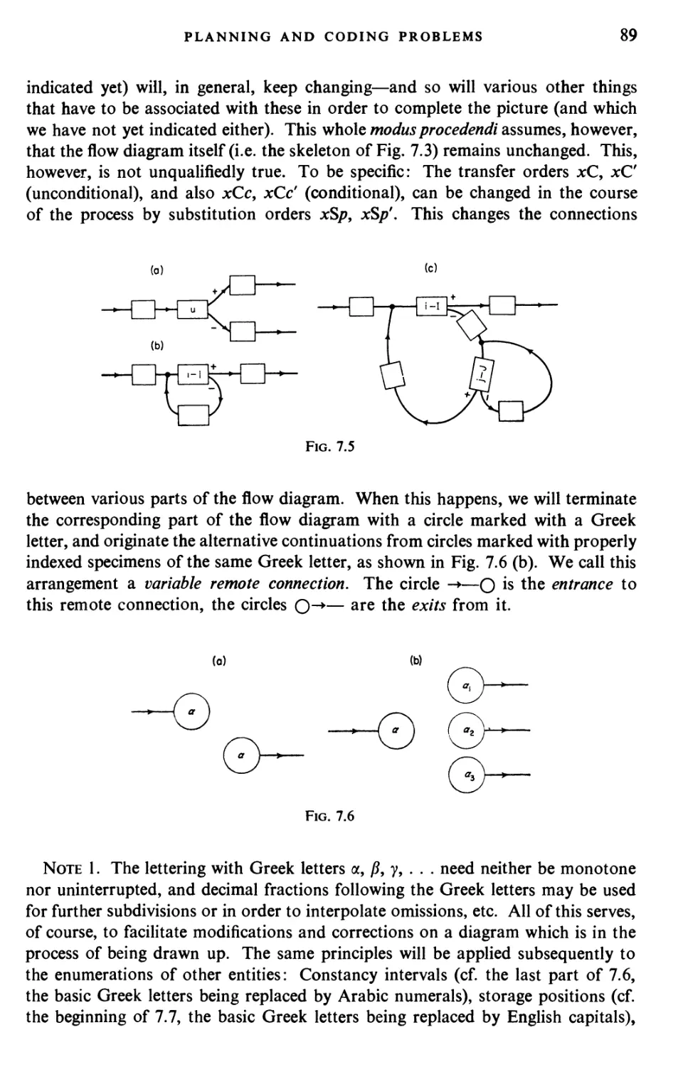
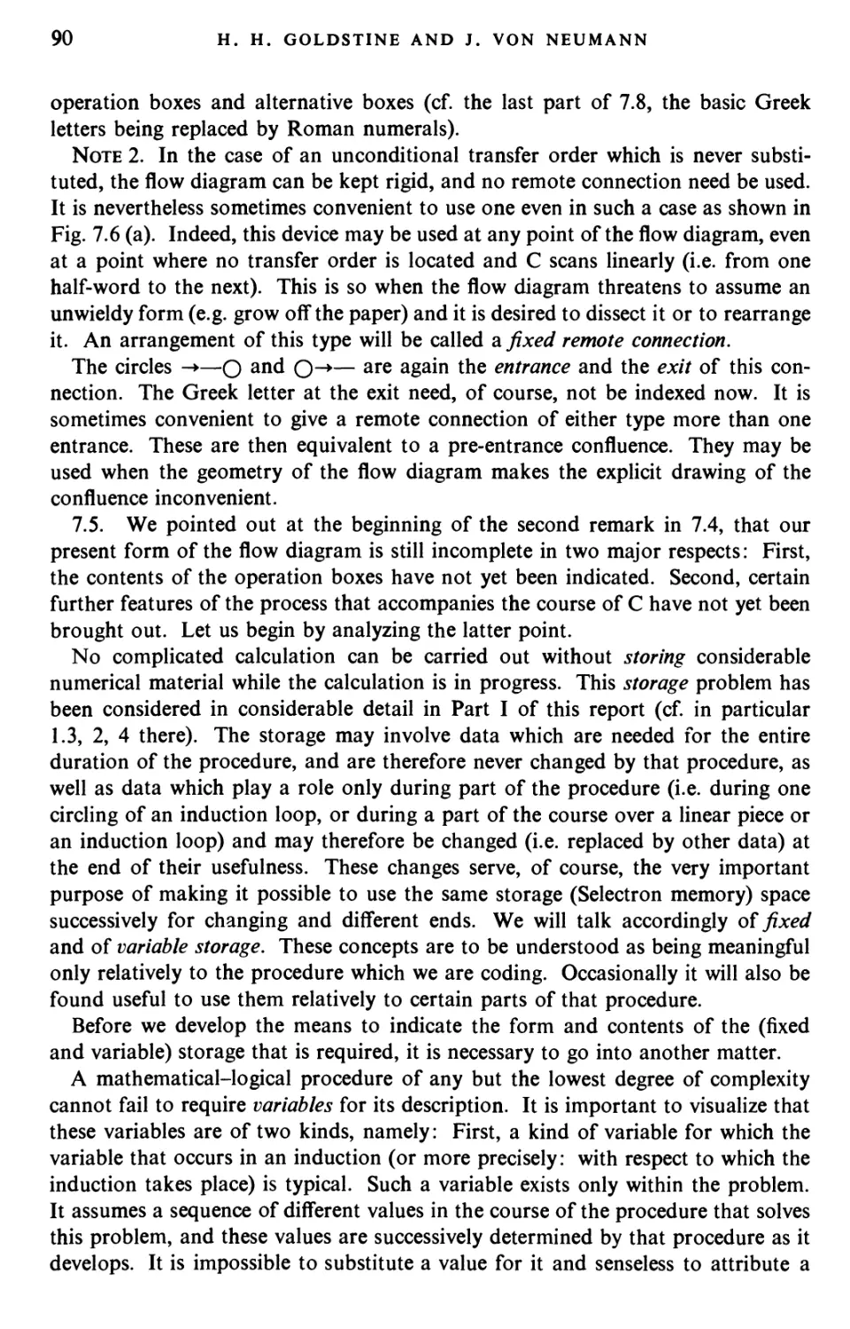
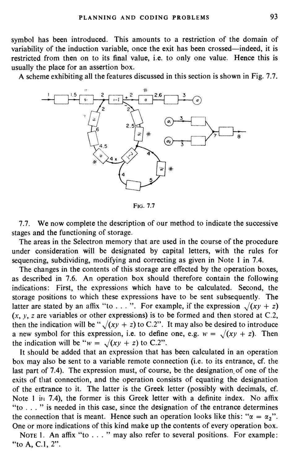
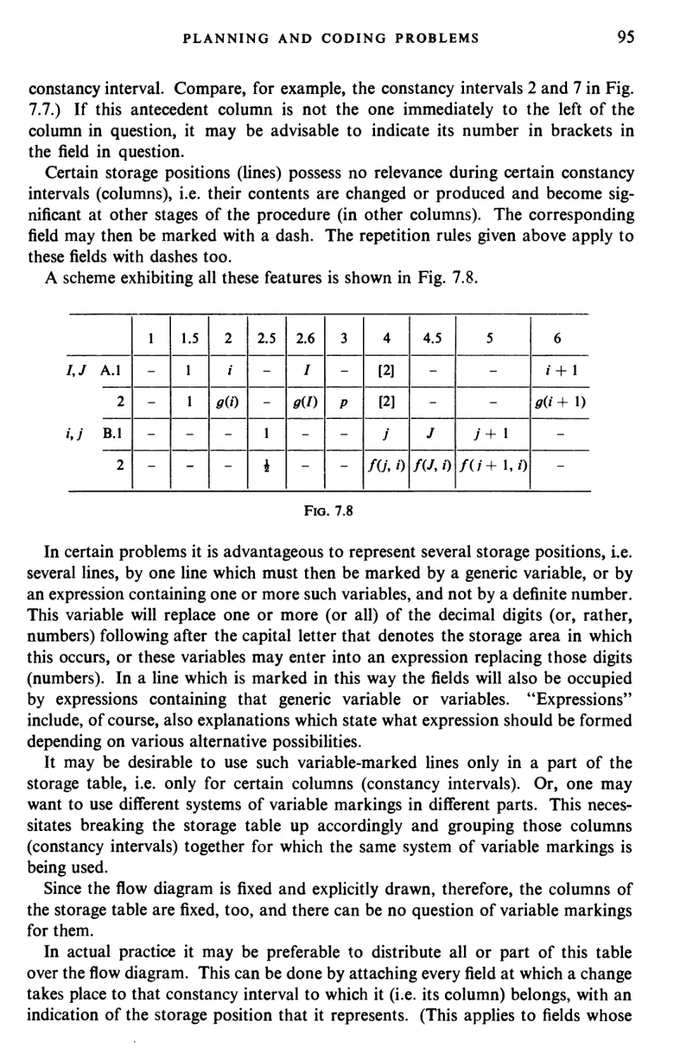
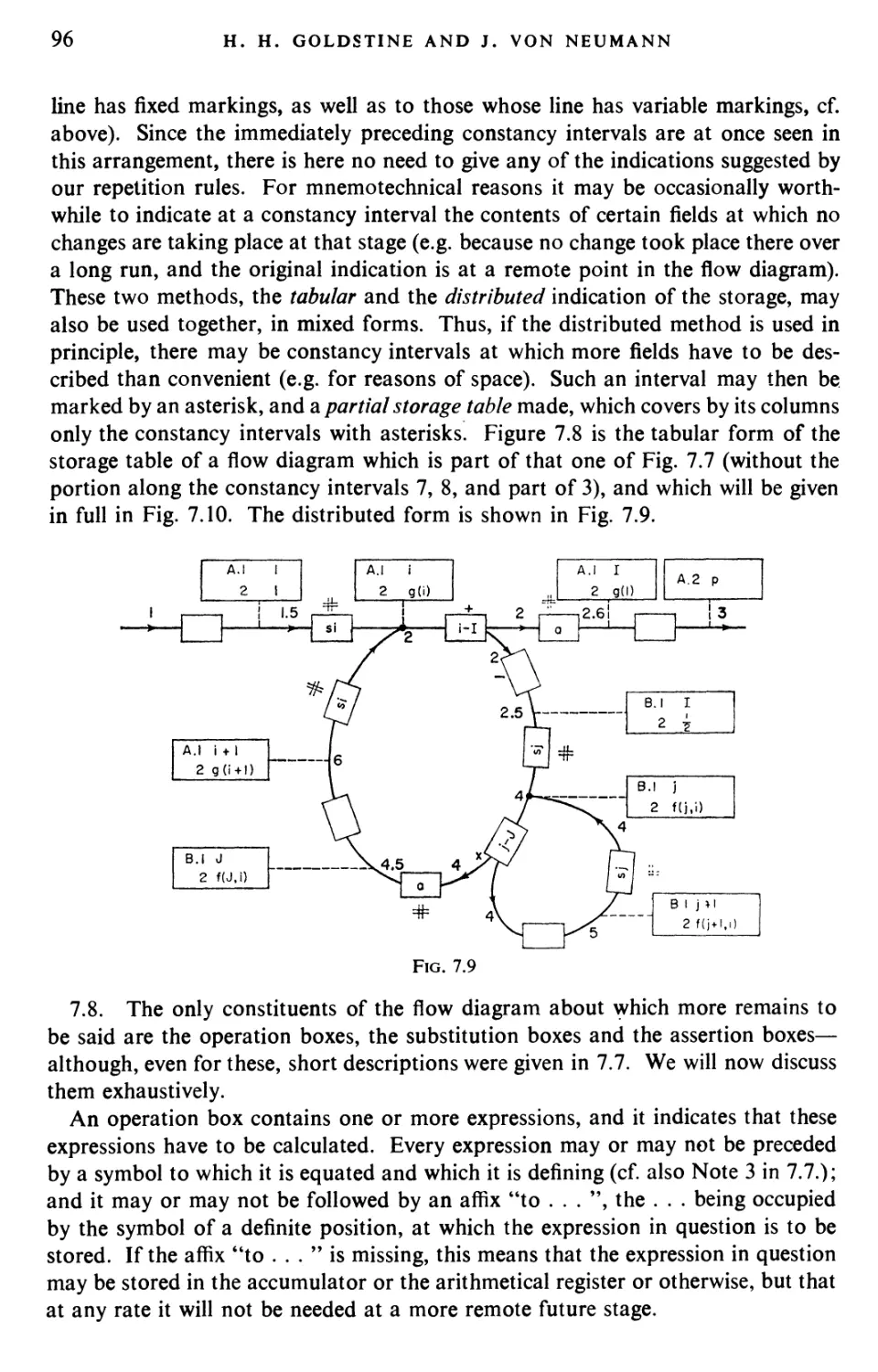
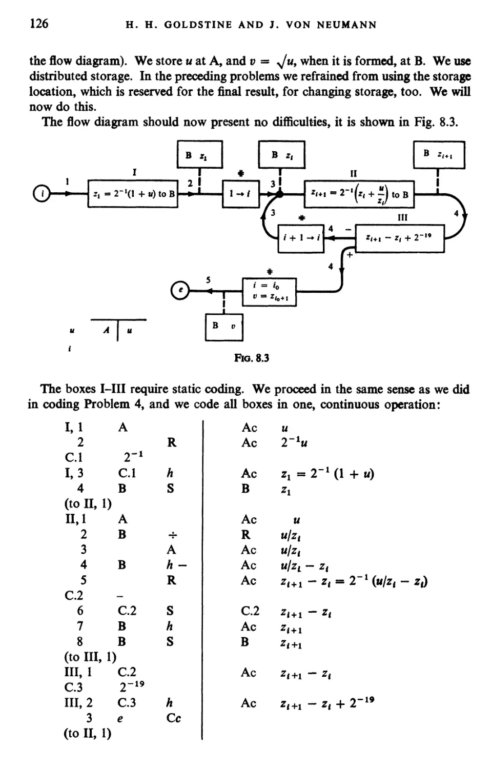
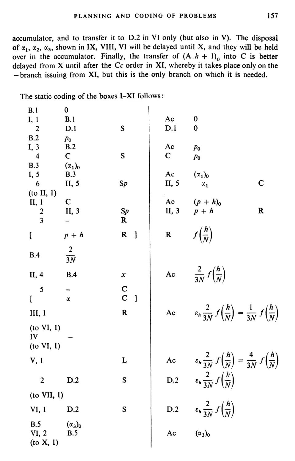
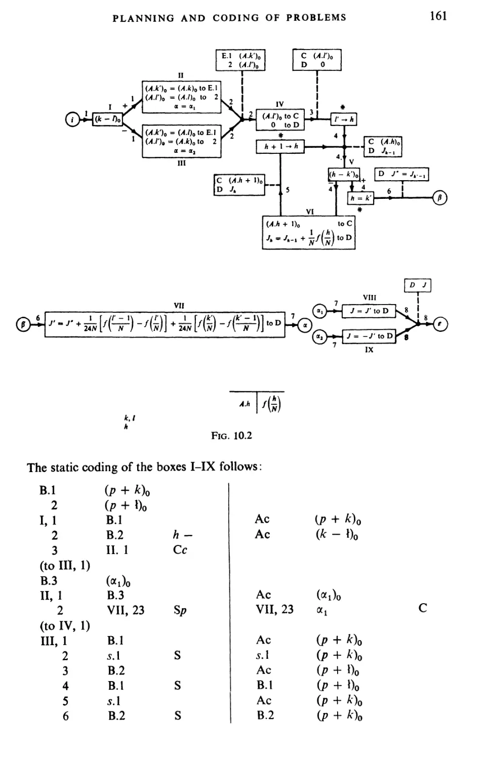
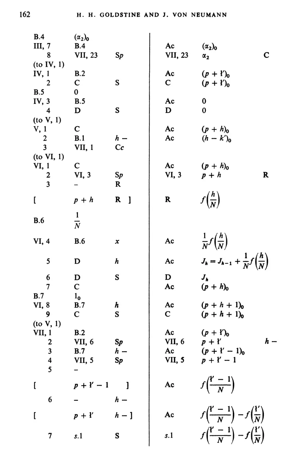
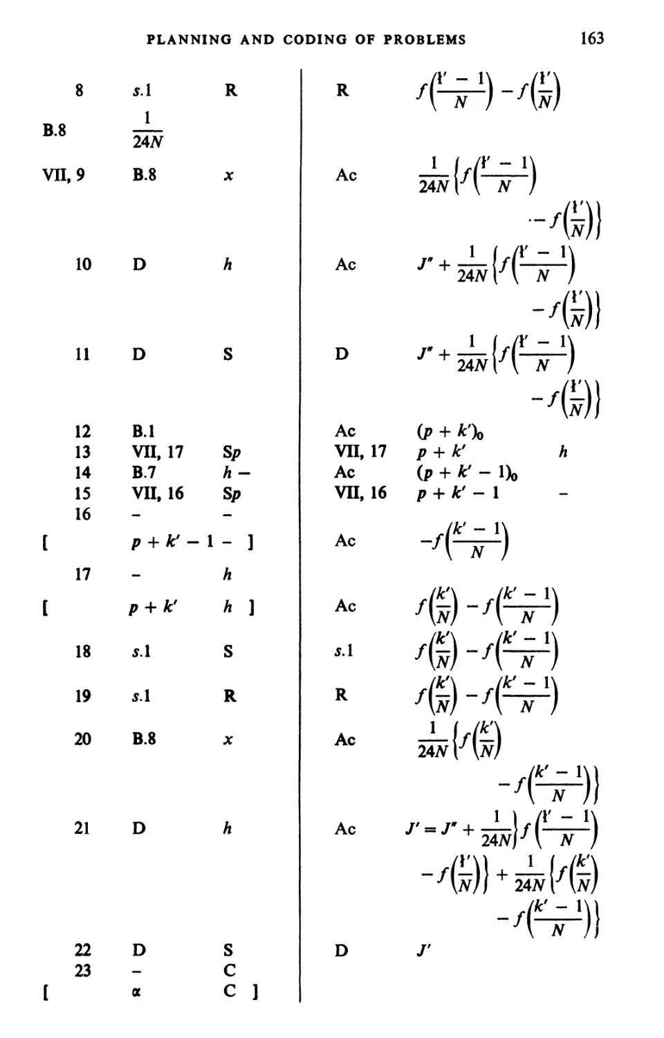
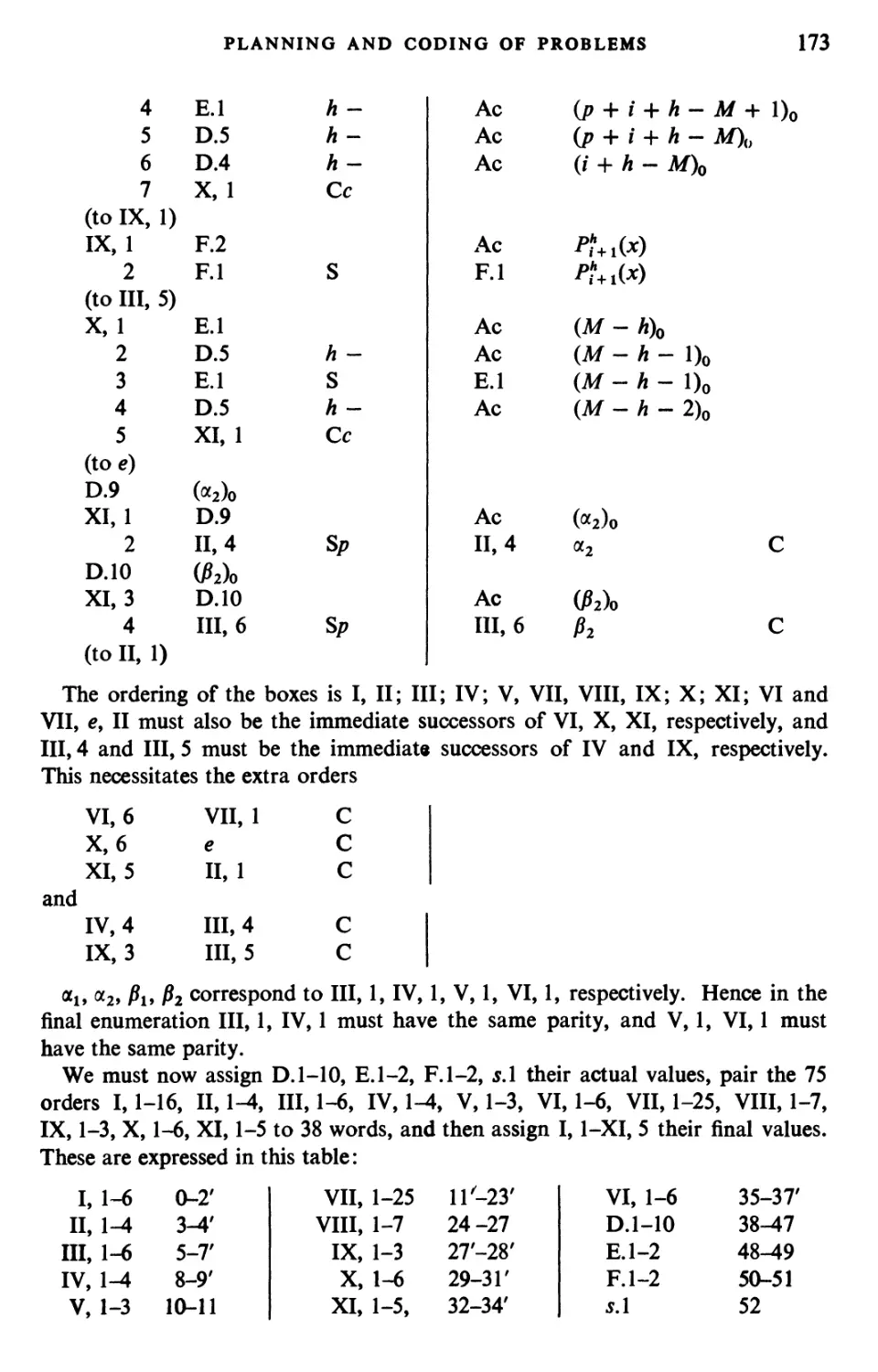
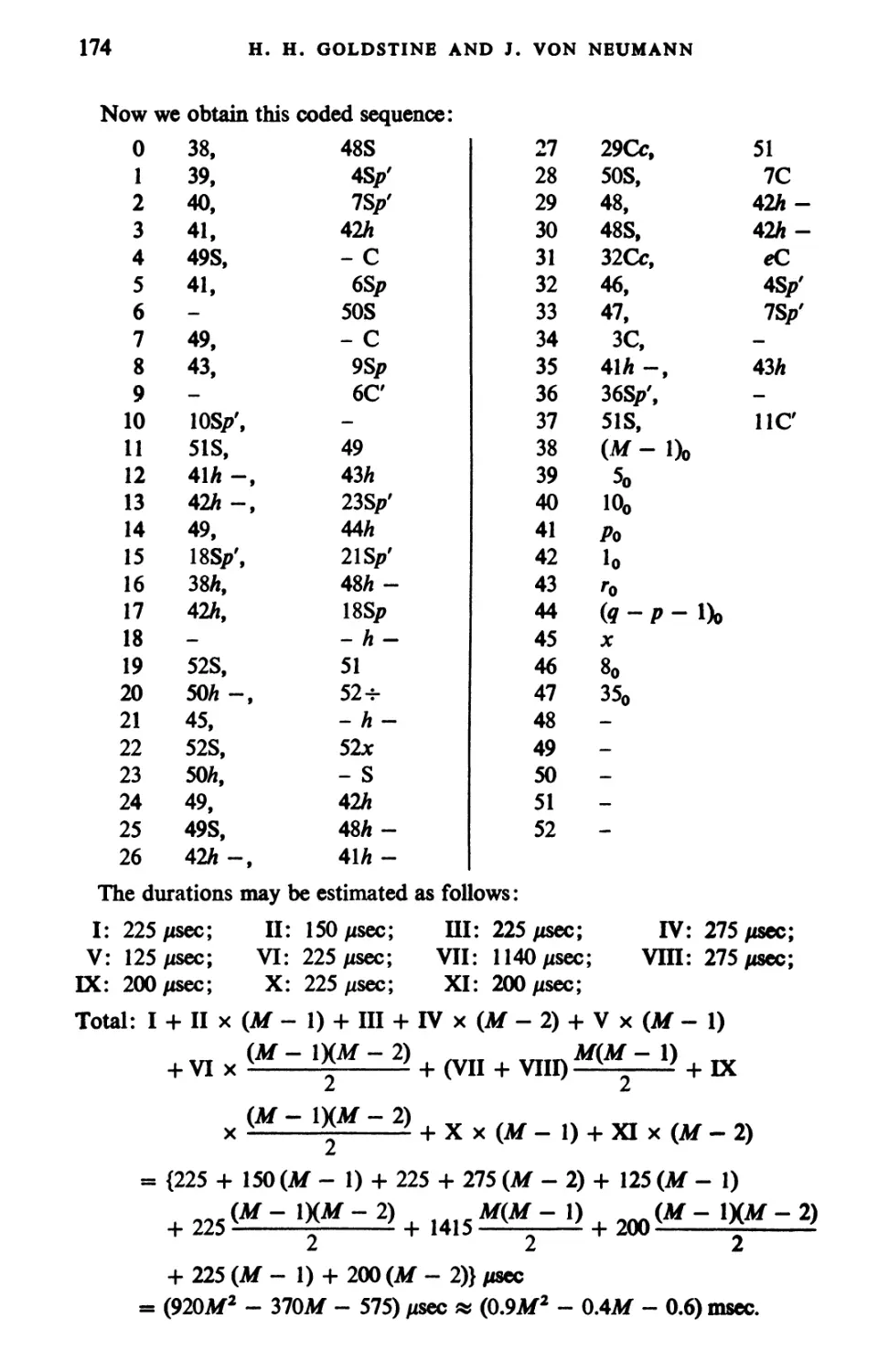
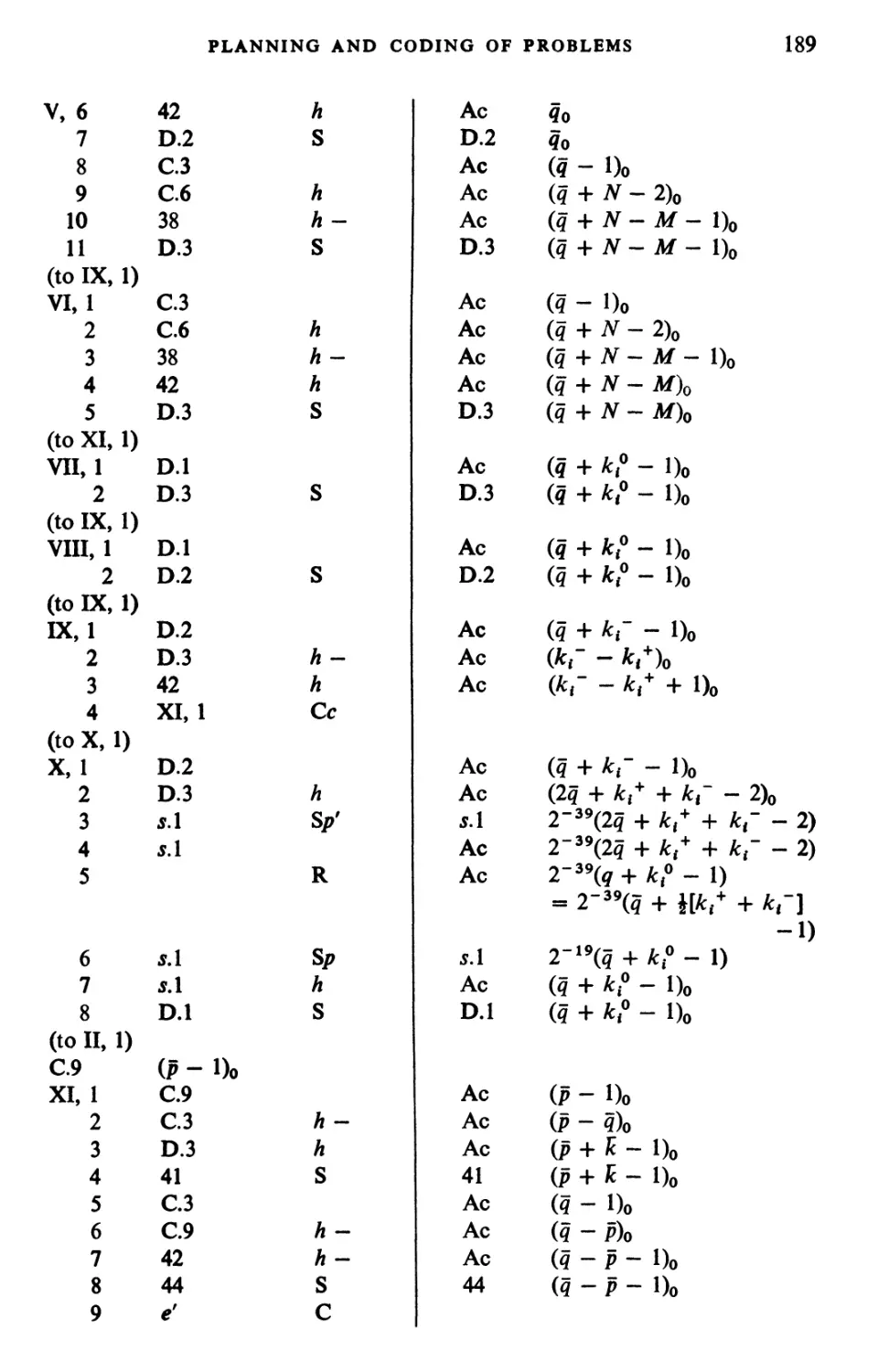
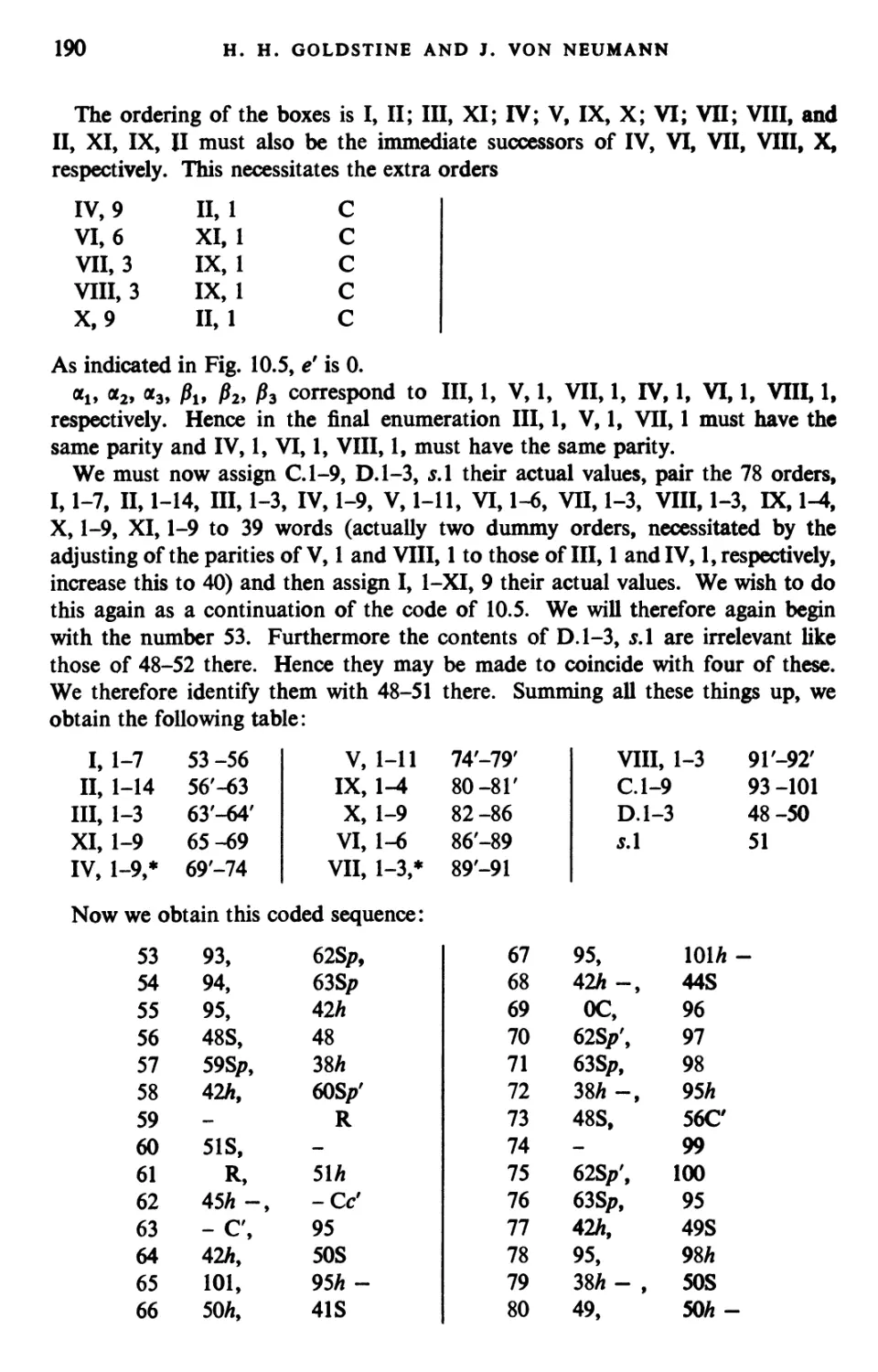
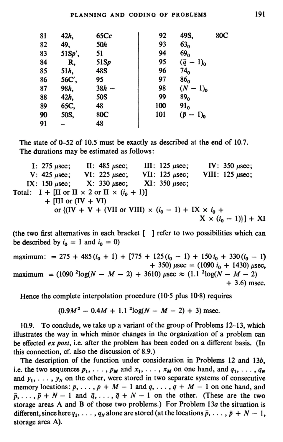
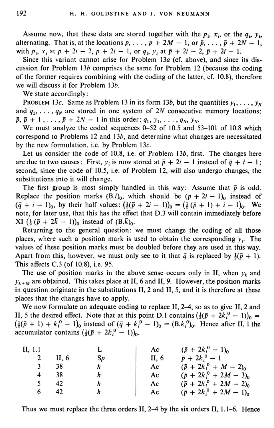
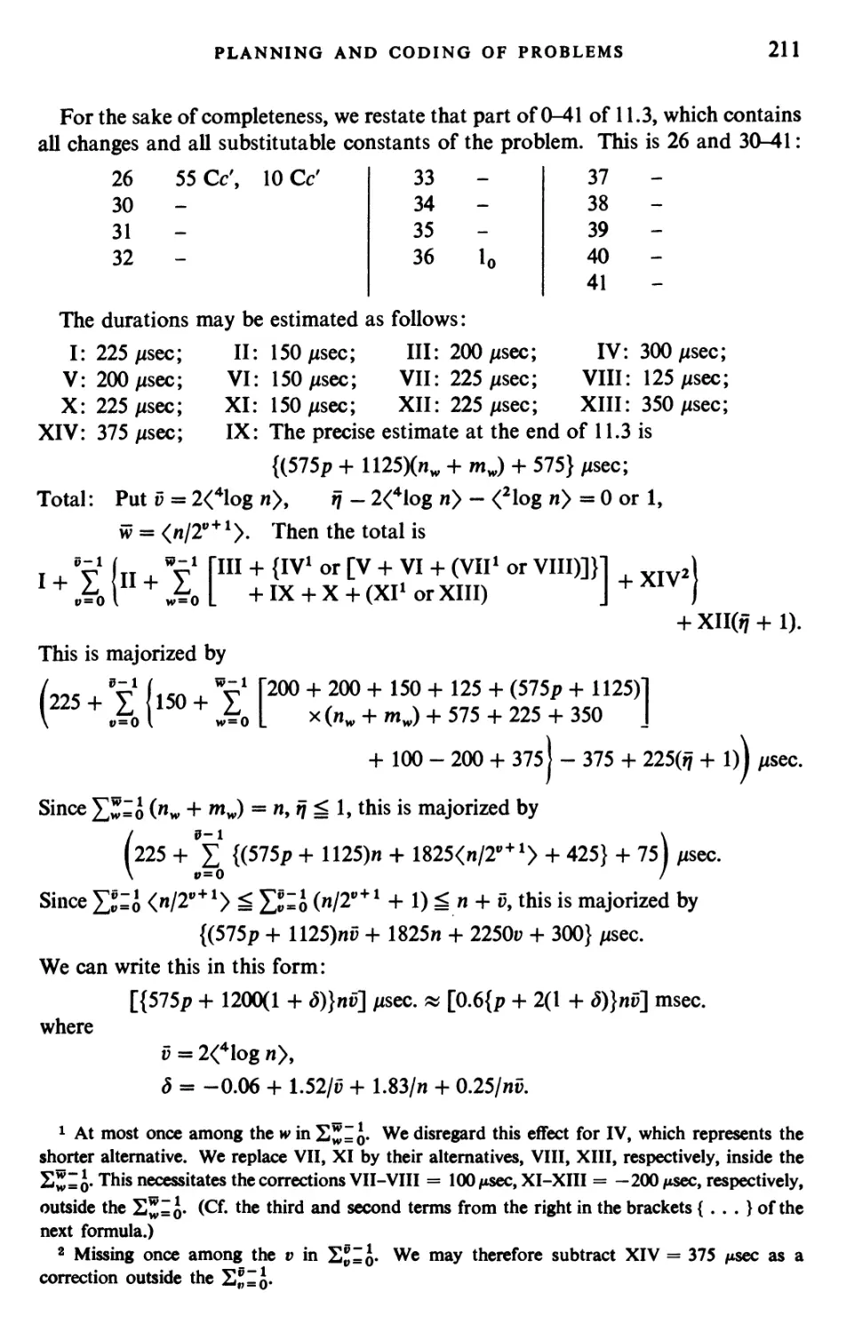
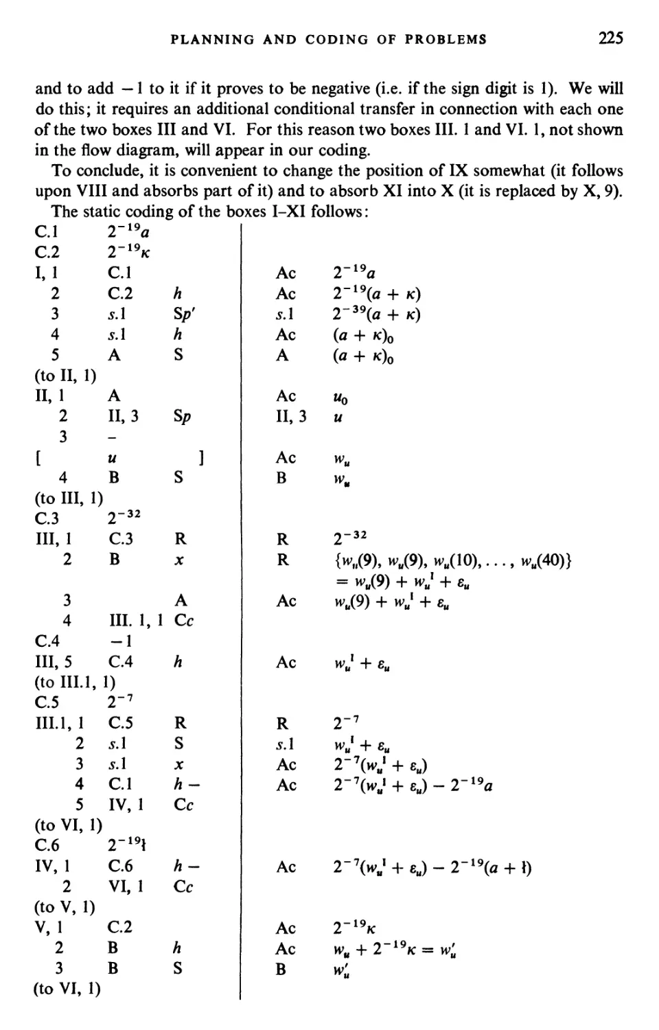
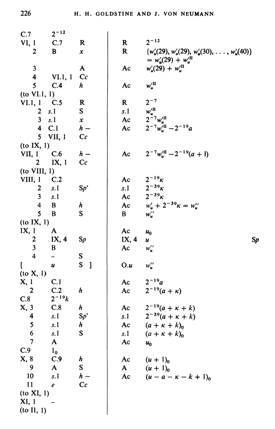
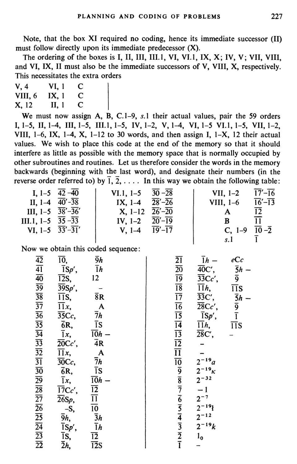
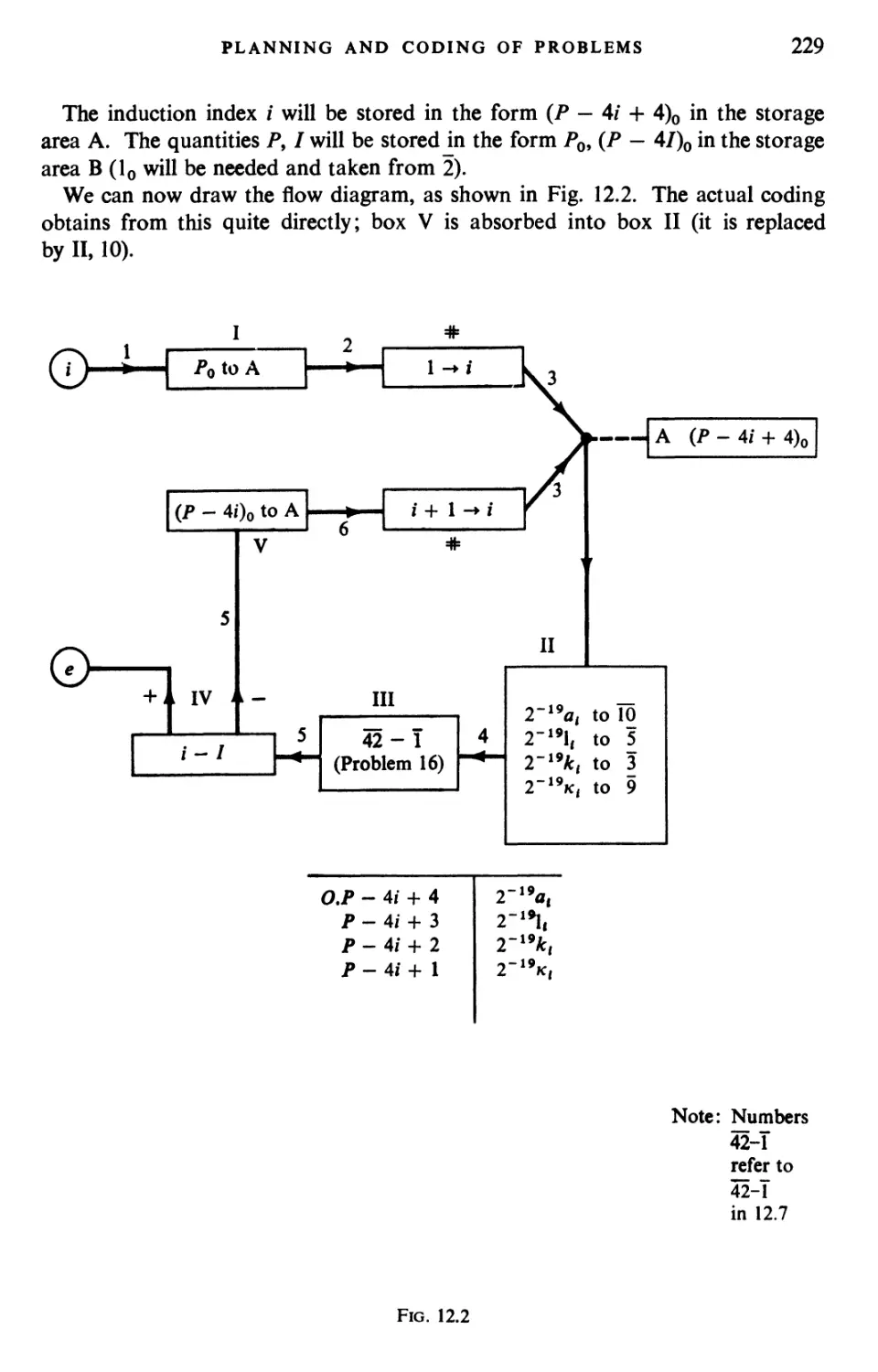
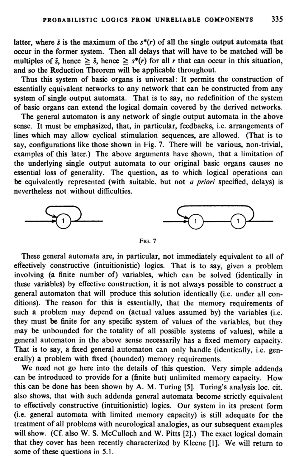
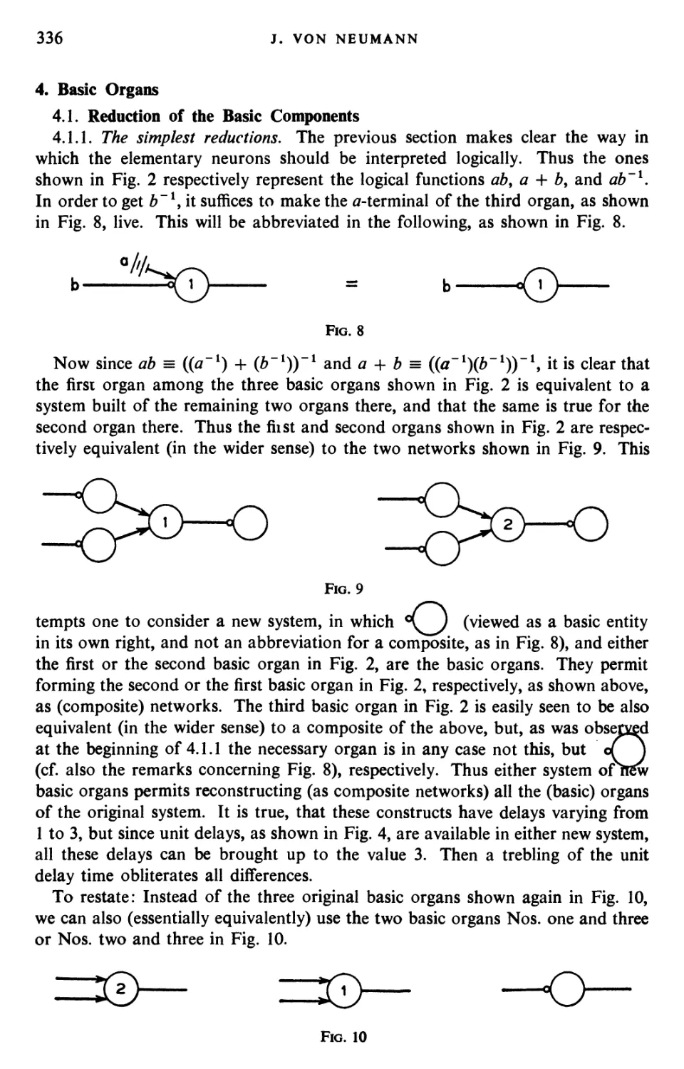
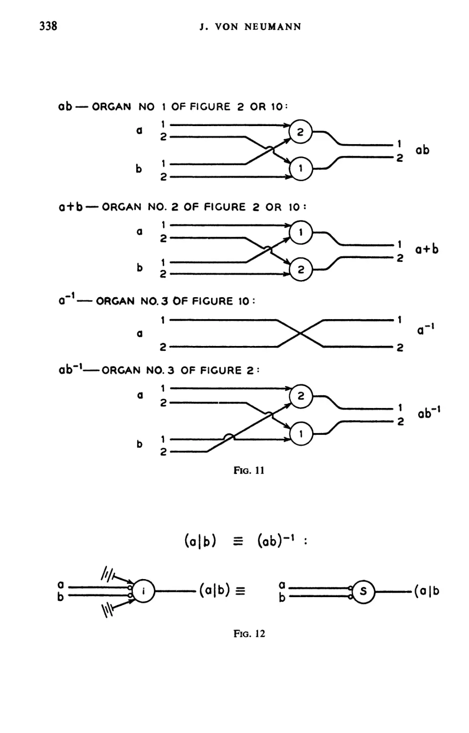
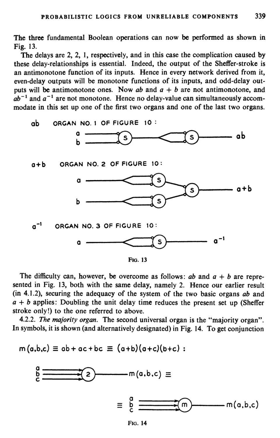
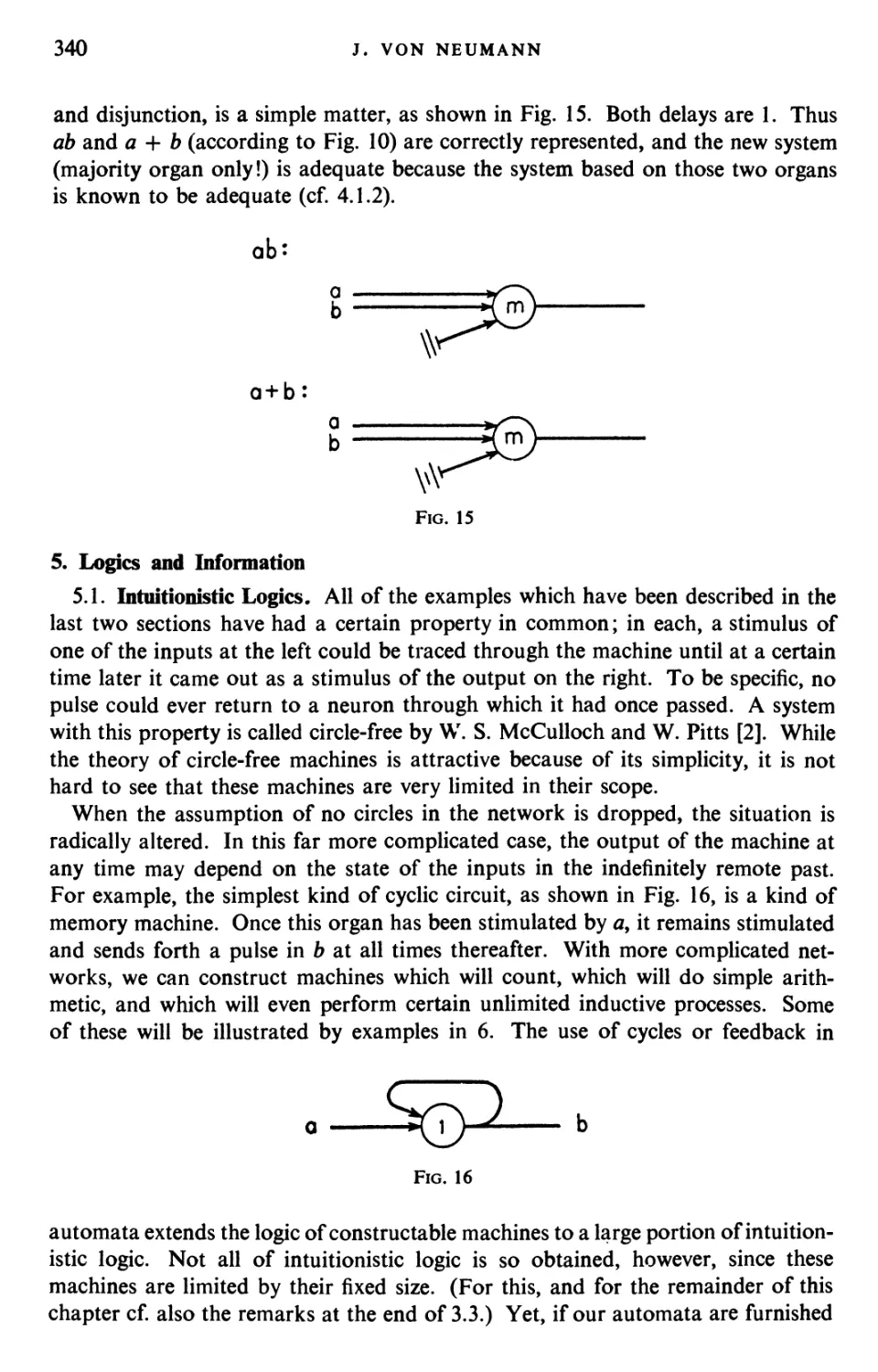
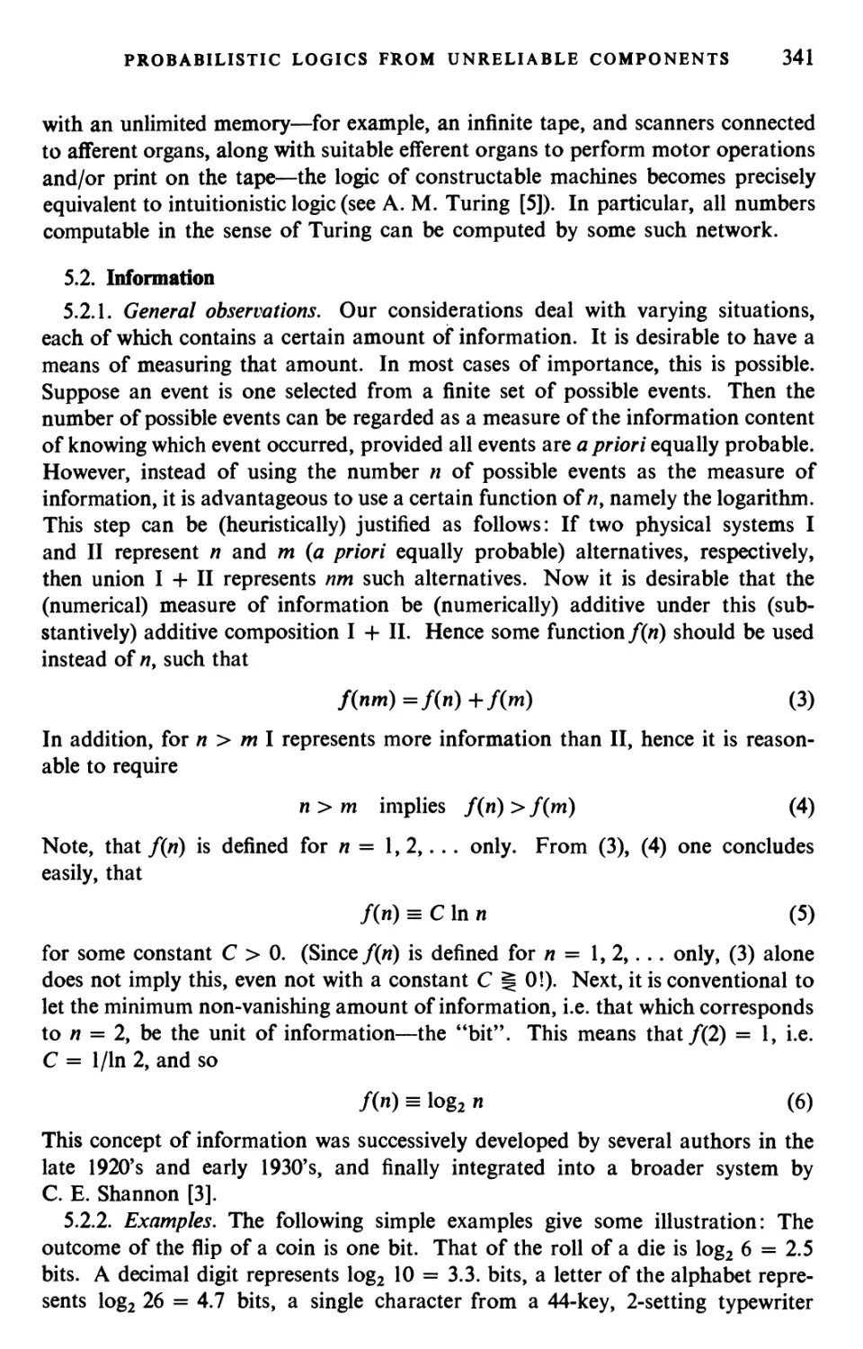
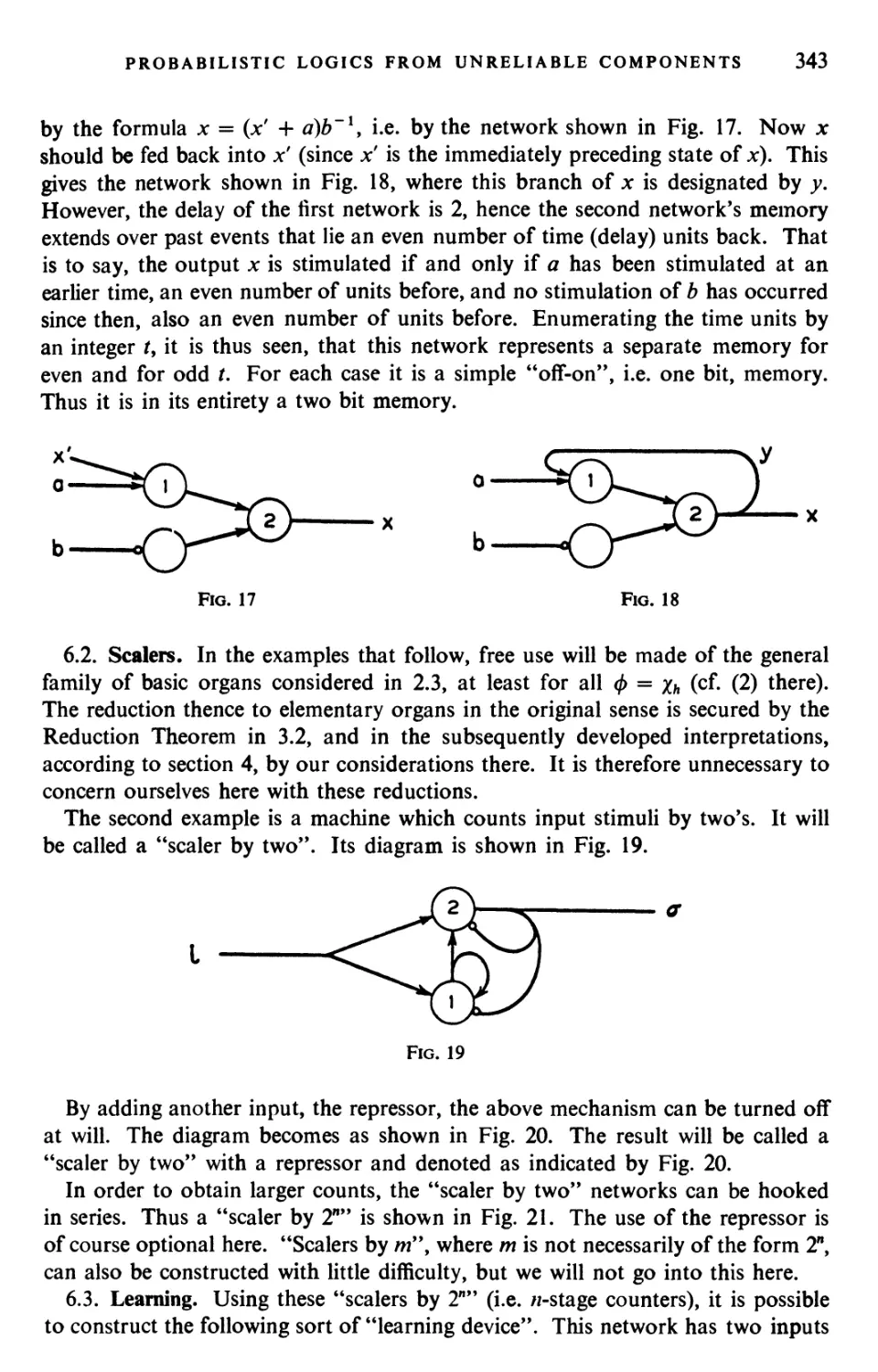
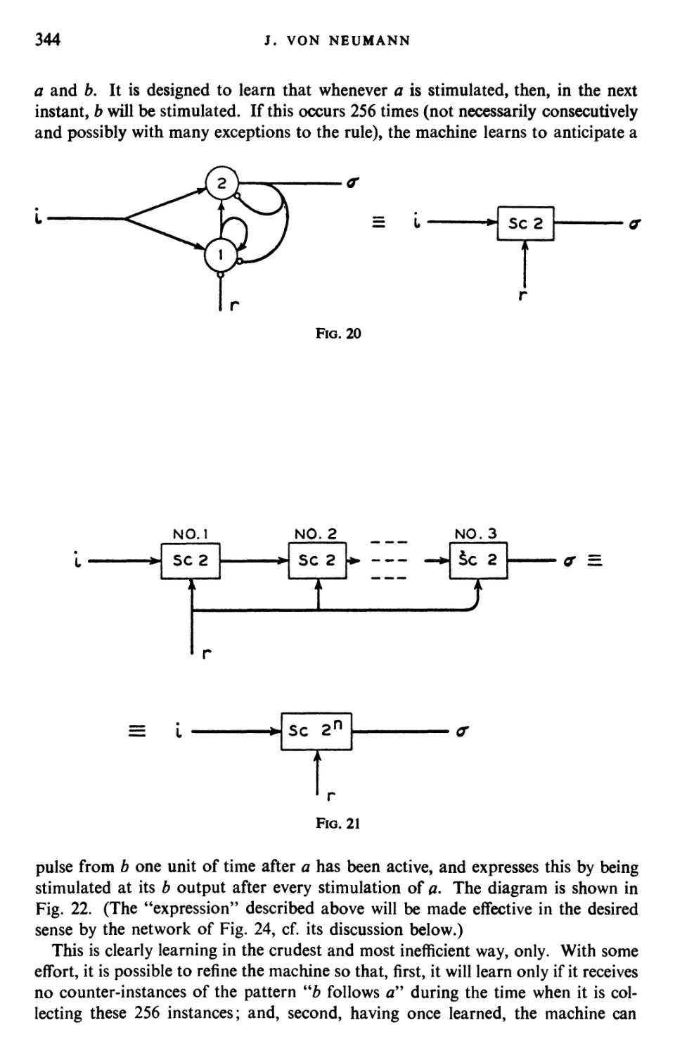
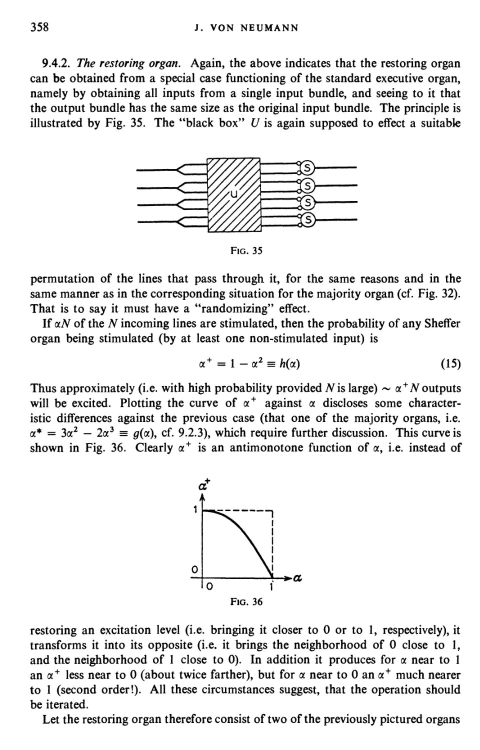
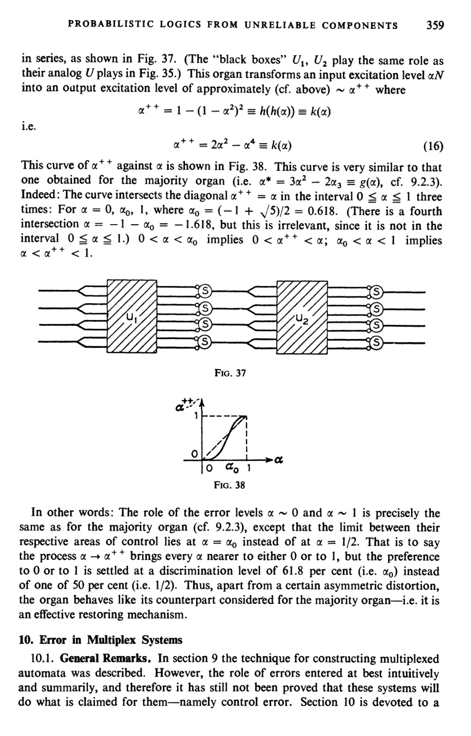
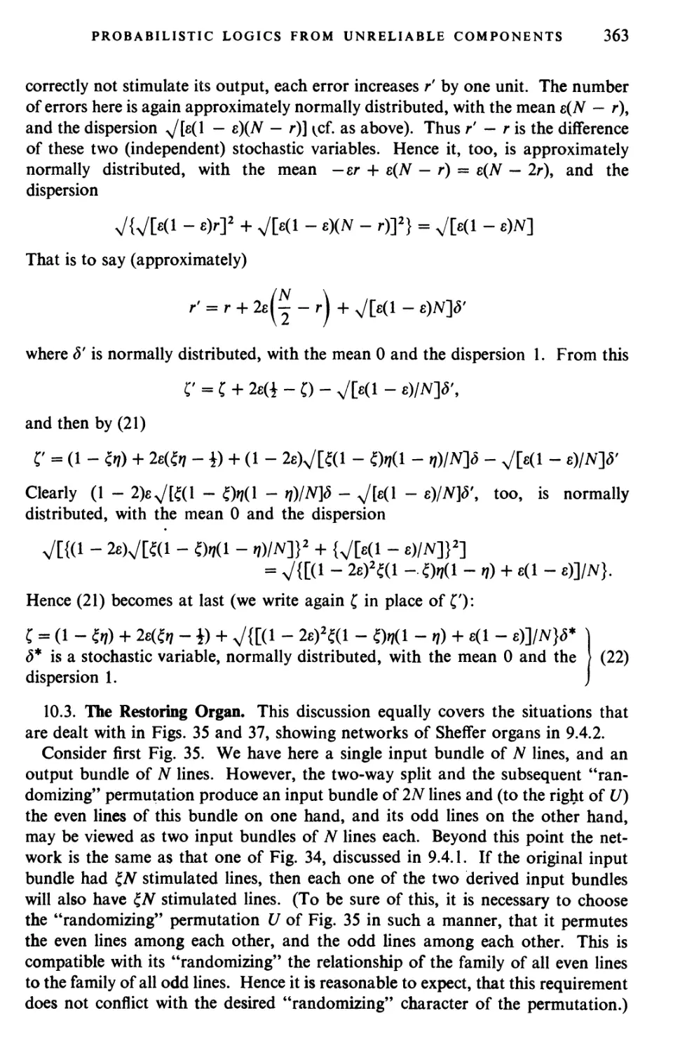
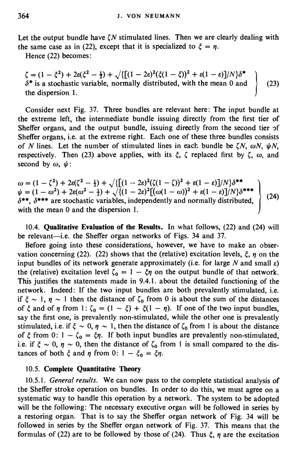
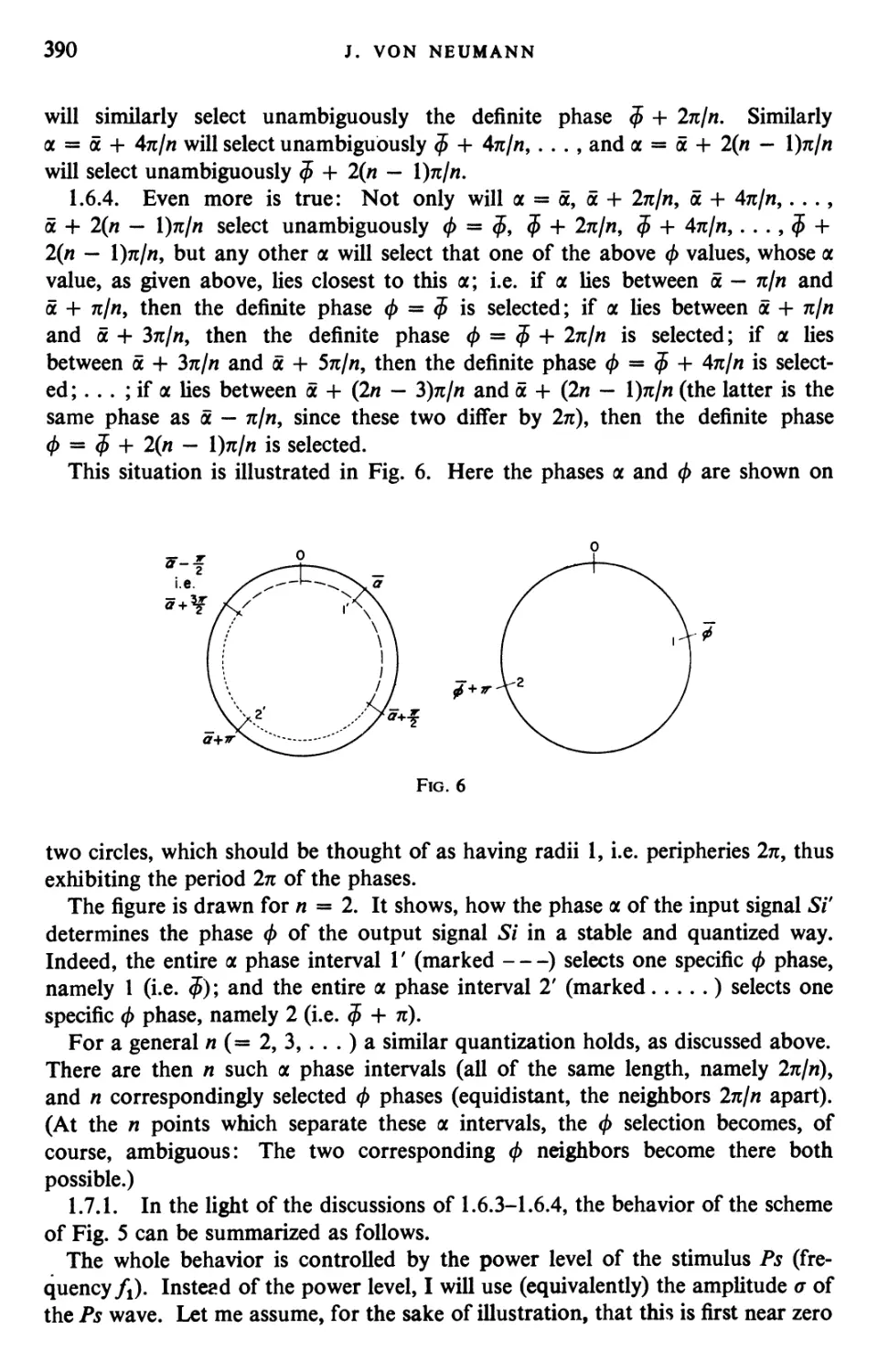
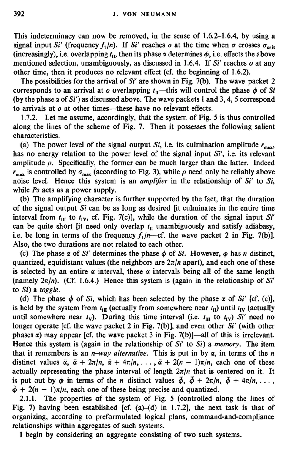
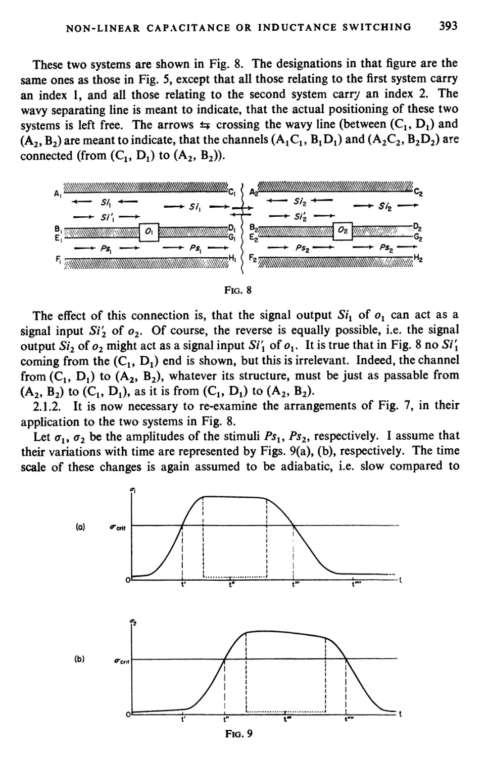
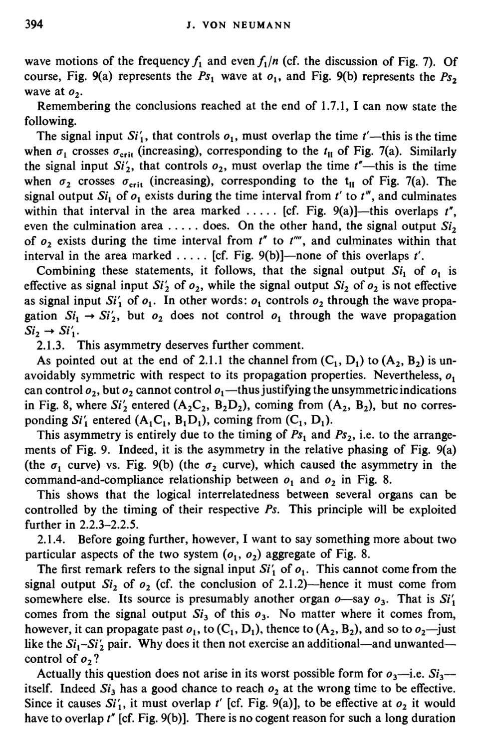
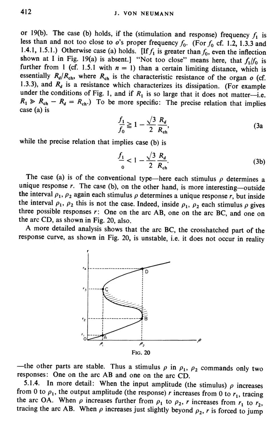
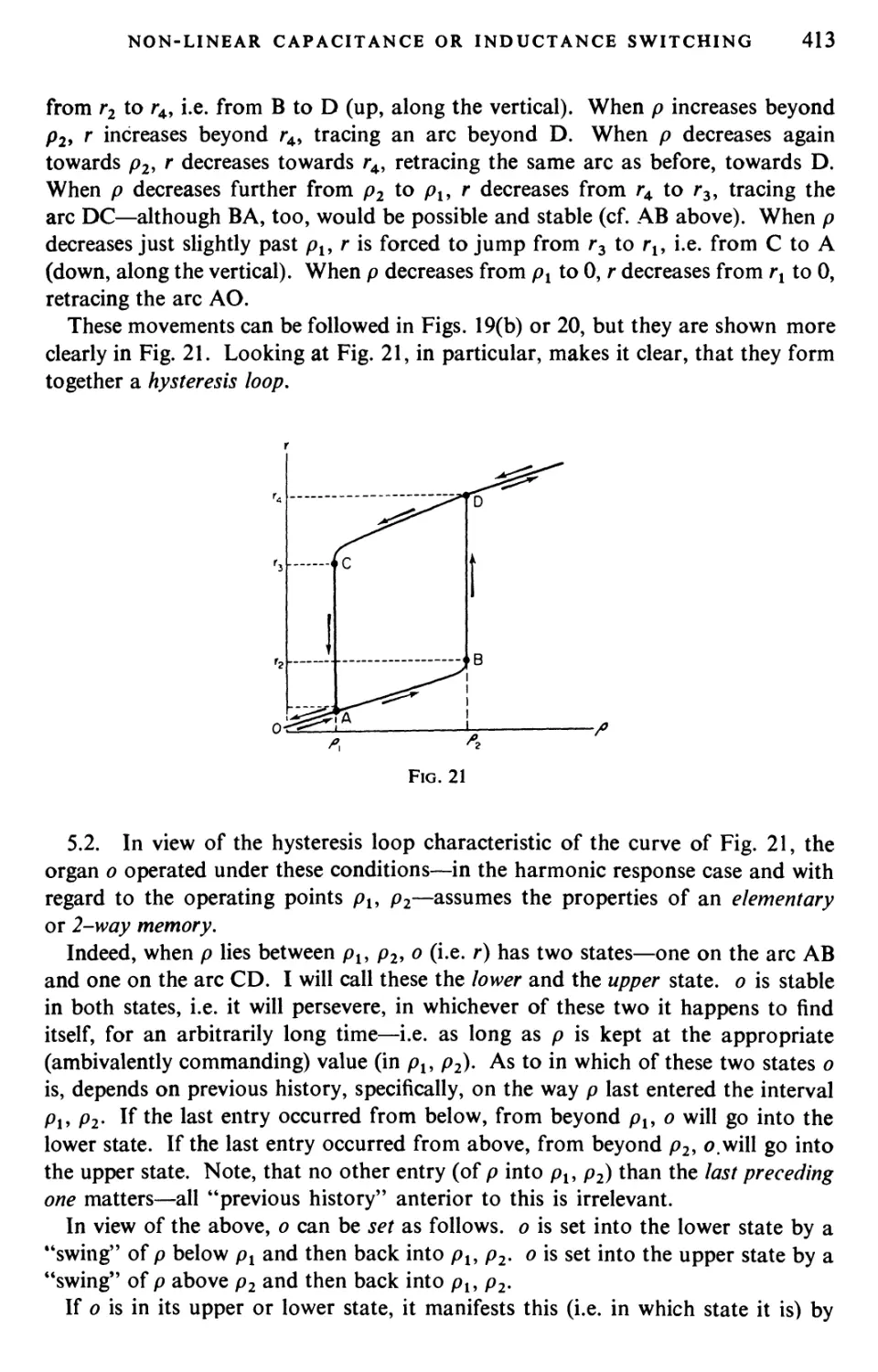
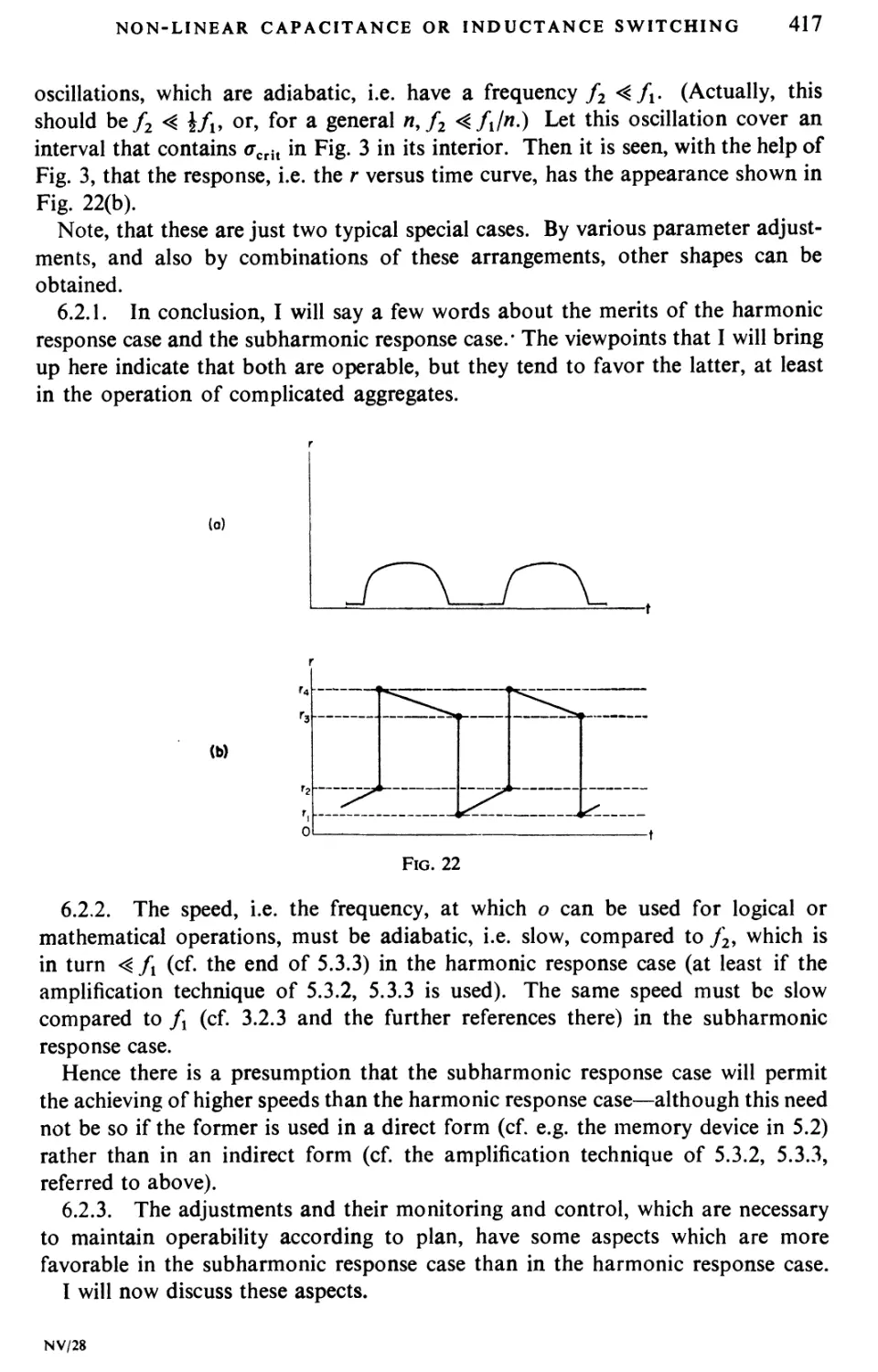
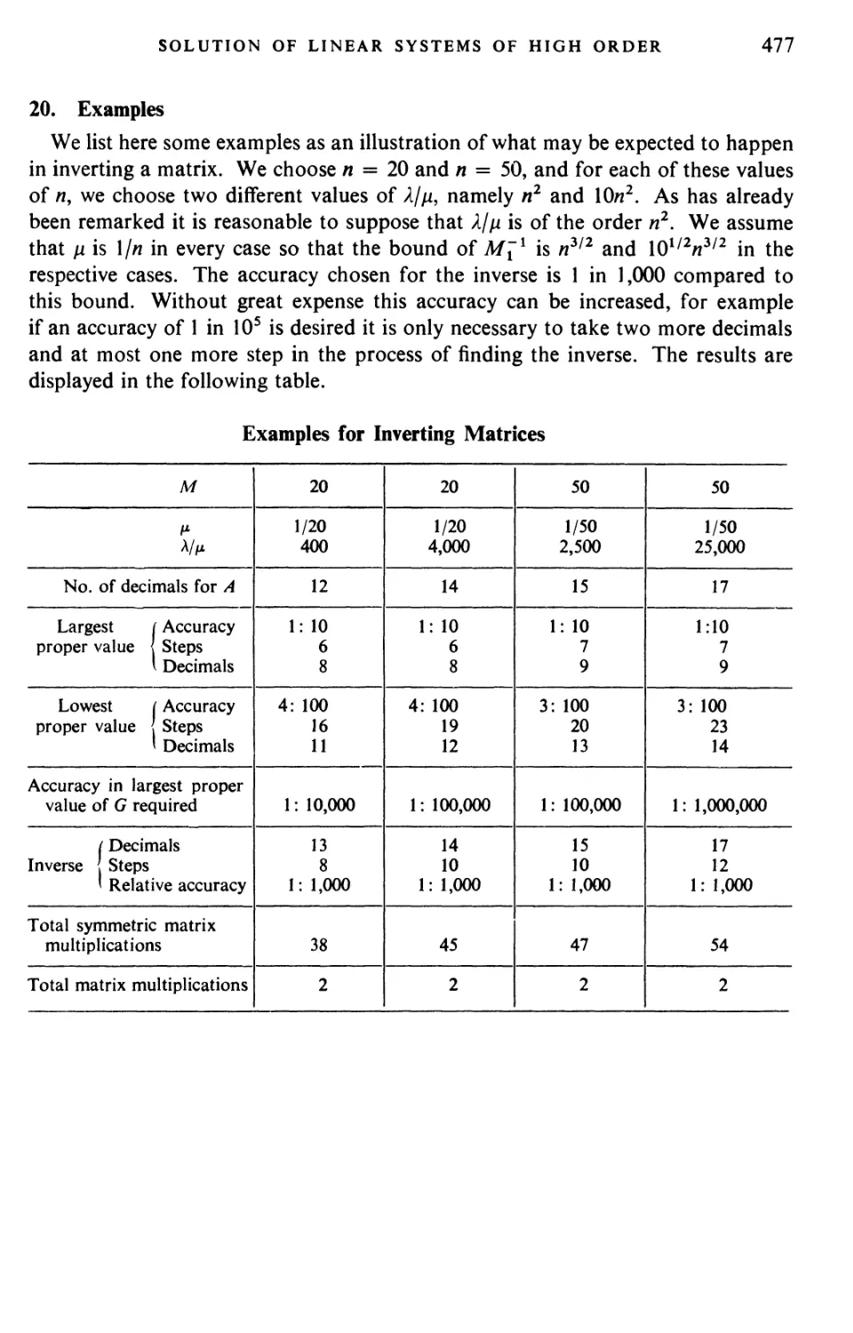
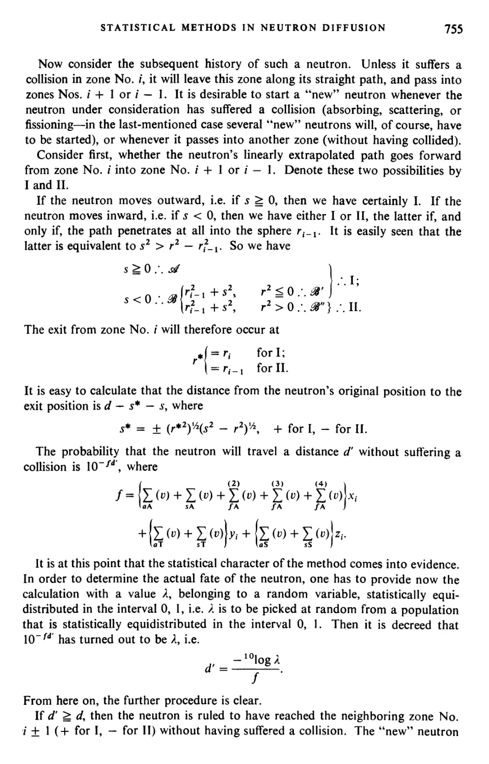
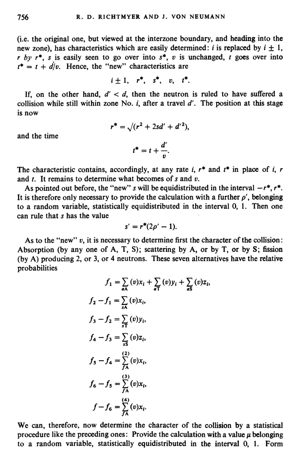
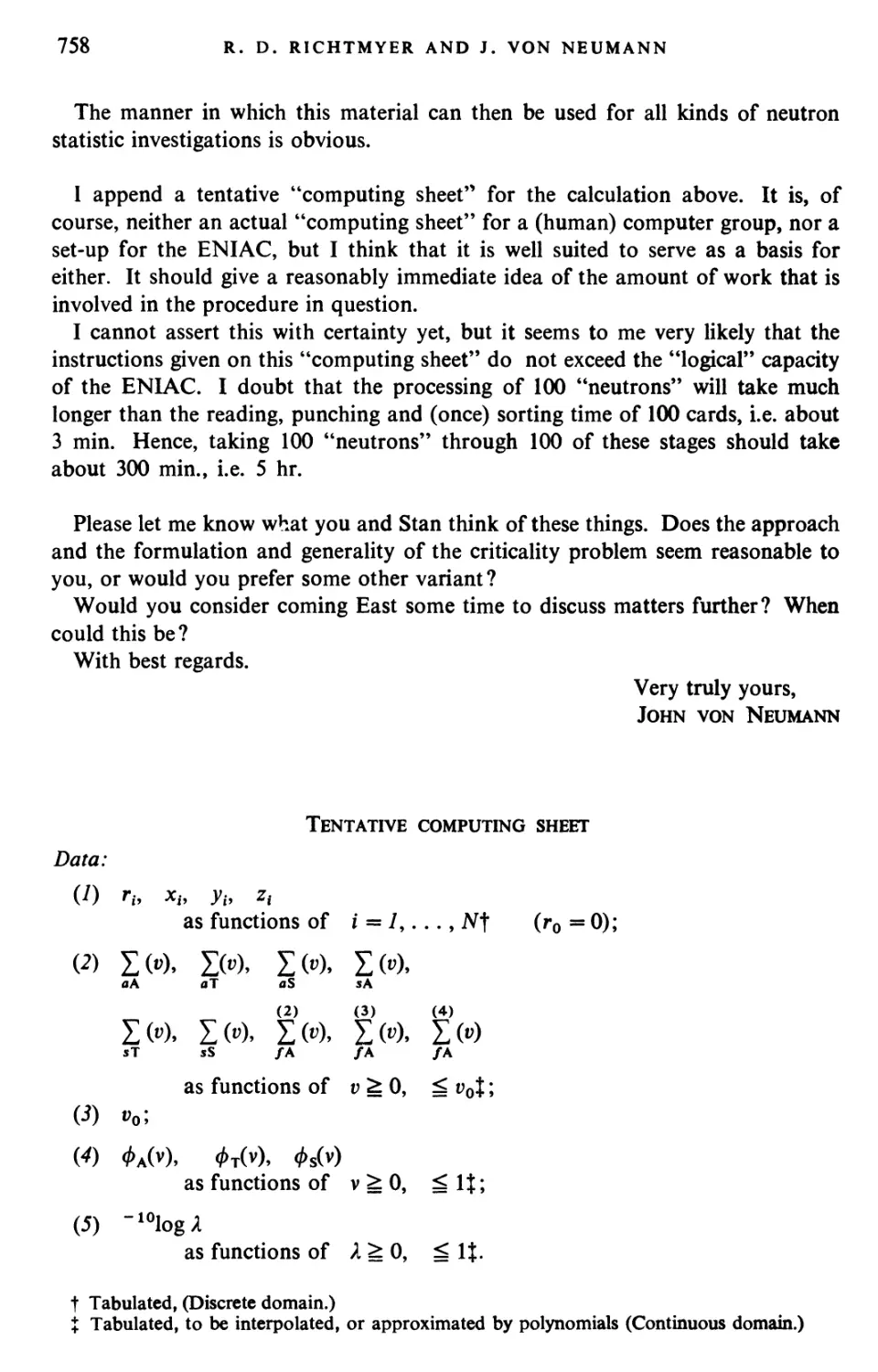
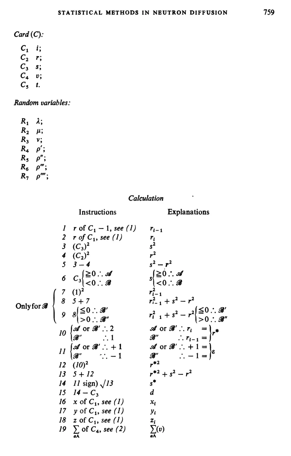
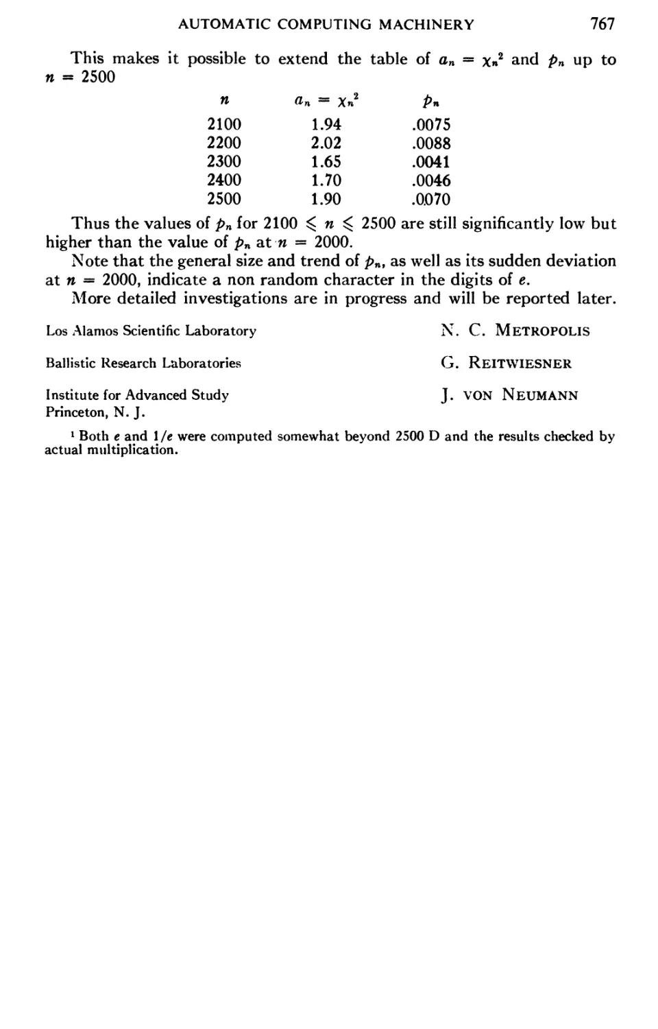
/


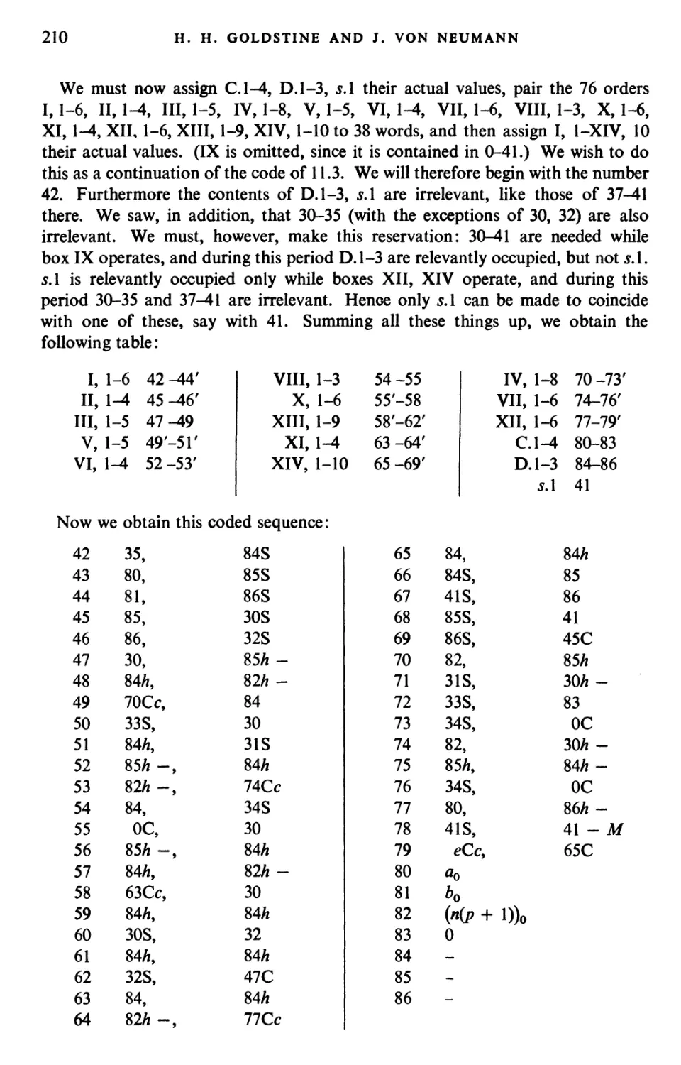


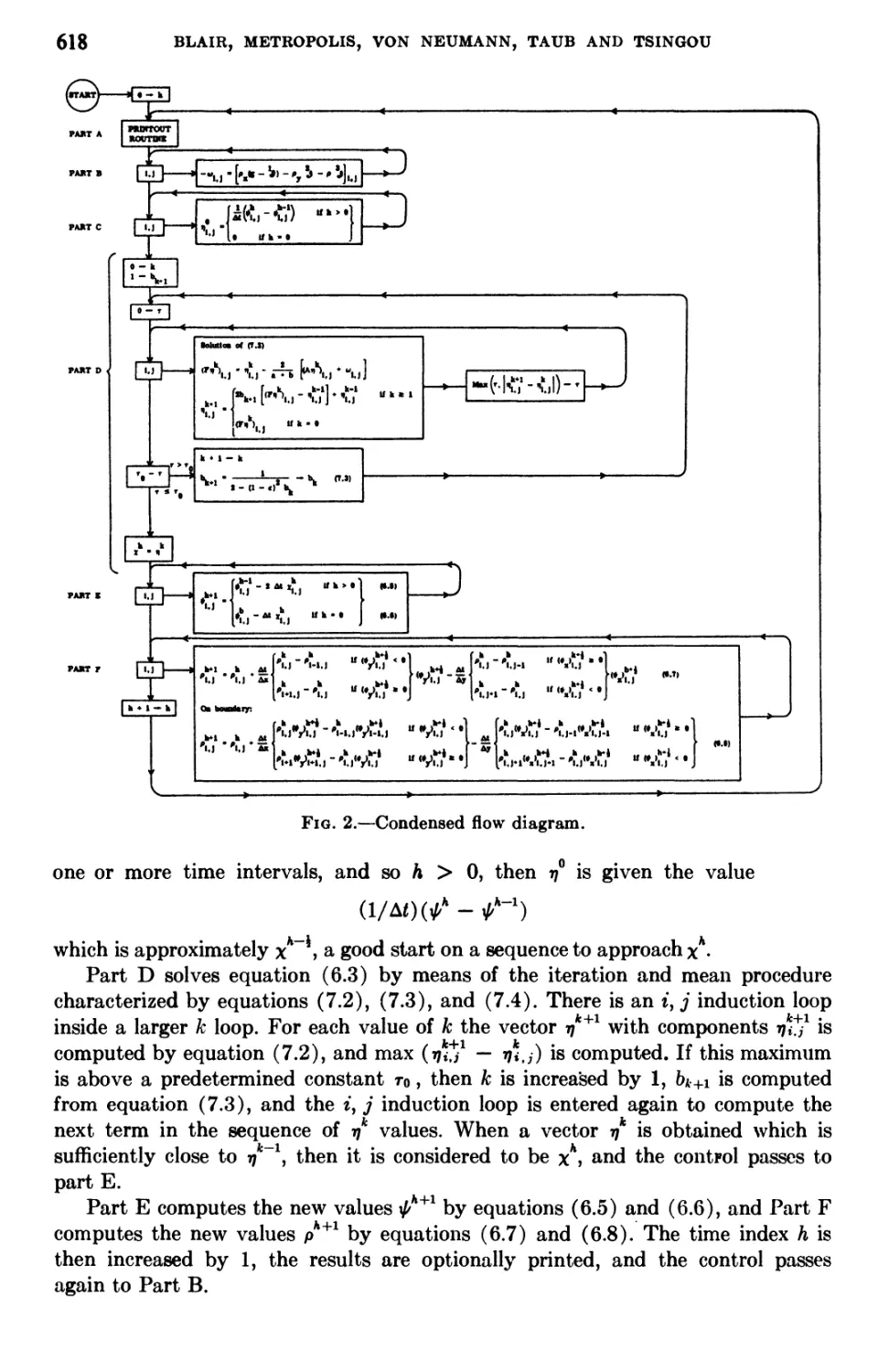


Текст
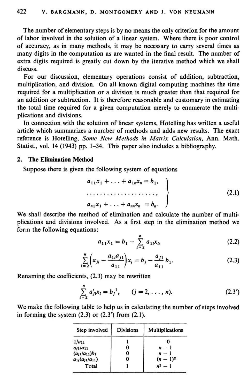
John von Neumann
COLLECTED WORKS
Volume V
DESIGN OF COMPUTERS,
THEORY OF AUTOMATA AND
NUMERICAL ANALYSIS
PUBLISHERS' NOTE
The Publishers wish to express their sincere gratitude for the
kind cooperation received from the publishers pf the various
publications in which the articles reproduced in these collected
works first appeared, and for permission to reproduce this material.
The exact source of each article appears in the Contents List, and
again in the Bibliography, where it is listed under the year of
publication.
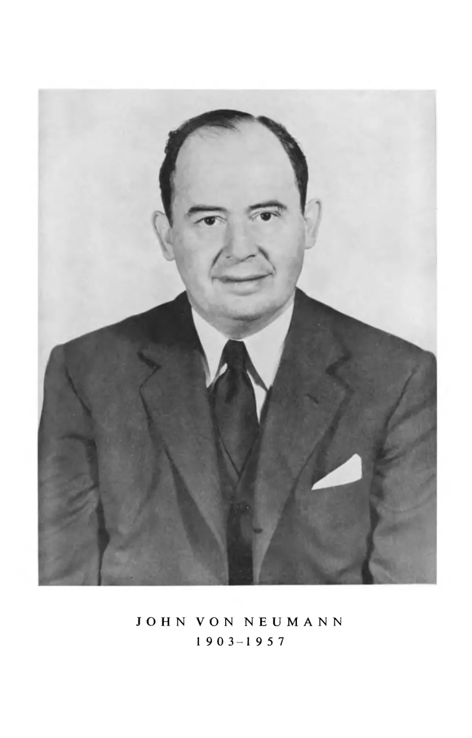
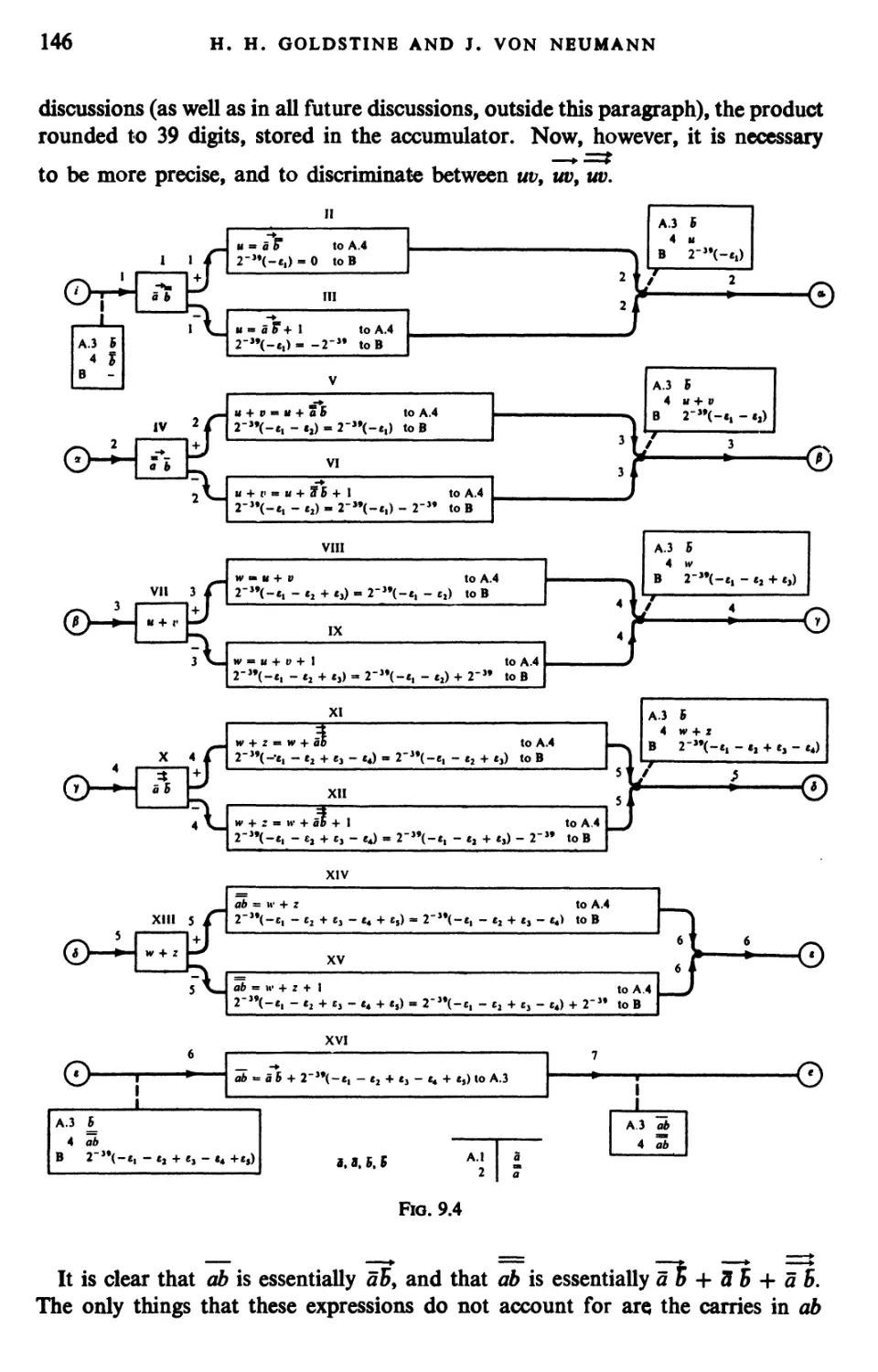
JOHN VON NEUMANN
1903-19 5 7
John von Neumann
COLLECTED WORKS
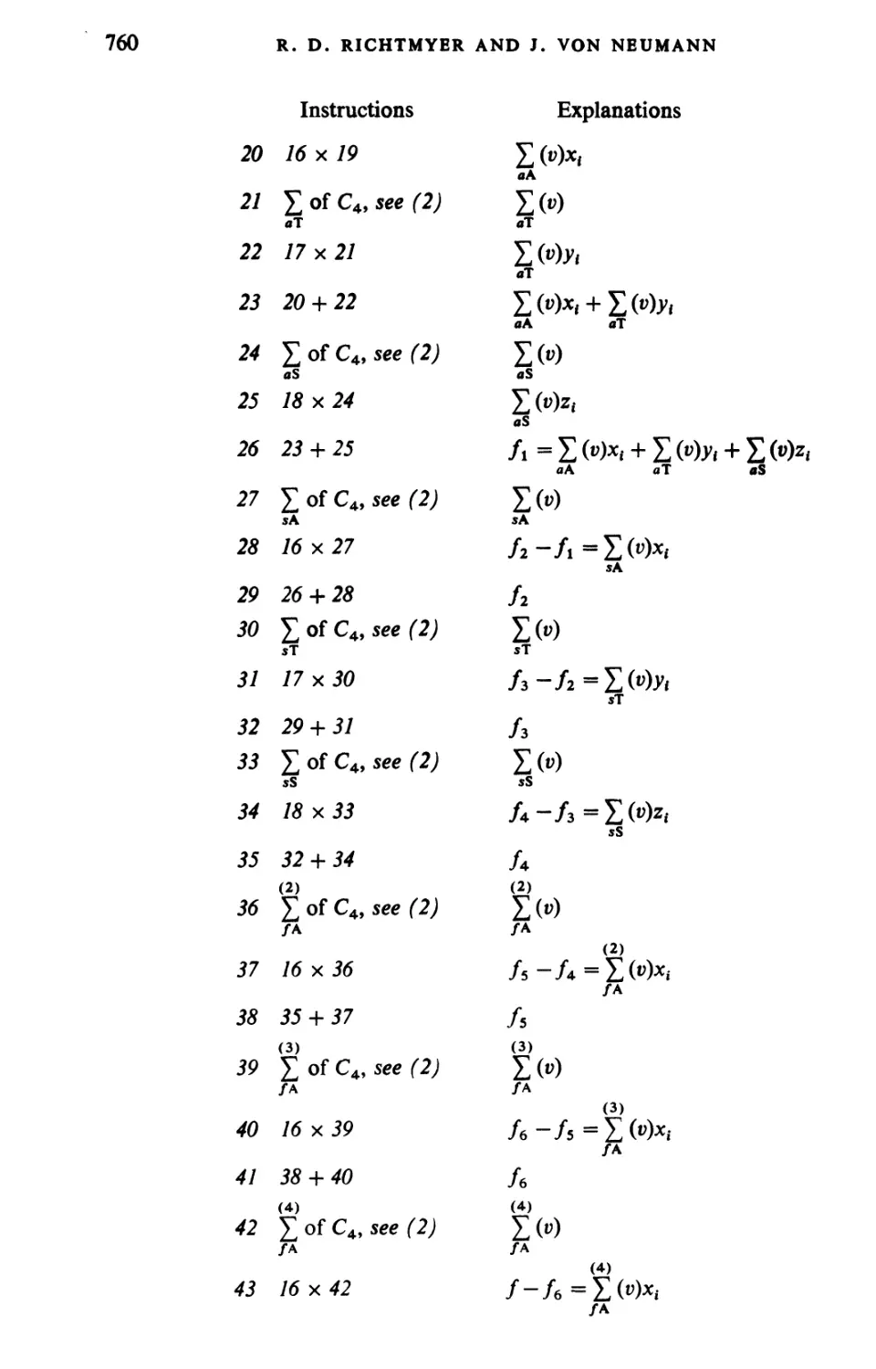
GENERAL EDITOR
A. H. TAUB
RESEARCH PROFESSOR OF APPLIED MATHEMATICS
DIGITAL COMPUTER LABORATORY
UNIVERSITY OF ILLINOIS
Volume V
DESIGN OF COMPUTERS,
THEORY OF AUTOMATA AND
NUMERICAL ANALYSIS
PERGAMON PRESS
OXFORD • LONDON • NEW YORK • PARIS
1963
PERGAMON PRESS LTD.
Headington Hill Hall, Oxford
4 & 5 Fitzroy Square, London WA
GAUTHIER-VILLARS
55 Quai des Grands-August ins, Paris 6
PERGAMON PRESS G.m.b.H.
Kaiserstrasse 75, Frankfurt am Main
Distributed in the Western Hemisphere by
THE MACMILLAN COMPANY • NEW YORK
pursuant to a special agreement with
PERGAMON PRESS LIMITED
Oxford, England
This Compilation
Copyright © 1961
Pergamon Press Ltd.
Library of Congress Catalog Card No. 59-14497
Printed in Great Britain by
PERGAMON PRINTING AND ART SERVICES LTD.
LONDON
ACKNOWLEDGEMENT
The publication of the six volumes of the collected works of John von Neumann
represents an imposing burden of work, great and broad knowledge, and
time-consuming research. It would hardly have been possible to make this
collection available to the scientific community, and surely not in so short a time,
had it not been for the welcome fact that Dr. A. H. Taub volunteered to undertake
the labor of assembling and editing the manuscript. His dedication and the
unselfish and intensive concentration with which he handled the task have made
this publication possible. I believe that he was motivated to take on this task by
the memory of a close personal friend, a man whom he admired for his scientific
work. I would like to be permitted to express my deepest gratitude to A. H. Taub,
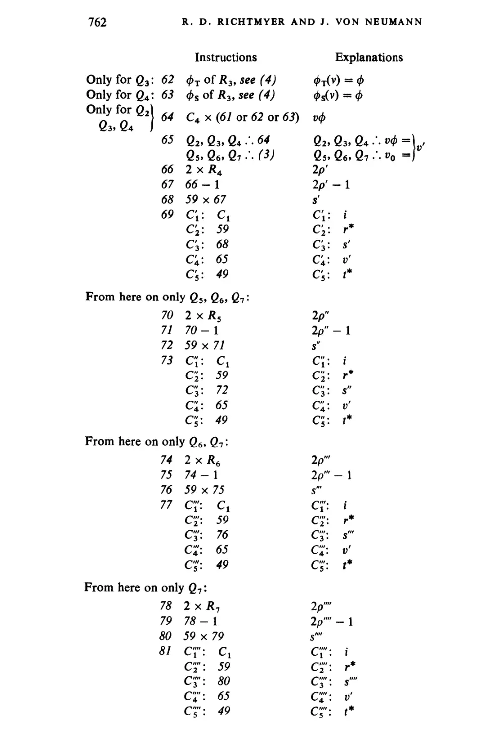
not only in my own name, but also in the name of the entire scientific community
who will benefit by his wonderful work. I know that many colleagues of John von
Neumann share my gratitude, and Dr. Oppenheimer of the Institute for Advanced
Study, where my late husband spent so many fruitful years, has asked to be
associated with this acknowledgement of a great debt to the Editor.
Klara von Neumann-Eckart
v
PREFACE
The following pages contain a reprinting of all the articles published by John von
Neumann, some of his reports to government agencies and to other organizations,
and reviews of unpublished manuscripts found in his files. The published papers,
especially the earlier ones, are given herein in essentially chronological order.
Exceptions in this ordering have been made in order that his work in certain
fields could be presented as a whole.
A number of reports written by von Neumann could not be included in this
collection because they are still classified. Others were not included because they
are essentially lecture notes which contain well-known material.
Shortly after von Neumann's death a number of people devoted much time to
studying the von Neumann files. One result of this study was the publication of
a posthumous paper by von Neumann :
Non-isomorphism of Certain Continuous Rings (with an introduction
by I. Kaplansky). Ann. Math. 67 (1958), pp. 485-496.
It also became apparent that there were a number of manuscripts which for one
reason or another were not suitable for publication but whose existence should
be made known to the scientific public, because these manuscripts contained
partial results or techniques of wide interest. It was decided to have such
manuscripts placed in the library of the Institute for Advanced Study and have reviews
of their contents included in this collection of von Neumann's work.*
The Bibliography given at the end of this Volume contains a listing of von
Neumann's scientific works, including his books and mimeographed lecture
notes. There is noted in this listing the volume and item number where any
particular paper or report in the bibliography, included in this collection, may be
found. A brief resume of the contents of the various volumes follows.
Volume I : Logic, Theory of Sets and Quantum Mechanics—starts with the
article entitled, " The Mathematician," first published in 1947, in which von
Neumann discusses the nature of the intellectual effort in mathematics. The
volume then continues with early papers on the subjects given in the title.
Volume II : Operators, Ergodic Theory and Almost Periodic Functions in a
Group—includes papers on the subjects listed in the title.
Volume III : Rings of Operators—contains his work on, and closely related to,
the theory of the rings of operators.
♦Additional material, consisting of unfinished manuscripts, notes and some of von Neumann's
scientific correspondence, is also on file in this library.
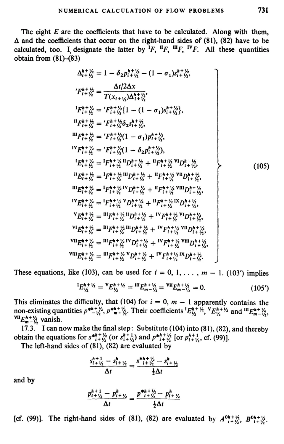
vii
PREFACE
Volume IV : Continuous Geometry and other topics—includes the papers on
continuous geometry, as well as papers written on a variety of mathematical topics.
Also included in this volume are four papers on statistics, and reviews of a number
of manuscripts found in his files.
Volume V : Design of Computers, Theory of Automata and Numerical
Analysis—is devoted to von Neumann's work in these topics.
Volume VI : Theory of Games, Astrophysics, Hydrodynamics and
Meteorology. Papers on these topics, as well as a number of articles based on speeches
delivered by von Neumann, are included in this volume.
The editor acknowledges the debt he owes for the comments made by the people
who studied the von Neumann files, and is particularly indebted for the remarks
of J. Bigelow, J. G. Charney, C. Eckart, P. Halmos, S. Kakutani, F. J. Murray,
E. Teller and E. Wigner.
He gratefully acknowledges the helpful advice given by S. Bochner, K. Godel,
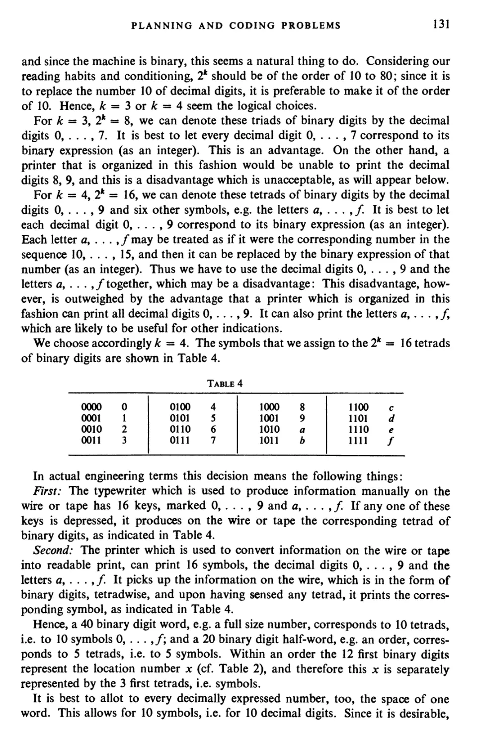
Deane Montgomery and S. Ulam. Special thanks are due to the persons who
evaluated many manuscripts and reviewed some : J. Bardeen, G. Birkhoff, H. H.
Goldstine, I. Halperin, G. A. Hunt, I. Kaplansky, H. W. Kuhn, G. W. Mackey,
O. Morgenstern and A. W. Tucker.
The Office of Naval Research gave financial support to the work of organizing
the von Neumann files and evaluating manuscripts. Without this support the
preparation of this collection would have been seriously hampered.
The editor is grateful to the Institute for Advanced Study for making its facilities
available to him and for providing many essential and helpful services. It is his
pleasure to acknowledge the debt he owes to Mrs. Elizabeth Gorman, who was
formerly secretary to Professor von Neumann, for her extremely valuable and
unstintingly given assistance.
A final and most important acknowledgement must be made. This is to the
untiring efforts of Klara von Neumann-Eckart, and her help in innumerable ways
in making available to the scientific community the various contributions of
John von Neumann.
A. H. Taub
Vlll
CONTENTS
of Volume V
Page
Acknowledgement by Klara von Neumann-Eckart v
Preface by Professor A. H. Taub vii
1. On the principles of large scale computing machines. (H. H. Goldstine and
J.v.N.) Unpublished (1946) 1
2. Preliminary discussion of the logical design of an electronic computing
instrument, Part I, Vol. 1. (A. W. Burks, H. H. Goldstine and J. v. N.) Report
prepared for U.S. Army Ord. Dept. (1946) 34
3. Planning and coding of problems for an electronic computing instrument,
Part II, Vol. 1. (H. H. Goldstine and J. v. N.) Report prepared for U.S. Army
Ord. Dept. (1947) 80
4. Planning and coding of problems for an electronic computing instrument,
Part II, Vol. 2. (H. H. Goldstine and J. v. N.) Report prepared for U.S. Army
Ord. Dept. (1948) 152
5. Planning and coding of problems for an electronic computing instrument,
Part II, Vol. 3. (H. H. Goldstine and J. v. N.) Report prepared for U.S. Army
Ord. Dept. (1948) 215
6. The future of high-speed computing. Proc. Comp. Sem. l.B.M. (1951) 236
7. The norc and problems in high-speed computing. Speech at 1st public showing of
l.B.M. Naval Ordnance Research Calculator (1954) 238
8. Entwicklung und Ausnutzung neuerer mathematischer Maschinen.
Arbeitsgemeinschaft für Forschung des Landes Nordrhein-Westfalen. Vol. 45. Düsseldorf
(1954) 248
9. The general and logical theory of automata. "Cerebral Mechanisms in Behaviour
—The Hixon Symposium". (John Wiley, New York) (1951) 288
10. Probabilistic logics and the synthesis of reliable organisms from unreliable
components. A utomata Studies, Princeton University Press (1956) 329
11. Non-linear capacitance or induction switching, amplifying and memory
devices. Unpublished (1954) 379
12. Notes on the photon-disequilibrium-amplification scheme. {Reviewed by J.
Bardeen) 420
13. Solutions of linear systems of high order. (V. Bargmann, D. Montgomery and
J.v.N.) Report prepared for Navy Bu. Ord. (1946) 421
14. Numerical inverting of matrices of high order. (H. H. Goldstine and J. v. N.)
Amer.Math.Soc. Bull. 53: 1021-1099 (1947) 479
15. Numerical inverting of matrices of high order. II. (H.H. Goldstine and J. v. N.)
Amer. Math.Soc. Proc. 2: 188-202(1951) 558
16. The Jacobi method for real symmetric matrices. (H.H. Goldstine, F. J. Murray
and J. v. N.) J.Assoc. Computing Machinery. 6: 59-96 (1959) 573
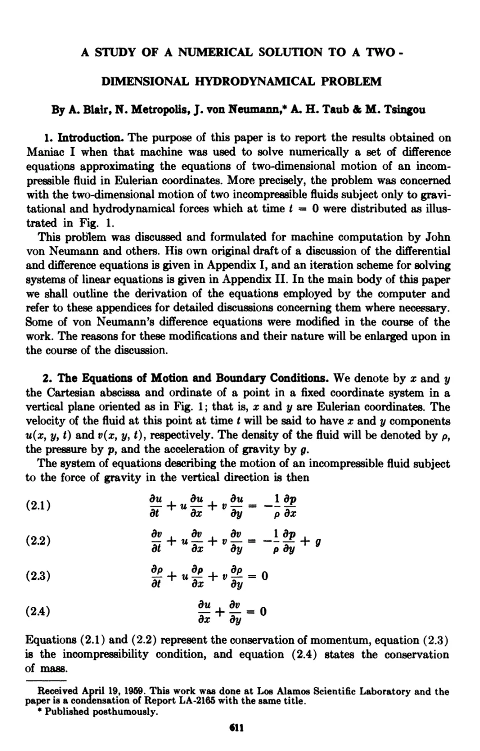
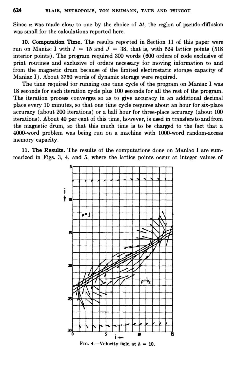
17. A STUDY OF A NUMERICAL SOLUTION TO A TWO-DIMENSIONAL HYDRODYNAMICAL PROBLEM.
(A. Blair, N. Metropolis, J. v. N., A. H. Taub and M. Tsingou) Math. Tables
and other Aids to Computation. 13:145-184(1959) 611
18. ON THE NUMERICAL SOLUTION OF PARTIAL DIFFERENTIAL EQUATIONS OF PARABOLIC TYPE.
(J. v. N. and R. D. Richmyer) LA-657 Los Alamos Scientific Laboratory ... 652
Report. „
19. First report on the numerical calculation of flow problems. {Unpublished)
June 22-July 6 (1948) 664
20. Second report on the numerical calculations of flow problems. (Unpublished)
July 25-Aug. 22(1948) 713
21. Statistical methods in neutron diffusion. (R. D. Richmyer and J. v. N.) Los
Alamos Scientific Laboratory Report. 551 (1947) 751
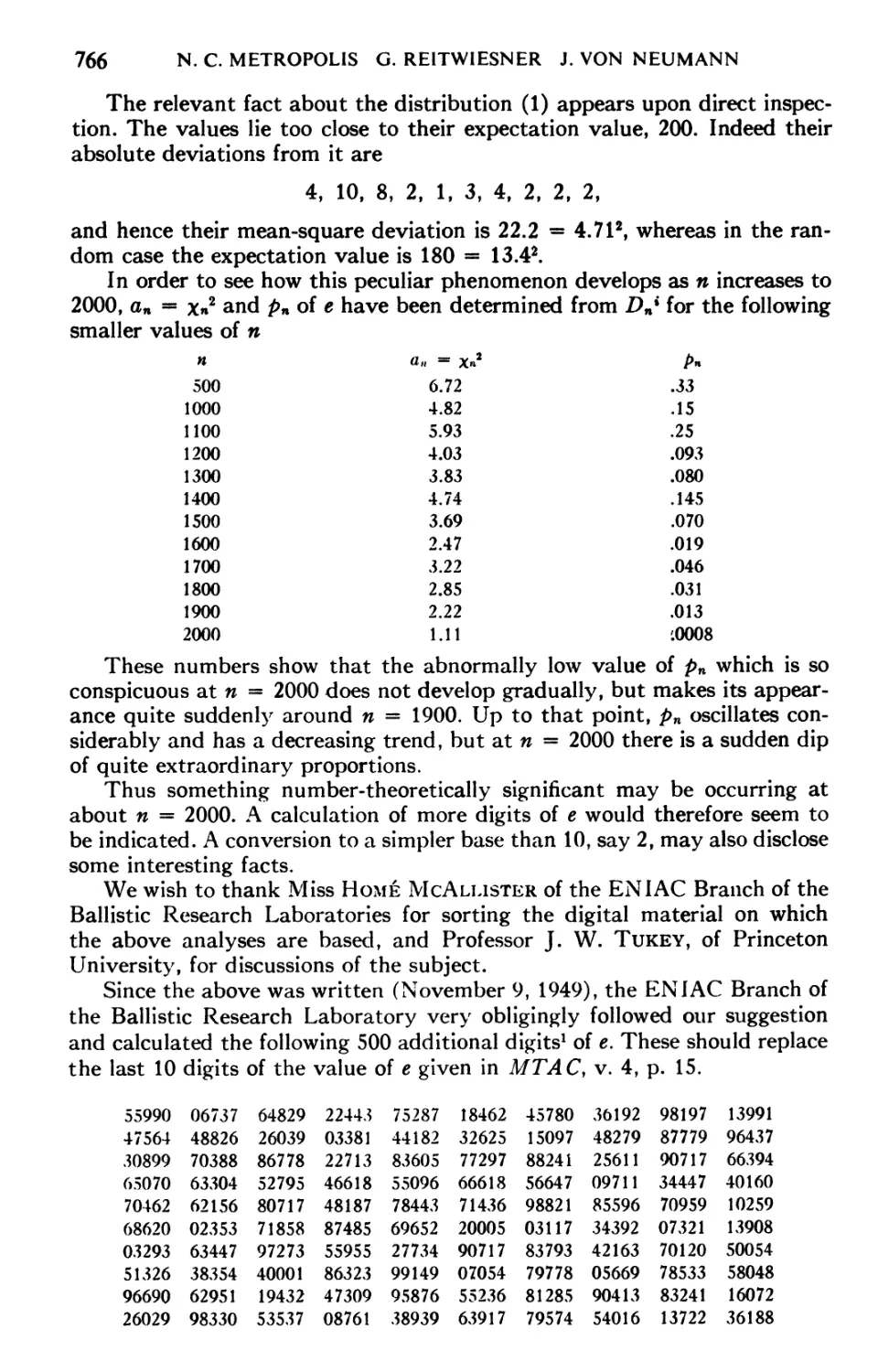
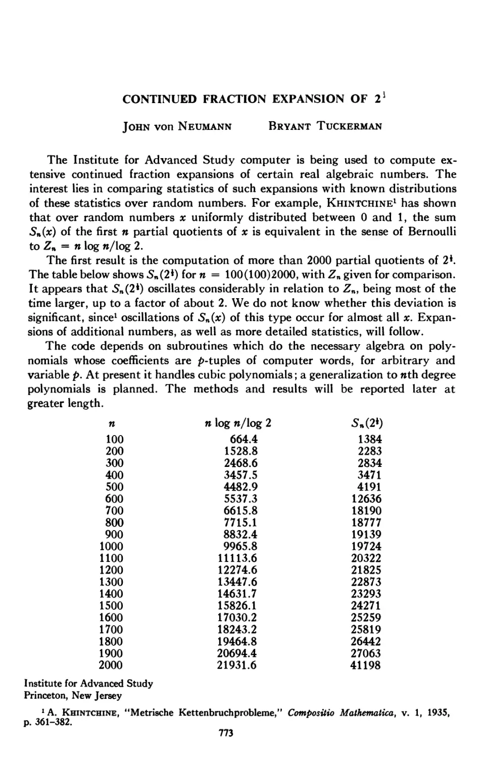
22. Statistical treatment of values of first 2000 decimal digits of e and of tt
calculated on the ENIAC. (N. C. Metropolis, G. Reitweisner and J. v. N.)
Math. Tables and other Aids to Comp. 4: 109-111 (1950) 765
23 Various techniques used in connection with random digits. /. Res. Nat. Bus.
Stand. Appl. Math. Series. 3: 36-38 (1951) 768
24. A numerical study of a conjecture of Kummer. (J. v. N. and H. H. Goldstine)
Math. Tables and other Aids to Comp. 7: 133-134 (1953) 771
25. Continued fraction expansion of 2*. (J. v. N. and Bryant Tuckerman) Math.
Tables and other Aids to Comp. 9: 23-34 (1955) 773
Bibliography of John von Neumann 775
Complete Contents of Volumes I to VI 783
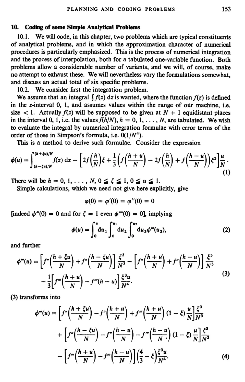
ON THE PRINCIPLES OF LARGE SCALE
COMPUTING MACHINES*
By Herman H. Goldstine and John von Neumann
1. Introduction
During the recent war years a very considerable impetus has been given to
applied mathematics in general, and in particular to mathematical physics,
particularly in certain important fields which have not been in the past in the focus of
most theoreticians' interest. Typical of these fields are various forms of continuum
dynamics, classical electrodynamics through hydrodynamics to the theories of
elasticity and plasticity. One might also mention various involved problems of
statistics and of the significance of statistics, but the examples could be multiplied
in many other directions. Again, partly under the influence of wartime necessities,
but partly also as a natural outgrowth of normal industrial development which is
turning increasingly towards automatic scanning and control procedures, the
methods of automatic perception, association, organization and direction have
been greatly advanced. These methods were in most cases of the high speed
electromechanical, or of the extremely high speed electronic type. Modern radar, fire
control and television techniques are good examples of this.
These two streams of evolution have produced both an increased need for large-
scale, high speed, automatic computing, and the means, or the potential means,
to develop the devices to satisfy this need. Accordingly a very extensive large-scale
renascence of interest in automatic computing machines has come about.
In this article we attempt to discuss such machines from the viewpoint not only
of the mathematician but also of the engineer and the logician, i.e. of the more
or less (we hope: "less") hypothetical person or group of persons really fitted to plan
scientific tools. We shall, in other words, inquire into what phases of pure and
applied mathematics can be furthered by the use of large-scale, automatic
computing instruments and into what the characteristics of a computing device must
be in order that it can be useful in the pertinent phases of mathematics.
Since our aim is not the exceedingly difficult and unsafe and partly contentious
one of describing and comparing computing instruments, we do not attempt to
give anything like a complete account of the remarkable developments that are at
present taking place in numerous organizations. It is unavoidable that our account
will be considerably biased by our own actual efforts in this field (cf. items 2 to 5 of
this volume), and we cannot pretend to give a truly balanced picture of the "state of
* This paper was never published. It contains material given by von Neumann in a number
of lectures, in particular one at a meeting on May 15, 1946, of the Mathematical Computing
Advisory Panel, Office of Research and Inventions, Navy Department, Washington, D.C. The
manuscript from which this paper was taken also contained material (not published here) which
was published in the Report, " Planning and Coding of Problems for an Electronic Computing
Instrument".
1
2
H. H. GOLDSTINE AND J. VON NEUMANN
the art". We will, nevertheless, aim to deviate from this balance no more than is
subjectively unavoidable. At any rate we shall from time to time make mention
of such attributes of existing or proposed machines as are relevant to our subject.
As pointed out above, our discussion must center around two viewpoints:
Where lie the main mathematical needs for high speed, automatic computing, and
what characteristics of a computing device are effective in the various pertinent
phases of mathematics ? In attempting such a doubly oriented discussion, we find
it impossible to give separate and consecutive accounts for each one of its two
underlying viewpoints. It would, in fact, be desirable to give but one discussion
based upon the broader problem: To what extent can human reasoning in the
sciences be more efficiently replaced by mechanisms? A discussion of this question
would, however, carry us too far afield. Instead we proceed in the following
oscillating fashion. We do not fix the order of the discussion but move from one
to the other viewpoint as frequently as seems desirable until a sufficient sense of the
interconnections between the two problems has been established to conclude the
paper with a joint discussion of both problems.
2. Importance to Mathematics
Our present analytical methods seem unsuitable for the solution of the important
problems arising in connection with non-linear partial differential equations and,
in fact, with virtually all types of non-linear problems in pure mathematics. The
truth of this statement is particularly striking in the field of fluid dynamics. Only
the most elementary problems have been solved analytically in this field.
Furthermore, it seems that in almost all cases where limited successes were obtained with
analytical methods, these were purely fortuitous, and not due to any intrinsic
suitability of the method to the milieu. This accidental character of such successes
becomes particularly plausible, if one realizes that changes in the physical definition
of the problem, which are physically quite irrelevant and minor, usually suffice to
make the previously successful analytical approach quite inapplicable. A typical
example for this phenomenon: The introduction of a small non-constancy of
entropy or of a curvature (spherical or cylindrical symmetry) in the
one-dimensional transient ("Riemann") or two-dimensional stationary ("Hodograph")
situations in compressible, non-viscous, non-conductive fluid dynamics. Compare
this "rigidity" of the non-linear problem with the ease and elegance with which
"perturbations" are handled in the linear calculus of quantum mechanics.
To continue this line of thought: A brief survey of almost any of the really
elegant or widely applicable work, and indeed of most of the successful work in
both pure and applied mathematics suffices to show that it deals in the main with
linear problems. In pure mathematics we need only look at the theories of partial
differential and integral equations, while in applied mathematics we may refer to
acoustics, electro-dynamics, and quantum mechanics. The advance of analysis is,
at this moment, stagnant along the entire front of non-linear problems. That this
phenomenon is not of a transient nature but that we are up against an important
conceptual difficulty is clear from the fact that, although the main mathematical
difficulties in fluid dynamics have been known since the time of Riemann and of
PRINCIPLES OF LARGE SCALE COMPUTING MACHINES 3
Reynolds, and although as brilliant a mathematical physicist as Rayleigh has spent
the major part of his life's effort in combating them, yet no decisive progress has
been made against them—indeed hardly any progress which could be rated as
important by the criteria that are applied in other, more successful (linear!) parts
of mathematical physics.
It is, nevertheless, equally clear that the difficulties of these subjects tend to
obscure the great physical and mathematical regularities that do exist. To name
one example: The emergence of shocks in compressible, non-viscous,
non-conductive fluids shows that non-linear partial differential equations tend to produce
discontinuities, that their theory does not form a harmonic whole without these
discontinuities, that the nature of the "characteristic curves" is probably seriously
affected by them. It seems, furthermore, that the "proper" way to introduce these
discontinuities necessarily violates Hankel's otherwise well established principle of
the "permanency of formal laws", since shocks cause entropy changes in the
nominally still, non-viscous, non-conductive flow. It also, and in connection with
this, somehow impairs the "reversibility" of the flow. Yet, our present information
about these phenomena, or rather about their deeper mathematical meaning, as
well as about the details of the formation, interaction and dissolution of these
discontinuities, is worse than sketchy. Another example: The emergence of
turbulence in incompressible, viscous hydrodynamics indicates that for non-linear,
partial differential equations of that mixed (parabolic-elliptic) type it is not always
the knowledge of the simplest, most symmetric (laminar) individual solutions which
matters, but rather information of certain large, connected families of solutions—
where each of these "turbulent" solutions is hard to characterize individually but
where the common statistical characteristics of the entire family contain the really
important insights. Again our properly mathematical information on these
turbulent solutions is practically nil, and even the united (semi-physical,
semi-mathematical) information is most tenuous. Even the analysis of the situations in which
they originate, the (linear!) perturbation-type stability discussion of the laminar
flow, has been carried out only in rare cases, and with methods of great apparent
difficulty.
It is important to avoid a misunderstanding at this point. One may be tempted
to qualify these problems as problems in physics, rather than in applied
mathematics, or even pure mathematics. We wish to emphasize that it is our conviction
that such an interpretation is wholly erroneous. It is perfectly true that all these
phenomena are important to the physicist and are usually mainly appreciated by
him. Yet this should not detract from their importance to the mathematician.
Indeed, we believe that one should ascribe to them the greatest significance from
the purely mathematical point of view as well. They give us the first indication
regarding the conditions that we must expect to find in the field of non-linear
partial differential equations, when a mathematical penetration into this area, that
is so difficult of access, will at last succeed. Without understanding them and
assimilating them to one's thinking even from the strictly mathematical point of
view, it seems futile to attempt that penetration.
That the first, and occasionally the most important, heuristic pointers for new
4
H. H. GOLDSTINE AND J. VON NEUMANN
mathematical advances should originate in physics, is not a new or a surprising
occurrence. The calculus itself originated in physics. The great advances in the
theory of elliptic differential equations (potential theory, conformal mapping,
minimal surfaces) originated in physical equivalent insights (Riemann, Plateau).
This applies even to the heuristic approach to the correct formulations of their
"uniqueness theorems" and of their "natural boundary conditions". Such advances
as have been made in the theory of non-linear partial differential equations, are also
covered by this principle, just in what seem to us to be the most decisive instances.
Thus, although shock waves were discovered mathematically, their precise
formulation and place in the theory and their true significance has been appreciated
primarily by the modern fluid dynamicists. The phenomenon of turbulence was
discovered physically and is still largely unexplored by mathematical techniques.
At the same time, it is noteworthy that the physical experimentation which leads
to these and similar discoveries is a quite peculiar form of experimentation; it is
very different from what is characteristic in other parts of physics. Indeed, to a
great extent, experimentation in fluid dynamics is carried out under conditions
where the underlying physical principles are not in doubt, where the quantities to
be observed are completely determined by known equations. The purpose of the
experiment is not to verify a proposed theory but to replace a computation from
an unquestioned theory by direct measurements. Thus wind tunnels are, for
example, used at present, at least in large part, as computing devices of the so-called
analogy type (or, to use a less widely used, but more suggestive, expression proposed
by Wiener and Caldwell: of the measurement type) to integrate the non-linear
partial differential equations of fluid dynamics.
Thus it was to a considerable extent a somewhat recondite form of computation
which provided, and is still providing, the decisive mathematical ideas in the field
of fluid dynamics. It is an analogy (i.e. measurement) method, to be sure. It seems
clear, however, that digital (in the Wiener-Caldwell terminology: counting) devices
have more flexibility and more accuracy, and could be made much faster under
present conditions. We believe, therefore, that it is now time to concentrate on
effecting the transition to such devices, and that this will increase the power of the
approach in question to an unprecedented extent.
We could, of course, continue to mention still other examples to justify our
contention that many branches of both pure and applied mathematics are in great
need of computing instruments to break the present stalemate created by the failure
of the purely analytical approach to non-linear problems. Instead we conclude
by remarking that really efficient high-speed computing devices may, in the field
of non-linear partial differential equations as well as in many other fields which
are now difficult or entirely denied of access, provide us with those heuristic hints
which are needed in all parts of mathematics for genuine progress. In the specific
case of fluid dynamics these hints have not been forthcoming for the last two
generations from the pure intuition of mathematicians, although a great deal of
first-class mathematical effort has been expended in attempts to break the deadlock
in that field. To the extent to which such hints arose at all (and that was much less
than one might desire), they originated in a type of physieal experimentation which
PRINCIPLES OF LARGE SCALE COMPUTING MACHINES 5
is really computing. We can now make computing so much more efficient, fast
and flexible that it should be possible to use the new computers to supply the
needed heuristic hints. This should ultimately lead to important analytical advances.
3. Preliminary Speed Comparisons
We begin by attempting a preliminary analysis of the problems which could be
furthered by new automatic computing devices. There are several cogent reasons
why such a survey cannot aim at anything like completeness at the present time.
First, the possible uses of automatic computing instruments lie in so many different
fields that it is extremely difficult for an individual to acquire a balanced viewpoint
and to avoid serious oversights. Second, the various applications of computers
depend importantly on their speed, flexibility and reliability—the two aspects of
the basic question formulated at the end of § 1 become badly entangled at this point.
Finally, the changes that they are likely to cause are so radical, that our present
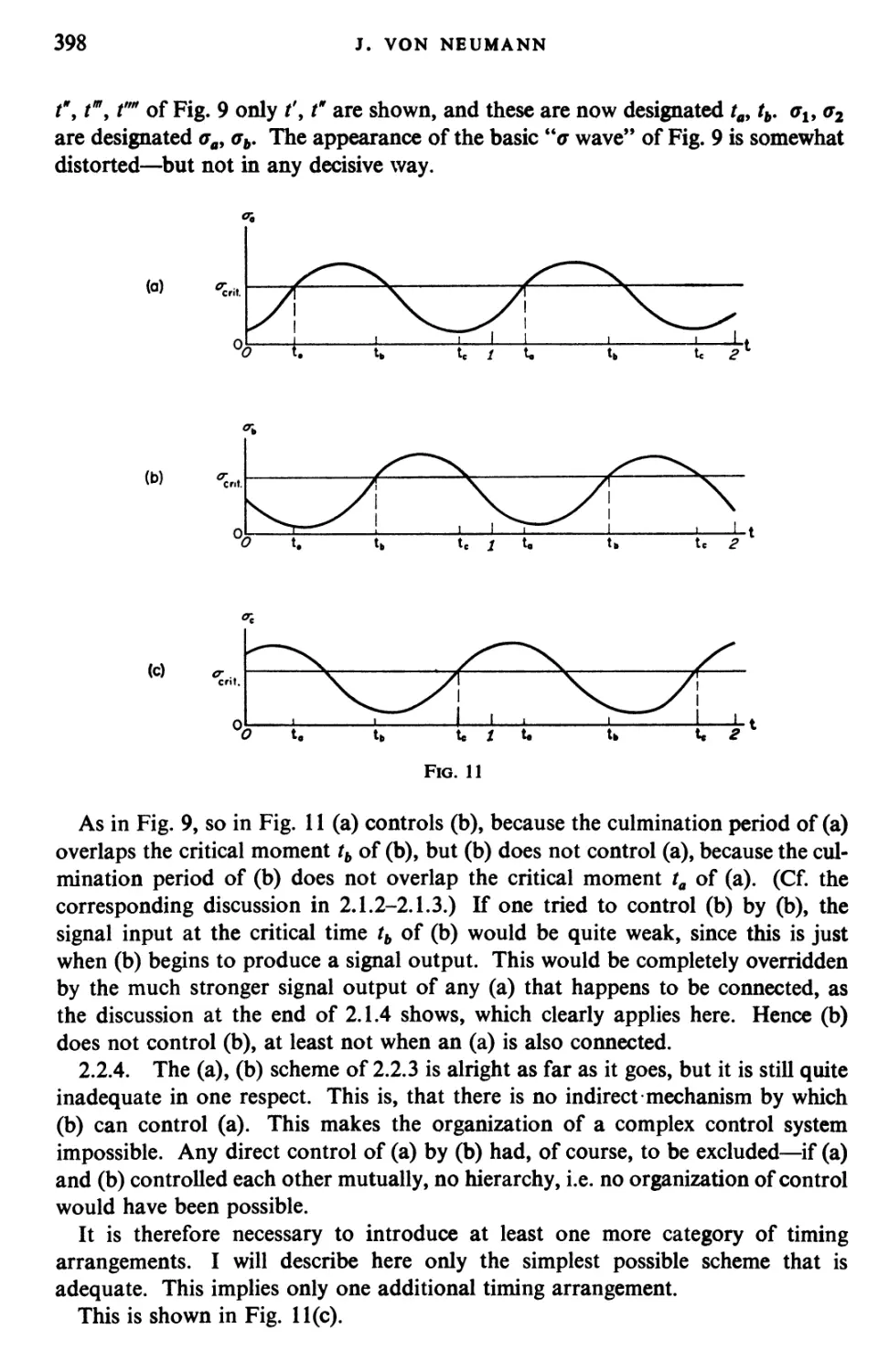
efforts at evaluating them can only be taken as tentative, advance estimates. It
will require a good deal of experience with the actual devices, in fact something
that may be better described as a thorough conditioning of our ways of thinking
by the continued use of and familiarity with such devices, before we can consider
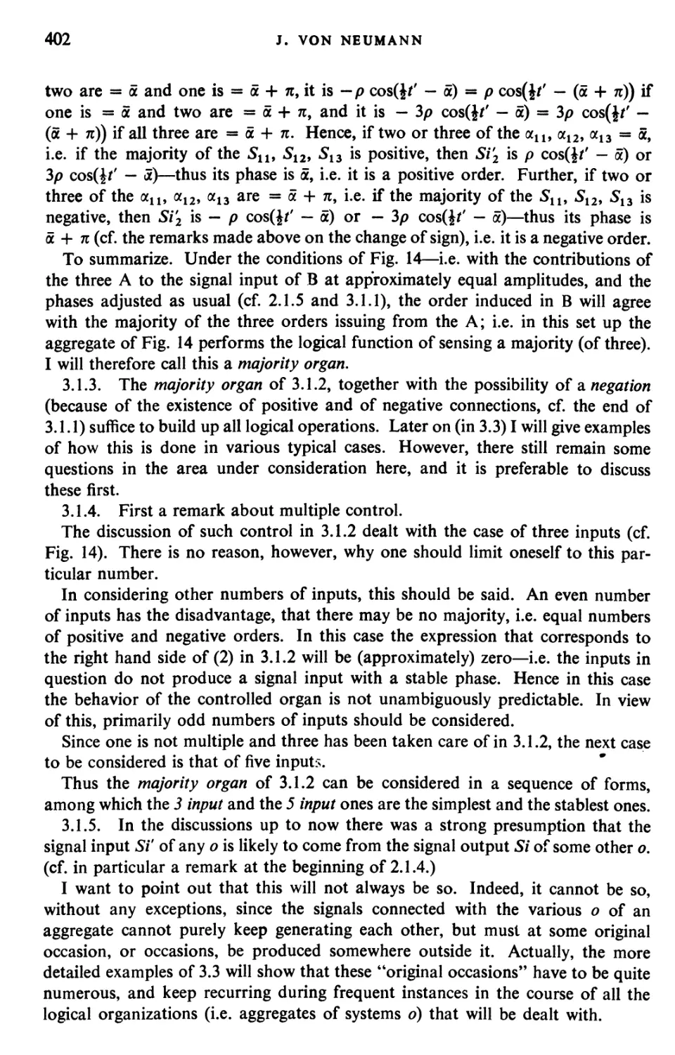
ourselves qualified to pass judgements that are anything like balanced.
In elaboration of this last point it is well to consider that the new machines
represent speed increases of anywhere between 103 and 105 as compared to present
hand methods (i.e. human computers using "desk multiplier" machines) or standard
IBM equipment techniques—for example, the ENIAC (the first electronic
computer) performs a multiplication in about 3 milliseconds as compared to 10 seconds
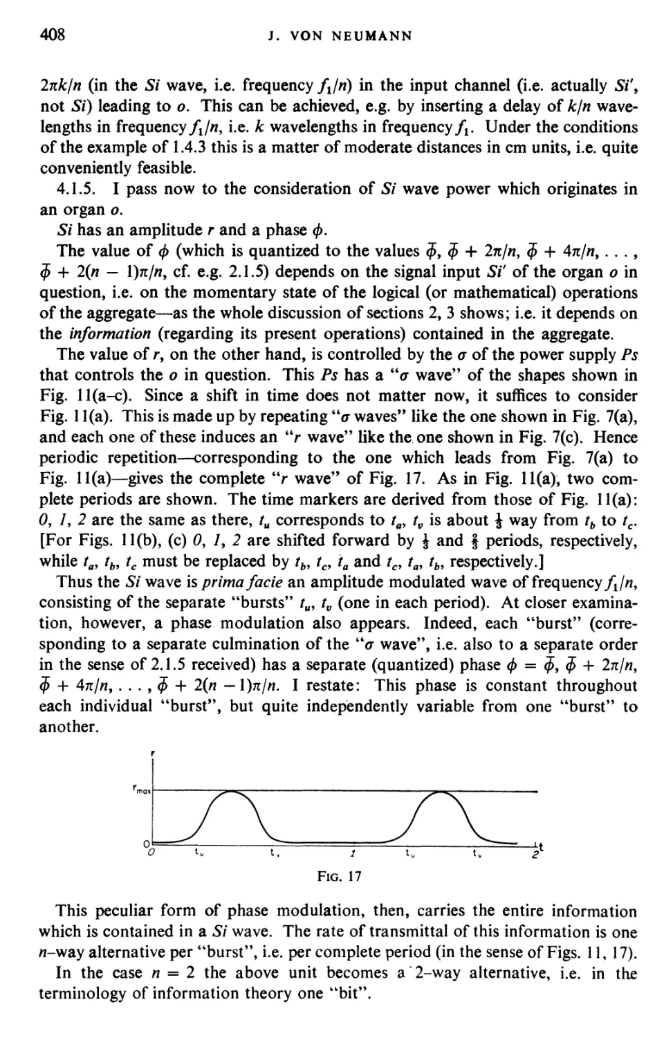
on a desk multiplier, or seven seconds on a standard IBM multiplier. To make
safe predictions based on so great an extrapolation is quite hazardous, especially for
workers in fields now somewhat removed from mathematics such as economics,
dynamic meteorology or biology, but in which important applications are sure to
arise. Add to this consideration the even more fundamental one relative to our
knowledge of numerical methods, concerning which our comments can be
somewhat more specific.
Our problems are usually given as continuous-variable analytical problems,
frequently wholly or partly of an implicit character. For the purposes of digital
computing they have to be replaced, or rather approximated, by purely arithmetical,
"finitistic", explicit (usually step-by-step or iterative) procedures. The methods by
which this is effected, i.e. our computing methods in the generic sense, are
conditioned by what is feasible, and in particular more or less "cheaply" feasible,
with the devices that are available now. The concept of effectiveness, in fact the
very concept of "elegance", of our computing techniques is fundamentally
determined by such practical considerations. Now the radical changes in computing
equipment, which we expect, will modify and distort these criteria of "practicality"
and "cheapness" out of all recognition. It must be emphasized that the changes
that we anticipate will work both ways: Certain things will become more available,
but the new, increased emphasis that will be worth placing on them will make
certain other things less available.
6
H. H. GOLDSTINE AND J. VON NEUMANN
Thus already our present, limited information seems to justify the following
observations: An arithmetical acceleration by a factor of the order 104 will justify
and even necessitate the development of entirely new computing methods. Not
only will this development be necessary because of the sharp increase in speed but
also because the economy of automatic computers is in every case that we know
(from actual experience or from reasonably advanced planning) exceedingly
different from that of manual devices. For example, the organs for storing numerical
and logical information at high speeds are quite limited in the new machines:
New electro-mechanical (relay) devices, such as the ones at Harvard, Dahlgren
Proving Ground (U.S. Navy Bureau of Ordnance), or those built by the Bell
Telephone Laboratories (Aberdeen Proving Ground, U. S. Army Ordnance
Department; Langley Field, National Advisory Committee on Aeronautics) can remember
between 100 and 150 numbers, counting as a "number" the equivalent of about
10 decimal digits in overall precision and information. The (electronic) ENIAC
can remember only 20 numbers of 10 decimal digits each (these estimates do not
include function tables which are included with all four). The new electronic
machine that we are planning should remember a few thousand numbers, on the
same scale. These figures are, all of them (even the last mentioned, very favorable
ones), lower than what the computing sheets of a long and complicated calculation
in a human computing establishment may store. Thus in an automatic computing
establishment there will be a "lower price" on arithmetical operations, but a
"higher price" on storage of data, intermediate results, etc. Consequently the
"inner economy" of such an establishment will be very different from what we
are used to now, and what we were uniformly used to since the days of Gauss.
Therefore, new computing methods, or, to speak more fundamentally, new criteria
of "practicality" and of "elegance" will have to be developed, as suggested further
above.
We are actually now engaged in various mathematical and mathematical-logical
efforts aiming towards these objectives. We consider them to be absolutely essential
parts of any well-rounded program which aims to develop the new possibilities of
very high speed, automatic computing. But it should be clear from the above
remarks that whatever attempts we make at rational extrapolation in this direction,
are unlikely to do full justice to the subject in the immediate future.
In returning to the survey mentioned above we seek some yardstick for measuring
speed- Among the arithmetical processes the linear operations (addition and
subtraction) and multiplication are the most frequent. Ordinarily the average
frequency of the former is of the same order as the latter. In fact, the former usually
occurs two to three times as often as the latter but require much less time to
perform. Since multiplication is the dominant operation from the point of view of
time consumption we may use the "multiplying speed" as our index for measuring
speed. We have, however, overlooked any discussion of the precision of a result.
Clearly the same devices will carry out multiplications to more significant digits
more slowly than to fewer digits—provided they have this inherent flexibility at all.
As a rule the multiplication time increases at a rate lying between proportionality
to the first and second power of the number of digits. In passing we remark that
PRINCIPLES OF LARGE SCALE COMPUTING MACHINES 7
for most digital or counting machines the number of digits lies between six and
ten, whereas for analogy or measuring devices a precision of between two and
four digits is achieved (the last mentioned upper bound is actually rarely attained).
We now proceed to discuss the multiplication time of various typical digital
devices. The "genuine" multiplication by hand on paper but without mechanical
aid requires probably on the average about 1.5 min for 5 digit numbers. Hence
about 5 min for 10 digit numbers would not seem to be an unfair estimate. The
usual desk multiplier such as a Friden, Marchant or Monroe spends about 10-15
sec for 10 digit numbers. Hence a reasonable speed ratio between the "genuine"
hand and "modified" hand methods is 300/10 = 30. This ratio is probably
unrealistic for two reasons. First, the former procedure soon results in considerable
fatigue with consequent slowing down, and second both schemes require the same
transfer time. That is, the desk machine does not record on the computer's paper
the result of the multiplication.
The standard IBM multiplier multiplies 8 digit numbers in about 7 sec and
records the result automatically on a card which can be used in another part of
the computation. Thus the transfer time attendant on the hand techniques is
eliminated. It is fair to say that a hand computation of either species takes between
two and five times the multiplying time whereas the use of IBM machines cuts this
factor to something between one and two. (There was recently displayed a new
IBM multiplier using vacuum tubes in which the multiplication time is about 15 msec.
In this device, however, the card-cutting time, i.e. transfer time, is still 100 cards
per minute, i.e. 0.6 sec = 40 multiplication times per card.)
Let us consider some of the newer devices relative to their multiplying speeds—
we postpone more detailed analyses until later in the paper.
The Harvard machine, "Mark I" (built in 1935-1942 by IBM and H. H. Aiken
of Harvard) multiplies 11 digit numbers in 3 sec and 23 digit numbers in 4.5 sec.
Using our speed principle we see that this represents a 5-fold acceleration over
the desk and standard IBM machines. The IBM Company has produced some
experimental machines now in use at the Ballistic Research Laboratory (Aberdeen
Proving Ground, U.S. Army Ordnance Department) which multiply 6 digit
numbers in from 0.2 to 0.6 sec—a 27- to 9-fold acceleration over our norm. Both
the standard IBM and the Harvard machines are partly relay and partly counter
wheel, whereas the machines at Aberdeen are purely relay in character.
Some newly developed relay machines of the Bell Telephone Laboratories
multiply 7 digit numbers in 1 sec. Due, however, to a special feature, the so-called
"floating decimal point", these are for most purposes equivalent to about 9 digits
and sometimes to considerably more. We therefore credit these machines with a
10-fold acceleration over our norm.
A relay machine, Harvard "Mark II" (which has just been completed by H. H.
Aiken for Dahlgren Proving Ground) will probably exceed this multiplication
speed still further. (It contains two 0.75 sec, 7 digit, multipliers, thus reaching an
effective multiplying velocity of about 0.4 sec.) It may be remarked that further
speed increases for machines using electro-mechanical relays will probably not give
rise to further acceleration factors of more than two or three.
8
H. H. GOLDSTINE AND J. VON NEUMANN
The ENIAC built by the Moore School of Electrical Engineering (University of
Pennsylvania) for the Ballistic Research Laboratory (Aberdeen), represents a bold
attempt to increase significantly the multiplying rate for computing machines. Its
multiplication time is 3 msec for 10 digit numbers, a 3,300-fold acceleration over
our original norm. The full 3,300 factor is rarely actually achievable, however,
due to a bottle-neck in storing and recording. It is probably fairer to attribute to
this device an acceleration factor of between 500 and 1,500. It is a very large
device, containing roughly 20,000 vacuum tubes of conventional types and
operating at a basic frequency of 100 kilocycles per second.
At the present time several very high speed, electronic, automatic
computing machine projects are being undertaken both in this country and abroad,
in most cases under the sponsorship or with the help of various government
agencies.
It is likely that several of these will be a good deal smaller than the ENIAC,
using 2,000 to 5,000 vacuum tubes and special memory devices, and operating
frequencies of \ to 1 megacycles per second. It seems probable that they may reach
multiplication times between 1 and 0.1 msec for the equivalents of about 10 decimal
digits (although some will be binary, 30 to 40 digits). This represents
accelerations of 104 to 105 over our original norm. It should be emphasized that with
proper planning these machines ought to allow the full exploitation of the increased
speed that they achieve. Of course, the postulate of "proper planning" will have
to be taken very seriously. It will have to comprise a thorough mathematical and
logical analysis of the major types of problems for which the machine approach
is expected to be the proper one, or which will become important in consequence
of the increasing use of the machine approach.
To conclude the present considerations on main machine types and their
relationship to overall speed, we observe this:
If one were to undertake a serious study of micro-wave techniques one could
probably obtain still greater gains in speed than those referred to above. Since,
however, the now contemplated machines will probably revolutionize our ideas
on methods and on the uses of these machines, it might be better to delay
somewhat the more ambitious advances that might be achieved.
All machines discussed above belong to the digital or counting type, i.e. treat
real numbers as aggregates of digits. (These digits are usually decimal. In one or
two new machines they will probably be binary. In principle other digital systems
might also receive consideration. Any non-decimal system raises, of course, for
practical reasons, the problem of conversion to and from the decimal one. This
problem can, however, be handled in a number of fully satisfactory ways.) There
is, however, another important class of computing machines, based on a
qualitatively different principle. This class has already been referred to previously; it
consists of the machines of the analogy or measurement type. In these a real number
is represented äs a physical quantity, e.g. the position of a continuously rotating
disk, the intensity of an electrical current or the voltage of an electrical potential,
etc. We do not discuss machines of this type further at this time beyond estimating
the ratio of their speeds to digital types in equivalent situations.
PRINCIPLES OF LARGE SCALE COMPUTING MACHINES 9
The validity of such estimates is at any rate limited by the wide variety of existing
analogy devices, which use a great number of different mechanical, elastic, and
electrical methods of expressing and of combining quantities as well as mixtures
of these, together with most known methods of mechanical, electrical and
photoelectrical control and amplification. Moreover, all analogy machines have a marked
tendency towards specialized, one-purpose character, and they are, therefore,
difficult to compare with the all-purpose, digital machines discussed above. Indeed it
may be seen on many typical examples, chosen from a wide variety of fields, that,
ceteris paribus, a one-purpose device is faster than a general purpose one. We
can, therefore, compare in a satisfactory manner to the all purpose, scientific,
digital devices in which we are interested, only such analogy instruments that can
also make claim to being reasonable all-purpose in character.
This leaves us to consider several variants of the well-known differential analyzer*.
In trying to estimate a multiplying speed for this machine we run immediately into
a serious difficulty due to the character of the elementary operations performable
by an analyzer. It deals with functions of a common, continuously increasing
independent variable and builds them up by continuous integration processes.
One of these functions may be the product of two others among them, but this is
usually formed as
Jw du + fv du.
Hence we are forced to compare the actual time of performance of the differential
analyzer on some typical problem against thecorresponding time on the digital devices.
Such a typical problem is the determination of an average ballistic trajectory.
A good analyzer will usually require 10 to 20 min to handle this problem with a
precision of about five parts in 10,000. Trajectories have been run on the ENIAC
and require about 0.5 min for complete solution including printing of needed data.
This corresponds to assuming 15 multiplications per point on the trajectory, and
50 points on the trajectory, which is quite realistic. The ENIAC's multiplication
time is 3 msec, hence the 750 multiplications that are required consume 2.25 sec,
giving a total arithmetical time well under 3 sec. On the other hand the ENIAC's
IBM card output can cut 100 cards, holding a maximum of 8 ten decimal digit
numbers each, per minute. This requires, for 50 cards, 0.5 min. Thus the ENIAC's
performance is in this case entirely controlled by its low output speed. It behaves
as if its multiplying speed were 20 times less than it is in reality: 60 msec. At the
same time the differential analyzer performs the equivalent of 750 multiplications
in 10-20 min. This amounts to 0.8-1.6 sec multiplication time, for about 4 decimal
digit precision. On the 10 decimal digit level this corresponds to about 4 sec.
This puts it into the speed class of the relay machines. Since those machines
usually spend £ to i of their total time in multiplying, it may be more fair to
consider 1 to 2 sec as the equivalent multiplying time. Hence we may evaluate
the analyzer's speed as corresponding in a general way to the speed class of the
more recent relay machines, lying somewhere between the Harvard "Mark I" and
"Mark II" machines, or the Bell Telephone Company's machines.
* V. Bush, F. and S. H. Caldwell Journ. Franklin Inst. Vol 240 (1945), pp. 255-326
10
H. H. GOLDSTINE AND J. VON NEUMANN
In conclusion we may say that, taking the 10 sec for 10 decimal digits rate of the
desk multiplier as a norm, a factor of 30 for electro-mechanical relay machines
and 104 to 105 for vacuum tube machines probably represent the orders of
magnitude which will be optimal for their respective kinds in the next few years. For
analogy machines a proper speed comparison is very difficult, but an imputation
of an acceleration factor 10 seems to be fair and reasonable.
In closing this section we wish, however, to warn the reader that the estimates
of speed made above express only the first, quite superficial assessment of complete
solution time. We have not evaluated the rate at which the machines can transfer
numbers, the speed with which its logical controls operate; the time needed to
set up the controls of the machine in order to make it run according to a
completely formulated plan; the time required to formulate such a plan, i.e. to convert
a mathematical problem into a procedure understandable by the machine; the
frequency of malfunctions such as errors or breakdowns and the average time
required to recognize, localize and remove them. All these factors are of utmost
importance and we shall try to discuss them in more detail below. For the present,
however, we shall use our crude estimates as yardsticks to perform a first analysis
of problems which justify the building of these machines.
4. Mathematical Significance of Speed
We ask now whether scientifically important problems exist which justify the
speeds we are striving to attain. To give a partial answer to this question we
consider in this section several classes of problems and evaluate their solution
times with the help of our yardsticks of the previous section. The reader is warned
that these time estimates are only to be interpreted as giving orders of magnitude.
The computation of a ballistic trajectory considered above is a reasonably
typical instance of a simple system of non-linear, total differential equations. As
we saw, it involves about 750 multiplications. This permits the calculation of the
total multiplication time. For most digital machines this will have to be multiplied
by a factor of about 2 to 3 to obtain the actual computing time of the machine. (The
ENIAC is an unfavorable exception, cf. above.) It may also be necessary to insert
a further factor 2 for checking, if the brute-force method of checking by total
repetition is used. However there are less expensive ways of checking (by
"smoothness" of the results of "successive differences" of various orders, by suitable
identities), also machines may be run in pairs and possibly be set up for automatic
checking in this or some other way. We will therefore use an average factor 3 to
convert the net multiplication time into a conventionalized total machine-
computing time. (Except for the ENIAC, cf. above.) With these conventions, and
with the previously estimated multiplication speeds, we will now obtain calculation
times per unit ballistic trajectory for the major prototypes of machines previously
discussed. We must emphasize, however, that the numbers to be given should
not be taken too literally to express actual computing times for the corresponding
devices. They are only very roughly correct, and they are primarily meant to
indicate what the durations would be if all other factors were standardized at
certain reasonable, but nevertheless conventional, levels.
PRINCIPLES OF LARGE SCALE COMPUTING MACHINES 11
These being understood, the following durations obtain: (1) Human norm
(10 sec multiplication time): 7 man-hr. (Definitely too low, our factor 3 is certainly
not adequate in this case.) (2) Harvard "Mark I" (3 sec): 2 hr. (3) Bell Telephone
Company (1 sec): 35 min. (4) Harvard "Mark II" (0.4 sec): 15 min. (No relay
machine is likely to have a much higher overall speed than this.) (5) Differential
Analyzer (cf. above). (6) ENI AC (cf. above): 0.5 min. (7) Advanced electronic
machines, now under development (0.1-1 msec): 0.25-2.5 sec.
It is now clear that if only one such trajectory were devised then even the longest
duration, the "norm" of 7 hr, would hardly be worth reducing since it requires a
good deal longer time to formulate the problem, to decide upon and formulate
the procedure, to set it up for computation and afterwards to analyze the results.
If, however, a moderate size survey (typified by 100 trajectories) is desired, advanced
relay machines are appropriate, they may require about 24 hr for this task, but it
is not essential to go to electronic instruments. When an exceptionally large survey
is needed (10,000 trajectories), an electronic machine is clearly indicated: The
ENIAC might require in this case 84 hr = (10.5) 8-hr shifts, while the more advanced
electronic machines might require 40 min to 7 hr.
Astronomical orbit calculations are in many ways quite similar to the ballistic
trajectory computations but the number of orbital points required is usually
considerably greater and the number of orbits required can also be quite large.
Hence the need for electronic devices will arise in astronomy in making moderate
surveys or ever for some voluminous problems such as tracing the moon's path
for several centuries. For such a problem it is not unreasonable to assume that
600,000 points (corresponding to a point per 3 hr for 200 yr) would have to be
calculated and that there would again be about 15 multiplications per point.
This gives about 107 multiplications, hence the equivalent of about 13,000 ballistic
trajectories is involved.
Let us consider next the situation in regard to partial differential equations.
First, we examine hyperbolic equations in two variables, x a distance, and /, time.
It is not unusual to partition the x axis into 50 subintervals; the time axis must
then be such that a sound wave cannot travel more than Ax in At seconds. Hence
it takes such a wave at least 50 intervals At to traverse the jc-interval; moreover a
problem in which a wave can cross this interval say four times is not exceptional.
We have, therefore, for the corresponding difference equation about 104 lattice
points, for each one of which it is not unreasonable to assume 10 multiplications.
This gives 105 multiplications for an exceedingly simple fluid dynamical problem.
This problem, therefore, corresponds to about 130 ballistic trajectories. For a
single solution the more advanced relay machines are appropriate, since it would
require about 32 hr, while the electronic machines now under development should
cut this to 0.5-5 min, which is presumably shorter than worthwhile. On the
other hand even for a moderate sized survey of, say, 100 solutions the electronic
times become 1-8 hr, i.e. here the use of electronic devices would be justified, and
even the differences within their range of speeds would begin to be significant.
The solution of hyperbolic equations with more than two independent variables
would afford a great advance to fluid dynamics since most problems there involve
12
H. H. GOLDSTINE AND J. VON NEUMANN
two or three spatial variables and time, i.e. three or four independent variables.
In fact the possibility of handling hyperbolic systems in four independent variables
would very nearly constitute the final step in mastering the computational problems
of hydrodynamics.
For such problems the number of multiplications rises enormously due to the
number of lattice points. It is not unreasonable to consider between 106 and
5 x 10⁶ multiplications for a 3-variable problem and between 2.5 x 10⁷ and
2.5 x 10⁸ multiplications for a 4-dimensional situation. Hence these are roughly
equivalent to 1,300 to 6,700 trajectories and to 33,000 to 330,000 trajectories,
respectively. It is then clear that for even one such problem the use of the most
advanced electronic machines is justified. In fact for a typical 3 variable problem
one such problem would require 330 to 1,700 hr on the fastest relay machine now
visualized and 0.25 to 1.25 hr on the electronic machines now under development.
(In order to simplify matters, we replace here the range of speeds of advanced
electronic instruments by one mean value. As such we choose the geometric mean
| sec per ballistic trajectory.) For a 4 variable problem even those devices would
require 6 to 62 hr for a single solution.
Four variable problems have about the same relationship to the best electronic
devices as the 2 variable problems to the best relay devices. They can just about
be solved in this manner, but in a clumsy and time-consuming manner, i.e. they
would seem to justify the development of something still faster.
Inasmuch as the parabolic type equation is, in the main, similar to the hyperbolic
one, we may forego further discussion here. The elliptic case is, however, essentially
different, and we will, therefore, consider it now. We assume there are two or more
independent variables x9 y9 . . . . Again we replace the system by a system of
simultaneous equations with the help of a lattice of mesh points. For 2 dimensions,
20 x 20 mesh points is not excessive; hence one should expect n, the number of
equations, to be at least of the order of 400. At the present time much smaller
values of n are usually used, but this is dictated by the limitations of our present
methods of computation. The natural size for n is several hundred at least, and
it is therefore desirable to have methods which permit n to take on such values.
We note first that the system of n simultaneous linear equations in n unknowns
derived from an elliptic equation is simpler than the general n equations in n
variables case. Indeed in the general situation each equation depends on all
variables while in the difference system originating from an elliptic equation only
the variables corresponding to a given point and its immediate mesh neighbors
appear.
The usual modus for handling such systems is the so-called "Relaxation"
technique which requires repeated application of the matrix of the system to various
successively obtained vector approximations to the desired solution. In the use of
this technique on a system with n = 400 about 20 iterations should suffice. Assume
therefore that n = 400, that there are 5 variables: in each equation, i.e. 5 terms in
each row of the wth order matrix and 20 successive relaxation steps required. There
are about 400 x 5 x 20 terms to be computed. The number of multiplications
per term may, of course, vary from zero for Laplace's equation to very high
PRINCIPLES OF LARGE SCALE COMPUTING MACHINES 13
numbers for non-linear elliptic equations. Let us assume 3 multiplications per
term. Thus about 120,000 multiplications are involved. (One should not be misled
by the fact that familiar solutions require nothing like this number of multiplications.
They treat usually much simpler equations, such as Laplace's, and they are handled
by various "individualistic" tricks or shortcuts, which are not easily mechanizable
and which probably do not apply for complicated, non-linear equations.)
To return to the 120,000 multiplications we see that tbjs is comparable to a 2
variable problem of hyperbolic type—about 100,000 multiplications and to about
130 standard ballistic trajectories. Hence our previous conclusions are applicable
to this situation.
In conjunction with the elliptic case some other more complicated problems can
be considered, some of which are of great importance. Such is the non-linear,
fourth order, part elliptic, part parabolic equation of viscous, incompressible
hydrodynamics
ol ox oy oy ox
where v is the kinematic viscosity coefficient, \f/ is the flow potential and A2 is the
Laplace operator. A direct numerical attack on this equation may in the less
involved cases be satisfactorily handled with about 2,500 mesh points; a direct,
numerical investigation of its "turbulent" solutions would necessitate considering
non-stationary solutions, i.e. ones containing t. One would probably require about
100 successive values of t and possibly many solutions would be required. Recall
that we wish the statistical characteristics of the established, finite sized turbulence
and not merely the infinitesimal perturbation discussion of the beginning of
turbulence, i.e. the discussion of the stability of the laminar flow.
An inspection of the equation shows that about 106 multiplications are involved.
We are, therefore, back to the orders of magnitude of previously considered cases.
We now turn attention away from differential equations and inquire into the
solution of integral equations. We may evidently approximate an integral equation
by a system of simultaneous equations whose matrix, however, may be quite general
in distinction from our previously considered situation, that one of elliptic
equations. Simultaneous systems of linear equations arise, of course, in a great many
other places in applied mathematics as, for example, in many-particle problems,
where the number of degrees of freedom is quite large, or in filtering and prediction
problems. The solution of such systems is a quite serious problem due to the
requirements of stability and accuracy and to the very great number of
multiplications involved. The classical elimination technique involves, for example, the
order of «3/3 multiplications. Thus the solution of a system of 50 equations in
50 unknowns would be analogous to a survey of about 50 trajectories and is thus
within the range of a fast relay machine, whereas a system of 100 x 100 is evidently
out of range of such a device.
One of the most serious problems arising in connection with the solution of
linear equations is the question of stability. The classical procedures, such as the
use of determinants (Cramer's formula) or the elimination method, require very
14
H. H. GOLDSTINE AND J. VON NEUMANN
thorough scrutiny as to their applicability before they are used for large values of n.
Indeed, there exists in all these cases a danger of considerable accumulation of
round-off errors, and also a danger of an amplification of errors of this type, which
occurred early in the process, by subsequent large factor multiplications or small
denominator divisions. It is this possible amplification process that we termed
instability. It may be avoided by special precautions which are not easy to assess
ex ante, and by keeping the round-off errors down. The latter means carrying
considerable numbers of digits, possibly more than the conventional 8 or 10
decimals. This may make the work unusually cumbersome and lengthy. In this
connection we may recall that increasing the number of digits usually produces a
more than proportional increase of the time of multiplication. The danger of
instability in methods centering around the elimination technique arises from the
error-pyramiding and amplifying mechanisms that are present in this case, and to
which we have already alluded. (The determinant methods, to the extent to which
they are practical at all, have the same main traits as the elimination method.)
Each stage of the elimination depends on all previous ones, and after all
eliminations are completed, the variables are obtained in the reverse order, one by one,
each one again depending on all its predecessors. Thus the whole process goes
through essentially 2" successive stages, all of them potentially amplifying!
Hotelling has estimated that for statistical correlation matrices an error may be
magnified by a factor of the order of 4". If this order were indeed correct in
general, we would need to use 0.6 n + d digits in the computation to achieve an
answer to d digits. Even for n ^ 20 and d = 4 this would mean starting with
16 digits.
Actually, this degree of pessimism, or something of this order of magnitude, may
perhaps be justified if the elimination method is used without proper precautions,
or in a particularly unfavorable case. The most favorable case consists of definite
matrices (these include the so-called correlation matrices). If the elimination
method is applied, with the proper precautions to the definite case, or in a
somewhat modified and improved form to the general case, then the results are
considerably more favorable. We have worked out a rigorous theory, which covers
all these cases. It shows the following things: First, the actual estimate of
the loss of precision (i.e. of the amplification factor for errors, referred to above)
depends not on n only, but also on the ratio / of the upper and lower absolute
bounds of the matrix. (/ is the ratio of the maximum and minimum vector length
dilations caused by the linear transformation associated with the matrix. Or,
equivalently, the ratio of the longest and the shortest axes of the ellipsoid on which
that transformation maps the sphere. It appears to be the "figure of merit"
expressing the difficulties caused by inverting the matrix in question, or by solving
simultaneous equation systems in which it appears. For a "random matrix" of
order n the expectation value of / has been shown to be about n.) Second; if the
calculation is properly arranged, then the loss of precision is at most of the order
n2l2 for the definite case (unmodified elimination method), and at most of the
order n2l3 in the general case (modified method). (Actually these two factors n2
are based on rigorous estimates, i.e. estimates that are valid for any conceivable
PRINCIPLES OF LARGE SCALE COMPUTING MACHINES 15
superposition of the round-off errors. If those errors are treated, which is
not unreasonable, as random quantities, then n2 may be replaced by
essentially n. We will not make use of this here.) This means that we need essentially
2 log10« + 2 log10/ + d (definite case) or 2 log10« + 3 log10/ + d (general case)
decimal digits throughout the calculation to achieve an answer to d decimal digits.
For n = 20, / = 50, d = 4 this means 10 (definite case) or 12 (general case) digits,
whereas the "unprocessed" elimination method (assuming the validity of Hotelling's
estimate for this case) might require, as we noted above, as much as 16 digits. For
n = 100, / = 400, d = 4 the corresponding figures are 13 or 16. as against 64
digits.
These considerations show that the "unprocessed" elimination method is
probably altogether unreliable and unsuited for large values of n, and that there is a
considerable premium on searching for new techniques in problems which lead to
"« equations in n variables" with large n. The "improved" or "processed"
elimination method, to which we referred above, is one instance of such a new technique,
and in the subsequent discussions we will mention some others.
Our discussion dealt with linear equations only, but the situation is, of course,
even more critical if the simultaneous equations are not linear.
5. Need for New Techniques
The remarks made above regarding the solution of simultaneous systems of
equations (linear or general) do not mean that there is an inherent mathematical
difficulty involved in the inversion of functions. Rather the usually adopted
techniques are not too well adapted for the purpose. There are other places in numerical
mathematics where the phenomenon of instability causes considerable difficulty
and necessitates a search for techniques—possibly too laborious for non-electronic
devices—that are stable, i.e. do not amplify errors.
At this point a brief excursus on the role, and the unavoidability, of errors in
computing is appropriate. To begin with, it is necessary to distinguish between
several different categories, all of which may pass as "errors".
First of all there are the actual malfunctions or mistakes, in which the device
functions differently from the way in which it was designed and relied on to
function. They have their counterparts in human mistakes, both in planning (for a
human or a machine computing establishment) and in actual human computing.
They are quite unavoidable in machine computing. The experience with all types of
large-scale automatic machines is that the "mean free path" between two successive
serious errors lies between a day or so and a few weeks. This source of difficulties
is met, both in human and in machine establishments by various forms of voluntary
(i.e. ad hoc planned) or automatic checking, and it is quite vital in planning and
running development like the one that we are analyzing. However, this is not the
type of error that we wish to discuss here.
This leaves us to consider those errors which are not malfunctions, i.e. those
deviations from the desired, exact solution, which the computing establishment
will produce even if it runs precisely as planned. Under this heading three different
types of errors have to be considered.
16
H. H. GOLDSTINE AND J. VON NEUMANN
One type, the second one in the general enumeration that we are now carrying
out, is due to the fact that in problems of a physical, or more generally of an
empirical origin, the input data of the calculation, and frequently also the equations
(e.g. differential equations) which govern it, may only be valid as approximations.
Any uncertainty of all these inputs (data as well as equations) will reflect itself as
an uncertainty (of the validity) of the results. The size of this error depends on
the size of the input errors, and of the degree of continuity of the problem as
stated mathematically. This type of error is absolutely attached to any
mathematical approach to nature, and not particularly characteristic of the
computational approach. We will, therefore, not consider it further here.
The next type, the third one in our general enumeration, deals with a specific
phase of digital computing. Continuous processes, like quadratures, integrations
of differential equations and of integral equations, etc., must be replaced in digital
computing by elementary arithmetical operations, i.e. they must be approximated
by successions of individual additions, subtractions, multiplications, divisions.
These approximations cause deviations from the exact result, known as truncation
errors. Analogy devices avoid them when dealing with one dimensional
integrations (quadratures, total differential equations), but at the price of other
imperfections (cf. below), and not at all in more involved situations (e.g. the
differential analyzer must treat one dimension of a partial differential equation just
as "discontinuously" as a digital device). At any rate, however, the truncation
errors can be kept under control by familiar mathematical methods (theory of the
methods of numerical integration, of difference and differential equations, etc.),
and they are usually (at least in complicated calculations) not the main source of
trouble. We will, therefore, pass them up, too, at this time.
This brings us to the last type, the fourth one in our general enumeration. This
type is due to the fact that no machine, no matter how it is constructed, is really
carrying out the operations of arithmetics in the rigorous mathematical sense. It
is important to realize that this observation applies irrespectively of the question,
whether the numbers which enter (as its two variables) into an addition, subtraction,
multiplication or division, are the exact numbers which the rigorous mathematical
theory would require at that point, or whether they are only approximations of
those. Irrespectively of this, there is no machine in which the operations that are
supposed to produce the four elementary functions of arithmetic, will really all
produce the correct result, i.e. the sum, difference, product or quotient which
corresponds precisely to those values of the variables that were actually used. In
analogy machines this applies to all operations, and it is due to the fact that the
variables are represented by physical quantities and the operations (of arithmetics,
or whatever other operations are being used as basic ones) by physical processes,
and therefore they are affected by the uncontrollable (as far as we can tell in this
situation, random) uncertainties and fluctations inherent in any physical
instrument. That is (to use the expression that is current in communications
engineering and theory) these operations are contaminated by the noise of the
machine. In digital machines the reason is more subtle. Any such machine has to
work at a definite number of (say, decimal) places, which may be large, but must
PRINCIPLES OF LARGE SCALE COMPUTING MACHINES 17
nevertheless have a fixed, finite value, say n. Now the sum and the difference of
two n digit numbers is again a strictly n digit number, but the product and the
quotient are not. (The product has, in general, 2n digits, while the quotient
has, in general, infinitely many.) Since the machine can only deal with n digit
numbers, it must replace these by n digit numbers, i.e. it must use as product or
as quotient certain n digit numbers, which are not strictly the product or the
quotient. This introduces, therefore, at each multiplication and at each division
an additive extra term. This term is, from our. point of view, uncontrollable (as
far as we can tell in this situation, usually random or very nearly so). In other
words: Multiplication and division are again contaminated by a noise term. This
is of course, the well known round-off error, but we prefer to view it in the same
light as its obvious equivalent in analogy machines, as noise. This shows, too,
where one of the main generic advantages of digital devices over analogy ones lies:
They have a much lower, indeed an arbitrarily low, noise level No analogy device
exists at present, with a much lower noise level than 10"4, and already the reduction
from 10"3 to 10"4 is very difficult and expensive. An n decimal digit machine,
on the other hand, has a noise level 10"", for the customary values of n from 8
to 10 this is 10"8 to 10"10, and it is easy and cheap, when there is a good reason,
to increase n further. (It is natural to increase the arithmetical equipment
proportionately to n9 as this extends the multiplication time proportionately to n, too.
Hence passing from n = 10 to n = 11, i.e. from noise 10"10 to noise 10"u,
increases both by 10 per cent only, which is indeed very little. Compare also the
remarks further below, concerning the method of increasing the number of digits
carried without altering the machine, just by increasing the multiplication time.
In this case this duration increases essentially proportionately to n2.) To sum up,
one may even say that the digital mode of calculation is best viewed as the most
effective way known at present to reduce the (communications) noise level in
computing.
It is the round-off ox noise source of error which will concern us in what follows.
It depends not only on the mathematical problem that is being considered and the
approximation used to solve it, but also on the actual sequencing of the arithmetical
steps that occur. There is ample evidence to confirm the view, that in complicated
calculations of the type that we are now considering, this source of error is the
critical, the primarily limiting factor.
Let us now consider a very complicated calculation in which the accumulation
and amplification of the round-off errors threatens to prevent the obtaining of
results of the desired precision, or of any significant results at all. As we have
observed previously, the most obvious procedure to meet such a situation would
involve increasing the number of digits to be carried throughout the calculation.
There should be no inherent difficulty in doing this. A reasonably flexible digital
machine, built for, say, p decimal digits, should be able to handle q digit numbers
as {q/p} aggregates ofp digit complexes ({x} is the smallest integer ^ x), i.e. as p
digit numbers. The multiplication time will usually rise by a factor of about
liq/p} ({q/p} + 0 Öe- f°r lar8e qIp essentially proportional to q29 as observed
before).
18
H. H. GOLDSTINE AND J. VON NEUMANN
Let us examine the implications of this remark. Assume that in the case of
solving n equations in n unknowns we need to carry about q digits to achieve a
reasonably accurate answer and we have at our disposal a machine which handles
10 digit numbers and produces a 20 digit product. Now we need {q/\Q} more
digits than before. This requires carrying out \ {qj\0} ({q/\0} + 1) ~ ^2/200
products. Hence the solution times mentioned above are increased by a factor
q2/200. Thus the elimination method requires the order of q2n3/600 multiplications.
Now consider a problem with n ~ 400. As we pointed out previously, this can
occur for rather simple elliptic partial differential equations (although in this case
there are certain simplifying circumstances) or integral equations (this case is
rather close to the general one). It is not unreasonable to expect I ~ n ~ 400.
To be safer, choose n ~ 400, / ~ 10,000. If we decided to use the "unprocessed"
elimination method, Hotelling's quoted estimate requires q ~ 240 (the number of
digits d required in the result is scarcely relevant). If we decided to use the
"improved" one, our earlier estimate requires (with d = 4) q ~ 21. Hence we
have 6 x 10⁹ multiplications in the first case, and 4 x 10⁷ multiplications in the
second case. Therefore the fastest electronic machines (0.3 msec multiplier, and an
excess factor 3 over the net multiplication time) would require 1,500 hr (i.e. 190
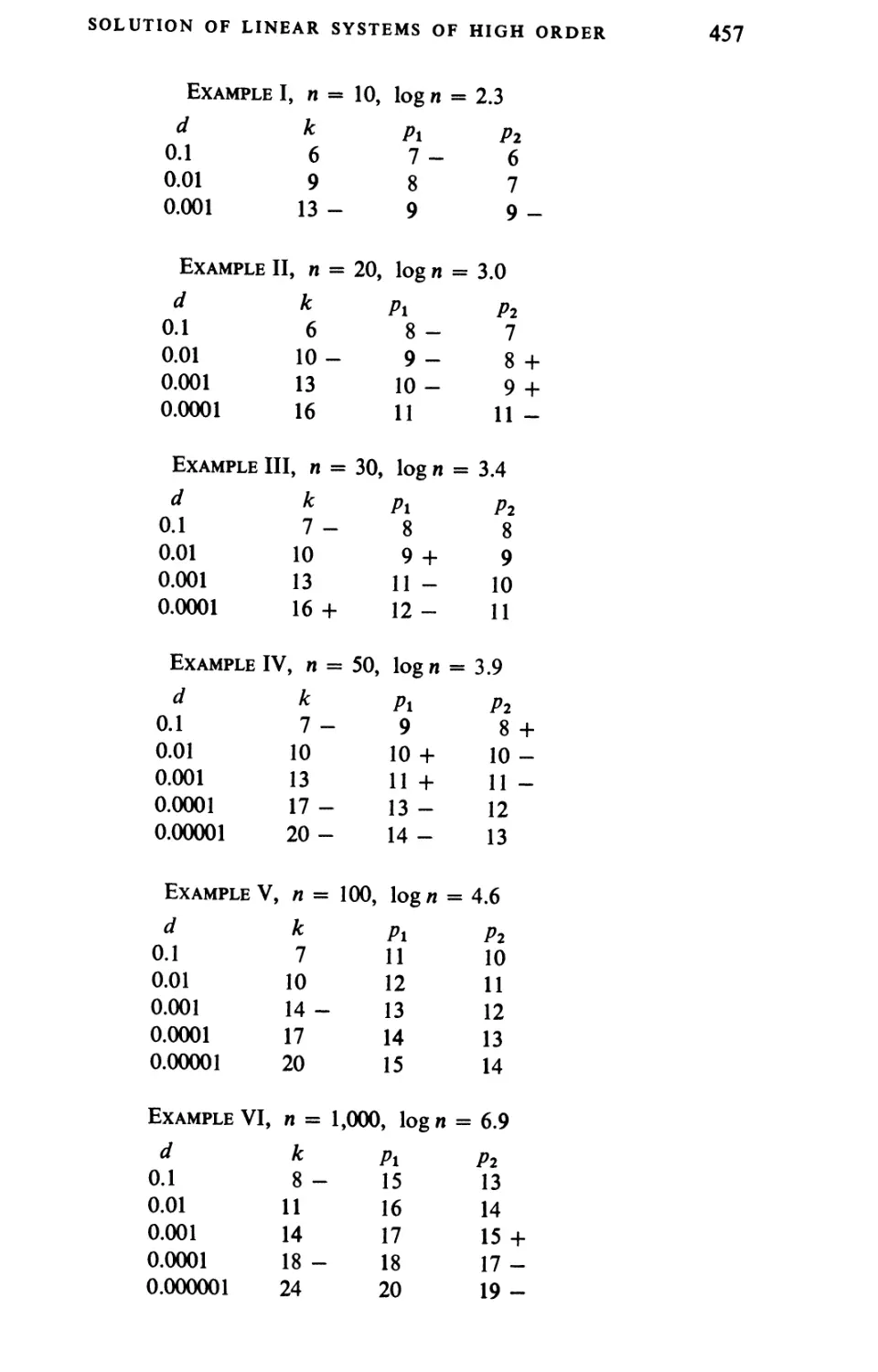
8-hr shifts) or 10 hr respectively, to produce a solution along such lines. It should
be added, that with the machines now under development these durations would
have to be extended by not unconsiderable factors, because the numerical material
that has to be manipulated (a matrix of order 400 has 160,000 elements!) will cause
difficulties in any system of storage (memory) that is at present within our reach.
All these estimates are, of course, still less reliable than the ones we made at
previous occasions. They should nevertheless suffice to make it clear that the
"unprocessed" elimination method is likely to be entirely impractical for large n,
and even the "improved" one may be quite clumsy.
In many cases better methods for solving equations, linear or non-linear, are
found by returning to the various successive approximation methods, even though
these may prima facie require considerably more multiplications. The point is,
that they are intrinsically stable, and that for this reason their requirements of
digital precision are likely to be less extraordinary.
Of these iterative procedures we mention only two. First the so-called relaxation
methods* are of considerable importance. In general, these methods replace
the given system by an associated surface in (n + l)-space and give a definite
procedure for moving along the surface from an arbitrary starting point to the
minimum point which is guaranteed to satisfy the original problem. One of these
methods, that of quickest descent, is easy to routinize for machine computation
and is quite powerful. In proceeding along the surface from a point this technique
causes the motion to be in the direction of the gradient and to be optimal in
amount. It requires repeated applications of a matrix A to a vector {. It is,
however, not possible to tell in general ex ante how many iterations are needed to
achieve a given precision, and the question is even in many important special cases
one of considerable delicacy.
* G. Temple, Proc. Roy. Soc, vol. 169 (1939) pp. 476-500.
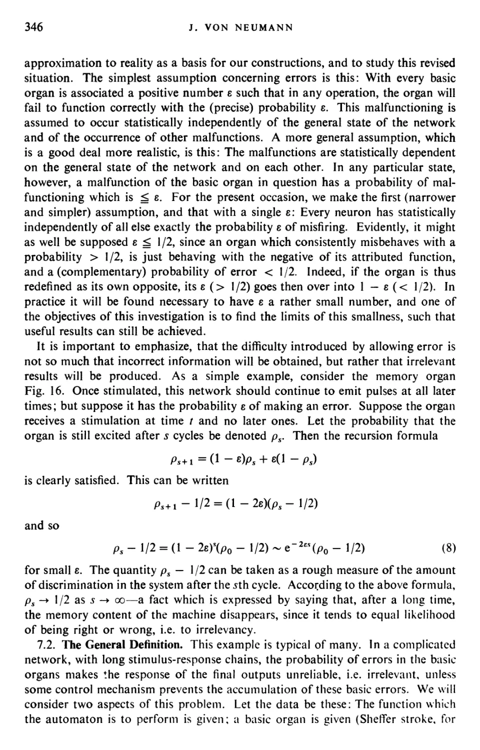
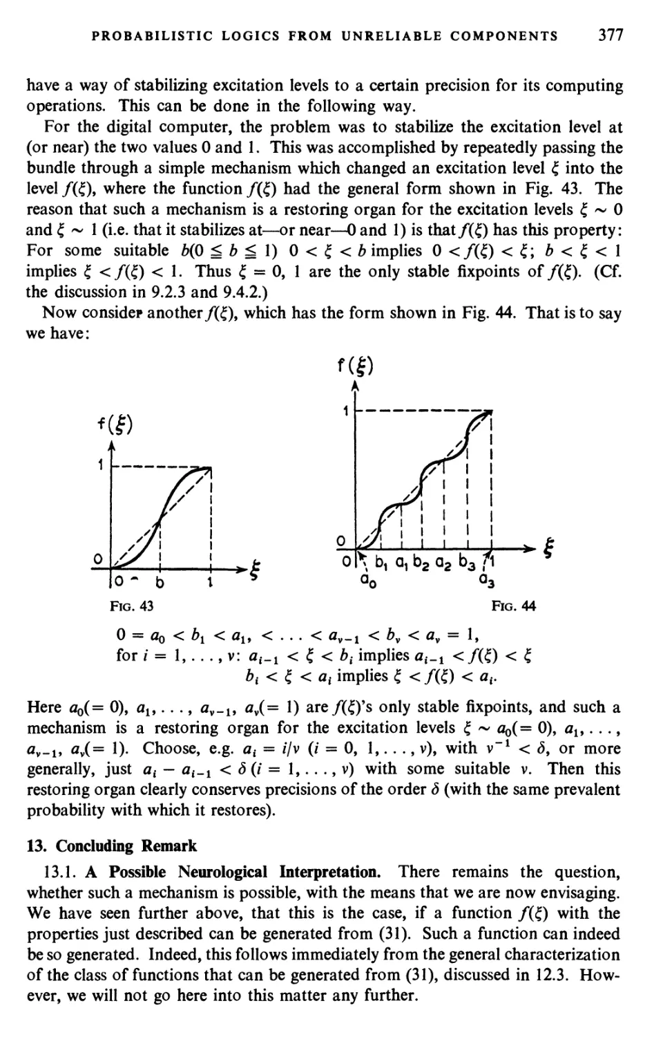
PRINCIPLES OF LARGE SCALE COMPUTING MACHINES 19
One of us, and others, recently modified a scheme of Hotelhng and obtained a
procedure which has the advantage of having a known precision at each step. It
gives, moreover, an initial estimate of the inverse.
We conclude these considerations with one more example to illustrate the need
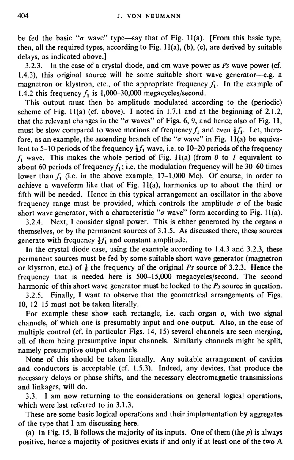
for new techniques in solving numerical problems. Suppose it is desired to find
the proper values of a given Hermitian matrix A = (a0). Viewed as a problem in
pure mathematics one might be tempted immediately to form the characteristic
equation
f(x) = x? + di**'1 + . . . + an = 0.
A reasonable modus procendendi in this direction would be first to form the
quantities tk = trace (Ak) fork= 1, 2,. . ., n (the order of the matrix) and then to find
the coefficients au a2, . . . , an of the characteristic equation by solving seriatim
the equations
tk + altk.l + a2tk.2 + . . . + ak^ltl + kak = 0
with k = 1, 2, . . . , n. This procedure would then yield the desired coefficients
with considerable ease and reasonable precision. There are, however, two related
difficulties with this scheme: First, Tschebyscheff showed that there exist
polynomials of degree n with leading coefficient 1 whose maximum on the interval
[— 1, 1] is 2~"w+1. If then our coefficients were not determined to at least n — 1
binary digits, the characteristic equation might appear to be identically zero. Thus
for n = 100 we would need at least a precision of 30 decimal digits. Second, a
machine will not really produce the traces tk but only a number whose first m digits,
say, are the first m digits of tk. If
1 ^ kx ^ k2 ^ . . . ^ kn
are the proper values, then it is clear that, as soon as k gets large, tk approaches
rkxk where r is the multiplicity of kv [We remark that tk is actually the sum of the
fcth powers of all kt (/ = 1, . . . , «).] Thus the values of many tk will contain,
almost exclusively, information regarding kv
Space does not permit us to discuss further other illustrations of the frequent
inadequacy of current techniques or of possible new procedures. We remark,
however, in closing the section, that very fast electronic devices have the speed
needed to render practicable a wide variety of novel iterative schemes and that
such methods are of utmost importance since they, to a large measure, obviate
stability questions.
6. Other Factors Affecting Speed
All our previous estimates have been based solely on the multiplication speed
(except for the correction applied in the case of the ENIAC), disregarding many
other important limitations such as speed of transfer, of logical control, memory
capacity, of input and output, difficulties of "setting up" a problem, etc. We shall
now go forward to examine the role of these other factors. It should be remarked,
however, that if these other factors are in appropriate balance with the rate of
20
H. H. GOLDSTINE AND J. VON NEUMANN
multiplying, then the solution time can be considered, as in our discussions up
to now, as a moderate multiple of the multiplication time.
For the purposes of our discussion we shall distinguish the following organs of
a digital computer: The memory, i.e. the part of the machine devoted to the
storage of numerical data; the arithmetic organ, i.e. that part in which certain of
the familiar processes of arithmetic are performed; the logical control, i.e. the
mechanism which comprehends and causes to be performed the demands of the
human operator; and the input-output organ which is the intermediary between
the machine and the outside world. We propose in the next few sections to describe
in more detail the functionings and interrelations of these organs as they relate
to our fundamental query.
7. The Input-Output Organ
We start with a discussion of this organ. This is particularly indicated, since the
most commonplace objection against a very high speed device is that, even if its
extreme speed were achievable, it would not be possible to introduce the data or
to extract (and print) the results at a corresponding rate. Furthermore, that even
if the results could be printed at such a rate, nobody could or would read them
and understand (or interpret) them in a reasonable time. There is unquestionably a
nucleus of truth, in particular in the second half of this objection in that it points
out there is at the end of the computation process a slower mechanical process
followed by a still slower human process of sensing, understanding and
interpreting the results. However, this objection can be restricted in its validity so
essentially by intelligent planning of the machine and its functioning as to become
completely irrelevant. We now proceed to analyze this situation, beginning with
the output.
Let us first consider existing machines of non-vacuum tube type. These machines
have such a low operating speed that the printing time constitutes only an
inconsequential addition to the solution time. To consider an example, the time required
to punch a standard 80 column IBM card or to print its contents is about 0.6 sec.
This provides for 8 full size (10 decimal) digit numbers, i.e. 75 msec printing or
punching time per full size number. Since it is not usually possible to organize
one's results so that more than 3 or 4 numbers can be recorded together, it is more
realistic to assign to a number a recording time of about 0.2 sec. We now compare
this rate with what obtains on punching standard tapes. This is difficult since the
standard IBM card puncher or printer carries out its operations on all 80 columns
in parallel whereas most tape punchers put only one transversal row of 5 to 10
holes simultaneously on the tape. Assuming 5 holes per transversal, we can just
about express one decimal digit by a line. Hence a 10-digit number requires about
10 transversal lines. With the usual speeds for these tapes it will require about 0.5
sec per number. This rate could probably be increased by redesign of the
equipment and could certainly be cut by the use of several in parallel. On the other
hand, these card and tape schemes are used with machines whose multiplication
rates are from 7 to 0.4 sec. Thus the recording time is short compared with the
multiplication time.
PRINCIPLES OF LARGE SCALE COMPUTING MACHINES 21
In contrast to these rates, the ENIAC has the standard IBM punch card
recording time, that we estimated as 0.2 sec, and with it a multiplication time of
3 msec. Thus the average recording time for a full size number is equivalent to
70 multiplications. This is clearly badly unbalanced for most problems. Hence
it is highly important in an electronic machine to determine whether the recording
of any particular number is really required.
In present practice, the main reasons for recording data are as follows:
(1) A number is printed because it represents an end result which the user wishes
to know and interpret. It may also be desired for the user's consideration in
connection with subsequent operations.
(2) A number is printed in order to check the "smoothness" of a curve, usually
representing an intermediary result. This is one of the most conventional checks
of errors in the machine or the process itself. The data from such printings are
frequently graphed.
(3) Printing and possibly subsequent graphing of intermediate data, as in (2)
above, may also be undertaken to follow the course of a calculation and to base
decisions on the later phases of the computation on these early results.
(4) A number is punched because it represents a result needed by the machine
at a later stage of the computation. This is storage and constitutes a function of a
memory organ.
Regarding these four items we make the following comments :
Ad. (1) This type record is necessary in all machines. It is fortunately not very
severe since those end results of a calculation that are intended for direct human
use are usually modest—e.g. the end result of solving a system of equations is one
vector. We return to this point later for a fuller discussion.
Ad. (2) This type should never be recorded in the traditional sense. Instead we
propose that it be handled by some automatic graphing device as, for example,
by an oscilloscope. Usually smoothness tests require one or more successive
differencings of the data. This should be handled by the machine (by its inner,
digital, arithmetical organs) as part of its routine, and the oscilloscope should then
project the differenced function of the desired order. While the original function
may be required to many places in order to produce the desired differences, that is
handled within the digital machines. The differences themselves need only be
graphed with precisions of a few per cent, in order to be viewed and assessed by
the user. This is fully within the scope of the customary oscilloscopic equipment.
The contemplated machines will have the logical flexibility to handle such a program
with ease.
Ad. (3) If the operator knows a priori all possible alternatives that might be
pursued in the course of the calculation as well as the exact mathematical criteria
by which these alternatives should be selected while the calculation is in progress,
he can instruct the machine accordingly. The machine will then take care of these
things automatically. If, on the other hand, he cannot produce ex ante such
unambiguous and exhaustive formulations, and wishes instead to exercise his
intuitive judgement as the calculation develops, he can arrange for that, too. He
can instruct the machine to present to him the relevant characteristics of the
22
H. H. GOLDSTINE AND J. VON NEUMANN
situation, continuously or in discrete succession, as the calculation progresses, by
oscilloscopic graphing. He can then intervene whenever he sees fit.
Thus this complex can require nothing worse than the procedures discussed in
connection with (2) above.
Ad. (4) As remarked earlier this is not properly a printing function but rather a
memory problem. It should be treated by appropriate storage device and not by
printing. We will consider it in the later pages.
Thus we see that only (1) is properly a recording problem. The others either
call for a new output device, a transiently responding fluorescent screen on an
oscilloscope or belong elsewhere, namely in the machine's memory.
We return to the consideration of (1). The user desires a printed page containing
his final results and not some medium such as a punched card, tape etc. It is,
however, not easy to visualize how the computer proper could produce such a
record, which it could itself later sense and re-use in a computation. Instead we
prefer to contemplate two forms of permanent output. The first one is to be
"intelligible" to the machine itself as well as to a typing (or printing) mechanism,
while the second one is to be intelligible to a human. The typing (or printing)
device forms the link between the two forms of recording. It is quite important
that the computer should be able to read its own output as will be seen below in
our discussion of memory.
In a truly high speed device we can carry out the first part of the functions of (1),
as outlined above, by using magnetic wires or tapes that can read or record 10 digit
decimal numbers at rates of about 500-1,000 per second per channel, i.e. we can
accelerate the card punching or tape rates by a factor of about 200 using a single
channel. Still greater rates could be obtained by the use of multiple channel
magnetic tapes. Thus the computer itself can read and record at rates fully
comparable with its multiplying time: One full size number reading or recording ~ 5
multiplication times. It is difficult to conceive of a problem which is sufficiently
complex to deserve being put on an elaborate, automatic computer and which
would not require at least this order of multiplication times per number introduced
or produced.
The data actually given the human user will then consist of graphs on an
oscilloscope which he can comprehend quickly and satisfy himself as to the course of his
computation and of a very small—perhaps a few hundred at most—numbers which
he will wish to analyze and interpret. These latter results can be produced at a rate
fully comparable to the human's ability to read them on one or more automatically
controlled typewriters, which are set up to sense and to type the desired portions
of the magnetic record. Similar devices will be needed to transform the input
information given by the user into a form "intelligible'* for the machine, i.e.
magnetically recorded on the wire or tape.
In regard to the last point it is worth calling attention to the fact that the
preparation of a specific new problem usually does not require a very elaborate
effort. The new electronic machines are being so devised that they can
comprehend generic instructions when these are supplemented by the parameters specific
to a problem. (For example, the instructions for interpolating, inverting matrices,
PRINCIPLES OF LARGE SCALE COMPUTING MACHINES 23
integrating systems of total or partial differential equations, solving implicit
equations, etc. can be produced a priori and used on specific problems at later
times merely by selecting from a "library" and introducing the appropriate tapes
or wires into the machine, and by further introducing the numerical data and the
additional instructions or equations pertinent to the particular situation.) Thus
once the logical instructions for a given class of problems have been put into the
form needed by the machine, a particular problem will require only a moderate
amount of specific additional data and instructions. The time required for
producing (i.e. planning, formulating and typing) these should therefore be reasonable,
and the actual introduction into the machine takes place anyhow at the high speed
of the magnetic tape or wire.
8. The Memory Organ
In discussing this aspect of computing devices we find it convenient first to
enumerate the main types of memory needed in fully automatic machines.
(1) In performing an operation (arithmetical or logical) it is usually necessary
to store the quantities entering into it; e.g. the multiplier, multiplicand and partial
products as they are formed.
(2) During a computation it is frequently necessary to store intermediate results
which will be used shortly afterwards in the next phase of the calculation, e.g. the
position and velocity of a particle at time / may be held in order to proceed to
time / + At in a step-wise integration of an orbit. Note that for partial differential
equations this may get fairly voluminous.
(3) The intermediate results of a computation may be needed at a fairly distant
time in the future—distant in terms of the machine's rate—and be so voluminous
as to tax the memory provided under (2) above. Such a situation might arise when
one multiplied together two matrices of high order, say n ^ 30, or when one
integrates fairly complex hyperbolic or elliptic systems, since in the former case the
behavior of the solution at a point will influence an extended wedge shaped region,
and in the latter, all other points.
(4) For many problems considerable initial data are needed to define the problem,
e.g. the boundary conditions of a partial differential equation.
(5) Often arbitrary functions play an essential role and must therefore be stored
in the machine. Such functions may be either analytically defined, e.g. In x, e*,
sin x9 arc sin x, etc.; or of empirical origin, e.g. the equation of state of a non-ideal
gas or of a liquid or solid at high pressures, or the drag function of a projectile.
(6) Finally the logical instructions must in some form be given to the machine,
i.e. the machine must in some manner be "wired" to do the specific routine
desired.
We now proceed to see how each of these groups is handled in existing machines
and then to develop our own ideas as to how we wish to treat them. Accordingly
we arrange our discussion as commentary to the groupings (1) through (6) above.
Ad. (1) Virtually all devices make provisions for this in the arithmetic organ
by means of so-called "counters" or "registers". Such units are aggregates of
wheels each of which indicates the value of a decimal digit by the position relative
24
H. H. GOLDSTINE AND J. VON NEUMANN
to a fixed position; or aggregates of electro-mechanical relays where the open or
closed state of each indicates the value of a binary digit, or the state of a group of
them—usually 4 or 5—expresses the symbol for a decimal digit; or an aggregate
of vacuum tubes or of thyratrons (gas filled, grid controlled tubes) which can be
combined (usually in pairs in the former case) to form "flip-flops" or "triggers"
which are the electronic equivalent of relays. The present machines usually employ
a few such registers in their arithmetic parts.
Ad. (2) Here again the existing devices use registers or counters. In the case
of the Harvard IBM and the Bell Telephone Company machines there are between
100 and 150 such units available for storage. In the case of the ENIAC there are
20 such units, each one being a large aggregate of vacuum tube "flip-flops". It
may be seen from the fact that each binary digit requires essentially one relay or
one pair of vacuum tubes (in the ENIAC each decimal digit requires 10 pairs of
vacuum tubes) that this form of storage rapidly becomes quite expensive, and it is
thus not practicable to utilize such units in case 3 below.
Ad. (3) To gain an approximate idea of the capacities required for such
intermediate results let us consider a few illustrations. A hyberbolic equation in two
variables, x91 may, as we saw earlier, require 50 x-points per /. We may also wish
to remember from 2 to 4 numbers at each lattice point. Thus 100-200 numbers
would surely be needed. If we increase by 1 the dimension of the equation then
one value of / may be associated with 502 (x, y) points and we may need to store
4-5 numbers per point for use at the next / value. This already fixes the memory
at over 104 numbers. If a third dimension is added we easily reach requirements of
5 x 10⁵ numbers. We could continue to examine other problems such as integral
equations, elliptic equations or systems of simultaneous equations—all of which
behave much alike—but instead we see that a capacity of about a million words
is not at all unreasonable.
The existing machines are somewhat inconvenient to use for problems in which
several hundred data are needed since none has a register capacity for more than
150 numbers. They all possess however a subsidiary memory in the form of tapes
or punch cards which can be fed back at a later time. This external memory is
adequate for non-electronic machines and need not upset for those our previous
time estimates. [It should be added, however, that for the Bell Telephone
Company's newest relay machines the tape speed is probably out of balance (too slow)
with the rest of the device.] It does however, create a serious unbalance in the
case of the ENIAC and was one of the reasons we modified downwards our estimate
of its "effective" multiplying rate.
Ad. (4) This really falls under cases (3) and (5).
Ad. (5) The methods used for storing fixed functions vary widely between
existing machines. The standard IBM machines sense functional data stored on
punched cards while the relay machines have both permanently connected banks
of relays for the most commonly used functions and punched tapes. The ENIAC
has banks of connections, so-called "function tables", which can be set a priori to
desired values and can then be sensed at electronic speeds, 0.2 msec per full size
number.
PRINCIPLES OF LARGE SCALE COMPUTING MACHINES 25
Ad. (6) Again here we find differences between existing machines. The standard
IBM machines are equipped with plugboards for establishing routines. They may
also be controlled by certain punches on cards and even by humans, e.g. transferring
stacks. Both the Harvard-IBM and the Bell Telephone Company machines are
controlled by instructions punched into several tapes and they can be ordered to
switch from one to the other as desired. They are usually referred to as "master
routine" and "sub-routine" tapes.
The ENIAC is controlled by manually set switches and plugs in combinations
with its electronic switching organs. Quite recently the "function tables" of the
ENIAC, already referred to in (5) above, are belQg increasingly used to store what
amounts in effect to logical instructions, rather than the numbers (functions) for
which they were originally intended.
In this connection it should be noted that the logical instructions are like the
function tables in that they are set up at the beginning of a problem. A detailed
analysis of such instructions shows that in the electronic machines now under
development an order requires about as many digits as a number and that quite
complex routines can be obtained with a few hundred instructions. We do not have
the space to analyze this problem in detail but merely state than an order memory
of about 1,000 words seems for the present a reasonable definition of a
goal.
We turn now to the question of how these groups can be handled in a new high
speed machine and what effects this has on the overall solution time of problems
in such devices.
Inasmuch as the arithmetic part of a computer need involve only a very few—
say three—registers or counters, we propose no drastic change in the manner of
treating (1) above. With regard to (2) through (6), it is clear that the only real
distinction lies in the capacity requirements in each category. We return to a
further analysis of this point after discussing item (6).
Due to its very nature a general purpose computer has only a very few of its
control connections permanently wired in. Apart from certain main
communication channels these fixed connections are usually those which suffice to guarantee
the device's ability to perform certain of the more common arithmetic processes,
such as addition, subtraction, multiplication and possibly division or square roots.
It is the function of the control organ and its associated memory to make and
unmake the balance of the connections needed to carry out the routine for a given
problem. As we saw in (6) above there are two main methods adopted in existing
devices for making these connections. We classify them as follows: (a) The method
of establishing all connections a priori, as exemplified by the ENIAC; and (b) The
method of establishing connections at the moment needed, the instructions
necessary for this being stored in some organ such as a paper tape.
We notice that the latter method has the great advantage that an indefinitely
large aggregate of instructions can be performed whereas in the former one only a
limited number can be performed in any one fully automatic run of the machine.
Scheme (a) has the added disadvantage of requiring a considerable set-up time since
physical connections must be made—in the case of the ENIAC this is of the order
26
H. H. GOLDSTINE AND J. VON NEUMANN
of 8 man-hr. This feature, of course, reduces greatly the flexibility of a device and
reduces the validity of our method of estimating solution times for short problems,
i.e. a problem that can be handled on the ENIAC in 5 minutes probably takes
nevertheless an 8-hour shift. A third disadvantage of scheme (a) from our point
of view is that it is usually expensive in the number of vacuum tubes required.
This arises out of the fact that often a great many wires may lead out of a given
terminus, only one of which is to be excited at a time. Hence non-linear elements
must be introduced to isolate one line from another. Scheme (a) has one great
merit however in that once the connections are established program instructions
can proceed at electronic rates—this is, incidentally, one of the reasons why it
was adopted in the ENIAC.
We desire to combine the advantages of both schemes (a) and (a) and do so by
making one important modification in the scheme (b).
It is evident that the storage of instructions in appropriately coded form on tape
is nothing other than the storage of digital information. It might, therefore, as
such, also be treated in exactly the same manner, cf. (2) through (5).
Recall our earlier remark that about 1,000 instructions is a reasonable upper
limit for the complexity of problems now envisioned. To summarize, we find that
cases (2) through (6) are entirely analogous and at most differ in the amount of
memory needed. In case (1), however, the requirements of the arithmetic and
control units make it desirable to have about three registers of flip-flop character.
We wish to treat the other cases (2) through (6) as identical, and have a common
memory organ to handle all of them, one that makes no distinction between the
various groups.
There is, however, an engineering problem that arises at this point, which makes
it difficult to achieve very great memory capacity at electronic speeds. We
accordingly admit the possibility of having a hierarchy of memory units forming our
memory organ. Specifically we may be forced to treat group (3) in this fashion.
Bpfore continuing in this direction further let us estimate the speeds needed to
enter or to leave the memory.
In performing a multiplication one usually performs about 3 or 4 associated
additions or subtractions or comparisons; hence at least 4-5 orders must be given
and at least that many numbers transferred—it is assumed that an order specifies
only one basic operation, together with its transfers. Thus we find that there is
associated with each multiplication at least 4-5 orders and 4-5 transfers of numbers.
Since, however, we agree to store our orders in the same place as our numbers,
we may say that there are about 10 transfers per multiplication—notice that no
time has been allowed for executing the orders. If the transfer time is not to be
the dominant speed factor, then the time for effecting 10 transfers must be of the
same order as the multiplication time. Since we wish to achieve a multiplication
rate of 10"4, the time of a transfer must be about 10"5 sec.
If such a transfer rate is to be achieved the memory organ must have a very fast
response. We are thus forced at the outset to exclude punched card or tape tech-.
niques and to consider organs which respond at electronic speeds. However, we
must also recall our first criterion which established the need for extensive capacity.
PRINCIPLES OF LARGE SCALE COMPUTING MACHINES 27
This latter point rules out conventional attacks such as the use of flip-flops. To
summarize, we see that a very fast memory of a capacity of several thousand words
is needed. Very fast means that the transfer velocities (in and out, as well as for
erasing) should be in the electronic range about 10"5 sec per word. By a word we
mean an aggregate of binary digits expressing either a simple order (about one
arithmetical or logical operation and its associated transfers) or a full size number
(of a precision of about 10 decimal digits or its equivalent). Our experience is
that such a word requires about 40 binary digits in either case. As to the capacity,
we have seen that we need about 1,000 words for logical purposes alone. To
balance this, it is reasonable to require this many, or somewhat more, words for
numbers. The number memory of the order of 106 words, referred to earlier, will
have to be handled by the next member of the memory hierarchy, i.e. by a slower
memory organ, as already indicated. We will consider the latter somewhat further
below. As far as the fastest electronic speed memory is concerned, however, we
see that a capacity of a few thousand words is desirable, each word consisting of
about 40 binary digits.
The most promising device having the characteristics just described is a cathode-
ray-type television tube in which the fluorescent screen is replaced by a dielectric
plate. It is well-known that such tubes can operate at the requisite speeds and
certainly are capable of large storage. In fact the existing television tubes which
should be used for comparison, the iconoscope and its various successors, scan
linearly over about 450 lines. Thus it seems reasonable to attribute to them linear
resolutions of about one part in 450, which corresponds, at least nominally, to a
storage capacity of about 4502 « 105 points. This estimate of the storage capacity
that is achievable with present techniques is, however, certainly unrealistically high
for our purpose, since the television requirements on the identity of a given point
are not so severe as ours. The Radio Corporation of America Research
Laboratories are in the process of developing a special tube, known as the Selectron,
which is expected to have the desired characteristics. This device is not yet
completed but gives every promise of being one of the most fruitful and remarkable
advances in the field of computational components. We remark parenthetically
that each such tube will store 642 = 4,096 = 212 binary digits.
The use of about 40 of these Selectrons will permit a memory capacity quite
capable of fulfilling the requirements of all groups above except possibly (3), the
case where voluminous .intermediate results need to be remembered until a (from
the machine's point of view) relatively distant time. We have already recognized,
that this calls for a second stage in the memory hierarchy, i.e. for a slower (than
electronic, i.e. than about 10"5 sec per word) but larger capacity memory. To
determine characteristics for this second stage in our memory hierarchy we inquire
into further speed requirements. Virtually all large scale calculations may be
broken up into large subcomputations following one after the other, e.g. in the
multiplication of matrices one can proceed by compounding submatrices
successively. We can thus use the secondary memory as a temporary repository for
data and at the appropriate time feed these data in a block into the primary high
speed storage organ. Thus we need a very rough estimate of the time a calculation,
28
H. H. GOLDSTINE AND J. VON NEUMANN
using only the primary memory, will consume. Let us assume that we have about
3,000 words available in the fast, primary memory, which is now supposed to be
used for intermediate results, and that we will perform at least two multiplications
with each datum, i.e. at least 6,000 multiplications, before we need to replenish
the primary memory from the secondary one. This number of products will require
about 5 sec. (We assume again 0.3 msec per multiplication and an excess factor 3
over the net multiplication time.) We can therefore allow a comparable period
of time for introducing new data from the secondary memory.
The magnetic wires or tapes discussed earlier are likely to operate at about
500-1,000 words per second, i.e. 1-2 msec per word, assuming only one channel,
and they can be made of indefinite length. They therefore fulfil our requirements
for a secondary memory even with a single channel. There are other considerations
dealing with "finding" a desired word in this memory which makes several channels
nevertheless desirable. We will not go into these in connection with the secondary
memory. However, they are sufficiently important from the point of view of the
primary memory too, that we will consider them briefly.
In "reading" a word from the memory, it is not only the time effectively
consumed in reading (sensing) which matters, but also the time needed to "find" it
at its specified location in the memory. In "writing" a word into the memory, it
is similarly not only the time effectively consumed in "writing" which matters, but
also the time needed to "find" the specified location in the memory at which it is
desired to store it. [That a number (or an instruction) that is to be read has to
be found at a definite place in the memory is evident. That a number that is to
be written, i.e. stored, has to be placed at a definite, possibly inconvenient place
in the memory may also be caused by absolutely compelling reasons: Other
possibly more convenient places may not be available, i.e. they may all be occupied
by numbers which are still needed, and therefore must not be erased to make place
for the new number to be stored. Or it may be that storage at that particular space
fits into the general plan of the calculation, and obviates the additional burden of
remembering specifically where the particular number in question is being stored.]
We call the first mentioned duration (actual reading or writing) the net transfer
time, and the second mentioned duration (finding of the place for reading or writing)
the transfer waiting time. Unless it is known in advance that the memory is to
be used in one, fixed linear order, the transfer waiting time is just as relevant as
the net transfer time.
It is one of the main virtues of the cathode-ray tube or inconoscope or Selectron
type memory devices that they "find" a specific place by deflecting or cutting off
or passing an electron beam which is very fast. So their transfer waiting times are
of the same order as their net transfer times. The magnetic wire or tape, on the
other hand, has to be scanned in a definite linear order. Finding a place on it
involves moving it mechanically, and the speed of this operation is limited by the
possibilities of mechanically accelerating and decelerating the wire or tape.
Therefore its transfer waiting time is usually considerably longer than its net transfer
time. There are various other, otherwise very tempting, electronic or part-electronic
memory devices which share this disadvantage.
PRINCIPLES OF LARGE SCALE COMPUTING MACHINES 29
Of course these shortcomings are rarely absolutely prohibitive. Also (for the
main function that we contemplate for the secondary memory: the renewal of the
primary memory) a simple linear scanning of the former is in many important
cases adequate (but not in all of them!). Finally these long-waiting time devices
usually lend themselves to multi-channel (parallel) arrangements, which may
improve the situation not inconsiderably. Nevertheless, for those memory devices
with long waiting times which are most significant from the engineering point of
view, this handicap does not appear to be completely removable, at least not with
the techniques now within our reach.
9. Coding of Problems
We have now shown that the time spent on introducing and withdrawing data
from a high speed machine is not a controlling parameter; that it will probably
be possible to build a memory organ which is sufficiently capacious for our present
needs, which is so fast that transfer times do not dominate multiplication times,
and whose logical control can be effected in an equally fast manner. It remains,
then, only to comment on the last objection frequently offered against high speed
computers: that the time of coding and setting up problems for such a machine
is the dominant consideration.
It is quite true that in existing machines the time for coding problems is
comparable to the solution time, and that every effort must be made to simplify the
coding of problems. It is equally true that a problem solvable in seconds cannot
be programmed in seconds. In a well conceived machine there must be provision
whereby not individual problems but rather whole classes of problems can be
coded in one operation. Thus we should, for example, contemplate preparing
general instructions for finding the proper values of a Hilbert-Schmidt type integral
equation. Then, when a specific kernel is before us, we only code the exact
description of this kernel and append this to our previously formulated routine. Similar
remarks apply, of course, to other classes of problems, such as inversion of matrices,
solution of differential systems, etc. Thus the time spent on coding problems after
a certain preliminary organizational period will, in general, consist of recognizing
in what category the problem falls, selecting the proper control tape or wire from
the library of previously prepared routines, and of formulating the peculiarities of
the given problem. As time goes on, new problems will come up, and these, as
well as new insights on old problems, will require the formulation of new general
routines, too. However, these are merely the usual burdens of scientific progress,
and not shortcomings of the machine approach.
This argument, however, does not exhaust our reasons for feeling that the
problem of coding routines need not and should not be a dominant difficulty. If
we were interested in speeding up by extraordinary factors the time required to
handle problems of current interest, then the time of coding would indeed be
severe. However our aim is to explore entirely new avenues heretofore quite
impossible by conventional tools. In this task we will spend hours, days and even
weeks of computing time to obtain solutions. Thus objections based on assuming
solution times of a few seconds are quite unrealistic.
30
H. H. GOLDSTINE AND J. VON NEUMANN
We do not wish to give the reader the false impression that we do not realize
the seriousness of the coding problem. In fact we have made a careful analysis of
this question and we have concluded from it that the problem of coding can be
dealt with in a very satisfactory way.
In addition to a quite flexible and general set of basic orders that can be
understood by his machine, the coder needs certain further things: An effective and
transparent logical terminology or symbolism for comprehending and expressing
a particular problem, no matter how involved, in its entirety and in all its parts;
and a simple and reliable step-by-step method to translate the problem (once it is
logically reformulated and made explicit in all its details) into the code.
Heretofore these requirements were not fulfilled, and this laid on coders an
exceedingly heavy burden of extensive and complex efforts towards understanding,
assessing, and reformulating in machine terms a problem that was presented in
conventional mathematical terms. This is particularly and conspicuously true for
computational procedures involving numerous and multiple inductions, where the
usual logical machinery of the mathematician assumes a very clumsy and
complicated shape, if it has to be made completely explicit.
We will now attempt to give a clearer and fuller idea of what is involved in
coding for a machine of the sort we have outlined, and what the procedures are
that seem to us appropriate for the actual task of coding. In order to do this, we
have to consider the control organ in somewhat more detail. It is desirable to
have the control so constituted that in general it scans the domain of the memory
in a linear manner, i.e. it starts from position 0 in the memory and after having
executed the instruction in place y proceeds to y + 1. If the control necessarily
proceeded in this fashion in all cases, such procedures as inductive definitions or
iterative processes, for example, would have to be rewritten for each value of the
index involved. This would require in many important cases, indeed, just in the
most relevant cases, much more space for the instructions than any storage device
that is now within our reach can provide. Besides, routines involving alternative
procedures, especially when the alternatives are decided by events which occur in
the course of the calculation, would then present great if not unsurmountable
obstacles to coding. Yet the latter category includes various important variable
length inductions, and hence, for example, the successive approximation
procedures. All of this clearly conflicts with any reasonable principles of simple and
effective coding, and is altogether unacceptable.
For these reasons we introduce a transfer order which can cause the control to
be moved from where it is to any other desired point in the memory space. We
distinguish two types of transfer orders: First, the unconditional transfer which
effects the transfer in every case, for example, where no discretion is left to the
machine to decide whether or not it should make the transfer of the control; and
second, the conditional transfer which effects the transfer only if a certain
(arithmetical) criterium is fulfilled. It is convenient to choose for this criterium the
non-negativity of the number that occupies at the moment in question a definite
position in the arithmetic organ. (It should be remarked that the unconditional
transfer is not logically independent of the conditional transfer; it can, in fact, be
PRINCIPLES OF LARGE SCALE COMPUTING MACHINES 31
programmed out of the latter but it occurs so frequently it is found convenient to
make it an explicit instruction.)
We also introduce instructions for transferring data between the arithmetic
registers and the memory together with orders for carrying out a class of arithmetic
processes such as + , —, x, -r-. Since these latter processes are two variable
functions, it would seem necessary to have each order involving these operations
make reference to two memory positions. The indication of the memory position
at which the result is to be stored would add to this the need of a third reference.
We prefer, however, not to "freeze" all orders to carrying three memory position-
references, because it is probably more the rule than the exception that the result
of an arithmetical operation is one of the variables entering into the next operation.
Hence obligatorily consigning it as a "result" to the memory just to have to bring
it back immediately thereafter as a "variable", would be time consuming "waste
motion". We avoid this by subdividing orders further, and thereby making them
more flexible. Specifically, we make the arithmetic orders read as follows: "Take
the contents of position x in the memory and add it to, or subtract it from, or
multiply with it, or divide by it the number which is stored at this moment in a
certain part of the arithmetic organ; when the operation is completed leave the
result in the arithmetic organ, where it has been formed." To these we must add
disposal orders, which read as follows: "Take the number which is at this moment
in a certain part of the arithmetic register, and move it to the position x in the
memory."
In this manner all orders refer only to one position x in the memory. (There
are a few exceptions, which contain no such reference at all, but we need not
discuss them here.) This arrangement has the effect that somewhat less than half
of a 40 digit word can hold an order. We plan, therefore, to have a full size (40
binary digit) word either contain one full size number (40 binary digits—this is a
precision equivalent to 12 decimal digits, but we will use the first binary digit [left]
to denote the sign) or two (20 binary digit) orders.
It should be added that there are two ways to send a number a from the
arithmetic organ to the memory, say to the memory position y. We either want to
place the entire 40 digit number a to occupy the entire space at y, or there may be
two orders at y, and we may only want to replace the memory-position-reference x
in one of these orders by part of a. Since we plan to have 4,096 = 212 viewed as a
12 binary digit number, hence it will require 12 digits of a, say the 12 last ones (to
the right). In view of this possibility we may also call the disposal orders
substitution orders. The first use (40 digits of a moved) is a total substitution, the second
use (12 digits of a moved) is a partial substitution, and according to whether the
first or the second order at y is modified, the partial substitution is left or right.
It should be added that this technique of automatic substitutions into orders,
i.e. the machine's ability to modify its own orders (under the control of other ones
among its orders) is absolutely necessary for a flexible code. Thus, if a part of the
memory is used as a "function table", then "looking up" a value of that function
for a value of the variable which is obtained in the course of the computation
requires that the machine itself should modify, or rather make up, the reference
32 H. H. GOLDSTINE AND J. VON NEUMANN
to the memory in the order which controls this "looking up", and the machine
can only make this modification after it has already calculated the value of the
variable in question.
On the other hand, this ability of the machine to modify its own orders is one
of the things which makes coding the non-trivial operation which we have
to view it as. Therefore this is a quite relevant circumstance in every respect.
PRELIMINARY DISCUSSION OF THE LOGICAL DESIGN OF
AN ELECTRONIC COMPUTING INSTRUMENT
By Arthur W. Burks, Herman H. Goldstine and John von Neumann
PREFACE TO FIRST EDITION
This report has been prepared in accordance with the terms of Contract
W-36-034-ORD-7481 between the Research and Development Service, Ordnance
Department, U.S. Army and the Institute for Advanced Study. It is intended as
the first of two papers dealing with some aspects of the overall logical
considerations arising in connection with electronic computing machines. An attempt is
made to give in this, the first half of the report, a general picture of the type of
instrument now under consideration and in the second half a study of how
actual mathematical problems can be coded, i.e. prepared in the language the
machine can understand.
It is the present intention to issue from time to time reports covering the various
phases of the project. These papers will appear whenever it is felt sufficient work
has been done on a given aspect, either logical or experimental, to justify
its being reported.
The authors also wish to express their thanks to Dr. John Tukey, of Princeton
University, for many valuable discussions and suggestions.
Arthur W. Burks
Herman H. Goldstine
John von Neumann
The Institute for Advanced Study
28 June 1946
PREFACE TO SECOND EDITION
In this edition the sections dealing with the arithmetic organ have been
considerably expanded and a more complete account of the arithmetic processes
given. In addition, certain sections have been brought up to date in the light
of engineering advances made in our laboratory.
Arthur W. Burks -
Herman H. Goldstine
John von Neumann
The Institute for Advanced Study
2 September 1947
34
Part I
1. Principal Components of the Machine
1.1. Inasmuch as the completed device will be a general-purpose computing
machine it should contain certain main organs relating to arithmetic, memory-
storage, control and connection with the human operator. It is intended that the
machine be fully automatic in character, i.e. independent of the human operator
after the computation starts. A fuller discussion of the implications of this remark
will be given in Chapter 3 below.
1.2. It is evident that the machine must be capable of storing in some manner
not only the digital information needed in a given computation such as boundary
values, tables of functions (such as the equation of state of a fluid) and also the
intermediate results of the computation (which may be wanted for varying lengths
of time), but also the instructions which govern the actual routine to be performed
on the numerical data. In a special-purpose machine these instructions are an
integral part of the device and constitute a part of its design structure. For an all-
purpose machine it must be possible to instruct the device to carry out any
computation that can be formulated in numerical terms. Hence there must be some
organ capable of storing these program orders. There must, moreover, be a unit
which can understand these instructions and order their execution.
1.3. Conceptually we have discussed above two different forms of memory:
storage of numbers and storage of orders. If, however, the orders to the machine
are reduced to a numerical code and if the machine can in some fashion distinguish
a number from an order, the memory organ can be used to store both numbers
and orders. The coding of orders into numeric form is discussed in 6.3 below.
1.4. If the memory for orders is merely a storage organ there must exist an
organ which can automatically execute the orders stored in the memory. We shall
call this organ the Control.
1.5. Inasmuch as the device is to be a computing machine there must be an
arithmetic organ in it which can perform certain of the elementary arithmetic
operations. There will be, therefore, a unit capable of adding, subtracting,
multiplying and dividing. It will be seen in 6.6 below that it can also perform additional
operations that occur quite frequently.
The operations that the machine will view as elementary are clearly those which
are wired into the machine. To illustrate, the operation of multiplication could be
eliminated from the device as an elementary process if one were willing to view
it as a properly ordered series of additions. Similar remarks apply to division. In
35
36 A. W. BURKS, H. H. GOLDSTINE AND J. VON NEUMANN
general, the inner economy of the arithmetic unit is determined by a compromise
between the desire for speed of operation—a non-elementary operation will
generally take a long time to perform since it is constituted of a series of orders
given by the control—and the desire for simplicity, or cheapness, of the machine.
1.6. Lastly there must exist devices, the input and output organ, whereby the
human operator and the machine can communicate with each other. This organ
will be seen below in 4.5, where it is discussed, to constitute a secondary form of
automatic memory.
2. First Remarks on the Memory
2.1. It is clear that the size of the memory is a critical consideration in the
design of a satisfactory general-purpose computing machine. We proceed to discuss
what quantities the memory should store for various types of computations.
2.2. In the solution of partial differential equations the storage requirements
are likely to be quite extensive. In general, one must remember not only the initial
and boundary conditions and any arbitrary functions that enter the problem but
also an extensive number of intermediate results.
(a) For equations of parabolic or hyperbolic type in two independent variables
the integration process is essentially a double induction. To find the values of the
dependent variables at time t + At one integrates with respect to x from one
boundary to the other by utilizing the data at time t as if they were coefficients
which contribute to defining the problem of this integration.
Not only must the memory have sufficient room to store these intermediate data
but there must be provisions whereby these data can later be removed, i.e. at the
end of the (t + Af) cycle, and replaced by the corresponding data for the (t + 2At)
cycle. This process of removing data from the memory and of replacing them with
new information must, of course, be done quite automatically under the direction
of the control.
(b) For total differential equations the memory requirements are clearly similar
to, but smaller than, those discussed in (a) above.
(c) Problems that are solved by iterative procedures such as systems of linear
equations or elliptic partial differential equations, treated by relaxation techniques,
may be expected to require quite extensive memory capacity. The memory
requirement for such problems is apparently much greater than for those problems in (a)
above in which one needs only to store information corresponding to the
instantaneous value of one variable [t in (a) above], while now entire solutions (covering
all values of all variables) must be stored. This apparent discrepancy in
magnitudes can, however, be somewhat overcome by the use of techniques which permit
the use of much coarser integration meshes in this case, than in the cases under (a).
2.3. It is reasonable at this time to build a machine that can conveniently
handle problems several orders of magnitude more complex than are now handled
by existing machines, electronic or electro-mechanical. We consequently plan on
a fully automatic electronic storage facility of about 4,000 numbers of 40 binary
digits each. This corresponds to a precision of 2"40 ~ 0.9 x 10"12, i.e. of about
12 decimals. We believe that this memory capacity exceeds the capacities required
LOGICAL DESIGN OF ELECTRONIC COMPUTING INSTRUMENT 37
for most problems that one deals with at present by a factor of about 10. The
precision is also safely higher than what is required for the great majority of
present day problems. In addition, we propose that we have a subsidiary memory
of much larger capacity, which is also fully automatic, on some medium such as
magnetic wire or tape.
3. First Remarks on the Control and Code
3.1. It is easy to see by formal-logical methods that there exist codes that are in
abstracto adequate to control and cause the execution of any sequence of operations
which are individually available in the machine and which are, in their entirety,
conceivable by the problem planner. The really decisive considerations from the
present point of view, in selecting a code, are more of a practical nature: simplicity
of the equipment demanded by the code, and the clarity of its application to the
actually important problems together with the speed of its handling of those
problems. It would take us much too far afield to discuss these questions at all
generally or from first principles. We will therefore restrict ourselves to analyzing
only the type of code which we now envisage for our machine.
3.2. There must certainly be instructions for performing the fundamental
arithmetic operations. The specifications for these orders will not be completely given
until the arithmetic unit is described in a little more detail.
3.3. It must be possible to transfer data from the memory to the arithmetic
organ and back again. In transferring information from the arithmetic organ back
into the memory there are two types we must distinguish: Transfers of numbers
as such and transfers of numbers which are parts of orders. The first case is quite
obvious and needs no further explication. The second case is more subtle and
serves to illustrate the generality and simplicity of the system. Consider, by way
of illustration, the problem of interpolation in the system. Let us suppose that
we have formulated the necessary instructions for performing an interpolation of
order n in a sequence of data. The exact location in the memory of the (n + 1)
quantities that bracket the desired functional value is, of course, a function of the
argument. This argument probably is found as the result of a computation in the
machine. We thus need an order which can substitute a number into a given
order—in the case of interpolation the location of the argument or the group of
arguments that is nearest in our table to the desired value. By means of such an
order the results of a computation can be introduced into the instructions governing
that or a different computation. This makes it possible for a sequence of instructions
to be used with different sets of numbers located in different parts of the memory.
To summarize, transfers into the memory will be of two sorts: Total substitutions,
whereby the quantity previously stored is cleared out and replaced by a new
number. Partial substitutions in which that part of an order containing a memory
location-number—we assume the various positions in the memory are enumerated
serially by memory location-numbers—is replaced by a new memory location-
number.
3.4. It is clear that one must be able to get numbers from any part of the
memory at any time. The treatment in the case of orders can, however, be more
38 A. W. BURKS, H. H. GOLDSTINE AND J. VON NEUMANN
methodical since one can at least partially arrange the control instructions in a
linear sequence. Consequently the control will be so constructed that it will
normally proceed from place n in the memory to place (n + 1) for its next
instruction.
3.5. The utility of an automatic computer lies in the possibility of using a
given sequence of instructions repeatedly, the number of times it is iterated being
either preassigned or dependent upon the results of the computation. When the
iteration is completed a different sequence of orders is to be followed, so we must,
in most cases, give two parallel trains of orders preceded by an instruction as to
which routine is to be followed. This choice can be made to depend upon the
sign of a number (zero being reckoned as plus for machine purposes).
Consequently, we introduce an order (the conditional transfer order) which will, depending
on the sign of a given number, cause the proper one of two routines to be
executed.
Frequently two parallel trains of orders terminate in a common routine. It is
desirable, therefore, to order the control in either case to proceed to the beginning
point of the common routine. This unconditional transfer can be achieved either
by the artificial use of a conditional transfer or by the introduction of an explicit
order for such a transfer.
3.6. Finally we need orders which will integrate the input-output devices with
the machine. These are discussed briefly in 6.8.
3.7. We proceed now to a more detailed discussion of the machine. Inasmuch
as our experience has shown that the moment one chooses a given component as
the elementary memory unit, one has also more or less determined upon much of
the balance of the machine, we start by a consideration of the memory organ. In
attempting an exposition of a highly integrated device like a computing machine
we do not find it possible, however, to give an exhaustive discussion of each organ
before completing its description. It is only in the final block diagrams that
anything approaching a complete unit can be achieved.
The time units to be used in what follows will be:
1 //sec = 1 microsecond = 10"6 seconds,
1 msec = 1 millisecond = 10 " 3 seconds.
4. The Memory Organ
4.1. Ideally one would desire an indefinitely large memory capacity such that
any particular aggregate of 40 binary digits, or word (cf. 2.3), would be immediately
available—i.e. in a time which is somewhat or considerably shorter than the
operation time of a fast electronic multiplier. This may be assumed to be practical
at the level of about 100 //sec. Hence the availability time for a word in the memory
should be 5 to 50 //sec. It is equally desirable that words may be replaced with
new words at about the same rate. It does not seem possible physically to achieve
such a capacity. We are therefore forced to recognize the possibility of constructing
a hierarchy of memories, each of which has greater capacity than the preceding
but which is less quickly accessible.
LOGICAL DESIGN OF ELECTRONIC COMPUTING INSTRUMENT 39
The most common forms of storage in electrical circuits are the flip-flop or
trigger circuit, the gas tube, and the electro-mechanical relay. To achieve a memory
of n words would, of course, require about 40« such elements, exclusive of the
switching elements. We saw earlier (cf. 2.2) that a fast memory of several thousand
words is not at all unreasonable for an all-purpose instrument. Hence, about 105
flip-flops or analogous elements would be required! This would, of course, be
entirely impractical.
We must therefore seek out some more fundamental method of storing electrical
information than has been suggested above. One criterion for such a storage
medium is that the individual storage organs, which accommodate only one binary
digit each, should not be macroscopic components, but rather microscopic elements
of some suitable organ. They would then, of course, not be identified and switched
to by the usual macroscopic wire connections, but by some functional procedure
in manipulating that organ.
One device which displays this property to a marked degree is the iconoscope
tube. In its conventional form it possesses a linear resolution of about one part
in 500. This would correspond to a (two-dimensional) memory capacity of
500 x 500 = 2.5 x 10⁵. One is accordingly led to consider the possibility of
storing electrical charges on a dielectric plate inside a cathode-ray tube. Effectively
such a tube is nothing more than a myriad of electrical capacitors which can be
connected into the circuit by means of an electron beam.
Actually the above mentioned high resolution and concomitant memory capacity
are only realistic under the conditions of television-image storage, which are much
less exigent in respect to the reliability of individual markings than what one can
accept in the storage for a computer. In this latter case resolutions of one part in
20 to 100, i.e. memory capacities of 400 to 10,000, would seem to be more
reasonable in terms of equipment built essentially along familiar lines.
At the present time the Princeton Laboratories of the Radio Corporation of
America are engaged in the development of a storage tube, the Selectron, of the
type we have mentioned above. This tube is also planned to have a non-amplitude-
sensitive switching system whereby the electron beam can be directed to a given
spot on the plate within a quite small fraction of a millisecond. Inasmuch as the
storage tube is the key component of the machine envisaged in this report we are
extremely fortunate in having secured the cooperation of the RCA group in this
as well as in various other developments.
An alternate form of rapid memory organ is the acoustic feed-back delay line
described in various reports on the EDVAC. (This is an electronic computing
machine being developed for the Ordnance Department, U.S. Army, by the
University of Pennsylvania, Moore School of Electrical Engineering.) Inasmuch
as that device has been so clearly reported in those papers we give no further
discussion. There are still other physical and chemical properties of matter in the
presence of electrons or photons that might be considered, but since none is yet
beyond the early discussion stage we shall not make further mention of them.
4.2. We shall accordingly assume throughout the balance of this report that
the Selectron is the modus for storage of words at electronic speeds. As now
40 A. W. BURKS, H. H. GOLDSTINE AND J. VON NEUMANN
planned, this tube will have a capacity of 212 = 4,096 « 4,000 binary digits. To
achieve a total electronic storage of about 4,000 words we propose to use 40
Selectrons, thereby achieving a memory of 212 words of 40 binary digits each.
(Cf. again 2.3).
4.3. There are two possible means for storing a particular word in the Selectron
memory—or, in fact, in either a delay line memory or in a storage tube with
amplitude-sensitive deflection. One method is to store the entire word in a given tube
and then to get the word out by picking out its respective digits in a serial fashion.
The other method is to store in corresponding places in each of the 40 tubes one
digit of the word. To get a word from the memory in this scheme requires, then,
one switching mechanism to which all 40 tubes are connected in parallel. Such a
switching scheme seems to us to be simpler than the technique needed in the serial
system and is, of course, 40 times faster. We accordingly adopt the parallel
procedure and thus are led to consider a so-called parallel machine, as contrasted with
the serial principles being considered for the ED VAC. (In the ED VAC the peculiar
characteristics of the acoustic delay line, as well as various other considerations,
seem to justify a serial procedure. For more details, cf. the reports referred to
in 4.1.) The essential difference between these two systems lies in the method of
performing an addition; in a parallel machine all corresponding pairs of digits are
added simultaneously, whereas in a serial one these pairs are added serially in time.
4.4. To summarize, we assume that the fast electronic memory consists of 40
Selectrons which are switched in parallel by a common switching arrangement.
The inputs of the switch are controlled by the control.
4.5. Inasmuch as a great many highly important classes of problems require a
far greater total memory than 212 words, we now consider the next stage in our
storage hierarchy. Although the solution of partial differential equations frequently
involves the manipulation of many thousands of words, these data are generally
required only in blocks which are well within the 212 capacity of the electronic
memory. Our second form of storage must therefore be a medium which feeds
these blocks of words to the electronic memory. It should be controlled by the
control of the computer and is thus an integral part of the system, not requiring
human intervention.
There are evidently two distinct problems raised above. One can choose a given
medium for storage such as teletype tapes, magnetic wire or tapes, movie film or
similar media. There still remains the problem of automatic integration of this
storage medium with the machine. This integration is achieved logically by
introducing appropriate orders into the code which can instruct the machine to read or
write on the medium, or to move it by a given amount or to a place with given
characteristics. We discuss this question a little more fully in 6.8.
Let us return now to the question of what properties the secondary storage
medium should have. It clearly should be able to store information for periods
of time long enough so that only a few per cent of the total computing time is
spent in re-registering information that is "fading off." It is certainly desirable,
although not imperative, that information can be erased and replaced by new data.
The medium should be such that it can be controlled, i.e. moved forward and
LOGICAL DESIGN OF ELECTRONIC COMPUTING INSTRUMENT 41
backward, automatically. This consideration makes certain media, such as punched
cards, undesirable. While cards can, of course, be printed or read by appropriate
orders from some machine, they are not well adapted to problems in which the
output data are fed directly back into the machine, and are required in a sequence
which is non-monotone with respect to the order of the cards. The medium should
be capable of remembering very large numbers of data at a much smaller price
than electronic devices. It must be fast enough so that, even when it has to be
used frequently in a problem, a large percentage of the total solution time is not
spent in getting data into and out of this medium and achieving the desired
positioning on it. If this condition is not reasonably well met, the advantages of the
high electronic speeds of the machine will be largely lost.
Both light- or electron-sensitive film and magnetic wires or tapes, whose motions
are controlled by servo-mechanisms integrated with the control, would seem to
fulfil our needs reasonably well. We have tentatively decided to use magnetic wires
since we have achieved reliable performance with them at pulse rates of the order
of 25,000/sec and beyond.
4.6. Lastly our memory hierarchy requires a vast quantity of dead storage, i.e.
storage not integrated with the machine. This storage requirement may be satisfied
by a library of wires that can be introduced into the machine when desired and at
that time become automatically controlled. Thus our dead storage is really nothing
but an extension of our secondary storage medium. It differs from the latter only
in its availability to the machine.
4.7. We impose one additional requirement on our secondary memory. It must
be possible for a human to put words on to the wire or other substance used and
to read the words put on by the machine. In this manner the human can control
the machine's functions. It is now clear that the secondary storage medium is
really nothing other than a part of our input-output system, cf. 6.8.4 for a
description of a mechanism for achieving this.
4.8. There is another highly important part of the input-output which we
merely mention at this time, namely, some mechanism for viewing graphically the
results of a given computation. This can, of course, be achieved by a Selectron-like
tube which causes its screen to fluoresce when data are put on it by an electron beam.
4.9. For definiteness in the subsequent discussions we assume that associated
with the output of each Selectron is a flip-flop. This assemblage of 40 flip-flops
we term the Selectron Register.
5. The Arithmetic Organ
5.1. In this chapter we discuss the features we now consider desirable for the
arithmetic part of our machine. We give our tentative conclusions as to which of
the arithmetic operations should be built into the machine and which should be
programmed. Finally, a schematic of the arithmetic unit is described.
5.2. In a discussion of the arithmetical organs of a computing machine one is
naturally led to a consideration of the number system to be adopted. In spite of
the longstanding tradition of building digital machines in the decimal system, we
feel strongly in favor of the binary system for our device. Our fundamental unit
42 A. W. BURKS, H. H. GOLDSTINE AND J. VON NEUMANN
of memory is naturally adapted to the binary system since we do not attempt to
measure gradations of charge at a particular point in the Selectron but are content
to distinguish two states. The flip-flop again is truly a binary device. On magnetic
wires or tapes and in acoustic delay line memories one is also content to recognize
the presence or absence of a pulse or (if a carrier frequency is used) of a pulse
train, or of the sign of a pulse. (We will not discuss here the ternary possibilities
of a positive-or-negative-or-no-pulse system and their relationship to questions
of reliability and checking, nor the very interesting possibilities of carrier frequency
modulation.) Hence if one contemplates using a decimal system with either the
iconoscope or delay-line memory one is forced into a binary coding of the decimal
system—each decimal digit being represented by at least a tetrad of binary digits.
Thus an accuracy of ten decimal digits requires at least 40 binary digits. In a true
binary representation of numbers, however, about 33 digits suffice to achieve a
precision of 1010. The use of the binary system is therefore somewhat more
economical of equipment than is the decimal.
The main virtue of the binary system as against the decimal is, however, the
greater simplicity and speed with which the elementary operations can be
performed. To illustrate, consider multiplication by repeated addition. In binary
multiplication the product of a particular digit of the multiplier by the multiplicand
is either the multiplicand or null according as the multiplier digit is 1 or 0. In the
decimal system, however, this product has ten possible values between null and
nine times the multiplicand, inclusive. Of course, a decimal number has only
log102 ~ 0.3 times as many digits as a binary number of the same accuracy, but
even so multiplication in the decimal system is considerably longer than in the
binary system. One can accelerate decimal multiplication by complicating the
circuits, but this fact is irrelevant to the point just made since binary multiplication
can likewise be accelerated by adding to the equipment. Similar remarks may be
made about the other operations.
An additional point that deserves emphasis is this: An important part of the
machine is not arithmetical, but logical in nature. Now logics, being a yes-no
system, is fundamentally binary. Therefore a binary arrangement of the
arithmetical organs contributes very significantly towards producing a more
homogenous machine, which can be better integrated and is more efficient.
The one disadvantage of the binary system from the human point of view is the
conversion problem. Since, however, it is completely known how to convert
numbers from one base to another and since this conversion can be effected solely
by the use of the usual arithmetic processes there is no reason why the computer
itself cannot carry out this conversion. It might be argued that this is a time
consuming operation. This, however, is not the case, (Cf. 9.6 and 9.7 of Part II.
Part II is a report issued under the title Planning and Coding of Problems for an
Electronic Computing Instrument.) Indeed a general-purpose computer, used as a
scientific research tool, is called upon to do a very great number of multiplications
upon a relatively small amount of input data, and hence the time consumed in
the decimal to binary conversion is only a trivial percentage of the total computing
time. A similar remark is applicable to the output data.
LOGICAL DESIGN OF ELECTRONIC COMPUTING INSTRUMENT 43
In the preceeding discussion we have tacitly assumed the desirability of
introducing and withdrawing data in the decimal system. We feel, however, that the
base 10 may not even be a permanent feature in a scientific instrument and
consequently will probably attempt to train ourselves to use numbers base 2 or 8 or 16.
The reason for the bases 8 or 16 is this: Since 8 and 16 are powers of 2 the
conversion to binary is trivial; since both are about the size of 10, they violate many
of our habits less badly than base 2. (Cf. Part II, 9.4.)
5.3. Several of the digital computers being built or planned in this country and
England are to contain a so-called "floating decimal point". This is a mechanism
for expressing each word as a characteristic and a mantissa—e.g. 123.45 would be
carried in the machine as (0.12345,03), where the 3 is the exponent of 10 associated
with the number. There appear to be two major purposes in a "floating" decimal
point system both of which arise from the fact that the number of digits in a word
is a constant, fixed by design considerations for each particular machine. The first
of these purposes is to retain in a sum or product as many significant digits as
possible and the second of these is to free the human operator from the burden of
estimating and inserting into a problem "scale factors"—multiplicative constants
which serve to keep numbers within the limits of the machine.
There is, of course, no denying the fact that human time is consumed in arranging
for the introduction of suitable scale factors. We only argue that the time so
consumed is a very small percentage of the total time we will spend in preparing
an interesting problem for our machine. The first advantage of the floating point is,
we feel, somewhat illusory. In order to have such a floating point one must waste
memory capacity which could otherwise be used for carrying more digits per word.
It would therefore seem to us not at all clear whether the modest advantages of a
floating binary point offset the loss of memory capacity and the increased
complexity of the arithmetic and control circuits.
There are certainly some problems within the scope of our device which really
require more than 2"40 precision. To handle such problems we wish to plan in
terms of words whose lengths are some fixed integral multiple of 40, and program
the machine in such a manner as to give the corresponding aggregates of 40 digit
words the proper treatment. We must then consider an addition or multiplication
as a complex operation programmed from a number of primitive additions or
multiplications (cf. § 9, Part II). There would seem to be considerable extra
difficulties in the way of such a procedure in an instrument with a floating binary point.
The reader may remark upon our alternate spells of radicalism and conservatism
in deciding upon various possible features for our mechanism. We hope, however,
that he will agree, on closer inspection, that we are guided by a consistent and
sound principle in judging the merits of any idea. We wish to incorporate into the
machine—in the form of circuits—only such logical concepts as are either necessary
to have a complete system or highly convenient because of the frequency with
which they occur and the influence they exert in the relevant mathematical
situations.
5.4. On the basis of this criterion we definitely wish to build into the machine
circuits which will enable it to form the binary sum of two 40 digit numbers. We
44 A. W. BURKS, H. H. GOLDSTINE AND J. VON NEUMANN
make this decision not because addition is a logically basic notion but rather
because it would slow the mechanism as well as the operator down enormously
if each addition were programmed out of the more simple operations of "and",
"or", and "not". The same is true for the subtraction. Similarly we reject the
desire to form products by programming them out of additions, the detailed
motivation being very much the same as in the case of addition and subtraction. The
cases for division and square-rooting are much less clear.
It is well known that the reciprocal of a number a can be formed to any desired
accuracy by iterative schemes. One such scheme consists of improving an estimate
X by forming X' = 2X — aX2. Thus the new error 1 — aX' is (1 — aX)29 which
is the square of the error in the preceding estimate. We notice that in the formation
of A", there are two bona fide multiplications—we do not consider multiplication
by 2 as a true product since we will have a facility for shifting right or left in one
or two pulse times. If then we somehow could guess \/a to a precision of 2"5,
6 multiplications—3 iterations—would suffice to give a final result good to 2"40.
Accordingly a small table of 24 entries could be used to get the initial estimate
of \/a. In this way a reciprocal \/a could be formed in 6 multiplication times, and
hence a quotient b/a in 7 multiplication times. Accordingly we see that the question
of building a divider is really a function of how fast it can be made to operate
compared to the iterative method sketched above: In order to justify its existence,
a divider must perform a division in a good deal less than 7 multiplication times.
We have, however, conceived a divider which is much faster than these 7
multiplication times and therefore feel justified in building it, especially since the amount
of equipment needed above the requirements of the multiplier is not important.
It is, of course, also possible to handle square roots by iterative techniques. In
fact, if X is our estimate of a1/2, then X' = \(X + a/X) is a better estimate. We
see that this scheme involves one division per iteration. As will be seen below in
our more detailed examination of the arithmetic organ we do not include a square-
rooter in our plans because such a device would involve more equipment than we
feel is desirable in a first model. (Concerning the iterative method of square-
rooting, cf. 8.10 in Part II.)
5.5. The first part of our arithmetic organ requires little discussion at this point.
It should be a parallel storage organ which can receive a number and add it to the
one already in it, which is also able to clear its contents and which can transmit
what it contains. We will call such an organ an Accumulator. It is quite
conventional in principle in past and present computing machines of the most varied
types, e.g. desk multipliers, standard IBM counters, more modern relay machines,
the ENIAC. There are of, course, numerous ways to build such a binary
accumulator. We distinguish two broad types of such devices: static, and dynamic
or pulse-type accumulators. These will be discussed in 5.11, but it is first necessary
to make a few remarks concerning the arithmetic of binary addition. In a parallel
accumulator, the first step in an addition is to add each digit of the addend to the
corresponding digit of the augend. The second step is to perform the carries, and
this must be done in sequence since a carry may produce a carry. In the worst
case, 39 carries will occur. Clearly it is inefficient to allow 39 times as much time
LOGICAL DESIGN OF ELECTRONIC COMPUTING INSTRUMENT 45
for the second step (performing the carries) as for the first step (adding the digits).
Hence either the carries must be accelerated, or use must be made of the average
number of carries or both.
5.6. We shall show that for a sum of binary words, each of length n9 the length
of the largest carry sequence is on the average not in excess of 2log n. Let pn(v)
designate the probability that a carry sequence is of length v or greater in the sum
of two binary words of length n. Then clearly pn(v) — pn(v+ 1) is the probability
that the largest carry sequence is of length exactly v and the weighted average
n
<*n = Z V[PM - Pn(» + *)]
v = 0
is the average length of such carry. Note that
t [pB(t>)-p„o>+i)]=i
v = 0
since pn(v) = 0 if v > n. From these it is easily inferred that
We now proceed to show that pn(v) ^ min [1, (n — v+ l)/2v+i].
Observe first that
pJLv) = pn- M + —^n if v ^ n.
Indeed, pn(v) is the probability that the sum of two «-digit numbers contains a
carry sequence of length ^ v. This probability obtains by adding the probabilities
of two mutually exclusive alternatives: First: Either the n — 1 first digits of the
two numbers by themselves contain a carry sequence of length ^ v. This has the
probability pn_x (v). Second: The n — 1 first digits of the two numbers by
themselves do not contain a carry sequence of length ^ v. In this case any carry
sequence of length ^ v in the total numbers (of length n) must end with the last
digits of the total sequence. Hence these must form the combination 1,1. The
next v — 1 digits must propagate the carry, hence each of these must form the
combination 1, 0 or 0, 1. (The combinations 1, 1 and 0, 0 do not propagate a
carry.) The probability of the combination 1, 1 is J, that one of the alternative
combinations 1, 0 or 0, 1 is \. The total probability of this sequence is therefore
MhY~l = (h)v+l- The remaining n — v digits must not contain a carry sequence
of length ^ v. This has the probability 1 — p»-v(v). Thus the probability of the
second case is [1 — p„-v(v)]/2v+l. Combining these two cases, the desired relation
obtains. The observation that/?„(i?) = 0 if v > n is trivial.
46 A. W. BURKS, H. H. GOLDSTINE AND J. VON NEUMANN
We see with the help of the formulas proved above that/?„(i?) — pn-i(v) is always
<; l/2"+1, and hence that the sum
n
Z [Pi(V)~ Pi-Mi =Pn(»)
i = v
is not in excess of (n - v + \)ßv+l since there are n - v + 1 terms in the sum;
since, moreover, each pn(v) is a probability, it is not greater than 1. Hence we have
p„(i;)^minll, y+1 I.
Finally we turn to the question of getting an upper bound on an = £S=i/*„(«>)•
Choose K so that 2K <; n <; 2K + l. Then
This last expression is clearly linear in n in the interval 2K <; « ^ 2* + 1, and it is =i£
for n =2K and =# + 1 for /i = 2* + *, i.e. it is = 2log n at both ends of this
interval. Since the function 2log n is everywhere concave from below, it follows that
our expression is <| 2log n throughout this interval. Thus an ^ 2log n. This holds
for all K, i.e. for all «, and it is the inequality which we wanted to prove.
For our case n = 40 we have an ^ log240 ~ 5.3, i.e. an average length of about 5
for the longest carry sequence. (The actual value of a40 *s 4.62.)
5.7. Having discussed the addition, we can now go on to the subtraction. It is
convenient to discuss at this point our treatment of negative numbers, and in order
to do that right, it is desirable to make some observations about the treatment of
numbers in general.
Our numbers are 40 digit aggregates, the left-most digit being the sign digit,
and the other digits genuine binary digits, with positional values 2"1,2"2,..., 2"39
(going from left to right). Our accumulator will, however, treat the sign digit,
too, as a binary digit with the positional value 2°—at least when it functions as an
adder. For numbers between 0 and I this is clearly all right: The left-most digit
will then be 0, and if 0 at this place is taken to represent a + sign, then the number
is correctly expressed with its sign and 39 binary digits.
Let us now consider one or more unrestricted 40 binary digit numbers. The
accumulator will add them, with the digit-adding and the carrying mechanisms
functioning normally and identically in all 40 positions. There is one reservation,
however: If a carry originates in the left-most position, then it has nowhere to go
from there (there being io further positions to the left) and is "lost". This means,
of course, that the addend and the augend, both numbers between 0 and 2,
produced a sum exceeding 2, and the accumulator, being unable to express a
digit with a positional value 21, which would now be necessary, omitted 2. That
is the sum was formed correctly, excepting a possible error 2. If several such
additions are performed in succession, then the ultimate error may be any integer
multiple of 2. That is the accumulator is an adder which allows errors that are
integer multiples of 2—it is an adder modulo 2.
LOGICAL DESIGN OF ELECTRONIC COMPUTING INSTRUMENT 47
It should be noted that our convention of placing the binary point immediately
to the right of the left-most digit has nothing to do with the structure of the adder.
In order to make this point clearer we proceed to discuss the possibilities of
positioning the binary point in somewhat more detail.
We begin by enumerating the 40 digits of our numbers (words) from left to right.
In doing this we use an index h = 1,..., 40. Now we might have placed the binary
point just as well between digits j and j + 1, j = 0, . . . ,. 40. Note, that j = .0
corresponds to the position at the extreme left (there is no digit h = j = 0);j = 40
corresponds to the position at the extreme right (there is no position h =j +
1 =41); andy = 1 corresponds to our above choice. Whatever our choice ofy, it
does not affect the correctness of the accumulator's addition. (This is equally true
for subtraction, cf. below, but not for multiplication and division, cf. 5.8.) Indeed,
we have merely multiplied all numbers by 2J~l (as against our previous
convention), and such a "change of scale" has no effect on addition (and subtraction).
However, now the accumulator is an adder which allows errors that are integer
multiples of 2J it is an adder modulo 2;. We mention this because it is
occasionally convenient to think in terms of a convention which places the binary point
at the right end of the digital aggregate. Then j = 40, our numbers are integers,
and the accumulator is an adder modulo 240. We must emphasize, however, that
all of this, i.e. all attributions of values to j\ are purely convention—i.e. it is solely
the mathematician's interpretation of the functioning of the machine and not
a physical feature of the machine. This convention will necessitate measures that
have to be made effective by actual physical features of the machine—i.e. the
convention will become a physical and engineering reality only when we come to
the organs of multiplication.
We will use the convention./ = 1, i.e. our numbers lie in 0 and 2 and the
accumulator adds modulo 2.
This being so, these numbers between 0 and 2 can be used to represent all
numbers modulo 2. Any real number x agrees modulo 2 with one and only one
number x between 0 and 2—or, to be quite precise: 0 = 3c < 2. Since our additf i
functions modulo 2, we see that the accumulator may be used to represent and to
add numbers modulo 2.
This determines the representation of negative numbers: If x < 0, then we have
to find the unique integer multiple of 2, 2s (s = 1, 2,. . .) such that 0 = x < 2 for
3c = x + 2s (i.e. — 2s = x < 2(1 — s)\ and represent x by the digitalization
of 3c.
In this way, however, the sign digit character of the left-most digit is lost: It
can be 0 or 1 for both x ^ 0 and x < 0, hence 0 in the left-most position can no
longer be associated with the + sign of x. This may seem a bad deficiency of the
system, but it is easy to remedy—at least to an extent which suffices for our
purposes. This is done as follows:
We will usually work with numbers x between — 1 and 1 —or, tobe quite precise:
- 1 <; x < 1. Now the 3c with 0 = 3c < 2, which differs from x by an integer
multiple of 2, behaves as follows: If x = 0, then 0 = x < 1, hence3c = x9 and so
0 = 3c < 1, the left-most digit of 3c is 0. If x < 0, then -1 ^ x < 0, hence
48 A. W. BURKS, H. H. GOLDSTINE AND J. VON NEUMANN
x = x + 2, and so 1 ^ x < 2, the left-most digit of 3c is 1. Thus the left-most
digit (of 3c) is now a precise equivalent of the sign (of x): 0 corresponds to +
and 1 to —.
Summing up:
The accumulator may be taken to represent all real numbers modulo 2, and it
adds them modulo 2. If x lies between —1 and 1 (precisely: — 1 <; x < 1)—as it
will in almost all of our uses of the machine—then the left-most digit represents
the sign: 0 is + and 1 is —.
Consider now a negative number x with —1 ^ x < 0. Put x = — y, 0 < y ^ 1.
Then we digitalize x by representing it as x + 2 = 2 — y = 1 + (1 — y). That is,
the left-most (sign) digit of x = — y is, as it should be, 1; and the remaining 39
digits are those of the complement of y = — x = |x|, i.e. those of 1 — y. Thus
we have been led to the familiar representation of negative numbers by
complementation.
The connection between the digits of x and those of — x is now easily formulated,
for any x|0. Indeed, — x is equivalent to
2 - x = {(21 - 2"39) - x} + 2"39 = ( f 2"' - x\ + 2"39.
(This digit index i = 1, . . . , 39 is related to our previous digit index h = 1,. . ., 40
by i = h — 1. Actually it is best to treat i as if its domain included the additional
value i = 0—indeed i = 0 then corresponds to h = 1, i.e. to the sign digit. In
any case i expresses the positional value of the digit to which it refers more simply
than h does: This positional value is 2~' = 2~(h~1}. Note that if we had positioned
the binary point more generally between j andy + 1, as discussed further above,
this positional value would have been 2~(h~J\ We now have, as pointed out
previously, j = 1.) Hence its digits obtain by subtracting every digit of x from 1—
by complementing each digit, i.e. by replacing 0 by 1 and 1 by 0—and then adding 1
in the right-most position (and effecting all the carries that this may cause). (Note
how the left-most digit, interpreted as a sign digit, gets inverted by this procedure,
as it should be.)
A subtraction x — y is therefore performed by the accumulator, Ac, as follows:
Form x + y\ where y' has a digit 0 or 1 where y has a digit 1 or 0, respectively,
and then add 1 in the right-most position. The last operation can be performed by
injecting a carry into the right-most stage of Ac—since this stage can never receive
a carry from any other source (there being no further positions to the right).
5.8. In the light of 5.7 multiplication requires special care, because here the
entire modulo 2 procedure breaks down. Indeed, assume that we want to compute
a product xy, and that we had to change one of the factors, say x, by an integer
multiple of 2, say by 2. Then the product (x + 2)y obtains, and this differs from
the desired xy by 2y. 2y, however, will not in general be an integer multiple of 2,
since y is not in general an integer.
We will therefore begin our discussion of the multiplication by eliminating all
such difficulties, and assume that both factors jc, y lie between 0 and 1. Or, to be
quite precise: 0 ^ jc < 1, 0 ^ ;> < 1.
LOGICAL DESIGN OF ELECTRONIC COMPUTING INSTRUMENT 49
To effect such a multiplication we first send the multiplier x into a register AR,
the Arithmetic Register, which is essentially just a set of 40 flip-flops whose
characteristics will be discussed below. We place the multiplicand y in the Selectron
Register, SR (cf. 4.9) and use the accumulator, Ac, to form and store the partial
products. We propose to multiply the entire multiplicand by the successive digits
of the multiplier in a serial fashion. There are, of course, two possible ways this
can be done: We can either start with the digit in the lowest position—position
32"9—or in the highest position—position 2"1—and proceed successively to the
left or right, respectively. There are a few advantages from our point of view in
starting with the right-most digit of the multiplier. We therefore describe that
scheme.
The multiplication takes place in 39 steps, which correspond to the 39 (non-sign)
digits of the multiplier* = O,^,^, • • • ,£39 = (0£i£2>• • .,^39), enumerated
backwards: £39, . . . , £2, £\. Assume that the k — 1 first steps (k = 1, . . . , 39) have
already taken place, involving multiplication of the multiplicand y with the k — 1
last digits of the multiplier: £39, . . . , £41_k; and that we are now at the &th step,
involving multiplication with the kih last digit: ^40-k. Assume furthermore, that
Ac now contains the quantity pk-l9 the result of the k — 1 first steps.
[This is the (k — l)st partial product. For k = 1 clearly p0 = 0.] We now
form 2pk= pk_x + £40 _*.>>,
i.e. 2Pk = Pk.l+yk, yk{Z°y £ ^J (1)
That is, we do nothing or add y, according to whether £40 _ k = 0 or 1. We can then
form pk by halving 2pk.
Note that the addition of (1) produces no carry beyond the 2° position, i.e. the
sign digit: 0 ^ ph < 1 is true for h = 0, and if it is true for h = k — 1, then (1)
extends it to h = k also, since 0 ^ yk < 1. Hence the sum in (1) is ^ 0 and < 2,
and no carries beyond the 2° position arise.
Hence pk obtains from 2pk by a simple right shift, which is combined with filling
in the sign digit (that is freed by this shift) with a 0. This right shift is effected by
an electronic shifter that is part of Ac.
Now
P39=2-1[2-1[2-1{...(2-^397 + ^38y)...} + ^] + ^i>']= !2-'^=x^.
Thus this process produces the product xy, as desired. Note that this xy is the
exact product of x and y.
Since x and y are 39 digit binaries, their exact product xy is a 78 digit binary
(we disregard the sign digit throughout). However, Ac will only hold 39 of these.
These are clearly the left 39 digits of xy. The right 39 digits of xy are dropped
from Ac one by one in the course of the 39 steps, or to be more specific,-of the 39
right shifts. We will see later that these right 39 digits of xy should and will also
be conserved (cf. the end of this section and the end of 5.12, as well as 6.6.3). The
left 39 digits, which remain in Ac, should also be rounded off, but we will not
discuss this matter here (cf. loc. cit. above and 9.9, Part II).
50 A. W. BURKS, H. H. GOLDSTINE AND J. VON NEUMANN
To complete the general picture of our multiplication technique we must
consider how we sense* the respective digits of our multiplier. There are two schemes
which come to one's mind in this connection. One is to have a gate tube associated
with each flip-flop of AR in such a fashion that this gate is open if a digit is 1 and
closed if it is null. We would then need a 39-stage counter to act as a switch which
would successively stimulate these gate tubes to react. A more efficient scheme is
to build into AR a shifter circuit which enables AR to be shifted one stage to the
right each time Ac is shifted and to sense the value of the digit in the right-most
flip-flop of AR. The shifter itself requires one gate tube per stage. We need in
addition a counter to count out the 39 steps of the multiplication, but this can be
achieved by a six stage binary counter. Thus the latter is more economical of
tubes and has one additional virtue from our point of view which we discuss in
the next paragraph.
The choice of 40 digits to a word (including the sign) is probably adequate for
most computational problems but situations certainly might arise when we desire
higher precision, i.e. words of greater length. A trivial illustration of this would
be the computation of n to more places than are now known (about 700 decimals,
i.e. about 2,300 binaries). More important instances are the solutions of N linear
equations in N variables for large values of N. The extra precision becomes
probably necessary when N exceeds a limit somewhere between 20 and 40. A
justification of this estimate has to be based on a detailed theory of numerical
matrix inversion which will be given in a subsequent report. It is therefore desirable
to be able tQ handle numbers of 39k digits and signs by means of program
instructions. One way to achieve this end is to use k words to represent a 39k digit number
with signs. (In this way 39 digits in each 40 digit word are used, but all sign digits,
excepting the first one, are apparently wasted, cf. however the treatment of double
precision numbers in Chapter 9, Part II.) It is, of course, necessary in this case to
instruct the machine to perform the elementary operations of arithmetic in a
manner that conforms with this interpretation of &-word complexes as single
numbers. (Cf. 9.8-9.10, Part II.) In order to be able to treat numbers in this
manner, it is desirable to keep not 39 digits in a product, but 78; this is discussed
in more detail in 6.6.3 below. To accomplish this end (conserving 78 product
digits) we connect, via our shifter circuit, the right-most digit of Ac with the
leftmost non-sign digit of AR. Thus, when in the process of multiplication a shift is
ordered, the last digit of Ac is transferred into the place in AR made vacant when
the multiplier was shifted.
5.9. To conclude our discussion of the multiplication of positive numbers, we
note this:
As described thus far, the multiplier forms the 78 digit product, xy9 for a 39
digit multiplier x and a 39 digit multiplicand y. We assumed x ^ 0, y ^ 0
and therefore had xy ^ 0, and we will only depart from these assumptions
in 5.10. In addition to these, however, we also assumed x < 1, y < 1, i.e. that
x9 y have their binary points both immediately right of the sign digit, which
implied the same for xy. One might question the necessity of these additional
assumptions.
LOGICAL DESIGN OF ELECTRONIC COMPUTING INSTRUMENT 51
Prima facie they may seem mere conventions, which affect only the
mathematician's interpretation of the functioning of the machine, and not a physical
feature of the machine. (Cf. the corresponding situation in addition and
subtraction, in 5.7.) Indeed, if x had its binary point between digits j andy + 1 from the
left (cf. the discussion of 5.7 dealing with thisy; it also applies to k below), and y
between k and k + 1, then our above method of multiplication would still give the
correct result xy, provided that the position of the binary point in xy is
appropriately assigned. Specifically: Let the binary point of xy be between digits / and
/ + 1. x has the binary point between digits j andy + 1, and its sign digit is 0,
hence its range is 0 ^ x < 2j~l. Similarly y has the range 0 ^ y < 2k_1, and xy
has the range 0 <; xy < 21"1. Now the ranges of x and y imply that the range of
xy is necessarily 0 <; xy < 2J~l 2k~l = 2j+k~2. Hence I =j + k - 1. Thus it
might seem that our actual positioning of the binary point—immediately right of
the sign digit, i.e.y = k = 1—is still a mere convention
It is therefore important to realize that this is not so: The choices
of y and k actually correspond to very real, physical, engineering decisions.
The reason for this is as follows: It is desirable to base the running of the
machine on a sole, consistent mathematical interpretation. It is therefore
desirable that all arithmetical operations be performed with an identically
conceived positioning of the binary point in Ac. Applying this principle to x and
y gives j = k. Hence the position of the binary point for xy is given by
j' + k — 1 = 2y — 1. If this is to be the same as for x, and y9 then 2y — 1 = y,
i.e. j = 1 ensues—that is our above positioning of the binary point immediately
right of the sign digit.
There is one possible escape: To place into Ac not the left 39 digits of xy (not
counting the sign digit 0), but the digits j to j + 38 from the left. Indeed, in this
way the position of the binary point of xy will be (2y — 1) — (y — 1) = y, the same
as for x and y.
This procedure means that we drop the lefty — 1 and right 40 + j digits of xy and
hold the middle 39 in Ac. Note that positioning of the binary point means that
x < 2j~i, y < 2J~l and xy can only be used if xy < 2j~l. Now the assumptions
secure only xy < 22J~2. Hence xy must be 2j~l times smaller than it might be.
This is just the thing which would be secured by the vanishing of the left j — 1
digits that we had to drop from Ac, as shown above.
If we wanted to use such a procedure, with those dropped lefty — 1 digits really
existing, i.e. withy # 1, then we would have to make physical arrangements for
their conservation elsewhere. Also the general mathematical planning for the
machine would be definitely complicated, due to the physical fact that Ac now
holds a rather arbitrarily picked middle stretch of 39 digits from among the 78
digits of xy. Alternatively, we might fail to make such arrangements, but this
would necessitate to see to it in the mathematical planning of each problem, that
all products turn out to be 2j~l times smaller than their a priori maxima. Such
an observance is not at all impossible; indeed similar things are unavoidable for
the other operations. [For example, with a factor 2 in addition (of positives) or
subtraction (of opposite sign quantities). Cf. also the remarks in the first part of
52 A. W. BURKS, H. H. GOLDSTINE AND J. VON NEUMANN
5.12, dealing with keeping "within range".] However, it involves a loss of
significant digits, and the choice j = 1 makes it unnecessary in multiplication.
We will therefore make our choice j = 1, i.e. the positioning of the binary point
immediately right of the sign digit, binding for all that follows.
5.10. We now pass to the case where the multiplier x and the multiplicand y
may have either sign + or —, i.e. any combination of these signs.
It would not do simply to extend the method of 5.8 to include the sign digits of
x and y also. Indeed, we assume —1 <; x < 1,-1 ^ y < 1, and the multiplication
procedure in question is definitely based on the ^ 0 interpretations of x and y.
Hence if x < 0, then it is really using x + 2, and if y < 0, then it is really using
y + 2. Hence for x < 0, y ^ 0 it forms
(x + 2)y = xy + 2y;
for x ^ 0, y < 0 it forms
x(y + 2) = xy + 2x;
for x < 0, y < 0, it forms
(x + 2)(y + 2) = xy + 2x + 2y + 4,
or since things may be taken modulo 2, xy + 2x + 2>>. Hence correction terms
— 2}>, — 2x would be needed for x < 0, y < 0, respectively (either or both).
This would be a possible procedure, but there is one difficulty: As xy is formed,
the 39 digits of the multiplier x are gradually lost from AR, to be replaced by the
right 39 digits of xy. (Cf. the discussion at the end of 5.8.) Unless we are willing
to build an additional 40 stage register to hold x, therefore, x will not be available
at the end of the multiplication. Hence we cannot use it in the correction 2x of xy,
which becomes necessary for y < 0.
Thus the case x < 0 can be handled along the above lines, but not the case y < 0.
It is nevertheless possible to develop an adequate procedure, and we now proceed
to do this. Throughout this procedure we will maintain the assumptions
— 1 <;*< 1, —1 <| y < 1. We proceed in several successive steps.
First: Assume that the corrections necessitated by the possibility of y < 0 have
been taken care of. We permit therefore ^ |0. We will consider the corrections
necessitated by the possibility of x < 0.
Let us disregard the sign digit of x, which is 1, i.e. replace it by 0. Then x goes
over into x' = x — 1 and as — 1 <; x < 0, this x' will actually behave like
(x— l) + 2 = x+ 1. Hence our multiplication procedure will produce
x'y = (x + \)y = xy + y, and therefore a correction — y is needed at the
end. (Note that we did not use the sign digit of x in the conventional way.
Had we done so, then a correction — 2y would have been necessary, as seen
above.)
We see therefore: Consider x|0. Perform first all necessary steps for forming
x'y(y § 0), without yet reaching the sign digit of x (i.e. treating x as if it were ^ 0).
When the time arrives at which the digit £0 of x has to become effective—i.e.
LOGICAL DESIGN OF ELECTRONIC COMPUTING INSTRUMENT 53
immediately after Zi became effective, after 39 shifts (cf. the discussion near the
end of 5.8)—at which time Ac contains, say, p (this corresponds to the/?39 of 5.8),
then form
This p is xy. (Note the difference between this last step, forming p, and the 39
preceding steps in 5.8, forming pl9 p2, . . . , />39.)
Second: Having disposed of the possibility x < 0, we may now assume x ^ 0.
With this assumption we have to treat all y % 0. Since y ^ 0 brings us back entirely
to the familiar case of 5.8, we need to consider the case y < 0 only.
Let y' be the number that obtains by disregarding the sign digit of / which is 1,
i.e. by replacing it by 0. Again y' acts not like y — 1, but like (y — 1) + 2 = y + 1.
Hence the multiplication procedure of 5.8 will produce xy' = x(y + 1) = xy + x9
and therefore a correction x is needed. (Note that, quite similarly to what we saw
in the first case above, the suppression of the sign digit of y replaced the previously
recognized correction — 2x by the present one — x.) As we observed earlier, this
correction — x cannot be applied at the end to the completed xy' since at that
time x is no longer available. Hence we must apply the correction — x digitwise,
subtracting every digit at the time when it is last found in AR, and in a way that
makes it effective with the proper positional value.
Third: Consider then x = 0, £lf £2, . . . , £39 = ({lf £2 . . . £39). The 39 digits
Zi .. . £39 of x are lost in the course of the 39 shifts of the multiplication procedure
of 5.8, going from right to left. Thus the operation No. k + 1 (k = 0, 1, . . . , 38,
cf. 5.8) finds £39-k in the right-most stage of AR, uses it, ard then loses it through
its concluding right shift (of both Ac and AR). After this step 39 - (k + 1)
= 38 — k further steps, i.e. shifts follow, hence before its own concluding shift
there are still 39—k shifts to come. Hence the positional values are 239~k times
higher than they will be at the end. £39_ k should appear at the end, in the correcting
term -x9 with the sign - and the positional value 2~(39~k). Hence we may inject
it during the step k + 1 (before its shift) with the sign - and the positional value 1.
That is to say, -£39-k in the sign digit.
This, however, is inadmissible. Indeed, £39-k might cause carries (if £39_k = 1),
which would have nowhere to go from the sign digit (there being no further
positions to the left). This error is at its origin an integer multiple of 2, but the 39 -k
subsequent shifts reduce its positional value 239~k times. Hence it might contribute
to the end result any integer multiple of 2~(38~k)—and this is a genuine error.
Let us therefore add 1 — £39_ k to the sign digit, i.e. 0 or 1 if £39_ k is 1 or 0
respectively. We will show further below, that with this procedure there arise no carries of
the inadmissible kind. Taking this momentarily for granted, let us see what the
total effect is. We are correcting not by — x but by YJ=i 2~l — x = 1 — 2"39 — x.
Hence a final correction by -1 + 2"39 is needed. Since this is done at the end
(after all shifts), it may be taken modulo 2. That is to say, we must add 1 + 2~39,
i.e. 1 in each of the two extreme positions. Adding 1 in the right-most
position has the same effect as in the discussion at the end of 5.7 (dealing with the
54 A. W. BURKS, H. H. GOLDSTINE AND J. VON NEUMANN
subtraction). It is equivalent to injecting a carry into the right-most stage of Ac.
Adding 1 in the left-most position, i.e. to the sign digit, produces a 1, since that
digit was necessarily 0. (Indeed, the last operation ended in a shift, thus freeing
the sign digit, cf. below.)
Fourth: Let us now consider the question of the carries that may arise in the
39 steps of the process described above. In order to do this, let us describe the
k\h step (k = 1,..., 39), which is a variant of the kth step described for a positive
multiplication in 5.8, in the same way in which we described the original kth step
loc. cit. That is to say, let us see what the formula (1) of 5.8 has become. It is
clearly 2pk = pk.x + (1 - £40_k) + Uo-k /> i.e.
2d -d 4-v' v'! = 1 f0r ^o-k=0
(2)
That is, we add 1 (/s sign digit) or / (y without its sign digit), according to whether
£40_k = o or 1. Then pk should obtain from 2pk again by halving.
Now the addition of (2) produces no carries beyond the 2° position, as we asserted
earlier, for the same reason as the addition of (1) in 5.8. We can argue in the same
way as there: 0 <* ph < 1 is true for h = 0, and if it is true for h = k - 1, then (1)
extends it to h = k also, since O^^g 1. Hence the sum in (2) is *z 0 and < 2,
and no carries beyond the 2° position arise.
Fifth: In the three last observations we assumed y < 0. Let us now restore the
full generality of y § 0. We can then describe the equations (1) of 5.8 (valid for
y ^ 0) and (2) above (valid for y < 0) by a single formula,
9 , „ J =/s sign digit for f40_k=0
*Pk Pk-1 + yk> yk\ = y without its sign digit for £4o_k =!
(3)
Thus our verbal formulation of (2) applies here, too: We add y's sign digit or y
without its sign, according to whether £40-k = 0 or 1. All pk are ^ 0 and < 1,
and the addition of (3) never originates a carry beyond the 2° position. pk obtains
from 2pk by a right shift, filling the sign digit with a 0. (Cf. however, Part II,
Table 2 for another sort of right shift that is desirable in explicit form, i.e. as
an order.)
For y ^ 0, xy is p39, for y < 0, xy obtains from p39 by injecting a carry into the
right-most stage of Ac and by placing a 1 into the sign digit in Ac.
Sixth: This procedure applies for x ^ 0. For x < 0 it should also be applied,
since it makes use of x's non-sign digits only, but at the end y must be subtracted
from the result.
This method of binary multiplication will be illustrated in some examples in 5.15.
5.11. To complete our discussion of the multiplicative organs of our machine
we must return to a consideration of the types of accumulators mentioned in 5.5.
The static accumulator operates as an adder by simultaneously applying static
voltages to its two inputs—one for each of the two numbers being added. When
steady-state operation is reached the total sum is formed complete with all carries.
For such an accumulator the above discussion is substantially complete, except
LOGICAL DESIGN OF ELECTRONIC COMPUTING INSTRUMENT 55
that it should be remarked that such a circuit requires at most 39 rise times to
complete a carry. Actually it is possible that the duration of these successive rises
is proportional to a lower power of 39 than the first one.
Each stage of a dynamic accumulator consists of a binary counter for registering
the digit and a flip-flop for temporary storage of the carry. The counter receives a
pulse if a 1 is to be added in at that place; if this causes the counter to go from
1 to 0 a carry has occurred and hence the carry flip-flop will be set. It then remains
to perform the carries. Each flip-flop has associated with it a gate, the output of
which is connected to the next binary counter to the left. The carry is begun by
pulsing all carry gates. Now a carry may produce a carry, so that the process
needs to be repeated until all carry flip-flops register 0. This can be detected by
means of a circuit involving a sensing tube connected to each carry flip-flop. It
was shown in 5.6 that, on the average, five pulse times (flip-flop reaction times) are
required for the complete carry. An alternative scheme is to connect a gate tube
to each binary counter which will detect whether an incoming carry pulse would
produce a carry and will, under this circumstance, pass the incoming carry pulse
directly to the next stage. This circuit would require at most 39 rise times for the
completion of the carry. (Actually less, cf. above.)
At the present time the development of a static accumulator is being concluded.
From preliminary tests it seems that it will add two numbers in about 5 //sec and
will shift right or left in about 1 //sec.
We return now to the multiplication operation. In a static accumulator we
order simultaneously an addition of the multiplicand with sign deleted or the sign
of the multiplicand (cf. 5.10) and a complete carry and then a shift for each of
the 39 steps. In a dynamic accumulator of the second kind just described we order
in succession an addition of the multiplicand with sign deleted or the sign of the
multiplicand, a complete carry, and a shift for each of the 39 steps. In a dynamic
accumulator of the first kind we can avoid losing the time required for completing
the carry (in this case an average of 5 pulse times, cf. above) at each of the 39 steps.
We order an addition by the multiplicand with sign deleted or the sign of the
multiplicand, then order one pulsing of the carry gates, and finally shift the contents
of both the digit counters and the carry flip-flops. This process is repeated 39 times.
A simple arithmetical analysis which may be carried out in a later report, shows
that at each one of these intermediate stages a single carry is adequate, and that a
complete set of carries is needed at the end only. We then carry out the complement
corrections, still without ever ordering a complete set of carry operations. When
all these corrections are completed and after round-off, described below, we then
order the complete carry mentioned above.
5.12. It is desirable at this point in the discussion to consider rules for rounding-
off to «-digits. In order to assess the characteristics of alternative possibilities for
such properly, and in particular the role of the concept of "unbiasedness", it is
necessary to visualize the conditions under which rounding-off is needed.
Every number x that appears in the computing machine is an approximation of
another number x\ which would have appeared if the calculation had been
performed absolutely rigorously. The approximations to which we refer here are not
56 A. W. BURKS, H. H. GOLDSTINE AND J. VON NEUMANN
those that are caused by the explicitly introduced approximations of the numerical-
mathematical set-up, e.g. the replacement of a (continuous) differential equation
by a (discrete) difference equation. The effect of such approximations should be
evaluated mathematically by the person who plans the problem for the machine,
and should not be a direct concern of the machine. Indeed, it has to be handled
by a mathematician and cannot be handled by the machine, since its nature,
complexity, and difficulty may be of any kind, depending upon the problem under
consideration. The approximations which concern us here are these: Even the
elementary operations of arithmetic, to which the mathematical approximation-
formulation for the machine has to reduce the true (possibly transcendental)
problem, are not rigorously executed by the machine. The machine deals with
numbers of « digits, where «, no matter how large, has to be a fixed quantity.
(We assumed for our machine 40 digits, including the sign, i.e. « = 39.) Now the
sum and difference of two «-digit numbers are again «-digit numbers, but their
product and quotient (in general) are not. (They have, in general, 2« or oo-digits,
respectively.) Consequently, multiplication and division must unavoidably be
replaced by the machine by two different operations which must produce «-digits
under all conditions, and which, subject to this limitation, should lie as close as
possible to the results of the true multiplication and division. One might call them
pseudo-multiplication and pseudo-division; however, the accepted nomenclature
terms them as multiplication and division with round-off. (We are now creating
the impression that addition and subtraction are entirely free of such shortcomings.
This is only true inasmuch as they do not create new digits to the right, as
multiplication and division do. However, they can create new digits to the left, i.e.
cause the numbers to "grow out of range". This complication, which is, of course,
well known, is normally met by the planner, by mathematical arrangements and
estimates to keep the numbers "within range". Since we propose to have our
machine deal with numbers between —1 and 1, multiplication can never cause
them to "grow out of range". Division, of course, might cause this complication,
too. The planner must therefore see to it that in every division the absolute
value of the divisor exceeds that of the dividend.)
Thus the round-off is intended to produce satisfactory «-digit approximations
for the product xy and the quotient x/y of two «-digit numbers. Two things are
wanted of the round-off: (1) The approximation should be good, i.e. its variance
from the "true" xy or x/y should be as small as practicable; (2) The
approximation should be unbiased, i.e. its mean should be equal to the "true" xy or x/y.
These desiderata must, however, be considered in conjunction with some further
comments. Specifically: (a) x and y themselves are likely to be the results of
similar round-offs, directly or indirectly inherent, i.e. x and y themselves should
be viewed as unbiased «-digit approximations of "true" x and y' values; (b) by
talking of "variances" and "means" we are introducing statistical concepts. Now
the approximations which we are here considering are not really of a statistical
nature, but are due to the peculiarities (from our point of view, inadequacies)
of arithmetic and of digital representation, and are therefore actually rigorously
and uniquely determined. It seems, however, in the present state of mathematical
LOGICAL DESIGN OF ELECTRONIC COMPUTING INSTRUMENT 57
science, rather hopeless to try to deal with these matters rigorously. Furthermore,
a certain statistical approach, while not truly justified, has always given adequate
practical results. This consists of treating those digits which one does not wish to
use individually in subsequent calculations as random variables with equiprobable
digital values, and of treating any two such digits as statistically independent (unless
this is patently false).
These things being understood, we can now undertake to discuss round-off
procedures, realizing that we will have to apply them to the multiplication and to
the division.
Let x = (.{t . . . O and y = (.r\x . . . rj„) be unbiased approximations of x' and
/. Then the "true" xy = (.Ci . . . C„C„+i • • • C2«) and the "true" x\y = (.cot . . .
con o)n + l (on+2 • • •) (this goes on ad infinitum]) are approximations of x'y' and x'\y'.
Before we discuss how to round them off, we must know whether the "true" xy
and x\y are themselves unbiased approximations of x'y' and x'\y'. xy is indeed
an unbiased approximation of x'y\ i.e. the mean of xy is the mean of x{ = x')
times the mean of y( = /), owing to the independence assumption which we made
above. However, if x and y are closely correlated, e.g. for x = y, i.e. for squaring,
there is a bias. It is of the order of the mean square of x — x\ i.e. of the variance
of x. Since x has n digits, this variance is about 1 j22n. (If the digits of x\ beyond n
are entirely unknown, then our original assumptions give the variance 1/12.22n.)
Next, xjy can be written as x.y~l9 and since we have already discussed the bias
of the product, it suffices now to consider the reciprocal y~l. Now if y is an
unbiased estimate of/, then y~l is not an unbiased estimate of v'"1, i.e. the mean
of/s reciprocal is not the reciprocal of /s mean. The difference is ~ y~3 times
the variance of y, i.e. it is of essentially the same order as the bias found above
in the case of squaring.
It follows from all this that it is futile to attempt to avoid biases of the order
of magnitude 1/22" or less. (The factor 1/12 above may seem to be changing the
order of magnitude in question. However, it is really the square root of the variance
which matters and y/(1112) ~ 0.3 is a moderate factor.) Since we propose to use
n = 39, therefore l/278( -3x 10"24) is the critical case. Note, that this possible
bias level is l/239( ~2x 10"12) times our last significant digit. Hence we will
look for round-off rules to «digits for the "true" xy = (.£i . . . £, C„ + i . . . (2„) and
xjy = {.o)x . . . o)n (on+l (on+2 • • • )• The desideratum (1) which we formulated
previously, that the variance should be small, is still valid. The desideratum (2),
however, that the bias should be zero, need, according to the above, only be
enforced up to terms of the order 1/22".
The round-off procedures, which we can use in this connection, fall into two
broad classes. The first class is characterized by its ignoring all digits beyond the
wth, and even the nth digit itself, which it replaces by a 1. The second class is
characterized by the procedure of adding one unit in the (n + l)st digit, performing
the carries which this may induce, and then keeping only the n first digits.
When applied to a number of the form (. vt . . . vnvn+1v„+2 . . .)(ad infinitum*),
the effects of either procedure are easily estimated. In the first case we may say we
are dealing with (.v1} . . . , vn_x) plus a random number of the form (.0, . . . ,
58 A. W. BURKS, H. H. GOLDSTINE AND J. VON NEUMANN
0v„vn+1vn+2 ...), i.e. random in the interval 0,1/2""l. Comparing with the rounded
off (.v^ . . . v„_1l), we therefore have a difference random in the interval —1/2",
1 /2". Hence its mean is 0 and its variance 1 /3 • 22n. In the second case we are dealing
with (.Vi . . . v„) plus a random number of the form (.0 . . . 00v„+1vn+2 . . .), i.e.
random in the interval 0,1/2". The "rounded-off" value will be (.vt... v") increased
by 0 or by 1/2", according to whether the random number in question lies in the
interval 0, l/2n+1, or in the interval l/2n+1, 1/2". Hence comparing with the
"rounded-off" value, we have a difference random in the intervals 0, l/2n+1, and 0,
- l/2n+1, i.e. in the interval-1/2"+1, l/2n+1. Hence its mean is 0 and its variance
(l/12)22n.
If the number to be rounded-off has the form (.vl . . . v„vn+1vn+2 . . . vn+p)
(p finite), then these results are somewhat affected. The order of magnitude of the
variance remains the same; indeed for large p even its relative change is negligible.
The mean difference may deviate from 0 by amounts which are easily estimated
to be of the order 1/2" • 1/2* = l/2n+*.
In division we have the first situation, xjy = {.a>x . . . (ona>n+la>n+2 • • • )» i-e.
p is infinite. In multiplication we have the second one, xy = (.£i... C„Cn+i • • • £2*)»
i.e. p = n. Hence for the division both methods are applicable without
modification. In multiplication a bias of the order of l/22n may be introduced. We have
seen that it is pointless to insist on removing biases of this size. We will therefore
use the unmodified methods in this case, too.
It should be noted that the bias in the case of multiplication can be removed in
various ways. However, for the reasons set forth above, we shall not complicate
the machine by introducing such corrections.
Thus we have two standard "round-off" methods, both unbiased to the extent
to which we need this, and with the variances 1/3 -22n, and (l/12)22n, that is, with
the dispersions (1/73)0/2") = 0.58 times the last digit and (l/273)(l/2n) = 0.29
times the last digit. The first one requires no carry facilities, the second one
requires them.
Inasmuch as we propose to form the product x'y' in the accumulator, which has
carry facilities, there is no reason why we should not adopt the rounding scheme
described above which has the smaller dispersion, i.e. the one which may induce
carries. In the case, however, of division we wish to avoid schemes leading to
carries since we expect to form the quotient in the arithmetic register, which does
not permit of carry operations. The scheme which we accordingly adopt is the
one in which o)„ is replaced by 1. This method has the decided advantage that it
enables us to write down the approximate quotient as soon as we know its first
(n — 1) digits. It will be seen in 5.14 and 6.6.4 below that our procedure for
forming the quotient of two numbers will always lead to a result that is correctly
rounded in accordance with the decisions just made. We do not consider as serious
the fact that our rounding scheme in the case of division has a dispersion twice as
large as that in multiplication since division is a far less frequent operation.
A final remark should be made in connection with the possible, occasional need
of carrying more than n = 39 digits. Our logical control is sufficiently flexible to
permit treating k (= 2, 3, . . .) words as one number, and thus effecting n = 39£.
LOGICAL DESIGN OF ELECTRONIC COMPUTING INSTRUMENT 59
In this case the round-off has to be handled differently, cf. Chapter 9, Part II.
The multiplier produces all 78 digits of the basic 39 by 39 digit multiplication:
The first 39 in the Ac, the last 39 in the AR. These must then be manipulated in an
appropriate manner. (For details, cf. 6.6.3 and 9.9-9.10, Part II.) The divider
works for 39 digits only: In forming x/y, it is necessary, even if x and y are
available to 39& digits, to use only 39 digits of each, and a 39 digit result will appear.
It seems most convenient to use this result as the first step of a series of successive
approximations. The successive improvements can then be obtained by various
means. One way consists of using the well known iteration formula (cf. 5.4). For
k = 2 one such step will be needed, for k = 3, 4, two steps, for k = 5, 6, 7, 8
three steps, etc. An alternative procedure is this: Calculate the remainder, using
the approximate, 39 digit, quotient and the complete, 39/: digit, divisor and
dividend. Divide this again by the approximate, 39 digit, divisor, thus obtaining
essentially the next 39 digits of the quotient. Repeat this procedure until the full
39A: desired digits of the quotient have been obtained.
5.13. We might mention at this time a complication which arises when a floating
binary point is introduced into the machine. The operation of addition which
usually takes at most 1/10 of a multiplication time becomes much longer in a
machine with floating binary since one must perform shifts and round-offs as well
as additions. It would seem reasonable in this case to place the time of an addition
as about 1/3 to 1/2 of a multiplication. At this rate it is clear that the number of
additions in a problem is as important a factor in the total solution time as are
the number of multiplications. (For further details concerning the floating binary
point, cf. 6.6.7.)
5.14. We conclude our discussion of the arithmetic unit with a description of
our method for handling the division operation. To perform a division we wish
to store the dividend in SR, the partial remainder in Ac and the partial quotient
in AR. Before proceeding further let us consider the so-called restoring and non-
restoring methods of division. In order to be able to make certain comparisons,
we will do this for a general base m = 2, 3, . . . .
Assume for the moment that divisor and dividend are both positive. The
ordinary process of division consists of subtracting from the partial remainder (at
the very beginning of the process this is, of course, the dividend) the divisor,
repeating this until the former becomes smaller than the latter. For any fixed
positional value in the quotient in a well-conducted division this need be done at
most m — 1 times. If, after precisely k = 0, 1,. .. , m — 1 repetitions of this step,
the partial remainder has indeed become less than the divisor, then the digit k is
put in the quotient (at the position under consideration), the partial remainder is
shifted one place to the left, and the whole process is repeated for the next position,
etc. Note that the above comparison of sizes is only needed at k = 0,1,..., m — 2,
i.e. before step 1 and after steps 1, . . . , m — 2. If the value k = m — 1, i.e. the
point after step m — 1, is at all reached in a well-conducted division, then it may
be taken for granted without any test, that the partial remainder has become
smaller than the divisor, and the operations on the position under consideration
can therefore be concluded. (In the binary system, m = 2, there is thus only one
60 A. W. BURKS, H. H. GOLDSTINE AND J. VON NEUMANN
step, and only one comparison of sizes, before this step.) In this way this scheme,
known as* the restoring scheme, requires a maximum of m — 1 comparisons and
utilizes the digits 0, 1, . . . , m — 1 in each place in the quotient. The difficulty of
this scheme for machine purposes is that usually the only economical method for
comparing two numbers as to size is to subtract one from the other. If the partial
remainder rn were less than the dividend d, one would then have to add d back into
rn — d in order to restore the remainder.. Thus at every stage an unnecessary operation
would be performed. A more symmetrical scheme is obtained by not restoring.
In this method (from here on we need not assume the positivity of divisor and
dividend) one compares the signs of rn and d\ if they are of the same sign, the
dividend is repeatedly subtracted from the remainder until the signs become
opposite; if they are opposite, the dividend is repeatedly added to the remainder
until the signs again become like. In this scheme the digits that may occur in a
given place in the quotient are evidently ±1, ±2, . . . , ±(m — 1), the positive
digits corresponding to subtractions and the negative ones to additions of the
dividend to the remainder.
Thus we have 2(m — 1) digits instead of the usual m digits. In the decimal
system this would mean 18 digits instead of 10. This is a redundant notation. The
standard form of the quotient must therefore be restored by subtracting from the
aggregate of its positive digits the aggregate of its negative digits. This requires
carry facilities in the place where the quotient is stored.
We propose to store the quotient in AR, which has no carry facilities. Hence
we could not use this scheme if we were to operate in the decimal system.
The same objection applies to any base m for which the digital representation
in question is redundant—i.e. when 2(m — 1) > m. Now 2(m — 1) > m
whenever m > 2, but 2(m — 1) = m for m = 2. Hence, with the use of a register which
we have so far contemplated, this division scheme is certainly excluded from the
start unless the binary system is used.
Let us now investigate the situation in the binary system. We inquire if it is
possible to obtain a quasi-quotient by using the non-restoring scheme and by
using the digits 1, 0 instead of 1, — 1. Or rather we have to ask this question:
does this quasi-quotient bear a simple relationship to the true quotient?
Let us momentarily assume this question can be answered affirmatively and
describe the division procedure. We store the divisor initially in Ac, the dividend
in SR and wish to form the quotient in AR. We now either add or subtract the
contents of SR into Ac, according to whether the signs in Ac and SR are opposite
or the same, and insert correspondingly a 0 or 1 in the right-hand place of AR.
We then shift both Ac and AR one place left, with electronic shifters that are
parts of these two aggregates.
At this point we interrupt the discussion to note this: multiplication required
an ability to shift right in both Ac and AR (cf. 5.8). We have now found that
division similarly requires an ability to shift left in both Ac and AR. Hence both
organs must be able to shift both ways electronically. Since these abilities have to
be present for the implicit needs of multiplication and division, it is just as well
to make use of them explicitly in the form of explicit orders. These are the orders
LOGICAL DESIGN OF ELECTRONIC COMPUTING INSTRUMENT 61
20, 21 of Table 1, and of Table 2, Part II. It will, however, turn out to be
convenient to arrange some details in the shifts, when they occur explicitly under the
control of those orders, differently from when they occur implicitly under the
control of a multiplication or a division. (For these things, c.f. the discussion of
the shifts near the end of 5.8 and in the third remark below on one hand, and in
the third remark in 7.2, Part II, on the other hand.)
Let us now resume the discussion of the division. The process described above
will have to be repeated as many times as the number of quotient digits that we
consider appropriate to produce in this way. This is likely to be 39 or 40; we will
determine the exact number further below.
In this process we formed digits Q = 0 or 1 for the quotient, when the digit
should actually have been C,- = — 1 or 1, with C,' = %\ - 1. Thus we have a
difference between the true quotient z (based on the digits £,-) and the quasi-
quotient z' (based on the digits £J), but at the same time a one-to-one connection.
It would be easy to establish the algebraical expression for this connection between
z' and z directly, but it seems better to do this as part of a discussion which clarifies
all other questions connected with the process of division at the same time.
We first make some general remarks:
First: Let x be the dividend and y the divisor. We assume, of course,
— 1 <* jc < 1, — \ ^y <\. It will be found that our present process of division
is entirely unaffected by the signs of x and y9 hence no further restrictions on that
score are required.
On the other hand, the quotient z = xjy must also fulfil — 1 g> z < 1. It seems
somewhat simpler although this is by no means necessary, to exclude for the
purposes of this discussion z = -1, and to demand \z\ < 1. This means in terms
of the dividend x and the divisor y that we exclude x = —y and assume |jc| < y.
Second: The division takes place in n steps, which correspond to the n digits
Ci, . . . , Cn °f the pseudo-quotient z\ n being yet to be determined (presumably
39 or 40). Assume that the k - 1 first steps (k = 1, . . . , n) have already taken
place, having produced the k - 1 first digits: Ci, • • • , Ck-i; and that we are now
at the fcth step, involving production of the fcth digit; £k. Assume furthermore,
that Ac now contains the quantity rk.u the result of the k - 1 first steps. (This is
the (k - l)st partial remainder. For k = 1 clearly r0 = x.) We then form
rk = 2rk_1 + y, according to whether the signs of rk_x and y do or do not agree,
i.e. ^^Ir^^y,
(is — if the signs of rk_ t and y do agree;
\is + if the signs of rk_ t and y do not agree. ^ '
Let us now see what carries may originate in this procedure. We can argue as
follows: \rh\ < \y\ is true for h = 0(|r0| = \x\ < |>>|),andifitistruefor/j = k - 1,
then (4) extends it to h = k also, since rk_l and ES y have opposite signs. The last
point may be elaborated a little further: because of the opposite signs
\rk\ = 2K.J - \y\ < 2\y\ - \y\ = |,|.
Hence we have always \rk\ < \y\, and therefore a fortiori \rk\ < 1, i.e. —1 < rk < 1.
62 A. W. BURKS, H. H. GOLDSTINE AND J. VON NEUMANN
Consequently in equation (4) one summand is necessarily > —2, <2, the other
is *£ 1, < 1, and the sum is > — 1, < 1. Hence we may carry out the operations
of (4) modulo 2, disregarding any possibilities of carries beyond the 2° position,
and the resulting rk will be automatically correct (in the range > —1, <1).
Third: Note however that the sign of rk_l9 which plays an important role in (4)
above, is only then correctly determinable from the sign digit, if the number from
which it is derived is S£ — 1, <1. (Cf. the discussion in 5.7.) This requirement
however is met, as we saw above, by rk_u but not necessarily by 2rk_1. Hence
the sign of rk.l (i.e. its sign digit) as required by (4), must be sensed before rk^l
is doubled.
This being understood, the doubling of rk.t may be performed as a simple left
shift, in which the left-most digit (the sign digit) is allowed to be lost—this
corresponds to the disregarding of carries beyond the 2° position, which we recognized
above as being permissible in (4). (Cf. however, Part II, Table 2, for another sort
of left shift that is desirable in explicit form, i.e. as an order.)
Fourth: Consider now the precise implication of (4) above. (J = 1 or 0
corresponds to EB = — or +, respectively. Hence (4) may be written
r*=2rk_1+(l-2C'k)>>,
i.e. 2"krfc=2-(fc-1)rfc_1 +(2-k-2-(k-1)Ci)^.
Summing over k = 1, . . . , n gives
2-»rn - x + {(1 - 2-») - £ 2-**-1) «} y9
i.e.
*=(-!+! 2"(k_1) « + 2"") y + 2~n rn.
This makes it clear, that z = — 1 + £j|= x 2~(*~1) (i + 2"" corresponds to true
quotient z = x/y and 2""r„, with an absolute value <2""|>>| ^ 2"", to the
remainder. Hence, if we disregard the term — 1 for a moment Ci, Ci» • • • > Cn> 1 are
the n + 1 first digits of what may be used as a true quotient, the sign digit being
part of this sequence.
Fifth: If we do not wish to get involved in more complicated round-off
procedures which exceed the immediate capacity of the only available adder Ac,
then the above result suggests that we should put n + 1 = 40, n = 39. The
Ci, • • • , C39 are then 39 digits of the quotient, including the sign digit, but not
including the right-most digit.
The right-most digit is taken care of by placing a 1 into the right-most stage of Ac.
At this point an additional argument in favor of the procedure that we have
adopted here becomes apparent. The procedure coincides (without a need for any
further corrections) with the second round-off procedure that we discussed in 5.12.
There remains the term -1. Since this applies to the final result, and no right
shifts are to follow, carries which might go beyond the 2° position may be
disregarded. Hence this amounts simply to changing the sign digit of the quotient z:
replacing 0 or 1 by 1 or 0 respectively.
LOGICAL DESIGN OF ELECTRONIC COMPUTING INSTRUMENT 63
This concludes our discussion of the division scheme. We wish, however, to
re-emphasize two very distinctive features which it possesses:
First: This division scheme applies equally for any combinations of signs of
divisor and dividend. This is a characteristic of the non-restoring division schemes,
but it is not the case for any simple known multiplication scheme. It will be
remembered, in particular, that our multiplication procedure of 5.9 had to contain
special correcting steps for the cases where either or both factors are negative.
Second: This division scheme is practicable in the binary system only; it has no
analog for any other base.
This method of binary division will be illustrated on some examples in 5.15.
5.15. We give below some illustrative examples of the operations of binary
arithmetic which were discussed in the preceding sections.
Although it presented no difficulties or ambiguities, it seems best to begin with
an example of addition.
Binary notation Decimal notation (fractional form)
Augend O.OlOllOOli 179/512
Addend 0.011010111 215/512
Sum .... 0.110001010 394/512
(Carries) . . . 1111 111
In what follows we will not show the carries any more.
We form the negative of a number (cf. 5.7):
Binary notation Decimal notation (fractional form)
0.101110100 372/512
Complement: . . 1.010001011
1
1.010001100
A subtraction (cf. 5.7):
Binary notation
Subtrahend . . . 0.011010111
Minuend .... 0.110001010
Complement of subtrahend 1.100101000
1
Difference . . . 0.010110011
Some multiplications (cf. 5.8 and 5.9)
Binary notation
Multiplicand . . . 0.101
Multiplier .... 0.011
0101
0101
0
Product .... 0.001111 15/64
-1 +140/512
Decimal notation (fractional form)
215/512
394/512
-1 + 297/512
179/512
Decimal notation (fractional form)
5/8
3/8
64 A. W. BURKS, H. H. GOLDSTINE AND J. VON NEUMANN
Binary notation
Multiplicand . . . 1.101
Multiplier .... 1.011
0101
0101
Decimal notation (fractional form)
-3/8
-5/8
.101111
Correction 1*
1
1.110111
Correction 2b (Complement
of the multiplicand). 0.010
1
0.001111
A division (cf. 5.14):
Binary notation
Divisor
Dividend
Quotient (uncorrected)
(corrected) .
1.011000
0.001111
0.011110
1.011000
1.110110
1.101100
0.100111
1
0.010100
0.101000
1.011000
0.000000
0.000000
1.011000
1.011000
0.110000
0.100111
1
1.011000
0.10011
1.100111
Q.D.<
* For the sign of the multiplicand.
b For the sign of the multiplier.
c Quotient digit.
15/64
Decimal notation (fractional form)
-5/8
15/64
-1 +39/64= -25/64
LOGICAL DESIGN OF ELECTRONIC COMPUTING INSTRUMENT 65
Note that this deviates by 1/64, i.e. by one unit of the right-most position, from
the correct result —3/8. This is a consequence of our round-off rule, which forces
the right-most digit to be 1 under all conditions. This occasionally produces
results with unfamiliar and even annoying aspects (e.g. when quotients like 0 : y
or y : y are formed), but it is nevertheless unobjectionable and self-consistent on
the basis of our general principles.
6. The Control
6.1. It has already been stated that the computer will contain an organ, called
the control, which can automatically execute the orders stored in the Selectrons.
Actually, for a reason stated in 6.3, the orders for this computer are less than half
as long as a forty binary digit number, and hence the orders are stored in the
Selectron memory in pairs.
Let us consider the routine that the control performs in directing a computation.
The control must know the location in the Selectron memory of the pair of orders
to be executed. It must direct the Selectrons to transmit this pair of orders to the
Selectron register and then to itself. It must then direct the execution of the
operation specified in the first of the two orders. Among these orders we can
immediately describe two major types: An order of the first type begins by causing
the transfer of the number, which is stored at a specified memory location, from
the Selectrons to the Selectron register. Next, it causes the arithmetical unit to
perform some arithmetical operations on this number (usually in conjunction with
another number which is already in the arithmetical unit), and to retain the
resulting number in the arithmetical unit. The second type order causes the transfer
of the number, which is held in the arithmetical unit, into the Selectron register,
and from there to a specified memory location in the Selectrons. (It may also be
that this latter operation will permit a direct transfer from the arithmetical unit
into the Selectrons.) An additional type of order consists of the transfer orders
of 3.5. Further orders control the inputs and the outputs of the machine. The
process described at the beginning of this paragraph must then be repeated with
the second order of the order pair. This entire routine is repeated until the end
of the problem.
6.2. It is clear from what has just been stated that the control must have a
means of switching to a specified location in the Selectron memory, for withdrawing
both numbers for the computation and pairs of orders. Since the Selectron memory
(as tentatively planned) will hold 212 = 4,096 forty-digit words (a word is either a
number or a pair of orders), a twelve-digit binary number suffices to identify a
memory location. Hence a switching mechanism is required which will, on
receiving a twelve-digit binary number, select the corresponding memory location.
The type of circuit we propose to use for this purpose is known as a decoding
or many-one function table. It has been developed in various forms independently
by J. Rajchman and P. Crawford.* It consists of n flip-flops which register an n
* Rajchman's table is described in an RCA Laboratories' report by Rajchman, Snyder and
Rudnick issued in 1943 under the terms of an OSRD contract OEM-sr-591. Crawford's work
is discussed in his thesis for the Master's degree at Massachusetts Institute of Technology.
66 A. W. BURKS, H. H. GOLDSTINE AND J. VON NEUMANN
digit binary number. It also has a maximum of 2" output wires. The flip-flops
activate a matrix in which the interconnections between input and output wires
are made in such a way that one and only one of 2" output wires is selected (i.e.
has a positive voltage applied to it). These interconnections may be established
by means of resistors or by means of non-linear elements (such as diodes or
rectifiers); all these various methods are under investigation. The Selectron is so
designed that four such function table switches are required, each with a three
digit entry and eight (23) outputs. Four sets of eight wires each are brought out
of the Selectron for switching purposes, and a particular location is selected by
making one wire positive with respect to the remainder. Since all forty Selectrons
are switched in parallel, these four sets of wires may be connected directly to the
four function table outputs.
6.3. Since most computer operations involve at least one number located in
the Selectron memory, it is reasonable to adopt a code in which twelve binary
digits of every order are assigned to the specification of a Selectron location. In
those orders which do not require a number to be taken out of or into the Selectrons
these digit positions will not be used.
Though it has not been definitely decided how many operations will be built
into the computer (i.e. how many different orders the control must be able to
understand), it will be seen presently that there will probably be more than 25 but
certainly less than 26. For this reason it is feasible to assign 6 binary digits for
the order code. It thus turns out that each order must contain eighteen binary
digits, the first twelve identifying a memory location and the remaining six
specifying an operation. It can now be explained why orders are stored in the memory
in pairs. Since the same memory organ is to be used in this computer for both
orders and numbers, it is efficient to make the length of each about equivalent.
But numbers of eighteen binary digits would not be sufficiently accurate for
problems which this machine will solve. Rather, an accuracy of at least 10"10 or
2"33 is required. Hence it is preferable to make the numbers long enough to
accommodate two orders.
As we pointed out in 2.3, and used in 4.2 et seq. and 5.7 et seq., our numbers
will actually have 40 binary digits each. This allows 20 binary digits for each
order, i.e. the 12 digits that specify a memory location, and 8 more digits specifying
the nature of the operation (instead of the minimum of 6 referred to above). It
is convenient, as will be seen in 6.8.2. and Chapter 9, Part II, to group these binary
digits into tetrads, groups of 4 binary digits. Hence a whole word consists of 10
tetrads, a half word or order of 5 tetrads, and of these 3 specify a memory location
and the remaining 2 specify the nature of the operation. Outside the machine
each tetrad can be expressed by a base 16 digit. (The base 16 digits are best
designated by symbols of the 10 decimal digits 0 to 9, and 6 additional symbols, e.g.
the letters a to f. Cf. Chapter 9, Part II.) These 16 characters should appear in
the typing for and the printing from the machine. (For further details of these
arrangements, cf. loc. cit. above.)
The specification of the nature of the operation that is involved in an order
occurs in binary form, so that another many-one or decoding function is required
LOGICAL DESIGN OF ELECTRONIC COMPUTING INSTRUMENT 67
to decode the order. This function table will have six input flip-flops (the two
remaining digits of the order are not needed). Since there will not be 64 different
orders, not all 64 outputs need be provided. However, it is perhaps worthwhile to
connect the outputs corresponding to unused order possibilities to a checking
circuit which will give an indication whenever a code word unintelligible to the
control is received in the input flip-flops.
The function table just described energizes a different output wire for each
different code operation. As will be shown later, many of the steps involved in
executing different orders overlap. (For example, addition, multiplication, division,
and going from the Selectrons to the register all include transferring a number
from the Selectrons to the Selectron register.) For this reason it is perhaps desirable
to have an additional set of control wires, each of which is activated by any
particular combination of different code digits. These may be obtained by taking the
output wires of the many-one function table and using them to operate tubes which
will in turn operate a one-many (or coding) function table. Such a function table
consists of a matrix as before, but in this case only one of the input wires is
activated at any one time, while various sets of one or more of the output wires
are activated. This particular table may be referred to as the recoding function
table.
The twelve flip-flops operating the four function tables used in selecting a
Selectron position, and the six flip-flops operating the function table used for
decoding the order, are referred to as the Function Table Register, FR.
6.4. Let us consider next the process of transferring a pair of orders from the
Selectrons to the control. These orders first go into SR. The order which is to be
used next may be transferred directly into FR. The second order of the pair must
be removed from SR (since SR may be used when the first order is executed), but
cannot as yet be placed in FR. Hence a temporary storage is provided for it. The
storage means is called the Control Register, CR, and consists of 20 (or possibly 18)
flip-flops, capable of receiving a number from SR and transmitting a number
toFR.
As already stated (6.1), the control must know the location of the pair of orders
it is to get from the Selectron memory. Normally this location will be the one
following the location of the two orders just executed. That is, until it receives an
order to do otherwise, the control will take its orders from the Selectrons in
sequence. Hence the order location may be remembered in a twelve stage binary
counter (one capable of counting 212) to which one unit is added whenever a pair
of orders is executed. This counter is called the Control Counter, CC.
The details of the process of obtaining a pair of orders from the Selectron are
thus as follows: The contents of CC are copied into FR, the proper Selectron
location is selected, and the contents of the Selectrons are transferred to SR.
FR is then cleared, and the contents of SR are transferred to it and CR. CC is
advanced by one unit so the control will be prepared to select the next pair of
orders from the memory. (There is, however, an exception from this last rule for
the so-called transfer orders, cf. 3.5. This may feed CC in a different manner, cf.
the next paragraph below.) First the order in FR is executed and then the order
68 A. W. BURKS, H. H. GOLDSTINE AND J. VON NEUMANN
in CR is transferred to FR and executed. It should be noted that all these
operations are directed by the control itself—not only the operations specified in the
control words sent to FR, but also the automatic operations required to get the
correct orders there.
Since the method by means of which the control takes order pairs in sequence
from the memory has been described, it only remains to consider, how the control
shifts itself from one sequence of control orders to another in accordance with
the operations described in 3.5. The execution of these operations is relatively
simple. An order calling for one of these operations contains the twelve digit
specification of the position to which the control is to be switched, and these digits
will appear in the left-hand twelve flip-flops of FR. All that is required to shift
the control is to transfer the contents of these flip-flops to CC. When the control
goes to the Selectrons for the next pair of orders it will then go to the location
specified by the number so transferred. In the case of the unconditional transfer,
the transfer is made automatically; in the case of the conditional transfer it is
made only if the sign counter of the Accumulator registers zero.
6.5. In this report we will discuss only the general method by means of which
the control will execute specific orders, leaving the details until later. It has already
been explained (5.5) that when a circuit is to be designed to accomplish a particular
elementary operation (such as addition), a choice must be made between a static
type and a dynamic type circuit. When the design of the control is considered,
this same choice arises. The function of the control is to direct a sequence of
operations which take place in the various circuits of the computer (including the
circuits of the control itself). Consider what is involved in directing an operation.
The control must signal for the operation to begin, it must supply whatever signals
are required to specify that particular operation, and it must in some way know
when the operation has been completed so that it may start the succeeding
operation. Hence the control circuits must be capable of timing the operations. It should
be noted that timing is required whether the circuit performing the operation is
static or dynamic. In the case of a static type circuit the control must supply static
control signals for a period of time sufficient to allow the output voltages to reach
the steady-state condition. In the case of a dynamic type circuit the control must
send various pulses at proper intervals to this circuit.
If all circuits of a computer are static in character, the control timing circuits
may likewise be static, and no pulses are needed in the system. However, though
some of the circuits of the computer we are planning will be static, they will
probably not all be so, and hence pulses as well as static signals must be supplied
by the control to the rest of the computer. There are many advantages in deriving
these pulses from a central source, called the clock. The timing may then be done
either by means of counters counting clock pulses or by means of electrical delay
lines (an RC circuit is here regarded as a simple delay line). Since the timing of
the entire computer is governed by a single pulse source, the computer circuits
will be said to operate as a synchronized system.
The clock plays an important role both in detecting and in localizing the errors
made by the computer. One method of checking which is under consideration is
LOGICAL DESIGN OF ELECTRONIC COMPUTING INSTRUMENT 69
that of having two identical computers which operate in parallel and automatically
compare each other's results. Both machines would be controlled by the same
clock, so they would operate in absolute synchronism. It is not necessary to
compare every flip-flop of one machine with the corresponding flip-flop of the
other. Since all numbers and control words pass through either the Selectron
register or the accumulator soon before or soon after they are used, it suffices to
check the flip-flops of the Selectron register and the flip-flops of the accumulator
which hold the number registered there; in fact, it seems possible to check the
accumulator only (cf. the end of 6.6.2). The checking circuit would stop the clock
whenever a difference appeared, or stop the machine in a more direct manner if
an asynchronous system is used. Every flip-flop of each computer will be located
at a convenient place. In fact, all neons will be located on one panel, the
corresponding neons of the two machines being placed in parallel rows so that one can
tell at a glance (after the machine has been stopped) where the discrepancies are.
The merits of any checking system must be weighed against its cost. Building
two machines may appear to be expensive, but since most of the cost of a scientific
computer lies in development rather than production, this consideration is not so
important as it might seem. Experience may show that for most problems the two
machines need not be operated in parallel. Indeed, in most cases purely
mathematical, external checks are possible: Smoothness of the results, behavior of
differences of various types, validity of suitable identities, redundant calculations,
etc. All of these methods are usually adequate to disclose the presence or absence
of error in toto\ their drawback is only that they may not allow the detailed
diagnosing and locating of errors at all or with ease. When a problem is run for the
first time, so that it requires special care, or when an error is known to be present,
and has to be located—only then will it be necessary as a rule, to use both machines
in parallel. Thus they can be used as separate machines most of the time. The
essential feature of such a method of checking lies in the fact that it checks the
computation at every point (and hence detects transient errors as well as steady-
state ones) and stops the machine when the error occurs so that the process of
localizing the fault is greatly simplified. These advantages are only partially gained
by duplicating the arithmetic part of the computer, or by following one operation
with the complement operation (multiplication by division, etc.), since this fails
to check either the memory or the control (which is the most complicated, though
not the largest, part of the machine).
The method of localizing errors, either with or without a duplicate machine, needs
further discussion. It is planned to design all the circuits (including those of the
control) of the computer so that if the clock is stopped between pulses the computer
will retain all its information in flip-flops so that the computation may proceed
unaltered when the clock is started again. This principle has already demonstrated
its usefulness in the ENIAC. This makes it possible for the machine to compute
with the clock operating at any speed below a certain maximum, as long as the
clock gives out pulses of constant shape regardless of the spacing between pulses.
In particular, the spacing between pulses may be made indefinitely large. The clock
will be provided with a mode of operation in which it will emit a single pulse
70 A. W. BURKS, H. H. GOLDSTINE AND J. VON NEUMANN
whenever instructed to do so by the operator. By means of this, the operator can
cause the machine to go through an operation step by step, checking the results
by means of the indicating-lamps connected to the flip-flops. It will be noted that
this design principle does not exclude the use of delay lines to obtain delays as
long as these are only used to time the constituent operations of a single step,
and have no part in determining the machine's operating repetition rate. Timing
coincidences by means of delay lines is excluded since this requires a constant
pulse rate.
6.6. The orders which the control understands may be divided into two groups:
Those that specify operations which are performed within the computer and those
that specify operations involved in getting data into and out of the computer. At
the present time the internal operations are more completely planned than the
input and output operations, and hence they will be discussed more in detail than
the latter (which are treated briefly in 6.8). The internal operations which have
been tentatively adopted are listed in Table 1. It has already been pointed out
that not all of these operations are logically basic, but that many can be
programmed by means of others. In the case of some of these operations the reasons
for building them into the control have already been given. In this section we will
give reasons for building the other operations into the control and will explain in
the case of each operation what the control must do in order to execute it.
In order to have the precise mathematical meaning of the symbols which are
introduced in what follows clearly in mind, the reader should consult the table at
the end of the report for each new symbol, in addition to the explanations given
in the text.
6.6.1. Throughout what follows S(x) will denote the memory location No. x
in the Selectron. Accordingly the x which appears in S(x) is a 12-digit binary, in the
sense of 6.2. The eight addition operations [S(x) -► Ac+, S(x) -► Ac-, S(x) -►
AA+, S(x)->AA-, S(x)->Ac+M, S(x)->Ac-M, S(x)->AA+M, S(x) -♦
Ah — M] involves the following possible four steps:
First: Clear SR and transfer into it the number at S(x).
Second: Clear Ac if the order contains the symbol c\ do not clear Ac if the order
contains the symbol h.
Third: Add the number in SR or its negative (i.e. in our present system its
complement with respect to 21) into Ac. If the order does not contain the symbol M,
use the number in SR or its negative according to whether the order contains the
symbol + or —. If the order contains the symbol M, use the number in SR or
its negative according to whether the sign of the number in SR and the symbol +
or — in the order do or do not agree.
Fourth: Perform a complete carry. Building the last four addition operations
(those containing the symbol M) into the control is fairly simple: It calls only
for one extra comparison (of the sign in SR and the + or — in the order, cf. the
third step above), and it requires, therefore, only a few tubes more than required
for the first four addition operations (those not containing the symbol M). These
facts would seem of themselves to justify adding the operations in question: plus
and minus the absolute value. But it should be noted that these operations can be
LOGICAL DESIGN OF ELECTRONIC COMPUTING INSTRUMENT 71
programmed out of the other operations of Table 1 with correspondingly few
orders (three for absolute value and five for minus absolute value), so that some
further justification for building them in is required. The absolute value order is
frequently in connection with the orders L and R (see 6.6.7), while the minus
absolute value order makes the detection of a zero very simple by merely detecting
the sign of - \N\. (If - \N\ ^ 0, then N = 0.)
6.6.2. The operation of S(x) -► R involves the following two steps:
First: Clear SR, and transfer S(x) to it.
Second: Clear AR and add the number in the Selectron register into it. The
operation of R -* Ac merits more detailed discussion, since there are alternative
ways of removing numbers from AR. Such numbers could be taken directly to
the Selectrons as well as into Ac, and they could be transferred to Ac in parallel,
in sequence, or in sequence parallel. It should be recalled that while most of the
numbers that go into AR have come from the Selectrons and thus need not be
returned to them, the result of a division and the right-hand 39 digits of a product
appear in AR. Hence while an operation for withdrawing a number from AR is
required, it is relatively infrequent and therefore need not be particularly fast.
We are therefore considering the possibility of transferring at least partially in
sequence and of using the shifting properties of Ac and of AR for this.
Transferring the number to the Selectron via the accumulator is also desirable if the
dual machine method of checking is employed, for it means that even if numbers
are only checked in their transit through the accumulator, nevertheless every
number going into the Selectron is checked before being placed there.
6.6.3. The operation S(x) x R -► Ac involves the following six steps:
First: Clear SR and transfer S(x) (the multiplicand) into it.
Second: Thirty-nine steps, each of which consist of the two following parts:
(a) Add (or rather shift) the sign digit of SR into the partial product in Ac, or add all
but the sign digit of SR into the partial product in Ac—depending upon whether the
right-most digit in AR is 0 or 1—and effect the appropriate carries, (b) Shift
Ac and AR to the right, fill the sign digit of Ac with a 0 and the digit of AR
immediately right of the sign digit (positional value 2"1) with the previously
right-most digit of Ac. (There are ways to save time by merging these two
operations when the right-most digit in AR is 0, but we will not discuss them here
more fully.)
Third: If the sign digit in SR is 1 (i.e. -), then inject a carry into the right-most
stage of Ac and place a 1 into the sign digit of Ac.
Fourth: If the original sign digit of AR is 1 (i.e. -), then subtract the contents
of SR from Ac.
Fifth: If a partial carry system was employed in the main process, then a
complete carry is necessary at the end.
Sixth: The appropriate round-off must be effected. (Cf. Chapter 9, Part II, for
details, where it is also explained how the sign digit of the Arithmetic register is
treated as part of the round-off process.)
It will be noted that since any number held in Ac at the beginning of the process
is gradually shifted into AR, it is impossible to accumulate sums of products in Ac
72 A. W. BURKS, H. H. GOLDSTINE AND J. VON NEUMANN
without storing the various products temporarily in the Selectrons. While this is
undoubtedly a disadvantage, it cannot be eliminated without constructing an extra
register, and this does not at this moment seem worthwhile.
On the other hand, saving the right-hand 39 digits of the answer is accomplished
with very little extra equipment, since it means connecting the 2"39 stage of Ac to
the 2"1 stage of AR during the shift operation. The advantage of saving these
digits is that it simplifies the handling of numbers of any number of digits in the
computer (cf. the last part of 5.12). Any number of 39k binary digits (where k is
an integer) and sign can be divided into k parts, each part being placed in a separate
Selectron position. Addition and subtraction of such numbers may be programmed
out of a series of additions or subtractions of the 39-digit parts, the carry-over
being programmed by means of Cc -► S(x) and Cc' -► S(x) operations. (If the 2°
stage of Ac registers negative after the addition of two 39-digit parts, a carry-over
has taken place and hence 2"39 must be added to the sum of the next parts.) A
similar procedure may be followed in multiplication if all 78 digits of the product
of the two 39-digit parts are kept, as is planned. (For the details, cf. Chapter 9,
Part II.) Since it would greatly complicate the computer to make provision for
holding and using a 78 digit dividend, it is planned to program 39/: digit division
in one of the ways described at the end of 5.12.
6.6.4. The operation of division Ac -r- S(x) -► R involves the following four
steps:
First: Clear SR and transfer S(x) (the divisor) into it.
Second: Clear AR.
Third: Thirty-nine steps, each of which consists of the following three parts:
(a) Sense the signs of the contents of Ac (the partial remainder) and of SR, and
sense whether they agree or not. (b) Shift Ac and AR left. In this process the
previous sign digit of Ac is lost. Fill the right-most digit of Ac (after the shift)
with a 0, and the right-most digit of AR (before the shift) with 0 or 1, depending
on whether there was disagreement or agreement in (a), (c) Add or subtract the
contents of SR into Ac, depending on the same alternative as above.
Fourth: Fill the right-most digit of AR with a 1, and change its sign digit.
For the purpose of timing the 39 steps involved in division a six-stage counter
(capable of counting to 26 = 64) will be built into the control. This same counter
will also be used for timing the 39 steps of multiplication, and possibly for
controlling Ac when a number is being transferred between it and a tape in either
direction (see 6.8.).
6.6.5. The three substitution operations [At -► S(x), A/> -► S(x), and
Ap' -► S(x)] involve transferring all or part of the number held in Ac into the
Selectrons. This will be done by means of gate tubes connected to the registering
flip-flops of Ac. Forty such tubes are needed for the total substitutions, At -► S(x).
The partial substitution Ap -> S(x) and Ap' -► S(x) requires that the left-hand
twelve digits of the number held in Ac be substituted in the proper places in the
left-hand and right-hand orders respectively. This may be done by means of extra
gate tubes, or by shifting the number in Ac and using the gate tubes required for
At -► S(x). (This scheme needs some additional elaboration, when the order
LOGICAL DESIGN OF ELECTRONIC COMPUTING INSTRUMENT 73
directing and the order suffering the substitution are the two successive halves of
the same word; i.e. when the latter is already in FR at the time when the former
becomes operative in CR, so that the substitution effected in the Selectrons comes
too late to alter the order which has already reached CR, to become operative at
the next step in FR. There are various ways to take care of this complication,
either by some additional equipment or by appropriate prescriptions in coding.
We will not discuss them here in more detail, since the decisions in this respect
are still open.)
The importance of the partial substitution operations can hardly be
overestimated. It has already been pointed out (3.3) that they allow the computer to
perform operations it could not otherwise conveniently perform, such as making
use of a function table stored in the Selectron memory. Furthermore, these
operations remove a very sizeable burden from the person coding problems, for they
make possible the coding of classes of problems in contrast to coding each
individual problem separately. Because Ap -► S(x) and A// -► S(x) are available, any
program sequence may be stated in general form (that is, without Selectron location
designations for the numbers being operated on) and the Selectron locations of
the numbers to be operated on substituted whenever that sequence is used. As
an example, consider a general code for nth order integration of m total differential
equations for p steps of independent variable t, formulated in advance. Whenever
a problem requiring this rule is coded for the computer, the general integration
sequence can be inserted into the statement of the problem along with coded
instructions for telling the sequence where it will be located in the memory [so that
the proper S(x) designations will be inserted into such orders as Cu -► S(x), etc.].
Whenever this sequence is to be used by the computer it will automatically
substitute the correct values of m, n,p and Ar, as well as the locations of the boundary
conditions and the descriptions of the differential equations, into the general
sequence. (For the details of this particular procedure, cf. Chapter 13, Part II.)
A library of such general sequences will be built up, and facilities provided for
convenient insertion of any of these into the coded statement of a problem (cf.
6.8.4). When such a scheme is used, only the distinctive features of a problem
need be coded.
6.6.6. The manner in which the control shift operations [Cu -► S(x), Cu' -► S(x),
Cc -► S(x), and Cc' -► S(x)] are realized has been dicussed in 6.4 and needs no
further comment.
6.6.7. One basic question which must be decided before a computer is built
is whether the machine is to have a so-called floating binary (or decimal) point.
While a floating binary point is undoubtedly very convenient in coding problems,
building it into the computer adds greatly to its complexity and hence a choice in
this matter should receive very careful attention. However, it should first be noted
that the alternatives ordinarily considered (building a machine with a floating
binary point vs. doing all computation with a fixed binary point) are not exhaustive
and hence that the arguments generally advanced for the floating binary point are
only of limited validity. Such arguments overlook the fact that the choice with
respect to any particular operation (except for certain basic ones) is not between
74 A. W. BURKS, H. H. GOLDSTINE AND J. VON NEUMANN
building it into the computer and not using it at all, but rather between building
it into the computer and programming it out of operations built into the computer.
(One short reference to the floating binary point was made in 5.13.)
Building a'floating binary point into the computer will not only complicate the
control but will also increase the length of a number and hence increase the size
of the memory and the arithmetic unit. Every number is effectively increased in
size, even though the floating binary point is not needed in many instances.
Furthermore, there is considerable redundancy in a floating binary point type of notation,
for each number carries with it a scale factor, while generally speaking a single
scale factor will suffice for a possibly extensive set of numbers. By means of the
operations already described in the report a floating binary point can be
programmed. While additional memory capacity is needed for this, it is probably
less than that required by a built-in floating binary point since a different scale
factor does not need to be remembered for each number.
To program a floating binary point involves detecting where the first zero occurs
in a number in Ac. Since Ac has shifting facilities this can best be done by means
of them. In terms of the operations previously described this would require taking
the given number out of Ac and performing a suitable arithmetical operation on it:
For a (multiple) right shift a multiplication, for a (multiple) left shift either one
division, or as many doublings (i.e. additions) as the shift has stages. However,
these operations are inconvenient and time-consuming, so we propose to introduce
two operations (L and R) in order that this (i.e. the single left and right shift) can
be accomplished directly. These operations make use of facilities already present
in Ac and hence add very little equipment to the computer. It should be noted that
in many instances a single use of L and possibly of R will suffice in programming a
floating binary point. For if the two factors in a multiplication have no superfluous
zeros, the product will have at most one superfluous zero (if \ £ X < 1 and
\ ^ Y<1, then J <> XY < 1). This is similarly true in division (if J ^ X < \
and \ £ Y < 1, then J < XIY < 1). In addition and subtraction any numbers
growing out of range can be treated similarly. Numbers which decrease in these
cases, i.e. develop a sequence of zeros at the beginning, are really (mathematically)
losing precision. Hence it is perfectly proper to omit formal readjustments in this
event. (Indeed, such a true loss of precision cannot be obviated by any formal
procedure, but, if at all, only by a different mathematical formulation of the
problem.)
6.7. Table 1 shows that many of the operations which the control is to execute
have common elements. Thus addition, subtraction, multiplication and division
all involve transferring a number from the Selectrons to SR. Hence the control
may be simplified by breaking some of the operations up into more basic ones.
A timing circuit will be provided for each basic operation, and one or more such
circuits will be involved in the execution of an order. The exact choice of basic
operations will depend upon how the arithmetic unit is built.
In addition to the timing circuits needed for executing the orders of Table 1,
two such circuits are needed for the automatic operations of transferring orders
from the Selectron register to CR and FR, and for transferring an order from CR
Table 1
Symbolization
Complete
S(jc)-Ac+
S(jc)-*Ac-
S(jc)->AcM
S(jc)->Ac-M
S(jc)-*AA+
S(jc)->AA-
S(jc)-*AAM
S(jc)->AA-M
S(jc)-R
R ->A
S(jc)xR-*A
A-f-S(jc)->R
Cu ->S(jc)
Cu' - S(x)
Cc -S(jc)
Cc' -S(jc)
A/ ->S(jc)
Ap -S(*)
Ap' - S(jc)
£
Ä
Abbreviated
X
x —
jcM
i jc-M
xh
xh-
xhU
jc-AM
jcR
A
xX
X -T-
jcC
*C'
jcCc
xCc'
jcS
xSp
xSp'
L
R
Operation
Clear accumulator and add number located at position x in the Selectrons into it
Clear accumulator and subtract number located at position x in the Selectrons into it
Clear accumulator and add absolute value of number located at position x in the Selectrons into it
Clear accumulator and subtract absolute value of number located at position x in the Selectrons into it
Add number located at position x in the Selectrons into the accumulator
Subtract number located at position x in the Selectrons into the accumulator
Add absolute value of number located at position x in the Selectrons into the Accumulator
Subtract absolute value of number located at position x in the Selectrons into the Accumulator
Clear register* and add number located at position x in the Selectrons into it
Clear accumulator and shift number held in register into it
Clear accumulator and multiply the number located at position x in the Selectrons by the number in the
register, placing the left-hand 39 digits of the answer in the accumulator and the right-hand 39 digits
of the answer in the register
Clear register and divide the number in the accumulator by the number located in position x of the
Selectrons, leaving the remainder in the accumulator and placing the quotient in the register
Shift the control to the left-hand order of the order pair located at position x in the Selectrons
Shift the control to the right-hand order of the order pair located at position x in the Selectrons
If the number in the accumulator is ^ 0, shift the control as in Cu -> S(jc)
If the number in the accumulator is ^ 0, shift the control as in Cu' -> S(jc)
Transfer the number in the accumulator to position x in the Selectrons
Replace the left-hand 12 digits of the left-hand order located at position x in the Selectrons by the left-
hand 12 digits in the accumulator
Replace the left-hand 12 digits of the right-hand order located at position x in the Selectrons by the left-
hand 12 digits in the accumulator
Multiply the number in the accumulator by 2, leaving it there
Divide the number in the accumulator by 2, leaving it there
r
o
o
o
>
r
ö
m
Ui
O
o
m
r
m
o
H
JO
O
o
o
3
C
H
2
o
3
Ui
H
JO
C
3
m
Z
H
* Register means arithmetic register.
in
76 A. W. BURKS, H. H. GOLDSTINE AND J. VON NEUMANN
to FR. In normal computer operation these two circuits are used alternately, so a
binary counter is needed to remember which is to be used next. In the operations
Cw' -* S(x) and Cc -* S(x) the first order of a pair is ignored, so the binary counter
must be altered accordingly.
The execution of a sequence of orders involves using the various timing circuits
in sequence. When a given timing circuit has completed its operation, it emits a
pulse which should go to the timing circuit to be used next. Since this depends
upon the particular operation being executed, these pulses are routed according
to the signals received from the decoding and recoding function tables activated
by the six binary digits specifying an order.
6.8. In this section we will consider what must be added to the control so that
it can direct the mechanisms for getting data into and out of the computer and
also describe the mechanisms themselves. Three different kinds of input-output
mechanisms are planned.
First: Several magnetic wire storage units operated by servomechanisms
controlled by the computer.
Second: Some viewing tubes for graphical portrayal of results.
Third: A typewriter for feeding data directly into the computer, not to be
confused with the equipment used for preparing and printing from magnetic wires.
As presently planned the latter will consist of modified Teletypewriter equipment,
cf. 6.8.2 and 6.8.4.
6.8.1. Since there already exists a way of transferring numbers between the
Selectrons and Ac, therefore Ac may be used for transferring numbers from and
to a wire. The latter transfer will be done serially and will make use of the shifting
facilities of Ac. Using Ac for this purpose eliminates the possibility of computing
and reading from or writing on the wires simultaneously. However, simultaneous
operation of the computer and the input-output organ requires additional
temporary storage and introduces a synchronizing problem, and hence it is not being
considered for the first model.
Since, at the beginning of the problem, the computer is empty, facilities must
be built into the control for reading a set of numbers from a wire when the operator
presses a manual switch. As each number is read from a wire into Ac, the control
must transfer it to its proper location in the Selectrons. The CC may be used to
count off these positions in sequence, since it is capable of transmitting its contents
to FR. A detection circuit on CC will stop the process when the specified number
of numbers has been placed in the memory, and the control will then be shifted
to the orders located in the first position of the Selectron memory.
It has already been stated that the entire memory facilities of the wires should
be available to the computer without human intervention. This means that the
control must be able to select the proper set of numbers from those going by.
Hence additional orders are required for the code. Here, as before, we are faced
with two alternatives. We can make the control capable of executing an order of
the form: Take numbers from positions p to p + s on wire No. k and place them
in Selectron locations v to v + s. Or we can make the control capable of executing
some less complicated operations which, together with the already given control
LOGICAL DESIGN OF ELECTRONIC COMPUTING INSTRUMENT 77
orders, are sufficient for programming the transfer operation of the first alternative.
Since the latter scheme is simpler we adopt it tentatively.
The computer must have some way of finding a particular number on a wire.
One method of arranging for this is to have each number carry with it its own
location designation. A method more economical of wire memory capacity is to
use the Selectron memory facilities to remember the position of each wire. For
example, the computer would hold the number tx specifying which number on the
wire is in position to be read. If the control is instructed to read the number at
position px on this wire, it will compare px with tY; and if they differ, cause the
wire to move in the proper direction. As each number on the wire passes by, one
unit is added or subtracted to tx and the comparison repeated. When px = tx
numbers will be transferred from the wire to the accumulator and then to the
proper location in the memory. Then both tx and px will be increased by 1, and
the transfer from the wire to accumulator to memory repeated. This will be iterated,
until tt + s and px + s are reached, at which time the control will direct the
wire to stop.
Under this system the control must be able to execute the following orders with
regard to each wire: Start the wire forward, start the wire in reverse, stop the wire,
transfer from wire to Ac, and transfer from Ac to wire. In addition, the wire must
signal the control as each digit is read and when the end of a number has been
reached. Conversely, when recording is done the control must have a means of
timing the signals sent from Ac to the wire, and of counting off the digits. The 26
counter used for multiplication and division may be used for the latter purpose,
but other timing circuits will be required for the former.
If the method of checking by means of two computers operating simultaneously
is adopted, and each machine is built so that it can operate independently of the
other, then each will have a separate input-output mechanism. The process of
making wires for the computer must then be duplicated, and in this way the work
of the person making a wire can be checked. Since the wire servomechanisms
cannot be synchronized by the central clock, a problem of synchronizing the two
computers when the wires are being used arises. It is probably not practical to
synchronize the wire feeds to within a given digit, but this is unnecessary since the
numbers coming into the two organs Ac need not be checked as the individual
digits arrive, but only prior to being deposited in the Selectron memory.
6.8.2. Since the computer operates in the binary system, some means of decimal-
binary and binary-decimal conversions is highly desirable. Various alternative
ways of handling this problem have been considered. In general we recognize two
broad classes of solutions to this problem.
First: The conversion problems can be regarded as simple arithmetic processes
and programmed as sub-routines out of the orders already incorporated in the
machine. The details of these programs together with a more complete discussion
are given fully in Chapter 9, Part II, where it is shown, among other things, that
the conversion of a word takes about 5 msec. Thus the conversion time is
comparable to the reading or withdrawing time for a word—about 2 msec—and is trivial
as compared to the solution time for problems to be handled by the computer. It
78 A. W. BURKS, H. H. GOLDSTINE AND J. VON NEUMANN
should be noted that the treatment proposed there presupposes only that the
decimal data presented to or received from the computer are in tetrads, each
tetrad being the binary coding of a decimal digit—the information (precision)
represented by a decimal digit being actually equivalent to that represented by 3.3
binary digits. The coding of decimal digits into tetrads of binary digits and the
printing of decimal digits from such tetrads can be accomplished quite simply and
automatically by slightly modified Teletype equipment, cf. 6.8.4 below.
Second: The conversion problems can be regarded as unique problems and
handled by separate conversion equipment incorporated either in the computer
proper or associated with the mechanisms for preparing and printing from magnetic
wires. Such convenors are really nothing other than special purpose digital
computers. They would seem to be justified only for those computers which are
primarily intended for solving problems in which the computation time is small
compared to the input-output time, to which class our computer does not belong.
6.8.3. It is possible to use various types of cathode ray tubes, and in particular
Selectrons for the viewing tubes, in which case programming the viewing operation
is quite simple. The viewing Selectrons can be switched by the same function tables
that switch the memory Selectrons. By means of the substitution operation
Ap -+ S(x) and Ap' -+ S(*), six-digit numbers specifying the abscissa and ordinate
of the point (six binary digits represent a precision of one part in 26 = 64, i.e. of
about 1.5 per cent which seems reasonable in such a component) can be
substituted in this order, which will specify that a particular one of the viewing
Selectrons is to be activated.
6.8.4. As was mentioned above, the mechanisms used for preparing and printing
from wire for the first model, at least, will be modified Teletype equipment. We
are quite fortunate in having secured the full cooperation of the Ordnance
Development Division of the National Bureau of Standards in making these modifications
and in designing and building some associated equipment.
By means of this modified Teletype equipment an operator first prepares a
checked paper tape and then directs the equipment to transfer the information
from the paper tape to the magnetic wire. Similarly a magnetic wire can transfer
its contents to a paper tape which can be used to operate a teletypewriter. (Studies
are being undertaken to design equipment that will eliminate the necessity for
using paper tapes.)
As was shown in 6.6.5, the statement of a new problem on a wire involves data
unique to that problem interspersed with data found on previously prepared paper
tapes or magnetic wires. The equipment discussed in the previous paragraph makes
it possible for the operator to combine conveniently these data on to a single
magnetic wire ready for insertion into the computer.
It is frequently very convenient to introduce data into a computation without
producing a new wire. Hence it is planned to build one simple typewriter as an
integral part of the computer. By means of this typewriter the operator can stop
the computation, type in a memory location (which will go to the FR), type in a
number (which will go to Ac and then be placed in the first mentioned location),
and start the computation again.
LOGICAL DESIGN OF ELECTRONIC COMPUTING INSTRUMENT 79
6.8.5. There is one further order that the control needs to execute. There
should be some means by which the computer can signal to the operator when a
computation has been concluded, or when the computation has reached a
previously determined point. Hence an order is needed which will tell the computer
to stop and to flash a light or ring a bell.
PLANNING AND CODING PROBLEMS FOR AN
ELECTRONIC COMPUTING INSTRUMENT
By Herman H. Goldstine and John von Neumann
Part II, Volume 1
PREFACE
This report was prepared in accordance with the terms of Contract No.
W-36-034-ORD-7481 between the Research and Development Service, U.S. Army
Ordnance Department and the Institute for Advanced Study. It is essentially the
second paper referred to in the Preface of the earlier report entitled, Preliminary
Discussion of the Logical Design of an Electronic Computing Instrument, by A. W.
Burks, H. H. Goldstine and John von Neumann, dated 28 June 1946.
During the time which has intervened it has become clear that the issuance of a
greater number of reports will be desirable. In this sense the report, Preliminary
Discussion of the Logical Design of an Electronic Computing Instrument should be
viewed as Part I of the sequence of our reports on the Electronic Computer. The
present report is Volume 1 of Part II. A Volume 2 of Part II will follow in a
few months.
Part II is intended to give an account of our methods of coding and of the
philosophy which governs it. It contains what we believe to be an adequate number
of typical examples, going from the simplest case up to several of high complexity,
and in reasonable didactic completeness. On the other hand, Part II in its present
form is preliminary in certain significant ways. On this account the following
ought to be said.
We do not discuss the orders controlling the inputs and outputs and the stopping
of the machine. (The inputs and outputs are, however, discussed to the extent
which is required for the treatment of the binary-decimal and decimal-binary
conversions in Chapter 8.) The reason for this is that in this direction some
engineering alternatives seem worth keeping open, and it does not affect the major
problems of coding relevantly.
The use of the input-output medium as a subsidiary memory is not discussed.
This will probably be taken up in Part III.
The code is not final in every respect. Several minor changes are clearly called
for, and even some major ones are conceivable, depending upon various engineering
possibilities that are still open. In all cases where changes are indicated or possible,
there are several alternative ones, between which it is not yet easy to choose with
much assurance. We believe that our present code is correct in its basic idea, and
at any rate a reasonable basis for the discussion of other proposals. That is, the
examples which we have coded, may serve as standards in comparing this code
with variants or with more basically different systems.
80
PLANNING AND CODING PROBLEMS
81
It should be noted that in comparing codes, four viewpoints must be kept in
mind, all of them of comparable importance: (1) Simplicity and reliability of the
engineering solutions required by the code; (2) Simplicity, compactness and
completeness of the code; (3) Ease and speed of the human procedure of translating
mathematically conceived methods into the code, and also of finding and
correcting errors in coding or of applying to it changes that have been decided upon
at a late stage; (4) Efficiency of the code in operating the machine near its full
intrinsic speed.
We propose to carry our comparisons of various variants and codes under
these aspects.
The authors wish to express their thanks to Professor Arthur W. Burks, of the
University of Michigan, for many valuable discussions, as well as for his help in
coding certain of the problems in the text.
H. H. Goldstine
J. von Neumann
The Institute for Advanced Study,
1 April, 1947.
7. General Principles of Coding and Flow-Diagramming
7.1. In the first part of this report we discussed in broad outline our basic
point of view in regard to the electronic computing machine we now envision.
There is included in that discussion a tabulation of the orders the machine will be
able to obey. In this, the second part of the report, we intend to show how the
orders may be used in the actual programming of numerical problems.
Before proceeding to the actual programming of such problems, we consider it
desirable to discuss the nature of coding per se and in doing this to lay down a
modus operandi for handling specific problems. We attempt therefore in this
chapter to analyze the coding of a problem in a detailed fashion, to show where
the difficulties lie, and how they are best resolved.
The actual code for a problem is that sequence of coded symbols (expressing a
sequence of words, or rather of half words and words) that has to be placed into
the Selectron memory in order to cause the machine to perform the desired and
planned sequence of operations, which amount to solving the problem in question.
Or to be more precise: This sequence of codes will impose the desired sequence of
actions on C by the following mechanism: C scans the sequence of codes, and
effects the instructions, which they contain, one by one. If this were just a linear
scanning of the coded sequence, the latter remaining throughout the procedure
unchanged in form, then matters would be quite simple. Coding a problem for
the machine would merely be what its name indicates: Translating a meaningful
text (the instructions that govern solving the problem under consideration) from
one language (the language of mathematics, in which the planner will have
conceived the problem, or rather the numerical procedure by which he has decided to
solve the problem) into another language (that one of our code).
This, however, is not the case. We are convinced, both on general grounds and
from our actual experience with the coding of specific numerical problems, that the
82
H. H. GOLDSTINE AND J. VON NEUMANN
main difficulty lies just at this point. Let us therefore describe the process that
takes place more fully.
The control scans the coded instructions in the selectron memory as a rule
linearly, i.e. beginning, say, with word No. 0, and proceeding from word No. y to
word No. y + 1 (and within each word from its first half to its second half), but
there are exceptions: The transfer orders xC, xC, xCc, xCc' (cf. Table 1 at the
end of the first part of the report, or Table 2 below) cause C to jump from word
y to the arbitrarily prescribed word x (unconditionally or subject to the
fulfilment of certain conditions). Also, these transfer orders are among the most critical
constituents of a coded sequence. Furthermore, the substitution orders xSp, xSp'
(and also xS, cf. as above) permit C to modify any part of the coded sequence
as it goes along. Again, these substitution orders are usually of great importance.
To sum up: C will, in general, not scan the coded sequence of instructions
linearly. It may jump occasionally forward or backward, omitting (for the time
being, but probably not permanently) some parts of the sequence, and going
repeatedly through others. It may modify some parts of the sequence while obeying
the instructions in another part of the sequence. Thus when it scans a part of the
sequence several times, it may actually find a different set of instructions there at
each passage. All these displacements and modifications may be conditional upon
the nature of intermediate results obtained by the machine itself in the,course of
this procedure. Hence, it will not be possible in general to foresee in advance
and completely the actual course of C, its character and the sequence of its
omissions on one hand and of its multiple passages over the same place on the
other, as well as the actual instructions it finds along this course, and their changes
through various successive occasions at the same place, if that place is multiply
traversed by the course of C. These circumstances develop in their actually assumed
forms only during the process (the calculation) itself, i.e. while C actually runs
through its gradually unfolding course.
Thus the relation of the coded instruction sequence to the mathematically
conceived procedure of (numerical) solution is not a statical one, that of a trans-
lation, but highly dynamical: A coded order stands not simply for its present
contents at its present location, but more fully for any succession of passages of C
through it, in connection with any succession of modified contents to be found
by C there, all of this being determined by all other orders of the sequence (in
conjunction with the one now under consideration). This entire, potentially very
involved, interplay of interactions evolves successively while C runs through the
operations controlled and directed by these continuously changing instructions.
These complications are, furthermore, not hypothetical or exceptional. It does
not require a deep analysis of any inductive or iterative mathematical process to
see that they are indeed the norm. Also, the flexibility and efficiency of our code
is essentially due to them, i.e. to the extensive combinatorial possibilities which
they indicate. Finally, those mathematical problems, which by their complexity
justify the use of the machine that we envision, require an application of these
control procedures at a rather high level of complication and of multiplicity of the
course of C and of the successive changes in the orders.
PLANNING AND CODING PROBLEMS
83
All these assertions will be amply justified and elaborated in detail by the specific
coded examples which cpnstitute the bulk of this report, and by the methods that
we are going to evolve to code them.
Our problem is, then, to find simple, step-by-step methods, by which these
difficulties can be overcome. Since coding is not a static process of translation,
but rather the technique of providing a dynamic background to control the
automatic evolution of a meaning, it has to be viewed as a logical problem and one
that represents a new branch of formal logics. We propose to show in the course
of this report how this task is mastered.
The balance of this chapter gives a rigorous and complete description of our
method of coding, and of the auxiliary concepts which we found convenient to
introduce in order to expound this method. (The subsequent chapters of the report
deal with specific examples, and with the methods of combining already existing
coded sequences.) Since this is the first report on this subject, we felt justified to
stress rigor and completeness rather than didactic simplicity. A later presentation
will be written from the didactic point of view, which, we believe, will show that
our methods are fairly easy to learn.
7.2. Table 2 is essentially a repetition of Table 1 at the end of Part I of this
report, i.e. it is a table of orders with their abbreviations and explanations. We
found it convenient to make certain minor changes. They are as follows:
First: 11 has been changed, so as to express the round off rule discussed in 5.11
in Part I of this report. In accord with the discussion carried out loc. cit., we use
the first round off rule described there. As far as the left-hand 39 digits are
concerned, this consists of adding one to digit 40, and effecting the resulting carries,
thereby possibly modifying the left-hand 39 digits. Since we keep track of the
right-hand 39 digits, too, it is desirable to compensate for this within the extreme
left (nonsign) digit of the right-hand 39 digits. This amounts to adding % in the
register. The number there is ^ 0 (sign digit 0), hence a carry results if and only if
that number is ^ £, i.e. if its extreme left (nonsign) digit is 1. In this case the carry
adds 2"39 in the accumulator and subtracts 1 in the register. Hence instead of
adding \ in the register we actually subtract \ there. However, the aggregate result
(on the 78 digit number) is in any event the addition of \ in the register (i.e. of one
to digit 40), hence it must be compensated by subtracting \ in the register.
Consequently we do nothing or subtract 1 in the register, according to whether its extreme
left (nonsign) digit is 0 or 1. And, as we saw above, we correspondingly do nothing
or add 2"39 in the accumulator. Note, that the operation + 2~39, which may
cause carries, takes place in the accumulator, which can indeed effect carries; while
the operation — 1, which can cause no carries, takes place in the register, which
cannot effect carries. Indeed: Subtracting 1 in the register, where the sign digit
is 0 (cf. above) merely amounts to replacing the sign digit by 1. The new
formulation of 11 expresses exactly these rules.
Second: 18, 19 have been changed somewhat for reasons set forth in 8.2 below.
We note that 18, 19 assume, both in their old form (Table 1) and their new form
(Table 2), that in each order the memory position number x occupies the 12 left
digits (cf. 6.6.5. in Part I of this report).
84
H. H. GOLDSTINE AND J. VON NEUMANN
Third: 20, 21 have also been changed. The new form of 20 is a right shift, which
is so arranged that it halves the number in the accumulator, including an
arithmetically correct treatment of the sign digit. The new form of 21 is a left shift,
which is so arranged that it doubles the number in the accumulator (provided that
that number lies between — ^and^), including an arithmetically correct treatment
of the sign digit. At the same time, however, 21 (in its new form) is so arranged
that the extreme left digit (after the sign digit) in the accumulator is not lost, but
transferred into the register. It is inserted there at the extreme right, and the
original contents of the register are shifted left correspondingly. The immediate
uses of 20, 21 are arithmetical, but the last mentioned features of 21 are required
for other, rather combinatorial uses of 20, 21. For these uses there will be some
typical examples in 9.5 and 9.6.
It should be added that various elaborations and refinements of 20, 21 might
be considered. Shifts by a given number of places, shifts until certain sizes have
been reached, etc. We do not consider the time mature as yet as to make any
definite choices in this respect, although some variants would have certain
advantages in various situations. We will, for the time being, use the simplest forms of
20, 21 as given in Table 2.
7.3. We now proceed to analyze the procedures by which one can build up
the appropriate coded sequence for a given problem—or rather for a given numerical
method to solve that problem. As was pointed out in 7.1, this is not a mere question
of translation (of a mathematical text into a code), but rather a question of
providing a control scheme for a highly dynamical process, all parts of which may
undergo repeated and relevant changes in the course of this process.
Let us therefore approach the problem in this sense.
It should be clear from the preliminary analysis of 7.1, that in planning a coded
sequence the thing that one should keep primarily in mind is not the original
(initial) appearance of that sequence, but rather its functioning and continued
changing while the process that it controls goes through its course. It is therefore
advisable to begin the planning at this end, i.e. to plan first the course of the process
and the relationship of its successive stages to their changing codes, and to extract
from this the original coded sequence as a secondary operation. Furthermore, it
seems equally clear, that the basic feature of the functioning of the code in
conjunction with the evolution of the process that it controls, is to be seen in the
course which the control C takes through the coded sequence, paralleling the
evolution of that process. We therefore propose to begin the planning of a coded
sequence by laying out a schematic of the course of C through that sequence, i.e.
through the required region of the Selectron memory. This schematic is t\it flow
diagram of C. Apart from the above a priori reasons, the decision to make the
flow diagram of C the first step in code-planning appears to be extensively justified
by our own experience with the coding of actual problems. The exemplification
of this kind of experience on a number of selected typical examples forms the bulk
of this report.
In drawing the flow diagram of C the following points are relevant:
First: The reason why C may have to move several times through the same
Table 2
Symbolization
Complete
Abbreviation
Operation
S(x)->
S(x)->
S(x)->
S(x)^
S(x)^
S(x)->
S(x)->
S(x)->
S(x)->
R ->
S(x) x
Ac
Ac-
AcM
Ac- M
Ah
Ah-
AhM
Ah - M
R
A
R-> A
A -r S(x) -> R
Cw
Ci/'
Cc
Cc'
At
A/7
A//
R
L
->S(x)
->S(x)
->S(x)
->S(x)
->S(x)
->S(x)
> S(x)
x —
ATM
x - M
x/*
XÄ-
xAM
x/* - M
xR
A
X X
xC
xC
xCc
xCc'
xS
xS/7
xS/?'
R
L
Clear accumulator and add number located at position x in the Selectrons into it
Clear accumulator and subtract number located at position x in the Selectrons into it
Clear accumulator and add absolute value of number located at position x in the Selectrons into it
Clear accumulator and subtract absolute value of number located at position x in the Selectrons into it
Add number located at position x in the Selectrons into the accumulator
Subtract number located at position x in the Selectrons into the accumulator
Add absolute value of number located at position x in the Selectrons into the accumulator
Subtract absolute value of number located at position x in the Selectrons into the accumulator
Clear register1 and add number located at position x in the Selectrons into it
Clear accumulator and shift number held in register into it
Clear accumulator and multiply the number located at position x in the Selectrons by the number in the
register, placing the left-hand 39 digits of the answer in the accumulator and the right-hand 39 digits
of the answer in the register. The sign digit of the register is to be made equal to the extreme left (non-
sign) digit. If the latter is 1, then 2~39 is to be added into the accumulator
Clear register and divide the number in the accumulator by the number located in position x of the
Selectrons, leaving the remainder in the accumulator and placing the quotient in the register
Shift the control to the left-hand order of the order pair located at position x in.the Selectrons
Shift the control to the right-hand order of the order pair located at position x in the Selectrons
If the number in the accumulator is ^ 0, shift the control as in Cu -> S(x)
If the number in the accumulator is ^ 0, shift the control as in Cu' -> S(x)
Transfer the number in the accumulator to position x in the Selectrons
Replace the left-hand 12 digits of the left-hand order located at position x by the 12 digits 9 to 20 (from
the left) in the accumulator
Replace the left-hand 12 digits of the right-hand order located at position x by the 12 digits 29 to 40 (from
the left) in the accumulator
Replace the contents £o £i £2 . . . £38 £39 of the accumulator by fo fo f 1 • . . £37 I38
Replace the contents £0 € 1 £2 . . . £38 £39 and 770 171 772 . . . ^38 7739 of the accumulator and the register
by fo f2 f3 . . • ^390 and 171772 773.. . 7739 f 1
r
>
z
z
o
>
z
G
O
O
O
z
o
o
CD
r
m
2
Register means arithmetic register.
00
86
H. H. GOLDSTINE AND J. VON NEUMANN
region in the Selectron memory is that the operations that have to be performed
may be repetitive. Definitions by induction (over an integer variable); iterative
processes (like successive approximations); calculations of sums or of products of
many addends or factors all formed according to the same law (but depending
on a variable summation or multiplication index); stepwise integrations in a simple
quadrature or a more involved differential equation or system of differential
equations, which approximate the result and which are iterative in the above sense;
etc.—these are typical examples of the situation that we have in mind. To simplify
the nomenclature, we will call any simple iterative process of this type an induction
or a simple induction. A multiplicity of such iterative processes, superposed upon
each other or crossing each other will be called a multiple induction.
When a simple induction takes place, C travels during each step of the induction
over a certain path, at the end of which it returns to its beginning. Hence this path
may be visualized as a loop. We will call it an induction loop or a simple induction
loop. A multiple induction gives rise to a multiplicity of such loops; they form
together a pattern which will be called a multiple induction loop.
We propose to indicate these portions of the flow diagram of C by a symbolism
of lines oriented by arrows. Thus a linear sequence of operations, with no inductive
elements in it, will be denoted by symbols like those in Figs. 7.1 (a-c), while a
simple induction loop is shown in (d), eod., and multiple induction loops are
shown in (e-f), eod.
(o) (b) (c) W)
(e) (f)
0 6^
Fig. 7.1
Second: It is clear that this notation is incomplete and unsatisfactory. Figures
7.1 (d-f) fail to indicate how C gets into these loops, how many times it circles each
loop, and how it leaves it. (e-f), eod. also leave it open what the hierarchy of the
loops is, in what order they are taken up by C, etc.
PLANNING AND CODING PROBLEMS
87
Actually the description of an induction is only complete if a criterion is specified
which indicates whether the iterative step should be repeated, i.e. the loop circled
once more, or whether the iterations are completed and a new path is to be entered.
Accordingly a simple induction loop, like the one shown in Fig. 7.1 (d), needs an
indication of the path on which C enters it at the beginning of the induction, the
path on which C leaves it at the end of the induction, and the area in which the
criterion referred to above is applied, i.e. where it is determined whether C is to
circle the loop again, or whether it is to proceed on the exit path. We will denote
this area by a box with one input arrow and two output arrows, and we call this
an alternative box. Thus Fig. 7.1 (d), becomes the more complete Fig. 7.2 (b).
The alternative box may also be used to bifurcate a linear, non-looped piece of C's
course. Indeed, alternative procedures may be required in non-inductive
procedures, too. This is shown in Fig. 7.2 (a). Finally multiple induction loops,
completed in this sense, are shown on (c-d), eod. It will be noted that in these
inductions in (c) the small loop represents an induction that is subordinate to that
one on the big loop, i.e. part of its inductive step. Similarly in (d) the two small
loops that are attached to the big loop are in the same subordinate relation to it,
while the loop at the extreme right is again subordinate to the loop to which it
is attached.
(a)
(c)
Third: The alternative boxes which we introduced correspond to the conditional
transfer orders xCc, xCc'. That is, the intention that they express will be effected
in the actual code by such an order. Of the two output branches (cf., for example,
Fig. 7.2 (a)) one leads to the order following immediately in the Selectron memory
upon the last order on the input branch, while the other leads to the left- or the
right-hand order in S(x). If at the moment at which this decision is made the
number u is in A, then u < 0 causes the first branch to be taken. We will place
the u which is thus valid into the alternative box, and mark the two branches
representing the two alternatives u ^ 0 and u < 0 by + and by — respectively.
In this way Figs. 7.2 (a-b) become Figs. 7.3 (a-b). Figure 7.3 (b) may be made still
more specific: If the induction variable is i, and if the induction is to end when i
reaches the value / (if fs successive values are 0, 1, 2, ... , then this means that /
88
H. H. GOLDSTINE AND J. VON NEUMANN
iterations are wanted), and if, as shown in Fig. 7.3 (b), the — branch is in the
induction loop while the + branch leaves it, then the u of this figure may be chosen
as i — /, and the complete scheme is that shown in Fig. 7.3 (c). (In many inductions
the natural ending is defined by i + 1, having reached a certain value /. Then the
above i — /is to be replaced by / — / + 1.)
(a)
Fig. 7.3
Fourth: Two or more paths of the flow diagram may merge at certain points.
This takes place of necessity at the input of the alternative box of an induction loop
(cf. Figs. 7.2 (b-d) and 7.3 (b-c)), but it can also happen in a linear, non-looped
piece of C's course, as shown in Fig. 7.4. This corresponds to two alternative
procedures leading up to a common continuation.
>-
Fig. 7.4
7.4. The flow diagram pf C, as described in 7.3 is only a skeleton of the process
that is to be represented. We pass therefore to examining the additions which
have to be made in order to complete the scheme.
First: Our flow diagram in its present form does not indicate what arithmetical
operations and transfers of numbers actually take place along the various parts
of its course. These, however, represent the properly mathematical (as
distinguished from the logical) activities of the machine, and they should be shown as
such. For this reason we will denote each area in which a coherent group of
such operations takes place by a special box which we call an operation box. Since
a box of this category is an insertion into the flow diagram at a point where no
branching or merger takes place, it must have one input arrow and one output
arrow. This distinguishes it clearly from the alternative boxes of Fig. 7.3. Figures
7.5 (a-c) show the positions of operation boxes in various looped and unlooped
flow diagrams.
Second: While C moves along the flow diagram, the contents of the alternative
boxes (which we have indicated) and of the operation boxes (which we have not
Ouf
PLANNING AND CODING PROBLEMS
89
indicated yet) will, in general, keep changing—and so will various other things
that have to be associated with these in order to complete the picture (and which
we have not yet indicated either). This whole modus procedendi assumes, however,
that the flow diagram itself (i.e. the skeleton of Fig. 7.3) remains unchanged. This,
however, is not unqualifiedly true. To be specific: The transfer orders xC, xC
(unconditional), and also xCc, xCc' (conditional), can be changed in the course
of the process by substitution orders xSp, xSp'. This changes the connections
(c)
-HD
Fig. 7.5
between various parts of the flow diagram. When this happens, we will terminate
the corresponding part of the flow diagram with a circle marked with a Greek
letter, and originate the alternative continuations from circles marked with properly
indexed specimens of the same Greek letter, as shown in Fig. 7.6 (b). We call this
arrangement a variable remote connection. The circle -►—O *s the entrance to
this remote connection, the circles Q~>— are tne exits from it.
(o)
(b)
O
G>
■Q
Fig. 7.6
Note 1. The lettering with Greek letters a, ß,y, . . . need neither be monotone
nor uninterrupted, and decimal fractions following the Greek letters may be used
for further subdivisions or in order to interpolate omissions, etc. All of this serves,
of course, to facilitate modifications and corrections on a diagram which is in the
process of being drawn up. The same principles will be applied subsequently to
the enumerations of other entities: Constancy intervals (cf. the last part of 7.6,
the basic Greek letters being replaced by Arabic numerals), storage positions (cf.
the beginning of 7.7, the basic Greek letters being replaced by English capitals),
90
H. H. GOLDSTINE AND J. VON NEUMANN
operation boxes and alternative boxes (cf. the last part of 7.8, the basic Greek
letters being replaced by Roman numerals).
Note 2. In the case of an unconditional transfer order which is never
substituted, the flow diagram can be kept rigid, and no remote connection need be used.
It is nevertheless sometimes convenient to use one even in such a case as shown in
Fig. 7.6 (a). Indeed, this device may be used at any point of the flow diagram, even
at a point where no transfer order is located and C scans linearly (i.e. from one
half-word to the next). This is so when the flow diagram threatens to assume an
unwieldy form (e.g. grow off the paper) and it is desired to dissect it or to rearrange
it. An arrangement of this type will be called a fixed remote connection.
The circles -*—O an(* 0~*— are again the entrance and the exit of this
connection. The Greek letter at the exit need, of course, not be indexed now. It is
sometimes convenient to give a remote connection of either type more than one
entrance. These are then equivalent to a pre-entrance confluence. They may be
used when the geometry of the flow diagram makes the explicit drawing of the
confluence inconvenient.
7.5. We pointed out at the beginning of the second remark in 7.4, that our
present form of the flow diagram is still incomplete in two major respects: First,
the contents of the operation boxes have not yet been indicated. Second, certain
further features of the process that accompanies the course of C have not yet been
brought out. Let us begin by analyzing the latter point.
No complicated calculation can be carried out without storing considerable
numerical material while the calculation is in progress. This storage problem has
been considered in considerable detail in Part I of this report (cf. in particular
1.3, 2, 4 there). The storage may involve data which are needed for the entire
duration of the procedure, and are therefore never changed by that procedure, as
well as data which play a role only during part of the procedure (i.e. during one
circling of an induction loop, or during a part of the course over a linear piece or
an induction loop) and may therefore be changed (i.e. replaced by other data) at
the end of their usefulness. These changes serve, of course, the very important
purpose of making it possible to use the same storage (Selectron memory) space
successively for changing and different ends. We will talk accordingly of fixed
and of variable storage. These concepts are to be understood as being meaningful
only relatively to the procedure which we are coding. Occasionally it will also be
found useful to use them relatively to certain parts of that procedure.
Before we develop the means to indicate the form and contents of the (fixed
and variable) storage that is required, it is necessary to go into another matter.
A mathematical-logical procedure of any but the lowest degree of complexity
cannot fail to require variables for its description. It is important to visualize that
these variables are of two kinds, namely: First, a kind of variable for which the
variable that occurs in an induction (or more precisely: with respect to which the
induction takes place) is typical. Such a variable exists only within the problem.
It assumes a sequence of different values in the course of the procedure that solves
this problem, and these values are successively determined by that procedure as it
develops. It is impossible to substitute a value for it and senseless to attribute a
PLANNING AND CODING PROBLEMS
91
value to it "from the outside". Such a variable is called (with a term borrowed
from formal logics) a bound variable. Second, there is another kind of variable
for which the parameters of the problem are typical—indeed it is essentially the
same thing as a parameter. Such a variable has a fixed value throughout the
procedure that solves the problem, i.e. a fixed value for the entire problem. If it
is treated as a variable in the process of planning the coded sequence, then a value
has to be substituted for it and attributed to it ("from the outside"), in order to
produce a coded sequence that can actually be fed into the machine. Such a
variable is called (again, borrowing a term from formal logics) a free variable.
In discussing the ways to indicate the form and contents of the storage that is
required, there is no trouble in dealing with free variables: They are as good as
constants, and the fact that they will acquire specific values only after the coding
process is completed does not influence or complicate that process. Also, fixed
storage offers no problems. The real crux of the matter is the variable storage
and its changes. An item in the variable storage changes when it is explicitly
replaced by a different one. (This is effected by the operation boxes, cf. 7.4 and
the detailed discussion in 7.7, 7.8.) When the value of a bound variable changes
(this is effected by the substitution boxes, cf. the last part of 7.6), this should also
cause indirectly a change of those variable storage items in whose expression this
variable occurs. However, we prefer to treat these variable value changes merely
as changes in notation which do not entail any actual change in the relevant variable
storage items. On the contrary, their function is to establish agreement between
preceding and following expressions (occupying identical storage positions), which
differ as expressions, but whose difference is removed by the substitution in
question. (For details cf. the third rule relative to storage in 7.8.)
7.6. After these preparations we can proceed to an explicit discussion of
storage and of bound variables.
In order to be able to give complete indications of the state of these entities, it
is necessary to keep track of their changes. We will, therefore, mark along the
flow diagram the points where changes of the content of any variable storage or
of the value or domain of variability of any bound variable takes place. These
points will be called the transition points. The transition points subdivide the flow
diagram into connected pieces, along each of which all changing storages have
constant contents and all bound variables have constant values. (The remote
connections of the second remark in 7.4 rate in this respect as if they were unbroken
paths. For a variable remote connection all possible branches are regarded in
this way.) We call these constancy intervals. Clearly a constancy interval is bounded
by the transition points on its endings.
Note. The constant contents and values attached to a constancy interval may,
of course, vary from one passage of C over that interval to another.
Let us now consider the transition points somewhat more closely. We have
introduced so far three kinds of interruptions of the flow diagram: alternative
boxes, operation boxes, remote connections. Of these the first and the third effect
no changes of the type under consideration, they influence only the course of C.
The second, however, performs arithmetical operations, therefore it may require
92
H. H. GOLDSTINE AND J. VON NEUMANN
storage, and hence effect changes in the variable storage. In fact, all variable
storage originates in such operations, and all operations of this type terminate in
consigning their results to storage, which storage, just by virtue of this origin,
must be variable. Accordingly the operation boxes are the transition points
inasmuch as the changing of variable storage is concerned. Thus we are left to take
care of those transition points which change the values or delimit the domains of
variability of bound variables. Changing the value of a bound variable involves
arithmetical operations which must be indicated. An inductive variable /, which
serves to enumerate the successive stages of an iteration, undergoes at each change
an increase by one. We denote this substitution by / + 1 -» /. It is, however,
neither necessary nor advisable to permit no other substitutions. Indeed, even an
induction or iteration begins with a different substitution, namely that one assigning
to / the value 0 [or 1] i.e. 0 -> / [or 1 -» /]. In many cases, of which we will present
examples, it is necessary to substitute with still more freedom, e.g./(/,/ £,...)-»/,
where /is a function of / itself as well as of other variables/ k, . . . . (For details
cf. the first part of 7.7.) For this reason we will denote each area in which a
coherent change or group of such changes takes place, by a special box, which we
call a substitution box. Next we consider the changes, actually limitations, of the
domains of variability of one or more bound variables, individually or in their
interrelationships. It may be true, that whenever C actually reaches a certain
point in the flow diagram, one or more bound variables will necessarily possess
certain specified values, or possess certain properties, or satisfy certain relations
with each other. Furthermore, we may, at such a point, indicate the validity of
these limitations. For this reason we will denote each area in which the validity
of such limitations is being asserted, by a special box, which we call an assertion box.
The boxes of these two categories (substitutions and assertions) are, like the
operation boxes, insertions into pieces of the flow diagram where no branchings
or mergers take place. They have, therefore, one input arrow and one output
arrow. This necessitates some special marks to distinguish them from operation
boxes. In drawing these boxes in detail, certain distinguishing marks of this type
will arise automatically (cf. as above), but in order to clarify matters we will also
mark every substitution and assertion by a cross #. In addition, we will, for the
time being, also mark substitution boxes with an s, followed by the bound variable
that is being changed and assertion boxes with an a.
Thus the operation boxes, the substitution boxes and the assertion boxes
produce together the dissection of the flow diagram into its constancy intervals. We
will number the constancy intervals with Arabic numerals, with the rules for
sequencing, subdividing, modifying and correcting as given in Note 1 in 7.4.
To conclude, we observe that in the course of circling an induction loop, at
least one variable (the induction variable) must change, and that this variable must
be given its initial value upon entering the loop. Hence the junction before the
alternative box of an induction loop must be preceded by substitution boxes along
both paths that lead to it: along the loop and along the path that leads to the
loop. At the exit from an induction loop the induction variable usually has a
(final) value which is known in advance, or for which at any rate a mathematical
PLANNING AND CODING PROBLEMS
93
symbol has been introduced. This amounts to a restriction of the domain of
variability of the induction variable, once the exit has been crossed—indeed, it is
restricted from then on to its final value, i.e. to only one value. Hence this is
usually the place for an assertion box.
A scheme exhibiting all the features discussed in this section is shown in Fig. 7.7.
Fig. 7.7
7.7. We now complete the description of our method to indicate the successive
stages and the functioning of storage.
The areas in the Selectron memory that are used in the course of the procedure
under consideration will be designated by capital letters, with the rules for
sequencing, subdividing, modifying and correcting as given in Note 1 in 7.4.
The changes in the contents of this storage are effected by the operation boxes,
as described in 7.6. An operation box should therefore contain the following
indications: First, the expressions which have to be calculated. Second, the
storage positions to which these expressions have to be sent subsequently. The
latter are stated by an affix "to . . . ". For example, if the expression yj(xy + z)
(x, y, z are variables or other expressions) is to be formed and then stored at C.2,
then the indication will be " yj(xy + z) to C.2". It may also be desired to introduce
a new symbol for this expression, i.e. to define one, e.g. w = J(xy + z). Then
the indication will be "u> = y/(xy + z) to C.2".
It should be added that an expression that has been calculated in an operation
box may also be sent to a variable remote connection (i.e. to its entrance, cf. the
last part of 7.4). The expression must, of course, be the designation, of one of the
exits of that connection, and the operation consists of equating the designation
of the entrance to it. The latter is the Greek letter (possibly with decimals, cf.
Note 1 in 7.4), the former is this Greek letter with a definite index. No affix
"to ..." is needed in this case, since the designation of the entrance determines
the connection that is meant. Hence such an operation looks like this: "a = a2".
One or more indications of this kind make up the contents of every operation box.
Note 1. An affix "to ..." may also refer to several positions. For example:
"to A, C. 1,2".
94
H. H. GOLDSTINE AND J. VON NEUMANN
Note 2. The optional procedure of defining a new symbol by an expression
formed in an operation box becomes mandatory when that box is followed by a
point of confluence of several paths. Indeed, consider the two operation boxes
from which the constancy interval 7 issues in Fig. 7.7. Assume that their contents
are intended to be "x + y to CI" and "x — y to CI", respectively. In order that
C.l have a fixed content throughout the constancy interval 7, as required by our
definitions, it is necessary to give the alternative expressions x + y and x — y
a common name, say z. Then the contents of the two operation boxes in question
will be "z = x + y to C.l" and "z = x - y to CI".
Note 3. A variant of the procedure of defining a new symbol is to define an
expression involving a new symbol, which will afterwards only occur as a whole,
or to define the value of a function for a new value of its variable (usually in an
induction). For example: "/(i + 1) = \f(i){\ -/(/)} to A.2".
The contents of a substitution box are one or more substitutions of the type
described in 7.6, in connection with the definition of the concept of a
substitution box. Such a substitution is written like this: "/(/, j, k, . . . ) -► /". Here i
is a bound variable, the one whose value is being changed (substituted), while
f — f (Uh K • • .) is an expression which may or may not contain i itself as well
as any other bound variables j, k9 . . . (and any free variables or constants).
The contents of an assertion box are one or more relations. These may be
equalities, or inequalities, or any other logical expressions.
The successive contents of the storage positions referred to above (A, B, C, . . .
with decimal fractions) must be shown in a separate table, the storage table. In
conjunction with this table a list of the free variables should be given (in one line)
and a list of the bound variables (in the next line).
The storage table is a double entry table with its lines corresponding to the
storage positions, and its columns to the constancy intervals. Columns and lines
are to be marked with the symbols and numbers of the entities to which they
correspond. Each field of this table should show the contents of the position that
corresponds to its line throughout the constancy interval corresponding to its
column. These contents are expressions which may contain bound variables as
well as free variables and constants. It should be noted that the bound variables
must appear as such, without any attempt to substitute for them their actual values,
since only the former are attached to a given constancy interval as such, while the
latter depend also on the specific stage in the course of C, in which C passes at a
particular occasion through that constancy interval.
It is obviously convenient to fill in a field in the storage table only if it represents
a change from the preceding constancy interval. Therefore we reserve the right
(without making it an obligation) to leave a field empty if it represents no such
change. In this case the field must be thought of as having the same content as
its line had in the column (or columns) of the constancy interval (or intervals)
immediately preceding it along the flow diagram. (In the plural case, which occurs
at a junction of the flow diagram, these columns [constancy intervals] must all
have the same content as the line in question. Indeed, without observing this rule,
it would not be possible to treat all incoming branches of a junction as one
PLANNING AND CODING PROBLEMS
95
constancy interval. Compare, for example, the constancy intervals 2 and 7 in Fig.
7.7.) If this antecedent column is not the one immediately to the left of the
column in question, it may be advisable to indicate its number in brackets in
the field in question.
Certain storage positions (lines) possess no relevance during certain constancy
intervals (columns), i.e. their contents are changed or produced and become
significant at other stages of the procedure (in other columns). The corresponding
field may then be marked with a dash. The repetition rules given above apply to
these fields with dashes too.
A scheme exhibiting all these features is shown in Fig. 7.8.
/,/ A.l
2
ij B.l
2
1
-
-
-
-
1.5
1
1
-
-
2
i
g(0
-
-
2.5
-
-
1
i
2.6
/
g{i)
-
-
3
-
P
-
-
4
[2]
[2]
J
f(J. 0
4.5
-
-
/
/(/, 0
5
-
-
7+ 1
/(/+1.0
6
i + l
9ii + 1)
-
-
Fig. 7.8
In certain problems it is advantageous to represent several storage positions, i.e.
several lines, by one line which must then be marked by a generic variable, or by
an expression containing one or more such variables, and not by a definite number.
This variable will replace one or more (or all) of the decimal digits (or, rather,
numbers) following after the capital letter that denotes the storage area in which
this occurs, or these variables may enter into an expression replacing those digits
(numbers). In a line which is marked in this way the fields will also be occupied
by expressions containing that generic variable or variables. "Expressions"
include, of course, also explanations which state what expression should be formed
depending on various alternative possibilities.
It may be desirable to use such variable-marked lines only in a part of the
storage table, i.e. only for certain columns (constancy intervals). Or, one may
want to use different systems of variable markings in different parts. This
necessitates breaking the storage table up accordingly and grouping those columns
(constancy intervals) together for which the same system of variable markings is
being used.
Since the flow diagram is fixed and explicitly drawn, therefore, the columns of
the storage table are fixed, too, and there can be no question of variable markings
for them.
In actual practice it may be preferable to distribute all or part of this table
over the flow diagram. This can be done by attaching every field at which a change
takes place to that constancy interval to which it (i.e. its column) belongs, with an
indication of the storage position that it represents. (This applies to fields whose
96
H. H. GOLDSTINE AND J. VON NEUMANN
line has fixed markings, as well as to those whose line has variable markings, cf.
above). Since the immediately preceding constancy intervals are at once seen in
this arrangement, there is here no need to give any of the indications suggested by
our repetition rules. For mnemotechnical reasons it may be occasionally
worthwhile to indicate at a constancy interval the contents of certain fields at which no
changes are taking place at that stage (e.g. because no change took place there over
a long run, and the original indication is at a remote point in the flow diagram).
These two methods, the tabular and the distributed indication of the storage, may
also be used together, in mixed forms. Thus, if the distributed method is used in
principle, there may be constancy intervals at which more fields have to be
described than convenient (e.g. for reasons of space). Such an interval may then be
marked by an asterisk, and & partial storage table made, which covers by its columns
only the constancy intervals with asterisks. Figure 7.8 is the tabular form of the
storage table of a flow diagram which is part of that one of Fig. 7.7 (without the
portion along the constancy intervals 7, 8, and part of 3), and which will be given
in full in Fig. 7.10. The distributed form is shown in Fig. 7.9.
A.I
2
A.I
2
g(i)
A.I I 1
2 g(D 1
A.2 p
B.I J
2 f(J,i)
7.8. The only constituents of the flow diagram about which more remains to
be said are the operation boxes, the substitution boxes and the assertion boxes—
although, even for these, short descriptions were given in 7.7. We will now discuss
them exhaustively.
An operation box contains one or more expressions, and it indicates that these
expressions have to be calculated. Every expression may or may not be preceded
by a symbol to which it is equated and which it is defining (cf. also Note 3 in 7.7.);
and it may or may not be followed by an affix "to . . . ", the . . . being occupied
by the symbol of a definite position, at which the expression in question is to be
stored. If the affix "to ..." is missing, this means that the expression in question
may be stored in the accumulator or the arithmetical register or otherwise, but that
at any rate it will not be needed at a more remote future stage.
PLANNING AND CODING PROBLEMS
97
A substitution box contains one or more expressions of the type "/-+ /", where
/ is a bound variable, and /is an expression which may or may not contain i and
any other bound variables, as well as any free variables and constants. A
substitution box is always marked with a cross #.
An assertion box contains one or more relations (cf. the corresponding
discussion in 7.7). It is always marked with a cross #.
The three categories of boxes that have just been described, express certain
actions which must occur, or situations which must exist, when C passes in its
actual course through the regions which they represent. We will call these the
effects of these boxes, but it must be realized, that these are effects in a symbolic
sense only.
The effects in question are as follows:
The bound variables occurring in the expressions of an operation box must be
given the values which they possessed in the constancy interval immediately
preceding that box, at the stage in the course of C immediately preceding the one
at which that box was actually reached. The calculated expression must then be
substituted in a storage position corresponding to the immediately following
constancy interval, as indicated.
A substitution box never requires that any specific calculation be made, it
indicates only what the value of certain bound variables will be from then on.
Thus if it contains "/-» /'", then it expresses that the value of the bound variable
/ will be/in the immediately following constancy interval, as well as in all subse-
sequent constancy intervals, which can be reached from there without crossing
another substitution box with a "g -* /'" in it. The expression / is to be formed
with all bound variab'es in it having those values which they possessed in the
constancy interval immediately preceding the box, at the stage in the course of C
immediately preceding the one at which that box was actually reached. (This is
particularly significant for / itself, if it occurs in/)
An assertion box never requires that any specific calculations be made, it indicates
only that certain relations are automatically fulfilled whenever C gets to the region
which it occupies.
The contents of the various fields of the storage table (tabulated or distributed),
i.e. the various storage positions at the various constancy intervals must fulfil
certain conditions. It should be noted that these remarks apply to the contents
of the field in the flow diagrams, and not to the contents of the corresponding
positions in the actual machine at any actual moment. The latter obtain from the
former by substituting in each case for every bound variable its value according
to the actual stage in the course of C—and of course for every free variable its
value corresponding to the actual problem being solved. Now the conditions
referred to above are as follows:
First: The interval in question is immediately preceded by an operation box
with an expression in it that is referred "to ..." this field: The field contains the
expression in question, unless that expression is preceded by a symbol to which it
is equated and which it is defining (cf. also Note 3 in 7.7), in which case it contains
that symbol.
98
H. H. GOLDSTINE AND J. VON NEUMANN
Second: The interval in question is immediately preceded by a substitution box
containing one or more expressions "/"* /", where i represents any bound variable
that occurs in the expression of the field: Replace in the expression of the field
every occurrence of every such i by its/. This must produce the expression which
is valid in the field of the same storage position at the constancy interval
immediately preceding this substitution box.
Third: The interval in question is immediately preceded by an assertion box:
It must be demonstrable, that the expression of the field is, by virtue of the relations
that are validated by this assertion box, equal to the expression which is valid in
the field of the same storage position at the constancy interval immediately
preceding this assertion box. If this demonstration is not completely obvious, then
it is desirable to give indications as to its nature: The main stages of the proof
may be included as assertions in the assertion box, or some reference to the place
where the proof can be found may be made either in the assertion box or in the
field under consideration.
Fourth: The interval in question is immediately preceded by a box which falls
into neither of the three above categories. The field contains a repetition of what
the field of the same storage position contained at the constancy interval
immediately preceding this box.
Fifth: If the interval in question contains a merger (of several branches of the
flow diagram), so that it is immediately preceded by several boxes, belonging to
any or all of the four above categories, then the corresponding conditions (as
stated above) must hold with respect to each box.
Finally: The contents of a field need not be shown if it is felt that the omission
(or rather the aggregate of simultaneously effective omissions of this type) will not
impose a real strain on the reader, due to the.amount of implicitly given material
that he must remember. Such omissions will be indicated in many cases where
mere repetitions of previous contents are involved. (Cf. the remarks made in this
connection in 7.7, in the course of the discussion of the distributed form of storage.)
The storage table need not show all the storage positions actually used. The
calculations that are required by the expressions of an operation box or of an
alternative box may necessitate the use of additional storage space. This space is
then specifically attached to that box, i.e. its contents are no longer required and
its capacity is available for other use as soon as the instructions of that box have
been carried out.
Figure 7.10 shows a complete flow diagram. It differs from that one of Fig. 7.9
only inasmuch that the operation boxes and the storage boxes were left empty
then. It is easily verified that it represents the (doubly inductive) procedure
defining the number p, which is described under it.
Among the boxes shown on this flow diagram the operation boxes an4 the
alternative boxes and the variable remote connections require further, detailed
coding. The substitution boxes and the assertion boxes (i.e. the boxes which are
marked by a cross #) are purely explanatory, and require no coding, as pointed
out earlier in 7.8. The storage boxes have to be coded essentially as they stand.
(For all this, cf. the details given in 7.9.) Thus the remaining problem of coding is
PLANNING AND CODING PROBLEMS
99
attached to the operation boxes, the alternative boxes and the variable remote
connections, and it will prove to be in the main only a process of static translation
(cf. the end of 7.1 as well as 7.9). In order to prepare the ground for this final
process of detailed (static) coding, we enumerate the operation boxes and the
(7\MltoA.l
v^ h to 2
A.l 1
2 1
TT"
A.l i
2 g(i)
—I
I #
+ 2
A.l I
2 g(D
—r
in
12,6
J.
A.2 p
1
l to a.i LÜ-J i_i LjU i_ / ►-J / = / Li_J
11to 21 i ir I k I j I
r~ iJ2 2irnoin
rt+l^r^ i»to 2
p - g(I? to A.2 M—(7)
A.l i + 1
2 g(i + 1)
-I 6
VI
I, J
'J
i+ 1 toA.l
g(i+ !)-*(/(/, 0 + 0(0) to 2
2-5
B.l J
2 /(/,/)
B.l 1
2 *
4-5
j - J
4 +
V.5
B.l
2
>+1 lj1/(y+i>o = (/(y,o2
j + 1 to B.l
-f(JJ))9(i) to 2
i-y
y-^
y+ i-y
B.i y
2 /an
p = ^(/)3,
g(l)= \fg(i+ l) = W0 + l/(/)),
/(l, 0 = *, AJ+ 1,0 = (/(y, I')2 - AJJ)) g{i).
Fig. 7.10
alternative boxes by Roman numerals, with the rules for sequencing, subdividing,
modifying and correcting as given in Note 1 in 7.4. Figure 7.10 shows such an
enumeration. The variable remote connections are already enumerated.
Finally, we indicate the beginning and the end of the completed flow diagram
by two circles, ©-►— and ->—® cf. Fig. 7.10.
7.9. We can now describe the actual process of coding. It is a succession of
steps in the following order.
First: Coding is, of course, preceded by a mathematical stage of preparations.
The mathematical or mathematical-physical process of understanding the problem,
of deciding with what assumptions and what idealizations it is to be cast into
equations and conditions, is the first step in this stage. The equations and
conditions thus obtained are rigorous, with respect to the system of assumptions and
idealizations that has been selected. Next, these equations and conditions, which
are usually of an analytical and possibly of an implicit nature, must be replaced by
arithmetical and explicit procedures. (These are usually step-by-step processes or
successive approximation processes, or processes with both of these characteristics
—and they are almost always characterized by multiple inductions.) Thus a
procedure obtains, which is approximate in that sense in which the preceding one was
rigorous. This is the second step in this stage.
It should be noted that the first step has nothing to do with computing or with
machines: It is equally necessary in any effort in mathematics or applied mathe-
100
H. H. GOLDSTINE AND J. VON NEUMANN
matics. Furthermore, the second step has, at least, nothing to do with
mechanization : It would be equally necessary if the problems were to be computed "by hand".
Finally, the precision of the approximation process, introduced by the second
step, must be estimated. This includes the errors due to the approximations
introduced by the second step, as well as the errors due to the machine's necessarily
rounding off to a fixed number of digits (in our projected machine to a sign plus 39
binary digits, cf. Part I of this report) after every intermediate operation
(specifically: after every multiplication and division). These are, of course, the well-
known categories of truncation errors and of round-off errors, respectively. In
close connection with these it is also necessary to estimate the sizes to which the
numbers that occur in any part and at any stage of the calculation, may grow.
After these limits have been established, it is necessary to arrange the calculation
so that every number is represented by a multiple (by a fixed power of 2) which
lies in the range in which the machine works (in our projected machine between — 1
and 1, cf. Part I of this report). This is the third and last step of this stage. Like
the second step, it is necessary because of the computational character of the
problem, rather than because of the use of a machine.
In our case there exists an alternative with respect to this third step: It may be
carried out by the planner, "mathematically", or it may be set up for computation,
in which case it may be advantageous to have it, too, carried out by the machine.
After these preliminaries are completed, the coding proper can begin.
Second: Coding begins with the drawing of the flow diagrams. This is the
dynamic or macroscopic stage of coding. The flow diagram must be drawn on the
basis of the rules and principles developed in 7.3-7.8. It has been our invariable
experience, that once the problem has been understood and prepared in the sense
of the preceding first remark, the drawing of the flow diagram presents little
difficulty. Every mathematician, or every moderately mathematically trained person
should be able to do this in a routine manner, if he has familiarized himself with
the main examples that follow in this report, or if he has had some equivalent
training in this method.
It is advisable to draw a (usually partial) storage table for the main data of the
problem, and use from then on either purely distributed, or mixed distributed and
tabular storage, pari passu with the evolution of the diagram. The flow diagram is,
of course, best started with one of the lowest (innermost) inductions, proceeding
to the higher inductions which contain it, reverting (after these are exhausted) to
another lowest induction (if any are left), etc. No difficulty will be found in
keeping the developing flow diagram complete at every stage, except for certain
enumerations which are better delayed to the end (cf. below).
It is difficult to avoid errors or omissions in any but the simplest problems.
However, they should not be frequent, and will in most cases signalize themselves
by some inner maladjustment of the diagram, which becomes obvious before the
diagram is completed. The flexibility of the sytem of 7.3-7.8 is such that corrections
and modifications of this type can almost always be applied at any stage of the
process without throwing out of gear the procedure of drawing the diagram, and
in particular without creating a necessity of "starting all over again".
PLANNING AND CODING PROBLEMS
101
The enumeration of the distributed storage and of the remote connections and
of the constancy intervals should be done pari passu with the drawing of the
diagram. The enumeration of the operation boxes and of the alternative boxes, on
the other hand, is best done at the end after the flow diagram has been completed.
After a moderate experience has been acquired, many simplifications and
abbreviations will suggest themselves to almost any coder. These are best viewed as
individual variants. We wish to mention only one here. If distributed storage is
extensively used, only a few (if any) among the constancy intervals will have to
be enumerated.
Third: The next stage consists of the individual coding of every operation box,
alternative box and variable remote connection. This is the static or microscopic
stage of coding. Its main virtue is that the boxes in question can now be taken
up one by one, and that the work on each one of them is essentially unaffected by
the work on the others. (With one exception, cf. below.)
We feel certain that a moderate amount of experience with this stage of coding
suffices to remove from it all difficulties, and to make it a perfectly routine
operation. The actual procedure will become amply clear by reading the examples that
follow in this report. We state here only general principles which govern the
procedure.
The coding of a variable remote connection is best attached to the immediately
preceding box. If it is preceded by several such boxes, either of these may be
used; if no suitable box is available, it may be given a Roman numeral and treated
as a separate box.
The coding of the (operation or alternative) boxes remains. The coding of each
box is a separate operation, and we called it, as such, static. This is justified in
this sense: The course of C during such a period of coding is strictly linear, i.e.
there are no jumps forward or backward (by the Cu or Cc type transfer orders—
the orders 13-16 in Table 2)—except possibly at the end of the period—C moves
without omitting anything and without ever going twice over the same ground
(within one period of this type). It is in this sense only that the process is static:
Substitutions, i.e. changes in the memory (hence either in the storage or in the
orders), occur at every step. In addition, partial substitutions (by the Sp type
substitution orders—the orders 18-19 in Table 2) cause a slight deviation from
strict linearity: They affect orders (the ones which are to be modified by
substitution) which may not have been coded yet. In this situation it is best to leave
in the substitution order the space reserved for the position mark of the order to
be substituted (in the preliminary enumeration, cf. below) empty, and mark the
substitution order as incomplete. After all orders have been coded, all these
vacancies can be filled in. These filling-in operations can be effected within a
single linear passage over the entire coded sequence.
The coding of such a box occurs accordingly as a simple linear sequence, and
it is therefore necessary to define a system for the enumeration of the code orders
within the sequence (of this box). We call it the preliminary enumeration, because
the numbers which we assign at this stage are not those that will be the x9s of the
actual position in the Selectron memory. The latter form the final enumeration
102
H. H. GOLDSTINE AND J. VON NEUMANN
to be discussed further below. The preliminary enumeration is defined as follows:
The symbol of the box under consideration is to be shown, then a comma, and
then an Arabic numeral—the latter being used to enumerate the code orders of
this sequence. (We might again allow the rules for sequencing, subdividing,
modifying and correcting as given in Note 1 in 7.4, for this enumeration, too. It
will, however, hardly ever be necessary to have recourse to these—there will almost
never be any difficulty in carrying out a simple linear numbering of the entire
sequence pari passu with its coding.)
Thus the enumeration for a box II. 1 might be II. 1,1; II. 1,2; Actually these
symbols will be written under each other, and the box symbol (II. 1 in the above
case) need be shown only the first time. In every order the expression S(x) will have
to be written with the full preliminary symbol of x, e.g.; S (II. 1, 3). (This example
must, of course, be thought of as referring to a Selectron position x containing an
order. If x contained a number, an expression like S (A.2, 2) would be typical.)
References to a variable remote connection are best made by its Greek letter
(possibly with decimals, cf. Note 1 in 7.4, and with or without indexing according
to whether the entrance or the exit is meant), since it may not be feasible or
convenient to determine at this stage the identifications of its parts with the
appropriate (Roman numeral) boxes.
Any storage that becomes necessary in the course of this coding (in excess of
the tabulated or distributed storage of the flow diagram, i.e. the storage attached
to the box, cf. the last part of 7.8), has to be shown separately, as local storage.
The local storage should be enumerated in the same way as indicated above, but
with a symbol s after the comma, e.g.: II. 1,5.1; II. 1,5.2;.... [For an S(x) which
refers to such a position one might write, e.g. S (II. 1, 5.2), in the sense of the
suggestion in the preceding paragraph. However, since the reference is by its
nature to the box under consideration at the time, it is legitimate to abbreviate by
omitting the box symbol, writing e.g. S (5.2).]
The coding itself should be done in a column of its own, enumerated as indicated
above. It is advisable to parallel it with another, explanatory, column, which
shows for each order the effect of the substitution that it causes. This effect appears,
of course, in one of the following places: The accumulator (symbol: Ac), or the
arithmetical register (symbol: R), or some storage position or coded order (symbols
as described up to now). The explanatory column then shows each time the symbol
of the place where the substitution takes place, and its contents after the
substitution. The Cw or Cc type transfer orders (the orders 13-16 in Table 2) cause
no substitution, they transfer C instead (and they occur only at the end of the
sequence)—hence they require no explanation.
An order in the sequence, which becomes effective in a substituted form
(substituted by an earlier order in the sequence), should be shown in its original form
and then, in brackets, in its substituted form. The original form may have a —,
the sign of irrelevance, or any other symbol (e.g. the number 0, of course, as a 12
digit binary), in place of its x (in its S(x)). It is this form which matters in the
actual coding. (In writing out a code, it is best to use the sign of irrelevance in
such a case. When it comes to real coding, however, an actual number must be
PLANNING AND CODING PROBLEMS
103
used, e.g. 0.) The substituted form, on the other hand, is clearly the one which
will actually control the functioning of the machine, and it is the one to which
the explanation should be attached.
We repeat: We feel certain that direct, linear coding according to this principle
presents no difficulties after a moderate amount of experience has been acquired.
Fourth: The last stage of coding consists of assigning all storage positions and
all orders their final numbers. The former may be enumerated in any order, say
linearly. The latter may then follow, also in a linear order, but with the following
restriction: The flow diagram indicates that a certain box must follow
immediately after another operation box, or immediately after the — branch of an
alternative box (—is the case where the transfer of C by a conditional transfer
order—type Cc—does not become effective). In this case the sequence of the
former box must begin immediately following the end of the sequence of the latter
box: It can happen, that this principle requires that a box be the immediate
successor of several boxes. In this case all of the latter boxes (except one) must
be terminated by (unconditional) transfer orders to the former box. Such a transfer
order is also necessary if a box requires as its immediate successor a non-initial
order of another box.
At this stage the identification of every part (entrance and exits) of every variable
remote connection with appropriate (Roman numeral) boxes (i.e. orders in them)
must be established. The Greek letter references to these connections will then
be rewritten accordingly.
These principles express all the restrictions that need be observed in the final,
linear ordering of the boxes. To conclude, we note that it must be remembered,
that two orders constitute together a word, i.e. that they have together one final
number, and are distinguished from each other as its "left" or "right" order.
After this final enumeration has been completed, one more task remains: In
every order, in the expression S(x) the preliminary number x must be replaced by
the final number x, and for those orders which substitute positions that are
occupied by orders (orders without or with primes—these are the orders 13-16 and
18, 19 in Table 2) the distinction between "left" and "right" must be made (i.e
the order must not be primed or it must be primed, respectively). In the case of
positions which correspond to the exits of one variable remote connection it is
clearly necessary that they be all "left" or all "right". This must be secured; the
ways to achieve this are obvious.
When the coding is thus completed, the positions where the sequence of orders
begins and ends (corresponding to i and e9 cf. the end of 7.8), should be noted.
There will be more to say about these when we get to the questions of subroutines
and of combining routines, to which reference will be made further below, but we
will not go into this matter now.
All these things being understood, it is indicated to state this in addition: There
are still some things which have to be discussed in connection with the coding of
problems, and which we have neglected to consider in this chapter, and will also
disregard in the chapters which follow in this Part II of the report. We refer to
the orders which stop the machine, to the orders which control the magnetic wire
104
H. H. GOLDSTINE AND J. VON NEUMANN
or tape and the oscilloscopic output of the machine, and to the logical principles
and practical methods applying to the use of the magnetic wire or tape inputs and
outputs as a subsidiary memory of the machine.
We made brief references to these matters in the paragraphs 4.5, 4.8, 6.8 (and
the sub-paragraphs of the latter) in Part I of this report. They require, of course, a
much more detailed consideration. That we neglect to take them up here, in
Part II of our report, is nevertheless deliberate. The main reason for this neglect
is that they depend on parts of the machine where a number of decisions are still
open. These are decisions which lead only to minor engineering problems either
way, but they do affect the treatment of the three subjects mentioned above (stop
orders, output orders, use of the input-output as a subsidiary memory) essentially.
So the corresponding discussion is better withheld for a later report.
Furthermore, the two first items are so simple, that they do not seriously impair
the picture that we are going to present in what follows. The potentialities of the
third item are much more serious, but we do not know as yet, to what an extent
such a feature will be part of the first model of our machine.
There are further important general principles affecting the efficient use of
coding and of routines. These are primarily dealing with general routines and
sub-routines and with their use in combining routines to new routines. These matters
will be taken up, as far as the underlying principles are concerned in Chapter 12,
and put to practical use in various examples, with further discussion in the
subsequent Chapters 13 and 14. In the immediately following Chapters 8-11, we will
give examples of coding individual routines, on the basis of the general principles
of this Chapter 7.
8. Coding of Typical Elementary Problems
8.1. In this chapter, as well as in the following ones, we will apply the general
principles of coding, as outlined in Chapter 7, to a sequence of problems of
gradually increasing complexity. The selection of these problems was made primarily
with the view of presenting a typical selection of examples, on which the main
problems, difficulties, procedures and simplifying and labor saving methods or
tricks of the actual coding process can be exhibited and studied. They will be
chosen from various parts of mathematics, and some of them will be of a more
logical than mathematical character. After having progressed from simple
problems to complicated ones within the category of those problems which have to be
coded as units, i.e. without breaking up into smaller problems, we will proceed
to problems which can be broken up into parts, that can be coded separately and
then fitted together to code the whole problem.
8.2. Before we start on this program of coding specific problems, however,
there remains one technical point that has to be settled first.
In all the coding that we are going to do, references to specific memory locations
will occur. These locations are 212 = 4096 in number, and we always enumerated
them with the help of a 12 binary digit number or aggregate, which we usually
denoted by x. (Compare, for example, through the Table 2 of orders.) We will
use for this 12 binary digit number or aggregate, in all situations where it may
PLANNING AND CODING PROBLEMS
105
occur, the generic designation of a memory position mark, or briefly position mark.
By calling it ambiguously number, aggregate or mark, we have purposely avoided
the question whether and how we wish to attribute a binary point position to this
digital aggregate. We now make the choice in the most convenient way: Let the
binary point be at the extreme right, i.e. let the position marks be integers. Thus
the position marks correspond to all 12 binary digit integers, i.e. to all (decimal)
integers from 0 to 212 - 1 = 4095.
This choice, however, is not entirely without consequences for the way in which
the position marks themselves must be placed into the memory, and manipulated
arithmetically by the machine, whenever such operations are called for. The point
is that the machine will not handle integers as such, but only numbers between — 1
and 1. Furthermore, in order that a position mark x that is stored in the memory
should become effective, it is necessary to substitute it into some order. This
involves bringing it from its storage position into the accumulator (by an order
S(j>) -* Ac + [abbreviated: y]9 assuming that the storage position in question has
the mark y\ and then make a partial substitution from the accumulator into the
desired order (by an order Ap -* S(z) or Ap' -+ S(z) (abbreviated: zSp or zSp'\
assuming that the order to be substituted has the position mark z).
If we followed the explanation of these orders (Nos. 18, 19) given in Table 1
or in 6.6.5 in Part I of this report, then both orders would move the left-hand 12
digits of the accumulator into the proper places at z (into the left-hand 12 digits
of the left-hand or right-hand order there, i.e. into digits 1 to 12 or 21 to 32 (from
the left) in that word). Now the position mark to be moved, x, is according to
the convention that we have chosen, an integer. Digit 1 in the accumulator is the
sign digit, while digit / (= 2,. . ., 40) there has the positional value 2"(I_1).
Therefore the accumulator should actually contain not x itself, but 2~llx
(modulo 2). Hence x should be stored in the memory (at y, cf. above) as 2~nx
(modulo 2).
From an engineering point of view it is preferable not to involve the sign digit
of the accumulator into these transfers, and not to effect both transfers (into the
left-hand orders and into the right-hand orders) from the same 12 accumulator
digits. This motivates the change which we made in Table 2, as against Table 1,
for these orders 18, 19: We effect these two transfers from the digits 9-20 and
29-40 (from the left) of the accumulator, respectively.
In view of these changes it is desirable to have in the accumulator the 12 digits
of x both at the digits 9 to 20, and at the digits 29 to 40, when the substitutions of
the type under discussion are being effected. That is, the accumulator should
contain 2" 19x + 2"39x.
We define accordingly:
A (memory) position mark x is always a 12 binary digit integer, i.e. a (decimal)
integer from 0 to 212 - 1 = 4095. Form
x0=2""19x + 2-39x.
Then whenever x has to be stored in the memory, or in any manner operated on
by the machine, it has to be replaced by the number x0 given above.
106
H. H. GOLDSTINE AND J. VON NEUMANN
The symbols introduced in Chapter 7 to denote storage positions for the tabular
or distributed storage (English capitals with decimals, cf. the beginning of 7.7) or
the local storage (Roman numeral with decimals (denoting operation or alternative
boxes) followed by an s and a decimal, cf. the latter part of 7.9) or for remote
connections (Greek letters with decimals, cf. Note 1 in 7.4) will be considered to be
position marks, i.e. integers x, and treated accordingly, in the sense of the above rule.
8.3. We now take up our first actual coding problem. This is a very elementary
problem, of a purely algebraical character and presenting no logical complications
whatever.
Problem 1. The constants a, b, c, d, e and the variable u are stored in certain,
given, memory locations. It is desired to form the expression
au2 + bu + c
v = -
du + e
and to store it at another, given, memory location.
The problem is so simple that it can be coded directly, without a flow diagram.
We may, therefore, attribute all storage to a single storage area A, and all
operational orders to a single operation box I. (Both of these are, in a way, "fictitious",
since we do not draw a flow diagram.)
Accordingly, let the constants a, b, c, d, e be stored at A.l to 5, the variable u
at A.6, the (desired) quantity v at A.7. Note that u is a free variable, atoe are
constants which may be viewed as free variables, while v is produced by the machine
itself and the content of A.7 at the start is therefore irrelevant.
Obviously the expressions that will have to be formed successively are:
(1) au, au + by au2 + bu = {au + b)u, au2 + bu + c;
(2) du, du + e;
ri\ aul + bu + c
(3) v= ^ .
du + e
Intermediate, i.e. local, storage is needed for whichever of the two quantities
au2 + bu + c and du + e is computed first, while the second one is obtained.
However, at this stage, A.7 is still available (v is not formed) and may be utilized
for that storage. It is convenient when the division of (3) begins to have its dividend
au2 + bu + c in the accumulator. Hence (1) should immediately precede (3).
Therefore (1) to (3) should be taken up in the order (2), (1), (3).
Some additional local storage is required for a certain quantity in transit, at a
moment when A.7 is no longer available. (This quantity is au + b, which has to
move from Ac to R, while A.7 is occupied by du + c. Cf. the orders 1.8,9 below.)
This requires an additional storage position A. 8.
The entire coding is static, and may be arranged as follows:
Storage at the beginning:
A.1
2
3
a
b
c
A.4
5
6
d
e
u
A.7
8
PLANNING AND CODING PROBLEMS
107
Coded sequence (preliminary enumeration), detailed form:
(Coding Column)
1,1
2
3
4
5
6
7
8
9
10
11
12
13
14
S(A.4) -► R
S(A.6) xR^A
S(A.5) -* Ah +
A/ -► S(A.7)
S(A.1)-+R
S(A.6) x R -► A
S(A.2) -► AA +
At -► S(A.8)
S(A.8) -* R
S(A.6) x R -► A
S(A.3) -► AA +
A -T- S(A.7) -> R
R-+A
A/ -► S(A.7)
(Explanatory Column)
R
Ac
Ac
A.7
R
Ac
Ac
A.8
R
Ac
Ac
R
Ac
A.7
d
du
du 4- e
du + e
a
au
au -\- b
au 4- b
au 4- b
au2 4- 6w
flrw2 + bu + c
flrw2 + 6w + c
*/w + e
V
V
Note, that 1,1-4 corresponds to (2) above, I, 5-11 to (1), and I, 12-14 to (3).
In all the codings which follow we will use the abbreviated notation of Table 2
of orders. Then the above coded sequence (preliminary enumeration) assumes the
following appearance:
I,
,1
2
3
4
5
6
7
8
9
10
11
12
13
14
A.4
A.6
A.5
A.7
A.l
A.6
A.2
A.8
A.8
A.6
A.3
A.7
A.7
R
X
h
S
R
X
h
S
R
X
h
+
A
S
R
Ac
Ac
A.7
R
Ac
Ac
A.8
R
Ac
Ac
R
Ac
A.7
d
du
du + e
du + e
a
au
au + b
au + b
au + b
au2 + bu
au1 + bu + c
au2 + bu + c
v ~ -j
du + e
V
V
The passage to the final enumeration consists of assigning A. 1-8 their actual
values, and of pairing the 14 orders I, 1-14 to 7 words. Let the latter be 0 to 6,
and let A. 1-8 be 7 to 14. Then the coded sequence becomes (the explanatory
column is no longer needed):
0
1
2
3
4
10R,
lift,
7R,
8 h,
14R,
12x
13S
12x
14S
12x
5
6
7
8
9
9 h,
A,
a
b
c
13-T-
13S
10
11
12
13
14
d
e
u
-
-
108
H. H. GOLDSTINE AND J. VON NEUMANN
In an actual application of this coded sequence the constants (or parameters,
or free variables) a to e and u, occupying the locations 7,. .., 12, would, of course,
have to be replaced by their actual, numerical values. The other locations, 0,..., 6,
on the other hand, will have to be coded exactly as they stand.
These remarks (concerning constants, or parameters, or free variables) apply, of
course, equally to all coded sequences that we will set up in the remainder of this
report. (Cf., however, the remarks on subroutines and on combining routines in
Chapter 12, which have a certain significance in this respect.)
8.4. We introduce next a slight logical twist into Problem 1.
Problem 2. Same as Problem 1, with this change: u and v are stored or to be
stored at certain locations m and n, which are not given in advance, but stored at
certain, given, memory locations.
This affects the use of storage. A flow diagram is still not necessary, but we must
reconsider the use of A. 1-8.
A.6, 7 are no longer needed for u, v, however, we still need A.7 for local storage
(cf. 8.3). Let m, n be stored at A.9, 10, of course, in the form m0, n0 (cf. 8.2).
When we will pass from the preliminary enumeration to the final one, the
following observations will apply: First, A.6 is missing, but this is irrelevant.
Second, the positions m, n are supposed to be part of some other routine, already
in the machine, therefore they need not concern us at this stage. Third, let us
assume that the coded sequence is supposed to begin at some position other than 0,
say 100, and that it is supposed to end at a prescribed position, say 50.
The abbreviated, preliminary coded sequence I, 1-14 will therefore have to be
modified in two ways: First, the references to A.6 (which transfer u) and to A.7
(inasmuch as they transfer v, and are not due to the use of A.7 for local storage)
have to be changed. Since u is needed repeatedly, it is advisable to assign to it a
fixed position A.ll. Hence I, 2, 6, 10 will have to refer to A. 11 instead of A.6,
and new orders will be needed to get u from m to A.ll, and (replacing I, 14) to
get v from Ac to n. Second, a new order is needed at the end of the coded sequence
to get the control to the desired endpoint 50.
The changes in I, 2, 6, 10 are trivial.
The transfer of u may take place at any time before I, 2. I, 2 assumes that d is
in R, so this transfer must either precede I, 1, too (since this moves d to R), or
leave R undisturbed. R is indeed not disturbed but we place the transfer routine
nevertheless before I, 1. It can be coded as follows:
1,0.1 A.9 I Ac m0
.2 1,0.3 Sp 1,0.3 m
.3
[ m ] Ac ii
.4 A.ll S I A.ll u
Note that the sign of irrelevance in an order, like I, 0.3 above, does not mean
that the entire order, i.e. the entire half-word, is irrelevant (and still less, that the
entire word is irrelevant). It means that an order S(x) -► Ac, abbreviated x, is
needed, but that x is irrelevant.
PLANNING AND CODING PROBLEMS
109
The transfer of v replaces the order I, 14. I, 14 assumes that v is in Ac, so the
operations required by this transfer must either precede I, 1-14 (since all of these
are needed to produce v in Ac), or leave Ac undisturbed. Ac is disturbed, so it is
necessary to place the transfer routine before I, 1. It is simplest to let it follow
immediately after our first transfer routine, i.e. immediately after I, 0.4 above.
It can be coded as follows:
1,0.5
.6
n0
n
A. 10 I Ac
1,14 Sp I 1,14
I, 14, in turn, must be rewritten as follows:
1,14 - S
[ n S]
Finally, we need an order after I, 14, to move the control to the desired end-
point 50. This is, of course:
1,15 50 C |
We can now rewrite the abbreviated, preliminary coded sequence:
Storage at the beginning:
m
n
A.1
2
u
v
a
b
A.3
4
5
7
c
d
e
A.8
9
10
11
m0
Coded sequence (preliminary enumeration):
1,0.1
.2
[
.4
.5
.6
1
2
3
4
5
6
7
8
9
10
11
12
A.9
1,0.3
m
A.ll
A.10
1,14
A.4
A.ll
A.5
A.7
A.l
A.ll
A.2
A.8
A.8
A.ll
A.3
A.7
Sp
Sp
R
x
h
S
R
x
h
S
R
x
h
Ac m0
1,0.3 m
Ac u
A.11 u
Ac n0
1,14 n S
R d
Ac du
Ac du + e
A.7 du + e
R a
Ac au
Ac au+ b
A.8 au + b
R au + b
Ac au2 + bu
Ac au2 + bu + c
au2 + bu + c
v =
du + e
110
H. H. GOLDSTINE AND J. VON NEUMANN
[
13
14
15
-
n
50
A
S
S]
C
Ac
The passage to the final enumeration consists of assigning A. 1-5, 7-11 their
actual values, pairing the 21 orders 1,0.1-15 to 11 words, and then assigning
I, 0.1-15 their actual values. We treat m, n like a to e or u: as free variables or
constants. The 11 words in question must begin with 100, so they will be 100 to 110.
Then A.l-5 may be 111 to 115, and A.7-11 may be 116-120. So we obtain this
coded sequence:
100
101
102
103
104
105
106
118,
~~ J
119,
114R,
115/j,
IHR,
112fc,
lOISp
120S
109Sp'
120*
116S
120*
117S
107
108
109
110
111
112
113
117R,
113/i,
A,
50C,
a
b
c
120*
116+
- S
—
114
115
116
117
118
119
120
d
e
-
-
m0
«0
-
Note that the sign of irrelevance in an order, like 101-left, means that it is an
order x [i.e. S(x) -► Ac] with x arbitrary. This is exactly the same situation as
in 109-right, which is — S, i.e. x S [i.e. At -► S(x)] with x irrelevant. On the other
hand, 110-right marked —, is actually entirely irrelevant, since this half-word was
not needed for any of our orders. Finally the sign of irrelevance in a full word, like
116 or 117 or 120, means, of course, that the entire content is irrelevant. The simplest
treatment of all these irrelevancies is to replace anything that is irrelevant by 0.
8.5. The coding of any problem should be followed by an estimate of the time
that the machine will consume in solving the problem, i.e. in carrying out the
instructions of the coded sequence.
In order to make such an estimate it is necessary to have some information
about the duration of each step that is involved, i.e. the time required by the
machine to carry out each one of the orders of Table 2. At the present stage of
our engineering development the order-time estimates are necessarily guesses.
The estimates which follow are made in a guardedly optimistic spirit. Unless there
are some major surprises in our engineering developments, they should be correct
within a moderate error-factor—say, within a factor 2.
In this sense our order-time estimates are as follows:
Table 3
1 X
2 x -
3 xM
4 x-M
5 xh
6 xh-
7 xhM
25 /
25
30
30
30
30
35
usee
8 xh-
9 xK
10 A
11 XX
12 jct
13 xC
14 *C
M
35/
25
5
100
150
25
25
usee
15
16
17
18
19
20
21
xCc
xCc'
xS
xSp
xSp'
L
R
30/usee
30
25
25
25
5
5
plus 20 /isec for every word
1 /usee = 1 microsecond; 1 msec = 1 millisecond
PLANNING AND CODING PROBLEMS
111
Considering the considerable uncertainties with which these estimates are
affected, we might as well use the following approximate rule:
Count 75 /isec for every word which contains two orders, subtract 25 /isec if
only one order is used, subtract 20 /isec for every order which refers to no memory
position x (i.e. A, R, L), add 70 /isec for every multiplication and 120/isec for
every division.
On this basis the coded sequences obtained in 8.3 and 8.4 should require
(7 x 75 - 20 + 3 x 70 + 120)/isec = 835 //sec « 0.8 msec,
and
(11 x 75 - 25 - 20 + 3 x 70 + 120) //sec = 1110 /isec « 1.1 msec,
respectively.
8.6. The next point to consider in connection with our coding of the Problems
1 and 2 is this:
We observed repeatedly that our machine will only deal with numbers lying
between —1 and 1. Ordinarily we will interpret this to exclude both endpoints,
i.e. we will keep all absolute values < 1. It should be noted, however, that the
precise definition of the numbers that our machine can handle as digital aggregates
(cf. 5.7 in Part I of this report) includes —1 and excludes 1.
This fact, that we have a — 1 but not a 1, is occasionally of importance. Actually
this is not often the case, indeed extremely less frequently than one might think.
There is hardly ever a need to store a 1: Its effect in multiplying or dividing is nil,
and the sizes which we wish to observe make it usually inconvenient to manipulate.
(Regarding position marks, where 1 might play a role, cf. 8.2. Regarding induction
indices, cf. Problem 3 in 8.7 as well as various subsequent problems.) In those
exceptional cases where 1 is actually arithmetically needed, it is always possible to
adjust the operations so that — 1 can be used instead. (For an example of this cf.
Problem 9 in 9.9, in particular the treatment of the box III—C.2 and III, 1—as
well as similar situations in the boxes VI, IX, XII, XV.) The complications which
arise in this manner are very rare, and when they occur, negligible, as the experience
of our problems amply illustrates.
In the present case, we will keep all absolute values < 1. It is in this sense,
therefore, that we observe that the above problems can only be handled if their
u and v lie between — 1 and 1. Furthermore, our procedure of 8.3 (and 8.4) also
requires that all data of the problem, i.e. the constants a to e should lie between — 1
and 1, as well as all intermediate results of the calculation, i.e. the expressions
(1) au, au + b, au2 + bu, au2 + bu + c,
(2) du, du + e.
Now assume that u is only known to lie between — 2P and 2P, v between — 2q
and 2q, and a toe between -2r and 2r(p,q, r = 0, 1, 2,. . .). Then the quantities
a to e and u, v simply cannot be stored by the machine, and it is necessary to store
others instead, e.g.
a' = 2~ra, ..., e' = 2're, u'=2~pu, v' = 2~9v.
112
H. H. GOLDSTINE AND J. VON NEUMANN
This, however, is not an answer to our problem since the relationship between
\i and v' is not expressed with the help of a' to e' in the same manner as the
relationship between u and v with the help of a to e. Hence we have to proceed
somewhat more circumspectly.
This is not difficult. Our original relation
au2 + bu + e
v =
du + e
implies
, __ a*u'2 + ft V + c*
V " d*uf + e* '
where
u' =2~pu, v' = 2~qv,
if
a* = 2p-q-sa, b* = 2p-q~5b9 c* = 2~q-sc, d* = 2P~% e* = 2~se,
where s = 0, ± 1, ± 2, . . . can be freely chosen. We can now use our freedom in
choosing s to force a* to e* as well as the expressions
(1*) flV, aV + ft*, *V2 + ftV, *V2 + ftV + c*;
(2*) dV, dV + e*
into the interval — 1, 1. Since
I a*u'2 + b*u' + c* I . . ,
-;— s = \V'\ < 1,
we may disregard the last expression in (1*), if all others are taken care of. Since
In'| < 1, it suffices to secure
\a*\, \b*\, \d*\, \e*\<i, |c*|<l.
This means that
s^2p- q + r+1, p-q + r+1, -q + r, p + r+1, r+l.
Hence we may choose
s = max(2p -tf + r+1, p + r + l)=p + max(p - q, 0) + r + 1.
This procedure is typical of what has to be done in more complicated situations.
It calls for some remarks, which we proceed to formulate.
First: a to e and u are data, and it is therefore natural that we have to assume
that some information, which is separate from this calculation, exists regarding
their sizes. (That is to say, that they lie between -2r and 2r, and between -2P and
2P, respectively.) v, however, is determined by a to e and m, so its limits (—2q and
2q) should be derivable from the information that exists concerning a to e and w.
In some cases this information need not be more than what was stated above
concerning their ranges (—2r to 2r for a to e, — 2P to 2P for w), in others it may require
PLANNING AND CODING PROBLEMS
113
additional information. But in any case the problem of foreseeing the sizes of the
quantities which the calculation will produce (as intermediate or as final results),
should be viewed as a mathematical problem in its own right. (Cf. the discussion of
the "first stage" or preparing a problem, in 7.9.) This problem of evaluating sizes
may be trivially simple, as in the present case; or moderately complex, as in most
problems that require extensive calculations; or really difficult, as e.g. in various
partial differential equation problems. It may even be, from the mathematical
point of view, the crux of the whole problem, i.e. the actual problem may require
more effective calculating than this subsidiary, evaluational problem, but the latter
may require more mathematical insight than the former. This can happen for very
important and practical problems, e.g. it is so for n simultaneous linear or
nonlinear equations in n variables for large values of«. (We will discuss this particular
subject elsewhere.) To conclude, we note that the estimation of errors, and of the
precision or significance that is obtainable in the result, is quite closely connected
with the estimation of sizes, and that our above remarks apply to these, too. (All
of these are covered by the "first stage" discussed in 7.9, as referred to above.)
Second: Under suitable conditions it may be possible to avoid the mathematical
analysis that is required to control the sizes (as described above), by instructing
the machine to rearrange the calculation, either continuously (i.e. for every number
that is produced) or at suitable selected critical moments, so that all scales are
appropriately readjusted and all numbers kept to the permissible size (i.e. between
— 1 and 1). The continuous readjusting is, of course, wasteful in time and memory
capacity, while the critical (occasional) readjusting requires more or less
mathematical insight. The latter is preferable, since it is almost always inadvisable to
neglect a mathematical analysis of the problem under consideration.
Examples of how to code the instructions to secure critical size readjustments
in various problems will be given subsequently.
Third: The process of continuous readjustment can be automatized and built
into a machine, as a. floating binary point. We referred to it previously in 6.6.7 in
the first part of this report. We formulated there various criticisms which caused
us to exclude this facility, at any rate, from the first model of our machine. The
above discussion re-emphasizes this point: The floating binary point provides
continuous size readjusting, while we prefer critical readjusting, and that only to
the extent to which it is really needed, i.e. inasmuch as the sizes are not foreseeable
without undue effort. Besides the floating binary point represents an effort to
render a thorough mathematical understanding of at least a part of the problem
unnecessary, and we feel that this is a step in a doubtful direction.
8.7. Let us now extend Problems 1 and 2 in a different respect. This extension
will bring in a simple induction, and thus the first complication of a logical nature.
Problem 3. Same as Problem 1 with this change: The calculation is desired
for / values of u: ui9 . . . , uh giving these v's: vu . . . , vh respectively. Each pair
ui9 vt (i = 1,...,/) is stored or to be stored at two neighboring locations
m + 2i — 2, m + 2i — lf the whole covering the interval of locations from m to
m + 2/ — 1. m and /are not given in advance, but stored at certain, given, memory
locations.
114
H. H. GOLDSTINE AND J. VON NEUMANN
This is the first one of our problems to require a flow diagram. We will therefore
apply the principles of Chapter 7, and more particularly of paragraph 7.9, to their
full extent, and avoid any shortcuts that were possible in connection with our
two previous problems.
Let A be the storage area corresponding to the interval of locations from m to
m + 2/ - 1. In this way its positions will be A.l, . . . , 2/, where A.jcorresponds
to m + j - 10= 1, . . . , 21). These positions, however, are supposed to be part
of some other routine, already in the machine, and therefore they need not appear
when we pass (at the end of the whole procedure) to the final enumeration of the
coded sequence.
Let B be the storage area which holds the given data (the constants) of the
problem: a to e and m, I. m is a position mark, we will therefore store m0 instead.
/is really relevant in the combination m + 21, which is a position mark (the storage
area A is an interval that begins at m and ends just before m + 2/), we will therefore
store (m + 2/)0 instead of /. We store a to e at B.l,..., 5 and m0, (m + 2/)0
at B.6,7. Finally, storage is required for the induction variable /. / is really relevant
in the combinations m + 2/ - 2, m + 2/ - 1, which are position marks (for
A.2/ - 1 containing ut and for A.2/ designated for vt)9 we select m + 2/ - 2,
and we will store (m + 2/ - 2)0 instead. This will be stored at C.
0-
m0 to C
1 -+i
i + I -+ /
i - / - 1
HI
au? + bu( + c
v{ = —±-, ■ to A.2;
du{ + e
im + 2/)0
toC
a, b, ct d, e
m,I
i
A.2/'
C
1
-
-
1.5
-
m0
2
— for /" ^ i
t>i. for /' < i
(m + 2/ - 2)0
3 |
— for i" > i
v{> for V ^ i
(m + 2/)o
A.2/' - 1
B.l
2
3
4
5
6
7
ur
a
b
c
d
e
m0
(m'+ 2/)0
Fig. 8.1
These things being understood, we can proceed to drawing the flow diagram.
We will use tabulated storage. A.2/ - 1 (i = 1,.. ., /) and B.l,..., 7 are the
fixed storage (the ut and the a,..., e, m, /, respectively), while A.2/ (/ = 1,... , /)
and C are the variable storage (the vt and /, respectively). The complete flow
diagram is shown in Fig. 8.1.
PLANNING AND CODING PROBLEMS
115
We are left with the task of doing the static coding. This deals with the boxes
I to III. We begin with the preliminary enumerations.
The coding of I is obvious:
u
2
B.6
C
Ac
C
m0
The coding of II is also quite simple, we must only observe that (m + 2i — 2)0 -
(m + 2/)0 has the same sign as i — / — 1. The code follows:
11,1
2
3
C
B.7
e
h-
Cc
Ac
Ac
(m + 2/ - 2)0
(m + 2i - 2)0
-(m + 2/)0
Here e is the position at which we want the control to finish the problem.
The coding of III is effected mainly after the pattern of Problem 2. This applies
to it inasmuch as it produces vh the additional task of producing (m + 2i)0 is
trivial. There is, however, this to be noted: In these operations (m + 2i — 2)0
must be used to produce (m + 2/ — 1)0, and (m + 2/)0. Hence the number 10 is
needed. This number must be stored somewhere. This is not exactly local storage,
because we are not dealing with a transient space requirement of III. It is fixed
storage, and we assign to it the position B.8. Now the coding can be done as
follows:
m,i
2
3
[
4
5
6
7
8
9
10
11
12
13
14
15
16
17
18
19
C
111,3
m + 2i-
s.l
C
B.8
III, 22
B.8
C
B.4
s.l
B.5
s.2
B.l
s.l
B.2
s.3
s.3
s.l
Sp
■2 ]
S
h
sP
h
S
R
X
h
S
R
X
h
S
R
*
Ac
111,3
Ac
s.l
Ac
Ac
III, 22
Ac
C
R
Ac
Ac
s.2
R
Ac
Ac
s.3
R
Ac
(m + 2/ - 2)0
(m + 2/ - 2)0
«i
"i
(m + 2i- 2)0
(m + 2i - 1)0
m + 2i - 1
(m + 2i)0
(m + 2i)o
d
du,
du, + e
dut + e
a
au.
aut + b
aiij + b
auj + b
au,2 + bu,
116 H. H. GOLDSTINE AND J. VON NEUMANN
20 B.3 h
21 5.2 +
22 - S
[ m + 2i-lS ]
23 II, 1 C
We had to use some local storage: $.1-3.
We now pass to the final enumeration, assigning B.l-8, C and 5.1-3 their actual
values, pairing the 27 orders I, 1, 2, II, 1-3, III, 1-22 to 14 words, and then
assigning I, 1,... , III, 22 their actual values. Let these 14 words be 0 to 13, then
B.l-8 may be 14 to 21, C may be 22, III, 5.1-3 may be 23-25, and we can put e
equal to, say 26. So we obtain this coded sequence:
0
1
2
3
4
5
6
7
8
19,
22,
26Cc,
3Sp',
23S,
21 ft,
21ft,
17R,
18ft,
22S
20ft-
22
-
22
13Sp
22S
23*
24S
9
10
11
12
13
14
15
16
17
14R,
15ft,
25 R,
16ft,
-s,
a
b
c
d
23x
25S
23x
24-r
1 C
The durations may be estimated as follows:
I: 75/zsec:
II: (2 x 75 - 25) //sec = 125 //see;
III: (12 x 75 - 25 + 3 x 70 + 120) //sec = 1205 /isec;
Total: I + II + (II + III) x / = {75 + 125 + (125 + 120
= (1330/+ 200)//sec «1.:
8.8. We give now an example of how to code instructions for a critical
readjustment, as mentioned in the second remark in 8.6.
Problem 4. The variables u, v are stored in certain, given locations. It is
desired to form u/v and to determine its size, in the following sense: Find the
integer n (= 0, ± 1, ± 2,...) for which 2n~l <L \u/v\ < 2", and then form
w = 2~n u/v. This scheme will fail if either u or v is zero, sense whether this is
the case.
We could also require that other things, e.g. the number of significant digits in
u and v, be determined. But we will not introduce these additional complications
here; they can be handled along the same lines as the main problem.
In our machine w, v + 0 imply 2"39 <> |w|, \v\ < 1, hence 2"39 < \u/v\ < 2+39,
hence - 38 ^ n g* 39. We will therefore signalize v = 0 with n = 50, and u = 0
(and d+0) with n = — 50. We will begin the calculation by sensing whether
v = 0 and whether u = 0. This is decided by testing — \v\ ^0 and — \u\ ^ 0.
If neither is the case, we decide whether n is going to be g 0 or > 0. This is done
Ac aui + but + c
au* + but + c
R vt =
dut + e
A.2i vt
18
19
20
21
72
23
24
25
e
™,
(m + 2/)0
lo
_
-
))/} //sec
/ msec.
PLANNING AND CODING PROBLEMS
117
by testing whether |w| — |i>| < 0, or not. After this we determine n by two obvious,
alternative inductions.
Let w, v be stored at A.l, 2. Since n has the values -38, -37,..., 39 and -50,
50, we store 2~39/i instead. We store n and 2~n u/v, when they are formed, at
B.l, 2. For u = 0 or v = 0, i.e. when n = —50 or 50, we will not form u/v, or
rather 2~n u/v. In this case, then, the content of B.2 is irrelevant. In any case, we
denote the content of B.2 by t.
In searching for n we will need an induction variable /, which will move over
0, -1, -2, ... to n if we have n ^ 0, and over 1, 2, ... to n if we have n > 0.
It is convenient to treat i the same way as n: Store 2~39/ instead of /. Since we
propose to use distributed storage, we need not enumerate further storage locations,
we are free to introduce them as the need for them arises, while we are drawing
the flow diagram.
These indications should suffice to clarify the evolution and the significance of
all parts of the flow diagram shown in Fig. 8.2.
The boxes I-XIV require static coding. Before we do that, we make three
remarks, which embody principles that will apply correspondingly to our future
static coding operations as well. They are the following:
First: Some additional fixed storage will be required. These are certain numbers
to which specific reference will have to be made, specifically 2~39-50, 2"39, 0. We
will store them at the positions D.l, 2, 3, respectively. We will state these explicitly
at the points where they become necessary, by interrupting the coding column there
and stating the storage.
Second: Every box coding either ends with an unconditional transfer order
(type xC, xC) or else it involves the assumption that the control goes on from
there to a definite position. (Ending with a conditional transfer order—type xCc,
xCc'—presents an intermediate case: We have the first one or the second one of
the two above alternatives according to whether the transfer condition is or is not
fulfilled.) If this latter alternative is present, then this position (i.e. its Roman
box numeral and its number within its box) has to be named at the end of the
box coding, with a reference "to . . . ".
Third: It will be found convenient to introduce an extra operation box, in
addition to those mentioned in the flow diagram. The reason is, that two
operations which should be carried out in two operation boxes immediately preceding a
confluence, can be merged and carried out after the confluence. (The two boxes
in question are XIII, XIV, the new box is XV.)
We now proceed to carry out the static coding of all boxes in one, continuous
operation:
I, 1 A.2 -M I Ac -\v\
2 II, 1 Cc
(to III, 1)
D.l 2"39-50
II, 1 D.l Ac 2~39-50
2 B.l s B1 2~39-50
3 e C
118
H. H. GOLDSTINE AND J. VON NEUMANN
B.l 2"39-50
B.1 2~39/i
2 —
OH
+ l
2"39-50toB.l
I 2
J
III
-M
+
^
i
V
IV
-2~39-50toB.l
I 1 4
50 -. n * v j *
— * mEIFk^
B.l Lh -S0-/r [^
CI u
2 v
1-=^
*! ©
VII
B.l 2"39
CI 2~lu
2 o
1
B.l 2"39/
CI 2~lu
2 v
0H
2~39to B.l
2-1MtoC.l|
JL
1 -W
—r
i
VIII
B.l 2~39«
C.l 2~" m
2 i;
|2-'u| - M
IX
i+ 1
3H
L_
2"39(/ + 1) to B.l,
2"1-1« to CI
I
! io
r.. M-£®
B.l 2"39(/+l)
C.l 2-i-,u
2 t>
B.l. 0
C.l u
2 2~lv
B.l 2~39/
CI u
2 2'-,t>
0H
0 to B.l
2-,i>toC2
ILL
0-»i
12!
XI
B.1 2"39/i
CI u
2 2""1»
12
M - 12'- »rl
12
# XII 12j
I"! ! ]13 l2"39(/- OtoB.l M
/hn2<-^ toc.2r^
I 14
,„ M-ii0
XIII
10
B.l 2"39(/ - 1)
C.l u
2 2'~2v
0-iJ r«^toB.2
XIV
0H
2'1« „„
/ * =rr to B.2
2" 'v
J5 I B.l 2~*'n I
I 2 t \
u, v
i
A.ll u
2 t>
Flo. 8.2
»-1 o
x a
S? 3?
Xww-X"1*0"0- -J OS W. *. w K) - X
SS? ** -* «3? B
_ ,J Ü. ^ W K) k. r W K) i- 5 w N M > K) h
x n n n o w o o < o o w a w goo n o 00 o k> <> > o > o > * 00 o 3 >
5k>— k> k) — Lo mm *_*,-* ^ _* />k>u — ^ -* k> i pk)M k> k> — ~ ~ l* * —
O ^ 2 w * cfl
n w^ö v) a-
2
CA JG </>
o S" 2 "^ "^ n w •
Q '
r
►
5
o
►
Ö
o
o
2
5
o
o
w
r
w
X
CA
> > O > > öö >
O O jo O O l-a O
■g"^- K) K) « O O
to
T
o > > öö > >
^ o o ^ o o
K) K) K> K) K) K)
T T «*"• o» o» w
I IS» v© vo v©
> >
o o
K) K)
I I
O > > öö >
^ o o ^ o
K) K) « K) K)
II II
> >
O O
I
n > n > öö >
k> ° — ° — °
« « « «
« «
+ +
1
K)
O
1
K)
Uk
O
fr
VO
120 H. H. GOLDSTINE AND J. VON NEUMANN
XII, 1
2
3
4
5
6
7
XIII, 1
2
(to XV,
XIV, 1
2
3
(to XV,
XV, 1
2
3
1)
1)
B.l
D.2
B.l
C.2
C.2
XI, 1
C.l
C.2
C.l
C.2
B.2
e
-h
S
R
S
C
-r
R
-T-
A
S
c
Ac
Ac
B.l
Ac
Ac
C.2
Ac
R /
Ac
Ac
R t
Ac
B.2
2"39/
2"39(/ -
2"39(/ -
2'"1«
2<-2v
2>-2v
2'"m
_ 2~ttu
v
u
2~xu
2"1«
2"~lv
t
t
-1)
-1)
We now proceed to the final enumeration. We must order the boxes I-XV for
this purpose in such a manner, that the indications "to ..." are obeyed. Any
sequence which is made necessary by an indication "to ..." will be marked by a
comma, and every sequence which is based on an arbitrary choice is marked by a
semicolon. In this manner we may set the following ordering: I, III, V, VI, X,
XI, XII; II; IV; VII, VIII, XIII; IX; XIV, XV. The ordering is imperfect,
inasmuch as XV should have been the immediate successor of XIII as well as of XIV,
since only one was possible, we chose XIV. Hence it is necessary to add at the end
of XIII an unconditional transfer order to XV:
XIII, 3
XV, 1
It remains for us to assign A.l, 2, B.l, 2, C.l, 2, D.1-3 their actual values,
to pair the 56 orders 1,1,2, 11,1-3, 111,1,2, IV, 1-3, V, 1-4, VI, 1-3,
VII, 1-5, VIII, 1-3, IX, 1-7, X, 1-5, XI, 1-3, XII, 1-7, XIII, 1-3, XIV, 1-3,
XV, 1-3, to 28 words, and then to assign I, 1, ... , XV, 3 their actual values.
These assignments are sufficiently numerous to justify making a small table:
1,1-2
III, 1-2
V, 1-4
VI, 1-3
X, 1-5
XI, 1-3
0, 0'
1, 1'
2-3'
4-5
5'-7'
8-9
XII, 1-7
II, 1-3
IV, 1-3
VII, 1-5
VIII, 1-3
XIII, 1-3
9'-12'
13-14
14-15'
16-18
18'-19'
20-21
IX, 1-7
XIV, 1-3
XV, 1-3
A. 1-2
B.l-2
C.1-2
D.1-3
21'-24'
25-26
26'-27'
28, 29
30, 31
32, 33
34-36
PLANNING AND CODING PROBLEMS
121
Now we obtain this coded sequence:
0
1
2
3
4
5
6
7
8
9
10
11
12
13
14
15
16
17
18
29-M,
28 -M,
28,
29,
28 M,
16Cc,
30S,
R,
32M,
25Cc,
35 -A,
33,
33S,
34,
eC,
30S,
35,
32,
32S,
13Cc
14Cc'
32S
33S
29A- M
36
33
33S
33A- M
30
30S
R
8C
30S
34-
eC
30S
R
32M
19
20
21
22
23
24
25
26
27
28
29
30
31
32
33
34
35
36
33A - M,
32,
26C,
35A,
32,
32S,
32,
33 4-,
31S,
u
V
-
-
-
-
2"39-50
2-39
0
21 Cc'
33 -=-
30
30S
R
18C
R
A
eC
In estimating durations, we have to pay attention to some points which did not
come up in Problems 1-3, namely: The flow diagram of Fig. 8.2 is never traversed
by the control C in its entirety. The course of C is, instead, dependent on the
behavior of w, v and n. Specifically, its course is as follows:
I, then
for
for
for
for
for
for
irati
v =
0
t/0
u = 0
u # 0
n > 0
« ^0
ons of
I
II
III
IV
V
II (end),
III, then
IV (end),
V, VI, then
VII, VIII x n, IX x (n -
X, XI x (-« + 1), X I x
XV.
the individual boxes are:
75 //sec VI: 125 //sec
125 VII: 180
75 VIII: 125
125 IX: 255
150 X: 180
1)
(-
'Xni \
-ri), XIVJ» te
XI: 125 //sec
XII: 255
XIII: 245
XIV: 225
XV: 105
Hence we have these total durations:
for v = 0:
for v # 0, u = 0:
fori? # 0, u # 0, n > 0:
fori? # 0, u # 0, n ^ 0:
200 //sec = 0.2 msec,
275 //sec ä 0.3 msec,
[380 («-1)4- 1080] //sec
[380 (-n) + 1060] //sec «
« [0.4 (n - 1) + l]msec,
[0A(-n) + 1] msec.
122
H. H. GOLDSTINE AND J. VON NEUMANN
8.9. It seems appropriate to make at this point a remark on how to correct
errors that are discovered at any stage of coding, including the possibility that
they are discovered after the coding has been completed. Together with correcting
actual errors, one should also consider the case where the coding is proceeding,
or has been concluded, without fault, when (for any reason whatever) a decision
is made to apply certain changes. Changes of both types (i.e. either corrections of
actual errors or voluntary transitions from one correct code to another one) fall
clearly into three classes: Omissions of certain parts of the coded sequence;
insertions at a certain place into a coded sequence; replacement of a certain part
of the coded sequence by another coded sequence (the new having the same length
as the old, or a smaller length, or a greater length). The important thing is, of
course, that it should be possible to effect such modifications, without losing the
result of any of the work done on those parts of the coded sequence which are not
to be modified, i.e. without any necessity to "start all over again" in whole or
in part.
There is, of course, no problem if the coding has not yet progressed very far.
The dynamic stage, i.e. the flow diagram, is easy to correct: Omissions can be
effected by erasing or crossing out the undesirable region, followed by "shorting",
i.e. taking the track directly from its immediate predecessors to its immediate
successors. This "shorting" may also be achieved by introducing (fixed) remote
connections. Insertions can be effected by drawing the new region separately, and
then detouring the track to it and back from it. Again fixed remote connections
may be helpful. Replacements can be effected by combining these two techniques
—provided that simple erasing and redrawing of the affected region is not practical.
Even in the static coding there is no real problem, as long as the stage of the
preliminary enumeration has not been passed. Erasing or crossing out, and
rewriting at the same place or elsewhere, will take care of everything considering
the great flexibility of our methods of (preliminary) enumeration. (Cf. Note 1
in 7.4 and the discussion of the preliminary enumeration in 7.9.)
The difficulties arise only when the final enumeration has already been achieved,
i.e. when the coded sequence has already been formulated in its final form, or
when it has even been put on the magnetic wire or tape. In this case, any omission,
or insertion, or replacement of any piece by one of different length, may force the
rewriting of considerable portions of the coded sequence, which may lie in any
part of it. Indeed, it will change primarily the physical positions of the words and
their (final) numbers, inasmuch as they lie after the region of the changes. If the
change in length amounts to an odd number of half words (orders), it will even
change the left or right position of all subsequent half words (orders) within their
words. Secondarily, it will change the x in all S(x) everywhere in the coded sequence,
which refer to words or half words whose position was changed primarily.
Let us discuss how changes are effected on a coded sequence that has been
formulated (on paper) in its final enumeration. We will afterwards touch quite
briefly upon the treatment of changes in a coded sequence which has already
reached the magnetic wire or tape stage. This latter phase can only receive a
preliminary consideration in this report, since its exact treatment is affected by a
PLANNING AND CODING PROBLEMS
123
number of engineering details which cannot be taken up here. It will become
clear, however, that the treatment of this problem is in any event possible along
essentially the same lines as the treatment of the first mentioned problem: That
one of a coded sequence formulated (on paper) in its final enumeration.
The best way to deal with this problem is by means of a specific example. We
will use the final coded sequence solving Problem 4, as given near the end of 8.8,
for this purpose. Our changes will consist of corrections of actual errors (we will
introduce such errors into that sequence), changes which correspond to voluntary
transitions from one correct code to another one offer clearly no new problems.
We consider, therefore, the final coded sequence 0-36 in 8.8. We take up several
hypothetical errors and their corrections:
First: Assume that by some mistake three orders which do not belong in this
sequence, had been placed into the three half word positions beginning with the
first half of 14. They occupy 14-15, and our actual orders 14-27' are at 15'—29,
and the storage words 28-36 are at 30-38. All references, on the other hand, are
correct with respect to this positioning. It is desired to remove the erroneous
orders, 14-15 (this is the old notation).
It suffices to replace the order 14 by an unconditional transfer
14 15 C,
14', 15 may be left standing. After 13' C gets to 14, and does nothing there, but
is immediately transferred to 15', where it belongs.
Second: Assume that by some mistake the two orders 6', 7 are missing. The
actual orders 7'-27' are at 6'-26', and the storage words 28-36 are at 27-35. All
references, on the other hand, are correct with respect to this positioning. It is
desired to insert the missing orders 6', 7 (this is the old notation).
Choose a location in the memory, where an unused interval of sufficient length
begins. This may be the first position following the coded sequence in question,
or any other position. We assume the former, and choose accordingly 36 (this is
the new notation). We displace the order immediately preceding the missing ones,
in the present case 6, and replace it by an unconditional transfer
6 36 C,
Beginning with 36, we add the removed order 6 as well as the missing orders 6', 7,
and conclude with an unconditional transfer back to the order immediately
following upon the missing ones. This gives.
36 29S, 32
37 R, 6 C
(The 32 in order 36 is the new notation for the old 33.) If the sequence contained
any references to 6 (which does not happen to be the case here), they have to be
replaced by references to 36.
Third: Assume that certain orders in the coded sequence were erroneously
replaced by other orders. The number of erroneous orders may or may not be
124
H. H. GOLDSTINE AND J. VON NEUMANN
equal to the number of the correct orders which they displace. In the latter case
the entire subsequent part of the coded sequence is displaced, but we assume that
at any rate all references are correct with respect to the actual positioning.
If the correct sequence has the same length as the erroneous one, we can simply
insert it in the place of the latter. If the correct sequence is shorter, then we insert
it, and proceed from there on as in the first case. If the correct sequence is longer,
then we insert as much of it as possible, and proceed from there on as in the
second case.
It will be clear from the above, that changing a coded sequence which is already
on the magnetic wire or tape can be effected according to the same principles.
This requires, of course, a device which can change single words on the magnetic
wire or tape. We expect, that the main machine itself, as well as the special
typewriter which produces the magnetic wire or tape under manual control, will be
able to do this. This means, that the desired changes can be effected either by the
main machine, with appropriate instructions, or by the typewriter, manually. The
latter procedure will probably be preferred in most cases. (Cf. however Chapter 12,
for a somewhat related situation where the first procedure turns out to be
preferable.)
8.10. Problems 1-4 were of a somewhat artificial character, designed to
illustrate certain salient points of our method of coding, but only indirectly and very
incompletely typifying actual mathematical problems. From now on we will lay a
greater stress on the realism of our examples. We will still select them so that they
illustrate various important aspects of our coding method, but we will also consider
it important that they should represent actual and relevant mathematical problems.
Furthermore, we will proceed from typical parts, which occur usually as parts of
larger problems, to increasingly completely formulated self-contained problems.
We begin with a code for the operation of square rooting. This is an important
problem, because our machine is not expected to contain a square rooting organ,
i.e. square rooting is omitted from its list of basic arithmetical operations.
Problem 5. The variable u is stored in a given memory location. It is desired
to form v = yju and to store it in another, given, memory location.
v should be obtained by iterating the operation z -* \(z + u\z).
This iterative process can be written as follows:
z,+1 =-(2, + -), (i=0,l,2,...)» lim 2i = y = VM-
Two questions remain: First, what should be the value of the initial z0 ? Second,
for what / = i0 should the iteration stop, i.e. which zio may be identified with yjul
The answers are easy:
Answer to the first question: Since we prefer to avoid adjustments of size, it is
desirable that all numbers with which we deal lie between —1 and 1. u will be
between —1 and 1, and it is necessary to have u _ 0, hence 0 _ u < 1. z{ must
be between — 1 and 1, and it is desirable to have z{ _ 0, hence 0 _ zi < 1.
Consequently the only numbers whose sizes must be watched are u\z{ and z{ + u\z{.
PLANNING AND CODING PROBLEMS
125
The first requires u < zh i.e. u < zt < 1. The second one may be circumvented,
by forming the desired £(** + ulzt) in this way-'
Next clearly
Hence zi+1 ^ ^/w, i.e. all zt ^ ^/w with the possible exception of z0. Choose
therefore z0 ^ VM> *-e- \lu = zo ^ 1- Then all z, ^ ^/u, and so zt > u (u < 1
implies m < yju) as desired. Nowz, ^ ^/u gives z, ^ u/zf, hence Zj ^ zi+1,andso
1 *> z0 ^ zt ^ ... ^ and converging to ^/u.
In choosing z0 we may choose any number that is reliably ^ y/u. The simplest
choice is z0 = 1. This gives zx = \{\ + u). Since this expression involves no
division, we might as well begin with i — 1 and zx = \ (1 + u).
Answer to the second question: u is known to within an error « £-2~39 = 2~40,
hence ^u is known within d\jujdu = 1/2 yju times this error, i.e.
e„ = 2-«(V«)_1-
For u # 0, as u varies from 1 to 2"39, eM varies from 2"41 to 2"21*5 « 0.7 x 2"21.
For m = 0 the above formula breaks down, however the error is clearly x/(2"40)
- ^0 = 2"20, i.e. 80 = 2"20. We assume u # 0, since the case u = 0 is quite
harmless. We should stop when zt lies within su of yju. Assume that the last step
is the one from zio to z,0+1, then we want |z,0+1 — y/u\ ^ eM. This means
\zi0 - >|2 = 2zi0|zi0+1 - Vu| £ 2~4<>, |zi0 - Vu| £ 2~20
orsincez,0+1 - yju is negligible compared to zio - Vw» lz»o""zio+il = 2~2°- Using
zio > zio+1, and making a safe overestimate gives
2i0-zi0+1g2-19. (2)
Using (1), it is easily seen, that (2), or the equivalent
zi0-y/u£2-19, (3)
obtains for i0 = 1 if l-2~8 ^ u < 1, for i0 = 2 if 1-2"3 ^ u ^ 1-2""8, for i0 = 3
if 2"1 ^m^ 1-2"3, for/0 = 4if 5_1 ^ wg 2"1,. . . ,/0 = 19forw = 2~40or0.
Hence for most values of u, specifically for 0.2 ^ u ^ 0.875 we need 3-4 iterations.
Larger numbers i0 of iterations are needed when u is small, if u is of the order 2~2j\
then i0 lies between y—3 andy— 1. It is therefore debatable whether we should not
adjust u first, by bringing it into the "favorable" range u ^ 0.2 by iterated
multiplications with 22. In order to simplify matters, we will not do this, and operate
with u unadjusted, relying on (2) only. The disadvantage thus incurred is certainly
not serious.
This arrangement of the iterative process has the effect, that there is no need
to store the iteration index / (but we will, of course, have to refer to i in drawing
126
H. H. GOLDSTINE AND J. VON NEUMANN
the flow diagram). We store u at A, and v = yju, when it is formed, at B. We use
distributed storage. In the preceding problems we refrained from using the storage
location, which is reserved for the final result, for changing storage, too. We will
now do this.
The flow diagram should now present no difficulties, it is shown in Fig. 8.3.
Fto. 8.3
The boxes I—III require static coding. We proceed in the same sense as we did
in coding Problem 4, and we code all boxes in one, continuous operation:
1,1 A
2
C.l 2_1
1,3 C.l
4 B
(to II, 1)
11,1 A
2 B
3
4 B
5
C.2
6 C.2
7 B
8 B
(to III, 1)
III, 1 C.2
C.3 2~19
III, 2 C.3
3 e
(to II, 1)
R
h
S
-=-
A
h-
R
S
h
S
h
Cc
Ac
Ac
Ac
B
Ac
R
Ac
Ac
Ac
C.2
Ac
B
Ac
Ac
u
2"1«
z, = 2"1 (1 + u)
Zl
u
u/z,
u/z,
u/zt - z,
*i+i -z< = 2 * («/*<-*«)
zl+l ~ zt
zl+l
zt+l
zt+l - zl
zt+i ~zt + 2"19
PLANNING AND CODING PROBLEMS
127
Next, we order the boxes, in the same sense as we did in coding Problem 4.
The ordering I, II, III results with one imperfection: II should have been the
immediate successor of III. This necessitates an extra order:
III, 4 II, 1 C |
To conclude, we have to assign A, B, C.l-3 their actual values, pair the 16
orders 1,1-4, II, 1-8, III, 1-4 to 8 words, and then assign 1,1,
actual values. These are expressed in this table:
I,
II.
Now
0
1
2
3
4
5
6
1-4 0-
1-8 2-
r
5'
we obtain this coded
8,
10A,
8,
A,
R,
Oh,
11,
R
9S
9 +
9A-
11S
9S
12
h
III, 1-4
A
sequence:
6-
8
7
8
9
10
11
12
7'
eCc,
u
-
2"1
-
2-19
B
C.l-3
2C
9
10
III, 4 their
12
The durations may be estimated as follows:
I: 130//sec; II: 380//sec; III: 150//sec;
Total: I + (II + III) x i0 = [130 + (380 + 150)/0] //sec
= (530/q + 130) //sec « (0.6i0 + 0.1) msec
As we saw above a reasonable mean value for / is 4. This gives a duration of
2.5 msec.
9. Coding of Problems Dealing with the Digital Character of the Numbers
Processed by the Machine
9.1. We will code in this chapter several problems, which fall into two classes.
First: The conversion of numbers given in the decimal system into their binary
form, and conversely.
Second: The instructions which are necessary to make the machine work with
numbers of more than 40 binary digits.
These problems are of considerable interest for a variety of reasons, and it seems
worth while to dwell on these somewhat extensively.
We note, to begin with, that both classes of problems furnish examples of
problems and procedures that deviate from the normal schemes of algebra, and
hence differ very relevantly from the problems that we have handled so far. Indeed,
up to now (as well as in all cases that we will consider after this chapter) the 40
digit aggregate, which is the number contained in a word, was the standard unit
which we manipulated. We applied to such units the elementary operations of
arithmetics (addition, subtraction, multiplication, division), but we never combined
them in any way except through these operations, and we never broke any such
unit up into smaller parts. In the problems of this chapter we will have to break
128
H. H. GOLDSTINE AND J. VON NEUMANN
up numbers into their digits, operate on these digits (or rather on certain digital
aggregates) individually, combine numbers in new ways, etc.; that is, our operations
will be in many important phases logical and combinatorial rather than
algebraically mathematical.
Next, we have to point out the practical importance of the two classes of problems
to which we have referred. The second class can be disposed of by a simpler
discussion than the first one; therefore we will consider the second class first.
9.2. Our standard numbers have 40 binary digits, or rather a sign and 39 binary
digits; hence they represent a relative precision of 2" 39 = 1.8 x 10"12. Comparing
this to the length of the interval which is available for them (from — 1 to 1; i.e.
length 2), the precision becomes 2"40 = 0.9 x 10"12. At any rate, we have here
a precision of about 12 decimals. This is a considerable precision, and adequate,
or more than adequate, for most problems that are of interest at this moment.
Yet there are even now certain exceptions; e.g. the summation of certain series,
the evaluation of certain expressions by recursion formulae, the integration of
some non-linear (total) differential equations, etc. Furthermore, these cases, where
12 decimals (or their equivalents) are inadequate, are likely to become more
frequent as more involved computing problems are tackled in the future. It will
therefore become increasingly difficult to choose an "appropriate" number of
digits for an all-purpose machine, especially since an unusually high number of
digits (for the standard number) would render it very inefficient when it deals
with problems that require ordinary precisions (and these will probably continue
to constitute the majority of all applications). This inefficiency would extend to
the use of the available memory capacity, the amount of equipment tied up in the
parallel digital channels of the machine, and the time required to perform
multiplications and divisions.
Consequently, it is important that the machine should allow being operated at
varying numbers of digits, i.e. at varying levels of digital precision. One might
consider building in alternative facilities for alternative precision levels, controlled
by manual switches, or partly or wholly automatically. We prefer, however, to
achieve this without any physical changes or extra organs of the 40 binary digit
machine. This can be done purely logically; that is, it is possible to instruct the
machine to treat k words, i.e. k aggregates of a sign and 39 binary digits, as if
they were forming a number with a sign of 39 k binary digits. (k—\ signs are
wasted in this process.) This increases the precision to 2"39*; that is, to 10"11,7*;
that is, to any desired level. It does require, however, new instructions for the
operations of arithmetics (addition, subtraction, multiplication, division), and it
cannot fail to reduce the speed and the memory capacity of the machine.
Nevertheless, it is perfectly reasonable as an emergency measure, when an exceptional
problem requires unusual precision.
These new arithmetical instructions are provided by the problems of our second
class.
9.3. Our machine will operate in the binary system. This is most satisfactory
from the point of view of its arithmetical and its logical structure, but it creates
certain problems in connection with its practical use.
PLANNING AND CODING PROBLEMS
129
In most cases the input data are given in the decimal system, and the output
figures (the results) are also wanted in that system. It is therefore important to be
able to effect the decimal-binary and the binary-decimal conversions by fast,
automatic devices. On the other hand, the use of these devices should be optional,
i.e. the machine should be able to receive and to emit data in the binary system,
too. The reasons for this requirement deserve being stated explicitly.
The use of the decimal system is only justifiable for inputs (data) which originate
(directly) in human operations, i.e. where the magnetic wire or tape that carries
them has been produced manually (by typing): and for outputs (results) which
are intended for (direct) human sensing, i.e. where the contents of the magnetic
wire or tape in question are to be made readable in the ordinary sense (by printing).
A good deal of the output of the machine is, however, destined solely for use as
subsequent input of the machine—in the same problem or in some later problem.
For this material no conversion is needed, since it need never be moved out of the
binary system. Thus there are, as a matter of principle, two categories within the
information stored on the magnetic wires or tapes: First, information that must
pass through human intellects (at its origin or at its final disposition); second,
information that never reaches (directly) a human intellect and remains at all
times strictly within the machine cycle. Only the first category need be transferable
to and from the decimal notation, i.e. only it requires the conversions that we are
going to consider. This circumstance is of great importance in dealing with these
conversions, because it sets for them much less exigent standards of speed than
would be desirable otherwise.
Indeed, information of the second category may be produced and consumed at a
rate which is only limited by the speed of writing on or reading from the magnetic
wire or tape. This can probably be done at rates of 50-100 thousand digits per
second. We may, at least at first, use a more conservative arrangement of about
25,000 digits per second. Even this means, for a 40 digit number, and with
reasonable time allowances for certain checking features, etc., about 2 msec per number.
In order that the conversions do not slow down these processes appreciably, they
would have to consume definitely less than 1 msec each. Information of the first
category, on the other hand, should not be produced or consumed faster than the
rate corresponding to that of printing, typing, and what is more restrictive, human
"understanding". Our 40 binary digit numbers correspond to numbers with about
10 decimal digits. It is difficult to assign a definite printing time to this, since one
may print many digits in parallel. Thus, the standard IBM printer will print 80
decimal digits in somewhat less than a second. Various unconventional processes
may be a good deal faster. On the other hand, typing will hardly ever be faster
than 10 decimal digits per second, and any form of human "understanding" (which
should be taken to mean at least critical reading) will be still slower. Even the
making of tables for publication need not exceed this rate, and besides it is likely
that the making of voluminous tables in book form will become less important
with the introduction of very high speed machine computing. To the extent to
which the machine is making "tables" for its own use, they fall into the second
category, i.e. they should remain on the wire or tape medium, and never be
130
H. H. GOLDSTINE AND J. VON NEUMANN
converted into the decimal system. Hence, information of the first category can
be handled-satisfactorily with any conversion methods that are considerably shorter
than a second. An upper limit of 100 msec would seem more than safe.
These considerations show that our subdivision of the input and output
information of the machine into the two categories discussed above is indeed relevant,
and that it is also important to realize that the desirability of the conversion applies
only to the first category. These things being understood, any conversion times
up to 100 msec turn out to be adequate.
The machine will easily effect the conversions in question at much faster rates
than this. With small changes in its controls we could even keep within the 1 msec,
which would be desirable if all information were to be converted, but we have
seen that this is altogether unnecessary. We will therefore make no changes at all.
The conversion times arrived at in this manner will be of the order of 5 msec.
In order to discuss these, one more preparation is necessary: If the machine is
to effect binary-decimal and decimal-binary conversions, then we must agree on
some method by which it can store decimal digits, i.e. express them in a binary
notation. This must also be correlated with various characteristics of the wire or
tape medium: How the decimal information is stored on it, how it can be put
on it by typing, and extracted from it by printing.
We will now proceed to consider these matters.
9.4. In discussing typing and printing, one should keep in mind that, while
it is necessary to be able to perform these operations in the decimal system, it is
quite desirable to have the alternative possibility of doing them in the binary
system. Since the inner functioning of the machine is binary, its extensive use will
successively lead to an increasing familiarity with the binary system, at least as
far as those are concerned who are directly engaged in operating it; making
arithmetical and other estimates for it; sensing, diagnosing and correcting its
malfunctions, etc. It is likely that the machine and the practice and theory of its
functioning will produce genuinely binary problems. It is therefore probable that
it will gradually cause, even in the interests of its users, a certain amount of a shift
from decimal to binary procedures. The problem of typing, printing and (human)
reading should therefore be faced in the binary as well as in the decimal system.
Consider, first, the binary case. The machine, as well as the wire or tape, treats
a number as an aggregate of 40 binary digits, i.e. digits 0 or 1. To type in this
fashion, and even more to print and to have to read in this fashion, would be
definitely inefficient, since we are already conditioned to recognize and use about
80 different alphabetic, numerical and punctuation symbols. A string of 40 digits
is definitely harder to remember and to manipulate than a string of 10 symbols,
even if the former are only 0's and Ts, while the latter may be chosen freely from
10 decimal digits 0, . . . , 9 or from 26 alphabetic symbols, a, . . . , z.
There is, however, an obvious way to circumvent this inconvenience. It consists
of choosing a suitable k = 1, 2, 3, ... , and of typing, printing and reading not in
terms of individual binary digits, but of groups of k such digits. This amounts,
of course, to using effectively a base 2* system instead of the base 2 (binary) system,
but since the conversions between these two are trivial to the point of insignificance,
PLANNING AND CODING PROBLEMS
131
and since the machine is binary, this seems a natural thing to do. Considering our
reading habits and conditioning, 2* should be of the order of 10 to 80; since it is
to replace the number 10 of decimal digits, it is preferable to make it of the order
of 10. Hence, k = 3 or k = 4 seem the logical choices.
For k = 3, 2* = 8, we can denote these triads of binary digits by the decimal
digits 0, . . . , 7. It is best to let every decimal digit 0, . . . , 7 correspond to its
binary expression (as an integer). This is an advantage. On the other hand, a
printer that is organized in this fashion would be unable to print the decimal
digits 8, 9, and this is a disadvantage which is unacceptable, as will appear below.
For k = 4, 2* = 16, we can denote these tetrads of binary digits by the decimal
digits 0, . . . , 9 and six other symbols, e.g. the letters a, . . . , /. It is best to let
each decimal digit 0, . . . , 9 correspond to its binary expression (as an integer).
Each letter a, . . . ,/may be treated as if it were the corresponding number in the
sequence 10, . . . , 15, and then it can be replaced by the binary expression of that
number (as an integer). Thus we have to use the decimal digits 0, . . . , 9 and the
letters a, . . . ,/together, which may be a disadvantage: This disadvantage,
however, is outweighed by the advantage that a printer which is organized in this
fashion can print all decimal digits 0, . . ., 9. It can also print the letters a, . . . , /,
which are likely to be useful for other indications.
We choose accordingly k = 4. The symbols that we assign to the 2* = 16 tetrads
of binary digits are shown in Table 4.
Table 4
0000
0001
0010
0011
0
1
2
3
0100
0101
0110
0111
4
5
6
7
1000
1001
1010
1011
8
9
a
b
1100
1101
1110
1111
c
d
e
f
In actual engineering terms this decision means the following things:
First: The typewriter which is used to produce information manually on the
wire or tape has 16 keys, marked 0, . . . , 9 and a, . . . ,/. If any one of these
keys is depressed, it produces on the wire or tape the corresponding tetrad of
binary digits, as indicated in Table 4.
Second: The printer which is used to convert information on the wire or tape
into readable print, can print 16 symbols, the decimal digits 0, . . . , 9 and the
letters a, . . . , /. It picks up the information on the wire, which is in the form of
binary digits, tetradwise, and upon having sensed any tetrad, it prints the
corresponding symbol, as indicated in Table 4.
Hence, a 40 binary digit word, e.g. a full size number, corresponds to 10 tetrads,
i.e. to 10 symbols 0, . . . ,/; and a 20 binary digit half-word, e.g. an order,
corresponds to 5 tetrads, i.e. to 5 symbols. Within an order the 12 first binary digits
represent the location number x (cf. Table 2), and therefore this x is separately
represented by the 3 first tetrads, i.e. symbols.
It is best to allot to every decimally expressed number, too, the space of one
word. This allows for 10 symbols, i.e. for 10 decimal digits. Since it is desirable,
132
H. H. GOLDSTINE AND J. VON NEUMANN
however, to leave space for a sign indication, these are not all available. The sign
could be expressed by one binary digit, but it seems preferable not to disrupt the
grouping in tetrads, and we propose therefore to devote an entire tetrad to the
sign. In addition, it is desirable to denote the two signs + and — by a tetrad which
differs in print from the decimal digits, i.e. which is printed in our system as a letter.
We assign therefore tentatively the letter a (tetrad 1010) to + and the letter b
(tetrad 1011) to —. Thus a 40 binary digit word can express a decimal number
which consists of a sign and of 9 decimal digits. It is indicated to assume for the
decimal numbers, as we did for the binary ones, that they lie between — 1 and 1,
i.e. that the decimal point follows immediately after the sign.
There is one more thing that need be mentioned in connection with the use of
the sign indication in the decimal notation. Our binary notation handled negative
numbers essentially by taking them modulo 2, i.e. a negative a = — \a\ was written
M 2+a = 2-H = l + (l- WW
The first 1 expressed the — sign, and so the digits to the right of the binary point
were those of 1 — |a|, i.e. the complements of the digits of \a\ (with a correction
of 1 in the extreme right place). (Cf. 5.7 in Part I of this report.) In our decimal
notation it will prove more convenient to designate any number a (whether negative
or not) by its sign indication followed (to the right of the decimal point) by the
digits of |ö|. This is in harmony with the usual notation in print, and it presents
certain advantages in the actual process of conversion (cf. 9.6, 9.7).
9.5. The arithmetical consequences of these conventions are now easy to
formulate.
The machine should be able to deal in two different ways with numbers that lie
between — 1 and 1 in terms of 40 binary digit words:
First: In the binary way: Sign digit and 39 binary digits.
Second: In the decimal or rather in the binary-decimal way: Sign tetrad, which
is 1010 for + and 1011 for — (both aggregates to be read as binary numbers),
and 9 decimal digits, each of which is expressed by a tetrad, that is simply its
expression as a binary number.
In order to make this double system of notations effective, we must provide
appropriate instructions for the conversions from each one to the other. This
means that our problem of conversion is to provide instructions for the binary to
binary-decimal and the binary-decimal to binary conversions. It should be noted
that these conversions take place between two 40 binary digit aggregates, and they
are to be performed by our purely binary machine.
At this point a question concerning precision presents itself. We are considering
conversions between what is effectively a 9 decimal digit number and between a
39 binary digit number, i.e. between a number given with the precision 10"9 and
a number given with the precision 2"39 = 1.8 x 10"12. The latter is 550 times
more precise than the former; is this not a sign of unbalance? We wish to observe
that this is not the case.
Indeed, the first mentioned, lower precision, occurs in the decimal numbers, i.e.
in the input (data) and the output (results); while the second mentioned, higher
PLANNING AND CODING PROBLEMS
133
precision, occurs in the binary numbers, i.e. in the intervening calculations. Hence
the observed disparity in precisions means only that we carry in the calculations
an excess precision factor of 550, i.e. of slightly less than three extra decimals,
beyond the precision of the data and the results. Now it is clearly necessary to
carry in any complicated calculation more decimals than the data or the results
require, in order to keep the accumulation of the round-off errors down. For a
calculation of such a complexity that justifies the use of a very high speed electronic
computing device, three extra decimals will probably not be excessive from this
point of view. They may even be inadequate, i.e. it may not be possible to utilize
in the data and the results the full number (9) of available decimals.
These considerations conclude our preliminary discussion. We add only one
more remark: With the exception of the arrangements relative to the typewriter
and the printer (cf. Table 4 and the two remarks which follow), we did not discuss
physical features of the machine, but only arbitrary conventions, to be made
effective by giving appropriate instructions to the machine. A variety of other
conventions would be equally possible (e.g. different positioning of the decimal
point, higher precision by using more than one word for a decimal and for a binary
number, conversions into and from other systems than the decimal one, etc.), and
could, if desired, be made effective by appropriate instructions. We are only
discussing one example in this chapter, as a prototype, although it seems to be
the simplest and the most immediately and generally useful one.
9.6. We are now in the position to discuss the actual conversion processes and
their coding. Throughout this paragraph and the next one we will have to use
alternately binary and decimal notations. We agree, therefore, that a digital
sequence with no special markings is to be read decimally, e.g. 0.987016 or 0.75102;
while one which is overscored is to be read binarily, e.g. 1011 or 0.1101. Thus, e.g.
17 = 10001,0.14 = 0.001000111101 .... In the tetrad notation of Table 4 the
two latter binary numbers would read 11 and 0.23d ....
We consider first:
Problem 6. The number a is stored, in its binary form, at a given memory
location. It is desired to produce its binary-decimal form a\ and to store it at
another, given, memory location.
According to this a is a binary number, lying between — 1 and 1. As pointed
out at the end of 9.4, we must first sense the sign of a, and then convert |a|. \a\ lies
between 0 and 1, and its decimal expansion can be obtained by this inductive
method:
«o = l4 (4)
0<+i + zi+i = 10a„ 0 = ai+1 < 1, zi+1 = 0,1, . . ., 9. (5)
If z* is the sign indication of a, then the decimal expansion of a (cf. the remark
at the end of 9.4) is z*, zu z2, .... If we write zu z2, . . . as (4 digit) binary
numbers, then this representation becomes binary-decimal.
„ ( =1010 = 10 for a^0,
ff Z 1 =ToTT = ll for a<0,
134 H. H. GOLDSTINE AND J. VON NEUMANN
then z*9 zl9 z2,..., z9 is a sequence of 40 binary digits. Let us view it as a binary
number between — 1 and 1, in the sense of the ordinary conventions of our machine.
Since z* begins at any rate with 1, it will be negative, and z* represents the actual
number
^ i =1.010 (binary, modulo 2) = -1 + 2"2 = -2"2• 3 for a = 0,
1 =1011 (binary, modulo 2) - - 1 + 2"2 +2~3 = -2~3-5 for a < 0.
It is convenient to introduce
* -2^** / ="6 f0r a^°'
Z°"2Z ( =-5 for a<0.
Z| represents the actual number 2~(4i+ 3)z,. Hence the binary number that we want
to produce is
a' = 2~3z0 + 2"7Zi + .. . + 2~39z9.
This can be defined inductively as follows:
a'0 = 2"39z0, z0
*;+i=2%'+2-39zl+i,
a' = a'9. (8)
This completes our definitions, except that it is more convenient to write, from
the point of view of our actual arithmetical processes, (5) in this form:
ai+i + zl+1 - 2\2-lat + 2"%), 0 = ai+l < 1, zl+1 = 0,1,..., 9. (5')
This form of (5) means that the addition that is required in (5') is performed
entirely within the range between — 1 and 1, indeed between 0 and 1, and that the
split into a "fractional part" ai+1 and an "integer part" z,+1, i.e. the operation
which necessarily requires exceeding that range, is initiated by a multiplication by
24 alone, i.e. by a quadruple left shift. This latter operation, a fourfold application
of the L of Table 2, automatically separates the fractional part and the integer
part, referred to above: The former appears in the accumulator, the latter,
multiplied by 2"39, in the register. At the same time it should be noted, that (7) involves
no true addition, but that if a\ is in the register, the above mentioned fourfold
application of L of Table 2 will replace it by 2%' and will at the same time introduce
there 2"39zi+1, too, thereby forming the desired
a;+1 = 2*a; + 2-392<+1.
These considerations show, by the way, that it is best to form the successive values
of a\ (for i = 0, 1,..., 9) in the register, and those of a, in the accumulator. Since
the register will not be required for any other purpose, we will even find it possible
to store the successive values of a\ in the register, while additional demands that
will have to be made on the accumulator will make it impossible to do the same
with at and the accumulator.
-6 for a^0,
-5 for a<0.
(6/
(7)
PLANNING AND CODING PROBLEMS
135
The iteration index i might be stored in the form 2"39/, but it is somewhat
preferable to store it in the form 2"39(8 — /). (A corresponding trick would have
been equally applicable in coding Problem 3.)
We can now draw the flow diagram as shown in Fig. 9.1. We note that the
storage space indicated for aj, B.l, is actually the register (cf. above), hence B.l
will not appear as such in the coding that follows. As to the final storage of the
result, a\ various alternatives are possible, including leaving it in the register. We
put it instead into a definite memory location, and choose for this B.2.
Ö-H
a |—^
a'0= -2~39-6toB.l
III
/ + 1 » /
-2~39-5toB.l
IV
B.l a'0
2 a0
3 2~39-8
> »
a0 « jfl| to B.2
2~39-8 toB.3
<vx—«-
VII
a' to B.2
<d
* I
B.2 ä
B.l a' = a'9\
0-»
B.l
2
3
a\
<*i
2"
39(8-
ol
<il+1 = FRACTIONAL PAJIT OF
24(2-Jfl, + 2"3<7,)
2"39(7-0
OF24(2-|flr + 2~3fl<)]
to B.2
to B.l
toB.3
/ = 8
5
5 I
b
VI
2"39(7 - /)
B.l
2
3
ai+i
2~39(7
-0
A a
Fig. 9.1
The boxes I-VII require static coding. We carry this out as in the preceding
problems:
1,1 A
2 II, 1 Cc
(to III, 1)
CI -2"39-6
II, 1 C.l R
(to IV, 1)
C.2 -2"39-5
III, 1 C.2 R
(to IV, 1)
Ac
R
R
4= -2"39-6
a'0 = -2"39-5
136
H. H. GOLDSTINE AND J. VON NEUMANN
IV, 1
2
C.3
IV, 3
4
(toV,
V, 1
2
3
4
5
6
7
8
9
10
11
12
C.4
V, 13
14
(to VI,
VI, 1
2
(toV,
VII, 1
2
3
1)
1)
1)
A
B.2
2"39-8
C.3
B.3
B.2
B.2
B.2
B.2
B.3
2-39
C.4
B.3
B.3
VII, 1
B.2
e
M
S
S
R
S
R
R
h
L
L
L
L
S
h-
S
Cc
A
S
C
Ac
B.2
Ac
B.3
Ac
Ac
B.2
Ac
Ac
Oo = a
2"39-8
2"39-8
2~1at
2~lat
2~3a,
2~iai + 2"3a,
Ac
R
B.2
Ac
Ac
B.3
«i+i
«i+i '
flj+i
2"39(8-0
2"39-(7-0
2"39'(7 - 0
Ac
Ac
B.2
)-39
(7 - 0
a' = ai
Next, we order the boxes, as in the preceding problems. The ordering I, III,
IV, V, VII; II; results, with two imperfections: IV, V should have been immediate
successors of II, VI, respectively. This necessitates two extra orders
11,2
VI, 3
IV, 1
V, 1
C
C
We now must assign A, B.2-3, C.1-4 their actual values, pair the 29 orders
1,1-2, II, 1-2, III, 1, IV, 1^1, V, 1-14, VI, 1-3, VII, 1-3 to 15 words, and then
assign 1,1-VII, 3 their actual values. These are expressed in this table:
1,1-2
III, 1
IV, 1-4
0-0'
1
l'-3
V, 1-14
VI, 1-3
VII, 1-3
3'-10
io'-ir
12-13
n, i-2
A
B.2-3
Cl-4
13'-14
15
16-17
18-21
1 Cf. the definitions of these quantities in V, Fig. 9.1.
PLANNING AND CODING PROBLEMS 137
Now we obtain this coded sequence:
0
1
2
3
4
5
6
7
8
9
10
15.
19R,
16S,
17S,
R.
R.
16Ä,
L.
L.
17.
17S,
13Cc'
15M
20
16
16S
R
L
L
16S
21A-
17
11
12
13
14
15
16
17
18
19
20
21
The durations may be estimated as follows:
I: 75/isec; II: 75/isec; III: 50/isec; IV: 150/isec;
V: 385 /isec; VI: 125 /isec; VII: 105 /isec;
Total: I + (II or III) + IV + (V + VI) x 9 + VII
= {75 + 75 + 150 + (385 + 125) x 9 + 105} /isec = 4995 /isec « 5 msec
9.7. We consider next:
Problem 7. The number a' is stored, in its binary-decimal form, at a given
memory location. It is desired to produce its binary form a, and to store it at
another, given, memory location.
According to this a1 is a binary-decimal number, lying between — 1 and 1. As
pointed out at the end of 9.4, we must first sense the sign of a', which is determined
by the digits 1-4 from the left, and then convert |a'|, which is directly given by the
remaining digits 5-40 from the left. \a'\ lies between 0 and 1 and its binary
expansion can be obtained as follows:
The digits 4/ + 1 to 4/ + 4 from the left in |a'|, i.e. in a1 (cf. above), are the
binary expression of the decimal digit wi9 which is digit i from the left in the
decimal expansion of a' (i = 1, . . ., 9). Hence we have the equation
|a'|= lElO-'w,
which may be interpreted as a relation that is valid in the binary system. Hence
it is better to write it like this:
|a|= £ KT'mv
i-l
Considering the precise definition of the operation L, the digits 4/ + 1 to 4i + 4
(from the left) of a' can be made to appear as the digits 37-40 (from the left) in
the register, if a' is placed into the accumulator and subjected to 4/ 4- 3 operations L.
12Cc,
A,
eC,
ic,
a
_2-39
_2-39
2-39
2~39
3C
16S
18R
—
•6
•5
•8
138
H. H. GOLDSTINE AND J. VON NEUMANN
If we treat a' as if it were a binary number, this amounts to performing these
operations:
a'0 + w* = 2V, 0 ^ a'0 < 1, w* = 0,1,..., 7. (9)
4+1 + wl+1 = 2V„ 0 ^ a,'+1 < 1, wi+1 = 0,1,..., 15. (10)
h* will correspond to the last three digits of the sign tetrad, i.e. 010 = 2 or
011 = 3, according to whether the number represented by a' (in its binary-decimal
interpretation) is ^ 0 or < 0. It is, however, simpler to get the sign indication
from a' itself: If a' is interpreted as a binary number, then we have
, f ^LOIO...1^ %
a' i 1.011 1 = -l+2-2 + 2-3 = -2-3-5
( = 1.011... ^J
according to whether the number represented by a' (in its binary-decimal
interpretation) is ^ 0 or < 0. That is, this sign is the opposite of the sign of a' + 2"3 • 5
in its binary interpretation.
wu . .., h>9 appear always as digits 37-40 (from the left) in the register, i.e.
actually as the numbers 2~39wu . .., 2~39h>9. It is therefore preferable to write
the equation \a\ = £?+i 10"' wt in this form:
\a\ = t 10-'23*.2-3V
i=l
In order to concentrate the divisions in one place we write
H-(i io9-'^-3^^-39^9.
This can be stated inductively as follows :
<*i = 2-3V. (11)
al+1 = 10a, + 2-39wi+1, (12)
a=a9 : 2"39109. (13)
In fine a obtains from |a| by noting that the sign of a is the opposite of the sign
of a' + 2~3-5 (binary interpretation, cf. above).
Again 10a, is best formed as 23at + 2at.
We can now draw the flow diagram, as shown in Fig. 9.2. The induction index i
can be treated as in the preceding problem.
The special use of the register which was made in Problem 6 is not possible
here: a\ has to be in the accumulator, since we want to form the fractional and
integer parts of 24aJ, and the operation L will only effect such things if we start
from the accumulator; at has to go through the accumulator, since we have to
form true sums (with carries) like 23af + 2a,; and neither can occupy the
accumulator continuously, since the accumulator is needed alternately for both as well
as for the sensing in connection with conditional transfer orders. There are, however,
1 Binary, reduced modulo 2 into the interval — 1,1.
PLANNING AND CODING PROBLEMS
139
certain storage functions, which are best handled by the accumulator or
register, in a manner not made explicit in the flow diagram. Thus 2~39.(7 — i) is
best stored in the accumulator as well as in B.3 before the use in III; |a| is best
stored in the register after IV, and the move of a to B.2 is only made subsequently
in VI and in VII.
The boxes I-VTI require static coding. We carry this out as in the preceding
problems:
1,1
2
3
4
5
CI
1,6
7
C.2
1,8
9
(to II, 1)
n,i
2
3
4
5
6
7
8
9
10
11
12
13
14
15
16
C.3
11,17
18
(to in, i)
iii,i
(to IV, 1)
IV, 1
A
B.1
0
CI
B.2
2~39-8
G2
B.3
B.l
B.l
s.\
B.2
B.2
s.l
B.2
B.3
2~39
C3
B.3
11,1
B.2
1 Cf . the definitions of these qua
L
L
L
S
S
S
L
L
L
L
S
A
S
L
L
h
L
h
S
h-
S
Cc
ntitiesinl,
Ac
Ac
B.l
Ac
B.2
Ac
B.3
Ac
Ac
R
B.l
Ac
5.1
Ac
Ac
Ac
Ac
Ac
B.2
Ac
Ac
B.3
Ac
n, Fig. 9.2 and
a'
a'o1
«0
0
0
2"39-8
2"39-8
*'i
*■ wt+l
a't+i
2~39wl+1
2-3V,+1
at
22a,
22a, + a,
23a, + 2a,
«i+i1
Ot + l
2"39-(8-/)
2"39(7-0
2"39(7 - 0
a9
in (9M13).
140
H. H. GOLDSTINE AND J. VON NEUMANN
o
I
B.l a'0
2 a0
3 2"3*-8
a'0 = FRACTIONAL PART OF 2V to B.l
a0 = 0 to B.2
2*39-8 to B.3
T
VII
r+2-3-5U'
7U
H B.2 Id
r + l-W
t*
! = - |o| to B.2 h-v
a = M to B.2 |—' \
I B.2 a I
II
0-/
B.l a\
2 at
3 2-39(8-/)|
ai+1 = FRACTIONAL PART OF
2Aa\ to B.1
a, + 1 = 23o, + 2a, + 2"39 [INTEGER
PART OF 24o;] to B.2
2~39(7 - i) to B.3
IV
B.2 a9
\a\ =rfl9:2~39-109toB.2
—r
5 I
/ « 8 h-%
. 1
HI
B.l a'l+l
3 2-39(7-/)|
rw(7-/)k
Fig. 9.2
PLANNING AND CODING PROBLEMS
141
C.4
IV, 2
(to V, 1)
v.i
C.5
V,2
3
(to VI, 1)
VI, 1
(to VII, 4)
VII, 1
2
3
4
5
2-3910.9
C.4
A
2"3-5
C.5
VII, 1
B.2
B.2
B.2
e
+
h
Cc
A
A
S
-
s
c
R
Ac
Ac
Ac
Ac
B.2
Ac
B.2
\a\ =a9:2-39-109
a'
a' + 2~3-5
a = \a\
M
M
a = - |a|
a
Next, we order the boxes, as in the preceding problems. The ordering I, II,
III, IV, V, VI; VII results, with one imperfection, VII, 4 should have been the
immediate successor of VI. This necessitates one extra order
VI, 2
VII, 4
We must now assign A, B.l-3, C.l-5, sA their actual values, pair the 40 orders
1,1-9; II, 1-18; III, 1; IV, 1,2; V, 1-3; VI, 1-2; VII, 1-5 to 20 words, and then
assign I, 1-VII, 5 their actual values. We wish to do this as a continuation of the
code of 9.6. We will therefore begin with the number 22. Furthermore the contents
of C.2, 3 coincide with those of 20, 21 in the code of 9.6, and the contents of B.l-3
and of sA are irrelevant like those of 16, 17 there. Hence two of these may be
made to coincide with 16, 17. Also a is in 15 and a! is produced in 16 there, while
we have now a' in A and produce a in B.2. Hence, we identify our A, B.l, 2 with
16, 17, 15 there. Summing all these things up, we obtain the following table:
1,1-9
II, 1-18
III, 1
IV, 1-2
V, 1-3
22-26
26'-35
35'
36-36'
37-38
VI, 1-
VII, 1-
A
B.l
B.2
»Jow we obtain this coded sequence:
22
23
24
25
26
27
28
16, L
L, L
17S, 48
15S, 20
42S, 17
L, L
L,
L
-2 38'-39
-5 39-41'
16
17
15
29
30
31
32
33
34
35
17S,
46S,
L,
15A,
46A,
42,
42
s,
B.3
CI
C.2-3
C.4-5
5.1
A
15
L
L
15S
21A-
36Cc
42
43
20-21
44-45
46
142
H. H. GOLDSTINE AND J. VON NEUMANN
36 15, 44 -S-
37 16, 45A
38 41Cc, A
39 41C, A
40 15S, 15-
41 15S, eC
The durations may be estimated as follows:
42
43
44
45
46
—
0
2-3». 109
2"3-5
I: 290/isec; II: 515/isec; III: 50/isec; IV: 195/isec;
V: 125/isec; VI: 55/isec; VII: 180/isec;
Total: I + (II + III) x 9 + IV + V + {(VI + VII, 4, 5) or VII}
= {290 + (515 + 50) x 9 + 195 + 125 + 180} /isec =
5875 /isec « 5.9 msec.
We may summarize the results of 9.6 and 9.7 as follows:
The binary-decimal and the decimal-binary conversions can be provided for by
instructions which require 47 words, i.e. 1.1 per cent of the total (Selectron)
memory capacity of 4096 words. These conversions last 5 msec and 5.9 msec,
respectively. This is short compared to the 100 msec which, as was shown in 9.3,
is a reasonable standard for conversion durations.
9.8. We proceed now to the problems of the second class referred to in 9.1
and 9.2: The problems that arise when we undertake to operate the machine in
such a manner, that it deals effectively with numbers of more than 40 binary digits.
There are various ways to deal with this situation, and it is actually advisable
to study every problem which requires more than normal (40 binary digit) precision
as an individual case: The most efficient way to keep track of numerical effects
beyond the 40 binary digit limit may vary considerably from case to case. On the
other hand, our interest is at present more in giving examples of our methods
of coding in typical situations, than in devising particularly efficient ways to
handle cases that require more than normal precision. We will therefore restrict
our discussion to the most straightforward procedure, although more flexibility and
speed could probably be secured in many actual instances by different schemes.
The procedure to which we alluded is that described in 9.2: By using k words
to express a number, we obtain numbers with (a sign and) 39 k binary digits. We
will actually restrict ourselves to the case of k = 2: Two words per number of
(a sign and) 78 binary digits. In this way the precision becomes 2"78 = 3.3 x 10"24
or (considering that the length of the available interval —1, 1 is 2) 2"79 »
1.6 x KT24
We will store every number in two successive words: The first word contains
the sign of the number in question and its digits 1-39 (from the left); in the second
word we put the sign digit equal to zero, and then let the digits 40-78 (from the
left) of the number follow.
The operations which have to be discussed are the four basic operations of
arithmetics: Addition, subtraction, multiplication, division.
Let us consider addition and subtraction first:
PLANNING AND CODING PROBLEMS
143
Problem 8. The (double precision) numbers a, b are stored in two given pairs
of memory locations. Form a ± b (also double precision) and store it at another
given, pair of memory locations.
Let a be stored at A. 1, 2, b at A.3, 4, and direct a ± b when formed, back to
A.1, 2. Denote the first and the second parts of a, b, a ± b by a, b, a ± b and
a, b, a±b, respectively.
It is easily seen that
a±b=li±l> + e, (14)
where e is the sign digit of a ± b,
a±b = a±b±2-39e
(15)
It should be remembered, of course, that all these relations must be interpreted
modulo 2, and that the positional value of the sign digit is 2°. Since 5, 5 have the
sign digit 0, a sign digit 1 in a ± 5 is equivalent to a carry from digit 40 to digit 39
(from the left).
0-*T-U±5
A.l 5
2 3
e = 1 toB.l
2~39e = 2"39toB.2
Or-
2t 21 , . 13
yJfl^ - a ± b ± 2~39e to A.lL/7\
. i lU± b = a±b + e toA.2|l^-^
III
toB.l
toB.2
B.l c
2 2"
A.l a±b
2 ^Tb
ä, 3, 5, I
A.3
4
Fig. 9.3
We can now draw the flow diagram, as shown in Fig. 9.3. It is convenient to
carry out some storage functions in a manner not made explicit in the flow diagram.
Thus a ± b is best formed and moved into A.2 already in the course of II and III,
and while a ± b is built up in the accumulator in the course of IV, the ground for
144
H. H. GOLDSTINE AND J. VON NEUMANN
this can be effectively prepared (in the accumulator) towards the end of II and III.
These arrangements have the effect, that neither B.l nor B.2 is actually required,
both represent storage effected at appropriate times in the accumulator.
The static coding of the boxes I-IV follows. Those orders which depend on
the alternative ±, are marked • in their + form and •• in their - form.
1,1
2«
2*«
3
(to II, 1)
CI
11,1
2
C.2
11,3«
3**
(to IV, 1)
111,1
C.3
111,2
(to IV, 1)
IV, 1
2«
2«*
3
4
A.2
A.4
A.4
111,1
-1
C.l
A.2
2-39
C.2
C.2
A.2
0
C.3
A.l
A.3
A.3
A.1
e
h
h-
Cc
h-
S
-
S
h
h
h-
S
C
Ac
Ac
Ac
Ac
A.2
Ac
Ac
A.2
Ac
Ac
Ac
Ac
A.l
5
3 + 5
3-5
~ä~£bx
a±b
2"39e - 2"39
-2-39e = -2"39
a±bl
0
ä ± 2-396
a + b1
a-bl
a± b
The ordering of the boxes is I, II, IV; III, and IV must also be the immediate
successor of III. This necessitates the extra order
111,3
IV, 1
I
We must now assign A. 1-4, C.l-3, their actual values, pair the 13 orders 1,1-3,
II, 1-3, III, 1-3, IV, 1-4 to 7 words, and then assign 1,1-IV, 4 their actual values.
These are expressed in this table:
1,1-3
1,1-3
0-1
l'-2'
IV, 1-4
m, i-3
3-4'
5-6
A. 1^1
C.l-3
7-10
11-13
1 Cf. the definitions of these quantities in IV, Fig. 9.3.
PLANNING AND CODING PROBLEMS
145
Now we obtain this coded sequence:
0*
<)••
1
2«
!••
3*
3**
4
5
8,
8,
5Cc,
8S,
8S,
7A,
7A,
7S,
8S,
10A
10A-
11A-
12
12-
9A
9A-
eC
13
6
7
8
9
10
11
12
13
3C,
ä
S
5
5
-1
2-39
0
If both variants (+ and —) are to be stored in the memory (which is likely to
be the case, if they are needed at all), their 7-13 can be common. Indeed 11-13
are likely to occur in other coded sequences, too. So the two variants are likely
to require together 18 to 21 words.
The durations may be estimated as follows:
I: 125/isec; II: 125/isec; III: 125/isec; IV: 150/isec;
Total: I + (II or HI) + IV = (125 + 125 + 150) /isec = 400 /xsec - 0.4 msec.
To sum up:
The double precision addition and subtraction can be provided for by
instructions which require 18 to 21 words, i.e. about 0.5 per cent of the total (Selectron)
memory capacity. The operations last 400 /isec = 0.4 msec each.
These sequences are comparable to A.l, A.3A (or A.3A —), A.IS in the case
of ordinary precision, which consume 125 /isec. Thus the double precision slows
addition and subtraction by a factor 3.2. The factor is actually slightly higher,
because the double precision system, as described above, is less flexible than the
ordinary one. However, as mentioned previously, there are various ad hoc methods
to increase its flexibility, but we do not propose to discuss them here.
9.9. We consider now the multiplication:
Problem 9. The (double precision) numbers a, b are stored in two given pairs
of memory locations Form ab (also double precision) and store it at another, also
given, memory location.
As in 9.8, let a be stored at A. 1,2, b at A.3,4. It is more convenient to direct ab,
when formed, to A.3, 4. Denote again the first and the second parts of a, b, ab
by a, B, ab and 3, B, ab, respectively.
The multiplication order (11, Table 2) multiplies two 39 digit quantities, u, v
by forming a 78 digit product uv. The sign and the digits 1-39 are formed in the
accumulator, while the digits 40-78 (with a sign digit 0) are formed in the register.
These are, of course, the uv and uv respectively, as we defined them above. They
are, however, subject to a subsequent (round off) modification, as described in,
and discussed in connection with, the multiplication order referred to above. We
denote therefore the actual contents of the accumulator and of the register by uv
and by uv. uv is, of course, the quantity which we denoted by to; in all past
146
H. H. GOLDSTINE AND J. VON NEUMANN
discussions (as well as in all future discussions, outside this paragraph), the product
rounded to 39 digits, stored in the accumulator. Now, however, it is necessary
to be more precise, and to discriminate between uv, uv, uv.
OH
1 ' f\ 2-"(-t.)
u = ö b* to A.4
0 toB
A.3 B
4 t
1 vj u = öfT +
1 to A.4
2-s»(-£,)- -2"M toB
0-H ft
u + v ** u + %5
IV 2f I 2-»(-£, - «,) ~ 2-a>(-£,) to B
1U
u + t' = u+ J 5 + 1 to A.4
2-"(-£, - £2) - 2-"(-£.) - 2"M to B
®-H
« + r h-^
w m u + v to A.4
2-"(-£, - «2 + «3) - 2-"(-£, - Cl) to B
3 VJ W8K + D+I
2-,»(-£, - £2 + £,) - 2-"(-£1 - £2) + 2-" tO B
0-H
,> + z = tv + 56
X 4 /n2-M(-'«l - e2 + e, - £4) = 2-3,(-e, - £2 + £,) to B
*"Tj
4 \J w + z-w + äb+l
A.3 B
4 u
B 2"J,(-£1)
-0
A.3 5
4 u+ o
B 2-"(-«1-«a)
r~
■©
?
A.3 5
4 »v
2-"(-£1 - £2 + £,)
■0
2",»(-£1 - ea + e, - O - 2",9(-«i - «a + «») - 2"" to E
A3 5
4 w + z
B 2-»(-£1 -«, + £,- £4)
5t '
KD
0-H
Cll! 5 C\ 2""(-Ci - c2 + cj - £4 +
to A.4
c,) - 2_,,(-£, - £2 + £j - £4) to B
ab = »»• + z + I
2",9(-£, - £2 + cj - £4 + £,) = 2-"(-e1 - c2 + cj - c4) + 2"" to B
3 6
toB I
-0
(7\
U j
1
[a.3 6_
4 a6
B 2-"(-£,
06 -
-£2 + e, - «4 +«»)
ab ^ ab + 2_,*(-£, - £2 + £3 - £4 + £,) to A.3
» I
a. a, Bt S
A.i a
2 7
A3 a*
4 Tb
■0
Fig. 9.4
It is clear that aft is essentially a 5, and that <rf> is essentially at + 35 + 56.
The only things that these expressions do not account for arc the carries in ab
PLANNING AND CODING PROBLEMS
147
from digit 40 to digit 39. It is easily seen that these, too, are. completely accounted
for by the following formulae:
u = ah + 8lf (16)
where et is the sign digit of ä 5,
where e2 is the sign digit of a 5,
v = 55 + e2,
(17)
(18)
w = u + v + 63,
Where 63 is the sign digit of u + i\
z = lit + e4, (19)
where e4 is the sign digit of 5fe,
a £ = w + z + e5, (20)
where e5 is the sign digit of w + z,
afe = öT + 2_39(-61 - £2 + e3 - 64 + e5). (21)
It should again be remembered, that all these relations must be interpreted
modulo 2, and that the positional value of a sign digit is 2°.
We can now draw the flow diagram, as shown in Fig. 9.4. There will again be
some transient storage in the accumulator, as well as in A.3, 4. Since we have
discussed similar situations in previous Problems, we need not now go into this
more fully.
The static coding of the boxes I-XVI follows. There will be one deviation from
the scheme indicated in Fig. 9.4; ab is formed in X, hence at the same time FS
becomes available. Since üb will be needed in XVI, we will store it after X. Since
h occupying A.3 is needed after X solely for the purpose of forming ife, we can
remove B, and store ab in A.3.
1.1
2
3
(to III, 1)
11,1
CI
11,2
3
(to IV, 1)
C.2
III, 1
2
C.3
111,3
4
(to IV, 1)
A.l
A.4
11,1
A.4
0
C.l
B
-1
C.2
A.4
2"39
C.3
B
R
X
Cc
S
s
h-
S
-
s
R
Ac
A.4
a
Hi
Ac
B
Ac
A.4
Ac
B
0
0
u = 5 1
u
_2~3»
_2-3»
+ 1
148
H. H. GOLDSTINE AND J. VON NEUMANN
IV, 1
2
3
(to VI, 1)
V, 1
2
(to VII, 1)
VI, 1
2
3
4
5
6
(to VII, 1)
VII, 1
2
(to IX, 1)
VIII
(to X, 1)
IX, 1
2
3
4
5
(to X, 1)
X,l
2
A.2
A.3
V, 1
A.4
A.4
A.4
C.2
A.4
C.3
B
B
A.4
VIII, 1
-
C.2
A.4
C.3
B
B
A.1
A.3
R
X
Cc
h
S
h
h -
S
-
h
S
Cc
h-
S
h
S
R
X
A.3
4
5
(to XII,
XI, 1
2
(to XIII,
XII, 1
2
3
4
5
6
(to XIII,
1)
1)
1)
XI, 1
A.4
A.4
A.4
C.2
A.4
C.3
B
B
A
Cc
h
S
h
h-
S
-
h
S
R
Ac
Ac
A.4
Ac
Ac
A.4
Ac
Ac
B
Ac
Ac
A.4
Ac
Ac
B
R
Ac
R
A.3
Ac
Ac
A.4
Ac
Ac
A.4
Ac
Ac
B
5
u + v
u + 3
K + t) = a + a5+l
U + V
_2-39
2-39(-6x) -2"39
2-3»(_ei) _2-3»
U + V
W = U + V + 1
w
2-39
2-39(-e, -62) + 2"39
2-39(_£i _e2) + 2-39
5
it
äB
w + z = w + a
w + a 5
w + z = w + 56 + 1
w + z
_2"39
2-39(-£l -£2 +£3) -2"39
2-39(-£l -62 +63) -2"39
PLANNING AND CODING PROBLEMS
149
XIII, 1
2
A.4
XIV, 1
(to XV, 1)
XIV
(to XVI,
XV, 1
2
3
4
5
(to XVI,
XVI, 1
2
3
4
1)
C.2
A.4
C.3
B
B
1)
A.3
B
A.3
e
Cc
h -
S
h
S
h
S
c
Ac
Ac
A.4
Ac
Ac
Ac
Ac
Ac
A.3
w + z
ab — w + z + 1
irfT
2-39
2-39(-e, -e2 + e3 -e4)
+ 2"39
2-39(-e, -e2 +63 -e4)
+ 2~39
ab = flT +
2"39 X (-6! - 62 + 63
- £4 + 65)
aft
Note, that the boxes VIII and XIV required no coding, hence their immediate
successors (X, 1 and XVI, 1) must follow directly upon their immediate
predecessors. However, these two boxes have actually no immediate predecessors,
VIII, 1 and XIV, 1 appear in the Cc orders VII, 2 and XIII, 2. Hence they must
be replaced there by X, 1 and XVI, 1.
The ordering of the boxes is I, III, IV, VI, VII, IX, X, XII, XIII, XV, XVI;
II; V; XI (VIII and XIV omitted, cf. above), and IV, VII, XIII must also be the
immediate successors of II, V, XI, respectively. This necessitates the extra orders
11,4
V,3
XI, 3
IV, 1
VII, 1
XIII, 1
Cc
Cc
Cc
We must now assign A. 1-4, B, C.l-3 their actual values, pair the 55 orders
1,1-3, II, 1-4, HI, 1-4, IV, 1-3, V, 1-3, VI, 1-6, VII, 1-2, IX, 1-5, X, 1-5, XI,
1-3, XII, 1-6, XIII, 1-2, XV, 1-5, XVI, 1-4 to 28 words, and then assign 1,1-XVI,
4 their actual values. These are expressed in this table:
1,1-3
III, 1-4
IV, 1-3
VI, 1-6
VII, 1-2
0-1
l'-3
y-A'
s-r
8-8'
IX, 1-5
X, 1-5
XII, 1-6
XIII, 1-2
XV, 1-5
XVI, 1-4
9-11
11*—13*
14-16'
17-17'
18-20
20'-22
II, 1-4
V, 1-3
XI, 1-3
A. 1-4
B
C.l-3
22'-24
24'-25'
26-27
28-31
32
33-35
150
H. H. GOLDSTINE AND J. VON NEUMANN
Now we obtain this coded sequence:
0
1.
2
3
4
5
6
7
8
9
10
11
12
13
14
15
16
17
28R,
22Cc\
31S,
32S,
30x,
3IA,
31S,
32Ä,
31,
34Ä -
35,
32S,
30x,
A,
31Ä,
31S,
32A,
31,
31*
34A -
35-
29R
24Cc'
34A-
35-
32S
HCc'
31S
32Ä
28R
30S
26Cc
34Ä-
35-
32S
20Cc'
1 l8
19
20
21
22
23
24.
25
26
27
28
29
30
31
32
33
34
35
34Ä -
35,
32S,
32A,
eC,
33,
3Cc\
31S,
31A,
17Cc,
ä
5
h
5
-
0
-1
31S
32A
30
30S
31S
32S
31A
8Cc
31S
—
2-39
Ill:
VII:
XII:
150/isec;
75 /isec;
225 fisec;
IV:
IX:
XIII:
195 jisec;
200 /isec;
75 /isec;
It is likely that this will be stored in the memory together with the two variants
(+ and —) of Problem 8. Hence 28-31, 33-35 of this code can be common with
7-10, 13, 11, 12, respectively, in the code of that problem. Also, 32 is likely to
occur in other coded sequences, too. So this problem is likely to require 28 or 29
additional words.
The durations may be estimated as follows:
I: 195/isec; II: 150jusec;
V: 125jusec; VI: 225 /isec;
X: 250/isec; XI: 125/isec;
XV: 200/isec; XVI: 150/isec;
Total: I + (II or III) + IV + (V or VI) + VII + (nothing or IX) + X
+(XI or XII) + XIII + (nothing or XV) + XVI
average = (195 + 150 + 195 + 175 + 75 + 100 + 250 + 175 + 75+100
+ 150) fisec = 1640 /isec « 1.6 msec.
To sum up:
The double precision multiplication can be provided for by instructions which
require 28 or 29 words in addition to those required by Problem 8 (double precision
addition and subtraction) i.e. about an additional 0.7 per cent of the total (Selec-
tron) memory capacity. The operation lasts 1640 /isec « 1.6 msec.
This sequence is comparable to A.1R, A.3x, A.3Sin the case of ordinary precision,
which consume 195 /isec. Thus the double precision slows multiplication by a
factor 8.4. In contrast with the situation described in connection with the double
precision addition and subtraction (cf. the end of 9.8), there is probably no
significant loss of flexibility involved in the present case.
PLANNING AND CODING PROBLEMS
151
9.10. Division offers no particular difficulties. In order to obtain a double
precision quotient of a (represented by a, a) by b (represented by 5, 5) one may
first "approximate" the desired double precision quotient q = a/b9 by forming the
ordinary precision quotient q0 = ä/B, and then refine the result by any one of
several well known methods. The availability of double precision addition,
subtraction, and multiplication makes these matters quite simple. We do not propose,
however, to go further into this subject now.
We may summarize the results of 9.8 and 9.9 as follows :
Double precision arithmetics, comprising addition, subtraction and
multiplication, can be provided for by instructions which require 46 to 50 words, i.e.
1.2 per cent of the total (Selectron) memory capacity. Due to these changes
addition and subtraction are slowed by a factor 3.2 and multiplication by a factor 8.4,
in comparison to ordinary precision operations. Furthermore there is a certain
loss in the flexibility of the use of the two first mentioned operations. It seems
therefore reasonable to expect an overall, average slowing by a factor between
6 and 8 in comparison to ordinary precision operations.
PLANNING AND CODING OF PROBLEMS FOR AN
ELECTRONIC COMPUTING INSTRUMENT
By Herman H. Goldstine and John von Neumann
Part II, Volume 2
PREFACE
This report was prepared in accordance with the terms of Contract No.
W-36-034-ORD-7481 between the Research and Development Service, U.S. Army
Ordnance Department and The Institute for Advanced Study. It is a continuation
of our earlier report entitled, Planning and Coding of Problems for an Electronic
Computing Instrument, and it constitutes Volume 2 of Part II of the sequence of
our reports on the electronic computer. Volume 3 of Part II will follow within a
few months.
Herman H. Goldstine
John von Neumann
The Institute for Advanced Study
15 April 1948
Introductory Remark
We found it convenient to make some minor changes in the positioning of the
parts of all orders of Table 2, and in the specific effect of two among them.
First: We determine that in each order of Table 2 the memory position number
x occupies not the 12 left-hand digits (cf. the second remark of 7.2, cf. also 8.2),
but the 12 right-hand digits. For example the digits 9 to 20 or 29 to 40 (from the
left) for a left-hand or a right-hand order, respectively.
Second: We change the orders 18, 19 (the partial substitution orders xSp9 xSp'\
so that they substitute these new positions, and these crosswise. For example 18
replaces the 12 right-hand digits of the left-hand order located at x [i.e. the digits
9 to 20 (from the left)] by the 12 digits 29 to 40 (from the left) in the accumulator.
Similarly 19 replaces the 12 right-hand digits of the right-hand order located at x
[i.e. the digits 29 to 40 (from the left)] by the 12 digits 9 to 20 (from the left) in
the accumulator.
For the standard form of a position mark, x0 *= 2~i9x + 2~39x9 as introduced
in 8.2, these changes compensate each other and have no effect. Therefore all the
uses that we made so far of these orders are unaffected.
On the other hand the new arrangement permits certain arithmetical uses of
these orders, i.e. uses when the position x is not occupied by orders at all, but
when it is used as (transient) storage for numbers. In this case the new arrangement
provides very convenient 20-digit shifts, as well as certain other manipulations.
These things will appear in more detail in the discussion immediately preceding
the static coding in 10.7.
152
PLANNING AND CODING PROBLEMS
153
10. Coding of some Simple Analytical Problems
10.1. We will code, in this chapter, two problems which are typical constituents
of analytical problems, and in which the approximation character of numerical
procedures is particularly emphasized. This is the process of numerical integration
and the process of interpolation, both for a tabulated one-variable function. Both
problems allow a considerable number of variants, and we will, of course, make
no attempt to exhaust these. We will nevertheless vary the formulations somewhat,
and discuss an actual total of six specific problems.
10.2. We consider first the integration problem.
We assume that an integral J/(z) dz is wanted, where the function/(z) is defined
in the z-interval 0, 1, and assumes values within the range of our machine, i.e.
size < 1. Actually/(z) will be supposed to be given at N + 1 equidistant places
in the interval 0, 1, i.e. the values f{hjN\ h = 0, 1,..., N, are tabulated. We wish
to evaluate the integral by numerical integration formulae with error terms of the
order of those in Simpson's formula, i.e. 0(1 JN*).
This is a method to derive such formulae. Consider the expression
(i)
There will be A = 0, 1 JV, 0 £ £ £ 1, 0 £ u £ 1.
Simple calculations, which we need not give here explicitly, give
<p(0) = <p'(0) = <p"(0) = 0
[indeed ^"(0) = 0 and for <J = 1 even #""(0) = 0], implying
<Ku) = f"du, Pdu2 f2d«3r(«3), (2)
Jo Jo Jo
and further
(3) transforms into
154
H. H. GOLDSTINE AND J. VON NEUMANN
Putting
Mfm = max\f""(z)\,
Z
we see that (4) yields
|*"(«)|;S2M/"g-2^££, (5)
and by (2)
i««>i*T(H)£-
Putting u = 1, and recalling (1), we find:
(7)
Putting (J = 1 and summing over A = 1 + 1,1 + 3,..., fc - 1 (1, k = 0, 1
N, k — I > 0 and even) we get Simpson's formula:
£>*- juW)*<K-^** )
l*»l* on iw5^'
> (8)
90 2W - 180 AT
Putting £ = J and summing over A = I + l, I + 2,..., k — l (I, A: = 0,
l N, k — I > 0 and of any parity) we get the related formula:
Jö+i)/* »-I+U+2 *-il_ \ N / \N/ J
+/(Sr)]ds+*>
+ ['(*)-'(Hr)-'(^)<)]^.
. . M/- fc-l-l^MT l
180 N> ~ 180 N4
PLANNING AND CODING OF PROBLEMS
155
10.3. We evaluate first by Simpson's formula, i.e. by (8), and in order to
simplify matters we put I = 0, k = N. Hence N must be even in this case.
Problem 10. The' function /(z), z in 0, 1, is given to the extent that the values
f(h/N)9 A = 0, 1,. . . , N, are stored at N + 1 consecutive memory locations p,
p + 1, . . . , p + N. It is desired to evaluate the integral f J/(z) dz by means of the
formula (8).
We could use either form of (8)'s right side for this evaluation. Using the first
form leads to an induction over the odd integers K = 1, 3, . . . , N — 1, but requires
at each step the preliminary calculation of the expression
[{/(ft + l)IN) + 4/WAQ +/{(A - DIN}]
3N
Using the second form leads to an induction over the integers A = 0, 1, . . . , N,
and requires at each step the simpler expression (2/3N)[f(h/N)] multiplied by a
factor eh = J or 1 or 2. This factor is best handled by variable remote connections.
A detailed comparison shows that the first method is about 20 per cent more
efficient, both regarding the space required by the coded sequence and the time
consumed by the actual calculation. We will nevertheless code this problem
according to the second method, because this offers a good opportunity to exemplify
the use of variable remote connections.
Thus the expression to be computed is
I**} for fe=0, N
T4 <°' **»• »-{IST
This amounts to the inductive definition
/-i=0,
^=A-1+**W(^) for *-0,l,...,JV,
J=JN.
Let A be the storage area corresponding to the interval of locations from p to
p + N. In this way its positions will be A.0, 1,. . . , N, where A. A corresponds to
p + A, and stores f(h/N). These positions, however, are supposed to be parts of
some other routine, already in the machine, and therefore they need not appear
when we pass (at the end of the whole procedure) to the final enumeration of the
coded sequence. (Cf. the analogous situation in Problem 3.)
Let B be the storage area which holds the given data (the constants) of the
problem p, N. [It will actually be convenient to store p, Nsisp09 (p + N - 1)0].
Storage will also have to be provided for various other quantities (0, 10; it is
convenient to store 2/3N; the exit-locations of the variable remote connections),
these too will be accommodated in B. Next, the induction index A must be stored.
156
H. H. GOLDSTINE AND J. VON NEUMANN
A is really relevant in the combination p + A, which is a position mark (for A.A,
storing f{h\N)\ so we will store (p + A)0 instead. (Cf. the analogous situation in
Problem 3.) This will be stored at C. Finally the quantities which are processed
during each inductive step will be stored in the storage area D.
These things being understood, we can now draw the flow diagram, as shown
in Fig. 10.1. It will prove to be convenient to store (2/3#)/(A/A0 after II as well
as eh(2l3N)f(hlN) after III and IV (but not after V) not at D.2, but in the
i
(7) > 0 to D.
(A.0)o to C
a = ot
04'
10
A = N
9 4+-4 9
(A - N)0
C (A.A + 1)(
D.l Jk
XI.
(A.A + 1)0
2 Jh
37V
C (A.0)o
D.l 0
—r
i
/(A)toD,
toC
vr
8 I
0-A
C (A.h)0
D.l /,_!
1
3 I 3
a ■« «t if A * 0', /V
a =*a2if A # 0,/v"and even
o = a3 if A odd
A-A + 1
III
o^, -L/(^toD.:
« ^ iV
t2 * iM£) !»»-<*-'»
Vll 17
-♦7 7T +
VIII
a »a.
IX
3
^fe>"
f-F¥i
©
5
-©
■©
-©
A.A
k»
A
Fig. 10.1
PLANNING AND CODING OF PROBLEMS
157
accumulator, and to transfer it to D.2 in VI only (but also in V). The disposal
of ax, a2, a3, shown in IX, VIII, VI will be delayed until X, and they will be held
over in the accumulator. Finally, the transfer of (A.// + 1)0 into C is better
delayed from X until after the Cc order in XI, whereby it takes place only on the
— branch issuing from XI, but this is the only branch on which it is needed.
The static coding of the boxes I-XI follows:
B.l
I, 1
2
B.2
1,3
4
B.3
1,5
6
(to II, 1)
11, 1
2
3
[
B.4
11,4
5
0
B.l
D.l
A>
B.2
C
(«i)o
B.3
11,5
C
11,3
-
p + h
2
3JV
B.4
-»
III, 1
(to VI, 1)
IV
(to VI, 1)
V, 1
2
(to VII, 1)
VI, 1
B.5
VI, 2
(to X, 1)
-
D.2
D.2
(a3)o
B.5
Sp
Sp
R
R 1
C
c
R
Ac
D.l
Ac
C
Ac
11,5
Ac
11,3
R
Ac
Ac
Ac
D.2
D.2
Ac
0
0
A>
Po
(«i)o
(P + h)o
p + h
4)
R
3N
f
Q
.1 f{!\ = J_ f[L\
' 3JV J \NJ 3N J \NJ
£hTTrf
«».
3W
2
3JV
2
e"3N
(«3)0
\NJ 3JV f\N/
4)
158
H. H. GOLDSTINE AND J. VON NEUMANN
VII, 1
B.6
VII, 2
3
(to VIII,
B.7
VIII, 1
(to X, 1)
IX, 1
(to X, 1)
X,l
2
3
4
(to XI, 1)
XI, 1
2
B.8
XI, 3
4
5
6
7
C
(p + N - 1)0
B.6
IX, 1
1)
(<*2)0
B.7
B.3
11,5
D.l
D.2
D.l
C
B.6
lo
B.8
e
C
B.8
C
h -
Cc
Sp
h
S
h -
h -
Cc
h
S
Ac
Ac
Ac
Ac
11,5
Ac
Ac
D.l
Ac
Ac
Ac
Ac
Ac
C
(P + h)0
(h-iN-1%
(«2)0
(«i)o
a C
A-i
•W-i+*^/(£)
Jh
(P + h)o
(h-(N- 1))0
(h-N)o
(P + h)o
(p + h + 1)0
(P + h + 1)0
(to II, 1)
Note, that box IV required no coding, hence its immediate successor (VI, 1)
must follow directly upon its immediate predecessor. However, this box has
actually no immediate predecessor; IV, 1 corresponds to a2. Hence it must be
replaced there by VI, 1.
The ordering of the boxes is I, II; III, VI, X, XI; V, VII, VIII; IX (IV omitted,
cf. above) and X. X, II must also be the immediate successors of VIII, IX, XI,
respectively. This necessitates the extra orders
VIII, 2 X, 1 C I
IX, 2 X, 1 C
XI, 8 II, 1 C J
«l, <*2> a3> correspond to III, 1, VI, 1 (instead of IV, 1), V, 1. In the final
enumeration the three a's must obtain numbers of the same parity. This may necessitate
the insertion of dummy (ineffective, irrelevant) orders in appropriate places, which
we will mark *.
We must now assign B.l-8, C, D.l-2 their actual values, pair the 35 orders
I, 1-6, II, 1-5, III, 1, V, 1-2, VI, 1-2, VII, 1-3, VIII, 1-2, IX, 1-2, X, 1-4, XI, 1-8
to 18 words, and then assign I, 1-XI, 8 their actual values. These are expressed
in this table:
PLANNING AND CODING OF PROBLEMS
159
I, 1-6
II, 1-5
HI, 1,*
VI, 1-2
0-2
3-5
5'-6
6'-7
X, 1-4
XI, 1-8
V, 1-2
VII, 1-3
7'-9
9'-13
13'-14
14'-15'
Now we obtain this coded sequence:
27S
26S
5Sp
4Sp
2\x
R
28S
5S/7
28«
26
25« -
26
26S
L
26
The durations may be estimated as follows:
0
1
2
3
4
5
6
7
8
9
10
11
12
13
14
18,
19,
20,
26,
-R,
-c,
-
22,
27,
27S,
23«-
eCc,
25«,
3C,
28S,
15
16
17
18
19
20
21
22
23
24
25
26
27
28
VIII, 1-2
IX, 1-2
B. 1-8
C
D. 1-2
23«-,
24,
20,
0,
Po
5o
iff
130
(P + N - 1)0
60
In
16-16'
17-17'
18-25
26
27-28
17Cc
1C
1C
I: 225/tsec; II: 270//sec; III: 30//sec; V: 55 jusec;
VI: 75/isec; VII: 125 jusec; VIII: 75/isec; IX: 75//sec;
X: 150 ^sec; XI: 300 jusec;
Total: 1 + II x (AT + 1) + III x 2 + VI x (£JV + 1) + (V + VII) + \N
+ VIII x UN - 1) + IX + (X + XI) x (JV + 1)
= [225 + 270 (JV + 1) + 60 + 75 (JiV + 1) + 180 (£JV)
+ 75 UN - 1) + 75 + 450 (TV + 1)] /xsec
= (8857V + 1080) /xsec « (0.97V +1.1) msec.
10.4 We evaluate next by the formula (9), and this time we keep 1, k general.
We had t, A: = 0, 1,..., TV and k - 1 > 0. This excludes A: = 0 as well as 1 = TV.
It is somewhat more convenient to write I — 1 for I. Then 1, A: = 1, . . ., TV and
k-1^0. Thus (9) becomes
|*2|£
M/"" fe - 1 M/"" 1
180 JV
5 ==
180 JV'
4'
160
H. H. GOLDSTINE AND J. VON NEUMANN
Finally the requirement k — 1 ^ 0 may be dropped, since for k — 1 ^ 0
r(k-y2)/N r(i-Vi)/N
J(i-V2)/N J(k-y2)/N
Thus N and 1, k = 1,..., N are subject to no further restrictions.
We state accordingly:
Problem 11. Same as Problem 10, with this change. It is desired to evaluate
the integral
r(k-y2)/N
f(z)dz (U=1,...,A0
J(l-V2)/N
by means of the formula (10) (for k ^ 1, for k < 1 interchange 1, k).
The expression to be computed is
J = ± J' for
where J' is defined as follows: Put
|/c<l
then
r = r +
and
H'l- '-Ill - GH
The last equation amounts to the inductive definition
/r-,-0,
J —Jk'-1-
The storage areas A, B, C, D and the induction index h will be treated the same
way as in Problem 10, but h runs now over !',!'+ 1, ...,&' — 1.
We can now draw the flow diagram as shown in Fig. 10.2. It will be found
convenient to store the contents of E.1-2, (p + k')0, (p + I'), in the same place
where (p + k)0, (p + 1)0 are originally stored, which proves to be B.1-2. This
simplifies II and reduces the memory requirements, but since we wish to have
B.1-2 at the end of the routine in the same state in which they were at the beginning,
it requires restoring B.1-2 in IX. VIII, on the other hand, turns out to be entirely
unnecessary.
PLANNING AND CODING OF PROBLEMS
161
E.l (A.k\
2 04./%
c (A.r)0
D 0
-VJ 0**')o = W-Oo to E.I L/* # 4 1
(/<./% = (/l.*)0 to 2
a = atj
/,+ !-/» » *
C (A.h + l)c
D Jk
C (>I.A)C
D V,
fr-*H 1D y',=
A-,
{A.h + l)o to C
(M--^K^)-4)]^[^)-/m]-KG
—i—'
7 (?HHy = y'toD M|
7 ix
it./
/<./!
Fig. 10.2
'(*)
The static coding of the boxes I-IX follows:
B.l
2
1,1
2
3
(to HI, 1)
B.3
H,l
2
(to IV, 1)
111,1
2
3
4
5
6
0> + fc)o
(P + l)0
B.l
B.2
II. 1
(<*i)o
B.3
VII, 23
B.l
5.1
B.2
B.l
s.\
B.2
h-
Cc
Sp
s
s
s
Ac
Ac
(P + k)0
(k - Do
Ac
VII, 23
Ac
s.l
Ac
B.l
Ac
B.2
(ai)o
<*i
<J> + k)0
(P + k)0
(P + Do
(/> + »)<>
(P + A')o
0> + A-)o
162
H. H. GOLDSTINE AND J. VON NEUMANN
B.4
111,7
8
(to IV, 1)
IV, 1
2
B.5
IV, 3
4
(to V, 1)
V, 1
2
3
(to VI, 1)
VI, 1
2
3
[
B.6
(«2)0
B.4
VII, 23
B.2
C
0
B.5
D
C
B.l
VII, 1
C
VI, 3
-
p + h
1
N
Sp
s
s
h-
Cc
Sp
R
R
VI, 4
B.6
5
6
7
B.7
VI, 8
9
(to V, 1)
VII, 1
2
3
4
5
D
D
C
lo
B.7
C
B.2
VII, 6
B.7
VII, 5
-
h
S
h
S
Sp
h-
Sp
p + Y-I
P + Y
s.l
Ac
VII, 23
Ac
C
Ac
D
Ac
Ac
Ac
VI, 3
Ac
Ac
D
Ac
Ac
C
Ac
VII, 6
Ac
VII, 5
Ac
Ac
s.l
(a2)o
<*2
(/» + *%
(P + *')o
0
0
(P + h)o
Qi - k\
(p + h)0
p + h
(*)
/
nj\nJ
(P + h)o
(p + h + l)o
(p + h+l)o
(P + YX
p + Y h
(P + Y-I)*
p + Y -I
'm-4)
/
m-4)
PLANNING AND CODING OF PROBLEMS
163
10
11
12
13
14
15
16
17
18
19
20
21
22
23
5.1
1
247V
B.8
B.1
vn, 17
B.7
VII, 16
Sp
h-
Sp
p + k' - 1 - ]
h
p + k'
5.1
5.1
B.8
h ]
S
D
S
C
C ]
'ft)-4)
Ac
Ac
247V
/' +
-4)\
24nV\ N J
-4))
^U'ft)
-4)\
Ac (p + k\
vn, 17 p + k'
Ac (p + K - \\
VH, 16 p + k' - I
Ac
Ac
5.1
R
Ac
Ac
~'ft)
4)-'ft)
4) -'ft)
4) -'ft)
~'ft))
r-' + ^'ft)
-4)hU4)
-'ft)}
r
164
H. H. GOLDSTINE AND J. VON NEUMANN
VI11
(toe)
IX, 1
2
3
4
5
6
7
8
D
D
B.l
s.l
B.2
B.l
5.1
B.2
s
s
s
s
(toe)
Ac
D
Ac
5.1
Ac
B.l
Ac
B.2
j= -r
J
(p + Do =
0> + i)o
(/> + k)Q .
(j> + k)0
(*» + »*>
0» + »)o
• 0> + *')o
- (p +t%
Note, that the box VIII required no coding, hence its immediate successor (e)
must follow directly upon its immediate predecessor. However, this box has actually
no immediate predecessor; VIII, 1 corresponds to <xi9 which may appear (by
substitution at II, 2) in the C order VII, 23. Hence VIII, 1 must be replaced by e
in olx.
The ordering of the boxes is I, III, IV, V, VI; II; VII; IX (VIII omitted, cf. above),
and IV, V, e must also be the immediate successors of II, VI, IX, respectively.
This necessitates the extra orders:
11,3
IV, 10
IX, 9
IV, 1
V, 1
e
C
C
c
olx corresponds to VIII, 1, i.e. to e (cf. above), <x2 corresponds to IX, 1. This
implies, as in the corresponding situation in Problem 10, that IX, 1 and e must
have in the final enumeration numbers of the same parity, ß need not be considered,
since it represents a fixed remote connection and therefore does not appear in the
above detailed coding.
We must now assign B.l-8, C, D, s.l their actual values, pair the 63 orders
I, 1-3, II, 1-3, III, 1-8, IV, 1-^, V, 1-3, VI, 1-10, VII, 1-23, IX, 1-9 to 32 words,
and then assign I, 1-IX, 9 their actual values. These are expressed in this table:
1,1-3
III, 1-8
IV, 1-4
V, 1-3
0-1
r-5
5'-7
7'-8'
VI, 1-10
II, 1-3
VII, 1-23
IX, 1-9
9-13'
14-15
15-26'
27-31
B.l-8
C
D
5.1
32-39
40
42
42
e is su
ipposed to have the parity of IX, 1, i.e. to be unprimed.
ji/ wp ohtflin tViic rndpA cpmiAnnp"
Now we obtain this coded sequence
0
1
2
3
4
5
32,
14Cc,
42S,
32S,
33S,
26Sp\
33A -
32
33
42
35
33
6
7
8
9
10
11
40S,
41S,
32A-,
40,
- R,
41A,
36
40
15Cc'
10S/>
37*
41S
PLANNING AND CODING OF PROBLEMS
165
12
13
14
15
16
17
18
19
20
21
22
23
24
25
26
27
28
40,
40S,
34,
sc,
18S/>,
17S/>',
-h-,
42R,
41A,
32,
38A-,
~~>
42S,
39x,
41S,
41-,
32,
38A
1C
26Sp'
33
38A-
-
42S
39*
41S
23Sp'
23Sp
- h
42R
41/;
- C
41S
42S
The durations may be estimated as follows:
I: 125/isec; II: 125//sec; III: 300 //sec; IV: 150//sec;
V: 125//sec; VI: 445//sec; VII: 1015//sec; IX: 350//sec;
Total: I + (II or III) + IV + V x (\k - t| + 1)
+ VI x \k - t| + VII + (VIII or IX)
maximum: = [125 + 300 + 150 + 125 (\k - i| + 1)
+ 445 \k - t| + 1015 + 350] /isec
= (570 \k - t| + 2065) //sec
maximum: = [570 (N - 1) + 2065] /isec
= (570 N + 1495) //sec « (0.6N + 1.5) msec.
10.5. We pass now to the interpolation problem.
Lagrange's interpolation formula expresses the unique polynomial/>(*) of degree
M — 1, which assumes M given values pl9. . . , pM at M given places xl9. . ., xM,
respectively:
P(x) = P(x„ pt;...; xM, pM\x) = |] p, ^^ . (11)
i=1 FI (*i-xj)
There would be no difficulty in devising a (multiply inductive) routine which
evaluates the right-hand side of (11) directly. This, however, seems inadvisable,
except for relatively small values of M. The reason is that the denominators
{"Jjtii*0 are likely to be inadmissibly small.
This point may deserve a somewhat more detailed analysis.
From our general conditions of storage and the speed of our arithmetical organs
one will be inclined to conclude that the space allotted to the storage of the functions
which are evaluated by interpolation should (in a given problem) be comparable
29
30
31
32
33
34
35
36
37
38
39
40
41
42
33,
42,
eC,
(P + *)o
(P + i)o
«0
270
0
1
N
lo
1
24N
-
-
-
32S
33S
-
166
H. H. GOLDSTINE AND J. VON NEUMANN
to the space occupied by the interpolation routine itself. The latter amounts to about
100 words. (Problem 12 occupies together with Problem 13a or 136 or 13c, 99
or 101 or 106 words, respectively, cf. 10.7 or 10.8 or 10.9 respectively. Other
possible variants occupy very comparable amounts of space.) One problem will
frequently use interpolation on several functions. It seems, therefore, reasonable to
expect that each of these functions will be given at ~ J • 100 ~ 25 points.
(This means that the N of 10.7 will be ~25—not our present M! Note also, that
the storage required in this connection is N in Problem 13a, but 2N in Problems
136 and 13c.) Hence we may expect that the points xi9. .., xM will be at distances
of the order ~2~5 between neighbors.
Hence \xt — Xj\ ~ \i — j | -2"5, and so
Mu + t)
n (*i - *j)
>(i-l)\(M-i)\2-SiM-l\
The round-off errors of our multiplication introduce into all these products absolute
errors of the order 2"40. Hence the denominators n^V^O** — xj); and with them
the corresponding terms of the sum Y¥=i m 00» are affected with relative errors
of the order
r-ro-DW-OB""«"--!^?:;).
The average affect of these relative errors is best estimated as the relative error
/[Iff 2SM"45 (M-l\)2] _ 2SM~45 /r " /M-l\2]
25M~45 /r/2tf-2\| _ 2SM"45 /r(2(M~i))n
(M - 1)! VM V [\ M - 1/J (M - 1)! VM V [{(M - 1)!}2J
= |[{2(tf-l)}n 1 M,4S
VL M J{(M-1)!}2
On the other hand, an interpolation of degree M — 1, with an interval length
~ 2"5, is likely to have a relative precision of the order ~ C*2"5M, where Cis a
moderately large number. (The function that is being interpolated is assumed to
be reasonably smooth.)
Consequently the optimum relative precision 6 which can be obtained with
this procedure, and the optimum M that goes with it, are determined by these
conditions:
V L M J {(M - 1)!}
From this
_ /r{2(M-!)}!] 1 ,,oM-43.r
M"VL m J'{(M-i)!r2 ~c-
PLANNING AND CODING OF PROBLEMS
167
Now we have
M
/m
3
8-10-e
4
IQ"2
5
5
6
1.8-103
7
6-10*
The plausible values of C are in the neighborhood of M = 5, while M = 6 is
somewhat high and A/ = 4 and 7 are extremely low and high, respectively. Hence
under these conditions A/ = 5 (biquadratic interpolation) would seem to be
normally optimal, with M = 6 a somewhat less probable possibility. We have
M I 5 I 6
.4-10"7 | 1.710-«
It follows, therefore, that we may expect to obtain by a reasonable application
of this method relative precisions of the order ~ 10"6 ~ 2"20. This is, however,
only the relative precision as delimited by one particular source of errors: The
arithmetical (round-off) errors of an interpolation. The ultimate level of precision
of the entire problem, in which this interpolation occurs, is therefore likely to be
a good deal less favorable.
These things being understood, it seems likely that the resulting level of precision
will be acceptable in many classes of problems, especially among those which
originate in physics. There are, on the other hand, numerous and important
problems where this is not desirable or acceptable, especially since it represents
the loss of half the intrinsic precision of the 40 (binary) digit machine. It is
therefore worthwhile to look for alternative procedures.
The obvious method to avoid the loss of (relative) precision caused in the
formula (11) by the smallness of a denominator n^i*0 (** "" xt)> *s to divide by
its factors xt — Xj (j = 1, . . . , M andy ^ /') singly and successively. This must,
however, be combined with a similar treatment of the numerators J^V0 (* "~ xj)*
since they may cause a comparable loss of (relative) precision by the same
mechanism. A possible alternative to (11), which eliminates both sources of error
in the sense indicated, is
**> -1p■ n r^r-
/=1 ;=i Xt — X j
(12)
(12) involves considerably more divisions than (11), but this need not be the
dominant consideration. There exists, however, a third procedure, which has all
the advantages of (12), and is somewhat more easily handled. Besides, its storage
and induction problems are more instructive than those of (11) or (12), and for
these reasons we propose to use this third procedure as the basis of our discussion.
This procedure is based on A. C. Aitken's identity
X — Xi
P(xu Pi;...;xM9 pM\x) = P(x29 p2;.. . ; xM, pM\x)
XM "~ Xl
(13)
XM "" X
XM *~" Xl
Ja*1> Pli • • • 9 XM-U Pm-\\x)'
168
H. H. GOLDSTINE AND J. VON NEUMANN
Since (13) replaces an M-point interpolation by two M — 1 point interpolations,
it is clearly a possible basis for an inductive procedure. It might seem, however,
that the reduction from an M-point interpolation to one-point ones (i.e. to
constants) will involve 2M_1 steps, which would be excessive, since (12) is clearly
an M(M — 1) step process. However, (13) removes either extremity (xt or xM)
of the point system xl9 . . . , xM; hence iterating it can only lead to point systems
xh . . . , Xj (i,j = 1, . . . , M9 i <J y, we will write y = i + h — 1), of which there
are only \M(M + 1); i.e. \M(M - 1), not counting the one-point systems. Hence
(13) is likely to lead to something like a \M(M — 1) step process.
Regarding the sizes we assume that xu . . . , xM as well as x and pu . . . 9pM
lie in the interval —1, 1. We need, furthermore, that the differences xi+h — xi9
x — xi9 pi+h — Pi also lie in the interval — 1, 1, and it is even necessary in view of
the particular algebraical routine that we use, to have all differences pi+h — p{
(absolutely) smaller than the corresponding xi+h — xt. (Cf. VII, 19.) That is, we
must use appropriate size adjusting factors for the ph to secure this "Lipschitz
condition". The same must be postulated for the differences P*+i(x) — P*(x) of
the intermediate interpolation polynomials. All of this might be circumvented to
various extents in various ways, but this would lead us deeply into the problems
of polynomial interpolation which are not our concern here.
We now state:
Problem 12. The variable values xu . . . , xM (xt < x2 < . . . < xM) and the
function values pl9 . . . , pM are stored at two systems of M consecutive memory
locations each: q9q + 1, . . . 9q + M— 1 and/?,/?+l, . . . 9p + M—\. The constants
of the problem are p9 q9 M9 x, and they are stored at four given memory locations.
It is desired to interpolate this function for the value x of the variable, using
Lagrange's formula. The process of reduction based on the identity (13) is to be
used.
It is clear from the previous discussion, that we have to form the family of
interpolants
Ph(x)-P(x D- x d \x\ f°r I = 1>- >M> (14>
M \X) — rKxb Pi> • • • 9 X/ + Ä-1» Pi + h-I \x) /i = 1 M — i 4- 1
Applying (13) to P(xi9 pt; . . . ; xi+h9 pl+h \x) instead of P(xl9 pl9. . . ; xM9 pM \x)
gives
Pf+i(x) = Jizii_ P?+l(x) + ^JlZ± pAx)>
xi + h "~ xi xi + h "~ xi
or equivalently
P?+ »(x) = Pt"(x) + *~Xi {P/V ,(*) - P,.*(x)}. (15)
xi + h "~ xi
Combining this with
Pi\x) = Pi (16)
and
P(x) = P(xl9 Pl;. . . ; xM, pM\x) - P^x), (17)
we have a (doubly) inductive scheme to calculate P(x).
PLANNING AND CODING OF PROBLEMS
169
Let A and B be the storage areas corresponding to the two intervals of locations
from p to p + M — 1 and from q to q + M — 1. In this way their positions will
be A.l, . . . , M and B.l, . . . , Af, where A./ and B.i correspond to p + i — 1 and
0 + /—1, and store />,- and jcf, respectively. As in the Problems 3, 10 and 11, the
positions of A and B need not be shown in the final enumeration of the coded
sequence.
The primary induction will clearly begin with the pu . . . , pM9 i.e.
Pil(x), . . . , PMi(x), stored at A, and obtain from thesePx2(x)9 . . . , P^^^x)', then
from these the Pi3(x), . . . , Pm-2(x)'> from these the Pi\x)9 . . . , Pm-3(x)9 etc., to
conclude with PxM(x)9 i.e. with the desired P(x). These successive stages correspond
to A = 1, 2, 3, . . . , M9 respectively. This A is the primary induction index.
In passing from A to A + 1, i.e. from P/fr), . . . , P^-h+iW to P\+l(x), . . . ,
Pm+-ji (*)>tne P? + x W have to be formed successively for / = 1, . . . , M — A. This i
is the secondary induction index.
There is clearly need for a storage area C which holds Pih(x), . . . , PhM-h+i(x)
at each stage A. As the transition to stage A + 1 takes place, each Pih(x) will be
replaced by P\+1(x)9 successively for all i = 1, . . . , M — A. Hence the capacity
required for C is M - A + 1 during the stage A, but for h = 1 the Ptl(x) = pt are
still in A, and need not appear in C. Hence the maximum capacity for C is M — 1.
Accordingly, let C correspond to the interval of locations from r to r + M — 2.
In this way its positions will be C.l, . . . , M — 1, where C.i corresponds to
r + / — 1, and stores Pi\x). The positions of the area C need not be shown in
the final enumeration of the coded sequence. All that is necessary is that they be
available (i.e. empty or irrelevantly occupied) when the instructions of the coded
sequence are being carried out by the machine.
As stated above, the P^ix) occupying C.i have necessarily h > 1. To give more
detail: Pi\x) moves into the location C.i at the end of the ith step of stage A — 1,
and remains there during the remainder (the M — A + 1 — i last steps) of stage
h — 1 and during the / first steps of stage A.
Further storage capacities are required as follows: The given data (the constants)
of the problem, /?, q9 r, M9 x9 will be stored in the storage area D. [It will be
convenient to store them as p0, (q — p — 1)0, r0, (M — 1)0, x.] Storage will also
have to be provided for various other fixed quantities (10, the exit-locations of
the variable remote connections), these too will be accommodated in D. Next,
the two induction indices A, /, will have to be stored. As before, they are both
relevant as position marks, and it will prove convenient to store in their place
(M — A)0, (/? + /)0 [i.e. (Ai + 1)0]. These will be stored in the storage area E.
Finally, the quantities which are processed during each inductive step will be
stored in the storage area F.
We can now draw the flow diagram, as shown in Fig. 10.3. The variable remote
connections a and ß are necessary, in order to make the differing treatments
required for A = 1 and for A > 1 possible: In the first case the Pih(x) are equal to
Pi and come from A, in the second case they come from C (cf. above). It should
be noted that in this situation our flow diagram rules impose a rather detailed
showing of the contents of the storage area C.
170
H. H. GOLDSTINE AND J. VON NEUMANN
The actual coding contains a number of minor deviations from the flow diagram,
inasmuch as it is convenient to move a few operations from the box in which they
are shown to ari earlier box. Since we had instances of this already in earlier
04
(Af - l)0toE.l
a = a,
E.l (M - Do
1
E.l (Af-A)0
»* | 1 -»A | >| » | (A.2)0 to eT"[—**
III
iv J>»{ i -1 h4-
*)rl * > i hr^A*) tof.i |7 j
/»/■(*) I for iig Af - h + I
C.i { t and A > 1
Otherwise
ur*T
1— oi
E.1 (M-A)0
2 (^.2)0
T"
4 !
■0
0l[A,jJ,a{pl'(x) = Pl to F.rJTi ? #
©H
C.i'
/>?.♦'(v) for i'</
,)/>,"(*) forigi'g Af-A + 1
( and A > 1
— Otherwise
E.1 (Af-A)0 F.I P,%x)
2 04./ + Do 2
hJU-
^0
vi \
2 (A.i + Do
F.I />/(*)
2 />?♦,(*)
VII
^+,(*)for/' < i
cr\ PAxH for i £ i' £ M - h + I
and A > !
- Otherwise
toC.f
VIII
CA'
fPhv*x(x) for i'&i
pAx)irori<r*M-k+i
\ andA>I
- Otherwise
C.V Pi+l(x)fori'£M-h I I (i + A - A/)0
1 ' *-• —
12
(Af - A - 2)0
i = Af - A
+*i
E.1 (A/-A),
2 04.i+ 2)o]
IX
F.I />?♦,(*)
2
04.i + 2)0 to E.2
/>?+,(*) to F.I
i + 1 -> /
XI
(Af - A - l)o to E.1
a = a2
ß = ßz
15
-*T-
A +
EDH-
—2®
A = Af- 1
16
-*r-
)e.1 (Af-A- l)tf|
©
E.l. (Af-A)0
C.i P,\x) for i g Af - A +
C.I Pix) = />/*(*)
/>, f, r, Af, *
h,i
A.f.
B.J
Fig. 10.3
problems, we will not discuss it here in detail. On the other hand, some further
condensations of the coding, which are possible, but deviate still further from the
flow diagram, will not be considered here.
PLANNING AND CODING OF PROBLEMS
171
The static coding of the boxes I-XI follows:
D.l
1,1
2
D.2
1,3
4
D.3
1,5
6
(to II, 1)
D.4
5
11,1
2
3
4
[
111,1
2
3
[
4
(M - 1)0
D.l
E.1
(«i)o
D.2
11,4
(ßi\>
D.3
111,6
Po
lo
D.4
D.5
E.2
-
a
D.4
111,3
-
P
F.l
S
Sp
Sp
h
S
C
c ]
Sp
]
s
E.2
6
[ ß
D.6 r0
IV, 1 D.6
2 IV, 3
3
[ r
(to III, 4)
V, 1 V, 2
2
[ P + i
3 F.2
(to VII, 1)
VI, 1 D.4
2 D.6
3 VI, 4
C
c ]
Sp
]
Sp
}
s
lilt
Sp
Ac
E.1
Ac
11,4
Ac
111,6
(A/- l)o
(M - 1)0
(«i)o
«i
(ftX.
ßi
Ac
Ac
E.2
Ac
111,3
Ac
F.l
Ac
Po
(P+ l)o
0>+l)o
Po
p
Pi\x) - Pi
Pi if reached from HI, 3
Pi\x) if reached from IV
(p + l)0 if reached from
111,4
(p + i)0 if reached from
IX (i.e. y)
Ac
IV, 3
Ac
V,2
Ac
F.2
Ac
Ac
VI, 4
'o
r
Pi"(x)
p + i
Pt + l
Pi + i
'o
(r + Oo
r + i
H. H. GOLDSTINE AND J. VON NEUMANN
[
5
(to VII,
VII, 1
2
3
4
5
6
D.7
VII, 7
8
9
10
11
12
13
14
[
15
[
16
17
18
19
D.8
VII, 20
21
[
22
23
24
r + i
F.2
1)
E.2
D.4
D.6
D.5
VII, 25
E.2
(q-p- 1)(
D.7
VII, 15
VII, 21
D.l
E.l
D.5
VII, 14
-
q+i+h-l
-
q + i - 1
s.l
F.2
F.l
s.l
X
D.8
-
q + i - 1
s.l
5.1
F.l
]
S
tili
h-
Sp
>
h
Sp
Sp
h
fill
Sp
]
lift-]
S
ft -
H-
h -
h-]
S
X
h
25 -
[ r + i
(to VIII, 1)
VIII, 1 E.2
2 D.5
3 E.2
S
S
h
S
Ac
F.2
Ac
Ac
Ac
Ac
VII, 25
Ac
Ac
VII, 15
VII, 21
Ac
Ac
Ac
VII, 14
^+100
^?+1(*)
(P + Oo
'o
(r + Oo
(r + i- Oo
r + i - 1 S
0> + 0o
(q + i- i)o
q + i - 1 h -
q + i - 1 A -
(q + i + M - 2X,
(q + i + h - 2)0
(q+i + h- l)0
q+i+h-l
Ac
Ac
Ac
s.l
Ac
Ac
xi + h
Ac
s.l
Ac
Ac
tt
xi + h ~" *i
*i+l ~~ *J
^?+*W
^?+1W - ^V)
i>*+1(x) - Pfa)
- **
X — JC,
X — Xt
X — X
P(*+1(X) = P?(x)
X — X,
+
Xt + h ~" *j
- tf(*))
C.i
Ac
Ac
E.2
Pf+l(x)
(P + Oo
(p + i + l)o
o> + / + >x,
PLANNING AND CODING OF PROBLEMS
173
4
5
6
7
(to IX, 1)
IX, 1
2
(to III, 5)
X, 1
2
3
4
5
(toe)
D.9
XI, 1
2
D.10
XI, 3
4
(to II, 1)
E.l
D.5
D.4
X, 1
F.2
F.l
E.l
D.5
E.l
D.5
XI, 1
(<*2)o
D.9
11,4
(&)<>
D.10
III, 6
h-
h-
h-
Cc
S
h -
S
h-
Cc
Sp
Sp
Ac
Ac
Ac
Ac
F.l
Ac
Ac
E.l
Ac
Ac
11,4
Ac
111,6
(p + i + h - M + 1)0
(p + i + h - M\,
(i + h- M)0
^?+i(*)
P?+i(x)
(M - A)0
(M-h- 1)0
(M-h- 1)0
(M-h- 2)0
(«2)0
<x2 C
(ßzX
ß2 C
VI, 6
X, 6
XI, 5
IV, 4
IX, 3
VII, 1
e
11,1
111,4
111,5
C
C
C
C
C
The ordering of the boxes is I, II; III; IV; V, VII, VIII, IX; X; XI; VI and
VII, e, II must also be the immediate successors of VI, X, XI, respectively, and
III, 4 and III, 5 must be the immediate successors of IV and IX, respectively.
This necessitates the extra orders
and
ai> a2> ßu ßi correspond to III, 1, IV, 1, V, 1, VI, 1, respectively. Hence in the
final enumeration III, 1, IV, 1 must have the same parity, and V, 1, VI, 1 must
have the same parity.
We must now assign D.l-10, E.l-2, F.l-2, sA their actual values, pair the 75
orders 1,1-16, II, 1^, III, 1-6, IV, 1^1, V, 1-3, VI, 1-6, VII, 1-25, VIII, 1-7,
IX, 1-3, X, 1-6, XI, 1-5 to 38 words, and then assign 1,1-XI, 5 their final values.
These are expressed in this table:
1,1-6
n, 1-4
in, 1-6
IV, \-4
V, 1-3
0-2'
3-4'
5-7'
8-9'
10-11
VII, 1-25
VIII, 1-7
IX, 1-3
X, 1-6
XI, 1-5,
11'-23'
24-27
27'-28'
29-31'
32-34'
VI, 1-6
D.l-10
E.l-2
F.l-2
5.1
35-37'
38-^7
48-^9
50-51
52
174
H. H. GOLDSTINE AND J. VON NEUMANN
Now we obtain this coded sequence:
0
1
2
3
4
5
6
7
8
9
10
11
12
13
14
15
16
17
18
19
20
21
22
23
24
25
26
38,
39,
40,
41.
49S,
41,
-
49,
43,
-
lOSp',
51S,
41A-,
42A-,
49,
18Sp',
38A,
42Ä,
-
52S,
50A-,
45,
52S,
50A,
49,
49S,
42A-,
48S
4S/
7Sp'
42A
-C
6Sp
50S
- C
9Sp
6C
-
49
43A
23Sp'
44A
21Sp'
48A-
18S/>
- h-
51
52-r
- A-
52x
- S
42A
48A-
41A-
27
28
29
30
31
32
33
34
35
36
37
38
39
40
41
42
43
44
45
46
47
48
49
50
51
52
29Cc,
50S,
48,
48S,
32Cc,
46,
47,
3C,
41A-,
36S/,
51S,
(A/-1X,
50
100
Po
lo
'o
(q - p - 1X>
X
8o
350
-
-
-
-
-
51
7C
42A-
42A-
eC
4Sp'
7Sp'
-
43A
-
11C
The durations may be estimated as follows:
I: 225/isec; II: 150/isec; III: 225/isec; IV: 275 jisec;
V: 125/isec; VI: 225/isec; VII: 1140/isec; VTO: 275aiscc;
IX: 200/isec; X: 225/isec; XI: 200/isec;
Total: I + II x (M - 1) + III + IV x (M - 2) + V x (M - 1)
+ VIx(3/-lXA/-2) + (vn + VIII)3/(3/-l) + IX
x W-W-2* + X x (3/ - 1) + XI x (3/ - 2)
= {225 + 150(3/ - 1) + 225 + 275 (3/ - 2) + 125(3/ - 1)
„,«(3/-1X^-2) tAiM(M-l) ^(M- 1X3/ -2)
+ 225 -+ 1415—^— '- + 200^ ^ -
+ 225 (3/ - 1) + 200(3/ - 2)} /isec
= (9203/2 - 3703/ - 575) /isec * (0.93/2 - 0.43/ - 0.6) msec.
PLANNING AND CODING OF PROBLEMS
175
10.6 We now pass to the problem of interpolating a tabulated function based
on the coding of Lagrange's interpolation formula in Problem 12.
Problem 13. The variable values yt yN (yt < y2 < ... < yN) and the
function values qt qN are stored at two systems of N consecutive memory
locations each: q, q + 1,. . ., q + N - 1 and p, p + 1 p + N - 1. The
constants of the problem are p, q N, M, y, to be stored at five given memory
locations. It is desired to interpolate this function for the value y of the variable,
using Lagrange's formula for the M points yt nearest to y.
The problem should be treated differently, according to whether the yt yN
are or are not to be equidistant.
Problem 13a. yt yN are equidistant, i.e. yt = a + (i - l)/(N — l)(b - a).
In this case only yx = a and yN = b need be stored.
Problem 136. yu ..., yN, are unrestricted.
In both cases our purpose is to reduce Problem 13 to Problem 12, with
*i xMequaltoj>k yk + M - l9andpl9. . . ,pMequalto?k,. . ., qk+M-t
where k = 1 N — M + 1 is so chosen that the yk yk+M-i lie as close
to y as possible.
10.7. We consider first Problem 13a.
In this case the definition of k, as formulated at the end of 10.6, amounts to
this: The remoter one of
fc-1 ,. x j fc + M-2„
Ä-« +jjf3-j(*-«) and yk+M-i=a+ N_x (b-a)
should lie as close as possible to y. This is equivalent to requiring that their mean,
2k + M-3/1
Kj>* + yk+M-i) = a + 2(jv-i) ^b "" *)'
lie as close as possible to y, i.e. that k lie as close as possible to
b — a 2
There are various ways to find this k = k, based on iterative trial and error
procedures. Since we will have to use a method of this type in connection with
Problem 136, we prefer a different one at this occasion.
This method is based on the function {z} which denotes the integer closest to z
Putting
we have clearly
k
= 1 for fc*^l,
= fc* for lgfcgJV-M + 1,
= N-Af + 1 for k*£N-M + l.
Now the multiplication order (11, Table 2), permits us to obtain {z} directly.
Indeed, the round off rule (cf. the discussion of the order in question) has the effect
176
H. H. GOLDSTINE AND J. VON NEUMANN
that when a product uv is formed, the accumulator will contain uv = 2 39 {239uv}9
and the arithmetical register will contain uv = 239uv — {239uv}. Hence putting
-2"CW-.> and -J^-^T,
will produce ~uv = 2~39{239ui?} = 2~39fc* in the accumulator.
After k* and Jc have been obtained, we can utilize the routine of Problem 12
to complete the task. This means, that we propose to use the coded sequence 0-52
of 10.5, and that we will adjust the coded sequence that will be formed here, so
that it can be used in conjunction with that one of 10.5.
Among the constants of Problem 12 only p, q, and x need be given values which
correspond to the new situation, x is clearly our present y. p, . . . , p + M — 1
are the positions of the pu . . . ,pM of Problem 12, i.e. the positions of our
present q^, . . . , qn+M-u i.e. they are p + Jc — 1, . . . , p + E + M — 2. Hence
p =p + k — 1. q, . . . 9q + M — 1 are the positions of the xu . . . , xM of Problem
12, i.e. the positions of our present yy . . . , yt+M-i- Since we determined in the
formulation of Problem 13a, that only yl = a and yN = b will be stored, but
not the entire sequence yl9 . . . 9 yN, this means that the desired sub-sequence
yi9 . . . , ya+M-i does not exist anywhere ab initio.
Consequently q may have any value, all that is needed is that the positions
q, . . . , q + M — 1 should be available and empty (or irrelevantly occupied) when
the coded sequence that we are going to formulate begins to operate. This sequence
must then form
xi=yk+i_l =a+ (b-a)
and place it into the position q + i — 1 for all i = 1, . . . , M.
It might seem wasteful to form xt first, then store it at q + / — 1, and finally
obtain it from there by transfer when it is needed, i.e. during the period VII, 1-19
of the coded sequence of 10.5. One might think that it is simpler to form x{ when
it is actually needed, i.e. in VII, 1-19 as stated above; the quantities needed are
more specifically xi9 xi+h9 in the combination (x — Xi)/(xi+h — xt), and thus avoid
the transfers and the storage. It is easy to see, however, that the saving thus effected
is altogether negligible, essentially because the size of our problem is proportional
to M2 (cf. the end of 10.5), while the number of steps required in forming and
transferring the x(9s in the first mentioned way is only proportional to M.
(Remember that M is likely to be ^ 7, cf. the beginning of 10.5.) It does therefore hardly
seem worthwhile to undertake those changes of the coded sequence of 10.5 which
the second procedure would necessitate, and we will adhere to the first procedure.
In assigning letters to the various storage areas to be used, it must be remembered
that the coded sequence that we are now developing is to be used in conjunction
with (i.e. as a supplement to) the coded sequence of 10.5. The latter requires
storage areas of various types: D-F, which are incorporated into its final
enumeration (they are 38-51 of the 0-52 of 10.5); A (i.e. />,...,/> + M - 1), which will
be part of our present A (i.e. of p, . . . , p + N — 1, it will be p + k — 1, . . . ,
PLANNING AND CODING OF PROBLEMS
177
p + k + M — 2); B (i.e. q9 . . . , q + M — 1), which may be at any available
place; and C (i.e. r, . . . , r + M — 2), which, too, may be at any available place.
Therefore we can, in assigning letters to the various storage areas of the present
coding, disregard those of 10.5, with the exception of B, C. Furthermore, there
will be no need to refer here to C (of 10.5), since the coded sequence of 10.5 assumes
the area C to be irrelevantly occupied. It will be necessary, however, to refer to B
(cf 10.5), since it is supposed to contain the x{ — ya+i-i (i = 1, . . . , M) of the
problem. We will therefore think of the letters which are meant to designate
storage areas of the coded sequence of 10.5 as being primed. This is, according
to the above, an immediate necessity for B. We can now assign freely unprimed
letters to the storage areas of the present coding.
Let A be the storage area corresponding to the interval from p to p + N — 1.
In this way its positions will be A.l, . . . , N9 where A./ corresponds to p + i — 1
and stores q(. As in previous problems, the positions of A need not be shown in
the final enumeration of the coded sequence.
The given data of the problem are p9 M9 N9 a, b9 y9 also the q9 r of the coded
sequence of 10.5. M9 r are already stored there (as (M — 1)0, r0 at 38, 43); and y,
too (it coincides with x at 45). q9 however, occurs only in combination with k [as
(q — p—l)o = (<7 — P — ß)o at 44] and p9 of course, contains k [as p0 = (p + k — 1)0
at 41); and k originates in the machine. Hence, 41, 44 must be left empty (or,
rather, irrelevantly occupied] when our present coded sequence begins to operate,
and they must be appropriately substituted by its operations. q9 however, must be
stored as one of the constants of our present problem. Hence the constants
requiring storage now (apart from M9 r9 y which we stored in 0-52, cf. above)
are p9 q9 N9 a9 b. They will be stored in the storage area B. [It will be convenient
to store them as a9 b9 (N — 1)0, (p — 1)0, (q — 1)0. We will also need 2"39 and 10;
we will store the former in B and get the latter from 42.) The induction index i is a
position mark; it will be stored as (q + i — 1)0 (i.e. B'./)0] in the storage area C.
The quantities which are processed during each inductive step will also be stored
in the storage area C.
Our task is to calculate k; to substitute
Po = (P + E - l)o and (q - p - 1)0 = (q - p - fe)0
into 41 and 44; and then to transfer x{ = yt + i-i from A.k + i — 1 to B'.i. This
latter operation is inductive. Finally, the control has to be sent, not to e9 but to
the beginning of 0-52, i.e. to 0.
We can now draw the flow diagram, as shown in Fig. 10.4.
The actual coding will again deviate in some minor respects from the flow
diagram, as in previous instances. In connection with this we will also need some
extra storage capacity in C (C.l.l).
A matter of somewhat greater importance is this: We have noted before that
since our machine recognizes numbers between — 1 and 1 only, integers \ must be
stored in some other form. Frequently the form of a position mark, t0, is per se
more natural than any other (cf. 8.2); occasionally 2"391 can be fitted more easily
to the algebraical use to be made of \ (cf. I in the present coding); sometimes 1/J
178
H. H. GOLDSTINE AND J. VON NEUMANN
is most convenient. (We could, of course, add to this list, but the three above
forms seem to be the basic ones.) The transitions between these three forms are
easily effected by using multiplications and divisions, but it seems natural to want
to achieve the transitions between the two first ones (\q and 2~391) in a more
direct way.
This can be achieved by means of the partial substitution orders 18, 19 of
Table 2 (xSp, xSP'), if they are modified in the Remark immediately preceding
0-H
I
[ t_y-<* M- 3
r ~ b - a 2{N - 1)
«*2-39(Ar~ 1)
2"39** = i?toC.l
C.I. 2'3***|
1
i
\ • r
\
IV
II
2-*9(k* - 1)
[2
2-Mfc-2-39
to CI
..Ji+
111
2~3'(** - N + M - 1)
+|2 V VI 2f-
1 2-"Z = 2"39(Ar - M + 1)1
to CI
1 3 '
2"39K = 2-3V
to CI
r3 3,
CI 2_39fl
(.rrfori'</
CI *,
2 (b:/)0
b:c
C.\ xt
2 (b:i)o
i*
1 -W
I
VIII
Xi » 0 + -
(B.'l)o
(b-a)
to CI
toC2
VII
(P + * ~ l)o to 41
(*-P-*)oto44
i + 1 - /
IX
x, to W.i
*!♦! -*l + ]y—lt0C1
(B!i + 1)0 to C2
i-M\
8
-*—r
-JL
■0
**1 1(/ ~ M)0
B!/' *,.
-,,,/*,. for/'£/
CI .v1+l
2 (B!i + Do
Note:
B' refers to the B of 10.5.
e refers to 0 of 0-52 in 10.5.
Numbers 0-52 refer to 0-52 in 10.5.
A./ ft
h 9* r* M* Nta%by
i
Fig. 10.4
PLANNING AND CODING OF PROBLEMS 179
this chapter. We propose to use these orders now for arithmetical rather than
logical (substitution) purposes, for positions x which contain no orders at all,
but which are storing numbers in transit. Specifically: With 10 in the accumulator,
xSp' produces 2"391 at the position x; with 2"391 in the accumulator xSp produces
2"191 at the position x, and a subsequent xh produces lo in the accumulator.
We mention that 1/1 can be obtained from \q or 2"391 by dividing them into 10
or 2"39, respectively, and this without more than the usual loss in precision:
Indeed, our division p: o is precise within an error 2"39, no matter how small a is
(subject, of course, to the condition |<r| > |p|), provided that p, a are given exactly.
(If they are not given exactly, then their errors are amplified by 1/c, p/<r2,
respectively. In this case a small a is dangerous, even though |<r| > |p|.) In the present
case p, g are given exactly. Forming 10, 10, as well as 2"39, 2"391, involves no
round-offs.
These methods will be used in our present coding: For transitions between !<,
and 2~39t, cf. I, 22-23, III, 3-4; VII, 1-3. For forming reciprocals: from (N - 1)0
as 10: (N — 1)0 in VIII, 4-5, and the very similar case of (M — 3)/2(N — 1) from
(M - 3)o, (N - 1)0 as (M - 3)0: 2(N - 1)0 in 1,9-15. Regarding \/(N - 1) we
also note this: We need (b - a)/(N - 1) in VIII. We will form \/(N - 1) = 10:
(N - l)o first and (b - a)/(N - 1) = [l/(N - 1)] x (b - a) afterwards. Forming
10 x (b - a) first and (b - a)/(N - 1) = [10 x (b - a)]: (N - 1)0 afterwards
would lead to a serious loss of precision, since 10 x (b — a) plays the role of p
above, and as it involves a round-off it is not given exactly, and hence may cause a
loss of precision as indicated there.
We will have to refer in our present coding repeatedly to 0-52 in 10.5. It should
therefore be remembered that this coded sequence is now supposed to be changed
insofar that 41, 44 are irrelevant and 45 contains y. 38, 43 contain (M — 1)0, r0,
as in 10.5.
The static coding
B.l
2
1,1
2
3
4
5
6
7
8
B.3
I, 9
10
a
b
B.2
B.1
5.1
45
B.l
5.1
5.1
(AT-
B.3
B.3
of the boxes I-X follows:
Do
h-
S
h-
A
S
Ac
Ac
5.1
Ac
Ac
R
Ar
i».V
5.1
Ac
Ac
b
b-a
b-a
y
y-a
y-a
b-a
y-a
b-a
y-a
b-a
(N-\\
2CAT-1X,
180
H. H. GOLDSTINB AND J. VON NEUMANN
11
12
13
14
5.2
38
42
42
15
16
17
18
19
s.2
5.2
5.1
s.2
h -
h-
A
S
h-
20
21
22
23
24
25
(to II, 1)
B.4
H,l
2
3
(to IV, 1)
III, 1
2
3
4
5
6
7
(to VI, 1)
IV, 1
(to V, 2)
V, 1
2
(to VII, 1)
VI, 1
(to VII, 1)
VII, 1
2
3
5.1
5.1
B.3
5.2
5.2
C.l
2-39
CI
B.4
III, 1
B.3
38
42
C.1.1
CI
C.1.1
V, 1
B.4
C.1.1
C.l
-
C.l
5.1
5.1
S
R
Sp'
X
S
h-
Cc
h -
h
Sp'
h-
Cc
S
Sp
h
s.2
Ac
Ac
Ac
R
2(tf - l)o
(M-l)o
{M-2\
(M-3)o
M - 3 _ (M -
2(N - 1) 2(N -
M - 3
■3)o
-l)o
Ac
5.2
Ac
Ac
Ac
CI
2(N - 1)
M- 3
2(N - 1)
y - a
b-a
.. y-a
M- 3
5.1
R
Ac
5.2
Ac
C.l
Ac
Ac
Ac
Ac
Ac
C.1.1
Ac
Ac
b-a 2(N - 1)
V
V
(N-l)o
u = 2_39(JV - 1)
2~39k* = uv
2~39k*
2-3V
2~39(k* - 1)
(N-l)o
(N-Af)o
(N-M+l)o
2~39(N -M+l)
2~39k*
2~3\k* -N+M-1)
)-39I
-39
2~39H = 2"39(AT - M + 1)
2~39n
Ac
5.1
Ac
2-39Z
2-19k
Z0 = 2~19k + 2~39k
PLANNING AND CODING OF PROBLEMS
B.5
VII, 4
5
6
B.6
VII, 7
8
9
(P-
B.5
41
5.1
(g-
B.6
5.1
44
(to VIII, 1)
VIII, 1
2
3
4
B.2
B.l
5.1
42
l)o
l)o
h
S
S
h
S
h
S
B.3
5.1
7 C.1.1
8 C.1.1
9
10
11
CI
B.4
5.1
12 5.1
13
S
R
h-
S
14
15
16
17
18
(to LX, 1)
LX, 1
2
3
4
5
6
[
B.l
CI
B.6
42
C.2
C.2
IX, 6
42
C.2
CI
-
g + i - 1
h
S
h
S
Sp
h
S
S
S]
C.1.1
Ac
41
5.1
Ac
Ac
44
Ac
Ac
5.1
Ac
R
Ac
C.1.1
R
Ac
Ac
5.1
R
(p + k~-
(P + k~-
(P + k~-
(g- Do
(g- p-
(g- p-
b
b-a
b-a
lo
1
AT- 1 ~
b-a
N- 1
b-a
N- 1
fe-a
N- 1
2-39JE
2~39(JE -
2"39(E -
^0
Af 1 V
■Do
■Do
■Do
E)o
a
lo
(#- Do
D
D
-a)
Ac
Ac
C.l
Ac
Ac
C.2
Ac
IX, 6
Ac
C.2
Ac
B'J
Ac
k~- 1
N- 1
(* -a)
xx = a +
(? - Do
«o
go
(g + i- i)o
tf + i-i
te + Ob
to +'%
l
JV- 1
(ft
li + l
= X,+
f>-a
iV- 1
182
H. H. GOLDSTINE AND J. VON NEUMANN
CI
(toX,
X, 1
2
3
4
5
6
(to IX,
0
1)
C.2
38
B.6
42
42
e'
CI
<•!+!
Ac
Ac
Ac
Ac
Ac
(a + Ob
{q + i - M + 1)q
(/ - M + 2)o
(/ - M + 1X>
('-M)o
A-
A-
A-
A-
Cc
Note, that the box VI required no coding, hence its immediate successor (VII)
must follow directly upon its immediate predecessor (III).
The ordering of the boxes is I, II, IV; III, VII, VIII, IX, X; V and VII, IX
must also be the immediate successors of V, X, respectively, and V, 2 must be the
immediate successor of IV. This necessitates the extra orders
and
V. 3
X,7
IV, 2
VII, 1
IX, 1
V,2
C
c
As indicated in Fig. 10.4, e' is 0.
We must now assign B.l-6, C.1-2, 1.1, 5.1-2 their actual values, pair the 82
orders 1,1-25, II, 1-3, HI, 1-7, IV, 1-2, V, 1-3, VII, 1-9, VIII, 1-18, IX, 1-8,
X, 1-7 to 41 words, and then assign 1,1-X, 7 their actual values. We wish to do
this as a continuation of the code of 10.5. We will therefore begin with the number
53. Furthermore the contents of C.1-2, C.1.1, s.l-2 are irrelevant like those of
48-52 there. Hence they may be made to coincide with these. We therefore identify
them accordingly. Summing all these things up, we obtain the following table:
I, 1-25 53 -65
II, 1-3 65'-66'
IV, 1-2 67 -67'
III, 1-7 68 -71
VII, 1-9 71'-75'
VIII, 1-18 76-84'
IX, 1-8 85 -88'
X, 1-7 89 -92
Now we obtain this coded sequence:
53
54
55
56
57
58
59
60
61
62
95,
51S,
94A-,
A,
96,
52S,
42A-,
52*,
52S,
52A-
94A
45
51H-
51S
96A
38
42A
A
51
51S
63
64
65
66
67
68
69
70
71
72
V.l-3
B.l-6
C.1-2
C.l-1
s. 1-2
51R, 96
52Sp', 52jc
48S, 48
97A-, 68Cc
97, 93C
96, 38A -
42A, 50Sp'
48, 50A -
92Cc', 48
51Sp, 51A
92'-93'
94-99
48-49
50
51-52
PLANNING AND CODING OF PROBLBMS
183
73
74
75
76
77
78
79
80
81
82
83
84
85
86
98A,
51S,
51A-,
95,
51S,
964-,
50S,
48,
51S,
A,
48S,
42A,
49,
42A,
41S
99
44S
94A-
42
51x
50R
97A-
5\x
94A
99
49S
87S/>'
49S
87
88
89
90
91
92
93
94
95
96
97
98
99
48, - S
50A, 48S
49, 38A -
99A -, 42A -
42A -, 0 Cc
85C, 50
48S, 71C
a
b
(N - l)o
2-39
(P ~ Oo
(1 ~ l)o
For the sake of completeness, we restate that part of 0-52 of 10.5 which contains
all changes and all substitutable constants of the problem. This is 38-52:
38
39
40
41
42
(M - 1)0
10„
h
43
44
45
46
47
r0
00
350
48
49
50
51
52
The durations may be estimated as follows:
1220 usee; II: 125 ^sec; III: 275 jusec;
150jusec; V: 125 ^sec; VII: 350/«ec;
I
IV
VIII
VIII: 915/xsec; IX:300jusec; X: 275/xsec;
Total: I + II + [IV or (III + V) or III] + VII + VIII + (IX + X) x
maximum = (1220 + 125 + 400 + 350 + 915 + 575M)jusec
= (575M + 3010) /isec ?s (0.6Af + 3) msec.
M
Hence the complete interpolation procedure (10-5 plus 10-7) requires
(0.9M2 + 0.2M + 2.4) msec.
10.8. We consider next Problem Mb. We are again looking for that
k = 1,. .. , N — M + 1, for which yk )>k+M-i lie as close to y as possible
(cf. the end of 10.6), i.e. for which the remoter one of yk and ^t+M_i lies as close
to y as possible.
Since yx, • • ■ ,yti are not equidistant, we cannot find k by an arithmetical
criterium, as in 10.7. We must proceed by trial and error, and we will now describe
a method which achieves this particularly efficiently.
We are then looking for a k — k which minimizes nk = max (y — yk,
A+M-i - y)ink = \ N - M + I.
Let us first note this: y — yk > y — yk+1, hence y — yk > yk+u — y implies
y — yk > nk+l, and therefore fik > nk+l. On the other hand yk+u-i — y >
184
H. H. GOLDSTINE AND J. VON NEUMANN
yk+M - y9 hence y - yk ^ yk+M - y implies \ik ^ yk+M - y9 and therefore /zfc ^
Hk+l. Hence nk > or g /zk+1, according to whether >> — yk > or ^ yk+M — y9
i-e. >>* + yk+M - 2y < or ^ 0.
In order to keep the size between — 1 and 1, it is best to replace yk + yk+M —
2y by
Zk = \yk + ±yk+M-y- (18)
zfc is monotone increasing in k. Therefore zk < 0 implies zh < 0 and hence
//h > /zh+1 for all h ^ k9 i.e. /^ > /z2 > • .. > ju* > |xfc+1. Similarly zfc ^ 0 implies
zh ^ 0 and hence \ih <; /^+1 for all h ^ k9 i.e. //* ^ nk+l ^ .. . ^jiN-M ^
Hn-m+i- From these we may infer
zk < 0 implies E > /c, .
zfc ^ 0 implies that we can choose Jc <| k.
Consequently we can obtain /c by "bracketing" guided by the sign of zk.
Note that zk can be formed for k = 1, . . . , N — M only, but not for
k = N — M + 1. The "bracketing" must begin by testing the sign of zk for
k = 1, if it is +, then Jc = 1, if it is —, then we continue. Next we test the sign of
zk for k = N — M, if it is —, then /c = N — M + 1, if it is +, then we continue.
In this case we know that \ < k < N — M. Put kl" = 1, kx + = N — M.
Consider more generally the case where we know that k(~ < Jc <; kt+. This implies
k(+ - kt~ ^ 1. If kt+ - k(~ = l,then/c = kt+; ifkt+ - kt~ > 1, then we
continue.
In this case we use the function [w] which denotes the largest integer <; w. Put
*i0 = [H*i++ *!")], (20)
and test the sign of zk for k = kt°, if it is + then k <; k?9 if it is — then k > k?.
We can therefore put kj~+l = k{~9 k*+i = k? or kj~+l = k?9 kf+l = &,+,
respectively. This completes the inductive step from i to i + 1. Sooner or later, say for
i = i0> fc.+ — fc.~ = 1 will occur, and the process will terminate.
Note that
k?+! - kr+1 ^ i(kt+ -kr + 1), i.e. kt+-kr> 2(kUt - K+1) - 1,
i.e. k?.x - kr_t ^ 2(kt+ - k{~) - 1.
For i = i0, however &f + — Ar,-~ = 1, A:^ — kf_x ^ 1, hence A:/^ — kf_t ^ 2.
Thus
fcj-t - fci"-! ^ 2, fc+_2 - kr_2 ^3, . . ., kt+ - kr Z 2*>"2 + 1.
However, kx+ - kx~ = N — M — 1, therefore,
i0 ^ 2log(N - M - 2) + 2. (21)
The virtue of this "bracketing" method is, of course, that the number of steps
it requires is of the order of 2log N9 and not, as it would be with most other trial
and error methods, of the order of N. (Note, that N is likely to be large compared
to M, which alone figures in the estimates of 10.5 and 10.7.)
PLANNING AND CODING OF PROBLEMS
185
After Jc has been obtained, we can utilize the routine of Problem 12 to complete
the task, just as at the corresponding point of the discussion of Problem \3a in 10.7.
This means that we propose to use the coded sequence 0-52 of 10.5, and that we
will adjust the coded sequence which will be formed here, just as in 10.7.
The situation with the constants of Problem 12 is somewhat simpler than it was
in 10.7. Again, p, q, and x need be given values which correspond to the new
situation, x is clearly our present y. p, . . . , p + M — 1 and q, . . . , q + M — 1
are the positions of the/?!, . . . ,pM and*!, ... . , xM of Problem 12, i.e. the positions
of our present qh . . . , qk+M-i and yh . . . , yk+M-u i.e. they are p + Jc - 1, . . . ,
p + Jc + M - 2 and q + k— 1, ...,q + k + M — 2. Hence p = p + Jc - 1,
q = q + k — 1. The complications in 10.7, connected with q, or, more precisely,
with the y-k, . . . , yk+M-\i do not arise nere> since Problem 13ft provided for storing
the entire sequence yu . . . , yN.
In assigning letters to the various storage areas to be used, it must be remembered,
just as at the corresponding point in 10.7, that the coded sequence that we are
now developing is to be used in conjunction with (i.e. as a supplement to) the
coded sequence of 10.5. As in 10.7, we have to classify the storage areas required
by the latter, but this classification now differs somewhat from that one of 10.7:
We have the storage areas D-F, which are incorporated in the final enumeration
(they are 38-51 of the 0-52 of 10.5); A and B ( i.e. /?, ...,/? + M - 1
and q, . . . , q -f M — 1), which will be part of our present A and B (i.e. of p, . . . ,
p + N - landg , . . . , q + N - 1, they will be p + Jc-l,...,p + Jc + A/-2
and q + k — I, . . . , q + k + M — 2); and C (i.e. r, . . . , r + M — 2), which
may be at any available place. Therefore, we can, in assigning letters to the various
storage areas in the present coding, disregard those of 10.5, with the exception
of C. Furthermore, there will again be no need to refer here to C (of 10.5), since
the coded sequence of 10.5 assumes the area C to be irrelevantly occupied. We
will, at any rate, think of the letters which are meant to designate storage areas
of the coded sequence of 10.5 as being primed. We can now assign freely unprimed
letters to the storage areas of the present coding.
Let A and B be the storage areas corresponding to the intervals from p to
p + N — 1 and from q to q + N — 1. In this way their positions will be
A.1, . . . , N and B.l, . . . , N, where A./ and B.i correspond to p + i — 1 and
q + i — 1 and store qt and yt. As in previous problems, the position of A and B
need not be shown in the final enumeration of the coded sequence.
The given data of the problem are p, q, M, N, y, also r of the coded sequence
of 10.5. M, r are already stored there [as (M — 1)0, r0 at 38, 43]; and y, too (it
coincides with x at 45). The definitions of /?, q involve Jc (p = p + Jc — 1,
q = q + k — 1), and Jc originates in the machine. The form in which p is stored
accordingly involves k (as p0 = (p + Jc — 1)0 at 41); while the form in which q is
stored does not happen to involve Jc [as (q — p — 1)0 = (q — p — 1)0 at 44].
Hence 41 must be left empty (or rather, irrelevently occupied) when our present
coded sequence begins to operate, and it must be appropriately substituted by its
operation. 44 might be used to store (q — p — 1)0 from the start, but we prefer
to leave it, too, empty (i.e. irrelevantly occupied) and to substitute it in the process.
186
H. H. GOLDSTINE AND J. VON NEUMANN
Hence the constants requiring storage now (apart from M, r, y which are stored
in 0-52, cf. above) are p, q, N. They will be stored in the storage area C. [It will
be convenient to store them as (p — 1)0, (q — 1)0, (N — 1)0.] The exit-locations
of the variable remote connections will also be accommodated in C. The induction
index / need not be stored explicitly, since the quantities fcj", k{~, kt+ contain all
that is needed to keep track of the progress of the induction. (The / = /0 for which
the "bracketing", i.e. the induction, ends, is defined by kt+ — k{~ = 1, cf. above.)
A;,0,A;,~,&,+ arepositionmarks,theywillbestoredas(<7 + k? — 1)0, (q + k{~ — 1)0,
(q + k(+ - 1)0 [i.e. (B.*,%, (B.V)o (B.A:,+)0] in the storage area D. Finally, ky
when formed [in the form (q + R — 1)0, i.e. (B.£)0], will be stored in D, replacing
the corresponding expression of k(+.
The index i runs from 1 to i0. In drawing the flow diagram, it is convenient to
treat the two preliminary steps (the sensing of the sign of zk for k = 1 and
k = N — M) as part of the same induction, and associate them ideally with two
values of/ preceding / = 1, i.e. with i = — 1 and i — 0. For / = — 1, 0 kt° may
be defined as the value of k for which the sign of zk is being tested (this is its role
for i ^ 1), i.e. as 1, N — M9 respectively; while &,", kt+ may remain undefined
for/ = -1,0.
Our task is to calculate k [in the form (q + Jc — 1)0, i.e. (B.E)0]; to substitute
Po = (P + ^ ~ l)o anc* (? — P — Oo — (<i — P — l)o int0 41 and 44; and finally
to send the control, not to e> but to the beginning of 0-52, i.e. to 0.
We can now draw the flow diagram, as shown in Fig. 10.5. The variable remote
connections a and ß are necessary in order to make the differing treatments for
/ = — 1, for / = 0, and for /'^ 1, possible (cf. above).
Regarding the actual coding we make these observations: Since k(~9 kt+ are
undefined for i = — 1, 0, therefore the contents of D.2, 3 are irrelevant for
i = —1, 0 (cf. the storage distributed at the middle bottom of Fig. 10.5). The
forming of (B.k?) in X, with k(° = [\ (kt+ + &,•"")], is best effected by detouring
over the quantities 2~39(q + k? - 1), 2~39(q + kr - 1), 2~39(q + kt+ - 1),
because the operation m = [\n] is most easily performed with the help of 2"39w,
2~39n: Indeed the right-shift R carries the latter directly into the former. The
transitions between \0 and 2"39l (in both directions) are performed as discussed
at the corresponding place in 10.7.
We will use 0-52 in 10.5 just as in 10.7, and the remarks which we made there
on this subject apply again.
The static coding of the boxes I-XI follows:
C.1
2
1,1
2
3
4
C.3
1,5
(<*i)o
(A)o
CI
II, 13
C.2
II, 14
(q ~ Do
C.3
S/7
Sp
Ac
II, 13
Ac
II, 14
(ai)o
«l
(Mo
ßx
Cc
C
Ac
(q - Do
PLANNING AND CODING OF PROBLEMS
187
©"
3
&-L
&-*-
(Ö-2-
<£I
VII
(BJtf+i), - (MD, to D.2
(B.*,**i)o~(B.*?)o to 3
f-0
k?- N-M
6
(B.*r)o - (B.l)o to D.2
(B.JtDo-CB.AT-AOo to 3
r^r^l__J_Z___il
3d
i- -l
JIL
<B.*)0 - (B.l)o
toD.3 |^i
#
1= -1
5
IV
a = a2
ß-ßi
toD.l
nl
/-o
J. 2£ .J,
» I (B.g)0-(BJ\r-M+l)0toD.3 1^1
vin
/£1
>
(mt^iX» - (Bifx» to d.2 Ii2r
(B.*,*M)o - (B.*,*)0 to 3 ^
< + 1
D.2 (B.*f)0
f M 3 (B.*,+)0
XI
0-
15.
(p + * - l)o to 41
(<?-p-l)0to44
D3 CB.E)o J
* 1—*-
11 | II
T I
in
14
(7V-H *-a
w | (BirljJo - (B.l)0 to D.l
* = *,♦
(B.*,°) to D.1
0-
10
-=—■ .—i—
ti
IX
<*r - *; + Do
i4 -
Zt.,, where Z.
D.l (B.*?)0
2 (B.*f)0
3 (B^)0
A./
B./
Note:
e' refers to 0 of
0-52 in 10.5.
Numbers 0-52 refer
to 0-52 in 10.5.
Ro. 10.5
188
H. H. GOLDSTINB AND
1,6
7
(to II, 1)
11,1
2
3
4
5
6
[
7
8
9
[
10
11
12
11,13
[
14
[
111,1
2
3
(to XI, 1)
C.4
5
IV, 1
2
3
4
C.6
IV, 5
6
7
8
(to II, 1)
C.7
8
V, 1
2
3
4
5
42
D.l
D.l
11,6
38
42
11,9
-
q + k,°-l
5.1
-
q+k,°+M-
5.1
45
_
a
-
ß
C.3
42
D.3
(«2)0
(Wo
C.4
11,13
C.5
11,14
(N - 1)0
C.6
38
C.3
D.l
(<*3)o
(ß3)o
C.7
II, 13
C.8
11,14
C.3
h
S
Sp
h
h
Sp
]
R
S
1 1
R
h
h-
Cc
Cc]
C
c ]
h
S
Sp
Sp
lift
S
Sp
Sp
J. VON
Ac
D.l
Ac
11,6
Ac
Ac
11,9
Ac
Ac
5.1
Ac
Ac
Ac
Ac
NEUMANN
«0
(q + k? - l)o
q+kt°-l
(q + kf + M- 2)0
(q + k,° + M - IX,
q + k,° + M - 1
taw»
iy^o+M
-y
Ac
Ac
D.3
Ac
II, 13
Ac
II, 14
Ac
Ac
Ac
D.l
Ac
11,13
Ac
11,14
Ac
(*-l)o
«o
«0
(«2)0
«2
(&)o
ßi
(N-1%
(N-M)0
(q + N- M-
(q+ N- M-
(«3>0
«3
(/»3>0
ß3
(«-l)o
Cc
C
l)o
Do
Cc
C
PLANNING AND CODING OF PROBLEMS
189
V, 6
7
8
9
10
11
(to IX, 1)
VI, 1
2
3
4
5
(to XI, 1)
VII, 1
2
(to IX, 1)
VIII, 1
2
(to LX, 1)
LX, 1
2
3
4
(to X, 1)
X, 1
2
3
4
5
6
7
8
(to II, 1)
C.9
XI, 1
2
3
4
5
6
7
8
9
42
D.2
C.3
C.6
38
D.3
C.3
C.6
38
42
D.3
D.l
D.3
D.l
D.2
D.2
D.3
42
XI, 1
D.2
D.3
s.l
s.l
s.l
s.l
D.l
(P - Do
C.9
C.3
D.3
41
C.3
C.9
42
44
e'
h
S
h
h-
S
h
h-
h
S
S
S
h-
h
Cc
h
Sp'
R
Sp
h
S
h-
h
S
h-
h-
S
C
Ac
D.2
Ac
Ac
Ac
D.3
Ac
Ac
Ac
Ac
D.3
Ac
D.3
Ac
D.2
Ac
Ac
Ac
Ac
Ac
s.l
Ac
Ac
s.l
Ac
D.l
Ac
Ac
Ac
41
Ac
Ac
Ac
44
4o
«0
(q ~ Do
(q + N - 2)0
(q + N - M - 1)0
(q + N - M - 1)0
(q ~ Do
(q + N - 2)0
(q + N-M-l)0
(q + N- M)0
(q + N- M)0
(q + kt° - l)o
(q + kt° - l)o
(q + kt° - 1)0
(q + kt° - 1)0
(q + kr - Do
(V ~ V)o
(kt- - kr + Do
(q + kr - Do
(25 + kr + kt- - 2)0
2-39(25. + *,+ + kt~ - 2)
2"39(2ö. + k,+ + kt~ - 2)
2~39(q + k? - 1)
- 2-39(5 + mr + k,-]
-D
2-»(q + *o _ i)
(5 + **° - Do
(5 + *«° - Do
(P ~ Do
(p - q)0
(p + n-i)o
(p + k- 1)0
(q ~ Do
(q - P)o
(q - p- l)o
(q - p - l)o
190
H. H. GOLDSTINE AND J. VON NEUMANN
The ordering of the boxes is I, II; HI, XI; IV; V, IX, X; VI; VII; VIII, and
II, XI, IX, II must also be the immediate successors of IV, VI, VII, VIII, X,
respectively. This necessitates the extra orders
IV, 9
VI, 6
VII, 3
VIII, 3
X.9
11,1
XI, 1
IX, 1
IX, 1
11,1
C
C
C
c
c
As indicated in Fig. 10.5, e' is 0.
«i, «2» «3, ß» ßi, ßs correspond to HI, 1, V, 1, VII, 1, IV, 1, VI, 1, VIII, 1,
respectively. Hence in the final enumeration III, 1, V, 1, VII, 1 must have the
same parity and IV, 1, VI, 1, VIII, 1, must have the same parity.
We must now assign C.l-9, D.l-3, 5.1 their actual values, pair the 78 orders,
1,1-7, II, 1-14, III, 1-3, IV, 1-9, V, 1-11, VI, 1-6, VII, 1-3, VIII, 1-3, IX, 1-4,
X, 1-9, XI, 1-9 to 39 words (actually two dummy orders, necessitated by the
adjusting of the parities of V, 1 and VIII, 1 to those of HI, 1 and IV, 1, respectively,
increase this to 40) and then assign I, 1-XI, 9 their actual values. We wish to do
this again as a continuation of the code of 10.5. We will therefore again begin
with the number 53. Furthermore the contents of D.l-3, 5.1 are irrelevant like
those of 48-52 there. Hence they may be made to coincide with four of these.
We therefore identify them with 48-51 there. Summing all these things up, we
obtain the following table:
1,1-7
II, 1-14
III, 1-3
XI, 1-9
IV, 1-9,*
53-56
56'-63
63'-64'
65-69
69'-74
Now we obtain this c<
53
54
55
56
57
58
59
60
61
62
63
64
65
66
93,
94,
95,
48S,
59S/J,
42A,
-
51S,
R,
45A-,
-C
42A,
101,
50A,
V,
IX,
x,
VI,
VII,
1-11
1-4
1-9
1-6
1-3,*
jded sequence:
62S/J,
63S/J
42A
48
38A
60S/>'
R
-
51A
-Cc'
95
50S
95A-
41S
74'
80
82
-79'
-81'
-86
86'-89
89'
-91
67
68
69
70
71
72
73
74
75
76
77
78
79
80
VIII
C.l-
D.l-
5.1
95,
42A-,
OC,
62S/>',
63S/>,
38A-,
48S,
-
62S/>',
63Sp,
42A,
95,
38A- ,
49,
,1-3
9
-3
101A
44S
96
97
98
95A
56C'
99
100
95
49S
98A
50S
50A-
91'-92'
93 -101
48-50
51
—
PLANNING AND CODING OF PROBLEMS
191
81
82
83
84
85
86
87
88
89
90
91
42A,
49,
SISp',
R,
51A,
56C,
98A,
42A,
65C,
50S,
-
65Cc
50A
51
5lSp
48S
95
38A-
50S
48
80C
48
92
93
94
95
96
97
98
99
100
101
49S,
630
690
(5 - l)o
740
860
(ff ~ l)o
890
910
(P-1X>
The state of 0-52 of 10.5 must be exactly as described at the end of 10.7.
The durations may be estimated as follows:
I: 275//sec; II: 485//sec; III: 125//sec; IV: 350//sec;
V: 425//sec; VI: 225//sec; VII: 125//sec; VIII: 125 /isec;
IX: 150//sec; X: 330//sec; XI: 350/xsec;
Total: I + [II or II x 2 or II x (/0 + 1)]
+ [III or (IV + VI)
or {(IV + V + (VII or VIII) x (/0 - 1) + IX x i0 +
X x Oo - 1)}] + XI
(the two first alternatives in each bracket [ ] refer to two possibilities which can
be described by i0 = 1 and i0 = 0)
maximum: = 275 + 485(i0 + 1) + [775 + 125(/0 - 1) + 15010 + 330(/0 - 1)
+ 350) //sec = (1090 i0 + 1430) //sec,
maximum = (1090 2log(N - M - 2) + 3610) //sec » (1.1 2log(N - M - 2)
+ 3.6) msec.
Hence the complete interpolation procedure (10-5 plus 10-8) requires
(0.9M2 - 0.4M +1.1 2log(tf - M - 2) + 3) msec.
10.9. To conclude, we take up a variant of the group of Problems 12-13, which
illustrates the way in which minor changes in the organization of a problem can
be efTected ex post, i.e. after the problem has been coded on a different basis. (In
this connection, cf. also the discussion of 8.9.)
The description of the function under consideration in Problems 12 and 136,
i.e. the two sequences pu . . . , pM and xi9 . . . , xM on one hand, and qi9 . . . , qN
and yl9 . . . , yN on the other, were stored in two separate systems of consecutive
memory locations: p9. . . 9p + M — 1 and q, . . . , q + M — 1 on one hand, and
p,. . . , p + N — 1 and q9. . . , q + N — 1 on the other. (These are the two
storage areas A and B of those two problems.) For Problem 13a the situation is
different, since hereqi9. . . , qN alone are stored (at the locations p,. . . ,p + N — 1,
storage area A).
192
H. H. GOLDSTINE AND J. VON NEUMANN
Assume now, that these data are stored together with the ph xh or the qi9 yi9
alternating. That is, at the locations p, . . . , p + 2M — 1, or p, . . . , p + IN — 1,
with ph xt at p + 2/ — 2, p + 2/ — 1, or qh yt at p + 2/ — 2, p + 2/ — 1.
Since this variant cannot arise for Problem \3a (cf. above), and since its
discussion for Problem 13/? comprises the same for Problem 12 (because the coding
of the former requires combining with the coding of the latter, cf. 10.8), therefore
we will discuss it for Problem 136.
We state accordingly:
Problem 13c. Same as Problem 13 in its form 13ft, but the quantities^,. . ., yN
and ql9 . . . , qN are stored in one system of IN consecutive memory locations:
p, p + \ ,...,p + 2N - 1 in this order: qu yl9 . . . , qN, yN.
We must analyze the coded sequences 0-52 of 10.5 and 53-101 of 10.8 which
correspond to Problems 12 and 13ft, and determine what changes are necessitated
by the new formulation, i.e. by Problem 13c.
Let us consider the code of 10.8, i.e. of Problem 13ft, first. The changes here
are due to two causes: First, y{ is now stored at p + 2/ — 1 instead of q + / — 1;
second, since the code of 10.5, i.e. of Problem 12, will also undergo changes, the
substitutions into it will change.
The first group is most simply handled in this way: Assume that p is odd.
Replace the position marks (B./)0, which should be (p + 2/ — 1)0 instead of
(q + / - 1)0, by their half values: (ftp + 2/ - 1))0 = (HP + 1) + i - Oo- We
note, for later use, that this has the effect that D.3 will contain immediately before
XI (£ (p + 2k - 1))0 instead of (B.£)0.
Returning to the general question: we must change the coding of all those
places, where such a position mark is used to obtain the corresponding yt. The
values of these position marks must be doubled before they are used in this way.
Apart from this, however, we must only see to it that q is replaced by \{p + 1).
This affects C.3 (of 10.8), i.e. 95.
The use of position marks in the above sense occurs only in II, when yk and
yk + M are obtained. This takes place at II, 6 and II, 9. However, the position marks
in question originate in the substitutions II, 2 and II, 5, and it is therefore at these
places that the changes have to apply.
We now formulate an adequate coding to replace II, 2-4, so as to give II, 2 and
II, 5 the desired effect. Note that at this point D.l contains (J(p + 2kt° — 1))0 =
(KP + 1) + k? - 1)0 instead of (q + kt° - 1)0 = (B.fc/V Hence after II, 1 the
accumulator contains (\(p + 2kt° — 1))0.
, 1.1
2
3
4
5
6
11,6
38
38
42
42
L
sp
h
h
h
h
Ac
11,6
Ac
Ac
Ac
Ac
(p + 2k P - 1)0
p + 2k? - 1
(p + 2k? + M-2)0
(p + 2k? + 2M- 3)0
(p + 2k? + 2M- 2)0
(p + 2k? + 2M- IX,
Thus we must replace the three orders II, 2-4 by the six orders II, 1.1-6. Hence
PLANNING AND CODING OF PROBLEMS
193
the third and second remarks of 8.9 apply: We replace II, 2-3 by II, 1.1-2, then
II, 4 by
II, 1.2.1 II, 1.3 C |
and let II, 1.3-6 be followed by
II, 1.7 II, 5 C |
Then II, 1.3-7 can be placed at the end of the entire coded sequence. We will
give a final enumeration that expresses these changes after we have performed all
the changes that are necessary.
The second group must be considered in conjunction with the code of 10.5,
i.e. of Problem 12. In the code of 10.8 only XI is involved in the operations
of this group. In the code of 10.5 the situation is as follows: Replace the position
marks A./, B.i (of 10.5), which should be (p + 2i - 2)0, (p + 2/ - 1)0, i.e.
(p + 2k + 2/ - 4)0, (p + 2k + 2/ - 3)0, instead of (/> + /- 1)0, (q + i - 1)0,
i.e. (p + k + / — 2)0, (q + k + i — 2)0, as nearly by their half values as possible.
Since p is odd, we will use the half value of the second expression: (J(p + 2k +
2* ~ 3))0 = (Up + 1) + k + i - 2)0. Then we must change the coding of all
those places where such position marks are used to obtain the corresponding p{
and >>,. The values of these position marks must be doubled before they are used
for a yh and then decreased by 1 before they are used for a pt. We must also
take care that the storage locations, which supply the modified (A./)0, (B./)0
position marks, are properly supplied themselves. Apart from these, however, we
must only see to it that XI (of 10.8) produces (Kp + 2k - 1))0 = (Kp + 0 +
k + i - 2)0|/ = 1 instead of (p + k - 1)0 = (p + k + i - 2)0|,=1. Since p9 q9 or
p, q, no longer appear independently, it is not necessary to produce (q — p — \)q
in XI.
The use of position marks in the above sense occurs only in III, V, and VII (of
10.5), when pl9 ph and xh xi+h are obtained. These take place at HI, 3, V, 2, and
VII, 14, 15, 21. However, the position marks- in question originate in the
substitutions III, 2, V, 1, and VII, 8, 9, 13, and it is therefore at these places that the
changes have to apply.
The position marks (A./)0, (B./)0 are supplied from E.2, which in turn is supplied
by II and IX (of 10.5). II will now supply to E.2 (Up + 2k + 1))0 = (Up + 1)
+ k + i - 2)o|u2 instead of (p + 1)0 = (p + k)0 = (p + k + i - 2)0|l=2. The
function of IX is actually performed by VIII, and it will maintain in E.2 (J(p +
2k + 2/ - 1))0 = (h(P + 1) + k + i - 1)0 instead of (p + /(1))0 = (p + k + /
— 1)0. If we keep these facts in mind when modifying III, V, VII, then we need
not change II, IX (i.e. VIII).
We now give adequate codings, to insert before 111,2 and before V, 1, and
also to replace VII, 7 before VII, 8, 9, and to replace VII, 10-12 before VII, 13,
so as to give III, 2, V, 1, and VII, 8, 9, 13 the desired effect. Note that at these
points, as we observed above, D.4 (i.e. 41, substituted from XI of 10.8) contains
(i(p + 2k - 1))0, and E.2 contains (Up + 2k + 1))0 and (KjP + 2k + 2i - 1))0,
respectively. Hence before 111,2, V, 1, and VII, 7, the accumulator contains
(Kp + 2/c - 1))0, (h(p + 2k + 2/ - 1))0 and (Kp + 2k + 2/ -1))0, respectively.
194
H. H. GOLDSTINE AND J. VON NEUMANN
111,1.1
2
V.0.1
2
VII, 6.1
2
VII, 9.1
2
3
4
D.5
D.5
D.5
E.2
D.l
E.l
L
h -
L
h-
h-
L
h
h-
L
Ac
Ac
Ac
Ac
Ac
Ac
Ac
Ac
Ac
Ac
(p + in - i)0
(P + 2k - 2)0
(p + 2K + 2i- 1)0
(p + 2K + 2/ - 2)0
(Kp + 2R + 2/ - 1) - 1)0
(p" + 2£ + 2/ - 3)0
(Kp + 2E + 2/ - 1))0
(Kp + 2£-2/- 1) + AT —1)0
(Kp + 2£ + 2/ - 1) + A - l)o
(p + 2E + 2/ + 2A - 3)0
Thus we must insert the orders III, 1.1-2 before III, 2; insert the orders V, 0.1-2
before V, 1; replace the order VII, 7 by the two orders VII, 6.1-2; and replace the
three orders VII, 10-12 by the four orders VII, 9.1-4. Hence the third and second
remarks of 8.9 apply again: We replace III, 1 by
111,0 111,1.0 C I
and let III, 1.0 coincide with III, 1 and be followed by III, 1.1-2 and then by
111,1.3 111,2 C |
Next we replace V, 1 by
V,0 V,0.1 C |
and let V, 0.1 be as specified above, and be followed by V, 0.2, then by V, 1, and
finally by
V, 1.1 V, 2 C |
Finally we replace VII, 7 and VII, 10-12 by VII, 6.1-2 and VII, 9.1-4. It is best
to effect this as a replacement of the entire piece VII, 7-12 by VII, 6.1-2, VII, 8-9,
VII, 9.1-4 (a total of six orders to be replaced by a total of eight orders). This
means that we replace VII, 7-11 by VII, 6.1-2, VII, 8-9, VII, 9.1, then we replace
VII, 12 by
VII, 9.1.1 VII, 9.2 C |
and let VII, 9.2-4 be followed by
VII, 9.2.5 VII, 13 C |
Then III, 1.0-3; V, 0.1-2, V, 1, V, 1.1; VII, 9.2-5 can be placed at the end of the
entire coded sequence. We will give a final enumeration that expresses these
changes after we have performed all the changes that are necessary.
Returning to the second group in the coding of 10.8, we note that it affects only
XI (cf 10.8). We saw above that XI must produce (£(j? + 2k — 1))0 and substitute
it into 41, and that this is all that has to be done there. However, we noted before
that D.3 before XI contains precisely (\{p + 2k - 1))0. Hence XI, 1-9 (i.e XI in
its entirety) may be replaced by
,0.1
2
3
D.3
41
e'
S
C
Ac
41
(Kp + 2K- i))0
(UP + 21- i))0
PLANNING AND CODING OF PROBLEMS
195
Hence we replace XI, 1-3 by XI, 0.1-3, and since operations of the code of 10.8
end at this point, XI, 4-9 may be left empty.
To conclude, we observe that C.3 must contain (J(p — 1))0 = (J(p + 1) — 1)0
instead of (q — 1)0, and that neither p nor q are needed in any other form, so that
C.9. may be left empty.
We are now in possession of a complete list of all changes of both codes 0-52
of 10.5 and 53-101 of 10.8. We tabulate the omissions and modifications first,
and the additions afterwards.
Omissions and modifications:
(10.8):
(10.5):
(10.8):
From
II, 2-3
11,4
HI, 1
v,i
VII, 7-8
VII, 9-10
VII, 11
VII, 12
XI, 1-3
XI, 4-9
C.3
C.9
To
II, 1.1-2
II, 1.2.1
111,0
V,0
VII, 6.1-2
VII, 8-9
VII, 9.1
VII, 9.1.1
XI, 0.1-3
Empty
(UP - l))o
Empty
Additions:
(10.8)
(10.5)
(10.5)
(10.5):
II, 1.3-7
III, 1.0-3
V, 0.1-2
V, 1
V, 1.1
VII, 9.2-5
We can use five of the six empty fields XI, 4-9 (from 10.8) to accommodate
II, 1.3-7 (from 10.8)—say XI, 4-8. C.9 is the last word of the code: 101, hence
we can place III, 1.0-3, V, 0.1-2, V, I, V, 1.1, VII, 9.2-5 (from 10.5) in a sequence
that begins there. They will then occupy these positions:
III, 1.0-3 101-102'
V, 0.1-2 103-103'
V, 1 104
V. 1.1 104'
VII, 2-5 105-106'
(All these are from 10.5)
Now we can formulate the final form of all changes in the coded sequences
0-52 and 53-101:
5 101C,
10 103C,
14
42Ä-
15
16
17
L,
21S/,
105C,
18Sp
49
196
H. H. GOLDSTINE AND J. VON NEUMANN
95
101
102
103
104
105
106
(K/>-
41,
42A -
L,
10Sp',
38A,
L,
l))o
9
L
5C
42Ä-
10C'
48Ä-
17C
57
58
65
66
67
68
69
L,
66C,
50,
e'C,
38A,
42A,
-
59Sp
41S
38Ä
42A
58C
The following durations are affected:
(10.5): III: + 130//sec,
V: + 130/isec,
VII: + 130/isec;
(10.8): II: + 180/isec,
IX: - 225/isec;
Total: (10.5): {130 + 130(M - 1) + 130M(M - l)/2} /isec
= 65M2 + 65M) /isec « (0.07M2 + 0.07M) msec;
Total: (10.8): {180(/o + 1) - 225/0} jusec = (-45/0 + 180) /isec
maximum « 0.2 msec.
Hence there is no relevant change in the estimate at the end of 10.8.
11. Coding of some Combinatorial (Sorting) Problems
11.1 In this chapter we consider problems of a combinatorial, and not
analytical character. This means that the properly calculational (arithmetical) parts
of the procedure will be very simple (indeed almost absent), and the essential
operations will be of a logical character. Such problems are of a not inconsiderable
practical importance, since they include the category usually referred to as sorting
problems. They are, furthermore, of a conceptual interest, for the following reason.
Any computing machine is organized around three vital organs: The memory,
the logical control, and the arithmetical organ. The last mentioned organ is
an adder-subtractor-multiplier-divider, and the multiplier is usually that aspect
which primarily controls its speed (cf. the discussions of Part I). The efficiency of
the machine on all analytical problems is clearly dependent to a large extent on the
efficiency of the arithmetical organ, and thus primarily of the multiplier. Now
the non-analytical, combinatorial problems, to which we have referred, avoid the
multiplier almost completely. (Adding and subtracting is hardly avoidable even
in purely logical procedures, since the operations are needed to construct the
position marks of memory locations and to effect size comparisons of numbers,
by which we have to express our logical alternatives.) Consequently these problems
provide tests for the efficiency of the non-arithmetical parts of the machine: The
memory and the logical control.
11.2. We will consider two typical sorting problems: Those of meshing and of
sorting proper. There are, of course, many others, and many variants for each
problem, but these two should suffice to illustrate the main methodical principles.
In order to formulate our two problems, we need the definitions which follow.
PLANNING AND CODING OF PROBLEMS
197
We operate with sequences of complexes. A complex A" = (x; ul9 . . . , up) consists
of p + 1 numbers: The principal number x and the subsidiary numbers ul9 . . . , ur
p is the order of the complex. A sequence S — (Ar(1), . . . , X(n)) consists of n
complexes X(i) = (x(l); w/0, . . . , Wp(0). n is the length of the sequence. Throughout
what follows we will never vary p9 the (arbitrary but) fixed order of all complexes
to be considered. We will, however, deal with sequences of various lengths.
A sequence S = (X(l\ . . . , X(n)) is monotone if the principal elements x(i) of
its complexes X(i) = (jc(0; ul{l)9 . . . , up(i)) form a monotone, non decreasing
sequence
xd)^x(2)^ ^x(n) (22)
A sequence T = (F(1), . . . , y(n)) is a permutation of another sequence S = (Ar(1),
. . . , A^ofthe same length, if for a suitable permutation / -► /' of the / = 1, . . . , n
y(l) = X(n (f = l,..., n). (23)
Given two sequences 5 = (Xil\ . . . , Xin))9 T = (7(1), . . . , Y(m)) (of not necessarily
equal lengths n9 m\ their sum is the sequence [5, 7] = (JT(1), . . . , X(n\ Y(l\ . . . ,
r(m)) (of length/j + m).
We can now state our two problems:
Problem 14. (Meshing). Two monotone sequences 5, T9 of lengths n9 m9
respectively, are stored at two systems of n(p + 1), m(p + 1) consecutive memory
locations respectively: s9 s + 1, . . . , s + n{p + 1) — 1 and /, / + 1, . . . , t +
m(p + 1) — 1. An accommodation for a sequence of length n + m9 consisting of
(n + m)(p + 1) consecutive memory locations, is available: r9r + 1, . . . , r +
(n + m)(p + 1) — 1. The constants of the problem are /?, n9 m9 s, t9 r9 to be stored
at six given memory locations. It is desired to find a monotone permutation R
of the sum [5, T\9 and to place it at the locations r, r + 1, . . . , r + (n + m) x
(p+l)-l.
Problem 15. (Sorting). A sequence 5 (subject to no requirements of monotony
whatever) is stored at n(p + 1) consecutive memory locations: s9 s + 1, . . . ,
s + tf(/> + 1) — 1. The constants of the problem are s9 n9 p9 to be stored at three
given memory locations. It is desired to find a monotone permutation S* of 5,
and to replace S by it.
11.3. We consider first Problem 14, which is the simpler one, and whose
solution can be conveniently used in solving Problem 15.
We have S = (JT(1), . . . , Ar(n)), T = (Yil\ . . . , Yim)) with X(i) = (x(I); ux(i\
. . . , up(i))9 YU) = (yij}9 i\iJ\ . . . , vpU))9 and we wish to form R = (Z(1),
. . . , Z(n+W)) with Z(k) = (z(k); V0, . . . , wp(k)), which is a monotone permutation
of [S9 T].
Forming R can be viewed as an inductive process: If Z(1), . . . , Z(k 1} for a
k = 1,...,« + w, have already been formed, the inductive step consists of
forming Z(k). It is preferable to allow k = n + m + 1, too, in the sense that when
this value of k is reached, the process is terminated. Assume, therefore, that we
have formed Z(1), . . . , Z(k_1) for a k = 1, . . . , n + m + 1. It is clear, that we
198
H. H. GOLDSTINE AND J. VON NEUMANN
may assume in addition, that these Z(1),. . . ,Z(k_1) are the X(1\ . . ., X(ik)
together with the Y(l\ . . ., Y(jk\ for two suitable ik9jk with
ih+Jh^k-l, ik = l, ...,/i, jk = l, ...,m. (24)
Then we have the following possibilities:
(a) ik = n9jk = m: By (24) k = n + m + 1, hence, as we observed above,
R is fully formed, and nothing remains to be done.
(b) Not ik = n9jk = m: By (24) k ^ n + m9 hence, as we observed above,
R is not fully formed, and Z(k) must be formed next. Clearly, we may
choose Z(k) as one of XUk+1) and Y(Jk+1\ we must decide which. We
introduce a quantity cok, so that (ok = 0 for Z(k) = jf<fc+1> and
cok = lforZ(k) = Y"k+1\
wk = 0 implies ik+1 = /k + 1, jk+l =yk; cok = 1 implies ik+1 = /k,
yk+1 = jk + 1. cok is determined according to the following rules:
(b.l) ik = w, hence jk ^ m: S is exhausted, hence cok = 1.
(b.2) yk = m9 hence /k ^ n: Tis exhausted, hence cok = 0.
(b.3) ik ^ n, jk ^ m\ Neither S nor T is exhausted. We must distinguish
further:
(b.3.1) x(ik+l) < y^fc+1>: Necessarily(ok = 0;
(b.3.2) x(ik+l) > //*+1>: Necessarily cok = 1;
(b.3.3) x(ik+1) = y^k+1>: Both o>k = 0 and cok = 1 are acceptable. We choose
(ok = 0.
As pointed out above, (a), (b) describes an inductive process which runs over
k = 1, . . . , n + m + 1. It begins with k = 1 and ik = jk = 0 [owing to (24)],
and then progresses from £ to k + 1, forming the necessary ik9 jk and cok as it
goes along.
It is convenient to denote the locations s and t, where the storage of the sequences
S and T begins, by a common letter and to distinguish them by an index:
s° = s, s1 = t. (25)
Correspondingly, let A0 and A1 be the storage areas corresponding to the two
intervals of locations from s° to s° + n(p + 1) — 1 and from sl to s1 + m(p + 1) — 1.
In this way their positions will be A°.l, ...,«(/?+ 1) and AM, . . . , m{p + 1),
where A0.a and Al.b correspond to s° + a — 1 and s1 + b — 1, and store jc(<)
for a = (1 - l)(/> + 1) + 1, u,(i) for a = (1 - l)(/> + 1) + q + 1,^> for fe =
0' ~ 0(P + 1) + 1, t',a) for b = 0* - l)(p + 1) + q + 1, respectively. Next, let
B be the storage area intended for the sequence R, corresponding to the interval of
locations from r to r + (n + m)(p + 1) — 1. In this way its positions will be
B.l, ...,(« + m\p + 1), where B.c corresponds to r + c — 1, and is intended
to store z(k) for c = (k - l)(/> + 1) + 1, n>,(k) for c = (k - l)(/> + 1) + q + 1,
respectively. As in several previous problems, the positions of A0, A1 and B need
not be shown in the final enumeration of the coded sequence.
Further storage capacities are needed as follows: The given data (the constants)
of the problem, s°9 s1, r, n9 m9 p9 will be stored in the storage area C. [It will be
convenient to store them as (s°)09 (sl)09 r0, (n(p + 1))0, (m(p + 1))0, (p + l^,. We
will also store 10 in C] Next the induction indices k9 q' will have to be stored.
PLANNING AND CODING OF PROBLEMS
199
It is convenient to store ik9jk9 too, along with k9 while it turns out to be unnecessary
to form and to store wk explicitly. These indices i,j, k9 q' are all relevant as position
marks, and it will prove convenient to store in their place (s° + i(p + 1))q,
(s1 +j(p + l))o, (r + (* - l)(/> + 0)o, (*" + h(p + 1) + q' - 1)0,
(r + (k- \)(p + 1) + q' - l)o (i.e. (A°.i(p + 1) + 1)0, (A1 ../(/> + 1) +1)0,
(B.(* - lXp + 1) + l)o, (Aw./i(p + 0 + «Oo. (B.(* - 1)(P + 1) + ^')o; here
(o = cok, and /j = / ory for co = 0 or 1, respectively). Note, that two position
marks that correspond to q' are being stored. The three first quantities will be
stored in the storage area D, and the two last ones in the storage area E.
We can now draw the flow diagram as shown in Fig. 11.1. The actual coding
obtains from this without a need for further comments.
T5T
2
3
(A°
(A1
"071
Do
(B.Do
Ib.(* - iX/» + i) +.1 a»
f (* - 1)0» + 1) + q + 1 w,w
.-.#3
Ida
2
E.I
A-.AO» + 1) + 1
KP + 1) + 9 +
<A°./'0> + 1) + 0«
(A1 ./(/>+ !)+!)•
(A-.AO» + 1) + l)o
x«*'
*,<*>
L
no
El (A-.MP + 1) + • + l)o
2 <B.<* - IX* + 1) + • + Do
B.(* - IXa» + 1) + I *it}
(k-lKp+ D + * + 1 w^for^^^'
— for? > f'
fa-1 />)
IX
hV<*> toB.(*-1X^+1) + ^+1
(A-./Kp + 1) + q' + 1)0 toE!
<B.(* - l)(p + 1) + 4 + !)• to 2
E.1 (A-.Mp + 1) + *%
2 (B.(*-l)0»+l)+O.
B.(*- 1X^+1) +
(* - IX* + I) + * + 1 »Vfor? < ^
fo-1 /»)
a°.Kp +
A°.*0» +
D+l
D + «+l
A'.X^+ 0 + 1
A».J(,+
0+f+l
*<'»
-<•
yu>
Fig. 11.1
200
H. H. GOLDSTINE AND J. VON NEUMANN
The static coding of the boxes I-X follows:
c.i (A,
I, 1 C.l
2 D.l
C.2 (A
I, 3 C.2
4 D.2
C.3 r0
I, 5 C.3
6 D.3
(to II, 1)
C.4 (n(p + l))o
II, 1 D.l
2 C.l
3 C.4
4 IV, 1
(to HI, 1)
C.5 (m(p + l))o
III, 1 D.2
2 C.2
3 C.5
4 VI, 1
(to V, 1)
IV, 1 D.2
2 C.2
3 C.5
4 e
(to VII, 1)
V, 1 D.l
2 V, 6
3 D.2
4 V, 5
5
[ s1 +j(p + 1)
6 -
[ s° + i(p + 1)
7 VI, 1
(to VII, 1)
C.6 (p + 1)0
VI, 1 D.l
2 E.l
3 C.6
4 D.l
(to VIII, 1)
S
S
S
h-
h-
Cc
h-
h-
Cc
h-
h-
Cc
Sp
Sp
]
fill- 1
Cc
S
h
S
Ac
D.l
Ac
D.2
Ac
D.3
Ac
Ac
Ac
Ac
Ac
Ac
Ac
Ac
Ac
Ac
V,6
Ac
V,5
Ac
Ac
Ac
E.1
Ac
D.l
(s%
(s°)o
(s\
(s\
Wo
(/%
(s° + i(p + 1))0
(i(P + l))o
((«' - nXp + 1))0
(s1 +j(p + 1))«,
(ÄP + l))o
(0- - ni*p + 1))0
(51+Xp+1)0)
(ÄP + l))o
(0'" mXp + D)o
(s° + i(p + 1))0
s° + i(p + 1)
(sl +j(p + l))o
s1 +j(p + i)
.V/+1
yj+i — -*j+i
(s° + i(p + 1))0
(s° + i(p + 1))0
(s° + a + \%p + d)o
(s° + (i + W + 1))0
A-
PLANNING AND CODING OF PROBLEMS
201
VII, 1
2
3
4
(to VIII,
VIII, 1
2
3
4
5
6
7
8
[
9
[
D.2
E.1
C.6
D.2
1)
D.3
VIII, 9
E.2
C.6
D.3
E.1
VIII, 8
a" + Kp + 1)
r+(fc-
(to IX, 1)
C.7
IX, 1
2
3
4
5
6
7
8
9
[
10
[
(to X, 1)
X, 1
2
3
4
lo
E.2
C.7
IX, 10
E.2
E.1
C.7
IX, 9
E.1
i)0>+i)
a» + A(p + 1) + <
-
r + (fc-
E.2
D.3
C.7
11,1
(to IX, 1)
s
h
S
S/>
S
A
s
Sp
]
s ]
h
Sp
S
h
Sp
S
7' 1
S
-i)0> + i)+?'
s ]
h-
h
Cc
Ac
E.1
Ac
D.2
Ac
VIII, 9
E.2
Ac
D.3
Ac
VIII, 8
Ac
B.(k-
Ac
Ac
IX, 10
E.2
Ac
Ac
IX, 9
E.1
Ac
B.(k-
Ac
Ac
Ac
(a1 +j(p + 1))0
(a1 +j(p + 1))0
(a1 + (J +l)(p + l))o
(s1 + (j + l)(p + l))«
(r + (k - \\p + 1))0
r + (k - l)(p + 1) S
(r + (k - l)(p + 1))0
(r + k(p+ 1))0
(r + *(/> + 1))0
(a- + A(p + 1))0
a" + Ä(/> + 1)
z<*>
1)0» + 1) + 1 2W
(r + (* - l)(p +l)+q'- l)o
(r + (*-l)(p + l) + ?')o
r + (k - l)(/> + 1) + q' S
(r + (*-lXl»+l) + *%
(a- + *0» + 1) + ?' - l)o
(a«9 + //(p + 1) + q')o
sa + h(p + 1) + q'
(a- + AG» + 1) + ?')o
v.,.(*>
!)(/> + 1)+ ^ + 1 w,.<*>
(r + (k - l)(p + 1) + ,%
(q'-p- l)o
(?' - />)o
The ordering of the boxes is I, II, III, V, VII, VIII, IX, X, and VII, VIII, IX
must also be the immediate successors of IV, VI, X, respectively. This necessitates
the extra orders;
IV, 5
VI, 5
X. 5
VII, 1
VIII, 1
IX, 1
c
c
c
202
H. H. GOLDSTINE AND J. VON NEUMANN
We must now assign C.1-7, D.1-3, E.1-2 their actual values, pair the 59 orders,
I, 1-6, II, 1-4, III, 1-4, IV, 1-5, V, 1-7, VI, 1-5, VII, 1-4, VIII, 1-9, IX, 1-10,
X, 1-5 to 30 words and then assign 1,1-X, 5 their actual values. These are expressed
in this table:
I, 1-6
II, 1-4
II, 1-4
V, 1-7
vfow we
0
1
2
3
4
5
6
7
8
9
10
11
12
13
14
15
16
17
18
19
20
0-2'
3-4'
5-6'
7-10
obtain this cod
30,
31,
32,
37,
33Ä -,
38,
34Ä -,
37,
38,
-
27Cc,
40S,
38S,
16S/>',
35A,
40,
-
41,
2lSp',
40,
2\Sp,
VII, 1-4
VIII, 1-9
IX, 1-10
X, 1-5
ed sequence:
37S
38S
39S
30A-
24Cc'
31A -
27Cc
9Sp'
9S/>
-h-
38
35Ä
39
41S
39S
16S/7
-S
36A
41S
36A
40S
["he durations may be estimated as fol
I: 225 //sec; II
V: 275/isec; VI
: 150 ^sec;
: 200 usee;
10'-12
12'-16'
17-21'
22-24
21
22
23
24
25
26
27
28
29
30
31
32
33
34
35
36
37
38
39
40
41
ows:
III: 150
VII: 150
-
41,
36A
IV, 1-5
VI, 1-5
C.1-7
D.1-3
E.1-2
,
17C,
31A
-.
eCc,
37,
35/i
,
12C,
(A
(s%
r0
(n(p + l))o
(m(p + l))o
0>+l)o
lo
-
-
-
-
-
/isec
/isec
; iv
; VIII
24'-26'
27-29
30-36
37-39
40-41
-S
39A-
3Cc
38
34A-
10Cc'
40S
37S
-
: 200/isec;
: 350 jusec;
IX: 375 //sec; X: 200//sec;
Total: I + {II + [III or (III + V) or IV]
+ (VI or VII) + VIII + (IX + X) x p) x (n + m) 4- (II + IV)
maximum = {225 + (150 + 425 + 200 + 350 + 575 x p)
x (n + m) + 350} //sec
= {(575p + 1125)(« + rn) + 575} //sec
« 0.6 {(/? + 2)(n + m) + 1} msec.
This result will be analyzed further in 11.5.
11.4. We pass now to Problem 15, which will be solved, as indicated above,
with the help of the solution of Problem 14.
PLANNING AND CODING OF PROBLEMS
203
We have S = (X(1\ . . ., Xin)) with X(i) = (x(i); uf\ . . . , wp(0), and we wish
to form an 5* = (X(v\. . . , X{n\ which is a monotone permutation of 5.
This can be achieved in the following manner: If a certain permutation
S*° = (X(v0)),. . ., Jr(n'0)) of S has been found, which may not yet be fully
monotone, but in which at least two consecutive intervals X(k'°\ . . . , x(k+i~v0) and
X(k+i'°\ . . ., x(k+i+j~l'0) are (each one separately) monotone, then we can mesh
these (in the sense of Problem 14), and thereby obtain a new permutation
S*00 = (X(V°°\. . ., X(n'00)) of 5*°, i.e. of 5, for which the whole interval X(k'00\
. . ., x(k+i+j"v°0) is monotone. Thus we can convert two monotone intervals of the
lengths i,j into one of the length / + / The original S is made up of monotone
intervals of length 1, since each Xik) (separately) may be viewed as such an interval.
Hence we can, beginning with these monotone intervals of length 1, build up
monotone intervals of successively increasing length, until the maximum length n
is reached, i.e. the permutation of S at hand is monotone as a whole.
This qualitative description can be formalized to an inductive process. This
process goes through the successive stages v = 0, 1, 2, .... In the stage v a
permutation S*v = (X(l'v\ . . . , Xin'v)) of S is at hand, which is made up of
consecutive intervals of length 2V, which are (each one separately) monotone. (Since
n may not be divisible by v, the length of the last interval has to be the
remainder rv of the division of n by 2V, rv < 2V. If n is divisible by 2V, we should
put rv = 0 and rule this interval to be absent, but we may just as well put rv = 2V,
and still rule it to be the last interval.) Now a sequence of steps of the nature
described above will produce a new permutation S*v+l of S*v, i.e. of 5, in which
the monotone intervals of length 2V in S*v are pairwise meshed to monotone
intervals of length 2v+i in S*v+l. (The end-effect for v + 1 can be described in
the same terms as above for v.) This inductive process begins with v = 0 and
5*° = 5. It ends when a v with 2V ^ n has been reached, the corresponding S*v is
the desired (monotone) 5*. (Note, that at this point there is only one interval: It
is the final interval of length rv <; 2V referred to above, in this case with rv = n.)
Using the function <z>, which denotes the smallest integer ^ z, we may therefore
say that this process terminates with v = <2log «>.
The induction over v = 0, 1, 2, ... , <2log«> is, however, only the primary
induction. For each v we have {n/2v} intervals of length 2V (cf. above), these
form Q(n/2vyy = {n/2v+l} pairs, which have to be meshed to <w/2t,+ 1> intervals
of length 2v+i (cf. above), in order to effect the inductive step from v to v + 1.
If we enumerate these interval pairs by an index w = 1, . . . , (nj2v+ly, then it
becomes clear that we are dealing with a secondary induction, of which w is the index.
We can now state the general inductive step with complete rigor:
Consider a v = 0, 1, 2, . . . , and assume that the permutation S*v = (Xil'v),
. . . , X(n'V)) has already been formed. We effect a secondary induction over a
w = 0, 1, 2, . . . . Assume that a certain w has already been reached. Then
2v+lw g n. We now have to mesh two intervals of the length nw, mw, i.e. X(i'0)
with i = 2v+1w + 1, . . . , 2v+1w + nw and X(j'0) withy + 2v+lw + nw + 1, . . . ,
2v+lw + nw 4- mw. Ordinarily nw = mw = 2V, i.e. this is the case when both these
intervals can be accommodated in the interval 1, . . . , n. Thus the condition for
204
H. H. GOLDSTINE AND J. VON NEUMANN
this case is 2v+l(w + 1) <i n. Otherwise, i.e. for 2v+i(w + 1) > n, we have two
possibilities: First: nw = 2V if this interval can be accommodated in the interval
1, . . . , n, i.e. if 2vt+iw + 2V <£ n. mw is then chosen so as to exhaust what is left
of the interval 1, . . . , n, i.e. mw = n - (2v+iw + 2V). Thus the condition for this
case is 2v+l(w 4- 1) > n ^ 2v+iw + 2\ We may include 2'+\w + 1) = n, too,
since the formulae of the present case coincide then with those of the previous one.
Second: Otherwise, i.e. for 2v*lw + 2V > n, the second interval is missing mw = 0.
nw is then chosen so as to exhaust what is left of the interval 1,..., n, i.e.
nw = n - 2v+lw. Thus the condition for this case is 2v+lw + 2V > n (and, of
course, ^ 2v*lw). We may include 2v*lw + 2V = n, too, since the formulae of
the present case coincide then with those of the previous one. These rules can be
summed up as follows:
nw= 2\ m„ = 2v \
for 2v+l(w+l)^n,
hw= 2\ mw = W-(r+1w + 2^ I
for 2v+l(w+l)^n^2v+lw + 2v, I KO)
nw = n — 2v+1w, mw=0
for 2t,+ 1w + 2^ n(^2v+lw). J
If 2v+l(w 4- 1) < n, then the (secondary) induction over w continues to w + 1; if
2v+l(w 4- 1) ^ n, then the induction over w stops. If the induction over w stops
with a w > 0, then the (primary) induction over v continues to v 4- 1; if the
induction over w stops with w = 0, then the induction over v stops. At any rate
these meshings form the permutation S*v+l. If the induction over v stops with a
certain v, then its S*v+i is the desired 5*.
There remains, finally, the necessity to specify the locations of S*v and 5*v+1,
which control the meshing processes that lead from S*v to 5*v+1. Assume that
S*v occupies the interval of locations from aiv) to a(v) 4- n(p 4- 1) - 1, and S*v+i
similarly the interval of locations from aiv+l) to aiv+l) 4- n(p 4- 1) - 1. Then the
meshing process which corresponds to a given w meshes the sequences that occupy
the intervals from a{v) 4- 2v+lw(p 4- 1) to a{v) 4- (2v+lw 4- nw)(p 4- 1) - 1 and
from aiv) 4- (2v+lw 4- n„)(p 4- 1) to a{v) 4- (2v+lw 4- nw 4- mj(p 4- 1) - 1, and
places the resulting sequence into the interval from aiv+l) 4- 2v+lw(p 4- 1) to
a(v+i) + (2v+lw 4- nw 4- wj(p 4- 1) - 1. The meshing process is that one of
Problem 14.
We distinguish the constants of that problem by bars. The above specifications
of the locations that are involved can then be expressed as follows:
s°=a(t,)4-2t,+ 1w(p4-l), \
si=ö(,;) + (2p+iw + ap+i),
r = a(»+1> 4- 2»+1w(P + 1),
n =nw, |
m = mw,
P =P- J
PLANNING AND CODING OF PROBLEMS
205
Clearly the interval from a(v) to a(v) + n{p + 1) - 1 and the interval from aiv+l)
to ö(t;+1) + n(p 4- 1) - 1 must have no elements in common.
We need such an a(v\ i.e. an interval from a(v) to a(v) + n(p + 1) — l,.for
every v for which S*v is being formed. It is, however, sufficient to have two such
intervals which have no elements in common, say from a to a + n(p + 1) — 1
and from b to b + n(p + 1) - 1. We can then let a(v) alternate between the two
values a and b, i.e. we define
for v even,
for v odd.
{::
(28)
Hence a(0) = a, but 5*° = 5, hence the statement of Problem 15 requires a(0) = s.
Consequently
s = a. (29)
Thus a is the s of Problem 14, and b is any such location such that the interval
from a to a 4- «(/> 4- 1) — 1 and the interval from b to 6 4- n(p 4- 1) — 1 have
no elements in common.
We want the final S* to occupy the location of the original S, i.e. we want
a&H-u = a(0) = a for the final v ^^ 5*»+i = 5* That is> this t; 4- 1 should
be even. We saw further above, that the induction over v can stop when the
induction over w stops with w = 0, i.e. when 2v+i ^ n. This v 4- 1 may be odd;
let us therefore agree to perform one more, seemingly superfluous, step from v to
v 4- 1. That is, we will terminate the induction over v when
2v+1^n and i> 4- 1 even, i.e. a(v+1} = a. (30)
Hence this v 4- 1 is the smallest even k with 2X ^ n, i.e. 2k' for the smallest integer
X with 22A' ^ /?; i.e. 4A' ^ n. This means that
y 4- 1 = 2<4 log n>. (31)
In the coded sequence that we will develop for our problem, the coded sequence
that solves Problem 14 will occur as a part, as we have already pointed out. This
is the coded sequence 0-43 in 11.3. We propose to use it now, and to adjust the
coded sequence that we are forming accordingly.
This is analogous to what we did in 10.6 and 10.7 for the Problems 13a and 13b:
There the coded sequence formed in 10.5 for Problem 12 was used as part of the
coded sequences of the two former problems. There is, however, this difference:
In 10.6, 10.7 the subsidiary sequence (of Problem 12) was attached to the end of
the main sequences (of Problems 13a, b), while now the subsidiary sequence (of
Problem 14) will occur in the interior of the main sequence (of Problem 15)—indeed
it is part of the inductive step in the double induction over i\ w. The constants
of Problem 14 have already been dealt with: They must be substituted according
to (27) above.
In assigning letters to the various storage areas to be used, it must be
remembered, just as at the corresponding points in 10.6, 10.7, that the coded sequence
that we are now developing is to be used in conjunction with (i.e. as an extension of)
the coded sequence of 11.3. It is therefore again necessary to classify the storage
206
H. H. GOLDSTINE AND J. VON NEUMANN
areas required by the latter: We have the storage areas C-E, which are
incorporated in the final enumeration (they are 30-41 of the 0-41 of 11.1); and A0,
A1 and B [i.e. s°, . . . , s° + n(p + 1) - 1; s1, . . ., sl + in(p + 1) - 1 and f,...,
r + (n + m)(p + 1) — 1], which will be part of our present A, B [i.e. of a, ...,
a + n(p + 1) - 1 and b, . . . , b + n(p + 1) - 1, they will be
*<■»
+ 2v+1w(p + 1), . . . , a™ + (2"+1w + /iw)Q> + 1) -1;
and
a(v) + (2»+iw + wJ(/? + 1), . . . , ae» + (2»+1w + nw + 0(/>+l) -1,
ao,+i) + 2»+1H</> + 1), . . . , a(t,+ 1) + (2v+lw + n„ + niw)Q> + 1) -1.
?
D.l (P + Do
2 (A.l)o
3 (B.l)o
D.l
2
3^
(2'(P
<A"
+ D)oj
Do
(A«-"M)o |
(p + l)o to D.l
(A. l)o to 2
(B.l)o to 3
I
■i-i
■OEE>
XIV
(2'*W D)otoD.l
(A"*».!), to 2
(A('>.lfe to 3
1
Xll|-|A.l -^'♦".H|
XI
+ f 8 1-
11
(A("».l)0 to30|
(A<"*,».l)0to32|
3
30 (A("U)o
32 (A'-'MX,
1 •
1
4 •
♦
—j 0 -♦ K' |
(Ae» 2-«(H. + lK/> + 1) + l)o to 30
(A,,M,.?*'(i.' + \KP + I) + Uoto 32
30 (A"»^*1 h<a» + I) + l)o
32 (A,r*l,2"*lH<A»+ 1)+ Oo
111
2"*,u' + 2r - *i
(A("> (2"*W + 2*XP + 1) + l)oto 31
{2'(p + l))o to 33
54 +
VI
(Ate}.n(p + 0 + Do to 31
((rt-2"*,K'Xp+ D)oto33
0 to 34
IV
2"*V+ 0-«
x | r*l(w + D-w I
- r 6 t
0-29
(Problem 14)
I T{p + I) to 34 I I ((« - I2"*w + 2"XA» + D)o to 34J
I
31 (A(">.(2"*ih. + «wXa»+1)+1)o
33 Mp + D)o
34 {mjj> + l))o
a, b, n, p
r, »v
a. f0>+i) + i
a. <o>+i) + * + i
Note:
Numbers 0-41
refer to 0-41
in 11.3.
Fig. 11.2
PLANNING AND CODING OF PROBLEMS
207
cf. (27) above]. Therefore we can, in assigning letters to the various storage areas
in the present coding, disregard those of 11.3.
Let A and B be the storage areas corresponding to the intervals from a to
a + n{p + 1) — 1 and from b to b + n(p + 1) — 1. In this way their positions
will be A.l,. . ., n(p + 1) and B.l, . . . , n(p + 1), where A./ and B.i correspond
to a + / - 1 and b + i - 1. A will store S at the beginning and 5* at the end of
the procedure. B may be at any available place, and we assume it to be irrelevantly
occupied. In the course of the procedure A and B are the alternate values of A(v)
(for a(v) = a and b, i.e. for v even and odd, respectively), and S(v) is stored at A(v)
while Siv) or S(v+l) is being formed. All these storages are arranged like the storage
of Sat A0 in 11.3.
The given data of the problem, a, b, n, p, will be stored in the storage area C,
with the exception of p. (It will be convenient to store them as Oq, b0, n(p + 1)0.
A 0 will also be stored in C.) p is also needed in the coded sequence of 11.3, and
it is the only one of the constants of that problem which is independent of the
induction indices v, w. (Cf. (27) above.) Hence its storage in that sequence, at 35
(as (p + 1)0) is adequate for our present purpose. The other constants of that
problem depend on i\ w (cf. above), hence their locations, 30-34, must be left
empty (or, rather, irrelevantly occupied), when our present coded sequence begins
to operate, and they must be appropriately substituted by its operation.
The induction index v will be stored in D. [It will be convenient to form
(2v+l(p + 1))0, and to store (a(v))0, (a(v+l))0 along with it.] The induction index w
is part of the expressions which have to be placed at 30 and 32 (s°)0 and (r)0,
i.e. by (27) (a(v) + 2v+lw(p + 1))0 and (a(v+l) + 2v+lw(p + 1))0, hence it requires
no other storage.
We can now draw the flow diagram, as shown in Fig. 11.2. The actual coding
obtains from this quite directly, in one instance (at the beginning of box VI) the
accumulator is used as storage between two boxes.
The static coding of the boxes I-XIV follows:
C.l
2
1,1
2
3
4
5
6
(to II,
11,1
2
3
4
<>o
b0
35
D.l
C.l
D.2
C.2
D.3
1)
D.2
30
D.3
32
S
S
S
S
S
Ac
D.l
Ac
D.2
Ac
D.3
Ac
30
Ac
32
(P+Do
(/>+l)o
00
«0
b0
b0
(a(°X
(aM)0
(a("+1))o
(a("+1))o
208
H. H. GOLDSTINE AND J. VON NEUMANN
III, 1 30
2 D.2
3 D.l
C.3 (n(p + 1))0
III, 4 C.3
5 IV, 1
(to V, 1)
IV, 1 C.3
2 D.2
3 31
4 30
5 33
C.4 0
IV, 6 C.4
7 34
(to IX, 1)
V, 1 D.l
2 33
3 30
4 D.l
5 31
(to VI, 1)
VI, 1 D.2
2 D.l
3 C.3
4 VII, 1
(to VIII, 1)
VII, 1 C.3
2 30
3 D.2
4 D.l
5 34
(to IX, 1)
VIII, 1 D.l
2 34
(to IX, 1)
IX (Problem 14: <
(toX,l)
X, 1 30
2 D.2
3 D.l
4 D.l
5 C.3
6 XI, 1
(to XIII, 1)
A-
h
h-
Cc
A
S
A-
S
S
S
A
S
A-
A
A-
Cc
A-
A
A-
S
S
3—29)
A-
A
A
A-
Cc
Ac
Ac
Ac
(a"» + 2'+1w(p + l))o
(2'+1h</> + l))o
((2-+V + 2%»+l))o
Ac ((2'+1w + 2"-ii)G>+l))b
Ac
Ac
31
Ac
33
Ac
34
Ac
33
Ac
Ac
31
Ac
Ac
Ac
Ac
Ac
Ac
Ac
34
Ac
34
Ac
Ac
Ac
Ac
Ac
("0> + l))o
(a« + n(p + 1))0
(a« + n(p + 1))0
((» - r+VXp + l))o
((«-2»+1M0(p+l))o
0
0
(2V + l))o
(2"0> + l))o
(a<"> + 2'+1w(p + l))o
(fl(») + (2^iM, + 2")0,+ i))0
(aW + Q.+iw + 2%, + 1)),,
((2"+1m> + T*p + l))o
(2"+V+l)0' + l))o
({2"+V + 1) - «X/> + l))o
(n(p + l))o ,_>.
({„_(2"+1h' + 2')KP+1))o
(2"0> + J))o
(2*0» + »))o
(dv) + T+1w(p + l))o
(2'^wip + l))o
((2»+1h- + 2"X/> + l))o
(2»+V+l)(p+l))0
({2-+V+l)-»Xp+l))»
PLANNING AND CODING OF PROBLEMS
209
XI, 1
2
3
4
(toXTV,
XII, 1
2
3
4
5
(to XIV,
XIII, 1
2
3
4
5
6
7
8
D.l
D.l
C.3
XII, 1
1)
CI
D.3
s.l
s.l
e
1)
30
D.l
D.l
30
32
D.l
D.l
32
(to III, 1)
XIV, 1
2
3
4
5
6
7
8
9
D.l
D.l
D.l
D.2
s.l
D.3
D.2
s.l
D.3
h
h-
Cc
h-
S
-M
Cc
h
h
S
h
h
S
*
h
S
S
S
s
Ac
Ac
Ac
Ac
Ac
s.l
Ac
Ac
Ac
Ac
30
Ac
Ac
Ac
32
Ac
Ac
Ac
Ac
s.l
Ac
D.2
Ac
D.3
(2"(P + l))o
(2»+V + l))o
((2"+1 - riip + 1))0
<h
(«-a("+1))o
(a-«("+1))o
-|(a-a("+1))ol
(a<"> + 2"+1w</> + 1))0
(fl<»> + (2"+V + T%p + l))o
(aW + 2»+»(w + 1)0» + 1))0
(fl(B) + 2»+V + 1)0> + D)o
(fl<"+1) + 2e+1w0» + 1))0
(a<"+1) + (2"+V + 2")^ + l))o
(fl<"+1> + 2"+1(H' + IXp + 1))0
(a(0+1) + 2"+V+lXP+ l))o
(2"(P + 1))0
(2»+10»+l))o
(2»+10> + l))o
(fl(B))o
(«(o))o
(a("+1))o
(fl(e+1))o
(«(e))o
(fl(,'))o
The ordering of the boxes is I, II, III, V, VI, VIII, IX, X, XIII; XI, XIV; IV;
VII; XII, and IX. IX, XIV, III, II must also be the immediate successors of IV,
VII, XII, XIII, XIV, respectively. In addition, IX cannot be placed immediately
after VIII, since DC, 1 is 0—but IX must nevertheless be the immediate successor
of VIII. All this necessitates the extra orders
IV, 8 IX, 1 C I
VII, 6 IX, 1 C
VIII, 3 IX, 1 C
XII, 6 XIV, 1 C
XIII, 9 III, 1 C
XIV, 10 II, 1 C I
Finally in order that X be the immediate successor of IX, the e of 0-41 (in 26)
must be equal to X, 1.
210
H. H. GOLDSTINE AND J. VON NEUMANN
We must now assign C.l-4, D.l-3, sA their actual values, pair the 76 orders
1,1-6, II, 1-^, III, 1-5, IV, 1-8, V, 1-5, VI, 1-4, VII, 1-6, VIII, 1-3, X, 1-6,
XI, 1-^, XII, 1-6, XIII, 1-9, XIV, 1-10 to 38 words, and then assign I, 1-XIV, 10
their actual values. (IX is omitted, since it is contained in 0-41.) We wish to do
this as a continuation of the code of 11.3. We will therefore begin with the number
42. Furthermore the contents of D.l-3, sA are irrelevant, like those of 37-41
there. We saw, in addition, that 30-35 (with the exceptions of 30, 32) are also
irrelevant. We must, however, make this reservation: 30-41 are needed while
box IX operates, and during this period D.l-3 are relevantly occupied, but not sA.
sA is relevantly occupied only while boxes XII, XIV operate, and during this
period 30-35 and 37-41 are irrelevant. Henoe only sA can be made to coincide
with one of these, say with 41. Summing all these things up, we obtain the
following table:
I,
II,
III,
v,
VI,
OW 1
42
43
44
45
46
47
48
49
50
51
52
53
54
55
56
57
58
59
60
61
62
63
64
1_6 42^4'
1-4 45 -46'
1_5 47.^9
1-5 49'-51'
l^t 52-53'
ive obtain this cod
35,
80,
81,
85,
86,
30,
84A,
70Cc,
33S,
84A,
85A-,
82A-,
84,
OC,
85A-,
84//,
63Cc,
84A,
30S,
84Ä,
32S,
84,
82A-,
VIII,
x,
XIII,
XI,
XIV,
1-
1-
1-
-3
-6
-9
1-4
1-
ed sequence
84S
85S
86S
30S
32S
85Ä -
82A-
84
30
31S
84Ä
74Cc
34S
30
84A
82A -
30
84A
32
84A
47C
84Ä
77Cc
54-55
55'-58
58'-62'
63-64'
-10 65 -69'
65
66
67
68
69
70
71
72
73
74
75
76
77
78
79
80
81
82
83
84
85
86
84,
84S,
41S,
85S,
86S,
82,
31S,
33S,
34S,
82,
85//,
34S,
80,
41S,
eCc,
<h
K
(r*p +
0
-
-
-
IV,
VII,
XII,
1-8 70-73'
1-6 74-76'
1-6 77-79'
C.l-4 80-83
D.l-3 84-86
0)o
s.l 41
84A
85
86
41
45C
85A
30A-
83
OC
30A-
84A-
OC
86A-
41 - M
65C
PLANNING AND CODING OF PROBLEMS
211
For the sake of completeness, we restate that part of 0-41 of 11.3, which contains
all changes and all substitutable constants of the problem. This is 26 and 30-41:
33
34
35
36 10
26
30
31
32
55 Cc',
-
-
—
10 Cc'
37
38
39
40
41
IV:
VIII:
XIII:
-
-
-
-
-
300
125
350
/isec;
fisec;
/isec;
The durations may be estimated as follows:
I: 225/isec; II: 150/isec; III: 200/isec;
V: 200 /isec; VI: 150 /isec; VII: 225 /isec;
X: 225/isec; XI: 150/isec; XII: 225/isec;
XIV: 375 /isec; IX: The precise estimate at the end of 11.3 is
{(575p + 1125)(nw + mw) + 575} /isec;
Total: Put v = 2<4log n>, rj - 2<4iog n> - <2log n> = 0 or 1,
w = (nßv+1 >. Then the total is
T 4- V III 4- V \lU + {IVl °r [V + VI + (VI11 °r VIH)]}1 4- XIV2!
I + Al+wkL + IX + X + (XI1orXIII) J+XIVJ
+ XII(*j + 1).
This is majorized by
ill* -L V /l SO 4- V I"200 + 200 + 15° + 125 + (575P + 1125>1
V"3 + vk \ £o L *("w + mw) + 575 + 225 + 350 J
+ 100 - 200 + 375 j - 375 + 225(j/ + 1)) jisec.
Since £w=o (nw + mw) = n, i/ =i 1, this is majorized by
(225 + *£ {(575p + 1125)n + 1825<n/2,'+1> + 425} + 75) jisec.
Since ^^o <»/2"+1> ^ X2-o ("/2"+1 + 1) ^ n + »f this is majorized by
{(575p + 1125)nt; + 1825n + 2250i> + 300} jisec.
We can write this in this form:
[{575p + 1200(1 + S)}nv] jisec. « [0.6{p + 2(1 + §)}nv\ msec.
where
t; = 2<4logn>,
5 = -0.06 + 1.52/ü + 1.83/n + 0.25/n».
1 At most once among the w in £|J=o* Wc disregard this effect for IV, which represents the
shorter alternative. We replace VII, XI by their alternatives, VIII, XIII, respectively, inside the
EJjIo- This necessitates the corrections VII-VIII = 100 /usee, XI-XIII = -200 /usee, respectively,
outside the EJJ=o- (cf- thc third an<^ second terms from the right in the brackets { . . . } of the
next formula.)
2 Missing once among the v in Ejjlo- We may therefore subtract XIV = 375 /usee as a
correction outside the Ejj=o-
212
H. H. GOLDSTINE AND J. VON NEUMANN
S is a small and slowly changing quantity: For n = 100; 1,000; 10,000 (the last
value is, of course, incompatible with the memory capacities which appear to be
practical in the near future) we have v = 8; 10; 14 and hence ö = 0.15; 0.09; 0.05,
respectively.
11.5. The meshing and sorting speeds of 11.3 and 11.4 are best expressed in
terms of msec per complex or of complexes per minute. The number of complexes
in these two problems is n + m and n, respectively, hence the number of msec
per complex is
» 0.6(/7 + 2) and » 0.6{p + 2(l + <5)}-2<4log/*> » \2(p + 2.3)<4log/j>,
respectively. The number of complexes per minute obtains by dividing these
numbers into 60,000, i.e. it is
100,000 f 50,000
r- anc* 7 *> -x ,At r, respectively. (32)
p + 2 (p + 2.3)<4log n>' J ' '
To get some frame of reference in which to evaluate these figures, one might
compare them with the corresponding speeds on standard, electro-mechanical
punch-card equipment.
Meshing can be effected with the IBM collator, which has a speed of 225 cards
per minute. Sorting can be effected by repeated runs through the IBM (decimal)
sorter. The sorting method which is then used is not based on iterated meshing,
and hence differs essentially from our method in 11.4. Strictly construed, it
requires as many runs through the sorter, as there are decimal digits in the principal
number. This number of digits is usually between 3 and 8. Since we are dealing
in our case with 40 binary digits, corresponding to 12 decimal digits, the use of
the value 6 in such a comparison does not seem unfair. The sorter has a normal
speed of 400 cards per minute, and it can unquestionably be accelerated beyond
this level. Fifty per cent seems to be a reasonable estimate of this potential
acceleration. Making the comparison on this basis, we have a speed of 400 x 1.5/6 = 100
cards per minute. Hence we have these speeds for meshing and sorting in cards
per minute:
225 and 100, respectively. (33)
A card corresponds to one of our complexes, since it moves as a unit in meshing
and in sorting. Hence the speeds of (32) and (33) are directly comparable, and
they give these ratios:
(32) 444 500
7T^:Ä * and ; t^ttt, t> respectively. (34)
(33) p + 2 (p + 2.3)<4log /*>
A standard IBM punch card has room for 80 decimal digits. This is equivalent
to about 270 binary digits, i.e. somewhat less than 7 of our 40 binary digit numbers.
It is, of course, in most cases not used to full capacity. Hence it is best compared
to a complex with p + 1 ^ 7, i.e. p = 1, . . . , 6. For n values from 100 to 1,000
seem realistic (in view of the probably available "inner" memory capacities, and
PLANNING AND CODING OF PROBLEMS
213
assuming that no "outer" memory is used, cf. the second remark at the end of
this section), hence <4log /?> = 4, 5. Consequently the ratios of (34) become
(32)
^-~ « 150 to 55 and 30 to 15, respectively. (34')
In considering these figures the following facts should be kept in mind:
First: In using an electronic machine of the type under consideration for sorting
problems, one is using it in a way which is least favorable for its specific
characteristics, and most favorable for those of a mechanical punch card machine. Indeed,
the coherence of a complex X = (x; uu . . ., up), i.e. the close connection between
the movements of its principal number x and the subsidiary numbers ui9 . . . , up,
is guaranteed in a punch card machine by the physical identity and coherence of
the punch card which it occupies, while in the electronic machine in question x and
each ul9 . . . , up must be transferred separately; there is no intrinsic coherence
between these items, and their ultimate, effective coherence results by synthesis
from a multitude of appropriately coordinated individual transfers. This situation
is very different from the one which exists in properly mathematical problems,
where multiplication is a decisive operation, with the result that the extreme speed
of the basic electronic organs can become directly effective, since the electronic
multiplier is just as efficiently organized and highly paralleled as its mechanical
and electromechanical counterparts. Thus in properly mathematical problems the
ratio of speed is of the order of the ratio of the, say, 0.1 msec multiplication time
of an electronic multiplier and of the, say, 1 to 10 sec multiplication time of an
electromechanical multiplier, i.e. say, 10,000 to 100,000—while (34') above gave
speed ratios of only 15 to 150.
Second: The "inner" memory capacities of the electronic machines that we
envisage will hardly allow of values of n (and m) in excess of about 1,000. When
this limit is exceeded, i.e. when really large scale sorting problems arise, then the
"outer" memory (magnetic wire or tape, or the like) must also be used. The
"inner" memory will then handle the problem in segments of several 100, or
possibly up to 1,000, complexes each, and these are combined hy iterated passages
to and from the "outer" memory. This requires some additional coded instructions,
to control the transfers to and from the "outer" memory, and slows the entire
procedure somewhat, since the "outer" memory is very considerably less flexible
and less fast available than the "inner" one. Nevertheless, this slowdown is not
very bad: We saw in 11.3 that meshing requires 0.6 msec per number. Magnetic
wires or tapes can certainly be run at speeds of 20,000-40,000 (binary) digits per
second, i.e. 500-1,000 (40 binary digit words or) numbers per second. This means
1-2 msec per number. Thus the times required for each one of these two phases
of the matter are of the same order of magnitude. In addition to this the "outer"
memory is likely to be of a multiple, parallel channel type.
We will discuss this large scale sorting problem later, when we come to the use
of the "outer" memory. It is clear, however, that it will render the comparison
of speeds, (34'), somewhat less favorable.
214 H. H. GOLDSTINE AND J. VON NEUMANN
Third: We have so far emphasized the unfavorable aspects of sorting with an
electronic machine of the type under consideration—i.e. one which is primarily
an all-purpose, mathematical machine, not conceived particularly for sorting
problems. Let us now point out the favorable aspects of the matter. These seem
to be the main ones:
(a) All the disadvantages that we mentioned are relative ones (i.e. in comparison
to the properly mathematical problems)—electronic sorting should nevertheless be
faster than mechanical, punch card sorting: In our above examples by factors of
the order of 10 to 100.
(b) The results of electronic sorting appear in a form which is not exposed to
the risks of the unavoidable human manipulations of punch cards: They are in
the "inner" memory of the machine, which requires no human manipulation
whatever; or in the "outer" memory, which is a connected, physically stable medium
like magnetic wire or tape.
(c) The sorting operations can be combined, and alternated, with properly
mathematical operations. This can be done entirely by coded instructions under
the inner control of the machine's own control organs, with no need for human
intervention and no interruption of the fully automatic operation of the machine.
This circumstance is likely to be of great importance in statistical problems. It
represents a fundamental departure from the characteristics of existing sorting
devices, which are very limited in their properly mathematical capabilities.
PLANNING AND CODING OF PROBLEMS FOR AN
ELECTRONIC COMPUTING INSTRUMENT
By Herman H. Goldstine and John von Neumann
Part II, Volume 3
PREFACE
This report was prepared in accordance with the terms of Contract No.
W-36-034-ORD-7481 between the Research and Development Service, U.S. Army
Ordnance Department, and The Institute for Advanced Study. It is another in a
series of reports entitled, Planning and Coding of Problems for an Electronic
Computing Instrument, and it constitutes Volume 3 of Part II of that sequence.
It is expected that Volume 4 of this series will appear in the near future.
Herman H. Goldstine
John von Neumann
The Institute for Advanced Study
16 August 1948
12. Combining Routines
12.1. Each one of the problems that we have coded in the past Chapters 8-11
had the following properties: The problem was complete in the sense that it led
from certain unambiguously stated assumptions to a clearly defined result. It was
incomplete, however, in another sense: It was certain in some cases, and very
likely in others, that the problem in question would in actual practice not occur
by itself as an isolated entity, but rather as one of the constituents of a larger and
more complex problem. It is, of course, justified and even necessary from a
didactical point of view, to treat such partial problems, problem fragments—
especially in the earlier stages of the instruction in the use of a code, or of coding
per se. As the discussion advances, however, it becomes increasingly desirable to
turn one's attention more and more from the fragments, the constituent parts, to
the whole. In our present discussion, in particular, we have now reached a point
where this change of emphasis is indicated, and we proceed, therefore, accordingly.
There are, in principle, two ways to effect this shift of emphasis from the parts
to the whole.
The first way is to utilize the experience gained in the coding of simpler (partial)
problems when one is coding more complicated (more complete) problems, but
nevertheless to code all the parts of the complicated problem explicitly, even if
equivalent simple problems have been coded before.
The second way is to code simple (partial) problems first, irrespective of the
contexts (more complete problems) in which they may occur subsequently, and
then to insert these coded sequences as wholes, when a complicated problem occurs
of which they are parts.
We should illustrate both procedures with examples: This is not easy for the
215
216
H. H. GOLDSTINE AND J. VON NEUMANN
first one, because its use is so frequent that it is difficult to circumscribe its
occurrences with any precision. Thus, if we had coded the calculation of the
general third order polynomial, then any subsequent calculation involving (as a
part) a third order polynomial, would offer such an example. Also, in view of
Problem 1, any calculation involving a quotient of a second order and a first
order polynomial would be an example. Problem 3, where the whole of Problem 1
is recoded as a part of the new coded sequence (but not Problem 2, where this is
not done) is a specific instance.
Examples of the second procedure are more clearly identifiable. Problem 12
was used in this sense as a part of Problem 13a and of Problem 13b, and also,
after some modifications, as a part of Problem 13c. Problem 14 was used as a
part of Problem 15. In addition it is fairly clear that all of the Problems 4-11
and 13-15 must be intended as parts of more complicated problems, and that it
would be very convenient not to have to recode any one of them when it is to be
used as part of another problem, but to be able to use it more or less unchanged,
as a single entity.
12.2. The last remark defines the objective of this chapter: We wish to develop
here methods that will permit us to use the coded sequence of a problem, when
that problem occurs as part of a more complicated one, as a single entity, as a
whole, and avoid the need for recoding it each time when it occurs as a part in a
new context, i.e. in a new problem.
The importance of being able to do this is very great. It is likely to have a
decisive influence on the ease and the efficiency with which a computing automat
of the type that we contemplate will be operable. This possibility should, more
than anything else, remove a bottleneck at the preparing, setting up, and coding
of problems, which might otherwise be quite dangerous.
This principle must, of course, be applied with certain common sense limitations:
There will be "problems" whose coded sequences are so simple and so short, that
it is easier to reoode them each time when they occur as parts of another problem,
than to substitute them as single entities—i.e. where the work of recoding the
whole sequence is not significantly more than the work necessitated by the
preparations and adjustments that are required when the sequence is substituted as a
single entity. (These preparations and adjustments constitute one of the main
topics of this chapter, cf. 12.3-12.5.) Thus the examples of the first procedure
discussed in 12.1 above are instances of problems that are "simple" and "short"
in this sense.
For problems of medium or higher complexity, however, the principle applies.
It is not easy to name a precise lower limit for the complexity, say in terms of the
number of words that make up the coded sequence of the problem in question.
Indeed, this lower limit cannot fail to depend on the precise characteristics of the
computing device under consideration, and quite particularly on the properties of
its input organ. Also, it can hardly be viewed as a quite precisely defined quantity
under any conditions. As far as we can tell at this moment, it is probably of the
order of 15-20 words for a device of the type that we are contemplating (cf. the
fourth remark in 12.11).
PLANNING AND CODING OF PROBLEMS
217
These things being understood, we may state that the possibility of substituting
the coded sequence of a simple (partial) problem as a single entity, a whole, into
that one of a more complicated (more complete) problem, is of basic importance
for the ease and efficiency of running an automatic, high speed computing
establishment in the way that seems reasonable to us. We are therefore going to
investigate the methods by which this can be done.
12.3. We call the coded sequence of a problem a routine, and one which is
formed with the purpose of possible substitution into other routines, a subroutine.
As mentioned above, we envisage that a properly organized automatic, high speed
establishment will include an extensive collection of such subroutines, of lengths
ranging from about 15-20 words upwards. That is, a "library" of records in
the form of the external memory medium, presumably magnetic wire or tape. The
character of the problems which can thus be disposed of in advance by means of
such subroutines will vary over a very wide spectrum—indeed a much wider one
than is now generally appreciated. Some instances of this will appear in the
subsequent Chapters 13 and 14. The discussions in those chapters will, in particular,
give a more specific idea of what the possibilities are and what aims possess, in
our opinion, the proper proportions.
Let us now see what the requirements and the difficulties of a general technique
are, if this technique is to be adequate to effect the substitution of subroutines into
routines in the typical situations.
12.4. The discussion of the precise way in which subroutines can be used, i.e.
substituted into other routines, centers around the changes which have to be
applied to a subroutine when it is used as a substituent.
These changes can be classified as follows:
Some characteristics of the subroutine change from one substitution of the
subroutine (into a certain routine) to another one (into another routine), but they
remain fixed throughout all uses of the subroutine within the same substitution
(i.e. in connection with one, fixed, routine). These are the changes of the first kind.
Other characteristics of the subroutines may even vary in the course of the
successive uses of the subroutine within the same substitution. These are the changes
of the second kind.
Thus the order position at which a subroutine begins is constant throughout
one substitution (i.e. routine, or, equivalently, one larger problem of which the
subroutine's problem is part), but it may have to vary from one such substitution
or problem to another. The first assertion is obviously in accord with what will be
considered normal usage, the second assertion, however, needs some further
elaboration.
If a given subroutine could only be used with its beginning at one particular
position in the memory, which must be chosen in advance of all its applications,
then its usefulness would be seriously limited. In particular, the use of several
subroutines within one routine would be subject to very severe limitations. Indeed,
two subroutines could only be used together if the preassigned regions that they
occupy in the memory do not intersect. In any extensive "library" of subroutines
it would be impossible to observe this for all combinations of subroutines
218
H. H. GOLDSTINE AND J. VON NEUMANN
simultaneously. On the other hand, it will be hard to predict with what other
subroutines it may be desirable to combine a given subroutine in some future problem.
Furthermore, it will probably be very important to develop an extensive "library"
of subroutines, and to be able to use it with great freedom. All solutions of this
dilemma that are based on fixed positioning of subroutines are likely to be clumsy
and of insufficient flexibility.
Hence we should postulate the variability of the initial order position of a
subroutine from one substitution to another. Consequently this is an example of a
change of the first kind. This requires corresponding adjustments of all references
made in orders of the subroutine to definite (order or storage) positions within the
subroutine, as they occur in the final form (the final enumeration) of its coding.
These adjustments are, therefore, changes of the first kind.
The parameters or free variables of the problem that is represented by the
subroutine (cf. 7.5) will, on the other hand, usually change from one use of the
subroutine (within the same substitution, i.e. the same main routine or problem) to
another. The same is true for the order position in the main routine, from which
the control has to continue after the completion (of each particular use) of the
subroutine. Since the subroutine sends the control after its completion to e (this
is the notation that we have used in all our codings up to now, and we propose to
continue using it in all subsequent codings), this observation can also be put as
follows: The actual value of e will usually change from one use of the subroutine
to another.
These remarks imply, that the parameters of the subroutines problem, as well
as the actual value of its e, will usually undergo changes of the second kind.
12.5. All the changes that the use of a subroutine in a given substitution
requires can be effected by the routine into which it is being substituted, i.e. by
including appropriate coded instructions into that routine. For changes of the
second kind this is the only possible way. For changes of the first kind, however,
it is not necessary to put this additional load on the main routine. In this case the
changes can be effected as preparatory steps, before the main routine itself is set
in motion. Such preparations might be effected outside the machine (possibly by
manual procedures, and possibly by more or less automatic, special, subsidiary
equipment). It seems, however, much preferable to let the machine itself do it by
means of an extra routine, which we call the preparatory routine. We will speak
accordingly of an internal preparation of subroutines, in contradistinction to the
first mentioned outside process, the external preparation of subroutines. We have
no doubt that the internal preparation is preferable to the external one in all but
the very simplest cases.
Thus changes of the first kind are to be effected by preparatory routines, which
will be discussed further below. Changes of the second kind, as we have pointed
out already, have to be effected by the main routine itself (into which the
subroutine is being substituted): Before each use that the routine makes of the
subroutine, it must appropriately substitute the quantities that undergo changes
of the second kind (the parameters of the subroutines problem and the actual value
of its e, cf. the discussion in 12.4), and then send the control to the beginning of
PLANNING AND CODING OF PROBLEMS
219
the subroutine (usually by an unconditional transfer order). It may happen that
some of these quantities remain unchanged throughout a sequence of successive
uses of the subroutine. In this case the corresponding substitutions need, of course,
be effected once, jointly for the entire sequence. If this sequence includes all uses
of the subroutine within the routine, then the substitutions in question need only
be performed once in the entire routine, at any sufficiently early point in it. In
this last case we are, of course, really dealing with changes of the first kind, and
the quantities in question could be dealt with outside the main routine, by a
preparatory routine. It is, however, sometimes preferable to view this case as an
extreme, degenerate form of a change of the second kind, or at any rate to treat
it in that way.
This discussion should, for the time being, suffice to clarify the principles of
the classification of subroutine changes, and of the effect which they (specifically:
the changes of the second kind) have on the arrangements in the main routine
(into which the subroutine is being substituted). We now pass to the discussion
of the preparatory routine, which effects the essential changes of the first kind:
The adjustments that are required in the subroutine by the variability of its initial
order position.
12.6. Assume that a given subroutine has been coded under the assumption
that it will begin at the order position a. (That is, at the left-hand order of
the word a. To simplify matters, we disregard the possibility that it may begin
at the right-hand order of the word a. In our past codings we had usually a = 0,
excepting Problem 2 where a = 100, Problems 13a-cwherea = 52, and Problem 15
where a = 42.) The orders that are contained in this subroutine can now be
classified as follows:
First: The order contains no reference to a memory position x. It is then one
of the orders 10, 20, 21 of Table 2.
Second: The order contains a reference to a memory position x, but the place
of this x is irrelevantly occupied in the actual code of the subroutine. In this case
the subroutine itself must substitute appropriately for x, before the control gets
to the order in question. That is, some earlier part of the subroutine must form
the substitution value for x, and substitute it into the order.
Third: The order contains a reference to a memory position x, the place of
this x is relevantly occupied in the actual code of the subroutine, and this actual
value of x corresponds to a memory position not in the subroutine.
Fourth: Same as the third case, except that the actual value of x corresponds
to a memory position in the subroutine.
Fifth: One of the preceding cases, but at some point the subroutine treats the
order or its x as if it were irrelevantly occupied, i.e. it substitutes there something else.
Assume next, that the subroutine, although coded as if it began at a, is actually
to be used beginning at ä. This necessitates certain changes, which are just the
ones that the preparatory routine has to effect, in the sense of the concluding
remark of 12.5. Our above classification of the orders of the subroutine permits
us to give now an exact listing of these changes.
Orders of the first and of the third kind require clearly no change. The same
220
H. H. GOLDSTINE AND J. VON NEUMANN
is true of the orders of the second kind if they produce x9s which correspond to
memory positions not in the subroutine. And even if x9s are produced which
correspond to memory positions in the subroutine, no change is necessary if the
following rule has been observed in coding the subroutine: a was used explicitly
in forming the x that corresponds to positions in the subroutine, and it was stored
not as the actual quantity a, but as a parameter of the subroutine's problem. If
it is then understood, that this parameter should have the value a, then it will be
adequately treated as a parameter in the sense of 12.5. Indeed, it represents that
degenerate form of a change of the second kind, which can also be viewed as a
change of the first kind, as discussed in 12.5. Thus it might be treated by a special
step in the preparatory routine, but we prefer to assume, in order to simplify the
present discussion, that it is handled as a parameter (of the subroutine) by the
main routine. In this way the orders of the second kind require no change either
(by the preparatory routine).
Orders of the fourth kind clearly require increasing their x by ä — a.
Orders of the fifth kind behave like a combination of an order of one of the
four first kinds with an order of the second kind. Since all of these orders are
covered by the measures that emerged from our discussion of the four first kinds
of orders, it ensues that the orders of the fifth kind are automatically covered, too,
by those measures.
Thus the preparatory routine has precisely one task: To add ä — a to the x of
every order of the fourth kind in the subroutine.
12.7. The next question is this: By what criteria can the preparatory routine
recognize the orders of the fourth kind in the subroutine?
Let \ be the length of the subroutine. By this we mean the number of words,
both orders and storage, that make it up. We include in this count all those words
which have to be moved together when the final code (final enumeration) of the
subroutine is moved (i.e. when its initial order position is moved from a to a),
and no others. The count is, of course, made on the final enumeration. In this
sense a word counts fully, even if it contains a dummy order (e.g. 14 in Problem 6,
and 6 in Problem 10 or 74,91 in Problem 13b). On the other hand storage positions
which are being referred to, but which are supposed to be parts of some other
routine, already in the machine (i.e. of the main routine, or of another subroutine)
do not count (e.g. the storage area A in Problem 3 or the storage area A in
Problem 10).
For an order of the fourth kind x must have one of the values a, . . . , a + 1 — 1,
i.e. it must fulfil the condition
a<Lx<a + \. (1)
For an order of the third kind x will not fulfil this condition. For orders of the
first and of the second kind the place of x is inessentially occupied. Concerning
its relation to condition (1) we can make the two following remarks:
First: We can stipulate, that in all orders where the position of x is inessentially
occupied, x should actually be put in with a value x° that violates (1). This is a
perfectly possible convention. The simplest ways to carry it into effect are these:
PLANNING AND CODING OF PROBLEMS
221
Let x° always have the smallest value or always have the largest value that is
compatible with its 12-digit character. (Regarding the latter, cf. section 6.2.)
That is, x° = 0 or x° = L - 1, where L - 1 is the largest 12-digit integer:
L = 212 = 4096. Then all subroutines must fulfil a 5£ 0 or a + \ ^ L9
respectively (in order that (1) be violated).
These rules are easy to observe. We chose a = 0 in most of our codes, hence
we might prefer the second rule, but this is a quite unimportant preference.
Second: If an order of the first or of the second kind has an x which fulfils (1),
and the order is thereupon mistakenly taken (by the preparatory routine) for one
of the fourth kind, and its x is increased by ä — a, this need not matter either.
Indeed: The place x is irrelevantly occupied, hence changes which take place
there before the subroutine begins to operate do not matter. There is, however,
one possible complication: Adding ä — a to this (inessential) x may produce a
carry beyond the 12 digits that are assigned to x. (Regarding these 12 digits, cf.
above, and also orders 18, 19 of Table 2 and the second remark among the
Introductory Remarks to Chapter 10. The carry in question will occur if ä — a > 0
and x ^ L — (ä — a), or if ä — a < 0 and x < —{a — a); L = 212, cf. above.)
Such a carry affects the other digits of the order, and thereby modifies its meaning
in an undesirable way. This complication can be averted by special measures that
paralyze carries of the type in question, but we will not discuss this here. No
precautions are needed, if we see to it that no such carries occur. (That is, if we
observe — (ä — a) ^ x <| L — (ä — a) for the inessential x9 cf. above.)
In view of these observations we may accept (1) as the criterion defining the
orders of the fourth kind. We will therefore proceed on this basis.
12.8. We have to derive the preparatory routines which are needed to make
subroutines effective. For didactical reasons, we begin with a preparatory routine
which can only be used in conjunction with a single (but arbitrary) subroutine.
Having derived such a single subroutine preparatory routine, we can then pass to
the more general case of a preparatory routine which can be used in conjunction
with any number of subroutines. This is a general, or multiple subroutine
preparatory routine. The point in all of this is, of course, that both kinds of preparatory
routines need only be coded once and in advance—they can then be used in
conjunction with arbitrary subroutines.
We state now the problem of a single subroutine preparatory routine. This
includes a description of the subroutine, in which we assume that the subroutine
has been coded in conformity with the (not a priori necessary) conventions that
we found convenient to observe in our codings in these reports. It does not seem
necessary to discuss at this place possible deviations from these conventions, and
the rather simple ways of dealing with them.
Problem 16. A subroutine Z consisting of \ consecutive words, of which the k
first ones are (two) order words, is given. (Concerning the definition of the length
of a subroutine, cf. the beginning of 12.7. The subroutine under consideration
may also make use of stored quantities, or of available storage capacity, outside
this sequence of \ words—or rather of the \ — k last ones among them. We
need not pay any attention to such outside positions in this problem.) This
222
H. H. GOLDSTINE AND J. VON NEUMANN
subroutine is coded as if it began at the memory position a. Actually, however,
it is stored in the memory, beginning at the position ä. It is desired to modify
it so that its coding conforms with its actual position in the memory.
Our task consists in scanning the words from ä to ä + k — 1, to inspect in each
one of these words the two orders that it contains, to decide for each order whether
its x fulfils the condition (1) of 12.7; and in that (and only in that) case increase
this x by k = ä — a.
Let the memory position u be occupied by the word wu. wu is then an aggregate
of 40 binary digits:
w. = K0X wM(2),. .., w„(40)}.
The two orders of which it consists are the two 20 digit aggregates
K(l), • • •, wM(20)}, {wM(21),. . ., wM(40)},
the two x in these orders are the two 12 digit aggregates
w.' = K(9),. .., wM(20)}, wM" = {wM(29),. .., w„(40)}
(cf. orders 18, 19 of Table 2).
Reading wu\ wuli as binary numbers with the binary point at the extreme left
(and an extra sign digit 0), the condition (1) of 12.7 becomes
2~l2a^wul <2"12(a + l), (2)
and
2-12a^wMn<2-12(a+t). (3)
Reading wu as we ordinarily read binary aggregates, i.e. as a binary number with
the binary point between the first and second digits from the left (the first digit
being the sign digit) we can now express our task as follows: If (2) or (3) holds,
we must increase wu by 2~19k or 2"39k, respectively. That is,
^ ( =Wu + 2~19k if (2) holds,)
u \ =wu otherwise, / (4)
w; + 2-39k if (3) holds,
w' otherwise.
< [
(5)
Note, that we may replace (3), for its use in (5), by
2-12a^w;,,<2-12(a+l), (3')
where
< = K(l), <(2),. .., wj(40)},
<» = K(29),.. ., wj(40)},
since wu and w'u have by (4) the same digits with the positional values 2"20,. . .,
2"39, i.e. with the numbers 21, . . . , 40.
The words wu with which we have to deal are in the interval of memory locations
a + K, . . . 9a + k + k — 1 (i.e. 5, . . ., ä + k — 1, cf. above). Let this be the
storage area O, we will index it with aw = a + K, . . . 9a + k + k — l,so that
O.w corresponds to w, and stores wu. This u has the character of an induction index.
PLANNING AND CODING OF PROBLEMS
223
Further storage capacities are required as follows: u (as Uq) in A, the wu under
consideration (and w'u after it) in B, the given data of the problem, a, 1, k9 k, in C.
(It will be convenient to store them as 2~19a, 2~19l, 2~19k, 2~19k. Regarding
these quantities cf. also further below.) Storage will also have to be provided
for various other fixed quantities (-1, 10, 2"7, 2"12, 2"32), these too will be
accommodated in C.
We can now draw the flow diagram, as shown in Fig. 12.1. In coding it, we
will encounter some deviations and complications which should be commented on.
a, 1, k, k must occasionally be manipulated along the lines discussed in
connection with the coding of Problem 13a. Thus in the case of k transitions to
2~39k and to k0 occur, and these would be rendered more difficult if we had to
allow for the possibility k < 0. In order to avoid this rather irrelevant
complication, we assume
k^O, i.e. ä^a. (6)
This has the further consequence, that the difficulties referred to in 12.7 can be
avoided by giving every irrelevant x the value 0 (because of the second remark
in 12.7) or the value L — 1 (because of the first remark in 12.7). We also note
this: (6) can be secured by putting all a = 0, i.e. by coding every subroutine as
if it began at 0, but we will not insist here that this convention be made.
The conditions (2), (3') can be tested by testing the signs of the quantities
wj -2"12a, wM,-2-12(fl+t), w;"-2-12a, w'u" - 2~l2(a + \)
or, equivalently, the signs of the quantities
2-V-2-19*, 2-V-:r19(a + t), 2-7w;"-2-19a, 2-1w'uu - 2~l9(a + 1).
It is easily seen that replacing 2"19a, 2~l9(a + \) by öq, (a + \)0 vitiates these
sign-criteria, but replacing
w«1 = K(9),. . ., wM(20)}
by
w«1 + eu = K(9), • • •, wM(20), wM(21),. . ., wM(40)}
does not have this effect. It is convenient to use wj + eu in place of wj.
Both quantities wj + eu and w'u11 must be read as binary numbers with the binary
point at the extreme left, with an extra sign digit 0. Indicating this sign digit, too,
we have
wMr + su = {0, wM(9),.. ., wM(40)}, \
w;n = {0, w;(29),. . . , w:(40)}./ U)
With the same notations,
wM = {wM(l), wM(2),. . ., wM(40)},|
w: = K(l), wM(2),. . ., wJX40)}.J W
In order to get the wul + eu9 w'" of (7) from the wu, w'u of (8), it seems simplest to
multiply wu, w'u by 2"32, 2"12, respectively, and to pick up wj + eu in the register
(cf. order 11 of Table 2). There is, however, one minor complication at this point:
224
H. H. GOLDSTINE AND J. VON NEUMANN
The register contains not the wj + su, w? of (7), but the aggregates
{wJ9), wu(9), wu(lO),.... wu(AO)}, \
K(29), wi(29), w;(30),..., wi(40)}.j
The simplest way to get from (7') to (7) is to sense the sign of each quantity of (7),
(7')
G
O.V H'
vL
) L
»1
I
(a + k)0 to A
2
YI
(ii + 1)0 to A
6 1
G>
u
►
7
X
* «
1
)
u - a —
#
a + k -*u
S3
# y
u + 1 -*u
(
9.v
w
J for a + k £
V < U
h»„ otherwise
A ii0
II
wm to B
//T i
V
b M-:
IV
III
r4
r—*
B wm
! wj - 2~t2a
+ t 4
| m-.1 - 2~l2(a + 1)
~r
\ 4 '
ll£ = H'„ + 2~!V
toB
i
K-k + 1
VI
w
VIII
VI
5
L+
Y -
^mm—"TH
Y
l
r5
hC" - 2",2a
[
5
;"-2-|2(a+l)
f 5 1
k = H-: + 2-3\|
to O.u
6
< '
r +
'
\
t 6
4 4
1 i
i
f—
*
w„ -* w'u
|T
IX
to O.U
O.r H'^' for a + k: ^ r < a + k + k
M- otherwise
O.ü w'J for a + 5 £ v £ u
M- otherwise
a, /, *, K-
Fio. 12.1
PLANNING AND CODING OF PROBLEMS
225
and to add — 1 to it if it proves to be negative (i.e. if the sign digit is 1). We will
do this; it requires an additional conditional transfer in connection with each one
of the two boxes III and VI. For this reason two boxes III. 1 and VI. 1, not shown
in the flow diagram, will appear in our coding.
To conclude, it is convenient to change the position of IX somewhat (it follows
upon VIII and absorbs part of it) and to absorb XI into X (it is replaced by X, 9).
The static coding of the boxes I-XI follows:
C.l
C.2
1,1
2
3
4
5
(to II, 1)
11,1
2
3
[
4
(to in, i:
C.3
III, 1
2
3
4
C.4
111,5
(to III.l,
C.5
III.l, 1
2
3
4
5
(to VI, 1)
C.6
IV, 1
2
(to V, 1)
V, 1
2
3
(to VI, 1)
2~l9a
2~19K
C.l
C.2
s.l
s.l
A
A
11,3
-
u
B
>
2"32
C.3
B
III. 1,
-1
C.4
1)
2~7
C.5
s.l
s.l
C.l
IV, 1
1
2-19j
C.6
VI, 1
C.2
B
B
h
S/>'
h
S
S/>
]
s
R
X
A
1 Cc
/;
R
S
X
h-
Cc
h-
Cc
h
S
Ac
Ac
s.l
Ac
A
Ac
11,3
Ac
B
R
R
Ac
2~l9a
2~l9(a + k)
2-39(a + k)
(a + k)0
(a + k)0
"o
u
wu
wu
2~32
{h>„(9), wu(9), wu(10),
= wu(9) + wul + bu
h>u(9) + wttl + eu
Ac
"„(40)}
w' + e„
R
5.1
Ac
Ac
2"7
W» + E„
2-\wJ +
2">' +
su)-2-l9a
Ac 2~\wJ + ett)-2-i9(a + \)
K = W„
Ac
Ac
B
2~l9K
wu + 2-19
Wu
226
H. H. GOLDSTINE AND J. VON NEUMANN
C.7
VI, 1
2
3
4
5
(to VI.l,
VI.l, 1
2
3
4
5
2"12
C.7
B
VI.l, 1
C.4
1)
C.5
s.l
s.l
C.l
VII, 1
(to IX, 1)
VII, 1
2
(to VIII,
VIII, 1
2
3
4
5
C.6
IX, 1
1)
C.2
s.l
s.l
B
B
(to IX, 1)
IX, 1
2
3
4
[
(to X, 1)
X, 1
2
C.8
X, 3
4
5
6
7
C.9
X, 8
9
10
11
A
IX, 4
B
-
u
C.l
C.2
2~19k
C.8
s.l
s.l
s.l
A
lo
C.9
A
s.l
e
(to XI, 1)
XI, 1
(to II, 1)
-
R
X
A
Cc
h
R
S
X
h-
Cc
h-
Cc
Sp'
h
S
Sp
s
s ]
h
h
Sp'
h
S
h
S
h-
Cc
R
R
Ac
Ac
R
s.l
Ac
Ac
Ac
Ac
s.l
Ac
Ac
B
Ac
IX, 4
Ac
O.M
Ac
Ac
Ac
s.l
Ac
s.l
Ac
Ac
A
Ac
2-12
{W'u(29),w'u(29),w'u(30),
= h/(29) + <»
w'u(29) + w'J1
w'u
2~7
<"
2-7v<"
2-V-2-19a
2-7w;"-2-19(a + l)
2"19K
2-39k
2"3V
w'u + 2-39k = w'u'
w"
"o
u
K
<
2~l9a
2~l9(a + K)
2-i9(a + K + k)
2~39(a + K + k)
(a + K + k)0
(a + K + k)0
«0
(« + l)o
(« + Oo
(u - a - k - k + 1)0
PLANNING AND CODING OF PROBLEMS
227
Note, that the box XI required no coding, hence its immediate successor (II)
must follow directly upon its immediate predecessor (X).
The ordering of the boxes is I, II, III, III.l, VI, VI. 1, IX, X; IV, V; VII, VIII,
and VI, IX, II must also be the immediate successors of V, VIII, X, respectively.
This necessitates the extra orders
V, 4 VI, 1 C
VIII, 6 IX, 1 C
X, 12 II, 1 C
We must now assign A, B, C.l-9, sA their actual values, pair the 59 orders
I, 1-5, II, 1-4, III, 1-5, III.l, 1-5, IV, 1-2, V, 1-4, VI, 1-5 VI. 1, 1-5, VII, 1-2,
VIII, 1-6, IX, 1-4, X, 1-12 to 30 words, and then assign I, 1-X, 12 their actual
values. We wish to place this code at the end of the memory so that it should
interfere as little as possible with the memory space that is normally occupied by
other subroutines and routines. Let us therefore consider the words in the memory
backwards (beginning with the last word), and designate their numbers (in the
reverse order referred to) by T, 2, ... . In this way we obtain the following table:
1,1-5
11,1-4
III, 1-5
1.1, 1-5
VI, 1-5
42-40
40'-38
38'-36'
35-33
33'-31'
ow we obtain this coded
42
41
40
39
38
37
36
35
34
33
32
31
30
29
28
27
26
25
24
23
22
10,
W,
12S,
39S/>',
US,
llx,
35Cc,
6R,
lx,
20Cc',
llx,
30Cc,
6R,
1*,
17Cc\
26Sp,
-s,
9A,
ISp',
is,
2A,
9A
1A
12
-
8R
A
7A
IS
10A-
4R
A
7A
IS
10A-
12
11
10
3A
1A
12
1.
2S
VI. 1, 1-5
IX, 1-4
X, 1-12
IV, 1-2
V, 1^4
sequence:
30
28'
26'
20'
W
-28
-26
-20
-19
-17
2l
20
19
18
17
16
15
14
13
12
11
10
9
8
7
6
5
4
3
2
1
VI]
VIII
Ta-
40C,
33Cc',
IIA,
33C,
28Cc',
IS/»',
IIA,
28C,
-
-
2-"a
2",9K
2"32
-1
2"7
2-19,
2"12
2-"*
lo
-
U-2
[, 1-6
A
B
C, 1-9
5.1
eCc
5A-
9
US
5A-
9
1
US
-
17'-
16'-
12
11
10
1
-16
-13
-2
228
H. H. GOLDSTINE AND J. VON NEUMANN
The durations may be estimated as follows:
I: 200/isec; II: 150/isec; III: 250/isec;
III. 1: 270/isec; IV: 75 /isec; V: 150/isec;
VI: 250/isec; VI. 1: 270/isec; VII: 75 jisec;
VIII: 225/isec; IX: 150/isec; X: 450/isec;
Total: I + [II + III + III. 1 + (01 or IV or IV 4- V)
+ VI + VI. 1 + (01 or VII or VII + VIII) + IX + X] x k
maximum = [200 + (150 + 250 + 270 + 75 + 150 + 250
+ 270 + 75 + 225 + 150 + 450) k] jisec
= (2315* + 200) /isec « (2.3k + 0.2) msec.
12.9. We now pass to the multiple subroutine preparatory routine. The
requirements for such a routine allow several variants. We will consider only the
basic and simplest one. It is actually quite adequate to take care of most situations
involving the use of several subroutines—even of very complicated ones. (Examples
will occur in our future codings, in particular in Chapters 13 and 14.)
Problem 17. Same as Problem 16 with this change. The modification is desired
for / subroutines 5^, . . . , Z,. The characteristic data for Zj (in the sense of
Problem 16) are ai9 \i9 kh k(. Each Z; is stored as its ai9 Kh and \t indicate (cf.
Problem 16), the ai9 lh ki9 k{ (/ = 1, . . . , /) are stored at 4, suitable, consecutive
memory locations.
In order to be able to use the treatment of Problem 16 in 12.8, we assume in
conformity with (6) in 12.8
Ktt0 for all i = l,...,7. (8)
(Cf. also the other pertinent remarks, be. cit.)
i is the induction index, running from 1 to /. For each value of i we have to
solve Problem 16. We can do this with the help of our coding of that problem,
but we must substitute the data of the problem, ah \h kh Kh into the appropriate
places. Inspection of the coded sequence shows that these places are TO, 5, 3, 9,
respectively.
We propose to place the coded sequence that we are going to develop
immediately before that one of Problem 16, i.e. immediately before 42, . . . , T. Let P
be the number of the memory location immediately before the coded sequence
that we are going to develop—i.e. if the length of that sequence is ¥ and the total
memory capacity is V (both in terms of words), then
p = 43 + r = u - 43' - V (9)
We will place the ah \h ki9 Kt (i = 1, . . . , /), in the form 2~l9ai9 2~l9\i9 2~l9kh
2~l9Ki9 immediately before these coded sequences, and in inverse order, i.e.
at P - 4/ + 4, P - 4/ + 3, P - 4/ + 2, P - 4/ + 1, respectively.
1 0 represents the possibility of going directly from III via 4, 5 to VI, or from VI via 5 to IX,
respectively, with no other boxes intervening. We will use this same notation in similar situations
in the future.
PLANNING AND CODING OF PROBLEMS
229
The induction index / will be stored in the form (P — 4/ + 4)0 in the storage
area A. The quantities P91 will be stored _in the form P0, (P - 4/)0 in the storage
area B (10 will be needed and taken from 2).
We can now draw the flow diagram, as shown in Fig. 12.2. The actual coding
obtains from this quite directly; box V is absorbed into box II (it is replaced
by II, 10).
cm
G>
I
P0 to A
1 -W
(P - 4/)0 to A
+ 1 IV
f + 1 -> i
III
/-/
42- 1
(Problem 16)
II
A (P_4/ + 4)o
2-19fl| to 10
2-19l, to 5
2-l9kt to 3
2~l9Kt to 9
O.P-
p-
p-
p-
4i + 4
• M + 3
■ 4/ + 2
- 4/ + 1
2"
2"
2"
2"
,9«i
■IfI.
l%
»Kt
Note:
Numbers
42-T
refer to
42-T
in 12.7
Fig. 12.2
230 H. H. GOLDSTINE AND J. VON NEUMANN
The static coding of the boxes I-V follows:
B.l
1,1
2
(to II, 1)
11,1
2
3
4
5
6
7
8
9
10
11
[
12
13
[
14
15
[
16
17
[
18
(to III, 1)
P0
B.l
A
A
II, 11
1
II, 13
2
II, 15
2
II, 17
2
A
-
P - 4/ + 4
IÖ
-
P-4i + 3
5
-
P - 4/ + 2
3
-
P - 4/ + 1
9
III (Problem 16: 42 - 1.)
(to IV, 1)
B.2
IV, 1
2
3
(K> V, 1)
V
(to II, 1)
(P ~ 4/)0
B.2
A
e
-
S
Sp
h-
Sp
h -
Sp
h -
Sp
h -
S
S
S
S
S
h -
Cc
Ac
A
Ac
II, 11
Ac
II, 13
Ac
II, 15
Ac
II, 17
Ac
A
Ac
10
Ac
5
Ac
3
Ac
9
^0
^0
(P - 4/ + 4)0
P- 4i + 4
(P - 4/ + 3)0
P - 4i + 3
(P - 4/ + 2)0
P- 4i + 2
(P ~ 4/ + 1)0
P - 4i + 1
(P ~ 4/)0
(P ~ 4/)0
2-»%
2"'%
2~l%
2-19l,
2"'%
2-*%
2~l9Ki
2~l9Ki
Ac
Ac
(P ~ 4/)o
(4(* - /))o
Note, that box V required no coding, hence its immediate successor (II) must
follow directly upon its immediate predecessor (IV).
The ordering of the boxes is I, II, III, IV, and II must also be the immediate
successor of IV. In addition, III cannot be placed immediately after II, since
PLANNING AND CODING OF PROBLEMS
231
III, 1 is 42 but III must nevertheless be the immediate successor of II. All this
necessitates the extra orders
II, 19 III, 1 C
IV, 4 II, 1 C
Finally, in order that IV be the immediate successor of III, the e of 42 — T (in 2T)
must be equal to IV, 1.
We must now assign A, B.l-2 their actual values, pair the 25 orders I, 1-2,
II, 1-19, IV, 1-4 to 13 words, and then assign I, 1-IV, 4 their actual values. (Ill
is omitted, since it is contained in 42 — T.) We wish to do this as a (backward)
continuation of the code of 12.8. In this way we obtain the following table:
I, 1-2 58-58'
II, 1-19
IV, 1-4
57-48
48'-46
A
B.l-2
Thus, in terms of equation (9), Y = 16 and
p = 59 = L' - 59.
Now we obtain this coded sequence:
58
57
56
55
54
53
52
51
44,
45,
2h-,
2h-,
2h-,
2h-,
-
-
45S
52Sp
5\Sp
50Sp
49Sp
45S
10S
5S
In addition 2\ in 42 - T of 12.8 must read
IT \h -, 48Cc'
The durations may be estimated as follows:
I: 75jusec; II: 725/isec; IV: 150/iSec;
III: The precise estimate at the end of 12.7 is
maximum = (2315&,- + 200) /isec;
Total: I + I(H + III + IV)
maximum
= (75 + £ (725 + 2315A:, + 200 + 150)Wc
= ^2315 £ fc, + 1075/ + 75Wee
« (2.3 £ fe. + 1.1/\msec,
45 _
44-43
(9')
50
49
48
47
46
45
44
43
-
-
42C,
4Sh -
57C,
-
Po
(P - 41]
3S
9S
43
eCc
—
In
£ kx is the total length of all subroutines. Hence it is necessarily
i=l
^L'^L=212=4096.
232
H. H. GOLDSTINE AND J. VON NEUMANN
Actually it is unlikely to exceed, even in very complicated problems, the order
i
» iL « 1000. 1.1/ is negligible compared to 2.3 £ kx. Hence
i«l
2300 msec = 2.3 sec
is a high estimate for the duration of this routine.
12.10. Having derived two typical coded sequences for preparatory routines,
it is appropriate to say a few words as to how their actual use can be contemplated.
We do not propose to present a discussion of this subject to any degree of
completeness—we only wish to point out some of the most essential aspects. Since
the routine of Problem 17 is more general than that one of Problem 16, we will
base our discussion on the former.
The discussion of the use of preparatory subroutines is necessarily a discussion
of a certain use of the input organs of the machine. We have refrained in our
reports, so far, from making very detailed and specific assumptions regarding the
characteristics of the input (as well as of the output) organs. At the present
juncture, however, certain assumptions regarding these organs are necessary. On
the basis of engineering developments up to date, such assumptions are possible
on a realistic basis. Those that we are going to formulate represent a very
conservative, minimum program.
Our assumptions are these:
As indicated in Section 4.5, we incline towards the use of magnetic wire
(soundtrack) as input (and output) medium. We expect to use it at pulse rates of about
25,000 pulses (i.e. binary digits) per second. We will certainly use several input
(and output) channels, but for the purposes of the present discussion we assume a
single one.
We assume that the contents of a wire can be "fed" into the machine, i.e.
transferred into its inner, Selectron memory, under manual control. We assume that
we can then describe by manual settings:
(1) to which memory position the first word from the wire should go (the
subsequent words on the wire should then go in linear order into the successive,
following memory positions);
(2) how many words from the wire should be so "fed".1
We assume finally, that single words can also be "fed" directly into the machine
by typing them with an appropriate "typewriter". (This "typewriter" will produce
electrical pulses, and will be nearly the same as the one used to "write" on the
magnetic tape.) We assume that we can determine the memory position to which
the typed word goes by manual settings.
The last assumption, i.e. the possibility of typing directly into the memory, is
not absolutely necessary. It is alternative to the previously mentioned "feeding"
of words from a magnetic wire. When longer sequences of words have to be fed,
the wire is preferable to direct typing. When single words, irregularly distributed,
1 These operations should also be feasible under the "inner", electronic control of the machine.
We will discuss this aspect of the input-output organ, and the logical, code orders which
circumscribe it, in a subsequent paper.
PLANNING AND CODING OF PROBLEMS
233
have to be fed, however, then feeding from appropriate wires would still be feasible,
but definitely more awkward than direct typing. In addition, the possibihty of
direct typing into the memory is probably very desirable in connection with
testing procedures for the machine. We are therefore assuming its availability.
These things being understood, we can describe the procedure of placing a,
presumably composite, routine into the machine. It consists of the following steps:
First: There are one or more constituent routines: The main routine and the
subroutines, where it is perfectly possible that the subroutines bear further
subordination relationships to each other, i.e. are given as a hierarchy. All of these
are coded and stored on separate pieces of magnetic wire.
These are successively fed into the machine, i.e. into the inner memory. The
desired positions in the memory are defined by manual settings.
Second: The multiple subroutine preparatory routine (Problem 17) is also
coded and stored on an individual magnetic wire. (It is, of course, assumed to be
part of the library of wires mentioned in Section 4.6.)
This is also fed into the machine, like the "constituent" routines of the first
operation, described above. As observed in 12.8 and 12.9 it has to be positioned
at the end of the memory.
Third: The constants of the multiple subroutine preparatory routine, i.e. of
Problem 17, are typed directly into the memory. They are the following ones:
(1) The number of subroutines, /, which is put in the form (P — 4/)0 into the
position
43=L'-43=P+16;
(2) The 4/data which characterize the /subroutines: ai9 \i9 ki9Ki(i = 1,.. ., /),
which are put in the form 2~l9ai9 2"191£, 2~i9ki9 2~l9Kt into the positions
P - 4i + 4, P - 4/ + 3, P - 4/ + 2, P - 4i + 1, respectively.
Fourth: The machine is setgoing, with the control set manually at the beginning
of the preparatory routine (58 = L' — 48 = P + 1), and the adjustment of all
subroutines to their actual positions (in the sense of 12.5-12.7) is thus effected.
Fifth: Any further adjustments which are necessitated by the relationships of
the subroutines to each other (cf. the first operation, as described above, and the
fifth remark in 12.11) are made by typing directly into the memory.
After all these operations have been carried out, the machine is ready to be set
going on the (composite) routine of the problem itself. The preparatory routine
(in the 58 last memory positions) and its data (in the 4/ preceding positions) are
now no longer needed. In other words, these positions may now be viewed, from
the point of view of the problem itself, as irrelevantly occupied. They are
accordingly available for use in this sense.
12.11. We can now draw some conclusions concerning the setting-up procedure
for a machine of the type contemplated, on the basis of the discussion of 12.10.
We state these in the form of five successive remarks.
First: The pure machine time required to feed the (main and subsidiary) routines
of the problem into the machine may be estimated as follows: A word consists
of 40 pulses. For checking and marking purposes it will probably have to contain
234
H. H. GOLDSTINE AND J. VON NEUMANN
some additional pulses. With the systems that we are envisaging, a total of, say,
60 pulses per word will not be exceeded. With the speed of 25,000 pulses per
second, as assumed in 12.10, this gives 2.4 msec per word.
Thus the pure machine time of the first and second operations of 12.10 is 2.4
msec per word.
The pure machine time of the third operation of 12.10 is, as we saw at the end
of 12.9, 2.3 msec per word.
We also observed at the end of 12.9, that even in very complicated problems
the number of words thus involved is not likely to exceed 1000. This puts on the
total time requirement on these counts an upper limit of 2.4 + 2.3 = 4.7 sec, i.e.
of less than 5 seconds.
Second: These time requirements are obviously negligible compared to the time
consumed by the attendant manual operations: The placing of the magnetic wires
into the machine, the setting of the (memory) position definitions, etc.
It follows, therefore, that there is no need and no justification for any special
routine-preparing equipment (other than the typing devices already discussed) to
complement a machine of the type that we contemplate.
Third: Assuming a composite routine made up of ten parts, i.e. of a routine
and nine subroutines, we have 7=9. This represents already a very high level
of complication. The preparatory routine requires 58 + 4/ words, i.e. for 7=9,
94 words. This represents 2.3 per cent of the total (Selectron) memory capacity,
if we assume that the latter is l! = 212 = 4096.
Fourth: Each subroutine requires the direct, manual typing of four words into
the machine (for ai9 1„ ki9 Kt), as well as one for all subroutines together (for /).
In addition the changes of the second kind in the sense of 12.4, i.e. those which
the main routine must effect on the subroutine, require several words. Indeed,
the sending of the control to the subroutine requires one order, i.e. half a word.
Any number is sent there at the price of two orders (bringing the number to be
substituted into ther subroutine into the accumulator, substituting it into the
subroutine) and of possibly one storage word (for the number to be substituted), i.e.
of a total of one or two words. There will usually be three or more such number
substitutions (the e of the subroutine, i.e. the memory position in the main routine
from where the control is to continue after the completion of the subroutine, and
two or more data for the subroutine). Thus five words for these changes is a
conservative estimate.
A subroutine consumes, therefore, ten words in extra instructions, by a
conservative estimate. It seems, therefore, that the storage of a subroutine in a library
of wires, in the sense of Section 4.6, and its corresponding treatment as an individual
entity becomes justified when its length in words is significantly larger than 10.
A minimum length of 15-20 words would therefore seem reasonable.
To conclude this discussion, we observe that in making these estimates, we
disregarded all operations other than the actual, manual typing of words (on wire
or into the machine). This is legitimate, because the time and the memory
requirements of the automatic operations that are involved are negligible, as we saw in
our three first remarks.
PLANNING AND CODING OF PROBLEMS
235
Fifth: We pointed out in our description of the first operation in 12.10, that
the various subroutines used in connection with a main routine, may bear further
subordination relationships to each other. In this case they will also contain actual
references to each other, and these will have to be adjusted to the actual positions
of the subroutines in question in the memory. These adjustments may be made
as changes of the second kind, in the sense of 12.4, by the routines involved. They
may also be handled by special preparatory routines. We expect, however, that
it will be simplest in most cases to take care of them by direct typing into the
memory, as indicated in the description of the fifth operation in 12.10.
The adjusting of the references of a subroutine to itself, to the actual position
of the subroutine in the memory, might also have been made by direct typing into
the machine. We chose to do it automatically, however, by means of a preparatory
routine, because these references are very frequent: The great majority of all
orders in a subroutine contain references to this same subroutine. References to
another subroutine, on the other hand, are likely to be rare and irregularly
distributed. They are, therefore, less well suited to automatic treatment, by a special
preparatory routine, than to ad hoc, manual treatment, by direct typing into
the machine.
Actual examples of such situations in which it will also be seen that the
proportions of the various factors involved are of the nature that we have anticipated
here, will occur in the subsequent chapters, and in particular in Chapters 13 and 14.
THE FUTURE OF HIGH-SPEED
COMPUTING*
JOHN VON NEUMANN
Institute for Advanced Study
AMAJORCONCERN which is frequently voiced in
connection with very fast computing machines,
particularly in view of the extremely high speeds which may now
be hoped for, is that they will do themselves out of
business rapidly; that is, that they will out-run the planning
and coding which they require and, therefore, run out of
work.
I do not believe that this objection will prove to be valid
in actual fact. It is quite true that for problems of those
sizes which in the past—and even in the nearest past—
have been the normal ones for computing machines,
planning and coding required much more time than the actual
solution of the problem would require on one of the hoped-
for, extremely fast future machines. It must be considered,
however, that in these cases the problem-size was dictated
by the speed of the computing machines then available.
In other words, the size essentially adjusted itself
automatically so that the problem-solution time became longer,
but not prohibitively longer, than the planning and coding
time.
For faster machines, the same automatic mechanism
will exert pressure toward problems of larger size, and the
equilibrium between planning and coding time on one
hand, and problem-solution time on the other, will again
restore itself on a reasonable level once it will have been
really understood how to use these faster machines. This
will, of course, take some time. There will be a year or
two, perhaps, during which extremely fast machines will
have to be used relatively inefficiently while we are finding
the right type and size problems for them. I do not
believe, however, that this period will be a very long one, and
it is likely to be a very interesting and fruitful one. In
addition, the problem types which lead to these larger sizes
can already now be discerned, even before the extreme
machine types to which I refer are available.
Another point deserving mention is this. There will
probably arise, together with the large-size problems which
♦This is a digest of an address presented at the IBM Seminar on
Scientific Computation, November, 1949.
are in "equilibrium" with the speed of the machine, other
and smaller, "subliminal" problems, which one may want
to do on a fast machine, although the planning and
programming time is longer than the solution time, simply
because it is not worthwhile to build a slower machine for
smaller problems, after the faster machine for larger
problems is already available. It is, however, not these
"subliminal" problems, but those of the "right" size which
justify the existence and the characteristics of the fast
machines.
Some problem classes which are likely to be of the
"right" size for fast machines are of the following:
1. In hydrodynamics, problems involving two and three
dimensions. In the important field of turbulence, in
particular, three-dimensional problems will have to be
primarily considered.
2. Problems involving the more difficult parts of
compressible hydrodynamics, especially shock wave formation
and interaction.
3. Problems involving the interaction of hydrodynamics
with various forms of chemical or nuclear reaction
kinetics.
4. Quantum mechanical wave function determinations
—when two or more particles are involved and the
problem is, therefore, one of a high dimensionality.
In connection with the two last-mentioned categories of
problems, as well as with various other ones, certain new
statistical methods, collectively described as "Monte Carlo
procedures," have recently come to the fore. These require
the calculation of large numbers of individual case
histories, effected with the use of artificially produced
"random numbers." The number of such case histories is
necessarily large, because it is then desired to obtain the really
relevant physical results by analyzing significantly large
samples of those histories. This, again, is a complex of
problems that is very hard to treat without fast, automatic
means of computation, which justifies the use of machines
of extremely high speed.
236
THE NORC AND PROBLEMS IN HIGH SPEED
COMPUTING
Address by
Dr. John von Neumann
On the occasion of the first public showing of the
IBM NAVAL ORDNANCE RESEARCH CALCULATOR
December 2, 1954
First of all, I feel sure that I am expressing the common
sentiment of all of us who have been involved in thinking
about computing machines, using computing machines, and
expecting to use future computing machines: the desire to
express our admiration and our felicitations both to the
United States Navy and to the IBM Corporation for having
asked for the NORC, for having produced it, for having in
their common deliberations and decisions set the standards
as remarkably high as they were set, and for having met
those standards. To put it briefly: for having completed this
really remarkable achievement.
I will now say a few things about what we hope the
NORC will do and what the significance of this
development is. To evaluate the significance of this machine
requires seeing what its position in contemporary computing
machine development is.
It is best to use as a point of reference for this evaluation
the first electronic computing machines. These came into
238
The NORC and PROBLEMS in HIGH SPEED COMPUTING 239
existence, beginning with the ENIAC, in the middle and
late 1940's. They represented improvements in speed by
factors of 100-1000 over the state of the art that had existed
before. Thus the level that had then been established was
very remarkable in itself, but even measured by this
standard the subsequent evolution was unusually fast.
The first large-scale and commercially available
electronic calculator of a completely integrated type that IBM
produced, the 701, was already ahead of the first
developments by a factor which, depending on how one measures
it, lies somewhere between 10 and 100, but for which an
average figure of, say 30, seems most reasonable.
This, by the way, was only about 2 years ago. Comparing
NORC to this, it is again hard to put down a definite, single
number as a ratio for comparing the two instruments, each
of which may perform differently in different situations,
but the ratio of improvement in speed is probably a factor
of, say 5, if not somewhat higher.
It happens only rarely that a very complex, very
sophisticated machine can be improved in less than a decade by a
factor of 30, and then in only two more years by another
factor of 5. This is very remarkable indeed. Of course, it is
less surprising in a very new technology, but computing
machine technology is not that new and that simple.
Modern computing machines are very complex objects and
to make such improvements requires quite exceptional
efforts and skills.
It is customary to measure the speed of a computing
machine not by enumerating all the partial speeds which
enter into it, but by one average figure, namely, its
multiplication speed. The time required by NORC to perform
a full multiplication can be assessed in various ways,
depending on how many of the subordinate operations
one attributes to it; but it is by and large of the order of
240
J. VON NEUMANN
1/20,000 of a second. This actually includes a number of
subordinate operations besides the multiplication itself.
One might ask why this speed is needed and what the
problems are which require it. Of course, asking this
question at this time, one is in a way "setting up a straw man
in order to knock him down." Most of us have asked this
question for years. Most of us have answered it by now to
our own satisfaction. I will therefore not repeat all of the
familiar arguments.
In speaking of problems which can be solved with NORC,
I will not mention those which ordinarily come into one's
njind, in particular the problems which are immediate in
the operation of the Bureau of Ordnance, and in the
operation of the Navy, or of other agencies that will share in the
machine; but I will mention some others which are less
familiar, although their importance is steadily increasing
and will probably become very great in the near future.
I will choose a few such problems with which I am
particularly familiar and where I know how to make reasonably
detailed estimates.
NORC, being a machine with a very high speed, a rather
large memory, and a very exceptional capability to ingest
data, is clearly suited for problems where large amounts of
material have to be processed. Therefore one must ask:
Where do scientific calculations require large amounts of
data? Clearly, this is most likely to occur when the area
to be covered by the calculation is large. Now largeness, in
this case, is achieved much more effectively by going into
depth, i. e. by going into many dimensions, than by going
into great linear extent. In all those problems of mechanics,
of electricity, of fluid dynamics, where all three dimensions
of space play an essential role, and where in addition
essential changes in time occur, one deals in fact with four
mathematical dimensions. These problems are, therefore, a
The NORC and PROBLEMS in HIGH SPEED COMPUTING 241
particularly exigent class from the above point of view.
Hence one should look for spatial problems, where quite
essential traits of the problem are lost, if one omits any
dimension. This is typically true in many parts of geophysics.
It is therefore instructive to see what a machine of the type
of NORC will do in geophysics.
The three main areas of geophysics are, of course, air,
water and earth. Let me begin with the air, i. e. with the
phenomena in the atmosphere. I am referring to dynamical,
or theoretical, meteorology. This subject has for a number
of years been accessible to extensive calculations. It is,
therefore, worthwhile to estimate what NORC could do in
this area.
We know today, mainly due to the work of J. Charney,
that we can predict by calculation the weather over an area
like that of the United States for a duration like 24 hours
in a manner which, from the hydrodynamicist's point of
view, may be quite primitive because one need for this
purpose only consider one level in the atmosphere, i. e. the
mean motion of the atmosphere.
We know that this gives results which are, by and large,
as good as what an experienced "subjective" forecaster can
achieve, and this is very respectable. This kind of
calculation, from start to finish, would take about a half minute
with NORC.
We know, furthermore, that this calculation can be
refined a good deal. One cannot refine the mathematical
treatment ad infinitum because once the mathematical
precision has reached a certain level further improvements lose
their significance, since the physical assumptions which
enter into it are no longer adequate.
In our present, simple descriptions of the atmosphere this
level, as we now know, is reached when one deals with
approximately three or four levels in the atmosphere. This
242
J. VON NEUMANN
is a calculation which NORC would probably do (for 24
hours ahead) in something of the order of 5 to 60 minutes.
We know that calculations of meteorological forecasts for
longer periods, like 30 to 60 days, which one would
particularly want to perform, are probably possible but that
one will then have to consider areas that are much larger
than the United States. In a duration like 30 days—in fact
in much shorter durations, like 10-15 days—influences from
remote parts of the globe interact. We also know that
interaction between the Northern and Southern Hemispheres
is not very strong. Therefore, one can probably limit the
calculation in the main to one entire hemisphere, but not
to a smaller area.
Such calculations have so far only been performed in
tentative and simplified ways and all those who have
worked on these problems have done so in the sense of a
preliminary orientation only.
One of the main reasons for going easy about this
problem is that with the best available modern computing
machines it is still a very large problem, and when one
deals with a new problem one must solve it a few dozen
times "the wrong way" before one gradually finds out by
trial and error, and by coming to grief many times, what
a reasonably "good way" is. Consequently, one will simply
not do it unless one can obtain individual solutions quite
rapidly.
A calculation of this order on NORC would, I think,
require something of the order of 24 hours' computing
time. This can be off by a factor of perhaps two, one way
or the other, but in any event this order of magnitude is
acceptable for research purposes.
In this area, therefore, an instrument like NORC becomes
essential at about this latter level. Indeed, whether one does
a simple 24-hour forecast in half an hour or in two minutes
The NORC and PROBLEMS in HIGH SPEED COMPUTING 243
is not decisive. But in a 30 day hemispheric calculation it is
very important whether one needs 24 hours or a month.
If it takes a month one will probably not do it. If it takes
24 hours, one may be willing to spend several months doing
it 20 times, which is just what is needed.
I will now pass to the second area, water, i. e. to
calculations relative to the ocean. I will only mention one thing,
which I think now has become possible. There has always
been a need for this and with a machine like NORC it can
now be done. I am referring to complete calculations of the
tidal motions in the entire oceanic system.
This will have to be done in two parts, namely, first for
the large body of the high seas; and secondly for the
marginal phenomena which are the primarily interesting ones,
i. e. the events near the continents. In the first calculation,
one will have to treat the phenomena close to the continents
summarily (at low spatial resolution), and then use these
primary results for the high seas as "external boundary
conditions" for the detailed calculations on limited areas
near the continents.
I will not try to put numbers in hours and days on
calculations of this type, because one has to go into considerable
details of evaluation before one can quote such figures
meaningfully. However, it seems that with a machine like
NORC, it will be for the first time that such a calculation
becomes a matter of days only, and therefore with all the
trials and errors that will be inevitable due to our general
ignorance, it becomes practical at this point only.
Next, I am coming to the third area, to things which
relate to the earth. The following problem is typical. It has
been realized for some time (by Bullard and Elsasser) that
the hydrodynamics of the liquid core of the earth are of
very great importance, in particular in explaining terrestrial
magnetism. It was also found that the liquid core of the
244
J. VON NEUMANN
earth is in a very complicated state of motion, where
mechanical and electromagnetic forces both play about
equally important roles, and that this motion belongs to
a very difficult class known as turbulent.
Calculations dealing with this motion are difficult and
complicated, and can probably not be reduced by any
idealizations to less than three dimensions. The pioneer
efforts in this field have made it possible to see what
calculations will be necessary here. It seems clear that this
class of problems too becomes accessible to exhaustive and
direct calculation now for the first time.
Another category of problems with which the experts
have been familiar for some time, but which have only been
treated occasionally and which have not yet been solved
systematically in the vast areas where they are truly
important, and with the fastest machines, are statistical
experiments of complicated situations. It has already been
pointed out here that a fast computing machine makes it
possible to calculate the outcome of something which one
might do before one has done it, and that this means that
one need not make as many experiments, as many tests, as
many trials, build as much equipment as one otherwise
would have to. One may be able to exclude 50 per cent,
80 per cent, 90 per cent of all those alternatives that won't
work, a priori, on the basis of calculation, i. e. one will not
exclude all the "duds," but one may exclude a large
fraction of them. The economic and organizational importance
that fast computing assumes in this sense, especially in an
organization with the great and varied problems of the
Navy, is very great.
These procedures can be extended further. There are
complicated processes which are not exactly mechanical,
like large-scale operations involving an organization,
involving many men, involving many units, e. g. combat
The NORC and PROBLEMS in HIGH SPEED COMPUTING 245
operations, or more simple logistical operations, where one
can perform an analysis in this way. One can stipulate
certain assumptions about the situation, stipulating certain
choices of parameters, which are really administrative or
command decisions that will have to be made later, and
about which one's mind is not yet made up. One can then
calculate what is going to happen under these hypothesized
conditions. One can even calculate this if these conditions
by themselves do not determine the event, because the event
depends on what somebody else will do; for instance, the
enemy in military problems. Further, one can even include
pure accidents, for instance, the state of the weather during
the operation, or other factors involving human eventualities.
One can, with a certain choice of parameters, go through
the calculation, say a hundred times, each time assuming
the accidental factors differently, distributing them
appropriately, and so in a hundred trials obtain the correct
statistical pattern. In this way one can evaluate ahead of
time by calculation how those parameters should be chosen,
how the decisions should be made—or at least obtain a
general orientation on these. This has been done on a
moderate scale in certain cases before, but it is a very
difficult art, and it has not been done more often and on a
larger scale mainly because each single trial takes so much
time, is so high priced in terms of equipment and patience,
and the penalty for being clumsy is so high. No one in
planning a research program, or an investigation, likes to
commit himself to a particular plan which may not work,
if this involves tying up the whole organization for a half
year. If, on the other hand, one can do these things rapidly,
one will be bolder and find out more quickly how to do it.
So even finding out how to do these things requires very
fast equipment. In addition, it can only be done in a routine
way, and on the scale on which it ought to be done, if such
246
J. VON NEUMANN
equipment is available. Here again the importance of
machines in the class of NORC will be very great.
Similar considerations apply to various other calculations
involved in planning and programming; those of you who
know the concepts of "linear programming" and
"nonlinear programming" and various other forms of logistic
programming will know what I mean.
In speaking of the importance of NORC, I would also
like to add that while the speed which is achieved is of great
importance—and I have indicated some of the reasons for
this—some other things have been achieved here which
are also of very great importance. Those of you present
who have lived with this field, and who have lived and
suffered with computing machines of various sorts and
know what kind of life this is, will have appreciated the
fact that this machine has been in a completely assembled
state for less than two months, has been working on
"problems" less than two weeks, and that it ran yesterday for four
hours without making a mistake. For those of us who have
been exposed to the realities of computing machines, it will
not be hard to see what this means. It is indeed sensational
for an object of this size, and that this has been achieved is
quite a reassurance regarding the state of the art and
regarding the complexity to which one will be able to go in
the future. This is a machine of about 9,000 tubes and
25,000 diodes. These numbers are very high, but such
numbers have occurred before. But machines of this type in the
past took a year or more to "break in."
The last thing that I want to mention can be said in a
few words, but it is nonetheless very important. It is this:
In planning new computing machines, in fact, in planning
anything new, in trying to enlarge the number of parameters
with,which one can work, it is customary and very proper
to consider what the demand is, what the price is, whether
The NORC and PROBLEMS in HIGH SPEED COMPUTING 247
it will be more profitable to do it in a bold way or in a
cautious way, and so on. This type of consideration is
certainly necessary. Things would very quickly go to pieces if
these rules were not observed in ninety-nine cases out of a
hundred.
It is very important, however, that there should be one
case in a hundred where it is done differently and where
one uses the definition of terms that Mr. Havens quoted a
little while ago. That is, to do sometimes what the United
States Navy did in this case, and what IBM did in this
case: to write specifications simply calling for the most
advanced machine which is possible in the present state of
the art. I hope that this will be done again soon and that
it will never be forgotten.
ENTWICKLUNG UND AUSNUTZUNG NEUERER
MATHEMATISCHER MASCHINEN
Professor Dr. John von Neumann, Princeton/USA
Ich werde über mathematische Maschinen, über schnelle Rechenmaschinen
sprechen. Bevor ich mit dem eigentlichen Vortrag beginne, muß ich mich
entschuldigen, denn die Objektivität meiner Darstellung wird etwas daran
leiden, daß ich in dieser Kategorie in erster Linie durch diejenigen Objekte
beeinflußt bin, die ich selber aus direkter Erfahrung kenne. Ich werde daher
über die existierenden Typen von Maschinen, und dabei besonders über die
sogenannten Ziffernmaschinen sprechen, weil ich mich hauptsächlich mit
diesen beschäftigt habe. Außerdem werde ich fast ausschließlich über die
Entwicklung in den Vereinigten Staaten sprechen, weil das die Entwicklung
ist, die ich aus erster Hand kenne. Ich bitte Sie daher, die Korrekturen, die
man an meiner Darstellung infolge dieser Umstände anbringen muß, selber
hinzuzufügen. An einigen Stellen werde ich mich kürzer fassen als es der
Gegenstand verdient, ich werde mich bemühen, dies jedesmal klar zu machen.
Ich wiederhole: Was ich sagen werde, wird dadurch beeinflußt sein, daß
die Ziffernmaschine und die Entwicklung in den Vereinigten Staaten in
den letzten zehn Jahren die Dinge sind, die ich aus erster Hand, aus
persönlicher Erfahrung kenne.
Wie Sie wissen, ist der Zweck einer Rechenmaschine lediglich, eine
menschliche Tätigkeit, die man selbstverständlich auch ohne maschinelle Hilfe
durchführen könnte, nämlich das Lösen von mathematischen Problemen
durch Rechnen, zu beschleunigen. Vor allem muß man sich darüber im
klaren sein, daß die Maschine absolut nichts tun wird, was ein Mensch
nicht auch ohne Maschine tun könnte, nur wird sie es schneller oder genauer
oder in irgendeiner anderen Weise zweckmäßiger tun. Es handelt sich dabei
großenteils um das Auflösen von Problemen, die entweder aus der reinen
Mathematik oder aus der angewandten Mathematik oder aus den
angrenzenden Wissensgebieten - Physik, Chemie usw. - herrühren, wobei das
Problem unter Umständen gar nicht ein Rechenproblem ist. Man sucht nach der
Lösung einer partiellen Differentialgleichung, man sucht nach der Lösung
248
Entwicklung und Ausnutzung neuerer mathematischer Maschinen 249
einer Integralgleichung, man sucht nach einem Objekt, welches irgendwie
durch die Angabe von gewissen Eigenschaften eindeutig bestimmt ist.
Daher muß man die eigentliche Zielsetzung zunächst durch eine ziffernmäßige
Rechnung ersetzen. Das ist etwas, was die Maschine nicht leisten wird. Also
man muß sich vorher überlegt haben, wie das Problem, auf das es ankommt,
in eine ziffernmäßige Rechnung zu übersetzen ist. Dies gilt absolut für
Ziffernmaschinen. Es gilt auch für einige andere. Es gibt einige wenige
Ausnahmen von dieser Regel, und ich werde sie gleich nennen. Aber im großen
und ganzen, und gerade bei den heute wahrscheinlich wichtigsten
Maschinentypen muß man zunächst auf irgendeine Weise zu einer Ziffernrechnung
kommen. Damit hat die Maschine nichts zu tun. Das ist ein Teil der
intellektuellen Vorbereitung, die mit den normalen Mitteln der Mathematik oder
der angewandten Mathematik oder der mathematischen Physik
durchgeführt werden muß. Wenn man einmal soweit ist, daß die Prozedur, die
man durchführen will, bloß eine Wiederholung von Additionen,
Subtraktionen, Multiplikationen und Divisionen ist - auch wenn es dabei auf eine
enorme Zahl solcher Operationen hinauskommt - dann ist diese
vorbereitende Phase zu Ende. Wenn dies erreicht ist, d. h., wenn es sich bloß noch
um eine sehr umfangreiche arithmetische Prozedur handelt, dann kann
die Mechanisierung der Rechnung nützlich eingreifen. Durch sie kann eine
weitgehende Beschleunigung der Prozedur erreicht werden.
Die moderne Ziffernmaschine funktioniert nunmehr folgendermaßen:
Nachdem die Arithmetisierung des Problems durchgeführt ist, wird die
arithmetische Behandlung auf sehr beschleunigte Weise durchgeführt. Wenn
man sagt, daß die Maschinen denken, lernen usw., so ist das symbolisch
zu verstehen. Sie tun natürlich nur das, was man ihnen vorher ganz genau
vorgekaut hat, und sie haben die weitere Eigentümlichkeit, daß sie alles
das, was man ihnen mitteilt, absolut ernst und wörtlich nehmen, also
tatsächlich das durchführen, was man ihnen vorgeschrieben hat, einschließlich
der Druck- und Denkfehler. Ich wiederhole: Eine der
Hauptschwierigkeiten im Operieren mit Maschinen ist, daß wirklich alles, was man sagt,
wortwörtlich genommen wird, und daß man logische Fehler, wesentliche
Denkfehler und einfache Übersichtsfehler, Druckfehler, mit einer absoluten
Genauigkeit ausmerzen muß, auf einem ganz anderen Niveau der Strenge,
als man es sonst gewohnt ist. Dieses Suchen nach Fehlern ist eine der
entscheidenden Operationen. Bei einer gut organisierten Maschine kommt es
häufig vor, daß das Ausmerzen der Fehler mehr Zeit in Anspruch nimmt
als das gesamte Planen des Prozesses und das gesamte Durchführen der
250
John von Neumann
Rechnung. Es ist durchaus möglich, daß in gewissen Phasen des Prozesses,
wie er heute existiert oder in der Zukunft ausgebildet werden wird, das
Beschleunigen der Fehlerbeseitigungsmethoden mindestens ebenso wichtig
ist wie das Beschleunigen der Planungsmethoden und das Beschleunigen der
Maschinen selber.
Bei den modernen Rechenmaschinen gibt es mehrere Typen. Vor allem
gibt es zwei Haupttypen, die sogenannte Analogiemaschine und die
sogenannte Ziffernmaschine. Analogiemaschinen beruhen darauf, daß man für
fast jeden Rechenprozeß irgendein Naturphänomen finden kann, welches
durch dieselben Gleichungen beherrscht wird wie die, die im Rechenprozeß
vorliegen. Und wenn dies nicht direkt geht, so kann man es trotzdem
indirekt erreichen, indem man im Sinne der üblichen analytischen und
algebraischen Behandlungsweise den Gesamtprozeß in eine Sequenz von
arithmetischen Operationen zerlegt. Die Integriermaschinen, die es seit fast
30 Jahren gibt, drücken Zahlen dadurch aus, daß ziemlich viele Räder und
Achsen in der Maschine vorgesehen sind, die sich alle um verschiedene
Zahlen von Graden drehen. Jede dieser repräsentiert irgendeine Zahl, die
dem Prozeß, den man berechnen will, angehört, und die Zahl der
Umdrehungen oder die Zahl der Grade, die die Umdrehung repräsentiert, ist,
in geeigneten Einheiten, der Wert dieser Zahl. Man kann mit solchen
Apparaten selbstverständlich Rechenoperationen durchführen. Man kann
zwar direkt keine Summe bilden, aber das wohlbekannte
Differentialgetriebe bildet die halbe Summe, das arithmetische Mittel, welches
operativ im wesentlichen verwendbar ist wie die Summe. Man kann nicht direkt
multiplizieren. Aber es gibt einfache Getriebewerke, die die Integration
durchführen, und man kann durch Integration das Multiplizieren auf
mehrere einfache Weisen nachahmen. Es gibt auch andere einfach
mechanisierbare physikalische Prozesse, die die Grundoperation der Arithmetik
nachahmen, und man kann durch geeignete Verknüpfungen solcher
„Elementarprozesse" beliebig verwickelte algebraische „Gesamtprozesse"
durchführen. Es gibt auch unmechanische Prozesse. Im letzten Jahrzehnt haben
sich elektrische Analogiemaschinen durchgesetzt, bei denen man die Zahlen,
die in der Rechnung vorkommen, durch Stromstärken oder Spannungen
repräsentiert, und die Operationen, das Dividieren, Multiplizieren,
Subtrahieren, Addieren auf elektrischem Wege nachbildet. Übrigens ist es auch
heute nicht viel anders, als es vor 30 Jahren war, d. h. man kann mit solchen
Methoden nur beschränkte Genauigkeiten erzielen. Man kann auf einer
guten mechanischen Anlage Genauigkeiten von 1 : 104 bis 1 :105 erreichen,
Entwidmung und Ausnutzung neuerer mathematisdier Masdiinen 251
während man bei der elektrischen Anlage, wenn ich nicht irre,
normalerweise nur auf 1 : 102 kommt und fast nie über 1 : 103 hinauskommt. Man
muß dabei bedenken, daß zwar bei den meisten Rechnungen das
Endresultat nicht mit großer Genauigkeit verlangt wird, daß man zum Beispiel bei
den meisten physikalischen und Ingenieurrechnungen mit (relativen)
Genauigkeiten von 1 : 102 oder höchstens 1 : 103 zufrieden sein kann, und daß es
bei vielen wichtigen Fragen überhaupt nur auf die Entscheidung zwischen
„ja" oder „nein" (also sozusagen relative Genauigkeit 1 : 2!) ankommt.
Aber man muß bedenken, daß bei einer langen Rechnung jede einzelne
Elementaroperation einen eigenen Ungenauigkeitsbeitrag liefert, und daß
sich diese Elementarbeiträge dann zu einer viel größeren Ungenauigkeit
im Endresultat anhäufen. Dies kann so weit gehen, daß in einer langen
Rechnung, etwa in einer mechanischen Integriermaschine, Elementar-
ungenauigkeiten von 1 : 105 eine untragbare Ungenauigkeit im Endresultat
verursachen mögen. Diese Lage wird noch dadurch verschlimmert, daß eine
früh in die Rechnung eingeschmuggelte Elementarungenauigkeit in ihrer
Auswirkung im weiteren Verlaufe der Rechnung verstärkt, d. h.
vergrößert werden kann. In der Tat ist diese sogenannte „Rechenunstabilität" bei
längeren Rechnungen ganz besonders gefährlich. All dies hat die
Auswirkung, daß man die meisten Ziffernmaschinen heute auf Genauigkeiten bis
zu zehn Dezimalziffern baut, d. h. die rechnerische
Elementarungenauigkeit auf 1 : 1010 herabdrückt. (Es kommen mitunter sogar noch höhere
Genauigkeiten vor.) 1 : 1010 ist natürlich physikalisch unsinnig - aber bloß
im direkten Sinn. Anders ausgedrückt: Das Resultat kann man fast nie mit
einer derartigen Genauigkeit benutzen. Auch die Einsatz-Angaben des
Problems liegen fast nie mit solcher Genauigkeit vor. Aber wenn man eine
schnelle Maschine baut, so tut man es vermutlich, weil man eine lange
Rechnung vor sich hat. Wenn man eine lange Rechnung vor sich hat, so ist es
höchstwahrscheinlich, daß sich die Fehler anhäufen werden, und die heutige
Erfahrung lehrt, daß, wenn man eine Maschine baut, die mit den
höchstmöglichen Geschwindigkeiten operiert, die ganze Anordnung aus dem
Gleichgewicht geschleudert würde, wenn man nicht Elementargenauigkeits-
Schranken im oben angedeuteten Ausmaße einhält.
Das ist einer der Hauptgründe, weshalb die neuere Entwicklung von der
Analogiemaschine weg zur Ziffernmaschine gegangen ist. Zu komplizierten
Problemen gehören schnelle und lange Rechnungen und bei langen
Rechnungen wird der Fehleranhäufungsprozeß sehr bedrohlich. Darum braucht
man sehr hohe Genauigkeiten, die man in Analogieprozessen nicht errei-
252
John von Neumann
chen kann, die aber in der Ziffernrechnung ohne weiteres zugänglich sind.
Es ist leicht, mechanisch eine Genauigkeit von 1 : 102 zu erzielen, man kann
es mit Spielbaukastenmethoden tun. Es ist nicht schwer, 1 : 103 zu erreichen.
1 : 105 ist wohl heute die Grenze des mechanisch Erreichbaren. 1 : 106 ist
heute unmöglich. D. h. mit zunehmender Genauigkeit nimmt hier
(mechanisch!) die Schwierigkeit mit großer Beschleunigung zu, und bald ist die
Grenze des Möglichen erreicht. Mit Ziffernmethoden ist es ganz anders.
Hier hat man eine Genauigkeit 1 : 105 mit fünf Ziffern, 1 : 106 mit sechs
Ziffern - bloß 20% mehr Aufwand. Die Erhöhung der Genauigkeit ist
hier viel leichter, und jede gewünschte Genauigkeit ist an und für sich
erreichbar.
Bei Ziffernmaschinen drückt man Zahlen normalerweise so aus, wie man
es in der Literatur tut - durch Ziffern. Ursprünglich geschah dies meistens
im Dezimalsystem. Im Laufe der letzten sechs oder sieben Jahre hat sich
eine ziemlich starke Tendenz gezeigt, zum Zweiersystem überzugehen. Ob
das endgültig ist, ob man zum Schluß wieder vorwiegend zum
Dezimalsystem zurückkehren wird, oder ob ausschließlich das Zweiersystem oder
beide Systeme nebeneinander existieren werden, ist nicht leicht zu raten,
auch nicht besonders wichtig. Ich glaube, daß man jedenfalls in
wissenschaftlichen Rechnungen und wohl auch in Ingenieurrechnungen größtenteils zum
Zweiersystem übergehen wird, da dieses beträchtliche Vorteile hat.
Das nächste, was zu bemerken wäre, ist, daß die Ziffernmaschinen im
wesentlichen logische Maschinen sind. Es handelt sich hierbei darum, daß
die Maschine, die fast immer elektrisch ist, irgendwie durch elektrische
Pulse auf verschiedenen Leitungen die Ziffern, mit denen sie gerade
arbeitet, anzeigt, und daher die aus diesen Ziffern aufgebauten und
mathematisch belangvollen Zahlen selbst durch die entsprechenden Pulssysteme
anzeigt, und daß die ganze Maschine so organisiert ist, daß zwischen diesen
Zahlen diejenigen Verknüpfungen hergestellt werden, die die plangemäß
nötigen neuen Zahlen erzeugen. Auf diese Weise entfaltet sich das ganze
vorgesehene Schema der Rechnung.
Bei allen diesen elektrischen Maschinen und auch bei den meisten
Analogiemaschinen ist ein Moment entscheidend, nämlich das der Verstärkung.
Die Prozesse, mit denen man innerhalb der Maschine Signale gibt, die die
Rechnung andeuten, benötigen alle gewisse Energien. Nun sind alle
denkbaren Signalisier- und Schaltprozesse mit Energieverlusten (genauer: mit
Energiedegradierung) verbunden. Eine schnelle Maschine, die in einer
Sekunde, sagen wir, eine Million Operationen durchführt, wird in einer
Entwicklung und Ausnutzung neuerer mathematischer Maschinen 253
Stunde 3,6 Milliarden Operationen durchgeführt haben. Es folgt daher aus
diesem durchaus typischen Beispiel, daß, wenn man bei jedem Sdiritt audi
nur ein zehntel Prozent der Signalenergie verliert, bei einer Million
Operationen, d. h. in einer Sekunde, die Energie bis auf einen Bruditeil
10"-480 verloren geht. Dies madit die Operation bereits in der ersten Sekunde
sinnlos - von einer Stunde braudien wir gar nidit zu spredien. Es ist daher
ganz bestimmt, daß man immer wieder unterwegs Verstärkung braucht.
Alle wesentlidien Rechenmaschinentypen hingen daher immer von den
Verstärkerprozessen ab, die man einführen konnte. Die ersten Integrier-
maschinen waren durdi die Einführung von gewissen medianischen
Verstärkern bedingt. Die modernen Elektronenmaschinen wurden dadurch
ermöglicht, daß man in der Elektronenröhre einen guten und schnellen
elektrischen Verstärker hatte, und es ist sehr wahrscheinlidi, daß die weitere
Entwicklung von Rechenmaschinen der Entwicklung verbesserter und
schnellerer elektrisdier Verstärkungsprozesse folgen wird.
Idi möchte jetzt beschreiben, was die wesentliche Organisation einer
Ziffernmaschine ist, aus weldien Teilen sie besteht und welche
technologischen Probleme von diesen einzelnen Teilen der Maschine herrühren. Im
großen und ganzen ist es immer so, daß die Maschine auf irgendeine Weise
Zahlen speidiern, d. h. festhalten kann. Nehmen wir an, daß die Maschine
im Zweiersystem arbeitet, und nehmen wir ferner an, daß sie mit Zahlen
arbeitet, die ungefähr die Genauigkeit von zehn Dezimalziffern haben.
Das bedeutet etwa 33 Zweier-Ziffern. Nehmen wir an, um eine runde
Zahl zu haben, daß sie eine Genauigkeit von 30 Zweierziffern hat, d. h.
neun Ziffern im Zehnersystem. Dann muß man es etwa so eingerichtet
haben, daß wiederholt ein elektrischer Puls da ist, der positiv oder negativ
ist, und der positive die Ziffer 1 und der negative Puls die Ziffer 0
darstellt. Auf dieser Grundlage wird man dann eigentliche, 30 Zweier-Ziffern-
Zahlen folgendermaßen darstellen: Die Zahl entspricht entweder einer zeit-
lidien Folge von 30 Pulsen im obigen Sinne, alle auf einer und derselben
elektrisdien Leitung - diese Darstellungsweise heißt serial, oder die Zahl
wird durch 30 gleichzeitige Pulse auf 30 versdiiedenen Leitungen
dargestellt - diese Darstellungsweise heißt parallel. Ein Vakuumröhrensystem,
das 30 Leitungen im letztgenannten Sinne auf einer beliebig vorgegebenen
Zahl (d. h. 30 Zweier-Ziffern-System) festhalten kann, heißt ein Register
- dies ist ein Speidier für eine solche Zahl. Es gibt natürlidi viele
elektrische Anordnungen, insbesondere Vakuumröhrenanordnungen, die so
einen elektrischen Zustand festhalten können. Da die Masdiine arithmetische
254
John von Neumann
Operationen durchführen soll, muß sie in der Lage sein, aus den Zahlen,
die in zwei Registern sitzen, auf Befehl, d. h. unter der Einwirkung eines
auf einer für diesen Zweck vorgesehenen Leitung ankommenden
elektrischen Pulses, eine Summe zu bilden. Noch komplizierter und höher
zusammengesetzt wird die Anordnung, wenn sie eine Multiplikation oder eine
Division durchzuführen imstande sein soll. Noch komplizierter wird es,
wenn man unter der Einwirkung geeigneter Alternativbefehle alle
Operationen der Arithmetik - addieren, subtrahieren, multiplizieren, dividieren -
haben will. Alle diese Aufgaben sind indessen seit Jahren untersucht und
auf mehrere zweckmäßige Weisen gelöst worden. Eine derartige
Vorrichtung nennt man das arithmetische Organ der Maschine.
Diese Schaltwerke können, wie gesagt, mit Vakuumröhren gebaut
werden. Bei den heutigen Konstruktionen handelt es sich um ziemlich große
Vakuumröhrenanlagen. Es handelt sich an diesem Punkte meistens um
mehrere hundert bis etwa tausend Vakuumröhren, im Durchschnitt etwa
300 bis 500. Die Vakuumröhre ist nicht das zuverlässigste aller möglichen
Organe und funktioniert nur dann richtig, wenn man sie von Zeit zu Zeit
beobachtet und richtig einstellt. Bei den üblichen Apparaten, die man etwa
in der Höhenstrahlungs- und Kernphysik verwendet, in denen meistens nur
ein paar Dutzend Röhren da sind, kann man das ohne allzu große
Schwierigkeiten machen. Bei einer Rechenmaschine, bei der man mehrere tausend
Röhren gleichzeitig richtig funktionierend erhalten muß, ist das natürlich
ein sehr schwieriges Problem. (Allerdings gibt es auch physikalische
Instrumente mit einigen hundert Röhren.) Das Planen, der Entwurf einer solchen
Maschine dreht sich großenteils darum, daß man Dinge tun will, die als
Vakuumröhrenprobleme an sich nicht besonders schwierig sind und bei
denen die Hauptschwierigkeit darin liegt, zu erreichen, daß im größten Teil
der Zeit wirklich alle Röhren in Ordnung sind, und zwar alle gleichzeitig,
und daß man an einem Tage, der aus 24 Stunden besteht, weniger als 24
Stunden damit verbringt, die Maschine in Ordnung zu bringen und zu
erhalten. Eines der klassischen Argumente, warum die
Vakuumröhrenmaschine unmöglich sei, war dieses: Es ist wohl bekannt, daß eine
Vakuumröhre im Durchschnitt nur 2000 Stunden lebt und da man
größenordnungsmäßig etwa 10 000 Röhren in einer Maschine braucht, so folgt, daß etwa
alle zehn Minuten eine Röhre den Geist aufgeben wird und daß man alle
zehn Minuten zusätzlich das Problem haben wird, zu ermitteln, welche
von den 10 000 Röhren gerade kaputt gegangen ist. Die Antwort auf die
Frage ist ziemlich einfach. Es ist nicht richtig, daß eine Vakuumröhre 2000
Entwicklung und Ausnutzung neuerer mathematischer Maschinen 255
Stunden lebt, richtig ist, daß bei den früheren Anwendungen der
Vakuumröhren das wirtschaftliche Optimum dort lag, dieselben gerade derartig zu
benutzen, daß sie 2000 Stunden leben. D. h. bei den meisten früheren
Apparaten mit Röhren lag das Optimum zwischen Schwierigkeit und
Billigkeit usw. gerade bei 2000 Stunden Lebensdauer. Wenn nun das
Problem des Imstandehaltens des Gesamtsystems ein viel größeres ist, so
verschiebt sich das Optimum, und zwar nicht nur das wirtschaftliche Optimum,
sondern überhaupt dasjenige der Operabilität der Maschine. Das heißt,
daß man die Vakuumröhren viel vorsichtiger behandeln muß. Aber es liegt
heute ausreichende Erfahrung vor zu beweisen, daß bei den Maschinen,
die man heute plant, das durchschnittliche Leben einer Vakuumröhre etwa
100 000 Stunden beträgt. Es ist die gleiche Röhre, daran hat sich nichts
geändert, nur hat man ihre Verwendung anders eingerichtet. Es ist kein
Naturgesetz, daß eine Röhre 2000 Stunden lebt und nicht 20 000 oder
200 000 Stunden. Es handelt sich nur darum, daß sie nicht so stark geheizt
wird, daß die Spannungsintervalle enger gehalten werden, und
verschiedene andere ähnliche Vorsichtsmaßregeln.
Ein zweiter Teil, den jede Maschine enthalten muß, ist der eigentliche
Speicher. Dies ist ein Zahlenspeicher, der fähig sein muß, ziemlich viele
Zahlen festzuhalten, zu speichern. Zum Vergleich: Ein Register, wie es
weiter oben beschrieben wurde, kann eine (30 zweier-ziffrige, vgl. w. o.)
Zahl festhalten. Das arithmetische Organ (vgl. w. o.) benötigt drei solche
Register (zwei für die zwei Eingangs-Variablen der arithmetischen
Operation, eines für das Resultat), d. h. es kann insgesamt drei Zahlen festhalten.
Der soeben erwähnte eigentliche Speicher muß demgegenüber so viele
Zahlen festhalten können, als jemals im Laufe des Gesamtproblems
gleichzeitig benötigt werden. Wie groß diese Anzahl ist, hängt natürlich vom
Problem ab, aber bei einem langen und komplizierten Problem kann sie
recht beträchtlich werden. Ich will hier nicht näher darauf eingehen, wie
man diese Anzahl analysiert und was die verschiedenen Anforderungen,
die dabei herauskommen, praktisch bedeuten. Aber ich möchte gleich sagen,
daß die Anzahl von (etwa 30 zweier-ziffrigen, vgl. w. o.) Zahlen, die man
bei den Rechnungen, die für die Maschinen der hier betrachteten Klasse
typisch sind, braucht, sich in den Tausenden bewegt. Man kann mit 1000
wohl noch gerade existieren, mit bloß 500 wäre die Existenz bereits recht
schwer. Ob man 1000, 2000, 4000, 8000 oder 16 000 braucht, hängt von
vielerlei Momenten ab, von der Natur der Probleme, von der Behandlungs-
weise, davon, wie weit man die Probleme in Teilprobleme zerlegt usw.
256
John von Neumann
Lassen Sie mich versuchshalber die Anzahl 1000 nehmen, wenn sie auch
nach heutigen Begriffen etwas niedrig ist. Der Speicher muß dann die
Fähigkeit haben, 1000 (30 zweier-ziffrige) Zahlen festzuhalten. Diese Zahlen
können durch Adressen identifiziert werden, die den Variabilitätsbereich
von 1—1000 haben. Im Zweiersystem braucht man 10 Ziffern, um die
Zahlen von 1—1000 auszudrücken (10 Zweier-Ziffern stellen die Zahlen
von 0 bis 210-1 = 1023 dar), also braucht man in diesem Falle eine 10-
ziffrige Adressen-Registration.
Im Lichte dieser Bemerkungen kann man nunmehr die allgemeine logische
Struktur der „Befehle", die die Maschine steuern, folgendermaßen
analysieren.
Ein Befehl enthält gewöhnlich eine oder mehrere „Adressen", um eine
Anweisung, eine mit diesen Speicher-Adressen irgendwie
zusammenhängende Handlung durchzuführen. Zum Beispiel könnte ein Befehl das
Speichern einer in einem gewissen Register befindlichen Zahl an einer
bestimmten Speicher-Adresse - etwa x - bezwecken. Dies ist ein (in-den-Speicher)
„Schreibe-Befehl", x ist die Adresse, der Rest des obigen Satzes die
„Handlungs-Anweisung". Umgekehrt könnte ein Befehl das Ermitteln der an
einer bestimmten Speicher-Adresse - etwa x - befindlichen Zahl und ihre
Wiedergabe in einem gewissen Register bezwecken. Dies ist ein (aus-dem-
Speicher) „Lese-Befehl", x ist die Adresse, der Rest des obigen Satzes ist
die „Handlungs-Anweisung". Diese zwei Befehle ermöglichen zusammen
das freie Herumführen der Zahlen, d. h. ihre freie Zuführung zu den
notwendigen (meistens arithmetischen) Operationen, die freie Abführung der
Resultate und das freie und plangemäße Verwenden des Speichers.
Es ist klar, daß außerdem weitere Befehle nötig sind, die die Operationen
als solche anordnen. Ein derartiger „Operations-Befehl" kann „rein" sein,
d. h. lediglich die gewünschte Operation anordnen, von
Eingangs-Variablen, die sich bereits in fest gegebenen Registern befinden, zu einem
Resultat, welches in einem gleichfalls fest gegebenen Register erzeugt wird, oder
er kann „zusammengesetzt" sein, d. h. etwa auch alle Speicher-Adressen, an
denen die Eingangs-Variablen vorzufinden sind, und die Speicher-Adresse,
an die das Resultat zu verfügen ist, angeben.
Die Schreibe- und Lese-Befehle sind offenbar „Ein-Adressen-Befehle",
reine Operationsbefehle sind „Null-Adressen-Befehle". Die soeben
beschriebenen zusammengesetzten Operations-Befehle sind, falls die Operation k
Eingangs-Variablen hat, „k + 1-Adressen-Befehle". Bei den arithmetischen
Operationen ( + , —, :, X) ist k = 2, so daß die letzteren Befehle dann
Entwicklung und Ausnutzung neuerer mathematischer Maschinen 257
„Drei-Adressen-Befehle" sind. Außerdem sind natürlich allerhand Zwischen-
Typen, die nur einen Teil der obengenannten Speicher-Adressen angeben und
sich sonst auf fest gegebene Register beziehen, möglich. Andererseits kann
die Zahl der Speicher-Adressen in einem Befehle auch dadurch um eins
erhöht werden, daß jene Speicher-Adresse angegeben wird, an der der
nächstauszuführende Befehl vorzufinden ist.
Natürlich wird man alle diese Befehle der Maschine nicht jedesmal „von
außen" erteilen wollen. Das Bedürfnis nach Höchstgeschwindigkeiten ist
bloß dann reell, wenn es sich nicht bloß um das schnelle Ausführen der
einzelnen Befehle handelt, sondern auch um das schnelle
Aufeinanderfolgenlassen dieser Handlungen. Daher muß die Maschine durch Befehle
gesteuert werden, die bereits irgendwie in ihr gespeichert sind, und dort
mit Höchstgeschwindigkeit sowie in der planmäßig vorgesehenen
Reihenfolge zugänglich sind. Dies wird am einfachsten so erreicht, daß die für ein
geplantes Rechenprogramm erforderlichen Befehle selber in den
Zahlenspeicher (vor Rechnungsbeginn) eingeführt und dort (für die
Rechnungsdauer) aufbewahrt werden. Hierzu müssen diese Befehle in Zahlenform
ausgedrückt werden. Für die in ihnen vorkommenden Speicher-Adressen,
die ja sowieso Zahlen sind, ist dies kein Problem. Die
„Handlungs-Anweisungen" dagegen müssen durch irgendeine Numerierungs-Vereinbarung in
einen Ziffern-Code übertragen werden.
Die Maschine vermag dann, wenn darüber nicht anders verfügt wird,
die Befehle in der Reihenfolge auszuführen, in der sie gespeichert sind,
d. h. nach jedem Befehle den nächstauszuführenden Befehl an der um eins
erhöhten Speicher-Adresse vorzufinden. Eine mögliche Abweichung von
dieser einfachen Befehl-Sequenz ist die weiter oben beschriebene
Anordnung, wo ein Befehl auch die Speicher-Adresse des nächstauszuführenden
Befehls enthält. Ein Befehl, der eine derartige Steuerung der Nächst-
Befehls-Adresse enthält, heißt ein „Transfer-Befehl", und zwar einer von
der „unbedingten" Art. Eine zweite mögliche Abweichung von der soeben
beschriebenen einfachen Befehl-Sequenz liegt in den sogenannten
„bedingten Transfer-Befehlen" vor, auf die ich weiter unten zu sprechen komme.
Eine typische Geschwindigkeit für eine moderne Maschine ist etwa (im
Mittel) 10 000 Befehle pro Sekunde. Eine typische Speicherkapazität ist
eine von so vielen Zahlen, daß Raum für das Speichern von etwa 2000
Befehlen verfügbar ist. Infolgedessen würde dies eine Problemlänge von
nur 7s Sekunde zulassen - falls keine Wiederholungen vorkämen. Nun
dauern typische, einigermaßen groß angelegte Probleme normalerweise
258
John von Neumann
mehrere Stunden. Daher müssen Wiederholungen vorgekommen sein
z. B. bei einer totalen Operationszeit von 2 Stunden im Mittel 36 000
Wiederholungen jedes Befehls! Dies entspricht in der Tat einem
mathematischlogisch wohlbekannten Umstand. In der Tat hat jede mathematische
Prozedur, deren Verwicklungsgrad überhaupt erwähnenswert ist, den
Charakter, daß Wiederholungen vorkommen, indem man eine gewisse Sequenz
von Operationen durchführt, dann einige Änderungen vornimmt, dann
dieselbe Sequenz wieder durchführt, dann wieder dieselben Änderungen
vornimmt usw. Hierbei ist es entscheidend, da ja der Prozeß ein Ende haben
muß, daß man nach jeder Wiederholung untersucht, ob gewisse Kriterien
für das Aufhören bereits erfüllt sind oder ob man weiter wiederholen
muß. Dies ist ein „Induktionszyklus", die soeben erwähnte Sequenz ist seine
„Grundsequenz". Derartige Prozesse können sich außerdem
nebeneinanderstellen oder verketten oder überlagern. Allenfalls benötigt man Befehle, die
den einem Induktionszyklus innewohnenden Wiederholungsprozeß steuern.
Dies geschieht, indem am Ende jedes Durchlaufens der Grundsequenz ein
bestimmtes Kriterium prüft, und auf Grund davon diese Grundsequenz
(im Ja-Falle) wiederholt oder (im Nein-Falle) abbricht und zu einem
anderswo befindlichen Nächstbefehle übergeht. Das Kriterium läßt sich
immer auf die Form bringen, daß eine auf eine gewisse Weise gebildete
Zahl nichtnegativ ist. Daher lautet der kritische Befehl etwa so: „Wenn
die ran der Speicher-Adresse x befindliche Zahl nichtnegativ ist, so finde
den nächstauszuführenden Befehl an der Speicher-Adresse y; wenn sie
dagegen negativ ist, so finde ihn an der Speicher-Adresse z." Dies ist ein
„bedingter Transfer-Befehl"• In der hier angegebenen Form ist er ein „Drei-
Adressen-Befehl, es sind aber auch andere Varianten möglich, die auf mehr
oder auf weniger Adressen führen.
Hiermit sind die Hauptarten derjenigen Befehle, die das „innere*
Funktionieren der Maschine steuern, aufgezählt, obwohl die Liste noch gewisser
minderer Zusätze bedarf, die sich aber von einem zum anderen
Maschinentyp ändern. Das Gesamt-Befehlssystem erfordert allenfalls das
Vorhandensein eines Organs (in der Maschine), welches die folgende Funktion
versorgt. Es kann den an einer gegebenen Speicher-Adresse befindlichen
Befehl aus dem Speicher „lesen", den Befehl „deuten", d. h. diesen durch
bedingte Maschinen-Handlungen veranlassen, und schließlich die Speicher-
Adresse des nächstauszuführenden Befehls feststellen (unbedingt oder
bedingt, vgl. weiter oben,) und dann diesen ganzen Prozeß wiederholen usw.,
usw. Dies ist das „Kontrolle-Organ" der Maschine.
Entwicklung und Ausnutzung neuerer mathematischer Maschinen
259
Auf Grund dieser Befehlssorten und mit diesen Organen - d. h. den drei
Organen 1) Speicher, 2) arithmetisches Organ, 3) Steuer-Organ - kann die
Maschine fortlaufend funktionieren, aber es bleibt offen, wie das
Anfangen und das Aufhören dieses Funktionierens zustande kommt. Daher
bedarf die Maschine noch zweier weiterer Organe - nämlich dieser: 4)
Eingangs-Organ, 5) Ausgangs-Organ.
Das Eingangs-Organ überträgt den ursprünglichen Inhalt des Speichers
(das Ausgangs-Zahlenmaterial und die das vorliegende Problem steuernde
Organisation von Befehlen) von einem durch Menschen herstellbaren
Speicher-Medium (etwa einer Lochkarten-Folge) in den Speicher und „startet"
sodann das „innere" Funktionieren der Maschine. Das Ausgangsorgan
überträgt, nachdem ein geeigneter Befehl das „innere" Funktionieren der
Maschine „gestopt" hat, den Inhalt des Speichers (d. h. die Resultate) auf
ein für einen Menschen, oder vorzugsweise für einen Druck-Apparat
lesbares Speicher-Medium (etwa wieder eine Lochkarten-Folge).
Ich wiederhole diese Aufzählung der fünf Haupt-Organe:
1) Speicher,
2) Arithmetisdies Organ,
3) Steuer-Organ,
4) Eingangs-Organ,
5) Ausgangs-Organ.
Hiermit sind alle wesentlichen Bestandteile einer vollautomatischen
Maschine aufgezählt. Alle technologischen Probleme drehen sich darum,
wie diese fünf Organe verwirklicht werden.
Ich werde daher jetzt einiges über die Natur dieser Organe sagen und
über die wichtigsten Züge der Entwicklungsgeschichte, die diese in den
letzten zehn Jahren durchgemacht haben.
Ehe man diese schnellen Maschinen hatte, dachte man sidi meist, daß
die großen Schwierigkeiten der Hochgeschwindigkeitsmaschinen am
Eingang und Ausgang lägen. Selbst wenn es möglich wäre, eine Multiplikation
etwa in Viooo Sekunde durchzuführen und Probleme zu finden, an denen
eine Maschine einen Tag laufen würde - das wären 80 Millionen
Multiplikationen, - wer kann 80 Millionen Faktorenpaare, d. h. 160 Millionen
Zahlen produzieren, die in diese Multiplikationen eingehen müssen, wer
wird sie auf Papier lochen - und umgekehrt, wer wird die resultierenden
Produkte, d. h. 80 Millionen Zahlen lesen? Die Antwort wird indessen
sofort klar, wenn man sich in diese Lage hineindenkt. In der Tat: Man
braucht hohe Geschwindigkeiten. Man braucht aber keineswegs hunderte
260
John von Neumann
von Millionen Zahlen. Es handelt sich vielmehr normalerweise darum, daß
man ein paar hundert Zahlen, die das Problem definieren, einführt und
ein paar Dutzend Resultate herausholt. Auch wenn diese Zahlen in die
Tausende wachsen - was durchaus vorkommen kann - ändert sich am
qualitativen Bilde nichts. Aber bei einem komplizierten Problem ist der Weg
von den Eingangsdaten bis zu den Ausgangsdaten (d. h. dem Resultat) so
kompliziert, daß man, um z. B. aus 200 Zahlen z. B. 50 Zahlen zu erzeugen,
einige hunderte von Millionen Multiplikationen durchführen muß. Mit
anderen Worten, die wirklichen Schwierigkeiten, die großen Zeitansprüche
liegen in der Regel nicht am Eingang und am Ausgang; in der Tat wird
sich wohl jeder, der ein schwieriges Problem zu lösen hat, sich diese schon
von vornherein überlegt haben. Die Beschränkungen des menschlichen
Verstandes sind eine Garantie, daß Eingangs- und Ausgangsproblem -
wenigstens bei wissenschaftlichen und technischen Problemen - kaum wirklich
schwierig sein können. Man kann hier meist mit Lochpapier (oder mit
Lochkartenfolgen) auskommen. Die großen Anhäufungen kommen meist
daher, daß der Weg vom Eingang zum Ausgang, d. h. von der
Problemangabe zum Resultat sehr lang ist. Man hat weder am Anfang noch am
Ende außergewöhnlich große Anzahlen (von Angaben, d. h. Zahlen), wohl
aber im Laufe des Gesamtprozesses, im Laufe zahlreich
aufeinanderfolgender Wiederholungen und Umformungen. Es ist übrigens charakteristisch,
daß, wenn eine Maschine z. B. in einer Sekunde tausendmal multipliziert
- was heute nicht einmal der Geschwindigkeitsrekord ist - und etwa an
einem Problem fünf Stunden läuft, dies eine durchaus mäßige
Problemlänge ist. Man wird ungern eine Maschine bauen, die in Anbetracht der
Probleme, die man hat, so schnell ist, daß ein Durchschnittsproblem nur
einige Minuten dauert. Wenn das geschieht, so hat man sich vermutlich
überflüssig angestrengt, man hat eine unnötig schnelle Maschine gebaut
und sich überflüssigerweise auf die Schwierigkeiten, die damit verbunden
sind, eingelassen. Also es ist vernünftig anzunehmen, daß es immer wieder
Probleme gibt, die ein paar Stunden dauern. Wenn man tausendmal in der
Sekunde multipliziert und fünf Stunden lang operiert, dann sollte man
18 Millionen Multiplikationen durchgeführt haben. Die Organisation dieser
Maschine ist bis heute noch nie so gut gelungen, daß die Maschine das
Multiplizierorgan in der Tat dauernd benutzen kann. Auf dem Niveau der
Maschinenplanung, das heute erreicht ist, mag es günstigenfalls gelingen,
das arithmetische Organ etwa 25 Prozent der Zeit in Bewegung zu halten,
in den übrigen 75 Prozent der Zeit beschäftigt sich die Maschine damit,
Entwicklung und Ausnutzung neuerer mathematischer Maschinen 261
herauszufinden, was man von ihr eigentlich verlangt. Also sie liest Befehle,
transportiert Befehle und Ziffern und Zahlen von einem Ort zum anderen.
D. h. in 75 Prozent der Zeit wird administriert und in 25 Prozent der
Zeit wird arithmetisch gehandelt. Aber auch das bedeutet, daß man
immerhin noch 4V2 Millionen Multiplikationen hat. Man wird also ganz bestimmt
9 Millionen Faktoren multipliziert und 4V2 Millionen Produkte gebildet
haben. Nun ist dies eine Maschine, die abgesehen davon, was man ein- und
ausführt, nicht gleichzeitig mehr als einige tausend Zahlen speichern kann.
Die statistische Natur des Prozesses muß daher derart gewesen sein, daß
man nie auf einmal mehr als einige Tausend Zahlen hatte, daß aber im
Laufe der fünf Stunden einige Millionen Zahlen produziert wurden und
daß die Eingangsdaten wahrscheinlich ein paar Hundert Zahlen waren und
noch einige Hundert Angaben, die der Maschine mitteilten, was man
eigentlich will, wie das Problem definiert ist, und die Ausgangsdaten
wahrscheinlich auch ein paar Hundert Zahlen, vielleicht noch weniger. Ich
kann Ihnen hierfür noch typische Beispiele angeben. Jedenfalls ist dies
nicht kritisch und verschiedene Methoden, die etwa vom Lochpapier zu
elektrischen Signalen und von elektrischen Signalen zum Lochpapier führen,
sind unter den heutigen Verhältnissen unschwer zu lösen.
Das Steuer-Organ und das arithmetische Organ sind einander sehr
ähnlich. Beides sind logische Organe, die gewisse Pulskombinationen, d. h.
Zweier-Ziffern und ihre Kombinationen erkennen und in elektrische
Handlungen umsetzen müssen. Wenn z. B. auf zwei Drähten gleichzeitig Signale
auftreten, wird etwas getan; wenn dagegen auf einem oder auf keinem
Draht Signale auftreten, wird nichts getan. Oder: Wenn das Signal auf
einem Drahte da ist und auf dem anderen nicht, dann und nur dann wird
etwas getan. Oder: Wenn von drei gegebenen Drähten alle drei angeregt
sind, wird etwas getan, wenn aber nur zwei angeregt sind und der dritte
nicht, wird etwas anderes getan, und in allen anderen Fällen geschieht
nichts. All das, was im Steuer-Organ und im arithmetischen Organ
durchgeführt werden muß, bedingt, daß es elektrische Einrichtungen einer
wohlbekannten Art sind, die die wesentlichen Koinzidenzen und Antikoinziden-
zen und deren Verknüpfungen beobachten und auf dieser Grundlage
bedingt handeln.
Beim heutigen Stand der Technologie liegen bei dieser technischen
Problemstellung die Hauptschwierigkeiten im Speicher. D. h. das Organ 1)
auf unserer Liste repräsentiert das Hauptproblem, während die Organe 2)
bis 5) bedeutend einfacher herzustellen sind.
262
John von Neumann
Für das Speicherproblem sind etwa die folgenden Verhältnisse typisch.
Es mögen Zahlen mit z. B. 30 Zweier-Ziffern vorliegen, und es sei etwa
eine Speicher-Kapazität von 1000 solcher Zahlen geplant. Somit ergibt sich
eine notwendige Speicher-Kapazität von 30 000 Zweier-Ziffern. Damit ist,
vom logisch-mathematischen Gesichtspunkte, d. h. von dem der
Anforderungen der anzustellenden Rechnungen, durchaus nicht besonders viel
verlangt. Die gewöhnliche Elektronenröhrenanordnung, die in jedem von zwei
Zuständen beliebig lang gleich stabil verweilen kann und die man schnell
von einem Zustand in den anderen hinüberwerfen kann, die sogenannte
„Kippschaltung" besteht in der Regel aus einer Doppel-Elektronenröhre
und einschließlich ihrer Eingangs- und Ausgangs- (oder Steuer-)
Vorrichtungen aus mindestens zwei Doppel-Elektronenröhren. Somit bedeutet eine
derartig verwirklichte Speicherkapazität von 30 000 Zweier-Ziffern eine
Organisation von 60 000 Doppel-Elektronenröhren und noch etwas mehr
mit den notwendigen Adressier- und Schalt-Anlagen. Beim heutigen Stand
der Dinge wird sich kaum jemand im normalen Betriebe mit einer Maschine
einlassen, die 60 000 Vakuumröhren hat. Die größte Rechenmaschine, die
mir bekannt ist und die sonderbarerweise als erste gebaut wurde, enthielt
nur 20 000 einfache Röhren. Sie existiert noch und sie ist durchaus brauch1
bar, aber es ist keineswegs leicht, sie fehlerfrei in Gang zu halten. Man
hat normalerweise täglich mehrmals Schwierigkeiten. Daß man eine
Maschine mit 60 000 Vakuumröhren ohne ganz außergewöhnliche
Sicherheitsmaßregeln in Betrieb halten kann, scheint jedem, der sich damit
beschäftigt hat, sehr unwahrscheinlich. Die ganze Vakuumröhrentechnik müßte
dazu wesentlich besser werden. Man muß daher für den Speicher zu anderen
Mitteln übergehen. Man kann das arithmetische Organ, das Steuerorgan mit
ein paar tausend Röhren aufbauen und beherrschen. Man braucht aber
andere Methoden, um Ziffern zu speichern. In der ganzen Entwicklung
lag die Hauptschwierigkeit immer an diesem Punkt, und so ist es auch
heute und in den nächsten Jahren wird es wohl immer noch der Fall sein.
Ich werde jetzt einiges über die physischen Eigenschaften dieser Maschine
sagen und wie die Entwicklung, die ich aus unmittelbarer Erfahrung kenne,
nämlich die in den Vereinigten Staaten, im letzten Jahrzehnt ausgesehen hat.
Ich will auch versuchen, einiges spekulativ darüber zu sagen, was in den
nächsten paar Jahren wohl passieren wird. Ich will auch Art und
Quantität der Maschinen kurz behandeln, die heute in den Vereinigten Staaten
vorhanden sind, und welche menschliche Organisation man im
Zusammenhang mit derartigen Maschinen braucht.
Entwicklung und Ausnutzung neuerer mathematischer Maschinen 263
Die Geschwindigkeiten, die man heute erreicht, sind dadurch
charakterisiert, daß man angibt, wie lange eine Multiplikation dauert. Man kann
natürlich zwei Maschinen bauen, die die gleiche Zeit für Multiplikationen
brauchen und in verschieden langer Zeit addieren. Aber diese Unterschiede
sind meist nicht groß und die statistischen Eigenschaften der
mathematischen Probleme sind derart, daß diese allenfalls nicht entscheidend sind.
Gewisse andere Faktoren erfordern eine genauere Betrachtung. Bei fast
jeder „inneren" Operation der Maschine ist „lesen" und „schreiben" aus
(oder in) dem Speicher, d. h. Zugang zum Speicher notwendig. Daher ist
die Zugangsgeschwindigkeit zum Speicher oder vorteilhafter ausgedrückt
die „Zugangszeit" zum Speicher eine sehr wesentliche Quantität. Mit jeder
Multiplikation ist in typischen Rechnungen im Mittel eine Addition (oder
Subtraktion) verbunden. Jede dieser Operationen erfordert normalerweise
4 Zugänge zum Speicher: Einen für den Befehl selbst, zwei für die zwei
Variablen (Faktoren oder Addenden), einen für das Resultat (Produkt oder
Summe). Dies sind insgesamt 8 Zugänge. Mit den zwei „arithmetischen
Befehlen" sind immer weitere „administrative Befehle" verknüpft, die
die Zahl der Zugänge in der Regel auf 12—16 bringen. Andererseits gibt
es Tricks, die die Anzahl der notwendigen Zugänge verringern, z. B.
mehrfache Speicherung von Befehlen oder mehrfache Funktionen in einem
Befehl; Zurückhalten eines Resultats in einem Register, aus dem es die
nächste Operation als eine ihrer Variablen direkt entnehmen kann u. ä.
Summa summarum ist es wohl gerechtfertigt, mit jeder Multiplikation im
Mittel etwa 10 Speicher-Zugänge anzusetzen. Infolgedessen ist die Maschine
zweckmäßig und „ausgeglichen", wenn die Zugangszeit etwa Vio der
Multiplizierzeit ist. Dann wird die Maschine bei einer Rechnung insgesamt
etwa zweimal soviel Zeit zubringen, als sie auf bloßes Multiplizieren
verwendet (hierin steckt übrigens auch noch die Annahme, daß die Additions-
[Subtraktions-] Zeit kurz ist [im Verhältnis zur Mulitplikationszeit] und
daß Divisionen selten sind [im Verhältnis zu Multiplikationen] - beides
ist meistens im wesentlichen zutreffend), d. h. der reine Multiplizier-Zeit-
anteil ist V2. Indessen wird dieser Idealzustand kaum je erreicht, bei einer
wohlgeplanten und -konstruierten modernen Rechenmaschine ist der reine
Multiplizier-Zeitanteil in der Regel Vs—lU.
Im einzelnen hat man heute die folgenden Operationsgeschwindigkeiten
erreicht. Die höchsten Zugangsgeschwindigkeiten sind von der
Größenordnung 10""5 Sekunden. Die höchsten Multipliziergeschwindigkeiten
- etwa für Zahlen mit 10 Dezimalziffern (d. h. 33 Zweier-Ziffern) kali-
264
John von Neumann
briert - liegen zwischen 5 und V2 mal 10-4 Sekunden, d. h. sie sind von
der Größenordnung 10-4 Sekunden. (Somit erfüllt dieser Zustand der
Technologie den soeben formulierten Wunsch, daß das Verhältnis von
Multiplizierzeit zu Zugangszeit etwa 10 sei.) Fast alle Sachverständigen sind
sich darin einig, daß man, ohne eine neue Entdeckung zu machen, ohne
neue Schaltorgane und Speicherorgane oder auch nur neue Röhrentypen
einzuführen, all dies wahrscheinlich noch um einen Faktor 2 oder 3
verbessern könnte, aber kaum um mehr.
Ich will jetzt eine typische mathematisch-physikalische Anwendung
einer schnellen, vollautomatischen Rechenmaschine kurz diskutieren. Meine
Wahl gerade dieser besonderen Anwendung - oder eher, dieses besonderen
Anwendungskreises - ist insbesondere dadurch begründet, daß ich sie aus
persönlicher Erfahrung kenne. Sie ist von meinem Mitarbeiter Dr. J. Charney,
mit meiner Mitwirkung und zusammen mit einer größeren Arbeitsgruppe
am Institute for Advanced Study in Princeton, wo ich tätig bin, im Laufe
der letzten sedis Jahre ausgebildet worden. Dies ist die rechnerische
Behandlung der dynamischen Meteorologie, d. h. insbesondere der
hydrodynamischen Untersuchung der Atmosphäre. Es handelt sich hierbei um
das Verstehen der Hauptzüge der atmosphärischen Zirkulationen im
großen, des Wetters im Kleinen und somit der klimatischen Verhältnisse im
Allgemeinen.
Die erste Stufe dieses Programms - aber auch nur die erste! - ist die
Ausarbeitung von mehr oder weniger vereinfachten hydrodynamischen
Modellen der Atmosphäre, deren Gültigkeit dadurch zu beweisen ist,
daß mit ihrer Hilfe kurzfristige Wettervoraussagen für beschränkte
Gebiete möglich sind. Aus diesem Grunde haben wir 24- und 48stündige
Voraussagen des hydrodynamischen Zustandes der Atmosphäre für die
Vereinigten Staaten und die angrenzenden Gebiete durchgeführt. Übrigens
waren diese Bemühungen recht erfolgreich, so daß der Wetterdienst der
Vereinigten Staaten zusammen mit der Marine und der Luftwaffe auf
Grund unserer Methoden einen dauernden rechnerischen
Wettervoraussagedienst einrichtet. Dieser wird wohl im Laufe des nächsten Jahres mit einer
großen, vollautomatischen Schnellrechenmaschine (vom Typ „701" der
International Business Machine Corporation) regelmäßig funktionieren.
Auf Grund unserer Erfahrungen mit der rechnerischen
Wettervoraussage läßt sich u. a. das Folgende sagen.
Das vereinfachte Modell der atmosphärischen Hydrodynamik, das wir
benutzten, beruhte darauf, nur die Druckverteilung in der Atmosphäre
Entwicklung und Ausnutzung neuerer mathematischer Maschinen 265
anzugeben. Das liegt daran, daß die rein hydrodynamischen Luftkräfte durch
andere Kräfte dominiert sind - obzwar sie natürlich selbst durchaus nicht
zu vernachlässigen sind, ja sogar der eigentliche und Grundgegenstand der
Untersuchung sind - nämlich in erster Linie durch die Schwerkraft und in
zweiter Linie durch die von der Drehgeschwindigkeit der Erde herrührende
Corioliskraft (die letztere aber nur außerhalb der Äquatorialzone!).
Hieraus folgen - durch gewisse legitime Vernachlässigungen - zwei wichtige
vereinfachende Prinzipien, nämlich das „hydrostatische Prinzip" (der
Schwerkraft entsprechend) und das „geostrophische Prinzip" (der Corioliskraft
entsprechend). Mit ihrer Hilfe bestimmt die Druckverteilung die
Temperaturverteilung (hydrostatisches Prinzip) und daher auch die
Entropieverteilung sowie die Horizontalkomponenten der
Geschwindigkeitsverteilung (geostrophisches Prinzip) und, wenn nötig, auch deren
Vertikalkomponente (Erhaltung der invarianten Kombination von Entropie und
Wirbelvektor - die „spezifische Wirbelstärke" von C. A. G. Rossby). Daher lassen
sich in dieser (sehr günstigen!) Situation die üblichen Differentialgleichungen
der Hydrodynamik derart umformen, daß in ihnen nur die
Druckverteilung vorkommt. Schließlich ist es vorteilhaft, bei gegebenen (irdischen)
Horizontalkoordinaten x, y die Beziehung zwischen der Vertikalkoordinate
z und dem Druck p umzukehren, d. h. nicht mit der Funktion p = p (x, y,z),
sondern mit der (gleichwertigen) Funktion z = z (x, y, p) zu arbeiten.
Diese Umformung der hydrodynamischen Differentialgleichungen und die
dazugehörende Ausnützung der zugrundeliegenden physikalischen
Prinzipien (vgl. weiter oben) ist eine der schönen Leistungen von J. Charney.
In dieser Form können die Differentialgleichungen dann für irgendwelche
ausgedehnte, in Bezug auf meteorologische Phänomene in allen Höhenlagen
und jederzeit wohlbeobachtete Teile der Erdoberfläche angesetzt werden.
Da heute die Ozeane in diesem Sinne nicht besonders gut beobachtet sind,
beschränkt dies gegenwärtig die einfachste Problemstellung auf gewisse
einheitliche Kontinentalbereiche, z. B. die Vereinigten Staaten oder Mittel-,
Nord- und West-Europa. Wir haben Rechnungen für die Vereinigten
Staaten, mit einer Ränderung von etwa 1000 km angestellt. Die „geographische
Auflösung", die die heute verfügbare Beobachtungsdichte rechtfertigt, ist
etwa 300 km. Somit haben wir etwa 300 km X 300 km Quadrate als
Elementargebiete und darum im Bereich der Untersuchung ungefähr 20 X 20
solcher Elementargebiete. Es kommt nun noch darauf an, in wieviele
Höhenlagen man die Atmosphäre vertikal „auflöst". Da die
Vertikalkoordinate der Druck ist, der von einer Atmosphäre = 1000 Millibar bis Null
266
John von Neumann
variiert, handelt es sich von der Aufteilung des Intervalles 1000—0
Millibar. Selbst ein einziger Teilpunkt ist möglich, diesen wird man bei 500
Millibar (d. h. etwa 5 km hoch) wählen, ferner zwei Teilpunkte, diese wird man
möglicher- aber nicht notwendigerweise bei 333Vs und 6662/s Millibar
wählen usw. usw.
Die Fehlerquellen der weiter oben beschriebenen Theorie sind groß genug,
um ein Einführen von mehr als fünf Teilpunkten (Höhenlagen) nicht zu
rechtfertigen. Somit hat man 1-, 2-, 3-, 4-, und 5- Lagen Modelle. Wir
haben mit allen diesen gearbeitet und sie an typischen „schwierigen"
Wettersituationen - etwa wo ein starkes Drucktief (d. h. ein Sturm) sich aus
einem anscheinenden „Nichts" entwickelt, wo also keinerlei
„Extrapolationsoder Fortsetzungs-Prozesse" richtig voraussagen würden - vergleichend
ausgewertet. Wir wissen, daß das 1- Lagen-Modell in der Regel ungefähr
so gut ist wie ein erfahrener „subjektiver" Wettersachversändiger (die
Korrelation K der vorausgesagten zur beobachteten 24stündigen
Höhenverschiebung der untersuchten Drucklage ist etwa K — 0.6 bis 0.7) während
das 3-Lagen-Modell wesentlich besser ist (etwa K ^ 0.8 bis 0.85 - die
Qualität und die Dichte der Beobachtungen und die üblichen
Interpretationsmethoden würden an sich selbst „ideal" - d. h. für O-ständige
Voraussage - nichts besseres als etwa K — 0.95 ermöglichen).
Das Differentialgleichungssystem ist tatsächlich ein Integro-Differential-
gleichungssystem, d. h. wir müssen bei jedem zeitlichen Elementar-Schritt
der Hauptdifferentialgleichung eine untergeordnete Laplacesche
Differentialgleichung auflösen. Bei dem 1-Lagen-Modell ist der zeitliche Elementar-
Schritt etwa IV2 Stunden (18 in 24 Stunden!), bei dem 3-Lagen-Modell
muß er etwa 2- bis 3mal kürzer sein.
Die 1-Lagen-Rechnung erfordert etwa 200 000 Multiplikationen. Unsere
Rechenmaschine hat eine Multiplikationszeit von etwa V* Millisekunde und
wir können in der Regel eine Multiplikationsdichte von etwa 25 °/o
erzielen, d. h. de facto 500 Multiplikationen pro Sekunde ausführen.
Dementsprechend dauerte bei uns eine 1-Lagen-Rechnung 6 Minuten. Eine 3-
Lagen-Rechnung ist etwa 8mal umfangreicher und dauert 50 Minuten.
Zum Schluß möchte ich noch einiges darüber sagen, wie die gegenwärtige
Lage in den Vereinigten Staaten in bezug auf solche Maschinen ist. Die
erste derartige Maschine wurde in den letzten Kriegsjahren gebaut, sie
hieß (auf Grund einer Anfangsbuchstaben-Kombination) ENIAC. Sie ist
für heutige Begriffe enorm, denn sie enthält 22 000 Vakuumröhren. Sie ist
etwa zehnmal langsamer als was typisch gelten mag: Die Multiplizierzeit
Entwicklung und Ausnutzung neuerer mathematischer Maschinen 267
beträgt 4 Millisekunden. Der „innere" Speicher ist recht beschränkt, 20
Zahlen - die Maschine ist decimal mit 10 Zehner-Ziffern per Zahl. Sie hat
heute einen zusätzlichen ferromagnetischen Speicher von 100 Zahlen. Ein-
und Ausgang sind auf Lochkarten.
Heute gibt es in den Vereinigten Staaten etwa 40 Maschinen mit
Multiplikationszeiten von 2 bis 0,4 Millisekunden, „inneren Speichern von 1000
bis 4000 Zahlen und Zugangszeiten von 300 bis 10 Mikrosekunden (etwa
die Hälfte dieser Maschinen gehören der Spitzenkategorie an) und mehr
oder minder ausgedehnten Hilfsspeichern auf magnetischen Trommeln und
Streifen. Der augenblickliche Rekord ist die NORC (ebenfalls eine
Kombination von Anfangsbuchstaben) der International Bussiness Machine
Corporation (für die Kriegsmarine gebaut). Hier ist die Multiplikationszeit
etwa 30 Mikrosekunden (mit gewissen festgelegten Hilfsoperationen -
Speicherzugänge, Dezimalpunktadjustation, mögliche zusätzliche induktive
Speicher-Adresse Änderungen - etwa das Doppelte), der „innere" Speicher
2000 Zahlen (je 14 Zehner-Ziffern und ein Zehner-Exponent von —50
bis +50), die Zugangszeit 8 Mikrosekunden.
Diese Maschinen enthalten 2000 bis 5000 Doppel-Elektronenröhren (9000
in NORC) und Null bis 9000 Kristalldioden (15 000 in NORC), ihr
Energiebedarf liegt zwischen 20 und 100 Kilowatt (200 bei ENI AC und NORC),
sie stellen Kapitalinvestitionen von je V2 bis IV2 Millionen Dollar dar
(etwas mehr bei NORC). Die heute meistverwendeten Speichermethoden
sind diese: Akustische Transitspeicher (0,3-1 Millisekunde Zugangszeit,
bereits etwas veraltet), elektrostatische (Kathodenröhren) Speicher (20-8
Mikrosekunden Zugangszeit, etwa nach dem System von F. C. Williams),
Ferritspeicher (in den neueren Formen 15-8 Mikrosekunden Zugangszeit).
Dies sind die „inneren" Speicher. Als Hilfs- (Sekundär-) Speicher werden
meistens magnetische Trommeln und Streifen verwendet.
Die Bedienungsorganisation einer solchen Maschine erfordert etwa 3 bis
5 Ingenieure und Mechaniker (für 2V2- bis 3-Schichten-Betrieb, was in jeder
Hinsicht - insbesondere für dauernde operative Überwachung und
Instandhaltung - das Zweckmäßigste ist), 2 oder 3 Mathematiker und 10 bis
20 Coder - also insgesamt 15-30 Leute. Hierbei sollte beachtet werden,
daß bei etwa 80 produktiven Wochenstunden (was bei 100 Gesamtstunden
= 2V2 Schichten nach einiger Erfahrung mit diesen Maschinentypen
durchaus erreichbar ist) die Spitzenklasse der obigen Maschinen (ausschließlich
NORC!) etwa 80 OOOmal mehr leistet als ein (mit einer elektrischen Büro-
Multipliziermaschine versehener, 40 Wochenstunden arbeitender) Mensch.
268
John von Neumann
Bei NORC ist dieser Faktor wohl 400 000. Dies mit der obengenannten
Belegschaft von 30 Mann vergleichend ergibt sich somit eine Erhöhung des
menschlichen Wirkungsgrades um einen Faktor von etwa 2700 (13 000 bei
NORC). Natürlich ist hierbei die obenerwähnte Kapitalinvestition auch im
Auge zu behalten. All dies sind aber, wie gesagt, Spitzenleistungen, ein 10-
bis 20mal kleinerer Aufwand mit weniger extremen Maschinentypen und
wohl etwas mehr als proportional verringerter Leistung ist auch möglich.
All dies ist die Entwicklung der letzten 8 Jahre. Ich glaube, daß die
nächsten 5 bis 8 Jahre wohl eine Verzehnfachung der Leistung pro Masdiine
und mindestens eine Verzehnfachung der Anzahl der Maschinen mit sich
bringen werden. Ich glaube nicht, daß sich bei dieser höheren Leistung der
Preis der Einzelmaschine mehr als verdoppeln wird, vielleicht wird es sogar
umgekehrt zu relativ wesentlichen Verringerungen kommen.
Es ließe sich noch vieles über den Maschinenbetrieb sagen: Über das dem
Planen vorangehende Abschätzen der Maschinen- und Zeit-Anforderungen
eines „anschaulich" gegebenen Problems, das Planen, das Coden, das
Ausnützen der vorhandenen Maschinenkapazität, das Umformen des Problems,
wenn diese Kapazität in Hinsicht irgendeiner der gültigen Beschränkungen
überschritten wird usw. usw. Audi ist das Erkennen von Fehlern und ihre
Isolierung und Richtigstellung sowohl im Code als in der operativen
Maschine wichtig, oft verzwickt und dabei recht interessant. Ich will aber auf
all dies hier nicht eingehen. Vielleicht werden Sie einiges hiervon noch in
der Diskussion herausbringen wollen.
DISKUSSION
Professor Dr. phil. Guido Hoheisel
Manche Probleme, zum Beispiel, wann eine Differentialgleichung auf
Quadratur zurückführbar ist, hatten für den angewandten Mathematiker
eine Bedeutung. Ich wollte fragen, ob derartige theoretisch bedeutsame
Fragestellungen auch heute noch in der Praxis von Bedeutung sind, oder
ob man die Programmierung heute sofort vornimmt, ohne auf solche
theoretischen Erwägungen einzugehen.
Professor Dr. John von Neumann
Diese Frage ist sehr wichtig. Man kann, wenn man eine partielle
Differentialgleichung hat und absolut nichts darüber weiß, wie weit sie mit
analytischen Mitteln zu lösen oder zumindest zu vereinfachen ist, mangels
tieferer Einsichten direkt und „gewaltsam" vorgehen, d. h. sie durch direkte
arithmetische schrittweise Näherungsverfahren lösen. Wenn man aber eine
analytische Lösung kennt, so kann man das schneller ausrechnen. Die
analytische Einsicht macht u. U. den Unterschied, ob es 100 Stunden oder eine
Stunde dauert oder vielleicht auch ob es zehn Milliarden Jahre oder fünf
Minuten dauert. Also kann das durchaus entscheidend sein. Es ist aber auch
richtig, daß, obwohl eine analytische Durchdringung immer wichtig ist, es
unter Umständen noch auf ganz andere Nuancen ankommen kann bei den
älteren (vor-maschinellen) Rechenmethoden. Anders ausgedrückt: Die
Kriterien, auf Grund derer man ein Problem oder besser gesagt eine
Auflösungsprozedur für ein Problem wertet, d. h. „schwer" von „leicht" unterscheidet,
haben sich jetzt verschoben. Aber mathematisch-analytische Einsicht ist
immer noch eines dieser Kriterien, in der Tat, sie ist wohl immer noch das
wichtigste, aber sie ist nicht mehr in dem Maße überwiegend, wie sie es
früher war.
269
270
Diskussion
Professor Dr. phil. Guido Hoheisel
Man hat früher nicht-lineare Systeme durch lineare approximiert. Wird
man das heute auch noch tun oder wird man lieber die Programmsteuerung
direkt auf das nichtlineare System abstellen?
Professor Dr. John von Neumann
Soweit man lineare Techniken gut beherrschte und die nicht-linearen
nur sehr unvollkommen, war man in der Vergangenheit sehr darauf
angewiesen zu linearisieren, gleichgültig ob dies als mathematische Näherung
mehr oder weniger gerechtfertigt war. Nun gibt es Fälle, wo man durch
Linearisierung recht viel verliert. In diesen Fällen wird man jetzt, wo man
nunmehr auch einfach direkt „durchrechnen" kann, nicht mehr
linearisieren- Aber das sind alles Fälle, bei denen man auch früher wußte, daß man
eigentlich nicht linearisieren sollte.
Professor Dr. phil. Ernst Peschl
Ich möchte fragen: Wie groß ist das sinnvolle Minimum des Ausmaßes
einer elektronischen Rechenmaschine? Hat es zum Beispiel einen Sinn eine
Rechenmaschine alten Stils elektronisch umzukonstruieren. An sich müßte
das doch gehen.
Professor Dr. John von Neumann
Das hängt sehr von der Rechenmaschine ab. Es ist bei vielen Maschinen
möglich, Bestandteile, die später entwickelt wurden, der Maschine
nachträglich anzugliedern. Es ist aber nie so wirksam, als wenn man von
vornherein daraufhin geplant hat. Wenn ich Herrn Professor Stiefel richtig
verstanden habe, hat er zum Beispiel einer Relaismaschine eine magnetische
Trommel angegliedert. Eine Maschine, die ich gut kenne, die ENIAC, die
vor acht Jahren gebaut wurde, wurde nachher mit allen möglichen
Zusätzen versehen, zum Schluß sogar mit einem kleinen ferromagnetischen
Speicher. Das geht, aber über ein gewisses Maß hinaus lohnt es sich
natürlich nicht. Mit anderen Worten: Nachträgliche Verbesserungsmöglichkeiten
bestehen, aber sie sind beschränkt. Wenn man zu viele Generationen von
neuen Organen anhängt, kommt man zu Situationen wie beim Automobil,
bei dem man nur den Motor, das Chassis und die Räder ersetzt hat. Die
Objekte, die ich beschrieben habe, sind sehr große Maschinen. Es gibt aber
Diskussion
271
bereits sehr viele Abarten von mittleren und kleinen Maschinen. Ich habe
den Eindruck - er mag vielleicht nicht richtig sein -, daß man augenblicklich
viel besser versteht, große Maschinen zu konstruieren als kleine.
Staatssekretär Professor Leo Brandt
Dann wird der Bau kleinerer Maschinen für unsere Ingenieure eine
dankenswerte Aufgabe sein.
Professor Dr. math. Eduard Stiefel
Gegenwärtig werden Handmaschinen gebaut, die an Stelle des
Zählerwerkes mit Röhren und anderen elektrischen Schaltern arbeiten nicht aber
wegen der Geschwindigkeitserhöhung, sondern um kleine Speicher
anschließen zu können, die auch bei der Handmaschine sehr erwünscht sind.
Professor Dr> phil. Heinrich Kaiser
Auf dem amerikanischen Markt werden kleine elektronische
Rechenmaschinen für Spezialaufgaben angeboten. Z. B. baut die Consolidated
Engineering Company eine Maschine, mit der man lineare
Gleichungssysteme lösen kann. Solche Maschinen sind sehr nützlich bei der
Auswertung von analytischen Messungen in der Massenspektrometrie oder auch in
der Molekülspektroskopie. Wahrscheinlich sind die Maschinen nach
demselben Prinzip gebaut, haben aber nur ein festgelegtes Programm und sind
deshalb billiger.
Ich habe dann noch eine Frage, die mein eigenes Arbeitsgebiet betrifft
und die sich auf Analogierechenmaschinen bezieht. Wir haben uns
überlegt, ob es nicht möglich wäre, die Schwingungsverhältnisse in
komplizierten organischen Molekülen, die man sehr schwer rechnen kann, durch
elektrische Analoga nachzubilden. Man könnte diese elektrischen Modelle
mit vergrößertem Zeitmaßstab bauen, und man könnte sie dann mit einem
Schwebungssummer durchmessen und auf einem Oszillographenschirm
unmittelbar die Schwingungsfrequenzen und vielleicht sogar die Intensitäten
ablesen. Dafür genügten verhältnismäßig grobe Modelle. Es wäre aber sehr
wichtig für die ganze Konstitutionsforschung, man könnte sehen, wie die
Moleküle gebaut sind, man könnte an ihnen herumbasteln und sie
irgendwie verändern. In einer Diskussion, die vor zwei Jahren in einem Kreis
von Infrarotspektroskopikern stattfand, erregte diese Frage allgemeines
272
Diskussion
Kopfschütteln. Dann wurde mir gesagt, mit elektrischen Netzwerken könne
man komplizierte räumliche Gebilde nicht nachbilden, sondern nur lineare.
Leider reichte die bei mir „gespeicherte Mathematik" nicht aus, um diese
Frage sofort beurteilen zu können, so ist sie offen geblieben.
Professor Dr. John von Neumann
Die Consolidated-Maschine ist, wenn ich nicht irre, eine echte
Analogiemaschine, wobei die linearen Gleichungssysteme im wesentlichen durch ein
elektrisches Netzwerk-Analogon gelöst werden. Ich glaube, daß sich diese
Maschine nicht zweckmäßig in eine Ziffernmaschine einordnen läßt, umso
mehr, als - falls man gewillt ist, die Kosten der Ziffernmaschine zu
akzeptieren - die letztere das lineare Gleichungssystem ohne weiteres selber
lösen kann.
Wie ich bereits erwähnte, ist der Preis einer großen Rechenmaschine
heute in den Vereinigten Staaten V2 bis IV2 Millionen Dollar. Ich glaube,
daß unter den Preis- und Arbeits-Verhältnissen von England und von
Schweden, wo ähnliche Projekte durchgeführt wurden, die amerikanischen
Kosten etwa zu halbieren sind- Es gibt am amerikanischen Markt jetzt auch
kleinere Maschinen für etwa 30 000 bis 200 000 Dollar - ich nehme an,
daß die europäischen Preise auch hier etwa die Hälfte sein werden. (Dies
ist in einem möglichen Vergleichsfalle, Frankreich-Vereinigte Staaten, den
ich kenne, einigermaßen bestätigt.) Diese kleineren Maschinen sind zumeist
Ziffernmaschinen, die weniger hohe Geschwindigkeiten haben und anstatt
des sehr empfindlichen elektrostatischen Speichers oder des noch recht neuen
Ferritspeichers wesentlich einfachere und bereits voll entwickelte
magnetische Trommelspeicher benutzen. Von diesen ist zu sagen, daß sich bisher
ein einheitlicher Typ viel weniger herausgebildet hat. Sonderbarerweise
ist es gerade die teuerste Klasse der ganz großen Maschinen, wo zum
Beispiel eine Firma (IBM) heute bereits 18 identische Maschinen gebaut
hat. Bei den kleineren Maschinen ist eine derartige Standardisierung noch
nicht zustande gekommen.
Zu der letzten Bemerkung: Die elektrischen Analoga, auf die Sie Bezug
nehmen, existieren, einerlei ob das Molekül 1-, 2- oder 3dimensional ist.
In der Tat, in jedem dieser Fälle handelt es sich um ein oscillator-artiges
klassisch-mechanisches System mit vielen Freiheitsgraden - für dieses sucht
man ein Modell und für dieses liefert ein (lineares) elektromagnetisches
Netzwerk (mit Widerständen, Induktionen und Kapazitäten) generisch
Diskussion
273
ein Modell. Ferner kann ich mir wohl denken, daß ein organischer
Chemiker, der ganz genau weiß, welche Art von Problemen ihn in
den nächsten fünf Jahren beschäftigen werden, ein derartiges
Analogiegerät ebensogut (oder vielleicht sogar etwas besser) benützen kann
als eine schnelle Ziffernmaschine. Aber er muß es äußerst genau wissen.
Der große Vorteil der Ziffernmaschine ist, daß, wenn man sie sich für ein
Problem angeschafft hat und dieses Problem erledigt ist oder sich geändert
hat, man sie auch für andere oder für geänderte Probleme benutzen kann.
Also: Es ist meistens möglich, bei einem Problem, das man sehr gut
verstanden hat und bei dem man sicher ist, daß der Problemtypus jahrelang
unverändert und unverändert wichtig bleiben wird, eine auf diesen
Problemtypus eigens zugeschnittene Spezialmasdiine zu bauen, die wohl eine
Analogiemaschine sein mag. Aber die Ziffernmaschinen haben den Vorteil,
daß sie einen viel weiteren Problemkreis umfassen und daß man sicher sein
kann, daß auch dann, wenn sich das Problem ändert, die Maschine nützlich
sein wird. Lediglich aus diesem Grunde glaube ich, daß die Ziffernmaschine
audi bei diesen Molekularproblemen überlegen ist - obwohl es Spezial-
situationen geben mag, die idi hier nidit mit erfaßt habe.
Professor Dr. rer. techn. Alwin Walther
Zum Auflösen von linearen Gleichungssystemen in der
Massen-Spektroskopie und in der Infrarot-Spektroskopie gibt es beispielsweise das
Analogiegerät CEC 30-103 der Consolidated Engineering Corporation
(CEC) in Pasadena/Californien. Es liefert die Unbekannten von maximal
12 Gleichungen mit vierziffrigen Koeffizienten und rechten Seiten nach dem
Iterationsverfahren von Gauß-Seidel schnell und bequem durdi
Potentiometer-Abgleich. Mehrere Mitarbeiter meines Instituts haben sich bei der
Badischen Anilin- und Sodafabrik (BASF) in Ludwigshafen für 6
Gleichungen mit 6 Unbekannten von der guten Arbeitsweise überzeugt- Umso
erstaunter war ich, von der Herstellerfirma zu erfahren, daß die Produktion
als zu speziell eingestellt worden sei.
Vielleicht aber ist diese Tatsache diarakteristisdi. Man kann
verhältnismäßig leicht Analogiegeräte auf Grund elektrischer Netzwerke für 4
oder 5 oder 6 Gleichungen, auch bis zu 12 Gleidiungen bauen. Ich bin aber
nicht sicher, ob sie sich wirklich lohnen. Denn bei so wenigen Unbekannten
kommt auch eine etwas geübte Rechnerin mit der gewöhnlichen,
ziffernmäßig arbeitenden Rechenmasdiine nadi dem modernisierten Gaußsdien
274
Diskussion
Algorithmus leicht und rasch durch. Diese Möglichkeit ist längst nicht bekannt
genug und wird von der Praxis nicht entfernt ausgenützt, obwohl der
zusätzliche Vorteil besteht, daß gewisse physikalische Schwierigkeiten
umfangreicher Analogiegeräte wie Temperaturabhängigkeit von selbst vermieden
werden.
Recht aussichtsreich erscheinen mir ziffernmäßige elektronische
Rechenautomaten mit dem speziellen Programm des Auflösens linearer
Gleichungssysteme. Zwar ist die Maschine von C. L. Perry für 300 Gleichungen mit
300 Unbekannten im Atomlaboratorium in Oak Ridge, wie er mir soeben
auf dem Amsterdamer Internationalen Mathematiker-Kongreß mitteilte,
wieder abgebaut worden. Man läßt - genau im Sinne der Ausführungen
von Herrn von Neumann - solche großen Probleme lieber von universell
verwendbaren Rechenautomaten bearbeiten und ärgert sich nicht mit langen
Magnetbändern eines Spezialgerätes herum. Für den Tagesbedarf
beispielsweise des Spektroskopikers aber bin ich gespannt, ob nicht ein kleiner
Ziffernautomat für etwa 10 oder 20 Gleichungen am besten sein wird. In
dieser Richtung liegt beispielsweise die von J. P. Walker jr. in der
ausgezeichneten Zeitschrift „Mathematical Tables and other Aids to
Computation" 7 (1953) 190-195 beschriebene Maschine mit Magnet-Trommelspeicher.
Professor Dr. John von Neumann
Ich kenne zufällig zwei Fälle, bei denen man die Geschichte einer
bestimmten Spezialmaschinengattung in den Vereinigten Staaten verfolgen
kann. Die eine ist eine sehr große Analogiemaschine, die man zur
Erforschung von großen elektrischen Starkstromnetzen benutzte. Diese hat man
jahrzehntelang benutzt und man war dabei recht erfolgreich. Wenn man
aber alle Fragen berücksichtigt, Kosten usw., so ist eine solche
Analogiemaschine heute bereits teurer als eine geeignete große Ziffernmaschine, die
es bestimmt schneller machen wird und mit weniger Quälerei. Hier hat
man daher ein Gebiet, auf dem man in diesem Falle die Analogiemaschine
sehr gut durcharbeiten konnte und bei dem man die hohen Kosten nicht
scheute. Aber zum Schluß ist es doch sehr schwierig, mit einer
Ziffernmaschine zu konkurrieren. Der zweite Fall ist der der Auswertung von
Laue-Diagrammen, d. h. von Röntgen-Interferenzdiagrammen zur
Kristallstrukturbestimmung. Hier handelt es sich um das Durchführen von Fourier-
transformationen (in der Regel von recht vielen). Für diesen Zweck
(Fouriertransformation) sind Spezialmaschinen (Analogiemaschinen ver-
Diskussion
275
schiedener Arten) gebaut worden. Einige sind recht erfolgreich benutzt
worden. Trotzdem geht es mit einer großen Ziffernmaschine, sobald zusätzliche
Schwierigkeiten (Wärmebewegung, zusätzliche chemische
Strukturinformation usw.) hinzukommen, wesentlich besser.
Professor Dr. rer. nat. Heinrich Behnke
Ich glaube, es wäre jetzt an der Zeit, daß wir versuchen, uns einen
Überblick über die in Betrieb und im Bau befindlichen großen Rechenautomaten
zu verschaffen. Vor 5 Jahren gab es ganz wenige, die schon in Betrieb
waren. In Harvard University war der von Aiken konstruierte Automatic
Sequence Controled Computer, dann gab es vor allem in Philadelphia den
von Eckert und Mauchley konstruierten wohlbekannten ENIAC
(Electronic Numerical Integrator and Computer), der wegen seiner Leistungen
erhebliches Aufsehen erregte. Insgesamt mögen es damals nicht mehr als
etwa 5 Maschinen gewesen sein. Inzwischen ist die Zahl wesentlich
vergrößert. Und auch auf dem europäischen Kontinent sind die ersten
Rechenautomaten in Tätigkeit getreten. So läuft schon längere Zeit in Zürich die
sogenannte Zuse-Maschine, die Zuse noch im Kriege im Allgäu konstruiert
hatte. Von Herrn Stiefel hörten wir, daß inzwischen in Zürich eine
leistungsfähigere gebaut wird. Aber auch bei uns in Westdeutschland sind Maschinen
im Bau und zwar in Göttingen, Darmstadt und München.
Versuchsmaschinen laufen in Göttingen sogar schon seit längerer Zeit. Wir können also
hoffen, daß die deutsche Kapazität an Großrechenanlagen auch stark
zunimmt.
Doch gibt es in Deutschland einen Engpaß. Das ist der Mangel an
Mathematikern, die auf dem Gebiete des Maschinenrechnens produktiv tätig sind.
Die mathematische Forschung hat in Deutschland immer einen besonderen
Zug ins Abstrakte gehabt. Das war sogar ihre Stärke. Nun aber benötigen
wir plötzlich Forscher, die sich ganz dem Maschinenrechnen zuwenden. Die
werden wohl mehr und mehr aus der jüngsten Generation kommen müssen.
Das geschieht aber vorläufig nicht von selbst, weil die angewandte
Mathematik an der Universität noch viel zu wenig gelehrt wird. Die an Begabung
hervorgehobene akademische Jugend wird - soweit ich sehe - nahezu
ausschließlich von der reinsten Theorie angezogen und in Stellungen verwandt,
die höchstens zusätzlich „die lästige Pflicht" nach sich ziehen, sich teilweise
mit angewandter Mathematik zu beschäftigen. In der Forschung bleibt
auch heute noch die „jeunesse doree" der reinen Mathematik verbunden.
276
Diskussion
Wenn wir .im Gebiete der Rechengiganten am wissenschaftlichen
Fortschritt der Welt beteiligt sein wollen, so muß auch die durch Leistung und
Gaben hervorgehobene mathematische Jugend dafür begeistert werden
können.
Professor Dr- rer. techn. Alwin Walther
Für die Nationale Rechenzentrale in Rom (Istituto Nazionale per le
Applicazioni del Calcolo) soll in diesen Wochen der Rechenautomat Nr. 4
der englischen Firma Ferranti Ltd. in Manchester geliefert werden. Nr. 5
steht schon in der Shell-Forschungsanstalt in Amsterdam und wird dort
nach dem Transport aus England soeben neu zusammengebaut. Diese
Anstalt hat übrigens meines Wissens 800 Mitarbeiter, darunter 300
Akademiker. Sie ist also ein leuchtendes Beispiel dafür, was man für die
Forschung tun kann, und bezeugt andererseits, wie sehr sich die Forschung lohnt
- denn sonst würde Shell nicht so viel Geld hineinstecken.
Der Ferranti-Rechenautomat ist einer von denjenigen, die bereits
kommerziell hergestellt werden. Nr. 1 befindet sich an der Universität
Manchester, Nr. 2 an der Universität Toronto. Das Ministry of Supply verfügt
über Nr. 3, 6, 7, die Royal Air Force über Nr. 8. Bereits erwähnt wurden
Nr. 4 in Rom und Nr. 5 in Amsterdam. Nr. 9 verbleibt vorläufig bei der
Herstellerfirma auf Lager und kann dort für etwa 100 000 Pfund, also
rund 1,2 Millionen DM erworben werden. Der Ferranti-Rechenautomat
hat eine ausgezeichnete Magnettrommel als Hauptspeicher,
Williams-Kathodenstrahlröhren als Schnellspeicher und eine technisch ausgereifte
lichtelektrische Lochstreifeneingabe, welche die erstaunliche
Abtastgeschwindigkeit von 200 Zeilen je Sekunde aufweist- Er ist billig gegenüber dem
UNIVAC der Eckert-Mauchley-Corporation in Philadelphia, der etwa
1 Million Dollar kostet und durch seine Verwendung zur Extrapolation der
ersten Teilergebnisse bei der letzten amerikanischen Präsidentenwahl
bekannt geworden ist.
Professor Dr. John von Neumann
An tatsächlich funktionierenden Maschinen, die in diese Klasse gehören,
wird es in den Vereinigten Staaten heute wohl 40 bis 50 geben. Ich würde
annehmen, daß vor drei Jahren die Zahl der funktionierenden Maschinen
kleiner war, vielleicht vier oder fünf.
Diskussion
277
Professor Dr. phil. Walter Weizel
Ich würde mich für die Möglichkeit interessieren, empirisches Material in
solchen Maschinen mitzuverwerten. Herr Stiefel hat schon gesagt, daß eine
empirische Funktion mit eingegeben werden kann. Aber das ist nicht das
eigentliche Problem der Eingabe empirischen Materials in eine solche
Maschine, denn dabei ist doch bereits vorausgesetzt, daß die eingegebenen
empirischen Zahlwerte richtig sind. Das ist aber nicht das Charakteristikum
des empirischen Materials, sondern empirisches Material eingeben bedeutet,
daß gewisse Zahlwerte oder auch gewisse Funktionen mit einem gewissen
Streubereich eingegeben werden. Die Frage ist die: kann man empirische
Daten mit gewissen Genauigkeitsgrenzen in die Maschine eingeben, so daß
die Maschine auch Rechenschaft von der Genauigkeit gibt, die erzielt wird.
Sonst ist das Eingeben empirischen Materials doch problematisch, weil das
Material überbewertet wird, wenn die Maschine die eingegebenen Zahlen
als völlig korrekt verwertet, während sie in Wirklichkeit gar nicht korrekt
sind. Ein zweites Problem scheint mir zu entstehen, wenn sehr viele Zahlen
ebenfalls mit einer gewissen Ungenauigkeit eingegeben werden. Da müßte
man wohl untersuchen, wie die Maschine mit dem umfangreichen, aber doch
in seiner Genauigkeit problematischen Material fertig wird. Es würde mich
interessieren, ob man in dieser Hinsicht Untersuchungen angestellt hat.
Professor Dr. John von Neumann
Es liegen hier zwei Probleme vor: 1. wie die Maschine ein umfangreiches
Material, das bei seiner Entstehung gar nicht ziffernmäßig ist, perzipiert.
Die zweite Frage, die Sie besonders betonten, ist die, was die Maschine mit
einem umfangreichen Material anfängt, welches an sich kritisch zu werten
(d. h- bekannterweise mit Fehlern behaftet) ist.
Bezüglich des Letzteren kann man folgendes sagen: Es handelt sich bei
der Ziffernmaschine um eine logische Maschine. Also kann man alles, was
man mit Worten eindeutig ausdrücken kann, auch der Maschine „erklären"
(d. h. in ihrem Code ausdrücken), und sie wird es dann der „Erklärung"
(d.h. den Code-Anweisungen) gemäß treu durchführen. Sie haben bereits
in anschaulicher Form angedeutet,.welche Behandlung des Zahlenmaterials
Sie im Auge haben. Sie hätten das auch in der Form einer
Ausgleichsrechnung mit verschiedenen Schmiegungsverfahren und Gewichten usw.
beschreiben können. Daraus hätte man einen Code machen können - und das kann
die Maschine dann durchführen. Ich möchte hierzu ein Beispiel angeben,
278
Diskussion
das ich gut kenne, weil meine Mitarbeiter daran gearbeitet haben, da es in
einem unserer Probleme vorkam. Wir wollten meteorologische
Voraussagen machen. Dies erfordert die Auflösung einer partiellen
Differentialgleichung und man behandelt diese zweckmäßigerweise auf einem
rechteckigen Gitter. (Dieses Gitter ist natürlich nicht auf der wirklichen
gekrümmten Erdoberfläche „rechteckig", sondern auf einer geeignet gewählten
ebenen Projektion - etwa der Polarprojektion.) Nun sind die Stationen, von
denen die meteorologischen Berichte einlaufen, nicht gleichmäßig verteilt,
ja, ihre Verteilung enthält sogar ein gewisses zeitlich veränderliches,
zufallsbedingtes Element. Damit verhält es sich so. In den Vereinigten
Staaten gibt es etwa 250 recht unregelmäßig verteilte Stationen, deren jede
3stündig Wetterberichte aus allen Höhenlagen (Radiosondenberichte) geben
sollte, von denen aber (wegen der Sichtbarkeitsverhältnisse u. ä.) bei jeder
Gelegenheit im Mittel nur etwa 170 berichten (dies ist die zeitlich
veränderliche zufallsbedingte Auswahl)- Ich nehme an, daß dies in Europa
ähnlich ist. Somit entsteht diese Information in einer nicht unmittelbar
verwendbaren Form. Dieses numerische Material muß vielmehr auf die
Eckpunkte des weiter oben erwähnten standardisierten rechteckigen Gitters
übertragen werden. Diese Eckpunkte bilden ein Netz von etwa 20 X 20
= 400 Punkten (vgl. weiter oben). Diese müssen aus etwa 170
unregelmäßig verteilten Punkt-Angaben (d. h. wirklichen Beobachtungen, vgl.
weiter oben) konstruiert werden. Außerdem weiß man von vornherein,
daß alle diese Angaben mit Beobachtungsfehlern behaftet sind und daß
meistens etwa zwei oder drei sogar durch Druckfehler
(Kommunikationsfehler) verfälscht sind. Man muß daher diese Übertragung (von den 170
Ursprungspunkten zu den 400 definitiven Gitterpunkten) durch eine
zweckmäßige Kombination von Ausgleichungs- und Schmiegungs-Verfah-
ren mit geeigneten Gewichten durchführen. (Verschiedene Stationen haben
verschiedene Beobachtungsfehlerniveaus, Windbeobachtungen - die auf
Grund des geostrophischen Prinzips den Druckgradienten bestimmen - sind
weniger zuverlässig - mehr durch lokale Turbulenz gestört - als
Druckbeobachtungen usw.). Man mag auch nachher diejenigen Beobachtungen,
deren Ausgleichungsfehler eine gewisse erfahrungsbestimmte
„Maximaltoleranz" überschreiten, als „druckfehlerverdächtig" ausschließen, d. h. die
ganze Ausgleichungsrechnung dann ohne sie wiederholen u. ä. Wir haben
derartige Verfahren auf unsere Maschine übertragen. Unser erstes
Verfahren beansprucht etwa 30 Minuten Rechenzeit per Höhenlage, aber es
ließe sich bestimmt noch bedeutend beschleunigen.
Diskussion
279
Übrigens werden gegenwärtig die Radiosondenbeobachtungen von
Menschen abgelesen, durditelegraphiert und bei der Rechenanlage wieder von
Menschen in Lochkarten gestanzt- Auch diese Zeitverluste sind behebbar.
Die elektrischen Radiosondenmeldungen sollten automatisch in einen Morse-
Code übertragen werden, dieser automatisch von jeder Beobachtungsstation
zur zentralen Redienstelle durditelgraphiert werden und dort automatisch
(über den Weg von Lochkarten oder audi direkt) in die Maschine
gefüttert werden.
Professor Dr. rer. tecbn. Alwin Walt her
Die Sdiwingungen organischer Moleküle hängen zusammen mit der
Fouriersynthese in der Kristallstrukturforsdiung. Dieses Problem ist ein
wunderbares Beispiel für das Zusammenwirken von numerischen und analy-
tisdien Verfahren in der Mathematik. Bekanntlich ist bei der
Fouriersynthese die Masse der Rechnungen sogar für moderne elektronische
Rechenautomaten schwer zu bewältigen. Das trifft aber nur zu, wenn man rein
numerisch arbeitet. In den letzten Jahren ist man in einem Triumph des
Geistes über die Masdiine dazu übergegangen, die Koeffizienten nur bis
zu einer gewissen nicht allzu hohen Grenze unmittelbar zu berücksiditigen.
Darüber hinaus sdiätzt man ihren Einfluß analytisch ab durdi eine von
Ewald wieder entdeckte Gaußsche Transformation, die bisher nur in der
Zahlentheorie und Reihenlehre eine Rolle spielte. So vermindert sich die
Zahlenrechnung auf ein tragbares Maß. Auf diesem Wege kann wahrschein-
lich auch die Frage von Herrn Dr. Kaiser nadi den Schwingungen
organischer Moleküle in absehbarer Zeit behandelt werden.
Zur Frage meines Freundes Behnke nadi Redienautomatenlisten bemerke
ich, daß mein Institut eine soldie Liste auf Grund einer großen internationalen
Umfrage nadi dem Stand vom Winter 1952/53 hergestellt und
vervielfältigt hat. Vom Office of Naval Research der amerikanischen Marine in
Washington rührt ein für 2 Dollar käufliches Obersichtsheft „A Survey of
Automatic Digital Computers" von 1953 her. Mit 6 Seiten Einleitung,
98 Seiten für je einen Redienautomaten und 11 Seiten Register läßt es
eindrucksvoll erkennen, wie viele Rechenautomaten sdion vorhanden sind und
welch stürmisdie Entwicklung auf diesem Gebiete herrsdit.
Zur Ausbildung darf ich folgendes beriditen. An der Technisdien Hoch-
schule Darmstadt haben wir regelmäßige Vorlesungen über Mathematik
und Tedinik der Redienautomaten. So hielt mein Oberingenieur Dr.-Ing.
H.-J. Dreyer im Sommersemester 1954 eine Vorlesung über Lochkarten-
280
Diskussion
maschinen mit Praktikum an unserer Lochkartenanlage. Im kommenden
Wintersemester 1954/55 wird er die Anwendung ziffernmäßiger
elektronischer Rechenautomaten behandeln. Ich empfinde es als äußerst dringlich,
daß Mathematiker und Elektrotechniker in dieses neue Gebiet eingeführt
werden. Dabei sind die technischen Möglichkeiten, Vorgehensweisen und
Grenzen auseinanderzusetzen. Die mathematischen Verfahren müssen den
Gegebenheiten des Rechenautomaten angepaßt oder neu dafür ausgearbeitet
werden. Schließlich kommt es darauf an, die Programmierung zu leisten
und in den Rahmen allgemeiner mathematisch-logischer Fragen
einzugliedern. Glücklicherweise wacht Deutschland im Hinblick auf die
Rechenautomaten-Entwicklung neuerdings stark auf. Diese Entwicklung ist neben der
Atomzertrümmerung wohl die wichtigste unserer Zeit. Materiell leitet sie
für das Rechnen hinsichtlich Quantität und Schnelligkeit die Epoche des
Fabrikbetriebs ein und bahnt weitere Automatisierungen an. Ideell eröffnet
sie der Mathematik neue Perspektiven, realisiert in bemerkenswerter Weise
logische Operationen und liefert primitive Modelle für Gehirn und
Nervensystem.
Zur Frage von Herrn Weizel über die Verarbeitung empirischen
Materials hebe ich hervor, daß bekanntlich die unmittelbare Eingabe empirischer,
durch Kurven dargestellter Zusammenhänge ein besonderer Vorteil der
stetig arbeitenden Integrieranlagen ist. Aber auch in ziffernmäßig
arbeitende Rechenautomaten kann man empirische Zusammenhänge eingeben,
und zwar in Tabellenform, beispielsweise durch Lochkarten. Ein noch
schöneres Beispiel bietet sich bei den Schwingtischen und bei den
Steuerungsgeräten für Raketen dar. An einen Schwingtisch kann unmittelbar ein
Analogiegerät (Simulator) oder ein Rechenautomat angeschlossen werden,
der die vom Schwingtisch gelieferten Daten übernimmt und
weiterverarbeitet. Die Rechnung läuft dann unmittelbar so ab, wie die Natur selbst
es verlangt, ohne daß die empirischen Befunde erst in die Zwangsjacke
einer Näherungsformel hineingepreßt werden mußten. In diesem
Zusammenhang verdient die Wichtigkeit der ZK-Wandler, d. h. der Geräte zur
Umsetzung von Zahlen- in Kurvenform (digital to analog converters),
und der umgekehrten Geräte hervorgehoben zu werden.
Professor Dr. phil. Ernst Peschl
Mir scheint es wichtig zu sein, das Problem der Dokumentation kurz
aufzugreifen. Es ist schon schwierig, jeweils den augenblicklichen Stand der
Anzahl von vorhandenen verschiedenen Typen von Rechenanlagen in den
Diskussion
281
verschiedenen Ländern zu kennen. Aber noch viel schwieriger ist es, das
erarbeitete Material, soweit es nicht geheim zu sein braucht, auszutauschen
und an dieses heranzukommen, um Doppelarbeit zu vermeiden. Das scheint
mit eine sehr wichtige Aufgabe zu sein. Denn um jede große Rechenanlage
gruppiert sich doch ein größerer Rechenstab. Es ist nicht mehr so, daß alle
diese Anlagen unbedingt im Bereich der Hochschulen stehen, und auch nicht
mehr so, daß alle diese Veröffentlichungen im Rahmen der üblichen
wissenschaftlichen Zeitschriften erscheinen. Viele wichtige Resultate werden
vielleicht in irgendeinem Institut oder in der Industrie erarbeitet, die den
anderen Rechenzentren entweder gar nicht oder erst nach sehr langer Zeit
bekannt werden. Ich glaube, daß es eine wichtige organisatorische Aufgabe
wäre, die eigentlich der Internationalen Mathematischen Union zufallen
müßte, hier einen Austausch zu organisieren, und zwar scheint mir diese
Aufgabe noch wichtiger zu sein als etwa die Errichtung eines
internationalen Rechenzentrums.
Es gibt bei jedem Rechenzentrum 1. gewisse Aufgaben, die - vielleicht
von besonderen Anlässen und Fragen des praktischen Lebens ausgehend -
wichtige mathematische Probleme behandeln, ohne geheim zu sein, sodann
2. andere Aufgaben, die nicht für die Öffentlichkeit bestimmt sind, sei es,
daß deren Geheimhaltung im öffentlichen Interesse des betreffenden
Landes oder im privaten industriellen Interesse liegt. Bei der Bearbeitung
solcher Probleme fallen aber ebenfalls oft Hilfsprobleme an, die rein
mathematischer Natur sind und deren Behandlung und Lösung sehr wohl im
Interesse aller Rechenzentren verdient, bekanntgemacht zu werden. Und
schließlich gibt es 3. noch gewisse große „Füllaufgaben", die immer
weiterlaufen werden, die sinnvolle Ergänzungen geben als fortwährend benötigtes
Hilfsmaterial für die laufenden Arbeiten. Manche dieser so erarbeiteten
wertvollen mathematischen Ergebnisse, Rechenerfahrungen, Tabellen und
sonstigen Materialien werden wegen des Umfangs nicht in die üblichen
Zeitschriften aufgenommen werden können, sondern oft nur in kleiner
Auflage und meist nur zum „Hausgebrauch" vervielfältigt werden. Dieses
umfassende wissenschaftliche Material gegenseitig auszutauschen und den
Austausch zu organisieren, erscheint mir im Interesse aller Rechenzentren sehr
erwünscht zu sein. Es ist im Augenblick schon sehr schwierig, eine
bibliographische Übersicht über alle Schriftenreihen zu geben, die von den
(öffentlichen und privaten) Rechenzentren aller Länder herausgegeben
werden. Aber außerdem fällt sicherlich in der Industrie und in anderen
Forschungszentren (auch solchen der Rüstungsforschung) außerhalb des
2Ä2
Diskussion
Rahmens der allgemein zugänglichen Schriften wertvolles Material an, das
bei vernünftiger Abgrenzung keineswegs geheimgehalten zu werden braucht
und dessen Austausch vermutlich allen beteiligten wissenschaftlichen
Instituten von erheblichem Nutzen wäre.
Professor Dr. phil. Heinrich Kaiser
Man sollte einmal die Frage stellen, ob es wirtschaftlich sinnvoll ist, wenn
an verschiedenen Stellen die ganze Entwicklung solcher Maschinen von
Anfang an wiederholt wird. Was bei diesen hochgezüchteten technischen
Geräten das meiste Geld kostet, ist die Überwindung der vielen technischen
Kinderkrankheiten. Wenn solche Maschinen auf dem Markt zu haben sind,
sollte man sie zunächst einmal kaufen. Das ist billiger: in der Großserie
werden die Krankenhauskosten für die Kinderkrankheiten aufgeteilt. Man
muß natürlich daran denken, daß wir die amerikanischen Geräte wegen des
hohen amerikanischen Lebensstandards etwa um den Faktor 2 zu hoch
bezahlen, so daß aus diesem Grunde eine europäische Entwicklung wohl
sinnvoll ist. Abgesehen davon sollte man nur dann neu entwickeln, wenn
man wichtige neue Ideen hat. Für bloße Autarkiebestrebungen ist die Welt
zu klein geworden. Eine ähnliche Situation haben wir auf dem Gebiet der
automatisch registrierenden Spektralapparate gehabt. Die deutschen Firmen
haben sich entschlossen, vorerst kaum zu entwickeln, sondern die Benutzer
auf die ausländischen Geräte hinzuweisen, weil bei uns die wirtschaftliche
Kraft nicht ausreicht, um die enorm hohen Kosten zu tragen.
Professor Dr. John von Neumann
Im Zusammenhang mit der Bemerkung von Herrn Professor Peschl
möchte ich noch sagen: Ich bin ganz Ihrer Ansicht, daß irgendeine
internationale Organisation dies tun sollte. Irgendeine der zwei internationalen
Unionen für Mathematik und für angewandte Mathematik und Mechanik
könnte dies besorgen. Ich glaube, es wäre sehr erwünscht, wenn man es im
Zusammenhang mit der Einrichtung des internationalen Rechenzentrums
in Rom erreichen könnte, daß diese Aufgabe mit übernommen wird. Aber
solange das nicht geschieht, sollte man es auf nationaler Grundlage machen,
das wäre audi besser, als wenn garnichts geschieht. Wenn ich es richtig
verstanden habe, wird dies in Deutschland jetzt eingeleitet. In den Vereinigten
Staaten gibt es zwei Unternehmungen, die Teile hiervon besorgen, zunächst
die Nachweise der amerikanischen Marine, auf die Herr Kollege Walther
Diskussion
283
hingewiesen hat, die sich aber mehr auf Maschinen und Charakteristika
von Maschinen beziehen, nicht auf Probleme. Es gibt auch eine ältere
Zeitschrift, die aus der Vormaschinenära stammt, die aber zu diesem Zweck
reorganisiert wurde, die heißt „Mathematical Tables and other Aides to
Computing" (MTAC), die sich bemüht, eine möglichst vollständige
Bibliographie zu publizieren. Ich weiß nicht, ob dieselbe wirklich vollständig ist,
aber sie ist jedenfalls recht nützlich.
Professor Dr. rer. nat. Hans Petersson
Ich würde midi für ein Problem rein mathematischer Art interessieren.
Wir haben gehört, daß sich gezeigt hat, daß gewisse Näherungsverfahren,
die man in der angewandten Mathematik in der Zeit vor den Maschinen
angewendet hat, sich bei den neueren Maschinen nicht so sehr bewährt haben.
Es ist da eine Umstellung eingetreten hinsichtlich der angewendeten
Methoden. Das erste, was ich wissen möchte, ist, ob sich dabei völlig neue
Methoden eingestellt haben, die auch theoretisch neu und von Interesse sind, und
sodann, ob man bei diesen oder bei alten Methoden infolge von
Erfahrungen nähere Aufschlüsse über die Güte der Konvergenz erhalten hat, als
man sie bisher kannte.
Professor Dr. John von Neumann
Mit manuellen oder quasimanuellen Methoden ist Arithmetik sehr teuer
und Speichern sehr billig. Mit Maschinenmethoden ist es gerade umgekehrt.
Das ist eine Verschiebung der Akzente, die notwendigerweise eine Reihe
von Methoden geändert hat. So wird man z. B., wenn man die Eigenwerte
einer Matrix ausredinen will und keine Maschine benutzt, kaum die Jako-
bisdie Methode (der.wiederholten ebenen Drehungen) benutzen. Mit einer
Maschine scheint diese aber bei weitem die beste Methode zu sein. So liegt
hier eine typische radikale Änderung der Methodik vor. Ein anderes
Beispiel ist dieses: Es gibt jetzt mehr und mehr statistische Methoden, die man
für die Lösung von exakten Problemen benutzen kann. Ich kenne mehrere
Fälle, wo man durdi massenhaftes Produzieren von Beispielen auf
statistische Weise sehr schwierige analytische Probleme gelöst hat. So verhält es
sich z. B. bei gewissen Rechnungen über die Höhenstrahlung, wo es klar
ist, daß man statistische Rechenexperimente machen muß, da es rein
analytisch viel zu schwierig ist. Es gibt auch andere gleich wichtige Beispiele. Alle
diese sind Methoden, die man ohne Maschinen kaum herangezogen hätte.
284
Diskussion
Professor Dr. rer. techn. Robert Sauer
Ich wollte kurz auf die Anregung von Herrn Kollegen Peschl
zurückkommen. In Deutschland haben wir schon einen Informationsdienst im
Bereich der Rechenanlagen, der gut funktioniert. Es kommt monatlich
einmal am Institut für Praktische Mathematik der TH Darmstadt (Professor
Walther) ein Mitteilungsblatt heraus im Auftrage der Deutschen
Forschungsgemeinschaft und im Zusammenwirken mit dem VDI. Diese
monatlichen Mitteilungen enthalten, glaube ich, etwa 200 bis 250 Literaturangaben.
Das ist schon ein sehr nützlicher Anfang in dieser Hinsicht.
Professor Dr. rer. techn. Alwin Walther
Die von meinem Darmstädter Institut im Auftrag der Deutschen
Forschungsgemeinschaft seit Januar 1954 herausgegebene Titelliste über
Rechenanlagen wird einstweilen vervielfältigt hergestellt und ist in dieser Form
beziehbar. Vielleicht wird der Verband Deutscher Elektrotechniker (VDE)
sie zum Druck übernehmen und dadurch allgemein zugänglich machen.
Monatlich bringt sie etwa 200 bis 250 Titel und läßt den riesig
anwachsenden Umfang des Gebietes und der literarischen Produktion auf ihm
erkennen.
Professor Dr. John von Neumann
Mein Eindruck ist, daß man besser daran sein wird, wenn man nicht
allzulange auf immer weitere Verbesserungen wartet - die Technologie ist
viel zu neu, „Vollkommenheit" und selbst eine einigermaßen stabile
Ausbildung von Standard-Typen ist noch recht weit in der Zukunft. Wenn man
auf die „Stabilisierung der Typen" warten will, so wird man noch viele
Jahre lang nicht rechnen können. Bisher war es noch mit jeder neuen Maschine
so, daß man, wenn sie fertig war, bereits wußte, daß man sie eigentlich anders
hätte bauen sollen- Trotzdem war sie nützlich und hatte in der Regel 5 bis
6 Jahre Produktivität vor sich, d. h. sie stellte ein Wertobjekt dar, bei dem
es sich ein halbes Jahrzehnt lang lohnt, es zu benutzen. Aber man muß sich
damit abfinden, daß man nicht den vollkommenen Typ und nicht einmal
einen stabilen Typ bekommt. Schließlich ist das garnicht so schlimm, es ist
in der Technologie einmal so.
Diskussion
285
Staatssekretär Professor Leo Brandt
Das Ist sogar bei so teuren Gegenständen wie Flugzeugen der Fall.
Anläßlich eines Besuches in Farnborough konnten wir feststellen, daß die
Flugzeugserien stets nur sehr klein sein können. Bei Beginn einer
Produktion kann man nämlidi bereits übersehen, daß bei einer neuen Serie wieder
erhebliche Änderungen berücksichtigt werden müssen. Man kann aber
die Produktion deswegen nicht unterbrechen.
Professor Dr. rer. nat. Emanuel Sperner
Die vorhin geäußerte Ansicht, daß eigene deutsche Entwicklungen auf
dem Gebiete der programmgesteuerten elektronischen Rechenmaschinen
unzweckmäßig seien, hält genauerer Überlegung nicht stand. Aus
verschiedenen Gründen ist es notwendig, daß die deutsche Wissenschaft und Technik
auch auf diesem Gebiete wieder den Anschluß findet. Die Entwicklung ist
ja auch in Amerika und England noch ganz im Fluß und keineswegs
abgeschlossen. Ganz von vorn anzufangen, ist garnicht nötig. Die deutschen
Entwicklungen standen m. W. von Anfang an mit amerikanischen und
englischen Stellen im Erfahrungsaustausch und sind dank deren
Unterstützung und eigener intensiver Arbeit gut vorangekommen. Es liegen
selbständig gemachte Erfahrungen vor, die durchaus brauchbar für die
Weiterentwicklung sind.
Professor Dr. math. Eduard Stiefel
Es mag vielleicht interessant sein zu erfahren, warum wir uns zum Bau
und nicht zum Ankauf einer Maschine entschlossen haben. Neben anderen
Gründen sind vielleicht die beiden folgenden erwähnenswert:
1. Man kennt eine Maschine, die man später betreiben muß, am besten,
wenn man sie selbst gebaut hat.
2. Die Industrie hat erklärt: Wir unterstützen wohl den Bau eines
Rechenautomaten finanziell, aber nicht den Ankauf, weil wir daran
interessiert sind, daß auch in der Schweiz die Technik der Speicherung von
Informationen wegen ihrer Bedeutung zum Beispiel für
Fernsprechzentralen entwickelt wird.
Professor Dr. rer. nat. Emanuel Sperner
Im Zusammenhang mit den Entwicklungen möchte ich noch ein Problem
anschneiden. Soweit ich weiß, ist auf dem Prinzip des Fernsehens ein
neuartiger Speicher entwickelt worden. Liegen darüber bereits Erfahrungen vor?
286
Diskussion
Professor Dr. John von Neumann
Der Speicher, den man beim Fernsehen hat, ist ein elektrostatischer
Speicher. Mehrere Typen von elektrostatischen Speichern sind versucht und
teilweise auch benutzt worden. Der Speicher von F. C. Williams ist
wahrscheinlich der, der in dieser Beziehung am erfolgreichsten #war. Ich weiß
nicht, welches System Sie im Sinne haben? (Zuruf: Williams!) Das Williams-
sche System ist sehr erfolgreich gewesen, es ist, solange die Ferritspeicher
nicht wirklich in Betrieb kommen, das schnellste der existierenden
Speichersysteme. Es hat seine Fehler, aber man kann damit leben und viele
Maschinen benutzen es heute. Eine Maschine, die wir gebaut haben, hat einen
Williams-Speicher. Die Williams-Speicher kommen auch vor in den Ferranti-
'schen Maschinen, weiter in etwa fünf Maschinen in Amerika, in einer Serie
von 18 Maschinen der International Business Machine Company, der
sogenannten „70r'-Serie. Die NORC-Maschine, die ich weiter oben erwähnte,
hat auch einen Williams-Speicher. Wahrscheinlich gibt es noch einige weitere
Maschinen, die ihn benutzen. Also: Die Williams-Speicher sind in ziemlich
ausgedehntem Gebrauch. Übrigens war für mich sehr interessant, daß, wenn
ich es richtig verstanden habe, die Entwicklung in Deutschland den
elektrostatischen Speicher überspringen wird, d. h. vom magnetischen
Trommelspeicher direkt zum Ferritspeicher gehen wird. Das beweist, daß man nicht
notwendigerweise immer und überall durch dieselben Zwischenstufen
gehen muß.
Staatssekretär Professor Leo Brandt
Würden Sie noch einige Ausführungen über die mathematische
Behandlung meteorologischer Probleme machen?
Professor Dr. John von Neumann
In der mathematischen Behandlung der Meteorologie gibt es mindestens
zwei Methoden, mit denen man das Problem angreifen kann. Die eine
beruht auf sehr genauen statistischen Analysen der Vergangenheit und
zielt darauf hin, die aus diesen abgeleiteten Korrelationen auf die Zukunft
anzuwenden. Die einfachste Ausdrucksweise ist die, daß man sich aus den
letzten 50 Jahren diejenige Wetterkarte aussucht, die der von heute am
ähnlichsten ist, und dann diejenige des nächsten Tages für morgen
prognostiziert. Das ist eine statistische und nicht kausal-mechanistische Unter-
Diskussion
287
suchung der Frage. Bei der anderen Methode geht man dynamisch vor.
Die Atmosphäre ist ja sdiließlidi und endlich eine Flüssigkeit, und man
kann ausredinen, was sie tun wird, und das in ziemlicher Unabhängigkeit
davon, was man über die letzten 50 Jahre weiß. Wir haben die
letztgenannte Methode ausgearbeitet. Es gibt mehrere Meteorologen, die in dieser
Richtung arbeiten.
Professor Dr. rer. techn. Alwin Walther ergänzte die beiden Vorträge nodi
durch Vorführung von Modellen zu den Grundlagen des elektronisdien
Rechnens, wie sie in seinem Aufsatz „Probleme im Wechselspiel von
Mathematik und Technik" in der Zeitsdirift des Vereines Deutscher Ingenieure
Bd. 96 (1954) Nr. 5, Seite 127-149 beschrieben sind.
THE GENERAL AND LOGICAL THEORY OF
AUTOMATA*
JOHN VON NEUMANN
The Institute for Advanced Study
I have to ask your forbearance for appearing here, since I am an
outsider to most of the fields which form the subject of this conference.
Even in the area in which I have some experience, that of the logics
and structure of automata, my connections are almost entirely on one
side, the mathematical side. The usefulness of what I am going to say,
if any, will therefore be limited to this: I may be able to give you a
picture of the mathematical approach to these problems, and to
prepare you for the experiences that you will have when you come into
closer contact with mathematicians. This should orient you as to the
ideas and the attitudes which you may then expect to encounter. I
hope to get your judgment of the modus procedendi and the
distribution of emphases that I am going to use. I feel that I need instruction
even in the limiting area between our fields more than you do, and
I hope that I shall receive it from your criticisms.
Automata have been playing a continuously increasing, and have
by now attained a very considerable, role in the natural sciences. This
is a process that has been going on for several decades. During the
last part of this period automata have begun to invade certain parts
of mathematics too—particularly, but not exclusively, mathematical
physics or applied mathematics. Their role in mathematics presents
an interesting counterpart to certain functional aspects of organization
in nature. Natural organisms are, as a rule, much more complicated
* This paper is an only slightly edited version of one that was read at the
Hixon Symposium on September 20, 1948, in Pasadena, California. Since it was
delivered as a single lecture, it was not feasible to go into as much detail on every
point as would have been desirable for a final publication. In the present write-up
it seemed appropriate to follow the dispositions of the talk; therefore this paper,
too, is in many places more sketchy than desirable. It is to be taken only as a
general outline of ideas and of tendencies. A detailed account will be published
on another occasion.
288
GENERAL AND LOGICAL THEORY OF AUTOMATA 289
and subtle, and therefore much less well understood in detail, than
are artificial automata. Nevertheless, some regularities which we
observe in the organization of the former may be quite instructive in
our thinking and planning of the latter; and conversely, a good deal of
our experiences and difficulties with our artificial automata can be to
some extent projected on our interpretations of natural organisms.
PRELIMINARY CONSIDERATIONS
Dichotomy of the Problem: Nature of the Elements, Axiomatic
Discussion of Their Synthesis. In comparing living organisms, and, in
particular, that most complicated organism, the human central nervous
system, with artificial automata, the following limitation should be kept
in mind. The natural systems are of enormous complexity, and it is
clearly necessary to subdivide the problem that they represent into
several parts. One method of subdivision, which is particularly
significant in the present context, is this: The organisms can be viewed as
made up of parts which to a certain extent are independent, elementary
units. We may, therefore, to this extent, view as the first part of the
problem the structure and functioning of such elementary units
individually. The second part of the problem consists of understanding
how these elements are organized into a whole, and how the
functioning of the whole is expressed in terms of these elements.
The first part of the problem is at present the dominant one in
physiology. It is closely connected with the most difficult chapters of organic
chemistry and of physical chemistry, and may in due course be greatly
helped by quantum mechanics. I have little qualification to talk about
it, and it is not this part with which I shall concern myself here.
The second part, on the other hand, is the one which is likely to
attract those of us who have the background and the tastes of a
mathematician or a logician. With this attitude, we will be inclined to remove
the first part of the problem by the process of axiomatization, and
concentrate on the second one.
The Axiomatic Procedure. Axiomatizing the behavior of the elements
means this: We assume that the elements have certain well-defined,
outside, functional characteristics; that is, they are to be treated as
"black boxes." They are viewed as automatisms, the inner structure
of which need not be disclosed, but which are assumed to react to
certain unambiguously defined stimuli, by certain unambiguously
defined responses.
This being understood, we may then investigate the larger organisms
that can be built up from these elements, their structure, their
functioning, the connections between the elements, and the general theoretical
290
J. VON NEUMANN
regularities that may be detectable in the complex syntheses of the
organisms in question.
I need not emphasize the limitations of this procedure. Investigations
of this type may furnish evidence that the system of axioms used is
convenient and, at least in its effects, similar to reality. They are,
however, not the ideal method, and possibly not even a very effective
method, to determine the validity of the axioms. Such determinations
of validity belong primarily to the first part of the problem. Indeed
they are essentially covered by the properly physiological (or chemical
or physical-chemical) determinations of the nature and properties of
the elements.
The Significant Orders of Magnitude. In spite of these limitations,
however, the "second part" as circumscribed above is important and
difficult. With any reasonable definition of what constitutes an element,
the natural organisms are very highly complex aggregations of these
elements. The number of cells in the human body is somewhere of the
general order of 1015 or 1016. The number of neurons in the central
nervous system is somewhere of the order of 1010. We have absolutely
no past experience with systems of this degree of complexity. All
artificial automata made by man have numbers of parts which by any
comparably schematic count are of the order 103 to 106. In addition,
those artificial systems which function with that type of logical
flexibility and autonomy that we find in the natural organisms do not lie at
the peak of this scale. The prototypes for these systems are the modern
computing machines, and here a reasonable definition of what
constitutes an element will lead to counts of a few times 103 or 104
elements.
DISCUSSION OF CERTAIN RELEVANT
TRAITS OF COMPUTING MACHINES
Computing Machines—Typical Operations. Having made these
general remarks, let me now be more definite, and turn to that part of the
subject about which I shall talk in specific and technical detail. As I
have indicated, it is concerned with artificial automata and more
specially with computing machines. They have some similarity to the
central nervous system, or at least to a certain segment of the system's
functions. They are of course vastly less complicated, that is, smaller
in the sense which really matters. It is nevertheless of a certain interest
to analyze the problem of organisms and organization from the point
of view of these relatively small, artificial automata, and to effect their
comparisons with the central nervous system from this frog's-view
perspective.
GENERAL AND LOGICAL THEORY OF AUTOMATA 291
I shall begin by some statements about computing machines as such.
The notion of using an automaton for the purpose of computing is
relatively new. While computing automata are not the most
complicated artificial automata from the point of view of the end results they
achieve, they do nevertheless represent the highest degree of
complexity in the sense that they produce the longest chains of events
determining and following each other.
There exists at the present time a reasonably well-defined set of ideas
about when it is reasonable to use a fast computing machine, and when
it is not. The criterion is usually expressed in terms of the
multiplications involved in the mathematical problem. The use of a fast
computing machine is believed to be by and large justified when the
computing task involves about a million multiplications or more in a
sequence.
An expression in more fundamentally logical terms is this: In the
relevant fields (that is, in those parts of [usually applied] mathematics,
where the use of such machines is proper) mathematical experience
indicates the desirability of precisions of about ten decimal places. A
single multiplication would therefore seem to involve at least 10 X 10
steps (digital multiplications); hence a million multiplications amount
to at least 108 operations. Actually, however, multiplying two decimal
digits is not an elementary operation. There are various ways of
breaking it down into such, and all of them have about the same degree of
complexity. The simplest wTay to estimate this degree of complexity
is, instead of counting decimal places, to count the number of places
that would be required for the same precision in the binary system
of notation (base 2 instead of base 10). A decimal digit corresponds
to about three binary digits, hence ten decimals to about thirty binary.
The multiplication referred to above, therefore, consists not of 10 X 10,
but of 30 X 30 elementary steps, that is, not 102, but 103 steps. (Binary
digits are "all or none" affairs, capable of the values 0 and 1 only. Their
multiplication is, therefore, indeed an elementary operation. By the
way, the equivalent of 10 decimals is 33 [rather than 30] binaries—
but 33 X 33, too, is approximately 103.) It follows, therefore, that a
million multiplications in the sense indicated above are more
reasonably described as corresponding to 109 elementary operations.
Precision and Reliability Requirements. I am not aware of any other
field of human effort where the result really depends on a sequence
of a billion (109) steps in any artifact, and where, furthermore, it has
the characteristic that every step actually matters—or, at least, may
matter with a considerable probability. Yet, precisely this is true for
292
J. VON NEUMANN
computing machines—this is their most specific and most difficult
characteristic.
Indeed, there have been in the last two decades automata which
did perform hundreds of millions, or even billions, of steps before they
produced a result. However, the operation of these automata is not
serial. The large number of steps is due to the fact that, for a variety
of reasons, it is desirable to do the same experiment over and over
again. Such cumulative, repetitive procedures may, for instance,
increase the size of the result, that is (and this is the important
consideration), increase the significant result, the "signal," relative to the
"noise" which contaminates it. Thus any reasonable count of the
number of reactions which a microphone gives before a verbally interpret-
able acoustic signal is produced is in the high tens of thousands.
Similar estimates in television will give tens of millions, and in radar
possibly many billions. If, however, any of these automata makes
mistakes, the mistakes usually matter only to the extent of the fraction of
the total number of steps which they represent. (This is not exactly
true in all relevant examples, but it represents the qualitative situation
better than the opposite statement.) Thus the larger the number of
operations required to produce a result, the smaller will be the
significant contribution of every individual operation.
In a computing machine no such rule holds. Any step is (or may
potentially be) as important as the whole result; any error can vitiate
the result in its entirety. (This statement is not absolutely true, but
probably nearly 30 per cent of all steps made are usually of this sort.)
Thus a computing machine is one of the exceptional artifacts. They
not only have to perform a billion or more steps in a short time, but
in a considerable part of the procedure (and this is a part that is
rigorously specified in advance) they are permitted not a single error.
In fact, in order to be sure that the whole machine is operative, and
that no potentially degenerative malfunctions have set in, the present
practice usually requires that no error should occur anywhere in the
entire procedure.
This requirement puts the large, high-complexity computing
machines in an altogether new light. It makes in particular a comparison
between the computing machines and the operation of the natural
organisms not entirely out of proportion.
The Analogy Principle. All computing automata fall into two great
classes in a way which is immediately obvious and which, as you will
see in a moment, carries over to living organisms. This classification is
into analogy and digital machines.
GENERAL AND LOGICAL THEORY OF AUTOMATA 293
Let us consider the analogy principle first. A computing machine
may be based on the principle that numbers are represented by
certain physical quantities. As such quantities we might, for instance, use
the intensity of an electrical current, or the size of an electrical
potential, or the number of degrees of arc by which a disk has been rotated
(possibly in conjunction with the number of entire revolutions
effected), etc. Operations like addition, multiplication, and integration
may then be performed by finding various natural processes which
act on these quantities in the desired way. Currents may be multiplied
by feeding them into the two magnets of a dynamometer, thus
producing a rotation. This rotation may then be transformed into an electrical
resistance by the attachment of a rheostat; and, finally, the resistance
can be transformed into a current by connecting it to two sources of
fixed (and different) electrical potentials. The entire aggregate is
thus a "black box" into which two currents are fed and which produces
a current equal to their product. You are certainly familiar with many
other ways in which a wide variety of natural processes can be used to
perform this and many other mathematical operations.
The first well-integrated, large computing machine ever made was
an analogy machine, V. Bush's Differential Analyzer. This machine, by
the way, did the computing not with electrical currents, but with
rotating disks. I shall not discuss the ingenious tricks by which the angles
of rotation of these disks were combined according to various
operations of mathematics.
I shall make no attempt to enumerate, classify, or systematize the
wide variety of analogy principles and mechanisms that can be used
in computing. They are confusingly multiple. The guiding principle
without which it is impossible to reach an understanding of the
situation is the classical one of all "communication theory"—the "signal to
noise ratio." That is, the critical question with every analogy procedure
is this: How large are the uncontrollable fluctuations of the mechanism
that constitute the "noise," compared to the significant "signals" that
express the numbers on which the machine operates? The usefulness of
any analogy principle depends on how low it can keep the relative
size of the uncontrollable fluctuations—the "noise level."
To put this in another way. No analogy machine exists which will
really form the product of two numbers. What it will form is this
product, plus a small but unknown quantity which represents the
random noise of the mechanism and the physical processes involved. The
whole problem is to keep this quantity down. This principle has
controlled the entire relevant technology. It has, for instance, caused the
adoption of seemingly complicated and clumsy mechanical devices
294
J. VON NEUMANN
instead of the simpler and elegant electrical ones. (This, at least, has
been the case throughout most of the last twenty years. More recently,
in certain applications which required only very limited precision the
electrical devices have again come to the fore.) In comparing
mechanical with electrical analogy processes, this roughly is true: Mechanical
arrangements may bring this noise level below the "maximum signal
level" by a factor of something like 1:104 or 105. In electrical
arrangements, the ratio is rarely much better than 1:102. These ratios
represent, of course, errors in the elementary steps of the calculation, and
not in its final results. The latter will clearly be substantially larger.
The Digital Principle. A digital machine works with the familiar
method of representing numbers as aggregates of digits. This is, by the
way, the procedure which all of us use in our individual,
non-mechanical computing, where we express numbers in the decimal system.
Strictly speaking, digital computing need not be decimal. Any integer
larger than one may be used as the basis of a digital notation for
numbers. The decimal system (base 10) is the most common one, and all
digital machines built to date operate in this system. It seems likely,
however, that the binary (base 2) system will, in the end, prove
preferable, and a number of digital machines using that system are now
under construction.
The basic operations in a digital machine are usually the four species
of arithmetic: addition, subtraction, multiplication, and division. We
might at first think that, in using these, a digital machine possesses (in
contrast to the analogy machines referred to above) absolute precision.
This, however, is not the case, as the following consideration shows.
Take the case of multiplication. A digital machine multiplying two
10-digit numbers will produce a 20-digit number, which is their
product, with no error whatever. To this extent its precision is absolute,
even though the electrical or mechanical components of the
arithmetical organ of the machine are as such of limited precision. As long as
there is no breakdown of some component, that is, as long as the
operation of each component produces only fluctuations within its
preassigned tolerance limits, the result will be absolutely correct. This
is, of course, the great and characteristic virtue of the digital
procedure. Error, as a matter of normal operation and not solely (as
indicated above) as an accident attributable to some definite breakdown,
nevertheless creeps in, in the following manner. The absolutely correct
product of two 10-digit numbers is a 20-digit number. If the machine
is built to handle 10-digit numbers only, it will have to disregard the
last 10 digits of this 20-digit number afcd work with the first 10 digits
alone. (The small, though highly practical, improvement due to a pos-
GENERAL AND LOGICAL THEORY OF AUTOMATA 295
sible modification of these digits by "round-off" may be disregarded
here.) If, on the other hand, the machine can handle 20-digit numbers,
then the multiplication of two such will produce 40 digits, and these
again have to be cut down to 20, etc., etc. (To conclude, no matter
what the maximum number of digits is for which the machine has been
built, in the course of successive multiplications this maximum will be
reached, sooner or later. Once it has been reached, the next
multiplication will produce supernumerary digits, and the product will have to
be cut to half of its digits [the first half, suitably rounded off]. The
situation for a maximum of 10 digits is therefore typical, and we might
as well use it to exemplify things.)
Thus the necessity of rounding off an (exact) 20-digit product to
the regulation (maximum) number of 10 digits introduces in a digital
machine qualitatively the same situation as was found above in an
analogy machine. What it produces when a product is called for is not
that product itself, but rather the product plus a small extra term—the
round-off error. This error is, of course, not a random variable like the
noise in an analogy machine. It is, arithmetically, completely
determined in every particular instance. Yet its mode of determination is so
complicated, and its variations throughout the number of instances of
its occurrence in a problem so irregular, that it usually can be treated
to a high degree of approximation as a random variable.
(These considerations apply to multiplication. For division the
situation is even slightly worse, since a quotient can, in general, not be
expressed with absolute precision by any finite number of digits. Hence
here rounding off is usually already a necessity after the first
operation. For addition and subtraction, on the other hand, this difficulty
does not arise: The sum or difference has the same number of digits
[if there is no increase in size beyond the planned maximum] as the
addends themselves. Size may create difficulties which are added to the
difficulties of precision discussed here, but I shall not go into these at
this time.)
The Role of the Digital Procedure in Reducing the Noise Level
The important difference between the noise level of a digital machine,
as described above, and of an analogy machine is not qualitative at all;
it is quantitative. As pointed out above, the relative noise level of an
analogy machine is never lower than 1 in 105, and in many cases as
high as 1 in 102. In the 10-place decimal digital machine referred to
above the relative noise level (due to round-off) is 1 part in 1010. Thus
the real importance of the digital procedure lies in its ability to reduce
the computational noise level to an extent which is completely
unobtainable by any other (analogy) procedure. In addition, further
296
J. VON NEUMANN
reduction of the noise level is increasingly difficult in an analogy
mechanism, and increasingly easy in a digital one. In an analogy
machine a precision of 1 in 10:l is easy to achieve; 1 in 104 somewhat
difficult; 1 in 10r> very difficult; and 1 in 10,; impossible, in the present
state of technology. In a digital machine, the above precisions mean
merely that one builds the machine to 3, 4, 5, and 6 decimal places,
respectively. Here the transition from each stage to the next one gets
actually easier. Increasing a 3-place machine (if anyone wished to
build such a machine) to a 4-place machine is a 33 per cent increase;
going from 4 to 5 places, a 20 per cent increase; going from 5 to 6
places, a 17 per cent increase. Going from 10 to 11 places is only a
10 per cent increase. This is clearly an entirely different milieu, from
the point of view of the reduction of "random noise," from that of
physical processes. It is here—and not in its practically ineffective
absolute reliability—that the importance of the digital procedure lies.
COMPARISONS BETWEEN COMPUTING MACHINES
AND LIVING ORGANISMS
Mixed Character of Living Organisms. When the central nervous
system is examined, elements of both procedures, digital and analogy,
are discernible.
The neuron transmits an impulse. This appears to be its primary
function, even if the last word about this function and its exclusive
or non-exclusive character is far from having been said. The nerve
impulse seems in the main to be an all-or-none affair, comparable to
a binary digit. Thus a digital element is evidently present, but it is
equally evident that this is not the entire story. A great deal of what
goes on in the organism is not mediated in this manner, but is
dependent on the general chemical composition of the blood stream or of
other humoral media. It is well known that there are various composite
functional sequences in the organism which have to go through a
variety of steps from the original stimulus to the ultimate effect—some
of the steps being neural, that is, digital, and others humoral, that is,
analogy. These digital and analogy portions in such a chain may
alternately multiply. In certain cases of this type, the chain can actually
feed back into itself, that is, its ultimate output may again stimulate
its original input.
It is well known that such mixed (part neural and part humoral)
feedback chains can produce processes of great importance. Thus the
mechanism which keeps the blood pressure constant is of this mixed
type. The nerve which senses and reports the blood pressure does it
by a sequence of neural impulses, that is, in a digital manner. The
GENERAL AND LOGICAL THEORY OF AUTOMATA 297
muscular contraction which this impulse system induces may still
be described as a superposition of many digital impulses. The
influence of such a contraction on the blood stream is, however, hydro-
dynamical, and hence analogy. The reaction of the pressure thus
produced back on the nerve which reports the pressure closes the
circular feedback, and at this point the analogy procedure again goes
over into a digital one. The comparisons between the living organisms
and the computing machines are, therefore, certainly imperfect at this
point. The living organisms are very complex—part digital and part
analogy mechanisms. The computing machines, at least in their recent
forms to which I am referring in this discussion, are purely digital.
Thus I must ask you to accept this oversimplification of the system.
Although I am well aware of the analogy component in living
organisms, and it would be absurd to deny its importance, I shall,
nevertheless, for the sake of the simpler discussion, disregard that part. I shall
consider the living organisms as if they were purely digital automata.
Mixed Character of Each Element. In addition to this, one may
argue that even the neuron is not exactly a digital organ. This point
has been put forward repeatedly and with great force. There is
certainly a great deal of truth in it, when one considers things in
considerable detail. The relevant assertion is, in this respect, that the fully
developed nervous impulse, to which all-or-none character can be
attributed, is not an elementary phenomenon, but is highly complex.
It is a degenerate state of the complicated electrochemical complex
which constitutes the neuron, and which in its fully analyzed
functioning must be viewed as an analogy machine. Indeed, it is possible to
stimulate the neuron in such a way that the breakdown that releases
the nervous stimulus will not occur. In this area of "subliminal
stimulation," we find first (that is, for the weakest stimulations) responses
which are proportional to the stimulus, and then (at higher, but still
subliminal, levels of stimulation) responses which depend on more
complicated non-linear laws, but are nevertheless continuously
variable and not of the breakdown type. There are also other complex
phenomena within and without the subliminal range: fatigue,
summation, certain forms of self-oscillation, etc.
In spite of the truth of these observations, it should be remembered
that they may represent an improperly rigid critique of the concept of
an all-or-none organ. The electromechanical relay, or the vacuum tube,
when properly used, are undoubtedly all-or-none organs. Indeed, they
are the prototypes of such organs. Yet both of them are in reality
complicated analogy mechanisms, which upon appropriately adjusted
stimulation respond continuously, linearly or non-linearlw and exhibit
298
J. VON NEUMANN
the phenomena of "breakdown" or "all-or-none" response only under
very particular conditions of operation. There is little difference
between this performance and the above-described performance of
neurons. To put it somewhat differently. None of these is an exclusively
all-or-none organ (there is little in our technological or physiological
experience to indicate that absolute all-or-none organs exist); this,
however, is irrelevant. By an all-or-none organ we should rather mean
one which fulfills the following two conditions. First, it functions in
the all-or-none manner under certain suitable operating conditions.
Second, these operating conditions are the ones under which it is
normally used; they represent the functionally normal state of affairs
within the large organism, of which it forms a part. Thus the important
fact is not whether an organ has necessarily and under all conditions
the all-or-none character—this is probably never the case—but rather
whether in its proper context it functions primarily, and appears to be
intended to function primarily, as an all-or-none organ. I realize that
this definition brings in rather undesirable criteria of "propriety" of
context, of "appearance" and "intention." I do not see, however, how
we can avoid using them, and how we can forego counting on the
employment of common sense in their application. I shall, accordingly,
in what follows use the working hypothesis that the neuron is an all-
or-none digital organ. I realize that the last word about this has not
been said, but I hope that the above excursus on the limitations of this
working hypothesis and the reasons for its use will reassure you. I
merely want to simplify my discussion; I am not trying to prejudge
any essential open question.
In the same sense, I think that it is permissible to discuss the neurons
as electrical organs. The stimulation of a neuron, the development and
progress of its impulse, and the stimulating effects of the impulse at
a synapse can all be described electrically. The concomitant chemical
and other processes are important in order to understand the internal
functioning of a nerve cell. They may even be more important than the
electrical phenomena. They seem, however, to be hardly necessary for
a description of a neuron as a "black box," an organ of the all-or-none
type. Again the situation is no worse here than it is for, say, a vacuum
tube. Here, too, the purely electrical phenomena are accompanied by
numerous other phenomena of solid state physics, thermodynamics,
mechanics. All of these are important to understand the structure of a
vacuum tube, but are best excluded from the discussion, if it is to
treat the vacuum tube as a "black box" with a schematic description.
The Concept of a Switching Organ or Relay Organ. The neuron, as
well as the vacuum tube, viewed under the aspects discussed above,
GENERAL AND LOGICAL THEORY OF AUTOMATA a 299
are then two instances of the same generic entity, which it is customary
to call a "switching organ" or "relay organ." (The electromechanical
relay is, of course, another instance.) Such an organ is defined as a
"black box," which responds to a specified stimulus or combination of
stimuli by an energetically independent response. That is, the response
is expected to have enough energy to cause several stimuli of the same
kind as the ones which initiated it. The energy of the response,
therefore, cannot have been supplied by the original stimulus. It must
originate in a different and independent source of power. The stimulus
merely directs, controls the flow of energy from this source.
(This source, in the case of the neuron, is the general metabolism of
the neuron. In the case of a vacuum tube, it is the power which
maintains the cathode-plate potential difference, irrespective of whether
the tube is conducting or not, and to a lesser extent the heater power
which keeps "boiling" electrons out of the cathode. In the case of the
electromechanical relay, it is the current supply whose path the relay
is closing or opening.)
The basic switching organs of the living organisms, at least to the
extent to which we are considering them here, are the neurons. The
basic switching organs of the recent types of computing machines are
vacuum tubes; in older ones they were wholly or partially
electromechanical relays. It is quite possible that computing machines will
not always be primarily aggregates of switching organs, but such a
development is as yet quite far in the future. A development which
may lie much closer is that the vacuum tubes may be displaced from
their role of switching organs in computing machines. This, too,
however, will probably not take place for a few years yet. I shall, therefore,
discuss computing machines solely from the point of view of
aggregates of switching organs which are vacuum tubes.
Comparison of the Sizes of Large Computing Machines and
Living Organisms. Two well-known, very large vacuum tube computing
machines are in existence and in operation. Both consist of about
20,000 switching organs. One is a pure vacuum tube machine. (It
belongs to the U. S. Army Ordnance Department, Ballistic Research
Laboratories, Aberdeen, Maryland, designation "ENIAC") The other
is mixed—part vacuum tube and part electromechanical relays. (It
belongs to the I. B. M. Corporation, and is located in New York,
designation "SSEC") These machines are a good deal larger than
what is likely to be the size of the vacuum tube computing machines
which will come into existence and operation in the next few years.
It is probable that each one of these will consist of 2000 to 6000
switching organs. (The reason for this decrease lies in a different attitude
300
J. VON NEUMANN
about the treatment of the "memory," which I will not discuss here.)
It is possible that in later years the machine sizes will increase again,
but it is not likely that 10,000 (or perhaps a few times 10,000)
switching organs will be exceeded as long as the present techniques and
philosophy are employed. To sum up, about 104 switching organs seem
to be the proper order of magnitude for a computing machine.
In contrast to this, the number of neurons in the central nervous
system has been variously estimated as something of the order of 1010.
I do not know how good this figure is, but presumably the exponent at
least is not too high, and not too low by more than a unit. Thus it is
very conspicuous that the central nervous system is at least a million
times larger than the largest artificial automaton that we can talk about
at present. It is quite interesting to inquire why this should be so and
what questions of principle are involved. It seems to me that a few
very clear-cut questions of principle are indeed involved.
Determination of the Significant Ratio of Sizes for the Elements.
Obviously, the vacuum tube, as we know it, is gigantic compared to a
nerve cell. Its physical volume is about a billion times larger, and its
energy dissipation is about a billion times greater. (It is, of course,
impossible to give such figures with a unique validity, but the above ones
are typical.) There is, on the other hand, a certain compensation for
this. Vacuum tubes can be made to operate at exceedingly high speeds
in applications other than computing machines, but these need not
concern us here. In computing machines the maximum is a good deal
lower, but it is still quite respectable. In the present state of the art, it
is generally believed to be somewhere around a million actuations per
second. The responses of a nerve cell are a good deal slower than this,
perhaps 1/2000 of a second, and what really matters, the minimum
time-interval required from stimulation to complete recovery and,
possibly, renewed stimulation, is still longer than this—at best
approximately 1/200 of a second. This gives a ratio of 1:5000, which,
however, may be somewhat too favorable to the vacuum tube, since
vacuum tubes, when used as switching organs at the 1,000,000 steps
per second rate, are practically never run at a 100 per cent duty cycle.
A ratio like 1:2000 would, therefore, seem to be more equitable. Thus
the vacuum tube, at something like a billion times the expense,
outperforms the neuron by a factor of somewhat over 1000. There is,
therefore, some justice in saying that it is less efficient by a factor of
the order of a million.
The basic fact is, in every respect, the small size of the neuron
compared to the vacuum tube. This ratio is about a billion, as pointed
out above. What is it due to?
GENERAL AND LOGICAL THEORY OF AUTOMATA , 301
Analysis of the Reasons for the Extreme Ratio of Sizes. The origin of
this discrepancy lies in the fundamental control organ or, rather,
control arrangement of the vacuum tube as compared to that of
the neuron. In the vacuum tube the critical area of control is the
space between the cathode (where the active agents, the electrons,
originate) and the grid (which controls the electron flow). This space
is about one millimeter deep. The corresponding entity in a neuron is
the wall of the nerve cell, the "membrane." Its thickness is about a
micron (1/1000 millimeter), or somewhat less. At this point, therefore,
there is a ratio of approximately 1:1000 in linear dimensions. This, by
the way, is the main difference. The electrical fields, which exist in the
controlling space, are about the same for the vacuum tube and for the
neuron. The potential differences by which these organs can be reliably
steered are tens of volts in one case and tens of millivolts in the other.
Their ratio is again about 1:1000, and hence their gradients (the field
strengths) are about identical. Now a ratio of 1:1000 in linear
dimensions corresponds to a ratio of 1:1,000,000,000 in volume. Thus the
discrepancy factor of a billion in 3-dimensional size (volume)
corresponds, as it should, to a discrepancy factor of 1000 in linear size,
that is, to the difference between the millimeter interelectrode-space
depth of the vacuum tube and the micron membrane thickness of
the neuron.
It is worth noting, although it is by no means surprising, how this
divergence between objects, both of which are microscopic and are
situated in the interior of the elementary components, leads to
impressive macroscopic differences between the organisms built upon them.
This difference between a millimeter object and a micron object
causes the ENIAC to weigh 30 tons and to dissipate 150 kilowatts of
energy, while the human central nervous system, which is functionally
about a million times larger, has the weight of the order of a pound
and is accommodated within the human skull. In assessing the weight
and size of the ENIAC as stated above, we should also remember that
this huge apparatus is needed in order to handle 20 numbers of 10
decimals each, that is, a total of 200 decimal digits, the equivalent of
about 700 binary digits—merely 700 simultaneous pieces of "yes"no
information!
Technological Interpretation of These Reasons. These considerations
should make it clear that our present technology is still very imperfect
in handling information at high speed and high degrees of complexity.
The apparatus which results is simply enormous, both physically and
in its energy requirements.
The weakness of this technology lies probably, in part at least, in the
302
J. VON NEUMANN
materials employed. Our present techniques involve the using of
metals, with rather close spacings, and at certain critical points
separated by vacuum only. This combination of media has a peculiar
mechanical instability that is entirely alien to living nature. By this I
mean the simple fact that, if a living organism is mechanically injured,
it has a strong tendency to restore itself. If, on the other hand, we hit
a man-made mechanism with a sledge hammer, no such restoring
tendency is apparent. If two pieces of metal are close together, the
small vibrations and other mechanical disturbances, which always
exist in the ambient medium, constitute a risk in that they may bring
them into contact. If they were at different electrical potentials, the
next thing that may happen after this short circuit is that they can
become electrically soldered together and the contact becorhes
permanent. At this point, then, a genuine and permanent breakdown will
have occurred. When we injure the membrane of a nerve cell, no such
thing happens. On the contrary, the membrane will usually
reconstitute itself after a short delay.
It is this mechanical instability of our materials which prevents us
from reducing sizes further. This instability and other phenomena of a
comparable character make the behavior in our componentry less than
wholly reliable, even at the present sizes. Thus it is the inferiority of
our materials, compared with those used in nature, which prevents us
from attaining the high degree of complication and the small
dimensions which have been attained by natural organisms.
THE FUTURE LOGICAL THEORY OF AUTOMATA
Further Discussion of the Factors That Limit the Present Size of
Artificial Automata. We have emphasized how the complication is
limited in artificial automata, that is, the complication which can be
handled without extreme difficulties and for which automata can still
be expected to function reliably. Two reasons that put a limit on
complication in this sense have already been given. They are the large
size and the limited reliability of the componentry that we must use,
both of them due to the fact that we are employing materials which
seem to be quite satisfactory in simpler applications, but marginal
and inferior to the natural ones in this highly complex application.
There is, however, a third important limiting factor, and we should
now turn our attention to it. This factor is of an intellectual, and not
physical, character.
The Limitation Which Is Due to the Lack of a Logical Theory of
Automata. We are very far from possessing a theory of automata which
deserves that name, that is, a properly mathematical-logical theory.
GENERAL AND LOGICAL THEORY OF AUTOMATA 303
There exists today a very elaborate system of formal logic, and,
specifically, of logic as applied to mathematics. This is a discipline
with many good sides, but also with certain serious weaknesses. This
is not the occasion to enlarge upon the good sides, which I have
certainly no intention to belittle. About the inadequacies, however, this
may be said: Everybody who has worked in formal logic will confirm
that it is one of the technically most refractory parts of mathematics.
The reason for this is that it deals with rigid, all-or-none concepts, and
has very little contact with the continuous concept of the real or of
the complex number, that is, with mathematical analysis. Yet analysis
is the technically most successful and best-elaborated part of
mathematics. Thus formal logic is, by the nature of its approach, cut off from
the best cultivated portions of mathematics, and forced onto the most
difficult part of the mathematical terrain, into combinatorics.
The theory of automata, of the digital, all-or-none type, as discussed
up to now, is certainly a chapter in formal logic. It would, therefore,
seem that it will have to share this unattractive property of formal
logic. It will have to be, from the mathematical point of view,
combinatorial rather than analytical.
Probable Characteristics of Such a Theory. Now it seems to me
that this will in fact not be the case. In studying the functioning of
automata, it is clearly necessary to pay attention to a circumstance
which has never before made its appearance in formal logic.
Throughout all modern logic, the only thing that is important is
whether a result can be achieved in a finite number of elementary
steps or not. The size of the number of steps which are required, on
the other hand, is hardly ever a concern of formal logic. Any finite
sequence of correct steps is, as a matter of principle, as good as any
other. It is a matter of no consequence whether the number is small
or large, or even so large that it couldn't possibly be carried out in a
lifetime, or in the presumptive lifetime of the stellar universe as we
know it. In dealing with automata, this statement must be significantly
modified. In the case of an automaton the thing which matters is not
only whether it can reach a certain result in a finite number of steps
at all but also how many such steps are needed. There are two reasons.
First, automata are constructed in order to reach certain results in
certain pre-assigned durations, or at least in pre-assigned orders of
magnitude of duration. Second, the componentry employed has on
every individual operation a small but nevertheless non-zero
probability of failing. In a sufficiently long chain of operations the
cumulative effect of these individual probabilities of failure may
(if unchecked) reach the order of magnitude of unity—at which
304
J. VON NEUMANN
point it produces, in effect, complete unreliability. The probability
levels which are involved here are very low, but still not too far
removed from the domain of ordinary technological experience. It is
not difficult to estimate that a high-speed computing machine, dealing
with a typical problem, may have to perform as much as 1012
individual operations. The probability of error on an individual
operation which can be tolerated must, therefore, be small compared
to 10-12. I might mention that an electromechanical relay (a telephone
relay) is at present considered acceptable if its probability of failure
on an individual operation is of the order 10-8. It is considered
excellent if this order of probability is 10~!). Thus the reliabilities
required in a high-speed computing machine are higher, but not
prohibitively higher, than those that constitute sound practice in
certain existing industrial fields. The actually obtainable reliabilities
are, however, not likely to leave a very wide margin against the
minimum requirements just mentioned. An exhaustive study and a non-
trivial theory will, therefore, certainly be called for.
Thus the logic of automata will differ from the present system of
formal logic in two relevant respects.
1. The actual length of "chains of reasoning," that is, of the chains
of operations, will have to be considered.
2. The operations of logic (syllogisms, conjunctions, disjunctions,
negations, etc., that is, in the terminology that is customary for
automata, various forms of gating, coincidence, anti-coincidence,
blocking, etc., actions) will all have to be treated by procedures
which allow exceptions (malfunctions) with low but non-zero
probabilities. All of this will lead to theories which are much less rigidly
of an all-or-none nature than past and present formal logic. They
will be of a much less combinatorial, and much more analytical,
character. In fact, there are numerous indications to make us believe
that this new system of formal logic will move closer to another
discipline which has been little linked in the past with logic. This is
thermodynamics, primarily in the form it was received from Boltzmann,
and is that part of theoretical physics which comes nearest in some of
its aspects to manipulating and measuring information. Its techniques
are indeed much more analytical than combinatorial, which again
illustrates the point that I have been trying to make above. It would,
however, take me too far to go into this subject more thoroughly on
this occasion.
All of this re-emphasizes the conclusion that was indicated earlier,
that a detailed, highly mathematical, and more specifically analytical,
theory of automata and of information is needed. We possess only
GENERAL AND LOGICAL THEORY OF AUTOMATA 305
the first indications of such a theory at present. In assessing artificial
automata, which are, as I discussed earlier, of only moderate size,
it has been possible to get along in a rough, empirical manner without
such a theory. There is every reason to believe that this will not be
possible with more elaborate automata.
Effects of the Lack of a Logical Theory of Automata on the
Procedures in Dealing with Errors. This, then, is the last, and very
important, limiting factor. It is unlikely that we could construct
automata of a much higher complexity than the ones we now have,
without possessing a very advanced and subtle theory of automata and
information. A fortiori, this is inconceivable for automata of such
enormous complexity as is possessed by the human central nervous
system.
This intellectual inadequacy certainly prevents us from getting
much farther than we are now.
A simple manifestation of this factor is our present relation to
error checking. In living organisms malfunctions of components occur.
The organism obviously has a way to detect them and render them
harmless. It is easy to estimate that the number of nerve actuations
which occur in a normal lifetime must be of the order of 1020.
Obviously, during this chain of events there never occurs a malfunction
which cannot be corrected by the organism itself, without any
significant outside intervention. The system must, therefore, contain tl\e
necessary arrangements to diagnose errors as they occur, to readjust
the organism so as to minimize the effects of the errors, and finally
to correct or to block permanently the faulty components. Our modus
procedendi with respect to malfunctions in our artificial automata is
entirely different. Here the actual practice, which has the consensus
of all experts of the field, is somewhat like this: Every effort is made
to detect (by mathematical or by automatical checks) every error as
soon as it occurs. Then an attempt is made to isolate the component
that caused the error as rapidly as feasible. This may be done partly
automatically, but in any case a significant part of this diagnosis
must be effected by intervention from the outside. Once the faulty
component has been identified, it is immediately corrected or replaced.
Note the difference in these two attitudes. The basic principle of
dealing with malfunctions in nature is to make their effect as
unimportant as possible and to apply correctives, if they are necessary at
all, at leisure. In our dealings with artificial automata, on the other
hand, we require an immediate diagnosis. Therefore, we are trying
to arrange the automata in such a manner that errors will become as
conspicuous as possible, and intervention and correction follow im-
306
J. VON NEUMANN
mediately. In other words, natural organisms are constructed to make
errors as inconspicuous, as harmless, as possible. Artificial automata
are designed to make errors as conspicuous, as disastrous, as possible.
The rationale of this difference is not far to seek. Natural organisms
are sufficiently well conceived to be able to operate even when
malfunctions have set in. They can operate in spite of malfunctions, and
their subsequent tendency is to remove these malfunctions. An artificial
automaton could certainly be designed so as to be able to operate
normally in spite of a limited number of malfunctions in certain
limited areas. Any malfunction, however, represents a considerable
risk that some generally degenerating process has already set in
within the machine. It is, therefore, necessary to intervene immediately,
because £ machine which has begun to malfunction has only rarely a
tendency to restore itself, and will more probably go from bad to
worse. All of this comes back to one thing. With our artificial automata
we are moving much more in the dark than nature appears to be with
its organisms. We are, and apparently, at least at present, have to be,
much more "scared" by the occurrence of an isolated error and by the
malfunction which must be behind it. Our behavior is clearly that of
overcaution, generated by ignorance.
The Single-Error Principle. A minor side light to this is that almost
all our error-diagnosing techniques are based on the assumption that
the machine contains only one faulty component. In this case, iterative
subdivisions of the machine into parts permit us to determine which
portion contains the fault. As soon as the possibility exists that the
machine may contain several faults, these, rather powerful, dichotomic
methods of diagnosis are lost. Error diagnosing then becomes an
increasingly hopeless proposition. The high premium on keeping the
number of errors to be diagnosed down to one, or at any rate as low
as possible, again illustrates our ignorance in this field, and is one of
the main reasons why errors must be made as conspicuous as possible,
in order to be recognized and apprehended as soon after their
occurrence as feasible, that is, before further errors have had time to
develop.
PRINCIPLES OF DIGITALIZATION
Digitalization of Continuous Quantities: the Digital Expansion
Method and the Counting Method. Consider the digital part of a
natural organism; specifically, consider the nervous system. It seems
that we are indeed justified in assuming that this is a digital mechanism,
that it transmits messages which are made up of signals possessing
the all-or-none character. (See also the earlier discussion, page 10.)
GENERAL AND LOGICAL THEORY OF AUTOMATA a 307
In other words, each elementary signal, each impulse, simply either
is or is not there, with no further shadings. A particularly relevant
illustration of this fact is furnished by those cases where the
underlying problem has the opposite character, that is, where the nervous
system is actually called upon to transmit a continuous quantity.
Thus the case of a nerve which has to report on the value of a pressure
is characteristic.
Assume, for example, that a pressure (clearly a continuous quantity)
is to be transmitted. It is well known how this trick is done. The nerve
which does it still transmits nothing but individual all-or-none
impulses. How does it then express the continuously numerical value
of pressure in terms of these impulses, that is, of digits? In other
words, how does it encode a continuous number into a digital notation?
It does certainly not do it by expanding the number in question into
decimal (or binary, or any other base) digits in the conventional
sense. What appears to happen is that it transmits pulses at a frequency
which varies and which is within certain limits proportional to the
continuous quantity in question, and generally a monotone function
of it. The mechanism which achieves this "encoding" is, therefore,
essentially a frequency modulation system.
The details are known. The nerve has a finite recovery time. In other
words, after it has been pulsed once, the time that has to lapse before
another stimulation is possible is finite and dependent upon the
strength of the ensuing (attempted) stimulation. Thus, if the nerve
is under the influence of a continuing stimulus (one which is
uniformly present at all times, like the pressure that is being considered
here), then the nerve will respond periodically, and the length of the
period between two successive stimulations is the recovery time
referred to earlier, that is, a function of the strength of the constant
stimulus (the pressure in the present case). Thus, under a high
pressure, the nerve may be able to respond every 8 milliseconds, that is,
transmit at the rate of 125 impulses per second; while under the
influence of a smaller pressure it may be able to repeat only every
14 milliseconds, that is, transmit at the rate of 71 times per second.
This is very clearly the behavior of a genuinely yes-or-no organ, of a
digital organ. It is very instructive, however, that it uses a "count"
rather than a "decimal expansion" (or "binary expansion." etc.) method.
Comparison of the Two Methods. The Preference of Living Organ-
isms for the Counting Method. Compare the merits and demerits of
these two methods. The counting method is certainly less efficient than
the expansion method. In order to express a number of about a million
(that is, a physical quantity of a million distinguishable resolution-
308
J. VON NEUMANN
steps) by counting, a million pulses have to be transmitted. In order to
express a number of the same size by expansion, 6 or 7 decimal digits
are needed, that is, about 20 binary digits. Hence, in this case only
20 pulses are needed. Thus our expansion method is much more
economical in notation than the counting methods which are resorted to
by nature. On the other hand, the counting method has a high stability
and safety from error. If you express a number of the order of a million
by counting and miss a count, the result is only irrelevantly changed.
If you express it by (decimal or binary) expansion, a single error in a
single digit may vitiate the entire result. Thus the undesirable trait of
our computing machines reappears in our digital expansion system;
in fact, the former is clearly deeply connected with, and partly a
consequence of, the latter. The high stability and nearly error-proof
character of natural organisms, on the other hand, is reflected in the
counting method that they seem to use in this case. All of this reflects
a general rule. You can increase the safety from error by a reduction
of the efficiency of the notation, or, to say it positively, by allowing
redundancy of notation. Obviously, the simplest form of achieving
safety by redundancy is to use the, per se, quite unsafe digital
expansion notation, but to repeat every such message several times. In the
case under discussion, nature has obviously resorted to an even more
redundant and even safer system.
There are, of course, probably other reasons why the nervous system
uses the counting rather than the digital expansion. The encoding-
decoding facilities required by the former are much simpler than those
required by the latter. It is true, however, that nature seems to be
willing and able to go much further in the direction of complication
than we are, or rather than we can afford to go. One may, therefore,
suspect that if the only demerit of the digital expansion system were
its greater logical complexity, nature would not, for this reason alone,
have rejected it. It is, nevertheless, true that we have nowhere an
indication of its use in natural organisms. It is difficult to tell how
much "final" validity one should attach to this observation. The point
deserves at any rate attention, and should receive it in future
investigations of the functioning of the nervous system.
FORMAL NEURAL NETWORKS
The McCulloch-Pitts Theory of Formal Neural Networks. A great
deal more could be said about these things from the logical and the
organizational point of view, but I shall not attempt to say it here.
I shall instead go on to discuss what is probably the most significant
result obtained with the axiomatic method up to now. I mean the
CFNERAL AMD LOGICAL THEORY OF AUTOMATA 309
remarkable theorems of McCulloch and Pitts on the relationship of
logics and neural networks.
In this discussion I shall, as I have said, take the strictly axiomatic
point of view. I shall, therefore, view a neuron as a "black box" with
a certain number of inputs that receive stimuli and an output that
emits stimuli. To be specific, I shall assume that the input connections
of each one of these can be of two types, excitatory and inhibitory.
The boxes themselves are also of two types, threshold 1 and threshold
2. These concepts are linked and circumscribed by the following
definitions. In order to stimulate such an organ it is necessary that it should
receive simultaneously at least as many stimuli on its excitatory inputs
as correspond to its threshold, and not a single stimulus on any one
of its inhibitory inputs. If it has been thus stimulated, it will after a
definite time delay (which is assumed to be always the same, and may
be used to define the unit of time) emit an output pulse. This pulse
can be taken by appropriate connections to any number of inputs of
other neurons (also to any of its own inputs) and will produce at
each of these the same type of input stimulus as the ones described
above.
It is, of course, understood that this is an oversimplification of the
actual functioning of a neuron. I have already discussed the character,
the limitations, and the advantages of the axiomatic method. (See
pages 2 and 10.) They all apply here, and the discussion which
follows is to be taken in this sense.
McCulloch and Pitts have used these units to build up complicated
networks which may be called "formal neural networks." Such a system
is built up of any number of these units, with their inputs and outputs
suitably interconnected with arbitrary complexity. The "functioning"
of such a network may be defined by singling out some of the inputs
of the entire system and some of its outputs, and then describing what
original stimuli on the former are to cause what ultimate stimuli on
the latter.
The Main Result of the McCulloch-Pitts Theory. McCulloch and
Pitts' important result is that any functioning in this sense which can
be defined at all logically, strictly, and unambiguously in a finite
number of words can also be realized by such a formal neural network.
It is well to pause at this point and to consider what the implications
are. It has often been claimed that the activities and functions of the
human nervous system are so complicated that no ordinary mechanism
could possibly perform them. It has also been attempted to name
specific functions which by their nature exhibit this limitation. It has
been attempted to show that such specific functions, logically, com-
310
J. VON NEUMANN
pletely described, are per se unable of mechanical, neural realization.
The McCulloch-Pitts result puts an end to this. It proves that anything
that can be exhaustively and unambiguously described, anything that
can be completely and unambiguously put into words, is ipso facto
realizable by a suitable finite neural network. Since the converse
statement is obvious, we can therefore say that there is no difference
between the possibility of describing a real or imagined mode of
behavior completely and unambiguously in words, and the possibility
of realizing it by a finite formal neural network. The two concepts
are co-extensive. A difficulty of principle embodying any mode of
behavior in such a network can exist only if we are also unable to
describe that behavior completely.
Thus the remaining problems are these two. First, if a certain mode
of behavior can be effected by a finite neural network, the question
still remains whether that network can be realized within a practical
size, specifically, whether it will fit into the physical limitations of the
organism in question. Second, the question arises whether every
existing mode of behavior can really be put completely and unambiguously
into words.
The first problem is, of course, the ultimate problem of nerve
physiology, and I shall not attempt to go into it any further here. The
second question is of a different character, and it has interesting
logical connotations.
Interpretations of This Result. There is no doubt that any special
phase of any conceivable form of behavior can be described
"completely and unambiguously" in words. This description may be lengthy,
but it is always possible. To deny it would amount to adhering to a
form of logical mysticism which is surely far from most of us. It is,
however, an important limitation, that this applies only to every
element separately, and it is far from clear how it will apply to the
entire syndrome of behavior. To be more specific, there is no difficulty
in describing how an organism might be able to identify any two
rectilinear triangles, which appear on the retina, as belonging to the
same category "triangle." There is also no difficulty in adding to this,
that numerous other objects, besides regularly drawn rectilinear
triangles, will also be classified and identified as triangles—triangles
whose sides are curved, triangles whose sides are not fully drawn,
triangles that are indicated merely by a more or less homogeneous
shading of their interior, etc. The more completely we attempt to
describe everything that may conceivably fall under this heading, the
longer the description becomes. We may have a vague and
uncomfortable feeling that a complete catalogue along such lines would not
GENERAL AND LOGICAL THEORY OF AUTOMATA 311
only be exceedingly long, but also unavoidably indefinite at its
boundaries. Nevertheless, this may be a possible operation.
All of this, however, constitutes only a small fragment of the more
general concept of identification of analogous geometrical entities.
This, in turn, is only a microscopic piece of the general concept of
analogy. Nobody would attempt to describe and define within any
practical amount of space the general concept of analogy which
dominates our interpretation of vision. There is no basis for saying whether
such an enterprise would require thousands or millions or altogether
impractical numbers of volumes. Now it is perfectly possible that the
simplest and only practical way actually to say what constitutes a
visual analogy consists in giving a description of the connections of
the visual brain. We are dealing here with parts of'logics with which
we have practically no past experience. The order of complexity is
out of all proportion to anything we have ever known. We have no
right to assume that the logical notations and procedures used in the
past are suited to this part of the subject. It is not at all certain that
in this domain a real object might not constitute the simplest
description of itself, that is, any attempt to describe it by the usual literary
or formal-logical method may lead to something less manageable and
more involved. In fact, some results in modern logic would tend to
indicate that phenomena like this have to be expected when we come
to really complicated entities. It is, therefore, not at all unlikely that
it is futile to look for a precise logical concept, that is, for a precise
verbal description, of "visual analogy." It is possible that the
connection pattern of the visual brain itself is the simplest logical expression
or definition of this principle.
Obviously, there is on this level no more profit in the McCulloch-
Pitts result. At this point it only furnishes another illustration of the
situation outlined earlier. There is an equivalence between logical
principles and their embodiment in a neural network, and while in the
simpler cases the principles might furnish a simplified expression of
the network, it is quite possible that in cases of extreme complexity
the reverse is true.
All of this does not alter my belief that a new, essentially logical,
theory is called for in order to understand high-complication automata
and, in particular, the central nervous system. It may be, however, that
in this process logic will have to undergo a pseudomorphosis to
neurology to a much greater extent than the reverse. The foregoing
analysis shows that one of the relevant things we can do at this
moment with respect to the theory of the central nervous system is to
point out the directions in which the real problem does not lie.
312
J. VON NEUMANN
THE CONCEPT OF COMPLICATION; SELF-REPRODUCTION
The Concept of Complication. The discussions so far have shown
that high complexity plays an important role in any theoretical effort
relating to automata, and that this concept, in spite of its prima facie
quantitative character, may in fact stand for something qualitative—
for a matter of principle. For the remainder of my discussion I will
consider a remoter implication of this concept, one which makes one
of the qualitative aspects of its nature even more explicit.
There is a very obvious trait, of the "vicious circle" type, in nature,
the simplest expression of which is the fact that very complicated
organisms can reproduce themselves.
We are all inclined to suspect in a vague way the existence of a
concept of "complication." This concept and its putative properties
have never been clearly formulated. We are, however, always tempted
to assume that they will work in this way. When an automaton
performs certain operations, they must be expected to be of a lower
degree of complication than the automaton itself. In particular, if an
automaton has the ability to construct another one, there must be a
decrease in complication as we go from the parent to the construct.
That is, if A can produce B, then A in some way must have contained
a complete description of B. In order to make it effective, there must
be, furthermore, various arrangements in A that see to it that this
description is interpreted and that the constructive operations that it
calls for are carried out. In this sense, it would therefore seem that
a certain degenerating tendency must be expected, some decrease in
complexity as one automaton makes another automaton.
Although this has some indefinite plausibility to it, it is in clear
contradiction with the most obvious things that go on in nature.
Organisms reproduce themselves, that is, they produce new organisms
with no decrease in complexity. In addition, there are long periods
of evolution during which the complexity is even increasing.
Organisms are indirectly derived from others which had lower
complexity.
Thus there exists an apparent conflict of plausibility and evidence,
if nothing worse. In view of this, it seems worth while to try to see
whether there is anything involved here which can be formulated
rigorously.
So far I have been rather vague and confusing, and not
unintentionally at that. It seems to me that it is otherwise impossible to give
a fair impression of the situation that exists here. Let me now try to
become specific.
GENERAL AND LOGICAL THEORY OF AUTOMATA 313
Turing's Theory of Computing Automata. The English logician,
Turing, about twelve years ago attacked the following problem.
He wanted to give a general definition of what is meant by a
computing automaton. The formal definition came out as follows:
An automaton is a "black box," which will not be described in detail
but is expected to have the following attributes. It possesses a finite
number of states, which need be prima facie characterized only by
stating their number, say n, and by enumerating them accordingly:
1, 2, • • • n. The essential operating characteristic of the automaton
consists of describing how it is caused to change its state, that is, to
go over from a state i into a state /. This change requires some
interaction with the outside world, which will be standardized in the
following manner. As far as the machine is concerned, let the whole
outside world consist of a long paper tape. Let this tape be, say, 1
inch wide, and let it be subdivided into fields (squares) 1 inch long.
On each field of this strip we may or may not put a sign, say, a dot,
and it is assumed that it is possible to erase as well as to write in
such a dot. A field marked with a dot will be called a "1," a field
unmarked with a dot will be called a "0." (We might permit more
ways of marking, but Turing showed that this is irrelevant and does
not lead to any essential gain in generality.) In describing the
position of the tape relative to the automaton it is assumed that one
particular field of the tape is under direct inspection by the automaton,
and that the automaton has the ability to move the tape forward and
backward, say, by one field at a time. In specifying this, let the
automaton be in the state i (= 1 • • • , n), and let it see on the tape
an e (= 0, 1). It will then go over into the state / (= 0, 1, • • • , n),
move the tape by p fields (p = 0, +1,-1; +1 is a move forward, —1
is a move backward), and inscribe into the new field that it sees
/ (= 0, 1; inscribing 0 means erasing; inscribing 1 means putting in
a dot). Specifying /, p, f as functions of t, e is then the complete
definition of the functioning of such an automaton.
Turing carried out a careful analysis of what mathematical processes
can be effected by automata of this type. In this connection he proved
various theorems concerning the classical "decision problem" of logic,
but I shall not go into these matters here. He did, however, also
introduce and analyze the concept of a "universal automaton," and
this is part of the subject that is relevant in the present context.
An infinite sequence of digits e (= 0, 1) is one of the basic entities
in mathematics. Viewed as a binary expansion, it is essentially
equivalent to the concept of a real number. Turing, therefore, based his
consideration on these sequences.
314
J. VON NEUMANN
He investigated the question as to which automata were able to
construct which sequences. That is, given a definite law for the
formation of such a sequence, he inquired as to which automata can be
used to form the sequence based on that law. The process of "forming"
a sequence is interpreted in this manner. An automaton is able to
"form" a certain sequence if it is possible to specify a finite length
of tape, appropriately marked, so that, if this tape is fed to the
automaton in question, the automaton will thereupon write the sequence
on the remaining (infinite) free portion of the tape. This process of
writing the infinite sequence is, of course, an indefinitely continuing
one. What is meant is that the automaton will keep running
indefinitely and, given a sufficiently long time, will have inscribed any
desired (but of course finite) part of the (infinite) sequence. The
finite, premarked, piece of tape constitutes the "instruction" of the
automaton for this problem.
An automaton is "universal" if any sequence that can be produced
by any automaton at all can also be solved by this particular
automaton. It will, of course, require in general a different instruction for
this purpose.
The Main Result of the Turing Theory. We might expect a priori
that this is impossible. How can there be an automaton which is at
least as effective as any conceivable automaton, including, for
example, one of twice its size and complexity?
Turing, nevertheless, proved that this is possible. While his
construction is rather involved, the underlying principle is nevertheless
quite simple. Turing observed that a completely general description
of any conceivable automaton can be (in the sense, of the foregoing
definition) given in a finite number of words. This description will
contain certain empty passages—those referring to the functions
mentioned earlier (/', p, f in terms of i, e), which specify the actual
functioning of the automaton. When these empty passages are filled in, we
deal with a specific automaton. As long as they are left empty, this
schema represents the general definition of the general automaton.
Now it becomes possible to describe an automaton which has the
ability to interpret such a definition. In other words, which, when fed
the functions that in the sense described above define a specific
automaton, will thereupon function like the object described. The ability
to do this is no more mysterious than the ability to read a dictionary
and a grammar and to follow their instructions about the uses and
principles of combinations of words. This automaton, which is
constructed to read a description and to imitate the object described, is
fh^n the universal automaton in the sense of Turing. To make it dupli-
GENERAL AND LOGICAL THEORY OF AUTOMATA 315
cate any operation that any other automaton can perform, it suffices
to furnish it with a description of the automaton in question and, in
addition, with the instructions which that device would have required
for the operation under consideration.
Broadening of the Program to Deal with Automata That Produce
Automata. For the question which concerns me here, that of "self-
reproduction" of automata, Turing's procedure is too narrow in one
respect only. His automata are purely computing machines. Their
output is a piece of tape with zeros and ones on it. What is needed for
the construction to which I referred is an automaton whose output
is other automata. There is, however, no difficulty in principle in
dealing with this broader concept and in deriving from it the
equivalent of Turing's result.
The Basic Definitions. As in the previous instance, it is again of
primary importance to give a rigorous definition of what constitutes
an automaton for the purpose of the investigation. First of all, we have
to draw up a complete list of the elementary parts to be used. This
list must contain not only a complete enumeration but also a complete
operational definition of each elementary part. It is relatively easy to
draw up such a list, that is, to write a catalogue of "machine parts"
which is sufficiently inclusive to permit the construction of the wide
variety of mechanisms here required, and which has the axiomatic rigor
that is needed for this kind of consideration. The list need not be very
long either. It can, of course, be made either arbitrarily long or
arbitrarily short. It may be lengthened by including in it, as elementary
parts, things which could be achieved by combinations of others. It
can be made short—in fact, it can be made to consist of a single unit
—by endowing each elementary part with a multiplicity of attributes
and functions. Any statement on the number of elementary parts
required» will therefore represent a common-sense compromise, in
which nothing too complicated is expected from any one elementary
part, and no elementary part is made to perform several, obviously
separate, functions. In this sense, it can be shown that about a dozen
elementary parts suffice. The problem of self-reproduction can then
be stated like this: Can one build an aggregate out of such elements
in such a manner that if it is put into a reservoir, in which there float
all these elements in large numbers, it will then begin to construct
other aggregates, each of which will at the end turn out to be another
automaton exactly like the original one? This is feasible, and the
principle on which it can be based is closely related to Turing's principle
outlined earlier.
316
J. VON NEUMANN
Outline of the Derivation of the Theorem Regarding
Self-reproduction. First of all, it is possible to give a complete description of
everything that is an automaton in the sense considered here. This
description is to be conceived as a general one, that is, it will again contain
empty spaces. These empty spaces have to be filled in with the
functions which describe the actual structure of an automaton. As before,
the difference between these spaces filled and unfilled is the difference
between the description of a specific automaton and the general
description of a general automaton. There is no difficulty of principle in
describing the following automata.
(a) Automaton A, which when furnished the description of any
other automaton in terms of appropriate functions, will construct that
entity. The description should in this case not be given in the form
of a marked tape, as in Turing's case, because we will not normally
choose a tape as a structural element. It is quite easy, however, to
describe combinations of structural elements which have all the nota-
tional properties of a tape with fields that can be marked. A
description in this sense will be called an instruction and denoted by a letter Z.
"Constructing" is to be understood in the same sense as before. The
constructing automaton is supposed to be placed in a reservoir in which
all elementary components in large numbers are floating, and it will
effect its construction in that milieu. One need not worry about how
a fixed automaton of this sort can produce others which are larger and
more complex than itself. In this case the greater size and the higher
complexity of the object to be constructed will be reflected in a
presumably still greater size of the instructions I that have to be furnished.
These instructions, as pointed out, will have to be aggregates of
elementary £arts. In this sense, certainly, an entity will enter the process
whose size and complexity is determined by the size and complexity
of the object to be constructed.
In what follows, all automata for whose construction the facility A
will be used are going to share with A this property. All of them will
have a place for an instruction I, that is, a place where such an
instruction can be inserted. When such an automaton is being described (as,
for example, by an appropriate instruction), the specification of the
location for the insertion of an instruction I in the foregoing sense is
understood to form a part of the description. We may, therefore, talk
of "inserting a given instruction I into a given automaton," without
any further explanation.
(b) Automaton B, which can make a copy of any instruction I that
is furnished to it. I is an aggregate of elementary parts in the sense
GENERAL AND LOGICAL THEORY OF AUTOMATA 317
outlined in (a), replacing a tape. This facility will be used when I
furnishes a description of another automaton. In other words, this
automaton is nothing more subtle than a "reproducer"—the machine
which can read a punched tape and produce a second punched tape
that is identical with the first. Note that this automaton, too, can
produce objects which are larger and more complicated than itself. Note
again that there is nothing surprising about it. Since it can only copy,
an object of the exact size and complexity of the output will have to
be furnished to it as input.
After these preliminaries, we can proceed to the decisive step.
(c) Combine the automata A and B with each other, and with a
control mechanism C which does the following. Let A be furnished
with an instruction I (again in the sense of [a] and [b]). Then C will
first cause A to construct the automaton which is described by this
instruction Z. Next C will cause B to copy the instruction I referred
to above, and insert the copy into the automaton referred to above,
which has just been constructed by A. Finally, C will separate this
construction from the system A + B + C and "turn it loose" as an
independent entity.
(d) Denote the total aggregate A + B +- C by D.
(e) In order to function, the aggregate D = A + B + C must be
furnished with an instruction I, as described above. This instruction,
as pointed out above, has to be inserted into A. Now form an
instruction ID, which describes this automaton D, and insert ID into A within
D. Call the aggregate which now results E.
E is clearly self-reproductive. Note that no vicious circle is involved.
The decisive step occurs in E, when the instruction IDy describing D,
is constructed and attached to D. When the construction (the
copying) of In is called for, D exists already, and it is in no wise modified
by the construction of ID. ID is simply added to form E. Thus there
is a definite chronological and logical order in which D and ID have
to be formed, and the process is legitimate and proper according to
the rules of logic.
Interpretations of This Result and of Its Immediate Extensions. The
description of this automaton E has some further attractive sides, into
which I shall not go at this time at any length. For instance, it is quite
clear that the instruction ID is roughly effecting the functions of a gene.
It is also clear that the copying mechanism B performs the
fundamental act of reproduction, the duplication of the genetic material, which
is clearly the fundamental operation in the multiplication of living
cells. It is also easy to see how arbitrary alterations of the system E,
and in particular of ID, can exhibit certain typical traits which appear
318
J. VON NEUMANN
in connection with mutation, lethally as a rule, but with a possibiHty
of continuing reproduction with a modification of traits. It is, of course,
equally clear at which point the analogy ceases to be valid. The
natural gene does probably not contain a complete description of the
object whose construction its presence stimulates. It probably contains
only general pointers, general cues. In the generality in which the
foregoing consideration is moving, this simplification is not attempted. It
is, nevertheless, clear that this simplification, and others similar to it,
are in themselves of great and qualitative importance. We are very far
from any real understanding of the natural processes if we do not
attempt to penetrate such simplifying principles.
Small variations of the foregoing scheme also permit us to construct
automata which can reproduce themselves and, in addition, construct
others. (Such an automaton performs more specifically what is
probably a—if not the—typical gene function, self-reproduction plus
production—or stimulation of production—of certain specific enzymes.)
Indeed, it suffices to replace the lD by an instruction Id+f> which
describes the automaton D plus another given automaton F. Let D, with
Id+f inserted into A within it, be designated by EF. This EF clearly
has the property already described. It will reproduce itself, and,
besides, construct F.
Note that a "mutation" of EFy which takes place within the F-part
of Id+f in EF, is not lethal. If it replaces F by F', it changes EF into
EF>, that is, the "mutant" is still self-reproductive; but its by-prodüct
is changed—F' instead of F. This is, of course, the typical non-lethal
mutant.
All these are very crude steps in the direction of a systematic theory
of automata. They represent, in addition, only one particular direction.
This is, as I indicated before, the direction towards forming a rigorous
concept of what constitutes "complication." They illustrate that
"complication" on its lower levels is probably degenerative, that is, that
every automaton that can produce other automata will only be able
to produce less complicated ones. There is, however, a certain
minimum level where this degenerative characteristic ceases to be
universal. At this point automata which can reproduce themselves, or even
construct higher entities, become possible. This fact, that complication,
as well as organization, below a certain minimum level is degenerative,
and beyond that level can become self-supporting and even
increasing, will clearly play an important role in any future theory of the
subject.
GENERAL AND LOGICAL THEORY OF AUTOMATA 319
DISCUSSION
dr. mcculloch: I confess that there is nothing I envy Dr. von
Neumann more than the fact that the machines with which he has to cope
are those for which he has, from the beginning, a blueprint of what
the machine is supposed to do and how it is supposed to do it.
Unfortunately for us in the biological sciences—or, at least, in
psychiatry—we are presented with an alien, or enemy's, machine. We
do not know exactly what the machine is supposed to do and certainly
we have no blueprint of it. In attacking our problems, we only know,
in psychiatry, that the machine is producing wrong answers. We
know that, because of the damage by the machine to the machine
itself and by its running amuck in the world. However, what sort of
difficulty exists in that machine is no easy matter to determine.
As I see it what we need first and foremost is not a correct theory,
but some theory to start from, whereby we may hope to ask a
question so that we'll get an answer, if only to the effect that our
notion was entirely erroneous. Most of the time we never even get
around to asking the question in such a form that it can have an answer.
I'd like to say, historically, how I came to be interested in this
particular problem, if you'll forgive me, because it does bear on this
matter. I came, from a major interest in philosophy and mathematics,
into psychology with the problem of how a thing like mathematics
could ever arise—what sort of a thing it was. For that reason, I
gradually shifted into psychology and thence, for the reason that I
again and again failed to find the significant variables, I was forced
into neurophysiology. The attempt to construct a theory in a field
like this, so that it can be put to any verification, is tough. Humorously
enough, I started entirely at the wrong angle, about 1919, trying to
construct a logic for transitive verbs. That turned out to be as mean a
problem as modal logic, and it was not until I saw Turing's paper
that I began to get going the right way around, and with Pitts' help
formulated the required logical calculus. What we thought we were
doing (and I think we succeeded fairly well) was treating the brain
as a Turing machine; that is, as a device which could perform the
kind of functions which a brain must perform if it is only to go
wrong and have a psychosis. The important thing was, for us, that we
had to take a logic and subscript it for the time of the occurrence
of a signal (which is, if you will, no more than a proposition on the
move). This was needed in order to construct theory enough to be
able to state how a nervous system could do anything. The delightful
thing is that the very simplest set of appropriate assumptions is
320
J. VON NEUMANN
sufficient to show that a nervous system can compute any computable
number. It is that kind of a device, if you like—a Turing machine.
The question at once arose as to how it did certain of the things
that it did do. None of the theories tell you how a particular operation
is carried out, any more than they tell you in what kind of a nervous
system it is carried out, or any more than they tell you in what part
of a computing machine it is carried out. For that you have to have
the wiring diagram or the prescription for the relations of the
gears.
This means that you are compelled to study anatomy, and to require
of the anatomist the things he has rarely given us in sufficient detail.
I taught neuro-anatomy while I was in medical school, but until the
last year or two I have not been in a position to ask any neuro-
anatomist for the precise detail of any structure. I had no physiological
excuse for wanting that kind of information. Now we are beginning
to need it.
dr. gerard: I have had the privilege of hearing Dr. von Neumann
speak on various occasions, and I always find myself in the delightful
but difficult role of hanging on to the tail of a kite. While I can follow
him, I can't do much creative thinking as we go along. I would like
to ask one question, though, and suspect that it may be in the minds
of others. You have carefully stated, at several points in your discourse,
that anything that could be put into verbal form—into a question
with words—could be solved. Is there any catch in this? What is the
implication of just that limitation on the question?
dr. von neumann: I will try to answer, but my answer will have
to be rather incomplete.
The first task that arises in dealing with any problem—more
specifically, with any function of the central nervous system—is to
formulate it unambiguously, to put it into words, in a rigorous sense.
If a very complicated system—like the central nervous system—is
involved, there arises the additional task of doing this "formulating,"
this "putting into words," with a number of words within reasonable
limits—for example, that can be read in a lifetime. This is the place
where the real difficulty lies.
In other words, I think that it is quite likely that one may give a
purely descriptive account of the outwardly visible functions of the
central nervous system in a humanly possible time. This may be 10
or 20 years—which is long, but not prohibitively long. Then, on the
basis of the results of McCulloch and Pitts, one could draw within
plausible time limitations a fictitious "nervous network" that can carry
out all these functions. I suspect, however, that it will turn out to be
GENERAL AND LOGICAL THEORY OF AUTOMATA 321
much larger than the one that we actually possess. It is possible that
it will prove to be too large to fit into the physical universe. What then?
Haven't we lost the true problem in the process?
Thus the problem might better be viewed, not as one of imitating
the functions of the central nervous system with just any kind of
network, but rather as one of doing this with a network that will fit
into the actual volume of the human brain. Or, better still, with one
that can be kept going with our actual metabolistic "power supply"
facilities, and that can be set up and organized by our actual genetic
control facilities.
To sum up, I think that the first phase of our problem—the purely
formalistic one, that one of finding any "equivalent network" at all—
has been overcome by McCulloch and Pitts. I also think that much of
the "malaise" felt in connection with attempts to "explain" the central
nervous system belongs to this phase—and should therefore be
considered removed. There remains, however, plenty of malaise due to
the next phase of the problem, that one of finding an "equivalent
network" of possible, or even plausible, dimensions and (metabolistic
and genetic) requirements.
The problem, then, is not this: How does the central nervous system
effect any one, particular thing? It is rather: How does it do all the
things that it can do, in their full complexity? What are the principles
of its organization? How does it avoid really serious, that is, lethal,
malfunctions over periods that seem to average many decades?
dr. gera.rd: Did you mean to imply that there are unformulated
problems?
dr. von neumann: There may be problems which cannot be
formulated with our present logical techniques.
dr. weiss: I take it that we are discussing only a conceivable and
logically consistent, but not necessarily real, mechanism of the nervous
system. Any theory of the real nervous system, however, must explain
the facts of regulation—that the mechanism will turn out the same
or an essentially similar product even after the network of pathways
has been altered in many unpredictable ways. According to von
Neumann, a machine can be constructed so as to contain safeguards
against errors and provision for correcting errors when they occur.
In this case the future contingencies have been taken into account in
constructing the machine. In the case of the nervous system, evolution
would have had to build in the necessary corrective devices. Since
the number of actual interferences and deviations producd by natural
variation and by experimenting neurophysiologists is very great, I
question whether a mechanism in which all these innumerable con-
322
J. VON NEUMANN
tingencies have been foreseen, and the corresponding corrective
measures built in, is actually conceivable.
dr. von neumann: I will not try, of course, to answer the question as
to how evolution came to any given point. I am going to make,
however, a few remarks about the much more limited question
regarding errors, foreseeing errors, and recognizing and correcting
errors.
An artificial machine may well be provided with organs which
recognize and correct errors automatically. In fact, almost every
well-planned machine contains some organs whose function is to do
just this—always within certain limited areas. Furthermore, if any
particular machine is given, it is always possible to construct a second
machine which "watches" the first one, and which senses and possibly
even corrects its errors. The trouble is, however, that now the second
machine's errors are unchecked, that is, quis custodiet ipsos custodes?
Building a third, a fourth, etc., machine for second order, third order,
etc., checking merely shifts the problem. In addition, the primary and
the secondary machine will, together, make more errors than the
first one alone, since they have more components.
Some such procedure on a more modest scale may nevertheless
make sense. One might know, from statistical experience with a certain
machine or class of machines, which ones of its components
malfunction most frequently, and one may then "supervise" these only, etc.
Another possible approach, which permits a more general
quantitative evaluation, is this: Assume that one had a machine which has a
probability of 10~10 to malfunction on any single operation, that is,
which will, on the average, make one error for any 1010 operations.
Assume that this machine has to solve a problem that requires 1012
operations. Its normal "unsupervised" functioning will, therefore, on
the average, give 100 errors in a single problem, that is, it will be
completely unusable.
Connect now three such machines in such a manner that they
always compare their results after every single operation, and then
proceed as follows. (a) If all three have the same result, they continue
unchecked, (b) If any two agree with each other, but not with the
third, then all three continue with the value agreed on by the majority,
(c) If no two agree with each other, then all three stop.
This system will produce a correct result, unless at some point in
the problem two of the three machines err simultaneously. The
probability of two given machines erring simultaneously on a given
operation is lO"10 X 10"10 = 10"20. The probability of any two
doing this on a given operation is 3 X 10""20 (there are three possible
GENERAL AND LOGICAL THEORY OF AUTOMATA 323
pairs to be formed among three individuals [machines]). The
probability of this happening at all (that is, anywhere) in the entire
problem is 1012 X 3 X 10"20 = 3 X 10"8, about one in 33 million.
Thus there is only one chance in 33 million that this triad of
machines will fail to solve the problem correctly—although each
member of the triad alone had hardly any chance to solve it correctly.
Note that this triad, as well as any other conceivable automatic
contraption, no matter how sophisticatedly supervised, still offers a
logical possibility of resulting error—although, of course, only with
a low probability. But the incidence (that is, the probability) of
error has been significantly lowered, and this is all that is intended.
dr. weiss: In order to crystallize the issue, I want to reiterate that
if you know the common types of errors that will occur in a particular
machine, you can make provisions for the correction of these errors
in constructing the machine. One of the major features of the nervous
system, however, is its apparent ability to remedy situations that could
not possibly have been foreseen. (The number of artificial interferences
with the various apparatuses of the nervous system that can be applied
without impairing the biologically useful response of the organism is
infinite.) The concept of a nervous automaton should, therefore, not
only be able to account for the normal operation of the nervous
system but also for its relative stability under all kinds of abnormal
situations.
dr. von neumann: I do not agree with this conclusion. The
argumentation that you have used is risky, and requires great care.
One can in fact guard against errors that are not specifically
foreseen. These are some examples that show what I mean.
One can design and build an electrical automaton which will
function as long as every resistor in it deviates no more than 10 per cent
from its standard design value. You may now try to disturb this
machine by experimental treatments which will alter its resistor
values (as, for example, by heating certain regions in the machine).
As long as no resistor shifts by more than 10 per cent, the machine
will function right—no matter how involved, how sophisticated, how
"unforeseen" the disturbing experiment is.
Or—another example—one may develop an armor plate which
will resist impacts up to a certain strength. If you now test it, it will
stand up successfully in this test, as long as its strength limit is not
exceeded, no matter how novel the design of the gun, propellant,
and projectile used in testing, etc.
It is clear how these examples can be transposed to neural and
genetic situations.
324
J. VON NEUMANN
To sum up: Errors and sources of errors need only be foreseen
generically, that is, by some decisive traits, and not specifically, that is,
in complete detail. And these generic coverages may cover vast
territories, full of unforeseen and unsuspected—but, in fine,
irrelevant—details.
dr. mcculloch: How about designing computing machines so that
if they were damaged in air raids, or what not, they could replace parts,
or service themselves, and continue to work?
dr. von neumann: These are really quantitative rather than
qualitative questions. There is no doubt that one can design machines
which, under suitable conditions, will repair themselves. A practical
discussion is, however, rendered difficult by what I believe to be a
rather accidental circumstance. This is, that we seem to be operating
with much more unstable materials than nature does. A metal may
seem to be more stable than a tissue, but, if a tissue is injured, it has a
tendency to restore itself, while our industrial materials do not have
this tendency, or have it to a considerably lesser degree. I don't think,
however, that any question of principle is involved at this point. This
reflects merely the present, imperfect state of our technology—a state
that will presumably improve with time.
dr. lashley: I'm not sure that I have followed exactly the meaning
of "error" in this discussion, but it seems to me the question of
precision of the organic machine has been somewhat exaggerated.
In the computing machines, the one thing we demand is precision;
on the other hand, when we study the organism, one thing which
we never find is accuracy or precision. In any organic reaction there
is a normal, or nearly normal, distribution of errors around a mean.
The mechanisms of reaction are statistical in character and their
accuracy is only that of a probability distribution in the activity of
enormous numbers of elements. In this respect the organism resembles
the analogical rather than the digital machine. The invention of
symbols and the use of memorized number series convert the organism
into a digital machine, but the increase in accuracy is acquired at the
sacrifice of speed. One can estimate the number of books on a shelf
at a glance, with some error. To count them requires much greater
time. As a digital machine the organism is inefficient. That is why
you build computing machines.
dr. von neumann: I would like to discuss this question of precision
in some detail.
It is perfectly true that in all mathematical problems the answer
is required with absolute rigor, with absolute reliability. This may,
but need not, mean that it is also required with absolute precision.
GENERAL AND LOGICAL THEORY OF AUTOMATA 325
In most problems for the sake of which computing machines are being
built—mostly problems in various parts of applied mathematics,
mathematical physics—the precision that is wanted is quite limited.
That is, the data of the problem are only given to limited precision, and
the result is only wanted to limited precision. This is quite compatible
with absolute mathematical rigor, if the sensitivity of the result to
changes in the data as well as the limits of uncertainty (that is, the
amount of precision) of the result for given data are (rigorously)
known.
The (input) data in physical problems are often not known to
better than a few (say 5) per cent. The result may be satisfactory to
even less precision (say 10 per cent). In this respect, therefore, the
difference of outward precision requirements for an (artificial)
computing machine and a (natural) organism need not at all be decisive.
It is merely quantitative, and the quantitative factors involved need
not be large at that.
The need for high precisions in the internal functioning of (artificial)
computing machines is due to entirely different causes—and these
may well be operating in (natural) organisms too. By this I do not
mean that the arguments that follow should be carried over too literally
to organisms. In fact, the "digital method" used in computing may be
entirely alien to the nervous system. The discrete pulses used in neural
communications look indeed more like "counting" by numeration than
like a "digitalization." (In many cases, of course, they may express a
logical code—this is quite similar to what goes on in computing
machines.) I will, nevertheless, discuss the specifically "digital"
procedure of our computing machine, in order to illustrate how subtle
the distinction between "external" and "internal" precision
requirements can be.
In a computing machine numbers may have to be dealt with as
aggregates of 10 or more decimal places. Thus an internal precision of
one in 10 billion or more may be needed, although the data are only
good to one part in 20 (5 per cent), and the result is only wanted to
one part in 10 (10 per cent). The reason for this strange discrepancy
is that a fast machine will only be used on long and complicated
problems. Problems involving 100 million multiplications will not be
rarities. In a 4-decimal-place machine every multiplication introduces
a "round-off" error of one part in 10,000; in a 6-place machine this
is one part in a million; in a 10-place machine it is one part in 10 billion.
In a problem of the size indicated above, such errors will occur 100
million times. They will be randomly distributed, and it follows
therefore from the rules of mathematical statistics that the total error will
326
J. VON NEUMANN
probably not be 100 million times the individual (round-off) error,
but about the square root of 100 million times, that is, about 10,000
times. A precision of 10 per cent—one part in 10—in the result should
therefore require 10,000 times more precision than this on individual
steps (multiplication round-offs): namely, one part in 100,000, that
is, 5 decimal places. Actually, more will be required because the
(round-off) errors made in the earlier parts of the calculation are
frequently "amplified" by the operations of the subsequent parts of
the calculation. For these reasons 8 to 10 decimal places are probably
a minimum for such a machine, and actually many large problems
may well require more.
Most analogy computing machines have much less precision than
this (on elementary operations). The electrical ones usually one part
in 100 or 1000, the best mechanical ones (the most advanced
"differential analyzers") one part in 10,000 or 50,000. The virtue of the
digital method is that it will, with componentry of very limited
precision, give almost any precision on elementary operations. If one
part in a million is wanted, one will use 6 decimal digits; if one part
in 10 billions is wanted, one need only increase the number of
decimal digits to 10; etc. And yet the individual components need
only be able to distinguish reliably 10 different states (the 10 decimal
digits from 0 to 9), and by some simple logical and organizational
tricks one can even get along with components that can only
distinguish two states!
I suspect that the central nervous system, because of the great
complexity of its tasks, also faces problems of "internal" precision
or reliability. The all-or-none character of nervous impulses may be
connected with some technique that meets this difficulty, and this—
unknown—technique might well be related to the digital system
that we use in computing, although it is probably very different from
the digital system in its technical details. We seem to have no idea
as to what this technique is. This is again an indication of how little
we know. I think, however, that the digital system of computing is
the only thing known to us that holds any hope of an even remote
affinity with that unknown, and merely postulated, technique.
dr. mcculloch: I want to make a remark in partial answer to
Dr. Lashley. I think that the major woe that I have always encountered
in considering the behavior of organisms was not in such procedures
as hitting a bull's-eye or judging a distance, but in mathematics and
logic. After all, Vega did compute log tables to thirteen places. He
made some four hundred and thirty errors, but the total precision of
the work of that organism is simply incredible to me.
GENERAL AND LOGICAL THEORY OF AUTOMATA 327
dr. lashley: You must keep in mind that such an achievement is
not the product of a single elaborate integration but represents a
great number of separate processes which are, individually, simple
discriminations far above threshold values and which do not require
great accuracy of neural activity.
dr. halstead: As I listened to Dr. von Neumann's beautiful analysis
of digital and analogous devices, I was impressed by the conceptual
parsimony with which such systems may be described. We in the field
of organic behavior are not yet so fortunate. Our parsimonies, for
the most part, are still to be attained. There is virtually no class of
behaviors which can at present be described with comparable
precision. Whether such domains as thinking, intelligence, learning,
emoting, language, perception, and response represent distinctive
processes or only different attitudinal sets of the organism is by no
means clear. It is perhaps for this reason that Dr. von Neumann did
not specify the class or classes of behaviors which his automata
simulate.
As Craik pointed out several years ago,* it isn't quite logically
air-tight to compare the operations of models with highly specified
ends with organic behaviors only loosely specified either hierarchically
or as to ends. Craik's criterion was that our models must bear a
proper "relation structure" to the steps in the processes simulated.
The rules of the game are violated when we introduce gremlins, either
good or bad gremlins, as intervening variables. It is not clear to me
whether von Neumann means "noise" as a good or as a bad gremlin.
I presume it is a bad one when it is desired to maximize "rationality"
in the outcome. It is probable that rationality characterizes a restricted
class of human behavior. I shall later present experimental evidence
that the same normal or brain-injured man also produces a less
restricted class of behavior which is "arational" if not irrational.
I suspect that von Neumann biases his automata towards rationality by
careful regulation of the energies of the substrate. Perhaps he would
gain in similitude, however, were he to build unstable power supplies
into his computers and observe the results.
It seems to me that von Neumann is approximating in his computers
some of the necessary operations in the organic process recognized
by psychologists under the term "abstraction." Analysis of this process
of ordering to a criterion in brain-injured individuals suggests that
three classes of outcome occur. First, there is the pure category.(or
"universal"); second, there is the partial category; and third, there is
the phenomenal or non-recurrent organization. Operationalism re-
* Nature of Explanation, London, Cambridge University Press, 1943.
328
J. VON NEUMANN
stricts our concern to the first two classes. However, these define the
third. It is probably significant that psychologists such as Spearman
and Thurstone have made considerable progress in describing these
outcomes in mathematical notation.
dr. lorente de no: I began my training in a very different manner
from Dr. McCulloch. I began as an anatomist and became interested
in physiology much later. Therefore, I am still very much of an
anatomist, and visualize everything in anatomical terms. According
to your discussion, Dr. von Neumann, of the McCulloch and Pitts
automaton, anything that can be expressed in words can be performed
by the automaton. To this I would say that I can remember what you
said, but that the McCulloch-Pitts automaton could not renjember
what you said. No, the automaton does not function in the way that
our nervous system does, because the only way in which that could
happen, as far as I can visualize, is by having some change
continuously maintained. Possibly the automaton can be made to maintain
memory, but the automaton that does would not have the properties of
our nervous system. We agree on that, I believe. The only thing that
I wanted was to make the fact clear.
dr. von neumann: One of the peculiar features of the situation,
of course, is that you can make a memory out of switching organs,
but there are strong indications that this is not done in nature. And,
by the way, it is not very efficient, as closer analysis shows.
PROBABILISTIC LOGICS AND THE SYNTHESIS OF RELIABLE
ORGANISMS FROM UNRELIABLE COMPONENTS f
By J. von Neumann
1. Introduction
The paper that follows is based on notes taken by Dr. R. S. Pierce on five
lectures given by the author at the California Institute of Technology in January
1952. They have been revised by the author but they reflect, apart from minor
changes, the lectures as they were delivered.
The subject-matter, as the title suggests, is the role of error in logics, or in the
physical implementation of logics—in automata-synthesis. Error is viewed,
therefore, not as an extraneous and misdirected or misdirecting accident, but as an
essential part of the process under consideration—its importance in the synthesis
of automata being fully comparable to that of the factor which is normally
considered, the intended and correct logical structure.
Our present treatment of error is unsatisfactory and ad hoc. It is the author's
conviction, voiced over many years, that error should be treated by thermo-
dynamical methods, and be the subject of a thermodynamical theory, as
information has been, by the work of L. Szilard and C. E. Shannon [cf. 5.2]. The
present treatment falls far short of achieving this, but it assembles, it is hoped,
some of the building materials, which will have to enter into the final structure.
The author wants to express his thanks to K. A. Brueckner and M. Gell-Mann,
then at the University of Illinois, to whose discussions in 1951 he owes some
important stimuli on this subject; to Dr. R. S. Pierce at the California Institute
of Technology, on whose excellent notes this exposition is based; and to the
California Institute of Technology, whose invitation to deliver these lectures
combined with the very warm reception by the audience, caused him to write this
paper in its present form, and whose cooperation in connection with the present
publication is much appreciated.
2. A Schematic View of Automata
2.1. Logics and Automata. It has been pointed out by A.M. Turing [5] in 1937
and by W. S. McCulloch and W. Pitts [2] in 1943 that effectively constructive
logics, that is, intuitionistic logics, can be best studied in terms of automata. Thus
logical propositions can be represented as electrical networks or (idealized) nervous
systems. Whereas logical propositions are built up by combining certain primitive
symbols, networks are formed by connecting basic components, such as relays in
electrical circuits and neurons in the nervous system. A logical proposition is
t This research was supported in part by the Office of Naval Research. Reproduction,
translation, publication, use and disposal in whole or in part by or for the United States Government
is permitted.
329
330
J. VON NEUMANN
then represented as a "black box" which has a finite number of inputs (wires or
nerve bundles) and a finite number of outputs. The operation performed by the
box is determined by the rules defining which inputs, when stimulated, cause
responses in which outputs, just as a propositional function is determined by its
values for all possible assignments of values to its variables.
There is one important difference between ordinary logic and the automata
which represent it. Time never occurs in logic, but every network or nervous
system has a definite time lag between the input signal and the output response.
A definite temporal sequence is always inherent in the operation of such a real
system. This is not entirely a disadvantage. For example, it prevents the occurrence
of various kinds of more or less overt vicious circles (related to "non-constructivity",
"impredicativity", and the like) which represent a major class of dangers in modern
logical systems. It should be emphasized again, however, that the representative
automaton contains more than the content of the logical proposition which it
symbolizes—to be precise, it embodies a definite time lag.
Before proceeding to a detailed study of a specific model of logic, it is necessary
to add a word about notation. The terminology used in the following is taken
from several fields of science; neurology, electrical engineering, and mathematics
furnish most of the words. No attempt is made to be systematic in the application
of terms, but it is hoped that the meaning will be clear in every case. It must be
kept in mind that few of the terms are being used in the technical sense which is
given to them in their own scientific field. Thus, in speaking of a neuron, we do
not mean the animal organ, but rather one of the basic components of our network
which resembles an animal neuron only superficially, and which might equally
well have been called an electrical relay.
2.2. Definitions of the Fundamental Concepts. Externally an automaton is a
"black box" with a finite number of inputs and a finite number of outputs. Each
input and each output is capable of exactly two states, to be designated as the
"stimulated" state and the "unstimulated" state, respectively. The internal
functioning of such a "black box" is equivalent to a prescription that specifies which
outputs will be stimulated in response to the stimulation of any given combination
of the inputs, and also the time of stimulation of these outputs. As stated above,
it is definitely assumed that the response occurs only after a time lag, but in the
general case the complete response may consist of a succession of responses
occurring at different times. This description is somewhat vague. To make it
more precise it will be convenient to consider first automata of a somewhat
restricted type and to discuss the synthesis of the general automaton later.
Definition 1: A single output automaton with time delay ö (ö is positive) is a
finite set of inputs, exactly one output, and an enumeration of certain "preferred"
subsets of the set of all inputs. The automaton stimulates its output at time t + ö
if and only if at time t the stimulated inputs constitute a subset which appears
in the list of "preferred" subsets, describing the automaton.
In the above definition the expression "enumeration of certain subsets" is taken
in its widest sense and does not exclude the extreme cases "all" and "none". If n
is the number of inputs, then there exist 2(2M) such automata for any given ö.
PROBABILISTIC LOGICS FROM UNRELIABLE COMPONENTS 331
Frequently several automata of this type will have to be considered
simultaneously. They need not all have the same time delay, but it will be assumed
that all their time lags are integral multiples of a common value ö0. This
assumption may not be correct for an actual nervous system; the model considered may
apply only to an idealized nervous system. In partial justification, it can be
remarked that as long as only a finite number of automata are considered, the
assumption of a common value <50 can be realized within any degree of
approximation. Whatever its justification and whatever its meaning in relation to actual
machines or nervous systems, this assumption will be made in our present
discussions. The common value <50 is chosen for convenience as the time unit. The
time variable can now be made discrete, i.e. it need assume only integral numbers
as values, and correspondingly the time delays of the automata considered are
positive integers.
Single output automata with given time delays can be combined into a new
automaton. The outputs of certain automata are connected by lines or wires or
nerve fibers to some of the inputs of the same or other automata. The connecting
lines are used only to indicate the desired connections; their function is to transmit
the stimulation of an output instantaneously to all the inputs connected with that
output. The network is subjected to one condition, however. Although the same
output may be connected to several inputs, any one input is assumed to be
connected to at most one output. It may be clearer to impose this restriction on the
connecting lines, by requiring that each input and each output be attached to
exactly one line to allow lines to be split into several lines, but prohibit the merging
of two or more lines. This convention makes it advisable to mention again that
the activity of an output or an input, and hence of a line, is an all or nothing
process. If a line is split, the stimulation is carried to all the branches in full.
No energy conservation laws enter into the problem. In actual machines or
neurons, the energy is supplied by the neurons themselves from some external
source of energy. The stimulation acts only as a trigger device.
The most general automaton is defined to be any such network. In general it
will have several inputs and several outputs and its response activity will be much
more complex than that of a single output automaton with a given time delay.
An intrinsic definition of the general automaton, independent of its construction
as a network, can be supplied. It will not be discussed here, however.
Of equal importance to the problem of combining automata into new ones is
the converse problem of representing a given automaton by a network of simpler
automata, and of determining eventually a minimum number of basic types for
these simpler automata. As will be shown, very few types are necessary.
2.3. Some Basic Organs. The automata to be selected as a basis for the synthesis
of all automata will be called basic organs. Throughout what follows, these will
be single output automata.
One type of basic organ is described by Fig. 1. It has one output, and may have
any finite number of inputs. These are grouped into two types: Excitatory and
inhibitory inputs. The excitatory inputs are distinguished from the inhibitory
inputs by the addition of an arrowhead to the former and of a small circle to the
332
J. VON NEUMANN
latter. This distinction of inputs into two types does actually not relate to the
concept of inputs, it is introduced as a means to describe the internal mechanism
of the neuron. This mechanism is fully described by the so-called threshold
^^900)
Fig. 1
function (j)(x) written inside the large circle symbolizing the neuron in Fig. 1,
according to the following convention: The output of the neuron is excited at
time t + 1 if and only if at time t the number of stimulated excitatory inputs k
and the number of stimulated inhibitory inputs / satisfy the relation k ^ $(/). (It
is reasonable to require that the function (f>(x) be monotone non-decreasing.)
For the purposes of our discussion of this subject it suffices to use only certain
special classes of threshold functions (j)(x). For example
(=0 x<h]
<Kx) = Mx)\ for (1)
(=00 x ^ h)
(i.e. < h inhibitions are absolutely ineffective, ^ h inhibitions are absolutely
effective), or
<Kx) = Xh(x) = x + h (2)
(i.e. the excess of stimulations over inhibitions must be ^> A). We will use #/,» and
write the inhibition number h (instead of Xh) inside the large circle symbolizing
the neuron. Special cases of this type are the three basic organs shown in Fig. 2.
These are, respectively, a threshold two neuron with two excitato-y inputs, a
threshold one neuron with two excitatory inputs, and finally a threshold one
neuron with one excitatory input and one inhibitory input.
The automata with one output and one input described by the networks shown
in Fig. 3 have simple properties: The first one's output is never stimulated, the
second one's output is stimulated at all times if its input has been ever (previously)
stimulated. Rather than add these automata to a network, we shall permit lines
leading to an input to be either always non-stimulated, or always stimulated. We
call the latter "grounded" and designate it by the symbol 11 h- and we call the
former "live" and designate it by the symbol 111 h-
Fig. 2
<=&— —5o
Fig. 3
PROBABILISTIC LOGICS FROM UNRELIABLE COMPONENTS 333
3. Automata and the Propositional Calculus
3.1. The Propositional Calculus. The propositional calculus deals with
propositions irrespective of their truth. The set of propositions is closed under the
operations of negation, conjunction and disjunction. If a is a proposition, then
"not c?\ denoted by a~l (we prefer this designation to the more conventional
ones — a and ~ a), is also a proposition. If #, b are two propositions, then "a
and V\ "a or V\ denoted respectively by ab, a + b, are also propositions.
Propositions fall into two sets, T and F, depending whether they are true or false. The
proposition a'1 is in T if and only if a is in F. The proposition ab is in T if and
only if a and b are both in T, and a -f b is in T if and only if either a or b is in T.
Mathematically speaking the set of propositions, closed under the three
fundamental operations, is mapped by a homomorphism onto the Boolean algebra of
the two elements ]_ and 0. A proposition is true if and only if it is mapped onto
the element L For convenience, denote by j_ the proposition ä + ä~l, by 0 the
proposition ää~\ where ä is a fixed but otherwise arbitrary proposition. Of
course, 0 is false and ]_ is true.
A polynomial P in n variables, n ^ 1, is any formal expression obtained from
xu . . ., xn by applying the fundamental operations to them a finite number of
times, for example [(xt + x^^x^'1 is a polynomial. In the propositional
calculus two polynomials in the same variables are considered equal if and only
if for any choice of the propositions xly . . ., xn the resulting two propositions are
always either both true or both false. A fundamental theorem of the propositional
calculus states that every polynomial P is equal to
i, = ±l i„=±l
where each of the/fl in is equal to 0 or L Two polynomials are equal if and only
if their/'s are equal. In particular, for each n, there exist exactly 2(2n) polynomials.
3.2. Propositions, Automata and Delays. These remarks enable us to describe
the relationship between automata and the propositional calculus. Given a time
delay s, there exists a one-to-one correspondence between single output automata
with time delay s and the polynomials of the propositional calculus. The number n
of inputs (to be designated v = 1, . . . , n) is equal to the number of variables.
For every combination /\ = +1, ...,/„ = ± 1, the coefficient/^ , m, in = 1, if and
only if a stimulation at time t of exactly those inputs v for which /v = 1, produces
a stimulation of the output at time t + s.
Definition 2: Given a polynomial P = P(xu . . ., xn) and a time delay s, we
mean by a P9 ^-network a network built from the three basic organs of Fig. 2,
which as an automaton represents P with time delay s.
Theorem 1: Given any P, there exists a (unique) s* = s*(P)9 such that a P9
^-network exists if and only if s g; s*.
Proof: Consider a given P. Let S(P) be the set of those s for which a P9 ^-network
exists. If s' *> s9 then tying s'-s unit-delays, as shown in Fig. 4, in series to the
output of a P, ^-network produces a P9 ^'-network. Hence S(P) contains with
an s all s' ^ s. Hence if S(P) is not empty, then it is precisely the set of all s *> s*9
334
J. VON NEUMANN
where s* = s*(P) is its smallest element. Thus the theorem holds for P if S(P)
is not empty, i.e. if the existence of at least one P, s-network (for some s\) is
established.
/A
■©- ■ -^^O-
or =
Fig. 4
Now the proof can be effected by induction over the the number p = p(P)
of symbols used in the def nitory expression for P (counting each occurrence
of each symbol separately).
If p(P) = l, then P(xl9 ...,*„) = xv (for one of the v = 1,..., n). The "trivial"
network which obtains by breaking off all input lines other than v, and taking the
input line v directly to the output, solves the problem with s = 0. Hence s*(P) = 0.
lfp(P) > 1, thenP = Q-xoxP = QRorP = Q + R, wherep(Q),p(R) < p(P).
For P = Q~l let the box \Q\ represent a Q, s'-network, with s' = s*(Q). Then
the network shown in Fig. 5 is clearly a P9 5-network, with $ = $' + 1. Hence
s*(P) ^ s*(Q) +1. For P = QR or Q + R let the boxes \Q\, \R\represent a Q,
^'-network and an R, ^'-network, respectively, with s" = Max($*(ß), s*(R)). Then
the network shown in Fig. 6 is clearly a P, 5-network, with P = QR or Q + R
for /j = 2 or 1, respectively, and with 5 = 5"+ 1. Hence s*(P) ^ Max($*(ß),
5*(/?) + 1).
4i
*>
Fig. 5
Fig. 6
Combine the above theorem with the fact that every single output automaton
can be equivalently described—apart from its time delay s—by a polynomial P,
and that the basic operations ab, a + b9 a'1 of the pro positional calculus are
represented (with unit delay) by the basic organs of Fig. 2. (For the last one,
which represents ab'1, cf. the remark at the beginning of 4.1.1.) This gives:
Definition 3: Two single output automata are equivalent in the wider sense,
if they differ only in their time delays—but otherwise the same input stimuli
produce the same output stimulus (or non-stimulus) in both.
Theorem 2 (Reduction Theorem): Any single output automaton r is equivalent
in the wider sense to a network of basic organs of Fig. 2. There exists a (unique)
s* = s*(r), such that the latter network exists if and only if its prescribed time
delay s satisfies s > s*.
3.3. Universality. General Logical Considerations. Now networks of arbitrary
single output automata can be replaced by networks of basic organs of Fig. 2:
It suffices to replace the unit delay in the former system by s unit delays in the
PROBABILISTIC LOGICS FROM UNRELIABLE COMPONENTS 335
latter, where s is the maximum of the s*(r) of all the single output automata that
occur in the former system. Then all delays that will have to be matched will be
multiples of s, hence ^ s, hence ^ s*(r) for all r that can occur in this situation,
and so the Reduction Theorem will be applicable throughout.
Thus this system of basic organs is universal: It permits the construction of
essentially equivalent networks to any network that can be constructed from any
system of single output automata. That is to say, no redefinition of the system
of basic organs can extend the logical domain covered by the derived networks.
The general automaton is any network of single output automata in the above
sense. It must be emphasized, that, in particular, feedbacks, i.e. arrangements of
lines which may allow cyclical stimulation sequences, are allowed. (That is to
say, configurations like those shown in Fig. 7. There will be various, non-trivial,
examples of this later.) The above arguments have shown, that a limitation of
the underlying single output automata to our original basic organs causes no
essential loss of generality. The question, as to which logical operations can
be equivalently represented (with suitable, but not a priori specified, delays) is
nevertheless not without difficulties.
—^P— -^o—cP—
Fig. 7
These general automata are, in particular, not immediately equivalent to all of
effectively constructive (intuitionistic) logics. That is to say, given a problem
involving (a finite number of) variables, which can be solved (identically in
these variables) by effective construction, it is not always possible to construct a
general automaton that will produce this solution identically (i.e. under all
conditions). The reason for this is essentially, that the memory requirements of
such a problem may depend on (actual values assumed by) the variables (i.e.
they must be finite for any specific system of values of the variables, but they
may be unbounded for the totality of all possible systems of values), while a
general automaton in the above sense necessarily has a fixed memory capacity.
That is to say, a fixed general automaton can only handle (identically, i.e.
generally) a problem with fixed (bounded) memory requirements.
We need not go here into the details of this question. Very simple addenda
can be introduced to provide for a (finite but) unlimited memory capacity. How
this can be done has been shown by A. M. Turing [5]. Turing's analysis loc. cit.
also shows, that with such addenda general automata become strictly equivalent
to effectively constructive (intuitionistic) logics. Our system in its present form
(i.e. general automata with limited memory capacity) is still adequate for the
treatment of all problems with neurological analogies, as our subsequent examples
will show. (Cf. also W. S. McCulloch and W. Pitts [2].) The exact logical domain
that they cover has been recently characterized by Kleene [1]. We will return to
some of these questions in 5.1.
336
J. VON NEUMANN
4. Basic Organs
4.1. Reduction of the Basic Components
4.1.1. The simplest reductions. The previous section makes clear the way in
which the elementary neurons should be interpreted logically. Thus the ones
shown in Fig. 2 respectively represent the logical functions ab, a + b, and ab~l.
In order to get fe"1, it suffices to make the tf-terminal of the third organ, as shown
in Fig. 8, live. This will be abbreviated in the following, as shown in Fig. 8.
>-%D— - b—O—
Fig. 8
Now since ab = ((a~l) + (b~l))~l and a + b = {(a~l)(b~l))~l, it is clear that
the first organ among the three basic organs shown in Fig. 2 is equivalent to a
system built of the remaining two organs there, and that the same is true for the
second organ there. Thus the fiist and second organs shown in Fig. 2 are
respectively equivalent (in the wider sense) to the two networks shown in Fig. 9. This
Fig. 9
tempts one to consider a new system, in which <\) (viewed as a basic entity
in its own right, and not an abbreviation for a composite, as in Fig. 8), and either
the first or the second basic organ in Fig. 2, are the basic organs. They permit
forming the second or the first basic organ in Fig. 2, respectively, as shown above,
as (composite) networks. The third basic organ in Fig. 2 is easily seen to be also
equivalent (in the wider sense) to a composite of the above, but, as was observed
at the beginning of 4.1.1 the necessary organ is in any case not this, but of J
(cf. also the remarks concerning Fig. 8), respectively. Thus either system of new
basic organs permits reconstructing (as composite networks) all the (basic) organs
of the original system. It is true, that these constructs have delays varying from
1 to 3, but since unit delays, as shown in Fig. 4, are available in either new system,
all these delays can be brought up to the value 3. Then a trebling of the unit
delay time obliterates all differences.
To restate: Instead of the three original basic organs shown again in Fig. 10,
we can also (essentially equivalently) use the two basic organs Nos. one and three
or Nos. two and three in Fig. 10.
=32>— =G>— —<^
Fig. 10
PROBABILISTIC LOGICS FROM UNRELIABLE COMPONENTS 337
4.1.2. The double line trick. This result suggests strongly that one consider the
one remaining combination, too: The two basic organs Nos. one and two in
Fig. 10, as the basis of an essentially equivalent system.
One would be inclined to infer that the answer must be negative: No network
built out of the first two basic organs of Fig. 10 can be equivalent (in the wider
sense) to the last one. Indeed, let us attribute to T and F, i.e. to the stimulated or
non-stimulated state of a line, respectively, the "truth values" J_ or 0, respectively.
Keeping the ordering 0 < \_ in mind, the state of the output is a monotone non-
decreasing function of the states of the inputs for both basic organs Nos. one
and two in Fig. 10, and hence for all networks built from these organs exclusively
as well. This, however, is not the case for the last organ of Fig. 10 (nor for the
last organ of Fig. 2), irrespectively of delays.
Nevertheless a slight change of the underlying definitions permits one to
circumvent this difficulty, and to get rid of the negation (the last organ of Fig. 10)
entirely. The device which effects this is of additional methodological interest,
because it may be regarded as the prototype of one that we will use later on in a
more complicated situation. The trick in question is to represent propositions
on a double line instead of a single one. One assumes that of the two lines, at
all times precisely one is stimulated. Thus there will always be two possible states
of the line pair: The first line stimulated, the second non-stimulated; and the
second line stimulated, the first non-stimulated. We let one of these states
correspond to the stimulated single line of the original system—that is, to a true
proposition—and the other state to the unstimulated single line—that is, to a false
proposition. Then the three fundamental Boolean operations can be represented
by the first three schemes shown in Fig. 11. (The last scheme shown in Fig. 11
relates to the original system of Fig. 2.)
In these diagrams, a true proposition corresponds to 1 stimulated, 2
unstimulated, while a false proposition corresponds to 1 unstimulated, 2 stimulated. The
networks of Fig. 11, with the exception of the third one, have also the correct
delays: Unit delay. The third one has zero delay, but whenever this is not wanted,
it can be replaced by unit delay, by replacing the third network by the fourth one,
making its a\ line live, its a2 line grounded, and then writing a for its b.
Summing up: Any two of the three (single delay) organs of Fig. 10—which may
simply be designated ab, a + b, a~l—can be stipulated to be the basic organs,
and yield a system that is essentially equivalent to the original one.
4.2. Single Basic Organs
4.2.1. The Sheffer stroke. It is even possible to reduce the number of basic
organs to one, although it cannot be done with any of the three organs enumerated
above. We will, however, introduce two new organs, either of which suffices by
itself.
The first universal organ corresponds to the well-known "Sheffer stroke"
function. Its use in this context was suggested by K. A. Brueckner and G. Gell-
Mann. In symbols, it can be represented (and abbreviated) as shown on
Fig. 12.
338
J. VON NEUMANN
Ob —ORGAN NO 1 OF FIGURE 2 OR 10:
a + b — ORGAN NO. 2 OF FIGURE 2 OR 10:
a"1— ORGAN NO. 3 OF FIGURE 10 :
1
X
ab"1 ORGAN NO. 3 OF FIGURE Z-
Fte. 11
(o|b) = (ab)-1
to
%
Fig. 12
<z>
PROBABILISTIC LOGICS FROM UNRELIABLE COMPONENTS 339
The three fundamental Boolean operations can now be performed as shown in
Fig. 13.
The delays are 2, 2, 1, respectively, and in this case the complication caused by
these delay-relationships is essential. Indeed, the output of the Sheffer-stroke is
an antimonotone function of its inputs. Hence in every network derived from it,
even-delay outputs will be monotone functions of its inputs, and odd-delay
outputs will be antimonotone ones. Now ab and a + b are not antimonotone, and
ab~l and a~l are not monotone. Hence no delay-value can simultaneously
accommodate in this set up one of the first two organs and one of the last two organs.
ab ORGAN NO. 1 OF FIGURE 10 :
;:=©—<=©—«b
a + b ORGAN NO. 2 OF FIGURE 10:
a
a + b
a"1 ORGAN NO. 3 OF FIGURE 10:
o <=© .-
Fig. 13
The difficulty can, however, be overcome as follows: ab and a + b are
represented in Fig. 13, both with the same delay, namely 2. Hence our earlier result
(in 4.1.2), securing the adequacy of the system of the two basic organs ab and
a + b applies: Doubling the unit delay time reduces the present set up (Sheffer
stroke only!) to the one referred to above.
4.2.2. The majority organ. The second universal organ is the "majority organ".
In symbols, it is shown (and alternatively designated) in Fig. 14. To get conjunction
m(a,bfc) = ab+ac + bc = (a+b)(a+c)(b+c) :
a i ^-^
b -»(2) m(a,b,c) =
b Sfm) m(atbtc)
Fig. 14
340
J. VON NEUMANN
and disjunction, is a simple matter, as shown in Fig. 15. Both delays are 1. Thus
ab and a + b (according to Fig. 10) are correctly represented, and the new system
(majority organ only!) is adequate because the system based on those two organs
is known to be adequate (cf. 4.1.2).
a + b:
a
b
a
W
=£>
■m m
Fig. 15
5. Logics and Information
5.1. Intuitionistic Logics. All of the examples which have been described in the
last two sections have had a certain property in common; in each, a stimulus of
one of the inputs at the left could be traced through the machine until at a certain
time later it came out as a stimulus of the output on the right. To be specific, no
pulse could ever return to a neuron through which it had once passed. A system
with this property is called circle-free by W. S. McCulloch and W. Pitts [2]. While
the theory of circle-free machines is attractive because of its simplicity, it is not
hard to see that these machines are very limited in their scope.
When the assumption of no circles in the network is dropped, the situation is
radically altered. In tnis far more complicated case, the output of the machine at
any time may depend on the state of the inputs in the indefinitely remote past.
For example, the simplest kind of cyclic circuit, as shown in Fig. 16, is a kind of
memory machine. Once this organ has been stimulated by a, it remains stimulated
and sends forth a pulse in b at all times thereafter. With more complicated
networks, we can construct machines which will count, which will do simple
arithmetic, and which will even perform certain unlimited inductive processes. Some
of these will be illustrated by examples in 6. The use of cycles or feedback in
5©^
Fig. 16
automata extends the logic of constructable machines to a large portion of
intuitionistic logic. Not all of intuitionistic logic is so obtained, however, since these
machines are limited by their fixed size. (For this, and for the remainder of this
chapter cf. also the remarks at the end of 3.3.) Yet, if our automata are furnished
PROBABILISTIC LOGICS FROM UNRELIABLE COMPONENTS 341
with an unlimited memory—for example, an infinite tape, and scanners connected
to afferent organs, along with suitable efferent organs to perform motor operations
and/or print on the tape—the logic of constructable machines becomes precisely
equivalent to intuitionistic logic (see A. M. Turing [5]). In particular, all numbers
computable in the sense of Turing can be computed by some such network.
5.2. Information
5.2.1. General observations. Our considerations deal with varying situations,
each of which contains a certain amount of information. It is desirable to have a
means of measuring that amount. In most cases of importance, this is possible.
Suppose an event is one selected from a finite set of possible events. Then the
number of possible events can be regarded as a measure of the information content
of knowing which event occurred, provided all events are a priori equally probable.
However, instead of using the number n of possible events as the measure of
information, it is advantageous to use a certain function of n, namely the logarithm.
This step can be (heuristically) justified as follows: If two physical systems I
and II represent n and m (a priori equally probable) alternatives, respectively,
then union I + II represents nm such alternatives. Now it is desirable that the
(numerical) measure of information be (numerically) additive under this
(substantively) additive composition I + II. Hence some function f(ri) should be used
instead of n, such that
/(nm)=/(n)+/(m) (3)
In addition, for n > m I represents more information than II, hence it is
reasonable to require
n> m implies f(n) > f(m) (4)
Note, that f(n) is defined for n — 1,2,... only. From (3), (4) one concludes
easily, that
f(n) = C In n (5)
for some constant C > 0. (Since f(ri) is defined for n = 1, 2,... only, (3) alone
does not imply this, even not with a constant C § 0!). Next, it is conventional to
let the minimum non-vanishing amount of information, i.e. that which corresponds
to n = 2, be the unit of information—the "bit". This means that/(2) = 1, i.e.
C = 1/ln 2, and so
f(n) = log2 n (6)
This concept of information was successively developed by several authors in the
late 1920's and early 1930's, and finally integrated into a broader system by
C. E. Shannon [3].
5.2.2. Examples. The following simple examples give some illustration: The
outcome of the flip of a coin is one bit. That of the roll of a die is log2 6 = 2.5
bits. A decimal digit represents log2 10 = 3.3. bits, a letter of the alphabet
represents log2 26 = 4.7 bits, a single character from a 44-key, 2-setting typewriter
342
J. VON NEUMANN
represents log2(44 x 2) = 6.5 bits. (In all these we assume, for the sake of the
argument, although actually unrealistically, a priori equal probability of all possible
choices.) It follows that any line or nerve fibre which can be classified as either
stimulated or non-stimulated carries precisely one bit of information, while a
bundle of« such lines can communicate n bits. It is important to observe that this
definition is possible only on the assumption that a background of a priori
knowledge exists, namely, the knowledge of a system of a priori equally probable events.
This definition can be generalized to the case where the possible events are not
all equally probable. Suppose the events are known to have probabilities
Pi>P2> • • • >/V Then the information contained in the knowledge of which of
these events actually occurs, is defined to be
H=-iPi\og2Pi (bits) (7)
i=l
In case pt = p2 = . . . = p» = 1/w, this definition is the same as the previous one.
This result, too, was obtained by C. E. Shannon [3], although it is implicit in the
earlier work of L. Szilard [4].
An important observation about this definition is that it bears close resemblance
to the statistical definition of the entropy of a thermodynamical system. If the
possible events are just the known possible states of the system with their
corresponding probabilities, then the two definitions are identical. Pursuing this, one
can construct a mathematical theory of the communication of information
patterned after statistical mechanics. (See L. Szilard [4] and C. E. Shannon [3].)
That information theory should thus reveal itself as an essentially therm ody namical
discipline, is not at all surprising: The closeness and the nature of the connection
between information and entropy is inherent in L. Boltzman's classical definition
of entropy (apart from a constant, dimensional factor) as the logarithm of the
"configuration number". The "configuration number" is the number of a priori
equally probable states that are compatible with the macroscopic description of
the state—i.e. it corresponds to the amount of (miscroscopic) information that is
missing in the (macroscopic) description.
6. Typical Syntheses of Automata
6.1. The Memory Unit. One of the best ways to become familiar with the ideas
which have been introduced, is to study some concrete examples of simple
networks. This section is devoted to a consideration of a few of them.
The first example will be constructed with the help of the three basic organs of
Fig. 10. It is shown in Fig. 18. It is a slight refinement of the primitive memory
network of Fig. 16.
This network has two inputs a and b and one output x. At time /, x is stimulated
if and only if a has been stimulated at an earlier time, and no stimulation of b has
occurred since then. Roughly speaking, the machine remembers whether a or b
was the last input to be stimulated. Thus x is stimulated, if it has been stimulated
immediately before—to be designated by x'—or if a has been stimulated
immediately before, but b has not been stimulated immediately before. This is expressed
PROBABILISTIC LOGICS FROM UNRELIABLE COMPONENTS 343
by the formula x = (x + a)b~\ i.e. by the network shown in Fig. 17. Now x
should be fed back into x' (since x is the immediately preceding state of x). This
gives the network shown in Fig. 18, where this branch of x is designated by y.
However, the delay of the first network is 2, hence the second network's memory
extends over past events that lie an even number of time (delay) units back. That
is to say, the output x is stimulated if and only if a has been stimulated at an
earlier time, an even number of units before, and no stimulation of b has occurred
since then, also an even number of units before. Enumerating the time units by
an integer t, it is thus seen, that this network represents a separate memory for
even and for odd t. For each case it is a simple "off-on", i.e. one bit, memory.
Thus it is in its entirety a two bit memory.
Fig. 17 Fig. 18
6.2. Scalers. In the examples that follow, free use will be made of the general
family of basic organs considered in 2.3, at least for all (j> = Xh (cf. (2) there).
The reduction thence to elementary organs in the original sense is secured by the
Reduction Theorem in 3.2, and in the subsequently developed interpretations,
according to section 4, by our considerations there. It is therefore unnecessary to
concern ourselves here with these reductions.
The second example is a machine which counts input stimuli by two's. It will
be called a "scaler by two". Its diagram is shown in Fig. 19.
Fig. 19
By adding another input, the repressor, the above mechanism can be turned off
at will. The diagram becomes as shown in Fig. 20. The result will be called a
"scaler by two" with a repressor and denoted as indicated by Fig. 20.
In order to obtain larger counts, the "scaler by two" networks can be hooked
in series. Thus a "scaler by 2"" is shown in Fig. 21. The use of the repressor is
of course optional here. "Scalers by w", where m is not necessarily of the form 2",
can also be constructed with little difficulty, but we will not go into this here.
6.3. Learning. Using these "scalers by 2n" (i.e. «-stage counters), it is possible
to construct the following sort of "learning device". This network has two inputs
344
J. VON NEUMANN
a and b. It is designed to learn that whenever a is stimulated, then, in the next
instant, b will be stimulated. If this occurs 256 times (not necessarily consecutively
and possibly with many exceptions to the rule), the machine learns to anticipate a
Sc 2
Fig. 20
N0.1
NO. 2
NO. 3
SC 2
SC 2
-Jk 2
7
a =
Sc 2r
r
Fig. 21
pulse from b one unit of time after a has been active, and expresses this by being
stimulated at its b output after every stimulation of a. The diagram is shown in
Fig. 22. (The "expression" described above will be made effective in the desired
sense by the network of Fig. 24, cf. its discussion below.)
This is clearly learning in the crudest and most inefficient way, only. With some
effort, it is possible to refine the machine so that, first, it will learn only if it receives
no counter-instances of the pattern "b follows a" during the time when it is
collecting these 256 instances; and, second, having once learned, the machine can
PROBABILISTIC LOGICS FROM UNRELIABLE COMPONENTS 345
unlearn by the occurrence of 64 counter-examples to "b follows a" if no (positive)
instances of this pattern interrupt the (negative) series. Otherwise, the behavior
is as before. The diagram is shown in Fig. 23. To make this learning effective, one
has to use x to gate a so as to replace b at its normal functions. Let these be
represented by an output c. Then this process is mediated by the network shown
in Fig. 24. This network must then be attached to the lines a, b and to the output x
of the preceding network (according to Figs. 22, 23).
Fig. 22
Fig. 23
Fig. 24
7. The Role of Error
7.1. Exemplification with the Help of the Memory Unit. In all the previous
considerations, it has been assumed that the basic components were faultless in
their performance. This assumption is clearly not a very realistic one. Mechanical
devices as well as electrical ones are statistically subject to failure, and the same
is probably true for animal neurons too. Hence it is desirable to find a closer
346
J. VON NEUMANN
approximation to reality as a basis for our constructions, and to study this revised
situation. The simplest assumption concerning errors is this: With every basic
organ is associated a positive number e such that in any operation, the organ will
fail to function correctly with the (precise) probability e. This malfunctioning is
assumed to occur statistically independently of the general state of the network
and of the occurrence of other malfunctions. A more general assumption, which
is a good deal more realistic, is this: The malfunctions are statistically dependent
on the general state of the network and on each other. In any particular state,
however, a malfunction of the basic organ in question has a probability of
malfunctioning which is ^ e. For the present occasion, we make the first (narrower
and simpler) assumption, and that with a single e: Every neuron has statistically
independently of all else exactly the probability e of misfiring. Evidently, it might
as well be supposed e ^ 1/2, since an organ which consistently misbehaves with a
probability > 1/2, is just behaving with the negative of its attributed function,
and a (complementary) probability of error < 1/2. Indeed, if the organ is thus
redefined as its own opposite, its e (> 1/2) goes then over into 1 — e (< 1/2). In
practice it will be found necessary to have e a rather small number, and one of
the objectives of this investigation is to find the limits of this smallness, such that
useful results can still be achieved.
It is important to emphasize, that the difficulty introduced by allowing error is
not so much that incorrect information will be obtained, but rather that irrelevant
results will be produced. As a simple example, consider the memory organ
Fig. 16. Once stimulated, this network should continue to emit pulses at all later
times; but suppose it has the probability e of making an error. Suppose the organ
receives a stimulation at time / and no later ones. Let the probability that the
organ is still excited after s cycles be denoted ps. Then the recursion formula
Ps+i = 0 -e)ps + e(l - ps)
is clearly satisfied. This can be written
ps+1-l/2 = (l-2eXp,-l/2)
and so
Ps - 1/2 = (1 - 2e)Xp0 " 1/2) ~ e"2"(p0 - 1/2) (8)
for small e. The quantity ps — 1/2 can be taken as a rough measure of the amount
of discrimination in the system after the 5th cycle. According to the above formula,
ps -> 1/2 as s -> oo—a fact which is expressed by saying that, after a long time,
the memory content of the machine disappears, since it tends to equal likelihood
of being right or wrong, i.e. to irrelevancy.
7.2. The General Definition. This example is typical of many. In a complicated
network, with long stimulus-response chains, the probability of errors in the basic
organs makes the response of the final outputs unreliable, i.e. irrelevant, unless
some control mechanism prevents the accumulation of these basic errors. We will
consider two aspects of this problem. Let the data be these: The function which
the automaton is to perform is given; a basic organ is given (SheiTer stroke, for
PROBABILISTIC LOGICS FROM UNRELIABLE COMPONENTS 347
example); a number e (< 1/2), which is the probability of malfunctioning of this
basic organ, is prescribed. The first question is: Given ö > 0, can a corresponding
automaton be constructed from the given organs, which will perform the desired
function and will commit an error (in the final result, i.e. output) with probability
^ <5? How small can S be prescribed? The second question is: Are there other
ways to interpret the problem which will allow us to improve the accuracy of
the result?
7.3. An Apparent Limitation. In partial answer to the first question, we notice
now that S, the prescribed maximum allowable (final) error of the machine, must
not be less than e. For any output of the automaton is the immediate result of
the operation of a single final neuron and the reliability of the whole system cannot
be better than the reliability of this last neuron.
7.4. The Multiple Line Trick. In answer to the second question, a method will
be analyzed by which this threshold restriction ö ^ e can be removed. In fact we
will be able to prescribe S arbitrarily small (for suitable, but fixed, e). The trick
consists in carrying all the messages simultaneously on a bundle of TV lines (N is a
large integer) instead of just a single or double strand as in the automata described
up to now. An automaton would then be represented by a black box with several
bundles of inputs and outputs, as shown in Fig. 25. Instead of requiring that all
a
b
c
x Each group = represents
y a bundle of N lines.
Fig. 25
or none of the lines of the bundle be stimulated, a certain critical (or fiduciary)
level A is set: 0 < A < 1/2. The stimulation of ^ (1 — A)N lines of a bundle is
interpreted as a positive state of the bundle. The stimulation of <; AN lines is
considered as a negative state. All levels of stimulation between these values are
intermediate or undecided. It will be shown that by suitably constructing the
automaton, the number of lines deviating from the "correctly functioning"
majorities of their bundles can be kept at or below the critical level AN (with arbitrarily
high probability). Such a system of construction is referred to as "multiplexing".
Before turning to the multiplexed automata, however, it is well to consider the
ways in which error can be controlled in our customary single line networks.
8. Control of Error in Single Line Automata
8.1. The Simplified Probability Assumption. In 7.3 it was indicated that when
dealing with an automaton in which messages are carried on a single (or even a
double) line, and in which the components have a definite probability e of making
an error, there is a lower bound to the accuracy of the operation of the machine.
It will now be shown that it is nevertheless possible to keep the accuracy within
reasonable bounds by suitably designing the network. For the sake of simplicity
348
J. VON NEUMANN
only circle-free automata (cf. 5.1) will be considered in this section, although the
conclusions could be extended, with proper safeguards, to all automata. Of the
various essentially equivalent systems of basic organs (cf. section 4) it is, in the
present instance, most convenient to select the majority organ, which is shown in
Fig. 14, as the basic organ for our networks. The number e (0 < e < 1/2) will
denote the probabability each majority organ has for malfunctioning.
8.2. The Majority Organ. We first investigate upper bounds for the probability
of errors as impulses pass through a single majority organ of a network. Three
lines constitute the inputs of the majority organ. They come from other organs
or are external inputs of the network. Let rju rj2, rj3 be three numbers (0 < rj( <; 1),
which are respectively upper bounds for the probabilities that these lines will be
carrying the wrong impulses. Then e + rjl + rj2 + rj3 is an upper bound for the
probability that the output line of the majority organ will act improperly. This
upper bound is valid in all cases. Under proper circumstances it can be improved.
In particular, assume: (i) The probabilities of errors in the input lines are
independent, (ii) under proper functioning of the network, these lines should always
be in the same state of excitation (either all stimulated, or all unstimulated). In
this latter case
0 = ViVi + Ma + >h>/3 - ^lrj2rj3
is an upper bound for at least two of the input lines carrying the wrong impulses,
and thence
e' = (1 - e)0 + e(l - 0) = e + (1 - 2e)0
is a smaller upper bound for the probability of failure in the output line. If all
rji <; */, then e + 3rj is a general upper bound, and
e + (1 - 2e)(3rj2 - 2rj3) ^ e + 3rj2
is an upper bound for the special case. Thus it appears that in the general case
each operation of the automaton increases the probability of error, since e + 3rj > rj,
so that if the serial depth of the machine (or rather of the process to be performed)
is very great, it will be impractical or impossible to obtain any kind of-accuracy.
In the special case, on the other hand, this is not necessarily so—e + 3rj2 < rj is
possible. Hence, the chance of keeping the error under control lies in maintaining
the conditions of the special case throughout the construction. We will now
exhibit a method which achieves this.
8.3. Synthesis of Automata
8.3.1. The heuristic argument. The basic idea in this procedure is very simple.
Instead of running the incoming data into a single machine, the same information
is simultaneously fed into a number of identical machines, and the result that
comes out of a majority of these machines is assumed to be true. It must be shown
that this technique can really be used to control error.
PROBABILISTIC LOGICS FROM UNRELIABLE COMPONENTS 349
Denote by O the given network (assume two outputs in the specific instance
picture in Fig. 26). Construct O in triplicate, labelling the copies, O1, O2, O3
respectively. Consider the system shown in Fig. 26.
Fig. 26
For each of the final majority organs the conditions of the special case
considered above obtain. Consequently, if rj is an upper bound for the probability
of error at any output of the original network O, then
rj* = e + (1 - 2e)(3rj2 - 2rj3) =fB(rj) (9)
is an upper bound for the probability of error at any output of the new network O*.
The graph is the curve rj* = fe(rj), shown in Fig. 27.
Consider the intersections of the curve with the diagonal rj* = rj: First, rj = 1/2
is at any rate such an intersection. Dividing rj — fe(rj) by r\ — 1/2 gives
2((1 - 2e)rj2 - (1 - 2e)rj + e),
hence the other intersections are the roots of (1 — 2s)rj2 — (1 — 2e)rj + e = 0, i.e.
That is to say, for e ^ 1/6 they do not exist (being complex (for e > 1/6) or = 1/2
(fore = 1/6)); while for e < 1/6 they are r\ = r\0, 1 — rj0, where
'•-Hi->/(T^)]",+3a8+- (10)
For rj = 0; rj* = e > rj. This, and the monotony and continuity of rj* = fe(rj)
therefore imply:
First case, e ^ 1/6: 0 ^ rj < 1/2 implies rj < rj* < 1/2; 1/2 < r\ ^ 1 implies
1/2 < rj* < rj.
Second case, e < 1/6: 0 < rj <; rj0 implies rj < rj* < rj0; rj0 < rj < 1/2 implies
rj0 < rj* < y\\ \/2 < rj < \ - rj0 implies r\ < rj* < 1 - rj0; 1 - rj0 < r\ < 1
implies 1 — rj0 < rj* < rj.
Now we must expect numerous successive occurrences of the situation under
consideration, if it is to be used as a basic procedure. Hence the iterative behaviour
of the operation rj -» rj* = fB(rj) is relevant. Now it is clear from the above, that
in the first case the successive iterates of the process in question always converge
to 1/2, no matter what the original r\\ while in the second case these iterates
converge to rj0 if the original rj < 1/2, and to 1 - rj0 if the original rj > 1/2.
350
J. VON NEUMANN
In other words: In the first case no error level other than rj ~ 1/2 can maintain
itself in the long run. That is to say, the process asymptotically degenerates to
total irrelevance, like the one discussed in 7.1. In the second case the error-levels
rj ~ rj0 and rj ~ 1 — rj0 will not only maintain themselves in the long run, but they
represent the asymptotic behaviour for any original rj < 1/2 or rj > 1/2,
respectively.
These arguments, although heuristic, make it clear that the second case alone
can be used for the desired error-level control. That is to say, we must require
s < 1/6, i.e. the error-level for a single basic organ function must be less than
~16 per cent. The stable, ultimate error-level should then be rj0 (we postulate,
of course, that the start be made with an error-level r\ < 1/2). rj0 is small if e
is, hence e must be small, and so
f/0 = e 4- 3e2 + .
(11)
This would therefore give an ultimate error-level of ~ 10 per cent (i.e. rj0 ~ 0.1).
for a single basic organ function error-level of ~ 8 per cent (i.e. e ~ 0.08).
»V
o
r
^
,eo
71
r\
r i
i
i
i
p-►
Fig. 27
8.3.2. The rigorous argument—To make this heuristic argument binding, it would
be necessary to construct an error controlling network P* for any given network P,
so that all basic organs in P* are so connected as to put them into the special case
for a majority organ, as discussed above. This will not be uniformly possible, and
it will therefore be necessary to modify the above heuristic argument, although
its general pattern will be maintained.
It is, then desired, to find for any given network P an essentially equivalent
network P*, which is error-safe in some suitable sense, that conforms with the ideas
expressed so far. We will define this as meaning, that for each output line of P*
(corresponding to one of P) the (separate) probability of an incorrect message
(over this line) is <; rjt. The value of r\x will result from the subsequent discussion.
The construction will be an induction over the longest serial chain of basic
organs in P, say \i = n(P).
Consider the structure of P. The number of its inputs / and outputs a is arbitrary,
but every output of P must either come from a basic organ in P, or directly from
an input, or from a ground or live source. Omit the first mentioned basic organs
from P, as well as the outputs other than the first mentioned ones, and designate
PROBABILISTIC LOGICS FROM UNRELIABLE COMPONENTS 351
the network that is left over by Q. This is schematically shown in Fig. 28. (Some
of the apparently separate outputs of Q may be split lines coming from a single
one, but this is irrelevant for what follows.)
m
m
->—^
Zr
Fig. 28
If Q is void, then there is nothing to prove; let therefore Q be non-void. Then
clearly n(Q) = n(P) - 1.
Hence the induction permits us to assume the existence of a network Q* which
is essentially equivalent to Q, and has for each output a (separate) error-probability
We now provide three copies of Q*: Q*1, Q*2, Q*3, and construct P* as shown
in Fig. 29. (Instead of drawing the, rather complicated, connections across the
two dotted areas, they are indicated by attaching identical markings to endings
that should be connected.)
Now the (separate) output error-probabilities of Q* are (by inductive
assumption) <; y]x. The majority organs in the first column in the above figure (those
without a □) are so connected as to belong into the special case for a majority organ
(cf. 8.2), hence their outputs have (separate) error-probabilities <; ft{r\y). The
majority organs in the second column in the above figure (those with a D) are
in the general case, hence their (separate) error-probabilities are <; e + Ifarji).
Consequently the inductive step succeeds, and therefore the attempted inductive
proof is binding, if
ß + 3/c(f7i) ^ >h
(12)
8.4. Numerical Evaluation. Substituting the expression (9) for fe(rj) into condition
(12) gives
4ß + 3(l-2ß)(3fy12-2fy13)^f7l
i.e.
3_a-2^_! 2-^>0
" -*" +W^2e),,l~MT^2e)-{
Clearly the smallest rjl > 0 fulfilling this condition is wanted. Since the left hand
side is < 0 for fyt <; 0, this means the smallest (real, and hence, by the above,
positive) root of
*s-*"a+6(i^),i"3(rhä-0
(13)
J. VON NEUMANN
i
J!*
J*
i
PROBABILISTIC LOGICS FROM UNRELIABLE COMPONENTS 353
We know from the preceding heuristic argument, that e ^ 1/6 will be necessary—
but actually even more must be required. Indeed, for nx = 1/2 the left hand side
of (13) is = -(1 + e)/(6 - 12e) < 0, hence a significant and acceptable nx (i.e.
an rji < 1/2), can be obtained from (13) only if it has three real roots. A simple
calculation shows, that for e = 1/6 only one real root exists nt = 1.425. Hence
the limiting e calls for the existence of a double root. Further calculation shows,
that the double root in question occurs for e = 0.0073, and that its value is
rji = 0.060. Consequently e < 0.0073 is the actual requirement, i.e. the error-
level of a single basic organ function must be < 0.73 percent. The stable, ultimate
error-level is then the smallest positive root rjt of (13). nt is small if e is, hence e
must be small, and so (from (13))
rjl=4s+ 152e2 + . . .
It is easily seen, that e.g. an ultimate error level of 2 per cent (i.e. nl = 0.02) calls
for a single basic organ function error-level of 0.41 per cent (i.e. e = 0.0041).
This result shows that errors can be controlled. But the method of construction
used in the proof about threefolds the number of basic organs in P* for an increase
of n(P) by 1, hence P* has to contain about 3/i(P) such organs. Consequently the
procedure is impractical.
The restriction to e < 0.0073 has no absolute significance. It could be relaxed
by iterating the process of triplication at each step. The inequality e < 1/6 is
essential, however, since our first argument showed, that for e ^ 1/6 even for a
basic organ in the most favourable situation (namely in the "special" one) no
interval of improvement exists.
9. The Technique of Multiplexing
9.1. General Remarks on Multiplexing. The general process of multiplexing in
order to control error was already referred to in 7.4. The messages are carried
on ;V lines. A positive number A(< 1/2) is chosen and the stimulation of 7z (1 — A)N
lines of the bundle is interpreted as a positive message, the stimulation of ^ AN
lines as a negative message. Any other number of stimulated lines is interpreted
as malfunction. The complete system must be organized in such a manner, that a
malfunction of the whole automaton cannot be caused by the malfunctioning of a
single component, or of a small number of components, but only by the
malfunctioning of a large number of them. As we will see later, the probability of
such occurrences can be made arbitrarily small provided the number of lines in
each bundle is made sufficiently great. All of section 9 will be devoted to a
description of the method of constructing multiplexed automata and its discussion,
without considering the possibility of error in the basic components. In section 10 we
will then introduce errors in the basic components, and estimate their effects.
9.2. The Majority Organ
9.2.1. The basic executive organ. The first thing to consider is the method of
constructing networks which will perform the tasks of the basic organs for bundles
of inputs and outputs instead of single lines.
354
J. VON NEUMANN
A simple example will make the process clear. Consider the problem of
constructing the analog of the majority organ which will accommodate bundles of
five lines. This is easily done using the ordinary majority organ of Fig. 12, as
shown in Fig. 30. (The connections are replaced by suitable markings, in the
same way as in Fig. 29.)
Fig. 30
9.2.2. The need for a restoring organ. It is intuitively clear that if almost all
lines of two of the input bundles are stimulated, then almost all lines of the output
bundle will be stimulated. Similarly if almost none of the lines of two of the input
bundles are stimulated, then the mechanism will stimulate almost none of its output
lines. However, another fact is brought to light. Suppose that a critical level
A = 1/5 is set for the bundles. Then if two of the input bundles have 4 lines
stimulated while the other has none, the output may have only 3 lines stimulated.
The same effect prevails in the negative case. If two bundles have just one input
each stimulated, while the third bundle has all of its inputs stimulated, then the
resulting output may be the stimulation of two lines. In other words, the relative
number of lines in the bundle, which are not in the majority state, can double in
passing through the generalized majority system. A more careful analysis (similar
to the one that will be considered in more detail for the case of the Sheffer organ
in section 10) shows the following: If, in some situation, the operation of the
organ should be governed by a two-to-one majority of the input bundles (i.e. if
two of these bundles are both prevalently stimulated or both prevalently non-
stimulated, while the third one is in the opposite condition), then the most probable
level of the output error will be (approximately) the sum of the errors in the two
governing input bundles; on the other hand, in an operation in which the organ
is governed by a unanimous behavior of its input bundles (i.e. if all three of these
bundles are prevalently stimulated or all three are prevalently non-stimulated),
then the output error will generally be smaller than the (maximum of the) input
errors. Thus in the significant case of two-to-one majorization, two significant
inputs may combine to produce a result lying in the intermediate region of
uncertain information. What is needed therefore, is a new type of organ which will
restore the original stimulation level. In other words, we need a network having
the property that, with a fairly high degree of probability, it transforms an input
bundle with a stimulation level which is near to zero or to one into an output
bundle with stimulation level which is even closer to the corresponding extreme.
PROBABILISTIC LOGICS FROM UNRELIABLE COMPONENTS 355
Thus the multiplexed systems must contain two types of organs. The first type
is the executive organ which performs the desired basic operations on the bundles.
The second type is an organ which restores the stimulation level of the bundles,
and hence erases the degradation caused by the executive organs. This situation
has its analog in many of the real automata which perform logically complicated
tasks. For example in electrical circuits, some of the vacuum tubes perform
executive functions, such as detection or rectification or gateing or coincidence-
sensing, while the remainder are assigned the task of amplification, which is a
restorative operation.
9.2.3. The restoring organ
9.2.3.1. Construction. The construction of a restoring organ is quite simple in
principle, and in fact contained in the second remark made in 9.2.2. In a crude
way, the ordinary majority organ already performs this task. Indeed in the simplest
case, for a bundle of three lines, the majority organ has precisely the right
characteristics: It suppresses a single incoming impulse as well as a single incoming
non-impulse, i.e. it amplifies the prevalence of the presence as well as of the absence
of impulses. To display this trait most clearly, it sufficies to split its output line
into three lines, as shown in Fig. 31.
Fig. 31
Now for large bundles, in the sense of the remark referred to above, concerning
the reduction of errors in the case of a response induced by a unanimous behavior
of the input bundles, it is possible to connect up majority organs in parallel and
thereby produce the desired restoration. However, it is necessary to assume that
the stimulated (or non-stimulated) lines are distributed at random in the bundle.
This randomness must then be maintained at all times. The principle is illustrated
by Fig. 32. The "black box" U is supposed to permute the lines of the input bundle
that pass through it, so as to restore the randomness of the pulses in its lines. This
is necessary, since to the left of U the input bundle consists of a set of triads,
where the lines of each triad originate in the splitting of a single line, and hence
are always all three in the same condition. Yet, to the right of U the lines of
the corresponding triad must be statistically independent, in order to permit the
application of the statistical formula to be given below for the functioning of the
majority organ into which they feed. The way to select such a "randomizing"
permutation will not be considered here—it is intuitively plausible that most
"complicated" permutations will be suited for this "randomizing" role. (Cf. 11.2.)
9.2.3.2. Numerical evaluation. If <xN of the N incoming lines are stimulated, then
the probability of any majority organ being stimulated (by two or three stimulated
inputs) is
a* = 3a2 - 2a3 = #(a) (14)
356
J. VON NEUMANN
Thus approximately (i.e. with high probability, provided N is large) <x*N outputs
will be excited. Plotting the curve if a* against a, as shown in Fig. 33, indicates
clearly that this organ will have the desired characteristics:
This curve intersects the diagonal a* = a three times: For a = 0, 1/2, 1.
0 < a < 1/2 implies 0 < a* < a; 1/2 < a < 1 implies a < a* < 1. That is to say
successive iterates of this process converge to 0 if the original a < 1/2 and to 1 if
the original a > 1/2.
In other words: The error levels a ~ 0 and a ~ 1 will not only maintain
themselves in the long run, but they represent the asymptotic behavior for any original
a < 1/2 or a > 1/2, respectively. Note, that because of g(\ - a) = 1 - g(u) there
is complete symmetry between the a < 1/2 region and the a > 1/2 region.
s®—
Fig. 32
The process a -+ a* thus brings every a nearer to that one of 0 and 1, to which
it was nearer originally. This is precisely that process of restoration, which was
seen in 9.2.2 to be necessary. That is to say one or more (successive) applications
of this process will have the required restoring effect.
Note, that this process of restoration is most effective when a — a* = 2a3 — 3a2 + a
has its minimum or maximum, i.e. for
6a2 - 6a + 1 = 0, i.e. for a = (3 ± ,/3)/6 = 0.788, 0.212
Then a — a* = +0.096. That is to say the maximum restoration is effected on
error levels at the distance of 21.2 per cent from 0 per cent or 100 per cent—these
are improved (brought nearer) by 9.6 per cent.
9.3. Other Basic Organs. We have so far assumed that the basic components of
the construction are majority organs. From these, an analog of the majority organ
—one which picked out a majority of bundles instead of a majority of single lines—
was constructed. Since this, when viewed as a basic organ, is a universal organ,
these considerations show that it is at least theoretically possible to construct any
network with bundles instead of single lines. However there was no necessity for
starting from majority organs. Indeed, any other basic system whose universality
was established in section 4 can be used instead. The simplest procedure in such a
case is to construct an (essential) equivalent of the (single line) majority organ
from the given basic system (cf. 4.2.2), and then proceed with this composite
majority organ in the same way, as was done above with the basic majority organ.
PROBABILISTIC LOGICS FROM UNRELIABLE COMPONENTS 357
Thus, if the basic organs are those Nos. one and two in Fig. 10 (cf. the relevant
discussion in 4.1.2), then the basic synthesis (that of the majority organ, cf. above)
is immediately derivable from the introductory formula of Fig. 14.
9.4. The Sheffer Stroke
9.4.1. The executive organ. Similarly, it is possible to construct the entire
mechanism starting from the Sheffer organ of Fig. 12. In this case, however, it is
simpler not to effect the passage to an (essential) equivalent of the majority organ
(as suggested above), but to start de novo. Actually, the same procedure, which
was seen above-to work for the majority organ, works mutatis mutandis for the
Sheffer organ, too. A brief description of the direct procedure in this case is
given in what follows:
Again, one begins by constructing a network which will perform the task of
the Sheffer organ for bundles of inputs and outputs instead of single lines. This
is shown in Fig. 34 for bundles of five wires. (The connections are replaced by
suitable markings, as in Figs. 29 and 30.)
Fig. 34
It is intuitively clear that if almost all lines of both input bundles are stimulated,
then almost none of the lines of the output bundle will be stimulated. Similarly,
if almost none of the lines of one input bundle are stimulated, then almost all
lines of the output bundle will be stimulated. In addition to this overall behavior,
the following detailed behavior is found (cf. the detailed consideration in 10.4).
If the condition of the organ is one of prevalent non-stimulation of the output
bundle, and hence is governed by (prevalent stimulation of) both input bundles,
then the most probable level of the output error will be (approximately) the sum
of the errors in the two governing input bundles; if on the other hand the condition
of the organ is one of prevalent stimulation of the output bundle, and hence is
governed by (prevalent non-stimulation of) one or of both input bundles, then the
output error will be on (approximately) the same level as the input error, if (only)
one input bundle is governing (i.e. prevalently non-stimulated), and it will be
generally smaller than the input error, if both input bundles were govening (i.e.
prevalently non-stimulated). Thus two significant inputs may produce a result
lying in the intermediate zone of uncertain information. Hence a restoring organ
(for the error level) is again needed, in addition to the executive organ.
358
J. VON NEUMANN
9.4.2. The restoring organ. Again, the above indicates that the restoring organ
can be obtained from a special case functioning of the standard executive organ,
namely by obtaining all inputs from a single input bundle, and seeing to it that
the output bundle has the same size as the original input bundle. The principle is
illustrated by Fig. 35. The "black box" U is again supposed to effect a suitable
Fig. 35
permutation of the lines that pass through it, for the same reasons and in the
same manner as in the corresponding situation for the majority organ (cf. Fig. 32).
That is to say it must have a "randomizing" effect.
If olN of the N incoming lines are stimulated, then the probability of any Sheffer
organ being stimulated (by at least one non-stimulated input) is
a+ = 1 -<x2 = h((x)
(15)
Thus approximately (i.e. with high probability provided N is large) ~ a+jV outputs
will be excited. Plotting the curve of a+ against a discloses some
characteristic differences against the previous case (that one of the majority organs, i.e.
a* = 3a2 — 2a3 = #(a), cf. 9.2.3), which require further discussion. This curve is
shown in Fig. 36. Clearly a+ is an antimonotone function of a, i.e. instead of
Fig. 36
restoring an excitation level (i.e. bringing it closer to 0 or to 1, respectively), it
transforms it into its opposite (i.e. it brings the neighborhood of 0 close to 1,
and the neighborhood of 1 close to 0). In addition it produces for a near to 1
an a+ less near to 0 (about twice farther), but for a near to 0 an a+ much nearer
to 1 (second order!). All these circumstances suggest, that the operation should
be iterated.
Let the restoring organ therefore consist of two of the previously pictured organs
PROBABILISTIC LOGICS FROM UNRELIABLE COMPONENTS 359
in series, as shown in Fig. 37. (The "black boxes" Ul9 U2 play the same role as
their analog U plays in Fig. 35.) This organ transforms an input excitation level olN
+ + where
into an output excitation level of approximately (cf. above) ~ a
a+ + = 1 - (1 - a2)2 = h(h((x)) = k(a)
i.e.
a
= 2a2 - a4 = fc(a)
(16)
This curve of a+ + against a is shown in Fig. 38. This curve is very similar to that
one obtained for the majority organ (i.e. a* = 3a2 - 2a3 = g(a), cf. 9.2.3).
Indeed: The curve intersects the diagonal a+ + = a in the interval 0 <; a ^ 1 three
times: For a = 0, a0, 1, where a0 = (-1 + V5)/2 = 0.618. (There is a fourth
intersection a = -1 - a0 = -1.618, but this is irrelevant, since it is not in the
interval 0 ^ a <; 1.) 0 < a < a0 implies 0 < a++ < a; a0 < a < 1 implies
Fig. 37
CL-
o cc0 1
Fig. 38
-**a
In other words: The role of the error levels a ~ 0 and a ~ 1 is precisely the
same as for the majority organ (cf. 9.2.3), except that the limit between their
respective areas of control lies at a = a0 instead of at a = 1/2. That is to say
the process a -► a++ brings every a nearer to either 0 or to 1, but the preference
to 0 or to 1 is settled at a discrimination level of 61.8 per cent (i.e. a0) instead
of one of 50 per cent (i.e. 1/2). Thus, apart from a certain asymmetric distortion,
the organ behaves like its counterpart considered for the majority organ—i.e. it is
an effective restoring mechanism.
10. Error in Multiplex Systems
10.1. General Remarks. In section 9 the technique for constructing multiplexed
automata was described. However, the role of errors entered at best intuitively
and summarily, and therefore it has still not been proved that these systems will
do what is claimed for them—namely control error. Section 10 is devoted to a
360
J. VON NEUMANN
sketch of the statistical analysis necessary to show that, by using large enough
bundles of lines, any desired degree of accuracy (i.e. as small a probability of
malfunction of the ultimate output of the network as desired) can be obtained with a
multiplexed automaton.
For simplicity, we will only consider automata which are constructed from the
Sheffer organs. These are easier to analyze since they involve only two inputs.
At the same time, the Sheffer organ is (by itself) universal (cf. 4.2.1), hence every
automaton is essentially equivalent to a network of Sheffer organs.
Errors in the operation of an automaton arise from two sources. First, the
individual basic organs can make mistakes. It will be assumed as before, that,
under any circumstance, the probability of this happening is just e. Any operation
on the bundle can be considered as a random sampling of size N (N being the
size of the bundle). The number of errors committed by the individual basic
organs in any operation on the bundle is then a random variable, distributed
approximately normally with mean eN and standard deviation yj[e(\ — e)N]. A
second source of failures arises because in operating with bundles which are not
all in the same state of stimulation or non-stimulation, the possibility of multiplying
error by unfortunate combinations of lines into the basic (single line) organs is
always present. This interacts with the statistical effects, and in particular with the
processes of degeneration and of restoration of which we spoke in 9.2.2, 9.2.3
and 9.4.2.
10.2. The Distribution of the Response Set Size
10.2.1. Exact theory. In order to give a statistical treatment of the problem
consider the Fig. 34, showing a network of Sheffer organs, which was discussed
in 9:4.1. Again let N be the number of lines in each (input or output) bundle.
Let X be the set of those / = 1,. . ., N for which line No. / in the first input bundle
is stimulated at time /; let Y be the corresponding set for the second input bundle
and time /; and let Z be the corresponding set for the output bundle, assuming
the correct functioning of all the Sheffer organs involved, and time t + 1. Let
X, Y have £N9 rjN elements, respectively, but otherwise be random—i.e. equi-
distributed over all pairs of sets with these numbers of elements. What can then
be said about the number of elements (>N of Z? Clearly <J, rj9 C, are the relative
levels of excitation of the two input bundles and of the output bundle, respectively,
of the network under consideration. The question is then: What is the distribution
of the (stochastic) variable £ in terms of the (given) £, rj ?
Let W be the complementary set of Z. Let p9 q9 r be the numbers of elements
of X9 Y9 W9 respectively, so that p = £N, q = rjN9 r• = (1 - QN. Then the
problem is to determine the distribution of the (stochastic) variable r in terms of
the (given) p9 q—i.e. the probability of any given r in combination with any
given p9 q.
W is clearly the intersection of the sets X9 Y: W = XY, Let U9 V be. the
(relative) complements of W in X9 Y9 respectively: U = X - W9 V = Y - W9
and let S be the (absolute, i.e. in the set (1,..., N)) complement of the sum of
X and Y: S = -(X + Y). Then W9 U9 V9 S are pairwise disjoint sets making
PROBABILISTIC LOGICS FROM UNRELIABLE COMPONENTS 361
up together precisely the entire set (1,... , N)9 with r9p-r9q-r9N-p-q + r
elements, respectively. Apart from this they are unrestricted. Thus they offer
together N! /[r! (p — r)! (q — r)! (N — p — q + r)! ] possible choices. Since there
are a priori N!/[p \{N — p)! ] possible choices of an X with p elements and a
priori N\/[q\(N — q)\] possible choices of a Y with q elements, this means
that the required probability of W having r elements is
__ / AM / N\ N! \
P " \rl(p - r)\(q - r)!(N - p - 4 + r)! / p!(JV - p)! *!(JV - q)l)
p\(N-p)\q\(N-q)\
r\(p - r)\(q - r)!(N - p - q + r)\Nl
Note, that this formula also shows that p = 0 when r < 0 or p - r < 0 or
q — r<0 or N — p — q + r < 09 i.e. when r violates the conditions
Max(0, p + q-N)^r^ Min(p, q)
This is clear combinatorially, in view of the meaning of X9 Y and W. In terms
of {, rj9 C the above conditions become
1 - Max(0, « + i| — l)^C^l — Mintf, 17) (17)
Returning to the expression for p9 substituting the f, */, £ expressions for p, #, r
and using Stirling's formula for the factorials involved, gives
>
where
a =
r s/(2nN)
(18)
(C + i - IXC + r, - i)(i - 0(2 -Z-t,-0
From this
0 = (C + t - l)In(C + { - l) + (C + 1, - l)ln(C + « - 1)
+ (1 - C)ln(l _0 + (2-{-i,- C)ln(2 - { - r, - 0
- Z In i - (1 - £)ln(l -0-i,lnif-(l- »?)ln(l - r,)
aeiBln(C + {-ixc + ij-i)
3C (1 - 0(2 -«-if-0
g2g l l i i
3c2_c+«-i+c+»j-i+n+2-{-i,-c
Hence 0 = 0, 50/5C = 0 for £ = 1 - ft, and d20/5C2 > 0 for all C (in its entire
interval of variability according to (17)). Consequently 6 > 0 for all £ ?* 1 — fy\
(within the interval (17)). This implies, in view of (18) that for all £ which are
362
J. VON NEUMANN
significantly ¥= 1 — &i, p tends to 0 very rapidly as N gets large. It suffices
therefore to evaluate (18) for C ~ 1 - tl- Now a = 1/K(1 - 0ij(l - if)}, d20/d£2
= 1/[«1 - OnO - «1)1 for C = 1 - ft. Hence
1
a ~ «i - £»(i - »»)
(C-(i-ft))»
~ 2£(1 - OiKl - r,)
for £ ~ 1 — £*/• Therefore
i f (c - a - m2 j ,1Q,
^V(2^(i-^(i-^)expU-^(i-,)NJ (19)
is an acceptable approximation for p.
r is an integer-valued variable, hence £ = 1 — r/TV is a rational-valued variable,
with the fixed denominator N. Since TV is assumed to be very large, the range of £
is very dense. It is therefore permissible to replace it by a continuous one, and to
describe the distribution of £ by a probability-density a, p is the probability of a
single value of £, and since the values of £ are equidistant, with a separation
d£ = \/N, the relation between a and p is best defined by cd£ = p, i.e. a = pN.
Therefore (19) becomes
1 I" 1/ C-(l-fr)
* ~ V(27OV(«! - QiKi - if)/AO xpL 2 V«(i - OiKi - i»)/AO
This formula means obviously the following:
£ is approximately normally distributed, with the mean 1 — £rj and the
dispersion yj[i(\ — £)//(l — rj)/N], Note, that the rapid decrease of the normal
distribution function (i.e. the right hand side of (20)) with N (which is exponential!)
is valid as long as £ is near to 1 — £rj9 only the coefficient of N (in the exponent, i.e.
-i{K - (1 — &01/VKO - ÖtfO ~ ri)IN]}2 is somewhat altered as £ deviates
from 1 — f. (This follows from the discussion of 0 given above.)
The simple statistical discussion of 9.4 amounted to attributing to £ the unique
value 1 — ly\. We see now that this is approximately true:
C = (i-ft) + V[S(i-<ö>?(i-'/)W, ,
b is a stochastic variable, normally distributed, with the (21)
mean 0 and the dispersion 1. j
10.2.2. Theory with errors. We must now pass from r, £, which postulate
faultless functioning of all Sheffer organs in the network, to r', £' which correspond to
the actual functioning of all these organs—i.e. to a probability e of error on each
functioning. Among the r organs each of which should correctly stimulate its
output, each error reduces r' by one unit. The number of errors here is
approximately normally distributed, with the mean er and the dispersion ^/[eO — e)r]
(cf. the remark made in 10.1). Among the N - r organs, each of which should
) ] (20)
PROBABILISTIC LOGICS FROM UNRELIABLE COMPONENTS 363
correctly not stimulate its output, each error increases r' by one unit. The number
of errors here is again approximately normally distributed, with the mean e(N — r),
and the dispersion j[e(\ — e)(N — r)] <cf. as above). Thus r' — r is the difference
of these two (independent) stochastic variables. Hence it, too, is approximately
normally distributed, with the mean — er + e(N — r) = s(N — 2r), and the
dispersion
vwmi - e>v+vw1 - *)(n - r)]2}=vwi - «m
That is to say (approximately)
r' = r + 2sl^ - r\ + 7[e(l - e)N]<5'
where 5' is normally distributed, with the mean 0 and the dispersion 1. From this
C = C + 2e(i - 0 - VW» " «)/W
and then by (21)
C = (1 - Zrj) + 2e(^ - i) + (1 - 2e)VK(l - £>/(l - iy)/AT|5 - Vl>ü - e)/N]«'
Clearly (1 - 2)eV[£(l - £>/(l - rj)/N]ö - V[e(l - e)/N]ö\ too, is normally
distributed, with the mean 0 and the dispersion
V[{(1 - 2sVK(l - OiKl - rj)IN]}2 + (V[e(l - e)/N]}2]
= V{[(1 - 2e)2£(l -.«iKl - i?) + e(l - e)]/N}.
Hence (21) becomes at last (we write again £ in place of £'):
C = (1 - {!,) + 2e(^ - ±) + V{[(1 - 2e)2£(l - S>/(1 - iy) + e(l - e)]/N}<5* ]
5* is a stochastic variable, normally distributed, with the mean 0 and the I (22)
dispersion 1. J
10.3. The Restoring Organ. This discussion equally covers the situations that
are dealt with in Figs. 35 and 37, showing networks of Sheffer organs in 9.4.2.
Consider first Fig. 35. We have here a single input bundle of N lines, and an
output bundle of N lines. However, the two-way split and the subsequent
"randomizing" permutation produce an input bundle of IN lines and (to the right of U)
the even lines of this bundle on one hand, and its odd lines on the other hand,
may be viewed as two input bundles of N lines each. Beyond this point the
network is the same as that one of Fig. 34, discussed in 9.4.1. If the original input
bundle had £N stimulated lines, then each one of the two derived input bundles
will also have £N stimulated lines. (To be sure of this, it is necessary to choose
the "randomizing" permutation U of Fig. 35 in such a manner, that it permutes
the even lines among each other, and the odd lines among each other. This is
compatible with its "randomizing" the relationship of the family of all even lines
to the family of all odd lines. Hence it is reasonable to expect, that this requirement
does not conflict with the desired "randomizing" character of the permutation.)
364
J. VON NEUMANN
Let the output bundle have (,N stimulated lines. Then we are clearly dealing with
the same case as in (22), except that it is specialized to { = r\.
Hence (22) becomes:
C = (1 - t2) + 2e(e - i) + V{[(1 - 2e)2m - £))2 + a(l - e)-]/N}ö* \
ö* is a stochastic variable, normally distributed, with the mean 0 and J (23)
the dispersion 1. J
Consider next Fig. 37. Three bundles are relevant here: The input bundle at
the extreme left, the intermediate bundle issuing directly from the first tier of
Sheffer organs, and the output bundle, issuing directly from the second tier of
Sheffer organs, i.e. at the extreme right. Each one of these three bundles consists
of N lines. Let the number of stimulated lines in each bundle be £N9 coN, \pN9
respectively. Then (21) above applies, with its f, C replaced first by £, co, and
second by co, \jt\
co = (1 - C2) + 2e(C2 - i) + VIR1 - 2e)2(C(l - 0)2 + *\ - e)]/N}5**
yjj = (1 _ co2) + 2e(co2 - i) + V{(1 - 2e)2[(co(l - co))2 + e(l - e)]/N}<5***
<5**, ö*** are stochastic variables, independently and normally distributed,
with the mean 0 and the dispersion 1.
10.4. Qualitative Evaluation of the Results. In what follows, (22) and (24) will
be relevant—i.e. the Sheffer organ networks of Figs. 34 and 37.
Before going into these considerations, however, we have to make an
observation concerning (22). (22) shows that the (relative) excitation levels, <J, rj on the
input bundles of its network generate approximately (i.e. for large TV and small e)
the (relative) excitation level Co = 1 — £*/ on tne output bundle of that network.
This justifies the statements made in 9.4.1. about the detailed functioning of the
network. Indeed: If the two input bundles are both prevalently stimulated, i.e.
if I, ~ 1, rj ~ 1 then the distance of Co fr°m 0 is about the sum of the distances
of £ and of r\ from 1: Co = 0 _ 0 + £0 _ >/)• If one of the two input bundles,
say the first one, is prevalently non-stimulated, while the other one is prevalently
stimulated, i.e. if £ ~ 0, rj ~ 1, then the distance of C0 from 1 is about the distance
of <J from 0: 1 — Co = £tf- If b°tn input bundles are prevalently non-stimulated,
i.e. if <J ~ 0, rj ~ 0, then the distance of Co from 1 is small compared to the
distances of both £, and rj from 0: 1 — £0 = £//.
10.5. Complete Quantitative Theory
10.5.1. General results. We can now pass to the complete statistical analysis of
the Sheffer stroke operation on bundles. In order to do this, we must agree on a
systematic way to handle this operation by a network. The system to be adopted
will be the following: The necessary executive organ will be followed in series by
a restoring organ. That is to say the Sheffer organ network of Fig. 34 will be
followed in series by the Sheffer organ network of Fig. 37. This means that the
formulas of (22) are to be followed by those of (24). Thus <J, rj are the excitation
PROBABILISTIC LOGICS FROM UNRELIABLE COMPONENTS 365
levels of the two input bundles, \j/ is the excitation level of the output bundle, and
we have:
C = (l-£/) + 2e(£y-i)
+ V{[(1 - 2e)2£(l - Oiy(l - rj) + e(l - e)]/N}<5*
co = (1 - C2) + 2e(C2 - i) +
+ V{[(1 - 2e)2[C(l - C)]2 + e(l - e)-]/N}S**
ijj = (1 - co2) + 2e(co2 - i) +
+ V{[(1 - 2£)2[co(l - co)]2 + e(l - e)]/JV}<5***
<5*, 5**, 5*** are stochastic variables, independently and normally
distributed, with the mean 0 and the dispersion 1.
Consider now a given fiduciary level A. Then we need a behavior, like the
"correct" one of the Sheffer stroke, with an overwhelming probability. This
means: The implication of \jj ^ A by £ ^ 1 — A, rj ^ 1 — A; the implication
of ij/ ^ 1 — A by { ^ A, rj ^ 1 — A; the implication of \jj ^ 1 — A by f g A,
rj ^ A. We are, of course, using the symmetry in £, */.)
This may, of course, only be expected for N sufficiently large and e sufficiently
small. In addition, it will be necessary to make an appropriate choice of the
fiduciary level A.
If N is so large and e is so small, that all terms in (25) containing factors 1/^/iV
and e can be neglected, then the above desired "overwhelmingly probable"
inferences become even strictly true, if A is small enough. Indeed, then (25) gives
C = Co = 1 " Zl>0) = (o0 = 1 - C2, <A = iAo = 1 - co2,i.e. iA = 1 - [2fr - (^)2]2.
Now it is easy to verify \jj = 0(A2) for £ ^ 1 - A, rj ^ 1 - A; ij/ = 1 - 0(A2)
for £ ^ A, rj ^ 1 - A; \jj = 1 - 0(A4) for £ ^ A, rj ^ A. Hence sufficiently small
A will guarantee the desiderata stated further above.
10.5.2. Numerical evaluation. Consider next the case of a fixed, finite N and a
fixed, positive e. Then a more elaborate calculation must be based on the complete
formulae of (25). This calculation will not be carried out here, but its results
will be described.
The most favorable fiduciary level A, from the point of view of this calculation
turns out to be A = 0.07. That is to say stimulation of at least 93 per cent of the
lines of a bundle represents a positive message; stimulation of at most 7 per cent
of the lines of a bundle represents a negative message; the interval between 7
and 93 per cent is a zone of uncertainty, indicating an effective malfunction of the
network.
Having established this fiduciary level, there exists also an upper bound for
the allowable values of e. This is e = 0.0107. In other words, if e ^ 0.0107, the
risk of effective malfunction of the network will be above a fixed, positive lower
bound, no matter how large a bundle size N is used. The calculations were
therefore continued with a specific e < 0.0107, namely, with e = 0.005.
With these assumptions, then, the calculation yields an estimate for the
probability of malfunction of the network, i.e. of the violation of the desiderata
(25)
366
J. VON NEUMANN
stated further above. As is to be expected, this estimate is given by an error
integral. This is
1 f °° 1
p(N) = -77— e"**2dx
J(2u)k
(26)
where
k = 0.062^/N
expresses, in a certain sense, the total allowable error divided by a composite
standard deviation. The approximation is of course valid only for large N. It
can also be written in the form
p(N)^-^-10-86N,10'00° (27)
The following table gives a better idea of the dependency expressed by the formula:
N = number of lines in a bundle p(N) = probability of malfunction
1,000 2.7 x 10"2
2,000 2.6 x 10"3
3,000 2.5 x 10⁻⁴
5,000 4 x 10"3
10,000 1.6 x 10""10
20,000 2.8 x 10"19
25,000 1.2 x 10"23
Notice that for as many as 1,000 lines in a bundle, the reliability (about 3 per cent)
is rather poor. (Indeed, it is inferior to the e = 0.005, i.e. 1/2 per cent, that we
started with.) Nowever, a 25 fold increase in this size gives very good reliability.
10.5.3. Examples
10.5.3.1. First example. To get an idea of the significance of these sizes and the
corresponding approximations, consider the two following examples.
Consider first a computing machine with 2,500 vacuum tubes, each of which
is actuated on the average once every 5 /isec. Assume that a mean free path of 8 hr
between errors is desired. In this period of time there will have been
| x 2500 x 8 x 3600 x 106 = 1.4 x 10¹³
actuations, hence the above specification calls for ö ~ 1/[1.4 x 1013] = 7 x
10"14. According to the above table this calls for an N between 10,000 and
20,000—interpolating linearly on — log10<5 gives N = 14,000. That is to say,
the system should be multiplexed 14,000 times.
It is characteristic for the steepness of statistical curves in this domain of large
numbers of events, that a 25 per cent increase of N9 i.e. N = 17,500, gives (again
by interpolation) ö = 4.5 x 10"17, i.e. a reliability which is 1,600 times better.
10.5.3.2. Second example. Consider second a plausible quantitative picture for the
functioning of the human nervous system. The number of neurons involved is
PROBABILISTIC LOGICS FROM UNRELIABLE COMPONENTS 367
usually given as 1010, but this number may be somewhat low, also the synaptic
end-bulbs and other possible autonomous sub-units may increase it significantly,
perhaps a few hundred times. Let us therefore use the figure 1013 for the number
of basic organs that are present. A neuron may be actuated up to 200 times per
second, but this is an abnormally high rate of actuation. The average neuron will
probably be actuated a good deal less frequently, in the absence of better
information 10 actuations per second may be taken as an average figure of at least
the right order. It is hard to tell what the mean free path between errors should be.
Let us take the view that errors properly defined are to be quite serious errors,
and since they are not ordinarily observed, let is take a mean free path which is long
compared to an ordinary human life—say 10,000 years. This means 1013 x 10,000
x 31,536,000 x 10 = 3.2 x 1025 actuations, hence it calls for 3 ~ 1/(3.2 x 1025)
= 3.2 x 10"26. According to the table this lies somewhat beyond N = 25,000—
extrapolating linearly on log10 S gives N = 28,000.
Note, that if this interpretation of the functioning of the human nervous system
were a valid one (for this cf. the remark of 11.1), the number of basic organs
involved would have to be reduced by a factor 28,000. This reduces the number of
relevant actuations and increases the value of the necessary S by the same factor.
That is to say, ö = 9 x 10"22, and hence N = 23,000. The reduction of N is
remarkably small—only 20 per cent! This makes a re-evaluation of the reduced
N with the new TV, ö unnecessary: In fact the new factor, i.e. 23,000, gives
S = 7.4 x 10"22 and this with the approximation used above, again N = 23,000.
(Actually the change of N is — 120, i.e. only 1/2 per cent!)
Replacing the 10,000 years, used above rather arbitrarily, by 6 months,
introduces another factor 20,000, and therefore a change of about the same size as the
above one—now the value is easily seen to be N = 23,000 (uncorrected) or
N = 19,000 (corrected).
10.6. Conclusions. All this shows, that the order of magnitude of N is
remarkably insensitive to variations in the requirements, as long as these requirements are
rather exacting ones, but not wholly outside the range of our (industrial or natural)
experience. Indeed, the N obtained above were all ~ 20,000, to within variations
lying between —30 and +40 per cent.
10.7. The General Scheme of Multiplexing. This is an opportune place to
summarize our results concerning multiplexing, i.e. the sections 9 and 10. Suppose it
is desired to build a machine to perform the logical function fix, y, . . .) with a
given accuracy (probability of malfunction on the final result of the entire
operation) rj, using Sheffer neurons whose reliability (or accuracy, i.e. probability of
malfunction on a single operation) is e. We assume e = 0.005. The procedure
is then as follows.
First, design a network R for this function fix, >>,...) as though the basic
(Sheffer) organs had perfect accuracy. Second, estimate the maximum number of
single (perfect) Sheffer organ reactions (summed over all successive operations of
all the Sheffer organs actually involved) that occur in the network R in evaluating
fix, y, . . .)—say m such reactions. Put b = >]/m. Third, estimate the bundle size N
that is needed to give the multiplexed Sheffer organ like network (cf. 10.5.2) an
368
J. VON NEUMANN
error probability of at most 3. Fourth, replace each single line of the network R
by a bundle of size N9 and each Sheffer nueron of the network R by the
multiplexed Sheffer organ network that goes with this N (cf. 10.5.1)—this gives a
network RiN). A "yes" will then be transmitted by the stimulation of more than
93 per cent of the strands in a bundle, a "no" by the stimulation of less than
7 per cent, a id intermediate values will signify the occurrence of an essential
malfunction of the total system.
It should be noticed that this construction multiplies the number of lines by N
and the number of basic organs by 3 TV. (In 10.5.3 we used a uniform factor of
multiplication TV. In view of the insensitivity of N to moderate changes in <5, that
we observed in 10.5.3.2, this difference is irrelevant.) Our above considerations
show, that the size of N is ~ 20,000 in all cases that interest us immediately. This
implies, that such techniques are impractical for present technologies of
componentry (although this may perhaps not be true for certain conceivable
technologies of the future), but they are not necessarily unreasonable (at least not on
grounds of size alone) for the micro-componentry of the human nervous system.
Note, that the conditions are significantly less favorable for the
non-multiplexing procedure to control error described in section 8. That process multiplied
the number of basic organs by about 3M, \i being the number of consecutive steps
(i.e. basic organ actuations) from input to output (cf. the end of 8.4). (In this
way of counting, iterative processes must be counted as many times as iterations
occur.) This for \i = 160, which is not an excessive "logical depth", even for a
conventional calculation, 3160 ~ 2 x 1076, i.e. somewhat above the putative order
of the number of electrons in the universe. For \i = 200 (only 25 per cent more!)
then 3200 - 2.5 x 1095, i.e. 1.2 x 10¹⁹ times more—in view of the above this
requires no comment.
11. General Comments on Digitalization and Multiplexing
11.1. Plausibility of Various Assumptions Regarding the Digital vs. Analog
Character of the Nervous System. We now pass to some remarks of a more
general character.
The question of the number of basic neurons required to build a multiplexed
automaton serves as an introduction for the first remark. The above discussion
shows, that the multiplexing technique is impractical on the level of present
technology, but quite practical for a perfectly conceivable, more advanced,
technology, and for the natural relay-organs (neurons). That is to say, it merely calls
for microcomponentry which is not at all unnatural as a concept on this level. It is
therefore quite reasonable to ask specifically, whether it, or something more or
less like it, is a feature of the actually existing human (or rather: animal) nervous
system.
The answer is not clear cut. The main trouble with the multiplexing systems,
as described in the preceding section, is that they follow too slavishly a fixed plan
of construction—and specifically one, that is inspired by the conventional
procedures of mathematics and mathematical logics. It is true, that the animal nervous
systems, too, obey some rigid "architectural" patterns in their large-scale
PROBABILISTIC LOGICS FROM UNRELIABLE COMPONENTS 369
construction, and that those variations, which make one suspect a merely statistical
design, seem to occur only in finer detail and on the micro-level. (It is characteristic
of this duality, that most investigators believe in the existence of overall laws of
large-scale nerve-stimulation and composite action that have only a statistical
character, and yet occasionally a single neuron is known to control a whole reflex-
arc.) It is true, that our multiplexing scheme, too, is rigid only in its large-scale
pattern (the prototype network R, as a pattern, and the general layout of the
executive-plus-restoring organ, as discussed in 10.7 and in 10.5.1), while the
"random" permutation "black boxes" (cf. the relevant Figs. 32, 35, 37 in 9.2.3
and 9.4.2) are typical of a "merely statistical design". Yet the nervous system
seems to be somewhat more flexibly designed. Also, its "digital" (neural)
operations are rather freely alternating with "analog" (humoral) processes in their
complete chains of causation. Finally the whole logical pattern of the nervous
system seems to deviate in certain important traits qualitatively and significantly
from our ordinary mathematical and mathematical-logical modes of operation:
The pulse-trains that carry "quantitative" messages along the nerve fibres do not
seem to be coded digital expressions (like a binary or a [Morse or binary coded]
decimal digitalization) of a number, but rather "analog" expressions of one, by
way of their pulse-density, or something similar—although much more than
ordinary care should be exercised in passing judgments in this field, where we
have so little factual information. Also, the "logical depth" of our neural
operations—i.e. the total number of basic operations from (sensory) input to (memory)
storage or (motor) output seems to be much less than it would be in any artificial
automaton (e.g. a computing machine) dealing with problems of anywhere nearly
comparable complexity. Thus deep differences in the basic organizational principles
are probably present.
Some similarities, in addition to the one referred to above, are nevertheless
undeniable. The nerves are bundles of fibres—like our bundles. The nervous
system contains numerous "neural pools" whose function may well be that of
organs devoted to the restoring of excitation levels. (At least of the two [extreme]
levels, e.g. one near to 0 and one near to 1, as in the case discussed in section 9,
especially in 9.2.2 and 9.2.3, 9.4.2. Restoring one level only—by exciting or
quenching or establishing some intermediate stationary level—destroys rather than
restores information, since a system with a single stable state has a memory
capacity 0 [cf. the definition given in 5.2]. For systems which can stabilize [i.e.
restore] more than two excitation levels, cf. 12.6.)
11.2. Remarks Concerning the Concept of a Random Permutation. The second
remark on the subject of multiplexed systems concerns the problem (which was so
carefully sidestepped in section 9) of maintaining randomness of stimulation. For
all statistical analyses, it is necessary to assume that this randomness exists. In
networks which allow feedback, however, when a pulse from an organ gets back
to the same organ ai some later time, there is danger of strong statistical correlation.
Moreover, without randomness, situations may arise where errors tend to be
amplified instead of cancelled out. For example it is possible, that the machine
remembers its mistakes, so to speak, and thereafter perpetuates them. A simplified
370
J. VON NEUMANN
example of this effect is furnished by the elementary memory organ of Fig. 16,
or by a similar one, based on the Sheffer stroke, shown in Fig. 39. We will discuss
the latter. This system, provided it makes no mistakes, fires on alternate moments
of time. Thus it has two possible states: Either it fires at even times or at odd times.
(For a quantitative discussion of Fig. 16, cf. 7.1.) However, once the mechanism
makes a mistake, i.e. if it fails to fire at the right parity, or if it fires at the wrong
parity, that error will be remembered, i.e. the parity is now lastingly altered, until
there occurs a new mistake. A single mistake thus destroys the memory of this
particular machine for all earlier events. In multiplex systems, single errors are
not necessarily disastrous: But without the "random" permutations introduced in
section 9, accumulated mistakes can be still dangerous.
Fig. 39
To be more specific: Consider the network shown in Fig. 35, but without the
line-permuting "black box" U. If each output line is now fed back into its input
line (i.e. into the one with the same number from above), then pulses return to
the identical organ from which they started, and so the whole organ is in fact a
sum of separate organs according to Fig. 39, and hence it is just as subject to error
as a single one of those organs acting independently. However, if a permutation
of the bundle is interposed, as shown, in principle, by U in Fig. 35, then the
accuracy of the system may be (statistically) improved. This is, of course, the
trait which is being looked for by the insertion of U, i.e. of a "random" permutation
in the sense of section 9. But how is it possible to perform a "random"
permutation?
The problem is not immediately rigorously defined. It is, however, quite proper
to reinterpret it as a problem that can be stated in a rigorous form, namely: It is
desired to find one or more permutations which can be used in the "black boxes"
marked with U or Ui9 U2 in the relevant Figs. 35, 37, so that the essential statistical
properties that are asserted there are truly present. Let us consider the simpler
one of these two, i.e. the multiplexed version of the simple memory organ of
Fig. 39—i.e. a specific embodiment of Fig. 35. The discussion given in 10.3 shows
that it is desirable, that the permutation U of Fig. 35 permute the even lines among
each other, and the odd lines among each other. A possible rigorous variant of
the question that should now be asked is this.
Find a fiduciary level A > 0 and a probability e > 0, such that for any rj > 0
and any s = 1,2,... there exists an iV= N(rj, s) and a permutation U = U(N\
satisfying the following requirement: Assume that the probability of error in a
single operation of any given Sheffer organ is e. Assume that at the time t all lines
of the above network are stimulated, or that all are not stimulated. Then the
PROBABILISTIC LOGICS FROM UNRELIABLE COMPONENTS 371
number of lines stimulated at the time / + s will be ^ (1 — A)N or ^ AN, respec-
tively,with a probability ;> 1 — S. In addition N(t], s) ^ C \n(s/rj), with a constant
C (which should not be excessively great).
Note, that the results of section 10 make the surmise seem plausible, that
A = 0.07, e = 0.005 and C - 10,000/[8.6 x In 10] - 500 are suitable choices for
the above purpose.
The following surmise concerning the nature of the permutation UiN) has a
certain plausibility: Let N = 2l. Consider the 2l complexes (dl9 d2,. . ., dt)
(dx = 0, 1 for X = 1,..., /). Let these correspond in some one to one way to
the 2l integers i = 1,..., N:
i*±(dl9d2,...9di) (28)
Now let the mapping
i -> V = U(N)i (29)
be induced, under the correspondence (28), by the mapping
(dl9d29. .. ,dt)->(dhdu . .. tdt-i) (30)
Obviously, the validity of our assertion is independent of the choice of the
correspondence (28). Now (30) does not change the parity of
hence the desideratum that UiN\ i.e. (29), should not change the parity of i (cf.
above) is certainly fulfilled, if the correspondence (28) is so chosen as to let / have
the same parity as
This is clearly possible, since on either side each parity occurs precisely 2l~l times.
This UiN) should fulfil the above requirements.
11.3. Remarks Concerning the Simplified Probability Assumption. The third
remark on multiplexed automata concerns the assumption made in defining the
unreliability of an individual neuron. It was assumed that the probability of the
neuron failing to react correctly was a constant e, independent of time and of all
previous inputs. This is an unrealistic assumption. For example, the probability
of failure for the Sheffer organ of Fig. 12 may well be different when the inputs
a and b are both stimulated, from the probability of failure when a and not b is
stimulated. In addition, these probabilities may change with previous history, or
simply with time and other environmental conditions. Also, they are quite likely
to be different from neuron to neuron. Attacking the problem with these more
realistic assumptions means finding the domains of operability of individual
neurons, finding the intersection of these domains (even when drift with time is
allowed) and finally, carrying out the statistical estimates for this far more
complicated situation. This will not be attempted here.
372
J. VON NEUMANN
12. Analog Possibilities
12.1. Further Remarks Concerning Analog Procedures. There is no valid reason
for thinking that the system which has been developed in the past pages is the
only or the best model of any existing nervous system or of any potential error-
safe computing machine or logical machine. Indeed, the form of our model-
system is due largely to the influence of the techniques developed for digital
computing and to the trends of the last sixty years in mathematical logics. Now,
speaking specifically of the human nervous system, this is an enormous mechanism
—at least 106 times larger than any artifact with which we are familiar—and its
activities are correspondingly varied and complex. Its duties include the
interpretation of external sensory stimuli, of reports of physical and chemical conditions,
the control of motor activities and of internal chemical levels, the memory function
with its very complicated procedures for the transformation of and the search for
information, and of course, the continuous relaying of coded orders and of more
or less quantitative messages. It is possible to handle all these processes by digital
methods (i.e. by using numbers and expressing them in the binary system—or,
with some additional coding tricks, in the decimal or some other system), and to
process the digitalized, and usually numericized, information by algebraical (i.e.
basically arithmetical) methods. This is probably the way a human designer would
at present approach such a problem. It was pointed out in the discussion in 11.1,
that the available evidence, though scanty and inadequate, rather tends to indicate
that the human nervous system uses different principles and procedures. Thus
message pulse trains seem to convey meaning by certain analogic traits (within the
pulse notation—i.e. this seems to be a mixed, part digital, part analog system),
like the time density of pulses in one line, correlations of the pulse time series
between different lines in a bundle, etc.
Hence our multiplexed system might come to resemble the basic traits of the
human nervous system more closely, if we attenuated its rigidly discrete and
digital character in some respects. The simplest step in this direction, which is
rather directly suggested by the above remarks about the human nervous system,
would seem to be this.
12.2. A Possible Analog Procedure
12.2.1. The set up. In our prototype network R each line carries a "yes" (i.e.
stimulation) or a "no" (i.e. non-stimulation) message—these are interpreted as
digits 1 and 0, respectively. Correspondingly, in the final (multiplexed) network
R(N) (which is derived from R) each bundle carries a "yes" = 1 (i.e. prevalent
stimulation) or a "no" = 0 (i.e. prevalent non-stimulation) message. Thus only
two meaningful states, i.e. average levels of excitation <J, are allowed for a bundle—
actually for one of these £ ~ 1 and for the other £ ~ 0.
Now for large bundle sizes N the average excitation level £ is an approximately
continuous quantity (in the interval 0 ^ £ <; 1)—the larger N, the better the
approximation. It is therefore not unreasonable to try to evolve a system in which
£ is treated as a continuous quantity in 0 ^ f fg 1. This means an analog
procedure (or rather, in the sense discussed above, a mixed, part digital, part analog
PROBABILISTIC LOGICS FROM UNRELIABLE COMPONENTS 373
procedure). The possibility of developing such a system depends, of course, on
finding suitable algebraic procedures that fit into it, and being able to assure its
stability in the mathematical sense (i.e. adequate precision) and in the logical sense
(i.e. adequate control of errors). To this subject we will now devote a few remarks.
12.2.2. The operations. Consider a multiplex automaton of the type which has
just been considered in 12.2.1, with bundle size N. Let £ denote the level of exitation
of the bundle at any point, that is, the relative number of excited lines. With this
interpretation, the automaton is a mechanism which performs certain numerical
operations on a set of numbers to give a new number (or numbers). This method
of interpreting a computer has some advantages, as well as some disadvantages in
comparison with the digital, "all or nothing", interpretation. The conspicuous
advantage is that such an interpretation allows the machine to carry more
information with fewer components than a corresponding digital automaton. A second
advantage is that it is very easy to construct an automaton which will perform
the elementary operations of arithmetics. (Or, to be more precise: An adequate
subset of these. Cf. the discussion in 12.3.) For example, given £ and rj, it is
possible to obtain $(£ + rj) as shown in Fig. 40. Similarly, it is possible to obtain
N LINES
STIMULATED
N LINES
7}N
STIMULATED
N LINES
STIMULATED
N LINES
7JN
STIMULATED
Fig. 41
af + (1 — (x)rj for any constant a with O^a^l. (Of course, there must be
a = M/N, M = 0, 1, . . . , N, but this range for a is the same "approximate
continuum" as that one for f, hence we may treat the former as a continuum just as
properly as the latter.) We need only choose (xN lines from the first bundle ancl
combine them with (1 — (x)N lines from the second. To obtain the quantity 1 — £rj
requires the set-up shown in Fig. 41. Finally we can produce any constant excitation
374
J. VON NEUMANN
level a(0 ^ a ^ 1), by originating a bundle so that 01N lines come from a live source
and (1 — a)N from ground.
12.3. Discussion of the Algebraical Calculus Resulting from the Above Operation.
Thus our present analog system can be used to build up a system of algebra where
the fundamental operations are
a I (for any constant a ) }
<tf + (l-a)iy \ inO^a^l), j (31)
All these are to be viewed as functions of f, rj. They lead to a system, in which
one can operate freely with all those functions f(£l9 f2> • • • > £*) °f anv k variables
f l, f 2> • • • > iky that the functions of (31) generate. That is to say with all functions
that can be obtained by any succession of the following processes:
(A) In the functions of (31) replace f, rj by any variables £i9 £j.
(B) In a function f(£*,. . ., £*), that has already been obtained, replace the
variables £?,..., if, by any functions g^, . . . , ik),. . . , g^, . . . , £k),
respectively, that have already been obtained.
To these, purely algebraical-combinatorial processes Ave add a properly analytical
one, which seems justified, since we have been dealing with approximative
procedures, anyway:
(C) If a sequence of functions/^,.. . , £k), u = 1,2,... , that have already been
obtained, converges uniformly (in the domain 0 ^ £t ^ I, . . . ,0 ^ £k ^ I)
for u -> oo to Mu . . . , fk), then form this fäu . . . , £k).
Note, that in order to have the freedom of operation as expressed by (A), (B),
the same "randomness" conditions must be postulated as in the corresponding
parts of sections 9 and 10. Hence "randomizing" permutations U must be
interposed between consecutive executive organs (i.e. those described above and re-
enumerated in (A)), just as in the sections referred to above.
In ordinary algebra the basic functions are different ones, namely:
a j (for any constant a ) \
Z + rj [ inO^a^l), / (32)
ft i
It is easily seen, that the system (31) can be generated (by (A), (B)) from the
system (32), while the reverse is not obvious (not even with (C) added). In fact
(31) is intrinsically more special than (32), i.e. the functions that (31) generates
are fewer than those that (32) generates (this is true for (A), (B), and also for
(A), (B), (C))—the former do not even include f + rj. Indeed all functions of (31),
i.e. of (A) based on (31), have this property: If all variables lie in the interval
0 ^ £ ^ 1, then the function, too, lies in that interval. This property is conserved
under the applications of (B), (C). On the other hand f + r\ does not possess this
property—hence it cannot be generated by (A), (B), (C) from (31). (Note, that
the above property of the functions of (31), and of all those that they generate, is a
quite natural one: They are all dealing with excitation levels, and excitation levels
must, by their nature, be numbers f with 0 ^ f ^ 1.)
PROBABILISTIC LOGICS FROM UNRELIABLE COMPONENTS 375
In spite of this limitation, which seems to mark it as essentially narrower than
conventional algebra, the system of functions generated (by (A), (B), (C)) from
(31) is broad enough for all reasonable purposes. Indeed, it can be shown that
the functions so generated comprise precisely the following class of functions:
All functions f(£l9 £2,. . ., £k) which, as long as their variables £l9 . . ., £k lie in
the interval 0 ^ £ ^ 1, are continuous and have their value lying in that interval,
too.
We will not give the proof here, it runs along quite conventional lines.
12.4. Limitations of this System. This result makes it clear, that the above
analog system, i.e. the system of (31), guarantees for numbers f with 0 <; f g 1 (i.e.
for the numbers that it deals with, namely excitation levels) the full freedom of
algebra and of analysis.
In view of these facts, this analog system would seem to have clear superiority
over the digital one. Unfortunately, the difficulty of maintaining accuracy levels
counterbalances the advantages to a large extent. The accuracy can never be
expected to exceed \/N. In other words, there is an intrinsic noise level of the
order l/N, i.e. for the N considered in 10.5.2 and 10.5.3 (up to - 20,000) at best
10"4. Moreover, in its effects on the operations of (31), this noise level rises from
l/N to \/y/N. For example for the operation 1 — £rj, cf. the result (21) and the
argument that leads to it.) With the above assumptions, this is at best ~ 10"2, i.e.
1 per cent! Hence after a moderate number of operations, the excitation levels
are more likely to resemble a random sampling of numbers than mathematics.
It should be emphasized, however, that this is not a conclusive argument that
the human nervous system does not utilize the analog system. As was pointed
out earlier, it is in fact known for at least some nervous processes that they are
of an analog nature, and that the explanation of this may, at least in part, lie in
the fact that the "logical depth" of the nervous network is quite shallow in some
relevant places. To be more specific: The number of synapses of neurons from
the peripheral sensory organs, down the afferent nerve fibres, through the brain,
back through the efferent nerves to the motor system may not be more than ~ 10.
Of course the parallel complexity of the network of neurons is indisputable.
"Depth" introduced by feedback in the human brain may be overcome by some
kind of self-stabilization. At the same time, a good argument can be put up that
the animal nervous system uses analog methods (as they are interpreted above)
only in the crudest way, accuracy being a very minor consideration.
12.5. A Plausible Analog Mechanism: Density Modulation by Fatigue. Two
more remarks should be made at this point. The first one deals with some more
specific aspects of the analog element in the organization and functioning of the
human nervous system. The second relates to the possibility of stabilizing the
precision level of the analog procedure that was outlined above.
This is the first remark. As we have mentioned earlier, many neurons of the
nervous system transmit intensities (i.e. quantitative data) by analog methods, but,
in a way entirely different from the method described in 12.2, 12.3 and 12.4.
Instead of the level of excitation of a nerve (i.e. of a bundle of nerve fibres) varying,
as described in 12.2, the single nerve fibres fire repetitiously, but with varying
376
J. VON NEUMANN
frequency in time. For example, the nerves transmitting a pressure stimulus may
vary in frequency between, say, 6 firings per second and, say, 60 firings per second.
This frequency is a monotone function of the pressure. Another example is
the optic nerve, where a certain set of fibres responds in a similar manner to
the intensity of the incoming light. This kind of behaviour is explained by the
mechanism of neuron operation, and in particular with the phenomena of threshold
and of fatigue. With any peripheral neuron at any time can be associated a
threshold intensity: A stimulus will make the neuron fire if and only if its
magnitude exceeds the threshold intensity. The behavior of the threshold intensity as a
function of the time after a typical neuron fires is qualitatively pictured in Fig. 42.
After firing, there is an "absolute refractory period" of about 5 msec, during which
no stimulus can make the neuron fire again. During this period, the threshold
value is infinite. Next comes a "relative refractory period" of about 10 msec,
during which time the threshold level drops back to its equilibrium value (it may
even oscillate about this value a few times at the end). This decrease is for the
most part monotonic. Now the nerve will fire again as soon as it is stimulated
with an intensity greater than its excitation threshold. Thus if the neuron is
subjected to continual excitation of constant intensity (above the equilibrium
intensity), it will fire periodically with a period between 5 and 15 msec, depending
on the intensity of the stimulus.
NORMAL
THRESHOLD •
LEVEL
absolute} Refractory interval
Fig. 42
Another interesting example of a nerve network which transmits intensity by
this means is the human acoustic system. The ear analyzes a sound wave into its
component frequencies. These are transmitted to the brain through different nerve
fibres with the intensity variations of the corresponding component represented
by the frequency modulation of nerve firing.
The chief purpose of all this discussion of nervous systems is to point up the
fact that it is dangerous to identify the real physical (or biological) world with
the models which are constructed to explain it. The problem of understanding
the animal nervous action is far deeper than the problem of understanding the
mechanism of a computing machine. Even plausible explanations of nervous
reaction should be taken with a very large grain of salt.
12.6. Stabilization of the Analog System. We now come to the second remark.
It was pointed out earlier, that the analog mechanism that we discussed may
PROBABILISTIC LOGICS FROM UNRELIABLE COMPONENTS 377
have a way of stabilizing excitation levels to a certain precision for its computing
operations. This can be done in the following way.
For the digital computer, the problem was to stabilize the excitation level at
(or near) the two values 0 and 1. This was accomplished by repeatedly passing the
bundle through a simple mechanism which changed an excitation level £ into the
level /(£), where the function /(£) had the general form shown in Fig. 43. The
reason that such a mechanism is a restoring organ for the excitation levels £ ~ 0
and £ ~ 1 (i.e. that it stabilizes at—or near—0 and 1) is that/(^) has this property:
For some suitable b(0 ^ b ^ 1) 0 < { < b implies 0 </(£) < £; b < £ < 1
implies f < /(£) < 1. Thus £ = 0, 1 are the only stable fixpoints of /(£). (Cf.
the discussion in 9.2.3 and 9.4.2.)
Now considep another/(£), which has the form shown in Fig. 44. That is to say
we have:
f(|)
A
1
0
0
\\ b, a, b2
a2
1
l
b3
i
i
i
i
i
i
i
i
r!
Fta. 44
0 = a0 < bx < al9 < . . . < av_! < bv < av = 1,
for i = 1,. . ., v: ai.i < £ < b{ implies a{.x </(£) < £
b{<Z <a{ implies £ < /(£) < a{.
Here a0(= 0), al9.. ., av-u av(= 1) are/(0's only stable fixpoints, and such a
mechanism is a restoring organ for the excitation levels £ ~ a0(= 0), al9. . .,
av_!, av(= 1). Choose, e.g. a{ = i/v (i = 0, 1,. . ., v), with v"1 < <5, or more
generally, just a{ — a{.x < ö(i = 1,. . ., v) with some suitable v. Then this
restoring organ clearly conserves precisions of the order ö (with the same prevalent
probability with which it restores).
13. Concluding Remark
13.1. A Possible Neurological Interpretation. There remains the question,
whether such a mechanism is possible, with the means that we are now envisaging.
We have seen further above, that this is the case, if a function /(£) with the
properties just described can be generated from (31). Such a function can indeed
be so generated. Indeed, this follows immediately from the general characterization
of the class of functions that can be generated from (31), discussed in 12.3.
However, we will not go here into this matter any further.
378
J. VON NEUMANN
It is not inconceivable that some "neural pools" in the human nervous system
may be such restoring organs, to maintain accuracy in those parts of the network
where the analog principle is used, and where there is enough "logical depth" (cf.
12.4) to make this type of stabilization necessary.
Bibliography
1. S. C. Kleene, Representation of events in nerve nets and finite automata, Automata Studies,
edited by C. E. Shannon and J. Mc Carthy, Princeton Univ. Press, 1956, pp. 3-42.
2. W. S. McCulloch and W. Pitts, "A logical calculus of the ideas immanent in nervous
activity," Bull Math. Biophys., 5 (1943), pp. 115-133.
3. C. E. Shannon, "A mathematical theory of communication," Bell Syst. Tech. J., 27 (1948),
pp. 379-423.
4. L. Szilard, "Über die Entropieverminderung in einem thermodynamischen System bei
Eingriffen intelligenter Wesen," Z. Phys., 53 (1929), pp. 840-856.
5. A. M. Turing, "On computable numbers," Proc. Lond. Math. Soc. 2 (42) (1936), pp. 230-265.
NON-LINEAR CAPACITANCE OR INDUCTANCE SWITCHING,
AMPLIFYING AND MEMORY DEVICES1
By John von Neumann
Introduction
1. There exist several kinds of machines which perform complicated control,
switching, and information and data handling functions. Broadly, they may be
called logical machines. Large computing machines, particularly those of the
digital types and with wholly or partly all purpose features, are a particularly
important example of these.
These machines are at present mainly based on the vacuum tube as a basic
component. High speed, long life, and great reliability are their most important
and desirable traits.
2. In view of the great complexity of such machines, their vacuum tube
components cannot be driven at the highest speeds at which vacuum tubes might be
individually operable. Specifically, basic vacuum tube switching times or reaction
times of 0.5 to 1 //sec are characteristic of the best, that is being normally achieved
even in the fastest large scale logical machines (particularly computing machines)
at present.
Under the conditions of a computing machine this implies that a multiplication
to, say, ten decimal places, or its equivalent precision in any other system, takes
about 200-1,000 /isec, and even with extreme acceleration about 50-100 /isec.
The use of vacuum tubes entails other limitations in addition. Thus vacuum
tubes are inherently mechanically sensitive and age-limited devices. They pose
considerable maintenance and replacement requirements, with a corresponding
reduction of the productive time fraction of the machine. Also, the average vacuum
tube dissipates several watts of power, so that a large computing machine's total
power dissipation may range from 20 to 200 kilowatts. This is released as heat,
and hence requires elaborate cooling arrangements and not inconsiderable volume
in space. The geometrical arrangement of the various components is thereby forced
on a larger scale, thus introducing greater linear distances than are desirable
electrically, especially at high operating speeds.
3. Because of these, and other similar limitations of vacuum tubes it is desirable
to replace them by other devices, which are faster, or smaller (more compact), or
dissipate less heat, or have more constant properties, greater reliability or longer
life. Any combination of some of these attributes, or of all of them, is likely to
lead to interesting and worthwhile devices. Various solid state devices are
1 This article was never published. A patent application based on it was filed April 28, 1954.
U.S. Patent 2, 815, 488 was granted December 3, 1957. The patent is assigned to International
Business Machines Corporation, New York, N.Y.
379
380
J. VON NEUMANN
particularly promising from the point of view of progress in some or in all of
these respects.
Thus the logical functions of vacuum tubes, i.e. switching, also the sensing of
conjunctions, disjunctions, parities, etc., have also been achieved by rectifier crystal
diodes and their combinations. Switching, coincidence sensing, and memory
functions have been implemented by ferromagnetic cores, and the use of
ferroelectric substances in this area is also beginning. Crystal triodes (transistors) are
being used for amplification, etc.
All these are necessary functions for logical (e.g. computing) machine
components, and a complete, large scale machine is likely to require all of them.
4. The principal object of the present invention is to provide for all of these
functions by a novel principle. This principle is the use of any electromagnetic device
possessing non-linear capacitance or inductance. These attributes produce the
desired effects referred to above by the use of the principles of (near) harmonic
response and of (near) subharmonic response. The way in which this is done is
discussed in detail in the body of this description.
Instead of stating the first mentioned principle in such generality, I can also
say, that this principle, i.e. the procedures of harmonic response and of sub-
harmonic response, can be implemented by numerous electromagnetic devices,
many of them being solid state devices.
5. Among the solid state devices, the crystal diode, which possesses a
nonlinear capacitance, deserves special mention. In addition to the usual advantages
of solid state devices it exhibits especially high speed—probably several 100, and
up to 1,000, times faster than the conventional vacuum tubes used as referred
to above.
Other solid state implementations are furnished by substances whose dielectric
constant or magnetic permeability depend on the electromagnetic field, thus
providing for non-linear capacitances or inductances. Ferroelectric and ferromagnetic
substances are, in view of their saturation properties, extreme examples of this.
With the help of these solid state devices specific examples of the arrangements
or circuits occurring in the body of this description can be provided. I mean the
descriptions given there in connection with Figs. 2, 5, 8, 18, and the discussions
of the power sources in paragraphs, 3.2.3, 3.2.4, 4.1.1, 4.1.4.
6. In the first example the organ o is a crystal diode. The operating frequencies
are likely to be very high, in the 1,000 to several 10,000 megacycles/second region.
The connecting channels are wave guides, or appropriately treated coaxial cables,
or suitable cavity and conductor arrangements, etc. The channels may merge in a
common cavity at o. o is linked to them by suitable electromagnetic elements or
antennae, etc. The power sources are very high frequency tubes, or special short
wave generators, like magnetrons, klystrons, etc.
7. In the second example o is a saturable magnetic core, possibly, but not
necessarily, ferromagnetic. The operating frequencies are likely to be lower, say,
in the range of one or several megacycles per second. The connecting channels
may now be conventional transmission lines, or even ordinary wires. Ordinary
means of frequency filtering are likely to be used, o is linked to these lines
NON-LINEAR CAPACITANCE OR INDUCTANCE SWITCHING 381
inductively, e.g. by one or more turns of each line around o. The power sources
are ordinary vacuum tube oscillators in the megacycle range.
8. The devices described here can also be used in other ways as circuit elements.
In this respect their capabilities in wave shaping, i.e. in producing steep wave
fronts, square waves, etc., should be mentioned.
Analytical Table of Contents
1. The main properties of the organ o 382-392
1.1. Characteristics of o, o may be electrical or other 383
1.2. Proper frequency foofo 3 83
1.3. Various electromagnetic realizations of o 383
1.3.1. Electrical realizations of o: Variable dielectric constant, magnetic
permeability; ferroelectricity, ferromagnetism; crystal diode 383
1.3.2. Crystal diode: Component parts 383
1.3.3. Crystal diode: Equivalent circuit; RCh,fo 383
1.3.4. Re-emphasization that these are only special cases 384
1.4. Basic concepts concerning the use of o 384
1.4.1. Irradiation of o with a frequency /i. Role of n = 1, 2, 3,... : (l//i)/i ^ fo 384
1.4.2. Values of/ot/i for a crystal diode, for other electrical devices 384
1.4.3. Harmonic response case, subharmonic response case 384
1.4.4. Power supply radiation, signal radiation 385
1.5. The subharmonic response behavior of o 385
1.5.1. Assuming the subharmonic response case 385
1.5.2. Basic arrangement of o with two channels, the waves Ps, Si 385
1.5.3. Specializations of the basic arrangement: Crystal diode, other 386
1.5.4. Behavior of the basic arrangement in the subharmonic response case: acrit,
determination of r by a 386
1.5.5. Role of the Si phase </>, its /i-valuedness 387
1.5.6. Summary of the behavior of r, </> in terms of a, acrit 388
1.6. The phases a and 4>, and the control of </> by a 388
1.6.1. Discussion of r, </> as a varies, </> is quantized but indeterminate when a > acrit 388
1.6.2. Control of the behavior of ^ for a > acrit: Role of Si' when a (increasing)
** acrit 389
1.6.3. Restatement of procedure, the waves Ps, Si, Si't role of the Si' phase a 389
1.6.4. The intervals of a 390
1.7. The control of o and its basic functions 390
1.7.1. The modulation of the Ps level o, the consequent control of Si by Si' 390
1.7.2. Role of o in view of these: Amplifier, toggle, w-way memory 392
2. Aggregation of organs o (Case n = 2, 3, 4,. . .) 392
2.1. The functioning of an aggregate of two organs o. The role of timing 392
2.1.1. Basic arrangement of an aggregate of two interacting organs o 392
2.1.2. Timing of the Ps for the two o, the ensuing asymmetric control relationship 393
2.1.3. Nature of this asymmetry, the importance of the timing 394
2.1.4. Parasitic effects of Si and Si' 394
2.1.5. Delay arrangements in the transition from Si to Si'. The order number and
its manipulation 395
2.2. The functioning of aggregates of many organs o. More elaborate timing
arrangements 396-400
2.2.1. Larger aggregates of organs o 396
2.2.2. Simplified notations for these aggregates 396
2.2.3. Timing arrangements for larger aggregates: The cases (a), (b) 397
2.2.4. Completion of the scheme, e.g. by an additional case (c). The classes A, B, C
of organs o 398
2.2.5. Control relationships between A, B, C, their reversal by a suitable delay 399
2.2.6. Change of the order number by the control 400
2.2.7. Multiple control, its role in logics 400
382
J. VON NEUMANN
3. General organization of large aggregates of organs o (Case n = 2) 400-406
3.1. The logical organization of large aggregates of organs o 400
3.1.1. Specialization to n = 2, positive and negative orders 400
3.1.2. Control by 3 inputs, the majority organ 401
3.1.3. Logical universality of the majority organ 402
3.1.4. Other numbers of inputs for the majority organ: Parity, 5 inputs 402
3.1.5. Origin of Si: An Si' or a permanent source 402
3.2. General arrangements for large aggregates of organs o 403
3.2.1. Simplified graphical notation: Need for discussion 403
3.2.2. Simplified graphical notation: Discussion 403
3.2.3. The sources for Ps: For the basic frequency/i, for the "a wave" modulation 404
3.2.4. The permanent sources for Si: For the basic frequency £/i 404
3.2.5. The geometrical arrangements of the organs o and their connections are
merely schemata 404
3.3. The basic logical operations: Disjunction, conjunction, implication, parity. The
basic binary addition stage 404
4. General arrangements for large aggregates of organs o (Case n = 2, 3, 4,. ..) 406-410
4.1. General arrangements and properties 406
4.1.1. Return to n = 2, 3,. . . . Forms of power for Ps, Si 406
4.1.2. The Ps wave power: Control of its phase 406
4.1.3. The Si wave power: Its two main forms 407
4.1.4. Si from a permanent source: Control of its phase, relation to tht Ps sources
phase 407
4.1.5. Si from an o: Nature of its amplitude modulation and its phase modulation 408
4.2. Automatic adjustment monitoring and control 409
4.2.1. The amplitude modulation of Si carries no information. Its use for
automatic adjustment control of the organs o 409
4.2.2. The automatic adjustment control of the organs o 409
4.2.3. Extension to the "a waves" 409
5. The harmonic response case (Case n = 1) 410-416
5.1. The harmonic response behavior of o 410
5.1.1. Return to the harmonic response case 410
5.1.2. Basic arrangement of o, possibility of a single channel 410
5.1.3. Behavior of the basic arrangement in the harmonic response case: Multivalued
dependence of r on p. Role of pi, p2 411
5.1.4. Discussion of r as p varies, the hysteresis loop 412
5.2. Role of o in view of these: 2-way memory 413
5.3. Role of o in view of these: Amplifier 414
5.3.1. Role of o as an amplifier 414
5.3.2. Detailed discussion of o as an amplifier, for a frequency fo <t.f\ modulation 414
5.3.3. Role of the frequency /a and of its frequency f\ ±/si sidebands in this
amplification 415
5.3.4. Extension of these techniques to the subharmonic response case 415
5.4. Saturation, hysteresis, and equivalence to a ferromagnetic core 416
5.5. General remarks on the harmonic response applications 416
6. General remarks 416-419
6.1. Wave shaping 416
6.2. Comparisons between the harmonic response case and the subharmonic
response case 417
6.2.1. General remarks 417
6.2.2. Comparison with respect to speed 417
6.2.3. Comparison with respect to the critical adjustments 417
6.2.4. Number of parameters that have to be controlled and the nature of these
requirements: pi, p2 vs. acrit 418
6.2.5. Problems of automatic monitoring and feedback-control. Role of the
information content of the signal amplitude modulation 418
1.1. The discussions that follow deal with an electrical organ o which has the
following properties:
NON-LINEAR CAPACITANCE OR INDUCTANCE SWITCHING 383
(a) It contains a non-linear capacitance, or a non-linear inductance, or both;
(b) Its dissipation is not too great in comparison with the non-linearity
mentioned in (a). This dissipation may be resistive—in parallel or in series with the
non-linearity of (a)—or it may be a hysteresis of the non-linear element (e.g. the
inductance hysteresis of a ferromagnet), etc.
Actually, the organ o need not even be electrical, since the inductance-resistance-
capacitance relationship has many other analogs, e.g. in mechanical and mixed
electrical-mechanical systems, and elsewhere. However, I will carry out the
discussion that follows in the electrical terminology—always remembering that the
area of validity is broader.
1.2. Although the capacitance and/or the inductance of o must be non-linear,
and its other electrical characteristics (e.g. one or more of its resistive elements)
may be, the organ will behave approximately linearly for small excitations near its
quiescent state. Like any inductive-capacitive system with a relatively low
dissipation, it can therefore then perform somewhat damped, approximately harmonic
oscillations around this quiescent state, its state of equilibrium. The frequency of
these oscillations is o\ zero-limit proper frequency, or, briefly, its proper frequency,
to be designated by/0.
1.3.1. Instead of keeping the discussion in the broadest possible terms, I will,
as indicated in 1.1, carry it out in electrical terms. Among the possible electrical
(or, rather, electromagnetic) embodiments I will mention only a few, although
others are also possible.
Non-linear capacitances and inductances can be obtained by using substances
whose dielectric constant or magnetic permeability, respectively, depends on the
local (electromagnetic) field strength. These traits are usually characterized by
saturation, and possibly also associated with hysteresis phenomena. Ferroelectricity
and ferromagnetism are extreme instances.
Non-linear capacitance is also present in certain forms of semiconductors, and
especially in the case of a crystal diode. This last example is of particular
importance, and I will give it special attention. I will introduce it in more detail
in 1.3.2-1.3.3.
1.3.2. A crystal diode is a crystal of an impurity semiconductor, like suitably
"doped" Ge (germanium) or Si (silicium), with a broad, soldered on, "ohmic"
electrode, and a small, microscopic contact, "whisker" electrode, and with a suitable
"forward bias" maintained between these two. The "welded contact" type whisker
electrode seems now to be a favored type. The "forward bias" means holding the
whisker electrode at a lower or higher potential than the ohmic one, depending on
whether lower or higher gives the lesser resistance in the rectifier use of the crystal.
(Lower for negative or electron-donor impurites—"doping" agents—like As
[arsenic], higher for positive or electron-acceptor impurities, like Al [aluminum].)
The favored difference is probably of the order of a few tenths of a volt.
1.3.3. The electrical schema of the crystal diode, i.e. its equivalent circuit, when
reduced to its essentials, is shown in Fig. 1. Here R is the (linear) bulk resistance
of the crystal, C its (non-linear) "barrier" capacitance, Rx its (non-linear, i.e.
rectifying) "barrier" resistance, L the (linear) inductance, mainly in the whisker.
384
J. VON NEUMANN
For, e.g., a welded contact crystal at 0.1-0.2 volts forward bias (cf. 1.3.2), the
barrier resistance Rt is usually so large (e.g. typically 5,000 ohms), compared to the
bulk resistance (e.g. typically 5 ohms) and the resonnant characteristic resistance
Rch = yJ(LjC) (e.g. typically 700 ohms), that its role is irrelevant and may, in a first
approximation, be neglected.
Other circuit complications, due to the crystal's cartridge and connections, etc.,
affect its use, but they, too, do not impair or alter, when properly used, the validity
of the principles that I will discuss.
The proper frequency, referred to above, is, of course^ = {2tcx/(LC)}"1.
R C. ^ L
-AAAA/WVW-
-np^nr^-
Ri
Fig. 1
1.3.4. All these things being understood, I wish to re-emphasize: These
specializations are merely for the sake of illustration, and they do not detract
from the full validity and generality of the principle that is involved, and from the
area of its possibilities of implementation and application.
1.4.1. The proposed use of the organ o, e.g. of the crystal diode in the sense
of 1.3.1, is this.
Let o be irradiated by a suitable form of wave power of a certain frequency fv
Let a certain moderate, integer fraction of/be near o's proper frequency f0
-7i«/o for an n = 1,2, 3,.... (1)
n
1.4.2. For the crystal diodes referred to above f0 may be 1,000-10,000
megacycles/second, and since n is not likely to be larger than, say 3,/i will presumably be
1,000-30,000 megacycles/second. Hence the wave power in question will be
shortwave power in the 30-1 cm range, preferably near the shorter wave end of this range.
For other possible electrical embodiments the frequencies fuf0 may be lower.
Thus for a saturable magnetic device (possibly, but not necessarily ferromagnetic),
which possesses a non-linear inductance, they will usually be a few megacycles
per second only. That is in such cases the wave power in question will consist of
ordinary electromagnetic oscillations in the megacycle range.
1.4.3. When n = 1, I will say that o is being used in near-harmonic response,
or, briefly, in harmonic response. When n = 2, 3, . . . , I will say that o is being
used in near-subharmonic response, or, briefly, in subharmonic response. In these
latter cases n is the order of the subharmonic involved. The main applications among
all of these seem to be n = 2, 3, and quite particularly n = 2. However, none of
these preferences have absolute validity.
NON-LINEAR CAPACITANCE OR INDUCTANCE SWITCHING 385
1.4.4. Under the conditions of (1) in 1.4.1, o will respond to the irradiation of
frequency/j by a stimulated radiation of its own, of a frequency that lies close to
its proper frequency f0—namely of the frequency fjn.
I will call the original irradiation, of frequency fu the power supply, and the
stimulated (or response) radiation, of frequency fjn (which is « f0) the signal.
In the harmonic response case (i.e. n = 1) the power supply frequency and the
signal frequency are equal (both/i), in the subharmonic response case (i.e. n = 2,
3,...) the power supply frequency and the signal frequency are different, the latter
being n times lower than the former (they are/i and/J/i, respectively). In view
of this the subharmonic response case is easier to handle, since the power supply
and the signal radiations (i.e. wave powers) are more obviously and practically
kept apart by their large difference in frequency. I will therefore concentrate on
discussing the subharmonic response case, and take up the harmonic response
case only quite briefly at the end.
1.5.1. I assume now, as indicated in 1.4.4, that the subharmonic response case
holds, i.e. that n = 2, 3, . . . . This means, of course, that, f0 being given by the
physical properties of o (i.e. of the crystal diode), I choose/i, the frequency of
the power supply, so that (1) in 1.4.2 holds with this n, i.e. that/J/o is near this
integer n.
1.5.2. Under these assumptions the basic arrangement for o is shown in Fig. 2.
OE
Fig. 2
This figure is drawn as if o were a crystal diode; it is actually the schema for all
the general applications of the underlying principle, as stated in 1.1 and 1.3.
The two channels (AC, BD) and (EG, FH) fulfil these purposes: (EG, FH)
conducts the power supply (frequency /i) wave power to o. (AC, BD) conducts
the signal (frequency fjn) wave power from (and, as will appear in 1.6.2, also to)
o. Hence (EF, GH) should pass freely, or, at least, attenuate only slightly, waves
of frequency fu while it should cut off, i.e. attenuate as much as possible, waves
of frequency/!//i. Furthermore, for (AC, BD) the reverse should be true. By
the nature of things, o must be electromagnetically linked to both channels (AC,
BD) and (EG, FH).
It should be re-emphasized at this point, that the actual geometrical
arrangements of Fig. 2 must not be taken literally. Quite apart from the remarks
concerning generality that were made in 1.1 and that follow in 1.5.3, the positioning
386
J. VON NEUMANN
of the two channels (AC, BD) and (EG, FH) and of the organ o, permits wide
variations from the schema of Fig. 2. The fact that in that figure o penetrates both
channels is only meant to indicate, that it is electromagnetically linked to both of
them. I will not go here into the clearly possible further expansions of this subject.
1.5.3. If o is a crystal diode, then the channels (AC, BD) and (EG, FH) might be
appropriate wave guides for short waves of the frequencies fjn and/i, respectively.
They could also be appropriately treated coaxial cables, suitable cavity and
conductor arrangements, etc. At lower frequencies (cf. the relevant remarks in 1.4.2)
other types of transmission lines may come in, etc. Regarding the geometry the
remarks made at the end of 1.5.2 apply.
Continuing, if o is a crystal diode, the two lines OE and WE show how the
ohmic electrode (tied to OE) and the whisker electrode (tied to WE) are kept at
the desired d.c. voltage levels—e.g. OE on "ground" and WE at the desired
forward bias from "ground" (cf. 1.3.2). I need not discuss the various well known
arrangements by which this can be done.
1.5.4. Returning to the general discussion of Fig. 2, the power supply Ps is
shown flowing past o in (EG, FH), while the signal Si flows out of o in both
directions in (AC, BD). The fact that Ps in (EG, FH) goes on past o (to (G, H)) is
irrelevant, but the fact that o radiates both ways (to (A, B) and to (C, D)) is relevant.
I will come back to this at the end of 2.1.1 and 2.1.2, and in 2.1.3.
<7cnt
Fig. 3
Under the conditions described here, the behavior of any organ o of the kind
considered—i.e. of any non-linear oscillator in the sense of (a), (b) in 1.1, with
its proper frequency f0 as discussed in 1.5.1—will be this.
Upon a strong power supply Ps (frequency fx) irradiation, o will respond by
emitting a very weak radiation of the same kind (frequency/i), and an intermediate
(i.e. weaker than Ps but much stronger than the frequency fx response) signal Si
(frequency fjn) radiation. Thus the stimulating power supply radiation Ps in
(EG, FH) induces a response signal radiation Si in (AC, BD).
The above, however, is true with this qualification. The amplitude r of the
response Si (at 6) is determined by the amplitude a of the stimulus Ps (at o). This
function r of a has the appearance shown in Fig. 3. That is, it is of the above
NON-LINEAR CAPACITANCE OR INDUCTANCE SWITCHING 387
mentioned, "intermediate" strength only when a exceeds a certain critical stimulus
level (7crit. When a is less than <rcrit, the (subharmonic!) response Si is absent (i.e.
r = 0). When a is more than <rCTit9 an "intermediate" strength response Si
appears (cf. above), and it can be made quite strong (i.e. r quite large) by making
the stimulus Ps sufficiently strong (i.e. a sufficiently large).
1.5.5. Not only does the amplitude a of Ps determine the amplitude r of Si
(cf. Fig. 3), but the phase ß of Ps also determines the phase <t> of Si (if a is given
and > (7crit, so that r > 0). This means the following.
The stimulus, i.e. Ps wave (at o), has the appearance shown in Fig. 4(a). Note,
that in all parts of Fig. 4 the time t has been replaced by t\ whose unit is so chosen
as to replace the frequency fx by \j2n\ t' = 2nf^t, Also, all phases are taken
relatively to an arbitrarily fixed zero of f, i.e. of t'.
A full period of the Ps wave is shown in Fig. 4(a) between the two dashed lines
at ß and 2n + ß (on the f'-axis), two further ones are shown between 2n + ß and
An + ß, and between An + ß and 6n + /?.
The response, i.e. the Si wave (at o) is shown in Fig. 4(b), which is drawn for
Fig. 4
(a) Ps wave: cos(r' — ß).
(b) Si wave: r cos(i/r — <£).
(c) Si wave: r cos {it' — ($ + n)} = — r cos(£fr — f).
Note: t' = 2«r/i./.
the case n = 2 (cf. 1.4.3). Hence a full period of the Si wave is twice as long as
that of the Ps wave. Such a full period of the Si wave is shown in Fig. 4(b) between
the two dashed lines at 2$ and 4n + 2$. (I prefer to write from here on $ for
this particular value of <£, rather than just 0. This facilitates the designations in
388
J. VON NEUMANN
1.6.4 and thereafter.) Note, that I must write 2$, An + 2$, and not $, 2n + $,
because the adjustment of t' to t was t' = 2nfx • f, causing the frequency fx to go
over into l/27i, whence the frequency \fx goes over into l/4n. Hence the apparent
doubling of phases.
As I stated above, ß determines (f> (a being given and > <rcrit). However, this
determination is ambiguous to this extent. (I am still assuming n = 2, cf. above.)
Increasing 2$ by 2rc, i.e. replacing it by 2$ + 2n, shifts both (a) and (b) in Fig. 4
to the right by 2n. In Fig. 4(a) this 2n is a full period, i.e. Fig. 4(a), the stimulus,
goes over into itself, absolutely unchanged. In Fig. 4(b), however, this 2n is a
half period, i.e. Fig. 4(b), the response, goes over into Fig. 4(c), which differs
from it substantially, [(c) happens to be opposite equal to (b), but this is not
essential.]
Thus the same stimulus Ps can produce two different responses Si. These differ
from each other by n in their own phase—indeed I replaced 2$ by 2$ + 2n9 i.e.
$ by $ + n—i.e. in the frequency \fu hence they are different. Yet, they differ
from each other by 2n in the phase of the stimulus, i.e. in the frequency fu hence
both have the same relation to the stimulus—i.e. both can be equally induced by
that stimulus. The phase shift between stimulus and response, caused by o, is, as
Fig. 4(a-c) show, 2$ — ß in the phase of the stimulus (frequency /i). Passing
from (b) to (c), i.e. from $ to $ + n, changes this phase shift by 2n—i.e. not at all
from the point of view of the stimulus.
For a general n (= 2, 3, . . . ) there will be similarly n possible phases for the
response, giving n different responses Si. These phases are
T T 2n T 4n _ 2(n — l)7r
0, <p + —, <p + —, . . . , <f> + .
n n n
1.5.6. The discussion of 1.5.4-1.5.5 shows, that a stimulus Ps with given
amplitude a produces no subharmonic response when a < aCTit, and a subharmonic
response Si with a definite amplitude r > 0 when a > <7crit. That is, this r is an
increasing function of a, as shown in Fig. 3. For a > <rcrii the phase (f> of the
response Si is also determined by the phase ß of the stimulus Ps (given c), but
there are n values of $—differing consecutively by 2n/n9 i.e. by an nth period of
the response Si (which is, of course, a full period of the stimulus)—with one
(given) value of ß. That is, the subharmonic response exists when and only when
a > (7crit, it is then definite in its amplitude r, but «-way quantized in its phase <£.
1.6.1. Returning once more to Fig. 2, let the stimulus Ps be absent, or at any
rate have an amplitude a < acrii. Now let a increase, i.e. the stimulus Ps grow
stronger, suddenly or gradually. Let a in this way become > acrit9 and finally
reach a preselected value (7max > acrit.
As long as a < aCTit, no subharmonic response Si is present. As c, in increasing,
crosses the value <rCTii, the subharmonic response Si sets in. When a reaches (7max,
the amplitude r of Si reaches its corresponding (maximum) value rmax. At this
moment/iphasesforS/arepossible—$, $ + 2n/n, $ + 4n/n9 . . . , $ + 2{n — \)n/n:
Which of these is realized is indeterminate, i.e. it depends on the minor, accidental,
NON-LINEAR CAPACITANCE OR INDUCTANCE SWITCHING 389
details of the process involved in increasing a. Actually the exact circumstances at
the time when a (increasing) crosses the value <rcrit are the important ones—i.e.
they alone matter.
This phase indeterminacy is, as I have shown, an ability of the phase <j> to lock
in on any one of n distinct (actually phase-equidistant), "quantized", values. This
selection (of one of these n phase values) seems to be quite fortuitous, but it can
be controlled by a very simple device.
1.6.2. The control is exercised by irradiating o with a very weak wave of the
signal type, i.e. of frequency fjn at the time when a (increasing) crosses aCTii.
To be precise: The irradiation by a very weak wave of the signal type may occur
at any time, but it will never produce any relevant effect (i.e. response), except at
the time when a (increasing) crosses <rcrit.
Let me designate this signal type wave by Si". In the representation of Fig. 2
it must come to o through the channel (AC, BD), since its frequency is fjn. Let it
come from the (A, B) side.
The situation that arises is shown in Fig. 5. This is a repetition of Fig. 2 (except
^U!!fi;iuiii:ii;uufiiiii!iUfi(iiiiii;iiuitnuimiuiz
Si « >- Si >
mmwii/iim
0
>iu/ii/i/iiii/iiiniim.
» Ps » *- Ps
Fig. 5
that I am no longer showing the connections OE and WE, which are irrelevant in
the present context). Note, that the incoming signal Si' in (AC, BD) goes on past o
(to {C, D)), but since it is much weaker than the outgoing (response) signal Si (when
this is effective, cf. 2.1.4), that signal makes this irrelevant.
1.6.3. The sequence of events is now as follows.
The input in (E, F) is the stimulus Ps (frequency f) whose amplitude a increases
in the critical time interval from near zero (or at any rate from a < <rCTit) to a
value (7max (which is > <rcrii). When a (increasing) crosses (7max, a second radiation
comes in, the input signal Si' (frequency fjn from (A, B)). (Si" may come at other
times, too, but those occurrences are ineffective.) Let p be the amplitude and a
the phase of Si' at o; i.e. with the same notations, as those used in Fig. 4(a-c),
let the Si wave (at 6) be p cos(£f' - a). (Again t' = Inf • t, cf. Fig. 4.)
Now there will be a certain value of a, say a, which will cause the subharmonic
response Si of o, which develops as a increases above aCTii and to (7max, assume the
definite phase $—and not any one of the other n — 1 possible phases $ + In/n,
$ + 47r//i, ...,$ + 2(n - l)//i. (For these cf. the end of 1.5.5, and also 1.6.1.)
Changing the phase in the frequency fjn radiations Si" and Si by 2n/n, changes
the phase in the frequency/! radiation Ps by 2rc, i.e. not at all. Hence a = ot + Injn
390
J. VON NEUMANN
will similarly select unambiguously the definite phase $ + Injn. Similarly
a = ä + Anjn will select unambiguously $ + 4nln, . . . , and a = ä + 2(n - l)7i//j
will select unambiguously $ + 2(n — l)7i//j.
1.6.4. Even more is true: Not only will a = ä, ä + 27i/n, ä + 47i/h,. . . ,
ä + 2(/j — 1)7c//j select unambiguously <j) = $, $ + 27i/h, $ + 47i/n, ...,$ +
2(/i — l)7r//j, but any other a will select that one of the above <j) values, whose a
value, as given above, lies closest to this a; i.e. if a lies between ä — n/n and
ä + 7c//j, then the definite phase <t> = $ is selected; if a lies between ä + 7ü//i
and ä + 37r//i, then the definite phase $ = $ + 27ü//i is selected; if a lies
between ä + 3nln and ä + 57r//i, then the definite phase <t> = $ + 47i//j is
selected;.. . ; if a lies between ä + (2/i — 3)n/n and ä + (2« — 1)7c/h (the latter is the
same phase as ä — n/n, since these two differ by 2rc), then the definite phase
<t> = $ + 2(n — l)7r//j is selected.
This situation is illustrated in Fig. 6. Here the phases a and 0 are shown on
Fig. 6
two circles, which should be thought of as having radii 1, i.e. peripheries 2rc, thus
exhibiting the period 2n of the phases.
The figure is drawn for n = 2. It shows, how the phase a of the input signal Si'
determines the phase <i> of the output signal Si in a stable and quantized way.
Indeed, the entire a phase interval 1' (marked ) selects one specific $ phase,
namely 1 (i.e. <ß); and the entire a phase interval 2' (marked ) selects one
specific <j) phase, namely 2 (i.e. $ + n).
For a general n (= 2, 3, . . .) a similar quantization holds, as discussed above.
There are then n such a phase intervals (all of the same length, namely 27c/h),
and n correspondingly selected $ phases (equidistant, the neighbors 2nln apart).
(At the n points which separate these a intervals, the $ selection becomes, of
course, ambiguous: The two corresponding (j> neighbors become there both
possible.)
1.7.1. In the light of the discussions of 1.6.3-1.6.4, the behavior of the scheme
of Fig. 5 can be summarized as follows.
The whole behavior is controlled by the power level of the stimulus Ps
(frequency /i). Instead of the power level, I will use (equivalently) the amplitude a of
the Ps wave. Let me assume, for the sake of illustration, that this is first near zero
NON-LINEAR CAPACITANCE OR INDUCTANCE SWITCHING 391
(or at any rate < (7crit), then increases to a value (7max (which is > (7crit), then
stays near that value, and finally decreases again to near zero (or at any rate
to < (7crh). This cycle is shown in Fig. 7(a).
(0) ^crit
Ps
(b)
Si'
A A , A . A _A
(0
Si
Fio. 7
The changes of the Ps amplitude o shown in Fig. 7(a) must be adiabatic, i.e.
slow compared to wave motions of the frequency ft and even/J/i; i.e. the curve of
Fig. 7(a) must be quite flat compared to the curves of Fig. 4(a-c), when all of
these are brought to the same true t scale.
The relevant time marks in this cycle are f„ when a begins to increase, f,„ when
it crosses <rcrit (increasing), tm when it has reached its culmination (<rmax), tlw, when
it starts decreasing, ?v, wn^n it crosses <rcrii (decreasing), and twl9 when it has
reached its minimum (near zero).
The signal output Si (frequency fjn—this is the subharmonic response) will,
accordingly, last from tu to fv, and culminate (at rmax, which corresponds to (7max)
from tlu to tiy. This is shown in Fig. 7(c).
These arrangements would still leave the phase <i> of the signal output Si in an
«-way indeterminacy, as discussed in 1.6.1—i.e. any one of the values <fi,<fi + 2n/n9
$ + 4nln, . . ., $ + 2(n — \)njn would be possible, and the selection is fortuitous.
392
J. VON NEUMANN
This indeterminacy can now be removed, in the sense of 1.6.2-1.6.4, by using a
signal input Si' (frequency fjn). If Si' reaches o at the time when a crosses <rCTit
(increasingly), i.e. overlapping tll9 then its phase a determines <p9 i.e. effects the above
mentioned selection, unambiguously, as discussed in 1.6.4. If Si' reaches o at any
other time, then it produces no relevant effect (cf. the beginning of 1.6.2).
The possibilities for the arrival of Si' are shown in Fig. 7(b). The wave packet 2
corresponds to an arrival at o overlapping tu—this will control the phase <t> of Si
(by the phase a of Si') as discussed above. The wave packets 1 and 3,4, 5 correspond
to arrivals at o at other times—these have no relevant effects.
1.7.2. Let me assume, accordingly, that the system of Fig. 5 is thus controlled
along the lines of the scheme of Fig. 7. Then it possesses the following salient
characteristics.
(a) The power level of the signal output Si9 i.e. its culmination amplitude rmax,
has no energy relation to the power level of the signal input Si'9 i.e. its relevant
amplitude p. Specifically, the former can be much larger than the latter. Indeed
rmax is controlled by (7max (according to Fig. 3), while p need only be reliably above
noise level. Hence this system is an amplifier in the relationship of Si' to Si9
while Ps acts as a power supply.
(b) The amplifying character is further supported by the fact, that the duration
of the signal output Si can be as long as desired [it culminates in the entire time
interval from tm to tiy, cf. Fig. 7(c)], while the duration of the signal input Si'
can be quite short [it need only overlap tn unambiguously and satisfy adiabasy,
i.e. be long in terms of the frequency fjn—cf. the wave packet 2 in Fig. 7(b)].
Also, the two durations are not related to each other.
(c) The phase a of Si' determines the phase $ of Si. However, $ has n distinct,
quantized, equidistant values (the neighbors are Injn apart), and each one of these
is selected by an entire a interval, these a intervals being all of the same length
(namely Injn). (Cf. 1.6.4.) Hence this system is (again in the relationship of Si'
to Si) a toggle.
(d) The phase 4> of Si9 which has been selected by the phase a of Si' [cf. (c)],
is held by the system from tm (actually from somewhere near f„) until tlv (actually
until somewhere near tw). During this time interval (i.e. tm to tiw) Si' need no
longer operate [cf. the wave packet 2 in Fig. 7(b)], and even other Si' (with other
phases a) may appear [cf. the wave packet 3 in Fig. 7(b)]—all of this is irrelevant.
Hence this system is (again in the relationship of Si' to Si) a memory. The item
that it remembers is an n-way alternative. This is put in by a, in terms of the n
distinct values ä, ä + 2nln9 ä + 47i//j,. . . , ä + 2(n — \)n/n9 each one of these
actually representing the phase interval of length Injn that is centered on it. It
is put out by <£ in terms of the n distinct values <ß9 $ + 2n/n9 $ + 4njn9. . . ,
$ + 2{n — \)njn9 each one of these being precise and quantized.
2.1.1. The properties of the system of Fig. 5 (controlled along the lines of
Fig. 7) having been established [cf. (a)-(d) in 1.7.2], the next task is that of
organizing, according to preformulated logical plans, command-and-compliance
relationships within aggregates of such systems.
I begin by considering an aggregate consisting of two such systems.
NON-LINEAR CAPACITANCE OR INDUCTANCE SWITCHING 393
These two systems are shown in Fig. 8. The designations in that figure are the
same ones as those in Fig. 5, except that all those relating to the first system carry
an index 1, and all those relating to the second system carry an index 2. The
wavy separating line is meant to indicate, that the actual positioning of these two
systems is left free. The arrows ±? crossing the wavy line (between (Q, D^ and
(A2, B2) are meant to indicate, that the channels (A^, B^) and (A2C2, B2D2) are
connected (from (Q, D^ to (A2, B2)).
A| w///if//ii//f/ifi//!//f///////////m ) Af//////////MM
Fig. 8
The effect of this connection is, that the signal output Sit of ox can act as a
signal input Si2 of o2. Of course, the reverse is equally possible, i.e. the signal
output Si2 of o2 might act as a signal input Si\ of ox. It is true that in Fig. 8 no Si[
coming from the (Q, Dx) end is shown, but this is irrelevant. Indeed, the channel
from (Q, Dx) to (A2, B2), whatever its structure, must be just as passable from
(A2, B2) to (Ci, DO, as it is from (Q, D^ to (A2, B2).
2.1.2. It is now necessary to re-examine the arrangements of Fig. 7, in their
application to the two systems in Fig. 8.
Let ou a2 be the amplitudes of the stimuli Psu Ps2y respectively. I assume that
their variations with time are represented by Figs. 9(a), (b), respectively. The time
scale of these changes is again assumed to be adiabatic, i.e. slow compared to
(a) <rcfjt
o1
f*
(b) *-cr.t
0'
Fig. 9
394
J. VON NEUMANN
wave motions of the frequency fx and even/i//j (cf. the discussion of Fig. 7). Of
course, Fig. 9(a) represents the Psx wave at ol9 and Fig. 9(b) represents the Ps2
wave at o2.
Remembering the conclusions reached at the end of 1.7.1, I can now state the
following.
The signal input Si\, that controls ol9 must overlap the time t'—this is the time
when <jy crosses <rcrit (increasing), corresponding to the tu of Fig. 7(a). Similarly
the signal input Si29 that controls o2, must overlap the time t"—this is the time
when a2 crosses <rcrii (increasing), corresponding to the t„ of Fig. 7(a). The
signal output Six of ox exists during the time interval from t' to t'\ and culminates
within that interval in the area marked [cf. Fig. 9(a)]—this overlaps t\
even the culmination area does. On the other hand, the signal output Si2
of o2 exists during the time interval from t" to /"", and culminates within that
interval in the area marked [cf. Fig. 9(b)]—none of this overlaps t'.
Combining these statements, it follows, that the signal output Six of ox is
effective as signal input Si2 of ol9 while the signal output 5/2 of o2 is not effective
as signal input Si\ of ox. In other words: ot controls o2 through the wave
propagation Sit -* Si29 but o2 does not control ot through the wave propagation
Si2 -* Si\.
2.1.3. This asymmetry deserves further comment.
As pointed out at the end of 2.1.1 the channel from (Cl9 Dt) to (A2, B2) is
unavoidably symmetric with respect to its propagation properties. Nevertheless, ox
can control ol9 but o2 cannot control ox—thus justifying the unsymmetric indications
in Fig. 8, where Si2 entered (A2C2, B2D2), coming from (A2, B2), but no
corresponding Si'i entered (A^, B^), coming from (Cl9 Dx).
This asymmetry is entirely due to the timing of Pst and Ps29 i.e. to the
arrangements of Fig. 9. Indeed, it is the asymmetry in the relative phasing of Fig. 9(a)
(the ax curve) vs. Fig. 9(b) (the o2 curve), which caused the asymmetry in the
command-and-compliance relationship between ox and o2 in Fig. 8.
This shows that the logical interrelatedness between several organs can be
controlled by the timing of their respective Ps. This principle will be exploited
further in 2.2.3-2.2.5.
2.1.4. Before going further, however, I want to say something more about two
particular aspects of the two system (ol9 o2) aggregate of Fig. 8.
The first remark refers to the signal input Si\ of ov This cannot come from the
signal output Si2 of o2 (cf. the conclusion of 2.1.2)—hence it must come from
somewhere else. Its source is presumably another organ o—say o3. That is Si\
comes from the signal output Si3 of this o3. No matter where it comes from,
however, it can propagate past oi9 to (Q, Dt), thence to (A2, B2), and so to o2—just
like the S^-Si^ pair. Why does it then not exercise an additional—and unwanted—
control of o2 ?
Actually this question does not arise in its worst possible form for o3—i.e. Si3—
itself. Indeed Si3 has a good chance to reach o2 at the wrong time to be effective.
Since it causes Si'l9 it must overlap t' [cf. Fig. 9(a)], to be effective at o2 it would
have to overlap t" [cf. Fig. 9(b)]. There is no cogent reason for such a long duration
NON-LINEAR CAPACITANCE OR INDUCTANCE SWITCHING 395
of this signal, although such a length is not at all excluded [cf. the time intervals
of culmination, marked . . ., in Fig. 9(a), (b)]. However, just as the signal input
Si2 of o2 came from the signal output Sit of ol9 and as the signal input Si\ was
assumed to be coming from the signal output 5/3 of an o3, similarly o3 needs a S/3
which comes probably from the S/4 of an 04, also 04 needs a S/4 which comes
probably from the Si5 of an o5, etc. Now one must expect that in this sequence
o3, o4, o5,. . . , there will be one or more organs 0, whose signal output Si reaches
02 at the right time for effective control—i.e. overlapping t". At this point the
above question arises unambiguously, and must be answered as such.
The answer is this. The Si in question, if it overlaps t\ is not at that moment
the only one to try to control o2—indeed, it is competing with Sit. That is these
two, by superposition, form the signal input Si'2 of 02. According to 1.6.3, the Sit
wave's contribution to Si2 at o2 is pt cos(£f' — at)—amplitude pl9 phase at.
Similarly, the Si wave's contribution to Si2 at o2 is p cos(£f' — a)—amplitude p,
phase a. The total Si2 is therefore
p* cos(£f' — a*) == p! cos(£f' — at) + p cos(£f' — a)
—amplitude p*, phase a*. Now it is clear that if p <^ px (no matter what a is),
then p* differs only slightly from pl9 and a* differs only slightly from at. Hence
the command function of Six exercised over o2 is only slightly impaired. Indeed,
because of the quantized dependence of $ on a [cf. e.g. 1.7.2(c)], this command
function will be absolutely unaffected, as long as a is kept reasonably close to the
center of each a interval [cf. 1.7.2(c)].
Thus all that is needed is this. At o2 the signal Si must have a substantially
greater amplitude than the signal Sit. Now Six comes from the immediate neighbor
ox of 02, while Si comes from a remoter source 0. Hence all that is needed is a
moderate amount of attenuation in the process of conducting these signals. In
the terminology of Fig. 5 this means, that the channel (AC, BD) must have some
attenuation even for the waves that it is its function to propagate, i.e. for the
signals Si9 Si' (frequency fi/ri). Of course, this attenuation must not be excessive
(cf. the discussion of Fig. 2 in 1.5.2).
2.1.5. The second remark deals with the manner in which the signal output
Sit of 0t goes over into the signal input Si2 of o2 (cf. again Fig. 8).
S^ has at ox n possible phases <£ = <ß9<fi + 2n/n9<ß + Anjn9 . . . , $ + 2(n — l)n/n.
At its arrival at 02 it is 5/2, and in order to exercise its command function there, it
must have the phases a = ä, 5t + 2n/n9 5t + 4n/n9 . . . , ä + 2{n — \)n/n in some
suitable correspondence to the foregoing—or at any rate be close to these. Note,
that the maximum allowable distance from these (central) a values is njn [cf.
1.7.2(c)], but actually, the smaller this distance, the better (cf. the end of 2.1.4).
Hence it is best to try to keep a quite closely to the above values. This a will,
then, cause 02 to generate a 0 with 0 = <ß9 $ + 2n/n9 $ + Anjn9 . . . ,
$ + 2{n — l)n/n9 respectively.
If an 0 emits a signal Si with the phase 0 = <ß9 $ + 2njn9 $ + 4n/n9 . . . ,
$ + 2(n — l)nln91 will say that it emits order number 0, 1, 2, . . . , n — 1,
respectively. Since a change of the phase <£ by an integer multiple of 2n is irrelevant, a
396
J. VON NEUMANN
change of the order number by an integer multiple of n is irrelevant. (That is
orders Nos. — 1, n — 1, In — 1, 3/i — 1 are the same, orders Nos. — n, 0, n, In
are the same, orders Nos. — n + 1, 1, n + 1, In + 1 are the same, etc.)
Hence, if the transit from ox to o2 shifts the phase of the signal by dt — $, then
$ (for Six) goes over into ä (for S7i), $ + 2nln (for 5/j) goes over into 5t + 27r//i
(forS7i),$ + Anjn (for S^) goes over into ä + 47i//i (for Si2)9 . . . , $ + 2(n — l)7i//i
(for 5/0 goes over into 5t + 2(/i — l)7i//i (for 5/i). That is the orders Nos. 0, 1,2,
. . . , n — 1 issuing from ox induce at o2 the orders Nos. 0, 1, 2, . . . , n — 1,
respectively.
It is also clear, that if the phaseshift from ox to o2 is ä — $ + 27i//j, then $ = $,
$ + 27c//j, $ + 4n/n, ...,$+ 2(/i — l)7i//j go over into $ + 27i//i, $ + 4n/n9
$ + 67i//i,. . . , $ + 2nn/n (the last phase is, of course, the same as <ß). That is
the orders Nos. 0, 1, 2,. . . , n — 1 issuing from ox induce at o2 the orders Nos.
1, 2, 3,. . . , n (the last number is, of course, the same as 0).
More generally: If the phase shift from ox to o2 is dt — $ + 27tk/n (k = 0, 1, 2,
. . .), then an order No. / (= 0, 1, 2,. . . , n — 1), issuing from ox will induce at o2
the order No. / + k.
Note that all these required phase changes 5t — $ + 27tä://i are likely to be of
the same order of magnitude at 2n. Hence they correspond to delays of the same
order of duration as the period of the signal wave (frequency/J«), and (unless
other delaying arrangements are used) necessitating effective distances between ox
and o2 of the same order as the wavelength of the signal wave.
Combining this with what I said in 1.7.1 and at the beginning of 2,1.2 about
adiabasy, the above delays are seen to be short in comparison with the durations
that are relevant in the arrangements of Figs. 6 and 9. Hence the timing
requirements that are inherent in these arrangements are not disturbed by the delays
in question.
For the crystal diode case, with the quantitative values of 1.4.3, the above
delays will be of the order of 10"9-10"10 sec, and the corresponding distances of
the order of 30-3 cm. The shorter wave end of this range allows, of course, a
very convenient direct handling of these delays.
2.2.1. The discussions of 2.1 have characterized the functioning of a two system
aggregate to a sufficient extent, so that I can now proceed to the consideration of
more extensive aggregates. (Cf. the beginning of 2.1.1.)
Such a "more extensive aggregate" will consist of a larger number of organs o—
say ou ol9 o3,. . . . Each one of these is in a setup like that of Fig. 5, and each
two that communicate (i.e. are in a command-and-compliance relationship) are
in a setup like that of Fig. 8.
Let me now discuss the structure of this aggregate as a whole.
2.2.2. It is desirable to have a somewhat simpler schematic representation for
the constituent parts of the aggregate. I will achieve this in the following way.
Where a single organ o is present, I will not draw the (already schematized, but
nevertheless quite complex) entire schema of Fig. 5, but only a rectangle with
two lines attached, to indicate the signal channel ((AC, BD) of Fig. 5). This is shown
in Fig. 10(a). Note, that the signal channel is not directed, in particular no input
NON-LINEAR CAPACITANCE OR INDUCTANCE SWITCHING 397
and no output side is indicated. This is in conformity with the remarks at the
end of 2.1.1 and at the beginning of 2.1.3. Note, also, that the power supply
channel ((EG, FH) of Fig. 5) is not shown at all—indeed, the further discussions
will never require it.
Where two organs ol9 o2 are communicating (through their signal channels, cf.
Fig. 8) I will not draw the (already schematized, but nevertheless quite complex)
entire scheme of Fig. 8, but only connect the signal channels of the two rectangles
that represent ou o2. This is shown in Fig. 10(b). A more composite aggregate
of several organs o, in which some pairs are connected, and others are not, is
shown in Fig. 10(c).
2.2.3. The notations of 2.2.2, i.e. of Fig. 10, are obviously incomplete, in that
(a)
(b)
(0
Fig. 10
they do not indicate the timing of the power supply to the various organs o. Indeed,
the functioning of the two system aggregate of Fig. 8 is entirely controlled by the
concurrent timing arrangements shown in Fig. 9. Without this the hierarchy of
command in Fig. 8—i.e. in its equivalent Fig. 10(b)—is quite indefinite. It is
therefore necessary to introduce some broader counterpart of the timing
arrangements of Fig. 9 into the scheme of Fig. 10—in particular into the general case to
which Fig. 10(c) refers.
The timing arrangements of Fig. 9 furnish the prototype for what is needed
here. However, since these systems will have to function repetitiously over long
periods of time, it will be necessary to repeat cyclically the process shown in Fig. 9;
i.e. the entire process shown in Fig. 9 has to be viewed as an elementary period,
which is immediately repeated as soon as it is completed. This repetitious
arrangement of Fig. 9—i.e. of its parts (a), (b)—is shown in Fig. 11(a), (b). Here two
complete elementary periods are shown—from 0 to / and from / to 2. Each one
of these elementary periods reproduces the entire Fig. 9. Of the time markers t\
398
J. VON NEUMANN
t\ tm, f of Fig. 9 only t\ t" are shown, and these are now designated ta, tb. <rl9 a2
are designated aa9 ab. The appearance of the basic "a wave" of Fig. 9 is somewhat
distorted—but not in any decisive way.
(a)
(b)
(0
Fig.
As in Fig. 9, so in Fig. 11 (a) controls (b), because the culmination period of (a)
overlaps the critical moment th of (b), but (b) does not control (a), because the
culmination period of (b) does not overlap the critical moment ta of (a). (Cf. the
corresponding discussion in 2.1.2-2.1.3.) If one tried to control (b) by (b), the
signal input at the critical time tb of (b) would be quite weak, since this is just
when (b) begins to produce a signal output. This would be completely overridden
by the much stronger signal output of any (a) that happens to be connected, as
the discussion at the end of 2.1.4 shows, which clearly applies here. Hence (b)
does not control (b), at least not when an (a) is also connected.
2.2.4. The (a), (b) scheme of 2.2.3 is alright as far as it goes, but it is still quite
inadequate in one respect. This is, that there is no indirect mechanism by which
(b) can control (a). This makes the organization of a complex control system
impossible. Any direct control of (a) by (b) had, of course, to be excluded—if (a)
and (b) controlled each other mutually, no hierarchy, i.e. no organization of control
would have been possible.
It is therefore necessary to introduce at least one more category of timing
arrangements. I will describe here only the simplest possible scheme that is
adequate. This implies only one additional timing arrangement.
This is shown in Fig. 11(c).
NON-LINEAR CAPACITANCE OR INDUCTANCE SWITCHING 399
The relationship of (a), (b), (c) to each other possesses perfect cyclical symmetry.
Hence (b) controls (c), while (c) does not control (b), nor does (c) control (c),
at least not when a (b) is also connected. Also (c) controls (a), while (a) does
not control (c), nor does (a) control (a), at least not when a (c) is also
connected.
Inspection of Fig. 11 also shows that each control is exercised from any
culmination period of the controlling organ to the immediately following—and
partially overlapping—culmination period of the controlled organ.
I will designate an organ o, that has the timing cycle (a) or (b) or (c), by writing
an A or B or C, respectively, into its rectangle in the schema of Fig. 10(a). This
is shown in Fig. 12(a). The equivalent of Fig. 8, in combination with Fig. 9, is
now shown in Fig. 12(b).
(o)
(b)
tn-
J A
-CD
D-
B
Fig. 12
I want to emphasize, that this scheme, with precisely three timing arrangements
(a), (b), (c), which in addition obtain from each other by simple shifts of the
"cr wave" in its period (cf. Fig. 11), and corresponding to the three classes A, B, C
of organs o, is merely one of many possible ones. It is, however, the simplest one.
One could have more than three timing arrangements (i.e. classes of organs o\
one could forego the complete cyclical (i.e. "cr wave" shift) symmetry, etc. Various
viewpoints and preferences with respect to these things are possible. However,
the above, simple scheme is at any rate adequate for organizing any hierarchical
system of command-and-compliance relationships—i.e. for all logical and
mathematical purposes. I will therefore, in what follows, limit myself to considerations
based on this scheme.
2.2.5. According to 2.2.4 this is true: A can be controlled by C, but not (in
preference to C) by A or B; B can be controlled by A, but not (in preference to A)
by B or C; C can be controlled by B, but not (in preference to B) by C or A.
Inserting a delay that is equivalent to J of the period in Fig. 11 (i.e. of the
duration from 0 to 1) clearly replaces in Fig. 11, with respect to the control function,
each "a wave" by one that is as much ahead of it in phase. That is (a) by
(c), (b) by (a), (c) by (b). Hence now A is preferentially controlled by B, B is
preferentially controlled by C, and C is preferentially controlled by A.
I will designate such a delay by writing a ® over the line that connects two
400
J. VON NEUMANN
organs o. This permits a variant for Fig. 12(b), where, e.g., a B controls an A, as
shown in Fig. 13.
B
®
A
Fig. 13
Note, that in comparing Fig. 12(b) with Fig. 13, the right-left transposition is
irrelevant, the only thing that matters is, that the absence or presence of the (J)
determines whether A controls B or conversely.
2.2.6. The schematic designations of 2.2.2-2.2.5 leave one last feature
unaccounted for.
I discussed in 2.1.5 how the controlling organ's order number determined the
controlled organ's order number. I showed in particular, how the latter number
could be made to be equal to the former order number plus k (cyclically in the
system of order Nos. 0, 1, 2,. . . , n — 1)—with any given (but presumably
moderate) k = 0, 1, 2,... . (Actually, I will only use k = 0, 1, cf. 3.1.1.) This required
a suitable delay on the connecting path, which is very short compared to the time
scale of Figs. 6 and 9, i.e. of Fig. 11. Hence this does not interfere with the delay
adjustments of 2.2.5.
I will indicate this k by writing it under the line that connects two organs o,
always suppressing the indication of k = 0.
Hence Figs. 12(b) and 13 imply k = 0, while a 1 under their connecting line
would indicate k = 1.
2.2.7. One more thing, that should be said in the present context, is this.
The discussions of 2.2.4-2.2.6 furnish criteria for the control of an organ o by
a single (effective) organ o. However it can occur that several organs o, each of
which is able to exercise effective control (i.e. belongs to the appropriate class),
are connected to the controlled organ o.
This would be the case in Fig. 10(c), if its rectangles were marked with
appropriate A, B, C—e.g. A for the two leftmost rectangles, and B for the middle
rectangle in the upper line.
It is therefore necessary to discuss these forms of multiple control, the more so,
because several basic logical operations (like the conjunction and the disjunction)
express multiple control.
3.1.1. At this point I prefer not to pursue general «(= 2, 3,. . .) set up any
further, but to limit myself to n = 2. In spite of the interest of n = 3, 4,. . . ,
and in particular of n = 3 (cf. 1.4.3), the case n = 2 is sufficiently important, to
deserve preference as a typifying special case.
For K = 2 it is preferable to give the orders Nos. 0, 1, as defined in 2.1.5, other
names. I will call order No. 0 positive and order No. 1 negative.
For k = 0 (cf. 2.1.5, also 2.2.6) No. 0 commands No. 0 and No. 1 commands
No. 1—i.e. positive commands positive and negative commands negative. This is
an affirmative connection. For k = 1 (cf. eod.) No. 0 commands No. 1 and No. 1
commands No. 0—i.e. positive commands negative and negative commands
NON-LINEAR CAPACITANCE OR INDUCTANCE SWITCHING 401
positive. This is a negative connection. This suggests changing the designations
introduced in 2.2.6. I will still make no indication for an affirmative connection
(k = 0), but I will write an n (instead of a 1) under the line to indicate a negative
connection (k = 1).
Note, that the affirmative connection expresses the absence of any logical
processing, while the negative connection expresses the logical operation "no".
3.1.2. I will now consider the operation of multiple control, to which I have
already referred in 2.2.7.
This means discussing the behavior of an organ o, to which several other organs o
are connected, each of which is able to exercise effective control over it.
In the example mentioned in 2.2.7 an o has two such connections. However, it
is preferable to discuss now a case with three such connections, as shown in Fig. 14.
A
A
A
B
Fig. 14
The question, then, is this: If the three A issue a given combination of positive
and negative orders, what will B do?
Let the three A organs be on, o12, o13, with the signal outputs Sill9 S/12, 5/13,
respectively, and let the B organ be o2, w*th the signal input Si'2. Let the
contributions of Siiu S/12, Sil3 to Si2 at o2 have the amplitudes pn,p12,p13, respectively
and the phases an, a12, a13, respectively. That is, these contributions are
Pn cos(£f - an), Pi2 cosftf' - a12), p13 cos(|f' - a13).
Obviously Si2 at o2 will be the sum of these three terms, i.e.
Pn cosQf - an) + pl2 cosC-jr - a12) + p13 cos(i*' - a13). (2)
Now the system should be so adjusted, that all three signals Silu 5/12, S/13
contribute approximately the same amplitude at o2—i.e. approximately
Pn = Pi2 = Pi3- Let p be this common value. Also, the an, a12, a13 are to be
adjusted as usual, i.e. each one is either ä (positive order) or ä + n (negative
order). (For this, cf. 2.1.5 and 3.1.1.)
Clearly, every term with alh = ä in (2) contributes to this expression the same,
standard, term p cos(|f' — ä). Similarly, every term with alh = ä + n contributes
the opposite equal term — p cos(£f' — a). (The relationship of these two terms
is the same as that shown—in a somewhat different context—in Fig. 4(b), (c).)
Hence the sum is 3p cos(£?' — ä) if all three alh are = ä, it is p cos(J?' — ä) if
NV/27
402
J. VON NEUMANN
two are = ä and one is = ä + n9 it is — p cos(£f' — ä) = p cos(£f' — (ä + rc)) if
one is = a and two are = ä + rc, and it is — 3p cos(£f' — ä) = 3p cos(£f' —
(a + rc)) if all three are = ä + n. Hence, if two or three of the an, a12, a13 = a,
i.e. if the majority of the Sll9 S12, Sl3 is positive, then 5/2 is p cos(£f' — ä) or
3p cos(£f' — öe)—thus its phase is <x, i.e. it is a positive order. Further, if two or
three of the an, a12, a13 are = ä -f rc, i.e. if the majority of the 5U, 512, 513 is
negative, then SV2 is — p cosQf' — ä) or — 3p cos(£f' — ä)—thus its phase is
ä + rc (cf. the remarks made above on the change of sign), i.e. it is a negative order.
To summarize. Under the conditions of Fig. 14—i.e. with the contributions of
the three A to the signal input of B at approximately equal amplitudes, and the
phases adjusted as usual (cf. 2.1.5 and 3.1.1), the order induced in B will agree
with the majority of the three orders issuing from the A; i.e. in this set up the
aggregate of Fig. 14 performs the logical function of sensing a majority (of three).
I will therefore call this a majority organ.
3.1.3. The majority organ of 3.1.2, together with the possibility of a negation
(because of the existence of positive and of negative connections, cf. the end of
3.1.1) suffice to build up all logical operations. Later on (in 3.3) I will give examples
of how this is done in various typical cases. However, there still remain some
questions in the area under consideration here, and it is preferable to discuss
these first.
3.1.4. First a remark about multiple control.
The discussion of such control in 3.1.2 dealt with the case of three inputs (cf.
Fig. 14). There is no reason, however, why one should limit oneself to this
particular number.
In considering other numbers of inputs, this should be said. An even number
of inputs has the disadvantage, that there may be no majority, i.e. equal numbers
of positive and negative orders. In this case the expression that corresponds to
the right hand side of (2) in 3.1.2 will be (approximately) zero—i.e. the inputs in
question do not produce a signal input with a stable phase. Hence in this case
the behavior of the controlled organ is not unambiguously predictable. In view
of this, primarily odd numbers of inputs should be considered.
Since one is not multiple and three has been taken care of in 3.1.2, the next case
to be considered is that of five inputs.
Thus the majority organ of 3.1.2 can be considered in a sequence of forms,
among which the 3 input and the 5 input ones are the simplest and the stablest ones.
3.1.5. In the discussions up to now there was a strong presumption that the
signal input Si' of any o is likely to come from the signal output Si of some other o.
(cf. in particular a remark at the beginning of 2.1.4.)
I want to point out that this will not always be so. Indeed, it cannot be so,
without any exceptions, since the signals connected with the various o of an
aggregate cannot purely keep generating each other, but must at some original
occasion, or occasions, be produced somewhere outside it. Actually, the more
detailed examples of 3.3 will show that these "original occasions" have to be quite
numerous, and keep recurring during frequent instances in the course of all the
logical organizations (i.e. aggregates of systems 6) that will be dealt with.
NON-LINEAR CAPACITANCE OR INDUCTANCE SWITCHING 403
These "original occasions", then, call for outside sources of signals; i.e. there
must be sources of wave power of the signal type (frequency \fx) which can feed
signal inputs of organs o wherever this is called for. These sources are best thought
of as being continuously active; i.e. they must have constant amplitude. Thus
they will be unlike the power supply sources, which furnish the wave power of the
power supply type (frequency /i), and which had varying amplitudes, as shown in
the 'V wave" diagrams of Fig. 11. (All these sources will be discussed in more
detail in 3.2.2-3.2.4.)
I will call such a constant amplitude source of wave power of the signal type a
permanent source. Because of its constant amplitude it can exercise its control
function over an organ o to which it is connected, at all times and for all classes
(A, B, C) of these organs. In the diagrams of the type of Figs. 12-14,1 will designate
a permanent source by a p. Figure 15 shows a (3 input) majority organ, one of
whose inputs is a /?, while the two others are as in Fig. 14.
p
A
A
B
Fig. 15
3.2.1. The schematization that I have applied in describing aggregates of
organs o was useful in providing simple notations. However, after this is
understood, it is indicated to comment briefly on some of those details of the actual
objects involved, which have been suppressed in this schematization in the interest
of simplicity.
3.2.2. The notations in question, as shown in Figs. 10, 12-15, do not show
the Ps channels, which appeared in Figs. 5,10(as (AC, BD), with or without indices).
These channels provide the Ps wave power, i.e. the energy on which the signal
outputs are maintained. It is also this power, whose amplitude variations—as
shown by the "cr waves" in Fig. 11—endow the organs o with their decisive classi-
ficatory property, i.e. make them belong to their assigned class A or B or C.
It is therefore necessary to emphasize that these channels must exist, and that
each organ o (i.e. each indicated rectangle in the figures representing the aggregates
under consideration) must be attached to them. Furthermore, these channels must
be so arranged, i.e. provided with such delays, that each organ o receives its "a
wave" in the proper phase; i.e. this phase must produce the pattern shown in
Fig. 11(a), (b), (c), if o belongs to class A, B, C, respectively.
At its origin (this may be at one or at more places), this Ps channel system must
404
J. VON NEUMANN
be fed the basic "a wave" type—say that of Fig. 11(a). [From this basic type,
then, all the required types, according to Fig. 11(a), (b), (c), are derived by suitable
delays, as indicated above.]
3.2.3. In the case of a crystal diode, and cm wave power as Ps wave power (cf.
1.4.3), this original source will be some suitable short wave generator—e.g. a
magnetron or klystron, etc., of the appropriate frequency fx. In the example of
1.4.2 this frequency /i is 1,000-30,000 megacycles/second.
This output must then be amplitude modulated according to the (periodic)
scheme of Fig. 11(a) (cf. above). I noted in 1.7.1 and at the beginning of 2.1.2,
that the relevant changes in the "c waves" of Figs. 6, 9, and hence also of Fig. 11,
must be slow compared to wave motions of frequency fx and even \fx. Let,
therefore, as an example, the ascending branch of the "a wave" in Fig. 11(a) be
equivalent to 5-10 periods of the frequency \j\ wave, i.e. to 10-20 periods of the frequency
/i wave. This makes the whole period of Fig. 11(a) (from 0 to 1 equivalent to
about 60 periods of frequency/i; i.e. the modulation frequency will be 30-60 times
lower than/i (i.e. in the above example, 17-1,000 Mc). Of course, in order to
achieve a waveform like that of Fig. 11(a), harmonics up to about the third or
fifth will be needed. Hence in this typical arrangement an oscillator in the above
frequency range must be provided, which controls the amplitude a of the basic
short wave generator, with a characteristic "a wave" form according to Fig. 11(a).
3.2.4. Next, I consider signal power. This is either generated by the organs o
themselves, or by the permanent sources of 3.1.5. As discussed there, these sources
generate with frequency J/i and constant amplitude.
In the crystal diode case, using the example according to 1.4.3 and 3.2.3, these
permanent sources must be fed by some suitable short wave generator (magnetron
or klystron, etc.) of J the frequency of the original Ps source of 3.2.3. Hence the
frequency that is needed here is 500-15,000 megacycles/second. The second
harmonic of this short wave generator must be locked to the Ps source in question.
3.2.5. Finally, I want to observe that the geometrical arrangements of Figs.
10, 12-15 must not be taken literally.
For example these show each rectangle, i.e. each organ o, with two signal
channels, of which one is presumably input and one output. Also, in the case of
multiple control (cf. in particular Figs. 14, 15) several channels are seen merging,
all of them being presumptive input channels. Similarly channels might be split,
namely presumptive output channels.
None of this should be taken literally. Any suitable arrangement of cavities
and conductors is acceptable (cf. 1.5.3). Indeed, any devices, that produce the
necessary delays or phase shifts, and the necessary electromagnetic transmissions
and linkages, will do.
3.3. I am now returning to the considerations on general logical operations,
which were last referred to in 3.1.3.
These are some basic logical operations and their implementation by aggregates
of the type that I am discussing here.
(a) In Fig. 15, B follows the majority of its inputs. One of them (the/?) is always
positive, hence a majority of positives exists if and only if at least one of the two A
NON-LINEAR CAPACITANCE OR INDUCTANCE SWITCHING 405
is positive; i.e. B is positive if and only if at least one of the two A is. Hence this
expresses the logical operation "or", the disjunction,
(b) In Fig. 16(a), too, B follows the majority of its inputs. However, now one
(0)
(b)
(0
p
p
A
A
A
n
n
B 1
(d)
^-4
>—£
tr-
n
3L
Fig. 16
of them (the p followed by n) is always negative, hence a majority of positives
exists if and only if both A are positive. That is B is positive if and only if both A
are positive. Hence this expresses the logical operation "and", the conjunction.
(c) Figure 16(b) differs from Fig. 15 only in that the upper A connection has
an n; i.e. (a) above implies that B is positive if and only if the upper A is negative
406
J. VON NEUMANN
or the lower A is positive (or both)—i.e. if and only if positivity of the upper A
implies positivity of the lower A. Hence this expresses the logical operation of
implication,
(d) Figure 16(c) can be discussed along the lines of Fig. 16(a) in (b) above.
B is positive if and only if all three A are positive. Hence this expresses again the
logical operation "and", the conjunction (for three).
(e) Figure 16(d) can be discussed as follows: The uppermost B is positive, if
and only if ^ 2 of the A on the left are positive (cf. 3.1.2). The middle B is positive,
if and only if all the A on the left are negative [cf. (d) above]. The lowest B is
positive, if and only if all the A on the left are positive [cf. (d) above]. The C is
positive, if and only if the uppermost as well as the middle B is negative [cf. (b)
above], i.e. if the number of positive ones among the A on the left is not ;> 2
and not 0, i.e. if it is 1. The A on the right is positive, if and only if either the C
or the lowest B is positive [cf. (a) above], i.e. if the number of positive ones among
the A on the left is either 1 or 3, i.e. if it is odd. Hence this aggregate senses parity,
(f) The majority organ (cf. 3.1.2) and the parity organ [cf. (e) above] determine
the carry digit and the sum digit in binary addition—the three inputs being the
digits of the two addends, that correspond to the stage of addition that is being
performed, and the carry digit from the immediately preceding stage of addition.
Hence these two organs provide for the basic operation of binary arithmetic.
To conclude, I note that in all aggregates of Figs. 15, 16 the inputs come from
organs o (of class A) which are also shown. Hence if such aggregates are put in
series, the last (rightmost, output) organ of each aggregate may be merged with
the appropriate one among the first (leftmost, input) organs o of its successor
aggregate in the series.
4.1.1. The wave power that has to be supplied to, or is induced within the
aggregates discussed in sections 2, 3 is sufficiently peculiar in its properties, and
in the requirements to which it is subject, that it deserves reconsideration at
this point.
In what follows the specializing assumption n = 2, which was made in 3.1.1,
and was valid throughout section 3, is no longer needed. I will therefore allow
from now on a general n — 3, 4, . . . .
The main distinction among the forms of wave power that are required was, of
course, all along that into the Ps (i.e. power supply) and the Si (i.e. signal) type.
I will consider these separately.
4.1.2. The Ps wave power was discussed in detail in 3.2.3. According to this,
it has frequency/! and is amplitude modulated according to the "a wave" pattern,
e.g. as shown in Fig. 11(a). This modulation had a fundamental of e.g. about
30-60 times lower frequency than fx and had to be reasonably well controlled as
to its shape, implying control of its harmonics up to the third or fifth.
The phase of these waves has to be controlled in two superposed ways.
First, the classification of the organs o, according to 2.2.4, of which the three
classes A, B, C, defined in 2.2.5, are a typical example, requires a system of delays.
These have to produce the patterns of Fig. 11(a), (b), (c) for these classes A, B, C of
this example. Thus their precision requirements need only be such as to safeguard
NON-LINEAR CAPACITANCE OR INDUCTANCE SWITCHING 407
the distinctness and the relevant mutual interrelatedness of these patterns—
i.e. they correspond to their relatively long period, i.e. their relatively low repetition
frequency (e.g. 30-60 times lower than/, cf. above) according to Fig. 11. In
other words, this is phase control for the amplitude modulation, the "o- wave".
Second, the phase ß of the frequency/! oscillations in the Ps waves has not been
mentioned again since 1.5.5, but it is basic for everything that followed.
Specifically, it furnishes the frame of reference for the phase <t> on which the entire phase
system (the <fi, $ + 2n/n, $ + 4n/n,. . . , $ + 2(n — \)njn obtained at the end
of 1.5.5 and used throughout thereafter) of the Si waves (frequency/!/«) was
based; i.e. it is the fixed frame of reference for the order system as defined in 2.1.5.
Consequently, this phase ß has to be controlled. The precision requirements are
now determined by the fact, that this phase control must be exercised with respect
to the frequency/ of the Ps waves. Hence it is considerably (in the above example
30-60 times) more stringent than the phase control mentioned under the first
heading. It is nevertheless perfectly feasible, since the frequency / corresponds
to cm waves (cf. 1.4.3 and 3.2.3).
Actually all these statements on phase control are incomplete since they do not
specify the absolute reference point with respect to which they are to be effected.
I will deal with this point in 4.1.4.
4.1.3. The Si wave power was discussed in 3.2.4. According to this, it has
frequency//2—but since that is the special case « = 2, the frequency is in the
present general case//« (cf. also 1.4.4.). It can be of two kinds: It may originate
in a permanent source (cf. also 3.1.5) or in an organ o.
4.1.4. The output of a permanent source has constant amplitude—i.e. it is a
pure harmonic wave (of frequency//«, of course subharmonic to the frequency
/). This requires, therefore, no special discussion.
However, the phase must also be controlled. Indeed, according to 2.1.5, this
phase must be—at the o whose control is to be effected or shared—ä plus a suitable
integer multiple of 2n\n. This is, of course, defined relatively to the controlled
phase ß of the Ps source (cf. 4.1.3). This "relative control" of the two phases ä
and ß calls for a somewhat more detailed discussion, which I will now give.
The Ps wave source is the «th harmonic of the Si wave source (frequencies /
and//«, respectively), and the two must be locked together so that this relationship
is rigorously maintained. There is, of course, no difficulty in doing this. In view
of this strict harmonic relationship the phase ß of the Ps wave can be locked to
the phase a of the Si wave—so that the lower harmonic (Si with ä) determines the
higher harmonic (Ps with ß).
It is true, that if one started at the other end, i.e. with ß9 then ä would only be
defined to within an additive integer multiple of 2n/n. It is, however, best to view
the situation that arises from this locking of a and ß, as defining ä (and not
a + 2n/n9 or ä + 47i/«,. . . , or ä + 2(« - l)7i/«); i.e. the permanent source must
then be viewed as giving the order No. 0 in the sense of 2.1.5.
This arrangement provides a firm frame of reference for all phase adjustments.
Note that if it is desired that a permanent source give a particular organ o the
order No. &(= 1, 2, . . .) (rather than No. 0), it suffices to insert a phase shift
408 J. VON NEUMANN
2nk/n (in the Si wave, Le. frequency fjn) in the input channel (i.e. actually Si\
not Si) leading to o. This can be achieved, e.g. by inserting a delay of k/n
wavelengths in frequency/J«, i.e. k wavelengths in frequency f. Under the conditions
of the example of 1.4.3 this is a matter of moderate distances in cm units, i.e. quite
conveniently feasible.
4.1.5. I pass now to the consideration of Si wave power which originates in
an organ o.
Si has an amplitude r and a phase <j>.
The value of (j> (which is quantized to the values $, $ + 2n/n, $ + 4n/n,. . . ,
$ + 2{n - l)n/n9 cf. e.g. 2.1.5) depends on the signal input Si' of the organ o in
question, i.e. on the momentary state of the logical (or mathematical) operations
of the aggregate—as the whole discussion of sections 2, 3 shows; i.e. it depends on
the information (regarding its present operations) contained in the aggregate.
The value of r, on the other hand, is controlled by the a of the power supply Ps
that controls the o in question. This Ps has a "<r wave" of the shapes shown in
Fig. ll(a-c). Since a shift in time does not matter now, it suffices to consider
Fig. 11(a). This is made up by repeating "<r waves" like the one shown in Fig. 7(a),
and each one of these induces an "r wave" like the one shown in Fig. 7(c). Hence
periodic repetition—corresponding to the one which leads from Fig. 7(a) to
Fig. 11(a)—gives the complete "r wave" of Fig. 17. As in Fig. 11(a), two
complete periods are shown. The time markers are derived from those of Fig. 11(a):
0, 1, 2 are the same as there, tu corresponds to ta, tv is about \ way from tb to tc.
[For Figs. 11(b), (c) 0, 1, 2 are shifted forward by J and § periods, respectively,
while ta, tb, tc must be replaced by tb9 tc, ia and tc, ta, tb, respectively.]
Thus the Si wave is prima facie an amplitude modulated wave of frequency fjn,
consisting of the separate "bursts" tu, tv (one in each period). At closer
examination, however, a phase modulation also appears. Indeed, each "burst"
(corresponding to a separate culmination of the "c wave", i.e. also to a separate order
in the sense of 2.1.5 received) has a separate (quantized) phase 0 = $, $ + 2n/n,
$ + 4njn, . . . , $ + 2(n -\)njn. I restate: This phase is constant throughout
each individual "burst", but quite independently variable from one "burst" to
another.
r
max
O tu tv i tu tv 2
Fig. 17
This peculiar form of phase modulation, then, carries the entire information
which is contained in a Si wave. The rate of transmittal of this information is one
«-way alternative per "burst", i.e. per complete period (in the sense of Figs. 11,17).
In the case n = 2 the above unit becomes a 2-way alternative, i.e. in the
terminology of information theory one "bit".
NON-LINEAR CAPACITANCE OR INDUCTANCE SWITCHING 409
4.2.1. The considerations of 4.1.5 showed that the Si waves had both amplitude
modulation and phase modulation, but that the entire information carried by the
Si wave is contained in the phase modulation. This is, of course, the information
which makes up the logical (or mathematical) operations of the aggregate.
In view of this, the amplitude modulation can be used for other purposes,
without interfering with the logical functioning of the aggregate.
This is important, because the fact that the amplitude modulation of each Si
wave is reasonably close to its desired pattern shown in Fig. 17, constitutes the
main guarantee that the entire aggregate, as well as all its parts, are functioning
properly. More specifically, for each constituent organ o, the fact that its signal
output Si follows in its amplitude modulation the pattern of Fig. 17 adequately
closely, means that this organ o is in proper adjustment.
Thus, for the crystal diode implementation (cf. 1.3.2), in particular, it means
that the crystal's "forward bias" is properly adjusted with regard to the momentary
temperature and physical condition of that crystal. ("Properly" means that it
gives operationally satisfactory values to the circuit parameters shown in Fig. 1,
together with their rates of change with bias, etc.)
This suggests strongly that the amplitude modulation pattern of each signal
output Si be continuously monitored, and used to keep its parent organ o in proper
adjustment. This monitoring, i.e. observing, is then best made automatic.
4.2.2. The automatization referred to above is not difficult to achieve, there
are clearly several ways along familiar lines to do this. In what follows I will
briefly sketch one possible procedure.
The monitoring of the shape of the amplitude modulation of a signal output,
i.e. of the "r wave" shown in Fig. 17 may be limited to observing its mean square
value r2. This can be done by branching off and intercepting a suitable fraction
of the signal output in question (from the (C, D) end of the channel (AC, BD) of
Fig. 5), rectifying it and feeding it to a circuit element whose time constant is long
compared to the period of the amplitude modulation (i.e. of Figs. 11, 17). In this
way an electrical "monitoring signal" obtains, which expresses at all times the
momentary value of r2. This "monitoring signal" can then be amplified and used
to control the adjustment of the organ o referred to above.
Note, that this last mentioned amplification does not occur in the very high
frequency domain in which all previous discussions had to be placed. The
adjustment control for an organ o must follow its changes in temperature, physical
condition, etc., with the time constant with which these fluctuate. This is likely
to be much longer than the other durations involved in all previous discussions;
i.e. the frequency characteristic of the amplifier, that is needed for the above
monitoring-and-feedback-control of adjustments, can cut off at the corresponding
frequencies, which are much lower than the very high frequencies referred to above.
These automatic adjustments will, of course, not take care of all adjustment
requirements of the aggregate and of its components. However, they should take
care of the most difficult part of them, the one which is least tractable by non-
automatic procedures.
4.2.3. The automatic monitoring and adjusting of the "r waves" of the Si
410
J. VON NEUMANN
waves, as introduced in 4.2.1 and discussed in detail with respect to one specific
procedure in 4.2.2, may furnish the prototype for another operation, too. Indeed,
it may be desirable to treat the "c waves" of the Ps waves similarly. Here the
shapes prescribed by Fig. 11(a), (b), (c) have to be maintained with reasonable
accuracy.
If the monitoring is to be restricted to a2, which is quite plausible, then the
procedure might be as follows. Figures 11(a), (b), (c) all give the same a2. It is
clearly not necessary to observe the "c wave" near every organ o, i.e. at every
such point of the channels (EG, FH) according to Fig. 5. However, one might, at a
few strategic locations along such channels, branch off and intercept a suitable
fraction of the power supply in question. From then on the procedure of 4.2.2
can be followed; i.e. this wave power can then be rectified, fed to a circuit element
whose time constant is long compared to the period of the present amplitude
modulation (i.e. of Fig. 11). This furnishes an electrical "monitoring signal",
which expresses at all times the momentary value of a1. This "monitoring signal"
can then be amplified and used to control the adjustment of the corresponding
original source of Ps wave power (cf. 3.2.3), or of some transmission element which
controls the entry of this wave power into the area to which this particular
"monitoring signal" refers.
It may also be desirable to monitor and control the phases of the culminations
of the "c wave" in Fig. 11(a), (b), (c), with respect to the period of that figure.
It is clear how this can be done by superposition with a standard wave of this type,
feeding through some non-linear device (e.g. a suitably biased rectifier), and then
averaging (with a suitably long time constant element), as above, followed by
amplification and use for phase (or delay) control.
The remarks made in the latter part of 4.2.2, concerning the moderate frequency
cut off requirements for the amplification that is involved in this monitoring-
and-feedback-control loop, apply here again.
The remark made at the end of 4.2.2 regarding the importance and role of such
automatic adjustments is probably also valid here.
5.1.1. In 1.4.3 I introduced the distinction between the harmonic response case
and the subharmonic response case. I explained in 1.4.4 why the subharmonic case
is easier to handle and to discuss, and all the subsequent discussions were
accordingly devoted to that case. I will now take up the harmonic case, as promised
in 1.4.4.
The harmonic response case corresponds to n = 1, i.e. here the Ps (power
supply) wave and the Si (signal) wave have the same frequency. Hence they cannot
be kept entirely apart. The whole procedure of discussion must therefore be
somewhat different from what it was in the harmonic case.
5.1.2. Let me discuss the basic situation of the harmonic case.
This may be referred back to the arrangement of Fig. 2 or Fig. 5. However,
now both channels (AC, BD) and (EG, PH) must pass the same frequency, /i (cf.
the discussion in 1.5.2). It is therefore even possible to merge these two channels.
In what follows, I will represent this possibility. Then o communicates with a
single channel, as shown in Fig. 18. The single channel is designated here (UX, VY).
NON-LINEAR CAPACITANCE OR INDUCTANCE SWITCHING 411
As in Fig. 2 or Fig. 5, the actual geometrical arrangements in Fig. 18 must not be
taken literally (cf. the end of 1.5.2). The fact that o penetrates the channel (UX, VY)
is only meant to indicate, that it is electromagnetically linked to it.
Regarding the arrangements of Fig. 18, all the observations of 1.5.3 and of the
first paragraph of 1.5.4 apply again.
////'
Si
■ ////
W//WW//L
Si
Ps
Ps
Fig. 18
5.1.3. Upon a strong power supply Ps (frequency/!) irradiation o will respond
by emitting an intermediate (i.e. weaker than Ps but not absolutely weak) signal Si
(also frequency/!) radiation. In contrast with the situation which existed in the
subharmonic response case (cf. in particular 1.5.4) these two radiations have now
the same frequency and remain in the same channel (UX, VY). Hence the signal
radiation Si is now simply linearly superposed on the power supply radiation Ps.
The amplitude r of the response Si (at 6) is determined by the amplitude p of
the stimulus Ps (at o). This function r of p has the appearance shown in Fig. 19(a)
(a)
(b)
412
J. VON NEUMANN
or 19(b). The case (b) holds, if the (stimulation and response) frequency fx is
less than and not too close to o's proper frequency/0. (For/0 cf. 1.2, 1.3.3 and
1.4.1, 1.5.1.) Otherwise case (a) holds. [If/i is greater than^, even the inflection
shown at I in Fig. 19(a) is absent.] "Not too close" means here, that fjf0 is
further from 1 (cf. 1.5.1 with n = 1) than a certain limiting distance, which is
essentially Rd/Rch, where Rch is the characteristic resistance of the organ o (cf.
1.3.3), and Rd is a resistance which characterizes its dissipation. (For example
under the conditions of Fig. 1, and if Rx is so large that it does not matter—i.e.
^i ^ ^ch ~" R<t = ^ch-) To be more specific: The precise relation that implies
case (a) is
r^-irr- (3a
JO L Kch
while the precise relation that implies case (b) is
o 2 Rch
(3b)
The case (a) is of the conventional type—here each stimulus p determines a
unique response r. The case (b), on the other hand, is more interesting—outside
the interval pl9 p2 again each stimulus p determines a unique response r, but inside
the interval pl9 p2 this is not the case. Indeed, inside pl9 p2 each stimulus p gives
three possible responses r: One on the arc AB, one on the arc BC, and one on
the arc CD, as shown in Fig. 20, also.
A more detailed analysis shows that the arc BC, the crosshatched part of the
response curve, as shown in Fig. 20, is unstable, i.e. it does not occur in reality
—the other parts are stable. Thus a stimulus p in pl9 p2 commands only two
responses: One on the arc AB and one on the arc CD.
5.1.4. In more detail: When the input amplitude (the stimulus) p increases
from 0 to px, the output amplitude (the response) r increases from 0 to ru tracing
the arc OA. When p increases further from px to p2, r increases from rx to r2,
tracing the arc AB. When p increases just slightly beyond p2, r is forced to jump
NON-LINEAR CAPACITANCE OR INDUCTANCE SWITCHING 413
from r2 to r4, i.e. from B to D (up, along the vertical). When p increases beyond
pl9 r increases beyond r4, tracing an arc beyond D. When p decreases again
towards p2, r decreases towards r4, retracing the same arc as before, towards D.
When p decreases further from p2 to pl9 r decreases from r4 to r3, tracing the
arc DC—although BA, too, would be possible and stable (cf. AB above). When p
decreases just slightly past pl9 r is forced to jump from r3 to ru i.e. from C to A
(down, along the vertical). When p decreases from pl to 0, r decreases from rx to 0,
retracing the arc AO.
These movements can be followed in Figs. 19(b) or 20, but they are shown more
clearly in Fig. 21. Looking at Fig. 21, in particular, makes it clear, that they form
together a hysteresis loop.
Fig. 21
5.2. In view of the hysteresis loop characteristic of the curve of Fig. 21, the
organ o operated under these conditions—in the harmonic response case and with
regard to the operating points pu p2—assumes the properties of an elementary
or 2-way memory.
Indeed, when p lies between pl9 p2, o (i.e. r) has two states—one on the arc AB
and one on the arc CD. I will call these the lower and the upper state, o is stable
in both states, i.e. it will persevere, in whichever of these two it happens to find
itself, for an arbitrarily long time—i.e. as long as p is kept at the appropriate
(ambivalently commanding) value (in pl9 p2). As to in which of these two states o
is, depends on previous history, specifically, on the way p last entered the interval
px, p2. If the last entry occurred from below, from beyond pl9 o will go into the
lower state. If the last entry occurred from above, from beyond p2, o.will go into
the upper state. Note, that no other entry (of p into pl9 p2) than the last preceding
one matters—all "previous history" anterior to this is irrelevant.
In view of the above, o can be set as follows, o is set into the lower state by a
"swing" of p below pt and then back into pu p2. o is set into the upper state by a
"swing" of p above p2 and then back into pl9 p2.
If o is in its upper or lower state, it manifests this (i.e. in which state it is) by
414
J. VON NEUMANN
the amplitude r of its response. It should be noted, that the phase of its response
is determined (uniquely) by p and r, and that the two states have accordingly not
only different response amplitudes r, but also different response phases. Hence the
response phase, too (of course in its relationship to the input phase, which furnishes
the natural frame of reference), may be used to sense the state of o.
All these traits, together, make it clear, that o is indeed an elementary memory.
5.3.1. The discussion of Fig. 21 made it clear, that certain changes of p are
reflected in much larger changes of r.
Thus a small change of p across px (decreasing, when o is on the arc CD) causes
the large change of r from r3 to rx; similarly a small change of p across p2
(increasing, when o is on the arc AB) causes the large change of r from r2 to r4.
Also, since the arc AB is vertical near B, and the arc CD is vertical near C,
small changes of p near to and to the left of B, or near to and to the right of C,
will cause relatively much larger changes of r. This is also true under the conditions
of Fig. 19(a). [Fig. 21, to which all the references above were made, corresponds to
Fig. 19(b)], if the inflection at I there is sufficiently steep.
Finally, it is possible to adjust the electrical parameters of o so that the height
of the hysteresis loop in Fig. 21 is significantly greater than its width—i.e. that
rl9 r4 differ significantly more than pl9 p2. Then, moving p from a point somewhat
below px to a point somewhat above p2 (or conversely), causes a change of r which
is significantly larger than the parent change of p.
All these procedures show, that o, when operated under these conditions, is an
amplifier. However, it is worth while to elaborate this amplifier aspect still
somewhat further.
5.3.2. All processes mentioned in 5.3.1 excepting the first pair (i.e. excepting a
simple and one-way crossing of px or p2 by p, under the conditions specified there)
can be run both forward and backward, and can be repeated (without any need
for an interposition of some restoring process) any number of times. Hence these
processes can be made repetitious with some frequency f2.
The amplitude changes of p and r, as shown in Figs. 19-21, and discussed in
5.2, must necessarily be adiabatic, i.e. slow compared to the changes that are
associated with the underlying oscillatory processes in o, which have the
fundamental frequency j\. That is the "p waves" and the "r waves" that they induce,
must contain essentially only frequencies <^ fx. The level of the frequencies
contained in these (p and r) waves is, of course, set by their repetition frequency f2
(cf. above). Hence the condition becomes f2 <^ fx.
Thus a modulation of the input amplitude p with a "ripple" of frequency f2
will induce a corresponding "ripple" of frequency f2 on the output amplitude r.
On the input side, i.e. in the Ps wave, an amplitude "ripple" of frequency f2 signifies
the presence of, and can be produced by the addition of, sidebands of the
frequencies/! ±/2. Indeed, even one of these two sidebands (i.e. frequencies) will
produce an amplitude "ripple" of frequency f2 (together with a phase "ripple" of
frequency/2, which, however, is irrelevant in this situation) in the Ps wave. On
the output side, i.e. in the Si wave, the amplitude ripple of frequency f2 will equally
produce the sidebands of the frequencies fx ±/2. Also, since o is a non-linear
NON-LINEAR CAPACITANCE OR INDUCTANCE SWITCHING 415
device, the response will in any case bring in the "combination tones" of / (and
its harmonics) and of f2 (and its harmonics)—i.e. primarily the above mentioned
sidebands/ ±/2.
5.3.3. The foregoing discussion, which showed that certain changes of p induce
larger changes of r, means in the present context the following. With suitable
adjustments of the operating points, and in particular of the mean amplitude p of
the Ps wave and of the "ripple" amplitude superposed on the amplitude p of the
Ps wave—i.e. of the amplitudes of the frequency / component and of the frequency
/i ±fi components in the Ps wave—the "ripple" in r will be larger than that one
in p—i.e. the frequency/! ± f2 components of the Si wave will be larger than the
frequency/ ± f2 components of the Ps wave.
It is also possible to perform similar adiabatic fluctuations, i.e. to impose a
similar "ripple", of frequency f2 on the forward bias of o—i.e. on its mean operating
level. This can be equivalently expressed by saying, that a frequency f2 component
is added to the Ps wave. This introduces a similar "ripple" in the mean reference
level of the output, and hence also in its amplitude r; i.e. it adds frequency f2 and
frequency/ ± f2 components to the Si wave. Here, too, and for the same reasons
as above, by suitable adjustments the frequency f2 component or the frequency
/i ± fi components of the Si wave may be made larger than the frequency f2
component of the Ps wave.
All of this shows, that, with suitable adjustments (of o and of the mean level of
the Ps wave), o may act as an amplifier in frequencies like/2 or/ + /2, where f2
is any frequency that is reasonably small compared to/i.
Thus o can be used as an amplifier in frequencies f2 <fx, or in the associated
sidebands / ±f2. The input is then effected by superposing waves of these
frequencies over the mean (i.e. constant amplitude, frequency/) Ps wave. The output
is isolated by filtering the relevant frequency—f2 or/ ±/2, as the case may be.
Under these conditions it is better to use the designations Ps, Si', Si (cf. Fig. 5
and its discussion) in a sense that is somewhat different from that suggested by
my previous observations regarding Ps, Si in the harmonic response case (cf.
Fig. 18 and its discussion). Indeed, it is now best to define Ps as the constant
amplitude, frequency/! input; Si' as the frequency f2 or/ ±f2 waves added to
this; Si as the/2 or/ ±/2 component or components in the output.
Of course, the "constant" amplitude of the (new) Ps wave can still undergo
changes adiabatically, i.e. slowly, relatively to the lowest frequency so far used,
which is/2 (<^Z). The same is true for the Si" and Si waves. Hence the control
techniques of section 2 can be applied on this level.
5.3.4. The amplifying techniques of 5.3.1-5.3.3, which were expounded there
for the case of harmonic response, can also be transposed to the case of sub-
harmonic response. For this the steep portions of the a vs. r (subharmonic)
response curve of Fig. 3 have to be used in the same way in which the steep portions
of the p vs. r (harmonic) response curve of Fig. 21 [i.e. of Fig. 19(b), or also of
Fig. 19(a), cf. the discussion in 5.3.1] were used according to 5.3.1. In particular,
the portion of the curve of Fig. 3 near its vertical part at a = orcrit on the c-axis
is suited for the same role, that was played by the portions of the curve of Fig. 21
416
J. VON NEUMANN
on the arc AB near its vertical part at B and on the arc CD near its vertical part at C.
Thus the amplification of separate pulses in the sense of 5.3.1, as well as that of
definite frequencies in the sense of 5.3.2-5.3.3, is possible with the techniques here
described, both by using harmonic response and subharmonic response.
In the case of the amplification of definite frequencies, the conclusions reached
at the end of 5.3.3 must be reconsidered. Here inputs in the frequencies f2 (<fi)
or/ ± f2 produced, by harmonic response, amplified outputs in the same system of
frequencies/2,/i ± /2. In the case of subharmonic response the amplified outputs
will, of course, be in the frequencies/2,/i/« ±/2. Hence frequency f2
amplification is unaffected, but for frequency/! ±f2 (or frequency//« ±/2) amplification
wave power must be transferred between the frequencies / ±/2 and//« ±/2.
However, this is feasible by linear frequency combination (heterodyning).
5.4. Another way to look at the conclusion of 5.1.4, and on its discussion in
5.2, is this.
The considerations in question made it quite clear, that the ordinary stimulus-
response characteristic of an organ 0 used under such conditions, as shown in
Fig. 21, is equivalent to the behavior of a large class of basic electromagnetic
components—namely of those that show saturation and hysteresis properties.
Among these the ferromagnetic core is a particularly typical example.
Hence in this setup 0 can be used for all those purposes for which a saturation-
and-hysteresis type electromagnetic organ—and thus particularly and typically a
ferromagnetic core—can be used.
This puts the memory discussions of 5.3.1 into an appropriate light, since it ties 0
in with all the applications of ferromagnetic cores. It has also some relevance to
the amplifier discussions of 5.3.2, 5.3.3.
5.5. I will not discuss the integration of the harmonic response use of 0 into a
larger logical or mathemetical aggregate, e.g. a computing machine, in fuller
detail. I did this for the subharmonic response use of 0 in sections 2, 3, and much
of what was said there applies, with the obviously necessary adjustments and
variations, now, too.
It should be clear, however, that the harmonic response use may be a possible
basic procedure per se, and may also well be a desirable complement to the
systematically exploited subharmonic response use.
Thus the memory function (cf. 5.3.1) furnishes a particularly simple amplitude
sensitive device, and this may in some situations be preferable to the phase sensitive
devices based on the subharmonic response. I will not go further into this
matter here.
6.1. Both harmonic response and subharmonic response can be used for a
purpose, which is rather different from the ones discussed up to now, and has
certain uses of its own. This is wave shaping.
I consider first the harmonic response case. Let p undergo harmonic oscillations,
which are adiabatic, i.e. have a frequency/2 <^/. Let this oscillation cover the
entire interval pu p2 in Fig. 21. Then it is seen, with the help of Fig. 21, that the
response, i.e. the r versus time curve, has the appearance shown in Fig. 22(a).
I consider next the subharmonic response case. Let a undergo harmonic
NON-LINEAR CAPACITANCE OR INDUCTANCE SWITCHING 417
oscillations, which are adiabatic, i.e. have a frequency f2 <fv (Actually, this
should be/2 <^ \fx, or, for a general n, f2 <fjn.) Let this oscillation cover an
interval that contains acrit in Fig. 3 in its interior. Then it is seen, with the help of
Fig. 3, that the response, i.e. the r versus time curve, has the appearance shown in
Fig. 22(b).
Note, that these are just two typical special cases. By various parameter
adjustments, and also by combinations of these arrangements, other shapes can be
obtained.
6.2.1. In conclusion, I will say a few words about the merits of the harmonic
response case and the subharmonic response case.* The viewpoints that I will bring
up here indicate that both are operable, but they tend to favor the latter, at least
in the operation of complicated aggregates.
(a)
(b)
Fig. 22
6.2.2. The speed, i.e. the frequency, at which o can be used for logical or
mathematical operations, must be adiabatic, i.e. slow, compared to f2, which is
in turn <£ fx (cf. the end of 5.3.3) in the harmonic response case (at least if the
amplification technique of 5.3.2, 5.3.3 is used). The same speed must be slow
compared to fx (cf. 3.2.3 and the further references there) in the subharmonic
response case.
Hence there is a presumption that the subharmonic response case will permit
the achieving of higher speeds than the harmonic response case—although this need
not be so if the former is used in a direct form (cf. e.g. the memory device in 5.2)
rather than in an indirect form (cf. the amplification technique of 5.3.2, 5.3.3,
referred to above).
6.2.3. The adjustments and their monitoring and control, which are necessary
to maintain operability according to plan, have some aspects which are more
favorable in the subharmonic response case than in the harmonic response case.
I will now discuss these aspects.
NV/28
418
J. VON NEUMANN
6.2.4. First, it must be pointed out, that the setup which guarantees the opera-
bility of an organ o according to the harmonic response procedure, is more
sensitive than that which guarantees the operability of an organ o according to
the subharmonic response procedure. Indeed, from the point of view of keeping
the correct input (Ps wave) power levels, i.e. the proper critical operating points
for the amplitude p (harmonic response) or a (subharmonic response), in the first
case two critical levels must be controlled, namely pt and p2 (cf. e.g. Fig. 21),
while in the second case only one critical level must be controlled, namely <7crit
(cf. e.g. Fig. 3, also Figs. 9, 11).
Apart from the fact, that it is easier to control one quantity (crcrit, this is the
subharmonic response case) than two (pl and p2, this is the harmonic response
case), there is this further consideration.
Consider an aggregate which is made up of a large number of organs o, say
several thousand—as a computing machine is likely to be. These are likely to have
different values of the critical parameters, i.e. of <rcrit (subharmonic response case)
or of pt and p2 (harmonic response case). Now all that is needed in order to operate
effectively with such an aggregate of organs o in the subharmonic response case
i.e. with their acrh values, is to have an operating point, which lies below all the
ccrjt, and a second operating point, which lies above all of them. (To verify this,
cf. Fig. 3 and Figs. 9, 11.) Such choices are clearly always possible for both of
these operating points, for any assemblage of <rcrh values. In the harmonic response
case, on the other hand, one needs an operating point, which lies below all the pu
a second operating point which lies inside all the intervals pu p2, and a third
operating point which lies above all the p2. (To verify this, cf. Fig. 21). Such
choices are clearly always possible for the first and for the third operating point,
for any assemblage of pt and p2 values. However, this is not necessarily true for
the second operating point—all the intervals pu p2 must have a common point,
say p*. That is a fixed p* must exist, so that all pt are always below p*, and all p2
are always above p*. Obviously, this requires special care in selecting the organs o
(i.e. their pl9 p2), and continued control over the constancy of their characteristics
with time.
6.2.5. Second, the continuous automatic monitoring of the performance of
each o, and the corresponding (also continuous and automatic) control of its
adjustment (cf. the end of 4.2.1, together with 4.2.2), should be considered in the
harmonic response case, as it was in the subharmonic response case (cf. the above
reference), and the two compared.
The methods to be used may be the same in both cases, i.e. essentially those
sketched in 4.2.2. However, their application will be somewhat more difficult in
the harmonic response case than in the subharmonic response case. Regarding
this, I will make the following remarks.
(a) In the former case two parameters (pt and p2) must be kept feedback-
controlled, while in the latter case only one (crcrit) requires this. Hence the former
will necessitate more observations, and probably also more elaborate feedback
arrangements than the latter. (It may be, that both cases also call for some
automatic phase control, but this is in each case an additional requirement.)
NON-LINEAR CAPACITANCE OR INDUCTANCE SWITCHING 419
(b) In the harmonic response case the response amplitude r carries information
(cf. e.g. the end of 5.5), while in the subharmonic response case this is not the case
(cf. the beginning of 4.2.1). Therefore in the latter case the automatic monitoring
can proceed—through the means of mean power (r2, cf. 4.2.2) observations—
concurrently with the substantive use of the machine, e,g. computation. For the
same reason, in the former case this is not possible, since the relevant means (e.g.
the r2 referred to above) will depend on the statistical properties of the actual
task of the machine, e.g. of the problem that it is actually computing.
Hence in this case (harmonic response) special tricks will be needed in order
to perform such continuous automatic monitoring. Such tricks are available.
One might introduce, with sufficient density, special monitoring periods, during
which the machine does not work on its substantive task, but on some test task
with fixed, standardized statistical properties. One might also replace each organ o
by, say, two, whose actions are always complementary, or otherwise balanced.
These are, of course, only two examples, and other examples could be found.
However, all these tricks are likely to complicate the setup.
NOTES1 ON THE
PHOTON-DISEQUILIBRIUM-AMPLIFICATION SCHEME
Dated September 16, 1953
Reviewed by John Bardeen
The possibility of making a light amplifier by use of stimulated emission in a
semiconductor is considered. By various methods, for example by injection of
minority carriers from a p-n junction, it is possible to upset the equilibrium
concentrations of electrons in the conduction band and holes in the valence band.
Recombination of excess carriers may occur primarily by radiation, with an
electron dropping from the conduction to the valence band and the energy emitted
as a photon with an energy slightly greater than the energy gap. The rate of
radiation may be enhanced by incident radiation of the same frequency in such a way
as to make an amplifier. The basic principle was used later by Townes and by
Bloembergen in the MASER (Microwave Amplification by Stimulated Emission
of Radiation), although not with recombination radiation in a semiconductor.
Calculations are made for an idealized semiconductor with effective masses in
both valence and conduction bands equal to the ordinary electron mass. It is
concluded that a very large concentration of excess carriers is required (~ 1021/cm3).
No method is given for obtaining and maintaining large excess carrier
concentrations in this concentration range. It is concluded that the large amount of heat
released by the radiation might be carried away without requiring an excessive
rise in temperature.
1 J. von Neumann who wrote these notes discussed the material contained therein with
E. Teller. The manuscript being reviewed was corrected by Dr. Teller.
420
SOLUTION OF LINEAR SYSTEMS OF HIGH ORDER
By V. Bargmann, D. Montgomery and J. von Neumann
This report was prepared in accordance with Contract No. NORD-9596 between
the Bureau of Ordnance, Navy Department and the Institute for Advanced Study.
V. Bargmann
D. Montgomery
J. von Neumann
25 October 1946
CHAPTER I
Survey of Methods
1. Introduction
In many problems in applied mathematics it is necessary to solve a system of
several equations in several unknowns. Although many of these systems are
nonlinear, it is nevertheless true that the linear case is of great interest and importance.
It is the simplest case and many problems lead directly to it. Aside from this it is
important because an approximate solution to a non-linear problem can often be
improved by solving a system of linear equations.
Linear equations arise in statistics, in electrical networks, in approximating the
solutions of linear differential and integral equations, and in many other places.
The examples which we have mentioned and others are such that n, the number of
equations and unknowns, is often quite large. In order to obtain a fairly accurate
approximation to the solution of a partial differential equation it may be necessary
to choose n = 20, 50, 100, or even larger, and equally large values of n may be
expected to arise in other problems.
The number of elementary steps necessary to solve a linear system for values
of n of this size is so great that the solution can only be carried out conveniently
by means of a high speed computing machine. This will become clear from the
discussion below.
In the present report we first review some of the methods available for the
solution of such problems, particularly as regards the number of elementary steps
involved and make a few remarks about the accuracy of the results obtained. We
shall be led to suggest a variation of a known iterative process as a very
satisfactory method. Although it leads to a large number of elementary steps it meets
the requirements of stability and accuracy, and it appears practical to use this
method for very large values of n with the help of a high speed machine. The
error in the method can be discussed with completeness, as we shall show, and to
obtain accuracy to any particular number of significant figures may take a great
deal less work by this method than by what a priori seems to be a simpler method,
because in this "simpler" method the control of accuracy may not be so favorable.
421
422 V. BARGMANN, D. MONTGOMERY AND J. VON NEUMANN
The number of elementary steps is by no means the only criterion for the amount
of labor involved in the solution of a linear system. Where there is poor control
of accuracy, as in many methods, it may be necessary to carry several times as
many digits in the computation as are wanted in the final result. The number of
extra digits required is greatly cut down by the iterative method which we shall
discuss.
For our discussion, elementary operations consist of addition, subtraction,
multiplication, and division. On all known digital computing machines the time
required for a multiplication or a division is much greater than that required for
an addition or subtraction. It is therefore reasonable and customary in estimating
the total time required for a given computation merely to enumerate the
multiplications and divisions.
In connection with the solution of linear systems, Hotelling has written a useful
article which summarizes a number of methods and adds new results. The exact
reference is Hotelling, Some New Methods in Matrix Calculation, Ann. Math.
Statist., vol. 14 (1943) pp. 1-34. This paper also includes a bibliography.
2. The Elimination Method
Suppose there is given the following system of equations
011^1 + .. • + *!»*» = &1, \
(2.1)
0*1*1 + • • • + annxn = bn. j
We shall describe the method of elimination and calculate the number of
multiplications and divisions involved. As a first step in the elimination method we
form the following equations:
n
011*1 =*i - Z au*i> (2.2)
i = 2
i (.,-fate)*-»,-ill»,. ,2.3,
Renaming the coefficients, (2.3) may be rewritten
£ a'jiXi = bjl9 0 = 2,...,«). (2.3')
i = 2
We make the following table to help us in calculating the number of steps involved
in forming the system (2.3) or (2.3') from (2.1).
Step involved
1/flii
aji/an
(ajilan)bi
Total
Divisions
1
0
0
0
1
Multiplications
0
n- 1
n- 1
(n - l)2
*2- 1
SOLUTION OF LINEAR SYSTEMS OF HIGH ORDER 423
We then start from the system (2.3') and carry out a similar step which we see
involved 1 division and (n — l)2 — 1 multiplications. Proceeding inductively, we
reach an equation
a%-l)xn = brl) (2.4)
and we see that to reach (2.4) has taken (n — 1) divisions and [(n2 — 1) + ...
+ (4 — 1)] multiplications. To continue with the method of elimination we must
now gradually work back and obtain a value for each xt. As a first step we obtain
which takes
1 division and 0 multiplications.
The remaining steps are indicated below together with the associated number of
operations.
xn_! = l/fljLVj- MS? - a^nxn) 2 multiplications,
xx = l/an(bx — £ auxA n multiplications.
We see that in all we have used
n divisions
and a number of multiplications equal to
n(n + l)(2n + 1) n(n + 1) 4 (n2 - l)(n 4- 3)
6 n + —i 1= 3 '
If we agree that divisions take an amount of time comparable to multiplications
or at any rate that the time for n divisions is negligible compared to that for n3/3
multiplications we may sum up the above discussion by saying that the time
required for carrying out the elementary operations of this method is about
n3/3 multiplication times.
What we have said above refers to the solution of the system (2.1). However, a
matrix may also be inverted by the elimination method and as the number of
elementary operations required is then different, we make the count for this case
below. For this purpose suppose we are given the system
allxl + ... + alnxn = yu \
(2.5)
anlxx + . . . + annxn = yn, )
and that we want to solve so as to express the x's in terms of the j>'s. We first form
the equations.
n
011*1 =^i- X auxi> (2.6)
£{■>»—)
i = 2\ An /
a
ji
x^yj-^yi. (2.7)
a
u
424 V. BARGMANN, D. MONTGOMERY AND J. VON NEUMANN
The differences between this case and the preceding one come about because of
the fact that the y's are variable and no arithmetic operations are performed upon
them. Therefore in the step which eliminates xt there are (n — 1) fewer
multiplications than before, those of line 3 of the table being omitted. Hence in this
first step the count is
1 division and n(n — 1) multiplications.
After xl9 . . . , xk have been eliminated, we obtain a system in which the left hand
side contains (n — k) equations and the right contains expressions of which the
one in the ith line is as follows:
yi - flaVi - ... - a^yk.
In eliminating xk+l we need one division and in analogy with the first step we
need (n — k)(n — k — 1) multiplications. Because of the changed form of the
right hand side we need an additional k{n — k — 1) multiplications. Hence the
totals for this step are
1 division and n(n — k — 1) multiplications,
where k runs from 0 to n — 2. By the last elimination we arrive at an equation of
the form
n-\
a(«-Dx _ v _ y a(»-Dv.
unn ^n Jn /_, um Jv
i=l
In order to obtain xn as a function of the j>'s we must perform
1 division and (n — 1) multiplications.
By the elimination we have obtained equations of which a typical one is the
following:
\ »=1 i=k+l /
where \/akkk~l) as well as a**""1* and b[ki~l) have been computed. Hence after xk+1
has been obtained as a linear expression in the >>'s, then xk+l, . . ., xn must be
inserted in the preceding expression. The number of multiplications involved in
obtaining xk is
(k - 1) + (n - fcXn + 1)
so that altogether in the first series of operations and in the second the combined
totals are n divisions and
(1 + 2 + . . . + n - l)(n + 1 + n + 1) = n(n2 - 1) multiplications.
If we count a division as a multiplication this is
n3 multiplications
and in any case this is certainly the correct order of magnitude.
As far as the number of multiplications is concerned this is a very efficient
method of inverting a matrix because it requires no more multiplications than are
SOLUTION OF LINEAR SYSTEMS OF HIGH ORDER 425
required in forming the product of two matrices which should be considered a
much simpler problem. By this method the inversion of a matrix requires only
three times as many multiplications as the solution of a system of equations. In
many cases it is necessary to solve a number of systems of equations having the
same coefficients a{j but different constants on the right hand sides. If the number
of such systems is sufficiently large it would be more economical to solve them by
first computing the inverse and then by operating on the vector bu . . . , bn with
this inverse. The process of operating on bl9 . . . , bm with the inverse involves n2
multiplications. If the number of systems is k, the total number of operations
needed when inversion is performed first is
n3 + kn2
whereas the number of operations in a direct solution of each system is about
/c(n3/3).
Hence the process of inverting first has, in general, the fewer number of steps if
k is at least 4.
In practice, elimination would not be carried out quite as we have described it
because at any step of the elimination the coefficient in the upper left hand corner
might be zero or very small. In any case it would be natural to rearrange the
equations so that as large a coefficient as possible appears in the upper left hand
corner. This would not affect the number of multiplications involved; however, it
would increase the complexity of the logical control in any machine computation.
We shall later make a few comments about accuracy in the elimination method.
3. Partitioning of Matrices
We shall now describe a method of inverting a matrix based on successive
partitioning into matrices of lower order and we shall compute the number of divisions
and multiplications involved. This method can be considered as a generalization
of the elimination method and it has been discussed by authors including Hotelling
[toe. «'/.].
If an n by n matrix is given we may express it in the form
\A B\
\C D\
where A, B, C, D are of type (/>, p\ (/>, q\ (q, p) and (q, q)\ a matrix is said to be
of type (/>, q) if it has p rows and q columns. Clearly p + q = h.
In order to invert we look for matrices U9 V, X, Y of the same types such that
\A B
\C D
U V
X Y
=
1 0
0 1
426 V. BARGMANN, D. MONTGOMERY AND J. VON NEUMANN
This means that the following conditions must hold:
(a) AU + BX = 1, (c) AV + BY=0,
(b) CU + DX=09 (d) CK + DY = 1.
We assume that D has an inverse. Then from (b)
(e) X = ~(D-lC)U.
By (a),
(f) (A-BD-lC)U = 1.
In order to avoid the computation of A "l we use (d) to obtain
(g) Y =D-1-(D"1C)K
and inserting in (c) gives
(h) (A-BD~lC)V + BD-1 = 0.
The things which must be computed are, then, the following:
(I) D~\
(II) J = D~lC,
(III) I = BD~l,
(IV) K = A-IC=A-BJ9
(V) U = K-\
(VI) X=-JU9
(VII) F =-£//,
(VIII) Y = D"1 - JF = D~l - A7.
Let p.n be the number of multiplications and dn the number of divisions involved.
Divisions can occur only in (I) and (V). With regard to multiplications we remark
that the formation of the product of two rectangular matrices of types (p, q) and
(q9 r) involves pqr multiplications. If we denote by npi dp and pq9 dq the
multiplications and divisions used to compute D"1 and K~l we then obtain
Hn=fiP + Pq + W + 3P2<?; dn = dp + Sq.
If D~l and K~l are computed by an analogous partition method, then a
corresponding set of equations will hold for pp9 dp and pqi dq.
For n = 1, ixx = 0 and dx = 1. If we make the inductive assumption that
dp = /? and vp = p3 — p9 then we can conclude for all /i that, independent of the
mode of partitioning we have
3» = n, A** = w3 - n.
The ordinary elimination method described in the previous section arises when
p = n — 1 and # = 1 and when, furthermore, the successive inverses are computed
by a similar type of partition.
SOLUTION OF LINEAR SYSTEMS OF HIGH ORDER
427
4. The Orthogonalizing Process
Another method which can be used to invert a matrix is the Gram-Schmidt
orthogonalizing process. If we denote by
»i» • • •» an
the rows of the matrix (atJ)9 we first must obtain n vectors
Wl> • • • » Wn
which are orthogonal to each other and are of the form
w^a^ \
W2 =021«! + »2,
(4.1)
Wk ~ Pklal + . . . + ßk,k- lak- 1 + ak-
In order to avoid the computation of square roots these vectors have not been
normalized, and the square norm of wk(=vVki + • • • + wln)ls equal to a number
<rk which is computed during the process. Then if W is the matrix (wtJ)
W-S-V (4.2)
where V is orthogonal and S is the diagonal matrix with elements y/al9 . . . , y]an.
From (4.1) it follows that
W = BA (4.3)
where B is a triangular matrix with Ts on the main diagonal and elements ßtJ
below the main diagonal. From (4.3)
A=B~lW
and hence
A~l = W~lB.
From (4.2)
where V* is the transpose of V. By (4.2)
Inserting this in the preceding equations we finally obtain
A'1 =W*S~2B. (4.4)
The matrix S~2 is a diagonal matrix with the elements
1/(7!, . . . , 1/(7,,.
Thus we see that no square roots are necessary.
We proceed now to examine the process in more detail and to enumerate the
multiplications and divisions which are involved. For any two vectors X, Y define
(X, Y) - £ X%Y%.
428 V. BARGMANN, D. MONTGOMERY AND J. VON NEUMANN
Then the Gram-Schmidt process is explicitly defined by the following formulas
wx = alf gx = (wlf wx), zx = (1/o-Ow!, x
w2 = a2 - (a2, z^W!, <r2 = (w2, w2), z2 = (l/(x2)w2,
W*+l —a*+l ~" 2j (a*+l> Zi)Wi> ak+\ — (W*+l> W*+l)>
1=1
Zfc+1 ^ (l/^ik+l^fc+l»
> (4.5)
We might proceed simply by orthogonalizing the a's in the order in which they
are given. In the interest of stability, and at the expense of a more elaborate logical
control, it appears necessary to select that ax for orthogonalization which leads to
the largest value of ax so that division will be by numbers as large as possible.
From (4.5) we have
°jk+l — (wk+l> wfc+l) — (a*+l> ak+l) ~" Lt °rl(afc+l» Zf)
i=l
The first step in the computation should be to find
«5 = (as, «s) (s = 1, 2,..., n)
which involves
n2 multiplications.
After the kth step compute
(»Jk + ». Z*) = & + *,* (S = 1, . . . , M - fc)
(4.6)
which requires
Next compute
which requires
Then compute
n(n — fc) multiplications.
<7*&2+s.* (s = 1,. .., n - k)
2(n — fc) multiplications.
k
7k + s,k = <*k + s - Z aißk + s,i
f=i
which requires no further multiplications. Choose the largest yfc+J,k, which occurs
say for s = s0 and form
wfc+l — ak + s0 ~" 2j Pk + soi^h
which requires
i=l
^fc+l =yfc + so,fc»
zfc+i =(l/o-fc+i)wfc+i
1 division and (fc + l)n multiplications.
SOLUTION OF LINEAR SYSTEMS OF HIGH ORDER 429
We assume that ak+so now becomes the vector in the position {k + 1) and that
the remaining ones are left in their original order.
Adding all the multiplications together we obtain
n\n + 1) + n(n - 1) multiplications. (4.7)
If we follow the Gram-Schmidt process without rearrangement it can be seen that
the number of multiplications is
n\n + 1).
The number of additional multiplications in the more stable procedure is n2 — n
which is negligible.
If the coefficients ß are computed up to the kth step, then by inserting the
corresponding expression (4.1) in the expression for wfc+1 in (4.5) we obtain the
coefficients j5k+lfl,. . ., Äk+i,k. In computing the coefficients ß as just described,
let us assume that they are computed up to the kth step. We then observe that to
obtain the ß9s in the (k + l)th step we mu*,t have
k(k - 1)
that is a total of
multiplications
n(n - l)(n - 2)
multiplications. (4.8)
We have now calculated all the multiplications and divisions used in finding the
matrices W, S~2, and B. According to (4.4) what we must now calculate in addition
is the number of multiplications necessary to form the product of these three
matrices. Forming the product of S~2 and B requires (since the diagonal terms
of B are all one)
n(n — 1)
— multiplications. (4.9)
Then forming the product of W* and S~2B requires
n\n + 1) , . ,. .
multiplications. (4.10)
Adding (4.7), (4.8), (4.9), and (4.10) and neglecting quantities of lower order we
see that the number of multiplications required to invert a matrix by this process
is about
(5/3)n3. (4.11)
The number of divisions is negligible.
Although the number of multiplications is somewhat higher than in some of
the other methods it is not greatly so.
5. The Method of Determinants
The solution of linear equations, or the inversion of a matrix, by the computation
of determinants is not a practical method. The direct calculation of a determinant
430 V. BARGMANN, D. MONTGOMERY AND J. VON NEUMANN
of order n from its algebraic definition requires (n\)(n — 1) multiplications. There
exist short cut methods of calculating determinants as for example the Doolittle
method which is essentially equivalent to the elimination method described above,
and therefore requires about «3/3 multiplications. In solving a linear system n + 1
determinants must be computed, giving, therefore, a total of about «4/3
multiplications which shows that the method is definitely inferior to the elimination
method. For inverting a matrix, the method of determinants compares still more
unfavorably to the elimination method.
6. Remarks on Instability
A method of computation is called stable if the rounding errors, which are
inevitable in any one stage, do not tend to accumulate in a serious way. Very
little is known about the stability of the methods so far described, and it appears
to be difficult to obtain accurate estimates of the errors involved. What information
there is tends to indicate that these methods are unstable and that rounding errors
accumulate so seriously that the methods are impractical for large values of n.
The number of multiplications involved is large but not excessive for an electronic
machine. The real difficulty is that instability, or, at least, lack of information on
stability, is so great that it becomes necessary to carry large numbers of digits over
the number required in the answer. This large number of extra digits increases the
amount of work to the point where it becomes prohibitive.
In considering errors it is essential to make a sharp distinction between two
different types. The first type of error arises from the fact that the given data may
not be exac\ The error from this cause is by definition the difference between two
rigorous solutions, one with the exact data, and one with inexact data. It does
not depend on the method of solution, but only on the given data. It can be
discussed quite accurately, and in general is far less serious than the second type
of error.
The second type of error is that arising from the nature of the method of solution,
being the result of an accumulation of round off errors. This type of error is very
serious and must be kept under strict control in order to have any confidence at
all in the final results. It depends heavily on the method used and no method can
be regarded as satisfactory unless it includes a rigorous discussion of this type
of error.
In the elimination method a series of n compound operations is performed each
of which depends on the preceding. An error at any stage affects all succeeding
results and may become greatly magnified; this explains roughly why instability
should be expected. It should be noticed that at each step a division is performed
by a number whose size cannot be estimated in advance and which might be so
small that any error in it would be greatly magnified by division. In fact such
small divisors must occur if the determinant of the matrix is small and may occur
even if it is not. The divisors used are essentially principal minors of the original
determinant, and even when that is safely away from zero, some of the principal
minors may not be. Another reason to expect instability is that once the variable xn
is obtained all the other variables are expressed in terms of it.
SOLUTION OF LINEAR SYSTEMS OF HIGH ORDER 431
Hotelling {Joe. cit.) has given a rough estimate of the error to be expected in
the elimination method for a special class of matrices, namely statistical correlation
matrices. For this case he has estimated that the error may be magnified by a
factor whose order is 4". Assuming this to be correct we see that to obtain accuracy
to k digits it would be necessary to use
n log104 + k « 0.6n + k
digits in the computation.
As we shall remark later it is sufficient to consider positive definite matrices (at
the expense of two matrix multiplications), and it is likely that restriction to such
matrices will yield more favorable estimates in certain cases. It is also likely that
the method of partitioning would yield more favorable estimates. Nevertheless,
it is reasonable to expect that stability under the methods so far discussed will not
be as good as in the iterative method which we discuss below. Forming the
determinant from the definition, aside from the fact that the amount of labor involved
is prohibitive, would appear to be a quite particularly unstable process.
It is rather natural to turn to a method of successive approximations, for by its
very nature such a method has the advantage that rounding errors are not very
serious. This is because the rounding errors in each stage of the process are not
combined with those in preceding stages. Furthermore we shall show below that
it is possible to estimate accurately what the errors will be, and it will turn out that
the number of extra digits which must be carried is not excessive.
CHAPTER II
Theoretical Determination of Maximal and Minimal Proper Values of
Symmetric Positive Definite and Positive Semi-definite Matrices
7. Reduction of Inversion of Matrices to the Case of Symmetric Positive Definite
Matrices
A symmetric matrix A is called positive definite if the quadratic form (Ax, x)
is positive unless x vanishes, and it is called positive semi-definite if (Ax, x) is
always non-negative. The first condition is equivalent to requiring all proper
values to be positive; the second is equivalent to requiring all proper values to be
non-negative. In the sequel whenever the terms definite and semi-definite occur,
they will mean positive definite and positive semi-definite.
We shall show why, in the study of linear systems, it is sufficient and even
desirable to consider only symmetric positive definite matrices. Suppose there is
given the following arbitrary system
Mx =y
432 V. BARGMANN, D. MONTGOMERY AND J. VON NEUMANN
where M is an arbitrary non singular n by n matrix and x and y are vectors with n
components. Then
M*Mx = M *y
where M* is the transpose of Af, and we know that M*M is symmetric and positive
definite. The second set of equations is equivalent to the first and hence a
knowledge of how to treat the second case will enable us to treat the non-symmetric
case. The same is true for the problem of inverting a matrix as we see from the
following equations:
(M*M)~l =Af-1M*-1
and
M"1 =(M*M)~lM*.
Thus once (M*M)~l is obtained, one additional matrix multiplication yields M~*.
One advantage of using symmetric matrices is that in squaring such matrices it
is only necessary to compute the elements in the main diagonal and above. More
generally, the same is true in multiplying two commutative symmetric matrices,
and only such matrix multiplications occur in the process to be proposed, since
the result is sure to be symmetric. Hence we need make only n2(n + l)/2
multiplications instead of the n3 which are required in general. In addition, positive
definite symmetric matrices have other properties which are very convenient. For
example the proper values are positive real numbers and the largest one of these
is the bound of the matrix.
A matrix A can be inverted only if it is non-singular, that is if none of its proper
values is equal to zero. In computation, numbers become distorted by round off
errors and hence in the case of practical computation the question is not whether
some proper value is zero but rather whether some proper value is smaller than
some given small quantity e. In the case of a symmetric matrix this is equivalent
to the question of whether or not the bound of the inverse is at most 1/e.
In finding the inverse of a matrix A by iterative procedures there are two general
methods either of which might be followed. First a process might be devised
which would converge to the inverse when its bound is less than 1/e, and otherwise
would yield a sequence of matrices Bk whose bounds increase beyond 1/e and such
that BhA does not come near 1. This method would then either yield the inverse
or the information that the bound of the inverse is greater than 1/e, and that
consequently the inverse cannot be obtained with the number of digits being used. A
second method would be to estimate in advance the value of the minimum proper
value, and then to use this information to decide whether the inverse can be
computed, and also to speed the computation. It is this second method which will mainly
concern us, and we shall discuss practical methods of obtaining maximal and
minimal proper values. These methods are also of interest for their own sake.
8. Summary of Facts about Matrices
For any vector x we define
ixi=(iv),/2
SOLUTION OF LINEAR SYSTEMS OF HIGH ORDER
Clearly
(x,x) = |x|2
and by Schwarz's well-known inequality
|(x,y)|£M|y|.
We define next for any matrix A the trace as follows:
t(A) = f ««
»=1
and norm as
NA = [t(A*A)Y> = [t(AA*)f> = [X fl|/J*4
The bound of A is given by
\A\ \AX\
\A\ = max Vt
l*l = i |x|
so that, clearly,
L4 = maxW.
1 ' x*o |x|
Furthermore for x ^ 0, y ^ 0
|(i4»,y)| Ji4x||y| \Ax\
HW = MM " W
and when y = Ax
(Ax,y)_ \Ax\2 \Ax\
\x\\y\ -|x|H-|x|-
Hence
\a\ \Ax\ \(A*>y)\
\A\ = max Vi = max ' , .. '
x*o |x| x,y*0 |x||y|
The triangular inequality (in n dimensions)
|x + y|s;|x| + |y|
is well known. In n2 dimensions it gives
N(A + B) ^ NA + NB.
The vectorial triangular inequality gives immediately
\A + B\Z\A\ + \B\.
From the definitions it follows that
NA* = NA.
We also have
04*x, y) = (x, Ay) = (Ay, x)
and hence the second expression for \A\ gives
434 V. BARGMANN, D. MONTGOMERY AND J. VON NEUMANN
The estimate
\AB\ ^ \A\ \B\
is immediate, and iterating it gives
\A1$\A\:
If the yth column of B is denoted by Uj then the yth column of AB is Vj = Auj.
We see that
IK
NB-[jii/]%, N(i4Ä)=[lp/]%
and
Hence
N(AB) ^ \A\NB.
Replacing AB, A, B by (AB)* = B*A*, B*, A* and using our previous results,
transforms this into
N(AB) ^ \B\NA.
For any matrix A,
NA = N(l-A) ^ N\\A\ = ni/2\A\,
where 1 is the unit matrix. If Wy is the y'th row of A, then the vector Ax has the
components (wy, x) and
^ = [lK|2]'/!
Hence
IAx\ = [E (w„ x)2] * ^ [l |w;Hx|2] * = JVAH
so that
|A| S NA.
Summing up, we have
\A\ £NA^ nA\A\.
We see that
(A*Ax, x) _ (Ax, Ax) _ jAx]2
Comparing the second definition of bound as applied to A*A with the original
one for A gives
\A*A\ > \A\\
However
and therefore
If A is such that
then \t(A)\ £ nc,
NA £ nc,
Ml ^ nc.
\A*A\ Z \A*\ \A\ = \A\>
\A*A\ = UP.
SOLUTION OF LINEAR SYSTEMS OF HIGH ORDER 435
The equality signs in the above may hold as they do in the case where each a(j is
equal to c. In the case of \A\ we see this by applying A to the vector whose
components are all unity.
In any mechanical computation it is wise, so far as possible, not to deal with
numbers of different orders of magnitude. Hence in carrying out the computation
of the maximal and minimal proper values it is desirable to make sure that the
matrix elements occurring are less than one in absolute value, and on the other
hand do not get exceedingly small. In order to insure the first it is sufficient to
keep the bounds of the matrices occurring at most one. For suppose that A is a
matrix. Let tyu . . . , tyn be the unit coordinate vectors. Then the matrix element
atj is given as follows:
au = (4>„ A^j).
Hence
kl*l*.H^I*W-M-WH4
Therefore if A has bound at most one, all elements occurring have absolute value
at most one. From the preceding, if \A\ <; 1 and \B\ g 1, then \AB\ ^ 1. Thus
\A\ s; 1 is a property hereditary under multiplication whereas the property of
having elements with absolute values at most one is not hereditary, as we shall
see later.
If \A | < 1, then 1 — A has an inverse. It is sufficient to show that (1 — A)x # 0
if x 5* 0. This follows from the inequality
|(1 - A)x\ = |x - Ax\ ä |x| - |^z| ^ |x| - \A\ |x| - (1 - \A\)\x\ > 0
which holds for x ^ 0. Furthermore in this case
""-«■'isrrpr
In fact we have
1 = (1 - A\\ - A)~l = (1 - A)~l - A{\ - A)~l
and hence
\A\ |(1 - A)~l\ £ \A(l - A)'1] - |(1 - Ay1 - 1| £ |(1 - A)~l\ - 1
(l-H)|(l-A)-»|gl.
If A is symmetric, then the relation \A*A\ = \A\2 becomes
\*\ - Ml2-
Iterating this gives
Ml - W-
Given any s, choose t with 2f greater than s. Then
\A ^ Ml5
\A2'-*\^\A\2'-°
\A2'\ £ \A2'-*\ \A°\ ^ \A\V-°\A\* = \A\2\
436 V. BARGMANN, D. MONTGOMERY AND J. VON NEUMANN
The fact that the first and last terms above are equal, as has been seen, implies
that all the inequality signs above are equality signs and that
Ml = Mls
for any symmetric matrix.
The definitions of bound, norm, and trace are invariant with respect to
orthogonal coordinate transformations. It may therefore be assumed that a
symmetric matrix is in diagonal form with proper values Xl9 . . . , Xn. It is evident
that
t(A) = t 4
1 = 1
in \i/2
"" -(,?/■)•
\A\ = max |Aj|.
From the last equation we again obtain a proof that \AS\ = \A\S for symmetric
matrices. For a semi-definite symmetric matrix A all proper values are non-
negative and hence
\A\ S «A).
It will now be seen that the property of having elements of absolute value at
most one is not hereditary under multiplication. Let A be symmetric positive
definite matrix with \A\ > 1. Then
Ml = W
and \A\S tends to infinity with s. Since
\A'\ ^ t(A*l
t(As) also tends to infinity with s and some diagonal element must be unbounded.
As we have seen, if a matrix is such that
\A\ may be as large as n.
9. Determination of Maximum Proper Value
We now describe the process to be used in estimating the largest proper value
of a semi-definite matrix A (the smallest is obtained by a very similar method as
we shall see). We first neglect round off errors entirely and then later return to
consider how these may be controlled.
We have already noticed that
and
\A*\ = \A\S (9.1)
-slW (9.2)
n t(A)
SOLUTION OF LINEAR SYSTEMS OF HIGH ORDER 437
Applying this inequality to A5 we have
1<J41<,
n = f(As) ~
or taking roots
1 |,4|
< —L_!— < i
nils = [t(A*)yis= '
Since nUs approaches 1 we see that
[t(A*)yi>^\A\.
The convergence can be speeded by successive squaring, that is by taking s = 2k.
Hence
„-2-^ 14_^i. (9.3)
Note that
so that
= [t{A»)T"
n-2'" = exp[-(log n)2-*] ^ 1 - (2-*) log n
l-2-*log»g '' gl.
This formula shows that the approximation will be good for moderate values
of k, because the sizes of n under consideration cause no serious difficulty. For
example for n = 100, log n = 4.6.
The above formula can be expressed by an iterative scheme:
A0 = A, Ak— (i4k_ J ,
mk = [t(Ak)y-k
and then
M
[n^1^-^
l-l-klogn^1—*-^ 1.
mk
Unless |i4| = 1, Ak will tend either to zero or infinity and in either case the
requirements we laid down for the matrix elements are violated. In order to circumvent
this difficulty we could make use of the device of normalizing all matrices which
occur so that their traces are 1. This would guarantee a bound between \/n and 1.
Actually in order to control the computation we modify the scheme still more
as we now indicate. We will choose a number r slightly less than one in a manner
which will later be described exactly. This number will be so chosen that even
with round off errors bounds are < 1.
We assume that A has trace r and if not we divide by the trace and multiply by r.
Then
B0 = A, Bk=-(Bk_l)2, (9.4)
where
*k = KBl-i). (9.5)
438 V. BARGMANN, D. MONTGOMERY AND J. VON NEUMANN
Hence for all k
t(Bk) = r.
Then Bk is proportional to Ak, that is
^k = Ck**k
and the recursive definition gives
so that
Next
and hence
As we have
Substitution
mk =
nk 2
C0 — 1, Ck — ~~~ck-
-(7) (7) ■■
t(Ak) = re»
w^HtT-
seen before
gives
@"
Ml
=(i/rx«,*»2* • • • »r")
1
r
■(?:
gr2"
2-k
1 -"-
'("""^1.
Thus (l/rXn^2 n21/4 . . . «£ k) is a very rapidly converging product development
for \A\.
It should also be noted that t(Bk.l) = r implies
r2ln^t{Bl_x)Sr
that is
r2/n ^nk^r.
Also t(Bk) = r implies
r/n ^ \Bk\ ^ r.
Hence the algorithm just stated produces only quantities in the desired range, that
is matrices with bound less than one and numbers of absolute value less than one.
We now add some remarks which will be useful in what follows. The procedure
discussed for obtaining the bound of a matrix holds for indefinite symmetric
matrices. It is true that (9.2) holds only for semi-definite matrices. However since
(9.1) holds for every symmetric matrix and since jp (9.3) only even powers occur
we see that (9.3) is always true. The same remarks apply to the procedure defined
by (9.4) and (9.5) so that (9.6) always is true. Thus if it is known for a symmetric
matrix that its largest positive proper value is greater than the absolute of any
negative proper value, then these procedures determine this largest proper value.
SOLUTION OF LINEAR SYSTEMS OF HIGH ORDER 439
Once the maximum proper value is obtained we may proceed in the following
way to obtain the minimum proper value. Let p be any number between the
maximum proper value and 1. Then the matrix
pi -A
is symmetric and positive definite and we may use the previously discussed method
to obtain its maximum proper value. If we subtract this from p we obtain the
minimum proper value of A.
CHAPTER III
Numerical Computation of Maximum and Minimum Proper Values of A
10a. Calculation of A from M
When a matrix M is given, it is necessary to prepare it for the methods used
below. In this section we discuss this preparation and the errors involved.
Numbers are assumed to be given in terms of a base b which can be any integer greater
than one, but which for all practical purposes will be either 2 or 10.
As we have already remarked the error in the final result of numerical work
arises from two distinct causes (1) errors in the given data, and (2) errors arising
from the particular method used in the computation. In the succeeding sections
we discuss errors of the second kind, that is we discuss the errors involved in
finding the proper values or the inverse of M as though M were rigorously given;
later some remarks are made about the first type of error.
The elements of M are assumed given to a certain number of significant figures.
As will be shown in detail it is usually necessary to carry more figures than these
in the computation so that zeros will have to be added to obtain the number of
figures required in the computation.
Let p be the number of digits to be carried in the computation. Our first step
is to move the decimal (or binary) point in a way we shall now indicate. Since it
is desirable that all numbers occurring have absolute value less than one, we shall
multiply M by bh where h will be chosen as follows. Let ß be the maximum of
the elements w,7. Then h is chosen such that
bhß<(\/n){l-n2(n + l)ö0}*,
bh+lß}i(lln){l-n2(n + l)ö0}K,
where ö0 = (\)b~p is the maximum round off error in a multiplication. Then
the matrix
Ml=bhM (10.1)
is formed with no errors at all simply by shifting the decimal (binary) point.
440 V. BARGMANN, D. MONTGOMERY AND J. VON NEUMANN
All the elements of Mt have an absolute value less than
a=(l/wXl-n2(n + l)^. (10.2)
This choice of a will be justified a little later.
We wish to calculate a matrix whose mathematical definition is
Ml*Ml
(10.3)
where the following conditions are satisfied
0.9 ^ r £ 1 - 4n3S,
n3S ^ 1/50, } (10.4)
n£3.
As will be seen later it will be desirable to use a greater accuracy in computing
Ml*Ml than in computing the largest proper value. We therefore distinguish S0
which is used in the first procedure from ö which is used in the second and we
assume
The number r will be kept fixed in the following discussion.
In forming Ml*Ml an error matrix X is introduced so that what is really obtained
is
MfM^+X. (10.5)
The numbers involved are less than one so that the multiplication of two numbers
introduces a round off error of at most S0, and therefore each element x(j of X
is such that
\xij\ ^ nö0.
This shows thai
\X\ £ n2509 NX ^ n2S0, t(X) ^ n2S0. (10.6)
The matrix
M^Mi + X + n^o'l (10.7)
will be definite and for convenience we work with this matrix. The addition of
n2ö0 •1 is, in any case, a small error and in finding proper values it creates no error
at all since its effect is known and is to add n2S0 to each proper value. Possibly
it is worth remarking that symmetry in the product matrix is assured by computing
the elements on and above the main diagonal and defining the remaining elements
accordingly.
Since MX*MX + X + n2S0l is semi-definite, the absolute value of each element
is less than the trace, and for this reason the numerical computation of
Ml*Ml + X + n280
ffM^Mi + X + n^o'
M,*M, +X + n2S0l
•1
1)
1
gives a matrix
M^Mj+X + ^SqI
KM^M.+X + n^o-l) + Y (108)
SOLUTION OF LINEAR SYSTEMS OF HIGH ORDER 441
where each element of Y has absolute value at most S0 so that
\Y\gn60, HY£n609 t(Y)£nö0. (10.9)
The last step is to multiply the matrix (10.8) by r which gives a new error matrix
Z each of whose elements is at most S0 in absolute value, and hence
|Z| g nd0, NZ ^ nS0, t(Z) g nö0.
This operation, then, leads to
We shall first see that all the numbers occurring in the calculation of A are of
absolute value smaller than one. The elements in (10.5) and (10.7) satisfy this
requirement because an element of Ml*Ml is smaller than the trace in absolute
value and
f(M1*M1)<n2a2.
Furthermore the absolute value of every element in (10.7) is majorized by
tiMSMj + NX + n280 < n20L2 + 2n2S0.
Also
t(Ml*M1 +X + n2S0l) < nV + n2S0 + n3S0 = 1.
The number a was so chosen as to insure the last inequality.
We shall next consider the norm of B0 = A, and we first recall that if a semi-
definite matrix is divided by its trace the norm of the resulting matrix is at most
one. Hence
NA£r(l + NY) + NZ^ r(l + n2ö0) + n2S0.
It is easily seen from (10.4) and the above that
NA < V(l ~ n25). (10.11)
In particular it follows that all elements of A have absolute value smaller than 1
and this completes the proof that this is the case for all elements occurring.
By (10.10) we see that t(A) is given by
*C4) = r + rf(Y) + f(Z)
and hecce
\t(A) - r\ < 2nS0. (10.11a)
By (10.10) A is expressed as the sum of a semi-definite matrix and the matrices
rY and Z. Hence by Courant's theorem stated in section 11, all the proper values
of A are larger than
-(r|Y| + |Z|)^-2n*0. (10.11b)
On the other hand
t(A) £ r - 2n60
442 V. BARGMANN, D. MONTGOMERY AND J. VON NEUMANN
so that the largest proper value of A is at least
r — 2nS0
n
From the conditions on r we see therefore that this largest proper value is positive
and greater in absolute value than any negative proper value.
10b. Control of Numbers occurring in Computation of Largest Proper Value
In the computation of the largest proper value we shall begin with the matrix A.
We wish to make the computations which are rigorously defined by the following
inductive procedure
B0=A9
r _ Bx2
k+l-rKB>)
In carrying out this procedure round off errors occur so that the actual
computation will proceed as in the four steps listed below. Instead of the theoretically
defined sequence Bk, we will obtain by computation a certain sequence B'k and
we now describe in detail the computation of Bk + ^{k = 0, 1, 2,.. .). Let B'0 = A.
Squaring B'k we obtain
(I) Uk+1=B'k2 + Xk+l
where Xk+l is the matrix of round off errors.
Then the trace is computed and is
(II) t(Uk+l) = t(B'k2) + t(Xk+l).
Multiplying (I) by r gives
(III) Vk+l=rUk+l + Yk+l
where Yk+l is the error matrix. As a final step we have
(IV) ßi+1=J^ + zk + 1.
This last step can be written in two parts
(IVa) Bk+1=r-£i±±. + Dk+u
(IVb) Dk+i=-£±±- + Zk+i.
We know that the following two inequalities hold when k = 0,
NB'k < 7(1 - nö), (10.12)
r-0£t(B'k)£r + e, 0 = 2n2<5. (10.13)
SOLUTION OF LINEAR SYSTEMS OF HIGH ORDER 443
We wish next to prove that if (10.12) and (10.13) hold for k, then (10.14) hold
for k + 1. Then (10.12) and (10.13) [i.e. (e) and (f) in (10.14)] hold for k + 1 too.
Hence (10.12) and (10.13) hold for all k = 0, 1, 2, ... , and so (10.14) holds for
allA: = 1,2, . . . ,•
(a) NUk+l<l9 (b) \t(Uk+l)\<l9 \
(c) NVk+l<l, (d) NVk+l<t(Uk+l)9 (10.14)
(e) Nß;+1<V(l-"2<5), (0 r-9^t(B'k+l)^r + 6. j
Conditions (a), (b), (c), and (e) insure that all numbers occurring have absolute
value less than one. Condition (d) insures that in the division, the divisor is
greater than the dividend.
By (I) elements of Xk+l are, in absolute value, at most n and hence
\t(Xk+l)\ ^ n2ö, \Xk+l\ ^ NXk+l ^ n2ö. (10.15)
But
NUk+1 ^ N(B'k2) + NXk+l ^ (NBk)2 + NXk+l < 1 - n2d + n2d = 1
which proves (a).
Also
\t(Uk+l)\ g \t(B'2)\ + |f(A'*+,)| = (NBtf + \t(Xk+1)\ <,l-n2ö + n2b = \
which proves (b).
The elements of Yk+l are at most ö in absolute value, so that
|f(yk+1)| g nö, \Yk+l\ ^ NYk+l ^ nö. (10.16)
We see that condition (c) follows from (b) and (d).
Now
t(Uk+l) = t{B'2) + t(Xk+l) > t{B'2) - n25
and hence
NVk+l<rNUk+i NYk+l
l(Uk+l) = t(Uk+l) t(Uk+l)
^N(B'2) + NXk+l nö
= t(B'k2) - n2d + t(B'2) - n23
^ t(B'2) + n2ö
nS
l(B'2) - n2d t(Bk2) - n2ö'
Let Ai be the proper values of Bk. Then
KB'k) = I X,
and by (10.13)
444 V. BARGMANN, D. MONTGOMERY AND J. VON NEUMANN
Therefore
t(B'k2) + n2ö (r - 0)2 + n3S
' t(B'k2) - n2S~ r (r - 0)2 - n3S
_»5 n2S
t(B'k2) - n26 ~ (r - 0)2 - n3S
It may be shown from our assumptions, that
P-r^BiF^^r;. .3 3, (10-17)
«- ^ir—r^ 77-^2—ji- do.18)
r <
(r - 0)2 - n35 > —^— > 0.5. (10.19)
2n — 1
Hence
q < 2n2S. (10.20)
We shall now prove that
This is equivalent to
r < (1 — 3fl <>) r—; -—;.
v ; 1 + n35/(r - 0)2
It is sufficient to prove that
and since r < 1 — 4n3S it is also sufficient to prove
l_4»^<(l-3n^)(l-2^5).
This is equivalent to requiring
. 3S „ 3s/l-3n2d 3\
4n3s>2n3iv^w2+^)-
The number in parentheses is smaller than
i + -L-<2
2 (0.88)2
and this proves the inequality. From the inequality (10.22) and previous results
p + q < 1 - n2ö
which proves
NV. . .
<l-n2ö
t(Uk + l)
so that (d) is true.
Now that (d) has been proved it follows that every element Zk+l is smaller
than ö in absolute value and we have
t(Zk+l) ^ no, \Zk+l\ <, NZk + l ^ nö. (10.22)
SOLUTION OF LINEAR SYSTEMS OF HIGH ORDER
445
From (10.22)
NB'k+l g —ül + NZk+l Zl-n2ö + nö< V(l - n2S)
*\Uk+l)
which proves (e).
We see that
t(B'k+l) = r + t(Dk+l)
and
n2<> c 2n — 1 ~ „ Ä ,
+ nd ^ n2(5 + nö = 2n2<S.
= (r - 0)2 - n3ö
Therefore
r-o:gf(£; + 1)^r + 0
which proves (f). Thus, as pointed out before (10.14), this holds for all k = 1,2,
This concludes the proof that, under the given assumptions on r, all numbers
occurring are less than one in absolute value.
11. Formulation of the Method
The theoretical method of obtaining the maximum proper value has already
been given, and we have also shown how the size of the numbers involved may be
controlled. We turn to a discussion of the errors involved in carrying out the
process numerically. The matrix A and the numbers r, n, and n3S are taken
subject to the same restrictions as in the preceding section.
The theoretical procedure is the following
B0=A9
» _rJ*zi_ | (11.1)
and we use the notation
We see that
nk ^KBk+i),
sk =nkni-l...n?-1, } (11.2)
** = nks2-i, "*=T^-- (H.3)
sk-l
By the numerical procedure we obtain the following
B'0=B0=A9 (11.4)
446 V. BARGMANN, D. MONTGOMERY AND J. VON NEUMANN
and here we use the notation
(11.5)
/ / /2 /2k_1
Sk = nknk-l • • • nl
From this
sk-l
In what follows we shall have occasion to use the following theorem (Courant-
Hilbert, Methoden der Math. Phys., vol. I. (1931) p. 27, implies this theorem).
Theorem: Let R, S, and Tbe three symmetric matrices with
R = S + T.
Then the proper values pl9 . . . , pn of R and au . . . , <r„ of S may be arranged in
such an order that
|p,-a,|£|T|.
Let j/M,. . ., nkn denote the proper values of B'k arranged in a suitable order.
Since the proper values of B'k2Ll are /**_!, i, . . ., fii-un ^ follows from the theorem
that the proper values of Bki t + Xk are
rtk-i.i + «w (H.7)
where
We have seen that every element of Xk has absolute value at most no. If we
wish to take into account the statistical distribution of errors then for large values
of n the absolute value of each element will be at most a number whose order
is (y/n)ö. To avoid committing ourselves at present we assume that each element
of Xk is bounded by zö, where z <| n and consequently that
\Xk\ £ rxzb
and
\t(Xk)\ < nzö.
Therefore
Ktl^nzö. (11.8)
Then by definition
»;-i(Äa+u + *j). (11-9)
7=1
From (11.7)
where
r r
SOLUTION OF LINEAR SYSTEMS OF HIGH ORDER 447
For convenience we let
*/* - 2u */*.»» Sk — 2, Sk,i
i=l i=l
and
We take a and ß such that
These inequalities will be satisfied if a = nzd and ß = 2n2ö/r, because ek
and r\k = t(Djr). From the definitions,
2*-2
t(A)=M2k)=Q »^.....»r1
that is
z*
2* 2*-2
What we wish to estimate
We define
Then
Ü* _ £* /5fc-i\
Wk sk \sk-l/
vk,i — /**,i5k-
Sk.
-2
£ VM = £ Mm5* = Kl + >/kK>
L VM "" 5k L ^k,i — Sk (n'k+l ~" efc+l)>
Z2 / /2
vk,i — sk+l ~~ ek+lsk •
Multiplying (11.10) with ^ gives
Since
we have
From (11.17)
n
S* = 2- V*-l,i + £/fcS*-l
i=l
, iT-i v*,i
st =
(11.12)
= ***),
(11.13)
(11.14)
(11.15)
(11.16)
(11.17)
* K1 + ?*)
448 V. BARGMANN, D. MONTGOMERY AND J. VON NEUMANN
and hence
v,
'*,< = r[v*2-u + (<*,, + ^^T^r + HwB-i A-u\
That is, if we define
^^l + ifc-i)2 (1U8)
then
vM = r[*2-u + «?.,( £ v4_u)2 + ,w ^t v?_1(>]. (11.19)
We see, too, that
at„l£r.|VM 1
W 1 + f» r*"a5J-i^
and
N2k-ir« i2*
If-itf
I»1 „2*-*
,. ir-ivw L'-ivg-» li'-.vT-^« %"<
In this notation
,i
-V" it2 " w2 V» «4 J'V« „2«+» ' ' 2k-»rii l2*
(11.20)
If we let qs be the general term of the above product and if we also let
m=k-s, N = 2s
then
1 Vn vN
= j. z^-i vm,< nun
r Li=\ Vm-l,i
si 1
s* i + >/k
12. Estimate of s;/sk
We wish to obtain upper and lower bounds for s'k/sk. Since from (11.12)
|e*,| ^ a* and |iyw| g ß (12.1)
where
we have
-vm,^vä-u + a*(t |vM_1,,|)2+ t vi-u-2^. (12.2)
r Y/=i / /=i r
SOLUTION OF LINEAR SYSTEMS OF HIGH ORDER 449
Hence
Put
qs ^ ifrr [DT = 4,- (12.3)
L\Vm-l,t\
p*=-niK-u\H-
Then it follows that qs is of the form
Plrip2r2...ptr<
L öM...rr p
(ri...re) *2JV
where the coefficients a are non-negative constants (independent of the v„_1J,
but depending on n, s, a*, and a), and where, because of the homogeneity of the
expression (12.3), rx + 2r2 + . . . + trt = IN.
We now use the following facts:
p/lp2r2 .. . p!*
^-^ — ^1. (12.4)
P2N
This is proved below.
If all v». _! ; are equal to each other, then (12.5)
the equality sign holds in (12.4).
This is evident from the definition ph.
Hence qs ^ £ an...rt = Cs and (s may be computed by setting all vm_lJ
(ri...rt)
equal to c. We then have
^ = c\\ + nß + n V).
r
Hence with
X = l + nß + n V (12.6)
we have
max qs = KN = K2\ (12.7)
Proof of inequality (12.4): Consider n non-negative numbers £f.
Set
rii=i n i=\
Then /?A+h* — ph.ph> may be written in the form
-2 (»£ r *' - i # £«/') = A z «rr + ?r - c - w>
= -2Z(Z<h-SJ!')(Zih'-Zjh').
NV/30
450 V. BARGMANN, D. MONTGOMERY AND J. VON NEUMANN
Since each product ({,* — £/)({j*' — £/') is non-negative, we find that
Ph+h'^Ph Ph'
and by induction
PhiPhi • • 'Phk =Pht+h2 + ...+hk-
If some of the ht occur repeatedly we obtain the inequality (12.4). [Cf. Hardy,
Littlewood, Polya, Inequalities, Cambridge (1934) p. 43].
We wish to obtain a lower bound for qs. From the preceding work we see that
„ _ 2j= 1 (Vw- l.i + £"M LJ= 1 Vm- l,j + tfm.i Li= 1 Vw- l,j) /nov
gs _ _ B u^-oj
Z-i=i vw-i,j
We discuss <ys for fixed values v,„_lti as a function of the variables
*i = £m,i, tt = >/m,i-
Since the denominator does not depend on xt or yt we have
n
qs = const. X fi(xt> yd =/(*> y)
where x and y denote the vectors with the components xh yt respectively. We
see that/(0, 0) = 1. The/f is of the form (at + bixi + cty$*, where N is an even
number, or 1 (for s = 0). Since uN is convex, that is
u* + J,*2(±±y, (12.9)
we have for every i
fi(x'i> yd +fiW, y'l) > 2ft (^y^> ^y^). (12.10)
Since all coefficients ah bh ct in the expression for/f are positive, cf. (12.8), it
follows that/) (xj, yd ^ ft (0, 0) if both xt and yt are non-negative. Hence
/(x,y)^/(0,0) = l (12.11)
if x and y have non-negative components. Denote by e the vector with components
1 . . . 1. Because of the inequalities (12.1) both a*e — x and ße — y have non-
negative components.
By (12.10) and (12.11)
/(x, y) +/(a*e - x, ße - y) ^ 2f(^,!jj ^ 2/(0, 0) = 2
and therefore
/(x,y)^2-/(a*e-x,j5e-y).
The absolute values of the components of a*e — x, ße — y are at most a* and ß
respectively. For this reason we may apply here our estimate of the maximum
of qs and we find
q5=f(x,y)2:2-K2\ (12.12)
We have now shown that
2 - K2S ^ qs < K2\
SOLUTION OF LINEAR SYSTEMS OF HIGH ORDER 451
From this it follows with the use of (11.22) that
A lower bound for s'kjsk is given by
- = 2-21 2L-1 ^ _^ (12.14)
sk l + f/k 1 + 0
where we assume explicitly that 2 — K2*~l ^ 0, and hence 2 — #2*-1 ^ 0 for
0£ *£ & - 1.
In order to see this we prove by induction that
It is clear that this is true when s = 0 by (12.12). Assuming it to be true for s,
and remembering that qs ^ 2 — #2*, we have by multiplication
q0 ... 4S £ (2 - ^2*-1)(2 - K2*) = 2 - K2"1-1 + 2(K2* - lX*2*"1 - 1).
The term (#2* — l)^2*"1 — 1) is positive and this completes the induction proof.
13. Computation of the Maximal Proper Value
After n\,. . . , rik have been computed it remains to compute ri?2 ri^4. . . nk/lk in
order to obtain an approximate expression for rX where X is the largest proper
value of A. Since this final computation will introduce new errors we must specify
the manner in which it is to be made. It seems best to make this final computation
by means of logarithms rather than by taking successive square roots, and in our
estimates we assume that this final computation is done in this way.
From section 9,
2"k rX
^^aT% ZT^1 (131>
©'
nx* n2«...ni
and consequently
\logb(rX) - lo&Oi^iia* . . . n2-k)| £ 2"* log, ". (13.2)
Here we use logarithms to the base b. The natural logarithm of y is denoted by
log y so that if c = log b then (logby) c = log y. Let ok be the computed value of
loft, (n^n^2. • • n2"k) and let xk be defined as follows
Then
|u;-lo&rA|^TJk + 2wMo&- (13.3)
r
and we now proceed to estimate xk and find conditions on k and S such that the
value of (13.3) is smaller than a prescribed error. We see from (11.3) and (11.6) that
5s_!s/iLi)~a. (13.4)
452 V. BARGMANN, D. MONTGOMERY AND J. VON NEUMANN
Also from (12.13) and (12.14)
(1 - ß)\2 - K»-*) n'k (1 + ßf K2k-l
(l+ß)K2k-2 ^nra-ßM-K2-'-1)2- (li:>)
The numbers n'k are such that
<^-'*„;<i.
n ~
Clearly in taking the logarithms of these numbers we are forced to abandon the
assumption that all numbers which occur are between — 1 and +1. Since k will
be a small number, we are actually concerned here with a very small number of
operations by comparison with what has gone before.
Taking logarithms is assumed to introduce an error whose absolute value is
bounded by <J.
Denoting by log' the logarithm obtained by computation we have
|log;*-logfrx|^£
for any number x which is such that
(r - 0)2 ^ <x
^ x S 1.
n
In computing
2 log* n'1 + 4log* n'2 + ' ' ' + 2*log* n'k
two kinds of errors are involved: (1) errors from taking logarithms; (2) errors
from division. Moreover, we must remember that there is an error coming from
the fact that rik may differ from nk. As we shall see, the first two kinds of errors
are negligible compared to this last kind.
Let (j)s be the computed value of (1/2S) logfr n5.
Then
4>, = 2* loS* n* + k = 2s (l°gb H's + ^ + ^s
where Cs is the error arising from division and £s is the error arising from taking
logarithms. We also have
1 1 nf 1
(j>s = - log» ns + - log» - + - & + C,. (13.6)
z l ns l
Since
k
<*k = Z &
s=l
where we assume that this addition introduces no error, we have
K " I i lo& ».I ^ t Ts log» ^ + t + kS. (13.7)
s=i L s=i z ns
SOLUTION OF LINEAR SYSTEMS OF HIGH ORDER
453
Let
Then
* 1 ri
s=i ^ ns
Tk g - Lk + i + kd
and we proceed to estimate Lk.
From (13.5) and since (1 + ß)/(l - ß)2 > (1 + ß)2/(l - 0),
* 1
Lk^max{£ -|log
^2*-l
(2-X2—- iy
* 1
s=l ^
log
2-ä:
2*-l
^2*-2
Now let
and we assume that
+,?i-l08(r^ en.«)
K = l + a
2ka ^ i.
(13.9)
(13.10)
In section 12 we assumed that 2 — K2k~l ^ 0 and we shall now show that the
assumption (13.10) implies this earlier assumption. We see that [using (13.10)]
K2k~l = (1 + a)2k~l = exp[(2k - 1) log(l + a)] ^ exp[(2k - l)a] £ e* < 2
and this completes the proof of the fact that (13.10) implies that
2-K2k-1^0.
As a first step toward obtaining an estimate for L notice that
K* = (1 + a)r = exp[f log(l + a)] < exp(ta)
and hence
Therefore
We write
where
and
log K* <ta.
2"l0g" ~ T
llogK-<<^<
(13.11)
(13.12)
A = £*, + £*, + log
(1 - ß)2
S=l ^
* 1 1
(13.13)
1\2
f-, 2s 8(2-.K2"~,-1):
* 1 1
= ,?t 2^ log l-iK2-1-1-!)'
(13.14)
454 V. BARGMANN, D. MONTGOMERY AND J. VON NEUMANN
Thus L'k is the sum on the right of (13.8) using the first of the two terms in the max,
and it will be necessary to obtain a bound for L'k. From (13.12) we have
Lkl g a(k - 1 + 2"*). (13.15)
Notice now that
»-'1. 1
^".Sy^T^öF
-i)
We will make use of certain inequalities for positive numbers
(13.16)
e*-Kx + y2(l + x/3 + x2/9 + ...) = x + !_l_<x + ^- (13.17)
where yx < 1/(1 — x0/3) if a:0 is the largest value of x occurring, and if x0 < \ then
Tl < 6/5.
Another inequality of use is
1 y2 y2 y3 1 y2 y3
log-—=y+L- + ...<y + y-+y--—<y+y +yy (i3.i8)
1 — y 2 231—y 2 3
where y2 may be chosen as 1/(1 — y0) if y0 is the largest value of y occurring. Let
y, = Kv-l-l, xs = (T-l)a. (13.19)
Then
y, = exp[(2s - 1) log(l +«)]-!< exp[(2s - l)a] - 1 = exp(xs) - 1
.(1+y*.)
<x,^l+^*,j. (13.20)
Since xs < \, ys < 13/20, and y2 may be chosen as 20/7. Using (13.18), (13.19)
and (13.20),
1 , 1 1 /, 1 20 ,\
4{4+H)(i+^+IM
<H)-H*)N**§4
(13.21)
Making use of (13.19) and (13.20) we change this into an expression in powers
of a. We also use the inequality
^ k^ (2ka)m
s=l s=l I — 1 m
Omitting the details we obtain (also using 2ka < $)
Lk2 < a[(k - 2 + 2-(k"1)) + 2*ö{l.l + (2*a)}]. (13.22)
SOLUTION OF LINEAR SYSTEMS OF HIGH ORDER
455
Together with (13.15) this gives (since log{(l + 0)/(l - ß)2} ^ Aß if ß < £, and
this is the case by our previous requirements),
Lk < a\2k - 3 + 3-2"* + 2ka{\.\ + (2ka)}] + Aß. (13.23)
Letting Lk be a bound for the sum on the right of (13.8), using the second of
the two terms in the max and also letting
L'kl=t\ogK2-2,
S=l
k 1 1
Uk2 = Si2slogi-(K2s-l-iy
It follows that
L'ki±L'kx+L'k2 + Aß
and we see that
Ukl^a(k-2 + 2-(k-l)).
The same procedure as before applies to Lk2, the only difference being that sums
run from 1 to k instead of from 1 to k — 1. We obtain
L'k2 < ö[(fc ^1 + 2"k) + 2ka{2.2 + 4(2ka)}] (13.24)
and therefore
L'k < a[2k - 3 + 3-2"k + 2ka{2.2 + 4(2ka)}] + Aß. (13.25)
The estimate for Lk is larger than that for Lk so that Lk is at most equal to Lk
and as a result
Lk < a[2k - 3 + 3-2"k + 2ka{2.2 + 4(2ka)}] + Aß. (13.26)
Since a = «2a* + nß, and since a* itself contains a factor nz it is clear that £,
and kb are negligible compared with (\/c)Lk. Therefore xk is essentially given
by (\/c)Lk.
Returning to (13.3) and inserting the values we have obtained
\(Tk - log, rX\ £ 2~k log," + - Lk + { + kS. (13.27)
In computing A, two additional errors are introduced, the first in computing
log, r and in taking the exponential. As a matter of fact, the numerical examples
below show r can be chosen so near to one that within the error of the method X
can be replaced by Xr. These are negligible compared to (l/c)Lk. Suppose we
want an accuracy d by which we mean if X1 is the computed value
(1 - d)X' < X < (1 + d)X'.
Then essentially djc is the maximum error to be permitted in the computed value
of the logarithm. This accuracy can be obtained by requiring
,_i, n d
2Mo&;<-
456 V. BARGMANN, D. MONTGOMERY AND J. VON NEUMANN
which determines the number of steps k, and Lk < id which determines the number
of digits to be carried. Writing these more explicitly, we have
4ß + a[2k - 3 + 3-2-k + 2ka{2.2 + 4(2kd)}] < d\2.
Summarizing the definition of the quantities involved and the requirements we
have made
a*=^±«, 0.9<r<;i-4n3<5, a - „«, ß-*?*, .
r2(l - ßf r ) (13.29)
a = n2(x* + nj8, n ^ 3, n3<5 ^ 1/50, 2ka ^ J.
It is always best to choose r as large as possible and in the estimates of (13.28)
r can safely be regarded as one.
Without any statistical estimate, z = n. Making a statistical estimate we proceed
as follows. The number z is to be the error in a single element of a product matrix.
It is the sum of n errors which we assume are independent and uniformly
distributed between —S and +S. For a single error, the mean is zero and the
dispersion is J<52. Consequently for sufficiently large n, we will probably obtain
an approximately normal distribution
ljrM~&) (13-30)
where a1 = \nb2. With a probability > 0.99 the absolute value of an element of
the error matrix X is smaller than 2.33c = 1.355 ^/w so that z may be taken to
be 1.35 >.
It should be noted that we base our estimate for the bound on the highest bound
attainable for elements with a given maximum absolute value. If we analyze the
statistical distribution of the bound of a matrix whose elements are independent
are all distributed according to (13.30), we may gain another factor of the order yjn.
However, we do not attempt this at this time.
14. Remarks and Examples
In this section we give some estimates on the values of k, and the number of
digits necessary in some typical cases. If we take a = n2b we get estimates not
using the statistical distribution or errors in multiplication. If we wish to take
account of the latter we must take a = 1.35/i3/2ö.
In the following examples k is the number of steps necessary to attain an accuracy
d9 px is the number of decimal digits which must be carried if we make no statistical
estimate of the round off error, and p2 is the number of steps with such a statistical
estimate.
SOLUTION OF LINEAR SYSTEMS OF HIGH ORDER
Example I, n = 10, log n = 2.3
d k px p2
0.1 6 7-6
0.01 9 8 7
0.001 13 - 9 9 -
Example 11
d
0.1
0.01
0.001
0.0001
, n =
k
6
10-
13
16
Example III, n =
d
0.1
0.01
0.001
0.0001
k
7 -
10
13
16 +
Example IV, n =
d
0.1
0.01
0.001
0.0001
0.00001
Example V,
d
0.1
0.01
0.001
k
7 -
10
13
17-
20-
n —
k
7
10
14-
20,
30,
50,
100,
logn
Pi
8 -
9 -
lO-
ll
logw
Pi
8
9 +
11 -
12-
logn
Pi
9
10 +
11 +
13 -
14-
log«
Pi
11
12
13
= 3.0
P2
7
8 +
9 +
11 -
= 3.4
Pt
8
9
10
11
= 3.9
Pi
8 +
lO-
ll -
12
13
= 4.6
Pi
10
11
12
0.0001 17 14 13
0.00001 20 15 14
Example VI,
d
0.1
0.01
0.001
0.0001
n =
k
8 -
11
14
18 -
1,000, logw
Pi
15
16
17
18
= 6.9
Pi
13
14
15 +
17-
0.000001 24 20 19 -
458 V. BARGMANN, D. MONTGOMERY AND J. VON NEUMANN
Although at present it is not practical to deal with matrices of order 1,000, the
last example is inserted to show the dependence of px and/?2 on n.
We observe that the number of digits required is fairly moderate even in case
n = 1,000, and that k, the number of steps required, increases very slowly with n.
These two facts imply that the amount of labor involved is roughly proportional
to n3 and not to some higher power of n as might conceivably be the case if either
k or p increased rapidly. For large values of n the amount of labor is very great,
but there is no doubt that high speed electronic machines now being built will
tremendously increase the size of n available.
15. Computation of the Smallest Proper Value
In this section it will be shown how the above discussion can be modified to
apply to the computation of the minimum proper value.
Let A be a matrix of the kind we have been considering, where r is subject to
the limitations stated previously. We assume that A, the maximum proper value
of A, is known with a relative accuracy d, that is that X\ the computed value, and
the actual value satisfy
X'(\-d)<X<A\\+d). (15.1)
The computation of the minimum proper value of A can be reduced to the
computation of the maximum proper value of p • 1 —A where p is so chosen that
p'\ —A is positive definite. Since A has a bound smaller than one, p = 1 is
always a possible choice. Our discussion will show that it is advantageous to choose
p as small as possible, and for this reason p is chosen as follows:
p = min[l - 2nd, X\\ + d)]. (15.2)
With this choice the matrix
H =p-l-A (15.3)
is positive definite and
t(H) =np- t(A). (15.4)
Also the largest proper value of H is less than one (10.11b). We wish to form
the matrix
"-§> <,5-5>
but by computation we obtain
rH
G' = m + X' (156)
where we first compute H/t(H) and then multiply by r. Since H is positive definite,
every matrix element of H has absolute value at most t(H) so that every division
involved will have an error at most equal to Ö'. The quantity Ö' is equal to J 10"p'
or \ 2~p' ifp' is the number of decimal or binary digits. In general it is advisable
to have p' larger than the p used in computing the maximal proper value. Since
SOLUTION OF LINEAR SYSTEMS OF HIGH ORDER 459
multiplication by r introduces errors whose absolute values have the same bound,
each element of X' has absolute value at most 2b' and therefore
\X'\<,2nb\ \t{X')\^2nb. (15.7)
From (15.6) we see that
r - 0' < t(G') <r + 0' (15.8)
where
0' = 2n2b' • (15.9)
so that (10.13) is satisfied. Let Xl be the maximum proper value of G. Then if \x
is the minimum proper value of A,
p — u
A> =£r^- (1510>
np — r
If X2 is the maximum proper value of G\ we have X2 = Xl + f where
|{| ^ \X'\ <> 2nb. (15.11)
Let us assume now that X'2 is the computed maximal proper value of G' and that
it has been computed with an accuracy d' so that
(1 - d')k'2 ^ X2 ^ (1 + d')X'2 (15.12)
and
(1 _ d<)x <g LUL + { g (l + d')k'2. (15.13)
np — r
From this follows
p-(np- r)(l + d')A'2 + (np -r)^/i ^
gp.(llp_rXl-d')A'2 + („p_r){.
Since from (15.10)
A*=P-(«p-r)*i (15.15)
it is natural to use this for finding the computed value of p. from the computed
value of Xx. Of course making this computation itself involves an error so that
if fx' is the computed value of p. we have
ji'-p-Oip-rMi + C (15.16)
where
C ^ nS'. (15.17)
Then, substituting in (15.14),
p-{p-li + 0(1 + d') + (np - r){ £ ii
^ p - (p - // + 0(1 ~ d') + (np - r){
or
ji'(l + d') + [(np - r){ - pd' - (1 + d')Q ^ >i
£ ji'(l - d') + [(np - rtf + pd' - (1 - dTC].
460 V. BARGMANN, D. MONTGOMERY AND J. VON NEUMANN
Rearranging and dividing by p!
* i _ „ + y + ni)t+ -rt-a-dw
L v- v- J
Remembering (15.11) and (15.17) we may write
l-(d' + 2n^)^ + ä'-r2n6' + il + d')nÖ'^
fi n' p
±l + (d' + 2n>6>)±-d' + r2n8' + «+d')nÖ'.
Since r g* 1 and d < 1 we may also write
Sl + (d' + 2n2ö') - - d' + 4 ^-. (15.19)
/* /*
In general it may be expected that the dominating term in this expression for
the accuracy of p' will be pjp\ and it is for this reason that we suggested the
desirability of keeping p as small as possible. To sum up, if we let
d* = (d' + 2n2S') - + 4^- - d'
we have
(1 - d*)fi' ^ it ^ (1 + d V-
From a statistical analysis which will be discussed in a later report1, we may draw
some conclusions about the probable size of p\\i'. In this analysis it is assumed
that Mis a matrix about which we know only that its elements have the same
normal distribution. Under this assumption it is shown that if A = M*M, then
at least for large n, the probable ratio of the largest to the smallest proper value
is about n2. This ratio can also be used in the case .vhen the matrix is not given
at random but arises from the attempt to solve approximately an elliptic partial
differential equation by replacing it by n linear equations. In view of (15.20) it
is therefore reasonable to expect that d' must be in general of the order \\n2.
By this computation we shall find either that the smallest proper value is safely
away from zero and that we may proceed to find the inverse or that the smallest
proper value is not greater than a certain positive number e so that within the
given accuracy we cannot decide whether or not the matrix has an inverse. In this
latter case it is impossible to proceed further.
1 The paper "Numerical Inverting of Matrices of High Order II", written with H. H.
Goldstine and published in A.M.S. Proc, vol. 2 pp. 188-202 (item 15 of this Volume) is based
on this unpublished report—A.H.T.
(15.20)
(15.21)
SOLUTION OF LINEAR SYSTEMS OF HIGH ORDER 461
If we have decided that we wish \i to be greater than e, we see from (15.19)
that a sufficient condition for concluding this to be the case is
//(l + d') > e + p(d' + 2n2d') + 4nS'. (15.22)
If this inequality is satisfied we are certain that A is positive definite and only in
this case would we proceed to find the inverse.
It may be pointed out that it is not necessary to know the highest proper value
with great accuracy because changing p by a few per cent does not affect (15.22)
appreciably. On the other hand it is clear that considerably greater accuracy is
required in the computation of \i.
16. Theoretical Determination of the Inverse Matrix
One method which has been suggested for finding the inverse of a matrix
(Hotelling, be. cit.) is an iterative procedure. If A is a positive definite symmetric
matrix of bound less than one, this iterative scheme may be defined in the following
way:
Fo = l,
Fk+l=Fk(2-AFk).
In order to discuss convergence and to show that Fk approaches A'1 let
C0 = A,
Ck = AFk.
Then
Q+i = Ck(2 — Ck)
and hence
l-Ck+1=(l-Ck)2
so that
l-Q=(l-.4)2k.
Taking bounds we see that
\\-ck\=\i-Af=n-nr
where \i is the smallest proper value of A. If \i > 0, then 1 — Ck must converge
to 0 and the rate of convergence is given by the above equation. From the
definitions
A~l - Fk = A'1 - A'lCk « A'\\ - Ck) = A-\l - A)2\
Hence
and we see that Fk approaches A * with a rate of convergence given by this
equation.
It should be noticed that for the definition of this procedure it is unnecessary to
know the largest and smallest proper values. It can also be shown (Hotelling,
loc. cit.) that estimates of the error involved may sometimes be made without
(16.1)
462 V. BARGMANN, D. MONTGOMERY AND J. VON NEUMANN
knowledge of the minimum proper value. We show that when Ck approaches 1,
Fk approaches A "l and for this purpose we proceed as follows:
A-1 -F&1 -F4[l -(1 -CJ]-1. (16.1a)
Hence
A~l - Fk=Fk{[l - (1 - Q)]-> - 1} = Fk(l - Q)[l - (1 - C»)]-1.
At any stage of the iterative process this formula can be used to estimate A "l — Fk.
Taking bounds
and replacing bounds on the right by norms
For this inequality we assume that not only the bound but also the norm of 1 — Ck
is less than 1. This will certainly be true for sufficiently large k if Ck converges to 1
and it is advantageous to use norms because they are readily computed.
If the minimum proper value is unknown in advance then it will be unknown
whether or not Ck converges to one. In case it converges it will also be unknown
how rapidly it converges and it will be unknown in advance how big Fks will
become. Therefore, it will not be known in advance how many digits must be used.
If the minimum proper value is known in advance then it will be known whether
or not A~l exists. Furthermore a knowledge of the minimum proper value can
be used to speed the convergence as we shall point out. This can be done by
modifying the iterative process.
In considering the preceding method in general terms we notice (a) that Ck+l
is a quadratic function of Ck; (b) that the maximum proper value of Ck is at most
one. The question arises as to whether there might not be a quadratic function
satisfying these conditions and at the same time making the minimum proper
value increase more rapidly. This quadratic function must be such that it also
defines Fk+1 in terms of Fk which means that it should be of the form
Ck{oik-ßkCk). (16.2)
If we consider the function
y=x(0L-ßx)=f(x) (16.3)
we must require
if 0 ^ x ^ 1, then x ^ y ^ 1 (16.4)
if nothing is known about the smallest proper value. However, if the minimal
proper value is equal to \i < 1, then we must require
if [i ^ x ^ 1, then \i < y ^ 1. (16.5)
In the first case, that is the case where nothing is known about the smallest
proper value, we see that f(x) must be monotonically increasing from 0 to 1,
SOLUTION OF LINEAR SYSTEMS OF HIGH ORDER
463
as x increases from 0 to 1. Among functions of this kind the function
f{x) = x (2 — x) is the best choice. It increases the minimal proper value most
rapidly, that is, for this function, at every point in the open interval 0 to l,/(x) — x
is greater than the corresponding increase for any other function compatible with
the conditions, as is easily verified. This coincides with the choice (16.1) of the
iterative process already described.
In the second case, that is the case where \i is known, a more advantageous choice
can be made as we will now indicate. The best choice in this case would be the
one in which the minimum of/(x) in the interval \i <> x ^ 1 is highest. By means
of an elementary discussion it can be shown that this function must be symmetric
about the midpoint of the interval iß, 1) where it reaches its maximum value one.
From this it follows that / is of the form
l + \i \ l + n!
then the minimum value off in the interval n ^ x g> 1 is
/GO =/(!)=;
4/*
We also notice that
(i+/x)2'
Using the function (16.6) the iterative procedure is defined as follows:
(16.6)
(16.7)
(16.8)
Hk+i =
4Wt
1 + W
2>
j"0=^,
(16.9)
+ 1
Fo
1 +
= 1.
Hk
I'"
1 +
*
J*
/
If Ck = AFk9 we have
and hence
C0 — A9
\ 1 + Mk/
With this method the smallest proper value of Ck is /zk and therefore
I»-*♦.!->-*♦.-(£*)'•
(16.10)
(16.11)
(16.12)
464 V. BARGMANN, D. MONTGOMERY AND J. VON NEUMANN
When nk is small we see from (16.9) that one of the iterative steps multiplies it
approximately by 4 and when nk is near 1 we see from (16.12) that, approximately,
1 — nk+l = J(l —ßk)2' In tne previous case when fxk was near zero it was
approximately multiplied by two in each step, and when fxk was near one,
1 - Vk+x = 0 - Vk)2-
Consequently we see that in the second method jxk increases more rapidly than
it did in the first method. As an illustration of the comparative speeds we give
here two numerical examples. In both cases we assume we want an accuracy
of 1 per thousand in the inverse matrix which implies for the two cases different
bounds for 1 — Ck.
Number of steps Number of steps
\i |l — Ck\ for method I for method II
0.01 10"5 11 6
0.0001 10"7 18 10
Although the second method looks more favorable it must not be forgotten that
in order to obtain \i several matrix multiplications are necessary. It should,
however, also be remembered that each step in the inversion procedure requires two
matrix multiplications, as compared to only one multiplication in every step for
the procedure for obtaining an extreme proper value. Also in the later stages of
the inversion process it is necessary to carry more digits. In the examples above
there is a saving of 10 matrix multiplications in the first case and 16 matrix
multiplications in the second case when method II is used instead of method I. Below
we shall point out that a knowledge of the maximum proper value saves
considerable labor by either method I or method II, and therefore in either case it is certainly
advisable to compute the maximum proper value. When we compute the minimum
proper value and use method II, there may be a small percentage of extra labor as
compared with method I, but we must remember that it gives us more information.
A knowledge of the maximum proper value saves labor in the computation of
the inverse, because with this knowledge we may normalize the matrix so that the
maximum proper value is about one. This increases the minimum proper value
by a corresponding amount and, accordingly, fewer steps are required, since we
have seen in both methods that the rate of convergence depends on the size of
the minimum proper value.
17. Numerical Computation of the Inverse
In applying the theoretical discussion of the preceding section, certain slight
modifications are necessary in order to take into account the occurrence of round
off errors. We now proceed to rigorously describe method II, thus suitably
modified for computation. One important consideration is that round off errors must
be prevented from accumulating so that the bound of the computed Ck becomes
greater than one. We must also keep in mind that while we cannot expect to
know the minimum of Ck precisely, we must be sure that some definite lower
bound for this minimum increases as rapidly as possible toward one.
SOLUTION OF LINEAR SYSTEMS OF HIGH ORDER
465
We also point out that we no longer attempt to devise a process in which all
numbers occurring are between — 1 and +1, although it would be possible to do
so by fairly simple changes in the following procedure. We assume that a fixed
number p of digits occur at the right of the decimal point.
We assume that A is a symmetric matrix. We also assume that the maximum
and minimum proper values have been determined within certain specific limits
of error. In what follows it is only necessary to know numbers ^* and A* such that if
jx and X are the smallest and largest proper values of A then
For the reasons mentioned in the preceding section we wish to normalize A so
that the maximum proper value is less than one but as near one as possible. Choose
a number X0 such that if ö" is the round off error in a single multiplication or
division, then
A^r^F<- (171>
We next divide A by X0. Remembering round off errors this leads to a matrix
^o=T- + * (17.2)
*0
where
Then
|*| ^ no". (17.3)
A*
\A0\ ^ — + n&" £ 1
and for the minimum proper value we obtain the following estimate
min AQ^- nö" = e0. (17.4)
We assume explicity that e0 > 0.
We proceed to describe in detail the method for computing the inverse of A0.
We change the procedure described in (16.9) by inserting a safety factor oik which
is slightly less than one and by replacing fik by a certain lower bound ek for fik.
The relation between ek + l and ek is not the same as that given in (16.9) for the
relation between fik + l and fik but must be changed accordingl •'. The procedure
thus becomes
F0 = U
(17.5)
NV/31
466 V. BARGMANN, D. MONTGOMERY AND J. VON NEUMANN
with constants ak and ek to be determined later. The actual computed matrices are
denoted by Fk and we have
(17.6)
F'o = F0 = 1,
4(xkFk / A0Fk\
where Rk is the error matrix. We have also, if C'k = A0Fk, that
«•■-^('-ny*"*- (1">
The numbers ak and sk will be so chosen that
(17.8)
(17.9)
0 < ak < 1,
0 < ek < 1.
We wish to make this choice in such a way that
|c;| ^ l,
min Q ^ ek.
From the definition of Ck9 we see that
|Fi|;S|V|.|C;|. (17.10)
Hence if we can control |Cjj| we will also be able to control \Fk\.
Since Ö" is the round off error in a single multiplication
Rk <i n^-^- [n(n + 1)<5"|F;| + n<5"] + <5"j (17.11)
so that except for negligible terms
M ^ ^ «3M<*"- (17.12)
If we wish to estimate errors statistically, this absolute bound could be lowered,
essentially by replacing n3 by n2.
Let
Pu ^ |**| (17.13)
and recall that
e0 ^ min A0 = min C'0.
We also assume pk ^ e0. It is clear that (17.9) is satisfied when k = 0, and we
assume now that we have reached the kth level with (17.9) satisfied. We shall
prove it at level k + 1 by induction.
SOLUTION OF LINEAR SYSTEMS OF HIGH ORDER 467
If y'kti are the proper values of Ck, in a suitable order, then
7*+u = T—- 1 ~~ TTT + Wh (17.14)
1 + ek \ 1 + ek/
where
Now consider the function
We see that
(1 + O2
and also that the maximum occurs at x = £(1 + e*) and is
/(0) = 0, f(ek) -/(l) - 7r-i5-2 (17.16)
/m.x = a* when x=—j^. (17.17)
Clearly for e* ^ Jt :£ 1 we have
(1 + a»)
By the hypothesis of the induction
h £ yii £ 1
m^JT—n- (17-18)
and this implies
We now choose
and
Then
4akek
4*k-lEk.l
d + e*-i)2
(17.19)
«t = 1 - Pk (17.20)
*-,< M-Pk-i- (17-21)
|Q+,| g 1, and min Ck ^ e*. (17.22)
From this it follows from (17.10) that
\F'k\ g \A^\. (17.23)
It may be desirable in some cases to let pk be variable, but it may also be desirable
in many cases to choose pk as constant and in fact as follows:
p = pk=4n3(l/eo)<5". (17.24)
We see that
e»'*(TTJF(1-<>>-''*(TTtF-2''-
(17.25)
468 V. BARGMANN, D. MONTGOMERY AND J. VON NEUMANN
We shall now see that in the process we have described, ek gets near 1. Of course
the existence of round off errors makes it impossible to get nearer to 1 than a
certain very small positive quantity. We shall first prove that some ek must be
greater than 1/10. If on the contrary ek were never greater than 1/10 the following
formula would always be true
We can then see by induction that
Sk - ((Tip) (e°" 4(i.ir2 -1)+ 4(i.ir2 -1
^(3.3)*(e0-^p). (17.26)
Since it has been assumed that p < e0, this formula shows that for sufficiently
large k9 sk must get large, in particular" it must get larger than 1/10. Hence we
have been led to a contradiction by assuming that ek is always less than or equal
to 1/10, and we have therefore established that some ek > 1/10.
We now assume further that
2p ^ 0.01 (17.27)
which would appear to be a very modest restriction. From (17.25) we see that
once any efc, is > 0.1, then ek> + l > 0.3, ek,+2 > 0.7 and efc, + 3 > 0.95.
Beginning at this point we have the following inequality for all subsequent k
l-ek + 1^ — (l-ek)2 + 2p.
This shows that sk is monotonic increasing as long as
that is (a fortiori) as long as
/ 1 - 0.95\ 1 - ek 1 - ek ^ , „ M
and this gives us a good estimate of how near 1 we may approach.
Let us return to the step by step process we described above. If 2p <^ 10"4,
then efc,+4 > 1 - 0.0026 and if 2p < 10"(4+r) then at a fifth step
l-lO"5,
whichever is smaller. If p is sufficiently small then, depending on p, one more
step would probably give efc,+6 > 1 — 10"9.
e*' + 5 >
SOLUTION OF LINEAR SYSTEMS OF HIGH ORDER
469
To sum up, we have seen that the process is sure to increase ek above 1/10, and
then for sufficiently small p that in six more steps ek is increased beyond 1 — 10"9.
The number of steps required to increase sk from 10"fl to 10"1 is about log4 100""1.
This completes our ♦ discussion of method II as modified for computation.
Method I could easily be modified to be suitable for computation in a similar way.
Without giving all details we may remark that the iterative formulas would be
Fk+l=<xkFk(2-AFk) J (17.28)
or if the maximum proper value has been estimated (cf. section 17)
Here again we must assume that \A\ < 1.
Again the number afc will have to be chosen as a real number slightly less than 1.
Since in this case we will know nothing about the bound of Aq 1 the numbers pk
will have to be variable and be chosen at each step either by using the norm of Fk
as an estimate for the bound, or by noticing that
Ms 2*.
The last remark is true because from (17.28) the bound of Fk+l is less than twice
the bound of Fk.
18. Computation of (M^M^f1
The matrix A was obtained by the following steps:
ß = M1*M1 + X + n2(50-l,
t = t(B),
A=-B + Sl9 where S^rY + Z, |S1|^2n50.
Then a matrix A0 was computed as follows:
A0 = y + Xl9 IX^^nS"
and we obtained an approximate value Fk for Aq l.
Therefore (l/A0)Ffc is an approximate value for A~l, and (rjxk0)F'k approximate
value for (M^MO-1.
Hence we have the following procedure:
First step: Compute
r
a = — + f/i (>h is the round off error). (18.1)
Second step: Multiply Fk by a which leads to a matrix
F"=(7F;+r. (18.2)
470 V. BARGMANN, D. MONTGOMERY AND J. VON NEUMANN
We now have to estimate the difference between F" and {M^My) 1, and we use
the following inequality:
F>-(MfMt)
-l
T/0
Un
n-Aö1
l-^-A^-iMSMJ-1
(18.3)
In order to estimate (18.1) notice that lß0 has been computed before. Moreover,
the computation of 1/t introduces an additional error d" so that the computation
of rjxX0 introduces an error of at most (1/A0 + 2)5", that is
\Mb¥
(18.4)
If F" is computed to the same number of significant digits as F'k, the error in one
multiplication is smaller than
fe+i)<
and hence
Assume, next, \F'k — Aq1\-£1,so that
(18.5)
To estimate the last term in the inequality (18.3), observe that for any two matrices
Wi> W2, we have
Wrl - W2~l = Wr \W2 - Wl)W2~l (18.6)
and hence
\wrl - w;1] g Iwv1! |^2_1| |^i - w2|- (18.7)
Observe also that
A0 = y + Xl = f (- ß + S,) + X, = -f- B + ?1 + Xt
A0 a0\T / TA0 X0
where
Hence
= -J- (A# i*Af! + X + n260) + ^ + Xl=-^-M1*Ml+L9
TA.Q Aq XAq
L=-^-(X+«250-l) + ^i + X1.
(18.8)
\L\ £ 2n250 -±- +
r 2 «5,
ta0
K)
+ no".
From (18.8) it follows that (r/xX0) min(M,*M1) ^ A0 - \l\.
SOLUTION OF LINEAR SYSTEMS OF HIGH ORDER
471
Since for a positive definite matrix U,\U *| = 1/min U, we have
KaCm,)"1!^
= TT Mo"
-II
Hence
xXo min A0 - |L| tV ° 'l-|V| |L|
T/0
-K^^)"!!^1*^"1
-/to-M.%
*fc£M) i-iviil|7ili
r u-ip lLl
-ta0^° i l-Moduli
Combining (18.4), (18.6), (18.9), we find
(18.9)
|F' - (MWI * £ {(l + *)*■ + C + K T r^T^j- (18-10)
For all practical purposes we may neglect the first term in the parenthesis (18.10)
and we may replace |L| by 2n2d0jxk0. Since r < 1, we finally have
|F"-(M1*M1)-1|g4 + —
2n2ön
tX0 (TA0)2l-2|V|n2äo/TV
To the same degree of accuracy
IVI
= u-
hence
|F"-(M1*M1)_1I^4- + ^-2-
2n2ön
(18.11)
tA0 t2 1 — 2|X-1|m250/t*
We turn now to the computation of A/f1. Starting from the formula
(Af *M\yl M,* -Mf1,
the last step is the multiplication of F" by A/,*, which leads to a matrix
6 = F"M? + X2 (18.12)
so that
Q-F"M1* = X2, and 6 - Mf1 = Ö - F'M,* + {F" - (Af ^MJ-'jM *
that is
\Q - M^\ Z \X2\ + \F" -(Af .»Af,)-1!.^,*| (18.13)
where an estimate for \F" - (A/^A/,)"1! is given by (18.11). If the multiplication
472 V. BARGMANN, D. MONTGOMERY AND J. VON NEUMANN
in (18.12) is carried out to the same number of significant figures as the
computation of F'k we find
\X2\ ^ (^ + l\ n2b\ since \Mt*\ g 1,
so that, with sufficient accuracy,
ig-Mr.|Si-+^ Jff- +g. (,s,4)
In this formula we may insert any estimate for \A~l\, that is it holds for both
methods of inversion which have been discussed, but the greater the accuracy
with which this is known, the better the estimate (18.14) becomes. Making use of
the knowledge of the highest and lowest proper values we can replace \A~l\ by
1/fi* where n* is a lower bound for the lowest proper value of A, which leads to
If p* has not been computed, we have to rely on estimates based on the equation
(16.1a). These, in general, will be less favorable and might lead to the sacrifice
of a factor of order about n2.
In (18.15) the third term on the right is negligible, but the first two terms are
of comparable size as will now be shown. From remarks already made it is
reasonable to expect n* to be of order \/n3 while t might be assumed to be of order 1.
The second term on the right of (18.15) therefore has order
n*ö0. (18.16)
This shows why it is necessary to choose <50 as small as possible.
We examine next the probable order of magnitude of the first term on the right
of (18.15). From (17.25) we see that 1 — A0Fl cannot be made smaller than 2p
where
An 3S"
Thus we are forced to assume that £ has order equal to
Sn3S"
so2
because \A0 l\ has order (l/e0). The order of e0 is \jn2 and the order of X0 is 1/w
so the order of the first term on the right of (18.15) is
8n8(5". (18.17)
From (18.16) and (18.17) we can estimate the probable number of decimal places
which must be carried to get any desired accuracy, remembering that for a more
accurate estimate in any particular case we must return to (18.15). To evaluate
these errors correctly it must be remembered that they are absolute errors and
that \Af[l\ may be expected to be order nV2.
SOLUTION OF LINEAR SYSTEMS OF HIGH ORDER
473
So far we have spoken only of round off errors and have assumed the matrix M
to be given exactly. In any practical case the matrix elements are given only to a
certain number of significant digits which means that they are given with a certain
small error. We now add a few remarks about the accuracy with which the inverse
is rigorously defined under these circumstances.
Let the theoretical value of the matrix be Ml and let the matrix actually given
be Mx + H. If every element of H is at most rj in absolute value then
|H| ^ nr,.
(If the matrix elements of H can be assumed to be statistically distributed then \H\
may be assumed of the order nl/V)
Now
M1 + H = M1(1 + Mr1//),
(A^ + tf)"1 =(l + Mr1H)-1Mri,
Mi" '-(M,+ H)~» = (Mf lH)(l +MTiH)~lMi1,
provided that
\M^\\H\<1.
If it is required to have the difference (18.18) small compared to \M^l\ then
i-\m;'\\h\
must be small compared to one, or what is equivalent
|Mr'||n|
must be small compared to one. It has been observed that M\l may be expected
to be of order n3/2. Hence the order of \M~[l\ \H\ will be n5,2rj so that rj must
be small compared to n~512. If the statistical assumption on H is made then r\
must be small compared to n~2.
19. Summary
In this section we summarize the procedure to be used for the numerical
computation of A, the extreme proper values of A, and the inverses of A and M. It
may be convenient to use different accuracies in these various operations and our
notation is as follows:
<50, round off error in computing A;
<5, round off error in computation of the largest proper value;
<5', round off error in computation of smallest proper value;
b\ round off error in computation of A~l.
We assume
474 V. BARGMANN, D. MONTGOMERY AND J. VON NEUMANN
(a) Calculation of A. The elements of the matrix M are given to a certain number
of significant figures and dQ is the maximum round off error in multiplying two
numbers of absolute values less than one. If b is the base of the number system
and p0 is the number of digits to the right of the decimal (binary) point then
*o= (1/2)6-*.
Let ß be the maximum absolute value of the elements m^ and choose h such that
bhß < (l/n){l - n\n + 1}Ö0}*
bh+lß ^(lln){l - n2(n + l)ö0}v\
Then
M! = bhM (19.1)
is formed without error. The next step is to calculate
M{*Ml + n%
^ rt(M,*M1 + n2U ( }
Here and elsewhere we do not attempt to indicate round off errors. As has already
been remarked it may be desirable to choose ö0 considerably smaller than Ö. The
numbers r, n9 and ö are required to satisfy
0.9 ^ r g 1 - 4n%
n3S ^ 1/50, } (19.3)
n^3.
(b) Calculation of Maximum Proper Value of A. The following inductive procedure
is to be followed:
B'0 = A,
R' - r B*- >
>
«J-<(*£,)
h + 4 log* «2 + • • • + J* lo&> "*•
K - log6 rA| < d
(19.4)
(19.5)
(19.6)
(19.7)
Let
and compute
Then to guarantee that
to a high degree of accuracy, we have only to require that
(l/2>g,(«/r) < djlc, (i9g)
4/?' + a[2k - 3 + 3-2-* + 2*a(2.2 + 4(2*a)] < \d
SOLUTION OF LINEAR SYSTEMS OF HIGH ORDER 475
where the symbols involved are defined as follows:
a+/n )
H\ - BV I
(19.9)
c
ß'
a
= log b,
=2n2dlr,
= 1.35n3/2<5,
a*
a
"r2(l
= «V
-ßY
+ nß'.
When (19.8) and (19.7) are true then to a high degree of accuracy we will have
that the largest proper value X and the computed largest proper value X' satisfy
(1 - d)X' < X < (1 + d)X' (19.10)
assuming that X' is computed from a'k as indicated in (19.7).
(c) Calculation of the Minimum Proper Value of A. Let
p = min[l - 2nd, X'{\ + d)] (19.11)
and compute
H=p-1-A (19.12)
and
rH
G' = . (19.13)
t(H) K }
If Xx is the maximum proper value of G and \i the minimum proper value of A then
X,=-^^. (19.14)
np - r
To estimate the error, let \i be the minimum proper value of A and let p! be the
computed value of p. Let d' be the accuracy with which the maximum proper
value of G has been computed and let
d* = {d' + 2n2ö')(p/pf) + And'In' - d'. (19.15)
Then
(1 - d*)ii' ^ [i ^ (1 + d*)p'. (19.16)
(d) Calculation of ,4 "l. Let /x and X be the smallest and largest proper values of A
and let p* and X* be numbers such that
Choose A0 such that
X*
Calculate
so that
1 - nd"
A0 =-r (19.17)
We assume e0 > 0.
A0
min A0^- nö" — e0.
476 V. BARGMANN, D. MONTGOMERY AND J. VON NEUMANN
We carry out an inductive process described as follows:
F'0 = U
4*kF'kit A0Fk\ ) (19-18)
Fk+l=:
I 1 + V
1 + ek \ l+ej
where e0 has already been defined and ek, and «k will now be defined in such a
way that 0 < ek < 1, 0 < <xk < 1. We wish to choose pk ^ \Rk\ and for this we
may choose pk to satisfy
Pk ^ /i<r{4[/!(« + \)\F'k\ + n] + 1}. (19.19)
Then let
«k = 1 - Pk* \
4«»-,*-, (19-20)
In many cases it may be desirable to let pk be constant and in fact
pk=p=4n3S"je0. (19.21)
Then
4ek
•-^(ir^-2*
(19.22)
which is a way of testing how near we are to a solution. We see also that since
1 — ek is the known estimate for |1 — A0Fk'\ we cannot expect to make this last
quantity smaller than 2p = 8a73<5"/£0-
Let
C£|Fi-VI- (19.23)
We may choose
C-Ü£ 0*24)
Then if t = t{Ml*Ml + n2S0\)
. ii C 2/?2<50 n2d"
'* ' tA0 /i*2t2(l -2n2V^*t) tA0
As a rough probable estimate we may say that the right hand side of (19.25) is
at most
n8S0 + SnsS" (19.26)
and this will show approximately how many decimal places must be carried in
general. To get exact information in any special case we must use (19.25).
In case we use the method of inversion in which we do not have information
about the proper values, then the estimate (19.25) must be replaced by the formula
(18.14) and in this case the result will not be as favorable as (19.26).
SOLUTION OF LINEAR SYSTEMS OF HIGH ORDER 477
20. Examples
We list here some examples as an illustration of what may be expected to happen
in inverting a matrix. We choose n = 20 and n = 50, and for each of these values
of n, we choose two different values of X\\i, namely n2 and 10«2. As has already
been remarked it is reasonable to suppose that X\\i is of the order n2. We assume
that n is \/n in every case so that the bound of Mj"1 is n3/2 and 101/2«3/2 in the
respective cases. The accuracy chosen for the inverse is 1 in 1,000 compared to
this bound. Without great expense this accuracy can be increased, for example
if an accuracy of 1 in 105 is desired it is only necessary to take two more decimals
and at most one more step in the process of finding the inverse. The results are
displayed in the following table.
Examples for Inverting Matrices
M
No. of decimals for A
Largest (Accuracy
proper value j Steps
I Decimals
Lowest (Accuracy
proper value { Steps
' Decimals
Accuracy in largest proper
value of G required
/ Decimals
Inverse J Steps
' Relative accuracy
Total symmetric matrix
multiplications
Total matrix multiplications
20
1/20
400
12
1: 10
6
8
4: 100
16
11
1: 10,000
13
8
1: 1,000
38
2
20
1/20
4,000
14
1: 10
6
8
4: 100
19
12
1: 100,000
14
10
1: 1,000
45
2
50
1/50
2,500
15
1: 10
7
9
3: 100
20
13
1: 100,000
15
10
1: 1,000
47
2
50
1/50
25,000
17
1:10
7
9
3: 100
23
14
1: 1,000,000
17
12
1: 1,000
54
2
Errata
NUMERICAL INVERTING OF MATRICES OF HIGH ORDER
p. 481, line 8:
"that" should be first word in line.
p. 496, line 21:
Ordinary paragraph for "(2.8) implies," then display line for the
formula that follows.
p. 508, line 4 from bottom should read:
... the aik{k)/akk(k)-fo\d of equation . . .
p. 513, formula (4.30) should read:
i
- Z aikckj for / > j\
k = j+l
with su = [ r.
J 1 for / = 7,
{ 0 for j < j.
p. 533, line 4 from bottom should read:
. . . 2q3j > 22/"',. . .
p. 534, formula (6.55) should read:
■ ■ ■ V» = t (zrk x ek(q)) x zyk. . .
k= 1
p. 544, line 4 from bottom should read:
. . . (6.50a) is not less than qx.
478
NUMERICAL INVERTING OF MATRICES OF HIGH ORDER
john von neumann and h. h. goldstine
Analytic table of contents
PREFACE 480
CHAPTER I. The sources of errors in a computation
1.1. The sources of errors.
(A) Approximations implied by the mathematical model.
(B) Errors in observational data.
(C) Finitistic approximations to transcendental and implicit
mathematical formulations.
(D) Errors of computing instruments in carrying out elementary
operations: "Noise.* Round off errors. "Analogy* and digital
computing. The pseudo-operations 481
1.2. Discussion and interpretation of the errors (A)-(D). Stability 485
1.3. Analysis of stability. The results of Courant, Friedrichs, and Lewy 486
1.4. Analysis of "noise" and round off errors and their relation to high speed
computing 487
1.5. The purpose of this paper. Reasons for the selection of its problem 488
1.6. Factors which influence the errors (A)-(D). Selection of the
elimination method 489
1.7. Comparison between "analogyn and digital computing methods 489
CHAPTER II. Round off errors and ordinary algebraical processes.
2.1. Digital numbers, pseudo-operations. Conventions regarding their
nature, size and use: (a), (b) 491
2.2. Ordinary real numbers, true operations. Precision of data. Conventions
regarding these: (c), (d) 493
2.3. Estimates concerning the round off errors:
(e) Strict and probabilistic, simple precision.
(f) Double precision for expressions £*-1 *W 493
2.4. The approximative rules of algebra for pseudo-operations 496
2.5. Scaling by iterated halving 497
CHAPTER III. Elementary matrix relations.
3.1. The elementary vector and matrix operations 499
3.2. Properties of |^|, |^| / and N(A) 500
3.3. Symmetry and definiteness 503
3.4. Diagonality and semi-diagonality 504
3.5. Pseudo-operations for matrices and vectors. The relevant estimates... 505
CHAPTER IV. The elimination method.
4.1. Statement of the conventional elimination method 507
4.2. Positioning for size in the intermediate matrices 509
4.3. Statement of the elimination method in terms of factoring A into semi-
diagonal factors C, B' 510
4.4. Replacement of C, B' by B, C, D 512
4.5. Reconsideration of the decomposition theorem. The uniqueness theorem 513
Presented to the Society, September 5, 1947; received by the editors October 1,
1947. Published with the invited addresses for reasons of space and editorial
convenience.
479
480 JOHN VON NEUMANN AND H. H. GOLDSTINE
CHAPTER V. Specialization to definite matrices
5.1. Reasons for limiting the discussion to definite matrices A 514
5.2. Properties of our algorithm (that is, of the elimination method) for a
symmetric matrix A. Need to consider positioning for size as well 515
5.3. Properties of our algorithm for a definite matrix A 516
5.4. Detailed matrix bound estimates, based on the results of the preceding
section 519
CHAPTER VI. The pseudo-operational procedure
6.1. Choice of the appropriate pseudo-procedures, by which the true
elimination will be imitated 521
6.2. Properties of the pseudo-algorithm^ 522
6.3. The approximatejiecomposition of A, based on the pseudo-algorithm.. 525
6.4. The inverting of B and the necessary scale factors 527
6.5. Estimates connected with the inverse of J? 529
6.6. Continuation 531
6.7. Continuation ^ 533
6.8. Continuation^ The estimates connected with the inverse of A 536
6.9. The general Aj, Various estimates 539
6.10. Continuation :_L 543
6.11. Continuation. The estimates connected with the inverse of Ai 545
CHAPTER VII. Evaluation of the results
7.1. Need for a concluding analysis and evaluation mjLr 547
7.2. Restatement of the conditions affecting ^4jind An (a/f) — (D) 547
7.3. Discussion of (e/f), (<B): Scaling of A and Ai 548
7.4. Discussion of (Q): Approximate inverse, approximate singularity 549
7.5. Discussion of (D): Approximate definiteness 551
7.6. Restatement of the computational prescriptions. Digital character of all
numbers that have to be formed 552
7.7. Number of arithmetical operations involved 554
7.8. Numerical estimates of precision 555
Preface
The purpose of this paper is to derive rigorous error estimates in
connection with the inverting of matrices of high order. The reasons
for taking up this subject at this time in such considerable detail are
essentially these: First, the rather widespread revival of mathematical
interest in numerical methods, and the introduction of new
procedures and devices which make it both possible and necessary to
perform operations of this type on matrices of much higher orders than
was even remotely practical in the past. Second, the fact that
considerably diverging opinions are now current as to the extremely
high or extremely low precisions which are required when inverting
matrices of orders »^10. (Cf. in this connection footnotes 10, 11, 12
below.)
It has been our aim to provide a rigorous discussion of this rather
involved problem in estimation. Our estimates of errors have
furthermore been carried out in strict observance of these two rules, which
NUMERICAL INVERTING OF MATRICES OF HIGH ORDER 481
seem to us to be essential: To produce no numbers (final or
intermediate) that lie outside a given finite interval (for which we chose
— 1, 1), and to treat these numbers solely as aggregates of a fixed
number of digits, given in advance.
The reader will find a complete enumeration and interpretation of
our results in Chapter VII, especially in §§7.7, 7.8. He may find it
convenient to consult these first. We conclude there, for example,
matrices of the orders 15, 50, 150 can usually be inverted with a
(relative) precision of 8, 10, 12 decimal digits less, respectively, than
the number of digits carried throughout. By "usually" we mean that
if a plausible statistic of matrices is assumed, then these estimates
hold with the exception of a low probability minority. These general
estimates are based on rigorous individual estimates, valid for all
matrices (cf. §§7.4-7.5). If we had been willing to use a probability
treatment for individual matrices, too, our estimates could have been
improved by several decimal digits (cf. §2.3).
We made no effort to obtain numerically optimal estimates, but we
believe that our estimates are optimal at least as far as the practical
orders of magnitude are concerned and with respect to the over-all
mathematical method used and the principles indicated above.
This work has been made possible by the generous support of the
Office of Naval Research, under Contract N7onr-388. Earlier related
work will be published elsewhere by V. Bargmann, D. Montgomery
and one of us. (Cf. the references in footnote 24 below.)
Chapter I. The sources of errors in a computation
1.1. The sources of errors. When a problem in pure or in applied
mathematics is "solved" by numerical computation, errors, that is,
deviations of the numerical "solution" obtained from the true,
rigorous one, are unavoidable. Such a "solution" is therefore meaningless,
unless there is an estimate of the total error in the above sense.
Such estimates have to be obtained by a combination of several
different methods, because the errors that are involved are
aggregates of several different kinds of contributory, primary errors. These
primary errors are so different from each other in their origin and
character, that the methods by which they have to be estimated
must differ widely from each other. A discussion of the subject may,
therefore, advantageously begin with an analysis of the main kinds
of primary errors, or rather of the sources from which they spring.
This analysis of the sources of errors should be objective and strict
inasmuch as completeness is concerned, but when it comes to the
defining, classifying, and separating of the sources, a certain sub-
NV/32
482
JOHN VON NEUMANN AND H. H. GOLDSTINE
jectiveness and arbitrariness is unavoidable. With these reservations,
the following enumeration and classification of sources of errors seems
to be adequate and reasonable.
(A) The mathematical formulation that is chosen to represent the
underlying problem may represent it only with certain idealizations,
simplifications, neglections. This is even conceivable in pure
mathematics, when the numerical calculation is effected in order to obtain a
preliminary orientation over the underlying problem. It will,
however, be the rule and not the exception in applied mathematics,
where these things are hardly avoidable in a mathematical
representation. This complex is further closely related to the
methodological observation that a mathematical formulation necessarily
represents only a (more or less explicit) theory of some phase of reality,
and not reality itself.
(B) Even if the mathematical formulation according to (A) is not
questioned, that is, if the theoretical description which it represents
and the idealizations, simplifications, and neglections which it
involves are accepted as final (and not viewed as sources of errors), this
further point remains: The description according to (A) may involve
parameters, the values of which have to be derived directly or
indirectly (that is, through other theories or calculations) from
observations. These parameters will be affected with errors, and these
underlying errors will cause errors in the result of our calculation.
(C) Now let (A), (B) (mathematical formulation and observational
data) go unquestioned. The next stumbling block is this: The
mathematical formulation of (A) will in general involve transcendental
operations (for example, functions like sin or log, operations like
integration or differentiation, and so on) and implicit definitions (for
example, solutions of algebraical or transcendental equations, proper
value problems of various kinds, and so on). In order to be
approached by numerical calculation, these have to be replaced by
elementary processes (involving only those elementary arithmetical
operations which the computer can handle directly) and explicit
definitions, which correspond to a finite, constructive procedure that
resolves itself into a linear sequence of steps.1
1 This applies directly to all digital computing schemes: Digital computing by
human operators, by "hand* and by semi-automatic "desk* machines, also computing
by the large modern fully automatic, "self-sequenced," computing machines.
Fundamentally, however, it applies equally to those "analogy" machines which can perform
certain operations directly, that are "transcendental" or "implicit" from the digital
point of view. Thus for machines of the genus of the "diflferential analyser"
differentiating, integrating and solving certain (essentially implicit) diflferential equations
are elementary, explicit operations. While a digital procedure must replace a total
NUMERICAL INVERTING OF MATRICES OF HIGH ORDER 483
Similarly every convergent, limiting process, which in its strict
mathematical form is infinite, must in a numerical computation be
broken off at some finite stage, where the approximation to the
limiting value is known to have reached a level that is considered to be
satisfactory. It would be easy to give further examples.
All these replacements are, as stated, approximative, and so the
strict mathematical statement of (A) is now replaced by an
approximate one. This constitutes our third source of errors.
(D) Finally, let not only (A), (B), but even the approximation
process of (C) pass unchallenged. There still remains this limitation:
No computing procedure or device can perform the operations which
are its "elementary" operations (or, at least, all of them)
rigorously and faultlessly. This point is most important, and is best
discussed separately for digital and for "analogy" procedures or
devices.
The case of the analogy devices is immediate and clear: An
analogy device which represents two numbers x and y by two
physical quantities & and J will form the sum x+y or the product xy
as two physical quantities x®$ or £®y. Yet x®y or x®y will
unavoidably be affected with the (more or less) random "noise" of the
computing instrument, that is, with the errors and imperfections
inherent in any physical, engineering embodiment of a mathematical
principle. Hence £® J and x® J will correspond not to the true x+y
and xy, but to certain #+y+€w and xy+eip), where €(*\ e(p) are
(more or less) random, "noise" variables, of which only the probable
(and possibly the maximum) size is known in advance. Also, e(Ä>, €(p)
assume new and (usually in the main) independent values with every
new execution of an operation + or X. The same goes for the other
operations which the device can perform, any or all of —, /, y/~, f,
d/dx, and possibly others.
differential equation by finite difference equations (to make it elementary) and
possibly use iterative, trial-and-error methods (to make it explicit), the "differential
analyser * may be able to treat such a problem "directly.* But for a partial
differential equation (where a digital procedure requires the same circuinventory measures
as in the above case of a total differential equation), the "differential analyser* can
give its "direct* treatment only to one (independent) variable, while on the other
(independent) variable or variables it will have to resort to finite-difference and
possibly iteration and trial-and-error methods, very much like a digital procedure has to
on all variables.
Thus the differences are only in degree (number of processes that rate as
"elementary* and "explicit*) but not in kind. Such differences, by the way, exist even
among digital devices: Thus one may treat square rooting as an "elementary,*
"explicit* process, and another one not, and so on.
484
JOHN VON NEUMANN AND H. H. GOLDSTINE
For digital procedures or devices, we must note first that they
represent (continuous, real) numbers x by finite digital aggregates
*==(<*i, • • •,a9) where eacha, = 0,1, • • •, j3 —1. Hereß( = 2,3, • • •)
is supposed to be the basis of the digital representation,2 s the number
of places used, while we need not for the moment pay attention to the
position / of the ß-adic point.8 Now for two s-place numbers £, y
the sum and the difference $±y are again s-place numbers,4 but their
product xy is not. xy is, of course, a 2s-place number. One might
carry along this xy in subsequent computations as a 2s-place number,
but later multiplications will increase the number of places further
and further, if such a scheme is being followed consistently. With any
practical procedure or device a line has to be drawn somewhere, that
is, a maximum number of places in a number x set. In our discussion
we might as well assume then that s has already reached this
maximum. Hence for two 5-place numbers £, y the true 2s-place product
xy must be replaced by some s-place approximation. Let us denote
this s-place approximation by £Xy, and call xy the true and $Xy the
pseudo-product.
The same observations apply to the quotient $/y, except that the
true x/y will in general have infinitely many places, and not only
25. We call x/y the true quotient, and a suitable s-place
approximation x + y the pseudo-quotient} Similar pseudo-operations should be
introduced for other operations if they are "elementary" for the device
under consideration (for example, the square root), but we need not
consider these matters here.
The transition from the true operations to their pseudo-operations
is effected by any one of the familiar methods of round off? Thus the
true £y, &/y are replaced by the pseudo xXy = £9+rj(p), £ + y = (x/y)
+i7(ff\ with the round off errors rj(*\ rjiq).
There is a good deal of similarity between these T7(p), rj(q) and the
e(8\ €(p) that we encountered above (for analogy devices): While the
1 The most probable choices are 0 — 10 and ß=*2.
8 This is between t and t+1 (t-0, 1, • • • , s): * = («i, • • • , a.)»!^"^.
4 Unless they exceed the permissible limits of size X+y^ß* or *—5><:0.
Regarding this, cf. footnote 17. We shall not discuss this complication here, nor the connected
one, that the digital aggregates have to be provided with a sign. The latter point is
harmless, and both are irrelevant at this point, cf., however, (a) in 2.1, particularly
(2.1).
5 We omit again discussions of size at this point. Cf. footnote 4 and its references.
6 The simplest method consists of omitting all digits beyond place s. A more
elaborate one required adding ß/2 units of place 5+1 first, and then (having effected
the carries which are thus caused) omitting as above. There exist still other
procedures.
NUMERICAL INVERTING OF MATRICES OF HIGH ORDER 485
77 are strictly very complicated but uniquely defined number
theoretical functions (of £, y), yet our ignorance of their true nature is
such that we best treat them as random variables. We know their
average and maximum sizes: with the usual round off method (the
second one in footnote 6), the maximum of 1171 is j3~*/2 (that is,
ß-ß-(8+1)/2 in the sense of loc. cit.), and if we assume rj to be equi-
distributed in -ß-*/2, +ß~'/2 then
(1.1) Mean 0?) = 0,
(1.2) Dispersion (v) = (Mean (i?2))1'2 = (ß-"/12)li* = .29/3—.
Finally, tj(p\ rj(q) assume new and (usually in the main) independent
values with every new execution of an operation Xor -f.
Thus the "digital" 77 are in many essential ways "noise" variables,
just as the "analogy" c.
These noise variables or round off variables c and 77, which are
injected into the computation every time when an "elementary"
operation is performed (excepting ± in the digital case) constitute our
fourth and last source of errors.
1.2. Discussion and interpretation of the errors (A)-(D). Stability.
The errors described in (A) are the errors due to the theory. While their
role is clearly most important, their analysis and estimation should
not be considered part of the mathematical or of the computational
phase of the problem, but of the underlying subject, in which the
problem originates. There can be little doubt regarding this
methodological position. We will therefore not concern ourselves here with
(A) any further.
The errors described in (B) are essentially the errors due to
observation. To this extent they are, strictly construed, again no concern of
the mathematician. However, their influence on the result is the
thing that really matters. In this way, their analysis requires an
analysis of this question: What are the limits of the change of the
result, caused by changes of the parameters (data) of the problem within
given limits? This is the question of the continuity of the result as a
function of the parameters of the problem, or, somewhat more loosely
worded, of the mathematical stability of the problem. This question of
continuity or stability is actually not the subject matter of this
paper, but it has some influence on it (cf. the discussion in §1.3), and
we can therefore not let it slip out of sight completely.
The errors described in (C) are those which are most conspicuous
as errors of approximation or truncation. Most discussions in
"approximation mathematics" are devoted to analysis and estimation
486 JOHN VON NEUMANN AND H. H. GOLDSTINE
of these errors: Numerical methods to obtain approximate solutions
of algebraical equations by iterative and interpolation processes,
numerical methods to evaluate definite integrals, stepwise (finite-
difference) methods to integrate differential equations correctly to
varying "orders in the differential," and so on. Just because these
errors have formed the subject of the major part of the existing
literature, we shall not consider them here to any great extent. In fact,
we have selected the specific problem of this paper in such a way
that this source of errors has no direct part in it. (Cf. §1.5.)
There is, however, one phase of this part of the subject about
which a little more should be said, just in view of the distribution of
emphases in our present work: This is its relation to the question of
stability, to which we have already referred in our above remarks on
(B). Let us therefore consider this matter, before we go on to the
discussion of (D).
1.3. Analysis of stability• The results of Courant, Friedrichs*
and Lewy. The point is this: (B) dealt with the continuity or stability
of (A), that is, of its result when viewed as a function of the
parameters. This applies not only to the errors in the values of those
parameters due to the causes mentioned in (B) (observational), but
also to any other perturbations which may affect the values of any
of the parameters which enter into the mathematical formulation of
(A). Such perturbations equally affect quantities which are usually
not interpreted as parameters at all, because they are not of
observational origin. (This aspect of the matter will be relevant in
connection with (D), cf. below in §1.4.)
Now (C) replaces the (strict) mathematical problem of (A) by a
different one (the approximate problem). The considerations of (C)
must establish that the problem of (C) differs quantitatively but little
from the problem of (A). This does, however, not guarantee
necessarily that the continuity or stability of (A) implies that of (C) as
well. (Cf. below.) Yet, the actual computation deals with the
problem of (C), and not with the problem of (A); consequently it is the
continuity or stability of the former (of which the latter is a limiting
case) that is really required.
That the stability of the strict problem need not imply that of an
arbitrarily close approximant was made particularly clear by some
important results of R. Courant, K. Friedrichs, and H. Lewy.7 They
showed, among other things, that although the partial differential
1 Über die partiellen Differenzengleichungen der Mathematischen Physik, Math.
Ann. vol. 100 (1927) pp. 32-74.
NUMERICAL INVERTING OP MATRICES OF HIGH ORDER 487
equation
is usually stable,8 its stepwise, finite-difference approximant
y« + At, x) - 2y{t, x) + y(t - At, x)
At2
(1.4) 1 j/y(t, x + Ax) - y(t, x)\
Ax \ \ Ax )
need not be, no matter how small A/, Ax are.9 The necessary and
sufficient condition for the stability of (1.4) is
(1.5) Ax^cAt where * = (—-M
in the entire domain of integration.
Thus (C) requires an extension of the stability considerations of
(B) from the original, strict problem of (A) to the secondary,
approximant problem of (C).
1.4. Analysis of "noise" and round off errors and their relation to
high speed computing. We now come to the errors described in (D).
As we saw, they are due to the inner "noise level" of the numerical
computing procedure or device—in the digital case this means: to the
round off errors.
These differ from the perturbations of the apparent or the hidden
parameters of the problem, to which we referred in §1.3, in this
significant respect: Those perturbations will cause a parameter to
deviate from its ideal value, but this deviation takes place only once,
and is then valid with a constant value throughout the entire
problem. The perturbations of (D), on the other hand, take place anew,
and essentially independently, every time an "elementary" operation
is performed. (Cf. the discussion in §1.1.) They form, therefore, a
8 This is the Lagrangean form of the equation of motion of a one-dimensional,
compressible, isentropic, nonviscous, nonconductive flow. It need not be linear,
that is, it may go beyond the "acoustic" approximation.
9 This approximant is correct up to second order terms in the differentials At, Ax,
and it is the one that is most frequently used in numerical work.
488
JOHN VON NEUMANN AND H. H. GOLDSTINE
constantly renewed source of contaminations, and are likely to be
more dangerous than the single perturbations of §1.3 (that is, of
(B)). Their influence increases with the number of "elementary*
operations that have to be performed. They are therefore especially
important in long computations, involving many such operations.
Such long computations will undoubtedly be normal for very high
speed computing devices.10 It is therefore just for the highest speed
devices that the source (D) will prove to be most important. We
propose to concentrate on it in this paper.
The errors which the source of (D) is continuously injecting into
a computation will be individually small, but appear in large numbers.
The decisive factor that controls their effect is therefore a
continuity or stability phenomenon of the type discussed in §1.3 above.
And it is the stability of the approximant procedure of (C), and not
of the strict procedure of (A), which matters—just as we saw in §1.3.
For this reason stability discussions in the sense of §1.3 should play
an important part in this phase of the problem.
1.5. The purpose of this paper. Reasons for the selection of its
problem. On the basis of what has been stated so far we can define
the purpose of this paper. We wish to analyze the stability of a
computational procedure in the sense of (D), that is, with respect to the
"inner noise* of the computation—in the digital situation: with
respect to the round off errors. We shall attempt to isolate the phase of
the problem that we want to analyze from all other, obscuring
influences as much as possible. We shall therefore select a problem in
which the difficulties due to (D) are a maximum and all others are a
minimum. In other words, we shall choose a problem which is
strictly "elementary," that is, where no transcendental or limiting
processes occur, and where the result is defined by purely algebraical
formulae. On the other hand the problem should lead with ease to
very large numbers of "elementary" operations. This points towards
problems with a high order iterative character. Finally, it should be
of inherently low, or rather insecure, stability. Errors committed
10 Fully automatic electronic computing machines which multiply two real
numbers (full size digital aggregates) in 10""4 to 10~* seconds, and which are sufficiently
well organized to be able to have a duty-cycle of 1/10 to 1/5 with respect to
multiplication, will probably come into use in a not too distant future. Single problems
consuming 2 to 20 hours on such a machine should be the norm.
Taking average figures: 3-10""4 second multiplier, 1/7 duty cycle and a 6 hour
problem, gives 107 multiplications for a single problem. This number may serve as an
orientation regarding the orders of magnitude that are likely to be involved. For more
specific figures in the problem of matrix inversion cf. the remarks at the end of §7.8.
NUMERICAL INVERTING OF MATRICES OF HIGH ORDER 489
(that is, noise introduced) in an earlier stage of the computation
should be exposed to a possibility of considerable amplification by the
subsequent operations of the computation.
For this purpose the problem of solving n (simultaneous) linear
equations in n variables seems very appropriate, when n assumes
large values.11 Besides this problem will be a very important one when
the fast digital machines referred to in footnote 10 become available;
those machines will create a prima facie possibility to attack a wide
variety of important problems that require matrix manipulations,
and in particular inversions, for unusually large values of n.12
1.6. Factors which influence the errors (A)-(D). Selection of the
elimination method. It should be noted that the four error sources
(A)-(D) show an increasing dependence on procedural detail: (A)
depends only on the strict mathematical statement of the problem,
and this is still true of (B), although observational elements begin
to appear. (C) introduces the dependence on the mathematical
approximations used. (D), finally, depends even on the actual
algorithm according to which the equations of (C) are processed: The
order in which they are taken up, whether an expression (a+b)c is
formed in this order or as ac+bct whether an expression ab/c is formed
in this order or as (a/c)b or a(b/c) or (a/cl,2)(b/clft) (regarding a set
of such alternatives cf. §6.1), and so on.
Since we wish to study the role of (D) in the problem of matrix
inversion, it is necessary to decide which of the several available
algorithms is to be used. We select the well known elimination
method, or rather a new variant of it that we shall develop, because we
conclude, from the results that we shall obtain, that this method is
superior to the other known methods. (For the details of the
procedure cf. the preliminary discussion of §§5.1, 5.2; the more specific
procedures at the end of §6.1, especially (6.3), (6.4); the first part of
§6.9; and the final discussion together with formally complete
references in §7.6. Regarding the value of the method, cf. §§7.7, 7.8.)
1.7. Comparison between "analogy" and digital computing
methods. We conclude this chapter with a general remark regarding the
comparison between digital and "analogy" machines, from the point
of view of the "noise variables" of (D) in §1.1.
We have noted the fact that these two categories of devices do not
differ very essentially in that respect, where one might prima facie
u The difficulties of present day numerical methods in the problem of
matrix-inversion begin to assume very serious dimensions when n increases beyond 10.
11 We anticipate that «~100 will become manageable. Cf. the end of §7.8.
490
JOHN VON NEUMANN AND H. H. GOLDSTINE
look for the main difference: we mean the circumstance that
"analogy" machines are undoubtedly "approximate" in their effecting the
"elementary" operations, while the digital devices might be viewed
as rigorous. This is not so, or at least not so in the sense in which it
really matters: "Analogy" devices are, of course, affected in their
"elementary" operations by a genuine, physical "noise." In digital
devices, on the other hand, the round off errors are unavoidable by the
intrinsic nature of things, and they play exactly the same role as the
true "noise" in an "analogy" device. It is therefore best to talk of
"noise" in both cases. In digital devices this "noise" affects only
multiplication and division, but not addition and subtraction—but
this circumstance does not cause a very important differentiation
from the "analogy" devices.
The circumstance which is important is that the "noise level" in
a digital device can be made much lower than in an "analogy" device.
For 5-place, base ß numbers it is ~.29/3~Ä. (Cf. (1.2). This is, of course,
relative to the maximum numerical size allowed.) A typical situation
is j3 = 10, 5 = 10,1* that is, the dispersion of the "noise variable" ry is
~3-10~n. Even the best "analogy" devices that are possible with
present techniques have dispersions greater than or equal to 10~6 for
their "noise variable" € (again relative to the maximum size
allowed).
In addition, a conventional "analogy" device which is built for
extreme precision is naturally working in an area of "decreasing
returns" for precision: Cutting the size of the dispersion of e by an
additional factor of, say, 2 gets the more difficult, the smaller this
dispersion is already. In a digital machine, on the other hand, cutting
the size of the dispersion of rj by an additional factor 2 (or 10) is
equivalent to building the machine with one more binary (or decimal)
digit, and this addendum gets percentually less when the number of
digits increases, that is, when the attained dispersion rj decreases.
Thus the digital procedure may be best viewed as the most effective
means yet discovered to reduce the "inner noise level" of computing.
This aspect becomes increasingly important as the rate at which this
"noise" is injected into the computation increases, that is, as the
computations assume larger sizes (consist of greater numbers of
"elementary" operations), and the machines which carry them out
get faster.
13 All existing machines (or almost all) are decimal, that is, have ß =» 10. With rare
exceptions 5 = 7 to 10, for example, on the familiar "desk" machines 5—8 or 10. The
"Mark P computer at Harvard University has 5 — 11 or 23.
Non-decimal machines of the future are likely to adhere, at least at first, to the
same standard: for example, ß—2, 5=30 to 40.
NUMERICAL INVERTING OF MATRICES OF HIGH ORDER 491
Chapter II. Round off errors and ordinary
ALGEBRAICAL PROCESSES
2.1. Digital numbers, pseudo-operations. Conventions regarding
their nature, size and use: (a), (b). In Chapter I, and more
particularly in §§1.5 and 1.6, we defined our purpose in this paper: We
wish to determine the precision and the stability of the familiar
elimination method for the inversion of matrices of order n, when n is
large, with the primary emphasis on the effects of the "inner noise" of
the digital computing procedure caused by the round off errors, that
is, we want to determine how many (base ß) places have to be
carried in order to obtain significant results (meeting some specified
standard of precision) in inverting a matrix of order n by the
elimination method. We should thus obtain a lower limit for the number s
of (base ß) places in terms of the matrix order n. In doing this, we
are prepared to accept as standard even such a variant of the
elimination method which may not be among the commonly used ones,
provided that it permits us to derive more favorable estimates of
precision—that is, lower limits of 5 in terms of n. (This will actually
happen, cf. the references at the end of §1.6.)
The main tools of our analysis will therefore be real members x
which are represented by s-place, base ß, digital aggregates in the
sense of (D) in §1.1. We shall call them digital numbers, to distinguish
them from the ordinary (real) numbers, which will also play a certain
role in the discussions. When we deal with digital numbers, we shall
observe certain rigid conventions, which facilitate an unequivocal and
rigorous treatment, and which seem to us to be simple and reasonable,
both in manipulation and in interpretation. It will, furthermore,
always be permissible to view (in an appropriate part of the
discussion) a number which was introduced as a digital number as an
ordinary real number. To the extent to which we do this, the
conventions in question will not apply.
We now enumerate these conventions:
(a) A digital number x is an 5-place, base ß, digital aggregate with
sign :14
S = €(aif ••-,«,);
(2.1) (+, that is, + 1
that is, — 1
-{*\
au • • • , «• = 0, 1, • • • , ß — 1.
The sum and the difference have their ordinary meaning, and will
be denoted by f ± J. The product and the quotient, on the other hand,
u This is our first step beyond the limitations of footnote 4.
492 JOHN VON NEUMANN AND H. H. GOLDSTINE
will be rounded off to s places (cf. (D) in §1.1), and the quantities
which result in this way will be called pseudo-product and pseudo-
quotient, and will be denoted by xXy and x + y. In addition to these
pseudo-operations, others could be introduced, for other "elementary"
operations (for example, for the square root), too. This, however,
does not seem necessary for our present purposes.
Occasionally a digital number x has to be multiplied by an integer
/ ( = 0, ±1, ±2, • • • ):lx. This should be thought of in terms of
repeated additions or subtractions, and it is therefore not a pseudo-
operation and involves no round offs.
(b) The position of the jS-adic point in representing & was already
referred to before (cf. (D) in §1.1, particularly footnote 3). It seems
to us simplest to fix it at the extreme left (that is, / = 0 in the
notations of loc. cit. above). Any other position can be made equivalent
to this one by the use of appropriate scale factors}1 Besides, other
positions of the j8-adic point are of advantage only in relation to
particular and very specifically characterized problems or situations,
while the position at the extreme left permits a considerable
uniformity in discussing very general situations. Finally, this positioning
has the effect that the maximum size of any digital number is 1, so
that absolute and relative error sizes16 coincide, which simplifies and
clarifies all assessments. This positioning requires, of course, a
careful and continuing check on all number sizes which develop in the
course of the computation, and the introduction of scale factors
when they threaten to grow out of range.17 It should be noted, how-
w These scale factors are of considerable importance. They are usually integer
factors, most conveniently powers ß* (p=0, ± 1, ±2, • • • ) of the base ß. (Cf. in this
respect the further analysis of §2.5.) Their main purpose is to keep the numbers
resulting from intermediate operations within the operating range of the machine (cf.
footnote 17 below), and also to avoid that they get crowded into a small segment of
this interval (usually near to 0) with an attendant loss of "significant digits,n that is,
of ultimate precision.
They are by no means characteristic of digital machines. They are equally
necessary in "analogyn machines. Thus, in differential analyzers appropriate gears are
essentia] to insure that no integrator runs off its wheel, and that none should be
limited systematically to insignificant movements, and so on.
For a proper appreciation of the importance of these scale factors it should be
realized that no computing scheme or estimation of errors and of validity in a
computing scheme is complete without a precise accounting for their role. We shall have
to do with them again subsequently: 2** in, §6.4; 2r\ 2*, 2*» in §6.7; 2ffi in §6.10; 2P, 2*
in §7.3.
M Relative to the maximum number size.
17 Owing to this positioning all |f| £1, |?| £1, cf. below. Hence automatically
\i\ ^1 for 3 —f X?, but not necessarily for 3=»f ± J or 3 —*-*-?. For 3 —f ±J a scale
factor/?"1 will always be adequate, for 3 =■*-!-? a scale factor ßr* with any «=»1,
NUMERICAL INVERTING OF MATRICES OF HIGH ORDER 493
ever, that this would be equally necessary for any other, fixed
positioning of the j8-adic point.18
This choice of the position of the jS-adic point permits us to expand
(2.1) to
*
€(«i, '••,<*,)= €^ ß~*<**'>
*-l
(+, that is, + II
\ , . J; «i, • • • , a, = 0, 1, • • • , j3 — 1,
V — , that is, — 1|
and to assert that
(2.2) a digital number x lies necessarily in the interval —1, 1.
2.2. Ordinary real numbers, true operations. Precision of data.
Conventions regarding these: (c), (d). To these convention-setting
remarks (a), (b) we add in a more discursive sense:
(c) We shall also use ordinary real numbers x. We shall even
reinterpret, whenever it is convenient and for any appropriate part of
the discussion, a number, which was introduced as a digital number,
as an ordinary real number.
Ordinary real numbers are subject to no restrictions in size, and
to them the true operations x±y, xy, x/y, and so on, apply.
(d) The parameters of our problem (that is, the elements of the
matrix to be inverted) wil! usually be introduced as digital numbers.
The question arises, as to what ordinary real numbers they replace.1*
The effects that these replacements, that is, errors, in the parameters
have on the result are properly the subject of (B) and not of (D). It is
therefore justified to view them separately, and to discuss (D) itself
under the assumption that the (digital) parameter values are strictly
correct. .Regarding (C) cf. also §1.3.
2.3. Estimates concerning the round off errors. Two further
remarks regarding the technique and character of the round off:
2, • • • may be called for. (Our first reference to these possibilities was made in
footnote 4.)
18 We shall not discuss here the possibilities of a movable and self-adjusting,
"floating" 0-adic point. From the point of view of the precision of the calculation
they do not differ from those of the continuous size-check-and-scale-factor procedure,
to which we propose to adhere. Indeed, these two procedures bear to each other
simply the relationship of automatic vs. mathematically conscious application of the
same arithmetical principles.
11 Possibly, but not necessarily, by round off. Cf., for example, the discussion of
§7.5.
£ =
(2.10
€ =
494
JOHN VON NEUMANN AND H. H. GOLDSTINE
(e) We pointed out in (D) that the round off errors20 rj behave, as
far as is known at present, essentially like independent random
variables, although they are actually uniquely defined number-
theoretical functions. Taking the probabilistic view of 77 we have (by
(1.1), (1.2))
(2.3) Mean (ij) = 0, Dispersion (ij) = .29-0-*;
taking the strict view, on the other hand, we can only assert that
(2.4) Max (| n|) = .5/3-.
This discrepancy becomes even more significant when we deal with a
sum of, say, m such quantities 771, • • • , rjm: Probabilistically we may
infer from (2.3) that
(2.5) Mean ( f) Vl J = 0, Dispersion ( f) Vl J = .29 w1'2-^*
while strictly we can infer from (2.4) only that
(2.6) Max(|f;r;ih^.S-w.i8-.
The estimate (2.6) is inferior to the estimate (2.5) by a factor
This creates a strong temptation to use probabilistic estimates
instead of strict estimates, especially because expressions of the form
(2.7.a) i;*^,
which give rise to round off errors
m mm m
(2.7.b) J2*iyi- H*iXyi= T,(*iyi-*iXyi) = £w
J-l J-l Z-l Z-l
of the type in question, will be particularly frequent in our
deductions. We shall, nevertheless, adhere to strict estimates throughout
this paper (with some specified exceptions in §3.5).
(f) There is an alternative method which reduces the total round
off error in the situations (2.7.a)-(2.7.b), and which deserves
consideration. In fact, it effects an even greater reduction of the round off
error in question than the probabilistic view of (e), and it does so on
the basis of strict estimates. It requires, however, an actual change
10 We mean i7<*>-*5>-*XJ and ^«>»(*/5>)-(f-5-5>). The considerations which
follow are primarily significant for q<*K
NUMERICAL INVERTING OF MATRICES OF HIGH ORDER 495
in the computing technique—but this is a change to which most
existing and most planned digital computing devices lend themselves
readily.
This method may be described as follows:
In multiplying two s-place numbers, most computing machines do
actually form the true 2s-place product, and the rounding off to
5-places is a separate operation, which may (and usually is) effected
subsequently, but which can also be omitted. The s-place character
of the machine finds its expression at a different point: The machine
can accept 5-place factors only, that is, it cannot form the product of
two 2^-place numbers (neither the 2^-place pseudo-product, nor the
As-place true product). In addition, it can accept 5-place addends (or
minuends and subtrahends) only. It is easy, however, to use such a
machine to add or to subtract 2s-place numbers, but it would be
considerably more involved to use it to obtain products of 2^-place
numbers.
It is therefore usually quite feasible and convenient to do this:
Maintain the definition of digital numbers as s-place aggregates, that
is, maintain (a)-(b) in (2.1). When the situation (2.7.a)-(2.7.b)
arises, that is, when an expression (2.7.a) has to be computed, then
do not form in the conventional way
(2.7.a') S*iX ?if
2-1
that is, do not round off each term of (2.7.a) separately to s places.
Instead, form the true 2s-place products xiyi of the s-place factors
*i> yu form their sum 2?li correctly to 2s-places, and then (at the
end) round off to 5 places. The result is a digital number in the
original sense, that is, 5-place, to be denoted by
(2.7. a") f)»*«fc.
J-l
This (2.7.a") is a much better approximant of (2.7a) than (2.7.a').
Indeed, for the latter we have only the estimate
(2.7.b')
while for the former clearly
(2.7.b")
]C xiyi — X £i X yx
Z-l J-l
Z) *iyi - Yfziyi
mßr*
~ 2
496 JOHN VON NEUMANN AND H. H. GOLDSTINE
Thus, the estimate (2.7.b') is mferior to the estimate (2.7.b") by a
factor m. Note that both estimates are strict (not probabilistic).
This is the double precision procedure. There are several places in
this paper where it could be used to improve our estimates. We shall,
however, not use it in this paper (with some specified exceptions in
§3.5).
2.4. The approximative rules of algebra for pseudo-operations. The
pseudo-operations with which we shall have to work affect the
ordinary laws of algebra in a manner which deserves some comment.
The laws to which we refer are these: Distributivity, commuta-
tivity, and associativity of multiplication, and the inverse relation
between multiplication and division. When we replace true
multiplication and division by pseudo-multiplication and division, then
all of these, with the sole exception of the commutative law of
multiplication, cease to be strictly valid. They are replaced by
inequalities involving the round off error j3~*/2.
The basic inequalities in this field are
(2.8) \äXh-dh\ gß-/2,
(2.9) |* + 5- ä/i\ gß-/2.
From these we derive further inequalities as follows:
(2.8) implies \ (a + h) X c - (a X ö + h X c)\ £ 30-/2.
However, the left-hand side is an integer multiple of ßr*% hence
(2.10) | (a + h) X c - (a X I + I X c) | £ 0-.
We mentioned already
(2.11) äXb = bXä.
Next
äX(iXc)- die = (a X (i X c) - d(h X t)) + ä{lXt- bö),
hence
(2.12) | ä X (h X c) - dhc\ g (1 + | ä| )jB-/2 g ßr:
Interchanging 5, c and adding gives
(2 13) ' d X (5 X C) ~ {ä X l) X C) '
S(2 + |*| +\t\)fi-/2*2ß-.
In addition, if either \ä\ ?*1 or |*| =^1, then this is less than 2ß~',
and since the left-hand side is an integer multiple of /3~», it is neces-
NUMERICAL INVERTING OF MATRICES OF HIGH ORDER 497
sarily less than or equal to ßr*. For |<f| = |tf| =1, that is, <f, £= ±1,
the left-hand side is clearly 0. Hence always
(2.130 I * X (5 X ö) - (<f X 6) X l\ £ /S-.
Finally
(^J)XJ-(f=((5-HJ)X{-(ä-r i)i) + (ä -7- I - <f/J)J,
hence
(2.14) I (* -7- J) X J - ä\ £ (1 + I h\ )/8—/2 ^ r*.
Again, if | b\ 5^1, then this is less than j8~*, and since the left-hand
side is an integer multiple of ß~* it is necessarily equal to 0. For
IJI =1, that is, J= ±1, the left-hand side is clearly 0. Hence always
(2.14') (« + i)Xl = t
On the other hand
(* X 5) -s- 5 -*=((* X 5) + 5 - (* X b)/h) + (ä X h - äh)/b,
hence
(2.15) I (* x *) + J - *| £ (1 + \b\-*)fi-/2 ^ I bh1/*-.
Note how unfavorably (2.15) compares with (2.14'), or even with
(2.14), especially when 5<C1. Distinctions of this type will play an
important role in our work, and they are worth emphasizing, since
they are not at all in the spirit of ordinary algebra.
2.5. Scaling by iterated halving. The pseudo-operations that we
have discussed so far are probably adequate for our work. It is
nevertheless convenient to introduce an additional one. It must be
said that both the need for this operation and the optimality of the
form in which we introduce it are less cogently established than their
equivalents for the pseudo-operations considered so far. The second
point is particularly relevant: Better ways of defining and
manipulating a new pseudo-operation with essentially the same potentialities
may be found. At present, however, the procedure that we propose
to follow seems reasonable and adequate.
The operation in question is needed in order to facilitate the
manipulation of the scale factors mentioned in (b) in 2.1. If an
increase in the size of a (digital) number ä is wanted, we can multiply
it with an integer/ ( = 2, 3, • • • ): Id. This is not a pseudo-operation
(cf. the end of (a) in §2.1). In order to be able to effect a decrease in
size, it is desirable to be able to perform the inverse operation:
Division by an integer / ( = 2, 3, • • • ). This is necessarily a pseudo-
Nv/33
498 JOHN VON NEUMANN AND H. H. GOLDSTINE
operation: 54-/. (Since I does not lie in the interval —1,1, it is not
a digital number in the sense of (a) in §2.1.) It will be important to
arrange this operation so that it can be iterated with as little extra
complication as possible, since scale factors in a calculation are
likely to be introduced successively and take cumulative effect. This
indicates the desirability of having the "associative law"
(2.16) (äT/)-rw = ^k
It also suggests that it might be sufficient to use only those / which
are powers of a fixed integer 7( = 2,3, • • • ):
(2.17) / = 7* (# = 0,1,2,...).
We can then obtain (2.16) with ease, by defining a+y* not as the
result of a single division of ä by I=7P, but of a p times iterated division
of ä by y. We shall adhere to this definition throughout what follows:
(2.18) a -T- yP = ( • • • ((* -T- 7) - 7) • • • ) - 7 (p times).
In the choice of y two considerations intervene. First, the smaller
7, the more precise, that is, the less wasteful, the adjustments of
scale will be that we base on it. (Cf., for example, the relationship of
(6.50.a) and (6.50.b).) Since 7 = 2, 3, • • • , this suggests the choice
7=2. Second, it simplifies things somewhat if we put y equal to the
base of our digital system: y =ß. Indeed, in this case ä+y is merely a
shift of ä by one place to the right. (Or, equivalently, a shift of the
j8-adic point by one place to the left. We prefer the first formulation,
in view of the convention regarding the position of the jS-adic point,
formulated in (b) in §2.1.)
Thus we have two competing choices: 7 = 2 and 7=j3. For ß = 2,
that is, in the binary system, the two coincide. Indeed, this seems to
be one of the major arguments in favor of the use of the binary system
in high speed, automatic computing. It seems preferable, however, to
make here no assumptions concerning ß, but to dispose of y only.
After taking all factors into account, it seems to us that the choice
(2.19) 7 = 2
is preferable for all ß, and we shall therefore use (2.19) throughout
what follows.
We conclude with two estimates.
Clearly
(2.20) |*-s- 2 - a/2 | £0-/2.
The formula
NUMERICAL INVERTING OF MATRICES OF HIGH ORDER 499
ä -7- 2* - a/2* = £ {{a -H 2*-1) -J- 2 - (5 ^ 2«-i)/2)/2^
«-1
now gives
|i + 2.-^.|*(l + T+... + — )T
From this we infer first:
(2.21) I <f -5- 2" - d/2" I < ß-.
Second, if \ä—b\ l*kß-*, then in view of the formula
a-r2»- i/2* = (« + 2" - a/2") + (a - b)/2»
we infer
£ (1 + Max (0, k - 1)) jS-
= Max (1, k) 0-,
that is,
I a — J I ^ */?-• implies
(2 22)
| * -s- 2» - 6/2* | ^ Max (1, k) 0-.
Chapter III. Elementary matrix relations
3.1. The elementary vector and matrix operations. Since our
discussions will center on nth order matrices
A = (an), B = (fin), • • • (t, j = 1, • • • , n),
we have to introduce matrix notations. It will also be convenient to be
able to refer to nth order vectors: £ = (#,), rj = (y<), • • • (i = 1, • • • , n).
At first we shall discuss these in terms of ordinary real numbers (and
true operations) only, but in §3.5 we shall introduce digital numbers
(and pseudo-operations), too.
We use, of course, the sum and the scalar product for vectors and for
matrices: £+*7 = (*»+?»), a£ = (a*t), i4+2J = (a</+6«/)f aA=(aau).
We fix the conventions for the application of a matrix to a vector:
,4£ = 77 with J^-i anXj = yi and for the matrix product: AB = C with
500 JOHN VON NEUMANN AND H. H. GOLDSTINE
2J.latt6^ = c$7, so as to have the mixed associative law.-i4(J3£) =
We need further:
For vectors: The inner product (£, 77) = J^?-i Xij» and the norm
|*|£0with|*|«-tt,8-Z?-i*J.
For matrices: The transposed matrix -4* = (a,»), the
determinant D(A), and the trace t(A)= S^T-i*«- Clearly t(AB)=t(BA)
= Uls-iaub»; the norm N(A)^0 with (JV(il))* = /(ilM)=*(i4i4*)
= 2Z">-i <4'» a'so the (upper) bound \A\ and the /<?ze;er bound \A\t,
which will be defined further below.
The properties of these entities are too well known to require much
discussion. We shall only touch briefly on those which link the most
crtical ones: \A |, \A | j and N(A).
3.2. Properties of | A |, | A \ 1 and N(A). We begin with \A\, \a\i.
We define:
(3.1.a) I ill = Max \At\,
Itl-i
(3.1.b) \a\i = Min \At\.
m-i
It follows immediately, that
(3.2 .a) I A I is the smallest c for which | A£ | ^ c \ £ | holds for all £,
(3.2.b) I A 11 is the largest c for which | A£ | ^ c \ £ | holds for all £.
Clearly
(3.3) \A\^\A\i^0.
Also:
(3.4) \A I >0 is equivalent to A j*0.
(3.5) IA I j>0 is equivalent to this:
(3.5.a) A£ = ri is a one-to-one mapping of all vectors £ on all vectors 77,
that is to this :
(3.5.b) A~l exists.
This is, of course, equivalent to
(3.5.c) D(A)*0,
and is termed the nonsingularity of A.
For a nonsingular A we have further:
NUMERICAL INVERTING OF MATRICES OF HIGH ORDER 501
(3.5.d) |iTl|-U|7\
(3.5.e) U_1|« = UT-
Other obvious relations are:
(3.6.a) |*l|-|a||il|,
(3.6.b) |*l|i-|a||il|i,
(3.7) 1/1-1/1,-1,
where I is the unit matrix :
(3.7.a) 7 = (*„),
Further
!"-{J
for i ='j,
for i 7* j.
(3.8.a) M + *ic;rj,^j,f
, , (£ \a\i + \b\,
(3.8.b) M + £l4ui,-M
(and the same with A, B interchanged),
(3.9) |^|,|^|,^| ^4Ä |«^ ^ J ^ jJl^'f} ^ I ^A I Si I ^ 11 ^ |.
Next
(3.10) |i4| is the smallest c for which | (A£, rj) | g c\ g| | y \.
To see this, it suffices to show that for any given c the validity of
\A%\ ^c\£\ for all £ is equivalent to the validity of I (-4£, rj) | ^c\^\\rj\
for all £, rj. Now the former implies [ (-4£, rj)\ ^\A^\ \rj\ ^c\^\ |ry|,
that is, it implies the latter; and the latter implies (with i7=-4£)
MSl'HC^» 48|S*|€||4€|. hence |i4{| gc\£\ (this obtains by
division by \A%\ when \A%\ >0, otherwise it is obvious, since
\A£\ = 0), that is, it implies the former.
Since (<4*£, rj) = (-4*7, £), therefore (3.10) implies
(3.11.a) |4|=U*|.
Since (A*)-1 exists if and only if A'1 exists and is then =(-4-1)*,
therefore (3.5) on one hand and (3.5.d), (3.5.e), (3.11.a) on the
other give
(3.11.b) j il|, = \A*\t.
502 JOHN VON NEUMANN AND R H. GOLDSTINE
Next
(3.12.a) \A*A\ «I il|».
Indeed: ^ follows from (3.9), (3.11.a). ^ obtains by using (3.10) for
A*A and (3.2.a) for A: \At\* = (A£, A£) = (A*AZ, Z)£\A*A\\Z\*,
\AS\ £(\A*A\)l»\i\, hence \A\ £(\A*A\)li*9 \A*A\ 2:\a\*.
If A"1 exists, then (A*A)"1 exists and equals A^^A"1)*; if
(-4M)-1 exists then -4"1 exists and equals (^M)-1^*. Hence (-4M)"1
exists if and only if <4-1 exists and is then ,4""1(<4""1)*. Therefore, (3.5)
on one hand and (3.5.d), (3.5.e), (3.11.b), (3.12.a) on the other give
(3.12.b) UM|, = |^|!.
We now pass to the consideration of N(A).
Clearly
(3.13) N(A) = N(A*),
and
(3.14) N(aA) = \a\N(A).
For A —(a**) fix j=l, • • • , n and view i=l, • • • , n as a vector
index, then A{J] = (a»/) (i = l, • • • , n) defines a vector A{JK Clearly
(N(A)y^J^ml \AU]\2. Now(A+B){J]=A{J]+B{J], hence
(n \l/2
(n \ :
S(|iiW|+|ÄW|)»)
(n \l/2 / n v:
gU"'h) +(z|äw|»)
^ #U) + iV(5),
that is
(3.15) N(A + B) £ N(A) + N(B).
Furthermore, (AB)ul-A(Bw), hence
(n \1/! / n vl/!
T,\A(Bu\)\^ s^EcUII*"»!)*)
(n \ 1/2
NUMERICAL INVERTING OF MATRICES OF HIGH ORDER 503
that is,
(3.16.a) N(AB) £\a\N(B).
Applying (3.16.a) to 5*, -4* (in place of A9 B) and using (-42*)* ==
B*A* as well as (3.11.a), (3.13) gives
(3.16.b) N(AB) £\b\N(A).
Given a vector £=(*») (*»lf • • • , n) define a matrix
r = (*<*) xn = \ % '
10 f or j 5* 1.
Then^(r) = k|,(^ö^=^(r).Hence(3.16.b)gives|^^|giVr(^)|^|,
that is, \A\^N(A). Combining this with (3.16.a) with 5 = J
(note that N(I) =n1/2) gives
(3.17.a) |il| £N(A) £nl*2\A\.
Both estimates of (3.17.a) are optimal: The second ^ becomes *=
for ^4=/ = (5i,), the first ^ becomes = for ,4 = (1).
Consider the vectors Iw = (5Ä) (i = 1 ,•••,»). | J1*11 = 1,
(4Jl», 7m)=av hence (3.10) gives |a</|£|;4|. Again (N(A))*
= ]C"j-i <4^tt2Maxt-,/_i nöJ, hence (by 3.17.a) (first ^) |^|
^»Maxl(,-i,... ,n | a»/|. Thus
(3.17.b) Max | a$J| ^ | 4 | ^ n Max \<n,\.
Both estimates of (3.17.b) are optimal: The first ^ becomes = for
-4=7; the second ^ becomes = for A = (1).
3.3. Symmetry and definiteness. We recall further the definitions
of symmetry and of definiteness21 for matrices. A is symmetric if
(3.18) A = 4*, that is, if at;- = a,,- (i, j = 1, • • • , »).
.4 is definite if it is symmetric and if
(3.19) 04f, f)£0 for all f.
We note:
(3.20) A*A is always definite.
Indeed: (A*A)*=A*A**=A*A, and (A*A$, £) = (4£, 4£) = |,4£|2
£0.
81 Our present concept of definiteness corresponds to what is usually known as
"non-negative semi-definiteness."
504 JOHN VON NEUMANN AND H. H. GOLDSTINE
We define the proper values Xi, • • • , Xn of a matrix A (with
multiplicities) as usual: They are the roots (with multiplicities) of the
nth order polynomial D(kl—A). We shall only use them when A
is symmetric; in this case they are all real. For a symmetric A defi-
niteness is equivalent to
(3.21.a) \i ^ 0 for all i = 1, • • • , n.
In this case we make it a convention to arrange the proper values in
a monotone nonincreasing sequence:
(3.21.b) XifeXsS; - •• £ X»£0.
For a definite A
(3.22.a) | il| = X = Xi,
(3.22.b) \A\i-p = K
and therefore (using (3.5))
(3.22.c) A is non-singular if and only if Xn > 0.
Further
(3.23) D(A) = fix«,
«•-i
(3.24) *G4) = X)X.-."
and by applying (3.24) to A*A=A2, whose proper values are
(n \l/2
3.4. Diagonality and semi-diagonality. To conclude, we refer to
the classes of diagonal, upper semi-diagonal and lower semi-diagonal
matrices. A matrix A = (a»-,-) belongs to these classes if a»-,- = 0
whenever ij*j9 or whenever i>j, or whenever i<j, respectively. Denote
these three classes by Qo, C+» C-» respectively. For C — Co or Q+ or
£_ define C = Co or (J_ or Q+, respectively. Now the following facts
are well known:
(3.26) Let A, B belong to Q. Then aA, A ±B, AB and (if it exists)
A-1 belong to Q, while A* belongs to Q\ A"1 exists if and only if all
n (3.23), (3.24) hold, of course, for all matrices A.
* Here A*»A is being used; (3.25) holds only for symmetric matrices A.
NUMERICAL INVERTING OF MATRICES OF HIGH ORDER 505
diagonal elements of A are unequal to 0. In all these procedures the
diagonal elements of A behave as if they formed a diagonal matrix by
themselves.
(3.27) For A = (at/) = (at-5<;) in Qo the diagonal elements a\% • • • , an
are the proper values of A (not necessarily monotone) and
| il| - Max \oi\,
\A\i = Min |a<|.
i-i,» • •,»
These two relations are not valid in Q+ and (?_.
For an -4 = (a,,) = (at-5»;) in Qo the formation of A"1 is trivial:
-4~1 = (ar18»v). For an A = (a»,) in £+ or £_, -4-"1 still obtains by a
fairly simple and explicit algorithm. We shall see subsequently (cf.
the end of §4.3) that this is one of the two salient points of the
elimination method.
3.5. Pseudo-operations for matrices and vectors. The relevant
estimates. We now pass to the pseudo-operations for matrices and
vectors. We shall actually need the matrix pseudo-product, and it is
quite convenient, essentially for the purpose of illustration, to
introduce the (vector) inner pseudo-product, too. Besides, we sfrall discuss
each one of these in two forms: ordinary precision (cf. (a) in §2.1)
and double precision (cf. (f) in §2.3).
In (a) in §2.1 we introduced digital numbers £, which could,
however, also be viewed as ordinary real numbers, cf. (c) in §2.2.
We introduce now, in the same sense, digital matrices A = (äii),
B = (t>ij)> ' ' ' (^»J = l» •••!») and digital vectors ! = (£<),
*? = (?»)» • • • (i-1, • • • , n)—the relevant fact being that the <ft;-,
5t/, • • • , **, Sh • • • are digital numbers. As indicated above, we
introduce only two pseudo-operations, but each in two forms:
The (ordinary precision) inner pseudo-product: (lOy) =]C?-i**Xy»;
the double precision inner pseudo-product: (lOO^) = X^i*»?»*;
the (ordinary precision) matrix pseudo-product: AXB = C with
Cij= ^l-iäikXhk,; the double precision matrix pseudo-product:
ZXXS = C with-ft, =£*****/•
The only ordinary law of algebra which is not invalidated by the
transition from true operations to pseudo-operations is, as in §2.4,
the commutative law of multiplication. It holds for the true inner
product, but not for the true matrix product, hence we obtain only
these pseudo-relations:
506 JOHN VON NEUMANN AND H. H. GOLDSTINE
(3.28.a) (|0«) «(SO©.
(3.28.b) (lOO«) - («OOl).
The other laws are, as in §2.4, replaced by inequalities involving the
round off error ßr*/2.
In order to obtain a first orientation concerning these, we begin
by restating from (e) and (f) in (2.3):
(3.29.a) | (|, rj) - (| O «) | ^ »0-/2 (strict),
(I» «) - (I O «) has a Mean = 0 and a Dispersion^ . 29nll*ßr*
(probabilistic),
(3.29.C) | (|, rj) - (f OO «) | £ 0-72 (strict).
We now pass to Zx5 and Zx XB. The elements of these matrices
and the corresponding ones in AB are built exactly like the
expressions (|0«), (lOO«) and (|, «). We have, therefore, in complete
analogy withj[3.29.a)-(3.29.c):
For AB-AXB = (pij)
(3.30. a) | pa | ^ nß-$/2 (strict),
Pa has a Mean = 0 and a Dispersion ^ .29»1/2/3~*
(3.30.b)
(probabilistic)
for AB-AXXB^idj)
(3.30.c) | au\ ^ /3-*/2 (strict).
(3.17.b) permits us to infer from (3.30.a) and (3.30.c):
(3.31.a) |Xff- AXB\ ^ n2ß-/2
, _ _, (strict).
(3.31.c) \AB- A XX B\ ^ «0-/2
Drawing a probabilistic inference from (3.30.b) is more difficult.
Using some results of V. Bargmann24 it is possible to show this:
(3.31.b) |ZiJ — AXB\ g>knßr* has a probability nearly 1 for
moderately large values of k.
It seems worth noting that the estimates of (3.31.b) and (3.31.c)
24 These results are contained in a manuscript entitled Statistical distribution of
proper values. This work was done under the auspices of the U. S. Navy, Bureau of
Ordnance, under Contract NORD9596 (1946), and will be published elsewhere.
In this connection we wish to mention further work done on matrix inversion by
the iteration method. It was done under the same contract and appeared in a
report by V. Bargmann, D. Montgomery, and J. von Neumann, entitled Solution of linear
systems of high order.
NUMERICAL INVERTING OF MATRICES OF HIGH ORDER 507
are of the same order of magnitude (that is, they involve the same
power of n), which is not true for the estimates of (3.29.b) and
(3.29.c), on which they are based. However, we do not propose to
pursue the probabilistic estimates of the type (b) any further in this
paper, although they are interesting and practically very relevant.
We shall consider them at a later occasion. We shall instead continue
here with the analysis of the strict estimates of the types (a) and (c).
(3.31.a), (3.33.c) give
(3.32.a) \AX(B + V)-(ÄXB + AXC)\£ 3n2ß~*/2,
(3.32.c) |IXX(5 + C)«(JXX£+IXXC)|^ 3*0-/2.
Further
A X (B X V) -ZSC = (2 X(5xC)-I(5xC))+I(2xC- BÜ),
and similarly
I XX (BXXÜ) -1BÜ= (Ä XX (BXXV) -A(BXXC))
+ A(BXXC-BÜ),
hence (3.31.a), (3.31.c) also give
(3.33.a) | A X (B X C) - TEC | £ (1 + 11\ )n*ß-/2,
(3.33.C) \AXX(BXXC)-ABC\ £ (1 + 11\)nß-/2.
Interchanging Z, C and adding gives
\AX(BX?)-(AXB)XV\
(3.34. a) ,_,,_,
|JXXC5XXÜ)-(JXX5)XXÜ|
(3'34'C) *<2 + |J|+|ü|)itf-/2.
In comparing (3.33.a)-(3.34.c) with (2.12), (2.13), it should be
remembered that we had there |<f|^l, |f| ^>1, whereas now we
have | äiA ^ 1, | £»,| 2* 1, but from this we can infer (by (3.17.b)) only
|3T|Sfif |C|S».
More detailed evaluations will be derived when we get to our
primary problems in Chapter VI.
Chapter IV. The elimination method
4.1. Statement of the conventional elimination method. In order
to have a fixed point of reference, and also in order to introduce the
508 JOHN VON NEUMANN AND R H. GOLDSTINE
notations that will be used in the subsequent sections of this paper,
we described first the conventional elimination method—using true
operations, and not yet pseudo-operations.
The elimination method is usually viewed as one for
equation-solving and not for matrix-inverting, but this actually amounts to the
same thing: Given a nonsingular matrix A »(a.-/) (i, i = l, • • • , n)
and the corresponding equation system
n
(*=!••• n),
(4.1)
that is,
(4.1')
the solution
(4.2)
13 OiiXf - yi
At = v,
n
13 tiiVi *■" **
i-1
(i = 1, • • • , n),
/-i
that is,
(4.20 r*-*,
is clearly furnishing the desired inverse:
(4.3) r^^-1.
Given the system of n equations (4.1) with the n unknowns
*it • • • t xnt the solution by elimination proceeds in the following,
familiar way:
Assume that the & —1 first unknowns Xi, • • • , #*-i (i — 1, • • • ,
n —1) have already been eliminated, and that, for the remaining
n—k+1 unknowns **, • • • , xn, n — k+1 equations have been
derived :
(4.4) X) aU xiÄ Vi (*=*••••! «)*
Then the elimination of the next unknown, **, is effected by
subtracting the a&Yaa^fold of equation number k from equation number
i (i = k+l, • • • , «). This gives a new set of equations
(4.5) 2L <*</ */ = y< (« = * + It • • • i «)»
where
NUMERICAL INVERTING OF MATRICES OF HIGH ORDER 509
(4.6)
(4.7)
<*+D (*>
y{ = y<
(*\i-* + l,-
(*•-*+!■•
••»»)»
•-,»).
The transition from (4.4) to (4.5) is clearly an inductive step from
k to k + 1. This induction begins, of course, with the original
equations (4.1), that is, we have
(4.8) an = an (i, j = 1, • • • , n),
(4.9) y< = yi {% = 1, • • • »).
The induction produces (4.4) successively for k = 1, • • • , n, that is,
it produces
(4.10) an (* = 1, •••,»; i, j = £,••• , »),
(4.11) yi (*= 1, •••,»; i =*,••• , »).
After all n systems (4.4) have been derived, the first equation of
each system is selected, and these are combined to a new system of n
equations with the n original unknowns x\9 • • • , xn:
(4.i2) zA-yr (»-1,...,»).
These are now solved by a backward induction over k = n, • • • , 1:
1 n <*>
(4.13) Xk-—yh "" £ "Si*''
4.2. Positioning for size in the intermediate matrices. Before we
undertake to analyze the procedure of §4.1, we note this:
The inductive step from k to k + 1 (on (4.4)) involves a division by
a^, and this division reappears in the &-step of (4.13). Hence it is
important, from the abstract point of view, that a^j^O and, from the
actual computational point of view, that a*t be essentially as large
as possible.
It is, however, perfectly conceivable, that an aSt turns out to be
small, or even zero, although A is nonsingular: The simplest example
is furnished by the possibility of Ou,asCu=0 (that is, k = 1), although
A is nonsingular. In the actual, numerical uses of the elimination
method this point is fully appreciated: It is customary to make
arrangements to have a^f possess the largest absolute value among
510
JOHN VON NEUMANN AND H. H. GOLDSTINE
all a™ (i,j = k, • • • , n)}* This is done by permuting the
i = k, • • • , n and the j = k, • • • , n (separately) in such a way that
Max*,/..if...fll la^l is assumed for t=j=*Jfe. This permutation is
effected just before the operations that lead from (4.4) to (4.5) are
undertaken, that is, just before the inductive step from k to k+l.
This occurs n —1 times: For £ = 1, • • • , » — 1.
We call these permutations of i and j positioning for size.
Note that this positioning for size will produce an af** 7*0 (in its
fc-step, & = 1, • • • , n), unless Max,-,,-.* n \a^\ = 0, that is, unless
a^-0 for all *,./ = *, • • • , n."
Now we prove:
(4.14) If A is nonsingular, then positioning for size will always
produce an a^-^O (& = lf • • • , n), that is, never a£) = 0 for all
i, j = k, • • • , n.
Assume the opposite: Let k = &i (= 1, • • • , n) be the smallest k so
that a^ = 0 for all i, j = k, • • • , n. The system of equations (4.1) is
clearly equivalent to the system of equations (4.4) with k = ki,
together with the system of equations (4.13) with £ = £i—1, •••,!.
Now our assumption amounts to stating that the left-hand sides in
the system (4.4) vanish identically. Hence the system (4.4), (4.13),
that is, the equivalent system (4.1), cannot have a unique solution
*ii • • • i Xn- This however is in contradiction with the nonsingularity
of the matrix A = (a*/) of (4.1).
(4.14) is the rigorous justification for the operation of positioning
for size. Throughout what follows, we shall keep pointing out whether
the positioning for size is or is not assumed to have taken place in any
particular part of the discussion.
4.3. Statement of the elimination method in terms of factoring A
into semi-diagonal factors C, J3'. We return now to the procedure
of §4.1, without positioning for size, for the balance of this chapter.
Summing (4.7) over & = 1, • • • , t — 1, and remembering (4.9),
gives
(4.15) y.-= yi + 2j — y* .
*-i 0(fc)
kk
96 Or at least one which has the same order of magnitude as the maximum in
question. We propose, however, to disregard this possible relaxation of the
requirement. We shall postulate that \a£\ be strictly equal to Max*,,«*,... .«(a^l.
18 Positioning for size, as described above, occurs only for k**lt • • • , n — 1. For
jfe=n, however, a£ is the only a™, hence the assertion is trivial.
NUMERICAL INVERTING OF MATRICES OF HIGH ORDER 511
We have £ = (*»), ^ = (yt), let us introduce in addition f = (ji°). Then
(4.12) and (4.15) express two very simple matrix relations between £
and f and between rj and f. If we define
B*
(»/*)
(4.16)
with Ä,
, ((hi
'""to
(dd
(«. j
(».;
(4.17)
with c»7 =
<;>, (i)
an/ay
thence
1
1, ••
for 1
for 1
1, ••
for 1
for i
for 1
,n)
i£j
~>j
,»)
>ZJ
-J
■<y
then (4.12), (4.15) become
(4.18) £'*-r,
(4.19) Cfi- if.
Since these are identities with respect to the original variables
*ii • ' ' t Xn, that is, with respect to £, therefore comparison of (4.18),
(4.19) with (4.1') gives
(4.20)
From (4.20)
(4.21)
A = CB'.
A"1 - B'^C-\
and (4.16), (4.17) show that J5', Care semi-diagonal (upper and lower,
that is, in Q+ and Q- respectively). Furthermore, (4.7), (4.13), which
represent the conventional way of expressing the elimination method,
are clearly the inductive processes that invert (4.15), (4.12), that is,
(4.19), (4.18), that is, they invert the matrices C, B'. C, B' are semi-
diagonal, and renewed inspection of (4.7), (4.13) shows at once that
these are indeed the inductive processes that are required to invert
semi-diagonal matrices. (In this connection cf. the remark at the end
of §3.4, and the explicit expressions (4.29), (4.30).)
We may therefore interpret the elimination method as one which
bases the inverting of an arbitrary matrix A on the combination of
two tricks: First, it decomposes A into a product of two semi-diagonal
matrices C, 5', according to (4.20), and consequently the inverse of
512
JOHN VON NEUMANN AND H. H. GOLDSTTNE
A obtains immediately from those of C, 2J', according to (4.21).27
Second, using the semi-diagonality of C, J3', it forms their inverses
by a simple, explicit, inductive process.
4.4*. Replacement of C, B' by B, C, D. The discussion of §4.3 is
complete, but it suffers from a certain asymmetry: B', C play quite
symmetric roles, being upper and lower semi-diagonal, and the right-
and left-factors of the decomposition (4.20) of A; however, all
diagonal elements of C are identically 1, whereas those of 5'are not.
This is easily remedied: Put
(4.22)
with
(4.23)
Then clearly
(4.24)
hence (4.20) becomes
(4.25)
and (4.21) becomes
(4.26)
To sum up:
with ba
D - {dibii)
di = an
B - (*„)
hi -
a,y/fl«
Thence
Ll
.0
a j
(*»i
= 1, • • • , n)
- 1, • • • , «)
for t ^ j,
for * = j, J
for * > j.
B' = DB,
A =CDB,
A-i = b-id-k-1
(4.27) B, C, D fulfill (4.25). They belong to £+, (?_, Qo, respectively
(cf. 3.4). All diagonal elements of B, C are identically 1.
Now (4.26) furnishes the desired A~l, based on B~l, C~l, D~l. D-1
is immediately given by
(4.28)
D
(di \d
(i, j = 1, • • • , »),
and JB"1, C"1 obtain from simple, explicit, inductive algorithms which
involve no divisions:
27 C, Bf could not both belong to the same class Q±, since each class Q± is reproduced
by multiplication (cf. 3.26), and A is, of course, not assumed to belong to either (to
be semi-diagonal). Indeed, C is in Q- and B' in Q+.
(4.29)
INVERTING OF MATRICES OF HIGH ORDER 513
£-* = R = fa, )
with fa = •
i
— ]C bikfkj
1
0
O1 - S = (*,)
with 5</ = *
H-i
l
k o
ft
ft
i -
i =
1, • • • , n)
for f < j,
for i = j,
for i > j,
1, • • • , n)
for i >j,
for f =7,
for f < 7.
(4.30)
Note that (4.29) obtains from BR = I, and gives for every fixed
j ( = 1, •••,») an inductive definition over i=j, •••,!; while
(4.30) obtains from SC = I, and gives for every fixed i( = l, •••,»)
an inductive definition over j=i, ••-,!.
4.5. Reconsideration of the decomposition theorem. The
uniqueness theorem. The decisive relation (4.24) or (4.25) can also be
derived directly from (4.6).
Indeed, consider two fixed i, j — l, • • • , ». Put i' = Min (i, j).
Form (4.6) for fc = l, • • • , V — 1, and note that
(4.60
for k~i and for k=j9 that is, for k=V. Summing all these equations,
and remembering (4.8), gives
(4.31)
<**•; = Z)
Jfc—1
&ik Qki
By (4.17), (4.22), (4.23) this may be written
(4.32)
Qii = z2 Cihdkbtj = z2 cikd*bkh
jb-i
t-i
and this is precisely the statement of (4.25).
We give this alternative derivation of (4.25), because it is ex post
more direct than the original one (in §§4.3,4.4), and because our final
discussion for pseudo-operations will have to follow this pattern
(cf. §§5.2 and 6.1, especially (6.3)).
NV/34
514
JOHN VON NEUMANN AND H. H. GOLDSTINE
To conclude, we show:
(4.33) Given A, (4.25) and (4.27) determine J5, C, D uniquely.
Let A = CDB and A = C\D\B\ be two decompositions that fulfill
(4.27). A is nonsingular, hence the same is true for JB, C, D, B\, G, A.
CDB = CxDxBi, hence C^C-AA-B-1/?-1. Now C, G belong to £_,
hence CfxC belongs to (J_. B, JBi belong to (J+, Z>, A belong to (% hence
also to (J+, so DiBiB"1D~1 belongs to £+. (For this, and what follows,
cf. §3.4.) Thus CTlC belongs to (J_and to (?+, hence it belongs %o (?o,
that is, it is diagonal. C, C\ are in (^_and have diagonal elements 1,
therefore the same is true for C^C. Owing to the above this means
that C^lC=I, that is, C=C\. Similarly (or by interchanging rows
and columns) B =5i. Now CDB = GAA gives D=A. Hence J5, C, Z)
coincide with Bi, Ci, A, as desired.
Note that all these results were formulated and derived without
the assumption of positioning for size.
Chapter V. Specialization to definite matrices
5.1. Reasons for limiting the discussion to definite matrices. We
have not so far been able to obtain satisfactory error estimates for
the pseudo-operational equivalent of the elimination method in its
general form, that is, for the equivalent of §§4.3-4.5. The reason for
this is that any such estimate would have to depend on the bounds of
some or of all of the matrices JB, JB""1, C, C"1, A Z?""1, that is, on
|B\, |B\ i, | C\, | C\ i, \D\, \D\ i (cf. (3.5. d)). It would be necessary
to correlate these quantities, or possibly other, allied ones, to |-4|,
| A | j.28 As stated above, we have not so far been able to derive such
correlations to any adequate extent.29
We did, however, succeed in securing everything that is needed in
the special case of a definite A. Furthermore, the inverting of an
unrestricted (but, of course, nonsingular) A is easily derivable from the
inverting of a definite one: Indeed, by (3.20), A*A is always definite
and, by the considerations that preceded (3.12.b), A"1 exists if and
only if (A*A)~l exists and then A"l^(A*A)-1A*.
For these reasons, which may not be absolutely and permanently
valid ones, we shall restrict the direct application of the elimination
method, or rather of its pseudo-operational equivalent, to definite
matrices A.
18 Cf. the corresponding results in §5.4, where the efforts in this direction prove
successful
19 Such correlations would probably also have to depend on the positioning for
size, in the sense of §4.2. Cf. also the discussion following (5.7).
NUMERICAL INVERTING OF MATRICES OF HIGH ORDER 515
In addition various important categories of matrices are per se
definite, for example, all correlation matrices.
The considerations of this chapter will still take place in terms of
true, and not of pseudo-operations. They do, however, set the pattern
for the subsequent pseudo-operatorial discussion of Chapter VI.
5.2. Properties of our algorithm (that is, of the elimination
method) for a symmetric matrix A. Need to consider positioning for
size as well. We shall show that if A is (nonsingular and) definite,
then all matrices
(5.1) A{ « (alj ) (k « 1, ••-,»; i, ; = kt • • • , n)
are also definite. Let us, however, consider first the connection
between A and the -4(fc) with respect to the weaker property of
symmetry.
We continue without positioning for size for a short while yet.
It is clear from (4.6) that aff^a® (for all i, j = £, • • • , n) implies
a£+1)=a#+1) (for all *\j = Jfe + lt • • • , n), that is, that the symmetry
of A<h) implies that of i4(*+1) (4 = 1, • • • , n — 1). If we begin with
A =-4(1), then we have:
(5.2) If A is symmetric, then all A™ (4 = 1, • • • , n) are.
From this we can infer:
(5.3) The symmetry of A is equivalent to having C=B* in (4.25),
that is, to (4.25) assuming the form A =J3*Z?J5.
Indeed: If A is symmetric, then by (5.2) always a^)ssa$\ hence,
by (4.23), (4.17), *, = &/<, that is, C = B*. Conversely, C = J3*, that is,
A=B*DB implies A* = B*D*B** = B*DB=A.
Let us now introduce positioning for size. This can disrupt the
validity of (5.2), (5.3) above. Indeed: If for any k ( = 1, • • • , n —1)
Maxt-f/_fc,...,n|fl$)| ls assumed for no pair i, j with i=j, then the
required permutations of i = k, • • • , n and of j = kf • • • , n are
unavoidably different (cf. §4.2). Hence these permutations will disrupt
the symmetry of A^k) inasmuch as it determines ^4<*+1> by (4.6), and
therefore they will a fortiori disrupt the symmetry of -4(*+1): Thus
(5.2) fails, and consequently (5.3) fails, too.
The behavior of the a§\ that is, of Aik\ to which we refer, is
perfectly possible. Clearly A =-4(1) itself may be like this.
This discussion shows that it is unsafe to postpone the
consideration of the problems of positioning for size any further. We shall there-
516 JOHN VON NEUMANN AND H. H. GOLDSTINE
fore face them from now on, and we assume accordingly that
positioning for size does take place in the cases which follow.
5.3. Properties of our algorithm for a definite matrix A. Consider
now the property of definiteness, that is, the case of a (nonsingular
and) definite A. It is best to derive a number of intermediate
propositions in succession.
(5.4) Let M=(ntii) be a definite matrix. Then we have:
(a) Always w«^0.
(b) Always marn^mJ.
(c) mtt = 0 implies m»/ = 0 for all j.
(d) If Max m« is assumed for i = A, then m**^ (#*»•> | foralU*,j.
Indeed: The diagonal minors of M are definite along with M, and
hence their determinants are greater than or equal to 0. Applying
this to the first and second order minors gives (a), (b), respectively,
(c), (d) are immediate consequences of (b) with (a).
(5.5) If an -4<*> = (a*)) is definite, and if Max».* nfl«* is assumed
for i = A, then Max»-,,-«* n \d%t\ *s assumed for i=j = A.,() We can
therefore choose the same permutation for i = k, • • • , n and for
j — Jfe, • • • , n when we comply with thfe requirements of positioning
for size. We propose to do this in all cases where it is possible. Hence
if Aw is definite, the positioning for size will not disrupt its
symmetry.
The first assertion follows from (5.4.d), all other assertions are
immediate consequences of the first one.
(5.6) If A=*AM is (nonsingular and) definite, then the same is
true for Aw, and
0 < | A |i - | A<» |i £ | A^ |i £ | A <2> | £ | AM | _ | A |.
Because of (3.5) the nonsingularity of A implies the assertion
0< \A 11 and conversely the assertion 0< |-4(2)| i implies the equally
asserted nonsingularity of -4(2). Of the remaining relations (equalities
and inequalities) only
(a) \AM\ £ | 4 cd |
and
(b) |iici>|ifc|iici>|i
" Note that we do not claim that Max*«*,...,*^ need be assumed for one **—Ä
only, nor that Max^-*,...,«^^! may not also be assumed for pairs «', j with iptj.
NUMERICAL INVERTING OF MATRICES OF HIGH ORDER 517
require proof.
Use for the moment the definiteness of -4(1), A®\ Then by (3.22.a)
and (3.22.b) \A™\ £X' or \A™\lZ:fx' (A = l, 2) is equivalent to
having all proper values of A<h) ^X' or ^m'i respectively; that is, all
proper values of X'-J —A<k) or Aih)— fi'-I, respectively, ^0; that is,
by (3.21.a) to the definiteness of X' • /—A(A) or Aih) —p' • J, respectively.
These, in turn, may be written (4<*>£, £)^X'|£|2 and (4<*>£, \)
s^/x'UK respectively. So we see:
(a') | A <*> | £ X' is equivalent to (jifc £) g X' | £ |2 for all £,
(b') | i4<*> \i £ p' is equivalent to (A$, Ö ^ /*' U I2 for a111
Put X'=|^(1)|> M'=M(1)|i. Then (a'), (b') with Ä = l show that
(c) X'UI'^^Ö^m'UI* foralU,
and (a'), (b') with A = 2 show that (a), (b) are equivalent to
(d) X'lthfcCiiWfcÖfcji'l*!* fora11*.
Note that the £ of (c) are n-dimensional vectors: £ = (xi, • • • , xn),
while the £ of (d) are n — 1-dimensional vectors: £ = (*i, • • • , #n).
Since AM=A is definite, it follows that we need to prove only
two things: The definiteness of A<2) and (d).
AM =A is definite, hence symmetric, hence by (5.5) the positioning
for size subjects i and j to the same permutation. Consequently the
form of (4.6) is unaffected, and -4(1) as well as Ai2) remain symmetric.
Therefore the definiteness of -4(2) is secure if C<4(2)£, £) ^0. This,
however, follows from (d).
Thus we need to prove (d) only.
Put, with £ = (*i, • • • , xn),
for i»l,
£'= (*i',*2', ••-,*»'),
*/'-
for i «« 2, • • • , »,
- Y ?±LX for f = 1
' 2 ii * ■* v*i f *i i • • • f *» ;•
Xi for i = 2, • • • , »,
A simple calculation based on (4.6) gives
»\;-2
2-r &u xl xf — an (x{') ^ 2^ *n*iXi,
<.;-l t>;-l
518
JOHN VON NEUMANN AND H. H. GOLDSTINE
that is,
™{s(^{,)'
- u<»r, n.
Using (c), the first relation gives
and the second relation gives
(a <*>*, o - 04<i>{", n ^ m' l *" I2 ^ m' U K
establishing together (d), as desired.
(5.6') If A is (nonsingular and) definite then the same is true for
all4<*>(* = l, • • • , n),and
0 < | il |i = | A<» \t £ | AW || £ • • • £ \AM |, ^ | 4<n) | ^ • • •
^|^4(2)| ^U^l = \a\.
This is immediate, by applying (5.6) to A =Ail) and to Aw, • • • ,
^(n-i) jn succession, in place of A.
We interrupt at this point our chain of deductions, in order to
make a subsidiary observation.
(5.7) If A is (nonsingular and) definite, then all a£p>0.
Assume that some cffi is not greater than 0. A{k) is definite, hence by
(5.4.a) this a^ is 0, and by (5.4.c) off = 0 for this (*. and) i and for all
j = &, ••-,«. Hence A<k) is singular, in contradiction with (5.6').
(5.7) shows that for a (nonsingular and) definite A the elimination
method could have been carried out without positioning for size in
the sense of 4.2, since all a«} >0 automatically, that is, just in that case
where positioning for size creates no difficulties (cf. the remarks at the
end of 5.2), it seems to be superfluous.
This, however, is not the complete truth. A (nonsingular and)
definite A could indeed be put through the algorithm of 4.1 in the
rigorous sense, without positioning for size. However, if pseudo-
operations are used, no satisfactory estimates seem to be obtainable,
unless positioning for size is also effected. This will become apparent
in several instances in Chapter VI, primarily inasmuch as the
estimate (6.8), which is identical with (6.23.d'), depends directly on
the positioning for size, and this (6.8) is the basis for the decisive
estimates (6.12), (6.25). This is our true reason for insisting on
NUMERICAL INVERTING OF MATRICES OF HIGH ORDER 519
positioning for size in the situation that we are going to discuss.
We return now to the main line of our deductions.
(5.8) If A is (nonsingular and) definite and all its elements lie in
— 1, 1, then all A{k) (* —1, • • • , n) are also definite and all their
elements also lie in —1, 1.
The matter of definiteness was settled in (5.67). By (5.4) all
a(££0, by (4.6) aP"-t&-(ag)*/(JgZa$>9 hence a^^a^
g . . . ^-flwSl. Thus Ogag^l. Now (5.4.b) gives \a%}\ £1,
that is, all a™ lie in —1, 1 as desired.
(5.9) Under the same assumptions as in (5.8) we have further:
(a) For all elements di of D, 0<dt^ 1.
(b) All elements of B lie in —1, t.
Proof of (a): By (4.22) dt = a{?, hence by (5.8) d> lies in —1, 1, and
by (4.14) it is not equal to 0. Furthermore, di is greater than or equal
to 0 by (5.4.a). All these give together 0<<Z<£1, as desired.
Proof of (b): Since the positioning for size has taken place, we
have I a» I ^|ö{f}| (for all i,j = k, ••-,«). Hence (4.23) guarantees
|&tj-|^l (fQT all i, j = k, • • • , n), that is all &,;liein — 1,1, as desired.
5.4. Detailed matrix bound estimates, based on the results of the
preceding section. For the balance of this chapter we assume A to be
(nonsingular and) definite, and positioning for size to have taken
place in the sense of (5.5). This implies (5.6'), (5.7), and hence (5.3),
too. We may therefore restate (4.27) (together with (4.25)) as follows:
(5.10) S, D fulfill
A = B*DB.
They belong to (?+, Qo9 respectively. All diagonal elements of B are
identically 1.
B\h \D\, \D\h
A [ 1, in the sense
We now proceed to derive estimates for LB
and some other, allied quantities, in terms of \A
of §5.1.
Let Xi, • • • , Xn be the proper values of A, ordered in a monotone
non-increasing sequence, cf. (3.21.b). We recall (3.22.a), (3.22.b) and
define X, fx:
(5.11.a) \A\ =X - Xi,
(5.11.b) I ^L |i — m — X».
From (4.22)
520
JOHN VON NEUMANN AND H. H. GOLDSTINE
(5.12) 0*-(«&«/) (»,i-l, •••,»)
for any exponent v; we shall use this for v = ± 1, ±1/2.
Now (D1i*B)*Dli*B = B*D1i2-D1i*B=B*DB=A. Hence (3.12.a),
(3.12.b) permit us to infer from (5.11.a), (5.11.b)
(5.13.a) | D««B | - A1'1,
(5.13.b) | D^B |, = m1/2.
i?,/2JB is in (?+ and its diagonal elements are those of D112, the d]1*.
Consequently (P1/2JB)_1 is also in Q+ and its diagonal elements are the
dTl/2. (Cf. (3.26).) Hence hy (3.17.b) (first half) |<*4,/a| ^\D"*B\ =X"2,
|rfr1/2| ^K-D'^-B)-1! =|Z>"25|r1=M-1/2. By (5.9.a), 0<d,£l. Hence
(S.14) ߣdi£\ and 1.
Now (5.12) and (3.27) give
(S.lS.a) M {
(S.lS.b) '^''{^x«
and 1 for j^O
for »gO
for » ^ 0
and 1 for jgO
Combining (5.13.a), (5.13.b) with (5.15.a), (5.15.b), v= ± 1/2, gives
(5.16.a) \DB\ gX and X1'2,
(5.16.b) \DB\i^n"\
(5.17.a) |5|g(X/M)^,
(5.17.b) | JB |r ^ (mA)1'2 and m1".
The estimates (5.13.a)-(5.13.b) justify this conclusion: The
primary estimates, on which all others are based, are those concerning
D1/2B, that is; (5.13.a), (5.13.b). These are consequently the sharpest
ones, as can also be inferred from the fact that they alone are
equalities, all others being inequalities. Hence Dlf2B is the truly
fundamental quantity in preference to J5, DB, and even to D.
Now the method of inversion discussed in §4.3 is based on B'=DB
and on C, which is now equal to B*. In §4.4 (specifically: (4.25),
(4.26)) we used J3, C (which is now equal to 2J*) and D. It follows from
the above that, if we use these matrices, the methods of estimating
should nevertheless emphasize Dl,1B. It will become apparent in
several places throughout §6.6 and in parts of §6.8 how we endeavor
to follow this principle.
NUMERICAL INVERTING OF MATRICES OF HIGH ORDER 521
Chapter VI. The pseudo-operational procedure
6.1. Choice of the appropriate pseudo-procedures, by which the
true elimination will be imitated. After the preparations in the
foregoing chapters we can now attack our main problem: The pseudo-
operational matrix inversion by means of the elimination method, the
latter being reinterpreted, modified and specialized in the sense of
chapters IV, V.
We consider accordingly a digital matrix Z= (£</) (i,j = l, •••,»)
(cf. §3.5), of which we assume that it is nonsingular and definite.
We have to begin by performing the pseudo-operational equivalent
of the manipulations of §4.1 on 3". This means that we define a
sequence of digital matrices 3(*) = (ö^)) (i, j = k, • • • , n) for
i = l, • • • , n. The induction begins for k = l with i4(1) = 3, that ist
(6.1) <xt;- - an (i, j = 1, • • • , »),
following (4.8). The inductive step from £ to &+1 (£ = 1, • • • , n — 1)
has to follow (4.6). This creates a new problem: How are the true
operations of the expression a^a^/a^ in (4.6) to be replaced by
pseudo-operations ?
There are obviously several ways of doing this. The simplest ones,
which are most economical in the number of operations to be
performed, are these:
(6.2.a)
(6.2.b)
(6.2.c)
Kflih X äkj) -5- a**,
äik X {fikj -s- äkk ),
{dik T- äkk) X ajt/.
The build of (6.2.b) and (6.2.c) is so similar that it suffices to discuss
(6.2.a) and (6.2.b). Comparing these with ä^ä^/ä^ which they are
supposed to approximate, we obtain
t<L o \ I äik «Wäjfck - (äik X ä^ ) •-*- äkk I
(6.3.a) . tk) i -i —»
£(i+M**| )ßr/2,
| äik äkj Iäkk — äik X \fikj — dkk) I
(6.3.b) i (*) i -«
£(1+| J» 1)0/2.
(Cf. these estimates with the very similar ones which were derived
and discussed at the end of §2.4: (2.14), (2.15).) Clearly the estimate
(6.3.a) is considerably less favorable than (6.3.b) (by a factor
522 JOHN VON NEUMANN AND H. H. GOLDSTINE
-1) and altogether unsatisfactory per se: It involves the terms
-1 which may be arbitrarily and unpredictably large. We reject,
therefore, (6.2.a). (6.2.b), on the other hand, has this flaw: If, in
anticipation of the symmetry of d§\ we write it in the form
(6.2.b0 «J? X («ff + am).
then the pseudo-character of its operations prevents it from being
symmetric in itj. We overcome this difficulty by using (6.2.b') only
when i^j, and interchanging itj when i>j. That is, we use this
expression :
( aw X Kßki' -r a>kk),
where V = Min (i, j)t j' = Max (i, j).
We formulate therefore the inductive step by replacing ä^ä^/ä^
in (4.6) by (6.2.b"). The inductive step consequently assumes this
form:
_<*+D _(*> _(*> (*> jk)
(6.3)
where V = Min (i, j), j' = Max (i, 7) (i,y = k + 1, • • • , n)
for £ = 1, • • • , w — 1.
We also assume that positioning for size takes place, but we
anticipate the equivalent of (5.5) by permitting only one joint
permutation for i and j. We define accordingly:
(6.4) Before (6.3) is effected, it must be made certain by an
appropriate joint permutation of it j = Jk, • • • , n that Max,.* no«* is
assumed for i = k.
Thus (6.1) and (6.3), (6.4) define the ä{$ (* = 1, ••-,»; i, j
= kt • • • , «). We also define the digital matrices
(6.5) A = (da ) (* = 1, •••,»; h j =£,•••, n).
It remains to show that all these definitions are indeed possible,
that is, that all numbers produced by (6.1), (6.3), (6.4) (including
the intermediate expressions £§?-*-äj*' and d$X(ä$ + ä$) in (6.3)),
and designated as digital numbers, are properly formed and, in
particular, lie in —1, 1. We shall prove this in 6.2 below. The
inductive proof which establishes this will also secure the equivalents of
(5.5)-(5.7).
6.2. Properties of the pseudo-algorithm. Assume that for a
k = 1, • • • , n this is true:
NUMERICAL INVERTING OF MATRICES OF HIGH ORDER 523
(6.6) (a) It is possible to form Z(1), • • • , Z(*\ obtaining properly
formed, digital numbers throughout.
(b) ^(fc) is (nonsingular and) definite.
(c) All <4l)^l.
By (5.4.a) we have äj^^O. From a§j**=0 we could infer, as in the
proof of (5.7), that Aik) is singular. Hence
(6.7)
Next by (5.4.d):
(6.8)
(6.7), (6.8) give
(6.9)
together:
All
0 < äu) £ 1.
1*71
an he
^ äkk
in —
1,1.
Now assume k^n, so that the validity of (6.6) for k + l can be
considered. (6.7)-(6.9) show that Z(*+1) can be formed, obtaining
properly formed digital numbers throughout, with the one limitation,
that it remains to be proved that the elements a§+l) lie in —1, 1.
Assume, furthermore, that
(6.10) | 2<*>!*> (n- k)ßr:
Since Z(fc) is definite, it is also symmetric. (6.4) does not affect the
form of (6.3), and Z(fc) as well as J***1* remain symmetric.
We may rewrite (6.3) as
.<*+!> ,(*) A*) „<*>,.<*) . <*>
(if j = * + 1, • • • , n; V = Min (f, j)t f = Max (t,j)),
that is, as
(6.11) an = da — äik äkj /äkk +riij (f, J = k + 1, • • • , «),
where by (6.8), (6.9)
(6.12) llfflS/f.
Put
(6.11 .a) 1(W) « (*CJ} - ä^äff/äÜÜ) (*, i = * + 1, • • • , »),
(6.11.b) H(fc+1) = (i,?) fti-*+l,--- »),
then (6.11) becomes
524 JOHN VON NEUMANN AND H. H. GOLDSTINE
(6.11') J<*+1> = Ä<*+» + #<*+».
Now we may replace A =-4(1), -4(2) in (5.6) by Z(*\ Ä(k+1); this gives
\Ä<»»\i±\lw\h
and hence, by (d) in the proof of (5.6),
(6.13) (if(fc+1)fc Ö ^ m* U |2 where M* = | A<» |,.
Next by (3.17.b) and (6.12) (note that we have here n — k in place of
n)
| #<*+*> | ^ (» - *)j8-f
and so
(6.14) |(ff<*+1)£,£)| £(«-*)/S-UI2-
(6.11') together with (6.13) and (6.14) gives
(6.15) (J<*+*>£, Ö^(| Z <*> |« - (n - *)/*-) | J |2.
By (6.10) this implies that
(6.16) !<"+» is definite.
We can now argue, exactly as in the derivation of (b') in the proof of
(5.6), that (6.15) is equivalent to
(6.17) | A<*+» \i ^ | Z<*> |i - (fi - k)ßr\
Now (6.10) secures | Z<*+1)|j>0, that is, by (3.5)
(6.18) 3T<*+i) is nonsingular.
For i=j we have i'=j'==*=./, hence the two factors of the second
term of the right-hand side in (6.3) have the same sign. Hence that
subtrahend is greater than or equal to 0. (If two digital numbers
have the same sign, then no round off rule will impair the non-
negativity of their pseudo-product and pseudo-quotient. Cf.
footnote 6.) Consequently
(6.19) äu ^ an .
Now we have established all parts of (6.6) for k+1: (a) follows
from the remark immediately preceding (6.10) with the one limitation
that it remains to be proved that the elements a{J+1) lie in —1, 1;
(b) is contained in (6.18), (6.16); (c) is contained in (6.7), (6.19). On
the basis of these we can now infer (6.7)-(6.9) for k+1, too, and
hence we have the last part of (a): All ($+1) lie in —1, 1. So we see:
NUMERICAL INVERTING OF MATRICES OF HIGH ORDER 525
(6.20) (6.6) for * and (6.10) imply (6.6) for * + 1 and (6.17).
Consider now the condition
(6.21) |2T|,>(if(if-l)/2)/fr-.
Then applying (6.20), (6.17) for all & = 1, • • • , n — 1 in succession
gives :
(6.22) If (6.6) holds for * = 1, that is, for A=A«\ and if (6.21)
holds, then (6.6) holds for all k = 1, • • • , n.
We restate this more explicitly, together with the inferences (6.7)-
(6.9) from (6.6):
(6.23) Assume the following:
(a) A is (nonsingular and) definite.
(b) All *«gl.
(c) U|i>(n(tt-l)/2)iS-\
Then we have:
(a') It is possible to form all Z(*\ obtaining only properly formed,
digital numbers throughout.
(b') All "Ä™ are (nonsingular and) definite,
(c') Always 0<4?SI.
(d') Always \ä^\^ä^.
(e') All dj1 lie in -1, 1.
Note that the assumptions (a), (b) above are reasonable in view
of the nature of our problem, (c) will be eliminated (or rather
absorbed by a stronger condition) after (6.67).
With (6.23) the question at the end of §6.1 is completely answered:
The processes (6.1), (6.3), (6.4) (including those of the intermediate
expressions äty-r-än and äj$ X (ä$ -f- ö2?) in (6.3)) produce indeed
digital numbers, which are properly formed, and, in particular, lie
in —1,1. Furthermore, we have the certainty, as we had it in the
corresponding situation in (5.5)-(5.6), that all the Z(A:)(& = 1, •••,»)
that we produce are (nonsingular and) definite.
6.3. The approximate decomposition of Z, based on the pseudo-
algorithm. We now proceed to derive the approximate equivalent of
(5.10) (that is, of (4.25)).
Rewrite (6.3) as
»•/ = an — [äh%' -*■ äkh )äkk ydki» — a**; + 0«/
(*\ i -» * + 1. • • • . n; i1 = Min (i, j), f = Max (t, j))t
526 JOHN VON NEUMANN AND H. H. GOLDSTINE
that is, as
(6.24)
äij = an — (an -:- aw )&kk {cttj — &kk ) -r «a
(*-!,••• ,»'- 1;*' = Min (*,»),
where by (6.23.d'),(6.23.e')
(6.25) |
eff I £ ß
(It should be noted that (6.24), (6.25) are analogous to (6.11), (6.12),
but not the same.)
We observe next that
(6.26) 0 = a,-/ — (aki — a** ;a** (dkj — 0**) + "*:>
for k =i and for & =j, that is, for & =i', with
(6.27)
*? i ^ r/2.
Summing all these equations (that is, (6.24) for & = 1,
and (6.26) for k = i'), and remembering (6.1), gives
i'-l
(6.28)
-(*> . .<*\ -(*>,.<*>
<*\
«ti = JL Va*< ~ ö** )#** \a*i — akk) + S»;
*-l
where f«,« Zi-i «?. hence by (6.25), (6.27)
(6.29) |ft-, | 5 (t'- 1/2)0-.
The relation (6.28) is the analog of (4.31), therefore we now wish
to perform the analog of the transition from (4.31) to (4.32). For this
purpose we define first, in analogy with (4.22), (4.23)
(6.30)
(6.31)
D = (di*,;)
with di = da
B = (i
with la a« «
hi)
Thence
LI
ß
(i, y = 1, • • • , n)
(i, j = 1, • • • , n)
for i £ 7,
for i = /,J
for i > y.
Now
NUMERICAL INVERTING OF MATRICES OF HIGH ORDER 527
/ . \0>k\ -5" äkk Jdkk \dkj -r- &kk )
(6.32) " „
= z2 tkidkbkj — 2-i bkidkhki-
k-\ k-\
We may, therefore, write for (6.28)
(6.33) 1 = 3*55 + Z where Z = (f<}).
Next by (6.29)
wz))> = 'i: titd* ^ i, (y - 4-)V2*
• / IV »2(2«2+l)
-eo—^ + 'V-t)' «—'
-2«
hence by (3.17.a)
| Z| ^ #(Z) ^ (w2(2n2 + l)/12)1/2>8—.
For n-*oo, (n2(2tt2+l)/12)1'2~w2/61'2 = .4084w2, and already, for
n^3, (n2(2n2+l)/12)1/2^.42w2. Hence (we assume from now on that
(6.34) | A - B*DB \ £ A2n2ß~:
6.4. The inverting of "B and the necessary scale factors, (6.34) is
the approximate analog of (5.10). It is, therefore, the point of
departure for inverting Z in the sense of (5.10), that is, of (4.27), that is,
of the formulae (4.25), (4.26). We proceed, therefore, in this direction.
In other words: Z is approximated by 5*55, therefore Z""1 will be
approximated by "B~lD~l(B-1)*, or, rather, by some approximant of
this expression. In any case we need 2H and Z)"1, or approximants of
these. Hence, we must analogise the formulae (4.29) and (4.28),
which gave B~l and D~l respectively.
We begin by considering B~l, that is, by analogising J5""1 and (4.29).
The obvious way of analogising (4.29) in terms of pseudo-operations
would seem to be to define
— ]£ hk X £kj for i < j,
(6.35') with ft,- =
1 for i = j,
0 for i >j.
528 JOHN VON NEUMANN AND H. H. GOLDSTINE
This, however, is unfeasible; the use of the notation %a for the
quantities obtained from (6.35'), which implies that they are digital
numbers, is improper: These quantities will not lie in general in —1, 1,
and in order to obtain an algorithm in terms of digital numbers it is
now necessary to introduce scale factors, in the sense of (b) in §2.1
and of §2.5. In order to effect this efficiently we note the following
facts:
First, the £,-/ with i>j present no difficulty at all. They are all zero,
and they do not enter into the definitions of the others. Second, as
far as the other £,/, that is, those with i£j9 are concerned, the
definition interrelates only ^/s with the same j. Third, for these
interrelated families of £t/s, that is, the *</, i = l, • • • ,j, with a fixed
j ( = 1, • • • , n), the definition is inductive in i, but it proceeds in the
direction of decreasing i: The *</s are obtained in this order:
•»it J-It ' ' ' , 1.
The scale factors must, therefore, be introduced separately for
every j, and must there be built up successively as i goes through the
values j, j —1, - • • , 1 (in this order).
Since the sequence x^ (j fixed) begins with %■= 1 the scale factors
must only be used to reduce the size of £,/. Hence the considerations
of §2.5 apply: The scaling of £t;- will be effected by (pseudo-) division
by an appropriate 2P (£ = 0, 1, 2, • • • ), say 2piK Denote the quantity
which corresponds to £,,• scaled down by the factor 2pi* by y»,-. In
the formula (6.35'), case i<jt the replacement of ft;- by yt;- and of
the Xkj by the y*;- requires, of course, that all of them be affected with
the same scale factor. Hence, the scale factor which applies to the left-
hand side, 2Pi', must be a multiple of those which apply to the terms
of the right-hand side, the 2w (£=*+1, . . . J). That is,pi^pkj for
k=i+l, • • • ,j\ Then the ifej-term of the right-hand side must be
"adjusted to scale" by (pseudo-) division by 2pi*-*h*. Furthermore,
pij must be chosen large enough to make the resulting y»/ lie in — lf 1.
After all yt/, i=j, j— 1, • - - , 1, have been obtained, they must all be
"adjusted to scale" with each other, by (pseudo-) division (of y,-,)
by 2pv-*<*. We call this "readjusted" form of yih zi9\ Thus s,;-
corresponds to *t7 scaled down by 2«.
The dependence of this scale factor on the column-index is worth
noting, it appears to be essential for the obtaining of efficient
estimates. (This is connected with the use of the vectors UUi of
(6.44).)
We can now reformulate (6.357)f and state it in its corrected and
valid form:
NUMERICAL INVERTING OF MATRICES OF HIGH ORDER 529
(a)
(6.35) (b)
9n - 1,
Pa - 0.
'9u - - E (*» X ?*,) -a- 2»r-M*,
t-.+i
/></is the smallest integer ^^<+i,/ (^ /><+«./ ^ • • • iHPm)
[which m^kes J</ lie in — 1, 1 (* = j — 1, • • •, 1).
(c) z
"Mo
-r- 2*tf-p« for i g j,
for % > j.
As a result of (6.35) all f{i and all 3<, lie in — 1, 1. By (6.23) all la
lie in — lf 1, too. Hence the processes (6.35) including those of the
intermediate expressions &«*Xjb/ and (SaXjbs) -*-2p»'~w produce
properly formed digital numbers, lying in — 1, 1.
6.5. Estimates connected with the inverse of 2?. Having defined
the digital numbers Jt/ by (6.35), we now form the (upper semi-
diagonal) digital matrix
(6.36) 2^ {lid tti-1.---*)
and proceed to investigate the properties of ~Z and of the «*/.
We begin by proving:
(6.37) 1/2 g Max | S</| £ 1 0'Ä h • • • , *).
* -1, • • •, y
Choose the largest * = 1, • • • ,j with pij = p\j. If *—j, then £i,-
=/>,7 = 0, hence yn^^jj—l. If f <j, then />t+i»j exists, and is
necessarily unequal to pu, that is, p%+i,j<pij. Hence pa>pi+uj. The reason
for choosing pa>pi+uj could only have been that this was necessary
to make |yt/| 5*1. Since pa must have been the smallest integer not
less than />t+i„- which has this effect, therefore pi, — l (which is also
not less than £<+i,/) cannot have had this property. This excludes
"yJ<l/2. Hence |yt-,|^l/2. Now *tf = y</ + 2w-*« = ;y</f hence
*</|£l/2.
Thus we have in any event a | Zi,\ ^1/2. We know that all 12<}-| gl.
These two facts together establish (6.37).
Let us now evaluate the elements of the matrix 5Z (true
multiplication!).
The y-element of this matrix is ]Qt-i 8****/- Since 5 and Z are both
upper semi-diagonal, we can conclude: For i>j all terms in this sum
are zero, so that the sum itself is zero. For i=j the sum has precisely
NV/35
530
JOHN VON NEUMANN AND H. H. GOLDSTINE
one nonzero term: &<«£«. Since S«—l, 2« = y«-*-2wl""*"=l-*-2pl'f
the sum is equal to l-s-2pl\ This deviates from 2"pli by not more
than ß~'/2. F°r *<J the only nonzero terms in the sum are those with
i^k^j. The £=i term is ln%ij = Zij. Hence in this case the sum is
hi + E huZkj = - ( E. (5** X 9ki) + 2«r-w ) 4- 2*r
pit
Jb-t-fi
If we replace all pseudo-operations by true ones, then both
terms on the right-hand side go over into the same expression:
]£i-i+i hk%j/2™-v*K By (2.21), (2.22) the error caused by these
transitions is not more than (j—i)ß~* in either term. Hence the right-
hand side, which is the difference of these two terms, deviates from
zero by not more than 2(J—i)ß-9.
To sum up: Put
(6.38) 1Z = A + U, A = (2-ViiSij), U = («„),
then
[ = 0 f or i > j>
(6.39) | «„| £0-/2 fori=y,
[g 2(y- 00- tori<j.
We are interested in the vectors U{J] = («t,) and in the matrix U.
We have
I ffW |l = i «?, ^ ( £ 4(i - 0» + j)r*
(i-i 1\
*-i 4/
/ j(j - l)(2j - 1) 1 \
that is,
(6.40)
I UH) |i g (2yy - i)(2y - i)/3 + 1/4)0-".
The right-hand side is not greater than
(2»(n - 1)(2« - l)/3 + l/4)/9-*»
= (2(» - 1)(2« - l)/3n» + l/4»<) w«j8-*.
NUMERICAL INVERTING OF MATRICES OF HIGH ORDER 531
For n ^ 10 this is not greater than .115 n*ßru. Hence (we assume from
now on that »2>10)
(6.40') I UV\\ £ .34n*ß-.
Next by (6.40)
(W))2 - £ I um \^(t 4i0' - MV - J) + tV2'
*-i \ ,-i 3 4 /
hence
| tf | g W) g (l/31'*)nI/3".
that is,
(6.40") | tf| g.58»2/9-.
To conclude this section, we define
(6.41) a = n2ß-/ß.
Then (6.34), (6.40"), (6.40') become:
(6.42) 11-B*T5B\ g.42/*a,
(6.43) |tf|g.58Ma,
(6.44) | tmi | g .34/xa.
6.6. Continuation. (6.42)-(6.44) (together with (6.38)) are the
decisive estimates on which we base all others. We proceed as follows.
\A\=\, \A\i=JP, hence (6.42) gives \B*'DB\^\+A2fia
gX(l+.42a), | B*DB\ j^M-.42/ia=M(l-Ala). Next,(Z)1«£)*(Z)1/s5)
= %*DB, hence | Z?1»»!2- \~E*DB\, \Dli*B\il = \ B*DB\,.
Consequently
(6.45.a) | &I*B\ g (X(l + .42a))1'2,
(6.45.b) | D^B |i £ (M(l - .42a))1'2.
We note two additional, minor facts:
(6.30), (6.23.cO imply
(6.46) \D'\£l fors^O.
Since all l£,y| gl, therefore /(^4)sa2*-i *«g». On the other
hand t(A) = 23*_i A<^«m- Hence
(6.47) m g 1.
532 JOHN VON NEUMANN AND H. H. GOLDSTINE
We now pass to considering the vectors Zw = (s,-,) and A'"
-(2-»«8</)-2-«tfw. By (6.38)
D1,2B(Zli)) = DVi(BZ)lil = ZJ'V" + Ulfl)
= i!.V,'7,'',+51V",).
By (6.45.b), (6.37)
| 2JMB»(Zm) | ^ |2f »U|Zm | ^ (1/2)(M(1 - .42«))»/»;
obviously
#W i = 2-^j;/2
and by (6.46), (6.44)
From all these relations we can infer that
(M(l - .42«))1/2/2 £ 2"P,iJr + .34m«,
2~VuiT £ (m(1 - -42«))1/2/2 - .34^«
- ((m(1 - -42«))1/J - .68/««)/2
and, remembering (6.47),
2~Plid? ^ (m(1 - .42«) - 2-(.68)m«)1/I/2
- (M(l - 1.78«))1/2/2,
that is,
(6.48) 2""/j}/* £ (m(1 - 1.78«))1/2/2.
Since A251/2 = (2-i>i«J,/aS<,), (6.48) may also be written
(6.48') | A251/21, £ (M(l - 1.78«)) 1/2/2.
Next by (6.38), (6.45.b), (6.46), (6.43), (6.48')
D1i*BZ~A-1D-ll2 = 2)»/2(A + tyA-1!)-1'2 = I + D^UA^D-1'2,
| V^BZA^D-1'2 | ^ | 5»/2B 111 ZA-iD-1'21
£ Cu(l - .42a))»/21 ZA-tD-1'2 \,
| D^UA-W-1'21 £ | D1'2 \\U\\ AD1'2 |f»
£ .58ju«.2/(m(1 - 1.78a))»/2
= 1.16m»/2«/(1 - 1.78a)»/2.
NUMERICAL INVERTING OP MATRICES OF HIGH ORDER 533
Hence
G*(l - A2a)y'2\ZA-lD-l'2\ £ 1 + lWVU - 1.78a)1'2
and by (6.47)
Gi(l - .42a))1'11 ZA-W-1'2 \
a (1 - 1.78a)1'2 + 1.16a
^ 1 + 1.16 = -
(1 - 1.78a)1'2 (1 - 1.78a)1'2
(1 - 1.78a/2) + 1.16a 1 + .27a
£
(1 - 1.78a)1'2 (1 - 1.78a)1'2
Consequently
. _ _ i 1 + .27a 1
(6.49) ZA-W-1'2 £
V ' ' (1 - .42a)»'«(l - 1.78a)1'2 ju1'2
Since_A~lD-l'2l* = (ZA"1^1'2)* and ZA-W-1!* = (A"^1'2!*)*
• (A-1D1/22*) (remember that A and D commute, because they are
diagonal matrices), therefore
. _ _ , 1 + .27a 1
(6.49') | A-W-^Z* | £
(6.49") |Za-*ZHZ*|£
(1 - .42a)1'2(l - 1.78a)1'2 m1'2
(1 + .27a)2 1
(1 - .42a)(l - 1.78a) /*
6.7. Continuation. Choose q ( = 0, 1, 2, • • • ) minimal with
4 1
(6.50.a) 2«> ,
1 - 1.78a m
that is, having in addition the property
8 1
(6.50.b) 2«
1 - 1.78a m
By (6.23.c'), (6.30), 0<J,^1. Hence we can form the maximal
r = 0, 1, 2, • • • with 2*tf,^l, say r,. We have
(6.51) 1/2 < 2>idi ^ 1.
By (6.48), (6.50.a), 2«Jy>2"w, 2«-*»W/>l. Hence q-2pu>rh that
is,
(6.52) q-2pu^r,+ l.
From (6.51), (6.52) we can infer:
534 JOHN VON NEUMANN AND H. H. GOLDSTINE
(6.53) ßj«) = (l/2-5-2r'Jy)-5-2«-,w-r'-1 is, together with all its
intermediate expressions, a digital number and well formed.11
Next by (6.50.a), (6.49")
(6.54) | 2-«ZA-3HZ* I g - (1 + '27<X)2 •
1 '41- .42«
Furthermore form
(6.55) W q = (w{) ), Wi) = £ (zvk X e{k ) X sy*
(f' = Min(f,i), / = Max (*,./)).
(We must still establish the digital character of Wiq) and of the
w<j\ which in this case amounts to showing that all w^ lie in —1, 1.
For this cf. (6.58), (6.59).) Now
W <«> - 2-«ZA-22?-1Z*
= (]C (*»•'* x e*fl)) x */'* - 2^*2"?+2Ptt^12>'* )•
\ *-l Jb-1 /
(Note that we replaced in the second term on the right-hand side i, j
by i't j'. This is permissible, since it is symmetric in i9j.) The ij-ele-
ment of the right-hand side can be written
]C ((*»v* Xe/)X-Zj>k — 2»'*2 * Pik(h «;'*),
or, since Z = (£,/) is upper semi-diagonal,
23 ((*»'* Xekq)X Zj>k — 2»'*2~* *'*<£"*/'*) t / = Max (i, 7).
A:-;'
For this we can further write
2^ {(*»•'* X ek ) X 2,'* — 2»'jfc6* s/'*) + *»'*(** — 2 d* >/'*}.
£0 A
a We are assuming here that 1/2 is a digital number. This is only true when the
base ß is even. This limitation could be removed with little trouble, but it does not
seem worthwhile, since 0=2 and £=»10 are both even.
*-!'
By (6.51),
5-2 dj — 2 dj
NUMERICAL INVERTING OF MATRICES OF HIGH ORDER 535
hence, by (2.22) and (6.53), \$>-7r*»»i&rl\ £&-*< Therefore the
second term in the { • • • } above has an absolute value not greater
than j8"#. The first term in this { • • • } has clearly an absolute value
not greater than ß~'/2+ß—/2=ß-: Hence this { • • • } has an
absolute value not greater than 2j8"*, and so the entire expression in
question is not greater than 2(n—j'+l)j3~#. Consequently
(N(Wiq) - 2-«ZA-25~1Z*))2
^ E 4(11 - f + 1)20~2* = £ 4(2/ - l)(n - / + W
» 2n(n + l)(w2 + n + 1)
= 53 4(2» - 2A + 1)A20-2' = ' V2*
Ä-i 3
and (n^lO, cf. the remark preceding (6.40')) is not greater than
.82n40-2«,
hence
| jp<«> - 2-*lA-*D-1Z* | g iV(F(^ - 2-«ZA-25-1Z*)
^ .91w2/3- = .91/*«,
that is,
(6.56) | F<«> - 2-«ZA-25-1Z* | £ .91m«.
From (6.54), (6.56), remembering (6.47), we get
lrm . 1 (1 + .27«)2
(6.57) | TT« | ^ - ~ —*- + .91«.
4 1 — .42a
We shall see later (cf. (6.67)) that it is reasonable to assume that
a^.l. This implies that the right-hand side of (6.57) is not greater
than .37. Consequently
(6.57') \W™\ £ .37.
From this, (3.17.b) (first half) permits us to infer
(6.57'.a) |*/;}| rgl (t, j = 1, . . . , n).
Next, since W^(I{J]) = (W^){J] and |/u,|=l, (6.57') implies
|(JF<«>)m| ^.37, that is,
E(Wr)2^C37)2^.14.
536 JOHN VON NEUMANN AND H. H. GOLDSTINE
If we replace in this sum (#<f )* by ti^Xti^i then the total change is
not greater than nj8-#/2=^l8~V2n«/ia/2n. Since a^.l , n^lO
(cf. above) and jti^l (by (6.47)), therefore this is not greater than
.005. Consequently
(6.57\b) E«/*' X W? ^ .99 (J - 1, • • • , »).
»-i
We sum up:
(6.58) For the minimal q ( = 0, 1, 2, • • • ) of (6.50.a) the conditions
(6.53), (6.57') are fulfilled. The latter implies (6.57'.a) and (6.57'.b).
In this section we use (6.57'.a); the need for (6.57'.b) will arise
later. (Cf. (6.92).)
We define:
(6.59) Let go be the minimal q ( — 0,1, 2, • • • ) for which the
conditions (6.53), (6.57'.a) are fulfilled.
Note that these are simple, explicit conditions, which permit
forming the go in question directly.32
(6.58) shows that the minimal g of (6.50.a) is not less than g0.
Hence go, too, fulfills (6.50.b), that is,
(6.60)
We now put
(6.61)
8 1
2«» ^ .
~ 1 - 1.78a m
Wo = f(,,) = (Wrv
The derivation of (6.56) was based on (6.53) alone, hence (6.56) holds
for Wo = W<q*\ too:
(6.62) | Wo - 2-*ZA-25-1Z* | ^ Mixet.
6.8. Continuation. The estimates connected with the inverse of A.
We are now able to effect our final estimates. The relevant auxiliary
estimates are (6.42), (6.43), (6.45.a), (6.45.b), (6.46), (6.48'), (6.49'),
(6.49"), (6.60), (6.62). The procedure is as follows:
Put
(6.63. a) A' = B*DB,
(6.63.b) W - 2-*ZA-25-1Z*.
* This would remain true if we replaced (6.57'.a) by (6.57,.b) (cf. (6.92)), but not
if we reverted to (6.570.
NUMERICAL INVERTING OF MATRICES OF HIGH ORDER 537
Owing to
2*1W* - 2M'r = (J - A')2"W + 2*2(Wo - W),
we have
I 2*3Fo - 2"»A'W'\ g 11 - A'11 2*PT| + 2*] J| | Wo - W'\.
By (6.42), (6.49"). (6.60), (6.62) this is less than or equal to
(1 + .27«)2 1 8 1
A2fia - - H X-.91/M*
(1 - .42a)(l - 1.78a) n 1 - 1.78a /i
T (l + .27a)2 1 1
= .42 —?- - +7.28 X a.
L (1 - .42a)(l - 1.78a) 1 - 1.78a J
T (l + .27a)* 1 "1
£ .42 —- - +7.28 X a.
L (1 - .42a) (1 - 1.78a) 1 - 1.78a J
Summing up:
2*ZF0 - 2«A'W I
(6.63) ^ r,» (* + 27ay
(1 - .42a) (1 - 1.78a)
Next
THA'W - I - S*51ZA-I^-1Z* - /
= 1*5(A + U)A-iD~17* - I
- (5*A-XZ* - 7) + 'E*fiUA-iD-iZ*
(remember that A and ~D commute, because they are diagonal matrices).
Now
&A-lZ* - I = (ZA"l5 - /)* = CB^CBZA-1 _ /)£)*
= (B-lUA + CO*-1 - J)3J)* = (B-lUA~lW)*
= ((pWEyiD^ViA-m-v*) (Dw'B))*,
hence, by (6.45.b), (6.46), (6.43), (6.48'), (6.45.a),
|5*A-i2*_7|
£ ID1'*?|7l 1Z51'211 U11 A251'2 IT11ZJ1'^I
1 2
.58Ma — ——-- (X(l + .42a))1'1
(m(1 - .42a))1'1 (m(1 - 1.78a))1'*
(1 + .42a)1'*
1.16 —- Wa.
(1 - .42a)1'»(l - 1.78a)1'2
Furthermore
538
JOHN VON NEUMANN AND H. H. GOLDSTINE
WDUA-W-1!* - (251/J2)*2J1/^(A-125-1'J)(A-15-1/JZ*),
hence by (6.4S.a), (6.46), (6.43), (6.48'), (6.49')
| %*DUA~*D-lZ* | £ | W11ZJ1'2 \\U\\ AD1'* \Tl | A-xS-l/*Z* |
2
£ (X(l + .42a))1',.58Ma
(M(l - 1.78a))1'2
1 +.27« 1
(1 - .42a) ^(l - 1.78a)1'2 m1/j
t£ (1 + ,42«)W»(1 + .27«) %wt
= 1.16 X1/2a.
(1 - .42a)1'2(l - 1.78a)
Summing up:
\2»A'W - l\
(6.64) (1 + .42a)1'2 / 1 1 + .27a \
V ' £\A6±— — ( + — )X1/2.
(1 - .42a)1'2 \(1 - 1.78a)1'2 1 - 1.78a/
Combining (6.63), (6.64) we obtain
I 2*JFo - /1
a.
_ L (1 - .42a)(l - 1.
(1 + .42a)1'2 /
(1 - .42a)1'2 \(1 - 1.78a)1'2 ' 1 - 1.78a/
.78a)
( '
\(1 - 1.78a)
(6.65) (1 + .42a)1/2 / 1 1 + .27a \
V +1.16--— — ( + JX1'2
X|a.
1.78a J
+ 7.28-
1 - 1.78a
If we now assume a^.l, then the right-hand side of (6.65) is less
than or equal to the expression
(6.66) (.56 + 2.83X1'2 + 8.86X)a.
It is indicated to scale Z= (äy) so that Max*, yui...., n (5<y) is near 1,
hence (by (3.17.b), first half) X is near or more than 1. Hence the above
coefficient of a is presumably greater than or equal to 10. This
implies that for a = .l the right-hand side of (6.65) is presumably
greater than or equal to 1. This, however, means that Wo was not
worth constructing since even 0 in place of Wo would have given a
right-hand side equal to 1. In other words: If a^.l does not hold,
then the result (6.65) is without interest. If a^.l holds, then the
NUMERICAL INVERTING OF MATRICES OF HIGH ORDER 539
right-hand side of (6.65) is less than or equal to the expression (6.66).
It seems therefore logical to assume
(6.67) a £ .1.
Note that this renders our earlier assumption (6.23.c) superfluous:
ag.l means that n2ß-$/n£l/10f 10n2j8""*^M» which implies the
relation in question.
We can now incorporate (6.66) into (6.65). In this way we obtain:
(6.650 I 2*JFo - / | ^ (.56 + 2.83X1'* + 8.86X)a.
Since X^^(l+X)/2 we can simplify (6.65') to
(6.65") | 2«IWo - /| £ (1.98 + 10.28X)«.
6.9. The general Hi. Various estimates. (6.65") (together with
(6.41) and (6.67)) is our final result for the Z fulfilling the conditions
of (6.23) (that is, (a), (b) there, (c) was eliminated, cf. above after
(6.67)). That is, this completes our work dealing with the definite A.
This result still requires some discussion and interpretation, but we
postpone these until Chapter VII. At this point we turn our
attention to the general (that is, nonsingular and not necessarily definite)
Z. In order to emphasize the difference, we shall denote the general
matrix in question by Hi instead of Z.
Let, then
(6.68) i-(*.</) tti- 1. •••.»)
be a general (nonsingular), digital matrix.
Since we have solved the problem of inverting a matrix in the case
when it is definite (cf. above), we wish to replace the problem of
inverting Ai by that one of inverting an appropriate definite matrix.
This should be done in analogy with the procedure suggested in §5.1.
More specifically: The inverting of Hi should be based on that of
AfHi. Since we are dealing with digital matrices, however, we have
to consider HfxHi instead of Hi*Hi. Furthermore, it will prove
technically more convenient to use Z/XZ/* rather than Hr*XHi (cf.
the algebraical manipulations leading up to (6.100). We introduce
accordingly
(6.69) Z= (ai,) = Hi X Z?.
(6.69) indicates that Z is a digital matrix. This, however, is not
immediate: If we assume of Hi merely that all its elements £/,</ lie
in —1, 1, then the elements
540 JOHN VON NEUMANN AND H. H. GOLDSTINE
n
(6.70) On - 2 *.'* X dr.a
of X need not lie in —1, 1. We shall rectify this shortcoming before
long, but we prefer to disregard it for a moment, and discuss a few
other matters first.
Put
(6.71.a) |Zr|-X,,
(6.71.b) |3>|i-Mr.
(6.72.a) | 3T| — X,
(6.72.b) \2\t = P.
(Cf. the analogous (5.11.a), (5.11.b).) Furthermore put
(6.73) «r - »V~7/£,
(6.74) a-nf/iu
(Cf. the analogous (6.41'). Note, however, that the denominator of
the right-hand side of (6.73) is /i* and not a»/.)
By (3.31.a)
(6.75) 11 - Jil* | £ nfT'll = ß*ai/2.
Hence
X - | Ä\ ^ | J/3?| +MW/2 - | JrT + iw/2
- xj + W«//2 ^ X*/(l + ar/2),
M = \A \t ^ | liAi |j — ix/ar/2 = | Jr |j — mw/2
= /*/ — /i/a//2 ■» /ij(l— a//2),
that is,
(6.76.a) X ^ X/(l + a//2),
(6.76.b) M^w(l-«//2).
From (6.76.b) and (6.73), (6.74)
(6.77) «^
1 - ar/2
Hence the condition (6.67), which we restate
(6.78) a^.l,
NUMERICAL INVERTING OF MATRICES OF HIGH ORDER 541
is fulfilled, if
(6.78') at g .095.
Accordingly, we postulate (6.78').
(6.78) implies /tt^O, that is, the nonsingularity of Z. (6.75) implies
|(ZfcÖ-(ZiZ?M)|£»«jh|72.
Next
<?,:£«. o = (tfe, 3?o -1 a?« I* ^ I a? |? 11 f.
Since | Zj*| j = | Z/| j=jtti, this is greater than or equal to
Hence
^,o^M/ur-M/«/Ui2/2,
and so, by (6.78'), (3T& £)«^0. Therefore i4 is definite. We sum up:
(6.79) Z is (nonsingular and) definite.
We conclude this section by securing the digital character of A,
that is, of all ä#. What is required is that all ay lie in — 1, 1. Now by
(6.70)
an — zL äi.tkäijk
*-i
^ nß */2 = n ß */2n = mj«//2w,
and, since n^lO, a/<.l, is less than or equal to
1
200i
1 t
■ML
Hence
(6.80) | au | £ E I *.<* I I *./* I + M//200.
*-i
Now
n / n X1'2/ n X1'2
t-i \ *-i / \ *-i /
(6.81) «
^ Max E(«/.**)2.
A-l, • • •, n »_!
*-l
542 JOHN VON NEUMANN AND H. H. GOLDSTINE
and, since ^/(/,M) =A\h] and |/w| =1,
M7 ^ I -4/ | == ]C (Ül.hk) ,
that is,
(6.82)
By (6.81), (6.82) we obtain from (6.80)
(6.83)
Again
2 "^ 2
ßi g. Min 52 (<*/.»*) •
*</| £ 1.005 Max £(<*/.**)*.
A-l. " • • • « *-l
zJ £/.** X <*/,** — 2^ (äi.hk)*
Ar—1
*-l
M/8
and, as above, is less than or equal to
2
200*
Hence
2
n n Mr
*=i *-i 200
and by (6.82) is greater than or equal to
.995 X; (äIthky.
Consequently
(6.84)
Thus
(6.85)
n 1 n
jfe-i .995 *«i
Z *.</ X äi.u ^ .99
(«-1.
implies by (6.84) and (6.82), (6.83)
(6.82') m £ 1,
(6.83') |4/|£1.
NUMERICAL INVERTING OF MATRICES OF HIGH ORDER 543
We assume the validity of (6.85). Then the digital character of A
and of the dij is secured.
6.10. Continuation. By (6.78), (6.79), and the remark after (6.83'),
Z fulfills the conditions (6.23a), (6.23b), (6.67). Hence our results
on inverting a definite matrix apply to it, and we can form the go
and Fo of §§6.7, 6.8 for this A. _
(6.65") shows that 2q°Wo is an approximate inverse of Z, and
(6.75) shows that A is approximately AiAi*. It is therefore reasonable
to expect that 2q91i¥Wo will be usable as an approximate inverse of
Xj. Since we want a digital matrix, we should consider 2*°Xj*xTFo
instead of 2«*'Ii*Wo. _ _
The digital character is, of course, desired for AfXWo, and not
for 29*Ai*xWo. (Cf. with respect to this the last remark in §7.6.)
However, the digital character of AfXWo is open to the same
doubts, which we discussed immediately after (6.69) in connection
with Z/X4/*: We know that the elements äj.y» of Ai* and the
elements tf$o) of Wo lie in —1, 1, but this does not guarantee that the
elements $»y = X£-i äi,*»X«$o)of HfxWo lie also in —1, 1. It is
therefore necessary that we make certain that the 5y do lie in —1, 1.
Write q for g0, and put
(6.86) »J?- Z*.wX*i?.
We argue as in the corresponding part of 6.9: By (6.86)
2-i
<; nß /2 = n ß /2n = fiiai/2n,
and, since »^10, a/^.l, and by (6.82')t is less than or equal to
1
200*
Hence
(6.87) |l«|iZI*.H||««l +
200
jk-i
Now
(6.88) ± | *.« 11 #J? \*(± toM)*Y( ± (•ff),Y'\
Furthermore
544
JOHN VON NEUMANN AND H. R GOLDSTINE
(6.89.a)
(6.89.b)
Therefore
(6.90. a)
(6.90.b)
]C *.« X äItki — X) (ö/.kt)2
_(«K2
Wki X w*/ — 2^ (wkj )
*«1
*«1
< <
" 2 "" 200
«jff~Ä l
<£ <
" 2 " 200
Z *.w X ft.** ^ .99,
Ar=l
«>*/ X W*y ^ .99
imply by (6.89.a), (6.89.b) with (6.88) and (6.87), that
(6.87')
-{9) I ^ 1
That is, in this case sjf* lies in —1, 1, as desired.
We propose to treat (6.90.a), that is,
(6.91)
!>/.;, X äf.ijg.99
U = i,
»).
like the analogous (6.85), as a postulate concerning ^4/. On the other
hand (6.90.b), which coincides with (6.57'.b), will be secured by an
appropriate choice of q. In other words:
The go, which was the value given to q throughout §6.8, was defined
by (6.59) in §6.7. It was the minimal q ( = 0, 1, 2, • • • ) fulfilling
(6.53), (6.57'.a). We have seen that we should now replace (6.57'.a)
by (6.57'.b), and thereby give q a new value <?i, instead of g0.
We define accordingly:
(6.92) Let qx be the minimal q ( = 0, 1, 2, • • • ) for which the
conditions (6.53), (6.57'.b) are fulfilled. (Cf. the remark after (6.58) and
footnote 32.)
We can now repeat a good deal of the argument following upon
(6.58) with practically no change:
(6.58) shows that the minimal q of (6.50.a) is not more than qx.
Hence qu too, fulfills (6.50.b), that is,
(6.93)
We put
2* <
8
1
1 - 1.78a m
NUMERICAL INVERTING OF MATRICES OF HIGH ORDER 545
(6.94) Wx = W(9l) = (#).
The derivation of (6.56) was based on (6.53) alone, hence (6.56) holds
for Wi = W^\ too:
(6.95) | TFi - 2-«ZA-2Z?-1Z* | ^ .91jua.
(6.93)-(6.95) are the precise equivalents of (6.60)-(6.62). Therefore
the entire argument of §6.8 can be repeated unchanged, and we obtain
the equivalent of (6.65"):
(6.96) | 2MFi - /| £ (1.98 + 10.28X)a.
In addition to this we know now that AfXWi is a properly
formed digital matrix.
6.11. Continuation. The estimates connected with the inverse of
Ai. We are now able to effect the final estimates of the general case.
The relevant auxiliary estimates are (6.75), (6.76.a), (6.76.b), (6.77),
(6.93), (6.96), us well as the two following ones: By (3.31.a)
(6.97) | Ti X Fi - AiW11 ^ nY*/2 = »iai/2.
By (6.96)
| I|i| 2*Fi| ^ 1 + (1.98 + 10.28X)a,
|J|* = M
hence
, _ , 1 + (1.98 + 10.28X)«
| 2*Wi| g —,
and by (6.76.a), (6.76.b), (6.77) this is less than or equal to
1 + (1.98 + 10-28(1 + ar/2)Xr)ar/(l - ai/2)
M?(l - at/2)
Since ar^.l, this is less than or equal to
1.20 + 1.20X*
that is,
. _ , 1.20 + 1-20X/
(6.98) 2«iWi £-
M?
NV/36
546 JOHN VON NEUMANN AND H. H. GOLDSTINE
These being understood, the procedure is as follows:
Put
(6.99) 5 = I/*Xfi.
(E is digital, cf. the end of §6.10.)
Owing to
2*Z/5 - I = 2*7/(2/* X Wi) - I
= 2*2/(3? X Fi - I/*Fi) - (2 - lilf)-2«Wi
+ (2Mfi - J),
we have
| 2*iArS - /| £ 2* | 2/| | 2/*X Wl - AfWi\
(6.100) + | A - 2/2* | | 2«Wx |
+ |2"2Fi-/|.
By (6.93), (6.97) the first term of the right-hand side is less than or
equal to
8 1 1 2
1 - 1.78a m 2
and by (6.77), (6.76.b) this is less than or equal to
1 1
X/a/,
1 - 1.78a,/(l - ai/2) 1 - «j/2
and, since a/^.l, is less than or equal to
5.20X/a/..
By (6.75), (6.98) the second term is less than or equal to
1 2 1.20 + 1.20X/ , 2
— yum = (.60 + .60X/)a/.
2 4
By (6.96) the third term is less than or equal to
(1.98 + 10.28X)«,
and by (6.76.a), (6.77) this is less than or equal to
(l.98 + 10.28 (l + yV)]"3
cull
Since a/^.l, this is less than or equal to
NUMERICAL INVERTING OF MATRICES OF HIGH ORDER 547
(2.09+ 11.35X/)ar.
Summing up, and using (6.100), we obtain:
(6.101) | 2«Jj3 - Z | £ (2.69 + 5.20X/ + 11.95X/)ar.
Since X/^(l+X/)/2, we can simplify (6.101) to
(6.102) | 2«iJ/5 - /1 ^ (5.29 + 14.55X/)a/.
Chapter VII. Evaluation of the results
7.1. Need for a concluding analysis and evaluation. Our final
result is stated in (6.65") for (nonsingular and) definite matrices A
and in (6.102) for (nonsingular) general matrices Ai. These
statements and the considerations which led up to them form a logically
complete whole. Nevertheless a concluding analysis and evaluation of
these results, including a connected restatement of their underlying
assumptions and of their constituent computations and
discriminations, is definitely called for. Indeed, both the assumptions and the
computations are dispersed over the length of Chapter VI and are
not easy to visualise in their entirety; furthermore the assumptions
were repeatedly modified, merged and rearranged. In addition, and
this is more important, there entered into the procedure various
quantities and properties which cannot be supposed to be known
when the problem of inverting a matrix ~A or Zj comes up: For some
of these the- determination involves problems which are at least as
difficult as that of inverting A or At, and may even be in themselves
closely connected or nearly equivalent to that inverting. Examples
of such quantities or properties are: |-4| =X, |i4|i=/i, \Ai\ =X/,
|-4/|i=M/» the nonsingularity of A or of Ai, the definiteness of A.
Indeed, the basic quantities a = n2ß-'/p and cci = n2ß"'/ß2I belong to
this category, and with them the final estimates (6.65") and (6.102)
and their preliminary conditions (6.67) (or (6.78)) and (6.78').
We shall clarify these matters, and show that our procedure is
actually self-consistent and leads directly to those types of results
that one can reasonably desire for a problem like ours.
In connection with this we shall also estimate the amount of
computation work that our procedure involves, and say something about
the standards by which this amount may be judged.
7.2. Restatement of the conditions affecting A and An {aA) — (D).
We assume, as we did throughout Chapter VI, that «^10. Indeed,
548
JOHN VON NEUMANN AND H. H. GOLDSTINE
for smaller values of n the problem of inverting a matrix hardly
justifies this thorough analysis.
Let us now consider the hypotheses concerning Z and 3/.
First, both are introduced as digital matrices. This secures
automatically that all their elements lie in —1, 1. This implies, of course,
(6.23.b) for Z. In the case of Ai we need more: (6.85), (6.91), that is,
n
(7.1/.a) £ äItii X *,</ ^ .99 (i = 1, • • • , »),
;-l
n
(7. l/.b) £ är.u X äl9ii £ .99 (j = 1, • • • , n).
Second, nonsingularity is required for both A and Ai, but this
means /z5^0 and fJLi^O, which is obviously subsumed in (6.67) (or
(6.78)) and (6.78'). We restate, however, these latter conditions:
(7.2) a ^ .1, that is, /x ^ 10nß~\
(7.2/) aT ^ .095, that is, ») ^ 10.5wV*.
Thus (6.23.c) (cf. the remark after (6.67)) and part of (6.23.a) for
A are taken care of.
Third, A has to be definite, which covers the residual part of
(6.23.a).
This is a complete list of our requirements. We restate it.
(<vf) A and Ai are digital.
(«) li fulfiHs (7.1/.a), (7.1/.b).
(C) £ and Ai fulfill (7.2) and (7.2,), respectively.
(D) A is definite.
(<vf), (43) are explicit conditions, of which (e/f) is automatic and (43)
immediately verifiable by digital computation. (Q)t (D), on the
other hand, represent the difficult type to which we referred in 7.1.
It is desirable to say a few things in connection with (c/f), (43)
before we begin the analysis of ((?), (D).
7.3. Discussion of (c/f), (43): Scaling of A and Zj. We noted
already that (d/f) is automatically fulfilled. (43) can be satisfied by an
appropriate "scaling down" of Zj, for example, by applying the
operation ~2P with a suitable p ( = 0, 1, 2, • • • ) to all its elements.
On the other hand, we may if necessary "scale up" A or Ai, for
example, by multiplying it by 2pf with a suitable £'( = 0, 1, 2, • • • ).
In the case of A, by choosing pf maximal without violating (<i/f), we
can make Maxtfy«i,...,n |äty| greater than or equal to one-half its
permissible maximum, that is,
NUMERICAL INVERTING OF MATRICES OF HIGH ORDER 549
(7.3) — ^ Max I 4,1 ^ 1.
2 ij ■• 1, • • •, n
In the case of Ar: if no p was needed (that is, if p = 0), we
can choose p' maximal without violating (e/f), (43); or, if p was
needed (that is, if p = 0 conflicts with (43)), we can choose p minimal
without violating (<B) and omit p' (that is, put />' = 0). This makes
Maxy«i,...,n or t-i,....n(X)?-i äi.<jXäi,nt ^i-i <*/, ty X a/, *;) greater
than or equal to one-quarter its permissible maximum, that is,
.99 / n n
(7.3/) ^ Max ( ]Cä/,t; X a/,,y, ]£ äi.a X äItij
^ .99.
We assume that these scaling operations have been effected, so
that we have (7.3) and (7.3/) for A and Z/, respectively.
(7.3) implies by (3.17.b) (first half)
(7.4) X ^ 1/2.
From (7.3/), on the other hand, we can infer this. X?-i är,ijXärtij
and X)?-i <*/.*7 differ by not more than w]8~*/2=Ati^//2w. Since we
shall assume a/^.l, we can argue, as we did at the end of 6.9, that
this quantity is not greater than 1/200. Hence
£ ä)tii ^ .24.
i-l
Now since A^I™) =A{/] and \l{j]\ =1, so
x2 ^ , V) .2 A 2 ^ _ .
Xj ^ I -4/ I =2 ft,*/ ^ .24,
that is,
(7.4/) X/^ .49.
We sum up:
(<i/f), (43) can and will be satisfied, indeed strengthened to (7.3)
and (7.3/), by scaling A and Ai by appropriate powers of 2.
7.4. Discussion of (Q): Approximate inverse, approximate
singularity. Let us now consider (Q).
Whether (Q) is fulfilled or not cannot be decided in advance by
any direct method, or to be more precise, it constitutes a problem
that is rather more difficult than the inverting of Z or of Z/. Accord-
550 JOHN VON NEUMANN AND H, H. GOLDSTINE
ingly, we do not propose to decide this in general. What we do
propose to do instead is this:
Given A or Zj, we wish to obtain an approximate inverse of A
(or Hi) by computational methods. Now it is clear that the solution of
this problem cannot consist of furnishing such an (approximate)
inverse, since A (or Ai) may not have any inverse, that is, since it
may be singular. Whether A (or Ai) is singular or not is in general
(that is, disregarding certain special situations) a problem of about
the same character and depth as the finding of an (approximate)
inverse (if one exists). Consequently the proper formulation of our
problem is not this: "Find an (approximate) inverse of "A (or At)"
but rather this: "Either find an (approximate) inverse of "A (or Ai),
or guarantee that none exists.n
Let us consider each one of these two alternatives more closely.
An approximate inverse of a matrix P might be defined as one
which lies close to the exact inverse «P"1. From the point of view of
numerical procedure it seems more appropriate however, to
interpret it as the inverse P'~l of a matrix Pf that lies close to P that is,
to permit an uncertainty of, say, e in every element of P. Thus we
mean by an approximate inverse of P a matrix Q = P'~l, where all
elements of P — P' have absolute values not greater than e.88
The nonexistence of an approximate inverse of a matrix should now
be interpreted in the same spirit. From the point of view of numerical
procedure it seems appropriate to interpret it as meaning that, with
the uncertainty e which affects every element of P, P is not
distinguishable from a singular matrix. That is, that there exists a
singular matrix P" such that all elements of P — P" have absolute values
not greater than e. (Cf. again footnote 33 above.)
We can now correlate our results concerning Z and Z/ with (Q):
We had, for A, (6.65") based on (7.2) (that is, (6.67) or (6.78)), and,
for An (6.102) based on (7.2/) (that is, (6.78')). The conditions
(7.2) and (7.2/) correspond, of course, to (Q).
We restate (6.65") and (6.102):
(7.5) | 2«oJFo - 11 g (1.98 + 10.28X)w2jS-/m,
(7.5/) | 2«iZ/5 - /1 g (5.29 + 14.55X/W~7m/,
respectively. By (7.4), (7.4/) these imply
* This corresponds, of course, to the source of errors (B) in §1.1. As we pointed out
before, the effects of (B) are not the subject of this paper. It seems nevertheless
reasonable to take (B) into consideration at this stage, when we analyse what
concept and what degree of approximation is to be viewed as significant.
NUMERICAL INVERTING OF MATRICES OF HIGH ORDER 551
(7.50 I 2*2Fo - /| £ 14.24(X/M)n2j8-',
(7.5/) | 2*iZ/3 - J | S 36.58(xJ//i7W^
respectively. (7.2) and (7.2/) are (sufficient) conditions for the validity
of these relations. We restate instead their negations, which are
alternatives to the relations in question. They'are:
(7.6) M < 10n2/3-,
(7.6/) ni< 10.5nV,
respectively.
Thus we have either (7.5') or (7.6) for Z, and either (7.5/) or
(7.6/) for Z/. Now (7.5'), (7.5/) on one hand and (7.6), (7.6/) on the
other correspond just to the two alternatives mentioned above:
(7.5') and (7.5/) express that 2«4Fo and 2q*5 are approximate
inverses of Z and Z/, respectively. (7.6) and (7.6/) express that A and
Zi, respectively, are approximately singular. We leave the working
out of the details, which can be prosecuted in several different ways,
to the reader.
7.5. Discussion of (O): Approximate definiteness. We come finally
to (D). _
Whether (O) is fulfilled or not, that is, whether A is definite or not,
is again difficult to ascertain. In this case, however, the situation is
somewhat different from what it was in the preceding ones.
(©) arises for A only. Indeed, it is the extra condition by which
the inverting of Z is distinguished from the inverting of Z/, that is,
which justifies the use of the more favorable estimates (7.5'), (7.6)
that apply to the former, instead of the less favorable estimates
(7.5/), (7.6/) that apply to the lattef. It states that Z is definite.
One will therefore let the need for (©) arise, that is, want to use the
Z-method, only when it is known a priori that (Ö) is fulfilled, that is,
that Z is definite; that is, only when A originates in procedures
which are known to produce definite matrices only.*4
This might seem to dispose of (O), but there is one minor
observation that might be made profitably:
Z will have been obtained by numerical procedures, which are
affected by (round off) errors. In spite of this we can assume that Z
is symmetric, but it need not be definite, only approximately definite.
That is, there will be an estimate, by virtue of which this can be
asserted: For a suitable definite matrix A' all elements of Z—A' have
M For example, when Z is a correlation matrix.
552 JOHN VON NEUMANN AND H. H. GOLDSTINE
absolute values, say not greater than e. (This may be interpreted as
a violation of the principle stated at the end of (d) in §2.2.)
This does not, of course, guarantee that Z is definite. It does,
however, imply this:
(7.7) If Z is not definite, then fx^ne.
Indeed: Assume that Z is not definite. It is assumed to be
symmetric, hence by (3.21.a) it has a proper value X»<0. Since X< is a
proper value, there exists a £?*0 with
(7.8) Zt-A*
Hence (2£, £)=X»|£|2<0, that is,
(7.9) (Z&Ö <0.
Since A' is definite, therefore
(7.10) 04'*, 0^0.
By (3.17.b) (second half) |3T-i4'| £ne hence by (3.10)
(7.11) | ((J- A% Öl ^n*\l \\
(7.9), (7.10), (7.11) imply together
(7.12) -neUMC^Ö SO.
Since (Z£, £)=Xt|£|2, (7.12) implies -ne|^|2^X%| SL2^0, hence
(7.13) \\i\^ne.
Now (7.8), (7.13) gives | A%\ ^ne\ £|, and therefore /*= | A\ t^ne, as
desired.
The significance of (7.7) is that it produces for (D) the same type
of alternative which we obtained, and found satisfactory, in the last
part of §7.4 for (Q). Indeed, (7.7) guarantees that Zis either definite,
that is, (€>) is fulfilled, or that
(7.70 M^»€
and (7.7') is exactly of the same type as the alternative conditions
(7.6) and (7.6/) in the part of §7.4 referred to.
7.6. Restatement of the computational prescriptions. Digital
character of all numbers that have to be formed. We can sum up our
conclusions reached so far as follows:
A and Z/ must be scaled by an appropriate power of 2 as indicated
in §7.3, that is, according to (7.3) and (7.3/), respectively. If 1 is
to be used, we assume in addition that it is symmetric and
approximately definite (in the sense of §7.5, within a termwise error of, say,
NUMERICAL INVERTING OF MATRICES OF HIGH ORDER 553
e). Our computational prescriptions then furnished the matrices
2*>Fo and 2*Fi, such that either (7.5) or (7.6) or (7.7')_holds in the
case of Z, and either (7.5/) or (7.6/) holds in the case of Ai. (7.5) arid
(7.5/) mean that we found an approximate inverse; (7.6) or (7.7'),
and (7.6/) mean that the matrix was not inverted, because we
found it to be approximately singular.
To this the following further remarks should be added:
The computational prescriptions to which we referred above are:
In the case of Z: Form the ä™ (£ = 1, • • • , n\ i, j = k, • • • , n)
according to (6.3), (6.4). From these obtain the J» (i = l, • • • , n) by
(6.30) and the 5,-y (i, j = l, • • • , n) by (6.31). From these obtain the
Pa, Vijf 2.';(*\j = l, • • • . n) by (6.35). Then form the ry0, = 1» ••••»)
by (6.51). From all these form the e^ (j = l, • • • , n) by (6.53) and
the wff (i,j = l, • • • , n) by (6.55), obtaining g = g0from (6.59) (that
is, with the help_of (6.53),J6.57'.a)). Finally put F0 = (4ff,)).
In the case of Ai\ Form A by (6.69). Then proceed exactly as in the
case of A above, with this exception: Instead of g = go obtain g = gi
from (6.92) (that is, with the help of (6.53), (6.57'.b)). Then form 3
by (6.99).
All these constructions were carried out and discussed in Chapter
VI. We also showed in the course of those discussions that all the
numbers to which we referred above, as well as all the intermediate
ones which occur in their constructions, are properly formed digital
numbers, and, in particular, lie in — 1, 1 (except go, 2*» and gi, 2%
cf. below). This depended however on our assumptions concerning
Z and Z/, which were summarized in (<^) — (V) in §7.2. Now
(e/f)-(D) are either contained in the assumptions made at the
beginning of the present section, or expressed by the alternative
possibilities (7.5), (7.6), (7.7') and (7.5/), (7.6/) enumerated there. We
can therefore assert this:
Either all the constructions that we enumerated above produce
only digital numbers (including all the intermediate ones which occur
in these constructions), which are properly formed, and, in particular,
lie in —1, 1; or one of the alternative conditions must hold: (7.6) or
(7.7') for A, (7.6/) for AT.
We conclude this section by noting: The approximate inverses of
A and Ai are, by (7.5) and (7.5/), 2«oTF0 and 2*3, respectively. Wo
and S are digital matrices, but 2«>Wo and 2*3 need not be: Their
elements need, of course, not lie in —1, 1. This is clearly unavoidable
for an approximate inverse. Since we want to use only digital
numbers, j2*TF0, 2*3 should be formed and recorded by keeping 2*, 2*
and Wo, 3 separately. Wot 3 are digital matrices, so they offer no
difficulty. 2q; 2* are not digital, but we may form and record the
554
JOHN VON NEUMANN AND H. H. GOLDSTINE
digital 2<fcj8-*, 2«ij8~* or the equally digital goß-*, gi/3~Ä instead. All
the computations to which we referred at the beginning of this
section deal, however, with digital numbers only, as we pointed out
further above.
7.7. Number of arithmetical operations involved. It may be of
interest to count the arithmetical operations that are involved in
our computational prescriptions, as stated at the beginning of §7.6.
Since most computations are dominated by the multiplications and
divisions they contain, we shall only count these.
Referring back to the enumeration at the beginning of §7.6, we
find: _
In the case of A:
Multiplications
(6.3) »(»+ l)(w + 2)/6M
(6.4)
(6.30)
(6.31)
(6.35) (n - 1)»(» + l)/6
(6.51) *
(6.53) M
(6.55) n(»+l)(» + 2)/6
(6.59)
Total (w1 + In1 + n)/2
Additional in the case of 3V:
From J (w* + 2w* + n)/2
(6.69) n*(n + l)/2
(6.99) w*
(4«> + 3»2 + »)/2 (»* + 3»)/2
•We do not omit trivial multiplications like JXl and trivial divisions like
£-*-£, since their numbers are irrelevant compared to the whole. We do, however,
omit scaling operations 2'd and d+29, since these are likely to be effected in simpler
ways than by full-sized multiplications and divisions. Besides their numbers, too, are
irrelevant.
Divisions
n(n+ 1)/2M
known from (6.3)
86
»M
(n* + 3»)/2
(»* + 3»)/2
NUMERICAL INVERTING OF MATRICES OF HJGH ORDER 555
Since we are interested in large values of » (at least »^ 10), we can
use the asymptotic forms: For A: n*/2 multiplications, »2/2 divisions.
For Ai'.2nz multiplications, »*/2 divisions. The divisions are
presumably irrelevant in comparison with the multiplications. Hence our
final result is: For Z:»8/2 multiplications, for Zr.2»8 multiplications.
Note that an ordinary matrix multiplication consists of nz
(number) multiplications. Hence the ^-method of inversion is comparable
to half a matrix multiplication, while the ^/-method of inversion is
comparable to two matrix multiplications. It is a priori plausible that
an inversion should be a more complicated operation than a
multiplication. Thus we have in the above a quantitative measure of the
high efficiency of inverting a matrix by elimination.
7.8. Numerical estimates of precision. In conclusion, it seems
desirable to make some effective numerical evaluations of our estimates:
Of (7.5'), (7.6) for A (definite case) and of (7.5/), (7.6j) for Ai
(general case).
Since the intervening quantities X, fx and Xj, in are not known in
general (or even, in most special cases, in advance), this cannot be
done without some additional hypotheses.
We shall introduce such a hypothesis in the form of the statistical
results of V. Bargmann,referred to in footnote 24. According to these,
we can assert for a "random" matrix Zj (which we may assume to
have been scaled in the sense of §7.3, that is, according to (7.3/))
that Xj, pi have with a probability ~1 the following sizes:
(7.14r.a) Xr-n1'8,
(7.14j.b) Mi'-'l/n1'2,
and hence
(7.14/.c) X///*/~n.
In order to reduce the probabilistic uncertainties to reasonably safe
levels, we allow a factor 10 in excess of each estimate (7.14j.a)-
(7.14j.c):
(7.14/. a) X/^ lOw1'8,
(7.14/.b) Mj^ 1/lOw1'*,
(7.14/.c) Xj/m/^ 10».
For the definite (or approximately definite) matrices it seems very
unreasonable to introduce any direct "randomness," since they are
556 JOHN VON NEUMANN AND H. H. GOLDSTINE
usually secondary, originating in other, general matrices. It does not
seem unreasonable to estimate their X, fx about as the squares of the
above X/, /z/; but we shall not attempt to analyze this hypothesis
here any further. If it is accepted, we obtain from (7.14/ .a)-(7.14/ .c):
(7.14'.a) X ^ lOOn,
(7.14'.b) M^ 1/100»,
(7.14'.c) X/M^ 100»2.
Now both estimates (7.6), (7.6/) imply (approximately):
(7.15) n^ Aß'*\
That is, an approximate inverse will usually be found if n does not
fulfill (7.15), that is, if
(7.150 n< Aß**\
Furthermore, the right-hand sides of both estimates (7.5'), (7.5/)
become (approximately):
(7.16) £ 2,000n4jS-*.
(The factor 2,000 should actually have been ~1,500 in the case of
(7.5'), and ~3,500 in the case of (7.5/). We replaced these by the
common (and, for the second alternative, low) value 2,000 in order
to simplify matters. This change is irrelevant, because in passing to
(7.160 a fourth root is being extracted. Besides, the estimate by
which we. passed from (7.5/) to (7.5/) was very generous, because X/
is likely to be essentially larger than indicated by (7.4/).)
Hence this is less than 1 if
(7.16') n<ASß"\
that is, an approximate inverse will usually be found if n fulfills
(7.160- Its (relative) precision is measured by the fourth power of
the factor by which n is below the limit of (7.16'), or by the first
power of the factor by which ß* is above it.
(7.160 is more stringent than (7.15') if .15pi*g.lp'\ which is
equivalent to /3''12^1.5, /3'^1.512«130. This is the case for all
precisions at which a calculation of the type that we consider is likely
to be carried out. (It is hardly conceivable that there should not be
jS'^lO6.) We may say therefore:
(7.160 is the critical condition, regarding the (relative) precision
of the approximate inverse, cf. the remark after (7.16').
NUMERICAL INVERTING OF MATRICES OF HIGH ORDER 557
Let us now consider some plausible precisions:
(7.17.a) /8* — 108 ~227,
(7.17.b) /8* — 1010 — 2«,
(7.17.c) /8* — 1012 — 240.
(7.16') becomes:
(7.18.a) n< 15,
(7.18.b) n< 50,
(7.18.c) n < 150,
respectively. As we saw in §7.7, these n correspond to maximally
~n8~3,500; 120,000; 3,500,000 multiplications. This might
provide a basis for estimating what degrees of precision are called for
in this problem by various possible types of procedures and
equipment.
NUMERICAL INVERTING OF MATRICES
OF HIGH ORDER. II
herman h. goldstine and john von neumann
Table of Contents
Preface 558
Chapter VIII. Probabilistic estimates for bounds of matrices
8.1 A result of Bargmann, Montgomery and von Neumann 558
8.2 An estimate for the length of a vector 561
8.3 The fundamental lemma 562
8.4 Some discrete distributions 564
8.5 Continuation 566
8.6 Two applications of (8.16) 568
Chapter IX. The error estimates
9.1 Reconsideration of the estimates (6.42)-(6.44) and their consequences.. 569
9.2 The general Aj 570
9.3 Concluding evaluation 570
Preface
In an earlier paper,1 to which the present one is a sequel, we derived
rigorous error estimates in connection with inverting matrices of
high order. In this paper we reconsider the problem from a
probabilistic point of view and reassess our critical estimates in this light.
Our conclusions are given in Chapter IX and are summarized in §9.3.
As in the earlier paper we have here made no effort to obtain
optimal numerical estimates. However, we do feel that within the
framework of our method our estimates give the correct orders of
magnitude.
This work has been made possible by the generous support of
the Office of Naval Research under Contract N-7-onr-388. We wish
also to acknowledge the use by us of some, as yet unpublished,
results of V. Bargmann, D. Montgomery, and G. Hunt, which were
privately communicated to us.
Chapter VIII. Probabilistic estimates for bounds of matrices
8.1 A result of Bargmann, Montgomery and von Neumann. We
seek a probabilistic result on the size of the upper bound of an nth
order matrix which was first established by Bargmann,
Montgomery, and von Neumann. Since the result is contained in an as
yet unpublished paper, we give below an outline of the proof and also
Received by the editors February 27, 1950.
1 Numerical inverting of matrices of high order, Bull. Amer. Math. Soc. vol. 53
(1947) pp. 1021-1099. The numbering of chapters and sections in the present paper
follows directly upon those of the one just cited.
558
NUMERICAL INVERTING OF MATRICES OF HIGH ORDER. II 559
we modify slightly the final theorem. Let
(8.1) A -(on)
(i,j = 1, 2, • • • , n)
be a matrix whose elements are independent random variables, each
of which is normally distributed with mean zero and dispersion <r.
Under these assumptions it is well known2 that
(a) The joint distribution function for the elements at> (i, j
= 1, 2, • • • , n) is given by
an\2T)»*l*
exp
V 2
t.J-1
2<72
TL dan;
(b) The joint distribution function for the elements of the definite
matrix A*A = B = (&#) (i, j = l, 2, • • • , n) is given by
W<
h*\bii; W
(Det 2?)-1'2
(21/1a)»V»^x>'4n r^-^—-)
exp
2a2 J
(c) The joint distribution function for the n proper values, Xi, X2
• • , Xn of the matrix B is given by
Kn exp —
r n }
l 2<r2 ;
where*
IKx<-x,)IIx.1/X-
-m/I
X.=
(8.2)
«»^('(^J
rm/2
<*^»n(r(i))*
(m= 1, 2, ..-)•
1 Cf. for example, S. S. Wilks, Mathematical statistics, Princeton, 1943, pp. 226 ff.
1 Cf. S. S. Wilks, op. cit., pp. 262-263. In his results » — 1 should be replaced by
n, X by «r1, and U by X< (t — 1, 2, • • • , n) to make them consistent with our nota-
tional practices.
560
H. H. GOLDSTINE AND JOHN VON NEUMANN
Next
(8.3) Assume that X=Xi is the largest proper value of B and that
<f>(k) is its probability density. Then, if r ^ 1,
Prob (X > 2a2rn) < ( J X
V-1/ 4(r - lXrTrw)1/2
To prove (8.3) let R be the region of (w — 1)-dimensional space
Xi^O (i = 2, 3, • • • , n) and for each X>0 let R\ be the sub-region of
R consisting of all (X2, X3, • • • , Xn) such that X^X2*ä • • • *äXn^0.
We then see that
♦W-«-»-p(-^)/«p
(8.4.a)
»-2
-1/2.
• n (x< - x;) n & - x/)xf rfx,-
25»<; j-2
**»-««p(-£;)/«p
Ex,
«-2
2<72
-1/2,
•II (x<-x,)I[x7 X-
2S«j j-2
< XnX""»'1 exp
V 2ff»/J«
exp
Ex,
2<r2
•n (x.-x^nx;'^,
2St<; ;«2
= Xn~8/2 exp
(-£)
Ül »Ül n-i,'
the first inequality follows at once from the fact that X—Xy^X
0 = 2, 3, • • • , n), the second from the fact that R\C.R and the last
equality is a known result.4 It now follows easily from (8.2) that
(8.4.b)
Kn
,1/2
*„_! (2<r«)"-w»(r(n/2))» '
and hence summing up, we have
Cf. S. S. WUks, op. cit., pp. 263-264.
NUMERICAL INVERTING OF MATRICES OF HIGH ORDER. II 561
(8.5) *(X) £ X«-»/V-*/*\
With the help of (8.5) and the substitution 2ai^—\ — 2a%rn we find
that
Prob (X > 2<r*r»)
u*m (2«r2)-1'I(r(»/2))J J„.„.
(r(»/2))» Jo
(8.6) (rn)—»'««^»*!/1 /•- / m\"",/!!
(n/2))* J. C\1 + mj **
(r(.
(m)»-»/2c-r»Tl/I
Jc-,i[l-(»-S/«)r»]^
0
(r(./2))»
(r(»/2))»(l - ((» - 3/2)/»*)) (r(»/2))»(r - 1)«
Finally we recall with the help of Stirling's formula that
('(f))
2 wnn"1
(8-7) (r(-))>7^T («-1.V");
now combining (8.6) and (8.7) we obtain our desired result:
(rn)nr-11 V"*1'V- 2"~*
Prob (X > 2<r2rn) <
Uff*""1^ — 1)»
(8.8)
V"1/ X 4(r - lXnrw)1'2 '
We sum up in the following theorem:
(8.9) The probability that the upper bound |i4| of the matrix A
of (8.1) exceeds 2.72<ra1/2 is less than .027X2-n«-1/2, that is, with
probability greater than 99% the upper bound of A is less than
2.72cm1'2 for* = 2, 3, • • • .
This follows at once by taking r = 3.70.
8.2 An estimate for the length of a vector. It is well known that
(8.10) If oi, a%, • • • , a» are independent random variables each of
which is normally distributed with mean 0 and dispersion a1 and if
\a\ is the length of the vector a = (ax$ a», • • • , a»), then
562 h. h. goldstine and john von Neumann
(8.11) P(| a I > (<rV»)1/J) TT f x^e^^ix}
11 2»'V»r(n/2) J (.w"
Let n = 2N and y=**; then (8.11) becomes
P( I a I < (l&N)1") f y*~W*dy.
Since the integral on the right is of the same form as the one in (8.6),
we see by the same sort of argument which led to (8.8) that
P(\a\> (2<r*rN)1») < —?— -
V' ' V erIlN(r - l)T(N)
£)'
1
X
vli*(r - i)(2#)1/2
that is, we have
(8.12) For random vectors a, as defined in (8.10), we have
(8.13.a) i>( | a \ > a(m)^) < (r^)»'2 X ——^ >
(?ra)1/2(r — 1)
(8.13.b) P(\a\ > 1.92cm1'2) < 0.21 X 2—.
The last inequality follows at once from (8.13.a) by setting
r=*3.70.
8.3 The fundamental lemma. To describe the result upon which
the body of the paper depends we need two definitions.
(8.14) Designate by Ui(a) the /th convolution of the uniform
distribution on the interval —a, +a.
(8.15) Let 0 be a non-negative valued function defined on a real
Jfcf-dimensional euclidean space and let it have the properties:
(a) 0 is continuous and convex, that is, for a?*b, <f>((a+b)/2)
S(*(<0+*(»)/2.
(b) 0 is positively homogeneous, that is, 0(sa) = \s\ -0(a) for
every real number $.
(c) 0 has bound 1, that is if \a\ ^1, 0(a) ^1.
If Jkf=n2and if the point a = (ai, a2, • • • , clm) is interpreted as an
nth order matrix, then the bound satisfies the properties (a)-(c) of
(8.15). Similarly, if M=n and if a is interpreted as a vector, then the
• Cf. for example, Cram6r, Mathematical methods of statistics, Princeton, 1946, p.
236.
NUMERICAL INVERTING OF MATRICES OF HIGH ORDER. II 563
length of a vector satisfies the properties (a)-(c) of (8.15). We
introduce the function 0 to unify the discussion of §§8.4-8.6 below,
which are devoted to probabilistic estimates for the bounds of
matrices and lengths of vectors.
Our principal result is
(8.16) Assume the following:
(a) A«(Ai, Ä2, • • • , Aif) is a vector whose elements Am are
independent random variables such that each Am has the distribution
UiJß~*/2) and let / be a number greater than or equal to lm
(m = l,2, • • ., M).
(b) a = (oif aj, • • • , clm) is a vector whose elements are independent
random variables such that each am is normally distributed with
mean 0 and dispersion (r* = (l+l)fi~u/4. Then we have for k>0
T (*+l)1/2 1
P\ 4>W > (jc + 2M1'2/-1'2)/*-
r (/+i)i/2 i
^2e™t*lP\ <f>(a) > - — tf- X (logt 21).
As a first step in establishing this result we state and prove an
unpublished theorem of G. A. Hunt.
(8.17) Assume the following:
(a) A is a vector having the property (a) of (8.16).
(b) g — Cfttftt • • • » gM) is a vector whose elements are independent
and which have the distribution Ui(ß~*/2).
Then for a>0
P(4>(g) >a)£ P(4>(h) > a)/2.
Hunt's proof, which is very simple and elegant, can in this context
be given as follows: Let/be a vector whose elements are independent
and which have the distribution C/j_jm(|8~*/2). Then clearly g and
/+A have the same distribution. Since <t> is convex we always have
Max(<£(A+/), <t>(Jt— /))^<£(A); and since the distribution Uiipc) is
symmetric about the mean 0, with probability at least 1/2, we have
<A(A+/)^0(A) for each vector A. Thus, by integrating over the set
0(A) >a we find P(0(g)>a)=P(*(*+/)>a)^P(0(*)>a)/2.
With the help of (8.17) we see that in order to establish (8.16) it
suffices to show
(8.18) Let g be a vector with the properties described in (b) of (8.17)
and let a be a vector with the properties described in (b) of (8.16).
Then
564 H. H. GOLDST1NE AND JOHN VON NEUMANN
r (i+i)x/* l
P [*(*) > 2 (« + 2M^l-l'*)ß-'j
.g etu,uP\ fa) > ^ —Kp-'\ X (log, 2/).
8.4 Some discrete distributions. To establish (8.18) we consider
a number of related distributions.
(8.19) Assume that
(a) b = (bi, bi, • • • , bit) is a vector whose elements are
independent and have the discrete distribution
/ 2hr \ 1 /. ((Jk+D/CJ+i)1")»
piß = ) = I e-'i^dx
(*-0, ±1, ±2,..-).
Then we have
/>(*(*) > c(k + AH'2/-1"))
(8.20) £ Pfo(a) > <tk)
-P.,
where a = (ai, at, • • • , av) is the vector described in (b) of (8.16).
To show this we note first that each b„ is expressible in the form
2a r u+w in
where a = (oi, a2, • • • , a^) has the property (b) of (8.16) and where
[x] means the integer part of x. Now, if we define a vector c
= \cu c2, • • • , cm) by
2a r (l+iy* 11
Cm=(TTI^rm_^_ + Tj
then 6=a+c and by (a), (b) of (8.15) we have 0(6)^0(a)+0(c);
moreover, we have at once | cm\ ^<r/(/+l)1/2 and thus by (c) of (8.15)
0(c) £a(M/l+iyt\ If <f>(b) >a(ic+(M/iy<2), then0(a) >w+(r(M//)1/2
—<r(M/(/+l))1/2>07c; our conclusion (8.20) now follows at once.
We interrupt momentarily our chain of argument to show
NUMERICAL INVERTING OF MATRICES OF HIGH ORDER. II 565
J ^t/41 /. «»*+I)/<H-l)W>»
. 2l <r(2ir)1/JJ((tjui)/(i+i)»'»).
/ 2 \1/l r**1'*
(* = 0, ±1, ±2, .... ±f/2),
where Cj.„ is the binomial coefficient.
Let
/. A+l/»
A-l/J
Then clearly we have for A^O
/(* + 1) 1/2 - h
/(A) 1/2 + A + 1
(J + 1) - (2A + 1)
(/ + 1) + (2A + 1)
1 - (2A + !)/(/ + 1)
gKCA+lj'-^/d+l)
ci(t»+i)/(l+i)
1 + (2A + l)/(/ + 1)
= eI(J*+l)/(l+l)+to(l-(J*+l))/(t+l)/(l+(2*+l)/(I+l))^ 1#
Thus for A£0, /(A+l) £/(A) £... ^/(0); but by Stirling's formula
/! (2r)llie-ll'+1iie1ilil
/(0) - C,.„, - ——-£
((//2)!)*~ 2T«r,(//2)«+1c1/*(«+i)
/ 2 \ w«
^ 2,c(1-,,>/1,,{,+1)( —) ,
and thus for A ^0
/(A) ^ 2,e<1-">/1"<'+1> ( — )
(8.22) = 2'e(1-*')/1"«+1)
<£ 2'c(,,+7)/1J'(l+1)
/ 2 W'+IV7*
\x(f +
r 2
\t(/ + 1)
But/(Ä) is even for all h and thus (8.22) is valid for all h.
Next we underestimate g(h). Notice that
566 H. H. GOLDSTINE AND JOHN VON NEUMANN
^-2(A+*),/(l+l)^=s I e~(4A/(l+l))*-(J/(l+l))»,(/a.
-1/2 J-1/2
/l/t
sinh (2A/(* + 1))
— e-i/2(i+D :—L:—!—iL ^ e-i/2(i+i).
2h/(l + 1) ~
combining this estimate for g(h) with (8.22) we obtain
*(*)
= Cx.m+h/ f^e-^nwdy £ v( ,* Y
' Jä-1/2 \t(/+1)/
.3/41
which implies (8.21) directly.
We pick up again the thread of our previous argument in
(8.23) Assume that
(a) c = (dt c2, • • • , cm) is a vector whose elements are independent
and have the distribution
(8.24) p(Y = (7^7)^) - ^rC'.</*+* (* - 0, ± 1, +2, • • • , ±1/2).
Then we have
Pfa(c) > «r(« + M1/2/-1/2)) ^ e»">4'Po,
where Po is defined in (8.20).
We see with the help of (8.21) that
/ 2ha \ / 2ha \
P[7 = ) ^ e*wp(ß= )
V (/ + i)W V (z + iW
and thus (8.23) follows directly from (8.19).
It is of some interest to notice that the distribution defined in
(8.24) is the /th convolution of the distribution ±<r/(l+l)l,t with
probability 1/2.
8.5 Continuation. The result (8.23) is true of course for a arbitrary
and, hence, is also true for a replaced by <r/2p.
(8.25) Let <*<*» = (<*[p), d£\ • • • , d$) with /> = 1, 2, • • • , q be a
vector whose elements are independent and have as their
distributions
/ 2ha \ 1
PIS = J = — Ci.
\ 2*(i+iyiy 2l
m+H (ä = 0, ±1, ±2, ... , ±1/2).
NUMERICAL INVERTING OF MATRICES OF HIGH ORDER. II 567
Since 4> is homogeneous (cf. (b) of 8.15), Po = P(<t>(a)><TK) is seen
to be independent of <r. It then follows directly from (8.23) that
P(4>(dM)>a(K+Ml»l-1t1)2->)getMi*lP0. Let
(8.26) e<«> = ]£ <*<*>.
Now if ^(<fW)^2-',<^(K+Af1/,^1/,) for all p = l, 2, • • • , q, then by
(8.15), $(e<«>) OOc+Af1'*/-1'*). Hence if ^(e<«>) ^(«H-Af1'2/-1'2), then
for some/) we must have#((f(p)) > 2~"<t(k+MllH~112) and thus we have
(8.27) -Pfo(e<4)) > <K* + MVH-1'*)) £ qetMi"P0.
(8.28) Let go be the smallest integer q' for which 2~«'^1// and let
the vector e = «<«<>> = £«•_, <*<*>.
Then if the q in (8.25), (8.26) is greater than g0, e(i) = c
+ Z5-..+1 <*(p)- I" the event that^(e<«>)><r(K+2il/1'1/-»/*), then by
(8.15)
(8.29) <r(/c + 2M1IH-1'*) < <t>(e) + £ *(<*(p)).
«0+1
To estimate <f>(d^) we recall from the definition of dip) that each of
its elements is in absolute value less than or equal to 2-p/<r/(/+l)1/2
S2-*»/1'i and thus that | d™ \ £ 2-*<rMlini». Hence #(<*<»>)
^-»aAPiH1» and
«0+1 «4+1
by (8.28). From this and (8.29) it now follows that
0(e) > <t(k + 2M1'H-1i2) - aM1'2/"1'2 = <t(k + Mm-1'*);
that is, #(*<«>) ><r0c+2Af1/1/-1'1) implies that <j>(e)><r(K+M1in-1't).
Hence by (8.27) with g = go we have for g^go
(8.27') P(4>(ew) > <t(k + 2Ml'il-1'1)) g g0eSJ"/4'Po.
Next if g< g0
P(*(«<«>) > <t(k + 23/1/2/-1'2)) ^ Pfo(e<«>) > ff(« + M1'2/"1'2))
£ ge»«/«P0 < qoe3Ml*lPo.
Thus (8.27') is valid for all g.
(8.30) If c<«> (g = l, 2, • • • ) is the vector defined in (8.26), (8.25)
then
568
H. H. GOLDSTINE AND JOHN VON NEUMANN
P(*(e<«>) > c(k + 2M1/2/-1'2)) < e*Mi*lP0-(\og2 21).
This follows at once from (8.28) since
?o ^ [log2 /] + 1 ^ log2 / + 1 = log2 21.
Also since <f> is a continuous function we see that
(8.31) If / is a vector whose elements are independent and have the
distribution C/,(<r/(/+l)1/2), then
P(4>(f) > «K« + 2Ml'H-1'2)) ^ e*M'*lPo-(log2 21).
To complete the proof of (8.18) we have only to adjust the size of
a. Let <r/(/+l)1/2 = j8"V2 and take the vector/ of (8.31) to be the g
of (8.18). Then by the definition of P0 in (8.20) we have (8.18) and
also (8.16).
8.6 Two applications of (8.16). We are, of course, interested in
(8.16) primarily for estimating probabilistically the bounds of
matrices and norms of vectors whose elements are sums of one or more
rounding errors. Stated more precisely:
(8.32) Assume the following:
(a) H=(hij) is a matrix whose elements are independent random
variables having the distributions Uiij(ß~*/2) with Uj^un (u^l).
(b) x = (x\9 x2i • • • , xm) is a vector whose elements are
independent random variables having the distributions Umi(ß~'/2), mi
Then we have for 4 ^ w ^ 1, n ^ 10
(c) P(\H\ >(u+.iy2(l.53 + l/ul'2)nß-)<.07X2-n,
(d) P(\x\ >(u+.l)1'2(lMnß-'))<.03X2'nf\
We now apply (8.8) and (8.16) to the derivation of (c) above. In
(8.16) we take M = n2 and interpret the w2-dimensional vectors h and
a there as nth order matrices H and A, respectively, with <j> = | |,
the bound of a matrix. Then (8.8) is applicable to A with <r2
= (/+l)]8'"2V4 and we choose/ = ww (4^w>l), K = (2rn)1/2 and recall
from §7.2 that n^lO. Thus we have by (8.8) and (8.16)
JP(| H\ > (u + .l)1/2((2r)1/2 + 2/ul'*)nfi-/2)
£ F(\H\> (un+ l)li*((2rn)1'* + 2(tt/w)1/2)£-/2)
(8.33) ^ 2e*«i*«P( \A\> ((iw + l)(2rn))l**fi-/2) X (log2 2un)
< (In 8n)(2reWu-')n X ((r - l)(nrf*)x'22 In 2)~l.
NUMERICAL INVERTING OF MATRICES OF HIGH ORDER. II 569
To complete the argument we note that «^ 1 and take r = 4.7. Then
2rel+*'*-'£l/2 and for n = 10, (In Sn)/nl'2£(\n SOyiO1'8.
We next apply (8.13.a) and (8.16) to the derivation of (d) above.
In (8.16) we, this time, take M = n and <f> to be the length of a vector.
Then (8.13.a) is applicable to the vector a with <r2 = (/+l)/3~V4
and we choose/ = «n, ic = (rn)1/2. Thus, we have by (8.13.a.) and (8.16)
P( | x | >(u +.l)l'\(rn)l't + 2/uW)nli*p-/2)
= P(| x\ >(un + l)l/»((m)i/» + 2/uW)ß-/2)
= 2e*i*»P( \a\> ((im + l)m)1'2 0-/2 X (log, 2un)
< (2 In 8»)e*/4(re1-')n/2-((' - 1)(™)1/2 In 2)-*
(In 8«)
= 2e*>* - (re1-')^2«' - l)ir1/2 In 2)~l.
To complete the argument we take r = 4 and note that («+.1)1/J
X(1.34n)^(«+.l)1/2(n1/2+l/«1/2)n1/2 for nÄ10.
Chapter IX. The error estimates
9.1 Reconsideration of the estimates (6.42)-(6.44) and their
consequences. The decisive estimates of §§6.3-6.10 are (6.42), (6.43), and
(6.44) and they yield (6.96) and (6.102) almost directly. We proceed
now to replace the strict estimates (6.42)-(6.44) by probabilistic
ones. These replacements are all based upon (8.32); and since we
assume n^lO they have probabilities of at least 99.9%.
First, we apply (8.32) to the matrix of (6.33) and see by (6.29)
that the u of (8.32) can be taken to be 2. Thus with high probability
we can replace (6.34) and the equivalent (6.42) by
(9.1) \A-B*DB\ g3.25w£".
Second, we apply (8.32) to the matrix [/of (6.39) and see by (6.39)
that u can be taken to be 4. Thus we replace (6.43) by
(9.2) \U\£ 4.12»jJ-.
Third, we apply (8.32) to the vectors UU] and see by (6.39) that
u can be taken to be 4. Thus we replace (6.44) by
(9.3) | UM\ £ 2.72nß~:
Next we define
(9.4)
a' = Snfi"/ß,
570 H. H. GOLDSTINE AND JOHN VON NEUMANN
and notice that (9.2)-(9.4) imply
(9.5) \l-TFlfli\ < .42/u*',
(9.6) \U\< .58Ma',
(9.7) | tfl«| g .34/**'.
Thus (9.5)-(9.7) are in form the same as (6.42)-(6.44) except that a
has been replaced by a'.
The estimate (6.65") will now be valid with a replaced by a',
provided only that (6.62) and (6.67) are valid under this same
replacement. Using (8.32) with « = 4, we find that (6.56) becomes
(9.9) | F<*> - 2-«ZA-2^-1Z* | ^ 4.12»£" < .91/*«'.
If now we assume that
(9.10) a! ^ .1,
then we have
(9.11) | 29oAWo - 71 ^ (1.98 + 10.28XV,
where q0 is defined in (6.59).
9.2 The general Ar. By analogy with (6.73) and (9.4) we define
(9.12) a^ = 8nß~'/ßi.
Then with the help of (8.32) with « = 1 we can replace (6.75) by
(9.13) | A - AiA*| < 2.66^ < Mr<*r/2,
and thus (6.78') and (9.10) can be replaced by
di £ .095.
All the results of §§6.9-6.11 are now valid with on replaced by a\
and in particular (6.102) is now
(9.14) | 2qiAiS - 71 g (5.29 + 14.55X/)^,
where q\ is defined by (6.92).
9.3 Concluding evaluation. In closing it is desirable for us to
evaluate once again our conclusions in a final capitulation.
First, the requirements of §§7.2 and 7.3 are unchanged except for
(7.2), (7.2/) which are now
(9.15) a' g .1, that is m ^ 80tt£-*,
(9.15/) a'i £ .095, that is mi £ 84.2»/T\
NUMERICAL INVERTING OF MATRICES OF HIGH ORDER. II 571
Second in the light of (9.11), (9.14), (7.5'), (7.5'/) now become
(9.16) | 2*°ZFo - /1 £ 114(X/M)»jJ-,
(9.16/) | 2'XS - 71 £ 293(X//M/)tt|8"",
and the conditions which are the negations of (9.15), (9.15/) are
(9.17) M < 80ttj8~*,
(9.17/) M/< 84.2»j3"\
Thus we have either (9.16) or (9.17) for J and either (9A6i) or (9^17/)
for Z/. The conditions (9.16), (9.16/) express that 2qoWo and 29*S are
approximate inverses for A and Ai, respectively, while the conditions
(9.17), (9.17/) express that A and Z/, respectively, are approximately
singular.
It is perhaps worth remarking that the coefficients 114 and 293
appearing in (9.16), (9.16/) and the coefficients 80, 84.2 in (9.15),
(9.15/) are probably not optimal, but result from the crudeness of
our probabilistic techniques. However, our principal aim was not to
produce "best possible" estimates, but was merely to obtain a feeling
for the sizes of the errors likely to be encountered.
By analogy with §7.8 we conclude with some numerical evaluations
of our estimates (9.16), (9.17) for A and (9.16/), (9.17/) for J/. Let
us accept the probabilistic estimates (7.14/.a)-(7.14/.c) for A/, /*/ and
(7.14'.a)-(7.14'.c) for X, p. Then (9.17), (9.17/) imply approximately
(9.18) n ^ .OljS"2;
that is, an approximate inverse will usually be found if
(9.180 n< .01|8"2.
Furthermore, the right-hand sides of the estimates (9.16), (9.16/)
become (again approximately)
(9.19) ^ 20,000n8/J-.
(In the case of (9.16) the factor 20,000 should have been ~ 11,000
and in the case of (9.16/) ~29,000. Cf. the remarks immediately
succeeding (7.16); the remarks made there are substantially
applicable here.)
For this to be less than one, we have
(9.18") n < (p/20)l'*/10 < .04j8'";
that is, an approximate inverse will usually be found if n satisfies the
condition (9.18"). If we assume that j8*^104, which is certainly
572 H. H. GOLDSTINE AND JOHN VON NEUMANN
reasonable, then condition (9.18") is more stringent than (9.180
and we therefore regard it as the critical condition regarding the
relative precision of the approximate inverse.
Considering the precisions (7.17.a)-(17.17c), we find that (9.18/0
becomes
(9.19.a) n < 19,
(9.19.b) n < 86,
(9.19.c) n <400.
THE JACOBI METHOD FOR REAL SYMMETRIC MATRICES*
H. H. Goldstine
International Business Machines Corporation, Yorktown, N. Y.
F. J. Murray
Columbia University, New York, N. Y.
AND
J. von Neumann!
Table of Contents
1. Classical procedures
1.1 The characteristic equation
1.2 Seriatim methods for finding characteristic values
2. Iterative rotational method
2.1 Statement of the problem
2.2 Description of the method
2.3 Analysis of number sizes
3. The pseudo-square root
3.1 Preliminary remarks
3.2 Two methods for finding square roots
3.3 Pseudo-square rooting: First method
3.4 Pseudo-square rooting: Second method
3.5 Some properties of pseudo-square roots and of pseudo-trigonometric functions
3.6 Pseudo-operational equivalents of sines and cosines
4. The pseudo-operational procedure
4.1 The choice of the pseudo-operational procedure
4.2 Properties of the pseudo-algorithm: Estimates associated with Ä^
4.3 Properties of the pseudo-algorithm: Estimates associated with Y^
4.4 Properties of the pseudo-algorithm: Estimates associated with r<«>MF<«>
5. Concluding evaluation
5.1 Concluding analysis and evaluation
5.2 Restatement of the computational algorithm
5.3 Size estimates and evaluations
5.4 The restrictions (4.14), (4.18), (4.20), (4.25).
5.5 Number of arithmetical operations involved
References
* Received September, 1958. An early version of this paper was privately circulated
and was first presented by H. H. Goldstine in August 1951 at a Symposium on Simultaneous
Linear Equations and the Determination of Eigenvalues held at the National Bureau
of Standards, Los Angeles, Calif.
t The late Professor von Neumann never had the opportunity to read this manuscript
with the care he would have liked. It may therefore not be wholly in the form he would
have desired. H. H. G., F. J. M.
573
574 H. H. GOLDSTINE, F. J. MURRAY, J. VON NEUMANN
1. Classical Procedures
1.1. The characteristic equation.1 Perhaps the most direct theoretical approach
to the characteristic value problem is to find and to solve the characteristic or
secular equation for the characteristic values. What is required for this is an
algorithm to determine the coefficients of the characteristic equation together
with an algorithm for solving the equation. That is, for a real, symmetric matrix
A we seek a procedure for finding the coefficients «i, • • • , an of the equation
D(A - xl) =.xn + axxn~l + • • • + an = 0, (1.1)
where D symbolizes determinant of, and a procedure for finding the n roots of
(1.1). Since we have agreed that A is symmetric, all roots of (1.1) must be real,
and it is then only necessary to find a method for locating all real roots of a
polynomial equation.
There are a number of quite fundamental difficulties in attempting such a
program, which we shall point out below. In fact, these obstacles seem to us of
such a character as to make this approach to the characteristic value problem
a difficult one; and we accordingly reject it, at least for the present.
In a recent paper Wayland [13] has given a quite complete description of the
known methods for determining the coefficients «i, • • • , an of equation (1.1).
We, therefore, do not again give such an enumeration but assume the reader to
be familiar with Wayland's paper. In general, these procedures divide into three
classes: In the first class lie those methods wherein the coefficients «i, • • • , a»
are determined as the solutions of a system of n linear equations in n unknowns,
«i, • • • , «n ; in the second class lie methods such as that of Danielewsky in
which the given matrix A is transformed by repeated matrix multiplications to
the Frobenius or rational canonical form [13, p. 282] in which the coefficients
«i, • • • , «n appear in the first row, the first diagonal below the main one
contains all ones, and all other elements are zero; in the third class lie methods such
as that of Reiers0l [13, p. 287] in which the at are determined by forming all
principal minors of orders i = 1, 2, • • • , n.
We may immediately reject methods such as Reiers0Ps on the grounds that
the number of multiplications2 involved is of the order 2W, which is certainly out
of the range of all currently planned computing instruments for n large, e.g.,
n ~ 100. While this objection may not be a permanently valid one, at the pres-
1 The notations used in this paper are the same as those given in the paper [12], by von
Neumann and Goldstine.
2 We can readily obtain an underestimate of the number of multiplications needed to
evaluate all the principal minors of a square matrix. A principal minor is determined by
a choice of rows since the same columns are used. Thus there are Crn principal minors of
order r. Now for r > 1, the formation of each such minor will require at least r multipli
cations and thus the total number of multiplications will exceed
2 rCrn = 2 rCrnx^ - 4- ( 2 CSx') - n
r't r-t Jx_, dx \r-0 / Jx_,
- — (1 -f x)n\ - n - n(l + aO"-1],-! - n - n(2«-1 - 1).
dx Jx= i
THE JACOBI METHOD FOK REAL SYMMETRIC MATRICES 575
ent time problems involving more than, say, 240 multiplications, are quite out
of our range.
To see why we reject methods in the first and second classes above, let us
consider the coefficients of the equation
(X _ i)* = x« + aiXn-1 + • • • + an = 0, (1.2)
which corresponds to the nth order matrix having £ down its main diagonal
and zeros elsewhere. It is clear that the constant term an in (1.2) is (|)w and
that
<n\ 1
ak \kj 2*'
We now find how large the ak are,—at least the order of magnitude of the
largest one.
It is easy to see that the ak increase monotonically with k as long as
n - k + 1 ^ 2k,
i.e., as long as 3k ^ n + 1. Let us, therefore, take k0 = [(n + l)/3], the largest
integer less than or equal to (n + l)/3. To simplify the estimations let us
suppose that n + 1 is divisible by 3 and thus that Ä:0 = (n + l)/3. Then we see with
the help of the well-known Stirling approximation that
(2*n)*nV" 1
<*k0
(2TkoM0e-ko\2w(n - fe,)]*(n - ko)n'k°e'n+k" 2k°
[2Tk0(n - A-o)J W \n - kj ' 2k°
= [__Jn__l[ J? L _ 1_ V? (S\*P
L27r(2n2 + n - 1) J \ n + 1/ \2/
V 2n - 1/
I2w(2n2 + n - 1)J \2/ \wnj \2/
n+1
(1.3)
1 /oXn+I—*lnn -•
A / o \ ^1 0(n+l-Jlnn)/2
- . - . > — 2K
r* \2/ = x*
Thus, for n = 98 we have
*.~?(tr-**$** **•****.
In this case the ratio of the largest to the smallest coefficient is at least of the
order 2143 ~ 1043. It is very difficult for us to see how any procedure which gets
all the coefficients a\ , • • • , an at one time, which is in essence what is
accomplished by the methods of the first two classes above, can give results with any
acceptable precision unless a very large number of digits are carried throughout.
576 H. H. GOLDSTINE, F. J. MURRAY, J. VON NEUMANN
Virtually all the methods suggested by Wayland require about n
multiplications, i.e., about n matrix multiplications (cf. in this connection his tabulation,
[13, p. 302]). The requirement of carrying enough digits to accommodate the
large differences between coefficients would probably increase effectively this
number of multiplications by a factor of 10. Thus it is probably fair to estimate
that about lOn matrix multiplications are needed to get the coefficients of the
characteristic equation.
Let us momentarily pass unchallenged the difficulties just mentioned and
turn instead to the problem of solving equation (2.1) for its n real roots
Xi, • • • , xn . That is to say, let us examine the available algorithms for finding
approximations to the roots of a polynomial equation. (Cf. [5, 1, 14].) These
methods are, in general, of two distinct types: those like the Newton-Raphson
and Ruffini-Horner, which depend on examining functional values of the
polynomial at selected abscissae, and those like Graeffe's, which depend solely upon
manipulations with the coefficients a\, • • • , an .
We now proceed to show by a simple example that those of the first type
require very great numbers of digits to be carried in order that the roots be
approximated with even modest precisions. For this purpose consider
Tschebyscheff's polynomial of degree n,
Tn(x) = (i)n-1 cos (n arcos x). (1.4)
As is well known, this is a polynomial in x with leading coefficient one, all of
whose roots are real, distinct and lie in the interval ( — 1, 1); in fact, these roots
are evidently
Xi = cos I —- J t , i = 1, • • • , n. (1.5)
It is also easy to see that the maximum value of Tn on (—1, 1) is (§)n~\ Thus
we have a polynomial whose functional values are zero to (n — 1) binary places
in precisely the interval in which all roots lie. If n — 100, then one would have
to carry throughout at least 99 binary places merely to observe the maximum
functional values of Tn . It would, therefore, seem reasonable to regard methods
such as Newton-Raphson's and Ruffini-Horner's as undesirable when applied to
equations of high degree because of the need for carrying many digits throughout
the calculation.
Precisely the same objections can be levied against GraefiVs method, as we
shall show below. It will be seen that a large number of digits must be carried
in order to get the roots with reasonable accuracy.
To make definite our discussion let us assume that we have transformed by
the usual method equation (1.1) into
xn + Axxn~l + • • • + An = 0 (1.6)
whose roots Xi, • • • , Xn are the roots of (1.1) raised to the power 2* where k
is a positive integer, i.e.,
.A. % ^ X{ , 1 ^ 1, ^, * * * , 71.
THE JACOBI METHOD FOR REAL SYMMETRIC MATRICES 577
Further, let us suppose that all roots Xi lie in (0, 1) and that they are all real
and distinct, since this is the simplest case. Finally, we assume that k has been
so chosen that the roots are widely separated, or more precisely that
A, = Xl + Cl , A2 = XXX2 + e2, • • • , (1.7)
where et is a small quantity. Then necessarily X2 ^ ei . Since a fixed number
of digits are being carried, X2 has only a few significant digits and hence can
be calculated from (1.7) with little accuracy. Similarly X3, • • • , Xn are
obtainable with less and less precision unless one starts with a large number of
digits to begin with.
To sum up: Calculating the characteristic values of a symmetric matrix by
means of its characteristic equation requires carrying very large numbers of
digits throughout the calculations if reasonable precisions are desired for the
final results. In most computing instruments this need for many digits in excess
of the normal number can be met but only at the price of considerably slowing
down the computation. While this objection may not be a permanently valid
one, it raises at least a strong presumption that the entire procedure is quite
unstable and that our cursory glance at the method has not revealed all of its
defects. Finally, we remark that the method seems to require the equivalent of
about lOn matrix multiplications plus what is involved in finding the roots of
(1.1), which is presumably small as compared to 10n matrix multiplications.
In closing this section it is perhaps worth mentioning a method for finding
the characteristic equation which Wayland described as a modification of
Krylov's method [13, p. 280] by Fräser, Duncan and Collar. Let 7(0) =
(C10, • • * , Cno) and y(i + 1) = Ay(i) = At+1y(0), where A is the matrix in
question and 7(0) is an arbitrary vector. Then this method consists of noting
that
y(n - 1)«! + y(n - 2)a2 + • • • + y(0)an = -7(n), (1.8)
since the matrix A satisfies in the usual sense its characteristic equation (1.1).
It follows at once from (1.8) that
n-l
2 Cikan-k = - Cin, i = 1, 2, • • • , rc, (1.9)
ifc=0
and the at can then be obtained as solutions of (1.9). The particular merit of
this scheme is that it involves the order of n3 multiplications, i.e., about 1/n
times as many multiplications as most schemes for finding the coefficients. It
has, however, one quite serious drawback which we now discuss. There is nothing
in the scheme to guarantee that the matrix Ctfc is nonsingular. In fact, if A = I,
the identity matrix, and if 7(0) = (1, 0, ••• ,0), then y(i) = 7(0) for
i = 0, • • • , n. Thus (1.9) becomes just one linearly independent equation
n-l
£«„-* = -1 (1.9')
and the a» are not determined.
NV/38
578 H- H- GOLDSTINE, F. J. MURRAY, J. VON NEUMANN
In section 1.2 below we shall show how the roots of a polynomial equation of
the form (1.1) can be found by matrix means. That is, we shall construct a
procedure, based on the matrix, for finding the characteristic values by a quite
stable process.
1.2. Seriatim methods for finding charoxteristic values. There are a considerable
number of methods for finding serially the characteristic values, such as, for
example, the methods described by Kincaid [9]. These methods, however, either
tend to be highly unstable when applied to matrices of high order, e.g., n ^ 100,
or require intervention by a human to make fairly deep decisions at the course
of the calculation, i.e., these methods lend themselves rather poorly to treatment
by purely automatic devices.
Virtually all these methods have, however, one striking point in common.
They depend in essence upon the well-known spectral decomposition of the
definite matrix A into the form
A = i)xt£t, (1.10)
where r is the number of distinct characteristic values Xi, • • • , Xr of A and
Ei, • • • , Er are the projection matrices associated with these characteristic
values, i.e., for each i the linear closed manifold Mi spanned by the columns of
Ei is the space of characteristic vectors £ associated with the value X», i.e.,
At = \£ for £ 6 Mi. (1.11)
The matrices Ei are such that
Ei = Ei, i = 1, • • • , r,
and hence it follows readily that
Ap = £,\iPEi, p = 0,1,2, .-.. (UOp)
t-i
Finally, the upper bound (cf. [12, p. 1042]) of each Ei is unity, and the trace
(cf. [12, p. 1042]) of each Ei is exactly the multiplicity of the root Xt, i.e., it
tells the number of linearly independent characteristic vectors corresponding
to the value X*, or geometrically it gives the dimension of the linear subspace
Mi corresponding to Xt.
Since these things are so well known we turn to the application made of these
facts for numerical calculations.
Let us rewrite (l.lO.p) in the form
Ap = Xip#i + Xip I) (\i/\i)pEi
i'-2
and agree that 1 ^ Xi > X2 > • • • > Xr ^ 0. Then evidently if p is sufficiently
large, all the ratios (Xt/Xi)p (i = 2, • • • , r) become insignificantly small, and
hence
4p~XiP#i.
(1.12)
THE JACOBI METHOD FOR REAL SYMMETRIC MATRICES 579
(1.12) is exploited by Fräser, Duncan and Collar [9] by noting that for an
arbitrary vector iy, not orthogonal to Mi,
Apv ~\iPEiri
and that Eirj is the projection of r\ into the linear manifold M\ of characteristic
directions associated with Xi, i.e., £ = E\i\ satisfies (1.11) with i = 1.
Their method, however, requires great care even for finding the largest value
Xi since it is quite important that the vector rj be so chosen it has a sizable
component in the manifold Mi, or else the method may require either many
iterations—a large p, or if rj is actually orthogonal to Mi it will yield the next
characteristic value X2.
If one succeeds, however, in finding Xi, then (1.12) provides a means for
getting the characteristic directions associated with Xi. This is quite important
since the methods described in section 1.1 yielded at best only the characteristic
values themselves.
A safer method than that of Fräser, Duncan and Collar is that described in
an Institute for Advanced Study report [2] by Bargmann, Montgomery and
von Neumann to the Navy Department. This method consists in effect of
noting that as a consequence of (1.12) we have, using traces of matrices,
t(Ap)~\iPri,
where rx is the multiplicity3 of Xi. It is clear that these methods are quite close
to Graeffe's, in fact they are seen to be root-squaring techniques. The primary
difference is that the methods using (1.12) yield more information at a lower
cost than those of section 1.1 since they depend upon a deeper result in linear
equation theory, namely the spectral resolution, than do methods arising from
the determinantal equations. These methods, however, are still costly in matrix
multiplications since they require k matrix multiplications per characteristic
value (assuming that we have stable means of passing from root to root), i.e.,
kr matrix multiplications in all. It can be seen from (1.13) that with n ~ 100,
then k must be chosen to be about 20 to achieve a precision of 10~5 for Xi. Actually
Bargmann, Montgomery and von Neumann show that along with these
conditions one must also carry 15 decimal digits to allow for loss of precision due
to the inherent instabilities of these methods.
Most of the schemes in the literature for getting the characteristic values
other than the largest one, Xi, are quite unstable in that the determination of,
Say Xt , depends upon the approximations to Xi, • • • , Xt_i already found in such
a way that the approximation to X» is contaminated with the errors in all previous
Xi, • • • , X;_i.
3 Their method of proof is actually different from the one suggested above. They noted
that 1/n ^ \i/t(A) ^ 1, and hence that
1 - In n/p ^ 1/n1'*» ^ Xi/^p^p) ^ 1 (1.13)
by taking p to be a power of 2, say 2*, we can speed the convergence of either method.
580 H. H. GOLDSTINE, F. J. MURRAY, J. VON NEUMANN
There are, however, stable methods for getting the roots serially, but we
reserve discussions of such methods for a later paper.
To sum up: We have seen in a quite cursory fashion that the previously
discussed algorithms intended for use in finding the characteristic values of a
matrix are either quite unstable or else do not lend themselves to large-scale
fully-automatic computers since they are not in a sense complete but rather
require considerable modification based on mathematical judgments made as
the calculation proceeds. In "hand" calculations the exercise of such judgments
is, of course, valuable both in increasing accuracy and speeding the calculation,
but in problems requiring the newest electronic machines the time spent on
human judgments may be prohibitively long and, perhaps more importantly,
the ability to exercise mathematical control may be quite weak due to the
magnitude of the problem. Thus we are forced to the conclusion that none of the
algorithms just discussed is suitable for application to characteristic value
problems of the size contemplated for the new computing instruments.4
2. An Iterative Rotational Method
2.1. Statement of the problem. In order to have a fixed point of reference and
to provide a notational basis for what follows in sections 3 and 4, we describe in
some detail the rotational method we propose for finding the characteristic
values and vectors. This procedure was devised originally by Jacobi to show that
the roots of a real symmetric matrix are real [8]. In recent times there has been a
very extensive literature on various methods for using this and related
techniques in the solution of numerical problems, cf. [4], [7], [10].
Throughout this section we shall be concerned with a real symmetric matrix
A = (a,jk), (j, k = 1, 2, • • • , n). In what follows we have several formulations
of the problem at hand. This first of these is:
{2.1} To find a unitary matrix* U and a diagonal matrix
h = O.A-t), j,k = 1,2, •-. , n (2.1)
such that
U*AU = 7X. (2.2)
or stated equivalently, such that
AU = C7/x, (2.3)
If the kth column (k = 1, 2, • • • , n) of U is U{k\ then (2.3) implies at once
that
AU[k] = \kU{k\ k = 1,2, ••• , n. (2.3')
4 These criticisms do not apply to Givens' method, which is widely used and with much
success on matrices of order less than 100. His technique does not require the evaluation
of the coefficients of the characteristic polynomial. There are a number of variants on
his method and the reader is referred to [6J.
5 I.e., an nth order matrix U such that U*U — /.
THE JACOBI METHOD FOR REAL SYMMETRIC MATRICES 581
{2.2} The diagonal elements \j (j = 1, 2, • • • , n) of I\ are the characteristic
values of A and the columns of U form an orthonormal set of n characteristic vectors
U{ji (j = 1, 2, • • • , n). t
This follows from (2.3') and the unitary character of U. It is important to
notice that the matrix U of {2.1} is not unique. If all the characteristic roots
of A are distinct, and both U and U' satisfy (2.2), then U' can be obtained from
U by a permutation of the columns of U and a change of the signs of certain
columns. If two or more values coincide, the vectors corresponding to the common
value span a linear manifold of dimension two or more. Any orthonormal set in
this manifold can be used in forming the unitary matrix U. The matrix I\ is
unique, however, since its diagonal elements Xi, • • • , X„ are the roots of
D(A - XI) = 0. (2.4)
To reformulate problem {2.1} more suitably, it will be convenient to
symbolize, for an arbitrary symmetric matrix M = (mjk) of order n, by t(M) the
sum of the squares of the off-diagonal elements of M;
r(M) = D m% = 2 £ m)k ^ 0. (2.5)
Before proceeding further let us recall a well-known theorem on unitary
invariants:
{2.3} The proper values, the norm, and the trace of a symmetric matrix M are
invariant under unitary transformations; that is, if U is a unitary matrix and
if M = U*MU, then the proper values, the norms, and the traces of M and M are
equal, respectively.
For completeness we sketch a proof for this theorem. First, the proper values
of M and M coincide. For if MV = VIM , then U*MUV = VI^ and hence
MW = WIß , where V and W = UV are unitary and 7M is diagonal. Thus both
M and M have been reduced to the same diagonal matrix. Second, the traces of
M and M are equal. For, by definition
n
ma = £ ukimkiuij (2.6)
implies
n n n n n
t(M) = £ w« = £ mki £ UkiUu = £ muihi = £ m** = t(M).
t_l k,l = l t = l k,l = l &=1
Third, the norms of M and M are equal. For, it follows from (2.6) that
n n n n n
N2(M) = £ m2ij = £ £ mkimk>v £ ukiuk>i £ uijUVj
n n n
= Z) IC mkimk>i>bkk>bw = £ m« = N2(M).
fc.fc' = l U'=l A-,i=l
It is evident from (2.5) that
r(/x) = 0
(2.7)
582 H. H. GOLDSTINE, F. J. MURRAY, J. VON NEUMANN
jand from {2.3} that
N\h) = £ X/ - N\A) = t(A) + £ al. (2.8)
We now show that
{2.4} 7/ U is a unitary matrix and if Ä = U*A U is such that r(Ä) = 0, then
Ä = h.
First, we note that Ä is symmetric since Ä* = (U*AU)* = (AU)*U =
U *A U = Ä. Second, r(Ä) = 0 implies that ajk = 0 0' ^ k). Hence Ä is a
diagonal matrix such that A U = C/^J. But .as we saw above this implies that I\ = Ä.
Thus we may reformulate {2.1}.
{2.5} To find a unitary matrix U such that
t(U*AU) = min. (2.9)
The unitary character of V implies
N(U*AU) = N(A) = const. (2.10)
With the help of (2.7), (2.8), and {2.4}, it is seen that formulations {2.1}
and {2.5} are equivalent.
Now that the problem has been formulated in terms of an isoperimetric
problem we can find a scheme for bringing it within our grasp. To this end we prove
first:
{2.6} Let V be a unitary matrix, and Let Ä = V*AV. Then if e > 0, V a
unitary matrix and Ä = V*AV are such that r(Ä) < e, N(Ä) = N(A), and we
have the following:
(a) The characteristic values Xi, • • • , Xn of A differ in absolute value from the
elements an , • • • , ann , in some order, by less than e*; that is,
where la = (äjj 8jk) ;
(b) The upper bound of AV — Via is less than e*, that is,
\AV - Vh\ < e*.
To prove (a) observe first that
\Ä - Ia\ ^ N(Ä - la) = r\Ä) < e*. (2.11)
Part (a) then follows from (2.11) with the help of the well-known minimax
principle for proper values [3, p. 28] or [2, p. 38]6, since the characteristic values
of A are the same as those of A (cf. (2.3)).
To prove (b) we note with the help of (2.11),
\AV - VIa\ = \V(V*AV - Ia)\ ^ \V\ • \Ä - Iä\ < J,
since \V\ = 1.
We are, however, not able to show that the matrix V of {2.6} is near to a
unitary matrix U satisfying (2.2). In fact, this need not be true as the following
example shows: Let
* In this paper the exact result we use is stated. This is the following: If R, S and T
are symmetric matrices with T = R — S, then the proper values pt of R and <r» of S
(i = 1, 2, • • • , n) may be so arranged that | p,- — <r» | ^ \T \,
THE JACOBI METHOD FOR REAL SYMMETRIC MATRICES 583
Then Ä = A, r(Ä) = e/2, and yet U is unique to within signs of columns in
this case and is given by
In this example |/\ — h\ = e*/2, since the proper values of A are 1 ± e*/2 and
are distinct although close together.
We shall say that two symmetric matrices M and M are unitarily equivalent
in case there is a unitary matrix U for which M = U*MU. This equivalence
relation is evidently reflexive, symmetric, and transitive and is thus a true
equivalence.
We now give our final reformulation of the problem.
{2.7} To find a sequence of unitary matrices Ui%) for which the matrices B{t)
Bd) = u^*AU{i\ i = 1, 2, • • • , (2.12)
have the properties:
(a) 0 ^ ri+l = r(B{i+1)) ^ Ti= r(B{i)), i = 1, 2, • • • ;
(b) n ^ exp (-i), i = 1, 2, • • • .
With the help of {2.6} we see that this formulation of our problem will yield
at each step a matrix B(l) whose diagonal elements are within e~tl2 of the true
proper values and a unitary matrix Ui%) whose n columns satisfy the equations
n
S o,jkXk — \jXj — Tj j = 1, 2, • • • , n,
with a vector p = (ry, r2, • • • , rn) of length less than e~l/2.
To sum up: If the problem {2.7} can be solved for each positive integer i,
then by choosing a sufficiently large i it is possible to approximate as closely as
desired to the proper values of A by the diagonal elements of Bil) and in the
sense of least squares to the solutions of the equations
n
J^ajkxk = XjXj, j = 1, 2, ••• ,
by the columns of the unitary matrix U(l).
2.2. Description of the method. Consider for the moment two arbitrarily
selected positive integers / < />;' in the range 1, 2, • • • , n and the angle
2<p = arctan ^^— . (2.13)
aw — Qsj'j'
We limit 2<p to be between — w/2 and w/2y and consequently cos 2<p is non-
negative. Let
R = [far - ayyf + 4a?^]\
Then
cos2v? = \ak'k' - ayy\/R, sin 2<p = 2 [sin (aw — ayy))ay^/R.
584 H. H. GOLDSTINE, F. J. MURRAY, J. VON NEUMANN
If ak'k> — CLj'j' = 0, we take 2$ = t/2. Thus <p satisfies — - < <p ^ T-This
implies that cos <p is positive and hence
cos <p = [|(1 + cos 2<p)]*, sin <p = \ sin 2^/cos <p.
Let V = (vjk) be the unitary matrix defined in the following manner:
Vjk = hjk if j 9* f or fc', or ^ f or A;';
fyy = Vk'k' — cos<p, Vj'k> = — Vk>j> = sin<p.
Thus, if j 9* f or k' for any a,
vaj = 5ay,
*Va = Sj'a COS <p + 8k'a SU1 <p,
^aj' = &aj' COS <p ~ 5afc' SU1 <p,
Vk'a = — Öj'a Sin <£> + Öaifc' COS <p,
and
^a/k' = $ay sin <p + 5a^ cos <p.
In terms of this matrix, we shall show
{2.8} The symmetric matrix Ä = V*AV has the following properties:
(a) It is unitarily equivalent to A;
(b) Ifj 9* / or k' and if k 9* / or k', then äjk = ajk ;
(c) Ifj 9* j' or k', äjj» = an* cos <p — ajk' sin <p, äjk> = a/y sin ^> + ajk' cos ^>;
(d) Ifk^ j' orkf, äyk = aj<k cos<p — a^ sin <p, a*/*; = ay* sin <p + a^'A: cos v?;
(e) ä,j>k' = ö*'y = 0,
ay? — \{ai'i' + akfk') + h(a3'j' ~* afc'fc') cos 2ip — ay^ sin 2<p,
aw = i(«i'i' + a*'*0 + Ka*'*' ~ «i'iO cos 2<p + aj.k> sin 2<p;
(f) r(I) = r(A) - 24*, g r(A).
To show (a), we prove that V is orthogonal. Let
n n
a—1 a-1
If j 9± j' or fc', we have
Wyjfe = Vjk = Syik .
On the other hand, if j = /,
wi'* - ( 2Z $«;'yaikj cos *> - ( £] t«k>vaic\ sin <p
— Vj'k cos ^ ~ Vk'k sin ^>
= (bj>k cos ^ + öjk'ik sin <p) cos <p
~~ ( — bj'ic sin ^ + 5ibib' cos (p) sin <p
= öy*(cos <p + sinV) = Sj'k.
THE JACOBI METHOD FOR REAL SYMMETRIC MATRICES 585
A similar argument shows that uvk = h'k. Thus u3k = 5/*, and hence V*V = /.
Since V is orthogonal, Ä is unitarily equivalent to A.
To show the statements on äjk , we begin with
n n
äjk = X V*aaaßVßk = 2 CiaßVajVßk. (2.14)
a ,0-1 a ,0-1
Thus if j 9* f or k', vaj = öay, and hence
n
äi* = ^djßVßk. (2.15)
If fc j* f or fc', fy* = 8ßk, and thus
äjk = ßj* •
This is (b). Returning to (2.15), we see that if fc = /,
Vßj> = hßj> cos <p — 8ßk' sin <p,
and hence
n n
flyy = E djßbßj» cos <p — 2^ aißößk' sin ^
0-1 0-1
== a^, cos ^> — (Ljk> sin ^>.
Furthermore, since Vßk> = fyy sin <p + fy*, cos <p, a similar argument will show
äjk' = a,-y sin ^ + a>jk' cos <p, and thus we have shown (c).
Returning to (2.14), we see that if & ?± / or k', we have Vßk = 8ßk, and hence
n
äjk = 2^ ^aj dak-
a-1
If we use the expressions for yaj-, and for vak' we will obtain (d). The expressions
for Vaj> and (2.14) yield
n
äj'i' = z2 a>aß(daj' cos ^ — $ak' sin <p)(dßj' cos ^ — d/u* sin ^)
a, 0-1
n n
= cos ip 2L a>aßbaj'dßj' ~ cos <p sin ^ 2^ daßbaj'bßk'
a ,0—1 a,0— 1
n n
— cos^sin^> X) daßhak'hi' + s^2 *> 23 «M^«*'^
a,0-1 a, 0-1
= äff cos ^ — 2a,j>k' sin ^ cos ^ + a*,*, sin 9
= \{dj,j, + a*,*,) + J(a,-»,v — aw) cos 2*> — ay,*, sin 2*>
The other formulas of (e) are proved in a similar manner.
Finally we establish (f) as follows. We have
2222 2
äj'j' + dk'k' = ayy + dk>k> + 2a,,*, ,
r(l) = N\A) - £ 4 = N\A) - £ ajy - 2a2,*,, (2.16a)
;-l j-l
t(A) = N2(A) - Eaji. (2.16b)
;-i
586 H. H. GOLDSTINE, F. J. MURRAY, J. VON NEUMANN
Thus we have at hand at least the germ of a method for handling problem
{2.7). We proceed now to develop this idea into a rigorously described procedure.
The description is inductive.
{2.9} Suppose that Vil \ A(t) for i' = 1, 2, • • • , i — 1 have been defined so that
(a) Each V{i>) is unitary and A{i>) = ^^M1''""^ for i' = 1, 2, • • • , i - 1
with A™ = A;
(b) 0 ^ r(A{i,)) ^ t(A) exp (-2i'/n(n - 1)).
Then define V{i) = (»#), A{i) = (a#), (i, * = 1, 2, • • • , n) as follows:
Let ay*^1}, with f < k', be the numerically largest off-diagonal element1 of A{x~l)
Then for
let
2Vi =
v$
v%
v%
til C belli ■ ; •■
= Sjk ,
= v$l =
= -vV).
2a,V
? - a^jP'
COS ipt ,
= sin ^i.
(2.17)
U,k} * \j',k'\.
Finally,
Aw = v(i)*A(i-»vii)t (2>18)
We now show that V(t\ A{t) have the desired properties. First, it is evident
that V{t) is unitary; furthermore, A{t) is symmetric and unitarily equivalent to
A by our inductive hypotheses. With the help of (3.8) and of (b) above, it
follows easily that
0 ^ T(A{i)) = r(i(H)) - 2(a5t1))t ^ r(i(M)) - 2r{A{i~l)) / n{n - 1)
= r(i(H)) (l - -T-^) ^ rW(M)) exp (- -T-^-T,) ,9 1Q.
\ n(n — 1)/ \ n(n — 1)/ (2.19)
^ r(A)exp(- , 2i A
\ n(n - 1)/
Note that all inequalities in {2.9 (b)J and (2.19) are strict unless A{t~1} is in
diagonal form.
We now define the unitary matrices C7(t) (i = 1, 2, • • •) of problem {2.7).
(2 101 Let U{i) = F(1)F(2) • • • y(t'n(n~1)/2) — r7(*-l)y((t-l)n(n-l)/2+l) ^ ^ ^ y(in(n-l)/2)
fori— 1, 2, • • • , wAere the V{%) are defined in (2.9) above and Vm = /. Then
the U{t) satisfy the requirements of problem (2,7).
Our method has a simple and quite obvious geometrical significance. If we
interpret the inner product (i4(t_1) £, £) = 1 with £ = (#i, x2, • • • , xn) as an
ellipsoid in n-space, then we may examine the plane sections of this ellipsoid
7 Note that we do not insist this element be unique; in fact, it will suffice for our proof
if we merely choose (a/**!*)* ^ r{A^~l))/n{n — 1), i.e., if (a,-**,1*)2 is not less than the
average size term in r(A{i~l)).
THE JACOBI METHOD FOR REAL SYMMETRIC MATRICES 587
made by the coordinate planes. In each of these planes we find an ellipse, none
of which is, in general, so oriented that its principal axes lie aiong the coordinate
axes, i.e., the equation for the ellipse will, in general, have a nonzero coefficient
for its cross-product term. Our method consists of finding among all these
ellipses the one having numerically the largest such coefficient and then in the
plane of this ellipse of rotating the axes so that the coordinate axes coincide
with the principal axes of the ellipse. (A(t)iy, rj) = 1 is the equation of the
ellipsoid in the new coordinate system.
2.3. Analysis of number sizes. We now assume that all elements satisfy the
relations
-1 S ay* g 1 0', k = 1, 2, • • • , n); (2.19a)
in fact we make the stronger assumption for the purpose of normalizing A:
{2.11) The matrix A is such that
N(A) = 1. (2.20)
This clearly implies (2.19a) since it implies that | A | ^ 1. We show that this
property is inherited by the Ai%) of {2.9} and hence by the B{%) of problem {2.7}
in section 2.1.
{2.12} The matrices U{i\ B(i) (i = 1, 2, • • •) of {2.10} and {2.7} as well as
the matrices F(t), A(t) of {2.9} are such thai
(a) | Uli> | = | F(0 | = 1,
(b) N(A{i)) = N(B{i)) = 1, i = 1, 2, • • • , n.
(c) Hence all elements of these matrices lie in the fundamental interval [—1, 1].
Part (b) follows with the help of (2.20) from the unitary equivalence of Ail\
B{x\ and A. Part (a) follows from the unitary.character of Ui%\ V{x\ and part
(c) is immediate from (a) and (b).
Thus all elements of all intermediate matrices in our procedure lie in the
interval [ — 1, 1]. It remains, of course, to examine the other intermediate
quantities. The angle 2<pt- of (2.17) need not, of course, lie in the interval, but we do
not require this number at any point. What is needed is the pair of numbers
cos 2<p, sin 2<p. Thus even at this point all quantities in question lie in [—1, 1]
including the various r(^4(t>), r(B{%)).
3. The Pseudo-Square Root
3.1. Preliminary remarks. It is now important for us to reformulate the
procedure described in section 2 above in terms of the pseudo-operations of a
computing instrument and to get detailed estimates on the loss of precision due to
rounding errors. Before doing this it is convenient to introduce explicitly
another pseudo-operation to the list already considered in [12]. This is the so-called
pseudo-square root, which we describe in sections 3.3 and 3.4. In the same
sections we show its relation to the "true" square root and give a few of its relevant
arithmetic properties.
588 H. H. GOLDSTINE, F. J. MURRAY, J. VON NEUMANN
Since the pseudo-square root, however defined, must be produced by a machine,
it must, in accordance with the conventions of [12, p. 1033], be a digital number,
i.e., it must be an s-place number, with sign, in the number system base ß and
must lie between — 1 and +1. Therefore, it can be only an approximation to the
true square root which, in general, has infinitely many digits.
Although some existing and planned machines regard the operation of square
rooting as elementary whereas in others a sequence of instructions must be
explicitly given to produce a square root, there is no essential difference in the
results obtained. In the former type machine the sequence of instructions which
orders a set of elementary operations, +, —, -*-, X, etc., is merely wired into
the control organs in such a way that the entire sequence is set into motion by a
single instruction or order. This is, however, irrelevant from our point of view,
which is to find the relation between the pseudo- and true-square root.
In section 3.2 below we discuss the two most commonly used methods for
approximating to the square root under the assumption that all operations can
be precisely performed, and in section 3.3 we discuss what happens when the
true operations involved are replaced by pseudo-operations in the sense of
[12, p. 1034].
3.2. Two methods for finding square roots. One of the best known schemes for
approximating the square root of a number a lying in [0, 1] arises by applying
the Newton-Raphson method to the function f(x) = x — a. This yields the
following inductive definition:
xi = 1, xi+1 = (xi + a/xt)/2, i = 1, 2, • • • . (3.1)
We shall now show that
{3.1} The sequence Xi (i = 1, 2, • • •) of (3.1) has the following properties:
(a) 1 = Xi ^ x2 ^ • • • ^ Xi ^ a* ^ a;
(b) // rji = (xi - ah)/a\ i.e., x> = a*(l + Vi) ,
0 ^ rji+i ^ \ Min (Vi, i?t2) (t = 1, 2, • • •);
(c) lim,««, Xi = a*.
To prove these statements we note first that
xi+i - ah = ± (Xi - a*)2, i = 1, 2 • • • . (3.2)
Thus we have at once xt ^ a* and also
Vi+l = K~ Vi ä* hVi • (3.3)
Again we see with the help of (3.1) that
a "~' x'
Xi+i - Xi = \{a/xi - xt) = —-—-•;. (3.4)
zx%
which together with Xi ^ a* implies that the sequence Xi is monotone decreasing
and bounded above and below by 1 and a\ respectively, as stated in (a). To
THE JACOBI METHOD FOR REAL SYMMETRIC METRICES 589
complete (a), it suffices to note that 0 ^ a ^ 1 implies a* ^ a. Returning to
(3.3), we see at once that i?t+i > \r\i would imply either that i?; = 0 or that
arji/2x% > |, i.e., that —a* > 0, which is impossible (we are tacitly assuming
that a is the positive root). If rn = 0, then rn+\ = 0, and (b) certainly holds
trivially; hence it holds in all cases.
With the help of (a) we observe that lim Xi exists and is not less than aK
Furthermore, we see from (b) that when the relative error is less than 1 at the
ith step it is better than squared at the (i + l)-st and that when it is greater
than or equal to 1 at the ith step it is at least halved at the (i + l)-st. Thus
if the relative error is greater than or equal to 1 at the beginning of the process,
it will in a finite number of steps become less than one and will then rapidly
approach zero. The convergence to a* is, therefore, assured.
It is of some interest to remark that the convergence can be greatly speeded
up by considering not a itself, but rather a = 22pa, where p is the smallest
integer greater than or equal to 0 for which 1 ^ a ^ f. For, if we imagine
relations (3.1) with a replaced by a, then
m = (l - «W ^ l,
and thus at the first step the relative error is already less than or equal to 1.
The second method often used for square rooting a number involves only
additive operations, in contrast to the previous method, and finding the larger
of two binary digits. It depends on the well-known fact that
1 + 3 + • • • + (2n - 1) = n\ n = 1, 2, • • • ,
We describe now the scheme as applied to a number a which, when expressed
to the base 0, is of the form
on a2 , . <Xi , .
a = ai a2 • • • on • • • = ~ + - + • • • + - + • • • , (3.5)
where 0 ^ at-^ ß — 1 (i = 1, 2, • • •) . The procedure can be described
inductively as follows:
First, subtract from a successively the odd multiples of ß~2: l-jff~2, 3-j3~2, • • •
until a number (2rti — l)*jS~2 is reached for which
rt = a - JC (2t- - 1)0~2 = a - n^"2 ^ 0 and r{ - (2nx + 1)/T2 < 0. (3.6)
Then define the quantity 2pi = 2n\ß~l. This is a first approximation to 2a in
the sense that
2Pl + | > 2a* ^ 2Pl. (3.7)
P
We also let a\ = riß.
Second, if ap_i, rp-i, and 2pp_i with p ^ 2 have been defined in such a way
that
rp-Y = ßp (a - pp-0 ,
Pp_! = miT1 + ri2ß-2 + • • • + rip-US"'*1,
590 H. H. GOLDSTINE, F. J. MURRAY, J. VON NEUMANN
subtract from ap_i successively the quantities: 2pp_1jS~1 + ljS~p_1, 2pp_i0~ +
3-jS~p~1, • • • , until a number 2pp_1ß~1 + (2np_i)jS~p~1 is reached for which
rP = a^i - Ü [2Pp_! ß'1 + (2t - l)^"1]
<-i (3.8)
and
ap_i - 2Pp_! np 0"1 - np 0 p ^ 0
rp - Ppp-^"1 + (2np + l)p-p"1] < 0.
Thus np and rp have been defined. Take ap to be Vpß and 2pp to be 2pp_i + 2ripß p.
It now follows easily from the inductive hypothesis that
rp = rp-i ß - 2pp-i np ß~l - npß~p~l
= ST1 {a - p2p-i) - 2Pp_1np/T1 - nPYv~l
- ^ [a - (p2p_, + 2p,., ^ + ^2)] - ^'(a - pp2),
and hence from the definitions of np and rp that
2pp ^ 2a1 < 2pp + 2ß~p (3.7')
since
rp - [2Pp-tf-1 + (2np + l)^p"1]
= ßp~\a - Pp2) - 2pp^-1 - /T*"1 = ßp~l\a - (Pp - /Tp)].
Finally, we see from the hypothesis on 2pp_i and the definition of pp that
ni0 l + ri2ß~2 + • • • + np_ü3~p+1 + np
Therefore, if the process is carried out until the approximation 2p* is reached,
then clearly 2p8 and 2a* differ from each other by less than 2ß~\
3.3. Pseudo-square rooting. First Method. To estimate the rounding errors
that arise in the first of the two methods of section 3.2, we must replace the
definitions (3.1) by their pseudo-operational equivalents. (Actually in (3.2)
below we find it convenient to modify slightly these definitions.) Moreover,
we must insure the digital character of all the quantities involved. In particular,
we replace the quantity a of section 3.2 by a digital number <z. We now define
a digital number <z*' inductively.
{3.2} Let übe a non-negative digital number.
(a) // ä ^ 1 - ß~\ define a" to be I. Then
\ah - ah | ^ -760"\ (3.0)
(b) If ä < ß~\ ä = 0; define a" to be 0. Then ä*' = äh and (3.9) is satisfied.
(c) // ß~8 ^ ä < 1 — ß~\ let xi = 1 — ß~*. Then there exists a positive integer
io + 1 such that the quantities
xi+i = Xi - (jti - a -T- xi) -J- 2, i = 1, 2, • • • , i0 (3.10)
THE JACOBI METHOD FOR REAL SYMMETRIC MATRICES 591
are well-formed digital numbers such that
1 - ß-' = xx ^ x2 ^ • • • ^ xio ^ a*; (3.11)
and
|ft0+i - Ä*| S .76/3-. (3.12)
Define a* Jo be ä»0+i. Thus in all cases (3.9) is satisfied.
First, if ä ^ 1 - jS~* then ä = 1 or 1 - /TV If ä = 1, then ä*' = 1 clearly
satisfies (3.9). If ä = 1 - 0"', then
I a*' - a* | = l - (l - O* = §0"' + ijS"2' + • • • ^ fiS- < .760-.
Since ß ^ 2 and s will certainly be taken greater than or equal to 2, this
establishes part (a) of {3.2}. Part (b) is immediate and needs no further comments.
Second, we show that X\ ^ a*. Since ä is digital the hypothesis of (c) insures
that ä ^ 1 - 2ß~" and hence that a* ^ (1 - 2ß~") ^ 1 - ß~" = xx.
Third, assume that a set 1 — ß~" = X\ ^ x2 ^ • • • ^ xt ^ a* of digital
numbers have been defined by (3.10) and that none of these quantities satisfies
| Xi> - <z* | ^ tjS"', tv = 1, 2, • • • , t. (3.13)
We shall now show that xi+i is digital, is less than or equal to X{, and is either
greater than or equal to a* or satisfies (3.13) withi' = i + 1. Since ä^ ö* ^ I,-,
then Xi+i consists of the sum of digital numbers; and there is an rj such that
Xi+i = hfa + a/xi) + 17, | * | g \ß~\ (3.14)
Moreover, (zt- + ä/xi)/2 ^ (zt- + a*)/2 ^ 1 — 0*"*, since <z* ^ fi. Thus we
havezt+i g 1 - f' + fjS~* ^ 1. We next show that zt+i ^ -1. To do this
we note with the help of (3.14) that
**1 "" ** = 25" (ft "" ^ + ^ " ~*jS~'' (3,15)
and thus that xi+i ^ <z* — fjff"8 ^ — f0~8 ^ — 1, which combined with zt+i g 1
shows that xi+i is of digital character.
Next, we observe with the help of (3.14) that
xi+1 - Xi g ±(|- - ztj + |0-' ^ J(d* - ft) + f/T*,
and this together with our inductive assumption implies that xi+x — ft ^ fß~*;
but ft+i — Xi is digital and, therefore, ft+i — ft ^ 0, i.e., ft+i. ^ ft.
Let us suppose that ft+i < äK With the help of (3.15) we then have at once
0 > ft+i - <z* ^ -fjS~* > -.760"'.
In this case clearly i0 + 1 = i + 1 is effective in {4.2}.
Finally, suppose there is no i for which ft+i < ä\ i.e., suppose we cannot use
the trick of the preceding paragraph. Then we must have, as we have seen,
1 - ß~* = x! ^ ft ^ • • • ^ ft^ a\ u = 1, 2, • • • .
592 H. H. GOLDSTINE, F. J. MURRAY, J. VON NEUMANN
In what follows it is convenient to designate xt — a* by e*, fß~9 by e, and etß*/2
by on . First we shall show that et+i < ex/2 provided that at > 3/(2ß*12 — 3)
and then we show that if i is such that at ^ 3/(2ß*/2 — 3), then i0 + 1 = i -f 1
is effective in {3.2}, i.e., that (3.12) is satisfied. (Note that ei = 1 — ß~9 — äh < 1.)
Relation (3.15) implies at once that
'■«*< + äS< + 2(lW-» 8.16)
since x{ ^ äh ^ ß~8'2 and hence since x{ = ä* + at/r*/2 ^ (1 + a{)ß~8l\ From
(3.16) we infer that
provided that at- > S/(2ß8/2 — 3). Thus, as long as the error e» exceeds
3/(2/3* — 3j3*/2), the error at each step, e,, is less than one-half of the previous
error, and hence in a finite number of steps we can reach an i0 for which
€»o ^ 3/(20* - 3ß812). For this i0, relation (3.16) clearly implies that
* + J * **" + 4(2^) ^
and, if we assume that ß8'2 > 13, this implies that
xio+l - ah < .76ß~9.
If we choose p to be the smallest integer for which a = 4p<z lies in the interval
[J, 1], then we can replace the statements in {4.2} concerning absolute errors
or errors relative to 1 by corresponding ones concerning relative errors and we
can then get, in general, a somewhat better äh by taking it to be a*'-2p. This
method speeds up the convergence of the sequence of 3.2 when applied to a.
{3.3} If ä ^ ß~\ let p be the smallest integer for which 1 ^ a = 4pa ;> \.
(a) If a ^ 1 - ß~8, let a*" = 1. Then
| a*" - a* | < l.te*0"' (3.17)
and äh" = 1/2P is such that
| a*" - Ä* | < 3.6<x*/T\ (3.18)
(b) // a < 1 — ß~\ let a*" be defined as in {3.2} with ä replaced by a. Then
a*" satisfies (3.17), and äh" = a*'/2p satisfies (3.18).
(c) //a < ß~\ let ah" = 0. Then a*" sa^es (3.18).
(d) 7/ the approximants in case (b) above to a* are yY, y2, • • • , ^t0+i w#A
Vi+i = £; ~ (ft - * -s- fr) -*- 2, t = 1, 2, • • • , to,
/Aen
I 9* ~ 511 < i
- fiS"' ^ fr+t - a* £ liT* + (fc - 51)2, t = 1, 2, • • • , to - 1.
Furthermore, if ix is such that yh — yil+i g rsß~"2, then | yh+i - a'| g .76/3"*
and a*' = #,1+i t's effective in (3.17).
THE JACOBI METHOD FOR REAL SYMMETRIC MATRICES 593
Relation (3.17) follows at once from (3.12) with Xi0+i replaced by 5^' and
äh by a*, since a* ^ £. To establish (d) we note with the help of (3.11) that
-if £ yi+i - a* ^ ±- (yi - a*) + \fT9 ^ (g< - a1)2 + \fT, (3.19)
since V% ^ a* ^ J is valid fort = 1, 2, • • • , i0. If U = 1, then clearly | 2/2—3*1 <
J. If not, then y2 ^ a*; thus (3.19) and £i = 1 — jff~* imply
I ft - a* | < l.
Finally, if £tl — £;l+i g &ß~°12 for some t'i, then either —10~* ^ ^1+i — a* ^ 0,
or
Vi - »*fi ^ i (ß* - a) + iiT* ^ f(fr - a*) - ijflT (3.20)
for i = t'i. Hence we have
^ £ *(y<2 - a) - f/T',
and therefore from (3.19) we have
I Vil+i - a* | ^ ijT* + rir/T* + tiT1' + iS"2' £ .760-
provided ß8 ^ 60, which is a perfectly reasonable assumption.
{3.41 Pseudo-square rooting. Second method. The rounding error caused by the
second method of section 3.2 is quite easy to evaluate. To make quite precise
the errors of the method, we replace the a of (3.5) by a digital quantity a, i.e.,
we assume a*• = 0 (i = s + 1, s + 2, • • •) and we seek a digital approximation
ah" to a\
At first glance it might seem reasonable to choose for a*'" the quantity 2p8,
suitably rounded. This choice is, however, inadmissible since the formation of
r, involves nondigital quantities such as 2p,_ij8~1 + l-jff"*"1. Thus the process
must terminate at 2p,_i. We show below that this is admissible and then
evaluate the rounding error.
To insure that all quantities ap, rp, 2pp (p = 1, •• • , s — 1) have digital
character we must assume that ä ^ J since, in the contrary case, 2<z* > 1. If
a < J, then (3.7) implies that 1 > 2pi = 2niß~1, and thus 2ni is a digit of the
number base ß. We accordingly assume a < \. Therefore, 2pi is a digital number;
to emphasize this digital character, we write it as 2j5i. Again, we see by (3.6)
thatO ^ 4i < (2nx + 1)0~2 ^ jS-jS""2 = 0"1 < 1, and hence n = rt is also digital;
also äi = d\ = riß is clearly digital. If äp-i, f„_i, 2$^ are assumed to have
digital character for p ^ 2, then (3.7) implies that njfTv ^ ö* — j5p_i and with
p replaced by p — 1 that a* — j5p_i < jS~p+1. These two relations together imply
that np < ß and thus that 2pp is a digital number, if it can at all be formed.
It follows directly from (3.8) that 0 ^ rp < 2pjß~l + ß"1^1 < ß~l + ß~p~l
and hence that fp = rp is digital, for p ^ s — 1, together with äp = fpß.
Thus, under the assumption c<iwe have shown that the second method can
in all its details be performed with the use of digital numbers alone, and we have
594 H. H. GOLDSTINE, F. J. MURRAY, J. VON NEUMANN
0 ^ 2äh - 2p,_i < 2jS~'+1. (3.21)
Thus 2j5,_i is always too small and the discrepancy is less than 2ß~8+l. Several
rounding procedures are possible, but for convenience we choose the following
one: Let 2p be 2p,_i + ß~8\ then (4.21) becomes
| 2j5 - 2<z* | < 2ß~9+l - ß~\ (3.22)
We then define a*'" to be 2p -J- 2 and note that
| <z*'" - <z* | < j8T-+l. (3.22')
Comparing this result with (4.9), which is the corresponding one for a*', we see
that a*'" is a less precise approximant to ä* than is a*' in case ä < J.
If, however, ä ^ £, then the method we are describing becomes even less
accurate, as we shall see. Let ä\ = ä -r- 4; then by an argument which may be
found in [12, preceding eq. (2.21)], we have | ä\ — ä/4 | g .750"*, and hence
| 2äxh - ä1 | < .51-3ß~'ä~* ^ 3.06/S"*. (3.23)
If ä > 1 — j3~*, then ä = 1 and we may take a*'" = 1. Thus we may assume
ö^l— ß~°. Form the quantity 2p, corresponding to ä\, as indicated above,
and let a1'" be 2j5. Then clearly by (3.22)
I ah" — Ä* | ^ I 2j5 — 2a!* I + I 2<X!* - <z* | < /T'+1 + SAß'9
(3.22")
= (p + 3.1)0-.
{3.5} Some properties of pseudo-square roots and of pseudo-trigonometric
functions. In sections 3.3, 3.4 above we define three approximate or pseudo-square
roots a*', a*" and a*'". Since the last of these is a poor approximation to ä* if
ä ^ 1, we shall not give further attention to this quantity but instead we shall
concern ourselves only with the former two: a*' and a*". Actually in what follows
(cf. section 4), we need only a*', since we can arrange things so that we never
take the square root of a small number (cf. in particular (3.38) below).
The replacement of "true" square roots by pseudo-square roots affects many
of the familiar results of algebra in a manner which perhaps deserves explicit
comments. Throughout the remainder of the paper, we assume that ß8 ^ 1000.
In addition to the rules of [12, sect. 2.4, p. 1038], the basic inequalities we
need are
\äh - äh\ g .76/T*, (3.24)
| <z* - äht | ^ \Mhß~\ (3.24')
From these we derive further inequalities as follows:
Relations (3.24) and (3.24') imply
| ä - {ahf | ^ 1.60-', | a - (<z*')2' I ^ 2/T', (3.25)
| ä - (<z*")21 ^ 3.3<x/T', | a - (<z*")2' | g 3äß~\ (3.25')
THE JACOBI METHOD FOR REAL SYMMETRIC MATRICES 595
where x' means x X x. The first of the inequalities in (3.24) and (3.25') are
immediate and the second of them follows since the left-hand sides are integral
multiples of ß~\
Next if ö ^ 5, then
ah ^ & - .76/?"'. (3.26)
{3.6} Pseudo-operational equivalents of sine and cosine. With the help of the
pseudo-square root a*', we are now able to define pseudo-operational equivalents
of the sine and cosine functions. These functions will be seen to be digital number-
valued; they play a decisive role in section 4 where we discuss the pseudo-
operational equivalent of rotating axes in a plane.
Let ä, 6 be two digital numbers, not both of which are zero; let
m = Min (| a |, I 5 |); M = Max (| a |, | 5 |), n = (m + M) -f- 2, f =
[(i) -s- (i + n*')r* and finally let
0 = arctan a/5, v/2 ^ 0 ^ v/2 . (3.27)
In terms of these quantities, all of which are digital except 0, the pseudo-sine,
s, and pseudo-cosine, c, may be defined as follows:
c(0) = f, s(0) = (sgn a)(sgn b)(2n X f) if | ä \ < \ b |,
(3.28)
0(6) = (2n X r), s(0) = (sgn <z)(sgn b) f if | b \ < \ ä |.
(It should be noted that 2n has digital character and thus that c(0) and s(0)
have also. Note also that we have excluded | ä | = | 5 |.)
We now proceed to see how closely c(0) and s(0) approximate cos 0 and sin 0,
respectively. To do this, it is first convenient to state a few preliminary
inequalities that will be useful to us.
| (1 + n)* - 1 | < .51 | n | for | n | S .01. (3.29)
Next,
I (i) + (1 + n2') - 1/(1 + 4rc2) |
£ I <i) + (1 + «*) - (J)/(J + n2') | + | (J)/(J + n2') - (J)/(J + n2) |
£ (.5 + .5/(1 + 4rc2)(J + rl2'))<r (3.30)
£ (.5 + 2/(1 + 4n2)2)<T.
Relations (3.30) and (3.29) now show that
|[(i) -s- (i + **')]* - (V(l + 4n2))*| g.51(l+4n2)l(.5 + 2/(l+4n2)2)i3-
^ 1.4/3"'. (3.31)
We are now able to over-estimate the quantities | c(0) — cos 0 | and
| s(0) — sin 0 | . We consider first the case ra = | a | and note that
8 We have here assumed J to be a digital number. (If ß is even, then \ is either a one-
or a two-digit number.) This assumption is not a serious limitation, but we make it since
the commonly used number bases are ß » 2, 10.
596 H. H. GOLDSTINE, F. J. MURRAY, J. VON NEUMANN
| 6(0) - cos 0 I <; I c(0) - [(I) 4- (J + n2')]11
+ I [(J) - tt + n2')t ~ (1/(1 + 4«*))* I (3.32)
+ | (1/(1 + 4n2))* - cos 0 | .
The first term in the right-hand side is by (3.24) less than or equal to .76/8"*,
and the second term is by (3.31) less than or equal to 1.4/3"*. To estimate the
size of the third term, we note that | n — (m/2M) | g .75/3"* and hence that
I n2 - (m/2Mf \ ^ .75/3"*. Thus
I (1 + 4n2)-1 - (1 + m7M2)_1| =S 3/3"'/(l + 4n2)(l + m2/M2)
£ 3ß-/(l + m2/M2),
| (1/(1 + 4n2))* - cos 0 | = | (1 + 4ä2)"J - (1 + m'/M2)"1 I
^ .51(1 + m2/ilf2)}-30- (3'33)
(1 + m2/M2)
1.53/T*
^ 1.53/3"
(1 + m2/AP)J
Combining these results, we find
| c(0) - cos 0 | < 4/3"' for m = \a\. (3.34a)
Since, however, there is a complete duality between s(0) and c(0) in the two
cases of (3.28), we also find
| s(0) - sin 0 | < 4/3"' for m = | 6 | . (3.34b)
We turn now to the case m = | ä | and discuss the size of | s(0) — sin 0 | .
By (3.28), (3.24), (3.31) and (3.33),
| s(0) - sin 0 | g | 2n X f - 2nf + \ 2n | | • | f - [(*) h- (J + n2')]J |
+ I 2« | • | {(\) + (J + n2')]1 - 1/(1 +_4n2)> |
+ | 2n | • | 1/(1 + 4n2)5 - 1/(1 + m2/M2)J | (3.35)
+ | cos 0 I • I 2n - m/M |
g (.5 + .76 + 1.4 + 1.53 + 1.5)/3~* < 6/3"'.
Thus we have by duality and (3.34a), (3.34b) always
| s(0) - sin 0 | < 6/T', | c(0) - cos 0 | < 6/3"*. (3.36)
We could now estimate directly the size of | c2(0) + s2(0) — 1 | , but it is
slightly more efficient to proceed as follows:
| c\0) + s2(0) - 1 I S I c2(0) + s\0) - (1 + 4n2)f21
+ f21 (1 + 4n2) - (1 + 4n2') |
+ (1 + 4n2') | f2 - (i) 4- (i + n2') | (3.37)
+ (1 + 4n2') | (i) -=- (i + n2') - (i)/(i + n2') |
^ (1 + 2 + 3.2 + l)/3"' = 7.2/3"*.
THE JACOBI METHOD FOR REAL SYMMETRIC MATRICES
597
It is important in section 4 to consider not only pseudo-sines and cosines of
0 but also of 6/2 and their inter-relationships. To make precise what is desired,
let us assume that v/2 ^ 6 ^ w/2. Then cos 6 ^ 0, and also c(6) ^ 0.
We are now able to define digital number-valued functions y(6/2) and ä(6/2)
which are approximants to cos (6/2) and sin (6/2). We do this as follows:
?(!) = [* +a»)+ 2]»',
*ViJ~(*(')"!"2) + H!)- (3-38)
That 7(0/2) is digital is immediate; that ä(6/2) is follows from | s(6) 4- 2 | S
.5 + .5/3"' and f (0/2) ^ (J)1 - .760"'. Thus both 7(0/2) and ä(6/2) have
digital character.
Next we wish to see how closely our quantities c(0), s(6), 7(0/2), and ä(6/2)
satisfy the familiar half-angle formulas of trigonometry, i.e., we wish to
overestimate the quantities | y2(6/2) - ä2(6/2) - c(6) | and | 2ä(6/2)y(6/2) - s(6) | ,
together with | y2(6/2) + &2(6/2) - 1 | .
We note first that if
fT9 ^ .001, (3.39)
then by (3.26), 7(0/2) ^ (h)h - .760"' ^ .7, and thus | s(6)/2y(6/2) | ^ 1/1.4 ^
.71. But
*<ß)/*9 (5) I ^ (.5 + .5/7 (0) 0" < 1.210-.
M2
Hence,
'!J.
£ .71 + (.5 + 5/27^j )/ar« ^ .72,
^(i)-^)/^.2
Then we see by (3.40), (3.37),
^n2-;+H2jn2-,|i-2i/r
g 1.21 (.72 + .71)0"' < 1.76/T'.
(3.40)
"I
'■}
+
§(i - «(*))
f(e)
4^(0/2) 2(1 + c(fl))
2(«)
Ae)
+
4tW2)
£ / 1.76 +
472(0/2)(l + c(0))
2(1 + m\
(1.6 + .5) +
- J(l - c(0))
3.6
(3.41a)
(1 + c(0))
ß~
£ (1.76 + .74 + 3.6)/3~" ^ 6.1/3"',
and also we have shown that
y U)-id+ «(»))
g 2.1/3"'.
(3.41b)
598 H. H. GOLDSTINE, F. J. MURRAY, J. VON NEUMANN
Combining (3.41a) and (3.41b), we find
'GH®-*»
l*®+'0)-l
KlH)-«»>|
< 9.0/3"',
< 9.0/3"*,
< 2.42/3"'.
(3.41c)
(3.41d)
(3.41e)
Finally, we connect up 7(0/2), #(0/2) with cos 0/2, sin 0/2, respectively. To
do this, we use (3.36) and remark that
t0
2
and hence by (3.29),
|§ + *(»)+ 2- cos2tig 3.5/T',
7 1,] -cos\
y (I) - (i + e(0) ^ 2)1
-(
(i + c(0) + 2)1- cost
+
.76 + .51 X 3.5/cos (|J J /3~' < 3.31/3"
Finally,
l-GD-
8in||S|ä(0-W)/2,(0
— sin 0/2y (-1 + sin 0
•
+
1/2
*)/2f (0
7(|)-l/2cost
^ 1.21 r + (6/27 (0 + 3.31/27 (|) cos ^j ) ß-
g (1.21 + .71(6 + 3.31 X 1.42))jS~* g 8.810"'.
(3.42a)
(3.42b)
4. 77ie Pseudo-Operational Procedure
4.1. TTie cÄotce of the pseudo-operational procedure. Now that we have laid the
foundations in the preceding chapters we are in a position to take up our main
problem: To describe completely in pseudo-operational terms the algorithm of
section 2, and to analyze the rounding errors introduced by the replacement of
exact processes by their pseudo-equivalents.
We consider, therefore, a digital matrix Ä = (äy*) (j, k = 1, 2, • • • , n) which
we assume to be symmetric and such that
\ ^ N(Ä) ^ 1.
(4.1)
This is not an essential assumption, but is rather one of convenience; its
purpose is to fix N(A) so that it is near to 1. We say more about this assumption
below in section 4.2, where we impose a more stringent restriction.
THE JACOBI METHOD FOR REAL SYMMETRIC MATRICES 599
We begin by performing the pseudo-operational equivalents of the processes
of section 2. This means we have to define two sequences of digital matrices
i(0 - fotf), V(i) = ($}) 0\ 4-1, 2, • • • , nLt - 0, 1, • • • , 9ii(n - l)/2).
The induction begins for i = 0 with Ä(0) = Ä and y(0) = J. The inductive
step from i — 1 to i must follow {2.9}.
To describe in detail this step, we let äy^f with j\ < ki be such that
|*J5!}| ^ \att~u\ j<k= 1,2, ...,n. (4.2)
Thus | aJX" I ^ (r(Ä(i-l))/n(n - 1))*. We the» define V(i) with the help of
section 3.6. We must replace the results of {2.8} by their pseudo-operational
equivalents, which we do as follows: If in formulas (3.27) and (3.28) we take
ä, 6 to be äfe?> (öm" -5- 2 - fijjj" -s- 2), respectively, then (3.27) defines
an angle %pi such that
2?< = arctan £&?/($£? - 2 - ajjj" - 2), (4.3)
which we can take to be in the interval ( —x/2, ir/2); (3.28) defines two digital
approximants, c(2<pi) and s(2<pt) to cos 2<pt- and sin 2<pt r respectively; and (3.38)
defines two digital approximants, y((pi) and afc) to cos <pt- and sin <p»,
respectively. (It should be noted that (3.28) and (3.38) do not require a knowledge
of the angle <pt-.) In terms of these digital quantities we define our pseudo-
operational analog of the unitary matrix V{i) with the help of the set L, =
(1, 2, • • • , n) — (Ji, ki) as follows:
V{i) = ($}) i, k = 1, 2, • • • , n,
^ = 5i* ifj^k and {y, *} 5* {./», *<},
= 7"(^) j = k$ Liy (4.4)
= *(tf>0 i = i*, k = ^ ,
= -^ * < y.
We are now enabled to define Äi%) = {&$) by analogy with (2.18) as follows:
atf = äljtl) j <k$U
= 0 j = ji,k = fct-
= ajr" - 2 + fii^i0 - 2 - a};?0 X *(2*,)
+ (^r0 - 2 - fi^0 -s- 2) X c(%pi) j = fc = j,,
= ff#-1} -5. 2 + ö^0 -s- 2 + ä^7° X *(2p<) (4.5)
- (<z jrn - 2- äijr.0 - 2) X c(2*<) j=k=ki,
= ä>rn X 7(^0 - flllk0 X *(*>») j = it-, * € it,
= äJJt" x *(*,) + aljr0 x 7(^0 j = kiyk e Li,
= äii} A: < j.
We show in section 4.2 below that Äi%) is digital.
600 H. H. GOLDSTINE, F; J. MURRAY, J. VON NEUMANN
Finally, we define by analogy with {2.10} a sequence of digital matrices
Yip) - (tfj*}) 0\ k - 1, 2, • • • , n; p = 1, • • • , q) by the relations
F* = (((jfo) x F(2)) X f(3)) ... X rpn{n~l)m) (p - 1, 2, ... , «), (4.6a)
f(p) . 2^(p) (4 6b)
4.2. Properties of the pseudo-algorithm. Estimates associated with A{i). We find
it convenient now to introduce an auxiliary unitary matrix W{%) = {w% )
which is near to V{i) in the following fashion:
10$ = */* j ^ k and {j, k} j* {j{, fc,}
= cos & j = k C Li,
= sm <pi J = Ji> k = kxy
Then we see at once that J5(0 = (btf) = jp^Ä«*-»^ is unitarily equivalent
to Ä(,_1). We now wish to compare corresponding elements of A{x) and 5(,). For
this purpose we make the inductive assumption
£ + 25w*/T' ^ N{A{i~l)) £ 1 - 25w'/T', (4.8)
and we introduce the number v*_i = [r(Ä(t~l))/2]K
By (4.5) and (4.7),
I 60S* - *& I - I *$« I - I *£il) cos 2* + («fr,0 - flijT») sin 2ft/2 |
_ 1 «ft? hi («föI} + 2 - aft? + 2) - «y/2 - 4fl72) I ,48a)
MS;01 + «5? + 2 - ÄJi7,l) + 2)T c ;
= I sin 2^ I ^ ^ /T\
Also by (3.36) we have for j = jt :
I $> - <&> i ^ i tör1' + 2 + *&" + 2) - (ä<rx) + 2 + a&M 1
+ I ä^sin 2?4 - $$£» X 8(2?<) |
+ I (a}r"/2 - äi^l72) cos 2*
(4.9b)
- (ä<rn + 2 - afo» + 2) x c(2*>,) I
S (1 + .5 + 6»«_i + .5 + 1 + 6)/3_'
^ (9 + toi-O/T',
and similarly for fc = fc,,
I btf - «U} I S (9 + 6v^)ß-'. (4.9c)
Finally, for fc € L, we have by (4.5), (3.42a), and (3.42b),
THE JACOBI METHOD FOR REAL SYMMETRIC MATRICES 601
I bfo - a$ | _ | föl) I • I cos <pi- y{Vi) I
+ I ak'^kl) | • | sin (pi — ä(<pi) |
+ I aJITW) - aft"" X fW I (4-9d)
+1 «ür0*^) - 4;rl) x *w i
g (3.3t>_i + 8.8»,-! + .5 + .5)|8"* - (1 + 12. l»«-!)^,
and similarly for fc 6 L<,
| 6$ - a& I _ (1 + 12.1t>,-i)/T*; (4.9e)
all other elements of BM and ii(,) are, of course, identical.
Since r\P + Q) £ r\P) + t\Q) and N(P + Q) _ JV(P) + iV(Q) for
arbitrary matrices P, Q, we clearly have
t\Ä{<)) <> t*(B(0) + r}(i(<> - _(i)), (4.10a)
as well as
2V(i<<-I)) - N(Äli) - _(<>) = N(B(i>) - N(Ä{i> - Bli)) £ N(Ä(i))
(4.10b)
^ JV^'0) + N(Ä(i) - B(0) = N(Ä(i-1}) + N(Ä(i) - Bw).
We see from (4.9a) to (4.9e) that
r*(l(ö - _(0) g [2/T2* + 4(n - 2)(1 + 12.1t>,_i)2/T2*]1
_ i (4.11a)
_ [V- + 2nl(l + 12.1»i_01ir',
^(1(<> - _(0) g [2/T2' + 4(n - 2)(1 + 12.lt/i_i)2 + 2(9 + 6t>,_i)Y|8~*
_ [V2 + 2nl(l + 12.1y,_0 + V2(9 + toi-OW
- i i i -,• « (4.11b)
g [(10V2 + 2nl) + (17.1n* + 6)r,(A(-I))]/3-*
g [(2n* + 14.2) + 20.2»lT*(I<4-,>)]/r,>
provided n ^ 4. Furthermore, it follows easily from the definition of B<0, (4.9a)
and (4.2) that
riß*) = tO*«-») + 26$! - 2flJSiot g r(i"-,)) - 2&W + 2/T2'
and thus it is immediate that
r4(B<0) _ r\Ä(<-l)) (l - 2 Y + V27r. (4.12b)
\ n(n - 1)/
Combining (4.10a), (4.11a) and (4.12b), we find
*(i<0) _ Ai«"0) [(l - „frit))* + 21 X 12.1n»/r]
+ (21 + 2n*)|Sr\
t*'
(4.13)
602 H. H. GOLDSTINE, F. J. MURRAY, J. VON NEUMANN
To simplify the right-hand side of (4.13), we impose a new relation between
n and ß~\ namely:
18n*ß-' £ .01. (4.14)
Then (4.13) becomes
r§(I(0) £ T*(i(M)) exp (- . " ^) + AnkfT for n 7> 2. (4.15)
\ n(n - 1)/
It is then immediately clear that
AAW) ^ r»(i) exp (- -J^\ + ^ 2 exP (~ -T^n)
V n(n - 1)/ *_o \ n(n - 1)/
£ tKA) exp (- w(w9^ ) + 4n»p(», n)jfr,
where p(t, n) = Min (t, n2/.99).
With the help of this inequality, of (4.11b), and of (4.14), we have
EiV(l(t) - B(k)) £ (2n* + 14.2)(i - 1)0-
+ 20.2n'r{TJ(i)(i - 1) + 2nH(i - \)0~'\ (4.17a)
£ (22.3n* + 14.2) (i - 1)0-;
for i — 2 ^ n2, and for « — 2 > n2 we have
£^(i(t) - ß(t)) £ (2nJ + 14.2)(t - 1)0- + 2O.2n10-jr'(i) (^ - l)
+ tfr ((" + y + 2) + ■£ («• - »' - 2))] (4.17b)
g (2n* + 14.2) (i - 1)0"- + 20.3n'/T* + .05n}i/3-'.
We thus have for i — 1 > n2,
| N(AW) - N(A) I £ E I # (i(t)) - N(Ä(k-l)) |
^ (2n* + 14.2)ijS"' + 20.3n!jS~' + .05n\i + l)ß~9 (4.17c)
^ ((2.1n* + 143)* + 20.3nf)/r'.
With the help of these relations it is now possible to show:
{4.1} Assume that (4.14) holds and that q is such that
\ + (4q + 15)nlß~" ^ N(Ä) £ 1 - (4? + 15)nf/T'. (4.18)
(a) Then for i = 0, 1, • • • , qn{n — l)/2 the matrices Ä(%) all have digital
character and are such that always \ ^ N(Ä(%)) ^ 1.
(b) r\Ä(i)) g r\A)e-m,n{n-l) + 4n*p(t, n)fT\
THE JACOBI METHOD FOR REAL SYMMETRIC MATRICES 603
(c) // the characteristic values of Ä(t_1) are xjt_1), then
| \r!) - Xj0) | g [(2.1n* + 14.2)t + 20.Snl]ß-\
(d) // the diagonal elements of Ä(%) are äjf (j f= 1, 2, • • • , n), JAen
| «#> - xf | £ ri(Ä)e-99t7n(n-1) + [(2.1n* + 14.2)t + 22n!]iS-'
(4.19)
(* > n2 + 1, i = 1, 2, • • • , n).
Part (a) follows directly from (4.18) and (4.17c), and part (b) from (4.16)*
To prove part (c), we note by the theorem cited in footnote 6 that
| X^-" - \j*'-2) I £ N(Ä(<-1) - B«-n) (j = 1, 2, • • • , n)
and thus by (4.17b) that
|XJ*-,} -X<0) | £l>(I(t) -B(t)).
*-i
Next we consider the matrix Z)(,) = (äjfSjk) and note that
I äjf - X^-" | g | D(*> - B(0 | ^ AT(D(0 - B(0) 0' = 1, 2, • • • , n).
We now evaluate the norm of JD(t> — ß(,).
It is clear from (4.12a), (4.9b), (4.9c), and (4.16) that
N0" - B<») = [r(B^) + («& - b)*^)2 + «C ~ W
+ «I« - O'J
<^(*"1))(1-^1)) + 2^
+2.(9 + 3 X 2M(i(<-1>))2/3"2'T
:§ r^I'*-») (l - -r-^Y
\ n(n - 1)/
+ 2J/T* + 2J(9 + 3 X 2M(I(<"")/3~'
£ T*a(*-U) [Yl - 2_ ) + 6/8—1 + 10 X 2»/r
g t*(i) exp (- •99t' ) + (20.3+ 4n»p(» - l,n))/T'.
\ n(n — 1)/
Therefore, we have
| a#> - xf | ^ rJ(Ä) exp (- ,"*' ) + /T'120.3 + 4n*p(t - 1, n)
\ n(n — 1)/
+ (2.1n* + 14.2)(j - 1) + 20.3n!]
£ r\Ä) exp (- ,"* .^ + [(2.1nJ + 14.2)» + 25.4n,]/T*.
\ n(n — 1)/
604 H. H. GOLDSTINE, F. J. MURRAY, J. VON NEUMANN
4.3. Properties of the pseudo-algorithm. Estimates associated with Y(p\ It
remains now to examine the matrices X(p\ Yip) (p = 1, 2, • • • , q). First let
pn(n-l)/2
B« _(,#>)_ IJ VU) (P= 1,2,... ,q), (4.20a)
t —1
and let
S(p) = (4P)) = PB(ff>/2 W(i) (p - 1, 2, ... , «), (4.20b)
where TF(0 is defined by (4.7). Next notice with the help of (3.42a) and (3.42b)
that
| V{i) - W{i) | ^ [2(3.31)2 + 2(8.81)2]*0~' < 13.50"'
(t = 1, 2, • • • , <?n(" ~ l)/2)
and hence that
| V(0 | S 1 + 13.50"'.
From this it follows easily that
A:
E
i-1
Ai)
ft 7(0 S (1 + 13.50-)*;
since each TF is unitary, it now follows that
| Rip) - Sip) | ^ 13.50-11 + | F(1) | + I 7(1)F(2) |+---]
pn(n-l)/2
g 13.50"* £ (1 + 13.50*
.*-o
n**- 1 - (1 + 13.5Q'",('-1)/2
= (1 + 13.5/3"')P"(""I)/2 - 1 S 6.8pn2/T'
provided that
(6.8)V2/T* g .09, (4.21)
(cf. (4.14)). Finally let R = RM, S = S(t>; then
| R - S | g 6.8gn2/T*. (4.22)
Now we wish to compare Xw to R(p)/2. Before doing this, we note that each
Vu) is digital and contains at most four elements which are neither zero nor one.
Hence if P is a digital matrix, then
| P X V(i> - PVU~> | 5 (2n)*/T'. (4.23)
(Cf. in this connection [12], p. 1048.)
THE JACOBI METHOD FOR REAL SYMMETRIC MATRICES 605
It follows, therefore, by an easy induction from (4.23) that
i(((yd) x f<2>) x ? (3>)... fW) | ^ jj| ?W | + (2n)^-gni vu) i
g (1 + 13.5/3-)* + (2n)J/T* E (1 + 13.5/3-)'
= (1 + 13.5/3-)* + ^- • 1(1 + 13.5/3-)* - 1] (4'24)
g 1 + 13.6/c/T8 + (2n)*-(l.l)fc/T'
g 1 + fc(13.6 + 1.6n*)/T*
g 2 - /T,
provided that fc g qn(n — l)/2 and that
(6.8 + .8rf)qnß~8 ^ 1 - j8~\ (4.25)
We shall see in section 5 that both (4.25) and (4.21) are satisfied by the choice
of q which minimizes the expression on the right-hand side of (4.19).
These things being understood we see easily that Xip) (p = 1, 2, • • • , q) of
(4.6a) is a digital matrix with bound gl.
Consider now the error matrix Xip) — Rip)/2 and observe that
p(p)
yip) J*
pn(n-l)/2
^ (2n)hß-° £ (1 + 12/T')* + /T*(l + 120
fc-0
s (2r£ (e6Pn^- _ 1} + r.(1 + 12r) (4.26)
g .75pnf/T*.
Thus we can now state
{4.2} (a) For p = 1, 2, • • • , q the matrices Xip) are digital and have bound g 1.
(b) Each Y{p) = 2Xip) approximates a unitary matrix in the sense that
| y{p) - Sip) | g (1.6n* + 12.2)pn2/T*.
4.4. Properties of the pseudo-algorithm. Estimates associated with Y(9)*ÄY{q).
Let us first examine Sip)*ÄSip) and see how near this lies to Aipnin~l)/2+l).
We see with the help of (4.7), the definition of B{i\ and of E{i) = B{i) - Ä{i)
that
(n wwY a (n wm\
= i<«> + #<•> + ±(fi wwY £("-u (n wm) (4-27)
= Ä(i) + F(i\
where Fik) represents all terms on the right-hand side of (4.27) except Äik). We
now estimate I Fi%) I .
(4.28)
606 H. H. GOLDSTINB, P. J. MURRAY, J. VON NEUMANN
Since each Wik) is unitary, we have first
| F(0 | £ t, | E™ I £ E N(Ä(k) - B(k}).
Then with the help of (4.17b) we have for t — 1 > n2
| F(0 | £ (2n* + 14.2)'/T* + 20.3n,/3"' + .05n*(i + l)ß~'
g ((2.1n* + 14.2)i + 20.3n')/T'.
Thus we have
{4.3} For S = Si9) we have
| S*ÄS - Ä(9nin-im I £ ((l.ln* + 7.1)9 + 2O.3nV0"'. (4.29)
It is then clear by {4.1} that if D = (ä,-/",(B"I)/%*) then
| S*ÄS - D | :g ((l.ln* + 7.1)g + 25n*)/T' + r*(i)e-496« (4.30a)
and thus that
| AS - SD | g ((l.ln* + 7.1)? + 25n*)/T* + r*(i)e-4M«. (4.30b)
If F = K(«\ then by {5.2(b)},
| ÄY - YD | ^ | i7 - AS | + | AS - SD | + | SD - YD \
^ | X | (1.5n* + \2.2)qnY' + ((l.ln* + 7.1)? + 25n*)/T'
+ r\Ä)e~Am + | X | (1.5n* + \2.2)qnY'
= [((1.1 + 3 | X | )n* + (7.1 + 24.4 | X | ))q + 25n*]/T*
+ r*(I)e-4M«,
where X is the largest characteristic value of Ä, i.e. | X | = | A | .
5. Concluding Evaluation
5.1. Concluding analysis and evaluation. Our final results are now all contained
in various formulas and remarks in section 4 and are logically complete. It is
desirable to pull together these scattered prescriptions, restrictions, and
evaluations into a few coherent paragraphs. We proceed now to do this in the
concluding pages.
5.2. Restatement of the computational algorithm. As before, we assume that the
given matrix A is real, symmetric and of order n. The first step in our
prescription is to replace A by a digital one Ä by scalings and truncations to the
precision level ß~8. This scaling of the elements of A must be performed so that the
norm of Ä satisfies the restriction (4.18). This restriction is in fact not severe,
as we shall see below. It amounts roughly to requiring that N(Ä) be slightly
more than one-half and slightly less than unity. This guarantees that all iterates
Ä(t) defined with the help of (4.5) are also digital and have their norms in the
interval [i, 1].
THE JACOBI METHOD FOR REAL SYMMETRIC MATRICES 607
The computational algorithm may now be outlined in the following inductive
fashion: Let i(0) = Ä, Vm = /. Then assumei(°, V(n (i[ = 0, 1, • • • , i - 1)
have already been determined. We choose an element a/**"/* from the matrix
Ä(t_1) to satisfy the condition (4.2). This fixes then the angle 2<£%- of (4.3), and
this in turn serves to determine, with the help of (4.5) and (4.4), the digital
matrices Ä{i\?(i\
The choice of a;**/* to satisfy (4.2) is sufficient but is stronger than is
necessary. The condition really used is that
| afc? | ^ (r(i(M))/n(n - 1))*, (5.1)
i.e., (aj**"/*)2 is not smaller than the average element (ä{jl~l))2 with j j* k. To
satisfy (4.2) requires searching through n(n — l)/2 elements for the largest
numerically, whereas to satisfy (5.1) requires merely finding an element not
below average in size. The choice of which procedure to adopt must probably
depend upon the internal economy of the computing instrument used. The
decision whether to do an extensive sorting or extensive multiplying must be
dependent upon the comparative speeds of the machine in question. We do not
pursue this topic further.
At any given point when i = qn(n — l)/2 we define an approximately unitary
matrix Y = Y(9) with the help of (4.6a), (4.6b) and a diagonal matrix
D = (äJ-r(B-,)/%*) = (d««*). (5.2)
such that the elements of D are approximately the characteristic values and the
columns of Y are approximately the characteristic directions. More precisely, if
Xy0) are the characteristic values of the matrix Ä, then when properly arranged
| d„ - \f | :g r*(A)e-495« + [(n* + l.\)q + ISn^'n2 = Enq,. (5.3)
Further, there is a unitary matrix S such that
I P - S | S (l-5n* + l2.2)qnY° = Kq9. (5.4)
Finally the columns of Y are such that
| AY - YD\ £ r\A)e~A"hq + [(4.1n* + 31.5)g + 25nh]n2ß~8 = Gnq,. (5.5)
To obtain these over-estimates several restrictions were made. They are these:
(4.14), (4.18), (4.21) and (4.25). We shall see below the significance of these
conditions.
5.3. Size estimates and evaluations. We now examine in a few typical cases the
magnitudes of our over-estimations Enq8, Fnq8, Gnq8 of (5.3), (5.4), (5.5).
The quantity Enq8 is composed of a monotone decreasing and a monotone
increasing term. It has its minimum value clearly when
.495r*(i)e-495* = (n* + 7A)n2ß-\ (5.6)
For this choice of q, Enq8 becomes
Enq, = [(n* + 7.1)(2 + q) + lSn^n2^. (5.7)
608 H. H. GOLDSTINE, F. J. MURRAY, J. VON NEUMANN
To examine this quantity in more detail we assume that r(Ä) ~ 1, and that
e~A9bq ~ knß-°/A95. (5.8)
Then (5.6) implies that
k ~ nh + 7.1. (5.9)
Thus we have for
n = 16, kn ~ 11,
n = 100, kn ~ 17,
n = 400, kn ~ 27.
To proceed, let us particularize ß to be 10. Then (5.8) yields values for qn9.
They are
n = 16, qna ~ 4.7s - 18,
n = 100, qn, ~ 4.7s - 25, (5.10)
n = 400, qn, ~ 4.7s - 31.
We utilize these values of q to evaluate the number Enq9, the figure of merit for
the djj, and to find for
n = 16, Enq8 ~ (1.3s - 3.2) X 104"',
n = 100, Enq8 ~ (8.0s - 26.3) X 106""',
n = 400, Enqa ~ (2.0s - 8.4) X 107~*.
For some typical values of s: s = 8, 10, 12, we see that
W ~ 7 X 10"4, 9.8 X 10"6, 1.2 X 10"7,
Em«.. ~ 3.8 X 10"2, 5.4 X lO^4, 7.0 X 10"6,
#400,*., ~ 7.6 X 10"1, 1.2 X 10~2, 1.6 X 1(T\
It should be recalled that these numbers are an over-estimate for the deviation
of the diagonal elements djj of the matrix J[(«n(n~1)/2) fr0m the true characteristic
values, where q is given in (5.10). To simplify what follows, we shall suppose
that for
n = 16, s = 8; n = 100, s = 10; n = 400, s = 12. (5.11)
Then
016,8 ~ 20, gioo.io ~ 22, 0400 ~ 25. (5.12)
We use these values to evaluate our over-estimates Fnqs, Gnq9, and to find
for these three "typical" sets of values that
Fn„ ~ 4.2 X 10"4, 6.0 X KT4, 1.7 X 10"4,
Gnq. ~ 2.8 X 10~3, 1.9 X 10"8, 1.4 X 10~2.
THE JACOBI METHOD FOR REAL SYMMETRIC MATRICES 609
Clearly if one were more interested in the characteristic directions than in the
characteristic values he could arrange matters to minimize Gnqs instead of Enqs.
This would result in somewhat improved values of Gnq9.
5.4. The restrictions (4.14), (4.18), (4.21), (4.25). We turn attention now to
the significance of the conditions imposed by (4.14), (4.18), (4.21), (4.25).
The restriction (4.14) specifies that the largest admissible n is n ~ 10*4(8~3*26)
Thus for 8 = 8, 10, 12,
n ^ 1019, 102 7, 103 5. (5.13)
The condition (4.18) limits the size of the norm of Ä. For the sets (5.11)'
(5.12) we see that the ends of the interval may safely be taken as J + 10~3>
1 - 10"3.
The condition (4.21) is seen to be very light in character. It requires that
(6.8)Vi2jS~* ^ .09. To see the force of this condition, let us take q = 25, ß = 10.
Then it implies that n ^ .9 X lO*"2. For s = 8, 10, 12, this yields
n ^ 1020, 1030, 1040. (5.14)
5.5. Number of arithmetical operations involved. To complete the discussion
it is now desirable to estimate how much work is required to diagonalize a
matrix by the computational prescription given. Since the only relevant
operations are multiplications and divisions we shall count only those and shall lump
them together. There is a frequent need to form square roots. We shall assume
each such operation requires 6. Then we have in one step of the iterative
procedure the following number of nonlinear operations:
(4.4): 7
(4.5): 4n - 2
(4.6a): 4n
Total: 8n + 5.
If we now iterate qn(n — l)/2 times, we find in all about n(n — I)(An + 3)q
multiplicative operations involved in diagonalizing Ä and in finding the unitary
matrix Y. The work is roughly halved if the unitary matrix is not desired.
The total effort can then be estimated after it is decided how large q is to be.
In practice the rate of convergence is much faster than the estimates we have
given, but it is difficult to see how to give better theoretical bounds.
REFERENCES
I.E. Bodewig, On GraenVs method for solving algebraic equations, Quart. Appl. Math.
4 (1946), 177-190.
2. Bargmann, Montgomery and von Neumann, Solution of linear systems of high
order, Institute for Advanced Study, 25 October 1946.
3. Courant-Hilbert, Methoden der Mathematischen Physik, vol. I, Berlin, 1931.
4. G. E. For8Ythe and P. Henrici, The cyclic Jacobi method for computing the
principal values of a complex matrix. To be published.
5. T. C. Fry, Some numerical methods for locating roots of polynomials, Quart. Appl.
Math. S (1945), 89-105.
6. W. Givens, Numerical computation of the characteristic values of a real symmetric
matrix, Oak Ridge National Laboratory, ORNL-1574, 1954.
NV/40
610 H. H. GOLDSTINE, F. J. MURRAY, J. VON NEUMANN
7. R. T. Gregory, Computing eigenvalues and eigenvectors, Math. Tables Aids Comp.
7 (1953), 215-220.
8. CG. J. Jacobi, Über ein leichtes Verfahren, die in der Theorie der Säcularstorungen
vorkommenden Geichungen numerisch aufzulösen, J. reine angew. Math. SO (1846),
51-95.
9. W. M. Kincaid, Numerical methods for finding characteristic roots and vectors of
matrices, Quart. Appl. Math. 5 (1947-1948), 320-345.
10. D. Pope and C. Tompkins, Maximizing functions of rotations, J. Assoc. Comp. Mach.
4 (1957), 459-466.
11. A. L. Turing, On computable numbers with an application to the Entscheidungs
problem, Proc. London Math. Soc. Ser. 2, # (1936-37), 230-285.
12. J. von Neumann and H. H. Goldstine, Numerical inverting of matrices of high prder,
Bull. Amer. Math. Soc. 5$ (1947), 1021-1099.
13. H. Wayland, Expansion of determinental equations into polynomial form, Quart.
Appl. Math. 2 (1945), 277-306.
14..Whitaker and Robinson, Calculus of Observations, Blackie and Son, Ltd., London,
1937, pp. 78-131.
A STUDY OF A NUMERICAL SOLUTION TO A TWO -
DIMENSIONAL HYDRODYNAMICAL PROBLEM
By A. Blair, N. Metropolis, J. von Neumann,* A. H. Taub & M. Tsingou
1« Introduction« The purpose of this paper is to report the results obtained on
Maniac I when that machine was used to solve numerically a set of difference
equations approximating the equations of two-dimensional motion of an
incompressible fluid in Eulerian coordinates. More precisely, the problem was concerned
with the two-dimensional motion of two incompressible fluids subject only to
gravitational and hydrodynamical forces which at time t = 0 were distributed as
illustrated in Fig. 1.
This problem was discussed and formulated for machine computation by John
von Neumann and others. His own original draft of a discussion of the differential
and difference equations is given in Appendix I, and an iteration scheme for solving
systems of linear equations is given in Appendix II. In the main bodjr of this paper
we shall outline the derivation of the equations employed by the computer and
refer to these appendices for detailed discussions concerning them where necessary.
Some of von Neumann's difference equations were modified in the course of the
work. The reasons for these modifications and their nature will be enlarged upon in
the course of the discussion.
2. The Equations of Motion and Boundary Conditions. We denote by x and y
the Cartesian abscissa and ordinate of a point in a fixed coordinate system in a
vertical plane oriented as in Fig. 1; that is, x and y are Eulerian coordinates. The
velocity of the fluid at this point at time t will be said to have x and y components
u(x, y, t) and v{xy t/, t), respectively. The density of the fluid will be denoted by p,
the pressure by p, and the acceleration of gravity by g.
The system of equations describing the motion of an incompressible fluid subject
to the force of gravity in the vertical direction is then
/oi\ du . du . du l dp
(2.1) ^r + w^- + t;— = — -£•
dt dx dy p dx
/00v dv . dv , dv 1 dp ,
(2.2) i: + Mr- + iir= — 37 + 0
dt dx dy p dy
«» £+«£+•£-•
<"> s+|-»
Equations (2.1) and (2.2) represent the conservation of momentum, equation (2.3)
is the incompres8ibility condition, and equation (2.4) states the conservation
of mass.
Received April 19, 1959. This work was done at Los Alamos Scientific Laboratory and the
paper is a condensation of Report LA-2165 with the same title.
* Published posthumously.
*U
612 BLAIR, METROPOLIS, VON NEUMANN, TAUB AND TSINGOU
(0,0)
X=IAX
y= JAY
Fig. 1.—Initial density distribution. BBX denotes the boundary separating the fluid of
density p » 1 from that of density p - $ at time t = 0.
At any exterior boundary of the fluid the component of velocity normal to the
boundary vanishes. That is
(2.5) u cos (x, n) + v cos (*/, n) = 0
where cos (x, n) and cos (y, n) are the cosines of the angles between the x axis and
the normal to the boundary and the y axis and the normal to the boundary,
respectively.
Along a curve across which there is a density discontinuity we must have the
component of the velocity normal to the curve continuous. That is, we must have
(2.6)
[u] cos (x, n) + [v] cos (y, n) = 0
where
U)=f(x+,y+) -f(x-,y~)
and x*, y+ and x~, y~ represent contiguous points on opposite sides of the curve of
discontinuities.
3. Discontinuities. The only discontinuities present in incompressible fluid
motion are density discontinuities and across these equation (2.6) must hold. In
NUMERICAL SOLUTION TO TWO-DIMENSIONAL HYDRODYNAMIC PROBLEM 613
the calculation to be described, such discontinuities are not explicitly taken into
account. Indeed, it was one purpose of the calculation to see if this type of
discontinuity could be followed in time from a plot of the density contours when no
special provision was made to provide for the discontinuities.
Initially the density distribution assumed was that given in Fig. 1. Some
provisions must be made in the difference equations to represent the spatial derivatives
of the density on the curve BBi at time t = 0 (and at subsequent times on the
curve into which BBi moves). We shall discuss this point subsequently.
4. The Stream Function. It follows from equation (2.4) that there exists a
function *p called the stream function such that
(4.1) u = -&,, v = ^*
On an exterior boundary, equation (2.5) obtains and this may be written as
(4.2) — yf/y cos (x, n) + ^* cos (y, n) = 0
If the equation of the boundary is given parametrically by
x = x(s), y = y(s)
with
<£)'+($)'-
1
then the direction cosines of the normal are
/ x dy
cos (x, n) = —~-
as
and equation (4.2) becomes
That is
/ \ dx
cos {y, n)=^
dx dy
yp = constant
on the exterior boundary. This constant may be chosen to be zero and the exterior
boundary condition becomes
(4.3) + = 0
5. Equations Determining the Stream Function and Density. Substituting from
equation (4.1) into equations (2.1) and (2.2), we obtain
p(ypty - Mxy + Myy) = 7>x
p{yptx — ypyypxx + txtxy) = —Pv + gp
614 BLAIR, METROPOLIS, VON NEUMANN, TAUB AND TSINGOU
where the subscript denotes a derivative with respect to the variable indicated.
Differentiating the first of these with respect to y and the second with respect to x
and adding, we have
(5.1) (a**), + (a**)„ = p*(q - 7) - Pyi - pi = -«
where
(5.2) 7 = fcfc, - M~
(5.3) 7 = M„ - M„
(5.4) 7 = My - Xx*tf
with
(5.5) X = +XX + +yy
If we now set
(5.6) X = -h
then
(5.7) -(pXx)x — (pxv)v = —«
where w is given in terms of 4/ and p by the right-hand side of equation (5.1), and
on the boundary
(5.8) X = 0
We may regard equation (5.1) and the boundary condition ^ = 0 as equations
for determining 4/ and use equation (4.1) to define u. The pressure may then be
calculated from equations (2.1) or (2.2).
The density may then be determined from equation (2.3), which may be written
as
(5.9) Pi = ^yPx - txPy
The system of equations (5.6) through (5.9) defines the problem to be
approximated by difference equations and to be solved numerically on the computer.
6. The Difference Equations. For any function a(x, y, t) let
(6.1) ahi,j = a(xi, yj, th)
where
Xi s iAx
yj = i±v
th a hM
i = 0, 1, ••• / - 1, /
j = 0, 1, • • • J - 1, J
h - 0, 1, 2, ...
(6.2)
and / and J are integers. Occasionally indices i =b J, j =b §, and h + \ are used.
The difference equations we shall consider will involve quanties ^u , xh , and
p\,j for Ä, t, and j given by equation (6.2). The mesh points with i = 0 or
I (j = 0, 1, • • • «/) or j = 0 or J (i = 0, 1, • • • /) are said to be boundary points.
NUMERICAL SOLUTION TO TWO-DIMENSIONAL HYDRODYNAMIC PROBLEM 615
The remaining mesh points are called interior points. Equations (4.3) and (5.8)
define \tn,j = Xij = 0 for boundary points. Hence, we must give an algorithm for
determining ^t-,y for interior points and pt,y for interior and boundary points. This
algorithm involves the finite difference representation of equation (5.7) for interior
points and equation (5.9) for all points.
Equation (5.7) is replaced by
TT-w [-pJ+U (Xt+U - Xij) + Pt-i.i (Xt.i - Xt-i.i)]
(6.3) (AX)
, 1 r h / h h \ , h / h *\i h
for interior points, that is, for
1 g t g / - 1
where
2p»±i,y = Pt±i,y + Pt.i
(6.4) 2pi,j±h = Pi,j±\ + Pt.y
and Jl,j is formed from ^J,y and p*,y as indicated in equation (A.14) of Appendix I.
Equation (5.6) is replaced by the equation
(6.5) fö1 = ^J"1 - 2Atxhu
for
h > 0
and by
(6.6) f1 = *!.,- - Afc!.i
when
h = 0
Equation (5.9) is replaced by the equation
(6.7)
h+1 h , /AA((pt-pU) if (*.)»* <oK,.m-
_/^\((pJ,-pJ.i-i) if (*•)»* ^ Ol
W^p^-pj,) if (*,m*<oj^'
for interior points, where
and a similar equation defines (^tf)ty •
On a boundary such as j = J, (^x)t.y = 0 from the boundary conditions, and
if initially pt,/ = constant, it will follow from equation (6.7) that p»,/ = p%j.
616 BLAIR, METROPOLIS, VON NEUMANN, TAUB AND TSINGOU
That is, the density discontinuity will not be able to reach the boundary j = J.
For this reason equation (6.7) does not seem to be a suitable one for determining
the time behavior of the density at the boundaries. It was replaced by
,+1 h , A* fp*y (**)# ~ pU; (*,)£*, if (*,)»* < 0)
p.-./ = Pij +
Ax{pIi (*,)ttly ~ P?.y (*,)»' if (fc)#*0J
A* fp?.i (*•)# ~ P*/-i (*.)S-i if (*•)# * 0|
*y [pUi (*,)JSii - P*y (*.)# if (*.)»' < Oj
for boundary points. This equation is a finite difference representation of
Pt = -(pw)x - (pt;)y
just as equation (6.7) is of equation (5.9).
Equation (6.7) differs from the finite difference form of equation (5.9) proposed
by von Neumann, namely
(6.9) pft1 = pIj + M(Pt)hij + ^ (Ptt)hij
where (pt)ij and (p«)*.y are evaluated from the values of pitJ, ^*,y and Xi.y by
substituting into the centered finite difference representation of equation (5.9) and
the equation obtained by differentiating this equation with respect to t and
substituting for pt from (5.9) and x for — ypt.
In the early calculations the finite difference form of equation (6.9) was used.
However, it was found that near a discontinuity in the density p the values of p
increased on the high side of the discontinuity and decreased on the low side, thus
steadily increasing the size of the discontinuity. This unstable behavior did not
occur when equation (6.7) was used.
7. The solution of Equation (6.3). This equation is of the form of a set of linear
equations which may be written as
(7.1) AX = co
where x is an unknown M[= (/ - I)(J — 1)] dimensional vector, co is a known
vector of this many dimensions, and A is a known M X M matrix.
In Appendix II von Neumann discusses iteration schemes for solving these
equations. He concludes that if A is a positive (or negative) definite matrix [the
matrix A of equation (6.3) is negative definite] with a largest proper value less
than or equal to b and a smallest one greater than or equal to a, then the "best"
(in the sense defined in Appendix II) iteration scheme is given by the equation
(7.2) v"+1 = 26m-. [v" ~ v"-1 + ^rb(»- Äv")] + V1"1
where
(7.3)
6, = 1
2 - (1 - e)26*
NUMERICAL SOLUTION TO TWO-DIMENSIONAL HYDRODYNAMIC PROBLEM 617
and
(7.4) . = *
a + b
In order to apply this scheme, bounds for the lowest and highest proper values,
the numbers a and 6, must be determined.
Using the equations given by von Neumann in Section 15 of Appendix II, we
may set
(7.5)
../l .27T, 1 • 2 7T \
\(AxY 2/ ^ (Ay)2 2J)
L At ( 1 2 IT , 1 27r\
6 = 4^(Ä^COS27+(Ä^COS2jj
where ä and b are lower and upper bounds, respectively, of the density. That is
(7.6) 0 < ä ^ Pij ^ b
for all i and j.
8. The Flow Diagram. A condensed flow diagram is reproduced as Fig. 2.
Before operation, initial values of ^t-,y and pitj at time h = 0 are stored. The values
of pij were prepared as follows: If i, j labels a mesh point wrhich does not lie on
the density discontinuity, the value p,-,,- = p{x%, 2/y). If X{, 2/y lies on the density
discontinuity, we define
Pij = \[p(*i, 2/y+i) + p(«< , 2/y-i)]
^l-,J was taken to be zero initially. When the routine is started, part A is traversed,
which sets h = 0 and optionally prints out the initial values of \f/ and p in a format
uniform with subsequent results.
Part B computes the values of Uij , the right side of equation (5.1), for all
values of i, j corresponding to interior points, as needed in equation (7.1). The
box with the sole notation i, j indicates an induction loop repeatedly using the
program of the box to right of it for all appropriate values of i, j. All derivatives in
the formula for ü>t,y are computed by taking the difference of the values of the
function at lattice points on each side, for example
(^x)i.i = ^ (ifr+i.y - fi-u)
except in certain cases near the boundary where one of these quantities does not
exist, and then a one-sided derivative, e.g.,
^ (*;+i.; - inj) for i = 0, j = 0,1,2, • • • , J
is used.
Part C computes 17, the first term in the sequence of vectors rf to be constructed
converging to x- If h = 0, then 17 is made zero, which is a reasonable estimate in
the case where the liquid starts moving from rest. After the motion has proceeded
618 BLAIR, METROPOLIS, VON NEUMANN, TAUB AND TSINGOU
F*"*) *<*■»* I
PABT B j I.J | -»
PATT C | l7i ) >
"u-('.«-!»-',5'-''4.i
<.-
0 Iffc'O j
-^
^~~
&
"«V'!'.,-.-Hh\r"ul
ft,, «> ■ •
Vi M
•Hfl-tO-
^R
k ♦ 1 - k
-J--\ M
[ÄJ
b
«•.»>
<•••>
Ei
>♦! h At
'uVu '«-i.jVi-i.j Vu
W
'<Vu
tf«.
<j-iWi-Wm "»,
Fig. 2.—Condensed flow diagram.
one or more time intervals, and so h > 0, then 17 is given the value
(1/A0(**-*M)
which is approximately x , a good start on a sequence to approach x*.
Part D solves equation (6.3) by means of the iteration and mean procedure
characterized by equations (7.2), (7.3), and (7.4). There is an t, j induction loop
inside a larger k loop. For each value of k the vector rjk+1 with components rjk+/ is
computed by equation (7.2), and max (rfij1 — rjktj) is computed. If this maximum
is above a predetermined constant to , then k is increased by 1, 6*+i is computed
from equation (7.3), and the i, j induction loop is entered again to compute the
next term in the sequence of rjk values. When a vector rjk is obtained which is
sufficiently close to rj _1, then it is considered to be x\ and the control passes to
part E.
Part E computes the new values ^*+1 by equations (6.5) and (6.6), and Part F
computes the new values ph+1 by equations (6.7) and (6.8). The time index h is
then increased by 1, the results are optionally printed, and the control passes
again to Part B.
NUMERICAL SOLUTION TO TWO-DIMENSIONAL HYDRODYNAMIC PROBLEM 619
The finite difference equations used in the numerical computation according to
the flow diagram are:
Part A. Part A has no formulae.
Part B. Part B is an induction loop for computing all interior points of c4,, as
a function of ^i,, and p^,,. The formulae used are
(B.l) 2( A») (*.)}., = *5+lfi - *J_i.i
(B.2) 2( Ay) (**)<.* = itj+i - ^,,_,
(B.3) 4(Ax)(A«/)(iM?,.; = ^i+i.i+i ~ ^i-i.y+i - iUu-i + **-i./-i
The next three formulae are computed as a five-cycle induction loop for (i', f) =
(*',i), (» + 1,3), (» - 1,3), (i,3+ 1), (*,3 ~ 1)
(B.4) (&x)\**.)ki>.i> = i>1>+i.j> - ty\:r + +<>-i.i>
(B.5) (Ay)'(*w)^ = *,.,-.+1 - 2*5..,. + ^..y^
(B.6) (Ax)*X}..,. = (A*),(^„){.li. + a(Ay)2(*w)J,,,.
where o ?= (Ax/Ay).
(B.7a) 2(A*)3(X,)*,,- = (A*A«+i.i - (Ax)*X<_i.i if t * 1, / -
(B.7b) (A»),(X.);.y = (AxAJ+i.i - (AxAJ.y if i =
(B.7c) (Ax)3(X,)*,,- = (Ax)2X-,,- - (Ax)2XLi,y if i = / -
(B.8a) 2(Az)2(Ay)(Xt,)*,,- = (Ax)2X*.i+1 - (A*)1*}.^ if j * 1, J -
(B.8b) (Ax)2(A2/)(X„)*,, = (Ax)2X*.,+1 - (AxAJ., if j =
(B.8c) (A*)*( Ay) (*«)«.* = (Ax)2X*,y - (Ax)X.i-1 if j = J -
(B.9) 2(Ax)(px)i,,- = pUi.i - Pi-i.s
(B.10) 2( Ay) (*)}., = p*,,+1 - pj.,-,
8(Ax)2(A2/)1/*.y = [2(A*)(*,)}.,][4(A*)(Ay)(fc,)iiy]
(B.ll) - 4[2(Ay)(^)*.y][(Ax)2(^)L]
8(Ax)(Ay)22/J,, = 4[2(Ax)(*I)*,i][(Ay)2(*w)*„]
(B.12) - \2(*v)(*,)uM**)(*V)(+~)U
4(Ax)s(A2/)3/L- = [2(Ax)(^)?.,][2(Ax)2(A2/)(Xv)*„]
(B.13) - [2(A»)(^){.i][2(A*),(X,)Jli]
16(Az),(Ay)«;ii = [2(Ax)(p,)*,,][8(Az)2(Ay)7*., - 8(Ax)\Ay)g)
(B.14) + a[2(A2/)(p,)*„][8(Ax)(A2/)2 7*.,] + [4p*„][4(Ax)3(A2/)J/*,i]
where
-®
620 BLAIR, METROPOLIS, VON NEUMANN, TAUB AND TSINGOU
Part C. Part C is an induction loop, with respect to t, j of all lattice points to
compute the first trial value, rj^j y at cycle h for use in the iteration process. The
formula is
( (Ax)(Ay) , Ä_i h v .f , )
(C.l) AxAyr,h= —ÄT~(^ -*'•'> lf Ä>°
[ 0 if A = 0 J
Part D. Part D is an induction loop with respect to k, with a smaller t, j
induction loop for each k. This is the solution of the difference equation by the iterative
and mean method. The actual formulae are
(D.l) 2pi+\.i = Pij + Pi+ij
(D-2) 2pi_jt<;- = pitj + pt_i,y
(D.3) 2ap,-,;+j = a(pitj + Pij+i)
As before
)•
(D-4) 2ap,',,_j = a(p<,y + p,-,,-i)
(D-5) aj,,- = 2p<+i,y + 2p*_j,; + 2apJ,,+J + 2apJ,,_i
-2(Ax)\Ay)(Ar,k)i,i = [2phi+ai(^)(^j)vUui]
(D.6) + [2pUMte)(Ay)v1-ij] + [2aphi.M}{(Ax)(Ay)vkiJ+l]
+ [2aP1,^][(Ax)(Ay)r,1,^] - au[(Ax)(Ay)Vk.i]
(Ax)(Ay)(Fvk)i,i = [(As)(Ay)„{.y] + \ \j^\ ([-2(Ax)3(Ay)(Avh)i,i]
(D.7)
- I [16(Aa;)3(A2/)a;l,])
where d s= i, cf. Eq. (7.4).
a
f2ft*+1{[(Aa:)(A»)(f,*)<iy] - [(A*)(A2/)^l]l
(D.8) (Ax)(Ay)vk^ =1 + [(A»)(A2/)^1] if * = 0
l(Az)(Ay)(Fi,*)M if k = 0
(D.9) 6, = 1 for k = 0
J_
2 - (1 - «)26t
(D.10) bt+l = ^ ,/ Atl- for fc > 0
Part E. Part E is an induction loop with respect to i, j and is used to compute
rf/ij1 for all points as a function of ^*^' and xl.i
(E.la) *ffl = ^-' - "T [(As)(Ay)xul if fc>0
(Ax) (Ay)
NUMERICAL SOLUTION TO TWO-DIMENSIONAL HYDRODYNAMIC PROBLEM 621
(E.lb) »ff - tfj - A^ [(Ax)(by)xU if A = 0
Part F. Part F is an induction loop with respect to i, j and is used to compute
pij1 as a function of yf/lj , yf/ij1, and pij .
(F.la)
ZU
As [ (p{+li. _ ,£,) if (^)W^o
(p?.y - pL-0 if (*,)# ^0, . .
(F.lb)
^ I (pUi - P*.y) ^ (*.)#<<>
for z = 0,1, • • • , I
j= 1,2,... ,J
*+1 = » A^ f PuWtf - pUi(^)ö.y if (*,)#<0l
p" PiJ + Ax \ ^Mftlt - &,(+,)# if (^)# * 0 J
for i = 1,2, •••,/- 1
i = 0,J
9. Stability and the Choice of At. The behavior of the solutions of equation
(6.7) with regard to stability is similar to that of the corresponding equation in one
dimension with a constant velocity of propagation which will be taken to be positive.
Then the equation of conservation of mass becomes
pt = —upx
which has the finite difference representation
h+l h At / h h \
Pi = Pi — ^ u\Pi - Pi-i)
or
(9.1) pj+l = (1 - a)p3- + ap*_i
where
(9.2) « = ^
Ax
Equation (9.1) has solutions of the form
(9.3) p/ = exp p£? (jAz - /JAAi)]
exp [-*B (M~\ = 1+ a exp [-*= A* - l]
where
622 BLAIR, METROPOLIS, VON NEUMANN, TAUB AND TSINGOU
and hence
(9.4) I exp (-^ ßAt\ I' = 1 - 4a(l - a) cos2 t ^
Thus ß will be real, and the equation will be stable if and only if
a g 1
That is, if
^ Ax
At ^ —
u
The value of At in the two-dimensional calculations was chosen so that
and
The units used were such that a change in At could be accomplished by changing
the value of the constant representing g the acceleration of gravity, and scaling yp.
It follows from equation (9.4) that up to second-order terms in Ax
(9.5) fl-«[l-.-(l-«|)gA,]
Hence the elementary solutions of equation (9.1) of the form of (9.3) may be
written as
(9.6) pi - exp pj? (jAx - hAtu)\ exp \-j feY Ax2ha(l - a)l
The first factor of this expression may be written as
exp Kj! (x - ut)\
with x = jAx and t = hAt. This is a solution of the differential equation. Thus
the second factor on the right-hand side of equation (9.6) shows how each of these
elementary solutions of the differential equation is distorted when that equation is
replaced by the finite difference equation (9.1).
Von Neumann in a personal communication to S. Ulam (cf. Appendix III of
reference 1) has used the term "pseudo-diffusion" for the distortion associated with
an initial distribution of density
, v fl for ^ tf
po(ä) = \0 for x < 0
He has shown that if this function is taken as an initial condition for the difference
equation (9.1), then the 0 values of p advance and the 1 values of p recede to the
NUMERICAL SOLUTION TO TWO-DIMENSIONAL HYDRODYNAMIC PROBLEM 623
0
c
1
t
1ft
1C
2n
£D
JU
He
38
(
S
s
y
s
\
's
J
/
J
''
A
/
r
P-
y
z
/
i
1
/
I
1
i
i
i
/
1
^
/
A
/
/
/
/
,'
i
/
i
\
}
/
A
1
i ,
' i
1
j t
i
1
i
i
i
\
>
^
\
i
4
t
i
i.
j
1
i
V
\
\
/;
/
/
/
//
/
'/
/
/
i
\
\
V
/
/
f ,
J
f
i
f
/
/
/
i
1
\
\
\
\
\
$
n
Ja
1
I
i
'N
^•1
*V|
/
f
/
f
/
'
\
<
TV
/
'/
f
f
^
/
/
/
/
/
i
\
\
j
A
*»...
**
usd
y
/
f
/
/
/
/j;
1
/"'
>•
/
/
I
1
1
f
,
£
r
**"*
9,'
/
f
/
f
P-
—
,**'
+*
r'
*
'"
/
^
1
\
■•*■'
^
y*
/
t*
—t
L.—I
n
J
s\
\
\
\
_j 1
15
55
50
30
20
10
0
Fig. 3.—Gravity flow of two incompressible inviscid fluids at various cycles h.
right with a velocity
hx
= u
and at the same time a pseudo-diffusion-mixing region forms around the interface
of advance whose width is essentially measured by
624 BLAIR, METROPOLIS, VON NEUMANN, TAUB AND TSINGOU
Since a was made close to one by the choice of At, the region of pseudo-diffusion
was small for the calculations reported here.
10. Computation Time. The results reported in Section 11 of this paper were
run on Maniac I with / = 15 and J = 38, that is, with 624 lattice points (518
interior points). The program required 300 words (600 orders of code exclusive of
print routines and exclusive of orders necessary for moving information to and
from the magnetic drum because of the limited electrostatic storage capacity of
Maniac I). About 3750 words of dynamic storage were required.
The time required for running one time cycle of the program on Maniac I was
18 seconds for each iteration cycle plus 100 seconds for all the rest of the program.
The iteration process converges so as to give accuracy in an additional decimal
place every 10 minutes, so that one time cycle requires about an hour for six-place
accuracy (about 200 iterations) or a half hour for three-place accuracy (about 100
iterations). About 40 per cent of this time, however, is used in transfers to and from
the magnetic drum, so that this much time is to be charged to the fact that a
4000-word problem was being run on a machine with 1000-word random-access
memory capacity.
11. The Results. The results of the computations done on Maniac I are
summarized in Figs. 3, 4, and 5, where the lattice points occur at integer values of
Fig. 4.—Velocity field at h - 10.
NUMERICAL SOLUTION TO TWO-DIMENSIONAL HYDRODYNAMIC PROBLEM 623
vi—1—i—1 1—1—1—r-
H H '
r l \ M j *'
I M A \ Y'
\\\\yj
\Wl\n
Ha wj[_
1 1 \ A A Ah\i\
• \\\ khhn\
i N /fr
t 3 MTV
r 'i'l M ST
is N /M4KJ.
\ I A A /i 'J
jlfl/M
1 MM
M F
J M i^M
11V
i TV 1
Ml
1 III \ If
H J 1 /J hi
\\\\\ \\l
\\\\\uk
u\
\Mu
J J/J//
1 1 ' I 1(7 If r
ill 1
^Kf^L
\ \MVtfc
xWW t 1>
^ b ^Sra^
1 k KMsrPH
38l L .1.1 1 1.1
J J^Jfi-J
J^W^rTi
\XJ(^\\ \ I
*M# i ill
r/y 1 I I 1 1
/W NN
/MS 1
n i i 1
1 1
N
N 1 1 1 1 1 1
N
IN 1 1 1 1 1 1
"M
"J 1
1\
l
/
l/if 1 V'*\ 1 1
/ 1
K \\\\\\\
L H J 1 1 1 1
L
1- 1 \ \ 1 1 1 1
rill 1 1
UTIi | 11
| 1 1 \ 1 1 II
r t 1 J II
i- M 1 1 1 If 1
M\\\ \\
V V M \ 1/4 1
uiiWA
ÖPPKM
rr^ttsC Kl 1
J- ^ JH*—H^'rill 1
10
15
Fig. 5.—Velocity field at h * 60.
the abscissae (i) and ordinates (j). In the first of these the locus of
P = Kpupper + piower) = 0.5625 is shown for various values of A, where hAt is the
time elapsed since the start of the calculations. Curves are shown for h = 0, 10, 20,
30, 40, 50, 55, and 60.
Figure 4 shows the velocity field at h = 10, as well as the loci p = 0.5625, and
p = 0.3875, and p = 0.7375. The latter two curves are the loci at which 30 and
70 per cent, respectively, of the initial difference in density are achieved. The band
NV/41
£26 BLAIR, METROPOLIS, VON NEUMANN, TAUB AND TSINGOU
covered by these two curves gives a measure of the pseudo-diffusion phenomenon.
It is evident from Fig. 4 that the zone of pseudo-diffusion is less than one mesh
length in thickness.
Figure 5 is similar to Fig. 4 but in this case h = 60. Now the pseudo-diffusion
phenomenon has increased but on the whole is still confined to a region of the order
of two mesh lengths.
If Ax = Ay is taken to be 1 centimeter, then the total time covered by the
calculations (60 At) would be 0.339 second. The maximum speed attained by the
fluid is 0.0184 centimeter/second.
In Fig. 5 the density distribution in the lower right-hand corner seems to have
a somewhat anomalous behavior. This may be due to the fact that equation (6.8)
was only applied to the boundaries j = 0 and j = J and not to the boundaries
* = 0 and i = /.
12. Concluding Remarks. The most time-consuming part of the calculations
performed was that devoted to the computation of x»,y • The subsequent
computation of the velocities uhitj = — (&,)*,/ and vtj = (\px)hitj, and the density p*,y took
relatively little time. However, the behavior of the density was most sensitive to
the type of integration formula used. It is not yet clear that the formulas actually
used were the best ones from the point of view of minimizing the zone of pseudo-
diffusion.
It is expected that the use of equation (6.8) for interior points as well as boundary
points or other devices will keep the region of pseudo-diffusion small enough so
that calculations on moving incompressible fluids with moving interfaces can be
made in Eulerian coordinates. If this conjecture would prove to be correct it would
be possible to use Eulerian coordinates and avoid the main difficulty of working in
Lagrangian ones; namely the necessity of introducing a new Lagrangian mesh
periodically because neighboring particles do not remain neighboring particles.
APPENDIX I*
The differential equations are:
Interior:
(1) Ut + UUX + VUy = —- px ,
p
(2)
(3)
(4)
Boundary:
(5)
vt + uvx + wy = — py + g,
p
Pt + UPx + Vßy = 0,
UX + Vy = 0.
cos (x, n) u + cos (y, n) v = 0
* Although the material in Appendix I and Appendix II was left by von Neumann in the
form of handwritten notes and not in a form intended for wide distribution, the value of its
content is thought to justify its inclusion in this paper.
NUMERICAL SOLUTION TO TWO-DIMENSIONAL HYDRODYNAMIC PROBLEM 627
From (4):
(6) u = -^, v = +x.
(6) replaces (4).
Now (5) becomes:
-cos (x, n) \py + cos (y, n) fx = 0,
i.e.,
fx-fy = cos (x, n):cos (y, n),
i.e.,
\frx , \fry is purely normal,
i.e.,
^tan = 0 (the tangential derivative of \f/ vanishes).
This means that
^ = C (= constant)
along the boundary. Now replacing \p by \p — C does not interfere with (6) (^'s
defining relation). Hence C = 0 may be assumed, i.e.:
(7) + = 0
(on the boundary). (7) replaces (5).
Now only (1), (2), (3) are left. These become:
-*v< + +v +zv ~ tz +w = — Px,
p
&r< ~ &, &rx + ^x ^xj, = Vv + 9,
p
Pt — +yPz + $z Py = 0,
i.e.,
(8) p[k + n*,*w)) = Px,
(9) p[*«x +/(*, iM -g] = -ptf,
(10) p< = -/(*,p).
(8), (9), (10) replace (1), (2), (3). p can be eliminated between (8), (9), by
forming (8)y + (9)* . This gives
Mhv + /(*, 4>v)]\v + M**x + /(*, **) - </])* = 0,
i.e.,
(11) {f4tx)x + (rtjy = -{-UP* + [p/(*, *x)]x + [p/(*, *„)]„).
(11) replaces (8), (9) (with p eliminated).
Thus the entire system now consists of (10), (11) (interior) and (7)
(boundary), while (6) is merely a definition.
Rewriting (10), (11) and (6):
Interior:
(12) Lh = ~{[P(-g + M, *,])], + [PI(+, t,)U,
628 BLAIR, METROPOLIS, VON NEUMANN, TAUB AND TSINGOU
where
Lx = (PXx)x + (ßXy)y ,
(13)
Pt = -/(^, p).
Boundary:
(14) * = 0.
This suggests the following procedure: Put
(15) x = -*i.
Then:
Let tfr, p be known. Then \f/t, pt are obtained by this procedure: Put
(16) co = M-0 + /(*, *,)]}. + [p/(*, h))v .
Determine x from this elliptic boundary value problem:
(17) LX = «,
where
^X = (pXx)x + (pXy)y ,
and on the boundary
(18) X = 0.
Then:
(19) it = -x,
(20) pt = -/(*, p).
The expression (16) for co may be rewritten:
co = pA-9 + /(*, *.)] + p[/(* *,)]. + */(*, *v) + PU(*, *v)]v •
Now
[/(*, *.)]. = /(*. , *.) + /(*, **x) = /(*, *xx),
[/(*, **)], = /(fc > **) + /(*, **) = /(*, *»)•
Hence
(21) CO = Px[-^ + /(*, *,)] + */(*, iy) +Pl(i, +XX + *„).
Equation (21) replaces (16); it is more convenient for numerical calculation
This is a more detailed expression for co:
(22.1) X = *« + *„,
(22.2) 7 = ****„ - +yfxx ,
(22.3) 7 = fc*w ~ *y*x„ ,
(22.4) 7 = +X\ - fy\X,
(22.5) co = Px(öf + 7) + py2I + P7.
NUMERICAL SOLUTION TO TWO-DIMENSIONAL HYDRODYNAMIC PROBLEM 629
In addition to this the right hand side of (20) is the negative of
(23) 7 = /(*, p),
where in detail
(24) 7 = +xPy - +yPx .
Thus the relevant equations are these: (17) with (22.1)-(22.5) and (on the
boundary) (18), and then (19) and (20) with (24).
Now introduce a finite lattice for x, y, t:
(25.1) x = Xi = i Ax, i — 0, 1,- • • , / — 1, /,
(25.2) y = Vi a j A*/, j = 0, 1,- • • , J - 1, </,
(25.3) t = th = h At, h = 0, 1, 2,— .
Occasionally indices z=fcj, y=fc£,Ä=fc£ are also used. For any quantity
(26.1) a = a(s, y, <)•
The following convention is used:
(26.2) an = a(xi,yi,t).
(17) and (22.1)-(22.5) are needed for i = 1, — , Z - l;j = l,--, J - 1
only. (18) is needed for the other z,,;' only: z = 0, 7; j = 0, 1,- • •, J — 1, J or
z = 0, 1,- • •, / - 1, I;j = 0, </. (19), (20) are needed for all z, j: i = 0, 1,- • •,
/- 1, I;j = 0, l,--, J - 1, J.
The entire system of equations can now be rewritten as follows:
\^hij is defined for i = 1,• • •, / — l;j= 1,• • •, J — 1.
plj is defined for i = 0, 1,- • •, / — 1, I;j = 0, 1,- • •, J — 1, J.
In (A.1)-(A.14):*
J - 1.
1 = 1,.
(A.1)
for z ?* 1, 7 - 1;
for z = 1 omit term ;
for z = / — 1 omit term
(A.2)
for; * 1, J - 1;
for,; = 1 omit term ;
for j = J — 1 omit term
• ,/- 1; j = 1, ••
(&)*i = $+ii — ti-U
(h)hij = ^i+i - ^iy-i
(A.3) (^xv)ü = ^i+ü+i — ti-ij+i ti+ij-i + ^i-ii-i
* The bar notation includes the required constant times Ax or Ay combinations.
630 BLAIR, METROPOLIS, VON NEUMANN, TAUB AND TSINGOU
fori 5* 1,/ - l;j ?* 1, J - 1;
for i = 1 omit terms ;
for i = / — 1 omit terms ;
for j = 1 omit terms ;
for j = J — 1 omit terms
In(A.4)-(A.6):
(*',/) - (U), (i+ l,i), (t- l,j), (i, j + 1), (U_-_l)
fort 5* 1,/- l;i 5* 1, J - 1;
for i = 1 omit term ;
for i = / — 1 omit term_ .;
for j = 1 omit term ;
for j = J — 1 omit term
(Hence i' = 1, • ,/ - 1;/ = 1,- • • , J - 1.)
(A.4) (fc,){v - *S w - 2tfv + rt'-ir
fort' ^1,7-1;
for i' = 1 omit term.
for i' = / — 1 omit term
(A.5) (&J <v = *<v+i " ^''"' + ^iZli
forj 5* 1, J - 1;
for / = 1 omit term_
for / = J — 1 omit terrn^^..
(A.6) ft;- - (*„)*'*' + a(*„frr
where
—esr-
(A.7) (Xx)»i = ^»+iy — ^i-iy
fori 5* 1,7 - 1;
for i = 1 replace the index i — 1 by 1 and double the entire expression;
for i = / — 1 replace the index i + 1 by I — 1 and double the entire expression.
(A.8) (\)ij = ^»y+i ~" ^»y-i
fori 5* 1, J - 1;
forj = 1 replace the index j — 1 by 1 and double the entire expression;
for i = J — 1 replace the index j + 1 by J — 1 and double the entire expression.
(A.9) (j5x)o- = Pi+Ü ~ Pi-Ü •
(A.10) (j5tf)*y = p»y+i — po--i •
(A.ll) 7{y - (fc)5;(fc,)*i - (*,)*;(*-)*/.
(A.12) «75,. - (fc)5y(fc)5y - (fc)5;(fc*)<i.
NUMERICAL SOLUTION TO TWO-DIMENSIONAL HYDRODYNAMIC PROBLEM 631
(A.13) 75,- = (h)kii(K)kii ~ (*,)«(*.)« •
(A.14) S>\, = (1,% (-g + Tu) + o(r.)\i Tit + tu *fli ,
where g = (Aa;)2 Lyg [for o, cf. (A.6)].
In (B.1)-(B.6):
t = 1, , / - 1; j=l,--,J-l.
This definition of xa [ie., (B.6)] is, however, implicit.
(B.l) ffij = Jiij + Jii+lj ■
(B.2) Va = Hhn + ntu ■
(B.3) **5i = o(rii + &+,).
(B.4) '*{, = aiplj + ^,_,).
(B.5) 5<4 = (Va + V(j) + a(Va + Vu) [for a, cf. (A.6)].
(B.6) an xi+ij -r on x»-i;+ <m xa+i + <r»y x»m — *n Xa = «,-,•
fori 5* 1,/ - l;i * 1, J - 1;
for i = 1 omit the term ;
for i = / — 1 omit the term .;
for,; = 1 omit the term ;
for j = J — 1 omit the term
The term with the double underscore should be C xa > the corrected xa .
In(C):
i= 1,... ,/- 1; j = 1,... ,J - 1.
(C) +)? = +1J1 - 46 xo-
where
6= A<
Ax Ai/
In (D.HD.3):
f-0, I,--.,/- 1,7; y = 0, I,- -.,</- 1, J.
As in (C):
b =
A*
(D.l) A* Ay
a = J&($y+i + $#1 - $;-i - ^>"-i),
for i ?* 0, / and j ** 0, J;
for i = 0, / omit the entire expression;
632 BLAIR, METROPOLIS, VON NEUMANN, TAUB AND TSINOOU
for i -^ 0,1 and J = 0 omit the terms and factor ;
for i ■£ 0, / and j = J omit the terms and factor
(D.2) ß = ib(-*i+iy - tftii + *«-iy + *£!;)
fori 5* 0, /andi 5* 0, J;
forj = 0, J omit the entire expression;
for i = 0 omit the terms and factor
forj 9* 0, J and i = / omit the terms and factor
pS"1 = pUi -«!.-£) + ^U« + «') + iptii(-q + qa)
(D.3) + yUiiß+J?) + y)j-i(-ß+f)
+ i(pi+ij+i ~ P»+ü-i ~ P»-i;+i + p»-i;-i) ~ a0
for i 9* 0,1 and j 5* 0, J;
for i = 0, / omit the terms
for j = 0, J omit the terms-*^^.
[Note: The points with i = 0, / and j = 0, J (together!) may be bypassed/
Alternatively, in place of (D.3):
6 = Sgn a, 17 = Sgn ß
PiT1 = Phij + (Pi+*J ~ Pii) I « I + (Piy+H PO*) I ß I
(D'.3)
+ (Pi+tj+i ~~ P»+«i ~~ P»i+* + P*j) I « I I 0 I
fori ^0,/andJ^ 0, J;
for i = 0, J omit the terms_
forj = 0, J omit the terms.—^.
[Note: The points with i = 0,1 smdj = 0, / (together!) may be bypassed.]
APPENDIX H
1. The purpose of this paper is to find a rapidly converging iterative method for
the solution of linear equation systems, and quite particularly of those which arise
from the difference equation treatment of partial differential equations of the
elliptic type [2nd order, s (= 2, 3,- • •) variables]. Sections 2-6 are introductory.
The method will be described and discussed in Sections 7-13. The application to
the (elliptic) differential equation case will be made in Sections 14-15. Some
comparisons will be made. The results are summarized in Sections 11, 13, 15.
2. Consider a system of n linear equations in n variables, written vectorially:
(1) Al - a.
NUMERICAL SOLUTION TO TWO-DIMENSIONAL HYDRODYNAMIC PROBLEM 633
Here a is a known nth order vector, A a known nth order matrix, £ the unknown
nth order vector. In order that the problem be meaningful, A must be
non-singular. This will be assumed.
An iterative method is based on a correction step, which replaces a (, that
may not solve (1), by a (\ that, in some suitable sense, should more nearly solve
(1). This correction step should be a linear operation F applied to the two nth
order vectors (, a, i.e., to the 2nth order vector {(, a}. It then produces the nth
order vector (*:
(2) ? = F&a).
It is convenient, to put in place of the nth order vector (* again a 2nth order
vector, namely {(\ a). In this case let us write E in place of F:
(3) {?,*} =£{(,«}.
Thus E is a 2nth order matrix.
Note that the linearity of F means that it can be written as follows:
(4) FU, «} - Gl + //«,
where G, H are nth order matrices.
(2), (3), (4) mean that the 2nth order matrix E can be written as a 2nd order
hypermatrix of nth order matrices, as follows:
(5) E
\o\i)-
Here, 0, / are the (nth order) zero and unit matrix, as usual.
3. A minimum requirement to be imposed on a correction step in the sense of 2
is this: If £* is the solution of (1), then the correction should leave £ = (*
unchanged, i.e., produce £ = £(= (*). This is the "weak" condition. A reasonable
further requirement is that if £ is not a solution of (1) (£* 9* (*), then the
correction should change (, i.e., produce a (* 5* £. This is the "strong" condition. That
is, the weak (strong) condition requires that ( = (* be sufficient (necessary and
sufficient) for (* = (.
By (2), (4) t - Z means
(6) (/ - G)( = Ha.
The weak condition requires, that (1) imply (6), i.e., that always
(/ - G)ü = HAH,
i.e.,
/ - G = HA,
(7)
G = / - HA.
The strong condition requires, in addition to this, that (6) imply (1), i.e., in
view of (7), that
HA% = Ha
imply
At = a.
634 BLAIR, METROPOLIS, VON NEUMANN, TAUB AND TSINGOU
This means obviously that
(8a) H is non-singular.
Equivalently:
(8b) 0 is not a characteristic root of H.
Since A is non-singular, non-singularity of H is equivalent to that of HA, i.e.,
[by (7)] of / — G; i.e., equivalent to this: 0 is not a characteristic root of / — G,
or equivalently:
(8c) 1 is not a characteristic root of G.
To begin with, we will only stipulate the weak condition, i.e., (7).
4. The ordinary iterative procedure consists of repeating the basic step (2)
successively, and to expect that the sequence so generated will converge to the
solution {* of (1), irrespective of the starting point £.
Disregarding for the moment the question of convergence, the sequence in
question, £°, £, if, • • •, is defined by
*° -t,
(9)
?+l-P[t,4 (*-0,1,2,.").
In view of (2), (3), the second equation of (9) can be written
U*+1,«} =#{$*,«) (4 = 0,1,2,...),
and hence (9) is equivalent to
(10) tf+1,«} =#*+U«} (4 = 0,1,2,...).
We know that for f = £* K* the solution of (1), cf. 3] all ? = £*, hence (10)
gives
Hence (10) is equivalent to what is obtained by subtracting this equation from
it, i.e., to
{«*-«*,<>} = jb*u-«*,<>},
i.e., in view of (5) to
(11) «*-«* = G*« - «*) (4 = 0,1,2,...).
Note that (10) is an effective calculational procedure, while (11) is not, since
it contains the unknown £*; however, some proofs and evaluations can be more
advantageously based on (11).
It is well known that frequently the convergence properties of a sequence can
be significantly improved by replacing each element of the sequence by a suitable
mean of itself and the preceding elements of the sequence. In this sense, one might
replace the sequence £°, ^, jf, • • • by a sequence n°, n1, n , • • •, where
k
(12) n* = Ea*tf' (4 = 0,1,2,...),
NUMERICAL SOLUTION TO TWO-DIMENSIONAL HYDRODYNAMIC PROBLEM 635
with a suitable set of coefficients aki. The characterization of the n* as means (of
the £*) makes it natural to require
k
(13) £a„ = 1 (Jb - 0, 1,2,-.-).
This condition can also be obtained from the natural requirement that for £ = {*,
when all £* = £*, there shall also be all n* = £*. At any rate, we stipulate (13).
The characterization of the n* as means might also suggest the requirement that
all ati ^ 0, but we will not impose it; indeed, the choice that we will later make,
and that seems to be particularly favorable, will violate this condition [cf.
Sections 7-9, in particular (53)].
Instead of working with the coefficients aki themselves, we can also work with
the corresponding polynomials
(14) Pk{Z) = J2aktZl (k = 0,1,2,...).
j-o
Then (13) becomes
(15) P*(l) = 1.
Thus Pk(Z) is a kth order polynomial fulfilling (15), and (so far) subject to no
other restrictions.
Now (12) becomes, using (10) [and (15)],
(16) {n*, «} = Pk(E) U, «},
or equivalently, using (11),
(i7) n* - e = Pk(G) a - «*).
The relationship between (16), (17) is similar to that between (10), (11), as
discussed immediately after (11).
The broader convergence problem for the iterative-and-mean procedure is this:
Choose the aki, i.e., the sequence [Po(Z), Pi(Z), P2(£),* • •], [Pk(Z) a kth order
polynomial fulfilling (15), cf. above], so that
(18) lim 11* = **
Jb-oo
for all choices of the starting point £. (18) can be also be written like this:
(19) limZ)(n* - $*) - 0,
Jb-oo
where Z)(0 is any norm in the space of all nth order vectors £ (i.e., in n-dimen-
sional Euclidean space), which is equivalent to the ordinary (Euclidean) topology
of that space. We will make a specific choice of Z)(0 soon: Section 7 (30).
The ordinary iteration convergence problem (without means, cf. the beginning
of 4) corresponds to the choice Pk(Z) ss Zk (k = 0, 1, 2,- • •) for the sequence
[Po(Z),P1(Z),P2(Z),...].
5. We will now consider the broad convergence problem (iterative-and-mean
procedure, cf. 4 above) in more specific detail.
636 BLAIR, METROPOLIS, VON NEUMANN, TAUB AND TSINGOU
(19) works with
(20)
and its requirement is
(21)
dk - D(n" - $*)
lim dk = 0
fc-oo
(t = 0,1,2,...),
(for all 0-
Hence the relevant quantity is dk , and we must concentrate on estimating its size
(for all 0.
Combining (20) and (17) gives
(22) dk = D[Pk(G)a],
where
co = z - r
(22), (21) show that the convergence problem is actually one of the convergence
of the matrices Pk(G)(k —► <x>) to zero.
Thus the problem presents itself in this form: Given a matrix G, what
conditions must a sequence of polynomials [Po(Z), Pi(Z), P2(Z),---] fulfill so as to
have
(23) lim Pk(G) = 0.
fc-*oo
The answer is well known: Let X* (i = 1,- • •, m, of course n ^ n) be the
characteristic roots of G, and let e» (= 1, 2, • • •) be the order of the elementary divisor
of G that corresponds to X;. Denote the pth derivative of P*(Z) by P*(P)(Z).
Then the necessary and sufficient condition for the validity of (23) is this:
(24) lim Pk(p) (\i) = 0
k-*ao
for all those combinations i(= 1,- • •, /u), p (= 0,1,- ••) for which e» > p. When
all d = 1, then (24) becomes simply
(25) limP*(Xt) =0 (i = 1,-.., M).
fc-oo
For a Hermitian G, in particular, this is always the case.
We saw in 4, that the P*(Z) are subject to the condition (15): P*(l) = 1.
Hence (24), i.e., (23), is unfulfillable if some Xt = 1, i.e., if 1 is a characteristic
root of G. In other words: The condition (8c), i.e., the strong condition of 3, is
reimposed for this reason. [This could have been seen directly too: If that
condition fails, then for some £ ^ £* there is £* = £, hence all %k = £, hence all nk = £,
and so linu^«, n* = J£ ?* £*, contradicting (18).]
If, on the other hand, (8c), i.e., the strong condition in 3, holds, i.e., if all Xt ^
1, then it is not difficult to see that (24) and (15) are compatible. Indeed, even a
fixed P(Z) [for all Pk{Z) with k ^ the precise order of P(Z), which is £,e\ cf.
below] will do:
P(Z) = cU(Z - X,)'1,
NUMERICAL SOLUTION TO TWO-DIMENSIONAL HYDRODYNAMIC PROBLEM 637
with c determined from (15), meets all requirements. This, however, is of small
practical importance, since the X» may not be known, and the above expression for
P(Z) may in any case be too complicated for actual evaluation. If it is only known
that the X» lie in the interior of a certain (bounded and closed) domain A, then a
sequence [Po(£), Pi(Z), Pz(Z),- • •] of the desired kind can still be specified, if
(and only if) A does not separate 1 from oo. We will, however, not go here into this
matter any further.
6. The ordinary iterative procedure corresponds, as we observed at the end of
4, to the choice Pk(Z) = Zk. Hence P*(P)(Z) = k(k - 1) • • • (k - p + \)Zk~\
Therefore the convergence criterion (24) requires precisely, that all | X» | < 1. We
state this explicitly:
The ordinary iterative procedure converges (cf. the beginning of 4)
(26)
if and only if | X | < 1 for all characteristic values X of G.
As we saw in the last part of 5, this condition is by no means necessary for the
convergence of some suitable iterative-and-mean procedure. We will nevertheless
limit ourselves to this case:
(27) | X | < 1 for all characteristic roots X of G.
In addition, we will assume that G is Hermitian, because this covers certain
important applications, and permits the employment of some rather effective
methods. We restate this:
(28) G is Hermitian.
(28) implies that all characteristic roots (or characteristic values) of G are
real. Hence (27) becomes this:
(29) — 1 < X < 1 for all characteristic values X of G.
Under these conditions the ordinary iterative procedure, i.e., the choice (20),
Pk(Z) = Zk (cf. above), is adequate, i.e., it guarantees convergence. We wish,
however, to determine that iterative-and-mean procedure, i.e., that sequence
[Po(Z), Pi(Z)y P2(Z),- • •] for which this convergence is (uniformly) fastest. We
will, therefore reconsider the convergence problem under this aspect, subject to
the restrictions (28), (29).
7. We want to choose the sequence [P0(Z), Pi(Z), P2(Z),- • •] so as to obtain
the uniformly fastest possible convergence. This convergence is to be taken in the
sense of (21), i.e., we want to make for each k the dk of (20) as small as possible.
|By (22) this means that we want to make D[Pjfc((r)<o] as small as possible.} This
should be true, in some suitable sense, uniformly—i.e., uniformly in the variables of
(22). These variables are [since k is given and Pk(Z) is being looked for] G and
<o( = £ — £*). Let us therefore examine the meaning of uniformity with respect to
G and <o.
First, since we are now dealing with a situation in which a Hermitian matrix,
G, occupies a central role, it is reasonable to prescribe that the norm Z)(0 De the
Euclidean norm
(30) z>(«~ |/gi^r
638 BLAIR, METROPOLIS, VON NEUMANN, TAUB AND TSINGOU
(fe ,• • •> {» are the [complex, numerical] components of the [nth order] vector £)•
(Cf. the remark following (19) in 4)
It is also useful to introduce, for a general (nth order) matrix K, the concepts
of the "upper bound" | K |tt and of the "lower bound" | K \i :
(31a) I K \u = Max ^^- = Min [C such that D(Kf) £ CD(01,
(31b) | K |i = Min ^§p = Max [C such that D{K£) £ CZ>(01.
Second, let us consider the variability of G. G is subject to the requirements
(28), (29), i.e., it must be Hermitian and fulfill (29). It is clearly logical to make
the requirement (29) with uniformity, i.e., to require for a suitable e > 0 that
(32a) -(1 - e) £ A £ 1 - e
for all characteristic values X of (j, or equivalently
(32b) | G \u £ 1 - e.
Third, let us consider the variability of o>. We want to make D[Pk(G)<a] as
small as possible (cf. above). a> = 0 is uninteresting, and it is plausible that we
should want to make the ratio D[Pk(G)o>]/Z)(ü>) uniformly small for all o>, i.e., to
make
Max^M
small. This means, by (31a), that we want to make | Pk(G) \u small.
Combining the second and the third remarks, we see that we want to make
| Pk(G) \u uniformly small for all Hermitian G that fulfill (32a) [i.e., (32b)]. That
is, we want to minimize
(««v äk = Max (| Pk(G) |„) = Min [C such that for all u and all Hermitian
(66) •■j—iü;- G with | G \u £ 1 - 6, D[Pk(G)t») £ CD(<*)}.
Now | Pk(G) \u is the maximum P*(X), where X runs over all characteristic
values of G. In view of the equivalence of (32a) and (32b), the precise limitation
on these Xis— (1 — e) ^ X ^ 1 - e. Hence the first part of (33) can be rewritten
(34) &- Max (|ft(A)|).
-U-«>SXS(l-«>
Thus we are looking for that fcth order polynomial P*(Z), fulfilling (15),
P*(l)= 1, for which
Max (\Pk(Z)\)
_(l-«)£Z;gl-€
is minimal. Equivalently: We are looking for that kth order polynomial Qk(Z),
fulfilling | Qk(Z) | S 1 for all Z in -(1 - e) S Z S (1 - €), for which Qk(l)
is maximal. Indeed, for this Q*(l) clearly
Max (|ft(Z)|) = 1,
-a-€)£Z£i-€
and
(35)
(36)
NUMERICAL
SOLUTION
-CITO TWO-DIMENSIONAL
Pk(Z)
Max
OgZ£(l-€
_ Qu{Z)
~ Q*(D '
^IPitf)!) =
HYDRODYNAMIC
1
= Q*(D"
PROBLEM
Again equivalently: We are looking for that fcth order polynomial Rk(Z), fulfilling
) R(Z) | S 1 for all Z in -1 ^ Z ^ 1, for which Rk[l/(l - e)] is maximal. Clearly
(37) Qk(Z)
-*m
8. The last problem in 7 [the one relative to Rk(Z)] is classical. It has been
solved by Chebyshev [2]. The Rk(Z) in question is the kth Chebyshev-polynomial,
defined by
(38) Rk (cos u) = cos (ku).
It is clear from (38) that Rk(Z) is the kth order polynomial, and that — 1 ^
Z ^ 1 implies | Rk(Z) | ^ 1, as desired. Putting u = iv gives Rk(Ch v) = Chjkv),
putting e = x gives Rk[h(x + x"1)] = \(xk + x~k), and putting x = Z + y/Z2 — 1
gives
(39) Ä*(Z) = §[(Z + V^H)* +{Z+ y/W~=D-*\.
Now putting Z = 1/(1 — e) gives
Combining (37) with (35), (36) gives:
(41) P«(Z) - —^ -'-
Max (|P*(Z)|) =
(42) -d-€)£Zgl-€
/vi
(r^,)
It is worthwhile to compare the efficiency of this scheme with that of the
ordinary iterative procedure (without means), i.e., with the choice Pk(Z) s= Zk (cf. the
end of 4 and the beginning of 6).
Consider first the present choice for Pk(Z) [i.e., (41)]. The logarithm of the
first term in the bracket on the right hand side of (40) is
ln(1 + yyf^)-*,
i.e., for e <K 1 it is ~ y/2e-k. The logarithm of the second term is correspondingly
~ —y/2t-k. Assume furthermore y/2k-k » 1, then the first term is dominant.
640 BLAIR, METROPOLIS, VON NEUMANN, TAUB AND TSINGOU
i.e.,
*(rh)~*'
with hi ~ x/2l'k, and so by (42)
(43a) Max (| Pk(Z) |) = 2<T*1
-(l-€)^Zgl-€
with hx ~ \Z2l-k, if e « 1, y/2l-k ».1.
Consider next the choice Pk(Z) = Zk. Then clearly
Max (\Pk(Z)\) = (1 - e)*.
The logarithm of the right hand side is ln(l — e)-fc, i.e., for e « 1 it is ~ e-k.
Hence in this case
(43b) Max (\ Pk(Z) \) = e~h*
-(l-€)^Z^l-€
with Ä2 ~ t'k, if e « 1.
Comparing (43a) and (43b), and remembering (34) shows that the speed of
uniform convergence, i.e., the speed of decrease of dk, compares as follows for the
choices of Pk(Z) under consideration—namely, the "optimum" choice of Pk(Z)
[i.e., (41)], and the "ordinary" (no means!) choice of Pk(Z) (i.e., = Zk): In the
first case the increase of k that e_1-folds dk (asymptotically!) is Ak — \/y/2t, in
the second case that increase is Ak = 1/e. Thus the first choice accelerates the
convergence over the second choice in the ratio \/2t\i = \/2/e.
9. Let us now return to the definition (38) of Rk(Z) [on which the "optimum"
definition (41) of Pk(Z) is based]. (38) is transcendental, the equivalent (39) is
irrational. It is desirable to replace these by a rational definition. Such a definition
obtains, in the form of a two-step recursion, from the identity
cos [(k + l)u] + cos [(k — l)u] 5s 2 cos u cos (ku).
In view of (38) this gives
Rk+1(Z) + Rk-dZ) ss 2ZRk(Z),
i.e.,
(44) Rk+i(Z) = 2ZRk(Z) - Rk-^Z) (k = 1,2,- • •)•
This relation, together with the "starting conditions"
(45) Ro(Z) = 1, RX(Z) s Z,
defines the Rk(Z) completely.
Now (41) permits us to pass to Pk(Z). Then (44) becomes
Pk+l(Z) a 2 jfL v - «/ Pk(z) ^i__!Z Pt_x(Z),
NUMERICAL SOLUTION TO TWO-DIMENSIONAL HYDRODYNAMIC PROBLEM 641
i.e.,
(46) Pk+l(Z) = 2Z -*±L pk(Z) - ak+l ak PM(Z),
1 — €
where
«mW
(47) a, = Vl " «'
*<^)
Putting Z = 1/(1 - e) in (44) and dividing by ß*[l/(l - e)] gives
(48) -L- -*- -a*.
a*+i 1 - e
Through (41), (45) becomes
(49) Po(Z) « 1, Pi(Z) s Z.
Also, (45) gives
(50) ai = 1 - e.
It is convenient to introduce
(51) 6'^T^>-
Then (50), (48) give
(52a) bi = 1,
(526) fc+i - 2 _ (1*_ tyh (* = 1,2, • • •).
Next, (46) gives
P»+i(Z) = 26t+1Z Pt(Z) - (1 - e)s 6*+, h Pk-i(Z).
Owing to (52b)
(1 - «)l 6*+, 6» - 26t+1 - 1,
hence the above equation can also be written like this:
(53) Pt+1(Z) = 26t+» [ZPk(Z) - P*_,(Z)] + P*-,(Z) (fc = 1, 2,- • • )•
FinaUy by (34), (42)
4- '
hence by (45), (47)
dk — ai • • • Ok ,
NV/42
642 BLAIR, METROPOLIS, VON NEUMANN, TAUB AND TSINQOU
and so by (51)
(54) & « (1 - e)*6i .. bk.
10. We can now pass from the Pk(Z) to the n(*}, of course with the help of (16).
We replace Z by the 2nth order matrix,# in both equations of (49) as well as in
(53). Thus in all three equations both sides become 2nth order matrices. We apply
these to the 2nth order vector {£, a}. In this way three equations obtain, each one
having 2nth order vectors on both sides. These are as follows:
From the first equation of (49), using (16):
{n°, a} = {*, a},
i.e.,
0
(55) n - I
From the second equation of (49), using (16):
{»', «j = E[t «),
i.e., recalling (2), (3):
(56) «' = F{?,a).
From (53), using (16):
\nk+\ «) = 2h+l(E\»\ «} - {«*-', a}) + {«*-', «),
i.e., again recalling (2), (3):
{n*+\ «} - 2bk+1[(F{n\ «}, «) - {nk~\ «}] + {n*"1, «}
- 2bk+l(F{n, «| -mM) + {■",«},
i.e.,
(57) nk+1 = 2bk+l(F{nk, «} - n*"1) + n*~\ (k = 1, 2, • • • )•
11. We have obtained an inductive definition of the sequence n°, n1, n2, • • • .
This is based on another, inductively defined, (numerical) sequence 6i, b*, • • • .
Actually the two inductions can proceed concurrently. We will now restate these.
The bk induction is given by (52a), (52b):
(la) 6i = 1,
db) bk+l = 2 _ (1^ €yhk (ft = 1,2,...).
The n* induction is given by (55), (56), (57):
(Ha) m' = fc
(Hb) n1 = F{1, «},
(He) n*+1 = 26t+l(F{n*, a} - n"'1) + »*-' (ft = 1, 2, • • •)•
We also restate the formula (54) for äk :
(HI) a* = (1 - e)V • •&*.
NUMERICAL SOLUTION TO TWO-DIMENSIONAL HYDRODYNAMIC PROBLEM 643
This can be expressed inductively:
(Ilia) do = 1,
(Ilia) &+i = (1 - e)bk+ldk (k = 0, 1, 2, • • ).
It is worthwhile to compare this process, and in particular its central piece (II)
(which produces the sequence n°, n1, n2, • • •), with the ordinary iterative process,
i.e., with (9) (which produces the sequence £°, £*, £2, • • •). (II) and (9) give the
same n* and (* for k = 0, 1, but they differ for k = 2, 3, • • • , i.e., for nk+1 and
£*+1 for k = 1, 2, • • • . Even here the first step in forming n*+1 is the same as the
(only) step in forming £*+1, the application of the original correction step F{ • • • , a}
(cf. 2). In forming nk+l, however, this is followed by the further step 2bk+i (• • •
— n*"1) + n*"1. This is clearly an extrapolation from n*"1 with the (excess) factor
2bk+i - 1. Note, that (I) implies J < bt < 1 (for alU = 1, 2, • • •), hence 0 < 2bt -
1 < 1. Thus the extrapolation (excess) factor lies between 0 and 1.
Now it is by no means unusual that an iterative correction method is improved
by combination with extrapolation steps. The noteworthy circumstance is rather,
that, in going from n* to nfc+1, the extrapolation should issue from n*"1. It is also of
interest, that a "universal" and "optimum" sequence of extrapolation factors
(i.e., the 2bk+i — 1) could be determined [by (I)].
12. The procedure summarized in 11 is complete, but it is based on the
knowledge of a Hermitian G fulfilling (32a) [or equivalently (32b)]. Thus there remains
the problem of constructing such a G.
More precisely, we need the F of (2), i.e., the G, H of (4). These are linked by
the relation (7), which we restate:
(58) G = / - HA.
A is, of course, given. Thus H is arbitrary, it determines G by (58), and this G must
then be Hermitian and fulfilling (32a). These conditions can also be stated in terms
of / — G = HA: The Hermitian character of G is equivalent to that of HA. (32a)
is equivalent to
(59) e ^ X ^ 2 - *
for all characteristic values of X of HA.
We repeat: We are looking for an H that makes HA Hermitian and fulfills (59).
We will now describe two procedures that achieve this:
First, put
(60) H = aA* (a > 0).f
Then (58) gives
(61) G = / - aA*A.
HA = aA*A is obviously Hermitian, it is also positive-definite. Hence the smallest
characteristic value of HA is | aA*A \i — a\ A*A \i = a(\ A \i) , and the largest
characteristic value of HA is | a A* A |« = a\ A* A \u = a(\ A \u) . Consequently
t A* is the "adjoint" of A, i.e., its complex-conjugate transposed.
644 BLAIR, METROPOLIS, VON NEUMANN, TAUB AND TSINGOU
(59) means that
(62a) <*(\A\i)* £ e,
(62b) a(\A |tt)2 £ 2 - e.
Assume that we know that
(63) 0 < a £ | A |i £ | A |„ £ 6,
i.e., so that a, 6 are known. Then (62a), (62b) can be guaranteed by prescribing
(64)
i.e.,
(65)
(66)
Now put
(67)
Then (66) becomes
(68)
«a2
= €>
a =
€ =
/
«6s = 2
2
o' + d8'
2a2
a' + b»-
_ 6
a '
p + r
Second, assume that A is Hermitian and positive-definite. In this case put
(69) H = a/ (a > 0).
Then (58) gives
(70) G = / - aA.
HA = a^4 is clearly Hermitian and positive-definite. Hence the smallest
characteristic value of HA is | a A \i = a\ A \i, and the largest characteristic value of
HA is | aA \u = ct\ A \u . Consequently (59) means that
(71a) a\ A |, > e,
(71b) a\ A \u £ 2 - €.
Assuming again the yalidity of (63), we can guarantee (71a), (71b) by prescribing
(72) aa = €, a6 = 2 - «,
i.e.,
2
(73)
(74)
' a + &'
2a
a + b'
NUMERICAL SOLUTION TO TWO-DIMENSIONAL HYDRODYNAMIC PROBLEM 645
Using (67) again, (74) becomes
(75)
13. The results of 12 deserve restatement and some comments. The common
assumptions of both parts of 12 are (63), (67):
(IVa) 0 <ag\A\i£\A\u£b,
(IVb) / - * .
a
The result of the first part is contained in (60), (61), (65), (66), (68):
(Va) H = aA*
(Vb) G = / - aA*A,
2
(Vc)
(Vd)
a2 + V
2a2 2
a* + ¥ P + T
A being otherwise unrestricted.
The result of the second part is contained in (69), (70), (73), (74), (75):
(Via) H - oJ,
(VIb) G - / - aA,
2
(Vic)
(Vld)
a + b'
2a = 2
a + 6 /+ T
A being assumed Hermitian and positive-definite.
(Va), (Vb) show that the first case is related to the iterative "steepest descent"
methods; (Via), (VIb) show that the second case is related to the iterative
"relaxation" methods.
Our derivation makes it plausible why the former are of universal applicability,
while the latter are limited to Hermitian and positive-definite matrices—i.e., if the
problem arises from the difference equation treatment of partial differential
equations of the elliptic type [2nd order, 8 (= 2, 3, • • •) variables, cf. 1 and again 14),
to the self-adjoint, elliptic case.
In general/ )$> 1. Then in the first case c ^ 2f~2 [by (Vd)], and in the second case
€ ~ 2/~l [by (Vld)]. Thus the first case gives a much smaller € than the second case,
i.e., in view of the remarks at the end of 8, a much slower convergence of the
iterative process.
This observation illustrates the general experience that whenever relaxation-
type procedures are applicable, the convergence is significantly faster than
otherwise.
646 BLAIR, METROPOLIS, VON NEUMANN, TAUB AND TSINOOU
14. We now pass to the consideration of the difference equation system for an
elliptic partial differential equation [2nd order, s (= 2, 3, • • •) variables].
Let the partial differential equation be
(76)
"S&(a'to)"a'
where X\, • • • , x9 are the independent variables, £ = £(xi, • • • , x9) is the dependent
variable, and a' = a\x\, • • • , x8)f (i = 1, • • • , s) and a = a(xi, • • • , x9) are
known functions of xx, • • • , x9. Also
(77) 0< Ä* £ a\xx, • • • , x.) £ V (t = 1, • • • , «),
the ä*, 6' (i = 1, • • • , s) being known constants. Finally the domain of the x\, • • • ,
x9 is
(78) 0 g x< ^ L» (t = 1, • • • , «),
and the boundary condition is
(79) { = 0 for Xi = 0 or L» (i = 1, • • • , «).
In order to pass to difference equations, we introduce a lattice
(80)
x» = 17» Ax» I Ax» = ~-j,
where in some cases
(80a) ij,= 0, 1 ••• ,ATt— 1,AT%,
in others
(80b) i>» = 1, • • • , Ni: - 1,
and in others again
(80c) 1,» = i, #, • • • , Ni: - i (t - 1, • • • , «)•
Of course, iV, = 2, 3, • • • , and it expresses the fineness of this lattice in the
x,-direction.
We write
(81) f(xx, •••x.) = £,,...,.,
using (80a). These {fr..f- are the unknowns, but since (79) gives
(82) £,,...,. - 0 for 1,» = 0, AT» (t = 1, • • • , s),
the unknown character is actually restricted to (80b).
It is convenient to use with a (80b) for the if, with j ^ i, and (80c) for i;» :
(83) a*(xi, • • • , x.) = <...,. ,
and for a (80b) throughout:
(84) a(xi, • • • , x,) = a,!...,. ,
these being known quantities.
NUMERICAL SOLUTION TO TWO-DIMENSIONAL HYDRODYNAMIC PROBLEM 647
Now (76) is best stated for (80b). It becomes
2-r I Try J löfr"w+*'"f«v{fi'"w+i'"f« {«•••«••-f«)
(85)
a*i****t—!•••*• v si» •••!»•••*• Mr"«-i'««f«/J ^ ^fi***?« •
We can view (85) as the equivalent of (1), with the following provisos: The
complex in , • • • , if., according to (80b), stands for the vector-index in (1). Hence
the order of the matrix A is
(86) i-nw-i).
i
The £,!•..,, are therefore the components of the (unknown) vector £, the a,!...,, are
the components of the (known) vector a. The left-hand side of (85) then defines
the (known) matrix A, Hence
(87) A-ti(j$Ai'
where the matrix A{ is defined by
A* = t,
(88) ?fi—f. ~ ""öfi—f.-H—f.(fci—f.+i—f. "" fci—f<—f.)
Furthermore, clearly
(89) Ai = £»*£<
[cf. footnote on page 177, where
(90)
In order to apply the results of 13, we now need estimates of | A \i, | A \u , in
accordance with (IV) in 13. From (87)
(91) X<\
From (89)
(92) M-(\BM
|A.-|, = (|B,U)1-
Finally, designate A<, B< with oj,...,^..,, = 1 [cf. the remark preceding (83)!] by
A?, B?. Then clearly
IAI. iVTF|B/|,.
I B.1. =S VF1 B<°1« •
(94)
648 BLAIR, METROPOLIS, VON NEUMANN, TAUB AND TSINGOÜ
Combining both sides of (93) with (92) gives
\Ai\t *ä'\A?\,,'
I A,1. 2£ 6'" | A? |. ,.
and combining (94) with (91) gives
i*i.*S*,(£),,*'l"l
Now consider A*. Applying (88) with ajr..„...,, = 1 shows, that the role of the
Vi ,j?*i> is now irrelevant in determining | A? \i, | At |« . Hence we may write in
place of (88)
fcu = —f»«+i + 2{„ — fc„_i.
This operator is Hermitian, its characteristic vectors are the ?""(»»,• = 1, • • •
N4: - 1) with
(95)
(97)
C»^™"
the characteristic value of £m< being
(98)
Hence
N< '
X«-2-3«£-4*P5f
(99)
|A,°|, = MinX*"' = X1 = 4sin'^,
mt AIS {
| Ai" |. = Max X"' - Xw'_1 - 4 erf ji . I
Combining (95) and (99) gives
(ioo) W'^S*^*'*']
Hence we can put in (IVa)
(101)
NUMERICAL SOLUTION TO TWO-DIMENSIONAL HYDODRYNAMIC PROBLEM £49
Therefore (IVb) gives
(102) /=l=L_VW 2N-.
if
(103) Max ^ = M, Max Nt
t_i,-..,< a, .-I.--.« •
Then (102) gives
(104) f£Mcot*^.
= N,
and, since
a fortiori
TT T 2AT
(105) /^-,M#*-
T
Now (VId) in 13 gives e = 2/(/ + 1) and the remarks at the end of 8 give for
the error-e_1-folding increase of k (asymptotically!)
M~^ = 2-V7TT~2:^'
i.e.,
(106) A*~iv7-
Hence, in view of (105),
(107) ^^-VÜN-
T
15. We restate the results of 14. The elliptic partial differential equation is given
in (76), the subsidiary conditions in (77)-(79), the lattice is defined in (80) and
(81)-(84), the difference equation system in (85). We do not restate these.
The o, 6, / of (IV) in 13 are given in (101), (102):
(VII.) „.4g*(g)'».'i,
(Vllb) 6- 4 ± 5,(0 co.'^-,
(vno, ,- S'-jf)^.
650 BLAIR, METROPOLIS, VON NEUMANN, TAUB AND TSINGOU
If
(Villa) Max ^ = M, Max AT* = ff,
then
(VHIb) / S iß" cot2 ^ g 1 Jlftf2
Los Alamos, New Mexico
1. A. Blair, N. Metropolis, J. von Neumann, A. H. Taub & M. Tsingou, A Study of a
Numerical Solution to a Two-dimensional Hydrodynamical Problem, Los Alamos Report
LA-2165, 1958.
2. S. Bernstein, Leqons sur les ProprUUs Extrtmales et la Meilleure Approximation des
Functions Analytiques d'une Variable Rtelle, Gauthier-Villars, Paris, 1926, p. 7-8. Also P.
Chebyshev, Collected Works, v. 2.
ON THE NUMERICAL SOLUTION OF PARTIAL DIFFERENTIAL
EQUATIONS OF PARABOLIC TYPE1
By J. von Neumann and R. D. Richtmyer
Abstract. A method is described for solution of parabolic differential equations by
calculating routines involving stepwise integration in both variables. The main features
of the method arise from manipulations introduced to avoid instabilities that generally
appear when partial differential equations are converted into difference equations.
I. The Equation
The equation
dF d I dF\ ^
where / and y are independent variables, F is the dependent variable and p, q, G
are given, smooth functions of /, y and F, is in essence the heat flow equation for a
system in which only one space coordinate enters (e.g. by reason of symmetry), in
which the thermal conductivity and the specific heat capacity depend on time,
position and temperature, and with a distributed heat production at a rate also
dependent on time, position and temperature.
If pq > 0 (which will henceforth be assumed), we have the well known stability
property of parabolic equations, namely that a solution free of singularities at one
time t is free of singularities at all later times.
This report concerns numerical methods of solving (1) by integration procedures
which are stepwise in both independent variables. It is clear in principle that if
Fis known at time t for all y in a certain domain and suitable boundary conditions
are applied at the boundaries of the domain, equation (1) then permits
determination of F at a slightly later time t + At and that this process can be repeated.
That the establishment of satisfactory calculating routines for doing this is not a
trivial problem will be apparent from section II below.
II. The Explicit Difference System
Let us choose a rectangular mesh of points (v,, /"), where / = 0, 1, 2, . . . ;
n = 0, 1, 2, . . . , in the y-t plane. Without loss of generality we may assume that
the spacing of the points is uniform in both directions, because the variables y, /
can be subject to transformations without departing from the assumed form of (1).
The actual distribution of mesh points, before this transformation, may have been
fixed by considerations of desired accuracy, rapidity of variation of /?, q and G
with y and t, and perhaps other calculating routines in an overall physical problem
of which equation (1) is only a part. The spacings will be denoted by At and A v.
1 This paper is a Los Alamos report, LA657 dated December 25, 1947.
652
NUMERICAL SOLUTION OF PARTIAL DIFFERENTIAL EQUATIONS 653
The value of any function, say F(y, f), at mesh point (yh f) will be denoted by F"
for brevity. Similarly q1+V2 denotes the value of q at a point midway between
(yh f1) and (yl+l, f)\ equivalently, to the degree of approximation we shall use,
q1+t/2 is the mean of q* and q?+l.
A system of difference equations approximating to (1) is
AlF| "a/' + p' <£y? l' (2)
The conditions for stability of this system has been discussed by one of us.1
Although the differential equation is stable in the sense that small irregularities
introduced at one time become reduced as time goes on, unless new irregularities
are introduced by the "heat production" term (7, the difference equations may be
unstable, that is, under some circumstances irregularities may be amplified and
grow without limit as time goes on; a solution of (2) does not in general approach
a solution of (1) as the mesh is made finer and finer unless a certain restriction
[equation (3) below] is applied to the relation between Ay and At at each stage of
the limiting process.
The argument may be summarized as follows: For a sufficiently fine mesh we
may treat /?, q and G as constant over a region that is small but nevertheless
contains many mesh points. If F at a given time t is expanded in a Fourier series in y,
we may regard F(y, t) as a superposition of functions, each depending ony through
a factor eißy, where ß is real, and on / through a factor ea', where a (depending
on ß) may be complex2. The relation between a and ß is found by substituting
such a function into (2) and cancelling out common factors. It is
T-eaA' = T- + 77^2 [e"* " 2 + e -"*],
At At (Ay)2 L J
or
= 1+2t^[cosOJAj>)-1].
(Ayf
(As noted above, we are treating p and q as constants.)
The condition for stability (condition that all disturbances get smaller as t
increases) is clearly that the real part of a should be negative for all real /?, or that
the quantity eaAI (which is seen to be real from the above equation) should lie
between — 1 and +1. From the above equation it is seen that eaA' cannot exceed
+ 1, and the requirement that it be greater than —1 for all real ß leads to the
condition
2pq(Krf<l (3)
1 Lectures (unpublished) delivered by J. von Neumann at Los Alamos in February, 1947.
2 It is, of course, the real part of such a function that is of interest. It follows that the bounded-
ness of the function to be expanded, over the range of y involved, for given ty allows us to restrict
consideration to functions with ß real (Fourier series or integral in v). The real and imaginary
parts of a yield an exponential growth or decay in time and a time dependence of the phase of
the sinusoid in >>, respectively. Neither of these can be excluded on a priori grounds, so a will
in general be complex.
654
J. VON NEUMANN AND R. D. RICHTMYER
for stability, because the square bracket in the above equation ranges from 0 to —2
as ß is varied.
Inequality (3) places severe restrictions on the choice of a mesh for numerical
calculation. It is linear in Ar and quadratic in Ay. Therefore, if Ay is chosen very
small in the interest of accuracy, Ar must be chosen very very small in the interest
of stability. It can happen that a prohibitively large number of steps Ar would
be required to complete the calculation by equation (2) over the desired domain
of values of r.
III. The Implicit Difference System
One of us has shown1 that the above difficulty disappears if in place of (2) we
write
'p., i r., pf\Mni\ - Fr1) - gi-^r1 - to
At ' ' At ' + 2 L (A>>)2
^■/l(F7+l-Ft")-^-,A(F,"-F?-l)1
+ (Äyp J+G'- (4)
This set of equations is in fact unconditionally stable: that is, irregularities always
decrease with increasing time r, for any choices of Ar and Ay. In this case
substitution of tißy ea' into (4) leads to
or
tanhf = g^[cos(^)-l],
as the relation between a and ß.
The left hand member of this equation is negative real, and its inverse hyperbolic
tangent is, therefore, negative real plus an integral multiple of ni, so that the real
part of a is always negative. The price one pays for this is that if we regard the
Fi+l (/ = 0, 1, 2, . . .) as the unknowns, system (4) is a large number of
simultaneous equations, whereas each equation of the system (2) gives one of the
unknowns explicitly. It may be noted in passing that (4) is a somewhat better
approximation to (1) than is (2). Indeed, if we had written pf+l, tft^, ^-^
instead of p", </?+,/,» <fi-y2 in the first term of the square bracket and had written
G1+l/2 instead of Gtn9 (4) would have been correct to second order in Ar. But if
this had been done, the system would have been still more implicit (and non-linear)
because the unknowns, F,n+1 would have occurred in the quantities p"+l, etc. Our
concern here is with stability rather than with accuracy.
Equation (4) is of interest primarily when Ay is smaller than the limit set by (3)
for a given Ar. We therefore first consider (formal) methods of solving (4) in the
1 von Neumann, lectures at Los Alamos, February, 1947.
NUMERICAL SOLUTION OF PARTIAL DIFFERENTIAL EQUATIONS 655
limit Ay -+ 0. That is, we retain the differential character of the original equation
(1) with respect to the variable y, and write
jtF(y9 t + At)=j-tF(y, t) + Z^-q^-[F(y, t) + F(y91 + Ar)] + G (5)
where it is understood that the variables entering implicitly through p,q, G are taken
to bey, t, F(y, t). For a given value of/, (5) is essentially an ordinary differential
equation, with F(y, t + At) and y the dependent and independent variables,
and with/?, q, G known functions of y. We therefore call
2
— = X = const., (6)
Ar
2 d l dF(y,t)\
-F(,,0 + 2G + P-(,-^i)=O=<I>(,)) (7)
F(y,t + At)=f=f(y) (8)
and write
v-'£(*«0+* <9)
IV. The Solution of Equation (9)
The general solution has two "constants of integration" to be fixed by the
boundary conditions. For many physical problems the boundary conditions
are imposed at two different points, yx and y2, so that a direct stepwise numerical
integration of (9) is not possible, unless a trial-and-error procedure be adopted.
But such a procedure is very difficult in the present case (i.e. with pq > 0 and /, O
large) because a solution which departs only slightly from the desired solution
at one value of y departs therefrom, in general, more and more as the integration
proceeds. The departure from the desired solution is roughly exponential in
character as y-* either ± oo and grows at a rate which is greater, the smaller A/.
It is preferable to solve (9) by means of a Green's function that can be constructed
from particular solutions of the corresponding homogeneous equation (Hubert's
"paramatrix") and which causes the boundary conditions to be satisfied automatically.
It is convenient to transform (9) to the canonical form of the Sturm-Liouville
theory. Introduce the new dependent and independent variables g and a\ and
known functions \j/, a as follows:
1 d2
656
J. VON NEUMANN AND R. D. RICHTMYER
From these definitions there follows the identity
for any function 0(y). Then (9) becomes
^"(^~a)* + ^ (10)
where
^ = (^-2 + A-^(pF(y,0) + 2pG
in which F(y, t) is to be regarded as a function of x through the relation
dy
X
-I
V(M)'
Let the boundary condition be
0(*l) = 01, 0(*2> =02-
Let 0o(*) ^e a solution of the corresponding homogeneous equation, vanishing at
x = jcj. That is, 0OC*) satisfies
dx
Define ^0oW by
10o = 0* + <r)0o, 0o(*i)=O. (11)
Wx)=JoWf» (12)
By differentiating (12) twice and using (11), we see that g0o(x) >s a'so a solution
of the homogeneous equation. That is,
iL d rdgofxi dz *i
dx^°°-dx[dxjx |>0(z)]2 J
d2g0 f* dz f" dz
-dP-J, [5o(2)]2~( +a)5oJ, [^jp
or
dx
and furthermore
T^2 000 = (A + (7)000, 0OO(*2> = 0 (13)
d d
0o(*) ^ 0oo(*) - 0oo(*) ^ 0o(*) = -1. (M)
Now define #(x) by
0W = 0ooWM 0oOO lW*)dz + al + 0o(x)N 0Oo(*) lW*)dz + 0 1 (15)
where a and ß are two constants.
NUMERICAL SOLUTION OF PARTIAL DIFFERENTIAL EQUATIONS 657
By differentiating (15) twice and using (11), (13), (14) we see that
d2
-j-^2 g = {X + a)g - ^,
or, in other words, that (15) is the general solution of (10). That is
dg(x)
dx
, &9oW
= ^7^ ffX *o(*) lW*)d* + a j + g00(x) g0(x) +(x)
• dx 0oo(z) ^{z)Az + ß\- g0(x) g00(x) tfr(x),
d2#(x) d2g00(x) \CX ] d0oo(x) , v ,, *
"d^ = ~*^~ II .^ ^ J ~d*~ 90(X) ^
+ %^ [£*oo« ^(z)dz + />] ~ ^T *oo(*> ^(x)
= (A + <r)0OoW 0oOO <A(^)dz + a
+ (^ + *)0o(*)[ 0oo(z) Hz)dz + ß]= iA(z)
by (11), (13), (14). The stated result then follows from definition (15).
g0(x) vanishes with positive slope $t x = xx and increases roughly exponentially
as x increases to x2. Conversely, g00 vanishes with negative slope at x = x2 and
increases roughly exponentially as x decreases to xt. (See also second paragraph
below.) For numerical application of this solution it is, therefore, convenient to
deal with quantities defined as follows:
* / x 0o(*) i / x 9oo\x) /Ar 1x
(d/dx)g0(x) (dldx)g00(x)
From (11) and (13) these quantities are seen to satisfy
— k0 = 1 - k02(X + a), -— /c00 = 1 - /c002(a + <r), (17a, b)
dx dx
fco(*i)=0> ^00(^2) =0. (18a, b)
Furthermore, the two terms on the right hand side of (15) will be denoted by A(x)
and B(x) respectively. These quantities are seen to satisfy, and be fixed by the
relations
— A(x) = A^ + k°^k°oM Mx) (Ma)
dx k00(x) k0(x) + k00(x)
d _, , B(x) k0(x)k00(x)
^ßW-w + fcow + w/w (19b)
and
A(Xl)=gu B(x2)=g2. (20a, b)
658
J. VON NEUMANN AND R. D. RICHTMYER
That is
= ^7^ [f%o(z) *(*) dz + a] + g00(x) 9o(x) ft*)
but
dA(x)
dx
; + 9oo(x) 9o(x) Hx)
= 9oo9o by (14),
dx
A(x)
k00(x)
kok00 QooGo
k0 + ^oo 0o(d0oo/d*) ~ 0oo(<Wdx)
and from this (19a) follows. (19b) is similarly obtained.
The procedure for numerical calculation consists of the following steps: integrate
(17a) from xx to x2 starting with (18a) and integrate (17b) from x2 to xx starting
with (18b); then integrate (19a) from xx to x2 and (19b) from x2 to xx starting
with (20a) and (20b) respectively; then the desired function is given by
g(x) = A(x) + B(x). (21)
Note that in a routine involving punch cards, the integrations of (17b) and (19b)
can be combined in a single pass through the card deck after the integration of
(17a) has been done.
The functions k0 and k00 have several advantages over g0 and g00 for numerical
work. If Xx/2(x2 - xx) > 1 (as is usually the case), the sizes of g0 and g00 vary by
many powers of 10 (because of their aforementioned roughly exponential character)
whereas k0 and k00 stay nicely in range. Furthermore, g0 and g00 generally change
by sizable fractions of themselves in a single step of the integration in x, requiring
the use of high order integration formulas, whereas k0 and k00 are usually nearly
constant over many steps of the integration. Lastly, k0 and k00 can be obtained
by integrating,/?™/ order differential equations (17a, b). The second of these
advantages is somewhat illusory, as we will have to develop elaborate integration
formulas for the k0, k00 also.
V. Difference Equations, Again
If equations (17a, b) and (19a, b) are rewritten as difference equations, we will
have a system essentially equivalent to (4), although the nature of the
approximation may have changed slightly by virtue of our detour through differential equation
theory. The advantage gained by the operations of section IV is, of course, that
our new set of difference equations can be solved directly, whereas the set (4)
cannot be, as it stands, except by inverting a matrix of order equal to the number
of mesh points with given n.
Corresponding to the fixed interval size Ay in y, there will be a variable interval
size:
Ax in x, given by
Ax=Ay(pq)-* (22)
so that condition (3) for the validity of the explicit method is
(Ax)2>2Ar or ,/AAx>2. (23)
NUMERICAL SOLUTION OF PARTIAL DIFFERENTIAL EQUATIONS 659
The implicit method, on the other hand, is valid, no matter what the relative
sizes of (Ax)2 and 2 At may be. But when (23) holds [in fact, under all conditions
except (Ax)2 <^ 2 At], one must use care in writing difference equations to
approximate (17a, b) and (19a, b). To illustrate, consider the special case of equation (17a)
in which (A + a) is a constant and consider a solution lying close to (A + a)~x/2
so we may write k0(x) = (A + a)~x/2 + ök0(x). If we had made (17a) into a
difference equation by writing
*o(*i+1) = *o(*i) + [1 - (A + *){fc0(x,)}2](xl +1 " *i). (24>
then ök0 would satisfy
**o(*l+1) = **o(*i)[l - 2(A + <r)*(xl+! - x,)] (25)
instead of the correct relation
Mo(*i + i) = **o(*i) exp[-2(A + (7)1/2(x,+ 1 - *,)] (26)
derivable from the differential equation. Clearly (25) agrees with (26) if (A + a)x/2
(xl+l - xt) <^ 1 but not otherwise. Indeed, if (A + a)x/2(xl+l — xt) > 1, the
Sk0(x) computed from (25) increases in magnitude exponentially as x increases,
instead of decreasing exponentially as it should. Thus the implicit method acquires
a sort of instability under just those conditions where the explicit method is stable.
We avoid the instability (and also the inaccuracy) that would result from use
of (25) as follows: to obtain a formula [alternative to (25)] for calculating k0(xl+l)
from k0(Xi), we solve (17a) analytically in each interval (xh xl+l) under the
assumption that A + a is constant in this interval. The general solution is
e2(A + <r)1/£(Jc-Jc,)_ a
(A + a)*k*x) - em+a)V>(x.Xt)+A°o , (27)
where A0 is a constant.
We give a its value ^/+y2 at the midpoint of the interval; we determine A0 in
terms of the known k0(xt) by setting x = xt; and then we set x = xl+l in (27).
The result is
n+« V/*Wv , _ [1 + (A + W/2fco(*t)>2Q> " [i ~ (A + *i + tt)*fco(*i>]
1/ + W *o(*l+1j - [! + (A + ^+1/2)^o(X/)]e^ + [1 - (A + W**o(*i)]
^ tanh o> + (A + gi+i^fcofo) m)
l+CtanhcoXA + ^+^fco^)
where
ct>=(A + (7/ + 1/2)1^ + 1-x/). (29)
The formula for k00(x) is the same except for interchange of xl+l and xt in (28)
[but not in (29)].
Equation (19a) for A(x) may be similarly treated by assuming k0(x) and k00(x)
constant in an interval (xt.l9 xt). It is advantageous not to assume that \//(x) is
660
J. VON NEUMANN AND R. D. RICHTMYER
constant, for reasons that will appear later. The solution which reduces to the
correct value Al_i at .v = xt-{ is
k k C*
A{x) = Al_l e-(x-x'-l)/*°° + ° 00 e"^"^-07*00 e^"*'"07*00^^. (30)
*0 + *00 Jxi-i
or
Ko*00
*0 + *00 U -00
-e~(JC,~
-*i-i)/*oo J*' ^"''-»^"^(Qdq. (31)
Calling r = (x - £)/&oo> we have generally
1 x c«-*>/fc^«)d{ = /coo f "W(x - /c00z)dz
J - oo JO
-*-f.v1
*W-^*'M + %-V(*)-...}<l*
— ^ooXooW
where primes denote differentiation with respect to x, and
Xooto = *K*) ~ fcoo^'W + ko<#'(*) ~ koo^^W + (32)
Then, calling
a>oo = —r » (33)
we have, in place of (31),
4 = A,.x e—- + ~^. ^oo(X|) _ c--*jtoo(*i-i)]. (34)
The integration formula for B(x) is quite similar. Calling
Xo(x) = +(x) + k0V(x) + toVW + toVW + • • • (35)
and
xi+i ~ xi ~,v
(o0 = - , (36)
the formula is
*i - B,+1 e— + ^^ JXo(X|) _ e--oXo(xl+,)]. (37)
For practical calculation, expressions (32) and (35) must of course be truncated.
In order to see how to do this in a reasonable way, we regard the entire development
so far as amounting to an expansion of the solution of the original equation (1) in
powers of the small quantity At; or in inverse powers of the large quantity X. For
example, since the error in (5) as written is at most of first order in A/, we may
regard (9) as being correct as written, and add 0(At) to the first member of (7).
NUMERICAL SOLUTION OF PARTIAL DIFFERENTIAL EQUATIONS 661
Therefore we may regard (10) as being correct as written, and write for ^
* = (s? + A " °) (p F(y' °)+ 2pG + °(l)' (38)
1
The order of magnitude, in A, of k0 can be found as follows: (17a) and (18a) yield
formally, for given x
o i-(77^)P = x~"Xl-
In this integral, the symbol a stands for a function of k and A is obtained by
substituting for x in the function <r(x) the inverse x(k) of the function k0(x). But
we shall assume that a(x) is bounded in the interval xt ^ x ^ x2 so that in any
case a < A asymptotically, or
/•Mx) dfc 1 fA**°<*) dp
p2
or
A^fco ~ tanh Al/4(x - *i) as A -► oo,
so
fc0(x) = O(A-%) for fixed x. (39)
By means of (38) and (39) we now write out explicitly the expression (32) for
Koo(*)> retaining only terms down to order A~l/4. The result is
Xoo(x)-i.pF(y91)
-k00l—{pF(y,t)}
. d2
+ (1 + tioü ^2 {P F{y, 0} ~ <rp F(y, 0 + 2pG
- *~ i [(&- *){' *»'»+H+°(i)- (40)
This equation has been so written that the first four lines contain terms in A,
yi/2, 1, A"l/2, respectively.
The corresponding expression for Xo(x) IS the same except for replacement of
Equations (28), (29), (34), (37), (40) are the final formulas. It is understood that
in (40) the derivatives are to be replaced in the usual way by difference ratios, e.g.
Pj+i*7+i ~ Pi- i*7-i
►
xi+i ~~ xi-i
[i{>Fi>- 4..-
VI. Asymptotic Equivalence to the Explicit Method
The explicit method [see section II, especially equations (2), (3)] is stable for
A > 4/(Ax)2, and we shall now show that the two methods are in approximate
agreement for sufficiently large values of A. The reader may tend to regard it as
662
J. VON NEUMANN AND R. D. RICHTMYER
self-evident that this should be true, because both methods purport to solve the
original equation (1) approximately. But because actual convergence proofs are
lacking for both methods, it is worthwhile to show the equivalence, especially since
the two methods appear to do quite different things. The explicit method deals
with local conditions: it gives F"+1 in terms of the values F\+u F", Fnl-l of F at
neighboring mesh points, whereas the implicit method makes F"+1 depend on F
at all the mesh points of cycle «, and also on distant boundary conditions.
Before demonstrating the equivalence, we first carry the argument leading to the
estimate (39) a little farther. We seek a solution of the equation
^ = l-a + <r)[/c0(x)]2 (41)
in the form
k0=rl/>[a0 + alr1/> + a2rl +fl3r% + ...]. (42)
where the coefficients a0, al9 a2, . . . are functions of x. By substitution of (42)
into (41) and equating coefficients of the various powers of X, we find a0 = 1,
ax = 0, a2 = ~ £<r, a3 = l(da/dx)9.... We note parenthetically that the series so
obtained fails to satisfy the boundary condition that fc0(*i) should vanish
identically in X. Apparently one must add to (42) a function of x and X which vanishes,
as X -* oo, more rapidly than any inverse power of X. The presence of such terms
was foreshadowed by the appearance of exponentials, as for example in the
hyperbolic tangent immediately preceding equation (39). But in any case we can write
k0(x) = X-*-\ oX~* + ~ X-2 + 0(X~K) (43)
and similarly
Wx) = r * - \ or* - \ fxx-> + oa~%
For sufficiently large A, (o00 = (xt — Xj-iV^oo Ä ^Hxi ~ xi-i) is > 1 and
similarly co0 > 1, so we may replace e"*000 and e"Wo by zero in (34) and (37).
Then
g(Xl) - 4, + B, = p F(yh t + At) = ° 00 [kooXoo + ^oXo]
* Kr* - ±<xr%)2üoo + Zo],
or
*w 411 -1) hF(^ °+il+i1 - 9} ^{p F(y-t)]
- lap F(y, t) + 4pGl
or
p F(y, t + At)*t\ \kp F(y, t) + 2 £-2 {p F(y, t)} - lap F(y, t) + lp(i\. (44)
NUMERICAL SOLUTION OF PARTIAL DIFFERENTIAL EQUATIONS 663
This can be rewritten, using the identity preceding equation (10), and the definition
A = 2/Af, as
which leads immediately to the "explicit" equation (2), as was to be shown.
Equation (45) is to be contrasted with equation (5) which was our starting point.
As a final remark, it is noted that near a boundary -at jc = xl9 or x = x2, we
must either choose the mesh size so that (Ax)2 <^ 2At or insure that the boundary
is in a place where errors do not matter. For if kVlAx is of order unity or greater,
it is seen from (17a, b) and (18a, b) that kQ or k00 will vary by a large fraction in
an interval Ax near the boundary, contrary to the assumption underlying the
derivation of (30) et seq.
FIRST REPORT ON THE NUMERICAL CALCULATION
OF FLOW PROBLEMS
By J. von Neumann
Editorial Note: von Neumann never published a general discussion of the methods he used
for the stability analysis of numerical methods for solving partial differential equations of the
hyperbolic and parabolic type. However, he gave a number of lectures on this topic in which
he discussed a method of obtaining stability criteria for difference-equations, which approximate
partial differential equations, by a linear-small-perturbation procedure and subsequent Fourier-
analysis. This method was developed by R. Courant, K. Friedrichs and H. Lewy in a paper
entitled Über die partiellen Differenzengleichungen der Mathematischen Physik, published in Math.
Ann. vol. 100 (1928) pp. 32-74. They used it to derive the stability and convergence criteria that
are characteristic of this method for the conventional difference-equation treatment of the
general quasilinear hyperbolic and parabolic differential equations for one dependent variable
and two independent ones.
von Neumann applied the Courant, Friedrichs and Lewy method to various more complicated
systems: those with more than one dependent variable, with more than two independent
variables, with order higher than two, and with various other differences.
While the Courant, Friedrichs and Lewy method, in the range treated by these authors, was
rigorous, his procedure was, as he always emphasized, at all times heuristic. It was used in various
"practical" situations for practical purposes but, as he once wrote (letter of November 10, 1950
to Werner Leuten), **. . . as far as any evidence that is known to me (J. v. N.) goes, ... it has
not led to false results so far".
On August 27, 1947 von Neumann talked about the solution of partial differential equations
by finite difference methods to the Mechanics Division of the Naval Ordnance Laboratory at
White Oak, Silver Spring, Md. Dr. M. A. Hyman wrote a resume of this talk, which was issued
as a Mechanics Division Technical Note No. SB/Tm-18.2-11, entitled Stability of Finite Difference
Representation, dated October 16, 1947.
Later, von Neumann allowed George C. O'Brien, Mortan A. Hyman and Sidney Kaplan to
incorporate a discussion of his heuristic technique of stability analysis (adopted from the Courant,
Friedrich, Lewy method and described at White Oak in 1947) in their paper, A Study of the
Numerical Solution of Partial Differential Equations, which appeared in J. Math. Phys. vol. 29
(1950) pp. 223-239. Although there are many references in the literature to the "von Neumann
method of stability analysis," there is no detailed published description of this method other
than the paper of O'Brien. Hyman and Kaplan mentioned above.
This and the following paper, written in the period June to August, 1948, are included in these
collected works partly because they contain excellent examples of von Neumann's use of his
methods of stability analysis. They were written in connection with work done for the Standard
Oil Development Company and are reprinted here with permission of that organization.
A. H. T.
664
NUMERICAL CALCULATION OF FLOW PROBLEMS 665
Part 1
General Remarks concerning Computing Machines
CHAPTER 1
The SSEC
1.1. I had some discussions with members of the IBM staff in New York
(590 Madison Avenue), in charge of the SSEC (self-sequencing electronic
computer). It seems that the machine could be rented this fall for several weeks. The
price is likely to be $300-$400 per hour of actual computing time. Regarding
this price the following should be said:
The machine multiplies (two 14 decimal digit numbers) in 20 msec.1 In parallel
with this, it consumes 20 msec in sensing and obeying any kind of an order. My
judgment is that it takes 3 to 4 orders to "administer" a multiplication. Hence it
is reasonable to allow about 70 msec, or with checking, 140 msec per
multiplication. This amounts to 7 multiplications per second, that is, 25,000 per hour.
At $350 per hour, this is 1.4 cents per multiplication.
In a human computing group a (10 decimal digit) multiplication (with a "Friden"
or "Marchant") takes about 10 sec. One should allow about a factor 4 for the
other operations that accompany a multiplication, a factor 2 for checking, and a
factor 2 for human inefficiency and fatigue. This gives 160 sec, or say, 3 min per
multiplication, that is, 20 multiplications per hour. From what I know about very
good human computing groups, this figure is by no means pessimistic. This gives
800 multiplications per 40 hr week. Allowing $50 per computer-week and a factor 2
for general overhead, this gives 12.5 cents per multiplication.
Hence, the SSEC is, at these prices, 12.5/1.4 = 9 times cheaper than a human
computer group.
Also, since 180 sec/140 msec = 1,300, it is equivalent to a group of about 1,300
human computers. In connection with this last estimate, this, however, should be
said: The performance of the human group is calculated on the basis of a 40 hr
week, allowing for human inefficiency. The SSEC is at present also run on a
40 hr week basis, and I doubt that it is possible to get more than 30-50 per cent
production time out of this. (N.b. the price of $300-$400 is stated to refer to
actual computing time, that is, it does not include time lost on the residual, non-
computing operations, but it does include time needed for checking.) Taking an
average of 40 per cent production time reduces the equivalent number of human
computers from 1,300 to 500.
1 Millisecond is abbreviated as msec.
666
J. VON NEUMANN
CHAPTER 2
Other Computing Machines
2.1. At this point I would also like to add that at several places computing
machines are now under development which are expected to have a 5 to 50 times
higher overall speed than SSEC. They are also intended to run 16 or 24 hr a
day, at least 5 and perhaps 7 days a week, and to be so organized as to produce
more than 50 per cent of this time. Assuming a 100 hr week and a 66 per cent
eificiency, this would make them exceed the SSEC by a factor 5 to 50 times a
factor (100/40) x (66/40) = 4.1, that is, by a factor 20 to 200. This would be
equivalent to 10,000 to 100,000 human computers.
All the machines to which I refer here are of the digital type, vacuum tube
circuits of 2,000 to 4,000 tubes, operating in the megacycle range.
I think that it will take \ to 1 year before the promise of any one of these projects
can be safely assessed, and 1 to 3 years before one can count on having the use of
such machines. Statements which are made at present about the immediate or
near availability of such machines should be taken with considerable reserve: The
standards of reliability required in a modern computing machine are far beyond
anything experienced in the past. Thus, any machine of this type will contain
important groups of components that operate on about 50 parallel channels, at
duty cycles of 50 per cent or more, a million times a second. (Even those machine
projects known to me, that are nominally "serial" and not "parallel", contain
such highly parallel organs at vital places. I will not go into details in this respeqt at
this time.) To have a mean free path of, say, 8 hr between two successive failures
requires a probability of failure of (50 x \ x 106 x 3,600 x 8)"1 = 1.4 x 10"12
per individual operation. The best existing telephone relays have failure
probabilities of the order of 10"8 to 10"9, and most vacuum tube circuitry of the past
work under much less stringent criteria. In most radar and communications
equipment failure probabilities of 10"2 to 10"4 (per individual operation) are
acceptable. The techniques to secure failure probabilities of the order of 10"12
are not unknown, but very few people realize at present their significance. Besides,
very little real life testing which is significant on this level has occurred in the past,
and a very thorough examination of any new machine project is necessary to make
sure that this minimum requirement of safety, as well as other similar ones which
I will not enumerate here, have really been met.
2.2. The U.S. Army Ordnance Department, Aberdeen Proving Ground,
possesses the other electronic computing machine now in existence, the ENIAC.
The ENIAC is at least 5 times faster than the SSEC, but it has some other
inconveniences and limitations, particularly on input-output and memory. I have some
doubts as to its suitability for the flow problem that interests us (to be described
in Chapter 3). Besides, it would probably be much more difficult to secure its use
for an industrial project, than the SSECs.
To conclude, I would like to add these numbers: The ENIAC is almost
completely electronic, containing about 18,000 vacuum tubes. The SSEC is mixed,
containing about 12,000 vacuum tubes and about 20,000 electromechanical relays.
NUMERICAL CALCULATION OF FLOW PROBLEMS
667
2.3. To sum up, it seems to me that for the nearer future, some use of the
SSEC on flow problems is worth considering, while other machine plans should
be considered only later. In order to assess the possibilities of using the SSEC
more specifically, it is necessary to go into definite mathematical considerations.
This is what I am now going to do.
Part II
Preliminary Considerations concerning the Flow Equations
CHAPTER 3
Formulation of the Partial Differential Equations
of the Gas-Liquid Flow Problem
3.1. Let me restate the differential equations of the gas-liquid system.
I assume one dimension, either with circular-symmetry (Case CS), that is around
a well; or with linear parallelity (Case LP), that is in a long field that is being
produced at one end. In either case I assume that a single, not very thick oil-
bearing layer is involved. In other words: This layer is viewed as two-dimensional,
but it can be described by a single spatial coordinate because of its symmetry. I
denote the single spatial coordinate in both cases (CS and LP) by x. For CS the
place of the* well is x = 0, or more precisely, x = xw > 0, where xw is the well-
radius (in practice very small). For LP the place of a (transversal) line of producing
wells is x = 0. In either case x -* oo corresponds to the region remote from the
well or wells, where more or less undisturbed, "static", conditions exist. The oil-
bearing layer need not be horizontal. Let / be the sine of its inclination. For CS /
probably will, and for LP it may, vary with x: I = l(x).
x is one independent variable of the problem; the other one is time /. The
beginning of the production process will usually be at t = 0, the period that is
of interest will then be t > 0.
The physical, dependent variables of the problem are the pressure p and the
(liquid) saturation (of the semipermeable medium in the oil-bearing layer) s. The
flow velocities of liquid and gas: VL #nd KG, will also play a role. The numbers
and functions which characterize the problem are: Porosity: n; Viscosities: vL
(liquid), vG (gas); Absolute permeability: K\ Relative permeabilities: kL(s) (liquid),
kG(s) (gas); Density of liquid: yL; Density of gas -r- pressure: y0* Gas absorbed
in the liquid -s- pressure: <r0.
The boundary conditions at x = oo are in either case, that p and s have their
static values, that is
P = P8o s=s8t. (1)
The boundary conditions at x = 0 are as follows:
Either
P = Pw> (2a)
or
Vl = ^lw. (2b)
668
J. VON NEUMANN
(2a) expresses a fixed well-pressure, (2b) a fixed production rate. For CS, either
(2a) or (2b) may be considered; for LP only (2b). Indeed, in this case jc = 0 is
not an actual well but the averaged locus of a line of wells, hence the averaged p
there does not correspond to the significant well-pressure, while the averaged VL
there expresses the significant rate of production. In certain instances of CS it is
better to replace jc = 0 by the more precise x = xw (cf. above).
The differential equations which I state apply to both CS and LP: As they are
written, they express CS, but by omission of the underscored factors or terms they
become valid for LP.
Bearing all these things in mind, the differential equations in question can be
stated as follows:
KkL(s) (dp , \
KL=- —^ + 7^), (3)
K.-So (£♦„„). ,4,
n Jt 0(yL - tfoP)] = — ^ O^iXVl ~ <r0P)]> (5)
71 Jt tsa°p + (1 ~ s)r°^ = ~x Jc ^Vl<ToP + ForoP)]- (6)
Putting
n n nvL
Vg &o 0o
c = —, ax — —, a2 = —9
vL 7o 7l
and^ = yLgl, that is,
0i(*) = JtdKx)
the equations (3)-(6) become
F^-^fc^g + ^w), (3')
| «1 - *2P)] = -~ [fVL(l - *2P)]. (5')
- [(*,s + 1 - s)p] = -- - [xia, FL + FG)p]. (6')
It seems permissible to neglect a2 = 0o/7l as weH as o^/ffi = y0/yL in the positions
where they stand in (4'), (5'), but not <rl = a0jy0 in (6'), since the term 1 - s to
NUMERICAL CALCULATION OF FLOW PROBLEMS 669
which it is added may itself vanish. Hence the equations (3')-(6') become
Pl=-*i*iX*)(|; + 0i(*)). (3")
FG = -— Wp (4")
c ox
Now put
I [{1 - (1 - a^p] = -~ J- [x^ KL + KG)p]. (6")
/Ci(s) = a^s) + - kG(s),
c
k2(s) = (1 - 0i)kL(s) + kx(s) - fcL(«) + - Ms);
c
I denote by ' (total) differentiation of variable functions according to their only
variable, e.g. k'L(s) = (d/ds)kL(s)9 g\(x) = dgjdx. Substituting (3") into (5")
and (30, (4") into (6") gives
=K,fcL(»)[y+?iw]
* dv ds
=XiilHMs)l+<TA(s)^(x))p
#1
dx2
ds dp „ ., ^ ds
= *i*i(s)pn + ^i^iMs)P3iW
+ KMsip — -^ + K^k'^p — g^x)
+ X, - M*)P^ + *> - <rtkL(s)p(Jl{x).
670
J. VON NEUMANN
That is,
l-'^^ + H+'^IS + H
+ ^^L(5)[| + ^WJ, (7)
{1 - (1 - ax)s} ^ = Kxk2{s)p ^ + KlkL(s)pg[(x)
+ Kx - fc2(*)P f? + ^ - fcL(s)p£ ^x). (8)
x dx x
Equations (7), (8) are equivalent to (3"H6"), and together with (1) and (2a) or
(2b) they contain the statement of our problem.
I now proceed to discussing methods by which these equations might be solved.
CHAPTER 4
Similarity (Total Differential Equation) Solutions
4.1. The first thing that meets the eye in looking at the system (7), (8) is that
the highest derivatives occurring in it are d/dt and d2/dx2. Hence it is a system
of partial differential equations of the "parabolic", the "heat conduction" type.
Next, one notes that d2/dx2 occurs only in connection with p9 but not with s.
Hence the problem is dominated by the behavior of p, while s is a subsidiary
quantity.
These things being understood, it is logical to look first for special solutions,
where p9 s do not have a general dependence on x, t, but contain only definite
combinations of these. Since the problem is of the "heat conduction type", it is
reasonable to expect that the combination xt~Vl will play an essential role. More
generally, one might look for solutions of the form
p = tap(z\ s = tbs(z), where z=xt~c, (9)
known as "similarity" solutions. However, the boundary conditions (1) are
incompatible with the presence of the factors f and tb, and so is the occurrence
of s in the empirical functions kL(s), kG(s), .... Hence, a = b = 0. Then the
dominant role of d/dt and d2jdx2 makes the choice c = J a necessity. Thus only
p = p(z), s = s(z\ where z = xt~l/29 (9')
can be considered.
NUMERICAL CALCULATION OF FLOW PROBLEMS 671
Inspection of (7), (8) shows that substitution of (9') into (7), (8) produces terms
which can be grouped as follows:
(a) Terms not involving g^ipc) or g[(x). These are of the form t~l times a
function of z.
(b) Terms involving gx{x) or g\(x). For a general gx{x) their dependence on x
cannot be brought into a form involving z instead of x. This can be done, however,
if and only if gx(x) = Cxd. In this case, all these terms are of the form t(d~i)/2 times
a function of z.
(There is, in these respects, no difference between CS and LP.) Hence a uniform
set of terms, which can be freed of t and yield equations involving z only, will
obtain only if (d — l)/2 = — 1, that is, for d = — 1. This means that gt(x), that
is, l(x) is proportional to x~l. If the equation of the oil-bearing layer is u =f(x)
(u is the depth of the layer), then for small / (which we should assume) / = dw/dx,
that is, l(x) = f'(x\ hence f(x) must vary proportionally to In x. This yields a
singularity near x = 0. It is, therefore, better to consider our problem first with
gx(x) = 0, that is, l(x) = 0, that is, with a horizontal layer.
4.2. It is, I suppose, debatable how much interest attaches to a horizontal-
layer problem in either case CS or LP. It seems to me, however, that neither case
is completely devoid of interest, and that in any event the horizontal case is worth
studying in the first, preliminary effort.
I will, therefore, assume for a while that gt(x) = 0, that is, l(x) = 0. Then
(7), (8) become
ds d2p ds dp 1 dp
- = KxkL(s) -r-i + K.k'ds) — / + Kx - kL(s) /, (7')
ot ex ox ox x ox
dp d2p ds dp
{1 - (1 - ffl)s} -£ = KykMp ■£ + K.k'Mp -„ ■£
Now substitute (9') into (7'), (8'). This gives
+ Klkl(s)['±) + K^kMP^- («')
- \zs' = KlkL(.s)p' + Ki*L(s)sy + *i " kL(s)p',
z
{1 - (1 - ax)s} - izp' = Klk2(s)ppf' + K^Wps'p'
+ Klkl(s)(p')2 + Kl*zk2(s)pp'.
We can express p" with the help of each one of these two equations:
p''=-wA(s)zs'-bs)s'p'-t: (10)
_£(s)sy_|i(s)^_iP<. (11)
K2 i^2 P Z
672
J. VON NEUMANN
Eliminating p" between these permits us to express s'
that is,
5 [{IK,)-l(kL(s))- lz + (*£/*L - k'2lk2)(s)p']p }
(12) should now be substituted into either (10) or (11). We prefer to rewrite (10),
with s' still in it
»"--[w^+fM*-^ <l3)
Thus the system of partial differential equations (7'), (8') is now replaced by the
system of total differential equation (12), (13).
Note, that underscored terms, which distinguish the cases CS and LP from each
other, occur in (13) [one such term: — (z)~lp'] but not in (12).
(12), (13) permit us to express s'y p" in terms of s, p, p'. It follows, therefore, that
a numerical stepwise integration of the system (12), (13) must be set up in this way:
At any point z of the integration—net the three quantities s, p, p' must be known.
Then (12), (13) yield s'9 p\ and any one of the standard extrapolation and
integration methods gives thence s, p, p' at the next point z of the integration—net
(that is, at z + Az), etc.
In this manner a numerical integration process starting at z = oo and moving
towards z = 0, or one starting at z = 0 and moving towards z = oo, can be set up.
In each case some precautions at the start are necessary, since both z = oo and
z = 0 may be singularities. Whichever the starting point, three data are required
there, since the integration process requires a continuing record of three quantities
(namely s, p, p\ cf. above).
4.3. The boundary conditions (1) correspond to x* = oo, f > 0, that is, z = oo.
(The same boundary conditions are also required for x > 0, / = 0, as will appear
in §6.1. At this point this is irrelevant, because x > 0, / = 0 is again z = oo.)
The boundary conditions (2a) or (2b) correspond to x = 0, t > 0, that is, to z = 0.
Hence, a start at z = oo should use (1) and a start at z = 0 should use (2a) or (2b).
The start requires three data (cf. above), actually (1) provides two and (2a) or (2b)
provides one. Since the well-pressure or the rate of production is an additional
parameter which one would normally vary, it is desirable to obtain a one-parameter
family of solutions. Hence, starting with (1), that is at z = oo, is natural. An
additional reason for not starting with (2a) or (2b), that is at z = 0, will become
clear in §4.4.
Let me now consider the actual numerical procedure involved in starting at
z = oo. It is, of course, not possible to start strictly at infinity. What one may
do, is to start with some large value of z, for which asymptotic expressions for the
three necessary quantities (s% p, p') can be used. Hence, it is necessary to derive
the asymptotic form of the solutions s, p (this implies p') of (12), (13) for z -+ oo.
NUMERICAL CALCULATION OF FLOW PROBLEMS 673
z -► oo implies s -* sst,p -* pst [by (1)] and/?' -► 0 (sincepst is finite). Hence (12)
becomes
s' « ,4p', where ,4 = {1 - (1 - cr^t} ^ (Sst) 1, (12')
and (13) becomes
pTv-Bzs', where £ =-L1 (*st) (13')
[the first term in (13), which is ~ Bzs', dominates the second one, (\/z)p\ owing
to (12')]. From (12'), (13')
p" « — 2C2zp\
where
C^^^^U-d-^jlcsjl]. (14')
Hence
P Ä^e Cz,
where q is an arbitrary constant, and therefore
Pkc2-\-cx Je"c2z2dz,
where c2, too, is an arbitrary constant. Now for z -* oo, p -* /?st and clearly
P < At- We mav> therefore, write the expression for p in this form
P ~ Pst - ^3^>(Cz),
where c3 is an arbitrary constant with c3 > 0, and
m-J."
-»*
O(m) = e"^ du.
Since O(w) is only relevant here in its asymptotic form for u -+> oo, we may use the
asymptotic formula <S>(u) « (l/2u)e~M2. Hence
P-Pst-^-e"^2, (14a)
z
where c4 is an arbitrary constant with c4 > 0. Now (12') gives s' « ,4p', hence
5 — sst « y4(/> — pst), and so by (14a)
s » sst - ylc4 - e"c2z2. (14b)
z
Finally by (14a)
p'Ä2C2c4e-cv. (14c)
In this way (14a)-(14c) furnish the starting point for a numerical integration
of (12), (13) beginning at, or rather in the "neighborhood" of z = oo. In actual
practice the integration will proceed as follows:
For a sufficiently large z start with s, /?, p' according to (14a)-(14c), and integrate
(towards decreasing values of z) according to (12), (13). That the initial z is indeed
674
J. VON NEUMANN
"sufficiently" large may be ascertained by seeing whether the s'9 p" obtained from
(12), (13) agree with those obtained by direct differentiation from (14a)-(14c)
s' « 2AC2c4 e"c2z2, (14d)
p"« -4C4c42e"c2z2. (14e)
I surmise that C2z2 > 1, that is
z>l (14*)
will suffice. The > in (14*) may be as little as an excess factor 3 or 4.
Note, that these formulae contain the arbitrary parameter c4 (>0). The
numerical integration (giving s, p as functions of z) should be carried out for
various values of c4, giving various well-pressures or production rates.
4.4. In order to obtain the well-pressure or the production rate that goes with
a particular solution s, p, it is necessary to carry on with the integration as far as
z = 0, or at any rate very close to z = 0, and then check against (2a) or (2b).
At this point, however, difficulties develop, which I will now analyze. To this end
it is best to consider the two cases CS and LP separately.
Case CS. In this case (13) contains the term (l/z)p'9 which becomes singular
at z = 0. Indeed, this is the dominant term for z -> 0, that is, the asymptotic form
of (13) for z-► 0 is
2
From this we conclude
p*-z,
where cs is an arbitrary constant.
Since p must decrease as z increases, it follows that cs > 0. Hence
p « cs In z, (15)
where cs is an arbitrary constant with cs > 0. Since z = xt~Vl one can write
p«c5(lnx-ilnO for x < tv\ (15')
(I will not discuss here in what units the condition x < tl/z must hold.)
(15') has these implications:
First: The solution cannot be continued as far as x = 0, since/? turns negative
in a sufficient propinquity of x = 0, which is physically meaningless. Hence, the
boundary for (2a) or (2b) cannot be meaningfully approximated by x = 0, but it
must be placed at x = xw, where xw (>0) is the actual well radius. Then (15')
becomes
x 2
pw c5(lnxw -iln i) =ic5 In -^ for t$> xw2. (15a)
[Regarding t > xw2, cf. the remark after (15').]
NUMERICAL CALCULATION OF FLOW PROBLEMS 675
Second: (15a) shows that it is impossible to satisfy (2a) with a constant />w.
Indeed, by (15a) pw has to decrease proportionally to (the increase of) In t. This is
obviously impossible to fulfil for all /: As t -> oo, />w will again have to turn
negative.
Nevertheless, it is not wholly nonsensical: In / varies slowly and increases slowly.
It is, therefore, possible that a pw derived from (15a) [and (2a)] may be usable
over a wide range in /, and even its slow decrease need not be altogether unrealistic.
In addition, (15') gives dp/dx ä c5/x hence for x = xw, dp/dx ä c5/xYf9 that is
independent of /. Hence, as long as s does not turn negative or singular, VL
[cf. (3"), remembering that we have here gx(x) = 0] is also essentially independent
of t at x = „yw. Hence it may be possible to fulfil (2b) with constant KLw.
I do not want to go deeper into the details of this case, a thorough elucidation
will probably require some numerical work in any event. I have only carried the
discussion as far as this in order to show that, while it is not certain that a numerical
exploitation of this particular case will give significant results, the situation is
nevertheless not without promise.
Case LP. In this case (13) does not contain the term (1/z)/?', hence there is no
singularity at z = 0. The solution can therefore be continued as far as z = 0,
that is, x = 0. (2a) can be satisfied with a constant />w. Since dp/dx = t~Vlp\z\
it follows that dp/dz, and with it VL [cf. (3"), remembering that we have here
gv(x) = 0], varies proportionally to t~Vl. Hence (2b) cannot be satisfied with a
constant KLw. Indeed FLw has to vary proportionally to t~vK
Now it is just in this case that (2b) is the only logical form of the boundary
condition, as I discussed earlier. Hence there is no getting away from this variable
boundary condition: The solution under consideration can only be used in this
case if one is willing to assume a production rate which decreases proportionally
tor*
Since /~l/z, too, varies moderately, this may not be completely inacceptable, but
I feel rather insecure on this subject. Can there be any interest in solutions which
give production rates of the type t~l/2l
4.5. These discussions can be summed up as follows:
The partial differential equations (7), (8) can be simplified to a very considerable
extent by assuming the form (9) for the solutions. This specializes immediately
to (9'), and necessitates assuming that the oil-bearing layer is horizontal.
With these assumptions, the total differential equations (12), (13) obtain. These
can be integrated by a stepwise, numerical procedure, beginning with a large z
and (14a)-(14c), and proceeding along decreasing values of z, towards z = 0. This
integration has to be carried out for various values of the parameter c4 (>0) which
occurs in (14a)-(14c).
As z = 0 is approached, (2a) or (2b) have to be discussed, in the way shown
above for the two cases CS and LP. For CS the solution is certainly not valid for
all values of t, but it may hold over a fairly wide range of values of /. It gives a
well-pressure which decreases slowly (like —In/), but possibly a constant
production rate. For LP the solution is valid everywhere, but it gives a production
rate which decreases moderately (like f~l/4).
676
J. VON NEUMANN
The calculations could, and I think should, be carried out in a few test cases,
unless you judge that the limitation that I have outlined above makes this set-up
seem too unrealistic. This should be done by hand, I do not think that it requires
or justifies mechanization. Besides, carrying out a stepwise, numerical integration
of the system (12), (13) will be a good preparation for your mathematical group
for later, more difficult calculations.
CHAPTER 5
The Complete, Partial Differential Equation, Problem
5.1. Let me now revert to the equations (7), (8) in their original, partial
differential equation, form, and discuss them without any specializing and limiting
assumptions.
In this case, a stepwise, numerical integration procedure will again be called for.
There is, however, this significant difference: A simple (linear) integration-net in
z was needed to integrate the total differential equations (12), (13); a double (plane)
integration-net in x, t is needed to integrate the partial differential equations (7), (8).
The consequences of this fact are considerable, and indeed going much deeper than
one might expect at first. I will analyze these consequences in what follows.
5.2. The first, immediately apparent consequence is this: The double network
in x, t has necessarily more points than the simple network in z. Stepwise
integration in x, t will therefore consist of a greater number of individual steps, and hence
it will involve more work.
To be more specific: Consider, for example, the case LP. Assume that the
length of the field, that is, the interesting range in x is 5 miles = 27,000 (I will
always express x in feet); that the resolution desired in x is Ax = 1,000; that
the total time period which is to be investigated, that is, the interesting range in t,
is 10 years = 3,650 (I will always express t in days); that the resolution desired
in Ms At = 30. This gives 27,000/1,000 = 27 ä 25 *-netpoints, 3,650/30 = 121.7
« 120/-netpoints, that is, a total of about 25 x 120 = 3,000 netpoints. Inspection
of the system (7), (8) indicates, that one evaluation of that system, that is, the
calculations associated with one netpoint (= one integration step), will require
about the order of 50 multiplications. (For a more precise count, cf. Chapter 12.)
Hence, one complete problem of this type will require about 3,000 x 50 = 150,000
multiplications.
In terms of the estimates which I made in Chapter I, this amounts in terms of
human computing to 150,000/20 = 7,500 man-hours, that is, 7,500/40 « 190 man-
weeks. On the SSEC it corresponds to 7,500/1,300 « 6 computing hours, or,
assuming 40 per cent efficiency (cf. Chapter 1) to 7,500/500 = 15 actual hours = 2
actual 8 hour days.
This means: The problem is rather out of the range of human computing, but
not at all large from the point of view of the SSEC.
The latter verdict is, however, only provisional, because there are further
difficulties to be overcome. (Cf. the final estimates in §12.3.)
NUMERICAL CALCULATION OF FLOW PROBLEMS 677
CHAPTER 6
Treatment of the Discontinuities due to the Conflicting
Boundary and Initial Conditions
6.1. The second, somewhat less superficial, consequence (cf. the end of §5.1)
is this: The partial differential equations (7), (8) and the boundary conditions (1)
and (2a) or (2b) do not determine the solutions s, p by themselves. In addition
to these initial conditions are required, that is, it is necessary to specify the values
of s, p at the beginning of the processes under investigation. This means, at the
time t = 0, immediately before production begins. At this moment p and s must
obviously have their static values everywhere, that is, for t = 0
P = Pst, s = sst. (16)
Note, that (16) has the same form as (1).
In the case of (12), (13) it was not necessary to mention (16) separately: (16)
corresponds to x > 0, t = 0, (1) corresponds to* = oo, t > 0, hence both
correspond to the same value of z = xt~l/2: z = oo. In our present case of (7), (8),
however, (1) and (16) represent two different and independent conditions, and both
must be postulated.
Now there is nothing wrong with the relationship of (1) and (16), but the situation
with respect to (2a) or (2b), on the one hand, and (16) on the other, is different.
(2a) requires p = />w for x = 0, t > 0; (16) requires p = psi for x > 0, t = 0. Of
course, pst > /?w. Hence, (2a) and (16) together prescribe a discontinuity of p at
their common limiting point x = 0, t = 0. (2b) requires VL = KLw for x = 0,
t > 0; (16) requires p = pst for x > 0, t = 0, and since this x is variable, this
implies dp/dx = 0 for x > 0, t = 0, and hence VL = [KkL(s)/vL]yLgl(x) for
x > 0, t = 0. There is no a priori reason to expect VLw = [KkL(s)lvL]yLgl(0)9
since KLw is determined by an arbitrarily set production rate. Indeed, the validity
of this equation means, that the permanent production rate is equal to the purely
gravity-determined flow into the wells (but not allowing for the force needed to
lift it out of the wells) at the moment of the beginning of the production. There
is obviously no reason why this should always be the case. For 1(0) = 0, that is,
horizontality of the oil-bearing layer at the site of the line of the wells, it would
actually mean KLw = 0, that is, no production at all. Allowing therefore
KLw 5* [KkL(s)lvL]yLgl(0\ (2b) and (16) together prescribe a discontinuity of
dp/dx at their common limiting point x = 0, t = 0.
Thus a discontinuity of either p or dp/dx at x = 0, t = 0 is unavoidable. This
is a difficulty which calls for some special measures. The discontinuity in question
will render d2p/dx2 infinite or meaningless, and thereby vitiate the usual stepwise,
numerical integration methods for the partial differential equations (7), (8), since
these methods assume the finiteness, and even the continuity, of the quantities that
are involved.
The "special measures", which are needed to remedy this situation, can be
discovered by proceeding in the following way:
678
J. VON NEUMANN
The seat of the difficulty is in the neighborhood of x = 0, t = 0. Here p or
dpjdx is discontinuous, hence d2p/dx2 at any rate, tends to infinity. Inspection of
the right-hand sides-of (7), (8) shows that because of this the terms containing
Qi(x) or g\{x) are necessarily dominated by other terms, namely at least by the
d2p/dx2 terms. This is physically clear, too: Gravity is important only when a
build-up over large distances is possible, its local influence near a discontinuity
of the pressure or of its gradient is negligible. Neglection of the gt(x) and g\(x)
terms has the effect that (7), (8) go over into (7'),. (8'). Now manipulations of the
type (9) again become possible. The conditions are, however, different from those
on the basis of which I discussed (9) in Chapter 4, hence a reconsideration of the
entire matter is necessary. It is again best to consider the cases CS and LP
separately.
6.2. Case CS. In this case, both types of boundary condition (2a) and (2b) are
possible, that is, p or dpjdx may be the (finite but) discontinuous quantity.
Consider first the case that p is discontinuous. There are various ways in which
one can make it plausible that a simplification of the type (9) should be attempted,
although it has now, of course, only asymptotic validity near x = 0, t = 0. The
arguments given in §4.1 in connection with (9) apply again: (9) specializes to (9'),
and transforms (7'), (8') into (12), (13). Since this is the case CS, the underscored
term in (13) is present. It causes a singularity at z = 0: p turns negative there,
which is physically meaningless. (Cf. the discussion of the original case CS in
§4.4.) It follows, therefore, that the boundary for (2a) cannot be meaningfully
approximated by x = 0, but that it must be placed at x = xw, where xw (>0) is
the actual well-radius.
Now the following consideration applies: In the neighborhood of x = 0
d2p/dx2 and (l/x)dpldx are of the same order of magnitude, but in the neighborhood
of x = xw > 0. d2pjdx2 dominates (\jx)dpldx (always assuming a discontinuity
of/?). Hence the underscored terms in (7'), (8') must be omitted, that is, although
this is the case CS, the equations will be those of the case LP. In addition, it is
the neighborhood of x = xw, t = 0. Replacing x by x' = x — xw does not change
the form of (7'), (8') (the underscored terms being absent), and the neighborhood
is again that one of x' = 0, t = 0.
This revision having occurred, the procedure of Chapter 4 with respect to (9)
can now be applied to the new situation. That is, I apply (9) to x\ t. It will again
have to be specialized to (9'), and then yield (12), (13)—all of these for x\ t. Hence
the total differential equations (12), (13) (without the underscored terms) have to
be integrated (stepwise, numerically), beginning with (14a)-(14c) (for large z), and
carrying right on to z = 0 (there is now no singularity there), as described in the
discussion following upon (14a)-(14c). z = 0 corresponds now, of course, to
x' = 0, that is, to x = *w. This has to be done for various values of the parameter
c4, so as to get the relationship between c4 and />w, and to be able to find the solution
that goes with a prescribed value of pw.
6.3. Consider next the case that p is continuous and that dpjdx is discontinuous.
This necessitates a somewhat different procedure.
I will go over rightaway to using the true well-radius xw (>0), and replacing
NUMERICAL CALCULATION OF FLOW PROBLEMS
679
x by x' = x — xw. This makes the underscored terms in (7'), (8') negligible, as
in §6.2, and produces again the equation of the case LP, although this is the
case CS.
Since p is continuous, it is physically plausible, and I think that it can also be
demonstrated mathematically (although I have not worked out all the details),
that s, too, is continuous. All of this takes place, of course, near x' = 0, t = 0, and
the limiting values of/?, s there are pst, ssV By (16) p = pst, s = sst for x' ^ 0,
t = 0, and it is physically clear that subsequent to this pressure and saturation fall
lower—that is, that p < pst9 s < sst for x' ^ t, t > 0. Putting
P = Pst - Pu s = 5st - sl9
this means
Pl = 0, st = 0 for x' ^ 0, t = 0,
px > 0, sx > 0 for x' ^ 0, f > 0.
In discussing the asymptotic behavior of (7'), (8') near x' = 0, t = 0, it is clearly
legitimate to replace p, s in their undifferentiated occurrences by psv ssv In this
way (7'), (8') become
dt ~ KiMSst) dx,2 K.kdssd dx, dx,, (7 )
{l-(l-*i)s«}^
3 Pi ds< dp, (ova
* *i*2(Oft. -^ - Kxk'2{ssi)p^ g~ ^7 - Kiki^\0) • (8")
The boundary condition (2b) at x' = 0 (that is, at x = ;cw) prescribes 3/>/d;c, that
is, dpjdx'.
The step which corresponds to (9) is now best taken in this form
Pi = *flPiOO> Si = tst(z)9 where z = x'rc. (9")
From this dpjdx' = f~cPu hence the finite but discontinuous character of
dpjdx = —dpjdx' (at *' = 0, t = 0) requires a = c. The vanishing of pu sl9 at
*' = 0, t = 0 requires a > 0, 6 > 0. Now substitution of (9") into (7"), (8") and
inspection of the resulting terms shows this: The terms on the right-hand sides
of (7") and of (8") are all functions of z, multiplied by t~a, tb~a, t°, respectively.
[The third term occurs in (8") only.] Hence the first term dominates in each case
the others. Next, the left hand sides of (7"), (8") are functions of z multiplied with
f*"1, f'1, respectively. Consequently, Z*"1, f'1 must both coincide with t~a.
This gives a = b = \. Thus only
Pi = *l/lPi(z)> *i = t^st(z)9 where z = x'Cx/\ (9")
can be considered. Now substituting (9W) into (7"), (8") gives (asymptotically)
\sx - \zs\ « KikiXsJp'i,
{1 - (1 - al)sst}(ip1 - izpi) « Klk2(sjpstpl
680
J. VON NEUMANN
We can express p\ with the help of each of these two equations:
Pi * ~2K~ T k^25'1 " 5l)>
rf * ~Ttr ^ -(1 - ^ W r(5st) -(zpi"Pi)-
2a i k2 Pst
These equations can be rewritten as follows:
p'( « -2D2(zpi - Pl), (17)
where
where
From (17)
hence
zs\ - Si » £(zp'x - pO, (18)
£ = {1-Ü- ^iKJr^t)-.
*2 Pst
Up! - Pi)' = zp'i« -2D2z(zpi - px),
*Pi - Pi « c6 e
where c6 is an arbitrary constant, hence
and therefore
Pi « c7z + c6z
It;--?- ~?
where c7, too, is an arbitrary constant. We may write
px « c7z + c9 *F(Dz),
where c7, c9 are arbitrary constants and
J« *>
Now for z -* oo (that is, t -+ 0) px -* 0 is required. Since *¥(Dz) -► 0, this implies
c7 = 0. Also Pi > 0, hence c9 > 0. Thus
Pl « c9 *F(Dz), (19)
where c9 is an arbitrary constant with c9 > 0, and
J« »
NUMERICAL CALCULATION OF FLOW PROBLEMS
681
Note, that a partial integration gives
T(«)=e""2-2«0(M),
where
Hence
and so
*(«)=r
e
vldv.
¥'(«) = -2m e""2 - 2«<D'(m) - 2<D(h) = -2<D(«),
¥'(0) = -2<D(0) = - V«.
Next, (18) gives (sj/z)' « E(pjz)', hence, since $i/z -► 0, pjz -* 0 for z -» oo
(that is, f -» 0), 5i/z « fpjz, that is, 5X « Ept. Thus
Sl sv £c9 V(Dz). (20)
From (19), (20) these expressions for/»,s obtain
pt*Pwt-c9t*¥(Dx'r*), (19')
s « sst - Ec9f*¥(D;c'r *). (20')
From (19')
Hence (cf. above)
-^ä -Dc94"(Dx'rl<*).
(äx7) = ~^n D°9 (here'> 0)'
and so (2b) becomes
Klw = *i*!&!> (^r*, + yLgm). (21)
VL
Thus in this case the relationship between c9 and KLw can be formulated explicitly
by means of (21).
6.4. It is now possible to summarize the conclusions reached in the case CS:
In this case the boundary condition (2a) postulates a discontinuity of /?, while
the boundary condition (2b) postulates one of dpjdx (but not of p). All of this
takes place at x = *w, t = 0, and it is necessary to distinguish ;cw (>0) from 0.
In both subcases [(2a) and p discontinuous, (2b) and dpjdx discontinuous] a special
system of total differential equations has to be solved to get the behavior of the
the solution near x = xw, t = 0. In the first subcase these are (12), (13) (without the
underscored terms), the procedure for their solution is indicated at the end of
the discussion ofthat subcase. In the second subcase these are (17), (18), explicitly
integrated by (19'), (20'), and discussed above.
The solutions obtained in this way must be used as "initial values", replacing
(16), near x = *w, t = 0. They must therefore be attributed to a t > 0 which is
so near 0, that the terms that were neglected in (7), (8) in deriving these solutions
682
J. VON NEUMANN
are indeed negligible. For jc's which are not near to ;cw (that is, where x' = x — xw
is not small, in appropriate units), the p, s of these solutions become pst, sst, hence
there (16) may again be used in its original form.
The result of all of this is, that the initial conditions (16) at t = 0, which cause
discontinuities at x = xw9 are now replaced by other initial conditions at some
suitable (small) t > 0, which cause no discontinuities.
Note, that among the terms in (7), (8) which have to be neglected, there appear
the underscored terms. This means that \jx at x = xw is negligible compared
to the d/dx applied to rapidly changing quantities. This means that all relevant
changes must here take place over intervals < ;cw. This represents, of course,
a limitation of the size of the above mentioned t > 0.
6.5. Case LP. In this case only the boundary condition (2b) is possible.
The only difference between CS with (2b) (cf. §6.3) and LP [also with (2b)] is
the presence of the underscored terms in (7), (8) in the case CS. I did show,
however, in 6.2 and 6.3, that these terms, although present in the case CS, have to be
neglected in that case. Hence, the procedure to be followed now is exactly the
same as for CS with (2b). The fact that the underscored terms in (7), (8) are
genuinely absent, instead of merely negligible, does, however, have these effects:
There is no ;cw > 0, x is not being replaced by x' = x — ;cw, that is, x plays
the role of x'. The negligibility of the underscored terms need not be ascertained.
Hence, the final remark made in the case CS (cf. §6.4), concerning the need that
all relevant changes take place over intervals <^ *w, becomes pointless.
6.6. The above discussions show that a stepwise integration of the partial
differential equations (7), (8) requires some preparatory steps, in order to remove
the difficulties which prima facie result from the discontinuities imposed by the
combination of the initial conditions (16) and the boundary conditions (2a) or (2b).
These preliminary steps are simpler for (2b) (case CS or LP) than for (2a) (case CS
only), but in any case they represent probably much less work than the stepwise
integration of the system (7), (8) itself (with respect to the two variables x, /)• I
think that it is, therefore, permissible to conclude, that the insonvenience caused
by these special measures is a minor one in relation to the size of the main problem.
CHAPTER 7
The Mechanisms Affecting Errors
7.1. The third, and most serious, consequence (cf. the end of §5.1) is in the
domain of the so-called stability conditions. Stability is actually one of the most
important phenomena which must be dealt with in connection with the numerical,
stepwise integration procedures for partial differential equations. I will, therefore,
consider them against a somewhat broader background and in fuller detail.
If a total or partial differential equation is to be integrated by a stepwise
(numerical) process, then an estimate of the errors which are generated by this
approximation process is clearly needed. The estimation of these errors has to
be based on the following constituent factors:
NUMERICAL CALCULATION OF FLOW PROBLEMS 683
First: Each individual step of the integration procedure introduces an error,
since it has to replace a differential quotient by a (finite) difference quotient. If a
"higher order integration formula" is used, then the simple difference quotient
may undergo various corrections which bring it nearer to the actual differential
quotient. But in any event, an approximation has to be used, and therefore, errors
will be introduced at this point.
The errors which are introduced in this way are the truncation errors.
Second: Within each individual step of integration, various arithmetical
operations have to be carried out. Of these, at least the multiplications and the divisions
are numerically never exact, but affected with the unavoidable omission of all
decimal places beyond a fixed number—with or without corrections—which can
in any case only be partially and statistically effective (like the "rounding to 5"
procedure).
The errors which are introduced in this way are the rounding errors.
The truncation errors and the rounding errors together are the elementary errors.
Third: The integration consists usually of as many steps as there are points in
the integration net. Hence, one should expect that the estimate of the elementary
error will have to be multiplied by the number of the points in the integration net
in order to give an estimate of the error in the final result.
This process is the accumulation of (elementary) errors.
Fourth: The description of the third constituent is incomplete in this respect:
An elementary error which arose in an integration step other than the last one,
will not in general enter into the final accumulation of errors with its original value.
The numbers whose values are affected by this error enter into further calculations
in the course of the subsequent integration steps. In the course of these steps the
original deviation of any one of these numbers from its true value may give rise
to larger or to smaller resultant deviations. That is, the original error will be
multiplied with factors which may be larger or small than one. When the final
step of the integration is reached, all these factors will be combined to a final
factor, which again may be larger or smaller than one. Each elementary error
has to be multiplied with the final factor, which depends, among other things, on
the position of its integration step (that is, the step in which this elementary error
originated) relatively to the final integration step. It is in this multiplied form that
this error actually contributes to the complete accumulation of errors referred to
above.
This process is the amplification ©/(elementary) errors.
7.2. The three first constituent factors described in §7.1 are normally in
everyone's mind when carrying out a numerical, stepwise integration. With a reasonable
intuition for the physical meaning of the underlying problem and its various parts,
and some experience with numerical computing and computing precision, one will
usually not go very wrong on these constituents, even if unaided by any more
elaborate, mathematical theory of the subject. The situation is, however, very
different with respect to the fourth constituent.
The question of the amplification of elementary errors is one which receives
little or no conscious consideration in the most familiar computing practices. The
684
J. VON NEUMANN
reason for this is that it is of a subordinate importance in the stepwise integration
of total differential equation systems, and these are the subject of the best known
and most widely practised computing procedures. (Error amplification does,
nevertheless, play a certain role even for total differential equations. This will become
clear from the examples that I am going to discuss in Chapter 8.) Error
amplification is, on the other hand, most critical and decisive in the stepwise integration
of partial differential equations (and their systems). Since the application of
numerical procedures to any really significant extent to these is of fairly recent
date (expecially for "non elliptic" equations, and error amplification happens to
play no important role in the customary ways of treating "elliptic" equations), the
problems of error amplification are not yet well or generally incorporated into the
common computing practice. They do, however, play a decisive role in connection
with any stepwise integration attack on the system (7), (8) (this system is essentially
"parabolic"). It is, therefore, necessary to consider them now in some detail.
I will, therefore, try to give a presentation of the problems of error amplification,
or of computational stability, which is as self-contained as I can make it without
consuming an excessive amount of space.
CHAPTER 8
Stability Discussions for Total Differential Equations
8.1. Let me consider first the case of a total differential equation, say
%=nf,*). (22)
Assume that this differential equation is to be solved by stepwise integration,
using an integration net of mesh-width Az. Consider first the crudest possible
method, which is probably never used in actual numerical work, based on the
"first order formula"
/l(z + Az)-/l(z) = f{/i(z)^ (23)
that is
Mz + Az) =fx(z) + Az F(fx{z\ z). (24)
(I denote the numerical approximate solution [belonging to (23)] by fi(z\ in
order to distinguish it from the rigorous solution [belonging to (22)] f(z).)
Assume now, that at the point z0 an elementary error ex = ei(z0) is present.
This will be subject to successive applications of (24) for z = z0, z0 + Az,
z0 + 2Az, .... Denote the error which is thus created at z by e^z). Since e^z)
is generated by (24), the equivalent of (24) holds
Uz + Az) + 6l(z + Az) =fx(z) + fil(z) + AzF{.Mz) + fil(z), z}. (25)
NUMERICAL CALCULATION OF FLOW PROBLEMS 685
Assume that e,(z) is small, so that the derivative of F can be used to express the
change of F. Then (25) becomes
f,(z + Az) + 8,(2 + Az)
*f,(Z) + 8,(2) + AzjVtMz), Z} + 8,(2) j£ {h(2\ z}j . (26)
Subtracting (24) from (26) gives
8,(2 + Az) « [l + Az ^ {A(z), z}] 6l(z). (27)
Disregarding terms, which are smaller by a factor of Az (or more) than the smallest
term considered [this means at this point: terms with (Az)2], (27) gives
8,(2 + Az) « expl Az — {f,(2\ z} le^z),
8,(2) « exp X Az T7 {/i(z)> zi) ei(zo)>
\_z\ =zo,zo + Az,...,z-Az Cy J
hence
and with the same principle for neglecting terms as above (this means now: terms
with Az, it includes replacing the sum ]T Az . . . by the integral
z\ =zo,zo + Az,...,z-Az
\\0 Az . . . , and also the approximate f, by the rigorous /)
rfz of i
8,(2) « expl — {f(2,\ 2,}d2, \e,(20). (28)
Hence, the error e,(z) undergoes amplification by a factor
r Cz dF i
^=expM — {f(z,\2,}Az,\. (29)
This means essentially, that the underlying (stepwise, numerical) procedure (23)
is stable. It is worth while to elaborate this point somewhat more fully.
First, the factor A is a fixed number, which does not depend on Az. Hence, any
desired precision in the (final) result can be obtained, since it is possible to choose
Az as small as necessary to reduce the elementary errors, and this will not affect A.
Second, the presence of the factor A is unavoidable in any event, because A
represents an error amplification factor not only for the (stepwise, numerical)
procedure (23), but also for the (rigorously interpreted) underlying differential
equation (22) itself. Indeed, replacing/(z) by/(z) + e(z) in (22) gives
d/(z) de(z)
^F" + ^7 = F{/(z) + e(z)'z}' (25)
assuming the smallness of e(z) and using correspondingly the derivative of F gives
d-^ + ^ = F{/(z),z} + 6(Z)^{/(z),z}( (26')
686
J. VON NEUMANN
subtracting (22) from (26') gives
de(z) dF
~dz~~~df
and hence
{/(z), z}e(z), (27')
6(z) = exp[ f * jjj {/(z,), z1}dz1]e(z0). (28')
(28') is clearly the rigorous equivalent of the approximate equation (28).
Third, the factor A is usually of moderate size. There are occasional problems
where A is excessively large, but even here the fact that A is independent of Az
guarantees a basic stability.
8.2. It is quite instructive to repeat this procedure with other integration
methods, to be more specific, with methods which are correct to a "higher order"
of approximation. I will, therefore, consider two "second order" methods. (All
these "orders" are, of course, with respect to Az.)
The procedure (23) is only "first order" correct, because the difference quotient
on the left-hand side is "centered" at z + JAz, while the right-hand side is taken
at z. The simplest way to make it "second order" correct consists of centering both
sides at the same place.
The most obvious way to achieve this consists of taking the difference quotient
on the left-hand side between z — Az and z + Az. This procedure is, in spite of
its simplicity, in disfavor among computers, and the analysis which follows will
disclose what I think is the underlying reason for the phenomena that are the
immediate causes of this disfavor.
(23) is replaced by
/,-(*+A»)-/A*-^>.f{/|.(2)|2}, p,,
[I denote the numerical approximate solution belonging to (23°) by /i°(z), cf. the
corresponding remark in §8.1 after (23).] Assume an elementary error e^ = ei°(z0)
at z0, which becomes ex°(z) at
z = z0, z0 + Az, z0 + 2Az, . . .
by successive applications of (23°). Going through the analogs of (24)-(26), finally
the analog of (27),
dF
ei°(z + Az) « fil°(z - Az) + 2Az — {/^(z), z}el°(z), (27°)
of
obtains. Add
[l-Az^f/AzXzjJeAz)
to both sides of (27°), this gives
£l°(z + Az) + [l - Az ^ {/^(z), z}]6l°(z)
* [l + Az ^ {/,"(*), z}j£l°(z) + «,°(z - Az). (30a)
NUMERICAL CALCULATION OF FLOW PROBLEMS
687
Subtract
from both sides of (27°), this gives
e,°(z + Az) - [l + Az ^ {A°(z)( z}]ei°(z)
* - [l - Az 0 {//(z), z}j6l°(z) + ei°(z - Az). (30b)
Now put
20(z) = ei°(z + Az) + [l - Az y {/."(z), z}]6l°(z), (31a)
2«z) = H°(z + Az) - [l + Az ^ {/,°(z), z}]8l°(z). (31b)
Then
ei°(z) = 0(O + C(z), (31c)
and (30a), (30b) become
0(z) * [l + Az ^ {/,°(z)( z}]<Kz- Az),
C(z) * - [l - Az yf {//(z), z}]c(z - Az).
This involves disregarding terms, which are smaller by a factor of Az (or more)
than the smallest term considered. This means at this point: (Az)2, and it implies
in particular disregarding the difference between
dF dF
Az — {/^(z), z} and Az — {/^(z - Az), z - Az}.
(32a), (32b) can be evaluated the same way as (27) in §8.1, and with the same
type of neglections (cf. there as well as above). In this way these equations obtain:
0(z) = exp[J' yf {/(z,), z1}dz1]o(z0), (28°a)
C(z) = ±exp[- f* ^ {XzO, zjdz^azo), (28°b)
where the + or the — sign is to be used, according to whether z — z0 is an even or
an odd multiple of Az.
This means thai 0(z) has the same amplification factor A as e^z) has according
to (28) and (29), while C(z) has the reciprocal amplification factor A~\ and in
addition an alternating sign (with period 2). Let me again comment on the
situation which exists in this case in somewhat more detail.
688
J. VON NEUMANN
First, the amplification factors A and A~l are independent of Az, hence the
method is stable in the same sense as I interpreted this in §8.1 for the procedure
(23), in the first remark after (29).
Second, the factor A in (28°a) is unavoidable in the same sense in which it was
unavoidable in §8.1 in (28), cf. the second remark after (29). The factor A'1 in
(28°b), on the other hand, represents a new complication, entirely alien to the
underlying (rigorous) problem (22), and attributable to the computing procedure
(23°) only. According to (28°b) this constituent is least stable when the problem
(22) itself is most stable, that is, when A is small. This is clearly very disturbing
and unreasonable. In addition, the term involved alternates in sign with period 2,
that is, it is violently oscillatory.
To sum up: The behavior of 0(z) is controlled by (28°a), and is according to
the above reasonable, like the behavior of e^z) in the earlier procedure of §8.1.
The behavior of ((z) is controlled by (28°b), and is according to the above
unreasonable. This "unreasonable" term, which appears in et(z) according to (31c), oscillates
with a period 2.
The circumstance, that (23°) causes violent oscillations of period 2, and that in
problems where there is seemingly least cause for instability, is well known in
practical computing, and this is the reason why the procedure (23°) is not
considered advantageous.
8.3. Another "second order" method is the "method of Heun". Here the
"second order" correct step from z to z + Az is based on an auxiliary "first order"
correct step from z to z + JAz. The method is much used in practical computing,
and the analysis which follows will tend to justify this.
(23) is replaced by
/r(z + iAz)-/^) = f{/r(zXz}( (2300a)
±Az
/r(z + Az)-/r(z)
Az
F{f2°° (z + ±Az), z + ±Az}. (23°°b)
[I denote the numerical approximate, "second order" correct solution obtained by
this method by f\°(z), and the auxiliary "first order" correct construct by f°2°(z).
Cf. the corresponding remarks after (23) in §8.1 and after (23°) in §8.2.]
Assume an elementary error s°l°(z0) in f\°{zQ) at z0, or one 62°(z0 + JAz) in
f°2°(zo + JAz) at z0. The first error will also, by application of (23°°a), give rise
to the second one. Then both will generate errors z\°(z) in/i°(z) at z = z0 4- Az, . . . ,
and errors e°2°(z + JAz) in f°2°(z + JAz) at z = z0 + Azlf . . . , by successive
applications of (23°°a) and (23°°b). Going through the analogs of (24)-(26), finally the
analogs of (27),
3F
s°2°(z + iAz) » e;°(z) + iAz — [/TOO, z}e°l°(z)9 (27°°a)
dF
e\°(z + Az) * e;°(z) + Az — {/5°(z + iAz), z + iAz}e°20(z + iAz), (27°°b)
NUMERICAL CALCULATION OF FLOW PROBLEMS 689
obtain. Disregard again terms which are smaller by a factor of Az (or more) than
the smallest term considered. [This means at this point: (Az)2, and it implies in
particular disregarding the difference between Az(dF/df) {f°i°(z), z} and Az(dF/df)
{f°2°{z + £Az), z + JAz}.] Then (27°°a), (27°°b) become
ai°(z + ±Az) « [l + |Az j-f {/J°(z), z}]«;°(z), (33a)
el°(z + Az) « [l + Az ^ {/?°(z), z}je;°(z). (33b)
(33b) can be evaluated the same way as (27) in §8.1, and with the same type of
neglections (cf. there as well as above). In this way this equation obtains
eV(z) * exp[J' j£ {/(*,), zjdz.jer^o). (2800a)
Omitting the Az term in (33a), this gives a statement for the comparative sizes of
e?°(z + £Az) and e°2°(z)
e°2°(z + iAz) » el°(z). (28°°b)
The conclusions from (28°°a) and (28°°b) are now immediate: (28°°b) shows that
it suffices to consider e\°(z) [without e°2°(z + iAz)]. (28°°a) shows that e\°(z) has
the same amplification factor A as et(z) has according to (28) and (29) in §8.1, so
that my three remarks made after (29) apply here unchanged.
This circumstance is probably the reason why the conclusions from extensive
practical computing experience have usually been favorable to the "method of
Heun", that is, to the procedure (23°°a), (23°°b).
Part HI
Stability Theory of the Flow Equations
CHAPTER 9
The Explicit Method of Stepwise Integration
and its Stability Condition
9.1. I will now pass to partial differential equations. Here the subject of error
amplification, that is of numerical stability, reappears in an entirely new light.
For total differential equations it sheds, as the examples of Chapter 8 show, some
light on quite interesting aspects of various stepwise integration methods, but it
does not disclose any fundamental limitations of such procedures. For partial
differential equations, on the other hand [or more precisely: for certain classes
of these, to which, however, the system (7), (8), which concerns us, happens to
belong], it becomes of paramount importance, and is altogether controlling with
respect to the stepwise integration methods than can be used.
NV/45
690
J. VON NEUMANN
I pointed out immediately after the derivation of the system (7), (8), at the
beginning of §4.1, that the more important equation of the two is probably (8),
the more important of the two unknown functions is probably />, and the critical
terms are the dp/dt and d2p/dx2 terms in (8). I will, therefore, carry out the first,
orienting considerations on the basis of these working hypotheses (in Chapter 9).
The complete investigation, which will be carried out afterwards (in Chapter 10),
will justify this procedure ex post.
Let me, therefore, consider a partial differential equation in which only the two
"decisive" terms dp/dt and d2p/dx2 occur. I will write it in this form
dp_ £2
dt "~ dx
-™rf- (34)
Comparison of (34) with (8) shows that m corresponds to
Klk2(s)p
1 - (1 - atf
I will, however, treat it at first as a constant.
I will now carry out a computational stability (or error amplification) discussion
for (34), in the same sense as I did it previously for (22). The procedure which
follows is a slightly simplified version of a part of the original analysis, by which
R. Courant, K. Friedrichs and H. Lewy discovered in 1927 the role and importance
of (computational) stability for the stepwise method of solving partial differential
equations. [Cf. their paper, Über die partiellen Differenzengleichungen der
Mathematischen Physik, Math. Ann., vol. 100 (1927) pp. 32-74.]
Assume that (34) is to be solved by stepwise integration, using an integration
net of mesh-widths Ax and Ar. The simplest method uses a formula which is
"first order" in Ar and "second order" in Ax
Pi(x, t + A0 - Pi(x, 0 pt(x + Ax, 0 - 2pt(x, Q 4- px(x - Ax, 0
It = m (KxY2 ■ (35)
that is
pt(x, t + A0 = Pl(x, t) + ^75 {Pi(x + A*> 0 - 2Pi(*> 0 + Pi(x - Ax, 0}. (36)
(I denote the approximate solution [belonging to (35)] by px(x, r), in order to
distinguish it from the rigorous solution [belonging to (34)] p(x, y).)
Assume now that the level t = t0 elementary errors st(x) = e^x, t0) are present.
These will be subject to successive applications of (36). These applications take
place in successive strata, corresponding to
t = r0, t0 + Ar, t0 + 2Ar,
Each stratum goes from its r (and all x) to t + Ar (and all x). Denote the errors which
are thus created by ex(x, r). Since e,(x, t) is generated by (36), /^(x, r) + e^x, r),
NUMERICAL CALCULATION OF FLOW PROBLEMS
691
too, must obey (36). Substituting/^(x, i) 4- e^x, t) into (36), and subtracting from
this the original (36) [for px(x, r)], gives
mAt
(Äx?
e^x, t 4- Ar) = e^x, t) 4- 7—5 [e^x 4- Ax, t) - Ie^x, i) 4- e^x - Ax, r)]. (37)
(37) is linear in e^x, i) [and e^x, t 4- Ar)] and has constant coefficients. Viewing
e^x, r) and e^x, t 4- Ar) as two functions of x, (37) establishes a linear relationship
with constant coefficients between these. It is, therefore, permissible to analyze
e^x, r) [and e^x, t 4- Ar)] into its Fourier components, and to state (37) for each
component separately. In this way
Bl(x,t)^a1(h,t)ci''\ (38)
h
Note, that since x changes only by integer multiples of Ax, h is only determined
up to integer multiples of 2n/Ax. If the interval of variability of x is from xx to x2,
with N = (x2 — x^/Ax, then the permissible values of h may be the (2n/NAx)ly
where / = 0, 1, . . . , TV — 1. All of this, however, matters at this point only to
the extent that it makes it clear that h must be real.
Substituting (38) into (37) (for t and for r 4- Ar), and viewing each Fourier
component of the resulting equation separately, gives
mAr
Since
ax(h, t 4- Ar) = ax(h, 0 + ^2 (e*** - 2 4- e'^^A, r). (39)
eihAx _ 2 + Q-ihAx = 2 cos(/iAx) - 2 = -4 sin2(-^j,
(39) can be written
al(M + A0 4-^sin^)}ai(/,,0. (40)
From this
4mAr . 2/hAx\\M t - t0
,, , ( 4mAr . 2(hAx\\M /f . u i# t - r
^«-(l-^^sm^—)Jfll(*fa where Af= —
(41)
Hence the Fourier component with the Fourier-frequency h, ax(h, r), of the error
ex(x, r) undergoes amplification by a factor
^ = d-4wA'
kf . 2/hAx\\M
where M =
(Ax)
(42)
At
This is a result which differs qualitatively from the corresponding one in the
692
J. VON NEUMANN
case of a total differential equation, described in §8.1 by (29) and in the discussion
after (29). I will now discuss this difference, and the actual character of (42).
Form
I Maximum of
for all Fourier frequencies h.
4m At . 2/hAx)
l~TKxfSm \~)\\=A0. (43)
L)l)^.
Given (34), that is, m, this quantity A0 depends on Ax, At only—that is, it does
not depend on h, since it is defined as a maximum with respect to the variable h.
Now the critical question is, whether for a given combination Ax, At this A0 g 1
or not. If A0 :g 1, then A ^ 1, hence (42) implies that errors are not amplified
(or, to be more precise: that no Fourier-component of any error is amplified),
and therefore any desired degree of approximation can be obtained in the result
by choosing Ax, At sufficiently small (subject to the condition A0 ^ 1). If, on the
other hand, A0 > 1, then the situation is entirely different. (42) now implies that
at least one Fourier-component of the error (when viewed as a function of x) is
amplified: that one with the maximizing h of (43). Indeed, then A = A0. This
expression depends on At. If Ax, At now tend to zero [in such a way that A0 > 1
remains fixed, or, which is quite sufficient, that A0 ^ A* > 1, where A* is fixed—10,
t remains fixed, I assume that for each combination Ax, At the maximizing h of
(43) is chosen], then this amplification factor A0 (t - t0)/At tends to infinity, and
will do so even if it is multiplied by any positive power of Ar. Hence, it is impossible
in this case to obtain any desired degree of approximation in the result by choosing
Ax, At small, indeed as Ax, At tend to zero (cf. above) conditions get worse.
Closer inspection of (43) also discloses this: If A0 > 1, then the maximum
absolute value of
4mAt
it . 2/hAx\
rnhr)
(Ax;
is > 1. Since this expression is always real and <£ 1, this maximum absolute value
is assumed for an h for which the quantity in question is < — 1. Hence it
corresponds to the maximum of the subtrahend {4mAt/(Ax)2} sin2(/*Ajc/2), that is,
to the maximum of sin2(/*Ax/2). This is sin2(/?Ajc/2) = 1, hAx = an odd
multiple of n, that is, Ax an odd-half-wavelength. Then the expression in
question is 1 — 4mAtf'(Ax)2, and A0 — — 1 4- 4m At I {Ax)2. Hence, A0 > 1 means
-1 + 4m At/(Ax)2 > 1, that is 4mAt/(Ax)2 > 2,
a, <A*)2
At>^m~'
The stability condition A0 ^ 1 therefore is
At g y—-. (44)
2m
NUMERICAL CALCULATION OF FLOW PROBLEMS 693
If (44) is violated, the critical Fourier-frequencies h make Ax an odd-half-
wavelength. At the same time, the 1 - {4mAt/(Ax)2} sin2(/*Ax/2) that corresponds
to A0 is negative, that is, for the oscillatory part of the variation with t, At is
also an odd-half-wavelength. Hence, the desired approximation fails, and the
calculation "blows up", under violent oscillations, both in x and in t.
To sum up: The computational stability of the procedure (35) is equivalent to
(44). This stability has no connection whatever with any stability properties of
the (rigorous) problem (34). This is obvious, because (44) involves Ax and Ar,
and these do not appear in (34). Besides (34) is the well-known "equation of heat
conduction", which is known to be stable in the ordinary sense of the word.
Hence, the numerical solution of (34) according to the procedure (35) requires
not only the smallness of Ax and At, but also (44), that is, a certain relation between
these "smallnesses". This situation has no analog for total differential equations.
9.2. I derived the condition (44) in §9.1 for the simple partial differential
equation (34) (with a constant m). Similar conditions hold, however, for many
other partial differential equations and systems of partial differential equations.
[For single partial differential equations they appear in all "hyperbolic" and
"parabolic" cases. (34), the "equation of heat conduction", is "parabolic".]
Various generalizations of this type (all of them, however, for single partial
differential equations) are discussed in the paper of Courant, Friedrichs and Lewy,
referred to in §9.1. I will not consider any such general questions, but concentrate
instead on the system (7), (8) in Chapter 3.
Consider a stepwise integration procedure, which bears the same relation to
(7), (8) as (35) does to (34). In this sense, use an integration net of mesh-widths
Ax and At. I will again use formulae which are "first order" in At and "second
order" in Ax. The number and variety of terms on the right-hand sides of (7), (8)
is such that this can be achieved in many different ways. In what follows I am
arbitrarily choosing one particular procedure, various other equally plausible
variants would lead to essentially the same conclusions. In this sense I formulate
the stepwise equivalent of (7), (8) as follows:
5l(x, t + At) - 5x(x, i)
At
r i f , ,m l"Pi(* + A*> 0 - 2Pi(*> 0 + Pi(x ~ A*> 0 , ,, J
= K^Mx, 0}[ 7^T2 + 0i(*)J
st(x + Ax, t) — st(x — Ax, t)
+ Kikiisfa 0}
2Ax
+
\pt(x + Ax, Q - px(x - Ax, i) ]
[ 2Äx + "WJ
694 J. VON NEUMANN
Pl(x, t + AO - Pl(x, t)
{l-a-^M*,*)}'
At
pt(x + Ax, 0 - 2pt(x,1) + px(x - Ax, 0
Kifc2{si(*> 0}pi(*, 0 fA v2
+ K^Mx, t)}Pl(x, t)g\(x)
st(x + Ax, 0 — sx(x — Ax, 0
+ tf1ki{s1(x,0}Pi(*,0:
X
2Ax
Pi(x + Ax, 0 — Pi(x — Ax, 0
2Ax
r, , / r • xi / x Sl(* + A*> 0 ~ «l(X - AX, t) , .
+ tf jfcLW*. OW*. 0 — ^T^ — <h(*)
l^/c^x,*)^
px(x + Ax, 0 - pt(x - Ax, Q'
2Ax
2
A ~ , / , A, Pi(* + Ax, Q - px(x - Ax, Q
, „ 1 ; , , ,,, f ,, Pi(* + Ax, 0 - px(x - Ax, 0
+ Kx - fc2{si(x, 0}Pi(*. 0 2Ä^
+ *i - fcL{si(x, 0}Pi(*, t)gx{x). (46)
(I denote the approximate solutions [belonging to (45), (46)] by px{x, t), s^x, t),
in order to distinguish them from the rigorous solutions [belonging to (7), (8)]
p(x, t), s(x, t). In the case CS, when the underscored terms, which contain l/x,
are present in (45), (46), the integration net points with x = 0 require special
consideration. I need not, however, go into this matter here.) Let me now treat
(45), (46) the same way as I treated (35) in §9.1.
Assume accordingly elementary errors 6t(x) = e^x, t0) and rj^x) = rjt(x, t0) in
Pi(x, t0) and 5j(x, t0), respectively, at the level t = t0. Successive applications of
(45), (46) generate the errors e^x, t) and rj^x, t), respectively, for t = t0, t0 + At,
t0 + 2At, .... Now substitute px{x, t) + Si(x, t), sx(x, t) + r\x(x, i) into (45),
(46), subtract from this the original (45), (46) [for px(x, t), s^x, t)], and assume
NUMERICAL CALCULATION OF FLOW PROBLEMS
695
that e^x, t), r\x(x, t) are sufficiently small to justify the neglection of all terms that
are of a higher order than the first one in these. This gives
^(x, t + At)- fit(x91)
At
et(x + Ax, t) - 2e1(x, t) + e^x - Ax, t)
- AjfCL(S^X, t)) —~5
+ lower order terms, (47)
{1 - (1 - gMx, 0} —
+ lower order terms
6x(x + Ax, Q - 2ex(x, t) + ex(x - Ax, t)
= K^s^x, 0}Pi(*> 0 7£T2
+ lower order terms. (48)
"Lower order terms" in (47), (48) mean this: Terms with a higher power of At
[on the left-hand side of (48)—the power of At occurring there is (At)~l, the
"higher" power is (At)0] or of Ax [on the right-hand sides of (47), (48)—the power
of Ax occurring there is (Ax)"2, the "higher" powers are (Ax)"1, (Ax)0]. It must
be stated that the powers of At, Ax come in the form (At)'1, (Ax)"1, and always
associated with a difference
6i(x, t + Af) - 6i(x, 0, £i(* + Ax, 0 - et(x, i)
(or the same for rj^ or
px(x, t + Af) - px(x, t), px(x + Ax, 0 - px(x, t)
(or the same for sx). They will be counted in the first type occurrences, that is, for
{zx(x, t + At) — ex(x, t)}/At, {6i(x + Ax, t) — et(x, t)}/Ax, . . . , but not for the
second type occurrences, that is, for {px(x, t + At) - px(x, t)}/At, {pt(x -f Ax, t) -
/>i(*> t)}/Ax,.... The reason for this is, that pt(x, t), sx(x, t) are presumably
slowly changing functions (on the scale defined by Ax and At),, comparable to
p(x, t), s(x, t), while et(x, t), r\x(x, t) may change arbitrarily fast (again on the scale
defined by Ax and At). [That e^x, t), r\x(x, t) may indeed change fast will become
clear from their Fourier analyses in x, and the determination of those Fourier-
frequencies h whose Fourier terms increase fastest, which will be carried out below.
These will behave very similarly to the corresponding entities connected with (34)
and (35), which I discussed in §9.1 in (3%)-(44). It will prove now, as it did then,
that the most dangerous irregularities are those for which Ax, as well as At, is an
odd-half-wavelength.]
696
J. VON NEUMANN
I will also neglect other deviations of the order Ax, and replace, in their
occurrences at this point, pt(x, t), s^x, t) by p(x, t), s(x, t) and
pt(x 4-*Ax, t) — pt(x — Ax, 0 Sj(x + Ax, t) — s^x — Ax, t)
2Ax 2Ax
by (dp/dx)(x, i), (ds/dx)(x, i), In this way (47), (48) become
yy^x, t 4- At) - r\x(x, t) et(x 4- Ax, t) - 2g1(x, t) 4- et(x - Ax, t)
At *K>kL(s) (Ax? ' (49)
£l(x, t 4- AO - 6i(x, 0
{1-(1-^)5}
rj^x, t 4- AO
At
6x(x 4- Ax, I) - 261(x, Q 4- 6j(x - Ax, t)
^lMW 7T"T2 > PO)
» *i(*. 0 + *jS ' M* + A*> 0 - 2£i(*> 0 + £i(* - A*> 0}, (51)
{1 - (1 - ^Osja^x, t 4- Af)
» {1 - (1 - «r^Ja^x, 0
+ Klk(^2At (£i(* + A*> 0 - 2ei(*> 0 + £i(* - A*> 0}. (52)
The system (51), (52) is linear in a^x, t), r\x{x, t) [and e^x, f 4-AO,
fy^x, t 4- AO] but the coefficients depend on s. Now s = $(x, 0 is not constant,
but it varies slowly on the scale defined by Ax and At. In other words: It is
usually possible to choose an x, f-area Q (Q may be conceived of as rectangular,
that is, defined by an x-interval and a f-interval), in which s varies very little, but
which nevertheless covers many intervals Ax and At. In such an area Q, s may
be viewed as (approximately) constant, and (51), (52) as having (approximately)
constant coefficients. Viewing e^x, t), ^(x, t) and e^x, t 4- At), r\x(x, t 4- AO as
two pairs of functions of x, (51), (52) then establish two linear relationships with
(approximately) constant coefficients between these.
In these circumstances, it is permissible to repeat the treatment of (34), (35) to
the extent of introducing a "local" Fourier-decomposition of e^x, t), r\x{x, t), that
is, one which is limited to Q. This will then be an analog of (38)
ei(*,0=Eai(M)el'',x, (53)
h
ih(*,0=E6i(M)elfaf. (54)
As in (38) in §9.1, h is again a real parameter.
NUMERICAL CALCULATION OF FLOW PROBLEMS
697
Substituting (53), (54) into (51), (52), and viewing each Fourier component of
the resulting equations separately, gives
bt(h, t + At) * &,(*, 0 + Kl^yAt (e*4* - 2 + e-'^a^h, t), (55)
{1 - (1 - <r1)s}a1(h, t + At) * {1 - (1 - <r1)s}al(h, t)
+ K^s)pAt (e'*Ax _ 2 + e-^a.d», 0- (56)
These can be transformed similarly to (39), and then interchanged. They then give
ax (, 4K1k2(s)pAt . 2/hAx\) ,. x
ai(ft''+A° -11 - {i-(i-,lW(A»)»sin (—h(h' °' (57)
&,(/., I + A*) * &i(/«, 0 *\ sin21—)a,(/t, 0.
(58)
From (57)
,. v f, 4K,fc2(s)pA* . 2(hAx\\M ,. x
where M =
At
(59)
It would be easy to derive a similar closed expression for bx(h, t) from (59). It
is, however, unnecessary to do this, since it is clear that the behavior of b^h, t) is
entirely controlled by that one of ax{h, t), and that, in particular, b^h, t) cannot
increase (for Ax -* 0, At -+ 0) essentially faster than a^h, i) [that is, by more
than factors (Ax)"1, (At)'1]. From the point of view of the stability discussion
it is, therefore, sufficient to consider ax(h, t\ that is, (59).
(59) gives the amplification factor
A= 1-
4Klk2(s)pAt . 2/hAx\\M \
{1 - (1 - ff,)s}(Ax)a
t-t0
2 !
(60)
where M =
At
(59), (60) coincide with (41), (42), if one puts
Kxk2(s)p
m =
1-0-uOs
(61)
This is precisely the analogy between (34) and (7), (8) that I pointed out in §9.1,
immediately after (34). This analogy has, therefore, now been replaced by a
mathematical equivalence.
698
J. VON NEUMANN
Because of this, the deductions following upon (42) in §9.1 and leading up to
(44), apply literally to the present situation, always through the intermediary of
(61). Substituting (61) into (44) gives, therefore, this stability condition
9.3. When I started to discuss the stepwise, partial differential equation
integration procedure for (7), (8) in Chapter 5 (cf. in particular the discussion of the
"first consequence" in §5.2, of the number of steps involved), I visualized a
definite integration net: I mentioned, for the LP-type problem of a 5-mile oil
field, these resolutions in x, t
Ax = 1,000 ft, Ar = 30 days (cf. §5-2).
It is essential to realize that, measured by these standards, the stability condition
(62) is extremely restrictive. To show this, I will give numerical values which are
realistic
g0 __ Density of gas absorbed in the liquid
1 y0 Density of gas phase
«0.6.
Kx = 2.3Darcy , .
:—r^ = 2.3 x 10 6 c.g.s. units,
centipoise
^2 = kL(s) + - kG(s) varies from 1 at s = 1 to perhaps 60 at
c
residual saturation, say s = 0.50; liquid only flows at s = 1,
and gas only flows at residual saturation.
p between 2,400 and 2,600, say p » 2,500 p.s.i.
This is 2,500/14 » 180 atmospheres, that is, 1.8 x 10⁸ c.g.s.
units. By virtue of this, 1 — (1 — a^s varies from 0.6 at
s = 1, to 0.8 at s = 0.50.
Hence the coefficient in (62) varies from
0.6
—-—^ . . n—--5 = 0.7 x 10"3 at s = 1
2 • 2.3 x 10 6 • 1.8 x 10⁸
to 1/45 times this, or 1.6 x 10"5 at s = 0.50.
This presupposes Ax At in c.g.s. units. Passing to feet and days, multiplies
the coefficient in question by 302/86,400 « 10"2. Hence, it varies from 0.7 x 10"5
to 1.6 x 10"7, say from 10"5 to 10"7. So (62) becomes
For the desired Ax = 1,000 ft therefore At <£ 10 days or At <£ 0.1 day results.
NUMERICAL CALCULATION OF FLOW PROBLEMS
699
All these At are shorter than the At = 30 days that I mentioned above as a
desideratum. At = 10 days may still be workable; At = 0.1 day is, of course,
entirely impossible with consideration of the high-speed computers now available.
These estimates are for LP. It is easy to see that for CS conditions would be vastly
less favorable: Ax can never be as large as above (1,000 ft) in CS, which is a
problem dealing with the region around a single well. Near the well itself Ax will
actually have to be smaller than the well radius xw, that is, a good deal smaller
than 1 ft. I will, therefore, continue to discuss LP.
It should be quite clear from these considerations, that it is not at present
possible to meet the stability condition (62).
CHAPTER 10
The Implicit Method of Stepwise Integration
and its Absolute Stability
10.1. The above result makes it necessary to look for a more stable way of
stepwise integration of (7), (8). Since the difficulty for (7), (8) is precisely the
same as for (34) (cf. §§9.1 and 9.2), it is best to carry out the orienting discussion
for (34) first.
Consider then (34) in §9.1, and its stepwise approximant (35). It is not difficult
to convince oneself that the potential source of instability in (35) is that this is a
pure "forward extrapolation formula"—an aspect which becomes even more
obvious if (35) is taken in the alternative form (36). This unstable element can be
damped, by removing the clean-cut separation between "present values" [that is,
values at f, on the right-hand side of (35)] and "future values" or "extrapolated
values" [that is, values at t + At, or rates of change between t and t + At, on the
left-hand side of (35)]. This principle can be realized by replacing the "present"
values in question [on the right-hand side of (35)] by averages of "present" and
"future" or "extrapolated" values. This amounts to replacing (35) by this equation
Pl°(x, t + At)- Pl°(x, t)
At
li[Pi(x + Ax, t + At) - 2p1°(x, t + At) + Pl°(x - Ax, t + At) \
+ pt°(x + Ax, Q - 2p1°(x, Q + Pl°(x - Ax, Q] j (35°)
that is, by
PlXx,t+At) = Pl°(x,t) + J?£L
x [Pi°(* + Ax, t + At) - 2Pl°(x, t + At) + Pl°(x - Ax, t + At)
+ Pl°(x + Ax, 0 -2Pl°(x,1) + Pl°(x - Ax, 0]. (36°)
[I denote the approximate solution belonging to (35°) by Pl°(x9 f), cf. the remark
after (35) in §9.1. Note, by the way, that (35°) is "second order" in both At and
Ax: Both sides are "centered" on x and t + \At.]
700
J. VON NEUMANN
Assume an elementary error e^x) = e^x, t0) at the level t = t0. Successive
applications of (35°) generate errors e^x, t) for
t = t0, t0 + Af, t0 + 2Af,....
Substitute /^(x, 0 + et°(x9 i) into (35°), subtract from this the original (35°)
[for Pi°(x9t)]9 this gives [in analogy to (37)]
x [ei°(x + Ax, t + Ar) - 2e1°(x, f + Af) + e^x - Ax, f + At)
+ ei°(x + Ax, t) - 2e1°(x, 0 + e1°(x - Ax, I)]. (37°)
(37°), too, is linear in et°(x91) [and e^x, t + At)] and has constant coefficients.
It is, therefore, again appropriate to analyze e1°(x, t) [and e1°(x, t + At)] into its
Fourier components, and state (37°) for each such component separately, just as
in §9.1. In this way
e1°(x,t)=llal°(h,tye>k*. (38°)
h
As in (38), h is again a real parameter.
Substituting (38°) into (37°) (for t and t + At), and viewing each Fourier
component separately, gives
al°(h9t + At) = a1°(h9t)
+ 2^p (*ihAx"2 + e"ttA"Hfli°^ ° + "^ ' + AtV> (39°}
that is,
«^(fc, t + Ar) = fl^fc, 0 - ^^ sin^^ffl^fc, 0 + fl^fc, f + A0},
and hence
1 - {2mAr/(Ax)2} sin2(ftAx/2) _ o
1 + {2mAr/(Ax)2} sin2(/iAx/2) "
From this
ax°(h, t + At) = , , )^A;,;AJ2 ■ 2K'n[ a AK t). (40°)
a °<h rt - A-{2mAf/(Ax)2}sin2(/,Ax/2)^
01 (*' ° " ll + {2mA*/(A*)*}sin*(AA*/2)J °l (K 'o)'
{2mAt/(Ax)2} sm2(hAxß)J
where M = ■ °
(41°)
At
(41°) gives the amplification factor
/l - B\M
a-(tTb)' (420)
where
NUMERICAL CALCULATION OF FLOW PROBLEMS 701
Since B ^ 0, therefore |(1 - B)j(\ + B)\ ^ 1 (for each alternative in5|l!),
and hence \A\ ^ 1. Consequently (42°) implies that errors are not amplified (or,
to be more precise: that no Fourier-component of any error is amplified), and
therefore any desired degree of approximation can be obtained in the result by
choosing Ax, Ar sufficiently small.
The procedure (35°) is thus computationally stable for all combinations Ax, At
—no stability condition of any kind [like (44) in §9.1] is needed.
10.2. Two more observations should be made concerning the stepwise
integration procedure (35°) of §10.1.
First, (35), in §9.1 was "first order" in Ar and "second order" in Ax, (35°) in
§10.1 is "second order" in both. Thus (35°) may seem to correct an unbalance
among the approximations effected by (35). This is, however, not the case: (35)
necessitates the stability condition (44), and according to (44) Ar has to be a
"second order" quantity in terms of Ax. Consequently, "first order" in Ar and
"second order" in Ax just match in the situation created by (35). (35°), on the
other hand, requires no stability condition, and Ax, Ar are, therefore, unrestricted.
It is, therefore, appropriate to consider them as "small" quantities of identical
orders of magnitude, and to match "second order" in Ar by "second order" in Ax
in (35°).
In other words, each one of (35) and (35°) is properly adjusted (with regard to
its approximation-order in Ar and in Ax) to the conditions that it creates.
Second, (35) is an "explicit" formula for the determination of pt(x91 + Ar),
while (35°) is an "implicit" one [for the determination of />i°(x, r + Ar)]. This is
to be understood in this sense: If for a given r, Pl(x91) is known for all x, then each
Pi(x91 + At) is explicitly given by (35), or even more clearly, by (36). If, on the
other hand, for a given r, p1°(x9 i) is known for all x, then the pl°(x91 + Ar) of
various x's are tied together (by threes) by (35°), and all that (35°) yields is an
implicit system to determine all of the />i°(x, r + Ar) for all x together. This
becomes particularly clear, if (35°) is written in this form:
-lPl°(x + Ax, t + Ar) + 11 + -^)/>i°(*> * + A*) - iPi°(x - Ax, t + Ar)
/ (Ax)2\
= iPl°(x + Ax, r) - ^1 - —£-JPl°(X91) + iPl°(x - Ax, r). (63)
The right-hand side involves only p^-values at r, and is therefore a known quantity;
the left-hand side involves only the unknown ^-values at r + Ar, and it is,
therefore, the unknown side of a linear equation; (63) taken for a fixed r and all x
is accordingly a system of simultaneous linear equations in the unknowns
Pl°(x91 + Ar).
Thus, while (36) gives px(x91 + Ar) explicitly and directly, (63) is implicit and
indirect, it furnishes only a simultaneous system of linear equations for the
determination of the />i°(x, r + Ar). This complication, which takes place when one
passes from (35) to (35°), that is, from (36) to (63), is actually the "price" of the
absolute stability of the procedure (35°).
702
J. VON NEUMANN
The procedure (35°) thus requires the solving of a large system of simultaneous
linear equations (63) for every t. If this had to be done under the conditions of
the LP-type oil-field problem that I discussed in §5.2 (it will indeed appear in
§10.5 that just this has to be done), the size of this system would be very
considerable: The range of x was 5 miles = 27,000 ft, Ax = 1,000 ft, hence 27 values of x
occur in the integration net. Consequently (63) represents in this case a system of
27 simultaneous linear equations in 27 unknowns. And since the range of t was
10 years, At = 30 days, about 120 values of t occur in the integration net, that is,
120 separate equation systems of this kind would have to be solved successively.
This would in general be a very formidable task. It is, however, greatly simplified
by the fact, that each equation (63) contains only three of the unknowns. I will
say a few more things about this in §§10.5 and 11.1.
10.3. I can now return once more from (34) in §9.1 to (7), (8) in Chapter 3
and see how the principles which produced absolute stability in the case of (34)
may be applied to (7), (8). This application to (7), (8) is indeed possible, and I
am going to carry it out in what follows.
Absolute stability was achieved in §10.1 by replacing the stepwise integration
formula of (34), that is, (35), by (35°). The corresponding task is now to effect
the analogous replacement of the stepwise integration formulae of (7), (8), that is,
of (45), (46), of §9.2. This procedure of replacement will, however, best be
combined with some minor modifications, which are due to the particular nature of
(45), (46).
The transition from (35) to (35°) was based on the consideration, that the purely
"extrapolatory" character of (35) is the cause of potential instability, and that this
can be removed by replacing the right-hand side of (35), which is an expression
at t, by the corresponding average taken between t and t + At. If I did precisely
the same thing to (45), (46), that is, if I replaced each term on their right-hand sides
by its average between t and t + At, this would complicate matters very badly:
The implicit character, already observed in §10.2 for (63), would again arise, but
this time the resulting equations would not even be linear. There is, however, a
simple way to avoid this additional difficulty.
It became apparent in the discussion of (47), (48), in §9.2, leading to (49), (50),
that the only terms on the right-hand sides of (7), (8), which really influenced the
stability discussion, are the d2p/dx2 terms—that is, in (45), (46), the {pt(x + Ax, i)
— 2pt(x, i) + px(x — Ax, t)}/(Ax)2 terms. [Actually, even these terms matter only
in the occurrence in (8), that is, in (46).] It is therefore reasonable to apply the
procedure of averaging between t and t + At to the {pt(x + Ax, t) - 2pt(x, t)
+ Pi(x — A*> 0}/(A*)2 terms only.
The presence of further terms on the right-hand sides of (45), (46) necessitates
one further adjustment. As I pointed out in the first remark in §10.2, a procedure
which depends on a stability condition like (44) or (62) may well be "first order"
in At and "second order" in Ax, but an absolutely stable procedure should be
"second order" in both At and Ax. Now both the left-hand sides of (45), (46),
and the {p^x + Ax, t) - 2/?1(x, t) + px(x - Ax, t)}/(Ax)2 terms averages between
/ and t + At on the right-hand sides of (45), (46), are "centered" at t + Atjl.
NUMERICAL CALCULATION OF FLOW PROBLEMS 703
Hence, "second order" correctness of (45), (46) requires, that the remaining terms
on the right-hand sides of (45), (46) be also "centered" at t + Af/2. As (45), (46)
now stand, however, these terms are taken at t. Consequently, they must be
moved up to t + A//2.
Since I do not wish to do this by averaging between t and t + At (cf. above),
some other method must be employed. One possibility would be to extrapolate
each term from t — At and t linearly to t + Af/2. This can be done with the
extrapolation formula
f(t + yj «1/(0-W-At).
An alternative procedure consists of leaving these terms at t> but moving the
"centering" of the previously mentioned ones from t + At/2 to t. This can be
achieved by taking the difference quotients on the left-hand sides of (45), (46),
and the averages that are to be introduced on the right-hand sides of (45), (46),
not between t and t + At, but between t - At and t + At.
It is not immediately clear which of these two methods is preferable. Both are
probably workable. I will assume, in what follows, that the first one is to be used.
On the basis of all these decisions, (45), (46) are now replaced by tvo new
formulae, which are better stated with the help of some auxiliary definitions.
They are as follows:
= F(x,I + f)p(x,I + f) + G(x,t + f), (45»)
= W(x,t + f)p(x,I + f)+/(x,t + f), (46»)
*l°(*.
Pi°(x,
t + At) -
At
t + At) -
- sAx,
Pi°(x,
.0
0
At
where
•(-!)=
pAx + Ax, t + At) - 2pt°(x, t + At) + p^ix -Ax,t + At\
+ Pl°{x + Ax, t) - 2Pl °(x, t) + Pl °(x - Ax, 0 /
2(Ax)2
(64a)
and
f(x,' + y) « Wx. 0 ~ i*(*. < " A0, (64b)
g(x, ' + y) = mx, t) - Mx, t - At), (64c)
hIx, * + y) - £**(*. 0 - i*(x* < ~ A0, (64d)
l(x, t + y) - \J(x, t) - \J{x, t - At), (64e)
704
J. VON NEUMANN
and finally
P(x, <)=*,*t{*i°(*.0}, (64f)
*(*,O-*l*L{*l°(*.O}0i(*)
Si °(x + Ax, t) - st °(x - Ax, 0
+ Klki{sl°(x,t)}
2Ax
^(x + Ax^-^x-Ax^^
+ Kt A M*,°(*. 0)plO(x + Ax> °2LPl°(X " ** ° + H»
(64g)
l-d-^KOcO
x {K|*l{*i°(*. 0}j»i°(*. 0<7'i(x)
S!°(x + Ax, I) - st°(x - Ax, 0
+ X1fei{s,o(x,0}Pio(x,0-
2Ax
pt°(x + Ax, t) - Pi°(x - Ax, Q
2Ax
+ *AWtx. OM*. 0V(^Ax,0^(^Ax,0^i(;c)
KiM*i°(*,0}(:
pt°(x + Ax, 0 - pt°(x - Ax, ry
2Ax
2
+ ^(.^ 0} ^(x + Ax,02^°(x-Ax,0 0igi{x)
+ Kt ^ fct{*i°(*. 0}Pi°(*. 0» i(*)}. (640
[I denote the approximate solutions belonging to (45°), (46°) and (64a)-(64i) by
/>,°(x, 0» *i°(*. 0» cf- tne remark after (45), (46). The observations made there
about case CS and the underscored terms apply here, too. It is best, however, to
think, for the present, in terms of the case LP, when the underscored terms are
NUMERICAL CALCULATION OF FLOW PROBLEMS
705
absent.] These formulae have to be discussed combining the principles of the
discussion of (45), (46) in §9.2 on one hand, and of the discussion of (35°) in
§10.1 on the other.
10.4. Assume, accordingly, elementary errors e^x) = e^x, t0) and r\f(x) =
rj^ix, t0) in Pi(x, t0) and st°(x9 t0), respectively, at the level t = t0. Successive
applications of (45°), (46°) [with (64a)-(64i)] generate the errors a^x, 0 and
rji°(x, t), respectively, for t = t0, t0 + At, t0 + 2At, Now treat (45°), (46°) the
same way as (45), (46) were treated: Substitute Pi°(x, t) + e^x, t)9s1°(x9 t) +
rj^ix, 0 into (45°), (46°), subtract from this the original (45°), (46°) [for px°(x, t),
Si°(x, t)], and assume that Si°(x, t), */i°(x, t) are sufficiently small to justify the
neglection of all terms that are of a higher order than the first one in these. This
gives [in analogy to (47), (48)]
ih0(xf t + A0 - rj
^=f(»,,+f),(,,,+d
At
+ lower order terms, (47°)
sfix, t + At)- 6!°(x, 0
ÄÄ(*.' + y)'(*.' + -j)
At
+ lower order terms, (48°)
where
Je^x + Ax, t + A0 - 2a1°(x, t + AO + a^x - Ax, t + At))
J At\ \ + efix + Ax, 0 - 2s fix, t) + e^x - Ax, 0 j
*\x>t + -2) 2(Ax?
(65)
"Lower order terms" in (47°), (48°) mean the same thing as explained after (47),
(48) in §9.2.
With the same neglections which lead from (47), (48) to (49), (50), the above
(47°), (48°) go over into
— « KifcL(5)*lx, t + — I, (49°)
8t0(x, r + AQ- Cl0(x, 0 _ Klk2(s)p J At\
s -i-o-^'rl+T> (50)
that is,
f?,0(x, * + A0 * >h°(x, 0 + KMsfrtix, t + j\, (51°)
NV46
706
J. VON NEUMANN
The system (51°), (52°) can now be discussed along the same lines as the system
(51), (52): A "local" Fourier-decomposition of et°(x91), j/i°(x, 0 for a limited
area Q can be effected, as an analog to (53), (54)
61°(x,0=Z«1°(A,0e^, (53°)
h
til0(x,t)-l,bl0(h,i)t>h". (54°)
h
Again h is a real parameter.
Substituting (53°), (54°) into (51°), (52°), and Viewing each Fourier component
of the resulting equations separately, gives
V(*. t + At) * M*. 0 + *yffr (^ - 2 + e~'"Aac>
x{ax\hyt) + ax°{Kt + At)}, (55°)
fll'(fc, r + Ar) » fll'(fc, 0 + „, ^^L ,2 (c^ - 2 + e"^
2{l-(l-(71)s}(Ax)2
x{fl1°(fcfr) + fl1°(fcfr + AO}. (56°)
These can be transformed slightly according to (39), and then interchanged. At
the same time the situation has similarities with that one which prevailed during
the transition from (39°) to (40°). In this way (56°) becomes
o/, x 2Klk2(s)pAt . 2/hAx\
a Ah. t + Ar) * «A*, t) - {1V-J}(A*)2 S1" (—)
x{a1°(A,r) + a1°(A,r + A0},
and from this
1 - {2X,fc2(s)pAr/[l ~ (1 ~ frtKRA*)2} sin2(/»Ax/2)
01 ( ' ' ~ 1 + {2K,k2{s)pMI\\ - (1 - a,)s](Ax)2} sinJ(ÄAx/2) a> l"' ''^
while (55°) becomes
VO», r + At)« V(*. 0 ('A^; sin2 (—J
x {a,°(A, 0 + a,0(fc, f + Ar)},
and from this and (57°)
V(A, t + A0 * &,0(fc, 0
(4X1fcL(s)Af/(Ax)2} sin2(/tAx/2)
~ 1 + {2X1fe2(s)pA'/[l - (1 ~ ffi)s](Ax)2} sin2(/iAx/2) a,°(fc*''" (580)
From (57°)
/l - {2X,fc2(s)pA'/[l ~ (1 ~ ai)5](Ax)2} sin2(feAx/2)\M
«. I», 0 * ^ + {2KlMs)Mf/[l - (1 - a,)s](Ax)2} sin*(ÄAx/2)/ °l ("' '0,'(59O)
where Af =
Ar
NUMERICAL CALCULATION OF FLOW PROBLEMS 707
It would be easy to derive a similar closed expression for bx°{h, t) from (58°). It is,
however, unnecessary to do this, for the same reasons which I explained in
connection with the discussion of (57)-(60) in §9.2. From the point of view of the
stability discussion it is, therefore, sufficient to consider ax°(h,t), that is, (59°).
(59°) gives the amplification factor
2Klk2(s)pAt ~/hAx\ J t -10
B=- ' 2 V\/A ,2sin2 -— and M==^T-2- (60°)
{1 - (1 - (7x)s}(Ax)2 \ 2 / At v '
where
(60°) is like (42°) in §10.1, and not like (60) in §9.2: It differs from (42°) only
in the definition of B, but B ^ 0 here as there, and this is the only property of B
which matters in the discussion of (42°).
Because of this the deductions following upon (42°) in §10.1 apply literally to
the present situation, and they justify this conclusion:
The procedure (45°), (46°) is computationally stable for all combinations Ajc,
At—no stability condition of any kind [like (62) in §9.2] is needed.
10.5. The procedure (45°), (46°) in §10.3 has the same implicit character that
became apparent in connection with the (similarly absolutely stable) procedure
(35°) in §10.1, and that I discussed in the second remark in §10.2, after the
derivation (350)-(42°). I will now carry out the corresponding considerations in
somewhat more detail for (45°), (46°).
Assume that pt0(x9 t'), sx°(x, t') are known for all t' = t, t — At, . . . (and all x),
and that it is desired to determine them for t' = t + Ar (and all x). I will use the
words "known" and "unknown" accordingly: The former refers to expressions
involving Pi(x, t'), s^ix, t') for t' = t, t — At, . . . only, the latter refers to
expressions involving these for t' = t + At as well.
In this sense the F(x, t + At/2), ...,/(*,? + At/2) in (45°), (46°) are "known",
while the left-hand sides of (45°), (46°) and P(x, t + At/2) are "unknown".
Now (46°) can be written as follows:
- W(* + Ax, t + At» (l + „JA;i2,/2)Af)Pl°(*, t + A0
-iPi°(* - Ax,» + At) = Jhc, t, t + -A (66)
where
The right-hand side of (66) is a known quantity by (67), the left-hand side of (66)
708
J. VON NEUMANN
is the unknown side of a linear equation. Thus (66) taken for a fixed t and all x is,
like (63), a system of simultaneous linear equations in the unknowns Pi°(x, t + At).
If the equations (66) have been solved, then the Pi°(x, t + At) for all x become
known quantities, too. With these the P(x, t + At/2) of (64a) can be computed,
and then the sfix, t + At) of (45°). Consequently, the system (45°), (46°) is then
completely resolved. The critical part of the entire procedure is therefore solving
the equations (66). I pass, therefore, to the consideration of this system of
equations.
The observations made at the end of the discussion after (63) in §10.2 apply
to the system of equations (66), and the assertion made there, that those
observations will be valid in the present situation, are justified. In the LP-type oil-field
problem mentioned there, (66) represents a system of 27 simultaneous linear
equations in 27 unknowns, and a total of 120 equation systems of this kind have
to be solved successively. The size of this task is, however, reduced by the fact,
that each equation (66) contains only three of the unknowns.
CHAPTER 11
Treatment of the Simultaneous Linear Equation System
11.1. There are various ways to solve the system of equations (66). I will refer
only to two, which seem particularly suited to the case.
First, since each equation (66) in §10.5 involves only three consecutive unknowns
Pi°(x91 + At), it follows that if two consecutive ones were known, (66) would give
the next one, and since then two further consecutive ones are known, a neighboring
application of (66) would give one more, etc. In fine, all values of Pi°(x, t + At)
will be obtained in this way. Now at either end of the range of x one value of
Pi°(x, t + At) is known. Hence, by assuming the neighboring one, it is possible
to calculate all Pi°(x, t + At), including the one at the other end of the range of x.
This can then be checked against the other boundary condition. The
interdependence of the Pi°(x, t + At) (for various x) is linear, therefore it suffices to
make two such trials—that is, for two guesses regarding the value of px°(x, t + At)
that is neighboring to the first mentioned boundary.
Based on these, one determines what linear interpolation of the two values of
Pi°(x, t + At) at the other boundary gives the value required by the boundary
condition that holds there. The same (linear) interpolation then gives the correct
values of Pi°(x, t + At) everywhere.
This method allows a few more variants. All of these are quite economical
regarding the numbers of arithmetical operations involved. All of them, however,
are also subject to a certain instability. Small changes in the (guessed) value of
the unknown Pi°(x, t + At), that is neighboring to the first mentioned boundary,
may cause very large changes in the final, calculated value of thep^ix, t + At) at
the other boundary. This is no disadvantage per se, but it may, in the course of
the calculation, lead to numbers of excessive size, beyond the capacity for
significant digits in the computing equipment used.
NUMERICAL CALCULATION OF FLOW PROBLEMS 709
I have considered this aspect of this method for the LP-type oil-field problem
mentioned above. It seems to be near to the borderline of practicality, although
I think that it is more likely than not that it will prove to be practical. In addition,
even in those cases where this method may prove to be quite unfavorable, it will
still be applicable (and, I think, worth applying), by combining it with the
precaution of calculating (in this part of the computations only!) with twice as many
digits as the computing equipment possesses. Regarding the practicality and the
possibilities of this measure, and the price (primarily in duration) that has to be
paid if it is used, a good deal more should be said. I will touch upon it once more,
and quite briefly, when I estimate the size of our calculations, in §12.2.
To sum up, I think that this method is probably preferable to the second one
that I am going to discuss next. Since, however, several of the points that I have
raised call for a more detailed discussion that I would prefer not to give at this
occasion, I will not consider this matter here any further.
11.2. Second, the equations (66) in §10.5 can be solved by various methods
of successive approximations, by the iteration of certain procedures. (These
methods are related to the so-called "relaxation method". I have referred to the
"relaxation method" in other conversations that we had with each other, and
also mentioned some of its literature in a letter that I wrote you last year [dated
Oct. 27, 1947]. I restate the main titles in this field: (1) R. V. Southwell,
Relaxation Methods in Engineering Science, Oxford University Press (1940). (2) R. V.
Southwell, ibid. (1947). (3) G. F. Temple, Proc. Roy. Soc, vol. 169a (1939),
pp. 476, et seq. (1), (2) are primarily for engineers. (3) is mathematically best.
The procedures to which I refer work along the following lines.
Assume that an approximate solution Pi°(x, t 4- At) = q(x) of the system (66)
is known. A better, but still approximate, solution/^(x, t 4- At) = q*(x) can then
be obtained by various methods to distribute the correction required by each (not
exactly satisfied) equation (66) over the various q(x). The simplest method consists
of allotting all of it to the middle term of (66) (because it has the largest coefficient).
This amounts to defining
jq(x - Ax) 4- jq(* + Ax) 4- J(x, t, t 4- At/2)
q {X) ~ l4-(Ax)2///(x,f4-Af/2)Af " (68)
The procedure has to start with an appropriate q0(x)9 and then form successively
?i(x)> Qiix\ . . . , so that the passage from qn(x) to qn+i(x) is always the passage
from q(x) to q*{x) according to (68) [or whatever else is being used in (68)'s place].
These iterations can stop as soon as the difference between qn(x) and qn+i(x) has
fallen below the tolerance that one is willing to allow at this point. The choice of
the initial q0(x) is of some importance, since it should be as near to the true
Pi°(x> t 4- At) as feasible. A simple, and possibly adequate choice is
«o(*) = Pi°(*.0. (69)
More elaborate, and presumably better, choices are these: q0(x) may be obtained
as Pi°(x91 4- At) by linear extrapolation from Pi°(x91)9 px0{x, t - At)
q0(x) - 2p1°(x, 0 - Pl°(x91 - At). (69 )
710
J. VON NEUMANN
(Of course, higher order extrapolations could also be used.) qQ(x) may be obtained
as Pi°(x91 + At) from (46) in §9.2, or, which is probably preferable, from the
following (explicit) variant of (46°) in §10.3: Keep (46°) and (64b)-(64i), but
replace P(x91 + At/2) in (46°) by a new quantity R(x91 + At/2) and
correspondingly (64a) by these analogs of (64b)-(64i)
*(*, t + y) = J*(x, 0 - i*(x, * - y), (64"a)
Ä(x, 0 =mATUA>>; TT («"»>)
P!°(x + Ax, 0 - 2p1°(x, 0 + px0(x - Ax, 0
(Ax)2
Then R(x91) and R(x91 + At/2) are known quantities, and the equivalent of (46°)
gives
)
q0(x) = Pi°(x91) + j//(x, * + y)*(x, * + y) + /(x, * + y) j A*. (69'
I will not discuss these procedures, and their respective advantages and
disadvantages, beyond this point at the present occasion. We can take up a more
detailed analysis later.
CHAPTER 12
Estimates of the Size of the Problem
12.1. I can now revert to the beginning of my discussion of the stepwise,
partial differential equation integration procedure for (7), (8) (cf. in particular the
discussion of the "first consequence" in §5.2: of the number of steps involved),
and I can justify an estimate of the necessary computational effort on a firmer basis.
I will adhere to the problem considered foe. cit.: the LP-type oil-field problem;
and also to the integration net introduced there: about 25 x-netpoints and about
120 f-netpoints. This is a total of 25 x 120 = 3,000 netpoints.
I estimated there, that about the order of 50 multiplications will be associated
with one netpoint (= one integration step). I can now make this more specific.
In order to solve (46°), it is necessary to calculate, first of all, the right-hand
side of (66), that is 7(x, f, t + Af/2). This requires the evaluation of the functions
kL, k2, gu ffi anc* then of the formulae (64b)-(64i) and (67). Assuming that £L, k2
require three multiplications each, that gu g\ require two multiplications each,
and that quantities like (Ax)2, l/2Ax, l/2(Ax)2 are precomputed, a count can be
made. I obtained in this way 55 multiplications and 4 divisions entering into
7(x, f, t + At/2). [This count includes (64b), (64c), (64f), (64g), which do not enter
into the calculation of 7(x, f, t + At/2), but will be needed later in the calculation
of sx°{x91 + At).] The underscored terms [in (64g) and (64i)] increase this by 13
multiplications. Since, however, this addition does not affect the order of
magnitude, and since it is absent in the case LP which I have been primarily
considering, I will disregard it. With the SSEC (the large IBM machine), as well as
with most "desk equipment" a division does not consume much more time than a
NUMERICAL CALCULATION OF FLOW PROBLEMS 711
multiplication, I will therefore simply count 59 multiplications. [With the ENIAC
(the large U.S. Army Ordnance Department machine) a correction would be
needed at this point, but this is not very important either.]
I will consider the effort required to solve the system (66), in the sense of §11.1,
further below. Assuming therefore that Pi°(x91 + At) has already been obtained,
let me now consider the calculation of ^(x, t + At). This requires the evaluation
of (64a) and of the resolution of (45°). This gives 3 multiplications. Hence I have
so far 62 multiplications.
12.2. I come now to solving the system (66), in the sense of §11.1. This has
to be effected once for each f, that is, for 25 values of x. Hence, this effort is
attributable to 25 netpoints together.
Solving the 25 equations of (66) by conventional methods would require 253
multiplications (this is the number of multiplications in the "elimination method"),
that is 252 = 625 multiplications per netpoint. This outweighs the 62
multiplications per netpoint, due to all other sources together, (cf. §12.1), by a factor 10,
and would be altogether prohibitive. [Cf. my earlier remark on this subject: The
"second remark" at the end of the discussion of (35°) in §10.2. Also, the remarks
in §11.1 immediately after (66), (67). At both occasions I used the number 27
instead of the present 25.] As I have pointed out, however, in the remarks following
(66), (67), the special character of (66) cuts this number down considerably. I
indicated there two methods, or rather, groups of methods, which should be
considered as simplified procedures to solve (66).
The number of multiplications per netpoint, when using the first method, will
depend somewhat on the precise form of the procedure, but it need not exceed 4.
This method may lead to excessively large numbers (cf. §11.1), and may
therefore require calculations with twice as many digits as the computing equipment
possesses. (Most "desk equipment" has 8 or 10 digits. The ENIAC has 10, the
SSEC has 14. Doubling this would give 16 or 20 or 28 digits.) This can usually
be done, but it slows the procedure down. Under the conditions of this problem
this slowing down should be equivalent to about a factor 3. I will, therefore,
count here 12 multiplications.
The number of multiplications per netpoint, when using the second method, is
harder to estimate. Without going into more details here, I will state that I think
that this number should not exceed 30.
12.3. Hence a total of 74 or 92 multiplications per netpoint results, according
to whether the first or the second method for the solution of (66) (cf. §§11.1 and
11.2) is used. I am quite certain, that the calculations accounted for in the above
estimates constitute the bulk of the problem. This means that it is not necessary
to pay much attention to the other, subsidiary, operations that must also be carried
out in connection with this problem—at least not in an approximate estimate,
like the present one.
These 74 or 92 multiplications per netpoint should be compared to the 50
multiplications per netpoint, which I used tentatively in the preliminary estimate
of §5.2. Hence, the conclusions drawn from that preliminary estimate have to
be corrected by a factor of 1.48 or 1.84.
712
J. VON NEUMANN
My conclusions in §5.2 were these: 150,000 multiplications per problem, that
is, 190 man-weeks (human computing) or 6 SSEC-hr (computing with the large
IBM machine). Assuming 40 per cent efficiency (cf. Chapter 1), this becomes
15 hr, that is, 2 8-hr days. Using the factor 1.48, attributed to the first method
for the solution of (66), these numbers become: 220,000 multiplications per
problem, that is, 280 man-weeks or 9 SSEC-hr. Assuming 40 per cent efficiency,
this becomes 23 hr, that is 3 8-hr days. Using the factor 1.84, attributed to the
second method for the solution of (66), these numbers become: 275,000
multiplications per problem, that is, 350 man-weeks or 11 SSEC-hr. Assuming 40 per
cent efficiency, this becomes 28 hr, that is, 3.5 8-hr days.
These new figures do not modify the conclusion that I based on the original
one: The problem is rather out of the range of human computing, but not at all
large from the point of view of the SSEC.
NOTE
These are some additional remarks concerning the stepwise, numerical
integration procedure for solving the LP-type oil-field problem of §5.2, which I also
considered in Chapter 12. I have investigated this subject further, and reached
the following conclusions.
I am satisfied, that the first method of §11.1 should be used to solve the
simultaneous equation system (66) of §10.5. I found a variant of this method, which
does not lead to the excessive number sizes referred to in §11.1.
This procedure also lends itself with ease to a direct treatment of the boundary
conditions which are peculiar to our problem (I did not go into this question in
§11.1), and obviates the difficulties and the need for special measures that I
analyzed in Chapter 6 (more specifically, in §§6.5 and 6.6).
A more careful count of the arithmetical operations involved in the formulae
(45°), (46°) and (64a)-(64i) of 10.3 shows that the total number of 72
multiplications per integration netpoint, derived in Chapter 12 (for the first method of
§11.1, which I am proposing to use, cf. above; see more specifically in §12.3)
can be reduced further. By incorporating the factor K, into the functions kh(s\
kG(s) [and hence kx(s\ k2(s)] 9 multiplications can be saved. The new variant of
the first method (of §11.1) requires 3 divisions and 2 multiplications per step, for
which I will count 5 multiplications (cf. §12.1). These are ordinary
multiplications; in §12.2 I allowed 12 ordinary (or 4 double precision) multiplications per
integration netpoint for this part of the procedure. Hence this saves 7
multiplications. Thus a total of 16 multiplications is saved out of the 72 multiplications
referred to above, that is, 22 per cent.
Hence the final estimate of §12.3 is reduced to 170,000 multiplications per
problem, that is 210 man-weeks, or 7 SSEC-hr. Assuming 40 per cent efficiency,
this becomes 18 hr, that is, 2.2 8-hr days.
I will discuss these and other connected matters more fully in a second report.
SECOND REPORT ON THE NUMERICAL CALCULATION
OF FLOW PROBLEMS
By J. von Neumann
Part IV
New Setup of the Flow Equations
CHAPTER 13
General Remarks
13.1. On the basis of our discussions in Tulsa during the week of July 19-25,
1948,1 can now give a reasonably complete formulation of the flow problem and
of the computing scheme for its evaluation. The physical assumptions and the
mathematical procedures that I am suggesting here are fundamentally those of my
first report, with various improvements that developed during our discussions,
and filling in the lacunae which still existed in the first report. I can now settle
the alternatives that it seemed better to leave open at that time.
13.2. In the physical setup I deviate from that one of my first report (described
in Chapter 3) in the following respects:
(A) I restrict myself to the case LP, the case of a linearly extended oil field (cf.
Chapter 3). The discussion of the case CS, the region surrounding a single oil
well (cf. lod.) is better postponed for another occasion: It is very similar to LP
in its physical assumptions, but the mathematical emphases and the numerical
orders of magnitude are considerably shifted. The discussion of CS will, however,
become much easier if it is taken up after the completion of that one of LP.
It will appear further below [cf. (B)] that LP can be given a much broader
interpretation and applicability, than may have been inferred from my first report.
(B) The longitudinal dimension of the oil field is described by the coordinate x.
I will allow the thickness of the oil-bearing layer and the width of the field to vary
with x. This means that fields with other than rectangular shape, indeed quite
irregularly shaped fields, too, can be subsumed under the case LP. Indeed, LP
should cover all those cases reasonably well, where a dominant direction of flow
through the entire field can be defined.
In addition a moderate curvature of the axis of the field, that is of the dominant
direction of flow referred to above, is probably also permissible.
(C) The viscosity of the gas, vG, is reasonably independent of the pressure p\
but the viscosity of the liquid, vL, depends on p through the following, indirect
mechanism: The liquid—that is the underground reservoir liquid—is actually a
713
714
J. VON NEUMANN
saturated solution of the gas in oil. (I will not consider here those situations,
where the liquid is not saturated with gas in any part of the field.) As p increases,
the (saturated) gas content of the liquid increases, and for this reason its viscosity
decreases. I will therefore allow a decrease of vL with increasing p.
(D) As pointed out in (C), the (reservoir) liquid is not entirely oil. This must
be expressed in formulating the equation of the conservation of matter for the
oil component [(5), Chapter 3].
(E) For the same reason the density of the (reservoir) liquid varies with p:
The actual compressibility of the oil itself is negligible (about 0.003 for 1,000 psi),
but as p varies the composition (gas content) of the liquid changes, and with it the
density. This must be expressed in formulating Darcy's flow equation for the
liquid [(3), Chapter 3], in its gravity term.
(F) It causes little extra computational work and may conceivably not be
entirely irrelevant, to keep the gravity term in Darcy's flow equation for the gas,
too [(4), Chapter 3]. I will do this.
(G) In Chapter 3 and thereafter I allowed two different possibilities for the
boundary conditions: (2a) or (2b) (Chapter 3). These expressed fixing the pressure
or the rate of flow. I think that we are now agreed that this should be done
differently, namely in closer agreement with physical reality. By this I mean the
following:
The field terminates where the permeability falls to zero. Hence by Darcy's
law both flows (liquid and gas) must be zero. The boundary condition must
therefore be
VL = VG = 0. (70)
It will appear later that this form of the boundary condition has considerable
computational advantages, too.
(H) The boundary condition (70) does not allow for withdrawal of liquid or of
gas at the ends of the field, that is for actual production. There is, however, a
better way to take care of this, as well as of other movements, and at the same
time to allow them to take place in any desired part of the field.
I will do this in such a way as to describe both production (of oil and gas) and
injection (of gas only). I will not locate these processes at definite points—this
would be unreasonable, since the present one-coordinate description of the field
calls for averaging over each x to x + Ax zone, and should not be combined with
precise locating of actual wells. I assume accordingly that every x to x + Ax
zone of the field has a definite production rate and a definite injection rate (each
one expressed per unit time and per unit zone length). Production is best described
in terms of oil produced, the concomitant gas production (dissolved plus free gas)
must then be determined as part of the calculation and accounted for. Injection
is described in terms of gas injected. Oil production must be viewed as a given
(known) function of x and t; gas injection may be viewed similarly or as a given
(known) fraction of the gas production.
13.3. In addition to these changes of the physical setup there will also be
deviations in the mathematical procedure. They are as follows:
NUMERICAL CALCULATION OF FLOW PROBLEMS
715
(I) Various characteristics of the (reservoir) liquid (e.g. shrinkage when brought
to the surface, dissolved gas content) vary linearly with the pressure p in the range
in which the calculations of the flow problem take place—that is between 1,000 psi
and 3,000 psi—but they deviate significantly from linearity below 1,000 psi. It is
therefore convenient to express them by linear formulae which are really valid in
the above mentioned range (1,000-3,000 psi) only and which extrapolate to
incorrect, "fictitious" values at p = 0—or, which is hardly distinguishable from
p = 0, at the atmospheric surface conditions: p = 14.5 psi.
Thus the true density of the gas dissolved in the saturated liquid phase (reservoir
liquid), <tg(p)> is best represented in the 1,000-3,000 psi range by the formula
<Tg(p) = °g + <ToP-
Here <rG is the "fictitious" value to which <fg(p) extrapolates for p = 0. (The true
value for p = 0 is, of course, 0.)
The actual density of the saturated liquid phase (oil plus gas), yLi(p), is similarly
represented in the 1,000-3,000 psi range by the formula
7li(p) = 7lU - <5iP)-
(<>! is actually >0, it could, a priori, be gO.) Here yL is the "fictitious" value to
which yLl(p) extrapolates for p = 0.
The actual density of the oil in the saturated liquid phase, yL2(j>)> is then given
in the same range by
7l2(p) = 7li(p) - °g(p)
= (?l - *g) - (ViA + °o)P-
It is convenient, however, to redefine the concept of "oil" by including into it the
amount aG of gas, its "fictitious" dissolved content at p = 0. Then <rG(p) has to
be replaced by
^g(p) = °g(p) - *g = <r0P<
and yL2(p) by
KiiP) = 7l2(p) + *g
= 7l - (ViA + °o)P
= 7l0 - S2p\
where S2 = <5i + ^0/7l» that is
tfo = 7l(^2 - <5i).
(<52 must always be >öu and >0.) The free gas obeys Boyle's law, hence its
density yG(p) is given by
yG(p) = yoP-
The viscosity of the saturated liquid phase depends on/7, as indicated in (C) above.
I denote it therefore by vL(p)
vL(p) = vL(l - <53P)-
(S3 must be >0.) The viscosity of the free gas, vG, is constant.
716
J. VON NEUMANN
I will discuss the numerical values of some of these constants, in a typical
special case, in Chapter 14 below.
(J) The treatment of the partial differential equations themselves, that is of the
equivalents of equations (3)-(6) in Chapter 3, will differ in several ways from
their treatment in my first report, that is in §§10.3, 10.5, and Chapter 11. I mean,
of course, the setting up of the finite-difference equations which approximate
these differential equations, and their numerical treatment, as discussed loc. cit.
The main point is that I will not eliminate KL, VG by substituting (3"), (4")
into (5"), (6") [(3"H6") are the simplified equivalents of (3)-(6), all in Chapter 3],
that is, that I will make no effort to reduce the number of the equations from four
[(3)-(6) or (3X6") in Chapter 3] to two [(7), (8) in Chapter 3]. By leaving the
equations in their original form (not eliminating KL, VG) several advantages from
the computer's point of view will be secured:
First, the boundary conditions (70) in (G) fit naturally into this arrangement.
Second, in the first report most spatial derivatives had to be replaced by finite-
difference quotients between x — Ax and x + Ax (of length 2Ax), cf. (64g) and
(64i) in §10.3. With the new arrangement it will be possible to take them between
x and x + Ax or x — Ax and x (of length Ax), cf. throughout Chapter 16 and
also in §17.2. This has, to a certain extent at least, the same effect as if the
resolution had been doubled, that is as if Ax had been replaced by Ax/2.
(K) It became apparent in §10.3, that the "implicit method", the "averaging"
or "interpolating" between t and t + At, cannot be applied to all terms of the
equations, but that it must be applied to the "leading" terms, that is the d2/dx2
terms, at least. The other terms are treated "explicitly", by "extrapolation" from
t and t — At. The d/dt terms are of course an exception: They involve t and
/ + At anyhow.
The new procedure, which does not eliminate KL, KG, will not produce d2/dx2
terms directly. It is therefore necessary to make a more careful analysis of the
terms in the four differential equations, to determine which ones must be treated
by "interpolation" ("implicitly"), which ones must be treated by "extrapolation"
("explicitly"), and what it is best to do for those terms where both alternatives
are open. I will do this in §16.3.
(L) The "implicit" method which I have to use (for the reasons given in §§10.4
and 16.3), leads to a system of simultaneous linear equations, very similar to those
discussed in Chapter 11, and also in the Note at the end of my first report. As
indicated in the Note, of the two methods referred to in Chapter 11, it is the first
one (discussed in §11.1) which is preferable—or rather a certain refinement of the
first one. I will now give a complete account of this method, and discuss the
actual computing procedure which is based on it in full detail (cf. Chapter 18).
NUMERICAL CALCULATION OF FLOW PROBLEMS
717
CHAPTER 14
Typical Numerical Values of some of the Main Parameters
14.1. It is quite instructive to see what the numerical values of the main
parameters introduced in (I) above are—at least in one typical instance.
I will use data referring to well "Bohannon" No. 1, NE Elmore Pool, which I
received in Tulsa. These data are as follows:
Density of oil (surface liquid): 0.88 in c.g.s. units.
Density of gas (at atmospheric pressure, that is at 14.5 psi): 0.8 times the density
of air, that is 0.001 in c.g.s. units.
At pressures of p = 800, 1,800, 2,800 psi/ft3 of gas released from solution per
residual (surface) bbl. of oil: 397, 737, 1,102. Reciprocal shrinkage factor
(reservoir bbl. per surface bbl.): 1.24, 1.38, 1.52.
From these one infers: Shrinkage factors (surface bbl. per reservoir bbl.): 0.81,
0.73, 0.66. Volume (ft3) of gas dissolved per reservoir bbl.: 320, 534, 725.
Converting ft3 to bbl. (dividing by 5.65) gives 57, 95, 128. That is: The solubility of
the gas in atmospheric volumes per reservoir liquid volume is 57, 95, 128.
I now pass to c.g.s. units. According to the above, a unit volume of reservoir
liquid contains 57, 95, 128 volumes, that is
0.057, 0.095, 0.128 unit masses of gas,
and 0.81, 0.73, 0.66 volumes, that is
0.71, 0.64, 0.58 unit masses of oil.
These are the density functions <rG{p) and yL2(p) (expressed in c.g.s. units).
They change over two contiguous 1,000 psi intervals (800 psi to 1,800 psi and
1,800 psi to 2,800 psi) by 0.038, 0.043 and 0.07, 0.06. These differ from each other
by 12 per cent and by 16 per cent, hence from their respective averages by 6 per cent
and by 8 per cent. The assumption of linearity in p (in the range in question) is,
therefore, permissible.
Extrapolating aG{p) and yL2(p) from 800 psi and 2,800 psi to 0 psi gives
800
aG = 0.057 - — (0.128 - 0.057) = 0.029,
yL - aG = 0.71 + ^ (0.71 - 0.58) = 0.762.
Hence
7l = 0.79.
Thus the "fictitious" substance "oil" has a density 0.79, of which.0.76 is actual
(surface) oil and 0.03 (more precisely: 0.029) is gas. The latter amounts to 29
atmospheric volumes per volume of "oil".
Differencing between 800 psi and 2,800 psi gives
(70Ap= 0.128-0.057 =0.071
and
(7iA + <5o)Ap = yL52Ap = 0.71 - 0.58 = 0.13
718
J. VON NEUMANN
for Ap = 2,000 psi. Hence
gq x (1,000 psi) = 0.035, (71a)
«! x (1,000 psi) = 0.04_2, (71b)
S2 x (1,000 psi) = 0.082. (71c)
Note, that the right-hand side of (71a) is, like a0p, a density in c.g.s. units; while
the right-hand sides of (71b), (71c) are, like örf, ö2p, dimensionless.
Two other quantities, which will play essential roles in what follows are
*1
*1
7o
= 7o
7l
Jg(pY
*iP =
_7oP _
7l
Jg(p)
In the present case yG04.5 psi) = 0.001 (density in c.g.s. units), hence
yG(l,000psi) = 0.069: also
aG (1,000 psi) = a0 x (1,000 psi) = 0.035 and yL = 0.79.
Therefore
ax =0.51, (71d)
T! x (1,000 psi) = 0.09_3. (71e)
Note, that the right-hand sides of (7Id), (71e) are, like ou x^p, ratios of two
densities, and hence dimensionless.
I will not attempt to estimate ö3p [in vL(/?), at the end of (I) in §13.3], this
(dimensionless) quantity is on the verge of negligibility in the range under
consideration.
CHAPTER 15
Reformulation of the Partial Differential Equations
of the Gas-Liquid Flow Problem
15.1. I will now formulate the flow equations. These correspond to (3)-(6),
or (3")-(6"), in Chapter 3, with the modifications that I discussed in §§13.2 and
13.3 above. The notations are, as far as practical, the same ones as in my first
report (in Chapter 3). This is a complete list:
Independent variables: Longitudinal coordinate along the field: x. Time: t.
Dependent variables: Pressure: p. Saturation (of the pore-volume with the
liquid phase—the liquid phase itself is assumed to be always saturated with gas): s.
Flow velocities (in volume units per unit time and complete cross section (x =
constant) of the oil-bearing layer and of the oil field: Liquid: VL. Gas: VG.
Characteristic numbers and functions: Sine of the inclination of the oil-bearing
layer at x: l(x). Porosity: II. Viscosities: Liquid: vL(l — ö3p). Gas: vG. Cross
section area of the medium, that is, thickness of the oil-bearing layer, multiplied
NUMERICAL CALCULATION OF FLOW PROBLEMS 719
by the width of the oil field (for a given x = constant): T(x). Absolute
permeability: K. Relative permeabilities: Liquid: kL(s). Gas: kG(s). Density of the
saturated liquid phase: yL(l — d^p). Density of "oil" (actual oil plus an amount
of gas corresponding to the density aG) in the saturated liquid phase: yL(l — d2p).
Density of "gas" (actual gas minus an amount of gas corresponding to the density
aG) dissolved in the saturated liquid phase: a0p. Density of free gas (Boyle's law):
y0p. [Note, that aQ = yL(S2 - ÖJ, cf. (I) in §13.3].
Production data: These are all referred to a given zone (a given value of x) in
the oil-field, and to a given time t. They are then expressed per unit zone width
(Ax) and unit time (At). Production of oil: This is to be expressed in terms of the
"fictitious" substance "oil" (actual oil plus an amount of gas corresponding to
the density aG, the whole being at the "fictitious" total density yL), in unit volumes.
The way to convert it into actual oil is obvious: The mass of the actual oil produced
is yL — <rG times this volume. I denote the production volume, as defined above,
by Ql(x> 0- This is assumed to be a known function of x, t. Injection of gas:
This is to be expressed in unit volumes at unit pressure. If p were expressed in
atmospheres, this would be the atmospheric surface volume; since p is expressed
in psi, this is 14.5 times more. I denote the injection volume, defined in this way
by ßc(*> 0- I pointed out at the end of (H) in §13.2, that QG(x, t) is either a
known function of x, t or a known fraction of the gas production.
In what follows, I will restrict myself to the first alternative: I will assume that
Ög(*> 0, t°°> is a known function of x, t. The other possibility, that QG(x, t) is a
known fraction of the gas production, presents no particular difficulties either, but
it seems better to discuss it at a later occasion. In such a discussion the two
following points will have to be taken into consideration:
First, the gas production that I will calculate below will not include the gas
content of the "fictitious" substance "oil". This is the fraction <xG/yL of the mass
of the "oil" produced, that is of the "fictitious" volume QL(x, t). That is, the mass
QL(x, t)aG, or the volume at unit pressure (cf. above) QL(x, t)aGjyQ. This quantity
will, then, have to be added to the "gas" production that I will calculate below, to
obtain the true gas production. And it is this true gas production, which has to
be used when the injection rate QG(x, t) is expressed as a (known) fraction of the
gas production.
Second, the injection rate QG(x, t) of any zone x need not be given in terms of
the gas production of that zone alone, but it may also include appropriate (known)
fractions of the gas production of other zones. Indeed, a rational pattern of
injection rates will normally represent a redistribution of the gas produced in
various zones.
In the calculations which follow, I will also need the quantity w, which is best
viewed as an additional dependent variable, w expresses (in the above units) the
amount of gas necessarily produced per unit production of "oil". This consists
of two parts: The gas dissolved in the reservoir liquid (the saturated liquid phase)
which furnishes the "oil" produced (minus the gas retained in the "fictitious"
substance "oil"): c^; plus the free gas flowing into the well together with the
liquid phase: (o2.
720
J. VON NEUMANN
These things being understood, the equations assume the following form:
Vl = "T(x) dr^j (i+ydl ~ SlP)gK4 (72)
K0--7t*)^(g + r.W«4 (73)
7tT(x) - {syL(\ - 52p)} = - — {FLyL(l - <S2p)} - yLQL(x, 0, (74)
8 ,
tt7(x) — {s(70p + (1 - s)y0p}
= -^ (KLu0p + ^gVoP) - 7lQl(*, Oco + 7oQg(*, 0- (75)
To express co, observe these facts: A unit volume reservoir liquid (saturated
liquid phase) contains 1 — d2p volumes of "oil" and a0p unit masses of dissolved
gas, that is o0Pho unit pressure volumes. Hence
1 <T0p
(ol = : .
1 - ö2p y0
The flow of reservoir liquid into the well is accompanied by a flow of free gas.
When expressed in actual volumes (under reservoir conditions) these two flows
bear the ratio of the respective quotients of partial permeability per viscosity.
Hence gas flow per liquid flow:
fcpfr) vl(1 - ö3p)
kL(s) vG
To convert the liquid flow into "oil" mass, division by yL(l — S2p) is necessary;
to change this into "fictitious" volume of "oil", the divisor yL has to be omitted;
to convert the gas into unit pressure volume, multiplication by p is necessary.
Hence
1 kG(s) vL(l - ö3p)
1 - d2p kL(s) vG
Now a) = o)i + (o2, and therefore
(O
i-s2p\y0 vG/cL(s) /
(72)-(76) is the complete system of equations. Note, that while (72), (74) belong
together, and (73), (75) belong together, they nevertheless do not refer to the same
things: (72) expresses Darcy's law (that is, essentially the viscous transport-balance
of momentum) for the saturated liquid phase, while (74) expresses the conservation
of matter (that is the depletion, flow, and production balance of a chemically
identifiable substance) for "oil" (that is, only one constituent of the liquid phase).
NUMERICAL CALCULATION OF FLOW PROBLEMS 721
Similarly (73) expresses Darcy's law for the free gas, while (75) expresses the
conservation of matter for all gas (dissolved plus free).
The boundary conditions of (72)-(76) are those of (70) in (G) in 13.2:
VL = FG=0.
15.2. I will effect a certain renormalization of (72)-(76), similarly to the passage
froto (3H6) to (3'M6') in Chapter 3.
Putting
n n nvL nvG
(for the two last ones, cf. also the end of Chapter 14), and
9i(x) = yu9K*\
the equations (72)-(75) become
FL=-TWr^(I+(1-^^)> <72'>
FG = - IX*)W*)(^ + titoi(x)). (73')
(Regarding the superscript markings " and \ cf. the end of §16.3)
T(x) | «1 - <52p)} = - A { FL(1 - <52p)} - - QL(x, 0, (74')
Ol OX 71
T(x)|[{l-(l-a1)s}p]
s 11
= -äl {(Fo + *i ?!>} ~ — Ql(x, t)(o + - QG(x, 0, (75')
OX X^Jl %
and (76) becomes
(o=T^rp\ai+i^)(l-d3P)r (76)
(Regarding the superscript marking *, cf. the end of §16.3.)
(70) is essentially unchanged
FL = FG=0. (70')
I pass now to the consideration of a specific numerical procedure for solving
the system (72')-(76') with (70').
722
J. VON NEUMANN
15.3. A last transformation of the flow equations is desirable: The left-hand
sides of (74'), (75') should be expressed in terms of ds/dt, dp/dt. If this is done,
(74'), (75') will assume the form
Tw((l-52p)|-52s^=A, (77)
IT(*)(-(1 - *i)p | + {1 - (1 - *iW ^f) = B9 (78)
where A, B are the right-hand sides of (74'), (75').
I restate this
A--H~{VL(1- S2p)} - - QL(x, 0, (79)
OX 71
B=-—{(VG + alVL)p} QL(x, t)a> + - QG(x, t). (80)
OX X{ll K
(76'), as well as (72'), (73') and (70'), have to be used along with (77H80). Finally,
I solve (77), (78) with respect to ds/dt, dp/dt. This gives
d
d
dt
s {1 - (1 - <Tt)s}A + 52sB
t ~ T(x)A
j_(l-<7l)pA + (l-S2p)B
T(x)A
Here A is the determinant
1 — 82p — d2s 1
-(1 - a2)p 1 - (1 - <Ti)s\,
(81)
(82)
that is
A = 1 - S2p - (1 - at)s. (83)
The complete system is now (79)-(83) with (76'), as well as (72'), (73') and (70').
15.4. Before I undertake the numerical discussion of the system (70'), (72'),
(73'), (76'), (79)-(83), as set up above, a remark concerning the common
denominator of the right-hand sides of (81), (82) is in order.
T(x) is the cross section area of the medium (cf. §15.1), hence it can never
vanish within the field. A, according to (83), however, requires .some additional
consideration.
For low p and s, A > 0, hence it is necessary to require A > 0 always. A is
smallest when 5=1, then A = al — b2p. Hence the condition A > 0 becomes
S2p<al. (84)
In the example of Chapter 14 (71c), (7Id) give
ö2 x (1,000 psi) = 0.08, ax =0.51.
NUMERICAL CALCULATION OF FLOW PROBLEMS
723
Hence even for p = 3,000 psi ö2p = 0.24 < a = 0.51, that is, (84) is fulfilled with
a wide margin.
If (84), that is A > 0, were not fulfilled, this would indicate a fundamental
instability of the oil-gas system at the pressure in question. Since this situation
does not occur in the problems now under consideration, I will not discuss it here.
CHAPTER 16
Arrangement of the Integration Net
16.1. In order to solve the system (70'), (72'), (73'), (76'), (79)-(83) in §§15.2,
15.3 numerically, I will first introduce a definite system of integration netpoints.
I consider first the spatial coordinate x.
Let x(I) and x(II) be the limits of the field, x(l) < x(II). [x(l) may, but need
not be 0.] Assume that the resolution to be obtained in space is m, that is, that
A x(H)-x(I) ,_..
Ax = . (85)
m
The integration net in x should therefore consist of the points
xt = x(I) + /Ax
[x0=x(I),xm = x(II)] ) (86)
with i = 0, 1, . . . , m — 1, m. It is, however, preferable to dispose otherwise
about i.
Indeed, it is clear from (72'), (73'), that it is best to define the FL, FG at midpoints
between the s, p: This forces the use of interpolated values of s, p in the coefficients
ka(s)l(l — Stp), kb(s), but permits the use of a differencing-interval length Ax in
the subsequent djdx terms—in contrast with the differencing-interval lengths 2Ax
which had to be used frequently in my first report [cf. (J) in §13.3]. This is a
considerable advantage, because the coefficients in question are far less "sensitive"
components of the set up than the d/dx terms.
It seems therefore, that it is desirable to offset the two systems s, p and FL, FG
against each other: That is, to define one system for integer values of /, and the
other for half-odd ones. The boundary condition (70') makes it natural to have
Vi,* Vg defined at i = 0, m. This determines the choice: FL, FG are defined for
integer values of i; s, p are defined for half-odd ones. I restate this
i=0, 1, 2, ..., m - 2, m - 1, m (FL, FG), \ g
16.2. I pass now to the time coordinate At.
724
J. VON NEUMANN
Let t(T) and f(II) be the limits of the period that is being investigated, f(I) < f(II).
[t(l) may, but need not, be 0.] Assume, that the resolution to be obtained in time
is n, that is, that
A,-*E^™. (88)
The integration net in t should therefore consist of the points
[t° = «I), I" = <H)] j (^}
with ä = 0, 1, . . . , n — \,n. It is, however, preferable to deviate somewhat from
this arrangement for h, too.
In this case it seems desirable to have s, p defined for integer values of h9 since
they should be defined at the beginning of the period: at h = 0, that is at t = f(I).
Now the discussion of the absolutely stable method in Chapter 10, and more
specifically in §§10.3 and 10.5, shows, that in evaluating the equations which
determine ds/dt, dp/dt [in the present case (81), (82)], it is important to take the
right-hand sides at t + Af/2, when the step from t to t + Afis being made. That
is, at h + J, when the step from h to h + 1 is being made. It follows, therefore,
that the right-hand sides of (81), (82) should be defined for half-odd values
of/?.
The s, p which occur on the right-hand sides of (81), (82) explicitly, as well as
semi-explicitly by means of A [cf. (83)], can be extrapolated linearly from h and
h - 1 to h + \ [by the formula f(h + £) « f/(/j) - \f(h- 1), cf. the
corresponding formula in §10.3, as well as in (97a) in §16.4 and in the first remark
in §19.2]. This is legitimate, because these (undifferentiated) terms are relatively
"insensitive" components of the setup, and because they do not affect the stability.
The latter fact is due to their not being terms of the maximum order of
differentiation [d2p/dx2, after substituting (72'), (73') into (81), (82) through (79), (80)], and
hence leading only to "lower order terms" in the stability discussion, in the sense
of (47°), (48°) in §10.4. For all of this, cf. the very analogous discussions of
§§10.3 and 10.4.
Regarding the other components of the right-hand sides of (81), (82), namely
A, B, this can be said: A, B are given by (79), (80). The right-hand sides of (79),
(80) have the following structure:
First, (79), (80) contain known quantities [QL(x9 t), QG(x91)] which offer no
difficulties.
Second, (80) contains s, p semi-explicitly by means of co [cf. (76')], and these
are in the same situation and should be treated the same way as the "explicit" s9p
of the right-hand sides of (81), (82), discussed above.
Third, (79), (80) contain the d/dx of expressions involving FL, FG as well as
explicit occurrences of p. The latter may still be treated the same way as the
NUMERICAL CALCULATION OF FLOW PROBLEMS 725
"explicit" s, p of the right-hand side of (81), (82): This p occurs behind a d/dx9
hence it is only differentiated once, and therefore (while not undifferentiated) not
differentiated as many times as the terms of the maximum order of differentiation
(d2p/dx29 cf. the corresponding discussion further above). Hence it is not as
"sensitive" as those terms and irrelevant from the point of view of stability (cf.
the corresponding discussion further above).
Fourth, there are the FL, FG referred to above. According to what has been
said so far, they must be defined at t + Ar/2, that is at A + \. Hence FL, FG must
be defined for half-odd values of A. FL, FG are given by (72'), (73'). The right-
hand sides of (72'), (73') contain undifferentiated forms of s, p as well as a
differentiated one: dp/dx. The former may be treated by extrapolation from A and
A — 1 to A + J, like the "explicit" occurrences of s, p on the right-hand side of
(81), (82): The reason is the same as that one given in the third remark above—
these terms are undifferentiated in (72'), (73'), hence differentiated once in (81), (82).
(They are also interpolated from i and i + 1 to i + £, cf. §16.1.)
Fifth, there remain the dp/dx in FL, FG in (72'), (73'). These represent the
highest order of differentiation occurring in the system: They create terms d2p/dx2
in (81), (82). These are, therefore, the terms which are critical from the point of
view of stability in the sense of §§10.3 and 10.4. Hence the conclusions of that
stability discussion apply to these terms: They must be obtained by interpolation
from A and A + 1 to A + J. (They are needed at i + \, but this is automatically
taken care of, since it is natural to replace djdx by differencing between i and
i + 1.) Consequently these terms give rise to the implicit character of the
procedure, which goes with absolute stability. (Cf. §§10.3 and 10.5.)
I restate the conclusions concerning the domain of A and the character of its
parts
A=0, 1, 2, ..., n-2, n-1, n (s, p), \
i, i ..., n-h n-i (VUVQ). J {™>
16.3. Having discussed the domains of i, A, and the domains s9 p, FL, FG
[(87) in §16.1 and (90) in §16.2], I can now return to the actual treatment of the
system (70'), (72'), (73'), (76'), (79)-(83)—that is, to the question of how to replace
these differential equations by difference equations. Of course, a good deal of
what was said in 16.1, 16.2 (in particular in the five remarks of §16.2) bears
relevantly on this.
The dp/dx terms in FL, FG [in (72'), (73')] must be formed for A + J, and they
must be obtained there by interpolating between h and h + 1. This is necessary
for the stability of the procedure, and it gives the procedure its (linearly) implicit
character. This was discussed in a general way in §§10.3 and 10.4, and quite
specifically in the fifth remark of §16.2. The other occurrences of s, /?, which have
to be formed at h + \, may be obtained by extrapolating from h and A — 1.
(Cf. loc. cit. above.)
There is, however, one more observation worth making in this respect: In
comparing the value of a function at A 4- J with its two approximations obtained
726
J. VON NEUMANN
by interpolation between h and h + 1 and by extrapolation for h and h — 1, it
is plausible that the error in the first case should as a rule be smaller than in the
second case. Using power series expansions, and comparing leading terms, their
ratio obtains as 1: —3, that is the extrapolatory error has triple size and opposite
sign compared to the interpolator error—and this is probably typical. It is
therefore desirable to use interpolation (between h and h + 1, to h + $) instead
of extrapolation (between h and h — 1, to h + £), wherever possible. That is,
not only in those terms which ultimately generate the d2p/dx2 terms [that is, the
dp/dx terms in (72'), (73'), cf. above], where this is necessary for reasons of stability
alone (cf. above), but also in as many other terms as feasible. With respect to
these the only relevant limitation would seem to be that one of linearity: If I
used interpolation (in the above sense) in all terms, the implicit system of equations
(to determine the s?+i/2, />?+4) would become non-linear, and thereby cause very
grave difficulties, as discussed in §10.3. It is therefore reasonable to apply
interpolation only to an extent to which it does not disturb linearity. That is: Never
apply it to a term inside a non-linear function [like ka(s), kb(s), or the reciprocal],
or to two terms which are multiplied with each other. In addition, I will only
apply it to p9 but never to s—in this manner the character of the (implicit) system
of simultaneous linear equations which results is not altered essentially. [This
system is the analog of that one of (66) in §10.5. Cf. the discussions of Chapter 18
for details.]
Keeping these rules in mind, it is, of course, reasonable to pick those terms for
interpolatory (rather than extrapolatory) treatment, with respect to which the
equations are most sensitive.
The markings " and * over certain terms in the system (72'), (73'), (76'), (79)-(83)
express my choices in this respect. [They occur actually only in (72'), (73'), (76').]
•• designates the terms which must be treated by interpolation [dp/dx in (72'),
(73'), cf. above]; * designates terms which may be treated by interpolation on the
basis of the criteria discussed above; and the terms constitute what now appears
to me to be a more or less optimum choice of a permissible system of this
kind.
16.4. In §§16.1, 16.2, I introduced the integration net of the xh f1 [cf. (85),
(86) and (88), (89)], with /, h integer or half-odd (in any combination). If/is a
function of x or of t or of both, I will designate its value for x = xt and for t = f1
by/ or/* or /\
From this point on, however, I will restrict /, h to integer values, and write
i ± h h ± i whenever a half-odd value is wanted.
It follows therefore from (87) and (90), that s, p must appear in the (original
form $?+V4, phi+iA, and that FL, FG must appear in the form VuV\ V^. To be
more precise
s?+1/2, pf+% for i = 0, 1, ...,m-l; h = 0, 1,. . . , n - 1, n. (91)
Vu\ Fgi+* for i = 0, l,...,m-l,m; h = 0, 1,.. ., n - 1. (92)
NUMERICAL CALCULATION OF FLOW PROBLEMS 727
There will also be a need of certain other (derived) forms of s9 p9 namely
*?+& Pi+% for i=0,l,...,m-l; ft=0,l,...,n-l, (93)
and
A**, P?+* for i = l,...,m-l; h = 0,1,. . ., n - 1, (94)
and
p? for i = 1,.. ., m - 1; h = 0, 1,..., n - 1. (95)
The logical order in which these quantities are tied together is the following one:
First, the ^?+^, pt+y,, of (91) represent the state of the flow at the time /*, A being
fixed and i variable according to (91). Accordingly, the $?+£» />?+y2 are assumed
to be known for this A and all /.
Second, the pth of (95) obtain from the /??+i/2 of (91) by interpolation
ft*-Hrf-% + rf+%). (96)
Third, the s$fß9 fäß of (93) obtain from the j?+V4, />?+V4 of (91) by one of the
three following processes:
(A) By linear extrapolation from A and A — 1 to A + }, that is, using (91) for A
as well as for A — 1
h+y2 — ?Pi+y2 iPi+y2- )
This is the extrapolatory process repeatedly referred to in §§16.2 and 16.3.
(B) by the simple identification
i+fcli**' 1 (97B>
Pl + fc -Pl + fc-
(C) By using the results 5**+^, /?*?+i^ of a previous run:
si+y2 ~~s i + y2> I /Q7r\
P»+i/2 — P i+i/2- J
Regarding the nature of s*ht+Ifc, p*hit$, cf. (99) below, as well as the beginning
of §17.2 and the observations of §17.3; and regarding their use in this connection,
cf. the third remark in §19.2.
I will discuss in §19.2 when each one of these three (alternative) procedures
(A), (B), (C) has to be used.
Fourth, the sh^v\ /?? + 1/2 of (94) obtain from the s\X^ />?+# of (93) by
interpolation
j»r*-iG*-+#+p?++g). ) (98)
728
J. VON NEUMANN
Fifth, the determination of the F£+*, F£,+l/* of (92) is part of the main problem
of solving the difference equations derived from the differential equation system
under consideration. This will be done in the course of the discussions of §17.2.
Sixth, after the desiderata of the remarks one to four have been effected, and
in parallel with the carrying through of the program of the fifth remark, the sj*+£f
Pi+\\ have to be calculated. To this determination the observations made in the
fifth remark concerning the F£+l/2, F<S|+1/* apply. The stf£, />?+4 wiu ** obtained
indirectly from another set of quantities
s*t+k = ¥,st+a + st+^), \ {
P i+v? =i(Pi+^ + Pi+K)- )
[Cf. (106aM107b) in §17.3.]
When the 5?+^, p\Xyx have been determined, the inductive step from h to h + 1
is completed. The solution of the flow problem consists of course, of a succession
of such inductive steps: For h = 0, 1, . . . , n — 1.
Part V
Discussion of the Numerical Procedure to Solve the Flow Equations
CHAPTER 17
Formulation of the Finite Difference Equations
17.1. On the basis of §16.4 I assume the following:
A certain h (=0, 1,..., n — 1) is given. For this h and all i (=0,1,. . . , m — 1)
the $?+%,/#+% of (91) are known. From these the/?/1 of (95) are computed according
to (96); then the sföß, fä% of (93) according to (97A) or (97B) or (97C) (cf. the
third remark in §16.4 and the reference at its end); and then the 5*+l/^, pf+% of
(94) are computed according to (98).
After these operations have been performed, the calculation of the quantities
referred to in the fifth and the sixth remarks of 16.4 has to be undertaken. These
are yu 9 vGi 9* i + y29 P i + y29 si+y29 Pi + y2-
These calculations constitute, as I pointed out loc. cit., the main operation of
solving the difference equations derived from the differential equation system
under consideration.
I proceed now to setting up these calculations.
17.2. The equations that I am going to set up will be of a linearly implicit
character, this was discussed in 16.3, and in a similar situation in §§10.3 and 10.5.
The unknowns of the implicit problem are the/>|+,^, but I propose to use the/>*?+$
of (99) instead, as discussed in the sixth remark of §16.4.
The quantities that I will calculate will not, therefore, be calculated as (known)
numerical quantities, but as linear expressions in the />*?+ $, with coefficients that
are (known) numerical quantities, and have to be calculated as such.
NUMERICAL CALCULATION OF FLOW PROBLEMS 729
The equations that have to be evaluated are (72'), (73'), with the help of (70');
(79), (80), with the help of (76'); (81), (82) with the help of (83). Terms marked -
or • are always p terms, and always taken at h + \ (cf. §16.3). As discussed
loc. cit., they have to be interpolated between h and h + 1. In view of (99) such a
term is therefore to be expressed by (the unknown) z?*^^, if it is taken at i + J;
and by the additional interpolation £(/>*?+ $ + /?*?+ #), if it is taken at i. Other
s and p terms (not marked •• or •)> which are taken at h + J, have to be
extrapolated from h and h — 1 (cf. loc. cit. above), hence they will be expressed by the
*X%> Pit* of (M) or the *?+* rf+* of (94).
These things being understood, the evaluation of J/u+,/4, V^'* is effected as
follows:
fs*%=ivcr v?-#+vc?+v+&
(100)
The five C are the coefficients that have to be calculated. They obtain from (72'),
(73')
C' 7Wl-53p*+V4'
-cr* - r(x<)fct(s?+''4),
■cr'^'cr^+f^w),
^♦*-'cr*(-£+|«iW>).
■»cr,'4 = -'cr,'W*,),
(101)
These equations can be used for i = 1,..., m — 1 only since 5*+1/4, /»i+1/* are
undefined for / = 0, m [cf. (94) and (98), for these i they would involve the non-
existing s*J$, ph+,£ and &\\, pkVfc]. For i = 0, m, however, (707) give
FL = FG = o, hence
■C*+^ = ... = vC?+,/4 = 0 for «=0,m.
(101')
This eliminates the additional difficulty, that (100) for i = 0, m apparently
contains the non-existing quantities p*hJ£, p*hm\%: Their coefficients lC%+Vi, IVCJ+V4
and "Cf*, yChm+* vanish.
730
J. VON NEUMANN
Next, I evaluate co and A, B. It is somewhat more convenient to deal with
AxA, AxB in place of A, B. These evaluations are effected as follows:
axax% - nWfa*1+% + mDX%P*n% + "VXlv*^ + yW& (io2)
ayr*+'/4 _ VID*+l4_** + y2 , Vllnd + Vi-***^ , Viilrdt + 'A **+',4 . Kn*+'/4 I
axai+<A ~ Ui+'/iP i-'A + ui+>/2P 1 + Vi + ^J + Vi" » + % + Wf + H- /
The nine Z) are the coefficients that have to be calculated. They obtain from
(760, (79), (80)
,n» + ,A *1 + {W£)/fca(s?:g)}(l - <3lfc%)
,,D?++^=,cr,/j(i-^r,/j),
-öf^ - "cr'^i - ^r*) - 'c?++fti - m;*4).
Ax
Ax
> (103)
viiin*+fc _ /vr* + y2 , nrfc + »Mnfc+^
ixj>*+% _ - /inr*+v4nfc+^ _ Hir*+y2n*+&\ . H2 o fY /*+1^
ui + iA--01\ <-i Pi ^i+i Pi+i i+ v£GV*i + i/2>* )>
These equations can be used for i = 0, 1, . . . , m — 1. Indeed the C occur in
the forms C, and Cl+1, but Cf is defined for / = 0, 1, . . . , m — 1, m. The sf+i^,
p\X'y2 are defined for all / = 0, 1, . . . , m - 1. ^+1/2, p^i2 occur, and they are
non-existent for / = 0, / = m — 1, respectively, but they are always multiplied
with a Cx or Ci+1, which vanishes for just that / [cf. (101')]. Note, that for the
same reason
110*+% = vW/+ % = iv^j^ = vih^^ = o (1030
This eliminates the additional difficulty, that (102) for / = 0, m — 1 apparently
contains the non-existing quantities p*h^iY2, P*mVy'- Their coefficients llDy+i/2,
WID1+K and "&+-% wlllDhmV<% vanish.
Now designate the right-hand sides of (81), (82) by A0, B°. It is somewhat more
convenient to deal with (At/2)A°, (At/2)B° in place of A0, B°. These evaluations
are effected as follows:
{aijZ)/i i+y2 — Zi+y2P i_i/2 -t- £<i + y2P i + y2 + ^,- + i^P i + 3/2 t ^i + »/2,
{t\i/Z}D i + y2 — r,j + i/2p £-1/2 ■+- ^i + i/2P i + v2 + &i + y2P i + y2 t ^i + Vi*
(104)
NUMERICAL CALCULATION OF FLOW PROBLEMS 731
The eight E are the coefficients that have to be calculated. Along with them,
A and the coefficients that occur on the right-hand sides of (81), (82) have to be
calculated, too. I. designate the latter by !F, "F, mF9 lvF. All these quantities
obtain from (81H83)
Ah+y2 _ i _ * nh+y2 _ /i _ n \~h+y2
^t+Vi "~ l °2Pi+y2 V1 vi)si+y29
,+^__Ar/2Ax_
iir* + V4 — iph + y2unh + y2 , Hc'fc + y2vinfc + i/^ ,
Ei+K-bi+V2 Di+ß+ Ft + ß Dt+y2> Y (105)
he* + V4 ~.iFh + y2iunh + y2 , iiE4 + V£viij)ft+tt
nir*+14 — iE* + V6iviyi + V6 4. »jr*+!/2 vnirJi+i/2
ive*+V4 _ifr* + ViV|yi + V4 . Uph + y2ixnh + y2
vph+y2 _ n\ph + y2unh + y2 , ive*+v£ vin*+%
^i+Vi "~ r» + V2 ^+!/2 + r» + !/2 Ui + V2>
\iFh + y2 _iiipA + V4i«n* + % 4. ivFA + y2vnr)fc + ^
vii c*+y2 _ ni e*+y2 iv nA + y2 , 1 v ph + y2 vm nh + y2
vnipfc + 1/2 _ iiir» + ^Vnii + i/2 , ivFh + y2ixnh + y2
These equations, like (103), can be used for 1 = 0, 1, . . . , m - 1. (103') implies
ijEj+K = VjBi + % = ih£j, + ^= v„£*+_* = 0 (105/)
This eliminates the difficulty, that (104) for i = 0, m - 1 apparently contains the
non-existing quantities p*k-£, P*mVfa> Their coefficients lE?/v\ v£*+1/> and mE*?Jb,
^£11$ vanish.
17.3. I can now make the final step: Substitute (104) into (81), (82), and thereby
obtain the equations for «y*j£# (or s^ty) and/>*J£# [or p\Xy^ cf. (99)].
The left-hand sides of (81), (82) are evaluated by
ft+1 _ h -*h+y2 .*
si + y2 si+y2 _s i+y2 — si+y2
At
and by
iAt
Pi+y2 — Pi + »/2 _ P i + y2 — Pi+i^
Ar %At
[cf. (99)]. The right-hand sides of (81), (82) are evaluated by A°K%, B°K%.
732
J. VON NEUMANN
Hence I can write (81)
s i+Vi — St+K + ^zA *+!/2> (luoaj
and
st:% = sf!+V2 + AtA0hi:% (106b)
and for (82)
n*h + yt _ n* . zl B0h+y2 (mia\
P i + tt — Pi+*A^ ^} D i+y2> ylvia)
and [note that I am using a different form than in (106b); the reason for this will
become apparent in §17.4 and its references]
ptt£ = 2p*?+#-rf+%. (107b)
17.4. I will discuss the uses of (106a), (106b), (107b) later (in 19.1). I want to
concentrate first of all on (107a). Substituting (104) into this equation gives
£<i + y2P i-y2 + v £i + y2 V)P i + y2 + &i + y2P i + y2 + I ^i + y2 + Pi+vi' "~ u-
Define
ixph+u _ i _ \iFh + y2 \
(108)
^i + y2 — £ji+y2 ^ Pi + y2> )
then the above equation becomes
_VFft+i/2«•*+% 4. IXFfc+i/2 *fc + i/2 _ VIIr*+*&•»+£ _ XF*+»/2 /ln0x
~ •C'i + i/zP i-y2 + ^i+y2P i + y2 ~ ^i+y2P i+y2 — ^i + y2- Uw)
The equation (109), like the equations (103) and (105), can be used for i = 0,
1, . . . , m — 1. Again, (109) for / = 0, m — 1 apparently contains the non-
existing quantities p*hJ$, P*hmVy2> but this difficulty is not real, because the
corresponding coefficients v£?/2+,/z and yuEhmV{% vanish.
Let me now reconsider (109) and the equations in the present chapter, which
lead up to it. These are (100)-(109), and they fall into two distinct classes: Those
which contain (one or more of) the unknown quantities p^+fä, and those which
do not. The former are (100), (102), (104), (109) the latter are (101), (101'), (103),
(103'), (105), (105'), (108). [I disregard (106a)-(107b): (107a) is restated in (109),
while the others will only be used later, in 19.1]. In the second category (103'),
(105') are better omitted, since they represent only "commentaries", but not
definitions. This leaves (101), (101'), (103), (105), (108) in the second category.
Now I can say, that the equations of the first category represent a mathematical
discussion, but not an actual calculation; while the equations of the second
category represent explicit definitions, and hence actual calculations.
Thus the equations of the second category, (101), (101'), (103), (105), (108)
must be effectively calculated. When this has been done, the only equation of
the first category which is relevant, is the last one: (109). This equation, or rather
this simultaneous system of equations (for / = 0, 1, . . . , m — 1), furnishes the
(implicit) definition of the (up to this point unknown) quantities /?*?+i^2 (for i = 0,
1 m - 1).
NUMERICAL CALCULATION OF FLOW PROBLEMS
733
CHAPTER 18
Treatment of the Simultaneous Linear Equation System
18.1. I restate the equation system represented by (109), omitting the upper
indices h + J, and writing a, b, c, d for WE, IXE, wnE, XE
~ai + V2Pt-V2 + *«+**>*+% " c*+V4P*+% = <W (109')
As stated in §17.4, these equations hold for / = 0, 1, . . . , w — 1; the unknowns
pf+1/2 are defined for / = 0, 1, . . . , m — 1; the apparent occurrence of (the non-
existing) /7*1/z, p*-y2 in the equations / = 0, m - 1 is obviated by the vanishing
of their coefficients al/2, cm_l/2 [cf. (105')].
Thus the system (109') represents m simultaneous linear equations in m
unknowns.
The system (109') is the analog of the system (66) in §10.5 in my first report.
Equation (66) is somewhat more special than (109'): It is characterized by ai + 1/z = 1
(for / i=- 0) and ci + i/2 — 1 (for i ^ m — 1). This generalization is, however, of
very little importance, and the observations made in Chapter 11 and in the Note
at the end of the first report concerning the system (66), apply, with only trivial
changes, to the system (109') as well.
As indicated at the end of §11.1 and in the Note (cf. above), of the two methods
discussed in Chapter 11, it is the first one, discussed in §11.1, or preferably its
variant referred to in the Note, which is best applied in solving the system of
simultaneous linear equations under consideration. I will proceed accordingly.
18.2. Let me begin by describing the first method of §11.1, without the
improvement referred to in the Note. This method itself has several variants, I will
describe what I think is the simplest one.
System (109') for / = 0 permits to express py* in terms of pV2* (p*-y2 is absent,
cf. §18.1). Then (109') for / = 1 permits expression of p*5/2 in terms of pi/2*, pl/2*y
that is ofpVl*; next (109') for / = 2 permits expression of p1/2* in terms of /?5/2*, Py*,
that is ofpl/2*; etc. In this way (109') for i = 0, 1, . . . , m — 2 successively expresses
Py*, Py*, • • • , P*-y2 in terms of pv*, that is all/??+1/2, / = 0, 1, . . . , m - 2, m - 1
(note that / = /w — 1 is included!) are expressed in terms of pl/2*. Now the one
remaining equation, (109') for / = m — 1, gives a relation between p*-y2 and
Pm-y2 (Pm+y2 is absent, cf. §18.1), that is a condition which can be used to
determine pl/2*. Once I have pi/2*y all pf+y2 are determined, too, according to
the above.
The final condition, (109') for i = m — 1, can also be interpreted in this way:
The essential fact about this equation is the absence of /^+i/2. This is due to
cm-y2 — 0 (cf. §18.1). If I arbitrarily redefine cm_i/z, by putting cm_1/2 = 1, then
this condition is (equivalently) expressed by p* + y2 = 0.
The procedure can therefore be formalized as follows: Put
pr+l/2 = lGi+l/2pl/-"Gi+,/4, (110)
734
J. VON NEUMANN
treating pv*y for the time being, as a variable. Then (109') becomes
\a _bt+lAGt+V2 - ai+lAGt-
/2 ) (111)
C«+V4
As pointed out above, (111) is valid for 1 = 0, 1, . . . , m — 2, m — 1, but for
i = m — 1 it is necessary to redefine cm_,/z
c-%-1. OH')
(111) is an inductive definition. It begins with i = 0. Here the values of 'C/-^,
nG_i/2 are not needed, because aVl = 0 (cf. §18.1), but lGi/2, "G^ are required.
For these (110) gives
lGy2 = 1.
»G1/2=0.
(112)
Now the final condition, which determines/^*, is/>*+1/2 = 0, that is
that is
un
p% =1^—• (113)
pl/2* having been obtained from (113), the equations (110) give all/?*_^.
Thus the equations (110)—(113) define the actual calculations which give the
p*+y2, except that (110) has to be used at the end of the procedure, and that (112)
has to precede (111).
18.3. These calculations are as simple and straightforward as one can wish.
They suffer, however, from a defect that I mentioned in §11.1: The calculation
is likely to produce the moderate-size numbers pf+i/2 over a detour involving
very large numbers. This involves a loss of significant places in the calculation,
which may be unbearable—that is, which may deprive the result of any significance.
To be more specific: (111) shows that the lGi+i/2 and the llGl+i/2 are defined by
three-term recursions. The coefficients bi+vJci+y2 and ai+l/2/ci+l/2 are likely to
vary only slowly with i (when i changes by 1, the true spatial variable, x, changes
only by the small amount Ax, cf. (86) in §16.1), hence the behavior of these
recursions will be similar to the behavior of recursions with constant
coefficients. It can be shown that the coefficient ai+vJci+V2 is usually ~ 1, from which
it follows that the variation of lGi+1/2 and of llGi+V2 is similar to that one of a
combination of two exponentials, the bases of which are reciprocal to each other—
hence one of them will in general be increasing. Hence lGl+i/2 and uGl+i/l go, in
general, exponentially to infinity as / increases. Hence the constant term in the
recursion for "(/,•+1/2 in (111), di+vJci+V29 becomes asymptotically of negligible
importance. Hence lGi+V2 and uGi+V2 have essentially the same recursion formula.
Both go to infinity (as i increases) like the same exponential. Consequently
uGt+y2/lGi+y2 converges rapidly (exponentially) to a fixed limit.
NUMERICAL CALCULATION OF FLOW PROBLEMS
735
Now (110) and (113) imply that the ratio of the two terms of the right-hand
side of (110),
lln lla
ui+v2Pv2 • Ij«"+V4"""v; ip—
um+y2 ^i+y2
is —^ 1. In addition the second term, llGi+l/2, becomes very large (as i increases).
Hence both terms are very large. Thus (110) defines p*+l/2 as the difference of
two numbers, which are both very large, and which are nearly equal to each
other (that is: have a ratio ~ 1).
This is, of course, the worst possible thing that can happen in a numerical
calculation, and should be avoided, if at all possible.
It is probable that there are some practically interesting problems, in which
this difficulty does not assume prohibitive proportions. It is also very probable,
however, that in many problems, possibly in the majority of the relevant cases,
it will be difficult to put up with. It is therefore of considerable importance to
find a (numerical) method for solving (109') which does not show these
undesirable traits.
As I pointed out in the Note at the end of my first report, such a method exists,
and it is more involved than one of §18.2 above. (Cf. the remarks be. cit., and
more specifically in §18.4 below and in the first remark in §19.7.) I am now
going to describe this method.
18.4. The alternative method is based on two auxiliary constructions. These
consist both of solving the system (109') in its homogeneous form, that is with all
di+1/2 = 0; first, beginning with i = 0, and going through i = 1, 2, ... as far as
i = m — 2; second, beginning with i = m — 1, and going through i = m — 2,
m — 3, ... as far as i = 1. Note, that the first time i = m — 1 and the second
time i = 1 is omitted. The reason for this will become apparent in the equations
(114)-(116b) below.
As pointed out in §18.1 ai/2 = cm-y2 = 0- The convention cm_Vi = 1 of §18.2
is no longer valid.
I will write in the first case y^.^ and in the second case zl+1/z for /?f+i/2.
The yi+i/t obey exactly the same recursion formula as the lGi+i/2 in §18.2 [the
first equation in (111)], hence the reasoning of §18.3 applies to them, too: yi+X/2
increases exponentially as i increases from Otow - 1. The zl+./2 obey the same
recursion formula, except that the i have to be gone through in the reverse order.
Hence the zl+./2 increases exponentially as i decreases from m — 1 to 0. Thus the
>>l+1/2, zi+./2 are likely to become very large (as i moves away from 0 or from m — 1,
respectively), while the quotients
«,-=*za ßi = Zj±^ (i = l,...,m-l), (114)
are likely to remain of moderate size. It is therefore advisable to organize the
computation around the <xi9 ßi9 rather than around the }\-+i/2, z»+i/2.
736
J. VON NEUMANN
These things being understood, the homogeneous equations (109') give in the
first case, for the j\-+y2, expressed in terms of the a^
«i-T*. (115a)
a.+ 1==I 5±ü for i = l,...,m-2. (115b)
This is clearly an inductive definition, beginning with at, and going through
a2, a3, . . . as far as 0Lm-v
Similarly, the homogeneous equations (109') give in the second case, for the
zl+vi, expressed in terms of the ft
ft=- g<+* for i = l,...,m-2. (116b)
This, too, is clearly an inductive definition, beginning with ßm-u and going through
ßm-2> ßm-s> - - - as far as ft.
18.5. I can now come somewhat nearer to the original, inhomogeneous form
of (109').
Choose ay = 0, 1,. . . , m - 1, and replace all di+i/2 in (109') with / =# j by 0,
but leave dj+iA unchanged. Write u$% for p*+1A. Write uj+lA. for uJ5%
The equations (109') with / < j9 that is with i = 0, 1,. . . J - 1, now all have 0
in place of di+i/i9 hence they are the same as the (homogeneous) equations (109')
in the first auxiliary construction of §18.4, defining the j>i+i/2. Hence the u\J^
agree with the yi+y2, as far as the influence of the (homogeneous) equations (109')
for / = 0, 1, . . . ,j — 1 reaches. Since each one of these equations contains an
i + 1 term (in addition to the i term and the possible i — 1 term), this takes care
of i = 0, 1, ... J - 1, j. Hence (114) can be used with u{$V2 in place of yi+i/2
for / = 0, . . . , j - 1,./. Consequently
UJ-V2 =Uj + y2<XjXj-u
(117)
Similarly: The equations (109') with / > y, that is with i = m — 1, m — 2,. . . ,
j + 1, now all have 0 in place of di+i/l9 hence they are the same as the
(homogeneous) equations (109') in the second auxiliary construction of §18.4, defining
the z,+vi. Hence the u\sixA agree with the zi+1/2, as far as the influence of the
(homogeneous) equations (109') for i = m - 1, m - 2, . . . J + 1 reaches. Since
NUMERICAL CALCULATION OF FLOW PROBLEMS
737
each one of these equations contains an / — 1 term (in addition to the / term and
the possible / + 1 term), this takes care of / = m - 1, m - 2, . .
(114) can be used with u^V2 in place of zI+y2 for / = m - 1, . .
sequently
J + \J. Hence
. J + I J. Con-
am
W»-V4 = "j+Vtßj+lßj + 2 • • • ßm-l.
Note that the equations of the first case of §18.4 were used for / < j only, hence
never for / = m — 1; and the equations of the second case of §18.4 were used
for / > j9 hence never for / = 0. This justifies the omission of / = m - 1 and
/ = 0, respectively, in the use of these equations in §18.4 (cf. there).
I obtained (117) from the equations (109') with / <y, and (118) from the
equations (109') with / > j—hence the equation (109') with / =y remains to be
used. This equation becomes, in view of (117), (118)
hence
°i + Vi ~ aj+lA*J ~ ci+ViP7+i
This equation holds for j = 0, 1, . . . , m — 2, m — 1. For j = 0, m - 1 it
apparently contains the non-existing quantities Oq, /?m, but this difficulty is
obviated by the vanishing of their coefficients aVl, cm-y2 (cf. tne beginning of
§18.4).
18.6. The solution of the original equations (109') is now immediate: In view
of the linearity of this system, it suffices to take the solutions of §18.5 for all
j = 0, 1,. . ., m — 1, and to add them over all these j. Hence
Now put
m-l
i-i
m-l
y=i+i
of (118) gives
?i+«/2 = ui-y2ßi
+ !*,_%&_,&
+
+ Ml/»2 • • '
\
/
A-
(120)
(121)
738
J. VON NEUMANN
From this follows:
^=0, (122a)
p,+V4 = (ui.lA + »!.%)/»,. (122b)
This is clearly an inductive definition beginning with vV2, and going through
»%»»%» • • • asfarasi?m_i/2.
Similarly, expressing W|+Vi with the help of (117) gives
+
From this follows:
ww-*=0, (123a)
*«•- % = (",-+ v* + w*+ %)««• (123b)
This, too, is clearly an inductive definition, beginning with wm_Vi, and going
through wm_y2, wm_5^, . . . as far as wl/2.
Finally from (120), (121),
P*+ % = Mi+% + **+V4 + w*+a- (124)
18.7. Let me now reconsider (124) and the equations in §§18.4-18.6, which
led up to it. These are (114)—(124), and they fall into two distinct classes: Those
which represent a mathematical discussion, but not an actual calculation; and
those which represent explicit definitions in their final forms, and hence actual
calculations. (Cf. the analogous discussion in §17.4.) The former are (114),
(117), (118), (120), (121); the latter are (115a)-(116b), (119), (122aH123b), (124).
Thus the equations of the second category, (115a)-(116b), (119), (122a)-(123b),
(124), must be calculated effectively.
In comparing the two procedures for the calculation of the p*+ i/z, that I have
described—(110)—(113) as circumscribed at the end of §18.2, and (115a)-024)
(with omissions) as circumscribed above—the following conclusions are apparent:
The first procedure is logically simpler than the second one. Indeed, the first
procedure consists of one induction over / = 0, 1, . . ., m — 1, m [increasing /,
this is (112), (111)]; then a single calculation [this is (113)]; and finally a family
of calculations for all / = 0, 1, . . . , m — 1 [not connected by induction, this is
(110)]. The second procedure, on the other hand, begins with two inductions, one
over / = 0, 1, . . . , m — 1 [increasing /, this is (115a), (115b)], and one over
/ = m — 1, m — 2, . . . , 0 [decreasing /, this is (116a), (116b)]; then a family of
calculations for all / = 0, 1, . . ., m — 1 [not connected by an induction, this
is (119)]; then two further inductions, one over i = m — 1, m — 2, . . . , 0
[decreasing i, this is (123a), (123b)], and one over / = 0, 1,. . ., m — 1 [increasing /,
this »s (122a), (122b)]; and finally one more family of calculations for all / = 0,
1, . . . , m — 1 [not connected by an induction, this is (124)].
NUMERICAL CALCULATION OF FLOW PROBLEMS 739
In spite of this, however, the second procedure does not involve much more
computing than the first one, as the count in §19.5 and the discussion in the first
remark in §19.7 will show. (Cf., however, the further references given there.)
In view of this, and of the discussion in §18.3 (in particular at the end of §18.3)
it is probably preferable to use in general the second procedure.
CHAPTER 19
Conclusion of the Calculations.
Counts of the Numbers of Operations Involved
19.1. The considerations of the last chapter produced explicit computational
procedures for the pf+iA, that is the p*\Xk- I can now return to the equations
(106a), (106b), (107b) in §17.3. (Cf. also the remark at the beginning of §17.4),
to obtain /#£ and **?+£, *?+£.
pJ+4 obtains from (107b), which I restate
rf;Ä-2p*?++#-ft\*. (125)
$*?+$, s}+£ obtain from (106a), (106b). In conjunction with restating these, I
will also restate the expression for (Af/2)i40*+$ in (104). I will denote the latter
quantity by //*£$. In this way the following formulae obtain
h\x% - iex%p*?+%+uwm:%+m$:mt%+,v^ a»)
[the apparent occurrence of the non-existing quantities p*hJ$9 />*£,+^ in (126) for
i = 0, m — 1 causes no real difficulty, because the corresponding coefficients
'£fc+* ■"£* + £ vanish]
»*?;#-*?+*+»?:& (127)
aft%-*?+tt + 2H?:& (128)
The equations (125)—(128) define the actual calculations which give the s*\X$
and the s?+£9 /#+£ [in addition to the />*?+i^ already given by (124)]. In this way
they conclude the inductive step from h to h + 1, referred to at the end of §16.4
and in §17.1.
19.2. The inductive step from h to h + 1, referred to above, is still incomplete
in one respect: In describing its earlier stages in §17.1, I did not specify, which
of the three alternative procedures (97A), (97B), (97C) of §16.4 is to be used in
forming the •??+■£, Pi+%. This question can be settled in the following way:
First, if h — 1 is available, that is, if h # 0 (hence h = 1, . . . , n — 1), (97A) can
be used, and it is presumably satisfactory: It produces first order correct
expressions for $?+$, rf+i^, hence in fine second order correct expressions for s?+4,
p\Xtfr as desired.
Second, if h — 1 is not available, that is for h = 0 only, (97B) has to be used.
This gives only zero order correct expressions for .??+$, p\X\fc hence in fine only
first order correct expressions for s?+4, />?+4- This is less precise than desired.
Third, whenever the completed calculations (for the h under consideration) give
740
J. VON NEUMANN
less precise results Sf+4» />?+4 than desired [e.g. only first order correct ones (cf.
the second remark above); or second order correct ones which, however, may be
numerically unsatisfactory], these results can be improved in the following manner:
A new calculation is carried out for the same h9 using (97C), with the s***$, />*?+ $
obtained in the previous (unsatisfactory) calculation. These s**Xy;> p^Zfä will
have been at least first order correct, hence the same is true for the new s*!+$, Ph\X\
of (97C), and therefore in fine second order correct expressions for the s\X^, p\X\\
will be obtained. In addition, even if the preceding results were already second
order correct, there is reason to believe that this "iterative" procedure will reduce
the numerical errors.
Fourth, this "iterative" step of the third remark will certainly have to be applied
to improve the (only first order correct) results obtained according to the second
remark, that is for h = 0.
Fifth, it may happen for the (second order correct) results obtained according
to the first remark, that is for h # 0 (hence h = 1, . . . , n — 1), that the precision
of the result is inadequate. This can be seen, e.g., by comparing the ^*?+i^, />*?+1%
of (127), (124) with the original $*+$, p\X^ anc* deciding whether the disagreement
between these is or is not above tolerance. (Defining this "tolerance level" is, of
course, a practical question that I will not attempt to discuss here.) If an
improvement of the results is judged to be necessary, the "iterative" step of the third
remark has to be applied.
Sixth, it is even conceivable that a set of "improved" results, that is of results
produced by an "iterative" step in the sense of the above remarks, is judged
unsatisfactory. This is to be understood in the sense of the fifth remark. In this
case a further "iterative" step in the sense of the third remark will have to be
applied. This procedure may even require repetition, etc.
19.3. On the basis of §19.2 it is possible to assess the entire induction over A,
which begins with h = 0, and goes through h = 1, 2, ... as far as h = n. The
unit of this multiple procedure is the single step from h to h + 1, which was
developed and circumscribed in the Chapters 17 and 18.
Assume first, that the entire induction over h can be effected on the basis of the
first to the fourth remarks in §19.2 alone. In this case the step from h to h + 1
has to be effected twice for h = 0 (cf. the second and the fourth remarks, be. cit.\
and once for each h = 1, ...,«— 1 (cf. the first remark, loc. cit.). Hence this
"unit" (the step from h to h + 1, cf. above) has to be effected n + 1 times in all.
Since n is presumably a large number (20 or more), the relative difference between
n + 1 and n is insignificant. That is, essentially n "units" are involved.
Next, it is possible that the considerations of the fifth and sixth remarks in §19.2
also become relevant. This means that the method of Chapters 17-18 (with the
above corrective for h = 0) is not sufficiently precise, and that it has to be improved
by using it as an "iterative" method throughout. Whenever this becomes necessary,
correspondingly more "unit" steps will be needed for the corresponding h. If the
average number of iterations is / (that is, the average over all h = 0, 1,..., n — 1;
/ = 1 means that only one "unit" step was made, that is, that no "iterating" in
the proper sense took place), then the total work will correspond to In "units".
NUMERICAL CALCULATION OF FLOW PROBLEMS 741
The general computing experience is, that for a reasonable choice of Ax and At
this / will be small; in somewhat comparable, although simpler problems (e.g. the
total differential equations of planetary astronomy, of ballistics, etc.), / is almost
always kept between 1 and 3. In the present problem, I think, / should be kept
fairly close to 1. That is, I think, that Ax and At should be chosen in such a manner,
that the need for "improvement" in the sense of the fifth and sixth remarks in
§19.2 should arise only exceptionally, and that for most values of h the procedure
runs on the basis of the first to the fourth remarks in §19.2 alone.
In view of these considerations, I will therefore assume, that the total work
amounts essentially to n "units", that is, inductive steps from h to h + 1.
19.4. I now pass to the consideration of one "unit", that is of one inductive
step from h to h + 1 in the sense of Chapters 17 and 18.
In assessing the "length" of such a step, that is the computing time that it is
likely to consume, it is best to count the number of arithmetical operations
(x, -7-, +, —, discrimination on a sign, transfer) that it contains, and also, as a
check, to keep a separate count of the non-linear operations (x, -r) among the
arithmetical operations. The time consumed by the large IBM machine in New
York, the SSEC (cf. Chapter 1 in my first report) is almost entirely controlled by
the number of arithmetical operations. The ratio of the number of arithmetical
operations to the number of non-linear operations among them, on the other
hand, provides what I think is in the present situation a good check as to whether
the problem is of a "normal" mathematical character, and whether, in particular,
ordinary computing experience (regarding questions of duration) applies to it
without considerable corrections. I will say somewhat more about this in the
third remark in §19.7.
For both categories of operations (arithmetical and non-linear) it is important,
whether an operation occurs only once during a "unit" step, or whether it is
repeated for every / = 1, 0, . . . , m — 1. In the latter case it must, of course, be
counted m fold. Occasionally one or both of / = 0 or / = m — 1 are missing,
changing the multiplicity torn- 1 or m — 2.
Occasionally, part of an expression, that has to be calculated, occurred in an
earlier expression—the corresponding operations need then not be counted again.
All these things being understood, I will now proceed to counting the operations
(arithmetical and non-linear) in the "unit step" of Chapters 17 and 18.
19.5. The tabulation which follows is to be understood in the sense:
The left-most column contains the number of each formula in the Chapters 17
and 18 which is needed in the course of the actual calculations. These formulae
are enumerated in the order in which they have to be calculated.
The next column gives the number of all arithmetical operations in the formula
in question. The third column gives the number of all non-linear operations. The
fourth column gives the multiplicity of the formula (1 or m or m — 1 or m — 2,
cf. §19.4 above). The fifth column gives further explanations: Whether the
formula is an alternative to another formula, and need not therefore be counted;
whether part of the formula is an expression that occurs in another formula, too,
and need therefore not be counted, etc.
742
J. VON NEUMANN
I will also group these formulae together, number these groups, and indicate
for each group what quantities it produces, whether it necessitates any special
precautions, etc.
This is the tabulation in question:
Group 1: Quantities Pi\ *f+g, />? + *, jf+* fi + *
(96) 2 1 m — 1 I am counting here, as well in several
subsequent instances, halving as a
multiplication
(97A) 6 2 m \a - \b is best formed as
a + \(a - 6)
(97B) 2 m Two transfers. Alternative to (97A)
(97C) 2 m Two transfers. Alternative to (97B)
(98) 2 1
Total 10m - 4 4m -
m - 1
- 2 Not counting (97B), (97C)
Group 2: Quantities C.
(101) 34 17 m - 1 Reading r(x,) or ^(xf): Two
operations
Forming ka(s) or /cfr(.y): One sign
discrimination and the forming of a
third degree polynomial, that is six
arithmetical, three non-linear
operations
—, —, — : Precomputed
Ax 2 2
Si Ti
y0i(**)> y0i (**)• Occur twice each
(101') 16
Total 34m - 18 17m -
1
- 17
Group 3:
16 transfers
Quantities D.
(103) 59 31 m Reading AxßL(xJ+V4, ./*+*),
AxßG(xi+1/2, **+V4):Two operations
each Forming ka(s) or kb(s): Same as
in Group 2 (5 is now different)
1 - <52/>?+1/2, 1 - *2P?+1*: Occur twice
each
Total 59m 31m
NUMERICAL CALCULATION OF FLOW PROBLEMS 743
Group 4: Quantities A, F, E.
(105) 37 25 m Reading T(xi+l/l): Two operations
1 ~ Ö2Phi+$: Occurred in Group 3
(1 - ox)shiX^: Occurs twice
A'
1 — fli, TT— : Precomputed
(108) 2 m
Total
39m
25m
Group 5a. 1: Quantities G
(111')
(112)
(HI)
Total
1
2
9
9m + 3
1 One transfer
1 Two transfers
6 m Induction over / = 0, 1 m — 1
6m Alternative to the Groups 5b
Group 5a.2: Quantities />*?+$.
(113)
(HO)
Total
Total
Groups
1
2
2ro+ 1
11m+ 4
. 5a
1 1
1 m
m + 1 Alternative to the Groups 5b
1m + 1 Alternative to the Groups 5b
Group 5b. 1: Quantities a, ß.
(115a)
(115b)
(116a)
(116b)
Total
1
3
1
3
6m- 10
1 1
2 m — 2 Induction over / = 1 m — 2
1 1
2 m — 2 Induction over i = m — 2, . . . , 1
4m — 6
Group 5b.2: Quantities u.
(119)
2
1 m Z>;+1/i - aj+t/<Xj, Cj+t/ßJ+i:
Occurred in Group 5b. 1
Total 2m m
744 J. VON NEUMANN
Group 5b.3: Quantities v> w.
(122a)
(122b)
(123a)
(123b)
Total
1
2
1
2
4m -
2
1 One transfer
1 m — 1 Induction over i = 1, . . . , m — 1
1 One transfer
1 m — 1 Induction over i = m — 1,. . . , 1
2m- 2
Group 5b.4: Quantities p*)^.
(124)
Total
1
m
Total 13m —
Groups 5b
12
m wi+i/2 + 1^+14: Occurred in Group 5b.3
-
7m- 8
Group 6: Quantities •**?+$ and 5J+4, />J+4.
(125)
(126)
(127)
(128)
Total
2
5
1
1
9m
Total 164m-
all Groups
34
m
3 m
m
m This is best formed as s*?+$ + H^lfc
3m
87m — 27 Not counting Groups 5a
19.6. It is reasonable to add to these calculations the following additional ones:
Evaluation of e^ = - vE]:%p*?±% + ,x^M+£ - "titfalW - XE)?fc
(129)
Evaluation of s*tf# - tffc p*f^ - ptfg. (130)
The purpose of (129) is to check the precision with which the system of equations
(109), that is (109'), has been solved by the procedure of the Groups 5a or 5b.
The purpose of (130) is to check, whether the precision of the entire "unit" step
(all Groups) is satisfactory, or whether an additional "iterative" "unit" step (for
the same A), in the sense of the third, fifth and sixth remarks in §19.2 (cf. also
§19.3) is necessary. Both checks are formulated as zero-checks, it seems therefore
best to effect them by printing and visual inspection at the end of each "unit" step.
(129), (130) form an additional group:
NUMERICAL CALCULATION OF FLOW PROBLEMS 745
Group 7: Checks
(129) 6
(130) 2
Total 8m
Total 172m-
all Groups
34
3
3m
90m-
27
m
m
-
19.7. The results of §§19.5 and 19.6 justify the following conclusions:
First, a comparison of the two procedures for the solution of the system of
equations (109), that is (109'), is now possible. The first procedure, described in
§18.2, corresponds to the Groups 5a; the second procedure, described in §§18.4-
18.6, corresponds to the Groups 5b. The difference in the number of arithmetical
operations is insignificant: 11m + 4 vs. 13m — 12, and that out of a total of
172m - 42; that is roughly 11 vs. 13 out of a total of 172. The difference is still
smaller, and even reversed, for the non-linear operations: 7m + 1 vs. 7m — 8, out
of a total of 90m - 27; that is roughly 7 vs. 7 out of 90. There is, therefore, on
these counts, no significant difference between the two procedures. Since the
second procedure is preferable for numerical reasons (cf. the discussion in §18.3),
this means that that procedure should be used. It will appear later (cf. the latter
parts of the fourth remark below) that the second procedure may differ from the
first one a good deal more seriously, as far as its time requirements are concerned,
for a different reason: because of the printing (punching) and (machine) reading
required by its four inductions, while the first procedure has only one induction.
It will appear, however, that even this difference is sufficiently small in comparison
with the time requirements of the entire "unit" step (cf. loc. cit. above), and that
it is therefore usually outweighed by the numerical advantages of the second
procedure. I think, accordingly, that in general the second procedure should
be used.
Second, since m is presumably a large number (10 or more), the numbers of
operations obtained at the end of §19.6, that is 172m — 34 and 90m — 27, can
be replaced, in sufficient approximation, by their leading terms: 172m and 90m.
Hence the number of operations in a "unit" step is essentially proportional to m,
the factor being 172 (arithmetical) or 90 (non-linear). The number of "unit" steps
within the entire calculation was estimated in §19.3: It proved to be essentially
In, I being the average number of "iterations" (for each h9 cf. loc. cit.), and
presumably / ~ 1. Hence the total number of operations is / times nm times 172
(arithmetical) or 90 (non-linear), nm is the number of integration netpoints (cf.
§§16.1 and 16.2). It follows, therefore, that the number of operations can be
expressed as follows:
The number of operations is essentially proportional to the number of
integration netpoints. Apart from a factor /, which should be / ~ 1 (cf. § 19.3), this
number is 172 (arithmetical) or 90 (non-linear) per netpoint.
746
J. VON NEUMANN
Third, it follows from the above that the ratio of all arithmetical operations to
the non-linear operations (multiplications or divisions) is 172/90 = 1.9. That is,
it takes on the average 0.9 (additional) arithmetical operations to "administer" a
multiplication or a division. This number is, by present experience, quite favorable.
It characterizes the flow-problem as a mathematically "normal" one.
Fourth, these counts apply only to the arithmetical operations, which include
transfers of numbers and readings of precomputed tables [like those of gx{x^
7X*,+%), A*öL(x,+i/2, /*+,/2), AxQG(xi+l/t, **+,/*)], but there is one further category
of operations which remains to be considered. This is the printing or punching of
some of the numbers that the machine computed, and the reading by the machine
of numbers which are not precomputed, but which were computed and punched
by the machine itself.
To be specific: For every pair i, h9 that is for every integration netpoint, the
following numbers should be punched (in order to be subsequently listed—printed
—or to be subsequently read by the machine).
Final results: At any rate s^y29 />?+i/2. Probably also **•+$, P*htt$- Because
of the additional physical information contained in them, probably also Vu'1/29
PJjt1/* and (JIXk [for thejatter, cf. the last part of §15.1, in particular (76)].
Note, that the Fl+i/2, VqY/2 were never computed—I only gave expressions for
them in (100), in terms of the then unknown />*J+i^2. Hence (100) has to be
evaluated for the sake of this punching. This means the following additional operations
per net point: 7 arithmetical, of these 4 non-linear.
wtlXlfc is the !/>?+^ />*?+# according to (102), (103). This adds one operation
(arithmetical and also non-linear).
Checks: £?+* [cf. (129)], ,•*+# - tffa />*?+# - />?+*.
Intermediate results: Most of the calculation is effected separately for each net-
point (that is, h being fixed, separately for each i)—except for the influence of its
immediate neighbors (the actual point of interest being usually i + £, and the
neighbors in question i, i + 1, and indirectly i — £, i + |)—and in these cases
the "inner memory" of the machine which is being primarily considered for this
problem (the SSEC, cf. Chapter 1 and §2.3 in my first report) should be adequate
for the storage that is immediately needed in the calculation. At certain points
in the calculation, however, its organization is "inductive". This means, that at
such a point certain quantities must be available for all /, then another group of
quantities has to be calculated for all i by going through these i in a definite,
"inductive" (increasing or decreasing) order, and only after this can the normal
mode of calculation (dealing with each i essentially independently of the others)
be resumed. Whenever such an induction occurs, the following punching-reading
operations become necessary: The data that the induction requires (the first
category of quantities mentioned above) must be punched (before the induction),
and read by the machine (during the induction, as it goes along). The results of
the induction must be punched (during the induction, as it goes along), and read
by the machine (after the induction). Quantities which are not needed during the
induction, but which have to be computed before the induction and used
afterwards, may have to be punched (before), and read by the machine (afterwards).
NUMERICAL CALCULATION OF FLOW PROBLEMS 747
All inductions occur in the alternative Groups 5a and 5b. Their punching and
reading requirements are as follows:
Common to both alternatives: Induction data: fl|+i/2, 6i+1/2, ci+1/2, di+V2.
Quantities which must be held over from before the inductions until afterwards:
■C?+* . . . , VC?+*. XD\X§ [for the sake of the V\$\ V&\ co*** calculations,
cf. the discussion of the final results that are to be printed, given further above,
and also (100), (102)].
Separate the Groups 5a: There is one induction: (111). Results: lGi+l/2, nGi+l/2.
Separate in the Groups 5b: There are four inductions: (115b), (116b), (122b),
(123b). Results: a„ ßi9 i?i+1/2, w,+,/2.
All these counts can be summarized as follows:
The following numbers of quantities must be handled per netpoint.
Punching: Final results: 7. Checks: 3. Intermediate results: Induction data: 4.
Induction results (alternatively): 2 (Groups 5a) or 4 (Groups 5b). Quantities held
over from before an induction until afterwards: 6.
Reading (by the machine): Final results: 5. ($?+ ,)2,/>?+ ,J2 or •**?+$, />*?+$ can
be omitted, depending on whether an "iterative" "unit" step is or is not coming.)
Checks: None. Intermediate results: Induction data: 4, but in the Groups 5b
these have to be read repeatedly. I think that 10 readings in this case are essentially
correct. Induction results (alternatively): 2, read twice, hence 4 (Groups 5a) or 4,
of which two are read twice, hence 6 (Groups 5b). Quantities held over: 6.
Thus the total is 22 or 24 punchings and 19 or 27 readings. These two types of
operations consume about equal amounts of time (per single operation), it is
therefore best to count them together: 41 or 51, according to whether the Groups 5a
or the Groups 5b are used—that is, whether the first or the second procedure of
Chapter 18, for the solution of the system of equations (109) is used. (It is possible
to effect small savings by the use of various tricks and by forcing the use of the
"inner memory" beyond the obvious, but I will not discuss this here.)
Of the operations above, the solution of the system (109)—that is the item
"Intermediate results" circumscribed above, which is due in its entirety to the
requirements of the inductions that occur in the solution of the system (109)—
accounts for 14 or 24.
Hence comparing the two procedures of Chapter 18 with respect to punching
and reading—in the same way as I did this for the arithmetical (and, among these,
for the non-linear) operations in the first remark above—this results: 14 vs. 24
out of a total of 51.
It may well be, that this way of accounting unduly underemphasizes the
difference. Certain punching operations, as well as certain reading operations, may
be carried out simultaneously. In this way one might even think of punching all
"final results" and "checks" simultaneously. I am not sure, however, whether
one can go quite so far: I do not know whether the facilities of the SSEC will
allow this, and besides this would certainly produce considerable inconveniences
in listing such data. Perhaps 4 successive punching times and 2 successive reading
times for these quantities are more reasonable. The punchings of the 6 "quantities
to be held over an induction" might be effected simultaneously; similarly the
748
J. VON NEUMANN
punching of the 4 data of the induction in the induction of the Groups 5a; similarly
the punching of the 2 results of the induction in the Groups 5a. The same
statements hold for the corresponding readings. For the Groups 5b the 4 data, which
go with the 4 inductions, may be punched the same way, simultaneously; their
readings must, however, be effected, in various combinations, 4 times separately.
The 4 results must be punched and read separately. [All this is true, because the
directions of these 4 inductions (with respect to /: increase or decrease) alternate.
Small savings might be possible by some tricks in arranging the two middle
inductions, but I will not discuss this here.]
Thus the new totals are 12 or 21.
Hence the ratio of the punching plus reading time requirements of the two
procedures of Chapter 18 changes from 51/41 = 1.24 to 21/12 = 1.67. That is,
the excess requirements of the second procedure over the first one change from
0.24-fold to 0.67-fold.
In addition to this, the second procedure may require some extra manipulation
(reversal) of punched tapes, since the directions of its 4 inductions (with respect
to i: increase or decrease) alternate.
The total time required for all these operations will be estimated in §20.3. It
will prove to be in such a relationship to the other requirements, that the differences
existing between the two procedures of Chapter 18 need not be viewed as very
important. I think, therefore, that the essential numerical advantages of the second
procedure should be determining and that the conclusion arrived at in the first
remark above should be maintained: In general the second procedure should
be used.
CHAPTER 20
Estimates of the Size of the Problem
20.1. I obtained the data which are required for these estimates in Chapter 19,
or, to be more specific, in the remarks of §19.7: The number of arithmetical and
of non-linear operations in the second remark, and certain additions to these
numbers, as well as the number of punching and (machine) reading operations in
the fourth remark. According to these the numbers of the operations in question
are as follows:
Per integration netpoint: Arithmetical operations: 172 plus 7 plus 1, that is 180.
Of these non-linear (multiplications and divisions): 90 plus 4 plus 1, that is 95.
Punching and reading operations (successive): 21.
On the basis of these data I can now make an approximate time estimate for
the SSEC.
20.2. The SSEC requires 20 msec per order, and I think that an "order" in
this sense is very nearly the same thing as what I called an "arithmetical operation".
The "non-linear operations", that is, the multiplications and divisions, are effected
simultaneously with these orders. They may, however, require slightly more time.
NUMERICAL CALCULATION OF FLOW PROBLEMS 749
I think that allowing an extra 5 msec for each non-linear operation does roughly
justice to this phase.
These items, then, add up to
(180 x 20 + 95 x 5) msec = 4,075 msec = 4.08 sec per netpoint.
20.3. It is more difficult for me to estimate the time requirements of the
punching and reading operations, since I am less familiar with these features of
the SSEC. I think, however, that the following estimates are not too misleading:
The SSEC punches and reads at normal punch-card equipment speeds. (It does
so, however, on many parallel channels.) This means about 0.6 sec per 12 line
card, that is 0.6/12 sec = 50 msec per line—that is per number. I think that it is
possible to organize the punching, reading and storing within the problem in
such a manner, that this speed is really effective. Hence punching and reading
should require
21 x 50 msec = 1,050 msec = 1.05 sec per netpoint.
The total, so far, is
(4.08 + 1.05) sec = 5.1 sec.
Replacing the "second procedure" by the "first procedure" (cf. the fourth
remark in §19.7) replaces 1.05 sec of this by 1.05/1.67 = 0.63 sec; that is it reduces
the total by 0-42 sec. This is 8 per cent of the total, and hence not important—in
conformity with the conclusion reached loc. cit.
Another point, that should be mentioned, is this: I pointed out (Joe. cit.) above
that the inductions of the "second procedure" may also require some manipulation
of the punched tapes, namely reversals. I think that 2 such reversals will do, and
they are needed once per "unit step", that is per m netpoints. Hence a reversal
should be compared with
m ~ . ~ ^ m
—- x 5.1 sec = 2.55 msec = —— min.
2 23.5
m will certainly be =10, and it may be as much as 25, hence the duration of
comparison is J-l min. It is not unlikely that it is permissible to double this
duration, if it should turn out to be uncomfortably close, because of the role of
checking. (This means, of course, that it should be possible to halve the relative
requirements of the manipulations in question.) It is not easy to tell, without an
operating knowledge of rather minor mechanical details of the SSEC, what fraction
of this duration a reversal of a punched tape consumes. I think, however, that it
should be possible to organize things in such a manner that this is a minor fraction,
especially if a number of comparable problems are being solved together, and
something like a "production line" has been set up. It will, of course, take a good
deal of experience both with the SSEC and with the problem, until such conditions
are secured.
To conclude, the following observation should be made: No matter what
computing procedure is used, it is probably advisable to allow for a non-trivial
750
J. VON NEUMANN
amount of manipulation of various parts of the machine by the operators—
especially between "unit" steps, that is between complete runs over all values of i,
leading from a given h to h + 1. (Concerning the time allowed for these, cf.
§20.4 below.) It is likely that the time referred to above, which is needed for two
punched tape reversals, can be absorbed into the time requirements for these
general manipulations, without any serious disturbance of the general time-economy.
20.4. The time requirement per netpoint—as derived in §§20.2 and 20.3, and
not allowing for external manipulations—is about 5.1 sec. In order to check all
operations of the SSEC, all calculations are, as a matter of policy, performed twice.
This gives 10.2 sec. I would add 25 per cent to this, to allow for underestimates of
operations that I may have made, and for general logical "red tape" in
controlling the runs over / and over h. This gives 12.7 sec. I would add to this another
25 per cent for external manipulations, remembering that it is probably possible
to organize the doubling of all calculations for the sake of checking in such a
manner that the external manipulations are required only once for each double run.
The remarks made towards the end of §20.3, concerning an efficient organization
of the calculation apply here, too. In any event, this last addition raises the time
estimate to 15.9 sec—say 16 sec.
Hence, a "small" problem with 10 Ax-intervals and 20 AMntervals, that is
m = 10, n = 20, and hence 200 netpoints, consumes an estimated
200 x 16 sec = 3,200 sec ~ 0.9 hr.
A "large" problem with 25 Ax-intervals and 120 AMntervals (cf. §5.2 in my first
report), that is m = 25, n = 120, and hence 3,000 netpoints, consumes an estimated
3,000 x 16 sec = 48,000 sec - 13.3 hr.
These "hours" are pure computing hours, when the machine is running and is
in a satisfactory state. Concerning this, cf. the discussion in Chapter 1, in my
first report.
STATISTICAL METHODS IN NEUTRON DIFFUSION
By R. D. Richtmyer and J. von Neumann
Abstract. There is reproduced here some correspondence on a method of solving
neutron diffusion problems in which data are chosen at random to represent a number
of neutrons in a chain-reacting system. The history of these neutrons and their progeny
is determined by detailed calculations of the motions and collisions of these neutrons,
randomly chosen variables being introduced at certain points in such a way as to represent
the occurrence of various processes with the correct probabilities. If the history is followed
far enough, the chain reaction thus represented may be regarded as a representative sample
of a chain reaction in the system in question. The results may be analyzed statistically to
obtain various average quantities of interest for comparison with experiments or for
design problems.
This method is designed to deal with problems of a more complicated nature than
conventional methods based, for example, on the Boltzmann equation. For example, it
is not necessary to restrict neutron energies to a single value or even to a finite number
of values and one can study the distribution of neutrons or of collisions of any specified
type not only with respect to space variables but with respect to other variables, such as
neutron velocity, direction of motion, time. Furthermore, the data can be used for the
study of fluctuations and other statistical phenomena.
THE INSTITUTE FOR ADVANCED STUDY
Princeton, New Jersey
School of Mathematics
March 11, 1947
Mr. R. Richtmyer
Post Office Box 1663
Santa Fe, New Mexico
Dear Bob,
This is the letter I promised you in the course of our telephone conversation
on Friday, March 7th.
I have been thinking a good deal about the possibility of using statistical methods
to solve neutron diffusion and multiplication problems, in accordance with the
principle suggested by Stan Ulam. The more I think about this, the more I become
convinced that the idea has great merit. My present conclusions and expectations
can be summarized as follows:
(1) The statistical approach is very well suited to a digital treatment. I worked
out the details of a criticality discussion under the following conditions:
(a) Spherically symmetric geometry.
(b) Variable (if desired, continuously variable) composition along the radius,
of active material (25 or 49), tamper material (28 or Be or WC), and slower-
down material (H in some form).
751
752
R. D. RICHTMYER AND J. VON NEUMANN
(c) Isotropic generation of neutrons by all processes of (b).
(d) Appropriate velocity spectrum of neutrons emerging from the collision
processes of (b), and appropriate description of the cross-sections of all processes
of (b) as functions of the neutron velocity; i.e. an infinitely many (continuously
distributed) neutron velocity group treatment.
(e) Appropriate account of the statistical character of fissions, as being able
to produce (with specified probabilities), say 2 or 3 or 4 neutrons.
This is still a treatment of "*nert" criticality: It does not allow for the
hydrodynamics caused by the energy and momentum exchanges and production of
the processes of (b) and for the displacements, and hence changes of material
distribution, caused by hydrodynamics; i.e. it is not a theory of efficiency. I do
know, however, how to expand it into such a theory [cf. (5) below].
The details enumerated in (a)-(e) were chosen by me somewhat at will. It seems
to me that they represent a reasonable model, but it would be easy to make
them either more or less elaborate, as desired. If you have any definite desiderata
in this respect, please let me know, so that we may analyze their effects on
the set-up.
(2) I am fairly certain that the problem of (1), in its digital form, is well suited
for the ENIAC. I will have a more specific estimate on this subject shortly. My
present (preliminary) estimate is this: Assume that one criticality problem requires
following 100 primary neutrons through 100 collisions (of the primary neutron
or its descendants) per primary neutron. Then solving one criticality problem
should take about 5 hours. It may be, however, that these figures (100 x 100)
are unnecessarily high. A statistical study of the first solutions obtained will clear
this up. If they can be lowered, the time will be shortened proportionately.
A common set-up of the ENIAC will do for all criticality problems. In changing
over from one problem of this category to another one, only a new numerical
constants will have to be set anew on one of the "function table" organs of the
ENIAC.
(3) Certain preliminary explorations of the statistical-digital method could be
and should be carried out manually. I will say somewhat more subsequently.
(4) It is not quite impossible that a manual-graphical approach (with a small
amount of low-precision digital work interspersed) is feasible. It would require a
not inconsiderable number of computers for several days per criticality problem,
but it may be possible, and it may perhaps deserve consideration until and unless
the ENIAC becomes available.
This manual-graphical procedure has actually some similarity.with a statistical-
graphical procedure with which solutions of a bombing problem were obtained
during the war, by a group working under S. Wilks (Princeton. University and
Applied Mathematics Panel, N.D.R.C). I will look into this matter further, and
possibly get Wilks's opinion on the mathematical aspects.
(5) If and when the problem of (1) will have been satisfactorily handled in a
reasonable number of special cases, it will be time to investigate the more general
case, where hydrodynamics also come into play; i.e. efficiency calculations, as
suggested at the end of (1). I think that I know how to set up this problem, too:
STATISTICAL METHODS IN NEUTRON DIFFUSION 753
One has to follow, say 100 neutrons through a short time interval Ar; get their
momentum and energy transfer and generation in the ambient matter; calculate
from this the displacement of matter; recalculate the history of the 100 neutrons
by assuming that matter is in the middle position between its original (unperturbed)
state and the above displaced (perturbed) state; recalculate the displacement of
matter due to this (corrected) neutron history; recalculate the neutron history due
to this (corrected) displacement of matter, etc., iterating in this manner until a
"self-consistent" system of neutron history and displacement of matter is reached.
This is the treatment of the first time interval At. When it is completed, it will
serve as a basis for a similar treatment of the second time interval A/; this, in turn,
similarly for the third time interval A/; etc. In this set-up there will be no serious
difficulty in allowing for the role of light, too. If a discrimination according to
wavelength is not necessary, i.e. if the radiation can be treated at every point as
isotropic and black, and its mean free path is relatively short, then light can be
treated by the usual "diffusion" methods, and this is clearly only a very minor
complication. If it turns out that the above idealizations are improper, then the
photons, too, may have to be treated "individually" and statistically, on the same
footing as the neutrons. This is, of course, a non-trivial complication, but it can hardly
consume much more time and instructions than the corresponding neutronic part.
It seems to me, therefore, that this approach will gradually lead to a completely
satisfactory theory of efficiency, and ultimately permit prediction of the behavior
of all possible arrangements, the simple ones as well as the sophisticated ones.
(6) The program of (5) will, of course, require the ENI AC at least, if not more.
1 have no doubt whatever that it will be perfectly tractable with the post-ENIAC
device which we are building. After a certain amount of exploring (1), say with
the ENI AC, will have taken place, it will be possible to judge how serious the
complexities of (5) are likely to be.
Regarding the actual, physical state of the ENI AC my information is this: It
is in Aberdeen, and it is being put together there. The official date for its
completion is still April 1st. Various people give various subjective estimates as to
the actual date of completion, ranging from mid-April to late May. It would
seem as if the late May estimate were rather safe.
1 will inquire more into this matter, and also into the possibility of getting some
of its time subsequently. The indications that I have had so far on the latter score
are encouraging.
In what follows, I will give a more precise description of the approach outlined
in (1); i.e. of the simplest way I can now see to handle this group of problems.
Consider a spherically symmetric geometry. Let r be the distance from the origin.
Describe the inhomogeneity of this system by assuming N concentric,
homogeneous (spherical shell) zones, enumerated by an index i = 1, . . . , N. Zone
No. / is defined by ri_l ^ r ^ rh the r0, ri9 r2, . . . , rN_l9 rN being given
0 = r0 < rt < r2 < . . . < r^_t < rN = R9
where R is the outer rad us of the entire system.
754
R. D. RICHTMYER AND J. VON NEUMANN
Let the system consist of the three components discussed in (1), (b), to be
denoted A, T, S, respectively. Describe the composition of each zone in terms
of its content of each of A, T, S. Specify these for each zone in relative volume
fractions. Let these be in zone No. i, xh yi9 zi9 respectively.
Introduce the cross sections per cm3 of pure material, multiplied by
10 log e = 0.43 . . ., and as functions of the neutron velocity v, as follows:
Absorption in A, T, S:
1(f), I0>), I(t»;
oA oT oS
Scattering in A, T, S:
IW, 1(f), 1(f).
sA sT sS
Fission in A, with production of 2, 5, 4 neutrons:
(2) (3) (4)
1(f), ZOO, 1(f).
/A /A /A
Scattering as well as fission are assumed to produce isotropically distributed
neutrons, with the following velocity distributions.
If the incident neutron has the velocity v, then the scattered neutrons velocity
statistics are described for A, T, S, by the relations
f' = v4>A{y)9 v' = ^t(v), V = t?0s(v).
Here v is the velocity of the scattered neutron, $A(v), $T(v), #s(v) are known
functions, characteristic of the three substances A, T, S (they vary all from 1 to 0),
and v is a random variable, statistically equidistributed in the interval 0, 1.
Every fission neutron has the velocity v0.
I suppose that this picture either gives a model or at least provides a prototype
for essentially all those phenomena about which we have relevant observational
information at present, and actually for somewhat more. It may be expected to
provide a reasonable vehicle for the additional relevant observational material that
is likely to arise in the near future.
Do you agree with this ?
In this model the state of a neutron is characterized by its position r, its velocity v,
and the angle 0 between its direction of motion and the radius. It is more
convenient to replace 0 by s = r cos 0, so that yj(r2 - s2) is the "perihelion distance"
of its (linearly extrapolated) path.
Note that if a neutron is produced isotropically, i.e. if its direction "at birth"
is equidistributed, then (because space is three-dimensional cos 0 will be
equidistributed in the interval —1,1; i.e. s in the interval — r, r.
It is convenient to add to the characterization of a neutron explicitly the No. /
ofthezonein which it is 'found, i.e. with rt_x ^ r ^ rt. It is, furthermore, advisable
to keep track of the time t to which the specifications refer.
Consequently, a neutron is characterized by these data:
i, r, s, v, l.
STATISTICAL METHODS IN NEUTRON DIFFUSION 755
Now consider the subsequent history of such a neutron. Unless it suffers a
collision in zone No. /, it will leave this zone along its straight path, and pass into
zones Nos. / + 1 or / — 1. It is desirable to start a "new" neutron whenever the
neutron under consideration has suffered a collision (absorbing, scattering, or
fissioning—in the last-mentioned case several "new" neutrons will, of course, have
to be started), or whenever it passes into another zone (without having collided).
Consider first, whether the neutron's linearly extrapolated path goes forward
from zone No. i into zone No. / + 1 or / — 1. Denote these two possibilities by
I and II.
If the neutron moves outward, i.e. if s ^ 0, then we have certainly I. If the
neutron moves inward, i.e. if s < 0, then we have either I or II, the latter if, and
only if, the path penetrates at all into the sphere ri_l. It is easily seen that the
latter is equivalent to s2 > r2 — rf_x. So we have
s<0
The exit from zone No. / will therefore occur at
J=rt fori;
\=ri-l for II.
It is easy to calculate that the distance from the neutron's original position to the
exit position is d - s* - s, where
s* = ± (r*2)v*(s2 - r2)v\ + for I, - for II.
The probability that the neutron will travel a distance d' without suffering a
collision is 10"/d, where
( (2) (3) (4) \
f= K») + X(») +1» + X w + 2>)k
\aA sA /A /A /A J
+(l(«0 + £(io)tt + fe(«0 + I>)k.
IflT sT J US sS J
It is at this point that the statistical character of the method comes into evidence.
In order to determine the actual fate of the neutron, one has to provide now the
calculation with a value A, belonging to a random variable, statistically equi-
distributed in the interval 0, 1, i.e. A is to be picked at random from a population
that is statistically equidistributed in the interval 0, 1. Then it is decreed that
10" fd' has turned out to be A, i.e.
., -10logA
d=—f —
From here on, the further procedure is clear.
If d' ^ d, then the neutron is ruled to have reached the neighboring zone No.
■/ ± 1 (+ for I, — for II) without having suffered a collision. The "new" neutron
rf. ,+*2,
r2 g 0 /.
r2 > 0.'.
.M;
}.-. II.
756
R. D. RICHTMYER AND J. VON NEUMANN
(i.e. the original one, but viewed at the interzone boundary, and heading into the
new zone), has characteristics which are easily determined: i is replaced by / ± 1,
r by r*, s is easily seen to go over into s*9 v is unchanged, t goes over into
t* == t + d'/v. Hence, the "new" characteristics are
i±l, r*, j*. v9 t*.
If, on the other hand, d' < d, then the neutron is ruled to have suffered a
collision while still within zone No. /, after a travel d'. The position at this stage
is now
r* = ^(r2 + 2sd' + d'\
and the time
t* = t + -.
v
The characteristic contains, accordingly, at any rate i, r* and f* in place of i, r
and r. It remains to determine what becomes of s and v.
As pointed out before, the "new" s will be equidistributed in the interval —r*, r*.
It is therefore only necessary to provide the calculation with a further p\ belonging
to a random variable, statistically equidistributed in the interval 0, 1. Then one
can rule that s has the value
s' = r*(2p' - 1).
As to the "new" u, it is necessary to determine first the character of the collision:
Absorption (by any one of A, T, S); scattering by A, or by T, or by S; fission
(by A) producing 2, or 3, or 4 neutrons. These seven alternatives have the relative
probabilities
a\ al aS
sA
/3-/2=X>)>\-,
sT
sS
(2)
/A
(3)
/6-/s-5>)*l,
/A
(4)
/A
We can, therefore, now determine the character of the collision by a statistical
procedure like the preceding ones: Provide the calculation with a value /i belonging
to a random variable, statistically equidistributed in the interval 0, 1. Form
STATISTICAL METHODS IN NEUTRON DIFFUSION 757
ß = /i/, this is then equidistributed in the interval 0, /. Let the seven above
cases correspond to the seven intervals 0, fiifuf2; h, h \ /3, h \ f*> fslfstfel
/6,/, respectively. Rule, that that one of those seven cases holds in whose interval ß
actually turns out to lie.
Now the value of v can be specified. Let us consider the seven available cases
in succession.
Absorption: The neutron has disappeared. It is simplest to characterize this
situation by replacing v by 0.
Scattering by A: Provide the calculation with a value v belonging to a random
variable, statistically equidistributed in the interval 0, 1. Replace v by
v' = v(j)A(v).
Scattering by T: Same as above, but
v' = v<l>T(v).
Scattering by S: Same as above, but
v = v<l>s(v).
Fission: In this case replace v by v0. According to whether the case in question
is that one corresponding to the production of 2, 3, or 4 neutrons, repeat this 2, 3,
or 4 times, respectively. This means that, in addition to the p\ s' discussed above,
the further p\ s"\ p'\ sm; p"\ s"" may be needed.
This completes the mathematical description of the procedure. The
computational execution would be something like this:
Each neutron is represented by a card C which carries its characteristics
i, r, s, t>, f,
and also the necessary random values
x, /*, v, p, p , p , p .
I can see no point in giving more than, say, 7 places for each one of the 5
characteristics, or more than, say, 5 places for each of the 7 random variables. In fact, I
would judge that these numbers of places are already higher than necessary. At
any rate, even in this way only 70 entries are consumed, and so the ordinary
80-entry punchcard will have 10 entries left over for any additional indexings, etc.,
that one may desire.
The computational process should then be so arranged as to produce the card C
of the "new" neutron, or rather 1 to 4 such cards C, C", C", C"" (depending on
the neutron's actual history, cf. above). Each card, however, need only be provided
with the 5 characteristics of its neutron. The 7 random variables can be inserted
in a subsequent operation, and the cards with v — 0 (i.e. corresponding to neutrons
that were absorbed within the assembly) as well as those with i = N + 1 (i.e.
corresponding to neutrons that escaped from the assembly), may be sorted out.
758
R. D. R1CHTMYER AND J. VON NEUMANN
The manner in which this material can then be used for all kinds of neutron
statistic investigations is obvious.
1 append a tentative "computing sheet" for the calculation above. It is, of
course, neither an actual "computing sheet" for a (human) computer group, nor a
set-up for the EN I AC, but I think that it is well suited to serve as a basis for
either. It should give a reasonably immediate idea of the amount of work that is
involved in the procedure in question.
I cannot assert this with certainty yet, but it seems to me very likely that the
instructions given on this "computing sheet" do not exceed the "logical" capacity
of the ENIAC. I doubt that the processing of 100 "neutrons" will take much
longer than the reading, punching and (once) sorting time of 100 cards, i.e. about
3 min. Hence, taking 100 "neutrons" through 100 of these stages should take
about 300 min., i.e. 5 hr.
Please let me know what you and Stan think of these things. Does the approach
and the formulation and generality of the criticality problem seem reasonable to
you, or would you prefer some other variant?
Would you consider coming East some time to discuss matters further? When
could this be?
With best regards.
Very truly yours,
John von Neumann
Tentative computing sheet
Data:
V) rh xh yh z,
as functions of i = 7,. .., JVf (r0 = 0);
(2) J», 2», 5», l(v\
«A flT flS sA
(2) (3) (4)
I», K*), I», 5», 2»
sT sS /A /A /A
as functions of d^0, ^ v0t;
(3) v0;
00 *a(v), <K(v), <£s(v)
as functions of v ^ 0, ^ 1$;
(5) -10logA
as functions of A ^ 0, ^ 1$.
t Tabulated, (Discrete domain.)
{ Tabulated, to be interpolated, or approximated by polynomials (Continuous domain.)
STATISTICAL MBTHODS IN NEUTRON DIFFUSION
Card(Q:
C2 r;
C3 s;
C4 v;
C5 t.
Random variables:
Ri A;
R2 ^;
R3
R*
R,
R6
ä7
v;
p';
p";
p-
pm
Only for #
Instructions
1 r of Ct — 1, see
2 r ofCu see (1)
3 (C3)2
4 (C2)2
5 5-4
6 Ci\<Q:.3i
7 (l)2
8 5+7
* °&y.%
<-*:;?
/^or^'.-. + 1
77 W" V. - 1
72 (10)2
13 5 + 12
14 11 sign) 775
75 14-Ci
16 x of Clt see (1)
17 yofCusee(l)
18 zofCusee(l)
19 £ of C4, see (2J
Calculation
(1)
Explanations
r»-i
ri
s2
r2
s2-r2
s\<o:.a
r2
rl-l
r2.1+s2-r2
■i.^-iti
st or &' :. rt = \
ar .-. r,_,=j
si or &' :. + 1 = 1
ar :. - 1 = J
r*2
r*2 + s2 - r2
s*
d
xt
yi
Z|
5»
R. D. RICHTMYER AND J. VON NEUMANN
Instructions Explanations
20 16 x 19
21 £ of C4, set
«T
22 17x21
23 20 + 22
24 Y, °f Q» see
aS
25 18x24
26 23 + 25
27 £ of C4, see
sA
2« 76x27
29 26 + 2«
50 £ of C4, sec
»T
31 17 x 50
32 29 + 31
33 £ of C4, see
sS
34 7« x 33
35 32 + 34
(2)
36 Y, °f C4> see
/A
37 76 x 36
38 35 + 37
(3)
39 X of C4, see
/A
40 76 x 39
41 38 + 40
(4)
42 £ofC4, see
/A
43 76 x 42
»W
■W
r^;
w
(2)
(2)
(2)
(2)
Y(v)x,
aA
1(f)
aT
Y(»)y,
aT
X(f)*( + E(f)*
aA aT
1(f)
aS
Z(f)z,
aS
fi=l (Pix, + !(%, + 1(f)
aA aT aS
1(f)
sA
sA
/a
1(f)
sT
/3-/2=I(f)y,
sT
/3
1(f)
sS
/4-/3=E(f)Z|
sS
A
(2)
5»
/A
(2)
/s-A = £(»)*,
/A
h
(3)
5»
/A
(3)
/A
/e
(4)
Id»
/A
(4)
/-/6 = E(^
/A
STATISTICAL METHODS IN NEUTRON DIFFUSION
Only for P:
Only for P:
44
45
46
47
48
49
50
51
Instructions
41 + 43
-10lögofR„ see (5)
45:44
P..15]
Q:.46\C*
Cs + 48
Ct + 11
C\: 50
C2: 10
C',: 14
Q: CA
C's: 49
From here on only Q:
Only for Q,:
52
53
54
55
56
57
58
59
60
R2 x 44
S2 < 26 :. Q,
\<29\--Q> 1
fä29l • o I
1<32|--03 1
m^ i
m-e> i
m-°. i
Z*l ■Qn
C3x46
2x54 :
(46)2
55 + 56 :
4 + 57
J58 ,
C\: C, <
C2: 59 <
C3: ... <
Q: 0 <
Q
: 49 (
Explanations
f
-10logA
d'
J*d:.p
d\<d:.Q
P:.d\
Q:.df = x
t* =t + x
i* = j + s
C\: i*
C2: r*
CJ: s*
Ci: v
C5: (*
«-«/"
B</i '. Öi
&}■■•*
#.)•••*
&}•••*
[^•••*
'$•■•*
*/6 -eT
5d'
Isd'
i'2
Isd' + d'2
r* + 2sd' + d'2
.*
Z\: i
Zr r*
"3: • • •
:;•. o
ys: t*
From here on only Q2> • • •» Qi:
Only for Q2: 6/ <£A of K3, see (4)
*a(v) = *
762
R. D. RICHTMYER AND J. VON NEUMANN
Only for Q3:
Only for Q4:
Only for Q2\
Q3,Q* 1
62
63
64
65
66
67
68
69
Instructions
<f>T of R3, see
<l>s of R3, see
(4)
(4)
C4 x {61 or 62 or 63)
02, Q3. 04 ••
05, 06. 07 ••
2xR4
66-1
59x67
Ci
c2
c3
c;
C5
c,
59
68
65
49
From here on only Q5, Q6, Q7:
70
71
72
73
2xÄ5
70-1
59 x 77
CT- C,
CJ: 59
CJ: 72
Q: 65
Q: 49
From here on only Q6, Q1:
74
75
76
77
2xÄ6
74-\
59 x 75
CT C,
CJ: 59
CJ: 76
CJ: 65
CJ: 49
From here on only Q7:
78
79
80
81
2xÄ7
75-1
59 x 79
CJ': 59
CT: 80
CT: 65
f^ini
<~5
: 49
64
(3)
Explanations
<£t(v) = <t>
<£s(v) = $
v<t>
02. 03. 04 '• V* =
05. 06. 07 •'• »0 =
2p'
2p'-l
s'
Ci: i
C2: r*
C3: s'
c;-. i»'
CJ: t*
2p"
2p" - 1
s"
C'i: »
C2: r*
C'T- s"
c;= »'
CJ: t*
ipr
2p'" - 1
s'"
CT i
CT- r*
CJ: s'"
CJ: t>'
CJ: t*
2p""
2p"" - 1
s""
C','": i
CJ': r*
CJ': s""
CJ': »'
cr: t*
STATISTICAL METHODS IN NEUTRON DIFFUSION 763
April 2, 1947
Professor John von Neumann
The Institute for Advanced Study
School of Mathematics
Princeton, New Jersey
Dear Johnny,
As Stan told you, your letter has aroused a great deal of interest here. We
have had a number of discussions of your method and Bengt Carlson has even
set to work to test it out by hand calculation in a simple case.
It has occurred to us that there are a number of modifications which one might
wish to introduce, at least for calculations of a certain type. This would be true,
for example, if one wished to set up the problem for a metal system containing a
49 core in a tuballoy tamper. It seems to us that it might at present be easier to
define problems of this sort than, for example, problems for hydride gadgets. It
is not so much our intention to suggest that the method you are working on now
should be modified as to suggest that perhaps alternative procedures should be
worked out also. Perhaps one of us could do this with a little assistance from you;
for example, during a visit to Princeton.
The specific points at which it seems to us modifications might be desired are
as follows:
(1) Of the three components A, T, S that you consider, only one is fissionable,
whereas in systems of interest to us, there will be an appreciable number of fissions
in the tuballoy of the tamper, as well as in the core material.
(2) On the other hand, we are not likely for some time to have data enabling
one to distinguish between the velocity dependence of the three functions
(2) (3) (4)
5>). 5». K«o
/A /A /A
that you introduce so that for any particular isotope these might as well be
combined into a single function of velocity with a random procedure used merely for
determining the number of neutrons emerging. If there is a single such function of
velocity for each of the three isotopes 25, 28, 49, the total number of function
tables required would be the same as in your letter.
(3) It is suggested that in the case of 25 or 28, one might wish to allow also for
the possibility of one neutron emerging from fission. The dispersion of the number
of neutrons per fission is not too well known but we think we could provide some
guesses.
(4) Because of the sensitive dependence of tamper fissions on the neutron energy
spectrum, it might be advisable to feed in the measured fission spectrum at the
appropriate point. This would, of course, require introduction of one or two
additional random variables and would raise the nasty question of possible velocity
correlation between neutrons emerging from a given fission.
(5) Material S could, of course, be omitted for systems of this sort. On the
other hand, when moderation really occurs, it seems to us there would have to be a
correlation between velocity and direction of the scattered neutron.
764
R. D. RICHTMYER AND J. VON NEUMANN
(6) For metal systems of the type considered, it would probably be adequate to
assume just one elastically scattering component and just one inelastically scattering
component. These could be mixed with the fissionable components in suitable
proportions to mock up most materials of interest.
In addition, we have one general comment as follows: Suppose that the initial
deck of cards represents a group of neutrons all having t = 0 as their time of origin.
Then after a certain number of cycles of operations, say 100, one will have a deck
of cards representing a group of neutrons having times of origin distributed from
some earliest tu to a latest, f2. Thus all of the multiplicative chains will have
been followed until time tx and some of them will have been followed to various
later times. Then if one wishes, for example, to find the spatial distribution of
fissions, it would be natural to examine all fissions occurring in some interval At
and find their spatial distribution. But unless the interval At is chosen within the
interval (0, tt) one cannot be sure that he knows about all the fissions taking
place in At; and the fissions that are left out of account may well have a
systematically different spatial distribution than those that are taken into account.
Therefor, if, as seems likely, tx < t2, it would seem to be necessary to discard most of
the data obtained by the calculation. The obvious remedy for this difficulty would
seem to be to follow the chains for a definite time rather than for a definite number
of cycles of operation. After each cycle, all cards having t greater than some pre-
assigned value would be discarded, and the next cycle of calculation performed
with those remaining. This would be repeated until the number of cards in the deck
diminishes to zero.
These suggestions are all very tentative. Please let us know what you think
of them.
Sincerely,
R. D. RICHTMYER
cc: S. Ulam
C. Mark
B. Carlson
STATISTICAL TREATMENT OF VALUES OF FIRST 2,000
DECIMAL DIGITS OF e AND OF tt CALCULATED ON THE ENIAC
N. C. METROPOLIS G. REITWIESNER J. VON NEUMANN
Discussions
Statistical Treatment of Values of First 2fi00 Decimal Digits
of e and of x Calculated on the EN I A C
The first 2,000 decimal digits of e and of x were calculated on the ENIAC
by Mr. G. Reitwiesner and several members of the ENIAC Branch of the
Ballistic Research Laboratories at Aberdeen, Maryland (MTAC, v. 4, p.
11-15). A statistical survey of this material has failed to disclose any
significant deviations from randomness for x, but it has indicated quite serious
ones for e.
Let Dj be the number of digits i (where i = 0, 1, • • •, 9) among the first
n digits of e or of x. The count begins with the first digit left of the decimal
point. If these digits were equidistributed, independent random variables,
then the expectation value of each ZV (with n fixed and i = 0, 1, • • •, 9)
would be n/10, and the x2 would be
«--x.'-l(jv-i5)Viö-
The system of the Dnvs (where i = 0, 1, • • •, 9) has 9 degrees of freedom.
Therefore let
be the cumulative distribution function of a = x2 for k degrees of freedom.
Then
pn - P™(an)
is a quantity which would be equidistributed in the interval [0, 1], if the
underlying digits were equidistributed independent random variables.
Consider n = 2000. In this case, the Dnvs for e are
(1) 196, 190, 208, 202, 201, 197, 204, 198, 202, 202.
Hence oR = Xn2=Ul and pn = .0008. The ZV's for x are
(2) 182, 212, 207, 189, 195, 205, 200, 197, 202, 211.
Hence a„ = x»2 = 4.11 and pn = .096.
The e-value of />2ooo is thus very conspicuous; it has a significance level of
about 1:1250. The x-value of />2ooo is hardly conspicuous; it has a significance
level of about 1:10.
765
766 N. C. METROPOLIS G. REITWIESNER J. VON NEUMANN
The relevant fact about the distribution (1) appears upon direct
inspection. The values lie too close to their expectation value, 200. Indeed their
absolute deviations from it are
4, 10, 8, 2, 1, 3, 4, 2, 2, 2,
and hence their mean-square deviation is 22.2 = 4.712, whereas in the
random case the expectation value is 180 = 13.42.
In order to see how this peculiar phenomenon develops as n increases to
2000, a„ = Xn2 and pn of e have been determined from Z>„» for the following
smaller values of n
n
500
1000
1100
1200
1300
1400
1500
1600
1700
1800
1900
2000
a„ = xn2
6.72
4.82
5.93
4.03
3.83
4.74
3.69
2.47
3.22
2.85
2.22
1.11
Pn
.33
.15
.25
.093
.080
.145
.070
.019
.046
.031
.013
.0008
These numbers show that the abnormally low value of pn which is so
conspicuous at» = 2000 does not develop gradually, but makes its
appearance quite suddenly around n = 1900. Up to that point, pn oscillates
considerably and has a decreasing trend, but at« = 2000 there is a sudden dip
of quite extraordinary proportions.
Thus something number-theoretically significant may be occurring at
about n — 2000. A calculation of more digits of e would therefore seem to
be indicated. A conversion to a simpler base than 10, say 2, may also disclose
some interesting facts.
We wish to thank Miss Home McAllister of the EN I AC Branch of the
Ballistic Research Laboratories for sorting the digital material on which
the above analyses are based, and Professor J. W. Tukey, of Princeton
University, for discussions of the subject.
Since the above was written (November 9, 1949), the EN I AC Branch of
the Ballistic Research Laboratory very obligingly followed our suggestion
and calculated the following 500 additional digits1 of e. These should replace
the last 10 digits of the value of e given in MTAC, v. 4, p. 15.
55990
47564
30899
65070
70462
68620
03293
51326
96690
26029
06737
48826
70388
63304
62156
02353
63447
38354
62951
98330
64829
26039
86778
52795
80717
71858
97273
40001
19432
53537
22443
03381
22713
46618
48187
87485
55955
86323
47309
08761
75287
44182
83605
55096
78443
69652
27734
99149
95876
38939
18462
32625
77297
66618
71436
20005
90717
07054
55236
63917
45780
15097
88241
56647
98821
03117
83793
79778
81285
79574
36192
48279
25611
09711
85596
34392
42163
05669
90413
54016
98197
87779
90717
34447
70959
07321
70120
78533
83241
13722
13991
96437
66394
40160
10259
13908
50054
58048
16072
36188
AUTOMATIC COMPUTING MACHINERY
767
This makes it possible to extend the table of an = Xn2 and pn up to
n = 2500
n
2100
2200
2300
2400
2500
«» = Xn2
1.94
2.02
1.65
1.70
1.90
Pn
.0075
.0088
.0041
.0046
.0070
Thus the values of pn for 2100 ^ n ^ 2500 are still significantly low but
higher than the value of pn at n = 2000.
Note that the general size and trend of pn, as well as its sudden deviation
at n = 2000, indicate a non random character in the digits of e.
More detailed investigations are in progress and will be reported later.
Los Alamos Scientific Laboratory N. C. METROPOLIS
Ballistic Research Laboratories G. ReiTWIESNER
Institute for Advanced Study J. VON NEUMANN
Princeton, N. J.
1 Both e and 1/e were computed somewhat beyond 2500 D and the results checked by
actual multiplication.
Various Techniques Used in Connection With
Random Digits
By John von Neumann
Summary written by George E. Forsythe
In manual computing methods today random
numbers are probably being satisfactorily obtained
from tables. When random numbers are to be
used in fast machines, numbers will usually be
needed faster. More significant is the fact that,
because longer sequences will be used, one is
likely to have more elaborate requirements about
what constitutes a satisfactory sequence of random
numbers. There are two classes of questions
connected with high-speed computation about
which I should like to make some remarks:
(A) How can one produce a sequence of random
decimal digits—a sequence where each digit
appears with probability one-tenth and where
consecutive ones are independent of each other in
all combinations? (B) How can one produce
random real numbers according to an assigned
probability distribution law?
On problem (A), I shall add very little to what
has been said earlier in this symposium. Two
quantitatively different methods for the
production of random digits have been discussed:
physical processes and arithmetical processes.
The main characteristics of physical processes
have been pointed out by Dr. Brown. There are
nuclear accidents, for example, which are the
ideal of randomness, and up to a certain accuracy
you can count them. One difficulty is that one is
never quite sure what is the probability of
occurrence of the nuclear accident. This difficulty has
been overcome by taking larger counts than one
in testing for either even or odd. To cite a human
example, for simplicity, in tossing a coin it is
probably easier to make two consecutive tosses
independent than to toss heads with probability
exactly one-half. If independence of successive
tosses is assumed, we can reconstruct a 50-50
chance out of even a badly biased coin by tossing
twice. If we get heads-heads or tails-tails, we
reject the tosses and try again. If we get heads-
tails (or tails-heads), we accept the result as heads
(or tails). The resulting process is rigorously
unbiased, although the amended process is at
most 25 percent as efficient as ordinary coin-
We see then that we could build a physical
instrument to feed random digits directly into a
high-speed computing machine and could have the
control call for these numbers as needed. The real
objection to this procedure is the practical need
for checking computations. If we suspect that a
calculation is wrong, almost any reasonable check
involves repeating something done before. At
that point the introduction 01 new random
numbers would be intolerable. I think that the direct
use of a physical supply of random digits is
absolutely inacceptable for this reason and for this
reason alone. The next best thing would be to
produce random digits by some physical
mechanism and record them, letting the machine read
them as needed. At this point we have
maneuvered ourselves into using the weakest portion of
presently designed machines—the reading organ.
Whether or not this difficulty is an absolute one
will depend on how clumsy the competing processes
turn out to be.
Any one who considers arithmetical methods of
producing random digits is, of course, in a state of
sin. For, as has been pointed out several times,
there is no such thing as a random number—there
are only methods to produce random numbers,
and a strict arithmetic procedure of course is not
such a method. (It is true that a problem that
we suspect of being solvable by random methods
may be solvable by some rigorously defined
sequence, but this is a deeper mathematical
question than we can now go into.) We are here
dealing with mere "cooking recipes" for making
digits; probably they can not be justified, but
should merely be judged by their results. Some
statistical study of the digits generated by a given
recipe should be made, but exhaustive tests are
impractical. If the digits work well on one
problem, they seem usually to be successful with others
of the same type.
If one nevertheless considers certain arithmetic
methods in detail, it is quickly found that the
critical thing about them is the very obscure, very
imperfectly understood behavior of round-off errors
in mathematics. In obtaining y as the middle
ten digits in the square of a ten-digit number x,
we are really mapping x onto y by a certain saw-
toothed discontinuous curve y=f(x), for 0<z<l,
0<y<l. When we take xi+i —j(xt) for i=l, 2,
3, ... , this curve will gradually scramble
the digits of xx and produce something fairly
768
VARIOUS TECHNIQUES USED IN
pseudo-random. A simpler process suggested by
Dr. Ulam is to use the mapping function
f(x)=4x(l— x). If one produces a sequence {xt}
in this manner, xi+l is completely determined by
xit so that independence is lacking. It is, however,
quite instructive to analyze the nature of
randomness that exists in this sequence. One can,
by an incomplete argumentation, apparently
establish one kind, and then see that in reality a
very different kind holds. First, let the relations
z<—sin2 ircti define the sequence {«<} (each modulo
1). Since xi+l=4x<(1—#<), one sees that a<+1=2a<
(modulo 1). The sequence {at} is thus obtained
in binary representation by shifting the binary
number «i=-01020304 ... as follows: a2=
•020304 ... , ... , ai = 'ßißi+lßi+2 • • • ,
... . It follows from the theorem of Borel
about the randomness of the digits of real
numbers that, for all numbers ax except those
in a set of Lebesgue measure zero, the numbers
at are uniformly distributed on the interval (0,1).
Hence, the xt are distributed like the numbers x—
sin2iry, with equidistributed y, i. e., with the
probability distribution (2tt)~1[x(\— x)]~Hdx.
However, any physically existing machine has
a certain limit of precision. Since the average
value of |/' (x) | on (0, 1) is 2, in each
transformation from Xi to Xt+i any error will be amplified on
the average by approximately two. In about 33
steps the first round-off error will have grown to
about 1010. No matter how random the sequence
{xt} is in theory, after about 33 steps one is really
only testing the random properties of the round-off
error. Then one might as well admit that one
can prove nothing, because the amount of
theoretical information about the statistical
properties of the round-off mechanism is nil.
As Dr. Hammer told us, sequences {xt} obtained
from the squaring routine have been successfully
used for various calculations. By the very
assumption of randomness, however, one is exposed
to the systematic danger of the appearance of self-
perpetuating zeros at the ends of the numbers xt.
Dr. Forsythe's remark that in some cases the zero
mechanism is the major mechanism destroying
the sequences is encouraging, because one always
fears the appearance of undetected short cycles.
I fear, however, that if we used one of Dr. Brown's
ingenious tricks to overcome the zero mechanism,
we might just bring out the next most disastrous
mechanism. In any case, I think nobody who is
practically concerned will want to use a sequence
produced by any method without testing it
statistically, and it has been the uniform
experience with those sequences that it is more
trouble to test them than to manufacture them.
Hence the degree of complication of the method
by which you make them is not terribly
important: what is important is to carry out a
relatively quick and efficient test. Personally
I suspect that it might be just as well to use some
cooking recipe like squaring and taking the middle
digits, perhaps with more digits than ten.
CONNECTION WITH RANDOM 769
Let me now consider questions of the class (B).
If one wants to get random real numbers on
(0, 1) satisfying a uniform distribution, it is
clearly sufficient to juxtapose enough random
binary digits. To avoid any bias it is probably
advisable always to force the last digit to be a 1.
If, however, the numbers are to satisfy some
nonuniform probability distribution j{x)dx on (0, 1),
some tricks are possible and advisable. Suppose
one lets t=F(x) = I j(u)du, and lets x=$(t)
represent the transformation inverse to F. If
the random variable T is uniformly distributed on
(0, 1), then the random variable X=<E> (T) obeys
the distribution law F(x). Now the human
computer can obtain the inverse function reasonably
efficiently by scanning, with or without the aid
of the rotating drum mentioned in Dr. Wilson's
paper earlier in this symposium. A machine scans
poorly, but might be instructed to calculate each
X from T. This calculation is, however, likely
to be quite cumbersome in practice, and I should
like to mention some other methods that are often
more efficient when they are applicable.
One trick is to pick a scaling factor a such
that qf(x)<\, and then to produce two random
numbers, X and F, from a uniform distribution on
(0, 1). If Y>aj{X), we reject the pair and call
for a new pair. If Y<qf(X), we accept X.
Since the acceptance ratio is proportional to
f(X), the accepted numbers X will have the
probability distribution j(x)dx. One can see that
the efficiency of the method depends on the ratio
of the average value of/(z) to its maximum value;
the smaller the ratio, the more difficult it will
be to use the method. One characteristic of this
method is that one can often make the test "is
y>a/(X)?" implicitly, without having to calculate
j{X) explicitly. For example, if
one may make the test "is X2+Y2>IV9 and
only elementary operations are needed.
Suppose one wants to produce random numbers
9 in ( — 1, 1) according to the distribution
The obvious procedure is to take a uniformly
distributed random variable T in (—1, 1) and
calculate
0=sin tT.
I have a feeling, however, that it is somehow silly
to take a random number and put it elaborately
into a power series, and in this case one can employ
a trick related to the last one. Select two random
numbers X, Y from a uniform distribution on
(0, 1); the point (X, Y) lies in the unit square. To
make sure that its angle,
0=arc tan (X/Y),
770 J- VON 1
is uniformly distributed on (0, t/2), we first reject
the pair if X2+Y2>1. If X*+Y*<1, we accept
tbe pair and form ±X/(X2+Y2)* (irandom),
which will have the desired distribution. The
efficiency of the process is clearly t/4. The only
disagreeable feature is the square root, and even it
may be eliminated by forming 6 not as
±sm<t>=±XI(X*+Y*)»,
but as
sin (20-t/2) = -cos 20=(X2-F2)/(X2+F2),
which has the same distribution.
Let me give one final example, the generation of
nonnegative random numbers A with the
distribution e~x dx. As you know, such numbers X
represent free paths m the slab problems discussed in
this symposium. Tbe normal procedure is to pick
T from a uniform distribution on (0, 1) and
compute X=— log T, but, as before, it seems
objectionable to compute, a transcendental function of a
random number. Another method for getting X
resembles a well known game of chance—Twenty-
one, or Black Jack. We select numbers F< from a
uniform distribution on (0,1) as follows. Pick Yx
and F2. If Fi<F2, we stop. If YC>Y2, we select
F3. If Y2<YZl we stop. Otherwise Yl>Y2>Yll
and we select F4, etc. With probability one there
will be a least n for which
Y,>Y2> . . . >Fn, but Fn<Fn+1.
Now if n is odd, we accept Fx as X, but if n is even,
we reject all the F<. To analyze this process, let
E„ represent the event
YX>Y2> . . . >Fn.
It is easily shown by induction that
Prob (£n)=(nD-1,
while
Prob {x<Yi<x+dx | givenEn}=nxn~ldx.
Hence the probability that we simultaneously
have
x<CYi<Cx+dxf En, and not-2£»+i
is
[xn-ll(n-l)l-xn/ni]dx.
Summing over all odd n, we see that
Prob{x<Yl<x+dx}=e-xdx.
We have therefore generated tbe portion 0<z<l
of the desired distribution; to get the complete
distribution we must do something with the
rejected fraction (e_1) of the trials. Since
e~x dx=e~l e~x+l dx,
what we do is repeat the rejected trial but interpret
the new Yx differently. If Yx from the retrial is
accepted, take X=Yi+l. If the retrial is
rejected, but the Fi from a second retrial is
accepted, we take X=Yx-\-2. Each time a trial is
rejected, the range of values of X is increased by
unity. A calculation shows that one may expect
to choose about
values of F for each Xt selected; the process
efficiency is thus about one-sixth. The machine has
in effect computed a logarithm by performing only
discriminations on the relative magnitude of
numbers in (0, 1). It is a sad fact of life, however,
that under the particular conditions of the Eniac
it was slightly quicker to use a truncated power
series for log (1-T) than to carry out all the
discriminations. In conclusion, I should like to
mention that the above method can be modified to
yield a distribution satisfying any first-order
differential equation.
A NUMERICAL STUDY OF A CONJECTURE OF KUMMER
J. VON NEUMANN H. H. GOLDSTINE
151. A Numerical Study of a Conjecture of Kummer.—The
generalization to the cubic case of the well-known (quadratic) Gauss sum
was first investigated by Kummer.1 He showed that the expression
(P-D/2
(1) xp = 1 + 2 £ cos (2tv*/p)
for all p =5 1 (mod 3) satisfies the cubic equation
(2) f(x) = x3 - 3px - pA = 0
where A is uniquely determined by the requirements
(3) 4/> = A2 + 21 B\ A m 1 (mod 3).
Equation (2) clearly has three real roots for each p. Kummer classified the
primes p = 1 (mod 3) according to whether the Kummer sum is the largest,
middle or smallest root of equation (2). He conjectured that the asymptotic
frequencies for these classes of p are (in the order above) £, £, £. To check
this surmise he calculated the first 45 of the xp and found the densities to
be .5333, .3111, .1556.
This problem was brought to the attention of the authors by E. Artin
who suggested the desirability of further testing the conjecture since its
truth would have important consequences in algebraic number theory.
Accordingly the primes p = 1 (mod 3) from 7 through 9,973 were tested.
We give below a summary of the resulting densities. In this tabulation we
have arbitrarily divided the primes into six groups of 100 each, designated
by I, • • •, VI and a final group of eleven primes, VII.
771
772
J. VON NEUMANN H. H. GOLDSTINE
Number of primes p = 1 (mod 3) such that
Group
I
II
III
IV
V
VI
VII
Total
Density
xp is the
largest root
54
41
46
39
43
44
5
272
.4452
Xp is the
middle root
28
38
33
32
29
38
3
201
.3290
xp is the
smallest root
18
21
21
29
28
18
3
138
.2258
These results would seem to indicate a significant departure from the
conjectured densities and a trend toward randomness.
The method of calculation was this: Each root of (2) lies in one of the
intervals (— 2/>*, — />*), (— />*, + />*), (/>*, 2/>*) as may be seen directly
from the form of (2) with the help of (3). For each relevant p the expression
(1) for xp was evaluated, its sign was determined and its square compared
to p. This determined in which of the three intervals just described the xp
lies. To check that xp was indeed a solution of (2), (3) and to determine the
precision of the evaluation the expression
(4) f(xp)/f{xp)
was then calculated. This latter check was performed by first transforming
the Xp into decimal form for tabulation and then retransforming these results
back into binary form before evaluating the expression (4). In this manner
both the calculation proper and the conversion to decimal form of the
results were checked.
The trigonometric expressions appearing in (1) were evaluated by power
series. Each angle was reduced mod 2tt and then mod t until it lay between
— t/2 and + t/2. Then the cosine of \ of this angle was calculated keeping
five terms in the series expansion. The "double-angle" formula for cosines
was then used twice to obtain the desired cosine.
The calculation involved about 15 million multiplications counting the
checking mentioned above. The values of p were introduced in blocks of 200.
The entire calculation was carried out twice to ensure reliability. The
authors are indebted to Mrs. Atle Selberg who programmed and coded
the calculation.
J. von Neumann
c ,_ , H. H. GOLDSTINE
Institute for Advanced Study
Princeton, New Jersey
1 E. E. Kummer, " De residuis cubicis disquisitiones nonnullae analyticae," Jn. f. d.
reine u. angew. Math., v. 32, 1846, p. 341-365.
CONTINUED FRACTION EXPANSION OF 2*
John von Neumann Bryant Tuckerman
The Institute for Advanced Study computer is being used to compute
extensive continued fraction expansions of certain real algebraic numbers. The
interest lies in comparing statistics of such expansions with known distributions
of these statistics over random numbers. For example, Khintchine1 has shown
that over random numbers x uniformly distributed between 0 and 1, the sum
Sn(x) of the first n partial quotients of x is equivalent in the sense of Bernoulli
to Z» = n log »/log 2.
The first result is the computation of more than 2000 partial quotients of 2*.
The table below shows S„(2*) for n = 100(100)2000, with Z„ given for comparison.
It appears that 5„(2*) oscillates considerably in relation to Zn, being most of the
time larger, up to a factor of about 2. We do not know whether this deviation is
significant, since1 oscillations of Sn(x) of this type occur for almost all x.
Expansions of additional numbers, as well as more detailed statistics, will follow.
The code depends on subroutines which do the necessary algebra on
polynomials whose coefficients are p-tuples of computer words, for arbitrary and
variable p. At present it handles cubic polynomials; a generalization to »th degree
polynomials is planned. The methods and results will be reported later at
greater length.
n
100
200
300
400
500
600
700
800
900
1000
1100
1200
1300
1400
1500
1600
1700
1800
1900
2000
Institute for Advanced Study
Princeton, New Jersey
n log »/log 2
664.4
1528.8
2468.6
3457.5
4482.9
5537.3
6615.8
7715.1
8832.4
9965.8
11113.6
12274.6
13447.6
14631.7
15826.1
17030.2
18243.2
19464.8
20694.4
21931.6
Sn(2*)
1384
2283
2834
3471
4191
12636
18190
18777
19139
19724
20322
21825
22873
23293
24271
25259
25819
26442
27063
41198
1 A. Khintchine, "Metrische Kettenbruchprobleme," Compositio Mathematica, v. 1, 1935,
p. 361-382.
773
BIBLIOGRAPHY OF JOHN VON NEUMANN
BOOKS
Mathematische Grundlagen der Quantenmechanik. Berlin, Springer (1932) ; New York, Dover
Publications (1943) ; Presses Universitaires de France (1947) ; Madrid, Instituto de Mathe-
maticas " Jorge Juan" (1949) ; trans, from German by Robert T. Beyer, Princeton
University Press (1955).
With O. Morgenstern. Theory of Games and Economic Behavior. Princeton University Press
(1944, 1947, 1953). 625 pp. German trans, by Docquier (in press).
Functional Operators. Vol. I : Measures and Integrals (Ann. Math. Studies, No. 21, 261 pp.) ;
Vol. II : The Geometry of Orthogonal Spaces (Ann. Math. Studies, No. 22, 107 pp.). Princeton
University Press (1950).
The Computer and the Brain (Silliman Lectures). Yale University Press (1958). 82 p.p
Continuous Geometry (with an introduction by I. Halperin). Princeton University Press (1960)
229 pp.
ARTICLES*
1922
1. With M. Fekete. Über die Lage der Nullstellen gewisser Minimumpolynome. Jahresb.
31:125-138 [Vol. I, No. 2]
1923
2. Zur Einführung der transfiniten Zahlen. Acta Szeged. 1:199-208 [Vol. I, No. 3]
1925
3. Eine Axiomatisierung der Mengenlehre. /. / Math. 154:219-240 [Vol. I, No. 4]
4. Egyenletesen sürü szamsorozatok. Math. Phys. Lapok 32:32-40 [Vol. I, No. 5]
1926
5. Zur Prüferschen Theorie der idealen Zahlen. Acta Szeged. 2:193-227 [Vol. I, No. 6]
1927
6. With D. Hilbert and L. Nordheim. Über die Grundlagen der Quantenmechanik. Math.
Ann. 98:1-30 [Vol. I, No. 7]
7. Zur Theorie der Darstellungen kontinuierlicher Gruppen. Sitzungsber, d. Preuss Akad.
pp. 76-90 [Vol. I, No. 8]
8. Mathematische Begründung der Quantenmechanik. Gott. Nach. pp. 1-57 [Vol. I, No. 9]
9. Wahrscheinlichkeitstheoretischer Aufbau der Quantenmechanik. Gott Nach. pp. 245-272
[Vol. I, No. 10]
10. Thermodynamik quantenmechanischer Gesamtheiten. Gott Nach. pp. 273-291 [Vol. 1,
No. 11]
11. Zur Hilbertschen Beweistheorie. Math. Zschr. 26:1-46 [Vol. I, No. 12]
♦With most items listed there is given a volume and a number. These denote the volume and
the order number in that volume where the item may be found. Thus, [Vol. I, No. 2] at the end
of item 1 implies that item 1 is the second article in Volume I.
775
776 BIBLIOGRAPHY
1928
12. Die Zerlegung eines Intervalles in abzählbar viele kongruente Teilmengen. Fund. Math.
11:230-238 [Vol. I, No. 13]
13. Ein System algebraisch unabhängiger Zahlen. Math. Ann. 99:134-141 [Vol. I, No. 14]
14. Über die Definition durch transfinite Induktion, und verwandte Fragen der allgemeinen
Mengenlehre. Math. Ann. 99:373-391 [Vol. I, No. 15]
15. t Zur Theorie der Gesellschaftsspiele. Math. Ann. 100:295-320 [Vol. VI, No. 1]
16. Die Axiomatisierung der Mengenlehre. Math. Zschr. 27:669-752 [Vol. I. No. 16]
17. With E. Wigner. Zur Erklärung einiger Eigenschaften der Spektren aus der
Quantenmechanik des Drehelektrons, I. Zschr. f. Phys. 47:203-220 [Vol. I, No. 18]
18. Einige Bemerkungen zur Diracschen Theorie des Drehelektrons. Zschr. f. Phys. 48:868-881
[Vol. I, No. 17]
19. With E. Wigner. Zur Erklärung einiger Eigenschaften der Spektren aus der
Quantenmechanik des Drehelektrons, II. Zschr. f. Phys. 49:73-94 [Vol. I, No. 19]
20. With E. Wigner. Zur Erklärung einiger Eigenschaften der Spektren aus der
Quantenmechanik des Drehelektrons, III. Zschr. f. Phys. 51:844-858 [Vol. I, No. 20]
1929
21. Über eine Widerspruchfreiheitsfrage der axiomatischen Mengenlehre. /. / Math. 160:
227-241 [Vol. I, No. 21]
22. Über die analytischen Eigenschaften von Gruppen linearer Transformationen und ihrer
Darstellungen. Math. Zschr. 30:3-42 [Vol. I, No. 22]
23. With E. Wigner. Über merkwürdige diskrete Eigenwerte. Phys. Zschr. 30:465-467 [Vol. I,
No. 23]
24. With E. Wigner. Über das Verhalten von Eigenwerten bei adiabatischen Prozessen.
Phys. Zschr. 30:467-470 [Vol. I, No. 24]
25. Beweis des Ergodensatzes und des H-Theorems in der neuen Mechanik. Zschr. f. Phys.
57:30-70 [Vol. I, No. 25]
26. Zur allgemeinen Theorie des Masses. Fund. Math. 13:73-116 [Vol. I, No. 26]
27. Zusatz zur Arbeit " Zur allgemeinen . . . ." Fund. Math. 13:333 [Vol. I, No. 27]
28. Allgemeine Eigenwerttheorie Hermitescher Funktionaloperatoren. Math. Ann. 102:49-131
[Vol. II, No. 1]
29. Zur algebra der Funktionaloperatoren und Theorie der normalen Operatoren. Math. Ann.
102:370-427 [Vol. II, No. 2]
30. Zur Theorie der unbeschränkten Matrizen. J.f. Math. 161:208-236 [Vol. II, No. 3]
1930
31. Über einen Hilfssatz der Variationsrechnung. Hamb. Abh. 8:28-31 [Vol. II, No. 4]
1931
32. Über Funktionen von Funktionaloperatoren. Ann. Math. 32:191-226 [Vol. II, No. 5]
33. Algebraische Repräsentanten der Funktionen " bis auf eine Menge vom Masse Null".
/./. Math. 165:109-115 [Vol. II, No. 6]
34. Die Eindeutigkeit der Schrödingerschen Operatoren. Math. Ann. 104:570-578 [Vol. II,
No. 7]
35. Bemerkungen zu den Ausführungen von Herrn St. Lesniewski über meine Arbeit " Zur
Hilbertschen Beweistheorie ". Fund. Math. 17:331-334 [Vol. II, No. 8]
36. Die formalistische Grundlegung der Mathematik. Report to the Congress, Königsberg,
September, 1931. Erkenntniss 2:116-121 [Vol. II, No. 9]
1932
37. Zum Beweise des Minkowskischen Satzes über Linearformen. Math. Zschr. 30:1-2 [Vol. II,
No. 10]
38. Über adjungierte Funktionaloperatoren. Ann. Math. 33:294-310 [Vol. II, No. 11]
39. Proof of the Quasi-ergodic Hypothesis. N.A.S. Proc. 18:70-82 [Vol. II, No. 12]
40. Physical Applications of the Ergodic Hypothesis. N.A.S. Proc. 75:263-266 [Vol. II,
No. 13]
41. With B. O. Koopman. Dynamical Systems of Continuous Spectra. N.A.S. Proc. 18:255-263
[Vol. II, No. 14]
42. Über einen Satz von Herrn M. H. Stone. Ann. Math. 33:567-57,3 [Vol. II, No. 15]
fTranslated by S. Bargmann. On the Theory of Games of Strategy. In : Contributions to the
Theory of Games, Vol. IV {Ann. Math. Studies, No. 40, Princeton University Press 1959), pp. 13-42.
BIBLIOGRAPHY 777
43. Einige Sätze über messbare Abbildungen. Ann. Math. 33:574-586 [Vol. II, No. 16]
44. Zur Operatorenmethode in der klassischen Mechanik. Ann. Math. 33:587-642 [Vol. II,
No. 17]
45. Zusätze zur Arbeit " Zur Operatorenmethode ... ." Ann. Math. 33:789-791. See also
No. 44 [Vol. II, No. 18]
1933
46. Die Einführung analytischer Parameter in topologischen Gruppen. Ann. Math. 34:170-190
[Vol. II, No. 19]
47. A koordinäta-meres pontossägänak hatärai az elektron Dirac-fele elmeleteben (Über die
Grenzen der Koordinatenmessungs-Genauigkeit in der Diracschen Theorie des Elektrons).
Mat. ts Term&szettud. . . trtesitö, 50:366-385 [Vol. II, No. 20]
1934
48. With P. Jordan and E. Wigner. On an Algebraic Generalization of the Quantum
Mechanical Formalism. Ann. Math. 35:29-64] Vol. II, No. 21]
49.^1 Zum Haarschen Mass in topologischen Gruppen. Compos. Math. 7:106-114. iVol. II,
No. 22]
50. Almost Periodic Functions in a Group. I. Amer. Math. Soc. 36:445-492 [Vol. II, No. 23]
51. With A. H. Taub and O. Veblen. The Dirac Equation in Projective Relativity. N.A.S.
Proc. 20:383-388 [Vol. II, No. 24]
1935
52. On Complete Topological Spaces. Amer. Math. Soc. Trans. 37:1-20 [Vol. II, No. 25]
53. With S. Bochner. Almost Periodic Functions in Groups. II. Amer. Math. Soc. Trans.
37:21-50 [Vol. II, No. 26]
54. With S. Bochner. On Compact Solutions of Operational-Differential Equations. I.
Ann. Math. 36:255-291 [Vol. IV, No. 1]
55. Charakterisierung des Spektrums eines Integraloperators. Actualities Scient. et Ind.
Series, No. 229. Exposes Math., publies ä la memorie de J. Herbrand, No. 13. Paris.
20 pp. [Vol. IV, No. 2]
56. On Normal Operators. M^.S./Voc. 21:366-369 [Vol. IV, No. 3]
57. With P. Jordan. On Inner Products in Linear, Metric Spaces. Ann. Math. 36:719-723
[Vol. IV, No. 4]
58. With M. H. Stone. The Determination of Representative Elements in the Residual Classes
of a Boolean Algebra. Fund. Math. 25:353-378 [Vol. IV, No. 5]
1936
59. On a Certain Topology for Rings of Operators. Ann. Math. 37:111-115 [Vol. HI, No. 1]
60. With F. J. Murray. On Rings of Operators. Ann. Math. 37:116-229 [Vol. HI, No. 2]
61. On an Algebraic Generalization of the Quantum Mechanical Formalism (Part I). Mat.
Shorn. 1:415-484 [Vol. Ill, No. 9]
62. The Uniqueness of Haar's Measure. Mat. Shorn. 1:721-734 [Vol. IV, No. 6]
63. With G. Birkhoff. The Logic of Quantum Mechanics. Ann. Math. 37:823-843 [Vol. IV,
No. 7]
64. Continuous Geometry. N.A.S. Proc. 22:92-100 [Vol. IV, No. 8]
65. Examples of Continuous Geometries. N.A.S. Proc. 22:101-108 [Vol. IV, No. 9.]
66. On Regular Rings. N.A.S. Proc. 22:707-713 [Vol. IV, No. 10]
1937
67. With K. Kuratowski. On Some Analytic Sets Defined by Transflnite Induction. Ann.
Math. 38:521-525 [Vol. IV, No. 19]
68. With F. J. Murray. On Rings of Operators, II. Amer. Math. Soc. Trans. 41:208-248
[Vol. Ill, No. 3]
69. Some Matrix-Inequalities and Metrization of Matrix-Space. Tomsk. Univ. Rev. 1:286-300
[Vol. IV, No. 20]
70. Algebraic Theory of Continuous Geometries. N.A.S. Proc. 23:16-22 [Vol. IV, No. 11]
71. Continuous Rings and Their Arithmetics. N.A.S. Proc. 23:341-349 [Vol. IV, No. 12]
•JA Russian translation of this article appears in Uspehi Mat. Nauk 2 (1936), pp. 168-176.
''* BIBLIOGRAPHY
72. j Über ein ökonomisches Gleichungssystem und eine Verallgemeinerung des Brouwerschen
Fixpunktsatzes. Erg. eines Math. Coll. Vienna, ed. by K. Menger, 8:73-83.
1938
73. On Infinite Direct Products. Compos. Math. 6:1-77 [Vol. Ill, No. 6]
1940
74. With I. Halperin. On the Transitivity of Perspective Mappings. Ann. Math. 41:87-93
[Vol. IV, No. 13]
75. On Rings of Operators, III. Ann. Math. 41:94-161 [Vol. Ill, No. 4]
76. With E. Wigner. Minimally Almost Periodic Groups. Ann. Math. 41:746-750 [Vol. IV,
No. 21]
77. + With R. H. Kent. The Estimation of the Probable Error from Successive Differences.
Ballistic Research Laboratory Report No. 175, February 14. 19 pp.
1941
78. With R. H. Kent, H. R. Bellinson and B. I. Hart. The Mean Square Successive
Difference. Ann. Math. Stat. 12:153-162 [Vol. IV, No. 33]
79. With I. J. Schoenberg. Fourier Integrals and Metric Geometry. Amer. Math. Soc. Trans.
50:226-251 [Vol. IV, No. 22]
80. Distribution of the Ratio of the Mean Square Successive Difference to the Variance. Ann.
Math. Stat. 12:367-395 [Vol. IV, No. 34]
81. t Shock Waves Started by an Infinitesimally Short Detonation of Given (Positive and Finite)
Energy. National Defense Research Council, Div. 8, June 30. AM-9.
82. Optimum Aiming at an Imperfectly Located Target. Appendix to : Optimum Spacing of
Bombs of Shots in the Presence of Systematic Errors, by L. S. Dederick and R. H. Kent.
Ballistic Research Laboratory Report 241, July 3. 26 pp. [Vol. IV, No. 37]
1942
83. A Further Remark Concerning the Distribution of the Ratio of the Mean Square Successive
Difference to the Variance. Ann. Math. Stat. 13:86-88 [Vol. IV, No. 35]
84. With P. R. Halmos. Operator Methods in Classical Mechanics, II. Ann. Math. 43:332-350
[Vol. IV, No. 23]
85. With S. Chandrasekhar. The Statistics of the Gravitational Field Arising from a Random
Distribution of Stars, I. Astrophys. J. 95:489-531 [Vol. VI, No. 12]
86. Note to : Tabulation of the Probabilities for the Ratio of the Mean Square Successive
Difference to the Variance, by B. I. Hart. Ann. Math. Stat. 13:207-214 [Vol. IV, No. 36]
87. Approximative Properties of Matrices of High Finite Order. Portugaliae Math. 3:1-62
[Vol. IV, No. 24]
88. Theory of Detonation Waves. A progress report to April 1, 1942. PB 31090, May 4.
34 pp. [Vol. VI, No. 20]
1943
89. With F. J. Murray. On Rings of Operators, IV. Ann. Math. 44:716-808 [Vol. Ill, No. 5]
90. With S. Chandrasekhar. The Statistics of the Gravitational Field Arising from a Random
Distribution of Stars. II. The Speed of Fluctuations ; Dynamical Friction ; Spatial
Correlations. Astrophys. J. 97:1-27 [Vol. VI, No. 13]
91. On Some Algebraical Properties of Operator Rings. Ann. Math. 44:709-715 [Vol. Ill,
No. 8]
92. t With R. J. Seeger. On Oblique Reflection and Collison of Shock Waves. PB 31918,
September 20. 3 pp.
93. Theory of Shock Waves. Progress report to Aug. 31, 1942. PB 32719, January 29. 37 pp.
[Vol. VI, No. 19]
94. Oblique Reflection of Shocks. PB 37079, October 12. 75 pp. [Vol. VI,'No. 22]
1944
95. Proposal and Analysis of a Numerical Method for the Treatment of Hydrodynamical Shock
Problems. OSRD-3617, March 20. 31 pp. [Vol. VI, No. 26]
{These items will not be found in the collected works. The Appendix to the Bibliography states
the nature of the material omitted.
BIBLIOGRAPHY 779
96. {Introductory Remarks (Sec. I), Theory of the Spinning Detonation (Sec. XII), Theory of
the Intermediate Product (Sec. XIII). In : Report of Informal Technical Conference on the
Mechanism of Detonation. AM-570, April 10. 19 pp.
97. J Rieman Method ; Shock Waves and Discontinuities (one-dimensional), Two-Dimensional
Hydrodynamics. Lectures in : Shock Hydrodynamics and Blast Waves, by H. A. Bethe,
K. Fuchs, J. von Neumann, R. Peierls and W. G. Penney. Notes by J. O. Hirschfelder.
AECD-2860, October 28. 106 pp.
1945
98. A Model of General Economic Equilibrium. Rev. Econ. Studies 13:1-9 [Vol. VI, No. 3]
99. Refraction, Intersection and Reflection of Shock Waves. In : Conference on Supersonic
Flow and Shock Waves, pp. 4-12. AM-1663, July 16 [Vol. VI, No. 23]
100. ; With A. H. Taub. Flying Wind Tunnel Experiments. PB 33263, November 5. 16 pp.
1946
101. With V. Bargmann and D. Montgomery. Solution of Linear Systems of High Order.
Report prepared for Navy BuOrd. Under Contract Nord-9596. 85 pp. [Vol. V, No. 13]
102. With A. W. Burks and H. H. Goldstine. Preliminary Discussion of the Logical Design of
an Electronic Computing Instrument. Part I, Vol. I. Report prepared for U.S. Army Ord.
Dept. under Contract W-36-034-ORD-7481. 42 pp. [Vol. V, No. 2]
103. With R. Schatten. The Cross-Space of Linear Transformations. II. Ann. Math. 47:
608-630 [Vol. IV, No. 29]
104. With H. H. Goldstine. On the Principles of Large Scale Computing Machines.
Unpublished [Vol. V, No. 1]
1947
105. The Mathematician. In : The Works of the Mind, ed. by R. B. Heywood (University of
Chicago Press), pp. 180-196 [Vol. I, No. 1]
106. With H. H. Goldstine. Numerical Inverting of Matrices of High Order. Amer. Math.
Soc. Bull. 53:1021-1099 [Vol. V, No. 14]
107. With H. H. Goldstine. Planning and Coding of Problems for an Electronic Computing
Instrument. Part II, Vol. I. Report prepared for U.S. Army Ord. Dept. under Contract
W-36-034-ORD-7481. 69 pp. [Vol. V, No. 3]
108. With R. D. Richtmyer. Statistical Methods in Neutron Diffusion. LAMS-551, April 9.
22 pp. [Vol. V, No. 21]
109. The Point Source Solution. Chapt. 2 of Blast Wave. LA-2000, August 13, pp. 27-55
[Vol. VI, No. 21]
110. With F. Reines. The Mach Effect and the Height of Burst. Chapt. 10 of Blast Wave.
LA-2000, August 13, pp. X-ll—X-84 [Vol. VI, No. 24]
111. With R. D. Richtmyer. On the Numerical Solution of Partial Differential Equations of
Parabolic Type. LA-657, December 25. 17 pp. [Vol. V, No. 18]
1948
112. With H. H. Goldstine. Planning and Coding of Problems for an Electronic Computing
Instrument. Part II, Vol. II. Report prepared for U.S. Army Ord. Dept. under Contract
W-36-034-ORD-7481. 68 pp. [Vol. V, No. 4]
113. With H. H. Goldstine. Planning and Coding of Problems for an Electronic Computing
Instrument. Part II, Vol. III. Report prepared for U.S. Army Ord. Dept. under Contract
W-36-034-ORD-7481. 23 pp. [Vol. V, No. 5]
114. On the Theory of Stationary Detonation Waves. File No. X122, B. R. L., Aberdeen Proving
Ground, Md., September 20. 26 pp.t
115. First Report on the Numerical Calculation of Flow Problems. June 22-July 6. 53 pp. [Vol.
V, No. 19]
116. Second Report on the Numerical Calculation of Flow Problems. July 25-August 22. 72 pp.
[Vol. V, No. 20]
117. With R. Schatten. The Cross-Space of Linear Transformations. III. Ann. Math.
49:557-582 [Vol. IV, No. 30]
1949
118. On Rings of Operators. Reduction Theory. Ann. Math. 50:401-485 [Vol. Ill, No. 7]
119. Recent Theories of Turbulence. (Report made to Office of Naval Research.) Unpublished
[Vol. VI, No. 32]
780
BIBLIOGRAPHY
1950
120. With R. D. Richtmyer. A Method for the Numerical Calculation of Hydrodynamic
Shocks. J. Appl. Phys. 21:232-237 [Vol. VI, No. 27]
121. With G. W. Brown. Solutions of Games by Differential Equations. In : Contributions
to the Theory of Games {Ann. Math. Studies No. 24, Princeton Univ. Press), pp. 73-79
[Vol. VI, No. 4]
122. With N. C. Metropolis and G. Reitwiesner. Statistical Treatment of Values of First
2000 Decimal Digits of e and of Pi Calculated on the ENI AC. Math. Tables and Other Aids
to Comp. 4:109-111 [Vol. V, No. 22]
123. With J. G. Charney and R. Fjortoft. Numerical Integration of the Barotropic Vorticity
Equation. Tellus 2:237-254 [Vol. VI, No. 29]
124. With I. E. Segal. A Theorem on Unitary Representations of Semisimple Lie Groups.
Ann. Math. 52:509-517 [Vol. IV, No. 25]
1951
125. Eine Spektraltheorie für allgemeine Operatoren eines unitären Raumes. Math. Nach.
4:258-281 [Vol. IV, No. 26]
126. The Future of High-Speed Computing. Proc, Comp. Sem. Dec. 1949, published and
copyrighted by I.B.M. (1951), p. 13 [Vol. V, No. 6]
127. Discussion on] the Existence and Uniqueness or Multiplicity of Solutions of the
Aerodynamical Equations. Chapter 10 of Problems of Cosmical Aerodynamics, Proceedings of
the Symposium on the Motion of Gaseous Masses of Cosmical Dimensions held at Paris,
August 16-19, 1949. Central Air Doc. Office, pp. 75-84 [Vol. VI, No. 25]
128. With H. H. Goldstine. Numerical Inverting of Matrices of High Order, II. Amer. Math.
Soc. Proc. 2:188-202 [Vol. V, No. 15]
129. Various Techniques Used in Connection with Random Digits. Chapter 13 of Proceedings
of Symposium on " Monte Carlo Method" held June-July 1949 in Los Angeles. J. Res. Nat.
Bur. Stand. Appl. Math. Series, 12:36-38 [Vol. V, No. 23]
130. The General and Logical Theory of Automata. In : Cerebral Mechanisms in Behavior—
The Hixon Symposium (September 1948, Pasadena), ed. by L. A. Jeffress (John Wiley,
New York), pp. 1-31 [Vol. V, No. 9]
1952
131. Discussion Remark Concerning Paper of C. S. Smith, Grain Shapes and Other
Metallurgical Applications of Topology. In : Metal Interfaces, Amer. Soc. for Metals, Cleveland,
Ohio, pp. 108-110 [Vol. VI, No. 39]
1953
132. A Certain Zero-Sum Two-Person Game Equivalent to the Optimal Assignment Problem.
In : Contributions to the Theory of Games, Vol. II {Ann. Math. Studies, No. 28, Princeton
University Press), pp. 5-12 [Vol. VI, No. 5]
133. With D. B. Gillies and J. P. Mayberry. Two Variants of Poker. In : Contributions to
the Theory of Games, Vol. II {Ann. Math. Studies, No. 28, Princeton University Press),
pp. 13-50 [Vol. VI, No. 6]
134. With H. H. Goldstine. A Numerical Study of a Conjecture of Kummer. M.T.A.C. VII,
No. 42, pp. 133-134 [Vol. V, No. 24]
135. Communication on the Borel Notes. Econom. 21:124-125 [Vol. VI, No. 2]
136. With E. Fermi. Taylor Instability at the Boundary of Two Incompressible Liquids. AECU-
2979, Part 2, August 19, pp. 7-13 [Vol. VI, No. 30]
1954
137. With E. P. Wigner. Significance of Loewner's Theorem in the Quantum Theory of
Collisions. Ann. Math. 59:418-433 [Vol. IV, No. 27]
138. The Role of Mathematics in the Sciences and in Society. Address at 4th Conference of
Association of Princeton. Graduate Alumni, June 1954, pp. 16-29 [Vol. VI, No. 34]
139. A Numerical Method to Determine Optimum Strategy. Naval Res. Logistics Quart.
1:109-115 [Vol. VI, No. 7]
140. The NORC and Problems in High Speed Computing. Speech at first public showing of
I.B.M. Naval Ordnance Research Calculator, December 2, 1954 [Vol. V, No. 7]
141. Entwicklung und Ausnutzung neuerer mathematischer Maschinen. Arbeitsgemeinschaft
für Forschung des Landes Nordrhein-Westfalen, Vol. 45. Düsseldorf [Vol. V, No. 8]
142. Non-Linear Capacitance or Inductance Switching, Amplifying and Memory Devices.
Unpublished. (Basic paper for Patent 2,815,488, filed April 28, 1954) [Vol. V, No. 11]
BIBLIOGRAPHY 781
1955
143. Can We Survive Technology ? Fortune, June [Vol. VI, No. 36]
144. with A. Devinatz and A. E. Nussbaum. On the Permutability of Self-Adjoint Operators.
Ann. Math. 62:199-203 [Vol. IV, No. 28]
145. With Bryant Tuckerman. Continued Fraction Expansion of 21'3. Math. Tables and
Other Aids to Computation, IX:23-24 [Vol. V, No. 25]
146. With H. H. Goldstine. Blast Wave Calculation. Comm. Pure Appl. Math. 8:327-353
[Vol. VI, No. 28]
147. Method in the Physical Sciences. In : The Unity of Knowledge, ed. by L. Leary (Doubleday,
New York), pp. 157-164 [Vol. VI, No. 35]
148. Defense in Atomic War. (Paper delivered at a symposium in honor of Dr. Robert H. Kent,
December 7, 1955.) The Scientific Bases of Weapons, pp. 21-23 [Vol. VI, No. 38]
149. Impact of Atomic Energy on the Physical and Chemical Sciences. (Speech at M.I.T.
Alumni Day Symposium.) Tech. Rev. November, pp. 15-17 [Vol. VI, No. 37]
1956
150. Probabilistic Logics and the Synthesis of Reliable Organisms from Unreliable Components.
In : Automata Studies, ed. by C. E. Shannon and J. McCarthy (Princeton University
Press), pp. 43-98 [Vol. V, No. 10]
151. The Impact of Recent Developments in Science on the Economy and on Economics.
(Speech at National Planning Assoc, Washington, D.C. Dec. 12, 1955.) Looking Ahead
4:11 [Vol. VI, No. 11]
1958
152. Non-Isomorphism of Certain Continuous Rings (with introduction by I. Kaplansky).
Ann. Math. 67:485-496 [Vol. IV, No. 14]
1959
153. With H. H. Goldstine and F. J. Murray. The Jacobi Method for Real Symmetric
Matrices. J. Assoc. Computing Machinery 6:59-96 [Vol. V, No. 16]
154. With A. Blair, N. Metropolis, A. H. Taub and M. Tsingou. A Study of a Numerical
Solution to a Two-Dimensional Hydrodynamical Problem. Math. Tables and Other Aids
to Computation. XIII:145-184 [Vol. V, No. 17]
Appendix to
Bibliography of John von Neumann
The following paragraphs describe the nature of the articles in the bibliography which arc
omitted from the collected works. The articles are identified by the number appearing in
the bibliography.
72. Ober ein ökonomisches Gleichungssystem und eine Verallgemeinerung des Brouwerschen
Fixpunkt satzes.
This paper has been translated and published as item number 98 of the bibliography,
which is included in Vol. VI, No. 3.
77. With R. H. Kent. The Estimation of the Probable Error from Successive Differences.
The results contained in this report are given in item 78, which is included in Vol. IV,
No. 33.
81. Shock Waves Started by an Infinitesimally Short Detonation of Given (Positive and Finite)
Energy.
Item 109 of the bibliography, which is in Vol. VI, No. 21, is another, more polished
version of this report.
92. With R. J. Seeger. On Oblique Reflection and Collision of Shock Waves.
The contents of this short memorandum are contained in item 94 of the bibliography.
The latter report is in Vol. VI, No. 22.
96. Introductory Remarks (Sec. I), Theory of the Spinning Detonation (Sec. XII), Theory of
the Intermediate Product (Sec. XIII). In : Report of Informal Technical Conference on the
Mechanism of Detonation.
The remarks made by von Neumann at the conference summarized in this document
are in the main contained in item 88 of the bibliography. The latter report is in Vol. VI,
No. 20.
97. Rieman Method ; Shock Waves and Discontinuities (one-dimensional) ; Two
Dimensional Hydrodynamics. Lectures in : Shock Hydrodynamics and Blast Waves, by H. A.
Bethe, K. Fuchs, J. von Neumann, R. Peierls and W. G. Penney. Notes by J. O.
Hirschfelder.
This report contains notes of lectures given by von Neumann at Los Alamos Scientific
Laboratory. The material in these notes is described in a number of treatises and text
books.
100. With A. H. Taub. Flying Wind Tunnel Experiments.
This report describes the first steps of an experimental program which was not carried
to completion.
114. On the Theory of Stationary Detonation Waves.
Item 88 of the bibliography, which is in Vol. VI, No. 20, contains all the results described
in this report and the mathematical derivation of the results.
782
COMPLETE CONTENTS OF VOLUMES I TO VI
Volume I
Logic, Theory of Sets and Quantum Mechanics—The Mathematician. Über die Lage der
Nullstellen gewisser Minimumpolynome. Zur Einführung der transfiniten Zahlen. Eine
Axiomatisierung der Mengenlehre. Egyenletesen sürü szamsorozatok. Zur Prüferschen Theorie
der idealen Zahlen. Über die Grundlagen der Quantenmechanik. Zur Theorie der
Darstellungen kontinuierlicher Gruppen. Mathematische Begründung der Quantenmechanik.
Wahrscheinlichkeitstheoretischer Aufbau der Quantenmechanik. Thermodynamik quantenmechanischer
Gesamtheiten. Zur Hilbertschen Beweistheorie. Die Zerlegung eines Intervalles in abzählbar
viele kongruente Teilmengen. Ein System algebraisch unabhängiger Zahlen. Über die
Definition durch transfinite Induktion und verwandte Fragen der allgemeinen Mengenlehre. Die
Axiomatisierung der Mengenlehre. Einige Bemerkungen zur Diracschen Theorie des
Drehelektrons. Zur Erklärung einiger Eigenschaften der Spektren aus der Quantenmechanik des
Drehelektrons, I. Zur Erklärung einiger Eigenschaften der Spektren aus der Quantenmechanik des
Drehelektrons, II. Zur Erklärung einiger Eigenschaften der Spektren aus der Quantenmechanik
des Drehelektrons, 111. Über eine Widerspruchfreiheitsfrage der axiomatischen Mengenlehre.
Über die analytischen Eigenschaften von Gruppen linearer Transformationen und ihrer
Darstellungen. Über merkwürdige diskrete Eigenwerte. Über das Verhalten von Eigenwerten bei
adiabatischen Prozessen. Beweis des Ergodensatzes und des //-Theorems in der neuen Mechanik.
Zur allgemeinen Theorie des Masses. Zusatz zur Arbeit " Zur allgemeinen Theorie des Masses."
Volume II
Operators, Ergodic Theory and Almost Periodic Functions in a Group—Allgemeine Eigen Werttheorie
Hermitescher Funktionaloperatoren. Zur Algebra der Funktionaloperatoren und Theorie der
normalen Operatoren. Zur Theorie der unbeschränkten Matrizen. Über einen Hilfssatz der
Variationsrechung. Über Funktionen von Funktionaloperatoren. Algebraische Repräsentanten
der Funktionen " bis auf eine Menge vom Masse Null." Die Eindeutigkeit der Schrödingerschen
Operatoren. Bemerkungen zu den Ausführungen von Herrn St. Lesniewski über meine Arbeit
" Zur Hilbertschen Beweistheorie." Die formalistische .Grundlegung der Mathematik. Zum
Beweise des Minkowskischen Satzes über Linearformen. Über adjungierte Funktionaloperatoren.
Proof of the quasi-ergodic hypothesis. Physical applications of the ergodic hypothesis.
Dynamical systems of continuous spectra. Über einen Satz von Herrn M. H. Stone. Einige
Sätze Über messbare Abbildungen. Zur Operatorenmethode in der klassischen Mechanik.
Zusätze zur Arbeit " Zur Operatorenmethode in der klassischen Mechanik." Die Einführung
analytischer Parameter in topologischen Gruppen. A koordinäta-meres pontossägänak hatärai
az elektron Dirac-fele elmeleteben (Über die Grenzen der Koordinatenmessungs-Genauigkeit
in der Diracschen Theorie des Elektrons). On an algebraic generalization of the quantum
mechanical formalism. Zum Haarschen Mass in topologischen Gruppen. Almost periodic
functions in a group. I. The Dirac equation in projective relativity. On complete topological
spaces. Almost periodic functions in groups. II. Comparison of Cells (Reviewed by G. Hunt).
Volume III
Rings of Operators—On a certain topology for rings of operators. On rings of operators. On
rings of operators, II. On rings of operators. III. On rings of operators, IV. On infinite direct
products. On rings of operators ; Reduction Theory. On some algebraical properties of operator
rings. On an algebraic generalization of the quantum mechanical fofmalism (Part I).
Characterization of Factors of Type IIj (Reviewed by I. Kaplansky).
Volume IV
Continuous Geometry and other topics—On compact solutions of operational-differential
equations. I. Charakterisierung des Spektrums eines Integraloperators. On normal operators.
On inner products in linear, metric spaces. The determination of representative elements in the
residual classes of a Boolean algebra. The uniqueness of Haar's measure. The logic of quantum
mechanics. Continuous geometry. Examples of continuous geometries. On regular rings.
Algebraic theory of continuous geometries. Continuous rings and their arithmetics. On the
transitivity of perspective mappings. Non-isomorphism of certain continuous rings (with
introduction by I. Kaplansky). Independence of F«, of the sequence v (Reviewed by I. Halperin).
783
784
Continuous geometries with a transition probability (Reviewed by I. Halperin). Quantum logics.
(Strict- and probability-logics) (Reviewed by A. H. Taub). Lattice abelian groups. (Reviewed by
G. Birkhoff). On some analytic sets defined by transfinite induction. Some matrix-inequalities
and metrization of matrix-space. Minimally almost periodic groups. Fourier integrals and
metric geometry. Operator methods in classical mechanics, II. Approximative properties of
matrices of high finite order. A theorem on unitary representations of semisimple lie groups.
Eine Spektraltheorie für allgemeine Operatoren eines unitären Raumes. Significance of Loewner's
theorem in the quantum theory of collisions. On the permutability of self-adjoint operators.
The cross-space of linear transformations. II. The cross-space of linear transformations. III.
Measure in Functional Spaces (Reviewed by I. Halperin). Representation of certain linear
groups by unitary operators in Hubert space (Reviewed by G. W. Mackey). The mean
square successive difference. Distribution of the ratio of the mean square successive difference
to the variance. A further remark concerning the distribution of the ratio, of the mean square
successive difference to the variance. Tabulation of the probabilities for the ratio of the mean
square successive difference to the variance. Optimum Aiming at an Imperfectly Located
Target.
Volume V
Design of Computers, Theory of Automata and Numerical Analysis—On the Principles of Large
Scale Computing Machines. Preliminary discussion of the logical design of an electronic
computing instrument. Part I, Vol. I. Planning and coding of problems for an electronic computing
instrument. Part II, Vol. I. Planning and coding of problems for an electronic computing
instrument. Part II, Vol. II. Planning and coding of problems for an electronic computing
instrument. Part II, Vol. III. The future of high-speed computing.The NORC and problems in
high speed computing. Entwicklung und Ausnutzung neuerer mathematischer Maschinen. The
General and Logical Theory of Automata. Probabilistic Logics and the Synthesis of Reliable
Organisms from Unreliable Components. Non-linear capacitance or inductance switching,
amplifying and memory devices. Notes on the photon-disequilibrium-amplification scheme
(Reviewed by J. Bardeen). Solution of linear systems of high order. Numerical inverting of
matrices of high order. Numerical inverting of matrices of high order, II. The Jacobi Method
for real symmetric matrices. A study of a numerical solution to a two-dimensional hydrodynamical
problem. On the numerical solution of partial differential equations of parabolic type. First
report on the numerical calculation of flow problems. Second report on the numerical calculation
of flow problems. Statistical methods in neutron diffusion. Statistical treatment of values of first
2000 decimal digits of e and of w calculated on the EN I AC. Various techniques used in
connection with random digits. A numerical study of a conjecture of Kummer. Continued Fraction
Expansion of 2,;3.
Volume VI
Theory of Games, Astrophysics, Hydrodynamics and Meteorology—Zur theorie der
Gesellschaftsspiele. Communication on the Borel Notes. A model of general economic equilibrium. Solutions
of games by differential equations. A certain zero-sum two-person game equivalent to. the
optimal assignment problem. Two variants of poker. A numerical method to determine optimum
strategy. Discussion of a maximum problem (Reviewed by A. W. Tucker and H. W. Kuhn).
Numerical method for determination of value and best strategies of 0-sum, 2-person game with
large number of strategies (Reviewed by A. W. Tucker and H. W. Kuhn). Symmetric solution
of some general n person games (Reviewed by D. B. Gillies). The impact of recent
developments in science on the economy and on economics. The statistics of the gravitational field arising
from a random distribution of stars, I. The statistics of the gravitational field arising from a
random distribution of stars, II. Static solution of Einstein field equation for perfect fluid with
7Pp = 0 (Reviewed by A. H. Taub). On the relativistic gas-degeneracy and the collapsed
configuration of stars (Reviewed by A. H. Taub). The point source model (Reviewed by A. H. Taub).
The point source solution, assuming a degeneracy of the semi-relativistic type p = Kp413 over the
entire star (Reviewed by A. H Taub). Discussion of DeSitter's space and of Dirac's equation
in it (Reviewed by A. H. Taub). Theory of shock waves. Theory of detonation waves. The point
source solution. Oblique reflection of shocks. Refraction, intersection and reflection of shock
waves. The Mach Effect and the Height of Burst. Discussion on the existence and uniqueness or
multiplicity of solutions of the aerodynamical equations. Statement of John von Neumann before
the Special Senate Committee on Atomic Energy. Proposal and analysis of a numerical method
for the treatment of hydro-dynamical shock problems. A method for the numerical calculation
of hydrodynamic shocks. Blast wave calculation. Numerical integration of the barotropic
vorticity equation. Taylor instability at the boundary of two incompressible liquids. Taylor
instability problem (Reviewed by H. H. Goldstine). Recent theories of turbulence. Description
of the conformal mapping method for the integration of partial differential equation systems with
1 -f2 independent variables (Reviewed by A. H. Taub). The role of mathematics in the sciences
and in society. Method in the physical sciences. Memorandum from John von Neumann to O.
Veblen—Use of variational methods in Hydrodynamics. Can we survive technology ?. Impact of
atomic energy on the physical and Chemical Sciences. Defense in Atomic War. Discussion
remark concerning paper of C. S. Smith entitled, " Grain shapes and other metallurgical
applications of topology."