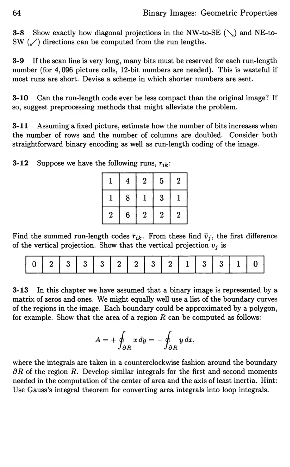
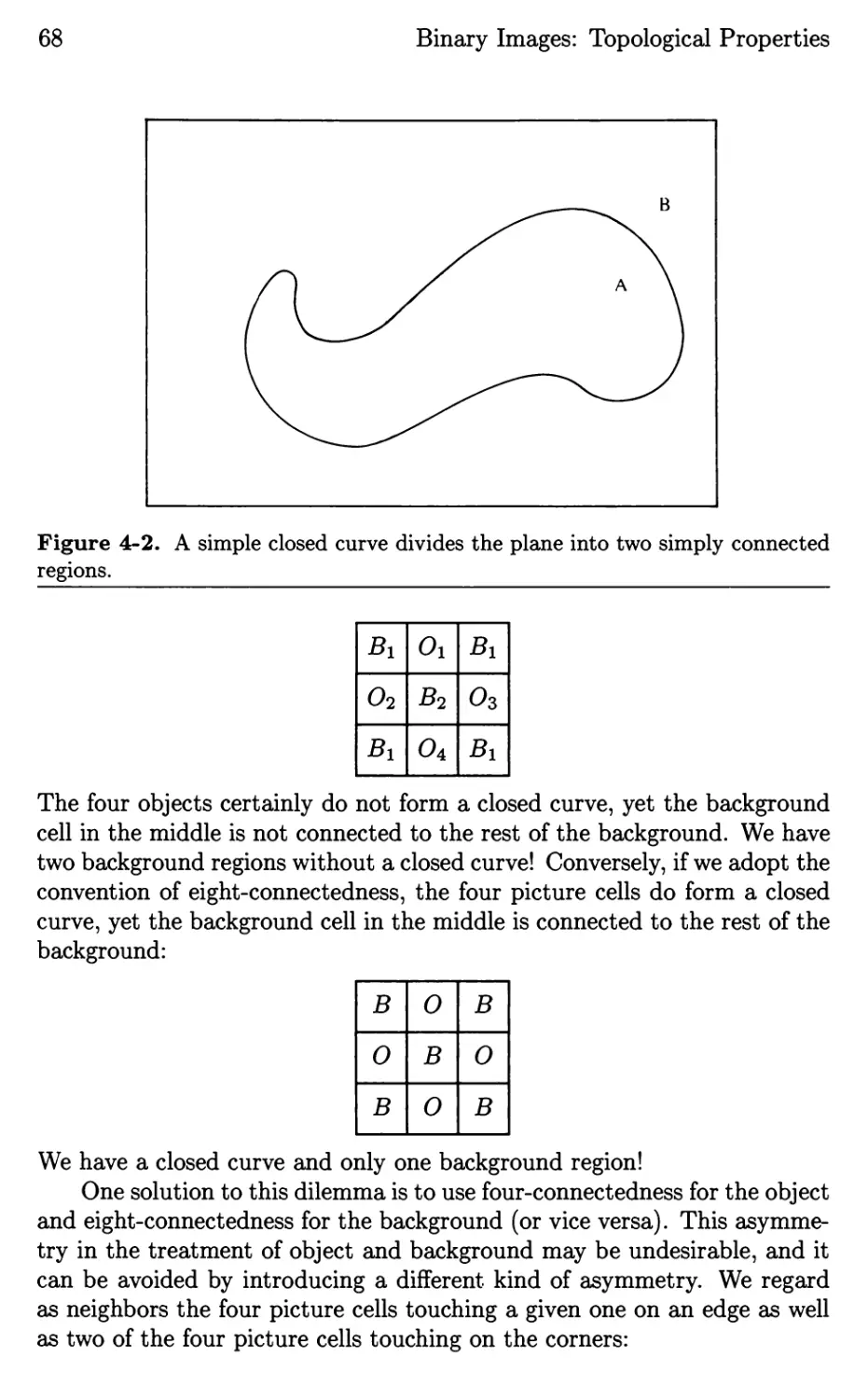
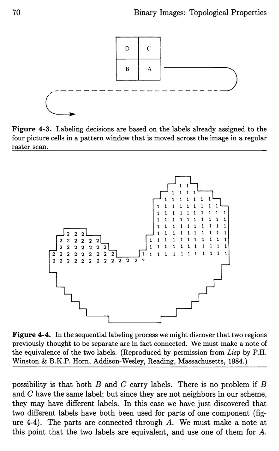
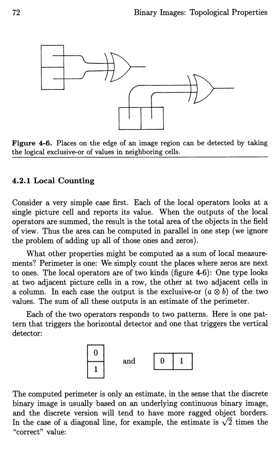
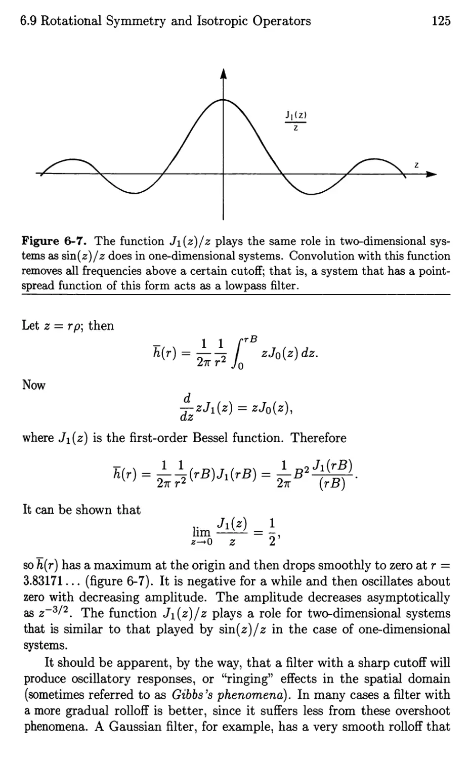
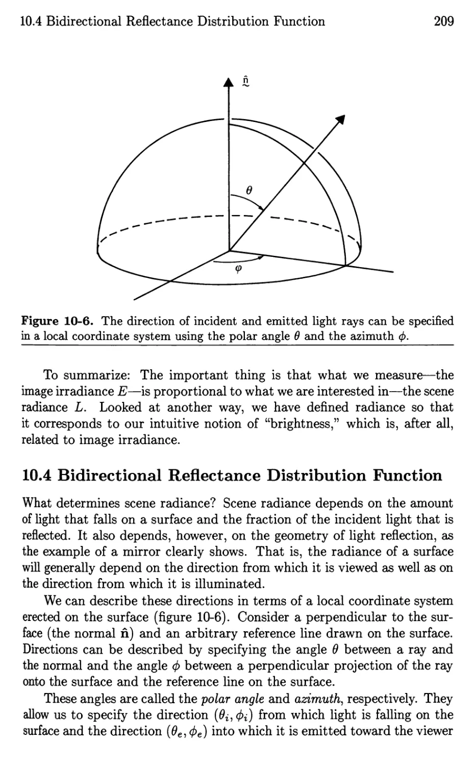
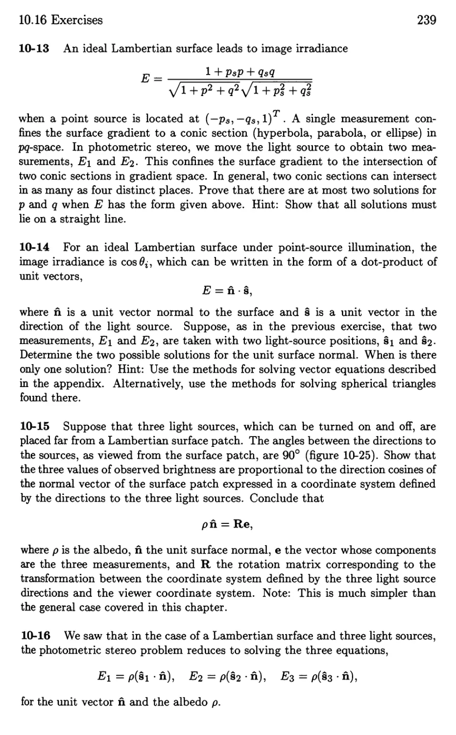
/


Текст
The MIT Electrical Engineering
and Computer Science Series
· · · .t
.
151'
Berthold Klaus Paul Hom
e IT Press
McG . w-Hill Book Compeny
Robot Vision
The MIT Electrical Engineering and Computer Science Series
Harold Abelson and Gerald Jay Sussman with Julie Sussman,
Structure and Interpretation of Computer Programs, 1985
William Siebert, Circuits, Signals, and Systems, 1986
Berthold Klaus Paul Horn, Robot Vision, 1986
Barbara Liskov and John Guttag, Abstraction and Specification in
Program Development, 1986
Robot Vision
Berthold Klaus Paul Horn
The MIT Press
Cambridge, Massachusetts
London, England
McGraw-Hill Book Company
New York St. Louis San Francisco
Montreal
Toronto
This book is one of a series of texts written by faculty of the Electri-
cal Engineering and Computer Science Department at the Massachusetts
Institute of Technology. It was edited and produced by The MIT Press
under a joint production-distribution arrangement with the McGraw-Hill
Book Company.
Ordering Information:
North America
Text orders should be addressed to the McGraw-Hill Book Company.
All other orders should be addressed to The MIT Press.
Outside North America
All orders should be addressed to The MIT Press or its local distributor.
Third printing, 1987
@ 1986 by The Massachusetts Institute of Technology
All rights reserved. No part of this book may be reproduced in any form or
by any electronic or mechanical means (including photocopying, recording,
or information storage and retrieval) without permission in writing from
the publisher.
This book was set under the direction of the author using the 'lEX type-
setting system and was printed and bound by Halliday Lithograph in the
United States of America.
Library of Congress Cataloging in Publication Data
Horn, Berthold Klaus Paul.
Robot vision.
(MIT electrical engineering and computer science
series)
Bibliography: p.
Incl udes index.
1. Robot vision. I. Title. II. Series
TJ211.3.H67 1986 629.8'92 85-18137
ISBN 0-262-08159-8 (MIT Press)
ISBN _Q-q7 -030349-5 (McGraw-Hill)
Contents
Preface . . . . . . . . . . . . . . . . vii
Acknowledgments . . .. ........ xi
1 In trod uc t io n . . . . . . . . . . . . . . 1
2 Image Formation & Image Sensing 18
3 Binary Images: Geometrical Properties 46
4 Binary Images: Topological Properties . . . . . 65
5 Regions & Image Segmentation . . . . 90
6 Image Processing: Continuous Images . . . . . 103
7 Image Processing: Discrete Images . . . . . . 144
8 Edges & Edge Finding.. ... . 161
9 Lightness & Color. . . . . . . . . . 185
10 Reflectance Map: Photometric Stereo . . . . . 202
11 Reflectance Map: Shape from Shading . . . . . 243
12 Motion Field & Optical Flow . . . . . . . . . 278
13 Photogrammetry & Stereo . . . . 299
14 Pattern Classification . .. ....... 334
15 Polyhedral Objects .. ...... . 349
16 Extended Gaussian Images . ....... 365
17 Passive Navigation & Structure from Motion . . 400
18 Picking Parts out of a Bin . . . . . . . . . . 423
Appendix: Useful Mathematical Techniques . . 453
Bibliography .. ....... . . 475
Index . . . . . . .. ......... 503
Preface
Machine vision is a young and rapidly changing field. It is exciting to write
about it, but it is also hard to know when to stop, since new results appear
at frequent intervals. This book grew out of notes for the undergraduate
course 6.801, "Machine Vision," which I have taught at MIT for ten years.
A draft version of the book has been in use for five years. The exercises are
mostly from homework assignments and quizzes. The course is a "restricted
elective," meaning that students can take it or choose instead some other
course related to artificial intelligence. Most students who elect to take
it do so in their junior year. Several chapters of the book have also been
used in an intensive one-week summer course on robotics for people from
industry and other universities.
Ten years ago, it was possible to introduce both robot manipulation
and machine vision in one term. Knowledge in both areas advanced so
quickly, however, that this is no longer feasible. (The other half of the orig-
inal course has been expanded by Tomas Lozano-Perez into 6.802, "Robot
Manipulation.") In fact, a single term now seems too short even to talk
about all of the interesting facets of machine vision.
Rapid progress in the field has made it possible to reduce the coverage
of less significant areas. What is less significant is, to some extent, a matter
of personal opinion, and this book reflects my preferences. It could not be
otherwise, for an in-depth coverage of everything that has been done in
machine vision would require much more space and would not lend itself to
presentation under a coherent theme. Material that appears to lack solid
theoretical foundations has been omitted.
Similarly, approaches that do not lead to useful methods for recov-
ering information from images have been left out, even when they claim
legitimacy by appeal to advanced mathematics. The book instead includes
information that should be useful to engineers applying machine vision
methods in the "real world." The chapters on binary image processing,
for example, help explain and suggest how to improve the many commer-
cial devices now available. The material on photometric stereo and the
extended Gaussian image points the way to what may be the next thrust
in commercialization of the results of research in this domain.
Implementation choices and specific algorithms are not always pre-
sented in full detail. Good implementations depend on particular features
of available computing systems, and their presentation would tend to dis-
tract from the basic theme. Also, I believe that one should solve the basic
machine vision problem before starting to worry about implementation. In
most cases, implementation entails little more than straightforward appli-
Vlll
Preface
cation of the classic techniques of numerical analysis. Still, details relating
to the efficient implementation in both software and hardware are included,
for example, in the chapters on binary image processing.
Almost from the start, the course attracted graduate students who felt
a need for exposure to the field, and some material has been included to
exploit their greater mathematical sophistication. This material should be
omitted in courses designed for a different audience, because it is hard to lay
the mathematical foundations and simultaneously cover all the material in
this book in a single term. This should present no difficulties, since several
topics can be taught essentially independently from the rest. Also note
that most of the necessary mathematical tools are developed in the book's
appendix.
Aside from the obvious pairing of some of the chapters (3 and 4, 6 and
7, 10 and 11, 12 and 17, 16 and 18), there is in fact little interdependence
among them. Students lacking background in linear systems theory may
be better served if the chapters on image processing (6, 7, and perhaps 9)
are omitted. Similarly, the chapters dealing with time-varying images (12
and 17) may also be left out without loss of continuity. A few chapters
present material that is not as well developed as the rest, and if these are
avoided also, one is left with a short, basic course consisting of chapters 1,
2, 3, 4, 10, 11, 16, and 18. There should be no problem covering that much
in one term.
This book is intended to provide deep coverage of topics that I feel
are reasonably well understood. This means that some topics are treated
in less detail, and others, which I consider too ad hoc, not at all. In
this regard the present book can be considered to be complementary to
Computer Vision by Dana Ballard and Christopher Brown, a book which
covers a larger number of topics, but in less depth. Also, many of the
elementary concepts are dealt with in more detail in the second edition of
Digital Picture Processing by Azriel Rosenfeld and A vinash Kak.
There is a strong connection between what is discussed here and the
study of biological vision systems. I place less emphasis on this, using as
an excuse the existence of an outstanding book on this topic, Vision: A
Computational Investigation into the Human Representation and Process-
ing of Visual Information, by the late David Marr. In a similar vein, I have
given somewhat less prominence to work on edge detection, feature-based
stereo, and some aspects of the interpretation of time-varying images, since
the books From Images to Surfaces: A Computational Study of the Human
Early Visual System by Eric Grimson, The Measurement of Visual Motion
by Ellen Hildreth, and The Interpretation of Visual Motion by Shimon
Ullman cover these subjects in greater detail than I can here. The same
goes for pattern classification, given the existence of such classics as Pat-
tern Classification and Scene Analysis by Richard Duda and Peter Hart.
Preface
IX
I have not been totally consistent, however, since there are two substantial
chapters on image processing, despite the fact that the encyclopedic Image
Processing by William Pratt covers this topic admirably. The reason is
that this material is important for understanding preprocessing steps used
in subsequent chapters.
Many of my students are at first surprised by the need for nontrivial
mathematical techniques in this domain. To some extent this is because
they have seen simple heuristic methods produce apparently startling re-
sults. Many such methods were discovered in the early days of machine
vision and led to a false optimism about the expected rate of progress in
the field. Later, significant limitations of these ad hoc approaches became
apparent. It is obvious now that the study of machine vision needs to be
supported by an understanding of image formation, just as the study of
natural language requires some knowledge of linguistics. Not so long ago
this would have been a minority view.
More seriously, machine vision is often considered merely as a means
of analyzing sensor information for a system with "artificial intelligence."
In artificial intelligence, there has been relatively little use, so far, of so-
phisticated mathematical manipulations. It is wrong to consider machine
vision and robot manipulator control merely as the "I/O" of AI. The prob-
lems encountered in vision, manipulation, and locomotion are of interest
in themselves. They are quite hard, and the tools required to attack them
are nontrivial.
A system that successfully interacts with the environment can be un-
derstood, in part, by analyzing the physics of this interaction. In the case
of vision this means that one ought to understand image formation if one
wishes to recover information about the world from images. Modeling the
physical interactions naturally leads to equations describing that interac-
tion. The equations, in turn, suggest algorithms for recovering information
about the three-dimensional world from images. This is my basic theme.
Perhaps surprisingly, quite a few students find pleasure in applying math-
ematical methods learned in an abstract context to real problems. The
material in this book provides them with motivation to practice methods
and perhaps learn new concepts they would not have bothered with other-
WIse.
The emphasis in the first part of the book is on early vision-how to
develop simple symbolic descriptions from images. Techniques for using
these descriptions in spatial reasoning and in planning actions are less
well developed and tend to depend on methodologies different from the
ones appropriate to early vision. The last five chapters deal with methods
that exploit the simple symbolic descriptions derived directly from images.
Details of how to integrate a vision system into an overall robotics system
are given in the final chapter, where a system for picking parts out of a bin
x
Preface
is constructed.
A good part of the effort of writing this book went into the design of
the exercises. They serve several purposes: Some help the reader practice
ideas presented in a chapter; some develop ideas in more depth, perhaps
using more sophisticated tools; and some introduce new research topics.
The exercises in a given chapter are typically presented in this order, and
hints are given to warn the reader about particularly difficult ones.
There has been a trend recently toward the use of more compact no-
tation. In several instances, for example, components of vectors, such as
surface normals and optical flow velocities, were used in early work. The
current tendency is to use the vectors directly; for example, th Gaussian
sphere is now employed instead of gradient space in the specification of
surface orientation. In the body of this text I have used the component no-
tation, which is easier to grasp initially. In some of the exercises, however, I
have tried to show how problems can be solved more efficiently using more
compact notation.
Most of the material included in this book has been presented else-
where, but here it is organized in a more coherent way, using a consistent
notation. In a few instances, new methods are presented that have not
been published before. Because the field is changing rapidly, some of what
is presented here may become obsolete, or at least of less interest, in just a
few years. Conversely, some things that I have not covered may eventually
form the basis for exciting new results. This is not a serious shortcom-
ing, however, since my concern is more with the development of a solid
approach to research in machine vision than with specific techniques for
tackling particular problems.
When will we have a "general-purpose" vision system? Not in the
foreseeable future, is my answer. This is not to say that machine vision
is merely an intellectual exercise of no practical import. On the contrary,
tremendous progress has been made in two ways: (a) by concentrating on
a particular aspect of vision, such as interpretation of stereo pairs, and (b)
by concentrating on a particular application, such as the alignment of parts
for automated assembly. A truly general-purpose vision system would have
to deal with all aspects of vision and be applicable to all problems that can
be solved using visual information. Among other things, it would have to
be able to reason about the physical world.
B.K.P.H.
Acknowledgments
The students of the "Machine Vision" course at MIT deserve much credit
for helping me to formulate and revise this material. My teaching assis-
tants have contributed to the generation of many of the problems. Robert
Sjoberg also prepared careful notes on several topics that I have unfortu-
nately been unable to incorporate due to time pressure. Robert Sjoberg,
Andy Moulton, Eric Bier, Michael Gennert, and Jazek Myczkowski pro-
vided numerous useful comments on earlier drafts.
A few of the chapters are based on papers that I wrote jointly with
others. I would like to thank Michael Brooks for his contribution to the
discussion of the shape-from-shading problem (chapter 11), Brian Schunck
for his help in the development of methods for the analysis of optical flow
(chapter 12), Anna Bruss for her contribution to the analysis of the pas-
sive navigation problem (chapter 17), and Katsushi Ikeuchi for his serious
dedication to implementing the bin-picking system (chapter 18).
Christopher Brown, Herbert Freeman, Eric Grimson, Ramesh Jain,
Alan Mackworth, and Lothar Rossol provided helpful comments on an
early draft. Michael Brady, Michael Brooks, Michael Gennert, and Ellen
Hildreth went over recent versions of the book and made many useful sug-
gestions. Michael Gennert contributed the problems on pattern classifica-
tion (chapter 14). Careful reading by Boris Katz and Larry Cohen helped
eliminate the more blatant linguistic problems. Unfortunately, I could not
resist the temptation to rewrite much of the material as time went on and
so have, no doubt, in the process reintroduced many bugs and typos.
The Department of Electrical Engineering and Computer Science gave
me a six-month sabbatical to write the first draft. Carol Roberts typed
that draft. Blythe Heepe drew most of the figures. Phyllis Rogers helped
me with the bibliography. Michael Gennert came to my rescue by taking
over final preparation of the camera ready copy. The illustration on the
dust cover is used with the kind permission of the artist, Hajime Sorayama.
Marvin Minsky got me started in machine vision by suggesting the
recovery of shape from brightness gradations in an image as a thesis topic.
Patrick Winston was supportive of my approach to machine vision from the
start, when it was not a popular one. Marvin is responsible for the creation,
and Patrick for the survival and expansion of the Artificial Intelligence
Laboratory at the Massachusetts Institute of Technology, where work on
machine vision has flourished for almost twenty years.
Many of the ideas reported here result from research supported by the
Defense Advance Research Projects Agency (DARPA) and the Office for
Naval Research (ONR).
1
Introduction
In this chapter we discuss what a machine vision system is, and what
tasks it is suited for. We also explore the relationship of machine vision
to other fields that provide techniques for processing images or symbolic
descriptions of images. Finally, we introduce the particular view of machine
vision exploited in this text and outline the contents of subsequent chapters.
1.1 Machine Vision
Vision is our most powerful sense. It provides us with a remarkable amount
of information about our surroundings and enables us to interact intelli-
gently with the environment, all without direct physical contact. Through
it we learn the positions and identities of objects and the relationships be-
tween them, and we are at a considerable disadvantage if we are deprived of
this sense. It is no wonder that attempts have been made to give machines
a sense of vision almost since the time that digital computers first became
generally available.
Vision is also our most complicated sense. The knowledge we have ac-
cumulated about how biological vision systems operate is still fragmentary
and confined mostly to the processing stages directly concerned with sig-
nals from the sensors. What we do know is that biological vision systems
are complex. It is not surprising, then, that many attempts to provide
machines with a sense of vision have ended in failure. Significant progress
2
Introduction
.--
---
.--
.,....,
.....-
--
-
'"'"
.....-
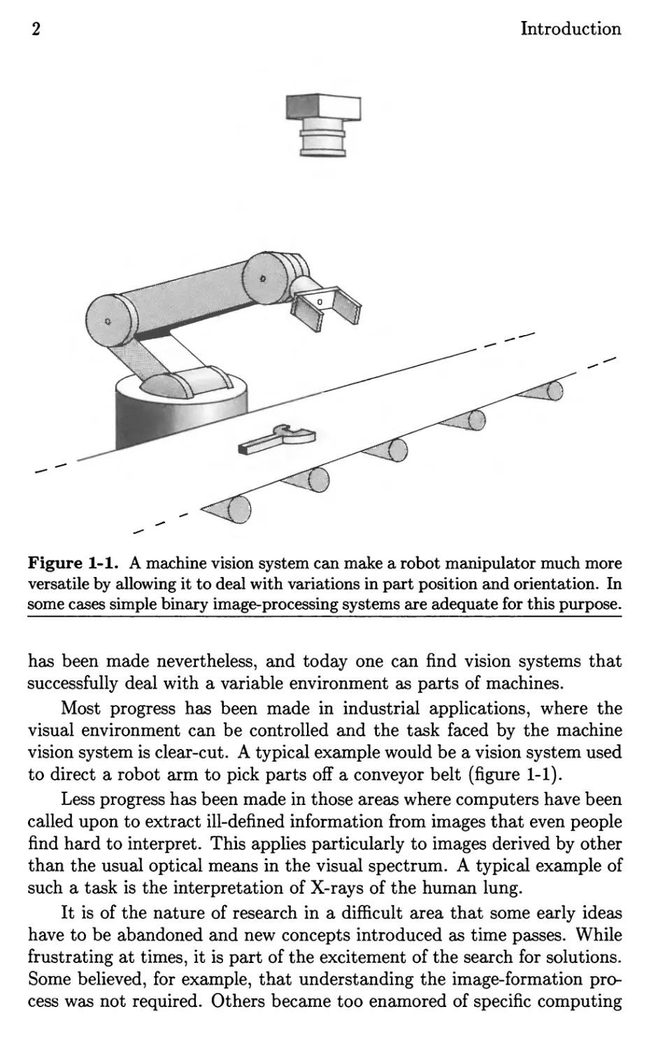
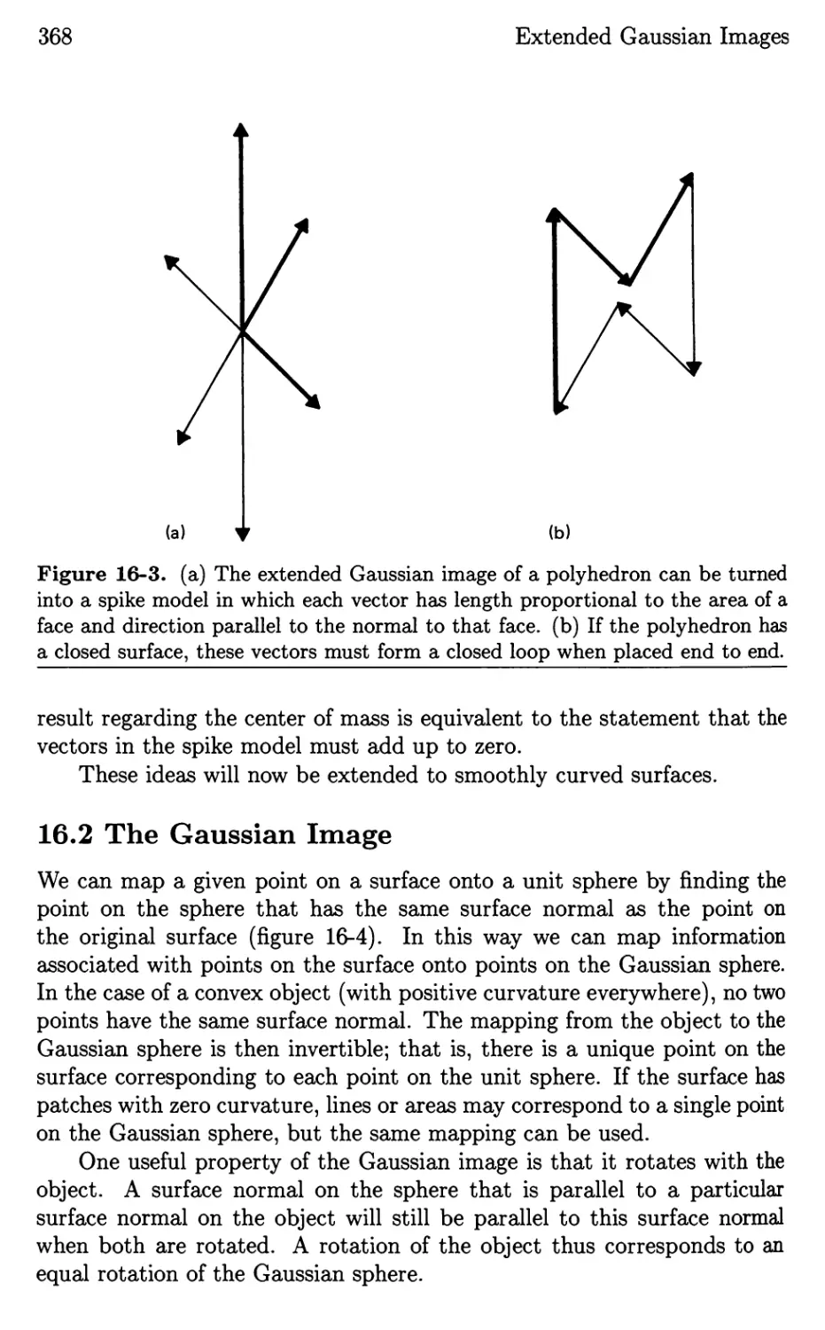
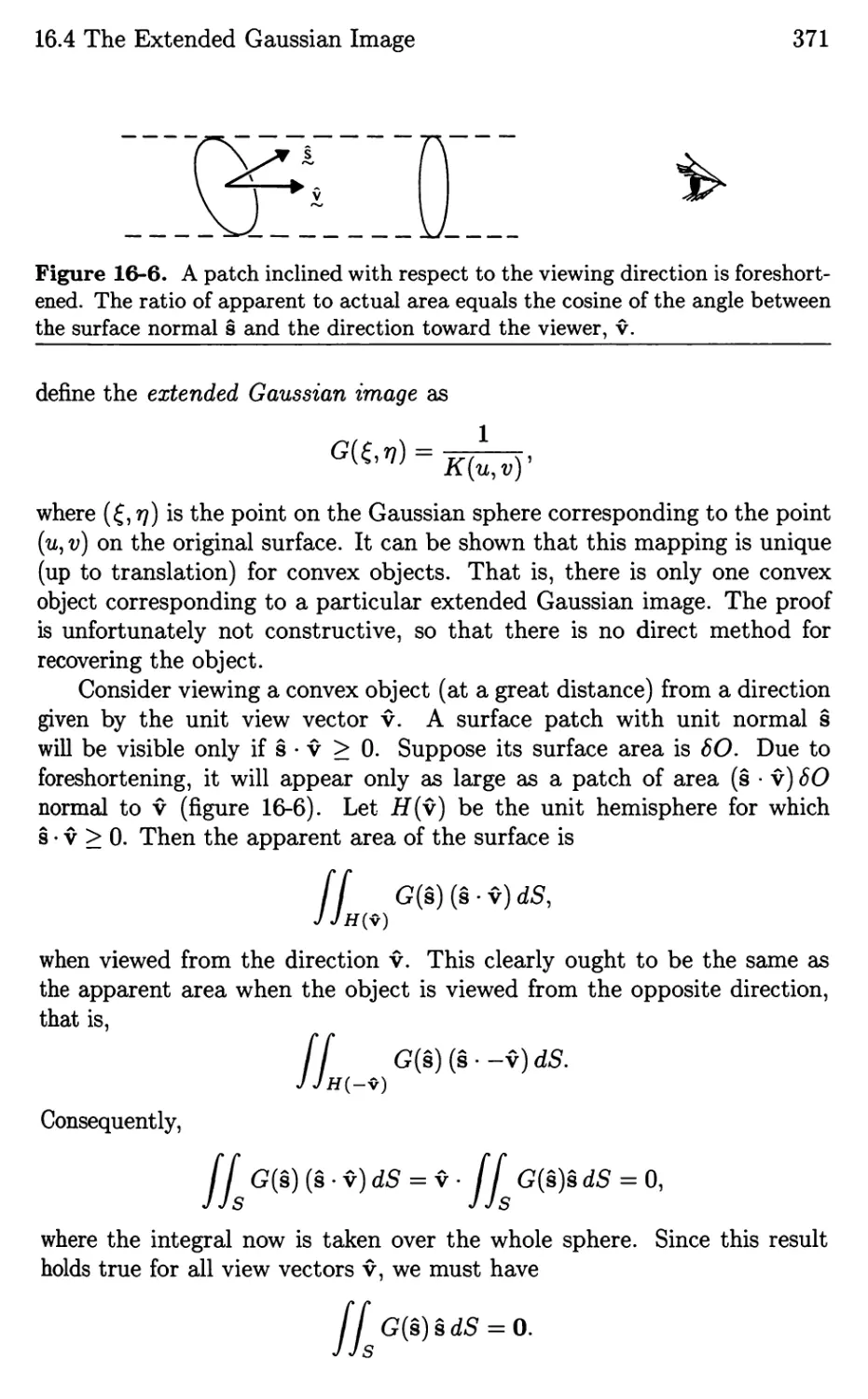
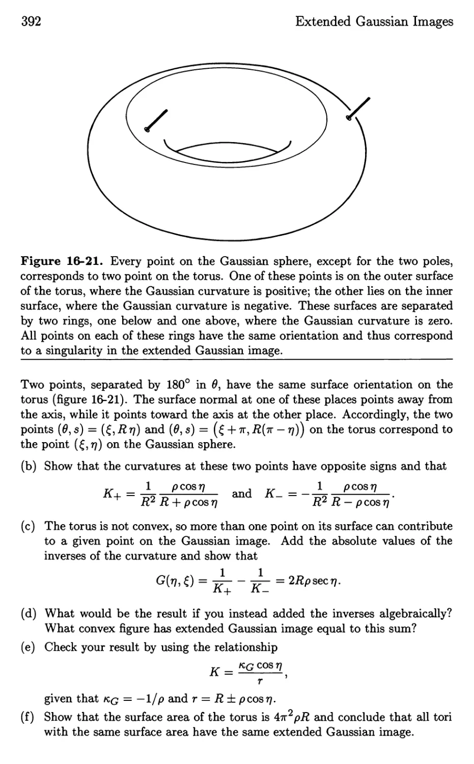
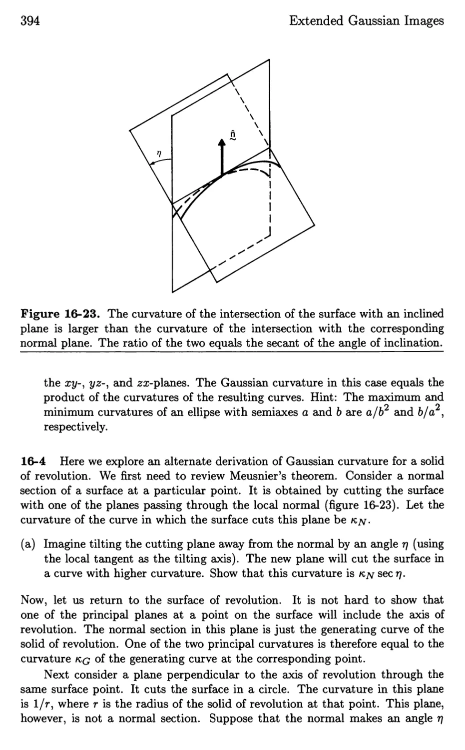
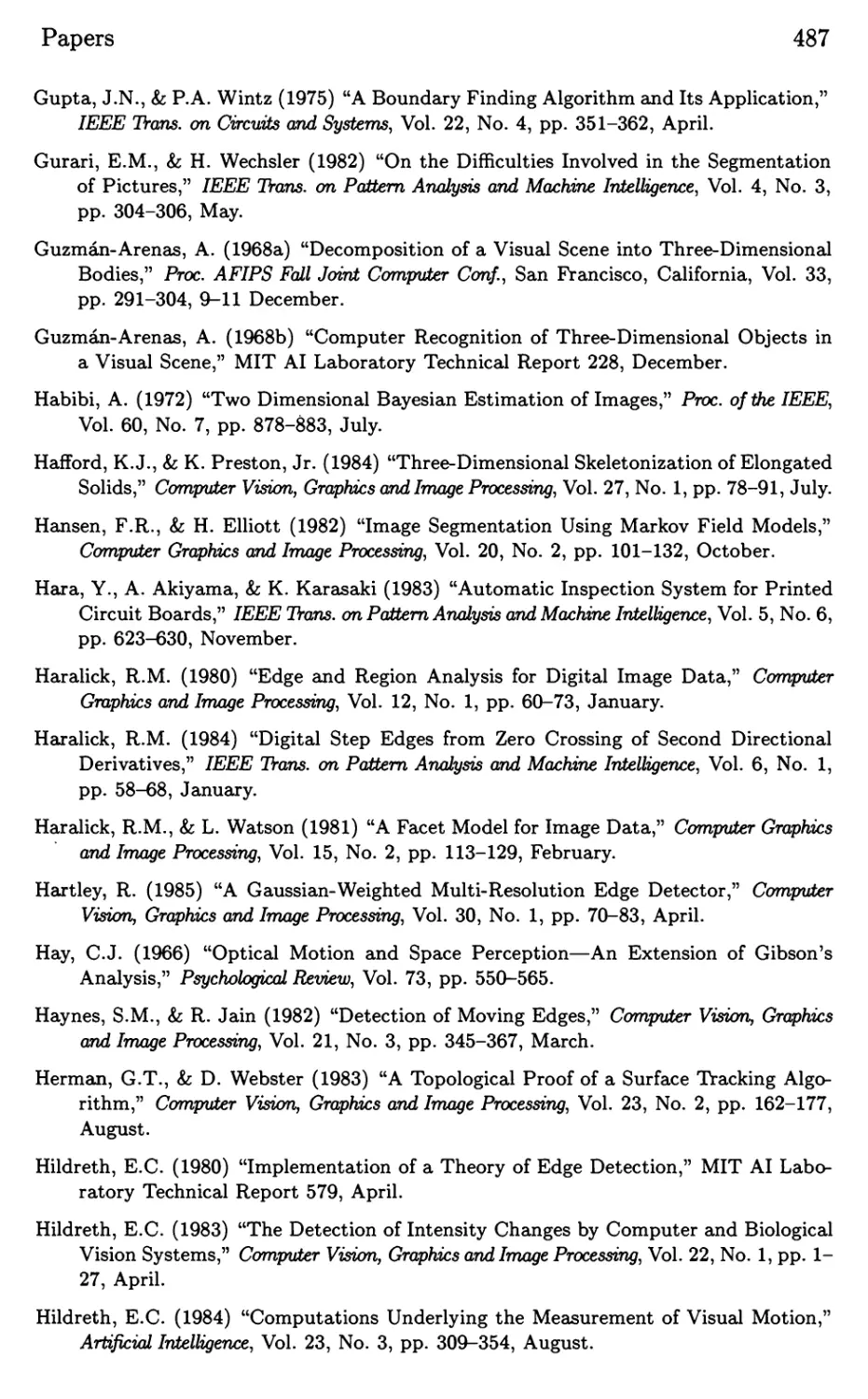
Figure 1-1. A machine vision system can make a robot manipulator much more
versatile by allowing it to deal with variations in part position and orientation. In
some cases simple binary image-processing systems are adequate for this purpose.
has been made nevertheless, and today one can find vision systems that
successfully deal with a variable environment as parts of machines.
Most progress has been made in industrial applications, where the
visual environment can be controlled and the task faced by the machine
vision system is clear-cut. A typical example would be a vision system used
to direct a robot arm to pick parts off a conveyor belt (figure 1-1).
Less progress has been made in those areas where computers have been
called upon to extract ill-defined information from images that even people
find hard to interpret. This applies particularly to images derived by other
than the usual optical means in the visual spectrum. A typical example of
such a task is the interpretation of X-rays of the human lung.
It is of the nature of research in a difficult area that some early ideas
have to be abandoned and new concepts introduced as time passes. While
frustrating at times, it is part of the excitement of the search for solutions.
Some believed, for example, that understanding the image-formation pr(}-
cess was not required. Others became too enamored of specific computing
1.2 Tasks for a Machine Vision System
3
Imaging
device
Machine
VISion
Scene
-1
Image
Description
I
\
"
Application
feedback
I
I
)
--------"
Figure 1-2. The purpose of a machine vision system is to produce a symbolic
description of what is being imaged. This description may then be used to direct
the interaction of a robotic system with its environment. In some sense, the
vision system's task can be viewed as an inversion of the imaging process.
methods of rather narrow utility. No doubt some of the ideas presented
here will also be revised or abandoned in due course. The field is evolving
too rapidly for it to be otherwise.
We cannot at this stage build a "universal" vision system. Instead,
we address ourselves either to systems that perform a particular task in a
controlled environment or to modules that could eventually become part of
a general-purpose system. Naturally, we must also be sensitive to practical
considerations of speed and cost. Because of the enormous volume of data
and the nature of the computations required, it is often difficult to reach a
satisfactory compromise between these factors.
1.2 Tasks for a Machine Vision System
A machine vision system analyzes images and produces descriptions of what
is imaged (figure 1-2). These descriptions must capture the aspects of the
objects being imaged that are useful in carrying out some task. Thus we
consider the machine vision system as part of a larger entity that interacts
with the environment. The vision system can be considered an element of
a feedback loop that is concerned with sensing, while other elements are
dedicated to decision making and the implementation of these decisions.
4
Introduction
The input to the machine vision system is an image, or several images,
while its output is a description that must satisfy two criteria:
. It must bear some relationship to what is being imaged.
. It must contain all the information needed for the some given task.
The first criterion ensures that the description depends in some way on the
visual input. The second ensures that the information provided is useful.
An object does not have a unique description; we can conceive of de-
scriptions at many levels of detail and from many points of view. It is
impossible to describe an object completely. Fortunately, we can avoid this
potential philosophical snare by considering the task for which the descrip-
tion is intended. That is, we do not want just any description of what is
imaged, but one that allows us to take appropriate action.
A simple example may help to clarify these ideas. Consider again the
task of picking parts from a conveyor belt. The parts may be randomly
oriented and positioned on the belt. There may be several different types of
parts, with each to be loaded into a different fixture. The vision system is
provided with images of the objects as they are transported past a camera
mounted above the belt. The descriptions that the system has to produce
in this case are simple. It need only give the position, orientation, and
type of each object. The description could be just a few numbers. In other
situations an elaborate symbolic description may be called for.
There are cases where the feedback loop is not closed through a ma-
chine, but the description is provided as output to be interpreted by a
human. The two criteria introduced above must still be satisfied, but it
is harder in this case to determine whether the system was successful in
solving the vision problem presented.
1.3 Relation to Other Fields
Machine vision is closely allied with three fields (figure 1-3):
. Image processing.
. Pattern classification.
. Scene analysis.
Image processing is largely concerned with the generation of new im-
ages from existing images. Most of the techniques used come from linear
systems theory. The new image may have noise suppressed, blurring re-
moved, or edges accentuated. The result is, however, still an image, usually
meant to be interpreted by a person. As we shall see, some of the tech-
niques of image processing are useful for understanding the limitations of
image-forming systems and for designing preprocessing modules for ma-
chine vision.
1.3 Relation to Other Fields
5
Image
processi ng
Input
image
9 ut put
Image
Pattern
classification
reature
vector
Class
number
Scene
analysis
Input
description
Output
descript ion
Figure 1-3. Three ancestor paradigms of machine vision are image processing,
pattern classification, and scene analysis. Each contributes useful techniques, but
none is central to the problem of developing symbolic descriptions from images.
Pattern classification has as its main thrust the classification of a "pat-
tern," usually given as a set of numbers representing measurements of an
object, such as height and weight. Although the input to a classifier is not
an image, the techniques of pattern classification are at times useful for
analyzing the results produced by a machine vision system. To recognize
an object means to assign it to one of a number of known classes. Note,
however, that recognition is only one of many tasks faced by the machine
vision system. Researchers concerned with classification have created sim-
ple methods for obtaining measurements from images. These techniques,
however, usually treat the images as a tw{}-dimensional pattern of bright-
6
Introduction
Figure 1-4. In scene analysis, a low-level symbolic description, such as a line
drawing, is used to develop a high-level symbolic description. The result may
contain information about the spatial relationships between objects, their shapes,
and their identities.
ness and cannot deal with objects presented in an arbitrary attitude.
Scene analysis is concerned with the transformation of simple descrip-
tions, obtained directly from images, into more elaborate ones, in a form
more useful for a particular task. A classic illustration of this is the in-
terpretation of line drawings (figure 1-4). Here a description of the image
of a set of polyhedra is given in the form of a collection of line segments.
Before these can be used, we must figure out which regions bounded by
the lines belong together to form objects. We will also want to know how
objects support one another. In this way a complex symbolic description
of the image can be obtained from the simple one. Note that here we do
not start with an image, and thus once again do not address the central
issue of machine vision:
. Generating a symbolic description from one or more images.
1.4 Outline of What Is to Come
The generation of descriptions from images can often be conveniently bro-
ken down into two stages. The first stage produces a sketch, a detailed but
undigested description. Later stages produce more parsimonious, struc-
tured descriptions suitable for decision making. Processing in the first
stage will be referred to as image analysis, while subsequent processing of
the results will be called scene analysis. The division is somewhat arbi-
trary, except insofar as image analysis starts with an image, while scene
analysis begins with a sketch. The first thirteen chapters of the book are
1.4 Outline of What Is to Come
7
+ - - - - 1- --
- -- L: _ - - -- - - ,-- I- I--f--
- -, --- - - - -- - -
1 I . - -- - -
.I.i. ·
.. . .1_1. ---
- - ----- - . .. -- --
.- .1- . . .,.,.
- ..... .----- - -----
l!_ . - -
JJIIIIr .1. ------
- - iIIIl ].. - _I.
=-l t i . '. _I. .I_- - - - =l.tli-=-- -----
- - _1--- T_iE __, ... ..I ___
- -
- - ,III. I . . L.J.'.': r.r.
- - = 1-1111 .. __ J.l" WI ===- I. .I .1- -1_==
.'... m.. ' t.i.' t 1:1:'1.
ililjj.I...I ,::,:: -,..,,1 ;.1:.I t==
:....!.f----i. I ...--- - .1.1.__
I _ ___ _'-rIil1j '-'l - . 1. -
I l l i 1 1 11-I.
, r I .._i_i..I..
Figure 1-5. Binary images have only two brightness levels: black and white.
While restricted in application, they are of interest because they are particularly
easy to process.
concerned with image analysis, also referred to as early vision, while the
remaining five chapters are devoted to scene analysis.
The development of methods for machine vision requires some under-
standing of how the data to be processed are generated. For this reason we
start by discussing image formation and image sensing in chapter 2. There
we also treat measurement noise and introduce the concept of convolution.
The easiest images to analyze are those that allow a simple separation
of an "object" from a "background." These binary images will be treated
first (figure 1-5). Some industrial problems can be tackled by methods that
use such images, but this usually requires careful control of the lighting.
There exists a fairly complete theory of what can and cannot be accom-
plished with binary images. This is in contrast to the more general case of
gray-level images. It is known, for example, that binary image techniques
are useful only when possible changes in the attitude of the object are con-
fined to rotations in a plane parallel to the image plane. Binary image
processing is covered in chapters 3 and 4.
Many image-analysis techniques are meant to be applied to regions of
an image corresponding to single objects, rather than to the whole image.
Because typically many surfaces in the environment are imaged together,
the image must be divided up into regions corresponding to separate entities
in the environment before such techniques can be applied. The required
segmentation of images is discussed in chapter 5.
In chapters 6 and 7 we consider the transformation of gray-level im-
ages into new gray-level images by means of linear operations. The usual
intent of such manipulations is to reduce noise, accentuate some aspect of
the image, or reduce its dynamic range. Subsequent stages of the machine
8
Introduction
,\1//
o
/" ........... Light source
/j I ...'
I
.....
......
/.. .....
. c;...:. . ·
. :
--
Lens
Object
surface
In lage plane
Figure 1-6. In order to use images to recover information about the world, we
need to understand image formation. In some cases the image formation process
can be inverted to extract estimates of the permanent properties of the surfaces
of the objects being imaged.
vision system may find the processed images easier to analyze. Such filter-
ing methods are often exploited in edge-detection systems as preprocessing
steps.
Complementary to image segmentation is edge finding, discussed in
chapter 8. Often the interesting events in a scene, such as a boundary where
one object occludes another, lead to discontinuities in image brightness or
in brightness gradient. Edge-finding techniques locate such features. At
this point, we begin to emphasize the idea that an important aspect of
machine vision is the estimation of properties of the surfaces being imaged.
In chapter 9 the estimation of surface reflectance and color is addressed
and found to be a surprisingly difficult task.
Finally, we confront the central issue of machine vision: the generation
of a description of the world from one or more images. A point of view
that one might espouse is that the purpose of the machine vision system is
to invert the projection operation performed by image formation. This is
not. quite correct, since we want not to recover the world being imaged, but
1.4 Outline of What Is to Come
9
t
,.
"
,
o
Figure 1-7. The appearance of the image of an object is greatly influenced by
the reflectance properties of its surface. Perfectly matte and perfectly specular
surfaces present two extreme cases.
to obtain a symbolic description. Still, this notion leads us to study image
formation carefully (figure 1-6). The way light is reflected from a surface
becomes a central issue. The apparent brightness of a surface depends on
three factors:
. Microstructure of the surface.
. Distribution of the incident light.
. Orientation of the surface with respect to the VIewer and the light
sources.
In figure 1-7 we see images of two spherical surfaces, one covered with a
paint that has a matte or diffuse reflectance, the other metallic, giving rise
to specular reflections. In the second case we see a .virtual image of the
world around the spherical object. It is clear that the microstructure of
the surface is important in determining image brightness.
Figure 1-8 shows three views of Place Ville-Marie in Montreal. The
three pictures were taken from the same hotel window, but under different
lighting conditions. Again, we easily recognize that the same objects are
10
Introduction
r;;..
- \..
:...;- --=
'"T"TT. ..... ---
..
, .'
-- -- _ I
-
..
. . . .
. ...
; :: I .
. ,
I a
, 1
1
-
..
:J. .&......:....1.....
ts'e.l .
\ 1.\ .
rl
...
... .--
.J .. . : :u .. --
, .
F
....- .
..,...
-.
.
I.
......
---:.. J-_ !-.a._ J..
.
.... ....
o .
I
=JIIII!F · .
-....... --
....J
E
.. ,
, u . .Iilm!
t
-=
. .
.
....
.-
.
.
-
,,
0"
.J
.-1 =-1
Figure 1-8. The appearance of the image of a scene depends a lot on the lighting
conditions. To recover information about the world from images we need to un-
derstand how the brightness patterns in the image are determined by the shapes
of surfaces, their reflectance properties, and the distribution of light sources.
1.4 Outline of What Is to Come
11
N
"
I
I
I
I I
I I
I I
t"1 " v
I I "'-.....-: / /
II ",/ "-.
IV.....
Figure 1-9. The reflection of light from a point source by a patch of an object's
surface is governed by three angles: the incident angle i, the emittance angle
e, and the phase angle g. Here N is the direction perpendicular, or normal, to
the surface, S the direction to the light source, and V the direction toward the
VIewer.
depicted, but there is a tremendous difference in brightness patterns be-
tween the images taken with direct solar illumination and those obtained
under a cloudy sky.
In chapters 10 and 11 we discuss these issues and apply the understand-
ing developed to the recovery of surface shape from one or more images.
Representations for the shape of a surface are also introduced there. In
developing methods for recovering surface shape, we often consider the
surface broken up into tiny patches, each of which can be treated as if it
were planar. Light reflection from such a planar patch is governed by three
angles if it is illuminated by a point source (figure 1-9).
The same systematic approach, based on an analysis of image bright-
ness, is used in chapters 12 and 13 to recover information from time-varying
images and images taken by cameras separated in space. Surface shape,
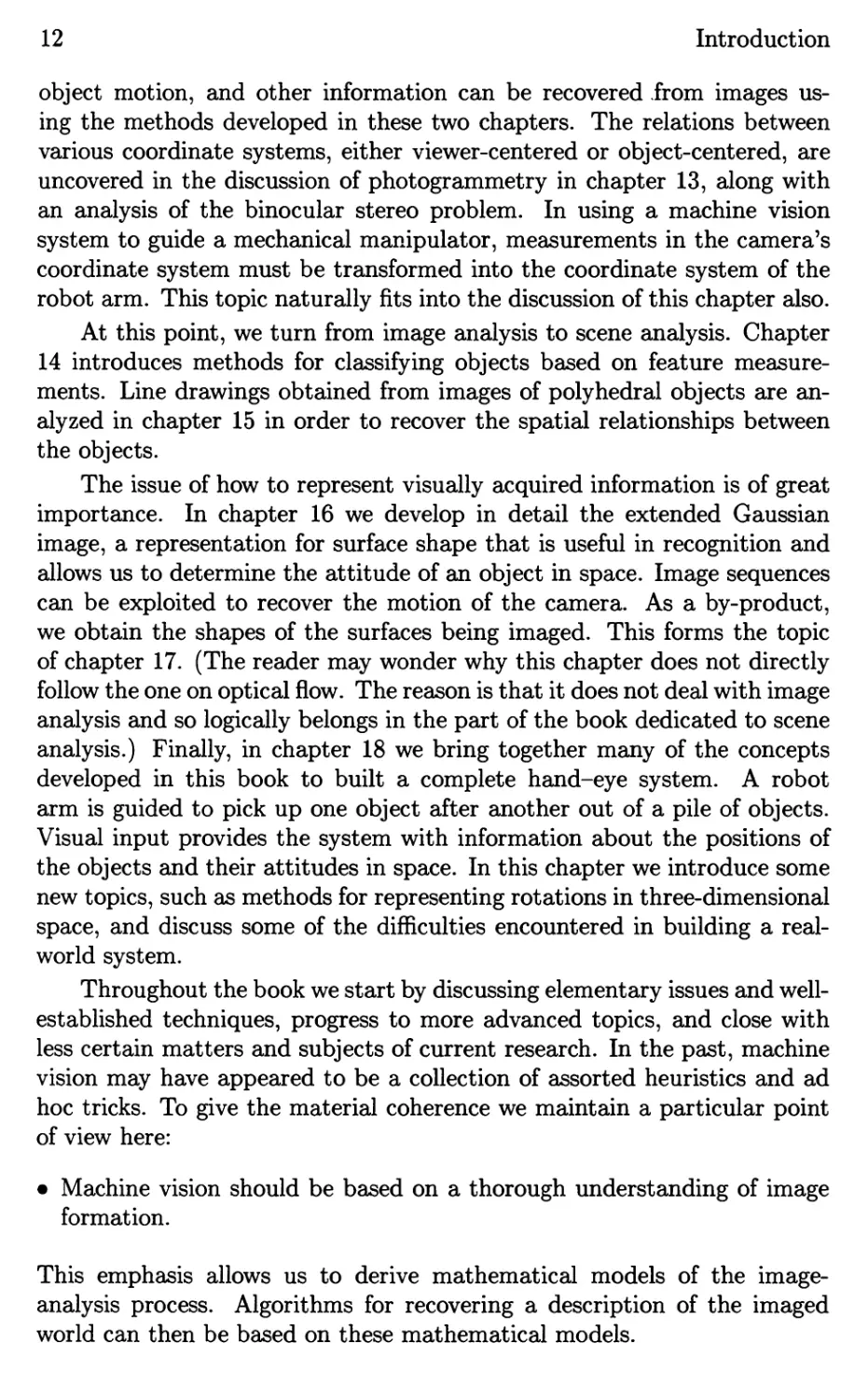
12
Introduction
object motion, and other information can be recovered .from images us-
ing the methods developed in these two chapters. The relations between
various coordinate systems, either viewer-centered or object-centered, are
uncovered in the discussion of photogrammetry in chapter 13, along with
an analysis of the binocular stereo problem. In using a machine vision
system to guide a mechanical manipulator, measurements in the camera's
coordinate system must be transformed into the coordinate system of the
robot arm. This topic naturally fits into the discussion of this chapter also.
At this point, we turn from image analysis to scene analysis. Chapter
14 introduces methods for classifying objects based on feature measure-
ments. Line drawings obtained from images of polyhedral objects are an-
alyzed in chapter 15 in order to recover the spatial relationships between
the objects.
The issue of how to represent visually acquired information is of great
importance. In chapter 16 we develop in detail the extended Gaussian
image, a representation for surface shape that is useful in recognition and
allows us to determine the attitude of an object in space. Image sequences
can be exploited to recover the motion of the camera. As a by-product,
we obtain the shapes of the surfaces being imaged. This forms the topic
of chapter 17. (The reader may wonder why this chapter does not directly
follow the one on optical flow. The reason is that it does not deal with image
analysis and so logically belongs in the part of the book dedicated to scene
analysis.) Finally, in chapter 18 we bring together many of the concepts
developed in this book to built a complete hand-eye system. A robot
arm is guided to pick up one object after another out of a pile of objects.
Visual input provides the system with information about the positions of
the objects and their attitudes in space. In this chapter we introduce some
new topics, such as methods for representing rotations in three-dimensional
space, and discuss some of the difficulties encountered in building a real-
world system.
Throughout the book we start by discussing elementary issues and well-
established techniques, progress to more advanced topics, and close with
less certain matters and subjects of current research. In the past, machine
vision may have appeared to be a collection of assorted heuristics and ad
hoc tricks. To give the material coherence we maintain a particular point
of view here:
. Machine vision should be based on a thorough understanding of image
formation.
This emphasis allows us to derive mathematical models of the image-
analysis process. Algorithms for recovering a description of the imaged
world can then be based on these mathematical models.
1.5 References
13
K no\\ led t:
about'-
I maglllg
K no\\ led e
about '-
appl ica lion
Image
-1
Sk.t:tch
Descript ion
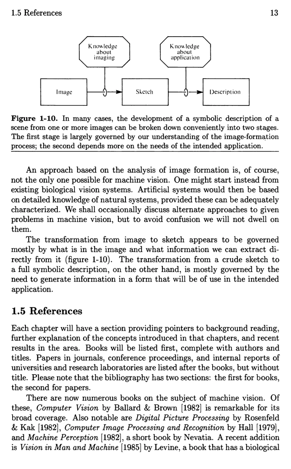
Figure 1-10. In many cases, the development of a symbolic description of a
scene from one or more images can be broken down conveniently into two stages.
The first stage is largely governed by our understanding of the image- form tion
process; the second depends more on the needs of the intended application.
An approach based on the analysis of image formation is, of course,
not the only one possible for machine vision. One might start instead from
existing biological vision systems. Artificial systems would then be based
on detailed knowledge of natural systems, provided these can be adequately
characterized. We shall occasionally discuss alternate approaches to given
problems in machine vision, but to avoid confusion we will not dwell on
them.
The transformation from image to sketch appears to be governed
mostly by what is in the image and what information we can extract di-
rectly from it (figure 1-10). The transformation from a crude sketch to
a full symbolic description, on the other hand, is mostly governed by the
need to generate information in a form that will be of use in the intended
application.
1.5 References
Each chapter will have a section providing pointers to background reading,
further explanation of the concepts introduced in that chapters, and recent
results in the area. Books will be listed first, complete with authors and
titles. Papers in journals, conference proceedings, and internal reports of
universities and research laboratories are listed after the books, but without
title. Please note that the bibliography has two sections: the first for books,
the second for papers.
There are now numerous books on the subject of machine vision. Of
these, Computer Vision by Ballard & Brown [1982] is remarkable for its
broad coverage. Also notable are Digital Picture Processing by Rosenfeld
& Kak [1982], Computer Image Processing and Recognition by Hall [1979],
and Machine Perception [1982], a short book by Nevatia. A recent addition
is Vision in Man and Machine [1985] by Levine, a book that has a biological
14
Introduction
vision point of view and emphasizes applications to biomedical problems.
Many books concentrate on the image-processing side of things, such
as Computer Techniques in Image Processing by Andrews [1970], Digi-
tal Image Processing by Gonzalez & Wintz [1977], and two books dealing
with the processing of images obtained by cameras in space: Digital Image
Processing by Castleman [1979] and Digital Image Processing: A Systems
Approach by Green [1983]. The first few chapters of Digital Picture Pro-
cessing by Rosenfeld & Kak [1982] also provide an excellent introduction
to the subject. The classic reference on image processing is still Pratt's
encyclopedic Digital Image Processing [1978].
One of the earliest significant books in this field, Pattern Classification
and Scene Analysis by Duda & Hart [1973], contains more on the sub-
ject of pattern classification than one typically needs to know. Artificial
Intelligence by Winston [1984] has an easy-to-read, broad-brush chapter
on machine vision that makes the connection between that subject and
artificial intelligence.
A number of edited books, containing contributions from several re-
searchers in the field, have appeared in the last ten years. Early on there
was The Psychology of Computer Vision, edited by Winston [1975], now
out of print. Then came Digital Picture Analysis, edited by Rosenfeld
[1976], and Computer Vision Systems, edited by Hanson & Riseman [1978].
Several papers on machine vision can be found in volume 2 of Artificial In-
telligence: An MIT Perspective, edited by Winston & Brown [1979]. The
collection Structured Computer Vision: Machine Perception through Hier-
archical Computation Structures, edited by Tanimoto & Klinger, was pub-
lished in 1980. Finally there appeared the fine assemblage of papers Image
Understanding 1984, edited by Ullman & Richards [1984].
The papers presented at a number of conferences have also been col-
lected in book form. Gardner was the editor of a book published in 1979
called Machine-aided Image Analysis, 1978. Applications of machine vi-
sion to robotics are explored in Computer Vision and Sensor-Based Robots,
edited by Dodd & Rossol [1979], and in Robot Vision, edited by Pugh [1983].
Stucki edited Advances in Digital Image Processing: Theory, Application,
Implementation [1979], a book containing papers presented at a meeting
organized by IBM. The notes for a course organized by Faugeras appeared
in Fundamentals in Computer Vision [1983].
Because many of the key papers in the field were not easily accessible,
a number of collections have appeared, including three published by IEEE
Press, namely Computer Methods in Image Analysis, edited by Aggarwal,
Duda, & Rosenfeld [1977], Digital Image Processing, edited by Andrews
[1978], and Digital Image Processing for Remote Sensing, edited by Bern-
stein [1978].
The IEEE Computer Society's publication Computer brought out a
1.5 References
15
special issue on image processing in August 1977, the Proceedings of the
IEEE devoted the May 1979 issue to pattern recognition and image pro-
cessing, and Computer produced a special issue on machine perception for
industrial applications in May 1980. A special issue (Volume 17) of the
journal Artificial Intelligence was published in book form under the title
Computer Vision, edited by Brady [1981]. The Institute of Electronics and
Communication Engineers of Japan produced a special issue (Volume J68-
D, Number 4) on machine vision work in Japan in April 1985 (in Japanese).
Not much is said in this book about biological vision systems. They
provide us, on the one hand, with reassuring existence proofs and, on the
other, with optical illusions. These startling effects may someday prove
to be keys with which we can unlock the secrets of biological vision sys-
tems. A computational theory of their function is beginning to emerge, to
a great extent due to the pioneering work of a single man, David Marr.
His approach is documented in the classic book Vision: A Computational
Investigation into the Human Representation and Processing of Visual In-
formation [1982].
Human vision has, of course, always been a subject of intense curios-
ity, and there is a vast literature on the subject. Just a few books will
be mentioned here. Gregory has provided popular accounts of the subject
in Eye and Brain [1966] and The Intelligent Eye [1970]. Three books by
Gibson-The Perception of the Visual World [1950], The Senses Consid-
ered as Perceptual Systems [1966], and The Ecological Approach to Visual
Perception [1979]-are noteworthy for providing a fresh approac.h to the
problem. Cornsweet's Visual Perception [1971] and The Psychology of Vi-
sual Perception by Haber & Hershenson [1973] are of interest also. The
work of Julesz has been very influential, particularly in the area of binoc-
ular stereo, as documented in Foundations of Cyclopean Perception [1971].
More recently, in the wonderfully illustrated book Seeing, Frisby [1982] has
been able to show the crosscurrents between work on machine vision and
work on biological vision systems. For another point of view see Perception
by Rock [1984].
Twenty years ago, papers on machine vision were few in number and
scattered widely. Since then a number of journals have become preferred
repositories for new research results. In fact, the journal Computer Graph-
ics and Image Processing, published by Academic Press, had to change
its name to Computer Vision, Graphics and Image Processing (CVGIP)
when it became the standard place to send papers in this field for review.
More recently, a new special-interest group of the Institute of Electrical
and Electronic Engineers (IEEE) started publishing the Transactions on
Pattern Analysis and Machine Intelligence (PAMI). Other journals, such as
Artificial Intelligence, published by North-Holland, and Robotics Research,
published by MIT Press, also contain articles on machine vision. There are
16
Introduction
several journals devoted to related topics, such as pattern classification.
Some research results first see the light of day at an "Image Under-
standing Workshop" sponsored by the Defense Advanced Research Projects
Agency (DARPA). Proceedings of these workshops are published by Science
Applications Incorporated, McLean, Virginia, and are available through
the Defense Technical Information Center (DTIC) in Alexandria, Virginia.
Many of these papers are later submitted, possibly after revision and ex-
tension, to be reviewed for publication in one of the journals mentioned
above.
The Computer Society of the IEEE organizes annual conferences on
Computer Vision and Pattern Recognition (CVPR) and publishes their
proceedings. Also of interest are the proceedings of the biannual Interna-
tional Joint Conference on Artificial Intelligence (IJCAI) and the national
conferences organized by the American Association for Artificial Intelli-
gence (AAAI), usually in the years in between.
The thorough annual surveys by Rosenfeld [1972, 1974, 1975, 1976,
1977, 1978, 1979, 1980, 1981, 1982, 1983, 1984a, 1985] in Computer Vi-
sion, Graphics and Image Processing are extremely valuable and make it
possible to be less than complete in providing references here. The most
recent survey contained 1,252 entries! There have been many analyses of
the state of the field or of particular views of the field. An early survey
of image processing is that of Huang, Schreiber, & Tretiak [1971]. While
not really a survey, the influential paper of Barrow & Tenenbaum [1978]
presents the now prevailing view that machine vision is concerned with the
process of recovering information about the surfaces being imaged. More
recent surveys of machine vision by Marr [1980], Barrow & Tenenbaum
[1981a], Poggio [1984], and Rosenfeld [1984b] are recommended particu-
larly. Another paper that has been influential is that by Binford [1981].
Once past the hurdles of early vision, the representation of information
and the modeling of objects and the physical interaction between them
become important. We touch upon these issues in the later chapters of this
book. For more information see, for example, Brooks [1981] and Binford
[1982].
There are many papers on the application of machine vision to in-
dustrial problems (although some of the work with the highest payoff is
likely not to have been published in the open literature). Several papers in
Robotics Research: The First International Symposium, edited by Brady
& Paul [1984], deal with this topic. Chin [1982] and Chin & Harlow [1982]
have surveyed the automation of visual inspection.
The inspection of printed circuit boards, both naked and stuffed, is a
topic of great interest, since there are many boards to be inspected and since
it is not a very pleasant job for people, nor one that they are particularly
good at. For examples of work in this area, see Ejiri et al. [1973], Daniels-
1.6 Exercises
17
son & Kruse [1979], Danielsson [1980], and Hara, Akiyama, & Karasaki
[1983]. There is a similar demand for such techniques in the manufacture
of integrated circuits. Masks are simp e black-and-white patterns, and
their inspection has not been too difficult to automate. The inspection of
integrated circuit wafers is another matter; see, for example, Hsieh & Fu
[1980] .
Machine vision has been used in automated alignment. See Horn
[1975b], Kashioka, Ejiri, & Sakamoto [1976], and Baird [1978] for ex-
amples in semiconductor manufacturing. Industrial robots are regularly
guided using visually obtained information about the position and orienta-
tion of parts. Many such systems use 'binary image-processing techniques,
although some are more sophisticated. See, for example, Yachida & Tsuji
[1977], Gonzalez & Safabakhsh [1982], and Horn & Ikeuchi [1984]. These
techniques will not find widespread application if the user has to program
each application in a standard programming language. Some attempts have
been made to provide tools specifically suited to the vision applications; see,
for example, Lavin & Lieberman [1982].
Papers on the application of machine vision methods to the vectoriza-
tion of line drawings are mentioned at the end of chapter 4; references on
character recognition may be found at the end of chapter 14.
1.6 Exercises
1-1 Explain in what sense one can consider pattern classification, image pro-
cessing, and scene analysis as "ancestor paradigms" to machine vision. In what
way do the methods from each of these disciplines contribute to machine vision?
In what way are the problems addressed by machine vision different from those
to which these methods apply?
2
Image Formation & Image Sensing
In this chapter we explore how images are formed and how they are sensed
by a computer. Understanding image formation is a prerequisite for full
understanding of the methods for recovering information from images. In
analyzing the process by which a three-din1ensional world is projected onto
a two-dimensional image plane, we uncover the two key questions of image
formation:
. What determines where the image of some point will appear?
. What determines how bright the image of some surface will be?
The answers to these two questions require knowledge of image projection
and image radiometry, topics that will be discussed in the context of simple
lens systems.
A crucial notion in the study of image formation is that we live in a
very special visual world. It has particular features that make it possi-
ble to recover information about the three-dimensional world from one or
more two-dimensional images. We discuss this issue and point out imag-
ing situations where these special constraint do not apply, and where it is
consequently much harder to extract information from images.
We also study the basic mechanism of typical image sensors, and how
information in different spectral bands may be obtained and processed.
Following a brief discussion of color, the chapter closes with a discussion of
2.1 Two Aspects of Image Formation
19
noise and reviews some concepts from the fields of probability and statis-
tics. This is a convenient point to introduce convolution in one dimension,
an idea that will be exploited later in its two-dimensional generalization.
Readers familiar with these concepts may omit these sections without loss
of continuity. The chapter concludes with a discussion of the need for
quantization of brightness measurements and for tessellations of the image
plane.
2.1 Two Aspects of Image Formation
Before we can analyze an image, we must know how it is formed. An image
is a two-dimensional pattern of brightness. How this pattern is produced
in an optical image-forming system is best studied in two parts: first, we
need to find the geometric correspondence between points in the scene and
points in the image; then we must figure out what determines the brightness
at a particular point in the image.
2.1.1 Perspective Projection
Consider an ideal pinhole at a fixed distance in front of an image plane
(figure 2-1). Assume that an enclosure is provided so that only light coming
through the pinhole can reach the image plane. Since light travels along
straight lines, each point in the image corresponds to a particular direction
defined by a ray from that point through the pinhole. Thus we have the
familiar perspective projection.
We define the optical axis, in this simple case, to be the perpendic-
ular from the pinhole to the image plane. Now we can introduce a con-
venient Cartesian coordinate system with the origin at the pinhole and
z-axis aligned with the optical axis and pointing toward the image. With
this choice of orientation, the z components of the coordinates of points
in front of the camera are negative. We use this convention, despite the
drawback, because it gives us a convenient right-hand coordinate system
(with the x-axis to the right and the y-axis upward).
We would like to compute where the image P' of the point P on some
object in front of the camera will appear (figure 2-1). We assume that no
other object lies on the ray from P to the pinhole O. Let r = (x, y, z)T be
the vector connecting 0 to P, and r ' = (x', y' , f') T be the vector connecting
o to P'. (As explained in the appendix, vectors will be denoted by boldface
letters. We commonly deal with column vectors, and so must take the
transpose, indicated by the superscript T, when we want to write them in
terms of the equivalent row vectors.)
Here f' is the distance of the image plane from the pinhole, while x'
and y' are the coordinates of the point P' in the image plane. The two
20
Image Formation & Image Sensing
y
I
. . . .
/:... ...
. ......: .
z
---
x
Figure 2-1. A pinhole camera produces an image that is a perspective projection
of the world. It is convenient to use a coordinate system in which the xy-plane is
parallel to the image plane, and the origin is at the pinhole o. The z-axis then
lies along the optical axis.
vectors r and r ' are collinear and differ only by a (negative) scale factor.
If the ray connecting P to P' makes an angle 0: with the optical axis, then
the length of r is just
r = - z sec 0: = - (r . z) sec 0:,
where z is the unit vector along the optical axis. (Remember that z is
negative for a point in front of the camera.)
The length of r ' is
r ' = I' sec 0:,
and so
1 I 1
I , r = r.
r.z
In component form this can be written as
X'
x
z
and
y' Y
f' z
f'
2.1 Two Aspects of Image Formation
21
Sometimes image coordinates are normalized by dividing x' and y' by f'
in order to simplify the projection equations.
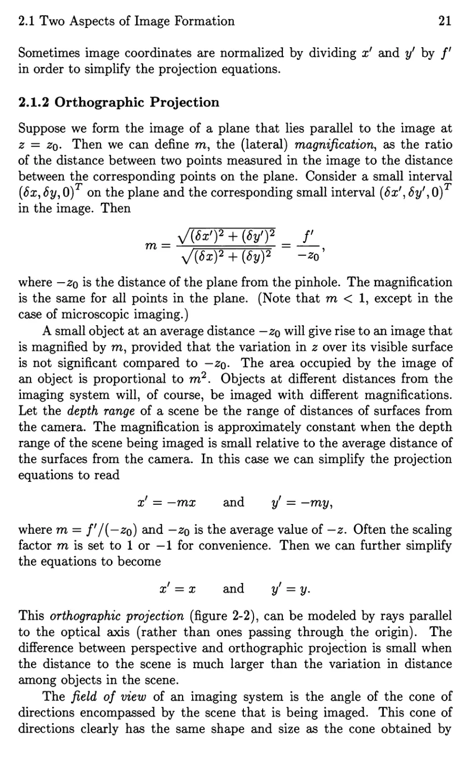
2.1.2 Orthographic Projection
Suppose we form the image of a plane that lies parallel to the image at
z = zoo Then we can define m, the (lateral) magnification, as the ratio
of the distance between two points measured in the image to the distance
between the corresponding points on the plane. Consider a small interval
(8x, 8y, 0) T on the plane and the corresponding small interval (8x', 8y', 0) T
in the image. Then
v (8x')2 + (8y')2 f'
m- --
- V (8x)2 + (8y)2 - -zo'
where -zo is the distance of the plane from the pinhole. The magnification
is the same for all points in the plane. (Note that m < 1, except in the
case of microscopic imaging.)
A small object at an average distance -zo will give rise to an image that
is magnified by m, provided that the variation in z over its visible surface
is not significant compared to -zoo The area occupied by the image of
an object is proportional to m 2 . Objects at different distances from the
imaging system will, of course, be imaged with different magnifications.
Let the depth range of a scene be the range of distances of surfaces from
the camera. The magnification is approximately constant when the depth
range of the scene being imaged is small relative to the average distance of
the surfaces from the camera. In this case we can simplify the projection
equations to read
x' = -mx
and
y' = -my,
where m = f' /( -zo) and -zo is the average value of -z. Often the scaling
factor m is set to 1 or -1 for convenience. Then we can further simplify
the equations to become
x' = x
and
y' = y.
This orthographic projection (figure 2-2), can be modeled by rays parallel
to the optical axis (rather than ones passing throug.h the origin). The
difference between perspective and orthographic projection is small when
the distance to the scene is much larger than the variation in distance
among objects in the scene.
The field of view of an imaging system is the angle of the cone of
directions encompassed by the scene that is being imaged. This cone of
directions clearly has the same shape and size as the cone obtained by
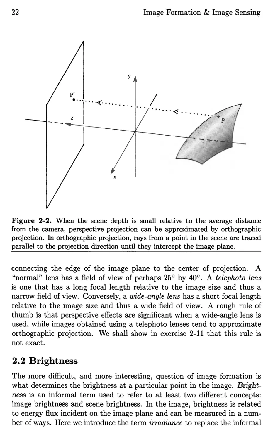
22
p'
Image Formation & Image Sensing
y
/
....
......-<::.... / I
7 0 .. p .
.....
. . . . . . . . . . . .
z
--:. ... ---
x
Figure 2-2. When the scene depth is small relative to the average distance
from the camera, perspective projection can be approximated by orthographic
projection. In orthographic projection, rays from a point in the scene are traced
parallel to the projection direction until they intercept the image plane.
connecting the edge of the image plane to the center of projection. A
"normal" lens has a field of view of perhaps 25° by 40°. A telephoto lens
is one that has a long focal length relative to the image size and thus a
narrow field of view. Conversely, a wide-angle lens has a short focal length
relative to the image size and thus a wide field of view. A rough rule of
thumb is that perspective effects are significant when a wide-angle lens is
used, while images obtained using a telephoto lenses tend to approximate
orthographic projection. We shall show in exercise 2-11 that this rule is
not exact.
2.2 Brightness
The more difficult, and more interesting, question of image formation is
what determines the brightness at a particular point in the image. Bright-
ness is an informal term used to refer to at least two different concepts:
image brightness and scene brightness. In the image, brightness is related
to energy flux incident on the image plane and can be measured in a num-
ber of ways. Here we introduce the term irradiance to replace the informal
2.2 Brightness
E= 8P
8A
(a)
23
8 2 p
L=-
8A8w
(b)
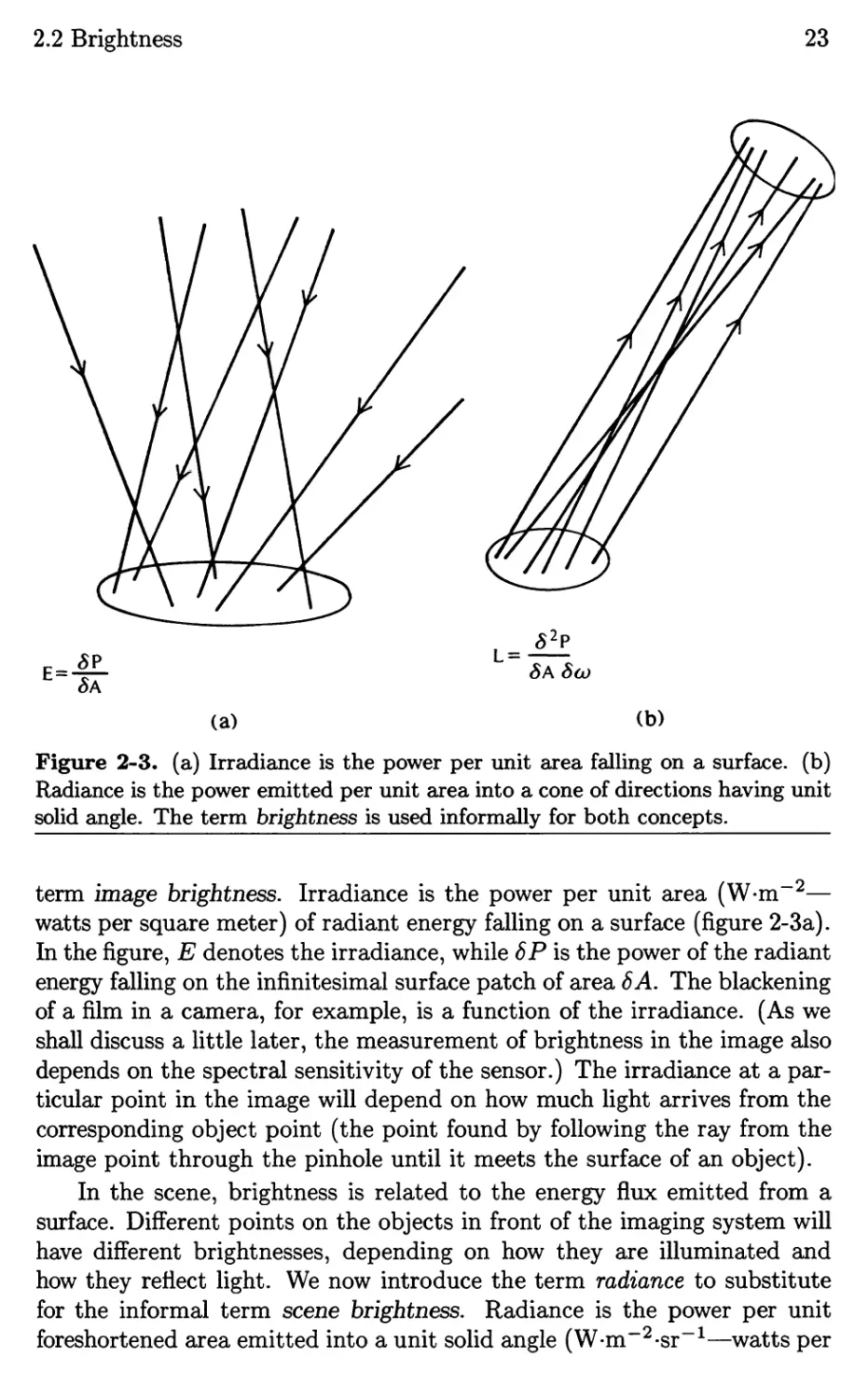
Figure 2-3. ( a) Irradiance is the power per unit area falling on a surface. (b)
Radiance is the power emitted per unit area into a cone of directions having unit
solid angle. The term brightness is used informally for both concepts.
term image brightness. Irradiance is the power per unit area (W.m- 2 -
watts per square meter) of radiant energy falling on a surface (figure 2-3a).
In the figure, E denotes the irradiance, while 8P is the power of the radiant
energy falling on the infinitesimal surface patch of area 8A. The blackening
of a film in a camera, for example, is a function of the irradiance. (As we
shall discuss a little later, the measurement of brightness in the image also
depends on the spectral sensitivity of the sensor.) The irradiance at a par-
ticular point in the image will depend on how much light arrives from the
corresponding object point (the point found by following the ray from the
image point through the pinhole until it meets the surface of an object).
In the scene, brightness is related to the energy flux emitted from a
surface. Different points on the objects in front of the imaging system will
have different brightnesses, depending on how they are illuminated and
how they reflect light. We now introduce the term radiance to substitute
for the informal term scene brightness. Radiance is the power per unit
foreshortened area emitted into a unit solid angle (W.m- 2 .sr- 1 -watts per
24
Image Formation & Image Sensing
square meter per steradian) by a surface (figure 2-3b). In the figure, L is the
radiance and 8 2 P is the power emitted by the infinitesimal surface patch
of area 8A into an infinitesimal solid angle 8w. The apparent complexity
of the definition of radiance stems from the fact that a surface emits light
into a hemisphere of possible directions, and we obtain a finite amount
only by considering a finite solid angle of these directions. In general the
radiance will vary with the direction from which the object is viewed. We
shall discuss radiometry in detail later , when we introduce the reflectance
map.
We are interested in the radiance of surface patches on objects because
what we measure, image irradiance, turns out to be proportional to scene
radiance, as we show later. The constant of proportionality depends on the
optical system. To gather a finite amount of light in the image plane we
must have an aperture of finite size. The pinhole, introduced in the last
section, must have a nonzero diameter. Our simple analysis of projection
no longer applies, though, since a point in the environment is now imaged
as a small circle. This can be seen by considering the cone of rays passing
through the circular pinhole with its apex at the object point.
We cannot make the pinhole very small for another reason. Because
of the wave nature of light, diffraction occurs at the edge of the pinhole
and the light is spread over the image. As the pinhole is made smaller and
smaller, a larger and larger fraction of the incoming light is deflected far
from the direction of the incoming ray.
2.3 Lenses
In order to avoid the problems associated with pinhole cameras, we now
consider the use. of a lens in an image-forming system. An ideal lens pro-
duces the same projection as the pinhole, but also gathers a finite amount
of light (figure 2-4). The larger the lens, the larger the solid angle it sub-
tends when seen from the object. Correspondingly it intercepts more of
the light reflected from (or emitted by) the object. The ray through the
center of the lens is undeflected. In a well-focused system the other rays
are deflected to reach the same iInage point as the central ray.
An ideal lens has the disadvantage that it only brings to focus light
from points at a distance - z given by the familiar lens equation
1 1 1
-+---
z' -z - f'
where z' is the distance of the image plane from the lens and f is the focal
length (figure 2-4). Points at other distances are imaged as little circles.
This can be seen by considering the cone of light rays passing through the
lens with apex at the point where they are correctly focused. The size of
2.3 Lenses
25
z'
-z
Figure 2-4. To obtain finite irradiance in the image plane, a lens is used instead
of an ideal pinhole. A perfect lens generates an image that obeys the same
projection equations as that generated by a pinhole, but gathers light from a
finite area as well. A lens produces well-focused images of objects at a particular
distance only.
the blur circle can be determined as follows: A point at distance - z is
imaged at a point z' from the lens, where
111
-, + ----= = f '
z -z
and so
( -' ' ) f f ( - )
z - z = (z + f) (z + f) z - z .
If the image plane is situated to receive correctly focused images of objects
at distance -z, then points at distance -z will give rise to blur circles of
diameter
d
-, Iz' - z'l ,
z
where d is the diameter of the lens. The depth of field is the range of
distances over which objects are focused "sufficiently well," in the sense
that the diameter of the blur circle is less than the resolution of the imaging
device. The depth of field depends, of course, on what sensor is used, but
in any case it is clear that the larger the lens aperture, the less the depth
of field. Clearly also, errors in focusing become more serious when a large
aperture is employed.
26
Image Formation & Image Sensing
Simple ray-tracing rules can help in understanding simple lens combi-
nations. As already mentioned, the ray through the center of the lens is
undeflected. Rays entering the lens parallel to the optical axis converge to
a point on the optical axis at a distance equal to the focal length. This fol-
lows from the definition of focal length as the distance from the lens where
the image of an object that is infinitely far away is focused. Conversely,
rays emitted from a point on the optical axis at a distance equal to the focal
length from the lens are deflected to emerge parallel to the optical axis on
the other side of the lens. This follows from the reversibility of rays. At an
interface between media of different refractive indices, the same reflection
and refraction angles apply to light rays traveling in opposite directions.
A simple lens is made by grinding and polishing a glass blank so that
its two surfaces have shapes that are spherical. The optical axis is the line
through the centers of the two spheres. Any such simple lens will have
a number of defects or aberrations. For this reason one usually combines
several simple lenses, carefully lining up their individual optical axes, so as
to make a compound lens with better properties.
A useful model of such a system of lenses is the thick lens (figure 2-5).
One can define two principal planes perpendicular to the optical axis, and
two nodal points where these planes intersect the optical axis. A ray arriv-
ing at the front nodal point leaves the rear nodal point without changing
direction. This defines the projection performed by the lens. The distance
between the two nodal points is the thickness of the lens. A thin lens is
one in which the two nodal points can be considered coincident.
It is theoretically impossible to make a perfect lens. The projection
will never be exactly like that of an ideal pinhole. More important, exact
focusing of all rays cannot be achieved. A variety of aberrations occur. In
a well-designed lens these defects are kept to a minimum, but this becomes
more difficult as the aperture of the lens is increased. Thus there is a
trade-off between light-gathering power and image quality.
A defect of particular interest to us here is called vignetting. Imagine
several circular diaphragms of different diameter, stacked one behind the
other, with their centers on a common line (figure 2-6). When you look
along this common line, the smallest diaphragm will limit your view. As
you move away from the line, some of the other diaphragms will begin to
occlude more, until finally nothing can be seen. Similarly, in a simple lens,
all the rays that enter the front surface of the lens end up being focused
in the image. In a compound lens, some of the rays that pass through
the first lens may be occluded by portions of the second lens, and so on.
This will depend on the inclination of the entering ray with respect to the
optical axis and its distance from the front nodal point. Thus points in
the image away from the optical axis benefit less from the light-gathering
power of the lens than does the point on the optical axis. There is a falloff
2.3 Lenses
27
t
"- No.dal
pOints
Principal
planes
Figure 2-5. An ideal thick lens provides a reasonable model for most real lenses.
It produces the same perspective projection that an ideal thin lens does, except
for an additional offset, the lens thickness t, along the optical axis. It can be un-
derstood in terms of the principal planes and the nodal points at the intersections
of the principal planes and the optical axis.
in sensitivity with distance from the center of the image.
Another important consideration is that the aberrations of a lens in-
crease in magnitude as a power of the angle between the incident ray and
the optical axis. Aberrations are classified by their order, that is, the power
of the angle that occurs in this relationship. Points on the optical axis may
be quite well focused, while those in a corner of the image are smeared out.
For this reason, only a limited portion of the image plane is usable. The
magnitude of an aberration defect also increases as a power of the distance
from the optical axis at which a ray passes through the lens. Thus the
image quality can be improved by using only the central portion of a lens.
One reason for introducing diaphragms into a lens system is to im-
prove image quality in a situation where it is not necessary to utilize fully
the light-gathering power of the system. As already mentioned, fixed di-
aphragms ensure that rays entering at a large angle to the optical axis do
not pass through the outer regions of any of the lenses. This improves
image quality in the outer regions of the image, but at the same time
greatly increases vignetting. In most common uses of lenses this is not
an important matter, since people are astonishingly insensitive to smooth
spatial variations in image brightness. It does matter in machine vision,
28
Image Formation & Image Sensing
Figure 2-6. Vignetting is a reduction in light-gathering power with increasing
inclination of light rays with respect to the optical axis. It is caused by apertures
in the lens system occluding part of the beam of light as it passes through the
lens system. Vignetting results in a smooth, but sometimes quite large, falloff in
sensitivity toward the edges of the image region.
however, since we use the measurements of image brightness (irradiance)
to determine the scene brightness (radiance).
2.4 Our Visual World
How can we hope to recover information about the three-dimensional world
using a mere two-dimensional image? It may seem that the available in-
formation is not adequate, even if we take several images. Yet biological
systems interact intelligently with the environment using visual informa-
tion. The puzzle is solved when we consider the special nature of our usual
visual world. We are immersed in a homogeneous transparent medium, and
the objects we look at are typically opaque. Light rays are not refracted
or absorbed in the environment, and we can follow a ray from an image
point through the lens until it reaches some surface. The brightness at
a point in the image depends only on the brightness of the corresponding
surface patch. Surfaces are two-dimensional manifolds, and their shape can
be represented by giving the distance z( x', y') to the surface as a function
of the image coordinates x' and y'.
This is to be contrasted with a situation in which we are looking into
a volume occupied by a light-absorbing material of varying density. Here
2.4 Our Visual World
29
we may specify the density p(x, y, z) of the material as a function of the
coordinates x, y, and z. One or more images provide enough constraint to
recover information about a surface, but not about a volume. In theory,
an infinite number of images is needed to solve the problem of tomography,
that is, to determine the density of the absorbing material.
Conditions of homogeneity and transparency may not always hold ex-
actly. Distant mountains appear changed in color and contrast, while in
deserts we may see mirages. Image analysis based on the assumption that
conditions are as stated may go awry when the assumptions are violated,
and so we can expect that both biological and machine vision systems will
be misled in such situations. Indeed, some optical illusions can be ex-
plained in this way. This does not mean that we should abandon these
additional constraints, for without them the solution of the problem of re-
covering information about the three-dimensional world from images would
be ambiguous.
Our usual visual world is special indeed. Imagine being immersed
instead in a world with varying concentrations of pigments dispersed within
a gelatinous substance. It would not be possible to recover the distributions
of these absorbing substances in three dimensions from one view. There
just would not be enough information. Analogously, single X-ray images
are not useful unless there happens to be sharp contrast between different
rp.aterials, like bone and tissue. Otherwise a very large number of views
must be taken and a tomographic reconstruction attempted. It is perhaps
a good thing that we do not possess Superman's X-ray vision capabilities!
By and large, we shall confine our attention to images formed by con-
ventional optical means. We shall avoid high-magnification microscopic
images, for instance, where many substances are effectively transparent,
or at least translucent. Similarly, images on a very large scale often show
the effects of absorption and refraction in the atmosphere. Interestingly,
other modalities do sometimes provide us with images much like the ones
we are used to. Examples include scanning electron microscopes (SEM)
and synthetic-aperture radar systems (SAR), both of which produce im-
ages that are easy to interpret. So there is some hope of analyzing them
using the methods discussed here.
In view of the importance of surfaces, we might hope that a machine
vision system could be designed to recover the shapes of surfaces given one
or more images. Indeed, there has been some success in this endeavor, as
we shall see in chapter 10, where we discuss the recovery of shape from
shading. Detailed understanding of the imaging process allows us to re-
cover quantitative information from images. The computed shape of a
surface may be used in recognition, inspection, or in planning the path of
a mechanical manipulator.
30
Image Formation & Image Sensing
d
.-1-
c
n
A
p
+1-
(a)
(b)
Figure 2-7. Photons striking a suitable surface generate charge carriers that
are collected and measured to determine the irradiance. ( a) In the case of a
vacuum device, electrons are liberated from the photocathode and attracted to
the positive anode. (b) In the case of a semiconductor device, electron-hole pairs
are separated by the built-in field to be collected in an external circuit.
2.5 Image Sensing
Almost all image sensors depend on the generation of electron-hole pairs
when photons strike a suitable material. This is the basic process in bi-
ological vision as well as photography. Image sensors differ in how they
measure the flux of charged particles. Some devices use an electric field
in a vacuum to separate the electrons from the surface where they are lib-
erated (figure 2-7a). In other devices the electrons are swept through a
depleted zone in a semiconductor (figure 2-7b).
Not all incident photons generate an electron-hole pair. Some pass
right through the sensing layer, some are reflected, and others lose energy
in different ways. Further, not all electrons find their way into the detect-
ing circuit. The ratio of the electron flux to the incident photon flux is
called the quantum efficiency, denoted q(A). The quantum efficiency de-
pends on the energy of the incident photon and hence on its wavelength A.
It also depends on the material and the method used to collect the liber-
2.5 Image Sensing
31
ated electrons. Older vacuum devices tend to have coatings with relatively
low quantum efficiency, while solid-state devices are near ideal for some
wavelengths. Photographic film tends to have poor quantum efficiency.
2.5.1 Sensing Color
The sensitivity of a device varies with the wavelength of the incident light.
Photons with little energy tend to go right through the material, while
very energetic photons may be stopped before they reach the sensitive
layer. Each material has its characteristic variation of quantum efficiency
with wavelength.
For a small wavelength interval 8A, let the flux of photons with energy
equal to or greater than A, but less than A + 8A, be b(A) 8A. Then the
number of electrons liberated is
i: b(A)q(A) dA.
If we use sensors with different photosensitive materials, we obtain different
images because their spectral sensitivities are different. This can be helpful
in distinguishing surfaces that have similar gray-levels when imaged with
one sensor, yet give rise to different gray-'1evels when imaged with a differ-
ent sensor. Another way to achieve this effect is to use the same sensing
material but place filters in front of the camera that selectively absorb dif-
ferent parts of the spectrum. If the transmission of the i th filter is Ii (A),
the effective quantum efficiency of the combination of that filter and the
sensor is Ii(A)q(A).
How many different filters should we use? The ability to distinguish
among materials grows as more images are taken through more filters.
The measurements are correlated, however, because most surfaces have a
smooth variation of reflectance with wavelength. Typically, little is gained
by using very many filters.
The human visual system uses three types of sensors, called cones, in
daylight conditions. Each of these cone types has a particular spectral
sensitivity, one of them peaking in the long wavelength range, one in the
middle, and one in the short wavelength range of the visible spectrum,
which extends from about 400 nm to about 700 nm. There is considerable
overlap between the sensitivity curves. Machine vision systems often also
use three images obtained through red, green, and blue filters. It should
be pointed out, however, that the results have little to do with human
color sensations unless the spectral response curves happen to be linear
combinations of the human spectral response curves, as discussed below.
One property of a sensing system with a small number of sensor types
having different spectral sensitivities is that many different spectral distri-
32
Image Formation & Image Sensing
butions will produce the same output. The reason is that we do not measure
the spectral distributions themselves, but integrals of their product with
the spectral sensitivity of particular sensor types. The same applies to bio-
logical systems, of course. Colors that appear indistinguishable to a human
observer are said to be metameric. Useful information about the spectral
sensitivities of the human visual system can be gained by systematically
exploring metamers. The results of a large number of color-matching ex-
periments performed by many observers have been averaged and used to
calculate the so-called tristimulus or standard observer curves. These have
been published by the Commission lnternationale de l'Eclairage (CIE) and
are shown in figure 2-8. A given spectral distribution is evaluated as fol-
lows: The spectral distribution is multiplied in turn by each of the three
functions X(A), Y(A), and Z(A). The products are integrated over the visibl
wavelength range. The three results X , Y , and Z are called the tristimulus
values. Two spectral distributions that result in the same values for these
three quantities appear indistinguishable when placed side by side under
controlled conditions. (By the way, the spectral distributions used here
are expressed in terms of energy per unit wavelength interval, not photon
flux. )
The actual spectral response curves of the three types of cones cannot
be determined in this way, however. There is some remaining ambiguity.
It is known that the tristimulus curves are fixed linear transforms of these
spectral response curves. The coefficients of the transformation are not
known accurately.
We show in exercise 2-14 that a machine vision system with the same
color-matching properties as the human color vision system must have sen-
sitivities that are linear transforms of the human cone response curves.
This in turn implies that the sensitivities must be linear transforms of the
known standard observer curves. Unfortunately, this rule has rarely been
observed when color-sensing systems were designed in the past. (Note that
we are not addressing the problem of color sensations; we are only interested
in having the machine confuse the same colors as the standard observer.)
2.5.2 Randomness and Noise
It is difficult to make accurate measurements of image brightness. In this
section we discuss the corrupting influence of noise on image sensing. In
order to do this, we need to discuss random variables and the probability
density distribution. We shall also take the opportunity to introduce the
concept of convolution in the one-dimensional case. Later, we shall en-
counter convolution again, applied to two-dimensional images. The reader
familiar with these concepts may want to skip this section.
2.5 Image Sensing
zL J
1.0
y(A)
1.0
x(A)
33
2.0
1.0
o
400
500
600
650
700 nm
450
550
y
o
400
550
650
700 nm
450
600
500
-
X
o
400
600
650
700 nm
500
450
550
Figure 2-8. The tristimulus curves allow us to predict which spectral distri-
butions will be indistinguishable. A given spectral distribution is multiplied by
each of the functions x(-X), y(-X), and z(-X), in turn, and the products integrated.
In this way we obtain the tristimulus values, X , Y , and Z , that can be used
to characterize the spectral distribution. Spectral distributions that lead to the
same tristimulus values appear the same when placed next to one another.
34
Image Formation & Image Sensing
Measurements are affected by fluctuations in the signal being mea-
sured. If the measurement is repeated, somewhat differing results may be
obtained. Typically, measurements will cluster around the "correct" value.
We can talk of the probability that a measurement will fall within a certain
interval. Roughly speaking, this is the limit of the ratio of the number of
measurements that fall in that interval to the total number of trials, as the
total number of trials tends to infinity. (This definition is not quite ac-
curate, since any particular sequence of experiments may produce results
that do not tend to the expected limit. It is unlikely that they are far off,
however. Indeed, the probability of the limit tending to an answer that is
not the desired one is zero.)
Now we can define the probability density distribution, denoted p(x).
The probability that a random variable will be equal to or greater than
x, but less than x + 8x, tends to p(x)8x as 8x tends to zero. (There
is a subtle problem here, since for a given number of trials the number
falling in the interval will tend to zero as the size of the interval tends
to zero. This problem can be sidestepped by considering the cumulative
probability distribution, introduced below.) A probability distribution can
be estimated from a histogram obtained from a finite number of trials
(figure 2-9). From our definition follow two important properties of any
probability distribution p( x ):
p(x» O for all x,
and
I: p(x) dx = 1.
Often the probability distribution has a strong peak near the "correct," or
"expected," value. We may define the mean accordingly as the center of
area, jj, of this peak, defined by the equation
I-" I: p(x) dx = I: xp(x) dx.
Since the integral of p( x) from minus infinity to plus infinity is one,
I-" = I: xp(x) dx.
The integral on the right is called the first moment of p(x).
Next, to estimate the spread of the peak of p(x), we can take the second
moment about the mean, called the variance:
u 2 = I: (x - 1-")2 p(x) dx.
The square root of the variance, called the standard deviation, is a useful
measure of the width of the distribution.
2.5 Image Sensing
35
h(j)
(a)
p(x)
(b)
x
Figure 2-9. (a) A histogram indicates how many samples fall into each of a
series of measurement intervals. If more and more samples are gathered, these
intervals can be made smaller and smaller while maintaining the accuracy of the
individual measurements. (b) In the limit the histogram becomes a continuous
function, called the probability distribution.
Another useful concept is the cumulative probability distribution,
P(x) = [Xoo p(t) dt,
which tells us the probability that the random variable will be less than
or equal to x. The probability density distribution is just the derivative of
36
Image Formation & Image Sensing
XI
X I + X 2 = X + Dx
x2
Figure 2-10. The probability distribution of the sum of two independent ran-
dom variables is the convolution of the probability distributions of the two vari-
ables. This can be shown by integrating the product of the individual probability
distributions over the narrow strip between Xl + X2 = X and Xl + X2 = X + bx.
the cumulative probability distribution. Note that
lim P(x) = 1.
x oo
One way to improve accuracy is to average several measurements, assuming
that the "noise" in them will be independent and tend to cancel out. To
understand how this works, we need to be able to compute the probability
distribution of a sum of several random variables.
Suppose that x is a sum of two independent random variables Xl and
X2 and that PI(XI) and P2(X2) are their probability distributions. How do
we find p(x), the probability distribution of X = Xl + X2? Given X2, we
know that Xl must lie between X - X2 and X + 8x - X2 in order for X to lie
between X and X + 8x (figure 2-10). The probability that this will happen
is PI (X - X2) 8x. Now X2 can take on a range of values, and the probability
that it lies in a particular interval X2 to X2 + 8X2 is just P2(X2) 8X2. To
find the probability that X lies between X and X + 8x we must integrate the
2.5 Image Sensing
37
product over all X2. Thus
p(X) bx = i: PI (X - X2) bxp2(X2) dX2,
or
p(X) = i: PI (X-t)P2(t)dt.
By a similar argument one can show that
p(X) = i: P2(X - t)pI(t)dt,
in which the roles of Xl and X2 are reversed. These correspond to two ways
of integrating the product of the probabilities over the narrow diagonal strip
(figure 2-10). In either case, we talk of a convolution of the distributions
PI and P2, written as
P = PI @ P2.
We have just shown that convolution is commutative.
We show in exercise 2-16 that the mean of the sum of several random
variables is equal to the sum of the means, and that the variance of the
sum equals the sum of the variances. Thus if we compute the average of
N independent measurements,
1 N
X = N L Xi,
i=l
each of which has mean jj and standard deviation u, the mean of the result
is also jj, while the standard deviation is u / VN since the variance of the
sum is N u 2 . Thus we obtain a more accurate result, that is, one less
affected by "noise." The relative accuracy only improves with the square
root of the number of measurements, however.
A probability distribution that is of great practical interest is the nor-
mal or Gaussian distribution
1 1 ( ) 2
p(x) = e- 2 (7
u
with mean jj and standard deviation u. The noise in many measurement
processes can be modeled well using this distribution.
So far we have been dealing with random variables that can take on
values in a continuous range. Analogous methods apply when the possible
values are in a discrete set. Consider the electrons liberated during a
fixed interval by photons falling on a suitable material. Each such event
38
Image Formation & Image Sensing
is independent of the others. It can be shown that the probability that
exactly n are liberated in a time interval T is
m n
Pn == e- m -
n!
for some m. This is the Poisson distribution. We can calculate the average
number liberated in time T as follows:
00 n 00 n-l
'""'"" _ m m _ m '""'"" m
L-t ne ---,- == me L-t ( _ 1) "
n. n.
n=1 n=1
But
00 n-l 00 n
'""'"" m '""'"" m m
L-t ( n - I ) ! == L-t n! == e ,
n=1 n=O
so the average is just m. We show in exercise 2-18 that the variance is also
m. The standard deviation is thus yIrii, so that the ratio of the standard
deviation to the mean is 1/ yIrii. The measurement becomes more accurate
the longer we wait, since more electrons are gathered. Again, the ratio of
the "signal" to the "noise" only improves as the square root of the average
number of electrons collected, however.
To obtain reasonable results, many electrons must be measured. It can
be shown that a Poisson distribution with mean m is almost the same as
a Gaussian distribution with mean m and variance m, provided that m is
large. The Gaussian distribution is often easier to work with. In any case,
to obtain a standard deviation that is one-thousandth of the mean, one
must wait long enough to collect a million electrons. This is a small charge
still, since one electron carries only
e == 1.602192. . . X 10- 19 Coulomb.
Even a million electrons have a charge of only about 160 fC (femto-
Coulomb). (The prefix femto- denotes a multiplier of 10- 15 .) It is not
easy to measure such a small charge, since noise is introduced in the mea-
surement process.
The number of electrons liberated from an area 8A in time 8t is
N = SAM I: b(A) q(A) dA,
where q(A) is the quantum efficiency and b(A) is the image irradiance in
photons per unit area. To obtain a usable result, then, electrons must be
collected from a finite image area over a finite amount of time. There is
thus a trade-off between (spatial and temporal) resolution and accuracy.
A measurement of the number of electrons liberated in a small area
during a fixed time interval produces a result that is proportional to the
2.5 Image Sensing
39
irradiance (for fixed spectral distribution of incident photons). These mea-
surements are quantized in order to read them into a digital computer.
This is done by analog-to-digitaJ (A/D) conversion. The result is called a
gray-level. Since it is difficult to measure irradiance with great accuracy,
it is reasonable to use a small set of numbers to represent the irradiance
levels. The range 0 to 255 is often employed-requiring just 8 bits per
gray-level.
2.5.3 Quantization of the Image
Because we can only transmit a finite number of measurements to a com-
puter, spatial quantization is also required. It is common to make mea-
surements at the nodes of a square raster or grid of points. The image is
then represented as a rectangular array of integers. To obtain a reason-
able amount of detail we need many measurements. Television frames, for
example, might be quantized into 450 lines of 560 picture cells, sometimes
referred to as pixels.
Each number represents the average irradiance over a small area. We
cannot obtain a measurement at a point, as discussed above, because the
flux of light is proportional to the sensing area. At first this might appear
as a shortcoming, but it turns out to be an advantage. The reason is that
we are trying to use a discrete set of numbers to represent a continuous
distribution of brightness, and the sampling theorem tells us that this can
be done successfully only if the continuous distribution is smooth, that
is, if it does not contain high-frequency components. One way to make a
smooth distribution of brightness is to look at the image through a filter
that averages over small areas.
What is the optimal size of the sampling areas? It turns out that
reasonable results are obtained if the dimensions of the sampling areas are
approximately equal to their spacing. This is fortunate because it allows us
to pack the image plane efficiently with sensing elements. Thus no photons
need be wasted, nor must adjacent sampling areas overlap.
We have some latitude in dividing up the image plane into sensing
areas. So far we have been discussing square areas on a square grid. The
picture cells could equally well be rectangular, resulting in a different res-
olution in the horizontal and vertical directions. Other arrangements are
also possible. Suppose we want to tile the plane with regular polygons. The
tiles should not overlap, yet together they should cover the whole plane.
We shall show in exercise 2-21 that there are exactly three tessellations,
based on triangles, squares, and hexagons (figure 2-11).
It is easy to see how a square sampling pattern is obtained simply by
taking measurements at equal intervals along equally spaced lines in the
image. Hexagonal sampling is almost as easy, if odd-numbered lines are
40
Image Formation & Image Sensing
Figure 2-11. The plane can be tiled with three regular polygons: the triangle,
the square, and the hexagon. Image tessellations can be based on these tilings.
The gray-level of a picture cell is the quantized value of the measured power
falling on the corresponding area in the image.
offset by half a sampling interval from even-numbered lines. In television
scanning, the odd-numbered lines are read out after all the even-numbered
lines because of field interlace, and so this scheme is particularly easy to
implement. Hexagons on a triangular grid have certain advantages, which
we shall come to later.
2.6 References
There are many standard references on basic optics, including Principles of
Optics: Electromagnetic Theory of Propagation, Interference and Diffrac-
tion of Light by Born & Wolf [1975], Handbook of Optics, edited by Driscoll
& Vaughan [1978], Applied Optics: A Guide to Optical System Design by
Levi [volume 1, 1968; volume 2, 1980], and the classic Optics by Sears
[1949]. Lens design and aberrations are covered by Kingslake in Lens De-
sign Fundamentals [1978]. Norton discusses the basic workings of a large
variety of sensors in Sensor and Analyzer Handbook [1982]. Barbe edited
Charge-Coupled Devices [1980], a book that includes some information on
the use of CCDs in image sensors.
There is no shortage of books on probability and statistics. One such
is Drake's Fundamentals of Applied Probability Theory [1967].
Color vision is not treated in detail here, but is mentioned again in
chapter 9 where we discuss the recovery of lightness. For a general discus-
sion of color matching and tristimulus values see the first few chapters of
Color in Business, Science, and Industry by Judd & Wyszeck [1975].
Some issues of color reproduction, including what constitutes an ap-
propriate sensor system, are discussed by Horn [1984a]. Further references
on color vision may be found at the end of chapter 9.
2.7 Exercises
41
Straight lines in the three-dimensional world are projected as straight
lines into the two-dimensional image. The projections of parallel lines inter-
sect in a vanishing point. This is the point where a line parallel to the given
lines passing through the center of projection intersects the image plane. In
the case of rectangular objects, a great deal of information can be recovered
from lines in the images and their intersections. See, for example, Barnard
[1983] .
When the medium between us and the scene being imaged is not per-
fectly transparent, the interpretation of images becomes more complicated.
See, for example, Sjoberg & Horn [1983]. The reconstruction of absorbing
density in a volume from measured ray attenuation is the subject of to-
mography; a book on this subject has been edited by Herman [1979].
2. 7 Exercises
2-1 What is the shape of the image of a sphere? What is the shape of the
image of a circular disk? Assume perspective projection and allow the disk to lie
in a plane that can be tilted with respect to the image plane.
2-2 Show that the image of an ellipse in a plane, not necessarily one parallel to
the image plane, is also an ellipse. Show that the image of a line in space is a line
in the image. Assume perspective projection. Describe the brightness patterns
in the image of a polyhedral object with uniform surface properties.
2-3 Suppose that an image is created by a camera in a certain world. Now
imagine the same camera placed in a similar world in which everything is twice
as large and all distances between objects have also doubled. Compare the new
image with the one formed in the original world. Assume perspective projection.
2-4 Suppose that an image is created by a camera in a certain world. Now
imagine the same camera placed in a similar world in which everything has half
the reflectance and the incident light has been doubled. Compare the new image
with the one formed in the original world. Hint: Ignore interflections, that is,
illumination of one part of the scene by light reflected from another.
2-5 Show that in a properly focused imaging system the distance f' from the
lens to the image plane equals (1 + m)f, where f is the focal length and m is
the magnification. This distance is called the effective focal length. Show that the
distance between the image plane and an object must be
(m+2+ )f.
How far must the object be from the lens for unit magnification?
42
Image Formation & Image Sensing
a
b
x
y
Figure 2-12. To determine the focal length and the positions of the principal
planes, a number of measurements are made. Here, an object lying in a plane a
distance x from an arbitrary reference point on one side of the lens is properly in
focus in a plane on the other side at a distance y from the reference point. The
two principal planes lie at distances a and b on either side of the reference point.
2-6 What is the focal length of a compound lens obtained by placing two thin
lenses of focal length fl and f2 against one another? Hint: Explain why an
object at a distance f 1 on one side of the compound lens will be focused at a
distance f2 on the other side.
2-7 The f-number of a lens is the ratio of the focal length to the diameter of
the lens. The f-number of a given lens (of fixed focal length) can be increased
by introducing an aperture that intercepts some of the light and thus in effect
reduces the diameter of the lens. Show that image brightness will be inversely
proportional to the square of the f-number. Hint: Consider how much light is
intercepted by the aperture.
2-8 When a camera is used to obtain metric information about the world, it
is important to have accurate knowledge of the parameters of the lens, including
the focal length and the positions of the principal planes. Suppose that a pattern
in a plane at distance x on one side of the lens is found to be focused best on a
plane at a distance y on the other side of the lens (figure 2-12). The distances
x and y are measured from an arbitrary but fixed point in the lens. How many
paired measurements like this are required to determine the focal length and
the position of the two principal planes? (In practice, of course, more than
the minimum required number of measurements would be taken, and a least-
squares procedure would be adopted. Least-squares methods are discussed in the
appendix. )
2.7 Exercises
43
Suppose that the arbitrary reference point happens to lie between the two
principal planes and that a and b are the distances of the principal planes from
the reference point (figure 2-12). Note that a + b is the thickness of the lens, as
defined earlier. Show that
(ab + bf + fa) - (xi(f + b) + Yi(f + a)) + XiYi = 0,
where Xi and Yi are the measurements obtained in the i th experiment. Suggest
a way to find the unknowns from a set of nonlinear equations like this. Can a
closed-form solution be obtained for f, a, b?
2-9 Here we explore a restricted case of the problem tackled in the previous
exercise. Describe a method for determining the focal length and positions of the
principal planes of a lens from the following three measurements: (a) the position
of a plane on which a scene at infinity on one side of the lens appears in sharp
focus; (b) the position of a plane on which a scene at infinity on the other side of
the lens appears in sharp focus; (c) the positions of two planes, one on each side
of the lens, such that one plane is imaged at unit magnification on the other.
2-10 Here we explore what happens when the image plane is tilted slightly.
Show that in a pinhole camera, tilting the image plane amounts to nothing
more than changing the place where the optical axis pierces the image plane
and changing the perpendicular distance of the projection center from the image
plane. What happens in a camera that uses a lens? Hint: Is a camera with an
(ideal) lens different from a camera with a pinhole as far as image projection is
concerned?
How would you determine experimentally where the optical axis pierces the
image plane? Hint: It is difficult to find this point accurately.
2-11 It has been stated that perspective effects are significant when a wide-
angle lens is used, while images obtained using a telephoto lenses tend to ap-
proximate orthographic projection. Explain why these are only rough rules of
thumb.
2-12 Straight lines in the three-dimensional world are projected as straight
lines into the two-dimensional image. The projections of parallel lines intersect
in a vanishing point. Where in the image will the vanishing point of a particu 1ar
family of parallel lines lie? When does the vanishing point of a family of parallel
lines lie at infinity?
In the case of a rectangular object, a great deal of information can be recov-
ered from lines in the images and their intersections. The edges of a rectangular
solid fall into three sets of parallel lines, and so give rise to three vanishing points.
In technical drawing one speaks of one-point, two-point, and three-point perspec-
tive. These terms apply to the cases in which two, one, or none of three vanishing
points lie at infinity. What alignment between the edges of the rectangular object
and the image plane applies in each case?
44
Image Formation & Image Sensing
2-13 Typically, imaging systems are almost exactly rotationally symmetric
about the optical axis. Thus distortions in the image plane are primarily ra-
dial. When very high precision is required, a lens can be calibrated to determine
its radial distortion. Commonly, a polynomial of the form
D.r/ = kl (r/) + k3(r/)3 + ks(r')S + . . .
is fitted to the experimental data. Here r/ = V x/ 2 + y/2 is the distance of a
point in the image from the place where the optical axis pierces the image plane.
Explain why no even powers of r/ appear in the polynomial.
2-14 Suppose that a color-sensing system has three types of sensors and that
the spectral sensitivity of each type is a sum of scaled versions of the human cone
sensitivities. Show that two metameric colors will produce identical signals in
the sensors.
N ow show that a color-sensing system will have this property for all metamers
only if the spectral sensitivity of each of its three sensor types is a sum of scaled
versions of the human cone sensitivities. Warning: The second part of this prob-
lem is much harder than the first.
2-15 Show that the variance can be calculated as
(72 = i: x 2 p(x) dx - 11- 2 .
2-16 Here we consider the mean and standard deviation of the sum of two
random variables.
( a) Show that the mean of x = x I + X2 is the sum J..L I + J..L2 of the means of the
independent random variables Xl and X2.
(b) Show that the variance of X = Xl + X2 is the sum ur + u of the variances
of the independent random variables Xl and X2.
2-17 Suppose that the probability distribution of a random variable is
(x) = { (1/2w), if Ixi < w;
P 0, if I X I > w.
What is the probability distribution of the average of two independent values
from this distribution?
2-18 Here we consider some properties of the Gaussian and the Poisson distri-
butions.
2.7 Exercises
45
(a) Show that the mean and variance of the Gaussian distribution
1 1 ( ) 2
p( X) = e - 2 CT
U
are J..L and u 2 respectively.
(b) Show that the mean and the variance of the Poisson distribution
n
-mm
Pn = e -
n!
are both equal to m.
2-19 Consider the weighted sum of independent random variables
N
L WiXi,
i=l
where Xi has mean m and standard deviation u. Assume that the weights Wi
add up to one. What are the mean and standard deviation of the weighted sum?
For fixed N, what choice of weights minimizes the variance?
2-20 A television frame is scanned in 1/30 second. All the even-numbered lines
in one field are followed by all the odd-numbered lines in the other field. Assume
that there are about 450 lines of interest, each to be divided into 560 picture cells.
At what rate must the conversion from analog to digital form occur? (Ignore time
intervals between lines and between successive frames.)
2-21 Show that there are only three regular polygons with which the plane can
be tiled, namely ( a) the equilateral triangle, (b) the square, and (c) the hexagon.
(By tiling we mean covering without gaps or overlap.)
3
Binary Images:
Geometric Properties
In this chapter we explore black-and-white (two-valued) images. These are
easier to acquire, store, and process than images in which many brightness
levels are represented. However, since binary images encode only infor-
mation about the silhouette of an object, they are useful only in restricted
situations. We discuss the conditions that must be satisfied for the success-
ful application of binary image-processing techniques. In this chapter we
concentrate on simple geometric properties such as image area, position,
and orientation. These quantities are useful in directing the interaction
of a mechanical manipulator with a part, for example. Other aspects of
binary images, such as methods for iterative modification, are explored in
the next chapter.
Since images contain a great deal of information, issues of representa-
tion become important. We show that the geometric properties of interest
can be computed from projections of binary images. These projections
are a great deal easier to store and to process. In much of this chapter
we deal with continuous binary images, where a characteristic function is
either zero or one at every point in the image plane. This makes the pre-
sentation simpler; but when we use a digital computer, the image must
be divided into picture cells. The chapter concludes with a discussion of
discrete binary images and ways of exploiting their spatial coherence to
reduce transmission and storage costs, as well as processing time.
3.1 Binary Images
47
b(x.y)= I
e
.
.
\b(X.y)=O
e
Figure 3-1. A binary image is defined by a characteristic function b(x, y) that
takes on the values zero or one. Often a binary image is obtained by thresholding
an ordinary image. It can also result from thresholding distance in an "image"
obtained by a distance-measuring technique.
3.1 Binary Images
Let us start by considering a single object in the field of view, with ev-
erything else taken as "background." If the object appears consistently
darker (or brighter) than the background, it is easy to define a character-
istic function b(x, y) that is zero for all image points corresponding to the
background and one for points on the object (figure 3-1). Such a two-valued
function, called a binary image, can be obtained by thresholding the gray-
level image. The thresholding operation simply defines the characteristic
function to be zero where the brightness is greater than some threshold
value and one where it is not (or vice versa).
Sometimes it is convenient to think of the image components, as well
as the holes in them, as sets. This will allow us to combine images using set
operations such as union and intersection. At other times it is convenient to
use point-by-point Boolean operations, such as logical and (/\) and logical
or (V). These are just two different ways of looking at the same basic
operations.
For a given image size, a binary image is easier to digitize, store, and
transmit than a full gray-level image, since it contains about an order of
magnitude fewer bits. Naturally, some information is lost and fewer options
are open to us in processing such an image. In fact, we can present a
48
Binary Images: Geometric Properties
fairly complete theory of what can and cannot be done with binary images,
something that still eludes us in the case of gray-level images.
Firs of all, we can compute various geometric properties, such as the
size and position of the object in the image. If there is more than one
object in the field of view, we can determine some topological properties
of the assembly, such as the difference between the number of objects and
the number of holes. It is also possible to label the individual objects and
to perform the geometrical computations for each one separately. Finally,
we can simplify binary images for further processing by modifying them in
an iterative fashion.
Binary image processing is well understood and lends itself to high-
speed hardware implementation, but one must keep in mind its limitations.
We have already mentioned the need for high object-to-background con-
trast. Moreover, the pattern obtained must be essentially two-dimensional.
Remember that all we have is the outline or silhouette of the object. This
gives little information about the object's overall shape or its attitude in
space.
The characteristic function b(x, y) has a value for each point in the
image. We call this a continuous binary image. Later, we shall consider
discrete binary images, obtained by tessellating the image plane suitably.
3.2 Simple Geometrical Properties
Assume for now that we have a single object in the field of view. The
area of the object, given the characteristic function b(x, y), can be found
as follows:
A= /1 b(x,y)dxdy,
where the integration is over the whole image I. If there is more than one
object, this formula will give the total area.
3.2.1 Area and Position
How do we determine the position of the object in the image? Since the
object is usually not just a single point, we must give a precise meaning
to the term "position." The usual practice is to choose the center of area
as the representative point (figure 3-2). The center of area is the center of
mass of a figure of the same shape with constant mass per unit area. The
center of mass, in turn, is that point where all the mass of the object could
be concentrated without changing the first moment of the object about any
axis. In the two-dimensional case the moment about the x-axis is
x /1 b(x,y)dxdy= /1 xb(x,y)dxdy,
3.2 Simple Geometrical Properties
49
y
x
Figure 3-2. The position of a region in a binary image can be defined by the
center of area of the region. This is the center of mass of a thin sheet of material
of the same shape.
and the moment about the y-axis is
y 11 b(x,y)dxdy= 11 yb(x,y)dxdy,
where ( x , y ) is the position of the center of area. The integrals appearing
on the left of these equations are, of course, just the area A, as noted above.
To find x and y we must assume that A is not equal to zero. Note, by the
way, that A is the zeroth moment of b( x, y).
3.2.2 Orientation
We also want to determine how the object lies in the field of view, that
is, its orientation. This is a little harder. Let us assume that the object
is somewhat elongated; then the orientation of the axis of elongation can
be used to define the orientation of the object (figure 3-3). (There is a
remaining two-way ambiguity, however, as discussed in exercise 3-7.) How
precisely do we define the direction in which the object is elongated? The
usual practice is to choose the axis of least second moment. This is the
two-dimensional equivalent of the axis of least inertia. We find the line for
which the integral of the square of the distance to points in the object is a
50
Binary Images: Geometric Properties
I
I
Figure 3-3. The orientation of a region in the image can be defined by the
direction of the axis of least inertia. This is the axis about which the second
moment of a thin sheet of material of the same shape is smallest.
minimum; that integral is
E= fl r 2 b(x,y) dxdy,
where r is the perpendicular distance from the point (x, y) to the line sought
after.
To choose a particular line in the plane, we need to specify two pa-
rameters. A convenient pair consists of the distance p from the origin to
the closest point on the line, and the angle () between the x-axis and the
line, measured counterclockwise (figure 3-4). We prefer these parameters
because they change continuously when the coordinate system is trans-
lated or rotated. There are no problems when the line is parallel, or nearly
parallel, to either of the coordinate axes.
Using these parameters, we can write the equation of the line in the
form
x sin () - ycos() + p = 0
by noting that the line intersects the x-axis at -pi sin () and the y-
axis at + pi cos (). The closest point on the line to the origin is at
(-psin(),+pcos()). We can write parametric equations for points on the
line as follows:
Xo = -psin() + scos()
and
Yo = +pcos () + s sin (),
3.2 Simple Geometrical Properties
51
y
V'
,
,
p "
\
,
x
Figure 3-4. Two parameters useful for identifying a particular line in the plane
are its inclination () relative to the x-axis, and its perpendicular distance p from
the origin.
where 8 is the distance along the line from the point closest to the origin.
Given a point (x, y) on the object, we need to find the closest point
(xo, Yo) on the line, so that we can compute the distance r between the
point and the line (figure 3-5). Clearly
r 2 = (x - xO)2 + (y - YO)2.
Substituting the parametric equations for Xo and Yo we obtain
r 2 = (x 2 + y2) + p2 + 2p(x sin () - y cos ()) - 28(X cos () + Y sin 0) + 8 2 .
Differentiating with respect to 8 and setting the result equal to zero lead
to
8 = X cos () + y sin O.
This result can now be substituted back into the parametric equations for
xo and Yo. From these we can compute the differences
x - Xo = + sin () (x sin () - y cos () + p) ,
y - Yo = - cos 0 (x sin () - y cos () + p) ,
52
Binary Images: Geometric Properties
.
(x.y)
( xo.yo)
Figure 3-5. The perpendicular distance from a point (x, y) to a line can be
found easily, once the closest point on the line, (XO, YO), is identified.
and thus
r 2 = (xsin9 - ycos9 + p)2.
Comparing this result with the equation for the line, we see that the line is
the locus of points for which r = O! Conversely, it becomes apparent that
the way we chose to parameterize the line has the advantage of giving us
the distance from the line directly.
Finally, we can now address the minimization of
E= /[(xsinO-ycosO+p)2b(x,y)dXdy.
Differentiating with respect to p and setting the result to zero lead to
A( x sin 9 - y cos9 + p) = 0,
where ( x , y ) is the center of area defined above. Thus the axis of least
second moment passes through the center of area. This suggests a change
of coordinates to x' = x - x and y' = y - y , for
xsin9 - ycos9 + p = x' sin 9 - y' cos9,
and so
E = a sin 2 9 - b sin 9 cos 9 + c cos 2 9,
3.3 Projections
53
where a, b, and c are the second moments given by
a = ! 1, (X')2 b(x, y) dx' dy',
b = 2 ! 1, (x'y') b(x, y) dx' dy',
c = ! 1, (y')2 b(x, y) dx' dy'.
Now we can write the formuia for E in the form
E= (a+c) - (a-c)cos2e- bsin2e
2 2 2'
Differentiating with respect to () and setting the result to zero, we have
tan 2() =
b
,
a-c
unless b = 0 and a = c. Consequently
sin 2 () = ::l:: b
J b 2 +(a-c)2
and
cos 2(} = ::l::
J b 2 +(a-c)2
a-c
Of the two solutions, the one with the plus signs in the expressions for sin 2(}
and cos 2(} leads to the desired minimum for E. Conversely, the solution
with minus signs in the two expressions corresponds to the maximum value
for E. (This can be shown by considering the second derivative of E with
respect to ().) If b = 0 and a = c, we find that E is independent of (). In
this case, the object is too symmetric to allow us to define an axis in this
way. The ratio of the smallest value for E to the largest tells us something
about how "rounded" the object is. This ratio is zero for a straight line
and one for a circle.
Another way to look at the problem is to seek the rotation () that makes
the 2 x 2 matrix of second moments diagonal. We show in exercise 3-5 that
the calculation above essentially amounts to finding the eigenvalues and
eigenvectors of the 2 x 2 matrix of second moments given by
( a b/2 )
b/2 c .
3.3 Projections
The position and orientation of an object can be calculated using first and
second moments only. (There is a remaining two-way ambiguity, however,
as discussed in exercise 3- 7 . ) We do not need the original image to obtain
54
Binary Images: Geometric Properties
y
, L
'\
\
x
Figure 3-6. The projection of a region in the image onto a line that makes an
angle () with respect to the x-axis can be found by integrating along lines such as
the one shown at L.
the first and second moments; projections of the image are sufficient. This
is of interest since the projections are more compact and suggest much
faster algorithms.
Consider a line through the origin inclined at an angle () with respect to
the x-axis (figure 3-6). Now construct a new line, intersecting the original
line at right angles, at a point that is a distance t from the origin. Let
distance along the new line be designated s. The integral of b(x,y) along
the new line gives one value of the projection. That is,
P8(t) = i b(t cos () - s sin (), t sin () + s cos (}) ds.
The integration is carried out over the portion of the line L that lies within
the image. The vertical projection (() = 0), for example, is simply
v(x) = i b(x, y) dy,
3.3 Projections
55
while the horizontal projection ((} = 1r /2) is
h(y) = i b(x, y) dx.
Now, since
A= /1 b(x,y)dxdy,
we have
A = / v(x)dx = / h(y)dy.
More important,
x A= /1 xb(x,y)dxdy= / xv(x)dx
and
y A = /1 yb(x,y) dxdy = / yh(y) dy.
Thus the first moments of the projections are equal to the first moments
of the original image.
To compute orientation we need the second moments, too. Two of
these are easy to compute from the projections:
/1 x 2 dxdy = / x 2 v(x) dx
and
/1 y2 dxdy = / y 2 h(y) dy.
We cannot, however, compute the integral of the product xy from the
two projections introduced so far. We can add the diagonal projection
(9 = 1r/4),
d(t) = / b ( (t - B), (t + B)) dB.
Now consider that
/ 1 (x + y)2 b(x, y) dxdy = /1 t 2 b(x, y) ds dt = / e d(t) dt,
and that
/1 (x+y)2b(x,Y)dXdY= /1 ( X2+Xy+ y2) b(x,y)dxdy.
So
/1 xy b(x, y) dx dy = / t 2 d(t) dt - / x 2 v(x) dx - / y 2 h(y) dy.
56
Binary Images: Geometric Properties
v(x)
h(Y)
Figure 3-7. The horizontal, vertical, and diagonal projections contain all the
information needed to compute the zeroth, first, and second moments of a region
in the image. These moments, in turn, provide all of the information that we
need to obtain the position and orientation of the region.
Thus all the integrals needed for the computation of the position and ori-
entation of a region in the binary image can be found from the horizontal,
diagonal, and vertical projections (figure 3-7).
It is interesting to compare tomographic reconstruction with what we
are doing here. In tomography one obtains integrals of the absorbing den-
sity of the material in some body. The problem is to reconstruct the dis-
tribution of the material. In the case of X-ray tomography, the body is
commonly treated as a stack of slices, and each slice is considered a sep-
arate two-dimensional problem. The projections obtained are analogous
to the projections discussed above. It can be shown that the distribution
of absorbing material can be determined if we have the projections for all
directions, provided that the density is zero outside some bounded region.
How does tomographic reconstruction relate to what we are doing here?
The main difference is that in our case the function over which the line in-
tegrals are taken can only have values zero and one. The other difference is
that we are not capturing sufficient information to reconstruct the original
3.4 Discrete Binary Images
57
1 1
1 I 1
1 1 1 1 I
I 1 1 1 I I
1 I I 1 1 I I ]
1 . 1 1 I 1 1 1 1
1 I I 1 1 I 1
I I ]
Figure 3-8. A discrete binary image consists of individual picture cells, each of
which may be either a zero or a one.
binary image, but only enough to determine the center of area and axis
of least inertia. There are some interesting unsolved problems in the re-
construction of binary images from projections. Suppose, for example, that
there is only one region that is nonzero and that this region is convex. How
many projections are required to determine fully the outline of the region?
Further, are there any noncircular shapes that have the same horizontal
and vertical projections as a circle?
3.4 Discrete Binary Images
So far we have dealt with continuous binary images, defined at all points
in the image plane. It should be obvious that the integrals become sums
when we turn to discrete binary images (figure 3-8). The area, for example,
can be computed (in units of the area of a picture cell) using the sum
n m
A = LLb ij ,
i=l j=l
where b ij is the value of the binary image at the point in the i th row and
58
Binary Images: Geometric Properties
the jth column. Here we have assumed that the image has been digitized
on a square grid with n rows and m columns.
Usually the image is scanned out row by row, in the same sequence as
the beam on a television set explores the screen (except for interlace). As
each picture cell is read, we check whether bij = 1. If so, we add 1, i, j,
i 2 , ij, and j2 to the accumulated totals for the area, first moments, and
second moments, as appropriate. At the end of the scan, the area, position,
and orientation can be easily calculated from these totals.
3.5 Run-Length Coding
For binary images there are several coding techniques that can compress
the data even further. A popular one is run-length coding. This method
exploits the fact that along any particular scan line there will usually be
long runs of zeros or ones. Instead of transmitting the individual bits, then,
we can send numbers indicating the lengths of such runs. The run-length
code for the image line
0 1 1 1 1 0 0 0 1 1 0 0 0 0
is just [1,4,3, 2,4]. Some special code may be used to indicate the beginning
of each line. Further, a convention is followed as to whether the line starts
with a zero or a one. If the line starts the other way, an initial run-length
code of zero is sent.
Let us use the convention that r ik is the k th run of the i th line and
that the first run in each row is a run of zeros. (Thus all the even runs
will correspond to ones in the image.) Suppose further that there are mi
runs on the i th line. (This number will be odd if the last run contains
zeros.) How do we use run-length codes to rapidly compute the desired
geometric properties? Clearly the area is just the sum of the run lengths
corresponding to ones in the image:
n mi/2
A = L L ri,2k.
i= 1 k= 1
Note that the sum is over the even runs only. The center of area is a
little harder to calculate. First of all, we obtain the horizontal projection
(figure 3-9) as follows:
mi/2
hi = L ri,2k.
k=l
3.5 Run-Length Coding
59
0
I I 2
I I I 3
1 1 1 1 I 5
J 1 I 1 1 1 6
1 I I I I 1 1 1 8
I I 1 1 1 I 1 I 8
.....-
I 1 I 1 1 1 1 7
1 1 1 3
0
hi)
Figure 3-9. The horizontal projection gives for each row the number of picture
cells in the row that have the value one. This projection is easy to obtain from
the run-length-coded image. We simply take the sum of the even runs in each
row.
From this we can easily compute the vertical position of the center of area
uSIng
n
A = 2: i hi.
i=1
But what about the vertical projection Vj? Remember that a particular
entry in this projection is obtained by adding up all picture cell values
in one column of the image. It is therefore hard to compute the vertical
projection directly from the run lengths.
Now consider instead the first difference of the vertical projection,
Vj = Vj - Vj-l, with V I = VI.
Clearly it can be obtained by projecting not the image data, but the first
horizontal differences of the image data:
bi,j = bi,j - bi,j -1.
The first difference b ij has the advantage over b ij itself that it is nonzero
only at the beginning of each run. It equals +1 where the data change from
60
Binary Images: Geometric Properties
+1 0 -1
+} 0 0 -1
+1 0 0 0 0 -1
+1 -1 +1 0 0 0 0 -1
+1. 0 0 0 0 0 0 0 -1
+1 0 0 0 0 0 0 0 -1
+1 0 0 0 0 0 0 -1
+} 0 0 -1
0 +2 +1 +2 -1 0 +1 +1 0 -1 -3 -'" 0
L
0 2 3 5 4 4 5 6 6 5 2 0 0
o
J
Figure 3-10. The first difference of the vertical projection can be computed
from the projection of the first differences of the rows of the image. The vertical
projection itself can then be found by summing the result from left to right.
a 0 to a 1, and -1 where the data change from a 1 to a 0 (figure 3-10). We
can locate these places by computing the summed run-length code Tik:
k
Tik == 1 + L T il
l=l
or, recursively, Ti,O == 1 and Ti,j+l == Ti,j + Ti,j. Then, for a transition at
j == Tik we add (_l)k+l to the accumulated total for the first difference of
the vertical projection v j .
From this first difference we can compute the vertical projection itself
3.6 References
61
using the simple summation
J
Vj == L V l,
l=1
or, recursively, Va == 0 and Vj+l == Vj + Vj +l. The computation is illus-
trated figure 3-10. Given the vertical projection, we can easily compute the
horizontal position J of the center of area using
m
Aj == Lj Vj.
j=1
We shall show in exercise 3-8 that the diagonal projection can be obtained
in a way similar to that used to obtain the vertical projection.
3.6 References
Another discussion of binary image processing can be found in Digital Pic-
ture Processing by Rosenfeld & Kak [1982]. The book edited by Stoffel,
Graphical and Binary Image Processing and Applications [1982], contains
some interesting recent work in binary image processing. To see implemen-
tations of some of the algorithms discussed here, look in the chapter on
binary image processing in Lisp, by Winston & Horn [1984]. Many inter-
esting binary images produced by artists can be found in Silhouettes-A
Pictorial Archive of Varied Illustrations, edited by Grafton [1979].
Run-length coding only exploits redundancy along one dimension.
There have been several attempts to make use of spatial coherence in two
dimensions in order to reduce transmission and storage costs. Perhaps the
most successful scheme of this nature so far is that developed by IBM and
described by Mitchell & Goertzel [1979]. Further references relating to
binary image processing may be found at the end of the next chapter.
Simon Kahan of Bell Labs has solved one of the problems at the end
of section 3.3. He has proven that no noncircular shape has the same
horizontal and vertical projections as a circle.
3. 7 Exercises
3-1 The extreme values of the moment of inertia can be written as
1 1
E = 2 (a + c) ::I:: 2 V b 2 + (a - c) 2 ,
where a, b, and c are as defined in this chapter. Show that E > O. When is
E=O?
62
Binary Images: Geometric Properties
3-2 Rewrite the expression for the second moment about an axis inclined by
an angle (),
E = (a + c) - (a - c) cos 28 - bSin 28,
in the form
E = (a + c) + J b 2 - (a - c)2 cos 2(8 - <1».
What is the angle <p?
3-3 Let a, b, and c be the integrals defined in this chapter.
(a) Write a, b, and c in terms of integrals over x and y, instead of x' and y'.
(b) Find expressions for sin () and cos () from the expressions given for sin 2() and
cos 2() .
3-4 It is useful, at times, to replace a shape with one that is simpler but has
the same zeroth, first, and second moments. Consider a region whose boundary
is an ellipse with semimajor axis 0 along the x-axis and semiminor axis {3 along
the y-axis. The equation of this ellipse is
( : )2 + ( )2 = 1.
Show that the minimum and maximum second moments of the region about an
axis through the origin are
7r {3 3
-0
4
and
7r 3
4 {30 ,
respectively. Now the second moment of any region about an axis inclined at an
angle () can be written in the form
E = a sin 2 () - b sin () cos () + c cos 2 ().
Compute the major and minor axes of an equivalent ellipse, that is, one that has
the same second moment about any axis through the origin.
3-5 A vector v with the property that Mv = AV for some A is called an
eigenvector of the matrix M. The constant multiplier A is the corresponding
eigenvalue.
3.7 Exercises
63
(a) Show that the symmetric 2 X 2 matrix
(b/2 b 2)
has two real eigenvalues given by
1 1
2 (a + c) ::I:: 2 V b 2 + (a - c) 2 .
Hint: A homogeneous set of linear equations has a solution only when the
determinant of the coefficient matrix equals zero.
(b) Show that the corresponding eigenv ector s are given by
( V v(a - c)2 + b 2 - (c - a), + V v(a - c)2 + b 2 - (a - C))
and
( J v(a - c)2 + b 2 - (a - c), - V v(a - c)2 + b 2 - (c - a))
(c) Show that the two eigenvector s are orthogonal and have magnitude
V 2 v(a - c)2 + b 2 .
(d) Relate these results to the problem of finding the axis of least inertia.
3-6 Show how the integral
/ I xyb(x,y) dxdy
can be computed from the horizontal and vertical projections and a projection
pe(t) at angle 0, where
P9(t) = / b(t cos 9 - s sin 9, t sin 9 + s cos 9) ds.
What restriction must be placed on 0 ?
3-7 The axis of least inertia uniquely defines a line through an object. The
methods introduced so far do not, however, assign an orientation to this line.
This two-way ambiguity in determining orientation may be significant in some
applications. One can use auxiliary measurements to provide the needed extra
bit of information. For example, it may be helpful to know where the point on
the silhouette is that is furthest from the center of area.
Alternatively, we can consider computing higher-order moments. How many
projections are required to find all moments up to the third? Which projections
are most conveniently added to the ones we already have, that is, the horizontal
( ), the vertical (1), and the diagonal from NW to SE ( )?
64
Binary Images: Geometric Properties
3-8 Show exactly how diagonal projections in the NW-to-SE ( ) and NE-to-
SW (/) directions can be computed from the run lengths.
3-9 If the scan line is very long, many bits must be reserved for each run-length
number (for 4,096 picture cells, 12-bit numbers are needed). This is wasteful if
most runs are short. Devise a scheme in which shorter numbers are sent.
3-10 Can the run-length code ever be less compact than the original image? If
so, suggest preprocessing methods that might alleviate the problem.
3-11 Assuming a fixed picture, estimate how the number of bits increases when
the number of rows and the number of columns are doubled. Consider both
straightforward binary encoding as well as run-length coding of the image.
3-12 Suppose we have the following runs, Tik:
1 4 2 5 2
1 8 1 3 1
2 6 2 2 2
Find the summed run-length codes if ik . From these find v j, the first difference
of the vertical projection. Show that the vertical projection Vj is
0 2 3 3 3 2 2 3 2 1 3 3 1 0
3-13 In this chapter we have assumed that a binary image is represented by a
matrix of zeros and ones. We might equally well use a list of the boundary curves
of the regions in the image. Each boundary could be approximated by a polygon,
for example. Show that the area of a region R can be computed as follows:
A = + 1 x dy = - 1 y dx,
JaR JaR
w here the integrals are taken in a counterclockwise fashion around the boundary
a R of the region R. Develop similar integrals for the first and second moments
needed in the computation of the center of area and the axis of least inertia. Hint:
Use Gauss's integral theorem for converting area integrals into loop integrals.
4
Binary Images:
Topological Properties
In this chapter we deal with cases in which more than one object appears
in the field of view, and develop some more sophisticated methods for
recovering information from binary images. In order to do this, we need to
define carefully what it means for two picture cells to be connected. We
study this question for different image tessellations and develop means for
labeling distinct image components in a sequential pass over the image.
Images contain a lot of information. One hope for processing such
data in a reasonable amount of time lies in massively parallel architectures.
There are two elegant classes of methods for processing binary images in
parallel: local counting methods and iterative modification methods. Both
are explored in this chapter. To understand just what quantities can be
computed in this way, we introduce the additive set property.
The methods developed here can be applied to problems in visual in-
spection, object detection, and recognition.
4.1 Multiple Objects
At times more than one object is in the field of view (figure 4-1). The
calculations of area, center of area, and orientation will produce an "aver-
age" value for all the components of the binary image. This is usually not
what is desired. Somehow the separate components of the image must be
66
Binary Images: Topological Properties
Figure 4-1. When several regions occur in an image, the computations of po-
sition and orientation have to be carried out separately for each. Picture cells
must be labeled so that those belonging to a particular region can be distin-
guished from the rest. To do this we need to decide which points belong to the
same region. Here A is considered to be connected to B because we can find a
continuous curve connecting the two that lies entirely in the black region. Clearly
A is not connected to C, because no such curve can be found.
labeled, and totals for the area and the first and second moments accumu-
lated separately for each component.
4.1.1 Labeling Components
We consider two points in a binary image to be connected if a path can
be found along which the characteristic function is constant. Thus in fig-
ure 4-1, A is connected to B but not connected to C. A connected com-
ponent of a binary image is a maximal set of connected points, that is,
a set such that a path can be found between any two of its points and
all connected points are included. In the figure, there are four connected
components and four holes (in addition to the background).
One way to label the objects in a discrete binary image is to choose
a point where b ij = 1 and assign a label to this point and its neighbors.
Next, label all the neighbors of these neighbors (except those that have al-
ready been labeled), and so on. When this recursive procedure terminates,
one component will have been labeled completely, and we can continue by
choosing another point. To find new places to start from, we can simply
scan through the image in any systematic way, starting a labeling operation
whenever an unlabeled point is found where b ij = 1. When we have tried
4.1 Multiple Objects
67
every cell in this scan, all the objects in the binary image will have been
assigned a label.
It should be clear that the "background" may be broken up into con-
nected components, too-the objects can have holes. We can label these
with a similar scheme, taking note of zeros instead of ones.
4.1.2 Connectedness
We have yet to consider carefully the meaning of the term neighbor. If we
are dealing with a square tessellation, we should presumably regard the
four picture cells touching a given cell on the edges as neighbors. But what
about the four cells touching on the corner? There are two possibilities:
. Four-connectedness: only edge-adjacent cells are considered neighbors.
. Eight-connectedness: corner-adjacent cells are considered neighbors, too.
These alternatives are shown in the following diagrams:
It turns out that neither of the e choices is entirely satisfactory. We can see
this by recalling that the background can be divided into connected com-
ponents also. We would like our intuitions about connected components
in continuous binary images to apply here. Thus, for example, a simple
closed curve should separate the image into two simply connected regions
(figure 4-2). This is called the Jordan curve theorem.
Now consider a simple image containing four picture cells with values
one, each touching a central cell, which is zero:
0 1 0
1 0 1
0 1 0
This is a cross with the center missing. If we adopt the convention of four-
connectedness, we see that there are four separate object components (0 1 ,
O 2 , 0 3 , and 0 4 ):
68
Binary Images: Topological Properties
Figure 4-2. A simple closed curve divides the plane into two simply connected
regIons.
B 1 0 1 B 1
O 2 B 2 0 3
B 1 0 4 B 1
The four objects certainly do not form a closed curve, yet the background
cell in the middle is not connected to the rest of the background. We have
two background regions without a closed curve! Conversely, if we adopt the
convention of eight-connectedness, the four picture cells do form a closed
curve, yet the background cell in the middle is connected to the rest of the
background:
B 0 B
0 B 0
B 0 B
We have a closed curve and only one background region!
One solution to this dilemma is to use four-connectedness for the object
and eight-connectedness for the background (or vice versa). This asymme-
try in the treatment of object and background may be undesirable, and it
can be avoided by introducing a different kind of asymmetry. We regard
as neighbors the four picture cells touching a given one on an edge as well
as two of the four picture cells touching on the corners:
4.1 Multiple Objects
69
or
The two corner cells must be on the same diagonal to ensure symmetry in
the relationship; that is, if picture cell A is a neighbor of picture cell B,
then picture cell B should be a neighbor of picture cell A. From now on
we shall use the first of the two options shown above, regarding the cells
in the directions N, E, SE, S, W, and NW (i, , ,l,f-,r\J as neighbors.
Both object and background can be treated using six-connectedness with-
out further inconsistencies. We shall use this convention for images with
square tessellations.
On a hexagonal tessellation life is easier. All six picture cells touching
a particular central cell are neighbors, so there is no ambiguity. What we
have done above can be viewed as a simple skewing of the square grid into
a hexagonal grid. To see this, consider shifting the row above a particular
picture cell a half cell width to the right while shifting the ro\v below to
the left by the same amount:
The chosen picture cell now touches six others, and they are exactly the
ones we used in the definition of six-connectedness.
4.1.3 A Sequential Labeling Algorithm
We are now ready to describe a labeling algorithm that is better suited
to sequential scanning of the image and does not require recursive calls.
Suppose we are scanning row by row, top to bottom, and left to right
(figure 4-3). Then, when we examine a particular cell, A, we know that
the cell to its left, B, has been labeled, as has, the cell directly above it, C.
Further, D, the cell above B, is considered connected to A and must also
be taken into account.
To simplify matters, assume that we are only labeling object compo-
nents at the moment. Then if A is zero, there is nothing to do. If A is
one, and if D has been labeled, we simply copy that label and move on.
Similarly if one of B or C is labeled, we again copy that label. If neither B
nor C is labeled, we must choose a new label for A. As far as we can tell,
this is the first time we have run into a new component. The remaining
70 Binary Images: Topological Properties
D C
_-------- __ A _________
".
L
Figure 4-3. Labeling decisions are based on the labels already assigned to the
four picture cells in a pattern window that is moved across the image in a regular
raster scan.
1 1
1 1 1 1 1
1 1 1 1 1 1 1
1 1 1 1 1 1 1 1
1 1 1 1 1 1 1 1
1 1 1 1 1 1 1 1
1 1 1 1 1 1 1 1
1 1 1 1 1 1 1 1
1 1 1 1 1 1 1 1
1 1 1 1 1 1 1 1
2 2 2 ?
Figure 4-4. In the sequential labeling process we might discover that two regions
previously thought to be separate are in fact connected. We must make a note of
the equivalence of the two labels. (Reproduced by permission from Lisp by P.H.
Winston & B.K.P. Horn, Addison-Wesley, Reading, Massachusetts, 1984.)
possibility is that both B and C carry labels. There is no problem if B
and C have the same label; but since they are not neighbors in our scheme,
they may have different labels. In this case we have just discovered that
two different labels have both been used for parts of one component (fig-
ure 4-4). The parts are connected through A. We must make a note at
this point that the two labels are equivalent, and use one of them for A.
4.2 Local Counting and Iterative Modification
71
Figure 4-5. Local counting methods combine outputs from individual comput-
ing cells each connected to a few picture cells in a small neighborhood.
This is the price we pay for the sequential algorithm.
At the end of the scan, data for all parts with equivalent labels have
to be merged. If all we are doing is accumulating totals for computing
zeroth, first, and second moments, we can avoid even this step. We simply
add the totals accumulated so far for the two components and add future
increments to the combined totals.
If we wish to show the regions with unique labels, we need to do a
second scan over the image, assigning to each region a representative label
from the equivalence class to which its original label belongs.
4.2 Local Counting and Iterative Modification
So far we have concentrated on sequential processing of the information in
a binary image. To increase speed and utilize the power of large-scale inte-
grated circuits, we should also consider what can be computed by applying
local operations in parallel to a binary image. By local we mean that each
of the operations receives inputs only from a small area of the image.
There are two types of computations that can be done this way: We
can combine, perhaps just by adding them up, the results of all the local
operations to obtain a result in one step (figure 4-5) or we can create a new
image from outputs of the local operations. The latter technique will be
discussed in the next section.
72
Binary Images: Topological Properties
Figure 4-6. Places on the edge of an image region can be detected by taking
the logical exclusive-or of values in neighboring cells.
4.2.1 Local Counting
Consider a very simple case first. Each of the local operators looks at a
single picture cell and reports its value. When the outputs of the local
operators are summed, the result is the total area of the objects in the field
of view. Thus the area can be computed in parallel in one step (we ignore
the problem of adding up all of those ones and zeros).
What other properties might be computed as a sum of local measure-
ments? Perimeter is one: We simply count the places where zeros are next
to ones. The local operators are of two kinds (figure 4-6): One type looks
at two adjacent picture cells in a row, the other at two adjacent cells in
a column. In each case the output is the exclusive-or (a 0 b) of the two
values. The sum of all these outputs is an estimate of the perimeter.
Each of the two operators responds to two patterns. Here is one pat-
tern that triggers the horizontal detector and one that triggers the vertical
detector:
o
1
and
I 0 1 1 I
The computed perimeter is only an estimate, in the sense that the discrete
binary image is usually based on an underlying continuous binary image,
and the discrete version will tend to have more ragged object borders.
In the case of a diagonal line, for example, the estimate is J2 tinles the
"correct" value:
4.2 Local Counting and Iterative Modification
73
I I , I I I
I , I I I I I . I I I
I I I I I I I I I I I I I
I I I I , :
.
I II TTT I I
I I TTT I I
I I I TT I
I ,
I T r T , I :
I I I TI I , I I I I
I I I I I TT I I , , , I
. ... .. I I I I I I I I T I fl I I I I ; I I I
.. ..1. I I I I I I I I I I I I I I
.' I. I - I I I I I I I I I I
.1. I'. I I I I I I I I I I I I .1 I I I I I
.. . .i. .,.1 1.'.1.. I .'..'. .'. . .! .1. I I I
.1. .:. ...1 I I .'.. I I. . I.. I '... 1.1.. I I I
'.1. '.1.1 I .1. . 1.'.1 1. 1 . 1 . 1 . 1. 1 .. I . I I I I I
... . ..1 I 1. 1 ... I . ..1 1.1 1.1.'. I I..' 1. 1 . I I I I I
I I I I I I I I I I I .1. I I
I I r I I I I I I
I I I I i I T T I
I I I I I I I r r I I
I I I I I I I I I I I
I I I I I I I I I I I j I
I I I I I I I I I I I I I I
I I I I I I I I I I I I I I I I
I I I I I I I I I I I I I I I I I I I I I I
I I I I I I I I I
. J
Figure 4-7. The Euler number is the difference between the number of objects
and the number of holes. The Euler number of this binary image is 4 since there
are 7 objects and 3 holes.
o
o 1
o 1
o 1
Averaging over all angles of inclination yields an average factor by which
the perimeter is overestimated. It is 4/7r = 1.273. .. . The estimate of the
perimeter can be improved by dividing by this number.
Besides area and perimeter, we can also use a local counting method
to compute the Euler number, which is defined as the difference between
the number of bodies and the number of holes. The capital letter "B,"
for example, has Euler number -1 since it is an object with two holes
(figure 4-7). The letter "i" has Euler number 2, the letter "n" has Euler
number 1, and so on. It may seem strange that the Euler number can
be computed by adding up local results. It turns out, for example, that
neither the number of bodies nor the number of holes can be computed
this way. Yet their difference, namely the Euler number, can!
4.2.2 The Additive Set Property
We can combine binary images in a number of ways. We can "or" them
74
Binary Images: Topological Properties
x
y
xny
XUy
Figure 4-8. Binary images can be thought of as sets. We can combine two
binary images by taking the union or intersection of these sets. The area of the
union, X U Y, of two binary images plus' the area of the intersection, X nY,
equals the sum of the areas of the original images X and Y.
together. The result is the union of the objects in the two images. We
can "and" them together. In this case the resul t is the intersection of
the objects. An interesting question is how various properties of these
derived images relate to corresponding properties of the original images.
One reason we are interested in such questions is that we hope to break up
the image into many parts, process the parts in parallel, and then combine
the results.
If we call the original images X and Y (figure 4-8), the logical or (V)
and the logical and (1\) of X and Y can be denoted X U Y and X nY,
respectively. The areas are related by
A(X) + A(Y) = A(X U Y) + A(X n Y),
since the sum of the areas of X and Y is equal to the area of their union plus
the area of the parts where they overlap. Any measurement on a binary
image that satisfies this condition is said to have the additive set property.
Perimeter also satisfies this condition, since the sum of the perimeters of
4.2 Local Count.ing and Iterative Modification
75
Stream direction
I -
I
..-
I .11
.1
!
Figure 4-9. An image can be cut up into slices, each of which is simple to
analyze. For quantities satisfying the additive set property, the value for the
whole image can be computed from the values obtained for each of the slices.
The computation can proceed incrementally, adding one new slice at a time.
X and Y is equal to the perimeters of their union plus the perimeter of the
part where they overlap. It so happens that the Euler number also satisfies
this condition. This is why all three of these properties can be computed
by adding the outputs of local operators. The condition permits us to split
an image up into smaller pieces and obtain an overall answer by combining
the results of operations performed on these pieces. We can illustrate this
for the Euler number.
Consider a continuous binary image. Choose a direction in the im-
age and call it the stream direction (figure 4-9). Now slice the image into
subimages using lines at right angles to the strearIl direction. Any measure-
ment satisfying the additive set property can be computed incrementally
by considering one of these strips at a time. If we call the added strip I,
and the part of the image considered so far I, then from the additive set
property for the Euler number we obtain
E(I u I) - E(I) = E( I) - E(I n I).
Now we can address a problem glossed over so far: how wide to make
the strips. Strips for which E( I) = E(I n I) are of little interest. We
concentrate on "interesting" places, where E( I) i= E(I n I). In the
76
Binary Images: Topological Properties
x
v
Figure 4-10. The interesting parts of image regions, as far as computation of
the Euler number is concerned, are the convexities (X) and concavities (V) facing
upstream.
case of the Euler number this happens when the strip t:!,.I contains a piece
of a new object or the end of a hole. We call these pieces upstream-facing
convexities and upstream-facing concavities, respectively (figure 4-10). In
the first case the Euler number changes by
t:!,.E = E( I) - E(I n I) = 1- 0 = +1,
in the second by
t:!,.E = E( I) - E(I n t:!,.I) = 1 - 2 = -1.
(Note that I and t:!,.I just touch, so their intersection will be line segments.)
The Euler number is just the difference between the number of upstream-
facing convexities, X, and the number of upstream-facing concavities, V.
It is tempting to note the similarity of the above difference with that
occurring in the definition of the Euler number. But B is not necessarily
equal to X, nor is H necessarily equal to V. One can easily see this by
considering a single object with many wiggles facing upstream (figure 4-11).
Then both X and V are large (and X = V + 1), while B = 1 and H = o.
It could not be otherwise, since B and H do not satisfy the additive set
property and thus cannot be computed by adding up the results of local
operations.
Finally, we need to find an analogous method that applies to discrete
binary images. Suppose we choose the stream direction to be from NW to
SE ( ). Then we need to count the number of times we see each of the
following patterns:
4.2 Local Counting and Iterative Modification
77
Str
:\ .
:\
:\
:\:
@.
:\
, :\ :\ :\
'" "- :\ "
:\ ""
.y
A :\
"
,,
.
earn direction
Figure 4-11. The Euler number is the difference between the number of up-
stream-facing convexities and the number of upstream-facing concavities. This
does not mean that these should be identified with the number of objects and
the number of holes, as this example illustrates.
o
o
o
o
1
and
1
1
1
For example, if the binary image contains a square with a square hole, then
X = 1 and V = 1, so that E = X - V = 0, as it should (figure 4-12). Other
patterns are obtained if we choose another stream direction, but of course
the Euler number is not changed (even though X and V may be different).
4.2.3 Iterative Modification
Instead of adding up the outputs of the local operators, we can make a new
binary image out of them (figure 4-13). The value for each new picture cell
is determined by the result of the local computation at the corresponding
picture cell in the original image. The new binary image can then be used
as input to another cycle of computation. This process, called iterative
modification, is useful because it allows us to incrementally change an image
that is difficult to process into one that might succumb to the methods
already discussed.
Useful changes only occur at the boundaries between the objects and
the background. This is because all picture cells inside an object are treated
78
Binary Images: Topological Properties
I '" I ,
'" I
X I I I " I I
I "
r- /' ; "- I I , ,
I J, I I I I I I I I I I
' I I I I 'III' ,
I / "- I I I I I I , , ,
(' I I I I I I I , I I
I \ ! ! ! t r"T I :r I , I
I I "- A I ! t j ! r j t y' , , I
t I ! Y j I t 10' 1 I j , , I I
I I i I I I t t I I I I
I , I I I , I I " .... I I I I
, I I I I I I I I I I I I ,
I I I I , I I I I I I
, I I I I I I I
I I I I I I
, I I I
I I I I
I I . I I
i -v- I
I I f I \.
, j , , \. I , j
I I I ;:a.. .,,- r--... I
, , I I I I I I \ I
I I I I I I I 1 ! I
, , I t f I I I j , ! I I
I I I t J 1 ! I t 'i- / r L
:I j I I
I I t . j j , J j t I i I
I I I I
I _.:... I
Figure 4-12. For this square region with a square hole, the Euler number is zero,
since there is one upstream-facing convexity and one upstream-facing concavity.
uniformly, as are all those inside a component of the background. Thus the
new image will usually differ from the original only at the boundaries. This
in turn suggests that a single computational step has limited utility. More
interesting things happen if we iterate, using the new image as input for the
next step. Computations can be repeated either a fixed number of times
or until no further changes are noted.
It is possible in this fashion to etch away the boundary of an object,
for example, until only a skeleton is left. The skeleton is what remains of
the figure after thinning has eroded so many cells that none of those left
can be etched away without changing the connectivity. It is important not
to etch away the last remnants of the skeleton. To deal with this issue we
must consider how the Euler number changes when we change a particular
picture cell. Those operations that do not change the Euler number are
called conservative.
Fortunately, because the Euler number satisfies the additive set prop-
erty, the change in Euler number depends only on the neighbors of a par-
ticular cell. If we turn a zero cell whose neighbors are all zero into a one
(figure 4-14), we increase the Euler number by one, independently of the
values of picture cells further away. Similarly, if all but one neighbor are
zero, or all but one neighbor are one, then the Euler number is unchanged
4.2 Local Counting and Iterative Modification
79
?'
I
I
I
\
\.
"
"-...
---e
'"'""-
\
I
/
,/
/'"
--
--
Figure 4-13. A new binary image is developed by means of many computing
cells, each connected to a small number of neighboring picture cells.
..
Figure 4-14. If we turn a zero into a one, in a sea of zeros, we create a new
object and thus increase the Euler number by one.
when the cell is changed; we are simply extending a body or shrinking a
hole.
Each picture cell has six neighbors in our scheme. Each neighbor can
have a value of either zero or one. There are thus 2 6 = 64 possible neighbor-
hoods. For each neighborhood we can compute the Euler differential E*,
the change in Euler number when the picture cell in the center is changed
from a zero to a one. (The change in Euler number when the center cell is
changed from a one to a zero is just - E* .) We are particularly interested
in those neighborhoods for which E* = 0, since we can freely alter picture
80
Binary Images: Topological Properties
Figure 4-15. The Euler differential for each of the five possible classes of sur-
round can be found by considering how the Euler number changes when the
center cell is changed from a zero into a one.
cells in such neighborhoods without changing the Euler number. There are
five cases (figure 4-15):
(1) E* = + 1 for a neighborhood that is all zeros: A new body is created.
(2) E* = +1 for a neighborhood that is all ones: A hole is filled in.
(3) E* = 0 when the six neighbors considered as a circular sequence can be
divided into exactly one sequential group of zeros and one sequential
group of ones.
(4) E* = -1 when there are two groups of ones interlaced with two groups
of zeros: Here two bodies are connected or a hole is split in two.
(5) E* = -2 when three ones are interlaced with three zeros.
This covers all possibilities, since there are only six cells in the neighbor-
hood. We can denote the specified sets of neighborhoods N+ 1 , No, N_ 1 ,
and N - 2, depending on their Euler differential.
4.2 Local Counting and Iterative Modification
81
There is one remaining difficulty. If we operate on all picture cells
in parallel, we may inadvertently change the Euler number after all. The
reason is that picture cells in the neighborhood of a particular cell can
be changed, invalidating the calculation of the Euler differential for that
cell. Two cells with value one, for example, touching on an edge, on a
background of zeros, both have Euler differential zero:
0 0 0 0
0 1 1 0
0 0 0 0
---?
0 0 0 .0
-
0 0 0 0
0 0 0 0
Thus it appears safe to remove them both!
If these operations were done sequentially, there would not be a prob-
lem, since the Euler differential for the second cell after removal of the first
would be one; it would not be removed. We certainly do not want to resort
to sequential operations, however. An alternative is to divide the image
into interlaced subfields. Then neighboring cells are in different subfields,
and these are operated upon sequentially. The smallest number of subfields
that makes this possible is three. On a square picture cell tessellation, we
can number the cells in a given row using the repeating sequence 1, 2, 3,
1, 2, 3, ... . The row below it is labeled similarly, except that it starts at
2, and the row below that starts with 3:
1 2 3 1 2 3
2 3 1 2 3 1
3 1 2 3 1 2
1 2 3 1 2 3
2 3 1 2 3 1
3 1 2 3 1 2
According to the definition of neighborhood that we have been using, no
two neighbors have the same label. This scheme is derived from an obvious
way of coloring the hexagonal tessellation with three colors.
This takes care of the problem of interaction between changes to neigh-
boring cells in a parallel scheme. We still need a concise notation to describe
an iterative image-modification algorithm. First, we must specify a set S of
neighborhoods. We define aij to have value one when the neighborhood of
the picture cell at (i, j) is in this set. We use b iJ o to denote the value of the
82
Binary Images: Topological Properties
picture cell itself. At each point in the tessellated image we compute a new
binary value that is the result for that point of the iterative modification
algorithm. It remains for us to specify how the new value, Cij, is to be
computed from aij and b ij .
Here a, b, and C are Boolean variables, in that they can only take on
the values zero and one. The computation of c from a and b can thus be
specified by a Boolean function of two variables. There are 2 4 = 16 possible
Boolean functions of two variables, as follows:
ab 0 1 2 3 4 5 6 7 8 9 10 11 12 13 14 15
00 0 0 0 0 0 0 0 0 1 1 1 1 1 1 1 1
01 0 0 0 0 1 1 1 1 0 0 0 0 1 1 1 1
10 0 0 1 1 0 0 1 1 0 0 1 1 0 0 1 1
11 0 1 0 1 0 1 0 1 0 1 0 1 0 1 0 1
Here each column represents a Boolean functions while each row represents
one of the possible combinations of values for the two inputs a and b. The
value at the intersection of a particular row and a particular column is the
output produced by the Boolean function when given the input shown on
the left. The functions can be conveniently numbered, as shown on the top
line.
Some of these functions are not very interesting. Number 0, for exam-
ple, always produces zeros as output, while Number 15 always produces
ones. Four more (Numbers 3, 5, 10, and 12) reproduce a, b and their com-
plements b, a . More interesting are the logical and (A-Number 1) and the
logical or (V-Number 7). These are also written a . b and a + b, respec-
tively. An important property of these particular operations is that they
are monotonic. The first one can only remove ones from the image, since
a . b < b,
while the second can only remove zeros, since
a + b > b.
Thus iterative operations using these functions are guaranteed to terminate,
since they either eventually stop changing the image or end up filling it
completely with ones or zeros, respectively. Some of the remaining Boolean
operations, such as a . b and a + b, are of little interest since the same effect
can be achieved by using the complement of the set S and employing a . b
and a + b instead. Finally, we are left with the exclusive-or (Number 6),
denoted a Q9 b. This operation is not monotonic. Of the sixteen operations,
then, four stand out as potentially useful:
4.3 References
83
1. Cij = aij This marks the places with the specified surround.
2. Cij = aij . b ij This tends to etch away the edges of objects.
3. Cij = aij + b ij This tends to grow objects.
4. Cij = aij Q9 b ij This generates waves propagating over the image.
The first of these is not very interesting since it makes sense only for a
single step and thus cannot form the basis for an iterative scheme. Fur-
thermore, the patterns one can detect in a small neighborhood are not very
interesting. The fourth operation, called custering, has found no applica-
tion. Finally, note that the third operation can be thought of as the second
operation applied to the background. This is equivalent to complementing
the image and the set S, since, by de Morgan's theorem,
a + b = a . b.
Consequently, we can focus our attention on a single kind of operation,
called thinning or shrinking. If S = No, we have a skeletonizing operation
that does not change the Euler number, since No is the set of surrounds
with Euler differential zero. A simply connected component will be reduced
to a point, an object with a hole to a ring, and so on. By modifying the
set S we can stop the computation before it reduces a simple object to a
single point. In this way we retain more of the object's original shape.
Thickening or swelling of the objects can be accomplished by thinning
or shrinking the background. Skeletonization reduces the components of
the object to a thin skeleton, one picture cell wide in almost all places. The
result is like a stick figure, with each picture cell connected to two neighbors,
except for the ones at the end of a "stick" and the branch points where
sticks are connected together. A simple sequential algorithm can be used
to trace along the sticks. As a result, a binary image can be converted to a
more manageable description in terms of its components, once it is reduced
to a skeleton.
It should be noted that during any particular step of the computation
nothing happens at most of the cells. Thus the massive parallelism is not
really exploited. In fact one might wonder whether a sequential process
applied to the boundaries could be just as efficient for typical binary images.
4.3 References
Many of the basic references on binary image processing were given at the
end of the previous chapter. Efforts to extend the ideas presented here
to three dimensions might benefit from a study of one of the space-filling
tessellations found in the book Polyhedra Primer by Pearce & Pearce [1978]
or in Regular Figures by Fejes Toth [1964]. For an attempt to apply the
iterative modification ideas to gray-level images, see Image Analysis and
Mathematical Morphology by Serra [1982].
84
Binary Images: Topological Properties
Nagy [1969] wrote one of the earliest papers on binary image process-
ing. Much of what is said in this chapter can be traced to an influential
paper by Gray [1971]. The advantages of hexagonal tessellations have been
exploited by Golay [1969], whose work was explained by Preston [1971].
The problem of connectivity was discussed by Rosenfeld [1970]. There has
been a lot of interest in parallel operations, particularly those involving
iterative modification. Some representative papers are those by Stefanelli
[1971], Arcelli & Levialdi [1972], Levialdi [1972], Dyer & Rosenfeld [1979],
Klette [1980], Pavlidis [1980, 1982], and Arcelli [1981]. Also of note is the
paper by Deutsch [1972] on thinning algorithms on various tessellations.
Much graphical information now exists on paper in the form of maps,
charts, and engineering drawings. To make this information available for
use with modern tools such as computer-aided design (CAD) systems, we
must convert it into a compatible symbolic representation. To start off
with, the drawing must be transformed into a collection of line segments.
This process is called vectorization. Thinning algorithms often are part and
parcel of such a process. Tafoya [1978] describes a vectorization system
developed by Broomal Industries. For other work on this problem see
Gibson & Lucas [1982].
Industrial inspection methods for simple patterns such as the ones
found on printed circuit boards have inspired methods for local parallel
checking of widths of patterns and gaps between patterns. Some of these
methods are described by Danielsson & Kruse [1979] and Danielsson [1980].
In tomography, when there is enough contrast in absorbing density
between different materials in the object being scanned, it is possible to
produce three-dimensional binary pictures. Extensions of the methods dis-
cussed here to the processing of three-dimensional binary pictures have
been examined by Lobregt, Verbeek, & Groen [1980], Tsao & Fu [1981],
Herman & Webster [1983], and Hafford & Preston [1984].
4.4 Exercises
4-1 Assume that none of the objects touch the image edge. Show that it s
possible to compute perimeter using only operators that detect the condition ab,
where a and b are the values of two adjacent cells. Hint: Show that you do not
need operators that detect the condition lib.
4- 2 Show that the perimeter of a circle is overestimated by a factor of 4/1r
using the simple method for computing perimeter. Hint: Find the length of the
computed perimeter for a monotonic curve from (xs, Ys) to (x f, Y f) in terms of
the starting and finishing values of x and y.
4-3 Suppose that the smallest rectangular region enclosing a convex curve has
width Wand height H. What estimate of the perimeter of the convex curve
4.4 Exercises
85
is obtained using the methods discussed in this chapter? What convex curve
fitting into the same rectangle has the smallest perimeter? For this worst case,
determine the ratio of the estimated perimeter to the true perimeter.
4-4 Estimates of area and perimeter can be obtained from gray-level images,
provided that a threshold level is given that defines the region boundaries. These
estimates of area and perimeter will be substantially better than those obtained
from binary images after thresholding. For simplicity, consider a tessellation into
hexagonal picture cells. A cell-group polygon is a set of cells that meet at a vertex.
In the case of the hexagonal tessellation a cell-group polygon consists of three
neighboring picture cells.
We can approximate the underlying image brightness function with a piece-
wise linear function. This approximation can be thought of as a surface composed
of triangular facets, one per cell group. Each corner of a triangular facet lies di-
rectly above the center of a particular picture cell, and the "height" of this corner
is the gray-level of that picture cell.
Suppose that the given threshold is t and that the gray-levels at the corners
A, B, and C of a particular facet are a, b, and c, respectively. Under what
conditions does a portion of the boundary of a region pass through this facet?
If a portion of the boundary passes through a facet, it is possible, by reorder-
ing A, B, and C, to arrange for the threshold t to lie between a and b and also
between a and c. Thus the portion of the boundary passing through the facet is
a straight line connecting a point on the edge from A to B with a point on the
edge from A to C. Find these two points.
Now calculate the length of the straight line connecting the two points. This
is the contribution to the overall measure of perimeter from one picture cell group.
Also calculate the area of the portion of the region that is above threshold inside
the facet. Be careful to distinguish between the case in which two of the three
gray-levels a, b, and c are below threshold and the case in which two of them are
above threshold.
4-5 Show that slices containing both downstream-facing convexities and down-
stream-facing concavities do not change the Euler number in the incremental
scheme of computing the Euler number. That is, in both cases, E = 1 - 1 = O.
4-6 The stencils used for computing X and V in this chapter were designed for
a stream direction from NW to SE ( ). Suppose we instead choose a stream
direction from SW to NE (/). Show that the stencils
o
1
1
1
and
o
o
o
1
will not work for six-connectedness as we have defined it. Design correct stencils
for a stream direction from SW to NE (/).
86
Binary Images: Topological Properties
(a)
(b)
Figure 4-16. (a) The truncated octahedron is the only semiregular polyhe-
dron that will fill space by itself. (b) The rhombic dodecahedron is the only
Archimedean dual that will fill space alone. (Figures reproduced by permission
from Polyhedra Primer by P. Pearce & S. Pearce, Van Nostrand Reinhold, New
York, 1978.)
4-7 How large a lookup table is needed to compute a result based on a cell and
its neighbors in a 3 X 3 image region?
4-8 There are obvious extensions of what we have done in this chapter to
three dimensions. This is especially useful in dealing with data obtained by a
tomographic machine, for example. In this case, each cell is zero or one, according
to whether that part of space is occupied by the object of interest or not. A
difficult issue, as is to be expected, is the choice of neighbors to which a particular
cell is considered connected. In the case of a tessellation into cubical cells, for
example, we might consider as neighbors:
. The 6 face-adjacent cells.
. The 6 face-adjacent and the 12 edge-adjacent cells.
. The 6 face-adjacent, the 12 edge-adjacent, and the 8 corner-adjacent cells.
Each of these choices leads to difficulties similar to the ones described for the
tessellation of the plane into squares. Unfortunately, the cube is the only regular
poly hedron that provides a space- filling tessellation.
There is only one semiregular polyhedron that can be used for this purpose:
the truncated octahedron. It has 14 faces and touches other cells only on its faces
(figure 4-16a).
( a) Devise a scheme for labeling all cells that are connected to a particular one
using this tessellation.
(b) Devise a local counting scheme that will determine the volume, surface area,
and Euler number of three-dimensional volumes. Warning: This takes a bit
of work.
Exercises
87
How can a tessellation composed of cubical cells be skewed so as to have the
connectivity of the tessellation using the truncated octahedron? Hint: Use
a method analogous to the one employed to skew a tessellation composed
of square picture cells so that it has the connectivity of a tessellation of the
plane into hexagonal cells.
now have exhausted the possibilities using regular and semiregular polyhedra.
e next most interesting cells to try are the duals of the Archimedean objects.
e only one that provides us with a space-filling tessellation is the rhombic
lecahedron (figure 4-16b).
Is there any difficulty in deciding which cells a particular one is connected
to when we use this tessellation?
Repeat parts (a) through (c) for the rhombic dodecahedron.
What are the relative merits of the three space-filling tessellations we have
explored?
We have demonstrated the division of a discrete image into the smallest
ssible number of subfields such that neighbors always belong to different sub-
lds. For processing methods that depend on larger numbers of nearby cells, we
ed to use a larger number of subfields.
Divide the image into four regular subfields.
Divide the image into seven regular subfields.
10 Show that custering is reversible. In what order must the sub fields be
lerated on? Can custering operations ever terminate?
11 Can a single thinning step be undone by a single thickening step? Can a
19le thickening step be undone by a single thinning step?
12 If we ignore rotations, then there are 14 possible surrounds of a cell on a
xagonallattice, as follows:
1
5
2
6
3
7
4
8
88
9
13
Binary Images: Topological Properties
10
12
11
14
Show that the Euler differentials for the sets of surrounds are as follows:
. For N-2 = {8}, it is -2.
. For N-l = {9, 10, 11, 12, 13, 14}, it is -1.
. For No = {2, 3,4,5, 6}, it is O.
. For N+l = {I, 7}, it is +1.
For each surround, determine the number of ways in which it can be rotated to
produce a different surround. Hint: The total should come to 64.
4-13 We can uniquely define the operation of an iterative modification scheme
by specifying four things:
. The set S of surrounds (for which aiJ. = 1).
. The Boolean function L(a, b) (where Cij = L(aiJo, biJo)).
. The number of iterations, n.
. The number of subfields, f, into which the image tessellation is divided.
Consider the following iterative modification schemes:
(1) S = {}, L(a, b) = 0, n = 1, f = 1
(2) S = {}, L(a, b) = b, n = 1, f = 1
(3) S = {7}, L( a, b) = ab, n = 1, f = 1
(4) S = {1,7}, L(a,b) =ab, n= 1, f = 1
(5) S = {I}, L( a, b) = ab, n = 1, f = 1
(6) S = {I}, L(a, b) = ab, n = 1, f = 1
(7) S = {2, 3, 4,5,6,7,8,9,10,11,12,13, 14}, L(a, b) = ab, n = 1, f = 1
(8) S = {4}, L( a, b) = ab, n = 1, f = 1
(9) S = {2}, L( a, b) = ab, n = 1, f = 1
(10) S = {3, 4}, L( a, b) = ab, n = 00, f = 3
( 11) S = {I, 2, 3}, L ( a, b) = ab, n = 00, f = 1
( 12) S = {5, 6, 7}, L ( a, b) = a + ab, n = 00, f = 3
4.4 Exercises
89
(13)8 = {2,3,4,5,6}, L(a,b) =ab, n = 00, f = 3
( 14) 8 = {I, 7, 8, 9, 10, 11, 12, 13, 14}, L ( a, b) = ab, n = 00, f = 3
(15)8 = {4,5,6, 7}, L(a,b) = a+ab, n = 00, f = 3
For each of these schemes, find the description in words below that best fits the
action it performs:
(a) Complements all picture cells in the image.
(b) Shrinks each blob to a single picture cell.
(c) Fills, all simple holes, swells blobs until convex.
( d) Resets all cells to zero.
(e) Keeps only isolated cells that are one.
(f) Cuts off all appendages (that is, thin lines).
(g) Removes edges of blobs, keeping the interior.
(h) Cleans up isolated cells that are one.
(i) Marks all corners, flushes the rest.
(j) Fills in small cavities.
(k) Skeletonizes until lines are only one picture cell wide.
(I) Removes interiors of blobs, keeping only edges.
(m) Marks ends of lines only.
(n) Recognizes the capital letter "B."
5
Regions & Image Segmentation
Many machine vision algorithms are meant to be applied to the image of
a single surface. If the image of a surface does not fill the field of view,
attention should be confined to the region that corresponds to the surface.
In this chapter we explore methods for segmenting images into regions that
appear to be images of different surfaces. To do this, we first appeal to
histograms of gray-levels and try to exploit the spatial coherence apparent
in images. Distinguishing different image regions is simpler when registered
images taken with different spectral sensitivities are available. In other
words, color information is helpful.
We contrast methods that progress by subdividing existing regions with
those that combine existing regions. In many cases, reliable segmentation
is only possible after significant information has been extracted about the
objects portrayed. Unfortunately, methods for extracting this information
often require an image that has already been segmented. We briefly discuss
this chicken-and-egg problem.
5.1 Thresholding Methods
To make a binary image from a gray-level image we have to set a threshold
(figure 5-1). Picture cells in which the gray-level is above the threshold give
rise to ones in the corresponding position of the binary image, and those
below it give rise to zeros (or vice versa). How do we choose this threshold?
5.1 Thresholding Methods
91
,
,
.
.
,
Figure 5-1. If the background is bright, with little light falling on the subject
of interest, a binary image can be obtained easily by thresholding the brightness
values. This particular picture may lead us to believe that mere silhouettes can
convey a great deal of information about three-dimensional objects. The artist's
carefully chosen viewpoint and our familiarity with the subject matter conspire
to give this impression. Silhouettes of unfamiliar objects, taken from randomly
chosen points of view, are typically quite difficult to interpret. (Reproduced from
Silhouettes, edited by C. B. Grafton, Dover, New York, 1979.)
We would presumably like to find an automatic method that can handle
variations in illumination and surface properties. One way to proceed is
to analyze the occurrence of gray-levels in the image, independent of the
positions of the picture cells.
For a continuous image, we can define the brightness distribution func-
tion, denoted p(x). For small 8x, p(x)8x is the fraction of the image that
has brightness equal to or greater than x, but less than x + 8x. Integration
yields the cumulative brightness distribution P(x). For a given value of x,
P(x) is the fraction of the image that has brightness equal to or less than
x:
P(x) = l x p(t) dt.
92
Regions & Image Segmentation
In a digitized image we can create a gray-level histogram that gives the
number of picture cells having a particular gray-level. The cumulative
gray-level histogram is obtained by summation. These tools will be useful
here.
5.2 Histogramming
Consider the ideal situation of an object of uniform brightness lying on a
background of uniform brightness. It is easy to choose a threshold as long
as the two image regions do not have the same brightness. We can use any
value between the gray-levels of the regions, such as an average of the two.
In practice, the picture cells corresponding to the object will not all
have exactly the same gray-level (figure 5-2). This is due to a number
of factors, including measurement noise. The determination of gray-levels
involves measurement of relatively small numbers of electrons liberated by
incident photons, and this gives rise some variability in the charges to be
measured. More noise is introduced by the device used to amplify the
charge. The effect of this noise is to smear out the probability distribution.
To be precise, the probability distribution that we would have obtained in
the absence of noise is convolved with the probability distribution of the
additive noise. In addition, sensors do not usually give exactly the same
response at each picture cell, nor are objects perfectly uniformly reflective
or uniformly illuminated. For these and other reasons we must expect a
spread in gray-level, for both the object and the background.
If we are lucky, the spread is small enough so that there will still
exist a threshold value that separates the two groups of gray-levels. Such a
threshold can be found by making a histogram of the gray-levels. We expect
to see two peaks corresponding roughly to the object and the background,
with a valley in between (figure 5-2). Ideally there will be a gap between
the two peaks in the histogram, but even when the two clusters overlap a
bit, we can choose a threshold where the histogram has a minimum. This
will allow us to turn the gray-level image into a binary image with only a
few errors in classification.
If the "signal" (the difference between the gray-levels of the object and
the background) is not much larger than the "noise" (the spread in the
distribution of gray-levels), we cannot hope to succeed by these means, of
course. It is helpful in this case to average neighboring picture cells. This
will reduce the noise by a factor proportional to the square root of the
number of cells averaged. The signal level will not be affected, but spatial
resolution will suffer.
So far we have assumed that each entry in the histogram corresponds
to a single gray-level. It is possible to make a coarser histogram by pooling
adjacent gray-levels. In constructing a histogram we always have a difficult
5.2 Histogramming
93
neE)
-
-
I r-- E
I J ....
-
Figure 5-2. A histogram of gray-levels is sometimes useful in determining a
threshold that can be used to segment the image into regions. Here n( E) is the
number of picture cells that have gray-level E.
choice to make: How wide should the bins of the histogram be? Each bin
contains the number of picture cells with gray-levels between the lower and
upper limit for that bin. If the bins are too wide, the resolution in gray-level
is low (in the extreme case, there is only one bin and no resolution). If the
bins are too narrow, each will contain only a few entries and the histogram
will be very ragged (in the extreme case, almost all bins contain zero, with
a few ones). It is hard to locate the minima in this latter case. Naturally,
this effect is less pronounced when the object covers a large area. Often
the histogram must be smoothed by combining neighboring bins, but in
this case we sacrifice resolution.
Yet another difficulty is presented by picture cells overlapping the edge
of the object (figure 5-3). These picture cells will have intermediate gray-
levels, smearing out and merging the skirts of the two peaks. The mag-
nitude of this effect depends on the fraction of picture cells that fall on
the edge. This fraction in turn is inversely proportional to the square root
of the ratio of the area of the object to the area of a picture cell. The
p oblem is thus less pronounced if the object is imaged at high resolution.
Conversely, the problem is aggravated by the averaging method proposed
earlier for increasing the signal-to-noise ratio.
Another problem occurs when the image area occupied by the object
is much larger or much smaller than that occupied by the background. In
this case the smaller peak in the histogram may become submerged in the
94
Regions & Image Segmentation
17/
10 10 10 10 10 10 10 10 10
./
"
",
10 10 10 10 10 10 10 13/ " "'23 29
./
18/ ,,'
10 10 10 10 10 10 27 30 30
/'
./
10 10 10 10 14 , V2.1 30 30 30 30
./
19/
10 10 10 28 30 30 30 30 30
./
/'
10 IG , /25 30 30 30 30 30 30 30
/'
22/ '"
29 30 30 30 30 30 30 30 :JO
/
.J'
./
Figure 5-3. Picture cells overlapping the edge between two regions will have
gray-levels intermediate in value to those of the two regions.
skirt of the larger peak. There may be no minimum at which to place a
threshold. Keep in mind also that the histogram will be "noisy" because
of the finite number of samples taken. So even if the underlying brightness
distribution is smooth and has well-defined peaks, we cannot expect this
to be true of the histogram of gray-levels.
If the fraction of the area occupied by the object is known, then a simple
modification of our method will work. First, construct the cumulative
histogram by summing the histogram itself. As mentioned before, the
cumulative histogram gives for each gray-level the number of picture cells
with that gray-level or a smaller one. Set the threshold at the level that
has the requisite fraction of the total number of picture cells with lower
gray-level. Note that we cannot now make use of the computed area of the
binary image, since we have fixed it already in order to choose a threshold!
Some of the cleanest binary images are not made from the usual kind
of optical image at all. For example, we can measure the distance above a
reference plane of every point on the surface of an object. A binary image
can then be derived by thresholding this "depth image." In this way the
outline of an object lying on a table or conveyor belt can be ascertained.
The distance-measuring scheme itself can be optical (figure 5-4). In
the figure, two light sources with cylindrical lenses produce sheets of light
that intersect in a line lying on the surface of a conveyor belt. A camera
above the belt is aimed so that this line is imaged on a linear array of
5.3 Spatial Coherence
95
@
Figure 5-4. A binary image can be obtained by thresholding a depth image,
which can in turn be derived by means of a particular kind of structured lighting.
In this figure, for example, a surface is being illuminated by a sheet of light.
A linear sensor is mounted vertically above the line where the sheet of light
intersects the surface. When there is an object on the surface, it will intercept
the sheet of light before it reaches the surface. The linear sensor will see light
only where it strikes the surface. To obtain a full image, we have to scan the
object past the sensitive area of the sensing system.
photosensors. When there is no object present, all the sensor cells are
brightly illuminated. When part of an object interrupts the incident light,
the corresponding region on the linear array is darkened. The motion of
the belt scans the object past the sensor, generating the second image
dimension. The width of the sheet of light and the optical arrangement
are designed so that the inevitable small vertical displacements of the belt
do not cause the sensor cells to receive significantly less illumination. As a
consequence the device is able to determine whether the height of an object
is within a given interval.
Two light sources are used to reduce "ghosts" due to shadowing of the
belt by a part that has not yet reached the line on which the sensor is
focused (deep holes, however, still present a problem and will not be seen
by the device).
5.3 Spatial Coherence
In typical images, the gray-levels of neighboring picture cells are not inde-
pendent. One can expect the image of a polyhedral object, for example,
to contain regions in which brightness is essentially constant. Similarly,
96
Regions & Image Segmentation
0 0 0 0 0 0 0 0 1 1
0 0 1 0 0 0 1 1 1 1
0 0 0 0 0 1 1 1 1 1
0 1 0 0 0 1 1 0 1 1
0 0 0 1 1 1 1 1 1 1
0 0 1 1 1 0 1 1 1 1
1 1 1 1 1 1 1 1 1 1
Figure 5-5. Salt-and-pepper noise comes from the interaction of inaccuracy in
brightness measurements and the fixed threshold used in developing a binary
image. It is particularly prevalent near the edges of regions.
images of smoothly curved objects have brightness that varies slowly with
position. We shall exploit this spatial coherence in a number of ways.
In image segmentation, there are, inevitably, a few cells that are mis-
classified, often due to the effects of noise. Unless the signal-to-noise ratio
is poor, almost all of these errors will be isolated, except near the boundary
of the object. This is called salt-and-pepper noise (figure 5-5). These errors
can be removed easily, after thresholding, by noting that a particular cell
is in a complementary neighborhood.
One can perhaps avoid making this kind of error in the first place by
considering the gray-levels at neighboring points before thresholding. If a
particular picture cell has a gray-level that is higher than the highest of
the gray-levels of its neighbors, it may have been unduly affected by noise.
It is an "outlier." It should then be replaced by the highest of the gray-
levels of the neighbors. A similar "filtering" operation can be applied if the
gray-level is lower than the lowest gray-level of the neighbors. Note that
the gray-levels of picture cells on the boundary between the object and the
background will not be altered by this operation.
Other filtering operations can be used to reduce noise. We have already
mentioned averaging of neighboring cells. This operation tends to smear
things out and thus reduces spatial resolution. As a result, it exacerbates
5.4 Image Segmentation
97
the problems encountered at boundaries. Another possibility is to replace
each gray-level not by the average of its neighbors but by the median value.
(There are as many members of a set below the median as there are above
it.) Like the first scheme, this does not affect picture cells on the boundary.
The median is, however, more difficult to compute than the maximum or
the minimum (or even the average).
Each of these methods allows us to reduce the number of picture cells
that will later be misclassified by the simple thresholding method. It is,
however, not possible to guarantee the results. Just as random noise can
occasionally produce a gray-level far from the expected one for a particular
picture cell, so it can affect several neighboring cells. The small probability
of a large error at one picture cell is then multiplied by the small prob-
abilities of large errors for the neighbors. The probability of the average
or median being affected as much as an individual gray-level is relatively
small.
We are making use here of spatial coherence. In the simple situations
addressed so far, the object is assumed to have roughly uniform brightness,
so that neighboring picture cells will tend to have similar gray-levels. In
this situation we introduce constraints based on assumptions about what
is in the image. This is an approach we shall exploit again later on.
5.4 Image Segmentation
It is desirable to break up an image into regions, each of which might
correspond to the surface of an object in the environment being imaged.
Further processing can then be separately applied to each of these image
regions. So far we have considered a very simple case "in which the objects
and the background are uniform in brightness. We extend these methods
now to cases in which each object has a different gray-level.
If we know the average gray-level of each of the regions, we may be able
to select thresholds lying between these levels that will allow us to classify
each of the picture cells. New problems crop up immediately, however.
Suppose region A abuts region C. At their common boundary, gray-levels
will be found that lie between the representative values for the two regions,
as explained earlier. If a third region B, in another part of the picture, has
a gray-level between those of regions A and C, then some of the boundary
points will be misclassified as belonging to B. This can be avoided by
using properties other than the gray-level. For example, the picture cells
in question form a ragged, torn strip rather than a large, bloblike area. If
we assume all regions to have at least a certain minimum width, we can
remove the erroneously labeled points. We can also make use of the fact
that these misclassified points are close to both region A and region C.
98
Regions & Image Segmentation
The required thresholds can sometimes be found using histogram anal-
ysis. Often, however, the histogram is quite ragged because fewer points
correspond to a particular peak and because peaks tend to overlap more
than in the case of a single object lying on a uniform background.
The noise problems alluded to earlier are also more severe here. If
there are several regions, the smallest difference in gray-levels between two
regions cannot be very large. It must be a small fraction of the overall
range of gray-levels. If the overall range is N and there are R regions, the
smallest difference must be less than or equal to N / (R -1). The probability
of misclassification is thus considerably increased. This problem can be
alleviated somewhat by making use of spatial coherence.
5.5 Using Color
Another way to improve classification is to use information about color.
Even when surfaces have similar gray-levels, as determined by using a single
image sensor, they may still differ in color. One way to make use of this
possibility is to digitize several images using sensors with different spectral
responses. This can be done by placing colored filters in front of the lens.
These filters selectively absorb some parts of the spectrum more than others
and so alter the inherent response of the sensor to different wavelengths of
light, as discussed in chapter 2. Typically three images are taken through
red, green, and blue filters. For the discussion here, the detailed response
curves of the filters are not important.
It is convenient to combine the gray-levels in these registered images
into a vector at each picture cell. Each component of the vector is a gray-
level obtained at that picture cell using one of the filters. Each region
corresponds to a point or a cluster of points in the corresponding vector
space. We show in exercise 5-7 that the distances between these clusters
in n-dimensional color space will be at least as large the corresponding
differences in the gray-levels of a black-and-white image.
Dividing up this space into volumes corresponding to different regions
is not easy. We shall look at some methods for doing this in our discussion of
pattern classification. One way to classify vectors is to measure the distance
from representative or average vectors for each of the regions. We can
assign the unknown to the class corresponding to the closest representative
vector. This corresponds to dividing the space up using planes that are
perpendicular to and that bisect the lines joining representative vectors.
5.6 Merging and Splitting
Suppose that by some method we have arrived at a detailed but crude
segmentation of the image. We can, for example, simply group together
5.7 References
99
neighboring cells that have the same gray-level. A better segmentation
can then be constructed by combining neighboring regions that are simi-
lar. "Similar" may mean having gray-levels that differ by less than some
threshold value. A test for similarity can also take into account geometric
factors, such as the ratio of the length of the common boundary to the
total length of boundary of two regions.
A more sophisticated test employs estimates of the average gray-level
and the variance of the gray-level of each region. Using standard methods
borrowed from statistics, we can find the probability that two regions have
similar gray-levels only because of chance. If this probability is low, we
merge the two regions. Merging is a monotonic operation that will eventu-
ally stop. Of course, by then the whole image may have been merged into
one region!
At times, such a process may merge regions with similar gray-levels
that should not be merged. Such errors can be detected using geometric
considerations. If, for example, the boundary has two deep incisions into
the shape from more or less opposite sides, then it is likely that a dividing
line should be drawn between the tips of the two incisions (figure 5-6).
Testing the mean and variance of the gray-levels of the resulting regions
may confirm this suspicion. This leads to methods that split rather than
merge regions. In a way these methods are looking for edges between
regions with different gray-levels. Edge finding will be discussed in more
detail later .
One of the problems with these methods for image segmentation is that
the premise on which they are based often does not apply to real situations.
While it is true that many surfaces have uniform reflectance, it is not true
that they will be imaged with uniform brightness. As we shall see later,
many factors influence brightness. Conversely, picture cells corresponding
to points on surfaces of different objects may have similar gray-levels. Only
in unusual situations can the image be usefully thought of as a collage of
regions of uniform brightness.
It is often more fruitful to postpone segmentation until other informa-
tion, such as an estimate of surface shape, has been found. One of the
difficulties in evaluating schemes for image segmentation is the lack of a
clear definition of the task. What is the "correct" segmentation? The
answer to this question depends on what one wants to do with the result.
5.7 References
One of the earliest papers on region analysis is that of Brice and Fennema
[1970]. Bajcsy [1973] was interested in segmentation based on texture mea-
sures. Also of note are papers by Gupta & Wintz [1975], Tenenbaum &
100
Regions & Image Segmentation
Figure 5-6. Sometimes the edges between regions can be inferred from the
context.
Barrow [1976], and Haralick [1980]. Surveys of the problems of image seg-
mentation have been provided by Rosenfeld & Davis [1979], Kanade [1980],
and Gurari & Wechsler [1982]. A region-segmentation method based on
multidimensional histograms was developed by Ohlander, Price, & Reddy
[1978]. More recently, Pong et al. [1984] devised a new region grower using
Haralick's facet model of the brightness surface.
The distance-measuring scheme described in this chapter using two
planes of light was developed at General Motors Research Laboratory as
part of a system called CONSIGHT that picks up parts from a conveyor
belt. The CONSIGHT system has been described by Holland, Rossol, &
Ward [1979]; some of its applications on the factory floor are listed in a
paper by Ward et al. [1982].
A very different approach to problems of image segmentation and line
finding can be found in the use of stochastic models of image generation.
This may have been hinted at in the paper by Habibi [1972]. Recent work
relevant to this topic may be found in Hansen & Elliott [1982], Blake [1983],
Geman & Geman [1983], Cohen and Cooper [1984], and Marroquin [1985].
We discuss image models further in the next chapter.
5.8 Exercises
101
5.8 Exercises
5-1 How is the area of a binary image affected by the choice of threshold? How
does the error in area vary with the ratio of the area of the object to the area of
a picture cell? Are elongated objects affected more by threshold variations than
more rounded ones?
5-2 Show how to use swelling and thinning operations to remove salt-and-
pepper nOIse.
5-3 A particular image is known to contain two classes of picture ells. Suppose
that there are Nb picture cells corresponding to the background with gray-level
distribution Pb (x). Correspondingly, there are No picture cells corresponding to
the object with gray-level distribution po(x). We want to segment this image
using a threshold that minimizes the "cost" of misclassification. Suppose that
the cost of misclassifying a background cell as object is Cb, while the converse
error costs Co. What threshold T minimizes the total cost? Is there always a
unique solution?
5-4 This is a continuation of the previous exercise. Suppose that the gray-level
distributions are normal. Let the Nb background picture cells have a brightness
that is a Gaussian random variable with mean J.Ll and variance ut. Similarly,
the No object picture cells have mean J.L2 and variance u . What value of T
minimizes the total number of cells misclassified when, by chance,
Nb No
Ub u 0
What is the value of T when Nb = No and Ub = uo?
5-5 Consider the following iterative scheme for finding a good threshold. Start-
ing with an arbitrary value somewhere in the distribution, compute the average
of the portion below threshold and the average of the portion above threshold.
Now set a new threshold at the average of these two numbers. Comment on the
convergence of this method. Is the solution unique? What if we use the weighted
average of the two means, with the weights proportional to the integrals of the
corresponding parts of the distribution?
5-6 Suppose that P(x) is the probability of a gray-level at any picture cell being
less than x. What is the probability that the maximum of the eight gray-levels in
a 3 x 3 neighborhood surrounding a particular picture cell is less than x? What
is the probability that the picture cell in the middle has a larger gray-level than
the other eight?
102
Regions & Image Segmentation
5-7 Consider two color vectors x = (Xl,.. ., Xn)T and Y = (YI,..., yn)T. The
corresponding gray-levels are formed from weighted sums of the color components
n
'"""' w.x.
i=l
and
n
L WiYi,
i=l
n
where L Wi = 1.
i=l
Show that the distance between the color vectors IS at least as large as the
difference in gray-levels.
5-8 Consider median filtering using a 3 X 3 neighborhood. The new value is
obtained by choosing the median of the nine gray-levels. If the probability of one
gray-level being larger than X is P = 0.1, what is the probability that the median
will be larger than x?
5-9 Consider average filtering using a 3 X 3 neighborhood. The new value is
obtained by taking the average of the nine gray-levels. Assume additive noise
with a normal distribution. If the probability of one gray-level being larger than
X is 0.15, what is the probability of the average being larger than x?
5-10 Segmentation can be performed using "texture" rather than brightness.
To do this, we have to compute some measure of the texture for each picture cell.
Typically, this calculation involves the neighborhood of the picture cell at which
the texture measure is to be computed. For example, we can use the standard
deviation of the brightness of the picture cells in a neighborhood as a simple kind
of measurement:
N ( N ) 2
X;- Xi
N-1
u=
where N is the number of picture cells in the neighborhood and {Xi} is the
set of brightness values of those cells. Another common measurement is the
range, defined as the differe ce between the maximum and minimum intensities
in a neighborhood. Briefly discuss the relative merits and drawbacks of these two
schemes. You may want to consider resolution, sensitivity to noise, neighborhood
size, and computational complexity.
6
Image Processing:
Continuous Images
It is often useful to transform an image in some way, producing a new one
that is more amenable to further manipulation. Image processing involves
the search for methods to accomplish such transformations. Most of the
methods examined so far are linear and shift-invariant. Methods with
these properties allow us to apply powerful analytic tools. We show in
this chapter that linear, shift-invariant systems can be characterized by
convolution, an operation introduced in its one-dimensional form when we
discussed the probability distribution of the sum of two random variables.
We also demonstrate the utility of the concept of spatial frequency and
of transformations between the spatial and the frequency domains. Image-
processing systems, whether optical or digital, can be characterized either
in the spatial domain, by their point-spread function, or in the frequency
domain, by their modulation-transfer function. The tools discussed in this
chapter will be applied to the analysis of partial differential operators used
in edge detection, and to the analysis of optimal filtering methods for the
suppression of noise.
Most of the methods discussed here are simple extensions to two di-
mensions of linear systems techniques for one-dimensional signals, but we
shall not assume that the reader is familiar with these techniques. We treat
the continuous case in this chapter and the discrete case in the next.
104
Image Processing: Continuous Images
g
f
Figure 6-1. An out-of-focus image g(x, y) can be thought of as a processed
version of the ideal image f (x, y).
6.1 Linear, Shift-Invariant Systems
An image can be thought of as a two-dimensional signal. We can develop
an approach to image processing based on this observation. Consider an
out-of-focus imaging system (figure 6-1). We can think of the image g(x, y)
produced by the defocused system as a processed version of the ideal im-
age, f(x, y), that one would obtain in a correctly focused imaging system.
Now, if the lighting is changed so as to double the brightness of the ideal
image, the brightness of the out-of-focus image is also doubled. Further,
if the imaging system is moved slightly, so that the ideal image is shifted
in the image plane, the out-of-focus image is similarly shifted. The trans-
formation from the ideal image to that in the out-of-focus system is said
to be a linear, shift-invariant operation. In fact, incoherent optical image-
processing systems that are more complicated are typically also linear and
shift-invariant. These terms will now be defined more precisely.
Consider a two-dimensional system that produces outputs gl (x, y) and
g2(X, y) when given inputs fl (x, y) and f2(X, y), respectively:
h' -i
h -i
Yl
Y2
The system is called linear if the output agl(x, y) + (3g2(X, y) is produced
when the input is afl(x,y) + (3f2(X,y), for arbitrary a and {3:
6.1 Linear, Shift-Invariant Systems
105
ah+{3h -+ -1
-+ ag! + (3g2
Most real systems are limited in their maximum response and thus cannot
be strictly linear. Moreover, brightness, which is power per unit area,
cannot be negative. The original input, an image, is thus restricted to
nonnegative values. Intermediate results of our computations can, however,
have arbitrary values.
Now consider a system that produces output g(X, y) when given input
f(x, y):
f(x,y) -+ -1
-+ g(x,y)
The system is called shift-invariant if it produces the shifted output g(x -
a, y - b) when given the shifted input f (x - a, y - b), for arbitrary a and b:
f(x - a,y - b) -+ -1
-+ g(x-a,y-b)
In practice, images are limited in area, so that shift invariance only holds for
limited displacements. Moreover, aberrations in optical imaging systems
vary with the distance from the optical axis; such systems are therefore
only approximately shift-invariant.
Methods for analyzing linear, shift-invariant systems are important for
understanding the properties of image-forming systems. System shortcom-
ings can often be discussed in terms of the linear, shift-invariant system
that would transform the ideal image into the one actually observed. More
importantly for us, a study of linear, shift-invariant systems leads to useful
algorithms for processing images using either optical or digital methods.
A simple example of a linear, shift-invariant system is one that pro-
duces the derivative of its input with respect to x or y. Linearity follows
from the rules for differentiating the product of a constant and some func-
tion and the rule for differentiating the sum of two functions. Shift invari-
ance is equally easy to prove. Systems taking derivatives will prove useful
as preprocessing stages in edge-detection systems.
We start by considering continuous images in order to lay the ground-
work for the discrete operations. Linear, shift-invariant systems for pro-
cessing images are extensions to two dimensions of one-dimensional linear ,
shift-invariant systems, such as simple passive electrical circuits. Not sur-
prisingly, most of the results presented here can be derived using simple
extensions of methods used to prove similar results applying to the one-
dimensional case. To simplify matters, we shall factor functions of two
variables into products of two functions of one variable whenever possi-
ble. This will allow us to split the two-dimensional integrals that arise into
products of one-dimensional integrals.
106
Image Processing: Continuous Images
In the analysis of one-dimensional systems, functions of time are typi-
cally used as both inputs and outputs. No system can anticipate its input.
This places a severe restriction on systems for processing one-dimensional
signals: They have to be causal. Only those that obey this restriction
can be physically realized. There is no such problem in the synthesis of
two-dimensional systems.
While we inherit the powerful methods of signal processing from one-
dimensional systems, we must also point out the shortcomings. The con-
straints of linearity and shift invariance are severe and greatly limit the
kinds of things we can do with an image. Still, it is hard to make progress
without some guiding theory.
6.2 Convolution and the Point-Spread Function
Consider a system that, given an input f(x, y), produces as its output
g(x, y) = i: i: f(x - , y - 'TJ)h( , 'TJ) d d'TJ.
Here 9 is said to be the convolution of f and h. It is easy to show that such
a system is linear by applying it to afl(x, y)+{3f2(X, y) and noting that the
output is agl(x,y) + (3g2(X,y). Here again gl(X,y) is the output produced
when fl (x, y) is the input and g2(X, y) is the output produced when f2(X, y)
is the input. The result follows from the rule for integrating the product
of a constant and a function and from the rule for integrating the sum of
two functions. It is also easy to show that the system is shift-invariant by
applying it to f(x - a, y - b) and noting that the output is g(x - a, y - b).
Thus a system whose response can be described by a convolution is linear
and shift-invariant. We shall soon show the converse:
. Any linear, shift-invariant system performs a convolution.
Convolution is usually denoted by the symbol Q9. So the above formula can
be abbreviated
9 = f Q9 h.
It would be useful to relate the function h(x, y) to some observable
property of the system. Given an arbitrary function h(x, y), can we always
find an input f(x, y) that causes the system to produce h(x, y) as output?
That is, can we find an f(x, y) such that
h(x, y) = i: i: f(x - , y - 'TJ)h( , 'TJ) d d'TJ?
Cursory inspection suggests that if this is to be true for arbitrary h(x, y),
then f(x, y) needs to be zero at all points away from the origin and "in-
fini te" at the origin. The "function" we are looking for is called the unit
6.2 Convolution and the Point-Spread Function
107
impulse, denoted 8 (x, y). It is also sometimes referred to as the Dirac delta
function.
Loosely speaking, 8(x, y) is zero everywhere except at the origin, where
it is "infinite." The integral of 8 (x, y) over any region including the origin
is one. (If we think of a function of x and y as a surface, then this integral
is the volume under that surface.) The impulse 8(x, y) is not a function
in the classical sense (that is, it is not defined by giving its value for all
arguments). It is a generalized function that can be thought of as the
"limit" as € ---+ 0 of a series of square pulses of width 2€ in x and y and of
height 1/(4€2). We shall have more to say about this later, but for now we
simply note the sifting property,
I: I: 8(x,y)h(x,y)dxdy = h(O,O),
by which the impulse can be defined. It follows that
I: I: 8(x - , y - 'fJ)h( , 'fJ) d d'fJ = h(x, y),
as can be seen by a simple change of variables. By comparing this with
our original equation for the output of the system, we see that h(x, y) is
the response of the system when presented with the unit impulse as input.
Considered as an image, 8(x, y) is black everywhere except at the origin,
where there is a point of bright light. Thus h(x, y) tells us how the system
blurs or spreads out a point of light. In the case of a two-dimensional
system it is called the point-spread function. It is the response of the two-
dimensional system to an impulse and is thus analogous to the familiar
impulse response of a one-dimensional system.
We now want to show that the output of any linear, shift-invariant
system is related to its input by convolution. The point-spread function of
the system, h(x, y), can be determined by applying the test input 8(x, y).
Given that the response to an impulse is now known, it is convenient to
think of the input, f(x, y), as made up of an infinite collection of shifted,
scaled impulses,
k(€, 1])8(x - €, y -1]).
A simple geometric construction will help show how this can be done.
Divide the xy-plane into squares of width €. On each such elementary
square erect a pulse of height equal to the average of f(x, y) in the square.
Figure 6-2 shows a cross section through such a two-dimensional array
of square pulses. The function f(x, y) is approximated by the piecewise-
constant function that is the sum of all these pulses.
We can go one step further and replace each rectangular pulse by an
impulse at the center of its square base. The volume under the impulse can
108
Image Processing: Continuous Images
f(x.y)
x
Figure 6-2. A continuous function can be thought of as the limit of a piecewise-
constant function. In turn, each of the constant pieces can be replaced by an
impulse whose area is proportional to the height of that piece. This leads to a
decomposition of a function into impulses.
be made equal to the volume of the rectangular pulse, that is, the integral
of the function f(x, y) over the elementary square. If the function f(x, y)
is continuous, and f is small enough, one can approximate this integral by
the product of the value of f(x, y) at the center of the square and the area
of the square. The desired result is obtained in the limit as we let f o.
The same decomposition of f(x, y) in terms of impulses can be obtained
by appealing to the sifting property of the unit impulse function. Either
way, we find that
f(x, y) = I: I: f(€, 1]) 8(x - €, y -1]) d€ d1]-
Having decomposed the function in terms of impulses, we can determine the
overall output, g(x,y), when f(x,y) is the input, by adding the responses
of the system to the shifted, scaled impulses. This is so because the system
is linear.
The response to k 8(x - €, y - 'f}) is k h(x - €, y - 'f}), since the system
is shift-invariant. Thus, since k is just f( €, 'f}),
g(x, y) = I: I: f(€, 1]) h(x - €, y -1]) d€ d1].
This can be written in the form h Q9 f. We show below that convolution is
6.2 Convolution and the Point-Spread Function
109
commutative, so that h Q9 1 = 1 Q9 h, and so
g(x, y) = i: i: f(x - €, y -1']) h(€, 1']) d€ d1'].
Linear, shift-invariant systems can always be described by a suitable point-
spread function h(x, y). Using this function we can compute the output
g(x, y), given an arbitrary input I(x, y). The point-spread function is a
complete characterization of a linear, shift-invariant system. We have thus
shown that a linear, shift-invariant system performs a convolution.
We now show that convolution is commutative, that is, that
b Q9 a = a Q9 b.
Let c = a Q9 b, or
c(x, y) = i: i: a(x - €, y -1']) b(€, 1']) d€ d1'].
Now let x - € = Q and y - 'f} = (3, so that
c(x, y) = i: i: a( 0:, (3) b(x - 0:, Y - (3) do: d{3.
Since Q and (3 are arbitrary dummy variables, we can substitute € and 'f)
for them without changing the value of the integral. We obtain
c(x, y) = i: i: b(x - €, Y -1']) a(€, 1']) d€ d1'],
which is b Q9 a. Convolution is also associative; that is,
(aQ9b) Q9C = aQ9 (bQ9c).
This allows us to consider the cascade of two systems with point-spread
functions hI (x, y) and h 2 (x, y):
f -1
hI
h 2
9
If the input is I(x, y), then the output of the first system is f@h I . This new
signal is the input of the second system, and so the output of the second
system is (I Q9 hI) Q9 h 2 . This can be written in the form 1 @ (hI @ h 2 ),
that is, the output produced when the input 1 is applied to a system with
point-spread function hI Q9 h 2 :
f -1 hI i8) h 2 9
110
Image Processing: Continuous Images
6.3 The Modulation-Transfer Function
It is harder to visualize the effect of convolution than it is the multiplica-
tion of two functions. Because convolution in the spatial domain becomes
multiplication in the frequency domain, a transformation to the frequency
domain is attractive in the case of linear, shift-invariant systems. Before
we can explore these ideas, however, we must understand what frequency
means for two-dimensional systems.
In the case of one-dimensional linear, shift-invariant systems we find
that e iwt is an eigenfunction of convolution. An eigenfunction of a system
is a function that is reproduced with at most a change in amplitude:
e iwt --+ --1
--+ A(w) e iwt
Here A(w) is the (possibly complex) factor by which the input signal is
multiplied. That is, if we apply a complex exponential to a linear, shift-
invariant system, we obtain a similar complex exponential waveform at the
output, just scaled and shifted in phase. We call w the frequency of the
eigenfunction. In practice, we use real waveforms like cos wt and sin wt,
corresponding to the real and imaginary parts of e iwt . The relationship
between the two forms is, of course, just
e iwt == cos wt + i sin wt.
The complex exponential form is used in deriving results because it makes
the expressions more compact and helps avoid the need to treat cosines
and sines separately.
In a two-dimensional linear, shift-invariant system, the input f(x, y) =
e+ i ( ux+vy) gives rise to the output
g(x,y) = i:i: ei(u(x- )+v(Y-"1»h(€,1])d€d1],
or
g(x,y) =e+i(ux+vy) i:i: e-i(u +V"1)h(€,1])d€d1].
The double integral on the right is a function of u and v only, and the
output g( x, y) is therefore just a scaled, possibly shifted, version of the
input f(x, y). Thus e+i(ux+vy) is an eigenfunction of convolution in two
dimensions:
e i ( ux+vy) --+ --1
r-- --+ A( u, v) e i ( ux+vy)
6.4 Fourier Transform and Filtering
111
Note that frequency now has two components, u and v. We refer to the
uv-plane as the frequency domain, in contrast to the xy-plane, which is
referred to as the spatial domain.
The real waveforms cos( ux + vy) and sin( ux + vy) correspond to waves
in two dimensions. The maxima and minima of cos( ux + vy) lie on parallel
equidistant ridges along the lines
ux + vy == k7r
for integer k (figure 6-3). Taking a cut through the surface at right angles
to these lines, that is, in the direction (u, v), gives us sinusoidal waves with
wavelength
A == 27r
y' u 2 + v 2
Such waves cannot occur on their own in an imaging system since brightness
cannot be negative. There must be an added constant offset.
If we let
H(u,v) = i:i: e-i(u +V'1/)h(€,1J)d€d1J,
then, in the special case treated so far,
g(x, y) == H(u, v) f(x, y),
as can be seen from the integral given previously. Thus H ( u, v) character-
izes the system for sinusoidal waveforms, just as h(x, y) does for impulsive
waveforms. For each frequency, it tells us the response of the system in
amplitude and phase. In the case of a two-dimensional system it is called
the modulation-transfer function. It is the frequency response of the two-
dimensional system and so is analogous to the familiar frequency response
of a one-dimensional system. (Note that H(u, v) need not be real-valued.)
Just as we can learn much about the quality of an audio amplifier
from its frequency response curve, so we can compare camera lenses, for
example, by looking at their modulation-transfer function plots.
6.4 Fourier Transform and Filtering
An input f(x, y) can be considered to be the sum of an infinite number
of sinusoidal waves, just as earlier we thought of it as the sum of an infi-
nite number of impulses. This is another convenient way to decompose the
input, since we once again already know the system's response to each com-
ponent, provided we are given the modulation-transfer function H(u, v). If
112
Image Processing: Continuous Images
x
27r
.-- V U 2 -rV 2
Figure 6-3. The eigenfunctions of two-dimensional linear, shift-invariant sys-
tems are complex exponentials. Their real parts are gratings, constant in one
direction. Cross sections, such as the one taken along the line A-A, are sinu-
soidal.
we decompose f(x, y) as
1 1 00 1 00
f(x,y) = 47r 2 -00 -00 F(u,v)e+i(UX+vy) dudv,
then
1 1 00 1 00
g(x, y) = 47r 2 -00 -00 H(u, v) F(u, v)e+i(UX+VY) dudv.
6.4 Fourier Transform and Filtering
113
(The 1/47r 2 occurs here for consistency with formulae introduced later on.)
The only problem is that the decomposition into sinusoidal waves is not
quite as trivial as the decomposition into impulses. How do we find F( u, v)
given f(x, y)? As we shall demonstrate in a moment, the answer turns out
to be
F(u,v) = i:i: f(x,y)e-i(ux+VY)dxdy
provided that this integral exists. We can see that this might be so by
changing variables,
F(u, v) = i: i: f(o:, (3)e- i (UOt+v(3) do:d{3,
and substituting into the expression for f(x, y) to obtain
4 2 i: i: f(o:,{3) [I: i: e i (U(X-Ot)+V(Y-{3») dUdV] do:d{3.
The inner integral does not converge. We show later, using so-called con-
vergence factors, that it can be considered to equal 47r 2 8(x - a, y - (3). We
therefore have
i: i: f( 0:, (3)6(x - 0:, Y - (3) do: d{3 = f(x, y),
so that
1 {OO (OO
47r 2 Loo Loo F(u,v)e+i(ux+VY) dudv = f(x,y).
F(u, v) is called the Fourier transform of f(x, y). Similarly, we can define
the Fourier transform G(u, v) of the output g(x, y). Finally,
G(u, v) == H(u, v) F(u, v),
which is simpler than
g(x, y) = i: i: f(x - €, y - rJ )h(€, rJ) d€ drJ.
Thus convolution has been transformed into multiplication!
We also see once again that the modulation-transfer function H(u,v)
specifies how the system attenuates or amplifies each component F( u, v)
of the input. A linear, shift-invariant system thus acts as a filter that se-
lectively attenuates or amplifies various parts of the spectrum of possible
frequencies. It can also shift their phase, but this is all it does. We might
114
Image Processing: Continuous Images
conclude that restricting ourselves to linear, shift-invariant systems seri-
ously limits what we can accomplish, but at the same time it allows us to
derive a lot of useful results, because the mathematics is manageable.
Note the minor asymmetry in the expressions for the forward Fourier
transform
F(u,v) = i: i: f(x,y)e-i(ux+VY) dxdy
and the inverse transform
1 1 00 1 00
f(x,y) = 471"2 -00 -00 F(u,v)e+i(UX+vy) dudv.
The constant multipliers are split up in this way to be consistent with
other textbooks. The fact that the transforms are almost symmetric makes
it possible to deduce properties that apply to the inverse transform, given
properties that apply to the forward transform. Observe, however, that
F(u,v) is generally complex, whereas f(x,y) is always real. Note also that
H(u,v) is the Fourier transform of h(x,y).
Not all functions have a Fourier transform. Functions in certain simple
classes are equal to the Fourier integrals of their Fourier transforms. But it
is hard to characterize exactly which functions do, and which do not, have
a transform.
A different kind of difficulty is that the integrals are taken over the
whole xy-plane, whereas imaging devices only produce usable images over
a finite part of the image plane. Moreover, computers only use discrete
samples of these images. These two issues will be discussed in more detail
in the next chapter.
6.5 The Fourier Transform of Convolution
Let c = a Q9 b; then the Fourier transform C(u, v) of c(x, y) is
i: i: [I: i: a(x - €, y -1])b(€, 1]) d€ d1]] e-i(UX+vy) dx dy
or
i: i: [I: i: a(x - €, y - 1] )e- i ( ux+vy) dx d Y ] b( €, 1]) d€ d1].
That is,
C(u,v) = i:i: A(u,v)e-i(u +V'1/)b(€,1])d€d1] = A(u,v)B(u,v).
6.5 The Fourier Transform of Convolution
115
Convolution in the spatial domain becomes multiplication in the frequency
domain. This it is the ultimate justification for the introduction of the
complex machinery of the frequency domain. The commutativity and as-
sociativity of convolution follow directly from the corresponding properties
of multiplication.
Noting the near-symmetry between forward and inverse transforms, we
can show that the transform of the product d = ab is
1
D(u, v) = 47r 2 A(u, v) @ B(u, v).
The argument is similar to the one used above.
Next, consider the convolution c = a @ b at (x, y) = (0,0) :
c(O,O) = i:i: a(-€,-17)b(€,17)d€d17.
We also have
1 roo roo
c(O,O) = 47r 2 Loa Loa C(u,v)dudv,
by taking the inverse transform of C ( u, v). Since
C(u,v) = A(u,v)B(u,v),
we have
f oo f oo 1 roo roo
-00 -00 a(-€,-17)b(€,17)d€d17 = 47r 2 1-001-00 A(u,v)B(u,v)dudv.
If we reflect a(x, y) and repeat the above argument for a( -x, -y), we obtain
instead
f oo roo 1 roo roo
-001-00 a(€,17)b(€,17)d€d17 = 47r 2 1-001-00 A*(u,v)B(u,v)dudv,
since the transform of a(-x,-y) is A*(u,v), the complex conjugate of
A( u, v). In particular, we see that
roo roo 1 roo roo
1-001-00 a 2 (€,17)d€d17 = 47r 2 Loa Loa IA(u,v)1 2 dudv,
assuming that a( x, y) is real. Here IA( u, v) 1 2 = A * (u, v )A( u, v). This re-
sult, equating power in the spatial domain with power in the frequency
domain, is known as Raleigh's theorem. The discrete equivalent is Parse-
val's theorem.
116
Image Processing: Continuous Images
6.6 Generalized Functions and Unit Impulses
The unit impulse 8(x, y) is not a function in the traditional sense, because
we cannot define its value for all x and y. A consistent interpretation is
possible, though, if we think of 8 (x, y) as the limit of a sequence of functions.
We need a function that depends on a parameter in such a way that its
properties approach those defined for the unit impulse as the parameter
tends to a specified limit. This sequence is said to define a generalized
function. An example will help clarify this idea.
Consider the sequence of square pulses of unit volume:
{) ( X ) - { 1/(4E2), for Ixl < E and Iyl < E;
€ , Y - 0, for Ixl > E or Iyl > E.
Cross sections through three functions in this sequence look like this:
L
--+
--+
Clearly
i:i: {jE(x,y)dxdy= 1,
and further, if 1 (x, y) is sufficiently well behaved,
f oo f oo 1 f € f €
! -00 -00 {jE(X, y)f(x, y) dx dy = ! 4f2 -E -E f(x, y) dx dy.
This is just 1(0,0), as can be seen by expanding I(x, y) in a Taylor series
about the point (0,0). Also
lim 8€(x, y) == 0 for any (x, y) =1= (0,0).
€-+O
Thus the sequence of functions {8€ (x, y)} can be thought of as defining the
unit impulse. When evaluating an integral involving 8(x, y), we can use
8€(x,y) instead and then take the limit of the result as E --+ O.
From the form given for 8€ (x, y) we see that 8 (x, y) can be thought of
as the product of two one-dimensional unit impulses,
8(x, y) == 8(x)8(y),
where the one-dimensional impulse is defined by the sifting property,
i: f(x) {j(x) dx = f(O) for arbitrary f(x).
6. Generalized Functions and Unit Impulses
117
The integral of the one-dimensional unit impulse is the unit step func-
tion,
iXoo S(t) dt = u(x),
where
{ I, for x > 0;
u(x) = 1/2, for x = 0;
0, for x < O.
Conversely, we can think of the unit impulse as the derivative of the unit
step function. This can be seen by considering the step function as the
limit of a sequence {u€(x)}, where
{ I, for x > +E.
u€(x) = (1/2)(1 + (X/E)), for 'x, < E;
0, for x < -E.
Then clearly
!£UE(x) = { 1/(2E), for ' l xi , < E;
dx 0, for x > E.
It must be pointed out that different sequences may define the same
generalized function. We can, for example, consider the sequence of Gauss-
Ians,
1 1 2: 2 +y2
8O'(x, y) = 2 2 e- 2 (7 2 ,
7ra
as u O. Functions in this sequence have unit volume, and 80' (x, y) tends
to zero for all points (x, y) =1= (0,0) as a --+ O. The sequence 8O'(x, y) has
the advantage over 8€(x, y) of being infinitely differentiable.
What is the Fourier transform of the unit impulse? We have
i: i: S(x, y)e-i(ux+vy) dx dy = 1,
as can be seen by substituting x = 0 and y = 0 into e-i(ux+vy), using the
sifting property of the unit impulse. Alternatively, we can use
! i: i: SE(X, y)e-i(ux+vy) dx dy,
or
1 f €. 1 f € .
lim - e- 2UX dx - e- 2VY dy,
€ o 2E _€ 2E _€
that is,
. .
1 . SIn UE sIn VE 1
1m = .
€ o UE VE
118
Image Processing: Continuous Images
---
..",---
'"
,
Figure 6-4. The integral of a sinusoid (shown solid) does not converge. If the
integrand is multiplied by a Gaussian (shown dotted), however, we obtain a
function that can be integrated. The original integral can be thought of as the
limit of the integral with the convergence factor as the convergence factor is made
flatter and flatter.
We conclude that a system whose point-spread function is the unit impulse
is the identity system, since it does not modify anything in the signal. All
frequencies are passed through with unit gain and no phase shift, since the
modulation-transfer function H( u, v) is unity: The output is equal to the
input.
,
6.7 Convergence Factors and the Unit Impulse
The integral
i: i: ei(ua+vb) dudv
does not converge. The problem is that the oscillations in the integrand
do not die away as u and v become large. One way to assign a meaning
to the integral, despite this problem, is to multiply the integrand by a
convergence factor that forces it to be small when u and v are large (fig-
ure 6-4). The convergence factor has to depend on a parameter in such a
way that the modified integral approaches the original one when the pa-
rameter approaches a specified limit. The value assigned to the integral is
the limit of the modified integral as the parameter approaches this limit.
The method will become clear as we apply the notion of convergence factor
to the integral given above.
6.7 Convergence Factors and the Unit Impulse
119
A convenient convergence factor, in this case, is the Gaussian,
1 u 2 +v 2
C ( uv ) =e-2' q 2
u , ,
where u is the parameter that will be varied. Note that
lim cu(u, v) 1,
u oo
for any finite (u, v).
The integral we have to evaluate is
/ 00 / 00 1 u2+v2 .
-00 -00 e- 2 ,, 2 e,(ua+vb) du dv,
or
/ 00 / 00
1 u 2 . 1 v 2 .
-00 e- 2 (q) +,uadu -00 e- 2 (q) +wbdv.
Now
/ 00
1 u 2 1 2 2
-00 e- 2 (q) cos( ua) du = ...!21rae- 'I a u ,
while
i: e-H )2 sin(ua)du=O,
since sin( ua) is an odd function of u. The overall integral is thus
27ru 2 e- (a 2 +b 2 )u 2
,
which tends to zero as u 00 as long as a 2 + b 2 =1= O. When a = b = 0,
however, the result does not tend to a finite limit as u 00. The integral
i: i: ei(ua+vb) dudv
must therefore be a scaled version of the impulse function 8(a, b). But what
is the scale factor? Since
i:i: 6(a, b) dadb = 1,
we can determine the scale factor by considering
lim / 00 / 00 27ru2e- (a2+b2)u2 dadb.
u oo -00 -00
The double integral can be split into the product of two single integrals as
follows:
/ 00 / 00
1 2 2 1 2 2
27ru 2 e- 2'a u da e-2'b u db = 47r 2 .
-00 -00
120
Image Processing: Continuous Images
The product is independent of u, and we finally have
i: i: ei(ua+vb) dudv = 47r 2 8(a, b).
This result was used earlier in our discussion of the Fourier transform.
6.8 Partial Derivatives and Convolution
We shall use differentiation to accentuate edges in images, and it will be
useful to know how the Fourier transform of the derived image is related
to the Fourier transform of the original image. That is, if F ( u, v) is the
Fourier transform of f (x, y), what are the Fourier transforms of a f / ax and
a f / ay? Consider the transform
/ 00 / 00 ()! e-i(ux+VY) dx dy,
-00 -00 ax
or
/ 00 [/ 00 a I e-iux dX ] e-ivy dy.
-00 -00 ax
We can attack the inner integral using integration by parts:
/ 00 a I. [ . ] 00 / 00 .
_e- ux dx = f(x, y)e- UX -00 + (iu) f(x, y)e- UX dx.
-00 ax -00
We cannot proceed, however, unless f(x, y) 0 as x oo. In that case
the Fourier transform is just
i: (iu) i: !(x,y)e-i(Ux'+v y ) dxdy = iuF(u,v).
The integral does not converge if f(x, y) does not tend to zero at infin-
ity, but we can resort to convergence factors if this happens and obtain
basically the same result. It is easy to show in a similar fashion that the
Fourier transform of al/ay is just ivF(u,v). We conclude that differ-
entiation accentuates the high-frequency components and suppresses the
low-frequency components. In fact, any constant offset or zero-frequency
term is lost completely.
The Laplacian of the function f(x, y) is defined as
2 a 2 f a 2 f
V ! = {)x 2 + {)y2 '
So the Fourier transform of the Laplacian is just
-(u 2 + v 2 ) F(u, v).
6.8 Partial Derivatives and Convolution
121
We can think of -( u 2 + v 2 ) as the modulation-transfer function of the
operator \72, in a sense to be made precise later. Note that this modulation-
transfer function is rotationally symmetric, that is, it depends only on
(u 2 + v 2 ), not on u and v independently. This suggests that the Laplacian
operator itself is rotationally symmetric.
It may seem a strange coincidence that taking derivatives in the spatial
domain corresponds to multiplication in the frequency domain, since we saw
earlier that convolution in the spatial domain corresponds to multiplication
in the frequency domain. This becomes less surprising when we consider
that differentiation is linear and shift-invariant! Is it possible that taking a
derivative is just like convolution with some peculiar function? (It has to
be a peculiar function, because it must be zero except at the origin, since
the derivative operates locally.) Let us study this question in more detail.
The modulation-transfer function H( u, v) corresponding to the first
partial derivative with respect to x is iu. We can find the point-spread
function corresponding to the first partial d rivative by finding the inverse
Fourier transform of iu:
1 1 00 1 00 .
iue+ (ux+vy) du dv.
47r -00-00
This integral does not converge. We could attack it using a convergence
factor, but it is easier to note that
i: i: e+i(ux+vy) dudv = 47r 2 8(x,y).
The integral is thus
a
ax 8(x, y),
since multiplication of the transform with iu corresponds to differentiation
with respect to x. Now 8(x, y) is already somewhat pathological, so we
cannot expect its derivative to be a function in the classic sense. It can,
however, be defined as the limit of a sequence of functions, for example, by
a x 1 :z;2+y2
_ a 8u(X,y) = - 2 4 e - 2 (1 2 .
X 7r0'
Alternatively, it can be thought of as the limit of the sequence
1
8 x ;€ (x, y) = 2E (8 (x + E, y) - 8 (x - E, y)) ,
where we have two closely spaced impulses of opposite polarity. The result,
called a doublet, will be denoted 8x (x, y). This definition corresponds to
122
Image Processing: Continuous Images
I
I
(a)
(b)
Figure 6-5. Application of the Laplacian operator can be thought of as a limit
of convolutions with rotationally symmetric functions with a center-surround
organization. (a) The Laplacian of the Gaussian provides an example of such a
function with continuous derivatives. (b) We can instead use a piecewise-constant
function.
the usual way of defining a partial derivative as the limit of a difference,
for
f( ) IOI{; ( ) _ f(x+€,y)-f(x-€,y)
x,y I(Y X;f x,y - 2€ '
so that
lim f(x, y)@8 x ;,(x,y)=f(x,y)@8 x (x,y)= 8 a f .
f O x
The generalized function corresponding to the Laplacian can be con-
sidered as the limit of the sequence
( x2 + y2 _ 0'2 ) _1 %2 +y2
Lu (x, y) = 2 6 e 2 (1 2 ,
7rO'
obtained by differentiating 8u(x, y), for example (figure 6-5a). This function
is circularly symmetric. It has a central depression of magnitude 1/(27rO' 4 )
and radius 0' surrounded by a circular wall of maximum height e- 3 / 2 /(7rU 4 )
and radius J3O'. The form of this function suggests another sequence
(figure 6-5b):
{ _2/(7r€4),
Lf(x,y) = +2/(37r€4),
0,
for 0 < x 2 + y2 < €2;
for €2 < x 2 + y2 < 4€2;
for 4€2 < x 2 + y2.
We shall find this form useful later when we look for discrete analogs of
these continuous operators.
6.9 Rotational Symmetry and Isotropic Operators
123
6.9 Rotational Symmetry and Isotropic Operators
The Laplacian is the lowest-order linear combination of partial derivatives
that is rotationally symmetric. That is, the Laplacian of a rotated image
is the same as the rotated Laplacian of an image. Conversely, if we rotate
an image, take the Laplacian, and rotate it back, we obtain the same result
as if we had just applied the Laplacian.
Another second-order operator that is rotationally symmetric is the
quadratic variation,
( a2 ) 2 ( a2 ) ( a2 ) ( a2 ) 2
8x 2 + 2 8x8y 8y8x + 8y2 .
It is, however, not linear. If we allow nonlinearity, then the lowest-order
rotationally symmetric differential operator is the squared gradient,
( :x r + ( :y r.
The Laplacian, the squared gradient, and the quadratic variation are useful
in detecting edges in images, as we shall see in chapter 8.
Rotationally symmetric operators are particularly attractive because
they treat image features in the same way, no matter what their orientation
is. Also, a rotationally symmetric function can be described by a simple
profile rather than a surface. Finally, the Fourier transform of a rotationally
symmetric function can be computed using a single integral instead of a
double integral, as we show next.
Let us introduce polar coordinates in both the spatial and the frequency
domains (figure 6-6):
x = rcos<jJ and y = r sin <jJ,
u = pcosa and v = pSlna,
so that ux + vy = rp cos( <jJ - a). Now, if f(x, y) = f (r), then the transform
F(u,v) = i:i: f(x,y)e-i(ux+VY)dxdy,
becomes just
F (p) = r {'x> r f (r )e-irpcos(<I>-Ci) dr d<jJ.
J -Tr Jo
(The r in the integrand is of course just the determinant of the Jacobian
of the transformation from Cartesian to polar coordinates.) If we change
124
Image Processing: Continuous Images
\
x
u
Figure 6-6. To deal with rotationally symmetric functions it is convenient to
introduce polar coordinates for both the spatial and the frequency domains.
the order of integration, then a simple change of variables turns the inner
integral into
j 7r e-irpcos <I> dc/J = 2 r cos(rpcos c/J) dc/J = 27r Jo(rp),
-Tr Jo
where Jo(x) is the zeroth-order Bessel function. Thus if F(u,v) = F (p),
then
F (p) = 27r loo r f (r)Jo(rp) dr.
Similarly, one can show that
f (r) = 2 loo pF (p)Jo(rp) dp.
These two formulae define the Hankel transforms. (The asymmetry can be
traced to our asymmetric definition of the Fourier transform.)
We conclude that the Fourier transform of a rotationally symmetric
function is also rotationally symmetric. It is also real, which means that
the phase shift is zero. We shall use these results in analyzing some simple
imaging system defects. As an example, consider the point-spread function
of a system that acts as a lowpass filter with cutoff frequency B, that is,
H (p) = { 1, for p < B;
0, forp>B.
Taking the inverse transform, we obtain
1 roo 1 r B
h (r) = 27r 10 pH(p)Jo(rp) dp = 27r 10 pJo(rp) dp.
6.9 Rotational Symmetry and Isotropic Operators
125
J I (z)
z
z
Figure 6-7. The function J 1 (z ) j z plays the same role in two-dimensional sys-
tems as sin(z)j z does in one-dimensional systems. Convolution with this function
removes all frequencies above a certain cutoff; that is, a system that has a point-
spread function of this form acts as a lowpass filter.
Let z = rp; then
- 1 1 i T B
h(r) = _ 2 7: zJo(z) dz.
7r r 0
Now
d
dz zJ 1 (z) = zJo(z),
where J 1 (z) is the first-order Bessel function. Therefore
- 1 1 1 2Jl(rB)
h(r) = 27r r2 (rB)lt(rB) = 27r B (rB) .
It can be shown that
lim J 1 (z) = !
z o z 2 '
so h (r) has a maximum at the origin and then drops smoothly to zero at r =
3.83171 . .. (figure 6-7). It is negative for a while and then oscillates about
zero with decreasing amplitude. The amplitude decreases asymptotically
as z-3/2. The function J 1 (z) / z plays a role for two-dimensional systems
that is similar to that played by sin( z) / z in the case of one-dimensional
systems.
It should be apparent, by the way, that a filter with a sharp cutoff will
produce oscillatory responses, or "ringing" effects in the spatial domain
(sometimes referred to as Gibbs's phenomena). In many cases a filter with
a more gradual rolloff is better, since it suffers less from these overshoot
phenomena. A Gaussian filter, for example, has a very smooth rolloff that
126
Image Processing: Continuous Images
extends over a considerable frequency band. It does not introduce any
spurious inflections into the filtered image.
6.10 Blurring, Defocusing, and Motion Smear
In a typical imaging system we find that the rays that would be focused
at a single point in an ideal system are, in fact, slightly spread out. This
blurring of the image can take various forms, but it can sometimes be
modeled by a Gaussian point-spread function,
1 1 x 2 +y2
h ( x y) = e-'2 0' 2
, 2 2 '
7rO'
with unit volume. This is a rotationally symmetric point-spread function,
since it depends only on x 2 + y2, not on x or y separately. We can compute
its Fourier transform using the Hankel transform formula.
Note, however, that the Gaussian happens to be separable into the
product of a function of x and a function of y. So another approach may
be easier:
1 00 1 00 1 1 x 2 +y2 .
H(u, v) = 2 e-'2 0' 2 e- (ux+vy) dx dy
-00 -00 27rO'
1 1 00 1 ( x ) 2. 1 1 00 1 ( 1l. ) 2 .
= e-'2 (i e- UX dx e-'2 0' e- vy dy.
J2;ITO' - 00 J2;ITO' - 00
The first integral on the right-hand side equals
1 1 00 1 ( X ) 2 1 2 2
e-'2 (i cos(ux) dx = O'e-'2 u (1 .
J2;ITO' - 00
So finally,
H( ) _1(u2+v2)(12
U, V = e 2 ,
which is rotationally symmetric, as expected.
We note that low frequencies are passed unattenuated, while higher
frequencies are reduced in amplitude, significantly so for frequencies above
about 1/0'. Now u is a measure of the size of the original point-spread
function; therefore, the larger the blur, the lower the frequencies that are
attenuated. This is an example of the inverse relationship between scale
changes in the spatial domain and corresponding scale changes in the fre-
quency domain. In fact, if f is a measure of the radius of a blur in the
spatial domain, and p is a measure of the radius of its transform, then fp
is constant.
One way to blur an image is to defocus it (figure 6-1). In this case the
point-spread function is a little pillbox, as can be seen by considering the
6.10 Blurring, Defocusing, and Motion Smear
127
h(x.y)
x
Figure 6-8. Defocusing an image amounts to convolving it with a pillbox, a
circularly symmetric function of unit volume.
cone of light emanating from the lens with its vertex at the focal point.
(This point does not lie on the image plane, but slightly in front of or
behind it.) The image plane cuts this cone in a circle. Within the circle,
brightness is uniform (figure 6-8), so we have
h ( x y) _ { 1/(1rR2), for x 2 + y2 < R2;
, - 0, for x 2 + y2 > R 2 .
Here
1 d
R=2 f' e,
where d is the diameter of the lens, l'the distance from the lens to the
correctly focused spot, and e the displacement of the image plane. We can
apply the Hankel transform formula to obtain
_ 2 (R J 1 (Rp)
H(p) = R2 10 rJo(rp) dr = 2 (Rp) ,
using the fact that
d
dz zJ 1 (z) = zJo(z),
as noted before. Again, low frequencies are passed unattenuated, while
higher frequencies are reduced in amplitude, and some are not passed at
all. Some are even inverted, since J 1 (z) oscillates about zero. For frequen-
cies for which J 1 (Rp) < 0 we find that the brightest parts of the defocused
image coincide with the darkest parts of the ideal image, and vice versa.
Components of the waveform with frequencies for which J 1 (Rp) = 0 are
128
Image Processing: Continuous Images
removed completely. Such components cannot be recovered from the de-
focused image. As mentioned before, the first zero of the function J 1 (z)
occurs at z = 3.83171... .We observe again the inverse scaling in the spa-
tial and frequency domains, since in our case z = Rp. That is, the larger
the defocus radius R, the lower the frequency p for which J 1 (Rp) = O.
Another form of image degradation is due to image motion. This can
result from motion of either the imaging system or the objects being im-
aged. In either case an image point is smeared into a line. For convenience,
suppose the motion is along the x-axis and the length of the line is 2l. Then
the point-spread function can be described by the product
1
hx(x, y) = 2I (u(x + I) - u(x - I)) 8(y),
where u( z) is the unit step function, as before. In this case the point-spread
function is not rotationally symmetric. Its Fourier transform can be found
as follows:
J oo 1 . J oo .
H(u, v) = -00 2I (u(x -I) - u(l- x))e- WX dx -00 8(y)e- WY dy,
or
H( ) 1 J l -iux d
u, v = 2l ex,
-l
so that
H( ) = sin( ul)
u, v ul'
The argument can easily be extended to motion in any direction. Once
again, low frequencies are hardly affected, while higher ones are attenuated.
Waves at some frequencies are inverted, and those for which ul = 1rk, where
k is an integer, are completely suppressed. Waves with crests parallel to
the direction of motion are not affected at all, of course.
6.11 Restoration and Enhancement
To undo the effects of image blur we can pass the image through a system
with a modulation-transfer function H' (u, v) that is the algebraic inverse
of the modulation-transfer function H( u, v) of the system that introduced
the blur. That is,
H( u, v )H' (u, v) = 1.
Equivalently, we need a system with point-spread function h'(x, y) such
that the convolution of h'(x, y) with h(x, y) is the unit impulse. That is,
h'(x, y) h(x, y) = 8(x, y):
6.12 Correlation and the Power Spectrum
129
f(x, y) -+ --1 h(x, y)
I h'(x, y) -+ f(x, y)
The cascade of the two systems is the identity system.
An immediate problem is that we cannot recover frequencies that have
been totally suppressed, for which H ( u, v) = O. A second problem occurs
when we try to compute the inverse Fourier transform of H' (u, v) in order
to obtain h' (x, y). I t is likely that the needed integral will not converge,
although we might be able to obtain a result by introducing a convergence
factor. Such a result will not be a function in the classical sense, however.
The most serious problem is noise. Real image measurements are in-
exact, and we can usually model this defect as additive noise. The noise
at one image point is typically independent of, and thus uncorrelated with,
the noise at all other image points. It can be shown that this implies that
the noise has a flat spectrum: The noise power in any given region of the
frequency domain is as large as that in any other region with same area.
Unfortunately, the noise we are concerned with here is introduced af-
ter the blurring. The effect is that strongly attenuated frequencies tend
to become submerged in the noise, and when we try to recover them by
amplification, we also amplify the noise. This is the basic limitation of
image restoration, and it is due to the fact that, at any given frequency,
we cannot distinguish between signal and noise.
One approach to restoration is heuristic. We can design a system that
has a modulation-transfer function approximately equal to the inverse of
the modulation-transfer function of the blurring system. We place an upper
limit, however, on the amplification. For example,
IH'(u, v)1 = min CH( , v)I ' A ) ,
where A is the maximum gain. Or more elegantly, we can use something
like
' ( ) H(u, v)
H u, v = H(u, v)2 + B2 '
where 1/(2B) is the maximum gain, if H( u, v) is real (figure 6-9).
6.12 Correlation and the Power Spectrum
When images are processed, it is at times useful to correlate them. In
this way we can tell, for example, how similar two brightness patterns are
(figure 6-10). The crosscorrelation of a(x, y) and b(x, y) is defined by
a * b = I: I: a( - x, T/ - y) b( , T/) d dT/.
130
Image Processing: Continuous Images
H'(u.v)
Figure 6-9. The inverse system that undoes the filtering performed by a given
system has modulation-transfer function H' (U, V) inversely proportional to the
modulation-transfer function H( u, v) of the given system. In practice, a limit is
placed on the amplification of the inverse system in order to limit the amplifica-
tion of noise.
We shall use the notation cPab(X, y) for this integral. Note the similarity to
the definition of convolution. The only difference lies in the arguments of
the first function in the integrand. Here a( €, 'rJ) is simply shifted by (x, y)
before being multiplied by b( €, 'rJ). In convolution the first function is also
"flipped over" in x and y:
a 0 b = i: i: a(x - , y -17) b( , 17) d d17.
If b(x, y) == a(x, y), the result is called the autocorrelation. The autocor-
relation of a function is symmetric, that is, cPaa( -x, -y) == cPaa(x, y). It
6.12 Correlation and the Power Spectrum
131
a(x.y)
b(x.))
Figure 6-10. Correlation can be useful in comparing two similar images, a(x, y)
and b(x, y). It can also be useful in determining the position of an image fragment
consisting of a known pattern.
can be shown that the autocorrelation of any function has a maximum at
(x, y) = (0,0), so that
<Paa (0, 0) > <Paa (x, y)
for all (x, y).
If b(x, y) is a shifted version of a(x, y),
b(x, y) = a(x - XO, Y - Yo),
then a similar maximum will occur for the appropriate value of shift. That
18,
<Pab(XO, Yo) > <Pab(X, y)
for all (x, y).
Note that there can be other maxima, particularly if a( x, y) is periodic.
Nevertheless, when b(x, y) is approximately equal to a shifted version of
a(x, y), then the shift can be estimated by looking for maxima in <Pab.
The Fourier transforms of the crosscorrelations and autocorrelations
are often informative. They are called power spectra for reasons that will
become apparent, and they are denoted <1>ab( u, v) and <1>aa( u, v), respec-
tively. If the Fourier transform of a( x, y) is A( u, v), then
<1>aa( u, v) = IA(u, v)1 2 = A*(u, v )A( u, v),
where A * (u, v) is the complex conjugate of A( u, v). Thus q, aa is always
real, a property that can also be deduced from the symmetry of <Paa and
the fact that the transform of a( -x, -y) is A*(u, v). In any case, for small
6u and 8v,
<1>aa( u, v) 8u 8v
132
Image Processing: Continuous Images
is the power in the rectangular region of the frequency domain lying be-
tween u and u + bu and v and v + bv. This explains the origin of the term
power spectrum.
Even when the Fourier transform of a(x, y) does not converge, its power
spectrum may still exist. It should also be noted that A( u, v) uniquely
specifies a(x, y) via the inverse Fourier transform, but there is no unique
function corresponding to a given q, aa ( U, v). Infinitely many functions have
the same autocorrelation and thus the same power spectrum. The power
spectrum does not change, for example, when an image is translated, since
only the phase of the Fourier transform is changed. If an object can be
recognized from the power spectrum of an image, then it can be recognized
independently of its position. Great hope was held out at one time, for
this reason, that Fourier transform methods would be important in solving
recognition problems. Unfortunately, such methods only work when the
object is alone in the image and does not rotate or change size. Moreover,
as we have seen, the power spectra of different objects may be the same.
Randonl noise provides another interesting illustration. The Fourier
transform of an image in which each point has independent random noise
with mean zero and standard deviation a is a similar random image with
mean zero and standard deviation 27ra. The average of the power spectra
of an infinite number of such random images tends to the constant (27ra)2
at all frequencies.
6.13 Optimal Filtering and Noise Suppression
The next section, dealing with optimal filtering, requires some patience
with nontrivial mathematical manipulations. The hasty reader may choose
to skip it on first reading without serious loss of continuity. It may be
worthwhile returning to this section later, however, since it is the first place
in this book where we introduce the tools of the calculus of variations.
Suppose that we are given the sum of the signal b(x, y) and the noise
n(x, y). Our task is to recover, as best we can, the signal b(x, y). The mea-
sure of how well we succeed will be the integral of the square of the differ-
ence between the output o(x, y) and the desired signal d(x, y) (figure 6-11).
Usually d(x, y) is just b(x, y). We choose to minimize the integral of the
square of the error because it leads to tractable mathematics. (This, of
course, is the real reason for the popularity of least-squares methods in
general.)
We have to minimize the squared error
E= i:i:(o(x,Y)-d(x,y))2 dxdy ,
6.13 Optimal Filtering and Noise Suppression
133
n(x.y)
i (x. y)
o(x.y)
h(x.y)
,
b(x.y) " d(x.y)
.....----------------
Figure 6-11. An optimal filter is one that minimizes the difference between the
output O(X, y) and the desired signal d(x, y) when noise n(x, y) is added to the
input b(x, y) of a linear, shift-invariant system with impulse response h(x, y).
If we are going to use a linear system for the filtering operation, we can
characterize the system by means of its point-spread function h(x, y). The
input to the system is
i(x, y) = b(x, y) + n(x, y),
and the output is
o(x, y) = i(x, y) h(x, y).
So
E = i: i: (o2(X, y) - 2o(x, y)d(x, y) + d 2 (x, y)) dxdy.
Since 0 2 = (i h) 2 ,
o2(X,y) = i: i: i(x - ,y -17)h( ,17)d d17
x i:i: i(x-o:,y-{3)h(o:,{3)do:d{3,
and so
i: i: o2(X, y) dxdy
= i: i: i: i: <Pii ( - 0:, 17 - {3)h( , 17 )h( 0:, {3) d d17 do: d{3,
where cPii(X, y) is the autocorrelation of i(x, y). Moreover,
o(x, y)d(x, y) = i: i: i(x - , y - 17 )h( , 17 )d(x, y) d d17,
134
Image Processing: Continuous Images
and so
i: i: o(x, y)d(x, y) dxdy = i: i: <Pid( , 'fJ)h( , 'fJ)) d d'fJ,
where cPid(X, y) is the crosscorrelation of i(x, y) and d(x, y). Finally we need
i: i: d 2 (x, y) = <Pdd(O, 0),
where cPdd(X, y) is the autocorrelation of d(x, y). We can now rewrite the
expression for the error term to be minimized in the form
E = i: i: i: i: <Pii ( - a, 'fJ - /3)h( , 'fJ )h( a, /3) d d'fJ da d/3
- 2 i: i: <Pid( , 'fJ )h( , 'fJ) d d'fJ + <Pdd(O, 0).
This expression is to be minimized by finding the point-spread function
h(x, y). This is a problem in the calculus of variations. (The calculus of
variations is covered in more detail in the appendix.) We shall attack the
problem using the basic method of that speciality. In the typical calculus
problem we look for a parameter value that results in a stationary value of
a given function. In the problem here, we are looking instead for a function
that leads to a stationary value of a given functional. A functional is an
expression that depends on a function, as, for example, E above depends
on h(€,17).
Suppose that h(x,y) gives the minimum value of E, and let 8h(x,y)
be an arbitrary function used to modify h(x,y). Then h(x,y) + €8h(x,y)
will give a value that cannot be less than E, no matter what 8h(x, y) is.
Let the value be E + 8E. If we are truly at a minimum, then
lim 8 8 (E + 8E) = 0
€-+O €
for all 8h(x, y).
If this were not the case, we could reduce E by adding a small multiple
of 8h(x, y) to h(x, y), thus contradicting the assumption that h(x, y) is
optimal. Now
lim 8 8 (E + 8E)
€-+O €
= 2 i: i: i: i: <Pii ( - a, 'fJ - /3)h( , 'fJ )8 h( a, /3) d d'fJ da d/3
- 2 i: i: <Pid( , 'fJ )8h( , 'fJ) d d'fJ,
6.13 Optimal Filtering and Noise Suppression
135
or
Hm a 8 (E + bE)
€--+Q €
= -2 i: i: [q)id( ' 17) - i: i: q)ii ( - a, 17 - !3)h( a,!3) da dl']
x 8h(€,17) d€d17.
If this is to be zero for all 8h(x, y), then the bracketed expression must be
zero, or
q)id( ,17) = i: i: q)ii( - a, 17 - !3)h(a,!3)dadl',
that is, perhaps surprisingly,
cPid = cPii h .
This simple equation for h(x, y) can be solved by taking the Fourier trans-
form,
q,id = Hq,ii,
where q,ii and q,id are the power spectra. The power spectra are thus all
we need to know to design the image-restoring system under the given as-
sumptions. The same system will be optimal for a large class of images, not
just a single one. (It would, of course, not be of much interest otherwise.)
As an example, consider a system designed to suppress noise, that is,
a system that takes the sum of the image b(x, y) and the noise n(x, y) and
produces an output o(x, y) that is as close as possible, in the least-squares
sense, to the original image b(x, y). Here d(x, y) = b(x, y) and
i(x, y) = b(x, y) + n(x, y).
So
q,id = q,bb + q,nb,
and
q,ii = q,bb + q,bn + q,nb + q,nn,
as can be seen by noting the definitions of q,ii and q,id. We now assume
that the noise is not correlated to the signal, so that q,bn = q,nb = O. Then
H = q,id = q,bb
q,ii q,bb + q,nn
1
1 + q,nn/q,bb .
It is clear what the optimal system is doing. In parts of the spectrum
where the signal-to-noise ratio, q,bb/q,nn, is high, the gain is almost unity;
136
Image Processing: Continuous Images
in parts where the noise dominates, the gain is very low, approximately
CPbb/CPnn, which is just the signal-to-noise ratio.
Now consider the case where the signal b(x, y) is passed through a
system with point-spread function h(x, y) before the noise n(x, y) is added.
The result,
i = b h + n,
is to be passed through a system with point-spread function h'(x, y). The
output
o = i h'
should be as close as possible to the original image b(x, y), in the least-
squares sense. Here d(x, y) = b(x, y), so that
CPid = HCPbb + CPnb
and
CPii = H2cpbb + H( cpnb + cpbn) + cpnn.
Assuming that the noise is not correlated with the signal, we have
H' = cpid = Hcpbb
cpii H2cpbb + CPnn .
If the signal-to- noise ratio is high in a particular part of the spectrum, then
H/
H
there, while gain is limited to about H(cpbb/cpnn) in parts where CPnn >
IHI2 cpbb. Note the similarity of this result to that derived heuristically
earlier.
Finally, it may be instructive to consider the optimal filter for estimat-
ing a processed version of the image rather than the image itself. Suppose
we want the least-squares estimate of
d(x, y) = b(x, y) p(x, y),
where p(x, y) is the point-spread function of a processing filter. Then
cPid = i * d = i * (b p) = (i * b) p = cPib p,
so that
cpid = cpib P,
where P( u, v) is the Fourier transform of p( x, y). Thus
H' = cpid = cpib P.
cpii cpii
6.14 Image Models
137
The optimal filter is just the cascade of the optimal filter for recovering the
image b( x, y) and the processing filter P( u, v). We do not need anything
else.
We should note at this point that the design of the optimal filter here
is much simpler than in the one-dimensional situation. This is because the
impulse response in the one-dimensional case must be one-sided, since a
system cannot anticipate its input. Limitations in the time domain do not
translate easily into understandable limitations in the frequency domain.
For example, it is hard to express the constraint that f(t) = 0 for t < 0 in
terms of F(w), the Fourier transform of f(t). Fortunately, there is no such
problem in the case of images, since the support of a point-spread function
can extend in all directions from the origin. The support of a function is
the region over which it is nonzero.
6.14 Image Models
In order to apply the optimal filtering methods, we must estimate the
power spectra of the images to be processed. Looking at the spectra of a
few "typical" images will quickly persuade you that most of the energy is
concentrated at the lower frequencies. It is useful to know about this falloff
with frequency since it helps separate the desired signal from the noise,
which has a flat spectrum. The observed falloff in power with frequency is,
in part, due to the fact that many objects or parts of objects are opaque
and have nearly uniform brightness. The corresponding image patches are
separated by discontinuities along edges where objects occlude one another.
A full discussion of image models lies beyond the scope of this book,
but we can get a rough idea by considering a simple rectangular patch
{ 1 for Ixl < Wand Iyl < H;
f(x, y) = 0: for Ixl > W or Iyl > H.
The Fourier transform is
F( ) = WH sin( uW) sin( vH)
u, v uW vH'
Shifting the patch just changes the phase, not the magnitude, of the trans-
form. Ignoring the oscillations, we see that the transform falls off as 1/ ( uv ).
Thus, depending on the direction we choose in the frequency domain, it
falls off as 1/ p or 1/ p2 with distance p from the origin.
Another useful component of an image model might be the "pillbox"
patch,
f (r) = { 1, for r < R;
0, for r > R.
138
Image Processing: Continuous Images
The transform in this case is
F ( ) = 2R 2 J 1 (pR)
p (pR) .
For large arguments, J 1 (z) behaves like
V 2 sin(z - 11"/4),
7rZ
so that, if we ignore the oscillations, F (p) falls off as 1/ p3/2 for large p.
Image models containing polygonal or circular patches tend to have
power spectra falling off as some power of frequency. At higher frequen-
cies real images fall off even more rapidly, due to the resolution limits of
the optical system. In telescopes, for example, there is an absolute cutoff
frequency, determined by the ratio of the aperture diameter to the wave-
length of light, above which there is no transmission at all. Microscopes
have a similar absolute limitation determined by the numerical aperture of
the objective and the wavelength of light.
A different application of the observation that most power in images is
concentrated at low frequencies can be found in image reproduction. Meth-
ods for displaying images, such as the printing of halftones, photographic
reproduction, and television, have limited dynamic range; that is, they can
only show a certain range of gray-level values. In terms of the quality of
reproduction, what we are interested in is the ratio of the brightest to the
darkest reproducible gray-level. One important consideration in display-
ing images is that small brightness differences be perceptible. Even large
differences in brightness between adjacent regions may not be noticeable if
the regions are themselves very bright. What is important is the relative
size of the brightness difference, that is, the ratio of the difference to the
smaller of the two. It is for this reason that dynamic range is measured
by the ratio of the brightest to the darkest level that can be reproduced,
rather than the difference.
The dynamic range of color transparencies can be over a hundred to
one, while that of newsprint is often not much more than ten to one. Nat-
ural images tend to have large dynamic ranges. Usually a compromise has
to be struck when they are to be reproduced. If we try to impose the vari-
ation in image brightness unchanged onto the medium, the brightest and
the darkest areas will not be reproduced properly. To avoid losing detail
in the highlights and shadows due to saturation, we have to compress the
dynamic range.
A power function can do this compression. If the brightness of the
reproduction is b' (x, y) and that of the original is b( x, y), then
b'(x,y) = (b(x,y))l,
6.15 References
139
where 0 < 1 < 1. Such reproductions are generally acceptable, although
barely perceptible brightness differences in the original will be impercepti-
ble in the reproduction.
Another approach is to take advantage of the fact that images usually
contain large low-frequency components. A filter that attenuates low fre-
quencies can be devised by subtracting from the image a smoothed version
of the image. Such a filter will tend to reduce the dynamic range. An
example is provided by a filter with a point-spread function
k 1 :z:2 +y2
h(x, y) = 8(x, y) - 2 2 e-"2 u 2
7rU
for 0 < k < 1. The modulation-transfer function of this filter is
1 ( 2 + 2 ) 2
H(u,v)=1-ke-"2U va.
Other smoothing functions can be used. A photographic technique for
achieving a similar effect is called unsharp masking. Here an out-of-focus
image is "subtracted," in part, from the original. Note that, in this case,
sharp edges are reproduced with their full contrast. We have to be careful in
applying this process, however, since the brightness values in the image are
shifted around and spurious changes in the appearance of the objects may
result. As we shall see later, the brightness values are used in recovering
surface shape, for example.
6.15 References
The classic reference on image processing is Digital Image Processing by
Pratt [1978]. The first few chapters of Digital Picture Processing by Rosen-
feld & Kak [1982] also provide an excellent introduction to the subject.
Much of the two-dimensional analysis is a straightforward extension of the
one-dimensional case aptly described in Signals and Systems by Oppenheim
& Willsky [1983] and Circuits, Signals, and Systems by Siebert [1986]. The
underlying theory of the Fourier transform is given in the standard reference
The Fourier Transform and Its Applications by Bracewell [1965, 1978]. An
enjoyable discussion of generalized functions appears in Lighthill's Intro-
duction to Fourier Analysis and Generalised Functions [1978]. Even more
detail can be found in Generalized Functions: Properties and Operations
by Gel'fand & Shilov [1964]. Few texts explicitly discuss convergence fac-
tors; one that does is Summable Series and Convergence Factors by Moore
[1966] .
The basic work on optimal filtering is due to Wiener. He uses a de-
lightfully symmetric definition of the Fourier transform in Extrapolation,
Interpolation, and Smoothing of Stationary Time Series with Engineering
Applications [1966]. The optimal filter is derived using the methods of
140
Image Processing: Continuous Images
the calculus of variations, for which volume I of Methods of Mathematical
Physics by Courant & Hilbert [1953] may be the best reference. Image
models are discussed in Pattern Models by Ahuja & Schachter [1983].
Image processing is a relatively old field that matured more than
ten years ago. A survey of early work on image processing is provided
by Huang, Schreiber, & Thetiak [1971]. The classic application of image
processing method has been in improving image quality, as discussed by
Schreiber [1978].
Detailed structure in an image that is too fine to be resolved, yet coarse
enough to produce a noticeable fluctuation in the gray-levels of neighboring
picture cells, constitutes texture. (Note that there are other notions of
what is meant by the term texture.) Texture may be periodic, nearly
periodic, or random. There has been work devoted to the derivation of
texture measures that allow classification. Other efforts are directed at
the segmentation of images into regions of differing texture, as in the work
of Bajcsy [1973] and Ehrich [1977]. Methods for the analysis of gray-level
co-occurrence histograms have found application in this domain. Another
approach depends on the appearance of peaks in the frequency domain.
Ahuja & Rosenfeld [1981] study the relationship of mosaic image models
to the notion of texture. Further references relating to image processing
will be given at the end of the next chapter.
6.16 Exercises
6-1 Find k(a) such that the family of functions
1 :1: 2 +y2
8(]' (x, y) = k( a) e -"2 cr 2
defines the unit impulse 8(x, y) as a O.
6- 2 Consider the family of functions
{ a, for r < 8;
L8(X,y) = b, for 8 < r < 28;
0, for 28 < r;
where r = V x2 + y2. For what values of a and b does this family define the
generalized function that corresponds to the Laplacian? That is, when is the
limit of the convolution of L8(X, y) with some given function f(x, y) equal to
\72 f(x, y)? Hint: It may help to apply the operator to the test function
122
4(x +y ),
whose Laplacian is known to be equal to one.
6.16 Exercises
141
6-3 Show that if f(x, y) is separable into a product of a function of x and a
function of y, its Fourier transform F( u, v) is also separable into a function of u
and a function of v.
6-4 Show that if f(x, y) > 0 for all x and y, then F(O,O) > IF(u, v)1 for all u
and v. When is F(O,O) = F(u, v)?
6-5 Usually the point-spread function h(x, y) of an operator used for smoothing
operations is largest at the origin, (x, y) = (0,0), positive everywhere, and dies
away as x and y tend to infinity. It can be conveniently thought of as a mass
distribution. Without loss of generality we shall assume that the center of mass
of this distribution lies at the origin. We need to be able to say how "spread
out" such a distribution is. The radius of gyration of a mass distribution is the
distance from its center of mass at which a point of equal mass would have to
be placed in order for it to have the same inertia as the given distribution. (The
inertia of a point mass is the product of the square of the distance from the origin
times the mass.)
The total mass M of a distribution h(x, y) is just
M = i: i: h(x,y)dxdy,
while the radius of gyration R is defined by
i:i:r2h(X,y)dXdY=R2 i:i: h(x,y)dxdy=MR 2 ,
where r 2 = x 2 + y2 .
(a) Find the radius of gyration of a pillbox defined by
bv(x, y) = { 1/(7rV2), for r < V;
0, for r > V.
(b) Find the radius of gyration of the Gaussian
1 _ 1. :z:2 +y2
Ga(x, y) = _ 2 2 e 2 0' 2 .
7rU
Note that the distributions in (a) and (b) both have "unit mass" and that it may
help to convert the required integrals to polar coordinates.
142
Image Processing: Continuous Images
( c) Show that the mass of the convolution of two smoothing functions is the
product of the masses of the two functions. Also show that, when smoothing
functions are convolved, their gyration radii squared add. That is, if J =
g @ h, then RJ = R + R , where Rf, Rg, and Rh are the radii of gyration
of J, g, and h, respectively.
(d) When a rotationally symmetric smoothing function is convolved with itself
many times, it becomes indistinguishable from the Gaussian. Suppose that
the pillbox is convolved with itself n times. What is the value of a of the
approximating Gaussian?
6-6 Show that a*(b@c) = (a*b)@c, where * denotes correlation and @ denotes
convolution.
6-7 The modulation-transfer function of an optical telescope is A( u, v)
P( u, v) @ P( u, v), where P( u, v) is the rotationally symmetric lowpass filter
P(u,v) = { I, for u 2 + v 2 < w 2 ;
0, for u 2 + v 2 > w 2 ,
for some w, where w is a function of the wavelength of light and the size of the
collecting optics.
(a) Find A(u, v). Hint: What is the overlap between two disks of equal diameter
w hen their centers are not aligned?
(b) What is the corresponding point-spread function? Hint: What does multi-
plication in the frequency domain correspond to in the spatial domain?
6-8 Consider a system that blurs images according to a Gaussian point-spread
function with standard deviation a. Suppose that the noise power spectrum is
flat with power N 2 , the signal power spectrum is also flat with power 8 2 , and
that 8 2 > N 2 . (Noise is added to the image after blurring.)
(a) Sketch the modulation-transfer function of the optimal filter for deblurring
the image.
(b) What is the low-frequency response?
( c) What frequency is maximally amplified?
(d) What is the maximal gain?
6-9 It is difficult to measure the point-spread function of an optical system di-
rectly. Instead, we usually image a sharp edge between two regions with different
brightnesses. In this fashion we obtain the edge-spread Junction.
6.16 Exercises
143
(a) How would you obtain the line-spread function l(x) from the response e(x)
to a unit step edge? The line-spread function is the response of the system
to an impulsive line.
(b) Show that l (x) is related to the point-spread function h( r) by
l(x) = 2 roo r h(r) dr.
1 x V r 2 - x 2
This is the definition of the Abel transform. Here l(x) is the Abel transform
of h( r). Assume that the point-spread function is rotationally symmetric.
(c) Show that the Abel transform obeys the relationships
f OO l(x) dx = 211" roo h(r) rdr
-00 10
and
l(O) = 21 00 h(r) dr.
(d) How would you recover the point-spread function from the measured line-
spread function? Show that
1 1 00 l'(x) 1 1 00 ...; d ( l'(X) )
h(r)=-- dx=-- x 2 -r 2 - - dx,
7r v x 2 - r 2 7r dx x
T T
where l'(x) is the derivative of l(x) with respect to x. This is the inverse
Abel transform.
6-10 A rotationally symmetric function f ( x, y) depends only on the radius r
and does not depend on the polar angle 0, where
r = ...; x 2 + y2
and
o = tan- 1 (yjx).
Show that the Gaussian is the only rotationally symmetric function that can be
decomposed into the product of a function of x and a function of y; that is,
f(x, y) = g(x)h(y). Hint: First prove that f(x, y) is rotationally symmetric if
and only if
1 af 1 af
ax - y ay .
You can then easily prove that, for some constant c,
: = cxg(x)
and
dh
dy = cyh(y).
7
Image Processing:
Discrete Images
In the previous chapter we explored linear, shift-invariant systems in the
continuous two-dimensional domain. In practice, we deal with images that
are both limited in extent and sampled at discrete points. The results
developed so far have to be specialized, extended, and modified to be useful
in this domain. Also, a few new aspects appear that must be treated
carefully.
The sampling theorem tells us under what circumstances a discrete
set of samples can accurately represent a continuous image. We also learn
what happens when the conditions for the application of this result are not
met. This has significant implications for the design of imaging systems.
Methods requiring transformation to the frequency domain have be-
come popular, in part because of algorithms that permit the rapid compu-
tation of the discrete Fourier transform. Care has to be taken, however,
since these methods assume that the signal is periodic. We discuss how
this requirement can be met and what happens when the assumption does
not apply.
7.1 Finite Image Size
In practice, images are always of finite size. Consider a rectangular image
of width Wand height H. Then the integrals in the Fourier transform no
7.1 Finite Image Size
145
longer need to be taken to infinity:
F(u, v) = j H/2 j W/2 f(x, y)e-i(ux+v y ) dxdy.
-H/2 -W/2
Curiously, we do not need to know F( u, v) for all frequencies in order to
reconstruct f(x, y). Knowing that f(x, y) = 0 for Ix I > W /2 and Iyl >
H/2 provides a strong constraint. Put another way, there is a lot less
information in a function that is nonzero only over a finite part of the
image plane than in one that is not.
To see this, consider the image plane tiled with copies of the image.
That is, extend the image in a doubly periodic fashion into a function
1( ) - { f(x, y), for Ixl < W /2 and Iyl < H/2;
x, y - f(x - kW, y - lH), for Ixl > W /2 or Iyl > H/2,
where
k = l x + ;' /2 J
and
l = l y +:/2 J .
Here l x J is the largest integer that is not larger than x. The Fourier
transform of the repeated image is
F(u, v) = i: i: J(x, y)e-i(ux+VY) dx dy
00 00 H/2 j w /2
L L j - f(x,y)e-i(u(x-kW)+v(y-1H))dxdy
k=-oo l=-oo -H/2 -W /2
00 00
L L e iukW e ivlH F( u, v).
k=-oo l=-oo
It is shown in exercise 7-1, using suitable convergence factors, that
00 00
L e ikx = 27r L 8(x - 27rk).
k=-oo k=-oo
Thus
00 00
F(u,v)=47r 2 L L 8(uW-27rk)8(vH-27rl)F(u,v)
k=-oo l=-oo
=47r 2 W 1 H f: f: 8(U- k)8(V- l)F(U,v),
k=-oo l=-oo
146
Image Processing: Discrete Images
from which we see that F( u, v) is zero except at a discrete set of frequencies,
( 27r 27r )
(u,v) = W k , H l .
Thus, to find 1( x, y) we only need to know F ( u, v) at these frequencies.
But f(x, y) can be obtained from l(x, y) by just "cutting out" the piece
for which Ixl < W /2 and Iyl < H/2. So we only need to know
( 27r 27r )
Fkl = F W k, H 1
for all k and 1 to recover f (x, y). This is a countable set of numbers.
Note that the transform of a periodic function is discrete. The inverse
transform can be expressed in the form of a series, since
1 / 00 / 00
J(x,y) = 47r 2 -00 -00 F(u,v)e+iCux+VY) dxdy
1 00 00 / 00 / 00 ( 27r ) ( 27r )
= W H k oo I oo -00 -00 8 u - W k 8 v - H l
x F(u, v)e+i(ux+VY)dxdy
00 00
1 e 27ri ( -<vx+-trY)
W H kl .
k=-oo l=-oo'
Another way to look at this is to consider f(x, y) a windowed version
of some l(x, y), where l(x, y) = f(x, y) within the window. That is,
f ( x, y) = 1( x, y) w ( x, y) ,
where the window function w(x, y) is defined as
W ( x ) - { 1, for Ixl < W /2 and Iyl < H/2;
,y - 0, for Ixl > W/2 or Iyl > H/2.
The transform of f(x, y) is then just the convolution of the transform of
l(x, y) with the transform of w(x, y). The latter is
W H sin( uW /2) sin( vH /2)
uW/2 vH/2'
The Fourier t:,ansform of f(x, y) is thus a highly smoothed version of the
transform of f ( x, y) . We shall see later that such a filtered function can
be fully specified by suitably chosen samples. The function at points other
7.2 Discrete Image Sampling
147
than the given sample points can easily be found by interpolation from the
given samples.
7.2 Discrete Image Sampling
When the image is digitized, the brightness is known only at a discrete set
of locations. We can think of the result as defined by a discrete grid of
impulses,
00 00
f(x, y) = wh L L fkl 8 (X - kw, y -lh),
k=-oo l=-oo
where wand h are the horizontal and vertical sampling intervals, respec-
tively. The Fourier transform now becomes
j oo j oo 00 00
F(u,v)=wh L L fkl 8 (X-kw,y-lh)e- i (ux+vY)dxdy
-00 -00 k=-oo l=-oo
00 00
= wh L L fkl e-i(ukw+vlh).
k=-oo l=-oo
This is a periodic function. The period in u is 21r / wand that in v is 21r / h.
Thus a discrete function transforms into a periodic one. This means that
we can forget the part of F(u,v) for lul > 1r/w and Ivl > 1r/h. We do not
need it to recover f(x, y).
It is of interest to recover the inverse transform of a function that is
equal to F( u, v) in this region and zero outside:
F(u,v) = { O F , (U,v), for lul < 1r/w and Iv I < 1r/h;
for lul > 1r/w or Ivl > 1r/h.
The inverse transform is
1 j 7r: / h j 7r: /w
J(x,y) = F(u,v)e+i(ux+VY) dxdy.
41r -7r: / h -7r: /w
This function is defined for all x and y, but we are particularly interested
in its values at the grid points (x, y) = (kw, lh). We can write the function
148
Image Processing: Discrete Images
as
h j 7r/h j 7r/W 00 00
J(X, y) = :2 L L hi e-i(ukw+vlh)e+i(ux+vy) dudv
-7r/h -7r/W k=-oo l=-oo
h 00 00 j 7r/h j 7r/W
:2 L L fkl ei(u(x-kw)+v(y-Ih)) dudv
k=-oo l=-oo -7r/h -7r/w
= t t hi sin(n"(x/w - k)) sin (7r(y/h -l))
k=-oo l=-oo 7r(x/w - k) 7r(y/h - l) .
At (x,y) = (kw,lh) the above reduces to fkl. Between grid points, J(x,y)
is interpolated using a kernel that is the product of a sin(x)/x term and a
sin(y)/y term.
Another way to look at this is to consider the function created by
multiplying f(x, y) by the sampling grid:
00 00
g(x,y)=wh L L 8(x-kw,y-lh).
k=-oo l=-oo
The Fourier transform of the result is 1/(47r 2 ) times the convolution of the
transform of f(x, y) with the transform of the sampling grid. The latter is
47r 2 k oo I oo 8 ( u - 2:k , v - 2 l ) ,
so that the Fourier transform of f(x, y) times g(x, y) is a sampled version
of the transform F(u,v) of f(x,y), namely
t t F ( 27r k, 27r l ) 8 ( u _ 27rk , v _ 2 7rl ) .
k=-oo l=-oo W h w h
7.3 The Sampling Theorem
From the foregoing discussion we see that a function that is bandlimited
is fully specified by samples on a regular grid. This result is known as the
sampling theorem. If F(u,v) = 0 for lul > 7r/w or Ivl > 7r/h, then f(x,y)
can be recovered from the set f(kw, lh) for all integers k and l. In fact, we
have an explicit interpolation formula,
f( ) = t t f sin(7r(x/w - k)) sin(7r(y/h -l))
x, y k=-oo 1=-00 kl 7r(x/w - k) 7r(y/h - l) ,
7.3 The Sampling Theorem
149
that does not involve the Fourier transform.
This is an important result because it justifies sampling the image. No
information is lost, provided that the function sampled is "smooth" enough,
that is, provided that it is bandlimited. The required sampling interval is
also specified. If only frequencies less than B occur, the sampling interval
can be as large as {) = 7r / B. Stated in a different way, the sampling interval
should be less than A/2 when A is the wavelength of the highest frequency
present. If 8 is the sampling interval, the result can be expressed in terms
of the Nyquist frequency, 7r / {). The signal can contain frequencies only up
to the Nyquist frequency if it is to be faithfully reconstructed from samples.
The sampling theorem makes clear the dangers of applying this method
to functions that are not limited in this way. Information is lost, and the
original function cannot be recovered. What happens specifically is that
higher frequencies, when sampled, look no different than frequencies within
the acceptable interval. It is as if their frequencies were "folded back" at
the frequency 7r / B . This is also called aliasing, since a wave of frequency
w > B produces the same samples as one of frequency 2B - w.
One of the advantages of sampling an image with a sensor that has a
finite area also becomes clear now. If each sensor element has a response
function r(x, y), the image is effectively convolved with r(x, y) before sam-
pling. This amounts to multiplication of the transform by the Fourier
transform of r(x, y). This smoothing operation will have the effect of at-
tenuating the higher frequencies.
Suppose, for example, that rectangular sensors of width wand height
h are tightly packed on the rectangular grid
r(x ) = { 1, for Ixl < w/2 and Iyl < h/2;
, y 0, for Ixl > w/2 or Iyl > h/2.
Then
R( ) = h sin( uw /2) sin( vh/2)
u, v w uw/2 vh/2'
This transfer function becomes zero for u = :l: (27r / w) and v = :l: (27r / h) .
This is twice the maximum frequency allowed by the sampling theorem.
While this filter does pass some of the higher frequencies, it at least atten-
uates them significantly. To do better, adjacent sensing areas would have
to overlap, and each sensing element would have to have sensitivity falling
off toward its edge. Another way to achieve the desired effect is to have the
imaging system itself introduce blurring of the right magnitude in order to
lowpass filter the image sufficiently. The overall point-spread function is
then equal to the convolution of the optical system point-spread function
with the sensing element response function r ( x, y).
150
Image Processing: Discrete Images
Ideally the sensor spacing should match the resolution of the optical
elements. If they are too far apart, the conditions of the sampling theorem
are violated. It is wasteful, on the other hand, to pack them too closely,
since no new information is picked up by the extra sensing elements. The
human visual system, for example, appears to have a reasonable match
between resolution and sensor spacing, at least for intermediate opening of
the pupil.
Filtering after sampling, of course, does no good. The damage has
already been done. It is certainly possible to suppress higher frequencies
within the acceptable band, but even higher frequencies in the original
image have already been aliased down to lower frequencies in the sampled
image. One cannot recover from such errors.
Bandlimited functions are "smooth" because their higher derivatives
are limited in amplitude. For example, the transform of
" 82f 82f
f (x, y) = ax 2 + ay2
IS
F"(u, v) = -(u 2 + v 2 )F(u, v).
So if F(u,v) = 0 for lul > B or Ivl > B, then
IF"(u,v)1 < B2IF(u,v)l.
Now the power in the signals f(x, y) and f"(x, y) is given by
f oo f oo 1 f oo f oo
P = -00 -00 f2(X,y)dxdy = 471"2 -00 -00 IF(u,v)1 2 dudv
and
p" = i:i: (J"(X,y))2 dxdy = 4 2 i:i: 1F"(u,v)1 2 dudv.
Therefore P" < B4 P. This places a constraint on how rapidly f ( x, y) can
fluctuate.
So far we have assumed that the image is sampled at points lying on
a rectangular grid. It turns out that there are some advantages to other
sampling schemes. We can use hexagonal picture cells lying on a triangular
grid, for example. Fewer samples are required using this tessellation when
the image is limited to frequencies p < B, say. Such a circularly symmetric
cutoff in the frequency domain is more natural than the rectangular one,
for which the rectangular tessellation is well suited. The difference between
the two tessellations comes from the different regions in the transform space
that can be recovered without aliasing. For a square tessellation this region
7.4 The Discrete Fourier Transform
]51
is square. To fit all of the disk p < R into the square, its side must be of
length 2p. For the hexagonal tessellation this region is hexagonal. To fit all
of the disk p < R into the hexagon, however, the maximum cross section
need only be ..j3p.
7.4 The Discrete Fourier Transform
A discrete image has a periodic transform. If we think of the image as
part of a periodic infinite image, then the transform is also discrete. Thus
both the image and its transform are periodic and discrete. Both are fully
defined. by a finite number of values. If the image is specified by the values
fkl of f(x,y) at points (kw,lh) for k = 0,1, ..., M -1 and I = 0,1, ...,
N - 1, the transform can be written as
M-l N-l
D -"" f _7ri( km + Ln )
.l'mn - kl e M N,
k=O l=O
and the inverse transform as
M-l N-l
f - 1 "" D +7ri( km + Ln )
kl - M N .l'mn e M N,
k=O l=O
where again we have near symmetry in the definitions of the forward and
inverse transforms. There is never any question about the existence of the
transforms, since they consist of finite sums of finite values.
Note that this transform is based on an image that is doubly periodic.
Unless the brightness of the left edge of the image happens to match that
of the right edge, there will be a step discontinuity in brightness where
adjacent copies of the image touch. Even if the image itself is very smooth,
this discontinuity will introduce some high-frequency components into the
transform. There are a number of ways to suppress this undesirable effect.
One is to flip copies of the image over sideways before attaching them on
the left and on the right. Similarly, copies of the image can be flipped
over top to bottom before being attached at the top and the bottom. The
brightness of the resulting doubly periodic function is continuous across the
image border, but the odd derivatives of brightness are still discontinuous.
Spurious spectral components will result, but at least these are typically
smaller than those due to discontinuities in brightness itself.
The resulting function is periodic, though the period is twice as long
as it was earlier when we simply replicated the image unchanged. On the
other hand, the function is even in both x and y, so that only cosinusoidal
components can occur. The discrete transform obtained, called the cosine
transform, is explored further in exercise 7 -6.
152
Image Processing: Discrete Images
Another way to ameliorate effects of potential discontinuities at the
image borders is to modulate the image by multiplying it by a function
that drops to zero on the border. Adjacent copies will then automatically
match. The modulation function itself should vary smoothly, so that it will
not introduce spurious effects. Such a function is often called a window
function since it provides us with a look through a weighted window into
the potentially infinite image.
An example of a simple window function is
( 1 + cos ( 21r ; )) (1 + cos ( 21r )) = cos 2 ( 1r ; ) cos 2 ( 1r ) .
We saw earlier that, just as convolution in the image domain is equivalent
to multiplication in the frequency domain, so multiplication in the image
domain is equivalent to convolution in the frequency domain. Thus the
transform of the windowed image is 41r 2 times the transform of the original
image convolved with the transform of the window function. Thus the
transform is smeared out somewhat by windowing. The transform of the
above window function is
1 ( 1 ( 21r ) 1 ( 21r ) )
2 2 8 W - u + 8(u) + 2 8 w + U
1 ( 1 ( 21r ) 1 ( 21r ) )
x 2 2 8 H - v + 8(v) + 2 8 H + v ;
each value in the transform is a local weighted average over a 3 x 3 neigh-
borhood. The center is multiplied by the weight 1/4, the four edge-adjacent
neighbors by 1/8, and the four neighbors on the corners by 1/16. This con-
volutional weighting scheme can be represented by the following stencil:
1
16
1 2 1
2 4 2
1 2 1
A stencil is a pattern of weights used in computing a convolution, arranged
in such a way as to suggest the spatial relationships between the places
where the weights are applied.
One of the reasons for the attention given the discrete Fourier trans-
form is that an algorithm has been discovered for computing it efficiently.
The obvious implementation, in which each term fkl is computed ::;epa-
rately, requires M N multiplications for each of M N results, that is, M 2 N 2
multiplications overall. The Fast Fourier Transform (FFT) takes only
4M N log2 M N multiplications to compute all results by clever sharing of
7.5 Circular Convolution
153
intermediate terms. This makes it reasonable to compute convolutions by
Fourier transformation, multiplication, and inverse transformation. Mod-
ern developments in parallel hardware, however, often favor direct convo-
lution methods.
We now turn to a consideration of noise in images. The discrete Fourier
transform of an image that is just noise will of course depend on the par-
ticular values at each picture cell. Can we say something in general about
the transform? We are interested in the expected values of each of the
transformed numbers. We have
M-l N-l
D - f _7ri( km + ln )
.l'mn - kl e M N.
k=O l=O
Here, each fkl is a random value independent of the others. For the mo-
ment, allow fkl to take on complex values. Note that
f -7ri( km + In )
kl e M N
is also a random value, with random phase, provided that fkl has ran-
dom phase. Thus each value F mn is obtained by adding M N independent
random complex numbers.
Now, if we further assume that fkl has a normal distribution with zero
mean and standard deviation u, we can conclude that Fmn also has zero
mean. The standard deviation wi ll be y' M N u since the standard deviation
of the sum of the M N values is y' M N times their individual standard de-
viation. It can further be shown that the resulting values are independent.
Thus the transform has properties identical to those of the original image
(except for a scale factor); that is, the transform is a set of independent
random numbers of mean zero and standard deviation y' M N u.
7.5 Circular Convolution
The interest in the discrete Fourier transform stems in large part from the
fact that convolutions can be computed by multiplying Fourier transforms.
Note, however, that there are problems at the edges of the window and the
filter function. It is assumed that both are periodic. Thus near the left
edge of the image the output will be affected somewhat by what appears
near the right edge of the image.
This may be undesirable. An alternative is to extend the image with a
border of zeros. The border should be as wide as the support of the filter,
that is, the region over which the point-spread function of the filter is
nonzero. Many filters do not have finite support and have to be artificially
truncated. This includes the Gaussian blob, one of our favorites.
154
Image Processing: Discrete Images
Adding a border of zeros has its own drawbacks since the output near
the border will be affected by the image extension. This is not surprising if
we consider the available image to be part of an unknown larger image. We
have to guess at how the image can be extended. The part of the image
affected this way is a border of width equal to the support of the filter.
Only the part inside this border is trustworthy. If this is all that will be
used, there is no point, of course, in adding a border of zeros outside the
original image.
In summary, we have seen how imaging systems can be character-
ized by their point spread function or their modulation-transfer function.
Shortcomings in such systems can be analyzed by studying the resulting
point-spread function. The sampling theorem allows us to rationally match
image sensors to image-forming systems. The optimal filtering methods al-
low us to design systems for extracting signals of interest in the presence
of noise. Convolutional methods will also be useful in edge detection.
7.6 Some Useful Rules
Some of the results we have developed can be summarized in a short table:
Spatial domain Frequency domain
Periodic Discrete
Symmetric Real
Sum of two functions Sum of two transforms
Convolution of two functions Product of two transforms
Periodic sampling Periodic copies
The implications go both ways in this table. Thus, for example, the trans-
form of a periodic function is discrete, and a function with a discrete trans-
form is periodic. Furthermore, the columns can be relabeled in inverted
order. That is, the transform of a discrete function is periodic, and a
function with a periodic transform is discrete. There are many more such
helpful relationships.
When the scale is compressed in one domain, it is expanded propor-
tionally in the other, so that the product of corresponding measures of size
is constant. For example, the product of the width of a Gaussian in the
spatial domain and the width of its transform in the frequency domain is
a constant.
A function has finite support when it is nonzero only over a bounded
region. It can be shown that the transform of a function with finite support
cannot also have finite support.
7.7 References
155
7.7 References
Many of the basic references on image processing were given at the end of
the previous chapter. Hamming first presented fast methods for computing
the discrete Fourier transform in Numerical Methods for Scientists and
Engineers [1962]. Somehow his method was overlooked, to be rediscovered
much later, as he observes dryly in another excellent book, Digital Filters
[1977, 1983]. He treated relatively short vectors since he was interested in
calculations that could be done by hand. It may not have been obvious to
others how his technique generalized to input vectors of arbitrary lengths.
Fast Algorithms for Digital Signal Processing by Blahut [1985] summarizes
what is known about fast algorithms for the discrete Fourier transform and
related problems.
The sampling theorem gives the conditions under which discrete sam-
ples contain enough information to fully describe a continuous image.
Mersereau [1979] shows the advantage of hexagonal image tessellations for
representing two-dimensional signals. Recovering the continuous image re-
quires interpolation and convolution methods. A discrete image can be
enlarged or reduced by sampling an interpolated version of the original.
Hou & Andrews [1978] discuss one approach to this. Ahmed, Natarjan,
& Rao [1974] discuss the discrete cosine transform, while Chen, Smith, &
Fralick [1977] describe fast ways of computing it.
Image restoration has been one of the main applications of the results
of the field of image processing. This is still an active area, as shown by
the recent paper by Ramakrishna, Mullick, & Rathore [1985].
7.8 Exercises
7-1 Show that
00 00
L e ikx = 27r L 8(x - 27rk).
k=-oo
k=-oo
Hint: A Gaussian makes a suitable convergence factor for use in evaluating this
sum.
7-2 A discrete two-dimensional system is characterized by the point-spread
function {h ii }. The output {gii} is computed from the input {Iii} according to
the rule
00 00
li,i = L L li-k,i-l hk,l'
k=-oo l=-oo
Compute the modulation-transfer function. Hint: Is the modulation-transfer
function discrete? Is it periodic?
156
Image Processing: Discrete Images
7-3 A discrete two-dimensional system performs a convolution, as in the pre-
vious exercise. Now suppose that the input {fij} is just noise. That is, each of
the fij is an independent random variable with zero mean and with variance (72.
(a) What are the mean and variance of the output gij?
(b) What point-spread function satisfying the constraint
00 00
L L hkl = 1
k=-oo l=-oo
minimizes the noise in the output? Hint: You may want to use a Lagrange
multiplier to enforce the constraint in the minimization (see the appendix).
( c ) What point-spread function satisfying the constraint
00 00
L L (k 2 +Z2)h kl = 1
k=-oo l=-oo
minimizes the noise in the output? Warning: This part is harder than the
rest of the problem.
7-4 Consider the discrete approximation of the Laplacian given by convolution
with the following pattern of weights:
1
6t 2
1 4 1
4 -20 4
1 4 1
where f is the spacing between picture cells. Write this weighting scheme as the
sum of nine impulse functions. Find the Fourier transform and show that near
the origin it tends to _(u 2 + v 2 ) as f --4 O.
7-5 Consider the discrete approximation of the Laplacian used in the previous
exercise. Apply this convolutional weighting scheme to a Taylor series expan-
sion of the image brightness about the central point. Show that the result is
independent of the constant and the linear terms. Show that it computes the
expected combination of the second-order terms. Also work out the lowest-order
error terms.
7-6 Suppose that an image f(x, y) lies in the region 0 < x < W, 0 < Y < H. To
avoid discontinuities in brightness at the borders, extend this by mirror imaging.
For example, let J(x,y) = f(2W - x,y) for W < x < 2W, while J(x,y) =
f(x,2H - y) for H < Y < 2H.
7.8 Exercises
157
(a) Show that the extended image has period 2W in the x-direction and period
2H in the y-direction. Also show that the extended image is an even function
of both x and y.
(b) Show that the extended image can be represented by the cosine series
00 00
J(x, y) = L L Ckl cos ( ; 7rk) cos ( 1 7rZ ) .
k=O l=O
( c) Show that the coefficients of the cosine series can be found using
4 [+H [+w
Cij = W H 10 10 f(x, y) cos ( ; 7ri) cos ( 1 7rJ) dx dy,
for i # 0 and j # O. Find the corresponding result for the cases where i = 0
or j = O.
(d) How can the above method be modified to deal with an image that lies in
the region -W /2 < x < W /2, -H/2 < Y < H/2?
(e) Is it possible to replicate a hexagonal image region in a way that will ensure
continuity in brightness across the image borders?
7-7 Show that, at least formally,
( u2 ) 1 ( u2 ) 2 1 ( u2 ) 3
1 + - \72 + - - \72 + _ _ \72 + . . .
2 2! 2 3! 2
is the inverse of convolution with the Gaussian
1 1 z2+y2
-e-2' (7' 2
27ru 2 .
122
Hint: Expand e"2 u W in a Taylor series.
Suppose that the first n terms of the series above are to be used to partially
undo the blurring introduced by convolution with a Gaussian. Let the blurred
image be f(x, y), while the partially deblurred version is g(x, y). Show that g(x, y)
can be found using the i terati ve scheme
gO = f,
gk+l = f + 1 ( u 2 \72 ) gk
n- k 2
for k = 0, 1, . . . , n - 1.
158
Image Processing: Discrete Images
7-8 An image can be smoothed by means of a simple 2 x 2 averaging filter.
The point-spread function of this filter can be written
h . . - { I /4,
J -
0,
for i = 0, 1, j = 0, 1;
otherwise.
Consider the function
hi j = { en(lx + 1/21 - 1/2) even(ly + 1/21 - 1/2),
for i = -1,0, j = -1,0;
otherwise,
where
( ) { +1, when z is even;
even z = .
-1, when Z IS odd.
Show that h j is a convolutional inverse to hij. (Note that, except near the axes,
h j is just a checkerboard of + Is and -Is.)
Discuss the difficulties we would encounter if we attempted to use this result
in practice. Suggest a suitable window function that can be employed to attenuate
the convolutional inverse for large arguments i and j. How would convolution
of a filtered image with the product of this window function and h j differ from
convolution with the "exact" inverse?
7-9 Here we establish a useful correspondence between power series and discrete
point-spread functions. We also show a way to approximate continuous Gaussian
fil ters using a discrete filter. Consider two polynomials f ( x) and 9 ( x ) .
(a) Show how the set coefficients of the product polynomial f(x)g(x) can be
obtained by discrete convolution of the sets of coefficients of the individual
polynomials f (x) and 9 ( x ). Extend this to power series that include negative
powers of x.
This result can be extended to two dimensions. That is, the coefficients of the
power series f(x, y)g(x, y) can be obtained by two-dimensional discrete convo-
lution of the coefficients of the power series f(x, y) and g(x, y). Note that as-
sociativity and commutativity of multiplication of power series follows from the
corresponding properties of discrete convolution. We now consider a particular
example.
(b) Show how convolution with a filter whose weights are given by the pattern
1
16
1 2 1
2 4 2
1 2 1
7.8 Exercises
159
can be accomplished by repeated convolution with a filter that has the pat-
tern
1
1
1
4
1
1
Show the weighting scheme that results when we convolve one more time
with the 2 x 2 pattern shown.
(c) Show that the modulation-transfer function of a discrete convolutional fil-
ter can be obtained by substituting e- iuw for x and e- ivh for y in the
corresponding power series, where wand h are the horizontal and vertical
sampling intervals, respectively.
(d) What is the Fourier transform of the convolutional filter corresponding to
the polynomial 1 + x + y + xy?
A polynomial of particular interest is obtained by expanding (1 + x) n:
(1 + x) n = ( ) + (7) x + (;) x 2 + . . . + (n n 1) x n - 1 + ( ) x n ,
where the binomial coefficients are
( n ) n!
r - (n-r)!r!'
(e) Suppose that we convolve the filter in part (d) with itself n times to obtain
the two-dimensional binomial distribution whose general term is
( ) (7)x ky1
for 0 < x < n, 0 < Y < n.
Show that the magnitude of the modulation-transfer function is
4 n cos n ( !uw) cos n ( !vh).
How can you remove the scale factor 4 n ? How can you arrange for the
modulation-transfer function to be real, at least when n is odd?
(f) The binomial distribution of order n approximates a Gaussian with mean
(n - 1) /2 and variance 2n-l. The amplitude of this Gaussian is about 2 n - 1 .
The modulation-transfer function also approximates a Gaussian. Find the
amplitude, mean, and variance of the Gaussian approximated by
4 n cos n ( !uw) cos n ( !vh).
Hint: Find the first few terms in the Taylor series expansion of the two
functions being compared and match coefficients.
The above analysis is useful when we wish to approximate a Gaussian with a
finite, discrete filter. This is a better approach than simply truncating the contin-
uous Gaussian after it becomes "small" enough. The latter approach introduces
spurious high-frequency components due to the arbitrary cutoff.
160
Image Processing: Discrete Images
7-10 Suppose that samples are taken not only of image brightness but also of
the first partial derivatives of brightness. Show that fewer samples are required to
capture all the information about a bandlimited image than are necessary when
only brightness is sampled. Show how to recover the bandlimited image from its
samples. Warning: This is not an easy problem.
7-11 How would you interpolate a bandlimited function from its samples on a
hexagonal grid? Hint: What is the inverse Fourier transform of a function that
is one inside a hexagonal region in the frequency domain and zero elsewhere?
8
Edges & Edge Finding
In this chapter we discuss edge detection and localization. Edges are curves
in the image where rapid changes occur in brightness or in the spatial
derivatives of brightness. The changes in brightness that we are particu-
larly interested in are the ones that mirror significant events on the surface
being imaged. These might be places where surface orientation changes
discontinuously, where one object occludes another, where a cast shadow
line appears, or where there is a discontinuity in surface reflectance proper-
ties. In each case, we hope to locate the discontinuity in image brightness,
or its derivatives, in order to learn something about the corresponding fea-
ture on the object being imaged. We show in this chapter how differential
operators can be used to accentuate those image features that help us lo-
cate places in the image where a fragment of an edge can be found. This
is done first in the continuous domain, and then the results are applied to
the discrete case.
Naturally, noise in the brightness measurements limits our ability to
uncover edge information. We find trade-offs between sensitivity and ac-
curacy and discover that to be detectable, short edges must have higher
contrast than long edges. Edge detection can be considered complementary
to image segmentation, since edges can be used to break up images into
regions that correspond to different surfaces.
162
Edges & Edge Finding
Figure 8-1. An idealized edge is a line separating two image regions of constant
brightness.
8.1 Edges in Images
Intuitively, a simple edge is a border between two regions, each of which
has approximately uniform brightness. Edges in images often result from
occluding contours of objects. In this case the two regions are images
of two different surfaces. Edges also arise from discontinuities in surface
orientation and from discontinuities in surface reflectance properties. If we
take a cross section of the image brightness along a line at right angles to an
edge, we might hope to see a step discontinuity. In practice, the transition
will not be abrupt because of blurring and limitations of the imaging device.
Also, some edge transitions are better modeled as step transitions in the
first derivative of brightness, rather than in the brightness itself.
For now, we shall use the simple model to gain some insight into op-
erators that might enhance edges in images by producing high values near
them. The edge-enhanced images must be processed further to extract
lines or curves. Most effort has so far been concentrated on the edge-
enhancement step, less on detection and localization of edge fragments,
but this has changed recently. Least work has been done on the organiza-
tion of the edge fragments into larger entities, that is, lines and curves in
the image.
8.2 Differential Operators
A simple model for an edge in an image is a straight line separating two
regions of contrast brightness (figure 8-1). We use the unit step function
u(t) defined by
{ I, for z > 0;
u(z) = 1/2, for z = 0;
0, for z < 0,
8.2 Differential Operators
163
noting that it is the integral of the one-dimensional unit impulse
u(z) = [Zoo 8(t) dt.
Suppose that the edge lies along the line
xsinO - ycosO + p = O.
Then we can write the image brightness in the form
E(x, y) = Bl + (B 2 - B 1 ) u(xsinO - ycosO + p).
The partial derivatives are
: = + sin 0 (B2 - Bd 8(x sinO - y cosO + p),
= - cosO (B 2 - Bd 8(xsinO - ycosO + p).
These differential operators are directional, producing results that depend
on the orientation of the edge. The vector (8Ej8x,8Ej8y)T is called
the brightness gradient. The brightness gradient is coordinate-system-
independent in the sense that it maintains its magnitude and orientation
relative to the underlying pattern when the pattern is rotated or translated.
Consider now the squared gradient,
( 8E ) 2 ( 8E ) 2
ax + ay = ((B2 - Bd 8(xsinO - ycosO + p))2.
This operator, while nonlinear, is rotationally symmetric, treating edges at
all angles equally.
The derivative of the unit impulse is called the unit doublet, denoted
6'. Using this notation, we have
: = sin 2 0 (B 2 - Bd 8'(xsinO - ycosO + p),
:: = - sin 0 cos 0 (B2 - Bd 8'(x sinO - ycosO + p),
: = cos 2 0 (B 2 - Bd 8'(xsinO - ycosO + p).
The Laplacian of the image E (x, y) is
8 2 E 8 2 E
ax 2 + ay2 = (B 2 - Bd 8'(xsinO - ycosO + p),
164
Edges & Edge Finding
a quantity that is also rotationally symmetric. Finally, the quadratic vari-
ation,
( 82 E ) 2 + 2 ( 82 E ) ( 82 E ) + ( 82 E ) 2
8x2 8x8y 8y8x 8y2
= ((B 2 -B 1 )8'(xsinO-ycosO+p))2,
is rotationally symmetric, too, as expected. In the case of our idealized
edge image, the quadratic variation happens to be equal to the square of
the Laplacian. Note that of the three rotationally symmetric operators
considered, only the Laplacian retains the sign of the brightness difference
across the edge, B 2 - B 1 . This allows us to determine which side of the
edge is brighter from the edge-enhanced image. Thus the Laplacian is the
only one of the three operators that might permit reconstruction of the
original image from the edge image. It is also the only one of the three
that is linear.
8.3 Discrete Approximations
Consider a 2 x 2 group of picture cells:
E. '+1 E i + 1 ,j+1
,J
E. . E.+ 1 .
,J ,J
The derivatives at the center of this group can be estimated as follows:
8E 1
ox 2E ((E i +1,j+l - Ei,j+d + (Ei+1,j - Ei,j)) ,
8E 1
- - (( E. +1 . +1 - E' +l . ) + ( E. . +1 - E. . ))
8y 2€ ,J ,J ,J ,J'
where € is the spacing between picture cell centers. Each estimate is the
average of two finite-difference approximations.
A finite-difference approximation of a derivative always applies to a
particular point. For example, the familiar first-difference formula gives an
estimate that is unbiased for a point midway between the two places where
the function is evaluated. The formulae shown above for estimating the
partial derivatives are used because they are unbiased at the same point,
namely the corner in the middle of the four picture cells. The squared
8.3 Discrete Approximations
165
gradient can now be approximated by
( aE ) 2 ( aE ) 2
ax + ay ((Ei+1,j+l - Ei,j)2 + (Ei,j+1 - Ei+l,j)2).
If we perform this simple computation all over the image, we obtain high
values at places where the brightness changes rapidly. In regions of constant
brightness the output is zero. (If noise is present, the output is nonzero,
but fairly small.) The results can be written into a new image array, in
which the edges will be strongly highlighted.
The squared gradient does not tell us anything about the direction of
the edge. This information is in the gradient itself, which points in the
direction of most rapid increase in brightness. The edge is at right angles
to the gradient since
( : ' ) T = (sin 0, - COS O)T (B 2 - Bd cS(xsin 0 - y cosO + p),
so that a E / ax is proportional to sin () and a E / ay is proportional to - cos ().
The gradient will point in a direction at right angles to the edge even if
the edge transition is more gradual, perhaps due to blurring. Naturally,
a discrete approximation of the gradient may not produce very accurate
estimates of edge direction, since the picture cells through which the edges
pass have intermediate values of brightness.
Now consider a 3 x 3 group of picture cells:
)
E i - 1 ,j+l E. '+1 E i + 1 ,j+l
,J
E i - 1 ,j E. . E.+ 1 .
,J ,J
E i - 1 ,j-1 E i ,j-1 Ei+l,j-l
To estimate the Laplacian at the center cell we use the approximations
a 2 E 1
ax 2 €2 (Ei-1,j - 2Ei,j + Ei+1,j),
.a 2 E 1
ay2 {2 (Ei,j-l - 2Ei,j + Ei,Hl) ,
166
Edges & Edge Finding
so that
a 2 E a 2 E 4 ( 1 )
8x 2 + 8y2 (2 4(E i - 1 ,j + Ei,j-l + EiH,j + Ei,jH) - Ei,j .
Here we subtract the value of the central picture cell from the average of
the neighbors. The result is clearly zero in regions of constant brightness.
This is true even in areas where brightness varies linearly.
Such approximations to differential operators are used in the finite-
difference solution of partial difference equations. Recall what was said
earlier about stencils. The coefficient by which a value is multiplied is
called a weight. The pattern of weights, arranged spatially to indicate which
picture cells they apply to, is called a stencil or computational molecule.
The stencil in our case is
1
€2
1
1 -4 1
1
where the term on the left is a multiplier to be applied to all weights. Re-
member that the application of the Laplacian is equivalent to convolution
with a generalized function defined by a sequence of functions that feature
a central depression surrounded by a positive wall. The above discrete
approximation should remind you of the functions in that sequence.
On a squared grid it is hard to come up with a stencil that approx-
imates the Laplacian and is symmetric. Earlier, when we tried to find a
consistent definition of connectivity for binary images, we had to make a
decision about which of the neighbors of a picture cell were to be consid-
ered connected to that picture cell. Here we are again faced with the issue
of whether we should include only the edge-adjacent picture cells, or the
corners as well. On a hexagonal grid this problem does not occur; all six
neighbors are weighted equally (figure 8- 2) .
One way to proceed is to consider a coordinate system rotated 45°
with respect to the xy-coordinate system. If we label the axes in the new
coordinate system x' and y', we can use the approximation
a 2 E 1
ax,2 2€2 (Ei+l,j+l - 2E i ,j + Ei-1,j-l),
a 2 E 1
8y'2 2(2 (Ei-l,j+l - 2E i ,j + EiH,j-d,
8.3 Discrete Approximations
167
2
3f 2
Figure 8-2. An excellent approximation of the Laplacian operator on a hexag-
onal grid is obtained by subtracting the value in the center from the average of
the six neighboring cells. The result is multiplied by a constant that depends on
the grid spacing €.
so that
8 2 E 8 2 E
-+-
8x 2 8y2
E; ( (Ei+1,j+1 + Ei-l,j+1 + Ei+1,j-l + Ei-l,j-d - Ei,j) .
The corresponding stencil is
1
2€2
1 1
-4
1 1
Clearly, linear combinations of the two stencils shown also produce esti-
mates of multiples of the Laplacian. A popular combination that, as we
show in exercise 8-8 provides a particularly accurate estimate of the Lapla-
CIan, IS
1
6€2
1 4 1
4 -20 4
1 4 1
This is produced by adding two-thirds of the first to one-third of the second
estimate introduced above. We show in the exercise that this operator can
168
Edges & Edge Finding
be written in the form
€2
\72 + - \72 ( \72 ) + e
12 '
where \72 is the Laplacian and e contains terms of sixth and higher order
multiplied by €4 and higher powers of €.
Finally, to obtain a discrete approximation of the quadratic variation
we need the cross derivative 8 2 E / 8x8y. A suitable stencil for computing
it is
-1 1
1
4€2
1 -1
It should be clear how to compute the quadratic variation now:
( 8 2 E ) 2 + 2 ( 8 2 E ) ( 8 2 E ) + ( 8 2 E ) 2
8x 2 8x8y 8y8x 8y2
f ((Ei-l,j - 2Ei,j + Ei+1,j)2 + (Ei,j-l - 2Ei,j + Ei,j+d 2
1 2 )
+ g(Ei+1,j+l - Ei+l,j-l + Ei-l,j-l - Ei-l,j+l) .
8.4 Local Operators and Noise
In practice, the local operators for accentuating edges introduced so far
are not directly useful, mainly because their output is seriously degraded
by noise in the image. Noise, being independent at different picture cells,
has a flat spectrum. The high-frequency components of noise are greatly
amplified by the simple differential operators, as we saw when we discussed
image processing. Edges of low contrast are simply lost in the noise.
We can apply the optimal filtering methods explored in chapter 6.
From our discussion there it should be apparent that the optimal filter for
recovering the Laplacian, for example, is
H ' 2 1
- -p
- 1 + i1}nn/ i1}bb .
We need to make some assumptions about the images in order to estimate
the power spectrum i1}bb. If an image has a flat power spectrum, little can
be done. However, images tend to have spectra that fall off with frequency,
as we discussed in chapter 6. The transform of a single step function, for
8.4 Local Operators and Noise
169
example, falls off as the inverse of frequency. Images in which regions of
uniform brightness are separated by sharp edges can be expected to have
similar properties.
Suppose that bb = 8 2 / p2 and nn = N 2 . Then
, p 2 8 2
H = - 8 2 + p2 N2 '
so that the optimal filter behaves like the Laplacian at low frequencies, but
does not amplify high frequencies as much. The maximum gain is -8 2 / N 2 ,
equal to (minus) the signal-to-noise ratio.
The optimal filter can be decomposed into two filters. The first re-
covers the image as well as possible in a least-squares sense. This is done
by multiplying the transform by 8 2 /(8 2 + p2 N2). The second filter com-
putes the desired output from the result produced by the first. In the case
discussed here, this is accomplished by applying the Laplacian, that is, by
multiplying by _p2. It is clear that an image with little information content
above a certain frequency is first lowpass filtered by the optimal filter. If
the power spectrum rolls off at some known frequency, the optimal filter
will tend to roll off near that frequency. Alternatively, we can apply this
filter to the differential operator, since convolution is associative. The op-
timal estimator of the Laplacian of an image is an operator with nonzero
spatial support, since it is obtained by applying the Laplacian to the op-
timal filter for estimating the image. This means that it is not local. In
practice, the region over which the operator has substantial weight can be
quite large.
If our objective is to obtain the best estimate of the image gradient,
then we find the gradient of the estimate of the original image produced
by the optimal filter. Alternatively we can take the x and y derivatives
of the point-spread function of the optimal filter and use these directly in
convolution with the computed image.
If, for example, the optimal filter for estimating the original image
E(x, y) is a Gaussian,
1 1 :z:2 +y2
h ( x y) = e-'2 0' 2
, 2 2'
7rU
then the point-spread function of the optimal filters for recovering Ex and
Ey are
X 1 :z:2 +y2
h ( X y) = - e - '2 0' 2
x, 2 4
7rU
Y _1 :z:2+y2
and hy ( x, y) = - 2 4 e 2 0' 2 ,
7rU
respectively. The support of these operators is large, quite unlike the lo-
cal operators considered earlier. Thus they compute weighted averages
over large areas. As a result, noise contributions are reduced, while the
170
Edges & Edge Finding
-) -) -) -) +) +) +) +)
-) -) -) +) +) +)
-) -) -) +) +) +)
-) -I +) +)
-) +)
Figure 8-3. A simple edge operator subtracts the sum of the gray-levels ob-
tained over one large area from the sum over an adj acent large area.
signal-the difference between the brightnesses of neighboring regions-is
maintained.
We can proceed from this intuition by considering a simple method for
estimating the difference in brightness across an edge (figure 8-3). Suppose
we take the difference between the average of N picture cells on one side
and the average of N picture cells on the other. The mean of the result
is the brightness difference. The standard deviation of the noise in the
result, on the other hand, is a / V N /2 , if the standard deviation in each
measurement is a. Thus the larger we make the patches on each side of
the edge, the less will the result be affected by noise.
If the patches become very large, however, other image regions may be
included (figure 8-4). The measurement will then be incorrect, unless the
image contains just one edge.
8.5 Edge Detection and Localization
If the edge-enhanced signal is substantially above the noise, we might con-
clude that there is an edge at a certain point in the image. Such a decision
is not perfectly reliable since the noise may just happen to add up suffi-
ciently at that point. All we can do is try to reduce the probability of this
happening by choosing the threshold applied to the edge-enhanced image
so that the number of false edge points is acceptable.
If the threshold is too high, weak edges will be missed. So there is a
trade-off between two kinds of errors. By increasing the size of the patches
8.6 Conclusion and Examples
171
82
81
Figure 8-4. A limit to the size of the support region of an edge operator is set
by the spacing between image features. If it is too large, other image detail will
be included. In some places-for example, near joints in an image of a polyhedral
scene-any finite support area will lead to inclusion of unwanted areas.
over which averages are taken, or equivalently by lowering the rolloff fre-
quency above which image components are suppressed, we can reduce the
effect of noise and make weak edges easier to detect. We face another
trade-off immediately, however, since other edges in the image might be
included in the larger patches. We note that short edges must have higher
contrast in order to be detectable.
The enhanced image will have high values not just for the picture
cells right on the edge, but also for a few neighboring ones. This effect
is particularly pronounced if the image has been smoothed to reduce the
effects of noise. Thus the problem of locating the edge arises. If it were
not for noise, we would expect to find the largest values right on the edge.
These large values could then be used to suppress neighboring large values.
In the case of the squared gradient, the edge-enhanced images will have
a ridge for each edge with height proportional to the square of the bright-
ness difference. In the case of the Laplacian and the quadratic variation,
there will be two parallel ridges, one on each side of the edge. For the
Laplacian the two ridges will have opposite polarity, and the edge can be
located where the sign changes.
8.6 Conclusion and Examples
Eventually it will be necessary to identify the physical cause of the edge.
What aspect of the three-dimensional scene created the changes in image
brightness picked up by the edge detector? Little is understood about this
172
Edges & Edge Finding
Figure 8-5. A photograph of a simple structure built out of children's toy blocks.
so far.
Much recent progress in edge detection can be attributed to attempts
to build optimal edge operators and to understand in more detail the trade-
offs between detection and localization. Much depends, of course, on the
definition of optimality and the basic image model chosen. The limitations
of the simple model of an edge as an ideal step function plus noise have
been acknowledged, and more realistic models are emerging.
One of the problems with many edge-detection methods is that the
premise on which they are based often does not apply to realistic situations.
While it is true that many surfaces have uniform reflectance, it is not true
that they will be imaged with uniform brightness. As we shall see later,
many factors influence brightness. Conversely, picture cells corresponding
to points on surfaces of different objects may very well have similar gray-
levels. Only in unusual situations can the image be usefully thought of as
a collage of regions of uniform brightness.
8.7 References
173
,
...
- ,
,
.-. .
..
, ,-
't
,
, ,
, -.,
.4 " .
:" ... ,
,
-. r: .
, ..
(, , , -,
\ , . .
. .
,
, , ..". - ..
,
/.. ,
,
, .J(/'I' ,
C'" f'"
T .
,
.
,
, I
Figure 8-6. Edge fragments found by a simple edge finder.
One of the difficulties in evaluating schemes for edge detection is the
lack of a clear definition of the task. How can we tell when an edge has
been "missed," or where a "spurious" edge appears? The answer to this
question depends on what we want to do with the result.
We now consider the results produced by an early edge-detection pro-
gram to illustrate some of the ideas introduced above. Figure 8-5 shows a
simple structure built using a few children's toy blocks. Figure 8-6 shows
the output of an edge finder applied to the image of this scene. Even in this
simple situation the edge fragments found are not perfect and will have to
be carefully processed if they are to be integrated into a clean line drawing
representing the edges of the objects.
8.7 References
Marr has had a strong influence on the prevalent view of the problem of
174
Edges & Edge Finding
early vision. His ideas can be found in the book Vision: A Computational
Investigation into the Human Representation and Processing of Visual In-
formation [1982]. Other books that discuss approaches to edge detection
based on similar ideas are From Images to Surfaces: A Computational
Study of the Human Early Visual System by Grimson [1981] and The Mea-
surement of Visual Motion by Hildreth [1983].
Edge detection has been one of the most active fields in machine vi-
sion. The classic paper by Roberts [1965] showed how to extract edges from
photographs of polyhedral objects digitized on a converted drum plotter.
Because of the high quality of the input signal, and the clever postprocess-
ing he employed, Roberts was able to obtain useful results with an operator
that had very small support. This may have misled others into seeking op-
erators featuring small support. Binford realized that a large image area
was needed to provide sufficient evidence for an edge in a noisy image;
see Horn [1971] and Binford [1981]. It was a while before this idea took
hold, but when it did, the search was on for the "optimal" convolutional
edge-enhancement operator with large support.
Not all methods for detecting and locating edges are based on the con-
volutional approach presented in this chapter. Duda & Hart [1972] consid-
ered use of the Hough transform, a mapping into the parameter space of the
line sought after. (A discussion of shortcomings of the Hough transform is
provided by Brown [1983].) The results produced by simple edge-finding
schemes left a lot to be desired. This suggested that other knowledge should
be brought to bear. Griffith [1973a,b], for example, introduced assumptions
about the statistics of image features, while Shirai [1973] exploited expec-
tations about the scene to focus attention on areas where lines were likely
to be found. Hueckel [1971, 1973] developed a least-squares fitting scheme
based on expansion of the brightness function in a region in terms of or-
thogonal functions. One advantage of his approach was that it forced the
use of a reasonably large support region. Nevatia [1977a] simplified this
method. More recently Haralick [1980] proposed the use of a piecewise-
linear approximation of the brightness surface.
Application of a first-derivative operator must be followed by a search
for peak values. A means of suppressing large values near the local max-
ima is also required. Partly for this reason, second-derivative operators
became more popular, since the edge is located where their output is zero.
N ow linear first-derivative operators are directional. So a second advan-
tage of second-derivative operators is that they can be made rotationally
symmetric. The Laplacian and various discrete approximations had been
proposed for edge detection. Horn [1972], for example, showed that it was
the lowest-order linear operator that preserved information required to re-
construct the image. He later used the Laplacian in the computation of
lightness [1974]. Modestino & Fries [1977] obtained an optimal estimate of
8.7 References
175
the Laplacian over a large support area.
The Gaussian had been popular for smoothing operations for several
reasons, one being that it is the only rotationally symmetric operator that
is the product of two one-dimensional operators, as noted by Horn [1972].
Another reason was the well-known property that it has the smallest prod-
uct of width in the spatial and frequency domains. The Gaussian, or rather
the difference between two spatially displaced Gaussians, had been used in
edge detection by MacLeod [1970a,b]. Some aspects of rotationally sym-
metric operators were discussed by Brady & Horn [1983]. Blake [1985] uses
the concept of coordinate-system-independent vectors in his discussion of
the lightness problem.
Marr [1976] at first proposed a directional operator for edge detection.
He later claimed that a rotationally symmetric operator was optimal. The
contours where the output of the operator passes through zero are called
zero-crossings. A new theory of edge detection based on finding the zero-
crossings of the output of an even-derivative operator applied to the image
is described by Marr & Hildreth [1980] and Hildreth [1980]. They took the
Laplacian operator and combined it with the Gaussian smoothing filter to
produce a rotationally symmetric edge operator. Ideally, the zero-crossings
of the filtered output are closed contours. This elegant new edge-finding
method thus appears to answer the wish for a marriage of region segmen-
tation and edge detection. Unfortunately, a good part of the zero-crossing
contour length consists of segments not related to significant image detail.
Rosenfeld & Thurston [1971] may have been the first to propose work-
ing on an image simultaneously at several levels of resolution. Further re-
sults are reported in Rosenfeld, Thurston, & Lee [1972]. Marr & Hildreth
[1980] and Hildreth [1980, 1983] developed the early vision processing mod-
ule using the zero-crossings of the output of the Laplacian of Gaussians of
four different widths. This is still an active area, as indicated by the recent
paper by Hartley [1985]. Witkin [1983, 1984] has derived some interest-
ing properties of a diagram tracking the zero-crossings over a continuum of
scales. These have been applied mostly to one-dimensional problems so far.
Yuille & Poggio [1983] have shown that the Gaussian is the only smoothing
filter that will not introduce spurious zero-crossings into a signal.
Recently there has been more concern about the accuracy and sensi-
tivity to noise of these edge-enhancement operators, expressed for example
in a paper by Berzins [1984]. Directional operators might have advantages
in this regard, as indicated in the exercises in this chapter. Haralick [1984]
studied the use of the second derivative in the direction of the brightness
gradient. This nonlinear operator had been used earlier for edge marking
(see Digital Picture Processing by Rosenfeld & Kak [1976, 1982]), but not
analyzed as carefully.
Canny [1983] has developed a one-dimensional operator that provides
176
Edges & Edge Finding
an optimal trade-off between localization and detection. He designed his
operator to minimize the sum of two error criteria, namely the probability
of failing to mark an edge or announcing an edge where there is none,
and the distance between the detected edge and the true edge. His first
error criterion also implicitly forces the probability of obtaining more than
one response to a single edge to be low. Canny restricted his search for
a solution to the space of linear, shift-invariant operators. He confirmed
the trade-off between signal-to-noise ratio and localization and showed that
the optimal operator can be written as a sum of four complex exponentials.
The result contains an arbitrary spatial scale factor, so that operators of
different sizes can be designed.
Since an edge has significant spatial extent, it can be located to a
precision considerably finer than the width of one picture cell. Subpixel
resolution has been of interest in both machine vision and biological vision,
as shown, for example, in the papers by Fahle & Poggio [1980], Fang &
Huang [1984b], and Tabatabai & Mitchell [1984]. Accuracy in edge detec-
tion can also be increased by tracking edges in time-varying imagery, as
discussed by Haynes & Jain [1982].
Other aspects of edge detection are discussed in papers by Fram &
Deutsch [1975], Gupta & Wintz [1975], Ramer [1975], O'Gorman & Clowes
[1976], Nevatia [1977a,b], O'Gorman [1978], Nevatia & Babu [1980], Ja-
cobus & Chien [1981], and Wojcik [1984]. Surveys of edge-detection tech-
niques and of new ways to rationalize them include those by Davis [1975],
Brooks [1978], Haralick [1980], and Peli & Malah [1982].
A very different approach to edge detection is based on stochastic mod-
els of the image. An example may be found in the paper by Cooper, Sung,
& Schencker [1980] on adaptive boundary finding. Earlier related work
is that of Habibi [1972] and Yakimovsky [1975]. A problem related to
edge detection is that of line detection. Tafoya [1978] describes a system
for vectorization, that is, production of a symbolic description from a line
drawing.
8.8 Exercises
Two of the topics explored in the exercises are the properties of the Gaussian
and the Laplacian, and the use of these operators in edge enhancement. To solve
some of the problems, you may need the following integrals:
8.8 Exercises
177
1 00 _pz2 d _ 1
e z---
o 2 p
roo 2n _ pz 2 d _ (2n - I)!!
J o z e z - 2(2p)n V p
for p > 0,
for p > 0 and n > 0,
1 00 2 ,
2n+l -pz d n.
o z e z = 2pn+l
for p > 0 and n > 0,
where
(2n)!! = 2 . 4 . 6 . .. (2n)
(2n + I)!! = 1 . 3 . 5 . .. (2n + 1).
8-1 Why did we not show a stencil for the discrete approximation of the
quadratic variation?
8-2 Show that the constant multiplier in the simple approximation for the
Laplacian operator on a hexagonal grid must be 2/ (3f 2 ) (figure 8-2).
8-3 One way to detect edges in an image is to look for extrema in the edge-
enhanced image, produced by applying a first-derivative operator to a smoothed
image. A different strategy involves finding the zeros in the output produced
by a second-derivative operator. The zero-crossings are places where the output
changes sign. (To be more precise, at a zero-crossing the function is zero, and in
any small circular neighborhood of the crossing a point can be found where the
function is positive and another where it is negative.)
The Laplacian is a second-derivative operator that is rotationally symmetric.
It suffers, however, from relatively poor signal-to-noise performance. It has been
suggested that one might instead use the second derivative of brightness in the
direction of the brightness gradient.
(a) Give a unit vector in the direction of the brightness gradient. Find the sine
and cosine of the angle () between this vector and the x-axis. Hint: You
might need the identities
1 + tan 2 () = sec 2 () and sin 2 () + cos 2 () = 1,
depending on your approach to this problem.
(b) What is E' , the first directional derivative of brightness in the direction of the
brightness gradient? How is this related to the magnitude of the brightness
gradient?
(c) Express E", the second directional derivative of brightness, in terms of the
first and second partial derivatives with respect to x and y.
(d) Is this directional second-derivative operator linear?
(e) Is it rotationally symmetric?
(f) What is E" where the brightness gradient is zero?
178
Edges & Edge Finding
8-4 The concept of noise in a continuous image is not a trivial one. Yet it
is useful in the analysis of continuous versions of the operators used to extract
edges, for example. It is convenient to deal with noise waveforms n(x, y) that
have zero mean, that is, waveforms for which, on average,
/1 n(x,y)dxdy=O
over any image region R. We also assume that the values of the noise waveform
at different points in the image can be considered to be independent random
variables, and that the noise has the same "power" in one area of the image as it
does in any other. Suppose, then, that the autocorrelation of a noise waveform
n(x, y) over a region R is given, on average, by
rPR(X, y) = / 1 n( - x, 'fJ - y) n( , 'fJ) d d'fJ = AN 2 8(x, y),
where A is the area of the image region R. Note the linear dependence of the
integral on the area of the region. This is reasonable, since we expect the result
computed over one half of the region to be independent of the result computed
over the other half, and so when we add these two random variables we expect
the variances to add.
The quantity N 2 characterizes the "power" of the noise per unit area. Note
that the actual power per unit area is infinite, since we are dealing with a "signal"
with a perfectly flat spectrum, that is, noise of infinite bandwidth. Only by
limiting the frequency range do we obtain a finite power per unit area. Passing
the noise through a smoothing filter is one way to do this.
(a) We are interested in the power per unit area of the noise after it is passed
through a filter with a given point-spread function h( x, y). The integral of
the square of the filtered noise is, on average,
/ 1 o2(x, y) dxdy,
where o(x, y) = n(x, y) @ h(x, y). Show that the integral of the square of the
output is
AN 2 i: i: h 2 (x,y) dxdy.
Note that the output noise is no longer uncorrelated, but that this does not
affect our integral of the square of the noise waveform.
(b) Consider passing an image through a Gaussian smoothing filter with point-
spread function
1 1 z2+y2
g(x,y)=- 2 2e-2 0- 2 .
7ra
What is the noise power per unit area in the output? How does this vary
with a? Consider the limit as a O.
8.8 Exercises
179
8-5 In this problem we compare the performance of three edge-enhancement
operators. In each case we first convolve the image with a Gaussian to smooth
it and thus reduce the effects of noise. Then we apply a differential operator to
increase the high-frequency components. One of the operators is a directional first
derivative. Another is a directional second derivative. The third is the Laplacian,
which is rotationally symmetric. We explore the response of each operator to a
step edge (the signal) and to random noise. The performance index in each case
will be the ratio of the peak signal to the root-mean-square noise.
Let
G 1 _.!. d G 1 _.!.
x = e 2 uL. an y = e 2 .
V2ia V2ia
The rotationally symmetric Gaussian G is just the product G x G y , or, if we let
1 1 x 2
G = e -"2 -;2" 8 (y)
V2ia
and
G ' 1 - 1. {' ( )
= e 2 U X
Y V2ia '
C.is just the convolution G @ G . Also note that differentiating the convolution
of the image with a Gaussian leads to the same result as does convolution of the
image with the derivative of the Gaussian. This is because differentiation is a
linear, shift-invariant operation and so commutes with convolution.
The three operators can be written in terms of their point-spread functions
as
8 8 2 2
01 = 8x G, 02 = 8x 2 G, 03 = V G.
Our test image will be a vertical unit step edge passing through the origin,
E(x, y) = u(x),
which we can also think of as
E(x,y) = lX oo 8(s)ds,
where 8 is the unit impulse function.
(a) Determine the response of each operator to this edge. Plan your attack care-
fully. Hint: Remember that differentiation and integration can be thought
of as convolution with a suitable generalized function. Some work can be
saved by noting that several of the operations commute. You may not want
to determine the point-spread functions of the three operators explicitly at
this stage, for example.
(b) Determine the maxima and minima of the enhanced image in each case. Two
of the enhanced images should have the same extrema.
If the image noise is characterized as in the previous exercise by the integral
! L n( - x, 'fJ - y) n( , 'fJ) d d'fJ = AN 2 8(x, y),
180
Edges & Edge Finding
then the noise power per unit area in the edge-enhanced result can be shown to
be
N 2 1:1: 02(x,y)dxdy,
where O(x, y) is the point-spread function of the operator.
(c) Compute the variance of the noise for each of the three operators. Compute
the ratio of peak signal to root-mean-square noise in each case. Here the
root mean square is just the square root of the variance. For fixed "size" q
of the operator, which one has the best performance? Which one performs
worst?
( d) The signal-to- noise ratio depends on the "size" a of the operator. How much
larger must the support of the third operator be than that of the first for
them to have equal signal-to- noise performance?
8-6 The zero-crossing of the Laplacian of the Gaussian applied to an image. of
an ideal straight step edge lies right on top of the edge. Here we explore what
happens when the edge is curved. Consider an image of an ideal disk-shaped
object,
L(x y) = { I, for x 2 + y2 < R2;
, 0, for x 2 + y2 > R 2 .
Zero-crossings, if any, of the convolution of this image with the Laplacian of the
Gaussian form circles, because of the rotational symmetry of the image and the
operators involved. Determine whether there is such a zero-crossing contour with
radius R. If not, is there a zero-crossing nearby? Are there any spurious zero-
crossing contours at other radii? Hint: It is difficult to find the convolution of
the Gaussian with the disk, so make use of the fact that linear operations can be
applied in any order.
8-7 Edge-enhancement operators are designed to operate well when there is a
single straight edge in their support region. Such operators are affected by other
image detail in the region over which their convolution weights are nonzero. In
particular, they do not respond as expected near a gray-level corner. Consider a
semi-infinite corner defined as follows:
{ I for 0 < () < a;
E(x,y) = 0 ' , h .
ot erWIse,
where () is defined by
x = T cos ()
and
y = T sin ()
for some T. Find the convolution of the corner with the Gaussian for a = 1r/2.
Find the zero-crossing of the Laplacian applied to the result. (It is difficult to
find the convolution for arbitrary values of a, so work it out only for the special
case 1r /2.)
8.8 Exercises
181
8-8 Show, using Taylor series expansion, that the operators represented by the
three stencils
1
€2
1
1 -4 1
1
1
2€2
1 1
-4
1 1
1
6€2
1 4 1
4 -20 4
1 4 1
produce
2 E 2 ( 84 8 4 ) 4
V + 12 8x 4 + 8 y 4 +O(E),
E 2 ( 84 8 4 8 4 )
'\72 + 12 8x 4 + 6 8x 2 8y2 + 8 y 4 . + O(E 4 ),
2
'\72 + 2 '\72('\72) + O(E 4 ),
respectively, where V 2 is the Laplacian.
8-9 Show that the image of an edge produced by an out-of-focus imaging system
has brightness transition
+ (Sin- 1 ( ) + J 1- ( r)
for Ixl < R. Use a vertically oriented unit step edge at x = 0 as input, and
assume that the blur circle has radius R. Remember that the integral of the
blur function has to be equal to one, since energy is merely redistributed, not
absorbed or created. Hint: The edge-spread function is the integral of the line-
spread function.
Show that the maximum slope of the edge-spread function is 4/7r times as
large as the ratio of the height of the transition to its width.
8-10 Rotationally symmetric operators are useful in that they produce scalar
outputs that are independent of the particular choice of coordinate system. We
have seen several rotationally symmetric operators, including the squared gra-
dient, the quadratic variation, and the Laplacian. Also useful is the concept of
a coordinate-system-independent vector. The magnitude of such a vector is inde-
pendent of the choice of coordinate system, and the vector points in a direction
that is fixed with respect to the surface. The brightness gradient is an example
of a coordinate-system- independent vector.
182
Edges & Edge Finding
(a) Suppose that the transformation from (x, y) to (x', y') is given by
where
(:;)=R(:),
R = ( e +s )
-s e
is an orthonormal rotation matrix; that is, e 2 + s2 = 1. Show that
( :: ) = R ( : ) .
(b) Show that (Ex, Ey)T is a coordinate-system-independent vector. Derive a
rotationally symmetric scalar from it.
(c) Now show that
Ex' x'
Ex' y'
Ey'x'
Ey'y'
= @R
Exx
Exy
Eyx
Eyy
where
se se s2
-se e 2 _s2 se
R@R= 2 2
-se -s e se
s2 -se -se e 2
is the Kronecker product of the rotation matrix R with itself.
Conclude that
e 2
(d)
( J V (E xx - Eyy)2 + 4Ei y + (Exx - Eyy) ,
J V (Exx - Eyy)2 + 4Ei y - (Exx _ E yy )) T
is a coordinate-system-independent vector. Derive a rotationally symmetric
scalar from it.
( e) Derive two rotationally symmetric scalars by combining first- and second-
order coordinate-system-independent vectors. Hint: Use dot-products, and
rotate one of the vectors by 90° to obtain the second scalar.
(f) Show that (a 2 - b 2 )(e 2 - d 2 ) + 4abed and (a 2 + c 2 )(b 2 + d 2 ) are rota-
tionally symmetric scalars when (a, b) T and (c, d) Tare coordinate-system-
independent vectors.
(g) Conclude that
(E; - E;) (Exx - Eyy ) - 4Ex Ey Exy and (E; - E ) Exy + Ex Ey (Exx - Eyy)
are rotationally symmetric scalars.
8.8 Exercises
183
8-11 In some cases we want to detect lines in images rather than edges. For
example, there is a lot of interest in turning engineering drawings into symbolic
form for further processing in computer-aided design (CAD) systems. The "lines"
in this case are one-dimensional curves of low brightness. So instead of looking
for extrema in the first derivative, or zero-crossings in the second derivative, we
ought to look for extrema in brightness, or zero-crossings of the first derivatives.
(a) Explain why a detector that checks whether Ex = 0 and Ey = 0 will not
perform well. Hint: Consider what happens when the minimum brightness
along the line is not constant.
(b) Consider E( x, y) as a three-dimensional surface. Show that the direction of
steepest ascent is given by the unit vector
1 ( E E ) T
_ / 2 2 x, Y
V Ex + Ey
and that the slope in that direction is vi Ei + E .
(c) Find unit vectors in the two directions in which the second directional deriva-
tive has its extrema. Show that the two directions are at right angles to one
another and that the second directional derivative attains the extreme values
((Exx + Eyy)::I: V (E xx - Eyy)2 +4Ei y ) .
Hint: In exercise 3-5 in chapter 3 we found the eigenvalues and eigenvectors
of a symmetric 2 x 2 matrix.
(d) Explain why the center of the sought-after line can be defined to lie where
the direction of steepest ascent is parallel to the direction in which the second
derivative is smallest.
(e) Develop a nonlinear operator that will detect this condition.
(f) What difficulties does your operator have with areas where brightness is
constant or varies linearly with x and y? Suggest ways to deal with these
problems.
8-12 Some methods for detecting edge fragments rely on a surface-fitting ap-
proach rather than convolution. Suppose we want to find the ideal step edge
that best fits the image brightness in a region R. Let the ideal step edge be a
transition between a region A of brightness a and a region B of brightness b. We
use the average, m = (a + b) /2, and the difference, c = b - a, in the following
discussion. The brightness of the ideal image can be written
P(x,y) = m + c(u(t) - 1/2),
where t = - x sin () + Y cos () - p is the perpendicular distance of a point from the
edge and
{ 0, for t < 0;
u(t) = 1/2, for t = 0;
1, for t > 0,
184
Edges & Edge Finding
is the unit step function. It is useful also to introduce a measure of distance along
the edge, 8 = X cos () + y sin ().
The error term we are trying to minimize by suitable choice of m, c, and the
location of the edge is
J = / L (E(x,y) - P(x,y))2 dxdy,
where E(x, y) is the observed image brightness.
(a) Show that the average brightness along the edge has to be m. That is,
l E(x,y)ds = mi,
where l is the length of the portion L of the edge falling within the region
R.
(b) Show that the first moment of brightness calculated along the edge has to
be zero, if it is measured relative to the center of L. That is,
l E(x,y)(s - so)ds = 0,
where 80 is the value of 8 at the center of L.
(c) Suppose that the areas of the regions A and Bare Aa and Ab, respectively,
while the average brightnesses observed in the two regions are Ea and Eb.
Show that
AaEa + AbEb = (Aa + Ab)m + (Aa - Ab)(c/2),
AaEa - AbEb = (Aa - Ab)m + (Aa + Ab)(c/2).
(d) Finally, show that m = (Ea + Eb)/2 and c = Ea - Eb.
9
Lightness & Color
In order to recognize an object or measure some of its properties, we need
to recover information about its shape and reflectance from an image. In
this chapter we discover that it is not trivial to obtain surface reflectance
information from image brightness measurements. This is because image
brightness depends on many factors, such as the illumination of the object,
not just on surface reflectance. If we can estimate surface reflectance from
images taken through several carefully chosen filters, we can estimate the
color of the surface.
We solve the problem here for the special case of a Mondrian picture.
This task provides us with an opportunity to apply several of the tools
developed in earlier chapters, particularly methods for analyzing linear,
shift-invariant systems and some of the operators suggested for edge detec-
tion. The iterative scheme we derive here bears a strong resemblance to
those we shall discuss in chapters 11 and 12 for recovering shape from shad-
ing and for analyzing time-varying imagery. We also explore some physical
models that will help us understand these computations and discuss how a
parallel computer might be structured for carrying them out at high speed.
9.1 Surface Reflectance and Land's Experiments
One of the properties that is particularly useful in recognition is the re-
flectance of an object's surface. The brightness of a point in the image
186
Lightness & Color
is proportional to the reflectance of the corresponding object point. It is,
however, also proportional to the amount of light falling on the object. In
general, image brightness can depend on yet other factors, such as the ori-
entation of the surface patch under consideration. Thus image brightness
cannot be used directly in estimating the reflectance of the surface.
Edwin Land drew attention to these problems in a series of ingenious
experiments. In one, he placed sheets of gray paper in a variety of places
around a room. Each sheet was carefully selected to have a reflectance
appropriate for the position it was to occupy. Relatively dark grays were
used in parts of the room that were brightly lit, while relatively light grays
occupied the areas that were shaded from direct light. Land used a pho-
tometer to ensure that the amount of light received by the viewer from each
sheet was the same. Thus a sheet of almost black paper in one part of the
room reflected as much light as a sheet of white paper in another position.
Despite this, the viewer had no difficulty determining the reflectances of
the different sheets of paper.
Multiple values of reflectance, measured in several spectral bands, are
very useful for recognition. We can attempt to estimate the "color" of a
surface using images obtained through several filters. We face the problem
discussed above again, since the spectral distribution of energy in the inci-
dent light affects brightness in the image. If we can come up with a way to
extricate reflectance from irradiance in one image, then we can do this for
multiple images taken with different spectral sensitivities. The problem of
estimating color is thus basically solved if we can estimate reflectance from
a single image.
In another of Land's experiments, a scene composed of colored objects
was illuminated by colored light sources with strong spatial gradients. (A
strong spatial variation in illumination can be produced, for example, by
placing the light source close to the objects, but off to the side; those ob-
jects nearer the source are more strongly illuminated than those farther
away.) Using two sources, one emitting more strongly in the long wave-
length end of the spectrum, the other more strongly in the middle, Land
set up a situation in which the incident light varied dramatically in bright-
ness and color from one part of the scene to another. Using a photometer,
he balanced the brightnesses of spatially separated areas in the scene in
the different spectral bands. These areas did not look the same, however.
Observers were able to identify the colors of the areas almost as well as if
they were viewing the scene under more natural lighting conditions.
This shows that it is possible to recover surface reflectance information
from image brightness measurements. Land developed a scheme for doing
this in the one-dimensional case. The scheme, which he called the retinex,
works well for certain simple scenes that we shall now explore.
9.2 Mondrian Pictures
187
...
Figure 9-1. A Mondrian is a figure consisting of patches of constant color.
Uneven illumination will lead to an image in which the patches are not of constant
brightness.
9.2 Mondrian Pictures
Consider a simple situation in which the surface orientation does not play
a role-a scene composed of a group of patches of constant reflectivity (fig-
ure 9-1). Such an arrangement was dubbed a Mondrian by Land. (Piet
Cornelis Mondrian was a turn-of-the-century Dutch artist who produced
numerous paintings consisting of overlapping patches of more or less uni-
form color.)
In the simple situation here, scene radiance is proportional to the prod-
uct of the irradiance falling on the object and the reflectance of the surface.
The image irradiance, in turn, is proportional to the scene radiance. We
can write
b' ( x, y) = r' ( x, y ) e' ( x, y),
where b'(x, y) is the image irradiance at the image point (x, y), while r'(x, y)
is the reflectance and e'(x, y) the irradiance at the point on the Mondrian
corresponding to the image point (x, y). (We use primes here so that we can
later use the same variables without the primes to denote the logarithms of
these quantities. The logarithms will be more frequently referred to.) Our
task is to separate the two contributions to the spatial variation in image
irradiance.
188
Lightness & Color
9.3 Recovering Lightness
How can we recover r/(x, y) and e/(x, y), given only their product? This is
obviously impossible without further assumptions. For a Mondrian, r/ (x, y)
is constant within a patch and has sharp discontinuities at edges between
patches. Conversely, we can assume that e/(x, y) varies smoothly, for while
the brightness of the incident light may vary from place to place, it will not
do so abruptly. An exception would be a sharp shadow cast by an object
illuminated by a point source.
If we were to take the Fourier transform of e/(x, y), the energy would
be concentrated mostly in the low frequencies, whereas the sharp edges in
r/(x, y) ensure that its Fourier transform has high-frequency components
also. This suggests filtering the image to bring out the high-frequency
components. A related way to approach this problem is to try to accentuate
the edges. Partial derivatives will do that, as we have seen.
Our plan is to produce an intermediate result in which the contribution
of one of the two components of image irradiance is increased relative to
the other, so that we can remove the vveaker one. Of course, we shall need
to recover the remaining component from the result. This means that we
must be able to undo the first, edge-accentuating, operation. Linear, shift-
invariant operations suggest themselves, since we know how to find their
Inverses.
Edges at all orientations ought to be treated equally. Rotationally sym-
metric operators are therefore called for. The lowest-order linear combina-
tion of partial derivatives that is rotationally symmetric is the Laplacian,
n2 _ 8 2 8 2
v - 8x 2 + 8y2 '
To make it easier to separate the contributions of irradiance from those
of reflectance, we first take the logarithm of image brightness, so that the
product is turned into a sum,
b(x, y) = r(x, y) + e(x, y),
where b = log b', e = log e', and r = log r'. (Fortunately both r/ and e/ are
positive.) Then we have,
d = \72b = \72r + \72e.
Now, \72e will have finite values, since e varies smoothly. In fact, if e varies
linearly with x and y, then \72e = 0 (the same is true of any harmonic
function, since it is a solution of Laplace's equation).
On the other hand, \72r, while zero almost everywhere, is "infinite"
on the edges between patches. Each step edge gives rise to a doublet edge
that can be thought of as two closely spaced impulse edges of opposite
9.3 Recovering Lightness
189
b
- -
----
d
- -
t
Figure 9-2. The sequence of processing steps in recovering lightness is illus-
trated here in one dimension. The process starts with differentiation to accen-
tuate the edge signal. Thresholding then removes the slow fluctuations due to
uneven lighting. The inverse operation, in this case, is simply integration. The
recovered lightness I is an estimate of the surface reflectance r.
polarity. There is a large positive impulse on the darker side of the edge,
and a large negative impulse on the brighter side. The amplitude of this
doublet is proportional to the difference in the logarithm of reflectance,
r( x, y), across the edge.
Now we can apply a nonlinear "threshold" operator that discards all
finite values, retaining only the doublets. If T is the operator, then
t = T(\J 2 r + \J2e) = \J2r.
Having eliminated the effect of e, we must now recover r.
In figure 9-2 we see the sequence of signals in the one-dimensional case,
where differentiation replaces application of the Laplacian, and where r can
190
Lightness & Color
be recovered simply by integrating the thresholded signal t. This is Land's
retinex scheme.
We cannot recover r completely, however, as we shall see. As a con-
sequence, it makes sense not to call the final result of this computation
"reflectance," but to choose the term "lightness" instead. Lightness is the
estimate of reflectance obtained from the image. (Under extreme circum-
stances to be described, it can be quite different from the reflectance.) The
logarithm of lightness will be denoted I (x, y).
9.4 Solving the Inverse Problem
We have to solve the partial differential equation
( 82 8 2 )
8x 2 + 8y2 l(x, y) = t(x, y),
which is called Poisson's equation. This form arises often in the analysis of
problems in physics.
We can obtain some insight into this problem by introducing a physical
model. Consider a planar resistive sheet into which current is injected. The
potential on the resistive sheet satisfies Poisson's equation if the current
density is t(x, y) at the point (x, y). Usually such a problem is given with
suitable boundary conditions. Such boundary conditions are not available
to us here; we have to consider the resistive sheet as extending to infinity.
One way to solve an elliptic partial differential equation is to find the
Green's function g(x, y; €, 'fJ) for it. The solution is then given in integral
form by
l(x,y) = 11 t( ,"l)g(X,Yj ,"l)d d"l.
The Green's function for a particular problem depends on the boundary of
the region R. If the boundary is at infinity, all points are treated the same
and the integration conveniently simplifies to a convolution,
l(x, y) = I: I: t( , "l) g(x - ,y - "l) d d"l.
We must now find the Green's function for Poisson's equation.
Note that I = t Q9 g. Taking the Fourier transform, we have
L = TG,
where L, T, and G are the Fourier transforms of I, t, and g, respectively.
Recall that taking the Laplacian of a function can be thought of as con-
volving the function with a peculiar generalized function whose transform is
9.5 Normalization of Lightness
191
_p2. Thus t = \721 becomes T = _p2 L, upon taking the Fourier transform.
Clearly, then,
G = -1/ p2 ,
and to find the point-spread function g(x, y), we have to find the inverse
transform of G ( u, v) ,
1 1 00 1
g(r) = -- 2 -Jo(rp) dp,
1r 0 P
where J o is the Bessel function of order zero, as before. The integral for
g(r) does not converge. In particular, it is infinite for r = O. Using suitable
convergence factors, it can be shown to be equal to
1
g(r) = 21r log(r) + c,
except at r = O. Here c is an arbitrary offset. We show in exercise 9-1 that
( 82 8 2 ) 2 2
ax 2 + ay2 log(x +y ) = 47r8(x,y),
a result that can be established using methods developed in our discussion
of generalized functions.
9.5 Normalization of Lightness
We recover the logarithm of the lightness, l(x, y), by convolving the "thresh-
olded" result with g(x, y). Reflectance cannot be recovered completely,
however. We know, for example, that the Laplacian removes the zero-
frequency component, since it corresponds to multiplication by _p2 in the
frequency domain. Thus a constant offset cannot be recovered. Now a con-
stant offset in l(x, y) corresponds to a constant multiplier in l'(x, y), so we
can recover reflectance only up to a scale factor. This is illustrated by not-
ing that we would obtain the same image if we halved all the reflectances
and doubled the irradiance.
Often we are only concerned with matte surfaces, which do not exhibit
specular or glossy reflections. In this case there is an upper limit to re-
flectance, represented by a surface that reflects all incident light, absorbing
none. We shall assign the value one to the reflectance of this ideal matte
surface. All reflectance values for matte surfaces must be less than or equal
to one, or equivalently, r( x, y) < o. If there is such a "white" object, then
the constant multiplier can be recovered. The computed values of l(x, y)
are adjusted by adding a constant so that the brightest value is zero, cor-
responding to a reflectance of one. If, by chance, there is no white patch,
all other values will be erroneously scaled up.
192
Lightness & Color
t
d
b
V 2
T
SS log r
Figure 9-3. The computation of lightness in two dimensions involves several
stages. The intermediate results are imagelike two-dimensional functions. The
Laplacian operator is first applied to the logarithm of image irradiance in order
to accentuate edges. The result is thresholded to remove smooth fluctuations
due to spatial variations in the incident light distribution. Finally, the logarithm
of lightness is estimated by convolving the result with the appropriate Green's
function.
To summarize the process: We take the Laplacian of the logarithm of
the image and threshold the result before taking the inverse transform by
convolution with the appropriate Green's function (figure 9-3). Normal-
ization is accomplished by adding a constant so that the maximum equals
zero. Finally, we compute lightness by taking the antilogarithm.
Note that once we have an estimate of the reflectance, the irradiance
can also be computed, since
e(x, y) = b(x, y) - r(x, y).
9.6 Selecting a Threshold
We might well feel a bit uncomfortable with a thresholding operation that
separates infinite from finite components. In practice, all images have finite
resolution, so that edges correspond to rapid, but not steplike, transitions
in brightness. Application of the Laplacian thus produces large, but finite,
9.7 Computing Lightness in the Discrete Case
193
values on either side of the edge. We use a finite threshold that is a com-
promise between insensitivity to weak edges and sensitivity to background
variations. The calculation of reflectance is no longer exact in this case; it
will be slightly corrupted by fluctuations in irradiance across the patches.
Why carry out this sequence of complicated forward and inverse trans-
formations? Couldn't we perhaps just apply the one-dimensional method
to image irradiance along curves in the image? That is, couldn't we trace
along a curve, ignore smooth changes, and note the ratio of brightness
across each edge as it is encountered? Normalized reflectance could then
be computed by setting the largest value found to one and determining the
remaining values by multiplying out all the ratios between the correspond-
ing patches. This is not the best way to make use of all the information in
the image, however, if there is any noise. The effects of noise are minimized
by a process that takes into account information all along an edge, not just
the brightness ratio at one point. Still, estimation of reflectance will be
affected by the noise to some extent. As we saw earlier, not much can be
done unless the noise has spectral characteristics that differ from those of
the signal.
9.7 Computing Lightness in the Discrete Case
In order to implement this idea for estimating reflectance from image
brightness, we have to consider discrete images. The Laplacian can be
estimated using the stencil
1
6E 2
1 4 1
4 -20 4
1 4 1
or something similar. Applying it to a sampled image will produce results
similar to those described earlier, except that the values near the edges will
be finite.
One remaining problem is to decide how finely the image should be
sampled. Let E be the spacing between picture cells. Smooth background
fluctuations produce results that are more or less independent of E. Near
an edge, however, the result will vary as 1/ E 2 , since the sharp discontinuity
has a fixed brightness difference and the weights in the stencil vary as 1/ E 2 .
This suggests that as the image is sampled more finely, better results are
obtained, that is, the signal-to-noise ratio is improved.
Real images have finite resolution, however, and a point will be reached
at which the stencil covers the blurred, smooth transition of an edge. Fur-
ther decreases in E will not increase the result near the edge (figure 9-4).
194
Lightness & Color
1 t
t t t
t t t
1
E=4
E=2
E =1
Figure 9-4. Separation of the slow lighting fluctuations from the rapid surface
reflectance changes is improved when the picture cell spacing is small. There is
no advantage, however, to making the spacing smaller than is warranted by the
resolution inherent in the imaging system. As shown here, a spacing of € = 2
produces twice the separation between the image components as does a spacing
of € = 4. On the other hand, little is gained by reducing the spacing to € = 1.
Thus the best results are obtained when the sampling matches the resolu-
tion of the image. This is in agreement with our earlier discussion of image
sampling. Another way to look at this is to note that our operator does
a good job of estimating the Laplacian of smooth image variations, but
underestimates the value near an edge, unless sampling is fine enough to
resolve the edge.
The next task is to construct an operator that will undo the edge
enhancement introduced by application of the stencil given above. We
could convolve the intermediate result with a discrete approximation of
1
211" log J x 2 + y2.
It should be clear, however, that a discrete approximation to the inverse of
the Laplacian will not be an exact inverse for the discrete approximation
to the Laplacian. We need to find a discrete function that produces the
unit impulse when convolved with the given stencil, that is, a function f
such that 9 Q9 f = 8. This convolution can be expanded into
9.7 Computing Lightness in the Discrete Case
195
-20I i ,J. + 4(/i+l,j + li,J.+l + li-l,J. + li,J.-1)
+ (/i+1,J.+1 + li-l,J.+l + li-l,J.-l + li+l,J.-l) == 0
for (i, j) =1= (0,0) and
-2010,0 + 4(/1,0 + 10,1 + 1-1,0 + 10,-1)
+ (/1,1 + 1-1,1 + 1-1,-1 + 11,-1) == 6€2.
This is a set of linear equations in the unknowns {/iJ.}' There is one
equation for each unknown. Unfortunately, because there are an infinite
number of unknowns, the usual techniques are not directly applicable.
We can approximate the answer by taking a finite image size and hence
a finite support for the discrete inverse. For reasonable accuracy we ought
to use a large image size, in which case iterative techniques such as the
Gauss-Seidel method are useful. This amounts to solving each of the equa-
tions above for the dominant term
f tl = (J l,j + fi,j+l + Jr'-l,j + fi,J"-l)
+ 2 (J l,j+l + Jr'-l,i+l + r:::-l,j-l + f l,j-l)
for (i,j) =1= (0,0), where the superscripts denote the iteration number. For
(i,j) == (0,0), a constant equal to (3j10)€2 is subtracted from the right-
hand side of the iterative formula. Starting values can be found by using
the continuous solution as an approximation.
The result of thresholding the edge-enhanced image is convolved with
this discrete approximation to obtain the result. The intermediate result
has to be extended with zeros. Note that extending the original image with
zeros is not appropriate, since spurious edges would be introduced at the
image border.
An alternative to finding the inverse of the discrete approximation to
the Laplacian is to solve directly the equations
20Ti,J. + 4 (Ti+l,J. + Ti,j+l + Ti-l,J. + Ti,J. -1)
+ (Ti+l,J.+l + Ti-l,J.+l + Ti-1,J.-l + Ti+1,J.-1) == 6€2ti,J.'
where {tiJ.} is the thresholded intermediate result. Iterative methods are
again suggested:
196
Lightness & Color
V4
VI
Figure 9-5. A network of resistors computes a weighted average V of the applied
potentials VI, V2, . . ., V6.
n+1 _ 1 ( n + n + n + n )
r i,j - 5 r i + I,j r i,j + I r i-I ,j r i,j - I
1 ( n n n n ) 3 2
+ 20 ri+l,j+1 + ri-l,j+1 + ri-I,j-I + ri+l,j-1 - 10 € ti,j.
Care has to be taken at the image boundary, as before.
9.8 A Physical Model
A physical implementation is suggested by the form of the equations. We
note that the equations we are trying to solve require that the difference
between the value at a point and a weighted average of the neighboring
values be equal to some specified input.
A weighted average is easily computed by a network of resistors (fig-
ure 9-5). Consider n resistors of resistance , each connected on one end
to a source of voltage Vi. If the resistors are connected together at their
other end, we obtain a voltage
v = L l Vi/Ri .
Li=ll/
This is easily shown by noting that the current in the i th resistor is (Vi -
V )/ and that by Kirchhoff's law the currents must cancel each other out
at the common node. Now imagine injecting a current I into this common
9.8 A Physical Model
197
Figure 9-6. A simple network of resistors computes the inverse operation in the
recovery of lightness.
node. The voltage there will rise by
1
"L 11/ '
as can be seen by redoing the above calculation for the case in which the
currents into the node add up to -1.
Now consider a rectangular network of resistors (figure 9-6), where each
node is connected to its immediate neighbors in the same row or column
by a resistor of resistance R and to its four neighbors in the diagonal
directions by resistors of resistance 4R. Current is injected proportional
to the thresholded value at each node. That is, the current at node (i,j)
is (5/ R)tij. The potentials at the nodes satisfy the equations given above
and thus form the desired output. Once again, care has to be taken at the
boundaries.
Note that this method for solving the implicit equation applies equally
well if we change the weight factors. There are many other methods for
solving these equations in parallel. One method employs operational am-
plifiers, devices that sum constant multiples of their inputs, in a feedback
circuit reminiscent of the Gauss-Seidel iteration (figure 9-7). In each case
we have to determine whether the iteration will converge or not.
198
Lightness & Color
1 i-I
1 .
I
1 i+ I
1 i+2
b i - I
b.
I
bi+1
bi+2
Figure 9-7. The lightness computation can also be carried out by a network of
operational amplifiers arranged in layers. Shown here is a circuit for the solution
of the one-dimensional problem. This circuit is used in exercise 9-4 to construct
a network suitable for the two-dimensional case.
We have now developed a method for estimating the reflectance of a set
of partially overlapping patches. By repeating this calculation for images
taken through several filters, we can assign a "color" to each of the patches.
In this case we do not even need to have a white patch for normalization.
For each filter we simply require that at least one of the surfaces reflect all
of the incident light within the spectral band of that filter. The maximally
reflecting surfaces can be different for different filters.
The method presented here will not work when the surface reflectance
of an object varies smoothly from place to place, because such smooth
variations are suppressed by the thresholding. We face a related problem
with curved objects, since they give rise to shaded images, as we note in the
9.9 References
199
next chapter. Such images are not dealt with here. Also, the normalization
method will fail if one of the patches is a light source, since it could be
brighter than a white patch. For similar reasons, a specularly reflecting
surface can throw off the normalization.
What we have shown is that in extracting useful information from the
image we do not use the raw image brightness measurements directly. They
are used only to estimate properties, such as reflectance, of the objects
portrayed. One difficulty we face is that too many factors are confounded
in the image. Often additional assumptions must be made if we are to
make progress in deciphering the puzzle.
9.9 References
Humans have been speculating about color vision for a long time. Some
of the results of this speculation over the last few centuries are brought
together by MacAdam in Sources of Color Science [1970]. Color Vision by
Wasserman [1978] is also useful for reviewing the history of the problem.
Other books of great interest are The Perception of Color by Evans [1974]
and Seeing by Frisby [1979].
There are numerous books that discuss partial differential equations,
among them Partial Differential Equations: Theory and Technique by Car-
rier & Pearson [1976], volume 2 of Methods of Mathematical Physics by
Courant & Hilbert [1962], Partial Differential Equations by John [1971],
and a book with the same title by Moon & Spencer [1969].
Land first startled the world with his experiments on color vision in
1959. His retinex theory was published in 1964. Land & McCann [1971]
developed it into the lightness theory. McCann, Land, & Tatnall [1970]
compared human visual responses to an early version of their theory of
lightness computation. Land [1983] still maintains an interest in the prob-
lem.
Horn [1974] extended Land's retinex to two dimensions and presented
several analog models and parallel architectures for implementing the com-
putation. The idea was based in part on an earlier use of the Laplacian
in an edge-marking scheme by Horn [1972]. Marr [1974] related one of
the architectures proposed to the structure of the interconnections in the
layers of the primate retina. (There now seems to be some evidence that
lightness is computed in the visual cortex, however.) Blake [1985] improved
upon Horn's method in a significant way, by changing the place where the
thresholding operation occurs.
There is much interest in the kind of massively parallel computation
that was first proposed for the computation of lightness. (For another
view of parallel computation in vision see Ballard, Hinton, & Sejnowshi
200
Lightness & Color
[1983]. For ideas on programming a modern parallel machine see Chris-
man [1984].) Poggio & Koch [1984] have related some of these ideas to
regularization and proposed analog models for the computations. Tradi-
tional methods for iteratively solving elliptic partial differential equations
on a grid have suffered from slow convergence. Recently, multiresolution
methods have been explored that appear to reduce this problem greatly.
Terzopoulos [1983, 1984a,b] has applied these methods to several machine-
vision algorithms, including the computation of lightness.
It would be a hopeless task to try to survey the literature on color
vision. Here we just mention a few random samples. The reader of Lettvin's
[1967] fascinating analysis of the problem may come away believing that
it is impossible to see colors! Livingstone & Hubel [1984] provide up-to-
date information on the anatomy and physiology of the color system in the
primate visual cortex.
9.10 Exercises
9-1 Let r 2 = x 2 + y2 and
2 8 2 8 2
V' = 8x 2 + 8y2 '
(a) Show that, except at r = 0, V' 2 1 0g r 2 = O.
(b) Consider instead V' 2 10g(r 2 +u 2 ). What generalized function does this family
of functions define as u tends to zero? Hint: It might help to convert the
integral of the result to polar coordinates.
9-2 Given the integral
[00 r ( log r ) Jo(rz) dr = - 1 2 (1 - e az ) for z # 0,
10 a+ v a 2 +r 2 z
explain why it is reasonable to think of - 27r / p2 as the Fourier transform of log r,
where p2 = u 2 + v 2 and r 2 = x 2 + y2.
9-3 Shown in figure 9-8 are outlines of regions in which brightness varies
smoothly in an image, together with some spot measurements taken in each case
on both sides of an edge where there is a rapid transition in brightness. Assuming
that the maximum reflectance is one, determine the reflectances of the patches
that gave rise to each of the image regions. What is the minimum reflectance?
Are the given data consistent?
9-4 Show how to extend the network in figure 9-7 to two dimensions so that it
can be applied to the computation of lightness from an image. Hint: First build
a series of parallel layers each containing such a network. Then add a second set
of parallel layers rotated 60°, and a third set rotated 120°.
The final summing amplifiers receive inputs from six surrounding cells. Show
that their outputs have to be divided by 6, not 2 as in the one-dimensional case.
9.10 Exercises
201
26 52
28
74 37 136 51
32 96
38 36
95 44 120
184
69 28 168
96 192
20
60
Figure 9-8. A sample Mondrian with pairs of brightness measurements, each
pair giving the brightnesses on opposite sides of an edge.
10
Reflectance Map:
Photometric Stereo
We are now ready to look more carefully at how the brightness pattern in
an image depends on the shape of the object being imaged. In this chapter
we develop the photometric stereo method for recovering the orientation
of surface patches from a number of images taken under different lighting
conditions. In the next chapter we consider the more difficult problem
of recovering surface shape from a single image. The photometric stereo
method is simple to implement, but requires control of the lighting. The
orientation of a patch of the surface corresponding to a given picture cell
is determined by means of a simple lookup table, which is built using a
calibration object of known shape. The orientations of the surface patches
are conveniently represented as a needle diagram.
In order to understand how these methods work, we need to know
something about radiometry. We have to make more precise the term
"brightness" and learn how image irradiance depends on scene radiance.
The detailed dependence of surface reflection on the geometry of incident
and emitted rays is given by the bidirectional reflectance distribution func-
tion. The reflectance map can be derived from that function and the dis-
tribution of light sources. The reflectance map is useful because it makes
explicit the relationship between surface orientation and brightness. It is of
critical importance in recovering surface orientation from measurements of
brightness. In practice, one can determine the reflectance map experimen-
10.1 Image Brightness
203
tally, using a calibration object of known shape, rather than computing it
from the bidirectional reflectance distribution function. The reader with
less interest in radiometry may want to skip the first few sections and
proceed directly to the discussion of the reflectance map.
Finally, we introduce the image irradiance equation, which will play an
important role in the next chapter.
10.1 Image Brightness
The image of a three-dimensional object depends on its shape, its re-
flectance properties, and the distribution of light sources. Three views
of a portion of the surface of Mars are shown in figure 10-1. The three
images were obtained using a camera in a fixed position. The differences
between them are due to differences in lighting conditions. While clearly
the same underlying surface is being portrayed, the detailed patterns of
brightness are quite different. Some edges that show up in strong contrast
in one of the pictures, for example, are not visible in another. This ex-
ample demonstrates the importance of the position and distribution of the
sources of illumination in determining the brightness pattern.
The image of a three-dimensional object also depends on the position
of the object relative to the imaging system and on the object's attitude in
space. In the case of a solid of revolution, attitude has only two degrees
of freedom, so that the attitude can be specified by giving the direction of
the axis of revolution. Figure 10-2 shows how the silhouette of a push-pin
changes with its attitude. More important, note how the brightness pattern
within the silhouette changes, particularly where the glossy surface reflects
light from the source directly toward the viewer. These variations in the
image of an object become even more complicated when we consider general
shapes, for then attitude has three degrees of freedom. It is clear that the
binary image-processing methods discussed earlier will be of no avail in
that situation.
We have to understand how the image is formed in order to turn the
process around and recover information about the permanent properties of
the object, such as its shape and surface reflectance. However, to under-
stand how the brightness at a particular point in the image is determined,
we must first discuss radiometry.
10.2 Radiometry
The amount of light falling on a surface is called the irradiance. It is the
power per unit area (W.m- 2 -watts per square meter) incident on the
surface. The amount of light radiated from a surface is called the radiance.
It is the power per unit area per unit solid angle (W.m- 2 .sr- 1 -watts per
204
Reflectance Map: Photometric Stereo
...
::.
,
-
-
-
o
....
.
.
....
- -.
- ...'
.e
...
_..
.
......
f
\ "
. .: . . a
.. -.,,;:A.:. .:
....
)
<"'.
.:. .
.. :.:
. _ "c
. . -
'-
. .
,
,
-.
-,.
...... .. - .
... -
..
- -
- -.
.
...:.-'- ,-
.......:.
"
. :-
-- .
-
.. .
.. -
. ""
,
..." .
- .. - .:
.. ....
. ( ..
- -.- ..
..-
"
.
..
.
.. ,...
."'- .'" - :.
... ,..... ..
"'-
c
....
" ..
...
J
.
....
... '"
\
... - . ;.. ...,.,
'"
-,
... .. - .-a
...,,- ..
-- .
-... . .
-.. ......
.
"'"
- ..
.. .
"
... - .
.
\.
--
,. '"II
.. ....
,
.1 ....
-
.. .... -: -:.
- .......
'" \
I --
. .
III
-
.
,
.. .
. .,
-
.. .,
.. ... -.
" .... .. -
--
..
.
Figure 10-1. The appearance of a surface depends greatly on the lighting con-
ditions. We have to understand how images are formed if we are to recover
information about the surface from one or more images. Shown here are three
views of the surface of Mars taken by Viking Lander I. (Pictures IPL PIC ID
77/03/06/134059, 77/02/09/172643, and 77/02/05/042935, courtesy of the Na-
tional Space Science Data Center, Greenbelt, Maryland.)
10.2 Radiometry
205
.
Figure 10-2. The appearance of an object depends greatly on its attitude in
space relative to the viewer. Not only does the outline vary, but the brightness
pattern within the silhouette changes.
square meter per steradian) emitted from the surface. The complexity of
the latter concept stems from the fact that a surface can radiate into a
whole hemisphere of possible directions and can radiate different amounts
of energy in different directions.
The solid angle of a cone of directions is defined as the area cut out by
the cone on the unit sphere. A hemisphere of directions, for example, has
a solid angle of 27r. A small planar patch of area A at distance R from the
origin (figure 10-3) subtends a solid angle
[2 = Acos{)
R2 '
where () is the angle between a surface normal and a line connecting the
patch to the origin.
Brightness is determined by the amount of energy an imaging system
receives per unit apparent area. The unit area mentioned in the definition
of radiance is the foreshortened area, the surface area multiplied by the
cosine of the angle between a perpendicular to the surface and the specified
direction.
206
Reflectance Map: Photometric Stereo
Figure 10-3. The solid angle subtended by a small patch is proportional to its
area A and the cosine of the angle of inclination 8; it is inversely proportional to
the square of its distance R from the origin.
10.3 Image Formation
We next find the relationship between the radiance at a point on an object
(scene radiance) and the irradiance at the corresponding point in the image
(image irradiance). Consider a lens of diameter d at a distance f from the
image plane (figure 10-4). Let a patch on the surface of the object have area
80, while the corresponding image patch has area 81. Suppose that the
ray from the object patch to the center of the lens makes an angle a with
the optical axis and that there is an angle () between this ray and a surface
normal. The object patch is at a distance -z from the lens, measured
along the optical axis. (The minus sign arises from our convention for the
coordinate system, with the z-axis pointing toward the image plane.)
The ratio of the area of the object patch to that of the image patch
is determined by the distances of these patches from the lens and by fore-
shortening. Rays passing through the center of the lens are not deflected.
As a result, the solid angle of the cone of rays leading to the patch on the
object is equal to the solid angle of the cone of rays leading to the cor-
responding patch in the image. The apparent area of the image patch as
seen from the center of the lens is 81 cos a, while the distance of this patch
from the center of the lens is f / cos a. Thus the solid angle subtended by
this patch is just
81 cos a
(f / cos a) 2 .
Similarly, the solid angle of the patch on the object as seen from the center
10.3 Image Formation
207
"
-z
Figure 10-4. To see how image irradiance is related to the radiance of the
surface, we must determine the size of the region in the image that corresponds
to the patch on the surface.
of the lens is
80 cos ()
( z / cos a) 2 .
If these two solid angles are to be equal, we must have
80 = cosa ( z ) 2
8 I cos () f .
Next, we need to determine how much of the light emitted by the sur-
face makes its way through the lens (figure 10-5). The solid angle subtended
by the lens, as seen from the object patch, is
1f d 2 cos a 1f ( d ) 2 3
[} = 4 (z/cosa)2 = 4 z cos a.
Thus the power of the light originating on the patch and passing through
the lens is
6P = L60 [}cosO = L60 : ( ) 2 cos 3 a cosO,
where L is the radiance of the surface in the direction toward the lens. This
power is concentrated in the image (if we ignore losses in the lens). Since
208
Reflectance Map: Photometric Stereo
---- d --
z
Figure 10-5. To see how image irradiance is related to the radiance of the
surface, we must determine how much of the light emitted by the surface is
gathered by the lens. This depends on the solid angle that the lens subtends
when viewed from the light-emitting surface.
no light from other areas reaches this image patch, we have
( ) 2
8P 80 1r d 3
E= 8I =L 8I4 z COSQcos(),
where E is the irradiance of the image at the patch under consideration.
Substituting for 80/81, we finally obtain
1r ( d ) 2 4
E = L 4 f cos a.
Thus image irradiance is proportional to scene radiance. This is the funda-
mental relationship we shall exploit in recovering information about objects
from their images.
The factor of proportionality in the formula above contains the inverse
of the square of the effective I-number, I / d. It also contains a term that
falls off with the cosine to the fourth power of the angle that the ray
from the image point to the center of the lens makes with the optical
axis. This falloff in sensitivity is not very important when the image covers
only a narrow angle, as in a telephoto lens. Moreover, in typical lens
systems, multiple apertures, lined up for axial rays, cut off part of the light
for ray directions that are inclined to the optical axis. This vignetting
effect, discussed in chapter 2, often causes a much more serious falloff in
brightness than the cosine term. Multiple apertures are usually introduced
to minimize distortions that would otherwise increase in severity as some
power of the off-axis angle Q. In any case, the dependence of the sensitivity
of a given imaging system on the off-axis angle is fixed and can be accounted
for.
10.4 Bidirectional Reflectance Distribution Function
209
n
--
Figure 10-6. The direction of incident and emitted light rays can be specified
in a local coordinate system using the polar angle () and the azimuth cPo
To summarize: The important thing is that what we measure-the
image irradiance E-is proportional to what we are interested in-the scene
radiance L. Looked at another way, we have defined radiance so that
it corresponds to our intuitive notion of "brightness," which is, after all,
related to image irradiance.
10.4 Bidirectional Reflectance Distribution Function
What determines scene radiance? Scene radiance depends on the amount
of light that falls on a surface and the fraction of the incident light that is
reflected. It also depends, however, on the geometry of light reflection, as
the example of a mirror clearly shows. That is, the radiance of a surface
will generally depend on the direction from which it is viewed as well as on
the direction from which it is illuminated.
We can describe these directions in terms of a local coordinate system
erected on the surface (figure 10-6). Consider a perpendicular to the sur-
face (the normal fl.) and an arbitrary reference line drawn on the surface.
Directions can be described by specifying the angle () between a ray and
the normal and the angle cP between a perpendicular projection of the ray
onto the surface and the reference line on the surface.
These angles are called the polar angle and azimuth, respectively. They
allow us to specify the direction (()i, cPi) from which light is falling on the
surface and the direction (()e, cPe) into which it is emitted toward the viewer
210
Reflectance Map: Photometric Stereo
,\\//
.......... 0 /
/ "-...
/ / \ \'
n
'"
«(}i,C{Jj)
«(}e.C{Je)
c
Figure 10-7. The bidirectional reflectance distribution function is the ratio of
the radiance of the surface patch as viewed from the direction (Be, cPe) to the
irradiance resulting from illumination from the direction (B i , cPi)'
(figure 10-7).
We can now define the bidirectional reflectance distribution function
(BRDF) f(Oi, cPi; Oe, cPe), which tells us how bright a surface appears when
viewed from one direction while light falls on it from another. Let the
amount of light falling on the surface from the direction (Oi, cPi)-the
irradiance-be 8E(Oi, cPi). Let the brightness of the surface as seen from
the direction (Oe, cPe)-the radiance-be 8L(Oe, cPe). The BRDF is simply
the ratio of radiance to irradiance,
( ) 8L(Oe, cPe)
f Oi, <Pi; Oe, <Pe = 8E(Oi, <Pi) .
We shall study specific examples of BRDFs for several idealized surfaces
later in this chapter.
A function of four variables is a bit too cumbersome to use directly
in exploring the relationship between image irradiance and surface shape.
Fortunately, for many surfaces the radiance is not altered if the surface is
rotated about the surface normal. In this case, the BRDF depends only on
the difference cPe - cPi, not on cPe and cPi separately. This is certainly true of
matte surfaces and specularly reflecting surfaces. It is not true of surfaces
with oriented microstructure, as for example the mineral called tiger's eye
or the iridescent feathers of some birds.
There is an interesting constraint on the form of the BRDF. If two
10.5 Extended Light Sources
211
...-
--
....----
Figure 10-8. In the case of an extended light source, we must integrate the
product of the bidirectional reflectance distribution function and the source ra-
diance over all incident directions.
surfaces are in thermal equilibrium, radiation reaching one from the other
must be balanced by radiation flowing in the opposite direction. If this were
not the case, the surface receiving more radiation would heat up and the
other would cool down, thus disturbing the equilibrium. This would violate
the second law of thermodynamics. It is easy to show that this implies that
the BRDF is constrained by the Helmholtz reciprocity condition:
!(Oi, cPi; Oe, cPe) = f(Oe, cPe; Oi, cPi).
10.5 Extended Light Sources
So far we have considered the case in which all of the light comes from one
direction. In practice, there can be several light sources, or even extended
sources, such as the sky. In the case of an extended source, we must
consider a nonzero solid angle of directions to obtain a nonzero radiance.
Consider an infinitesimal patch of the sky, of size 80i in polar angle and
84>i in azimuth (figure 10-8). This patch subtends a solid angle
8w = sin Oi 80 i 8cPi.
If we let E ( Oi, cPi) be the radiance per unit solid angle coming from the
direction (Oi, cPi), then the radiance from the patch under consideration is
E( Oi, cPi) sin Oi 80 i 8cPi,
212
Reflectance Map: Photometric Stereo
and the total irradiance of the surface is
j 7r 1 7r /2
Eo = E ( 0 i, cPi) sin 0 i cos 0 i dO i dcPi,
-7r 0
where the cos Oi term accounts for the foreshortening of the surface as seen
from the direction (Oi, cPi).
To obtain the radiance of the surface we must integrate the product
of the BRDF and the irradiance over the hemisphere of possible directions
from which light can fall on a surface. Thus
j 7r 1 7r /2
L(Oe, cPe) = f(Oi, cPi; Oe, cPe)E(Oi, cPi) sin Oi cos Oi dO i dcPi.
-7r 0
Again, the cos Oi term in the integrand accounts for foreshortening. The
result is a function of two variables only, Oe and cPe, which specify the
direction of the ray emitted toward the viewer.
10.6 Surface Reflectance Properties
An ideal Lambertian surface is one that appears equally bright from all
viewing directions and reflects all incident light, absorbing none. From
this definition we can deduce that the BRDF f(Oi, cPi; Oe, cPe) must be a
constant for such a surface. What is this constant? To determine it, we
integrate the radiance of the surface. over all directions and equate the total
radiance so obtained to the total irradiance:
j 7r 1 7r /2
f E cos Oi sin Oe cos Oe dOe dcPe = E cos Oi,
-7r 0
or
(7r /2
27r f 10 sin Oe cos Oe dOe = 1.
Using the identity 2 sin 0 cos 0 = sin 20, we obtain 1r f = 1. Thus, for an
ideal Lambertian surface,
1
f(Oi,cPi;Oe,cPe) = -.
1r
Note that since the BRDF is constant for a Lambertian surface, we can
compute the radiance L from the irradiance Eo using
1
L = -Eo.
1r
This simple method cannot, of course, be used for surfaces with other
reflectance properties.
10.6 Surface Reflectance Properties
213
The other extreme of surface reflectance properties is illustrated by
an ideal specular reflector, which reflects all of the light arriving from the
direction (Oi, cPi) into the direction (Oi, cPi + 7r) (figure 10-9). The BRDF
in this case is proportional to the product of two impulses, 8(Oe - Oi) and
8(cPe - cPi - 7r). But what is the factor of proportionality k? Once again
we integrate over all emittance directions to compute the total radiance of
the surface and equate this to the irradiance:
j 7r 1 7r /2
k8(Oe - Oi)8(cPe - cPi -7r)sinOecosOedOedcPe = 1,
-7r 0
or
k sin Oi cos Oi = 1.
Thus, in this case,
f ( 0. A... 0 A. ) = 8 ( 0 e - 0 i) 8 ( cP e - cPi - 7r)
, "P , e, "Pe . 0 0 .
SIn i cos i
We can use this result immediately to determine the radiance of a specularly
reflecting surface under an extended source:
j 7r 1 7r/2 8(Oe - Oi)8(cPe - cPi - 7r) .
L(Oe,cPe) = . 0 0 E(Oi,cPi)sInOicosOidOidcPi
-7r 0 SIn i cos i
= E(Oe, cPe - 7r).
The radiance is just equal to the radiance of the reflected piece of the
extended source. This makes eminent sense, since we are looking at the
virtual image of the extended source. This simple relationship obviously
does not hold for surfaces with other reflectance properties.
The BRDF can be determined experimentally by illuminating a flat
sample of the material of interest with a lamp mounted on a goniometer
and measuring its irradiance using a sensor mounted on another goniome-
ter. (A goniometer has two axes of rotation, so that a device mounted
on it can be aimed in an accurately known direction.) The experimental
determination of the BRDF is quite tedious because of the four variables
involved. Fortunately, only three-Oi, 0 e, and (cPe - cPi )-are typically really
significant.
Another way to obtain the BRDF is to model how light is reflected from
a surface and to find the corresponding reflectance properties analytically
or by numerical simulation. This has been done for some simple models of
surface microstructure. Closed-form solutions are often possible if suitable
approximations are introduced. We shall not pursue this topic further here.
214
Reflectance Map: Photometric Stereo
\1/
:::: o
./' .........
/ I \
8i=
Figure 10-9. A specular surface reflects all incident light in a direction that lies
in the same plane as the incident ray and the surface normal. The emittance
angle Be between the reflected ray and the normal equals the incident angle ()i
between the incident ray and the normal.
10. 7 Surface Brightness
How bright will a Lambertian surface be when it is illuminated by a point
source of radiance E? A point source located in direction (0 s, cPs) has
radiance
E (O . A.. ) = E 8(Oi - Os) 8(cPi - cPs)
, \.}/ . 0 '
SIn s
where the sin Oi term ensures that the integral of this expression is just E.
That is, we must have
j 7r 1 7r/2
E ( 0 i, cPi) sin 0 i dO i dcPi = E.
-7r 0
Using the known BRDF for a Lambertian surface, it is easy to show that
in this case
1
L = -ECOSOi
1r
for 0 i > 0
This is the familiar "cosine" or Lambert's law of reflection from matte
surfaces. (Note that the dependence on the cosine of the incident angle
comes directly from the dependence of the irradiance on that factor and
so can be traced to the foreshortening of the surface as seen from the
light source.) Surfaces covered with finely powdered transparent materials,
such as barium sulfate or magnesium carbonate, come closest to obeying
Lambert's law. It is a reasonable approximation for many other materials,
such as paper, snow, and matte paint.
10.8 Surface Orientation
215
Next, consider the same surface under a "sky" of uniform radiance E.
Here
j 7r 1 7r /2 E
L == - sin ()i cos ()i d()i dcPi == E.
-7r 0 1r
The radiance of the patch is the same as the radiance of the source!
This leads to an interesting thought experiment. If we were to build
a bottle of arbitrary shape, coated the interior with Lambertian material,
and then introduced some light through a tiny hole, every surface patch
would be equally bright. Peering through another tiny hole, we would not
be able to discern the shape of the inner surface, since every portion of
it would look equally bright. With an overcast sky, snow fields tend to
have very low contrast and make vision difficult for the same reason. This
is called a white-out condition. The fact that the surface is white is, of
course, not the problem, since the shape of the surface is easy to discern
under point-source illumination. Recall that a specular surface under a
uniform extended source also appears to have the same radiance as the
extended source. So Lambertian reflection is not required for this effect to
occur.
A more complicated case, but more realistic perhaps, is a hemispherical
sky above a tilted Lambertian surface patch. We show in exercise 10-3 that
the total radiance in this case is
E 2 Q
"2 ( 1 + cos Q) == E cos 2" '
where Q is the inclination of the surface normal with respect to the vertical
direction. The variation in brightness due to surface orientation changes is
less here than it would be if there were a single point source overhead.
10.8 Surface Orientation
The BRDF is of fundamental importance for understanding reflectance
from a surface. It is not exactly what we need, however, to understand
image formation. First of all, to factor in the distribution of light sources
we need to integrate the BRDF over all possible directions of the incident
light. This yields a function that depends on two parameters only. We can
relate these two parameters to surface orientation, a very important aspect
of the surfaces being imaged. To do this successfully, however, we have to
abandon the local coordinate system used in the definition of the BRDF
and use a viewer-centered coordinate system instead.
Let us start by developing a reasonable notation for surface orientation.
A smooth surface has a tangent plane at every point. The orientation of
this tangent plane will be taken to represent the orientation of the surface
at that point. The surface normal, a unit vector perpendicular to the
216
Reflectance Map: Photometric Stereo
z
\
",
II
x
Figure 10-10. A surface can be conveniently described in terms of its perpen-
dicular distance - z( x, y) from some reference plane parallel to the image plane.
tangent plane, is appropriate for specifying the orientation of this plane.
The normal vector has two degrees of freedom, since it is a vector with three
components and one constraint-that the sum of squares of the components
must equal one.
Alternatively, we can imagine placing this vector with its tail at the
center of a unit sphere, called the Gaussian sphere. The head of the vector
touches the sphere at a particular point, which we can use to denote surface
orientation. The position of this point on the sphere can be specified by
two variables, polar angle and azimuth, say, or latitude and longitude.
We must fix the coordinate system relative to which these measure-
ments are to be made. It is convenient to choose this system so that one
axis is lined up with the optical axis of the imaging system. We can place
the origin of the system at the center of the lens, with two axes parallel
to the image plane. Since we would like to have a right-handed coordinate
system, we choose to have the z-axis point toward the image.
A portion of a surface can now be described by its perpendicular dis-
tance -z from the lens plane (or any reference plane parallel to it). This
distance will depend on the lateral displacement (x, y) (figure 10-10). What
we would like to do next is to write the surface normal in terms of z and
the partial derivatives of z with respect to x and y.
The surface normal is perpendicular to all lines in the tangent plane
of the surface. As a result, it can be found by taking the cross-product of
any two (nonparallel) lines in the tangent plane (figure 10-11). Consider
taking a small step 8x in the x-direction starting from a given point (x,y).
10.8 Surface Orientation
217
z t
/Y
,\y
p /)x
Figure 10-11. Surface orientation can be parameterized by the first partial
derivatives p and q of the surface height z.
The change in z can be shown (using Taylor series expansion) to be
az
flz = ax flx + e,
where e contains higher-order terms. We use the abbreviations p and q
for the first partial derivatives of z with respect to x and y, respectively.
Thus p is the slope of the surface measured in the x-direction, while q is
the slope in the y-direction. The relationship of p and q to the orientation
of the surface patch is shown in figure 10-12. If we take a small step of
length flx in the x-direction, the height changes by p flx. Similarly, a small
step of length fly in the y-direction leads to a change in height of fly.
We can write the first small step in vector form as (flx, 0, p flx) . Thus
a line parallel to the vector
r x = (1,0,p)T
lies in the tangent plane at (x, y). Similarly, a line parallel to
ry = (0, 1, q)T
lies in the tangent plane also. A surface normal can be found by taking
the cross-product of these two lines. It remains for us to decide whether
we want the normal to point toward or away from the viewer. If we let it
point toward the viewer, we obtain
n = r x x ry = (-p, -q, 1)T .
Appropriately enough, (p, q) is called the gradient of the surface, since its
components, p and q, are the slopes of the surface in the x- and y-directions,
218
Reflectance Map: Photometric Stereo
Q \
. . £Y.
kJ.:
Figure 10-12. The normal is parallel to the cross-product of any two distinct
tangents.
respectively.
The unit surface normal is just
A n (_p,_q,1)T
n---
- Inl - yl 1 + p2 + q2 .
We can immediately calculate the angle ()e between the surface normal and
the direction to the lens, provided that the point considered is close to the
optical axis relative to the distance from the reference plane. In this case
the unit view vector v from the object to the lens is (0,0, 1)T , so that
1
cos ()e == ,
yl 1 + p2 + q2
a result obtained by taking the dot-product of the two unit vectors.
How do we specify where the light sources are located? Assuming
that they are far away from the object, relative to the size of the object,
we can specify the direction to each one by a fixed vector. There exists
a surface orientation that corresponds to this vector, that is, a surface
oriented perpendicularly to the rays arriving from the source. If a normal
to this surface is (-Ps, -qs, 1)T , then the gradient (Ps, qs) can be used to
specify the direction of the source (provided it lies on the same side of the
object as the viewer).
From now on, we shall assume that the viewer and the light sources
are far from the objects being imaged.
10.9 The Reflectance Map
The reflectance map makes explicit the relationship between surface ori-
entation and brightness. It encodes information about surface reflectance
10.9 The Reflectance Map
219
properties and light-source distributions. It is a representational tool used
in developing methods for recovering surface shape from images.
Consider a source of radiance E illuminating a Lambertian surface.
The scene radiance is
1
L == - E cos ()i
1r
for ()i > 0,
where ()i is the angle between the surface normal and the direction toward
the source. Taking dot-products of the corresponding unit vectors, we
obtain
cos ()i == 1 + PsP + qsq .
V I + p2 + q 2 V l + p + q;
This gives us a good idea of how brightness depends on surface orientation.
The result is called the reflectance map, denoted R(p, q). The reflectance
map depends on the properties of the surface material of the object and
the distribution of light sources. (Note that radiance cannot be negative,
so we should, strictly speaking, impose the restriction 0 < ()i < 1r /2. The
radiance will be zero for values of ()i outside this range.)
Image irradiance is proportional to a number of constants, such as
the inverse of the square of the f-number and the fixed brightness of the
source. For this reason, the reflectance map is usually normalized in some
way, for example, so that its maximum is one. For the Lambertian surface
illuminated by a single distant point source we can use
R( ) == 1 + PsP + qsq
p, q .
V I + p2 + q 2 V 1 + p + q
Thus, aside from a fixed scale factor, the reflectance map gives the depen-
dence of scene radiance on surface orientation.
It is often convenient to plot the surface R(p, q) as a function of the
gradient (p, q). The pq-plane is called gradient space, and every point in it
corresponds to a particular surface orientation. The point at the origin, for
example, respresents the orientation of all planes that are perpendicular
to the viewing direction. A contour map in gradient space can be used to
depict a reflectance map (figure 10-13). In the case of Lambertian surface
material, contours of constant brightness are nested conic sections in the
pq-plane, since R(p, q) == c implies
(1 + PsP + qsq)2 == c 2 (1 + p2 + q2)(1 + p; + q;).
The maximum of R(p, q) is at (p, q) == (Ps, qs), as we show in exercise 10-11.
As another example, consider a surface that emits radiation equally
in all directions. (This is actually not physically plausible, but we shall
describe a feasible modification later.) Such a surface appears brighter
220
Reflectance Map: Photometric Stereo
Figure 10-13. The reflectance map is a plot of brightness as a function of
surface orientation. Here it is shown as a contour map in gradient space. In the
case of a Lambertian surface under point-source illumination, the contours turn
out to be nested conic sections. The maximum of R(p, q) occurs at the point
(p, q) = (Ps, qs), found inside the nested conic sections, while R(p, q) = 0 all
along the line on the left side of the contour map.
when viewed obliquely, since the same power comes from a foreshortened
area. This sort of behavior is clearly different from that of a Lambertian
surface. Brightness in this case depends on the inverse of the cosine of the
emittance angle. Taking into account the foreshortened area as seen from
the source, w e find that the radiance is proportional to cos ()il cos ()e. Since
cos()e = l/ V l + p2 + q2, we have
R( ) = 1 + PsP + qsq
p,q .
V I + p + q;
The contours of constant brightness are parallel straight lines (figure 10-14),
since R(p, q) = e implies
1 + PsP + qsq = e v l + p + q;.
These lines are orthogonal to the direction (p s, q s ) .
It turns out that no real surface can have radiance proportional to
cos ()il cos ()e, for this expression can be shown to violate the basic constraint
10.9 The Reflectance Map
221
Figure 10-14. In the case of the material in the maria of the moon, the re-
flectance map can be closely approximated by a function of a linear combination
of the components of the gradient. The contours of constant brightness are par-
allel straight lines in gradient space.
discovered by Helmholtz. The square root of this expression, however,
does obey Helmholtz reciprocity, as shown by Minnaert. We are interested
here in the shape of the contours in gradient space, and these are straight
lines for any function of cos Oil cos Oe, including, of course, its square root.
Curiously, the material in the maria of the moon has reflectance properties
that can be modeled reasonably well by a function of cos Oil cos Oe.
As a final example, consider a glossy surface. The light reflected from
many surfaces has two components, one due to reflection at the interface
between air and the material of the surface, the other due to internal scat-
tering of light that has penetrated into the surface layer. If the outer
surface is perfectly smooth, the first component of reflection will be es-
sentially mirrorlike or specular. The second component will be diffuse or
matte. If the surface is not perfectly smooth, the specular component will
tend to be smeared out, so that a point source will give rise to a high peak
in the reflectance map, rather than an ideal impulse. This is called glossy
reflection.
Absorption by the particles in the surface layer will change the bright-
ness of the matte component, while the brightness of the glossy component
depends primarily on the refractive index of the material in which these
particles are embedded. As a result, the spectral composition of the glossy
component is usually fairly close to that of the incident light, while the dif-
fuse component is strongly affected by selective absorption in the surface
222
Reflectance Map: Photometric Stereo
q
p
Figure 10-15. Many real surfaces combine diffuse and glossy components of
reflection. The glossy component comes from reflection at the interface between
air and the surface material, while the diffuse component can be traced to the
component of light that has penetrated some distance into the surface, to be
refracted and reflected until it reemerges from the surface layer. The reflectance
map for such a material illuminated by a point source can have two peaks, cor-
responding to the surface orientations that maximize each of the two different
types of reflection.
layer.
The surface orientation that maximizes the diffuse reflection compo-
nent is typically one for which the surface normal points at the light source.
The surface orientation that maximizes the glossy component, on the other
hand, is usually one for which the surface normal points about halfway be-
tween the light source and the viewer. Correspondingly, the reflectance
map can have two maxima (figure 10-15). Typically, the global maximum
is at the glossy peak.
10.10 Shading in Images
How is the brightness pattern recorded in the image affected by the shape
of an object? As an example, consider a polyhedron. Ideally, the image
10.10 Shading in Images
223
n
,...,
r-r-1
Figure 10-16. The reflectance map is circularly symmetric when the source lies
in the same direction as the viewer. In the case of a Lambertian sphere, we obtain
a smooth falloff in brightness toward the edge of the circular image of the sphere.
This shading effect allows us to estimate the shape of the object.
of a polyhedron will consist of polygonal regions of uniform brightness,
since all points on a face of a polyhedron have the same orientation. The
brightness of a region in the image depends on the orientation of the corre-
sponding face of the polyhedron. Now consider instead a smoothly curved
object. The image of such an object will have spatial variations in bright-
ness due to the fact that surface patches with different orientations appear
with different brightness. This variation of brightness is called shading.
Unfortunately, it depends on more than just the shape of an object. The
reflectance properties of the surface and the distribution of light sources
are also 0 important.
The reflectance map captures the dependence of brightness on surface
orientation. At a particular point in the image we measure the image
irradiance E(x, y). It is proportional to the radiance at the corresponding
point on the surface imaged, as determined by the projection equation.
If the surface gradient at that point is (p, q), then the radiance there is
R(p, q). If we normalize by setting the constant of proportionality to one,
we obtain
E ( x, y) == R (p, q).
This image irradiance equation is fundamental to the methods for recover-
ing surface shape discussed in this and the next chapter.
As an illustration of the shading effect, consider a sphere with a Lam-
bertian surface illuminated by a point source at essentially the same place
224
Reflectance Map: Photometric Stereo
as the viewer (figure 10-16). In this case ()e = ()i and (Ps, qs) = (0,0), so
that
R ( ) = 1
p, q - /1 2 2 .
V +p +q
If the sphere is on the optical axis, we can write the equation for its surface
as
Z = Zo + v r 2 - (x 2 + y2)
for x 2 + y2 < r 2 ,
where r is the radius and -zo is the distance of its center from the lens.
Thus
x
and
y
q= -
z - Zo
p=-
z - Zo
so that
1
V I + p2 + q2
z - Zo
r
Finally, we have
V x 2 + y2
E(x,y) = R(p,q) = 1- r 2 .
The brightness falls off smoothly from its maximum at the center of the im-
age of the sphere to zero at the edges. It is this variation in brightness that
allows us to conclude that this is an image of a round, probably spherical,
object.
If the sphere had a surface with different reflectance properties, it would
give rise to a different image. For example, if
R(p, q) = 1 + PsP + qsq
V I + p + q;
and (Ps, qs) = (0,0), we would obtain a uniformly bright disk in the image.
We can see this also by noting that brightness is a function of COS()i/ cos(}e
in this case, and ()e = ()i. Thus such a sphere, illuminated from a position
near that of the viewe , appears flat to someone used to objects with surface
materials that have reflectance properties similar to those of a Lambertian
surface. This is why the full moon looks like a flat disk marked with
blotches. The blotches are brightness variations due to differences in the
surface's reflecting efficiency. Often reflectance properties can be described
in terms of the product of two factors: a geometric term expressing the
dependence on the angles of light reflection, and another term that is the
fraction of the incident light reemitted by the surface. The latter factor is
called the albedo. We shall discuss methods later for recovering both shape
and albedo from images.
10.11 Shaded Graphics
225
.58 .71 .81 .86 .91 .98 .99
.53 .70 .79 .85 .88 .97 .98
.43 .5 ] .70 .80 .83 .87 .90
.32 .42 .51 .71 .80 .84 .85
.18 .29 .41 .50 .70 .78 .80
.08 .13 .28 .40 .50 .66 .67
.01 .06 . ] 1 .26 .39 .49 .51
+.35
+025
+.15
+005
q
005
.15
.25
.35
-035 -025 -.15 -.05 +.05 +.15 +.25 +:35
P
Figure 10-17. To produce shaded graphics, we can encode the reflectance map
in a quantized lookup table.
10.11 Shaded Graphics
The reflectance map R(p, q) comes in handy when we are portraying a
shape graphically. To compute the gray-level at a point in the image of a
given surface, z( x, y), we find the point of intersection of the corresponding
ray from the viewer with that surface. Then we find the gradient (p, q) at
that point and use R(p, q) to determine the appropriate brightness.
Reproduction media are limited in the number of gray-levels they can
display, and humans can only resolve a relatively small number of brightness
gradations. Consequently, we do not need to know R(p, q) with extreme
precision. This makes it possible to use a lookup table to estimate R(p, q)
based on quantized values of p and q (figure 10-17). A simple computation
then allows us to determine the brightness for each point in the image. This
information can be loaded into a hardware lookup memory between the
frame buffer and the display. The frame buffer is a memory normally used
to store image gray-levels. In the method discussed here, it stores encoded
surface orientation instead. Changes in surface reflectance properties and
light-source arrangements require nothing more complicated than changing
the lookup table.
A block diagram obtained from a digital terrain model of the Dent
de Morcles region in the southwestern part of Switzerland is shown in
figure 10-18. A block diagram is the oblique projection of a set of profiles
226
Reflectance Map: Photometric Stereo
-
... .....
. .,
.r :".'"
-- ...
'"
'
-:-........ .. - .
. -, ... " ',... -- .....
; ""'-; . -... :::::
'- . ' '. . -
. , ft "
-- .. " , .' - ' . :--. '
"", .'.' -. ... """
, ,.-: ' , ...' , , ", .., \'1.' '
,'- '- ' ; ':::- \. , ' " ,
:' ,' ' ,' '\' " .-
- , ' "
' ' , ,« \'
. - ' ' '.'
\', , \\\ . , ,
'" ,L ( i l\" L
- .
.....
,'-- -
"'-
""-
_....-
Figure 10-18. A block diagram made from a depth map of the surface of a
mountainous region of the earth. (Digital terrain model kindly provided by Kurt
Brassel. )
obtained by cutting the surface with a series of parallel vertical planes
running from west to east.
Figure 10-19 shows two orthographic shaded views of the same surface,
obtained using the shading methods described above, under two different
assumed lighting conditions.
10.12 Photometric Stereo
The reflectance map is extremely useful in computer graphics, where an
image is created from a description of the shape of an object. But we
would like to go in the other direction: Given an image, we would like
to be able to recover the shape. There is a unique mapping from surface
orientation, specified by p and q, to radiance, given by the reflectance map
R(p, q). The inverse mapping is not unique. An infinite number of surface
orientations give rise to the same brightness. A contour of constant R(p, q)
connects such a set of orientations in the reflectance map.
10.12 Photometric Stereo
227
. -t...
,
.. "
"\. .,
" .
" " . \
, '\-
" ....
.,.. , ....
" .. ,
-.
"'"
"
.. I .,. ....... :, ' :\
-
. "I - .,
....
, r "
.
...
1
"-' ."
-" ....
- ..
,
-::: ;c._
, '
, '\
-
Figure 10-19. Shaded views of the surface shown in the previous figure. Here
we are looking down on the surface from above. In the figure on the left, the
light is assumed to come from the lower right, as is appropriate for a point on the
earth north of the equator in the morning. In the figure on the right, the light is
assumed to come from the lower left, corresponding to lighting conditions in the
afternoon.
Surface orientation can usually be determined uniquely for some special
points, such as those where the brightness is a maximum or minimum of
R(p, q). For a Lambertian surface, for example, R(p, q) == 1 only when
(p, q) == (Ps, qs). In general, however, the mapping from brightness to
surface orientation cannot be unique, since brightness only has one degree
of freedom, while orientation has two.
To recover surface orientation locally, we must introduce additional
inform.ation. To determine two unknowns, p and q, we need two equations.
Two images, taken with different lighting, will yield two equations for each
image point (figure 10-20):
Rl (p, q) == El
and
R 2 (p, q) == E 2 .
If these equations are linear and independent, there will be a unique solu-
tion for p and q.
228
Reflectance Map: Photometric Stereo
\\/
O
//\'
,,\ / /
__ 0 --
-- """
//\'
n
"V
Figure 10-20. In photometric stereo, more than one image is taken from the
same viewpoint with different lighting. The brightness of a patch of the surface
will generally be different under the two lighting conditions.
Suppose, for example, that
RI(p, q) = VI + PIP + qIq
rl
and R 2 (p, q) = ./1 + P2P + q2q ,
V r2
where
TI = J 1 + P + q
and
T2 = J 1 + P + q .
Then
(Erri - 1)q2 - (E r2 - l)ql
P= ,
PI q2 - qIP2
(E r2 - l)PI - (Erri - 1)p2
q= ,
PI q2 - qIP2
provided Pi/qi f= P2/Q2. Thus a unique solution can be obtained for surface
orientation at each point, given two registered images taken with different
lighting conditions. This is an illustration of the method of photometric
stereo.
Incidentally, the condition Pl/QI f= P2/Q2 precludes the use of this
approach on telescopic images of the maria of the moon obtained from
earth, because the moon orbits the earth in a plane that is almost the same
as the plane in which the earth orbits the sun. The light-source positions
corresponding to various phases of the moon all lie along a straight line
passing through the origin in gradient space. The form of the equation
10.12 Photometric Stereo
229
q
p
Figure 10-21. In the case of a Lambertian surface illuminated successively by
two different point sources, there are at most two surface orientations that pro-
duce a particular pair of brightness values. These are found at the intersection
of the corresponding contours in two superimposed reflectance maps.
above also suggests that the error in the gradient (p, q) due to the error in
brightness (EI' E 2 ) depends inversely on PIq2 - q1P2. For best results, the
two light-source directions should be far apart in gradient space.
If the equations are nonlinear, we can have either no solutions or several
solutions (figure 10-21). Suppose, for example, that
R ( ) - 1 + PIP + qIq
I P q -
, V 1 + p2 + q2 V 1 + P I + q r
and
R ( ) - 1 + P2P + q2q
2 p,q - Vl+p2+q2Jl+p +qr
We show in exercise 10-13 that there can be two solutions, one solution, or
none, depending on the particular values of RI and R 2 . (In pathological
cases, such as when (PI, ql) = (P2, q2), there can even be an infinite number
of solutions. )
Often it is better to use three rather than two different illuminating
conditions. In some cases this makes the equations linear. More important,
230
Reflectance Map: Photometric Stereo
it can improve accuracy and increase the range of surface orientations over
which a solution can be obtained. Finally, the third image can allow us to
recover another parameter, albedo, as shown in the next section.
10.13 Recovering Albedo
Often a surface is not uniform in its reflectance properties. The easiest sit-
uation to deal with is one in which radiance is the product of a reflectance
factor, or albedo, and some function of orientation only. Here we take
albedo to be a number between zero and one that indicates how much light
the surface reflects relative to some ideal surface with the same geometric
dependence in the BRDF. Suppose, for example, that a matte surface be-
haves like a Lambertian surface, except that it is "gray," that is, it does
not reflect all of the incident light. Its brightness is p cos Oi, where p is the
albedo, which can vary from place to place. To recover the albedo and the
gradient (p, q), we need three pieces of information, which we can obtain
from three image measurements.
As before, we can work out the solution directly in terms of the com-
ponents of the normal vector, or we can use a more compact notation. If
we introduce unit vectors in the directions of three source positions,
A (-pi, -qi, I)T
8i ==
V I + p ; + q ?
for i == 1, 2, 3,
then
E i == p(8i . Ii)
for i == 1, 2, 3,
where
A (-p, -q, I)T
n==
V I + p2 + q2
is the unit surface normal. We thus have three equations
E 1 == p(81 . Ii), E 2 == p(82 . Ii), E3 == p(83 . Ii)
for the unit vector Ii and the albedo p. We can combine these equations to
obtain E == pSIi, where the rows of the matrix S are the source directions
81, 82, and 83, and the components of the vector E are the three bright-
ness measurements. Thus p Ii == S -1 E, provided that the matrix S is not
singular. We show in exercise 10-16 that in fact
pn= [A AlA ] (E 1 (82 X 83) +E2(83 X8d+E 3 (81 X 82)),
81 82 8 3
where [81 8283] is the triple product 81 . (82 X 83)' The direction of the
surface normal is therefore a constant times a linear combination of three
10.14 Lookup Tables for Surface Orientation
231
Figure 10-22. Photometric stereo is a fast and robust method for recovering
surface shape. The calculation can be encoded in a lookup table based on quan-
tized values of the brightness measurements.
vectors, each of which is perpendicular to two of the light-source directions.
Each of these vectors is multiplied by the brightness observed when the
third source is used. The albedo is recovered by finding the length of the
resulting vector. The computation is straightforward in this case, and a
unique result is assured.
10.14 Lookup Tables for Surface Orientation
The reflectance map is usually determined experimentally, in which case
it will not be possible to find a closed-form solution to the photometric
stereo. problem. Moreover, even if a closed-form solution can be found,
it usually involves a great deal of computation. Lookup tables indexed
on the observed brightness measurements offer a solution to this impasse
(figure 10-22). They provide rapid results and adequate accuracy, given
that brightness can only be measured with limited accuracy anyway.
The lookup table can be constructed from a reflectance map given as an
explicit formula, or it can be filled in experimentally. A calibration object
of known shape, such as a sphere, is imaged. The gray-levels obtained at a
particular point under various lighting conditions are used to determine an
entry in the table. The surface orientation is computed using the known
shape of the object and is entered in the appropriate place in the table.
Gaps that occur in the table when the sampling of the calibration object
does not touch a point with the corresponding orientation can be filled in
232
Reflectance Map: Photometric Stereo
by interpolation.
When the photometric stereo technique is applied to an image, a sur-
face orientation estimate is obtained for every picture cell. The result is
called a needle diagram. It can be displayed graphically by showing a top
view of the surface covered with a regular grid of short normal vectors.
Each "needle" is the projection of a surface normal vector erected on the
patch of the surface corresponding to a particular picture cell. The di-
rection of the needle in the picture is the direction of steepest descent on
the surface, and the length is the foreshortened length, proportional to the
sine of the angle between the normal and the viewing direction. A needle
diagram encodes surface shape and can be used to recognize an object and
recover its orientation in space. An example of a needle map is shown in
chapter 18, where we discuss picking parts out of a bin. Needle diagrams
are used there to provide information that will allow us to determine the
attitude in space of an object of known shape.
There are, of course, other ways to encode surface shape, as, for ex-
ample, in a depth map. A needle diagram can be obtained trivially from a
depth map by taking first differences to estimate the gradient, but the re-
verse problem is overdetermined and requires a least-squares method. We
postpone discussion of this problem to the last part of the next chapter,
after we introduce the calculus of variations.
10.15 References
A book by Moon & Spencer, The Photic Field [1981], discusses radiometry
and methods for calculating light flux. It is based in part on Moon's earlier
book The Scientific Basis of Illumination Engineering [1961], which deals
mostly with the flow of light flux in buildings.
The Gaussian sphere and the stereographic projection are described in
the book Geometry and the Imagination by Hilbert & Cohn-Vossen [1952].
Do Carmo also discusses the Gauss map and Gaussian curvature in Differ-
ential Geometry of Curves and Surfaces [1976]. Shafer [1985] uses gradient
space to analyze shadows and occluding contours in his book Shadows and
Silhouettes in Computer Vision.
The terms used in radiometry have changed over the years, becoming
standardized only relatively recently. This was a problem in particular in
the case of the notion of "reflectance." Fortunately, Nicodemus et al. [1977]
at the National Bureau of Standards have resolved these issues.
Horn [1977] introduced the reflectance map and showed several of its
applications to machine vision. Later, Horn & Sjoberg [1979] related the
reflectance map to the bidirectional reflectance distribution function of
Nicodemus et al.. Attempts to automate hill shading have a long history;
see, for example, Brassel [1974]. Horn [1981] explained these attempts in
10.16 Exercises
233
terms of the unifying notation provided by the reflectance map. Horn &
Bachman [1978] registered satellite images with digital elevation models
using similar techniques.
A large video lookup table to store the quantized reflectance map is
described by Sloan & Brown [1979] and Bass [1981]. Methods developed in
computer graphics for portraying shape made use of shading, often based
on heuristic approaches. In a few cases, however, fairly realistic physical
models of surface structure were employed. See, for example, Tuong-Phong
[1975]. Better models for surface reflection are dealt with in the references
mentioned at the end of the next chapter.
The photometric stereo method was developed by Woodham [1978b,
1980] and analyzed by Horn, Woodham, & Silver [1978]. Silver [1980] de-
veloped ways to apply the basic method to surfaces whose reflectance prop-
erties depend on several parameters, while Ikeuchi [1981b] used extended
light sources to deal with surfaces that have specular or glossy reflectance
properties. Since then, others have used and analyzed the method; see, for
example, Coleman & Jain [1982], Ray, Birk, & Kelley [1983], and Horn &
lkeuchi [1984].
Use of the needle diagram for describing surface topography was re-
ported by Horn in 1979. Application of photometric stereo to the bin
picking problem is described in chapter 18.
10.16 Exercises
10-1 In this chapter we determined the cosines of the emittance angle Be and
the incident angle Bi in terms of the components of the gradient, p and q. In
order to calculate an angle accurately we must know both its cosine and its sine.
Show that
sin Be =
p2 + q2
1 + p2 + q2 '
sin Bi =
(p - ps)2 + (q - qs)2 + (qsp - psq)2
(1 + p2 + q2) (1 + p; + q )
10-2 Here we consider some apparent paradoxes relating to image and scene
brightness.
( a) Why is the irradiance of the image of a surface independent of the distance
from the surface? After all, when the lens is twice as far from the surface, it
collects only one-quarter as much of the light emitted from a given surface
patch.
(b) Show that the radiance of the image of a surface in a perfectly specular
mirror is equal to the radiance of the surface itself, independent of the shape
of the mirror.
(c) The term intensity, frequently misused, refers to the power emitted per unit
solid angle by a light source (W.sr- 1 -watts per steradian). Show that the
intensi ty of the virtual image of a point source formed by a convex mirror is
234
Reflectance Map: Photometric Stereo
Figure 10-23. A surface patch inclined to the horizontal will receive radiation
only from a portion of a hemispherical sky.
less than the intensity of the point source itself. How does the intensity of
the virtual image vary with the curvature?
( d) Reconcile the apparently contradictory conclusions of parts (b) and (c).
10-3 Consider a hemispherical sky above a tilted Lambertian surface patch
(figure 10-23). Suppose that the surface normal makes an angle Q < 7r /2 with
respect to the zenith. The half of the hemisphere above the surface is unoccluded
and thus gives rise to a component of radiance equal to E/2, using the result
obtained previously for a Lambertian surface. The other half has a dark sector.
Only a section from the zenith up to polar angle 0' is visible.
(a) Show that
. 0 ' . A. 0 '
SIn sIn Q cos 'P = COS COS Q,
by considering the relevant spherical triangle. Conclude that
tan ( ; - 8/) = tanacosq,.
Hint: See the appendix for useful formulae from spherical trigonometry.
(b) The contribution from the bright sector of this hemisphere is
j 7r /2 1 81 E
7r sin 0 cos 0 dO d</J.
-7r /2 0
Show that
j 7r/2 j 7r/2
sin 2 0' d</J = 1 d</J.
27r -7r /2 27r -7r /2 1 + tan 2 Q cos 2 </J
10.16 Exercises
235
Hint: J sin 0 cos 0 = (1/2) sin 2 0.
(c) Show that the contribution to the radiance from the portion of the sky
considered is
! 1 d A-.. 1 -1 ( tan cP )
= tan ,
1 + a 2 cos 2 <P V I + a 2 V I + a 2
or (E /2) cos a.. Conclude that the total radiance is
E 20.
"2 ( 1 + cos a.) = E cos 2" .
10-4 Determine the reflectance map for a specular surface illuminated by a
point light source. That is, find the radiance from the appropriate bidirectional
reflectance distribution function and the light-source distribution. Hint: This
may seem a bit tricky because the integrand contains the product of two impulse
functions, but it can be dealt with easily using the sifting property of the unit
impulse.
10-5 The bidirectional reflectance distribution function for a Minnaert surface
IS
k+1 ( ) k-l
f (Oi, <Pi; Oe, <Pe) = 27r cos Oi cos Oe ,
where 0 < k < 1. A collimated point source from the direction (Os, <Ps) with
irradiance Eo is given by
E. ( n. A-... ) = E 8(Oi -Os) 8(cPi - <Ps)
U , 0 . n .
SIn Us
Show that the radiance of the surface is
k + 1 k-l k
Lr = Eo 27r cos Oe cos 0i,
provided that -7r /2 < Oi < 7r /2. For what values of k is the radiance independent
of viewing direction?
10-6 The gnomonic projection can be used to map the Gaussian sphere, cen-
tered at the origin, onto the plane tangent at the north pole. This is done by
projecting lines from the origin through points on the sphere onto the plane z = 1.
The point Ii on the Gaussian sphere maps into the point
Ii
Ii . Z
in the plane. This plane is just the gradient space we have been using.
236
Reflectance Map: Photometric Stereo
( a) The stereographic projection provides another way to map the Gaussian
sphere onto a plane. Here, a line is constructed from the south pole of
the sphere, through points on the sphere, onto the plane z = 1. What point
in the z = 1 plane corresponds to the point Ii on the Gaussian sphere? Hint:
Figure 11.9 might be helpful in visualizing the relationships.
(b) What contour on the sphere corresponds to points on the occluding boundary
of an object? Where in the stereographic plane does this contour map to?
Assume that the direction from the scene to the viewer is parallel to the
north-south axis of the sphere. Hint: On the occluding contour the viewing
direction is tangent to the surface.
10-7 The reflectance map can be parameterized in various ways. In this chapter
we have concentrated on using the gradient (p, q) as a means of specifying surface
orientation. In some cases, the Gaussian sphere is more suitable for this purpose.
Each point on the Gaussian sphere corresponds to a particular direction, from
the center of the sphere to that point. The orientation of a surface patch can
be specified by giving the direction of its surface normal. Thus a given surface
orientation can be identified with a particular point on the Gaussian sphere. The
reflectance map is merely a means of associating brightness with orientation.
( a) What are the contours of constant brightness on the Gaussian sphere in
the case of a Lambertian surface illuminated by a point source? Hint: See
figure 10- 24a.
(b) Show that there are at most two surface orientations that give rise to a given
pair of brightness values when the photometric stereo method is applied to a
Lambertian surface. Assume that two different light sources are used. Hint:
See figure 10-24b.
10-8 A perfectly specular surface illuminated by a single point source gives rise
to a simple reflectance map. It can be represented on the Gaussian sphere by an
impulse lying halfway between the direction toward the source and the direction
toward the viewer.
(a) Now consider a glossy surface whose microstructure can be modeled in terms
of a random variation in surface orientation about a local average. Suppose
that there is a limit to the angular deviation of the normal from the local
average normal. Describe the reflectance map of this surface on the Gaussian
sphere.
(b) Next, consider a perfectly specular surface illuminated by a circularly sym-
metric source. Suppose that the source has a limited diameter. What is the
reflectance map in this case? Hint: It is not the same as the one derived
above, although somewhat similar.
( c) Compare the two reflectance maps. How would you distinguish between the
two cases in practice?
10.16 Exercises
237
o \ 1/ ,/
./ .........
/ 1\
,1/
O
./ .........
/ I \
......... 0 ' I /-::..
./ .........
/ I \
(a)
(b)
Figure 10-24. The reflectance map can be plotted on the Gaussian sphere. ( a)
The contours of constant brightness are particularly simple for a Lambertian
surface illuminated by a point source. (b) This makes it easy to prove that there
are at most two solutions to the two-source photometric stereo problem in this
case.
10-9 Show that in the case of Lambertian reflectance, the average brightness
of a region R of a surface is the dot-product of the average surface normal n and
the unit vector s in the direction of the light source. Here
An = ! L ft dA,
where A is the area of the region in the image. What happens when part of the
region is self-shadowed? What does this tell us about the problem of recovering
shape from shading? Hint: Note that n is usually not a unit vector.
Suppose we were to model the microstructure of a surface using undulations
on a scale too small to resolve. Suppose also that, considered on this small scale,
the undulating surface behaved like a Lambertian reflector. Would the surface,
considered on a scale at which the undulations cannot be resolved, behave like
a Lambertian reflector? Treat separately the two limiting cases in which the
incident rays and the direction to the viewer become nearly tangent to the surface.
10-10 Show that in the case of Lambertian reflectance, an extended light source
can be replaced by an equivalent point source whose brightness and position can
238
Reflectance Map: Photometric Stereo
be determined by integrating the brightness of the extended source over the unit
sphere of incident directions,
E s = / l E(a) adS,
where E(s) is the radiance of the source in the direction s. What does this tell
us about the problem of recovering shape from shading?
Apply this idea to the hemispherical sky example. Show that the equivalent
light source is at an angle a./2 from the nadir, and that its brightness is propor-
tional to cos(a./2). Hint: Some part of the extended light source cannot be seen
from the surface patch.
10-11 A Lambertian surface illuminated by a point source has a reflectance
map of the form
R ( ) - 1 + PsP + qsq
P, q - ,
vi 1 + p2 + q2 vi 1 + p + q
where the light source lies in the direction (-Ps, -qs, 1) T .
(a) What value of the gradient (p, q) maximizes this expression? Is your maxi-
mum a global one? Is it unique?
(b) For what values of the gradient is R(p, q) = o? What is the corresponding
contour in gradient space?
10-12 Suppose that a surface has brightness vi cos Oi/ cos Oe, or
vnos
R(ft) = ,
n.v
where ft is the unit surface normal, s is the direction toward the light source, and
v is the direction toward the viewer. We measure the brightness at a particular
point on the surface under two lighting conditions. We obtain brightness E1
using light source S 1, and brightness E2 using light source S2. Show that
ft. (Er v - s 1) = 0 and ft. (E v - S2) = o.
Conclude that ft is parallel to
n = ::I:: (Er(S2 x v) - E (S1 X v) + (S1 x S2)) .
The sign is to be chosen to make ft . z > O. Hint: You can check the result by
taking dot-products with S1, S2, and ft.
10.16 Exercises
239
10-13 An ideal Lambertian surface leads to image irradiance
E = 1 + psP + qsq
V I + p2 + q 2 V 1 + p; + q
when a point source is located at (-Ps, -qs, 1) T . A single measurement con-
fines the surface gradient to a conic section (hyperbola, parabola, or ellipse) in
pq-space. In photometric stereo, we move the light source to obtain two mea-
surements, E1 and E2. This confines the surface gradient to the intersection of
two conic sections in gradient space. In general, two conic sections can intersect
in as many as four distinct places. Prove that there are at most two solutions for
p and q when E has the form given above. Hint: Show that all solutions must
lie on a straight line.
10-14 For an ideal Lambertian surface under point-source illumination, the
image irradiance is cos 0i, which can be written in the form of a dot-product of
unit vectors,
E ..........
= n . B,
where Ii is a unit vector normal to the surface and s is a unit vector in the
direction of the light source. Suppose, as in the previous exercise, that two
measurements, E1 and E2, are taken with two light-source positions, S1 and S2.
Determine the two possible solutions for the unit surface normal. When is there
only one solution? Hint: Use the methods for solving vector equations described
in the appendix. Alternatively, use the methods for solving spherical triangles
found there.
10-15 Suppose that three light sources, which can be turned on and off, are
placed far from a Lambertian surface patch. The angles between the directions to
the sources, as viewed from the surface patch, are 90° (figure 10-25). Show that
the three values of observed brightness are proportional to the direction cosines of
the normal vector of the surface patch expressed in a coordinate system defined
by the directions to the three light sources. Conclude that
pIi = Re,
where p is the albedo, Ii the unit surface normal, e the vector whose components
are the three measurements, and R the rotation matrix corresponding to the
transformation between the coordinate system defined by the three light source
directions and the viewer coordinate system. Note: This is much simpler than
the general case covered in this chapter.
10-16 We saw that in the case of a Lambertian surface and three light sources,
the photometric stereo problem reduces to solving the three equations,
E1 = p(S1 . Ii), E2 = p(S2 . Ii), E3 = P(S3 . Ii),
for the unit vector Ii and the albedo p.
240
Reflectance Map: Photometric Stereo
I
I
I
I
I
I
I
!y
K\
Figure 10-25. If three light sources in directions at right angles to one another
are used to illuminate a Lambertian surface, the brightness measurements are
proportional to the direction cosines of the surface normal, independent of the
viewing direction.
( a) By subtracting equations pairwise, show that
pfi.. (E182 - E281) = 0
and
pfi.. (E283 - E382) = o.
(b) Now use the fact that fi. is perpendicular to both (E182 - E281) and (E2 8 3-
E382) to show that it must be parallel to
(E1 8 2 -E281) X (E283 -E382) = E2 (E1 (82 X83)+E2(83 X81)+E3(81 X82)).
(c) Conclude that
pfi. = k(E1(82 x 83) + E2(83 x 81) + E3(81 x 82))
for some constant k.
(d) By taking the dot-product of this relationship with 81, and remembering
that E1 = p(fi. . 81), show that
p (fi.. 81) = k E1 [818283],
where [81 8283] is the triple product 81 . (82 X 83)'
(e) Show that k = 1/[81 82 83], so that
(E1(82 x 83) + E2(83 x 81) + E3(81 x 82))
pfi. =
[81 82 83]
10.16 Exercises
241
10-17 In this chapter we discussed a method for recovering albedo and orien-
tation of a Lambertian surface using three light sources. This method works only
for surface patches oriented so that they receive light from all three sources.
(a) Here we study the range of orientations that can be recovered successfully.
Show that this range can be thought of as a spherical triangle on the unit
sphere. Demonstrate that the corners of this triangle lie at 83 x 81, 82 X 83,
and 81 x 82. Hint: A distant point source will illuminate surface patches
with orientations lying in a hemisphere.
(b) What are the angles at the corners of this triangle? What is the solid angle
of directions of the surface normal for which the photometric stereo method
works? Hint: The area of a spherical triangle with angles Q:, {3, and 1 is
equal to the radius squared times the spherical excess, the difference between
the sum of the angles and 7r:
A = R 2 (Q: + {3 + 1 - 7r).
(c) How can we maximize the range of orientations? Hint: The spherical triangle
under consideration cannot be made larger then a hemisphere.
(d) There is an additional consideration. It is wasteful to have part of the spher-
ical triangle lie in the hemisphere that corresponds to orientations of surface
patches that are turned away from the viewer. Show that this will not hap-
pen if the view vector lies inside the spherical triangle formed by 81, 82, and
83, that is, if
v = a81 + b82 + C83
for some a > 0, b > 0, and c > O.
We are not entirely free to place the light sources anywhere we want. We know,
for example, that if two of them are in the same place, no new information is
obtained when the second image is taken. Also, when two of them lie in nearly
the same direction, there will be only a very small difference in the measurements
they provide. It is likely that noise will have a bad influence on the result in this
case.
(e) Consider small variations in the brightness measurements. How do they
affect the resulting estimates of the surface normal? Hint: Differentiate the
equation for pn with respect to the vector E = (E1, E2, E3)T .
(f) The standard deviation in the result equals the derivative so obtained times
the standard deviation in the measurements. How can the sensitivity to
noise be minimized? Hint: The triple product [81 82 83] is the volume of the
parallelepiped that can be built by extending the corner formed by the three
unit vectors.
(g) Discuss the conflict between the source placements suggested by the above
considerations. Consider ways to overcome these limitations using extended
light sources.
242
Reflectance Map: Photometric Stereo
10-18 We might want to take more than two brightness measurements in order
to improve accuracy when using the photometric stereo method. Imagine that n
light sources are used in turn to obtain n images. Suppose that the surface under
consideration is Lambertian and that the direction to the i th source is given by
the unit vector Si. This time we assume that the surface can have an albedo p
different from one. At each point in the image, we wish to find the unit surface
normal fi. that minimizes
n
L (pfi.. Si - Ei)2 ,
i=1
where Ei is the i th measurement of brightness at that point.
(a) Show that the vector that minimizes the error sum is
[ n ] -1 n
pfi. = L SiSr L Eis i ,
i=1 i=1
where ab T is the dyadic product of the vectors a and b,
( axbx
ayb x
azb x
axb y
ayb y
azb y
axb z )
ay b z ,
azb z
and [ ] -1 indicates the inverse of the matrix.
(b) What is the smallest number n of measurements needed to guarantee that
the indicated matrix inverse exists? Warning: This part of the problem is
nontrivial.
(c) How does all this change if we assume that the albedo is one? Hint: You
may need to introduce a Lagrange multiplier to enforce this constraint, as
explained in the appendix.
11
Reflectance Map:
Shape from Shading
In the previous chapter we introduced the reflectance map and the image
irradiance equation, and we used them to recover surface orientation from
registered images taken under different lighting conditions. In this chapter
we concentrate on the recovery of surface shape from a single image. This is
a more difficult problem that will require the development of more advanced
tools. We first examine the case of a linear reflectance map. It turns out
that, under point-source illumination, the reflectance maps of the surface
material in the maria of the moon and on rocky planets such as Mercury are
functions of linear combinations of the components of the gradient. Next,
we consider the shape-from-shading problem when the reflectance map is
rotationally symmetric. This applies, for example, to images taken with
the scanning electron microscope. We then solve the general case.
The image irradiance equation can be viewed as a nonlinear first-order
partial differential equation. The traditional methods for solving such equa-
tions depend on growing characteristic strips. This is a sequential process.
We are more interested in methods that ultimately lead to parallel algo-
rithms. Consequently, we formulate a minimization problem that leads to
a relaxation algorithm on a grid. We choose to minimize the integral of
the difference between the observed brightness and that predicted for the
estimated shape.
It is, of course, very important to know whether a solution to these
244
Reflectance Map: Shape from Shading
problems exists and whether there is more than one solution. Unfortu-
nately, these existence and uniqueness questions are difficult to decide with-
out detailed assumptions about the reflectance map. We briefly explore
what is known in this regard and then finish the chapter by showing how
the ideas developed here can be applied to improve the results obtained by
means of the photometric stereo method discussed in the previous chapter.
11.1 Recovering Shape from Shading
How can we recover the shape of a surface from a single image? Differ-
ent parts of the surface are oriented differently and thus will appear with
different brightnesses. We can take advantage of this spatial variation of
brightness, referred to as shading, in estimating the orientation of surface
patches. Measurement of brightness at a single point in the image, however,
only provides one constraint, while surface orientation has two degrees of
freedom. Without additional information, we cannot recover the orienta-
tion of a surface patch from the image irradiance equation
E ( x, y) == R (p, q).
We have already discussed one method for introducing a other constraint:
the use of additional images taken under different lighting conditions.
11.1.1 Growing a Solution
But what if we have only one image? People can estimate the shapes of fa-
cial features using a single picture reproduced in a magazine. This suggests
that there is enough information or that we implicitly introduce additional
assumptions. Many surfaces are smooth, lacking discontinuities in depth.
Also, there are often no discontinuities in the partial derivatives. An even
wider class of objects have piecewise-smooth surfaces, with departures from
smoothness concentrated along edges.
The assumption of smoothness provides a strong constraint. Neigh-
boring patches of the surface cannot assume arbitrary orientations. They
have to fit together to make a continuous, smooth surface. Thus a global
method exploiting a smoothness constraint can be envisioned.
11.1.2 Linear Reflectance Maps
To begin with, we consider some special cases. Suppose that
R(p, q) == f( ap + bq),
11.1 Recovering Shape from Shading
245
q
(a,b)
p
Figure 11-1. A reflectance map that is a function of a linear combination of
the components of the gradient is particularly simple. The contours of constant
brightness are parallel straight lines in gradient space.
where a and b are constants (figure 11-1).
Here f is a strictly monotonic function that has an inverse, f-l (fig-
ure 11-2). From the image irradiance equation we then have
ap+ bq = f-l(E(x,y)).
We cannot determine the gradient (p, q) at a particular image point from a
measurement of image brightness alone, but we do have one equation that
constrains its possible values.
The slope of the surface, in a direction that makes an angle 0 with the
X-axlS, IS
m ( 0) = p cos 0 + q sin O.
This is the directional derivative. N ow choose a particular direction 0 0
(figure 11-1), where tan 0 0 = bfa, that is,
cos O o = a/ v a2 + b 2
and
sin 0 0 = b/ V a2 + b 2 .
246
Reflectance Map: Shape from Shading
f( s)
E
ap + bq
s
Figure 11-2. If the function f is continuous and monotonic, an inverse can be
found and s = ap+bq can be recovered from the brightness measurement E(x, y).
The slope in this direction is
m ( Oo ) = ap + bq 1 f 1 ( E ( ))
v' a 2 + b 2 = v' a 2 + b 2 - X, Y .
Thus we can determine the slope in a particular direction. Note that we
know nothing about the slope in the direction at right angles to this, how-
ever.
Starting at a particular image point we can take a small step of length
8 €, producing a change in z of 8 z = m 8 €. Thus
dz _ 1 -l ( E ( x ))
d - v' a 2 + b2 f , Y ,
where
x( €) = Xo + € cos 0
and
Y (€) = Yo + € sin O.
Suppose that we start the solution at the point (xo, Yo, zO)T on the
surface. Integrating the differential equation for z derived above, we obtain
1 {€
z( )=zo+ v'a 2 +b 2 Jo f-l(E(x,y))d ,
where x and y in the integrand are the linear functions of € given above.
In this fashion we obtain a profile of the surface along a line in the spe-
cial direction defined above (one of the straight lines in figure 11-3). The
profile is called a characteristic curve. In practice, of course, the integrand
will not be given as a formula, so that numerical integration is called for.
11.1 Recovering Shape from Shading
247
x
Figure 11-3. The base characteristics are parallel straight lines when the re-
flectance map is a function of a linear combination of the components of the
gradient. The surface can be recovered by integration along these lines, provided
the height Zo (TJ) along some initial curve is given.
We cannot determine the absolute distance to the surface--the constant
of integration-since the absolute distance does not influence the shading,
only variations in depth do. If we require information about absolut dis-
tance, we shall need to know the value Zo at one point. The shape can be
recovered without this additional information, however.
Now suppose that we are given initial information not just at a point,
but as a profile z ( 1]) along some curve that is now here parallel to the special
direction (a, b) (figure 11-3). Then we can integrate along lines starting at
points of this initial curve. The whole surface can be explored in this way
if the initial curve extends far enough. The general case, to be explored
later, is similar in that the surface is determined by integration along special
curves in the image. The general case differs, however, in that these curves
are not predetermined straight lines.
The special case discussed here is of practical importance because the
material in the maria of the moon has reflectance properties that can be
closely approximated by some function of cos Oil cos Oe, as already men-
tioned. The reflectance map, in this case, is a function of a linear combi-
248
Reflectance Map: Shape from Shading
nation of p and q. This was the version of the shape-from-shading problem
that first received attention. We use orthographic projection for simplicity
here, but the method can be extended to the case of perspective projection.
11.1.3 Rotationally Symmetric Reflectance Maps
If the light source is distributed in a rotationally symmetric fashion about
the viewer, then the reflectance map is rotationally symmetric, too. That
is, we can write
R(p, q) = f(p2 + q2)
for some f. One situation leading to a rotationally symmetric reflectance
map is provided by a hemispherical sky, if we assume that the viewer is
looking straight down from above. Another example is that of a point
source at essentially the same place as the viewer.
Now suppose that the function f is strictly monotonic and differen-
tiable, with inverse f-l. From the image irradiance equation we obtain
p2 + q2 = f-l (E(x, y)).
The direction of steepest ascent makes an angle Os with the x-axis, where
tan Os = q/p, so that
cosO s = p/ V p 2 + q2
and
sin Os = q/ V p 2 + q2.
The slope in the direction of steepest ascent is
m(Os) = V p2 +q2 = y f- 1 (E(x,y)).
Thus in this case we can find the slope of the surface, given its brightness,
but we cannot find the direction of steepest ascent.
Suppose we did know the direction of steepest ascent, given by (p, q).
Then we could take a small step of length 8 in the direction of steepest
ascent. The changes in x and y would be given by
8x = P 8
V p2 + q2
The change in z would be
and
8y= q 8 .
V p2 + q2
8z = m8 = V p2 + q2 8 = Y f-l(E(x,y)) 8 .
To simplify these equations, we could take a step of length V p2 + q2 8€
rather than 8 . Then
8x=p8 , 8y=q8 , 8z=(p2+q2)8 =f-l(E(x,y))8 .
11.1 Recovering Shape from Shading
249
The problem with this approach is that we need to determine the values
of p and q at the new point in order to continue the solution. We need to
develop equations for the changes 8p and 8q in p and q, respectively.
Before we address this issue, let us look at the image brightness gradient
(Ex,Ey)T. We know that a planar surface patch gives rise to a region of
uniform brightness in the image. Thus a nonzero brightness gradient can
occur only where the surface is curved. To find the brightness gradient, we
differentiate the image irradiance equation
E(x, y) = f(p2 + q2)
with respect to x and y. Let r, s, and t be the second partial derivatives
of z with respect to x and y as defined by
82Z
r = 8x 2 '
82Z 82z
-s-
8x8y - - 8y8x'
82Z
t = 8y2 '
Then, using the chain rule for differentiation, we obtain
Ex=2(pr+qs)f' and Ey=2(ps+qt)f',
where f' (s) is the derivative of f( s) with respect to its single argument s.
Now we return to the problem of determining the changes 8p and 8q
occasioned by the step (8x,8y) in the image plane. We find
8p = r8x + s8y and 8q = s8x + t8y
by simple differentiation. In our case 8 x = p 8 and 8y = q 8 , so that
8p=(pr+qs)8 I and 8q = (ps + qt) 8 ,
or
Ex and Ey
8p= 2f, 8 8q= 2f, 8 .
In the limit as 8 ---+ 0, we obtain the differential equations
x = p, y = q, z = p2 + q2,
. Ex . Ey
p = 2f" q = 2f"
where the dots denote differentiation with respect to . Given starting
values, this set of five ordinary differential equations can be solved numer-
ically to produce a curve on the surface of the object. Curves generated
in this fashion are called characteristic curves, and in this particular case
they happen to be the curves of steepest ascent. These curves are every-
where perpendicular to the contours of constant height. In the case treated
250
Reflectance Map: Shape from Shading
previously, in which the reflectance map was a linear function of p and q,
the characteristic curves were parallel planar sections of the surface.
By differentiating x = p and iJ = q one more time with respect to ,
we obtain the alternate formulation
.. Ex
x = 2f"
.. Ey
y = 2f"
z = f-l (E(x, y)).
Naturally, these equations can only be solved numerically, since Ex and
Ey are image brightness measurements, not functions of x and y given in
closed form.
The special case discussed above is of practical importance, since scan-
ning electron microscopes produce images analogous to those produced in
an optical system with a light source disposed around the viewer in a ro-
tationally symmetric fashion. In such a device a focused beam of electrons
strikes a surface in a position determined by two orthogonal deflection coils.
Secondary electrons are generated as a result of collisions between the in-
cident primary electrons and the atoms in the material. Some of these
escape and are collected by an electrode. Secondary electrons generated
deep inside the material have less of a chance to escape than those gener-
ated near the surface. The secondary electron flux is thus lowest when the
beam strikes the surface at right angles and is highest at grazing incidence.
The probing beam scans out a raster, while the brightness of a cathode
ray tube scanned in the same fashion is modulated in proportion to the
secondary electron current. The result is a (highly magnified) picture of
the surface. People find such pictures easy to interpret, because they ex-
hibit shading due to the dependence of brightness on surface orientation.
The only strange thing about these images is that surface patches perpen-
dicular to the viewer appear darkest, not brightest, in a scanning electron
microscope picture.
11.1.4 The General Case
Suppose that we have the coordinates of a particular point on the surface
and that we wish to extend the solution from this point. Taking a small
step (8x, 8y), we note once more that the change in depth is given by
8z = p8x + q8y,
where p and q are the first partial derivatives of z with respect to x and y
(figure 11-4). We cannot proceed unless p and q are also known. Unfortu-
nately, the image irradiance equation provides only one constraint; this is
not enough information to allow a solution for both p and q.
Suppose for the moment that we did know p and q at the given point.
Then we could extend the solution from (x, y) to (x + 8x, y + 8y). But to
11.1' Recovering Shape from Shading
251
..&
/..
./
./
./
./
./
./
./
r<
I
q5y I
:-....
"
"
"
........
"-
"
"-
"
"-
./;::,
." I
I
I
I
t
pOx
Figure 11-4. The change in height, bz, is the sum of pbx, the change in height
due to a small step in the x-direction, and q by, the change in height due to a
small step in the y-direction.
continue from there we would need the new values of p and q at that point
(figure 11-5). Now the changes in p and q can be computed using
8p = r8x + s8y and 8q = s8x + t8y,
\vhere r, s, and t are the second partial derivatives of z with respect to x
and y. This can be written in a more compact form as
( 8 P ) = H ( 8X )
8q 8y ,
where H is the Hessian matrix of second partial derivatives:
H=(: :).
The Hessian provides information on the curvature of the surface. For
small surface inclinations, its determinant is the Gaussian curvature, to be
introduced later. Also, the trace of the Hessian (the sum of its diagonal
elements) is the Laplacian of depth, which for small surface inclinations is
twice the so-called mean curvature. We shall explore surface curvature in
chapter 16, where we discuss extended Gaussian images.
252
Reflectance Map: Shape from Shading
x+5x. y+5y.I+5z.p+5p.q+5q
Figure 11-5. The solution of the shape-from-shading problem is determined by
solving five differential equations for x, y, z, p, and q. The result is a characteristic
strip, a curve in space along which surface orientation is known.
To use the Hessian matrix for computing the changes in p and q, we
need to know its components, the second partial derivatives of z. To keep
track of them we would need still higher derivatives. We could go on
differentiating ad infinitum. Note, however, that we have not yet used the
image irradiance equation! Differentiating it with respect to x and y, and
using the chain rule, we obtain
Ex = r Rp + s Rq
and
Ey = s Rp + t Rq,
or
( :) =H( ),
where the Hessian H once again makes an appearance. This is a rela-
tionship between the gradient (Ex, Ey)T in the image and the gradient
(Rp, Rq)T in the reflectance map. We cannot solve for H, since we have
only two equations and three unknowns r, s, and t, but fortunately we do
not need the individual elements of H. While we cannot continue the solu-
tion in an arbitrary direction, we can do so in a specially chosen direction.
This is the key idea. Let
( ) = ( ) 8 ,
where 8 is a small quantity. Then
( 8 P ) = H ( 8X ) = H ( Rp ) 8
8q 8y Rq'
11.2 Characteristic Curves and Initial Curves
253
p
Figure 11-6. Curiously, the step taken in pq-space is parallel to the gradient of
E(x, y), while the step taken in xy-space is parallel to the gradient of R(p, q).
or
( :) = ( :) 8 .
Thus, if the direction of the change in the image plane is parallel to the
gradient of the reflectance map, then the change in (p, q) can be computed.
The direction of the change in gradient space is parallel, in turn, to the
gradient in the image (figure 11-6). We can summarize all this in five
ordinary differential equations:
x = Rp,
iJ = Rq,
z=pRp+qR q ,
p = Ex,
q = Ey,
where the dots denote differentiation with respect to . A solution of these
differential equations is a curve on the surface. The parameter will vary
along this curve. By rescaling the equations, we can easily arrange for to
be any function of length along the curve.
11.2 Characteristic Curves and Initial Curves
The curves traced out by the solutions of the five ordinary differential
equations are called characteristic curves, and their projections in the image
are called base characteristics. The solutions for x, y, z, p, and q actually
254
Reflectance Map: Shape from Shading
form a characteristic strip, since they define not only a curve in space but
surface orientation along this curve as well (figure 11-5).
To obtain the whole surface we must patch together characteristic
strips. Each requires a point where initial values are given in order to
start the solution. If we are given an initial curve on the surface, a solution
for the surface can be obtained as long as this curve is nov\rhere parallel to
any of the characteristics. On this curve, starting values of p and q can be
obtained using the image irradiance equation,
E ( x, y) = R (p, q),
and the known derivatives of z along the curve. Suppose, for example, that
the initial curve is given in terms of a parameter TJ, as x ( TJ ), y ( TJ ), and z ( TJ ).
Then, along this curve,
az ax ay
aTJ = p aTJ + q aTJ .
We have just derived the method of characteristic strip expansion for solv-
ing first-order partial differential equations. In our case the relevant equa-
tion is the image irradiance equation, a (possibly very nonlinear) first-order
partial differential equation.
Figure 11-7 shows a digitized picture of a face, the face with base char-
acteristics superimposed, and the face with a contour map of the recovered
shape.
11.3 Singular Points
We are normally not given an initial curve along with the image of an ob-
ject. How much can we tell about shape in the absence of such auxiliary
information? Are there any points where surface orientation can be deter-
mined directly? Suppose that R(p, q) has a unique isolated maximum at
(Po, qo); that is,
R(p, q) < R(po, qo)
for all (p, q) i= (po, qo).
Also assume that at some point (xo, Yo) in the image, E(xo, Yo) = R(po, qo).
Then it is clear that at this point the gradient (p, q) is uniquely determined
to be (po, qo). It would seem, then, that we could start the solution at
such a singular point. Unfortunately, at a maximum of R(p, q) the partial
derivatives Rp and Rq are zero. Thus the solution will not move from such
a point because x and iJ are zero. One way to bypass this apparent impasse
is to construct a small "cap" at this point and start the solution at the edge
of this cap, as we shall show in the next section.
1.4 Power Series near a Singular Point
255
&.
.
"'lJ
..",- \
-. . .,.
... --.r,'!! . .' 't....,. ...'
. . ###.... " .. ,
...#.#! / .
'# ",... · "l'- ;<
#I,,,rt _ "..__
.4, .r, Li"'## " . ...,.,
, , ,
: t. #,t.
fill'. ,,\\\..
'"11 1 1 'I.t"
.1"" '&- , .,\\
'II. . ." - ,. .a. ..,
... ...;'" ... I
.... . -t' · .::- __
.... -, , .....
...: . ,, ..,..
... .
. ; : ri;:
.. "" -
-
1
.,
:' I .....
+.'# .# -., ..
. ...... #.-
. #.. .......
()
, \,.
"j · \ '- J ji
y --- ., , -
\\ II J
Figure 11-7. The shape-from-shading method is applied here to the recovery
of the shape of a nose. The first picture shows the (crudely quantized) gray-level
image available to the program. The second picture shows the base characteristics
superimposed, while the third shows a contour map computed from the elevations
found along the characteristic curves.
11.4 Power Series near a Singular Point
To observe what happens near a singular point, consider the reflectance
map
) 1 2 2
R(p,q = 2(P +q).
256
Reflectance Map: Shape from Shading
In this case we have a unique isolated minimum. Let there be a singular
point at the origin such that E(O,O) = O. We conclude that (p, q) = (0,0)
at this point. If the surface is smooth enough, we can expand z as a power
series in x and y with the first-order terms missing. If we also ignore
higher-order terms near the origin, we can write
1
Z = ZO + 2(ax 2 + 2bxy + cy2).
Thus
p = ax + by
and
q = bx + cy.
Substituting these values in the formula for the reflectance map, we obtain
1 1
E(x,y) = 2(a 2 + b 2 )X 2 + (a + c)bxy + 2(b 2 + C 2 )y2.
Our task is to determine the coefficients a, b, and c, given the image bright-
ness and its derivatives near the origin. Before we go on, observe that the
surface
Z = Zo - (ax 2 + bxy + Cy2 )
gives rise to exactly the same shading pattern, so we already know that
there will be at least two solutions.
The brightness gradient is given by
Ex = (a 2 + b 2 )x + (a + c)by,
Ey = (a + c)bx + (b 2 + c 2 )y.
Thus (Ex, Ey)T = (0, O)T at (x, y) = (0,0), as it should. We cannot use the
brightness gradient to recover the shape. Differentiating again, we obtain
the three equations
Exx = a 2 + b 2 , Exy = (a + c)b, Eyy = b 2 + c 2 ,
in the three unknowns a, b, and c. Three second-order polynomials in three
unknowns can have up to eight solutions. The three equations found here
have a rather special form, however, and there are only four solutions, as
shown in exercise 11-10.
In any case, given one of these local solutions, we can construct a small
cap. The edge of this region then constitutes an initial strip for the method
of characteristic strip expansion, since p and q as well as z are known on
the edge. Note also that the solution will move away from the edge, since
Rp and Rq are nonzero there.
The above analysis can be generalized to singular points away from the
origin and to other rotationally symmetric reflectance maps. It provides
11.5 Occluding Boundaries
257
Figure 11-8. The occluding boundary provides an important constraint on the
solutions of the shape-from-shading problem. The surface orientation of any
solution has to match the known surface orientation along the silhouette.
a means for starting a solution a small distance away from the singular
point. A possible problem is that more than one shape might give rise to
the same shading, since the nonlinear equations containing the coefficients
of the power series near the singular point can have more than one solution,
as they did here.
11.5 Occluding Boundaries
At what other point is the surface orientation known? If the object has
a smooth surface, then the silhouette also provides valuable information
(figure 11-8). The occluding boundary is the curve on the surface that
projects to the silhouette. The orientation there is known, since the tangent
plane includes the direction to the observer and also the tangent at the
corresponding point on the silhouette. In other words, the surface normal
on the occluding boundary lies in a plane parallel to the image plane and
is perpendicular to the silhouette.
The only problem with this kind of information is that the slope of the
surface is infinite on the occluding boundary. It is thus difficult to incor-
porate this information as an "initial curve." Nevertheless, it is possible
to show that if the reflectance map is a strictly monotonic function of a
quadratic function of p and q, then there is a unique surface correspond-
ing to a particular shaded image that exhibits a simple closed silhouette.
Conversely, if the reflectance map is a linear function in p and q, then an
infinite number of surfaces gives rise to the same shading. In many cases
shading and auxiliary information determine a surface uniquely. In some
cases they do not, unfortunately: The shading on a small patch of the
258
s
(a)
Reflectance Map: Shape from Shading
s
(b)
Figure 11-9. Because points on the Gaussian sphere specify directions in space,
the reflectance map can be plotted on the Gaussian sphere. (a) More commonly,
we project the upper hemisphere onto an infinite plane, called the gradient space.
If we want to deal with the occluding boundary of an object, another projection is
more useful. (b) Here, the whole sphere, except for one point, is projected onto a
plane, called the stereographic plane. (Figures reproduced with permission from
the chapter by Woodham in Image Understanding 1984, edited by S. Ullman &
W. Richards, Ablex Publishing Corp., Norwood, New Jersey, 1984.)
surface of an object, for example, without any other information, does not
determine the local shape of the surface.
11.6 Stereographic Projection
Orientation has two degrees of freedom. We can specify the orientation
of a patch by giving its gradient (p, q). Alternatively we can erect a unit
normal n. As noted in the previous chapter, we can use the Gaussian
sphere to represent the direction in which the surface normal is pointing.
The Gaussian sphere itself is often inconvenient to use because of its curved
surface. This is why we usually project it onto a plane to obtain the gradient
space (figure 11-9a).
Consider an axis through the sphere parallel to the z-axis. We can
project points on the "northern" hemisphere onto a plane tangent at the
"north" pole, using the center of the sphere as the center of projection.
This is called the gnomonic projection. It is easy to show that position in
this plane equals (-p, -q). One disadvantage of gradient space (the plane
so defined) is that we can only project one hemisphere onto the plane if we
want to avoid ambiguity.
Often we are only concerned with surface elements facing the viewer.
These correspond to points on the northern hemisphere. But at times di-
rections in the other hemisphere are needed also. In a scene lit from behind,
for example, the direction to the light source can be specified by a point
in the southern hemisphere. We just came across another difficulty with
11.7 Relaxation Methods
259
gradient space. Orientations of surface patches on the occluding boundary
correspond to points on the equator of the Gaussian sphere, which project
to infinity in gradient space.
One way out of these difficulties is provided by the stereographic projec-
tion. Here again we project onto a plane tangent at the north pole, but this
time the center of projection is the south pole (figure 11-9b). All points on
the sphere, except for the south pole, can be mapped. The equator projects
to a circle of radius two. Let us call the coordinates in stereographic space
f and g. We show in exercise 11-13 that
f = 2p
1 + vi 1 + p2 + q2
and
2q
g-
- 1 + vi 1 + p2 + q2 .
Conversely,
4f
p==
4 - f2 - g2
and
4g
q-
- 4 - f2 - g2 .
An added advantage of stereographic space is that it is a conformal projec-
tion of the Gaussian sphere. That is, angles on the surface of the sphere
are projected faithfully into equal angles in the plane. One disadvantage,
however, is that some formulae become more complicated when expressed
in stereographic coordinates.
11.7 Relaxation Methods
The method of characteristic strip expansion suffers from a number of prac-
tical problems, including sensitivity to measurement noise. Special means
must be employed to prevent adjacent characteristics from crossing over
each other as a result of small errors accumulating in the numerical in-
tegration of the differential equations. This method also makes it hard
to utilize the information on surface orientation available on the occlud-
ing boundary. Finally, it suggests neither biological nor parallel machine
implementations.
More desirable would be an iterative scheme similar to one of the finite-
difference methods used for solving elliptic second-order partial differential
equations. This would immediately suggest ways to incorporate boundary
and other auxiliary information.
11.7.1 Minimization in the Continuous Case
Our objective is to find two functions, f(x, y) and g(x, y), that ensure that
the image irradiance equation,
E(x, y) == Rs(f, g),
260
Reflectance Map: Shape from Shading
is satisfied, where Rs(/, g) is the reflectance map expressed in stereographic
coordinates. We also want I(x, y) and g(x, y) to correspond to a smooth
surface. Of the many ways to measure smoothness, we choose one that
penalizes rapid changes in I and g. We try to minimize the integral
e s = 11 (({; + I;) + (g; + g;)) dxdy,
where Ix, Iy, gx, and gy are the first partial derivatives of I and g with
respect to x and y. Other measures of departure from "smoothness" could
also be used. These would lead to somewhat different algorithms.
So far, the plan is to minimize e s . subject to the constraint that I and
g must satisfy the image irradiance equation. In practice, there are errors
in both the measurements of the irradiance and the determination of the
reflectance map. Instead of insisting on equality of E(x, y) and Rs(/, g),
we could try to minimize the error
ei = I I (E(x, y) - Rs(f, g)) 2 dx dy.
Overall, then, we are to minimize e s + Aei, where A is a parameter that
weights the errors in the image irradiance equation relative to the depar-
ture from smoothness. This parameter should be made large if brightness
measurements are very accurate, and small if they are very noisy.
The minimization of an integral of the form
II F(f,g,/x,/y,gx,gy)dxdy
is a problem in the calculus of variations (a topic covered in the appendix).
The corresponding Euler equations are
a a
F f - -F f - -F f ==0
ax :z: ay y ,
a a
Fg - ax Fg% - ay Fgy = 0,
where Ff is the partial derivative of F with respect to I. In the present
case,
F == (I; + I;) + (g; + g;) + A(E(x, y) - Rs(/, g))2.
The aim is to minimize the integral of F. The Euler equations for this
problem yield
v 2 / = --\(E(x, y) - Rs(f, g)) aa s ,
V 2 g = --\(E(x, y) - Rs(f, g)) aa s ,
11.7 Relaxation Methods
261
where
a 2 a 2
'\72 = 8x 2 + 8y2
is the Laplacian operator. The result is a coupled pair of elliptic second-
order partial differential equations. These can be solved by iterative meth-
ods once the values of I and 9 on the silhouette are introduced.
11.7.2 Minimization in the Discrete Case
We can develop a numerical method either by approximating the contin-
uous solution found in the previous section or by directly minimizing a
discrete version of the integral. Readers uncomfortable with the calcu-
lus of variations may be more satisfied with the latter approach. We can
measure the departure from smoothness at the point (i, j) by
1 ( 2 2
8i,J" == 4 (/i+l,J. - li,j) + (/i,j+1 - li,J")
+ (gi+I,J. - gi,J.)2 + (gi,J"+1 - gi,J.)2),
while the error in the image irradiance equation is given by
T iJ. == (Eij - Rs (/ij , gij ) ) 2 ,
where E ij is the observed image irradiance at the grid point (i, j). We seek
a set of values {/iJ.} and {giJ.} that minimize
e == L L(Sij + ATiJ")'
J
Differentiating e with respect to Ikl and gkl, we obtain
8 :1 = 2(fkl - h d - 2>'(Ekl - Rs(fkl,gkl)) s ,
ae _ aRs
_ a == 2(gkl - gkl) - 2A(Ekl - Rs(lkl, 9kl)) _ a '
gkl 9
where I and g are local averages of I and g:
- 1
li,J" == 4 (/i+l,j + li,j+1 + li-I,j + li,j-I) ,
1
gi,J" == 4 (gi+l,i + gi,j+1 + gi-I,j + gi,J.-I).
We have to be careful when performing this differentiation, since Ikl and gkl
occur in four terms of the sum; the new subscripts k and l are introduced
to avoid confusion with the subscripts i and j that occur in the sum.
262
Reflectance Map: Shape from Shading
The extremum is to be found where the above derivatives of e are equal
to zero. If we rearrange the resulting equations by solving for fkl and gkl,
an iterative solution method suggests itself:
f /l = f l + >'(Ekl - Rs(fkl, gkl)) f)f) s ,
n+1 -n ' (E R (i n n )) aRs
gkl == gkl + /\ kl - s kl, gkl ag '
where the new values for I and g at each grid point are obtained using
the old values of I and g in evaluating Rs(/, g), aRs/al, and aRs/ag. It
can be shown that a stable method is obtained if we use the local averages
f and 9 in evaluating Rs (I, g) and the two partial derivatives, provided
suitable boundary conditions are introduced and A is small enough.
The simple iterative scheme described above can be improved in various
ways. The estimates of the Laplacians of I and g, proportional to ( I kl- fkl)
and (gkl - gkl), can be replaced by more accurate formulae, for example.
Then the local average is computed as
- 1
f i,J. == 5 (/i+l,j + li,j+1 + li-I,J. + li,j-I)
1
+ 20 (/i+l,j+1 + li+l,j-1 + li-I,J.-I + li-l,j+l) ,
and similarly for gi,j. The computation of the average can be represented
by the stencil
1
20
1 4 1
4 4
1 4 1
which is derived directly from one we used earlier to approximate the Lapla-
cian operator.
Figure 11-10 shows a picture made from the image of a small resin
droplet obtained by means of a scanning electron microscope. To apply the
iterative shape-from-shading scheme, we have to know the reflectance map.
A commonly used model of secondary electron emission from a surface
suggests that brightness should vary as the secant of the incident angle,
sec ()i. Using this model, we obtained the shape shown in figure 11-11.
11.7.3 Application to Photometric Stereo
The gradient values computed at adjacent image points using the photo-
metric stereo method are not necessarily consistent. Even in the case of a
11.7 Relaxation Methods
263
::;
( _ __ _r .- _ " - -.. ';>1/," ,..,
; : 'o.;Jt: :' .. \......,.- t :.':, ,.-. - :;..
:.. «...... 'i ...';. ... .J ll ;il::. :Y - :-:-
..... '-. - A/ .:,j fo <; ''' ;
-". . .. .. ... <;-..;.:c.
r';.':pt:""";: .... -;-
.:t
-.(
')
"f;;;;
..,..'
".,':..--:- :;r:; :"'\) ,'; :'i. "
,. :.1,::;:; 1.. '.JI.' '; y'" i ";', :...
.:;. : ..& I .£.{f::'
. ".' £:. It... t1f',);,:, .
I. ;; & .....(.., " f: ."-
: ..,:.'!...:]. .t.:- i."''' ;'':'.. _,
'.:; .-4 - .i. { 'f ; ; g::;: .
.,: , I .: %.f- tf :E :' :;:: . -; .
.! . ..- "' ":-':':: -. ).
": . ::. I -'). .i . " ,.. _ !. .. s - f( ' .
., . "'):<t" \ ';' 1... . h.
"-'. '.Pl- .!.q ' 'i'....,. ""i.,' "'" _
.;:: ;. :S :, #::i. : I
, . . .' v .. . { ? ;1:' q"
.' .'. .'"'>j tSl. ;.n' ' :f,. ,
J "i. :'" II -, . ...It-:!:{ :,
.. ....tv ,.",.ct5.. . ' rnv: ":P
,..> {; tj, . tIF.; .:-:t;.:. b: " l>
., .l IJ:> ltC' '1 A.,. ,;}... ,:t-¥! " i:'ill\ " .M\*. 2:t>).< ;:'
_, ... .\.' !..""....fL..'r:\v";.'1J:: . co'). )_ ,...l:Ti -;:\ :'; .' .f'''...'' ,'S.
...""A - . ". J.' .1;.::!tf t!;"j c.'.p;;J , ; \:?;,,::; .:,:,:,."A .:t i2) "\. l { f-
, '2; /} . ij' ' , :,;"!:o/.:-'::$;:: ;:'\ t- ',' . I$' . , ....: X"" :,1.
_.iJ.' Jt) c\v} -b
.', .'.' . " '). .'" "i " "ch' S.:.l
., .: . -. ,,," .... . .:"'i; ...' ) .') > '; I'- '
'. ; .: .:.. '. " ct . ,1 ! :;:::" d Vr.'\'.:;. t1::il'
r)t. ' '. ...... p;- .A...:.."'" ,. \ .. <;(1. ... ",, : '?' \. tJ. 7.-....: r . :':-:.r::' }..
"
ok
,.
'.,
'.Yv: .' ',:
Figure 11-10. Display of the image of a small resin droplet on a flower of
a Cannabis sativa plant. (Reproduced by permission from the book Magni-
fications-Photography with the Scanning Electron Microscope by David Scharf,
Schocken Books, New York, 1977.)
planar surface, there can be fluctuations in estimated surface orientation
due to measurement errors. If we know that the surface is smooth, we
can use the method presented in this chapter to improve the results of the
photometric stereo method.
If there are n images, we can formulate this problem in terms of the
minimization of
e = f 1 ((J + f;) + (g; + g;)) dxdy
+ t>'i /1 (Ei(X,y) - J4(J,g))2 dxdy,
i=l I
where E i is the brightness measured in the i th image and Jli, is the corre-
sponding reflectance map. The constant multipliers Ai are parameters that
weight the errors in the image irradiance equations relative to the depar-
ture from smoothness. They are unequal if the information provided by
the cameras is not all equally reliable.
264
Reflectance Map: Shape from Shading
. . . . . . . . . . . . . . . . . \, I I I I I I I I' /. . . . . . . . .. .. . .
. . . . . . . . . . . . . . . . \ \ \ \ I I I I I ", 1/. . . . . ... . . . . . .
. . . . . . . . . . . . . ." \" \ I I .. """ "II'. .. . . . . . . . . .
. . . . . . . . . . . . .,-", \" ... ",,,,,,, ""'. . . .. . .. . .. .
. . . . . . . . . . . ." "'" , , , , , , . . . t , , , , " , , "'. . . . . . . . . . .
. . . . . . . . . . . . "'" """ , .. , , . . . , , , , ,,,,, -'-. . . . . . . . . . .
. . . . . . . . . . .,..., «!II , , " , . . , , , , J J , , , _ . . . . . . . . . . .
. . . . . . . . . . . --.,.. , , . . , , , , .r J.r _ _ _ _ _. . . . . . . . . . .
. . . . . . . . . . ." ,... " , , . . , , - - - - - - - - . . . . . . . . . . .
. . . . . . . . . ." '" . . . . . . . - - - - - - -" .... . . . . . . . . . . .
. . . . . . . . . \ , , '" - . . . . . . , , , '" '" '" " " , .... ,. . . . . . . . . . .
. . . . . . . .", '" -.... . . . ...."... '" "''' '" " 'I . . . . . . . . . . .
. . . . . . \,', - . . , , , . . . " , , \. '"'' '" ,. . . . . . . . . . . .
. . . . ., "'" ... - - - , , , , , . . . . , , , "'" "'" "'" ,. . . . . . . . . . . . .
. . . .- - - , J J , , , , , . . I . , , , " " " " "'" ""'. . . . . . . . . . . . . .
. . . . . /" , " , , , , , , , . . . I \ , \ , , " " "'" ,. . . . . . . . . . . . . .
. . . . . . . . f f f f' , , , I I I I \ \ \ ,\" ,. . . . . . . . . . . . . . .
. . . . . . . . . . . . f f , I , I I I "\ , \ \ ,. . . . . . . . . . . . . . . .
..............", """ \\,.................
:::::::::::::::::!! :::::::::::::::::::::: :
Figure 11-11. Needle diagram calculated by the iterative scheme under the
assumption that the reflectance map is sec (Ji. (The surface orientation data are
actually available on a finer grid; they are sampled coarsely here for display
purposes.) The needle diagram is the estimate of the shape of the surface of the
resin droplet shown in the previous figure. (Figure kindly provided by Katsushi
Ikeuchi. )
The Euler equations in this case yield
2 n a
V 1 = - 2: Ai(Ei(X,y) - (f,g))7iJ'
i=l
2 n a
V g = - 2: Ai(Ei(X,y) - (f,g))8.
i l 9
The corresponding discrete equations suggest an iterative scheme:
n+l -n ( ( ) a[4
I kl = hI + LAi Ei;kl - !kl,gkt) 01 '
i=l
g tl = gkl + t Ai (Ei;kl - (fkt, gkl)) °o .
i=l 9
The simple photometric stereo method discussed in the previous chapter
can be used to obtain good initial values for {!kl} and {gkl}. This will
ensure rapid convergence to the solution.
11.8 Recovering Depth from a Needle Diagram
265
Figure 11-12. If surface orientation is known, elevation of the surface above
some reference plane can be determined by integration along curves in the image.
To be consistent, the integral of the surface gradient along a closed curve should
be zero, since the overall change in elevation when one walks in a closed loop on
a single-valued surface is zero.
11.8 Recovering Depth from a Needle Diagram
Several machine vision methods, including photometric stereo, produce
surface shape information in the form of a needle diagram, in which surface
orientation is given for every picture cell. In some cases we may want to
represent surface shape in a different way. Often a depth map, giving height
above some reference plane, is a desirable objective.
Given p and q, the partial derivatives of z(x, y) with respect to x and
y, we can recover z(x, y) by integrating along arbitrary curves in the plane
j (X,y)
z(x, y) == z(xo, YO) + (p dx + q dy).
(xo ,Yo)
In practice, p and q are recovered from noisy image data by imperfect meth-
ods. Thus the above integral might depend on the path chosen. Indeed,
an integral along a closed path, as shown in figure 11-12, can be different
from zero. Now since both p and q are available, we actually have more
information than we really need. This suggests that we use a least-squares
method to find the surface that best fits the imperfect estimate of the
surface gradient.
We can, for example, choose z(x, y) so as to minimize the error
/1 ((Zx - p)2 + (Zy - q)2) dxdy,
where p and q are the given estimates of the components of the gradient,
while Zx and Zy are the partial derivatives of the best-fit surface. Again,
this is a problem in the calculus of variations. We have to minimize an
266
Reflectance Map: Shape from Shading
integral of the form
II F(z,zx,zy)dxdy.
The Euler equation is
a a
F - -F - -F 0
z ax Zx ay Zy == ,
so that from
F == (zx - p)2 + (Zy _ q)2
we obtain
a a
ox (zx - p) + oy (Zy - q) = 0,
or just
v 2 z == Px + qy.
This equation accords with intuition, since it states that the Laplacian of
the desired surface must equal Px+qy, which is an estimate of the Laplacian
based on the given data.
As usual, we also need to know what to do about the boundary of
the region over which this equation is to be solved. The natural boundary
condition (see appendix) for an integral of the form
II F(z,zx,zy)dxdy
IS
dy dx
Fzx ds - F zy ds == O.
Here s is arclength along the boundary. We note at this point that
(dx/ds,dyjds)T is a tangent vector. In our case we obtain
dy dx
(zx - p) ds == (Zy - q) ds '
or
T ( d Y dX ) T ( d Y dX )
( zx, Zy) . ds ' - ds T = (p, q) . ds ' - ds T,
where the vector
( d Y _ dX ) T
ds ' ds
is a normal to the boundary curve at the point s. This result is eminently
reasonable, since it states that the normal derivative of the desired surface
must equal the estimate of the normal derivative obtained from the data.
11.9 References
267
An iterative method can be used to solve this equation. It can be based
on a discrete approximation of the equation or a least-squares analysis
applied directly to a discrete approximation of the original error integral,
thus sidestepping the need for application of the calculus of variations.
Initial values can be generated by some simple scheme, such as integrat-
ing p( x, 0) along the x-axis to obtain one profile, then integrating q( Xo, y)
along y starting at each point Xo on the x-axis. (This crude method by
itself, of course, does not produce a particularly good surface.)
11.9 References
The scanning electron microscope is described in Scanning Electron Mi-
croscopy by Wells [1974]. Many interesting pictures made using such in-
struments are shown in Tissues and Organs: a Text-Atlas of Scanning
Electron Microscopy by Kessel & Kardon [1979] and in Magnifications-
Photography with the Scanning Electron Microscope by Scharf [1977].
There are numerous books discussing partial differential equations,
among them Partial Differential Equations: Theory and Technique by Car-
rier & Pearson [1976] and volume II of Methods of Mathematical Physics
by Courant & Hilbert [1962]. But perhaps the most relevant for the first-
order equations explored in this chapter is Garabedian's Partial Differential
Equations [1964].
The calculus of variations is also the topic of many books, including
Calculus of Variations: With Applications to Physics 8 Engineering by
Weinstock [1974] and volume I of Methods of Mathematical Physics by
Courant & Hilbert [1953]. In some of the exercises we relate the methods
used in this chapter to regularization techniques for producing well-posed
problems from ill-posed ones. Regularization is discussed by Tikhonov &
Arsenin in Solutions of Ill-Posed Problems [1977].
There was a lot of interest in determining the shape of the surface
features of the moon from telescopic images taken from the earth, at least
until we could send probes, and finally people, to the vicinity of our rocky
satellite. Since the libation of the moon, as well as the ratio of the radius
of the earth to the distance between the two bodies, is small, we always
see the moon from essentially the same direction. Thus binocular stereo
can be ruled out as a viable method for recovering surface shape in this
instance. Astronomers used shadows to estimate the relief of crater edges
above the surrounding terrain. Van Digellen [1951] was the first to suggest
the possibility of using shading, but he was only able to make some heuristic
estimates of surface slope in the direction of the light source. Rindfleisch
[1966] used photometric models developed in Russia by Fesenkov [1962]
and others to derive a complex integration method for recovering the shape
along profiles that we now know to be characteristic lines.
268
Reflectance Map: Shape from Shading
Horn [1970, 1975a] found the general solution of the shape-from-
shading problem and later [1977] reworked the solution to make use of
the reflectance map. Woodham [1979, 1981, 1984] provides excellent dis-
cussions of this topic, using the Hessian matrix as a tool.
The existence and uniqueness of solutions to the nonlinear first-order
partial differential equation were explored by Bruss [1981, 1982, 1983],
Brooks [1982], and Deift & Sylvester [1981].
Horn [1970] searched for a way to reformulate the problem so that the
solution would take the form of a parallel iterative algorithm on a grid,
much like the one he later used for the computation of lightness [1974].
Strat [1979] developed the first such algorithm. This algorithm was not,
however, able to deal with the occluding boundary, since it used the gra-
dient to parameterize surface orientation. Ikeuchi & Horn [1981] recti-
fied this problem by introducing stereographic coordinates and a "lack-of-
smoothness" term, now recognized as a regularization term. (For other
ideas on parallel computation in vision, see Ballard, Hinton, & Sejnowshi
[1983]. For a discussion of the use of regularization in dealing with ill-posed
early vision problems, see Poggio & Torre [1984].)
Unfortunately the method of Ikeuchi and Horn, in turn, did not guar-
antee the integrability of the resulting needle diagram. Horn & Brooks
[1985] have remedied this deficiency by using the surface normal to param-
eterize surface orientation. They avoid the use of a regularizing term in
their work.
Shape can also be calculated from texture gradients or regular pat-
terns; see Horn [1970], Bajcsy & Lieberman [1976], Witkin [1981], and
Ikeuchi [1984]. These methods are inherently simpler, however, since more
information is available at each image point than when shading is used.
Most shape-from-shading methods require that the reflectance map be
given. There have been attempts to reduce dependence on such detailed
knowledge. Pentland [1984], for example, tries to extract information lo-
cally. This inevitably requires strong assumptions, such as that the surface
is spherical. Local methods cannot lead to unique results, since it is known
from the work of Bruss [1981, 1982, 1983] and Brooks [1982] that singular
points and occluding boundaries provide strong constraints, which are not
available to a method that only considers shading in a small region of the
Image.
A compromise between exact knowledge of the reflectance map and
not knowing anything at all is the use of a parameterized reflectance map.
It is possible, for example, to recover the position of the light source from
the image when certain assumptions are made. See Pentland [1982], Lee
[1983], and Brooks & Horn [1985].
One can say something about the relationship between shading and
surface shape without detailed solution of the image irradiance equation.
11.10 Exercises
269
For an example, see Koenderink & van Doorn [1980]. The silhouette of
the image of an object provides a great deal of information. Marr [1977]
was concerned with the recovery of surface shape information from the
occluding contour alone. Stevens [1981] considered the recovery of surface
shape from special contours on the surface.
Much work has been devoted to understanding the interaction of light
with the surface layer of an object. Typically a surface layer model is either
so complex that only numerical results can be obtained or so simple as to
be unrealistic. The photometric model of the lunar surface was refined by
Minnaert [1961], whose reflectance function is used in exercise 11-1. Useful
models for glossy reflection were developed by Torrance & Sparrow [1967]
and Trowbridge & Reitz [1975].
11.10 Exercises
11-1 Consider a sphere of Lambertian material with center on the optical axis.
Assume that the light source is a point source of unit intensity in the direction
(-Ps, -qs, l)T .
( a) What is the irradiance E (x, y)? Assume that the radius of the sphere is R
and that the image is obtained using orthographic projection.
(b) Show that contours of constant brightness in the image are nested ellipses
of equal eccentricity. Hint: What are the contours of constant brightness on
the sphere?
(c) What do the contours of constant brightness in the image look like if we
assume instead that the surface has the reflectance properties of the mate-
rial in the maria of the moon? Hint: What are the contours of constant
brightness on the sphere in this case?
11-2 Show that the slope of a surface in the direction that makes an angle 0
with the x-axis is
m(O) = P cos 0 + q sin O.
Find the direction of steepest ascent. Conclude that the slope in the direction of
steepest ascent is
m(Os) = V p2 + q2.
11-3 Show that the two surfaces
Zl = 2(x 2 +xy+y2)
and
Z2 = (x 2 + 4xy + y2)
give rise to the same shading near the origin if a rotationally symmetric reflectance
map applies.
270
Reflectance Map: Shape from Shading
11-4 When are the base characteristics parallel straight lines in the image
plane? That is, what class of reflectance maps lead to solutions that have this
property, independent of the shape of the surface? Hint: For the base character-
istics to be straight lines there must be a proportionality between x and iJ in the
equations for the characteristic strip.
11-5 Suppose that the reflectance map is linear in p and q, so that
R(p, q) = ap + bq + c.
We have an image, including the silhouette of a simple convex object of shape
Z = f ( x, y). Show that the surface
z = f(x, y) + g(bx - ay),
for an arbitrary differentiable function g( s), will give rise to the same image.
Does the surface z have the same silhouette? Assume that the derivative of g is
bounded.
11-6 Scanning electron microscope images are unusual in that surface patches
inclined relative to the viewer are brighter than a patch that is orthogonal to
the viewing direction. One might imagine that simply printing such images in
negative form would improve their interpretability. This is not the case. Explain
why. Hint: "Shadows" in scanning electron microscope images are dark.
11-7 Here we explore the importance of singular points in reducing the am-
biguity in the shape-from-shading problem. Suppose that we have a paraboloid
defined by the equation
1 2 2
z( x, y) = ZQ + 2 (x + Y )
and a reflectance map
R(p, q) = p2 + q2 .
(a) Show that the image can be written
E(x,y) = x 2 + y2
and that there is a singular point at the origin.
(b) N ow demonstrate that the image irradiance equation that applies here can
be expressed in polar coordinates as
2 1 2 2
Zr + 2Z8 = r ,
r
where Zr and Z8 are the partial derivatives of Z with respect to r and 8,
respectively.
11.10 Exercises
271
(c) Show that the solution of this equation is the paraboloid we started with,
provided that Z8 = O. (We cannot, of course, distinguish a convex paraboloid
from a concave paraboloid, or recover its absolute distance from the viewer.)
(d) Now suppose instead that Z8 = k. Show that the solution in this case is
i T r::-k2
z(r) = ZQ ::f:: V t 2 - (idt.
TO
Over what range of r is this expression valid?
(e) Perform the indicated integration and conclude that
z( r) = Zo ::I:: ( J r 4 - k 2 + ksin -1 r )'
(f) The solution is unique if the image includes the singular point. Is the solution
unique if we are only given the part of the image in an annular ring around
the singular point? What if we are given the image in a simply connected
region that does not include the singular point?
11-8 For a surface of low inclination (that is, small Zx and Zy), the Gaussian
curvature and the mean curvature are given by
KIK2 ZxxZyy - ZxyZyx and
1 1
2" ( K 1 + K2) 2 (zxx + Zyy).
Express these results in terms of the Hessian matrix H.
11-9 The Gaussian curvature of a surface z(x, y) can be written in the form
ZxxZyy - ZxyZyx
K= 2'
(1 + z + z )
Rewrite this in terms of p and q as well as r, s, and t as defined in this chapter.
A ruled surface is one that can be generated by sweeping a straight line,
caIled the generator, through space. At each point on a ruled surface, we can find
a tangent that lies in the surface (the generator for that part of the surface). A
hyperboloid is an example of a ruled surface. Developable surfaces constitute a
subclass of ruled surfaces. Intuitively, a developable surface is one that can be
cut open and flattened out. In the case of a developable surface, all points on
a tangent that lies in the surface have a common normal direction. Cylindrical
and conical surfaces are examples of developable surfaces (figure 11-13). The
Gaussian curvature on a developable surface is everywhere zero.
Suppose we are told that a surface we are viewing happens to be developable.
Show that we can perform a local shading analysis to recover the second partial
derivatives of the surface. Specifically, show that
E 2
r- x
- RpEx + RqEy ,
ExEy
s-
- RpEx + RqEy ,
E 2
t = y .
RpEx + RqEy
272
Reflectance Map: Shape from Shading
Figure 11-13. A developable surface, such as a cone, has zero Gaussian curva-
ture everywhere.
11-10 Here we consider in detail what happens near a singular point in the
case of a simple reflectance map. Suppose that the surface shape near the origin
is given by
z=zo+ (x y)(: n(:).
Let the reflectance map be
1 2 2
R(p, q) = 2 (p + q ) .
We wish to determine exactly how many solutions there are locally for surface
shape, and how they are related to one another.
( a) Show that
1 ( a
E(x, y) = 2 (x y) b
)2(:).
(b) Show that
( Exx
Eyx
Ex y ) = ( a
Eyy b
b ) 2 ( a2+b2
c - (a+c)b
(a + C)b )
b 2 + c 2 .
Next, we evaluate the second partial derivatives in a rotated coordinate system.
Suppose that
( X' ) ( cos 0
y' = - sin 0
sin 0 ) ( x ) .
cos 0 y
For convenience, we call the rotation matrix in this equation R(O). We shall also
use the shorthand notation c = cos 0 and s = sin O.
11.10 Exercises
273
(c) Show that
( Ex,x, Ex'y' ) , = R(O) ( Exx Exy ) RT(O)
Ey'x' Ey'y' Eyx Eyy
( c2 Exx + 2sc Exy + s2 Eyy (c 2 - s2)Exy - sc(Exx - E yy ) )
= 2 2 2 2
(c - s )Exy - sc(Exx - Eyy) s Exx - 2sc Exy + c Eyy .
Hint: Use the chain rule for differentiation.
(d) Show that the off-diagonal elements, Ex'y' and Ey'x" are zero when
2Exy
tan 20 = E E '
xx - yy
Find expressions for sin 20 and cos 20.
( e) Show that
2 L} _ 1 J(Exx - Eyy)2 + 4Ei y + (Exx - Eyy)
cos u - 2 '
J (Exx - Eyy)2 + 4Ei y
. 2 1 J (Exx - Eyy)2 + 4Ei y - (Exx - Eyy)
SIn 0 = 2 .
J (Exx - Eyy)2 + 4Ei y
Conclude that
Ex'x' = (1 + V(E xx - Eyy)2 + 4Eiy ) ,
Ey'y' = (1 - V (E xx - Eyy)2 + 4Eiy) .
Hint: The eigenvalues and eigenvectors of a symmetric 2 X 2 matrix are
developed in exercise 3-5.
(f) Show that the second-order polynomial for z does not contain a cross-term
in the rotated coordinate system. That is, we can write
' ( , ) 2 + ' ( , ) 2
z=ax cy.
Find a' and c' in terms of a, b, and c.
(g) Show that there are exactly four surfaces that have the observed second-
order partial derivatives of image brightness. How are they related? Hint:
What are the Gaussian curvatures of the solutions?
274
Reflectance Map: Shape from Shading
11-11 A surface z(x, y) with continuous second partial derivatives has to satisfy
an integrability constraint, that is,
82Z 82z
8x8y 8y8x'
or py = qx. The iterative shape-from-shading scheme presented in this chapter
does not guarantee this. Suppose you wish to minimize the brightness error,
! 1 (E(x,y) - R(p,q))2 dxdy,
by suitable choice of the two functions p(x, y) and q(x, y), subject to the integra-
bili ty constraint py = qx.
( a) Show that the appropriate Euler equations are
(E(x,y) - R(p,q))Rq = -Ax and (E(x,y) - R(p,q))R p = +Ay,
where A(X, y) is a Lagrange function and
f)_ = 8 R
.I. vp 8p ,
f)_ = 8R
.I."q 8q'
8A
Ax = -,
8x
8A
Ay = -.
8y
(b) Conclude that the desired functions p( x, y) and q( x, y) must satisfy the equa-
tion
((E - R)R pp - )Px + ((E - R)Rpq - RpRq) (py + qx) + ((E - R)Rqq - R )qy
= (ExRp + EyRq),
as well as the constraint py = qx. Hint: Total derivatives with respect to x
and yare required in order to eliminate the Lagrange multiplier.
( c) Show that you end up with the same Euler equation if you try to minimize
! 1 (E(x, y) - R(zx, Zy))2 dx dy
by suitable choice of z(x, y).
11-12 Suppose instead that you wish to minimize the sum of the brightness
error and the deviation from integrability,
! 1 ((E(X,y) - R(p,q))2 + A(Py - qx)2) dxdy,
by suitable choice of the two functions p(x, y) and q(x, y).
11.10 Exercises
275
(f.g)
(p. q)
Figure 11-14. Cross section of the Gaussian sphere and a plane tangent at the
north pole. The gnomonic projection is obtained by connecting points on the
surface of the sphere to its center. The stereographic projection is obtained by
connecting points on the surface of the sphere to its south pole.
(a) How does this approach differ from that of the previous problem? Hint: Note
that A here is a constant.
(b) Show that the appropriate Euler equations are
(E(x, y) - R(p, q)) R p = A(Pyy - qxy),
(E(x, y) - R(p, q)) Rq = A(qxx - pxy).
(c) Suggest an iterative scheme based on isolation of the central values in discrete
approximations of the second-order derivatives pyy and qxx.
11-13 Here we explore the stereographic projection of the Gaussian sphere. A
cross section through the Gaussian sphere useful for understanding the gnomonic
and stereographic projections is shown in figure 11-14.
(a) Show that the relationship between the stereographic projection and the
gnomonic projection can be expressed in the form
f - 2p
- 1 + vi 1 + p2 + q2 '
2q
g-
- 1 + vi 1 + p2 + q2 .
(b) Show that
4f
p=
4 - f2 - g2
and
4g
q-
- 4 - f2 - g2 .
(c) Further, show that the integrability condition py = qx can be expressed in
terms of stereographic coordinates as
fy(4 + f2 - g2) - gx(4 - f2 + g2) + 2fg(gy - Ix) = o.
276 Reflectance Map: Shape from Shading
11-14 Show that
V' X (-p, -q, 1) T = 0,
where \7 X n is the curl of the vector n. Hint: First show that
( - P, - q, 1) T = \7 (ZQ - Z ( x, y) ) ,
where \7 f(x, y, z) is the gradient
( 8 f 8f 8 f ) T
8x'8y'8z
of the function f(x, y, z).
11-15 Suppose that we have calculated a discrete needle map {(Pij, qij)} by
means of some shape-from-shading method. We now wish to recover the surface
{Zij}. To do this, we minimize
n m
L L(zx - Pij)2 + (Zy - qij)2
i=l j=l
by suitable choice of {Zij}. Use the estimates
1
Zx 2h (Zi,j+l - Zi,j + zi+l,j+l - Zi+l,j),
1
Zy 2h (Zi+l,j - Zi,j + zi+l,j+l - Zi,j+l),
for the derivatives. Note that these estimates are unbiased for the corners where
four picture cells meet, not for picture-cell centers. Show that a necessary con-
dition for a minimum is that
1
h ( 4Z k,l - (Zk+l,l-l + zk-l,l+l + Zk+l,l+l + Zk-l,l-l))
= ( Pk l-l - Pk l + Pk-ll-l - Pk-ll ) + ( qk-ll - qk l + qk-ll-l - qk l-l ) .
, , , , " , ,
Compare this result to that obtained in the continuous case in this chapter using
the calculus of variations.
11-16 So far we have assumed that we know where the light sources are and
that we do not know the shape of the object. At times we may in fact know
the shape of some object in the scene, but not where the light is coming from.
Assume that the surface is Lambertian and that it is illuminated by a distant
point source. How can we recover the direction s to that source?
11.10 Exercises
277
(a) Minimize the integral of the square of the difference between the observed
and the predicted brightness,
! 1 (E(x,y) - n(x,y). s)2 dxdy.
(b) Show that
/1 Endxdy = [/1 nn T dXd Y ] s,
where nn T is the dyadic product of n with itself, which is a 3 X 3 matrix.
(c) Conclude that the unknown source position can be computed as follows:
S = [/1 nn T dXd Y ] -1 /1 Endxdy.
(d) Develop a suitable discrete scheme based on this analysis. Replace the inte-
grals by sums.
(e) How many points on the surface of the object must be measured to ensure
that the sum of the dyadic products is a nonsingular matrix? Warning: This
part is harder than the rest of the problem.
(f) Can the same sort of thing be done for a surface whose brightness is pro-
portional to V cos {Ji / cos {Je? Hint: In this case, it may be inconvenient to
minimize the difference between the observed and the predicted brightness.
Instead, minimize a related quantity in order to make sure that the resulting
equations are tractable.
12
Motion Field & Optical Flow
A great deal of useful information can be extracted from time-varying im-
ages. At first, it might seem foolhardy to consider processing sequences of
images, given the difficulty of interpreting even a single image. Curiously,
though, some information is easier to obtain from a time sequence. The
apparent motion of brightness patterns observed when a camera is mov-
ing relative to the objects being imaged is called the optical flow. In this
chapter we discover how, given a sequence of images, we can calculate the
optical flow. We start by contrasting the optical flow with the motion field,
a purely geometric concept. A constraint equation is then uncovered that
relates the gradient of brightness to the local flow velocity. We find that it
is not possible to recover the optical flow locally. Additional information
is required. One way to provide such information is to make assumptions
about the shapes of the surfaces being imaged. We derive an iterative
scheme for estimating the optical flow under the assumption that it varies
smoothly.
The optical flow is a useful concept even when the surfaces being im-
aged deform, but in the special case of rigid body motion the optical flow
is highly constrained. In chapter 17, where we explore passive navigation,
we discuss how to recover both the motion of the camera relative to a fixed
environment and the shapes of the surfaces being imaged. Some of methods
we discuss there use the optical flow as an intermediate result.
12.1 Motion Field
279
Pi
v.cH
....,1
",
Po
./
",
,/
,/
",
",
",
",
/'"
/'"
",
Figure 12-1. Displacement of a point in the environment causes a displacement
of the corresponding image point. The relationship between the velocities can be
found by differentiating the perspective projection equation.
12.1 Motion Field
When objects move in front of a camera, or when a camera moves through
a fixed environment, there are corresponding changes in the image. These
changes can be used to recover the relative motions as well as the shapes
of the objects.
We first define the motion field, which assigns a velocity vector to
each point in the image. At a particular instant in time, a point Pi in
the image corresponds to some point Po on the surface of an object. The
two are connected by the projection equation. In the case of perspective
projection, a ray from the image point through the center of the lens can
be extended until it strikes an opaque surface (figure 12-1).
Let the object point Po have velocity v 0 relative to the camera. This
induces a motion Vi in the corresponding image point Pi. The point Po
moves v 0 8t in a time interval 8t, and its image Pi moves Vi 8t. The veloc-
ities are given by
dro
V o == -
dt
and
dri
Vi == dt '
where r 0 and r i are related by
1 1
I ' r i == A r 0 .
ro . z
280
Motion Field & Optical Flow
' 0 \1/......-
,
/ 1 \ II
C ::jl """"
.::
..., >\ " t.
\I/ \I/
o o
......- "" /' ""
/ I \ / I \
\
\.\
1fY
'\'
\,
.
.
,
"\I..
'\
.
(a)
( b)
Figure 12-2. The optical flow is not always equal to the motion field. In (a)
a smooth sphere is rotating under constant illumination-the image does not
change, yet the motion field is nonzero. In (b) a fixed sphere is illuminated by a
moving source-the shading in the image changes, yet the motion field is zero.
Differentiation of this perspective projection equation yields
1 (ro.z)vo-(vo.z)r o (roxvo)xz
I' Vi = (ro . z)2 = (ro . z)2 .
We shall not pursue this any further in this chapter. What is important
here is that a vector can be assigned in this way to every image point.
These vectors constitute the motion field.
Neighboring points on an object have similar velocities. We expect,
then, that the induced motion field in the image is also continuous in most
places. Exceptions will occur on the silhouettes of the images of the objects,
where discontinuities in the motion field can be expected.
12.2 Optical Flow
Brightness patterns in the image move as the objects that give rise to
them move. Optical flow is the apparent motion of the brightness pattern.
Ideally the optical flow will correspond to the motion field, but we show
next that this need not always be so.
Consider first a perfectly uniform sphere rotating in front of an imaging
system (figure 12-2a). There will be spatial variation of brightness, or
12.2 Optical Flow
281
Figure 12-3. The apparent motion of brightness patterns is an awkward con-
cept. It is not easy to decide which point p' on a contour C' of constant brightness
in the second image corresponds to a particular point P on the corresponding
contour C in the first image.
shading, in the image of the sphere, since the surface is curved. This
shading, however, does not move with the surface, and so the image does
not change with time. In this case the optical flow is zero everywhere,
despite a nonzero motion field. Next, consider a fixed sphere illuminated
by a moving light source (figure 12-2b). The shading in the image will
change as the source moves. In this case the optical flow is clearly nonzero,
while the motion field is zero everywhere. Virtual images and shadows lead
us to other cases in which the optical flow is not equal to the motion field.
What is accessible to us is the optical flow, and we shall have to depend
on the fact that, except for special situations such as the ones discussed
above, the optical flow is not too different from the motion field. This will
allow us to estimate relative motion by means of the changing image.
What do we mean by apparent motion of the brightness pattern? Con-
sider a point P in the image with brightness E at time t (figure 12-3). To
which point P' in the image at time t + 8t does it correspond-that is, how
did the brightness pattern move in the intervening time? Typically there
will be many points near P with the same brightness E. If brightness varies
continuously in the part of the image of interest, then the point P will lie
on an isobrightness contour C. At time t + 8t there will be some nearby
isobrightness contour G' with the same brightness level. But what is the
correspondence between points on G and points on G'? This question is
hard to answer since the two contours will typically not even have exactly
the same shape.
We thus note that the optical flow is not uniquely determined by local
information in the changing image. Another example will make this clear.
282
Motion Field & Optical Flow
Consider a patch of uniform brightness in the image that does not change
with time. Perhaps the "most likely" optical flow is one that is zero ev-
erywhere. But in fact within the uniform patch we can assign any pattern
of vector displacements we like. Presumably, though, we would prefer the
simplest explanation of the observed changing (or in this case unchanging)
Image.
Let E(x, y, t) be the irradiance at time t at the image point (x, y).
Then, if u(x, y) and v(x, y) are the x and y components of the optical flow
vector at that point, we expect that the irradiance will be the same at time
t + bt at the point (x + bx, y + by), where bx == ubt and by == vbt. That is,
E(x + ubt, y + v bt, t + bt) == E(x, y, t)
for a small time interval bt. This single constraint is not sufficient to
determine both u and v uniquely. It is also clear that we can take advantage
of the fact that the motion field is continuous almost everywhere.
If brightness varies smoothly with x, y, and t, we can expand the left-
hand side of the equation above in a Taylor series and so obtain
BE BE BE
E(x, y, t) + 8x Bx + 8y By + 8t Bt + e = E(x, y, t),
where e contains second- and higher-order terms in bx, by, and bt. Cancel-
ing E(x, y, t), dividing through by bt, and taking the limit as bt -? 0, we
obtain
BE dx BE dy BE _ 0
Bx dt + By dt + Bt - ,
which is actually just the expansion of the equation
dE == 0
dt
in the total derivative of E with respect to time. Using the abbreviations
dx
u == dt '
dy
v == dt '
BE
Ex == Bx '
BE
Ey= By '
BE
Et == Bt '
we obtain
Exu + Eyv + Et == O.
The derivatives Ex, Ey, and Et are estimated from the image. The above
equation is called the optical flow constraint equation, since it expresses a
constraint on the components u and v of the optical flow.
12.3 Smoothness of the Optical Flow
283
'7/
/
/ (Ex- E y )
/
/
u
Figure 12-4. Local information on the brightness gradient and the rate of
change of brightness with time provides only one constraint on the components
of the optical flow vector. The flow velocity has to lie along a straight line per-
pendicular to the direction of the brightness gradient. We can only determine the
component in the direction of the brightness gradient. Nothing is known about
the flow component in the direction at right angles.
Consider a two-dimensional space with axes u and v, which we shall call
velocity space (figure 12-4) . Values of (u, v) satisfying the constraint equa-
tion lie on a straight line in velocity space. All that a local measurement
can do is to identify this constraint line. We can rewrite the constraint
equation in the form
(Ex, Ey) . (u, v) = -Et.
The component of optical flow in the direction of the brightness gradient
(Ex, Ey)T is thus
Et
..j E2 + E2
x y
We cannot, however, determine the component of the optical flow at right
angles to this direction, that is, along the isobrightness contour. This
ambiguity is also known as the aperture problem.
12.3 Smoothness of the Optical Flow
Now it is time to introduce additional constraint. In chapter 17, where we
284
Motion Field & Optical Flow
explore passive navigation, we shall make the assumption that we are deal-
ing with rigid bodies. In that case, translation and rotation of the camera
relative to the object are the key parameters to recover. The assumption of
rigid body motion is very restrictive and provides a powerful constraint on
the solution. Here, however, we want to explore less limiting assumptions
so that we can deal with more general situations, such as deforming elastic
bodies.
Usually the motion field varies smoothly in most parts of the image.
We shall try to minimize a measure of departure from smoothness,
e s = / / ((u; + u ) + (v; + v )) dxdy,
the integral of the square of the magnitude of the gradient of the optical
flow. The error in the optical flow constraint equation,
e c . = / / (Exu + Eyv + Et)2 dx dy,
should also be small. Overall, then, we want to minimize es+Ae c , where A is
a parameter that weights the error in the image motion equation relative to
the departure from smoothness. This parameter will be large if brightness
measurements are accurate and small if they are noisy. Minimizing an
integral of the form
/ / F(u, v, u x , Uy, v x , v y ) dx dy
is a problem in the calculus of variations (see the appendix). The corre-
sponding Euler equations are
a
Fu - ax Fuz
a
Fv - ax Fv z
a .
- By Fu y = 0,
a
- By Fv y = o.
In our case,
F == (u + u ) + (v; + v ) + A (Exu + Eyv + Et)2,
so the Euler equations yield
V' 2 u == A (Exu + Eyv + Et) Ex,
V' 2 v == A (Exu + Eyv + Et) Ey,
where
2 a 2 a 2
V = Bx2 + By2
12.4 Filling in Optical Flow Information
285
is the Laplacian operator. This coupled pair of elliptic second-order partial
differential equations can be solved using iterative methods.
12.4 Filling in Optical Flow Information
We can derive some information about the solution method by inspecting
these equations. For example, where the brightness gradient is zero, the
right-hand sides of the equations are also zero. In these regions, u and
veach satisfy Laplace's equation. Thus, in regions of uniform brightness,
where the optical flow velocity cannot be found locally, it is interpolated
from the optical flow velocities in surrounding areas. Similarly, along an
edge, the optical flow component in the direction of the edge itself cannot
be found but must be interpolated from values further along the edge. In
this case, however, the motion of the edge itself at least provides constraint
in the direction of the brightness gradient.
At a corner, the direction of the brightness gradient changes rapidly
as we go from one picture cell to another, so that constraint is available
in a small neighborhood to determine the optical flow fully. Reliable infor-
mation is available at brightness corners, less so at places where brightness
is constant along some direction in the image, and least where brightness
does not vary spatially at all. In the case of a rectangular region of uniform
brightness moving against a background, information is filled in from the
corners and the edges.
12.5 Boundary Conditions
A problem is said to be well-posed if a solution exists and if the solution is
unique. A partial differential equation typically has an infinite number of
solutions unless it is constrained by suitable boundary conditions. Hence, a
problem leading to a partial differential equation is well-posed when bound-
ary conditions are given that will ensure a unique solution. In the case of
an elliptic linear second-order partial differential equation, such as Pois-
son's equation, giving the value of the function on a simply closed curve
enclosing the region of interest is one way to guarantee a unique solution.
Alternatively, we can give the normal derivative, that is, the derivative of
the unknown function in a direction perpendicular to the boundary curve.
Higher-order differential equations typically require additional constraint,
such as both the value of the function and the normal derivative.
When we use the calculus of variations, we may have information about
the behavior of the solution on the boundary, or we may instead allow the
boundary to be free. The latter case leads to natural boundary conditions
286
Motion Field & Optical Flow
(see the appendix for more details). In minimizing an integral of the form
II F(u,v,ux,Uy,vx,vy)dxdy
the natural boundary conditions can be shown to be
dy dx
Fu x ds = Fu y ds
and
dy dx
Fv x ds = Fv y ds '
where s denotes arclength along the boundary curve. Now
fi. = ( d Y _ dx ) T
ds ' ds
is a unit vector perpendicular to the boundary. We can thus rewrite the
above conditions in the form
(Fu x , Fu y ) T . fi. = 0
and
(Fv x , Fv y ) T . fi. = O.
In our case,
( u x , u y ) T . fi. = 0
and
(V x , vy)T . fi. = 0,
that is, the normal derivatives of u and v must be zero.
12.6 The Discrete Case
We could now approximate the continuous solution using a finite-difference
scheme, but readers not yet comfortable with the calculus of variations
might prefer the following direct method. Using the values of the optical
flow at the grid point (i, j) and its neighbors (figure 12-5) allows us to
measure the departure from smoothness as
1 ( 2 2
s. . = - ( U. +1 . - U. . ) + ( U. . +1 - U. . )
,J 4 ,J ,J ,J ,J
+ (Vi+l,j - Vi,j)2 + (Vi,j+l - Vi,j )2),
while the error in the optical flow constraint equation is
Cij = (ExUij + EyVij + Et)2 ,
where Ex, Ey, and Et are estimates of the rates of change of brightness
with respect to x, y, and t at the point (i, j). We seek a set of values {Uij}
and {Vij} that minimize
e = L L(Sij + A Cij).
J
12.6 The Discrete Case
287
i . j + 1
i . j + 1
i -I.j
I.J
i + I.j
i -I.j
I.J
i + I.j
i. j-I
i. j-I
u
v
Figure 12-5. The sum of squares of the first partial derivatives of u and v can
be estimated using the differences of the optical flow components at neighboring
points.
Differentiating e with respect to Ukl and Vkl yields
ae
_ a == 2(Ukl - U kl) + 2A (ExUkl + EyVkl + Et) Ex,
Ukl
ae
_ a == 2(Vkl - V kl) + 2A (ExUkl + EyVkl + Et) Ey,
Vkl
where U and v are local averages of U and v. The extremum occurs where
the above derivatives of e are zero. The resultant equations can be rewritten
in the form
(1 + AE;)Ukl + AExEyVkl == U kl - AExEt,
AEyExUkl + (1 + AE;)Vkl == V kl - AEyEt.
We can think of this as a pair of equations in Ukl and Vkl. The deter-
minant of the 2 x 2 coefficient matrix is
1 + A(E; + E;),
so that
(1 + A(E; + E;)) Ukl == +(1 + AE;) U kl - AExEy V kl - AExEt,
(1 + A(E; + E;)) Vkl == -AEyEx U kl + (1 + AE;) V kl - AEyEt.
We can solve these equations now for Ukl and Vkl. The result immediately
288
Motion Field & Optical Flow
v
(Ex.Ey)
u
Figure 12-6. In the iterative scheme for estimating the optical flow, the new
value (u, v) at a point is the average of the values of the neighbors, ( u , v), minus
an adjustment in the direction toward the constraint line.
suggests an iterative scheme such as
Un+1 _ -n _ Exukl + Eyvkl + Et E
kl -Ukl 1+A(E +E ) x,
n+l _ -n _ Exukl + EyVkl + Et E
V kl - vkl 1 + A(E + E ) y'
There is an interesting geometric interpretation of these equations (fig-
ure 12-6). The new value of (u, v) at a point is set equal to the average of
the surrounding values, minus an adjustment, which in velocity space is in
the direction of the brightness gradient.
To implement this scheme we need to estimate the spatial and time
derivatives of brightness. This can be done easily using first differences of
values on a grid (figure 12-7). If the indices i, j, and k correspond to x,
y, and t, respectively, then consistent estimates of the three first partial
derivatives can be obtained as follows:
1
Ex 48x (E i + 1 ,j,k + E i + 1 ,j,k+l + E i + 1 ,j+l,k + E i + 1 ,j+l,k+l)
1
- 48x (Ei,j,k + Ei,j,k+l + E i ,j+l,k + E i ,j+l,k+l) ,
12.6 The Discrete Case
289
J"-....
j+1 ""
Figure 12-7. The first derivatives required in the iterative scheme can be esti-
mated using first differences in a 2 X 2 X 2 cube of brightness values. The estimates
apply to the point where four picture cells meet, at a time halfway between two
succeSSIve Images.
1
Ey >::::: 4 t5y (Ei,j+l,k + E i ,j+1,k+l + E i +1,j+l,k + E i +1J+1,k+d
1
- 4 t5y (Ei,j,k + E i ,j,k+1 + E i +1,j,k + E i +1,j,k+d ,
1
Et 48t (Ei,j,k+l + Ei,j+l,k+l + Ei+l,j,k+l + E i + 1 ,j+l,k+l)
1
- - ( E. . k + E. . 1 k + E. 1 . k + E. 1 . 1 k)
4 8t ,J, ,J+ , + ,J, + ,J+, .
This means that the optical flow velocities will be estimated at points lying
between picture cells and between successive frames.
Figure 12-8 shows four successive synthetic images of a rotating sphere
covered with a smoothly varying brightness pattern. Spatial and time
derivatives of brightness estimated from these images provide the input to
the iterative optical flow algorithm described above.
The estimated optical flow after 1, 4, 16, and 64 iterations is shown in
figure 12-9. The first guess is influenced strongly by the brightness pattern
on the sphere. After a few iterations, the estimated flow vectors converge
to the correct solution, except on the silhouette.
The computed motion field is shown for comparison in figure 12-10b.
The estimated optical flow shown in figure 12-10a differs only a little from
the motion field, except on the silhouette.
290
Motion Field & Optical Flow
(a)
(b)
(c)
(d)
Figure 12-8. Four frames of a synthetic image sequence showing a sphere slowly
rotating in front of a randomly patterned background.
12.7 Discontinuities in Optical Flow
There will be discontinuities in the optical flow on the silhouettes, where
one object occludes another. We must detect these places if we are to
prevent the method presented above from trying to continue the solution
smoothly from one region to the other. This seems like a chicken-and-egg
problem: If we have a good estimate of the optical flow, we can look for
places where it changes very rapidly in order to segment the picture. On
12.7 Discontinuities in Optical Flow
. . p .
.
1-:"::..
" .
.. .
. ,-;" , ,
, -... , .
,....
" '! , .
p........
. " .. .. ".
....."........../.
. " .
" " .... ... , " .
e "............
"...,.. .I.
.. , " .
. . .. j "''' .. . -. -.. ... -. .... .... -.. . \ .. .. . . .
". " .... p . _. r' .... .... r" ... __ _ __.. .. . .- .. . .
.,./ ''''1 ...rr.'.".....................
. "', , , _, \ .. 4 . " -...... _ _..:. .. _ . .
....,,,. . _,'\ \ " . .. .'." oi . . -..__....,.. :.-...- . .
. . , . . .. __""'"'.... _.. ... p . . ." 4" ,j . "- ___ .o" l .. . . ...
T . . .. - ---........ ." w"....",.....".... . . ,' i . , : .. . 1 ..: - _ - . 'e . . .
...... ... ,;' .... ........". .., ........ - ...... .. . , .
. _..."....,;' ot' ... . . , ... .. ....,..., .... ., 1 ! !, l '..
· J _....,;'... " .. ..,.\ .., "" .. · . 1 l , ", - .
,;' ... . . ... ........-....
, --.r''' ., ", '.... '\ ., .. I ,;-
':;ff :": \ : .: ::-:-::.
, , , T T T , . ; r_ , y-.,..r · . " " ... ..
."'Tf'..' ,"li"l ..."...........
..;. r...4J"' . "r:--....
. . . i' '-.J . . 4 4' , , , , . .. 4 4 . . . . . . .
...... .//.//.....--.. .........
. . . ,
'.,':...........
,-"'. . . .
, . , .
.
(a)
.."...
! ..
,_.....,.".....- ......
.,,,..,
,,;",,,. ..
......,.",. ..., \.............
... T ...... ". \.
... , , "".. ........J 1. ,,'O.
" , , '" .. . ., " .. ... .. .. .. .. .... " J 4 , ,
, { .. , , ." ." ." '" ... -.. _ _ _ .. " " ... ot' " , J , " . . .
, /' ,\.\ ". ." ". .., '" ... _ _ _ _.... .... .... ,;' .... ot' " I , J . . . .
.'T ,\'\ "'-.....______........,;''' '''._4.
, r \ '\ \ '\. , .., , ..... .... - - - - - - - -" w" ./ , " --
, , , \ '\. '\. '_, '-..... ........_______...."..." / I , ,, , .
., \ ,'-..................... _ .... ... 'r. \'
. , '\ , ,....... .......................--...... .-.... ....""',..,.-:' I J .. .
T '\, '-....... ___ _"'-.I . - ......."/.... / II ot".
" , '\ '\. ................... _..... -.:-- _.... ,.." / / / J .
...'\'...................... __....... __-----....////w"
. .. , \ '\ , ....... ........ .............................. _ -.r" .., .... ./ /' / ...." ...
.. ...... '\ "''' ................................--........ -..# -/ .....-............... ". .
.... , -\ \ ", .........->-4: - · & .- ........
. \ \ "',........ ................... __-., V". -.... _...._....J
. ......"....................... " --- ---, . .
. .................... .................-...J " . - ---" J
... ...._................ . ....- _.-4/.... 4. .
r .. ..... ....... . """C . , .. ___a .
. . ..
'. .
- .. -- -----. .
r . ,." ......"" ".... ... .. . .
....,.............
(c)
291
. l' .. ·
e , .
,-..........--- ............
. ,
. . ,.
,,. .
. "
. . . ,
. .. . .
. .. "
. 4. \ -.. \ I
...."J \. l
"........... ........ot'. ,
eo "" " ... - .. r ........ .... .. ..1 ,
,___r'r'.,..___.."JJ
" . .
" .,
" .
. . p / . . .... ... . eo
. '."." .'I..
'" .. 'I. , . eo
, . ....'. , ...... r" r' ,. r ., .. ... __ __ _ .... r" . ... 4 .
, . . " _ . " . .. ot'''' ... .. .. ..... __,;' , . _ _ .
..... ', ' ; . . .. ot' ot' ... _ __..../ I , . .
a... ....... -.._....""ot"",;' _ /lllr.\,
. , .. _ __ ............._____ ",......../ II J & . .
.!........ .. _ _ _ _ ....... ... ii' J , , .....
...-......_ _...."',............................-.....,J'II/.
. ........_- .".. '\ "".""". J '.i I/r".
..' _, ....... ___ .. .. . '\ , '\ "', ... , " .. . J,.... /.....- _.... . . .
.. 01 . .\. _ , ......... __-.. .. ... " , , '- ..... -.. '" .. , / ___ .
. . . \ "'. "'.............--.....,...............-------.......... ----.... .
.. 1\ _ eo. eo. ... ,.."., ,. .t' rI .. " " .... .. .
....." . . . " .. .. .... -........................" . . ... .. ... & . . . . .
....: ::..... " " .. . .. ... ,;' " ... .. . . --,
. .. _ .:.......... ... _ ",;',;' ot"ot"ot"ot'. ...../...,
. .. _ ... ---="'",,,,........................--. -.
.o/' ,
... !
, ,
, , .
.
.. ...... ............................... _.. .
.. .... " ......-.. .
, .
(b)
..."...
.. ! ...
.-.....,.".....- ..........
.,...,
......,,,?,,,,. ......
,.". ......, \.. .-..
., T .. .". ... &
. T "".. .JJ 11l"..
; I" i ; " ., : ' :. :. : : : : : : " ... . 1 : . . .
I' /' , e.. . eo -. eo --... " .... ..... __ _ -- r' r' ,. ., . ." l J
.'T ",.........._----_....ot"" ot' .i.
T i. .. .: .: .., ,,'- ....._------........w"....... ...,j 01 - - .
, T t . ,,' .".' '.'" ,...........----- ....ot"........ .' " .. ·
. '. . _ .:.. "-...... ....:.............. -....: .-.... ....ot"..' 01' " r. .\ '
. , " ". . '...... ........................._-...J .-........ ........"..' .', : .. .
. , ,,'. , .....-..:....................__ __"'-.1 -........ ",,,'/.',, i ,,-
.. T ": ": ,.... ,...............................__ __"'-.1 · - ,,/ /,/ ."f J . . .
. . _, .... '" ....:.............................______-....: ..# . ...-.- ...../ / /" w".. .
. .... ,, .,...."':...., .......----------.:: . ,-....... ///....".. .
.. ,, . " . ...............................------.:: & . . .-/ /.....-................. . . .
. .. . ".. .... ,.........___ ...e...e . .................. ....r""..
. . . .' .: .: ...:-........ .................___-.: . V" , ¥ .................... r""
. ...:.... ....:...................___ ...e. . ; · ...- .... oI. .
· .............................___ ...e. . · .-.- r_:" .. . .
... ...._.................... ... 1:'" ....... -- .... " · ·
.. .. .............---..: .-
. " ,,-- ....... ..............................--."...-....-... .
.r . .'" ................... ".... .... ... .. .. .
. . . , . . . . . . . .
(d)
Figure 12-9. Estimates of the optical flow shown in the form of needle diagrams
after 1, 4, 16, and 64 iterations of the algorithm.
the other hand, if we could segment the picture well, we would produce
a better estimate of the optical flow. The solution to this dilemma is
to incorporate the segmentation into the iterative solution for the optical
flow. That is, after each iteration we look for places where the flow changes
rapidly. At these places we set down marks that inhibit the next iteration
from smoothly connecting the solution across the discontinuities. We first
set the threshold for this decision very high in order to prevent premature
carving up of the image. We reduce the threshold as better and better
estimates of the optical flow become available.
We can get some feel for how well our assumption of smoothness holds
292
. p.............................
................................
. . . . . . . . . . . . . .. . . . .,. . . . . . . . . . . .
. . . . . . . . . , . .. .. .. . "'- £ .. . . . . . . . . . .
. . . . . . . . 4 . .. . . . . .. . . . . . .
. . . . . . . r , ". .. .... ..'..-..-. .. . . . . . . . .
. ... . . ...""" . . ..... . ... ,-, .. . . . . . . .
. . . . · , ,. , , r , . . . . . . . · II. . .. .. --., . . .. . .
..... ", ,,, e......". £ I .....
. . . . . , 7 , , " , , . . r J J I . . . . .
. . . . _ , , '\ , , , . _ _ J , , , l l l .. . . .
...I , ","' ___ ,, "'l,....
..,"\\\"" ,_____ , ,JJ"...
..,\\\\ "' ,----- , /",....
..,\\\,'\""'------ , // "...
. . -\ -.. \ .... ,..., ........................._---p"',,, /.1, , . . .
. . ,, .. '\ \ '.............................. ...... .,."" .I / 1 . . .
.. '''..."'-'",,.....................-...-.....J r-.- ..,..,, //I......
. . ", '\ '\. ................ .......................-... -.I . "1-.- ...............//./ I.. . . .
. . - " '\ \ ...................................... . "1-.- ,,////J. . . .
. . . , , ".........,..............-.: . . ///...... .. . . . .
. . . . " "......... ,...................... . . /............... -. . . .
.. . - ",........."................ , ......................'..r.. . . .
...., "............................. . . .. -c:.. ....... .............../ .....
. · . · e '\ ,.......,....... -.r. . - ......./ , '\ . . . . .
. . . . , '\ \ ........,............... -.....:- ..,..".. . . . . . . .
. . . . . " '\ ... '\. -.......... .......- . -. . . . . . . .
. . . . . . ... ___ '--.a..-. --....... I .. tI . . . . . . . . .
Motion Field & Optical F10w
............................. ..
...............................
............................. ..
. . . . . . . . . . ......... .".. --- -................. . . . . . . . . . . . .
........ .",. .._... ......,..................
. . . . . . . / ? " -' , ",. .. . . " " '-" . . . . . . . .
. . . . . ./'"" . . . . . . "...... \. "'.... . . . . . ..
.... ./1" r". -...... ... \,\\......
..../, 1 T' '\"...... II II \, \\.....
. . . . , , T , '\ '\ , , , . . , , J l 1 1 } . . . . .
. . . I r , , , , , , , ... - - - , .. J , , , l , \ . . . ·
. .. t '\\\" ' ---- ,.. 'J ....
.. \ \\\'\''''' _____ .,, ''Jl ) ...
. . \ \ \ '\" ""'_----- ,,"'./, 'J ...
.. \ \ ""......,-- - ,, //I' ...
.. \\'-",................... __ _ p"'", ///,J...
.. \\'-"............................ _ .,...,..,, ////J...
.. . \ '\. ......... ......... ........ ....... ....... -... - .. ......./...... / / / I J . . .
. . .\, '\.......... ,...................... -I . r-....... ........./// / I J . . .
. · ,,,,,,....................... -.:..6 ...-p"" .......////II...
. . . \" ",.........,........ . . .......,..../// I. . . .
. . . . "",........,....... .. . .......//// I. . . .
. . . .\"........."........, 1. .. , .......////. . . . .
. . . . \ "................., 1. .. , ..............////. . . . .
. . . . . "................., --e..t .. -....... ///. . . . . .
. . . . .. ,................., --e..t.. # ..............//. ......
. . . . . . . ......... ........., 1. . # ;.-"'.............. . . . . . . .
. . . . . . . . . ,......... -.....::-...... . . v. . . . . . . . . .
. . . . .. . . . . ... .... _ _._ - .J' .I . . . . ... . . . . . . . . . . . . . . . . . ........--
. . . . . . . . . . . III. . ..., -..... . . . . . . . . . . . . . . . . . . . . . . . . · . . . . . . . . . . . . . . . . . ..
. . . . . . . . . . . . . . .. . . p . . . . . . . . . . . . . . . . . . . . . . . . . . . . . . . . . . . . . . . . . . .
(a) (b)
Figure 12-10. (a) The estimated optical flow after several more iterations. (b)
The computed motion field.
up in situations of practical interest. A common case is that of an object
performing a rigid body motion, a translation, and a rotation. For simplic-
ity, we shall work here with orthographic projection. Translation leads to
uniform optical flow in the image region corresponding to the moving ob-
ject. The flow within that region is (exceptionally) smooth. As expected,
there will be discontinuities at the boundaries of the region, where the
object occludes the background.
Rotation is a little harder to understand. First of all, we are concerned
here with instantaneous quantities only. That is, we are concerned only
with derivatives of coordinates at a particular instant in time; we do not
follow the motion over time. We show in exercise 12-6 that rotation about
an arbitrary axis is equivalent to rotation about a parallel axis through
the origin, combined with a translation. This compensating translation is
equal to the cross-product of a vector from the origin to the axis and the
rotation vector. In any case, we can, without loss of generality, restrict our
attention to rotation about an axis through the origin.
Sup¥ose that the rotation of the object is specified by the vector w =
(a, (3, 1) , where the length of the vector gives the rate of rotation, while
the axis of rotation lies along the vector. The velocity of a Qoint on the
object is equal to the cross-product of a vector r = (x, y, z)T, from the
axis of rotation to the point, and the given rotation vector w. Since we are
dealing with orthographic projection, the image coordinates x' and y' are
the same as the object coordinates x and y, respectively. The components
12.8 References
293
u and v of the optical flow are just the x and y components of the velocity
of the point on the object:
u = {3z - ,y
and
v = ,x - az.
It is now trivial to determine the departure from smoothness of the optical
flow. We have
(u; + u ) + (v; + v ) = (a 2 + (32)(z; + z ) - 2,(az x + (3Zy) + 2,2.
The optical flow will not be smooth near silhouettes of smoothly curved
objects, since the slope of the surface approaches infinity there. Moreover,
rotation about the optical axis increases the measure that we used for the
departure from smoothness.
An important application of the method for computing the optical flow
is in passive navigation. Here we must determine the path and instanta-
neous attitude of a vehicle from information gleaned about the environ-
ment, but without emitting sampling radiation from the vehicle. This is a
subject to which we shall return in chapter 17.
12.8 References
The books by Hildreth, The Measurement of Visual Motion [1983], and
Ullman, The Interpretation of Visual Motion [1979], discuss the determi-
nation and interpretation of visual motion. Huang edited a collection of
work presented at a NATO conference in Image Sequence Processing and
Dynamic Scene Analysis [1983].
The calculus of variations is treated in many books, including volume
I of Methods of Mathematical Physics by Courant & Hilbert [1953] and
Calculus of Variations: With Applications to Physics (3 Engineering by
Weinstock [1974].
There are numerous books discussing partial differential equations,
among them Partial Differential Equations: Theory and Technique by Car-
rier & Pearson [1976], volume II of Methods of Mathematical Physics by
Courant & Hilbert [1962], Partial Differential Equations by John [1971],
and a book of the same title by Moon & Spencer [1969]. Regularization
is discussed by Tikhonov & Arsenin in Solutions of Ill-Posed Problems,
[1977] .
Some of the earliest work on time-varying imagery had as its motive
compression of the highly redundant video signal of a typical slow-changing
scene. See, for example, Limb & Murphy [1975], Netravali & Robbins
[1979], and Stuller, Netravali, & Robbins [1980]. Other early work was
done by Fennema & Thompson [1979].
Gibson coined the term "optical flow." For some of his ideas, see
Gibson et al. [1959]. This area has seen tremendous activity in the last
294
Motion Field & Optical Flow
five years. Horn & Schunck [1981] developed a simple iterative algorithm
for estimating the optical flow. Schunck & Horn [1981] expanded on this
and explored a slightly different approach. Edges at various scales contain
most of the information in an image, and Hildreth [1983, 1984] has therefore
approached the problem from the point of view of determining the motion
of curves, such as zero-crossing contours, rather than the brightness pattern
directly. Nagel [1982, 1983a] has developed methods for tracking brightness
corners. One of his schemes [1983b] is a complex modification of the method
developed by Horn & Schunck that allows smoothing effects to propagate
only in certain directions.
Another approach to the problem involves tracking distinctive bright-
ness patterns in the image. Edges in particular seem to be suitable targets
for such an effort, as shown by Haynes & Jain [1982] and Hildreth [1983,
1984]. Other relevant papers include Thompson [1981], Marr & Ullman
[1981], Ullman [1981], Schalkoff & McVey [1982], Paquin & Dubois [1983],
Wohn, Davis, & Thrift [1983] and Longuet-Higgins & Prazdny [1980].
12.9 Exercises
12-1 Optical flow cannot be determined locally in image regions where bright-
ness is constant and thus the brightness gradient is zero. The method presented
in this chapter fills the flow in from the surround using Laplace's equation. Here
we investigate circumstances in which the filling-in operation happens to produce
exactly the desired result.
(a) Consider a brightness pattern translating with velocity (uo, vo) in the image.
Suppose that the optical flow velocity has been determined accurately on
the border 8R of some region R where brightness is constant. Show that
the solutions of the Laplace equations V 2 u = 0 and V 2 v = 0, given the
boundary conditions, produce the correct optical flow in the region R. Hint:
The expected flow will be the unique solution of the problem if and only if
the Laplacian within the region is zero and the flow satisfies the boundary
conditions.
(b) Does the filling-in method always produce the correct optical flow in the case
of translation of the camera parallel to a planar surface that is perpendicular
to the optical axis?
(c) Consider a brightness pattern rotating about the image point (xo, Yo) with
angular velocity w. What is the optical flow? Suppose that the optical flow
velocity has been determined accurately on the border 8R of some region R
in which brightness is constant. Do the solutions of the Laplace equations
V 2 u = 0 and V 2 v = 0, given the boundary conditions, produce the correct
optical flow in the region R?
(d) Does the filling-in method always produce the correct optical flow in the case
of rotation of the camera about the optical axis?
12.9 Exercises
295
12-2 Consider a camera moving along its optical axis toward a planar surface
at right angles to the optical axis.
(a) Show that the optical flow is given by
W W
u = Zx and v = ZY,
where W is the velocity and Z the distance to the plane. (Note the lack of
dependence on the focal length of the lens.)
(b) Is the optical flow stationary (that is, independent of time)?
(c) Is the Laplacian of the optical flow zero?
(d) How could you predict the time to impact? (Note that this can be done
despite the fact that we cannot recover the absolute value of either height or
velocity. )
12-3 Here we consider some optical flow patterns that do not correspond to
rigid body motions.
( a) Suppose you are looking down on the surface of a liquid in a container with
a flat bottom. The liquid is running out of a hole in the center of the bottom
of the container. If you assume that the depth of the liquid is constant
(despite the flow), what is the optical flow? Assume that the optical axis
is perpendicular to the surface of the liquid and that it passes through the
hole. Hint: The flow of liquid through anyone cylindrical surface with axis
passing through the hole must equal the flow through any other cylindrical
surface with axis passing through the hole.
(b) Find the Laplacian of the flow in the above case. Is there a singularity (that
is, a place where the flow becomes infinite)?
(c) A cross section through a flow vortex, around a line in three dimensions,
shows circular symmetry with no material moving inward or outward. Fur-
thermore, the angular momentum of a layer of given thickness at one radial
distance from the line is the same as that of another layer at a different radial
distance. What is the optical flow?
(d) Find the Laplacian of the flow in the above case. Is there a singularity?
12-4 Show that the Laplacian of a second-order polynomial in x and y is zero if
the coefficients of x 2 and y2 are equal in magnitude and opposite in sign. Apply
this result to the previous problems.
12-5 Suppose we use as the measure of departure from smoothness the integral
es = !! (V 2 u)2 + (V 2 v)2 dxdy,
instead of
es = !! ((u + u ) + (v + v )) dxdy.
What would be the appropriate Euler equations?
296
Motion Field & Optical Flow
12-6 Show that rotation about an arbitrary axis is equivalent to rotation about
an axis through the origin combined with a translation. Show that the compen-
sating translation is equal to the cross-product of a vector from the origin to the
axis and the rotation vector.
12-7 A rigid body rotates about an axis through the origin. The axis of rotation
is parallel to the vector w, while the angular velocity is given by the magnitude
of this vector. The velocity of a point r on the body is the cross- product w X r.
Define r = (x, y, z)T and w = (a., (3, I)T . Show that the smoothness of the
optical flow is related to the smoothness of the rotating body. What happens on
the silhouette? Assume orthographic projection. Hint: Show that V 2 u and V 2 v
are related to V 2 z.
12-8 Here we study the interaction of shading and motion. When an object
moves in front of a camera, the brightness at a given point in the image changes,
because different patches of surface are imaged there at different times. These
patches can have different reflectance properties and different orientations. We
assume from now on that the reflectance map is the same for all points on the
surface and consider only the effect of varying surface orientation. Now, when a
new patch is brought into view, we must, first of all, consider how its orientation,
before it was moved, differed from that of the old patch. This is not sufficient,
however. We must also take into account how the orientation of the new patch
was changed by rotation.
(a) Suppose a part of the surface of the object translates in such a way that the
corresponding image patch has velocity (u, v) in the xy-plane. What is the
rate of change of p and q due to this motion alone? Show that the resulting
change in brightness is
: = : =-(u V)(: :)( ),
where r, s, and t are the second partial derivatives of z. Rewrite this in
terms of the image brightness gradient (Ex, Ey) T. Hint: Note that the x-
coordinate of the point on the surface that corresponds to a fixed place in
the image decreases with time.
(b) A rigid body rotates about an axis through the origin. The axis of rotation is
parallel to the vector w, while the angular velocity is given by the magnitude
of this vector. Consider a point with coordinates r = (x, y, z)T , and let the
components of the rotation vector be given by w = (a., (3, I) T . Show that
dr ( (3z - IY )
dt = IX - o.z .
o.y - {3x
N ow assume orthographic projection, that is, x' = x and y' = y. What is
the induced motion field (u, v) in this case?
12.9 Exercises
297
(c) As the object rotates, the orientation of a particular patch changes. Find
dft/ dt in terms of wand ft. Next, find an expression for dft/ dt in terms of
dp / dt and dq / dt by differentiating the equation
A n
n= ,
n.v
where
n = (-p, -q, l)T and n. v = V I + p2 + q2.
By identifying suitable terms, show that in this case
ap 2
at = pq a - (1 + p ) {3 - q I'
aq 2
at = (1 + q )a - pq {3 + PI'
(d) An object rotates in front of an image-forming system. As already mentioned,
the brightness changes at a point in the image can be thought of as resulting
from two contributions:
. A portion of the surface with a different orientation is brought into
VIew.
. The surface patch brought into view is rotated as it is moved, thus
changing its orientation.
We computed the first contribution in part (a), assuming a motion field (u, v).
In part (b) we computed the velocity of the image point corresponding to
a particular point on the object. For simplicity we assume orthographic
projection, so that x' and y' in the image are just the first two components
of r = (x, y, z)T . The second contribution was computed in part (c). Now
combine these two to find dp/dt and dq/dt as functions of the components
of w = (a, {3, I) T .
(e) As an application of these results, consider a sphere of radius R with center
at the origin. Show that
x
p= --
z
and
y
q = --.
z
Also show that
r=- (l+(;f), s=- : , and t=- (l+( f).
What is the determinant of the Hessian matrix?
(f) Substitute these results for the first and second partial derivatives of z into
the formulae for dp / dt and dq / dt developed in part (d). Show that
dE =0
dt
for any rotation w, as expected for a rotating sphere with uniform surface
properties.
298
Motion Field & Optical Flow
12-9 In developing machine vision algorithms, it is often useful to start with
a controlled situation in which the answer is known. This usually requires use
of synthetic images based on models of surface shape, reflectance, and motion.
Suppose you are asked to create synthetic image data for a proposed optical flow
algorithm. Assume that the surface is given as a function of two parameters, €
and TJ. The radiance of the surface is L ( € , TJ) . The surface is translating with
velocity t and rotating with angular velocity w relative to the viewer. Describe
how you would create the synthetic image and determine its spatial and time
derivatives.
12-10 Here we study the optical flow produced by a rotating sphere covered
with a pattern of varying reflectance. Our aim is to determine whether the optical
flow constraint equation holds.
Consider a sphere of radius R, with center at the origin, rotating about the
y-axis with angular velocity w. An image is obtained by orthographic projection
along the z-axis. That is, x' = x and y' = y, where (x', y') are the coordinates of
a point in the image corresponding to the point (x, y, z) T on the surface of the
sphere.
Points on the sphere can be referenced using longitude € and latitude TJ at
time t = O. This coordinate system rotates with the sphere, so t:p.at a particular
surface marking is associated with fixed (€, TJ). We shall need transformations
between image coordinates and coordinates on the surface of the sphere.
(a) Find formulae for x' and y' in terms of €, TJ, and t. Find formulae for € and
TJ in terms of x', y', and t.
(b) Determine the components u and v of the motion field. Is the motion field
stationary (that is, constant with respect to time)?
(c) Show that the Jacobian of the coordinate transformation from (x', y') to
( €, TJ) is
J= ( ¥
% ) = ( V R2_1X2_y2
8"., 0
oy;
Hint: If tan 0 = a/b, then
dO 1 d ( a ) b -a
dx = 1+(a/b)2 dx b = a 2 +b 2 .
N ow suppose that a reflectance pattern R( €, TJ) on the sphere is given in terms of
longitude € and latitude TJ. Image brightness will be proportional to reflectance,
provided that the sphere is illuminated evenly from all directions.
( d) Determine Ex, Ey, and Et in terms of Rf.. and R"." using the chain rule for
differentiation and the partial derivatives in the Jacobian.
( e) Is the optical flow constraint equation,
uEx + vEy + Et = 0,
satisfied everywhere, independent of the reflectance pattern on the sphere?
If not, how should it be modified? Warning: This may be tricky.
x y )
(R2_y2) y R2-x 2 _y2
1 .
y R2_y2
13
Photogrammetry & Stereo
When one asks how it is that we can see objects in depth, that vision
is "three-dimensional," the most common reply is that we use the differ-
ence between the images in our left and right eyes to judge depth. While
binocular stereo provides only one of many depth cues, it is the one that,
superficially at least, seems easiest to understand. Points on the surfaces
of objects are imaged in different relative positions depending on their dis-
tances from the viewer.
We start this chapter by exploring photogrammetry, in order to under-
stand how points in the environment are imaged by cameras in different
positions and with different orientations. To interpret a stereo pair, we
must start by recovering the transformation between the two camera coor-
dinate systems. We begin with the simple situation in which both distances
and directions are known. We then tackle the more difficult problem in
which only directions are measured. We also apply these techniques to cal-
ibrate a machine vision coordinate system to a mechanical manipulator's
coordinate system; this determines the hand-eye transform.
The key to an automated stereo system is a method for determining
which point in one image corresponds to a given point in the other image.
We leave this, the mo t challenging part of the problem, to the end. A num-
ber of different approaches are discussed, including correlation methods,
gray-level matching, and edge-based methods. At this time, edge-based
300
Photogrammetry & Stereo
\
\
\
\
\
\
\
......
....
.......
.......
.......
"-
.......
"-
"
......
......
"-
.......
Origi)
o
.......
.......
......
(Xt'. Yt')
(X r ' . Yr')
Figure 13-1. Simple camera geometry for stereo photography. The optical axes
are parallel to one another and perpendicular to the baseline connecting the two
cameras.
methods appear to be the most successful, but they provide only sparse
depth information. Interpolation must be employed to fill in the rest. We
end the chapter by discussing methods for smooth interpolation.
13.1 Disparity between the Two Images
A simple example will illustrate the basic geometry. Suppose that we rigidly
attach two cameras to each other so that their optical axes are parallel and
separated by a distance b (figure 13-1). The line connecting the lens centers
is called the baseline. Assume that the baseline is perpendicular to the
optical axes and orient the x-axis so that it is parallel to the baseline. The
coordinates of a point (x, y, z)T in the environment are measured relative
to an origin midway between the lens centers. Let the image coordinates
in the left and right images be (xl, yf) and (x , y ), respectively. Then
x' x + b/2 x' x - b/2
l and T
f z f z
while
Yl Y Y
-
f f ,
z
13.2 Photogrammetry
301
where f is the distance from the lens center to the image plane in both
cameras. These three equations can be solved for the three unknowns x,
y, and z. First, note that
xl-x _b
f z
The difference in image coordinates, xl - x , is called the disparity. We
have
_ b (xl + x )/2
x- , , ,
Xl - X r
== b (Yl + y )/2
Y x' - x' ,
l r
f
z==b , "
xl - X r
Distance is inversely proportional to disparity. The distance to near
objects can therefore be measured accurately, while that to far objects
cannot . Note also that the disparity is directly proportional to b, the
distance between lens centers. Thus, given a fixed error in determining the
disparity, the accuracy of the depth determination increases with increasing
baseline. Unfortunately, as the separation of the cameras increases, the two
images become less similar. Some objects imaged by one camera may not
even be visible to the other, for example. Disparity is also proportional to
the effective focal distance f, because the images are magnified as the focal
length is increased.
A point in the environment visible from both camera stations gives
rise to a pair of image points called a conjugate pair. Note that a point
in the right image corresponding to a specified point in the left image
must lie somewhere on a particular line, because the two have the same
y-coordinate. This line is the epipolar line. A feature that appears in the
left image mayor may not have a counterpart in the right image; but if it
does, it must appear on the corresponding epipolar line. It cannot appear
elsewhere. Note that for this simple geometry all epipolar lines are parallel
to the x-axis. This is not true in the general case, as we shall see.
Figure 13-2 shows a stereo pair taken by Viking Lander I on the surface
of Mars. The spacing between the pictures is chosen so as to permit viewing
with a pocket stereoscope. Here we are interested primarily in measuring
the disparity, though. The change in disparity from the horizon to the
nearest rocks is quite dramatic, since the baseline is large (0.8 meter) and
the nearest rocks are only a couple of meters away. It is instructive to
measure the distance between corresponding points in the foreground and
compare this with the distance between corresponding points nearer to the
horizon.
13.2 Photogrammetry
In practice, the two cameras used to obtain a stereo pair will not be aligned
exactly, as we have assumed so far in our simplified analysis. It would be
very difficult to arrange for the optical axes to be exactly parallel and for
302
Photogrammetry & Stereo
-
-
- -
+- -".
-
.u.....
..: .' --
..
..... l" '_
: ..)a.-
- -" , . ...... ..
,
..
.
,
-c.._' ...
...
-..
'..
...
L.
t"-.
..
.
,
... ... rt" t'
-
. .:....
.
.-. It-
....
-
.-:r
,
, ....
...
. A
..
...... .... ..
" . - -"::. . ; =
- --
.. -
.
-
... ...
. ....
.;,;: -
..
.
wi
W' ,
-
..
I
,
Figure 13-2. 'Views of the surface of Mars taken by two cameras mounted on
Viking Lander I. Disparity changes rapidly as we move from the horizon to-
ward the images of nearby rocks. (Pictures IPL PIC ID 78/10/19/171012 and
78/10/19/175118, courtesy of the National Space Science Data Center, Green-
bel t, Mary land. )
the baseline to be exactly perpendicular to the optical axes. In fact, if
the two cameras are to be exposed to more or less the same collection of
objects, they may have to be turned so that their optical axes come closest
within the region where these objects lie.
One of the most important practical applications of stereo is in pho-
togrammetry. In this field the shape of the surface of an object is deter-
mined from overlapping photographs taken by carefully calibrated cameras.
The information needed to generate topographic maps of the surface of the
earth, for example, is obtained from a series of images taken at fixed inter-
vals by a camera carried in an airplane along a predetermined flight line.
With high enough resolution, topographic maps can even be derived from
satellite images. Adjacent pairs of photographs are presented to the left
and right eye in a device called a stereo comparator that makes it possible
for an observer to accurately measure the disparity of identifiable points
on the surface. Contour maps are then traced using an artificial floating
mark whose apparent height can be selected by the operator.
The pilot of the plane taking the photographs always attempts to ex-
pose the film at predetermined positions with the optical axes oriented ver-
tically, but departures from the ideal are the rule. Before we can use the
resulting photographs, then, we must determine the relation between the
camera's positions and orientations when the exposures were made. This
13.2 Photogrammetry
303
",. /
",./' /
/' /
II/'/' /
/' / Ir
/'
/' /
",./' /
",. Zr /
/'/' /
/' /
//' /
/' I
/'
/'
X r
Figure 13-3. The transformation from one camera station to another can be
represented by a rotation and a translation. The relation between the coordi-
nates, rl and rr, of a point P can be given by means of a rotation matrix and an
offset vector.
process, called relative orientation, determines the transformation between
coordinate systems fixed to the camera at the two exposure stations.
At times we also need to relate three-dimensional coordinates deter-
mined by a stereo system, or by some other system capable of measuring
distances, such as a laser range finder, to coordinates measured in another
system. This is the problem of absolute orientation, which we shall dis-
cuss first, since it is somewhat simpler to understand than the relative
orientation problem.
The transformation between two camera stations can be treated as
a rigid body motion and can thus be decomlosed into a rotation and a
translation (figure 13-3). If rl = (Xl, Yl, Zl) is the position of point P
measured in the left camera coordinate system and r r = (xr, Yr, Zr ) T is the
position of the same point measured in the right camera coordinate system,
then
rr=Rrl+ro,
where R is a 3 x 3 orthonormal matrix representing the rotation and ro is
an offset vector corresponding to the translation. An orthonormal matrix
has columns that are mutually orthogonal unit vectors, so that
R TR = I
,
where I is the 3 x 3 identity matrix.
304
Photogrammetry & Stereo
13.3 Absolute Orientation
In this section we assume that the actual three-dimensional coordinates
rl and r r are known. The recovery of the relation between two coordi-
nate systems is called absolute oTientation. We use it, for example, when
we have measured points using a stereo system in a coordinate system at-
tached to the cameras and we know the coordinates of the same points in
another system, perhaps that of a second stereo system or of a mechanical
manipulator.
We can expand the equation rr = Rrl + ro to
TII X l + TI2Yl + TI3 Z l + TI4 = X r ,
T2I X l + T22Yl + T23 Z l + T24 = Yr,
T3I X l + T32Yl + T33 Z l + T34 = Zr,
where the first three columns of coefficients, TII... T3I, TI2... T32, and
TI3 . . . T33, are the three columns of the rotation matrix R, while the
fourth column, T14. . . T34, is the offset vector r o' Normally we mi$-t view
this set of equations as a means of computing rr = (Xr, Yr, zr) given
rl = (Xl, Yl, Zl)T . Here we instead consider the coefficients TII, T12, . . . , T34
as unknowns to be determined given corresponding values of Xl, Yl, Zl, X r ,
Yr, and Zr'
Clearly we cannot find twelve unknowns given only three equations.
How can we impose more constraint? If we can identify several conjugate
pairs, we can obtain several sets of equations. With four points, for ex-
ample, we end up with twelve equations, enough to solve for the twelve
unknowns. The equations are linear, so that in general there will be a
unique solution, as shown in exercise 13-4.
13.3.1 Orthonormality of the Rotation Matrix
In the above approach we did not enforce the orthonormality of the rotation
submatrix. Inaccuracies in the measurements will inevitably lead to a
submatrix that is not quite orthonormal. One way out of this difficulty is
to find the orthonormal matrix closest, in a least-squares sense, to the one
computed by the simple method above.
A better approach is to incorporate the six constraints directly. They
can be written
2 2 2 1
TII + TI2 + TI3 = ,
2 2 2 1
T2I + T22 + T23 = ,
2 2 2 1
T3I + T32 + T33 = ,
13.3 Absolute Orientation
305
and
TII T 21 + T12 T 22 + T13T23 == 0,
T21 T31 + T22 T 32 + T23 T 33 == 0,
T31 T ll + T32 T 12 + T33T13 == 0,
since RTR == I. It might seem that measurements of two points in the two
coordinate systems should now provide enough information, since they lead
to six equations, which, with the six constraints above, should allow us to
solve for the twelve unknowns. However, this is not the case. We might
expect more than one solution, since the set of equations is now nonlinear,
but the situation is actually worse.
The indicated approach does not work because some of the information
provided is redundant. The distance between the two points must be the
same in the two coordinate systems:
(Xl,2 - Xl,1)2 + (Yl,2 - Yl,1)2 + (Zl,2 - Zl,1)2
- ( X - X ) 2 + (y - Y ) 2 + ( z - Z ) 2
- r,2 r,l r,2 r,l r,2 r,l'
This follows from the condition of orthonormality. Thus the second point
provides only two pieces of new information, not three.
Moreover, because of measurement errors, the second point provides
inconsistent information. Of the three new equations, then, one must be
discarded to avoid conflict, and a third point is thus needed. It turns out
that the third point provides only one independent additional constraint,
since two of the three equations it provides must be discarded to avoid
inconsistency. This is a nice illustration of how blind equation counting
can lead us astray. We have to make sure that the equations that are
counted are independent and consistent.
Iterative methods for solving the nonlinear equations need good start-
ing values. These are easily found if approximate information on the rela-
tive orientation of the two coordinate systems is available. This is always
the case in photogrammetry.
13.3.2 Geometrical Interpretation of Absolute Orientation
It is hard to develop a good intuitive feel for a problem through blind
manipulation of sets of equations. Physical models that satisfy the same
equations can be very useful in clarifying the basic issues. Here, for exam-
ple, we can ascertain how much constraint is required to tie two coordinate
systems together by reasoning about a simple model.
Consider two rigid solids, rotated and displaced relative to each other.
Now choose a point in each of them and move one of the solids to bring
the two points into coincidence (figure 13-4a). With this attachment, one
306
( a)
Photogrammetry & Stereo
-p
(b)
( c)
Figure 13-4. The relationship between two coordinate systems is easy to find
if we can measure the coordinates of a number of point.s in hoth systems. It
takes three measurements to tie two coordinate system together uniquely. ( a)
A single measurement leaves three degrees of freedom of motion. (b) A second
measurement removes all but one degree of freedom. (c) A third measurement
rigidly attaches the two coordinate systems to each other.
of the rigid solids can still rotate (in three different ways) relative to the
other.
Now choose a second point in each object. If these points are at the
same distance from the previously chosen points, they can also be brought
into coincidence (figure 13-4b). One object can still rotate relative to the
other, but only about the line connecting the two chosen points.
Finally, choose a third point in each object. If these new points have
the same distances from each of the two points already chosen, then they,
too, can be brought into coincidence (figure 13-4c). Now the two objects
are rigidly connected, unless, of course, the three chosen points lie on a
straight line.
13.3.3 Solving the Overdetermined Systems
As mentioned above, three points provide too much information. When we
add the second point, for example, we really only need to know its direction
(two unknowns). We thus have an overdetermined set of equations. The
best way to deal with this situation is to use a least-squares method. We
know that the equations will not be satisfied exactly because of measure-
ment errors. We therefore try to minimize the sum of the squares of the
errors. Let e = (ex, e y , ez)T be an error vector, where
ei = (Rrl,i + ro) - rr,i
13.3 Absolute Orientation
307
L/I
Lr3
Figure 13-5. The least-squares problem can be modeled by a mechanical system
in which corresponding points in the two coordinate systems are attached to each
other by means of springs. The solution to the least-squares problem corresponds
to the equilibrium position of the system, which minimizes the energy stored in
the springs.
at the i th sample point. Using the notation lel 2 == e . e, we can write the
term we wish to minimize as
3
L leil 2 ,
i=1
subject to the six constraints due to the requirement that R be orthonor-
mal.
The minimization is with respect to the parameters TII, T12, ..., T34.
This is a nontrivial task because of the nonlinearity of the equations. La-
grange multipliers can be introduced and a solution found (see the appendix
for a discussion of constrained minimization). We can, of course, now take
more than three measurements to increase accuracy further. The sum of
error terms given above just has to be extended to include the new values.
Additional insight is gained by considering a mechanical analog of this
solution method. Suppose that each point on one of the objects is attached
to the corresponding point on the other by means of a spring (figure 13-5).
This mechanical system will seek its least-energy state. Since the energy
in a spring is proportional to the square of its length, the stable state is
the one in which the sum of the squares of the lengths of the springs is
minimized.
308
Photogrammetry & Stereo
13.4 Relative Orientation
We want to relate the coordinate systems of two cameras to each othe
but we do not know the points rl == (Xl, Yl, Zl) T and rr == (xr, Yr, zr)
themselves, only their projections in the image. Given the focal lengths of
the cameras, we can determine the ratios of X and Y to Z using
X' Xl
-1-
f Zl
and
I
Yl _ Yl
f Zl '
and similarly for x and Y . We can regard Zl and Zr as additional un-
knowns. Each pair of corresponding points now provides only one con-
straint, not three. It appears that twelve pairs would be needed to de-
termine the twelve unknowns. Unfortunately, the equations are nonlinear.
This makes them harder to solve and raises the specter of multiple solu-
tions. We have, for a given point pair,
I I f f I Zr
TII X l + T12Yl + T13 + T14- == X r -,
Zl Zl
I I f f I Zr
T21 X l + T22Yl + T23 + T24- == Yr-'
Zl Zl
I I f f f Zr
T31 X l + T32Yl + T33 + T34- == -.
Zl Zl
There are three equations in the fourteen unknowns Tll, T12, ..., T34, Zl,
and Zr' Each additional point pair provides three more equations, but also
introduces two more unknowns.
Note that the unknowns T14, T24, T34, Zl, and Zr appear in ratios only.
Thus uniform scaling will not affect the above e¥uations. That is, if there is
a solution with offset vector ro == (T14, T24, T34) and distances Zl,i and Zr,i
for the i th point in the left- and right-hand coordinate systems, respectively,
then there is also a solution with offset vector k ro and distances k Zl,i and
k Zr,i (for k =I 0).
We can show that this is reasonable by considering what happens when
all distances are doubled-both the baseline separation between the two
camera systems and the separation between the points. Directions and
angles are not altered by this operation-the points project the same way
into the images.
To force a unique solution, then, we need an additional constraint. A
simple one might be
r 0 . r 0 == 1.
13.4 Relative Orientation
309
13.4.1 Constraints Due to Orthonormality
We have not yet used the fact that the rotation matrix should be orthonor-
mal. This introduces six additional constraints. Given n point pairs, we
have 12 + 2n unknowns and 7 + 3n constraints. A solution is thus possible
if we have five point pairs, provided that the equations are independent.
This will be the case unless the points are badly chosen (for example, if
they all lie in a plane).
While it is of theoretical interest to discover the minimum number of
point pairs, in practice we always use more pairs. This is because individual
measurements are not precise and we can improve the overall accuracy by
using additional data. Moreover, choosing more than the minimum number
of points allows us to check for gross errors. If the transformation computed
using n - 1 of the points does not fit the remaining point reasonably well,
we might well suspect the data for that point.
There is no closed-form solution to the problem of relative orientation,
but various iterative methods can be used to find a solution that minimizes
the sum of the squares of the errors.
13.4.2 A Geometrical Interpretation of Relative Orientation
It may, once again, be helpful to consider a simple physical model that
gives us a feel for how much constraint is imposed between two coordinate
systems when it is known that a given ray from the origin of one coordinate
system intersects a particular ray from the origin of another system.
Consider two Cartesian coordinate systems rotated and translated rel-
ative to each other. Now choose a ray through the origin in each. Rotate
one system until the two rays collide. Attach a movable collar at their
intersection (figure 13-6a). The coordinate systems still have considerable
freedom of movement.
Now repeat with a second ray for each coordinate system (figure 13-6b).
Rotation about the line joining the two points of intersection is still possi-
ble. Moreover, the origin of one system can be moved along a sector of the
circle that passes through the two points, since a sector of a circle subtends
the same angle from all points on the circumference of the circle. In fact,
if we fix the two points, the origin of each system can be moved anywhere
on a toroidal surface generated by rotating the corresponding circle about
the line joining the two points. (This surface, by the way, has two cusps,
one at each end of the line.)
Even with three points, the transformation is not fully determined (fig-
ure 13-6c). Consider the three rays from a single camera position. Intersect
them with an arbitrary plane. Now construct the three toroidal surfaces by
considering the points pairwise. The origin of the second coordinate system
is at an intersection of the three surfaces. We can, however, find an infinite
310
(a)
(b)
Photogrammetry & Stereo
(c)
Figure 13-6. The situation is more complicated when we only know the di-
rections to the points. Then even three measurements are not enough. Three
degrees of freedom remain when we tie two sets of rays together using three
moving collars.
number of solutions by choosing different planes of intersection. There are
three degrees of freedom here. The orientation of the plane has two, and
its distance from the origin has another. It becomes harder to see what
happens as we add yet more points. In practice, we use a least-squares
formulation with four or more points.
13.5 Using a Known Relative Orientation
From now on we shall assume that the relative orientations of the camera
stations are known. An image point (xl' yf) in the left image corresponds
to a ray through the origin of the coordinate system:
I
Xl == Xl S,
I
Yl == Yl S,
Zl == f S.
In the right coordinate system the coordinates of points on this ray are
X r == (TII X l + T12yf + T13f)s + T14,
Yr == (T21 X l + T22yf + T23f)s + T24,
Zr == (T31 X l + T32Yl + T33f)s + T34,
and they project into
X'
r
f
X r
Zr
and
Y
f
Yr
,
Zr
13.6 Computing Depth
311
assuming that the two image planes are at the same distance f from the
two lenses. If we use the abbreviations
x r = as + U, Yr = bs + v, Zr = cs + w,
then
x a cu - aw 1
7 = c + c cs + w '
Y b cv - bw 1
7 = c + c cs + w
This is a straight line connecting the point (u / w, v / w ), for s = 0, to
(a/c,b/c), as s -+ 00. (The first of these points is the image of the left
camera station in the right-hand image; the second is the vanishing point
for the ray.) It describes a ray from the right camera station parallel to
the given ray from the left camera station.
This is all illustrated in figure 13-7. Consider the left camera for the
moment. The center of the lens is at Sl, while the image of the point P is
at P{. The right camera station is imaged at SE, and the vanishing point
of the ray from the right camera station to the point P lies at Df. The
points SE, P{, and Dflie on a straight line, which is obtained by cutting the
image plane with a plane containing the point P and the camera stations
Sl and Sr. A similar line is obtained in the right image. These are the
epipolar lines. An object imaged-on the epipolar line in the left image can
only be imaged on the corresponding epipolar line in the right image (if it
is imaged at all).
An epipolar line is the intersection of the image plane with an epipolar
plane, which is a plane containing the two lens centers. The epipolar lines in
one image all radiate from one point, namely the image of the other camera
station. Of course, in practice, the image plane will be of limited extent
and might not actually include the image of the other camera station.
13.6 Computing Depth
Once R and r 0 are known, we can compute the position of a point with
known left and right image coordinates. If (xl, yf) and (x , y ) are these
coordinates, then
( X' Y' ) x'
TU ; + T12 ; + T13 Zl + T14 = ; Zr,
( X' Y' ) y'
T21 ; + T22 ; + T23 Zl + T24 = ; Zr,
( X' y' )
T31 ; + T32 ; + T33 Zl + T34 = Zr"
312
Photogrammetry & Stereo
p
Base line
Figure 13-7. The images p{ and P: of a point P in the environment must lie on
corresponding epipolar lines. All epipolar lines in the right image pass through
the image S: of the left camera's center of projection Sl, and vice versa.
We can use any two of these equations to solve for Zl and Zr and then
compute
( ' , ) T
T xl Yl
rl = (Xl, Yl, zd = /' /' 1 Zl,
( ' , ) T
r r = (xn Yn Zr f = 7 , 7 ' 1 Zr.
13.7 Exterior Orientation
So far we have been concerned with the problem of relating the coordinate
systems of two cameras. This is done in order to determine where the
epipolar lines lie, so that we can efficiently match features in the two images.
This matching process, to be analyzed in more detail later, provides us
with depth information in a viewer-centered coordinate system. Often this
information has to be related to an external, object-centered coordinate
system. This happens, for example, when the visual information is used
to guide a mobile platform, or to command a mechanical manipulator to
interact with the objects being viewed. In photogrammetry this is referred
to as exterior orientation, while the term hand-eye calibration is commonly
used in robotics.
13.7 Exterior Orientation
313
The problem here is a mix of the two we have considered so far: In one
system distances are known, while in the other we only have direction rays.
Let us distinguish coordinates in the external system by the subscript a
and coordinates in the camera system by the subscript c. We can write,
just as we did when we related the coordinate systems of two cameras,
TII X a + T12Ya + T13 Z a + T14 = Xc,
T21 X a + T22Ya + T23 Z a + T24 = Yc,
T31 X a + T32Ya + T33 Z a + T34 = Zc,
where the 3 x 3 submatrix is orthonormal. In the camera system only the
ratios of Xc and Yc to Zc are accessible to us, since
X'
f
Xc
Zc
and
y' Yc
f Zc
Overall we have
X'
f
TII X a + T12Ya + T13 Z a + T14
,
T31 X a + T32Ya + T33 Z a + T34
T21 X a +T22Ya +T23 Z a +T24
T31 X a + T32Ya + T33 Z a + T34
y'
f
Our problem is to determine the twelve coefficients of the transformation.
Since the submatrix is orthonormal, there are, of course, only six degrees of
freedom. One way to proceed is to use a number of calibration points whose
coordinates are known in the external system. The transformation can be
recovered if we measure the coordinates of the corresponding points in
the image. Each such measurement provides two independent constraints.
Three points should therefore provide enough information, as long as they
are not collinear.
Each measurement of the image coordinates x' and y' leads to two
constraint equations,
x' (T31Xa + T32Ya + T33 Z a + T34) - f (TII X a + T12Ya + T13 Z a + T14) = 0,
y' (T31 X a + T32Ya + T33 Z a + T34) - f (T21 X a + T22Ya + T23 Z a + T24) = 0,
which are linear in the twelve unknowns Tll, T12, ..., T34. The system of
equations to be solved is nonlinear, however, because the orthonormality
constraint contributes six equations containing products of the unknown
coefficients. Consequently, we might expect more than one solution. The
argument made before, that the camera must lie on the intersection of three
toroidal surfaces, applies here also, and we might therefore expect to see
up to eight solutions. If we know roughly where the camera is, and how it
314
Photogrammetry & Stereo
is oriented, then we can discard all but one of these solutions and obtain a
unique answer. In any case, a fourth point should settle the issue, unless it
is chosen poorly. In practice, to increase accuracy and to have a check on
measurement errors, we use more points and apply a least-squares method.
The nonlinearity of the problem precludes a closed-form solution, and we
must resort to iterative methods.
13.8 Interior Orientation
We have glossed over one detail: We have implicitly assumed that we know
the effective focal length, that is, the exact distance from the lens to the
image plane, as well as the exact place where the optical axis pierces this
plane. We need this information to effect the transformation from the
camera coordinates xc, Yc, and Zc to the image coordinates x' and y'. We
have implicitly assumed that the origin of the image coordinate system lies
on the optical axis. Now, we can certainly choose the camera coordinate
system axes to be parallel to the axes of the image coordinate system, so
rotation is not an issue, but we do need to know f, and we also need to
place the origin of the image coordinate system on the optical axis.
The information we need is obtained through the process of internal
orientation. If the lens has radial distortions that are significant enough to
influence the results, then the problem of internal orientation is taken to
include the measurement of this distortion as a function of radial distance
from the origin.
Curiously, we can get around the problem of discovering the exact dis-
tance from the lens to the image plane and the exact place where the optical
axis pierces it by combining internal orientation with exterior orientation.
The idea is to acknowledge that image measurements are not perfect and
to relax the assumption of orthonormality. This simplifies the problem,
since the remaining equations are linear.
So far we have also assumed perfect measurements of the image co-
ordinates x' and y'. In an electron-optical system for image acquisition,
however, it may be difficult to guarantee that the two axes of the measure-
ment system are exactly orthogonal and that distances measured along the
axes are scaled equally. We can take these effects into account by intro-
ducing a linear transformation from the ideal coordinates to those actually
used. An affine transformation in the plane is linear and can account for
uniform scaling, translation, rotation, skewing, and shearing. Such a trans-
formation can absorb all of the departures from the ideal situation that we
have discussed:
. Scaling error, due to inaccurate knowledge of f.
. Translation error, due to inaccurate knowledge of the origin.
13.8 Interior Orientation
315
. Rotation, due to inaccurate knowledge of image sensor rotation.
. Skewing error, due to departures from orthogonality in the sensor.
. Shearing error, due to unequal scaling in the image axes.
An affine transformation has six parameters and can be written in the form
x' = all (Xc/ Zc) + a12 (Yc/ Zc) + a13,
y' = a21 (Xc/ Zc) + a22(Yc/ Zc) + a23,
so that
x'
f
811 X a + 812Ya + 813 Z a + 814
,
831 X a + 832Ya + 833 Z a + 834
821 X a + 822Ya + 823 Z a + 824
,
831 X a + 832Ya + 833 Z a + 834
y'
f
w ere the new coefficients {8ij} are sums of products of the old coefficients
{r ij} with the coefficients {aij} of the affine transformation. These equa-
tions have the same form as those we studied earlier. The difference is
that the 3 x 3 submatrix of coefficients need no longer, be orthonormal.
As a result, we need not consider the nonlinear equations induced by the
orthonormality constraint. We are left with one pair of linear equations of
the form
x' (831Xa + 832Ya + 833 Z a + 834) - f (811 X a + 812Ya + 813 Z a + 814) = 0,
y' (831 X a + 832Ya + 833 Z a + 834) - f (821 X a + 822Ya + 823 Z a + 824) = 0,
for each image measurement. It appears, at first, that we need six such
measurements to solve for the twelve unknowns. However, these equations
are homogeneous, or, put another way, the transformation is not affected
by uniform scaling of all coefficients, so that we actually only have eleven
degrees of freedom. In any case, without further assumptions, five measure-
ments are not enough, and six are more than enough. In practice, many
more points are measured and a least-squares method is used to find the
best-fitting transformation. This is simple now, since the equations are all
linear, as we demonstrate in exercise 13-11.
A method similar to the one described above is needed to relate the
coordinate system of an industrial robot to that of an image sensor. We
explore some approximations that are even simpler to deal with in the
exercises. We shall see an application of such methods in chapter 18, where
we put together many of the ideas in this book in order to construct a
system that picks parts out of a bin.
316
Photogrammetry & Stereo
13.9 Finding Conjugate Points
Now we are ready to tackle the key problem in stereo: How can we locate
corresponding points in two images? The correspondence problem is that
of identifying features in two images that are projections of the same entity
in the three-dimensional world. Once this is done, we can compute the
distance to this entity. A point on the surface of an object might not be
visible from either camera station; but if it does appear in both images,
then, as we have shown, the two image points must lie on corresponding
epipolar lines.
How can we identify conjugate points? One school of thought has it
that we ought to analyze each image separately first and extract "features."
These might be objects that have been identified or places where there are
distinctive gray-level patterns that we have some confidence in matching.
A convenient feature for this purpose is an edge. We might also look for
gray-level "corners," where the brightness surface has nonzero Gaussian
curvature.
We shall examine edge-based methods later, but for now we follow a
different approach. We might hope that the brightness patterns are the
same or at least similar in a small neighborhood of each image point. An
extreme notion might be that the gray-levels at the two points should
be equal. Usually, however, there will be several places on corresponding
epipolar lines where the gray-levels match. How can we distinguish among
them?
13.9.1 Gray-Level Matching
Consider a portion of a surface that is smooth and not tilted too much with
respect to lines connecting it to each camera station. Then neighboring
points on the surface will map into neighboring points in both images. Thus
we might expect gray-levels of neighboring points in one image to match
gray-levels of neighboring points in the other image. We can think of the
problem, then, as one of matching gray-level waveforms on corresponding
epipolar lines. These waveforms are not simply shifted versions of one
another, but are compressed and expanded as a result of differences in the
foreshortening of surface intervals as viewed from two camera stations.
Consider the simple geometry of camera positions we started with (fig-
ure 13-1), where
x x + b/2
f z
We are to find a function z(x, y) such that
and
x'
r
x - b/2
f
z
El ( x , yf) = Er ( x , y ) ,
13.9 Finding Conjugate Points
317
or
E ( I x + b/2 ' ) == E ( I x - b/2 ' )
l z(x,y) ,y r z(x,y)'Y'
It is convenient to change variables at this point, so that we can work in
image coordinates (x', y')T rather than the world coordinates (x, y, z)T .
Let
x'
f
x
z
bf
and d(x', y') == -.
z
We are looking for a disparity function d(x', y') such that
El(X' + d(x"Y'),Y') = Er(x'- d(x"Y'),Y').
We also want z, and hence d, to vary smoothly. Thus we might look for a
solution that minimizes some measure of departure from smoothness, such
as
e s = !! ('V 2 d)2 dx' dy'.
(We chose the Laplacian squared here as the smoothness term, because a
method based on the sum of the squares of first derivatives tends to flatten
the solutions excessively.) Image brightness measurements are not exact, so
we should not insist that the condition El == Er be obeyed exactly. Instead
. . .
we mInImIze
ei = !! (El - Er)2 dx' dy'.
Overall, then, we are minimizing e s + Aei, where A is a weighting factor
that is large if brightness measurements are accurate and small if they are
not. The Euler equation here is
a a
Fd - -Fd' - -Fd' == 0
ax' x ay' Y ,
where
( 1 1 ) 2
F = ('V 2 d)2 + A El (x' + 2 d (x', y'), y,) - Er (x' - 2 d (x', y'), y,) ,
so that
V 2 ( V 2 d ) == A ( E _ E ) ( aE l aEr )
l r 2 ax' + ax' .
Here El and aEl/aX' are measured at the point (x' + (1/2)d(x',y'),y')
in the left image and Er and a Er / ax' are measured at the point (x' -
318
Photogrammetry & Stereo
(1/2)d(x', y'), y') in the right image. The operator
V'2(V'2) = +2 8 4 +
8x,4 8x,2 y,2 8y,4
is called the biharmonic operator.
In the discrete case we use K(dij - d ij ) instead of V 2 (V 2 d), where d
is the result of convolving d with a computational molecule derived from a
molecule that is appropriate for the biharmonic operator. This leads to an
iterative scheme of the form
d0 1 = . - (El- Er) ( :: + ; ),
where the partial derivatives of El and Er are estimated using first differ-
ences. If the left picture is brighter than the right picture at an estimated
match point, then the disparity will be increased or decreased depending
on whether the brightness gradients are positive or negative. It should be
clear that this will tend to reduce the difference in brightness.
Note also that neighboring disparities will tend to be similar. This
scheme, then, has some desirable properties. It has problems, however,
when the gray-levels at corresponding points in the two images do not
match. Disparity also changes rapidly where objects overlap. Most serious,
though, is the need for good initial values. Without them, convergence is
not likely. The problem is that individual disparity values can be pulled in
the wrong direction by the effects of the brightness gradients. Alternatively,
they can be locked into a spurious match. The problem occurs when the
correct match is much more than one picture cell away from the correct
estimate. If the gray-level surface fluctuates a great deal, the estimates of
the brightness gradients can be quite wrong.
Smoothing or blurring the images helps to reduce these effects, since
components with high spatial frequencies are removed. This suggests per-
forming the match first on a pair of smoothed images and then using the
results as initial values for a computation on a finer scale. To obtain good
initial values for the match on the smoothed images, we could smooth them
even more. The smoothed images do not have to be sampled as finely. In
this way we can generate a sequence of images, each a smoothed and re-
duced version of the previous one. The matching results on the reduced
version are used as initial values for the iterative process applied to the less
smoothed image.
A similar iterative adjustment of disparity arrays is used in some auto-
mated stereo systems. The method works well if reasonable initial values
are available. It does not work well where disparity changes rapidly, where
the images lack detail at a particular scale, or where the gray-levels of
conjugate points do not match.
13.9 Finding Conjugate Points
319
The gray-levels of conjugate points are in general not exactly the same
since the surface is being observed from two different directions. Specular
surfaces present an extreme example. Such a surface can be oriented to
reflect rays from the light source toward one eye of the viewer and none
toward the other. More commonly, small but noticeable differences between
gray-levels recorded in the two images will occur.
13.9.2 Correlation Methods
IT conjugate patches of two images have similar brightness patterns, we
can try to locate them by correlating patches of the two images. Given a
patch from one image, we compute the correlation with all patches along
the corresponding epipolar line. We then choose the point with the largest
correlation value.
How large should the patches be? If they are too small, the brightness
pattern will not be distinctive enough-many false matches may be found.
IT they are too large, resolution is lost, since neighboring image regions
with different disparities will be combined in the measurement. Worse,
the two patches will not match well, unless disparity is constant. Again a
multiple resolution scheme suggests itself: First, find correlation matches
on reduced images. Then use these to confine the search for matches in the
next higher resolution pair of images.
While correlation methods are often the first ones to be suggested,
they do not perform very well. Perhaps their most serious shortcoming is
their sensitivity to differences in foreshortening (figure 13-8). If a surface is
tilted relative to the baseline, it will appear shorter in one image than in the
other. We cannot expect the two gray-level waveforms to be particularly
well correlated in this case.
Correlation methods need not be applied directly to the raw images,
though. They work better when the edges have been enhanced, for example,
but it is not possible to overcome their basic shortcomings in this fashion.
These shortcomings include the sensitivity of these methods to differences
in foreshortening and their inability to determine disparity in regions that
lack image detail.
A modification of the correlation approach that leads to usable results
is the incorporation of warping in the images to undo the foreshortening
effect. It is possible to compensate for foreshortening by referring both
left and right images to some fictitious intermediate image, one we would
obtain using a camera position between the two actual camera positions.
Alternatively, one image can be referred to the other. In either case, the
shape of the surface is needed to undo the foreshortening effects. This
appears to pose a chicken-and-egg problem, since the whole point is to re-
cover the shape using correlation matching! In practice, we use an iterative
320
Photogrammetry & Stereo
L
R
.
Figure 13-8. An inclined area will have different amounts of foreshortening in
two images. This seriously affects the performance of straightforward correlation
schemes.
scheme in which the current estimate of the disparity is employed to warp
the images before they are subjected to the correlation method. The result
produced by the correlation peak finder is then used to update the estimate
of disparity.
Such an iterative scheme is not guaranteed to converge. Indeed, ma-
chines using approaches like this depend on operator assistance to help
them in areas where the method fails.
13.9.3 Edge-Matching Methods
If the gray-level is more or less constant in a part of the image, it is hard to
find conjugate points. Correlation methods using patches smaller than the
size of the uniform region will produce no clear maximum. The gray-level
matching methods discussed earlier will obtain disparities in such regions
by filling in from neighboring areas that have suitable gray-level variations.
It might be more reasonable to estimate disparity only where there are
rapid fluctuations, as on the edges between patches of more or less uniform
brightness. Matching is now carried out between crude symbolic descrip-
tions of the images rather than between the images themselves. Some of
the same issues are relevant, however. First, there is the possibility of false
matches. Since there may be many edges in either image along a given
epipolar line, some additional information is needed to disambiguate the
situation. We can, for example, associate auxiliary information with each
edge, recording such things as the difference in gray-level value across the
13.9 Finding Conjugate Points
321
I
I
I /
I / ./
I / //
/ /
/
/
/
/
c,
Bf AI
C r Br A"
Figure 13-9. If we are looking at a continuous surface, images of points along
a particular epipolar line will be ordered the same way as the images of these
points along the corresponding epipolar line in the other image. This provides a
powerful constraint on the matching of features.
edge. Matches between edges are only acceptable when the edge descrip-
tions match reasonably well. Moreover, when we are looking at a continu-
ous surface, the edges must be ordered the same way along corresponding
epipolar lines (figure 13-9). Only if one object lies in front of another can
the sequence of edges be different in two images.
In particularly simple cases, all edges visible in one image are also
visible in the other. Most automated schemes will not work well if this
condition is not satisfied. Aerial photography of urban areas violates this
condition, since the vertical sides of some buildings will be visible in one
image but not in the other.
Even with such helpful assumptions and the fact that matching can
be confined to corresponding epipolar lines, there is still a great deal of
ambiguity. It might help to note that matches on neighboring epipolar
lines are usually not too different. The most useful method again involves
multiple scales.
When we smooth the images, we lose detail, and edges corresponding to
small image features disappear. Matching along epipolar lines is simplified
by reducing the number of edges to match. We start by matching edges in
images that have been smoothed a great deal. These matches are then used
322
Photogrammetry & Stereo
to limit and guide the search for matches at higher resolution. It is possible
to estimate the distribution of intervals along epipolar lines between edges
using our knowledge of the degree of smoothing. This, in turn, allows
us_ to determine the probability of inadvertently matching edges that do
not correspond. The interval over which a search for a matching edge is
conducted can be limited appropriately to keep the probability of error
acceptably low.
We recall that the brightness changes more rapidly at an edge than
in other places. Thus the first derivative of brightness has a maximum
and the second derivative has a zero there; that is, there is an inflection
point in the brightness. We can thus search for potential edge locations
in the smoothed images by looking for the zero-crossings of the second
derivatives. In chapter 8, where we discussed edge detection, we explored
the application of the Laplacian operator to a smoothed image. Smoothing
can be accomplished by convolution with a Gaussian, and Gaussians of
various widths can be used to achieve filtering at different scales.
In our previous discussion of edge detection, we were interested in ro-
tationally symmetric operators, since lines of all orientations were to be
found. Here we are primarily interested in edges that make a large angle
with the epipolar lines, since edges parallel to an epipolar line provide no
useful disparity information. It is therefore convenient to consider the sec-
ond derivative along the direction of the epipolar image line. One advantage
of this approach becomes apparent when we remember that a rotationally
symmetric edge operator is somewhat more sensitive to noise than a direc-
tional one with the same size support.
13.9.4 Interpolation
One disadvantage of methods that match points of rapid brightness change
is that disparity is only known at these points. If disparity is needed
everywhere, we must use an interpolation scheme. How can we interpolate
a smooth surface from known points? This is a problem that has been
addressed in many contexts. Methods for interpolating from a regular grid
are particularly well understood. Here, however, the data are given along
contours that are not in predetermined positions.
A number of issues arise in selecting an interpolation method. Aside
from producing a smooth surface, we would also hope for a unique solution,
for example. Moreover, the result should not depend on the orientation
of the coordinate axes. This suggests rotationally symmetric operators.
One way to come up with a suitable method is to consider a physical
analog. Assume, for example, that the known disparity values along edges
are represented by "walls" of height proportional to the disparity. The
walls are built along the curve that the edge takes in the image. Now let
13.10 References
323
us stretch a rubber sheet over these walls, tacking it down to the tops of
the walls. The height of the rubber sheet is taken to be the interpolated
disparity value.
The resulting surface is continuous and does not depend on the orien-
tation of the coordinate axes. It is also smooth, except on the walls, where
discontinuities in the surface normal occur. The rubber sheet takes on the
shape that minimizes the stored energy. For small deflections, this energy
is proportional to
/ / (z; + z;) dxdy.
Considering the Euler equation for this problem yields the Laplace equation
\72 z == 0,
except on the walls, as can be verified by applying the calculus of variations.
To avoid discontinuities in surface normal across a wall, we can use a
thin sheet of metal instead of the rubber sheet. The thin sheet will also
adopt a shape that minimizes the internal energy. For small deflections the
internal energy is proportional to
/ / (V 2 z)2 dxdy.
The Euler equations for this problem yield the biharmonic equation
\72 (\7 2 z) == 0,
or
a 4 z a 4 z a 4 z
8x 4 + 2 8x 2 8y2 + 8 y 4 = 0,
except on the walls, as can be verified by applying the calculus of variations.
These equations can be solved numerically using straightforward iterative
schemes.
Such methods produce good results where the surface is continuous.
Problems occur where one object occludes another, since disparity is not
continuous there. It is therefore necessary to start by segmenting the image
into regions where disparity is continuous. The interpolation process can
then be applied to these regions separately.
13.10 References
Binocular stereo in biological vision systems is discussed at length by Julesz
in Foundations of Cyclopean Perception [1971]. He demonstrated, using
324
Photogrammetry & Stereo
random-dot stereograms, that matching occurs before recognition. Grim-
son discusses edge-based automated stereo in detail in From Images to Sur-
faces: A Computational Study of the Human Early Visual System [1981].
Moravec [1981] describes work at Stanford on a motion stereo system for
a mobile cart in Robot Rover Visual Navigation. One of many excellent
texts on photogrammetry is Elements of Photogrammetry by Wolf [1974].
Least-squares methods often lead to problems that can be tackled using
the pseudoinverse. Here one can recommend Albert's Regression and the
Moore-Penrose Pseudoinverse [1972].
The photogrammetric aspects of the use of machine vision have usually
been considered too trivial to report and were buried in internal reports.
See, for example, Sobel [1970], Horn [1972], and Ganapathy [1984]. This is
despite the fact that they form an important part of any hand-eye system
or mobile robot system. Longuet-Higgins [1981] reported on the recon-
struction of scenes from one or more views in an article in Nature. Fischler
& Bolles [1981] showed that there are four solutions to the problem of
determining the location of a camera from a minimum number of known
points on the surface.
There were several large-scale efforts in the late sixties and early sev-
enties to devise machines that would recover surface topography from pairs
of aerial photographs. Most of these relied on correlation or some simple
modification thereof, because the focus was on speed, whereas attention
should have been concentrated first on solving the basic matching prob-
lem. Most projects ended after discovering the difficulties noted in this
chapter, but a few machines eventually achieved reasonable performance
on simple terrain. Significant operator interaction is still required, though.
An early version of one such machine, the UNAMACE, is described by
Bertram [1969], while Kelly, McConnell, & Mildenberger [1977] describe
the Gestalt photomapper, apparently the most successful commercial ef-
fort so far. Konecny & Pape [1981] provide a useful review of the various
machines built up to 1981. Five papers dealing with automated stereo
matching can be found in the April 1983 issue of Photogrammetric Engi-
neering and Remote Sensing.
Levine, O'Handley, & Yagi [1973] developed a stereo system for a pro-
posed Mars Rover using an adaptive correlation window. Mori, Kidode, &
Asada [1973] used an iterative method that would undo the warping intro-
duced by variable foreshortening. Similar methods were later incorporated
in many correlation-based schemes. See Gruen [1985] for a method involv-
ing iterative adjustment of the foreshortening correction. Keating, Wolf, &
Scarpace [1975] pointed out the utility of exploiting the epipolar constraint
to restrict the matching search.
Sutro & Lerman [1973] developed a simple gray-level matching method
that used a disparity array and a scheme for eliminating false matches. Dev
13.10 References
325
[1975] used disparity arrays and proposed excitatory and inhibitory inter-
actions, found again later in Marr & Poggio's [1976] first stereo system. See
also Marr, Palm, & Poggio [1978]. These efforts were concerned with the
random-dot stereograms popularized by Julesz. Marr & Poggio [1979] later
came up with a different method based on matching zero-crossings, many
details of which were fleshed out by Grimson. Grimson [1982, 1983b, 1984],
for example, developed the methods needed to interpolate the surface from
the sparse data provided by the matching of zero-crossings. Marroquin
[1984] dealt with the depth discontinuities that the simple interpolation
methods do not treat.
Grimson also showed [1983a] that, provided reasonable assumptions
were made about the reflectance properties of the surface, inflection points
would not go unnoticed in the search for zero-crossings. A popular account
of the two stereo theories mentioned above was presented by Poggio [1984]
in Scientific American.
The method of Barnard & Thompson [1980] matches points located by
an interest operator. Mayhew & Frisby [1981] disputed the sufficiency of
matching only zero-crossings and developed their own method for stereo
matching. For more recent work along these lines, see Mayhew [1982] and
Mayhew & Longuet-Higgins [1984]. Baker & Binford [1981, 1982] devel-
oped yet another stereo matching method at Stanford University. More
recently, Ohta & Kanade {1983] at Carnegie-Mellon University pursued use
of dynamic programming in the matching stage.
Nishihara [1983] developed a method that can determine disparity val-
ues on a coarse raster quickly, using a binary correlation method applied
to the sign bit of the output of the edge-enhancement filter. He addressed
himself to the need for speed in industrial applications, as for example
in picking parts out of a bin. An experiment along these lines has been
reported by Ikeuchi et al. [1984].
Brady & Horn [1983] studied rotationally symmetric operators such as
the ones used in surface interpolation and edge-enhancement operations.
The interpolation schemes developed by Grimson involve iterative solu-
tion of discrete versions of elliptic partial differential equations. As in the
case of the computation of lightness, slow convergence can be a problem.
Multiresolution methods have been developed that appear to reduce this
problem greatly. Terzopoulos [1983, 1984a,b] has explored application of
these methods to several machine vision algorithms, including interpola-
tion.
There are representations for rotation other than orthonormal matri-
ces. The book by Korn & Korn [1968], for example, lists seven such meth-
ods. In chapter 18, where we develop a system for picking parts out of a
bin, we study unit quaternions and find that they have certain advantages.
Some of the orientation problems do not have closed-form solutions using
326
Photogrammetry & Stereo
b
Figure 13-10. In the simple stereo camera geometry shown in figure 13-1, it is
easy to relate distance h to disparity Or - Ol and other quantities shown in the
figure.
the notation introduced here, yet can be solved using unit quaternions. For
examples of this see Thompson [1959] and Schut [1960].
13.11 Exercises
13-1 Here we explore the relationship between distance and disparity. Let the
length of the baseline, the line connecting two camera stations, be b. Suppose
that an object can be seen from both station points and that the lines from the
left and right cameras to the object make angles Ol and Or, respectively, with the
baseline (see figure 13-10).
(a) Show that the perpendicular distance to the object from the baseline (or its
extension, if needed) is
h = b sin Or sin Ol
sin( Or - Ol) .
Note the inverse dependence on the disparity Or - 0l.
(b) What is the variance in the distance h if the variance in the measurements
Or and (}l is u 2 ? Hint: Differentiate h with respect to Or and 0l.
(c) How does the accuracy of this stereo method degrade with distance?
13-2 In this exercise we mount an analytic attack on the problem solved ge-
ometrically in the previous exercise. Let the image coordinates in the left and
right images be (xl, yf) and (x , y ), respectively, while the coordinates of a point
(x, y, z)T in the environment are measured relative to a point midway between
the lens centers. Assume that the line connecting the lens centers is perpendic-
ular to the optical axes, that the x-axes are parallel to this line, and that the
qptical axes are parallel. Show that the relative error in distance measurement
is proportional to the relative error in disparity measurement, that is,
8 z 8 (xl - x )
z (xl - x ) .
13.11 Exercises
327
13-3 This exercise exposes the redundancy encountered when the coordinates
of many points are measured in two different coordinate systems. Let the trans-
formation between two camera stations be given by
rr = Rrl + ro,
T
where R R = I.
Show that the distance between two particular points is the same in the left and
right coordinate systems; that is,
\rl,2 - rl,1\2 = \rr,2 - rr,1\2 ,
where we use the standard notational shorthand Ixl 2 = x . x.
13-4 In this problem we develop a method for uncovering the transformation
between two coordinate systems, that is, we solve the absolute orientation prob-
lem. Rewrite the equations
rr i = M rl i + ro
, ,
for T = 1,2,3,4,
in a form that shows as unknowns the elements T11, T12, ..., T34 of the matrix
formed by adjoining the vector ro to M. The coefficient matrix should be square.
Do not assume that M is orthonormal. Show that the system of equations is
singular if all four points lie in a plane. Conclude that in general four points
uniquely determine absolute orientation.
13-5 Here we explore a different method for solving the absolute orientation
problem. Let ai,j = r l, i - r l,j be the difference between the coordinates of the i th
and i th point in the left image coordinate system. Similarly, bi J " = r r i - r r J " .
, , ,
Given four points, construct three sets of such differences by taking them in pairs.
Now construct 3 x 3 matrices A and B by adjoining these difference vectors:
A = (a1,2 a2,3 a3,4 )
and
B = (b1,2 b2,3 b3,4) .
Show that the rotation matrix M is given by M = AB -1, provided that B is
not singular. When is B singular? How can the offset ro be computed? Under
what circumstances will M be orthonormal?
13-6 We now consider situations in which more than the minimum required
number of measurements are available and a least-squares approach is appropri-
ate.
328
Photogrammetry & Stereo
(a) Find the matrix M and the offset ro that minimize the error sum
n
LeT,
i=l
where ei = (Mrl,i + ro) - rr,i' Note that M need not be orthonormal in
this part.
(b) Find the orthonormal matrix R and the offset r 0 that minimize the error
sum
n
LeT,
i=l
where ei = (Rrl,i + ro) - rr,i. Note that R has to be orthonormal in this
part. Warning: This part of the problem is much harder than the previous
one.
13-7 Once again, suppose that we have two devices capable of measuring the
positions of points in space. These devices are linear to high accuracy, but are
not ideal in other ways. Specifically, the axes of their coordinate systems are not
necessarily orthogonal, and the scales along the different coordinate axes are not
necessarily equal.
To use these devices effectively, we must find the relationship between mea-
surements made by one device and measurements made by the other. Let the
transformation from one, (a, b, c) T , to the other, (d, e, f) T , be given by
(;) =M ( ) + ( ),
where
( mIl
M = m21
m31
ml2
m22
m32
m 13 )
m23
m33
and x, y, and z are offsets.
To determine the spatial relationship between the two devices, we measure
several sample points using both of them. Let the coordinates of the i th point
be (ai, bi, Ci) T as measured by one of the devices and (di, ei, fi) T as measured
by the other.
(a) What is the smallest number n of sample points that must be measured in
both coordinate systems to determine the coefficients of the transformation?
Hint: Determine how many unknowns there are, and how many independent
constraints each measurement provides.
(b) Show that this transformation can also be written in the form
(;) = N
a
b
C
1
13.11 Exercises
329
What is the shape of the matrix N, and how are its coefficients nij related
to the coefficients mij of the matrix M?
(c) N ow form the matrix A by adjoining the column vectors (ai, b i , Ci, 1) T ,
which are in turn built from the measurements by adjoining a "I." Also
form the matrix D by adjoining the column vectors (di, ei, fi)T . That is,
the i th column of D is the i th measurement vector in the second system.
Clearly, N A = D. State conditions on the number of measurements nand
on the matrix A or the matrix D that will guarantee a unique solution for
the unknown matrix N.
(d) Show that a point x lies in the plane defined by three points u, v, w if and
only if x = au +,8v + ')'W for some a, ,8, 1 such that a +,8 + 1 = 1. Hint: You
might want to use the fact that the volume of the parallelepiped defined by
the edge vectors k, I, and m is given by the triple product [klm] = (kxl).m.
(e) Give a necessary and sufficient condition for the existence of a unique solution
for N in terms of the relative positions of the sample points (ai, bi, Ci)T .
Hints: When is the volume of the parallelepiped zero? Is the determinant of
a matrix altered by subtracting one row from another? Is the determinant of
a 3 x 3 matrix equal to the triple product of its rows considered as vectors?
13-8 Up to this point, we have made measurements in both coordinate systems
of all three coordinates for each test point. Now we consider the problem of
relative orientation, in which directions only are available. Consider the three
equations
I I f f I Zr
TII X l + T12Yl + T13 + T14- = X r -,
Zl Zl
I I f f I Zr
T21 X l + T22Yl + T23 + T24- = Yr-,
Zl Zl
I I f f f ' Zr
T31 X l + T32Yl + T33 + T34- = r-'
Zl Zl
Eliminate Zr and Zl to obtain one equation in the unknowns Tll, T!2, ..., T34.
Base a method for recovering the unknowns from several image measurements
on this equation.
13-9 The three linear equations in Zl and Zr given above provide more than
enough information. Due to measurement error, though, they may be inconsis-
tent.
(a) Find the solution that minimizes the errors in the object. That is, find the
point P* that minimizes the sum of the squares of the distances between
point P* and the two rays defined by the image points (x , yD and (x , Y ) .
(b) Find the solution that minimizes the errors in the image. That is, find the
point P* that minimizes the sum of the squares of the distances between the
observed image points (x , Y ) and (x , Y ) and the proj ections of point P*
in the image planes. Warning: This may be harder than the previous part
of this problem.
330
Photogrammetry & Stereo
13-10 Suppose that you want to determine a hand-eye transform, that is, a
transformation from the coordinate system of a mechanical manipulator to that
of an electronic camera. This is a problem of exterior orientation. Assume that
the camera system can determine the position of the image of a special mark on
the gripper of the robot arm. You are free to command the arm to move to any
position in its workspace. The transformation, as usual, can be broken down into
a translation and a rotation. Show that you need at least four calibration points
to determine the transformation.
13-11 In the calibration method we described for determining the exterior ori-
entation, we obtained two linear equations in the unknown coefficients for every
measurement made. Suppose that the point (x, y, z)T in the external coordinate
system is imaged at (x', y'). The idea is to use several such measurements to pro-
vide enough information to pin down the unknown parameters of the coordinate
transformation.
(a) Show that the two constraints induced by a single measurement can be writ-
ten in the form u. c = 0 and v . c = 0, where
u = (- fx, - fy, - fz, - f, 0, 0, 0, 0, x' x, x' y, x' z, x')T,
v = (0,0,0,0, -fx, -fy, -fz, -f,y'x,y'y,y'z,y')T,
c = (Sll,S12,S13,S14,S21,S22,S23,S24,S31,S32,S33,S34)T.
(b) N ow consider accumulating a large enough number of measurement vectors,
Ui and Vi, to fully constrain the unknown vector c. Show that five measure-
ments are not enough and that six are too many.
(c) Find a vector c that is orthogonal to eleven vectors obtained from the six
measurements by discarding one constraint. Hint: The so-called Gram-
Schmidt orthogonalization procedure can be used to construct a set of or-
thonormal vectors that span the same space as the given vectors obtained
directly from the measurements.
( d) Now, instead, set one of the coefficients, r34, for example, equal to one. This
is reasonable because we know that the transformation is not changed if all
the coefficients are multiplied by the same positive constant. Write a set of
eleven linear equations whose solution yields the unknown vector.
(e) Suppose that more than six measurements are taken to improve accuracy.
It is no longer possible to find a set of coefficients that will make all of the
constraint equations exactly equal to zero. Instead, minimize the sum of
squares of the errors,
n
L (Wi' c)2 ,
i=l
where the Wi are vectors obtained from the measurements. To avoid the
trivial solution in which all coefficients are zero, you will need to impose
13.11 Exercises
331
some additional constraint, such as Icl = 1. Hint: The constraint can be
imposed using a Lagrange multiplier, as shown in the appendix.
(f) Finally, instead of imposing a nonlinear constraint as we did in the previous
part, we can solve the minimization problem when one of the coefficients,
834, for example, is fixed in value. Hint: Set up a matrix whose rows contain
the first eleven components of the measurement vectors.
13-12 We can avoid the full complexity of the general transformation between
an external coordinate system, such as that of a mechanical manipulator, and
that of a camera by approximately lining up the axes of the two systems. Here we
explore one such method. Let us distinguish coordinates in the external system
with the subscript a and coordinates in the camera system with the subscript c.
Then we can write, just as we did when we related the coordinate systems of two
cam.eras,
TII X a + T12Ya + T13 Z a + T14 = Xc,
T21 X a + T22Ya + T23 Z a + T24 = Yc,
T31 X a + T32Ya + T33 Z a + T34 = Zc,
where the 3 x 3 submatrix is orthonormal. We explore a particularly simple case
first.
(a) Suppose that the xy-plane of the external coordinate system is exactly par-
allel to the xy-plane of the camera coordinate system. Which terms in the
transformation are zero? N ow consider a plane Za = Zo in the external co-
ordinate system. Show that the image coordinates for the point (x, y, zO)T
in the external plane are given by
x' 1
- f = (TII X + T12Y + T14),
Zo + T34
y' 1
- f = (T21 X + T 22Y+T24).
Zo + T34
Conclude that the transformation from the external plane to the image plane
is composed of a translation, a rotation, and a linear scaling operation. Hint:
x' / f = Xc / Zc and y' / f = Yc / Zc
In practice, it is not possible to make the image plane exactly parallel to the
xy-plane of the external coordinate system. So we next treat a more general
case.
(b) Suppose that the image plane is tilted relative to the xy-plane of the external
coordinate system, but only a little bit. That is, T31 and T32 (as well as T13
and T23) are small. Show that
x' 1 ( ) ( T31X + T32Y )
- f TII X + T12Y + (T13 Z 0 + T14) 1 - ,
T33 Zo + T34 T33 Zo + T34
y' 1 ( ) ( T31 X + T32Y )
_ I T21 X + T22Y + (T23 Z 0 + T24) 1 - .
T33 Z 0 + T34 T33 Z 0 + T34
332
Photogrammetry & Stereo
Hint: 1/(1 + €) (1 - €) for I€I « 1.
( c ) Conclude that the transformation from the plane in the external coordinate
system to the image plane can be adequately approximated by an affine
transformation, that is, a linear transformation of the form
I
x = allx + a12Y + a13,
I
Y = a21X + a22Y + a23.
Find the six coefficients aij in terms of the coefficients r ij and the focal
length f. To make this approximation, is it necessary to make any additional
assumptions about the distance to the objects in the scene or about the size
of the field of view? Hint: Ignore second-order terms.
(d) Note that there may now be some skewing between axes and differences in
magnification measured in different directions. Show that the transformation
is no longer just a composition of translation, rotation, and scaling. Hint:
Show that the 2 x 2 submatrix need not be orthonormal.
( e) Devise a calibration procedure for estimating the six parameters of the affine
transformation. How many test points must be measured? Hint: Each test
point contributes two independent constraints.
(f) Invert the affine transformation to determine the point in the plane that
corresponds to a particular point in the image. Hint: The inverse transfor-
mation is also affine.
(g) Explain how you could use two such affine transformations, determined for
two parallel external planes, Z = Zl and Z = Z2 say, to find the ray in the
external coordinate system on which an object must lie in order to appear
at a particular point (x', y')T in the image.
13-13 Suppose you wish to accurately determine the position and attitude of a
large object that is constrained to be near some standard position and attitude.
You have available a number of camera systems, each of which is capable of
accurately locating the image of some notable feature on a portion of the surface
of the object. Show that you need three cameras to determine the position and
attitude of the object. How would you calibrate the system? That is, how would
you determine the parameters needed in the algorithm for recovering the position
and attitude?
13-14 Now we concentrate on the stereo matching problem. Show that if a
single continuous surface is imaged, then conjugate points have to be in the same
order in both images. That is, if A images to the left of B in one image, then A
cannot be imaged to the right of B in the other. Under what circumstances can
a reversal of order occur?
13-15 In edge-based stereo methods, edges in the left image are matched with
edges in the right image to obtain disparity measurements. Here we limit our-
selves to matching along a single epipolar line, thus reducing the problem to one
of matching in one dimension.
13.11 Exercises
333
(a) Suppose there are n edges in each image along an epipolar line. If each edge
has a unique match in the other image, how many different mappings are
there? Do not include the constraint that edges must be ordered the same
way in both images.
(b) Now add the constraint that edges must be ordered the same way in both
images. If every edge has a unique match, how many different mappings are
there?
(c) Now let the right image have m edges (m < n). Then n - m of the left
edges will be matched with the "null edge." How many different mappings
are there if we do not require that order be preserved?
( d) Repeat part (c) for the case in which the edges are ordered the same way in
both images.
( e ) Now consider the case in which there are n edges in the left image and m
edges in the right image, and any edge can either have a match in the other
image or not. How many different mappings are there with and without the
ordering constraint? Warning: We do not know the answer.
You should find that adding the ordering constraint greatly simplifies the prob-
lem. However, there are cases in which this constraint does not hold, as we saw
in the previous exercise. These cases seem to be difficult even for humans to
disambiguate.
13-16 Consider the following gray-level matching scheme for the stereo prob-
lem. The camera positions are such that
X x + b/2
f z
and
X
f
x - b/2
z
We want to find a function z(x,y) such that El(xf,yf) = Er(x ,y ). This can be
approached by minimizing a function of the form es + Aei, where
es = f fC'i12z)2 dxdy
and
ei = f f(El- Er)2dxdy.
What must V 2 (V 2 z) be equal to? How does this result differ from the one derived
earlier in which the smoothness term applied to disparity instead of distance?
Given the result developed in the last part of exercise 13-1, which of the two
methods is to be preferred?
14
Pattern Classification
The methods discussed so far in this book belong to the realm of image
analysis or early vision, that is, the processing of images themselves to
extract useful data. The information so derived might go into a sketch, a
detailed symbolic description of what is in the image. In the rest of the
book we concern ourselves with scene analysis, that is, what can be done
with this detailed information. This chapter deals with one of the simplest
applications-the classification of objects based on measurements obtained
from images.
One of the tasks a machine vision system must accomplish is recogni-
tion. After it has estimated various properties of an object, such as surface
reflectance or color, the system needs some scheme to assign the object
to one of a number of known classes. The field of pattern classification
provides means for accomplishing this task. The basic idea is to extract
features-measurements of quantities thought to be useful in distinguishing
members of different classes. Measurements of different features are then
adjoined to form a feature vector. In this way the information obtained
from the image of an object is used to identify a point in some multidimen-
sional space. In this chapter we discuss a number of methods for dividing
this space into regions that correspond to different classes. An unknown is
assigned to the class whose label adorns the region into which the feature
vector falls. The assumption is that feature vectors of members of different
14.1 Introductory Example
335
classes tend to form separate clusters.
We also discuss how we might form these clusters based on models of
probability distributions. We close by emphasizing that the performance of
a classification method is limited by the quality of the feature measurements
provided.
14.1 Introductory Example
The plan in pattern classification is to measure characteristic features of the
entities we want to classify and use them to determine class membership.
If, for example, all cats weighed less than 10 kg and all dogs weighed more,
we could use this information to classify a set of animals. This example
illustrates both the advantages and the disadvantages of the pattern clas-
sification approach. Because some cats weigh more than 10 kg and many
dogs weigh less, our criterion does not lead to perfect discrimination. The
method, while simple, is not foolproof. Various embellishments will lead to
better, but also more complicated, methods.
Continuing with our simple example, we might first try to select a
better weight threshold. To do this well we should obtain statistical infor-
mation on the distribution of weights for both cats and dogs. Looking at
the probability distributions of weight, we might hope to locate a value that
provides better separation. It would also help us to_ know what fraction of
the test cases are expected to be cats and what fraction dogs.
We can make two kinds of errors here: A cat could be misclassified as
a dog, and vice versa. A good threshold might be one that minimized the
number of expected errors. Commonly, though, the classification decision
leads to some action, and we can use these actions to attach a cost to each
error. We can then adjust the threshold to minimize this cost rather than
simply minimizing the total number of expected errors.
14.2 Feature Vectors
Given that we cannot achieve perfect classification using one measurement,
we might introduce others. We might find the age of the animals, for
example, and choose a second threshold for discrimination on the basis of
the fact that cats tend to live a little longer than dogs. The results of the
two separate tests can be combined using such logical operations as and
(1\) and or (V).
A more intelligent use of the data is suggested by the fact that age and
weight are correlated. The two measurements can be combined, perhaps
by dividing weight by age, or by dividing weight by the average of the
expected weights for that age for both types of animals. Discrimination
336
Pattern Classification
based on the derived factor is likely to be better than one based on either
factor alone.
We can do better still by considering a labeled scattergram of weight
versus age. A scattergram shows the points in a feature space corresponding
to the known samples from the different classes. The density of points, for
a particular class, tends to the two-dimensional probability distribution for
that class as more and more samples are included. If we are lucky, we
might find that a smooth curve can be drawn that separ'ates all the points
labeled "cat" from all the points labeled "dog." It is quite likely that we
cannot do this, however. In that case we might at least be able to draw a
curve that divides the plane in such a way that we make only a few errors.
To do better, we need more measurements. The space that we have to
divide into compartments corresponding to different classes will then have
more dimensions. Frequently this approach leads to rapidly diminishing re-
turns. That is, new measurements are often correlated with measurements
already available and thus provide little new information. Such measure-
ments do not improve discrimination. Moreover, some measurements might
be unrelated to the particular decision to be made.
To use statistical information as a guide to the selection of decision
boundaries, we must derive multidimensional probability distributions.
Complicated decision methods can be invented, but these are often hard
to implement or require large amounts of computation.
Of course, if you know animals, you know that cats have retractable
claws and dogs do not. Thus, in this case discrimination is possible using
one binary feature. The lesson here is that pattern classification methods
should not be adopted blindly; the results are only as good as the features
selected for measurement. No amount of sophistication in the decision
algorithm can make up for a poor selection of features.
14.3 The Basic Approach
Each measurement is called a feature. The basic paradigm is to make n
measurements on the entity to be classified and then consider the result
as a point in an n-dimensional feature space. A feature vector is formed
by adjoining the feature measurements. Various algorithms have been ex-
plored for dividing the feature space into compartments that can be used
in classification. The unknown entity is assigned to a class corresponding
to the compartment into which its feature vector falls.
What does all this have to do with machine vision? Once an image
has been segmented, measurements can be made on each of the image
regions. An attempt can then be made to identify the object that gave rise
to each region by classification based on these measurements. Examples of
14.4 Nearest-Neighbor Classification
337
simple features are area, perimeter, and minimum and maximum inertia of
a binary image region.
A significant problem with these methods is the acquisition of enough
information to allow intelligent placement of the decision boundaries. If the
underlying probability distributions are available, we can place the bound-
aries to minimize some error criterion. Usually, though, these distributions
are estimated from a finite number of examples drawn from each of the
classes, and we can often work directly with this information, rather than
estimating probability densities.
The underlying assumption here is that points belonging to the same
class tend to cluster and that points belonging to different classes tend to
be separated. At times these assumptions are not warranted: Pattern clas-
sificatioYl methods are not good for distinguishing rational from irrational
numbers or black from white squares on a checkerboard, for example.
A serious problem in the application of machine vision is that images
are two-dimensional projections of a three-dimensional reality. It is difficult
to come up with simple feature measurements, based directly on the image,
that will be independent of the object's spatial attitude as well as of lighting
and distance. Pattern classification methods will only perform well when
they are based on features that are invariant to the particular imaging
situation, that is, when we have extracted estimates of true properties of
the object, such as reflectance and shape. But by then, of course, the
problem has basically been solved!
14.4 Nearest-Neighbor Classification
Suppose that we have been given examples drawn from each of a number
of classes. Let the feature vector of the jth sample in the i th class be Xi,j.
One way to classify an unknown vector x is to find the nearest example
and note the class that it belongs to. That is, if for some k and l,
IXk,l - xl < IXi,j - xl
for all i and j,
then the unknown x is assigned to class k.
There are two problems with this simple idea. First, while the examples
corresponding to individual classes often form clusters, these clusters can
overlap. Unknowns that fall into a region of overlap will be considered to
belong to the class that happens to have a representative nearby. Thus
classification in such regions is essentially random. This may well be the
best we can do, but a simple boundary is usually preferable.
One way to do better is to look at several neighbors. We might, for
example, assign an unknown to the class that occurs most often among the
k nearest neighbors. This makes for somewhat better performance in the
338
Pattern Classification
overlap regions, since it provides an estimate of which class has the highest
probability density there.
A second problem with nearest-neighbor classification is computa-
tional. A lot of storage is required if many examples are given. Moreover,
distances between the unknown and all the examples must be computed,
unless some scheme is used to divide up the space. Still, it is a straightfor-
ward method that does not require many assumptions about the distribu-
tion of the class representatives.
In some cases the clusters will form nonoverlapping blobs. If the convex
hulls of the clusters do not intersect, the faces of the convex hull can be used
instead of all the examples in the clusters. This results in a considerable
savings in both storage and computational effort.
A big advantage of nearest-neighbor classification is that clusters can
have complicated shapes; they need not be rotationally symmetric or even
convex.
14.5 Nearest-Centroid Classification
Now suppose that the examples for, each class form a nice round cluster
and that clusters corresponding to different classes are similar in extent
and do not overlap too much. It might seem wasteful to have to remember
all the examples for each class in this case. Instead, the center of mass can
be used to represent each one. An unknown is then considered to belong
to the class whose center of mass is nearest to it.
Both storage and computation are greatly reduced by this process.
Moreover, classes are now separated by smooth boundaries. In fact, the
components are polytopes bounded by hyperplanes. (Polytopes are gener-
alizations of convex polyhedra to other than three dimensions. They are
formed by the intersection of halfspaces.) To show that the boundaries
are hyperplanes, suppose that x is a point on the boundary between the
compartment that contains the centroid X l and the one that contains the
centroid X 2. Then
I X I - xl = I X 2 - xl .
Squaring both sides, we have
I X I _x12 = I X 2 _xI2,
or
-2 2 - + 2 -2 2 - + 2
Xl - Xl' X X = X2 - X2. X X,
so that
1
( X l - X 2)'X = 2( X I - X 2)' ( X l + X 2)'
14.6 Example: Classification of Leukocytes
339
This equation is linear in x. It describes a hyperplane with normal X l -
X 2 passing though the point (1/2)( X I + X 2). The boundary is thus the
perpendicular bisector of the line connecting the two centroids.
This simple way of dividing up the feature space is appropriate if the
clusters are rotationally symmetric and similar in extent-or if they are
well separated.
14.6 Example: Classification of Leukocytes
Figure 14-1 is a scattergram of two feature measurements obtained from
microscopic images. The data are derived from samples of the five common
types of white blood cells. The centroids of the clusters are shown by
underlining the letter corresponding to a particular class. The dashed lines
show the best linear boundaries for separating the five classes.
It is clear that reliable classification using just these two features is not
possible. Other measurements are needed. We might, for example, measure
the brightness of various parts of the stained cell in different spectral bands.
These measurements on their own would not provide reliable classification
either (see figure 14-2). We can, however, construct a four-dimensional
space using all four of the features introduced so far, and the samples
shown here turn out to be separable by hyperplanes in this space.
14.7 Design Using Probability Density Models
If one of two neighboring clusters is much smaller than the other, it makes
sense to move the boundary between them closer to the centroid of the
smaller one. Similarly, if the clusters are elongated in a direction other
than along the line connecting their centroids, the boundary should be
tilted toward the direction of their elongation. The best way to approach
these modifications of the simple scheme presented above is to use simple
models of the probability distributions.
The Gaussian distribution in n dimensions,
1 1 Ix-xl2
e -"2 0- 2
(27r )n/2a n '
with mean X and standard deviation a, is commonly employed. This is
done not so much because it approximates probability distributions found
in practice, but because it leads to tractable mathematics. We start with
two distributions with the same spread a and centroids at X l and X 2,
respectively. We might decide to place the boundaries where the probability
densities have decayed to the same value, that is, where
1 1 IX-XlI2 1 1 IX-X212
e-"2 0- 2 = e-"2 0- 2
(27r )n/2a n (27r )n/2a n
340
Pattern Classification
100,u2 _ I
I
/
N /
E I
A rea of / M
Ctto - - N E E /
........
p asm ....... EE E N E / M
....... M M
" E
....... " - E / M
N........ ......... / M
N N E ........
N ........'1
NE N ,
N \
M
50 12 - N N \ M
",
N N "
.".
.".
NN ,,- LL \ ", M
", ,...
N/ \M M
"
", N \ ,... " BB
,,-
", L MY" ,... M
", N B
", L B
." I
" L L L M B
L LL L I B !!
LL I M M
LL L I B
I M
L I
B B
0,u2 I I I
Area of nucleus
0.u 2 50,u2 100,u2
Figure 14-1. Scattergram of cytoplasm area versus nuclear area for five differ-
ent common types of white blood cells. The letters denote the different classes,
with the centroids underlined. The dashed lines show linear boundaries that
best separate the classes. Several samples are misclassified. (Plotted from data
in "Automated Leukocyte Recognition" by LT. Young, Ph.D. thesis, MIT, Cam-
bridge, Massachusetts, 1969.)
or simply
IX- X II = Ix- x 21.
This again is the equation of the perpendicular bisector of the line connect-
ing X l to X 2. We have found a particular theoretical model that justifies
the method earlier introduced using heuristic arguments. The boundary is
placed so that equal numbers of the two different types of errors are made.
14.8 Clusters with Different Shapes
We now suppose that one class is much more common than the other.
14.8 Clusters with Different Shapes
341
.40-
B
\
\
\
\
\ LM
L L
\M LL L L / /
\ LL LN
\ L L
\ L bN/"N
\ /NN N
B ./---_ -< N NL
./ ./ M NNN N
./ N L ',N
", ./ , MM
B_ --< M M ,N
_--" M M ,
- E "M Ml M'
M ' M'
, L ,
, '
" '
E' M'
,
, M
,
,
"
"
"
"
"
"
B
/
/
Cyto.
plasm -
color
B
B
!! B
Green
channel-
B
B
.35 -
--
--
--
E
E
M
E E
E
E
E
E
.30- 1
I
.10
I
Nuclear color
I
.10
Red channel
I
.30
Figure 14-2. Scattergram of brightness of the cytoplasm and the nucleus mea-
sured through two different filters. The centroids are indicated by underlining,
and the dashed lines are the linear boundaries that best separate the classes. It
is clear that reliable classification using just these two features is not possible.
(Plotted from data in "Automated Leukocyte Recognition" by LT. Young, Ph.D.
thesis, MIT, Cambridge, Massachusetts, 1969.)
Using the perpendicular bisector as the boundary leads to equal fractional
errors. That is, the same fraction of unknowns from each class will be
misclassified. This mayor may not be what is desired. Certainly the total
error in this case can be decreased by moving the boundary toward the
centroid of the class that occurs less frequently. This change increases the
occurrence of the rare errors and decreases the occurrence of the common
errors. Let PI and P2 be the probabilities of the unknown being in the first
and second class, respectively. Then we want
PI _ 1. IX-XlI2 P2 _ 1. IX-X212
e 2 0' 2 = e 2 0' 2
(27r )n/2a n (27r )n/2a n
342
Pattern Classification
or
Ix - x ll 2 Ix - x 21 2
log PI - 20"2 = logp2 - 20"2 .
That is,
1
( X l - X 2) . X = "2 ( X l - X 2) . ( X l + X 2) + a 2 (log P2 -logpd.
This, once again, is the equation of a hyperplane with normal X l - X 2.
This time, however, it is displaced from the point midway between X l and
X 2 by
1 2 I P2
0" og-
I X I - x 21 PI
toward the centroid associated with the smaller of the probabilities PI and
P2. Note, by the way, that if 0" and the ratio of P2 to PI are large enough,
the hyperplane may not even pass between the two centroids!
Next consider the case in which one cluster is more compact than the
other. The boundary ought to be closer to the centroid of the more compact
cluster. Let the two distributions have spreads 0"1 and 0"2, respectively.
Then if we match probability densities on the boundary, we obtain
1 1 IX-XlI2
e - '2 (7' 2
(27r )n/20"1
1 1 IX-X212
e - '2 (7' 2
(27r)n/20"2'
or
Ix - X ll 2 Ix - x 21 2
-nlogO"l - 2 2 = -nlog0"2 - 2 2 .
0"1 0"2
This time the x2 terms do not cancel. The boundary surface is thus
quadratic, not a hyperplane. While it may be harder to visualize, we can
still use this equation to implement the decision method.
These results can be extended to the situation in which there are more
than two classes. The boundary placement need not be guided by simple
matching of probability densities. We can instead use maximum-likelihood
methods or minimize some cost function. The mathematics can become
intractable, however.
The simple model of the probability distributions used so far does not
allow us to deal with clusters that have complex shapes. Clusters in the
shape of a banana, a torus, or even a helix are hard to deal with. At times
a class might even give rise to several separate clusters; in this case it is
possible to treat each cluster separately in classification.
In general, if the feature measurements are suitable, any simple classifi-
cation method will work. Conversely, if the measurements are not suitable,
even sophisticated methods will not help.
14.9 Automatic Cluster Formation
343
14.9 Automatic Cluster Formation
Occasionally points will form such distinct clusters that we can contem-
plate automated means of discovering which points belong together. This
is referred to as unsupervised learning. Some such methods work by suc-
cessively merging existing clusters. At first, we consider each data point a
separate embryonic cluster. At each step of the iterative process, we find
two clusters containing two points that are closer together than any other
two points in distinct clusters. These two clusters are merged. The itera-
tion is stopped either when the expected number of clusters has been found
or when the next point to be added to a cluster is more than some thresh-
old distance away. Numerous heuristics have been developed to guide this
process.
A contrasting strategy splits existing clusters along lines of weakness.
Initially the whole collection of points is considered to be one huge cluster.
At each stage a cluster is found that can be split in two. The iteration
stops either when a desired number of divisions has been achieved or when
splitting no longer appears attractive in terms of some predetermined cri-
terion. In most cases of interest to us here, however, we know which points
belong together in a class.
14.10 A Fairy Tale
Once upon a time there were two neighboring farmers, Jed and Ned. Each
owned a horse, and the horses both liked to jump the fence between the
two farms. Clearly the farmers needed some means to tell whose horse was
whose.
So Jed and Ned got together and agreed on a scheme for discriminating
between the horses. Jed would cut a small notch in one ear of his horse.
Not a big, painful notch, but one just big enough to be seen. Well, wouldn't
you know it, the day after Jed cut the notch in horse's ear, Ned's horse got
caught on the barbed wire fence and tore his ear the exact same way!
Something else had to be devised, so Ned tied a big blue bow on the
tail of his horse. But the next day, Jed's horse jumped the fence, ran into
the field where Ned's horse was grazing, and chewed the bow right off the
other horse's tail. Ate the whole bow!
Finally, Jed suggested, and Ned concurred, that they should pick a
feature that was less apt to change. Height seemed like a good feature to
use. But were the heights different? Well, each farmer went and measured
his horse, and do you know what? The brown horse was a full two inches
taller than the white one!
As from any fairy tale, a moral can be extracted from this one:
344
Pattern Classification
. When you have difficulty in classification, do not look for ever more
esoteric mathematical tricks; instead, find better features.
14.11 References
There is a vast literature on pattern classification. The classic Pattern
Classification and Scene Analysis by Duda & Hart [1973] covers that topic
as well as early machine vision work. For a more recent effort see Kanal's
Pattern Recognition [1980]. The automatic generation of classifiers is a
problem of great interest in biology, as discussed by Sokal & Sneath in
Principles of Numerical Taxonomy [1963]. Another book on this topic is
Cluster Analysis by Everitt [1980]. Drake's Fundamentals of Applied Prob-
ability Theory [1967] is a representative text on probability and statistics.
The automatic generation of clusters and taxonomies has fascinated
researchers for a long time. The hope is that automation will remove the
inevitable bias of the person devising a taxonomy. A recent paper on this
subject is that by Michalski & Stepp [1983].
The automatic classification of white blood cells was a burning issue
in the late sixties and early seventies, since many leukocyte differentials
were done manually each day, the cost was rapidly rising, and the results
were not always reliable. Young [1969] described a system that was able to
distinguish between the five major types of cells. Ingram & Preston [1970]
discussed this problem in a popular article. The. interest in the problem
faded when it was found possible to stain the cells in such a way that a
simple particle-counting method could reliably and cheaply yield accurate
numbers. It turns out, however, that such chemical techniques cannot yet
deal with the pathological cells, and machine vision techniques may yet
playa role after all. See, for example, the article by Brenner et al. [1974].
On the whole, machine vision methods have not had a great deal of
impact on the processing of images of biomedical interest. This is in part
because they are very different from the images we are used to, being ob-
tained by means of optical microscopes, electron microscopes, tomographic
devices, and radioisotope scanners. People find many of these images hard
to interpret and so often cannot form reliable judgments based on them. It
is unrealistic to expect machine vision methods to uncover information that
the marvelous human visual system has difficulty finding. For some exam-
ples of work on images of biomedical interest, see Preston [1976], Savol, Li,
& Hoy [1980], Selfridge & Prewitt [1981], and De Souza [1983].
The classic application of pattern recognition methods is to character
recognition. Printed characters can be read at high speed, provided they
are in a known character font and without defects. Systems for reading
characters in fixed fonts are now commercially available; their cost is re-
lated to speed and reliability. Only recently has it become possible to deal
14.12 Exercises
345
with degraded characters. Hand-printed characters are another matter.
Isolated hand-printed characters can now be recognized under favorable
circumstances. In Japan, numbers printed by hand in predetermined lcr
cations on envelopes are used to direct the delivery of the mail. See Mori
et al. [1970] and Mori, Yamamoto, & Yasuda [1984]. Duerr et al. [1980]
give an account of another system that deals with handwritten numerals.
Cursive script still poses many tricky problems, some analogous to those
in speech recognition.
The fairy tale was told to me by Michael Gennert, who attributed it
to Kermit Klingbail of PAR Technology Corporation, New Hartford, New
York.
14.12 Exercises
14-1 We observe a vector x and want to assign x to one of c classes. Let
Pr ( Ci I x) be the probability that Ci is the class to which x belongs. It makes
sense to assign it to the most likely class C m (x) such that
pr( C m I x) > pr( Ci I x)
for i = 1, 2, . . . , c.
(a) Show that
pr( C m I x) > !.
c
(b) The average probability of error is
Pe = 1 - J pr( C m I x) p(x) dx.
Show that Pe < c l . When is Pe = c l ?
14-2 The general multivariate normal density for n variables is written
p(x) = 1 e-!(x-x)TE-1(x-x),
(27r)n/2 11 lll/2
where x is the mean vector and is the covariance matrix. If the components of
x are independent, then the components of the matrix are
{ u for i = j'
U ij = O ' r . . '
, lor 't I J.
Assuming that the components of x are independent, show that p(x) can be
written in the form
n
p(x) = II Pi (Xi)'
i=l
What is Pi(Xi) ?
346
Pattern Classification
14-3 Here we examine the shape of the decision surface for the 2-class multi-
dimensional classifier discussed in section 14.8. Let class i have mean vector Xi
and covariance matrix uTI, for i = 1, 2. Samples from each class obey a normal
distribution,
1 IX-Xi 1 2
( ) 1 - "2 CT
Pi x = (27r)n/ 2 u i e
Show that the decision surface is rotationally symmetric. What is the axis of
symmetry? Hint: Decompose the distance between a vector to be classified and
each class mean into two orthogonal components.
14-4 The error rate for the nearest-neighbor classifier can be estimated in sev-
eral ways. In this problem we examine a classifier under the assumption that
there are very many known samples in each class. Let Pe,i (x) be the probability
of misclassifying a vector x from class i, and let Pc,i(X) be the probability of
correctly classifying a vector x from class i.
(a) If pri is the a priori probability for class i, show that the probability of
correctly classifying a vector from class i is
Pc i (x) = priPi (x) ,
, prjPj(x)
J
where Pi(X) is the probability distribution for class i. What is Pe,i(X)?
(b) Assulne there are only two equally likely classes. Show that the average
probability of correctly classifying a vector from class i is
P .- J p;(x) dx
c, - PI (X) + P2 (X) .
Show that Pc i is independent of i. Show that the average probability of
,
error Pe i is also independent of i and is given by
,
P. - P . - J PI (X)P2(X) d
e - e, - PI (X) +P2(X) x.
(c) Now let the vectors in class i be distributed by
1 1 IX-Xi 1 2
Pi (x) = (21r)n/2a n e- 2 ,, 2
Show that the probability of error is
Pe = 2 e-id2 J e-!z2 (COSh z: ) -1 dz,
1 1 d 2
where d = I X I - x 21 /u. Conclude that Pe < 2e-s . When does Pe =
1 - 1. d 2 ?
e 8 .
Note: It is best to use a nearest-centroid classifier when the data are known to
be normally distributed. Nonetheless, even a nearest-neighbor classifier achieves
a low error rate when the distance between class means is greater than u.
14.12 xercises
347
14-5 Classifier parameters are often estimated from sample vectors whose class
is initially known, a process known as training or supervised learning. Here we
determine the absolute minimum number of samples needed to train various clas-
sifiers. Assume that there are c equally likely classes and that the dimensionality
of the feature space is n. Furthermore, assume that we choose the sample vectors
intelligently, so that we do not choose the same sample vector twice.
(a) What is the absolute minimum number of samples needed to build a nearest-
neighbor classifier? Aside: Strictly speaking, nearest-neighbor classifiers are
not trained.
Let each class be characterized by its mean vector Xi and covariance matrix i,
where i is symmetric and positive-definite.
(b) If:Ei = u 2 1, independent of i, what is the minimum number of samples
needed to train a nearest-centroid classifier?
The variance u 2 of a scalar normal random variable x can be estimated from s
samples Xi by the following unbiased estimator:
s
2 1 L -2
u = - ( X . - X )
s-l J '
j=l
where x is the estimated mean.
(c) If
i = ( uI 0 )
o u;
independent of i, what is the minimum number of samples needed to train
the classifier?
(d) If:Ei = u;l, what is the minimum number of samples needed?
(e) If
Ul1 0
i=
2
ui n
,
o
what is the minimum number of samples needed?
In the most general case, i need not be diagonal. It can be estimated from s
samples by the following unbiased estimator:
s
Ei = s 1 1 L(x.;,j - x.; )(x.;,j - x.; )T,
j=l
where Xi,j is the jth sample from class i. This is a straightforward generalization
of the unbiased variance estimator for a scalar random variable.
348
Pattern Classification
(f) Show that there are cn(n+3)/2 different parameters that must be estimated.
(g) The above result might suggest that at least c(n + 3)/2 samples are needed
to train the classifier. This figure is too low, however, because :Ei must
be positive-definite. Prove that the minimum number of samples needed to
train the classifier is c( n + 1) by showing that when the above estimator is
used, :Ei is singular (and thus not positive-definite) for s < d and that :Ei
can be nonsingular for s > n + 1. Warning: This part is difficult.
Important note: In practice, a classifier designer will use training sets that are
at least three or four times larger than the minimum to ensure robust estimation
of the classifier parameters.
15
Polyhedral Objects
Ideally, the image of a polyhedral object will be composed of a number
of regions of uniform brightness corresponding to the faces of the object.
Such an image is highly redundant and can be conveniently described by
a line drawing. Line drawings can be obtained using the edge-detection
schemes described in chapter 8. In this chapter we discuss how to interpret
line drawings of scenes that contain one or more polyhedral objects. There
are two aspects to this problem. The first is to determine which regions
in the image belong together, in the sense that they correspond to faces of
the same polyhedral object. We develop labeling techniques that make use
of precompiled tables of valid labelings for joins where lines come together.
The second part of the problem is the recovery of three-dimensional
information about the vertices, edges, and faces of the objects. We use
gradient space, introduced earlier in our discussion of shading, to help in
this endeavor. We find that a line drawing alone does not provide enough
constraint to allow full recovery of three-dimensional shape. The addition
of brightness measurements for each of the regions removes the ambiguity.
We end the chapter with a brief discussion of a simple closed-loop hand-eye
system that uses a mechanical manipulator to build a copy of a structure
composed of children's toy blocks.
350
Polyhedral Objects
15.1 Line Drawings of Polyhedral Scenes
Suppose we know that in a particular situation we will only see objects
bounded by planar faces; smoothly curved surfaces will not occur. Nu-
merous simplifications arise in this situation. Perhaps most important is
the fact that polyhedra can be represented conveniently in the computer.
We can, for example, give the coordinates of the vertices, then note which
vertices are connected. Alternatively, the equations of the planar faces
can be given, together with notes describing which of their intersections
lie on the object. There are many \vays to represent polyhedral objects in
terms of vertices, edges, and faces. The important thing is that no inherent
approximation is involved, as is usually the case with curved surfaces.
A planar face has the same surface orientation throughout. To a first
approximation such a face gives rise to a region of constant brightness in the
image. An edge on the object, corresponding to a discontinuity in surface
orientation, will usually give rise to a discontinuity in brightness. This
discontinuity will extend along the line in the image that is the projection
of the edge. It seems, then, that the image should consist of a patchwork
of polygonal regions, each of uniform brightness.
Edge-detection and line-finding methods might be expected to produce
a perfect line drawing from the image. In practice, regions rarely have
constant brightness, and the brightness discontinuities between regions can
be submerged in noise. The line drawings produced will not be perfect for
these reasons, but for now we assume that they are.
To change the topic slightly for a moment, consider an issue glossed
over previously when we expressed concern about evaluating the perfor-
mance of segmentation and edge-detection schemes. These misgivings came
about because we lacked a clear idea of what the ideal output of either of
these two types of systems ought to be when they are presented with an
arbitrary image. In the case of a scene composed of polyhedral objects, the
issue is clear: A scene segmenter ought to produce a set of regions corre-
sponding to faces of the polyhedral objects, while an edge finder ought to
recover a set of lines corresponding to the edges. It is not obvious what
scene segmentation or edge finding should lead to when we are dealing with
a scene that is not composed of polyhedral objects.
15.2 Recovering Three-Dimensional Structure
Given a line drawing of a polyhedron, we might be asked to determine its
three-dimensional structure. Curiously, good methods for attacking this
problem have been found, while we still struggle with the problem of making
a good line drawing in the first place! Each vertex lies on a ray defined by
the corresponding junction in the line drawing. We do not know how far
15.2 Recovering Three-Dimensional Structure
351
along this ray the vertex lies, however. Determining the arrangement of
vertices in three dimensions, then, implies finding the distances to each of
the vertices.
If all the faces are triangular, we receive no help in this task, since
we can freely move all of the vertices along the rays. If a face has four
sides, and hence four vertices, a constraint on their distances is induced
by their coplanarity. Suppose that the four vertices have coordinates VI,
V2, V3, and V4. Then V4 must lie on the plane defined by VI, V2, and V3.
Equivalently we want the volume of the parallelepiped with sides V2 - VI,
V3 - VI, and V 4 - VI to be zero. That is,
[(V2 - VI) (V3 - VI) (V4 - VI)] == 0,
or
[V4 VI V2] + [V2 V3 V4] == [VI V2 V3] + [V3 V4 VI],
where the triple product [a be] is a . (b xc). If we assume that the image
was formed by perspective projection, then
VI == ZI V I, V2 == Z2 V 2, V3 == Z3 V 3, V4 == Z4 V 4,
where Z I, Z2, Z3, and Z4 are the distances to the points and V I, V 2, V 3, and
v 4 are vectors to the known image points.
The above constraint can be written
[ v 4 V I V 2] [ V 2 V 3 V 4] [ V I V 2 V 3] [ V 3 V 4 V I]
+ == + .
Z3 ZI Z4 Z2
This equation is linear in the reciprocals of the distances. The coefficients
are determined from the coordinates of the points in the image plane.
Thus a face with four sides provides one constraint on the four unknown
distances. Similarly, a face with Pi sides provides Pi - 3 constraints. The
total number of constraints is
m
L(Pi - 3),
i=I
where m is the number of faces and Pi is the number of vertices on the i th
face. The number of unknowns is P, the total number of vertices. Note
that this is not equal to
m
LPi,
i=I
since some vertices will be found on more than one face.
As an example, look at a cube from a point somewhere along a line
connecting its center to one of its corners. Three faces are visible, each
352
Polyhedral Objects
with four vertices. Together, they provide three constraints. Unfortunately,
there are seven vertices and thus seven unknowns. We know that we cannot
determine the absolute distance to the cube from a single image, so we
might as well set one of these distances to some fixed value. That still
leaves us three constraints short. Are there situations in which the image
information provides complete constraint?
The answer is no. We can show that
m
(p - 3) > L(Pi - 3).
i=I
This is certainly true for a single polygon with P sides. If we bring together
two polygons with PI and P2 sides along an edge of common length, then
a new figure results that has a number of vertices two less than the sum of
the number of vertices of the component figures. Since
(PI + P2 - 2) - 3 > (PI - 3) + (p2 - 3),
the inequality above is preserved.
Suppose that instead we draw a line across a polygon with P sides, split-
ting it into two polygons with PI and P2 sides, respectively. The number
of vertices remains the same. Now P = PI + P2 - 2, and since
(PI + P2 - 2) - 3 > (PI - 3) + (p2 - 3),
the inequality is preserved once more.
We always have at least three more unknowns than constraints. A
unique solution is not possible without additional information, such as the
lengths of some of the sides, the angles between them, or the plane in which
some of the vertices lie.
The fact that the system of equations is underdetermined is no guaran-
tee that it is consistent, by the way. If two faces meet along two edges, for
example, we obtain two pairs of equations that are not consistent, unless
the two edges are collinear. The only other possibility is that the two faces
are coplanar, in which case we would not expect to see a brightness dis-
continuity between them. Configurations of lines that do not correspond
to objects composed of planar faces lead to more subtle inconsistencies.
15.3 Gradient Space
If we know the coordinates of the vertices, we can determine the equations
of the planes in which the faces lie. Conversely, we can establish these first,
then compute the coordinates of the vertices. We choose to consider the
15.3 Gradient Space
353
case of orthographic projection here. What we need to do is to determine
the orientation of each face. If the equation of a plane is
ax + by + ez = d,
then
8z a 8z b
and
8x e 8y e
The gradient (-ale, -ble) can be used to define the orientation of a plane.
Thus each face of the polyhedron corresponds to a point in gradient space.
We need to determine the arrangement of these points.
What constraints are there on the positions of these points in gradient
space? It turns out that the lines in the image are of great importance.
Suppose we have two planes with normals a and b. Their line of intersection
will be parallel to the cross-product of the two normals,
v = a x b.
The orthographic projection of this vector into the image plane is
v - (v . z)z,
where z is the unit vector along the optical axis. This can be written
(z . z)v - (v . z)z,
or
(z xv) x z,
since (a x b) x c = (a. c)b - (b. c)a. Thus the line in the image that is
the projection of the edge is parallel to
(z x (a x b)) x Z.
The gradient-space points A and B corresponding to the two planes are
( - - Z )
a.z
and
( - -z )
b A ,
.z
respectively. The line connecting these two points in gradient space is
parallel to
(b . z)a - (a . z)b
(a . z) (b . z)
z x (a x b)
(a . z) (b . z) .
We saw earlier that the line in the image is parallel to (z x (a x b)) x z.
So the line in gradient space must be perpendicular to the image line!
Each image line separating regions gives rise to one constraint of this
kind. In the case of the cube we obtain three constraints, one for each line
354
Polyhedral Objects
radiating outward from the vertex facing the viewer. If the gradient-space
points corresponding to the three visible regions are A, B, and C, then they
form a triangle, the angles of which are determined by the angles between
the three lines radiating from the central corner. The three constraints
determine the shape and orientation of the gradient-space figure, but not
its size and position.
Again, line drawings that do not correspond to any polyhedron do not
have proper gradient-space figures. If two faces intersect in two edges, for
example, these edges must be collinear unless the two planes have the same
gradient.
15.4 Shading and the Gradient Space
Use of the gradient space here may have reminded you of the reflectance
map that tells us how bright a surface patch with a given orientation should
appear. This provides additional constraint that is normally lost in the line
drawing. Suppose, however, that we do have a representation that allows us
to retain the measured brightness of each region. Then the image irradiance
equation gives us one constraint for each region. The corresponding point
in gradient space must fall on a particular contour of the reflectance map.
Consider again the image of a cube. We obtain three constraints from
the condition that the lines in gradient space must be orthogonal to the lines
in the image. We obtain three more from the image irradiance equation.
This is enough to solve for the six unknowns, that is, }he three positions
in gradient space. In fact, for more complex polyhedra the problem is
now overdetermined, there being more constraints than unknowns. Any
trihedral corner in isolation allows for a local solution. It is clear, then,
that shading provides a powerful additional cue.
15.5 Segmentation and Multiple Objects
So far we have dealt with a single polyhedron. The lines in the image are
the projections of edges lying between faces on the object. In some cases
both faces are visible, in others only one. Edges in the latter case are called
occluding edges. In the case of a single convex polyhedron, only the lines
forming the silhouette of the line drawing correspond to occluding edges.
The edges corresponding to all other lines lie between visible faces. Thus
all interior lines generate a constraint on the gradients of adjacent faces.
If there are multiple objects, the situation is more complicated, since
some interior lines of the line drawing correspond to edges where one object
occludes another. The problem here is to figure out which regions in the
image belong together, in the sense that the corresponding faces all belong
15.5 Segmentation and Multiple Objects
355
to the same object. How do we segment the image into collections of regions
corresponding to separate objects?
This problem cannot be solved if objects are allowed to touch each
other, since we cannot tell from an image whether the objects are solidly
connected where they touch or whether they can be separated. Suppose,
for example, that we put a cube on the end of a brick-shaped object lying
flat. We cannot tell from an image whether this is a single L-shaped object
or two objects.
The two faces corresponding to the regions on either side of an occlud-
ing line do not intersect in an edge corresponding to that line. The edge is
generated instead by the intersection of a hidden face and one of the two
visible ones-the other visible face bears no relation to the edge. Clearly,
then, the gradient-space constraint cannot be imposed on the two visible
faces.
We could try to determine the three-dimensional structure of a scene
assuming that all lines correspond to connect edges-those between visi-
ble faces. Typically we would quickly find the resulting equations to be
inconsistent.
At this point we could remove one of the constraints and try again. If
the equations are no longer inconsistent, then it is possible to interpret the
line drawing in terms of an arrangement of polyhedra. This is not to say
that no other interpretations are possible. For example, we could assume
that all the edges are occluding edges. Then the faces would be portions
of arbitrary planes arranged in any way we please along the rays through
their vertices.
A line in an image corresponds either to an obscuring edge or to one
that separates two connected faces of a polyhedral object. It is easy to
systematically explore all possible combinations of interpretations for all of
the lines in the image. Typically, the "most-connected" interpretation ar-
rived at agrees with human judgment of what a line drawing is supposed to
represent. Naturally, all of these considerations are moot if the brightness
values of the region are known, since there is then no ambiguity.
Segmentation of an image into regions corresponding to distinguishable
entities in the environment is a ubiquitous problem. Many techniques for
analyzing images apply only if they are confined to one such region and fail
if applied, without restriction, to the whole image. Methods for determin-
ing the translational and rotational components of motion from the optical
flow, for example, do not work if the data are a mixture of information
from two objects moving in different ways. As we saw, the computation of
optical flow is definitely hampered by the lack of image segmentation.
356
Polyhedral Objects
15.6 Labeling Line Drawings
Often the available information does not permit a complete determination
of the three-dimensional structure. Yet some information can be deter-
mined from what is available. It can be useful simply to distinguish lines
that correspond to connected edges from those that do not.
If a line corresponds to an occluding edge, it is helpful to know which
of the two regions on either side of the line corresponds to the occluding
face. We shall use a convenient graphical notatioll labeling occluded lines
with arrows. The direction of the arrow indicates which region corresponds
to the occluding face; the corresponding image region lies to our right when
we look in the direction of the arrow.
If the line corresponds to an edge between two vIsible faces, we can
also distinguish two qualitatively different cases. In one situation the edge
is convex-that is, the relative positions of the two gradients in gradient
space are the same as those of the two regions in the image. In the other,
the edge is concave-that is, the relative positions of the gradients of the
two faces are reversed in gradient space relative to their positions in the
image. We denote a convex edge by a plus sign and a concave edge by a
. .
mInus sIgn.
Altogether, then, each line in the line drawing must have one of four
different labels, and our task is to discover this labeling. Certain combina-
tions of labels are impossible, as we shall see.
We restrict ourselves to the situation in which three faces meet at a
vertex. (Other types of vertices tend to complicate the analysis.) Further-
more, we assume that all lines meeting at a point in the image correspond
to edges that meet at a vertex on some object. In this way we avoid an
accidental alignment in which we happen to be viewing a vertex from a
direction that makes it line up with a more distant edge. We also assume
that the outer lines of the line drawing-its silhouette-correspond to edges
that occlude the "background."
A vertex at which three faces meet can be viewed only from certain
directions and can give rise to only a few possible configurations of labels
at the corresponding join of lines in the image. First, consider the corner
of a cube. The three planes meeting at the corner divide space up into
octants. The corner can be viewed from each of the seven octants in which
the material of the cube does not occlude the corner. Viewed from a point
along a line from the center to the corner, three lines are seen meeting
at a point, each line to be labeled convex. From anywhere within that
octant, the arrangement of lines looks pretty much the same, with the
angles between lines always less than 180°.
Thus one possible labeling of a Y-joint-a joint at which three lines
meet with angles less than 180°-is to have all three lines convex.
15.6 Labeling Line Drawings
+
(a)
(f)
( i )
(j)
(0)
(b)
(C)
357
(d)
(e)
( g)
(h)
(k)
( I )
(m)
( n)
( r)
Figure 15-1. In a polyhedral world in which only trihedral vertices are allowed,
it is easy to set up a dictionary of all allowed labelings, since there are only four
joint types.
(p)
(q)
The remaining oct ants come in two groups of three. From one of these
groups we can also see three lines, but now one of the angles is larger than
180 0 . The two lines forming this angle are obscuring edges. A possible
labeling of this arrow-joint has the shaft labeled convex, while the other
two lines are labeled obscuring, in the sense that the faces on the side
containing the shaft of the arrow correspond to the obscuring faces.
From the other octants only two lines appear, both obscuring. Thus
one possible labeling of an L-joint has both lines obscuring, in the sense
that the obscuring face is on the side where the angle between the lines is
less than 180 0 .
This exercise can now be repeated for the situation in which 3, 5, and
7 octants are occupied by the object, instead of just one. In the last case,
358
Polyhedral Objects
Figure 15-2. Each line in a line drawing can be assigned a label in such a way
that the combination of labels at each vertex can be found in the dictionary. If
no consistent labeling exists, then the scene is "impossible," that is, no collection
of polyhedra with trihedral vertices could have given rise to it. There may, on
the other hand, be several different valid labelings.
for example, we find only one more possible labeling for a Y-joint-one in
which all the lines are concave. Altogether we find 5 possible labels for a
V-joint, 3 for an arrow-joint, and 6 for an L-joint (figure 15-1). Compare
this to all possible ways of assigning four labels to three lines or two lines,
respectively!
If one object occludes another, we might see a T-joint, at which an
edge of one object partially occludes an edge of another. The point where
the lines meet in the image does not correspond to a vertex, a particular
point on an object, as it does in the other cases. Thus the upright portion
of the "T" can be labeled in four different ways. The bar of the T, however,
must be labeled occluding. Thus there are four possible ways to label a
T-joint.
We have now developed a "dictionary" of possible joint labelings (fig-
ure 15-1). How do we apply this dictionary to label a line drawing? The
labels we choose must be consistent with the dictionary. Each line can have
only one label, and both of its ends must be labeled the same way. As an
example, a valid labeling of a line drawing representing a fireplace with a
mantel is shown in figure 15-2.
One way to proceed would be to try all possible ways of labeling a
line drawing and check whether the result is consistent with the dictionary.
15.7 The Copy Demonstration
359
Because a drawing with n lines leads to 4 n possible assignments, though,
this is not a good approach, except for very simple images.
A more reasonable approach is to organize the algorithm as a tree
search. We choose a joint, label it in an acceptable way, move along one
line to a second joint, choose a label from the dictionary consistent with
what we already have, and so on. When a joint cannot be labeled, we back
up and try another alternative for the last choice. Such a depth-first tree
search can still be very slow for a complicated scene.
It might help to start by eliminating labels that are "obviously" wrong
to avoid retrying them many times. One way to do this is to check for local
consistency only. Start by tabulating at each joint the possible labels from
the dictionary. Now systematically eliminate those that are not consistent.
For example, if joints A and B are connected by a line and the possible
labels at B allow only convex and concave as labels for the line joining
them, then all labels at A that require the line to be obscuring can be
removed.
This is an iterative process, since the reduced set of possibilities at
joint A may further constrain the possibilities at joint B and others. This
constraint propagation process is rapid, despite its iterative nature. While
it is not guaranteed to eliminate all but the correct labelings, it often does
just that. At times, though, a complicated situation requires that the
results be further processed by the tree-search method.
These labeling methods can be further extended to deal with shadows,
which actually reduce ambiguity. It is also possible to deal with planes
instead of solid objects, in which case ambiguity is increased. In the case
of objects with curved surfaces, the situation becomes much more compli-
cated, since an edge can change type from one end to the other.
15.7 The Copy Demonstration
An early version of these labeling ideas was used in a system built in 1970
by Patrick Winston, Berthold Horn, and Eugene Freuder to perform the
"copy-demo." An edge finder, devised in part by Thomas Binford, analyzed
the image of a simple structure built by stacking toy blocks. This line
drawing was then transformed into a symbolic description of the scene,
in which the objects were identified and their spatial relationships made
explicit. Based on this description, a plan was developed for taking the
structure apart.
Separate calibration programs determined distortions in the camera as
well as the hand-eye transformation-the transformation from the coordi-
nate system of the mechanical manipulator to that of the camera. Least-
squares techniques were employed, quite similar to the ones discussed in
chapter 13. The mechanical manipulator carried out the reverse of the
360
- -
-
........ .
' ..
fi-"
'.-
."
.-
, :
'-:-.. -- """""'--
I {
....
.......
, ' -.: '
. ..
..-
.-
. .
'j
,' '1ft I.
. L .
-. I
1
Polyhedral Objects
b..,
"
4-1
.. J
I I' I
_ '&0
'-
I'
1 ..' \
.
. II
.
,
-
-
-
..
...
,
..'
I
1
I -
I, ,,
I
--r-
Figure 15-3. The mechanical manipulator used in the "copy-demo," one of the
first projects in which visual information was used to plan the motions of an
industrial robot. (Photo by Steve Slesinger.)
assembly plan in order to build a copy of the structure using spare parts
found in a "warehouse" (figure 15-3).
15.8 References
Roberts [1965] not only developed a line finder, but also pioneered the
interpretation of the resulting line drawings. His program found the best
fit between what appeared in the line drawing and the stored models it had
available. Guzman-Arenas [1968a,b] developed a heuristic program that did
not require explicit models of the objects. For a while its success encouraged
the heuristic programming school of artificial intelligence. Soon, however,
it was discovered that a potentially endless series of exceptions would have
to be dealt with by means of various ad hoc fixes.
It turns out that line finders are not perfectly reliable and that missing
15.8 References
361
lines and extra lines confuse the simple schemes. Freuder came up with a
heuristic method that was used in 1970 in the M.I.T. "copy-demo" system;
see Winston [1972] and Freuder [1976, 1980]. Falk [1972], facing the same
kinds of problems in hand-eye work at Stanford, invented another way
to deal with imperfect line drawings. For other early work see Barrow &
Popplestone [1971].
The next step in the evolution of line interpretation schemes was taken
independently by Clowes [1971] and Huffman [1971]. The new labeling
schemes for lines appeared to provide a means of distinguishing impossible
from possible scenes. There were two problems with these schemes; one was
the possibility of many valid labelings applying to a simple scene, and the
other was the lack of an efficient, systematic way to uncover all of the legal
labelings. Waltz [1972] found that adding information from shadows, while
making the labeling dictionary much larger, greatly reduced the ambigu-
ity. He also invented the "constraint propagation" scheme, which quickly
finds a set of potentiallabelings that then can be subjected to more thor-
ough checking. Rosenfeld, Hummel, & Zucker [1976] applied relaxation
algorithms to the scene-labeling problem. Ullman [1979] considered re-
laxation methods as iterative schemes for solving constrained optimization
problems. Cooperative processes are surveyed by Davis & Rosenfeld [1980],
while Hummel & Zucker [1980] study the foundations of relaxation labeling
processes.
The work of Huffman and Clowes has been extended in several ways.
First of all, there have been efforts to deal with worlds more complex than
that of children's blocks. Kanade [1980b, 1981, 1983], for example, dealt
with free-standing surfaces, his so-called Origami world. Many more papers
have been published, since the analysis of line drawings was at one point the
focus of vision work in the artificial intelligence community. Representative
papers are those of Sankar [1977] and Barrow & Tenenbaum [1981b].
Quantitative analysis started early on, almost in parallel with the line-
labeling work. Mackworth [1973] introduced the gradient space in order
to deal with metric aspects of line drawings. He was motivated by the
discovery that line drawings that could not be the projections of collec-
tions of polyhedral objects would be labeled and accepted by the schemes
that did not take quantitative information into account. The gradient
space was then adopted by Horn [1977] in the definition of the reflectance
map. Mackworth [1977] provides a very readable critique of the efforts in
scene analysis up to that point. Huffman [1975] used. the Gaussian sphere
and Gaussian curvature to reason about the folding of paper. Huffman
[1977a,b] explored the dual space in his search for the ultimate method for
distinguishing impossible from possible objects. Draper [1981] continued
use of the gradient space and the dual space in line-drawing interpretation.
Shafer, Kanade, & Kender [1983] extended the use of gradient space to the
362
Polyhedral Objects
case of perspective projection, and Shafer & Kanade [1983] found shadows
useful in discovering surface orientation.
The final breakthrough in the quantitative analysis came with Sug-
ihara's [1982a,b, 1984a,b] systematic analytical attack. Shapira [1984]
pointed out a problem with Sugihara's result that has, however, been re-
solved since then. Sugihara's work has not received the attention it de-
serves, since it does not fit into the mold of previous work and depends on
mathematical techniques that may not be accessible to all.
Line drawings of smoothly curved objects have also been considered.
Work in this area includes that of Turner [1974], Shapira & Freeman [1979],
Jain & Aggarwal [1979], and Draper [1981]. Malik [1985] recently came up
with a rigorous scheme for interpreting line drawings of opaque objects
with piecewise-smooth surfaces.
15.9 Exercises
15-1 Are there other valid labelings of the line drawing of the fireplace with a
mantel shown in figure 15-2? If so, which lines have labels that are the same in
all possible labelings?
15-2 Imagine that you find yourself in a world of smooth, convex objects. By
smooth we mean continuous in first derivatives; that is, there are no discontinu-
ities in surface orientation and therefore no edges. Assume an image-processing
system that provides flaw less line drawings of the scene before the camera. As-
sume general position, meaning that you do not need to consider accidental align-
ments.
(a) List all possible ways that a line may be labeled. Hint: Note that lines
appear only where the line of sight is tangent to the surface.
(b) List the joint types and all possible ways of labeling a joint of each type.
Hint: There is only one joint type.
(c) What extensions would be needed to deal with smooth objects that are not
convex? Hint: Consider "joints" at which one line ends without meeting
another.
15-3 Suppose that each line in a drawing can be labeled in one of four differ-
ent ways and that there are n lines in a drawing. Compare the computational
requirements of the following approaches to line labeling:
. Brute-force-systematically try all possibilities.
. Tree search-depth-first, for example.
. Constraint propagation-the iterative elimination of inconsistent labels.
How many steps do you expect each method to take? Assume that the average
branching factor in the case of tree search is two, while constraints typically prop-
agate to 2.5 neighboring vertices in the filtering approach. Make other suitable
assumptions to render the problem manageable.
15.9 Exercises
363
15-4 In reasoning about points, lines, and planes in space, it is often useful
to use a construct called dual space. The point a in object space corresponds to
the plane with equation a . v = 1 in dual space. Symmetrically, the plane with
equation a. v = 1 in object space maps into the point a in dual space. Note that
the dual of the dual of a point or a plane is the point or plane itself.
(a) Show that the unit normal of the plane a . v = 1 is a = a/lal and that
the perpendicular distance of the plane from the origin is 1/ lal, where lal =
.
(b) A line can be defined either by two points it passes through or as the inter-
section of two planes that contain it. What is the dual of the line connecting
the two points al and a2? What is the dual of the line formed by the in-
tersection of the two planes al . v = 1 and a2 . v = I? Hint: The line of
intersection of two planes is perpendicular to the normals of both planes.
(c) Now superimpose dual space on object space. Show that a line is perpen-
dicular to its dual. Hint: The lines need not intersect, so just show that the
dot-product of vectors parallel to the directions of the two lines is zero.
We can project object space orthographically into image space. That is, a point
v in object space is mapped into
I ( A ) A
V =v- v.zz
In Image space. (We can drop the third component of this vector since it is
zero.) We use perspective projection, on the other hand, to map dual space into
gradient space. That is, a point v in dual space is mapped into
I V A
V = --z
v.z
in gradient space. (Once again, the third component of this vector can be dropped
since it is zero.)
(d) Project a line into image space and project its dual into gradient space. Now
superimpose image space and gradient space. Show that the two projected
lines are perpendicular to each other. Hint: This does not follow directly
from the fact that the lines in object space and dual space are perpendicular.
15-5 Suppose the polyhedral objects being imaged are known to be rectan-
gular. The problem here is to determine the attitude in space of a rectangular
polyhedron, or brick, from the angles between the three lines in the projection
of one corner (figure 15-4). Let us call these three lines La, Lb, and Le. They
correspond to three edges Ea, Eb, and Ee on the object. We know that these
three edges are mutually orthogonal.
Suppose that the angle between Lb and Le (that is, the angle opposite the
line La) is A, the angle opposite Lb is B, and the angle opposite Le is C. Assume
orthographic projection. Let a be the angle between the edge Ea and a plane
parallel to the image plane, with band c defined similarly. The attitude in space
of the brick is fully determined once we know these three angles.
364
Polyhedral Objects
Figure 15-4. The orientation in space of a rectangular object can be recovered
from an orthographic view. The angles A, B, and C measured in the image allow
us to determine the angles between each of the three edges meeting at the corner
and a plane parallel to the image plane.
Show that
SIn a =
cos B cos C
sin B sin C
and
cosa =
cosA
sin B sin C .
Similar formulae for the other two angles can be obtained by simultaneous cycli-
cal permutation of the variables. Hint: You might find useful the relationships
between the sides and angles of spherical triangles given in the appendix.
16
Extended Gaussian Images
Representational issues are of great importance in machine vision. In this
chapter we explore a particular way of representing the shape of an object.
Extended Gaussian images are useful for such tasks as recognition and
determining the attitude of an object in space. Extended Gaussian images
can be computed easily from needle diagrams obtained using photometric
stereo, or depth maps obtained using the binocular stereo method. To
introduce this concept, we first describe the Gaussian image and define
Gaussian curvature. When we use a computer to manipulate this kind
of information, it must be discretized. The orientation histogram is a
discrete version of the extended Gaussian image. We discuss various ways
of tessellating the surface of the unit sphere used to generate the cells
needed for the orientation histogram.
Several examples of extended Gaussian images are developed. Those
of solids of revolution are particularly easy to derive. In the exercises we
explore the extended circular image, the two-dimensional analog of the
extended Gaussian image. The extended circular image is useful in the
analysis and processing of curves in the plane. We also introduce the
support function and the mixture of two objects, two new concepts that are
important in a scheme for matching an experimentally obtained orientation
histogram with a stored prototype. The matching problem and the problem
of determining the attitude of an object using an orientation histogram are
366
Extended Gaussian Images
explored in more detail in chapter 18, where we discuss a system that picks
parts out of a bin.
16.1 Convex Polyhedra
In order to recognize objects and determine their attitude in space, we
must have a way to represent the shapes of their surfaces. One possibility
is to give the distances to the surfaces along rays corresponding to each
picture cell. This representation is called a depth map. A range finder
produces surface descriptions in this form. Unfortunately, these distances
do not transform in a simple way when an object rotates. Alternatively, the
surface orientation might be given for points on the surface corresponding
to each picture cell. Such a representation is called a needle diagram.
Photometric stereo produces surface descriptions in this form. This, too,
is not a particularly helpful representation when it comes to comparing
surfaces of objects that may be rotated relative to one another.
The extended Gaussian image, on the other hand, does make it easy
to deal with varying attitude of an object in space. Some information
appears to be discarded in the formation of the extended Gaussian image,
but curiously, at least in the case of convex objects, the representation is
nevertheless unique. That is, no two convex objects have the same extended
Gaussian image.
We start our discussion with objects having planar faces. Minkowski
showed that a convex polyhedron is fully specified by the area and orien-
tation of its faces. We then review the definition of the Gaussian sphere,
introduced in chapters 10 and 11 in our discussion of the reflectance map.
Imagine moving the unit surface normal of each face so that its "tail" is at
the center of a unit sphere. The "head" of the unit normal then lies on the
surface of the sphere. Each point on this Gaussian sphere corresponds to
a particular surface orientation. The extended Gaussian image is obtained
by placing a mass at each point on the sphere equal to the surface area of
the corresponding face of the polyhedron (figure 16-1).
It seems at first as if some information is lost in this mapping, since the
positions of the surface normals are discarded. Viewed another way, the in-
formation on which face is adjacent to which is lost. It can nevertheless be
shown that (up to translation) the extended Gaussian image uniquely de-
fines a convex polyhedron. Iterative algorithms have recently been invented
for recovering a convex polyhedron from its extended Gaussian image.
Mass distributions on the sphere that lie entirely on a great circle
correspond to infinitely long, infinitely narrow cylinders (figure 16-2). We
shall exclude such pathological cases from our considerations.
Some properties of the extended Gaussian image are important. First,
note that the total mass of the extended Gaussian image is just equal to
16.1 Convex Polyhedra
367
.
Figure 16-1. The extended Gaussian image of a polyhedron is a collection of
impulses on the unit sphere. Each face corresponds to an impulse with weight
equal to its area, at a place on the sphere where the tangent is parallel to the
face. To make this figure easier to interpret, we give each spot on the sphere the
shape of the corresponding face on the cuboctahedron. Impulses on the other
side of the sphere are not shown.
.
\
\
\
"
/
I
I
,
\
\
\
\
\
\
,
"
'-.... ......
--.
Figure 16-2. Mass distributions on the sphere that are entirely confined to a
great circle do not correspond to bounded closed figures. They can be thought of
as the limits of the extended Gaussian images of families of cylindrical objects as
they are made longer and longer and, at the same time, narrower and narrower.
the total surface area of the polyhedron. Next, if the polyhedron is closed,
it will have the same projected area when viewed from any pair of opposite
directions. This can be shown to imply that the center of mass of the
extended Gaussian image is at the origin. An equivalent representation,
called a spike model, is a collection of vectors parallel to the surface normals,
with lengths equal to the areas of the corresponding faces (figure 16-3). The
368
Extended Gaussian Images
(a)
(b)
Figure 16-3. (a) The extended Gaussian image of a polyhedron can be turned
into a spike model in which each vector has length proportional to the area of a
face and direction parallel to the normal to that face. (b) If the polyhedron has
a closed surface, these vectors must form a closed loop when placed end to end.
result regarding the center of mass is equivalent to the statement that the
vectors in the spike model must add up to zero.
These ideas will now be extended to smoothly curved surfaces.
16.2 The Gaussian Image
We can map a given point on a surface onto a unit sphere by finding the
point on the sphere that has the same surface normal as the point on
the original surface (figure 16-4). In this way we can map information
associated with points on the surface onto points on the Gaussian sphere.
In the case of a convex object (with positive curvature everywhere), no two
points have the same surface normal. The mapping from the object to the
Gaussian sphere is then invertible; that is, there is a unique point on the
surface corresponding to each point on the unit sphere. If the surface has
patches with zero curvature, lines or areas may correspond to a single point
on the Gaussian sphere, but the same mapping can be used.
One useful property of the Gaussian image is that it rotates with the
object. A surface normal on the sphere that is parallel to a particular
surface normal on the object will still be parallel to this surface normal
when both are rotated. A rotation of the object thus corresponds to an
equal rotation of the Gaussian sphere.
16.3 Gaussian Curvature
369
n
""
->;
Figure 16-4. The image of a point on the surface under the Gaussian map is
the point on the unit sphere that has the same surface orientation.
16.3 Gaussian Curvature
Consider a small patch of area 80 on the object (figure 16-5). Each point
in this patch corresponds to a particular point on the Gaussian sphere. The
patch on the object therefore maps onto a patch on the Gaussian sphere
whose area we can call 88. If the surface is strongly curved, the normals of
points in the object patch will point in a wide fan of directions. The cor-
responding points on the Gaussian sphere will be spread out. Conversely,
if the surface is planar, the surface normals on the object will be parallel
and will map into a single point.
These considerations suggest a suitable definition of curvature. The
Gaussian curvature K is defined as the limit of the ratio of the two areas
as they tend to zero. That is,
. 88 d8
K = 6g o 80 = dO '
From this differential relationship we can obtain two useful integrals. Con-
sider first integrating over a finite patch 0 on the object,
f fo K dO = f l dS = S,
where 8 is the area of the corresponding patch on the Gaussian sphere.
The expression on the left is called the integral curvature. This relationship
allows us to deal with surfaces that have discontinuities in surface normal.
370
Extended Gaussian Images
"
"
/
00
,
""
Figure 16-5. The Gaussian image of a surface patch is just the set of images of
the points in the patch. The magnitude of the Gaussian curvature is equal to the
ratio of the area 6S of the patch on the unit sphere to the area 60 of the patch
on the surface of the object. It is positive if the boundaries of the two patches
are traversed in the same sense, and negative otherwise.
Now consider instead integrating over a patch S on the Gaussian sphere:
fl 1 / KdS = f£ dO=O,
where 0 is the area of the corresponding patch on the object. This rela-
tionship suggests the use of the inverse of the Gaussian curvature in the
definition of the extended Gaussian image. It also shows, by the way, that
the integral of 1/ K over the Gaussian sphere is just the total area of the
object.
16.4 The Extended Gaussian Image
A mapping can be defined that associates the inverse of the Gaussian cur-
vature at a point on the surface with the corresponding point on the unit
sphere. Let u and v be parameters used to specify points on the original
surface. Similarly, let € and 'YJ be parameters sed to specify points on the
Gaussian sphere (these could be longitude and latitude, for example). We
16.4 The Extended Gaussian Image
371
-_ L.ii_
Figure 16-6. A patch inclined with respect to the viewing direction is foreshort-
ened. The ratio of apparent to actual area equals the cosine of the angle between
the surface normal s and the direction toward the viewer, v.
define the extended Gaussian image as
1
G ( €, "7) = K ( u, v) ,
where (€, 'YJ) is the point on the Gaussian sphere corresponding to the point
(u, v) on the original surface. It can be shown that this mapping is unique
(up to translation) for convex objects. That is, there is only one convex
object corresponding to a particular extended Gaussian image. The proof
is unfortunately not constructive, so that there is no direct method for
recovering the object.
Consider viewing a convex object (at a great distance) from a direction
given by the unit view vector v. A surface patch with unit normal 8
will be visible only if 8 . v > 0. Suppose its surface area is 80. Due to
foreshortening, it will appear only as large as a patch of area (8 . v) 80
normal to v (figure 16-6). Let H(v) be the unit hemisphere for which
S . v > O. Then the apparent area of the surface is
/ . f G(s)(s . v) dB,
1 H(v)
when viewed from the direction V. This clearly ought to be the same as
the apparent area when the object is viewed from the opposite direction,
that is,
/ . f G(s)(s. -v) dB.
lH(-v)
Consequently,
f l G(s) (s . v) dB = v . f l G(s)s dB = 0,
where the integral now is taken over the whole sphere. Since this result
holds true for all view vectors v, we must have
f l G(s) s dB = o.
372
Extended Gaussian Images
That is, the center of mass of the extended Gaussian image is at the origin.
(This result, by the way, is often not helpful in practice, since we can
usually see only one side of the object.)
Another property of the extended Gaussian image is also easily demon-
strated. The total mass of the extended Gaussian image equals the total
surface area of the object. If we wish to deal with objects of the same
shape but differing size, we can normalize the extended Gaussian image by
dividing it by the total mass.
We can think of the extended Gaussian image in terms of a mass density
on the unit sphere. It is then possible to deal in a consistent way with places
on the surface where the Gaussian curvature is zero, using the integral of
1/ K shown earlier. A planar region, for example, corresponds to a point
mass. This yields an impulse function on the Gaussian sphere with volume
proportional to the area of the planar region. (The volume under a function
defined on the sphere is just the integral of the function taken over the
surface of the sphere.)
Three things happen when the surface is not convex:
. The Gaussian curvature for some points will be negative.
. More than one point on the object will contribute to a given point on
the sphere.
. Parts of the object may be occluded by other parts.
We choose to define the extended Gaussian image in this case to be the
sum of the absolute values of the inverses of the Gaussian curvature at all
points having the same surface orientation. This definition is motivated by
the method used to compute the discrete approximation of the extended
Gaussian image, as we shall see later.
16.5 Examples of Extended Gaussian Images
The extended Gaussian image of a sphere of radius R is
G( €, 'YJ) = R 2 ,
as can be seen by noting that a patch of area 80 on the sphere occupies
a solid angle w = 80/ R 2 when viewed from the center of the sphere. The
corresponding patch on the unit sphere clearly has area 88 = w.
Slightly more interesting is the case of an ellipsoid with semiaxes a, b,
and c lined up with the coordinate axes (figure 16-7). An equation for its
surface can be written in the form
c r + ( r + e r = 1.
16.5 Examples of Extended Gaussian Images
373
Figure 16-7. Computing the extended Gaussian image of an ellipsoid with three
different semiaxes presents an interesting challenge.
More useful for our purposes is the parametric form
x = a cos fJ cos <p,
y = b sin fJ cos <p,
z = e sin <p.
The surface normal at
r = (a cos fJ cos <p, b sin fJ cos <p, e sin <p)T
IS
n = (be cos fJ cos <p, ea sin fJ cos <p, ab sin <p) T .
It is shown in exercise 16-5, using methods developed later in this chapter,
that the Gaussian curvature at this point is
K= ( abe ) 2
(be cos fJ cos <p)2 + (ea sin fJ cos <p)2 + (ab sin <p)2 .
If € is the longitude and 'YJ the latitude, the unit normal at the point (€, 'YJ )
on the sphere is
ft = (cos € cos 'YJ, sin € cos 'YJ, sin €) T .
Identifying terms in the expressions for surface normals at corresponding
points on the ellipsoid and the Gaussian sphere, we finally obtain
1 ( abe ) 2
G(€,17) = K = (acos € cos17)2 + (bsin € cos 17)2 + (c sin 17)2 .
The extended Gaussian image in this case varies smoothly and has the
stationary values
( ) 2 , ( c; ) 2 , ( :b r
374
Extended Gaussian Images
at the points (1,0, O)T , (0,1, O)T , and (0,0, I)T , respectively.
Later we shall derive the extended Gaussian image of a torus, an object
that is not convex.
16.6 The Discrete Case
Consider a surface broken up into small pa..tches of equal area. Let there
be p patches per unit area. Erect a surface normal on each patch. Con-
sider the polyhedral object formed by the intersection of the tangent planes
perpendicular to these surface normals. The approximation of the original
surface by this polyhedral object becomes better and better as we make
the patches smaller and smaller, that is, as p becomes larger and larger.
The extended Gaussian image of the original (smoothly curved) convex
object is approximated by impulses corresponding to the small patches.
The volume of each impulse is approximately 1/ p, which is the area of the
patch it rests on. Impulses arising from strongly curved areas are spread
over a large area on the Gaussian sphere, while areas that are nearly planar
give rise to impulses that are concentrated in a small area. In fact, the
number of impulses per unit area on the Gaussian sphere approaches p
times the absolute value of the Gaussian curvature. This can be shown
using the integral of 1/ K given earlier.
The division of the surface into planar patches can be arbitrary, as long
as the volumes of the impulses on the Gaussian sphere are made propor-
tional to the area of the corresponding patches on the surface. Alterna-
tively, the surface can be divided up according to the division of the image
into picture cells (figure 16-8a). In this case we must take into account the
foreshortening of the area occupied by the image of a given patch. The
actual surface area is proportional to sec e, where e is the angle between
the surface normal and the line of sight (figure 16-6). (This angle is easily
determined since the surface normal is known.)
Measurements of surface orientation from images will not be perfect,
since they are affected by noise in the brightness measurements. Similarly,
surface orientations obtained from range data will be somewhat inaccurate.
Consequently, the impulses on the Gaussian sphere are displaced a little
from their true positions. The expected density on the Gaussian sphere
nevertheless tends to be equal to the inverse of the Gaussian curvature. The
impulses corresponding to a planar surface are, however, not coincident.
Instead they form a small cluster.
Extended Gaussian images of surfaces of prototypical object models
must also be computed. In this case it is best to find a convenient way to
parameterize the surface and break it up into many small patches. Let the
surface be given in terms of parameters u and v as r( u, v) (figure 16-9).
Then ru and rv are tangents at the point (u, v). The cross-product of these
16.7 The Extended Gaussian Image of a Torus
375
Figure 16-8. In mapping image information onto the extended Gaussian sphere,
we must cope with quantization of both the image and the tessellation of the
sphere. For each picture cell on the left, a surface orientation is found. The
accumulated count in the corresponding cell in the discrete representation of
the sphere on the right is then incremented. The discrete approximation of the
extended Gaussian image is called an orientation histogram.
tangents is a normal to the surface, and we can thus derive the unit normal
A ru x rv
n=
Iru x rvl.
Knowing this unit normal allows us to determine the point on the Gaussian
sphere to which the given surface patch corresponds. Let us divide the
range of u into segments of size 8u and the range of v into segments of size
bv. Then the area of the patch,
8A = Iru x rvl 8u8v,
can be used to determine what contribution to place on the unit sphere.
Note that we need not explicitly compute the Gaussian curvature or take
second partial derivatives.
16.7 The Extended Gaussian Image of a Torus
We shall now derive the extended Gaussian image of a torus using simple
geometrical reasoning (figure 16-10). We call a plane containing the axis
of the torus an axial plane. Such a plane intersects the torus in two cir-
cles. The points on either of these circles map onto a great circle on the
Gaussian sphere. The two circles on the torus formed by the intersection
376
Extended Gaussian Images
Figure 16-9. The computation of the extended Gaussian image of a surface
is facilitated by use of a suitable surface parameterization. Given a means of
identifying points on the surface using two parameters u and v, we can easily
find tangent directions by differentiation, and from the tangents we can derive
the local normal. The area of each patch of the surface is also found readily from
the derivatives of the parametric equations.
of a particular axial plane map onto the same great circle on the Gaussian
sphere. If we choose a different axial plane, we obtain two intersections
that map onto a different great circle.
Let us define the poles of the Gaussian sphere to be the places where
an axis parallel to the axis of the torus pierces its surface. Now note that
the great circles, which are maps of the circular intersection of the axial
planes with the torus, all pass through the poles of the Gaussian sphere.
They are thus meridians, that is, lines of constant longitude. Also observe
that, aside from the poles, every point on the Gaussian sphere corresponds
to exactly two points on the torus.
We expect that the extended Gaussian image will have higher values
near the poles, since the meridians crowd together there. To obtain a
quantitative result, we shall have to look at patches of known area on the
torus and see what areas on the Gaussian sphere they map to. Consider
two axial planes that are nearly parallel (figure 16-11). These planes will
carve out two narrow (opposite) slices of the torus.
These slices in turn map onto lunes on the Gaussian sphere. Each
lune is a slice cut out of the surface of a sphere by planes passing through
its axis parallel to the two planes cutting the torus (figure 16-12a). The
width of a lune varies with latitude. It is difficult, as a result, to calculate
16.7 The Extended Gaussian Image of a Torus
377
.........-----................
/
"
Figure 16-10. A plane passing through the axis cuts the torus in two circles.
directly what area on the Gaussian sphere a given area on one of the slices
of the torus, maps to. If we add two opposite slices, however, we obtain a
cylindrical band of constant width, because the widths of the bands vary
linearly with distance from the axis of the torus. The two slices taken
together, then, contribute equal amounts to each latitude band on the
Gaussian sphere.
The corresponding lune on the Gaussian sphefe becomes narrower as
it approaches the pole; in fact, its width is proportional to cos 'YJ, where 'YJ is
the latitude. Thus a fixed surface area on the torus maps into a smaller and
smaller area on the Gaussian sphere as we approach the poles. We conclude
that the extended Gaussian image must be proportional to sec 'YJ. This can
be seen in another way by tessellating the Gaussian sphere using meridians
and parallels (figure 16-12b). Each cell in the tessellation corresponds to a
fixed area on the torus. If we place a unit mass in each cell on the Gaussian
sphere, we see that the density increases as we approach the pole because
the areas of the cells become smaller there.
We now know that the extended Gaussian image of the torus is pro-
portional to the secant of latitude. To obtain the constant of integration
we can consider a small patch on the sphere near the equator, where 'YJ O.
Let the extent of the patch be 8'YJ in latitude and {; € in longitude. This
378
Extended Gaussian Images
.
Figure 16-11. Two axial planes cut opposite slices out of the torus. These can
be combined for purposes of projecting their surface onto the Gaussian sphere.
The combination is approximately equivalent to a cylindrical band.
:.. ..
\\
\\
. 2
L: i
r I
t-
,
j::
j---
I-
.
(a)
( h)
Figure 16-12. The area on the Gaussian sphere corresponding to the slices of
the torus consists of two opposite lunes. (a) Since the same surface area maps
into any given latitude band, the value of the extended Gaussian image increases
with latitude. (b) If we place a unit mass in each cell in a tessellation of the
sphere by meridians and parallels, we find a dependence of density on the secant
of latitude.
16.8 Tessellation of the Unit Sphere
379
patch on the Gaussian sphere corresponds to two patches on the torus with
total area
(R - p) 8€ p8'fJ + (R + p) 8€ p8'fJ = 2Rp8'fJ 8€,
where R is the major radius and p the minor radius of the torus. We
conclude that
G ( €, 'fJ) = 2 Rp sec 'fJ .
An alternate way to determine the constant of proportionality is to note
that the total area of the torus is 47r 2 pR, and that this has to be equal to
the integral of G ( €, 'fJ) over the whole sphere.
16.8 Tessellation of the Unit Sphere
In order to represent the information on the Gaussian sphere in a computer,
it is useful to divide the sphere up into cells. Associated with each cell is
the area of the surface facing into the cone of directions defined by that cell.
This discrete approximation of the extended Gaussian image is called the
orientation histogram. Ideally the cells should satisfy the following criteria:
. All cells should have the same area.
. All cells should have the same shape.
. The cells should occur in a regular pattern.
. The cells should have rounded shapes.
. The division should be fine enough to provide good angular resolution.
. There should be some rotations that bring the pattern of cells into coin-
cidence with itself.
Elongated cells should be avoided since they combine information about
surface patches that have orientations differing more than would be the
case for more rounded cells of the same area. At the same time, if cells
occur in a regular pattern, the relationship of a cell to its neighbors will be
the same for all cells, and such arrangements are desirable. Unfortunately,
these criteria cannot be simultaneously satisfied.
One possible tessellation consists of a division into latitude bands, each
of which is then further divided along longitudinal strips (figure 16-13). The
resulting cells can be made nearly equal in area by having fewer strips at
higher latitudes. One advantage of this scheme is that it makes it easy to
compute the cell to which a particular surface normal should be assigned.
Still, this arrangement does not come close to satisfying the criteria noted
above. It is, for example, not possible to rotate the tessellated sphere so as
380
Extended Gaussian Images
Figure 16-13. A sphere can be divided into cells by meridians and parallels.
This tessellation, however, has few of the properties desirable for storage of the
orientation histogram.
to bring cells into alignment with themselves (except for rotations about
an axis through the poles).
Better tessellations can be found by projecting onto the unit sphere
regular polyhedra whose centers coincide with that of the sphere. A regu-
lar polyhedron has regular polygons as faces, and these polygons are all the
same. Consequently, a division obtained by projecting a regular polyhedron
has the property that all of the cells have the same shape and area. Also,
all cells have the same geometric relationship to their neighbors. Unfortu-
nately, there are only five regular solids from which to choose (tetrahedron,
hexahedron, octahedron, dodecahedron, and icosahedron). In the case of
the dodecahedron, the cells are fairly well rounded (figure 16-14a). The
dodecahedron, however, has only twelve cells. Even the icosahedron pro-
vides too coarse a sampling of orientations (figure 16-14b). Furthermore,
its twenty cells are not well rounded.
We can go further by considering semiregular polyhedra. Their faces
also are regular polyhedra, but need not all be the same. Nor are the
areas of all the faces equal. In some cases, it is possible to derive a new
polyhedron that has the same adjacency relationships between faces as
a given semiregular polyhedron but whose faces are of equal area. The
shapes of some of these faces are then no longer regular. An example of
a tessellation using a semi regular polyhedron is provided by a soccer ball
(figure 16-15a). It is based on the truncated icosahedron, a figure that has
12 pentagonal faces and 20 hexagonal faces. Unfortunately, there are only
13 semi regular polyhedra (the five truncated regular polyhedra, cubocta-
hedron, icosidodecahedron, snub cuboctahedron, snub icosidodecahedron,
truncated cuboctahedron, rhombicuboctahedron, truncated icosidodecahe-
16.8 Tessellation of the Unit Sphere
(a)
381
(b)
Figure 16-14. The dodecahedron and icosahedron can be projected onto the
unit sphere to provide tessellations with 12 and 20 cells, respectively.
(a)
(b)
Figure 16-15. The truncated icosahedron is a semiregular figure with 32 faces.
The pentakis dodecahedron has 60 triangular facets. Finer divisions of the surface
of the unit sphere can be based on these semiregular polyhedra.
dron, and rhombicosidodecahedron). They do not provide us with fine
enough tessellations.
If we desire a finer subdivision still, we can consider splitting each face
of a given tessellation into triangular facets. If, for example, we split each
pentagonal face of a dodecahedron into five equal triangles, we obtain a
pentakis dodecahedron with 60 faces (figure 16-15b). This happens to be
382
Extended Gaussian Images
Figure 16-16. Geodesic divisions can be based on any of the projections of the
regular and semiregular polyhedra. Each facet is divided into triangular cells.
The one shown here is based on the icosahedron and has twelve vertices at which
five cells meet. All other vertices touch six cells.
the dual of the truncated icosahedron.
To proceed further, we can divide the resulting triangles into four
smaller triangles according to the well-known geodesic dome constructions
(figure 16-16). We attain high resolution by relenting on several of the cri-
teria given above. Actually, the duals of geodesic domes are better, since
they have facets that are mostly (irregular) hexagons, with a dozen pen-
tagons thrown in (figure 16-8b). Tessellations of arbitrary fineness can be
constructed in this fashion.
To use this approach, we have to be able to efficiently compute the cell
to which a particular surface normal belongs. In the case of the tessellations
derived from regular polyhedra, we can easily compute the cosines of the
angles between a given unit vector and the vectors corresponding to the
centers of the cells. (These vectors correspond to the vertices of the dual of
the regular polyhedron.) The given unit vector is then assigned to the cell
whose center is closest. In the case of the geodesic dome, we can proceed
hierarchically. The geodesic dome is based on some regular polyhedron.
The appropriate facet of this polyhedron is found as above. Next, we
determine which of the triangles of the first division of this facet the given
unit normal falls into. This process is then repeated with the four triangles
into which this facet is divided, and so on. In practice, we can use lookup
table methods, which, while not exact, are very quick.
Let the solid angle occupied by one of the cells on the sphere be w (in
the case of the icosahedron, w = 47r /20). The expected number of surface
normals mapped into a cell is pw IG(€,1J)1 for a convex object.
It is clear that the orientation histogram-the discrete approximation
16.9 Gaussian Curvature of a Solid of Revolution
383
C (J
Figure 16-17. A solid of revolution is produced by spinning a planar curve, the
generator, about an axis lying in the plane of the curve.
of the extended Gaussian image-can be computed locally. We simply
count the number of surface normals that belong in each cell. The ex-
pression for the Gaussian curvature, on the other hand, includes first and
second partial derivatives of the surface function. In practice, estimates
of derivatives are unreliable because of noise. It is important, therefore,
that the extended Gaussian image can be computed without estimating
the derivatives.
16.9 Gaussian Curvature of a Solid of Revolution
In the case of the surface of a solid of revolution, the Gaussian curvature is
rather easy to determine. A solid of revolution can be produced by rotating
a generating curve about an axis (figure 16-17). Let the generating curve
be specified by the perpendicular distance from the axis, r( s ), given as a
function of arclength s along the curve. Let () be the angle of rotation
about the axis.
Now consider the Gaussian sphere positioned so that its axis is aligned
with the axis of the solid of revolution. Let € be the longitude and TJ the
latitude on the Gaussian sphere (figure 16-18).
We can arrange for € to correspond to (). That is, a point on the object
produced when the generating curve has rotated through an angle () has a
surface normal that lies on the Gaussian sphere at a point with longitude
€ = (). Consider a small patch on the Gaussian sphere lying between €
384
Extended Gaussian Images
Figure 16-18. Points on the Gaussian sphere can be identified by their longitude
E and their latitude TJ.
and € + 8€ in longitude and between TJ and TJ + 8TJ in latitude. Its area is
cos TJ 8€ 8TJ. We need only determine the area of the corresponding patch
on the object. It is r 80 88, where 8s is the change in arclength along the
generating curve corresponding to the change 8TJ in surface orientation.
The Gaussian curvature is the limit of the ratio of the two areas as they
tend to zero, that is,
K = lim cos TJ 8€ 8TJ = lim cos TJ 8TJ = cos TJ dTJ .
b'YJ-+O r 80 88 b'YJ-+O r 88 r d8
b -+0
The curvature of the generating curve, KG, is just the rate of change of
direction with arclength along the curve, that is,
dTJ
KG = ds '
and hence
K = KG COS TJ .
r
This can be written in another form if we note that sin TJ = -rs, where Ts
is the partial derivative of r with respect to s (figure 16-19). Then
dTJ
cOSTJ ds = KGCOSTJ = -rss,
and so we obtain the simple formula
K=_ r ss .
r
16.9 Gaussian Curvature of a Solid of Revolution
385
/////\
bz
«55
\
/'
/'
/'
./'
-«5r
(J
CD
Figure 16-19. This figure gives the relationships between infinitesimal changes
in arclength s along the generator, distance r from the axis, and height z above
some reference point. These relationships allow us to calculate the latitude 'rJ of
the corresponding point on the Gaussian sphere.
For a sphere of radius R, for example, we have r = R cos( s / R) for
-(7r/2)R < s < +(7r/2)R. Thus rss = -r/R2 and K = 1/R2, as ex-
pected.
For some purposes it is more useful to express r as a function of the
distance along the axis rather than as a function of arclength along the
curve. Let the distance along the axis be denoted by z. Then we have
tanTJ = -r z , and so
2 dTJ d dz
sec TJ ds = ds (-r z ) = -r zz ds '
where
dz
ds = cos TJ.
We see now that
dTJ 4
KG COS TJ = ds cos TJ = -r zz cos TJ,
and finally
K = _ r zz
r(l + r;)2 '
SInce
sec 2 TJ = 1 + r;.
386
Extended Gaussian Images
We apply these methods to the torus in exercise 16-2 in order to check the
result obtained earlier using a geometrical argument.
16.10 Gaussian Curvature in the General Case
Let x = x( u, v), y = y( u, v), and z = z( u, v) be parametric equations for
points on a given surface. Let r = (x, y, z)T be a vector to a point on the
surface. Then
8r
ru=-
8u
8r
and r v = 8v
are two tangents to the surface. The cross-product of these two vectors,
n=ruxr v ,
will be perpendicular to the local tangent-plane. The length of this normal
vector squared is
n 2 = n. n = (ru . ru)(rv . rv) - (ru . rv)2,
since (a x b). (c x d) = (a. c) (b. d) - (a. d) (b. c). A unit vector ii = n/n
can be computed using this result.
The Gaussian curvature is the limit of the ratio of the area of a patch on
the Gaussian sphere to the area of the corresponding patch on the surface
as the latter shrinks to zero. Consider an infinitesimal triangle formed by
the three points on the surface corresponding to (u, v), (u + c5u, v), and
(u,v+c5v). The lengths of two sides of this triangle are Irul c5u and Irvl c5v,
while the sine of the angle between these sides is
Iru x rvl
Irullrvl.
An outward normal with length equal to the area of the triangle is therefore
given by
1 1
2(r u x rv) c5uc5v = 2nc5uc5v.
To determine the area of the corresponding triangular patch on the Gauss-
ian sphere we need to find the unit surface normals at the three points.
These are ii, ii + iiu c5u, and ii + Dv c5v if we ignore terms of higher order in
c5u and c5v. (Here Du and iiv are the partial derivatives of ii with respect
to u and v. Note that iiu and iiv are perpendicular to ii.) The area of the
patch on the Gaussian sphere is given by the magnitude of the vector
(nu x nv) 8u 8v,
16.10 Gaussian Curvature in the General Case
387
by reasoning similar to that used in determining the area of the original
patch on the given surface. We need to find nu and nv to compute this
area. Now
A B n
nu = -- =
Bun
nnu - nnu
n 2
From n 2 = n. n we obtain
nnu=n.nu,
so that
A (n . n)nu - (n . nu)n (n x nu) x n
nu = =
n 3 n 3
and, similarly,
A (n.n)nv-(n.nv)n (nxnv)xn
nv= 3 = 3 '
n n
since (a x b) x c = (a. c)b - (b. c)a. Consequently,
2
nu x nv = n 6 (( II . ll) (llu X llv) + (ll . llu) (llv X ll) + (ll . llv)( II X llu)),
n
or
A A 1 [ ]
nu x nv = 4 n nu nv n,
n
since [a b c]p = (a. p) (b xc) + (b . p) (c x a) + (c . p) (a x b), where [a be]
is the triple product (a x b) . c, as before.
This shows that the patch on the Gaussian sphere has the same ori-
entation as the patch on the surface, as it should. An outward-pointing
normal with length equal to the area is given by
1 1
2 n4 [n nu nv]n 8u 8v.
The ratio of the two areas, that is, the Gaussian curvature, is just
K = [nnunv]
4 .
n
Now
n=ruxr v ,
so that
nu = ruu x rv + ru x ruv,
nv = ruv x rv + ru x rvv.
388
Extended Gaussian Images
Using (a x b) x (c x d) = [abd]c - [abc]d or (a x b) x (c x d)
[a c d]b - [b c d]a, we obtain
Du X Dv = -[ruu rv ruv]rv + [ruu rv rvv]ru
- [ruu rv ru]rvv + [ru ruv rv]ruv + [ru ruv rvv]ru,
so that
[nDu Dv] = D' (Du X Dv) = [ru rv ruu][ru rv rvv] - [ru rv ruv]2,
and finally
K = [ru rv ruu][ru rv rvv] [ru rv ruvF .
Iru x rvl
This result can be used to derive the expression for curvature of a solid of
revolution in a more rigorous fashion.
A commonly used notation for the first and second fundamental forms
of a surface uses the dot-products
E=ru.ru, P=ru.rv, G=rv.rv,
and the triple products
L = [ru rv ruu]
y' EG - p2 '
M = [ru rv ruv]
y' EG - p2 '
N = [ru rv rvv]
y' EG - p2 '
so that we can also write
LN - M 2
K = EG _ p2 .
If the surface is given as z(x, y), the above formula reduces to the familiar
2
K _ ZxxZyy - Zxy
- (1 + z + z ) 2 .
16.11 Use of the Extended Gaussian Image
If we are dealing with a world containing objects of known shape, we can
develop prototypes of these shapes in the form of orientation histograms.
Experimentally obtained orientation histograms can then be compared with
these prototypes in order to assign an unknown object to one of the known
classes. In the process, the orientation of the object must be found relative
to the stored prototype, since the extended Gaussian image is sensitive
to rotation. In some applications, recovery of the attitude of the object
is actually the main objective. These issues, and others, are addressed in
chapter 18.
16.12 References
389
16.12 References
The Gaussian sphere and the stereographic projection are described in the
book Geometry and the Imagination by Hilbert & Cohn-Vossen [1952].
Do Carmo discusses the Gauss map and Gaussian curvature in Differential
Geometry of Curves and Surfaces [1976]. Convex polytopes are the topic of
Lysternik's Convex Figures and Polyhedra [1963] and Griinbaum's Convex
Polytopes [1967]
There are many books on differential geometry, including Differential
Geometry by Pogorelov [1956] and Elementary Differential Geometry by
O'Neill. Polyhedra appear in Regular Figures by Fejes Toth [1964], Regu-
lar Polyhedra by Coxeter [1973], Polyhedra-A Visual Approach by Pugh
[1976], and the Polyhedra Primer by Pearce & Pearce [1978]. Kenner covers
aspects of the construction of geodesic tessellations in Geodesic Math-and
How to Use It [1976]. Also of interest are Wenninger's two books, Polyhe-
dron Models [1971] and Spherical Models [1979].
The basic result that convex polyhedra are determined up to trans-
lation by the areas and orientations of their surfaces is due to Minkowski
[1897]. Extensions to smoothly curved surfaces can be found in Alexandroff
[1942]. Perhaps the most accessible source of information on this topic is,
however, the second edition of Pogorelov's book [1979].
Huffman [1975] used the Gaussian sphere and Gaussian curvature to
reason about the folding of paper. Horn extended the Gaussian image to
include surface curvature information; see Horn [1979] and Bajcsy [1980].
This work was summarized in a recent tutorial paper by Horn [1984b].
Smith [1979] attempted to come up with a reconstruction algorithm for
convex polyhedra, given the areas and orientations of the faces. Ikeuchi
[1981a] succeeded in this endeavor, although his method was not practical.
Little [1983] invented an ingenious iterative scheme exploiting the mixed
volume used by Minkowski in his original proof. Smith [1979] described
the moment-matching method, mentioned in chapter 18, which can be used
when the whole extended Gaussian image is available.
The orientation histogram was used by Brown [1977] to study the dis-
tribution of directions of neuronal processes. More recently, Ballard &
Sabbah [1981a] have used surface normals directly in detecting object ori-
entation.
The extended Gaussian image has been used for segmentation of three-
dimensional objects by Dane & Bajcsy [1981]. Use in recognition and the
recovery of the attitude has been reported by Ikeuchi [1981a, 1983] and
Horn & Ikeuchi [1984]. Brou [1983, 1984] developed a method for placing
points uniformly in the space of rotations, a topic that is taken up in
chapter 18. He also attempted to extend the basic methods to nonconvex
objects. Little [1985] showed that correlation-like matching methods for
390
Extended Gaussian Images
extended Gaussian images have serious shortcomings and invented a new
method exploiting the fact that the volume of the mixture of an object with
a rotated version of itself is always greater than or equal to the volume of the
mixture obtained without rotation. We touch on this topic in exercise 16-9.
The mixed volumes, by the way, are the configuration space obstacles used
by Lozano-Perez [1983] in spatial reasoning and robot motion planning.
The convex object with the same extended Gaussian image as the torus
is a solid of revolution that has the least energy curve as a generator. An
explicit equation for the least energy curve was found by Horn [1983].
As discussed in exercise 16-7, we can define the extended circular im-
age of a closed curve in the plane in analogy with the extended Gaussian
image of a closed surface. Nahin [1974] developed a machine for estimating
something akin to the extended circular image in parallel. The extended
circular image and the smoothing of curves by filtering are explored by
Horn & Weldon [1985]. Van Hove & Verly [1985] use a redundant spherical
representation from which the extended circular image of a silhouette can
be obtained simply.
Often it is proposed that range-finding devices ought to greatly simplify
the recovery of information about the shapes of objects. Some problems
are indeed simplified using range data, but others are made harder. Sur-
face orientation can be estimated by applying finite-difference methods to
range data. Thus the- methods presented in this chapter can be used to
analyze the result. For information on range-finding schemes and use of the
resulting data see Nitzan, Brain, & Duda [1977], Duda, Nitzan, & Barrett
[1979], and Jarvis [1983a,b]. For recent work on interpretation of depth
maps see Besl & Jain [1984].
Many other ways to represent the shape of the surface of an object
have been proposed. Boyse [1979] developed a geometrical method that
is particularly useful in reasoning about objects and space. Binford [1971]
proposed use of the generalized cylinder in machine vision. See also the
work of Agin & Binford [1973] and Nevatia & Binford [1977] on the de-
scription and recognition of curved objects. Marr & Nishihara [1978] and
Nishihara [1981] adopted generalized cylinders for describing the parts in
their hierarchical scheme for representing the spatial organization of three-
dimensional structures. See also Ballard & Sabbah [1981b].
Freeman [1961] developed the chain code, a way to encode discrete
plane curves. Blum [1967] developed one of the earliest schemes for de-
scribing two-dimensional shapes. Hoffman [1983] tried to extend a simple
classification of two-dimensional curve segments to three-dimensional sur-
faces. For related recent work see Asada & Brady [1984].
16.13 Exercises
391
R
.
R
Figure 16-20. A torus can be generated by rotating a circle about an axis lying
in the same plane as the circle but passing outside the circle. Points on the
surface can be identified by the arclength s above the plane of symmetry and the
rotation angle ().
16.13 Exercises
16-1 In exercise 11-9, where we discussed recovering shape from shading, we
introduced ruled and developable surfaces. Recall that a ruled surface is one
that can be generated by sweeping a straight line, called the generator, through
space. At each point on a ruled surface, we can find a tangent that lies in the
surface. Developable surfaces constitute a subclass of ruled surfaces. In the case
of a developable surface, a tangent that lies in the surface contains points that
all have the same surface normal. Show that the Gaussian curvature is zero
everywhere on a developable surface. Hint: Show that a patch on the object
maps onto a line on the Gaussian sphere.
16-2 Here we compute the extended Gaussian image of a torus using the meth-
ods we developed for solids of revolution. Let the torus have major radius R and
minor radius P, as before (figure 16-20). A point on the surface can be identified
by () and s, where () is the angle around the axis of the torus and s is the arclength
along the surface measured from the plane of symmetry. Then r = R+pcos(sl R).
(a) Show that
rs = -(pi R) sin(sl R)
and
rss = -(pi R2) cos(sl R).
Conclude that
K _ pcos(sIR)
- R+pcos(sIR).
392
Extended Gaussian Images
/
Figure 16-21. Every point on the Gaussian sphere, except for the two poles,
corresponds to two point on the torus. One of these points is on the outer surface
of the torus, where the Gaussian curvature is positive; the other lies on the inner
surface, where the Gaussian curvature is negative. These surfaces are separated
by two rings, one below and one above, where the Gaussian curvature is zero.
All points on each of these rings have the same orientation and thus correspond
to a singularity in the extended Gaussian image.
Two points, separated by 180 0 in (), have the same surface orientation on the
torus (figure 16-21). The surface normal at one of these places points away from
the axis, while it points toward the axis at the other place. Accordingly, the two
points ((), s) = ( , R TJ) and ((), s) = ( + 7r, R (7r - TJ)) on the torus correspond to
the point ( , TJ) on the Gaussian sphere.
(b) Show that the curvatures at these two points have opposite signs and that
K - pcoSTJ and K- = _ pcoSTJ .
+ - R2 R + pcoSTJ R2 R - pcoSTJ
(c) The torus is not convex, so more than one point on its surface can contribute
to a given point on the Gaussian image. Add the absolute values of the
inverses of the curvature and show that
1 1
G(TJ, ) = K+ - K- = 2RpsecTJ.
(d) What would be the result if you instead added the inverses algebraically?
What convex figure has extended Gaussian image equal to this sum?
( e ) Check your result by using the relationship
K= GCOSTJ ,
T
given that G = -1/ P and T = R:f: pcoSTJ.
(f) Show that the surface area of the torus is 47r 2 pR and conclude that all tori
with the same surface area have the same extended Gaussian image.
16.13 Exercises
393
I
I
I
r----.....
I
I
I
I
l
......
'-
.......
'-
......
""
""
/'
/'
""
Figure 16-22. A normal section of a surface is obtained by intersecting it with
a plane that includes the surface normal. There is a one-parameter family of
such planes. The curvature of the intersection varies smoothly with orientation
of the normal plane. The product of the two extrema of curvature is the Gaussian
curvature.
16-3 Here we explore an alternate definition of Gaussian curvature. Consider a
plane containing the surface normal at a point on a smooth surface (figure 16-22).
The surface cuts this plane along a curve called a normal section, whose curvature
we denote by N. Consider the one-parameter family of planes containing the
surface normal. Let () be the angle between a particular plane in this family and
a given reference plane. Then N varies with () in a periodic fashion. In fact,
if we measure () from the plane that gives maximum curvature, it can be shown
that
2 e .2 ()
N = 1 cos . + 2 SIn ,
where 1 is the maximum and 2 the minimum curvature. These values of
It are called the principal curvatures, and the corresponding planes are called
the principal planes. The two principal planes are orthogonal provided that the
principal curvatures are distinct.
(a) Show that K = 1 2 is equivalent to the Gaussian curvature introduced
earlier.
(b) Check the result in the cases of a plane and a sphere. Consider also devel-
opable surfaces.
(c) Check the stationary values found in this chapter for the curvature of the sur-
face of the ellipsoid by sectioning it with three perpendicular planes, namely
394
Extended Gaussian Images
\
\
\
\
\
\
\
Figure 16-23. The curvature of the intersection of the surface with an inclined
plane is larger than the curvature of the intersection with the corresponding
normal plane. The ratio of the two equals the secant of the angle of inclination.
the xy-, yz-, and zx-planes. The Gaussian curvature in this case equals the
product of the curvatures of the resulting curves. Hint: The maximum and
minimum curvatures of an ellipse with semi axes a and bare alb 2 and bla 2 ,
respectively.
16-4 Here we explore an alternate derivation of Gaussian curvature for a solid
of revolution. We first need to review Meusnier's theorem. Consider a normal
section of a surface at a particular point. It is obtained by cutting the surface
with one of the planes passing through the local normal (figure 16-23). Let the
curvature of the curve in which the surface cuts this plane be "'N.
(a) Imagine tilting the cutting plane away from the normal by an angle TJ (using
the local tangent as the tilting axis). The new plane will cut the surface in
a curve with higher curvature. Show that this curvature is '" N sec TJ.
Now, let us return to the surface of revolution. It is not hard to show that
one of the principal planes at a point on the surface will include the axis of
revolution. The normal section in this plane is just the generating curve of the
solid of revolution. One of the two principal curvatures is therefore equal to the
curvature "'G of the generating curve at the corresponding point.
Next consider a plane perpendicular to the axis of revolution through the
same surface point. It cuts the surface in a circle. The curvature in this plane
is 1/r, where r is the radius of the solid of revolution at that point. This plane,
however, is not a normal section. Suppose that the normal makes an angle TJ
16.13 Exercises
395
with respect to this plane. Then we also see that the local tangent plane makes
an angle TJ with respect to the axis of revolution.
(b) Construct a cutting plane that includes the normal and is inclined by an
angle TJ relative to the one we have just studied. The intersection of the
surface with this plane gives us the second principal section. Show that the
curvature of the curve found in this normal section is "'N = (l/T) cOSTJ. Hint:
Use Meusnier's theorem developed in part (a).
(c) Now show that the Gaussian curvature is
K = "'G cos TJ .
T
(d) Check the result in the case of a sphere of radius R.
To make this result more usable, erect a coordinate system with the z-axis aligned
with the axis of revolution. The generating curve is given as T( z). Let the first and
second derivatives of T with respec t to z be denoted by T z and T zz, respectively.
(e) Show that cos TJ = 1/ V I + T .
(f) Show that
Tzz
"'G = - (1 + T )3/2
and
K - _ Tzz
- T( 1 + T )2 .
In order to use this result in deriving extended Gaussian images, we must identify
points on the surface with points on the unit sphere. Let us introduce a polar
angle () such that x = T COS () and y = T sin ().
(g) Show that a unit normal to the surface is given by (figure 16-24)
( cos (), sin (), - T z ) T
V I + T
and that the unit normal on the Gaussian sphere is
(cos cos TJ, sin cos TJ, sin TJ ) T ,
so that, finally, = () and tan TJ = -Tz.
16-5 Show that the Gaussian curvature of an ellipsoid defined by the paramet-
ric equations
x = a cos () cos (jJ, y = b sin () cos (jJ, z = e sin (jJ
IS
( ) 2
K= abc .
(be cos () cos (jJ)2 + (ea sin () cos (jJ)2 + (ab sin (jJ)2
396
Extended Gaussian Images
fi
'"
c:::> ()
Figure 16-24. The direction of the unit normal can be found from the para-
metric form of the generator of the solid of revolution.
16-6 Here we study the extended Gaussian image of a particular solid of rev-
olution. We can consider the surface of a solid of revolution to be generated by
rotation of a curve about an axis. For convenience, align the z-axis of a coordi-
nate system with the axis of revolution. Measure distance T from the axis to the
surface along a line perpendicular to the axis. The shape of the object is then
fully determined by the curve T (z ) .
The Gaussian curvature of the surface was shown to be
K - _ Tzz
- T(1+T )2'
where Tz and Tzz are the first and second derivatives of T with respect to z.
We can use longitude and latitude TJ to refer to points on the Gaussian
sphere. Also, for simplicity, we align the axis of the Gaussian sphere with the
axis of the solid of revolution.
Consider an object with an elliptical cross section in a plane containing the
axis of revolution. Let the maximum radius be T = a, while the height z ranges
from -b to +b. Hint: You might want to check your results as you go along,
using the special case of a sphere, for which a = b.
(a) Find Tz and Tzz, the first and second derivatives of T with respect to z. You
might find it useful to determine 1 + T; at this point also.
(b) Show that the Gaussian curvature is
K = ( b 2 + (a 2 b 2 )(z/b)2 ) 2 .
16.13 Exercises
397
(c) Determine the inclination TJ of the surface normal with respect to a plane
at right angles to the axis of the solid of revolution in terms of r and its
derivatives with respect to z. Show that
_ tan TJ = (z / b) .
b V I - (z/b)2
You might find it useful to find sin TJ and cos TJ at this point also. Hint: Use
the identities 1 + tan 2 TJ = sec 2 TJ and sin 2 TJ + cos 2 TJ = 1.
(d) What is the latitude of the point on the Gaussian sphere corresponding to
the point on the surface that has a surface normal inclined TJ with respect to
a plane at right angles to the axis of the solid of revolution?
(e) Show that the extended Gaussian image can be written
( a2b ) 2
G( , TJ) = .
a 2 cos 2 TJ + b 2 sin 2 TJ
Hint: Remember that G = 1/ K, and show that
2 b 2
2 . 2 a
( a cos TJ ) + (b SIn TJ ) = b 2 + (a 2 _ b2) ( z / b) 2 .
(f) What are the maximum and minimum values of G( , TJ), and where do they
occur? Distinguish between the two cases a < b (football) and a > b (pump-
kin) .
16-7 The notions developed in this chapter can be applied to simply connected
figures in the plane. Instead of the unit sphere, we map onto the unit circle.
(a) Define the extended circular image R ( 1/J) of a closed figure in the plane in anal-
ogy with the extended Gaussian image of a closed object in three-dimensional
space. Here 1/J is the angle between the normal vector and an arbitrary refer-
ence direction, which we take to be the x-axis. Give a geometrical interpre-
tation of R( 1/J ). Show that the center of mass of the extended circular image
of a closed figure must be at the center of the unit circle.
(b) Show that the extended circular image of an ellipse with semiaxes a and b
along the x-axis and y-axis, respectively, is
( ) 2
R 1/J = ab .
() ( a cos 1/J ) 2 + (b sin 1/J ) 2
Hint: Use the parametric equations x = a cos () and y = b sin ().
( c) Develop a method for reconstructing the boundary curve, x ( s) and y ( s), of
a convex figure from its extended circular image.
(d) Show that circular convolution of the extended circular image of a closed
figure with an arbitrary positive function on the circle produces an extended
398
Extended Gaussian Images
circular image corresponding to a figure that is also closed. Show that the
boundary of the new figure is smoother than the boundary of the original
figure. Hint: The circular convolution of two periodic functions Rand S is
defined by
(27r
R'(t/J) = 10 R(t/J - "1)8("1) d17.
16-8 The support function p( 1/J) of a convex figure in the plane gives the per-
pendicular distance p of the closest line that does not pass into the interior of
the region. The distance is measured from some arbitrary origin inside the figure
and expressed as a function of the angular orientation 1/J of the line. The function
can be found readily given a parametric representation of the boundary curve,
such as x ( s) and y ( s ). Then
p(1/J) = max{x(s)cos1/J +y(s) sin 1/J).
s
(a) Show that for a smoothly curved convex figure,
p( 1/J) = x( 1/J) cos 1/J + y( 1/J) sin 1/J.
(b) Define the support figure to be the figure obtained by plotting p( 1/J) versus 1/J
in polar coordinates. Show that the support figure of a line with one end at
the origin is a circle with the given line as diameter.
( c) Show that the support figure of the union of two figures A and B is the union
of the support figures of A and B.
(d) Show that the support figure of a convex polygon is piecewise-circular. SUJr
pose the support figure is superimposed on the polygon. Where do the
circular arcs touch the polygon? How do the contact points move when the
origin is moved? Hint: The contact points fall into two distinct classes. The
locations of points in one class depend on the choice of origin, while the
locations of the others do not.
( e) Generalize the notion of support figure to the three-dimensional case. Show
that the support figure of a convex polyhedron is piecewise-spherical.
16-9 The mixture of the convex figures X and Y is denoted X EB Y. The
extended circular image of the mixture is just the sum of the extended circular
images of the two component figures. That is,
RXffiy(1/J) = Rx(1/J) + Ry(1/J),
where R X ( 1/J) and Ry ( 1/J) are the extended circular images of X and Y, respec-
tively.
16.13 Exercises
399
(a) Show that the support function of the mixture of two convex figures is the
sum of the support functions of the two figures. That is,
PXffiy(1/J) = PX(1/J) + PX(1/J).
(b) Derive the following formula for the area of the mixture of two convex figures
X and Y:
A(X EB Y) = A(X) + M(X, Y) + A(Y),
where the mixed area M(X, Y) is given by
[2 [2
M(X, Y) = 10 px(1/J) Ry(1/J) d1/J = 10 py(1/J) Rx(1/J) d1/J.
Verify this result for the cases of X a point and of X = Y.
(c) Let A(X) be the area of the figure X, and let Rot8(X) be the figure obtained
by rotating X counterclockwise by 9. Show that the area of the mixture of
a curve and a rotated version of the curve is never less than the area of the
mixture of the curve with itself, without rotation. That is,
A(XEBRot8(X)) > A(XEBX)
for all 9.
Devise a method for determining the rotation of a closed convex curve in the
plane based on this observation.
(d) Generalize the argument above to three dimensions. That is, consider ex-
tended Gaussian images of closed convex objects and a suitable generaliza-
tion of the support function to three dimensions. How would you efficiently
compute the support function? How would you efficiently compute the mixed
volume? In what ways might this approach be superior to methods involving
direct matching of extended Gaussian images? Warning: This last part is
much harder than the rest of the problem. Hint: Look at the exercises in
chapter 18.
Passive Navigation &
Structure from Motion
In this chapter we investigate the problem of passive navigation using op-
tical flow information. We wish to determine the motion of a camera from
time-varying imagery or, in the discrete case, from an image sequence. Our
assumption is that the camera is moving with respect to a fixed environ-
ment. If there is more than one object with independent motion, then we
shall assume that the image has been segmented and that we can concen-
trate on one region corresponding to a single object. Curiously, if there is
a translational component to the motion, then we obtain the shape of the
surface as a by-product of the recovery of the motion parameters.
We discuss three approaches that have been taken to this problem. We
then focus on a least-squares approach that takes into account all the in-
formation in the image. Closed-form solutions are derived for the cases of
purely rotational and purely translational motion, and the set of nonlinear
equations that must be solved iteratively in the general case is displayed.
In the exercises a method is outlined that solves the problem without com-
puting the optical flow as an intermediate product.
Recovering motion and surface shape from time-varying imagery is use-
ful in guiding a moving platform through a known environment. The shapes
recovered can be used for recognition by one of the techniques considered
in earlier chapters.
17.1 Recovering the Motion of the Observer
401
17.1 Recovering the Motion of the Observer
Suppose we are viewing a film. We wish to determine the motion of the
camera from the sequence of images, assuming that the instantaneous ve-
locity of the brightness patterns, also called the optical flow, is known at
each point in the image. Several schemes for recovering the observer's mo-
tion have been suggested. These approaches can be classified into three
categories:
. The discrete approach.
. The differential approach.
. The least-squares approach.
In the discrete approach, information about the movement of bright-
ness patterns at only a few points is used to determine the motion of the
camera. In particular, using such an approach, we attempt to identify and
match discrete points in a sequence of images. Of interest in this case is the
photogrammetric problem of determining the minimum number of points
from which the motion can be calculated for a given number of images.
This approach requires that we track features, or identify corresponding
features in images taken at different times. It can be shown that, in gen-
eral, seven points are sufficient to determine the motion uniquely. These
points must satisfy a constraint on their position, but the constraint is a
weak one. It is even possible, if more points are available, to write a set of
linear equations in the unknown parameters of the motion.
In the differential approach, the first and second spatial partial deriva-
tives of the optical flow are used to compute the motion of a camera. It has
been claimed that it is sufficient to know the optical flow and both its first
and second derivatives at a single point to determine the motion uniquely.
This turns out to be incorrect, except for a special case. Furthermore, noise
in the measured optical flow is accentuated by differentiation.
In the least-squares approach, the whole optical flow field is used. A
major shortcoming of both the discrete and differential approaches is that
neither allows for errors in the optical flow data. This is why we choose
the least-squares approach to devise a technique to determine the motion
of the camera from the measured optical flow. The algorithm takes the
abundance of available data into account and is robust enough to allow
numerical implementation.
17.2 Technical Prerequisites
In this section we review the equations describing the relation between
the motion of a camera and the optical flow that motion generates. We
can assume either a fixed camera in a changing environment or a moving
402
Passive Navigation & Structure from Motion
camera in a static environment. Let us assume a moving camera in a static
environment. A coordinate system is fixed with respect to the camera,
with the Z-axis pointing along the optical axis. Any rigid body motion
can be resolved into two components, a translation and a rotation about
an axis through the origin. We shall denote the translational component
of the motion of the camera by t and its angular velocity by w. Let the
instantaneous coordinates of a point P in the environment be (X, Y, Z)T .
(Note that here Z > 0 for points in front of the imaging system.)
Let r be the column vector (X, Y, Z)T , where T denotes the transpose.
Then the velocity of P with respect to the XY Z coordinate system is
V = -t - w x r.
If we define the components of t and w as
t = (U, V, W)T
and
w = (A, B, C)T ,
we can rewrit.e this equation in component form as
X = -U - BZ + CY,
Y=-V-CX+AZ,
Z = -W - AY + BX,
where the dot denotes differentiation with respect to time.
The optical flow at each point in the image plane is the instantaneous
velocity of the brightness pattern at that point. Let (x, y) denote the
coordinates of a point in the image plane. Here we assume perspective
projection between an object point P and the corresponding image point
p; thus the coordinates of pare
X
x=-
Z
and
Y
y = Z .
The optical flow at a point (x, y), denoted by (u, v), is
u=x
and
v = y.
Differentiating the equations for x and y with respect to time and using
the derivatives of X, Y, and Z, we obtain the following equations for the
optical flow:
u = ; - ; = ( - - B + Cy) - x ( - - Ay + Bx ) ,
v = - ; = ( - - Cx + A ) - y ( - - Ay + BX) .
17.3 The Translational Case
403
We can write these equations in the form
U =Ut+Ur
and
v = Vt + V r ,
where (Ut, Vt) denotes the translational component of the optical flow and
(u r , v r ) the rotational component:
-u + xW and U r = Axy - B (x 2 + 1) + C y,
Ut= Z
- V + yW and V r = A (y2 + 1) - B xy - ex.
Vt = Z
So far we have considered a single point P. To define the optical flow
globally we assume that P lies on a surface defined by a function Z(X, Y)
that is positive for all values of X and Y. With any surface and any motion
of a camera we can therefore associate a certain optical flow, and we say
that the surface and the motion generate this optical flow.
Optical flow, therefore, depends upon the six parameters of motion
of the camera and upon the surface whose images are analyzed. Can all
these unknowns be uniquely recaptured solely from optical flow? Strictly
speaking, the answer is no. To see this, consider a surface 8 2 that is a
dilation by a factor k of a surface 8 1 , Furthermore, let two motions M 1
and M 2 have the same rotational component, and let their translational
components be proportional to each other with the same proportionality
factor k (we say that M 1 and M 2 are similar). Then the optical flow
generated by 8 1 and M 1 is the same as the optical flow generated by 8 2
and M 2 . This follows directly from the definition of optical flow given
above.
Determining the motion of a camera from the optical flow is much
easier if the motion is purely translational or purely rotational. The next
two sections deal with these two special cases. We then turn to the case in
which no a priori assumptions about the motion of the camera are made.
17.3 The Translational Case
In this section we discuss the case in which the motion of the camera is
purely translational. As before, let t = (U, V, W)T be the velocity of the
camera. Then the following equations hold:
Ut =
-U + xW
Z
and
- V + yW
Vt = Z .
404
Passive Navigation & Structure from Motion
17.3.1 Similar Surfaces and Similar Motions
We want to show that if two purely translational motions generate the
same optical flow, the two surfaces are similar and the two camera motions
are similar. Let Zl and Z2 be two surfaces and let t 1 = (U 1 , V 1 , W1)T and
t2 = (U 2 , V 2 , W 2 )T define two different motions of a camera such that Zl
and t1 and Z2 and t2 generate the same optical flow, that is,
u=
-U 1 + xW 1
Zl
-U2 + xW 2
Z2
and
u=
and
-V 1 + yW 1
v = Zl '
-V 2 + yW 2
Z2
v=
Eliminating Zl, Z2, u, and v from these equations, we obtain
-U 1 + xW 1
-V 1 + yW 1
-U 2 + XW2
-V 2 +y W 2.
We can rewrite this as
(-U 1 + xW 1 )( -V 2 + yW 2 ) = (-U 2 + xW 2 )( -V 1 + yW 1 ),
or
U 1 V2 - XV2W1 - yU 1 W 2 + XyW 1 W 2 = U 2 V 1 - XV 1 W 2 - yU2 W 1 + Xy W 2 W 1.
Since we are assuming that Zl and t1 and Z2 and t2 generate the same
optical flow, the above equation must hold for all x and y. Therefore the
following must hold:
U 1 V 2 = U 2 V 1 ,
-V 2 W 1 = -V 1 W 2,
-U 1 W 2 = -U 2 W 1 .
These equations can be rewritten in ratio form as
U 1 : V 1 : W 1 = U2 : V 2 : W 2 ,
from which it follows that Z2 is a dilation of Z 1. It is clear that the scaling
factor between Zl and Z2 (or equivalently between t1 and t2) cannot be
recovered from the optical flow, regardless of the number of points at which
the flow is known. We shall say that the motion of the camera is uniquely
determined if it has been determined up to a constant scaling factor.
17.3 The Translational Case
405
17.3.2 A Least-Squares Formulation
In general, the directions of the optical flow at two points in the image plane
uniquely determine the purely translational motion of a camera. There
is, however, a drawback to utilizing so little of the available information.
The optical flow we measure is corrupted by noise, and we would like to
develop a robust method that takes this into account. Thus we suggest
using a least-squares method to determine the movement parameters and
the surface (that is, the best fit with respect to some norm).
For the following we assume that the image plane is the rectangle
x E [-w, w] and y E [- h, h]. The same method applies if the image has
some other shape. (In fact, it can be used on subimages corresponding to
individual objects, in the situation where the environment contains several
objects that can move with respect to one another.) Usually, there is a
lower limit to the distance between the objects and the camera, so we can
assume that 1/ Z is a bounded function. Moreover, most scenes will consist
of a number of cohesive objects with continuous surfaces, so that depth
will be continuous "almost everywhere." Specifically, let us assume that
the set of points where 1/ Z is discontinuous is of measure zero. (This
means that the integral of a characteristic function, which equals one in
these places and zero elsewhere, is zero.) This condition ensures that all
necessary integrations can be carried out.
We wish to minimize the expression
II ((u- -u ;xW r + (v- -V ;YW r) dxdy.
In this case, then, we determine the best fit with respect to the M £2 norm,
which is defined as
Ilf(x,y)1I = IIU(x,y))2 dXdY .
The steps in the least-squares method are as follows: First, we determine
the value of Z that minimizes the integrand at every point (x, y); then we
determine the values of U, V, and W that minimize the integral.
It is convenient to define
a = -U + xW
and
{3 = -V +yW.
Note that the expected flow, given U, V, and W, is simply
a
U =-
Z
and
- {3
v = Z '
406
Passive Navigation & Structure from Motion
Then we can rewrite the integral above as
II ((u- ; f + (v - i f) dxdy.
We proceed now with the first step of our minimization method. Differen-
tiating the integrand with respect to Z and setting the resulting expression
equal to zero yields
( u - ; ) ;2 + (v - i ) :2 = o.
Therefore we can write Z as
a 2 + (32
Z .
ua + v(3
This equation, by the way, imposes a constraint on U, V, and W, since
Z must be positive. We do not make use of this except to help us choose
between two opposite solutions for the translational velocity later on. Note
that now
a u(3 - va
u - Z = +{3 a 2 + {32
and
(3 u(3 - va
v - Z -a a2 + (32 '
and we can therefore rewrite the integral above as
If (u(3 - va)2 d d
2 (3 2 X y.
a +
It should be clear that uniformly scaling U, V, and W does not change the
value of the integral. This is a reflection of the fact that we can determine
the motion parameters only up to a constant factor.
Before proceeding with the second step, we give a geometrical interpre-
tation of what we have done so far. Suppose that the motion parameters
U, V, and Ware given. At any given point (xo,Yo), optical flow depends
not only upon the motion parameters but also upon the value Zo of Z
at that point. However, the direction of (u, v) does not depend upon Zo.
The point (u, v) must lie along the line L in the uv- plane defined by the
equation u(3 -va o. Let the measured optical flow at (xo, Yo) be denoted
( Urn, v rn ), and let the closest point on the line L be (u a , va). This corre-
sponds to a particular Za. The remaining error is the distance between the
point (urn, v rn ) and the line L. The square of this distance is given by the
integrand of the integral above.
17.3 The Translational Case
407
For the second step, we differentiate the integral with respect to U, V,
and Wand set the resulting expressions equal to zero:
ff (3(u{3 - vo.)(uo. + v(3) d d = 0
(0. 2 + (32) 2 X Y ,
- ff o.(u{3 - vo.)(uo. + v(3) d d = 0
(0. 2 + (32)2 x Y ,
ff (yo. - x(3)(u{3 - vo.)(uo. + v(3) d d = 0
(0. 2 + (32) 2 X Y .
If we introduce the abbreviation
K = (u{3 - vo.)(uo. + v(3)
(0. 2 + (32)2 '
the equations can be rewritten as
J J (( -V + yW)K) dxdy = 0,
- J J ((-U + xW)K) dxdy = 0,
J J ((-yU + xV)K) dxdy = O.
The sum of U times the first integral, V times the second integral, and W
times the third integral is identically zero. Thus the three equations are
linearly dependent. This is to be expected, for if
f(kU, kV, kW) = f(U, V, W),
where f is a differentiable function and k a constant, then
af af af
U au + V av + W aw = o.
The result is also consistent with the fact that only two equations are
needed, since the translational velocity can be determined only up to a
constant factor. Unfortunately, the equations are nonlinear in U, V, and
W, and we are not able to show that they have a unique (up to a constant
scaling factor) solution.
17.3.3 Using a Different Norm
There is a way, however, to devise a least-squares method that allows us
to display a closed-form solution for the motion parameters. Instead of
408
Passive Navigation & Structure from Motion
minimizing the integral above, we try to minimize the expression
II ((u- -u;xw f +(v- -V;YW f) (a 2 +{32)dxdy,
obtained by multiplying the integrand by a 2 + (32. Then we apply the same
least-squares method as before. When the measured optical flow is not
corrupted by noise, both integrals can be made equal to zero by substituting
the correct motion parameters. We thus obtain the same solution for the
motion parameters. If the measured optical flow is not exact, then using
the new integral for our minimization yields the best fit with respect not
to the M L 2 norm, but to another norm that we shall call the M Lo.{3 norm,
namely
Ilf(x, y)IIQ,8 = I I (J(x, y))2(a 2 + (32) dx dy.
What we have here is a minimization in which the error contributions are
weighted, greater importance being given to points where the optical flow
velocity is larger. This is most appropriate when the measurement of larger
velocities is more accurate.
Which norm gives the best results depends on the properties of the
noise in the measured optical flow. The first norm is better suited to
the situation in which the noise in the measurements is independent of the
magnitude of the optical flow. Note also that if we really want the minimum
with respect to the M L 2 norm, we can use the results of the minimization
with respect to the M Lo.{3 norm as starting values in a numerical process.
We now apply our least-squares method to the case in which the norm is
chosen to be M Lo.{3. First, we determine Z by differentiating the integrand
with respect to Z and setting the result equal to zero. We again obtain
( u - ) ;2 + (v - i ) :2 = 0,
from which it follows that
a 2 + (32
Z-
- ua + v(3.
We therefore want to minimize
II (u{3-va)2dxdy.
If we call this integral g(U, V, W), then, since
u(3 - va = (vU - uV) - (xv - yu)W,
17.3 The Translational Case
409
we have
g(U, V, W) = aU 2 + bV 2 + cW 2 + 2dUV + 2eVW + 2fWU,
where
a= II v 2 dxdy,
b= II u 2 dxdy,
c = II (xv - YU)2 dxdy,
d = - I I uv dx dy,
e= II u(xv-yu)dxdy,
!=- IIV(XV-YU)dXd y .
Now g(U, V, W) cannot be negative, and g(U, V, W) = 0 for U = V = W =
o. Thus a minimum can be found by inspection, but it is not what we might
have hoped for! In fact, to determine the translational velocity using our
least-squares method, we must solve the following homogeneous equation
for t:
Gt = 0,
where
G= ( ) .
fee
This clearly has a solution other then zero if and only if the determinant
of G is zero. Then the three equations are linearly dependent and t can be
determined up to a constant factor. In general, however, because the data
are corrupted by noise, g(U, V, W) cannot be made equal to zero for nonzero
translational velocity, and so t = (0,0, O)T will be the only solution. To
see this another way, note that g has the form
g(kU, kV, kW) = k 2 g(U, V, W),
where k is a constant. Clearly g(U, V, W) assumes its minimum value for
U = V = W = O.
What we are really interested in is determining the direction of t that
minimizes g, for a fixed length of t. Hence we impose the constraint that
t be a unit vector. If t is constrained to have unit magnitude, then the
410
Passive Navigation & Structure from Motion
minimum value of g is the smallest eigenvalue of the matrix G, and the
value of t for which g assumes its minimum can be found by determining
the eigenvector corresponding to this eigenvalue. This follows from the
observation that g is a quadratic form that can be written as
g(U, V, W) = tTGt.
Note that G is a positive semidefinite Hermitian matrix since a > 0, b > 0,
e > 0, ab > d 2 , be > e 2 , and ea > f2. (The last three inequalities follow
from the Cauchy-Schwarz inequality.) Hence all the eigenvalues Ai are real
and nonnegative; they are the solutions of the third-degree polynomial
A 3
-(a+b+e)A 2
+ (ab + be + ea - d 2 - e 2 - f2)A
+ (ae 2 + bf2 + ed 2 - abe - 2def) = O.
There is an explicit formula for the least positive root in terms of the real
and imaginary parts of the roots of the quadratic resolvent of the cubic.
In our case, this gives us the desired smallest root, since the roots cannot
be negative. For the sake of completeness, however, various pathological
cases that might come up will be discussed next, even though they are of
little practical interest.
Note that A = 0 is an eigenvalue if and only if G is singular, that is, if
the constant term in the polynomial equals zero. In fact, if the determinant
of G is zero, we can find a translational velocity t that makes g zero. It
follows from a theorem in calculus that this happens only when the optical
flow is correct "almost everywhere," that is, when the set of points where
it is corrupted is of measure zero. The theorem states that if the integral of
the square of a bounded and continuous function is zero, then the function
itself is zero. Hence errors can only occur at points where the optical flow
is discontinuous, and these are exactly the points where the surface defined
by Z is discontinuous. (These are also the places where existing methods
for computing the optical flow are subject to large errors.)
It is impossible for exactly two eigenvalues to be zero, since this would
imply that the coefficient of A in the polynomial is equal to zero, while that
of A 2 is not. That in turn would imply that ab = d 2 , be = e 2 , and ea = f2,
while a, b, and e are not all zero. For equality to hold in the Cauchy-
Schwarz inequalities, however, u and v must both be proportional to xv -
yu. This can only be true (for all x and y in the image) if u=v=O. But
then all six integrals become zero, and consequently all three eigenvalues
are zero. This situation is of little interest, since it occurs only when the
optical flow is zero everywhere. Then the velocity is also zero.
17.3 The Translational Case
411
Once the smallest eigenvalue is known, it is straightforward to find the
translational velocity that best matches the given data. To determine the
eigenvector corresponding to an eigenvalue AI, we must solve the following
homogeneous set of linear equations:
(a - AI)U + dV + fW = 0,
dU + (b - AI)V + eW = 0,
fU + eV + (c - AI)W = o.
Because Al is an eigenvalue, these equations are linearly dependent. Let
us for a moment assume that all eigenvalues are distinct, that i , the rank
of the matrix (G - AI) is two, where I is the identity matrix. Then we
can use any pair of equations to solve for U and V in terms of W. There
are three ways to do this. To obtain a symmetric answer we add the three
results:
U = (b - AI)(C - AI) - f(b - AI) - d(c - AI) + e(f + d - e),
V = (c - AI)(a - AI) - d(c - AI) - e(a - AI) + f(d + e - f),
W = (a - AI)(b - AI) - e(a - AI) - f(b - AI) + d(e + f - d).
Note that Al will be very small if the data are good, and we might want
simply to approximate the exact solution by using the above equations
with Al set to zero. (Then, of course, there is no need to determine the
eigenvalue.) In any case, the resulting velocity can now be normalized so
that its magnitude is one. There is one remaining difficulty, arising from
the fact that if t is a solution to our minimization problem, so is -to Only
one of these solutions will correspond to positive values of Z, however. This
can be seen easily by evaluating Z at some point in the image. The case in
which the two smallest eigenvalues are the same will be discussed below.
There is a simple geometrical interpretation of what we have done so
far. Consider the surface defined by g(U, V, W) = k, where k is a constant.
Note that we can always find a new coordinate system (U, \1, W) in which
g(U, V, W) can be written in the form
""'2 ""'2 --2
AIU + A2V + A3W = k,
where the Ai (i = 1, 2, 3) are the three eigenvalues of the quadratic form.
If the eigenvalues are all nonzero, the surfa ce g( U, V, W) = k is an ellipsoid
with three orthogonal semiaxes of length y' kj Ai. We are particularly inter-
ested in the case where the constant k is the smallest eigenvalue. Then all
three semiaxes have lengths less than or equal to one. Hence the ellipsoid
lies within the unit sphere. If the two smallest eigenvalues are distinct,
the unit sphere touches the ellipsoid in two places, corresponding to the
412
Passive Navigation & Structure from Motion
largest axis. If the two smaller eigenvalues happen to be the same, however,
the unit sphere touches the ellipsoid along a circle, and as a result all the
velocity vectors lying in a plane spanned by two eigenvectors give equally
low errors. Finally, if all three eigenvalues are equal, no direction for t is
preferred, since the ellipsoid becomes the unit sphere.
The case in which exactly one eigenvalue is zero also has a simple
geometrical interpretation. The surface defined by g(U, V, W) = 0 is a
straight line, as can be seen easily from an examination of the equation
""'2 ""'2
AIU +A2V =0,
written for the case in which A3 is zero. (Remember that Al and A2 are
both positive.) Clearly the unit sphere intersects this line in exactly two
points, one of which corresponds to positive values for Z.
The method just described can be easily implemented. To this end,
the problem can be discretized. We can derive an expression similar to the
above, but with the integrals approximated by sums. Our minimization
method can then be applied to these sums. The resulting equations are
similar to ones described in this section, with summation replacing inte-
gration. We can use the ratio of the biggest to the smallest eigenvalue,
the condition number, as a measure of confidence in the computed velocity.
The computed velocity is sensitive to errors in the measurements unless
the condition number is much larger than one.
The same error integral as above is obtained when we use the M Lz uv
norm defined by
Ilf(x,y)ll zuv II (J(x,y)Z(X,y))2(u 2 +v 2 )dxdy.
Moreover, we can arrive at a similar solution by multiplying the integrand
by Z2 instead of a 2 + (32. In that case the minimization is carried out with
respect to the M L z norm defined by
Ilf(x, y)lIz = I I (J(x, y)Z(x, y))2 dx dy.
Here optical flow velocities for points that are farther away are weighted
more heavily. This is most appropriate when the measurement of larger
velocities is less accurate. We end up with a quadratic form similar to g,
but the integrals for the six constants corresponding to a, b, c, d, e, and f
are a bit more complicated. Curiously, they depend only on the direction
of the optical flow at each point, not on its magnitude.
Other constraints could also be used. If we insist on U 2 + V 2 = 1,
for example, we obtain a quadratic instead of a cubic equation, and if we
use W = 1, only a linear equation needs to be solved. The disadvantage
17.4 The Rotational Case
413
of these approaches is that the result is sensitive to the orientation of the
coordinate axes. Clearly, in the case of exact data, we can obtain the
correct solution using any of the three constraints mentioned above.
17.4 The Rotational Case
Suppose now that the motion of the camera is purely rotational. In order
to determine the motion from optical flow, we again use a least-squares
algorithm with the M £2 norm described in the previous section. Recall
that in this case the optical flow is
U r == Axy - B(x 2 + 1) + Cy,
V r == A(y2 + 1) - Bxy - Cx.
We shall show now, in a fashion analogous to the earlier approach t that two
different rotations, WI == (AI, B I , CI)T and W2 == (A 2 , B 2 , C 2 ) , cannot
generate the same optical flow. If we assume the converse, the following
equations must hold for all values of x and y:
Alxy - BI(X 2 + 1) + Cly == A 2 xy - B2(X 2 + 1) + C 2 y,
AI(y2 + 1) - Bixy - CIx == A2(y2 + 1) - B 2 xy - C 2 x,
from which we can immediately deduce that WI == W2.
In general, the direction of the optical flow at two points and its mag-
nitude at one point uniquely determine the purely rotational motion of a
camera. We choose instead to minimize the following expression:
II ((u - u r )2 + (v - v r )2) dxdy.
Because the motion is purely rotational, the optical flow does not depend
upon the distance to the surface, and we can therefore omit the first step
used in our method for the translational case. Thus we immediately dif-
ferentiate the integral with respect to A, B, and C and set the resulting
expressions to zero:
II ((u - ur)xy + (v - v r )(y2 + 1)) dxdy = 0,
II ((u - u r )(x 2 + 1) + (v - vr)xy) dxdy = 0,
I I (( u - U r )y - (v - V r )x) dx dy = 0.
414
Passive Navigation & Structure from Motion
We can rewrite these equations as
II (uxy + V(y2 + 1)) dxdy = II (urxy + v r (y2 + 1)) dxdy,
II (u(x 2 + 1) + vxy) dxdy = II (u r (x 2 + 1) + vrxy) dxdy,
II (uy-vx)dxdy = II (Ury-vrx)dxdy,
and expand them to yield
a A + d B + f C = k ,
d A + bB + eC = 1,
f A + eB + cC = m ,
where
a = II (X2y2 + (y2 + 1)2) dxdy,
b = II ((X2 + 1)2 + x 2 y2) dxdy,
C = II (x 2 + y2) dxdy,
d =- II(Xy(x2+y2+2))dXdY,
e = - II ydxdy,
f = - II xdxdy,
and
k = II (uxy + v(y2 + 1)) dxdy,
I = - II (u(x 2 + 1) + vxy) dxdy,
m = I I ( uy - vx) dx dy.
If we call the coefficient matrix M and the column vector on the right-hand
side n, we have
M w = n.
17.5 General Motion
415
Thus, provided that the matrix M is nonsingular, we can compute the
rotation as
w = M-1n.
We show in exercise 17-9 that the matrix M is nonsingular in the spe-
cial case of a rectangular image plane. As the extent of the image plane
decreases, however, the matrix M becomes ill-conditioned. That is, in-
accuracies in the integrals k , 1, and m computed from the observed flow
are greatly magnified. This makes sense, since we cannot expect to de-
termine accurately the component of rotation about the optical axis when
observations are confined to a small cone of directions about the ptical
axIS.
As before, in numerical implementations of the algorithm the integrals
can be approximated by sums.
17.5 General Motion
We would like now to apply a least-squares algorithm to determine the mo-
tion of a camera from optical flow data with no a priori assumptions about
the motion. It is plain that a least-squares method is easiest to use when
the resulting equations are linear in all the motion parameters. Unfortu-
nately, there exists no norm that will allow us to achieve this goal. There
is a norm, however, that results in equations that are linear in some of the
unknowns and quadratic in the others. We again attack the minimization
problem using the M LO:{3 norm under the constraint that U 2 + y2 + W 2 = 1.
The ensuing equations are polynomials in the unknowns U, y, W, A, B,
and C and can be solved by a standard iterative procedure such as New-
ton's method or Bairstow's method or by an interpolation scheme such as
regula falsi. The expression we wish to minimize is
I I ( (u - ( ; + u r ) r + (v - ( + v r ) ) 2) (a 2 + fi2) dx dy.
The first step is to differentiate the integrand with respect to Z and set
the resulting expression equal to zero, yielding
a 2 + (32
Z=
(u - U r ) a + (V - V r ) (3 .
We introduce the Lagrange multiplier A and attempt to minimize
II ((u - ur)fi - (v - v r )a)2 dxdy + A(U 2 + V 2 + W 2 -1).
416
Passive Navigation & Structure from Motion
The equations we have to solve to determine the motion parameters are
obtained by differentiation:
II ((u - u r ){3 - (v - vr)a) (-xy{3 + (y2 + l)a) dxdy = 0,
II ((u - u r ){3 - (v - vr)a) ((x 2 + 1){3 - xya) dxdy = 0,
II ((u - u r ){3 - (v - vr)a) (y{3 + xa) dxdy = 0,
II ((u - u r ){3 - (v - vr)a)(v - v r ) dxdy + >'U = 0,
II ((u - u r ){3 - (v - vr)a)(u - u r ) dxdy - >'V ='0,
II ((u - u r ){3 - (v - vr)a) ((u - ur)y + (v - vr)x) dx dy + >'W = 0,
U 2 + V 2 + W 2 = 1.
Note that the first three of these equations are linear in A, B, and C, so
that these parameters can be determined uniquely in terms of U, V, and
W. Then we can determine U, V, and W from the last four equations by
a numerical method. This immediately suggests an iterative scheme. To
this end, we can discretize the problem and derive analogous equations in
which summation of the appropriate expressions replaces integration.
In summary, our objective was to devise a method for determining the
motion of a camera from optical flow, allowing for noise in the measured
data. The least-squares method proposed in this chapter meets our goal
and is also suitable for numerical implementation. One interesting exten-
sion explored in exercise 17-11 is the possibility of determining the motion
directly from image brightness gradients without computing the optical
flow.
17.6 References
The books by Hildreth, The Measurement of Visual Motion [1983], and by
Ullman, The Interpretation of Visual Motion [1979], discuss the determi-
nation and interpretation of visual motion. Huang edited a collection of
work presented at a NATO conference in Image Sequence Processing and
Dynamic Scene Analysis [1983].
There has been rapid progress in this field in the last five years. The
rigid-body assumption provides a powerful constraint to simplify the anal-
ysis. Most of the papers cited use it, although some allow for more than
17.6 References
417
one rigid body in the scene being viewed. The special cases of pure rotation
and pure translation are particularly easy to deal with, as we discussed;
see, for example, Bruss & Horn [1983] and Jain [1983].
A lot of the published work has been based on what we have called
the discrete approach. In this context, it is important to establish the
minimum number of points that force a unique solution. In the process,
much of what is known in photogrammetry, discussed earlier in chapter 13,
has been rediscovered.
Clocksin [1980] attempted to recover the motion from derivatives of
the optical flow. Neumann [1980b] showed that changes in shading due to
motion do not constitute a solid basis for recovering motion information.
Prazdny [1980, 1981] tackled the passive navigation and structure-from-
motion problems directly. This earlier work is refined in Prazdny [1983].
Nagel [1981b] and Dreschler & Nagel [1982] worked on recovering the shape
and motion of a moving object and explored the representational issues.
Jain [1981] wrote another early paper on the recovery of motion and depth
from optical flow. Ballard & Kimball [1983] tried to determine rigid body
motion from optical flow. Webb & Aggarwal [1982] extended the analysis
to multiple objects mutually mechanically restrained.
Tsai, Huang, & Zhu [1982] started the careful analysis of optical flow in
the case of a planar patch. Hay [1966] apparently was the first to mention
the two-way ambiguity noted by Tsai, Huang, & Zhu. Waxman & Ull-
man [1983] also addressed the two-way ambiguity for planar surfaces. For
shorter proofs of the main result see Maybank [1984] and Negahdaripour
& Horn [1985].
Bruss & Horn [1983] tackled the problem using the least-squares
method advocated in this chapter. Fang & Huang [1984a,b], Jerian &
Jain [1984], and Sugihara & Sugie [1984] still used the discrete approach,
however. Tsai & Huang [1984a,b] tried to show that the motion can be
recovered uniquely when the object's surface is curved and dealt with the
case in which three successive images are available. Waxman & Wohn
[1984] dealt with the planar surface case in more detail.
Other important papers include those by Koenderink & van Doorn
[1976], Neumann [1980a], Longuet-Higgins [1981], Tsai [1982], Hoffman &
Flinchbaugh [1982], Yen & Huang [1983], and Adiv [1984].
Negahdaripour & Horn [1985] found a way to go directly from bright-
ness gradients to the motion of the observer without computing the optical
flow or matching discrete features. Using a simplified notation, they found
a shorter proof of the result that there are two planar surfaces giving rise
to the same instantaneous motion field.
418
Passive Navigation & Structure from Motion
17. 7 Exercises
17-1 Here we extend some of the results developed in chapter 12, where we
discussed optical flow, using the equations developed for the translational and
rotational components.
(a) Show that the Laplacian of the optical flow is zero when a camera viewing
a planar surface is translating parallel to the image plane. The plane being
viewed need not be parallel to the image plane.
(b) Show that the Laplacian of the optical flow is zero when a camera is translat-
ing relative to a plane that is orthogonal to the optical axis. The translation
need not be parallel to the image plane.
(c) Show that the Laplacian of the optical flow is not zero when the camera is
rotating about an axis other than the optical axis.
17-2 In the case of pure translation, the optical flow consists of vectors of
varying length that all pass through a single point when extended. This point
where the optical flow is zero is called the focus of expansion; it is the image of
the ray along which the camera moves. How are the coordinates of the focus of
expansion related to the parameters U, V, and W? Show that in the case of pure
translation the motion can be determined (up to a scale factor) by considering
the direction of the optical flow at two image points. Explain why this may not
be the best way to use optical flow information.
17-3 In the case of pure rotation, the optical flow consists of vectors whose
lengths do not depend on the distances of the objects. Instead, the magnitudes
and directions. of the vectors are determined by the axis of rotation and the an-
gular velocity. Define the center of rotation to be the point where the optical flow
is zero, somewhat analogous to the focus of expansion in the previous problem.
Show that in the case of pure rotation, the motion can be determined from the
optical flow at two points. Demonstrate further that at one of these points we
need to know only the direction of the flow. Explain why this may not be the
best way to use optical flow information.
17-4 An alternate approach to passive navigation involves the identification
and tracking of "features." U sing the methods developed in our discussion of
photogrammetry and stereo, determine the smallest number of points on an object
that fully determine its motion when they are identified in two images taken a
small interval apart. Hint: This is nontrivial.
17-5 Show that if f(kr) = f(r), then \l f(r) . r = 0, where \l produces the
gradient, a vector whose components are the derivatives of f with respect to x,
y, and z.
17-6 Suppose that g(t) = tTGt. Show that the extrema of g(t) correspond to
the eigenvectors of the matrix G if t is constrained to be a unit vector. Hint:
Introduce a Lagrange multiplier, as shown in the appendix.
17.7 Exercises
419
17-7 Consider the case of purely translational motion. Show that minimization
with respect to the M L z uv norm leads to the same equations as minimization
with respect to the M La:{3 norm. Explain why this should be so.
17-8 Consider the case of purely translational motion. Suppose we carry out
the minimization with respect to the M L z norm defined by
IIf(x, y)lIz = !! (J(x, y)Z(x, y)) 2 dx dy.
Here optical flow velocities for points that are farther away are weighted more
heavily. Show that the result in this case depends only on the direction of the
optical flow at each point, not on its magnitude.
17-9 Show that in the case of a rectangular image plane of width 2W and
height 2H,
( H4 2H2 ) 4W3 H 3
a = 4W H .5 + 3 + 1 + 9 '
_ ( W 4 2W2 ) 4W3 H 3
b = 4W H 5 + 3 + 1 + 9 "
C = 4 H (w 2 + H2) ,
d = e = f = 0,
where a, b, c, d, e, and f are the integrals defined above for the purely rotational
case. Show that the matrix M is not singular and find its inverse.
17-10 Under somewhat impoverished conditions, it is possible for a passive
navigation problem to have more than one solution. Here we explore the case in
which a planar surface is being imaged.
(a) Suppose that the surface being imaged is the plane and that
Z = Zo + pX + q Y,
where X, Y, and Z are coordinates of points on the surface. Show that
Zo
Z = 1 - px - qy,
where x and yare image coordinates.
(b) Show that the motion field in this case is given by the following second-order
polynomials in x and y:
1 2
U = Ut + Ur = Zo (-U + xW)(l - px - qy) + Axy - B(x + 1) + Cy,
1 2
v = Vt + Vr = Zo (-V + yW)(l - px - qy) + A(y + 1) - Bxy - Cx.
420
Passive Navigation & Structure from Motion
Simplify these equations by substituting U = U/Zo, V{ = V/Zo, and W =
W /Zo.
( c) N ow imagine that there are two different planar surfaces that, when viewed
under two different sets of motion parameters, give rise to the same optical
flow. Suppose that the parameters of the two surfaces and the two motions
are distinguished by numerical subscripts. By equating coefficients of the
powers of x and y that occur in the equations UI = U2 and VI = V2, derive
the following eight conditions:
vI - V2 = Al - A2,
W ql - W 2 q2 = Al - A2,
U - U2 = B2 - BI,
W PI - W2P2 = B2 - BI,
U ql - U2Q2 = C2 - CI,
V{PI - V2P2 = CI - C2,
U PI - U2P2 = W2 - W ,
V{ql - V2Q2 = W2 - W .
( d) Find a pair of planar surfaces, and corresponding motions, that produce the
same motion field.
17-11 So far we have assumed a two-stage process for the passive navigation
calculation:
. First, compute the optical flow.
. Second, use the optical flow to determine shape and motion.
This approach, while intuitively appealing, has some drawbacks that we shall
explore in this problem. The least-squares approach developed in this chapter
for finding the motion parameters weights optical flow data from all image points
equally, yet we know that it is more reliable in some places than in others. We
could take this into account by developing a least-squares method that gives less
weight to the information in areas of low brightness gradient, for example. It is
probably more reasonable to try to recover shape and motion directly from the
time-varying images, that is, without computing the optical flow. From the basic
constraint equation we develop the error term
ec = !! (Exu + Eyv + Et)2 dxdy,
which depends on the surface Z(x, y) and the motion parameters (U, V, W)T and
(A, B, C) T (since U and V depend on them). There is, of course, not enough
17.7 Exercises
421
constraint locally to recover all of the parameters. We need to introduce some
measure of departure from "smoothness," as, for example,
es = f f Cfil2(1/Z)) 2 dx dy.
(a) Develop the Euler equations for the function d(x, y) = l/Z(x, y) that mini-
mizes es + Aec. Hint: Remember that the total "error" depends also on the
six rigid body motion parameters.
(b) Find some rationale for the choice of the smoothness term. That is, why
does it contain l/Z instead of Z, and why use the square Laplacian rather
than the sum of squares of first derivatives?
17-12 Let R = (X, Y, Z)T be the vector to a point on an object, and r =
(x, y, f)T the vector to the corresponding image point. In addition, let Er =
(Ex, Ey, O)T be the spatial brightness gradient, and Et the time derivative of
brightness.
(a) Show that in the case of rigid body motion, the constraint equation relating
spatial and time derivatives of brightness can be written in the form
s.t
Et - (s X r) . w + R ..... = 0,
.z
where s = (Er X z) X r. Hint: Use the projection equation, r = R/(R. z),
to show that the time derivatives of rand R are related by
rt = R Z (z X (Rt X r)).
Then use the rigid body motion equation, Rt = -w X R - t, and the as-
sumption of constant brightness, that is, Er . rt + Et = O.
(b) Find the form of the constraint equation in the special case of a planar
surface, R . n + 1 = O.
(c) In the case of a general surface, solve the constraint equation for the depth
Z(x, y) = R . Z.
Given any set of motion parameters t and w, a surface Z(x, y) can be calculated
that satisfies the constraint equation. The values of depth found may not be
positive, however, if the parameters do not correspond to those of the motion
generating the time-varying imagery. The problem is therefore to find parameters
that make the depth calculated from the constraint equation positive everywhere
in the image. In practice, because of noise in the brightness measurements, we
expect there to be places where the computed depth is negative even with the
correct motion parameters. We therefore turn this into an optimization problem.
422
Passive Navigation & Structure from Motion
( d) Find the set of motion parameters t and w that maximize
!! sgn(s. t)sgn(Et - (s X r) . w) dxdy,
where
{ + 1, for Z > 0;
sgn(Z) = 0, for Z = 0;
-1, for Z < O.
Warning: This is a research project; we do not know the answer (yet).
18
Picking Parts out of a Bin
In this chapter we bring together several of the techniques developed earlier
in order to construct a complete hand-eye system. Here a robot "arm" is
directed to pick up an object, in a pile of objects, using information gained
by a camera "eye." Such a closed-loop system provides an interesting test
for machine vision algorithms. Presumably, if the system interacts success-
fully with its environment using visual information, then the machine vision
part of it must be working. This is a much more satisfactory test than is
afforded by presenting the results in graphic form on a display screen. A
human interpreter might be seduced into believing that the system per-
formed the task at hand simply because of the remarkable ability of the
observer's own eye and brain to integrate information in the display.
Another reason for tackling a problem like bin-picking is that there is
a practical need for its solution. One of the remaining obstacles to the
widespread introduction of industrial robots is their inability to deal with
parts that are not precisely positioned. In the case of manual assembly,
components are often presented in bins, but current automated systems
require separate feeders that present the parts with carefully controlled
position and attitude. Here we show how results in machine vision provide
techniques for automatically directing a mechanical manipulator to pick
one object at a time out of a pile.
It is always interesting to translate theoretical results into practice. In
424
Picking Parts out of a Bin
.. : \ i i i
. . . . \ \ I I I I
. . . \ \ I I I I I I I
.\\ 111/11,11"111
..\\\1/111111111111
.' \ 11/11/111..",...
. .\ \ \ I 1/1/ I' I......,.....
. .'\\\11/////,.,.",,_....
.'-\\ \ I 111//;"",,___.., 01.
. .'\.\\ \ I 11///;,...___......." I
.,'\\ \ I 111//".",___......"" I
.,'\\ \ 11////",____.......'\'\\ \ I
,',\\ \\ 1/1///__",,\\\ \1
" \.\\ I 1////__",\\\\ \1
,..... ., \. \ \ \ I I I I I __......, \. \ \. . .
, .... , , \ \. " \ \ \ I I I I . . . . . .
___..... , , , " \ \ \ \ I I I . . . . . .
__..... .... .... , , '\ \ \ \ \ \ I I I I I I .
___................,\'\\\\\\\ 1111
___ - - _...... ... , \ '\ '\ \ \ \ \ \ I I
._ - - - - -. ... ... ... , , " , \ \ \ \ \ \ I I I I I
i i : . . . .
I I I I / . . . .
I I I I I I I I I I / . . .
11\\\\\\\ 1111/...
1",\\\\\\11\ I 11/..
. ."",,\,\,\\\.\\ 111/...
.""..", '\ '\ \. \ \ \ 111//. .
. . . . _ .. .. ... ... ... , '. \. \ \ \ I I I I /. .
. . . , - - - ... ................ \. \. \ \ \ I I 1//.
I}" ,,,--...-........,\.\ \ \ 11/1/..
I} " ,,."".--....,.,'\\ \ \ 11////.
1"1,,.....,,.---'.,\\ \ \ I 111//..
I ,I I / I ,- ,. .... '" - --...... '\..\ \ \ I I I 1 1 / / /.
I I I I 1 I / ....;' --- '"-. \ \ \ I I I I 1 / / / /.
. . . . . '/ / / /-_ \. \ \ I I I 1 1 I / / ". /.
. I. . . . . \ II \ I I I I / / / ; ". ". _.
. . . . . . I I I I I / I I / / ,. ", _ _.
. \ \ I I I I I I I J / I / / , .... " __.
I I I I I I I I I I I I " ,. , ,.. '" _ _ _.
I I I I I 1 , I I I , ,. , ,. ". ". _ _ _ _.
, , 1 , , , , , , , ,. ,. , _ _ _ _ __.
I I I
. __ __ _ _ _ ... --. "" "" ... , , , , , , \ , . I t tit . I I , I , I , , , ,. ,. , , _ _ _ .... .
. ".,. _ _ _ _ --. ... .... .... '" " '" '" , , I I I I It' , . , , , , ,. , ,. , _ _ _ _ __ ".......
. , , - - - - - - - '" '" " " '"
..,,..,,,,,,,. "''''''' - - - - - - ..
./ /".,., ,. ,. ,. , , , , ,. . . . . .
. / / ," ; .' ,. '" , , , , I ' , , ,
.///.'" / I' '" I I I I
.///1//1 1, "',
. / 1 I I I I J I I
. I I I I I I I /
. . . . . . : I
".,. - - - - -----.-....,....".
... -. - ---.. .............",.....,.
"" '\ "'....... ',..."--,.....,..."',,'..
. '" '" '" "" """,....","',.
1111 """'\'\\"\"'\..
IJ II \\\\\'\\\\.\.\\\.
IIII \\\\\\\\\\\.
1111\\\\\\\\....
! ! ! ! : . . . . . . .
Figure 18-1. Surface orientation information derived from photometric stereo,
or some other method, can be displayed in the form of a needle diagram. Shown
here is a needle diagram of an inclined torus obtained by means of photometric
stereo. (Figure kindly provided by Katsushi Ikeuchi.)
the process a lot of effort must be expended on details that at first sight
do not seem important. One must, for example, deal with the facts that
image projection is not orthographic, that the light sources are not infinitely
far away, and that the image sensor does not have uniform sensitivity.
Something is always learned from an implementation effort such as the one
described here. We allude to some of these issues in this chapter.
18.1 Overview of the Method
The attitude of the object to be picked up is determined using a histogram
of the orientations of visible surface patches. Surface orientation, in turn,
is determined using the photometric stereo method applied to multiple
images. These images are taken with the same camera but differing lighting.
The result is a needle diagram giving the orientations of surface patches
corresponding to the picture cells in the image (figure 18-1).
18.1 Overview of the Method
425
.\ \ l .
\ ,
\
t I .
\\ j/
.... \ J
.
'"'-.. "- I /.""
\ /'
.......... "--. /
- '" / ..--
---- .-
--
--
-- - ..-
r
- ---
, ....
----
.... ......
, .............
.-- / I "'" .-..,
/ ,
/ . / \
./ \ " '"
I '"
I .
/
I \ \.
, \
./. r
\.
Figure 18-2. An orientation histogram can be displayed as a set of spikes whose
lengths are proportional to the counts in each cell of the chosen tessellation of the
sphere. Shown here is the orientation histogram obtained from the needle dia-
gram of a torus. The relatively long vectors near the top and bottom correspond
to the direction of the axis of the torus, where the extended Gaussian image has
singulari ties.
The needle diagram is then projected onto a tessellated unit sphere to
create an orientation histogram, a discrete approximation of the extended
Gaussian image (figure 18-2). The orientation histogram can be matched
against a synthetic orientation histogram obtained from prototypical mod-
els of the objects to be manipulated. Such models can be obtained from
computer-aided design (CAD) databases. The method thus requires that
426
Picking Part out of a Bin
the shape of the objects be described, but it is not restricted to particular
types of objects.
18.2 Motivation
Mechanical manipulators are being used increasingly for machine loading,
welding, painting, deburring, and sealing. They have not been utilized
extensively for such applications as assembly. One of the reasons for this
is that the manipulators typically just play back a sequence of motions
taught to them. The blind robot has difficulty dealing with uncertainty in
the positions of the parts. Feeding mechanisms and fixtures are needed to
present parts in precisely the place where the industrial robot expects to
find them.
The system described here will determine the position and attitude
of a part in a pile of parts using a few images taken by an electronic
camera. The results can be used to direct a mechanical manipulator to
pick up the part. The system uses stored models of the objects and can
identify which of several parts is seen. The method is not restricted to
cylindrical parts or even solids of revolution. Extended light sources can
be used in essentially arbitrary positions, and the objects need not have
special reflectance properties. The system adapts to these two variables by
means of a calibration step involving an object of known shape. Another
calibration process is used to determine the transformation between the
coordinate system of the manipulator and that of the camera.
18.3 The Bin of Parts
In manual assembly it is common to find components arranged in bins sur-
rounding the work station. In automating assembly operations, it seems
natural to use machine vision techniques to provide a mechanical mani
ulator with the information needed for it to reach into a bin and pick up
a part. Binary image-processing techniques have made their way into the
factory. However, as we saw earlier, such techniques require that:
. There must be strong contrast between the object and the background.
. Parts must be separated.
. Rotation must be confined to a plane parallel to the image plane.
All three of these conditions are violated in the case of interest here. An
obvious solution is not to jumble parts together in the first place, but to
keep them carefully oriented right from the time they are made. There is
a trend to do this now, partly because of the shortcomings of present-day
automation techniques. Parts may be organized on carriers or attached to
18.4 Segmentation
427
pallets, so that they can be mechanically positioned without the need for
sensIng.
There are costs associated with this solution. The carriers and pallets
must be designed and manufactured, often to tight tolerances. Pallets
typically are heavy, take up a lot of space, and may need to be redesigned
whenever the part is modified. Often the design of the part itself must
be altered to allow automatic feeding. In any case, there are still plenty
of situations where the limited volume has not presented the incentive to
depart from traditional manual methods.
A number of attempts have been made to find mechanical solutions
to this problem. In many cases, it is possible to throw the parts into a
vibratory bowl with carefully designed selectors and have them emerge ori-
ented at a feeder station. Screws and objects with cylindrical geometry are
particularly well-suited to this approach. Not all parts can be handled this
way, however. Large or heavy parts, as well as parts with complex shapes,
do not succumb to this methodology. Robot arms have been equipped with
electromagnets and vacuum suckers, with limited success.
The use of machine vision in this domain has so far been restricted
to cylindrical pieces of metal that have been ground. Grinding produces
surface striations that reflect light in a special way. If an object of this
type is illuminated by a point source, a shiny highlight will appear along
the projection of the axis of the cylinder into the image plane. A slanted
mechanical chute can be used to complete the reorientation of the part
after it is picked up. There is, however, not a great practical need for a
system of this type, since cylindrical parts can be oriented using vibratory
bowls.
18.4 Segmentation
The particular system described here uses photometric stereo to obtain
information about the shapes of the surfaces of the objects in the field of
view (figure 18-3). The needle diagrams so computed, representing surface
orientation, are then matched with stored prototypes of the objects.
Before we can apply the methods developed earlier for dealing with
extended Gaussian images, we must isolate an image region correspond-
ing to a single object. One of the harder problems in machine vision, as
we have seen, is the segmentation of an image into regions corresponding
to different objects. Only when this is done can we apply the techniques
used to recognize an object and determine its attitude. We can combine
several methods to obtain robust segmentation. First of all, some points
are marked as suspicious by the photometric stereo system. Most entries
in the lookup table are actually blank (figure 18-4). A blank entry indi-
cates an "illegal" brightness combination, one that could not arise in the
428
Picking Parts out of a Bin
Figure 18-3. The photometric stereo method uses three images taken with the
same camera under different lighting conditions. Quantized brightness measure-
ments at corresponding picture cells in the three images are used as an index in
a three-dimensional lookup table. Picture cells that draw a blank in the table
are assigned to the background. They are of great importance in segmentation
of the image into regions that correspond to separate objects.
absence of shadowing or mutual illumination. Since surface orientation has
but two degrees of freedom, valid brightness combinations lie on a two-
dimensional surface in the three-dimensional space defined by the three
brightness measurements. In practice, this surface is expanded into a layer
of finite thickness in the discrete lookup table to allow for measurement
noise, quantization, and limited variations in surface reflectance.
Objects cast shadows on one another. The result is that some points
on the shadowed object have brightness readings different from what they
would have had if there were no shadowing. We must detect this condition
lest it lead to incorrect estimates of surface orientation. A crude way
to detect shadowing is to use thresholds on each of the three brightness
measurements. Note, by the way, that objects near the top of the pile,
those of most interest to us, will typically not suffer from shadowing.
Mutual illumination, or interflection, is another problem. When objects
of high albedo face each other, light from one may significantly increase the
illumination falling on the other. Again, we find brightness combinations
that would not occur if the object were only illuminated directly by the
source. Mutual illumination should be detected as well to avoid incorrect
estimates of surface orientation. Fortunately, points where this is a problem
18.4 Segmentation
..._..
........, .
. .. .. . .. ."
. .. . . . .,
i: : :
II..
.1"
. ."
. . . -,,, . . . . . . . . .
. . . . .,,,, . . . . . . . .
ju mm
................
................
: : : : : , \ : : : : : : :
...... .,,'1"....
; H : j
:.: : : : : : u i . : : : :
..........11 , ...
::::::::::::.1::
: : : : : : : : : : : : : : :.
-...
. _..
.......
. . . .. . -.
. .....
..-
....-
. .............
. ...........
.. ..........
.. .. .. ---- .. .. . . . . .. .. ..
. . . . ---. .. . .. .. .. . . .
................
................
................
.. .. .. . .. .. .. .. .. . ..... .. ..
.. .. .. . .. .. .. .. . . . .. .,. ..
. .. .. . .. . . .. .. . . . . ,,,.
.............."
....-... ........
..---...........
. .. ......... .............
. .. . . .... . . .. . . .. . .
. . . . .. ._,.. . . .. . . .. .
.. .. .. .. .. . .. . . . . . .. . .. ..
.. ......... .........
..........."...
. .. .. .. . .. .. . .. .. . "". .
................... ",.
.. ... ........ .."
...............,
..,...............
...-.."..........
.. .. .. ......... .. .. .. .. .. .. .. ..
.. .. .. .. .. .,., .. .. .. .. .. .. ..
.. ....".......
.. .. .. .. .. .. .. ... ... .. .. .. ..
:::::::::: :;;: :
. . . . . . . . . . .. ",.
.... .........."
. ..............,
, .. ..
"...
:I;: S;
: :: :
,- . . . . .
,.... . . . .
. ..,. . . .
. . " ,a .
:::
,...............
"..............
" . . . . . - . . . . . . .
. '1" . . . . . . . . . . .
.. .",..........
...............
................
.. .... .. .... .... ,......... .
.. .. .. .. .. .. .. .. .. ,. .. .. .. ..
.. .. .. .. .. .. .. .. .. .. ,,.. .. .. ..
.. .... ...... .... .. .... "... ..
.. .. .. .. .. .. .. .. .. .. .. .. ,...-
.............---
:::::::::::::::
,...............
-..............
." . . . - . . . . . . . . .
. ." ...........
.. .. -",.. ................
.. .. .. -.,. .. .. .. .. .. .. .. .. .
:::::: :;:::::::
................
.. .. .. .. .. .. .. .. .. .... - .. .. ..
.. .. . .. .. .. .. .. .. .. ..., ..
.............- ..
.............-
......_.......
-.............
..::;..: : : : : : : : : : :
.. .. .. -". .. .... .........
.. .. .. .. -,.. .. .. .. .. :.. .. ..
............ ....
. .. .. .. .. .. .. . . .. .. .. .. .. ..
...........-....
.. .. .. .. .. .. .. .. .. .. .. .--- ..
... ............---
..................
429
1m;i J
............,....
.. .. .. .. .. .. .. .. .. .. .. .. . .. .
.. .. .. .. .... ...............
.. .. .. .. .. .. .. .. .. .. .. .. . .. .
u1 i,ii ,H
: : : : : : : : : : ... :
. . . . . . . . . . . . . ....
: %;/:t
...... ",. .-.
.. .. .. .. .. .. -. ".....
... . .. . - '" ..
: : : : : .. :
. . . . . . . . .. .......
1: ;k;::' .:;j
........., '...
::::.:::: .. ::::
... ... ..-. --.
Figure 18-4. Most entries in the lookup table based on three brightness mea-
surements are blank, corresponding to brightness combinations that should not
occur if we assume that the surface has uniform reflectance. Here we see layers
of such a lookup table laid out side by side. Each table entry is shown either as a
small needle, indicating the surface orientation recorded for a particular bright-
ness combination, or as a dot, indicating a blank corresponding to an "illegal"
brightness combination.
tend to occur near the edges of objects and the boundaries where objects
occlude one another.
Next, note that there will usually be a discontinuity in surface orien-
tation wherever one object occludes another. We therefore look for places
where the surface orientation changes rapidly. This works well for smooth
objects, but can create spurious segmentation in the case of objects with
sharp edges. Finally, we look for places where the surface normal is almost
at right angles to the viewing direction. These are typically near edges
where one object occludes another. Unfortunately, objects with sharp edges
can have occluding edges where the viewing direction is not tangent to the
surface. In this case, however, a discontinuity in surface orientation should
help mark the edge.
The above cues for segmentation should be used to ensure that all ob-
jects are separated. In the segmentation phase, it is useful to consider only
patches with normals within 45° of the direction to the viewer to be part
of the object. Because of this aggressive approach, the remaining object
430
::::: :::::::::: i::::: ::: :::::::::::, i; ::::::
........... .\,_.. ',.................1 ,,___,'....
; i i
................-. ,.......'O...- _. ._.',/.'''...,.......'O..._. .'O
i ; i 1
.. .. .. .. .. .. .. .. . .. .. , .. . I " '" _ , , .. __ . _.. .. .. .. .. .. . .., . _. . .. , I ,.....'O . ..
.. .. .. .. .. .. .. . . .. .. .. , , , , I I \ .. .. ." .. .. ,. .. .. .. .. .. 'O. , .. .. .. -- ...,. .. . .
! :. i::!!J i i 11UiJ t WHH1 llt fF j :
....'O.... .........'O.............,. _,......""._. ",'O"" 'O'O... "........
.. .. .. .. .. .. .. .. - . -.. .. .. .. .. .." . ,. .. .. .. ..JI" .. " ..... . ".. .. .. .. .. .. -, , " .. .. .. ..
.. .. .. .. .. .. .. -- .. -.. .. .. .. .. .. - . -. .. .. .. .. .. , , .. , " ,. .. .. .. .. .. .- , " .. .. .. ..
.. .. .. .. .. .. .. ." . -,. .. .. .. .. - . -- .. .. .. ., - " .." " ,. .. .. .. .. .. .- .. .. .. .. .. ..
: : : : : : : : : ; :: : : ; :- : : : : -:: : : : : :-: : : :
.. .. .. .. .. .. . .. .. .. .. I I I " , .. .. .. I ,........,. - ",. .. .. .. I I " .. .. . " , .. .. .. .. .. .. ..
. . . ... . - . .. . . . . . . . . . , \... ....... . . .. . . "1 \... \ - - . . . . . -
(a)
Picking Parts out of a Bin
::::::::::::::::::::::::::::::.::::::::::::::::::::::::::::::::::::::::::::::::::::::::::::::::::::::::::::::::::::::::::::::::::::::::
H ; ;;; ;;;; ;;;;;; ; ;;;; :::: :=: :: :;:;; ;;; ;;;;;;; ;; ; ; ; ; ;;;;;;; ;;;;;;;;;;;; ; :;; ; ; ;
:;::::::::::::::::::::::::::::: :=...:..=::-----=== =::::::::::::::::::::::::::::::::::::::: ::: -:: :::::::
:::::::::::::::::::::::::::: ::- : :::::::::::::::::::::::::::::::::::::. ----- -:::::::
:::::::::::::::::::::::::::: -_.. . -.--_:::::::::::::::::;:.:.:.:..:..:.:::;:::::::::: =: ::::::::: ===:: :::::
:::::::::::::::::::::::::: :=== ::::::::::::::: :::::=:::..;.: :: ::::::=. .:::::: ::::::::::::::::::: === ::::
H 11 1 1 1 1111 11 1 1 1 1 :::::: ;:::: 1 jjj1 j;: _:
!!i!!! 11 lif£ 1 ii ili ::: . ::!! j!i !! !!!
(b)
Figure 18-5. Information in the needle diagram is used to help segment the
image into regions corresponding to separate surfaces. In (a) we see a needle
diagram of a pile of toroidal objects. Derived from it is the binary image, shown
in (b), that is used for segmentation. Both figures are shown at reduced resolution
so that the needles in the needle diagram are large enough to be visible.
patches will be considerably reduced in area. This can be remedied later
by applying a swelling operation borrowed from binary image processing.
In some cases, a region corresponding to an object that is highly inclined
with respect to the viewing direction may be broken up because of this
approach. In the application described here, this is not a serious problem,
since objects that are highly inclined are difficult to pick up in any case. It
is better to concentrate on the other objects.
Figure 18-5a shows a needle diagram of a scene consisting of a pile
of toroidal objects. Figure 18-5b shows the binary image used in segmen-
tation. The binary image is derived from the needle diagram in the way
described above.
18.5 Prototypical Object Models
In order to recognize an unknown object and determine its attitude in space,
we compare data derived from the image of the object with data derived
from a stored model. The approach outlined in chapter 16 works well for
determining an orientation histogram of an object given as a prototype.
The surface can be described by a set of equations for x, y, and z in terms
of two parameters, u and v. We can divide the range of u into n intervals
of width 6u and the range of v into m intervals of width 6v. This, in effect,
breaks the surface up into small patches. We then systematically step
through these patches, computing their surface normals. A contribution
proportional to the area is added to the cell on the sphere that includes the
direction specified by the unit normal. Note that the prototypical extended
Gaussian image is known over the whole sphere, unlike the one obtained
from image information.
18.6 Foreshortening of the Surface
431
Figure 18-6. The apparent area of a surface patch is less than its actual area,
unless the patch happens to be viewed along a direction parallel to its surface
normal. If we simply increment cell counts every time we find a picture cell in
which the surface has the orientation appropriate for that cell, we will shortchange
the cells corresponding to surface patches that are inclined relative to the viewer.
We can eCkc:;ily take this into account, however, since the orientation is known for
each cell of the tessellation.
18.6 Foreshortening of the Surface
The stored prototypical extended Gaussian image is to be compared with
one obtained from a needle map. The picture cells in the image all have the
same area, but the areas of the corresponding patches on the surface of the
object are not all the same. This may seem surprising since we are sampling
the image uniformly. A surface patch will appear foreshortened, however,
unless we happen to be looking at it from a direction perpendicular to its
surface (figure 18-6). We could correct for this effect by dividing the ap-
parent area by the cosine of the angle between the direction toward the
viewer and the surface normal, since we already know the latter. Apply-
ing the correction this way has the unfortunate effect of amplifying errors
associated with measurements of surface patches whose normal is nearly
at right angles to the direction toward the viewer. I t is better, therefore,
to multiply the prototypical extended Gaussian image by the cosine factor
when matching.
Note that we can calculate the actual area only if we know the proper-
ties of the camera and the distance to the object. Photometric stereo does
not provide us with the latter information. We cannot tell the absolute size
of the object in this case. The extended Gaussian image can be normalized
by dividing by its integral over the sphere, and the result can be used in
432
Picking Parts out of a Bin
Sadd Ie
Saddle
Figure 18-7. The moment of inertia of a mass distribution depends on the
axis about which that moment is measured. There are three stationary values
of the moment of inertia-a maximum, a minimum, and a saddle point. The
axis directions corresponding to these extrema, called principal axes, lie at right
angles to one another. Two mass distributions rotated relative to each other can
be aligned by aligning their principal axes.
matching. Naturally, we lose the ability to distinguish objects with the
same shape but differing in size if we do this.
A further complication in the case of an extended Gaussian image de-
rived from images is that we only obtain information on the visible hemi-
sphere. A surface whose normal is turned more than 90° from the direction
toward the viewer cannot be seen. In fact, because of limitations of the pho-
tometric stereo method, we typically have information about the surface
over an even smaller area, perhaps only up to 60° from the direction to-
ward the viewer. Several obvious methods for matching extended Gaussian
images work only if the whole sphere is known.
18.7 Moment Calculations
It is not difficult to calculate the inertia matrix of a mass distribution on the
sphere. We just need all of the first and second moments. A rotation can
then be found that diagonalizes he inertia matrix. The coordinate axes in
the rotated frame are called the principal axes. The rotation between two
extended Gaussian images of the same object can be found by calculating
the rotation needed to align their principal axes (figure 18-7). This provides
us with an explicit algorithm for directly computing the attitude of an
object relative to its prototype. The approach only fails when the object is
too symmetric to have unique principal axes. Nothing more than finding
the eigenvectors of a 3 x 3 matrix is involved, and that, in turn, just requires
the solution of a cubic polynomial.
18.8 Objects That Are Not Convex
433
We cannot use such eiegant methods here, because the experimental
orientation histogram is known only over part of the sphere. Moreover, the
match must take into account the foreshortening effect. We do not, how-
ever, have to throw out methods based on moment calculations altogether.
We have seen, for example, that the center of mass of the complete
extended Gaussian image is always at the origin. It seems, therefore, to
be of little use in matching. The center of mass of the visible hemisphere,
however, will be at a position that depends on the attitude of the object.
Consider a plane cutting the sphere into visible and invisible hemispheres.
Clearly the center of mass of the visible hemisphere will lie somewhere
above this plane. We show in exercise 18-2 that the height above the plane
times the mass at the center of mass is equal to the apparent area visible to
the viewer. The mass at the center of mass is just equal to the actual area
of the visible surface. Thus the height above the plane is proportional to
the ratio of the actual surface area to the apparent surface area. This will
typically vary with viewing direction. Moreover, the lateral displacement
of the center of mass will depend on the attitude of the object in space.
While the center of mass of the visible hemisphere does not uniquely
define the attitude of the object, it can be used to save computation. To
speed the matching process, we can precompute the expected center of
mass given the prototypical extended Gaussian image and a set of viewing
directions for which the match is to be attempted. For convenience, the
discrete set of viewing directions for which this calculation is performed
can be chosen to be the directions toward the cells of the Gaussian sphere.
Any viewing direction for which the center of mass is not at least in approx-
imately the right position need not be subjected to more detailed scrutiny.
18.8 Objects That Are Not Convex
There are three problems with objects that are not convex:
. The Gaussian curvature is negative for some points on the surface.
. More than one point on the object contributes to a given point on the
Gaussian sphere.
. One part of the object can occlude another.
The precise definition of Gaussian curvature takes into account the di-
rection in which the boundary of corresponding patches on the object and
the Gaussian sphere are traversed. At a convex point the Gaussian cur-
vature is positive and the boundaries are traversed in the same direction:
If they are traversed in opposite directions, as happens at a saddle point,
the Gaussian curvature is considered negative. Analysis of our simple local
434
Picking Parts out of a Bin
process for computing the discrete approximation of the extended Gauss-
ian image suggests that we extend our definition to be the inverse of the
absolute value of the Gaussian curvature.
Consideration of the local process for computing the discrete approxi-
mation of the extended Gaussian image suggests how to deal with the fact
that more than one point on the surface will contribute to a given point
on the sphere. We simply add up the inverses of the absolute values of the
Gaussian curvature at the corresponding points on the object. If there are
n such points, then
n 1
G( ,''7) = L IK( . .)1"
i=l u , v
This idea can be further developed to allow us to deal with cases in which
all points along a curve or even in a region have the same orientation. In
these cases we obtain impulse functions on the Gaussian sphere.
The mapping from the object to the Gaussian sphere is not invertible
if the object is not convex. The only consequence of concern to us here
is that there are an infinite number of nonconvex objects corresponding
to a particular extended Gaussian image. We do not, however, expect to
encounter two different objects with the same extended Gaussian image in
a typical application.
Occlusion is a more difficult issue. In many cases it will be a small
effect except for certain viewing directions, from which parts of the object
appear to be lined up. One solution is to take occlusion into account
by building a different extended Gaussian image for each possible viewing
direction, adding in only the contributions from surface patches that are
actually visible. For convenience, the discrete set of viewing directions
for which this calculation is performed can be chosen to be the directions
toward the cells of the Gaussian sphere. There is a considerable increase
in storage required, but the matching is no longer disturbed by the effects
of occlusion.
18.9 Attitude in Space
An object's attitude in space is its rotation relative to some reference. To
determine its attitude, we match the object's extended Gaussian image
with the prototypical extended Gaussian image. It is easiest to explain
how this can be done in the case of solids of revolution.
A solid of revolution is obtained by spinning a generating curve about
an axis. Obviously, the resulting object will be symmetric about this axis.
Then the object's attitude is fully specified if the direction of this axis is
given, since we cannot determine the rotation about the axis itself. The
axis can be given as a unit vector or a point on a sphere and thus has but
18.9 Attitude in Space
435
two degrees of freedom. It can also be given in terms of the angle it makes
with the image plane (elevation) and the angle between its projection in
the image and some reference axis (azimuth).
The image of a solid of revolution is symmetric about the projection
of its axis. We could therefore simply find the axis of least inertia of the
image region corresponding to the projection of the object. That would
pin down one degree of freedom with very little computation. We would,
however, be resorting to binary image-processing methods whose accuracy
depends on how well we can find the silhouette of the object. It is better
to work with the surface orientation information.
We can sample the space of possible orientations for the axis, trying to
match the extended Gaussian image for each one. It is desirable to sample
this space evenly, for the sake of efficiency. Sampling one area more finely
than another would be inefficient, and should therefore be avoided. This
leads us to the problem of placing n points "uniformly" on the surface of
a hemisphere. We are looking for placements that maximize the minimum
distance between points.
This problem has received some attention. It is known, for example,
that the best placements for n = 4, 6, and 20 are obtained by projecting
the regular tetrahedron, octahedron, and icosahedron onto the sphere (fig-
ure 1S-8a). The other two regular solids, the cube and dodecahedron, do
not lead to optimal placements. (We have already met the regular solids in
chapter 16, where we discussed the extended Gaussian image. There they
were used for a different purpose, however.)
It turns out that for n = 32 the combination of the dodecahedron and
its dual, the icosahedron, works well (figure 18-8b) . Unfortunately, there
is no general rule for the optimum. This problem is related to the one
of finding "nice" tessellations of the sphere for the orientation histogram.
There we ended up with geodesic domes and their duals. Here we find
that reasonable placements can be obtained by choosing the centers of
the triangles in geodesic domes or, equivalently, the vertices of their duals
(figure 18-8c,d).
We need not perform a detailed match for each of these orientations of
the object's axis. Only orientations for which the center of mass matches
reasonably well need be explored further. This means that very few full
matches of extended Gaussian images actually have to be performed. The
axis orientation that gives the best match is considered to be the true
orientation of the axis of the solid of revolution.
Another approach is to determine the axis of least inertia of the mass
distribution on the visible hemisphere of the extended Gaussian image. The
projection of this axis into the image plane gives us the axis of symmetry of
the image of the object. This pins down one degree of freedom (azimuth)
with very little computation. It only remains for us to find the inclination
436
Picking Parts out of a Bin
.
. 0 .
. .
. .
. . .
.
. . .
. .
.
. .
.
.
. . .
. .
.
0 . . .
.
. 0 . .
. .
.
.
. .
. . . .
. . .
. 0 . .
0 0
. .
(d)
Figure 18-8. A completely even sampling of the sphere with 20 points is ob-
tained by projecting the vertices of the icosahedron onto the sphere, as shown in
(a). The combination of the icosahedron and its dual, the dodecahedron, works
well for 32 points, as shown in (b). The optimal placement is not known when the
number of points is large. However, the vertices of the duals of geodesic domes
work quite well, as shown in (c) and (d).
of the axis of the solid of revolution (elevation). Thus the search space
is reduced from two degrees of freedom to one. Note that the axis of
least inertia can actually be computed easily from the needle map before
the normals are projected onto the unit sphere. It is easy to add up the
required totals to compute the first and second moments. This approach
has the advantage that the tessellation of the sphere can be lined up with
the axis of least inertia before we project the surface normals onto the
Gaussian sphere.
18.10 Representing Rotation
437
18.10 Representing Rotation
How should we represent rotations? There are about eight commonly used
alternatives. These include 3 x 3 orthonormal matrices as well as Euler
angles. What we need, however, is a way to sample the space of possible
rotations uniformly. To do that, we need a way to talk about the "distance"
between two attitudes. That is, the space of rotations must be described
in such a way that we can define a metric on it. It turns out that we can
define such a metric if we represent rotations by means of unit quaternions.
18.10.1 Quaternions
Quaternions are elements of a vector space endowed with multiplication.
A quaternion can be thought of as a vector with four components. Alter-
natively, it can be thought of as a very complex number, with one real part
and three different types of imaginary parts. Yet another way of viewing a
quaternion is as the sum of a scalar and a vector part:
o
q = q + q.
Quaternions can be multiplied as follows. If
000
r = p q,
then the scalar and vector parts of f are determined by
r=pq-p.q and r=pq+qp+pxq.
Multiplication is associative but not commutative, as can easily be checked.
We can define a dot-product on quaternions:
o 0
p . q = pq + p . q.
The norm of a quaternion is given by
141 = 4 . 4 = q2 + q . q.
A unit quaternion has norm equal to one, that is, 4 . 4 = 1. The conjugate
4* of a quaternion 4 is obtained by changing the sign of the vector part:
4* = q - q.
Rotations in three-dimensional space can be conveniently represented
by unit quaternions. The unit quaternion corresponding to a rotation 0
about the unit vector w is given by
o . 0 0
q = SIn 2 + w cos 2 .
438
Picking Parts out of a Bin
Note that the quaternion -q defines the same rotation as q, since a rotation
of -() about the axis -w is the same as a rotation of () about the axis w.
The conjugate q* of a unit quaternion q, on the other hand, corresponds to
rotation through the same angle but about the opposite axis. The conjugate
of a unit quaternion is thus the inverse of the unit quaternion. As a result,
for a unit quaternion,
0*0 00* 1
q q = qq = .
Unit quaternions correspond to points on the unit sphere in four-
dimensional space. Two opposite points on this sphere correspond to one
particular rotation. Equivalently, we can consider rays through the origin in
four-dimensional space as corresponding to rotations in three-dimensional
space.
A rotation specified by the quaternion q transforms a vector x into a
vector x' according to the formula
(0 + x') = q(O + x)q* .
Composition of rotations corresponds to multiplication of quaternions:
(0 + x") =px/p* =p(q(O+x)q*)p* = (pq)(O+x)(pq)*.
The unit quaternion representation can often simplify problems in which
we have to deal with the attitude of an object in space. Some of the
photogrammetric problems dealt with in chapter 13, for example, can be
solved in closed form using this notation.
18.10.2 Even Sampling of the Rotation Space
The problem of even sampling of the rotation space then becomes the
problem of uniformly placing points on the unit sphere in four dimensions.
The reason we prefer even sampling of the rotation space is that, for a given
number of samples, we would like the smallest distance between samples
to be as large as possible.
The brute-force matching of orientation histograms can become expen-
sive if the attitude is to be determined with high precision. This is because
the space of rotations is three-dimensional and the number of samples we
must try goes up with the cube of the inverse of the distance between
samples. Hill-climbing methods for searching the space of rotations may
therefore appear attractive, but they do not seem to work very well. It
appears that the correlation value rises significantly only when we are very
near the correct match, and the correlation function is very "bumpy" be-
cause of various quantization effects. In exercise 18-8 we explore a new
method that does not suffer from this problem.
18.11 Matching Orientation Histograms
439
18.11 Matching Orientation Histograms
Two orientation histograms with their cells aligned can be matched in
several ways. We might, for example, take the sum of the squares of the
differences of the counts in corresponding cells as a measure of dissimilarity.
The best match of a given orientation histogram with those in a set of
prototypical orientation histograms is the one for which this sum of squares
of differences is smallest. Alternatively, we can use the sum of the products
of the counts in corresponding cells as a measure of similarity. In this
case, the best match is the one that produces the largest correlation. An
advantage of the first method is that a poor match can be rejected without
completing the computation whenever the running total of the sum of the
squares of the differences becomes large. More complicated, but also more
ad hoc, comparison functions are easy to dream up.
The problems with this approach are best illustrated using a polyhe-
dron as an example. Suppose that one of the faces has a normal that points
in a direction that just happens to correspond to the edge between two cells
on our tessellation of the sphere. A tiny change in attitude can then move
the full contribution of this particular face from one cell to a neighboring
cell. The extended Gaussian image is changed rather dramatically, and the
match will be upset. The problem is much reduced for smoothly curved
surfaces, but it cannot be ignored.
One way to approach this problem is to perform the projection several
times for each orientation, with slightly different alignments of the cells.
This would have to be done for both the prototypical and the experimental
data. The total amount of work would be multiplied by the number of
shifted tessellations that are used.
Noise in estimating surface orientation tends to smooth the distribution
on the sphere, since it displaces some surface normals to the cells next
to the ones they ought to have been assigned to. The fineness of the
tessellation also enters into the issue. If we make the cells large, few surface
normals will be placed into the wrong cells. Each cell will have a large count
that, statistically speaking, is likely to be a more accurate estimate of the
average of the inverse of the Gaussian curvature. At the same time, large
cells mean poor accuracy in the determination of attitude. Conversely, if
the cells are very small, many will have a zero count, or perhaps just a
count of one. Such noisy distributions are hard to match. The problem is
entirely analogous to that of choosing the "right" bin size for estimating
two-dimensional probability distributions from a finite number of random
samples.
No elegant solution to this problem has yet been found. Inspired by the
smoothing effect of noise, however, we might consider deliberately smooth-
ing the orientation histogram before matching. Equivalently, we could
440
Picking Parts out of a Bin
match a given cell with a weighted average of the corresponding cell and
its neighbors. It is also possible to distribute the contribution of one sur-
face patch to several cells according to how close their normals are to that
of the given surface patch.
How many orientations should we try for the axis of the object? A
first answer can be obtained by noting that surface normals are not known
perfectly. We cannot expect to find the orientation of the axis with much
more accuracy than that with which the surface normals can be found. A
second answer can be obtained by considering the fineness of the tessellation
of the sphere. An orientation must be tried that is close enough to the
correct one so that most of the cells line up with each other. This means
that we need to try on the order of a hundred or so. Remember, though,
that extended Gaussian images will have to be matched for only a few of
these orientations. The rest are rejected on the basis of a gross mismatch
in the center of mass.
In any case. we find that in practice the direction of the axis of an
object can be determined with an accuracy of about 5° to 10°. This is good
enough to permit a manipulator to pick the object up. If better accuracy
is required, a mechanical alignment method can be used afterward.
18.12 Reprojection of the Needle Diagram
If we wish to compare the experimental orientation histogram obtained
from the needle diagram with the synthetic one obtained from the object
model, we can arrange for the cells of the two orientation histograms to line
up. When the experimental orientation histogram is rotated, however, its
cells will generally no longer line up with those of the synthetic orientation
histogram. This means that we must rotate the normals in one of the
orientation histograms before projecting them onto a tessellated sphere in
the standard orientation. Reprojection of the normals is perhaps most
conveniently performed with the synthetic data, since it can be done ahead
of time and the results stored. We can greatly reduce our effort if the
chosen tessellation has the property that the cells line up again for at least
some rotations. A tessellation with this property simplifies matching, since
some rotations of the orientation histogram merely permute the counts
corresponding to the cells. This is why we were interested in choosing
tessellations that have this property.
The faces of the regular solids will line up for the rotations belonging
to the finite subgroup of the continuous group of rotations corresponding
to that solid. These subgroups have sizes 12, 24, and 60 for the tetrahe-
dron, octahedron, and icosahedron, respectively. Tessellations based on the
icosahedron and its dual, such as those of the soccer ball and the pentakis
dodecahedron, have the same rotation group. In the case of the soccer
18.13 Corrections for Departures from the Ideal
441
ball, we can easily list the rotations by considering three types of axes of
rotation:
. There is a five-fold symmetry about any axis passing through the center
of one of the pentagonal cells (this gives us (12/2) x 4 = 24 rotations).
. There is a three-fold symmetry about any axis passing through the center
of one of the hexagonal cells (this gives us (20/2) x 2 = 20 rotations).
. Finally, there is a two-fold axis of symmetry about the center of any edge
between hexagonal cells (this gives us another (30/2) = 15 rotations).
If we add in the identity, we end up with 60 distinct rotations altogether.
There are no finite subgroups that span the space of rotations and have
a larger number of elements. To deal with more than 60 rotations, then,
reprojection is required.
18.13 Corrections for Departures from the Ideal
Several of the implicit assumptions in the above analysis are violated in
practice. It is assumed, for example, that the brightness of a surface de-
pends only on its orientation, not on its position. This is true when the
light sources are infinitely far away. In practice, light sources are close
enough to the surface on which the objects are placed so that the inverse-
square law comes into play. We can take this into account by normalizing
the brightness values. We first take images of a uniform white surface
with each of the three sources in turn. Typically a linear approximation
of the resulting brightness distribution is accurate enough. All images are
then corrected for the nonuniformity in illumination by means of a linear
function of the x and y positions in the image.
There is another problem that is harder to deal with. Since the light
sources are nearby, the direction of the incident rays is not the same for all
points. This means that the computed surface normals will be incorrect.
The error due to this effect is typically smaller and harder to correct than
that due to nonuniform illumination, so we may not wish to account for it
explicitly.
No image-sensing device is perfect, but charge-coupled-device (CCD)
cameras have very good geometric accuracy and are linear in their response
to brightness. The sensor cells do not, however, all have the same sensitivity
to light. Some, due to defects in the silicon, are weaker than others. We
,can take this into account by taking a picture of a point source on the
optical axis of the camera with the lens removed. This provides uniform
illumination of the image plane, and the result can be used to correct future
brightness measurements.
442
Picking Parts out of a Bin
Alternatively, we can normalize the three brightness measurements at
each picture cell by dividing them by their sum. This eliminates the ef-
fect of nonuniform sensor response and also accounts for fluctuations in
illumination. Furthermore, it makes the system insensitive to differences
in surface albedo from point to point on the object. Objects often do
not have perfectly uniform surface reflectance properties. Typically, for
example, experiments of this nature entail considerable debugging effort,
including episodes of rough handling of the parts by the manipulator. The
normalization method used to deal with nonuniform sensitivity of the im-
age sensor automatically provides for fluctuations in surface reflectance.
At the same time, this approach makes it harder to detect shadowing and
mutual illumination, which, as we saw, are helpful in segmentation of the
Image.
At times, because of severe noise, an imaging device defect, or a sur-
face mark, an isolated point in the image will not be assigned a surface
orientation by the photometric stereo method. We can search for these
isolated points and enter a normal equal to the average of the neighboring
values. The main reason for going to this trouble is that such a blemish
would otherwise count as a hole in the computation of the Euler number.
In section 11.7.3 we developed a photometric stereo method that deals
with noise by using a constraint based on the assumption that surface ori-
entation varies smoothly almost everywhere. This iterative method, based
on the solution to a problem in the calculus of variations, can deal with
severe noise, bu tit is slow.
18.14 Picking the Object To Pick Up
Once the image has been segmented into regions that appear to be parts
of objects, a decision must be made about which region is to be analyzed
further. The region chosen should correspond to an object near the top of
the pile, and as little as possible of this object should be occluded. This
requirement will allow the manipulator to pick up the object easily and will
also ensure that matching with the prototype will work well. There may
also be reasons to prefer objects with certain attitudes, either because they
are easier to pick up or because it is known that the system is more accurate
in determining their attitude. Because no absolute depth information is
available from photometric stereo, it is not trivial to choose a suitable
object.
Several heuristics can be used to select one of a number of objects that
the manipulator could pick up. First, the region in the image should have
a relatively large area if the object is unoccluded. The ratio of perimeter
squared to area can also be used to estimate the elongation of the region
in the image. A highly elongated region might be a cue that the object
18.15 Moving the Arm
443
lies in an attitude that the manipulator will have difficulty with. Finally,
the Euler number may be relevant at times. In the case of an unoccluded
toroidal object, the Euler number will be zero, unless the axis of the torus
is highly inclined relative to the direction toward the viewer.
Another task for the system is to decide how to pick up the object once
its attitude in space is known. The system has to be told which points on
the surface of the object are suitable for grasping. The gripper should be
placed so that it will not interfere with neighboring objects. It is helpful in
this regard to choose a point that is relatively high on the object. This can
be done since the object's shape and attitude are known. It would also be
reasonable to avoid places on the object that correspond to places in the
image where neighboring regions come close to the region analyzed.
It may not always be possible to guarantee that the object can be picked
up as calculated, particularly if absolute depth information is not available.
In this case, tactile sensors help to detect problems such as collisions with
neighboring objects and loss of grip on the part being picked up. If such a
problem occurs, it is best to remove the arm from the field of view and start
over. Another obvious problem is that the rate at which parts are picked
up will not be constant, but this problem can be solved by a mechanical
buffering scheme.
When there are no more objects to pick up, the needle diagram will be
uniform. Image segmentation will fail to separate any interesting regions
from the background, and the system will come to a halt.
18.15 Moving the Arm
Control of the mechanical manipulator is relatively straightforward com-
pared to the vision part. We have used photometric stereo and matching
of orientation histograms to determine the attitude of the object we wish
to pick up. The position of the region of interest can be estimated by find-
ing its center of area. This binary image-processing technique should be
avoided, however, since the silhouette of this region can be quite rough.
It is better to obtain the position more accurately by matching the needle
diagram with one computed using the object prototype and the now-known
attitude of the object.
The position in the image of the region corresponding to the object
of interest defines a ray from the camera. Since photometric stereo does
not provide absolute depth information, we cannot tell how far along this
ray the object is. The arm is therefore commanded to move along the
ray, starting at some safe height above the surface on which the objects
lie (figure 18-9). A proximity sensor can be used to detect when the arm
comes near an object. For example, a modulated infrared light beam from
one finger of the gripper to the other can be used to determine when an
444
Picking Parts out of a Bin
/
/
/
/
/
.... ,
Ii.-.
...1.
1fl..
/
- - - - - - - - - - - - - - - -/ - - - - - - - - - - - - - - - - - - - - - - - --
,
/
-----------0-------- ---8 0-- --------
Figure 18-9. Photometric stereo does not provide absolute depth information.
Consequently, while the attitude of the object is known, its position is only con-
strained to lie along a given ray from the camera. The robot gripper can search
along this ray until a proximity sensor is triggered. The manipulator hand can
then be reoriented to pick the object up.
object lies between the fingers. At this point the hand can be reoriented
so that its attitude matches that of the object. The gripper is then closed
and the object lifted free from the rest.
18.16 The Hand-Eye Coordinate Transform
In order to command the arm to trace along a particular ray from the
camera, it is necessary to transform coordinates measured relative to the
camera to coordinates measured relative to the arm. This transformation
has six degrees of freedom and can be represented by a translation and a
rotation. It is hard to determine it with sufficient accuracy using direct
measurements of the camera's position and attitude. It is much more con-
venient to have the arm move through a series of known positions in front
of the camera. The position of the image of the arm in the camera is then
determined and used to solve for the parameters of the transformation. To
ensure high accuracy, more than the minimum number of measurements
are used, and a least-squares adjustment is carried out.
18.16 The Hand-Eye Coordinate Transform
445
Figure 18-10. The transformation between the coordinate system of the me-
chanical manipulator and that of the electronic camera can be found by deter-
mining where in the image an object held by the arm appears. The surveyor's
mark is particularly easy to recognize. An affine transformation is found between
the image plane and each of two planes parallel to the ground. Each image point
corresponds to a ray connecting a known point in one of these planes to a known
point in the other.
Today, it is still very hard to develop a program that can recognize and
track the arm. For this reason we actually have the arm hold a surveyor's
mark whose image is easy to locate (figure 18-10). This is essentially a 2 x 2
subblock of a checkerboard. The intersection of the two lines separating
dark and light areas can be located with high precision.
The camera can be mounted above the arm in such a way that it
effectively looks straight down. In this way, we arrange for the image plane
to be nearly parallel to the plane containing two of the axes of the arm's
coordinate system. This means that for this plane, or one parallel to it,
we can approximate the perspective projection by an affine transformation
having six parameters. This method was explored in more detail in exercise
13-12. In order to simplify matters, we can actually have the arm move
446
Picking Parts out of a Bin
through a number of points in one such plane, near the support surface, to
determine one affine transform. This process is then repeated in a plane
closer to the camera, at a height near the maximum height of the planned
workspace. In this way, each point in the image can be mapped into one
point in each of the two planes. The process thus defines a ray in arm space
(figure 18-9).
18.17 Objects of Arbitrary Shape
The methods described above made use of the fact that the objects were
solids of revolution. We only had to recov,er the two degrees of freedom of
the axis of the object. In the general case, the extended Gaussian image
can still be used, but attitude now has three degrees of freedom. One way
to see this is to note that an object can be rotated about an arbitrary axis
by an arbitrary angle. It takes two parameters to specify the axis and one
for the angle. What this means is that matching becomes a little more
tedious. A larger number of potential matches must be tried. The same
filtering operations can be employed to eliminate most of these potential
matches immediately.
A simple extension of the method described above allows us to deal
with objects that are not solids of revolution. We once again use the axis
of least inertia of the mass distribution on the visible hemisphere to pin
down one degree of freedom. The remaining problem is to determine the
direction from which the object is viewed. The possible directions can be
specified by points on a sphere. We generate a discrete sampling of the
surface of the sphere that is as near to being uniform as possible. We
can use the same tessellation of the sphere as is used for the orientation
histogram.
One might think that the methods for searching the space of attitudes
are inefficient compared to something like hill-climbing. We could first find
a rough estimate of the attitude by considering the 60 rotations of the icosa-
hedron, for example. The one that produced the best match would then be
used as an initial value for an iteration that at each step sought to improve
the match further by making small adjustments in the attitude. This does
not work, however, because the match does not become significantly better
until we are close to the correct attitude.
18.18 Conclusions
In this chapter we have studied a machine vision system for picking objects
out of a pile. An artist's rendition of selected pictures out of a sequence
taken while the system was carrying out its task is shown in figure 18-11.
18.19 A Final Word
447
This system uses multiple images obtained with one camera under chang-
ing lighting conditions. From these images a needle map is computed that
gives estimates of the orientation of surface patches of the objects. This,
in turn, is used to compute the orientation histogram, which is a discrete
approximation of the extended Gaussian image. The experimental orienta-
tion histogram is then matched against orientation histograms computed
from computer models of the objects. In this way we obtain the attitude of
the object in space. A manipulator can then be sent along a ray in space
to pick up the object.
While the experimental system described here is not particularly fast,
there is no reason why a faster one could not be built, since all of the
computations are simple, mostly involving table lookup methods. Special-
purpose hardware could also be built to speed up the matching process. It
would not have to be very complicated since it performs a kind of correla-
tion process.
This approach seems to be robust for the recognition of objects and
the determination of their attitude. It will work better, for example, than
an approach based on reco izing some special feature of the object, given
that only a few thousand picture cells are scanned per object region. In the
case of an approach based on recognition of special features, a few thousand
points would be needed just for that feature, so that the number of picture
points for the whole object would be much larger.
The needle diagram can be computed from a depth map by taking
first differences. The method described here is therefore also applicable
to other kinds of surface information, such as depth maps obtained using
laser range finders. Laser range finders were not used in the experiments
reported here, since they are still expensive and slow. Depth maps obtained
using binocular stereo could, of course, also be employed.
18.19 A Final Word
This chapter has drawn together many of the techniques explored in this
book. We have emphasized the issues of representation and constraint.
The bin-picking system demonstrates that robust, practical machine vision
systems can be devised if we are prepared to go beyond simple heuristic
approaches. Crucial to its success are such concepts as photometric stereo,
the extended Gaussian image, and even sampling of the space of rotations.
The process described is representative of a new approach to problems in
machine vision. It is based on careful analyses of the physics of image
formation and a view of machine vision as an inversion problem. It is only
a start, however, and much remains to be learned.
448
Picking Parts 'Out of a Bin
1
4
J1 i
11
2
5
11 /
11
J1
3
6
Figure 18-11. An artist's rendering of six frames out of a sequence of pictures
showing a robot arm, guided by a photometric stereo system, picking up one
object after another out of a pile of objects.
18.21 Exercises
449
18.20 References
Applications of machine vision to robotics are explored in Computer Vision
and Sensor-Based Robots, edited by Dodd & Rossol [1979] and in Robot
Vision, edited by Pugh [1983].
Polyhedra are discussed in Regular Figures by Fejes Toth [1964], Reg-
ular Polyhedra by Coxeter [1973], and the Polyhedra Primer by Pearce
& Pearce [1978]. Hamilton treated quaternions in great detail in the two
volumes of Elements of Quaternions [1899].
There has been considerable interest in the development of methods
for feeding parts from a pile or out of a bin. A system that uses visual
information to do this for cylindrical objects is described by Kelley et al.
[1982]. A different approach to automated parts orientation is described
by Bolles, Horaud, & Hannah [1983]. The use of photometric stereo, the
extended Gaussian image, and near-uniform sampling of the rotation space
to solve this problem was first reported by Ikeuchi & Horn [1984]. A popular
article in Scientific American by Horn & Ikeuchi [1984] explained some of
the details.
Nishihara's [1983] binary correlation stereo system, described at the
end of chapter 13, was used in a later version of this bin-picking system
to obtain absolute depth information, which was not available from the
photometric stereo system alone. This is described by Ikeuchi et al. [1984]
in an internal report. Ikeuchi [1985] recently developed a novel binocular
stereo system that matches needle diagrams obtained using two photomet-
ric stereo systems. Finally, Little [1985] has shown a better way to match
orientation histograms using the concept of the mixed volume. The mixed
volumes, by the way, are the configuration space obstacles used by Lozano-
Perez [1983] in spatial reasoning and robot motion planning.
An internal report by Salamin [1979] describes clearly the advantages
of the unit quaternion representation for rotation and its relation to some
other representations. Taylor [1979] promoted the use of quaternions in
planning robot manipulator motions, while Canny [1984] used quaternions
to advantage in his work on collision detection for moving polyhedra.
18.21 Exercises
18-1 Here we review the method for determining the orientation histogram of
an object given as a prototype. Suppose that points on the surface are param-
eterized by u and v. We can divide the range of u into n intervals of width 8u
and the range of v into m intervals of width 8v. We systematically step through
the small patches, accumulating totals in the orientation histogram. To do this,
we must know the normal of each patch, as well as its area.
450
Picking Parts out of a Bin
(a) Show that a unit normal is given by
A rU X rV
n-
- Iru X rV I '
where ru and rv are the first partial derivatives of the vector r = (x, y, z)T .
(b) Show that the surface area of a patch is given by
80 = Iru X rvl 8u 8v.
18-2 The center of mass of the visible hemisphere of an extended Gaussian
image will lie somewhere above the plane separating the visible hemisphere from
its complement. Show that the height above the plane times the mass at the
center of mass is equal to the apparent area visible to the viewer. Also show
that the mass at the center of mass is just equal to the actual area of the visible
surface.
18-3 In what way would addition of a binocular stereo system change the bin-
picking system described here? Consider speed, complexity, and cost.
18-4 Could we use two photometric stereo systems to recover absolute depth
as well as the attitude in space of the objects? Compare this approach with the
one in the previous exercise.
18-5 Let p, q, and r be quaternions. Show that
( 00 ) * 0* 0*
pq =q p,
(pq) . (pq) = (p . p) (q . q),
(pq) . (pr) = (p . p) (q . r).
18-6 A rotation is specified by the quaternion q. Show that a vector x becomes
the vector x' upon rotation, where
x' . (q2-q.q)x+2qqxx+2(q.x)q.
Compare this with the formula of Rodrigues,
x' = (cosO) x + (sinO) w X x + (1 - cosO)(w. x) w.
Show that fewer arithmetic operations are required if the formula above is rewrit-
ten in the equivalent form
x' = x + 2qq X x - 2( q X x) X q.
Hint: Use the vector identities found in the appendix.
18.21 Exercises
451
18-7 Let the components of the unit quaternion q be qO ql, q2, and q3, re-
spectively, where qO is the scalar part and q = (ql, q2, q3) T is the vector part.
Show that the equivalent rotation matrix is
( 2 2 2 2
qo + ql - q2 - q3
R = 2(qOq3 + q2ql)
2( -qOq2 + q3ql)
2( -qOq3 + qlq2)
222 2
qo - ql + q2 - q3
2(qOql + q3q2)
2(qOq2 +qlq3) )
2( -QOQl + Q2Q3) .
2 2 2 2
Qo - Ql - Q2 + Q3
How would you recover the quaternion given an orthonormal matrix?
18-8 In this chapter we have considered matching extended Gaussian images
by a method akin to correlation. As with correlation, there are some problems
inherent in this approach. In this exercise we consider an alternative. We define
the mixture of two objects, A and B, to be the object C = A ffi B whose extended
Gaussian image is the sum of the extended Gaussian images of A and B. That
is, Gc = GA + GB. Now let B be a rotated version of A, that is, B = Rq(A).
The volume of the mixed figure is a function of the relative attitude of B with
respect to A. It can be shown that this volume is least when B is aligned with
A, that is, when q = 1. Develop a method for computing the mixed volume, and
use it to determine the attitude of an object. Hint: Use as a model the solution
to exercise 16-9. Warning: This is quite a large project.
Appendix:
Useful Mathematical Techniques
This appendix contains concise reviews of various mathematical techniques
used in this book. We start with formulae useful for solving triangles, both
planar and spherical. Next, some aspects of the manipulation of vectors
are summarized. These include solution methods for vector equations and
conventions for differentiation with respect to a vector and a matrix. Least-
squares methods for linear systems come next. These are followed by a
review of optimization methods, both unconstrained and constrained. The
appendix ends with a look at the calculus of variations.
A.I Solving Triangles
Suppose a planar triangle has sides a, b, and c with opposite angles A, B,
and C (figure A-la). The diameter of the circumscribed circle equals the
length of one side divided by the sine of the opposite angle. Since this is
true for all three choices of sides, we have
a b
sin A sin B
c
sin C .
This is the well-known law of sines. The law of cosines is given by
a 2 = b 2 + c 2 - 2bccosA.
454
Appendix: Useful Mathematical Techniques
Two similar formulae can be obtained by simultaneous cyclical permutation
of a, b, c and A, B, C. The projection theorem states that
c = acosB + bcosA.
(There are many other useful relationships, but we can usually manage
with just these three; others can be derived from them if necessary.) The
area of the triangle can be written
S = absinC.
A spherical triangle is a figure on the sphere whose three sides are seg-
ments of great circles (figure A-lb). Suppose that the angles of intersection
at the three corners are A, B, and C. On the unit sphere, the length of a
side is equal to the angle it subtends at the center of the sphere. Let the
lengths of the three sides be a, b, and c. In the case of a spherical triangle,
the law of sines is
sIn a sin b
sin A sin B
The law of cosines for the sides is
sinc
sin C .
cosa = cosbcosc + sinbsinccosA,
while the law of cosines for the angles is
cos A = - cos B cos C + sin B sin C cos a.
There are two more formulae in each case obtained by simultaneous cyclical
permutation of a, b, c and A, B, C. (Other relations can be derived from
these if necessary.)
Sometimes it is difficult to determine which quadrant an angle lies in.
In this case, the rule of quadrants comes to the rescue: ! (A + B) is in the
same quadrant as ! (a + b). Finally, we note that the area of a spherical
triangle is
SR = R 2 €.
Here R is the radius of the sphere, while € = A + B + C - 7r is called the
spherical excess (measured in radians).
A.2 Manipulation of Vectors
We shall assume that the reader is familiar with the properties of vector
addition, scalar multiplication, and dot- and cross-products. Vectors will
be denoted by boldface letters. We commonly deal with column vectors
and therefore have to take the transpose, indicated by the superscript T,
when we want to write them in terms of the equivalent row vectors.
A.2 Manipulation of Vectors
455
a
(a)
(b)
Figure A-l. A planar triangle (a) and a spherical triangle (b).
A.2.1 More Complex Products of Vectors
The vector triple produ-ct is defined as follows:
[a b c] = a . (b xc) = (a x b) . c.
The magnitude of the result is independent of the order of the vectors, since
it is the volume of the parallelepiped defined by the three vectors. The sign
of the result is the same for all triple products with the same cyclical order.
If the three vectors lie in a plane, they are linearly dependent, and in this
case the triple product is zero.
The following identities apply to other complicated products of vectors:
a x (b x c) = (c. a)b - (a. b)c,
(a x b) x c = (c. a)b - (b. c)a.
Thus we have
((a x b) x c) . d + ((b x c) x a) . d + ((c x a) x b) . d = 0,
a x (b x (c x d)) = (b. c)(d x a) - (b. d)(c x a),
(a x b) . (c x d) = (c . a) (b . d) - (d . a) (b . c),
and from these we can derive
(a x b) . (c x d) + (b x c) . (a x d) + (c x a) . (b x d) = 0,
la x bl 2 = lal 2 1bl 2 - (a. b)2.
Note that this last quantity cannot be negative. Also,
(a x b) x (c x d) = [dab]c - [abc]d,
(a x b) x (c x d) = [cda]b - [bcd]a.
456
Appendix: Useful Mathematical Techniques
From this it follows that
[ (a x b) (c x d) (e f)] = [d a b] [c e f] - [a b c] [d e f],
and so
[(a x b) (b x c) (c x a)] = [a bC]2.
We can express any given vector d in terms of any three independent
vectors a, b, and c:
[a bc]d = [bcd]a + [dca]b + [da b]c.
This identity can be used to solve linear vector equations.
A.2.2 Solving Vector Equations
Suppose we are to find a vector x given its dot-products with three known
linearly independent vectors, a, b, and c. We have
x . a = lX,
x . b = (3,
and
x . c = I.
The unknown x can be expressed in terms of any three independent vectors.
Rather than use a, b, and c for this purpose, consider a linear combination
of their pairwise cross-products:
x = u(b x c) + v(c x a) + w(a x b).
It remains for us to determine the three scalars u, v, and w. Taking the
dot-product of the above expression with the three vectors a, b, and c, we
obtain
u[a b c] = lX,
v[a b c] = {3, and w[a b c] = I.
Thus we have
1
x = [a be] (a(b x e) + (3(e x a) + l(a x b}).
The same result could have been obtained by noting that
[a b c]x = (b xc) (a . x) + (c x a) (b . x) + (a x b) (c . x).
The above method amounts to solving three equations in three un-
knowns. The result can therefore be used in inverting a 3 x 3 matrix M
that has the vectors aT, b T , and c T as rows:
M = ( ;) .
A.2 Manipulation of Vectors
457
The determinant of this matrix is just [a b c]. According to the previous
result, the inverse of this matrix is just the matrix of column vectors ob-
tained by taking the pairwise cross-products, divided by the value of the
determinant:
M- 1 = [a c] ((b x c) (c x a) (a x b)).
The result is easily checked by matrjx multiplication. There is a symmetric
form of this result in which the columns rather than the rows of the original
matrix are considered as vectors.
We turn now to other vector equations. Given an equation
AX + X x a = b,
we want to find the unknown x. It can be shown that
A(b - AX) + A-l(b. a)a - a 2 x = b x a,
so that
Ab+A-l(b.a)a-bxa
X = A 2 + a 2 '
provided A i= O.
Given another vector equation,
AX+ (x. b)a = c,
we again want to find x. Taking the dot-product with b, we get
(X.b)(A+a.b) =b.c,
so that
1 ( b.c )
x= A c-a A + a . b '
provided A + a . b i= o.
Next, consider finding a vector x, gi ven its size and its dot-products
with two test vectors a and b. Thus
a . x = a,
b . x = (3,
and
x . x = /.
Unless a and b are parallel, we know that a, b, and a x b 'are linearly
independent. Thus the unknown vector can be expressed as
x = ua + vb + w(a x b).
We can find u and v from
la x bl 2 u = +a(b. b) - (3(a. b),
la x bl 2 v = -a(a. b) + (3(a. a).
458
Appendix: Useful Mathematical Techniques
Moreover,
la x bl 2 (ua + vb) = [(b. b)a - (a. b)b]a - [(a. b)a - (a. a)b],s,
and so
la x bl 2 1ua + vbl 2 = la x bl 2 (ua + vb) . c = l,sa - abl 2 .
Now
x . x = lua + vbl 2 + w 2 la x bl 2 ,
or
la x bl 4 w 2 = la x bl 2 1 - l,sa - abl 2 .
We thus obtain the two solutions
V ia x bl 2 I - l.Ba - abl 2
w= .
la x bl 2
A.3 Vector and Matrix Differentiation
Often a set of equations can be written more compactly in vector notation.
The advantage of this may evaporate when it becomes necessary to look
at the derivatives of a scalar or vector with respect to the components of
a vector. It is, however, possible to use a consistent, compact notation in
this case also.
A.3.1 Differentiation of a Scalar with Respect to a Vector
The derivative of a scalar with respect to a vector is the vector whose
components are the derivatives of the scalar with respect to each of the
com ponents of the vector. If r = (x, y, z) T, then
df T
dr = (fx, fy, fz) .
Consequently,
d d
da (a . b) = band db (a . b) = a.
The length of a vector is the square root of the sum of the squares of its
elements,
lal= .
We see that
d 2
da lal = 2a,
A.3 Vector and Matrix Differentiation
459
so that
d lal = a,
where a = aj lal; also,
d
da [abc]=bxc,
where [a be] = a . (b xc) as before. Furthermore,
,
d aTMb = Mb
In particular,
and
d
db aTMb = M T a.
d
dx xTMx = (M + MT)x.
The derivative of a scalar with respect to a matrix is the matrix whose
components are the derivatives of the scalar with respect to the elements
of the matrix. Thus if
M = ( a b )
cd'
then
df = (
dM !!i
de
!!i )
db
!!i .
dd
Consequently,
d
dM Trace(M) = I,
where the trace of a matrix is the sum of its diagonal elements and I is the
identity matrix. Also,
d
dM a™b = ab T .
In particular,
d
dM xTMx = xx T ,
Note that a b T is not the scalar a . b. The latter equals aTb. If
a = (ax, a y , az)T and b = (b x , by, bz)T, the dyadic product is
( axbx axb y 'axb z )
a b T = ayb x ayb y ayb z .
azb x azb y azb z
Another interesting matrix derivative is
d
dM Det(M) = Det(M) (M- 1 )T.
460
Appendix: Useful Mathematical Techniques
That this is the matrix of cofactors can be shown as follows. Consider a
particular element mij of the matrix M. We can express the determinant
as the sum
n
Det(M) = L mikCik
k=l
by expanding along the row containing this element, where Cij is the cofac-
tor of mij. Thus the derivative of the determinant with respect to mij is
just Cij. (The cofactor Cij is (-1 )i+j times the determinant of the matrix
obtained by deleting the i th row and the jth column.) The result follows
from the fact that the inverse of a matrix equals the transpose of the matrix
of cofactors divided by the value of the determinant.
Next, if A and B are compatible matrices (that is, if A has as many
columns as B has rows), then
d' d T
dA Trace (A B) = B T and dB Trace (A B) = A .
Also, in general,
d
dM Trace(AMB) = ATBT,
One norm of a matrix is the square root of the sum of squares of its
elements:
IIMI12 = Trace(MTM).
We see that
IIMII2 = 2M,
and it follows from
IIA - BI12 = Trace(A T A - B T A - A TB + BTB)
or
IIA - BI12 = IIAI12 - 2 Trace (A TB) + IIBI12
that
d IIA - BI12 = 2(A - B) and
d 2
dB IIA - BII = 2(B - A).
A.4 Least-Squares Solutions of Linear Equations
461
A.3.2 Differentiation of a Vector with Respect to a Vector
Occasionally it is also useful to define a matrix that contains as elements the
derivatives of the components of one vector with respect to the components
of another:
db
da
db x
da x
db y
da x
db z
da x
db x
day
db y
day
db z
day
db x
da z
db y
da z
db z
da z
This matrix is just the Jacobian J of the coordinate transformation from
a to b. Clearly,
Ma = M
da
for any matrix M. We also see that
( 0 -a z
(aXb)= +a z 0
-a y +a x
and so conclude that
a x b = ( +: :
-a z
o
+a x
+a y )
-ax ,
o
+a y )
-;x b.
This defines an isomorphism between vectors and antisymmetric matrices
that can be useful when we are dealing with cross-products.
A.4 Least-Squares Solutions of Linear Equations
Let a = Mb, where M is an m x n matrix, a is a vector with m com-
ponents, and b is a vector with n components. Suppose that we have n
measurements {ai} and {b i } and wish to calculate the matrix M. We
can form the matrices A and B by adjoining the vectors {ai} and {b i },
respectively. (That is, the i th column of the matrix A is ai') Then
A = MB.
Now B is a square matrix. If it has an inverse, then
M = AB- 1 .
Suppose that we have more measurements. The problem is then overdeter-
mined, with more equations than unknowns. We can define an error vector
e with m components
ei = ai - Mbi.
462
Appendix: Useful Mathematical Techniques
Adjoining these k vectors, we obtain
E = A - M B.
The sum of the squares of the errors is
L leil 2 = Lei' ei = L er ei,
or
Trace(ETE) = Trace((A - MB)T(A - MB)),
or
Trace(ETE) = Trace(A T A - BTM T A - ATMB + BTMTMB).
Thus
Trace(ETE) = -AB T - AB T + (BTMT)TBT + (BTMT)TBT.
dM
If this is to equal zero, then A B T = M B BT, that is,
M = ABT(BBT)-l.
The term BT(B BT)-l is called the pseudoinverse of the nonsquare matrix
B.
The problem is underdetermined, on the other hand, if there are fewer
equations than unknowns. There are then infinitely many solutions. In
this case the pseudoinverse provides the solution with least norm, but it
has to be computed differently. The pseudoinverse of a matrix B can be
defined as the limit
B+ = lim (BTB + 8 2 1) -lBT.
8-+0
Alternatively, it can be defined using the conditions of Penrose (see Albert
[1982]), which state that the matrix B+ is the pseudoinverse of the matrix
B if and only if
. B B+ and B+B are symmetric,
. B+BB+ = B,
. BB+B = B+.
The pseudoinverse can also be found using spectral decomposition. The
eigenvectors of the pseudoinverse are the same as those of the original
matrix, while the corresponding nonzero eigenvalues are the inverses of the
nonzero eigenvalues of the original matrix.
A.5 Lagrange Multipliers
463
A.5 Lagrange Multipliers
The method of Lagrange multipliers provides powerful techniques for solv-
ing extremal problems with constraints. We first consider the case of a
single constraint equation, then generalize to several constraints.
A.5.1 One Constraint
Suppose we want to find an extremum of a function f(x, y) subject to the
constraint g(x, y) = O. If we can solve the latter equation for y,
y = </J(x),
we can eliminate y by substitution and find the extrema of
f (x, </J( x))
by differentiating with respect to x. Using the chain rule for differentiation,
we obtain
af + afd</J =0.
ax ay dx
Often, however, it is impossible or impractical to find a closed-form solution
for y in terms of x. In this situation we use the method of Lagrange mul-
tipliers. We shall not prove that the method provides necessary conditions
for extrema, just indicate why it works.
Consider the curve defined by g(x, y) = O. Let s be a parameter that
varies as we move along the curve. Then
ag dx + ag dy = 0
8x ds ay ds '
and the slope of this curve is
dy _ 8g / 89
dx - - ax ay '
Substituting this for d</J/dx in the equation for the extrema derived earlier,
we obtain
af ag
--
axay
af ag
--
8y ax .
This equation applies even when the constraint equation g(x, y) = 0 cannot
be solved explicitly for y.
Now consider instead the extrema of the function
F(x, y, A) = f(x, y) + Ag(X, y).
464
Appendix: Useful Mathematical Techniques
Differentiating with respect to x, y, and A, we have
of \ O g 0 d O f \ O g = 0
- + A- = an + A
8x ox oy oy .
If we eliminate A, we obtain again
of og
--
oxoy
of og
--
oy ox .
Thus the extrema of f(x, y) subject to the constraint g(x, y) = 0 can be
found by finding the extrema of F ( x, y, A).
To make this seem plausible, consider moving along the curve defined
by g(x, y) = 0, searching for an extremum of f(x, y). There can be no
extremum where the contours of constant f(x, y) cross the curve we are
following, since we can move a small distance along the curve and find a
slightly larger or slightly smaller value of f(x, y), as needed. The extrema
are where the contours of constant f(x, y) are parallel to the constraint
curve. Note also that the constraint curve in turn is a curve of constant
g(x, y). Contours of constant f(x, y) are perpendicular to the gradient of
f(x, y),
\7 f = ( Of Of ) T
8x ' 8y ,
while contours of constant g(x, y) are perpendicular to the gradient of
g(x,y),
( Og Og ) T
'il g = ax ' ay .
These two gradients must be parallel.
Consider now finding an extremum of F(x, y, A). Differentiation gives
us
of og of 8g
ax + A ax = 0 and ay + A ay = 0,
or
( of 8f ) T = _A ( 8 9 (9 ) T
oX ' oy ox ' oy ,
which is a statement of the condition that the two gradients must be par-
allel. The factor -A is simply the ratio of the magnitudes of the two
gradients.
As an example, let us find the point on the line
xsin8 - ycos8 + p = 0
A.5 Lagrange Multipliers
465
that is closest to the origin. Here we have to minimize x 2 + y2 subject to
the given constraint. Conversely, we can minimize
(x 2 + y2) + A(xsin8 - ycos8 + p).
Differentiating with respect to x and y, we find
2x + A sin 8 = 0
and
2y - Acos8 = o.
Thus x cos 8 + Y sin 8 = O. Substituting in the constraint equation, we
obtain
x sin 8 + x cos 2 8 j sin 8 + p = 0,
or
x = -psin8,
and
-ysin 2 8j cos8 - ycos8 + p = 0,
or
y = +pcos 8.
The same method applies if we have more than three independent
variables. To find an extremum of f(x, y, z) subject to the constraint
g(x, y, z) = 0, we look for places where the surfaces of constant f(x, y, z)
are tangent to the surfaces of constant g(x, y, z). Because the gradient is
perpendicular to the tangent plane, we can also look for places where the
gradient of f(x, y, z) is parallel to the gradient of g(x, y, z). We thus look
for extrema of
f(x, y, z) + Ag(X, y, z),
since this leads to the equations
o f A og = 0
ox + ox '
of A 8g = 0
oy + oy ,
of , og = o
oz + /\ oz '
or
( Of of 8 f ) T _ -A ( Og og Og ) T
ox' oy' oz - ox' oy' oz .
A.5.2 More than One Constraint
With three independent variables, we can add a second constraint. The
extrema of f(x, y, z) = 0 subject to the constraints g(x, y, z) = 0 and
h(x, y, z) = 0 are the same as the extrema of
f(x, y, z) + Ag(X, y, z) + J-lh(x, y, z)
466
Appendix: Useful Mathematical Techniques
subject to those constraints. Differentiating with respect to x, y, and z
yields
af og ah
ax + A ax + J-l ax = 0,
of og ah
By +). By + f..l By = 0,
of og ah
az + A oz + J-l az = O.
These equations state that the gradient of f must be a linear combination
of the gradients of 9 and h:
\! f = -A\! 9 - J-l\!h.
The constraints g(x, y, z) = 0 and h(x, y, z) = 0 each define a surface. Their
intersection is the curve along which we search for extrema. The gradient
of a surface is perpendicular to the tangent plane. Thus curves on a surface
are perpendicular to the gradient. In particular, the intersection of the two
surfaces is perpendicular to both gradients. The curve of intersection is
thus parallel to the cross-product of the two gradients. At an extremum,
the gradient of f(x, y, z) should not have any component in this direction-
otherwise we can increase or decrease the value of f(x, y, z) by moving a
little along the curve. The gradient of f(x, y, z) will satisfy this condition
if and only if it can be expressed as a linear combination of the gradients
of g(x, y, z) and h(x, y, z).
As an example, let us find the box with largest volume subject to the
constraints that one face of the box has unit area and that the sum of the
width, height, and depth of the box is four. Let the dimensions of the box
be a, b, and e. We minimize
abe + A(ab - 1) + J-l(a + b + e - 4).
Differentiating with respect to a, b, and e yields
be + Ab + J-l = 0,
ae + Aa + J-l = 0,
ab + J-l = O.
Eliminating A and J-l from these equations, we obtain a = b. From the first
constraint it follows that a = b = 1. The second constraint gives e = 2.
A.5.3 The General Case
Let x = (Xl, X2,... , xn)T be a vector in an n-dimensional space. The set
of values x that satisfy the constraint g(x) = 0 form a subspace. Consider
A.5 Lagrange Multipliers
467
some curve lying entirely in this subspace. Let s be a parameter that varies
as we move along this curve. The direction of the curve at a point is defined
by the tangent at that point,
dx = ( dXI dX2 dxn ) T
ds ds ' ds ,..., ds
The rate of change of g(x) with s is given by
dg = ag dXl + ag dX2 + . . . + ag dXn = V g . ax ,
ds aXI ds aX2 ds aX n ds ds
where \7 9 is the gradient of g,
\7 9 = ( a ag ' a a g ,..., a ag ) T
Xl X2 X n
Because the curve remains in the subspace where g(x) = 0, we have
dx
\7 g. ds = O.
That is, the curve must at each point be perpendicular to the gradient of
g(x). The allowed tangent directions at a particular point form an (n - 1)-
dimensional subspace as long as the gradient is nonzero. We can see this by
noting that only n - 1 components of the tangent vector are independent,
the remaining component being constrained by the last equation.
Now suppose that there are m constraints gi(X) = 0 for i = 1, 2, ...,
m. The intersection of the subspaces defined by each of the constraints
individually is also a subspace. A curve lying in this common subspace
must be perpendicular to all of the gradients of the gi; thus
dx
\7 gi' ds = 0
for i = 1, 2, ..., m.
If the m gradients are linearly independent, the common subspace has
dimension n - m, since only n - m components of the tangent vector can
be freely chosen, the rest being constrained by the m equations above.
If f(x) is to have an extremum at a point in the subspace defined by
the constraints, then the first derivative of f along any curve lying in the
subspace must be zero. Now
df -Vf. dx
ds - ds '
so that we want
Vf. dx =o
ds
468
Appendix: Useful Mathematical Techniques
for any tangent direction that satisfies
dx
V gi . ds = 0
That is, at the extremum, the tangent must be perpendicular to the gra-
dient of I as well. This certainly is the case if the gradient of I happens
to be a linear combination of the gradients of the gi at the point. What
we want to show is that V I must be a linear combination of the V gi at an
extremum.
It is easy to show that the constraints
for i = 1, 2, . . . , m.
dx
V gi . - = 0
ds
define a vector space. Any vector can be uniquely decomposed into a
component that lies in this subspace and one that is orthogonal to it.
The vector V I can be decomposed into a component g that is a linear
combination of the V gi and a component c that is orthogonal to each of
the V gi. Suppose that c is nonzero. Then
dx dx dx dx
V/.-=g.-+c.-=c.-
ds ds ds ds '
since g is a linear combination of the V gi. We can choose a curve for which
dx
ds = c,
since V gi . C = 0 for i = 1, 2, ..., m. In this case
dx
V I. ds = c . c i- o.
This contradicts the condition for an extremum, and c must therefore be
zero after all. That is, V I must be a linear combination of the gradients
V gi. We can write this condition as
m
VI = - LAiVgi
i=l
for some set of coefficients Ai.
Consider now the function
m
I(x) + L Aigi(x).
i=l
A.6 The Calculus of Variations
469
If we try to find an extremum by differentiating with respect to x, we
obtain
m
Vf + LAiVgi = 0,
i=l
which is just the equation shown to be satisfied at an extremum of f.
To summarize, then, the extrema of f(x), subject to the m constraints
gi(X) = 0, can be found by locating the extrema of
m
f(x) + L Aigi(X)
i=l
subject to the same constraints. Here x is a vector with n components and
n> m.
A.6 The Calculus of Variations
Calculus teaches us how to find extrema of functions. We are allowed to
vary one or more parameters of some function. A solution is a set of param-
eters that corresponds to an extremum of the function. Differentiation of
the function leads to a set of (algebraic) equations that represent necessary
conditions for an extremum.
In the calculus of variations we look for extrema of expressions that
depend on functions rather than parameters. Such expressions are called
functionals. Now we obtain differential equations rather than ordinary
equations to represent the necessary conditions for an extremum.
A.6.! Problems without Constraints
As an example, consider the simple integral
l X2
I = F(x, f, f') dx.
Xl
Here F depends on the unknown function f and its derivative f'. Let us
assume that the curve to be found must pass through the points f (Xl) =
f1 and f(X2) = f2. Suppose that the function f(x) is a solution of the
extremum problem. Then we expect that small variations in f(x) should
not change the integral significantly.
Let 'fJ (x) be a test function. If we add E 'fJ (x) to f (x), we expect that
the integral will change by an amount proportional to E 2 for small values
of E. If, instead, it varied linearly with E, we could increase or decrease
470
Appendix: Useful Mathematical Techniques
the integral as desired and would therefore not be at an extremum. To be
precise, we want
dI
-0
dE €=o - .
This must be true for all test functions 'fJ ( x ) .
In our specific problem, we must have 'fJ (Xl) = 0 and 'fJ (X2) = 0 to
satisfy the boundary conditions. Also, if f (x) is replaced by I (x) + E 'fJ (x),
then I'(x) is replaced by I'(x) + E 'fJ'(x). The integral then becomes
l X2
I = F(x, I + E'fJ, I' + E'fJ') dx.
Xl
If F is suitably differentiable, we can expand the integrand in a Taylor
serIes,
F(x, I + E'fJ, I' + E'fJ')
= F(x, f,!,) + E :f F(x, f, 1')", (x) + E a / F(X, f, !,)",'(X) + e,
where e consists of terms in higher powers of E. Thus
l X2
I = (F + E'fJ(X )FI + E'fJ' FI' + e) dx,
Xl
and differentiating with respect to E and setting E equal to zero yields
l X2
o = ( 'fJ ( x ) F I + 'fJ' ( x ) F I' ) dx.
Xl
Using integration by parts, we see that
l X2 l x2 d
",' (x )Ff' dx = 1",( x )Ff' ] - ",( x) d Ff dx,
Xl Xl X
where the first term is zero because of the boundary conditions. We must
therefore have
o = 1 2 ",(x) (Ff - Ff') dx.
If this is to be true for all test functions 'fJ ( x ), then
d
FI - dx FI ' = O.
This is called the Euler equation for this problem.
A.6 The Calculus of Variations
471
The method can be generalized in a number of ways. First, suppose
that the boundary conditions I(X1) == 11 and I(X2) == 12 are not given.
Then in order for the term
[1}(x)Fi']
to be zero for all possible test functions 1} (x), we must introduce the natural
boundary conditions
Fi ' == 0
at x == Xl and X == X2.
Next, the integrand might contain higher derivatives,
l X2
I == F ( x, I, I I , I II, . . . ) dx.
Xl
The Euler equation in this case becomes
d d 2
Fi - dx Fi ' + dx 2 Fi" - . . . == o.
In this case we must specify the boundary values of all but the highest
derivatives in order to pose the problem properly.
We can also treat the case in which the integrand depends on several
functions 11 (x), 12(X), ... instead of just one. That is,
l X2
I == F ( x, 11, 12, . . . , I , I , . . . ) dx.
Xl
In this case there are as many Euler equations as there are unknown func-
tions:
d
F f . - -F i , == O.
1. dx i
Consider next a case in which there are two independent variables x
and y and we are to find a function I(x, y) that yields an extremum of the
integral
I = ! L F(x, y, I, lx, Iy) dxdy.
Here Ix and I y are the partial derivatives of I with respect to x and y,
respectively, and the integral is over some simply-connected closed region
D. We introduce a test function 1}(x, y) and add E 1}(x, y) to I(x, y). We
are given the values of I(x, y) on the boundary aD of the region, so the
test function must be zero on the boundary. Taylor series expansion yields
472
Appendix: Useful Mathematical Techniques
F(x, y, I + E'fJ, Ix + €'fJx, I y + €'fJy)
a
= F(x, y, I, Ix, Iy) + E a I F(x, y, I, Ix, ly)"I(x, y)
a a
+ E a Ix F(x, y, I, Ix, I y )"Ix(x, y) + E a I y F(x, y, I, Ix, ly)"Iy(x, y) + e,
where e consists of terms in higher powers of €. Thus
I = I L (F + E"IFf + E"IxFf:" + E"IyFfJ dxdy,
and differentiating with respect to € and setting € equal to zero yields
o = I L ("IFf + "IxFfz + "IyFfy) dx dy.
Now by Gauss's integral theorem,
IL ( + : ) dxdy = faD (Qdy - Pdx),
so that
IL ( :X ("IFfz) + :y ("IFf y )) dxdy= faD ("IFfz dY-"IFfy dx).
Given the boundary conditions, the term on the right must be zero, so that
I L ("IxFfz + "IyFfy) dx dy = - I L ("I :x Ffz + "I :y Ffy) dx dy.
Consequently,
0= IL "I (Ff - :x Ffz - :y Ffy) dxdy
for all test functions 'fJ. We must have, then, that
a a
Ff - -F f - -F f = O.
ax :J: ay Y
Here the Euler equation is a partial differential equation. An immediate
extension is to the case in which the value of I on the boundary aD is not
specified. For the integral
r "I (Ffzdy - Ffydx)
laD
A.6 The Calculus of Variations
473
to be zero for all test functions TJ, we must have
F dy _ F dx
f:J; ds - f Y ds '
where s is a parameter that varies along the boundary.
The extension to more than two independent variables is also immedi-
ate.
A.6.2 Variational Problems with Constraints
A problem in the calculus of variations can also have constraints. Suppose,
for example, that we want to find an extremum of
l X2
I = F ( x, 11, 12, . . . , In, I , I , . . . , I ) dx
Xl
subject to the constraints gi(X, 11, 12"." In) = 0 for i = 1,2, ..., m, with
m < n. We can solve the modified Euler equations
a d a _ 0
81i - dx alI -
subject to the constraints. Here
for i = 1, 2, ... , n
m
= F + L Ai(x)gi(x, 11, 12'...' In)'
i=1
The unknown functions Ai(x) are again called Lagrange multipliers.
Constraints in the form of integrals are treated similarly. Suppose we
want to find an extremum of the integral
l X2
I = F ( x, 11, 12, . . . , In, I , I , . . . , I ) dx
Xl
subject to the constraints
l X2
gi(x,I,/l,/2,...,ln,/ ,/ ,...,/ )dx = Ci
Xl
for i = 1, 2, . . . , m,
where the Ci are given constants. We now solve the modified Euler equa-
tions
a 'It d a'It _ 0
a Ii - dx a II -
subject to the constraints. Here
for i = 1, 2, .. . , m
m
'It = F + L Ai gi ( x, 11 , 12, . . . , In)'
i=1
474
Appendix: Useful Mathematical Techniques
The unknown constants Ai are still called Lagrange multipliers.
A. 7 References
A valuable mathematical encyclopedia is the Mathematical Handbook for
Engineers and Scientists by Korn & Korn [1968]. Difficult integrals can be
looked up in the Table of Integrals, Series, and Products by Gradshteyn
& Ryzhik [1980]. All elementary and many special functions can be found
in the Handbook of Mathematical Functions with Formulas, Graphs, and
Mathematical Tables edited by Abramowitz & Stegan [1964]. Smaller col-
lections of this kind of information may be found in Burington's Handbook
of Mathematical Tables and Formulas [1973] and Dwight's Tables of Inte-
grals and Other Mathematical Data [1964].
Chisholm provides an elementary treatment of vectors in Vectors in
Three-Dimensional Space [1978], while Schey deals with differential opera-
tors applied to vectors in Div, Grad, Curl, and All That: An Informal Text
on Vector Calculus [1973]. Generally useful mathematical tools are cov-
ered in many books, such as Hildebrand's Methods of Applied Mathematics
[1952] .
There is no shortage of books on probability and statistics. One such
is Drake's Fundamentals of Applied Probability Theory [1967].
The calculus of variations is explained in Methods of Mathematical
Physics, volume I, by Courant & Hilbert [1953] and Calculus of Variations:
With Applications to Physics & Engineering by Weinstock [1974].
Least-squares methods often lead to problems that can be tackled using
the pseudoinverse. Here one can recommend Albert's Regression and the
Moore-Penrose Pseudoinverse [1972]. Gill, Murray, & Wright cover prac-
tical aspects of optimization problems in Practical Optimization [1981].
Deeper coverage of the theoretical issues can be found in Luenberger's In-
troduction to Linear and Nonlinear Programming [1973].
Numerical methods are covered in such books as Elementary Numer-
ical Analysis-an Algorithmic Approach by Conte & de Boor [1972] and
Hamming's Numerical Methods for Scientists and Engineers [1962].
Bibliography
The bibliography is divided into two sections. The first contains only references to books.
The second contains only references to papers and reports.
Books
Abramowitz, M., & LA. Stegan (eds.), Handbook of MaihemaJ:ica1 FUnctions with Farmu-
las, Graphs, and Mathernatico1 Tables, National Bureau of Standards,' United States
Department of Commerce, 1964.
Aggarwal, J.K., R.O. Duda, & A. Rosenfeld (eds.), Campu;ter Metlwds in Image Analysis,
IEEE Press, New York, 1977.
Ahuja, N., & B.J. Schachter, Pattern Models, John Wiley & Sons, New York, 1983.
Albert, A., Regression and the Moore-Penrose Pseudoinverse, Academic Press, New York,
1972.
Andrews, H.C., Campu;ter Techniques in Image Processing, Academic Press, New York, 1970.
Andrews, H.C. (ed.), Digital Image Processing, IEEE Press, New York, 1978.
Ballard, D.H., & C.M. Brown, Campu;ter Vision, Prentice-Hall, Englewood Cliffs, New
Jersey, 1982.
Barbe, D.F. (ed.), Charge-Coupled Devices, Springer-Verlag, New York, 1980.
Bernstein, R. (ed.), Digital Image Processing far Remote Sensing, IEEE Press, New York,
1978.
476
Bibliography
Blahut, R.E., Fast Algorithms far Digital Signal, Processing, Addison-Wesley, Reading, Mass-
achusetts, 1985.
Born, M., & E. Wolf, Principles of Optics: Elect:romagnetic Theory of Prapagation, Interference
and Diffraction of Light, Pergamon Press, Oxford, 1975.
Bracewell, R.N., The Fourier 1tansfarm and Its Applications, McGraw-Hill Book Co., New
York, 1965 & 1978.
Brady, J.M. (ed.), Campu;ter Vision, North-Holland Publishing Co., Amsterdam, 1981.
Brady, .J.M., & R. Paul (eds.), Robotics Research: The First InternoJ:iona}, Symposium, MIT
Press, Cambridge, Massachusetts, 1984.
Burington, R.S., Handbook of Ma:thematico1 Tables and Formulas, Fifth Edition, McGraw-Hill
Book Co., New York, 1973.
Carrier, G.F., & C.E. Pearson, Partial Differential Equa;t:ions: Theory and Technique, Aca-
demic Press, New York, 1976.
Castleman, K.R., Digital Image Processing, Prentice-Hall, Englewood Cliffs, New Jersey,
1979.
Chisholm, J .S.R., Vectors in Three-Dimensional Space, Cambridge Univ. Press, Cambridge,
1978.
Conte, S.D., & C. de Boor, Elementary Numerical Analysis-an Algorithmic Approach, Second
Edition, McGraw-Hill Book Co., New York, 1972.
Cornsweet, T.N., Visual Perception, Academic Press, New York, 1970.
Courant, R., & D. Hilbert, Methods of MathernaJ:ical Physics, Vol. I, John Wiley & Sons,
New York, 1953.
Courant, R., & D. Hilbert, Methods of MathernaJ:ical Physics, Vol. II, John Wiley & Sons,
New York, 1962.
Coxeter, H.S.M., Regular Polyhedra, Dover Publications, New York, 1973.
do Carmo, M.P., Differential Geometry of Curves and Surfaces, Prentice-Hall, Englewood
Cliffs, New Jersey, 1976.
Dodd, G.G., & L. Rossol (eds.), Campu;ter Vision and Sensar-Based Robots, Plenum Press,
New York, 1979.
Drake, A.W., FUndamentals of AppliedProbahility Theory, McGraw-Hill Book Co., New York,
1967.
Driscoll, W.G., & W. Vaughan (eds.), Handbook of Optics, McGraw-Hill Book Co., New
York, 1978.
Duda, R.O., & P.E. Hart, Pattern Classification and Scene Analysis, John Wiley & Sons,
New York, 1973.
Dwight, H.B., Tables of Integrals and Other MathernaJ:ical DaJ;a, Macmillan, New York, 1964.
Evans, R.M., The Perception of Color, John Wiley & Sons, New York, 1974.
Everitt, B., Cluster Analysis, Halsted Press, New York, 1980.
Faugeras, O.D. (ed.), FUndamentals in Campu;ter Vision, Cambridge Univ. Press, Cam-
bridge, 1983.
Books
477
Fejes Toth, L., Regular Figures, Pergamon Press, New York, 1964.
Frisby, J.P., Seeing, Oxford Univ. Press, Oxford, 1979.
Garab dian, P.R., Partial Differential Equo;tions, John Wiley & Sons, New York, 1964.
Gardner, W.E. (ed.), Machine-Aided Image Analysis, 1978, The Institute of Physics, Bristol
& London, 1979.
Gel'fand, LM., & G.E. Shilov, Generalized FUnctions: Praperl:ies £3 Operations, Vol. I, Aca-
demic Press, New York, 1964.
Gibson, J.J., The Perception of the Visual Warld, Houghton Mifflin Co., Boston, 1950.
Gibson, J.J., The Senses Considered as Perceptual Systems, Houghton Mifflin Co., Boston,
1966.
Gibson, J.J., The Ecological, Approach to Visual Perception, Houghton Mifflin Co., Boston,
1979.
Gill, P.E., W. Murray, & M.H. Wright, Practical Optimization, Academic Press, New York,
1981.
Gonzalez, R.C., & P. Wintz, Digital Image Processing, Addison-Wesley, Reading, Massa-
chusetts, 1977.
Gradshteyn, LS., & LM. Ryzhik, Table of Integrals, Series, and Products, Academic Press,
New York, 1980.
Grafton, C.B. (ed.), SiJhouettes-A Pictorial Archive of Varied Rlustrations, Dover Publica-
tions, New York, 1979.
Green, W.B., Digital Image Processing: A Systems Approach, Van Nostrand Reinhold Co.,
New York, 1983.
Gregory, R.L., Eye and Brain, McGraw-Hill Book Co., New York, 1966.
Gregory, R.L., The Intelligent Eye, McGraw-Hill Book Co., New York, 1970.
Grimson, W.E.L., Pram Images to Surfaces: A Camputational, Study of the Human Early Visual
System, MIT Press, Cambridge, Massachusetts, 1981.
Griinbaum, B., Convex Polytopes, John Wiley & Sons, New York, 1967.
. Haber, R.N., & M. Hershenson, The Psyclwlogy of Visual Perception, Holt, Rinehart &
Winston Inc., New York, 1973.
Hall, E., Campu;ter Image Processing and Recognition, Academic Press, New York, 1979.
Hamilton, W.R., Elements of Qua;temions, Vols. 1 & 2, Chelsea Publishing, New York,
1899.
Hamming, R.W., Numerical Methods far Scientists and Engineers, McGraw-Hill Book Co.,
New York, 1962.
Hamming, R. W., Digital Filters, Prentice-Hall, Englewood Cliffs, New Jersey, 1977 &
1983.
Hanson, A.R., & E.M. Riseman (eds.), Campu;ter Vision Systems, Academic Press, New
York, 1978.
478
Bibliography
Herman, G. T. (ed.), Image Reconstruction fram Projections-Implemerliation and App ,
Springer- Verlag, New York, 1979.
Hilbert, D., & S. Cohn-Vossen, Geometry and the Imagination, Chelsea Publishing Co.,
New York, 1952.
Hildebrand, F.B., Methods of Applied MathernoJ:ics, Prentice-Hall, Englewood Cliffs, New
Jersey, 1952.
Hildreth, E.C., The Measurement of Visual Motion, MIT Press, Cambridge, Massachusetts,
1983.
Huang, T.S. (ed.), Image Sequence Processing and Dynamic Scene Analysis, Springer-Verlag,
New York, 1983.
John, F., Part:iol Differential Equations, Springer-Verlag, New York, 1971.
Judd, D.B., & G. Wyszeck, Color in Business, Science, and Industry, John Wiley & Sons,
New York, 1975.
Julesz, B., Foundations of Cyclopean Perception, Univ. of Chicago Press, Chicago, 1971.
Kanal, L.N. (ed.), Pattern Recognition, Thompson Book Co., Washington, D.C., 1980.
Kenner, H., Geodesic MaJh-and How to Use It, Univ. of California Press, Berkeley, Cali-
fornia, 1976.
Kessel, R.G., & R.H. Kardon, Tissues and Organs: A Text-Atlas of Scanning Electron Mi-
croscopy, W.H. Freeman & Co., San Francisco, 1979.
Kingslake, R., l£ns Design Pundamentals, Academic Press, New York, 1978.
Korn, G.A., & T.M. Korn, Mathematicol Handbook for Engineers and Scient:ists, McGraw-Hill
Book Co., New York, 1968.
Levi, L., Applied Optics: A Guide to Optical System Design, Vol. 1, 1968 & Vol. 2, 1980, John
Wiley & Sons, New York.
Levine, M.D., Vision in Man and Machine, McGraw-Hill Book Co., New York, 1985.
Lighthill, M.J., Introduction to Fourier Analysis and Generalised Punctions, Cambridge Univ.
Press, Cambridge, 1978.
Luenberger, D.G., Introduction to Linear and Nonlinear Programming, Addison- Wesley, Read-
ing, Massachusetts, 1973.
Lysternik, L.A., Convex Figures and Polyhedra, Dover Publications, New York, 1963.
MacAdam, D.L., Sources of Color Science, MIT Press, Cambridge, Massachusetts, 1970.
Marr, D., Vision: A Camp1JioJ:iona1 Investigation into the Human Representation and Processing
of Visual Information, W.H. Freeman & Co., San Francisco, 1982.
Moon, P., The Scientific Basis of RluminaJ:ion Engineering, Dover Publications, New York,
1961.
Moon, P., & D.E. Spencer, Part:iol Differential Equations, D.C. Heath & Co., Massachusetts,
1969.
Moon, P., & D.E. Spencer, The Photic Field, MIT Press, Cambridge, Massachusetts, 1981.
Books
479
Moore, C.N., Sumrnahle Series and Convergence Factors, Dover Publications, New York,
1966.
Moravec, H.P., Robot Rover Visual Navigation, University Microfilms International, Ann
Arbor, 1981.
Nevatia, R., Machine Perception, Prentice-Hall, Englewood Cliffs, New Jersey, 1982.
Norton, H.N., Sensor and Analyzer Handbook, Prentice-Hall, Englewood Cliffs, New Jersey,
1982.
O'Neill, B., Elementary Different:ia1 Geometry, Academic Press, New York, 1966.
Oppenheim, A.V., & A.S. Willsky, Signals and Systems, Prentice-Hall, Englewood Cliffs,
New Jersey, 1983.
Pearce, P., & S. Pearce, Polyhedra Primer, Van Nostrand Reinhold Co., New York, 1978.
Pogorelov, A.V., Differential Geometry, Noordhoff, Groningen, The Netherlands, 1956 &
1979.
Pratt, W., Digital Image Processing, John Wiley & Sons, New York, 1978.
Pugh, A., Polyhedra-A Visual Approach, Univ. of California Press, Berkeley, California,
1976.
Pugh, A. (ed.), Robot Vision, IFS (Publications) Ltd., U.K., 1983.
Rock, L, Perception, Scientific American Books, New York, 1984.
Rosenfeld, A. (ed.), Digital Picture Analysis, Springer-Verlag, New York, 1976.
Rosenfeld, A., & A.C. Kak, Digital Picture Processing, Vols. 1 & 2, Second Edition, Aca-
demic Press, New York, 1982.
Scharf, D., Magni,jica;t:ions-Photography 'UJith the Scanning Electron Microscope, Schocken
Books, New York, 1977.
Schey, H.M., Div, Grad, Cur and All That: An Informal Text on Vector Calculus, W. W. Norton
& Co., New York, 1973.
Sears, F. W., Optics, Addison-Wesley, Reading, Massachusetts, 1949.
Serra, J., Image Analysis and Mathematicol Morphology, Academic Press, New York, 1982.
Shafer, S.A., Shadows and SiDwuettes in Campu;ter Vision, Kluwer Academic Press, Boston,
1985.
Siebert, W., Circuits, Signals, and Systems, MIT Press, Cambridge, Massachusetts, 1985.
Sokal, R.R., & P.H.A. Sneath, Principles of Numerical Ta:ronomy, W.H. Freeman & Co.,
San Francisco, 1963.
Stoffel, J.C. (ed.), Graphical and Binary Image Processing and Applications, Artech House,
Inc., Massachusetts, 1982.
Stucki, P. (ed.), Advances in Digital Image Processing: Theory, Application, Implementation,
Plenum Press, New York, 1979.
Tanimoto, S., & A. Klinger (eds.), Structured Campu;ter Vision: Machine Perception through
Hierarchical Camputation Structures, Academic Press, New York, 1980.
480
Bibliography
Tikhonov, A.N., & V.Y. Arsenin, Solutions of Rl-Posed Problems, Winston & Sons, Wash-
ington, D.C., 1977.
Ullman, S., The Interpretation of Visual Motion, MIT Press, Cambridge, Massachusetts,
1979.
Ullman, S., & W. Richards (eds.), Image Understanding 1984, Ablex Publishing Corp.,
Norwood, New Jersey, 1984.
Wasserman, G.S., Color Vision: An Historical Introduction, John Wiley & Sons, New York,
1978.
Weinstock, R., Calculus of Variations: With Applications to Physics & Engineering, Dover Pub-
lications, New York, 1974.
Wells, O.C., Scanning Electron Microscopy, McGraw-Hill Book Co., New York, 1974.
Wenninger, M.J., Polyhedron Models, Cambridge Univ. Press, Cambridge, 1971.
Wenninger, M.J., Sphericol Models, Cambridge Univ. Press, Cambridge, 1979.
Wiener, N., Extrapolation, Interpolatation, and Smoothing of Stationary Time Series with Engi-
neering Applications, MIT Press, Cambridge, Massachusetts, 1966.
Winston, P.H. (ed.), The Psychology of Campu;ter Vision, McGraw-Hill Book Co., New
York, 1975.
Winston, P.H., Artificial Intelligence, Second Edition, Addison-Wesley, Reading, Massa-
chusetts, 1984.
Winston, P.H., & R.H. Brown (eds.), Artificial Intelligence: An MIT Perspective, Vol. 2, MIT
Press, Cambridge, Massachusetts, 1979.
Winston, P.H., & B.K.P. Horn, liisp, Second Edition, Addison-Wesley, Reading, Massa-
chusetts, 1984. .
Wolf, P.R., Elements of Photogrammetry, McGraw-Hill Book Co., New York, 1974.
Papers
481
Papers
Adiv, G. (1984) "Determining 3-D Motion and Structure from Optical Flow Gener-
ated by Several Moving Objects," COINS Technical Report 84-07, Computer and
Information Science, Univ. of Massachusetts, Amherst, Massachusetts, April.
Agin, G.J., & T.O. Binford (1973) "Computer Description of Curved Objects," Proc. of
the Intern. Joint Conf. on Artijicia1 Intelligence, Stanford, California, pp. 629-640, 20-23
August.
Ahmed, N., T. Natarjan, & K.R. Roo (1974) "On Image Processing and a Discrete
Cosine Transform," IEEE Ttans. on Campu;ters, Vol. 23, No.1, pp. 90-93, January.
Ahuja, N., & A. Rosenfeld (1981) "Mosaic Models for Textures," IEEE 1tans. on Pattern
Analysis and Machine Intelligence, Vol. 3, No.1, pp. 1-11, January.
Alexandroff, A. (1942) "Existence and Uniqueness of a Convex Surface with a Given
Integral Curvature," Camptes Rendus (Do/dady) de l'Acadimie des Sciences de l'URSS,
Vol. 35, No.5, pp. 131-134.
Arcelli, C. (1981) "Pattern Thinning by Contour Tracing," Campu;ter Graphics and Image
Processing, Vol. 17, No.3, pp. 130-144, October.
Arcelli, C., & S. Levialdi (1972) "Parallel Shrinking in Three Dimensions," Campu;ter
Graphics and Image Processing, Vol. 1, No.1, pp. 21-30, April.
Asada, H., & J.M. Brady (1984) "The Curvature Primal Sketch," MIT AI Laboratory
Memo 758, February.
Baird, M.L. (1978) "SIGHT-I: A Computer Vision System for Automated IC Chip Man-
ufacture," IEEE 1tans. on Systems, Man and Cybernetics, Vol. 8, No.2, pp. 133-139,
February.
Bajcsy, R. (1973) "Computer Identification of Visual Surfaces," Campu;ter Graphics and
Image Processing, Vol. 2, No.2, pp. 118-130, October.
Bajcsy, R. (1980) "Three-Dimensional Scene Analysis," Proc. Pattern Recogni;I:ion Conf.,
Miami, Florida, pp. 1064-1074, 1-4 December.
Bajcsy, R., & L. Lieberman (1976) "Texture Gradient as a Depth Cue," Campu;ter Graphics
and Image Processing, Vol. 5, No.1, pp. 52-67, March.
Baker, H.H., & T.O. Binford (1981) "Depth from Edges and Intensity Based Stereo,"
Proc. of the Intern. Joint Conf. on Artijicia1 Intelligence, Vancouver, B.C., pp. 631-636,
24-28 August.
Baker, H.H., & T.O. Binford (1982) "A System for Automated Stereo Mapping," Proc.
Symp. ISPRS Cammission II, Ottawa, Canada.
Ballard, D.H., G.E. Hinton, & T.J. Sejnowshi (1983) "Parallel Visual Computation,"
Nature, Vol. 306, No. 5938, pp. 21-26, 3 November.
Ballard, D.H., & O.A. Kimball (1983) "Rigid Body Motion from Depth and Optical
Flow," Campu;ter Vision, Graphics and Image Processing, Vol. 22, No.1, pp. 95-115,
April.
Ballard, D.H., & D. Sabbah (1981a) "Detecting Object Orientation from Surface Nor-
mals," Proc. Pattern Recognition Conf., Miinchen, pp. 63-67, December.
482
Bibliography
Ballard, D.H., & D. Sabbah (1981b) "On Shapes," Proc. of the Intern. Joint Conf. an
Artificial Intelligence, Vancouver, B.C., pp. 607-612, 24-28 August.
Barnard, S.T. (1983) "Interpreting Perspective Images," Artificial Intelligence, Vol. 21,
No.4, pp. 435-462, November.
Barnard, S.T., & W.B. Thompson (1980) "Disparity Analysis of Images," IEEE '!'ram.
on Pattern Analysis and Machine Intelligence, Vol. 2, No.4, pp. 333-340, July.
Barrow, H.G., & R.J. Popplestone (1971) "Relational Descriptions in Picture Process-
ing," in Machine Intelligence 6, B. Meltzer & D.M. Michie (eds.), Edinburgh Univ.
Press, pp. 377-396.
Barrow, H.G., & J.M. Tenenbaum (1978) "Recovering Intrinsic Scene Characteristics
from Images," in Campu;ter Vision Systems, A.R. Hanson & E.M. Riseman (eds.),
Academic Press, New York, pp. 3-26.
Barrow, H.G., & J.M. Tenenbaum (1981a) "Computational Vision," Proc. of the IEEE,
Vol. 69, No.5, pp. 572-595, May.
Barrow, H.G., & J.M. Tenenbaum (1981b) "Interpreting Line Drawings as Three-
Dimensional Surfaces," Artificial Intelligence, Vol. 17, Nos. 1-3, pp. 75-116, August.
Bass, D.H. (1981) "Using the Video Lookup Table for Reflectivity Calculations: Specific
Techniques and Graphic Results," Campu;ter Graphics and Image Processing, Vol. 17,
No.3, pp. 249-261, November.
Bertram, S. (1969) "The UNAMACE and the Automatic Photomapper," Photogrammetric
Engineering, Vol. 35, No.6, pp. 569-576, June.
Berzins, V. (1984) "Accuracy of Laplacian Edge Detectors," Campu;ter Vision, Graphics
and Image Processing, Vol. 27, No.2, pp. 195-210, August.
Besl, P., & R. Jain (1984) "Surface Characterization for Three-Dimensional Object
Recognition in Depth Maps," RSD-TR-20-84, Center for Research on Integrated
Manufacturing, Dept. of Electrical Engineering & Computer Science, Univ. of
Michigan, Ann Arbor, Michigan, December.
Binford, T.O. (1971) "Visual Perception by Computer," Proc. IEEE Systems Science and
Cybernetics Conf., Miami, December.
Binford, T.O. (1981) "Inferring Surfaces from Images," Artificial Intelligence, Vol. 17,
Nos. 1-3, pp. 205-244, August.
Binford, T.O. (1982) "Survey of Model-Based Image Analysis Systems," The Intemationol
Journal of Robotics Research, Vol. 1, No.1, pp. 18-64, Spring.
Blake, A. (1983) "The Least-Disturbance Principle and Weak Constraints," PatternRecog-
nition utters, Vol. 1, Nos. 5 & 6, pp. 393-399, July.
Blake, A. (1985) "Boundary Conditions for Lightness Computation in Mondrian World,"
Campu;ter Vision, Graphics and Image Processing, to appear.
Blum, H. (1967) "A Transformation for Extracting New Descriptors of Shape," Proc.
Symp. on Models for Perception of Speech and Visual Form, W. Whaten-Dunn (ed.),
MIT Press, Cambridge, Massachusetts.
Bolles, R.C., P. Horaud, & M.J. Hannah (1983) "3DPO: Three-Dimensional Parts Ori-
entation System," Proc. of the Intern. Joint Conf. on Artificial Intelligence, Karlsruhe,
West Germany, pp. 1116-1120, 8-12 August.
Papers
483
Boyse, J. W. (1979) "Interference Detection among Solids and Surfaces," Cammunications
of the ACM, Vol. 22, No.1, pp. 3-9, January.
Brady, J.M., & H. Asada (1984) "Smoothed Local Symmetries and Their Implementa-
tion," The Internationol Journal of Robotics Research, Vol. 3, No.3, pp. 36-61, Fall.
Brady, J.M., & B.K.P. Horn (1983) "Rotationally Symmetric Operators for Surface
Interpolation," Campu;ter Vision, Graphics and Image Processing, Vol. 22, No.1, pp. 70-
95, April.
Brassel, K. (1974) "A Model for Automatic Hill Shading," The American Cartographer,
Vol. 1, No.1, pp. 15-27, April.
Brenner, J.F., S. Gelsema, T.F. Necheles, P.W. Neurath, W.D. Selles, & E. Vastola
(1974) "Automated Classification of Normal and Abnormal Leukocytes," The Jour-
nal of Histochemistry & Cytochemistry, Vol. 22, No.7, pp. 697-706.
Brice, C.R., & C.L. Fennema (1970) "Scene Analysis Using Regions," Artificial Intelligence,
Vol. 1, No.3, pp. 205-226, Fall.
Brooks, M.J. (1978) "Rationalizing Edge Detectors," Campu;ter Graphics and Image Pro-
cessing, Vol. 8, No.2, pp. 277-285, October.
Brooks, M.J. (1982) "Shape from Shading Discretely," Ph.D. Thesis, Essex Univ., Colch-
ester, England.
Brooks, M.J., & B.K.P. Horn (1985) "Shape and Source from Shading," Proc. of the
Intern. Joint Conf. on Artificial Intelligence, Los Angeles, California, pp. 932-936, 18-
23 August.
Brooks, R.A. (1981) "Symbolic Reasoning among 3-D Models and 2-D Images," Artificial
Intelligence, Vol. 17, Nos. 1-3, pp. 285-348, August.
Brou, P. (1983) "Finding Objects in Depth Maps," Ph.D. Thesis, Dept. of Electrical
Engineering & Computer Science, MIT, Cambridge, Massachusetts, September.
Brou, P. (1984) "Using the Gaussian Image to Find the Orientation of Objects," The
Internationol Journal of Robotics Research, Vol. 3, No.4, pp. 89-125, Winter.
Brown, C.M. (1977) "Representing the Orientation of Dendritic Fields with Geodesic
Tessellations," Internal Report TR-13, Computer Science Dept., Univ. of Rochester.
Brown, C.M. (1983) "Inherent Bias and Noise in the Hough Transform," IEEE 1tans. on
Pattern Analysis and Machine Intelligence, Vol. 5, No.5, pp. 493-505, September.
Bruss, A.R. (1981) "The Image Irradiance Equation: Its Solution and Application," MIT
AI Laboratory Technical Report 623, June.
Bruss, A.R. (1982) "The Eikonal Equation: Some Results Applicable to Computer Vi-
sion," Journal of MaJh. Physics, Vol. 23, No.5, pp. 890-896, May.
Bruss, A.R. (1983) "Is What You See What You Get?" PTOC. of the Intern. Joint Conf. on
Artificial Intelligence, Karlsruhe, West Germany, pp. 1053-1056, 8-12 August.
Bruss, A.R., & B.K.P. Horn (1983) "Passive Navigation," Campu;ter Vision, Graphics and
Image Processing, Vol. 21, No.1, pp. 3-20, January.
Canny, J. (1983) "Finding Edges and Lines in Images," MIT AI Laboratory Technical
Report 720, June.
484
Bibliography
Canny, J. (1984) "Collision Detection for Moving Polyhedra," MIT AI Laboratory
Memo 806, October.
Chen, W.H., C.H. Smith, & S. Fralick (1977) "A Fast Computational Algorithm for
the Discrete Cosine Transform," IEEE Ttans. on Cammun:ications, Vol. 25, No.9,
pp. 1004-1009, September.
Chin, R.T. (1982) "Automated Visual Inspection Techniques and Applications: A Bib-
liography," Pattern Recognition, Vol. 15, No.4, pp. 343-357.
Chin, R.T., & A. Harlow (1982) "Automated Visual Inspection: A Survey," IEEE 1tans.
on Pattern Analysis and Machine Intelligence, Vol. 4, No.6, pp. 557-573, November.
Chrisman, D.P. (1984) "Programming the Connection Machine," S.M. Thesis, Dept.
of Electrical Engineering & Computer Science, MIT, Cambridge, Massachusetts,
November.
Clocksin, W.F. (1980) "Perception of Surface Slant and Edge Labels from Optical Flow:
A Computational Approach," Perception, Vol. 9, No.3, pp. 253-269.
Clowes, M.B. (1971) "On Seeing Things," Artificial Intelligence, Vol. 2, No.1, pp. 79-116,
Spring.
Cohen, F.S., & D.B. Cooper (1984) "Simple Parallel Hierarchical and Relaxation Al-
gorithms for Segmenting Noncausal Markovian Random Fields," .Internal Report
LEMS-7, Laboratory for ManlMachine Systems, Brown U niv., Providence, Rhode
Island, July.
Coleman Jr., E.N., & R. Jain (1982) "Obtaining 3-Dimensional Shape of Textured and
Specular Surface Using Four-Source Photometry," CampUJ;.er Graphics and Image Pro-
cessing, Vol. 18, No.4, pp. 309-328, April.
Cooper, D.B., F. Sung, & P.S. Schencker (1980) "Towards a Theory of Multiple- Window
Algorithms for Fast Adaptive Boundary Finding in Computer Vision," Internal
Report ENG-PRMI 80-3, Division of Engineering, Brown Univ., Providence, Rhode
Island, July.
Dane, C., & R. Bajcsy (1981) "Three-Dimensional Segmentation Using the Gaussian
Image and Spatial Information," PTOC. Pattern Recognition and Image Processing Con/.,
Dallas, Texas, pp. 54-56, 3-4 August.
Danielsson, P.-E. (1980) "Euclidian Distance Mapping," Campu;ter Graphics and Image
Processing, Vol. 14, No.3, pp. 227-248, November.
Danielsson, P.-E., & B. Kruse (1979) "Distance Checking Algorithms," Campu;ter Graphics
and Image Processing, Vol. 11, No.4, pp. 349-376, December.
Davis, L.S. (1975) "A Survey of Edge Detection Techniques," Campu;ter Graphics and
Image Processing, Vol. 4, No.3, pp. 248-270, September.
Davis, L.S., & A. Rosenfeld (1980) "Cooperating Processes for Low-Level Vision: A Sur-
vey," Internal Report TR-851, Univ. of Maryland, College Park, Maryland, January.
Deift, P., & J. Sylvester (1981) "Some Remarks on the Shape-from-Shading Problem in
Computer Vision," Journal of Mathematicol Analysis and Applications, Vol. 84, No.1,
pp. 235-248, November.
De Souza, P. (1983) "Automatic Rib Detection in Chest Radiographs," Campu;ter Vision,
Graphics and Image Processing, Vol. 23, No.2, pp. 129-161, August.
Papers
485
Deutsch, E.S. (1972) "Thinning Algorithms on Rectangular, Hexagonal, and Triangular
Arrays," Cammunications of the ACM, Vol. 15, No.9, pp. 827-837, September.
Dev, P. (1975) "Perception of Depth Surfaces in Random-Dot Stereograms: A Neural
Model," Internationol Journal of Man-Machine Studies, Vol. 7, No.4, pp. 511-528, July.
Draper, S.W. (1981) "The Use of Gradient Space and Dual Space in Line-Drawing
Interpretation," Artificial Intelligence, Vol. 17, Nos. 1-3, pp. 461-460, August.
Dreschler L., & H.-H. Nagel (1982) "Volumetric Model and 3D Trajectory of a Moving
Car Derived From Monocular TV Frame Sequences of a Street Scene," Campu;ter
Graphics and Image Processing, Vol. 20, No.3, pp. 199-228, November.
Duda, R.O., & P.E. Hart (1972) "Use of the Hough Transformation to Detect Lines and
Curves in Pictures," Cammunications of the ACM, Vol. 15, No.1, pp. 11-15, January.
Duda, R.O., D. Nitzan, & P. Barrett (1979) "Use of Range and Reflectance Data to Find
Planar Surface Regions," IEEE 1tans. on Pattern Analysis and Machine Intelligence,
Vol. 1, No.3, pp. 259-271, July.
Duerr, B, W. Haettich, H. Tropf, & G. Winkler (1980) "A Combination of Statistical
and Syntactical Pattern Recognition Applied to Classification of Unconstrained
Handwritten Numerals," Pattern Recognition, Vol. 12, No.3, pp. 189-199.
Dyer, C.R., & A. Rosenfeld (1979) "Thinning Algorithms for Gray-Scale Pictures," IEEE
Trans. on Pattern Analysis and Machine Intelligence, Vol. 1, No.1, pp. 88-89, January.
Ehrich, R.W. (1977) "Detection of Global Edges in Textured Images," IEEE Trans. on
Campu;ters, Vol. 26, No.6, pp. 589-603, June.
Ejiri, M., T. Uno, M. Mese, & S. Ikeda (1973) "A Process for Detecting Defects in
Complicated Patterns," Campu;ter Graphics and Image Processing, Vol. 2, Nos. 3 & 4,
pp. 326-339, December.
Fahle, M., & T. Poggio (1980) "Visual Hyperacuity: Spatiotemporal Interpolation in
Human Vision," Proc. of the Royal Society of London B, Vol. 213, pp. 415-477.
Falk, G. (1972) "Interpretation of Imperfect Line Data as a Three-Dimensional Scene,"
Artificial Intelligence, Vol. 3, No.2, pp. 101-144, Summer.
Fang, J.Q., & T.S. Huang (1984a) "Solving Three-Dimensional Small-Rotation Mo-
tion Equations: Uniqueness, Algorithms, and Numerical Results," Campu;ter Vision,
Graphics and Image Processing, Vol. 26, No.2, pp. 183-206, May.
Fang, J.Q., & T.S. Huang (1984b) "Some Experiments on Estimating the 3-D Motion
Parameters of a Rigid Body from Two Consecutive Image Frames," IEEE 1tans. on
Pattern Analysis and Machine Intelligence, Vol. 6, No.5, pp. 545-554, September.
Fennema, C.L., & W.R. Thompson (1979) "Velocity Determination in Scenes Containing
Several Moving Objects," Campu;ter Graphics and Image Processing, Vol. 9, No.4,
pp. 301-315, April.
Fesenkov, V. (1962) "Photometry of the Moon," in Physics and Astronamy of the Moon, Z.
Kopal (ed.), Academic Press, New York, pp. 99-130.
Fischler, M.A., & R.C. Bolles (1981) "Random Sample Consensus: A Paradigm for
Model Fitting with Applications to Image Analysis and Automated Cartography,"
Cammunications of the ACM, Vol. 24, No.6, pp. 381-395, June.
486
Bibliography
Fram, J.R., & E.S. Deutsch (1975) "On the Evaluation of Edge Detection Schemes and
Their Comparison with Human Performance," IEEE 1tans. on Campu;ters, Vol. 24,
No.6, pp. 616-628, June.
Freeman, H. (1960) "Techniques for the Digital Computer Analysis of Chain-Encoded
Arbitrary Plane Curves," Proc. National Electronics Conf., Chicago, Illinois, Vol. 17,
pp. 421-432,9-11 October.
Freuder, E.C. (1976) "A Computer System for Visual Recognition using Active Knowl-
edge," MIT AI Laboratory Technical Report 345, June.
Freuder, E.C. (1980) "On the Knowledge Required to Label a Picture Graph," Artificial
Intelligence, Vol. 15, Nos. 1 & 2, pp. 1-17, November.
Ganapathy, S. (1984) "Decomposition of Transformation Matrices for Robot Vision,"
Proc. IEEE Conf. on Robotics, Atlanta, Georgia, pp. 130-139, 13-15 March.
Geman, S., & D. Geman (1983) "Stochastic Relaxation, Gibbs Distributions, and the
Bayesian R,estoration of Images," Internal Report, Brown U niv., Providence, Rhode
Island, and Univ. of Massachusetts at Amherst.
Gibson, E.J., J.J. Gibson, O.W. Smith, & H. Flock (1959) "Motion Parallax as a De-
terminant of Perceived Depth," Journal of Experimental Psychology, Vol. 8, No.1,
pp. 40-51.
Gibson L., & D. Lucas (1982) "Vectorization of Raster Images Using Hierarchical Meth-
ods," Campu;ter Graphics and Image Processing, Vol. 20, No.2, pp. 82-89, September.
Golay, M.J.E. (1969) "Hexagonal Parallel Pattern Transformations," IEEE 1tans. an
Campu;ters, Vol. 18, No.8, pp. 733-740, August.
Gonzalez, R.C., & R. Safabakhsh (1982) "Computer Vision Techniques for Industrial
Applications and Robot Control," Campu;ter, Vol. 15, No. 12, pp. 17-32, December.
Gray, S.B. (1971) "Local Properties of Binary Images in Two Dimensions," IEEE 1tans.
on Campu;ters, Vol. 20, No.5, pp. 551-561, May.
Griffith, A.K. (1973a) "Edge Detection in Simple Scenes Using A Priori Information,"
IEEE 1tans. on Campu;ters, Vol. 22, No.4, pp. 371-381, April.
Griffith, A.K. (1973b) "Mathematical Models for Automatic Line Detection," Journal of
the ACM, Vol. 20, No.1, pp. 62-80, January.
Grimson, W.E.L. (1982) "A Computational Theory of Visual Surface Interpolation,"
Philosophical Trans. of the Royal Society of London B, Vol. 298, pp. 395-427.
Grimson, W.E.L. (1983a) "Surface Consistency Constraints in Vision," Campu;ter Vision,
Graphics and Image Processing, Vol. 24, No.1, pp. 28-51, October.
Grimson, W.E.L. (1983b) "An Implementation of a Computational Theory of Visual
Surface Interpolation," Campu;ter Vision, Graphics and Image Processing, Vol. 22, No.1,
pp. 39-69, April.
Grimson, W.E.L. (1984) "On the Reconstruction of Visible Surfaces," Chapter 9 in
Image Understanding 1984, S. Ullman & W. Richards (eds.), Ablex Publishing Corp.,
Norwood, New Jersey.
Gruen, A.W. (1985) "Adaptive Least Squares Correlation-A Powerful Image Matching
Technique," Proc. ACSM-ASP Convention, Washington, D.C., March.
Papers
487
Gupta, J.N., & P.A. Wintz (1975) "A Boundary Finding Algorithm and Its Application,"
IEEE Trans. on Circuits and Systems, Vol. 22, No.4, pp. 351-362, April.
Gurari, E.M., & H. Wechsler (1982) "On the Difficulties Involved in the Segmentation
of Pictures," IEEE Trans. on Pattern Analysis and Machine Intelligence, Vol. 4, No.3,
pp. 304-306, May.
Guzman-Arenas, A. (1968a) "Decomposition of a Visual Scene into Three-Dimensional
Bodies," Proc. AFIPS Fall Joint Campu;ter Conf., San Francisco, California, Vol. 33,
pp. 291-304, 9-11 December.
Guzman-Arenas, A. (1968b) "Computer Recognition of Three-Dimensional Objects in
a Visual Scene," MIT AI Laboratory Technical Report 228, December.
Habibi, A. (1972) "Two Dimensional Bayesian Estimation of Images," Proc. of the IEEE,
Vol. 60, No.7, pp. 878-883, July.
Hafford, K.J., & K. Preston, Jr. (1984) "Three-Dimensional Skeletonization of Elongated
Solids," Campu;ter Vision, Graphics and Image Processing, Vol. 27, No.1, pp. 78-91, July.
Hansen, F.R., & H. Elliott (1982) "Image Segmentation Using Markov Field Models,"
Campu;ter Graphics and Image Processing, Vol. 20, No.2, pp. 101-132, October.
Hara, Y., A. Akiyama, & K. Karasaki (1983) "Automatic Inspection System for Printed
Circuit Boards," IEEE Trans. on Pattern Analysis and Machine Intelligence, Vol. 5, No.6,
pp. 623-630, November.
Haralick, R.M. (1980) "Edge and Region Analysis for Digital Image Data," Campu;ter
Graphics and Image Processing, Vol. 12, No.1, pp. 60-73, January.
Haralick, R.M. (1984) "Digital Step Edges from Zero Crossing of Second Directional
Derivatives," IEEE Trans. on Pattern Analysis and Machine Intelligence, Vol. 6, No.1,
pp. 58-68, January.
Haralick, R.M., & L. Watson (1981) "A Facet Model for Image Data," Campu;ter Graphics
. and Image Processing, Vol. 15, No.2, pp. 113-129, February.
Hartley, R. (1985) "A Gaussian-Weighted Multi-Resolution Edge Detector," Campu;ter
Vision, Graphics and Image Processing, Vol. 30, No.1, pp. 70-83, April.
Hay, C.J. (1966) "Optical Motion and Space Perception-An Extension of Gibson's
Analysis," Psychological Review, Vol. 73, pp. 550-565.
Haynes, S.M., & R. Jain (1982) "Detection of Moving Edges," Campu;ter Vision, Graphics
and Image Processing, Vol. 21, No.3, pp. 345-367, March.
Herman, G.T., & D. Webster (1983) "A Topological Proof of a Surface Tracking Algo-
rithm," Campu;ter Vision, Graphics and Image Processing, Vol. 23, No.2, pp. 162-177,
August.
Hildreth, E.C. (1980) "Implementation of a Theory of Edge Detection," MIT AI Labo-
ratory Technical Report 579, April.
Hildreth, E.C. (1983) "The Detection of Intensity Changes by Computer and Biological
Vision Systems," Campu;ter Vision, Graphics and Image Processing, Vol. 22, No.1, pp. 1-
27, April.
Hildreth, E.C. (1984) "Computations Underlying the Measurement of Visual Motion,"
Artificial Intelligence, Vol. 23, No.3, pp. 309-354, August.
488
Bibliography
Hoffman, D.D. (1983) "Representing Shapes for Visual Recognition," Ph.D. Thesis,
Dept. of Psychology, MIT, Cambridge, Massachusetts.
Hoffman D.D., & B.E. Flinchbaugh (1982) "The Interpretation of Biological Motion,"
Biological Cybernetics, Vol. 42, No.3, pp. 195-204.
Holland, S. W., L. Rossol, & M.R. Ward (1979) "CONSIGHT -I: A Vision-Controlled
Robot System for Transferring Parts from Belt Conveyors," in Campu;ter Vision and
Sensor-Based Robotics, G.G. Dodd & L. Rossol (eds.), Plenum Press, New York,
pp.81-100.
Horn, B.K.P. (1970) "Shape from Shading: A Method for Obtaining the Shape of a
Smooth Opaque Object from One View," MIT Project MAC Internal Report TR-
79 & MIT AI Laboratory Technical Report 232, November.
Horn, B.K.P. (1971) "The Binford-Horn Linefinder," MIT AI Laboratory Memo 285,
July.
Horn, B.K.P. (1972) "VISMEM: A Bag of 'Robotics' Formulae," MIT AI Laboratory
Working Paper 34, December.
Horn, B.K.P. (1974) "Determining Lightness from an Image," Campu;ter Graphics and
Image Processing, Vol. 3, No.1, pp. 277-299, December.
Horn, B.K.P. (1975a) "Obtaining Shape from Shading Information," Chapter 4 in The
Psychology of Campu;ter Vision, P.H. Winston (ed.), McGraw-Hill Book Co., New
York, pp. 115-155.
Horn, B.K.P. (1975b) "A Problem in Computer Vision: Orienting Silicon Integrated
Circuit Chips for Lead Bonding," Campu;ter Graphics and Image Processing, Vol. 4,
No.1, pp. 294-303, September.
Horn, B.K.P. (1977) "Image Intensity Understanding," Artificial Intelligence, Vol. 8, No.2,
pp. 201-231, April.
Horn, B.K.P. (1979) "Sequins and Quills-Representations for Surface Topography,"
MIT AI Laboratory Memo 536, May.
Horn, B.K.P. (1981) "Hill-Shading and the Reflectance Map," Proc. of the IEEE, Vol. 69,
No.1, pp. 14-47, January.
Horn, B.K.P. (1983) "The Least Energy Curve," ACM 1tans. on Mathematical Soft:ware,
Vol. 9, No.4, pp. 441-460, December.
Horn, B.K.P. (1984a) "Exact Reproduction of Colored Images," Campu;ter Vision, Graphics
and Image Processing, Vol. 26, No.2, pp. 135-167, May.
Horn, B.K.P. (1984b) "Extended Gaussian Images," Proc. of the IEEE, Vol. 72, No. 12,
pp. 1671-1686, December.
Horn, B.K.P., & B.L. Bachman (1978) "Using Synthetic Images to Register Real Images
with Surface Models," CammunicaJ:ions of the ACM, Vol. 21, No. 11, pp. 914-924,
November.
Horn, B.K.P., & M.J. Brooks (1985) "The Variational Approach to Shape from Shading,"
MIT AI Laboratory Memo 813, March.
Horn, B.K.P., & K. Ikeuchi (1984) "The Mechanical Manipulation of Randomly Oriented
Parts," Scientific American, Vol. 251, No.2, pp. 100-111, August.
Papers
489
Horn, B.K.P., & B.G. Schunck (1981) "Determining Optical Flow," Arl:ificial Intelligence,
Vol. 17, Nos. 1-3, pp. 185-203, August.
Horn, B.K.P., & R.W. Sjoberg (1979) "Calculating the Reflectance Map," Applied Optics,
Vol. 18, No. 11, pp. 1770-1779, June.
Horn, B.K.P., & E.J. Weldon (1985) "Filtering Closed Curves," Proc. Campu;ter Vision
and Pattern Recognition Conf. San Francisco, California, pp. 478-484, 19-23 June.
Horn, B.K.P., R.J. Woodham, & W. Silver (1978) "Determining Shape and Reflectance
Using Multiple Images," MIT AI Laboratory Memo 490, August.
Hou, H.S., & H.C. Andrews (1978) "Cubic Splines for Image Interpolation and Digital
Filtering," IEEE Trans. on Acoustics, Speech, and Signal, Processing, Vol. 26, No.6,
pp. 508-517, December.
Hsieh, Y.Y., & K.S. Fu (1980) "An Automatic Visual Inspection System for Integrated
Circuit Chips," Campu;ter Graphics and Image Processing, Vol. 14, No.4, pp. 293-343,
December.
Huang, T.S., W.F. Schreiber, & O.J. Tretiak (1971) "Image Processing," Proc. of the
IEEE, Vol. 59, No. 11, pp. 1586-1609, November.
Hueckel, M. (1971) "An Operator Which Locates Edges in Digital Pictures," Journal of
the ACM, Vol. 18, No.1, pp. 113-125, January.
Hueckel, M. (1973) "A Local Visual Operator Which Recognizes Edges and Lines,"
Journal of the ACM, Vol. 20, No.4, pp. 634-647, October.
Huffman, D.A. (1971) " Impossible Objects as Nonsense Sentences," in Machine Intelli-
gence 6, B. Meltzer & D.M. Michie (eds.), Edinburgh Univ. Press, pp. 295-323.
Huffman, D.A. (1975) "Curvature and Creases: A Primer on Paper," Proc. Conf. Campu;ter
Graphics, Pattern Recognition, £3 Doia Structure, pp. 360-370, 14-16 May.
Huffman, D.A. (1977a) "A Duality Concept for the Analysis of Polyhedral Scenes," in
Machine Intelligence 8, E.W. Elcock & D.M. Michie (eds.), Ellis Horwood, Chichester,
pp. 475-492.
Huffman, D .A. (1977b) "Realizable Configurations of Lines in Pictures of Polyhedra," in
Machine Intelligence 8, E.W. Elcock & D.M. Michie (eds.), Ellis Horwood, Chichester,
pp. 493-509.
Hummel, R.A., & S.W. Zucker (1980) "On the Foundations of Relaxation Labeling
Processes," Internal Report TR-80-7., Computer Vision and Graphics Lab., Dept.
of Electrical Engineering, McGill Univ., Montreal, July.
Ikeuchi, K. (1981a) "Recognition of 3-D Objects Using the Extended Gaussian Image,"
Proc. of the Intern. Joint Conf. on Arl:ificial Intelligence, Vancouver, B.C., pp. 595-600,
24-28 August.
Ikeuchi, K. (1981b) "Determining Surface Orientations of Specular Surfaces by Using the
Photometric Stereo Method," IEEE 1tans. on Pattern Analysis and Machine Intelligence,
Vol. 3, No.6, pp. 661-669, November.
Ikeuchi, K. (1983) "Determining the Attitude of an Object from a Needle Map Using
the Extended Gaussian Image," MIT AI Laboratory Memo 714, April.
490
Bibliography
Ikeuchi, K. (1984) "Shape from Regular Patterns," Arl:ificial Intelligence, Vol. 22, No.1,
pp. 49-75, January.
Ikeuchi, K. (1985) "Determining a Depth Map Using Region Matching on Surface-
Orientation Maps Obtained by a Pair of Photometric Stereo Systems," Internal
Report 85-2E, Information Processing Group, Electrotechnical Laboratory, Sakura-
mura, Ibaraki 305, Japan.
Ikeuchi, K., & B.K.P. Horn (1981) "Numerical Shape from Shading and Occluding
Boundaries," Arl:ificial Intelligence, Vol. 17, Nos. 1-3, pp. 141-184, August.
Ikeuchi, K., & B.K.P. Horn (1984) "Picking up an Object from a Pile of Objects," in
Robotics Research: The First International Symposium, J .M. Brady & R. Paul (eds.),
MIT Press, Cambridge, Massachusetts, pp. 139-162.
Ikeuchi, K., H.K. Nishihara, B.K.P. Horn, P. Sobalvarro, & S. Nagata, (1984) "Deter-
mining Grasp Points Using Photometric Stereo and the PRISM Binocular Stereo
System," MIT AI Laboratory Memo 772, August.
Ingram, M., & K. Preston, Jr. (1970) "Automatic Analysis of Blood Cells," Scientific
American, Vol. 223, No.5, pp. 72-82, November.
Jacobus, C.J., & R.T. Chien (1981) "Two New Edge Detectors," IEEE Trans. on Pattern
Analysis and Machine Intelligence, Vol. 3, No.5, pp. 581-592, September.
Jain, R. (1981) "Extraction of Motion Information from Peripheral Process," IEEE Trans.
on Pattern Analysis and Machine Intelligence, Vol. 3, No.5, pp. 489-503, September.
Jain, R. (1983) "Direct Computation of the Focus of Expansion," IEEE Trans. on Pattern
Analysis and Machine Intelligence, Vol. 5, No.1, pp. 58-64, January.
Jain, R., & J .K. Aggarwal (1979) "Computer Analysis of Scenes with Curved Objects,"
Proc. of the IEEE, Vol. 67, No.5, pp. 805-812, May.
Jarvis, R.A. (1983a) "A Perspective on Range Finding Techniques for Computer Vision,"
IEEE 1tans. on Pattern Analysis and Machine Intelligence, Vol. 5, No.2, pp. 122-139,
March.
Jarvis, R.A. (1983b) "A Laser Time-of-Flight Range Scanner for Robotic Vision," IEEE
Trans. on Pattern Analysis and Machine Intelligence, Vol. 5, No.5, pp. 505-512, Septem-
ber.
Jerian, C., & R. Jain (1984) "Determining Motion Parameters for Scenes with Transla-
tion and Rotation," IEEE Trans. on Pattern Analysis and Machine Intelligence, Vol. 6,
No.4, pp. 523-530, Jul
Kanade, T. (1980a) "Region Segmentation: Signal vs. Semantics," Campu;ter Graphics and
Image Processing, Vol. 13, No.4, pp. 279-297, August.
Kanade, T. (1980b) "A Theory of Origami World," Artificial Intelligence, Vol. 13, No.3,
pp. 279-311, May.
Kanade, T. (1981) "Recovery of the Three-Dimensional Shape of an Object from a Single
View," Arl:ificial Intelligence, Vol. 17, Nos. 1-3, pp. 409-460, August.
Kanade, T. (1983) "Geometrical Aspects of Interpreting Images as a Three-Dimensional
Scene," Proc. of the IEEE, Vol. 71, No.7, pp. 789-802, July.
Papers
491
Kashioka, S., M. Ejiri, & Y. Sakamoto (1976) "A Transistor Wire-Bonding System Uti-
lizing Multiple Local Pattern Matching Techniques," IEEE 1tans. on Systems, Man
and Cybernetics, Vol. 6, No.8, pp. 562-570, August.
Keating, T.J., P.R. Wolf, & F.L. Scarpace (1975) "An Improved Method of Digital
Image Correlation," Photogrammetric Engineering and Remote Sensing, Vol. 41, No.8,
pp. 993-1002, August.
Kelley, R.B., J.R. Birk, H.A.S. Martins, & R. Tella (1982) "A Robot System Which
Acquires Cylindrical Workpieces from Bins," IEEE 1tans. on Systems, Man and Cy-
bernetics, Vol. 12, No.2, pp. 204-213, Marchi April.
Kelly, R.E., P.R.H. McConnell, & S.J. Mildenberger (1977) "The Gestalt Photomapping
System," Photogrammetric Engineering and Remote Sensing, Vol. 43, No. 11, pp. 1407-
1417, November.
Kirousis, L., & C.H. Papadimitriou (1984) "The Complexity of Recognizing Polyhedral
Scenes," Internal Report STAN-CS-84-105, Dept. of Computer Science, Stanford
Univ., Stanford, California, August.
Klette, R. (1980) "Parallel Operations on Binary Images," Campu;ter Graphics and Image
Processing, Vol. 14, No.2, pp. 145-158, October.
Koenderink, J.J., & A.J. van Doorn (1976) "Local Structure of Movement Parallax of
the Plane," Journal of the Optical Society of America, Vol. 66, No.7, pp. 717-723, July.
Koenderink, J.J., & A.J. van Doorn (1980) "Photometric Invariants Related to Solid
Shape," Acta Optica, Vol. 27, No.7, pp. 981-996, July.
Konecny, G., & D. Pape (1981) "Correlation Techniques and Devices," Photogrammetric
Engineering and Remote Sensing, Vol. 47, No.3, pp. 323-333, March.
Kulpa, Z. (1977) "Area and Perimeter Measurement of Blobs in Discrete Binary Pic-
tures," Campu;ter Graphics and Image Processing, Vol. 6, No.5, pp. 434-451, October.
Land, E.H. (1959) "Experiments in Color Vision," Scientific American, Vol. 200, No.5,
pp. 84-99, May.
Land, E.H. (1964) "The Retinex," American Scientist, Vol. 52, No.2, pp. 247-264, June.
Land, E.H. (1983) "Recent Advances in Retinex Theory and Some Implications for
Cortical Computations: Color Vision and the Natural Image," Proc. Nat'l Acad. Sci.,
Vol. 80, No. 16, pp. 5163-5169, August.
Land, E.H., & J.J. McCann (1971) "Lightness and Retinex Theory," Journal of the Optical
Society of America, Vol. 61, No.1, pp. 1-11, January.
Lavin, M.A., & L.L Lieberman (1982) "AML/V: An Industrial Machine Vision Program-
ming System," The Intemationa1 Journal of Robotics Research, Vol. 1, No.3, pp. 42-56,
Fall.
Lee, C.-H. (1983) "Improved Methods of Estimating Shape from Shading Using the
Light Source Coordinate System," TR-1277, Computer Vision Laboratory, Com-
puter Science Center, Univ. of Maryland, College Park, Maryland, October.
Lettvin, J.Y. (1967) "The Color of Colored Things," Quarterly Progress Report 87,
Research Laboratory of Electronics, MIT.
492
Bibliography
Levialdi, S. (1972) "On Shrinking Binary Picture Patterns," Cammunications of the ACM,
Vol. 15, No.1, pp. 7-10, January.
Levine, M.D., D.A. O'Handley, & G.M. Yagi (1973) "Computer Determination of Depth
Maps," Campu;ter Graphics and Image Processing, Vol. 2, No.2, pp. 131-150, October.
Limb, J.O., & J.A. Murphy (1975) "Estimating the Velocity of Moving Images in Tele-
vision Signals," Campu;ter Graphics and Image Processing, Vol. 4, No.4, pp. 311-327,
December.
Little, J.J. (1983) "An Iterative Method for Reconstructing Convex Polyhedra from
Extended Gaussian Images," Proc. of the National Conf. on Arl:ificial Intelligence, Wash-
ington, D.C., pp. 247-254, 22-26 August.
Little, J.J. (1985) "Determining Object Attitude from Extended Gaussian Images," Proc.
of the Intern. Joint Conf. on Artificial Intelligence, Los Angeles, California, pp. 960-963,
18-23 August.
Livingstone, M.S., & D.H. Hubel (1984) "Anatomy and Physiology of a Color System in
the Primate Visual Cortex," The Journal of Neuroscience, Vol. 4, No.1, pp. 309-356.
Lobregt, S., P.W. Verbeek, & F.C.A. Groen (1980) "Three-Dimensional Skeletonization:
Principle and Algorithm," IEEE Trans. on Pattern Analysis and Machine Intelligence,
Vol. 2, No.1, pp. 75-77, January.
Longuet-Higgins, H.C. (1981) "A Computer Algorithm for Reconstructing a Scene from
Two Projections," Nature, Vol. 293, No. 5828, pp. 133-135, 10 September.
Longuet-Higgins, H.C., & K. Prazdny (1980) "The Interpretation of a Moving Retinal
Image," Proc. of the Royal Society of London B, Vol. 208, pp. 385-397.
Lozano-Perez, T. (1983) "Spatial Planning: A Configuration Space Approach," IEEE
1tans. on Campu;ters, Vol. 32, No.2, pp. 108-120, February.
Mackworth, A.K. (1973) "Interpreting Pictures of Polyhedral Scenes," Artificial Intelli-
gence, Vol. 4, No.2, pp. 121-137, Summer.
Mackworth, A.K. (1977) "How to See a Simple World," in Machine Intelligence 8, E. W.
Elcock & D.M. Michie (eds.), Ellis Horwood, Chichester, pp. 510-537.
MacLeod, LD.G. (1970a) "A Study in Automatic Photo-Interpretation," Ph.D. The-
sis, Dept. of Engineering Physics, Australian National Univ., Canberra, Australia,
March.
MacLeod, LD.G. (1970b) "On Finding Structure in Pictures," in Picture Language Ma-
chines, S. Kaneff (ed.), Academic Press, London, pp. 231-256.
Malik, J. (1985) "Interpretation of Line Drawings of Curved Objects," Ph.D. Thesis,
Dept. of Computer Science, Stanford Univ., Stanford, California.
Marr, D. (1974) "The Computation of Lightness by the Primate Retina," Vision Research,
Vol. 14, pp. 1377-1388.
Marr, D. (1976) "Early Processing of Visual Information," Philosaphical Trans. of the Royal
Society of London B, Vol. 275, pp. 483-524.
Marr, D. (1977) "Analysis of Occluding Contour," Proc. of the Royal Society of London B,
Vol. 197, pp. 441-475.
Papers
493
Marr, D. (1980) "Visual Information Processing: The Structure and Creation of Visual
Representations," Philosaphical Trans. of the Royal Society of London B, Vol. 29, pp. 199-
218.
Marr, D., & E. Hildreth (1980) "Theory of Edge Detection," Proc. of the Royal Society of
London B, Vol. 207, pp. 187-217.
Marr, D., & N.K. Nishihara (1978) "Representation and Recognition of the Spatial
Organization of Three-Dimensional Structure," Proc. of the Royal Society of London B,
Vol. 200, pp. 269-294.
Marr, D., G. Palm, & T. Poggio (1978) "Analysis of a Cooperative Stereo Algorithm,"
Biological Cybernetics, Vol. 28, No.4, pp. 223-239.
Marr, D., & T. Poggio (1976) "Cooperative Computation of Stereo Disparity," Science,
Vol. 194, No. 4262, pp. 283-287, 15 October.
Marr, D., & T. Poggio (1979) "A Computational Theory of Human Stereo Vision," Proc.
of the Royal Society of London B, Vol. 204, pp. 301-328.
Marr, D., & S. Ullman (1981) "Directional Selectivity and Its Use in Early Visual Pro-
cessing," Proc. of the Royal Society of London B, Vol. 211, pp. 151-180.
Marroquin, J .L. (1984) "Surface Reconstruction Preserving Discontinuities," MIT AI
Laboratory Memo 792, August.
Marroquin, J.L. (1985) "Optimal Bayesian Estimators for Image Segmentation and Sur-
face Reconstruction," MIT AI Laboratory Memo 839, April.
Maybank, S.J. (1984) "The Angular Velocity Associated with the Optical Flow Field
Due to a Single Moving Rigid Plane," Proc. of the Sixth European Conf. on Artificial
Intelligence, Elsevier, Dordrecht, The Netherlands, pp. 641-644, September.
Mayhew, J .E. W. (1982) "The Interpretation of Stereo-Disparity Information: The Com-
putation of Surface Orientation and Depth," Perception, Vol. 11, No.4, pp. 387-403.
Mayhew, J.E.W., & J.P. Frisby (1981) "Psychophysical and Computational Studies
towards a Theory of Human Stereopsis," Arl:ificial Intelligence, Vol. 17, Nos. 1-3,
pp. 379-386, August.
Mayhew, J.E.W., & H.C. Longuet-Higgins (1984) "A Computational Model of Binocular
Depth Perception," Chapter 5 in Image Understanding 1984, S. Ullman & W. Richards
(eds.), Ablex Publishing Corp., Norwood, New Jersey.
McCann, J.J., E.H. Land, & S.M.V. Tatnall (1970) "A Technique for Comparing Human
Visual Responses with a Mathematical Model for Lightness," American Journal of
Optometry, Vol. 47, No. 11, pp. 845-855, November.
Mersereau, R.M. (1979) "The Processing of Hexagonally-Sampled Two-Dimensional Sig-
nals," Proc. of the IEEE, Vol. 67, No.6, pp. 930-949, June.
Michalski, R.S., & R.E. Stepp (1983) "Automated Construction of Classifications: Con-
ceptual Clustering Versus Numerical Taxonomy," IEEE 1tans. on Pattern Analysis
and Machine Intelligence, Vol. 5, No.4, pp. 396-410, July.
Minkowski, H. (1897) "Allgemeine Lehrsatze iiber die konvexen Polyeder," Nachrichten
von der KOniglichen GeselLschaft der Wissenschaften, rnai.hernatisch-physiko1ische Klasse,
Gottingen, pp. 198-219.
494
Bibliography
Minnaert, M. (1961) "Photometry of the Moon," in Planets and Satellites, Vol. 3, G.P.
Kuiper & B.M. Middlehurst (eds.), Univ. of Chicago Press, Chicago, pp. 213-248.
Mitchell, J.L., & G. Goertzel (1979) "Two-Dimensional Facsimile Coding Scheme," IBM
Research Report RC 7499, January.
Modestino, J. W ., & R. W. Fries (1977) "Edge Detection in Noisy Images Using Recursive
Digital Filtering," Campu;ter Graphics and Image Processing, Vol. 6, No.5, pp. 409-433,
October.
Mori, K., H. Genchi, S. Watanabe, & S. Katsuragi (1970) "Microprogram Controlled Pat-
tern Processing in a Handwritten Mail Reader-Sorter," Pattern Recognition, Vol. 2,
No.3, pp. 175-185, September.
Mori, K., M. Kidode, & H. Asada (1973) "An Iterative Prediction and Correction
Method for Automatic Stereocomparison," Campu;ter Graphics and Image Processing,
Vol. 2, Nos. 3 & 4, pp. 393-401, December.
Mori, S., K. Yamamoto, & M. Yasuda (1984) "Research on Machine Recognition of
Handprinted Characters," IEEE 1tans. on Pattern Analysis and Machine Intelligence,
Vol. 6, No.4, pp. 386-405, July.
Nagel, H.-H. (1981a) "Representation of Moving Rigid Objects Based on Visual Obser-
vations," Campu;ter, Vol. 14, No.8, pp. 29-38, August.
Nagel, H.-H. (1981b) "On the Derivation of 3-D Rigid Point Configurations from Im-
age Sequences," Proc. Pattern Recognition and Image Processing Conf., Dallas, Texas,
pp. 103-108, 3-4 August.
Nagel, H.-H. (1982) "On Change Detection and Displacement Vector Estimation in
Image Sequences," Pattern Recognition utters, Vol. 1, pp. 55-59, October.
Nagel, H.-H. (1983a) "Displacement Vectors Derived from Second-Order Intensity Vari-
ations in Image Sequences," Campu;ter Vision, Graphics and Image Processing, Vol. 21,
No.1, pp. 85-117, January.
Nagel, H.- H. (1983b) "Constraints for the Estimation of Displacement Vector Fields from
Image Sequences," Proc. of the Intern. Joint Conf. on Artificial Intelligence, Karlsruhe,
West Germany, pp. 945-951, 8-12 August.
Nagy, G. (1969) "Feature Extraction on Binary Patterns," IEEE Trans. on Systems Science
and Cybernetics, Vol. 5, No.4, pp. 273-278, October.
Nahin, P.J. (1974) "The Theory and Measurement of a Silhouette Descriptor for Im-
age Preprocessing and Recognition," Pattern Recognition, Vol. 6, No.2, pp. 85-95,
October.
Negahdaripour, S., & B.K.P. Horn (1985) "Determining 3-D Motion of Planar Objects
from Image Brightness Measurements," Proc. of the Intern. Joint Conf. on Arl:ificial
Intelligence, Los Angeles, California, pp. 898-901, 18-23 August.
Netravali, A.N., & J.D. Robbins (1979) "Motion-Compensated Television Coding: Part
I," The Bell System Technical Journal, Vol. 58, No.3, pp. 631-670, March.
Neumann, B. (1980a) "Motion Analysis of Image Sequences for Object Grouping and
Reconstruction," Proc. Pattern Recognition Conf., Miami, Florida, pp. 1262-1265, 1-4
December.
Papers
495
Neumann, B. (1980b) "Exploiting Image Formation Knowledge for Motion Analysis,"
IEEE Trans. on Pattern Analysis and Machine Intelligence, Vol. 2, No.6, pp. 550-554,
November.
Nevatia, R. (1977a) "Evaluation of a Simplified Hueckel Edge-Line Detector," Campu;ter
Graphics and Image Processing, Vol. 6, No.6, pp. 582-588, December.
Nevatia, R. (1977b) "A Color Edge Detector and Its Use in Scene Segmentation," IEEE
Trans. on Systems, Man and Cybernetics, Vol. 7, No. 11, pp. 820-826, November.
Nevatia, R., & K.R. Babu (1980) "Linear Feature Extraction and Description," Campu;ter
Graphics and Image Processing, Vol. 13, No.3, pp. 257-269, July.
Nevatia, R., & T.O. Binford (1977) "Description and Recognition of Curved Objects,"
Arl:ijicia1 Intelligence, Vol. 8, No.1, pp. 77-98, February.
Nicodemus, F.E., J.C. Richmond, J.J. Hsia, LW. Ginsberg, & T. Limperis (1977) "Geo-
metrical Considerations and Nomenclature for Reflectance," NBS Monograph 160,
National Bureau of Standards, U.S. Dept. of Commerce, Washington D.C., October.
Nishihara, H.K. (1981) "Intensity, Visible-Surface, and Volumetric Representations,"
Artificial Intelligence, Vol. 17, Nos. 1-3, pp. 265-284, August.
Nishihara, H.K. (1983) "PRISM: A Practical Real-Time Imaging Stereo Matcher," Proc.
SPIE Cambridge Symp. on Optical and Electro-Optical Engineering, Cambridge, Massa-
chusetts, 6-10 November.
Nitzan, D., A.E. Brain, & R.O. Duda (1977) "The Measurement and Use of Registered
Reflectance and Range Data in Scene Analysis," Proc. of the IEEE, Vol. 65, No.2,
pp. 206-220, February.
O'Gorman, F. (1978) "Edge Detection Using Walsh Functions," Arl:ijicia1 Intelligence,
Vol. 10, No.2, pp. 215-223, April.
O'Gorman, F., & M.B. Clowes (1976) "Finding Picture Edges through Collinearity of
Feature Points," IEEE Trans. on Campu;ters, Vol. 25, No.4, pp. 449-456, April.
Ohlander, R., K. Price, & D.R. Reddy (1978) "Picture Segmentation Using a Recursive
Region Splitting Method," Campu;ter Graphics and Image Processing, Vol. 8, No.3,
pp. 313-333, December.
Ohta Y., & T. Kanade (1983) "Stereo by Intra- and Inter-scanline Search Using Dy-
namic Programming," CMU-CS-83-162, Dept. of Computer Science, Carnegie-
Mellon Univ., Pittsburgh, October.
Paquin, R., & E. Dubois (1983) "A Spatio-Temporal Gradient Method for Estimating
the Displacement Field in Time- Varying Imagery," Campu;ter Vision, Graphics and
Image Processing, Vol. 21, No.2, pp. 205-221, February.
Pavlidis, T. (1980) "A Thinning Algorithm for Discrete Binary Images," Campu;ter Graph-
ics and Image Processing, Vol. 13, No.2, pp. 142-157, June.
Pavlidis, T. (1982) "An Asynchronous Thinning Algorithm," Campu;ter Graphics and Image
Processing, Vol. 20, No.2, pp. 133-157, October.
Peli T., & D. Malah (1982) "A Study of Edge Detection Algorithms," Campu;ter Graphics
and Image Processing, Vol. 20, No.2, pp. 1-21, September.
496
Bibliography
Pentland, A.P. (1982) "Finding the Illuminant Direction," Journal of the Optical Society of
America, Vol. 72, No.4, pp. 448-455, April.
Pentland, A.P. (1984) "Local Shading Analysis," IEEE Trans. on Pattern Analysis and
Machine Intelligence, Vol. 6, No.2, pp. 170-187, March.
Poggio, T. (1984) "Vision by Man and Machine," Scientific American, Vol. 250, No.4,
pp. 106-116, April.
Poggio, T., & Koch, C. (1984) "An Analog Model of Computation for the Ill-Posed
Problems of Early Vision," MIT AI Laboratory Memo 783, May.
Poggio, T., & Torre, V. (1984) "Ill-Posed Problems and Regularization Analysis in Early
Vision," MIT AI Laboratory Memo 773, April.
Pong, T.-C., L.G. Shapiro, L.T. Watson, & R.M. Haralick (1984) "Experiments in Seg-
mentation Using a Facet Model Region Grower," Campu;ter Vision, Graphics and Image
Processing, Vol. 25, No.1, pp. 1-23, January.
Prazdny, K. (1979) "Motion and Structure from Optical Flow," Proc. of the Intern. Joint
Conf. on Arl:ijicia1 Intelligence, Tokyo, Japan, pp. 702-704, 20-24 August.
Prazdny, K. (1980) "Egomotion and Relative Depth Map from Optical Flow," Biological
Cybernetics, Vol. 36, No.2, pp. 87-102.
Prazdny, K. (1981) "Determining the Instantaneous Direction of Motion from Optical
Flow Generated by a Curvilinearly Moving Observer," Campu;ter Graphics and Image
Processing, Vol. 17, No.3, pp. 238-248, November.
Prazdny, K. (1983) "On the Information in Optical Flows," Campu;ter Vision, Graphics
and Image Processing, Vol. 22, No.2, pp. 239-259, May.
Preston, Jr., K. (1971) "Feature Extraction by Golay Hexagonal Pattern Transforms,"
IEEE 1tans. on Campu;ters, Vol. 20, No.9, pp. 1007-1014, September.
Preston, Jr., K. (1976) "Computer Processing of Biomedical Images," Campu;ter, Vol. 9,
No.5, pp. 54-68, May.
Ramakrishna, R.S., S.M. Mullick, & R.K.S. Rathore (1985) "A New Iterative Algorithm
for Image Restoration," Campu;ter Vision, Graphics and Image Processing, Vol. 30, No.1,
pp. 47-55, April.
Ramer, E. U. (1975) "The Transformation of Photographic Images into Stroke Arrays,"
IEEE 1tans. on Circuits and Systems, Vol. 22, No.4, pp. 363-374, April.
Ray, R., J. Birk, & R.B. Kelley (1983) "Error Analysis of Surface Normals Determined
by Radiometry," IEEE 1tans. on Pattern Analysis and Machine Intelligence, Vol. 5, No.6,
pp. 631-645, November.
Rindfleisch, T. (1966) "Photometric Method for Lunar Topography," Photogrammetric
Engineering, Vol. 32, No.2, p. 262, March.
Roberts, L.G. (1965) "Machine Perception of Three-Dimensional Solids," in Optical and
Electro-Optical Inforrrw1:ion Processing, J.T. Tippett et al. (eds.), MIT Press, Cam-
bridge, Massachusetts, pp. 159-197.
Rosenfeld, A. (1970) "Connectivity in Digital Pictures," Journal of the ACM, Vol. 17,
No.1, pp. 146-160, January.
Papers
497
Rosenfeld, A. (1972) "Picture Processing: 1972," Campu;ter Graphics and Image Processing,
Vol. 1, No.4, pp. 394-416, December.
Rosenfeld, A. (1974) "Picture Processing: 1973," Campu;ter Graphics and Image Processing,
Vol. 3, No.2, pp. 178-194, June.
Rosenfeld, A. (1975) "Picture Processing: 1974," Campu;ter Graphics and Image Processing,
Vol. 4, No.2, pp. 133-155, June.
Rosenfeld, A. (1976) "Picture Processing: 1975," Campu;ter Graphics and Image Processing,
Vol. 5, No.2, pp. 215-237, June.
Rosenfeld, A. (1977) "Picture Processing: 1976," Campu;ter Graphics and Image Processing,
Vol. 6, No.2, pp. 157-183, April.
Rosenfeld, A. (1978) "Picture Processing: 1977," Campu;ter Graphics and Image Processing,
Vol. 7, No.2, pp. 211-242, April.
Rosenfeld, A. (1979) "Picture Processing: 1978," Campu;ter Graphics and Image Processing,
Vol. 9, No.4, pp. 354-393, April.
Rosenfeld, A. (1980) "Picture Processing: 1979," Campu;ter Graphics and Image Processing,
Vol. 13, No.1, pp. 46-79, May.
Rosenfeld, A. (1981) "Picture Processing: 1980," Campu;ter Graphics and Image Processing,
Vol. 16, No.1, pp. 52-89, May.
Rosenfeld, A. (1982) "Picture Processing: 1981," Campu;ter Graphics and Image Processing,
Vol. 19, No.1, pp. 35-75, May.
Rosenfeld, A. (1983) "Picture Processing: 1982," Campu;ter Vision, Graphics and Image
Processing, Vol. 22, No.3, pp. 339-387, June.
Rosenfeld, A. (1984a) "Picture Processing: 1983," Campu;ter Vision, Graphics and Image
Processing, Vol. 26, No.3, pp. 347-393, June.
Rosenfeld, A. (1984b) "Image Analysis: Problems, Progress and Prospects," Pattern
Recognition, Vol. 17, No.1, pp. 3-12.
Rosenfeld, A. (1985) "Picture Processing: 1984," Campu;ter Vision, Graphics and Image
Processing, Vol. 30, No.2, pp. 189-242, May.
Rosenfeld, A., & L.S. Davis (1979) "Image Segmentation and Image Models," Proc. of
the IEEE, Vol. 67, No.5, pp. 7646-772, May.
Rosenfeld, A., R.A. Hummel, & S. W. Zucker (1976) "Scene Labelling by Relaxation
Operations," IEEE Trans. on Systems, Man and Cybernetics, Vol. 6, No.6, pp. 420-
433, June.
Rosenfeld, A., & M. Thurston (1971) "Edge and Curve Detection for Visual Scene Anal-
ysis," IEEE 1tans. on Campu;ters, Vol. 20, No.5, pp. 562-569, May.
Rosenfeld, A., M. Thurston, & Y.H. Lee (1972) "Edge and Curve Detection: Further
Experiments," IEEE 1tans. on Campu;ters, Vol. 21, No.7, pp. 677-715, July.
Salamin, E. (1979) "Application of Quaternions to Computation with Rotations," Stan-
ford AI Laboratory Internal Working Paper, Dept. of Computer Science, Stanford
Univ., Stanford, California.
498
Bibliography
Sankar, P.V. (1977) "A Vertex Coding Scheme for Interpreting Ambiguous Trihedral
Solids," Campu;ter Graphics and Image Processing, Vol. 6, No.1, pp. 61-89, February.
Savol, A.M., C.C. Li, & R.J. Hoy (1980) "Computer-Aided Recognition of Small
Rounded Pneumoconiosis Opacities in Chest X-Rays," IEEE 1tans. on Pattern Anal-
ysis and Machine Intelligence, Vol. 2, No.5, pp. 479-482, September.
Schalkoff, R.J., & E.S. McVey (1982) "A Model and Tracking Algorithm for a Class of
Video Targets," IEEE 1tans. on Pattern Analysis and Machine Intelligence, Vol. 4, No.1,
pp. 2-10, January.
Schreiber, W.F. (1978) "Image Processing for Quality Improvement," Proc. of the IEEE,
Vol. 66, No. 12, pp. 1640-1651, December.
Schunck, B.G., & B.K.P. Horn (1981) "Constraints on Optical Flow Computation,"
Proc. Pattern Recognition and Image Processing Conf., Dallas, Texas, pp. 205-210, 3-4
August.
Schut, G.H. (1960) "On Exact Linear Equations for the Computation of the Rotational
Elements of Absolute Orientation," Plwtogrammetria, Vol. 17, No.1, pp. 34-37.
Selfridge, P.G., & J.M.S. Prewitt (1981) "Organ Detection in Abdominal Computer-
ized Tomography Scans: Application to the Kidney," Campu;ter Graphics and Image
Processing, Vol. 15, No.3, pp. 265-278, March.
Serra, J. (1980) "The Boolean Model and Random Sets," Campu;ter Graphics and Image
Processing, Vol. 12, No.2, pp. 99-126, February.
Shafer, S.A., & T. Kanade (1983) "Using Shadows in Finding Surface Orientations,"
Campu;ter Vision, Graphics and Image Processing, Vol. 22, No.1, pp. 145-176, April.
Shafer, S.A., T. Kanade, & J. Kender (1983) "Gradient Space under Orthography and
Perspective," Campu;ter Vision, Graphics and Image Processing, Vol. 24, No.2, pp. 182-
199, November.
Shapira, R. (1984) "A Note on Sugihara's Claim," IEEE Trans. on Pattern Analysis and
Machine Intelligence, Vol. 6, No.1, pp. 122-123, January.
Shapira, R., & H. Freeman (1979) "The Cyclic Order Property of Vertices as an Aid in
Scene Analysis," Cammunications of the ACM, Vol. 22, No.6, pp. 368-375, June.
Shirai, Y. (1973) "A Context-Sensitive Line Finder for Recognition of Polyhedra," Arti-
ficial Intelligence, Vol. 4, No.2, pp. 95-119, Summer.
Silver, W.M. (1980) "Determining Shape and Reflectance Using Multiple Images," S.M.
Thesis, Dept. of Electrical Engineering & Computer Science, MIT, Cambridge,
Massachusetts, June.
Sjoberg, R.J., & B.K.P. Horn, (1983) "Atmospheric Effects in Satellite Imaging of Moun-
tainous Terrain," Applied Optics, Vol. 22, No. 11, pp. 1702-1716, June.
Sloan, Jr., K.R., & C.M. Brown (1979) "Color Map Techniques," Campu;ter Graphics and
Image Processing, Vol. 10, No.4, pp. 297-317, August.
Smith, D.A. (1979) "Using Enhanced Spherical Images," MIT AI Laboratory Memo 530,
May.
Smith, J.A., T.L. Lin, & K.J. Ranson (1980) "The Lambertian Assumption and Landsat
Data," Plwtogrammetric Engineering and Remote Sensing, Vol. 46, No.9, pp. 1183-1189,
September.
Papers
499
Sobel, L (1970) "Camera Models and Machine Perception," Stanford AI Memo 121,
Dept. of Computer Science, Stanford U niv., Stanford, California, M y.
Stefanelli, R. (1971) "Some Parallel Thinning Algorithms for Digital Pictures," Journal
of the ACM, Vol. 18, No.2, pp. 255-264, April.
Stevens, K.A. (1981) "The Visual Interpretation of Surface Contours," Artificial Intelli-
gence, Vol. 17, Nos. 1-3, pp. 47-73, August.
Strat, T.M. (1979) "A Numerical Method for Shape from Shading from a Single Image,"
S.M. Thesis, Dept. of Electrical Engineering & Computer Science, MIT, Cambridge,
Massachusetts, January.
Stuller, J.A., A.N. Netravali, & J.D. Robbins (1980) "Interframe Television Coding Using
Gain and Displacement Compensation," Bell Systems Technical Journal, Vol. 59, No.7,
pp. 1227-1240, September.
Sugihara, K. (1982a) "Classification of Impossible Objects," Perception, Vol. 11, No.1,
pp. 65-74.
Sugihara, K. (1982b) "Mathematical Structures of Line Drawings of Polyhedrons-
Toward Man-Machine Communication by Means of Line Drawings," IEEE Trans. on
Pattern Analysis and Machine Intelligence, Vol. 4, No.5, pp. 458-469, September.
Sugihara, K. (1984a) "An Algebraic Approach to Shape-from-Image Problems," Artificial
Intelligence, Vol. 23, No.1, pp. 59-95, May.
Sugihara, K. (1984b) "A Necessary and Sufficient Condition for a Picture to Represent
a Polyhedral Scene," IEEE 1tans. on Pattern Analysis and Machine Intelligence, Vol. 6,
No. .5, pp. 578-586, September.
Sugihara, K., & N. Sugie (1984) "Recovery of Rigid Structure from Orthographically
Projected Optical Flow," Campu;ter Vision, Graphics and Image Processing, Vol. 27,
No.3, pp. 309-320, September.
Sutro, L.L., & J .B. Lerman (1973) "Robot Vision," Internal Report R-635, Charles Stark
Draper Laboratory, Cambridge, Massachusetts, April.
Tabatabai, A.J., & O.R. Mitchell (1984) "Edge Location to Subpixel Values in Digital
Imagery," IEEE 1tans. on Pattern Analysis and Machine Intelligence, Vol. 6, No.2,
pp. 188-201, March.
Tafoya, B.R. (1978) "A Unique Cartographic, Scanning, Vectorizing & Editing System,"
Image Understanding Systems £3 Indust:ria1 Applications, Proc. SPIE 22nd Annual Tech-
nical Symp., San Diego, California, Vol. 155, pp. 2-7, 28-31 August.
Taylor, R.H. (1979) "Planning and Execution of Straight Line Manipulator Trajectories,"
IBM Journal of Research and Development, Vol. 23, No.4, pp. 424-436, July.
Tenenbaum, J.M., & H.G. Barrow (1976) "Experiments in Interpretation-Guided Seg-
mentation," Technical Note 123, Stanford Research Institute, Menlo Park, Califor-
nia, March.
Terzopoulos, D. (1983) "Multilevel Computational Processes for Visual Surface Recon-
struction," Campu;ter Vision, Graphics and Image Processing, Vol. 24, No.1, pp. 52-96,
October.
500
Bibliography
Terzopoulos, D. (1984a) "Efficient Multiresolution Algorithms for Computing Lightness,
Shape from Shading, and Optical Flow," Proc. of the Fourth National Conf. on Artificial
Intelligence, University of Texas, Austin, Texas, pp. 314-317, 6-10 August.
Terzopoulos, D. (1984b) "Multiresolution Algorithms in Computational Vision," Chap-
ter 10 in Image Understanding 1984, S. Ullman & W. Richards (eds.), Ablex Publishing
Corp., Norwood, New Jersey.
Thompson, E.H. (1959) "An Exact Linear Solution of the Problem of Absolute Orien-
tation," Plwtogrammetria, Vol. 15, No.4, pp. 163-179.
Thompson, W.B. (1981) "Lower-Level Estimation and Interpretation of Visual Motion,"
Campu;ter, Vol. 14, No.8, pp. 20-28, August.
Torrance, K.E., & E.M. Sparrow (1967) "Theory for Off-Specular Reflection from Rough-
ened Surfaces," Journal of the Optical Society of America, Vol. 57, No.9, pp. 1105-1114,
September.
Trowbridge, S., & K.P. Reitz (1975) "Average Irregularity Representation of a Rough
Surface for Ray Reflection," Journal of the Optical Society of America, Vol. 65, No.5,
pp. 531-536, May.
Tsai, R.Y. (1982) "Multiframe Image Point Matching and 3-D Surface Reconstruction,"
Report RC 9398, IBM T.J. Watson Research Center, Yorktown Heights, New York,
May.
Tsai, R.Y., & T.S. Huang (1984a) "Uniqueness and Estimation of Three-Dimensional
Motion Parameters of Rigid Objects with Curved Surfaces," IEEE 1tans. on Pattern
Analysis and Machine Intelligence, Vol. 6, No.1, pp. 13-27, January.
Tsai, R.Y., & T.S. Huang (1984b) "Estimating Three-Dimensional Motion Parameters of
a Rigid Planar Patch, III: Finite Point Correspondences and the Three-View Prob-
lem," IEEE Trans. on Acoustics, Speech, and Signal, Processing, Vol. 32, No.2, pp. 213-
220, April.
Tsai, R.Y., T.S. Huang, & W.-L. Zhu (1982) "Estimating Three-Dimensional Motion
Parameters of a Rigid Planar Patch, II: Singular Value Decomposition," IEEE Trans.
on Acoustics, Speech, and Signal, Processing, Vol. 30, No.4, pp. 525-534, August.
Tsao, Y.F., & K.S. Fu (1981) "A Parallel Thinning for 3-D Pictures," Campu;ter Graphics
and Image Processing, Vol. 17, No.4, pp. 315-331, December.
Thong-Phong, B. (1975) "Illumination for Computer-Generated Images," Cammunica-
t:ions of the ACM, Vol. 18, No.6, pp. 311-317, June.
Thrner, K.J. (1974) "Computer Perception of Curved Objects Using a Television Cam-
era," Ph.D. Thesis, Univ. of Edinburgh, Edinburgh, U.K.
Ullman, S. (1979) "Relaxation and Constrained Optimization by Local Processes," Cam-
pu;ter Graphics and Image Processing, Vol. 10, No.2, pp. 115-125, June.
Ullman, S. (1981) "Analysis of Visual Motion by Biological and Computer Systems,"
Campu;ter, Vol. 14, No.8, pp. 57-69, August.
Van Digellen, J. (1951) "A Photometric Investigation of the Slopes and Heights of the
Ranges of Hills in the Maria of the Moon," Bulletin of the Astronamica1 Instit:u:te of the
Netherlands, Vol. 11, No. 423, July.
Papers
501
Van Hove, P.L., & J .G. Verly (1985) "A Silhouette-Slice Theorem for Opaque 3-D
Objects," PTOC. IEEE Intern. Conf. on Acoustics, Speech and Signal, Processing, Tampa,
Florida, pp. 933-936, 26-29 March.
Waltz, D.L. (1972) "Generating Semantic Descriptions from Drawings of Scenes with
Shadows," Chapter 3 in The Psyclwlogy of Campu;ter Vision, P.H. Winston (ed.),
McGraw-Hill Book Co., New York.
Ward, M.R., D.P. Rheaume, S.W. Holland, & J.H. Dunseth (1982) "Production Plant
CONSIGHT Installations," Internal Report GMR-4156, General Motors Research
Laboratories, Warren, Michigan, August.
Waxman, A.M., & S. Ullman (1983) "Surface Structure and 3-D Motion from Image
Flow: A Kinematic Analysis," Report CAR- TR-24, Computer Vision Laboratory,
Center for Automation Research, Univ. of Maryland, College Park, Maryland, Oc-
tober.
Waxman, A.M., & K. Wohn (1984) "Contour Evolution, Neighborhood Deformation and
Global Image Flow: Planar Surfaces in Motion," Report CAR- TR-58, Computer
Vision Laboratory, Center for Automation Research, Univ. of Maryland, College
Park, Maryland, April.
Webb, J.A., & J.K. Aggarwal (1982) "Structure from Motion of Rigid and Jointed
Objects," Arl:ijicia1 Intelligence, Vol. 19, No.1, pp. 107-130, September.
Winston, P.H. (1972) "The MIT Robot," in Machine Intelligence 7, B. Meltzer & D.M.
Michie (eds.), Edinburgh Univ. Press, pp. 431-463.
Witkin, A.P. (1981) "Recovering Surface Shape and Orientation from Texture, Arl:ificial
Intelligence, Vol. 17, Nos. 1-3, pp. 17-45, August.
Witkin, A.P. (1983) "Scale-Space Filtering," Proc. of the Intern. Joint Conf. on Arl:ificial
Intelligence, Karlsruhe, West Germany, pp. 1019-1022, 8-12 August.
Witkin, A.P. (1984) "Scale Space Filtering: A New Approach to Multi-Scale Descrip-
tion," Chapter 3 in Image Understanding 1984, S. Ullman & W. Richards (eds.), Ablex
Publishing Corp., Norwood, New Jersey.
Wohn, K., K.S. Davis, & P. Thrift (1983) "Motion Estimation Based on Multiple Local
Constraints and Nonlinear Smoothing," Pattern Recognition, Vol. 16, No.6, pp. 563-
570.
Wojcik, Z.M. (1984) "An Approach to the Recognition of Contours and Line-Shaped
Objects," Campu;ter Vision, Graphics and Image Processing, Vol. 25, No.2, pp. 184-
204, February.
Woodham, R.J. (1977) "A Cooperative Algorithm for Determining Surface Orientation
from a Single View," Proc. of the Intern. Joint Conf. on Artificial Intelligence, Cambridge,
Massachusetts, pp. 635-641, 22-25 August.
Woodham, R:'J. (1978a) "Reflectance Map Techniques for Analyzing Surface Defects in
Metal Castings," MIT AI Laboratory Technical Report 457, June.
Woodham, R.J. (1978b) "Photometric Stereo: A Reflectance Map Technique for Deter-
mining Surface Orientation from a Single View," Image Understanding Systems and
Indust:ria1 Applications, Proc. SPIE 22nd Annual Technical Symp., San Diego, Cali-
fornia, Vol. 155, pp. 136-143, 28-31 August.
502
Bibliography
Woodham, R.J. (1979) "Relating Properties of Surface Curvature to Image Intensity,"
PTOC. of the Intern. Joint Conf. on Arl:ificiol Intelligence, Tokyo, Japan, pp. 971-977,
20-24 August.
Woodham, R.J. (1980) "Photometric Method for Determining Surface Orientation from
Multiple Images," Optical Engineering, Vol. 19, No.1, pp. 139-144, January/February.
Woodham, R.J. (1981) "Analysing Images of Curved Surfaces," Arl:ificiol Intelligence,
Vol. 17, Nos. 1-3, pp. 117-140, August.
Woodham, R.J. (1984) "Photometric Method for Determining Shape from Shading,"
Chapter 4 in Image Understanding 1984, S. Ullman & W. Richards (eds.), Ablex
Publishing Corp., Norwood, New Jersey.
Yachida, M., & S. Tsuji (1977) "A Versatile Machine Vision System for Complex Indus-
trial Parts," IEEE 1tans. on Campu;ters, Vol. 26, No.9, pp. 882-894, September.
Yakimovsky, Y. (1975) "Boundary and Object Detection in Real World Images," Proc. of
the Intern. Joint Conf. on Arl:ificiol Intelligence, Tbilisi, Georgia, U.S.S.R., pp. 695-704,
3-8 September.
Yen, B.L., & T.S. Huang (1983) "Determining 3-D Motion and Structure of a Rigid
Body Using Spherical Projection," Campu;ter Vision, Graphics and Image Processing,
Vol. 21, No.1, pp. 21-32, January.
Young, LT. (1969) "Automated Leukocyte Recognition," Ph.D. Thesis, Dept. of Elec-
trical Engineering, MIT, Cambridge, Massachusetts, June.
Yuille, A.L., & T. Poggio (1983) "Scaling Theorems for Zero-Crossings," MIT AI Lab-
oratory Memo 722, June.
Index
Italics indicate references to exercises.
Abel transform, 143
Aberration
of lens, 26-27
of optical imaging system, 105
Absolute orientation, 303-307, 327
Accidental alignment, 356
Accuracy vs. resolution, 38
Additive set property, 74
Affine transformation, 314-315
Albedo, 224, 230-231, 241
Aliasing, 149
Aperture problem, 283
Arrow-joint, 357
Attitude in space, 363-364, 434-436
Autocorrelation, 130-132
Axial plane, 375
Axis of least inertia, 49-50, 435-437
Azimuth, 209, 216, 435
Base characteristic, 253
Baseline, 300
Bessel function, 124-125
Bidirectional reflectance distribution
function (BRDF), 210-211
examples, 212-213
Biharmonic operator, 318
Binary image, 7, 47-48
continuous, 48
discrete, 57-58
as a set, 74
Binary image processing, 48
Bin of parts problem, 423, 426-427
Binomial coefficient, 159
Block diagram, 225
Blurring, 25, 107, 126
Boolean function, 82
Boolean variable, 82
Boolean operations
in binary image processing, 47, 82-
83
in pattern classification, 335
504
Brightness, 22-24, 105
apparent, 9
corner, 285, 316
gradient, 163
image, 22-23, 28, 186, 203-205 (see
also Irradiance)
scene (surface), 23 (see also Radi-
ance)
Brightness distribution function, 91
Calculus of variations, 134-135, 469-
474
Calibration, 231, 312, 330-332, 426
(see also Hand-eye calibration)
Cascade of systems, 109, 129
Causal systems, 106
Cell-group polygon, 85
Center of area, 48-49
Center of rotation, 418
Centroid, 339
Characteristic curve, 246, 249, 253-
254
Characteristic function, 47
Characteristic strip, 252, 254, 256
Cluster, 337, 340-343
Color, 186, 198
segmentation using, 98
sensing, 31-32
Compound lens, 26
Computational molecule, 166. See
also Stencil
Concave edge, 356
Condition number, 412
Cone of directions, 205
Cones, 31-32
Configuration space obstacles, 390,
449
Conjugate pair (points), 301, 316
Connected component, 66
Connect edge, 355
Connectedness, 66-69
Conservative operation, 78
Constrained optimization. See La-
grange multiplier
Constraint propagation, 359
Continuous function, 107-108
Convergence factor, 118-120
Index
Convex edge, 356
Convex polyhedra, 366-368
Convolution, 37, 106, 109, 121
circular, 153, 398
Fourier transform of, 114-115
Coordinate-system-independent vec-
tor, 163, 181-182
Copy demonstration, 359-360
Correlation, 131, 319-320. See also
Autocorrelation, Crosscorrelation
Correspondence problem, 316
Cosine law. See Lambert's law of re-
flection
Cosine transform, 151, 157
Covariance matrix, 345
Crosscorrelation, 129-131
Cumulative probability distribution,
35-36
Curl, 276
Curvature
Gaussian, 271, 369-370, 384-388
393-395, 433-434
integral, 369
mean, 251, 271
principal, 393
Custering, 83
Decision boundary, 339-340, 342, 346
Defocusing, 104, 126-128
Delta function. See Unit impulse
Depth, computation of, 311-312
Depth-first search, 359
Depth map, 265, 366
Depth of field, 25
Depth range, 21
Developable surface, 271, 391
Diaphragm, 26-27
Differential operator, 163-164
Diffuse reflection, 221. See also Matte
surface
Dirac delta function. See Unit im-
pulse
Discontinuity
in optical flow, 290-291
surface, 162
Discrete approximation, 164-168
Discrete binary image, 57-58
Index
Discrete Fourier transform, 151-153
Disparity, 301
and distance, 326
Distance-measuring scheme, 94-95
Doublet, 188-189. See also Unit dou-
blet
Dual space, 363
Dyadic product, 242, 459
Dynamic range, 138
compression of, 138-139
Early vision, 7
Edge-based stereo methods, 315-316
Edge detection, 105, 162, 170-173,
177. See also Laplacian operator,
Quadratic variation, Squared gradi-
ent
Edge-enhancement operator, 179-180
Edge finding, 8, 350
Edge localization, 171
Edge matching, 320-322
Edge-spread function, 142-143, 189
Eigenfunction, 110
Eigenvalue, 62-63,462
Eigenvector, 62-63, 462
Electron-hole pairs, 30
Elevation, 435
Enhancement, 128-129
Epipolar line, 301, 311
Epipolar plane, 311
Euler differential, 79-81
Euler equation, 470-473
depth from needle diagram, 266
gray-level matching, 317
interpolation, 323
optical flow, 284
passive navigation, 421
photometric stereo, 264
shape from shading, 260
Euler number, 73, 75-77
Extended Gaussian image, 366-368,
370-372, 374, 434
examples, 372-373, 375-379, 391-392
Extended circular image, 397-399
Extended source, 211-213
Exterior orientation, 312-314, 330-
331
505
Fast Fourier transform, 152-153
Feature, 336, 418
space, 336
vector, 335-336
Field of view, 21-22
Filling in. See Interpolation of infor-
mation
Filter, 31
Filtering, 96, 111-114, 150, 188. See
also Lowpass filter, Optimal filter-
Ing
F-number, 42, 208
Focal length, 24
effective, 42
Focusing, 24-25. See also Defocusing
Focus of expansion, 418
Football, 397
Foreshortening, 205, 212, 431
Fourier transform, 111-114, 144-147.
See also A bel transform, Cosine
transform, Discrete Fourier trans-
form, Fast Fourier transform
examples, 117, 120-121, 128, 137
Frame buffer, 225
Frequency, 110
Frequency domain, 111, 123, 154
Functional, 134, 469
Gaussian distribution. See Normal
distribution
Gaussian image, 368. See also Ex-
tended Gaussian image
Gaussian operator (filter), 117, 119,
126,158-159,169, 175, 179-180
Gaussian sphere, 216, 366, 368
Gauss-Seidel method, 195-197
Gauss's integral theorem, 472
Generalized function, 107, 116-117
Generalized cylinder, 390
General position, 362
Generator, 271, 391
Geometrical properties, of binary im-
age, 48-53
Ghosts, 95
Gibbs's phenomena, 125
Glossy reflection. See Specular reflec-
tion
506
Gnomonic projection. See Projection
Goniometer, 213
Gradient, 217
space, 219, 258, 352-354
Gray-level, 7, 39, 316-319, 333
Green's function, 190
Hand-eye calibration, 312. See also
Exterior orientation
Hand-eye transformation, 330, 359,
444-446
Hankel transform, 124-125
examples, 124-125, 127-128, 137-138
Helmholtz reciprocity, 211, 221
Hessian matrix, 251
Hill shading, 232-233. See also
Shaded graphics
Histogram of gray-levels, 34-35, 92-94
Hough transform, 174
Ideal lens, 24-25
Image
analysis, 6
binary, 7, 47-48, 57
brightness. See Irradiance
formation, 19-22, 206-209
out-of-focus, 104
model, 137-138
plane, 19
processing, 4
reproduction, 138
restoration, 128-129
sampling, 39-40, 147, 149-151
sensing, 30-32, 441-442
signal, 104
Image irradiance equation, 223
Impulse response, 107. See also Point-
spread function
Inertia matrix, 432
Initial curve, 254, 257
Integrability, 274-275
Intensity, 233-234
Interflection, 42, 428
Interlacing, 81
Internal orientation, 314-315
Interpolation of information, 148, 285,
294, 322-323
Index
Irradiance, 22-23, 38-39, 187, 203,
206-209, 233-234
Isotropic operator, 123
Iterative modification, 77-83, 88
Iterative solution
constraint propagation, 359
gray-level matching, 318
optical flow, 286-289
photometric stereo, 264
shape from shading, 261-262
Jacobian, 298
Jordan curve theorem, 67
Kirchhoff's law, 196
Kronecker product, 182
Labeling components, 69-71
Labeling lines, 356-359, 362
Lagrange multiplier, 463-469, 473-474
Lambertian surface, 212, 214-215,
229, 234, 237-241, 269. See also
Matte surface
Lambert's law of reflection, 214
Laplace's equation, 188, 285, 294
Laplacian operator, 120-123, 163,
165-168
Law of cosines, 453-454
Law of sines, 453-454
Least-squares method, 461-463
Lenses, 25-29
Lightness
normalization, 191
recovery of, 188-196
Light source estimation, 276
Linearity, 104
Linear, shift-invariant system, 104-
106
Line detection, 183. See also Edge
detection
Line drawing, 350, 354, 356-359
Line-spread function, 143
L-joint, 357
Local, 71
counting, 72-73
operation, 71
operator, 164-168
Index
Logical operations. See Boolean oper-
ations
Lookup tables for surface orientation,
231-232
Lowpass filter, 124
Lune, 376-377
Magnification, 21
Matching, 316-322, 439-440, 446
Matte surface, 191, 210, 214. See also
Lambertian surface
Mean, of a probability distribution,
34, 37-38
Mean vector, 345
Measure zero, 405
Median, 97
Merging and splitting, 98-99
Meridian, 376
Metamer, 32, 44
Meusnier's theorem, 394
Microscope, 138. See also Scanning
electron microscope
Minnaert surface, 235
Mixture of figures, 398-399, 451
Modulation-transfer function, 110-111
of telescope, 142
Molecule, 166. See also Stencil
Moment
of an object, 48-53
of a probability distribution, 34 (see
also Mean, Variance)
Moment of inertia, 61
Mondrian, 187, 200-201
Motion field, 279-280
Motion smear, 128
Natural boundary condition, 266,
285-286, 471
Nearest-centroid classification, 338-
339, 346
Nearest-neighbor classification, 337-
338, 346
Needle diagram, 232, 264-267, 366,
424, 440-441
Neighborhood, 67-69, 79
Nodal point, 26
Noise, 36-38, 92, 129, 153
in a continuous image, 178
507
and local operators, 168-170
salt-and-pepper, 96
suppression. See Optimal filtering
Normal derivative, 285
Normal distribution, 37-38
n-dimensional, 339, 345
Normal section, 393
Normal vector. See Surface normal
Nyquist frequency, 149
Object-centered coordinate system,
312
Obscuring line, 357. See also Occlud-
ing edge
Observer motion, 401
general case, 415-416
Occluding
boundary, 257-258
contour, 162, 434
edge, 354, 429
Optical axis, 19, 26
Optical flow, 280-283, 401-403
constraint equation, 282, 298
discontinuities in, 290-293
Optical illusion, 29
Optimal filtering, 132-137, 168
Order of an aberration, 27
Orientation, 49-53. See also Absolute
orientation, Exterior orientation,
Relative orientation, Surface orien-
tation
Orientation histogram, 379, 433. See
also Extended Gaussian image
matching, 439-440
Orthographic projection. See Projec-
tion
Orthonormal matrix, 303-305, 309,
328
Overdetermined system, 306, 461
Parseval's theorem, 115
Partial derivative, 120-122
estimation, 164
Passive navigation, 401-416
Pattern classification, 4-5, 334
Perimeter computation, 84-85
Perspective projection. See Projection
508
Photogrammetry, 301-303. See also
Absolute orientation, Relative ori-
entation
Photometric stereo, 226-230, 242,
262-264, 428
Picking an object, 442-443
Picture cell (pixel), 39-40, 45
Piecewise-constant function, 108
Pillbox, 126-127, 137, 141
Pinhole camera, 19-20, 24
Pixel. See Picture cell
Point source, 214
Point-spread function, 107, 109, 158
Poisson distribution, 38
Poisson's equation, 190
Polar angle, 209, 216
Polar coordinates, 123
Polyhedral scenes, 350-352
Polytope, 338
Power series, 158-159, 256
Power spectrum, 131-132
typical, 137
Principal axes, 432
Principal plane, 26, 393
Probability density distribution, 34-
36. See also Normal distribution,
Poisson distribution
Probability density model, 339-340
Projection, 53-56
gnomonic, 235, 258, 275
orthographic, 21-22, 363
perspective, 19-21, 279-280, 363
stereographic, 236, 258-259, 275
Projection theorem, 454
Prototypical object model, 430
Pseudoinverse, 462
Pumpkin, 397
Quadratic variation, 123, 164, 168
Quantization, 39-40
Quantum efficiency, 30
Quaternion, 437-438, 450, 451
Radiance, 23-24, 187, 203, 206-209,
214-215, 233-234
Radiometry, 203-205
Radius of gyration, 141-142
Raleigh's theorem, 115
Index
Range finder, 366
Ray-tracing rules, 26
Reflectance, 185-186. See also Bidi-
rectional Reflectance Distribution
Function
map, 218-220, 223, 236, 244, 248,
270
Regularization, 267
Relative orientation, 303, 308-310,
329
Relaxation methods, 259-265
Reprojection, 440-441
Resistive sheet, 190, 196-197
Resolution, 38
Retinex, 186, 190
Rigid body motion, 402
Ringing. See Gibbs's phenomena
Rodrigues's formula, 450
Rotation, 292, 402, 413-415, 437-438.
See also Quaternions
Rotationally symmetric operator, 121,
123, 163-164
Ruled surface, 271, 391
Rule of quadrants, 454
Run-length coding, 58
Runs, 58
Sampling theorem, 39, 148-149
Scanning electron microscope, 29,
250, 262, 270
Scattergram, 336, 341
Scene analysis, 4, 6
Scene brightness. See Radiance
Segmentation, 97-99, 350, 354-355,
427-430
Shaded graphics, 225
Shading, 223-226, 244
and gradient space, 354
and motion, 296
Shape from shading, 244-253
Shift invariance, 105
Shrinking. See Thinning
Sifting property, 107, 116
Signal-to-noise ratio, 92-93, 135-136
Silhouette, 257, 356
Similar motion, 404
Simple lens, 26
Index
Singular point, 254-257, 270-273
Skeleton, 78
Skeletonizing, 83
Sketch, 6
Smoothness of optical flow, 283-285
Smooth surface, 244, 362
Solid of revolution, 203, 383-386,
396-397, 434
Spatial coherence, 95-97
Spatial domain, 111, 123, 154
Spatial frequency, 110-111
Specular reflection, 210, 213, 221, 235,
236
Spherical excess, 241, 454
Spherical triangle, 454
Spike model, 367-368
Splitting. See Merging and splitting
Spring model, 307
Squared gradient, 123, 163-165
Standard deviation, 34, 37-38
Standard observer curve. See Tristim-
ulus curve
Stencil, 152, 166, 181
examples, 72, 77, 85, 152, 156, 158-
15 166-168, 181, 262
Stereo comparator, 302
Stereographic projection. See Projec-
tion
Stereo matching problem, 332
Stream direction, 75-76
Structured lighting, 95
Support figure, 398
Support of a function, 137, 153-154,
398
Surface
fitting, 183-184
normal, 209, 215-218
orientation, 215-218, 231, 241
Surveyor's mark, 445
Swelling. See Thickening
Synthetic-aperture radar, 29
Telephoto lens, 23
Telescope, 138, 142
Television, 39-40
Tessellation, 39-40, 66, 69. See also
Connectedness
509
of Gaussian sphere, 377, 379-382,
435, 440-441
of image plane, 39-40, 150-151
three-dimensional, 86-87
Texture, 102, 140
Thickening, 83, 101
Thick lens, 26
Thin lens, 26
Thinning, 83, 101
Thresholding, 47
methods, 90-92
Tiling. See Tessellation
T-joint, 358
Tomography, 29, 56
Torus, 375-379, 391-392
Trace of a matrix, 251, 459
Training, 347-348
Translation, 292, 402-404
Triple product, 455
Tristimulus curve, 32-33
Underdetermined system, 462
Unit doublet, 121-122, 163
Unit impulse, 106-107, 116-120
Unit sphere, 379-383
Unit step function, 117
Unsharp masking, 139
Upstream-facing concavity and con-
vexity, 76
Unsupervised learning, 343
Vanishing point, 43, 311
Variance, 34, 37
Vectorization, 84, 176
Velocity space, 283
Viewer-centered coordinate system,
215, 312
Vignetting, 26-27, 208
Well-posed problem, 285
White-out, 215
Wide-angle lens, 23
Windowing, 146, 152
X-rays, 29, 56
Y -joint, 356
Zero-crossing, 175, 177, 180, 325
MIT P ;.;: Edition
HORVH
0-262-08159-8